
Turbo Code Applications
393
-
Upload
khangminh22 -
Category
Documents
-
view
3 -
download
0
Transcript of Turbo Code Applications


TURBO CODE APPLICATIONS

Turbo Code Applications
Edited by
KEATTISAK SRIPIMANWAT
National Electronics and Computer Technology Center (NECTEC),
A Journey from a Paper to Realization
Pathumthani, Thailand

A C.I.P. Catalogue record for this book is available from the Library of Congress.
ISBN 10 1-4020-3686-8 (HB)ISBN 13 978-1-4020-3686-6 (HB)ISBN 10 1-4020-3685-X ( e-book)ISBN 13 978-1-4020-3685-9 (e-book)
Published by Springer,
P.O. Box 17, 3300 AA Dordrecht, The Netherlands.
www.springeronline.com
Printed on acid-free paper
All Rights Reserved
© 2005 Springer
No part of this work may be reproduced, stored in a retrieval system, or transmitted
in any form or by any means, electronic, mechanical, photocopying, microfilming, recording
or otherwise, without written permission from the Publisher, with the exception
of any material supplied specifically for the purpose of being entered
and executed on a computer system, for exclusive use by the purchaser of the work.
Printed in the Netherlands.

To all scientists who have dedicatedtheir efforts to the growth of communicationengineering and information theory societies

Preface
Turbo Code Applications: a journey from a paper to realization presents con-temporary applications of turbo codes in thirteen technical chapters. Eachchapter focuses on a particular communication technology utilizing turbocodes, and they are written by experts who have been working in relatedareas from around the world. This book is published to celebrate the 10th
year anniversary of turbo codes invention by Claude Berrou Alain Glavieuxand Punya Thitimajshima (1993-2003). As known for more than a decade,turbo code is the astonishing error control coding scheme which its perfor-mance closes to the Shannon’s limit. It has been honored consequently as oneof the seventeen great innovations during the first fifty years of informationtheory foundation. With the amazing performance compared to that of otherexisting codes, turbo codes have been adopted into many communication sys-tems and incorporated with various modern industrial standards. Numerousresearch works have been reported from universities and advance companiesworldwide. Evidently, it has successfully revolutionized the digital communi-cations.
Turbo code and its successors have been applied in most communicationsstarting from the ground or terrestrial systems of data storage, ADSL modem,and fiber optic communications. Subsequently, it moves up to the air channelapplications by employing to wireless communication systems, and then fliesup to the space by using in digital video broadcasting and satellite commu-nications. Undoubtedly, with the excellent error correction potential, it hasbeen selected to support data transmission in space exploring system as well.
To emphasize on its applications, the effort for editing this book is notonly to focus on the technical aspect of turbo code, but also to depict itsimpacts and up-to-date research works. This book aims to place in coursesfor graduate students, to involve in research for professional scientists andengineers, and to be a reference book. These interests lie in the field of dig-ital communications, coding theory and information technology. Principle ofturbo codes can be found widely in many text books and other online mate-rials. Thus, this book intends to provide an advance coverage of turbo codeapplications for readers with background experience in this topic, and targetsto review up-to-date applications of turbo code and its successors. With thebest effort of well-known authors in related fields including the strong support
VII

VIII Preface
of technical committee, readers are expected of having a technical book thatobtains contemporary fruitful results of turbo codes.
Acknowledgments
The organization of this editorial textbook was co-sponsored by 1) the Elec-trical Engineering/Electronics, Computer, Telecommunications, and Informa-tion Technology Association of Thailand (ECTI) and 2) the National Elec-tronics and Computer Technology Center (NECTEC) of the National Scienceand Technology Development Agency (NSTDA). That was also with tech-nical supports from Thailand chapters of the IEEE Communications Soci-ety, IEEE CAS Society, and IEEE MTT/AP/ED. Completing this editorialbook, it was with valuable contribution from many people in various ways.To express this appreciation, first special thanks are for consulting mem-bers: Sawasd Tantaratana (SIIT)-Chair, Witold Krzymien (U of Alberta),Johann Weinrichter (TU-Wien), Sirikiat Ariyavisitakul (Texas Instruments),and Thaweesak Koanantakool (NECTEC).
This book is particularly indebted to technical committee and reviewers.Their suggestions for all possible improving of the manuscript and ensur-ing of chapters consistency, are highly appreciated. Thus, grateful thanks arefor Sorin Adrian Barbulescu, Piengpen Butkatanyoo, Ditsapon Chumchewkul,Ivan Fair, Peter Hamilton, Nguyen H. Ha, Chutima Indaraprasirt, Chai-wat Keawsai, Busaba Kramer, Pham Manh Lam, Komsak Meksamoot, Am-porn Poyai, Chumnarn Punyasai, R.M.A.P. Rajatheva, Athikom Roeksabutr,Hamid Sadjadpour, Mathini Sellathurai, Christian Seyringer, Morakot Sri-swasdi, Nidapan Sureeratanan, Phubate Udomsaph, Johann Weinrichter, andYan Xin.
It is pleased to acknowledge the administrative support for preparingthe final manuscript. That was provided by an assistant editor, TheeraputhMekathikom, with co-supporting from Warapong Suwanarak. Also, thanks toMark de Jongh and Helga Melcherts of Springer publisher for their supportive.
Since the kick off time for organizing this book, it was strongly encouragedby the general secretary team. Grateful thank is then for Pornchai Supnithi(KMITL), and the profound appreciation is to Poramate Tarasak (U of Vic-toria) for the support that was provided continuously throughout the entiresteps of this book.
Finally, to all scientists for the dedication to develop our communicationengineering society, and to their (our) families for understanding, thank you.
ECTI & NECTEC - NSTDA Keattisak SripimanwatPathumthani, Thailand February 2005

Contents
1 Book IntroductionKeattisak Sripimanwat . . . . . . . . . . . . . . . . . . . . . . . . . . . . . . . . . . . . . . . . . . . . 11.1 A Brief History of Turbo Codes . . . . . . . . . . . . . . . . . . . . . . . . . . . . . . . 3
1.1.1 Evolutions and Milestones . . . . . . . . . . . . . . . . . . . . . . . . . . . . . 31.1.2 Golden Patents and Awards . . . . . . . . . . . . . . . . . . . . . . . . . . . . 7
1.2 Outline of Book: a journey from a paper to realization . . . . . . . . . . . . 10References . . . . . . . . . . . . . . . . . . . . . . . . . . . . . . . . . . . . . . . . . . . . . . . . . . . . . . 13
Part I Data Storage Systems
2 Iterative Codes in Magnetic Storage Systems
2.1 Introduction . . . . . . . . . . . . . . . . . . . . . . . . . . . . . . . . . . . . . . . . . . . . . . . . 172.2 Turbo Equalization . . . . . . . . . . . . . . . . . . . . . . . . . . . . . . . . . . . . . . . . . . 20
2.2.1 Turbo Codes Concatenated with Partial Response Channels 222.2.2 Single Convolutional Code Concatenated with PR Channel . 232.2.3 EXIT Chart Analysis of Turbo Equalization . . . . . . . . . . . . . . 25
2.3 Development . . . . . . . . . . . . . . . . . . . . . . . . . . . . . . . . . . . . . . . . . . . . . . . . 262.4 Simulation Results . . . . . . . . . . . . . . . . . . . . . . . . . . . . . . . . . . . . . . . . . . . 29
2.4.1 Bit Error Rate (BER) Performance . . . . . . . . . . . . . . . . . . . . . 292.4.2 Sector Failure Rate (SFR) Performance . . . . . . . . . . . . . . . . . . 332.4.3 Block Error Statistics . . . . . . . . . . . . . . . . . . . . . . . . . . . . . . . . . . 342.4.4 Transfer Functions of the Channel Detector and Decoder . . . 372.4.5 FPGA Based Reconfigurable Platform for LDPC Code
Evaluation . . . . . . . . . . . . . . . . . . . . . . . . . . . . . . . . . . . . . . . . . . . 412.5 Conclusions . . . . . . . . . . . . . . . . . . . . . . . . . . . . . . . . . . . . . . . . . . . . . . . . . 42References . . . . . . . . . . . . . . . . . . . . . . . . . . . . . . . . . . . . . . . . . . . . . . . . . . . . . . 42
Hongwei Song and B. V. K. Vijaya Kumar . . . . . . . . . . . . . . . . . . . . . . . . 17
IX

X Contents
3 Turbo Product Codes for Optical Recording SystemsPornchai Supnithi . . . . . . . . . . . . . . . . . . . . . . . . . . . . . . . . . . . . . . . . . . . . . . . . 453.1 Optical Recording Systems . . . . . . . . . . . . . . . . . . . . . . . . . . . . . . . . . . . . 46
3.1.1 Writing . . . . . . . . . . . . . . . . . . . . . . . . . . . . . . . . . . . . . . . . . . . . . . 463.1.2 Reading . . . . . . . . . . . . . . . . . . . . . . . . . . . . . . . . . . . . . . . . . . . . . 483.1.3 Error Correction Codes (ECC) in Optical Recording Systems 49
3.2 The Physics of Optical Recording . . . . . . . . . . . . . . . . . . . . . . . . . . . . . . 503.2.1 Recording on Phase-Change Media . . . . . . . . . . . . . . . . . . . . . . 513.2.2 Magneto-Optical Media . . . . . . . . . . . . . . . . . . . . . . . . . . . . . . . . 523.2.3 Multilevel Recording (ML) on Optical Media . . . . . . . . . . . . . 53
3.3 Channel and Noise Modeling . . . . . . . . . . . . . . . . . . . . . . . . . . . . . . . . . . 543.3.1 Optical Recording Channel Modeling . . . . . . . . . . . . . . . . . . . . 55
3.4 Turbo Product Codes in Optical Recording Systems . . . . . . . . . . . . . . 573.4.1 Turbo Product Codes (TPC) . . . . . . . . . . . . . . . . . . . . . . . . . . 573.4.2 Multilevel Coding . . . . . . . . . . . . . . . . . . . . . . . . . . . . . . . . . . . . . 59
3.5 System Performance . . . . . . . . . . . . . . . . . . . . . . . . . . . . . . . . . . . . . . . . . 593.5.1 Performance Parameters . . . . . . . . . . . . . . . . . . . . . . . . . . . . . . . 593.5.2 Performance Results . . . . . . . . . . . . . . . . . . . . . . . . . . . . . . . . . . . 60
3.6 Approved DVD Standards . . . . . . . . . . . . . . . . . . . . . . . . . . . . . . . . . . . . 62References . . . . . . . . . . . . . . . . . . . . . . . . . . . . . . . . . . . . . . . . . . . . . . . . . . . . . . 62
Part II Wireline Communications
4 Turbo and Turbo-like Code Design in ADSL Modems¨
4.1 Turbo Encoder Design for ADSL Modems . . . . . . . . . . . . . . . . . . . . . . 694.2 Turbo Decoder Design for ADSL Modems . . . . . . . . . . . . . . . . . . . . . . 714.3 Interleaver Design for Turbo Code in ADSL Modems . . . . . . . . . . . . . 744.4 LDPC Codes and LDPC Encoder Design for ADSL Modems . . . . . . 804.5 LDPC Decoder Design for ADSL Modems . . . . . . . . . . . . . . . . . . . . . . 844.6 Performance . . . . . . . . . . . . . . . . . . . . . . . . . . . . . . . . . . . . . . . . . . . . . . . . 874.7 Final Remarks . . . . . . . . . . . . . . . . . . . . . . . . . . . . . . . . . . . . . . . . . . . . . . 90References . . . . . . . . . . . . . . . . . . . . . . . . . . . . . . . . . . . . . . . . . . . . . . . . . . . . . . 91
5 Turbo Codes for Single-Mode and Multimode Fiber OpticCommunications
5.1 Forward Error Correction in Fiber Optic Links . . . . . . . . . . . . . . . . . . 955.2 Turbo Product Codes . . . . . . . . . . . . . . . . . . . . . . . . . . . . . . . . . . . . . . . . 97
5.2.1 Background . . . . . . . . . . . . . . . . . . . . . . . . . . . . . . . . . . . . . . . . . . 975.2.2 Finite Bit Precision Effects on TPC Decoding . . . . . . . . . . . . 98
5.3 Single-Mode Fiber Links . . . . . . . . . . . . . . . . . . . . . . . . . . . . . . . . . . . . . . 1005.3.1 System Model . . . . . . . . . . . . . . . . . . . . . . . . . . . . . . . . . . . . . . . . 1025.3.2 FEC Performance . . . . . . . . . . . . . . . . . . . . . . . . . . . . . . . . . . . . . 104
5.4 Multimode Fiber Links . . . . . . . . . . . . . . . . . . . . . . . . . . . . . . . . . . . . . . . 109
Hamid R. Sadjadpour and Sedat Olcer . . . . . . . . . . . . . . . . . . . . . . . . . . . . . . 67
Cenk Argon and Steven W. McLaughlin . . . . . . . . . . . . . . . . . . . . . . . . . . . . . 95

Contents XI
5.4.1 MMF System with MSD . . . . . . . . . . . . . . . . . . . . . . . . . . . . . . . 1115.4.2 MSD and TPC for MMF Links . . . . . . . . . . . . . . . . . . . . . . . . . 114
5.5 Results and Future Research . . . . . . . . . . . . . . . . . . . . . . . . . . . . . . . . . . 1175.6 Acknowledgment . . . . . . . . . . . . . . . . . . . . . . . . . . . . . . . . . . . . . . . . . . . . 117References . . . . . . . . . . . . . . . . . . . . . . . . . . . . . . . . . . . . . . . . . . . . . . . . . . . . . . 118
Part III Wireless Communications
6 Iterative Demodulation and DecodingChristian Schlegel . . . . . . . . . . . . . . . . . . . . . . . . . . . . . . . . . . . . . . . . . . . . . . . . 1236.1 Information Theoretic Communications . . . . . . . . . . . . . . . . . . . . . . . . . 123
6.1.1 The Shannon Capacity . . . . . . . . . . . . . . . . . . . . . . . . . . . . . . . . 1236.1.2 Spectral and Power Efficiency . . . . . . . . . . . . . . . . . . . . . . . . . . 1246.1.3 Discrete-Time Communications . . . . . . . . . . . . . . . . . . . . . . . . . 1256.1.4 Low-Density Parity-Check and Turbo Codes . . . . . . . . . . . . . . 126
6.2 Large-Constellation Channels . . . . . . . . . . . . . . . . . . . . . . . . . . . . . . . . . 1276.2.1 The Demodulation Problem . . . . . . . . . . . . . . . . . . . . . . . . . . . . 1276.2.2 The Code-Division Multiple Access (CDMA) Channel . . . . . 1296.2.3 The Multiple Antenna Channel . . . . . . . . . . . . . . . . . . . . . . . . . 131
6.3 Layering of Large-Constellation Channels . . . . . . . . . . . . . . . . . . . . . . . 1326.3.1 Back to Single-Stream Channels . . . . . . . . . . . . . . . . . . . . . . . . 1326.3.2 The Zero-Forcing Filter (Decorrelation) . . . . . . . . . . . . . . . . . . 1336.3.3 Minimum-Mean Square Error (MMSE) Layering . . . . . . . . . . 1346.3.4 Iterative Filter Implementations . . . . . . . . . . . . . . . . . . . . . . . . 135
6.4 Iterative Decoding . . . . . . . . . . . . . . . . . . . . . . . . . . . . . . . . . . . . . . . . . . . 1386.4.1 Signal Cancellation . . . . . . . . . . . . . . . . . . . . . . . . . . . . . . . . . . . . 1406.4.2 Convergence – Variance Transfer Analysis . . . . . . . . . . . . . . . . 1416.4.3 Filters in the Loop . . . . . . . . . . . . . . . . . . . . . . . . . . . . . . . . . . . . 1446.4.4 Low-Complexity Loop Filters . . . . . . . . . . . . . . . . . . . . . . . . . . . 146
6.5 Asymmetric Operating Conditions . . . . . . . . . . . . . . . . . . . . . . . . . . . . . 1496.6 Conclusions . . . . . . . . . . . . . . . . . . . . . . . . . . . . . . . . . . . . . . . . . . . . . . . . . 150References . . . . . . . . . . . . . . . . . . . . . . . . . . . . . . . . . . . . . . . . . . . . . . . . . . . . . . 153
7 Turbo Receiver Techniques for Coded MIMO OFDMSystems
7.17.1.1 MIMO OFDM Modulation . . . . . . . . . . . . . . . . . . . . . . . . . . . . . 1607.1.2 Channel Capacity . . . . . . . . . . . . . . . . . . . . . . . . . . . . . . . . . . . . . 1637.1.3 Transmitter Structure . . . . . . . . . . . . . . . . . . . . . . . . . . . . . . . . . 163
7.2 Turbo Receivers for LDPC-Coded MIMO OFDM . . . . . . . . . . . . . . . . 1647.2.1 Turbo Receiver with Ideal CSI . . . . . . . . . . . . . . . . . . . . . . . . . . 1657.2.2 Turbo Receiver without Ideal CSI . . . . . . . . . . . . . . . . . . . . . . . 1677.2.3 Simulation Results . . . . . . . . . . . . . . . . . . . . . . . . . . . . . . . . . . . . 172
7.3 Design of LDPC for MIMO OFDM . . . . . . . . . . . . . . . . . . . . . . . . . . . . 175
LDPC-Coded MIMO OFDM Systems . . . . . . . . . . . . . . . . . . . . . . . . . . 160Ben Lu and Xiaodong Wang . . . . . . . . . . . . . . . . . . . . . . . . . . . . . . . . . . . . . . 157

XII Contents
7.3.1 Low Density Parity Check (LDPC) Codes . . . . . . . . . . . . . . . . 1777.3.2 Density Evolution Design of LDPC Coded MIMO OFDM . . 1777.3.3 Numerical Results . . . . . . . . . . . . . . . . . . . . . . . . . . . . . . . . . . . . 178
7.4 Conclusion . . . . . . . . . . . . . . . . . . . . . . . . . . . . . . . . . . . . . . . . . . . . . . . . . . 187References . . . . . . . . . . . . . . . . . . . . . . . . . . . . . . . . . . . . . . . . . . . . . . . . . . . . . . 188
8 Space-Time Turbo Coded Modulation for Future WirelessCommunication SystemsDjordje Tujkovic . . . . . . . . . . . . . . . . . . . . . . . . . . . . . . . . . . . . . . . . . . . . . . . . . 1938.1 System Model . . . . . . . . . . . . . . . . . . . . . . . . . . . . . . . . . . . . . . . . . . . . . . . 195
8.1.1 Encoder . . . . . . . . . . . . . . . . . . . . . . . . . . . . . . . . . . . . . . . . . . . . . 1958.1.2 Information Interleaver . . . . . . . . . . . . . . . . . . . . . . . . . . . . . . . . 1958.1.3 Decoder . . . . . . . . . . . . . . . . . . . . . . . . . . . . . . . . . . . . . . . . . . . . . 196
8.2 Performance Analysis . . . . . . . . . . . . . . . . . . . . . . . . . . . . . . . . . . . . . . . . 1978.2.1 Upper Bounds over AWGN and Fading Channels . . . . . . . . . 1978.2.2 Distance Spectrum Interpretation . . . . . . . . . . . . . . . . . . . . . . . 1988.2.3 Truncated Union Bound for N = 1 . . . . . . . . . . . . . . . . . . . . . . 2008.2.4 Truncated Union Bound for N = 2 . . . . . . . . . . . . . . . . . . . . . . 2008.2.5 Iterative Decoding Convergence . . . . . . . . . . . . . . . . . . . . . . . . . 204
8.3 Constituent Code Optimization . . . . . . . . . . . . . . . . . . . . . . . . . . . . . . . . 2068.3.1 Distance Spectrum Optimization for N = 1 . . . . . . . . . . . . . . 2068.3.2 Design Criteria N > 1 . . . . . . . . . . . . . . . . . . . . . . . . . . . . . . . . . 2078.3.3 Subset of Candidate Constituent Codes for N ≥ 1 . . . . . . . . . 2088.3.4 Distance Spectrum Optimization for N = 2 . . . . . . . . . . . . . . 210
8.4 Performance Evaluation . . . . . . . . . . . . . . . . . . . . . . . . . . . . . . . . . . . . . . 2118.4.1 New versus Old Constituent Codes in TTCM and ST-TTCM2128.4.2 Bit versus Symbol Information Interleaving . . . . . . . . . . . . . . . 2168.4.3 TTCM versus ST-TTCM in N = M = 2 Systems . . . . . . . . . 216
8.5 Summary . . . . . . . . . . . . . . . . . . . . . . . . . . . . . . . . . . . . . . . . . . . . . . . . . . . 218References . . . . . . . . . . . . . . . . . . . . . . . . . . . . . . . . . . . . . . . . . . . . . . . . . . . . . . 219
9 Turbo-MIMO for High-Speed Wireless Communications
9.1 Turbo-MIMO . . . . . . . . . . . . . . . . . . . . . . . . . . . . . . . . . . . . . . . . . . . . . . . 2239.2 Theory . . . . . . . . . . . . . . . . . . . . . . . . . . . . . . . . . . . . . . . . . . . . . . . . . . . . . 225
9.2.1 ST-BICM . . . . . . . . . . . . . . . . . . . . . . . . . . . . . . . . . . . . . . . . . . . . 2259.2.2 Iterative Detection and Decoding . . . . . . . . . . . . . . . . . . . . . . . 227
9.3 Suboptimal MIMO Detection . . . . . . . . . . . . . . . . . . . . . . . . . . . . . . . . . . 2299.3.1 List Sphere Detection . . . . . . . . . . . . . . . . . . . . . . . . . . . . . . . . . 2299.3.2 Iterative Tree Search Detection . . . . . . . . . . . . . . . . . . . . . . . . . 2309.3.3 Multilevel Mapping ITS Detection . . . . . . . . . . . . . . . . . . . . . . 2319.3.4 Soft Interference Cancellation MMSE Detection . . . . . . . . . . . 233
9.4 Simulation Results . . . . . . . . . . . . . . . . . . . . . . . . . . . . . . . . . . . . . . . . . . . 2349.5 Applications . . . . . . . . . . . . . . . . . . . . . . . . . . . . . . . . . . . . . . . . . . . . . . . . 2389.6 Summary and Discussion . . . . . . . . . . . . . . . . . . . . . . . . . . . . . . . . . . . . . 239
Mathini Sellathurai and Yvo L.C. de Jong . . . . . . . . . . . . . . . . . . . . . . . . . . 223

Contents XIII
References . . . . . . . . . . . . . . . . . . . . . . . . . . . . . . . . . . . . . . . . . . . . . . . . . . . . . . 240
10 Turbo Codes in Broadband Wireless Access Based on theIEEE 802.16 Standard
10.1 Brief Overview of BWA based on the IEEE802.16 Standard . . . . . . . 24310.1.1 Frequency Range 10-66 GHz . . . . . . . . . . . . . . . . . . . . . . . . . . . 24410.1.2 Frequency Range 2-11 GHz . . . . . . . . . . . . . . . . . . . . . . . . . . . . 245
10.2 Turbo Codes in the IEEE802.16 Standard. . . . . . . . . . . . . . . . . . . . . . . 24610.2.1 Block Turbo Code . . . . . . . . . . . . . . . . . . . . . . . . . . . . . . . . . . . . 24610.2.2 Convolutional Turbo Code . . . . . . . . . . . . . . . . . . . . . . . . . . . . . 248
10.3 Performance Analysis of BTC . . . . . . . . . . . . . . . . . . . . . . . . . . . . . . . . . 25110.4 Implementation . . . . . . . . . . . . . . . . . . . . . . . . . . . . . . . . . . . . . . . . . . . . . 25210.5 Conclusions . . . . . . . . . . . . . . . . . . . . . . . . . . . . . . . . . . . . . . . . . . . . . . . . . 253References . . . . . . . . . . . . . . . . . . . . . . . . . . . . . . . . . . . . . . . . . . . . . . . . . . . . . . 254
Part IV Satellite and Space Communications
11 Turbo Codes on Satellite CommunicationsSorin Adrian Barbulescu . . . . . . . . . . . . . . . . . . . . . . . . . . . . . . . . . . . . . . . . . . 25711.1 A New Turbo World . . . . . . . . . . . . . . . . . . . . . . . . . . . . . . . . . . . . . . . . . 25711.2 Turbo-like Coding Technology Used in Satellite Services . . . . . . . . . . 258
11.2.1 Convolutional Turbo Codes . . . . . . . . . . . . . . . . . . . . . . . . . . . . 25811.2.2 Block Turbo Codes . . . . . . . . . . . . . . . . . . . . . . . . . . . . . . . . . . . . 26111.2.3 LDPC Codes . . . . . . . . . . . . . . . . . . . . . . . . . . . . . . . . . . . . . . . . . 262
11.3 Turbo Satellite Modem Manufacturers . . . . . . . . . . . . . . . . . . . . . . . . . . 26311.3.1 Comtech EF Data . . . . . . . . . . . . . . . . . . . . . . . . . . . . . . . . . . . . . 26311.3.2 Radyne . . . . . . . . . . . . . . . . . . . . . . . . . . . . . . . . . . . . . . . . . . . . . . 26411.3.3 Paradise . . . . . . . . . . . . . . . . . . . . . . . . . . . . . . . . . . . . . . . . . . . . . 26411.3.4 Advantech . . . . . . . . . . . . . . . . . . . . . . . . . . . . . . . . . . . . . . . . . . . 26611.3.5 iDirect . . . . . . . . . . . . . . . . . . . . . . . . . . . . . . . . . . . . . . . . . . . . . . . 26611.3.6 ViaSat . . . . . . . . . . . . . . . . . . . . . . . . . . . . . . . . . . . . . . . . . . . . . . . 26611.3.7 Iterative Connections . . . . . . . . . . . . . . . . . . . . . . . . . . . . . . . . . . 26711.3.8 Datum Systems . . . . . . . . . . . . . . . . . . . . . . . . . . . . . . . . . . . . . . . 26911.3.9 STM Networks . . . . . . . . . . . . . . . . . . . . . . . . . . . . . . . . . . . . . . . 269
11.4 Satellite Systems Using Turbo-like Codes . . . . . . . . . . . . . . . . . . . . . . . 26911.4.1 Inmarsat Broadband Global Area Network . . . . . . . . . . . . . . . 27011.4.2 SKYPLEX . . . . . . . . . . . . . . . . . . . . . . . . . . . . . . . . . . . . . . . . . . . 27011.4.3 iPSTAR . . . . . . . . . . . . . . . . . . . . . . . . . . . . . . . . . . . . . . . . . . . . . 27111.4.4 Satellite IP: Boeing (Connexion) . . . . . . . . . . . . . . . . . . . . . . . . 27111.4.5 Anik F2 . . . . . . . . . . . . . . . . . . . . . . . . . . . . . . . . . . . . . . . . . . . . . 27211.4.6 Satellite TV . . . . . . . . . . . . . . . . . . . . . . . . . . . . . . . . . . . . . . . . . . 27211.4.7 Telemetry Channel Coding . . . . . . . . . . . . . . . . . . . . . . . . . . . . . 27311.4.8 Australian Federation Satellite . . . . . . . . . . . . . . . . . . . . . . . . . . 274
Poramate Tarasak and Theeraputh Mekathikom . . . . . . . . . . . . . . . . . . . . . 243

XIV Contents
11.5 New Applications and Technologies . . . . . . . . . . . . . . . . . . . . . . . . . . . . 27411.5.1 Improved Security in Satellite Communications . . . . . . . . . . . 27411.5.2 Joint Source-channel Coding . . . . . . . . . . . . . . . . . . . . . . . . . . . 27711.5.3 Higher Order Modulations for Satellite Systems . . . . . . . . . . . 28111.5.4 Decoder-assisted Synchronization . . . . . . . . . . . . . . . . . . . . . . . 28611.5.5 Turbo Codes for Frequency-Hopped Spread Spectrum . . . . . 28711.5.6 Turbo Codes for Jammed Channels . . . . . . . . . . . . . . . . . . . . . 28711.5.7 Chaotic Turbo Codes . . . . . . . . . . . . . . . . . . . . . . . . . . . . . . . . . . 28811.5.8 Analog Decoders . . . . . . . . . . . . . . . . . . . . . . . . . . . . . . . . . . . . . . 28811.5.9 De-mapping and Decoding . . . . . . . . . . . . . . . . . . . . . . . . . . . . . 29011.5.10 Performance in Nonlinear Channels . . . . . . . . . . . . . . . . . . . . . 291
11.6 A New Turbo Hat? . . . . . . . . . . . . . . . . . . . . . . . . . . . . . . . . . . . . . . . . . . 295References . . . . . . . . . . . . . . . . . . . . . . . . . . . . . . . . . . . . . . . . . . . . . . . . . . . . . . 296
12 Turbo and LDPC Codes for Digital Video Broadcasting
12.1 DVB-RCS . . . . . . . . . . . . . . . . . . . . . . . . . . . . . . . . . . . . . . . . . . . . . . . . . . 30212.1.1 Encoding . . . . . . . . . . . . . . . . . . . . . . . . . . . . . . . . . . . . . . . . . . . . 30312.1.2 Decoding . . . . . . . . . . . . . . . . . . . . . . . . . . . . . . . . . . . . . . . . . . . . 30512.1.3 Simulation Results . . . . . . . . . . . . . . . . . . . . . . . . . . . . . . . . . . . . 309
12.2 DVB-S2 . . . . . . . . . . . . . . . . . . . . . . . . . . . . . . . . . . . . . . . . . . . . . . . . . . . . 31012.2.1 Encoding . . . . . . . . . . . . . . . . . . . . . . . . . . . . . . . . . . . . . . . . . . . . 31212.2.2 Decoding . . . . . . . . . . . . . . . . . . . . . . . . . . . . . . . . . . . . . . . . . . . . 31412.2.3 Simulation Results . . . . . . . . . . . . . . . . . . . . . . . . . . . . . . . . . . . . 316
12.3 Putting It All Together . . . . . . . . . . . . . . . . . . . . . . . . . . . . . . . . . . . . . . . 31612.4 About the Simulations . . . . . . . . . . . . . . . . . . . . . . . . . . . . . . . . . . . . . . . 318References . . . . . . . . . . . . . . . . . . . . . . . . . . . . . . . . . . . . . . . . . . . . . . . . . . . . . . 318
13 Turbo Code Applications on Telemetry and Deep SpaceCommunications
Vassallo . . . . . . . . . . . . . . . . . . . . . . . . . . . . . . . . . . . . . . . . . . . . . . . . . . . . . . . . 32113.1 Theory . . . . . . . . . . . . . . . . . . . . . . . . . . . . . . . . . . . . . . . . . . . . . . . . . . . . . 32213.2 CCSDS Turbo Codes Performance . . . . . . . . . . . . . . . . . . . . . . . . . . . . . 324
13.2.1 Error Rates Curves and Comparisons . . . . . . . . . . . . . . . . . . . . 32713.2.2 Minimum Distances and Error Floors . . . . . . . . . . . . . . . . . . . . 329
13.3 Symbol Synchronization Properties . . . . . . . . . . . . . . . . . . . . . . . . . . . . 33213.4 Applications: CCSDS Turbo Codes and Space Missions . . . . . . . . . . . 34013.5 Future Developments . . . . . . . . . . . . . . . . . . . . . . . . . . . . . . . . . . . . . . . . . 34113.6 Conclusive Remarks . . . . . . . . . . . . . . . . . . . . . . . . . . . . . . . . . . . . . . . . . . 34313.7 Acknowledgment . . . . . . . . . . . . . . . . . . . . . . . . . . . . . . . . . . . . . . . . . . . . 344References . . . . . . . . . . . . . . . . . . . . . . . . . . . . . . . . . . . . . . . . . . . . . . . . . . . . . . 344
Matthew C. Valenti, Shi Cheng and Rohit Iyer Seshadri . . . . . . . . . . . . . . . 301
Gian Paolo Calzolari, Franco Chiaraluce, Roberto Garello and Enrico

Contents XV
14 VLSI for Turbo CodesGuido Masera . . . . . . . . . . . . . . . . . . . . . . . . . . . . . . . . . . . . . . . . . . . . . . . . . . . 34714.1 General Architecture of a Turbo Decoder . . . . . . . . . . . . . . . . . . . . . . . 34914.2 Digital Architectures for SISO Processing . . . . . . . . . . . . . . . . . . . . . . . 351
14.2.1 Reduced Complexity Implementation . . . . . . . . . . . . . . . . . . . . 35214.2.2 Fixed-point Representation . . . . . . . . . . . . . . . . . . . . . . . . . . . . . 355
14.3 SISO Architecture . . . . . . . . . . . . . . . . . . . . . . . . . . . . . . . . . . . . . . . . . . . 35914.4 Parallel Architectures . . . . . . . . . . . . . . . . . . . . . . . . . . . . . . . . . . . . . . . . 365
14.4.1 Design of Collision-Free Turbo Codes . . . . . . . . . . . . . . . . . . . . 36714.4.2 Design of Collision-Free Architectures . . . . . . . . . . . . . . . . . . . 369
14.5 Energy Aware Techniques . . . . . . . . . . . . . . . . . . . . . . . . . . . . . . . . . . . . . 37014.6 Standards & Products . . . . . . . . . . . . . . . . . . . . . . . . . . . . . . . . . . . . . . . . 37514.7 Concluding Remarks . . . . . . . . . . . . . . . . . . . . . . . . . . . . . . . . . . . . . . . . . 378References . . . . . . . . . . . . . . . . . . . . . . . . . . . . . . . . . . . . . . . . . . . . . . . . . . . . . . 378
Index . . . . . . . . . . . . . . . . . . . . . . . . . . . . . . . . . . . . . . . . . . . . . . . . . . . . . . . . . . 383
Part V Implementations

List of Contributors
C. ArgonSeagate TechnologyBloomingtonMN 55435, USA
S. A. BarbulescuInstitute for TelecommunicationsResearch, University of SouthAustralia, Mawson LakesSA 5095, Australia
G. P. CalzolariEuropean Space AgencyD/OPS, ESOCRobert-Bosch-Straße 564293 Darmstadt, Germany
S. ChengLane Dept. of Computer Scienceand Electrical EngineeringWest Virginia UniversityMorgantown, WV 26506-6109, USA
F. ChiaraluceDipartimento di ElettronicaIntelligenza Artificiale eTelecomunicazion, UniversitaPolitecnica delle MarcheVia Brecce Bianche60131 Ancona, Italy
R. GarelloDipartimento di ElettronicaPolitecnico di TorinoCorso Duca degli Abruzzi24, 10129 Torino, Italy
Y. L. C. de JongCommunications Research Centre3701 Capling Ave.,OttawaOntario K2H 8S2, Canada
B. V. K. Vijaya KumarDept. of Electrical andComputer EngineeringCarnegie Mellon UniversityPittsburghPA 15213, USA
B. LuSilicon LaboratoriesBroomfieldCO 80021, USA
G. MaseraDipartimento diElettronica, Politecnico diTorino, Corso Duca degliAbruzzi 24-10129, Torino, Italy
S. W. McLaughlinSchool of Electrical andComputer EngineeringGeogia Institute of TechnologyAtlanta GA 30332, USA
XVII

XVIII List of Contributors
T. MekathikomNational Electronics andComputer Technology Center-NSTDAThailand Science ParkPathumthani 12120, Thailand
S. OlcerIBM Research DivisionZurich Research LaboratorySaeumerstrasse 48803 Rueschlikon, Switzerland
H. SadjadpourSchool of EngineeringUniversity of California1556 High StreetSanta Cruz, CA 95064, USA
C. SchlegelDept. of Electricaland Computer EngineeringUniversity of AlbertaEdmenton, ABT6G 2V4, Canada
M. SellathuraiCommunications Research Centre3701 Capling Ave.,OttawaOntario K2H 8S2, Canada
R. I. SeshadriLane Dept. of Computer Scienceand Electrical EngineeringWest Virginia UniversityMorgantownWV 26506-6109, USA
H. SongAgere Systems1921 Corporate Center CircleSuite 3-A LongmontCO 80504, USA
K. SripimanwatNational Electronics andComputer Technology Center-NSTDAThailand Science ParkPathumthani 12120, Thailand
P. SupnithiDept. of TelecommunicationsEngineering, Faculty of EngineeringKing Mongkut’s Instituteof Technology LadkrabangBangkok 10520, Thailand
P. TarasakDept. of Electrical andComputer EngineeringUniversity of VictoriaVictoria, BCV8W3P6, Canada
D. TujkovicCentre for WirelessCommunications (CWC)University of OuluP.O. Box 4500,FIN-90014 Oulu, Finland
M. C. ValentiLane Dept. of Computer Scienceand Electrical EngineeringWest Virginia UniversityMorgantownWV 26506-6109, USA
E. VassalloEuropean Space AgencyD/OPS, ESOCRobert-Bosch-Straße 564293 Darmstadt, Germany
X. WangDepartment of ElectricalEngineering, Columbia UniversityNew York, NY 10027, USA

List of Acronyms
3GPP 3rd Generation Partnership Project4-PSK Quaternary Phase Shift Keying8PSK 8-ary Phase Shift KeyingADSL Asymemtric Digital Subscriber LineAGC Automatic Gain ControlAPP a posteriori probabilityAPSK Amplitude Phase Shift KeyingARQ Automatic Repeat RequestASIC Application Specific Integrated CircuitASIP Application Specific Instruction set ProcessorASK Amplitude Shift KeyingASM Attached Sync MarkerATM Asynchronous Transfer ModeAWGN Additive White Gaussian NoiseBCC Binary Convolutional CodesBCCC Binary Concatenated Convolutional CodesBCH Bose-Chaudhuri-Hocquenghem codeBCJR Bahl, Cocke, Jelinek, and Raviv AlgorithmBER Bit Error RateBICM Bit-Interleaved Coded Modulationbps bit per secondBPSK Binary Phase Shift KeyingBSC Binary Symmetric ChannelBTC Block Turbo CodeBWA Broadband Wireless AccessCCSDS Consultative Committee for Space Data SystemsCD Compact DiscCDMA Code Division Multiple AccessCD-R Read-only CDCD-ROM Read-only Memory CD
XIX

XX List of Acronyms
CD-RW Rewritable CDCGA Chase-GMD AlgorithmCIRS Cross-Interleaved Reed-Solomon codesCMOS Complementary Metal Oxide SemiconductorCNES Centre National d’Etudes SpatialesCPM Continuous-Phase ModulationCRC Cyclic Redundancy CheckCRSC Circular Recursive Systematic ConvolutionalCSI Channel State InformationCTC Convolutional Turbo CodeDFE Decision Feedback EqualizerDFG Data Flow GraphDLR Deutschen Zentrum fur Luft- und RaumfahrtDMC Discrete Memoryless ChannelDMS Discrete Markov SourceDMT Discrete Multi-ToneDOW Direct OverwriteDSB-SC Double Side-Band Suppressed CarrierDSL Digital Subscriber LineDSP Digital Signal ProcessingDVB Digital Video BroadcastingDVB-RCS Digital Video Broadcasting-Return Channel via SatelliteDVB-S Digital Video Broadcasting-SatelliteDVB-S2 Digital Video Broadcasting-Satellite (second generation)DVD Digital Video DiscDVD-R Read-only DVDDVD-RW Rewritable DVDEFM Eight-to-Fourteen ModulationeIRA extended Irregular Repeat Accumulate (code)EM Expectation-Maximization algorithmESA European Space AgencyETSI European Telecommunications Standards InstituteEXIT Extrinsic Information TransferFER Frame Error RateFIR Finite Impulse ResponseFPGA Field Programmable Gate-ArrayFSE Fractionally-Spaced EqualizerFSM Finite State MachineFWHM Full Width at Half Maximum densityGF Galois FieldGMD Generalized Minimum DistanceGMSK Gaussian Minimum Shift KeyingGPR Generalized Partial ResponseHCCC Hybrid Concatenated Convolutional CodeHD-DVD High-Density DVD

List of Acronyms XXI
HDL Hardware Description Languagei.i.d. Independent and Identically DistributedIIR Infinite Impulse ResponseISI Inter Symbol InterferenceJAXA Japan Aerospace Exploration AgencyLAN Local Area NetworkLBC Linear Block CodeLDPC Low Density Parity Check codeLLR Log-Likelihood RatioLMMSE Linear Minimum Mean-Square-ErrorMAC Medium Access ControlMAN Metropolitan Area NetworkMAP Maximum a posteriori ProbabilityMIMO Multiple-Input Multiple-OutputMLC Multilevel Coded modulationMLSD Maximum Likelihood Sequence DetectorMMF Multimode FiberMMSE Minimum-Mean Square ErrorMO Magneto-OpticalMPEG Moving Picture Experts GroupM-PSK M-ary Phase Shift KeyingMTF Modulation Transfer FunctionNASA National Aeronautics and Space AdministrationNPML Noise-Predictive Maximum-LikelihoodNRC Non Recursive ConvolutionalNRZ Nonreturn-to-ZeroNRZI Non-Return-to-Zero-InvertedOFDM Orthogonal Frequency Division MultiplexingPAM Pulse Amplitude ModulationPC Phase ChangePCC Parallel Concatenated CodePCCC Parallel Concatenated Convolutional CodePCE Parallel Concatenated EncoderPR Partial ResponsePRML Partial Response Maximum LikelihoodPWM Pulse-Width ModulationQAM Quadrature Amplitude ModulationQPSK Quadrature Phase Shift KeyingRAM Random Access MemoryRCPCC Rate-Compatible Punctured Convolutional CodeRCST Return Channel Satellite TerminalRIBB Ring Interleaver Bottleneck BreakerRLL Runlength-LimitedRM Reed-Muller CodeRS Reed-Solomon Code

XXII List of Acronyms
RSC Recursive Systematic ConvolutionalRSPC Reed-Solomon Product CodesSCC Serial Concatenated CodeSCCC Serial Concatenation Convolutional CodeSCE Serial Concatenated EncoderSCTC Serially-Concatenated Turbo CodesSCTCM Serial Concatenated Trellis Coded ModulationSDR Sigma-to-Dynamic RatioSER Symbol Error RateSIC Soft Interference CancellationSIHO Soft-Input / Hard-OutputSIMO Single-Input Multiple-OutputSISO Soft-Input / Soft-OutputSMF Single-Mode FiberSNR Signal to Noise RatioSOVA Soft Output Viterbi AlgorithmSPB Sphere Packing BoundSSPA Solid State Power AmplifierST Space-TimeST-BICM Space-Time Bit-Interleaved Coded ModulationSTTrCs Space-Time Trellis CodesST-TTCM Space-Time Turbo Trellis Coded ModulationTCC Turbo Convolutional CodeTCM Trellis Coded ModulationTPC Turbo Product CodeTTCM Turbo Trellis Coded ModulationUEP Unequal Error ProtectionUMTS Universal Mobile Telecommunication ServiceVA Viterbi AlgorithmVLSI Very Large Scale Integrated circuitsVSAT Very Small Aperture TerminalWEF Weight Enumerating FunctionWER Word Error RateWGN White Gaussian NoiseWSSUS Wide Sense Stationary random processes with Uncorrelated ScatteringZF-LE Zero-Forcing Linear Equalizer

Chapter 1
Book Introduction
Keattisak Sripimanwat
National Electronics and Computer Technology Center-NSTDA, Thailand
“The invention of turbo codes did not result from a linear limitmathematical demonstration. It was the outcome of an empirical con-struction of a global coding/decoding scheme, using existing bricks thathad never been put together in this way before.” [1]
Claude Berrou (2001)
Getting a method to control or to mitigate error for data transmission orstorage in digital communication systems, error control coding is one of themain communication techniques for this purpose. Obviously for more than fiftyyears, in advanced communication systems error control coding has played avery important role. It has been developing and adopted successfully intomany application platforms.
Briefly regarding the historical timeline of error correcting codes, it wasofficially started in the year 1948 with the introduction of an information the-ory by Claude E. Shannon. A prediction of Shannon is that arbitrarily reliablecommunications are achievable by redundant channel coding. Subsequently,there were many pioneer works or milestones after Shannon’s discovery. Start-ing in early 1950s, most researches emphasized on theoretical side or on thefoundation of concerned mathematics [2]. Next, greater effort on searching forgood codes structure was done during 1960s. Through the 1970s, the designof families of codes with larger code lengths and better performance was fo-cused as the main target. Then, the transformation from theoretical era to thepractice was concentrated in 1980s. It is noted that new design of encodersand decoders were presented frequently to digital communication engineeringcommunity during this period of time.
In that past fifty years, intensive research efforts have been done world-wide in order to achieve coding solution for solving related communicationproblems. Those are, among other things, 1) to have the better coding gain,2) to reduce decoding complexity, and 3) to support or to associate working
1
© 2005 Springer. Printed in the Netherlands.
K. Sripmanwat (ed.), Turbo Code Applications: a journey from a paper to realization, 1–14.

2 Keattisak Sripimanwat
with other communication techniques. As the coding target, performance ofthe systems has been sailing closing to that Shannon’s limit gradually. Re-sulting to recognized milestones along the past five decades, development ofthat error control coding came up many successful results. For examples, theyare block codes, Hamming codes, Convolutional codes and Viterbi algorithm,Bose and Chaudhuri and Hocquenghem codes (BCH), Reed-Solomon codes(RS), and Trellis Coded Modulation (TCM). The historical breakthrough ofturbo codes then arrived at early of 1990s.
In the year 1993, an annual international conference on communicationsor ICC was organized in Geneva, Switzerland. In that technical event, it wasrecognized that a paper of Claude Berrou Alain Glavieux and Punya Thitima-jshima introduced an invention of new error control coding scheme. This novelmethod provides virtually error-free communications or obtains much bettercoding gain beyond that of any other existing codes. Gradually, it became aforefront of communication research and also inspires to generate other newnumerous ideas until date. Turbo codes, on the same hand, plays an importantrole in most modern communication systems. It stepped out from that paperand successfully entered for the commercialization in the present telecom-munication market. Undoubtedly from those accomplishments, a number ofawards were then honored to its inventors [3]. As known for more than tenyears, the first appearance of turbo codes to the public was on a paper entitled“Near Shannon limit error-correcting coding and decoding: turbo-codes” [4].
In this first chapter, it is an introduction of this great coding invention withrelated stories to the motivation and the organization of this book. That wouldgive readers with more basic point of view before going on to its applicationin the following chapters. This book emphasizes mainly on advanced turbocodes applications. For more information, readers can find more details forthe concept of error control coding and the principle of turbo codes from anumber of other good sources. The helpful materials are available both onlineand in hardcopy styles. Some suggested books are as in [2, 5–7].
To follow by Sec. 1.1, it engulfs a brief turbo codes history. That providesthe explanation to its evolutions and milestones, main related publications,patents, and awards. Sec. 1.2 guides readers to the organization of the bookwhich emphasizes on the utilization. It summarizes all further thirteen chap-ters which present the grasp of turbo codes applications, and were written byleading scientists in the related communication areas.

1 Book Introduction 3
1.1 A Brief History of Turbo Codes
“At first, it was a great surprise to observe that the bit error rate(BER) of these reconstructed symbols after decoding was lower thanthat of decoded information d. We were unable to find any explanationfor this strange behavior in the literature.” [8]
Claude Berrou and Alain Glavieux (1998)
This section is giving readers with a collection of important materialsalong the turbo codes discovery. That begins with a group of scientists whichtheir work based on the contemporary scheme of convolutional encoding andViterbi algorithm decoding. The main events are also depicted in the timelineof Fig. 1.1. Its details are presented as follows.
1.1.1 Evolutions and Milestones
Refer in the “Reflections on the Prize Paper: Near optimum error-correctingcoding and decoding: turbo codes” published on June 1998 in IEEE informa-tion theory society newsletter [8], Claude Berrou, Alain Glavieux, and PatrickAdde were mentioned as key persons prior to the time of turbo codes invention.At the Ecole Nationale Superieure des Telecommunications de Bretagne ofFrance, these scientists started their work focusing on the Soft-Output ViterbiAlgorithm (SOVA). It was based on the literature of G. Battail in 1987 [9] andof J. Hagenauer and P. Hoeher in 1989 [10]. Those were certainly referred tofamous papers of A.J. Viterbi, “Convolutional codes and their performance incommunication systems” [11], and of G.D. Forney, “The Viterbi algorithm”[12]. Initially, their research was to transfer the SOVA algorithm into hardwareplatform on MOS transistors in the simplest possible way as the target.
Consequently, they observed that SOVA can be considered as a signal-to-noise (SNR) amplifier. This could be mentioned as the beginning of “turbo”-codes concept because it stimulated them to consider “feed back” techniquesthat commonly used with electronic amplifier circuits. To explore that con-cept, they cascaded that signal-to-noise (SNR) amplifier or their SOVA versionin order to obtain large asymptotic gains. This connection bases on “concate-nation” coding technique of the well known concept in the literature. Theirexperiments were done on a serial concatenation of two ordinary convolutionalcodes at the early step. It was later concentrated on parallel concatenation.Because the idea of two component decoders working with the same clocksignal matches with that the reason of hardware implementation (in paral-lel) for clock signal distribution. This parallel concatenation with amplifierswas considered to be meaningful only if the code is systematic, and it was astraightforward to use recursive systematic convolutional (RSC) codes at thefinal.

4 Keattisak Sripimanwat
TIME LINE
TURBO CODES
1988
1990
1992
(year)
1986
Claude Berrou, Alain Glavieux, and Patrick Adde
started the work on Soft-Output Viterbi Algorithm
(SOVA) and Feedback that was based on papers of
G. Battail (1987) and J. Hagenauer & P. Hoeher (1989).
Punya Thitimajshima, a Ph.D student, joined this
group to analyze the distance properties of recursive
systematic convolutional (RSC) code.
Patent (Application Number : Patent Number)FR91 05279 : FR 2 675968
(Maximum Likelihood (ML) Decoding
Inventor : C. Berrou and P. Adde)
was filed in April 23.
Patent FR91 05280 : FR2 675 971
(Turbo Codes - Inventor : C. Berrou)
was filed in April 23.
Patent US 870,483 : US 5,406,570
(ML Decoding - Inventor : C. Berrou and P. Adde)
was filed in April 16.
Patent EP92 460011.7 : EP 0 511 139
(ML Decoding - Inventor : C. Berrou and P. Adde)
was filed in April 22.
Patent US 870,614 : US 5,446,747
(Turbo Codes - Inventor : C. Berrou)
was filed in April 16.
Patent EP92 460013.3 : EP 0 511 141
(Turbo Codes - Inventor : C. Berrou)
was filed in April 22.
Fig. 1.1. Milestones of Turbo Codes.

1 Book Introduction 5
1994
1996
1998
2000
2002
2004
1993
2003
“Near Shannon limit error correcting coding anddecoding:Turbo-Codes” by Claude Berrou,
Alain Glavieux and Punya Thitimajshima was
presented in ICC’93 at Geneva with
patent application no. FR91 05279, EP92 460011.7
and US 870,483 (ML Decoding).
“Recursive Systematic Convolutional codes andapplication to parallel concatenation” by
Punya Thitimajshima was published in Globecom’95
“Near Optimum Error Correcting Coding andDecoding : Turbo-Codes” by Claude Berrou and
Alain Glavieux was published in IEEE Transactions
on Communications on October.
IEEE Stephen O. Rice Award (Best Paper on
IEEE Trans. Commun.) was presented to
Claude Berrou and Alain Glavieux.
IEEE Information Theory Society Paper Award was
awarded to Claude Berrou and Alain Glavieux for
their publication in IEEE Trans. Commun. in 1996.
Claude Berrou, Alain Glavieux, and
Punya Thitimajshima recieved Golden Jubilee Awards
for Technological Innovation for the Invention of
Turbo Codes on August.
Claude Berrou and Alain Glavieux recieved the
IEEE Richard W. Hamming Medal for invention of
turbo codes, which have revolutionized digital
communications.
Punya Thitimajshima recieved Thailand’s Outstanding
Technologist Award.
10 years anniversary for the invention of turbo codes
(1993-2003).
th
Fig. 1.1. Milestones of Turbo Codes (continued).

6 Keattisak Sripimanwat
During this time of turbo codes foundation, a Ph.D student, Punya Thiti-majshima, started joining this group to work on the distance properties analy-sis in the year 1989. His dissertation devotes to studying distance propertiesand of error probability of the recursive punctured systematic convolutional(RPSC) codes and their concatenation in serial and parallel styles. Certainly,it is combined with iterative decoding [13]. This work entitled “Les codes Co-volutifs Rcursifs Systmatiques et leur application la concatenation parallel”,as a dissertation at l’Universit de Bretagne Occidentale (UBO).
Gradually, the construction of original turbo codes was formed with re-lated technical bricks. In order to solve obstruction in those initial works whichreported on weighting problems, the beginning of SOVA was then replaced byBahl-Cocke-Jelinek-Raviv (BCJR) algorithm [14] at the end of the discovery.It was mentioned that the first experiment with this novel coding construc-tion was run in 1991 [15]. With the founding of following well known technicalterms of extrinsic information, iterative decoding, recursive systematic con-volutional codes, parallel concatenation, and non-regular interleaving, turbocodes was born finally.
There are two other main publications regarding turbo codes which ap-peared to the public after its introduction. First, a part of above dissertationwas published in “Recursive Systematic Convolutional codes and applicationto parallel concatenation”, which was presented at IEEE Globecom 1995 con-ference by Thitimajshima [16]. Moreover, at a year later another well knownarticle was published as “Near optimum error correcting coding and decoding:turbo-codes” on the IEEE transactions on communications. That was issuedon October 1996 and written by Claude Berrou and Alain Glavieux [17].
Since 1993, the legacy of turbo codes has opened new technical researchareas continuously. It sparks new numerous ideas to improve its own perfor-mance. Moreover, its concept is combined with other communication tech-niques in order to improve overall system performance. Those examples of“turbo codes effect” are;
• Turbo product codes / Turbo block codes - a new iterative decoding algo-rithm for product (block) codes based on soft decoding and soft decisionoutput of the component codes. It was invented as a new generation codingscheme with a high code rate.
• Turbo equalization - an iterative equalization technique that achieveshighly impressive performance for communication through intersymbolinterference (ISI) channels. That is for the multi-path propagation en-vironment of wireless communications, or for other bandlimited-channelsystems.
• Turbo codes for multilevel or turbo trellis coded modulation (TTCM) - thecombined technique of turbo coding with high spectral efficiency modula-tion or non-binary (high) order signaling.

1 Book Introduction 7
• Space-time turbo codes - the application of turbo codes with multiple trans-mit antennas for improving the data rate and/or the reliability of commu-nications over fading channels for wireless communications.
• Low-density parity-check codes (LDPC) - a long time forgotten code thatwas invented much earlier in 1962. Turbo codes recall researchers to thisdate-back invention of LDPC codes. Then, to develop this complex cod-ing scheme of the past to be a today competitive method for obtainingthe better coding gain. This LDPC has returned to the society of com-munication engineering and has obtained the closer performance to thatShannon’s limit. Obviously, LDPC was re-stimulated from the inventionof turbo codes.
Moreover, turbo codes / turbo principle and their successors of above men-tioned, have been applied successfully with other popular communication tech-niques. For examples, those are multiuser detection, multiple-input multiple-output (MIMO) - a technique that results to high spectral efficiency andcapacity-approaching performance, and orthogonal-frequency division multi-plexing (OFDM) - an efficient method capable of establishing high speeddigital transmission through frequency selective fading channels. Details arepresented in the upcoming chapters.
Finally, an obvious milestone of a young turbo code, has settled perma-nently along the road of digital communication development. Its successors,then, have been continuously following on the next miles and ahead.
1.1.2 Golden Patents and Awards
After the successful revolution in the year 1993, turbo code has been praisedand crowned widely. Its impacts are not only in its technical communitiesbut also found on economic, educational, and academic aspects. It affects tosparking of other technical ideas as mentioned before. Following its emergence,enhanced researchers worldwide generate a number of new related works. Morethan 400 patents involving its theory and applications have been filed after-ward [18]. Successfully, it became one of the core technology for today’s cuttingedge communication products.
Prior to mentioning to the high valued patent of turbo codes, principleof the invention should be redefined with the construction concept compris-ing of a). Recursive Systematic Convolutional (RSC) coding and its parallelconcatenation, b). iterative decoding, and c). extrinsic information.
Initially, it recalled us to the first glance of turbo code appearance inICC’93, that was on the context with patent filing numbers of 91 05279(France), 92 460011.7 (Europe), and 07/870,483 (USA) [4]. In fact, thesenumbers are entitled in French of “Procede de decodage d’un code convolutifa maximum de vraisemblance et ponderation des decision, et decodeur corre-spondants” for filing in France and Europe. “Method for a maximum likelihooddecoding of a convolutional code with decision weighting, and corresponding

8 Keattisak Sripimanwat
decoder” is the coincided title that was filed in USA. They are all invented byClaude Berrou and Patrick Adde [19–21].
However, to follow above mentioned turbo coding concept, there are othernumbers of concerned patents. The main or the golden patent should mostmatch with that in the title of “Procede de codage correcteur d’erreurs a aumoins deux codages convolutifs systematiques en parallele, procede de decodageiteratif, module de decodage et decodeur correspondants” or “Error-correctioncoding method with at least two systematic convolutional coding in parallel,corresponding iterative decoding method, decoding module and decoder”. Thefirst one was first filed in France (number 91 05280) on April 23, 1991. Later,this number was used as a priority data for filing other two main patents forexpanding the right on turbo codes covering over Europe and USA. ClaudeBerrou is solely the inventor of them. Details are collected in Table 1.1.
Legally, the exclusive right on a patent exists for twenty years from the fil-ing date. The patent owner may give permission to, or license, other parties touse the invention on mutually agreed terms. However, the patented inventionmay be available for commercial exploration by others in the countries whichthe patent is not filed. Thus, above mentioned turbo code patents which filedover three places (France, Europe, and USA), are then free to use at otherplaces as in Asian countries.
The exclusive right on turbo codes and other turbo code related patentshave been licensed and used for various application platforms. Many industrialstandards have been incorporated. Consequently, a lot of product models froma number of chip making manufacturers have been placed in the market. Inearly of 2000s, the commercialization of this innovation focuses mainly forthe new generation mobile and satellite communication systems. Licensing ofthose patents has been reported with impressive stories on its values [15, 22,23].
Apparently, turbo code has revolutionized the communication engineering.Its successful stories and impacts have been highlighted. To guarantee thoseaccomplishments, below awards and honors to its invention are the witness.
• In 1997, information theory society paper award was announced for ClaudeBerrou and Alain Glavieux. That was based on their work of “Near op-timum error-correcting coding and decoding: Turbo codes,” published inIEEE transaction on communications–October 1996 [24]. In the sameevent, an honorable mention was given to Punya Thitimajshima for hiscontribution to the first turbo code paper in ICC’93.
• Based on the same work, Claude Berrou and Alain Glavieux were recipientsof 1997 Stephen O. Rice award for the best paper in IEEE transactions oncommunications.
• Again, turbo code was honored in the year 1998 as one of the seventeen ofgreat innovations. It was presented in the fifty year anniversary of informa-tion theory that Claude Berrou, Alain Glavieux and Punya Thitimajshimacaptured the IEEE information theory society’s golden jubilee award for

1 Book Introduction 9
Table 1.1. Basic Information of Golden Turbo Code Patent
Institut National de la Propriete Industrielle (INPI),France
Title of invention :Proede de codage correcteur d’erreurs a au moins deux codagesconvolutifs systematiques en parallele, procede de decodageiteratif, module de decodage et decodeur correspondants
Inventor Claude Berrou
Assignee France Telecom and Telediffusion de France S.A.
Application number 91 05280
Patent number 2675971
Filing date April 23, 1991
European Patent Office(EPO), Europe
Title of invention :Proede de codage correcteur d’erreurs a au moins deux codagesconvolutifs systematiques en parallele, procede de decodageiteratif, module de decodage et decodeur correspondants
Inventor Claude Berrou
Assignee France Telecom and Telediffusion de France S.A.
Application number 92 460013.3
Patent number 0 511141
Filing date April 22, 1992
United States Patent Office (USPTO), USA
Title of invention :Error-Correction coding method with at least two systematicconvolutional coding in parallel, corresponding iterative decod-ing method, decoding module and decoder
Inventor Claude Berrou
Assignee France Telecom and Telediffusion de France S.A.
Application number 870614
Patent number 5446747
Filing date April 16, 1992
technological innovation. This award was among other great inventionswhich were invented earlier during the past fifty years. For examples,those are algebraic decoding algorithm, convolutional codes, concatenatedcodes, Reed-Solomon (RS) codes, trellis coded modulation (TCM), andthe Viterbi algorithm [3].
• In 2003, Clude Berrou and Alain Glavieux received IEEE Richard W. Ham-ming medal, for the invention of turbo codes, which have revolutionizeddigital communications. Punya Thitimajshima was honored with the 2003Thailand’s outstanding technologist award for turbo code invention.
All above impressive turbo code stories, from its invention through therelated technological development as well as the achievements, motivates us

10 Keattisak Sripimanwat
to organize for this editorial book. Also, it is in order to celebrate anothersuccessful milestone for the first fifty years of the information theory that wasfounded by Claude E. Shannon.
1.2 Outline of Book: a journey from a paper torealization
“It’s not often in the rarefied world of technological research thatan esoteric paper is greeted with scoffing. Its even rarer that paperproves in the end to be truly revolutionary.” [15]
Erico Guizzo (2004)
Starting with the application in data storage systems, first two chapterspresent with the application of turbo and turbo-like codes in the magnetic andoptical storage media respectively. Typically, the demand for higher capacity,transfer rate, and storage density, is the main target of research in the field. Inthe hard-drive system, although the increasing of storage capacity is leadingby the advances in head and media technologies, however coding and signalprocessing are those the cost-efficient methods to improve this storage capacityas well. In Chapter 2, the traditional media of magnetic recording channelswhere the application of recent developed error-control codes including turbocodes and low density parity check (LDPC) codes, is reviewed under theturbo equalization structure. It is remarked in this chapter that the iterativedetection and decoding technique is the most potential candidate for the nextgeneration read channels.
Another storage media follows in the Chapter 3. It presents the environ-ment of read/write system of binary and multilevel (ML) for optical recordingsystems. In this chapter, it provides interesting principle of optical recordingsystem through the mechanism of multilevel. Turbo product codes are ap-plied potentially in this high-density storage system comparing with otherconventional schemes. In addition, the concatenated coding for future opti-cal recording systems is also discussed. It is noted with the necessity of usingReed-Solomon (RS) code as the outer part, and with iterative decoding naturecodes as the inner one.
For wire or land line communication systems, applications of turbo codesare provided in two chapters. Those are for classical metal line and in fiber op-tic systems respectively. Chapter 4 presents turbo and turbo-like codes that isdesigned for Asymmetric Digital Subscriber Line (ADSL) which allows house-hold consumers to access high speed broadband internet. In ADSL channel,by employing turbo and turbo-like coding it is possible to operate DSL linkswith greater robustness and reliability under the imperfect channel conditions.This chapter illustrates the approach to improve transmission performance byincorporating turbo and LDPC coding into ADSL technologies. The results of

1 Book Introduction 11
those applications are provided and compared with that of the concatenatedcoding scheme in ANSI standard (T1.413 or Wei code).
To reduce the negative effect from various types of noise and dispersionin fiber optic communications, error control coding by using turbo codes isone of the solutions. Chapter 5 reviews the application of turbo product codes(TPC) in optical fiber networks for both long-haul applications using single-mode fibers, and for short-haul multimode fiber links. Well organized sectionsand a thorough review would give readers with a complete guide to understandthe basic of using contemporary error control codes in this type of channel.
For the present popular wireless communication systems, the applicationof turbo code principle is reviewed in five chapters. In order to improve overallperformance in the wireless environment, they combine the turbo or iterativeprinciple with other techniques. Those are, for examples, the multiple-inputmultiple-output (MIMO), space time coding, and orthogonal-frequency divi-sion multiplexing (OFDM).
In Chapter 6, the fascination of iterative demodulation and decodingfor large constellation channel is presented. Code-Division Multiple Access(CDMA) and the multiple antenna technique are illustrated as that typeof channel. Incorporating with turbo decoding principle, it is shown as theextremely useful scheme. Moreover, iterative demodulation and decoding isconsidered as a very powerful methodology to work with large numbers ofinterfering signals, and as the undergoing significant research.
Chapter 7 discusses importance of the application of the iterative decodingprinciple to the demodulation and error control decoding operations within acoded MIMO OFDM system. The principle of turbo decoding, that of iterativeexchange of extrinsic information, is extended to this system and its receiverarchitecture. These techniques result high spectral efficiency and capacity-approaching performance in wireless channels.
Chapter 8 introduces a new paradigm for MIMO signal transmission bysummarizing single and multiple antenna turbo coded modulation for using inthe future wireless communication systems. This chapter presents the combin-ing application techniques of space-time coding, turbo coding, and high ordermodulation scheme as the space-time turbo coded modulation (ST-TTCM).In the same hand, it is an application of turbo codes to design space-timetrellis codes.
Currently, wireless communication industries have shown considerable in-terest in the progress of development of MIMO products which is used tosupport for high speed wireless communication systems. MIMO is advocatedto be used in the future wireless data networks such as wireless local area net-work of IEEE 802.11 standards. It also will likely to be included in the nextphase of the third generation (3G) mobile communication standardization.Chapter 9 reviews the turbo or iterative techniques with the above mentionedMIMO (turbo-MIMO systems). Its concentration is on the trade-off betweenperformance and complexity for different detection schemes. Specifically, it in-

12 Keattisak Sripimanwat
cludes low complexity MIMO transceiver design and low-complexity detectordesigns that challenges for practical solutions.
Chapter 10 gives an interesting application among the broadband wire-less access (BWA) communications. That is the metropolitan area networks(MANs) based on IEEE 802.16a standard. This wireless system is an alter-native broadband service for urban or suburban areas when ADSL and cablemodem communications are disrupted or almost saturated. Turbo code andits derivative will be a crucial component in this emerging wireless system, asthey have been proposed as an option error coding scheme. In addition, relatedsystem architectures and the survey on concerned turbo code implementationare presented.
For the satellite communications, digital video broadcasting (DVB), anddeep space communication systems, high potential coding scheme is quitenecessary for improving the system performance in these low signal marginchannels. Certainly, these communications focus to the application of turbocode concept.
Firstly, turbo codes have already revitalized the satellite industry with avery substantial increase in bandwidth efficiency. It is likely that all futuresystems will be based on turbo codes, or the successors. New applications ofturbo codes are actively pursued, which will provide on-going and substantialimprovements in communications over satellite. Chapter 11 gives an interest-ing and comprehensive review of the use of turbo codes in satellite communi-cation applications. In addition to providing a review of systems where thesecodes are currently being used, it also reviews new applications of turbo codesbeing developed which could be used in future systems.
Chapter 12 presents the application of turbo codes in DVB system that wasfounded by the European Telecommunications Standards Institute (ETSI).This DVB system takes benefit of the previous satellite communication linksfor delivering the digital television services. In this type of communicationchannel, turbo codes have been adopted in the return channel via satellite(DVB-RCS) which is set for the additional services of internet and data de-livering. Because the little margin signal on the uplink to the satellite, thenthe strong forward error correction as turbo codes, is desired. Consequently,with a circular duobinary turbo code that selected for this DVB-RCS, in-ternet service via satellite became a serious competitor to cable modem andDSL services. Moreover, up to the latest standard of DVB-S2, LDPC has beenadopted achieving a significant improvement in the satellite downlink.
Various aspects of turbo codes on a standard of Consultative Committeefor Space Data Systems (CCSDS) are presented in Chapter 13. In this CCSDS,turbo codes were chosen as an option since the year 1999. Indeed, performanceof turbo codes is shown as the excellent method to improve power efficiencyover that of existing codes. Impressively, the principle of turbo code has beeninvolving in many space exploring projects. Those are missions to the Moon,Mercury, Comet, and Mars.

1 Book Introduction 13
Chapter 14 reviews main achievements of hardware implementation in-cluding the critical aspects of its design. The attempt to obtain turbo decoderwith the cheaper, faster, or more energy efficient, has presented as one of themost fascinating cases of study or a formidable example for VLSI designers.In this final chapter, the related standards and products of turbo codes aresurveyed as well. That would give readers through the understanding of turbocode implementation.
References
1. Claude Berrou, “Turbo Codes: Some Simple Ideas for Efficient Communica-tions”, The Seventh International Workshop on Digital Signal Processing Tech-niques for Space Communications, 1-3 October 2001, Sesimbra, Portugal
2. Man Young Rhee, Error Correcting Coding Theory, McGraw-Hill, 1989.3. “IEEE Information Theory Society Golden Jubilee Awards for Technological
Innovation,” IEEE Information Theory Society Newsletter, special issue, Sep-tember 1998.
4. C. Berrou, A. Glavieux, P. Thitimajshima: “Near Shannon limit error-correctingcoding and decoding : turbo-codes” Proceedings of ICC’93, Geneva, pp. 1064-1070, May 1993.
5. Christian Schlegel and Lance Perez, Trellis and turbo coding, Piscataway, NJWiley-IEEE Press; 2003.
6. L. Hanzo, T.H. Liew, B.L. Yeap, Turbo coding, turbo equalisation and space-timecoding : for transmission over fading channels,John Wiley, 2002.
7. Bernard Sklar, Digital Communications: Fundamentals and Applications, (2ndEdition), Prentice Hall (2001)
8. Claude Berrou and Alain Glavieux, “Reflections on the Prize Paper: Near op-timum error-correcting coding and decoding: turbo codes,” IEEE InformationTheory Society Newsletter, Vol. 48, No.2, June 1998.
9. G. Battail, “Ponderation des symboles decodes par l’algorithme de Viterbi” (inFrench), Ann. Telecommun., Fr., 42, N 1-2, pp. 31-38, Jan. 1987.
10. J. Hagenauer and P. Hoeher, “A Viterbi algorithm with soft-decision outputsand its applications”, Proc. of Globecom ’89, Dallas, Texas, pp. 47.11-47.17,Nov. 1989.
11. A. J. Viterbi, “Convolutional codes and their performance in communicationsystems,” IEEE Trans. Com. Technology, vol. COM-19, No. 15, pp. 751-772,Oct. 1971.
12. G. D. Forney, “The Viterbi algorithm,” Proc. IEEE, vol. 61, N 3, pp. 268-278,Mar. 1973.
13. P. Thitimajshima, “Les codes convolutifs recursifs systematiques et leur appli-cation a la concatenation parallele” (in French), these N 284, Universite deBretagne Occidentale, Brest, France, Dec. 1993.
14. L.R. Bahl, J. Cocke, F. Jelinek and J. Raviv, “Optimal decoding of linear codesfor minimizing symbol error rate,” IEEE Trans. Inform. Theory, IT-20, pp.248-287, Mar. 1974.
15. Erico Guizzo, “Closing in on the perfect code,” IEEE Spectrum, March 2004,pp.28-34.

14 Keattisak Sripimanwat
16. Punya Thitimajshima, “Recursive Systematic Convolutional codes and applica-tion to parallel concatenation,” IEEE Globecom’95, Singapore, pp.2267-2272.
17. Claude Berrou and Alain Glavieux, “Near optimum error correcting coding anddecoding: turbo-codes,” IEEE Transactions on Communications, vol.11, no.10,October 1996.
18. http://ep.espacenet.com and http://www.uspto.gov19. Claude Berrou and Patrick Adde, Procede de decodage d’un code convolutif a
maximum de vraisemblance et ponderation des decision, et decodeur correspon-dants, France patent: 2675968, application number: 91 05279, filing date: April23, 1991.
20. Claude Berrou and Patrick Adde, Procede de decodage d’un code convolutif amaximum de vraisemblance et ponderation des decision, et decodeur correspon-dants, European Patent: 511139, application number: 92 460011.7, filing date:April 22, 1992.
21. Claude Berrou and Patrick Adde, Method for a maximum likelihood decodingof a convolutional code with decision weighting, and corresponding decoder, USpatent: 5406570, application number: 92 0870483, filing date: April 16, 1992.
22. http://www.3gnewsroom.com/3g news/dec 01/news 1606.shtml23. Chris Hergard and Stephen B. Wicker, Turbo Coding, KAP, 1999, pp. 4-5.24. IT Society Paper Award, IEEE Information Theory Society Newsletter, Vol. 48,
No.1, March 1998

Part I
Data Storage Systems

Chapter 2
Iterative Codes in Magnetic Storage Systems
Hongwei Song1 and B. V. K. Vijaya Kumar2
1 Agere Systems, USA2 Carnegie Mellon University, USA
The development of information technology has spurred enormous demandfor vast and reliable data storage. In the past decade, the areal density ofcommercial hard disk drives has increased at an unprecedented rate of 60%compound annual growth, basically doubling the data storage density every18 months. The goal of future hard disk drives is to realize storage densities of1 Terabits/in2 and higher. The storage capacity increase up to now has beenprimarily driven by the advances in head and media technologies; however,coding and signal processing are being increasingly recognized as cost-efficientmeans of improving storage capacity as advances in VLSI circuit technologyare enabling increasingly sophisticated signal processing methods at negligiblecost increases.
2.1 Introduction
Fig. 2.1 shows a block diagram of a read/write channel in a hard disk drive.Encoder and decoder are denoted as “Enc” and “Dec” respectively. In thewrite process, user data is organized into sectors of 4096 bits, appended withseveral bytes of cyclic redundancy check bits, and fed to a Reed-Solomon (RS)[1] encoder that operates on 8 or 10-bit symbols. The modulation code [2] isa high-rate code that imposes a run-length constraint to facilitate timing re-covery and for perpendicular recording, also imposes a running-digital-sumconstraint to reduce baseline wander. The modulation encoder is followed bya parity encoder that appends one or more parity bits to the modulation code-word. The parity bits allow detection and correction of certain type of errorevents [3, 4]. In order to alleviate the effect of the nonlinearities in the writingprocess, a write precompensation is employed. The major causes of these non-linearities are bandwidth limitations in the write path and the demagnetizingfields in the magnetic medium. These nonlinearities will cause data pattern-dependent displacements of recorded transitions relative to their nominal po-sitions. The write precompensation compensates for these displacements by
17
K. Sripmanwat (ed.), Turbo Code Applications: a journey from a paper to realization, 17–44.
© 2005 Springer. Printed in the Netherlands.

18 Hongwei Song and B. V. K. Vijaya Kumar
LPF Viterbi
Detector
Mod
Dec
RS
Dec
RS
Enc
Preamplifier
Equalizer
Write
Precomp
Read channel
Write channel
Controller
Mod
Enc
Parity
Enc
Parity
P.P.
Fig. 2.1. Major Components in a Typical Read/Write Channel.
introducing data pattern-dependent compensating shifts into the signals. Dig-ital information is stored on magnetic media by saturating the media in oneof two magnetic directions. The recording is accomplished by alternating thedirection of the current in the write head coil, which alternates the directionof the magnetic field emanating from the head while the magnetic media isin motion. The alternating head field magnetizes the medium accordingly,producing regions along the medium that are magnetized in either of twodirections.
To retrieve data from the disk drive, the read head senses the transitions(i.e., changes) in the magnetization and converts the stored information backto an electronic waveform. The analog playback signal is amplified beforefeeding it to the read channel shown schematically in Fig. 2.1. A front-end lowpass filter (LPF) is employed to suppress out-of-band noise and perform somepreliminary equalization (e.g., pulse shaping). An analog-to-digital convertersamples the analog signal from the LPF at the desired sampling phase that isadjusted by a timing recovery loop. The obtained symbol-rate-sampled signalis further shaped into a partial response (PR) signal [5] by the equalizer andfed to the channel detector. An optimal sequence detector for a parity-codedsystem is a Viterbi detector [6] that combines channel states and code states[4]. The decoder ensures that the states at the parity block boundary satisfythe parity constraint. A suboptimal decoding of a parity coded system beginswith the detection of recorded bits using the Viterbi algorithm matched tothe PR channel only. Then, a parity-based post processor (denoted as “ParityP.P.”) is employed to correct a specified number of the most likely error eventsat the output of the Viterbi detector by exploiting the parity information inthe incoming sequence. The post processor produces the final estimate ofthe PR channel input sequence. This sequence is passed to the modulationdecoder that delivers estimates of the modulation encoder input to the RS

2 Iterative Codes in Magnetic Storage Systems 19
decoder. Finally, the RS decoder corrects up to certain number of byte errors,and sends the recovered data to the host computer. The RS encoding anddecoding are performed in the disk controller.
The role of write/read electronics in a digital data storage system is simi-lar to that of the transmitter/receiver in a digital communication system. Arecording channel can be modeled as a linear, intersymbol interference (ISI)channel with noise, subject to a binary input constraint. The fundamentalproblem of a recording channel lies in being able to encode and then readback bits of data at increasing data rates and areal densities while keepingerror rates below an acceptable level, typically 10−15. At high linear recordingdensities and high data rates, coping with noise and ISI becomes increasinglydifficult. As a result, advanced equalization, estimation and detection, andcoding techniques are needed to ensure reliable recovery of the stored infor-mation.
In his seminal paper [7], Forney proved that the optimal detection ofdata in an ISI channel can be achieved by a maximum likelihood sequencedetector (MLSD). However, the complexity of MLSD grows exponentiallywith the length of the channel ISI. To reduce the ISI length, an equalizeris commonly used to shape the channel pulse response to some short well-controlled ISI target (called the partial response target), which combined withsequence detection is usually referred to as partial response maximum likeli-hood (PRML) technique. It was not until early 1990s that PRML became anindustry standard for advanced magnetic recording, and made it possible foradvanced coding and signal processing to be applied to the recording channelto achieve higher data capacity. A family of partial response (PR) targetsof the form (1 − D)n(1 + D)m has traditionally been used due to their goodmatch with the real channel pulse response and integer coefficients. However,these partial response shapes do not match the recording channel well athigh densities, leading to noise enhancement at the equalizer output. Gen-eralized partial response (GPR) polynomials with real coefficients provide abetter match to the magnetic recording channel than the conventional PRtargets with integer coefficients do. In particular, the polynomials of the formG(D) = (1−D)(1+p1D+p2D
2+...+pnDn) with a spectral null at DC can bedesigned to whiten the noise at the input of the channel detector, provided theequalizer and the GPR target are sufficiently long. This class of generalizedpartial response (GPR) targets is significant in practice and, when combinedwith sequence detection, gives rise to noise-predictive maximum-likelihood(NPML) systems [8].
No matter what equalization and detection are used, the performance ofa linear recording channel cannot exceed the matched filter bound and thisraw bit error rate (BER) is simply too large for data storage systems thatrequire system bit error rates of 10−15 and better. To meet such very low BERrequirement for magnetic recording systems, error-correcting codes (ECC) arecommonly employed to improve the reliability of information storage on noisyrecording channels.

20 Hongwei Song and B. V. K. Vijaya Kumar
ku
Noise
Encoder Channel Equalizer LPF kx
Sampler
ky
Fig. 2.2. Schematic of a magnetic recording channel.
Up until 1993, coding research in magnetic recording was limited to highrate codes in order to minimize the code rate loss. In 1993, with the inventionof turbo codes by Berrou, Glavieux and Thitimajshima [9], which achievederror correction performance very close to the theoretical limits, turbo codingstarted receiving more attention than ever in the data storage industry. Inthe wake of the excellent performance of turbo codes, another class of codescalled Low-Density Parity-Check (LDPC) or Gallager codes [10, 11], offeringan alternative approach of increasing signal-to-noise ratio (SNR) gains, wasrediscovered. Soon after, various forms of concatenated codes were proposed,which under iterative decoding, forms a class of iterative codes.
Another significant development following the introduction of turbo codesis the iterative equalization and decoding of ISI channels, also referred to asturbo equalization pioneered in [12]. The basic idea in turbo equalization is totreat the ISI channel as an inner code in a serial concatenated system and toapply an iterative soft decoding procedure to equalize the channel and decodethe outer code. The emergence of iterative codes and turbo equalization hasopened the door to new and intriguing possibilities of achieving significantcoding gains in the magnetic recording channels. Current research efforts incoding for recording channel thus are focusing on the potential applicabilityof this emerging iterative coding technology and its implementation.
2.2 Turbo Equalization
A digital recording channel can be approximated by an equivalent basebandmodel, as shown in Fig. 2.2, where the channel and the receiver are representedby a linear filter. The readback waveform is passed through a front-end LPF,sampled at symbol rate, and further shaped by a linear equalizer which forcesthe transfer function of the overall channel response to a partial responsepolynomial h(D) =
∑νi=0 hiD
i. The equalizer output at time k may be writtenas
yk =ν∑
i=0
hixk−1 + nk (2.1)
where xk ∈ −1, 1 is the channel input bit (i.e., the output of the encoder),and nk is a sample of a noise process at time k.

2 Iterative Codes in Magnetic Storage Systems 21
Ideally, the goal of an optimal receiver is to minimize the probability oferror P (uk | y) for each user bit, or equivalently, maximize the a posterioriprobability (APP) given the received samples y
uk = arg maxu∈0,1
P (uk = u | y) =∑
∀uuk=u
P (u | y) =∑
∀uuk=u
p(y | u)p(u)p(y)
(2.2)which is computationally impractical since it depends on the entire user se-quence u.
In magnetic recording channel, this sequence estimation problem is tradi-tionally performed in two steps. First, the equalized samples are fed to thechannel detector (typically a Viterbi detector) tuned to the PR polynomial.The detector produces hard bit decisions, which are further processed by anECC decoder to protect the integrity of the user data. Substantial performancedegradation is induced through the separation of these inherently dependenttasks. This performance gap can be significantly narrowed using the idea ofturbo equalization, which facilitates information exchange between the chan-nel detector and the decoder by working on the same set of received samples.
The block diagram in Fig. 2.3 illustrates the receiver structure of a turboequalization system, which consists of one soft-input soft-output (SISO) chan-nel detector, one interleaver π, one deinterleaver π−1, and one SISO decoder.The channel detector employs SISO algorithms such as the BCJR algorithm[13] or the soft output Viterbi algorithm (SOVA) [14] to compute the log-likelihood ratios LLR(xk) = log P (xk=+1|y)
P (xk=−1|y) for the channel input sequence x,and delivers the extrinsic information, Lext(xk) , defined as
Lext = LLR(xk) − L(xk) = logP (xk = +1 | y)P (xk = −1 | y)
− logP (xk = +1)P (xk = −1)
(2.3)
where the a priori LLR, L(xk), is zero for the first iteration assuming equalprobability for +1 and -1, and is provided by the decoder in the 2nd iterationand so on. In a similar fashion, the SISO decoder accepts the interleaveddetector output Lext(xk) as a priori L(uk), computes the extrinsic information
Channel
DetectorDecoder
( )kL x
ˆku( )ext kL xky
1π −
π( )kL u
( )ext kL u
Fig. 2.3. Turbo Equalizer.

22 Hongwei Song and B. V. K. Vijaya Kumar
MUX
Puncture
π2π1
1
kp
2
kp
xkPR Chan
yk
uk
Precoder RSC 1
RSC 2
Fig. 2.4. Turbo encoder concatenated with PR channel.
Lext(uk) and feeds it back to the channel detector for further iterations.
Lext(uk) = LLR(uk) − L(uk) = logP (uk = +1 | L(u))P (uk = −1 | L(u))
− logP (uk = +1)P (uk = −1)
(2.4)where L(u) is the decoder input sequence. This extrinsic information exchangeprocess is repeated several times over a block of received samples. In thefinal iteration, the decoder estimates the user data based on the a posterioriLLR(uk).
2.2.1 Turbo Codes Concatenated with Partial Response Channels
Fig. 2.4 shows a serial concatenation of a turbo encoder and a PR channelsandwiched with another interleaver π2. Note that π1 and π2 have differentsizes since the turbo code rate is not 1. Precoder is essentially a rate-1 re-cursive systematic code (RSC) encoder (e.g., 1/(1 ⊕ D) where the symbol ⊕denotes modulo-2 addition). Precoder can significantly affect the convergenceand BER performance of the system, including the error floor.
Fig. 2.5 shows the decoding system corresponding to the encoding struc-ture shown in Fig. 2.4. Three SISO decoders are employed: one channel MAPdetector matched to the precoded PR channel, and two MAP decoders corre-sponding to the two RSC encoders. In general, use of precoder will not increasedecoding complexity since it only modifies the input/output mapping of thedetector trellis, and does not change the number of states in the detector.The channel MAP detector provides the soft information LLR(xk) about thechannel bits xk (xk includes the information bits uk and the parity bits pk)that is subtracted by the output of the parallel decoder to get the extrinsicinformation Lext(xk) (to be deinterleaved by π−1
2 and used for the paralleldecoder). The depuncturer pads zeros to yp1 and yp2 where parity bits werethrown away by the puncturer in the encoder, and demultiplexes the extrinsicinformation into three streams: yuk
, yp1k
and yp2k. MAP decoder1 uses extrin-
sic information Luext (deinterleaved by π−1
1 ) from the MAP decoder2 as wellas yp1
kto estimate the soft information L(uk) about the information bits uk

2 Iterative Codes in Magnetic Storage Systems 23
+
( )kL x
kuy
1kp
y
( )1
kL p ( )2
kL p-
uextL
( )ext kL xChan
MAP
1
2π − DEMUX
Depuncture
MAP
Dec2yk
π2 ˆ( )kL u
1
1π −
π1MAP
Dec1
ku
-
-
-
MUX
Puncture
2kp
y
Fig. 2.5. Decoder architecture for turbo code concatenated with PR channel.
and the soft information L(p1k) about the parity bits p1
k. Then MAP decoder2uses the π1 interleaved extrinsic information from MAP decoder1 and yp2
kto
estimate the soft information L(uk) about the information bits uk and thesoft information L(p2
k) about the parity bits p2k. The soft information L(uk),
L(p1k) and L(p2
k) are then punctured and multiplexed to get the extrinsic in-formation from the turbo decoder, which is fed back to channel detector as apriori information L(xk). In the end, the soft information L(uk) is comparedto a threshold (e.g., 0) to get the final hard decision uk.
The BER performance of this decoding structure is denoted as “fullturbo”in the chapter. If the turbo decoder makes no attempt to take ad-vantage of the channel MAP detector matched to the PR target, no iterationbetween the channel detector and turbo decoder is involved. In the plots, “par-tial turbo” is used to differentiate this decoding structure from “full turbo”architecture.
2.2.2 Single Convolutional Code Concatenated with PR Channel
Motivated by the excellent performance of serial concatenated convolutionalcodes [15] for additive white Gaussian noise (AWGN) channels, Souvignier etal [16] explored a reduced-complexity serial concatenated system for magneticrecording channels which uses a single convolutional code as the outer codeand treats the PR channel as an inner code, as shown in Fig. 2.6. There is onlyone interleaver between the outer convolutional code and the inner precodedPR channel. The precoder is important to this serial concatenation system. PRchannel itself does not possess recursive nature (e.g., EPR4 is 1+D−D2−D3).Since precoder is RSC, precoding makes PR channel appear like an inner rate-1, non-binary RSC encoder. The corresponding receiver requires only twoSISO decoders as shown in Fig. 2.7.

24 Hongwei Song and B. V. K. Vijaya Kumar
uk
kpπ xk
PR Chan yk
Precoder
RSC
MUX
Puncture
Fig. 2.6. Single convolutional code concatenated with PR channel.
ˆ( )kL u( )kL p
yk
-
kuy
kpyChan
MAP π 1− Outer
Decoder
ku
π MUX
Puncture
( )kL x -
DEMUX
Depuncture
( )ext kL x
Fig. 2.7. Decoder structure for the concatenated system shown in Fig. 2.6.
Low-density parity check (LDPC) codes, first introduced by Gallager in hisPh.D. dissertation, were rediscovered as another category of codes approach-ing the Shannon capacity limit with practical decoding complexity. Gallagerdefined an (n, j, k) LDPC code with a matrix H of n columns that has jones in each column, k ones in each row, and zeros elsewhere. The columnweight is important to the performance of a regular LDPC code. The mostcommon method for iterative soft decoding of LDPC coded data is known asthe sum-product algorithm and is based on a bipartite graph representationof the LDPC code [17].
The application of LDPC codes for intersymbol interference (ISI) channelor PR channel is similar to applying turbo codes for PR channel–adding aSISO channel detector matched to the PR channel in front of the LDPCdecoder so that the reliability information is exchanged between the LDPCdecoder and the SISO channel detector as Fig. 2.8 shows.
In Fig. 2.8, the channel detector estimates the extrinsic information anddelivers that to the LDPC decoder. The LDPC decoder accepts as channelvalues, propagates the beliefs within the associated Tanner graph iterativelyto refine the estimates, and passes the refined extrinsic information back as apriori information for the channel detector. Different number of iterations inLDPC decoder is possible for every iteration between the channel detector andthe LDPC decoder. Given that the computational complexity of the channeldetector using the BCJR algorithm or the SOVA is much higher than that of

2 Iterative Codes in Magnetic Storage Systems 25
ku
Noise
LDPC
Encoder Channel
Channel
Detector
LDPC
Decoder Equalizer
( )kL x
ˆku
PR channel
( )kL u
Fig. 2.8. LDPC codes concatenated with PR channel.
the LDPC decoder using the sum-product algorithm, more number of itera-tions in LDPC decoding and fewer number of iterations for channel detectoris preferred. Iterations are terminated when a valid codeword is declared bythe LDPC decoder. If the LDPC decoder does not find a valid codeword, thedecoding process is terminated after a predetermined maximum number ofiterations between the channel detector and LDPC decoder is reached.
2.2.3 EXIT Chart Analysis of Turbo Equalization
A large body of research has been undertaken to provide tools for iterativecode design. One analysis approach proposed by ten Brink [18], known asthe extrinsic information transfer (EXIT) chart, is to track the extrinsicinformation transformation between the channel detector and the decoder.Under i.i.d. and Gaussian assumptions, the channel detector and the decodercan be treated approximately as a signal-to-noise ratio transformers. Then,the turbo equalization receiver can be modeled as a dynamical system whereeach module functions like a SNR transformer [19].
Consider the input and output SNRs for the turbo equalization system ateach iteration, as shown in Fig. 2.9. The channel detector delivers extrinsicinformation SNRC
out to the decoder as input SNRLin information, while the
decoder passes its extrinsic information SNRLout to the channel detector as
a priori information SNRCin. The usual signal-to-noise ratio measuring the
quality of the channel symbols is denoted as SNR. The transfer functions forthe channel detector (denoted by fC) and decoder (denoted by fL) are definedas
SNRCout = fc(SNRC
in, SNR) (2.5)
SNRLout = fL(SNRL
in) (2.6)
The convergence of the turbo equalization receiver can be evaluated bymeasuring the evolution in the SNR of the extrinsic information from oneiteration to the next.
For a detector/decoder using the BCJR algorithm, no simple analyticalexpression for the transfer function is available. The function fc is assessedempirically by Monte Carlo simulation. Density evolution [20] or Gaussian ap-proximation [21] technique is typically used to compute the transfer functionof LDPC decoder.

26 Hongwei Song and B. V. K. Vijaya Kumar
Channel
DetectorDecoder
π
1π −
SNRCinSNR
CoutSNR L
inSNRLoutSNR
Fig. 2.9. Dynamical model for a turbo equalization system.
Assuming that the incoming messages to the bit nodes and check nodesinvolved in sum product algorithm have Gaussian densities and are indepen-dent, it is statistically sufficient to track their means at each iteration. Themean of the extrinsic information of bit nodes and check nodes at l-th LDPCdecoding iteration can be shown as follows [21]:
m(l)b = mu0 + (j − 1)m(l−1)
u (2.7)
m(l)u = φ−1
(1 −
[1 − φ(m(l)
b )]k−1
)(2.8)
where j and k denote column weight and row weight of the LDPC code mb,mu, and mu0 are the means of the density of message passed from bit to check,from check to bit and from channel detector to LDPC decoder, respectively.Note that m
(0)u = 0 since the initial message from any check node is 0. The
function φ(x) is defined as
φ(x) =
1 − 1√
4πx
∫ +∞−∞ tanh
(u2
)e−
(u−x)2
4x du ifx > 01 ifx = 0
(2.9)
Density evolution or Gaussian approximation was initially proposed to calcu-late the decoding thresholds of LDPC codes. For a fixed channel noise power,Eq. 2.7 and (2.8) are run iteratively until the density of bit node converges.The threshold is defined as the maximum noise level such that the proba-bility of error goes to zero, i.e., mb → ∞, as the number of iterations tendsto infinity. The value of threshold determines the boundary of the error-freeregion asymptotically, as the block length tends to infinity. For LDPC codeswith small to moderate block lengths that are of practical interest in magneticrecording channels, such a threshold value is not very meaningful. However,the idea of tracking density of message can be used to analyze the convergenceof iterative decoding and offers insights useful for code design.
2.3 Development
Although iterative codes and turbo equalization have been investigated ex-tensively as potential candidates for magnetic recording channels [16, 22, 23],

2 Iterative Codes in Magnetic Storage Systems 27
more investigations must be performed before they are ready to be imple-mented in a commercial read channel chip.
One major challenge in applying turbo/LDPC codes to hard disk drivesis how to achieve 10−15 type corrected bit error rate (BER). Turbo codessuffer from a phenomenon known as “error floor”. Due to a small number ofcodewords with low weight, the BER versus SNR performance curves oftenexhibit a region with small slope at BER about 10−6. In this region, increas-ing SNRs bring only small improvements in BER. An outer ECC such as RScode may still be required to handle the residual errors after the turbo/LDPCdecoder. Empirical simulations of turbo/LDPC codes concatenated with mag-netic recording channels show that these codes exhibit long burst errors, re-quiring powerful RS codes (i.e., more redundancy) to correct the residualerrors, thus eating up the potential coding gain. This is one of the majorobstacles the chip manufacturers face in developing read channel with itera-tive codes. Low column weight LDPC codes [23] and single parity code basedproduct codes [24] have been proposed to be used in conjunction with RScode, since they may work more in harmony with RS codes.
Iterative code concatenated with an outer RS ECC is widely investigatedand expected as the first iterative coding solution in magnetic recording chan-nel, since the RS code has been the standard ECC technology for manydecades in data storage. For this concatenated coding scheme, reducing er-ror propagation of the iterative code is crucial to achieve good post ECCperformance.
Recently, Richardson [25] introduced a computational technique that pre-dicts the performance of a given LDPC code in the error floor region withAWGN channel, and observed that the error floor does not typically arisefrom low-weight codewords. A concept of trapping set is introduced to an-alyze the error floor behavior. It remains an open question if LDPC codesexhibit similar error floor in turbo equalization system where interaction withchannel detector is possible. Design of LDPC codes with large minimum dis-tance is of great importance to magnetic recording application, due to thevery low mis-correction probability requirement.
A problem with many magnetic read heads is the occurrence of thermalasperities and media defects. A thermal asperity occurs when, for example,a read head hits a dust particle on a disk, and may produce a long burstof errors. As the areal density increases, burst errors introduced by thermalasperities and media defects etc become difficult to deal with. It is challengingto design iterative codes which are robust again random errors as well as bursterrors.
RS codes are the most widely used error correcting codes in digital com-munications and data storage. They have provable good minimum distance,and are robust against burst errors. Recently, several breakthroughs [26, 27]have been achieved in improving the error-correction capability of RS codeswith soft decoding at the price of higher computation complexity. Therefore,

28 Hongwei Song and B. V. K. Vijaya Kumar
complexity-reduced soft RS decoding has naturally become a hot researchtopic.
The stringent data rate and power dissipation specifications demanded ofthe read/write channel electronics present formidable hurdles for the practicalimplementation of iterative soft decoding. Simple decoding algorithms aredesired without significant performance degradation. While LDPC codes canbe iteratively decoded using the sum-product algorithm with less complexitythan the BCJR algorithm used for turbo code decoding, the memory andbandwidth required to specify the nonzero elements in a randomly constructedlow density parity check matrix can still be a major challenge for hardwareimplementation. Construction of good LDPC codes with hardware-friendlystructure [28, 29] is particularly important for magnetic recording channels,where data rates of 2 Gbps is commercially achieved.
The trellis-based MAP/ML algorithms (BCJR and SOVA) provide excel-lent performance in the turbo equalization systems; however, these schemesoften suffer from high computational burden for channels with long mem-ory. Thus, one active research topic is to investigate low complexity turboequalizers with small performance degradation. An important class of reduced-complexity alternatives to the MAP/ML algorithms consists of a combinationof a linear filter and an interference canceller [30, 31]. In these structures, thereceived signal goes through a linear filter, and the residual ISI of the filteroutputs is cancelled based on the decoder output.
In a typical magnetic recording system as shown in Fig. 2.1, the modulationcode is designed to limit its error propagation such that the decoder does notgenerate burst errors which may fail the RS code. On the other hand, themodulation code has to be high rate (e.g., 30/31) to minimize the severe rateloss penalty associated with recording channel. The use of modulation codingposes a potential problem for the iterative soft decoder since the standardmodulation decoders accept and deliver hard decisions. Therefore, methods formaking the iterative soft decoders compatible with the modulation constraintare required. Reverse ECC architecture provides a solution to this problem,where the user data are first encoded by a modulation code before feeding to asystematic ECC encoder. Very high rate (e.g., 200/201) modulation codes canbe used in reverse ECC because error propagation is no longer a concern, whichresults in 0.3∼0.5dB less rate penalty compared to the standard modulationcode with low error propagation. Soft modulation decoders have also beenproposed for iterative decoding system, where the demodulation step convertssoft channel information into soft information about the demodulated outputand passes it to the soft ECC decoder [32]. It is also an interesting researchtopic to design an iterative code with run length limited constraint.

2 Iterative Codes in Magnetic Storage Systems 29
2.4 Simulation Results
In this section, BER performance is investigated via computer simulations fora selected set of PR targets, precoder and decoding architecture choices. TheSNR is defined as
SNR = 10 · log10
(Eb
N0
)= 10 · log10
(Ec
2Rσ2
)(2.10)
where Eb is the user bit energy, Ec = R · Eb is the code bit energy, R is thecode rate, and N0/2 is the two-sided power spectral density and σ2 is thevariance of the white Gaussian noise being added to the read-back samplesafter the equalizer. This SNR definition is used throughout the rest of thechapter unless it is explicitly stated differently. Random interleavers are usedfor all the simulation results in this chapter.
2.4.1 Bit Error Rate (BER) Performance
Fig. 2.10 shows the BER vs. SNR results for the EPR4 (1+D−D2−D3) chan-nel concatenated with (i) a turbo code, (ii) a single convolutional code and(iii) no outer code. A Viterbi channel detector is assumed for the uncodedEPR4 channel, while the BCJR algorithm is used for the channel detectorfor the other systems. Both the convolutional codes employed use the same16-state RSC code with the encoder polynomials (31, 23)8, where 31 is thefeedback polynomial. No effort is applied to terminate the trellis. All the codedPR channels have the same overall code rate 8/9 and codeword length of N= 4608 to incorporate 4096 information bits. The iterative soft decoding em-ployed 15 iterations although only the results of the last iteration are plotted.No precoder is used in conjunction with outer turbo codes. Also presentedis the BER performance of the single convolutional code with the precoder1/(1 ⊕ D2).
As seen in Fig. 2.10, over the range of SNRs investigated, the “full turbo”decoding appears to perform about 0.8 dB better than the “partial turbo”decoding by feeding the extrinsic information from the turbo decoder to thechannel detector as a priori information, both showing more than 4.0 dB SNRgain over the uncoded EPR4 channel for a target BER of 10−5. The EPR4channel concatenated with the single convolutional code (denoted as “SCC”)does not have as steep a BER vs SNR curve as the turbo codes. However,the single convolutional code combined with the precoder 1/(1⊕D2) providessignificant coding gain for the EPR4 channel, i.e., it outperforms the full turbodecoder over the BER range investigated. For larger SNR values, the simplersingle code with a precoder solution exhibits an error floor, whereas the othertwo schemes exhibit a significantly faster decrease in BER with increasingSNR. A recently proposed approach [33] for computing the information rateof binary-input AWGN channels with memory allows us to compute that rate

30 Hongwei Song and B. V. K. Vijaya Kumar
4 5 6 7 8 9 10 11
10−6
10−5
10−4
10−3
10−2
10−1
SNR (dB)
BE
RUncoded EPR4Partial Turbo Eq.Full Turbo Eq.SCC, no precoderSCC, precoder
3.6dB
Fig. 2.10. BER vs. SNR for the EPR4 channel concatenated with a rate 8/9 turbocode, a rate 8/9 single convolutional code (SCC), and no outer code.
3 4 5 6 7 8 9 10 1110
−7
10−6
10−5
10−4
10−3
10−2
10−1
SNR (dB)
BE
R
Uncoded EPR4N = 108N = 1125N = 4608N = 11250
Fig. 2.11. BER versus SNR for the 11⊕D2 precoded EPR4 channel concatenated
with a rate 8/9 single convolutional code of various block length N .

2 Iterative Codes in Magnetic Storage Systems 31
4 5 6 7 8 9 1010
−7
10−6
10−5
10−4
10−3
10−2
10−1
SNR (dB)
BE
R
Uncoded EPR4Turbo, 1/10 iterationsTurbo, 10/1 iterationsLDPC, 1/15 iterationsLDPC, 5/3 iterationsSCC, 15/1 iterations
Fig. 2.12. BER performance of rate 8/9, j=3 LDPC code, turbo code and singleconvolutional code for EPR4 channel with different iteration schemes.
5 6 7 8 9 10 11
10−8
10−6
10−4
10−2
SNR (dB)
BE
R
Uncoded EPR4j=3 LDPC, 5/3 iterationsj=4 LDPC, 5/3 iterations
Fig. 2.13. BER performance of rate 0.94 LDPC codes for EPR4 channel withdifferent column weights j=3 and 4, respectively.

32 Hongwei Song and B. V. K. Vijaya Kumar
8/9 coded EPR4 channel requires 3.6dB to achieve its capacity as indicatedby the arrow in Fig. 2.10.
The effect of interleaver size on the BER performance for the EPR4 chan-nel concatenated with the rate 8/9 single convolutional code is shown inFig. 2.11. The precoder 1/(1 ⊕ D2) is used to achieve the recursive prop-erty. Simulated results are shown for four interleaver sizes of N=108, 1125,4608 and 11250. Significant improvements are observed by increasing inter-leaver size from N=108 to N=4608. Small performance gain is achieved in thecliff region by further increasing interleaver size from N=4608 to N=11250;however, the error floor is lowered significantly. The interleaving gain is im-portant to recording channels as it does not sacrifice code rate. Unfortunately,larger interleaver size does introduce larger memory and longer delay.
Fig. 2.12 compares the BER performance of column weight j=3 LDPCcode with turbo codes for EPR4 channel. The performance of single convolu-tional code for EPR4 channel is also plotted as a reference. The concatenatedsystems have the same code rate 8/9 and codeword length N=4608. The it-eration schemes are denoted by “x/y iterations” in the legend, meaning xnumber of global iterations between the channel detector and the decoder areperformed with y number of iterations inside the decoder for each outer itera-tion. For example, “turbo, 1/10 iterations” denotes that the channel detectorperforms only once followed by 10 iterations of turbo decoding, which wasdenoted earlier by “Partial turbo”. Fig. 2.12 indicates that LDPC codes haveBER performance comparable to turbo codes for EPR4 channel, both losingless than 1 dB if the decoders do not exchange information with the chan-nel detector. Single convolutional codes concatenated with precoded EPR4channel perform best down to 10−6 BER among the concatenated systemsinvestigated, but reach the error floor sooner than the others.
In an effort to check if LDPC codes exhibit error floor similar to turbocodes, long sequence of up to 1010 bits are simulated bit-by-bit for ideal EPR4channel, and the BER performance are shown in Fig. 2.13. Two randomly con-structed LDPC codes are used for this study with same iteration schemes (i.e.,5/3 iterations): a column weight j=3 LDPC code with code length N=4352,and a column weight j=4 LDPC code with code length N=4360, both ofcode rate R=0.94. No error floor is observed in the BER range simulated. AtSNR=7.0dB, 10 blocks in error were collected among the 2.1 million trials forj=3 LDPC code. Six out of the 10 blocks are undetected errors with 4 errorbits in each case (note that the tested j=3 LDPC code has minimum dis-tance of 4), while the remaining blocks contain detected errors. At the sameSNR=7.0dB, 1.1 million blocks are simulated for j=4 LDPC code to collect4 detected errors with each containing around 50 error bits, no undetectederrors are observed. If further iterations are allowed, the numbers of blockswith detected errors remain the same, though numbers of error bits in eachblock are reduced slightly. However, undetected errors are not reduced by in-creasing number of iterations. Fig. 2.13 suggests that both codes can achieve10−7 BER for EPR4 channels with significant coding gains, but high rate

2 Iterative Codes in Magnetic Storage Systems 33
LDPC codes with column weight j=3, code length N=4352 are not sufficientto provide 10−15BER.
2.4.2 Sector Failure Rate (SFR) Performance
In hard disk drive, a sector failure is declared if any recovered bit in the sectoris in error. Therefore, sector failure rate is an important metric to measurethe performance of a recording system. Fig. 2.14 compares the sector failurerate (SFR) performance of EPR4 channel with LDPC codes of block lengthN=4608, rate 8/9, and column weight j=3, 4 and 5, respectively. The SFR ofa RS code with the same code rate is also presented as a reference. The col-umn weight j=3 LDPC code performs best in the SFR region simulated. AtSFR=2e-5, it outperforms the RS code by 1.8dB with 5 full iterations and 3 lo-cal iterations. Without global iteration (denoted as “1/50 iter”), the j=3 and 4codes performs similar, both slightly outperforming the j=5 code at low SNR,but appear to have crossover with j=5 code at SFR=1e-4. Though not shownhere, simulations across a family of PR targets indicate that LDPC codeshave 1.5∼2.0dB gain over RS codes with the same redundancy at SFR=1e-5.Unfortunately, it is still not clear if similar gain holds at SFR=1e-12 which istypically required in commercial hard disk drives. Hardware platforms suchas a field programmable gate array (FPGA) are required to verify the perfor-mance of LDPC codes at low SFR region.
5 5.5 6 6.5 7 7.5 8 8.510
−6
10−5
10−4
10−3
10−2
10−1
100
SNR (dB)
Sec
tor
Fai
lure
Rat
e
j=3, 1/50 iterj=4, 1/50 iterj=5, 1/50 iterj=3, 5/3 iterj=4, 5/3 iterj=5, 5/3 iterRS ECC
Fig. 2.14. SFR performance of rate 8/9 RS code and LDPC codes for EPR4 channelwith different column weights j=3 and 4, respectively.

34 Hongwei Song and B. V. K. Vijaya Kumar
2.4.3 Block Error Statistics
The BER comparisons around 10−5 do not reveal the overall system perfor-mance in magnetic recording systems since a RS ECC is usually required toprovide 10−15 type BER. If an outer RS ECC is employed in addition to theturbo/LDPC code, then, it is important to make sure that the number oferrors after the decoder is well within the error correction capability of theRS code. Therefore, the block error statistics of serial concatenated partialresponse systems are investigated via simulations.
As one illustration of the importance of observing the block failure sta-tistics, Fig. 2.15 shows the number of blocks as a function of the number oferrors per block for a single convolutional coded EPR4 without precoding. Alarge number of blocks have no errors, and the total number of blocks withno errors is not being shown in this figure for the sake of clarity. Also listedin the subplot are the SNR and BER, the number of blocks simulated. Forthe three cases simulated, the number of errors per block (given that theblock is in error) is typically constrained within a small number of bits. AsSNR increases, the maximum number of errors per block observed decreasessteadily. Fig. 2.16 presents similar block error statistics as in Fig. 2.15 butfor EPR4 channel with 1/(1 ⊕ D2) precoder. Although coded EPR4 channelwith precoding outperforms EPR4 channel without precoder in terms of BERperformance at SNR=5 dB, inclusion of precoder results in two blocks withmore than 100 errors out of 5000 trials, which may be beyond the error cor-rection capability of an outer RS code. Therefore, caution should be exertedin using precoder in magnetic recording channels if an outer RS code is usedto correct the residual errors.
Fig. 2.17 shows the block error statistics of j=2 LDPC coded EPR4 with-out precoding. Similar to the error statistics of single RSC code shown inFig. 2.15, the number of errors per block is typically constrained within asmall number of bits. This is due to the fact that j=2 LDPC code and RSCcode have similar extrinsic information transfer characteristic, thus similarBER performance as well as block error statistics. At SNR=6.5dB, a signif-icant number of undetected errors with Hamming weight 4 were observed,which contributes to the high peak in the bottom subplot.
Fig. 2.18 shows block error statistics plots but for LDPC codes with columnweight j=3, 4 and 6 respectively. Although these codes outperform j=2 codein terms of BER performance, they have some blocks with more than 100errors which will fail the conventional outer RS ECC. As the column weightincreases, the probability of getting blocks with burst errors increases forthe same SNR. Therefore, LDPC codes with large column weights are notsuggested to use in conjunction with an outer RS code.
It should be noted that although simulation results suggest that singleRSC code and j=2 LDPC code may work in more harmony with the outerRS ECC, the statistics are nonetheless insufficient. Due to the suboptimaliterative soft decoding, it is difficult to predict the BER performance and

2 Iterative Codes in Magnetic Storage Systems 35
0 5 10 15 20 250
200
400
600
0 5 10 15 20 250
500
1000
Num
ber
of b
lock
s
0 5 10 15 20 250
200
400
Number of errors per block
SNR=5dB, BER=7.3e−4Total number of blocks = 5000
SNR=6dB, BER=6.1e−5Total number of blocks = 10000
SNR=5.5dB, BER=2.1e−4Total number of blocks = 14340
Fig. 2.15. Number of blocks as a function of the number of bit errors for singleconvolutional code concatenated with EPR4 channel without precoding.
0 20 40 60 80 100 120 140 1600
5
10
0 2 4 6 8 100
5
10
Num
ber
of b
lock
s
0 2 4 6 8 100
5
10
Number of errors per block
SNR=5dB, BER=6.2e−5Total number of blocks = 5000
SNR=5.5dB, BER=1.3e−6Total number of blocks = 10000
SNR=5.25dB, BER=2.0e−6Total number of blocks = 10000
Fig. 2.16. Number of blocks as a function of the number of bit errors for singleconvolutional code concatenated with EPR4 channel 1/(1 ⊕ D2) precoder.

36 Hongwei Song and B. V. K. Vijaya Kumar
0 2 4 6 8 10 12 14 160
50
100
0 2 4 6 8 10 12 14 160
50
100
Num
ber
of b
lock
s
0 2 4 6 8 10 12 14 160
50
100
Number of errors per block
SNR=5dB, BER=2.2e−4Total number of blocks = 1000
SNR=6.5dB, BER=1.9e−6Total number of blocks = 50752
SNR=5.5dB, BER=3.0e−5Total number of blocks = 3228
Fig. 2.17. Number of blocks as a function of the number of bit errors for j=2 LDPCdecoded EPR4 channel without precoder, 5/3 iterations.
0 20 40 60 80 100 1200
20
40
60
0 20 40 60 80 100 120 140 160 1800
5
10
15
Num
ber
of b
lock
s
0 50 100 150 200 2500
2
4
Number of errors per block
j=3, SNR=4.75dB, BER=1.3e−4Total number of blocks = 833
j=6, SNR=5.75dB, BER=5.1e−6Total number of blocks = 37012
j=4, SNR=5.25dB, BER=2.2e−6Total number of blocks = 50540
Fig. 2.18. Number of blocks as a function of the number of bit errors for j=3, 4and 6 LDPC decoded EPR4 channel without precoder, 5/3 iterations.

2 Iterative Codes in Magnetic Storage Systems 37
block error statistics behavior accurately. Therefore, hardware tools such asan FPGA are needed before a convincing argument can be made.
2.4.4 Transfer Functions of the Channel Detector and Decoder
Fig. 2.19 shows the transfer functions fc(SNRCin, SNR) of the channel de-
tector at SNR = 4.75dB for 1 − D2 (PR4), 1 + D − D2 − D3 (EPR4),1 + 2D − 2D3 − D4 (EEPR4), 1 + D (PR1), (1 + D)2 (PR2) and (1 + D)3
(PR3) PR channels without precoder and an EPR4 target with a precoder1/(1⊕D2). PR4 and PR1 target have identical transfer functions, both exhibitthe largest output SNRC
out if SNRCin = 0, i.e., when a priori information is
all zero. Although the transfer function curves for the six PR channels startfrom different output SNRC
out when SNRCin = 0, they all flatten out to zero
slope and saturate at the same output SNRCout if SNRC
in is sufficiently large.This indicates that PR4 and PR1 targets outperform the other PR targetsfor the first iteration (SNRC
in = 0) at SNR = 4.75dB, but the six PR chan-nels eventually have similar performance if SNRC
in is improved upon LDPCdecoding. Similar behavior was observed for various PR targets and at largerange values of SNR. Fig. 2.19 also shows SNRC
out versus SNRCin for EPR4
channel with a precoder. In contrast to the transfer function for the PR chan-nel without precoding, the transfer function of the precoded EPR4 channelapproaches a straight-line asymptote with slope 1. The distinct transfer func-tions of PR channel with and without precoder stem from the recursive natureof the precoder. A precoder is essentially rate-1 recursive concolutonal codewhich shapes the overall distance spectrum by mapping an input sequencewith small information weights to sequence with large weights. It is shownin [34] that inclusion of precoder always results in a loss in information atthe first iteration compared with no precoding. On the other hand, recursivenature is crucial to generate additional extrinsic information for the precodedPR channel when a priori information is highly reliable.
Fig. 2.20 shows the measured extrinsic information transfer functions fora rate R = 8/9, block length N=4608 RSC codes with generator polynomial(31, 23)8. For comparison, Fig. 2.20 also shows the transfer functions afterthree iterations for j=2 and j=6 LDPC codes calculated using Eq. 2.7 and2.8. The transfer functions of both LDPC codes cross the functions of RSCcode, i.e., they gain smaller SNR improvement at low SNR input, but more athigh SNR input than the convolutional codes. Note that the behavior of j=6LDPC code is significantly different from the rest, as it possesses very sharptransition at the input SNR around 5.5. The j=2 code has transfer functionmore similar to that of (31, 23)8 code compared to j=6 code, though it isconstructed in a markedly different way than the (31, 23)8 code.
Fig. 2.21 plots the transfer function fL of the decoder for j=2 LDPCcode after 3 decoding iterations, as well as the channel detector inverse trans-fer functions f−1
c (SNRCout, SNR) for channel SNR increasing from 4.5dB to
7.5dB in steps of 0.5dB from the left to the right, and the evolution of the SNR

38 Hongwei Song and B. V. K. Vijaya Kumar
0 1 2 3 4 5 60
1
2
3
4
5
6
7
8
SNRCin
(dB)
SN
RC ou
t (dB
)
PR4EPR4EEPR4PR1PR2PR3
EPR4, 1/(1+D2)
Fig. 2.19. Extrinsic information transfer function of channel detector for variousPR targets at SNR = 4.75dB.
3 4 5 6 7 8 9 100
5
10
15
20
25
30
SNRLin
(dB)
SN
RL ou
t (dB
)
Conv.(31,23)8
j=2 LDPC codej=6 LDPC code
Fig. 2.20. Extrinsic information transfer functions of three outer decoders.

2 Iterative Codes in Magnetic Storage Systems 39
2 3 4 5 6 7 8 9 100
2
4
6
8
10
12
14
16
18
20
SNRLin
, SNRCout
SN
RL ou
t, SN
RC in
j=2 LDPC decoderchannel detector
fixed points
Fig. 2.21. Extrinsic information transfer chart for LDPC coded PR4 channel overa set of channel SNR values (4.5 dB to 7.5 dB in steps of 0.5 dB from the left to theright).
4 4.5 5 5.5 6 6.5 7 7.5 8
10−8
10−6
10−4
10−2
SNR (dB)
BE
R
PR4EPR4PR1PR2PR3Predicted
Fig. 2.22. BER versus SNR plots for j=2, rate 8/9 LDPC code, concatenated withPR4, EPR4, PR1, PR2 and PR3 channels. Predicted: PR4 channel.

40 Hongwei Song and B. V. K. Vijaya Kumar
3.5 4 4.5 5 5.5 6 6.5 7 7.510
−7
10−6
10−5
10−4
10−3
10−2
10−1
100
SNR (dB)
BE
R
PR4EPR4EEPR4E3PR4PR1PR2PR3j=2 code
Fig. 2.23. BER versus SNR plots for a rate R=8/9 convolutional code with poly-nomial (31, 23)8 concatenated with different PR channels without precoder.
between the two modules as well. Iteration starts with the channel detectordelivering a nonzeroto the LDPC decoder. The decoding trajectory denotedby the staircase path graphically depicts the progress of the iterations betweenthe channel detector and the LDPC decoder. For the example shown, SNRimprovements at successive iterations are eventually trapped at fixed pointswhere the two curves cross. Then, the overall SNR of the system is calculatedas
SNRall = SNRLout(fixed) + SNRL
in(fixed) (2.11)
where SNRLin(fixed) and SNRL
out(fixed) are the input and output SNR val-ues for the LDPC decoder at the fixed point. Under the i.i.d. Gaussian assump-tion, the BER of the system can be approximated as BER = Q(
√SNRall).
Fig. 2.22 shows the predicted BER versus SNR results for PR4 channel.Also plotted are the simulation results for j=2 LDPC coded PR4, EPR4,PR1, PR2 and PR3 channels without a precoder. The predicted BER for PR4matches well with the simulated results in the studied BER region. Notice thatPR4 and PR1 channels have identical BER performance, both outperformingthe other PR targets at low SNR. While PR2 channel outperforms PR3channel by about 1dB and experiences less than 1dB loss compared to EPR4channel in high BER region, all the investigated PR channels appear to exhibitthe same BER performance once they catch up with the BER curve of thePR4 channel at medium-to-high SNRs. This matches well with the transferfunction analysis of Fig. 2.19.

2 Iterative Codes in Magnetic Storage Systems 41
4 4.5 5 5.5 610
−12
10−11
10−10
10−9
10−8
10−7
10−6
10−5
10−4
10−3
10−2
10−1
100
SNR (dB)
BE
R/B
LER
BER
BLER
Fig. 2.24. BER/BLER performance of a column weight j=5, code rate R=8/9,block length N=4637 array code with 50 iterations for AWGN channel.
Fig. 2.23 presents simulated BERs of RSC (31, 23)8 code concatenatedwith different PR channels without a precoder. The BER performance of var-ious PR targets is different only in the waterfall region. They have almostidentical BER performances in the high SNR region. Fig. 2.23 also presentsthe BERs of j=2 LDPC code for EPR4 channel without a precoder for com-parison. Both codes suffer from “error floor” since their transfer functionsintersect with that of the channel detector and form fixed points which pre-vent further accumulation of extrinsic information, but j=2 LDPC code hassteeper BER curve due to its steeper transfer function shown in Fig. 2.20.
2.4.5 FPGA Based Reconfigurable Platform for LDPC CodeEvaluation
In an effort to check if LDPC codes exhibit error floor similar to turbo codes, ahigh-throughput, fully-reconfigurable field programmable gate array (FPGA)based platform has been developed by Prof. Kumar’s group at Carnegie MellonUniversity [35] to evaluate the BERs of LDPC codes down to 10−12 whichis essentially impractical in software simulations. Fig. 2.24 shows the FPGAsimulated bit error rate (BER) as well as block error rate (BLER) for a columnweight j=5, code rate R=8/9, and block length N=4637 array code [36] forAWGN channel. The plotted BER and BLER performance correspond to 50LDPC decoder iterations with the 50th iteration results highlighted. For this

42 Hongwei Song and B. V. K. Vijaya Kumar
array code, the hardware LDPC decoder achieves throughput up to 1.4Gbpsper iteration with 100 MHz system clock.
2.5 Conclusions
Coding and signal processing are increasingly being recognized as a cost-efficient approach to achieving substantial areal density growth while preserv-ing the high integrity of magnetic storage systems. While it is well under-stood that the data dependent noise prediction technique [37] employed incurrent read channel achieves near maximum likelihood detection, the recentadvances in iterative codes hold the promise to push the areal density to theultimate coding limit for recording channels. In this chapter, the applicationof turbo codes and low density parity check (LDPC) codes in magnetic record-ing channel is reviewed under the turbo equalization structure. Iterative codesconcatenated with partial response (PR) channels achieve performance gainsof 1.5∼2.0 dB at sector failure rate of 10−4 over the state-of-the-art Reed-Solomon (RS) error correcting codes (ECC) that is currently the standard inhard disk drives. However, commercial disk drives require an overall sectorfailure rate of 10−12. The challenge of predicting the onset of error floors andthe coding gain at the required sector failure rate (SFR) remain an open prob-lem, which is the main impediment in applying iterative codes to magneticrecording as ECC. It is also critical to design iterative codes which are robustagain both random errors and burst errors for magnetic recording systems.The stringent data rate and power dissipation specifications demanded of theread/write channel electronics present hurdles for the practical implementa-tion of iterative soft decoding. Design and analysis of iterative codes withgood tradeoff between performance, implementation complexity and latencyfor recording channels is an area of active research. Despite the aforementionedchallenges, iterative detection and decoding technique is widely accepted asthe most potential candidate for the next generation read channels.
References
1. W.W. Peterson and E. J. Weldon, Jr., Error-Correcting Codes. MIT Press:Cambridge, Mass., 1972.
2. K. Immink, P. Siegel, and J. Wolf, “Codes for digital recorders,” IEEE Trans.Inform. Theory, vol. 44, no. 6, pp. 2260–2299, 1998.
3. T. Conway, “A new target with parity coding for high density magnetic record-ing channels,” IEEE Trans. on Magnetics, vol. 34, no. 4, pp. 2382–2386, July1998.
4. Z. Wu, P. A. McEwen, K. K. Fitzpatrick, and J. M. Cioffi, “Interleaved paritycheck codes and reduced complexity detection,” in Proc. ICC’1999, pp. 1648-1652, June 1999.

2 Iterative Codes in Magnetic Storage Systems 43
5. H. K. Thapar and A. M. Patel, “A class of partial response system for increasingstorage density in magnetic recording,” IEEE Trans. Magn., vol. Mag-25, pp3666–3668, Sep. 1987.
6. A. J. Viterbi and J. K. Omura, Principles of Digital Communication and Cod-ing. New York: McGraw-Hill, 1979.
7. G. D. Forney, “Maximum-likelihood sequence estimation of digital sequencesin the presence of intersymbol interference,” IEEE Trans. Inform. Theory, vol.IT-18, no. 3, pp. 363–378, May 1972.
8. P. Chevillat, E. Eleftheriou, and D. Maiwald, “Noise predictive partial-responseequalizers and applications,” in Proc. ICC1992, pp. 942–947. June 1992.
9. C. Berrou, A. Glavieux, and P. Thitimajshima, “Near Shannon limit error-correcting coding and decoding: Turbo codes,” in Proc. ICC’1993, pp. 1064–1070, 1993.
10. R. G. Gallager, Low-Density Parity Check Codes. MIT Press, Cambridge, MA,1963.
11. D. J. C. Mackay and R. M. Neal, “Good codes based on very sparse matri-ces”, Cryptography and Coding. 5th IMA Conference, 1995. Available fromhttp://wol.ra.phy.cam.ac.uk.
12. C. Douillard, M. Jezequel, C. Berrou, A. Picart, P. Didier and A. Glavieux,“Iterative correction of intersymbol interference: Turbo-equalization,” EuropeanTransaction on Telecommunications, vol. 6, pp. 507–511, Sep. 1995.
13. L. Bahl, J. Cocke, F. Jelinek, and J. Raviv, “Optimal decoding of linear codesfor minimizing symbol error rate,” IEEE Trans. Inform. Theory, vol. IT-20,pp. 284–287, Mar. 1974.
14. J. Hagenauer and P. Hoeher, “A Viterbi algorithm with soft-decision outputsand its applications,” in Proc. IEEE Globecom. Conf., pp. 1680–1686, Nov.1989.
15. S. Benedetto, D. Divsalar, G. Montorsi, and F. Pollara, “Serial concatenation ofinterleaved codes: Performance analysis, design, and iterative decoding,” IEEETrans. on Inform. Theory, vol. IT-44, no. 3, pp. 909–926, May 1998.
16. T. Souvignier, A. Friedmann, M. Oberg, P. Siegel, R. E. Swanson, and J. K.Wolf, “Turbo codes for PR4: parallel Versus serial concatenation,” in Proc.ICC’1999, pp. 1638–1642, June 1999.
17. F. Kschischang, B. Frey, and H. Loeliger, “Factor graphs and the sum-productalgorithm”, IEEE Trans. Inform. Theory, vol. 47, no. 2, pp. 498–519, Feb. 2001.
18. S. Ten Brink, “Convergence of iterative decoding,” Electronics Letters, vol. 35,no. 10, pp. 806–808, May 1999.
19. H. El Gamal and A. R. Hammons Jr., “Analyzing the turbo decoder using theGaussian approximation,” IEEE Trans. Inform. Theory, vol. 47, pp. 671-686,Feb., 2001.
20. T. J. Richardson, and R. Urbanke, “The capacity of low-density parity-checkcodes under message-passing decoding,” IEEE Trans. Inform. Theory, vol. 47,No.2, pp. 599–618, Feb. 2001.
21. S. Y. Chung, “On the construction of some capacity-approaching codingschemes,” Ph.D. dissertation, Massachusetts Institute Technology, Sep. 2000.
22. J. Fan, E. Kurtas, A. Friedmann, S.W. McLaughlin, “LDPC codes for magneticrecording,” Proc. of 36th Allerton Conf., Monticello, Illinois, pp. 1314–1323,Sept. 1999.

44 Hongwei Song and B. V. K. Vijaya Kumar
23. H. Song, J. Liu and B. V. K. Vijaya Kumar, “Low complexity LDPC codesfor partial response channels,” in Proc. IEEE Globecom. Conf., pp. 1294–1299,Taipei, Nov. 2002.
24. J. Li, K. Narayanan, E. Kurtas, and C. N. Georghiades, “On the performanceof high-rate TPC/SPC Codes and LDPC codes over partial response channels,”IEEE Trans. Commun., vol. 50, no. 5, May 2002, pp. 723–734.
25. T. J. Richardson, “Error floors of LDPC codes,” Proc. of 41th Allerton Conf.,2003.
26. V. Guruswami and M. Sudan, “Improved decoding of Reed-Solomon andalgebraic-geometric codes,” IEEE Trans. Inform. Theory, vol. 45, no. 6, pp.1757–1767, September 1999.
27. R. Koetter and A. Vardy, “Algebraic soft-decision decoding of Reed-Solomoncodes,” IEEE Trans. Inform. Theory, vol. 49, no.11, pp. 2809–2825, Nov. 2003.
28. Y. Kou, S. Lin and M. Fossorier, “Low density parity check codes based onfinite geometries: a rediscovery,” Proc. IEEE International Symposium on In-formation Theory, Italy, June 2000.
29. H. Song, “Iterative soft detection and decoding for data storage channels,”Ph.D. dissertation, Dept. of ECE, Carnegie Mellon University, Pittsburgh, PA,2002.
30. TC. Laot, A. Glavieux, and J. Labat, “Turbo equalization: adaptive equaliza-tion and channel decoding jointly optimized,” IEEE Journal on Sel. Areas inComm., vol 19, pp. 1744–1752, September 2001.
31. M. Tuchler, R. Koetter and A. C. Singer, “Turbo equalization: principles andnew results,” IEEE Trans. Comm., vol. 50, no. 5, pp. 754–767, May 2002.
32. J. Fan, Constrained coding and soft iterative decoding, Kluwer Academic Pub-lishers, July 2001.
33. D. Arnold and H. Loeliger, “On the information rate of binary-input channelswith memory,” in Proc. ICC2001, Helsinki, Finland, pp. 2692–2695, June 2001.
34. K. R. Narayanan, “Effect of precoding on the convergence of turbo equlizationfor partial response channels,” IEEE Journal on Sel. Area. Commun., vol 19,pp.686–698, April 2002.
35. S. Lin, H. Song and B.V.K. Vijaya Kumar, “Performance evaluation of near-shannon limit performance code using reconfigurable computing,” submittedto 2005 ACM/SIGDA 13th international Symposium on FPGA, Aug. 2004.
36. J.L. Fan, “Array codes as Low-Density Parity Check Codes” 2nd InternationalSymposium on Turbo Codes and Related Topics (Brest, France), September2000.
37. A. Kavcic and J. M. Moura, “The Viterbi algorithm and Markov noise memory,”IEEE Trans. Inform. Theory, vol. 46, pp. 291–301, Jan. 2000.

Chapter 3
Turbo Product Codes for Optical RecordingSystems
Pornchai Supnithi
King Mongkut’s Institute of Technology Ladkrabang, Thailand
Since the introduction of read-only compact disc (CD-ROM) in the early 80s,optical recording has found its place in mainstream data storage. They arequite a success as removable media particularly in the entertainment and datastorage industry. As explosive amount of information in the 90s fueled an everincreasing demand for data storage, further development of optical record-ing systems in terms of higher capacity, transfer rate and areal density havebecome major goals in research and development and commercial communi-ties. An evolution of “Blu-ray” and its rival “ High-density DVD (HD-DVD)”have recently been envisioned as the next generation optical disc to achievethe recording of a two-hour program in digital HiVision. The standards agreeon the capacity of 25 GB with improvement of numerical aperture (NA)and the wavelength λ alone. As of September 2004, HD-DVD aims to provide15-GB single-layer disc, and 30-GB dual-layer disc, while Blu-ray aims forupto 27-GB and 54 GB for single-layer and dual-layer discs, respectively [1].Current formats such as Read-only/Rewritable compact discs (CD-R/RW)and read-only/rewritable digital video discs (DVD-R/RW) are based on stor-ing binary symbols on the optical media. The technology path from CD toDVD employs combined signal processing and coding techniques such as Reed-Solomon codes or RS codes and Runlength-limited codes or RLL codes. Toachieve the goal of even higher storage capacity, more sophisticated signalprocessing and coding techniques would be required. In the early 1990s, therewas an evolution of the field of error-correction codes with the introductionof “turbo codes” [2]. For additive white Gaussian noise (AWGN) channel, thenovel code provides coding gain that almost reaches the theoretical Shannoncapacity. This planted the seed for active research and development in thearea of iterative decoding, variants of turbo codes, and turbo equalizationin many communication systems. The advanced signal processing and codingsuch as turbo codes and turbo-like codes thus have a potential of providingadditional coding gain as required in the future generations of high-densityoptical storage systems. In this chapter, the focus is on the use of a variant of
45
K. Sripmanwat (ed.), Turbo Code Applications: a journey from a paper to realization, 45–63.
© 2005 Springer. Printed in the Netherlands.

46 Pornchai Supnithi
turbo codes so called “Turbo Product Codes” [3] in multileveled (ML) opticalrecording systems.
3.1 Optical Recording Systems
An overview of the WRITE/READ system of binary and ML optical discs ata system level is illustrated in Fig. 3.1. The systems consists of the WRITEside where the information is coded and then written on the physical disc,and the READ side where the stored data is read, usually in altered form,and decoded as the original information.
3.1.1 Writing
On the write side, a binary input sequence is first encoded by the error-correction codes (ECC), which acts as an outer code to handle bursty errors.
Write
Strategy
ECC Encoder
Modulation
Encoder
Precomp
ECC Decoder
Demodulator
AdaptiveEqualizer
Desnaker
A/D
AGC
Timing
Recovery
Format
0 0 3 3 1 0 3 2 3 0 0 3 3
−0.1 0.2 3.2 3.1 1.2 −0.3 3.4
2.0 2.8 −0.2 0.2 3.2 3.1
0 1 0 0 1 1 1 0
0 1 0 0 1 1 1 0 1 1
1 0 3 2 3
0 1 0 0 1 1 1 0 1 1
0 0 0 1 0 0 0 1 0 0 0 1 0 0...
0 0 1 0 0 0 1 0 0 0 1 0 0 0 1 0 0
−0.2 0.3 0.95 0.2 −0.3 0.1 1.1 0.2 −0.1 0.11.2 0.4 −0.3 0.2 0.8 0.1 −0.2
BINARYML
Fig. 3.1. Block diagram of typical binary and ML optical recording system.

3 Turbo Product Codes for Optical Recording Systems 47
Bursty errors are errors that occur next together after the decoding of modu-lation decoder either due to the nature of modulation decoder or bursty errorson the disc itself. Scratches and dust particles on the surface layer are someof the examples. The ECC is usually a form of concatenated Reed-Solomon(RS) code [4]. The modulation code is designed to add redundancy so thatthe intersymbol interference (ISI) is minimized as well as for timing recoverypurpose. The binary CD/DVD uses runlength-limited (RLL) code [5], whilethe ML version of CD/DVD employs trellis-coded modulation (TCM), andturbo and turbo-like codes. Details of advanced modulation code like turboand turbo-like codes will later on be explained in Sec. 3.4. After the mod-ulation block, binary or multilevel data are then processed according to thespecified formats, normally extra information is added for headers, addressing,dc control, synchronization and etc. To reduce the nonlinearity of the channel,the precompensation and write strategy blocks determine the power level towrite the marks corresponding to the written levels and their neighbors aspreviously explained in Sec. 3.2.3.
Binary and ML optical recording systems differ on how marks are writtenon the media as shown in Fig. 3.2. The binary system writes only mark ‘0’and ‘1’ to the disc using non-return-to-zero-inverted (NRZI) format or pulse-width modulation (PWM). The ML system, on the other hand, writes morelevels using pulse-amplitude modulation (PAM). Information in a binary CDis thus encoded in edges while that in an ML CD-RW is encoded in levels.The smallest cell size of the binary CD is 0.83µm, while on an ML CD-RW,each mark is positioned inside the cell of a fixed size of 0.6 µm. The mark sizeas a function of reflectivity is determined before the writing process using theWrite strategy and Write compensation. Comparison of optical parameters of
(Real marks)
600 nm
830 nm
CD−RW
ML CD−RW
Fig. 3.2. Marks on a CD-R/RW and ML CD-R/RW.

48 Pornchai Supnithi
Table 3.1. The key parameters of a binary and an ML optical recording systems.
Parameters CD-R/RW ML CD-R/RW DVD-R/RW Future DVD-R/RW
M 2 8 2 2(binary) or 12 (ML)λ 780 nm 780 nm 780 nm 405 nm
Laser type Red Red Red BlueNA 0.5 0.5 0.6 0.85
Mark size 0.833 µm 0.60 µm - -(min mark) (data cell)
Track width 1.6 µm 1.6 µm - -
Table 3.2. Coding and signal processing parameters for current optical recordingsystems.
Subsystem CD-R/RW ML CD-R/RW DVD-R/RW
ECC Concatenated Product ProductRS codes RS codes RS codes
Modulation code EFM TCM EFMPlusDC control EFM marks inserted EFMPlusEqualization None Zero-forcing None
linear equalizer
these two systems are listed in Table 3.1. In a binary optical recording system,a transmitted signal is a runlength-limited (RLL) signal , whereby the receiverdetects and decodes the received signal according to multiple values of periodT , nT . RLL(d, k) codes ensures that at least d zeros and at most k zeros areallowed in the transmitted signal. An RLL(2,10) code is typical in a binaryCD and DVD system. Thus at the receiver, n is between 3 and 11. The MLsignal used here does not, however, utilize the RLL code and instead of usingthe threshold detector at the zero-crossings, the ML receiver detects receivedsequences of multi-levels.
3.1.2 Reading
On the read side, efforts are made to recover the noise-corrupted signal utiliz-ing the equalization (for multilevel recording) followed by decoders for ECCand modulation code. The sampled received signal is first synchronized, thenthe desnaker remaps the signal to straighten the symbol boundaries and resetthe reference line. For binary disc, the EFM or EFMPlus decoder1 is em-ployed, alternatively, for ML discs, the adaptive fractionally-spaced equalizer1 EFM = Eight-to-Fourteen is used in CD (however, the resulting codeword is
added with three merging bits, thus the final code rate = 8/17)EFMPlus is a newer version of EFM code, but with modification and the rate is8/16 = 1/2. It is used in DVD

3 Turbo Product Codes for Optical Recording Systems 49
(FSE), using a zero-forcing linear equalizer (ZF-LE), removes the intersymbolinterference (ISI) and outputs 1×-sampled M -ary PAM sequences [6]. Thedemodulator is a Viterbi decoder that sequentially decodes the equalizer out-puts, or equivalently, estimated TCM-coded sequences. Finally, the ECC de-coder corrects random and bursty errors emanating from the EFM, EFMPlusor Viterbi decoder. A summary of coding and signal processing parameters ofML CD-RW is in Table 3.2.
3.1.3 Error Correction Codes (ECC) in Optical Recording Systems
In this section, we provide a brief review on two forms of Reed-Solomon(RS)codes used as outer codes in the optical recording systems with the goal ofcorrecting bursty noise. Note that in many communication systems, RS codesare also employed for the same purpose.
Cross-Interleaved Reed-Solomon (CIRS) Codes
A CIRS code is primarily used audio CD. It consists of two levels of RS codesas shown in Fig. 3.3. The C1 level is RS(32,28) and the C2 level is RS(28, 24),both of which are shortened RS codes whose alphabets are from GF(256).The CIRS encoder begins by encoding 24-byte data into 28-byte codewordusing RS(28,24) which is a 2-error-correcting code. The 28-byte coedword isthen interleaved and then encoded with the RS(32, 28) to produce a 32-bytecodeword. The output is then interleaved with a new pattern. The interleavingoperation is done to distribute errors in the system. The C2 level is to correctrandom errors due to the physical condition of the disc, while the C1 level ismainly used for correcting burst errors due to fingerprints and scratches. Onthe receive side, the operations are reversed. The CIRS code used on audioCDs can correct burst errors of upto 3500 bits and can interpolate error burstsof up to 12,000 bits.
Reed-Solomon Product Codes (RSPC)
An RS product code is a two-dimensional RS codes P = C1 ⊗ C2 whichconsists of two constituent codes: C1 and C2. The code C1(n1, k1, δ1) andC2(n2, k2, δ2) are RS codes, where ni is the length of codeword symbols,ki is the length of input symbols, and δi = ni − ki + 1 is the minimumHamming distance of code i, for i = 1, 2. An example of a well-known RSproduct code is a DVD code used as an ECC in the DVD decoder. It isalso considered for use as ECC in ML optical recording systems. A DVDcode is a powerful RS product code P with C1 = RS(182, 172, 11) and C2 =RS(208, 192, 17) as shown in Fig. 3.4. The row and column codes are shortenedRS codes over GF (256). Their combination make them suitable for randomand burst error correction. A DVD encoder encodes 172× 192 input bytes to

50 Pornchai Supnithi
C2(28,24) Encoder Interleaver
C1(32,28) Encoder
(a)
C1(32,28) Decoder
Deinterleaver C2(28, 24) Decoder
(b)
Fig. 3.3. Cross-Interleaved Reed-Solomon codes (a) Encoder (b) Decoder.
182×208 output bytes, the size of a standard ECC block. The total minimumHamming distance of the DVD code is δ = 17 × 11 = 187, thus the errorcorrecting capability, t, is 93 bytes. This powerful code is purposefully used asan outer code to exploit erasure correction ability of RS codes. It is designed tocorrect errors and erasures from the EFM/EFMPlus decoder in binary opticalrecording systems. In later section, we will consider the use of turbo productcodes in ML optical recording system, any random and burst errors from theoutput of turbo decoder will be handled by the RSPC decoder.
As mentioned earlier, at present some form of RS codes are used in com-bination with RLL codes. RLL codes are, however, not designed for errorcorrection. Future high-density optical discs require powerful error correctioncontrol. Thus, the use of turbo codes or turbo-like codes proved to acheive ex-ceptional coding gain in other communication systems promise similar codinggains in the optical recording systems. Later we will discuss a variant of turbocodes so called turbo product codes (TPC) for use in ML optical recordingsystems. It is, however, practical to use the TPC in combination with RSproduct codes because the required bit error rate in the system is extremelylow like 10−12 and TPC alone is not enough.
3.2 The Physics of Optical Recording
The concept of optical recording involves the use of optical stylus, a tightlyfocused laser beam, to heat the optical medium for writing and reading pur-poses. The minimum size of focused spot is controlled by diffraction effects.The smallest possible mark size, often called “full width at half maximumdensity (FWHM),” depends on the laser wavelength (λ) and the numerical

3 Turbo Product Codes for Optical Recording Systems 51
. . .. . .. . .. . . ...
10 BYTES
T
RINFORMATION
BYTES
Y
P A R I T Y
P
A
I
172 BYTES
192 BYTES
16 BYTES
10 BYTES
Fig. 3.4. Construction of the standard DVD code.
aperture(NA) of the lens, i.e.,
FWHM ∼= 0.6λ/NA (3.1)
The smallest resolvable mark size, on the other hand, lMF , is given by λ/4NA[7]. Numerical aperture is a measure of solid angle of a focused beam; typicalvalues are 0.45-0.6 (CD uses NA = 0.45, DVD uses NA = 0.6). Common diodelaser wavelengths are 635-780 nm. Smaller mark size requires the laser withsmaller wavelength and/or the lens with larger numerical aperture. Recently,blue laser with wavelength of 460 nm, and NA = 0.85 have been consideredand proposed for use in “High definition/High density DVD (HD-DVD)” and“Blu-ray” disc. Current optical recording technology include magneto-optical(MO) and phase change (PC) recording technology, both are suitable forwrite-once and rewritable discs. Below are short reviews of these two tech-nologies, readers are encouraged to refer to [7] [8] for detailed information.
3.2.1 Recording on Phase-Change Media
Phase change media exist in two stable states, amorphous and crystalline.The amorphous state is “dull” and has low reflectivity, while the crystallinestate is “shiny” with high reflectivity. Thus when illuminated with a smallenough laser, the phase change material reflects light in two ways dependingon the state of the medium, making it suitable for binary recording. Since thetransition between these two states is reversible, information can be erasedand/or overwritten many times. A GeTe thin film medium, for example, has acontrast of 20% in reflectivity level at the temperature of 150 and 200 Celsius.Widely used phase change materials belong to one of the two families, GeSbTeand AgInSbTe alloy [9]. The phase change material is a “stack” as illustratedin Fig. 3.5.
The recording layer is sandwiched between dielectrics layers which helpprotect the phase change media from the environment. The protective layers

52 Pornchai Supnithi
Recording film
Pre−grooved substrate
Dielectric layer
Dielectric layer
Reflective layer
Protective Plate
Fig. 3.5. A multilayer structure of a phase-change disc.
can also optimize the optical contrast between the amorphous and crystallinestate of the phase change layer. Together with other layers in the stack, suffi-cient write sensitivity and cooling rate must be well controlled.
A phase change media can be used for both write-once and erasable MLdiscs. For a write-once disc, an annealing process turns the disc of an amor-phous state into a stable crystalline one. However, for a recordable/rewritabledisc, recording is achieved by heating the media with a focused laser, then lo-cally cooling it, quenching the medium into an amorphous state. [10]Recordedamorphous marks are erased by operating the laser at an intermediate con-tinuous erase power level, thus heating the recording layer between the glasstransition temperature, Tg, and the melting point, Tm, where Tm < Tg. Be-tween these temperatures, the media can turn into a crystalline state.
For overwrite applications, fast switching times between states are essen-tial. The recrystallization of the amorphous state should occur within thedwell time of the laser spot, and needs to be stable at room temperature; Tm
must be at least 100oC. In order to support direct overwrite (DOW) cyclabil-ity, increased noise level due to imperfect recrystallization and track crosstalkneeds to be minimal [10]. Furthermore, the materials must be tested at variouslinear velocities and data rates.
3.2.2 Magneto-Optical Media
At room temperature, it is difficult to change the magnetization of the record-ing layer. External bias magnetic field is required to coerce the magnetization,or so called “coercivity.” Erasibility occurs above the Curie temperature,Tcurie, where the magnetic structure disappears and the change of magne-tization is dependent on the applied external field. Two common types of

3 Turbo Product Codes for Optical Recording Systems 53
magnetization domains are logitudinal magnetization and vertical magneti-zation. The readout process relies on the Kerr magnetio-optical effect whichsenses the magnetic field from the surface layer. Another method that is usedis the Faraday effect. The Kerr effect has an advantage that the readout canoccur on the same side as the recording material.
The magneto-optical (MO) media are also suitable for both write-once andrewritable applications. Quite a few overwrite methodds exist but here twoimportant approaches are detailed: Modulated field recording and Demagneti-zation field recording. In modulated field recording, the laser heats the surfaceabove the Tcurie so that the memory is erased. The modulated bias magneticfield is then applied to change the magnetization and , in effect, rewrite thedata.
The demagnetization field method, on the other hand, does not requireexternal bias field. The high laser power heats the recording surface untilthe coercivity disappears, the resulting demagnetization field then automat-ically switches the magnetization and causes stable domains. This functionsas recording mode. Low laser power, however, causes unstable domains andserve as erasing mode.
3.2.3 Multilevel Recording (ML) on Optical Media
In Sec. 3.1 the details on writing/reading multilevel (ML) signals on a con-ventional phase change media will be presented. In short, an ML signal isachieved by writing smaller binary amorphous and crystalline marks, andcarefully controlling their size and relative position.
Write strategy initialization enables ML writing on binary medium, whilewrite precompensation reduces nonlinearity in ML reading. The write strategyinitialization is essential to how each mark is written on the disc. The processbegins at the plot of contours of equal reflectivity where we select the reflectiv-ity section with high linearity. Corresponding power levels are then recorded.The write precompensation is the process which determines the power levelsnecessary to ensure a written mark have a linear response on the receiver side.For example, if a mark ‘1’ needs less power than a mark ‘8,’ during the writeprocess, the mark ‘1’ in the sequence ‘8 1 8’ requires less power than ‘3 1 3’because the reading lens obtain additional reflectivity from neighboring mark‘8’s. For example, an ML CD-RW disc, with M = 8, produced by Calimetrics,Inc. utilizes the write precompensation technique based on two neighboringmarks. The precompensation table contains 256 entries since for each mark,there are 64 possible combinations of neighboring marks. Fig. 3.6 shows asequence of steps required to achieve an ML response from a binary medium.

54 Pornchai Supnithi
P_on
(mW
)
Lev
el
Write Lookup Table
Write signal ML marks on disc
100 200 300
tau_on(ns)Distance(µm) Distance(mm)
0 10 20 300 10 20 30
13121110 9 8
86420 0
1
Integer Levels
Fig. 3.6. Sequence of writing steps on a CD-R/RW.
3.3 Channel and Noise Modeling
Given the input is the sequence ai (ai ∈ 0, 1, 2, . . . ,M − 1), which getsmultiplied by pulses pT (t) with a duration of T seconds. The output is givenby
r(t) =
(∑i
aipT (t − iT )
)∗ hc(t) + n(t), (3.2)
where hc(t) is the impulse response of the optical recording channel and T isthe duration of one channel symbol.
The noise n(t) is a combination of electronic and media noise. In opticalrecording systems, noise sources are modeled as white Gaussian noise (WGN)and media noise. Shot noise, electronic noise, laser noise and others are mod-eled as additive white Gaussian noise (AWGN). The media noise includeswrite noise, and variations in reflectivity and absorption, typically caused byphysical properties which are intrinsic to the discs [8]. Media noise is a majorcontributor to the total noise in the system [11][12]. It is common to see 80%-90% of noise to be media noise in an optical recording channel. In Fig. 3.8, adetail of the noise signal n(t) is given. The electronic noise is a white Gaussianrandom process n1(t) that is scaled by
√β then added to the output of the
recording channel. The media noise is generated by another Gaussian noisen2(t) scaled by
√1 − β before its spectrum shaped by |Hc(f)|2. The factor β
gives the proportion of the electronic noise in the noise signal. Then the totalnoise n(t) is zero-mean, band-limited noise with power spectral density
Sn(f) =1 − β
K
No
2|Hc(f)|2 + β
No
2, (3.3)

3 Turbo Product Codes for Optical Recording Systems 55
hc(t)
n(t)pT (t − iT )
pT (t)
−T2
T2
ai x(t) r(t)
Fig. 3.7. Model for the Optical Recording Channel.
h (t)c
n(t)
1−
~
β
β n (t)
n (t)
1
2
Fig. 3.8. Model for Noise Signal n(t).
where K = (∫W
−W|Hc(f)|2 df) and W is optical recording channel bandwidth.
The assumption that the noise is band-limited can be justified by the factthat the noise is filtered
3.3.1 Optical Recording Channel Modeling
The analysis of readout signal of an optical recording channel requires knowl-edge of diffraction theory as described in [8]. In essence, an impulse responseof an optical recording channel is determined by the type of irradiance distrib-ution or the distribution of the optical field incident on the objective apertureof a read spot dependent on the spatial frequency, the disc reflectance, and thecollection aperture. For phase-change media and magneto-optical media twocommon irradiance profiles are Airy profile and truncated Gaussian profile. Inreal applications, it is desirable to balance between the two. Assuming a cir-cular aperture under uniform illumination with the Airy profile, the frequencyresponse of a binary optical recording channel is the modulation transfer func-tion(MTF) [13] defined as

56 Pornchai Supnithi
Hc(fn) =2π
(arccos |fn| − |fn|
√1 − f2
n
)(3.4)
where fn = f/fc is a normalized frequency variable, such that fn ∈ [−1, 1].This means that Hc(f) is non-zero only for f ∈ [−fc, fc]. The frequency fc isthe critical frequency of the optical recording channel given by
fc =2NA
λv [Hz] (3.5)
where NA is the numerical aperture of the focusing lens, v is the linear velocityand λ is the wavelength of the laser.
As for ML disc on the phase-change media [13] the channel response, hc(t)of which the frequency response, Hc(fn), is given by
Hc(fn) =(
2π
(arccos |fn| − |fn|
√1 − f2
n
))2
(3.6)
Two earlier channel models are in the form of frequency responses; their cor-responding time responses are, however, difficult to derive. Another channelmodel is [14][15]
hc(t) =12[u(t) − u(t − Tb)] (3.7)
where
u(t) = erf
(2√
ln(2)vt
FWHM
)(3.8)
and erf(x) = 2√π
∫ x
0e−t2dt and FWHM is the full width at half-maximum
(FWHM) as defined in Eq. 3.1. In terms of the critical frequency, fc, Eq. 3.8,u(t) is then
u(t) = erf
(√ln(2)fct
0.55
)(3.9)
The normalized density S is defined as
S = FWHM/Tb (3.10)
where Tb is the bit interval.Similar to magnetic recording, a technique on the receive side to equalize
to partial response (PR) targets has received research and practical interests.The PR targets for optical recording [11] in the D-transform are
h(D) = (1 + D)n (3.11)
where D is a unit time delay and n is an integer. Another form of PR targetinvestigated is PR(a,b,b,a) [16], where the variables a and b are integers in
h(D) = a + bD + bD2 + aD3 (3.12)

3 Turbo Product Codes for Optical Recording Systems 57
3.4 Turbo Product Codes in Optical Recording Systems
Like any other communication systems, optical recording systems suffer sig-nal degradation due to nonlinearities and noises. Other impediments includescratches and dusts on the disc surface. Besides, readibility and reliability ondrives produced by various manufacturers are design challenges not found inmagnetic recording systems. Powerful error correction design is thus needed.Current products include concatenated RS codes or 2-D RS codes as well asRLL code as the means to meet stringent specifications. The bit error raterequired is in the range of 10−12 or lower [7]. Next generation optical discscan exploit advanced coding algorithms, upto now, turbo codes and turbo-like codes have been studied for optical recording systems [15, 17–19]. Somewere investigated via modeling and simulations, others have been tested onreal discs. Recently, turbo product code (TPC) [3] was demonstrated to bea powerful codes. In [3], upto a 7-dB coding gain was obtained over uncodedsystem for a code rate 0.65 with QPSK modulation with AWGN channel atBER of 10−5 In this section, TPC is investigated and applied to ML opticalrecording systems.
3.4.1 Turbo Product Codes (TPC)
Turbo product codes are N -dimensional codes of which constituent codesare linear block codes. In the original paper [3], Bose-Chaudhuri-Hocqenghem(BCH) codes were demonstrated. The product code under considerationis a serially concatenated code. It consists of two systematic linear codesC1(n1, k1, δ1) and C2(n2, k2, δ2) where ni, ki, and δi are code length, mes-sage length, and minimum Hamming distance, respectively. The product codeP = C1 ⊗ C2 is conveniently obtained by coding k2 rows using code C1 andcoding k1 columns using C2, as shown in Fig. 3.9. In addition, the (n2 − k2)parity rows and (n1 − k1) columns are encoded similarly. The final size ofthe product code is then n1n2, thus the code rate is k1k2/(n1n2). To reducecomplexity, one can resort to use the same constituent codes, i.e., C1 = C2.
The decoding involves soft decoding of block codes based on Chase’s algo-rithm [20] and exchanges of soft information of each bit from rows to columnsand vice versa. Using the Maximum-likelihood decoding (MLD), for an AWGNchannel, the optimum decision D = (d1, d2, ..., dn) where n is the codewordlength is given by
D = Ci if |R − Ci|2 ≤ |R − Cl|2 ∀l ∈ [1 , 2 k ], (3.13)
where Ci = (ci1, c
i2, ..., c
in) is the ith codeword of the code C, R = (r1, r2, ..., rn)
is the received sequence and |R − Ci|2 =∑n
j=1(rj−cij)
2 is the squared Euclid-ean distance. Note that l is an index of possible codewords Cl, the total is 2k,where k is the binary message length. The complexity of exhaustive search ofD is exponential. Pyndiah proposed a complexity reduced search algorithmas follow [3]:

58 Pornchai Supnithi
Step 1 : Determine the p = δ/2 least reliable positions and values of R,where δ is the minimum Hamming distance of the code. The reliability of aposition j is defined as (2/σ2)rj where σ2 is the noise variance.
Step 2 : Decode 2p possible codewords from step 1, using an algebraic(hard) decoder, and determine D.
At high SNRs, the computation of soft output, r′j requires two codewords,one is D and the other is the codeword C′, of which cj has an opposite signto dj in D as shown below:
r′j =( |R − C′|2 − |R − D|2
4
)dj , (3.14)
When a codeword C cannot be found, use
r′j = β × dj , (3.15)
with β ≥ 0. The values of β may be iteration dependent and obtained fromexperiments. At the end of an iteration, the hard decision of r′j gives harddecoded bit of 0 or 1. To start the next iteration we pass the extrinsic infor-mation of bit j, wj , defined as
wj = r′j − rj (3.16)
For example, at iteration 2,
R(2) = R + α(2)W(2), (3.17)
where α(2) is a scaling factor and W(2) is the extrinsic information afteriteration 1.
Other decoding algorithms are combined Chase-GMD algorithms (CGA)[21] and an adaptive versions [22].
2k .........
..
..... . .
k1
. . .
. . .
. . .. . .
. . .. . .
. . .n
1
n2
Fig. 3.9. A turbo product code P = C1 ⊗ C2.
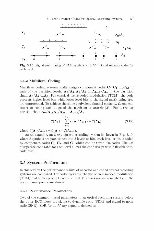
3 Turbo Product Codes for Optical Recording Systems 59
Λ0
Λ2
1 2 3 4 5 6 7 8
1 3 5 7
0 1
0 1 0 1
/Λ1Λ0
Λ
Λ1
1
/Λ2
C0
C
C
1
2
2 4 6 8
1 5 3 7 2 6 4 8
0 1 0 1 0 1 0 1
Fig. 3.10. Signal partitioning of PAM symbols with M = 8 and separate codes foreach level.
3.4.2 Multilevel Coding
Multilevel coding systematically assigns component codes C0,C1, ...,CM toeach of the partition levels, Λ0/Λ1,Λ1/Λ2, ...,ΛL−1/ΛL, in the partitionchain Λ0/Λ1/...ΛL. For classical trellis-coded modulation (TCM), the codeprotects higher-level bits while lower-level bits in the signal partitioning treeare unprotected. To achieve the same equivelent channel capacity, C, one canresort to coding each stage of the partition separately [23]. For a regularparition chain Λ0/Λ1,Λ1/Λ2, ...,ΛL−1/ΛL,
C(Λ0) =L−1∑i=0
C(Λi/Λi+1) + C(ΛL), (3.18)
where C(Λi/Λi+1) = C(Λi) − C(Λi+1).As an example, an 8-ary optical recording system is shown in Fig. 3.10,
where 8 symbols are partitioned into 3 levels or bits; each level or bit is codedby component codes C0,C1, and C2 which can be turbo-like codes. The useof separate code rates for each level allows the code design with a flexible totalcode rate.
3.5 System Performance
In this section the performance results of uncoded and coded optical recordingsystems are compared. For coded systems, the use of trellis-coded modulation(TCM) and turbo product codes on real ML discs are implemented and theperformance points are shown.
3.5.1 Performance Parameters
Two of the commonly used parameters in an optical recording system beforethe outer ECC block are sigma-to-dynamic ratio (SDR) and signal-to-noiseratio (SNR). SDR for an M -ary signal is defined as

60 Pornchai Supnithi
SDR =σ
A=
σ
2 ∗ (M − 1)(3.19)
where σ is the noise standard deviation and A is a dynamic range valueSNR which is common in communication systems; for a channel with unitmagnitude, SNR at the channel output is defined as
SNR =E(X2)
σ2=
M2 − 13σ2
(3.20)
where X ∈ −(M − 1), ...,−1, 1, ...,M − 1 and E(X2) is the average energyof transmitted symbols. Other forms of SNR also appear in the literature, forexample, SNR = Eb/N0 where Eb is the average bit energy, and N0 = 2σ2
n,where σ2
n is the noise variance. When the code rate, R, is considered, one canuse SNR = Eb/RN0 These two parameters typically are measured after theequalization, i.e., at the input of the Viterbi detector. For example, an MLdisc with M = 8 has A = 14 and a typical value of SDR in an ML CD-R/RWsystem is 1%−2%. The corresponding SNR range is thus 24-30 dB. Althoughthe SNR parameter is useful, one should note that unlike most communicationsystems, we cannot modify SNRs by adjusting the transmitted power.
3.5.2 Performance Results
Current research of turbo and tubo-like codes exist for binary and multi-leveled optical recording systems. As for binary optical recording systems,the use of turbo code were recently investigated [15] [17][18][19]. In [15], theperformance of the serially concatenated turbo codes(SCTC) and low-densityparity-check codes (LDPC) is investigated on PR equalized targets. The PRchannels are typcially considered inner codes with the precoder for each PRtarget is included. turbo codes offer coding gain of 4-5 dB over uncoded PRMLsystems. The SCTC provides better performance than the LDPC codes at S= 2.0, but comparable to the later at lower density S = 1.0. Furthermore,turbo codes provide resilience to transition noise and lose only 1 dB at 15%transition noise. In [17], work on a combination of SCTC and RLL codes areinvestigated for DVD systems. The PR targets of (1+D) and (1+D+D2+D3)are used together with the PRML technique. The turbo-coded system providesbetter formance with media noise and offers higher density gains.
As far as the author is concerned, up to date, the only product that is testedturbo-like codes on real optical discs are the MultiLevel disc or ML opticaldiscs [6] by Calimetrics, Inc. (now part of Hewlett Packard) The MLTM discswere first demonstrated using red laser on phase-change media. In [13] theuse of various equalizers and error correction control shows the performancegain relative to the capacity at M = 8 as a function of signal-to-noise ratio asshown in Fig. 3.11. For uncoded systems, there are three sets of 3-point plotsfor the case of, from left to right, M = 2, M = 4, and M = 8, respectively. Itis evident that the MLSE performs the best for all Ms considered.

3 Turbo Product Codes for Optical Recording Systems 61
0 5 10 15 20 25 30 35 40 45 5010
−1
100
101
Signal to Noise Ratio (dB)
Cap
acity
(bi
ts/M
F)
CTD=1D=1/2ZF−LEZF−DFEMLSETurbo CodeTCM
Fig. 3.11. The performance of ML optical recording system with various detectorsand codes.
For coded system, an actual 8-ary ML CD-RW uses the TCM and turbocode as channel code (inner code in the complete optical recording system).The turbo code which is represented by ’+’ on the plot is actually the turboproduct code designed for 8-level ML discs. The TCM code of a code rateof 5/6 with 256 states offers 2.5 bits/mark, but the turbo product codesdesigned for each separate level of the partitioning of PAM signals with M= 8 yields 2.75 bits/mark. Coded systems shows the gain of at least 6.5 dBwhen compared with the simulation result of uncoded systems at the BERof Pb(E) = 10−5. Original turbo codes [2] are not considered due to thedecoding complexity requirement. Later on, improvement from 8 to 12 levelsare verified in combination with the use of MultiLevel Coded Modulation(MCM) [24]. This results in a 10-GB DVD-RW system with coding efficiencyof 3.08 bits/data cell using red laser.
Fig. 3.11 compares the system performance versus the theoretical capacity.Three capacity curves are plotted. CT is for the continous-time channel modelof MTF 2, while for D = 1 and D = 1/2 are for discrete-time version ofthe channel model. D = 1 is when the mark size is the same as minimumfeature, and D = 1/2 is when the mark size is twice the size of the minimumfeature(MF). The minimum feature is theoretically the smallest mark size onecan write and the read lens can distinguish. Thus, with discrete-time channel,we lose a bit of capacity.

62 Pornchai Supnithi
It is, however, important to note that in the near future, an RS code isstill needed as the outer code and the codes with iterative decodig nature areused as the inner code.
3.6 Approved DVD Standards
As of the end of 2004, two rival formats are being developed. The first ofwhich, HD-DVD, is supported by DVD Forum with over 200 members likeHitachi, NEC, and etc. The single-layer type holds 15 GB, while the dual layerone holds 30 GB. The other camp, the Blu-Ray Disc Founders Association,with members like Dell, Sony, and etc., offer DVD with upto 27GB for asingle-layer disc and 54 GB for the dual layer disc [1]. Many companies aremembers of both groups.
Acknowledgment
The author would like to acknowledge Professor Steven W. McLaughlin forhis extensive work in this field of optical recording systems and be gratefulto his advisement during the author’s academic work at Georgia Instituteof Technology, Atlanta, GA, USA during 1997-2002 and also to Calimetrics,Inc., Alameda, California, which was the first company to develop the testbedfor ML CD/R-RW and ML DVD/R-RW. The company offered the author aninternship in during April-November of 2001.
References
1. Website:, http://www.dvdforum.org.2. C. Berrou, A. Glavieux, and P. Thitimajshima, “Near shannon limit error-
correcting coding and decoding: Turbo codes,” in Proc. 1993 Int. Conf. Com-mun., 1993, pp. 1064–1070.
3. R. Pyndiah, “Near-optimum decoding of product codes : Block Codes,” IEEETrans. on Communications, vol. 46, no. 8, pp. 1003–1010, Aug. 1998.
4. K. Immink, Coding Techniques for Digital Recorders. Englewood Cliffs, NewJersey: Prentice-Hall Internation(UK) Ltd., 1991.
5. ——, “Runlength-limited sequences,” Proceedings of IEEE, vol. 78, no. 11, pp.1745–1759, 1990.
6. S. McLaughlin, D. Lee, T. Lo, C. Pepin, P. Supnithi, and D. Warland, “Codingand signal processing for multilevel CD-RW, CD-R and DVD-RW,” in OpticalData Storage Conference, 2001.
7. A. Marchant, Optical Recording: A Technical Overview. New York: Addison-Wesley, 1990.
8. T. McDaniel and R. Victora, Handbook of Magneto-optical data recording. NewJersey: Noyes Publications, 1997.

3 Turbo Product Codes for Optical Recording Systems 63
9. K. Daly-Flynn and D. Strand, “InSbTe phase change materials for high per-formance multi-level recording,” in Optical Data Storage Conference, Hawaii,2002.
10. H. Borg and R. van Woudenberg, “Trend in optical recording,” Journal of Mag-netism and Magnetic Materials, vol. 193, pp. 519–525, 1999.
11. R. Lynch, “Channels and codes for magnetooptical systems,” IEEE Journal ofSelected Areas in Communications, vol. 10, no. 1, pp. 57–72, Jan. 1992.
12. D. Treves and D.A.Bloomberg, “Signal, noise, and codes in optical memories,”Opt. Eng., vol. 25, no. 7, pp. 881–891, 1986.
13. E. Licona, P. Supnithi, and S. McLaughlin, “M − ary signaling onrewritable/write-once optical discs: fundamental limits and actual perfor-mance,” in Globecom’01, San Antonito, TX, 2001, pp. 102–107.
14. M. Levenson, R. Lynch, and S. Tan, “Edge detection for magneto-optical datastorage,” in Appl. Opt., 1988, pp. 723–727.
15. H. S. et. al., “Iterative decoding for partial response (PR, equalized, magneto-optical (MO) data storage channels,” JSAC, vol. 19, no. 4, pp. 774–782, Apr.2001.
16. M. G. K. et al., “Performance comparisons of detection methods in magneto-optical disk system with (1,7) RLL code,” in Globecom’95, 1995, pp. 1389–1393.
17. L. McPheters and S. McLaughlin, “Concatenated codes and iterative (turbo)decoding for PRML optical recording channels,” in Optical Data Storage Con-ference, 1999, pp. 342–343.
18. H. Song, B. V. Kumar, E. Kurtas, and Y. Yuan, “Turbo decoding for opticalstorage,” in ICC 2000, vol. 1, New Orleans, LA, 2000, pp. 104–108.
19. L. McPheters, “Turbo-coded optical recording for channels with dvd minimummark size,” IEEE Trans. on Magnetics, vol. 38, no. 1, pp. 298–302, Jan. 2002.
20. D. Chase, “A class of algorithms of decoding block codes with channel mea-surement information,” IEEE Trans. on Information Theory, vol. IT-18, pp.170–182, Jan. 1972.
21. M. Fossier and S. Lin, “Chase-type and gdm coset decodings,” IEEE Trans. onCommunications, vol. 48, pp. 345–350, Mar. 2000.
22. A. Mahran and M. Benaissa, “Iterative decoding of product codes via adaptiveapplication of the combined Chase-2 and GMD decoding algorithm,” in ICC’01,Helsinki, Finland, 2001, pp. 2256–2260.
23. J. Huber and U. Wachsmann, “Capacities of the equivalent channels in multi-level coding schemes,” IEE Electronics Letters, vol. 30, pp. 557–558, Mar. 1994.
24. S. McLaughlin, Y. Lo, C. Pepin, and D. Warland, “MultiLevel DVD: codingbeyond 3 bits/data cell,” in Optical Data Storage Conference, 2002.

Part II
Wireline Communications

Chapter 4
Turbo and Turbo-like Code Design in ADSLModems
Hamid R. Sadjadpour1 and Sedat Olcer2
1 University of California, Santa Cruz, USA2 IBM Research Division, Switzerland
The invention of the Turbo codes in 1993 by Berrou et al. [1] represents per-haps one of the most important advances in coding theory in the past decade.The application of the turbo coding techniques for error correction in practicaldata transmission and recording systems has since then attracted consider-able interest. In this chapter, a new application of turbo coding to transmis-sion systems that utilize multi-carrier modulation is presented. In particular,the proposed method is used in Asymmetric Digital Subscriber Line (ADSL)modems that employ the Discrete Multi-tone (DMT) technology. DMT mod-ulation can be regarded as a variation of the Orthogonal Frequency DivisionMultiplexing (OFDM) technique used mostly in the context of wireless com-munications [2].
The ANSI standard T1.413 [3], which is the first ADSL standard publishedin 1995, specified the use of Reed-Solomon (RS) coding for forward errorcontrol (FEC). Later, the ANSI standard introduced the concatenation of RScoding with a 16-state 4-dimensional trellis code, known as Wei code, as aninner coding technique. In this chapter, the performance of turbo codes iscompared with that of the Wei code and is shown to lead to a higher codinggain than the recommended Wei code. The described turbo coding schemeis also bandwidth efficient, which is an important feature given that signalbandwidth for transmission over twisted-pair wires is limited. This schemeemploys a parallel concatenated convolutional code in combination with multi-tone Quadrature Amplitude Modulation (QAM) suitable for ADSL modems.
One challenge in the design of such codes is the length of the interleaver.Turbo codes have a near-Shannon limit error correcting performance when thelength of the interleaver is in the order of several thousand bits. However, manypractical applications, including ADSL, have limitations in terms of delay orlatency. Such delay constraints force the designer to limit the length of theinterleaver in turbo codes. For this reason, special attention must be given tothe design of interleavers. In this chapter, several pseudo-random interleaverdesigns with short block length suitable for turbo codes are presented thatresult in high coding gains. The proposed pseudo-random interleavers avoid
67
K. Sripmanwat (ed.), Turbo Code Applications: a journey from a paper to realization, 67–93.
© 2005 Springer. Printed in the Netherlands.

68 Hamid R. Sadjadpour and Sedat Olcer
Decoder
Synch. Correlation Phase-lock loop
DATA INPUT Encoder PSK or QAM
MappingIFFT Add
Prefix
D/A
Channel
A/D
Time Dispersion
Equalizer
Remove
Cyclic
PrefixFFT
Freq.
Domain
Equal.
Transmitter
Receiver
DATA
OUT
Fig. 4.1. Block diagram of an ADSL modem.
error floor effects in the practical range of bit error rates (BERs) for ADSLapplications.
Since the symbol constellation size in different sub-carriers of the ADSLmodem can be different, the code rate for each QAM constellation varieswithin one DMT symbol (frame). For this reason, special attention should bepaid to decode this system having possibly a different code rate in each sub-carrier. A simple encoding and decoding procedure is here introduced thatallows different constellation sizes and code rates to be used within one turboblock.
This chapter also describes the application of low-density parity-check(LDPC) codes to ADSL transmission as this class of codes represents animportant alternative to turbo codes for near-Shannon limit communications.Binary LDPC codes have been known since the early 1960s [4, 5] but theircapacity-approaching performance has only been demonstrated in the pastdecade [6, 7]. There is currently considerable research activity to explore ef-ficient constructions of such codes as well as to understand their theoreticallimits.
Turbo codes can be viewed as LDPC codes and the decoding algorithmsused for both types of codes can be derived from the formalism of factor graphs[8]. Other turbo-like codes, such as serial turbo codes, turbo product codes,or repeat accumulate codes will not be considered in this chapter. However,the techniques explained can be extended to encompass these classes of codesas well.
Fig. 4.1 shows a block diagram of an ADSL modem. The encoder (decoder)in this system consists of an outer RS encoder (decoder) and an inner encoder(decoder) for a turbo or an LDPC code.

4 Turbo and Turbo-like Code Design in ADSL Modems 69
Uncoded Data
Input
Interleaver
(1)
Interleaver
(2)
RSC 1
RSC 2
Channel Assignment
Controller
Parity
bit
selection
Multi-tone
QAM
Modulator To Channel
Systematic
data
Parity 2
Parity 1
Fig. 4.2. Block diagram of the turbo encoder.
4.1 Turbo Encoder Design for ADSL Modems
Fig. 4.2 describes a block diagram of a turbo encoder that can be used for in-ner coding in the system shown in Fig. 4.1. The structure of the turbo encoderis similar to that of the original scheme in [1] with an additional interleaverin the path of systematic data. The turbo encoder receives the informationbits as input and it generates one interleaved systematic data bit and twoparity bits for each information bit. The additional interleaver provided inthe path of systematic data is designed to combat impulse noise that some-times affects signals transmitted over twisted pair wires. The parity bits arepunctured based on the information provided by the channel assignment con-troller (CAC) . During the initialization of the modem, the CAC collects theinformation about the noise level and channel condition of each sub-carrier.Based on these measurements for a particular loop, the power mask, andthe power budget constraint, CAC allocates a combination of uncoded data,interleaved systematic data, and punctured parity bits to each sub-carrier.In particular, a bit loading algorithm [9, 10] is used to assign the number ofinformation and parity bits for each sub-carrier, and hence determines theconstellation size for each sub-carrier. The CAC determines the appropriatecombination of uncoded bits, interleaved systematic bits, and punctured par-ity bits for mapping onto a M-QAM symbol. Note that some information bitsare not passed through the turbo encoder. These bits are usually assignedto the most protected bits in a M-QAM symbol to ensure higher protection.The most protected bit is the one that has the least probability of incorrectdetection compared to the other bits in one symbol. This can be defined fora symbol or for each dimension (I or Q) of a complex symbol. Gray codemapping is the most common mapping for assignment of the bits to an M-QAM constellation. In this case, each I or Q component of a M-QAM symbolis mapped using Gray coding separately. In Gray code mapping, the most

70 Hamid R. Sadjadpour and Sedat Olcer
inputD
output
D D+
+
+ + +
Fig. 4.3. RSC encoder for turbo codes with generator matrix [1, 17oct15oct
].
protected bit is the most significant bit. The main advantage of Gray codemapping is its simplicity in terms of implementation complexity. From thedata that is generated at the output of the turbo encoder, parity bits are as-signed to the remaining more significant bits and systematic bits to the leastsignificant bits. There should be an equal number of puncturing of parity bitsfrom each component of the turbo encoder.
Each turbo block contains N information bits. Also the total number ofbits that can be transmitted during one DMT frame in ADSL depends on thecharacteristics of the particular twisted pair wire that is carrying the signal.In general, there is no relationship between the turbo block size, N , and thenumber of bits loaded in each ADSL frame, Nf . Nf depends on the channelcharacteristics, i.e., the channel attenuation function and the noise and in-terference level in a particular line. The CAC function will ensure that theboundaries of the turbo block are properly processed in the transmitter, sothat the receiver can decode each turbo block accordingly. The CAC alsocontrols the flow of data in the receiver. In the receiver, the conditional prob-ability of each transmitted bit can be directly computed from the M-QAMconstellation. The details of the decoder will be discussed later.
For the components of the turbo encoder, recursive systematic convolu-tional (RSC) codes can be used similar to [1]. Each RSC encoder has a gen-erator matrix [1, gff (D)
gfb(D) ], where gff (D) and gfb(D) are the feedforward andfeedback polynomials of the RSC encoder respectively. The feedback polyno-mial is usually selected as a primitive polynomial [11]. Fig. 4.3 demonstratesone example of the RSC encoder recommended for turbo codes with feedbackand feedforward generator polynomials equal to 15oct and 17oct respectively.More details on the encoder and decoder structure of turbo codes can be foundin [1].
For example, a 4096-QAM (12 bits) symbol with a spectral efficiency of10 bits/s/Hz can be constructed with or without uncoded bits. Table 4.1demonstrates the mapping for such a symbol if uncoded bits are not used.

4 Turbo and Turbo-like Code Design in ADSL Modems 71
Table 4.1. Mapping for 4096-QAM constellation with code rate 56
using only turboencoded data.
Systematic encoded data dk d1 d2 d3 d4 d5 d6 d7 d8 d9 d10
parity y1k y1
1 - - - - - - - - -
parity y2k - - - - - y2
6 - - - -
4096-QAM symbol (d1, d2, d3, d4, d5, y11 , d6, d7, d8, d9, d10, y
26)
Table 4.2. Mapping for 4096-QAM constellation with code rate 56, with nine un-
coded bits and three bits from the turbo encoder.
uncoded data uk u1 u2 u3 u4 u5 u6 u7 u8 u9
Systematic encoded data dk d1 - - - - - - - -
parity y1k y1
1 - - - - - - - -
parity y2k y2
1 - - - - - - - -
4096-QAM symbol (d1, y11 , y2
1 , u1, u2, u3, u4, u5, u6, u7, u8, u9)
Based on this Table, for each symbol, a total of eighteen parity bits from thetwo RSC encoders are punctured to construct one symbol.
If uncoded bits are used, then many different combinations are possible.For example, if we want to minimize puncturing, we can have a total of nineuncoded bits together with a systematic bit and two parity bits from the out-put of the turbo encoder mapped to the 4096-QAM constellation. By changingthe number of uncoded bits to construct a 4096-QAM symbol, we can have adifferent level of puncturing pattern in the turbo encoder. As it is clear fromthese examples, the use of only up to two parity bits per symbol is preferredin order to maintain high spectral efficiency.
4.2 Turbo Decoder Design for ADSL Modems
The original turbo decoder utilized a maximum a posteriori (MAP) algorithmalso known as BCJR [12] algorithm for soft decoding. The MAP algorithm isused in a recursive manner in the turbo decoder [1] by computing the Log-Likelihood Ratio (LLR) of each bit based on the entire observed data blockof length N, which is also the interleaver length. The LLR is computed as
Λ1(dk) = logPr(dk = 1|RN
1 )Pr(dk = 0|RN
1 )= log
∑s
∑s′ γ1(Rk, s
′, s)αk−1(s
′)βk(s)∑
s
∑s′ γ0(Rk, s′ , s)αk−1(s
′)βk(s),
(4.1)where Rk = dr
k, yri
k is the observed data at the receiver, drk and yri
k are thereceived systematic data and parity information from the i-th RSC encoder

72 Hamid R. Sadjadpour and Sedat Olcer
at time k, γj(Rk, s′, s) consists of the transition probability of the discrete
Gaussian memoryless channel and transition probabilities of the encoder trellis[12], αk(s) and βk(s) are two parameters that can be computed by forwardand backward recursions respectively based on γj(Rk, s
′, s), and s is the state
of the trellis at any given time. The details of this derivation is described in[1]. It can be shown that γj(Rk, s
′, s) can be written as
γj(Rk, s′, s) = Pr(Rk|dk = j, Sk = s, Sk−1 = s
′) × Pr(dk = j|Sk = s, Sk−1s
′)
× Pr(Sk = s|Sk−1 = s′) (4.2)
The second term in Eq. 4.2 is the transition probability of the discrete channel,the third term is equal to 1 or 0 depending on whether it is possible for dk = jwhen the system transition is from state s
′to state s, and the fourth term is
the transition state probabilities and for equiprobable binary data, it is equalto 1
2 . The second term in Eq. 4.2 can be divided into two terms:
Pr(Rk|dk = j, Sk = s, Sk−1 = s′) = Pr(dr
k|dk = j, Sk = s, Sk−1 = s′)
× Pr(yri
k |dk = j, Sk = s, Sk−1 = s′)(4.3)
Accurate computation of γj(Rk, s′, s) from the received signals is very impor-
tant for obtaining the other parameters of the MAP decoding algorithm. Notethat, in DSL application the received signal is an M-QAM (M = 2m) symbol.The symbol consists of m bits from parity, systematic, and uncoded data. Ina Gray code labeling, each bit dk in a M-QAM symbol is represented by thereal (I) or imaginary (Q) part of the M-QAM symbol. Therefore, if this bit isrepresented by the real part of the QAM symbol, the second term in Eq. 4.3can be written as
Pr(drk|dk = j, Sk = s, Sk−1 = s
′) =
m2∑
k1=0
Pr(Irk1|Ik1 = i, Sk = s, Sk−1 = s
′)
(4.4)Here m is assumed to be an even number. If the bit (dk) was represented bythe imaginary (Qk1) part of the QAM signal, then Ik1 will be replaced by Qk1
in the above equation. Pr(yri
k | . . .) can be computed using a similar approach.Once these conditional probability values are computed, then we can use theMAP decoding algorithm for the binary case as described in [1, 12].
The MAP algorithm is computationally complex and sensitive to SNRmismatch and inaccurate estimation of the noise variance [13]. This algo-rithm requires non-linear functions for computation of the probabilities andboth multiplications and additions are needed. For example, the fixed-pointrepresentation of the MAP decoding variables usually require between 16 to24 bits for a QPSK signal constellation. Based on the above hardware re-quirements, the MAP algorithm is not practical to implement in a chip. Thelogarithmic version of the MAP algorithm [14–16] and the Soft Output Viterbi

4 Turbo and Turbo-like Code Design in ADSL Modems 73
Channel FFT
I channel
Q channel
GammaComputation
Mapping Data Mapping Data ChannelAssignmentController
TurboDecoder
DecodedData
I1
-1
′γj (dk , s , s)
r
γ ′j (yk , s , s)
ri
Fig. 4.4. Block diagram of turbo decoder.
Algorithm (SOVA) [17, 18] are the practical decoding algorithms for imple-mentation. These algorithms are less sensitive to SNR mismatch and inaccu-rate estimation of the noise variance, and fixed-point representation of theirvariables require approximately 8 bits for a QPSK signal constellation. All dif-ferent logarithmic versions of the MAP algorithm only involve additions anda max-operation that can be realized utilizing a simple look-up table [16] or athreshold detector [19]. Fig. 4.4 demonstrates the block diagram of the turbodecoder at the receiver of the ADSL modem. The sampled received signal isprocessed by an FFT block. At the output of this block, complex QAM sym-bols representing information in the real (I) and imaginary (Q) dimensionsare obtained. This information is used to compute the Gamma variables andthe results are fed into the turbo decoder after de-interleaving the Gammavariables related to the systematic data. The CAC controls the boundaries ofthe FFT frame and the turbo code.
Extensive simulations have been conducted to investigate the effectivenessof the turbo code for ADSL transmission. Fig. 4.5 compares the bit errorrate (BER) performance of turbo code to Wei code when the turbo RSCcomponent codes are eight-state codes with a block length of 1000 bits andwith the same generator polynomial as in Fig. 4.3. The simulation results arebased on only three iterations using the Log-MAP decoding algorithm. Theadditional coding gain due to the use of turbo code compared to Wei codevaries from 4.1 dB for 4-QAM to 1.8 dB for 256-QAM constellation. For thisexample, there is one parity bit in each dimension and the remaining bits aresystematic data from the output of the turbo encoder. No uncoded bit is usedto construct these QAM symbols and consequently, the remaining parity bitsfrom the output of the turbo encoder are punctured. For 1, 2, 3, 4, and 6

74 Hamid R. Sadjadpour and Sedat Olcer
Turbo vs. Wei code for different QAM signals
1.00E+00
1.00E-02
1.00E-03
1.00E-04
1.00E-05
1.00E-06
1.00E-07
1.00E-01
Turbo 4 QAM (r=1/2)
Wei, 4 QAM
Turbo 16 QAM (r=1/2)
Wei, 8 QAM
Wei, 16 QAM
Wei, 32 QAM
Wei, 128 QAM
Turbo 16 QAM (r=3/4)
Turbo 64 QAM (r=2/3)
Turbo 256 QAM (r=3/4)
BER
Eb/No, dB
Fig. 4.5. BER performance of the turbo and Wei codes for various QAM modulationlevels.
information bits per sub-carrier, constellation sizes of 4, 16, 16, 64, and 256QAM with code rates of 0.5, 0.5, 0.75, 0.667, and 0.75 are used respectively.
Another approach to construct QAM symbols is to combine coded anduncoded data. Fig. 4.6 demonstrates the symbol error rate (SER) performanceof turbo code using the normalized signal-to-noise ratio (SNRnorm) as definedin [20]. The normalized SNR for a modulation and coding scheme operatingat a given rate of η (in bits per two-dimensional symbol) is defined as
SNRnorm =SNR
2η − 1=
η
2η − 1Eb
No(4.5)
Note that if the coding scheme achieves Shannon capacity, then SNRnorm = 0dB. The turbo block length for this example is 2022 bits and the simulationresults are for 20 iterations of the Log-MAP decoding algorithm. For thisexample, the QAM symbol mapping is done using one systematic bit and oneparity bit in each dimension and the remaining bits are uncoded bits. TheRSC component codes used here are similar to the previous example. Thecode rates for this example are 0.5, 0.5, 0.75, and 0.833 for 4, 16, 256, and4096 QAM constellation sizes respectively.
4.3 Interleaver Design for Turbo Code in ADSL Modems
An interleaver π is a permutation i → π(i) that maps a data sequence of Ninput symbols d1, d2, . . . , dN into the same sequence in a new order. If theinput data sequence is d = [d1, d2, . . . , dN ], then the permuted data sequenceis dP , where P is an interleaving matrix with a single 1 in each row andcolumn, all other entries being zero. Every interleaver has a correspondingde-interleaver (π−1) that acts on the interleaved data sequence and restoresit to its original order. The de-interleaving matrix is simply the transpose ofthe interleaving matrix (PT ).

4 Turbo and Turbo-like Code Design in ADSL Modems 75
1.00E-01
1.00E-02
1.00E-03
1.00E-04
1.00E-05
1.00E-06
1.00E-07
1.00E-08
0 10987654321
uncoded
4-QAM
16-QAM
256-QAM
4096-QAM
Sym
bo
l err
or r
ate
SNRnorm (dB)
Fig. 4.6. SER Performance of turbo code for interleaver length of 2022 bits and atotal of 20 iterations of the Log-MAP algorithm.
A random interleaver is simply a random permutation π. For large values ofN , most random interleavers utilized in turbo codes perform well. However,as the interleaver block size decreases, the performance of the turbo codedegrades substantially, up to a point when its BER performance is worse thanthat of a convolutional code with similar computational complexity. Thus thedesign of short interleavers for turbo codes is an important problem [21–24].
An S-random interleaver (where S = 1, 2, 3, . . .) is a “semi-random” in-terleaver constructed as follows. Each randomly selected integer is comparedwith S previously selected random integers. If the difference between the cur-rent selection and S previous selections is smaller than S, the random integeris rejected. This process is repeated until N distinct integers have been se-
lected. Computer simulations have shown that if S ≤√
N2 , then this process
converges [25] in a reasonable time. This interleaver design ensures that theshort cycle events are avoided. A short cycle event occurs when two bits areclose to each other both before and after interleaving.
The proposed turbo code for ADSL modems requires two interleavers. It iswell-known that for a given block length, the design of the interleaver can havea significant effect on the decoder performance, due to the different values ofthe minimum effective free distance that each interleaver can have. Therefore,

76 Hamid R. Sadjadpour and Sedat Olcer
in this section, two types of interleaver design are described. The first type isthe interleaver that is at the input of the RSC encoder (see Fig. 4.3). For shortturbo block length, this interleaver is responsible to produce large minimumeffective free distance, dmin, at the output of the turbo encoder. When theturbo block length is short, then a random interleaver can create small dmin
which results in poor BER performance for the turbo code. There are variousshort interleaver designs for turbo codes described in the literature. Here, afew of these interleaver designs are briefly described.
In [22], the author considers three objectives: 1) the low weight input datasequences do not create low weight at the output of at least one of the RSCencoders; 2) the design provides a large span for the input sequences thatresult in a zero terminating phase for all the component codes; and finally3)the design provides large distance for the terminating right edge of thesequences at the output of one or both encoders. The design includes a linearsum assignment optimization problem that can be solved using the Hungarianmethod [26].
An interleaver design was proposed based on the performance of iterativedecoding in turbo codes [27]. Turbo codes utilize an iterative decoding processbased on the MAP or other algorithms that can provide soft output. At eachdecoding step, some information related to the parity bits of one decoder isfed into the other decoder together with the systematic data sequence andthe parity bits corresponding to that decoder. Fig. 4.7 shows this iterativedecoding scheme. The inputs to each decoder are the input data sequence,dk, the parity bits y1
k or y2k, and the logarithm of the likelihood ratio (LLR)
associated with the parity bits from the other decoder (W 1k or W 2
k ), which isused as a priori information. All these inputs are utilized by the decoder tocreate three outputs corresponding to the weighted version of these inputs.In Fig. 4.7, dk represents the weighted version of the input data sequence,dk. Also dn in the same figure demonstrates the fact that the input datasequence is fed into the second decoder after interleaving. The input to eachdecoder from the other decoder is used as a priori information in the nextdecoding step and corresponds to the weighted version of the parity bits. Thisinformation will be more effective in the performance of iterative decodingif it is less correlated to the input data sequence (or interleaved input datasequence). Therefore it is reasonable to use this as a criterion for designing theinterleaver. For large block size interleavers, most random interleavers providea low correlation between W i
k and input data sequence, dk. The correlationcoefficient, r1
W 1k1
,dk2, is defined as the correlation between W 1
k1and dk2 .
It has been shown [21] that r1W 1
k1,dk2
can be analytically approximated by
r1W 1
k1,dk2
=
a exp−c|k1−k2| if k1 = k2
0 if k1 = k2(4.6)
where a and c are constants that depend on the encoder feedback and feed-forward polynomials. The correlation coefficient at the output of the second

4 Turbo and Turbo-like Code Design in ADSL Modems 77
De-Interleaver
Decoder 1
Interleaver
Decoder 2dk dk dn dn
yk1
Wk2
Wk1
Wk2
Wn1
yn2
Wn2
Wn1
Fig. 4.7. Turbo decoder.
decoder, r2W2,d, is approximated by
r2W2,d =
12r1W1,dP (I + r1
W1,d) (4.7)
where the two terms on the right hand side of Eq. 4.7 correspond to thecorrelation coefficients between W2 and the input data, i.e., W1 and d [21].In this section, r2
W2,d represents the correlation coefficient matrix and r2W 2
k1,dk2
represents one element of this matrix.Similar correlation coefficients can be computed for the de-interleaver. The
correlation matrix corresponding to de-interleaver, r′2
W2,d, is the same as inEq. 4.7 except that P is replaced by PT .
Then Vk1 is defined to be
Vk1 =1
N − 1
N∑k2=1
(r2W 2
k1,dk2
− ¯r2W 2
k1,d) (4.8)
where
¯r2W 2
k1,d =
1N
N∑k2=1
r2W 2
k1,dk2
(4.9)
V ′k1
is defined in a similar way using r′2
W2,d. The iterative decoding suitability(IDS) measure is then defined as
IDS =1
2N
N∑k1=1
(Vk1 + V ′k1
) (4.10)
A low value of IDS is an indication that the correlation properties between W1
and d are equally spread along the data sequence of length N. An interleaverdesign based on the IDS condition is proposed in [27].

78 Hamid R. Sadjadpour and Sedat Olcer
Another interleaver design, a 2-step S-random interleaver, is presented in[28]. The goal is to increase the minimum effective free distance, dmin, ofthe turbo code while decreasing or at least not increasing the correlationproperties between the information input data sequence and W i
k. Hokfelt etal. [21, 27] introduced the IDS criterion to evaluate this correlation properties.The two vectors for the computation of IDS in Eq. 4.10 are very similar andfor most interleavers it is sufficient to only use one of them, i.e., Vk1 . Instead,a new criterion based on decreasing the correlation coefficients for the thirddecoding step can be defined, i.e., the correlation coefficients between extrinsicinformation from the second decoder and information input data sequence. Inthis regard, the new correlation coefficient matrix, r′
2
W2,d, is defined as
r′2
W2,d =12r2W2,dPT (I + r2
W2,d)
=14(r1
W1,d + r1W1,dP r1
W1,dPT ) (4.11)
× (I +12r1W1,dP +
12r1W1,dP r1
W1,d)
V′(new)k1
can now be computed in a similar way to Eq. 4.8 by using Eq. 4.11.The new iterative decoding suitability (IDS1) is then defined as
IDS1 =1
2N
N∑k1=1
(Vk1 + V′(new)k1
) (4.12)
A small value for IDS1 only guarantees that the correlation properties arespread equally throughout the data sequence. However, this criterion does notattempt to reduce the power of correlation coefficients, i.e., (r2
W 2k1
,dk2)2 and
(r′2
W 2k1
,dk2)2. Therefore, the following additional condition is recommended as
a second iterative decoding suitability criterion:
IDS2 =1
2N2
N∑k1=1
N∑k2=1
((r2W 2
k1,dk2
)2 + (r′2
W 2k1
,dk2)2) (4.13)
Finally, the average of these two values is used as a new IDS criterion.
IDS(new) =12(IDS1 + IDS2) (4.14)
Minimizing Eq. 4.14 is then one of the goals in optimizing the interleaver.Unlike [27], where the interleaver design is just based on the IDS criterion,
this interleaver is designed in two stages [28]. In the first stage, an interleaverthat satisfies the S-random criterion together with an additional condition isdesigned [28]. In the second stage, the minimum effective free distance (dmin)of the turbo code is increased while considering the IDS(new) constraint. The

4 Turbo and Turbo-like Code Design in ADSL Modems 79
SNR, dB
BE
R
2step S-random
S-random
Random
1.E-01
1.E-02
1.E-03
1.E-04
1.E-05
1.E-06
1.E-07
0.2 0.4 0.6 0.8 1.0 1.2 1.4
Fig. 4.8. Performance of turbo code for different interleavers of size 400 bits andBPSK signal.
design is as follows. First the values of S1 and S2 are selected.
Step 1: Each randomly selected integer π(i) is compared with the previ-ous selections π(j) to check that if i − j ≤ S1 then |π(i) − π(j)| > S1. Theinterleaver must also satisfy |i − π(i)| > S2.
Besides the above conditions, the last m tail bits used for trellis termina-tion in the first decoder are chosen to satisfy π(1) = N , and if π(i) = N − kwith k < m then i < N/2. This condition will guarantee that trellis termi-nation for the first decoder is sufficient and there will not be any low weightsequence at the output of the second decoder caused by failure of trellis ter-mination.
Step 2: The procedure in the second step guarantees that all the inputdata sequences with a minimum weight less than or equal to wdet have aminimum effective free distance greater than dmin,wdet
where these parametersare defined in [28].
For the deterministic interleaver that is in the path of systematic data inFig. 4.3, a row-column interleaver can be used to combat impulse noise.
Fig. 4.8 compares the BER performance of a turbo code with componentcodes of Fig. 4.3. Turbo code utilizes 18 iterations of Log-MAP algorithm andthree types of interleaver of length 400 bits with BPSK modulation are imple-mented. The simulation result clearly shows that proper choice of interleaverhas significant effect on the performance of the turbo code.

80 Hamid R. Sadjadpour and Sedat Olcer
4.4 LDPC Codes and LDPC Encoder Design for ADSLModems
A binary (N, K) linear code is a set of binary vectors of length N, calledcodewords, that satisfy a set of M ≥ (N − K) parity-check equations. Thelength of the information vector is denoted by K. A parity-check equation canbe conveniently represented as a binary vector of length N in which a “1” inposition n, 1 ≤ n ≤ N , implies that the n-th codeword symbol participates inthe parity check. The set of M parity checks can then be represented by anM ×N parity-check matrix H. A “1” in the (m,n)-th position in H indicatesthat the m-th parity check involves the n-th symbol of the codeword, or equiv-alently, that codeword symbol n participates in the m-th parity check. Thissuggests a natural graphical representation of the parity-check matrix H as a“bipartite” graph with two kinds of nodes: N symbol or variable nodes thatcorrespond to the codeword symbols, and M check nodes that correspond tothe parity checks represented by the rows of matrix H [6, 30]. The connectiv-ity of the bipartite graph, known as the Tanner graph, is such that H is itsincidence matrix, i.e., for each “1” in the (m,n)-th position, the graph has anedge connecting check node m with symbol node n. No two nodes of the samekind are connected by an edge.
A binary (N, K) LDPC code [4, 5] is a linear block code described by asparse (N, K) parity-check matrix H, i.e., H has a low density of 1s. Eachsymbol is checked by a small number of parity checks, and each parity checkincludes a small number of symbols. An LDPC code is called (ds, dc)-regularif in the corresponding bipartite graph every symbol node is connected to ds
check nodes and every check node is connected to dc symbol nodes; otherwiseit is called an irregular LDPC code. Fig. 4.9 shows an example of the Tannergraph of a (ds = 3, dc = 4)-regular LDPC code of block length N = 12 havingM = 9 parity-check equations. In this figure, the left nodes represent symbolnodes and the right nodes represent parity-check nodes.
The parity-check matrix of a regular LDPC code thus contains ds onesin each column and dc ones in each row. By contrast, the number of ones ineach column, respectively in each row, can vary widely for an irregular LDPCcode. Excellent performance can be achieved with well-designed regular LDPCcodes. The regularity of the code usually allows reducing hardware complexityand leads to efficient decoder implementations. However, irregularity improvesperformance further and makes this class of codes capacity approaching.
Irregular LDPC codes [31, 32] are conveniently specified by a pair of “de-gree distribution” polynomials: a degree distribution polynomial λ(x) is asso-ciated with the symbol nodes and a degree distribution polynomial ρ(x) withthe check nodes. In general,
λ(x) =d∗
s∑i=1
λixi−1 and ρ(x) =
d∗c∑
i=1
ρixi−1

4 Turbo and Turbo-like Code Design in ADSL Modems 81
Fig. 4.9. An example of a (ds = 3, dc = 4)-regular Tanner graph.
where λi and ρi denote the fraction of edges connected to a symbol node,respectively to a check node, of degree i. Furthermore, d∗s(d
∗c) represents the
maximum symbol (check) degree. For example, for the (ds = 3, dc = 4)-regularLDPC code in Fig. 4.9, λ(x) = x2 and ρ(x) = x3.
As mentioned earlier, in DMT modulation for ADSL, each subcarrier ismodulated by symbols taken from constellations of possibly very differentsizes, such as BPSK, QPSK, 16, 32, 64-QAM, etc., ultimately up to a 215-symbol constellation. One alternative for LDPC coding in a multilevel mod-ulation system consists of using nonbinary LDPC codes [33]. Here, the focusis on the use of binary LDPC codes for multilevel modulation [34] as thisapproach makes the LDPC encoding and soft iterative decoding functions in-dependent of the number of modulation levels employed. Therefore, at thereceiver, the number of modulation levels only affects soft demapping, i.e.,the extraction of soft information on individual code bits from the receivednoisy symbols.
Fig. 4.10 shows a block diagram of the encoder for an LDPC code thatcan be used to realize the inner coding function in Fig. 4.1. Information bitsrepresenting data or control messages are encoded into a binary codeword oflength N. The symbol mapper collects groups of coded bits, possibly along

82 Hamid R. Sadjadpour and Sedat Olcer
Fig. 4.10. LDPC encoding/symbol mapping and symbol demapping/decoding func-tions for DMT-based DSL transmission. Mapping and demapping functions areshown for the real (Re) and imaginary (Im) parts of a complex QAM symbol.
with uncoded information bits as shown in the figure, and builds QAM sym-bols for frequency-domain modulation by an inverse discrete Fourier transformoperation. As discussed earlier in connection with turbo encoding, uncodedbits are mapped to the most protected bits, i.e., the more significant bits, of aQAM symbol. Furthermore, as explained below, a double Gray-code labelingis assumed for symbol mapping, wherein the less significant coded bits andthe more significant uncoded bits are Gray-coded separately. As usual, thesize of the QAM constellation used on each subchannel is determined througha “bit-loading” algorithm [35].
The symbol-mapping function is now explained in more detail with refer-ence to the block diagram of Fig. 4.11. If the constellations employed havea square shape, soft demapping at the receiver is greatly simplified becausethe real and imaginary parts of the received noisy complex signals can bedemapped independently. Thus the transmit symbols are chosen from a 2b-QAM symbol constellation, where b = 1 or b = 2m, with m a positive integer.
When b = 2m, two binary m-tuples v = (vm−1, vm−2, . . . , v1, vo) and w =(wm−1, wm−2, . . . , w1, wo) independently select two L-ary real symbols, L =2m, representing the real and imaginary parts, respectively, of the complex

4 Turbo and Turbo-like Code Design in ADSL Modems 83
Fig. 4.11. A more detailed representation of the multilevel encoding and symbol-mapping function shown in Fig. 4.10.
QAM symbol to be transmitted. The L-ary symbols belong to the set
A = Al = 2l − (L − 1), l = 0, 1, . . . , L − 1
The real part of a QAM symbol conveys mvL code bits and mv
M uncodedbits, with mv
L + mvM = m. Similarly the imaginary part conveys mw
L codebits and mw
M uncoded bits, with mwL + mw
M = m. Symbol mapping relieson the partition of the set A into 2mv
L [2mwL ] subsets such that the minimum
Euclidean distance between the symbols within each subset is maximized. Themv
L[mwL ] less-significant bits (LSBs) of v[w] label the subsets of A following a
Gray-coding rule. The remaining more-significant bits (MSBs) mvM [mw
M ] labelsymbols within a subset following a separate Gray-coding rule.
When b = 1, only the code bit vo is employed. This case corresponds toBPSK modulation.
The number of uncoded and coded bits per transmit symbol is a designparameter that involves a trade-off in terms of performance and decodingcomplexity.
Double Gray-code labeling offers a good trade-off in terms of achievableperformance and implementation complexity. The efficiency of symbol map-ping based on this labeling technique can be assessed by computing the capac-ity of the binary-valued-input and continuous-valued-output AWGN channelthat also includes the bit-to-symbol mapping function. More precisely, assum-ing ideal interleaving of the binary input sequence prior to the mapping of mconsecutive bits into a multilevel symbol, the capacity of the equivalent “bit-interleaved” channel [36] can be determined. The results show that for 8-level

84 Hamid R. Sadjadpour and Sedat Olcer
modulation and higher, it is sufficient to employ 2 or 3 code bits per sym-bol and to leave the remaining bits uncoded, provided that high-rate codesare employed [37]. As double Gray labeling results in lower decoding com-plexity than full Gray labeling, a good trade-off in terms of capacity versusimplementation complexity is achieved.
For full flexibility, the number of uncoded and coded bits per transmitsymbol can be specified by the receiver for each symbol constellation duringinitialization. Assuming, for example, that 1024-QAM is employed on eachsubchannel, with a total number of 200 subchannels, and that three codedbits are carried per dimension, a codeword of length N = (3+3) bits × 200 =1200 bits along with 4 bits × 200 = 800 uncoded bits can be mapped into aDMT frame. In this case, with a DMT frame rate of 4000 Hz, the line datarate is 10 bits × 200 × 4000 Hz = 8 Mbit/s.
Before concluding this section on encoder design for LDPC codes, it ismeaningful to ask what are the important aspects that must be consideredin designing LDPC codes for (A)DSL systems? First, high code rates are de-sirable to achieve high spectral efficiencies for bandwidth-constrained DSLtransmission. Second, it should be possible to adapt the code parameters togiven transmission-channel characteristics and application-specific constraintsto achieve best performance. A simple solution would consist in allowing thereceiver to select the most appropriate code from a small set of pre-definedcodes after the channel measurement phase during transceiver initialization.An approach that appears to be even more attractive, because of its greaterflexibility, is one that would allow code construction “on the fly,” providedthat the processing effort needed to compute the parity-check matrices of theLDPC codes is small. A third aspect is linear-time encodability, meaning thatencoding for an LDPC code of length N requires O(N) operations. This prop-erty is very important for the practical implementation of LDPC encoders.
4.5 LDPC Decoder Design for ADSL Modems
The graphical representation of LDPC codes is attractive not only because ithelps understand their parity-check structure but, more importantly, becauseit facilitates a powerful decoding approach. The key steps in this decodingtechnique are the local application of the Bayes rule at each node and theexchange of the results, or messages, with “neighboring” nodes. In essence,the technique works as follows. At any given iteration, two types of messagesare passed: probabilities from symbol nodes to check nodes, and probabilitiesfrom check nodes to symbol nodes. The message from symbol node n to checknode m is the probability, as seen by the n-th symbol node, that the value ofsymbol n is a 1 or a 0, based on messages from all parity checks involving n,except parity check m. Similarly, the message from check node m to symbolnode n is the probability, as seen by the m-th check node, that the value of

4 Turbo and Turbo-like Code Design in ADSL Modems 85
symbol n is a 1 or a 0, based on all the symbols the m-th check node checks,except symbol n.
The message-passing decoding approach outlined above can be speci-fied in an algorithmic form, leading to the so-called sum-product (or belief-propagation) algorithm. The sum-product algorithm can also be expressedwithin the formalism of factor graphs [8].
Using a notation similar to that in [7], let M(n) denote the set of checknodes connected to symbol node n, i.e., the positions of 1s in the n-th columnof the parity-check matrix H. Let N(m) denote the set of symbol nodes thatparticipate in the m-th parity-check equation, i.e., the positions of 1s in them-th row of H. Furthermore, N(m)\n represents the set N(m), excluding then-th symbol node, and similarly, M(n)\m represents the set M(n), excludingthe m-th check node.
In addition, let qn→m(0) and qn→m(1) denote the message that symbolnode n sends to check node m, indicating the probability of symbol n being0 or 1, respectively, based on all the checks involving n except m. Similarly,rm→n(0) and rm→n(0) denote the message that the m-th check node sendsto the n-th symbol node indicating the probability of symbol n being 0 or 1,respectively, based on all the symbols checked by m except n. Finally, y =[y1, y2, . . . , yN ] denotes the received word corresponding to the transmittedcodeword x = [x1, x2, . . . , xN ].
In the probability domain, the inputs to the sum-product decoding al-gorithm are the a posteriori probabilities (APPs) P (xn = 0|yn) and P (xn =1|yn) , which are computed based on the channel statistics as will be explainedlater. The sum-product decoding algorithm is then summarized as follows.
Initialization: Each symbol node n is assigned APPs qn→m(0) = P (xn =0|yn) and qn→m(1) = P (xn = 1|yn), which are sent to check node m as theinitial message, for all m.
Step (i) (check-node update): For each m, for each n ∈ N(m), compute fori = 0, 1:
rm→n(i) =∑
x(n′:n′∈N(m)\n,∑ ⊕x
n′=i)
∏n′∈N(m)\n
qn′→m(xn′),
where∑⊕ denotes modulo-2 summation.
Step (ii) (symbol-node update): For each n, for each m ∈ M(n), computefor i = 0, 1:
qn→m(i) = µn→mP (xn = i|yn)∏
m∈M(n)
rm→n(i),
where the normalization constant µn→m is chosen such that qn(0)+qn(1) = 1.For each n, compute the “pseudoposterior” probabilities for i = 0, 1:
qn(i) = µnP (xn = i|yn)∏
m∈M(n)
rm→n(i),

86 Hamid R. Sadjadpour and Sedat Olcer
where the normalization constant µn is chosen such that qn→m(0)+qn→m(1) =1.
Step (iii) (decision): Quantize x = [x1, x2, . . . , xN ] such that xn = 0 ifqn(0) ≥ 0.5 and xn = 1 if qn(0) < 0.5. If xHT = 0, then halt the algorithmwith x as the decoder output; otherwise go to Step (i). If the algorithm doesnot halt within some maximum number of iterations, then declare a decoderfailure.
Because the check-node update in Step (i) requires the computation ofsums of products of probabilities, the algorithm is called the “sum-product”algorithm.
A number of variations to the above sum-product algorithm have beenproposed in order to simplify its implementation in practical systems. Forexample, using LLRs as messages offers implementation advantages over us-ing probabilities or likelihood ratios because multiplications are replaced byadditions and the normalization step is eliminated.
More precisely, let us define the LLRs Zn→m(xn) log(qn→m(0)/qn→m(1))and Lm→n(xn) = log(rm→n(0)/rm→n(1)). Then, the LLR-based sum-productalgorithm is obtained, and can be summarized as follows.
Initialization: Each symbol node n is assigned an a posteriori LLR L(xn|yn) =log(P (xn=0|yn)
P (xn=1|yn) ). For every position (m,n) such that Hn,m = 1, set
Zn→m(xn) = L(xn|yn),
Lm→n(xn) = 0
Step (i) (check-node update): For each m, and for each n ∈ N(m), compute
Lm→n(xn) = (∏
n′∈N(m)\n
sign(Zn′→m(xn′)))f(∑
n′∈N(m)\n
f(|Zn′→m(xn′)|))
Step (ii) (symbol-node update): For each n, and for each m ∈ M(n), compute
Zn→m(xn) = L(xn|yn) +∑
m′∈M(n)\m
Lm′→n(un)
For each n, compute
Zn(xn) = L(xn|yn) +∑
m∈M(n)
Lm→n(xn).
Step (iii) (decision): Quantize x = [x1, x2, . . . , xN ] such that xn = 0 ifZn(xn) ≥ 0 and xn = 1 if Zn(xn) < 0. If xHT = 0, then halt the algo-rithm with x as the decoder output; otherwise go to Step (i). If the algorithmdoes not halt within some maximum number of iterations, then declare a de-coder failure. In the check-node update of Step (i), the function f(x) is definedas

4 Turbo and Turbo-like Code Design in ADSL Modems 87
f(x) = logex + 1ex − 1
= − log[tanh(x
2)]
Clearly, the check-node updates represent the computationally most demand-ing part of the LLR sum-product algorithm. Therefore, a number of solutionshave been proposed in the literature to simplify the check-node processing stepof the algorithm and to achieve decoder architectures that are suited for high-speed digital applications. The reader is referred to [38] and the referencestherein for details on the topic.
Finally, the APPs needed to initialize the sum-product algorithm are ob-tained through the following soft demapping operation. Let y denote the real(equivalently, the imaginary) part of the noisy received signal:
y = A + v,
with v a sample of an AWGN process with variance σ2n. The APP of code bit
i conveyed by symbol A being equal to x = 0, 1 is obtained as:
P (i = x|y) =
∑Al∈Ai,x
exp− (y−Al)
2
2σ2n∑
Al∈A exp− (y−Al)
2
2σ2n
i = 0, 1, . . . , mvL − 1,
where Ai, x denotes the subset of all symbols in A with label value x = 0, 1in position i.
4.6 Performance
It appears that high-rate LDPC codes with medium block length, whoseparity-check matrices are constructed similarly to those of array codes [39],exhibit as good a performance as random LDPC codes do. Array-code-basedLDPC coding was shown in [40] to offer a number of advantages for DSLtransmission. The LDPC parity-check matrix is specified, in that case, by asmall set of parameters and constructed deterministically without requiring“preprocessing” operations. Furthermore, array LDPC codes are amenable tolinear-time encoding.
The array-code parity-check matrix is specified by three parameters: aprime number p and two integers k and j such that k, j ≤ p. It has dimensionsjp × kp and is given by
HA =
⎡⎢⎢⎢⎢⎢⎣
I I I . . . II α α2 . . . αk−1
I α2 α4 . . . α2(k−1)
......
.... . .
...I αj−1 α2(j−1) . . . α(j−1)(k−1)
⎤⎥⎥⎥⎥⎥⎦

88 Hamid R. Sadjadpour and Sedat Olcer
where I is the p × p identity matrix and α is a p × p permutation matrixrepresenting a single left or right cyclic shift of I. Powers of α in HA indicatemultiple cyclic shifts, with the number of shifts given by the value of theexponent.
To achieve efficient linear-time encoding for array-like LDPC codes, it wasproposed in [40] to transform the above parity-check matrix into the followingtriangular form
H =
⎡⎢⎢⎢⎢⎢⎣
I I . . . I I . . . I0 I α . . . αj−2 αj−1 αk−2
0 0 I . . . α2(j−3) α2(j−2) α2(k−3)
......
.... . .
......
...0 0 . . . . . . I αj−1 . . . α(j−1)(k−j)
⎤⎥⎥⎥⎥⎥⎦
where 0 is the p × p null matrix. The LDPC codes defined by H have acodeword length N = kp, M = jp parity checks, and an information blocklength K = (k − j)p. Also, H is 4-cycle free. Note that the triangular forminduces a slight irregularity in the initially regular LDPC code. Indeed, thesymbol-node and check-node degree distribution polynomials are given by
λ(x) =j∑
i=1
λjxi−1;λi =
1k 1 ≤ i ≤ j − 11 − (j−1)
k i = j
and
ρ(x) =k∑
i=k−(j−1)
ρixi−1; ρi =
1j, k − (j − 1) ≤ i ≤ k
respectively.The typical performance that can be achieved by the multilevel LDPC-
coding scheme and the deterministic array-based code construction mentionedabove is now briefly illustrated by means of simulations. The telephone-twisted-pair channel introduces frequency-dependent signal distortion as wellas several other forms of disturbances, of which crosstalk is the most im-portant. In the simulations, disturbance by AWGN only will be assumed. Thereason for this is that if each DMT subchannel has a sufficiently narrow band-width, then each one independently approximates an AWGN channel with aparticular SNR value. Clearly, impulse noise and narrowband interference ofvarious origins, e.g., AM radio signals, also affect the reliability of commu-nications in DSLs. Performance should ultimately be assessed using actualtest-loop conditions.
Fig. 4.12 shows the SER performance of three array-code-based LDPCcodes of block lengths N = 529, 2209, and 4489 bits, and code rates 0.870,0.915 and 0.940, respectively. For 16-QAM symbol mapping, all bits are coded.For 256 and 4096-QAM, there are three coded bits along each dimension, andthe remaining bits are uncoded.

4 Turbo and Turbo-like Code Design in ADSL Modems 89
Fig. 4.12. Performance of three LDPC codes: (a) (529, 460), (b) (2209, 2021),and (c) (4489, 4221), for transmission over the AWGN channel using 16, 256, and4096-QAM.

90 Hamid R. Sadjadpour and Sedat Olcer
As mentioned earlier, latency is an important parameter in DSL systems.“Voice” applications are known to demand rather low latency whereas otherapplications, such as video streaming, tolerate larger delays but need strongererror-correction capability. Thus, in studying new coding techniques for DSLs,trade-offs between coding gain and latency have to be clearly established.Generally speaking, if higher latencies can be tolerated, then longer–and hencemore powerful–codes can be employed. Conversely, lower coding gains areimposed by small latencies. Recall that DMT frames in ADSL systems aregenerated at the rate of 4000 Hz. Therefore if one information block is encodedinto one DMT frame, the encoding and decoding functions introduce a latencyof 250 µs each, resulting in a total latency of 0.5 ms. When a codeword spansmore than a single frame, latency increases accordingly.
Finally, similar to turbo codes, LDPC codes offer significant gains overTCM, see e.g., [41]. Notice, however, that care should be exercised in at-tempting a comparison between turbo and LDPC codes because they mostlyoperate at different spectral efficiencies and discrepancies usually exist be-tween code rate, latency, implementation complexity, etc. For this reason,such a comparison was not included in this chapter.
4.7 Final Remarks
In the wake of the invention of the turbo codes, an intense research effort hasbeen undertaken in the information-theory and coding community in order toimprove the understanding of capacity-approaching codes as well as to designtools and techniques for constructing codes with practical utility. While im-portant work is still ongoing in this field, the state of the art has reached a levelof maturity that encourages engineers in the communications and recordingindustries to port these coding methods into the realm of practical realiza-tions. This chapter has described, at some level of detail, possible approachesfor incorporating turbo and LDPC coding into ADSL technologies.
For both DSL subscribers and network operators, the benefits of capacity-approaching coding will be measured in terms of the achievable increase indata rates, loop reach and service penetration. By employing turbo or turbo-like coding, it will be possible to operate DSL links with greater robustnessand reliability under difficult transmission conditions due to spectral crowding,loop unbundling, etc. It is indeed conjectured that the ‘turbo principle’ willbe applied, in various forms, in all future high-performance receiver designsin order to maximize performance.
Other techniques, such as the use of selectable masks for signal transmis-sion, dynamic spectrum management, multi-input multi-output transmission,have partly found and will find their way into the definition of future DSLmodems. Capacity-approaching coding is complementary to these techniques,as it can be combined with essentially anyone of them to achieve close toShannon-limit performance in future generations of DSL systems.

4 Turbo and Turbo-like Code Design in ADSL Modems 91
References
1. C. Berrou, A. Glavieux, and P. Thitimajshima, “Near Shannon limit error-correcting coding and decoding : Turbo codes,” in Proc. IEEE InternationalConference in Communications, pp. 1064–1070, June 1993.
2. J. Terry and J. Heiskala, OFDM Wireless LANs: A Theoretical And PracticalGuide, Sams Publisher, 1st edition, December 2001.
3. ANSI Network and Customer Installation Interfaces — Asymmetric DigitalSubscriber Line (ADSL) Metallic Interface, American National Standard forTelecomm., vol. T1.413, 1995.
4. R.G. Gallager, Low-density Parity-check Codes, IRE Transaction on Informa-tion Theory, vol. IT-8, pp. 21–28, January 1962.
5. R.G. Gallager, Low Density Parity Check Codes, Cambridge, MA: MIT Press,1963.
6. N. Wiberg, Codes and Decoding on General Graphs, Ph.D. Thesis, LinkpingUniversity, Sweden, 1996.
7. D.J.C. MacKay, “Good error-correcting codes based on very sparse matrices,”IEEE Trans. Inform. Theory, vol. 45, pp. 399–431, March 1999.
8. H.-A. Loeliger, “An introduction to factor graphs,” IEEE Signal ProcessingMagazine, vol. 45, pp. 28–41, January 2004.
9. J. Tu and J. Cioffi, “A loading algorithm for the concatenation of coset codeswith multichannel modulation methods,” Proc. IEEE Globecom 1990 , pp. 1183–1187.
10. R. Sonalkar and H.R. Sadjadpour, “A New Initialization Method for Minimiza-tion of Near End Cross Talk due to DMT Transmission in Cable Binders,”Proc. ICCS2000 , Singapore, November 20-24, 2000.
11. S. Lin and D.J. Costello Jr., Error Control Coding: Fundamentals and Appli-cations, Prentice-Hall Publisher, 1983.
12. L. Bahl, J. Cocke, F. Jelinek, and J. Raviv, “Optimum decoding of linear codesfor minimizing symbol error rate,” IEEE Trans. on Inf. Theory, vol. IT-20, pp.284–287, March 1974.
13. T.A. Summers and S.G. Wilson, “SNR Mismatch and Online Estimation inTurbo Decoding,” IEEE Trans. on Comm. vol. 46, no. 4, pp. 421–424, April1998.
14. P. Robertson, P. Hoeher, and E. Villebrun, “Optimal and Sub-Optimal Maxi-mum A Posteriori Algorithms Suitable for Turbo Decoding,” European Trans.on Telecomm. vol. 8, no. 2, pp. 119–126, March-April 1997.
15. P. Robertson, E. Villebrun, and P. Hoeher, “A Comparison of Optimal andSub-optimal MAP Decoding Algorithms Operating in the Log Domain,” Proc.International Conference on Communications, pp. 1009–1013, June 1995.
16. S. Benedetto, G. Montorsi, D. Divsalr, and F. Pollara “Soft-Output DecodingAlgorithm in Iterative Decoding of Turbo Codes,” TDA Progress Report 42-124, pp. 63–87, February 15, 1996.
17. J. Hagenauer and P. Hoeher, “A Viterbi Algorithm with Soft-Decision Outputsand Its applications,” Proc. of GLOBECOM , pp. 1680–1686, November 1989.
18. J. Hagenauer, “Source-Controlled Channel Decoding,” IEEE Transaction onCommunications, vol. 43, No. 9, pp. 2449–2457, September 1995.
19. W.J. Gross and P.G. Gulak, “Simplified MAP algorithm suitables for imple-mentation of turbo decoders,” Electronics Letters, vol. 34, no. 16, August 6,1998.
92 Hamid R. Sadjadpour and Sedat Olcer
20. V.M. Eyuboglu and G.D. Forney, “Trellis Precoding: Combined Coding, Pre-coding and Shaping for intersymbol Interference Channels,” IEEE Transactionon Information Theory, pp. 301–314, March 1992.
21. J. Hokfelt, O. Edfors, and T. Maseng, “Turbo Codes: Correlated ExtrinsicInformation and its Impact on Iterative Decoding Performance,” Proc. IEEEVTC ’99 , Houston, Texas.
22. A.K. Khandani, “Group Structure of Turbo Codes with Applications to theInterleaver Design,” Proc. International Symposium on Information Theory,pp. 421, August 1998.
23. O.Y. Takeshita and D.J. Costello Jr., “New Classes of Algebraic Interleaversfor Turbo Codes,” Proc. International Symposium on Information Theory, pp.419, August 1998.
24. H. Herzberg, “Multilevel Turbo Coding with Short Interleavers,” IEEE Journalon selected areas in Communications, vol. 16, no. 2, pp. 303–309, February 1998.
25. S. Dolinar and D. Divsalar, “Weight Distribution for Turbo codes Using Ran-dom and Nonrandom Permutations,” JPL Progress report 42-122 , pp. 56–65,August 15, 1995.
26. B. Kreko, Linear programming, translated by Ahrens and Safe, Sir Isaac Pitman& Sons Ltd., 1968.
27. J. Hokfelt, O. Edfors, and T. Maseng, “Interleaver Design for Turbo CodesBased on the Performance of Iterative Decoding,” Proc. IEEE ICC ’99 , Van-couver, Canada.
28. H.R. Sadjadpour, N.J.A. Sloane, M. Salehi, G. Nebe, “Interleaver Design forTurbo Codes,” IEEE Selected Areas in Communications, pp. 831–837, May2001, special issue on Turbo codes.
29. J. Yuan, B. Vucetic, and W. Feng, “Combined Turbo Codes and InterleaverDesign,” IEEE Trans. on Comm., vol. 47, no. 4, pp. 484–487, April 1999.
30. R.M. Tanner, “A recursive approach to low complexity codes,” IEEE Trans.Inform. Theory, vol. 27, pp. 533–548, September 1981.
31. M.G. Luby, M. Mitzenmacher, M.A. Shokrollahi, and D.A. Spielman, “Im-proved low-density-parity-check codes using irregular graphs,” IEEE Trans.Inform. Theory, vol. 47, No. 2, pp. 585–598, February 2001.
32. T. J. Richardson, M. A. Shokrollahi, and R. Urbanke, “Design of capacity-aproaching irregular low-density-parity-check codes,” IEEE Trans. Inform.Theory , vol. 47, No. 2, pp. 619–637, February 2001.
33. M.C. Davey and D.J.C. MacKay, “Low density parity check codes over GF(q),”IEEE Commun. Letters, June 1998.
34. E. Eleftheriou and S. Olcer, “Low-density parity-check codes for multilevelmodulation,” in Proc. 2002 IEEE International Symp. on Information Theory,ISIT 2002, Lausanne, Switzerland, p. 442, June 30-July 5, 2002.
35. T. Starr, J.M. Cioffi, and P.J. Silverman, Digital Subscriber Line Technology ,Upper Saddle River, NJ: Prentice Hall, 1999.
36. G. Caire, G. Taricco, and E. Biglieri, “Bit-interleaved coded modulation,” IEEETrans. Inform. Theory, vol. 44, No. 3, pp. 927–946, May 1998.
37. E. Eleftheriou and S. Olcer, Advanced coding techniques for Digital SubscriberLines, in DSL Handbook, CRC Press, to be published.
38. J. Chen, A. Dholakia, E. Eleftheriou, M. Fossorier, and X.Y. Hu, “Reduced-Complexity Decoding of LDPC Codes,” IBM Research Report , RZ 3498, June2003.

4 Turbo and Turbo-like Code Design in ADSL Modems 93
39. J.L. Fan, “Array codes as low-density parity-check codes,” in Proc. 2nd Int’lSymposium on Turbo Codes and Related Topics, Brest, France, pp. 543–546,September 2000.
40. E. Eleftheriou and S. Olcer, “Low-density parity-check codes for digital sub-scriber lines,” in Proc. High-Speed Networks Symp. ICC 2002, New York, NY,paper D21-3, April-May 2002.
41. E. Eleftheriou, S. Olcer, and H. Sadjadpour, “Application of capacity-approaching techniques to digital subscriber lines,” IEEE CommunicationsMagazine, vol. 42, No. 4, pp. 88–94, April 2004.

Chapter 5
Turbo Codes for Single-Mode and MultimodeFiber Optic Communications
Cenk Argon1 and Steven W. McLaughlin2
1 Seagate Technology, USA2 Georgia Institute of Technology, USA
In this chapter, the application of turbo product codes in both single-mode andmultimode fiber optic links is reviewed. In the case of single-mode fiber links,it is shown that turbo product codes outperform the current standard for-ward error correction approach which is using a hard-decision Reed-Solomoncode. Furthermore, for multimode fiber links, it is demonstrated that turboproduct codes can be combined with spatial equalization techniques to enablesignificant enhancement of fiber reach.
5.1 Forward Error Correction in Fiber Optic Links
Fiber optic links are now widely deployed for high-speed communications.When compared to their electrical counterparts, i.e., copper cables (twistedpair or coax), optical fiber has the following advantages [1]: (i) Higher band-width, (ii) smaller diameter and light weight, (iii) no crosstalk between parallelfiber cables, (iv) immunity to inductive interference, (v) security, (vi) safety,(vii) long life span, etc. Today’s optical fiber systems are mainly of inten-sity modulation / direct detection (IM/DD) type [2]. In these systems, eitherlasers or light emitting diodes (LED’s) are employed as optical transmitters[3]. LED’s are usually used for short-distance applications, whereas long-haul(or long-distance) systems use lasers. Typical transmission wavelengths areabout 850, 1300, and 1550 nm, where optical fiber has low attenuation. Fur-thermore, the major portion of optical receivers are of direct detection type,where incident optical power is converted to a proportional electrical current.A direct detection receiver consists usually of a photodetector [PIN (positive-intrinsic-negative) or Avalanche photodiode] followed by a transimpedanceamplifier (TIA), which can be viewed as a current-to-voltage converter [3].
Receiver noise is one of the important design parameters of optical fiberlinks. Major noise sources at the receiver side are [4] : (i) Quantum or shotnoise, (ii) dark-current noise, (iii) thermal noise, and (iv) amplifier noise. Be-sides these receiver noise factors, the main impairment in optical fiber links is
95
K. Sripmanwat (ed.), Turbo Code Applications: a journey from a paper to realization, 95–119.
© 2005 Springer. Printed in the Netherlands.

96 Cenk Argon and Steven W. McLaughlin
dispersion. Dispersion is basically the broadening of a light pulse as it travelsalong the fiber. At high data rates, this introduces intersymbol interference(ISI) [5] that must be compensated for. Dispersion is also the dominant lim-iting factor in multimode fiber (MMF) links, since each mode inside the fibertravels at different speeds (this is also termed as intermodal distortion [4]).
The application of turbo codes [6] can reduce the negative effects of noiseand dispersion in fiber optic communications by many orders of magnitude.Nevertheless, the turbo implementation is challenging, since especially theextraction of soft-information from the optical channel can be costly. Fur-thermore, although forward error control (FEC) codes in general have beenapplied to many types of communications systems, their application to op-tical communications can be considered as recent. The main reason for thelate consideration of FEC codes for optical systems is due to the outstandingproperties and low bit error probabilities of optical devices and subsystems.
On the other hand, with the increasing demand for higher capacity fordense wavelength division multiplexing (DWDM) systems, and with the de-mand for fiber links with longer repeater or amplifier spacing, FEC codesattract much attention. In general, FEC codes can provide increased systemmargins and relaxed component tolerances. FEC codes for optical networksare classified as in-band and out-of-band [9]. Out-of-band FEC codes can pro-vide unrestricted error correcting capability and are protocol independent.However, out-of-band FEC codes also increase the data rate due to code re-dundancy. On the other hand, in-band FEC codes use idle periods of thetransmission protocol; therefore, in-band FEC codes preserve the transmis-sion data rate. For example, for the SONET (synchronous optical network)protocol, a shortened version of a triple error correcting (8191,8152) Bose,
Chaudhuri, and Hocquenghem (BCH) code is applied for in-band FEC. Thiscode is shortened so that the number of information bits is equal to 4320,and the code length is 4359. The 39 redundant bits of a codeword are sent inunused slots of the SONET protocol. Hence, the line rate is preserved. Whencompared to out-of-band codes, the main disadvantage of in-band codes isthat they have limited strength because of the limited amount of idle periodsdepending on the applied protocol. As an example for out-of-band codes, a(255,239) Reed-Solomon (RS) code with hard-decision decoding is now widelyapplied in most modern trans-oceanic optical transmission systems [7][8]. Inaddition, critical aspects for the application of FEC codes (and especiallyturbo codes) in high-speed optical communications systems are reframe timeand decoding latency. Reframe time is the time it takes for the FEC decoderto obtain all information before it can start decoding of the received code-words. Decoding latency is the delay until the decoder outputs the correctedcodeword.
As the requirements for fiber link lengths and noise margins increase, soft-decision decoding will likely replace the current hard-decision decoding ap-proach, and the application of turbo codes, and in particular turbo productcodes (TPC) [10], also called block turbo codes (BTC), will be possible. In

5 Turbo Codes for Fiber Optic Communications 97
this chapter, the application of TPC’s in optical fiber networks for both long-haul applications using single-mode fibers, and for short-haul multimode fiberlinks is investigated. For single-mode fiber links, the performance of TPC’sis compared with that of the current standard RS code. Furthermore, it isdemonstrated that for multimode fiber links, TPC’s can be combined with aspatially resolved equalizer to improve fiber reach drastically.
5.2 Turbo Product Codes
5.2.1 Background
Turbo product codes (TPC’s) [10], or block turbo codes (BTC’s), form a sub-class of turbo codes. Different than regular turbo codes that are formed withconvolutional codes, turbo product codes are typically formed via linear blockcodes. Therefore, TPC’s can be processed with algebraic decoders. Further-more, efficient decoding algorithms for TPC’s have been suggested recently[11][12][13][14]. Due to their low implementation complexity and high perfor-mance, TPC’s are attractive FEC codes for future optical fiber links. Theseare basically the main motivations for the application of TPC’s in fiber linksas considered here.
A two-dimensional TPC is implemented as follows: To encode, the infor-mation bits (or symbols) are initially arranged in a two-dimensional k1 × k2
array. Afterwards, the columns are encoded using an (n1, k1, δ1) linear blockcode C1, and the resulting n1 rows are encoded using an (n2, k2, δ2) linearblock code C2. Here, nw, kw, and δw (w = 1, 2) are the codeword length, num-ber of information bits, and minimum Hamming distance of the FEC code,respectively. Furthermore, codes C1 and C2 are called the component (or con-stituent) codes. The resultant product code has parameters (n1n2, k1k2, δ1δ2).The order of row and column encoding does not matter; i.e., encoding firstthe rows and then the columns yields the same product code.
At the TPC decoder, the Chase algorithm [15] is applied iteratively onthe rows and columns of the product codeword. At each iteration, a reliabilityinformation, or log-likelihood ratio (LLR), is calculated for all decoded bitpositions. For a stationary additive white Gaussian noise (AWGN) channeland a communications system using binary phase shift keying (BPSK), theLLR for bit position dl can be approximated by [11][12]
Λ(dl) ≈(
R · D − R · D2
)dl. (5.1)
Here, l ∈ 0, 1, . . . , n − 1, n is the code length (typically n = n1 = n2), dl ∈−1,+1, D = d0d1 . . . dn−1 is the decided codeword after Chase decoding,D (if it exists) is a competing codeword that has a different bit value at itslth bit position when compared to D, R = r0r1 . . . rn−1 is the received noisy

98 Cenk Argon and Steven W. McLaughlin
sequence, and A·B denotes the inner product [11] of vectors A = a0a1 . . . an−1
and B = b0b1 . . . bn−1 defined as
A · B =n−1∑l=0
albl. (5.2)
The above described algorithm can be easily generalized to N -dimensionalproduct codes, and it can be shown that TPC decoding can achieve near-optimum performance levels at low signal-to-noise ratios (SNR’s). For furtherdetails on TPC’s, the interested reader is referred to [10][16].
5.2.2 Finite Bit Precision Effects on TPC Decoding
Under the assumption that soft information is available from the optical chan-nel, the effects of finite bit precision on the performance of TPC’s have tobe investigated. This is an important issue, since analog-to-digital converters(ADC’s) are used after photodetection, and quantized data is passed to theFEC decoder, rather than the original received analog signal.
Integrated electronic ADC’s form the bottleneck in today’s high-speed op-tical communications systems at gigabit data rates. Current electronic ADC’shave a limiting speed of about 1-2 Gbps [17]. Hence, the current trend is toinvestigate the design of electro-optical [18] or all-optical ADC’s [19][17]. Thedesign of these converters is critical for the application of FEC soft decodingin high-speed optical communications. To circumvent the need for electronicADC’s, alternative approaches propose to perform FEC decoding in the op-tical domain instead in the electrical domain. For example, all-optical FECdecoding of low-density parity-check (LDPC) codes is proposed in [20], wherethe message passing algorithm is implemented via optical splitters and adders.In case of TPC’s, the incoming optical signal needs to be converted to an elec-trical equivalent. Hence, it is desirable to assess the quantization effects duringelectro-optical conversion on the TPC performance.
Fig. 5.1, 5.2, and 5.3 show the quantization effects on the performanceof an eBCH(64,57)2 TPC, eBCH(128,120)2 TPC, and eBCH(256,247)2 TPC,respectively. Here, eBCH(n, k)2 TPC denotes that both the row and columncomponent codes of the product code are extended BCH codes [i.e., the rowand column codes are eBCH(n, k) codes]. Furthermore, the Chase decoderhas parameter p equal to four; i.e., for each row or column decoding of theproduct code, 2p candidate codewords are formed. For all three code types,it is noticed that about q = 5 quantization bits (or 2q = 32 quantizationlevels) are required to achieve performances close to the performance with noquantization.
Therefore, in the following discussions, it is assumed that the ADC’s haveat least q = 5 or q = 6 bits quantization, so that the TPC performancedegradation due to quantization can be ignored. However, it must be alwayskept in mind that the electronic analog-to-digital conversion is one of the

5 Turbo Codes for Fiber Optic Communications 99
2 3 4 5 6 7 8 9 10 1110
−6
10−5
10−4
10−3
10−2
10−1
SNR = Eb/N
0 (dB)
BE
RUncoded BPSKeBCH(64,57)2 q = 1 bit eBCH(64,57)2 q = 2 bitseBCH(64,57)2 q = 3 bitseBCH(64,57)2 q = 4 bitseBCH(64,57)2 q = 5 bitseBCH(64,57)2 q = ∞
Fig. 5.1. Quantization effects on eBCH (64,57)2 TPC decoding (p = 4, four itera-tions, AWGN channel).
3 4 5 6 7 8 9 10 1110
−6
10−5
10−4
10−3
10−2
10−1
SNR = Eb/N
0 (dB)
BE
R
Uncoded BPSKeBCH(128,120)2 q = 1 bit eBCH(128,120)2 q = 2 bitseBCH(128,120)2 q = 3 bitseBCH(128,120)2 q = 4 bitseBCH(128,120)2 q = 5 bitseBCH(128,120)2 q = ∞
Fig. 5.2. Quantization effects on eBCH (128,120)2 TPC decoding (p = 4, fouriterations, AWGN channel).

100 Cenk Argon and Steven W. McLaughlin
3 4 5 6 7 8 9 10 1110
−6
10−5
10−4
10−3
10−2
10−1
SNR = Eb/N
0 (dB)
BE
RUncoded BPSKeBCH(256,247)2 q = 1 bit eBCH(256,247)2 q = 2 bitseBCH(256,247)2 q = 3 bitseBCH(256,247)2 q = 4 bitseBCH(256,247)2 q = 5 bitseBCH(256,247)2 q = ∞
Fig. 5.3. Quantization effects on eBCH (256,247)2 TPC decoding (p = 4, fouriterations, AWGN channel).
major limiting factors in the implementation of these advanced FEC codes athigh data rates.
5.3 Single-Mode Fiber Links
Optical fiber can be classified as single-mode fiber (SMF) and multimode fiber(MMF). When compared to MMF, SMF enables higher data rates and/orlonger reach. Hence, SMF is primarily deployed for long-haul links. In contrastto MMF, in an SMF, as the name implies, only a single mode travels withinthe fiber. This is illustrated in Fig. 5.4. SMF’s have a much smaller corediameter than MMF’s (8-12 µm for SMF compared to about 50-62.5 µm forMMF), permitting only a single mode (or ray) of propagation. On the otherhand, since the core diameter of the MMF is much larger, multiple modes (orrays) are supported in the MMF light-guiding medium. This causes higherdispersion, making MMF links applicable only for short-haul purposes, like inlocal area networks (LAN’s).
Although dispersion in SMF is much lower when compared to MMF, com-pensation techniques are still required for long distances or high data rates.One method for dispersion compensation is the use of dispersion-compensatingfiber (DCF) [4] in DWDM systems.

5 Turbo Codes for Fiber Optic Communications 101
Fig. 5.4. Optical fiber propagation model for (a) SMF, and (b) MMF.
The main types of dispersion sources in SMF are chromatic dispersion,waveguide dispersion, and polarization mode dispersion [4]. Chromatic dis-persion occurs because of the wavelength dependency of the refractive indexof the SMF core material. This variation in index causes pulse spreading, al-though different wavelengths travel along the same path. A standard SMF,where chromatic dispersion is considered as the primary limiting factor, canbe modeled as a linear system with transfer function [21]
HSMF(f) = e−jbf2, (5.3)
where
b = πD(λ)λ2
cL. (5.4)
Here, λ, D(λ), c, and L are the wavelength, dispersion coefficient, speed oflight, and length of the fiber link, respectively. For example, at a wavelength of1550 nm, the dispersion coefficient D(λ) for a standard SMF is 17 ps/nm/km[23].
The second type of dispersion is waveguide dispersion due to the portionof optical power traveling inside the cladding of the fiber. A typical SMFconfines about 80% of the light inside the core, and 20% inside the cladding.Furthermore, the core has a higher refractive index than the cladding. There-fore, the light inside the cladding travels faster than the light inside the core,resulting in pulse broadening.
Finally, polarization mode dispersion (PMD) can be one of the limitingfactors in SMF. In general, two orthogonal polarization modes of an opti-cal signal are present in an SMF. A fiber cannot be manufactured perfectlyround and symmetric, leading to a varying birefringence [4] along the axis ofpropagation. This variation in birefringence causes each polarization mode to

102 Cenk Argon and Steven W. McLaughlin
travel at a slightly different group velocity, again, leading to pulse broadening.Typically, PMD is critical for speeds beyond 10 Gbps. The output electricalsignal of an IM/DD optical system with SMF and PMD can be expressed asa first-order approximation given by [21]
se(t) = κsi(t) + (1 − κ)si(t − τ). (5.5)
Here, si(t) is the input electrical signal, κ is a parameter depending on initialpolarization conditions (0 ≤ κ ≤ 1), and τ is the time delay, i.e., differentialgroup delay (DGD), between the two polarization signals. Chromatic disper-sion is relatively stable, whereas PMD is highly random. Hence, statisticalmethods are needed for the PMD characterization in Eq. 5.5. Instead of theinstantaneous value of τ , which is varying randomly depending on time andtype of source, usually the expected value, or time-averaged mean denoted byτ , is used to characterize PMD. The mean DGD is approximated by
τ ≈ DPMD
√L, (5.6)
where L is the fiber length in km, and DPMD is the average PMD parametermeasured in ps/
√km. Typical values for DPMD are in the range from 0.1 to
1.0 ps/√
km. One effective method in the electrical domain to compensate forPMD has been outlined and experimentally verified in [22] for a 10 Gbps SMFlink. Here, a simple tapped delay line equalizer is used after photodetectionto delay and attenuate some portion of the received signal. After the delayand attenuation process, this signal is subtracted from the original receivedsignal to compensate successfully for the PMD.
Besides dispersion, another important factor to be considered for the de-sign of fiber links is attenuation of light pulses due to absorption and scatteringinside the fiber. One approach to compensate attenuation in the transmittedoptical signal is the use of electro-optical repeaters, where the optical signal isconverted to the electrical domain, regenerated and amplified, and convertedback to an optical signal. A different solution is implementing all-optical am-plifiers such as erbium-doped fiber amplifiers (EDFA’s) or semiconductor op-tical amplifiers (SOA’s) [4].
In the following system model, it is assumed that the major limiting factorof the SMF link is chromatic dispersion, and that attenuation and PMD canbe compensated for. However, it should be pointed out that the effects ofattenuation and PMD must be considered for long-haul links and high datarates.
5.3.1 System Model
To evaluate the performance of TPC’s and other FEC codes for SMF links,an IM/DD type optical system as shown in Fig. 5.5 is considered.
Here, solid arrows indicate electrical signals, and dashed arrows indicateoptical signals. The FEC encoded data is the input to a filter with impulse

5 Turbo Codes for Fiber Optic Communications 103
Fig. 5.5. SMF link model with FEC.
response p(t). In general, p(t) has a raised cosine rise and fall characteristics toaccount for the limited bandwidth of the transceiver. The filter output, whichis a non-return-to-zero (NRZ) signal, externally modulates the laser sourceto produce the optical signal x(t), that is then fed into to SMF. Under theassumption that chromatic dispersion is the dominant factor of limitation, andthat PMD is relatively small [i.e., κ ≈ 1 and τ ≈ 0 in Eq. 5.5], the standardSMF is characterized by the transfer function HSMF(f) as given in Eq.5.3. Infact, HSMF(f) is the equivalent low-pass presentation of the fiber. Hence, allsignals in Fig. 5.5 are equivalent low-pass signals, and the carrier frequencyof the laser has not to be taken into consideration.
The output optical signal so(t) of the SMF can be expressed as the con-volution
so(t) = x(t) ∗ hSMF(t). (5.7)
Here, hSMF(t) is the impulse response obtained by taking the inverse Fouriertransform of HSMF(f), and is determined as
hSMF(t) =√
π
be−jπ/4ejπ2t2/b. (5.8)
It can be observed that both the real and imaginary parts of the impulseresponse do not decay with time. In fact, |hSMF(t)| =
√π/b for all t. Hence,
instead of evaluating the convolution in Eq. 5.7, evaluation in the Fourierdomain is preferable to obtain
So(f) = X(f)HSMF(f). (5.9)
Here, X(f) denotes the Fourier transform of signal x(t) and to determineso(t), simply the inverse Fourier transform is applied to So(f).
For the opto-electronic conversion, a square-law detector is assumed, i.e.,optical power is converted to an electrical current via a photodiode. Here, theassumption is made that the responsivity (i.e., the ability of the photodetectorto convert incident optical power to an electrical signal) is equal to unity, i.e.,1 Ampere/Watt. Hence, the electrical signal se(t) is expressed as
se(t) = |so(t)|2. (5.10)
As mentioned before, several noise sources exist at the receiving side, suchas shot, dark-current, thermal, and amplifier noise. Usually, the aggregate

104 Cenk Argon and Steven W. McLaughlin
noise is modeled as an AWGN signal v(t) added to the photodetector outputse(t). This is a valid assumption for practical direct detection receivers, wherenoise in the electrical signal is mainly because of thermal noise [21].
The noisy photodetector output is the input signal to an ADC with suffi-cient levels of quantization. In case no FEC is used, or a simple hard-decisionFEC is employed, the ADC is simply replaced by a threshold device that,depending on the signal intensity, determines which bit (0 or 1) has beenreceived. Data is finally recovered after the FEC decoder.
Since the input of the system is an optical signal while the dominant noiseis in the receiver electronics, it is necessary to define the optical signal-to-noiseratio, SNRo, as
SNRo =Pavgσn
, (5.11)
where Pavg is the average received optical power, is the responsivity ofthe detector, and σn is the standard deviation [or root-mean-square (RMS)]value of the noise current of the pre-amplifier referenced at the output of thephotodetector. By doing this, at all times a relative measurement is main-tained with the exception of the responsivity , which is normalized to 1Ampere/Watt. Since square-law detectors are employed, the equivalent elec-trical SNR is defined as
SNRe = (SNRo)2. (5.12)
For the remainder of this chapter, the electrical SNR is considered while eval-uating the performance of optical fiber links.
5.3.2 FEC Performance
Using the system model in Fig. 5.5, the noise-free eye-diagrams for an SMFlink at a data rate of 10 Gbps and for fiber lengths L = 50 km and L = 120km are shown in Fig. 5.6 and 5.7, respectively. The transceiver characteristicsp(t) is modeled with a raised cosine pulse with 80% rise and fall times, andfull-width half-maximum (FWHM) equal to the bit interval. Furthermore, abinary communications system using on-off keying (OOK) and nonreturn-to-zero (NRZ) line coding is assumed, and the transmission wavelength is set toλ = 1550 nm. As stated before, at this wavelength, the dispersion coefficientD(λ) for a standard SMF is 17 ps/nm/km [23].
Fig. 5.6 and 5.7 reveal that as the SMF link distance is increased, theeffects of chromatic dispersion become severe and result in strong ISI at theSMF output. This reduces the eye opening in both the vertical and horizontaldirections at the optimum sampling time.
Especially for higher data rates and longer lengths of fiber, the systemsensitivity to noise increases due to the decrease in eye opening. To enhancethe link performance, i.e., to increase the electro-optical repeater (or all-opticalamplifier) spacing, and enable error-free signal detection at lower SNR’s, FECtechniques play an important role in SMF links. As mentioned before, the

5 Turbo Codes for Fiber Optic Communications 105
0 0.1 0.2 0.3 0.4 0.5 0.6 0.7 0.8 0.9 1
x 10−10
0
0.2
0.4
0.6
0.8
1N
orm
aliz
ed O
utpu
t Sig
nal s
e(t)
Time (sec)
Fig. 5.6. SMF link eye-diagram at 10 Gbps, L = 50 km, λ = 1550 nm (circle showsthreshold at optimum sampling time).
0 0.1 0.2 0.3 0.4 0.5 0.6 0.7 0.8 0.9 1
x 10−10
0
0.5
1
1.5
Nor
mal
ized
Out
put S
igna
l se(t
)
Time (sec)
Fig. 5.7. SMF link eye-diagram at 10 Gbps, L = 120 km, λ = 1550 nm (circleshows threshold at optimum sampling time).

106 Cenk Argon and Steven W. McLaughlin
Table 5.1. Line rates for various FEC codes.
Information Data Rate (Gbps) 1.25 2.5 5 10 40
RS(255,239) 1.333 2.667 5.334 10.669 42.677eBCH(256,247)2 TPC 1.342 2.685 5.371 10.742 42.968eBCH(128,120)2 TPC 1.422 2.844 5.688 11.377 45.511eBCH(64,57)2 TPC 1.575 3.151 6.303 12.606 50.427
RS(255,239) FEC code is the standard for long-haul SMF links [7]. However,with the increasing demand for denser wavelengths and increased data rates,more advanced coding techniques need to be applied. For this reason, TPC’sseem to be the perfect advanced FEC candidates for SMF links, since TPC’sprovide high performance at a relatively low decoding complexity. Therefore,a performance comparison is needed for FEC codes at various data rates andfiber lengths. In this context, out-of-band codes are considered where the linerate is higher than the information data rate due to the FEC redundancy.
The line rates for various FEC codes are shown in Table 5.1. It can beobserved that especially for low code rates, the line rate has to be increasedsignificantly so that the net information data rate is maintained. This has theeffect that more ISI is present for low code rate FEC codes.
The simulation results for an SMF link at a data rate of 5 Gbps andlength of 200 km are shown in Fig. 5.8. Here, all TPC’s are implemented withfour iterations and 16 test patterns. It is observed that a TPC coded systemcan outperform the standard RS(255,239) code by more than 2 dB at BER= 10−6. It is also observed that the eBCH(256,247)2 TPC outperforms theeBCH(128,120)2 and eBCH(64,57)2 TPC’s. As stated before, this is due tothe fact that more ISI is present in out-of-band FEC with low code rates.
The same phenomenon is seen when the fiber length is increased to L = 300km (Fig. 5.9). In this case, the ISI for the low code rate eBCH(64,57)2 TPCis so severe that up to an SNR of 16 dB, the uncoded system performs better.
Similar results are obtained when the data rate is increased to 10 Gbps.Fig. 5.10 and 5.11 show the BER versus SNR curves for L = 50 km andL = 75 km, respectively.
A close inspection of these figures reveal that the performance curves for5 Gbps and L = 200 km are very close to the curves obtained for 10 Gbpsand L = 50 km. Similarly, the performance curves for 5 Gbps and L = 300km are almost overlapping with the curves obtained for 10 Gbps and L = 75km. Hence, it can be concluded that doubling the data rate results in about4× decrease in the fiber reach. However, it is noted that these performancecurves depend strongly on the transceiver characteristics, which in simulationsis typically approximated by a raised cosine function with 80% rise and falltimes.

5 Turbo Codes for Fiber Optic Communications 107
6 7 8 9 10 11 12 13 14 1510
−6
10−5
10−4
10−3
10−2
10−1
SNRe (dB)
BE
RUncodedRS(255,239), rate=0.93eBCH(64,57)2 TPC, rate=0.79eBCH(128,120)2 TPC, rate=0.87eBCH(256,247)2 TPC, rate=0.93
Fig. 5.8. SMF performance (data rate = 5 Gbps, λ = 1550 nm, L = 200 km).
8 10 12 14 16 18 20 2210
−6
10−5
10−4
10−3
10−2
10−1
SNRe (dB)
BE
R
UncodedRS(255,239), rate=0.93eBCH(64,57)2 TPC, rate=0.79eBCH(128,120)2 TPC, rate=0.87eBCH(256,247)2 TPC, rate=0.93
Fig. 5.9. SMF performance (data rate = 5 Gbps, λ = 1550 nm, L = 300 km).

108 Cenk Argon and Steven W. McLaughlin
6 7 8 9 10 11 12 13 14 1510
−6
10−5
10−4
10−3
10−2
10−1
SNRe (dB)
BE
RUncodedRS(255,239), rate=0.93eBCH(64,57)2 TPC, rate=0.79eBCH(128,120)2 TPC, rate=0.87eBCH(256,247)2 TPC, rate=0.93
Fig. 5.10. SMF performance (data rate = 10 Gbps, λ = 1550 nm, L = 50 km).
8 10 12 14 16 18 20 2210
−6
10−5
10−4
10−3
10−2
10−1
SNRe (dB)
BE
R
UncodedRS(255,239), rate=0.93eBCH(64,57)2 TPC, rate=0.79eBCH(128,120)2 TPC, rate=0.87eBCH(256,247)2 TPC, rate=0.93
Fig. 5.11. SMF performance (data rate = 10 Gbps, λ = 1550 nm, L = 75 km).

5 Turbo Codes for Fiber Optic Communications 109
As an overall result, it can be stated that TPC’s outperform the standardRS codes for SMF links. This is an expected result, because typically, on anISI-free AWGN channel, a soft-decision FEC performs about 3 dB better thanhard-decision FEC. However, one interesting result obtained is that TPC’swith low code rates do not perform as well as expected due to the increase inline rate resulting in strong ISI. To achieve better performances with TPC’swith lower code rates, equalization techniques have to be used prior to FECdecoding. One suggestion for equalization for SMF links is to use a decisionfeedback equalizer (DFE) [5] as outlined by Otte and Rosenkranz [23], whopropose a squared-DFE structure that takes the square-law detection at thephotodetector into account. Other proposals, such as in [21], treat the overallfiber channel as near-linear, and apply well-known equalization techniques.Critical aspects in applying electrical equalization techniques in high-speedoptical communications systems, as it is the case for FEC implementations,are again the design of ADC’s and other high-speed circuitry.
5.4 Multimode Fiber Links
The increased demand in local area networks (LAN’s) has led to the deploy-ment of Gigabit Ethernet optical LAN’s, which will of course lead to deploy-ment of 10 Gigabit Ethernet LAN’s. As discussed earlier, Non-LAN (or long-haul) optical links consist of SMF, whereas LAN’s are primarily comprisedof multimode fiber (MMF). The current installed base of MMF dramaticallylimits the bandwidth-distance product of the link. Specifically, the differentpropagation velocities of the distinct optical modes in MMF lead to large dif-ferential mode delay (DMD) resulting in intersymbol interference (ISI). Theseverity of ISI can limit MMF links to bandwidth-distance products of a few500 MHz-kilometers. Since the ISI in MMF is caused by multiple modes (orrays) traveling inside the fiber, this phenomenon is called intermodal disper-sion (IMD). IMD significantly limits the achievable data transmission rateson today’s installed base of MMF links.
Looking towards 10 Gigabit Ethernet LANs, there are several possibilitiesincluding:
(i) reusing the current installed base of MMF and augmenting the trans-mission equipment to include new modulation and/or receiver signal process-ing techniques,
(ii) developing and deploying new MMF with better dispersion propertiesto upgrade LANs, and
(iii) deploying single-mode fiber in the LAN.

110 Cenk Argon and Steven W. McLaughlin
Options (ii) and (iii) are extremely costly because they require deployingnew fiber. Given the huge installed base of MMF in buildings and campuses,option (i) is an attractive from an overall cost perspective. In the followingwe will adopt this strategy and propose our own unique solution. It should benoted that there are number of other novel solutions, most include some kindof signal equalization at the receiver, FEC and possibly alternative modulationschemes. It should be noted that in SMF, FEC is sufficient for getting anincrease in coding gain and increased reach. In MMF, ISI is the limiting factorand FEC alone is not sufficient for increasing reach and/or data rate.
To compensate for the ISI, either electrical equalization, optical equaliza-tion, or a combination of equalization and FEC techniques need to be applied.For example, Kasper [24] suggests to implement electrical equalization tech-niques, such as a linear equalizer or a DFE for MMF systems. However, thereare also optical domain approaches to increase the bandwidth of MMF. Onemethod is based on exciting only the higher order modes by using an offsetlaunch scheme (OLS) [25] . OLS is basically a technique where light is initiallyinjected into an SMF and then into an MMF. The launch from the SMF intothe MMF is performed with an offset of about 14-20 µm from the core centerof the MMF, and it is shown that this technique can increase the bandwidth.One major drawback of this technique is the need for a single-mode lasersource. Furthermore, splicing of the SMF to the MMF might cause difficultiesthat presents a controversy to the economics of MMF links. Hence, opticaldomain equalization is a more attractive method when compared to OLS.
Optical domain compensation of ISI is complicated by the large numberof modes (channels) propagating in MMF, and the difficulty in separating themodes at the receiver. However, a simple and effective multisegment detector(MSD) [26] can be employed to obtain diversity information which in turncan be used to compensate for ISI. An MSD is based on spatially resolvingthe optical energy at the fiber output. In the following we shall show MSDtogether with FEC can provide a relatively low cost option for augmentingthe installed fiber base to handle significantly higher data rates and/or reach.
In general, an MMF link with an MSD can be viewed as a single-inputmultiple-output (SIMO) system . Diversity combining and equalization forSIMO systems are well studied techniques for multiple antenna receivers em-ployed in wireless communications [27][28] . On the other hand, a novel ap-proach for performance improvement of MMF links, i.e., the combination ofan optical domain MSD and FEC techniques is presented in [29]. In par-ticular, the effectiveness of using optical domain equalization and TPC’s isdemonstrated. Furthermore, an MSD can be efficiently combined with electri-cal equalization techniques, such as a DFE or a Viterbi detector as investigatedin [30], [31], and [32].

5 Turbo Codes for Fiber Optic Communications 111
Fig. 5.12. Short-haul MMF link with multisegment detector (MSD) (solid arrowsindicate electrical signals, dashed arrows indicate optical signals).
5.4.1 MMF System with MSD
The block diagram of an MMF system with a multisegment detector (MSD)is shown in Fig. 5.12.
At the transmitter side, information bits (or symbols) are fed into anopto-electronic (OE) transmitter (i.e. an LED or a laser with appropriatedrive electronics) with transfer function HTX(f). The optical output powerP (t) of the OE transmitter is then coupled into the short-haul MMF linkcharacterized by transfer function HMMF(f). At the receiver side, instead of astandard photodetector with a single segment, it is proposed to use an MSDwith HRX(f), where denotes, as before, the responsivity of the photode-tector. HRX(f) may include equalization effects of the MSD to compensatefor the ISI. Due to the spatial diversity present in the received optical powerPin(t), an N -segment MSD is able to provide N output currents, denotedby Im(t), where m = 1, 2, . . . , N . Using this diversity information, electricalequalization can be applied later to compensate for the ISI present in thereceived optical signal.
As stated before, photodetectors are square-law detectors. Therefore, theoutput current of the mth segment of the MSD is equal to
Im(t) = Pm(t), (5.13)
where Pm(t) is the input optical power to the mth detector segment. This fiberchannel is treated as a linear system with respect to optical power. This ispossible assuming spatially and temporally incoherent interaction among theguided modes in the fiber. It should be noted that this is not only a convenientassumption, but also necessary due to potential concerns with modal noise.Hence, the output power Pm(t) in terms of input power P (t) can be obtainedusing the convolution integral defined as
Pm(t) = P (t) ∗ hm(t) =∫ +∞
−∞P (τ)hm(t − τ)dτ, (5.14)
where hm(t) is the impulse response of the MMF link as received by the mthsegment. In this system model, the dispersion limited channel is considered

112 Cenk Argon and Steven W. McLaughlin
Fig. 5.13. MMF link model with a two-segment MSD.
and it is assumed that white Gaussian noise is added by electronics afterphotodetection.
An MSD is a very promising alternative to standard single-segment pho-todetection. The focus in this section is on two-segment multisegment detec-tors; however, the ideas and principles presented here can be easily gener-alized to N -segment detectors. To demonstrate the efficiency of an MSD, atwo-segment device has been actually designed and fabricated at the GeorgiaInstitute of Technology [26]. This device consists basically of two concentricphotodetectors, i.e., an inner segment, and an outer segment. In general, foran N -segment MSD, there would be N concentric photodetectors.
In a typical MMF used for communications, the number of modes, orchannels, in the fiber can number in the hundreds. As shown in Fig. 5.13,each received mode power Vi(t) can be represented as the input power P (t)scaled by ηi and delayed by τi seconds, i.e.,
Vi(t) = ηiP (t − τi), (5.15)
where i = 1, . . . , M denotes the mode number, and
M∑i=1
ηi = 1. (5.16)
Here, the assumption is made that the MMF exhibits minimal intermodalcoupling, and that the impulse response of each mode is dominated by itsgroup-delay.
In Fig. 5.13, the two concentric segments are denoted by PD1 (inner seg-ment) and PD2 (outer segment). In an MMF, modes of propagation canhave significant spatial overlap making their isolation and separation difficult.That is, a fraction of mode power Vi(t) can be detected by the first segment,while the remaining fraction can be detected by the second segment. However,

5 Turbo Codes for Fiber Optic Communications 113
0.5 1 1.5 2 2.5 3
0
0.2
0.4
0.6
0.8
1
Time (ns)
Nor
mal
ized
Opt
ical
Sig
nal (
a.u.
)I1(t) (inner segment)
I2(t) (outer segment)
Fig. 5.14. Measured impulse responses for inner and outer segments of two-segmentMSD.
despite the large spatial overlap among the fiber modes, there still exists sig-nificant diversity in the signals detected by the MSD. In fact, as stated earlier,using an MSD at the MMF output is in some ways comparable to the use ofmultiple antennas in wireless communications systems.
In the simplest case of spatial equalization, the outer segment signal I2(t)can be subtracted from the inner segment signal I1(t) within the MSD viaalternating bias polarity. This configuration results in the overall output signal
IOE(t) = I1(t) − I2(t). (5.17)
Throughout the remainder of the following discussions, a two-segment MSDwith inherent subtraction of signals is denoted by MSD-i.
In earlier studies [24], Gaussian approximations have been used to modelthe impulse response of an MMF link. To obtain a more realistic model ofthe MMF, it is suggested to use measured impulse responses. Fig. 5.14 showsthe temporal impulse response3 for the inner and outer segments of a two-segment MSD. For this measurement, a 1.1-km MMF optical link has beenexcited with a 1 ps optical pulse at 1550 nm wavelength.
Fig. 5.14 justifies the subtraction of the outer signal from the inner signalin Eq. 5.17 to achieve a narrower overall impulse response. Using this simple
3 MMF impulse response measurements provided by Ketan M. Patel of GeorgiaInstitute of Technology.

114 Cenk Argon and Steven W. McLaughlin
0.5 1 1.5 2 2.5 3
0
0.2
0.4
0.6
0.8
1
Time (ns)
Nor
mal
ized
Opt
ical
Sig
nal (
a.u.
)Standard DetectorIOE
(t) = I1(t) − I
2(t)
Fig. 5.15. Measured impulse responses for standard photodetection and two-segment MSD-i.
but effective approach, it is possible to compare the simple MSD configurationoutput to that of a standard single-segment photodetector in Fig. 5.15.
Fig. 5.15 reveals that standard detection is severely affected by DMD.On the other hand, with the two-segment MSD-i, most of the interference iseliminated. It can be shown that a fixed MSD-i geometry can result in a 2×increase in bandwidth as measured by the 3-dB cutoff. Nevertheless, it is alsoobserved in Fig. 5.15 that a power penalty (about 4 dB) is introduced whencompared to standard single-segment detection. As will be shown next, TPC’sare suitable to reduce the effects of this power penalty.
5.4.2 MSD and TPC for MMF Links
The two-segment MSD-i presented in [26] is a very efficient method to en-hance MMF performance and fiber reach. However, as indicated earlier, dueto the inherent subtraction of inner and outer signals, an unavoidable powerpenalty is present in the overall output signal of this device. To recover thispower penalty, the combination of this device with FEC codes is considered; inparticular, the combination with advanced codes such as TPC’s. The systemmodel employing this technique is shown in Fig. 5.16.
The system model considered in Fig. 5.16 is similar to the model usedfor SMF links, with the exception that there is an MSD-i instead of a singlesegment photodetector at the receiving end. The optical and electrical SNR’s

5 Turbo Codes for Fiber Optic Communications 115
!
Fig. 5.16. MMF link model with MSD-i and FEC.
are also defined as before. However, in contrast to the SMF case where thefrequency response has been approximated by HSMF(f), for the MMF case,measured impulse responses are used for both standard single-segment detec-tion and MSD-i detection. Hence, more realistic models of the MMF link areachieved.
As in the SMF case, the transceiver characteristics p(t) is modeled bya raised cosine function with 80% rise and fall times, and FWHM equal tothe bit interval. Furthermore, binary communications with OOK and NRZ areassumed. It should be pointed out that the following results are actually quasi-simulated, because, except the transceiver characteristics and noise model,measured real data (as shown in Fig. 5.14 and 5.15) is used for the impulseresponses for standard and MSD-i detection of the MMF link output.
As in the SMF case, out-of-band FEC is considered, i.e., the line rate isincreased so that the information data rate is preserved for all codes. Thisagain causes more ISI for codes with lower code rates. First, a 1.1 km MMFlink at a data rate of 1.25 Gbps is considered. The obtained BER versus SNRcurves are shown in Fig. 5.17.
For an information data rate of 1.25 Gbps, standard detection, and aneBCH(64,57)2 TPC, the line rate has to be increased to about 1.575 Gbps.However, at this line rate, the ISI is too severe. Therefore, standard detectionis not applicable and an eBCH(64,57)2 TPC cannot be used at this data rate.On the other hand, an eBCH(128,120)2 TPC and eBCH(256,247)2 TPC areapplicable and achieve superior BER levels when compared to the standardRS(255,239) code. Considering system complexity, the number of iterationsfor TPC decoding is equal to four and the number of test patterns used by theChase algorithm equal to 16. Similar to the SMF case, the eBCH(256,247)2
TPC outperforms the eBCH(128,120)2 TPC. On the other hand, an MSD-i with no FEC achieves a coding gain of about 7 dB (BER = 10−6) whencompared to standard detection with no FEC. In fact, MSD-i with no cod-ing outperforms the standard detection and FEC combinations. This showsthe effectiveness of this simple spatially resolved equalization technique. Toincrease the performance level, it is of course possible to combine the MSD-iwith FEC codes. Fig. 5.17 shows that the simple RS code with an MSD-i canperform about 3.4 dB better than the MSD-i with no coding. Furthermore,more gain can be achieved when MSD-i is combined with TPC’s. Here, all

116 Cenk Argon and Steven W. McLaughlin
14 16 18 20 22 24 26 28 30 32 34 36 3810
−6
10−5
10−4
10−3
10−2
10−1
SNRe (dB)
BE
RStandardStandard + RS(255,239)Standard + eBCH(128,120)2 TPCStandard + eBCH(256,247)2 TPCMSD−iMSD−i + RS(255,239)MSD−i + eBCH(64,57)2 TPCMSD−i + eBCH(128,120)2 TPCMSD−i + eBCH(256,247)2 TPC
Fig. 5.17. MMF performance of MSD-i and FEC codes at 1.25 Gbps.
three TPC’s perform about the same order, however, when the BER curvesare extrapolated to levels below 10−6, it is again observed that the highercode rate TPC, i.e., eBCH(256,247)2 TPC, outperforms the other two TPC’s.
When the data rate is set to 2.5 Gbps, standard detection completely failsdue to eye closure at the MMF output. Hence, for this data rate, neitherstandard detection alone nor standard detection and FEC combinations areapplicable. For this data rate, an MSD-i or MSD-i and FEC combinationsmust be used. The performance curves for 2.5 Gbps are shown in Fig. 5.18.
Here, the MSD-i and RS code combination achieves a coding gain of about4.9 dB when compared to MSD-i detection alone. The eBCH(256,247)2 TPCimproves the required SNR by 3.65 dB. On the other hand, the eBCH(64,57)2
and eBCH(128,120)2 TPC’s require about only 22.3 dB to achieve BER =10−6. In fact, it can be said that an MSD-i actually enables the use of FECcodes, because single segment detectors fail to operate at high data rates.Hence, the MSD-i technique is an attractive low-cost solution for performanceimprovement of MMF links. Nevertheless, as indicated earlier, the use of out-of-band FEC codes increases the required line rates and hence, introducesmore ISI. This can be avoided when electrical equalization is applied prior toFEC decoding; i.e., in the above examples the introduced ISI is treated asnoise, whereas an equalizer would enhance system performance via undoingthe ISI. For this reason, efficient methods for the combination of MSD’s andelectrical equalization techniques must be considered as presented in [30].

5 Turbo Codes for Fiber Optic Communications 117
14 16 18 20 22 24 26 28 30 32 34 36 3810
−6
10−5
10−4
10−3
10−2
10−1
SNRe (dB)
BE
RMSD−iMSD−i + RS(255,239)MSD−i + eBCH(64,57)2 TPCMSD−i + eBCH(128,120)2 TPCMSD−i + eBCH(256,247)2 TPC
Fig. 5.18. MMF performance of MSD-i and FEC codes at 2.5 Gbps.
5.5 Results and Future Research
In this chapter, the TPC application for optical fiber links has been consid-ered. It has been observed that TPC decoding can be combined with opticalequalization techniques. Furthermore, future research on the promising mul-tisegment detection technique and electrical signal processing approach forshort-haul MMF links has been motivated. With this respect, the joint per-formance of equalization and TPC decoding has to be assessed for SMF links,too. To apply TPC’s, LDPC codes or convolutional turbo codes, means ofextracting soft information from the equalizer or from the optical channel de-tector must be obtained. Due to complexity and high data rate reasons, TPC’shave been investigated in this chapter. Hence, it must be pointed out that theapplication of LDPC codes and convolutional turbo codes can be (and are)also considered for optical links, in case the implementation and complexityissues with these codes are addressed.
5.6 Acknowledgment
The authors would like to thank Ketan M. Patel and Stephen E. Ralph ofGeorgia Institute of Technology for their support in the performance evalua-tion of the combination of turbo product codes and multisegment detectorsfor multimode fiber links.

118 Cenk Argon and Steven W. McLaughlin
References
1. J.H. Franz and V.K. Jain, Optical Communications: Components and Sys-tems. Narosa Publishing House, 2000.
2. V.W.S. Chan, “Coding and error correction in optical fiber communicationsystems,” in Optical Fiber Telecommunications IIIA, ed. I.P. Kaminow andT.L. Koch, Academic Press, 1997, pp. 42-62.
3. T.E. Stern and K. Bala, Multiwavelength Optical Networks. Addison-Wesley,1999.
4. G. Keiser, Optical Fiber Communications. 3rd Ed., New York, NY: McGraw-Hill, 2000.
5. J.G. Proakis, Digital Communications. 3rd Ed. New York, NY: McGraw-Hill,1995.
6. C. Berrou, A. Glavieux, and P. Thitimajshima, “Near Shannon limit error-correcting coding and decoding: turbo-codes,” in Proc. IEEE ICC 1993,(Geneva, Switzerland, May 1993), pp. 1064-1070.
7. International Telecommunication Union, Telecommunication StandardizationSector, “Forward error correction for submarine systems,” Tech. Recommen-dation G. 975.
8. O. Aitsab, “FEC techniques in submarine transmission systems,” in Proc.OFC 2001, pp. TuF1-1 - TuF1-3, 2001
9. A. Schmitt, “Improving optical networks with forward error correction,” Elec-tronic Engineering, pp. 87-90, March 2000.
10. R. Pyndiah, “Near-optimum decoding of product codes: block turbo codes,”IEEE Trans. Commun., vol. 46, no. 8, pp. 1003-1010, Aug. 1998.
11. C. Argon and S.W. McLaughlin, “Efficient decoding of turbo product codes,”in Proc. 39th Annual Allerton Conference on Communications, Control andComputing, (Monticello, Illinois, USA, Oct. 2001).
12. C. Argon and S.W. McLaughlin, “An efficient Chase decoder for turbo prod-uct codes,” IEEE Trans. Commun., vol. 52, no. 6, pp. 896-898, June 2004.
13. S.A. Hirst, B. Honary, and G. Markarian, “Fast Chase algorithm with anapplication in turbo decoding,” IEEE Trans. Commun., vol. 49, no. 10, pp.1693-1699, Oct. 2001.
14. S. Dave, J. Kim, and S.C. Kwatra, “An efficient decoding algorithm for blockturbo codes,” IEEE Trans. Commun., vol. 49, no. 1, pp. 41-46, Jan. 2001.
15. D. Chase, “A class of algorithms for decoding block codes with channel mea-surement information,” IEEE Trans. Inform. Theory, vol. IT-18, no. 1, pp.170-182, Jan. 1972.
16. J. Hagenauer, E. Offer, and L. Papke, “Iterative decoding of binary blockand convolutional codes,” IEEE Trans. Inform. Theory, vol. 42, pp. 429-445,Mar. 1996.
17. E. Dunkor, P.D. Kumavor, S. Summers, M. Hayduk, and R. Bussjager, “A5 gigabit/sec all-optical parallel analog-to-digital converter,” in Proc. IEEECLEO 2001, (Baltimore, MD, May 2001), pp. 182-183.
18. C. Pala, L. Thylen, M. Mokhtari, and U. Westergren, “A high-speed electro-optical analog-to-digital converter principle,” in Proc. IEEE ISCAS 2001,(Sydney, NSW, Australia, May 2001), pp. 432-435.
19. L. Brzozowski and E.H. Sargent, “All-optical analog-to-digital converters,hardlimiters, and logic gates,” IEEE J. Lightw. Techn., vol. 19, no.1, pp.114-119, Jan. 2001.

5 Turbo Codes for Fiber Optic Communications 119
20. A. Banihashemi and S. Hemati, “Decoding in Optics,” in Proc. IEEE ISIT2002, (Lausanne, Switzerland, July 2002), pp.231.
21. J.H. Winters and R.D. Gitlin, “Electrical signal processing techniques in long-haul fiber-optic systems,” IEEE Trans. Commun., vol. 38, no. 9, pp. 1439-1453, Sept. 1990.
22. H. Bulow, D. Schlump, J. Weber, B. Wedding, and R. Heidemann, “Electronicequalization of fiber PMD-induced distortion at 10 Gbit/s,” in Proc. OFC ’98,1998, pp. 151-152.
23. S. Otte and W. Rosenkranz, “A decision feedback equalizer for dispersioncompensation in high speed optical transmission systems,” in Proc. IEEEICTON ’99, 1999, pp. 19-22.
24. B.L. Kasper, “Equalization of multimode optical fiber systems,” Bell Syst.Tech. J., vol. 61, pp. 1367-1388, Sept 1982.
25. L. Raddatz, I.H. White, D.G. Cunningham, and M.C. Nowell, “Influence ofrestricted mode excitation on bandwidth of multimode fiber links,” IEEEPhoton. Tech. Lett., vol. 10, no. 4, pp. 534-536, April 1998.
26. K.M. Patel and S.E. Ralph, “Enhanced multimode fiber link performanceusing a spatially resolved receiver,” IEEE Photon. Tech. Lett., vol. 14, no. 3,pp. 393-395, Mar. 2002
27. P. Balaban and J. Salz, “Optimum diversity combining and equalization indigital data transmission with applications to cellular mobile radio - Part I:Theoretical considerations,” IEEE Trans. Commun., vol. 40, no. 5, pp. 885-894, May 1992.
28. Y. Li and Z. Ding, “A simplified approach to optimum diversity combiningand equalization in digital data transmission,” IEEE Trans. Commun., vol.43, no. 8, pp. 2285-2288, Aug. 1995.
29. C. Argon, K.M. Patel, S.W. McLaughlin, and S.E. Ralph, “Spatially resolvedequalization and forward error correction for multimode fiber links,” in Proc.IEEE ICC 2002, (New York, NY, USA, April 2002).
30. C. Argon, K.M. Patel, S.W. McLaughlin, and S.E. Ralph, “Exploiting diver-sity in multimode fiber communications links via multisegment detectors andequalization,” IEEE Commun. Letters, vol. 7, no.8, pp. 400-402, Aug. 2003.
31. C. Argon, K.M. Patel, S.W. McLaughlin, and S.E. Ralph, “Spatially resolvedequalization and decision feedback equalization for multimode fiber links,” inProc. IEEE/LEOS Summer Topical Meetings 2002, (Mont Tremblant, Que-bec, Canada, July 2002).
32. S.E. Ralph, K.M. Patel, C. Argon, A. Polley, and S.W. McLaughlin, “Intel-ligent receivers for multimode fiber: Optical and electronic equalization ofdifferential modal delay,” in Proc. IEEE/LEOS Annual Meeting 2002.

Part III
Wireless Communications

Chapter 6
Iterative Demodulation and Decoding
Christian Schlegel
University of Alberta, Canada
6.1 Information Theoretic Communications
6.1.1 The Shannon Capacity
Among the many contributions of Claude Elwood Shannon, the channel cod-ing theorem is probably one of the most far reaching results [1]. Shannonposed the communications problem as that of “reproducing at a point, eitherexactly or approximately, a message chosen at another point”. The theoreticalsolution of this problem led to his celebrated source-channel coding theorem[2]. This theorem essentially establishes an upper bound on the maximumtransmission rate at which digital data can be moved between two pointssuch that the original message can be restored reliably. This maximum trans-mission rate is the capacity of the channel, and depends on many channelproperties, foremost its bandwidth and received average signal power-to-noisepower ratio.
Transmission above the channel capacity is theoretically impossible with-out the loss of a reliable message reconstruction at the receiver. The theoremalso proves that transmission right up to capacity is possible with arbitraryreliability. However, the proof methodology used then and now is one of av-erages using the law of large numbers. This proof gives no descriptive way ofconstructing good communications systems.
However, the general structure of the solution is known and requires theuse of error control codes. Fig. 6.1 shows the basic configuration of a point-to-point digital communications link using error control coding. Digital data tobe transmitted over this link typically consists of a string of binary symbols,ones and zeros. These symbols enter the encoder/modulator whose function itis to condition them for transmission over the channel. The encoder acceptsthe input digital data and introduces controlled redundancy. The modulatorconverts discrete symbols from the encoder into waveforms which are suitablefor transmission through the channel. On the receiver side the demodulatorreconverts the waveforms back into a discrete sequence of received symbols,
123
K. Sripmanwat (ed.), Turbo Code Applications: a journey from a paper to realization, 123–155.
© 2005 Springer. Printed in the Netherlands.

124 Christian Schlegel
EncoderModulator
WaveformChannel
DemodulatorDecoder
DataSink
DataSource
Fig. 6.1. Capacity achieving system for a point-to-point communications link.
and the decoder reproduces an estimate of the digital input data sequence,which is forwarded to the data sink. The purpose of the error control functionsis to maximize data reliability when transmitted over an unreliable channel.
The most fundamental channel is the additive white Gaussian noise(AWGN) channel, whose only impairment is the addition of Gaussian noiseto the transmitted signal. This channel model is as simple as it profound.Without the presence of noise, the communications problem would not exist,since one could reconstruct a signal arbitrarily accurately after transmission,and hence, in theory, transmit an infinite amount of information with a finiteamount of resources.
For the AWGN channel with a limited bandwidth W , Shannon’s capacityevaluates to
C = W log2 (1 + S/N) [bits/second]. (6.1)
In this formula C is the channel capacity, measured in bits per second, W isthe bandwidth of the channel, and S/N is the signal-to-noise power ratio atthe receiver.
6.1.2 Spectral and Power Efficiency
The parameter which characterizes how efficiently a system uses its allottedbandwidth is the spectral efficiency η, defined as
η =Bit Rate
Channel Bandwidth W[bits/s/Hz]. (6.2)
Using (6.1) and dividing by W we obtain the maximum spectral efficiency foran additive white Gaussian noise channel, the Shannon limit, as
ηmax = log2
(1 +
S
N
)[bits/s/Hz]. (6.3)
To calculate η we must suitably define the channel bandwidth W . Onecommonly used definition is the 99% bandwidth definition, i.e., W is definedsuch that 99% of the transmitted signal power falls within the band of widthW . This 99% bandwidth corresponds to an out-of-band power of -20dB.
The average signal power S can be expressed as
S =kEb
T= REb, (6.4)

6 Iterative Demodulation and Decoding 125
where Eb is the energy per received bit, k is the number of bits transmittedper symbol, and T is the duration of that symbol. The parameter R = k/Tis the transmission rate of the system in bits/s. Rewriting the signal-to-noisepower ratio S/N , where N = WN0, i.e., total noise power simply equals thenoise power spectral density N0 multiplied by the width of the transmissionband, we obtain
ηmax = log2
(1 +
REb
WN0
)= log2
(1 + η
Eb
N0
). (6.5)
Since R/W = ηmax is the limiting spectral efficiency, we obtain a bound from(6.5) on the minimum bit energy required for reliable transmission, given by
Eb
N0≥ 2ηmax − 1
ηmax, (6.6)
also called the Shannon bound.In the limit as we allow the signal to occupy an infinite amount of band-
with, i.e., ηmax → 0, we obtain
Eb
N0≥ lim
ηmax→0
2ηmax − 1ηmax
= ln(2) = −1.59dB, (6.7)
the minimum bit energy to noise power spectral density required for reliabletransmission. It is remarkable that such a limit exists, stating that as soon asthe signal-to-noise ratio exceeds (6.7), completely reliable communication ispossible.
6.1.3 Discrete-Time Communications
In order to relate the continuous communications problem to a time-discreteequivalent problem, we apply a fundamental signal decomposition theorem.Nyquist showed in 1928 [3] that a channel of bandwidth W (in Hz) is capableof supporting 2W independent signal dimensions per second. If two carriers(sin(2πfc) and cos(2πfc)) are used in quadrature, as in double side-band sup-pressed carrier (DSB-SC) amplitude modulation [4], we alternatively have Wpairs of dimensions (or complex dimensions) per second, leading to the pop-ular QAM constellations, represented by points in 2-dimensional space. Somepopular constellations for DSB-SC modulation are shown in Fig. 6.2.
With these assumptions, the equivalent discrete channel is a memorylesschannel given by
ri = ci + zi (6.8)
where ci is a complex signal point (Fig. 6.2), zi is a complex Gaussian randomvariable with variance N0/2 in each independent component, and ri is thereceived complex symbol at time i. The channel is memoryless, i.e., there isno correlation between ni and ni+j , j = i. (For more details see [4, 5]).

126 Christian Schlegel
BPSK QPSK 8-PSK
64-QAM16-QAM8-AMPM
Fig. 6.2. Popular 2-dimensional signal constellations used for digital radio systems.
Fig. 6.3 shows the power and bandwidth efficiencies of some popular un-coded quadrature constellations as well as that of a number of coded transmis-sion schemes, comparing them to the Shannon bound. Preferably, one wouldwant to operate a system in the top left hand corner of this graph, but theShannon bound draws a sharp line between what is and what is not possible.As a performance point approaches the Shannon bound, more resources interms of computational complexity have to be expended. However, the figureclearly demonstrates the advantages of error control coding.
6.1.4 Low-Density Parity-Check and Turbo Codes
As we mentioned above, the theoretical capacity of a channel is approachedby strong error control coding methods. Among the most accomplished suchmethods we find the low-density parity-check (LDPC) codes, proposed byGallager in 1962 [6], and the turbo codes proposed by Berrou in 1993 [7, 8].Shortly after their discovery, LDPC codes were forgotten, then rediscovered[9, 10] in the wake of the storm that swept the communications field afterthe discovery of turbo codes [11]. Nowadays both codes are known as graph-based codes, which includes a variety of powerful codes that approach theShannon capacity [4]. With the discovery of turbo codes, a novel decodingmethod, iterative graph-based decoding pioneered by Tanner [12], becamefashionable. Iterative decoding of graph-based codes is today considered tobe the “magic bullet” of error control coding, since it allows the Shannoncapacity to be approached virtually arbitrarily closely. The current record is

6 Iterative Demodulation and Decoding 127
Eb/N0 [dB]-2 0 2 4 6 8 10 12 14 16 18
10-1
1
10
η [
bits
/s/H
z]
(65536,18) Turbo Code
(65536,18) Turbo Code
(4,1,14) CC
(1024,18) Turbo
(64,32) RS
(2,1,6) CC
(3,1,6) CC
(24,12) Golay
(32,6) Mariner
(32,6) Reed-Muller
(31,26) Hamming
BPSK
(255,223) RS
QPSK
16PSK
64QAM
idealpulse-shaping
(256) (4)(64) (16)
16QAM TCM
(256) (4)(64) (16)
8PSK TCM
TTCMroll-off 0.3
Nyquist pulse-shaping
16QAM
8PSK
32QAM
BPSK Bound
Unachievable
Region
Fig. 6.3. Spectral and power efficiencies achieved by various coded and uncodedtransmission methods. The open circles assume ideal Nyquist-rate transmission,while the solid circles are for a more practical Nyquist pulse with excess bandwidthof 0.3 (see [4]).
held by an LDPC code that obtains an error rate of below 10−6 at an SNRof only 0.04dB above capacity [13].
6.2 Large-Constellation Channels
6.2.1 The Demodulation Problem
A close inspection of Fig. 6.3 shows quickly that at higher values of the signal-top-noise ratio large constellations are required in order to exploit a channel’scapacity. At 20dB a single channel can support 10 bits per complex dimension.The signal constellation therefore contains 1024 signal points. In the demod-ulator, a reliability measure for each of the symbols has to be generated.We call this, somewhat inappropriately, demodulation of a complex receivedsignal point. In its direct form then, a demodulator generates the reliability

128 Christian Schlegel
measure mi = |ri − si|2 for each signal point si. This measure is directly re-lated to the probability that signal point si was transmitted, and is used bythe error control decoder. As long as the signal points are nicely arranged ona rectangular grid, as in Fig. 6.2 this task is relatively simple to accomplish.Even with points on a more general lattice, efficient demodulation structurescan be found [4].
However, in many circumstances, the channel itself will correlate trans-mitted signal points and generate a constellation with very difficult disorderlygeometrical arrangements. In this case it is often not possible to generate thelist of reliabilities mi in an efficient manner. In other words, the generation ofthese lists would require the computation of all distances |ri − si|2. Clearly,if the constellation becomes large, this enumeration becomes computationallyimpossible. Channels that fall into this category are the code-division multipleaccess (CDMA) channel and the multiple antenna channel, both discussedbelow. Another example is the multi-wire crosstalk channel that arises inhigh-speed chip-to-chip communications.
The channels mentioned above are all linear channels, composed of lin-ear passive elements. We therefore model a general multi-input multi-output(MIMO) channel by the following complex linear algebraic equation
ri = Rci + zi, (6.9)
where r = (r1i, · · · , rNi) is the N -dimensional received complex vector attime i, s = (s1i, · · · , sMi) is the M -dimensional vector of complex transmitsymbols, R is the N × M matrix of correlation gains. The transmission isembedded in noise, and n is a N -dimensional complex Gaussian noise vectorwith variance N0 for each complex entry.
The Shannon capacity of this channel can be calculated by applying themulti-dimensional capacity formula [2], and is given by
C = log2
[det
(IN +
Es
N0MRR+
)]; [bits/channel use], (6.10)
which is a generalization of the capacity formula (Eq. 6.1). Es is the energy ofthe entire M -dimensional symbol, and IN is the identity matrix of dimensionN .
If the channel R is known at the transmitter, a reductionist approachcan be used via decomposition into the eigenmodes of the channel. This isaccomplished by applying the singular-value decomposition (SVD) [14] to Rto obtain
R = UDV + (6.11)
where both U and V are unitary matrices of size N × N and M × M , andtherefore invertible, i.e., U−1 = U+. The beauty of the SVD is that thematrix D is diagonal and contains the singular values d1 ≥ · · · ≥ dn ≥ 0;n =min(M,N) of R, which are the square roots of the non-zero eigenvalues ofRR+.

6 Iterative Demodulation and Decoding 129
Simple manipulations now lead to a decomposed equivalent channel form:
r = Rc + z
= UDV +c + z
y = U+r = Dc + z. (6.12)
Due to the unitary nature of U , z and z have the same statistics.Eq. 6.12 is now simply an aggregate of n = min(M,N) parallel channels.
Each channel has power d2j , corresponding to the j-th singular value of R.
That is, simple linear pre-, and postprocessing by multiplying the transmittedand received symbol vectors by unitary matrices decomposes the channel intoparallel channels, and conventional coding techniques can be used on theseindividual channels. The real problem arises when the channel is not knownat the transmitter, which is often the case.
6.2.2 The Code-Division Multiple Access (CDMA) Channel
CDMA as an accessing method [15, 16] grew out of the military’s direct se-quence spread spectrum program. Spread spectrum signals have a numberof desirable advantages, such as resistance to interference, inherent frequencydiversity, and low spectral power levels which lets them co-exist with othertransmission in the same frequency band. Direct sequence spreading of a givennarrow-band signals is accomplished simply by multiplying the signal with alarge-bandwidth signature sequence, which is typically a sequence of rapidand random positive and negative pulses. The application of spread spectrumtechniques to multiple access channels is relatively recent, and creates a veryinteresting large-constellation channel.
The basic model of asynchronous CDMA is shown in Fig. 6.4. K inde-pendent transmitters generate binary signal vectors uk, which are encodedby K error control encoders each with code rate R. Equal rates are chosenfor model simiplicity. Random interleavers may separate the error control en-coders from the spreading operation, where each signal stream is multiplied bythe user individual signature sequence ak,l(t), which may vary with each sym-bol l, as well as with each user. The particular properties of these signaturesequences shall not interest us here, other than that we assume that they be-have like completely random sequences, an assumption that can be supportedwell by practical sequences used [15]. We also assume that one-dimensionalBPSK modulation is chosen as the modulation format, but extensions arequite straightforward.
The signal from the kth spreader is given by
ck(t) =L−1∑l=0
√Pkdk,lak,l(t − lT − τk) (6.13)
where L is the number code symbols per user per frame, dk,l is the l-th symbolin the data stream of user, and Pk is the power of user k. Each signal may

130 Christian Schlegel
uK
u2
u1
cK(t)
c2(t)
c1(t)
dK
d2
d1
aK,l(t)
a2,l(t)
a1,l(t)
τK
τ2
τ1
πK
π2
π1
×
×
×
+
r(t)
FEC Encoder 1
FEC Encoder 2
FEC Encoder K
Spreading Function
Fig. 6.4. Asynchronous CDMA with error control system model. The spreadingsequences randomly change for each symbol period l.
experience a random delay τk as it passes through the channel, causing theasynchronicity of system. The spreading waveform of user k during symboltime l, ak,l(t) is supported on the interval [0, T ] and may be a random pulsesequence as illustrated in Fig. 6.5.
In this paper we consider an AWGN channel multiple access channel andthe received signal is
r(t) =K∑
k=1
ck(t) + z(t), (6.14)
Pulse: pw(t)
Tc
The signature sequence
is the pulse train:
ak,l(t) =
N−1∑n=0
ak,l,npw(t − nTc)
Fig. 6.5. Example signature sequence using random binary pulses.

6 Iterative Demodulation and Decoding 131
where z(t) is zero mean white Gaussian noise with double-sided noise powerspectral density σ2 = N0/2.
Assuming that timing and phase references have been established, the re-ceived signal sampled by chip matched filters can be written in the convenientdiscrete chip-based matrix model
r = RAd + z (6.15)
where z is an (L + 1)N vector of sampled white noise with variance σ2, R isan (L + 1)N × LK matrix whose j-th column is ak,l = [0lN+τk/Tc
, ak,l,0, · · · ,ak,l,N−1,0(L−l)N−τk/Tc
]T ; where l = j/K is the symbol time index, 0i is alength-i all-zero column vector, d = [d1,0, . . . , dK,0, d1,1, . . . , dK,L−1]T is theKL-sized vector of encoded (BPSK) symbols, and A is a diagonal matrixcontaining the amplitudes
√Pk of each user.
6.2.3 The Multiple Antenna Channel
Another popular representative of a large-constellation channel is the multipleantenna channel. This wireless radio channel uses an array of transmit andan array of receive antennas shown in Fig. 6.6.
Each transmit antenna is fed with a DSB-SC modulated signal, representedby a complex number, and therefore each channel from transmit antenna i toreceive antenna j is conveniently described by a complex path gain hij . Thisconstitutes the most simple model which does not suffer from intersymbolinterference, given that the symbol rate is slower than the channel dispersion[17]. The composite channel can again be described by the complex vectorequation
ri = Rci + zi, (6.16)
+
+
+cMr
c1r
c2r
h11
hMN
hij
rNr
r2r
r1r
zNr
z2r
z1r
Transmit
Antenna
Array
Receive Array
Fig. 6.6. Multiple antenna wireless transmission creates a multiple-input multiple-output (MIMO) channel.

132 Christian Schlegel
where ci = (c1i, · · · , cMi) is the M -dimensional vector of complex transmitsymbols, called the space-time symbol.
The capacity of this wireless channel has been studied in a number of recentpapers [18–20] and analyzed as a function of the transmission environment[21, 22]. Under favorable conditions it is possible that this channel increasesthe Shannon capacity by a factor of n = min(M,N), i.e., essentially by thenumber of antennas in the array. Measurements in real indoor and outdoorenvironments confirm these conclusions [23–25].
The multiple antenna and CDMA channels are formally equivalent, how-ever, in practice there are some important differences. The multiple antennachannel is synchronous, since all transmissions originate at the same location.It is also possible to jointly code over the different signal streams, while in theCDMA channel only independent individual coding is practical. Interestingly,these advantages of the multiple antenna channel do not produce a higherinformation theoretic capacity, which is given in both cases by Eq. 6.10.
In many applications the channel gains hij are subject to fading, modeledby Rayleigh fading [17]. For the case where these channels are uncorrelated,Telatar [18] has calculated the capacity by averaging Eq. 6.10 over the randomentries of R using random matrix theory arguments. In the case of uncorre-lated fading, the primary conclusion that capacity grows with n remains valid.Severe correlation among the channel path hij will degrade this linear capac-ity growth. More detailed information on the information theoretic behaviorof this channel, as well as the CDMA channel, can also be found in [26].
6.3 Layering of Large-Constellation Channels
6.3.1 Back to Single-Stream Channels
If the cardinality of the large-constellation channel (Eq. 6.9) is large, directdemodulation becomes infeasible due to the large number of signal points. Forexample, a multiple antenna channel with 10 transmit antennas using 8-PSKon each will generate 230 = 1, 073, 741, 824 signal vectors ci. A maximum-likelihood search through all of these is going to dominate the complexity ofthe receiver, and, in fact, is quite unnecessary as we will demonstrate below.
The generic approach to solving this demodulation problem is called signallayering, first proposed for the multiple antenna channel by Foschini [19, 27].The basic idea is to decouple the channel by judicious processing into parallelor layered single-stream channels, each with smaller constellation sizes.
Using a matched filter bank on the received signal ri generates a sufficientstatistic for the detection of the symbols ci, that is,
rMF,i = R∗ri = R∗RAci + R∗zi = CAci + zi, (6.17)
where the noise z is multi-variate, zero-mean Gaussian with correlationE [zz∗] = C. Invertible linear preprocessing does not diminish the capacity of

6 Iterative Demodulation and Decoding 133
LinearPre-
processor
large-constellation channel
single-stream channel
Encoder Decoder
Fig. 6.7. Reduction of a large-constellation channel by linear processing.
the original channel, but conditions the channel for improved single-streamdetection. The goal is to create single-stream channels whose aggregate ca-pacity is as large as possible, ideally identical to that of the original channel.This principle is shown in Fig. 6.7.
Appropriate encoding and decoding operations can now efficiently exploitthe capacity of this layered channel. Hence it is very important to understandthe capacity of the layered channels.
6.3.2 The Zero-Forcing Filter (Decorrelation)
The conceptually simplest way to layer the channel is to simply invert thechannel matrix C, or equivalently to pseudo-invert R in Eq. 6.17. If thecolumns of R are linearly independent, then the correlation matrix C is in-vertible and we proceed to calculate
ci = C−1rMF,i = ci + C−1R∗zi (6.18)
The elements of ci are an estimate for Aci. If the symbols c are antipodal bi-nary, a decision can be made by a sign detector, also known as the decorrelator[28]:
cDEC,i = sign (C−1R∗ri) . (6.19)
A fairly sophisticated analysis assuming random signature sequences andsignal projection [29], or using random matrix theory [30] as in [31], can beused to show that the per-dimension capacity of the zero-forcing receiver withrandom matrix entries is given by
Cdec =β
2log
(1 + 2
REb
N0
(1 − β +
1N
))bits/dimension (6.20)
In this equation the load β = K/N is the ratio of users or data streamsto number of complex received dimensions. A system with β > 1 is called

134 Christian Schlegel
oversaturated. In this cased the decorrelator equation becomes indeterminatesince C has no inverse.
Eq. 6.20 in turn can be converted into a Shannon Bound for the zero-forcedlayered sub-channel given by
Eb
N0≥ 22C/β − 1
2C(1 − β), (6.21)
and shown in Fig. 6.8 for a few different loads with comparisons to a channelwithout interference, i.e., the AWGN Shannon bound (Eq. 6.6). Optimal loadsare 0.5 ≤ β ≤ 0.75 for most of the range of interest. It is instructive to notethat there is a significant loss in capacity that has to be paid as a prize forthe simplicity of the layering.
6.3.3 Minimum-Mean Square Error (MMSE) Layering
The MMSE detector is an estimation theory concept transplanted to the fieldof detection. Functionally it is completely analogous to the decorrelator, andthe sub-channels are created by inversion also, as
AWGN Shannon Bound
DecorrelatorCapacities
β = 0.25
β = 0.9
β = 0.5
β = 0.75
-2 0 2 4 6 8 10 12 14 16 Eb/N0
0.1
1
10
Capaci
tyin
bits/
(rea
l)dim
ensi
on
Fig. 6.8. Spectral efficiencies achievable with a zero-forcing layering filter.

6 Iterative Demodulation and Decoding 135
ci =(C + σ2P−1
)−1rMF,i; P = AT A. (6.22)
The difference lies in the kernel matrix that is being inverted. The MMSEfilter is defined as the filter M which minimizes the squared norm from thedata vector, that is,
Mmmse = arg minM
E[‖c − Mr‖2
], (6.23)
whose solution leads to Eq. 6.22. The derivation proceeds via the well-knownorthogonality principle and can be found in [26]. This filter has been proposedfor joint detection of CDMA by [32], then been further developed in [33, 34].
A sophisticated random analysis similar to that for the decorrelator letsus calculate spectral efficiencies of this filter for the case where the signaturesequences are random via the distribution of eigenvalues of random matrices[26, 31]. The resulting layered channel capacity is given by
Cmmse =β
2log
[1 + 2
REb
N0− 1
4F(
2REb
N0, β
)], (6.24)
where the function [31]
F(x, z) =[√
x(1 +
√z)2 + 1 −
√x(1 −√
z)2 + 1
]2
. (6.25)
Setting βR = Cmmse leads to an implicit equation for the maximum spec-tral efficiency, i.e., the Shannon bound for the MMSE filter, which is shownin Fig. 6.9. It is worth noting that the MMSE filter is quite close to capacityfor low values of Eb/N0, however, at these low values noise is dominant, andsimple matched filtering, i.e., ci = R∗ri will do very well also.
In either case, both filters will fail for oversaturated systems with β > 1;the decorrelator because no inverse can be found, the MMSE filter becauseit will strongly suppress the desired channel also. Nontheless, the spectralefficiencies achievable with the MMSE filter are strictly larger than thoseachievable with the decorrelator. The difference is most marked for low SNRvalues or for large loads.
6.3.4 Iterative Filter Implementations
Despite these drawbacks of linear layering structures, they are very powerfulfor the amount of processing complexity that is required. This is particularlythe case for iterative implementations of these filters. Iterative filter imple-mentations are based on iterative matrix solution methods which were knownsince the days of Gauss [14, 35].
Consider the linear system Mx = v, and let M = S − T be a arbitrarysplitting of M. Now
Sx = Tx + v =⇒ Sx(j+1) = Tx(j) + v, (6.26)

136 Christian Schlegel
AWGN Shannon Bound
MMSECapacities
Decorrelator
β = 2
β = 0.5
β = 0.5
β = 1
-2 0 2 4 6 8 10 12 14 16 Eb/N0
0.1
1
10
Capaci
tyin
bits/
(rea
l)dim
ensi
on
Fig. 6.9. Spectral efficiency of a channel layered with the MMSE filter.
and we have generated an iterative equation for x:
x(j+1) = S−1(Tx(j) + v
). (6.27)
The question is now simply if, and under what conditions, this equation con-verges to the solution of Mx = v. Convergence of Eq. 6.27 is understood bystudying the error. Let x(j) = x + e(j), where e(j) is the error at iteration j.
Consider then
S(x + e(j+1)) = T(x + e(j)) + v
Se(j+1) = Te(j)
e(j+1) = S−1Te(j) = (S−1T)j e(0). (6.28)
We can use the spectral decomposition [14] to write S−1T = QΛQ∗, where Λis a diagonal matrix of the eigenvalues of S−1T, and hence convergence alwaysoccurs if ∥∥∥e(j+1)
∥∥∥ =∥∥∥QΛjQ∗e(0)
∥∥∥ <∥∥∥e(0)
∥∥∥−→ ρ(S−1T) < 1, (6.29)

6 Iterative Demodulation and Decoding 137
where ρ(M) is the spectral radius of M, i.e., the absolute value of the largesteigenvalue [36]. If Eq. 6.29 is fullfilled, then Eq. 6.27 will converge to the truesolution of the linear equation irrespective of the starting point x(0) = 0.
The only question to be resolved now is to find an efficient splitting, nat-urally one such that S−1 is easy to compute, or nothing is gained by thisprocedure. The first such splitting is called the Jacobi iteration, where wesimply select S = diagM, which is trivially invertible.
Using either C or C+σ2P−1 as matrix M we can iteratively solve Eq. 6.19or Eq. 6.22. For the first case, the update formulas are given by the Jacobidecorrelator as
c(j+1) = rMF − (C − I) c(j) =⇒ c(j)k = rk −
K∑i=1i=k
Rkic(j−1)i , (6.30)
where we have used as convenient initial estimate c(0) = rMF. This applicationof iterative matrix inversion to decoding CDMA systems was first proposedby [37], but early versions of cancellation receivers following the format ofEq. 6.30 were proposed in [38] without exploring the connection to matrixtheory. These used the the iterative feedback equation
c(j)k = rk −
K∑i=1i=k
Rkisign(c(j−1)i
), (6.31)
realizing that ci ∈ ±1.A thorough analysis of iterative cancellation receivers in [39] revealed that
the Jacobi decorrelator suffers from a serious drawback in that, for large sys-tems using random signature sequences, it converges to the decorrelator ifand only if K < N(
√2 − 1)2, i.e., for a system load of only 17% or less. An
illustration of this behavior is shown in Fig. 6.10, where the divergence forloads β > 0.17 becomes evident, even for the hard-decision iterative cancelerproposed in [38].
There are many other iterative matrix solution methods which more orless can all be used in cancellation receivers [35, 39]. Their performance doesnot typically differ by much, however, arguably the most efficient structure isthe Gauss-Seidel canceler. It is based on the matrix splitting
M = diag(M) − ωL − (1 − ω)L − L∗, (6.32)
where −L is the lower triangular part of M. Eq. 6.32 is the splitting leading tothe general form of over-relaxation iterative inversion. Choosing the relaxationparameter ω = 1 we obtain the Gauss-Seidel iteration equation
(diag(M) − L) c(j+1) = rMF + L∗c(j). (6.33)
The major consequence for an interference canceler is that computed valuesare used in the next iteration as soon as they are available, unlike the Jacobi

138 Christian Schlegelbit
-err
or
rate
1
10−1
10−2
10−3
10−4
0 0.2 0.4 0.6 0.8 1
System load β
Jacobi
Hard
Decorrelator
Eb/N0 = 7dB
β = (√
2 − 1)2
Fig. 6.10. BER performance versus load of Jacobi-type decorrelators.
canceler, which performs a complete block update before new values are used.The iteration equations are therefore given by
c(j)k = rk −
k−1∑i=1
Rkic(j)i −
K∑i=k+1
Rkic(j−1)i (6.34)
6.4 Iterative Decoding
Iterative Decoding involves the error control decoder in the iterative decodingloop. It results from interpreting the joint multiple access system with errorcontrol coding in Fig. 6.4 as a serially concatenated coding system [4, 26], inwhich the error control codes take the role of outer codes and the multipleaccess channel takes the role of the inner code. With this interpretation, asoft information exchange decoding algorithm suggests itself, similar to theturbo decoding algorithm, and has proven very effective. A diagram of suchan iterative multiuser decoder is shown in Fig. 6.11.
The error control decoders are soft-output a posteriori probabiltiy (APP)decoders [4] which generate the a posteriori probabilities of the individualtransmitted coded bits, i.e.,

6 Iterative Demodulation and Decoding 139
Filter Deinterleaver Soft OutputFEC Decoder
Deinterleaver Soft OutputFEC Decoder
Deinterleaver
tanh( )
tanh( )
tanh( )
Soft OuputFEC Decoder
Filter
Filter
Interleaver
Interleaver
Interleaver
CDMA
Interference
Resolution
Function
r
λ(dK)
λ(d2)
λ(d1)
rK
r2
r1
wTK
wT2
wT1
π−1K
π−12
π−11
πK
π2
π1
Fig. 6.11. Iterative multiuser decoder with soft information exchange.
Pr(dk,i = 1|rk); Pr(dk,i = −1|rk), (6.35)
which is typically calculated as the symbol-wise log-likelihood ratio (LLR)
λ(dk,i) = log(
Pr(dk,i = 1|rk)Pr(dk,i = −1|rk)
). (6.36)
The interleavers π1, · · · , πK are assumed to be large enough to destroy anycorrelation between different LLR values. This independance assumption isvery important for the statistical analysis of the detector, as well as for itssuccessful operation.
Iterative decoders mainly differ in the type of FEC codes used, in thesoft-output decoding algorithms applied, in the CDMA interference resolutionfunction employed, and, in the loop filters wT
k used. We will see in the nextsections that a cancellation front-end is not only an attractive low-complexitysolution, but, in conjunction with different received power levels or code rates,can approach the capacity of the multiple access channel [40].

140 Christian Schlegel
6.4.1 Signal Cancellation
The interference resolution block has the function of extracting soft estimatesfrom the received vector r using as input soft estimates of the coded symbolsfrom the soft-output error control decoders. A possible way of doing this is bycalculating the APP probability of the coded symbols using the channel con-straints [26], but this leads typically to a receiver with prohibitive complexity.Such an APP front-end would calculate
dk,i = arg maxd∈DKN
∑d:dk,i=d
Pr(r|d)Pr(d), (6.37)
where Pr(r|d) is the multiple access channel transition probability and isGaussian for CDMA, and Pr(d) is the vector of a priori probabilities of thetransmitted symbols learned from a previous iteration.
Eq. 6.37 represents the “optimal” APP detector proposed by Moher [41].Unfortunately, even a cursory analysis shows that the sum has 2K terms andbecomes thus quickly unmanageable, and is therefore not of much practicalinterest.
Guided by information theoretic thinking, or simple intuition, one canargue that the next best thing to do is to cancel the interference for eachof the individual users by subtracting an appropriate estimate
√Pkdk,jsi,j of
the interference caused by other users. This operation generates a receivedsequence rk for user k as
rk =N∑
i=1
√Pkdk,isi,k +
Ik︷ ︸︸ ︷N∑
i=1
K∑j=1
(j =k)
√Pj
(dj,i − dj,i
)si,j +z
=N∑
i=1
√Pkdk,isi,k + Ik + z. (6.38)
That is, rk is the signal of the k-th user distorted by additive noise and theinterference Ik. Central limit theorem arguments quickly establish that thisinterference, which results from incomplete cancellation of the interferenceusers’ signals, is Gaussian. The filters wT
1 , · · · ,wTK are receiver loop filters
inserted in the processing chain of each of the users. In the absence of multipleaccess interference these filters would simply be signal matched filters.
The question now turns to how to generate the estimate of interference.Clearly, if we know precisely all of the interfering symbols, perfect cancellationis theoretically possible. However, the other APP decoders are not, initially,capable of generating exact estimates. We therefore strive to minimize theerror of the estimate dj,i − dj,i between actual and estimated symbols in themean square sense. This is accomplished by using as estimated symbols theconditional expectations
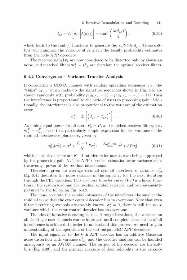
6 Iterative Demodulation and Decoding 141
dj,i = E
[dj,i
∣∣∣∣λ(dj,i)]
= tanh(
λ(dj,i)2
), (6.39)
which leads to the tanh(·) functions to generate the soft-bits dj,i. These soft-bits will minimize the variance of Ik given the locally probability estimatesfrom the code APP decoders.
The received signal rk are now considered to by distorted only by Gaussiannoise, and matched filters wT
k = sTi,k are therefore the optimal receiver filters.
6.4.2 Convergence – Variance Transfer Analysis
If considering a CDMA channel with random spreading sequences, i.e., the“chips” ak,l,n which make up the signature sequences shown in Fig. 6.5, arechosen randomly with probability p(ak,l,n = 1) = p(ak,l,n = −1) = 1/2, thenthe interference is proportional to the ratio of users to processing gain. Addi-tionally, the interference is also proportional to the variance of the estimationerror
σ2d = E
[(dj,i − dj,i
)2]
. (6.40)
Assuming equal power for all users Pk = P , and matched receiver filters, i.e.,wT
k = sTk,i, leads to a particularly simple expression for the variance of the
residual interference plus noise, given by
σ2IC(σ2
d) = σ2 +K − 1
NPσ2
d;K,N→∞
=⇒ σ2 + βPσ2d, (6.41)
which is intuitive: there are K−1 interferers for user k, each being suppressedby the processing gain N . The APP decoder estimation error variance σ2
d isthe average power of the residual interference.
Therefore, given an average residual symbol interference variance σ2d,
Eq. 6.41 describes the noise variance in the signal rk for the next iterationthrough the FEC decoders. This variance transfer curve (VT) is a linear func-tion in the system load and the residual symbol variance, and be convenientlypictured by the following Fig. 6.4.2.
The more accurate the symbol estimates of the interferers, the smaller theresidual noise that the error control decoder has to overcome. Note that evenif the interfering symbols are exactly known, σ2
d = 0, there is still the noisevariance which the error control decoder has to overcome.
The idea of iterative decoding is, that through iterations, the variance onall the single-user channels can be improved until complete cancellation of allinterference is achieved. In order to understand this process, we need to gainunderstanding of the operation of the soft-output FEC APP decoders.
The input signal rk to the k-th APP decoder has an additive Gaussiannoise distortion with variance σ2
IC, and the decoder analysis can be handledanalogously to an AWGN channel. The output of the decoder are the soft-bits (Eq. 6.39), and the primary measure of their reliability is the variance

142 Christian Schlegel
σ2d: cancelled symbol variance σ2
d = 1σ2d = 0
Sin
gle
-use
rnois
ele
vel
σ2 IC
channel
noise
level
slope:
system
load
Fig. 6.12. Soft cancellation variance transfer curve.
σ2d. While much numerical analysis [42, 43] seems to indicate that the LLRs
(Eq. 6.36) are Gaussian distributed with good accuracy, the soft-bits are notGaussian distributed. However, since in the limit of many users, the numberof terms in Ik is large, Ik is still asymptotically Gaussian by central limittheorem arguments, and therefore σ2
d is a sufficient measure of the reliabilityof dj,i.
The FEC code has a similar VT curve which translates input noise vari-ance σ2
IC into soft-output symbol variance values σ2d, and the operation of an
iterative receiver now carries out in the following way: Cancelled signals rk
for each user are generated according to Eq. 6.38 and passed to the FEC APPdecoders. They, in turn, generate soft estimates of the coded signals whichare used to generate interference estimates to be used in a new cancellationiteration. If the interleavers used in the system are large enough to ensurethat the implicit assumption of independence between signals is accurate, theprocess of iterative cancellation and decoding can be captured by a variancetransfer chart shown in Fig. 6.13 for the rate R = 1/3, ν = 3 convolutionalcode and a system load of β = 3.
Decoding starts at point (0) where the FEC decoders have to work withthe full interference and noise. Nonetheless, after one iteration, the systemmanages to reduce the interference by subtracting estimates of the interferingsignals, this leads to point (1), whose vertical component is the now reducednoise variance at the input of the soft-output error control decoder. In the next

6 Iterative Demodulation and Decoding 143
(0)
(1)
(2)
Rate 1/3 CC
K = 30
N = 10
Eb/N0 = 10dB
Soft-bit variance σ2d
σ2 IC
β = 3
Interference
Limitation
Noise Limitation
0
0.5
1
1.5
2
2.5
3
0 0.2 0.4 0.6 0.8 1 σ2d
Fig. 6.13. VT transfer chart and iteration example for a highly loaded CDMAsystem. FEC code VT is dashed, the cancellation VT curve is the solid curve.
iteration, the noise variance can be further reduced to point (2), and so on,until the iterations reach the intersection point between the two curves, thesolid point in the enlargement. At this point virtually all the interference hasbeen cancelled, and only channel noise is left. This intersection point is a fixpoint of a one-dimensional iterated variance transfer map, which models thebehavior of the iterative decoder. The performance of the individual decodersat that point is essentially that of the decoders in Gaussian noise, and we callit the noise limitation of the iterative decoder.
Note that along the iterative trajectory there is an section which forms anarrow channel through which the trajectory progresses in small steps. Thisarea is the interference limitation. A small increase in the system load willcreate another intersection point between the two VT curves, and the variancewill stop improving at that new fix point, rather than at the noise limitationfix point. The decoder does not function due to an excessive system load. Asthe load decreases, or the signal-to-noise ratio increases, the channel opensup and convergence to the noise limitation fix point is suddenly enabled. Thiseffect happens at a very sharp signal-to-noise threshold, and gives rise to theabrupt, cliff-like behavior of the error rates in such systems, which is illustratedby the simulations shown in Fig. 6.18. Clearly visible is the sharp onset of thedrop in error rates as the signal-to-noise ratio is increased sufficiently to open

144 Christian Schlegel
Table 6.1. Serial concatenated codes of total rate R = 1/3 used in Fig. 6.14.
Inner Code Outer Code Rate
SerialConcatenatedCode 1
g1 =
[1 0 1+D2
1+D+D2
0 1 1+D1+D+D2
]g2 = [1 1+D2
1+D+D2 ] 13
SerialConcatenatedCode 2
g1 =
[1 0 1+D2
1+D+D2
0 1 1+D1+D+D2
]rate 1/2 repetition code 1
3
the convergence channel and allow the decoder system to progress beyond theinterference limitation. At sufficient signal-to-noise ratios the bit error ratesclosely follow those of the FEC code operated in additive noise alone, this isthe noise limitation and is only a function of the FEC code used.
The question now poses itself as to what FEC code should be used forefficient communication. Examining stronger error control codes, such as turbocodes or LDPC codes will be beneficial in the noise limitation area, where thesingle-user performance of the codes comes to bear. Fig. 6.14 show the VTcurves of a selection of powerful error control codes, several rate R = 1/3LDPC codes at their first iteration and at iteration 20, as well as two rateR = 0.5 serially concatenated turbo codes, whose rates and component codesare given in the following table. All of these codes have good to excellentperformance on AWGN channels, and their VT transfer curves all show ageneral trend. The more powerful the code, the more abrupt the transitionbetween unreliable and reliable code output behavior. Further analysis on theimpact of the code and code choices are explored in [26, 40].
6.4.3 Filters in the Loop
A simple processing filter wTk in Fig. 6.11 is a filter matched to the spreading
waveform of user k. Such a matched-filter canceler is both computationallyefficient and has good performance. Nontheless, more sophisticated loop filterscan eek out extra system gain. In this section we explore the potential of alocal per-user minimum-mean square error (MMSE) filter, originally proposedby Wang and Poor [44]. From a (local) variance point of view the MMSE filteris the optimal choice. We therefore consider the filter
wTi,k = arg min
w∈RNE(∥∥dk,i − wT rk
∥∥2)
. (6.42)
The advantage of the MMSE filter over the matched filter comes from its ca-pability to include the correlation inherent in the residual interference signal.The derivation of the filter follows standard steps [26], and we obtain

6 Iterative Demodulation and Decoding 145
(2,4) regular LDPC
irregular LDPCs
(4,8) regular LDPC
Serial ConcatenatedCode 2
iteration 1
iteration 20
SerialConcatened Code 1
σ2 eff
0
0.5
1
1.5
2
2.5
3
0 0.2 0.4 0.6 0.8 1 σ2d
Fig. 6.14. Illustration of variance transfer curves of various powerful error controlcodes, such as practical-sized LDPC codes of lenght N = 5000 and code rate R = 0.5,as well as two serially concatenated turbo codes.
wTi,k =
√PksT
i,k
(SkPkST
k + σ2I)−1
Pk + sTi,k
(SkPkST
k + σ2I)−1
sTi,k
. (6.43)
We see that this filter now depends not only on the spreading sequence ofthe interfering users, but also on their powers Pk, where Pk equals P withthe k-th entry removed. Furthermore, since these are residual powers, thematrix inverse in Eq. 6.43 has to be recomputed for every iteration – a trulytremendous effort.
In the case of a system with equal received power, a result by Tse andHanly [45] allows us to calculate the signal-to-noise ratio after the MMSEfilter in closed form as a function of the residual interference as
βk =σ2
dP (β − 1) − σ2
2σ2+
√(σ2
dP )2(β − 1)2
4σ22 +σ2
dP (β − 1) − σ2
2σ2+
14. (6.44)
Schlegel et. al. [26, 40] prove the following limit result
limwσ2 →∞
σ2IC
σ2d
= β − 1, (6.45)

146 Christian Schlegel
0 0.2 0.4 0.6 0.8 10
0.5
1
1.5
2
2.5
Soft-bit variance σ2d
Res
idualM
UV
ari
ance
σ2 IC
Es/N0 = 0
Es/N0 → ∞
Fig. 6.15. Variance transfer curves for matched filter (simple) cancellation andper-user MMSE filter cancellation (dashed lines) for β = 2 and Es/N0 = 0dB andEs/N0 → ∞.
which is illustrated by the canceler VT curves shown in Fig. 6.15. This leadsto the following conclusion: If simple cancellation can support a load of β, theuse of per-user MMSE filters instead of the matched filters allows a load ofβ + 1 for high signal-to-noise ratios. Therefore, an appreciable performancegain can be achieved for systems with a moderate level of loading.
6.4.4 Low-Complexity Loop Filters
While the MMSE loop filter can produce a marked advantage for a certainrange of channel loads, its implementation is significantly more complex thanthat of a matched filter due to the inverse in Eq. 6.43. However, if we replace
Ki,k = Si,kPkSTi,k + σ2I (6.46)
in Eq. 6.43 by the first-order stationary multi-stage approximation
K−1i,k = (I − τKi,k)n +
n−1∑l=0
τ (I − τKi,k)l
= φn (Ki,k) (6.47)

6 Iterative Demodulation and Decoding 147
according to the principles explored in Sec. 6.3.4, the resulting system com-plexity is much reduced, depending only on the number of stages n. As shownin [26], this number does not depend on N or K, and only very few stagesrecover almost all of the difference between a matched-filter iterative decoderand an MMSE iterative decoder.
Instead of Eq. 6.43, the loop filter is now
wi,k = φn (Ki,k) si,k (6.48)
where we have dropped the normalization factor in Eq. 6.43 since its variancegoes to zero for large systems with K,N → ∞.
Fig. 6.16 below shows such VT curves for a number of stages and twovalues of the signal-to-noise ratio. It is remarkable that one or two stages arealmost completely sufficient to achieve the VT characteristics of the MMSEloop filter over a wide range of input soft bit variance σ2
d and channel signal-to-noise ratios.
We use the following numerical example to illustrate the accuracy of theanalysis as well as the power of the multi-stage loop filters. The test exampleis made up of a convolutional rate R = 1/3 four-state code with G(D) =[1 + D2, 1 + D + D2, 1 + D + D2] and a two-stage first order stationary loop
0 0.2 0.4 0.6 0.8 10
0.5
1
1.5
2
2.5per-userMMSE Filter
Matched FilterInterferenceCancellation
4 stages
5 stages
10 stages
2 stages
2 stages
1 stage
1 stage
Soft-bit variance σ2d
Res
idualM
UV
ari
ance
σ2 IC
Es/N0 = 0dB
Es/N0 = 20dB
Fig. 6.16. Variance transfer curves for various multi-stage loop filters for a β = 2and two values of the signal-to-noise ratio: Es/N0 = 0dB and Es/N0 = 20dB.

148 Christian Schlegel
filter with stationarity parameter τ = 2/(N0 +(√
K−1N + 1
)2
to guaranteeconvergence.
Fig. 6.17 shows the matching between the two-stage loop filter cancelerand the 4-state convolutional codes used as FEC. At a signal-to-noise ratio ofEb/N0 = 4.5dB, both the two-state loop filter and a full MMSE loop filter forthe load of β = 3 converge, while a matched filter canceler would no longerachieve low error rate since its VT curve intersects with that of the FEC codesat high values of σ2
d, that is, before the turbo cliff.Fig. 6.18 shows bit error rates for this example system, showing the typical
turbo cliff occur as soon as the convergence channel opens at around 4.5dB.The number of users is K = 45, and the spreading gain is N = 15, creatingsystem load β = 3. Note that a full MMSE canceler would gain only about0.3dB in signal-to-noise ratio over the two-stage loop filter – hardly worth theadditional complexity.
0 0.2 0.4 0.6 0.8 10
0.5
1
1.5
2
2.5
3
3.5
4
(1)
(3)
(2)
(4)
(5)K = 45, N=15L
u = 5000
(1): VT for rate 1/3 CC (v=2)(2): VT for interference canceller(3): simulation trajectory(4): VT for 1st order filter (2 stages)(5): VT for per user MMSE
Soft-bit variance σ2d
Res
idualM
UV
ari
ance
σ2 IC
Fig. 6.17. Variance transfer chart for an iterative decoder using convolutional errorcontrol codes and a two-stage loop filter, showing an open channel at Eb/N0 = 4.5dB.

6 Iterative Demodulation and Decoding 149
single-user performance
30 Iterations
20 Iterations
10 Iterations
1 Iteration2-stage loop filter
MMSE Filter(30 Iterations)
1
10−1
10−2
10−3
10−4
10−5
Bit
Err
or
Rate
3 3.5 4 4.5 5 5.5 Eb/N0
Fig. 6.18. Bit error rate performance of an iterative canceler with a two-stage loopfilter, compared to the performance of an MMSE loop filter.
6.5 Asymmetric Operating Conditions
The analysis in this chapter focused on equal power and equal rate systems,and one rightfully raises the question how these results change as differentreceived power levels are enabled, or codes with different rates are used. Whilea detailed discussion of these issues is beyond the scope of this chapter, wewish to summarize key results here.
A first important result concerns linear filter multiuser detectors, includ-ing their iterative implementations. It can be shown that the overall efficiency,either in terms of minimally required Eb/N0, or maximal capacity per dimen-sion, is optimal for an equal received power situation [45]. In the case ofunequal received powers the required signal-to-noise ratio is averaged over allusers. This is arguably a meaningful measure, albeit it other measures couldbe more relevant depending on the application. The result that equal receivedpower maximizes system performance is quite straight-forward to show for thematched filter receiver – in fact this is the major reason for the enormous ef-forts that are being undertaken to implement power control in current CDMAsystems – and has also been shown to be true for the MMSE filter detector.

150 Christian Schlegel
The conclusion we draw from this result is that power control is an importantfeature in CDMA systems, even if a linear joint detector is used.
For iterative decoders which include the error control code in the loop,the converse is true, i.e., the equal power case produces the worst case perfor-mance of the overall system in terms of average signal-energy to noise powerratio versus spectral efficiency. However, we are not aware of a rigorous proofof this statement. What is known is that, with properly adjusted power levels,the capacity of the multiple access channel can be achieved with an iterativedecoder. Unfortunately these power levels are exponentially distributed [40].The same effect can be achieved with different coding rates, rather than dif-ferent power levels, also achieving the capacity of the channel. It seems safeto conclude that in a scenario where the received powers are not controlled,and where large fluctuations in the received power are expected, an iterativedecoder including FEC will fare significantly better than a mere linear filterfront-end. On the other hand, in a power regulated scenario, where the re-ceived powers are constant, linear processing – iterative or not – achieves avery large portion of the theoretical capacity of the channels for system loadsas large as β = 1.
Fig. 6.19 shows achievable information theoretic capacities for randomCDMA systems using both a linear minimum mean-square error filter andoptimal processing for two system loads. The two capacities for β = 0.5 showvery little difference, and it is therefore “nearly optimal” to use a minimummean square error filter as linear preprocessor which converts the CDMA chan-nel into parallel single-user AWGN channels where well-known FEC methods
can be used. This is the case for β≈≤ 0.5 in random CDMA channels. Even
for β = 1 the improvement possible is only in order of about 50% in terms ofcapacity. As the system load increases, linear preprocessing becomes increas-ingly less efficient, and for highly loaded systems joint detection can providesignificant extra gains. When and where joint detection provides a capacityadvantage depends on the particular system. In general, systems with a smallnumber of users per signal dimension do not profit significantly from jointprocessing.
This picture changes if powers and/or rates are unequal, where iterativedecoding can make a large difference. A precise analysis depends on the par-ticular distribution of the power levels, and will have to be evaluated case bycase. Further results, an in-depth discussion of asymmetric operating condi-tions, and proofs of the results stated above can be found in [26].
6.6 Conclusions
The topic of iterative demodulation and decoding is fascinating. The methodis extremely powerful in handling large constellations arising from the (linear)superposition of a large number of signals, which we wish to decode, eitherdependently, or independently. The turbo decoding principle, which was so

6 Iterative Demodulation and Decoding 151
AWGN Capacity
optimalβ = 1
Linearβ = 1
optimalβ = 0.5
Linearβ = 0.5
-2 0 2 4 6 8 10 12 14 16
Eb/N0 [dB]
0.1
1
10C
apaci
ty[b
its/
dim
ensi
on]
Fig. 6.19. Comparison of the per-dimension capacity of optimal and linearlyprocessed random CDMA channels. The solid lines are for β = 0.5 for both lin-ear and optimal processing, the dashed lines are for a full load β = 1.
successful in achieving the Shannon capacity on the AWGN channel [8], hasalso proven extremely useful in iterative demodulation and decoding.
We have shown that there are essentially two avenues to approach theproblem. The first is linear filtering, which separates the superposed channelsinto independent channels via direct or iterative multistage linear operations.This method works very well for systems whose numbers of signal dimensionsexceeds the number of signals – the typical case to date. Power control maybe necessary to maintain a large system efficiency, even with use of these jointdemodulators.
The second avenue is to consider a full iterative (turbo) decoder with softinformation messages cycling back to an appropriate cancellation front-end.This approach is more powerful, benefits from different received power levels,and under judicious operating conditions, can be shown to achieve the capacityof the multiple access channel. It is also more complex, but not significantly

152 Christian Schlegel
so. Both approaches essentially scale linearly in the number of joint signalthat need to be detected.
Future implementers will have to carefully weigh the advantages and costsof these two approaches in order to find optimal system configurations. Last,but not least, we wish to point out that this area is still undergoing sig-nificant research, and that hybrid systems are feasible. For example, simplesoft-thresholding devices put into the iterative matrix inversion loops haveproven to be very effective in improving performance of the linear demodula-tors. These non-linear devices can be viewed as simple symbol-level decoders.
In either way, iterative demodulation and decoding is a very powerfulmethodology to work with large numbers of interfering signals. Their com-plexity only linearly depends on the number of signals to be treated, and theyare thus implementable even for large systems.

6 Iterative Demodulation and Decoding 153
References
1. C.E. Shannon, “A mathematical theory of communications,” Bell Syst. Tech.J., vol.27, pp. 379-423, July 1948.
2. T. Cover and J. Thomas, Elements of Information Theory, John Wiley, NewYork, 1991.
3. H. Nyquist, “Certain topics in telegraph transmission theory,” AIEE Trans.,pp. 617–644, 1928.
4. C. Schlegel and L. Perez, Turbo and Trellis Coding, IEEE/Wiley, PiscatawayNJ, 2004.
5. J.M. Wozencraft and I.M. Jacobs, Principles of Communication Engineering,John Wiley and Sons, New York, 1965, reprinted by Waveland Press, 1993.
6. R. G. Gallager, “Low-density parity-check codes”, IRE Trans. on Inform. The-ory, pp. 21–28, Vol. 8, No. 1, January 1962.
7. C. Berrou, A. Glavieux, and P. Thitimajshima, “Near Shannon limit error-correcting coding and decoding: Turbo-codes,” Proc. 1993 IEEE ICC, Geneva,Switzerland, pp. 1064–1070, 1993.
8. C. Berrou and A. Galvieux, “Near optimum error correcting coding and decod-ing: turbo-codes,” IEEE Trans. Commun., Vol. 44, No. 10,pp. 1261–1271, Oct.1996.
9. D. J. C. MacKay and R. M. Neal, “Near Shannon limit performance of lowdensity parity check codes”, IEE Electronic Letters, vol. 32, no. 18, pp. 1645–1646, August 1996.
10. D. J. C. MacKay, “Good error-correcting codes based on very sparse matrices”,IEEE Trans. Inform. Theory, vol. IT-45, No. 2, pp. 399–431, March, 1999.
11. E. Guizzo, ”Closing in on the perfect code”, IEEE Spectrum, Vol. 41, No. 3,pp. 36–42, Mar. 2004.
12. R.M. Tanner, “A recursive approach to low complexity codes,” IEEE Trans.Inform. Theory, vol. IT-27, pp. 533–547, September 1981.
13. S. Y. Chung, G. D. Forney, T. J. Richardson and R. Urbanke, “On the design oflow-density parity-check codes within 0.0045 dB of the Shannon limit”, IEEEComm. Letters, vol. COMM-5, no. 2, pp. 58–60, February, 2001.
14. R.A. Horn and J.C. Johnson, Matrix Analysis, Cambridge University Press,New York, 1990.
15. A.J. Viterbi, CDMA : Principles of Spread Spectrum Communication, PrenticeHall,1995.
16. R.E. Ziemer, R.L. Peterson, D.E. Borth Introduction to Spread Spectrum Com-munications, Pearson Education, 1995.
17. J.G. Proakis, Digital Communications, McGraw-Hill, Inc., 1995.18. E. Telatar, “Capacity of Multi-antenna Gaussian Channels,” Europ. Trans.
Telecommunications, vol. 42, no. 2/3/4, pp. 1617–1627, Nov.-Dec. 1999.19. G.J. Foschini, “Layered space-time architecture for wireless communication in
a fading environment when using multi-element antennas,” Bell Labs Tech. J.,vol. 1, Aug. 1996, pp. 41 – 59.
20. T.L. Marzetta and B.M. Hochwald, “Capacity of a mobile multiple-antennacommunication link in Rayleigh flat fading,” IEEE Trans. Inform. Theory, vol.45, no. 1, pp. 139–157, Jan. 1999.
21. Z. Bagley and C. Schlegel, “Classification of correlated flat fading MIMO chan-nels,” Proc. Third Canadian Workshop on Inform. Theory, Vancouver, Canada,June 2001.

154 Christian Schlegel
22. D. Gesbert, H. Bolcskei, D.A. Gore, and A.J. Paulraj, “Outdoor MIMO wire-less channels: Models and performance prediction,” IEEE Trans. Commun., toappear.
23. A.L. Swindlehurst, G. German, J. Wallace, M. Jensen, “Experimental mea-surements of capacity for MIMO indoor wireless channels,” 3rd IEEE SignalProc. Wshp., Taiwan, Mar. 20–25, 2001.
24. P. Goud Jr, C. Schlegel, R. Hang, W. Krzymien, Z. Bagley, ”MIMO ChannelMeasurements for an Indoor Office Environment,” IEEE Wireless ’03, July 7-9,Calgary, AB, Canada.
25. P. Goud Jr, C. Schlegel, W.A. Krzymien, R. Hang, “Multiple Antenna Commu-nication Systems - An Emerging Technology,” Canadian Journal of Electricaland Computer Engineering, accepted for publication.
26. C. Schlegel and A. Grant, Coordinated Multiple User Communications, SpringerPublishers, 2005.
27. G.J. Foschini and M.J. Gans, “On limits of wireless communication in a fadingenvironment when using multiple antennas,” Wireless Personal Commun., vol.6, no. 3, pp. 311–355, Mar. 1998.
28. R. Lupas and S. Verdu, “Linear multiuser detectors for synchronous code–division multiple–access channels,” IEEE Trans Inform. Theory, vol. 35, no. 1,pp. 123–136, January 1989.
29. P. D. Alexander, L. K. Rasmussen, and C. Schlegel, “A linear receiver for codedmultiuser CDMA,” IEEE Trans. Commun., vol. 45, pp. 605–610, May 1997.
30. Z.D. Bai and Y.Q. Yin, “Limit of the smallest eigenvalue of large dimensionalsample covariance matrix,” Ann. Probab.,, vol. 21, pp. 1275–1294, 1993.
31. S. Verdu and S. Shamai, “Spectral Efficiency of CDMA with Random Spread-ing,” IEEE Trans. Inform. Theory, vol. 45, pp. 622–640, March 1999.
32. Z. Xie, R. Short, and C. Rushforth, “A family of suboptimum detectors forcoherent multiuser communications,” IEEE. J. Select. Areas Commun., vol. 8,no. 4, pp. 683–690, May 1990.
33. P. B. Rapajic and B. S. Vucetic, “Adaptive receiver structures for asynchronousCDMA systems,” IEEE J. Select. Areas Commun., vol. 12, no. 4, pp. 685–697,May 1994.
34. U. Madhow and M.L. Honig, “MMSE interference suppression for direct–sequence spread–spectrum CDMA,” IEEE Trans. Commun., vol. 42, no. 12,pp. 3178–3188, Dec. 1994.
35. O. Axelsson, Iterative Solution Methods, Cambridge University Press, 1994.36. Gilbert Strang, Linear Algebra and its Applications, Harcourt Brace, 3 edition,
1988.37. H. Elders-Boll, H-D. Schotten, and A. Busboom, “Efficient implementation of
linear multiuser detectors for asynchronous CDMA systems by linear interfer-ence cancellation,” Europ. Trans. Telecommun, vol. 9, pp. 427–438, Sept-Oct.1998.
38. M.K. Varanasi and B. Aazhang, “Multistage detection in asynchronous code-division multiple-access communications,” IEEE Trans. Commun., vol. 38, No.4, pp. 509–519,April 1990.
39. A. Grant and C. Schlegel “Iterative Implementations for Linear Multiuser De-tectors” IEEE Trans. Commun., vol. 49, pp. 1824-1834, October 2001.
40. C. Schlegel, Z. Shi, and M. Burnashev, “Asymptotically Optimal Power Al-location and Code Selection for Iterative Joint Detection of Coded RandomCDMA,” IEEE Trans. Inform. Theory, in revision.

6 Iterative Demodulation and Decoding 155
41. M. Moher, “An Iterative Multiuser Decoder for Near-Capacity Communica-tions”, IEEE Trans. Commun., vol. 47, pp. 870–880, July 1998.
42. S. ten Brink, “Convergence behavior of iteratively decoded parallel concate-nated codes,” IEEE Trans. Commun., vol. 49, no. 10, October, 2001.
43. D. Divsalar, S. Dolinar, and F. Pollara, “Iterative Turbo decoder analysis basedon density evolution,” TMO Progress Report 42-144, February 15, 2001.
44. X. Wang and H.V. Poor, “Iterative (Turbo) Soft Interference Cancellation andDecoding for Coded CDMA”, IEEE Trans. Commun., vol. 47, no. 7, July 1999.
45. D. Tse and S. Hanly, “Linear Multiuser Receivers: Effective interference, ef-fective bandwidth and user capacity,” IEEE Trans. Inform. Theory, vol. 45,pp. 641–657, Mar. 1999.

Chapter 7
Turbo Receiver Techniques for Coded MIMOOFDM Systems ∗
Ben Lu and Xiaodong Wang
Columbia University, USA
In recent years, iterative (“turbo”) processing techniques have received con-siderable attention stimulated by the discovery of the powerful turbo codes[2, 3]. The so called “turbo principle” can be successfully applied to many de-tection/decoding problems such as serial concatenated decoding, equalization,coded modulation, multiuser detection and joint source and channel decoding[16, 37, 44]. We start the discussion of this chapter by illustrating the generalconcept of turbo processing for concatenated systems using a simple example.
A typical communications system in general consists of a cascade of sub-systems with different signal processing functionalities. Consider, for exam-ple, the simple communication system employing channel coding and signal-ing over an inter-symbol interference (ISI) channel, as shown in Fig. 7.1. Ina “conventional” receiver, the demodulator makes hard decisions about thetransmitted bits b[i] based on the received signal r(t), which are then passedto the channel decoder to decode the transmitted information. The problemwith this approach is that by making hard decisions of the bits, informationloss is incurred in each subsystem (i.e., demodulator and decoder). This is be-cause while the subsystem only indicates whether it believes that a given bitis a “0” or a “1”, it usually has sufficient information to estimate the degreeof confidence in its decisions. One straightforward way to reduce the loss ofinformation, and the resulting loss in performance, is to pass the confidencelevel along with the decision, i.e., to render soft decisions. This is often donewhen passing information from a demodulator to a channel decoder, whichis known to result in approximately a 2dB performance gain in the additivewhite Gaussian noise (AWGN) channel [39]. However, even if optimal bit-by-bit soft decisions are passed between all the subsystems in the receiver,the overall performance can still be far from optimal. This is due to the factthat, while later stages (e.g., the channel decoder) can use the information
∗ This work was supported in part by the U.S. National Science Foundation (NSF)under grants CCR-0225826 and CCR-0207550, and in part by the U.S. Office ofNavel Research (ONR) under grant N00014-03-1-0039.
157
K. Sripmanwat (ed.), Turbo Code Applications: a journey from a paper to realization, 157–191.
© 2005 Springer. Printed in the Netherlands.

158 Ben Lu and Xiaodong Wang
deinterleaver
interleaverchannelencoder
channeldecoder
modulator
demodulator
ISI channel
r(t)
b[i]
Fig. 7.1. A coded communication system signaling through an inter-symbol inter-ference (ISI) channel.
gleaned from previous stages (e.g., the demodulator), the reverse is not gen-erally true. While the optimal performance can be achieved by performinga joint detection, taking all receiver processing into account simultaneously(e.g., maximum likelihood detection based on the super-trellis of both thechannel code and the ISI channel), the complexity of such a joint approach isusually prohibitive. This motivates an iterative (turbo) processing approachwhich allows earlier stages (e.g., the demodulator) to refine their processingbased on information obtained from later stages (e.g., the channel decoder).
In order to employ turbo processing in the system shown in Fig. 7.1, boththe demodulator and the channel decoder are of the maximum a posterioriprobability (MAP) type. The function of the MAP demodulator is to producesoft decisions which reflect the probability that a given bit is a “0” or a “1”. Atthe lth iteration, the information available to the MAP demodulator consists ofthe received signal r(t) and the a priori probabilities of the input bits, the laterof which are applied by the MAP channel decoder based on its output fromthe (l−1)th iteration. The MAP demodulator uses this information, combinedwith knowledge of the chosen modulation and of the channel structure, toproduce the a posteriori probabilities (APPs) of the channel bits
P l(b[i] = 1 | r(t)) =p(r(t) | b[i] = 1)P l−1(b[i] = 1)
p(r(t)), (7.1)
and P l(b[i] = 0 | r(t)) =p(r(t) | b[i] = 0)P l−1(b[i] = 0)
p(r(t)), (7.2)
for all b[i]i. Consider the log-likelihood ratio (LLR) formed from the a pos-teriori probabilities of Eq. 7.1 and 7.2:

7 Turbo Receiver Techniques for Coded MIMO OFDM Systems 159
Λl1(b[i])
= logP l(b[i] = 1 | r(t))P l(b[i] = 0 | r(t))
= logp(r(t) | b[i] = 1)p(r(t) | b[i] = 0)︸ ︷︷ ︸
λl1(b[i])
+ logP l−1(b[i] = 1)P l−1(b[i] = 0)︸ ︷︷ ︸
λl−12 (b[i])
. (7.3)
It is seen from Eq. 7.3 that the LLR is the sum of two distinct quantities.The first term, λl
1(b[i]), is the so-called extrinsic information produced by thefirst stage subsystem in the receiver (i.e., the MAP demodulator), which isinformation that the MAP demodulator gleans about b[i] from the receivedsignal r(t) and the a priori probabilities of the other transmitted bits, withoututilizing the a priori probability of b[i]. The second term, λl−1
2 (b[i]), containsthe a priori probability of b[i]. Note that typically, for the first iteration (l =1), we set P 0(b[i] = 1) = P 0(b[i] = 0) = 1
2 , i.e., λ02(b[i]) = 0 for all i. The
extrinsic information λl1(b[i]) produced by the MAP demodulator, is sent
to the second stage subsystem, i.e., the MAP channel decoder, as the a prioriinformation for channel decoding.
Based on the a priori information provided by the MAP demodulator,and the channel code constraints, the MAP channel decoder computes the aposteriori LLR of each code bit
Λl2(b[i])
= logP (b[i] = 1 | λl
1(b[i]); code structure)P (b[i] = 0 | λl
2(b[i]); code structure)
= λl2(b[i]) + λl
1(b[i]). (7.4)
Here again we see that the output of the channel decoder is the sum of theextrinsic information λl
2(b[i]) obtained by the second stage subsystem (i.e.,the MAP channel decoder), and the prior information λl
1(b[i]) delivered by theprevious stage (i.e., the MAP demodulator). The extrinsic information λl
2(b[i])is then fed back to the MAP demodulator as the a priori information in thenext (i.e., (l+1)th) iteration. It is important to note that Eq. 7.3 and 7.4 holdonly if the inputs to the demodulator or the decoder are independent. Sinceboth the ISI channel and the channel encoder have memory, this independenceassumption will not be valid; therefore, interleaving (i.e., permutation of timeorder) must be present between the demodulator and the decoder in order toprovide approximate independence. Finally, the turbo receiver structure forthe coded ISI system is illustrated in Fig. 7.2. This scheme was first introducedin [10], and is termed a “turbo equalizer”. The name “turbo” is justifiedbecause both the demodulator and the decoder use their processed outputvalues as a priori input for the next iteration, similar to the operation of aturbo engine. The same turbo processing principle can be applied to codedCDMA systems, yielding the so-called turbo multiuser detection [35, 40, 53–55].
In this chapter, we introduce the applications of turbo principle in thereceiver design and code optimization of low-density parity-check (LDPC)

160 Ben Lu and Xiaodong Wang
MAP
demodulatordeinterleaver + interleaver
Λ 2 λ 2λ 1Λ1 MAP
decoder+
r(t)
-
-
Fig. 7.2. A turbo receiver for coded communication over ISI channel.
coded multiple-input multiple-output (MIMO) orthogonal-frequency division-multiplexing (OFDM) systems.
7.1 LDPC-Coded MIMO OFDM Systems
Multiple-input multiple-output (MIMO) data transmission through sparsely-spaced antennas at both transmitter and receiver provides substantial increasein spectral efficiency of wireless links, both in theory and in practice. Techni-cally, MIMO transmission can potentially accomplish both multiplexing gain,i.e., the information rate increase due to virtual multiple air-links, and di-versity gain, i.e., the spatial diversity due to multiple antennas in additionto time-domain and frequency-domain diversity. Key to realizing such highspectral efficiency (i.e., high data rate) promised by MIMO systems is thepractical coded modulation schemes. For small block size (e.g., smaller thanten), there are many solutions such as orthogonal space-time block codes [46],linear dispersion codes [17], threaded algebraic space-time codes [9] and lat-tice space-time codes [13]. When the block size is around several hundred, op-tions include space-time trellis codes [47] and ‘wrapped’ space-time codes [5].For moderate-to-large block size (e.g., larger than 1000) which is suitable formost data traffic in broadband communications, existing schemes are mostlybased on powerful binary random codes (e.g., turbo codes or LDPC codes),and they include bit-interleaved coded modulation (BICM), [24, 27, 49, 56],[18, 19], stratified diagonal BLAST [43]. The LDPC-coded MIMO OFDMscheme proposed in this chapter falls into the category of BICM based MIMOwith moderate-to-large block size.
7.1.1 MIMO OFDM Modulation
Consider a quasi-static block fading model for a generic MIMO OFDM modu-lation, as illustrated in Fig. 7.3. It is assumed that the fading channels remainstatic during each OFDM slot but vary independently from one OFDM slotto another. Assume proper cyclic insertion and sampling, the MIMO OFDMsystem with K subcarriers decouples frequency-selective channels into K cor-related flat-fading channels with the following input-output relation

7 Turbo Receiver Techniques for Coded MIMO OFDM Systems 161
......
......
. . .
. . .
. . .......
Frequency
Time
#1
#2
#K
#1 #3 #P#2
#1
#2
#Nr#Nt
#2
#1
Rx AntennaTx Antenna
#3
Fig. 7.3. System description of a MIMO OFDM system over correlated fadingchannels. Each transmit frame spans K subcarriers and P time slots; at a particularsubcarrier and at a particular time slot, coded symbols are transmitted from Nt
transmitter antennas and received by Nr receiver antennas.
y[p, k] =√
γ
NtH[p, k]x[p, k]+n[p, k] , k = 0, . . . , K−1, p = 0, . . . , P−1,
(7.5)where Nt (Nr) denotes the number of transmitter (receiver) antennas; H[p, k] ∈CNr×Nt is the matrix of complex channel frequency responses to be definedlater; x[p, k] ∈ ΩNt and y[p, k] ∈ CNr are respectively the transmitted signalsand the received signals at the k-th subcarrier and the p-th slot; C denotes theset of complex number; Ω denotes quadrature amplitude modulation (QAM)constellation with unit average power; n[p, k] ∈ CNr is the additive noise withindependent and identically distributed (i.i.d.) entries n[p, k] ∼ Nc(0, I); γdenotes the average signal-to-noise ratio (SNR) at each receiver antenna.
Consider the channel response between the j-th transmitter antenna andthe i-th receiver antenna. Following [39], the time-domain channel impulseresponse can be modeled as a tapped-delay line. With only the non-zero tapsconsidered, it can be expressed as
hi,j(τ ; t) =Lf∑l=1
αi,j(l; t)δ(
τ − nl
K∆f
), (7.6)
where δ (·) is the Dirac delta function; Lf denotes the number of non-zerotaps; αi,j(l; t) is the complex amplitude of the l-th non-zero tap, whose de-lay is nl/(K∆f ), where nl is an integer and ∆f is the tone spacing of theOFDM system. In mobile channels, for the particular (i, j)-th antenna pair,the time-variant tap coefficients αi,j(l; t), ∀l,∀t, can be modeled as wide-sensestationary random processes with uncorrelated scattering (WSSUS) and withband-limited Doppler power spectrum [39]. For the signal model in Eq. 7.5, weonly need to consider the time responses of αi,j(l; t) within the time intervalt ∈ [0, PT ], where T is the total time duration of one OFDM word plus itscyclic extension, and PT is the total time involved in transmitting P adja-

162 Ben Lu and Xiaodong Wang
cent OFDM words. Following [20], for the particular l-th tap of the (i, j)-thantenna pair, the dimension of the band- and time-limited random processαi,j(l; t), t ∈ [0, PT ] (defined as the number of significant eigenvalues in theKarhunen-Loeve expansion of this random process), is approximately equal
to Lt= 2fdPT + 1, where fd is the maximum Doppler frequency. Hence,
ignoring the edge effects, the time response of αi,j(l; t) can be expressed interms of the Fourier expansion as
αi,j(l; t) fdPT∑
n=−fdPTβi,j(l, n)ej2πnt/(PT ) , (7.7)
where βi,j(l, n)n is a set of independent circularly symmetric complexGaussian random variables, indexed by n.
For OFDM systems with proper cyclic extension and sample timing, withtolerable leakage, the channel frequency response between the j-th transmitterantenna and the i-th receiver antenna at the p-th time slot and at the k-thsubcarrier, which is exactly the (i, j)-th element of H[p, k] in Eq. 7.5, can beexpressed as [28, 52]
Hi,j [p, k]= Hi,j(pT, k∆f ) =
Lf∑l=1
αi,j(l; pT )e−j2πknl/K = hHi,j(p)wf (k) ,
(7.8)
where hi,j(p)= [αi,j(1; pT ), . . . , αi,j(Lf ; pT )]H is the Lf -sized vector contain-
ing the time responses of all the non-zero taps; H denotes matrix or vectorHermitian transpose; and wf (k)
=[e−j2πkn1/K , . . . , e−j2πknLf
/K]T containsthe corresponding DFT coefficients.
Using Eq. 7.7, αi,j(l; pT ) can be simplified as
αi,j(l; pT ) =fdPT∑
n=−fdPT
βi,j(l, n)ej2πnp/P = βHi,j(l)wt(p) , (7.9)
where βi,j(l)= [βi,j(l,−fdPT ), · · · , βi,j(l, 0), · · · , βi,j(l, fdPT )]H is an Lt-
sized vector; and wt(p)=
[e−j2πpfdT , . . . , ej0, . . . , ej2πpfdT
]T contains thecorresponding inverse DFT coefficients. Substituting Eq. 7.9 into Eq. 7.8, weget
Hi,j [p, k] = gHi,jW
′t(p)wf (k) , (7.10)
with gi,j=[βH
i,j(1), . . . ,βHi,j(Lf )
]HL×1
,
W ′t(p)
= diagwt(p), . . . ,wt(p)L×Lf
,

7 Turbo Receiver Techniques for Coded MIMO OFDM Systems 163
where βi,j(l, n)n are properly normalized as∑
l
∑n Varβi,j(l, n)n =
1, ∀i, j. From Eq. 7.10, it is seen that due to the close spacing of OFDM sub-carriers and the limited Doppler frequency, for a specific antenna pair (i, j),the channel responses Hi,j [p, k]p,k are different transformations [specifiedby wt(p) and wf (k)] of the same random vector gi,j , and hence they arecorrelated in both frequency and time.
7.1.2 Channel Capacity
With no channel state information (CSI) at the transmitter side, the channelcapacity for the above MIMO OFDM modulation has been studied in [11, 33].Assume Gaussian signaling (i.e., Ω → C), for MIMO OFDM channels withinfinite fading channel observations (i.e, P → ∞), the ergodic capacity is givenby
Cerg(γ)= E
1
KP
K−1∑k=0
P−1∑p=0
[log2 det
(INr +
γ
NtH [p, k]HH[p, k]
)]︸ ︷︷ ︸
I|H(γ)
bits/Hz/sec,
(7.11)
where the expectation is taken over random channel states H, with H =
H[p, k]p,k; I|H(γ) is the instantaneous mutual information conditioned onH . For MIMO OFDM channels with finite fading channel observations (i.e,P ∞), the outage capacity/probability is a more sensible measure. For atarget information rate R, the outage probability is given by
Pout(R, γ) = Pr(I|H(γ) < R) . (7.12)
However, in practice, the transmitted signals usually take values from con-straint constellation, i.e., x ∈ ΩNt . In this case, following [51], the mutualinformation is computed instead as
I|H(γ) = Nt log2 |Ω| − 1KP |Ω|Nt
K−1∑k=0
P−1∑p=0
|Ω|Nt−1∑j=0
E
log2
|Ω|Nt−1∑i=0
exp[−∥∥√γ/Nt H[p, k]
(xj − xi
)+ z
∥∥2 +∥∥z
∥∥2]
,
(7.13)
where the expectation is taken over random noise vector z ∼ Nc(0, I).
7.1.3 Transmitter Structure
For an LDPC coded MIMO OFDM system with K subcarriers, Nt transmit-ter antennas and Nr receiver antennas, the transmitter structure is illustrated

164 Ben Lu and Xiaodong Wang
...
LDPC
Encoder Modulator
MQAM
Bits Symbols
Coded
IFFT
IFFT
IFFT
Info. CodedS/P
Bits
Fig. 7.4. Transmitter structure of an LDPC coded MIMO OFDM system.
in Fig. 7.4. A block of k bits of information data is encoded by a rate r = k/nLDPC code. The output n coded bits are interleaved. The interleaved bits aremodulated by QAM constellation Ω into a block of n/ log2 |Ω| QAM symbols.During each OFDM slot, NtK out of the total n/ log2 |Ω| QAM symbols aretransmitted from K OFDM subcarriers and Nt transmitter antennas simul-taneously. Due to the inherent random structure of LDPC codes, the NtKsymbols can be mapped to K subcarriers and Nt transmitter antennas in anyorder. Without loss of generality, we assume (n/ log2 |Ω|) / (NtK) = P , i.e.,the total block of QAM symbols is transmitted in P OFDM slots. Note thatin Fig. 7.4, LDPC could also be replaced by other error-control codes suchas turbo codes, however the relatively low and scalable decoding complexityand the freedom for code optimization make LDPC codes a more favorablecandidate.
As in a typical data communication scenario, communication is carried outin a burst manner. A data burst is illustrated in Fig. 7.5. It spans (Pq + 1)OFDM words, with the first OFDM word containing known pilot symbols.The rest (Pq) OFDM words contain q LDPC-based space-time code (STC)code words.
7.2 Turbo Receivers for LDPC-Coded MIMO OFDM
In this section, we consider receiver design for the proposed LDPC-codedMIMO OFDM system. Even with ideal CSI, the optimal decoding algorithm
... ...... ...0 1 P
Pilot
Pq
one STC wordone STC word
q STC words
2 P(q-1)+1P(q-1)+2
Fig. 7.5. OFDM time slots allocation in data burst transmission. A data burstconsists of (Pq + 1) OFDM words, with the first OFDM word containing knownpilot symbols. The rest (Pq) OFDM words contain q STC code words.

7 Turbo Receiver Techniques for Coded MIMO OFDM Systems 165
for this system has an exponential complexity. Hence the near-optimal turboreceiver based on the turbo principle [16] becomes attractive.
7.2.1 Turbo Receiver with Ideal CSI
When ideal CSI is available at the receiver, we employ a serial concatenatedturbo iterative receiver (as shown in Fig. 7.6) to approach the maximumlikelihood (ML) receiver performance of joint MIMO OFDM demodulationand LDPC decoding. The extrinsic information of the LDPC coded bits isiteratively passed between a soft-input-soft-output (abbreviated as ‘soft’) de-modulator and a soft belief-propagation LDPC decoder; in each demodulator-decoder iteration, a number of inner iterations is performed within the softLDPC decoder during which extrinsic information is passed along the edgesin the bipartite graph of LDPC code.
Demodulation of MIMO OFDM
It is clear from Eq. 7.5 that the demodulation of the received signals at aparticular subcarrier and in a particular slot can be carried out independently.For notational convenience, in this subsection we temporarily drop the index[p, k].
As illustrated in Fig. 7.6, at the l-th turbo iteration, the soft MIMO OFDMdemodulator computes extrinsic information of the LDPC code bit bi as
λl1(bi) = g(y, λl−1
2 (bj)j) (7.14)
where y is the received data; λl−12 (bj)j is the extrinsic information computed
by LDPC decoder in the previous turbo iteration, at the first turbo iterationλl−1
2 (bj) ≡ 0,∀j; g(·) denotes the demodulation function, which is describedbelow.
At a given subcarrier and time slot, Nt symbols or correspondinglyNt log2 |Ω| LDPC code bits are transmitted from Nt transmitter anten-nas. In maximum a posterior (MAP) MIMO OFDM demodulator, λl
1(bi)(i = 1, . . . , Nt log2 |Ω|) is computed as
...
FFT
FFT
FFT
λ11
2
M
Turbo iterative demodulation & decoding
Demod.
MIMO LDPC
DecoderDecision
Info. Bits
λ2
Fig. 7.6. A turbo receiver structure, which employs a soft MIMO demodulator anda soft LDPC decoder, for an LDPC coded MIMO OFDM system.

166 Ben Lu and Xiaodong Wang
λl1(bi)
= log
P (bi = +1|y)
P (bi = −1|y)− log
P (bi = +1)
P (bi = −1)︸ ︷︷ ︸λl−12 (bi)
= log
∑x+∈C+
iexp
(−‖y −√
γ/NtHx+‖2 +∑Nt log2 |Ω|
j=1 x+j · λl−12 (bj)/2
)∑
x−∈C−i
exp(−‖y −√
γ/NtHx−‖2 +∑Nt log2 |Ω|
j=1 x−j · λl−12 (bj)/2
)−λl−1
2 (bi), (7.15)
where C+i is the set of x for which the i-th LDPC coded bit bi is “+1”,
and C−i is similarly defined; x+j denotes the corresponding j-th binary bit
of the symbol x+, and similarly does x−j . The soft MAP demodulator inEq. 7.15 has a complexity at O(|Ω|Nt), and can only be used in practice forsmall constellation size and small number of transmit antennas.
We next describe a suboptimal soft demodulator, which is based on the lin-ear minimum-mean-square-error soft-interference-cancellation (LMMSE-SIC)techniques [54] and has a relatively low complexity at O(|Ω|3). Based on the apriori LLR of the code bits provided by the LDPC decoder, λl−1
2 (bi), we firstform soft estimates of the symbol transmitted from the j-th (j = 1, 2, . . . , Nt)antenna as
xj=
∑x∈Ω
xP (xj = x) =∑x∈Ω
x
log2 |Ω|∏k=1
[1 + exp
(−xk · λl−12 (xjk)
)]−1.
(7.16)
Denote xj= [x1, . . . , xj−1, 0, xj+1, . . . , xNt
]T , where T represents matrix orvector transpose. We then perform a soft interference cancelation yj to obtainyj
= y−Hxj = H (x − xj)+n. Next an instantaneous linear MMSE filteris applied to yj , to obtain zj = wH
j yj , where the filter wj ∈ CNr is chosento minimize the mean-square error between the transmit symbol xj and thefilter output zj , i.e.,
wj =√
γ
Nt
(γ
NtH∆jH
H + I
)−1
Hej (7.17)
with ∆j = diag1 − |x1|2, . . . , 1 − |xj−1|2, 1, 1 − |xj+1|2, . . . , 1 − |xNt
|2 ;(7.18)
and ej denotes a Nr-sized vector with all-zero entries, except for the j-thentry being 1. The detailed derivation of Eq. 7.17 is further referred to [54].
As in [54], we approximate the soft instantaneous MMSE filter output zj
as Gaussian distributed, i.e., p(zj | xj) ∼ Nc
(µjxj , η
2j
).Conditioned on xj ,
the mean and variance of zj are given respectively by

7 Turbo Receiver Techniques for Coded MIMO OFDM Systems 167
µj= Ezj x∗
j =γ
NteT
j HH
(γ
NtH∆jH
H + I
)−1
Hej , (7.19)
η2j
= varzj = E|zj |2 − µ2j = µj − µ2
j . (7.20)
The extrinsic information λl1(bj,i) (i = 1, . . . , log2 |Ω|) delivered by the
LMMSE-SIC demodulator is calculated as
λl1(bj,i)
= log
P(bj,i = +1|zj
)P(bj,i = −1|zj
) − logP(bj,i = +1
)P(bj,i = −1
)︸ ︷︷ ︸λl−1
2 (bj,i)
= log
∑x+
j ∈S+i,j
exp(−‖zj − µjx
+j ‖2/η2
j +∑log2 |Ω|
k=1 x+j k · λl−1
2 (bj,k)/2)
∑x−
j ∈S−i,j
exp(−‖zj − µjx
−j ‖2/η2
j +∑log2 |Ω|
k=1 x−j k · λl−1
2 (bj,k)/2)
−λl−12 (bj,i), (7.21)
where S+i,j is the set of all possible values of xi for which the i-th LDPC coded
bit is “+1”, and S−i,j is similarly defined; x+
j k denotes the corresponding k-thbinary bit of the symbol x+
j , and similarly does x−j k. Note that, LMMSE-
SIC demodulator extracts the extrinsic LLR of code bit bj,i from zj , the scalaroutput of the LMMSE filter, whereas MAP demodulator collects the extrinsicLLR from y, the Nr-size vector of the received signals. The complexity of softLMMSE-SIC demodulator hence is significantly lower than that of soft MAPdemodulator, especially when Nt and |Ω| are large.
Decoding of LDPC Codes
The details of belief propagation LDPC decoding algorithm are referred to[12, 31].
7.2.2 Turbo Receiver without Ideal CSI
When ideal CSI need to be estimated, we employ a novel serial concatenatedturbo iterative receiver, as illustrated in Fig. 7.7. As compared to the re-ceiver with ideal CSI in Fig. 7.6, the major difference is that the soft MAPdemodulator there is replaced by a soft maximum a posteriori expectation-maximization (MAP-EM) demodulator and its associated EM initializationcircuit in Fig. 7.7. In addition, the data burst transmission frame defined inFig. 7.5 is used. We next describe each component of the receiver in Fig. 7.7.
MAP-EM Demodulator
For notational simplicity, here we consider an LDPC-coded MIMO OFDMsystem with two transmitter antennas and one receiver antenna. The re-sults can be easily extended to a system with Nt transmitter antennas and

168 Ben Lu and Xiaodong Wang
...
FFT
FFT
FFT
Initial
MAP-EM
Value of
1
2
M
Turbo iterative detection & decoding
Demod.
Soft MAP-EM LDPC
DecoderDecision
Info. Bits
λ
λ1
(p=0)oo
X(0)
Pilot(p=1,..,Pq)
X(I)
2
Fig. 7.7. The turbo receiver structure, which employs an MAP-EM demodulatorand a soft LDPC decoder, for multiple-antenna LDPC-coded MIMO OFDM systemsin unknown fading channels.
Nr receiver antennas. Note that for the purpose of performance analysis,the hi,j(p) defined in Eq. 7.8 only contains the time responses of Lf non-zero taps; whereas for the purpose of receiver design, especially when theCSI is not available, the hi,j(p) needs to be re-defined to contain the timeresponses of all the taps within the maximum multipath spread. That is,
hi,j(p)=
[hi,j [1; p], . . . , hi,j [L′
f ; p]]T
, with L′f
= τmK∆f + 1 ≥ Lf and
τm being the maximum multipath spread; and wf (k) is correspondingly re-
defined as wf (k)=
[ej0, . . . , e−j2πk(L′
f−1)/K]H
. The received signal duringone data burst can be written as
y[p] = X[p]Wh[p] + n[p] , p = 0, 1, . . . , P q , (7.22)
with X[p]= [X1[p],X2[p]]
K×(2K) ,
Xj [p]= diag xj [p, 0], xj [p, 1], . . . , xj [p,K − 1]
K×K, j = 1, 2,
W= diag[W f ,W f ](2K)×(2L′
f ) ,
W f= [wf (0),wf (1), . . . ,wf (K − 1)]H
K×L′f
,
h[p]=[hH
1,1(p),hH1,2(p)
]H(2L′
f )×1,
where y[p] and n[p] are K-sized vectors which contain respectively the receivedsignals and the ambient Gaussian noise at all K subcarriers and at the p-th

7 Turbo Receiver Techniques for Coded MIMO OFDM Systems 169
time slot; the diagonal elements of Xj [p] are the K coded symbols transmittedfrom the j-th transmitter antenna and at the p-th time slot.
Without CSI, the maximum a posteriori (MAP) detection problem is writ-ten as,
X[p] = arg maxX[p]
log p(X[p]|y[p]) , p = 1, 2, . . . , P q . (7.23)
(Recall that X[0] contains pilot symbols.) The optimal solution to Eq. 7.23 isof prohibitive complexity. We next discuss the application of the expectation-maximization (EM) algorithm [15] for solving Eq. 7.23.
The basic idea of the MAP-EM algorithm is to solve problem Eq. 7.23iteratively according to the following two steps: (For notational convenience,we temporarily drop the time index p, with the understanding that the MAP-EM algorithm discussed below is applied to each OFDM word in the databurst.)
1. E-step: Compute Q(X|X(i)) = E
[log p(y|X,h)]∣∣∣y,X(i)
; (7.24)
2. M-step: Solve X(i+1) = arg maxX
Q(X|X(i)) + log P (X) ; (7.25)
where X(i) denotes hard decisions of the data symbols at the i-th EM itera-tion, and P (X) represents the a priori probability of X, which is fed back bythe LDPC decoder from the previous turbo iteration. It is known that the like-lihood function Q(X|X(i)) is nondecreasing and under regularity conditionsthe EM algorithm converges to a local stationary point [34].
In the E-step, the expectation is taken with respect to the “hidden” chan-nel response h conditioned on y and X(i). It is easily seen that, conditionedon y and X(i), h is complex Gaussian distributed as
h|(y,X(i)) ∼ Nc(h, Σh) , (7.26)
with h= (W HX(i)HΣ−1
n X(i)W + Σ†h)−1W HX(i)HΣ−1
n y
= (W HX(i)HX(i)W + Σ†h)−1W HX(i)Hy ,
Σh= Σh − (W HX(i)HΣ−1
n X(i)W + Σ†h)−1W HX(i)HΣ−1
n X(i)WΣh
= Σh − (W HX(i)HX(i)W + Σ†h)−1W HX(i)HX(i)WΣh ,
where Σn and Σh denote respectively the covariance matrix of the ambientwhite Gaussian noise n and channel responses h. According to the assump-tions in Sec. 7.1.1, both of them are diagonal matrices as Σn
= E(nnH) = I
and Σh= E(hhH) = diag[σ2
1,1, . . . , σ21,L′
f, σ2
2,1, . . . , σ22,L′
f], where σ2
j,l is the av-
erage power of the l-th tap related with the j-th transmitter antenna; σ2j,l = 0
if the channel response at this tap is zero. Assuming that Σh is known (or mea-
sured with the aid of pilot symbols), Σ†h
= diag[γ1,1, . . . , γ1,L′
f, γ2,1, . . . , γ2,L′
f]
is defined as the pseudo inverse of Σh as γj,l = 1/σ2j,l if σ2
j,l = 0 and γj,l = 0otherwise. Using Eq. 7.5 and 7.26, Q(X|X(i)) is computed as

170 Ben Lu and Xiaodong Wang
Q(X|X(i)) = −Eh|(y,X(i))
‖y − XWh‖2
+ const.
= −K−1∑k=0
[y[k] − xH[k]W ′
f (k)h]2
+[xH[k]Σh(k)x[k]
]︸ ︷︷ ︸
q(x[k])
+const. ,
(7.27)
with x[k]= [x1[k], x2[k]]H2×1 ,
W ′f (k)
=[
wHf (k) 00 wH
f (k)
]2×(2L′
f )
,
Σh(k)=[
[WΣhW H](k+1,k+1) [WΣhW H](K+k+1,k+1)
[WΣhW H](k+1,K+k+1) [WΣhW H](K+k+1,K+k+1)
]2×2
,
where [WΣhW H](i,j) denotes the (i, j)-th element of the matrix [WΣhW H].Next, based on Eq. 7.27, the M-step proceeds as follows
X(i+1) = arg maxX
[Q(X|X(i)) + log P (X)
]= arg max
X
[−
K−1∑k=0
q(x[k]) +K−1∑k=0
log P (x[k])
](7.28)
=K−1∑k=0
arg minx[k]
[q(x[k]) − log P (x[k])] ,
or x(i+1)[k] = arg minx[k]
[q(x[k]) − log P (x[k])] , k = 0, 1, . . . , K − 1 ,
(7.29)
where Eq. 7.28 follows from the assumption that X contains independentsymbols. It is seen from Eq. 7.29 that the M-step can be decoupled into Kindependent minimization problems, each of which can be solved by enu-meration over all possible x ∈ Ω × Ω (Recall that Ω denotes the set of allmodulated symbols). Hence the total complexity of the maximization step isO(K|Ω|2). Note that unlike in [8], here the maximization in the M-step iscarried out without taking the LDPC coding constraints into considerations,i.e., the symbols in X are treated as uncoded symbols. The LDPC codingstructure is exploited by the turbo iteration as well as the LDPC decoder.
Within each turbo iteration, the above E-step and M-step are iteratedfor I times. At the end of the I-th EM iteration, the extrinsic a posterioriLLR’s of the LDPC code bits are computed, and then fed to the soft LDPCdecoder. At each OFDM subcarrier, two transmitter antennas transmit twocoded symbols, which correspond to (2 log2 |Ω|) LDPC code bits. Based onEq. 7.29, after I times EM iterations, the extrinsic a posteriori LLR of the j-th(j = 1, . . . , 2 log2 |Ω|) LDPC code bit at the k-th subcarrier dk,j is computedat the output of the MAP-EM demodulator as follows,

7 Turbo Receiver Techniques for Coded MIMO OFDM Systems 171
λl1(dk,j) = log
P (dk,j = +1|y)P (dk,j = −1|y)
− logP (dk,j = +1)P (dk,j = −1)︸ ︷︷ ︸λl−1
2 (dk,j)
= log
∑x+∈C+
jexp
(− q(x+) + log P (x+)
)∑
x−∈C−j
exp(− q(x−) + log P (x−)
) − λl−12 (dk,j) .(7.30)
Initialization of MAP-EM Demodulator
The performance of the MAP-EM demodulator (and hence the overall re-ceiver) is closely related to the quality of the initial value of X(0)[p] [cf.Eq. 7.24]. At each turbo iteration, X(0)[p] needs to be specified to initial-ize the MAP-EM demodulator. Except for the first turbo iteration, X(0)[p]is simply taken as X(I)[p] given by Eq. 7.28 from the previous turbo itera-tion. We next discuss the procedure for computing X(0)[p] at the first turboiteration.
The initial estimate of X(0)[p] is based on the method proposed in [21, 23],which makes use of pilot symbols and decision-feedback as well as spatial andtemporal filtering for channel estimates. The procedure is listed in Table 7.1.In Table 7.1, Freq-filter denotes either the least-square error estimator (LSE)or the minimum mean-square-error estimator (MMSE) as
LSE: Freq-filter
y,X
= (W HXHXW )−1W HXHy ,
MMSE: Freq-filter
y,X
= (W HXHXW + Σ†h)−1W HXHy ,
where X represents either the pilot symbols or X(I) provided by the MAP-EM demodulator. Comparing these two estimators, the LSE does not needany statistical information of h, but the MMSE offers better performance interms of mean-square-error (MSE). Hence, in the pilot slot, the LSE is used toestimate channels and to measure Σh; and in the rest data slots, the MMSEis used. In Table 7.1, Temp-filter denotes the temporal filter, which is used tofurther exploit the time-domain correlation of the channel,
Temp-filter
h[p − 1], h[p − 2], . . . , h[p − ι]
=ι∑
j=1
ajh[p − j] , (7.31)
where h[p − j] , j = 1, . . . , ι , is computed from () [cf. Tab.1]; ajιj=1
denotes the coefficients of an ι-length (ι ≤ Pq) temporal filter, which canbe obtained by solving the Wiener equation or from the robust design as in[21, 23]. From the above discussions, it is seen that the computation involvedin initializing X(0)[p] mainly consists of the ML detection of X(0)[p] in () andthe estimation of h[p] in (). In general, for an LDPC-coded MIMO OFDMsystem with parameters (Nt, Nr,K, L′
f ), the total complexity in initializingX(0)[p] is O[(K|Ω|Nt) + Nr(NtL
′f )3].

172 Ben Lu and Xiaodong Wang
Table 7.1. Procedure for computing X (0)[p] for the MAP-EM demodulator (at thefirst turbo iteration).
pilot slot: h[0] = Freq-filter
y[0], X [0]
data slots: for p = 1, 2, . . . , P q
h[p] = Temp-filter
h[p − 1], h[p − 2], . . . , h[p − ι]
X (0)[p] = arg maxX
log p
[y[p]
∣∣∣X , h[p]]
()
X (I)[p] = MAP-EM
y[p], X (0)[p]
[cf. Eq. 7.24-7.25]
h[p] = Freq-filter
y[p], X (I)[p]
()
end
7.2.3 Simulation Results
In this section, we provide computer simulation results to illustrate the perfor-mance of the proposed LDPC-coded MIMO OFDM system in frequency- andtime-selective fading channels. The characteristics of the fading channels aredescribed in Sec. 7.1.1. In the following simulations the available bandwidth is1 MHz and is divided into 256 subcarriers. These correspond to a subcarriersymbol rate of 3.9 KHz and OFDM word duration of 256µs. In each OFDMword, a guard interval of 40µs is added to combat the effect of inter-symbolinterference, hence T = 296µs. For all simulations, 512 information bits aretransmitted from 256 subcarriers at each OFDM slot, therefore the informa-tion rate is 2 × 256
296 = 1.73 bits/sec/Hz. Unless otherwise specified, all theLDPC codes used in simulations are regular LDPC codes with column weights = 3 in the parity-check matrices and with appropriate block-lengths andcode rates, constructed by the method in [32]. The modulator uses quadra-ture phase shift keying (QPSK) constellation with Gray mapping. Simulationresults are shown in terms of the OFDM frame-error-rate (FER) versus thesignal-noise-ratio (SNR) γ.
Performance with Ideal CSI
Fig. 7.8–7.9 show the performance of multiple-antenna (Nt transmitter anten-nas and one receiver antenna) LDPC-coded MIMO OFDM systems by usingturbo detection and decoding with ideal CSI. Performance is compared forsystems with different fading profiles and different number of transmitter an-tennas. Namely, Ch1 denotes a channel with a single tap at 0µs, Ch2a denotesa channel with two equal-power taps at 0µs and 5µs, Ch2b denotes a channelwith two equal-power taps at 0µs and 40µs, and Ch6a denotes a channel withsix equal-power taps which equally spaced from 0µs to 40µs. Suffix N2 denotesa system with two transmitter antennas (Nt = 2), and similarly denotes N3;suffix P1 denotes that each LDPC-based STC code word spans one OFDM

7 Turbo Receiver Techniques for Coded MIMO OFDM Systems 173
slot (P = 1), and similarly denote P5 and P10. Unless otherwise specified,all the STC-OFDM systems are assumed to use two transmitter antennas(Nt = 2) and each STC code word spans one OFDM slot (P = 1).
First, Fig. 7.8 shows the performance of the LDPC-coded MIMO OFDMsystem in frequency-selective and time-nonselective channels. The dash-dotcurves represent the performance after the first turbo iteration; and the solidcurves represent the performance after the fifth iteration. It is seen that the re-ceiver performance is significantly improved through turbo iterations. Duringeach turbo iteration, in the LDPC decoder, the maximum number of itera-tions is 30; and as observed in simulations, the average number of iterationsneeded in LDPC decoding is less than 10 when FER is less than 10−2. Com-pared with the conventional trellis-coded MIMO OFDM system (see figuresin [1]), the LDPC-coded MIMO OFDM system significantly improves perfor-mance, (e.g., there is around 5 dB performance improvement in Ch2a/Ch2bchannels and even more improvement in Ch6a channels). Compared with anenhanced 256-state trellis-coded MIMO OFDM system [25, 26], the LDPC-coded MIMO OFDM system has lower decoding complexity but still has about1-2 dB performance improvement in all these channels. Moreover, due to theinherent interleaving in LDPC encoder, the proposed LDPC-coded MIMOOFDM scheme narrows the performance difference between Ch2a and Ch2bchannels (essentially the outage capacity of these two channels are same).As the selective-fading diversity order L increases from Ch1 to Ch6a, LDPC-coded MIMO OFDM can efficiently take advantage of the available diversityresources and hence can significantly improve the system performance. More-over, in a highly frequency-selective channel Ch6a, the LDPC-coded MIMOOFDM performs only 3.0 dB away from the outage capacity of this channel(at high information rate 1.73 bits/sec/Hz) at FER of 2 × 10⁻⁴.
Next, Fig. 7.9 shows the performance of the LDPC-coded MIMO OFDMsystem in frequency- and time-selective (P ≥ 1) fading channels. The maxi-mum Doppler frequency is 200 Hz (i.e., the normalized Doppler frequency isfdT = 0.059). Again, it is seen that the performance of the system improves asthe selective-fading diversity order L (including both the frequency-selectivityand time-selectivity) increases.
Finally, Fig. 7.8 also compares the performance of LDPC-coded MIMOOFDM systems with same multipath delay profiles (Ch2a) but with differentnumber of transmitter antennas (Nt = 2 or Nt = 3). Since Ch2bN3 has largeroutage capacity than Ch2bN2, it is seen that at medium to high SNR’s Ch2bN3starts to perform better than Ch2bN2 with a steeper slope, which shows thatthe LDPC-coded MIMO OFDM can be flexiblely scaled according to differentnumber of transmitter antennas and can still improve the performance byexploiting the increased spatial diversity, especially at low FER, (which isattractive in data communication applications).

174 Ben Lu and Xiaodong Wang
2 4 6 8 10 12 14 16 1810
−4
10−3
10−2
10−1
100
LDPC−based STC OFDM in Freq−selective Fading Channels
OF
DM
Wor
d E
rror
Rat
e, W
ER
Signal−to−Noise Ratio (dB)
Ch1N2 Iter#1Ch1N2 Iter#5Ch2aN2 Iter#1Ch2aN2 Iter#5Ch2bN2 Iter#1Ch2bN2 Iter#5Ch2bN3 Iter#1Ch2bN3 Iter#5Ch6aN2 Iter#1Ch6aN2 Iter#5Ch6aN2 Outage
Fig. 7.8. Frame error rate (FER) of an LDPC-coded MIMO OFDM system withmultiple antennas (Nt = 2, 3, Nr = 1) in frequency-selective and time-nonselectivefading channels, with ideal CSI.
6 8 10 12 14 16 1810
−4
10−3
10−2
10−1
100
LDPC−based STC OFDM in Freq− and Time−selective Fading Channels
OF
DM
Wor
d E
rror
Rat
e, W
ER
Signal−to−Noise Ratio (dB)
Ch2aP1 Iter#1Ch2aP1 Iter#5Ch2aP5 Iter#1Ch2aP5 Iter#5Ch2aP10 Iter#1Ch2aP10 Iter#5Ch6aP1 Iter#1Ch6aP1 Iter#5
Fig. 7.9. Frame error rate (FER) of an LDPC-coded MIMO OFDM system withmultiple antennas (Nt = 2, Nr = 1) in frequency-selective and time-selective fadingchannels, with ideal CSI.

7 Turbo Receiver Techniques for Coded MIMO OFDM Systems 175
Performance with Unknown CSI
In the following simulations, the receiver performance with unknown CSI isshown. The system transmits in a burst manner as illustrated in Fig. 7.5.Each data burst includes 10 OFDM words (q = 9, P = 1), the first OFDMword contains the pilot symbols and the rest 9 OFDM words contain theinformation data symbols. Simulations are carried out in two-tap (two equal-power taps at 0 µs and 1 µs) frequency- and time-selective fading channels.The maximum Doppler frequency of fading channels is 50 Hz or 150 Hz (withnormalized Doppler frequencies 0.015 and 0.044 respectively). Note that inFig. 7.10–7.11, the energy consumption of transmitting pilot symbols is nottaken into account in computing SNR’s.
The turbo receiver performance of a regular LDPC-coded MIMO OFDMsystem is shown in Fig. 7.10; whereas that of an irregular LDPC-coded MIMOOFDM system is shown in Fig. 7.11 (The average column weight in the parity-check matrix of the irregular LDPC code is 2.30). TurboDD denotes the turboreceiver as simulated in Sec. 7.2.3, except that the perfect CSI is replacedby the pilot/decision-directed channel estimates as proposed in [22]; and Tur-boEM denotes the turbo receiver with the MAP-EM demodulator as proposedin Sec. 7.2.2. The temporal filter parameters are taken from [21]. The perfor-mance of these two receiver structures are compared when using either theregular LDPC codes or the irregular LDPC codes. From the simulations, it isseen that with ideal CSI the receiver performance is close between the regu-lar LDPC-coded MIMO OFDM system and the irregular LDPC-coded MIMOOFDM system. When the CSI is not available, the proposed TurboEM receiversignificantly reduces the error floor. Moreover, it is observed that by using theirregular LDPC codes, both the TurboDD receiver and the TurboEM receiverimprove their performance, and the TurboEM receiver can even approach thereceiver performance with ideal CSI in low to medium SNR’s. We believe thatthe reason for the better performance of irregular LDPC-based STC than reg-ular LDPC-based STC in the presence of non-ideal CSI is due to the betterperformance of the irregular LDPC codes at low SNR’s. In simulations, theturbo receiver takes 3 turbo iterations; and at each turbo iteration, the MAP-EM demodulator takes 3 EM iterations. At the cost of 10% pilot insertion anda modest complexity, the proposed turbo receiver with the MAP-EM demod-ulator is shown to be a promising receiver technique, especially in fast fadingapplications.
7.3 Design of LDPC for MIMO OFDM
In this section, we briefly introduce the background of LDPC codes and ex-plain the basic idea of designing and optimizing the LDPC coded MIMOOFDM systems under the framework of turbo signal processing; more detailsare referred to [29].

176 Ben Lu and Xiaodong Wang
6 8 10 12 14 16 1810
−3
10−2
10−1
100
LDPC−based STC OFDM in two−path Fading Channels, without CSI
OF
DM
Wor
d E
rror
Rat
e, W
ER
Signal−to−Noise Ratio (dB)
TurboDD Iter#1 Fd= 50HzTurboDD Iter#3 Fd= 50HzTurboEM Iter#1 Fd= 50HzTurboEM Iter#3 Fd= 50HzTurboDD Iter#1 Fd=150HzTurboDD Iter#3 Fd=150HzTurboEM Iter#1 Fd=150HzTurboEM Iter#3 Fd=150HzIdeal CSI
Fig. 7.10. Frame error rate (FER) of a regular LDPC-based STC-OFDM systemwith multiple antennas (Nt = 2, Nr = 1) in two-tap (L = 2) frequency-selectivefading channels, without CSI.
6 8 10 12 14 16 1810
−3
10−2
10−1
100
LDPC−based STC OFDM in two−path Fading Channels, without CSI
OF
DM
Wor
d E
rror
Rat
e, W
ER
Signal−to−Noise Ratio (dB)
TurboDD Iter#1 Fd= 50HzTurboDD Iter#3 Fd= 50HzTurboEM Iter#1 Fd= 50HzTurboEM Iter#3 Fd= 50HzTurboDD Iter#1 Fd=150HzTurboDD Iter#3 Fd=150HzTurboEM Iter#1 Fd=150HzTurboEM Iter#3 Fd=150HzIdeal CSI
Fig. 7.11. Frame error rate (FER) of an irregular LDPC-based STC-OFDM systemwith multiple antennas (Nt = 2, Nr = 1) in two-tap (L = 2) frequency-selectivefading channels, without CSI.

7 Turbo Receiver Techniques for Coded MIMO OFDM Systems 177
7.3.1 Low Density Parity Check (LDPC) Codes
A low density parity check (LDPC) code is a linear block code specified bya very sparse parity check matrix. The parity check matrix P of a regular(n, k, s, t) LDPC code of rate r = k/n is a (n − k) × n matrix, which has sones in each column and t > s ones in each row where s n, and the onesare typically placed at random in the parity check matrix. When the numberof ones in every column is not the same, the code is known as
an irregular LDPC code.The code with parity check matrix P can be represented by a bipartite
graph which consists of two types of nodes - variable nodes and check codes.Each code bit is a variable node while each parity check or each row of theparity check matrix represents a check node. An edge in the graph is placedbetween variable node i and check node j if Pj,i = 1. That is, each checknode is connected to code bits whose sum modulo-2 should be zero. Irreg-
ular LDPC codes are specified by two polynomials λ(x) =dlmax∑i=1
λi xi−1 and
ρ(x) =drmax∑
i=1
ρi xi−1, where λi is the fraction of edges in the bipartite graph
that are connected to variable nodes of degree i, and ρi is the fraction ofedges that are connected to check nodes of degree i. Equivalently, the degreeprofiles can also be specified from the node perspective, i.e., two polynomi-
als λ(x) =dlmax∑i=1
λi xi−1 and ρ(x) =drmax∑
i=1
ρi xi−1, where λi is the fraction of
variable nodes of degree i, and ρi is the fraction of check nodes of degree i.
7.3.2 Density Evolution Design of LDPC Coded MIMO OFDM
Density evolution is first proposed in [30, 42] as an effective technique to opti-mize the irregular LDPC codes; later on, it is further extended to analyze andoptimize the general communication systems under the framework of turboiterative signal processing, e.g., [36, 50]. The principal idea of density evolu-tion is to treat the extrinsic information that is passed in the iterative processas random variables. Then, by estimating the pdf of the random variablesas a function of SNR γ and iteration number, we can compute the probabil-ity of error at every iteration. When the length of the codewords n → ∞,the extrinsic information passed along the edges connected to every checknode and variable node can be assumed to be independent variables. Thismakes it possible to compute the pdf’s relatively easily. More specifically, it isknown that the extrinsic information passed from soft LDPC decoder to softMIMO OFDM demodulator can be modeled as mixture symmetric Gaussiandistributed [7, 14, 48]; and we propose to approximate the extrinsic informa-tion passed from soft MIMO OFDM demodulator to soft LDPC decoder as

178 Ben Lu and Xiaodong Wang
a mixture of symmetric Gaussian as well [29], therefore we can easily trackthe pdf’s of the extrinsic LLRs within the LDPC code by only evaluating themeans of the component Gaussian pdf’s rather than the convolution or evalu-ation of exact pdf’s. This significantly reduces the complexity in LDPC codeoptimization without sacrificing much performance. The optimized LDPC de-gree profiles λ∗(x) and ρ∗(x) and the minimum operational SNRmin.op aresuch that the means of the extrinsic information in turbo iterative processingtend to +∞. A non-linear optimization procedure called differential evolution[38, 41] can be employed to numerically find the optimal solutions to the aboveproblem.
We remark that besides density evolution, an alternative way to designLDPC code based systems is by extrinsic information transfer (EXIT) charts[49]. Overall, density evolution yields better design results at the cost of rel-atively higher design complexity, as compared to EXIT charts.
7.3.3 Numerical Results
In this section, we present numerical results for the design and optimizationof LDPC coded MIMO OFDM systems. For each transmit-receive-antennapair, DoCoMo’s physical fading channel model, exponentially distributedfrequency-selective fading with 88.8ns maximum delay spread, is adopted.OFDM modulation is used with subcarrier spacing 131.836 kHz and cyclicprefix interval of 1.54 µs; as a parameter to be discussed, the number ofsubcarriers K is specified next. It is clear that the total bandwidth is approx-imately K times of the subcarrier spacing, and the multipath resolution ofthe frequency-selective fading channel is the inverse of total bandwidth. Forinstance, with K = 1024 there are 12 resolvable paths in DoCoMo’s chan-nel model, but with K = 512 the number of resolvable paths is reduced to6. The modulator uses the QPSK constellation with Gray mapping; for theconsidered MIMO systems with large number of antennas, the capacity (bothergodic and outage) difference between QPSK signaling and Gaussian signal-ing is small (e.g., ∼ 0.2dB at 4 bits/Hz/sec when Nt = Nr = 4). All theLDPC codes designed and optimized below have rate 1/2 and appropriatecode lengths. (For clarity, the rate loss due to cyclic prefix is not countedhere.)
All the regular LDPC codes are (s = 3, t = 6) codes constructed by themethod in [32]. All the irregular LDPC codes are obtained from the pro-posed design procedure of density evolution with mixture Gaussian approxi-mation. For example, the optimized degree profile for the spatially uncorre-lated 2×2 MIMO OFDM systems employing the MAP demodulator is λ(x) =0.269052x+0.135031x2+0.024564x4+0.028685x5+0.075819x6+0.033661x7+0.024360x8 + 0.020951x9 + 0.018975x10 + 0.014373x12 + 0.035585x13 +0.015569x14+0.013611x16+0.289765x19 and ρ(x) = 0.307710x7+0.692290x8,and that for the spatially uncorrelated 2 × 2 MIMO OFDM systems em-ploying the LMMSE-SIC demodulator is λ(x) = 0.294388x + 0.100255x2 +

7 Turbo Receiver Techniques for Coded MIMO OFDM Systems 179
0 0.5 1 1.5 2 2.5 3 3.5 410
−6
10−5
10−4
10−3
10−2
10−1
Large size LDPC code (n=880,640), 1x1 Uncorrelated MIMO−OFDM
SNR (dB)
Bit
Err
or R
ate
(BE
R)
CapacityMAP+reg_LDPC − D.E.MAP+reg_LDPC − SimuSIC+reg_LDPC − D.E.SIC+reg_LDPC − SimuMAP+irr_LDPC − D.E.MAP+irr_LDPC − SimuSIC+irr_LDPC − D.E.SIC+irr_LDPC − Simu
Fig. 7.12. Performance computed by density evolution analysis and computer sim-ulations for ergodic 1×1 MIMO OFDM channels with no spatial correlation.
0.056131x3+0.042069x4+0.032675x5+0.065028x7+0.030813x8+0.027357x9+0.025533x10+0.029996x11+0.014911x15+0.020255x17+0.013650x18+0.246939x19
and ρ(x) = 0.738497x7 + 0.261503x8.In Sec. 7.3.3–7.3.3, the performance of the LDPC codes in ergodic MIMO
OFDM channels is demonstrated by bit-error-rate (BER) versus SNR (seeEq. 7.5); in Sec. 7.3.3, the performance in non-ergodic MIMO OFDM channelsis demonstrated by frame-error-rate (FER) versus SNR.
Different Number of Antennas
If only single-transmit-receive-antenna is used, a cellular system designed for100 Mbps peak rate downlink transmission requires very broad spectrum,as well as broadband transceiver circuitry; either of which could be costlyfor commercial applications. MIMO techniques provide a promising meansto ameliorate this issue. For example, to achieve a fixed data rate of 100Mbps, traditional single-antenna system requires 100 MHz bandwidth (as-sume QPSK modulation and coding rate 1/2), whereas a 4-transmit-4-receive-antenna system could potentially transmit the same 100 Mbps data rate usingonly 25MHz bandwidth. We note that the information rate in the single-antenna system is 1 bit/Hz/sec, whereas in the 4×4 MIMO system it is in-creased to 4 bits/Hz/sec (higher information rate implies a more efficient useof spectral resource).

180 Ben Lu and Xiaodong Wang
0 0.5 1 1.5 2 2.5 3 3.5 410
−6
10−5
10−4
10−3
10−2
10−1
Large size LDPC code (n=880,640), 2x2 Uncorrelated MIMO−OFDM
SNR (dB)
Bit
Err
or R
ate
(BE
R)
CapacityMAP+reg_LDPC − D.E.MAP+reg_LDPC − SimuSIC+reg_LDPC − D.E.SIC+reg_LDPC − SimuMAP+irr_LDPC − D.E.MAP+irr_LDPC − SimuSIC+irr_LDPC − D.E.SIC+irr_LDPC − Simu
Fig. 7.13. Performance computed by density evolution analysis and computer sim-ulations for ergodic 2×2 MIMO OFDM channels with no spatial correlation.
0 0.5 1 1.5 2 2.5 3 3.5 410
−6
10−5
10−4
10−3
10−2
10−1
Large size LDPC code (n=880,640), 4x4 Uncorrelated MIMO−OFDM
SNR (dB)
Bit
Err
or R
ate
(BE
R)
CapacityMAP+reg_LDPC − D.E.MAP+reg_LDPC − SimuSIC+reg_LDPC − D.E.SIC+reg_LDPC − SimuMAP+irr_LDPC − D.E.MAP+irr_LDPC − SimuSIC+irr_LDPC − D.E.SIC+irr_LDPC − Simu
Fig. 7.14. Performance computed by density evolution analysis and computer sim-ulations for ergodic 4×4 MIMO OFDM channels with no spatial correlation.

7 Turbo Receiver Techniques for Coded MIMO OFDM Systems 181
In our study, it is assumed that the number of receive antennas is the sameas the number of transmit antennas, i.e., Nt = Nr. We consider 1×1, 2×2 and4×4 MIMO OFDM systems. The design and optimization results are shown inFig. 7.12–7.14. In these figures, the ergodic channel capacity computed fromEq. 7.11 and 7.13 is denoted by “Capacity”. First, we focus on the performanceof iterative receiver employing soft MAP demodulator, i.e., the curves denotedby “MAP+regLDPC –D.E.”, “MAP+regLDPC –Simu”, “MAP+irrLDPC –D.E.”and “MAP+irrLDPC –Simu”, where suffix “D.E.” denotes the results from den-sity evolution analysis and “Simu” denotes that from computer simulations.In order to achieve ergodic channel capacity, large block-size LDPC codes(n = 880640) are used to capture large number of fading channel realizations(P = 430). It is seen that by applying MIMO techniques, the informationrate is increased to Nt bits/Hz/sec, while the ergodic capacity (the “Capac-ity” curve) is also slightly improved. Moreover, by employing the optimizedirregular LDPC codes and the turbo iterative receiver employing the MAPdemodulator, the operational SNRmin.op of LDPC coded MIMO OFDM sys-tems is within 1 dB from the information theoretic ergodic capacity. It is alsoseen that the performance calculated by density evolution analysis (the “D.E.”curves) is in match with that obtained from simulations (the “Simu” curves).At last, we observe that the performance gap between the regular and theirregular LDPC codes tends to be smaller for systems with larger number ofantennas.
Different Demodulation Schemes
The performance when employing sub-optimal LMMSE-SIC demodulatoris demonstrated in Fig. 7.12–7.14, by the curves “SIC+regLDPC –D.E.”,“SIC+regLDPC –Simu”, “SIC+irrLDPC –D.E.” and “SIC+irrLDPC –Simu”.Compared to the MAP demodulator based performance (as in Sec. 7.3.3),the use of the LMMSE-SIC demodulator brings less than 1dB performanceloss for 1×1, 2×2 and 4×4 systems. Therefore, in spatially uncorrelated er-godic MIMO OFDM channels, LMMSE-SIC demodulator appears to be apromising choice in practical implementation, for its good performance andrelatively low-complexity.
Spatial Correlation
In this subsection, we discuss the performance of MIMO OFDM systems withspatial (antenna) correlation. Following [4], we assume uniform linear antennaplacement at both the transmitter and the receiver. The channel model inEq. 7.5 is modified as
y[p, k] =√
γ
NtR1/2H[p, k]S1/2x[p, k] + n[p, k] ,
k = 0, . . . , K − 1, p = 0, . . . , P − 1, (7.32)

182 Ben Lu and Xiaodong Wang
2 2.5 3 3.5 4 4.5 5 5.5 610
−6
10−5
10−4
10−3
10−2
10−1
Large size LDPC code (n=880,640), 2x2 Correlated MIMO−OFDM
SNR (dB)
Bit
Err
or R
ate
(BE
R)
CapacityMAP+reg_LDPC − D.E.MAP+reg_LDPC − SimuSIC+reg_LDPC − D.E.SIC+reg_LDPC − SimuMAP+irr_LDPC − D.E.MAP+irr_LDPC − SimuSIC+irr_LDPC − D.E.SIC+irr_LDPC − Simu
Fig. 7.15. Performance computed by density evolution analysis and computer sim-ulations for ergodic 2×2 MIMO OFDM systems with spatial correlation.
2 2.5 3 3.5 4 4.5 5 5.5 610
−6
10−5
10−4
10−3
10−2
10−1
Large size LDPC code (n=880,640), 4x4 Correlated MIMO−OFDM
SNR (dB)
Bit
Err
or R
ate
(BE
R)
CapacityMAP+reg_LDPC − D.E.MAP+reg_LDPC − SimuSIC+reg_LDPC − D.E.SIC+reg_LDPC − SimuMAP+irr_LDPC − D.E.MAP+irr_LDPC − SimuSIC+irr_LDPC − D.E.SIC+irr_LDPC − Simu
Fig. 7.16. Performance computed by density evolution analysis and computer sim-ulations for ergodic 4×4 MIMO OFDM systems with spatial correlation.

7 Turbo Receiver Techniques for Coded MIMO OFDM Systems 183
0 1 2 3 4 5 6 7 8 910
−3
10−2
10−1
100
Small size LDPC code (n=2048), 1x1 Uncorrelated MIMO−OFDM
Fra
me
Err
or R
ate
SNR (dB)
CapacityMAP+reg_LDPCSIC+reg_LDPCMAP+irr_LDPCSIC+irr_LDPC
Fig. 7.17. Performance for non-ergodic 1×1 MIMO OFDM channels with no spatialcorrelation.
0 1 2 3 4 5 6 7 8 910
−3
10−2
10−1
100
Small size LDPC code (n=2048), 2x2 Uncorrelated MIMO−OFDM
Fra
me
Err
or R
ate
SNR (dB)
CapacityMAP+reg_LDPCSIC+reg_LDPCMAP+irr_LDPCSIC+irr_LDPC
Fig. 7.18. Performance for non-ergodic 2×2 MIMO OFDM channels with no spatialcorrelation.

184 Ben Lu and Xiaodong Wang
0 1 2 3 4 5 6 7 8 910
−3
10−2
10−1
100
Small size LDPC code (n=2048), 4x4 Uncorrelated MIMO−OFDM
Fra
me
Err
or R
ate
SNR (dB)
CapacityMAP+reg_LDPCSIC+reg_LDPCMAP+irr_LDPCSIC+irr_LDPC
Fig. 7.19. Performance for non-ergodic 4×4 MIMO OFDM channels with no spatialcorrelation.
where R = R1/2R1/2 and S = S1/2S1/2 represent the receive and transmitspatial-correlation matrices, and are given by
[R](m,n) = exp(−j2π(n − m)dt cos(θt) − (2π(n − m)dt sin(θt)σθt
)2/2),
(7.33)[S](m,n) = exp
(−j2π(n − m)dr cos(θr) − (2π(n − m)dr sin(θr)σθr)2/2
),
(7.34)
where dt denotes the transmitter antenna spacing normalized by carrier wave-length; θt denotes the mean angle of departure for each scatterer cluster atthe transmitter; σ2
θtdenotes the root-mean-square (RMS) of angle of depar-
ture at the transmitter; dr, θR and σ2θr
denote the corresponding variablesat the receiver side. In our experiments, we consider an urban micro-cell sce-nario [45] and for simplicity assume that all L paths follow the same spatialparameters as θt = 53, θr = 18, σθt
= 8, σθr= 2; we also let dt = 4.0 and
dr = 0.5 to reflect the situations that the antennas at base station are easierto be sparsely placed than the antennas at mobile devices. It is worth to notethat some parameters (e.g., σθr
= 2) here are intentionally set to be worsethan typical scenarios in order to highlight the effect of spatial correlation.Going through the same design and optimization procedure, we obtain theanalysis and design results in Fig. 7.15–7.16. (The issue of antenna corre-lation does not exist for 1×1 systems.) Compared to spatially uncorrelated

7 Turbo Receiver Techniques for Coded MIMO OFDM Systems 185
systems, antenna correlation causes channel capacity loss for the systems con-sidered here. Nevertheless, the optimized irregular LDPC codes along with theMAP demodulator based iterative receiver can yield a performance within 1dBfrom the capacity of correlated channels. This demonstrates again the gener-ality and efficacy of the methods of density evolution with mixture Gaussianapproximation in optimizing LDPC-coded OFDM MIMO systems. However,compared to the corresponding result in spatially uncorrelated channels (4×4systems in particular) the performance of the LMMSE-SIC based receivers isdegraded, this is because the correlation matrices R and S lead to a largerconditional number of matrix R1/2H[p, k]S1/2 and therefore the matrix op-erations in LMMSE-SIC (e.g., matrix inverse) are more subject to numericalinstability.
Small Block-Size LDPC Coded MIMO OFDM
So far, we have focused on the design and optimization of the LDPC-codedMIMO OFDM systems aiming to achieve the ergodic capacity. In doing so,large block-size LDPC codes were employed for the following reasons. (1) Inorder to achieve the ergodic channel capacity, the LDPC code word must belong enough to experience a very large number of fading channel realizations.(2) The results of the density evolution analysis are based on the assumptionthat extrinsic messages connected to each check node and variable node are in-dependent, which holds valid when LDPC code block-size is very large. (3) Inthe procedure of the density evolution analysis and design, optimized degreeprofiles, λ(x) and ρ(x), are first obtained, from which irregular LDPC codesare then randomly constructed; according to the theorem of concentrationaround ensemble average and the theorem of convergence to cycle-free ensem-ble average [41], such randomly constructed LDPC codes are guaranteed tohave vanishing probability of error above the SNRmin.op threshold (correspondto the optimized λ(x) and ρ(x)), when its code block-size is very large. In re-ality, however, the price paid for achieving the ergodic channel capacity (orerror-free communications) by employing very large block-size codes is largedecoding delay. Usually, if small amount of fading outage is tolerable, it is amore common practice to employ a small block-size LDPC code, which spansa small number of fading channel states. The sensible performance measureaccordingly is outage capacity [cf. Eq. 7.12]. Next, a heuristic design approachwhich claims no theoretical optimality is proposed. The design begins withthe degree profiles that have been optimized above for the ergodic channels(i.e., P → ∞). Based on these degree profiles, a small block-size LDPC codeis randomly constructed with proper girth conditioning, e.g., the bit-fillingalgorithm in [6].
The heuristically constructed small block-size LDPC codes (n = 2048)are simulated in non-ergodic MIMO OFDM channels (P = 1). In Fig. 7.17–7.19, the performance of regular and irregular LDPC codes when employed insystems with different number of antennas and different types of demodula-

186 Ben Lu and Xiaodong Wang
1.5 2 2.5 3 3.5 4 4.5 5 5.54.5
5
5.5
6
6.5
7Small size LDPC code (n=2048), 4x4 Uncorrelated MIMO−OFDM
Req
uire
d S
NR
to a
chie
ve F
ER
of 1
0−2 (d
B)
Number of turbo receiver iteration
MAP+reg_LDPCSIC+reg_LDPCMAP+irr_LDPCSIC+irr_LDPC
Fig. 7.20. For short block-size LDPC codes in 4×4 MIMO OFDM systems with nospatial correlation, the performance is plotted as the required SNR (dB) to achievethe FER of 10−2 versus the number of turbo receiver iteration. Note that flattercurves indicate faster receiver convergence.
tor is presented. Similar to the conclusions we drew in ergodic channels, theproposed LDPC coded MIMO OFDM systems can achieve both informationrate increase and performance improvement when using multiple antennas;the MAP demodulator based iterative receiver can perform 1.5dB from theoutage capacity; and the low-complexity LMMSE-SIC demodulator based re-ceiver incurs additional small performance loss (< 1dB). Furthermore, in or-der to demonstrate the process of receiver convergence, the results shown inFig. 7.17–7.19 are presented in another form in Fig. 7.20, namely the requiredSNR (dB) to achieve a FER of 10−2 versus the number of turbo receiver it-eration. In spatially uncorrelated 4×4 MIMO OFDM systems, for both MAPand LMMSE-SIC receivers, we see that although the performance differencebetween regular and irregular LDPC codes after receiver convergence (thecurve “Iter #6”) is negligible, the irregular LDPC codes based designs havefaster receiver convergence speed. Around 0.5dB gain is achieved after thefirst receiver iteration for both MAP and LMMSE-SIC receivers. This obser-vation suggests another benefit of optimizing LDPC codes, i.e., to help reducethe number of receiver iterations and consequently the receiver complexity innon-ergodic MIMO OFDM channels.

7 Turbo Receiver Techniques for Coded MIMO OFDM Systems 187
Table 7.2. A mismatch study to demonstrate the reward of channel-matching irreg-ular LDPC design. The performance is obtained through simulations in the spatial-uncorrelated MIMO OFDM channels. LDPC.I denotes the irregular LDPC codesoptimized for the corresponding MIMO OFDM channels; LDPC.II denotes the irreg-ular LDPC codes originally designed for AWGN channels. The performance (SNR)of the short block LDPC coded MIMO OFDM is measured at FER of 10−2.
Large Block Irregular LDPC Small Block Irregular LDPC
SNR (dB) LDPC.I LDPC.II Channel-specific LDPC.I LDPC.II Channel-specificDesign Gain Design Gain
MAP (1 × 1) 2.57 2.57 0.00 7.08 7.08 0.00MAP (2 × 2) 2.56 2.61 0.05 5.57 5.72 0.15MAP (4 × 4) 2.46 2.65 0.19 4.48 4.81 0.33SIC (1 × 1) 2.52 2.52 0.00 7.06 7.06 0.00SIC (2 × 2) 2.75 2.92 0.17 6.32 6.44 0.12SIC (4 × 4) 2.82 3.17 0.35 5.33 5.70 0.37
A Mismatch Study
In the above, the performance of the optimized LDPC coded MIMO OFDMis demonstrated, with LDPC codes being optimized for specific MIMO chan-nels. The reward of the channel-specific LDPC code design is exhibited inTable 7.2, by comparing the performance of both MIMO-channel-optimizedirregular LDPC codes and AWGN-channel-optimized irregular LDPC codes inMIMO OFDM channels. In general, the channel-specific design gain increasesfor systems with larger number of antennas. In addition, in non-ergodic chan-nels, a good AWGN-optimized irregular LDPC code also exhibits the fasterconvergence of turbo iterative receiver than the non-optimized regular LDPCcodes.
7.4 Conclusion
In this chapter, we have presented the applications of turbo principle in re-ceiver design and code optimization of an LDPC coded MIMO OFDM sys-tem, which achieves high spectral efficiency and capacity-approaching per-formance in wireless channels. In order to bring the proposed LDPC-basedMIMO OFDM system into practice, we considered the receiver design whenchannel state information (CSI) is not directly available and only a low per-centage of known pilot symbols is transmitted, and developed a novel turboreceiver which employs an MAP-EM demodulator and a soft LDPC decoder.Simulations show that in fast fading channels the proposed turbo receiver canapproach the receiver performance with ideal CSI in low SNRs and signifi-cantly reduce error floors which exist in conventional non-iterative receivers.In order to further improve the system performance, we considered the LDPC

188 Ben Lu and Xiaodong Wang
code optimization by density evolution, and optimized the degree profiles ofirregular LDPC codes for various demodulation schemes and spatial channelcharacteristics. Simulations show that the optimized LDPC MIMO OFDMsystems can perform less than 1.0 dB from ergodic capacity and less than 1.5dB from outage capacity of MIMO OFDM channels
References
1. D. Agrawal, V. Tarokh, A. Naguib, and N. Seshadri. “Space-time coded OFDMfor high data-rate wireless communication over wideband channels.” In IEEEVehicular Technology Conference, 1998., Ottawa, Canada, May 1998.
2. C. Berrou and A. Glavieux. “Near optimum error correction coding and decod-ing: Turbo-codes.” IEEE Trans. Commun., 44:1261–1271, Oct. 1996.
3. C. Berrou, A. Glavieux, and P. Thitimajshima. “Near shannon limit error-correction coding and decoding: Turbo codes.” In Proc. 1993 InternationalConference on Communications. ICC’93, Geneva, Switzerland, May 1993.
4. H. Bolcskei, D. Gesbert, and A. J. Paulraj. “On the capacity of OFDM-basedspatial multiplexing systems.” IEEE Trans. Commun., pages 225–234, Feb.2002.
5. G. Caire and G. Colavolpe. “On low-complexity space-time coding for quasi-static channels.” IEEE Trans. Inform. Theory, 49:1400–1416, June 2003.
6. J. Campello, D. S. Modha, and S. Rajagopalan. “Designing LDPC codes usingbit-filling.” In IEEE International Conference on Communications (ICC) 2001,pages 55–59, Oct. 2001.
7. S.-Y. Chung, G. D. Forney, T. J. Richardson, and R. Urbanke. “On the designof low-density parity-check codes within 0.0045 dB of the shannon limit.” IEEECommun. Lett., 52:58–60, Feb. 2001.
8. C. Cozzo and B. L. Hughes. “Joint detection and estimation in space-time codingand modulation.” In Thirty-Third Asilomar Conference on Signals, Systems &Computers, pages 613–617, Asilomar, CA, Oct. 1999.
9. M.O. Damen, H. El Gamal, and N.C. Beaulieu. “Linear threaded algebraicspace-time constellations.” IEEE Trans. Inform. Theory, 49:2372–2388, Oct.2003.
10. C. Douillard et al. “Iterative correction of intersymbol interference: Turbo equal-ization.” European Trans. on Telecommun., 6:507–511, Sept.-Oct. 1995.
11. G. J. Foschini and M. J. Gans. “On limits of wireless communications in afading environment when using multiple antennas.” Wireless Personal Commu-nications, 6:311–335, Mar. 1998.
12. R. G. Gallager. “Low density parity check codes.” IRE Trans. Inform. Theory,8:21–28, 1962.
13. H. El Gamal, G. Caire, and M. O. Damen. “Lattice coding and decoding achievethe optimal diversity-vs-multiplexing tradeoff of MIMO channels.” IEEE Trans.Inform. Theory, 2004.
14. H. El Gamal and A. R. Hammons. “Analyzing the turbo decoder using theGaussian assumption.” IEEE Trans. Inform. Theory, pages 671–686, Feb. 2001.
15. C. N. Georghiades and J. C. Han. “Sequence estimation in the presence ofrandom parameters via the EM algorithm.” IEEE Trans. Commun., 45:300–308, Mar. 1997.

7 Turbo Receiver Techniques for Coded MIMO OFDM Systems 189
16. J. Hagenauer. “The Turbo principle: Tutorial introduction and state of the art.”In Proc. International Symposium on Turbo Codes and Related Topics, Brest,France, Sept. 1997.
17. B. Hassibi and B. Hochwald. “High-rate codes that are linear in space andtime.” IEEE Trans. Inform. Theory, 48:1804–1824, 2002.
18. H. Imai and S. Hirakawa. “A new multilevel coding method using error-correcting codes.” IEEE Trans. Inform. Theory, 23:371–377, May 1977.
19. L.H.-J. Lampe, R. Schober, and R.F.H. Fischer. “Multilevel coding for multiple-antenna transmission.” IEEE Trans. Wireless Commun., 3:203–208, 2004.
20. H. J. Landau and H. O. Pollack. “PSWFs-III: The dimension of the space ofessentially time- and band-limited signals.” Bell Syst. Tech. J., pages 1295–1320,July 1962.
21. Y. Li, L. J. Cimini, and N. R. Sollenberger. “Robust channel estimation forOFDM systems with rapid dispersive fading channels.” IEEE Trans. Commun.,46:902–915, July 1998.
22. Y. Li, N. Seshadri, and S. Ariyavisitakul. “Channel estimation for OFDM sys-tems with transmitter diversity in mobile wireless channels.” IEEE J. Select.Areas Commun., 17:461–471, Mar. 1999.
23. Y. Li and N. R. Sollenberger. “Adaptive antenna arrays for OFDM systemswith cochannel interference.” IEEE Trans. Commun., 47:217–229, Feb. 1999.
24. Y. Liu, M.P. Fitz, and O.Y. Takeshita. “Full rate space-time turbo codes.”IEEE J. Select. Areas in Commun., 19:969–980, 2001.
25. B. Lu and X. Wang. “Space-time code design in OFDM systems.” In IEEEGlobecom Conference, 2000, San Francisco, CA, Nov. 2000.
26. B. Lu and X. Wang. “A space-time trellis code design method for OFDMsystems.” Wireless Personal Commun., 24(3), pp.403-418, Feb. 2003. 2000.
27. B. Lu, X. Wang, and K. R. Narayanan. “LDPC-based space-time coded OFDMsystems over correlated fading channels.” IEEE Trans. Commun., 50:74–88,Jan. 2002.
28. B. Lu, X. Wang, and Y.G. Li. “Iterative receivers for space-time block codedOFDM systems in fading channels.” IEEE Trans. Wireless Commun., 1(2),pp.213-225, Apr. 2002.
29. B. Lu, G. Yue, and X. Wang. “Performance analysis and design optimization ofLDPC coded MIMO OFDM systems.” IEEE Trans. Signal Processing, 52:348–361, Feb. 2004.
30. M. G. Luby, M. Mitzenmacher, M. A. Shokrollahi, and D. A. Spielman. “Analy-sis of low density codes and improved designs using irregular graphs.” In Pro-ceeding of 30th ACM Symp. on Theory of Computing, 1998.
31. D. J. C. MacKay. “Good error-correcting codes based on very sparse matrices.”IEEE Trans. Inform. Theory, 45:399–431, Mar. 1999.
32. D. J. C. MacKay and R. M. Neal. “Near shannon limit performance of lowdensity parity check codes.” Electronic Letters, 33:457–458, Mar. 1997.
33. I. E. Telatar. “Capacity of multi-antenna Gaussian channels.” European Trans.Telecommun., 10:585–595, Nov.-Dec. 1999.
34. G. J. McLachlan and T. Krishnan. The EM Algorithm and Extensions. JohnWiley & Sons, Inc., New York, USA, 1997.
35. M. Moher. “An iterative multiuser decoder for near-capacity communications.”IEEE Trans. Commun., 46:870–880, July 1998.

190 Ben Lu and Xiaodong Wang
36. K. R. Narayanan, X. Wang, and G. Yue. “Design of low density parity checkcodes for SIC/MMSE turbo equalization.” Submitted to IEEE Trans. WirelessCommun., Feb. 2002.
37. H. V. Poor. “Turbo multiuser detection: A primer.” J. Communictions andNetworks, 3:196–201, Sep. 2001.
38. K. Price and R. Storn. “Differential evolution - a simple and efficient heuristicfor global optimization over continuous spaces.” Journal of Global Optimization,11:341–369, 1997.
39. John G. Proakis. Digital Communications. McGraw-Hill, Inc., New York, USA,3rd edition, 1995.
40. D. Reynolds and X. Wang. “Low-complexity turbo equalization for diversitychannels.” Signal Processing, 81:989–995, May. 2001.
41. T. J. Richardson, M. A. Shokrollahi, and R. L. Urbanke. “Design of capacity-approaching irregular low-density parity-check codes.” IEEE Trans. Inform.Theory, 47:619–637, Feb. 2001.
42. T. J. Richardson and R. L. Urbanke. “Capacity of low density parity checkcodes under message passing decoding.” IEEE Trans. Inform. Theory, 47:599–618, Feb. 2001.
43. M. Sellathurai and G.J. Foschini. “Stratified diagonal layered space-time ar-chitectures: signal processing and information theoretic aspects.” IEEE Trans.Sig. Proc., 51:2943–2954, Nov. 2003.
44. P.H. Siegel, D. Dvisalar, E. Eleftheriou, J. Hagenauer, and D. Eowitch (Eds.).“Special issue on the turbo principle: From theory to practice i & ii.” IEEEJournal on Selected Areas in Communications, 19, May & Sept. 2001.
45. M. Stege, M. Bronzel, and F. Fettweis. “MIMO-cpacities for COST 259 scenar-ios.” In Proc. Inter. Zurich Seminar on Broadband Commun., Feb. 2002.
46. V. Tarokh, H. Jafarkhani, and A. R. Calderbank. “Space-time block codes fromorthogonal designs.” IEEE Trans. Inform. Theory, 45:1456–1467, July 1999.
47. V. Tarokh, N. Seshadri, and A. R. Calderbank. “Space-time codes for highdata rate wireless communication: Performance criterion and code construc-tion.” IEEE Trans. Inform. Theory, 44:744–765, Mar. 1998.
48. S. ten Brink. “Convergence of iterative decoding.” Electronics Letters, pages1117–1118, June 1999.
49. S. ten Brink, G. Kramer, and A. Ashikhmin. “Design of low-density parity-checkcodes for modulation and detection.” IEEE Trans. Commun., 52:670–678, Apr.2004.
50. M. Tuchler, R. Koetter, and A.C. Singer. “Turbo equalization: principles andnew results.” IEEE Trans. Commun., 50:754–767, May 2002.
51. G. Ungerboeck. “Channel coding with multilevel/phase signals.” IEEE Trans.Inform. Theory, 28:55–67, Jan. 1982.
52. J.-J. van de Beek, O. Edfors, M. Sandell, S. K. Wilson, and P. O. Borjesson.“On channel estimation in OFDM systems.” In IEEE Vehicular TechnologyConference, 1995. VTC’95, Chicago, IL, July 1995.
53. X. Wang and R. Chen. “Adaptive Bayesian multiuser detection for synchronousCDMA with Gaussian and impulsive noise.” IEEE Trans. Signal Processing,48:2013–2028, July 2000.
54. X. Wang and H. V. Poor. “Iterative (Turbo) soft interference cancelation anddecoding for coded CDMA.” IEEE Trans. Commun., 47:1046–1061, July 1999.

7 Turbo Receiver Techniques for Coded MIMO OFDM Systems 191
55. Z. Yang, B. Lu, and X. Wang. “Bayesian Monte Carlo multiuser receivers forspace-time coded multicarrier CDMA systems.” IEEE J. Select. Areas Com-mun., 19:1625–1637, Aug. 2001.
56. E. Zehavi. “8-PSK trellis codes for a Rayleigh channel.” IEEE Trans. Commun.,40:873–884, May 1992.

Chapter 8
Space-Time Turbo Coded Modulation forFuture Wireless Communication Systems
Djordje Tujkovic
University of Oulu, Finland
Inspiring the recent renaissance in spatial and temporal signal processing,the latest results in information theory [1, 2] supported by massive field mea-surement campaigns [3, 4] have demonstrated the potentially large capacityincrease for certain multiple-input multiple-output (MIMO) wireless chan-nels [5, 6]. As an eventual evolution of space-time (ST) processing techniques[7], ST coding [8, 9] is a signalling method intended to approach the MIMOchannel capacity by simultaneously encorrelating signals across spatial andtemporal domains.
Owing to its integrated trellis coding and modulation design with a re-dundancy expansion in both the signal and antenna space, space-time trelliscodes (STTrCs) [10, 11] can be characterized as a generalization of classicaltrellis coded modulation (TCM) [12, 13] to multi-antenna systems. The highcomputation complexity compelled by the lack of systematic procedure forreducing the cardinality of the searched class of codes, restrained true STTrCoptimization mostly to low constraint-length, up to 64-state trellis codes. Be-ing primarily designed to achieve the maximum transmit diversity gain, suchSTTrCs commonly settled with rather modest coding gains. As another disad-vantage of limited freedom, their optimization was almost exclusively boundfor either slow or fast fading channels. Therefore, in practical applicationscharacterized by extremely variable Doppler frequencies, STTrCs from theliterature fail to demonstrate much needed robustness.
In an analogy to Robertson et al. single antenna turbo coded modulationfrom [14], a design method for constituent recursive STTrCs (Rec-STTrCs)and parallel concatenated space-time turbo coded modulation (ST-TTCM)was introduced recently by author in his Ph.D. thesis [15]. The new ST codingframework, applicable to any STTrC from the literature, originally integratedcode concatenation into a random-like ST coding approach [16]. Similar tosingle antenna turbo codes [17], the large equivalent constraint-lengths andrandomness were jointly provided by an information interleaver, a buildingblock that due to iterative decoding does not add considerably to decodingcomplexity.
193
K. Sripmanwat (ed.), Turbo Code Applications: a journey from a paper to realization, 193–222.
© 2005 Springer. Printed in the Netherlands.

194 Djordje Tujkovic
Paper [16] considered a punctured recursive constituent code (CC) designbased on 4-, 8- and 16-state Tarokh et al. STTrCs (Tarokh-STTrCs) from [10],handcrafted for a spectral efficiency of 2 bps/Hz with two transmit antennasand QPSK modulation. The approach was further extended in [18, 19] to 3and 4 bps/Hz employing 8PSK and 16QAM modulation, respectively. Similarschemes were studied in parallel in [20, 21], [22] and their accompanied papers[23–25], with distinct CCs and information interleaving structural differencesthat will become apparent after examining the system model in the nextsection.
The promising results were obtained when considering the application ofST-TTCM to different multi-antenna air-interfaces. This included orthogonalfrequency division multiplexing (OFDM) systems in [26], wide-band code divi-sion multiple access (WCDMA) systems in [27, 28] and multi-carrier CDMAsystems in [29]. The unified approach to single- and multi-antenna TTCMdesign, performance analysis and constituent TCM optimization was furtherintroduced in [30]. ST-TTCM was analyzed in terms of the two-dimensionaldistance spectrum (DS), the truncated union bound (UB) and the iterative de-coding convergence. The derived bounds appeared to be tight over fast fadingchannels but rather optimistic over quasi-static fading channels. Nevertheless,the rank deficient part of the DS has been well enumerated, which turned outto be crucial for the accurate design of the full transmit diversity ST-TTCMin the second half of [30].
Modified design criteria for space-time (ST) codes over quasi-static andfast fading channels were further introduced to capture the joint effects oferror coefficients and multiplicities in the code’s DS. A recursive systematicform with a primitive equivalent feed-backward polynomial was assumed forconstituent codes (CCs) to assure good convergence of iterative decoding. TheDS optimization produced new sets of CCs for ST-TTCM resulting in a robustST coding scheme with improved performance over both quasi-static and fastfading channels. Full transmit diversity was achieved with no constrains onthe implemented pseudo-random information interleaving. The results of codeoptimization for the special case of two-transmit antenna ST-TTCM overquasi-static and fast fading channels were further reported in [31] and [32],respectively.
The unified approach was further applied to single-antenna TTCM overAWGN and fading channels in [33]. The upper bounds appeared as rathertight over both AWGN and fast fading channels. Owing to accurate DS in-terpretation, the new set of constituent TCMs resulted in robust TTCM interms of both FER and BER. Compared to Robertson et al. [14], the newlydesigned set of constituent TCMs resulted in robust TTCM in terms of bothFER and BER. Considerable gains were achieved in the error floor region overAWGN and fast fading channels.
In this book chapter, the recent findings on single- and multi-antennaturbo coded modulations for future wireless communication systems are sum-marized. The ST-TTCM, as a new paradigm for MIMO signal transmission

8 Space-Time Turbo Coded Modulation 195
which combines space-time coding, turbo coding and higher order modulationunder the same framework, will be put into the broader perspective of priorart in channel coding theory.
8.1 System Model
This section introduces the system model and main notations used throughoutthe chapter.
8.1.1 Encoder
Consider a general ST-TTCM system with N transmit and M receive anten-nas depicted in Fig. 8.1, which for N = M = 1 includes the special case ofRobertson et al. TTCM from [14]. As in [16, 19], the transmitter employs a par-allel concatenation of two CCs followed by puncturing, multiplexing and chan-nel interleaving. The input information frame d = [d (1) , d (2) , . . . ,d (L)]consisting at each time instant l, l = 1, 2, . . . , L, of a sequence of K bitsd (l) = [d1 (l) , d2 (l) , . . . , dK (l)] is first encoded by the first CC to producea coded frame x1 =
[x1 (1) , x1 (2) , . . . ,x1 (L)
]. At each time instant l, a
coded frame consists of N complex symbols x1 (l) =[x1
1 (l) , x12 (l) , . . . , x1
N (l)]
each belonging to a 2Z complex constellation with unit average energy. Theinterleaved version of the input information sequence is then encoded bythe second CC to produce a coded frame x2 =
[x2 (1) ,x2 (2) , . . . ,x2 (L)
],
x2 (l) =[x2
1 (l) , x22 (l) , . . . , x2
N (l)]. To preserve the overall rate, the two coded
frames are punctured and multiplexed so that at one time instant, onlyone of the component encoders has access to N transmit antennas. Unlike[16, 19], only the trellis of the first CC was terminated at the end of thetransmission frame while the trellis of the second CC was left open. Theresulting ST-TTCM coded frame is denoted by x = [x (1) ,x (2) , . . . ,x (L)],x (l) = [x1 (l) , x2 (l) , . . . , xN (l)] with x (l) = x1 (l) for l odd and x (l) = x2 (l)for l even. Symbol
√Esxn (l), n = 1, 2, . . . , N is assigned to transmit antenna
n during time instant l. Prior to transmission, symbol streams on transmitantennas are interleaved with the same symbol-wise channel interleaver πc.
8.1.2 Information Interleaver
Apart from distinct CCs, the information interleaver structure is the main fea-ture that distinguishes different ST-TTCMs proposed in parallel in [16, 20–22].In [20] a single pseudo-random bit-wise interleaver of length LK was appliedand no puncturing was assumed resulting in ST-TTCM with a reduced rateas compared to its constituent STTrCs. In [21] a single symbol-wise pseudo-random interleaver of length L was utilized. Due to additional symbol de-interleaving employed after the second CC, the input information bits were

196 Djordje Tujkovic
π
CC-1
PunctandMux
O
E
CC-2
c
c
d(l) x1 (l)
x2 (l)
x (l)
(a)
+
-
-
+SymbolMAP 1
SymbolMAP 2
sym/bit
sym/bit
bit/sym
bit/sym
πO,E
πO,E-1
De-mux
πc-1
πc-1
Comp. decoder 1 Comp. decoder 2(b)
Fig. 8.1. System model. (a) Parallel concatenated encoder. (b) Iterative decoder.
equally protected. However with no constrains imposed on the informationinterlever, the second CC was non-uniformly punctured. In [22] the samesymbol-wise odd–even information interleaver from [14] was adopted. Likethe one implemented in [21], such an interleaver assures that the positionsof the input bits in the input symbol d (l) = [d1 (l) , d2 (l) , . . . , dK (l)] remainunchanged. The interleaver utilized in [16, 19] and in this paper consists oftwo pseudo-random bit-wise interleavers, πO for odd l and πE for even l inputpositions, i.e., it enables the mapping of any input bit from a given even (odd)input symbol to any bit position of any even (odd) symbol.
8.1.3 Decoder
The block diagram of the ST-TTCM decoder is depicted in Fig. 1(b). Prior toiterative decoding, channel de-interleaving and received signal de-multiplexingis undertaken. Due to quite severe puncturing, constituent TCMs for N = 1easily become catastrophic. Therefore, to trigger the decoding process, a prioriinputs of the first constituent TCM are sub-optimally doped by the outputsof an additional soft-output demodulator (not showed in Fig. 1(b)) in the first

8 Space-Time Turbo Coded Modulation 197
iteration [34]. Notice that such an additional complexity is avoided in N > 1case due to the increased cardinality of the set of output TCM symbols [15].The component codes are decoded with symbol-by-symbol MAP decoders.Due to the assumed bit-wise information interleaving, component decoders in-clude additional symbol-to-bit and bit-to-symbol reliability transforms. Hence,the exchange of extrinsic information between the two component decodersduring iterative decoding is done on the bit level. When symbol-wise informa-tion interleaving is employed, the exchange of extrinsic information is donedirectly on the symbol level, i.e., the schemes proposed in [21, 22] operate onthe symbol level. The superior performance of the bit-level ST-TTCM from[16] over the symbol-level ST-TTCM from [21] was demonstrated in [19].
8.2 Performance Analysis
The performance of single-antenna and multi-antenna TTCM is analyzed inthis section. After the short introduction of the pair-wise error probability(PEP) in Sec. 8.2.1, the generalized two-dimensional DS, as a key ingredientfor UB analysis is introduced in Sec. 8.2.2. Analytical UB and simulationresults for single-antenna and multi-antenna TTCM are presented in Sec. 8.2.3and 8.2.4, respectively. Finally, dynamics of sub-optimal iterative decodingalgorithm are analyzed in Sec. 8.2.5.
8.2.1 Upper Bounds over AWGN and Fading Channels
Assuming maximum likelihood (ML) decoding with a perfect knowledge ofchannel state information (CSI) at the receiver, the UB on the FER and BERfor a given code over fading channels with AWGN is given by
PUB =∑D
H (∆H,∆P) PPEP (∆H,∆P) (8.1)
where ∆H = ∆H (x,e) and ∆P = ∆P (x,e) denote the effective Hammingdistance (EHD) and the effective product distance (EPD), respectively, be-tween the transmitted sequence x and its erroneously decoded counterparte. The set D includes all distinct 〈∆H,∆P〉 pairs in a two-dimensional code’sDS. H (∆H,∆P)s in Eq. 8.1 are multiplicities in a two dimensional code’s DS,i.e., the average number of error events x→e with a given EHD and EPD.The second term in the product from Eq. 8.1 is the PEP as a function of errorcoefficients and signal-to-noise ratio (SNR=NEs/N0) [35]
PPEP (∆H,∆P) ≤(
2∆HM − 1∆HM − 1
)∆−∆HM
P
(SNRN
)−∆HM
(8.2)
On quasi-static fading channels, ∆P (x,e) is defined as the geometric mean ofnon-zero eigenvalues of the N × N epoch-by-epoch calculable squared code-word difference matrix (SCDM)

198 Djordje Tujkovic
A (x,e) =L∑
l=1
[∆ex1 (l) , . . . , ∆ex
N (l)]H [∆ex1 (l) , . . . , ∆ex
N (l)] (8.3)
with ∆exn (l) = en (l) − xn (l). ∆H (x,e) is given as a rank of A (x,e). There-
fore on quasi-static fading channels, the EHD is bounded by 1 ≤ ∆H ≤ N .Notice that when ∆H (x,e) = N , the EPD is equal to a determinant of theSCDM, i.e., ∆P (x,e) = det (A (x,e)). On fast (perfectly interleaved) fadingchannels, ∆P (x,e) is given as the geometric mean of non-zero epoch-by-epochcalculable terms
λl (x,e) = [∆ex1 (l) , . . . , ∆ex
N (l)] [∆ex1 (l) , . . . , ∆ex
N (l)]H (8.4)
and ∆H (x,e) denotes the cardinality of a set of time instances l in whichterms in Eq. 8.4 are non-zero. On AWGN channels, tight PEP bound can beobtained from
PPEP =12erfc
√Es∆P
4N0(8.5)
where the EPD represents the squared Euclidean distance between x and e
∆P (x,e) =L∑
l=1
N∑n=1
|∆exn (l)|2 (8.6)
8.2.2 Distance Spectrum Interpretation
Consider the two pair-wise error events from x1→e1 and x2→e2 in thefirst and the second CC, respectively. Due to its additive property, the SCDMfrom Eq. 8.3 can be decomposed as
A (c,e) = A(c1,e1
)+ A
(c2,e2
)(8.7)
with separated terms contributed from error events in the two CCs. For fastfading channels, the EHD and EPD can be directly decomposed from Eq. 8.4
∆P (x,e) =(∆P
(x1,e1
))∆H( x1,e1 )∆H(x,e)
(∆P
(x2,e2
))∆H( x2,e2 )∆H(x,e) (8.8)
∆H (x,e) = ∆H
(x1,e1
)+ ∆H
(x2,e2
)(8.9)
On AWGN channels, the lack of diversity gain reduces the spectral interpre-tation to one-dimensional DS wrt the EPD. From Eq. 8.6 it directly follows
∆P (x,e) = ∆P
(x1,e1
)+ ∆P
(x2,e2
). (8.10)
For an error event x→e, let M = M (x,e) denote the subset of rele-vant PEP measures for a given type of a channel. For quasi-static fading andAWGN channels, M is equal to the SCDF and EPD, respectively. Likewise,

8 Space-Time Turbo Coded Modulation 199
for fast fading channels M includes both the EPD and EHD. Also, let the bi-nary operator “” denote the subset of appropriate operations from Eq. 8.7–8.10 for a given type of channel and related performance measure. That is,on quasi-static fading and AWGN channels, the corresponding measures aresummed according to Eq. 8.7 and 8.10, respectively. Likewise, on fast fadingchannels, “” processes the EPDs and the EHDs of its operands accordingto Eq. 8.8 and 8.9, respectively. Let M0 denote the identity element fromM, i.e., M = M M0. Further, let d and d denote the correctly anderroneously decoded information sequences related to x1 and e1, respectively.In addition to set M, each error event in the given CC will be identified bythe Hamming distance vector h = h
(x1,e1
)between d and d. The two CCs
share the same information error event d→d. That is, correctly and erro-neously decoded information sequences for x2→e2 are interleaved versionsof d and d, respectively. Therefore, h
(x1,e1
)= h
(x2,e2
)holds. The four
components of h = [hO1, hO2, hE1, hE2] enumerate the number of bit positionsof type dk (l) , dk (l) = 0, 1 and type dk (l) , dk (l) = 1, 0 in the twoinformation interleavers. The sum over components of h, denoted hereafterby h, is equal to the Hamming distance between d and d. For the rigorousdefinition of h see [30].
Let Hj1,ψ
(h,Mj
)denote the average number of single error events of
length ψ in the CC-j, j = 1, 2, with the given measures h and Mj . Multi-plicities Hj
1,ψ
(h,Mj
)include both the odd- and even-punctured single error
events that diverge from an arbitrary state at the time instant l = 1. Toenumerate the set Hj
1,ψ
(h,Mj
)in each of the punctured CCs, the General
algorithm presented in [13] for the general class of geometrically non-uniformcodes has been modified as in [30] to include the enumeration of both theHamming distance vector h and the set of performance measures Mj .
The average number of compounded error events with the given h and Mj
that start at an arbitrary time instant l ≥ 1 and consist of Θ ≥ 1 concatenatedsingle error events of total length Ψ ≤ L is determined by
HjΘ,Ψ
(h,Mj
)= Γ (Θ,Ψ)
Θ∏θ=1
Hj1,ψθ
(hθ,Mj
θ
)(8.11)
with h = h1 + . . . + hθ + . . . + hΘ, Ψ = ψ1 + . . . + ψθ + . . . + ψΘ, Mj =Mj
1 . . .Mjθ . . .Mj
Θ, where hθ, ψθ and Mjθ correspond to the θth error
event in the concatenation. In analogy to [36], the function Γ (Θ,Ψ) is definedas
Γ (Θ,Ψ) =(
L2 − Ψ
2 + ΘΘ
)(8.12)
The contribution of single error events that diverge at time instant l > 1 isalso encountered with above. The multiplicities in the two-dimensional DS ofthe CC-j are calculated as
Hj(h,Mj
)=√
C (h, L,K)∑Θ
∑Ψ
HjΘ,Ψ
(h,Mj
). (8.13)

200 Djordje Tujkovic
For BER evaluation C (h, L,K) = h/LK while for FER evaluation it reducesto C (h, L,K) = 1. To enable the analysis tractable, both the odd and even bit-wise information interleavers were assumed to be uniform [36]. The resultantDS of ST-TTCM wrt M as averaged over all possible πO − πE informationinterleavers is given by
H(M = M1 M2
)=∑h
H1(h,M1
)H2
(h,M2
)(LK/2
hO1, hO2
)(LK/2
hE1, hE2
) . (8.14)
For fast fading and AWGN channels, the DS wrt M can be directly pluggedinto Eq. 8.1. Otherwise, for the quasi-static fading case where M = A (x,e),the rank and the geometric mean of the non-zero eigenvalues have to be cal-culated for each SCDM in Eq. 8.14 to arrive at the two-dimensional DS wrtthe EHD and EPD.
8.2.3 Truncated Union Bound for N = 1
Let us truncate the UB in Eq. 8.1 by replacing the set D with its subset P.The subset P is denoted as the significant part of the code’s DS if adding anydisjoint element from D to P has a negligible effect to the truncated sum inEq. 8.1.
The FER and BER simulation and UB results for Robertson et al. TTCMfrom [34] employing constituent TCM with generator polynomials [11; 02; 04]in octal form over AWGN and fast fading channels are depicted in Fig. 8.2. No-tice that extensive computer simulations have been, so far, the only methodsfor studying the performance of TTCM schemes from [34]. Fig. 8.2 includes re-sults for both bit- and symbol-wise information interleaver. Bit-level TTCMstypically outperform symbol-level ones in the error floor region which comeswith the expense of slightly higher convergence thresholds. Such an effect willbe more exaggerated for TTCM with the new CCs designed in Sec. 8.3.
The set P was empirically determined adopting all punctured single errorevents with a Hamming distance up to hmax = 4, a sequence length up toψmax = 8 and an EPD up to ∆Pmax = 48 were first enumerated in each of theCCs. Compounded error events consisting of up to Θmax = 3 concatenatedsingle error events were then formed. The frame size effects of LK = 260 and2048 were comparatively studied. The upper bounds appeared as rather tightover both AWGN and fast fading channels. Similar to binary turbo convo-lutional codes, the asymptotic FER of TTCM does not depend of the framesize. For BER, considerable performance gains can be achieved increasing theframe size due to the spectral thinning effect similar to [37].
8.2.4 Truncated Union Bound for N = 2
The choice of parameters that uniquely determine the significant part of theDS is a complex multi-dimensional problem. The main bottleneck of the intro-duced DS interpretation is not its computational complexity but the memory

8 Space-Time Turbo Coded Modulation 201
5 6 7 8 9 10 1110
−8
10−7
10−6
10−5
10−4
10−3
10−2
10−1
100
SNR(dB)
BE
R, F
ER
TTCM b/w CC−Robert UB L=260TTCM b/w CC−Robert simul L=260TTCM b/w CC−Robert UB L=2048TTCM b/w CC−Robert simul L=2048TTCM s/w CC−Robert simul L=2048
(a)
8 9 10 11 12 13 14 15 16 17 18 19 2010
−7
10−6
10−5
10−4
10−3
10−2
10−1
100
SNR(dB)
BE
R, F
ER
TTCM b/w CC−Robert UB L=260TTCM b/w CC−Robert simul L=260TTCM b/w CC−Robert UB L=2048TTCM b/w CC−Robert simul L=2048TTCM s/w CC−Robert simul L=2048
(b)
Fig. 8.2. The simulation and union bound performance of Robertson et al. TTCM,N = M = 1, 8-state CCs, 10 decoding iterations, LK = 260 and 2048 bits. (a)AWGN. (b) Fast Fading.

202 Djordje Tujkovic
requirements. The multiplicities of a 4 + N2 and 6 dimensional variables areenumerated with the GA over quasi-static and fast fading channels, respec-tively. With a further error event concatenation inside the CCs and their sta-tistical combing over all possible πO–πE realizations, the DS of the ST-TTCMbecomes extremely rich.
Given the above memory constrains, for the quasi-static fading case, thefollowing parameters were chosen hmax = 6, ψmax = 6, ∆Pmax = 16 andΘmax = 3. On fast fading channels, the significant part of the DS was identifiedwith hmax = 6, ψmax = 6, ∆Pmax = 48 and Θmax = 3. Despite the largeincrease in the number of DS entries, a further increase in any of the aboveparameters for 8-state CC from [16] over fading channels has been empiricallyfound to insignificantly contribute to the sum in Eq. 8.1.
Fig. 8.3 depicts the FER analytical and simulation results of the ST-TTCMover quasi-static and fast fading channels. The two configurations proposed in[16, 19] were comparatively studied. The first one denoted “ST-TTCM 2x8stRec-STTrC” was built from two 8-state Rec-STTrCs from [16]. In the sec-ond configuration denoted “ST-TTCM 2x8st Tarokh&Rec-STTrC”, one ofthe CCs was replaced with a non-recursive Tarokh-STTrC [10]. Such a con-figuration was shown in [16] to lead to better performance over quasi-staticfading channels. Notice that both configurations employ the non-systematicCCs. Both ST-TTCMs achieve a spectral efficiency of 2 bps/Hz applyingQPSK modulation (Z = K = 2) over N = 2 transmit and M = 1 receiveantennas. The length of the information frame was set to LK = 260 bits and10 decoding iterations were assumed in simulations.
With no additional bounding of the conditional PEP as in [38, 39], upperbounds of the ST-TTCM over quasi-static fading channels in Fig. 3(a) canbe characterized as rather optimistic. Nevertheless, the rank deficient errorevents have been well enumerated, which will appear crucial for the accuratedesign of the full rank ST-TTCM in Sec. 8.3. The ST-TTCM exhibited theeffect of spectral thinning [37], which resulted in a DS with very few codewordswith low EHDs and EPDs, and a majority of codewords with average-to-highEHDs and EPDs, similar to the DS expected from random-like ST codes.Evidently, the determinant criterion [10], commonly applied for design of thestand-alone STTrCs may not necessarily be adequate for CC optimization inthe ST-TTCM framework.
From Fig. 3(a), it is apparent that without particular CC and/or informa-tion interleaving optimization, the punctured parallel concatenation in gen-eral does not preserve the full rank of its CCs. That is, the two-dimensionalDS of ST-TTCM over quasi-static fading channels has the non-zero entriesH (∆H,∆P) for ∆H < N . For the fully recursive configuration, a quite large“code energy” concentrated in the rank deficient part of the DS severely dete-riorated the performance. On the other hand, the non-fully recursive configu-ration experienced a negligible performance deviation away from the secondorder diversity slope in the range of low-to-medium SNRs typically exhibitedin practice.

8 Space-Time Turbo Coded Modulation 203
5 10 15 20 2510
−4
10−3
10−2
10−1
100
SNR(dB)
FE
R
Tarokh−STTrC 8st UBTarokh−STTrC 8st simul.ST−TTCM 2x8st Rec−STTrC UB EHD<=NST−TTCM 2x8st Rec−STTrC UB EHD=NST−TTCM 2x8st Rec−STTrC simul.ST−TTCM 2x8st Tarokh&Rec−STTrC UB EHD<=NST−TTCM 2x8st Tarokh&Rec−STTrC UB EHD=NST−TTCM 2x8st Tarokh&Rec−STTrC simul.
(a)
7 8 9 10 11 12 13 14 15 16 17 1810
−4
10−3
10−2
10−1
100
SNR(dB)
FE
R
Tarokh−STTrC 8st UBTarokh−STTrC 8st simul.ST−TTCM 2x8st Rec−STTrC UBST−TTCM 2x8st Rec−STTrC simul.ST−TTCM 2x8st Tarokh&Rec−STTrC UBST−TTCM 2x8st Tarokh&Rec−STTrC simul.
(b)
Fig. 8.3. The simulation and the union bound performance of the fully recursive andthe non-fully recursive ST-TTCM, 8-state CCs, 10 decoding iterations, LK = 260bits, N = 2, M = 1. (a) Quasi-static fading channel. (b) Fast fading channel.

204 Djordje Tujkovic
On fast fading channels, UB of ST-TTCM in Fig. 3(b) appeared to be tight.The similar tightness was observed for constituent non-punctured stand-aloneSTTrCs. The configuration with both Rec-STTrCs exhibited the strongerwater-falling effect, i.e., the higher slope in the transition region towards the“error-floor”. The error-floor here refers to the asymptotical high SNR be-havior with the slope of the FER curve characterized by the diversity gain.The non-fully recursive ST-TTCM experienced no performance degradationin the low SNR region, i.e., the water-fall and error-floor regions were indis-tinguishable. The reasons for such interesting behavior will become apparentafter examining the iterative decoding convergence properties in the next sub-section.
8.2.5 Iterative Decoding Convergence
Similar to [40, 41], an i.i.d. symmetric Gaussian approximation of extrinsic in-formation was assumed in this paper to trace the convergence of iterative de-coding. Each component decoder from Fig. 1(b) was modelled as a non-linearsystem with a certain transfer function. The SNR at the input of the jth com-ponent decoder, denoted hereafter by SNRi
dj , was varied and the correspond-ing output SNR, denoted hereafter by SNRo
dj , measured to empirically de-termine the non-linear transfer function Gj . Functions SNRo
d1 = G1
(SNRi
d1
)and SNRi
d2 = G−12 (SNRo
d2) were plotted on the same graph. This was donecomparatively in Fig. 8.4 for two ST-TTCMs from Sec. 8.2.4 assuming anAWGN channel with SNRs of 5.4 dB and 4.9 dB. The convergence thresholdwas defined in [40] as the channel SNR value at which two transfer functionsjust touch. Above this SNR value, the “tunnel” of iterative decoding opens[40] and the SNRo
dj increases over iterations without bound. In practise, thismeans that the probability of error, inversely proportional to such SNRo
dj
[41], converges towards the error-floor even with finite, large enough value ofSNRo
dj .From Fig. 4(a), the convergence threshold of the fully-recursive ST-TTCM
is 5.4 dB. On the other hand, the tunnel of iterative decoding for the non-fullyrecursive ST-TTCM is never open. The first CC being non-recursive has a zeroasymptotic slope of its extrinsic information transfer function, which conflictswith the asymptotic slope one of the recursive second CC. However, due tothe almost complementary outlook of its transfer functions at low SNRi
di,the non-fully recursive ST-TTCM enables reasonably good evolution of itsextrinsic information within 10 decoding iterations. At the channel SNR=5.4dB, the non-fully recursive ST-TTCM has a remarkably larger value of SNRo
dj
than the recursive one whose tunnel is pinched at a very low value of SNRodj .
Fig. 4(b) shows that even lower values of channel SNR enable a reasonableevolution of SNRo
dj for a non-fully recursive configuration.The good convergence properties are essential for the satisfactory perfor-
mance of turbo-like codes over quasi-static fading channels [41]. Adding toit a less deteriorating effect of the rank deficient part of the DS, it is easy

8 Space-Time Turbo Coded Modulation 205
0 1 2 3 4 5 60
1
2
3
4
5
6
SNRd1i , SNR
d2o
SN
Rd1o
, SN
Rd2i
Tarokh−STTrC as CC1Rec−STTrC as CC1Rec−STTrC as CC2
SNR=5.4dB
(a)
0 1 2 3 4 5 60
0.5
1
1.5
2
2.5
3
3.5
4
4.5Tarokh−STTrC as CC1Rec−STTrC as CC1Rec−STTrC as CC2
SNR=4.9dB
(b)
Fig. 8.4. Iterative decoding convergence for fully recursive and non-fully recursiveST-TTCM on an AWGN channel. (a) SNR=5.4dB. (b) SNR=4.9dB.

206 Djordje Tujkovic
to understand the superior performance of the non-fully recursive ST-TTCMover the fully recursive one experienced through simulations over quasi-staticfading channels. On fast fading channels where good DS characteristics playa more important role, the fully-recursive ST-TTCM outperformed the non-fully recursive one in spite of its inferior convergence properties.
8.3 Constituent Code Optimization
The design of new CCs for single-antenna and multi-antenna TTCM is ad-dressed in this section. The results of UB and DS optimization of single-antenna TTCM over AWGN and fast fading channels are presented inSec. 8.3.1. For multi-antenna TTCM, new design criteria are first definedin Sec. 8.3.2. The new system model for constituent multi-antenna TCM isfurther introduced in Sec. 8.3.3. Finally, the results of DS optimization formulti-antenna TTCM over quasi-static and fast fading channels are presentedin Sec. 8.3.4.
8.3.1 Distance Spectrum Optimization for N = 1
Authors in [34] optimized TTCM over AWGN channels by extensive TCMcode search that maximized the minimal Euclidean distance (also known asfree distance) of each constituent TCM under assumption that parity bits inevery second time instant are randomly picked. Such an optimization did notaccount for Hamming weight distribution of input information error events. In[42, 43], TTCM was optimized over AWGN channels by maximizing the min-imal Euclidean distance in each TCM that corresponds to Hamming weight 2input information sequences (so called effective free distance). For fast fadingchannel optimization in [42], the output symbol Hamming distance and theproduct of the squared Euclidean distances along the error events that corre-spond to Hamming weight 2 input information sequences were maximized ineach constituent TCM.
To capture the joint effects of pair-wise error events with error coefficientsboth equal and greater than the minimum but also the contribution of multi-plicities in the DS of TTCM, the search for constituent TCMs that minimizethe union bound in Eq. 8.1 is further performed. To reduce the complexity,the sum in Eq. 8.1 was further truncated to P defined by hmax = 4, ψmax = 6,∆Pmax = 48 and Θmax = 2. To assure that optimization is performed in theerror-floor region, the moderately high SNR of 8dB and 14dB were chosen forAWGN and fast fading channels, respectively. The subset of candidate codesfor search was defined by Ungerboeck’s single antenna systematic recursiveTCM model from [44]. The results of a code search are summarized in Ta-ble 8.1. Interestingly enough, the separate DS optimization over AWGN andfast fading channels resulted in the same two best TCMs. The special case of8-state constituent TCM for N = 1, K = 2 and Z = 3 was considered, i.e.,

8 Space-Time Turbo Coded Modulation 207
Table 8.1. The best ν = 3 8PSK N = 1 constituent TCM for 2 bps/Hz TTCMover AWGN and fast fading channels.
CC G PBER|Pawgn PBER|Pfastf
Robert. [11; 02; 04] 1.96 × 10⁻⁶ 4.86 × 10⁻⁶
Ua [15; 02; 06] 3.15 × 10⁻⁸ 1.48 × 10⁻⁷
Ub [13; 04; 06] 3.15 × 10⁻⁸ 1.48 × 10⁻⁷
TTCM for 2 bps/Hz with 8PSK modulation and single transmit antenna. Theextension to higher order modulations and bandwidth efficiencies is straight-forward but beyond the scope of this book chapter.
8.3.2 Design Criteria N > 1
The maximization of the minimum EHD, coined the rank criterion on slowfading channels and the distance criterion on fast fading channels was identifiedas the primary importance ST coding design criterion in [10]. The maximiza-tion of the minimum EPD, denoted the determinant criterion on slow fadingchannels and product criterion on fast fading channels was established as thesecondary importance ST coding design criterion therein. In [45] it was fur-ther argued that for a moderately large diversity order, i.e., ∆HM ≥ 4, aMIMO fading channel converges reasonably close to an AWGN channel. Insuch a case the PEP is inversely proportional to the code squared Euclideandistance in Eq. 8.6. The maximization of it, denoted the trace criterion, wasintroduced in [45] as a secondary importance design criterion. The rank andthe distance criteria were sustained therein as the primary ones to meet thecondition ∆HM ≥ 4 with fewer receive antennas. Similar conclusions on the im-portance of the code squared Euclidean distance, though as a primary designcriterion over quasi-static fading channels for systems with a large number ofreceive antennas but also those operating in the low SNR region were driven in[46, 47]. In the moderate SNR region, the PEP was further determined in [46]to be inversely proportional to det (I + A) where I denotes the identity ma-trix. The equal eigenvalue criterion was introduced independently in [48, 49] ina context of the determinant criterion and optimal coding gain, arguing thatthe maximization of the minimum code squared Euclidean distance renderseigenvalues of the SM to be equal, which maximizes the minimum EPD.
All of the above design criteria concentrated on error coefficients. As aresult, different codes with the same minimum EHD and EPD sometimesexhibited different performance in simulations. To capture the joint effectsof pair-wise error events, with error coefficients both equal to and greaterthan the minimum, but also the contribution of multiplicities to the unionbound in Eq. 8.1, we introduce the following design criteria for ST codes overquasi-static fading channels:

208 Djordje Tujkovic
• Significant full rank. To maximize the diversity gain over quasi-static fadingchannels, the STC must satisfy the full rank criterion in its significant partof the DS, i.e., H (∆H, ∆P) = 0 for ∀〈∆H, ∆P〉 ∈ P|∆H<N
• Minimum spectral product. To maximize the coding gain, among all ST codesthat satisfy the significant full rank criterion choose the one that minimizes
∆DS =∑
〈∆H,∆P〉∈P|∆H=N
H (∆H, ∆P) ∆P−∆HM . (8.15)
The significant full rank criterion guaranties the full spatial diversity given thelarge enough cardinality of set P. Notice that Eq. 8.15 follows directly fromEq. 8.1 and 8.2, cancelling the terms independent of the EPD. Once the STcode’s DS wrt M = A in Eq. 8.14 is enumerated, the minimum spectral prod-uct optimization can be performed based on either of three EPD definitions,i.e., assuming ∆P = det (A), ∆P = det (I + A) or ∆P = trace (A)
The importance of a code’s DS, though in the context of stand-aloneSTTrCs and methods for its optimization over quasi-static fading channelswere in parallel also studied in [50]. A recent attempt to apply the similarcriteria from Eq. 8.15 to fast fading channels was made in [51]. However, onfast fading channels, it is not possible to accurately remove the SNR termfrom the DS optimization. The pair-wise error events with the same EPDmay in general have different lengths and therefore experience different levelsof diversity. Hence, given the SNR point, the DS optimization over fast fadingchannels in Sec. 8.3.4 will assume the minimization of the truncated UB inEq. 8.1.
8.3.3 Subset of Candidate Constituent Codes for N ≥ 1
In contrast to [16, 19] where CCs were defined by trellis diagrams, here we in-troduce the new multi-antenna transform domain model with binary generatorpolynomials. To each of K parallel input bits from d (l) = [d1 (l) , d2 (l) , . . . , dK (l)],a binary recursive feedback shift register with memory order νk, k = 1, . . . , K,was associated. The sum ν = ν1 +ν2 + . . .+νK denoted the total memory orderof the CC and each νk satisfied ν/K ≤ νk ≤ ν/K. Each xn (l) was assumedto be the result of mapping Z coded bits cn (l) = [c1
n (l) , c2n (l) , . . . , cZ
n (l)] to agiven 2Z level amplitude and/or phase modulation. Fig. 8.5 depicts the kthshift register and its relation with the uth register, u = 1, . . . , K. Introducingan indeterminate D to denote a delay operator, the input/output relationscan be represented using a binary polynomial arithmetic relation
czn (D) =
K∑k=1
(fd
nzkdk (D) + fnzk (D) ak (D))
(8.16)
with z = 1, . . . , Z and ak (D) denoting a signal entering the kth shift register
ak (D) =K∑
k=1
(bdkudu (D) + bku (D) Dau (D)
). (8.17)

8 Space-Time Turbo Coded Modulation 209
Fig. 8.5. The kth shift register in the constituent code.
fdnzk and bd
ku are binary constants, fnzk (D) is a degree νk binary feed-forward polynomial from shift register k to the output bit z at the trans-mit antenna n, bku (D) is a degree νu − 1 binary feed-backward polyno-mial from shift register u to the input of the shift register k. Assumingthat CCs in parallel concatenation are the same, the optimization over thecode subset defined with Eq. 8.16 and 8.17 requires a tedious search over2NZ(ν+2K)+K(ν+K) different codes. In the following we restrict to the specialcase of N = K = Z = 2, ν = 3 (ν1 = 1, ν2 = 2) and the natural QPSK mapping,i.e., xn (l) =
√Esexp√−1
(c1
n (l) + 2c2n (l)
)π/2. Therefore, the redundancy ex-
pansion is assumed only in the antenna space. The above special case coversa quite large set of 238 8-state CCs with a spectral efficiency of 2 bps/Hz.Therefore we further constrain the set of candidate codes to:
• Subset of systematic CCs since they were shown in [40] for classical singleantenna turbo codes to result in better convergence of iterative decoding.Therefore the following parameters were chosen: fd
112 = fd121 = 1, f112 (D) =
f121 (D) = 0, fd122 = fd
111 = 0, f122 (D) = f111 (D) = 0, fd212 = fd
222 = fd211 =
fd221 = 0.
• Fully connected trellises without parallel transitions, i.e., bd11 = bd
22 = 1 andbd12 = bd
21 = 0 respectively.
Solving Eq. 8.16 and 8.17 with the above assumptions, the input-output re-lations in the CC can be further simplified as

210 Djordje Tujkovic
cz1 (D)=d(3−z) (D) (8.18)
cz2 (D)=
2∑k=1
fezk (D)
be (D)dk (D) (8.19)
with z = 1, 2 and equivalent feed-forward and feed-backward polynomials givenas
fezk (D)=f2zk (D)
(1 + Db(3−k)(3−k) (D)
)+ Df2z(3−k) (D) b(3−k)k (D) (8.20)
be (D)=1 + (b11 (D) + b22 (D)) D + (b11 (D) b22 (D) + b12 (D) b21 (D)) D2(8.21)
Notice that a degree ν binary polynomial be (D) is a function of feed-backwardpolynomials only.
For each k, let the polynomial hk (D) = dk (D) + dk (D) denote a sequenceof one step Hamming distances between dk (D) and dk (D). Due to recursivefeedback, the summed coefficients of hk (D) over all k has the minimum valueof 2, which occurs in one of the four distinct cases: 1) h1 (D) = 1 + DL1 ,h2 (D) = 0; 2) h1 (D) = 0, h2 (D) = 1 + DL2 ; 3) h1 (D) = 1, h2 (D) = DL3 ; 4)h1 (D) = DL4 , h2 (D) = 1. Following the intuition from [37], the maximizationof min (L1, L2, L3, L4) is expected to result in code-word gaining EHD andEPD. Choosing the degree ν primitive polynomial for be (D) maximizes theminimum L1 and L2 to L1 = L2 = 2ν−1 = 7. A primitive be (D) is also expectedto result in better convergence of iterative decoding [40].
Let us define a matrix of polynomial coefficients B (D) = [b11 (D) ; b12 (D) ;
b22 (D) ; b21 (D)], with bku (D) = b0ku + b1
kuD + . . . + bνu−1ku Dνu−1, k, u = 1, 2. Let-
ting be (D) = 1 + D + D3 results in four solutions for the feed-backward poly-nomials, i.e., B1 = [10; 10; 01; 10], B2 = [10; 01; 00; 10], B3 = [00; 11; 11; 10] andB4 = [00; 01; 10; 10]. B1 and B2 have min (L3, L4) = 2 while B3 and B4 havemin (L3, L4) = 1. Therefore we restrict further code searches to B1 and B2
cases only. The above optimization of feed-backward polynomials reduced thecode search to a subset of 210 = 1024 candidate CCs for each of B1 and B2.The feed-forward polynomials f2zk (D), z, k = 1, 2 were further optimized inthe next subsection applying design criteria from Sec. 8.3.2 to the resultantDS of the ST-TTCM enumerated in Sec. 8.2.2.
8.3.4 Distance Spectrum Optimization for N = 2
To simplify the DS optimization, both CCs in the parallel concatenation wereassumed to be the same. Also, in contrast to [16, 19] the N outputs of thesecond CC were altered during multiplexing, i.e., xn (l) = x2
N−n+1 (l) for l
even. In cases when error events in two CCs are both either odd- or even-punctured, such altering will, due to the systematic nature of CCs, assurethat corners of the SCDM on the main diagonal have non-zero entries. Thiswill presumably increase the number of candidate ST-TTCMs that satisfy thesignificant full rank criterion over quasi-static fading channels with no impacton the performance over fast fading channels.

8 Space-Time Turbo Coded Modulation 211
Table 8.2. The best ν = 3 QPSK N = 2 constituent codes for 2 bps/Hz ST-TTCMover quasi-static fading channels.
CC B F Full rank ∆DS ∆DS ∆DS PFER
|Pquasif |det(A) |det(I+A) |trace(A) |Pfastf
Qa [2; 2; 1; 2] [5; 6; 1; 4] yes 2.5 × 10⁻³ 6.2 × 10⁻⁴ 5.4 × 10⁻² 3.5 × 10⁻⁴
Qb [2; 2; 1; 2] [5; 6; 4; 2] yes 2.5 × 10⁻³ 6.2 × 10⁻⁴ 5.4 × 10⁻² 3.5 × 10⁻⁴
Qc [2; 1; 0; 2] [6; 6; 3; 4] yes 2.5 × 10⁻³ 6.2 × 10⁻⁴ 5.4 × 10⁻² 3.5 × 10⁻⁴
Qd [2; 1; 0; 2] [6; 6; 5; 2] yes 2.5 × 10⁻³ 6.2 × 10⁻⁴ 5.4 × 10⁻² 3.5 × 10⁻⁴
To reduce complexity for the extensive code search over quasi-static fadingchannels, the cardinality of set P was reduced compared to the truncated UBanalysis from Sec. 8.2.4. To define Pquasi the following parameters were as-sumed: hmax = 3, ψmax = 8, ∆Pmax = 12 and Θmax = 3. Compared to Sec. 8.2.4,hmax and ∆Pmax were reduced, which was partly compensated by the slightlyincreased ψmax. For each of B1 and B2, 30 out of 1024 candidate CCs re-sulted in ST-TTCM that satisfied the significant full rank criterion. A furthersearch over the minimum spectral product criterion was performed for eachof the three EPD definitions from Sec. 8.3.2, i.e., assuming ∆P = det (A),∆P = det (I + A) or ∆P = trace (A). Interestingly, for each of B1 and B2,the same two CCs satisfied the minimum spectral product criterion for allthree EPD definitions. This concedes the equal eigenvalue criterion from [49].Table 8.2 summarizes the results of a code search over quasi-static fadingchannels where F = [f212 (D) ; f211 (D) ; f222 (D) ; f221 (D)] includes polynomialcoefficients of f2zk (D) = f0
2zk + f12zkD + . . . + fνk
2zkDνk . All four codes have thesame value of ∆DS for a given EPD definition.
On fast fading channels, the reduced cardinality set Pfast was determinedby hmax = 4, ψmax = 8, ∆Pmax = 48 and Θmax = 2. Compared to the trun-cated UB from Sec. 8.2.4, hmax and Θmax were decreased, which was partlycompensated by increasing ψmax. For each of B1 and B2, the DS optimiza-tion produced two new CCs. The moderately high SNR=12dB was assumedto assure that optimization is performed in the error-floor region. Table 8.3summarizes the results of a code search over fast fading channels. All fourcodes in Table 8.3 have the same value of the given performance measure.
8.4 Performance Evaluation
The performance of single-antenna and multi-antenna TTCM with newly de-signed CCs is evaluated in Sec. 8.4.1. Sec. 8.4.2 addresses the main issuesrelated to the choice of bit-level vs. symbol-level information interleaving. Fi-nally, the performance comparison between single-antenna and multi-antennaTTCM is evaluated in Sec. 8.4.3.

212 Djordje Tujkovic
Table 8.3. The best ν = 3 QPSK N = 2 constituent codes for 2 bps/Hz ST-TTCMover fast fading channels.
CC B F Full rank ∆DS ∆DS ∆DS PFER
|Pquasif |det(A) |det(I+A) |trace(A) |Pfastf
Fa [2; 2; 1; 2] [3; 4; 4; 6] no 9.2 × 10⁻⁴ 3 × 10⁻⁴ 4.3 × 10⁻² 2.5 × 10⁻⁵
Fb [2; 2; 1; 2] [3; 4; 7; 2] no 9.2 × 10⁻⁴ 3 × 10⁻⁴ 4.3 × 10⁻² 2.5 × 10⁻⁵
Fc [2; 1; 0; 2] [1; 4; 6; 2] no 9.2 × 10⁻⁴ 3 × 10⁻⁴ 4.3 × 10⁻² 2.5 × 10⁻⁵
Fd [2; 1; 0; 2] [1; 4; 7; 6] no 9.2 × 10⁻⁴ 3 × 10⁻⁴ 4.3 × 10⁻² 2.5 × 10⁻⁵
8.4.1 New versus Old Constituent Codes in TTCM and ST-TTCM
The performance of the TTCM with the new constituent TCM Ua from Ta-ble 8.1 over AWGN and fast fading channels is depicted in Fig. 8.6. Morethan 1dB and 5dB gains are achieved over AWGN and fast fading channels,respectively, in both the asymptotic FER and BER compared to the TTCMfrom [34].
The DS spectra of the TTCM with the new and the old constituent TCMsare depicted in Fig. 8.7. Despite its much lower free distance, the new CCsresult in the considerably better overall DS characteristics, i.e., the lowermultiplicities for the majority of the spectral lines. This is the key point whereturbo-like codes turn the conventional design criteria [34] on its head, makingerror multiplicities more important than the minimum distance [36].
Fig. 8.8 justifies the assumptions on the importance of the systematicnature of CCs and their primitive equivalent feed-backward polynomial toST-TTCM decoder convergence. The newly designed CCs result in ST-TTCMwith a 0.5 dB lower convergence threshold than with constituent Rec-STTrCsfrom [16, 19].
Fig. 8.9 depicts the FER performance of the ST-TTCM with the newlyintroduced CCs from Tables 8.2 and 8.3 over quasi-static and fast fadingchannels. As expected, different CCs from the same Table resulted in ST-TTCM with exactly the same performance. For brevity, only one curve perTable is plotted. The same parameters were adopted as in Sec. 8.2.4. Asseen from UB and simulation results in Fig. 9(a), new CCS from Table 8.2resulted in full transmit diversity ST-TTCM with improved performance overboth schemes studied in [16, 19]. New CCs from Table 8.3 offered additionalgain over a fast fading channel and performed exactly the same as CCs fromTable 8.2 over a quasi-static fading channel. Although ST-TTCM with CCsTable 8.3 did not satisfied the significant full rank criterion, the noticeableperformance degradation was foreseen by UB only for large SNRs, high abovethose typically exhibited in practise. In summary, ST-TTCM with new CCsachieved more than 1.5 dB gain at FER 10−3 over both quasi-static and fastfading channels.

8 Space-Time Turbo Coded Modulation 213
6 7 8 9 10 1110
−8
10−7
10−6
10−5
10−4
10−3
10−2
10−1
100
SNR(dB)
BE
R, F
ER
TTCM b/w CC−Robert UBTTCM b/w CC−Robert simulTTCM s/w CC−Robert simulTTCM b/w CC−Ua UBTTCM b/w CC−Ua simulTTCM s/w CC−Ua simul
(a)
8 9 10 11 12 13 14 15 16 17 18 19 2010
−8
10−7
10−6
10−5
10−4
10−3
10−2
10−1
100
SNR(dB)
BE
R, F
ER
TTCM b/w CC−Robert UBTTCM b/w CC−Robert simulTTCM s/w CC−Robert simulTTCM b/w CC−Ua UBTTCM b/w CC−Ua simulTTCM s/w CC−Ua simul
(b)
Fig. 8.6. Performance of TTCM with the new constituent TCM, N = M = 1, 10decoding iterations, LK = 2048 bits. (a) AWGN. (b) Fast Fading.

214 Djordje Tujkovic
0 5 10 15 20 25 3010
−8
10−6
10−4
10−2
100
102
104
Euclidean distance
Ave
rage
mul
tiplic
ity
Turbo−TCM CC−RobertTurbo−TCM CC−Ua
Fig. 8.7. The average number of error events as a function of the Euclidean distancein the FER distance spectrum of TTCM.
0 2 4 6 8 10 120
2
4
6
8
10
12
SNRd1i , SNR
d2o
SN
Rd1o
, SN
Rd2i
SNR=4.9dBSNR=5.4dB
Fig. 8.8. Iterative decoding convergence of the ST-TTCM with the newly designedCC-Qc, AWGN channel, SNR=4.9dB, SNR=5.4dB.

8 Space-Time Turbo Coded Modulation 215
10 15 20 25
10−4
10−3
10−2
10−1
100
SNR(dB)
FE
R
Tarokh−STTrC 8st simul.CC Qc 8st UBCC Qc 8st simul.CC Fa 8st UBCC Fa 8st simul.ST−TTCM 2x8st Tarokh&Rec−STTrC simul.ST−TTCM 2x8st CC−Qc UB EHD<=NST−TTCM 2x8st CC−Qc UB EHD=NST−TTCM 2x8st CC−Qc simul.ST−TTCM 2x8st CC−Fa UB EHD<=NST−TTCM 2x8st CC−Fa UB EHD=NST−TTCM 2x8st CC−Fa simul.
(a)
7 8 9 10 11 12 13 14 15 16 17 18 1910
−4
10−3
10−2
10−1
100
SNR(dB)
FE
R
Tarokh−STTrC 8st simul.CC Qc 8st UBCC Qc 8st simul.CC Fa 8st UBCC Fa 8st simul.ST−TTCM 2x8st Rec−STTrC simul.ST−TTCM 2x8st CC−Qc UBST−TTCM 2x8st CC−Qc simul.ST−TTCM 2x8st CC−Fa UBST−TTCM 2x8st CC−Fa simul.
(b)
Fig. 8.9. Performance of ST-TTCM with the new 8-state CCs, 10 decoding itera-tions, input information frame of LK = 260 bits, N = 2, M = 1. (a) Quasi-staticfading channel. (b) Fast fading channel.

216 Djordje Tujkovic
8.4.2 Bit versus Symbol Information Interleaving
The new CCs from Table 8.2 were designed to satisfy the significant full rankcriterion for an arbitrary realization of the pseudo-random bit-wise informa-tion interleaving. This includes also the special case when all the K informa-tion interleavers have the same pattern, i.e., for the symbol-wise informationinterleaving. The comparison between the bit-wise and the symbol-wise inter-leaved ST-TTCM with the newly designed CC-Qc over quasi-static and fastfading channels is depicted in Fig. 8.10. The two schemes are denoted as “ST-TTCM b/w 2x8st CC-Qc” and “ST-TTCM s/w 2x8st CC-Qc”, respectively.Despite the potential loss induced during symbol-to-bit and bit-to-symboltransformations in component decoders [52], no performance degradation ofbit- compared to symbol-wise interleaved ST-TTCM was experienced throughsimulations over quasi-static fading channel. Independent mapping of K inputbits from the given input symbol allows spreading the components of one errorevent to approximately K times more single error events, typically accumu-lating more diversity [43]. As a result, on a fast fading channel, a significantimprovement of the bit compared to symbol level ST-TTCM was exhibited,i.e., more than 3 dB gain at FER 10−3. The similar effect is observed forTTCM in Fig. 8.6 where gains for bit level scheme range from 0.7 dB overAWGN to 3 dB over fast fading channels.
For comparison, Fig. 8.10 also includes the performance of the symbol-level ST-TTCM proposed by Firmanto, Chen, Vucetic and Yuan (FCVY) in[22, 25]. The scheme is denoted as “ST-TTCM s/w 2x8st CC-FCVY” andemploys also the 8-state CCs. With no particular optimization other thanthat regularly applied for CCs as stand-alone STTrCs, the ST-TTCM from[22, 25] failed to achieve the full transmit diversity over quasi-static fadingchannels. On fast fading channel, a performance loss was induced comparedto both the bit-level and the symbol-level ST-TTCMs with the new CCsdesigned in this paper. Fig. 8.10 also demonstrates that by increasing theframe size, the considerable FER coding gain can be achieved for ST-TTCMwhen transmission frame experiences more than one independent realizationof fading. However, such a coding gain is restricted to convergence region andas such will not effect the asymptotic FER performance.
8.4.3 TTCM versus ST-TTCM in N = M = 2 Systems
For multi-antenna transmission and reception (N = M = 2), single-antennaTTCM with constituent TCMs from Table 8.1 was further concatenated withinner space-time block code (STBC) [8] and compared to ST-TTCM withCCs from Table 8.2 in Fig. 8.11. With redundancy expansion in spatial ratherthan higher order modulation domain, ST-TTCM with QPSK modulationoffers 1 dB and 1.5 dB gains over quasi-static and fast fading channel, respec-tively. With single antenna reception (N = 2,M = 1), the performance of two

8 Space-Time Turbo Coded Modulation 217
9 10 11 12 13 14 15 16 17 18 19 20 2110
−3
10−2
10−1
100
SNR(dB)
FE
R
Tarokh−STTrC 32st 260Tarokh−STTrC 64st 260ST−TTCM s/w 2x8st CC−FCVY 260ST−TTCM s/w 2x8st CC−Qc 260ST−TTCM b/w 2x8st CC−Qc 260ST−TTCM b/w 2x8st CC−Qc 1300channel outage prob
(a)
7 8 9 10 11 12 13 1410
−3
10−2
10−1
100
SNR(dB)
FE
R
Tarokh−STTrC 32st 260ST−TTCM s/w 2x8st CC−FCVY 260ST−TTCM s/w 2x8st CC−Qc 260ST−TTCM b/w 2x8st CC−Qc 260ST−TTCM b/w 2x8st CC−Qc 1300
(b)
Fig. 8.10. The comparison between ST-TTCMs operating with the bit level andsymbol level information interleaver, 8-state CCs, 10 decoding iterations, input in-formation frame of LK = 260, 1300 bits, N = 2, M = 1. (a) Quasi-static fadingchannel. (b) Fast fading channel.

218 Djordje Tujkovic
2 3 4 5 6 7 8 9 10 1110
−2
10−1
100
SNR(dB)
FE
R
TTCM+STBC b/w CC−UaTTCM+STBC s/w CC−UaST−TTCM b/w CC−Qc
Fig. 8.11. Comparison between 8PSK TTCM with inner STBC and QPSK ST-TTCM, N = M = 2, 2bps/Hz, LK = 260, quasi-static and fast fading.
schemes is nearly the same (not showed). ST-TTCM is still more advanta-geous for practical implementation as it achieves the same spectral efficiencywith lower order modulation and somewhat reduced decoding complexity, i.e.,neither STBC combining nor doping in the first decoding iteration is needed.
8.5 Summary
The recent findings on turbo coded modulation for future wireless communica-tion systems have been summarized in this book chapter. The ST-TTCM, asa new paradigm for MIMO signal transmission which combines space-timecoding, turbo coding and higher order modulation has been put into thebroader perspective of prior art in channel coding theory. The unified approachto single- and multi-antenna TTCM design, performance analysis and con-stituent TCM optimization was further introduced. The performance analysisincluded the two-dimensional DS interpretation, the truncated UB and the it-erative decoding convergence analysis. The DS and UB analysis discovered theeffect of spectral thinning similar to single antenna binary turbo codes. Thisrevealed the importance of multiplicities for the general ST-TTCM design. Itwas further shown that without particular optimization of CCs and/or infor-mation interleaving, the punctured parallel concatenation in general does notpreserve full transmit diversity over quasi-static fading channels. The trun-cated UB appeared to be tight over AWGN and fast fading channels but ratheroptimistic over quasi-static fading channels. Nevertheless, the rank deficient

8 Space-Time Turbo Coded Modulation 219
error events seem to have been well enumerated, which appeared crucial forthe accurate design of the full transmit diversity ST-TTCM.
The modified design criteria for TTCM over AWGN, quasi-static and fastfading channels were further introduced that capture the joint effects of errorcoefficients and multiplicities in the code’s DS. To assure the good conver-gence of iterative decoding, a binary recursive systematic form with a prim-itive equivalent feed-backward polynomial was assumed to model the subsetof candidate CCs. The DS based optimization produced new sets of CCs thatresulted in ST-TTCM with more than 1.5 dB gain at FER 10−3 over bothquasi-static and fast fading channels. The full transmit diversity over quasi-static fading channels was achieved with no constrains on the implementedpseudo-random information interleaving. This leaves plenty of degrees of free-dom for the eventual code-matched interleaving design. For single antennaTTCM, more than 1dB and 5dB gains are achieved over AWGN and fast fad-ing channels, respectively, in both the asymptotic FER and BER compared toRobertson et al. TTCM. The superior performance of the bit-level comparedto the symbol-level ST-TTCM was demonstrated through simulations overfading channels. Finally, for more than one antenna at the receiver, the ST-TTCM was showed advantageous over single-antenna TTCM concatenatedwith inner STBC.
References
1. E. Telatar, “Capacity of multi-antenna gaussian channels,” European Trans.Telecommun., vol. 10, no. 6, pp. 585–595, Nov.-December 1999.
2. G. J. Foschini, “Layered space-time architecture for wireless communicationsin a fading environment when using multi-element antennas,” The Bell SystemTechnical Journal, pp. 41–59, 1996.
3. H. Xu, M. Gans, D. Chiznik, J. Ling, P. Wolniansky, and R. Valenzuela, “Spatialand temporal variations of MIMO channels and impacts on capacity,” in Proc.IEEE Int. Conf. Commun., vol. 1, 2002, pp. 262–266.
4. A. Molisch, M. Steinbauer, M. Toeltsch, E. Bonek, and R. S. Thom, “Capacityof MIMO systems based on measured wireless channels,” IEEE J. Select. AreasCommun., vol. 20, no. 3, pp. 561–569, Apr. 2002.
5. D. Gesbert, H. Bolcskei, D. Gore, and A. Paulraj, “MIMO wireless channels: Ca-pacity and performance prediction,” in Proc. IEEE Global Telecommun. Conf.,vol. 2, 2000, pp. 1083 –1088.
6. D. Chizhik, G. Foschini, M. Gans, and R. Valenzuela, “Keyholes, correlations,and capacities of multielement transmit and receive antennas,” IEEE Trans.Wireless Commun., vol. 1, no. 2, pp. 361–368, Apr. 2002.
7. A. J. Paulraj and C. B. Papadias, “Space-time processing for wireless commu-nications,” IEEE Signal Processing Mag., vol. 14, no. 6, pp. 49–83, Nov. 1997.
8. S. Alamouti, “A simple transmit diversity technique for wireless communica-tions,” IEEE J. Select. Areas Commun., vol. 16, no. 8, pp. 1451–1458, Oct1998.

220 Djordje Tujkovic
9. A. F. Naguib, N. Seshadri, and A. R. Calderbank, “Increasing data rate overwireless channels,” IEEE Signal Processing Mag., vol. 17, no. 3, pp. 76–92, May2000.
10. V. Tarokh, N. Seshadri, and A. R. Calderbank, “Space-time codes for highdata rate wireless communication: Performance criterion and code construc-tion,” IEEE Trans. Inform. Theory, vol. 44(2), no. 2, pp. 744–765, 1998.
11. J. Grimm, M. P. Fitz, and J. V. Krogmeier, “Further results on space-timecoding for Rayleigh fading,” in Proc. Annual Allerton Conf. Commun., Control,Computing, Allerton House, Monticello, USA, Sept. 23-25 1998.
12. S. H. Jamali and T. Lengoc, Coded-modulation techniques for fading Channels.Kluwer Academic Publishers, 1994.
13. S. Benedetto, M. Mondin, and G. Montorsi, “Performance evaluation of trellis-coded modulation schemes,” Proc. IEEE, vol. 82, no. 6, pp. 833–855, June 1994.
14. P. Robertson and T. Woerz, “Coded modulation scheme employing turbocodes,” Electron. Lett., vol. 31, pp. 1546–1547, Aug. 1995.
15. D. Tujkovic, “Space-time turbo coded modulation for wireless communicationsystems,” Ph.D. dissertation, University of Oulu, Oulu, Finland, 2003. Availableat http://www.cwc.oulu.fi/%7edjordje/.
16. ——, “Recursive space-time trellis codes for turbo coded modulation,” in Proc.IEEE Global Telecommun. Conf., vol. 2, San Francisco, USA, Nov. 27 - Dec. 12000, pp. 1010–1015.
17. G. Battail, “A conceptual framework for understanding turbo codes,” IEEE J.Select. Areas Commun., vol. 16, no. 2, pp. 245–254, Feb. 1998.
18. D. Tujkovic, “High bandwidth efficiency space-time turbo coded modulation,”in Proc. IEEE Int. Conf. Commun., vol. 4, Helsinki, Finland, June 11-14 2001,pp. 1104–1109.
19. D. Tujkovic, M. Juntti, and M. Latva-aho, “Space-time turbo coded modulation:Design and applications,” EURASIP Journal on Applied Signal Processing, Spe-cial Issue on Space-Time Coding and its Applications, Part I, vol. 2002, no. 3,pp. 236–248, Mar. 2002.
20. K. R. Narayanan, “Turbo decoding of concatenated space-time codes,” in Proc.Annual Allerton Conf. Commun., Control, Computing, 1999.
21. D. Cui and A. M. Haimovich, “Design and performance of turbo space-timecoded modulation,” in Proc. IEEE Global Telecommun. Conf., 2000.
22. W. Firmanto, Z. Chen, B. Vucetic, and J. Yuan, “Design of space-time turbotrellis coded modulation for fading channels,” in Proc. IEEE Global Telecom-mun. Conf., 2001.
23. D. Cui and A. M. Haimovich, “Error performance analysis of turbo space-timecoded modulation over fading channels,” in Proc. IEEE Int. Conf. Commun.,2001.
24. ——, “Performance of parallel concatenated space-time codes,” IEEE Commun.Lett., vol. 5, no. 6, pp. 236–238, June 2001.
25. W. Firmanto, Z. Chen, and B. V. J. Yuan, “Space-time turbo trellis codedmodulation for wireless data communications,” EURASIP Journal on AppliedSignal Processing, Special Issue on Space-Time Coding and its Applications,Part II, vol. 2002, no. 5, pp. 459–470, May 2002.
26. D. Tujkovic, M. Juntti, and M. Latva-aho, “Space-frequency-time turbo codedmodulation,” IEEE Commun. Lett., vol. 5, no. 12, pp. 480–482, Dec. 2001.

8 Space-Time Turbo Coded Modulation 221
27. D. Tujkovic and E. Sottani, “Combined array processing and space-time turbocoded modulation for WCDMA downlink over frequency-selective Rayleigh fad-ing channels,” in Proc. IEEE Int. Symp. Spread Spectrum Techniques and Ap-plications, Prague, Czech Republic, Sept. 2002.
28. ——, “Orthogonalized spatial multiplexing for WCDMA downlink overfrequency-selective Rayleigh fading channels,” in The 6th Baiona Workshop onSign. Process. in Commun., Baiona, Spain, Sept. 2003.
29. M. Vehkapera, D. Tujkovic, L. Zexian, and M. Juntti, “Space-frequency codingand receiver design in spatially layered MIMO MC-CDMA system,” in Proc.IEEE Int. Conf. Commun., Paris, France, June 2004.
30. D. Tujkovic, “Performance analysis and constituent code design for space-timeturbo coded modulation over fading channels,” IEEE Trans. Inform. Theory,Mar. 2003, submitted. Available at http://www.cwc.oulu.fi/%7edjordje/.
31. ——, “Constituent code optimization for space-time turbo coded modulationbased on distance spectrum and iterative decoding convergence,” in Proc. IEEEInform. Theory Workshop, vol. 1, Paris, France, Mar. - Apr. 2003, pp. 107–110.
32. ——, “Constituent code optimization for space-time turbo coded modulationover fast fading channels,” in Proc. IEEE Int. Symp. Inform. Theory, Yokohama,Japan, June-July 2003.
33. ——, “Distance spectrum of turbo-TCM: Union bound and code design for awgnand fading channels,” IEEE Trans. Comm. , 2004, submitted.
34. P. Robertson and T. Woerz, “Bandwidth-efficient turbo trellis-coded modu-lation using punctured component codes,” IEEE J. Select. Areas Commun.,vol. 16, no. 2, pp. 206–218, Feb. 1998.
35. S. Siwamogsatham, M. P. Fitz, and J. H. Grimm, “A new view of performanceanalysis of transmit diversity schemes in correlated Rayleigh fading,” IEEETrans. Inform. Theory, vol. 48, no. 4, pp. 950–956, Apr. 2002.
36. S. Benedetto and G. Montorsi, “Unveiling turbo codes: Some results on parallelconcatenated coding schemes,” IEEE Trans. Inform. Theory, vol. 42, no. 2, pp.409–428, Mar. 1996.
37. L. Perez, J. Seghers, and D. J. Costello Jr., “A distance spectrum interpretationof turbo codes,” IEEE Trans. Inform. Theory, vol. 42, no. 6, pp. 1698–1709, Nov.1996.
38. E. Malkamaki and H. Leib, “Evaluating the performance of convolutional codesover block fading channels,” IEEE Trans. Inform. Theory, vol. 45, no. 5, pp.1643–1646, July 1999.
39. A. P. Rosiers and P. Siegel, “On performance bounds for space-time codedmodulation on fading channels,” in Proc. IEEE Int. Symp. Inform. Theory andits Applications, Honolulu, Hawaii, USA, Nov.5–8 2000.
40. D. Divsalar, S. Dolinar, and F. Polara, “Iterative turbo decoder analysis basedon density evolution,” IEEE J. Select. Areas Commun., vol. 19, no. 5, pp. 891–907, May 2001.
41. H. E. Gamal and A. R. Hammons, “Analyzing the turbo decoder using Gaussianapproximation,” IEEE Trans. Commun., vol. 47, no. 2, pp. 2321–2334, Feb.2001.
42. S. Benedetto, D. Divsalar, G. Montorsi, and F. Polara, “Bandwidth efficientparallel concatenated coding scheme,” Electron. Lett., vol. 31, no. 24, pp. 2067–2069, May 1995.

222 Djordje Tujkovic
43. C. Fragouli and R. D. Wesel, “Turbo-encoder design for symbol-interleaved par-allel concatenated trellis-coded modulation,” IEEE Trans. Commun., vol. 49,no. 3, pp. 425–435, Mar. 2001.
44. G. Ungerboeck, “Channel coding with multilevel/phase signals,” IEEE Trans.Inform. Theory, vol. 28, Jan. 1982.
45. Z. Chen, J. Yuan, and B. Vucetic, “Improved space-time trellis coded modula-tion scheme on slow Rayleigh fading channels,” Electron. Lett., vol. 37, no. 7,pp. 440–441, Mar. 2001.
46. M. Tao and R. S. Cheng, “Improved design criteria and new trellis codes forspace-time coded modulation in slow flat fading channels,” IEEE Commun.Lett., vol. 5, no. 7, pp. 313–315, July 2001.
47. E. Biglieri, G. Taricco, and A. Tulino, “Performance of space-time codes fora large number of antennas,” IEEE Trans. Inform. Theory, vol. 48, no. 7, pp.1794–1803, July 2002.
48. D. M. Ionescu, “New results on space-time code design criteria,” in Proc. IEEEWireless Commun. and Networking Conf., 1999, pp. 684–687.
49. D. M. Ionescu, K. Mukkavilli, Z. Yan, and J. Lilleberg, “Improved 8- and 16-state space-time codes for 4PSK with two transmit antennas,” IEEE Commun.Lett., vol. 5, no. 7, pp. 301–303, July 2001.
50. Y. S. Jung and J. H. Lee, “New measure of coding gain for space-time trelliscodes,” in Proc. IEEE Int. Symp. Inform. Theory, Washington DC, USA, June24–29 2001, p. 198.
51. Y. Sasazaki and T. Ohtsuki, “Improved design criteria and new trellis codeson space-time trellis coded modulation in fast fading channels,” in Proc. IEEEGlobal Telecommun. Conf., 2002.
52. B. Scanavino, G. Montorsi, and S. Benedetto, “Convergence properties of itera-tive decoders working on bit and symbol level,” in Proc. IEEE Global Telecom-mun. Conf., vol. 2, 2001, pp. 1037–1041.

Chapter 9
Turbo-MIMO for High-Speed WirelessCommunications
Mathini Sellathurai and Yvo L.C. de Jong
Communications Research Centre, Canada
Recent research has shown that the performance of multiple antenna systems,often referred to as multiple-input multiple-output (MIMO) systems, can besignificantly improved by using the principle of iterative, or “turbo” process-ing. The resulting class of MIMO systems is referred to as Turbo-MIMO.This chapter discusses a Turbo-MIMO architecture based on space-time bit-interleaved coded modulation (ST-BICM), which is highly effective if usedin conjunction with receivers employing iterative detection and decoding. Itreviews three recent low-complexity detection schemes that can be used insuch systems, i.e., minimum mean-squared based soft-interference cancella-tion soft-interference cancellation (SIC-MMSE), iterative tree search (ITS)detection, and list sphere detection. Simulation results are presented whichshow that, with the aid of these or similar schemes, the embodiment of theturbo processing principle with MIMO architectures provides a practical so-lution to the requirement of high data-rate transmission in a reliable mannerfor future wireless communication.
9.1 Turbo-MIMO
In 1993, Berrou et al. developed the revolutionary iterative, or “turbo” re-ceiver for decoding concatenated convolutional codes [1]. Turbo codes arecapable of approaching the Shannon limit of channel capacity in a compu-tationally feasible manner. What is even more profound is the fact that theturbo processing principle has been successfully applied not only to channeldecoding, but to a wide range of areas in communications, including channelequalization, coded modulation, multi-user detection, and joint source andchannel decoding. This chapter describes the application of the turbo princi-ple to multiple-input, multiple-output (MIMO) wireless
communication systems. As was pointed out by Foschini in 1996 and iswell-known by now, such systems have the potential of providing enormous
223
K. Sripmanwat (ed.), Turbo Code Applications: a journey from a paper to realization, 223–241.
© 2005 Springer. Printed in the Netherlands.

224 Mathini Sellathurai and Yvo L.C. de Jong
capacity increase as well as diversity gain compared to conventional, single-antenna systems [2]. A large body of work has been devoted to the problem ofdesigning space-time signaling and processing schemes capable of capitalizingon this potential (see [3–12] and the references therein).
It is known that the computational complexity of any optimal, joint de-tection and decoding scheme for MIMO systems grows exponentially with theburst size, among other factors. This property prohibits the use of optimalMIMO processing in virtually all practical MIMO scenarios. Fortunately, aswill be shown in this chapter, near-optimal performance can be achieved bymeans of iterative detection and decoding, in which the detection stage is effec-tively decoupled from the channel decoding stage, thus making its complexityindependent of the burst size. In an iterative receiver, extrinsic informationfrom the output of the detector is fed to the channel decoder and vice versa,which permits the iterative process to take its natural course in response tothe received noisy signal and the code constraints. Both the detector and thechannel decoder must be soft-input/soft-output (SISO) modules, i.e., bothmust be capable of accepting and producing soft-decision information (see[13] for SISO decoding). An interesting feature of this approach is that it canbenefit from the use of powerful existing channel codes, such as turbo codesor turbo-like codes, provided the code words are appropriately mapped ontothe MIMO channel. This MIMO architecture [3–11] will be referred to hereinas Turbo-MIMO. The hallmark of this architecture is that its error perfor-mance improves with the number of iterations in the detector/decoder loopand, most importantly, exceeds the performance of correspondingly encodednon-iterative MIMO systems such as V-BLAST [15].
Space-time bit-interleaved coded modulation (ST-BICM) is a highly effec-tive MIMO mapping scheme, in which the bits at the output of the channelencoder are scattered individually across the transmit antennas and the burstlength, so as to maximize diversity gain. In ST-BICM MIMO systems, theuser’s information bits are first encoded using a predetermined linear block ortrellis channel code. The encoded binary data stream is permuted using a bitinterleaver, which can be random or optimized according to some performancecriterion. The coded and interleaved bit stream is then serial-to-parallel con-verted into parallel substreams, each of which is mapped onto a sequence ofPSK or QAM symbols that is transmitted from a separate antenna. Process-ing of the received signal proceeds in an iterative fashion, as discussed above,with the understanding that the extrinsic information exchanged between thedetector and the channel decoder must be appropriately de-interleaved andre-interleaved. Several papers have demonstrated the excellent performance ofST-BICM systems in Rayleigh fading environments, showing that this schemeis capable of achieving a significant portion of the MIMO channel capacity atrelatively low complexity [5–7].
The complexity of the iterative receiver is determined by the complexitiesof the detection and decoding stages. Thanks to the availability of powerful,low-complexity channel codes, for example 4-state turbo codes, the complex-

9 Turbo-MIMO for High-Speed Wireless Communications 225
ity of the channel decoder is generally not predominant with respect to theoverall receiver complexity. The complexity of the optimal detection schemefor iterative MIMO receivers, the maximum a posteriori probability (MAP)detector, is exponential in the number of code bits transmitted in parallel persymbol duration, and often becomes prohibitively high for practical MIMOsystems. Among the sub-optimal detection schemes that have recently beenproposed as a consequence of this observation are the SIC-MMSE schemeof [5], the iterative tree search (ITS) detector of [7], and the list spheredetector proposed in [6]. Highly promising performance results have been re-ported for all of these schemes. This chapter, after a more detailed review ofTurbo-MIMO, will present and discuss simulation results demonstrating theperformance-complexity trade-offs that can be made using the three detectionschemes mentioned above.
9.2 Theory
Turbo-MIMO systems based on ST-BICM exploit the ideas of bit-interleavedcoded modulation (BICM) [17] and the turbo processing principle in a space-time coding framework. Fig. 9.1 shows a block diagram of such a system withNt transmit antennas and Nr receive antennas. In the following, it is assumedthat Nr ≥ Nt. Instead of employing dedicated space-time codes, as proposedin [14], the transmitter uses a one-dimensional forward error-correcting blockcode to encode the user’s information bits. The channel encoder is followedby a pseudo-random interleaver, Π, and a space-time mapper, as discussedbelow. This configuration can be thought of as a serial concatenation of twoconstituent encoders separated by the interleaver, the inner encoder being thespace-time mapper in conjunction with the channel.
9.2.1 ST-BICM
Denoting a block of information bits by the vector d and the transfer functionof the channel code by G, the codeword at the output of the outer encodercan be written as c = Gd, and c = Π(c) represents the interleaved sequenceof code bits. The modulation format is limited herein to be identical for alltransmit antennas, and the number of bits per constellation point is denotedby Mc. The space-time mapper partitions c into L subvectors
c(l) =[c(l)1,1, · · · , c
(l)1,Mc
, c(l)2,1, · · · , c
(l)Nt,Mc
]T, l = 1, · · · , L (9.1)
and maps each of them onto a symbol vector
x(l) =[x
(l)1 , · · · , x
(l)Nt
]T (9.2)
according to a unique, predetermined bit mapping scheme. To simplify nota-tion, the superscripts (l) will be omitted whenever possible. If H ∈ CNr×Nt is

226 Mathini Sellathurai and Yvo L.C. de Jong
SPACE-TIMEMAPPER
CHANNELENCODER
BINARYSOURCE
BINARYSINK
CHANNELDECODER
MIMO DETECTOR
x
H
rn
-1
c
OUTER CODEINNER CODE
OUTER SISOINNER SISO
I( )c
I( )cA
I( )cext O
( )cA
O( )cext
O( )c
+-
+-~
~
~
c
~
O( )d
d
Fig. 9.1. Block diagram of a MIMO system employing ST-BICM and an itera-tive receiver. Π and Π−1 denote interleaving and de-interleaving, respectively. Thevectors c and d refer to coded and uncoded bits, respectively.
used to denote the MIMO channel, which is assumed to be narrowband, thereceived signal is given by
r = Hx + n (9.3)
where n ∈ CNr×1 is an additive noise vector whose elements are independent,complex-valued Gaussian variables with zero mean and variance σ2.
In theory, it is possible to model the ST-BICM code, consisting of the twoencoders, the interleaver and the channel, as a single Markov process. How-ever, the associated trellis representation is extremely complex and does notlend itself to computationally feasible decoding. The computational complex-ity of a full search procedure over such a trellis increases exponentially withthe product of Nt, Mc, and L. Fortunately, however, the interleaver separat-ing the outer and inner encoders enables near-optimal decoding at reasonablecomputational complexity, by exploiting the principle of iterative, or turboprocessing. This approach, often referred to as iterative detection and decod-ing (IDD), is similar to the decoding of serially concatenated turbo codes[16].
In general, the outer code of an ST-BICM MIMO system can be any typeof error-correcting code that can be decoded with a soft-input soft-outputdecoder, for example convolutional or turbo codes. Turbo or turbo-like codesare often preferred because of their exceptionally high performance. The space-time mapper provides the flexibility to design the MIMO system such as toachieve the desired trade-off between multiplexing and diversity gain [12].To achieve the maximum multiplexing gain, each antenna must transmit anindependent information stream, i.e., the space-time mapper must be a spatialmultiplexer. On the other hand, space-time block codes such as those proposedin [14] can be used to achieve the maximum diversity order.

9 Turbo-MIMO for High-Speed Wireless Communications 227
9.2.2 Iterative Detection and Decoding
Iterative decoding of serially concatenated codes is now a well-established andpractical alternative to optimal, joint maximum-likelihood decoding. Fig. 9.1shows the iterative receiver of an ST-BICM MIMO system, which separatesthe overall decoding problem into two stages, inner decoding (detection) andouter decoding (channel decoding), and exchanges the information learnedfrom one stage to another iteratively until the receiver converges. The de-interleaver, Π−1, is used to compensate for the interleaving operation used atthe transmitter. Furthermore, together with the interleaver, Π, it serves todecorrelate the output from one decoding stage before it is passed to the next.The iterative receiver updates and generally improves the soft decisions on theinformation bits as well as the code bits at each iteration of the informationexchange process. These soft decisions are produced in the form of a posteriorilog-likelihood ratios (LLRs), defined as
Λ(c) = lnP(c = +1|·)
P(c = −1|·) (9.4)
In this equation, the probabilities are conditioned on the received signal vectorr or the constraints of the channel code if the LLR is an output of the inneror outer decoder, respectively. Using Bayes’ theorem, and assuming statisticalindependence between bits, which is a reasonable assumption because of theinterleaving operation, any a posteriori LLR can be written as
lnP(c = +1|r)
P(c = −1|r)︸ ︷︷ ︸Λ(c)
= lnP(c = +1
)P(c = −1
)︸ ︷︷ ︸ΛA(c)
+ lnp(r|c = +1
)p(r|c = −1
)︸ ︷︷ ︸Λext(c)
(9.5)
where ΛA(c) constitutes the a priori information on the bit c, and Λext(c)constitutes the extrinsic information. This extrinsic information is the incre-mental new information learned from either the received signal vector or thechannel code constraints, using the available a priori information. The ex-trinsic information produced by the inner decoding stage is used as a prioriinformation by the outer decoder, and vice versa.
With the above definitions, the iterative decoding algorithm, in its optimalimplementation, has the following steps:
Step 1: The inner decoder, or detector, generates extrinsic LLRs foreach of the NtMc code bits mapped onto the symbol vector symbol x.This extrinsic information can be written as
ΛIext(cjk) = ln
∑c∈Cjk,+1
exp µ(x)∑c∈Cjk,−1
exp µ(x)− ΛI
A(cjk) (9.6)

228 Mathini Sellathurai and Yvo L.C. de Jong
where Cjk,±1 are the sets of all possible bit sequences of length NtMc forwhich cjk equals +1 and -1, respectively, i.e.,
Cjk,±1 = c|cjk = ±1 (9.7)
The metric µ(x) is given by
µ(x) = − 1σ2
‖r − Hx‖2 +Nt∑i=1
∑j∈Ji
ΛIA(cij) (9.8)
whereJi =
j|j ∈ 1, · · · ,Mc and cij = +1
(9.9)
During the first iteration, all information bits are assumed equally likelyto have been transmitted, i.e., ΛI
A(cij) = 0 for all i, j. The detectionalgorithm based on Eq. 9.6–9.9 is known as the APP or MAP algorithm.Note that the inner decoder produces sets of NtMc extrinsic LLR valuesfor all L symbol vectors transmitted during a block period. The block ofextrinsic LLR values associated with the bits in c is denoted by ΛI
ext(c),and becomes available to the outer decoder as a priori information afterde-interleaving:
ΛOA(c) = Π−1ΛI
ext(c) (9.10)
Step 2: The outer decoder, in turn, processes the soft information ΛOA(c)
and computes updated extrinsic information on both the information andcode bits, based on the trellis structure of the channel codes. The extrinsicinformation on the code bits, denoted by ΛO
ext(c) is re-interleaved and fedback to the inner decoder:
ΛIA(c) = ΠΛO
ext(c) (9.11)
Steps 1 and 2 are repeated until some convergence criterion is achieved.At that point, hard decisions on the information bits are made by taking thesigns of the a posteriori LLR values ΛO(d).
The complexity of the iterative receiver is determined by the two con-stituent decoders. If the channel code is a turbo-like code, the outer decoderis usually implemented as a concatenation of soft-input soft-output modulesbased on the BCJR algorithm [13] or approximations thereof. The complex-ity of the channel decoder is generally not predominant with respect to theoverall receiver complexity. The APP detector, although optimal, is hardlya practical choice for the inner decoder due to its high computational com-plexity. As can be observed by inspecting Eq. 9.6, this detector performs anexhaustive search over the entire set of length-NtMc bit sequences that can bemapped onto a symbol vector x. The associated complexity per bit is thereforeasymptotically proportional to 2NtMc . Even for moderate numbers of trans-mit antennas and commonly used modulation formats, this complexity canbe prohibitively high. In practice, therefore, suboptimal, reduced-complexityMIMO detection schemes such as those discussed in the next section are oftenpreferred.

9 Turbo-MIMO for High-Speed Wireless Communications 229
9.3 Suboptimal MIMO Detection
9.3.1 List Sphere Detection
Sphere detection, sometimes also referred to as sphere decoding, is a reduced-complexity approximation to APP detection in which the search space is lim-ited to the set of symbol vectors for which γ(x) = ‖r − Hx‖2 ≤ r2, i.e.,for which Hx lies within a hypersphere of some predetermined radius r, cen-tered around the noisy received signal. The rationale for this approach is thatsymbol vectors for which ‖r − Hx‖2 is large are less likely to contribute sig-nificantly to the detector output Eq. 9.6, because their metrics, µ(x), definedin Eq. 9.8, are more likely to be small. These symbol vectors can thereforebe excluded from the search space with limited degradation in performance.Because the reduced search space is, in general, only a small subset of theentire set of possibly transmitted signal points, the complexity of the spheredetector is considerably lower than that of the APP detector.
The procedure employed by the sphere detector to find the set of symbolvectors for which γ(x) ≤ r2 avoids an exhaustive search, and is based on thefact that γ(x) can be written as
γ(x) = ‖r − Hx‖2 = (x − x)HHHH(x − x) (9.12)
where x = [x1, · · · , xNt]T = (HHH)−1HHr is the unconstrained maximum-
likelihood solution. The superscript H denotes conjugate transpose. BecauseHHH is Hermitian and positive definite, it has a Cholesky decompositionHHH = LHL, in which L = [lij ] is an Nt × Nt lower triangular matrix withreal, positive diagonal entries. Using this Cholesky decomposition, it is easy toshow that Eq. 9.12 can be evaluated in a symbol-by-symbol manner, startingwith the first symbol x1 and proceeding to xNt
, as follows:
γ1 = |l11(xi − xi)|2
γi = γi−1 +∣∣∣∣lii(xi − xi) +
i−1∑j=1
lij(xi − xi)∣∣∣∣2, i = 2, · · · , Nt
γ(x) = γNt
(9.13)
Because the increments in Eq. 9.13 are non-negative, the search criterionγ(x) ≤ r2 implies that γi ≤ r2 for i = 1, · · · , Nt. Hence, the sphere detectionalgorithm starts by selecting the set of symbols x1 for which γ1 ≤ r2. For eachof these symbols, the algorithm subsequently selects the symbols x2 for whichγ2 ≤ r2, and this procedure continues until i = Nt is reached.
In [9], the authors propose a list version of this scheme, called list spheredetector (LSD). In this scheme, only the M symbol vectors that lie closestto the received signal vector, referred to collectively as the candidate list, L,are used to produce the detector output. Mathematically, the output of thedetector output is described by

230 Mathini Sellathurai and Yvo L.C. de Jong
ΛIext(cjk) = ln
∑c∈(L∩Cjk,+1)
exp µ(x)∑c∈(L∩Cjk,−1)
exp µ(x)− ΛI
A(cjk) (9.14)
For M = 2NtMc and sufficiently large r, the LSD scheme is identical to theAPP detector. Results presented in [18] indicate that its expected worst-casecomplexity is still exponential in NtMc, even though it is considerably lowerthan the APP complexity.
It is noted that, in practice, the log-sum over exponential functions, whichis a relatively complex operation, is often approximated by
log∑
j
exp µj ≈ maxj
µj (9.15)
with little performance degradation. This is referred to as the max-log ap-proximation. It is further noted that, at each iteration, the quality of thecandidate list can be improved by taking into account the a priori informa-tion computed in the previous iteration. This is utilized in the iterative treesearch (ITS) detection scheme proposed in [7], where it is shown that consid-erably better performance than that of the LSD scheme can be achieved atthe same list sizes.
9.3.2 Iterative Tree Search Detection
The ITS detection scheme proposed in [7] has better performance than the listsphere detector, as it produces an improved candidate list at each iterationof the receiver, by taking into account the a priori information fed back fromthe outer decoder. This improved candidate list is generated with the aid of abreadth-first tree search algorithm known as the M-algorithm, as illustratedin Fig. 9.2. The set of all possible symbol vectors can be represented by a treestructure of depth Nt, having a single symbol on each branch and 2Mc branchesemanating from each node. Each path within the tree is uniquely associatedwith a sequence of symbols s1, · · · , sd and a metric µd, where d ≤ Nt indicatesthe depth of the path and µd can be computed as follows:
µ1 = |l11(xi − xi)|2 +∑j∈J1
ΛIA(c1j)
µi = µi−1 +∣∣∣∣lii(xi − xi) +
i−1∑j=1
lij(xi − xi)∣∣∣∣2 +
∑j∈Ji
ΛIA(cij), i = 2, · · · , Nt
(9.16)
Every possible symbol vector corresponds to a path to the maximum depth,and has an associated metric µ(x) = µNt
, as defined in Eq. 9.8. The ITSdetector uses the M-algorithm to search for the best paths through the tree,

9 Turbo-MIMO for High-Speed Wireless Communications 231
d = 1 d = 2 d = 3ROOT
00
01
10
11
10
00
01
01
01
10
10
10
10
10
01
11
x1 x2 x3 x4
d = N = 4t
Fig. 9.2. Example of sequential tree search, for Nt = 4, Mc = 2. At each symboldepth, the best M = 4 paths are retained. Deleted paths are not shown.
i.e., those with the largest metrics. At each depth smaller than Nt, the al-gorithm keeps a candidate list, L, of the best M paths found thus far, andmoves forward by extending each of these paths to form M · 2Mc new paths.Path metrics are then updated with the aid of Eq. 9.16, and only the M bestnew paths are retained in the updated list; the remaining M(2Mc − 1) pathsare deleted. When the algorithm reaches the maximum depth, the candidatelist L is used to compute an approximation of the APP detector output, usingEq. 9.14 or the max-log approximation.
Theoretically, the performance of the ITS detector is identical to that ofthe APP detector only for the maximum possible list size 2NtMc . In practice,however, near-optimum performance is often achieved when M is only a smallfraction of the full search space. The complexity per bit of the ITS detectoris linearly dependent on Nt and, like the list sphere detector, its dependenceon the signal constellation size is of order 2Mc .
9.3.3 Multilevel Mapping ITS Detection
The ITS detector’s exponential growth in complexity with increasing Mc isa consequence of the fact that the number of branches departing from eachnode in the tree structure and, therefore, the number of metric updates at eachstep of the tree search, is proportional to the alphabet size, 2Mc . Obviously,this rapid complexity increase is a disadvantage if higher-order modulationschemes are employed, which are of special interest if high spectral efficiencyis desired. Fortunately, the use of multilevel mapping(MLM) QAM signalconstellations can significantly reduce the complexity of the tree search [7].
A QAM constellation with a multilevel bit mapping has the property thatit can be partitioned into four equal subsets such that (i) the maximum Euclid-

232 Mathini Sellathurai and Yvo L.C. de Jong
000000 000010 001010 001000 101000 101010 100010 100000
000001 000011 001011 001001 101001 101011 100011100011 1100001
000101 000111 001111 001101 101101101101 1101111 100111100111 1100101
000100 000110 001110 001100 101100 101110101110 100110100110 1100100
010100 010110 011110011110 0011100 111100111100 111110111110 110110 110100
010101 0101111 011111011111 0011101 111101111101 111111111111 1110111 110101
010001 010011 011011 0110011 111001111001 111011111011 1110011 110001
010000 010010 011010 0110000 111000111000 1111010 1100100 110000110000
Fig. 9.3. Example of a 64-QAM signal constellation with a multilevel Gray bitmapping.
ean distance between the signal points in each subset is minimized, (ii) eachsubset is uniquely identified by the first two bits of its signal points, and (iii)the remaining Mc − 2 bits of each subset again form a new MLM. An exam-ple of a 64-QAM signal constellation with a multilevel Gray bit mapping isshown in Fig. 9.3. As indicated by the dotted lines, this constellation can besuccessively partitioned into square subsets with minimum mean intra-subsetEuclidean distance. At each partitioning level l, the 2l most significant bitsof a signal point determine in which subset it is located. Because the subsetsform dense clusters of signal points, decisions on the first bit pairs in the labelcan be made without considering the subsequent bits, by selecting the subsetwhose center of gravity best matches the received signal.
In the MLM-ITS detection scheme, the breadth-first tree search is per-formed in steps of two bits at a time, even if Mc > 2. At any stage, the sur-viving paths are extended according to the four possible values of the next, saylth, bit pair in the label of the current symbol xi. The “intermediate” metricassociated with each of these extended paths is evaluated from Eq. 9.16, inwhich xi is replaced by the center of gravity of the corresponding constellationsubset at the lth partitioning level. Furthermore, the a priori LLRs ΛI
A(cij)with j > 2l are replaced by zeros in the evaluation of Eq. 9.16. Similar tothe ITS detector, after each step, only the M largest intermediate metricsare retained. When the paths departing from the previous symbol depth havebeen extended by Mc bits, they reach the next symbol depth. At this point,the actual 2Mc -ary QAM signal points can be used in the computation of thepath metrics.
Because the number of metric updates per bit in the MLM-ITS detectionscheme is 2M , instead of M · 2Mc/Mc in the basic ITS scheme, its complexityper bit is practically independent of the alphabet size. Moreover, computer

9 Turbo-MIMO for High-Speed Wireless Communications 233
simulations have shown that the complexity reduction due to the use of MLMdoes not lead to any performance degradation relative to the basic scheme.
9.3.4 Soft Interference Cancellation MMSE Detection
The soft interference cancellation minimum mean-squared error (SIC-MMSE)detector proposed in [5] treats each of the symbols in the symbol vector xas being distorted by the other Nt − 1 symbols in x and noise. It uses the apriori information available at its input to estimate and cancel the interferencedue to the other symbols, and suppresses the residual interference and noisewith the aid of the MMSE criterion. This scheme was originally developed forconstant-envelope modulation, but can also be extended for QAM modulation.
Let xj be the desired symbol, then Eq. 9.3 can be rewritten as
r = hjxj︸︷︷︸desired signal
+∑i =j
hixi
︸ ︷︷ ︸interference
+ n︸︷︷︸noise
(9.17)
where hj ∈ CNr×1 denotes the jth column vector of H. The SIC-MMSEscheme produces an estimate of xj by subtracting the estimated interferencedue to the other symbols from r, and suppressing the residual interferenceand noise by means of adaptive linear filtering, as follows:
ˆxj = wHj (r −
∑i =j
hixi) (9.18)
Estimates of the interfering symbols are obtained as
xi = Exi (9.19)
and the corresponding mean-squared estimation errors are denoted by
σ2x,i = E|xi − xi|2 (9.20)
In these equations, the expectation E· is taken over the 2Mc possible real-izations of xi, weighted by their respective a priori probabilities, which aredetermined from ΛI
A(c). The optimal weighting vector wj,opt ∈ CNr×1 min-imizes the mean-squared error in the estimate of xj after soft interferencecancellation and linear filtering, i.e.,
wj,opt = arg minwj
E∣∣ˆxj − xj
∣∣2 (9.21)
The solution to this optimization problem can be obtained by standard min-imization techniques, and is given by
wj,opt =(hjhH
j +∑i =j
(σ2x,i/σ2
x)hihHi + (σ2/σ2
x)INr
)−1hj (9.22)

234 Mathini Sellathurai and Yvo L.C. de Jong
where σ2x is the average power used on each of the transmit antennas. In arriv-
ing at this solution, use was made of the fact that all symbols are statisticallyindependent of the noise and among themselves.
Based on the assumption that the error ˆxj − xj is a zero-mean complexGaussian variable, statistically independent of the errors on the other symbolsin x, the SIC-MMSE detector approximates the APP detection output Eq. 9.6as
ΛIext(cjk) = ln
∑cj∈Cjk,+1
exp ζ(xj)∑cj∈Cjk,−1
exp ζ(xj)− ΛI
A(cjk) (9.23)
in which cj = [cj1, · · · , cjMc]T is the vector of bits mapped onto xj , and
ζ(xj) = − |ˆxj − xj |2σ2
x(1 − hHj wj)
+∑l∈Jj
ΛIA(cjl) (9.24)
In Eq. 9.23, Cjk,±1 has a slightly different definition than in Eq. 9.7, namely
Cjk,±1 = cj |cjk = ±1 (9.25)
The log-sum function in Eq. 9.23 can be approximated using the max-logapproximation.
For large Nr, the complexity of the SIC-MMSE detector is dominatedby the inversion of the Hermitian positive definite matrix in Eq. 9.22, andis of order N3
r . For large Mc, on the other hand, the overall complexity isdominated by the evaluation of Eq. 9.19 and 9.20, and the complexity per bitis in the order of 2Mc .
9.4 Simulation Results
In this section, results are provided of computer simulations of an ST-BICMMIMO system employing an iterative receiver. The first three examples illus-trate the performance of the SIC-MMSE inner decoder in various scenarios.The last example provides a comparison, in terms of BER performance, ofthe suboptimal, reduced-complexity inner decoding schemes described in theprevious section.
Example 1: Convolutional versus Turbo Codes
The outer codes considered in the first example are 8-state, rate-1/2 turboand convolutional codes. The turbo codes are composed of two identical 8-state convolutional codes generated by using a recursive feedback genera-tor polynomial [1011] and a feedforward polynomial [1101]. No effort was

9 Turbo-MIMO for High-Speed Wireless Communications 235
0 1 2 3 4 5 6 7 8 9 1010
−8
10−7
10−6
10−5
10−4
10−3
10−2
10−1
100
SNR (dB)
BE
R
Turbo, real channelTurbo, iid channelConv, real channelConv, iid channel
(1.6 dB) (3 dB)
Fig. 9.4. Error performance of a 4 × 4 ST-BICM MIMO system employing theSIC-MMSE detector, using 8-state, rate-1/2 turbo and convolutional codes as chan-nel codes. Modulation format is QPSK, channel is measured or i.i.d., and knownperfectly.
made to optimize either the pseudo-random interleaver used in the turbo en-coder and decoder, or the interleaver used to separate the channel encoderfrom the space-time mapper. The antenna configuration considered here isNt = Nr = 4. The modulation format is QPSK, and the MIMO detectionscheme is SIC-MMSE. Both real-life measurements, taken in Manhattan usinga (16,16) MIMO testbed [10], and a theoretical model were used to generatethe MIMO channel coefficients. The theoretical model generates temporallyand spatially uncorrelated complex-Gaussian distributed channel coefficientsfor each symbol interval. This channel is “ideal” in the sense that it providesmaximum diversity, and is referred to as an identically and independentlydistributed (i.i.d.), or uncorrelated Rayleigh fading channel. In this simula-tion, the number of outer (detector-decoder) iterations is fixed to 5, and thenumber of inner (turbo decoding) iterations is 1, 2, 4, 8 and 10 in successivedetector-decoder iterations. The transmission is organized in blocks of 3200information bits. The SNR on the horizontal axis is the average signal-to-noise ratio at each receive antenna. Perfect knowledge of the channel stateinformation (CSI) is assumed.
In Fig. 9.4, the performance results obtained by using real-life channeldata are represented by solid lines, and those obtained with the aid of thei.i.d. channel model by dashed lines. The figures show that the use of a turbochannel code results in a gain of more than 4 dB (at a BER of 10−6) over thesame system employing the convolutional code. Note that the performance

236 Mathini Sellathurai and Yvo L.C. de Jong
1 1.5 2 2.5 3 3.510
−6
10−5
10−4
10−3
10−2
10−1
100
SNR (dB)
BE
R
Iter [1 2 4 8 10]Iter [5 5 5 5 5]
Fig. 9.5. Error performance of a 4 × 4 ST-BICM MIMO system employing theSIC-MMSE detector, using an 8-state, rate-1/2 turbo code. Modulation format isQPSK, channel is i.i.d., and known perfectly.
in the theoretical MIMO channel is 1-2 dB better than the performance forthe real-life data. This is because the capacity limit associated with real-lifechannels, which are typically correlated in space and time, is lower than thatof an ideal, uncorrelated MIMO channel. In the figures, the ergodic capacitylimits [2] corresponding to both the uncorrelated Rayleigh fading channel andthe measured channel are indicated by vertical lines.
Example 2: Performance versus Number of Iterations
Fig. 9.5 shows the error performance of the SIC-MMSE receiver for 1, 2, 3,4 and 5 detector-decoder iterations. The channel (outer) code is the 8-stateturbo code discussed in the previous example, and two different sets of channeldecoding iterations are considered. Uncorrelated Rayleigh fading is assumed,the number of information bits per block is 3200, and the channel is assumedto be known perfectly. For both sets of channel decoding iterations, the per-formance of the receiver improves significantly with an increasing number ofdetector-decoder iterations. However, due to increasing correlation among theSISO outputs, the incremental gains become smaller after the first few it-erations. These gains can be further increased by increasing the interleaversize. With the first set of channel decoding iterations (1, 2, 4, 8 and 10 perdetector-decoder iteration), the receiver tends to perform better than with thesecond set (5 channel decoding iterations in each detector-decoder iteration).

9 Turbo-MIMO for High-Speed Wireless Communications 237
0 2 4 6 8 10 12 14 16 18 20 22 24 26 2810
−5
10−4
10−3
10−2
10−1
100
SNR (dB)
BE
R
QPSK 16−QAM 64−QAM
LSD, M≥256
MLM−ITS, M=8
MLM−ITS, M=16
MLM−ITS, M=32
MLM−ITS, M=64
SIC−MMSE
QPSKlimit
16−QAMlimit
64−QAMlimit
Fig. 9.6. Error performance of a 4×4 ST-BICM MIMO system employing the LSD,MLM-ITS and SIC-MMSE detector. Channel code is a 4-state turbo code of rate1/2.
Example 3: Comparison Between Suboptimal Detection Schemes
The last example provides a comparison of BER performance for the reduced-complexity MIMO detection schemes discussed in the previous section. Again,the antenna configuration is Nt = Nr = 4. The channel code is a turbo codeof rate 1/2 and memory 2, whose feedforward and feedback generators are[101] and [111], respectively. The elements of the channel matrix are samplesof independent, complex-valued, zero-mean Gaussian processes. The channelis assumed to remain constant over blocks of 192 information bits, and everynew channel realization is statistically independent of previous blocks. Theblock length of the channel code and, therefore, the size of the interleaver Π,is equal to 18432 code bits. The number of iterations in the detector/decoderloop is 4, and that of the turbo decoder is limited to 8 per outer iteration.All interleavers are pseudo-random; no attempt was made to optimize theirdesign. The modulation formats considered are QPSK, 16-QAM and 64-QAM,all with multilevel Gray mapping.
Fig. 9.6 shows performance results for the LSD scheme, which were takenfrom [6], as well as for MLM-ITS and SIC-MMSE detection. Note that the listsize of the LSD scheme is 256 for QPSK, and 512 for 16-QAM and 64-QAMmodulation. The performance of the basic ITS detection scheme is identicalto that of MLM-ITS, and is not shown in the figure. Ergodic MIMO capacitybounds are shown as a reference. On the basis of the results presented in thefigure, the following observations can be made:

238 Mathini Sellathurai and Yvo L.C. de Jong
• As expected, the performance of MLM-ITS improves if the list size M isincreased, in this case from 8 to 64.
• The performance of MLM-ITS can be made equal to that of SIC-MMSEby tuning the list size. Interestingly, simulation results indicate that thecomplexities of both schemes are comparable at the same performancelevel. However, an advantage of MLM-ITS is that its performance can betraded off for lower complexity.
• To achieve comparable error performance, the list size of the LSD schememust be chosen approximately 8 times larger than that of MLM-ITS.
• The ST-BICM system with the best performance shown in Fig. 9.6, whichis the LSD scheme, operates at approximately 1, 3 and 4 dB from thecapacity limit (at a BER of 10−5) for QPSK, 16-QAM and 64-QAM, re-spectively.
9.5 Applications
Although MIMO is currently still a relatively young technology, the wirelessindustry has shown considerable interest, and is making significant progressin the development of MIMO products for wireless data networks and third-generation (3G) mobile wireless.
Theoretically, transmission rates supported by existing wireless systemscan be increased proportionally to the number of transmit antennas. Man-ufacturers of telecommunications devices such as Lucent Technologies andAgere Systems have advocated the use of MIMO in next-generation wirelesslocal area network (LAN) systems based on the IEEE 802.11 standards [21],to achieve data rates over several hundreds of Mbps. MIMO technology is alsoproposed for metropolitan area networks (MANs), referred to as IEEE 802.16a[21]. Such systems typically operate in the non-line-of-sight channel conditionsthat are beneficial to MIMO, and support continuously varying traffic levelsat speeds approaching those offered by fiber optic networks. Because thesesystems need to operate at a very high spectral efficiency, techniques suchas MIMO will likely be applied in IEEE 802.16a. Furthermore, MIMO is ex-pected to be adopted in a next phase of 3G mobile wireless standardization, inwhich a technology referred to as high-speed downlink packet access (HSDPA)will enable transmission rates up to 20 Mbps for multimedia services.
The use of multiple-antenna technologies in wireless devices requires addi-tional analog hardware, as well as sophisticated processing capabilities, espe-cially for signal detection and decoding at the receiver. The Turbo-MIMOarchitecture discussed in this chapter provides superior performance com-pared to non-iterative MIMO techniques, but is also more computationallycomplex. Research focused on low-complexity MIMO transceiver design andlow-complexity detection, such as the work discussed in this chapter, will bekey to the success of Turbo-MIMO in practical systems.

9 Turbo-MIMO for High-Speed Wireless Communications 239
9.6 Summary and Discussion
In this chapter, a number of reduced-complexity detection schemes for space-time bit-interleaved coded modulation (ST-BICM) Turbo-MIMO systemswere reviewed. Such systems distinguish themselves from more conventionalspace-time architectures such as BLAST by the use of iterative processing atthe receiver. They generally have considerably better performance than non-iterative MIMO systems, although currently available schemes do not operateas close to the Shannon limit as similarly encoded single-antenna systems. Atthe same time, their computational complexity is reasonably low. In contrastto the optimal APP detector, the reduced-complexity schemes discussed inthis chapter (LSD, ITS and SIC-MMSE detection) do not exhibit the sameexponential growth in complexity as the number of transmit antennas is in-creased. The complexity per bit of the multilevel mapping ITS detector islinear in the number of transmit antennas, and practically independent ofthe signal constellation size. Like the LSD scheme, it also offers the possibil-ity of trading off performance for lower complexity, by changing the list sizeparameter of the algorithm. The SIC-MMSE scheme is quite different fromthe other schemes in that it is based on an adaptive filtering approach, buthas comparable performance as MLM-ITS at roughly the same computationalcost.
Although the Turbo-MIMO architectures discussed herein are farther awayfrom theoretical capacity limits than similarly encoded single-antenna wirelesssystems, they can provide considerably larger spectral efficiency. Possible waysto decrease the remaining MIMO capacity gap include
• signal-constellation shaping [6],• improved turbo codes by using designed interleavers for turbo codes to
achieve good minimum distance [20],• designing turbo-like codes such as low-density parity check codes (LDPC)
or repeat accumulate codes that optimize the performance of the ST-BICMMIMO systems [9].
• asynchronous transmission of spatially multiplexed data streams [19], and• stratified processing uses the fact of multilevel coding principle [22].
Acknowledgments
The authors are grateful to Prof. Simon Haykin, McMaster University, Hamil-ton, Ontario, Canada, and Lucent Bell Labs, Crawford Hill, New Jersey, USA,for providing access to the MIMO measured channel database.

240 Mathini Sellathurai and Yvo L.C. de Jong
References
1. C. Berrou, A. Glavieux, and P. Titmajshima, “Near Shannon limit error-correction coding and decoding: turbo codes”, in Proc. International Conferenceon Communications, pp. 1064–1090, Geneva, Switzerland, May 1993.
2. J. G. Foschini, “Layered space-time architecture for wireless communication ina fading environment when using multi element antennas”, Bell Labs TechnicalJournal, vol. 2, pp. 41–59, Autumn 1996.
3. S. L. Ariyavisitakul, “Turbo space-time processing to improve wireless channelcapacity”, IEEE Trans. Communications, vol. 48, no. 8, pp. 1347–1359, Aug.1999.
4. H. El Gamal and A. R. Hammons, Jr., “New approach to layered space-timecoding and signal processing”, IEEE Trans. Information Theory, vol. 47, pp.2321–2334, Sept. 2001.
5. M. Sellathurai and S. Haykin, “Turbo-BLAST for wireless communications:theory and experiments”, IEEE Trans. Signal Processing, vol. 50, no. 20, pp.2538–2546, Oct. 2002.
6. B.M. Hochwald and S. ten Brink, “Achieving near-capacity on a multiple-antenna channel”, IEEE Trans. Communications, Vol. 51, no. 3, March 2003.
7. Y.L.C. de Jong and T.J. Willink, “Iterative tree search detection for MIMOwireless systems”, in Proc. VTC 2002-Fall, Vancouver, BC, vol. 2, pp. 1041–1045, Sept. 2002.
8. Y.L.C. de Jong and T.J. Willink, “Iterative tree search detection for MIMOwireless systems”, submitted to Trans. Communications, Sept. 2003.
9. S. ten Brink and G. Kramer, “Design of repeat-accumulate codes for iterativedetection and decoding”, IEEE Trans. Signal Processing, vol. 51, no. 11, pp.2764–2772, Nov. 2003.
10. S. Haykin and M. Sellathurai, “Turbo-BLAST with multi-loop feedback re-ceiver”, in Proc. 3rd International Symposium on Turbo Codes and RelatedTopics, Brest, France, Sept. 2003 (8 pages).
11. H. El Gamal, M. O. Damen, “Universal space-time coding”, IEEE Trans. In-formation Theory, vol. 49, no. 5, pp. 1097–1119, May 2003.
12. L. Zheng and D.N.C. Tse, “Diversity and multiplexing: a fundamental trade offin multiple-antenna channels”, IEEE Trans. Information Theory, vol. 49, no.5, p. 1073–1096, May 2003.
13. L. Bahl, J. Cocke, F. Jelinek, and J. Raviv, “Optimal decoding of linear codesfor minimizing symbol error rate”, IEEE Trans. Information Theory, vol. 20,no. 2, pp. 284–287, Mar. 1974.
14. V. Tarokh, N. Seshadri, and A. R. Calderbank, “Space-time codes for high datarate wireless communications: performance criterion and code construction”,IEEE Trans. Information Theory, vol. 44, pp. 744–765, Mar. 1998.
15. G. D. Golden, J. G. Foschini, R. A. Valenzuela, and P. W. Wolniansky, “Detec-tion algorithm and initial laboratory results using V-BLAST space-time com-munication architecture”, Electronics Letters, vol. 35, pp. 14–15, Jan. 1999.
16. S. Benedetto, D. Divsalar, G. Montorsi, and F. Pollara, “Serial concatenationof interleaved codes: performance analysis, design and iterative decoding”, JPLTDA Progress Report, vol. 42–126, Aug. 1996.
17. G. Caire, G. Taricco, and E. Biglieri, “Bit-interleaved coded modulation”, IEEETrans. Information Theory, vol. 44, no. 3, pp. 927–946, May 1998.

9 Turbo-MIMO for High-Speed Wireless Communications 241
18. B. Steingrimsson, Z.-Q. Luo, and K.M. Wong, “Soft quasi-maximum-likelihooddetection for multiple-antenna wireless channels”, IEEE Trans. Signal Process-ing, vol. 51, no. 11, pp. 2710–2719, Nov. 2003.
19. Y.L.C. de Jong and T.J. Willink, “Iterative trellis search detection for asyn-chronous MIMO systems”, in Proc. VTC 2003-Fall, Orlando, FL, 2003.
20. S. Crozier and P. Guinand, “High-performance low-memory interleaver banksfor turbo-codes”, in Proc. VTC 2001-Fall, Atlantic City, NJ, USA, Oct. 2001.
21. ”Part 11: Wireless LAN Medium Access Control (MAC) and Physical Layer(PHY) Specifications: High speed physical layer in the 5GHz Band, IEEE Stan-dard 802.11a-1999. Local and Metropolitan Area Networks-Part 16,” IEEEStandard 802.16a.
22. M. Sellathurai and G. Foschini, “A stratified diagonal layered space-time ar-chitecture: information theoretic and signal processing aspects”, IEEE Trans.Signal Processing, vol. 51, no. 11, pp. 2943–2954, Nov. 2003.

Chapter 10
Turbo Codes in Broadband Wireless AccessBased on the IEEE 802.16 Standard
Poramate Tarasak1 and Theeraputh Mekathikom2
1 University of Victoria, Canada2 National Electronics and Computer Technology Center-NSTDA, Thailand
Due to the success of wireless communications industry, it is now the time toreconsider whether the traditional wireline Internet access using copper wireor optical fiber is the best technology. Broadband wireless access (BWA) isemerging as an alternative way to achieve connectivity to the core network. Inthe physical layer, turbo code is once again one of the most crucial part thatimproves the system performance, capacity and/or coverage. This chapterreviews the application of advance turbo coding schemes that have recentlybeen approved in the IEEE 802.16 standard [1].
10.1 Brief Overview of BWA based on the IEEE802.16Standard
Traditional broadband Internet access technologies, which are ADSL and ca-ble modem, are now facing a challenge by broadband wireless access (BWA).The inherent advantage of BWA lies on its wireless transmission mediumwhich is a large cost saving factor and allows fast scalable growth. There-fore, as in Fig. 10.1, BWA can complement ADSL and cable modem very wellin the area where telephone lines and optical fibers are not worth installed,e.g., a rural area. BWA can also be an alternative Internet access choice forcustomers in the urban and suburban areas when ADSL and cable modemservices are disrupted or almost saturated. It is envisioned that at the endof the day the customer can buy the BWA equipment and perform indoorself-installation to access the Internet at the speed greater than 20 Mbit/s[2, 3]. To reach this goal and ensure interoperability among vendors, a work-ing group IEEE802.16 was established in August 1998. Until now, the workinggroup has already published two main standards for the BWA air interface.The first one, IEEE802.16 published in 2002 under the name WirelessMAN(Wireless Metropolitan Area Network), addresses the air interface whose oper-ating frequency is from 10 to 66 GHz. The second one, IEEE802.16a publishedin 2003, is an amendment of the IEEE802.16 in order to accommodate the
243
K. Sripmanwat (ed.), Turbo Code Applications: a journey from a paper to realization, 243–254.
© 2005 Springer. Printed in the Netherlands.

244 Poramate Tarasak and Theeraputh Mekathikom
Rural Area
Urban Area
Suburban Area
Broadband Satellite
BWA
ADSL / Cable modemADSL / Cable modem
WLL
Fig. 10.1. BWA complements ADSL and cable modem services (artwork by Wara-pong Suwannarak).
frequency range from 2 to 11 GHz. The standards define both Medium AccessControl (MAC) and Physical (PHY) layers.
For MAC layer, many advanced techniques and requirements were definedin the standard. The protocol function is to support point-to-multipoint com-munications. It has to support both continuous and busty traffic which aretime-varying in nature. The MAC provides bandwidth allocation and datatransporting services to ATM and packet-based in the above layer. The MACis designed to accommodate the adaptive PHY layer in which both coding andmodulation schemes can be adjusted on a burst-by-burst basis for optimal per-formance. In addition, MAC provides a security function by authentication ofnetwork access and connection establishment.
Due to hostile characteristics of the wireless channel, many challenges haveto be accounted in PHY layer of BWA system. PHY layer shall be discussedin two separate parts according to the operating frequency range.
10.1.1 Frequency Range 10-66 GHz
At this frequency range, the signal is much directional and will have severeattenuation if there is blocking in the signal path. Therefore, it requires lineof sight in which there is no multipath. Single carrier transmission fits wellin this scenario. The standard addressing this frequency range is then namedWirelessMAN-SC. Both time division duplexing (TDD) and frequency divi-sion duplexing (FDD) are defined. Multiple access is supported by time divi-sion multiple access (TDMA) and demand assigned mulitple access (DAMA)

10 Turbo Codes in BWA Based on IEEE 802.16 Standard 245
in the uplink. Downlink transmission uses time division multiplexing wheredata are transmitted continuously for all subscribers. Forward error controlcoding exploits Reed-Solomon, Reed-Solomon concatenated with block convo-lutional code, and Reed-Solomon concatenated with single parity check codeas well as block turbo code (BTC) as optional coding schemes. The codedsequences are mapped to QPSK, 16-QAM or 64-QAM (optional) symbol se-quence. Since line of sight is mandatory, the antenna must therefore be locatedon the roof and outside the building. Thus, the target customers for this fre-quency range are business customers who have access to the roof.
10.1.2 Frequency Range 2-11 GHz
To ease BWA equipment installation, the frequency range from 2 to 11 GHzwas chosen to operate when no line-of-sight exists or the antenna is placedinside the building. Under this scenario, the channel experiences severe multi-path. This necessitates mitigation of intersymbol interference (ISI) by eithersingle carrier (SC) method or multicarrier method. The first three subcate-gories cover licensed bands while the last one covers license-exempt bands.
• WirelessMAN-SCa: Single carrier information transmission is in the timedomain. FEC applies a concatenated Reed-Solomon and pragmatic TCMcode derived for a rate 1/2 convolutional code. Puncturing inner TCMcode results in various code rates. No-FEC is also supported for QPSK.Block turbo code (BTC) and convolutional turbo code (CTC) are optional.At the receiver, frequency domain equalization is performed to mitigateISI. Either linear equalizer or decision feedback equalizer may be used.The advantages of this SC approach is that there is no power backoffproblem like in the OFDM approach while SC linear equalization has thesame complexity as uncoded OFDM. In addition, SC outperforms OFDMin the uncoded case since SC has an inherent frequency diversity whileOFDM requires coding across subcarriers to achieve frequency diversity[4].
• WirelessMAN-OFDM: This applies orthogonal frequency division multi-plexing (OFDM) with 256-point transform with 200 useful subcarriers.FEC is a concatenated Reed-Solomon and rate-compatible punctured con-volutional code (RCPCC) while BTC and CTC are optional. The advan-tage of OFDM is that it outperforms SC approach when the coding rateis low while OFDM enjoys low receiver complexity. Also, OFDM is morerobust to phase noise, i.e., has lower timing error sensitivity.

246 Poramate Tarasak and Theeraputh Mekathikom
• WirelessMAN-OFDMA: Orthogonal frequency division multiple access(OFDMA) is applied with 2048-point transform with 1702 useful subcarri-ers. OFDMA divides total bandwidth into groups of contiguous subcarri-ers. Each subchannel is composed of a subcarrier from each group. Similarto OFDM subcategory, FEC applies a concatenated Reed-Solomon andRCPCC with optional BTC or CTC. OFDMA enjoys the advantages ofOFDM and also has better interference rejection and enables single fre-quency network where all neighbor cells use the same set of frequencies.
• WirelessHUMAN (Wireless High-speed Unlicensed Metropolitan AreaNetworks): The system in this category follows WirelessMAN-SCa,WirelessMAN-OFDM or WirelessMAN-OFDMA with the additional con-straints on the transmitted spectral density. Its advantage is the free fre-quency resource which is available nationwide.
10.2 Turbo Codes in the IEEE802.16 Standard
To ensure high transmission performance in the hostile propagation environ-ment, turbo coding schemes are proposed as optional FEC in IEEE802.16.BTC and CTC are two competing schemes which are mainly contributed byAHA corporations and ICORE coding respectively.
10.2.1 Block Turbo Code
Block turbo code (BTC) or in another name turbo product code (TPC) wasoriginally an optional FEC in WirelessMAN-SC. BTC can be illustrated asin Fig. 10.2. It is composed of a two dimensional array of information bits.Suppose the size of this array is k2×k1. Each row and each column is encodedby a systematic block component code of rate k1
n1and k2
n2respectively. The
parity bits are appended to the information bits at the corresponding rows andcolumns. Normally the encoding is done row-wise first and then column-wise.Each column of the parity bits in the last n1 − k1 columns is encoded by thecolumn encoder. The resulting parity bits are appended in the correspondingcolumns. The codeword of BTC is then an array of size n2 × n1. The overallcode rate is k1k2
n1n2. In general case, more than two dimensional arrays are
possibly constructed and the encoder in each dimension can be different.The codeword is read out starting from the first bit in the first row of
the codeword array. This continues row-by-row until the last bit. Note thatan interleaver is not required to encode BTC but it can be incorporated aswell. A simple block interleaver may be implemented just by reading out bitscolumn-by-column starting from the first bit in the first column.
Iterative decoding of BTC performs soft decoding for each row first andthen feeds the soft output to the column decoder. The iterative process iscontinued until some stopping criterion is reached. The advantage of BTCin this regard is that the block component code usually has a well-known

10 Turbo Codes in BWA Based on IEEE 802.16 Standard 247
PP
PI2n
1n
2k
1k
Fig. 10.2. TPC codeword.
algebraic structure. This allows soft algebraic decoding which has much lowercomplexity than soft maximum likelihood decoding. Other advantages of BTCincludes [7]
• BTC has a large minimum Hamming distance. The minimum Hammingdistance of the BTC is the product of minimum Hamming distances ofthe row and column component codes. The minimum Hamming distanceaffects the code performance at the error floor region, i.e. at the high SNRor very low BER. Hence, BTC does not suffer from the error floor as muchas the CTC does.
• Matching the codeword to the required frame size is easy. This is usuallydone by shortening first few rows and columns which is equivalent to fillingthose rows and columns with zeros and not transmitting them. Since zeroinput bits do change the state of the encoder, the encoder needs to knowonly how many bits is to be encoded in each row and column. Puncturingparity bits of the corresponding information bits is not needed. (Punctur-ing parity bits may result in poor performance compared to the mothercode as in the case of CTC.)
• Performance analysis is easier than CTC since BTC has a well-knownalgebraic structure. This can be useful when selecting an appropriate codematching to the system requirement.
• BTC has less latency than CTC. This means that for a given decodingtime BTC might exploit higher number of iterations which results in animproved performance.
• BTC chip is widely available since its implementation less complex thanCTC.
WirelessMAN-SC recommends an extended Hamming code as a con-stituent code of the two dimensional TPC. The extended Hamming codes isderived from a Hamming code appended by a single parity check (SPC) bit.With the SPC code, the minimum Hamming distance of BTC increases signif-icantly with very small additional complexity. For example, WirelessMAN-SCdefines (32,26) extended Hamming code which is derived from a (31,26) Ham-

248 Poramate Tarasak and Theeraputh Mekathikom
Data bits
Hamming ECCComputation
Overall ParityComputation Encoded
Bits
1 x x4
Fig. 10.3. (16,11) BTC encoder.
ming code and the SPC code. The minimum distance of the (31,26) Hammingcode is three. With one additional single parity check bit, the minimum dis-tance of the extended Hamming code becomes four. Hence, the minimumHamming distance of the BTC is 16 which is largely increases from the con-stituent Hamming code alone.
An example of (16,11) BTC encoder with the generator x4+x+1 is shownin Fig. 10.3. The (32,26) and (64,57) BTCs which were defined in IEEE802.16can be designed with similar concept.
10.2.2 Convolutional Turbo Code
Recent advance in convolutional turbo code (CTC) attracts much interestin its applications. Conventional CTC suffers from high error floor due toits relative small minimum Hamming distance and suffers from performancedegradation due to puncturing. Nonbinary CTC has recently emerged and itseems to solve many flaws of classical binary CTC. In addition, the conceptof tail-biting convolutional code has been applied to CTC. The concept oftail-biting code improves the spectral efficiency of CTC since it solves theproblem of tail bits used to terminate the state of the encoder.
Tail-Biting and Circular Convolutional Codes
Conventional encoding of a nonrecursive convolutional code usually add anumber of zero bits to ensure that the terminating state is zero. The numberof required zero bits is equal to m, the number of encoder memory. This resultsin loss of spectral efficiency since these zero bits carry no information.
Tail-biting code was proposed to terminate the known state without lossof spectral efficiency. Tail-biting code takes the last m information bits asthe initial state of the encoder. This results in the code whose initial stateand terminating state are the same. Although the decoder does not know theinitial or terminating state, it can assumes each of the possible state as initialand terminating states and find the ML sequence. However, this approach oftail-biting code works only on the nonrecursive code. For the recursive code,the terminating state depends on the whole information sequence. Therefore,taking only the last m information bits as the initial state will not ensure thesame terminating state.

10 Turbo Codes in BWA Based on IEEE 802.16 Standard 249
Circular convolutional code is a variant of a tail-biting code but accom-modates a recursive code. Circular encoding ensure that after encoding op-eration the terminating state ends up with the initial state. Such a state iscalled circular state which exists only when N, the length of the informationsequence, is not a multiple of the generator. The way to find the initial stateis to pre-encode the information sequence with the zero initial state. The re-sulting terminating state, S0
N , is used to compute the initial state, Sc fromSc = (I + GN )−1S0
N , where G is the generator matrix. In practice, Sc canbe found from a precomputed table lookup. Since CTC composes of two con-stituent codes, pre-encoding has to be performed two times to find the initialstate for each encoder.
Nonbinary Turbo Codes
Nonbinary turbo codes take more than one bit input at a time. Other struc-tures follow classical binary turbo codes which are parallel concatenated ofrecursive systematic convolutional codes composing of two constituent en-coders, an interleaver and an optional puncturer. The interleaver has a uniquestructure in which it introduces ‘local disorder’ in the input bits. For exam-ple, if two-bit input enters the encoder at a time (double-binary code), theinterleaver permutes its location pairwise and also introduces local disorderby swapping the two-bit input at every even interval. The local disorder isneeded to enhance the randomness of the interleaved sequence since pair in-terleaving has some regular structure to handle low weight error. Therefore,nonbinary turbo code requires two-step interleaving.
Recent CTC combines two concepts above and it enjoys many advantages[8].
• CTC has better convergence than BTC and classical turbo code. Thestructure of CTC reduces the correlation between outputs from two con-stituent encoders. It seems that CTC has significant performance gain inthe waterfall region.
• CTC has larger minimum distance than classical turbo code due to two-level interleaving. Therefore, the error floor of CTC is much less visible aswell.
• Although puncturing for CTC is needed to match the frame size, it turnsout that CTC is quite robust to it. Thanks to the nonbinary structure,CTC requires less puncturing of parity bits. Performance of high rate codeis therefore improved.
• Since more than one bit at a time enters the encoder, latency is reduced.• It was observed that CTC is robust to suboptimal decoding such as Max-
Log-MAP. This might be because the block size is smaller for nonbinaryturbo codes. This leads to less complex receiver.
• Compared to BTC, CTC requires less messaging in the MAC layer.

250 Poramate Tarasak and Theeraputh Mekathikom
InterleaverCTC
constituentcode
puncturing
A
B
1
2
switch
C
C
Y
Y1 1
2 2
constituent encoder
Fig. 10.4. CTC encoder.
IEEE802.16 defines CTC as an optional code in 2-11GHz frequency range.It uses a double binary circular recursive systematic convolutional code. TheCTC encoder is illustrated in Fig. 10.4. The generator polynomial for theparity bit Y is 1 + D2 + D3 and the generator polynomial for the feedbackbranch is 1 + D + D3. Interleaving is done in two steps as follows.
1. The couple bits are switched (A,B) = (B, A) in every even encodinginterval.
2. The interleaved address i of the couple j is computed from• if j mod 4 = 0 or 1, i = (P0 · j + 1) mod N
• if j mod 4 = 2 or 3, i = (P0 · j + 1 + N/4) mod N
Noted that the CTC encoder structure in Fig. 10.4 has also been adopted inHIPERMAN and DVB-RCS standards [9]. HIPERMAN is another broadbandwireless access standard. DVB-RCS stands for digital video broadcasting-return channel via satellite. Both standards origanated from Europe.
It is important to note that a fair comparison between CTC and BTCis a difficult task. Since both have their own advantages and drawbacks,IEEE802.16 includes both BTC and CTC as optional coding schemes to covermost operating conditions and to acquire more flexibility.

10 Turbo Codes in BWA Based on IEEE 802.16 Standard 251
10.3 Performance Analysis of BTC
Since BTC is a linear code, a classical union bound approach can be usedto evaluate the performance and it can be assumed that all zero sequence istransmitted. The union bound approach needs to know the weight enumerat-ing function (WEF) of the code. To compute the WEF of BTC, one may applythe knowledge of WEF of the constituent row and column codes. However,the complete WEF of BTC is still an open problem. It is generally convenientto consider those codewords with the minimum weight.
Let us consider BTC codewords with the minimum weight. A minimumnonzero weight codeword of BTC occurs as follows [6]. Suppose we chooseone row in the BTC as a minimum nonzero weight row codeword. On thisrow, we choose one column with bit ‘1’ and then fill this column with sameor another minimum nonzero weight codeword. To make it a BTC codeword,we still have to fill other rows and columns with the minimum nonzero weightcodewords. However, after we already chose one row and one column, thisleaves us no other choice but to have other row and column codewords areidentical row-wise and column-wise, respectively, and other rows and columnsare all zero codeword. Therefore, the number of minimum weight codewordsof BTC, Ap, is
Ap = Ar × Ac (10.1)
where Ar, Ac are the number of minimum weight codewords of row- andcolumn- constituent codes, respectively. Ar, Ac can be found from the coeffi-cients of the terms with minimum nonzero order in the WEF of the constituentcodes. The WEF of an (n, k) Hamming code is computed from
A(z) =1
n + 1
[(1 + z)n + n(1 − z)(1 − z2)
n−12
](10.2)
For an extended code whose WEF of the original code is A(z), it can bereadily found that the WEF is computed as
Ae(z) =12
[A(z)(1 + z) + A(−z)(1 − z)] (10.3)
Therefore, the WEF of an (n + 1, k) extended Hamming code is
Ae(z) =1
n + 1
[(1 + z)n+1
2+
(1 − z)n+1
2
+n(1 − z2)n−1
2 +1]
(10.4)
Suppose the channel is AWGN, the union bound on the bit error performanceof an (n, k) linear code is [5]
Pb ≤n∑
d=dmin
Adωd
kQ
(√2dREb
N0
)(10.5)

252 Poramate Tarasak and Theeraputh Mekathikom
0 0.5 1 1.5 2 2.5 3 3.5 410
−10
10−9
10−8
10−7
10−6
10−5
10−4
10−3
10−2
10−1
Eb/N
0(dB)
BE
R
BTC (32,26)X(32,26)BTC (64,57)X(64,57)uncoded
Fig. 10.5. Performance of (32,26)x(32,26) and (64,57)x(64,57) BTCs in AWGNchannels.
where Ad is the number of weight-d codewords, ωd is the average weight ofthe input sequence yielding a weight-d codeword, R is the code rate. If weconsider only the minimum weight codewords, for the BTC composing ofextended Hamming codes, the bit error performance is asymptotically givenby
Pb ≈ Apωp
16
k2Q
⎛⎝√
2(16)RpEb
N0
⎞⎠ (10.6)
where Rp is the code rate of the BTC and ωp16 is computed from ωp
16 = ωr4×ωc
4
and ωr4, ω
r4 is found by computer simulation.
Fig. 10.5 shows the asymptotic performance of BTC on AWGN channels.Both BTCs used in IEEE802.16 have huge performance gains over uncodedtransmission.
Performance analysis of CTC is still an active research problem. Somepreliminary results can be found in [10].
10.4 Implementation
Communication Industry has acknowledged the potential impact and hugerevenue from BWA business. WiMAX Forum was established in 2003 by in-dustry leaders as a mean to ensure compatibility and inter-operability of BWAequipment.
Although the performance of turbo code is better than those of the re-quired channel coding schemes in the standard, it becomes an optional schemedue to its higher complexity and latency in the decoding. Nevertheless, for anon-real-time application that can afford high complexity, turbo code is anexcellent choice to be deployed. Implemenation of turbo code in practice isstill an early stage. Few practical implementation will be mentioned as follows.

10 Turbo Codes in BWA Based on IEEE 802.16 Standard 253
• Comtech AHA Corporation has produced AHA4525, a standaloneIEEE802.16 compliant BTC chip. [17] It has 60Mbit/s channel rate and50Mbit/s payload data rate for (64, 57) × (64, 57) with 3 iterations. Thechip integrates independent encoder and decoder functions and can beconfigured for full or half duplex operation. Its code rate can be flexiblychosen from 0.25 to 0.97 while its supported block size is from 64 bits to4 Kbits.
• Xilinx has produced separated chips for BTC encoding and decoding func-tions based on Comtech AHA Corporation TPC Galaxy core [18, 19]. Thechips were designed with structural VHDL and can support block sizefrom 64 bits to 4 Kbits. A data rate of 45Mbit/s can be achieved for(64, 57) × (64, 57) with 5 iterations while a data rate of 155Mbit/s can beachieved with four SISO option.
• TurboConcept has produced TC3401 and TC3404 for low and high trans-mission rates, respectively [20, 21]. TC3401 provides 37Mbit/s decod-ing rate for (64, 57) × (64, 57) with 5 iterations while TC3404 provides140Mbit/s decoding rate. The supported block size is up to 65 Kbits whichis considerably larger than the other companies.
Note that only BTC for IEEE802.16 were implemented until now. However,since CTC for IEEE802.16 has similar structure to CTC for DVB-RCS, itis expected that the companies that produce chips for DVB-RCS will soonproduce CTC chips for IEEE802.16. TurboConcept and iCoding are two suchcompanies that have CTC products in hand.
Recent implementation effort is to produce a complete 802.16 standardchip (system-on-a-chip WiMAX). This results in a fierce competition amongbig companies such as Intel and Fujitsu. Intel claimed to ship its samples of thefirst WiMAX chip, called Rosedale, to key system makers in September 2004.However, not much details were given and the news seems to be quiet sincethen. Wavesat, a Montreal-based company, claimed to ship the first chip whichfully comply with the IEEE802.16 standard [22]. The chip is now available tothe market. However, the DM256 chip from Wavesat doesn’t include turbocoding feature. Sequans communications, a French company, is another newcompetitor to produce a WiMAX chip.
10.5 Conclusions
IEEE802.16 standard has finally been finalized in October 2004. Turbo codeis an option to be incorporated in the devices and has a significant role tomake BWA a practical alternative. There is no doubt that turbo code andits derivative will be a crucial component in the emerging wireless accessapplication while its full potential is yet to be proved.

254 Poramate Tarasak and Theeraputh Mekathikom
References
1. IEEE 802.16-2004, “IEEE standard for local and metropolitan area networks –Part 16: Air interface for fixed broadband wireless access systems,” Oct. 2004.
2. C. Eklund, R.B. Marks, K.L. Stanwood and S. Wang, “IEEE standard 802.16: Atechnical overview of the WirelessMANTM air interface for broadband wirelessaccess,” IEEE Commun. Magazine, vol. 40, no. 6, pp. 98–107, June 2002.
3. I. Koffman and V. Roman, “Broadband wireless access solutions based on OFDMaccess in IEEE802.16,” IEEE Commun. Magazine, vol. 40, no. 4, pp. 96–103,Apr. 2002.
4. Z. Wang, X. Ma and G.B. Giannakis, “OFDM or single–carrier block transmis-sions?,” IEEE Trans. Commun., vol. 52, no. 3, pp. 380–394, Mar. 2004.
5. S. Lin and D.J. Costello Jr., Error Control Coding: Fundamentals and Applica-tions, Prentice-Hall, 1983.
6. N.Y. Yu, Y. Kim and P.J. Lee, “Iterative decoding of product codes composed ofextended Hamming codes,” in Proc. IEEE Symposium on Computer and Com-munications, pp. 732–737, July 2000.
7. R. Pyndiah, “Near-optimum decoding of product codes: block turbo codes,”IEEE Trans. Commun., vol. 46, no. 8, pp. 1003–1010, Aug. 1998.
8. C. Berrou, M. Jezequel, C. Douillard and S. Kerouedan, “The advantages ofnon-binary turbo codes,” in Information Theory Workshop, pp. 61-63, Sept.2001.
9. C. Douillard et al., “The turbo code standard for DVB-RCS,” in Proc. 2nd Int.Symposium on Turbo Code, Sept. 2000.
10. Y. O.-C.-Mouhamedou, S. Crozier and P. Kabal, “Distance measurementmethod for double binary turbo codes and a new interleaver design for DVB-RCS,” in Proc. IEEE Globecom, vol. 1, pp. 172-178, Dec. 2004.
11. IEEE 802.16.3c-01/14, “Turbo code comparison (TCC v TPC),” 17 Jan. 2001.12. IEEE C802.16.3a-02/80, “Method for using concatenated convolutional turbo
codes in IEEE 802.16a,” 4 July 2002.13. IEEE 802.16a-02/73r1, “Block turbo codes for 802.16 optional coding,” 9 July
2002.14. IEEE C802.16a-02/81, “TPC/TCC complexity comparison (latency, data rate,
size,” 9 July 2002.15. IEEE C802.16a-02/76, “Convolutional turbo codes for 802.16,” 2 July 2002.16. D. Williams, “Turbo product code tutorial,” tutorial slides, 1 May 2000.17. Comtech AHA Corporation, “Product specification AHA4525 IEEE802.16a
compliant turbo product code encoder/decoder.”18. Xilinx Logicore, “IEEE802.16 compatible turbo product code encoder v1.0
product specfication.”19. Xilinx Logicore, “IEEE802.16 compatible turbo product code decoder v1.1
product specfication.”20. TurboConcept, “Low complexity turbo product code decoder TC3401.”21. TurboConcept, “Very high-speed turbo product code decoder TC3404.”22. Wavesat, “DM256-Product description IEEE802.16d OFDM PHY.”

Part IV
Satellite and Space Communications

Chapter 11
Turbo Codes on Satellite Communications
Sorin Adrian Barbulescu
University of South Australia, Australia
11.1 A New Turbo World
The first modem designed for a satellite application of turbo codes [1] wastested only four years after the publication of the first paper which introducedthe concept of turbo codes [2–5]. Such a short span between the invention ofa radical new concept and its application is also a first in the brief history ofthis field. Satellite communications took off in early 70’s, with Intelsat beingthe first international body that coordinated the activities in this sector andacted as an enabler through standards definition process. For example, theIESS308/309/310 standards allowed different satellite modem manufacturersto build Viterbi and Reed-Solomon codecs that were compatible with oneanother.
In the late 90’s, with the move towards privatization, Intelsat’s rolechanged. With the explosion of different turbo-like codes and no standardsavailable, Intelsat issued generic standards (IESS 315/316) which do not spec-ify the details of the coding scheme but only its performance requirements.Therefore, one can see today a wide range of proprietary solutions using turbo-like codes. Performance-wise, there are very small differences between the lat-est contenders, e.g., in the order of fractions of a dB. Additional featureslike code rate flexibility, variable delay, performance in non-linear channels(Sec. 11.5.10) or increased security (Sec. 11.5.1) became the differentiatorfactors, on top of the cost issue.
Another trend encouraged by the iterative decoding techniques introducedwith the invention of turbo codes is the joint source-channel decoding, an ex-ample being briefly described in Sec. 11.5.2. In conjunction with the latestMPEG4 standard, this could improve significantly the link budget for im-age/video transmissions.
The chapter is organized in the following sections:
• Sec. 11.2 looks at the latest turbo-like technology that is used or has thepotential to be used in satellite applications.
257
K. Sripmanwat (ed.), Turbo Code Applications: a journey from a paper to realization, 257–299.
© 2005 Springer. Printed in the Netherlands.

258 Sorin Adrian Barbulescu
• Sec. 11.3 covers the current manufacturers of satellite modems based onturbo-like products.
• Sec. 11.4 presents a survey of current satellite services based on turbo-likecodes. It doesn’t include a description of the DVB-S2 standard.
• Sec. 11.5 presents the latest developments which can impact future satelliteservices.
There are also a wide range of turbo-like code proposals for different otherservices, e.g., ADSL and 802.16, which might also find their application insatellite communications, but are not covered in this section.
Please note that the prices for various equipments or services presented inthis Chapter are indicative only and are based on a web survey in late 2004.
11.2 Turbo-like Coding Technology Used in SatelliteServices
Convolutional and block turbo codes together with LDPC codes representdifferent flavors of the turbo coding technology for the new generation ofsatellite services. This section is focused on the implementation of these turbo-like codes and their performance.
11.2.1 Convolutional Turbo Codes
A survey of some of the most popular satellite communication technologiesbased on parallel and serial concatenation of convolutional codes is attemptedbelow. Apart from the original turbo codes, most of the codecs are proprietarysolutions and the reader is directed to the relative web site for more infor-mation. The largest field programable gate array (FPGA) manufacturers likeXilinx (www.xilinx.com) or Altera (www.altera.com) also offer cores forturbo codecs, but are not reviewed in this section.
DVB-RCS
The new European Digital Video Broadcasting (DVB) standard [6–9] hasadopted turbo codes for the return channel over satellite application (DVB-RCS). This standard allows a large number of small terminals to send returnsignals to a central gateway while they receive IP data (DVB/MPEG2) on theforward link. The users send small packets using multi-frequency time divisionmultiple access (MF-TDMA) on demand assigned multiple access (DAMA).After the link is established, it is permanently available for the IP connectionmaking efficient use of the satellite resources.
The turbo-coding scheme described in [10] allows transmission of data bitrates from 144 kbit/s up to 2 Mbit/s and uses double-binary circular recursivesystematic convolutional (CRSC) component codes. It can handle ATM (53

11 Turbo Codes on Satellite Communications 259
bytes) or MPEG (188 bytes) packets, the actual block sizes being variable from12 to 216 bytes. The coding rates can be selected from 1/3, 2/5, 1/2, 2/3, 3/4,4/5 and 6/7. Given the fact that the DVB-RCS is a published standard, thereare a few codec manufacturers that provide ASIC or core FPGA solutionssuch as:
• TC1000 turbo encoder/decoder, from (www.turboconcept.com).• S2000 from (www.icoding.com).• ECC3110 from (www.eccincorp.com).
S − tecTM
Iterative Connections (www.iterativeconnections.com) launched in late2003 the S − tecTM family of serial concatenated convolutional codes. Thesecodes allow satellite communications at less than 1 dB from channel capacityfor a BER of less than 1E-10. In addition to the power efficiency, they offer theuser the option to switch to a secure communication mode. This is achievedby a unique codec configuration between the transmitter and the receiver.This mode, described in more detail in Sec. 11.5.1 can be used in principleby any serial concatenated scheme where the information is not sent in clear.The S − tecTM family was integrated in the Datum Systems line of modemsas a plug-in option (www.datumsystems.com) and it is also offered as a newline of satellite modems, Premier 5/20/45, by Iterative Connections.
FlexiCodes
TrellisWare Technologies (www.trellisware.com) launched in early 2004 anew family of turbo like codes called FlexiCodes. There are basically threeelementary encoders combined in a serial concatenated mode: a 4-state outerrate 1/2 convolutional code, followed by a single parity check (SPC) codeand an inner rate 1 convolutional code. Both outer and inner codes have atime varying trellis. The SPC input is organized in groups of J bits, whilea single output bit representing the modulo-2 sum of the input is produced.The overall code rate is J/(J+2). This is the way in which various codingrates can be generated. The decoder architecture is a serial concatenation ofthree decoders. The soft output demapper of the I and Q received channelinputs provides estimates for the outer and inner decoders. The outer decoderproduces estimates which, after interleaving, are fed to the SPC decoder; inturn, the SPC decoder output is used by the inner decoder. The feedback loopstarts from the inner decoder which passes extrinsic information to the SPCdecoder; after deinterleaving, the bit estimates produces by the SPC decoderare input to the outer decoder. This family of codes performs very close tocapacity for a wide range of coding rates and modulations.

260 Sorin Adrian Barbulescu
STMicroelectronics
One of the largest suppliers of set-top boxes, (www.st.com), developed theSTV0499 8PSK turbo codec. Live satellite tests in collaboration with Frenchsatellite pay-TV operator TPS and Eutelsat were performed over the EURO-BIRD 2 at 33 East. The chip allows a 50% increased throughput over today’scapability or a reduction by more than 33% in dish size. The chip is also fullycompliant with DVB-S and DIRECTV specifications. It can use QPSK, 8PSKand 16QAM modulations. In addition to the turbo codec it supports the DiS-EqC 2.x technology for bi-directional data communication with the Outdoorequipment. Sec. 11.4.6 gives more details related to chips compatible with theDVB-S2 standard.
Broadcom
The BCM4500 from (www.broadcom.com) is an integrated digital receiverthat supports BPSK, QPSK and 8PSK in conjunction with turbo codes for upto 30 Mbaud. It includes a 7-bit A/D converter, demodulator, turbo decoder,interface to the BCM7020 HD graphics and video subsystem (MPEG2 or DI-RECTV format), controller for two way communication with LNB. Pairedwith the BCM3440, a direct conversion satellite tuner, for USD20 in largevolumes, it is the cheapest solution for direct broadcast satellite market avail-able today. Another turbo code chip is the TurboQAM BCM3348 single chipcable modem that is compatible with the DOCSIS 2.0 specification which usesAdvanced TDMA and synchronous CDMA. It has built in a 200 MHz MIPS32Communication Processor, 16 bit, 100 MHz SDRAM interface, 10/100 Eth-ernet MAC and USB interface. It supports 4/16/32/64/128/256/512/1024QAM FEC decoding. If 1024QAM is unlikely today to be used over the satel-lite, the capability to use smaller constellations might be also useful for emerg-ing satellite applications compatible with the DOCSIS standard.
iCoding
A few families of high speed iterative decoders are available from (www.icoding.com). The S1000 is a 15 Mbit/s iterative decoder for Xilinx or AlteraFPGAs or 45 Mbit/s in an ASIC. The S4000 is a high speed turbo decoderthat can run at 200 Mbit/s in Virtex II or 100 Mbit/s in Virtex E.
Small World Communications
High speed MAP decoders are available from (www.sworld.com.au) whichcan be programmed for different codes and coding rates. They are available asBIT/MCS files for download into Xilinx Virtex or Spartan field programmablegate arrays (FPGA) or EDIF/VHDL core.

11 Turbo Codes on Satellite Communications 261
11.2.2 Block Turbo Codes
Iterative decoding of two concatenated block codes was introduced in [11]-[14]. Block turbo codes are suitable for high code rates, typically with ratesgreater than 0.75, for systems that require high spectral efficiencies. Their per-formance does not depend too much on the interleaver design [11, 15] becausethe rows and columns of concatenated block codes are independent. Randominterleaving of data bits does not produce any significant improvement. Re-sults from [13] and [16] conclude that for spectral efficiencies greater than 4bits/s/Hz, block turbo coded quadrature amplitude modulation (QAM) sys-tems outperform convolutional coded turbo coded QAM.
The performance improvements of block coded based turbo codes appliedto quadrature phase shift keying (QPSK) is not as great as that obtainedfor 16QAM. Another interesting observation from [16] is that block turbocodes using 16QAM are not degraded in performance when the input data isquantized to only 4 bits, unlike convolutional based turbo codes which exhibita minimum degradation of 0.5 dB. The product codes used in [13] and [16]were generated using identical Bose-Chaudhuri-Hocquenghem (BCH) codes(C1=C2).
Similarly, [14, 17, 18] report the performance of a sub-optimum iterativedecoding algorithm for two dimensional product codes using Reed-Solomon(RS) codes and a Hamming (7, 4) code. The resultant minimum Hammingdistance is 147 and the code rate is 0.5. Results indicate that a BER of 1E-6would be possible at an Eb/No of 2.5 dB.
One advantage of using block codes is that error detection can be per-formed after iterative decoding without using additional check bits for errordetection. This solution is attractive for small data block time division multi-ple access (TDMA) systems with high code rates and where ARQ systems arein place. As an example of the performance that can be achieved with blockturbo codes, a (512, 502, 4)2 BCH code achieved a BER less than 1E-5 at 0.8dB and 0.45 dB from Shannon’s limit after four iterations and forty iterations,respectively [11]. The iterative decoding process is similar to turbo codes. Acomparison is made in [19] between parallel concatenated block codes (PCBC)using systematic cyclic codes and serial concatenated block codes (SCBC)using Hamming and BCH codes. The SCBCs perform better than PCBCs,but significantly worse than the equivalent structures based on convolutionalcodes. The performance of RS(63, 56, 8) used in a PCBC structure is remark-able for code rates higher than 0.8 and small data blocks.
There is considerable research effort targeted to developing faster RS de-coders. A new technique to decode parallel RS codes based on the Multise-quence Shift-register Synthesis algorithm [20] is described in [21]. Another newdecoding algorithm that is 2-3 orders of magnitude less complex relative tothe Vardy-Be’ery algorithms is described in [22]. This algorithm can be easilymodified to produce soft output estimates. It is very likely to see FPGA coresavailable for block codes based on RS codes in the near future.

262 Sorin Adrian Barbulescu
Turbo Product Codes (TPC)
A particular implementation of block turbo codes is the Turbo Product Code(TPC) for which very fast ASIC decoders are available from Comtech AHACorporation (www.aha.com). The family of TPCs starts with AHA4501 Astro36 Mbit/s codec. There is AHA4522 Astro LE 2k and AHA 4524 Astro LE 4kwhich use 2k or 4k interleavers. The AHA4525 is an IEEE 802.16 compliantcodec. AHA4540 Astro OC-3 device is a single-chip TPC encoder / decodercapable of 155 Mbit/s data rates for code rates higher than 0.9. On top of theTPC code there is a CRC computation used to check data integrity at thedecoder end. The chip can handle coding rates from 0.25 to 0.98 in fixed blocksizes. It includes a soft metric computation module for BPSK, QPSK, 8PSK,16QAM, 64QAM and 256QAM schemes. The AHA4540B is an improved ver-sion of AHA4540A, but mechanically the same size and the same footprint.The B version is approximately 15% faster which allows a wider selection ofcodes that meet the OC3 standard data rate to be used. AHA4541 is a codecthat can run up to 311 Mbit/s (or 360 Mbit/s channel rate). The perfor-mance for QPSK modulation is relatively good for BERs down to 1E-8. Someimplementations offer a concatenation between TPC and BCH codes in or-der to lower the error floor. Other manufacturers are (www.eccincorp.com),(www.turboconcept.com), etc.
11.2.3 LDPC Codes
There are many flavors of LDPC codes developed in the last few years whichwere targeted to specific emerging standards but could also be used in a closedloop satellite link. This section will not cover any of the LDPC proposalsnor the solution selected for DVB-S2 standard. The focus will be on thosemanufacturers who have already a chip or an FPGA core which could beincluded in a satellite modem design.
Comtech LDPC/BCH
Comtech EF Data (www.comtechefdata.com) has developed in-house aLDPC BCH scheme which achieves very good performance as shown inFig. 11.1 and 11.2.
V-LDPC
Flarion Technologies (www.flarion.com) has developed a Vector-LDPCTMfamily suitable for satellite applications with a range of coding rates from 1/6to 5/6. The codes can be designed for either low threshold with high errorfloor or best BER with higher threshold.

11 Turbo Codes on Satellite Communications 263
1E-9
1E-8
1E-7
1E-6
1E-5
1E-4
1E-3
1E-2
1E-1
1 2 3 4 5 6 7 8 9 10 11 12
Eb/No in dB
Uncoded
BPSK/QPSK
Comtech LDPC/BCH Codec
(16k block)
Rate 1/2 QPSK
Rate 2/3 QPSK
Rate 3/4 QPSK
PRELIMINARY RESULTS
(32k block results are
approx 0.2 dB better)
1 2 3 4 5 6 7 8 9 10 11 12BER
Rate 2/3
Rate 1/2
Rate 3/4
Fig. 11.1. BER Performance of ComtechEFData LDPC/BCH codes and QPSK(Courtesy of Comtech EF Data).
DVB-S2
Some of the manufacturers of set top box silicon tuners for the DVB-S2 stan-dard based on BCH/LDPC codes are mentioned in Sec. 11.4.6.
11.3 Turbo Satellite Modem Manufacturers
Until recently, the only commercially available satellite modems which incor-porated turbo-like codes, apart from those compatible with the DVB-RCSstandard, used only TPCs. Although TPCs are a significant step forwardrelative to the Viterbi / Reed-Solomon standard, their performance can befurther improved to get closer and closer to capacity. With the new explo-sion of turbo-like codecs it is likely to see a further breakdown of the marketinto closed networks which use a specific coding scheme optimized for theirparticular applications.
11.3.1 Comtech EF Data
Comtech EF Data was the first company to incorporate TPCs in theirCDM550T and later on CDM600 series (www.comtechefdata.com). From

264 Sorin Adrian Barbulescu
1E-9
1E-8
1E-7
1E-6
1E-5
1E-4
1E-3
1E-2
1E-1
1 2 3 4 5 6 7 8 9 10 11 12
Eb/No in dB
Uncoded
BPSK/QPSK
Comtech LDPC/BCH Codec
(16k block)
Rate 2/3 8-QAM
Rate 3/4 8-QAM
PRELIMINARY RESULTS
(32k block results are
approx 0.2 dB better)
1 2 3 4 5 6 7 8 9 10 11 12BER
Rate 3/4 8-QAM/LDPC
30% more bandwidth efficient
0.8dB less power requirement
than 8-PSK/TCM/RS
Rate 2/3 8-QAM/LDPC
11% more bandwidth efficient
2dB less power requirement
than 8-PSK/TCM/RS
Uncoded
8-PSK
8-PSK/TCM/RS
(IESS-310 - typical
performance)
Fig. 11.2. BER Performance of ComtechEFData LDPC/BCH codes and 8QAM(Courtesy of Comtech EF Data).
the first release in August 1999 until early 2003, the company advertises thatit sold around 5,000 TPC enabled modems. There is a wide range of turbosatellite modems to choose from depending of maximum data rate, modu-lation, L-band interface, etc. The company has improved continuously theperformance of their TPC and also developed their own LDPC/BCH codecand a new 8QAM modulation technique.
Their latest results are shown in Fig. 11.3.
11.3.2 Radyne
An excellent modem using TPC is the DMD20 satellite modem from Ra-dyne ComStream (www.radynecomstream.com). The modem can operatefrom BPSK to 16QAM, up to 20 Mbit/s data rates, offers L-band interfaces,TPCs or compatibility with IESS 308/309/310/314/315 standards. For moreinformation on this and other products the reader should visit the companyweb site.
11.3.3 Paradise
Paradise Datacom, (www.paradisedata.com), part of the Intelek group, sup-plies the P300 series of modems which also offer the option of TPC codec.

11 Turbo Codes on Satellite Communications 265
0.6
0.81
1.2
1.4
1.6
1.82
2.2
2.4
2.6
2.83
0.5
11
.52
2.5
33
.54
4.5
55
.56
6.5
77
.58
8.5
99
.5
Eb
No
(d
B)
Spectral Efficiency, bps/Hz
QP
SK
cap
acit
y
AT
10
BE
R
-7
8-P
SK
ca
pa
cit
yT
CM
+R
S, 2/3
, 8P
SK
Fig
.11.3
.T
PC
vs
LD
PC
codes
(Court
esy
ofC
om
tech
EF
Data
).

266 Sorin Adrian Barbulescu
Fig. 11.4. Premier 5 satellite modem (Courtesy of Iterative Connections).
This family of modems includes the P300VMUX, a combination of a turbosatellite modem and the V100 Multiplexer from Vocality International, tar-geted to SNG/DSNG operators. It provides up to eight voice/fax ports, IPBridge/Router for speeds up to 2 Mbit/s.
11.3.4 Advantech
Advanced Microwave Technologies, (www.advantech.ca), released in early2004 their AMT-70 satellite modem with a range from 8 kbit/s to 140Mbit/s, BPSK to 16QAM, 70/140 MHz or L-band version with an En-hanced TPC option. The SPL-ACT (also an Advantech AMT company),(www.advantechamt.com) offers the AMS 8192 series of satellite modemswhich are compatible with IESS and DVB-S standards, data rates up to 8192kbit/s with L-band or 70 Mhz interface.
11.3.5 iDirect
The iDirect technology used in their line of satellite modems, (www.idirect.net), is based on Turbo Product Codes. The company claims it achieves 25%higher IP throughput than the DVB standard or 62% more data on equivalentsatellite bandwidth usage.
11.3.6 ViaSat
ViaSat, (www.viasat.com) offers a few products based on turbo-like codes:LinkStar, Surfbeam and WildBlue. LinkStar is a two-way bandwidth-on-demand broadband VSAT system using the DVB-Multi-protocol Encapsu-lation forward link and the DVB-RCS return link standards. Surfbeam andWildBlue are based on a satellite-enabled version of the Data Over Cable Ser-vice Interface Specifications (DOCSIS1.1) standard. This is a mature technol-ogy with very significant benefits such as low cost subscriber terminals due tovery high volume chip sets, fast time to market, availability of infrastructureproducts for network control, system management, subscriber management,and billing systems. These terminals will also be used for the latest CanadianKa-band spot beam satellite, Anik F2. Intelsat and Eutelsat currently allowconsumers to choose either LinkStar or SufBeam satellite modems.

11 Turbo Codes on Satellite Communications 267
S-Tec
TPC
Viterbi-RS
Rate 1/2 QPSK
1.0 1.5 2.0 2.5 3.0 3.5 4.01.E+00
1.E-01
1.E-02
1.E-03
1.E-04
1.E-05
1.E-06
1.E-07
1.E-08
1.E-09
1.E-10
BE
R
Eb/No [dB]
Fig. 11.5. Premier 5 BER curve for rate 1/2 (Courtesy of Iterative Connections).
11.3.7 Iterative Connections
Iterative Connections, (www.iterativeconnections.com) has integrated itsown new S − tecTM codec technology in an enhanced Datum Systems modemwhich can achieve synchronization at an Eb/No below 1 dB. This new satellitemodem, Premier 5, shown in Fig. 11.4 can provide data rates up to 5 Mbit/sin QPSK mode with coding rates 1/2, 3/4 and 7/8.
The performance of Premier 5 is shown in Fig. 11.5 for rate 1/2 and inFig. 11.6 for rate 3/4.
Premier 5 satellite modem is the most power efficient satellite modemcurrently available in the market. This is the first in a series that includesthe Premier 20 and Premier 45 satellite modems which will provide 8PSKand 16QAM modulations for up to 20 and 45 Mbit/s respectively. Specific tothe S − tecTM codec is its capability to work in a secure mode which allowsa unique configuration setup for each modem based on a unique interleaverconfiguration. This makes it extremely hard for an attacker to intercept thecommunications in a point-to-point link. There are currently up to 45000!combinations for the pseudo-random interleaver to chose from. Even if theattacker finds 90% of the particular interleaver used for a particular frame,the BER is almost 0.3 which makes any decoded data useless as shown inFig. 11.7 for rate 1/2.

268 Sorin Adrian Barbulescu
S-Tec
TPC
Viterbi-RS
Rate 3/4 QPSK
BE
R
Eb/No [dB]
2.5 3.0 3.5 4.0 4.5 5.01.E+00
1.E-01
1.E-02
1.E-03
1.E-04
1.E-05
1.E-06
1.E-07
1.E-08
1.E-09
1.E-10
Fig. 11.6. Premier 5 BER curve for rate 3/4 (Courtesy of Iterative Connections).
BE
R
Eb/No [dB]
0.5 0.7 0.9 1.1 1.3 1.5
1.E+00
1.E-01
1.E-02
1.E-03
1.E-04
1.E-05
1.E-06
1.E-07
1.E-08
1.E-09
1.E-10
1.7 1.9
100%
99.90%
99%
90%
Fig. 11.7. BER sensitivity to interleaver (Courtesy of Iterative Connections).

11 Turbo Codes on Satellite Communications 269
Solante Connect Turbo with upto
n X E1 Drop and Insert and LAN port
for Carrier Network
Solante Connect Turbo
Voice Gateway
Network Control Terminal
NetworkManagement
System
BTSBTS
VoIP
SIP enabled Solante Connect Turbo with
serial ports for Enterprise Network
TCP Acc
QOS
PSTNPSTN
Internet
Or VPN backhaul
To Data Centre
Solante Connect Turbo
Data Gateway
Upto 8 Mbps,
Turbo Coding
QPSK, 8PSK,
16QAM, BOD
FRADFRAD
OW
Channels
A Sample Solante Connect Turbo Network
Video
Conf.
Fig. 11.8. Solante Network (Courtesy of STM Networks).
11.3.8 Datum Systems
Datum Systems satellite modems, (www.datumsystems.com), as mentionedin the previous section, do accept plug-in-codec cards that use the newS − tecTM technology.
11.3.9 STM Networks
The Solante product family, produced by STM Networks, (www.stmi.com), isa full mesh interconnected VSAT network system that uses MF-TDMA alongwith SCPC overlay for on demand or reconfigurable high speed data links.The new Solante Turbo with the S − tecTM codec can be used for a varietyof applications as shown in Fig. 11.8. The product has a built in drop andinsert capability, plus an IP port supporting SIP protocol. The modulationand coding rate can be configured on the fly on every on-demand link to meetthe throughput requirements using the available satellite capacity.
11.4 Satellite Systems Using Turbo-like Codes
This section describes satellite systems based on turbo codes which are alreadylaunched or in field trials.

270 Sorin Adrian Barbulescu
11.4.1 Inmarsat Broadband Global Area Network
The first commercial service to use of the original turbo codes was Inmarsat’smultimedia service [3–5]. This is a new service based on turbo codes and16QAM that allows the user to communicate with existing Inmarsat-3 spot-beam satellites from a laptop-sized terminal at 64 kbit/s. The NarrowbandTechnology based on 16QAM and turbo-coding provides significant reduction(> 50%) in the required bandwidth for mobile satellite channels, at the sametime improving the satellite power efficiency. An Inmarsat compatible turbodecoder core is offered by (www.sworld.com.au/products/pcd04i.html).
Three Inmarsat-4 satellites, built by Astrium will support the new Broad-band Global Area Network (BGAN) (regionalbgan.inmarsat.com)that willbe introduced in 2005. BGAN will be compatible with third-generation (3G)cellular systems. Inmarsat-4 will deliver Internet and intranet solutions, videoon demand, videoconferencing, fax, e-mail, phone and LAN access at speedsup to 432 kbit/s, the satellites will be 100 times more powerful than the presentgeneration. The coverage area is Europe, Middle East, India and North Africa.
The BGAN air interface was designed for a land-portable directional an-tenna. An extension of the service is planned for a mobile environment includ-ing maritime and aeronautical applications. This implies support for omni-directional antenna with the option for low to medium data rates that canbe implemented in smaller and low cost terminals. Also the point-to-point S-UMTS service will be extended to a multi-casting architecture that comprisesof a multicast server, radio access network and user terminal.
New services targeted are telemedicine, WEB TV, live news broadcast andothers. (www.outfittersatellite.com/rbgan.htm) advertises terminals forUSD1339 or rent at USD120 per week (2004). The Hughes’ data satelliteterminal can interface through Ethernet, USB or Bluetooth to allow a 144kbit/s connection to a BGAN user terminal.
11.4.2 SKYPLEX
SkyPlex is the on board processor specified by EUTELSAT and ESA (www.esa.int) that allows multiplexing to be performed on board of the satellite.The turbo code scheme is defined by the DVB-RCS standard. Downward-compatible solutions based on hierarchical modulations, with conventionalDVB-S and DVB-DSNG reserved for the high-priority stream, could also useturbo coding for low-priority streams or for non real time services such as theDVB Multimedia Home Platform.
This technology eliminates the need for on-ground hub, two terminals be-ing able to communicate with each other enabling LAN to LAN connectivity.A 2 Watt amplifier and DVB PC Card define the Satellite Interactive Termi-nal (SIT), or the DVB set-top-box. The small dish, between 45 cm and 84 cmallow a hub to SIT data rate of up to 4 Mbit/s and a return link of 16 kbit/s.Also, the estimated price at under €4,000 (2004) makes it attractive for pull

11 Turbo Codes on Satellite Communications 271
services (high speed web browsing where a single user requests a specific item)or push / multicast services (a file or stream is transmitted to many users atthe same time).
There are 18 SkyPlex units on four EUTELSAT satellites: W3A (6 units),HotBird 6 (8 units), HotBird 4 (1 unit) and EuroBird 2 (3 units). Each unitcan receive uplink signals from different sources, multiplex them on board, andgenerate a single DVB downlink signal. Some of the services that can be pro-vided are: Intranets, Tele-health, Tele-education, Web TV, Video streaming,IP-multicast, etc.
11.4.3 iPSTAR
iPSTAR (www.thaicom.net/ipstar.html) is a spot-beam satellite placed at120 degree East longitude designed to provide two-way Internet service oversatellite, with information capacity up to 40 Gbps, to customers in India,China, East Asia, South East Asia, Australia and New Zealand.
The physical layer uses higher order modulation and turbo product codes(TPC) in a Dynamic Link Assignment (DLA) system designed by Shin Satel-lite Public Company (Shin Sat). The DLA is able to control both the type ofmodulation and coding rate function of channel condition, from a maximumof 3.52 bits per symbol using 16QAM modulation with a 0.879 rate TPC toa minimum of 0.65 bits per symbol using QPSK with a 0.325 rate TPC. TheiPSTAR satellite provides transponders of 65, 90, 120 and 150 Watts allowingeach user a forward link of up to 12 Mbps and a return link of up to 4.1 Mbps.The access for the return link uses Aloha to gain entry to the system, SlottedAloha for non-real time applications and Multiple Frequency Time DivisionMultiple Access for high data rate services. The home user has a forward linkcapacity from 256 kbit/s up to 2 Mbit/s and a return link of 256 kbit/s. Thebusiness user has allocated from 384 kbit/s up to 8 Mbit/s in the forward linkand 384 kbit/s for the return link. On top of the last mile coverage, iPSATARoffers second mile coverage intended to complement the terrestrial network byproviding redistributed ADSL to Cable Heads ends or Wireless Base stations.It can also act as a gateway for ISP’s point of presence with capacity of up to45 Mbit/s.
The dish size can be between 75 cm and 1.8 m with a 1 Watt to 2 Wattblock up-converter that can be used with conventional Ku-Band satellitesas well as the new multi-beam iPSTAR Satellite. The user terminal can beinterfaced with a PC if operated in single-user mode or can be networked viaEthernet interface (www.ipstar.com.au).
11.4.4 Satellite IP: Boeing (Connexion)
The Connexion service (www.connexionbyboeing.com) is another applica-tion of TPCs introduced by Boeing and adopted by airlines like Lufthansa,Japan Airlines, British Airways, Scandinavian Airlines, Korean Airlines and

272 Sorin Adrian Barbulescu
others with network coverage available for flights over most of the U.S. andCanada, the North Atlantic, most of Europe, the Mediterranean Sea, Russia,India, China, Japan and most of Southeast Asia. The service costs US$25to US$35 per flight and provides 20 Mbit/s of downstream bandwidth and 1Mbit/s for the upstream. It is estimated that it can support up to 120 usersat a time. WiFi or Ethernet cables can be used inside the airplane to connectthe users to Access Points (2004).
The networking is provided by Cisco Aironet 350 Series Access Points,Catalyst 3548 XL Switches and a 3640 Router. The latest 3200 Mobile AccessRouter allows seamless mobility between wireless networks specifically tar-geted to airplane services. Three geostationary satellites are used in a seam-less transfer as relays to connect to the ground. Main applications are email,web browsing, security (remotely controlled cameras from the ground), med-ical monitoring, baggage management, aircraft management, etc. The marketresearch shows that 75% of the 45 million people travelling on business eachyear use laptops with 62% interested in broadband in-flight access.
11.4.5 Anik F2
Anik F2, the “little brother” in the Inuit language, is a Boeing 702 satellitethat will help Telesat, Canada’s national satellite communications company,to provide one of the first Ka-band services across North America bringingbroadband Internet, e-government services, distance learning and interactivetelemedicine to rural areas of the United States and Canada. The satelliteuses 45 spot beams which concentrate the power on small geographical ar-eas allowing the use of low-cost satellite terminals such as WildBlue satellitemodems. The five or six time reuse of Ka-band frequency will allow a sig-nificant increase in the number of users. The spacecraft has 24 active 30 WTWTAs at C-band, 32 active (8 spare) 127 W TWTAs at Ku-band and 38active (12 spare) 90 W TWTAs at Ka-band.
11.4.6 Satellite TV
There are three satellite TV providers in US, all of them taking advantage ofthe new turbo-like technologies.
DIRECTV
With over 12 million customers, DIRECTV, (www.directv.com) (2004), isthe largest provider of satellite TV service in USA. Monthly cost starts fromUS$34 for base packages. Hughes Network Systems (HNS), (www.hns.com),was until recently the main manufacturer of DIRECTV receivers. Now HNSoffers a satellite Internet service, DIRECWAY, which can be enhanced toprovide DIRECTV reception through the same dish. The next generation,

11 Turbo Codes on Satellite Communications 273
SPACEWAY, will be launched in 2005. It will operate in the Ka-band, usingon-board digital processing, packet switching and spot-beam technology. HNShad a significant contribution to the new DVB-S2 standard, their BCH/LDPCproposal being adopted ahead of other turbo coding schemes. There are al-ready a few manufacturers that offer integrated circuits for DVB-S2 which arealso backward compatible with DVB-S. STMicroelectronics, (www.st.com),released in October 2004 the new set top box tuner STB6100 which will beavailable in January 2005 at a price of US$3 when purchased in high volumes.Conexant, (www.conexant.com), also released in 2004 the CX24116 demod-ulator and forward error correction decoder which in conjunction with theCX24118 tuner RF represent a complete satellite front-end solution.
DISH Network
EchoStar Communications, (www.dishnetwork.com), is the second largestU.S. provider of digital television services through its DISH Network suppliedby its fleet of nine satellites. It offers hundreds of video and audio channelsto more than 10 million satellite TV subscribers. It had an active role inthe technical forum regarding the new DVB-S2 standard pushing a particularturbo code solution which was implemented in a Broadcom family of chipsdescribed in Sec. 11.2.1. The 8PSK turbo code technology will be used inthe latest line of satellite receivers, DISH 111/311/322/811, Dish Player-DVR522/921 products. It increases data throughput by 35% in the same bandwidthwith no extra power requirements which means more programming services.Monthly costs start from US$25.
Voom
Voom, (www.voom.com), is another satellite television service provider for UScustomers using the same technology as EchoStar. Their advanced settop boxdelivers high definition (HD) channels over the Rainbow-1 satellite. Voomstarted operation in October 2003 and has a relatively low subscriber base(around 25,000 in August 2004). The basic equipment costs around US$750with a monthly cost from US$40.
11.4.7 Telemetry Channel Coding
The Consultative Committee for Space Data Systems (CCSDS) approved in2002 a new standard for the telemetry channel based on turbo codes (www.ccsds.org). This is already part of some European Space Agency (ESA)projects such as SMART-1 or will be used in future missions such as BepiColombo to be launched in 2009. Launched on September 2003, the SMART-1 spacecraft tested primary solar-electric propulsion using an ion engine whichhas operated for about 3300 hours and covered a distance of some 78 millionkilometers, with only 52 kilograms of propellant. It has also successfully testeda laser link with an optical ground station.

274 Sorin Adrian Barbulescu
TCP/IP
ATM
Crypto
Error control
Spread Spectrum
On board processing
Satellite spot beam
Adaptive beam nulling
Fig. 11.9. Armored cable model (Courtesy of Jeffrey McCarthy, DSTO).
11.4.8 Australian Federation Satellite
In December 2002 an Australian micro satellite, FedSat, was launched forscientific research and technology demonstrations (www.crcss.csiro.au/fedsat/default.htm) The communications payload functions are imple-mented in a Base-Band Processor (BBP) module with a total power dissi-pation of less than 5 Watts. A turbo codec, using the original turbo codes, isimplemented in a Xilinx FPGA that allows communication with small mobileterminals (e.g., 250 mW transmit power) in a TDMA mode, up to 250 kbit/s.A modified version of the communications payload is on board of the Koreansatellite K4.
11.5 New Applications and Technologies
This section covers potential new satellite services and applications based onturbo-like codes. Some of these can be used in military applications, otherslike joint source and channel coding are general purpose applications.
11.5.1 Improved Security in Satellite Communications
Satellite communications, like any other wireless system, can be very easilyintercepted and monitored. There are many layers of protection which arecurrently used in modern satellite systems. A typical armored cable model,Fig. 11.9, might have all or a combination of the following layers that protectthe user application: TCP/IP (IPSEC), ATM, crypto, error control, spreadspectrum techniques (direct sequence and/or frequency hopping), ultra high

11 Turbo Codes on Satellite Communications 275
ENC1
INT ENC2
MAP
Fig. 11.10. Transmitter block diagram.
LLR SISO2
DSISO
1
I
Fig. 11.11. Receiver block diagram.
frequencies (EHF), on board processing (to reduce jammer interference), spotbeam discrimination (e.g., steerable dish, phased arrays) and adaptive nulling(e.g., multiple beams).
The error control layer was initially included in this armored cable modeldue to the use of an interleaver in a serial concatenated scheme that is ableto break bursts of errors. The most popular conventional error control schemeused today is a Reed-Solomon outer code concatenated with a inner convolu-tional code. Enhanced security may be obtained using a serial concatenatedturbo-like code in the error control layer. By employing very large interleavers,e.g., up to 1E6 bits, and a secret exchange of encode/decode parameters a veryhigh level of security may be obtained. A typical transmitter sub-system thatcould be used with this approach is shown in Fig. 11.10.
The binary encrypted data is encoded by a turbo-like scheme made fromthe serial concatenation of two elementary encoders: ENC1 and ENC2 blocksare two 16 state encoders of rate 2/3 and 3/4 respectively to produce anequivalent rate 1/2 code. Each of them could be implemented from rate halfencoders with some puncturing pattern. The INT block represents a largepseudo-random interleaver of size N bits, e.g., N = 1E6. The pseudo-randominterleaver table can be automatically generated for a given seed. In theorythere are N! combinations. In practice there are slightly less given the partic-ular constraint that the interleaved bits need to be spaced from their originalneighbors at a distance greater than s, the separation threshold [27]. TheMAP block maps a group of bits to the transmitted constellation symbol.Assume a simple 16QAM constellation, for every 4 bit sequence, there are 24mapping positions available which can be used. It should be noted that theserial concatenation doesn’t send the uncoded data at all as is the case ofthe original turbo codes (parallel concatenation). Therefore the informationbits, even decoded with errors, can’t be retrieved without the knowledge ofthe interleaver table. The receiver sub-system is shown in Fig. 11.11.
The demodulated received symbol is used by the LLR block to calculatethe log-likelihood ratio for each bit in the symbol. The same mapping pattern

276 Sorin Adrian Barbulescu
used in the MAP block has to be used by the LLR block. These ratios, softestimates of each transmitted bit, are then passed to the iterative decodermade by the two soft-in soft-out (SISO) blocks separated by the deinterleaving(D) and interleaving (I) stages. The same pseudo-random interleaver table hasto be used by the transmitter INT block and by the receiver D and I blocks.Also the initial states of the two ENC encoders must be the same with theinitial state of the two SISO decoders. The particular parameters that needto be established before communication can start are as follows:
• Interleaver size N and the generator seed used to generate the pseudo-random interleaver
• S, the separation threshold used to generate the pseudo-random interleaver• ENC1 and ENC2 state used to initialize the encoder state at the beginning
of each block; the same states are used to initialize both decoder blocks• Puncturing pattern, only in the case that there is any puncturing that
occurs at the output of each encoder block; the same puncturing patternneeds to be used by the decoders.
• Bit to symbol mapping used by the MAP and the LLR blocks.
Some implementations that use unique words (UW) to identify the beginningof a new block restrict the number of parameters that can be used. There aretechniques based on codec self-synchronisation, e.g., using probability surfacemetric, which avoid the use of UW [28]. All the above parameters representthe secret key that has to be exchanged between the transmitter and receiver.The receiver is always configured in a well defined default state, advertised asa public key. This public key contains the following three numbers: p, g andy. The y number was calculated using a secret number a such that y = ga
(mod p).
Secret Key Exchange
The secret key could contain the parameters for a sequence of different seedsthat can be used on a block by block basis. The secret key exchange is basedon Diffie Hellman algorithm and contains the following steps:
• Both the transmitter and receiver are configured in the default mode.• The transmitter uses a secret number, b, to calculate the secret key, s, that
needs to be exchanged with the receiver. This secret key is calculated usingthe public key y of the receiver: s = yb (mod p) = (ga)b (mod p) = gab
(mod p). More values of b might be tried before a valid seed is achieved.• Once the transmitter decides that s is a good seed, he sends z = gb
(mod p). All this communication takes place in the well known defaultmode.
• After normal demodulation and decoding of z, the receiver calculates thevalue: za (mod p) = (gb)a (mod p) = s
Both transmitter and receiver re-initialize themselves using the same secretkey s.

11 Turbo Codes on Satellite Communications 277
Possible Interleavers
The S-type interleaver design method was described in [27] as follows: eachrandomly selected integer is compared to s previously selected integers. Ifthe current selection is equal to any s previous selections within a distanceof +/-s, then the current selection is rejected. This process is repeated untilall N integers are selected. The duration of this search depends on s andusually converges very quickly for s <
√N/2. The choice of s also depends
on the performance desired for the codec. For example, the degradation inperformance is less than 0.3 dB if the interleaver size is changed from 32,768to 16,384. Therefore, if this penalty is acceptable, s can take any value between√
8, 192 ≈ 90 and√
16, 384 = 128.All possible permutations of a block of N bits is N ! However, for a pseudo-
random interleaver with a fixed separation threshold s, there are fewer pos-sibilities. For the first mapping operation from position i to position P (i)there are N options available, including the identity mapping. The mappingof position i + 1 can be done in any of the (N − 1 − 2s) positions. This isbecause the mapping of two adjacent bits should not occur at a distance lessthan s, the separation threshold. The mapping of i + 2 can be done in anyof the (N − 2 − 4s) positions (worst case). Furthermore, any neighbors at upto s positions before and after the current position i, have to be mapped ata distance s from their neighbour. Therefore, the mapping of the k − th bit,where i − s < k < i + s, can be done in any of the (N − k − 2ks) positions(worst case). If s is made variable in a certain range, the total number ofinterleavers of size N can be increased accordingly.
11.5.2 Joint Source-channel Coding
Significant advances in the area of joint source and channel coding werepresented in [29]. Some of the results and figures from the cited referencesare reproduced here courtesy of Dr Wei Xiang (www.usq.edu.au/users/xiangwei). Shannon’s classical separation result states that the optimiza-tion of the end-to-end system design can be done by separately optimizingthe source encoder-decoder pair and the channel encoder-decoder pair. How-ever, this result holds only in the limit of infinite source code dimension andinfinite channel code block length. For practical systems, a joint source andchannel code design may reduce distortion, as well as complexity and delay.
State Transition Probabilities of VLC-Trellis
The source information is usually encoded in a variable length coded (VLC)sequence which can be represented by a trellis structure proposed by Bal-
akirsky in [30]. Thus, a bit-level soft-in/soft-out (SISO) decoding module forVLCs can be derived by applying the BCJR (known also as the MAP) algo-rithm to such a VLC-trellis. Therefore, an a posteriori probability (APP) VLC

278 Sorin Adrian Barbulescu
R
T3 T2 T1
T4T5
1
1
1
1
0
00
0
R Rk k+1
= Ti0
0
0
01
1
1
1
I2 I1
I3
I1
I2
I3
I1
I2
I3
Fig. 11.12. Tree representation and VLC trellis with parallel transitions.
source decoder can be implemented to generate soft outputs and exchange ex-trinsic information between the source VLC APP decoder and channel APPdecoder. For a variable length coded sequence, the symbol or codeword prob-abilities are usually assumed to be known. The state transition probabilities(STP) [29] can be considered as source a priori information based on thebit-level trellis representation of variable length codes.
The advantage of STPs is that they can be naturally incorporated intothe maximum a posteriori (MAP) algorithm to improve system performance.For example, the Huffman code in [30] can be represented as a variable lengthcode C = 00, 01, 10, 110, 111. The corresponding codeword probabilities areP =p1, p2, p3, p4, p5. Fig. 11.12 shows the tree representation and the bit leveltrellis of the variable length code C. The nodes in the tree are subdivided intoa root node (R), internal nodes (I) and terminal nodes (T).
The VLC trellis can be treated as an irregular trellis in comparison to thetrellis of a recursive systematic convolutional (RSC) code. The trellis of anRSC code has nice systematic properties. Each state has two paths emanatingand two paths merging with the same probabilities. In contrast to the sys-tematic trellis of an RSC code, each state in the VLC trellis might have anarbitrary number of emanating or merging paths or even have parallel pathsemanating and merging between states. Moreover, different paths might em-anate or merge to a state with different probabilities from each other becausethe codeword probabilities of VLCs are in general different. The codewordprobabilities of VLCs can be utilized to derive the state transition probabili-ties which are used as a priori information to facilitate iterative source channeldecoding.

11 Turbo Codes on Satellite Communications 279
Fig. 11.13. Iterative source and channel decoder.
Iterative Decoding using RVLC
Codeword probabilities of VLCs can be used to derive the state transitionprobabilities as a priori information to facilitate iterative source-channel de-coding. The error-correcting capability of a VLC is dominated by the free dis-tance metric. As far as soft decoding of VLCs is concerned, reversible VLCs(RVLCs) with large free distance usually have better performance in termsof symbol error rate. Therefore, the free distance is a critical design criterionone has to take into consideration to construct an RVLC from an existingHuffman code. A block diagram of an iterative source and channel decoder isshown in Fig. 11.13.
It was interesting to observe that, when Huffman codes are used in this it-erative decoding process, no significant gain is achieved. This can be explainedby the fact that Huffman codes are too good, they do not leave enough redun-dancy to kick-start the iterative decoding process. If the Huffman codes arereplaced with less efficient codes with a higher average codeword length, theiterative decoding process performs very well. The optimum case observed wasfor codes with 20% higher average codeword length than the Huffman code,as C2 in Table 11.1.
The system that was simulated used a variable channel coding rate thatwould decrease in the same proportion with the increase in the average code-word length of the source, thus having no bandwidth expansion in the system.Simulation results shown in Fig. 11.14 confirm that iterative source-channeldecoding of JPEG coded images provides a significant coding gain. Since mostof the existing image/video standards use Huffman codes as the entropy code,the iterative source-channel decoding can be extended to those standards.

280 Sorin Adrian Barbulescu
Table 11.1. Proposed variable length codes.
DC Symbol OccurrenceProbabilityP
JPEG LuminDC HuffmanCode CH
SymetricRVLC C1
Asym. RVLCC2 with df =2
Asym.VLCC3 withPfxDist= 2
0 0.371745 00 00 00 000
1 0.071615 010 111 111 011
2 0.102214 011 010 010 10100
3 0.147135 100 101 1101 11000
4 0.132812 101 0110 1011 1011100
5 0.124349 110 1001 0110 1101100
6 0.049479 1110 11011 10101 1011111
7 0.000651 11110 01110 11001 1101111
8 0.0 111110 10001 110001
9 0.0 1111110 011110 1001001
10 0.0 11111110 100001 1010010100
11 0.0 111111110 110011 10011001100
Average code length 2.6790 2.9857 3.1228 4.7279
0 1 2 3 4 5 61 0
-6
1 0-5
1 0-4
1 0-3
1 0-2
1 0-1
1 00
JPEG DC Huffman code C_H
Proposed sym RVLC C_1
Proposed asym RVLC C_2
Proposed asym VLC C_3
Eb/No[dB]
Sym
ble
Erro
rRat
e (S
ER)
Fig. 11.14. BER curves for joint source channel decoding.

11 Turbo Codes on Satellite Communications 281
Table 11.2. New 8PSK bit mapping.
bit 1 bit 2 bit 3 bit 4 Symbol I Q
0 0 0 1 S1 = (0, 0, 0) −A sin(22.5o) −A cos(22.5o)
0 0 1 1 S2 = (0, 0, 1) −A sin(22.5o) A cos(22.5o)
0 1 0 0 S3 = (0, 1, 0) −A cos(22.5o) −A sin(22.5o)
0 1 1 0 S4 = (0, 1, 1) −A cos(22.5o) A sin(22.5o)
1 0 0 1 S5 = (1, 0, 0) A sin(22.5o) −A cos(22.5o)
1 0 1 1 S6 = (1, 0, 1) A sin(22.5o) A cos(22.5o)
1 1 0 0 S7 = (1, 1, 0) A cos(22.5o) −A sin(22.5o)
1 1 1 0 S8 = (1, 1, 1) A cos(22.5o) A sin(22.5o)
11.5.3 Higher Order Modulations for Satellite Systems
Until the invention of turbo codes, the use of higher order modulations insatellite systems was hampered by the need to operate in the linear region ofa power amplifier. This operating mode was much less efficient than in thecase of a QPSK or 8PSK modulation which could be used with the amplifieroperating in saturation mode. However, with the advent of turbo codes, thesatellite industry started to shift towards a more bandwidth efficient modu-lation which, when used with turbo codes, exhibited a significant improvedperformance from the standard convolutional codes. A new 8PSK mappingtechnique and 16QAM specific issues are discussed in detail in the followingparagraphs.
8PSK
This section describes a particular bit to symbol mapping that can be appliedto any conventional 8PSK modulator. This new technique allows for two ofthe three bits that are mapped on an 8PSK symbol to achieve an error prob-ability close to the BPSK modulation while the soft demapper can perform acombining technique to estimate the third bit, therefore improving the overallsystem performance by 0.3 to 0.5 dB. This new mapping is based on indepen-dent I and Q modulation used in 16QAM and described in [2]. This mappingtechnique is applied to produce an 8PSK symbol as if it belongs to a 16QAMconstellation where the fourth bit is the second bit inverted as described inTable 11.2 and shown in Fig. 11.15. The 8PSK symbol is defined by the firstthree bits. Bit 1 and bit 2 define the value for the I component whereas bit 3and bit 4 (which is bit 2 inverted) define the value for the Q component.
This particular mapping allows independent I and Q mapping, that is eachof them can be seen to be identical with a 4AM signal (4 levels amplitudemodulation) [2]. In the case of the I signal, bit one is mapped to the mostprotected position of the 4AM symbol and bit two is mapped to the leastprotected position of the 4AM symbol. In the case of the Q signal, bit threeis mapped in the most protected position of the 4AM symbol and bit four is

282 Sorin Adrian Barbulescu
mapped in the least protected position of the 4AM symbol. Every group ofthree bits to be transmitted is first transformed in a group of four bits, thefourth bit being the inverted version of the second bit. Then the four bits aremapped to a symbol as described above. The I and Q values associated withthat symbol are sent through the channel.
The soft demapper calculates first the L1 and L2 values based on thereceived I component. Then the soft demapper calculates the L3 and L4 valuesbased on the received Q component. The soft demapper makes its final decisionas follows: bit 1 value is the L1, bit 3 value is the L3, and bit 2 value is(L2 − L4)/2 for equal gain combining.
For a 16QAM scheme, the symboluk(uk1 , uk
2 , uk3 , uk
4), is sent through thechannel at time k and the point rk in a two dimensional space is received. The16QAM symbol is defined by the I and the Q components which are 4AMsignals. Each signal is modulated independently by two bits. It is assumedthat at time k, uk
1 and uk2 modulate the I component, as in Fig. 11.16, and uk
3
and uk4 modulate the Q component of a 16QAM scheme, as in Fig. 11.17. At
the receiver, the I and Q signals are treated independently in order to takeadvantage of the simpler formulae for the 4 bit-LLR values.
For an AWGN channel, the following two LLRs need to be evaluated fromthe received I signal. These represent soft estimates for each bit of the 4AMsymbol.
LLR(uk1) = log
∑2i=1 exp[− 1
2σ2 (Ik − ak1,i)
2]∑2i=1 exp[− 1
2σ2 (Ik − ak0,i)2]
= logexp[− 1
2σ2 (Ik − A2)2] + exp[− 12σ2 (Ik − A3)2]
exp[− 12σ2 (Ik − A0)2] + exp[− 1
2σ2 (Ik − A1)2]
QS2 S6
S8S4
S3
S1 S5
S7
I
Fig. 11.15. New 8PSK symbol mapping.

11 Turbo Codes on Satellite Communications 283
Fig. 11.16. Mapping in the I dimension.
Fig. 11.17. Mapping in the Q dimension.
LLR(uk2) = log
∑2i=1 exp[− 1
2σ2 (Ik − ak1,i)
2]∑2i=1 exp[− 1
2σ2 (Ik − ak0,i)2]
= logexp[− 1
2σ2 (Ik − A1)2] + exp[− 12σ2 (Ik − A3)2]
exp[− 12σ2 (Ik − A0)2] + exp[− 1
2σ2 (Ik − A2)2]
The above LLRs are renamed L1 and L2. The L1 estimate is more reliable thanthe L2 estimate and the performance of the turbo decoder depends on thesereliabilities. Similar, for the Q dimension, the mapping is shown in Fig. 11.17.
For an AWGN channel, the following two LLRs need to be evaluated fromthe received Q signal:
LLR(uk3) = log
∑2i=1 exp[− 1
2σ2 (Qk − ak1,i)
2]∑2i=1 exp[− 1
2σ2 (Qk − ak0,i)2]
= logexp[− 1
2σ2 (Ik − B2)2] + exp[− 12σ2 (Qk − B3)2]
exp[− 12σ2 (Qk − B0)2] + exp[− 1
2σ2 (Qk − B1)2]
LLR(uk4) = log
∑2i=1 exp[− 1
2σ2 (Qk − ak1,i)
2]∑2i=1 exp[− 1
2σ2 (Qk − ak0,i)2]
= logexp[− 1
2σ2 (Ik − B1)2] + exp[− 12σ2 (Qk − B3)2]
exp[− 12σ2 (Qk − B0)2] + exp[− 1
2σ2 (Qk − B2)2]
The above LLRs are renamed L3 and L4. These four values, L1, L2, L3 andL4 are used in making the final estimates for the three bits for every received8PSK symbol.

284 Sorin Adrian Barbulescu
Q
S2
S6 S8
S4
S3
S1
S5
S7
I
Fig. 11.18. 8PSK Natural Mapping.
A conventional 8PSK mapper associates a group of 3 bits to a particularsymbol defined in a 2-dimensional space by the (I, Q) values. One examplecalled natural mapping is given in Table 11.3 and Fig. 11.18 where A repre-sents a fixed value. Each symbol has the same error probability, however, theindividual bit probabilities are different.
At the receiver, the I and Q signals can not be treated independently inorder to take advantage of the simpler formulae for the LLR values. For eachof the three bits in the 8PSK symbol, the LLR calculations would typicallycompute the following ratio: the summation of the metrics between the re-ceived symbol and the constellation symbols for which the particular bit is1 divided by the summation of the metrics between the received symbol andthe constellation symbols for which the particular bit is 0.
16QAM
The specific issues for turbo coded QAM can be summarized as follows:
Table 11.3. 8PSK natural bit mapping.
bit 1 bit 2 bit 3 Symbol I Q
0 0 0 S1 = (0, 0, 0) A 0
0 0 1 S2 = (0, 0, 1) A/√
2 A/√
2
0 1 0 S3 = (0, 1, 0) 0 A
0 1 1 S4 = (0, 1, 1) −A/√
2 A/√
2
1 0 0 S5 = (1, 0, 0) −A 0
1 0 1 S6 = (1, 0, 1) −A/√
2 −A/√
2
1 1 0 S7 = (1, 1, 0) 0 −A
1 1 1 S8 = (1, 1, 1) A/√
2 −A/√
2

11 Turbo Codes on Satellite Communications 285
1. The low operating point of turbo coding schemes makes the system lesssensitive to Carrier to Interferer (C/I) ratio due to adjacent channel inter-ference (ACI) or co-channel interference (CCI). The reason for this is thatthe thermal noise is the dominant source of system degradation. This canbe seen in Figure 2 of [23], showing that the loss versus SNR for variousC/I ratios is significantly reduced due to the lower operating point of theturbo coded system.
2. Higher order modulation systems usually require a larger back-off thanconstant amplitude modulation schemes in order to maintain the operat-ing point of a High Power Amplifier (HPA) in the linear region to avoidsaturation. Due to the specific mapping of the information bits, a turbocoded system can sustain a higher level of distortion applied to the 16QAMconstellation than a conventional convolutional code. As shown in Figure1 of [3], the 16QAM constellation can sustain significant distortion, theouter points becoming almost circular, without any penalty in perfor-mance. This is translated directly in a more efficient use of the HPA,with smaller back-off than for the traditional 16QAM systems based onconvolutional codes. This is an extremely important consideration, whichis specific to the ability of turbo codes to operate in a very low signal-to-noise ratio environment. Iterative demapping-decoding techniques andnon-linear channels will be discussed later on.
3. When turbo codes are used in conjunction with very high order mod-ulations, the complexity of estimating the bit probability from the re-ceived symbol becomes a significant problem. The independent mappingdescribed before uses different bits to produce the two orthogonal com-ponents of a 2-dimensional constellation. Therefore, the bit estimate cal-culation requires only the I component or the Q component of the re-ceived signal. Thus it has the advantage of reduced number of compu-tations/memory required for each bit estimate from the received symbolat no significant penalty in performance. For example, for a 1024QAMconstellation (used in ADSL) made of two independent one dimensional32PAM signals, only 32 possible transmitted symbols are compared toestimate the bit probability for each bit in the 32PAM symbol. If no in-dependent I and Q mapping is used, then all 1024 possible transmittedsymbols have to be used to estimate the probability of each transmittedbit. The process has to be repeated for every received symbol.
4. The bit mapping within a QAM symbol can place either the informa-tion bits or the parity bits in the most protected positions of the QAMsymbol for coding rates. As confirmed in [2, 24], for low coding rates and16QAM/64QAM modulation, the mapping of the information bits in themost protected position gains 0.5 dB in an AWGN channel at BERs higherthan 1E-8 when compared with mapping the parity bits into the mostprotected position. This is due to the higher sensitivity of turbo codes toerrors that appear in the information bits rather than in the parity bits.However, when different channels are considered, e.g., impulse noise chan-

286 Sorin Adrian Barbulescu
nel, simulation results have indicated that more protection of the paritybits is required.
5. The parallel concatenation is known to perform closer to capacity thanthe serial concatenation, at similar complexity/delay and for relativelylow BER with the crossover point around 1E-6 or 1E-7 [25]. The extracoding gain of the proposed parallel scheme gives around 0.3 to 0.5 dBimprovement over serial concatenation schemes at the BER of interest.This scheme achieves a target BER of 1E-7 at as close as 0.8 dB fromcapacity for relative small block sizes.
Trellis coded modulation (TCM) can be applied to both PCCC andSCCC [26]. Turbo trellis coded modulation (TTCM) only performs marginallybetter than a Gray coded QAM structure with rate 1/2 turbo coding in anAWGN channel. The turbo TCM transmitter and receiver are more compli-cated to implement than the much simpler 16QAM scheme with the rate 1/2turbo decoder proposed in [2].
TTCM structures have also been proposed in [26]. They offer improve-ments over conventional TCM techniques.The same authors investigatedTTCM schemes for 8PSK, 16QAM and 64QAM modulation schemes withvarying overall bandwidth efficiencies. The simulation results are only forBER higher than 1E-6 and show an “error floor” that can not be loweredbelow the 1E-6 threshold. The independent mapping of I and Q, each beingtreated as a 4AM signal, was presented for the first time in [2] achieves a verygood performance using a less complex decoder than in the case of TTCMstructures. Further more, the BER curve doesn’t exhibit an error floor evenfor very low BERs below 1E-10.
A thorough investigation was performed in the non-linearities introducedby the high power amplifier (HPA) on the mobile terminal. Simulations andhardware measurements have shown that with minimum power amplifier back-off, optimal performance can be achieved with the 16QAM modulation. Ofparticular importance was the extra 0.5 dB coding gain that can be gainedin higher order modulation schemes by mapping the information bits to themost protected positions in the 16QAM symbol.
11.5.4 Decoder-assisted Synchronization
The most power efficient coding schemes operate at very low SNRs that mightexceed the ability of the receiver to achieve initial synchronization using tra-ditional techniques. In [33], the error correction decoder is used to aid framesynchronization using the concept of list-synchronization, i.e., concatenatedsynchronization in which the first module generates a list of potential frameboundaries and the second module makes a hard decision. The same idea isapplied to a turbo coded system in [34]. Instead of a traditional header, syn-chronization bits are embedded in a mid-amble of the information packet. Astandard synchronization method is used to provide a list of potential delays.

11 Turbo Codes on Satellite Communications 287
The turbo decoder is trying various potential frame starting points whilemonitoring the anticipated state sequences. The probability of the decoderselecting the correct frame starting position improves with the number ofiterations.
An even more bandwidth efficient technique that doesn’t use any synchro-nisation words was presented in [35]. It relies on monitoring the amplitude ofthe MAP decoder output. Stream-oriented turbo codes [36] make use of non-block interleavers with low periodicity which present lower synchronizationambiguity than block interleavers. A maximum likelihood frame synchronisa-tion technique that exploits both the presence of pilot symbols and the softinformation provided by the MAP decoder was presented in [37]. The decodercan also assist other blocks in the demodulator, e.g., carrier phase recoveryblocks, to achieve performance close to Cramer-Rao bound which would not bepossible in “code-unaware” systems at very low signal-to-noise ratio [38–40].
11.5.5 Turbo Codes for Frequency-Hopped Spread Spectrum
Performance of a turbo coded system in non-coherent FH-SS with partial bandinterference was investigated in [41]. It shows a gain of more than 6 dB whencompared with a RS-CC scheme described in [42]. However, there are somedifferences between the two systems that could not be eliminated, so the actualgain might be smaller. A dynamic power allocation among different dwells ina turbo coded system was presented in [43]. A new iterative algorithm forchannel variance and carrier phase estimation (side information) was shownto provide superior performance to the case where no side information isavailable.
A turbo trellis coded modulation in conjunction with continuous phasemodulation was used in a frequency-hop packet radio system as discussedin [44]. The interleaving was done across the hop frequencies to improve re-sistance to frequency-selective fading and partial-band interference. Diagonalinterleaving was used to provide protection to co-site interference that mayproduce periodic bursts of noise.
11.5.6 Turbo Codes for Jammed Channels
It was shown in [45] that M-ary orthogonal signalling with coding can achieveerror-free communications over the worst case partial band jamming. Theminimum Eb/Nj is shown to be 4ln2 (4.43 dB) in the case of soft outputs andthe optimum code rate that minimizes Eb/Nj is 1/2. Turbo code performancein partial band jamming was investigated in [46]. Simulation results have indi-cated that when side information is available, the turbo code is able to operatewithout degradation due to partial band jamming under various jammer oc-cupancies and thermal noise levels. A similar conclusion was reached in [47]where Rayleigh fading was added to the channel model. If channel state es-timates can be calculated accurately, turbo coded systems can mitigate the

288 Sorin Adrian Barbulescu
MAPPER
D
LCIRC D
PAM
Yk
= Xk
+Yk-1
+LCIRC (Yk-2
) mod 2L
LCIRC(z) = (2zmod2L
)+(2z div 2L
)
Yk
Fig. 11.19. Chaotic encoder.
effects of jamming and fading turbo codes were also considered a good can-didate for medium data rates waveform in [48]. It was shown that even forshort frame oriented systems, which are likely to be used in future satellitecommunications systems, turbo codes can provide better performance thanconvolutional codes by 1.5 to 2.5 dB for FH-SS.
11.5.7 Chaotic Turbo Codes
Chaos theory dates back to early 60’s with the discovery of attractors withinmeteorological prediction systems. Analog systems were characterized in termsof their stability measured by Lyapunov Exponents. Recently, linear digitalfilters were designed to exhibit a “chaotic” behavior with a stable Lyapunovexponent using a nonlinear element [49]. The nonlinear element is a left cir-cular shift register that is left to overflow. These digital filters can be usedto produce “chaotic digital modulation” or can very easily be combined in achaotic encoder scheme [50] as shown in Fig. 11.19.
The main advantage of these schemes is that the output of the encoder hasa broadband noise-like spectrum. Another advantage is that the initial statesof the decoder must be the same as at the encoder (otherwise the decoder willnot work). The mapper is a serial to parallel converter. The delay elements andthe adders have dimension L. The output from the shift register is convertedto a PAM signal with 2L levels. For almost all choices of input sequences, twoidentical encoders initialized with two different but arbitrarily close states,will produce divergent outputs. This outputs are uncorrelated to one another.
A chaotic turbo encoder could be constructed as shown in Fig. 11.20.
11.5.8 Analog Decoders
Analog decoders have significantly less complexity than their digital relatives.Very simple transistor circuits were used in [51, 52] to implement the basicengines of iterative decoders. A decoder network was designed as an analognetwork in [53] using 940 BJTs and 650 PMOS transistors in a standard 0.8

11 Turbo Codes on Satellite Communications 289
Fig. 11.20. Chaotic turbo encoder.
microns BiCMOS technology. Its power consumption is 98 mW. With 90 nsdecoding time per codeword, the analog decoder can achieve a data rate of100 Mbit/s.
An analog tail-biting MAP decoder was implemented in analog VLSI using0.25 microns BiCMOS technology [55]. It achieves a speed of 160 Mbit/s andthe power consumption is 20 mW. It is estimated that the digital equivalentdecoder would have a 3.3 times increase in overall performance degradation,assuming 8 bits resolution, 8 times higher power dissipation and 5.2 timeslarger area. The analog decoding of high rate tail-biting codes using the dualcode was presented in [56].
It was shown that the complexity of a decoder based on the dual trellisgrows linearly (from a certain number of inputs) compared to an exponen-tial growth in complexity for a decoder operating on the original trellis. Anexample is given for a rate 9/10 code that would require 25,000 transistorscompared with 2,800 for the dual code implementation.
Analog decoding of product codes was presented in [57] with the potentialto use larger code sizes. This can be achieved using currents to encode prob-abilities and differential voltages to encode log-likelihood ratios in the samecircuits. Therefore differential sample-and-hold circuits can be used to storea stream of analog signals which can later be input in parallel to the decoder.Analog decoders have the potential to achieve very high speeds at very lowpower consumption. They can easily be integrated in the front end of thereceiver together with similar circuits like adaptive equalizers. They are bestsuited for inter-chip communications, regardless of their sensitivity to noise,temperature and component variations.
It was observed in [58] that the physics of CMOS transistors in subthresh-old mode is very similar to that of nervous cells. This points towards very

290 Sorin Adrian Barbulescu
LLR SIS01 SIS02
Fig. 11.21. Iterative demapping - decoding loop.
interesting research in reproducing in silicon the highly power efficient in-formation processing that occurs in living organisms. Although the CMOStechnology is slow, it has the advantage of occupying a small area. This al-lows for larger blocks to be used in the code structure. All implementationsrely on the translinear principle: the current is proportional with the expo-nential voltage. Therefore the voltage sum becomes a sum of logarithms ofcurrent which in turn, represents current multiplication.
The work on decoder implementation is extended to eliminate the standalone conventional A/D converter and to integrate it into the turbo decoderchip. Using differential sample and hold techniques, billions of bits can beheld for decoder processing. The average power consumption for 1 Mbit/sthroughput is below 1 mW, increasing to 4 mW for more than 100 Mbit/sthroughput. Currently, only very small codes are being used: 24 bit LDPC,(8, 4) Hamming codes or (16, 11)2 product codes.
A novel circuit topology for CMOS analog decoders which eliminates theneed for bias voltages and can operate at lower supply voltages (e.g., 0.4 V)than typical Gilbert-style multipliers was described in [59]. The power con-sumption can be reduced even further using a special class of reversible LDPCcodes which can use the decoder architecture for encoding thus implementinga time multiplexed analog codec [60].
11.5.9 De-mapping and Decoding
In the case of higher order modulation, the receiver needs to estimate theindividual bit probabilities for each received symbol. These bit probabilitiesare then sent to the soft input soft output (SISO) outer decoder. Once thewhole block was received, the outer and inner SISO decoders start their iter-ative process. The performance of the decoder depends on how accurate thebit probabilities are calculated. Simulation results for a linear channel andequiprobable constellations have indicated small performance improvements(e.g., 0.3 to 0.6 dB) if the symbol to bit log-likelihood ratio (LLR) estimatormodule is included in the iterative decoding loop as shown in Fig. 11.21.
Based on this approach, significant higher coding gains can be achievedin nonlinear channels or non-equiprobable constellations as described in thenext section.

11 Turbo Codes on Satellite Communications 291
11.5.10 Performance in Nonlinear Channels
Sec. 11.5.3 introduced the specific issues that have to be considered when turbocodes are used in conjunction with higher order modulations, e.g., 16QAM.This section will focus on the specific non-linear channel that models mostpopular types of satellite transponders.
Equiprobable Constellations
It is well known that 16QAM and higher order modulations are sensitive toany non-linearity, e.g., the AM-AM and AM-PM transfer characteristics ofa solid-state power amplifier (SSPA) in a satellite transponder. This sectiondescribes the excellent performance of the SCCC scheme even when the SSPAis operated at as little as 3 dB input back off (IBO) using 16QAM.
The AM-AM and AM-PM characteristics of an SSPA can be defined by twofour-parameter algebraic formulas as described in [61]. The model used pro-vided results which are reasonably close to the measurements of a GaAs FETpower amplifier over the whole input range. The modelling method is basedon a curve fitting technique; it is quite simple and allows very accurate char-acterization of any type of SSPA or travelling wave tube amplifier (TWTA).For the transmitted rectangular 16QAM constellation considered here, the av-erage energy, Eav is 10. The outer constellation points, have energy 18, thatis an increase of 10log(18/10) = 2.55 dB to the right of the average energyoperating point. This means that for an IBO of 3 dB relative to the averageenergy, Eav, the outer constellation points are only 0.45 dB from saturation.The distortion introduced by the SSPA is shown in Fig. 11.22 for IBO of 3 dB.The distorted constellation is scaled back to have the same average energy asthe rectangular constellation. This factor is the output back off (OBO) andwill be considered later on in the final link budget. Perfect synchronizationis assumed in this scenario. Fig. 11.23 shows the performance of the codingscheme only, in a linear channel, function of the number of iterations.
The SCCC rate 1/2 codec used a sliding window of 100 bits, an overlappingblock of 4 bits and a channel interleaver of 256 bits. The SCCC interleaverwas 8,192 bits. Increasing the interleaver size to 32,768 bits or increasing from8 to 32 iterations, another 0.4 dB coding gain is expected. Fig. 11.24 showsthe performance of the coding scheme function of the IBO after 8 iterations.Simulation results for a BER of 1E-10 show that for an IBO of 10 dB, thepenalty with reference to the linear case is only 0.2 dB. Reducing the IBO to6 dB, the SCCC needs 0.7 dB more Eb/No to achieve the same performanceas in the linear case. The lower the IBO the higher the required Eb/No toachieve the same performance as in the linear case.
The final link budget has to consider the OBO mentioned before which iscalculated for different IBO values in Table 11.4. It can be seen that there isan optimum operating point, IBO, for a given transponder characteristic. Forthis particular SSPA, the optimum operating point is at an IBO = 4 dB.

292 Sorin Adrian Barbulescu
−4 −3 −2 −1 0 1 2 3 4−4
−3
−2
−1
0
1
2
3
4
160AM costellations: reference (red diamonds) vs IBO =IBO = dB (blue circles)
Fig. 11.22. Distortion of rectangular 16QAM constellation at an IBO 3 dB.
2.8 3 3.2 3.4 3.6 3.8 4 4.210
-10
10-8
10-6
10-4
10-2
100
Eb/No [dB]
Bit E
rror
Rat
e
16QAM, Rate 1/2, Linear Amplifier, 8 iterations
Fig. 11.23. BER in a linear channel after 8 iterations.

11 Turbo Codes on Satellite Communications 293
Fig. 11.24. Degradation of BER function of IBO.
In the final link budget that accounts for the OBO loss, the requiredEb/No is 6.6 dB. Adding 0.2 dB to reach 1E-10 and 0.2 dB due to ACIcaused by spectral re-growth, the final Eb/N0 is 7.0 dB, a 2.5 dB increasefrom the IF loop back result. The value of Eb/No = 7.0 dB is the commonstandard value used by rate 1/2 convolutional based QPSK modems to achievea BER less than 1E-10 over a satellite channel. Hardware measurements usinga development hardware platform called the Iterative Satellite Transceiver,(www.itr.unisa.edu.au/rd/epg/overview.html), have shown that, for thesame data rate, the bandwidth can be halved without any increase in theold link budget used for industry standard rate 1/2 QPSK modems. In realapplications, the OBO is changing function of the number of carriers on thetransponder. The main advantage offered by the Iterative Satellite Transceiveris that it can identify the current OBO used by the satellite transponder andestimate the nonlinear distortion of the transmitted constellation.
Table 11.4. Optimal operating point.
Required Eb/No for BER = 10−6
IBO [dB] 0 2 3 4 5 6 10
OBO [dB] 0 0.77 1 1.36 1.75 2.2 4.4
Eb/No for same average energy[dB] − 7.4 5.9 5.24 4.9 4.5 4.05
Final budget [dB] − 8.17 6.9 6.6 6.65 6.7 8.45

294 Sorin Adrian Barbulescu
Fig. 11.25. 256QAM in nonlinear channels at IBO of 10 dB.
Fig. 11.26. 256QAM BER performance.

11 Turbo Codes on Satellite Communications 295
Nonequiprobable Constellations
Constellation shaping techniques for Gaussian channels are well known to in-crease the performance of the communication system. The constellation shap-ing refers to a Gaussian like distribution of the frequency with which eachsignal is used, leading to a reduced average energy.
To achieve the shaping gain, there were a number of proposed solutions.Trellis shaping was proposed in [62] where 1 dB gain can be achieved with asimple 4-state shaping code. Another approach proposed in [63] using variablerate codes or divide signal constellation into sub-region with different sizeas in [64]. The idea of using uniform space constellation with nonuniformdistribution of signal point was explored in [65] or in [66], the authors proposeda solution where distance among signal points are varied while probabilitytransmission of each signal point is the same. A recent publication of [67]follows the method presented in [63] and achieved a gain of 0.6 dB in linearchannels.
This section applies nonequiprobable constellations to nonlinear channels.Depending on the IBO, a gain of almost 3 dB can be achieved. More details canbe found in [68]. The LLRs output from the soft-demapper after being deinter-leaved and demultiplexed are input into a normal binary turbo decoder usinglog-MAP algorithm. The comparison is made for the same spectral efficiencyof 4 bits/s/Hz per 2-dimensional symbol. This requires the code rates for theequiprobable and nonequiprobable systems are different. The first scheme usesrate 1/3 turbo codes in conjunction with a 256QAM nonequiprobable constel-lation. The second scheme uses a rate 1/2 turbo code in conjunction with a256QAM equiprobable constellation. The distortion of both constellations atan IBO = 10 dB is shown in Fig. 11.25. The performance of the two schemesis shown in Fig. 11.26. A few conclusions can be drawn:
• In a linear channel, the nonequiprobable scheme performs with almost 1dB better than the equiprobable scheme.
• In the nonlinear channel, the gain of the nonequiprobable scheme increasesto 1.5 dB at 10 dB IBO and to 3 dB at 3 dB IBO relative to the equiprob-able scheme.
• An obvious flatenning of the BER curve is observed in the case of thenonequiprobable scheme. More research is required to reduce further theerror floor in order to take advantage of the significant coding gains.
11.6 A New Turbo Hat?
Turbo-like codes are clearly the best coding technology developed at the endof the 20th century. In conjunction with the latest advances in antenna design,they will be soon used in wearable devices for personal satellite communica-tions. An example is the microstrip antenna designed at the National Instituteof Information and Communications Technology, Koanei-shi, Japan. This is

296 Sorin Adrian Barbulescu
a very flexible antenna which can be sewn into clothing and hats and allowscommunications in S-band with the Engineering Test Satellites (ETSs). It isestimated that it can receive data rates of 512 kbit/s with a low noise ampli-fier with NF of 1.5 dB and 0.5 dB feed cable loss which would result in a G/Tof -19.6 dB/K. It will also be able to transmit data rates up to 7 kbit/s usinga power amplifier of 0.25W and feed cable loss of 1 dB which will generatean EIRP of the terminal of -2.52 dBW. The same antenna can be used forGPS receivers thus opening the area of new applications related to healthmonitoring services.
The ever increasing need for communications anytime and everywhere us-ing smaller and faster devices will rely more and more on turbo-like tech-nologies capable to approach the channel capacity. In the near future satellitecommunications will no longer require large, bulky dishes but will be achievedwith coin size antennas and will become a fashion statement!
This is indeed a wonderful new turbo world!
References
1. Berrou C, Glavieux A, Thitimajshima P (1993) “Near Shannon limit error-correcting coding and decoding: turbo-codes”. ICC 1993, Geneva, Switzerland1064–1070
2. Barbulescu SA, Farrell W, Gray P, Rice M (1997) “Bandwidth Efficient TurboCoding for High Speed Mobile Satellite Communications”. International Sym-posium on Turbo Codes and Related Topics, Brest, France 119–126
3. Feldman H, Ramana DV (1999) An “Introduction to Inmarsat’s New MobileMultimedia Service”. The Sixth International Mobile Satellite Conference, Ot-tawa 226–229.
4. Trachtman E, Hart T (1999) “Research elements Leading to the Development ofInmarsat’s New Mobile Multimedia Services”. The Sixth International MobileSatellite Conference, Ottawa 209–212
5. Broughton J, Nemes J (1999) “Multimedia Services for Aeronautical MobileSatellite Applications”. The Sixth Int. Mobile Satellite Conference, Ottawa 1–4
6. ETSI PR EN 301 790 (2000) Digital video broadcasting (DVB): Interactionchannel for satellite distribution systems (V1.1.1, Apr. 2000)
7. ETSI EN 300 421 (1997) Digital Video Broadcasting (DVB): Framing Structure,Channel Coding and Modulation for 11/12 GHz satellite services. (V1.1.2, Aug.1997)
8. ETSI EN 301 210 (1999) Digital Video Broadcasting (DVB): Framing Structure,Channel Coding and Modulation for Digital Satellite News Gathering (DSNG)and other contribution applications by satellite.(V1.1.1, Mar. 1999)
9. ETSI EN 300 744 (1997) Digital video broadcasting (DVB-T); Framing struc-ture, channel coding and modulation for digital terrestrial television. (V1.1.2,August 1997)
10. Douillard C, Jezequel M, Berrou C, Brengarth (2000) “The Turbo Code Stan-dard for DVB-RCS.” The 2nd International Symposium on Turbo Codes, Brest,France, 535–538

11 Turbo Codes on Satellite Communications 297
11. Pyndiah R (1997) “Iterative decoding of product codes”. Proceedings Interna-tional Symposium on Turbo Codes and Related Topics, Brest, France, 71–79
12. Lodge J, Young R, Hoeher P, Hagenauer J(1993) “Separable MAP filters for thedecoding of product and concatenated codes.” IEEE ICC’93, Geneva, Switzer-land 1740–1745
13. Pyndiah R, Glavieux A, Picart A, Jack S (1994) “Near optimum decoding ofproduct codes.” IEEE GLOBECOM’94, New Orleans, USA, 1/3:339–343
14. Hagenauer j, Offer E, Papke L (1996) “Iterative decoding of binary block andconvolutional codes.” IEEE Transactions on Information Theory, Vol. 42, 429–445
15. Barbulescu SA (1995) Iterative Decoding of Turbo Codes and Other Concate-nated Codes. Ph.D. Dissertation, University of South Australia, 23–24
16. Pyndiah R, Glavieux A, Picart A (1995) “Performance of block turbo coded16-QAM and 64-QAM modulations.” GLOBECOM’95, Singapore, 1039–1043
17. Lentmaier M (1997) Soft iterative decoding of generalised low-density parity-check codes based on MAP decoding of component Hamming codes. Diplomathesis, University of Ulm, Sweden
18. Rice M (1993) Soft-decision Reed-Solomon decoder. Workshop on coding forradio channels, Adelaide, Australia
19. Benedetto S, Montorsi G, Divsalar D, Pollara F (1996) “Serial concatenationof interleaved codes: performance analysis, design and iterative decoding.” JPLTDA Progress Report 42–126
20. Proakis JG (1989) Digital Communications. New York, McGraw-Hill21. Krachkovsky VY, Lee YX (1998) “Decoding of parallel Reed-Solomon codes
with applications tp product and concatenated codes.” 1998 IEEE Interna-tional Symposium onInformation Theory, MIT, Cambridge, MA, USA 55
22. Ponnampalam V, Vucetic B (1998) “Maximum likelihood decoding of Reed-Solomon codes.” 1998 IEEE International Symposium onInformation Theory,MIT, Cambridge, MA, USA, 368
23. Rice M, Gray P, Barbulescu SA (1997) “Coding and modulation techniques forhigh speed data services by satellite.” ICICS’97, Singapore
24. Benedetto S, Montorsi G (2000) “Versatile Bandwidth-efficient Parallel andSerial Turbo-Trellis-Coded Modulation.” The 2nd International Symposium onTurbo Codes, Brest, France, 201–208
25. Barbulescu SA, Pietrobon SS (1999) “Turbo Codes: A Tutorial on a New Classof Powerful Error Correcting Coding Schemes.” Journal of Electrical and Elec-tronics Engineering, Australia, Vol.19, No.3, 129–152
26. Robertson P, Woerz T (1996) “A novel bandwidth efficient coding scheme em-ploying turbo codes.” Proceedings ICC’96, 962–967
27. Divsalar D, Pollara F (1996) “MultipleTurbo Codes for Deep-Space Commu-nications.” TDA Progress Report, Jet Propulsion Laboratory, California, USA,42–121
28. Sodha J (2002) “Turbo code frame synchronisation.” Signal Processing Journal(Elsevier), 82:803–809
29. Xiang W, Pietrobon SS, “Barbulescu SA (2003) Joint source-channel codec: amore powerful efficient technology for image transmission.” 3rd InternationalSymposium on Turbo Codes and Related Topics, Brest, France, 59–62
30. Balakirsky VB (1997) “Joint source-channel coding with variable codes.” Pro-ceedings of IEEE ISIT, Ulm, Germany

298 Sorin Adrian Barbulescu
31. Xiang W, Pietrobon SS, Barbulescu SA (2003) “Iterative decoding of JPEGcoded images with channel coding.” Proceedings of IEEE International Con-ference on Telecommunications, Papeete, Tahiti, 1356–1360
32. Guivarch L, Carlach L, Siohan P (2000) “Joint source-channel soft decodingof Huffman codes with turbo codes.” Proceedings of IEEE Data CompressionConference, Snowbird, UT
33. Howlander MMK, Woerner BD (2000) “Decoder-assisted frame synchronisationof convolutionally encoded packet transmission.” MILCOM’00
34. Howlander MMK, Woerner BD (2001) “Decoder-assisted frame synchronisationfor turbo coded systems.” Electronics Letters, 37:6, 362–363
35. Pietrobon SS (1996) “Efficient omplementation of continuous MAP decodersand a synchronisation techniquefor turbo decoders.” ISITA’96
36. Hall EK, Wilson SG (2001) “Stream Oriented Turbo Codes.” IEEE Transac-tions on Information Theory, 47:5
37. Wymeersch H, Moeneclaey M (2003) “Code-aided frame synchronizers forAWGN channels.” 3rd International Symposium on Turbo Codes and RelatedTopics, Brest, France, 243–246
38. Noels N, Steendam H, Moeneclaey M (2003) “Carrier Phase Recovery in turboreceivers: Cramer-Rao bound and synchronizer performance.” 3rd InternationalSymposium on Turbo Codes and Related Topics, Brest, France, 323–326
39. Sutskover I, Shamai S, Ziv J (2003) “A novel approach to iterative joint decod-ing and phase estimation.” 3rd International Symposium on Turbo Codes andRelated Topics, Brest, France, 83–86
40. Zhang L, Burr A (2003) “Application of turbo principle to carrier phase recov-ery in turbo encoded bit-interleaved coded modulation system.” 3rd Interna-tional Symposium on Turbo Codes and Related Topics, Brest, France, 87–90
41. Kang JH, Stark WE (1998) “Turbo codes for noncoherent FH-SS with partialband interference.” IEEE Transactions on Communications, Vol. 46, 1451–1458
42. Frank C, Pursley M (1996) “Concatenated coding for frequency-hop spread-spectrum with partial band interference.” IEEE Transactions on Communica-tions, Vol. 44, 377–387
43. El Gamal H, Geraniotis E (1998) “Turbo codes with channel estimation anddynamic power allocation for anti jam FH/SSMA.” MILCOM’98
44. Grass JH, Curry PJ, Langford CJ (1999) “An application to turbo trellis codedmodulation to tactical communications.” MILCOM’99
45. Chu MJ, Stark WE (1998) “Asymptotic performance of a coded communicationsystem with orthogonal signalling in partial band jamming.” MILCOM’98
46. Jordan MA (1998) “Turbo code performance in partial band jamming.” MIL-COM’98
47. Kang JH, Stark WE (1998) “Performance of turbo coded FH-SS with partialband interference and Rayleigh fading.” MILCOM’98
48. Levannier G, Bailly H (1999) “Comparison of convolutional codes against turbocodes for a frequency hopped SDPSK receiver in partial band jamming.” MIL-COM’99
49. Frey DR (1993) “Chaotic digital encoding: an approach to secure communica-tions.” IEEE Transactions on Circuit Systems 40:10, 660–666
50. Barbulescu SA, Guidi A, Pietrobon S (2000) “Chaotic Turbo Codes”. IEEEInternational Symposium on Information Theory, Sorrento, Italy

11 Turbo Codes on Satellite Communications 299
51. Loeliger HA, Helfenstein M, Lustenberger F, Tarkoy F (1998) “ProbabilityPropagation and Decoding in Analog VLSI.” IEEE International Symposiumon Information Theory, Cambridge, MA, 146
52. Hagenauer J, Winklhofer M (1998) “The Analog Decoder.” IEEE InternationalSymposium on Information Theory, Cambridge, MA, 145
53. Lustenberger F, Helfenstein M, Loeliger HA, Tarkoy F, Moschytz GS (1999)“An Analog VLSI Decoding Technique for Digital Codes.” IEEE InternationalSymposium on Circuits and Systems, II-424-II-427
54. Hagenauer J, Moerz M, Offer E (2000) “Analog Turbo-Networks in VLSI: TheNext Step in Turbo Decoding and Equalization.” The 2nd International Sym-posium on Turbo Codes, Brest, France, 209–218
55. Moerz M, Gabara T, Yan R, Hagenauer J (2000) “An Analog 0.25mm BiC-MOS Tailbiting MAP Decoder.” 2000 IEEE International Solid-State CircuitsConference, 356–357
56. Moerz M, Schaefer A, Offer E, Hagenauer J (2001) “Analog decoders for highrate convolutional codes.” Information Theory Workshop, Cairns, Australia,128–130
57. Winstead C, Myers C, Schlegel C, Harrison R (2001) “Analog decoding ofproduct codes.” Information Theory Workshop, Cairns, Australia, 131–133
58. Mead C (1989) Analog VLSI and Neural Systems. Addison-Wesley59. Winstead C, Nguyen N, Gaudet VC, Schlegel C (2003) “Low-voltage CMOS
circuits for analog decoders.” 3rd International Symposium on Turbo Codes andRelated Topics, Brest, France, 271–274
60. Haley D, Winstead C, Grant A, Schlegel C (2003) “An analog LDPC codeccore.” 3rd International Symposium on Turbo Codes and Related Topics, Brest,France, 391–394
61. Saleh AAM (1981) “Frequency independent and frequency dependent nonlinearmodels of TWT amplifiers.” IEEE Transactions in Communications, COM-29:11, 1715–1720
62. Forney G (1992) “Trellis Shaping.” IEEE Transaction on Information Theory,IT-38:281–300
63. Kschischang F, Pasupathy S (1993) “Optimal Nonuniform Signalling forGaussian Channels.” IEEE Transactions on Information Theory, 39:3
64. Livingston J (1992) “Shaping Using Variable-Size Regions.” IEEE Transactionson Information Theory, 38:4
65. Calderbank A, Orazou L (1990) “Nonequiprobable Signalling on GaussianChannels.” IEEE Transactions on Information Theory, 36:4
66. Fragauli C, Wesel RD, Sommer D, Fettweis GP (2001) “Turbo Codes with Non-uniform Constellation.” IEEE International Conference on Communication,1:70–73
67. Raphaeli D, Gurevitz A (2004) “Constellation Shaping for Pragmatic Turbo-Coded Modulation With High Spectral Efficiency.” IEEE Transaction on Com-munications, 52:3
68. Ngo N, Barbulescu SA, Pietrobon SS (2005) “Performance of Nonuniform M-ary QAM constellation on nonlinear channels.” Australian CommunicationsTheory Workshop

Chapter 12
Turbo and LDPC Codes for Digital VideoBroadcasting
Matthew C. Valenti, Shi Cheng, and Rohit Iyer Seshadri
West Virginia University, USA
The Digital Video Broadcasting (DVB) Project was founded in 1993 by theEuropean Telecommunications Standards Institute (ETSI) with the goal ofstandardizing digital television services. Its initial standard for satellite de-livery of digital television, dubbed DVB-S, used a concatenation of an outer(204,188) byte shortened Reed Solomon code and an inner constraint length7, variable rate (r ranges from 1/2 to 7/8) convolutional code [1].
The same infrastructure used to deliver television via satellite can alsobe used to deliver Internet and data services to the subscriber. Internet overDVB-S is a natural competitor against cable modem and DSL technology,and its universal coverage allows even the most remote areas to be served.Because DVB-S only provides a downlink, an uplink is also needed to enableinteractive applications such as web browsing. The uplink and downlink neednot be symmetric, since many Internet services require a faster downlink.
One alternative for the uplink is to use a telephone modem, but this doesnot allow for always-on service, has modest data rates, and can be costly inremote areas. A more attractive alternative is for the subscriber equipmentto transmit an uplink signal back to the satellite over the same antenna usedfor receiving the downlink signal. However, given the small antenna apertureand requirement for a low-cost, low-power amplifier, there is very little marginon the uplink. Therefore, strong FEC coding is desired. For this reason, theDVB Project has adopted turbo codes for the satellite return channel in itsDVB-RCS (Return Channel via Satellite) standard [2].
At the same time that the DVB Project was developing turbo coding tech-nology for the return channel, it was updating the downlink with modern cod-ing technology. The latest standard, called DVB-S2, replaces the concatenatedReed-Solomon/convolutional coding approach of DVB-S with a concatenationof an outer BCH code and inner low density parity check (LDPC) code [3].The result is a 30% increase in capacity over DVB-S. In this chapter, thecoding strategies used by both DVB-RCS and DVB-S2 are discussed.
301
K. Sripmanwat (ed.), Turbo Code Applications: a journey from a paper to realization, 301–319.
© 2005 Springer. Printed in the Netherlands.

302 Matthew C. Valenti, Shi Cheng, and Rohit Iyer Seshadri
12.1 DVB-RCS
The DVB-RCS turbo code was optimized for short frame sizes and high datarates. Twelve frame sizes are supported raging from 12 bytes to 216 bytes,including a 53 byte frame compatible with ATM and a 188 byte frame com-patible with both MPEG-2 and the original DVB-S standard. The return linksupports data rates from 144 kbps to 2 Mbps and is shared among termi-nals by using muti-frequency time-division multiple-access (MF-TDMA) anddemand-assigned multiple-access (DAMA) techniques. Eight code rates aresupported, ranging from r = 1/3 to r = 6/7.
Like the turbo codes used in other standards, a pair of constituent RSCencoders is used along with log-MAP or max-log-MAP decoding [4]. The de-coder for each constituent code performs best if the encoder begins and endsin a known state, such as the all-zeros state. This can be accomplished byindependently terminating the trellis of each encoder with a tail which forcesthe encoder back to the all-zeros state. However, for the small frame lengthssupported by DVB-RCS, such a tail imposes a non-negligible reduction incode rate and is therefore undesirable. As an alternative to terminating thetrellis of the code, DVB-RCS uses circular recursive systematic convolutional(CRSC) encoding [5], which is based on the concept of tailbiting [6]. CRSCcodes do not use tails, but rather are encoded in such a way that the endingstate matches the starting state.
Most turbo codes use binary encoders defined over GF(2). However, tofacilitate faster decoding in hardware, the DVB-RCS code uses duobinaryconstituent encoders defined over GF(4) [7]. During each clock cycle, the en-coder takes in two data bits and outputs two parity bits so that, when thesystematic bits are included, the code rate is r = 2/4. In order to avoid par-allel transitions in the code trellis, the memory of the encoder must exceedthe number of input bits, and so DVB-RCS uses constituent encoders withmemory three (a constraint length of four).
There are several benefits to using duobinary encoders. First, the trelliscontains half as many states as a binary code of identical constraint length(but the same number of edges) and therefore needs half as much memoryand the decoding hardware can be clocked at half the rate as a binary code.Second, the duobinary code can be decoded with the suboptimal but efficientmax-log-MAP algorithm at a cost of only about 0.1-0.2 dB relative to theoptimal log-MAP algorithm. This is in contrast with binary codes, whichlose about 0.3-0.4 dB when decoded with the max-log-MAP algorithm [8].Additionally, duobinary codes are less impacted by the uncertainty of thestarting and ending states when using tailbiting and perform better thantheir binary counterparts when punctured to higher rates.

12 Turbo and LDPC Codes for Digital Video Broadcasting 303
1S 2S 3S
W Y
A
B
Fig. 12.1. Duobinary CRSC constituent encoder used by DVB-RCS.
12.1.1 Encoding
The CRSC constituent encoder used by DVB-RCS is shown in Fig. 12.1.The encoder is fed blocks of k message bits which are grouped intoN = k/2 couples. The number of couples per block can be N ∈48, 64, 212, 220, 228, 424, 432, 440, 752, 848, 856, 864. The number of bytesper block is N/4. In Fig. 12.1, A represents the the first bit of the couple,and B represents the second bit. The two parity bits are denoted W and Y .For ease of exposition, subscripts are left off the figure, but below a singlesubscript is used to denote the time index k ∈ 0, ..., N − 1 and an optionalsecond index is used on the parity bits W and Y to indicate which of the twoconstituent encoders produced them.
Let the vector Sk = [Sk,1 Sk,2 Sk,3]T , Sk,m ∈ 0, 1 denote the state of theencoder at time k. Note that although the inputs and outputs of the encoderare defined over GF(4), only binary values are stored within the shift registerand thus the encoder has just eight states. The encoder state at time k isrelated to the state at time k − 1 by
Sk+1 = GSk + Xk (12.1)
where
Xk =
⎡⎣Ak + Bk
Bk
Bk
⎤⎦ (12.2)
and
G =
⎡⎣1 0 1
1 0 00 1 0
⎤⎦ (12.3)
Because of the tailbiting nature of the code, the block must be encodedtwice by each constituent encoder. During the first pass at encoding, the

304 Matthew C. Valenti, Shi Cheng, and Rohit Iyer Seshadri
encoder is initialized to the all-zeros state, S0 = [0 0 0]T . After the block isencoded, the final state of the encoder SN is used to derive the circulationstate
Sc =(I + GN
)−1SN (12.4)
Where the above operations are over GF(2). Note that the matrix I + GN isnot invertible if N is a multiple of the period of the encoder’s impulse response(which is seven for this encoder). However, this is not a problem because noneof the permitted values of N are multiples of seven. In practice, the circulationstate Sc can be found from SN by using a lookup table (which is specified inthe standard). Once the circulation state is found, the data is encoded again.This time, the encoder is set to start in state Sc and will be guaranteed toalso end in state Sc.
The first encoder operates on the data in its natural order, yielding paritycouples Wk,1, Yk,1. The second encoder operates on the data after it hasbeen interleaved. Interleaving is performed on two levels. First, interleaving isperformed within the couples, and second, interleaving is performed betweencouples. Let A′
k, B′k denote the sequence after the first level of interleaving
and A′′k , B′′
k denote the sequence after the second level of interleaving. In thefirst level of interleaving, every other couple is reversed in order, i.e. (A′
k, B′k) =
(Bk, Ak) if k is even, otherwise (A′k, B′
k) = (Ak, Bk). In the second level ofinterleaving, couples are permuted in a pseudorandom fashion. The exactdetails of the second level permutation can be found in the standard [2].
After the two levels of interleaving, the second encoder (which is identicalto the first) encodes the sequence A′′
k , B′′k to produce the sequence of parity
couples Wk,2, Yk,2. As with the first encoder, two passes of encoding must beperformed, and the second encoder will have its own independent circulationstate. To create a rate r = 1/3 turbo code, a codeword is formed by firsttransmitting all the uninterleaved data couples Ak, Bk, then transmittingYk,1, Yk,2 and finally transmitting Wk,1,Wk,2. The bits are transmittedusing QPSK modulation, so there is a one-to-one correspondence betweencouples and QPSK symbols. Alternatively, the code word can be transmittedby exchanging the parity and systematic bits, i.e. Yk,1, Yk,2, followed byWk,1,Wk,2 and finally Ak, Bk.
Code rates higher than r = 1/3 are supported through the puncturingof parity bits. To achieve r = 2/5, both encoders maintain all the Yk butdelete odd-indexed Wk. For rate 1/2 and above, the encoders delete all Wk.For rate r = 1/2, all the Yk bits are maintained, while for rate r = 2/3 onlythe even-indexed Yk are maintained, and for rate r = 4/5 only every fourthYk is maintained. Rates r = 3/4 and 6/7 maintain every third and sixth Yk
respectively, but are only exact rates if N is a multiple of three (otherwise therates are slightly lower).

12 Turbo and LDPC Codes for Digital Video Broadcasting 305
Duo-BinaryCRSC
Decoder 2
Inte
rleav
er
DeI
nter
leav
er
Duo-binaryCRSC
Decoder 1
--,1( )kWΛ ,1( )kYΛ
,2( )kYΛ,2( )kWΛ
( ), ( , )i
a b k kA BΛ
( ), ( , )o
a b k kA BΛ
( ) '' '', ( , )o
a b k kA BΛ
( ) '' '', ( , )i
a b k kA BΛConvert
toBit-wise
LLR
( )kAΛ ( )kBΛ
Fig. 12.2. A decoder for the DVB-RCS code.
12.1.2 Decoding
Decoding of the DVB-RCS code is complicated by the fact that the con-stituent codes are duobinary and circular. As with conventional turbo codes,decoding involves the iterative exchange of extrinsic information between thetwo component decoders. While decoding can be performed in the probabilitydomain, the log-domain is preferred since the low complexity max-log-MAPalgorithm can then be applied [4]. Unlike the decoder for a binary turbo code,which can represent each binary symbol as a single log-likelihood ratio, thedecoder for a duobinary code requires three log-likelihood ratios. For exam-ple, the likelihood ratios for message couple (Ak, Bk) can be represented inthe form
Λa,b(Ak, Bk) = logP (Ak = a, Bk = b)P (Ak = 0, Bk = 0)
(12.5)
where (a, b) can be (0, 1), (1, 0), or (1, 1).An iterative decoder that can be used to decode the DVB-RCS turbo code
is shown in Fig. 12.2. The goal of each of the two constituent decoders is toupdate the set of log-likelihood ratios associated with each message couple.In the figure and in the following discussion, Λ(i)
a,b(Ak, Bk) denotes the setof LLRs corresponding to the message couple at the input of the decoder andΛ(o)
a,b(Ak, Bk) is the set of LLRs at the output of the decoder. Each decoder is
provided with Λ(i)a,b(Ak, Bk) along with the received values of the parity bits
generated by the corresponding encoder (in LLR form). Using these inputsand knowledge of the code constraints, it is able to produce the updated LLRsΛ(o)
a,b(Ak, Bk) at its output.As with binary turbo codes, extrinsic information is passed to the other
constituent decoder instead of the raw LLRs. This prevents the positive feed-back of previously resolved information. Extrinsic information is found bysimply subtracting the appropriate input LLR from each output LLR, as in-dicated in Fig. 12.2.
The extrinsic information that is passed between the two decoders mustbe interleaved or deinterleaved so that it is in the proper sequence at the

306 Matthew C. Valenti, Shi Cheng, and Rohit Iyer Seshadri
000
001
010
011
100
101
110
111
000
001
010
011
100
101
110
111
kSABWY
1100 0000 0111 1011
0111 1011 1100 0000
0110 1010 1101 0001
1001 0101 0010 1110
0010 1110 1001 0101
1101 0001 0110 1010
0011 1111 1000 0100
1000 0100 0011 1111
k+1S
Fig. 12.3. Trellis associated with the duobinary CRSC constituent encoder used byDVB-RCS. The numbers on the left indicate the labels (A, B, W, Y ) of the branchesexiting each state. From left to right, the groups of numbers correspond to theexiting branches from top to bottom.
input of the other decoder. Interleaving and deinterleaving between the twoconstituent decoders must be done on a symbol-wise basis by assuring that thethree likelihood ratios Λ0,1(Ak, Bk), Λ1,0(Ak, Bk), Λ1,1(Ak, Bk) belonging tothe same couple are not separated.
The trellis for the duobinary constituent code is as shown in Fig. 12.3.The trellis contains eight states, with four branches entering and exiting eachstate. Note that this is in contrast with a conventional binary code which onlyhas a pair of branches entering and exiting each state. The trellis contains two4 by 4 butterflies, and because these two butterflies are independent, they canbe processed in parallel. In the following, the ith state is denoted by Si wherei ∈ 0, ..., 7 for DVB-RCS. Note that the subscript i takes on a slightlydifferent connotation depending on whether encoding or decoding is beingdiscussed. When discussing encoding, the subscript was used to indicate atime step, but when discussing decoding the subscript indicates a particularstate.

12 Turbo and LDPC Codes for Digital Video Broadcasting 307
The extension of the log-MAP and max-log-MAP algorithms [4] to theduobinary case is fairly straightforward. Each branch must be labeled withthe log-likelihood ratios corresponding to the systematic and parity couplesassociated with that branch. Because QPSK modulation is orthogonal, theLLR of message couple (A,B) can be initialized prior to being fed into thefirst decoder as Λ
(i)a,b(Ak, Bk) = aΛ(Ak) + bΛ(Bk), where Λ(C) = log[P (C =
1)/P (C = 0)]. Because extrinsic information about the parity bits is notexchanged, the parity bits can always be decomposed in a similar manner.However, for the systematic bits, the three likelihood ratios defined in Eq. 12.5must be calculated during each iteration and exchanged between the decoders.
Let γk(Si → Sj) denote the branch metric corresponding to state tran-sition Si → Sj at time k. The branch metric depends on the message andparity couples that label the branch along with the channel observation andextrinsic information at the decoder input. In particular, if transition Si → Sj
is labelled by (Ak, Bk,Wk, Yk) = (a, b, w, y) then
γk(Si → Sj) = Λ(i)a,b(Ak, Bk) + wΛ(Wk) + yΛ(Yk) (12.6)
As with binary codes, the constituent decoder must perform a forwardand a backward recursion. Let αk(Si) denote the normalized forward metricat trellis stage k and state Si, while α′
k+1(Sj) is the forward metric at trellisstage k + 1 and state Sj prior to normalization. The forward recursion is
α′k+1(Sj) = max∗
Si→Sj
αk(Si) + γk(Si → Sj) (12.7)
where the max∗ operation1 is performed over the four branches Si → Sj
leading into state Sj at time k + 1. While the log-MAP algorithm uses theexact definition of max∗, the max-log-MAP algorithm uses the approximationmax∗(x, y) ≈ max(x, y).
After computing α′k+1(Sj) for all Sj at time k+1, the forward metrics are
normalized with respect to the metric stored in state zero
αk+1(Sj) = α′k+1(Sj) − α′
k+1(S0) (12.8)
Similarly, let βk+1(Sj) denote the normalized backward metric at trellisstate k+1 and state Sj and β′
k(Si) denote the backward metric at trellis statek and state Si prior to normalization. The backward recursion is
β′k(Si) = max∗
Si→Sj
βk+1(Sj) + γk(Si → Sj) (12.9)
where max∗ is over the four branches Si → Sj exiting state Si at time k. Aswith α, the β’s are normalized with respect to the metric stored in state zero
1 The max∗ operation is defined in [9] as max∗(x, y) = max(x, y)+log(1+e−|x−y|).Multiple arguments imply a recursion of pairwise operations, i.e. max∗(x, y, z) =max∗(x, max∗(y, z)).

308 Matthew C. Valenti, Shi Cheng, and Rohit Iyer Seshadri
βk(Si) = β′k(Si) − β′
k(S0) (12.10)
Because the encoders are circular, special care must be taken to initializethe forward and backward recursions. Since the starting and stopping statesare identical, the code trellis can be visualized as a cylinder (see, for example,Fig. 1 in [10]). The forward recursion can be interpreted as going around thecylinder in the clockwise direction and the backward recursion as going aroundthe cylinder in the counter-clockwise direction.
Several algorithms are presented in [10] for decoding circular/tailbitingconvolutional codes. The most practical algorithm, called algorithm A3 in [10],begins by initializing the decoder so that all initial states are equally likely. Theforward recursion is initialized so that α0(Sj) = 0,∀Sj . The forward recursionthen cycles through the entire trellis in the clockwise direction. If the encoderwas terminated in a known state, then the forward recursion could halt onceit reaches the end of the trellis. However, since the starting and ending statesare not known, the forward recursion continues around the cylinder a secondtime. During the second cycle, the new value of the αk’s are compared againstthe same value computed during the first cycle, and the new αk’s are used toreplace the ones from the last cycle. Once all the αk’s are close to the valuefrom the last cycle, the forward recursion halts. The number of extra trellissections beyond the first cycle around the cylinder is called the wrap depth.For long frames, the wrap depth is typically smaller than the frame length (soan entire second cycle does not need to be run). However, for short frames,a third or fourth cycle around the trellis cylinder could be required, i.e. thewrap depth could exceed N .
The backward recursion is executed in similar manner, with βN (Si) =0,∀Si and the decoder cycling around the cylinder in the counter-clockwisedirection. After making one lap around the cylinder, the algorithm continuesuntil the βk’s closely match the values computed during the previous lap.
After the forward and backward recursions have been completed, a full setof αk and βk metrics will be stored in memory. The next step is for thedecoder to use these metrics to compute the LLRs given by Eq. 12.5. This isaccomplished by first computing the likelihood of each branch
Zk(Si → Sj) = αk(Si) + γk(Si → Sj) + βk+1(Sj) (12.11)
Next, the likelihood that message pair (Ak, Bk) = (a, b) is calculated using
tk(a, b) = max∗Si→Sj :(a,b)
Zk (12.12)
where the max∗ operator is over the eight branches labelled by message couple(a, b). Finally, the LLR at the output of the decoder is found as
Λ(o)a,b(Ak, Bk) = tk(a, b) − tk(0, 0) (12.13)
where (a, b) ∈ (0, 1), (1, 0), (1, 1).

12 Turbo and LDPC Codes for Digital Video Broadcasting 309
After the turbo decoder has completed a fixed number of iterations or metsome other convergence criterion, a final decision on the bits must be made.This is accomplished by computing the LLR of each bit in the couple (Ak, Bk)according to
Λ(Ak) = max∗
Λ(o)1,0(Ak, Bk), Λ(o)
1,1(Ak, Bk)
−max∗
Λ(o)0,0(Ak, Bk), Λ(o)
0,1(Ak, Bk)
Λ(Bk) = max∗
Λ(o)0,1(Ak, Bk), Λ(o)
1,1(Ak, Bk)
−max∗
Λ(o)0,0(Ak, Bk), Λ(o)
1,0(Ak, Bk)
, (12.14)
where Λ(o)0,0(Ak, Bk) = 0. The hard bit decisions can be found by comparing
each of these likelihood ratios to a threshold.
12.1.3 Simulation Results
In this section, simulation results are presented that illustrate the performanceof the DVB-RCS turbo code. Fig. 12.4 shows the frame error rate (FER) ofseveral decoding algorithms when using blocks of N = 212 message couples(53 bytes) and code rate r = 1/3. One problem with using circular constituentcodes is that the circulation state is unknown at the decoder. The two low-ermost curves in Fig. 12.4 show the impact of the unknown circulation statewhen using eight iterations of log-MAP decoding. The lowermost curve wascreated by using a genie-aided decoder that knows the exact circulation stateof the encoder. While this decoder is not feasible in practice, it serves as abound for more practical decoders. The second curve shows the performancewhen the circulation state is not known and algorithm A3 from [10] is usedto compensate for the unknown circulation state. Note that the loss due toimperfect knowledge of the circulation state is only about 0.02 dB at a FERof 10−4.
The uppermost curve in Fig. 12.4 shows the performance when using eightiterations of the max-log-MAP algorithm along with algorithm A3 from [10]to handle the unknown circulation state. At a frame error rate (FER) of 10−4,the loss due to using max-log-MAP is only about 0.16 dB. This is in contrastwith the 0.3 − 0.4 dB losses that are incurred when decoding binary turbocodes with the max-log-MAP algorithm, and for this reason many DVB-RCSdecoder implementations use max-log-MAP [11].
Fig. 12.5 shows the influence of the block size. Frame error rate resultsare shown for blocks of N = 48, 64, 212, 432, 752 message couples, or corre-spondingly 12, 16, 53, 108, 188 bytes. In each case, the code rate is r = 1/3,the circulation state is unknown at the decoder, and eight iterations of max-log-MAP decoding are performed. The SNR required to achieve a FER of 10−4
is Eb/No = 3.02, 2.77, 1.86, 1.65, 1.44 dB for N = 48, 64, 212, 432, 752, re-spectively.

310 Matthew C. Valenti, Shi Cheng, and Rohit Iyer Seshadri
0 0.2 0.4 0.6 0.8 1 1.2 1.4 1.6 1.8 210
-5
10-4
10-3
10-2
10-1
100
FER
Max-Log-MAP, unknown circulation statelog-MAP, unknown circulation statelog-MAP, known circulation state
Eb/No in dB
Fig. 12.4. Influence of decoding algorithm on the performance of the DVB-RCSturbo code. The frame length is K = 212 (53 bytes) and code rate is r = 1/3. Eightiterations of decoding are performed. The curve with the best performance shows theperformance of the log-MAP algorithm if the circulation state used by the encoderwere to be known by the decoder. The other two curves show the performance of log-MAP and max-log-MAP decoding when the decoder does not know the circulationstate and uses algorithm A3 from [10].
Fig. 12.6 shows the influence of the code rate. Frame error rate results areshown for all seven code rates when the block size is N = 212 message couples.As with Fig. 12.5, eight iterations of max-log-MAP decoding are performedand the circulation state is unknown at the decoder. The SNR required toachieve a FER of 10−4 is Eb/No = 1.86, 2.03, 2.37, 3.29, 3.96, 4.57, 5.21 dBfor r = 1/3, 2/5, 1/2, 2/3, 3/4, 4/5, 6/7, respectively.
12.2 DVB-S2
The DVB-S2 standard uses a serial concatenation of two binary linear codes:an outer BCH code and an inner low density parity check (LDPC) code [3].With binary linear block codes, a k bit message d is encoded into a n bitcodeword c according to
c = dG, (12.15)
where G is the k by n generator matrix and the matrix multiplication ismodulo-2. The parity-check matrix H is a m = n − k by n matrix that spansthe null space of G and therefore satisfies GHT = 0.

12 Turbo and LDPC Codes for Digital Video Broadcasting 311
0 0.5 1 1.5 2 2.5 3 3.510
-5
10-4
10-3
10-2
10-1
100
FER
N=48N=64N=212N=432N=752
Eb/No in dB
Fig. 12.5. Influence of block size on the performance of the DVB-RCS turbo code.The code rate is r = 1/3, block size is N message couples, and eight iterations ofmax-log-MAP decoding are performed.
0 1 2 3 4 5 610
-5
10-4
10-3
10-2
10-1
100
FER
r=6/7r=4/5r=3/4r=2/3r=1/2r=2/5r=1/3
Eb/No in dB
Fig. 12.6. Influence of code rate on the performance of the DVB-RCS turbo code.The code rate is r, block size is N = 212 message couples, and eight iterations ofmax-log-MAP decoding are performed.

312 Matthew C. Valenti, Shi Cheng, and Rohit Iyer Seshadri
Table 12.1. The input k′ and output n′ word sizes of the outer BCH code used bynormal DVB-S2 frames. Also listed is the error correcting capability t of the BCHcode.
rate k’ n’ t
9/10 58192 58320 88/9 57472 57600 85/6 53840 54000 104/5 51648 51840 123/4 48408 48600 122/3 43040 43200 123/5 38688 38880 121/2 32208 32400 122/5 25728 25920 121/3 21408 21600 121/4 16008 16200 12
LDPC codes are characterized by having very sparse parity check matri-ces. An LDPC code is said to be regular if all rows in H have the same weight(number of ones) and all columns in H have the same weight; otherwise thecode is irregular. LDPC codes were originally proposed by Gallager in his1960 dissertation [12] along with an iterative process for decoding. AlthoughGallager proved that the codes were good in theory, they were largely ig-nored until the advent of turbo codes because the decoder was thought tobe too complex. However, after turbo codes showed the practicality of itera-tive decoding, interest in LDPC codes was soon renewed. In the mid-1990’s,MacKay rediscovered LDPC codes [13, 14] and showed that they are capableof approaching the Shannon limit. Soon afterwards, Richardson and Urbanke[15] and Luby et al [16] showed that long irregular LDPC codes can be supe-rior to turbo codes of the same length and can approach the Shannon capacityby a fraction of a decibel [17].
12.2.1 Encoding
The DVB-S2 channel encoder begins by first encoding a length k′ binarymessage into a n′ bit systematic BCH codeword. The k = n′ BCH codewordis then encoded into a n bit systematic LDPC codeword. The codeword lengthn can be either 64,800 or 16,200 bits long, producing normal and short frames,respectively. Note that unlike DVB-RCS, which fixes the value of the encoderinput, DVB-S2 fixes the length of the encoder output. Because of this, thelength k′ of the input to the BCH encoder and the length k of the input to theLDPC encoder (which equals the length n′ of the output of the BCH encoder)are variable and depend on the rate r of the LDPC code. Normal framescan be encoded at eleven different code rates, as shown in Table 12.1. Shortframes can be encoded at all the same code rates except for rate r = 9/10,which is not supported, as shown in Table 12.2. For short frames, the “rates”

12 Turbo and LDPC Codes for Digital Video Broadcasting 313
Table 12.2. The input k′ and output n′ word sizes of the outer BCH code usedby short DVB-S2 frames. Each of these BCH codes has error correcting capabilityt = 12. Also listed is the actual rate r = k/16200 of the inner LDPC code.
rate k’ n’ actual r
8/9 14232 14400 8/95/6 13152 13320 37/454/5 12432 12600 7/93/4 11712 11880 11/152/3 10632 10800 2/33/5 9552 9720 3/51/2 7032 7200 4/92/5 6312 6480 2/51/3 5232 5400 1/31/4 3072 3240 1/5
1/4, 1/2, 3/4, 4/5, and 5/6 are misnomers because the actual rates, as definedby r = k/n = k/16200 are 1/5, 4/9, 11/15, 7/9 and 37/45, respectively.
For short frames, the BCH code can correct t = 12 errors at the outputof the LDPC decoder, while for normal frames it can correct between t = 8and t = 12 errors, depending on rate of the LDPC code. The BCH coderequires 168 parity bits for short frames and between 128 and 192 parity bitsfor long frames. Thus the overall rate r′ of the concatenated BCH/LDPC codeis slightly lower than that of the LDPC code alone. For instance, short framesencode messages of length k′ = k − 168 = 16200r − 168 and thus have overallrate r′ = r − 168/16200.
Unlike with turbo codes, the encoding of LDPC codes can be very complexif the code is not designed with encoding in mind [18]. This is especially truefor systematic LDPC codes, because a sparse H matrix could require a denseG matrix. In order to facilitate systematic encoding and produce irregularLDPC that are especially suitable for high code rates, DVB-S2 uses a classof LDPC codes called extended irregular repeat accumulate (eIRA) codes [19].With eIRA codes, the parity check matrix is constrained to be in the form
H = [H1 H2] (12.16)
where H1 is a sparse m by k matrix and H2 has the form
H2 =
⎡⎢⎢⎢⎢⎢⎢⎣
11 1
1 1· · ·
1 11 1
⎤⎥⎥⎥⎥⎥⎥⎦ (12.17)
Given the constraint on the H matrix, the generator matrix can be ex-pressed in systematic form as
G = [I P] (12.18)

314 Matthew C. Valenti, Shi Cheng, and Rohit Iyer Seshadri
where P = HT1 H−T
2 and the form of H−T2 is
H−T2 =
⎡⎢⎢⎢⎢⎢⎣
1 1 · · · 1 11 · · · 1 1
. . ....
...1 1
1
⎤⎥⎥⎥⎥⎥⎦ (12.19)
The matrix H−T2 is actually the generator matrix for a differential encoder
(also called an accumulator). Thus the encoding of the DVB-S2 LDPC codecan be accomplished in two stages. First the output of the BCH encoderd is multiplied by the sparse matrix HT
1 , yielding the intermediate resultp′ = dHT
1 . The standard specifies the matrix HT1 in the form of a table that
lists the locations of the ones in the sparse matrix HT1 for each code rate and
length. Next, the intermediate result is differentially encoded yielding the setof parity bits p = p′H−T
2 . Finally the parity bits and message are combinedinto the systematic codeword as c = [d p].
The modulation can be either QPSK, 8PSK, 16APSK, or 32APSK. The16APSK constellation consists of two concentric rings with 4 uniformly spacedsymbols on the inner ring and 12 uniformly spaced symbols on the outer ring.The 32APSK adds a third ring outside the 16APSK constellation, with 16equally spaced symbols along the third ring. For the higher order modulations(everything except QPSK), a bit interleaver is placed between the channelencoder and the modulator, and thus the system uses bit interleaved codedmodulation (BICM) [20].
12.2.2 Decoding
An LDPC code can be decoded iteratively using a message passing algorithm[14] over a graphical representation of the code’s parity check matrix called aTanner graph [21]. A Tanner graph is a bipartite graph consisting of n variablenodes (v-nodes) and m check nodes (c-nodes). Variable node yj is connectedto check node fi if and only if the (i, j)th entry of H is equal to one. Asan example, consider the systematic (7, 4) Hamming code with parity checkmatrix:
H =
⎡⎣1 1 1 0 1 0 0
1 1 0 1 0 1 01 0 1 1 0 0 1
⎤⎦ (12.20)
The corresponding Tanner graph for this code is shown in Fig. 12.7.In the message passing algorithm, messages (in the form of extrinsic infor-
mation) flow up from the variable nodes to the check nodes and down fromthe check nodes to the variable nodes. A full description of the decoding al-gorithm is presented in [22], so here only the main results are presented. The

12 Turbo and LDPC Codes for Digital Video Broadcasting 315
f0 f1 f2
y0 y1 y2 y3 y4 y5 y6
v-nodes
c-nodes
Fig. 12.7. Tanner graph for the (7, 4) systematic Hamming code. Each row of His represented by a check node and each column of H is represented by a functionnode.
goal of the decoder is to compute the LLR of the ith code bit, Λ(o)(ci), fromwhich the systematic bits can be extracted and a hard decision made.
In the following, let qi,j represent the message passed from v-node i toc-node j and rj,i represent the message passed from c-node j to v-node i. LetCi = j : hj,i = 1 denote the row locations of the 1’s in the ith column ofH and likewise Rj = j : hj,i = 1 the column locations of the 1’s in the jth
row. The set Rj\i is equal to Rj with i excluded.Initially, the messages passed from the v-nodes to the c-nodes are set to
the channel likelihood values, i.e. qi,j = Λ(i)(ci). Then each c-node computesthe messages that it sends to every v-node it is attached to according to:
rj,i =
⎛⎝ ∏
i′∈Rj\i
sign(qi′,j)
⎞⎠φ
⎛⎝ ∑
i′∈Rj\i
φ (|qi′,j |)⎞⎠ (12.21)
where the nonlinear φ(x) function is defined as
φ(x) = − log tanh(x
2
)= log
(ex + 1ex − 1
). (12.22)
Next, each v-node updates the LLR of its corresponding code bit accordingto
Λ(o)(ci) = Λ(i)(ci) +∑j∈Ci
rj,i (12.23)
and then generates the output message sent to every c-node that it is con-nected to
qi,j = Λ(o)(ci) − rj,i (12.24)

316 Matthew C. Valenti, Shi Cheng, and Rohit Iyer Seshadri
Table 12.3. The Eb/No required to achieve FER = 10−3 for the LDPC codes usedin DVB-S2. Values marked with an asterisk (*) are extrapolated from Fig. 12.9.
rate short normal
9/10 N/A 3.78 dB8/9 3.78 dB 3.68 dB5/6 3.06 dB 3.03* dB4/5 2.72 dB 2.68 dB3/4 2.33 dB 2.18 dB2/3 1.95 dB 1.86* dB3/5 1.59 dB 1.36 dB1/2 0.93 dB 0.85* dB2/5 0.55 dB 0.54 dB1/3 0.37 dB 0.22* dB1/4 0.25 dB 0.13 dB
A hard decision can be made by simply comparing Λ(o)(ci) to a threshold.Since LDPC codes are linear block codes, they have a built in error detectingmechanism. When the estimated codeword c is a valid codeword, then cHT =0 and thus the decoder can halt. If cHT = 0, then the decoder can iterate byhaving each c-node compute new messages to send to the v-nodes accordingto Eq. 12.21. Once a maximum number of iterations is reached, the decoderwill quit.
12.2.3 Simulation Results
In this section, simulation results are presented that illustrate the performanceof the DVB-S2 LDPC code. Fig. 12.8 shows the frame error rate (FER) per-formance of the short frame size and Fig. 12.9 shows the FER performanceof normal frame size. In each case, up to 100 iterations of the log-domainsum-product algorithm [14] described in the last subsection are executed. Ta-ble 12.3 shows the Eb/No required to achieve a FER of 10−3 for each rate andframe size. Because of the large size of the normal frame size code and thesteepness of the corresponding FER curve, results could not be simulated allthe way down to a FER 10−3 for every code rate. Thus, extrapolated resultsare given for rates r = 1/3, 1/2, 2/3 and 5/6. Note that the results presentedhere are only for the LDPC code. The outer BCH code used by DVB-S2 helpsto clean up additional errors at the output of the LDPC decoder and will im-prove the overall performance (mainly be reducing an error floor that beginsto emerge below the shown error rates).
12.3 Putting It All Together
The turbo principle stands to revolutionize the delivery of digital contentvia satellite. The future of the DVB project hinges upon turbo-like coding

12 Turbo and LDPC Codes for Digital Video Broadcasting 317
0 0.5 1 1.5 2 2.5 3 3.5 4 4.5 5 5.510
-4
10-3
10-2
10-1
100
FER
r=8/9r=5/6r=4/5r=3/4r=2/3r=3/5r=1/2r=2/5r=1/3r=1/4
Eb/No in dB
Fig. 12.8. Frame error rate performance of the n = 16, 200 bit (short frame)LDPC code used in DVB-S2. The decoder uses 100 iterations of the log-domainsum-product algorithm.
0 1 2 3 4 510
-4
10-3
10-2
10-1
100
Eb/No dB
FE
R
r=9/10r=8/9r=5/6r=4/5r=3/4r=2/3r=3/5r=1/2r=2/5r=1/3r=1/4
Fig. 12.9. Frame error rate performance of the n = 64, 800 bit (normal frame)LDPC code used in DVB-S2. The decoder uses 100 iterations of the log-domainsum-product algorithm.

318 Matthew C. Valenti, Shi Cheng, and Rohit Iyer Seshadri
techniques. The DVB-RCS standard, which uses a circular duobinary turbocode, provides a return channel for Internet services, thereby instantly mak-ing satellite a serious competitor to cable modems and DSL. The DVB-S2standard, which uses LDPC codes, represents a significant improvement inthe satellite downlink. However, for these technological improvements to be acomplete success several hurdles remain. Turbo and LDPC codes are still morecomplex than their convolutional and Reed Solomon brethren, and thereforesignificant advances in implementation must still come to fruition. In addi-tion, iteratively decodable codes are more sensitive to channel estimation andsynchronization errors and therefore these issues must be dealt with carefully.
12.4 About the Simulations
The software to generate the plots in this chapter has been made availableto the public at the http://www.iterativesolutions.com website. The softwareruns within matlab, but the key encoding and decoding functions are writtenin c for rapid execution and called as c-mex functions from matlab.
References
1. European Telecommunications Standards Institute. “Digital broadcasting sys-tem for television, sound, and data services.” ETS 200 421, 1994.
2. European Telecommunications Standards Institute. “Digital video broadcasting(DVB); interaction channel for satellite distribution systems;.” ETSI EN 301790 V1.2.2 (2000-12), 2000.
3. European Telecommunications Standards Institute. ‘Digital video broadcasting(DVB) second generation framing structure, channel coding and modulation sys-tems for broadcasting, interactive services, news gathering and other broadbandsatellite applications.” DRAFT EN 302 307 DVBS2-74r15, 2003.
4. P. Robertson, P. Hoeher, and E. Villebrun. “Optimal and sub-optimal maxi-mum a posteriori algorithms suitable for turbo decoding.” European Trans. onTelecommun., 8(2):119–125, Mar./Apr. 1997.
5. C. Berrou, C. Douillard, and M. Jezequel. “Multiple parallel concatenation ofcircular recursive convolutional (CRSC) codes.” Annals of Telecommunication,54(3-4):166–172, Mar.-Apr. 1999.
6. H. H. Ma and J. K. Wolf. “On tail biting convolutional codes.” IEEE Trans.Commun., 34:104–111, May 1986.
7. C. Berrou and M. Jezequel. “Non binary convolutional codes for turbo coding.”IEE Electronics Letters, 35(1):39–40, Jan. 1999.
8. M. C. Valenti and J. Sun. “The UMTS turbo code and an efficient decoderimplementation suitable for software defined radios.” Int. J. Wireless Info.Networks, 8:203–216, Oct. 2001.
9. A. J. Viterbi. “An intuitive justification and a simplified implemetation ofthe MAP decoder for convolutional codes.” IEEE J. Select. Areas Commun.,16(2):260–264, Feb. 1998.

12 Turbo and LDPC Codes for Digital Video Broadcasting 319
10. J. B. Anderson and S. M. Hladik. “Tailbiting MAP decoders.” IEEE J. Select.Areas Commun., 16:297–302, Feb. 1998.
11. M. R. Soleymani, Y. Gao, and Y. Vilaipornsawai. Turbo Coding for Satelliteand Wireless Communications. Kluwer Academic Publishers, Dordrecht, theNetherlands, 2002.
12. R. G. Gallager. Low-Density Parity-Check Codes. PhD thesis, MassachusettsInstitute of Technology, Cambridge, MA, 1960.
13. D. J. C. MacKay and R. M. Neal. “Near Shannon limit performance of lowdensity parity check codes.” IEEE Electronics Letters, 32:1645–1646, Aug. 1996.
14. D. J. C. MacKay. “Good error correcting codes based on very sparse matrices.”IEEE Trans. Inform. Theory, 45:399–431, Mar. 1999.
15. T. Richardson, A. Shokrollahi, and R. Urbanke. “Design of capacity approachingirregular low density parity check codes.” IEEE Trans. Inform. Theory, 47:618–637, Feb. 2001.
16. M. Luby, M. Mitzenmacher, A. Shokrollahi, and D. Spielman. “Improved low-density parity-check codes using irregular graphs.” IEEE Trans. Inform. Theory,47:585–598, Feb. 2001.
17. S. Y. Chung, G. D. Forney, T. J. Richardson, and R. Urbanke. “On the designof low-density parity-check codes within 0.0045 dB of the shannon limit.” IEEECommun. Letters, 5:58–60, Feb. 2001.
18. T. Richardson and R. Urbanke. “Efficient encoding of low-density parity-checkcodes.” IEEE Trans. Inform. Theory, 47:638–656, Feb. 2001.
19. M. Yang, W. E. Ryan, and Y. Li. “Design of efficiently encodable moderate-length high-rate irregular LDPC codes.” IEEE Trans. Commun., 52:564–571,Apr. 2004.
20. G. Caire, G. Taricco, and E. Biglieri. “Bit-interleaved coded modulation.” IEEETrans. Inform. Theory, 44:927–946, May 1998.
21. R. M. Tanner. “A recursive approach to low complexity codes.” IEEE Trans.Inform. Theory, 27:533–547, Sept. 1981.
22. W. E. Ryan. An introduction to LDPC codes. In B. Vasic, editor, Handbook forCoding and Signal Processing for Recording Systems. CRC, New York, 2004.

Chapter 13
Turbo Code Applications on Telemetry andDeep Space Communications
Gian Paolo Calzolari1, Franco Chiaraluce2, Roberto Garello3 and EnricoVassallo1
1 European Space Agency, Germany2 Universita Politecnica delle Marche, Italy3 Politecnico di Torino, Italy
Telemetry from space is regulated by the CCSDS (Consultative Committeefor Space Data Systems) recommendations, used worldwide by internationalspace Agencies (CNES, DLR, ESA, JAXA, NASA, RSA, etc.). These recom-mendations establish common basis for all aspects of space telemetry com-munication links, including their physical layers, data formats and protocols.Applications, ranging from space research, deep space and near-Earth mis-sions, to Earth-observation, meteorological, tracking and data-relay satellites,cover a wide range of different requirements.
The CCSDS Telemetry Channel Coding Recommendation [1] establishes acommon framework and provides a standardized basis for the coding schemesused by CCSDS Agencies for space telemetry data communications. This stan-dard traditionally provides the benchmark for new and emerging coding tech-nologies. Turbo codes were chosen as a new option for this standard in 1999,only 6 years since their official presentation to the international community:this was the first international standard including turbo codes. The reasonwas the significant improvement in terms of power efficiency assured by turbocodes over the old codes of the standard. At that time, the standard includedthese coding options:
• RS: a (255,223) Reed-Solomon code with 8-bit symbols and Error Correc-tion Capability of 16 symbols.
• CC: a 64-state, rate-1/2 binary convolutional code.• SC: the serial concatenation of the Reed-Solomon code RS (outer code)
and the convolutional code CC (inner code) through an interleaver oflength (255 I ) bytes, with I = 1,2,3,4, or 5.
Turbo codes demonstrated an additional coding gain larger than 2 dB withrespect to the concatenated scheme SC. This significant gain was consideredessential for new missions with constrained link budgets as those for deepspace missions.
321
K. Sripmanwat (ed.), Turbo Code Applications: a journey from a paper to realization, 321–344.
© 2005 Springer. Printed in the Netherlands.

322 G. P. Calzolari, F. Chiaraluce, R. Garello, E. Vassallo
In this chapter various aspects of CCSDS turbo codes performance arepresented and discussed, including simulation error rate curves, comparisonwith theoretical limits, minimum distance and error floor behavior, and sym-bol synchronization properties. Space missions using turbo codes are reviewed,and some hints on future development of CCSDS standard discussed.
13.1 Theory
Let us denote by d the k-bit input frame of the CCSDS turbo encoder. Withspecific reference to packet telemetry [2], the input frame consists of:
• The frame primary header: 48 header bits introduced for various uses(spacecraft identification, virtual channel identification, frame count, etc.).
• The frame data field: (k − 64) data bits.• The frame error control field: 16 parity check bits added by a (k, k − 16)
Cyclic Redundancy Check (CRC) encoder with the generator polynomialG(D) = 1+D5+D12+D16. (Since the CRC encoder is preset to an all ”1”state prior to encoding, the parity check bits are inverted with respect toa usual CRC encoding. As an example, (k−16) all “0” input bits generate16 all “1” parity check bits.)
(Other than packet telemetry systems, the CCSDS turbo codes are also ap-plicable, for example, to Advanced Orbiting Systems (AOS) [3]. In this case,the structure of the input frame is very similar.)
When turbo codes are used, the input frame length k must assume one ofthese values:
k = 1784, 3568, 7136 or 8920 bits
(These lengths were chosen for commonality with other codes of the standardsand therefore to re-use existing telemetry frame generators.)
The structure of the CCSDS turbo encoder is depicted in Fig. 13.1, andconsists of the parallel concatenation of:
• Two equal binary, linear, systematic, recursive convolutional encoders E1
and E2 with rate-1/4 and 16 states. Their feedback polynomial is (1 +D3 + D4), while their forward polynomials are (1 + D + D3 + D4), (1 +D2 + D4),(1 + D + D2 + D3 + D4).
• A block interleaver with length k, characterized by a permutation lawπ : Zk → Zk. The input bits of E1 are not permuted, whereas those of E2
are permuted by π. Therefore, given d, the i-th input bit is di for E1 anddπ(i) for E2.
The interleaver permutation laws π : Zk → Zk were proposed by Berrou,and are generated by the following algorithm [1]:
• First express k as k = k1k2 where k1 = 8 and k2 = k/8.

13 Turbo Code Applications on Telemetry and Deep Space Comm. 323
INPUT FRAME
(k bits)
INTERLEAVER
PERMUTATED
INFORMATION FRAME
Information bits
D D D D
E
D D D D
Always connected
Never connected
Connected every
other symbol
1/2 1/3 1/4 1/6
1
E2
u1,i
p11,i
p12,i
p13,i
u2,i
p21,i
p22,i
p23,i
Fig. 13.1. Encoder for the CCSDS turbo code family.
• Then, for each s from 0 to (k − 1), compute π(s) by using the followingequations:
m = s mod 2
i = s
2k2
j = s
2 − ik2
t = (19i + 1) mod 4
q = t mod 8 + 1
c = (pqj + 21m) mod k2
π(s) = 2t + 8c + 1 − m
where pq denotes one of the following eight prime integers:
p1 = 31; p2 = 37; p3 = 43; p4 = 47; p5 = 53; p6 = 59; p7 = 61; p8 = 67.
It is worthwhile to mention that an algorithmically generated permutationlaw of turbo code interleavers is important for space applications to avoid on-board large memory storage. In space, cosmic rays may alter the memory con-tent. In case of single event upset of this kind, it would be easier to re-transmitto the spacecraft the generating algorithm than the whole permutation law.
Four nominal code rates Rc = 1/r, for r = 2, 3, 4, and 6, can be obtainedthrough the puncturing options described in Fig. 13.1. As an example, forthe rate-1/3 code the output sequence is composed of k triplets of the form

324 G. P. Calzolari, F. Chiaraluce, R. Garello, E. Vassallo
Table 13.1. Parameters for the CCSDS turbo codes: codeword length n as a func-tion of input frame length k and nominal code-rates.
n [bits]k [bits] Rc=1/2 Rc=1/3 Rc=1/4 Rc=1/61784 3576 5364 7152 107283568 7144 10716 14288 214327136 14280 21420 28560 428408920 17848 26772 35696 53544
(u1,i, p11,i, p21,i) while, for the rate-1/2 code, the output sequence is composedof (k/2) 4-tuples of the form (u1,i, p11,i, u1,i+1, p21,i+1).
The constituent convolutional encoders are terminated in four steps whichgenerate (4r) additional output bits. As a consequence of termination, theturbo code becomes a block code C(n, k) with n = (k + 4)r. The resulting(n, k) pairs are summarized in Table 13.1.
For codeword synchronization at the receiver side, an attached sync marker(ASM) is appended to each codeword before transmission. The ASM is nota part of the input frame and it is not encoded. It is simply attached beforethe codeword at the output of the turbo encoder. The ASM length dependson the code-rate: it consists of (32r) predefined bits [1].
CCSDS standards include a number of modulation options [4], like 2-PSK,4-PSK, GMSK, and others. All the results presented in this chapter are re-ferred to a Gray-labelled 4-PSK modulation.
13.2 CCSDS Turbo Codes Performance
In this section, several aspects of CCSDS turbo code performance are pre-sented and discussed. In Sec. 13.2.1, simulated error rate curves are presentedand compared against theoretical limits. The code minimum distance and thecorresponding error floors are reviewed in Sec. 13.2.2. Symbol synchronizationproperties are discussed in Sec 13.3.
Throughout the remainder of the chapter, reference will be made to theAdditive White Gaussian Noise (AWGN) channel. This choice is justified bythe observation that the deep space channel, which is the main subject of thepresent analysis, can be considered to be AWGN at the frequencies currentlyin use. Possible interferences with other deep space probes are avoided thanksto predictions based on orbits and other mission parameters. These previsionsare developed in large advance with respect to the launch date (space agenciesstrictly co-operate on this task). Possible interferences from other systems, likepoint-to-point and point-to-multipoint terrestrial systems or non deep-spacemissions, are also avoided by using very severe protection rules, continuouslyenforced in the Earth stations that receive deep-space data. In such a scenario,it is therefore justified that gaussian noise is practically the only significantdisturbance contribution.

13 Turbo Code Applications on Telemetry and Deep Space Comm. 325
1.E-06
1.E-05
1.E-04
1.E-03
1.E-02
1.E-01
1.E+00
-0.2 -0.1 0 0.1 0.2 0.3 0.4 0.5 0.6 0.7 0.8 0.9 1 1.1 1.2 1.3 1.4 1.5 1.6
Eb/N0 [dB]
BE
R-
FE
R
B.E.R.
F.E.R.
1/6 1/41/3
1/2
Fig. 13.2. BER and FER simulated performance of CCSDS turbo codes for k=1784bits.
1.E-08
1.E-07
1.E-06
1.E-05
1.E-04
1.E-03
1.E-02
1.E-01
1.E+00
-0.3 -0.2 -0.1 0 0.1 0.2 0.3 0.4 0.5 0.6 0.7 0.8 0.9 1 1.1 1.2 1.3 1.4
Eb/N0 [dB]
BE
R-F
ER
B.E.R.
F.E.R.
1/6
1/4
1/2
1/3
Fig. 13.3. BER and FER simulated performance of CCSDS turbo codes for k=3568bits.

326 G. P. Calzolari, F. Chiaraluce, R. Garello, E. Vassallo
1.E-09
1.E-08
1.E-07
1.E-06
1.E-05
1.E-04
1.E-03
1.E-02
1.E-01
1.E+00
-0.5 -0.4 -0.3 -0.2 -0.1 0 0.1 0.2 0.3 0.4 0.5 0.6 0.7 0.8 0.9 1 1.1 1.2 1.3
Eb/N0 [dB]
BE
R-F
ER
B.E.R.
F.E.R.
1/6
1/4
1/31/2
Fig. 13.4. BER and FER simulated performance of CCSDS turbo codes for k=7136bits.
1.E-08
1.E-07
1.E-06
1.E-05
1.E-04
1.E-03
1.E-02
1.E-01
1.E+00
-0.5 -0.4 -0.3 -0.2 -0.1 0 0.1 0.2 0.3 0.4 0.5 0.6 0.7 0.8 0.9 1 1.1 1.2
Eb/N0 [dB]
BE
R-F
ER
B.E.R.
F.E.R.
1/61/4
1/3 1/2
Fig. 13.5. BER and FER simulated performance of CCSDS turbo codes for k=8920bits.

13 Turbo Code Applications on Telemetry and Deep Space Comm. 327
0.0 0.4 0.8 1.210
-8
10-7
10-6
10-5
10-4
10-3
10-2
10-1
100
5 Iterations
10 Iterations
20 Iterations
50 Iterations
k = 8920, Rc=1/2
FE
R
Eb/N
0(dB)
Fig. 13.6. FER performance of the CCSDS turbo code with k=8920 bits andRc = 1/2 for different values of the number of iterations.
13.2.1 Error Rates Curves and Comparisons
The Bit Error Rate (BER) and Frame Error Rate (FER) simulated perfor-mance of the CCSDS turbo codes over the AWGN channel are reported inFig. 13.2 (k=1784), Fig. 13.3 (k=3568), Fig. 13.4 (k=7136), and Fig. 13.5(k=8920), by considering the four nominal code rates Rc = 1/2, 1/3, 1/4 and1/6 (written within circles in the figures). They have been obtained by 10iterations of the SISO (Soft Input Soft Output) decoding algorithm.
The effect of different choices for the iteration number on the FER perfor-mance is shown in Fig. 13.6, by assuming k=8920 bits and Rc = 1/2 (similarbehaviors hold for the other frame lengths and rates). By assuming 10 it-erations, the FER performance in the water-fall region is less than 0.1 dBworse than assuming 20 iterations. On the other hand, performance with 50iterations is only slightly better than with 20 iterations, whilst the processingtime is much higher. The assumption of 10 iterations seems then a reason-able compromise, in the perspective to obtain good performance with limitedcomplexity (i.e., acceptable processing time).
To investigate the “goodness” of CCSDS turbo code performances, it isuseful to compare them against the channel coding theoretical limits. For afixed code-rate k/n and a specific constellation, the ideal spectral efficiencyη (measured in bps/Hz) is computed by referring to ideal Nyquist base-bandfilters. For 4-PSK constellations the following expression results:
η = 2k
n.

328 G. P. Calzolari, F. Chiaraluce, R. Garello, E. Vassallo
-2 -1 0 1 20
1
2
[bps
/Hz]
η
Rc=1/6
Rc=1/4
Rc=1/3
7136
7136
3568
3568
7136 35681784
8920
8920
8920
1784
1784
178489207136 3568
Rc=1/2
unconstrained capacity 4-PSK capacity
FER=10-4
Eb/N
0 [dB]
Fig. 13.7. CCSDS turbo codes FER simulated performance at FER=10−4 vs. theunconstrained capacity and the 4-PSK capacity.
Given η, it is possible to invoke the Shannon limit and compute the minimumEb/N0 ratio which allows vanishing error probability for that spectral effi-ciency. In Fig. 13.7, the Eb/N0 ratios required by the CCSDS codes to achieveFER=10−4 are reported and compared against both the unconstrained capac-ity and the 4-PSK capacity curves.
These results show that the CCSDS turbo codes have good performance,not far from 4-PSK capacity at FER=10−4. However, the capacity curves areachievable by codeword lengths growing to infinite. For taking into account ofthe unavoidable penalty introduced by codeword length finiteness, it is possi-ble to compute the Sphere Packing Bound (SPB). Given η, the SPB providesa lower bound to the FER performance achievable by a code with finite code-word length [5], as a function of the Eb/N0 ratio. For infinite codeword length,the SPB converges on the capacity limit for the considered constellation (4-PSK for CCSDS codes).
For a fixed Frame Error Rate value (for example FER=10−4), the distancein dB between the code FER curve and the SPB curves is a fair indicationabout the “goodness” of the considered code, taking into account also thefiniteness of codeword lengths. The comparisons between the FER simulatedperformance of the CCSDS turbo codes and the corresponding sphere packing

13 Turbo Code Applications on Telemetry and Deep Space Comm. 329
0.0 0.2 0.4 0.6 0.8 1.0 1.2 1.4 1.6 1.8 2.010
-6
10-5
10-4
10-3
10-2
10-1
100
SPB k=1784
SPB k=3568
SPB k=7136
SPB k=8920
simulat. k=1784
simulat. k=3568
simulat. k=7136
simulat. k=8920
Rc=1/2
FE
R
Eb/N
0(dB)
Fig. 13.8. CCSDS turbo codes FER simulated performance vs. the sphere packinglower bound: rate-1/2 codes.
lower bounds are reported in Fig. 13.8 (rate-1/2 codes), Fig. 13.9 (rate-1/3codes), Fig. 13.10 (rate-1/4 codes) and Fig. 13.11 (rate-1/6 codes).
As a general comment, it is possible to observe that the CCSDS turbo codeperformances are very good. At FER = 10−4, most of the codes stay within0.8 dB from the SPB. Clearly, this gap is destined to increase for larger Eb/N0
values (lower error rates).
13.2.2 Minimum Distances and Error Floors
Turbo codes are characterized by coding gains extremely large for low/mediumsignal-to-noise ratios (high/medium error rates), very close to the theoreticalShannon limits. However, it is well known that their performance may be notas good at very high signal-to-noise ratios (very low error rates), where the“error floor” phenomenon occurs. As will be shown in the following of thissection (see Eq. 13.1 and 13.2 in particular), in the region of high signal-to-noise ratios, the performance of any binary code is dominated by its minimumdistance dmin (the minimum Hamming distance between codewords, which co-incides with the minimum Hamming weight of a nonzero codeword for linearcodes) and its multiplicity values. In some cases, turbo codes may have verylow minimum distances, despite very large interleaver lengths. This causestheir performance curves to flatten according to the slope imposed by dmin,after the typical “water-fall” decreasing at low signal-to-noise ratios. To es-timate the turbo code performance in the region of very low error rates (for

330 G. P. Calzolari, F. Chiaraluce, R. Garello, E. Vassallo
-0.6 -0.4 -0.2 0.0 0.2 0.4 0.6 0.8 1.0 1.2 1.410
-6
10-5
10-4
10-3
10-2
10-1
100
SPB k=1784
SPB k=3568
SPB k=7136
SPB k=8920
simulat. k=1784
simulat. k=3568
simulat. k=7136
simulat. k=8920
Rc=1/3
FE
R
Eb/N
0(dB)
Fig. 13.9. CCSDS turbo codes FER simulated performance vs. the sphere packinglower bound: rate-1/3 codes.
-0.8 -0.6 -0.4 -0.2 0.0 0.2 0.4 0.6 0.8 1.0 1.210
-6
10-5
10-4
10-3
10-2
10-1
100
SPB k=1784
SPB k=3568
SPB k=7136
SPB k=8920
simulat. k=1784
simulat. k=3568
simulat. k=7136
simulat. k=8920
Rc=1/4
FE
R
Eb/N
0(dB)
Fig. 13.10. CCSDS turbo codes FER simulated performance vs. the sphere packinglower bound: rate-1/4 codes.

13 Turbo Code Applications on Telemetry and Deep Space Comm. 331
-1.0 -0.8 -0.6 -0.4 -0.2 0.0 0.2 0.4 0.6 0.8 1.010
-6
10-5
10-4
10-3
10-2
10-1
100
SPB k=1784
SPB k=3568
SPB k=7136
SPB k=8920
simulat. k=1784
simulat. k=3568
simulat. k=7136
simulat. k=8920
Rc=1/6
FE
R
Eb/N
0(dB)
Fig. 13.11. CCSDS turbo codes FER simulated performance vs. the sphere packinglower bound: rate-1/6 codes.
example BER ≤ 10−9), extremely long simulations are needed, usually impos-sible without a dedicated hardware. As an alternative, an analytical approachcan be applied, requiring the computation of the minimum distance.
Consider the transmission of a binary turbo code over the AWGN channelby a Gray labelled 4-PSK. At very high signal-to-noise ratios (SNR), thatis very low error rates, the code performance practically coincides with theunion bound, truncated to the contribution of the minimum distance [6]. TheFER and BER code performance can then be approximated by:
FER 12Amin erfc
(√dmin
k
n
Eb
N0
)(13.1)
BER 12
wmin
kerfc
(√dmin
k
n
Eb
N0
)(13.2)
where Amin is the code dominant multiplicity (number of codewords withweight dmin), and wmin is the code dominant information multiplicity (sumof the Hamming weights of the Amin information frames generating the code-words with weight dmin). When comparing the simulated curves with Eq. 13.1and 13.2 a small fixed penalty (usually less than 0.25 dB for turbo codes) mustbe also taken into account, due to the sub-optimality of iterative decoding.
Eq. 13.1 and 13.2 allow to obtain a good approximation of the code per-formance in the region of very low error rates, without resorting to exhausting

332 G. P. Calzolari, F. Chiaraluce, R. Garello, E. Vassallo
Table 13.2. The minimum distances (and the multiplicities) of the CCSDS turbocodes, computed by the constrained subcode algorithm (k=1784 and k=3568) andthe all-zero algorithm (k=7136 and k=8920).
k rate dmin Amin wmin rate dmin Amin wmin rate dmin Amin wmin rate dmin Amin wmin1784 1/2 17 2 6 1/3 32 1 2 1/4 42 1 2 1/6 70 1 23568 1/2 20 1 1 1/3 40 3 9 1/4 56 2 6 1/6 93 2 67136 1/2 25 1 3 1/3 48 3469 20814 1/4 66 1 3 1/6 117 2 68920 1/2 25 1 3 1/3 48 1414 8484 1/4 72 1 3 1/6 108 1 1
simulations. However, in order to apply such an analytical approach for eval-uating turbo code performance in this region, an efficient algorithm for turbocode minimum distance evaluation is required. The CCSDS turbo code dis-tances and their multiplicity values were computed in [6] by applying theconstrained subcode algorithm to all the codes with k=1784 and k=3568.This algorithm provides the exact values of the computed parameters. How-ever, its application to larger frame lengths is limited by complexity problems.In this case, it is possible to apply the iterative all-zero algorithm [7], whichwas used to compute the CCSDS turbo code distances and their multiplicityvalues for k=7136 and k=8920. It is important to remark that, in general,the iterative all-zero algorithm may produce false results. In the case of turbocodes, however, its reliability is very high; as a consequence, for the codeshere of interest, the probability that the true distances are lower, or the truemultiplicities are larger, than those obtained via the all-zero algorithm is verysmall [7].
To summarize, the minimum distances and the multiplicities of the CCSDSturbo codes, computed by the constrained subcode (k=1784 and k=3568) andthe all-zero algorithm (k=7136 and k=8920) are reported in Table 13.2.
The corresponding FER analytical error floor curves, computed by ap-plying Eq. 13.1 are depicted in Fig. 13.12 (k=1784), Fig. 13.13 (k=3568),Fig. 13.14 (k=7136) and Fig. 13.15 (k=8920).
These analytical error floor curves provide useful information on the codebehavior for very low error rates. When joined with the simulated performancecurves at high/medium error rates presented in the previous subsection, theyprovide a complete analysis of the turbo code performance. As an example, theFrame Error Rate simulated performance and error floor curves for the rate-1/2 turbo code with data frame length k=1784 bits are reported in Fig. 13.16.It is clear that the error floor curve allows to foresee the behavior of the turbocode for low error rates, without resorting to exhausting simulations.
13.3 Symbol Synchronization Properties
In order to acquire and maintain symbol synchronization at the receiver side,the coded bits produced by the turbo encoder (simply called “symbols” in

13 Turbo Code Applications on Telemetry and Deep Space Comm. 333
0 1 2 3 410
-12
10-11
10-10
10-9
10-8
10-7
10-6
10-5
10-4
10-3
10-2
10-1
Rc=1/2
Rc=1/3
Rc=1/4
Rc=1/6
k = 1784FE
R
Eb/N
0(dB)
Fig. 13.12. CCSDS turbo codes FER error floor curves: k=1784 bits.
0 1 2 3 410
-12
10-11
10-10
10-9
10-8
10-7
10-6
10-5
10-4
10-3
10-2
10-1
Rc=1/2
Rc=1/3
Rc=1/4
Rc=1/6
k = 3568
FE
R
Eb/N
0(dB)
Fig. 13.13. CCSDS turbo codes FER error floor curves: k=3568 bits.

334 G. P. Calzolari, F. Chiaraluce, R. Garello, E. Vassallo
0 1 2 3 410
-12
10-11
10-10
10-9
10-8
10-7
10-6
10-5
10-4
10-3
10-2
10-1
Rc=1/2
Rc=1/3
Rc=1/4
Rc=1/6
k = 7136
FE
R
Eb/N
0(dB)
Fig. 13.14. CCSDS turbo codes FER error floor curves: k=7136 bits.
0 1 2 3 410
-12
10-11
10-10
10-9
10-8
10-7
10-6
10-5
10-4
10-3
10-2
10-1
Rc=1/2
Rc=1/3
Rc=1/4
Rc=1/6
k = 8920
FE
R
Eb/N
0(dB)
Fig. 13.15. CCSDS turbo codes FER error floor curves: k=8920 bits.

13 Turbo Code Applications on Telemetry and Deep Space Comm. 335
0 1 2 310
-9
10-8
10-7
10-6
10-5
10-4
10-3
10-2
10-1
100 Simulation - 10 Iter.
Error Floor
k=1784
Rc=1/2
FE
R
Eb/N
0(dB)
Fig. 13.16. FER performance of the CCSDS turbo code with rate-1/2 and k=1784bits: simulation and error floor curves.
the following) and transmitted over the channel must have a sufficient sym-bol transition density. In fact, it is well known that practical demodulatorsencounter trouble during acquisition or tracking whenever the number of tran-sitions is too small or when long sequences of equal symbols are received.
As a consequence, a certain number of quantities are important for syn-chronization ability:
• The transition probability P(TR) (probability that an encoded binarysymbol is different from the previous one) and the no-transition probabilityP(NTR).
• The symbol probabilities P(0) and P(1) (probability that a symbol is 0or 1).
• The probability P(RL = i) of having a run of length i (i equal consecutivesymbols).
• The maximum run-length MAX RL (maximum number of equal consec-utive symbols).
• The probability P(T1000 = i) of having i transitions in a sequence of1000 consecutive symbols.
• The minimum number MIN T1000 of transitions in any sequence of 1000consecutive symbols.
These quantities must be compared against realistic requirements of prac-tical circuits for symbol synchronization recovery. As a benchmark, CCSDSrecommends [4]:

336 G. P. Calzolari, F. Chiaraluce, R. Garello, E. Vassallo
Table 13.3. Relevant parameters for symbol synchronization: CCSDS turbo codewith k=8920 bits.
Rc P(TR) P(NTR) P(0) P(1) MAX RL CCSDS MIN T1000 CCSDS1/2 0.499943034 0.500056966 0.499999799 0.500000201 42 64 407 2751/3 0.499923689 0.500076311 0.500000708 0.499999292 51 64 408 2751/4 0.499929704 0.500070296 0.500000391 0.499999609 68 64 380 2751/6 0.499888131 0.500111869 0.500000285 0.499999715 90 64 394 275
• A maximum run-length MAX RL of 64 symbols.• A minimum number of transitions MIN T1000 of 275.
The other quantities can instead be compared against the characteristicsof an ideal random sequence of equiprobable and independent binary symbols,which is characterized by:
• P(TR) = P(NTR) = 0.5• P(0) = P(1) = 0.5• P(RL = i) = 1/2i (1/2 of the runs are of length 1, 1/4 of length 2, and
so on).
Similar to the error rate performance evaluation, the only way to properlyanalyze the synchronization properties of a turbo code employing a chosen de-terministic interleaver is to simulate it with sufficient detail. Here, a numberof 10,000,000 input frames have been simulated to obtain the results (corre-sponding, for a mission data rate Rb = 1 Mbit/s and a frame length k = 8920bits, to about one day of continuous working). To perform this analysis somereasonable hypotheses have been undertaken. With reference to the telemetrysystems input frame structure described in Sec. 13.1, the data bits have beensupposed equally likely and independent one each other, and the 48 bits ofthe frame primary header have been assimilated to data bits. (An extendeddiscussion on the analysis assumptions and their consequences can be foundin [8].)
For the sake of brevity, in this section only the case k=8920 bits is pre-sented (in [8] also smaller frame lengths were considered, by demonstratingthey lead to quite similar results). In Table 13.3 the parameters P(TR),P(NTR), P(0), P(1), MAX RL, MIN T1000 are listed for all the fournominal code-rates, and compared against the CCSDS requirements (simplynoted by CCSDS in the table).
The probabilities P(RL = i) are plotted explicitly as a function of therun-length i in Fig. 13.17–13.20. As a reference, the behavior of an idealbinary random sequence is also depicted. The probabilities P(T1000 = i)are reported in Fig. 13.21 for code-rate 1/2 (the curves for the other ratesbeing very similar [8]).
Based on the presented results, it is possible to state that the binarysequences output by the CCSDS turbo encoder have excellent characteristicsfor symbol synchronization.

13 Turbo Code Applications on Telemetry and Deep Space Comm. 337
0 10 20 30 40 5010
-13
10-12
10-11
10-10
10-9
10-8
10-7
10-6
10-5
10-4
10-3
10-2
10-1
100
k=8920
Rc=1/2
simulated
idealPro
bab
ility
P(R
L=
i)
Run-length i
Fig. 13.17. P(RL = i) for CCSDS turbo code with k=8920 and code-rate 1/2,and ideal behavior.
0 10 20 30 40 50 6010
-1610
-1510
-1410
-1310
-1210
-1110
-1010
-910
-810
-710
-610
-510
-410
-310
-210
-110
0
k=8920
Rc=1/3
simulated
ideal
Pro
bab
ility
P(R
L=
i)
Run-length i
Fig. 13.18. P(RL = i) for CCSDS turbo code with k=8920 and code-rate 1/3,and ideal behavior.

338 G. P. Calzolari, F. Chiaraluce, R. Garello, E. Vassallo
0 10 20 30 40 50 60 7010
-22
10-20
10-18
10-16
10-14
10-12
10-10
10-8
10-6
10-4
10-2
100
k=8920
Rc=1/4
simulated
idealPro
bab
ility
P(R
L=
i)
Run-length i
Fig. 13.19. P(RL = i) for CCSDS turbo code with k=8920 and code-rate 1/4,and ideal behavior.
0 10 20 30 40 50 60 70 80 90 10010
-2810
-2610
-2410
-2210
-2010
-1810
-1610
-1410
-1210
-1010
-810
-610
-410
-210
0
k=8920
Rc=1/6
simulated
ideal
Pro
bab
ility
P(R
L=
i)
Run-length i
Fig. 13.20. P(RL = i) for CCSDS turbo code with k=8920 and code-rate 1/6,and ideal behavior.

13 Turbo Code Applications on Telemetry and Deep Space Comm. 339
350 400 450 500 550 600 650
0.00
0.01
0.02
0.03 k=8920R
c=1/2
Prob
abili
ty P
(T10
00=i
)
Run-length i
Fig. 13.21. P(T1000 = i) for CCSDS turbo code with k=8920 and code-rate 1/2.
The requirement on MIN T1000 is always satisfied: in any case the min-imum values found were by far larger than the minimum (275) imposed bythe practical design considerations settled by CCSDS recommendation [4]. Onthe contrary, it is possible to observe that the requirement on MAX RL wassatisfied for rates 1/2 and 1/3, but not for rates 1/4 and 1/6. In order tocorrectly interpret the results, it is necessary to stress they represent proba-bilistic outputs, obtained by simulating a very large number of informationframes composed of ideal random information bits. As a matter of fact, theyrepresent the probability of a given event in one-day continuous working of atransmission link working at a data rate Rb = 1 Mbps. So, they show that, inideal working conditions, critical events on MAX RL for code-rates 1/4 and1/6 may occur, even if with very small probabilities.
As for the comparison of turbo codes against the ideal random sequencecharacteristics, there is a satisfactory match, not only in terms of transi-tion/symbol probabilities, but also in terms of run-length probability, espe-cially for rate-1/2 and rate-1/3 codes, extended down to probabilities less than10−6. For the sake of comparison, by evaluating the run-length distributionof usual block and convolutional codes, it is easy to verify that their match issignificantly less pronounced, usually limited to probabilities not smaller than10−4 [8]. For the other two code-rates, some run-lengths never appear, andthis may explain less pronounced match with the ideal case. From an unusualpoint of view, these results give another support to the random coding inter-pretation of turbo codes, where their excellent performances are explained bytheir similarity to random binary codes.

340 G. P. Calzolari, F. Chiaraluce, R. Garello, E. Vassallo
As a general comment based on the presented results, it is possible to con-clude that the CCSDS turbo encoder scheme has very good performance interms of transition density with respect to both practical requirements andrandom behavior, with only a few exceptions. Since the CCSDS standard [1]calls for an optional pseudo-randomizer to be used in cases where data ran-domness at the telemetry generator output is not guaranteed, these exceptionsare not a problem for practical use.
13.4 Applications: CCSDS Turbo Codes and SpaceMissions
As mentioned in introducing the chapter, the CCSDS Telemetry ChannelCoding recommendation [1] is used worldwide by space Agencies for spacecommunications links. Its primary application is the transmission between aremotely located data source to users located in space or on Earth. Typically,data are generated by scientific and engineering sensors on board a spacecraft,and transmitted to Earth. The categories of missions interested to use CCSDSturbo codes include deep space missions and near-Earth missions in highlyelliptical orbits or at Lagrangian points (1.5 Mkm from Earth) for whichcommunications margins are low.
Currently, ESA’s SMART-1 mission is using turbo codes as an experiment.SMART-1 was launched to the Moon in September 2003. Propelled by solarelectric propulsion, its main scope is the testing of miniaturization technologyand new techniques while exploring the Moon from its orbit. Actually, in arecent experiment, the KaTE (Ka-band Transmission Experiment) instrumentof SMART-1 has transmitted turbo encoded frames (rate 1/4) that have beenreceived at the ESA Tracking of Villafranca del Castillo (Spain) and decodedby the ESA prototype turbo codes decoder developed by Space EngineeringRome (Italy) and Politecnico of Torino (Italy) on behalf of the EuropeanSpace Agency.
Turbo codes are successfully being used also on NASA’s MESSENGER,the first Mercury orbiter, launched on August 2004. The spacecraft is us-ing the length 8920-bit, rate-1/6 turbo code, at a variety of rates up to 104Kbits/second.
Other turbo-coded transmissions are planned for the near future. ForESA’s Rosetta mission it will be possible to programme the on board comput-ers to use turbo codes. The goal of Rosetta is to study the origin of comets,the relationship between cometary and interstellar material and its implica-tions with regard to the origin of the Solar System. After postponement of theinitial launch, its new target is Comet 67 P/Churyumov-Gerasimenko, with a10 year journey to the comet. Future candidates for using turbo codes are alsoESA’s Gaia and BepiColombo missions. Gaia plans be launched in 2010: itsgoal is to chart a three-dimensional map of the Milky Way, in the process re-vealing the composition, formation and evolution of the Galaxy. BepiColombo,

13 Turbo Code Applications on Telemetry and Deep Space Comm. 341
an ESA mission in cooperation with Japan, will explore Mercury, and plansto be launched in 2012.
Moreover, a number of NASA missions, recently launched, near to belaunched or in the development phase have planned to use turbo codes. Amongthese missions, we can mention: Deep Impact (launched January 2005, to im-pact comet Tempel 1 and study the induced crater), Stereo (launch November2005, to study the Sun-Earth system), New Horizons (launch January 2006,the first probe to reach Pluto, its moon Charon, and go deeper to visit one ormore Kuiper Belt Objects), and Dawn (launch June 2006, to orbit Vesta andCeres, two of the largest asteroids in the solar system).
13.5 Future Developments
Traditionally designed for deep-space missions, CCSDS standard coding op-tions must cover new demanding applications like Earth observation missions,characterized by high data rates and very stringent requirements in terms ofbandwidth and power. In particular, coding schemes realizing high spectralefficiency and large coding gains are strongly needed.
It is worthwhile to mention that, in the last years, a few other codingoptions with high code-rate have been added to [1], with respect to turbocodes and the other previous options listed at the beginning of the chapter:
• RS8: a (255,239) Reed-Solomon code with 8-bit symbols and Error Cor-rection Capability of 8 symbols.
• CCP: a family of 64-state convolutional codes with code-rate 2/3, 3/4,5/6, and 7/8, obtained by puncturing the mother rate-1/2 code CC.
• All possible serial concatenation of an outer standard Reed-Solomon code(RS/RS8) and an inner standard convolutional code (CC/CCP) throughan interleaver of length (255 I ) bytes, with I = 1,2,3,4, or 5. (Recently,the interleaving depth I = 8 has also been added to the options.)
Moreover, a number of coding schemes approaching the Shannon limit arecurrently studied by the CCSDS working groups for possible inclusion in thestandard, like LDPC (Low Density Parity Check) Codes, Serial Turbo Codesand others. A few years ago, ESA investigated the performance of high ratepunctured CCSDS turbo codes for possible inclusion, but this solution hascurrently been abandoned. It is, however, interesting to briefly review theircharacteristics, given the context of this book.
Punctured CCSDS turbo codes are obtained by simply puncturing theoutput of the CCSDS turbo encoder of Fig. 13.1. A set of nominal code-rates(3/4, 7/8, and 15/16) was largely studied in [9], [10].
The performance of rate-3/4 punctured CCSDS turbo codes is very good,especially for large data frame lengths. As an example, the FER performanceof a rate-3/4 turbo code is depicted in Fig. 13.22, in terms of both simula-tion curve and error floor behavior. This code is obtained by puncturing the
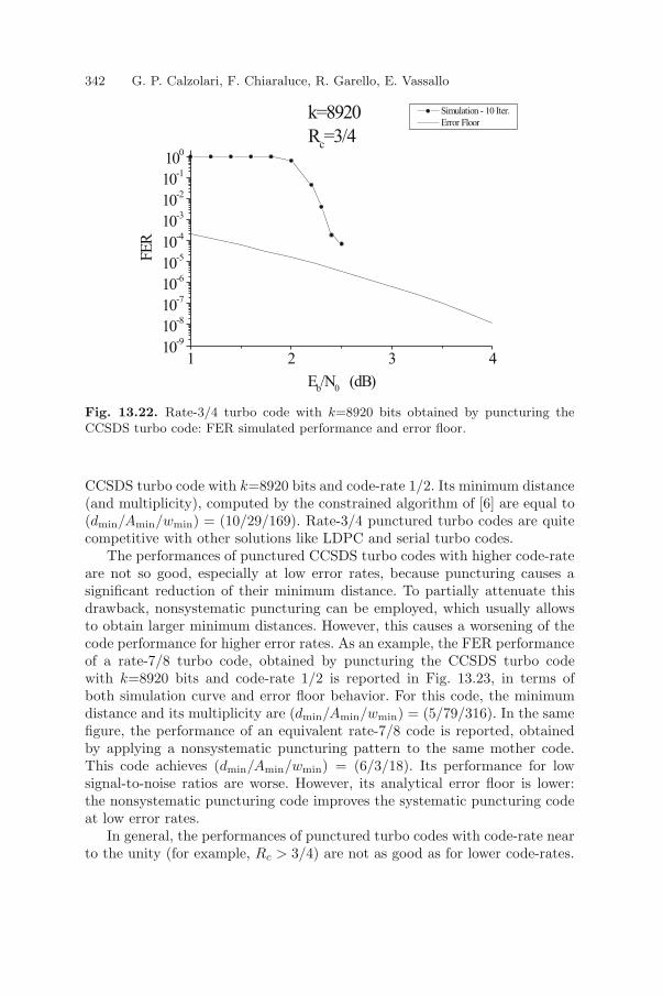
342 G. P. Calzolari, F. Chiaraluce, R. Garello, E. Vassallo
1 2 3 410
-9
10-8
10-7
10-6
10-5
10-4
10-3
10-2
10-1
100
k=8920
Rc=3/4
Simulation - 10 Iter.
Error Floor
FE
R
Eb/N
0(dB)
Fig. 13.22. Rate-3/4 turbo code with k=8920 bits obtained by puncturing theCCSDS turbo code: FER simulated performance and error floor.
CCSDS turbo code with k=8920 bits and code-rate 1/2. Its minimum distance(and multiplicity), computed by the constrained algorithm of [6] are equal to(dmin/Amin/wmin) = (10/29/169). Rate-3/4 punctured turbo codes are quitecompetitive with other solutions like LDPC and serial turbo codes.
The performances of punctured CCSDS turbo codes with higher code-rateare not so good, especially at low error rates, because puncturing causes asignificant reduction of their minimum distance. To partially attenuate thisdrawback, nonsystematic puncturing can be employed, which usually allowsto obtain larger minimum distances. However, this causes a worsening of thecode performance for higher error rates. As an example, the FER performanceof a rate-7/8 turbo code, obtained by puncturing the CCSDS turbo codewith k=8920 bits and code-rate 1/2 is reported in Fig. 13.23, in terms ofboth simulation curve and error floor behavior. For this code, the minimumdistance and its multiplicity are (dmin/Amin/wmin) = (5/79/316). In the samefigure, the performance of an equivalent rate-7/8 code is reported, obtainedby applying a nonsystematic puncturing pattern to the same mother code.This code achieves (dmin/Amin/wmin) = (6/3/18). Its performance for lowsignal-to-noise ratios are worse. However, its analytical error floor is lower:the nonsystematic puncturing code improves the systematic puncturing codeat low error rates.
In general, the performances of punctured turbo codes with code-rate nearto the unity (for example, Rc > 3/4) are not as good as for lower code-rates.

13 Turbo Code Applications on Telemetry and Deep Space Comm. 343
2 3 4 5 6 710
-9
10-8
10-7
10-6
10-5
10-4
10-3
10-2
10-1
100
Systematic
Non Systematic
Floor Systematic
Floor Non Systematic
k=8920
Rc=7/8
FE
R
Eb/N
0(dB)
Fig. 13.23. Rate-7/8 turbo codes with k=8920 bits obtained by puncturing theCCSDS turbo code: FER simulated performance and error floor for systematic andnonsystematic puncturing.
The penalty introduced by puncturing is significant and other coding schemes,like LDPC or Hamming product codes, can outperform them [10].
13.6 Conclusive Remarks
In this chapter the turbo codes family of CCSDS standard, the first interna-tional standard including turbo codes in early 1999, has been analyzed. Theyare 16-state parallel turbo codes, with code-rates ranging from 1/6 to 1/2,and input frames from 1784 to 8920 bits. Their performances have been pre-sented, in terms both of simulated error rates and analytical error floors com-puted from their minimum distances. It has been shown that they are indeedexcellent codes, performing near the theoretical limits. CCSDS turbo codesalso possess valuable properties for codeword synchronization at the receiverside. Analysis of punctured CCSDS turbo codes show that their performance,still rather good up to code-rate 3/4, becomes worse at higher rates due topuncturing action. CCSDS agencies will use turbo codes for space telemetry,where their very large coding gain will be extremely useful for missions withlow communications margins.

344 G. P. Calzolari, F. Chiaraluce, R. Garello, E. Vassallo
13.7 Acknowledgment
CCSDS turbo codes were included in the standard as the result of a joint sci-entific effort of the international space agencies. Relevant contributions camefrom NASA-JPL, in particular through the work of Fabrizio Pollara and Dar-iush Divsalar, and from ESA, in co-operation with Claude Berrou (ENST),Sergio Benedetto and Guido Montorsi (Politecnico di Torino). Finally, a spe-cial contribution came from Warner H. Miller of NASA, who was Chairmanof the Channel Coding working group and provided his excellent contributionto numerous standards for error control coding. This chapter is dedicated tohis memory.
References
1. Consultative Committee for Space Data Systems (2003) TM Synchronizationand Channel Coding. Blue Book 131.0-B-1
2. Consultative Committee for Space Data Systems (2000) Packet Telemetry. BlueBook 102.0-B-5
3. Consultative Committee for Space Data Systems (2001) Advanced Orbiting Sys-tems, Networks and Data Links: Architectural Specifications. Blue Book 701.0-B-3
4. Consultative Committee for Space Data Systems (2003) Radio Frequency andModulation Systems - Part 1: Earth Stations and Spacecraft. Blue Book 401.0-B-14
5. Beyer G, Engdahl K, Zigangirov K Sh (2001) “Asymptotic analysis and com-parison of two coded modulation schemes using PSK signaling - Part I.” IEEETransactions on Information Theory 47:2782–2792
6. Garello R, Benedetto S, Pierleoni P (2001) Computing the free distance of turboCodes and serially concatenated codes with interleavers. IEEE J. on SelectedAreas on Communications 19:800–812
7. Garello R, Vila A (2004) “Turbo code minimum distance computation bythe all-zero iterative decoding algorithm.” In: Proceedings of ICC’04 :800–812,Paris, France
8. Calzolari G P, Chiaraluce F, Garello R, Vassallo E (2001) “Symbol synchro-nization properties of CCSDS turbo codes.” International Journal of SatelliteCommunications 20:379-390
9. University of Ancona (2000) Study of Bandwidth-Efficient Coding Schemes forNear-Earth Applications. ESA/ESOC Contract No. 14128/00/D/SW - FinalReport
10. University of Ancona (2001) Highly Efficient Channel Codes for High Data RateMissions. ESA/ESOC Contract No. 15048/01/D/HK(SC) - Final Report

Part V
Implementations

Chapter 14
VLSI for Turbo Codes
Guido Masera
Politecnico di Torino, Italy
The impressive developments of high performance digital CMOS technologiesin the last years have made possible the implementation of very complex al-gorithms in low cost chips. Digital signal processors, programmable devicessuch as FPGAs and VLSI technologies have come to the point where thecomputing power and the memory required to execute several real time ap-plications can be incorporated even in cheap portable devices. Among theseveral application fields that have been strongly developed by this technol-ogy progress, channel decoding is one of the most significant and interesting:as predicted by Shannon, the achievement of performance close to the theo-retical limit implies the adoption of high complexity algorithms, so makingthe search for good decoding architecture a challenging and fascinating prob-lem for many digital architects and VLSI designers. There are a number ofaspects of turbo codes that make them so interesting also from an implemen-tation point of view: first of all the algorithms that are used to implement theMAP decoding (such as the so called BCJR algorithm) are of great complex-ity; this complexity, coupled with the iterative nature of the whole decodingprocess, makes very difficult the accomplishment of throughput, latency, costand energy dissipation constraints imposed by several modern multimedia andinteractive applications. Moreover turbo decoders include large RAM memo-ries that need to be organized and managed properly. Finally, the decodingalgorithm can be parallelized in several ways, acting at different levels and thebest solution for each application can only be selected by carefully exploringthe space of design alternatives.
The chapter reviews all main achievements obtained in the last 10 yearsin the hardware implementation of turbo codes and particularly the criticalaspects that designers have to deal with. The main addressed problems arethe following.
• Digital architectures for the implementation of basic BCJR equations, re-lated to the forward and backward recursionsStarting from the straightforward mapping of the SISO equations to a
347
K. Sripmanwat (ed.), Turbo Code Applications: a journey from a paper to realization, 347–382.
© 2005 Springer. Printed in the Netherlands.

348 Guido Masera
hardware architecture, quite similar to those used in Viterbi decoders, al-ternative structures have been subsequently proposed, achieving differenttrade-offs between implementation complexity and accuracy in the equa-tion approximation; the architectural definition is also strictly related tothe numerical representation of involved metrics, which strongly impactson the error correcting capabilities of the code and on its cost.
• Global decoder architectures, aimed at satisfying application dependent con-straints of cost, energy consumption, throughput and latencyAs an example, the achievement of high throughputs requires replicationof hardware resources by introducing parallelism at several levels. The de-coding algorithm can be split in a number of working units that process thereceived blocks in parallel, so achieving a throughput roughly proportion-ally to the number of working units employed. Alternatively, for a giventhroughput, this solution allows for a reduced clock frequency, so implyingless power consumption. Parallelism is generally introduced at the SISOlevel, by allocating resources capable of handling all states at the sametime, or at the level of block of data to be decoded. Parallelism can alsobe introduced at the iteration level; this enables the simultaneous alloca-tion of more decoding iterations to different hardware units, but involvesa serious penalty in terms of cost, especially for what concerns memories.
• Specific techniques for the reduction and the management of energy con-sumptionThese techniques include the optimization of RAM memories, which areresponsible for a large percentage of energy consumption, and the dynamiccalibration of the number of decoding iterations.
• Design of collision-free architecturesThe iterative nature of the decoding algorithm poses another obstacleto the parallelization of the decoder; extrinsic information is exchangedbetween the SISO modules via interleaving and de-interleaving, so thateach SISO module and each interleaver memory has to be split into morehardware units. As the memories have to be accessed both in the naturaland in the scrambled order, it is not generally possible to guarantee that nomultiple access is simultaneously required for the same RAM; this event isreferred to as a “collision” and most of the recently proposed solutions tothis problem can be grouped in two categories. The first one attempts toincorporate the requirement of parallelism in the design of the constituentcodes, so that they are intrinsically collision-free; the other one assumesa given Turbo Code and attempts to eliminate collisions or at least toalleviate their effects by operating at the architecture level.

14 VLSI for Turbo Codes 349
N
E1N
r1
I E2
r2
N/(r1 r2)N/r1N/r1
B
D
I
SISO2 SISO1N/(r1 r2)
N/r1
N/r1
Fig. 14.1. SCCC encoder and decoder structure
14.1 General Architecture of a Turbo Decoder
At a high level of representation, the architecture of a turbo decoder consistsof two kinds of key components, combined in different topologies, the SISOunit and the interleaver: the first one implements the fundamental APP (APosteriori Probability) algorithm for a given convolutional code, while theother scrambles the processed data according to the permutation law appliedat the encoder. In principle, a turbo encoder could be obtained by means ofmany different topologies of interconnected convolutional encoders and inter-leaving memories [1], but only parallel and serial concatenation schemes havebeen considered for practical implementation.
The serial concatenation case is given in Fig. 14.1, where E1 and E2 aretwo convolutional encoders of rate r1 and r2 respectively, I is an interleaverof length N , D the corresponding deinterleaver and B the input buffer thatprovides the decoder with received LLRs (Logarithmic Likelihood Ratios). Forboth encoder and decoder, the amount of data that are carried from one blockto the other for each block is indicated: for example, at the encoder side, E1
receives N bits for each block and generates a number of parallel bits equalto 1
r1for each information bit, for a total of N
r1bits; on the other side, SISO2
receives from the buffer, at each decoding iteration, Nr1r2
LLRs and generatesNr1
outputs, to be written into the deinterleaver.It is worth noticing that the two SISOs do not operate simultaneously,
as while one of the two is processing a block of data the other has to stayin idle condition, waiting for the completion of the current half iteration. Inorder to better exploit the allocated hardware units, two blocks of data shouldbe concurrently processed, but this choice would have the effect of doublingthe size of input buffer and interleaver memories; the full usage of allocatedhardware is also obtained using a single, parametric SISO unit, capable to bealternatively configured as inner and outer SISO.

350 Guido Masera
N/r1
(u:I)
N/r2
N
NN
N
N/r1 + N/r2
I
E1
E2
SISO1
SISO2
B I D
π
(u:O)π
π(c:I)
r1
r2
N N/r1
N/r2
Fig. 14.2. PCCC encoder and decoder structure
Fig. 14.2 shows the encoder and decoder structures for the case of parallelconcatenation. Symbols have the same meaning as in the SCCC picture andalso for this configuration the 100% exploitation of architecture resources isachieved by a single SISO structure, playing alternatively the roles of SISO1and SISO2.
Components I and D are critical in a turbo decoder, both in terms oferror correcting capabilities and in terms of implementation cost. In practicethe permutation function of an interleaver or deinterleaver is often imple-mented relying on a random access memory (RAM), where LLRs are writtensequentially and read in the permuted order, or vice-versa. The generationof sequential addresses is obtained by means of a counter, but the scrambledaddresses require more expensive circuits.
The best interleavers, such as S-random interleavers, imply that scrambledaddresses are stored in a separate read only memory (ROM), or in a secondRAM in case the permutation law must be changed. This address memoryhas the same number of cells as the RAM used for data storage (N , that isthe block size), but it is log2N bit wide, what is often more than the 5-6 bitstypically used to represent LLRs.
In the case of deterministic interleavers, the scrambled address sequencecan be generated on the fly, by means of calculation algorithms usually basedon simple addition and shifting operations [2]. Although this approach is sim-pler than the address storage, the cost reduction advantage is usually offsetby the performance degradation associated to the adoption of a deterministicinterleaver.
Another critical point in the interleaver implementation is related to thespeed limitation due to the RAM access time. In current CMOS technologies,

14 VLSI for Turbo Codes 351
the access time is around 2 ns for large, single port RAMs; assuming that 4accesses are required per iteration and 10 iterations are performed to decodea block, the 2 ns RAM sets an upper bound for the throughput at 11 Mb/s;this data rate is enough for 3GPP-UMTS wireless cellular communication,but not for wireless networking or digital video broadcasting (DVB). In highspeed applications, the interleaver RAM must then be partitioned into moreparallel devices, as discussed in Sec. 14.4.
An important difference between the serial and parallel concatenationschemes must be considered. In a SCCC decoder the interleaver and dein-terleaver memories are connected serially to inner and outer SISOs, so thatthe required size for them is increased by a factor 1/r1 with respect to thesize of the decoded block N . On the contrary, in the PCCC decoder, theinterleaver memories are required to store a number N of data.
This difference has two important consequences that tend to make theSCCC scheme less favorable than the PCCC one:
(a) For the same block size and data representation, interleaver memories inSCCC decoders are 1/r1 larger than for PCCC decoders, what impliesboth area and power dissipation penalties
(b) In a single RAM architecture, the interleaver (and deinterleaver) has aserial access policy, while SISO1 and SISO2 in Fig. 14.1 needs to readdata from D and write data into I with a parallelism of 1/r1; in otherwords, I and D units need N/r1 cycles to process a block, and the SISOsonly N . The effect of this difference is that the SISO’s operating efficiencyis reduced by a factor 1/r1.
The solution of the second problem can be found by splitting the inter-leaver/deinterleaver into 1/r1 separated memories, so allowing the SISOs toperform parallel accesses.
14.2 Digital Architectures for SISO Processing
The decoding process for both serial and parallel concatenation schemes con-sists of the iterative execution of a fundamental algorithm, widely known asBCJR [3]; this algorithm basically receives as inputs blocks of soft informationassociated to each processed bit and it is capable to refine them, generatingas output new more reliable soft bits. The basic equations implementing suchalgorithm in the original form have been introduced in previous chapters andare repeated here for convenience.
Pk(c;O)=Hc
∑e:c(e)=c
Ak−1[sS(e)]Pk[u(e);I] Bk[sE(e)]
Pk(u;O)=Hu
∑e:u(e)=u
Ak−1[sS(e)]Pk[c(e);I] Bk[sE(e)]

352 Guido Masera
where the same notation adopted in [4] is used:
index k indicates the time step and runs on the whole transmission length,while symbol s represents a code state;
e is a generic trellis edge, while c(e) and u(e) are the output and inputcoder symbols associated to the edge e;
sS(e) and sE(e) indicate the starting and ending states for the generictrellis edge e;
Hu and Hc are normalization constants.
Ak−1 and Bk−1 are probability distributions accumulated in the forward andbackward directions along the trellis, according to the following updating re-lations:
Ak(s)=∑
e:sE(e)=s
Ak−1[sS(e)]Pk[u(e);I]Pk[c(e);I]
Bk(s)=∑
e:sS(e)=s
Bk+1[sE(e)]Pk+1[u(e);I]Pk+1[c(e);I]
14.2.1 Reduced Complexity Implementation
It is clear from the direct inspection of these equations that their straightfor-ward implementation in a digital architecture would rise at least two seriousproblems:
(a) the updating of the involved metrics implies that the whole sequence oftransmitted data (block) has been received and stored. This requirementhas the effect of increasing the complexity of the decoder because of thelarge memories that are needed and additionally it worsen the decodinglatency.
(b) A large number of multiply operations is involved, what also has a badeffect on the decoder complexity: for a given silicon technology, the com-plexity of a multiplier in terms of silicon area is larger that a simple adderby a factor typically ranging between 10 and 40 times, depending on bitwidth and required speed (see [5] for a wide collection of synthesis resultson several arithmetic blocks).
The first problem is usually faced resorting to the implementation of an ap-proximated version of the original algorithm, largely known as sliding windowBCJR algorithm [6] [7] [8]; the hardware implementation of this approxima-tion will be detailed in Sec. 14.3, but the basic effect is that the equations willbe applied separately to portions, or windows, of the global block of data.
As far as the second problem is concerned, the usual solution is provided byre-formulating the algorithm in the logarithmic domain. In fact, by processinglogarithmic likelihood ratios rather than the original reliability metrics allowsto replace multiplications with additions. The new BCJR equations obtainedwith such transformations are given below.

14 VLSI for Turbo Codes 353
αk(s)=∗
maxe:sE(e)=s
αk−1[sS(e)] + πk[u(e);I] + πk[c(e);I]
(14.1)
βk(s)=∗
maxe:sS(e)=s
βk+1[sE(e)]+πk+1[u(e);I]+πk+1[c(e);I]
(14.2)
πk(c;O) =∗
maxe:c(e)=c
αk−1[sS(e)]+πk[u(e);I]+βk[sE(e)]
(14.3)
πk(u;O) =∗
maxe:u(e)=u
αk−1[sS(e)]+πk[c(e);I]+βk[sE(e)]
(14.4)
where the introduced symbols α, β and π are defined according to [4]:
πk(c; I)= log[Pk(c; I)] πk(u; I)
= log[Pk(u; I)]
πk(u;O)= log[Pk(u;O)] πk(c;O)
= log[Pk(c;O)]
αk(s)= log[Ak(s)] βk(s)
= log[Bk(s)]
and the max∗ operator is a basic building element in the log domain processingdefined as
∗max
i(λi) = ln
(n∑
i=1
exp λi
)(14.5)
and requiring a proper approximation for VLSI implementation; from an al-gorithmic point of view, the max∗ operator is typically evaluated with thefollowing iterative procedure:
a(l) = max(a(l−1), al) + log[1 + exp(−|a(l−1) − al|)] (14.6)
for l = 2, ..., n, with a(1) = a1 and a ≡ a(n).Internally to the SISO, some approximations have been proposed for the
key operations Eq. 14.1 to 14.5 and the search for good solutions still is subjectof investigation inside the scientific community, since each approximation is atrad-eoff between decoder performance, in terms of error correcting capability,and processing delay associated with the operation of metric update. Thespeed of this part of the decoder is extremely important, due to the factthat backward metric computation is a recursive operation, where the setof newly generated metrics is the basis for the following repetition of theupdating process. In this kind of loop algorithms, the pipelining spitting of acomplex combinational operation into more simpler processing steps is of nohelp and the only possibility is to reduce as much as possible the delay alongthe combinational path running from the input to the output metrics.

354 Guido Masera
LOG. CORRECTIONCOMP
π
πk-1
k-1π
π
k-1
ADD
LUT
k-1
AD
DA
DD
AD
DA
DD
CO
MP
(state si)
(state sj)
α
α
(u1;I)
(u2;I)
(c1;I)
(c2;I)
SEL
α(state s)
Fig. 14.3. Block scheme for a max star architecture
The two most widely known techniques to approximate Eq. 14.5 are themax and max star solutions:
(a) In the max approximation, given in Eq. 14.7, add operations are usedto evaluate the logarithm of two or more product terms (indicated as λ1
and λ2 in Eq. 14.5), while the max operation, implemented as a compareand select sequence of steps, approximates the logarithm of a sum ofexponential terms. This solution, known as max-log-MAP,
ln(exp(λ1) + exp(λ2)) ≈ max(λ1, λ2) (14.7)
is of course a great simplification from the implementation point of view,but is known to determine a performance loss of about 0.5 dB on the BERcurve of a turbo coded system [9].
(b) The max star approximation achieves coding gains within 0.1 dB fromthe ideal MAP decoder by simply adding to the previously defined maxoperation a correction term based on the difference of the two λs:
ln(exp(λ1)+exp(λ2)) ≈ ∗max(λ1, λ2) = max(λ1, λ2)+ln(1+exp(−|λ1−λ2|))
(14.8)A few bits are typically used to represent the correction term, which canthen be stored in quite a small look-up-table.
The max star approximation is slightly more complicated than the simplemax operator, requiring the addition of a correction term usually generatedthrough a look-up table. The typical structure of the arithmetic unit imple-menting the computation of Eq. 14.1 or 14.2 by means of max star approx-imation is given in Fig. 14.3: the block diagram resembles the ACS (Add-Compare-Select ) architecture traditionally adopted in Viterbi decoders, butis completed by the final adder that sum the correction term provided bythe look-up table. The main drawback of this solution is mainly related tothe delay contribution that is due to the final adder placed along the metric

14 VLSI for Turbo Codes 355
Table 14.1. Comparison between max and max star approximations in a modifiedACS unit
approximation Virtex Virtex2Pbit nr. gates frequency gates frequency
max ACS 6 660 91 MHz 600 114 MHz4 500 128 MHz
max star ACS 6 900 63 MHz 900 98 MHz4 700 104 MHz
computation path; this adder and the look-up table of course also extend theoccupied area. It has been proved that the performance loss associated withthe max star approximation is in the order of 0.1 dB relative to the exact MAPformulation, what is usually considered acceptable. Synthesis results are givenin Table 14.1 for a modified ACS unit implemented with the two mentionedapproximations; the reported figures refer to two different FPGA technologiesand show that the max star version roughly costs 30% of additional area anddelay with respect to the pure max structure. For this example, input LLRsare represented on 6 and 4 bits (second table column), while state metrics arenumbers respectively on 9 and 7 bits (see Sec. 14.2.2 for a discussion on thefixed point representation of received and internal metrics).
The original formulation of the BCJR algorithm, based on a sum-productalgorithm, is implemented in the special case of analog decoders, as an alter-native to the logarithm probability domain; Gilbert multipliers are typicallyallocated to evaluate the probability products, achieving very high perfor-mance to complexity ratios [10] [11] [12], with reduced power dissipations.However the advantages of the analog turbo decoder implementation are atthe moment offset by typical limitations of analog circuits, such as the sensitiv-ity to temperature and process variation and poor scalability with technology.
14.2.2 Fixed-point Representation
One of the key points in the implementation of channel decoders is the fixedpoint representation for all quantities involved in the decoding algorithm.This design choice is usually based on acceptable trade-offs between errorcorrecting performance on one hand, and cost and power dissipation on theother: both dynamic and precision adopted for representing data tend to affectheavily the decoder behaviour; the allocated number of bits also has a directimpact on cost and power dissipation, especially when dealing with hardwareimplementation for FPGA and VLSI technologies. The choices to be takenare related to
finite precision representation of LLRs finite precision arithmetic for SISO internal processing
The finite precision representation of input LLRs has a strong impact fromthe hardware point of view as it directly affects the capacity of input buffers;

356 Guido Masera
as a consequence the number of allocated bits has to be set to the minimumpossible for a given bit error rate target. The log-likelihood ratio producedfor a given coded bit c by an ideal, infinite precision demodulator is a realnumber that can be expressed as
λ = logp(y|c = 1)p(y|c = 0)
= 4y√
ES
N0
where y is the output of the matched filter, ES is the signal energy and N0/2is the two-sided noise power spectral density. According to the fixed pointrepresentation, in general d bits will be used to represent the integer part of λ(d is usually defined as the “dynamic”) and p additional bits will be reservedfor the decimal part (“precision”):
λ → bd−12d−1 + ... + b121 + b020 + b−12−1 + ... + b−p+12−p+1 + b−p2−p
Simulations results have been used to understand the influence of both pre-cision and dynamic on the performance of turbo codes and so to properlychoose the LLRs representation. In general, when a low number of bits d isallocated for the dynamic, metrics saturate at low values and this tends tobadly affect the “error floor” of the performance curve; on the contrary, aninsufficient number of bits p of precision affects the decoder behaviour at lowSNRs (convergence abscissa of the iterative decoding). As an example, in [13]and [14] extensive simulations have been performed on some significant cases(such as for example the UMTS turbo decoder) for different choices of p andd: from the performed simulations, two bits of precision and three of dynamicgive performance very close to the ideal case, while reducing p to one singlebit results in a loss around 0.1 dB at low to medium SNRs and setting d = 2costs 0.3 dB
Concerning the fixed-point processing performed internally to the SISO,it must be considered that path metrics α and β increase their values withk, and some action is required in order to avoid an arithmetic overflow (orunderflow). Three possible solutions have to be considered:
(a) subtracting the smallest metric from all the path metrics (α or β);(b) subtracting the metric related to the same state at each trellis step;(c) managing the overflow effects, rather than avoiding it.
The first solution implies that a set of comparators and subtracters are allo-cated to find the smallest metric and to perform the normalization; of coursethis choice results in both area and delay penalty.
In the second solution, instead of searching for the smallest metric at eachstep, a fixed state metric is subtracted from all path metrics, so avoiding theallocation of comparators; saturation must be used to prevent overflows.
The normalization of the α and β metrics at each updating step can beavoided by adopting a proper numerical representation of the metric differ-ences.

14 VLSI for Turbo Codes 357
metrics are updated after relative comparisons performed by the ACS sec-tions and the result does not change if the same constant is added to eachα or β metric;
all possible differences between pairs of path metrics are upper-bounded:path metrics may grow from one trellis step to the other, but their relativedifferences have an upper limit, ∆MAX , which depends on the distanceprofile of the code and on the number of bits used to represent LLRs. Anexpression giving the largest difference assumed by the SISO path metricshas been derived in [14]:
∆MAX = minw
(wMu + dmin(w)Mc)
where dmin(w) is the minumum weight of the code sequences generated byinput sequences with weight w, ±Mu and ±Mc are the bounds for respec-tively extrinsic information and LLRs received by the soft demodulator:while dmin(w) depends on the considered code, ±Mu and ±Mc are sim-ply related to the number of allocated bits in the intrinsic and extrinsicinformation.
For the convolutional code of the UMTS-3GPP standard, dmin(w) = 8 forw = 2 and dmin(w) = 6 for w = 3 [14]; assume that Nb = 6 bits of quantizationare used for both the received LLRs and extrinsic information, represented intwo’s complement format: the maximum absolute values for u and c symbolsare
Mu = Mc = 2Nb−1 = 32
the worst case is when all LLRs along the trellis path are equal to Mc; in thiscase, the maximum path metric difference is given by
∆MAX = wMu + dmin(w)Mc = 3 × 32 + 6 × 32 = 288
If path metrics are represented as positive integers using n bits, where n isgiven by
n = log2∆MAX + 1 (14.9)
(n is equal to 10 in this example) the metric difference has a range from−2n−1 = −512 to 2n−1 − 1 = 511, so that it can be represented in general asa 2’s complement value with n bits and the sign bit has weight n − 1.
As also done for the computation of metrics in Viterbi decoders [15] [16],the limited spread of path metrics can be exploited to achieve two importantimplementation results:
to define the proper number of bits to be used to represent metrics to avoid the normalization step when updating the forward and backward
metrics, so saving the implementation cost of subtractors.
Both choices are based on the fact that, if metrics are represented accordingto Eq. 14.9, the metric spread will always be smaller than the half of the

358 Guido Masera
0.4
0.3
0.2
0.1
1 2 3 4 5 6 7 8 9 10 11
f(b)
b
λπππππ
iter. 1iter. 3iter. 5iter. 7iter. 10
Fig. 14.4. Density of LLR values in a 8 state SISO with Nint = 320 and Eb/N0 = 0dB
maximum quantity that can be represented by the n bits; under this con-dition the result of a subtraction between two metrics is unaffected by theoccurred overflows or underflows and as a consequence the normalization isnot required.
For a given fixed point representation of LLRs, the number of bits requiredto represent path metrics can be reduced by slightly reducing the dynamicrange of LLRs, with a minor impact on the decoder performance: for theUMTS-3GPP example, if LLRs are saturated to ±21 instead of −32 and +31,we have:
Mc = 21 ∆MAX = 255
so the required number of bit is
n = log2∆MAX + 1 = 9
A further choice to be taken in the hardware implementation of iterativedecoders is related to the management of fixed-point quantities between oneiteration and the other. During the iterative decoding process, the extrinsicinformations generated at the output of the SISOs tend to modify their sta-tistics in a way that depends on the signal to noise ratio: typically at highSNR the LLRs values show a fast growing, while at low SNR the growing isnull or slow.
Fig. 14.4 reports the LLR density for the case of a 8 state SISO withNint = 320 and Eb/N0 = 0 dB: extrinsic information (πi) and input LLR(λk) are described through the probability density function
f(b) = P [2b−2 ≤ |γ| < 2b−1]
A second example, again for a 8 state SISO with Nint = 320, is given forthe case Eb/N0 = 2 dB in Fig. 14.5.

14 VLSI for Turbo Codes 359
λπππππ
iter. 1iter. 3iter. 5iter. 7iter. 10
0.8
0.6
0.4
0.2
f(b)
1 2 3 4 5 6 7 8 9 10 11
b
12 13
Fig. 14.5. Density of LLR values in a 8 state SISO with Nint = 320 and Eb/N0 = 2dB
To better accommodate this statistical distribution of extrinsic informa-tion along the different stages of the decoding process, the number of bitsused to represent the integer part of LLRs (d) propagated from one SISOto the other can be increased, so improving the “error floor” on the perfor-mance curve. A simulation study reporting the effect of different choices forthe UMTS turbo code is available in [14]: the work shows that the outputLLR dynamic should be d + 2 when setting to d the dynamic of the inputLLRs. If a single SISO hardware unit is shared among different stages, thegiven rule results in the constraint that all input and output metrics make useof the same representation; when multiple hardware units are allocated to ex-ecute in pipelining subsequent iterations, the number of bits can be changedfrom one unit to the other, gradually increasing the dynamic and reducingthe precision. More in general, the fixed point representation may be madeadaptive with the changing SNR measured on the channel: at high SNR, d canbe reduced, by shifting the decimal point to the left, while at low SNR, p hadbetter be increased (right shift). To support this function, a SISO unit needsto be completed with adaptive logic capable of modifying the point positionaccording to provided SNR estimations (Fig. 14.6).
14.3 SISO Architecture
In the sliding window approximation, the block of data to be decoded is di-vided into a number of segments, or windows (length NW ), and the decodingalgorithm is applied to each of them in sequence. It has been proved thatthe performance loss due to this approximation is negligible, provided that,in addition to the considered window, Eq. 14.1 and 14.2 are applied along ainitialization portion of the trellis (length NS), which is processed just withthe purpose of obtaining reliable starting state metrics for the actual decod-ing of the current window (see Fig. 14.7). In order to properly concatenate

360 Guido Masera
SISOshift shift
shift control
SNR estimation (off line)
π π
λ
ii-1
k
Fig. 14.6. Adaptive logic to control dynamic and precision
recursion
0 N N + NW II WN − NW
NW NNI I
α init.
β inith.
α recursion
β
Fig. 14.7. Forward and backward recursions with initialization portions
the portions of updated metrics, windows have to be overlapped, resulting insome overhead of required hardware resources.
The lowest cost solution is to limit the window overlap to the backwardrecursion, obtaining the starting α metrics for a given window from the lastmetrics of the previous one. This solution, known as single flow structureand already introduced in [17] as an alternative to the storage of the entirestate metric history, consists in performing a double β backward recursion:the first one starts with uniform LLR’s and goes back along the trellis forNI steps (say from step NW + NI back to step NW ), without the need ofstoring intermediate β values, except for the last ones, that are generated atthe trellis position NW ; these values become reliable initialization metrics forthe second β backward recursion, going from step NW back to step 0. Duringthis second recursion, all generated β metrics are reliable enough to be usedfor decoding in Eq. 14.3 and 14.4. Three processing units are then required:one is needed to update α metrics, two must be allocated to support twosimultaneous backward recursions, respectively along the currently decodedwindow and along the overlapped portion of the following one.
In practical implementations adopting the structure with three processingunits, the overlapping portion is usually made equal to the full window length,since this choice results in the best performance to cost ratio and also tends

14 VLSI for Turbo Codes 361
to make simple the control unit. This can be easily shown by means of thefollowing estimations.
Assume that f is the processing rate of the three units that calculate αand β metrics in the single flow structure, NW is the window length and NI
the length of the overlapped portion (NI ≤ NW ); the SISO throughput willbe given by
t =NW
NW + NIf
The hardware complexity can be roughly estimated as
c = a × NW + b
where the first term, linear with NW , is the cost due to memories that storewindow metrics and the second term includes the other contributions not re-lated to the window length. For a fixed value of NI , imposed by the expecteddecoder performance, the throughput to cost ratio will have a maximum forNW = NI . This conclusion, obtained through an oversimplified cost and per-formance model, is substantially confirmed also by more accurate investiga-tions, adopting precise cost, delay and even energy consumption models [18];it is worth noticing here that different optimization criteria for NW and NS
have been derived in [19] when more general SISO structures are consideredand the problem of joint minimization of decoding delay and metric storageis addressed.
A powerful while simple and elegant tool for the analysis of complex signalprocessing algorithms is represented by the data flow graph (DFG) [20], thathas also been applied to various formulations of the sliding window SISO [21][22] [23] [19]. A simplified DFG representation for a possible organization of αand β recursions in the SISO decoding algorithm is given in Fig. 14.8, wheretime measured along the trellis runs horizontally across data blocks, whileprocessing time runs vertically from top to bottom; both the initializationportions and the updating windows are indicated for α and β processing.More DFG of the kind shown in Fig. 14.8 can be combined to obtain differentscheduling schemes of the involved operations, and the DFG representationcan be used to evaluate both decoder performance (throughput and latency)and hardware cost (in terms of number of processing units to be allocated andamount of required storage for branch and path metrics).
A popular structure that makes use of the three processing units mentionedabove can be represented with the DFG of Fig. 14.9 (single flow structure),where the concatenation of three blocks of data is shown; in this structure, noinitialization is required for α metrics, as they are inherited from the end of oneblock to the beginning of the following one, while two β processing units arealways operating at the same time to perform β update and initialization alongconsecutive windows. The black filled square boxes placed along β recursionindicate the operation of output LLR generation, that needs forward andbackward path metrics as well as branch metrics related to the current trellisstep (αk−1, βk, πk(u) or πk(c)).

362 Guido Masera
I
trellis time (blocks)
proc
essi
ng ti
me
β
α
β
α
recursioninit.
recursion
recursion
init.recursion
NWNW
N
Fig. 14.8. DFG representation for α and β recursions and initializations
W
trellis time (blocks)
proc
essi
ng ti
me
trellisposition
k
NW
deco
ding
del
ay =
3 N
Fig. 14.9. DFG for the single flow structure

14 VLSI for Turbo Codes 363
MUX
MU
X
MUX
MU
X
RAM 3RAM 2RAM 1α RAM
MUX MUX MUX
(u;O)π
LIFO LIFO
1/NN
AC
S
AC
S
AC
Sα β β
ACS cACS u
(c;O)π
(u;I)π(u;I)π
Fig. 14.10. Single flow SISO architecture
Memories are therefore required to store branch and path metrics and theamount of necessary memory can be estimated from the DFG analysis. Ifa vertical slice of the DFG in Fig. 14.9 is considered, it can be easily seenthat three operations performed in different times are aligned on the sametrellis position, so requiring the same input branch metric: these are the βinit., α and β update operations indicated at the trellis position k by thefilled black circles. Three buffer memories of size NW are therefore requiredto store branch metrics along the three involved windows.
Additionally, the updated α metrics generated while processing a givenwindow (these are indicated in Fig. 14.9 with black triangles) have to bestored up to the output LLR calculation in the following window (see arrowedcurves going from triangles to black squares): a fourth memory of size NW
must be used to store these metrics.From the DFG, the decoding delay can also be evaluated looking at the
amount of time that the full decoding of a window takes along the verticalaxis: for this example, the delay is given by 3×NW , as three complete windowprocessing are required.
A general view of the architecture implementing the described processingstructure is given in Fig. 14.10, where two further processing units are in-dicated as ACS u and ACS c: these blocks generate the output LLRs, π(u)and π(c); these outputs are evaluated simultaneously with the β backwardrecursion and as a consequence they are generated in the reversed order; thecorrect order can be restored either allocating LIFO memories at the SISOoutput or changing properly the interleaving law of the decoder.
The indicated multiplexers distribute the stored branch metrics to thedifferent processing units that operate in a synchronous way, so that a singlecounter can be used as address generator for all memories.
The DFG representation together with the described method to evaluatedecoding delay and required storage can be applied to different computational

364 Guido Masera
structures. For example, a double flow processing structure has been proposedin [18] as a low latency solution, capable of reducing the decoding delay totwo time windows instead of the three required by the single flow case: inthis solution, the same processing is applied to both β and α recursions, fora DFG similar to that given in Fig. 14.8.
Again the DFG method can be applied to the study of parallel SISOimplementations, where more windows are processed in parallel rather thanserially [23] [24] [25]: for parallel structures, more DFG’s such as the two previ-ously considered, have to be aligned laterally, so supporting the simultaneousdecoding of multiple windows.
Although the practical implementation of high performance decoders alsoinvolves other important issues, such as the reduction of the dissipated energyor the search for parallel interleaving schemes, a clear and complete studyon the many possible alternatives in the SISO internal organization has beenrecently published by M. Mansour and N. Shanbhag [19], who formally derivedexpressions for the optimization of decoding delay and metric memories insingle flow and parallel SISO’s.
A completely different approach, which has been recently proposed [26], isbased on the idea of evaluating backward state metrics in the forward direc-tion: in principle this is possible if one is able to invert the basic β updatingequation, so expressing βk as a function of βk−1’s. The possible advantage of-fered by this approach comes from the elimination of the path metric memoryin the SISO architecture: in fact the decoding algorithm, after a backwardrecursion with no storage of intermediate results, two forward processes canbe started that simultaneously generate α and β metrics and immediatelycalculate the output LLR’s with very reduced memory requirements.
Therefore the forward calculation of reverse state metrics is potentiallyable to reduce both SISO complexity and energy dissipation, and some im-plementations have already been proposed [27] [28] reporting improvementsbetween 15% and 35%; however this approach seems to be critical for twomain reasons: first of all, the inversion of the original β recursive equationsposes problems of singularity and computational complexity; moreover thenumerical precision in the reversed computation has an heavy impact on theBER performance of the code, so that techniques such as the periodic par-tial storing of traced back metrics are currently being studied as methods forcontrolling the BER degradation.
The use of radix-4 computation structures has also been explored [29]: sim-ilarly to what is routinely done in the implementation of Viterbi decoders [16],the trellis can be compressed in time, collapsing two trellis steps in a singleone; this potentially doubles the throughput for a given clock frequency withrespect to the radix-2 version, but on the other hand also doubles the edgesfor each state, so requiring the implementation of radix-4 log-MAP or max-log-MAP units with tree organization [30] [29]. In order to actually exploit thepotential speed advantage, a careful optimization is required for the processingunits of the SISO.

14 VLSI for Turbo Codes 365
14.4 Parallel Architectures
Additionally to the widely known adoption of turbo codes for some importantcommunication standards, such as for example DVB-RCS for digital videobroadcasting, 3GPP UMTS and CCSDS for space telemetry, they have alsobeen applied to some other different contexts, where very high data through-puts are required, such as 10 Gb/s optical communications and 1 Gb/s highperformance storage [31]. In those contexts the hardware implementation ofefficient turbo decoders represents a remarkable challenge and a parallel for-mulation of the decoding process is mandatory to achieve the wanted datarates.
There are a number of possibilities to introduce forms of parallelism ina turbo decoder. The most straightforward idea is to simply allocate moreprocessing units capable of decoding in parallel a number of received datablocks. This approach offers the advantage of reusing an already availabledecoder and to keep low the latency of the parallel system, which will bethe same as the latency of the single processing unit, while the throughputroughly increases linearly with the number of parallel units. Of course the costpaid for these advantages is the area increase, resulting from both allocateddecoder instances and additional communication and storage resources: espe-cially with large block sizes, the required buffering between pipelining stagesand the replicated interleavers would lead to unacceptable die areas; moreoverthe complexity increase is accompanied by a proportional power dissipationincrease.
Rather then having multiple complete decoders working at the same time,specific sub-parts of the decoding algorithm can be arranged for parallelprocessing; typically the levels of parallelism that are considered are related tothe path metric update Eq. 14.1–14.4, to the data block and to the iterationprocess.
Parallelism is routinely introduced in the implementation of the ACS mod-ules that implement Eq. 14.1–14.4: forward and backward updating recursionscan be applied independently for each state by allocating multiple hardwareunits that work in parallel on the different states of the convolutional code.
The sliding window technique described in Sec. 14.3 enables the inde-pendent processing of consecutive sub-blocks and can therefore be seen as amethod to perform parallel decoding at the block level. Although the indepen-dent decoding of sub-blocks implies a degradation of the performance in termsof error correcting capability, due to the fact that state-metrics at the bor-ders of each sub-block are not known, in practice the effect on performancecan be made negligible provided that the border metrics are estimated onoverlapped initialization windows of extension typically equal to a few timesthe constraint length of the convolutional code [32]. For example, the datablock can be divided in M sub-blocks and, instead of having a single hard-ware module for the whole forward metric updating, M modules can be usedto start simultaneously the processing on each of the M sub-blocks; the initial

366 Guido Masera
metrics for each sub-block are computed on the tail of the previous sub-blockand this can be achieved by simply overlapping the sub-blocks (overlappingsliding window method [33]).
An alternative method that avoids the throughput and latency penaltycoming from this overlapping is to initialize the border metrics at the valuesthat metrics assumed in the previous iteration of the decoding process.
The independent encoding of each sub-block has also been proposed [34]as a method to support block level parallelism without sub-block overlapping:this method, known as multiple slice turbo encoding, modifies the encoder,where separated sub-blocks are independently encoded with proper tail ter-minations; on the decoder side the additional overhead is limited to the esti-mation of starting and ending states for each sub-block.
Finally parallelism can be added at the iteration level, allocating multipledecoders (I) that work in a pipelined fashion: at a given time each of the Idecoders performs a single iteration on a separated block, so supporting a de-coding throughput I times higher than for a single decoder architecture. Sim-ilarly to the parallelization of whole decoders working on subsequent blocks,also the unfolding of the iterative decoding algorithm in a pipelined architec-ture requires additional storage for the multiple blocks that are simultaneouslyprocessed.
In order to speed-up the decoding process without excessive penalty interms of memories to store blocks of data, the single decoder must be madefaster, rather than simply putting more decoders in parallel or in pipelin-ing. This approach implies that each SISO is replicated in M parallel units,again interconnected either in parallel or in pipelining. However this approachgenerates another obstacle to the parallelization of a turbo decoder that iscurrently subject of investigation by several researchers. In a turbo decoder,extrinsic information has to be exchanged among SISO units via interleaversor de-interleavers, at each decoding iteration; interleaver and deinterleaverare typically implemented as unique memories with proper addressing units.In the case of a parallel architecture, multiple SISOs generate a number ofsoft values that have to be carried in parallel to another set of SISO unitsin a scrambled order, that is through an interleaver: in the parallel structure,the interleaver cannot be mapped to a unique memory, because its accesstime would set a severe throughput limitation and the interleaver would be-come the system bottleneck. Instead more memories must be allocated, withthe constraint that all simultaneous accesses are always referred to differentmemories.
It can be easily seen that meeting this constraint is not trivial and arandom interleaver frequently generates access requests referred to the samememory: this event is usually known as collision. There are a number of tech-niques to avoid collisions. The most straightforward solution to this problem isto simply accept the collision and to stop the decoder when a collision occurs:in other words, when two SISOs need to read a data from the same memory,two subsequent access operations are scheduled and the decoding process is

14 VLSI for Turbo Codes 367
slowed down. This solution is rarely acceptable, due to its cost in terms oflatency and throughput.
As the interleaver plays a key role in determining the error correcting ca-pabilities of a turbo code, the design of a dividable interleaver that avoids anycollision when mapped to a given number of parallel memories is not straight-forward, but requires to jointly consider performance and collision avoidanceconstraints. Many works are available in the literature on the subject of colli-sion management in turbo codes and the proposed techniques can be classifiedin two categories. The first broad category includes several methods of design-ing turbo codes capable of supporting up to a given amount of parallelism: inthis case, the collision constraint has been inserted in the process of code de-sign, so that the obtained codes are intrinsically collision-free and they can besupported by suitable parallel architectures. The second category on the otherhand collects architectural approaches that are collision-free independently onthe code, or at least capable of reducing the effects of collisions for all possiblecodes. Sec. 14.4.1 and 14.4.2 present the most interesting solutions proposedfor the two categories.
14.4.1 Design of Collision-Free Turbo Codes
In principle the design of a collision-free turbo code implies a proper definitionof the permutation law, where the two defined access sequences - the “in order”and the “scrambled” ones - are both supported by a parallel architecture.The problem of partitioning of the interleaver on more parallel memories canbe represented by means of a graph in which each vertex represents a bitposition in the block (and therefore an address in an undivided interleavermemory) and the edges connect vertexes that are accessed simultaneously:adjacent vertexes represent cells that must be placed in different partitions.Thus the interleaver partitioning in sections can be stated as a graph coloringproblem [35]. In Fig. 14.11, a simple example of interleaver partitioning isreported. On the left the interleaver access graph is shown, where the “inorder” and the “scrambled” sequences are represented with solid and dashedlines respectively. On the right the obtained partitioning is reported: in thiscase only two memories (RAM1 and RAM2) are needed.
A simple technique to design a collision-free interleaver, with assignedblock size and number of parallel SISOs, applies special transformations toa starting row-column interleaver [36] [33]: these transformations are a se-quence of cyclic shifts along the columns of the starting matrix and theireffect is to evenly distribute the accesses among available memories, so ob-taining a collision-free interleaver. In order to reduce the regularity of theobtained permutation law and to increase its spreading properties, both intra-row and inter-row permutations have been suggested as additional transfor-mations that do not affect the property of avoiding collisions, but at the sametime improve decoder performance. The authors also show how the proposed

368 Guido Masera
Fig. 14.11. A simple example of interleaver partitioning.
technique can be applied for all possible combinations of block size and degreeof parallelism of the decoder architecture.
In [33] a scalable and parametric architecture implementing parallel PCCCdecoders is presented: the overlapping windows technique is adopted in con-junction with collision-free interleavers (obtained through column cyclic shifts)and results are provided in terms of occupied area, dissipated power and of-fered throughput for several block sizes. The proposed solution has been shownto achieve the same performance as the UMTS interleaver [33]. Additionallyit has the advantage of generating simple and highly scalable decoder archi-tectures; on the other hand, comparisons in terms of performance with otherinterleavers, such as S-random interleavers, are not provided.
The generation of a collision-free S-random interleaver is described in [37]and [38], together with its implementation in the specific case of a rate 1/3turbo code and block size equal to 4096. The proposed technique basicallyinserts collision avoidance constraints in a procedure for the generation of S-random interleavers and the resulting penalty in terms of code performanceis limited.
The combination of spatial and temporal permutations is another tech-nique that has been recently explored to obtain dividable interleavers result-ing in good performance. In [39] a bit reversal permutation is concatenatedwith optimized shuffle patterns capable of avoiding low-weight error events.In [40] a two stage interleaver is proposed able to cover a wide range of inter-leaver sizes: the first stage implements a spatial permutation by means of across-bar unit, while the second one applies a temporal permutation to eachparallel SISO; the most interesting feature of this solution is perhaps that itoffers trade-offs between latency of the obtained architecture and performanceof the code. A further proposal recently published [34] again combines spatialand temporal permutations with specific optimizations aimed at obtaining ahigh spread on single error events; the main limitation of the this solutiondeals with the application of the tail-biting technique to the case of shortsub-blocks.

14 VLSI for Turbo Codes 369
14.4.2 Design of Collision-Free Architectures
Instead of constraining the interleaver design to be supported in a paralleldecoder, the collision problem can be faced by designing proper architecturescapable of masking the conflicts in the memory access. The indubitable ad-vantage of this approach is that it is viable in principle for any permutationlaw and, as a consequence, it is standard compliant.
Two main solutions can be mentioned for this interleaver-independent ap-proach. The first solution is based on the simple observation that, when an in-terleaver is mapped to more parallel memories, frequent conflicts in the accessto a specific RAM are generated for a random interleaver, but each memory ison average accessed once per cycle. Rather than modifying the permutation inorder to eliminate the conflicts, one can simply manage the conflicts by buffer-ing data that cannot be immediately written to (or read from) the memory. Anumber of papers have been published on this approach, proposing differentbuffering architectures [41] [42] [43] [44], which in fact work as routers. Basi-cally, for a parallel architecture with M SISOs and M interleaving memories,a ring-shaped network is allocated, consisting of M RIBB (Ring InterleaverBottleneck Breaker) cells placed between each pair SISO unit - memory: eachcell is connected to the previous and to the following ones in a ring structureand include a local buffer. A LLR generated by a SISO is accompanied witha tag identifying the destination RAM; according to this tag, the LLR is sendalong the ring and, when received by the cell connected to the destinationRAM, it is either written into the memory or, in case a conflict occurs, storedlocally for later writing. A RIBB cell also needs buffers at the left and rightring outputs to accommodate simultaneous circulating data. As authors show,the required buffer length decreases with M for the local buffer, but the sizeincreases for right and left buffers; due to their impact on required area anddissipated energy, the large size sometimes reached for these buffers is themajor limitation of the proposed solution.
With the purpose of combating the growth of buffer size, the RIBB schemehas been generalized in a subsequent work [43], allowing for more connectionsbetween one cell and the others. The new scheme, named GIBB, for Gen-eralized Interleaver Bottleneck Breaker, makes use of more complex networktopologies that reduce both the latency in the transport of LLRs and thelength of the buffers; on the other hand, in this case the area required for thecommunication structure is expected to increase significantly with respect tothe RIBB case.
The second approach recently proposed to obtain parallel interleavers withno constraints on the permutation law is described in [45] [46]: the work showsthat, given an arbitrary permutation law and a degree of parallelism M , it isalways possible to find a proper mapping that associates each interleaver inputto a specific memory bank with no collision. A two step algorithm is proposedthat starts with a preliminary partial mapping and iteratively completes themapping with a procedure called “annealing”. The described approach results

370 Guido Masera
M
.
.
.
.
.
.
π
π
π
π
1
2
3
M
inS (i) outS (i)
in
in
in
in
out
out
out
out
1
2
3
M
1
2
3
Fig. 14.12. Implementation of a parallel interleaver
in the implementation architecture shown in Fig. 14.12, consisting of a threelayers of processing: an input nonblocking switch, which applies a time-varyingpermutation to the M inputs received at each cycle; a bank on M memoriesacting as independent interleavers of size N/M , where N is the block size; afinal switch implementing a second time-varying permutation.
In this approach, the natural order of memory access cannot be guarantiedfor neither of the two steps of a decoding iteration; this implies that two map-pings for the two half iterations have to be stored, so doubling the memoryrequirements with respect to schemes that make use of a single scramblingsequence. Although this penalty can be severe for large block sizes, this ap-proach has the advantage of allowing to implement standard compliant turbodecoders.
14.5 Energy Aware Techniques
The adoption of turbo codes as the Forward Error Correction technique inimportant standards for wireless communications imposes the search for ICsolutions capable of reducing the energy computation. This is a hard task forcomplex systems such as turbo decoders, that tend to have a larger powerconsumption than other decoders [47] because of three main reasons: (1) thehardware complexity is larger than for other decoders, such as Viterbi de-coders for example; (2) the decoding process is iterative and this implies thatthe clock frequency must be kept high with respect the the decoding through-put; (3) large memories are included in the decoder architecture, such as theinterleaver memories and the input-output buffers.
In order to reduce as much as possible the dissipated energy per decodedbit and per iteration, one has to face the problem optimizing the implemen-tation at different levels: algorithm, architecture and circuit.
At the algorithm level, a popular technique for controlling the energy dis-sipation is to introduce in the decoding process some methods for stopping theiterations after a given reliability has been reached in the decoded outputs.A very simple idea is to employ a CRC (cyclic redundancy checking) scheme

14 VLSI for Turbo Codes 371
concatenated with the turbo decoder: when the frame is completely decodedand no errors are signaled by the CRC, no redundant iteration is performed.
The algorithm for stopping the iterations can be adaptive:
(a) Initialize the number of iterations S to 1 and identify a maximum numberof supported iterations, S < SMAX .
(b) Decode the frame, increment S and see from the concatenated CRC ifthere is any bit error in the frame.
(c) Steps (a) and (b) are repeated until S = SMAX or no errors are detectedin the current frame.
When the job is finished, the circuit is shut down before the next data framearrives. As the energy dissipation tends to grow linearly with iteration, thepercentage of power saved with this approach is roughly equal to the averagereduction achieved in the number of iterations, which can be as large as 75%at high SNRs. The effect of this algorithm on a rate 1/3 turbo decoder withblock length 736 has been reported in [48].
The iteration number can also be controlled by means of a decision-aidedstop criterion, somehow related to the QoS requirements. A known methodmakes use of output log-likelihood ratios that are compared to a threshold pre-viously set on the basis of the target bit error rate [49]: if LLRs magnitudes ofall bits in a block are under the threshold, decisions are not considered reliableenough are new iterations are scheduled, while a passed threshold indicatesthat a sufficient confidence in the decoded outputs has been achieved andthe block decoding is stopped. Also this technique gives percentages of energyreduction as high as 50%. Simpler and less precise techniques to control the it-eration number include the evaluation of the number of 1’s accumulated fromthe output of the decoded block at each iteration [13]: a necessary conditionfor having identical decoded bits from current and previous iterations is thatthe two accumulated values are equal.
It is well known that in complex digital systems very large margins of powerreduction are offered by architecture-level optimizations, which basically con-sist of design exploration aimed at finding the best area-energy trade-off fora given application.
From the analysis of the main contributions to power consumption in aturbo decoder, many authors founded that most of power is dissipated inthe memories; more precisely, for a sliding window approach, around 90% ofenergy consumption in a SISO module is due to the branch and path metricmemories; moreover a large part of the energy consumption is typically dueto the interleaver memories and to the input/output buffers. Of course therelevance of the memory contribution to the global power dissipation tendsto reduce when high-speed, parallel or pipelined architectures are considered,because of the increased amount of logic and clock frequency.
In systems including memories, large percentages of reduction in energydissipation are achievable by RAM partitioning. In fact splitting a memory inmultiple RAMs allows relaxing the constraints on access times and the gained

372 Guido Masera
delay margins can be exploited to either increase the speed of the system, or toreduce the power consumption: in the latter case, the original throughput canbe kept, but the supply voltage scaled down, so largely reducing the dissipatedenergy. This technique is very effective because the dissipated dynamic powerPd depends quadratically on the supply voltage VDD, while the access delaydepends almost linearly on VDD: a fairly typical expression for a first orderestimation of delay as a function of supply voltage is the following [50],
Td ∝ VDD
(VDD − Vth)η(14.10)
where, for a 0.25µm technology, η is equal to 1.3 ÷ 1.5 and the thresholdvoltage Vth is 0.22 times the original supply voltage.
In the architecture of a turbo-decoder, the access sequence for each mem-ory is usually fixed and known in advance, although in some cases, such as3GPP-UMTS standard, it can vary from frame to frame. Thus each memorycan be split in separated sections so that two cells included in the same sectionare not accessed in two consecutive steps and time constraints are relaxed bya factor of 2. Extending this procedure, memories can be split so that twocells included in the same section are not accessed for s steps, relaxing timingconstraints by a factor of s. The partitioning is straightforward for input andoutput buffers, because the access scheduling to these memories is always thesame, that is the natural order from the first to the last address.
The interleaver memory, on the other side, cannot be partitioned withoutapplying proper techniques to avoid collisions, as described in Sec. 14.4. Themethod shown in Fig. 14.11 can be used to represent the constraints that haveto be imposed on a given interleaver in order to partition it into a number ofseparated memories. In the graph each vertex represents a memory cell andthe edges connect vertexes that are accessed in a number of s consecutivesteps or less: adjacent vertexes represent cells that must be placed in differentpartitions. Thus the interleaver partitioning in sections can be stated as agraph coloring problem. The method has been applied to different cases [35]and an average power saving of 75% has been reached with an area overheadof 23%.
A wide range of trade-offs in turbo decoder architectures have been studiedin [22] [18], and several architectural parameters have been introduced, withthe aim of finding a storage organization efficient from the energy point ofview. It is proved in [18] that the optimal choice of these parameters is stronglydependent on the specific turbo code and on the technology models used; theoptimal parameter setting is obtained by simulation on high level models.
Data flow transformations are applied to reduce both the storage of statemetrics and the number of memory transfers: in order to achieve this, themetrics actually stored in RAM’s are limited to a fraction 1/θ of the total,while the other metrics are recalculated when needed or temporarily storedin register files. While this idea does not provide any area benefit, it is quite
14 VLSI for Turbo Codes 373
effective in reducing the energy dissipation: percentage reduction around 50%are reported for values of θ between 2 and 4.
In the same work, the delay and energy benefits deriving from the adoptionof some degree of parallelism in the decoding architecture is shown for aparticular case of parallel decoding scheme, known as double flow structure:in the proposed architecture, the usual sliding window approach is adoptedfor the first half of the data block, meaning that α recursion is continuouslyapplied starting from the initial trellis state and two simultaneous β recursionsare processed along sliding windows. At the same time, the second half of thedata block is processed, with the α and β roles swapped:
β metrics are updated in the backward direction starting from the blocktermination,
α metrics are processed according to the sliding window scheme by meansof two α processor that go through the trellis in time reverse direction.
This architecture can be viewed as a particular case of the more general para-metric description based on the DFG [19] and mentioned in Sec. 14.4, but inthis case it is shown that it allows for a 25% of reduction in dissipated energywith respect to the usual single flow structure.
At the circuit level, a possible approach to reduce energy dissipation isbased on the handling of the supply voltage. It is well known that the dominantpart of power dissipation in modern digital circuits is quadratic with thesupply voltage, so that any scaling of the supply voltage has a very positiveeffect on the power dissipation; however this scaling also affects the circuitdelay and a proper trade-off must be found in each application between speedand power requirements.
Following this general idea, a potential reduction in the energy dissipationcan be achieved by adaptively changing the supply voltage according to the in-stantaneous decoder workload that is represented by the number of iterationsrequired to decode the current block; this workload is not usually uniform,but rather it is changing with the channel conditions: when the workload isbelow the peak value, that is a lower number of iterations has to be allocatedin the available time frame, the circuit had better be run at a low speed byscaling the supply voltage.
Under the hypothesis that the number of required iterations is known inadvance, an optimum supply voltage could be selected for the current itera-tion. Unfortunately this information is not available when the block decodingis scheduled and the optimal voltage assignment cannot be determined; how-ever heuristic techniques have been studied to dynamically change the supplyvoltage according to the estimated SNR.
As an example, in [48], a as slow as possible algorithm has been proposedto adapt the supply voltage to the instantaneous workload. The algorithm isbased on estimations of the energy and delay associated to the decoding of agiven data block.

374 Guido Masera
1 2 3 4 5 6
Voltagelevel
normalized time
V3
V2
V1
5BLOCK
1BLOCK
2BLOCK
3BLOCK
4BLOCK
Fig. 14.13. Profile of supply voltage assignments in different iterations
The energy consumption for the kth processing iteration of block n isEnk = CeffV 2
nk, where Ceff is the equivalent total switching capacitance ofthe decoder and Vnk is the assigned supply voltage.
According to Eq. 14.10, the time delay in a digital circuit can be approxi-mately expressed as
tnk =θVnk
(Vnk − Vth)η
where θ and η are process dependent constants and Vth is the threshold volt-age.
The problem is to find a set of voltages Vnk to be assigned to each iterationapplied to a sequence of N data blocks, so that the total energy consumptionis minimum and a given constraint on the decoding delay (Ttot). The totalenergy for the decoding of the N blocks can be expressed as
Etot(Vnk;n = 1..N, k = 1..Kn) =N∑
n=1
Kn∑k=1
Enk
where a variable number of iterations Kn can be used for each block n; thedelay constraint is stated as
N∑n=1
Kn∑k=1
tnk ≤ Ttot
The proposed optimization algorithm starts with a low voltage (as-slow-as-possible approach) and increases the supply voltage from one iteration tothe other when required, so obtaining profiles of supply voltage such as thatprovided in Fig. 14.13: here the decoding of each block is started assigningthe lowest voltage level; the decoding process then continues with supplyvoltages set according to the available time: when new iterations are startedfor the the same block, the supply voltage is increased in order to speed upthe decoding. If the previous block required a large number of iterations and

14 VLSI for Turbo Codes 375
as a consequence there is the need of saving decoding time while processingthe current block, a high supply voltage is assigned for the new block (see thethird and fourth blocks in the Figure).
In order to better exploit the potential energy advantage coming from thesupply voltage scaling, the SNR estimation has been suggested as a methodto determine in advance the required number of iteration and so optimallyassign Vnk to the iterations of each block. It can be proved that the lowestenergy consumption is achieved when the circuit is running at constant speedall the time and this implies that the best voltage assignment is found bydistributing uniformly the global workload.
The actual effectiveness of this approach depends on the SNR and on thenumber of available voltage levels: reported results show that with 5 levels theenergy consumption can be reduced by percentages ranging from 10% at lowSNR up to 80% at high SNR.
At the publication time, the lowest values of dissipated power in actuallyimplemented turbo decoders are large than 1 nJ per bit and per decodingiteration. Example of recent published data are in [29] and [51]. The firstwork presents a 0.18 µm CMOS turbo decoder for 3GPP-HSDPA (High SpeedDownlink Packet Access) where power dissipation is reduced combining archi-tectural techniques, such as clamping of extrinsic information to save memory,and iteration control by means of efficient stopping criteria. The second workachieves better power performance (1.45 nJ/ bit per decoding iteration) bymeans of several algorithm and architecture level optimization: reported datarefer to a UMTS-like decoder, implemented in 0.18 µm CMOS technology andsupporting 75 Mbps.
14.6 Standards & Products
After years from their introduction, iterative decoding for forward error cor-rection have been adopted for a number of communication standards. Themost widely known is probably the 3GPP UMTS standard for wireless cel-lular communication that, in addition to a traditional convolutional code,specifies the use of a “turbo” code for forward error correction: the selectedsolution is a parallel concatenation scheme, with two 8-state convolutionalencoders and a wide selection of interleavers, up to a maximum size of 5120bits; the global code rate is 1/3 and the highest bit rate is 2 Mb/s.
Several commercial implementations have been developed in the last yearsfor decoders compliant with the 3GPP standard, both in the form of pro-prietary “hard IP” cores, integrated in complete transceiver components bymanufacturing companies, and in the form of “soft IP” cores, made availableas synthesizable HDL (Hardware Description Language) source code: someexamples of available IP cores are given in [52], [53], [54], [55], [56].
VLSI design figures, such as complexity, power dissipation and clock fre-quency, are sometimes available for these hard and soft cores. An example

376 Guido Masera
of a complete 3GPP channel decoder known to the author and implementedby a major microelectronic company using a 0.25 µm CMOS technology ischaracterized by a total gate count of 75,000 and an operating frequency of60 MHz.
The ASIC approach is not the only solution for the implementation ofturbo decoders. Different platforms can be selected for the development ofhigh performance decoders, according to the application and cost constraints.However processing speed, latency, energy consumption and complexity arenot the only specifications for modern platforms, but a rapidly increasing roleis played by two additional features, namely scalability and flexibility. Scala-bility is the capability of a platform to adapt to different choices for systemlevel parameters, such as for example the mother convolutional codes or thesize of the processed block; throughput, latency and power consumption typi-cally change with these parameters and additional implementation complexityis paid to support scalability, however the decoder architecture is not changedor reconfigured when adapting to a different set of parameters.
On the other hand, the term flexibility is used to indicate the possibility toupdate an implementation platform in order to support a completely differentdecoder that does not simply requires a change in some parameters; as anexample, a decoder that can be configured for different concatenation schemes(parallel as well as serial) would be flexible.
The most flexible and versatile solution is for sure offered by softwareprogrammable platforms such as microprocessors and DSP (Digital SignalProcessor). Especially for the case of wireless cellular communications, the useof DSPs to support several processing functions, including the forward errorcorrection, has become very popular and dedicated hardware units have beenadded to the execution units of some recent DSP, with the purpose of achievinga sufficient speed-up in the processing to support decoding throughputs ashigh as 2 Mb/s. The turbo-decoder coprocessor TMS320C64X DSP is a typicalexample of this approach [57].
A high degree of flexibility is also offered by the use of embedded processorsspecifically targeted to the decoding application: this approach, also known asASIP (Application Specific Instruction set Processor), is well suited to highperformance applications, giving the designer the possibility to exactly tunethe structure of the processor to the specific tasks to be executed; at thesame time, an ASIP, being software programmed, is almost as flexible as acommercial DSP. ASIP implemented turbo decoders compliant to the 3GPPstandard have been recently demonstrated [58] [59].
A different kind of flexibility is provided by FPGA based solutions. Herethe large amount of internal resources are exploited to achieve higher process-ing capabilities with respect to DSP implementations, while still offering flexi-bility through device reconfiguration. The programming process for an FPGAconsists in the uploading of a bit stream containing the information for theinternal configuration of logic blocks, interconnects and memories. For mostdevices, the reconfiguration process takes a long time and implies that the

14 VLSI for Turbo Codes 377
Table 14.2. VLSI design figures for some ASIC implementations
[63] [29] [64] [65]
technology process 0.13 µm 1.2 V 0.18 µm 1.8 V 0.25 µm 2.5 V 0.18 µm 1.8 Vcore area 10 mm2 14.5 mm2 8.9 mm2 7.16 mm2
clock frequency 350 MHz 145 MHz 135 MHz 160 MHzthroughput 350 Mb/s 24 Mb/s 5.48 Mb/s 75.6 Mb/spower figure of merit 1.4 nJ/bit/it. 10 nJ/bit/it. 6.98 nJ/bit/it. 1.45 nJ/bit/it.gate count 410k 34,400 373kmemory 0.45 Mb 201 kb 36 kbmax block size 2048 5114 20730 432nr. of iterations 5 16 6architecture 5 stages serial, radix-4 serial 7 concurrent
SISO unitsapplication generic 3GPP-HSDPA W-CDMA and generic
CDMA2000
hardware previously mapped to the FPGA is stopped; these two main diffi-culties are overcome in recent devices that support partial and dynamic re-configuration. Another major limitation to the adoption of FPGA platformsfor wireless communications comes from the high power dissipation of fieldprogrammable devices, especially in static conditions.
In spite of these problems, the very short development time connected withthe use of FPGAs, coupled to their good performance in terms of processingspeed and flexibility determined an impressive growth in the development ofFPGA based systems. A number of implementations addressed various turbodecoders achieving medium throughput figures [60], [61], [62], [56].
Iterative concatenated convolutional codes have also been specified bythe digital video broadcasting standard (DVB-RCS) that requires decod-ing throughput significantly higher that wireless cellular communications (68Mb/s); even higher precessing speed would be required for other applications,such as high performance storage and optical communications. In order tosupport throughput ranging from tens of Mb/s up to several Gb/s, high par-allelism architectures have to be implemented and the custom ASIC is themost suited platform for these applications. Implemented ASIC turbo de-coders therefore offer high performance and reduced complexity at the costof almost no flexibility in the obtained result. Among the commercially avail-able ASIC solutions, a number of cores are offered in [56] for DVB-RCS (60Mb/s) and other high speed applications, such as disk storage (320 Mb/s)and Echostar/Broadcom video broadcast (110 Mb/s). Several ASIC turbo de-coders are available in the scientific literature; Table 14.2 summarizes some ofthe recently published IC implementations, with available figures and archi-tecture details. The four decoders have been published in [63] [29] [64] [65].

378 Guido Masera
year1996−97 1998−99 2000−01 2002−03
10
30
70
90
50
Num
ber
of p
aper
s
Fig. 14.14. Published IEEE/IEE papers on the implementation of turbo decoders
14.7 Concluding Remarks
The interest of the international community on the implementation of turbocodes has grown very fast after the historical paper published by Berrou,Glavieux and Thitimajshima, and it is now reaching the age of maturity,although many researchers are still active in this field.
A simple search for key words such as “turbo”, “implementation” and “ar-chitecture” on the IEEE web engine provides evidence for this trend, showingthat the number of published works on the implementation of turbo decodershas been continuously increasing for 10 years (see Fig. 14.14).
“Turbo decoders” represent one of the most fascinating cases of study forarchitecture designers and a formidable example of how the close cooperationbetween theory experts and VLSI architects is the best via to efficiently trans-late an idea into a practical application. The attempt to obtain cheaper, fasteror more energy efficient decoders has driven the designer efforts for severalyears, giving up to the commercial diffusion of many implementations. Nev-ertheless the search for new architectures is still active, primarily directed bythe need of more than 1 Gb/s throughput that is typical of some applicationfields and by the increasing request for scalable or flexible solutions, able toefficiently support multiple codes with different figures of throughput, latency,code rate, etc.
References
1. S. Benedetto, D. Divsalar, G. Montorsi, F. Pollara (1998) “Soft-input soft-output modules for the construction and distributed iterative decoding of codenetworks”, European transactions on telecommunications, vol. ETT 9, March-April 1998

14 VLSI for Turbo Codes 379
2. O. Y. Takeshita and D. J. Costello (2000) “New deterministic interleaver de-signs for turbo-codes”, IEEE Trans Info. theory, IT-46, Sept. 2000, pp. 1988–2000
3. L.R. Bahl, J. Cocke, F. Jelinek, and J. Raviv (1974) “Optimal Decoding ofLinear Codes for Minimizing Symbol Error Rate”, IEEE Transactions on In-formation Theory, March 1974, pp.284–287.
4. S. Benedetto, D. Divsalar, G. Montorsi, F. Pollara (1996) “Soft-output decod-ing algorithms for continuous decoding of parallel concatenated convolutionalcodes”, Proceedings of ICC’96, Dallas, Texas, June 1996.
5. www.etek.chalmers.se/groups/arithdb6. S. Benedetto, D. Divsalar, G. Montorsi, F. Pollara (1996) “Soft input soft out-
put MAP module to decode parallel and serial concatenated codes”, in TDAProgr. Rep. 42-127, Jet Propulsion Lab., Pasadena, CA, pp. 1–20, 1996.
7. S. A. Barbulescu (1996) Iterative decoding of turbo codes and other concatenatedcodes, Ph.D. dissertation, Univ. South Australia, pp. 23-24, 1996.
8. S. S. Pietrobon (1996) “Efficient implementation of continuous MAP decodersand a synchronization technique for turbo decoders”, in Proc. Int. Symp. In-form. Theory Appl., Victoria, B.C., Canada, 1996, pp. 586–589.
9. P. Robertson, E. Villebrun, P. Hoeher (1995) “A comparison of optimal and sub-optimal MAP decoding algorithms operating in the log domain” Proc. ICC95,pp. 1009–1013, 1995.
10. V. C. Gaudet, P. G. Gulak (2003) “A 13.3-Mb/s 0.35 µm CMOS analog turbodecoder IC with a configurable interleaver”, Solid-State Circuits, IEEE Journalof , Volume: 38 , Issue: 11 , Nov. 2003 pp. 2010–2015
11. H. A. Loeliger, F. Tarkoy, F. Lustenberger, M. Helfenstein (1999) “Decoding inanalog VLSI” Communications Magazine, IEEE , Volume: 37 , Issue: 4 , April1999 pp. 99–101
12. H. A. Loeliger (2001) “Probability propagation and decoding in analog VLSI”,IEEE Trans. Info. Theory, Vol.47, Feb. 2001, pp. 837-843
13. Z. Wang, H. Suzuki, and K.K. Parhi (1999) “VLSI Implementation Issues ofTurbo Decoder Design for Wireless Applications”, IEEE Workshop on SignalProcessing Systems, 20-22 October 1999, pp. 503–512
14. G. Montorsi, and S. Benedetto (2001) “Design of Fixed-Point Iterative Decodersfor Concatenated Codes with Interleavers” IEEE Jurnal on Selected Areas inCommunications, Vol. 19, No. 5, May 2001, pp.871-882
15. A.P. Hekstra (1989) “An alternative to metric rescaling in Viterbi decoders”,IEEE Trans. Commun., Vol. 37, No. 11, pp. 1220-1222, 1989
16. P.J. Black, T.H. Meng (1992) “A 140-Mb/s, 32-State, Radix-4 Viterbi Decoder”IEEE Journal of Solid-State Circuits vol. 27, no. 12, December 1992, pp.1877-1885.
17. A.J. Viterbi (1998) “An intuitive justification of the MAP decoder for convo-lutional codes”, IEEE Journal on Selected Areas in Communications, Vol. 16,No. 2, February 1998.
18. C. Schurgers, F. Catthoor, M. Engels (2001) “Memory Optimization of MAPTurbo Decoder ALgorithms”, IEEE Trans. on VLSI Systems, Vol. 9, No. 2,April 2001, pp. 305–312
19. M. Mansour, N. R. Shanbhag (2003) “VLSI Architectures for SISO-APP De-coders”, IEEE Tras. on VLSI Systems, Vol. 11, No. 4, August 2003
20. K. K. Parhi (1999) VLSI Signal Processing Systems: Design and Implementa-tion, Jhon Wiley & Sons, 1999

380 Guido Masera
21. H. Diwid, H. Meyr (1995) “Real-time algorithms and VLSI architectures forsoft output MAP convolutional decoding,” Proc. Personal, Indoor, and MobileRadio Communications, PIMRC’95, vol. 1, 1995, pp. 193–197
22. C. Schurgers, F. Catthoor, M. Engels (1999) “Energy efficient data transfer andstorage organization for a MAP turbo decoder module,” Proc. of Low PowerElectronics and Design Symposium, 16-17 Aug. 1999, pp. 76–81
23. A. Worm, H. Lamm, N. When (2000) “A High Speed MAP architecture withoptimized memory size and power consumption,” Proc. IEEE Workshop Signalprocessing Systems, SiPS 2000, pp. 265-274
24. F. Viglione, G. Masera, G. Piccinini, M. Ruo Roch, M. Zamboni (2000) “A 50Mbit/s Iterative Turbo-Decoder,” Proc. of DATE 2000 Conference, pp. 176–180, March 2000.
25. Z. Wang, Z. Chi, K. K. Parhi (2002) “Area-efficient high-speed decodingschemes for turbo decoders,” IEEE Trans. on VLSI Systems, Vol. 10, No. 6,December 2002, pp. 902–912
26. Y. Wu, W. J. Ebel, B. D. Woerner (2000) “Forward computation of backwardpath metrics for MAP decoders,” IEEE VTC, pp. 2257–2261, 2000
27. I. Atluri, T. Arslan (2003) “Low power VLSI implementation of the MAP de-coder for turbo codes through forward recursive calculation of reverse statemetrics,” IEEE Int. SOC Conf. 17-20 Sept. 2003, pp. 408–411
28. J. Kwak, S. M. Park, K. Lee (2003) “Reverse tracing of forward state metricin log-MAP and max-log-MAP decoders,” Int. Symp. on Circuits and Systems,25-28 May 2003
29. M. Bickerstaff, L. davis, C. Thomas, D. Garret, C. Nicol (2003) “A 24 Mb/sradix-4 LogMAP turbo decoder for 3GPP-HSDPA mobile wireless,” Interna-tional Solid-State Circuits Conference, ISSCC, February 11, 2003, Session 8,paper 8.5
30. G. Masera, G. Piccinini, M. Ruo Roch, M. Zamboni (1999) “VLSI architecturesfor turbo codes”, IEEE Trans. on VLSI Systems, Vol.7, No.3, September 1999,pp.369-379
31. E. Yeo, P. Pakzad, B. Nikolic, V. Anantharam (2001) “VLSI architectures foriterative decoders in magnetic recording channels,” IEEE Trans. Magn., vol.37, pp. 748–755, Mar. 2001
32. A. Hunt, S. Crozier, M. Richards, K. Gracie (1999) “Performance degradationas a function of overlap depth when using sub-block processing in the decodingof turbo codes,” Proc. of IMSC’99, 1999, Ottawa, Canada, pp. 276–280
33. B. Bougard, A. Giulietti, L. Van der Perre, F. Catthoor (2002) “A class of powerefficient VLSI architectures for high speed turbo-decoding,” Global Telecommu-nications Conference, 2002, GLOBECOM 2002, Vol. 1 , pp. 549–553
34. D. Gnaedig, E. Boutillon, M. Jezequel, V.C. Gaudet, P.G. Gulak (2003) “Mul-tiple Slice Turbo Codes,” Proceedings of the 3rd International Symposium onTurbo Codes and Related Topics, pp 343-346, Brest, France, Sept. 2003
35. G. Masera, M. Mazza, G. Piccinini, F. Viglione, M. Zamboni (2002) “Architec-tural Strategies for Low-Power VLSI Turbo-Decoders,” IEEE Trans. on VLSI,vol. 10, No. 3, June 2002, pp. 279-285
36. A. Giulietti, L. Van der Perre, M. Strum (2002) “Parallel turbo coding inter-leavers: avoiding collisions in accesses to storage elements”, Electronics Letters,Vol. 38, Iss. 5, Feb. 2002, pp. 232-234
37. J. Kwak, K. Lee (2002) “Design of dividable interleaver for parallel decodingin turbo codes”, Electronics Letters, Vol. 38, Iss. 22, Oct. 2002, pp.1362-1364

14 VLSI for Turbo Codes 381
38. J. Kwak, S. Min Park, S. Yoon, K. Lee (2003) “Implementation of a parallelturbo decoder with dividable interleaver,” Int. Symp. on Circuits and Systems,25-28 May 2003
39. A. Nimbalker, T.K. Blankenship, B. Classon, T.E. Fuja, D.J. Costello Jr. (2003)“Inter-Window Shuffle Interleavers for High Throughput Turbo Decoding,”Proceedings of the 3rd International Symposium on Turbo Codes and RelatedTopics, pp 355-358, Brest, France, Sept. 2003
40. R. Dobkin, M. Peleg, R. Ginosar (2003) “Parallel VLSI architectures and Par-allel Interleaving Design for Low- Latency MAP Turbo Decoders,” TechnicalReport CCIT-TR436, Electrical Engineering, Technion-Israel Institute of Tech-nology, July 2003
41. M.J. Thul, F. Gilbert, N. Wehn (2002) “Optimized concurrent interleaving ar-chitecture for high-throughput turbodecoding,” 9th Int. Conf. On Electronics,Circuits and Systems 2002, vol. 3, pp. 1099-1102
42. F. Gilbert, M.J. Thul, N. Wehn (2002) “Communication centric architecturesfor turbo-decoding on embedded multiprocessors,” Conference and Exhibitionon Design, Automation and Test in Europe 2003, pp. 356–361
43. M.J. Thul, F. Gilbert, N. Wehn (2003) “Concurrent Interleaving architecturesfor high-throughput channel coding,” Proceedings of ICASSP 2003, Vol. 2, pp.613–616
44. F. Speziali, J. Zory (2004) “Scalable and area efficient concurrent interleaverfor high throughput turbo-decoders,” Euromicro Symposium on Digital SystemDesign, Aug. 31 - Sept. 3, 2004 pp. 334–341
45. A. Tarable, G. Montorsi, S. Benedetto (2003) “Mapping interleaving laws toparallel Turbo decoder architectures,” Proceedings of the 3rd International Sym-posium on Turbo Codes and Related Topics, pp. 153–156, Brest, France, Sept.2003
46. A. Tarable, S. Benedetto (2004) “Mapping interleaving laws to parallel Turbodecoder architectures,” IEEE Comm. Letters, Vol. 8, No. 3, March 2004, pp.162–164
47. A. P. Worthen, S. Hong, R. Gupta, W. E. Stark (1999) “Performance opti-mization of VLSI transceiver for low-energy communications systems,” MilitaryCommunication Conference, MILCOM 1999, Vol. 2, 31 Oct.-3 Nov. 1999, pp.1434-1438
48. O.Y. Leung, C. Y. Tsui, R. S. Cheng (2001) “Reducing power consumptionof turbo decoder using adaptive iteration with variable supply voltage,” IEEETrans. on VLSI Systems, Vol. 9, No. 1, Feb. 2001, pp. 34-40
49. C. Schurgers, L. Van der Perre, M. Engels, H. De Man (1999) “Adaptive TurboDecoding for Indoor Wireless Communication,” IEEE Wireless Communica-tions and Networking Conference (WCNC), 21-24 September 1999, pp. 1498–1502
50. R. Gonzales, B. M. Gordon, M. A. Horowitz (1997) “Supply and ThresholdVoltage Scaling for Low Power CMOS,” IEEE Journal of Solid-State Circuits,vol. 32, no. 8, pp. 1210–1216, August 1997.
51. B. Bougard, A. Giulietti, C. Desset, L. Van der Perre, F. Catthoor (2003) “ALow-Power High Speed Parallel Concatenated Turbo-decoding Architecture,”3rd Int. Symp. on Turbo Codes and Related Topics, Brest, France, 2003, pp.511–514
52. www.latticesim.com/products

382 Guido Masera
53. www.xilinx.com/products/logicore/alliance54. www.altera.com/products/ip55. www.us.design-reuse.com/sip56. www.icoding.com/products.htm57. www.tij.co.jp/jsc/docs/dsps/support/dowload/c600058. A. La Rosa, C. Passerone, F. Gregoretti, L. Lavagno (2004) “Implementation
of a UMTS turbo-decoder on a dynamically reconfigurable platform”, Design,Automation and Test in Europe, Volume: 2 , 16-20 Feb. 2004 pp. 1218–1223Vol.2
59. P. Salz, O. Schliebusch, D. Kammler, G. Ascheid, R. Leupers, H. Meyr (2004)Specification and Implementation of an Application Specific Instruction SetProcessor (ASIP) for Turbo Decoding, Diploma Thesis, Institute for IntegratedSignal Processing Systems, RWTH Aachen”
60. S. Sharma, S. Attri, F.C. Chauhan (2003) “A simplified and efficient imple-mentation of FPGA-based turbo decoder” Proceedings of the 2003 IEEE Inter-national Conference on Performance, Computing, and Communications Con-ference, 9-11 April 2003 pp. 207–213
61. Xiao-Jun Zeng, Zhi-Liang Hong (2002) “Design and implementation of a turbodecoder for 3G W-CDMA systems” Consumer Electronics, IEEE Transactionson , Volume: 48 , Issue: 2 , May 2002 pp. 284–291
62. J. Steensma, C. Dick (2001) “FPGA implementation of a 3GPP turbo codec,”Thirty-Fifth Asilomar Conference on Signals, Systems and Computers, Volume:1 , 4-7 Nov. 2001, pp. 61–65 vol.1
63. P. Urard et al. (2004) “A Generic 350 Mb/s Turbo-Codec Based on a 16-states SISO Decoder,” International Solid-State Circuits Conference, ISSCC,February 18, 2004, Session 23, paper 23.4
64. Myoung-Cheol Shin, In-Cheol Park (2003) “A Programmable Turbo Decoderfor Multiple 3G Wireless Standards,” International Solid-State Circuits Con-ference, ISSCC, February 11, 2003, Session 8, paper 8.7
65. B. Bougard et al. (2003) “A Scalable 8.7 nJ/bit 75.6 Mb/s Parallel Con-catenated Convolutional (Turbo-) CODEC,” International Solid-State CircuitsConference, ISSCC, February 11, 2003, Session 8, paper 8.6

Index
add-compare-select (ACS) 354additive white gaussian noise (AWGN)
channel 324all-zero algorithm 332analog decoders 355application specific instruction set
processor (ASIP) 376arithmetic overflow 356ASIC 376asymmetric digital subscriber line
(ADSL) 67channel assignment controller (CAC)
69discrete multi-tone (DMT) 67M-QAM 67orthogonal frequency division
multiplexing (OFDM) 67sum-product algorithm 86Wei code 67
BCJR 351bit-interleaved coded modulation
(BICM) 225block turbo code (BTC) 95, 97blu-ray 45broadband wireless access (BWA) 243
capacity curves 328channel assignment controller (CAC)
69chaotic turbo codes 288chase algorithm 97circular recursive systematic convolu-
tional (CRSC) 302
code-division multiple access (CDMA)128, 129
constellation shaping 239constrained subcode algorithm 332consultative committee for space data
systems (CCSDS) 321cross-interleaved reed-solomon (CIRS)
codes 49
deep space communications 321constrained subcode algorithm 332error floor 324space telemetry 321symbol synchronization 332additive white gaussian noise
(AWGN) channel 324all-zero algorithm 332capacity curves 328CCSDS telemetry channel coding
recommendation 321consulative commitee for space data
systems (CCSDS) 321minimum distance 324punctured CCSDS turbo codes 341sphere packing bound (SPB) 328
dense wavelength division multiplexing(DWDM) 96
differential mode delay (DMD) 109digital signal processor (DSP) 376digital video broadcasting (DVB)
circular recursive systematicconvolutional (CRSC) 302
demand-assigned multiple-access(DAMA) 302
383

384 Index
DVB-RCS (return channel viasatellite) 301, 302
DVB-S 301DVB-S2 310multi-frequency time-division
multiple-access (MF-TDMA)302
dispersion-compensation 100diversity combination 110
equiprobable constellations 291erbium-doped fiber amplifier (EDFA)
102error floor 324extrinsic information transfer (EXIT)
25
fiber optic communications 95chase algorithm 97dense wavelength division multiplex-
ing (DWDM) 96differential mode delay (DMD) 109dispersion-compensating 100diversity combination 110erbium-doped amplifier (EDFA)
102finite bit precision 98full-width half-maximum (FWHM)
104gigabit ethernet 109intermodal dispersion (IMD) 109local area network (LAN) 109multimode fiber (MMF) 95, 100,
109multisegment detector (MSD) 110,
111offset launch scheme (OLS) 110photodetector 95polarization mode dispersion (PMD)
101quantization 98semiconductor optical amplifier
(SOA) 102single-input multiple-output (SIMO)
110single-mode fiber (SMF) 95, 100synchronous optical network
(SONET) 96
field programmable gate array (FPGA)41, 347, 376
finite bit precision 98fixed point representation 355frequency division multiplexing
(OFDM) 245frequency-hopped spread spectrum
287full-width half-maximum (FWHM)
50, 104
gigabit ethernet 109
hardware description language (HDL)375
high-density DVD (HD-DVD) 45
IEEE 802.11 standards 238intermodal dispersion (IMD) 109intersymbol interference (ISI) 19, 47iterative decoding 138iterative filter 135iterative tree search (ITS) 223, 225,
230
jammed channel 287
large-constellation channels 127list sphere detection 223, 229local area network (LAN) 109low-density parity-check (LDPC) 126low-density parity-check codes (LDPC)
27, 41, 80
magnetic storage systems 17equalization 18extrinsic information transfer (EXIT)
25low-density parity-check codes
(LDPC) 20noise-predictive maximum-likelihood
(NPML) 19partial response (PR) 18, 19partial response channels 22partial response maximum likelihood
(PRML) 19read/write channel 17transfer functions 37turbo equalization 20
magneto-optical (MO) 51, 53

Index 385
max-log-MAP approximation 354medium access control (MAC) 244minimum mean-squared error (MMSE)
134, 233multilevel coding 239multilevel mapping (MLM) 231multileveled (ML) optical recording
systems 46multimode fiber (MMF) 95, 100multiple-input multiple-output (MIMO)
128, 160, 223multisegment detector (MSD) 110,
111
noise-predictive maximum-likelihood(NPML) 19
non-return-to-zero-inverted (NRZI) 47nonequiproble constellations 295numerical aperture (NA) 45
offset launch scheme (OLS) 110optical recording systems 45
blu-ray 45full-width half-maximum (FWHM)
50high-density DVD (HD-DVD) 45intersymbol interference (ISI) 47magneto-optical (MO) 51, 53multileveled (ML) 46non-return-to-zero-inverted (NRZI)
47numerical aperture (NA) 45pulse-width modulation (PWM) 47read-only compact disc (CD-ROM)
45read-only/rewritable compact discs
(CD-R/RW) 45read-only/rewritable digital video
discs (DVD-R/RW) 45zero-forcing linear equalizer (ZF-LE)
49orthogonal frequency division multiple
access (OFDMA) 246
parallel concatenated block codes(PCBC) 261
parallel formulation 365partial response (PR) 18, 19partial response channels 22
partial response maximum likelihood(PRML) 19
polarization mode dispersion (PMD)101
pulse-amplitude modulation (PAM)47
pulse-width modulation (PWM) 47
radix-4 364read-only compact disc (CD-ROM) 45read-only/rewritable compact discs
(CD-R/RW) 45read-only/rewritable digital video discs
(DVD-R/RW) 45read/write channel 17recursive STTrCs (Rec-STTrCs) 193reed-solomon (RS) 17, 45reed-solomon product codes (RSPC)
49reversible VLC (RVLC) 279runlength-limited (RLL) 45, 48
satellite communications 257equiprobable constellations 291nonequiproble constellations 295analog decoder 288chaotic turbo codes 288digital video broadcasting (DVB)
258DVB-RCS 258frequency-hopped spread spectrum
287jammed channel 287parallel concatenated block codes
(PCBC) 261reversible VLC (RVLC) 279satellite modem 263satellite TV 272secret key exchange 276serial concatenated block codes
(SCBC) 261Vardy-Be’ery algorithm 261variable length coded (VLC) 277
satellite TV 272secret key exchange 276semiconductor optical amplifier (SOA)
102single-input multiple-output system
(SIMO) 110

386 Index
single-mode fiber (SMF) 95, 100sliding window 365soft interference cancellation minimum
mean-squared error (SIC-MMSE)233
soft-input soft-output (SISO) 21space telemetry 321space-time bit-interleaved coded
modulation (ST-BICM) 223, 224space-time trellis codes (STTrCs) 193space-time turbo coded modulation
(ST-TTCM) 193sphere packing bound (SPB) 328stratified processing 239symbol synchronization 332synchronous optical network (SONET)
96
turbo equalization 20turbo product codes (TPC) 46, 50, 57,
95, 97turbo satellite modem 263turbo-MIMO 223, 225
V-BLAST 224variable length coded (VLC) 277viterbi detector 18VLSI 347
analog decoders 355arithmetic overflow 356collision 367energy consumption 370fixed point representation 355parallel formulation 365power consumption 371radix-4 364sliding window 365
weight enumerating function (WEF)251
wireless communications 123, 157,193, 223, 243
broadband wireless access (BWA)243
code-division multiple access(CDMA) 128, 129
IEEE802.16 243
iterative decoding 138
iterative filter 135
iterative tree search (ITS) 223, 225
large-constellation channels 127
list sphere detection 223, 229
medium access control (MAC) 244
MIMO OFDM modulation 160
minimum mean-squared error(MMSE) 134
multiple-input multiple-output(MIMO) 128
physical layers (PHY) 244
recursive STTrCs (Rec-STTrCs)193
space-time bit-interleaved codedmodulation (ST-BICM) 223
space-time trellis codes (STTrCSs)193
space-time turbo coded modulation(ST-TTCM) 193
time division duplexing (TDD) 244
weight enumerating function (WEF)251
wireless metropolitan area network(WirelessMAN) 243
WirelessMAN-OFDM 245
zero-forcing filter 133
zero-forcing filter 133
zero-forcing linear equalizer (ZF-LE)49