A linear code parameter search algorithm with applications to immunology

Comput Optim Appl (2009) 42: 155–171DOI 10.1007/s10589-007-9118-9

A linear code parameter search algorithmwith applications to immunology

Gregory M. Constantine · John Bartels ·Carson C. Chow · Gilles Clermont ·Yoram Vodovotz

Received: 14 February 2006 / Revised: 26 February 2007 / Published online: 15 November 2007© Springer Science+Business Media, LLC 2007

Abstract The immune system is modeled by way of a system of ordinary differentialequations involving a large number of parameters, such as growth rates and initialconditions. Key to successful implementation of the model is the estimation of suchparameters from available data. A parameter search algorithm based on linear codesis developed having as aim the identification of different regimes of behaviour ofthe model, the estimation of parameters in a high dimensional space, and the modelcalibration to data.

Keywords Optimization · Differential equations · Immune system · Dynamicalsystem modeling

1 Introduction

Acute systemic inflammation is triggered by stresses on a living organism such asinfection or trauma. The body response involves a cascade of events mediated by a

This work was funded under the NIH grant GM67240.

G.M. Constantine (�) · C.C. ChowDepartment of Mathematics, University of Pittsburgh, Pittsburgh, PA 15260, USAe-mail: [email protected]

J. BartelsImmunetrics, Inc., Pittsburgh, PA 15260, USA

G. ClermontDepartment of Critical Care Medicine, University of Pittsburgh Medical Center, Pittsburgh,PA 15260, USA

Y. VodovotzDepartment of Surgery, University of Pittsburgh Medical Center, Pittsburgh, PA 15260, USA

mailto:[email protected]

156 G.M. Constantine et al.

network of cells and molecules. The process localizes and identifies an insult, strivesto eliminate offending agents, and initiates a repair process.

Complexities of the immune system are discussed in [1, 7, 8]. It has been sug-gested that mathematical modeling might provide an effective tool to grapple withthe complexity of the inflammatory response to infection and trauma [2, 9, 10]. Mod-eling is increasingly being used to address clinically relevant biological complexity,in some cases leading to novel predictions [3, 5]. In silico simulations based on math-ematical models have recently been shown to be useful at the therapeutic level; cf. [4].We embarked on an iterative process of model generation, verification and calibrationin animal models, and subsequent hypothesis generation. The model, described by asystem of differential equations (see [3] for explicit lists of the ordinary differentialequations involved) aims to explain the reaction of the immune system in severalscenarios, by engaging processes that take place at the molecular level. The focus ofthis paper is on the development of a global search strategy of the parameter spacethat aids in predicting regime behaviour of the model as well as optimizing its fit toobserved data. The general outline of the algorithm is presented in Sect. 2. Imple-mentational issues along with pseudocode are included in Sect. 3, while comparisonswith other known algorithms forms the contents of Sect. 4. The regime classifica-tion and prediction, based on a multinomial logistic model, is described in the lastsection.

2 A parameter optimization algorithm based on linear codes

A linear code is a subspace of a finite dimensional vector space over a finite field.The algorithm was developed out of the need to survey a high dimensional parameterspace in which varying one or two parameters at a time, while keeping the othersfixed, is simply not feasible. It has at its core a (not necessarily linear nor binary)code with “efficient” covering properties of the high dimensional parameter space.More specifically, the covering radius of a code is the minimum number r with theproperty that the distance from any vector in the space to some element of the code isless than or equal to r . In general, even for linear codes, if the dimension of the spacen and the dimension of the code k are given, the code with the smallest coveringradius r(n, k) is not known (and neither is the value of r(n, k)). For given n and k byan efficient code we understand a code whose covering radius is as small as is knownin the literature, or as small as is possible to construct. Perfect codes are examplesof efficient codes, since the covering radius is known to be minimal for such codes;see [12, p. 78]. Vast families of efficient codes are known and are described in [6]. Tosimplify terminology, unless otherwise specified, in this paper by code we mean anefficient linear code.

For expository transparency we work with Hamming (binary) codes, but othercodes over arbitrary finite fields may be used. We restrict attention to linear codes,since they are generally easier to implement and to sequentially generate. The generalsetting is that of a finite dimensional vector space V of dimension n over F2, thebinary field, endowed with the usual inner product with values in F2. We specify the

A linear code parameter search algorithm with applications 157

code as the orthogonal complement of the space generated by the row vectors of aparity check matrix H of full row rank. The code is, therefore,

C = {x : Hx = 0}.Let the dimension of C be k. Of equal interest are the cosets of the code. A coset Cy

is specified as follows:

Cy = {x : Hx = y},where y is the “syndrome” vector defining the coset in question. Since C has dimen-sion k, the vector y is a column vector of dimension n − k. The set {Cy} representsthe set of 2n−k cosets of C, as y runs over the set of all binary vectors of dimen-sion n − k. The reader is referred to MacWilliams and Sloane [6] for large classes ofefficient codes and basic material on coding theory.

We write out some of the details for the Hamming code in 7 dimensions, assumingthat we have seven parameters, defined by the parity check matrix

H =(1 0 1 0 1 0 1

0 1 1 0 0 1 10 0 0 1 1 1 1

).

The matrix H yields a code of dimension 4, consisting of 16 binary vectors. It isknown to be a perfect code.

We shall make use of a binary code C in the following way. The response functionf of n (usually real) parameters x1, . . . , xn is to be investigated over a product spaceB = ∏n

i=1[ai, bi], with ai ≤ xi ≤ bi; 1 ≤ i ≤ n. For illustrative purposes we assumethat the usually vector-valued response function is a scalar function. This function isin practice obtained by integrating the ODE system numerically (which we call themodel) and assigning a measure of discrepancy between the model and the data. Todescribe how the algorithm works we assume that we want to numerically find theminimum of f over B. Take a vector x = (x1, . . . , xn) ∈ B. Code x as a binary vectorby placing a 0 in coordinate position i if xi ∈ [ai,

ai+bi

2 ] and a 1 otherwise; write x̄

for the coded x.By either a deliberate or a random process select a point xi0 ∈ [ai,

ai+bi

2 ] = Bi0

and a point xi1 ∈ (ai+bi

2 , bi] = Bi1; 1 ≤ i ≤ n. A point (x1j1 , . . . , xnjn), with jm beingeither 0 or 1, belongs to the “cell”

∏ni=1 Biji

. Consider now the set of coded pointsof B ,

{(x̄1j , . . . , x̄nj ) : j = 0,1}.This process defines 2n binary vectors which we now view as the elements of ann-dimensional vector space V over the field with two elements F2. Indeed, with thepoints xij fixed, the correspondence

(x1j1, . . . , xnjn) ↔ (x̄1j1 , . . . , x̄njn),

with jm = 0 or 1, is a bijection by way of which we shall identify the selected pointsof B , which we denote by V (B), with elements of V. In particular, any subset S of


points of V identifies through this bijection a corresponding set of points in B, whichwe write as S(B). This is the case with the set of vectors in a linear code C of V aswell. If C is a linear code of dimension k, the subset C(B) consists of 2k points in B.

By abuse of language, we may on occasion refer to C(B) as the points of the code C.If the objective is to minimize function f over B, the algorithm first identifies the

cells Bij associated with the code C. Within each cell Bij the algorithm replicatesitself, that is, it treats cell Bij as a new space B. It selects points in Bij in accordanceto (a code equivalent to) C. [Two codes are called equivalent if one is obtained fromthe other upon a permutation of coordinates.] We evaluate the function f at all pointsselected in Bij , for all cells Bij . This allows us to identify a subset L of cells thatyield the smallest values of f. If the minimum obtained so far is less than a thresholdchosen a priori, we stop. Else we iterate the procedure within each of the cells in L.

This allows evaluation of the function f on a finer local mesh (at a deeper level ofiteration). We stop when the minimum reached on f is below the chosen threshold.The list L keeps tabs of the addresses of the cells of interest at the various levelsof iteration. All this happens only for cells associated with the code C. We can thusselect from list L a point xC (found in some cell of code C) such that f (xC) is thesmallest value of f found so far. Produce the list of differences L = {f (x)−f (xC)

‖x−xC‖ : x ∈C(B)} and select x0 ∈ C(B) such that f (x0)−f (xC)

‖x0−xC‖ is maximal. [In general x in the list

L actually runs over the set of cosets selected so far.] Along the line xC − t (x0 − xC)

find a smallest positive value t0 of t such that xC − t0(x0 −xC) is in a cell of V (B) notexamined thus far. The coded version of xC − t0(x0 − xC) = y defines a vector in V

not previously considered, and hence identifies a new coset Cy = y +C of C. Beforemoving to the next coset a local analysis of the best cells found so far is performedas described in detail in the implementational section.

The coset Cy thus identified has the same optimal covering properties of V asdoes C. The process followed for code C is now repeated for the coset Cy. Afterexamining m ≤ n− k cosets of C, call them {Cy1 , . . . ,Cym} (let y1 = 0, so Cy1 = C),we obtain m points P = {xCyi

: 1 ≤ i ≤ m} from the corresponding m lists. The pointin P at which f attains a minimum is the point the algorithm gives as solution to theoptimization problem. The algorithm thus combines local gradient properties withglobal reach throughout the region B by way of the cosets of the code C.

3 Implementational issues

This recursive process of subdivision and evaluation provides a general frameworkfor our search algorithm. In order to actually implement this as a procedure, we mustmake several decisions about the details of our search process. Below we discuss themajor considerations that must be addressed, and present our strategies for dealingwith them.

3.1 Search procedure

The search algorithm proceeds in a manner similar to A* search; that is, we generatecandidate subregions of the space to be searched, compute an estimated quality score


for each candidate, and build a ranked list of these candidates. On each iteration of thealgorithm, we remove the most promising region from the front of the list, evaluatesample points within that region to update our quality estimate, re-insert the updatedregion into the list, and possibly add to the list new candidate regions discoveredduring evaluation. As discussed later, some additional work may be done to boundthe list growth within finite memory limitations. The following discussion assumesthe existence of a customizable ranking function R(c), which computes a measureof the quality of a given cell c in the coded space V . While the choice of R(c) iscrucial to successful use of the algorithm, the search procedure itself is independentof how R(c) is defined. Our discussion casts the search as a minimization problemand thus assumes that lower values of the objective function f (x) and the rankingfunction R(c) are preferred, though this could be inverted for maximization problems.Immediately below we describe the details of the search procedure in terms of anabstract R(c), while discussion of the design considerations for a concrete R(c) arecontinued later.

We require initial bounds for each parameter Pi , of the form Pi ∈ [Li,Hi]. Thesebounds completely specify the n-dimensional search space B , and thus define ourinitial search cell c0. We create the empty ranked-cell list L, and insert a record forc0 into this list. We also define Sb to be the best solution seen so far, and initiallyset it to null. The routine then selects the most promising cell c from L, such thatR(c) ≤ R(c′) for all c′ in L. The next step is to perform an evaluation of c, whichrequires a design decision on how to apply the code C to cell c to identify the samplepoints for evaluation. Since each coset of C defines a minimal set of points whichcover the search space at the desired resolution, we consider a coset to be our small-est unit of evaluation; i.e., k sample points are evaluated each time a cell is scored,where k is equal to the number of codewords in (each coset of our) code C. We nowintroduce a function NextCoset(c), which determines the coset of C that should beapplied during a given cell evaluation. The very first time a cell is evaluated, the pri-mary coset of the code is applied. If the same cell c is later selected for re-evaluation(i.e., it becomes the best ranked cell in L), we may wish to evaluate a different cosetof C to broaden our exploration of the cell. In our experiments, we tried two sim-ple definitions of NextCoset(c): the gradient method outlined above, and a sequentialselection method. The sequential selection method simply indexes all j cosets of C

from {0,1, . . . , j − 1}, and selects the coset Cq , where q = p mod j on the p-thevaluation of cell c. Once the coset is chosen, we must map each codeword in thecoset from the discretized space V to a solution vector in the real-valued space B, asdiscussed previously. It is important to define this mapping in a non-static manner,so that repeated evaluations of the same coset in cell c sample different points ratherthan repeating previous samples. Our current implementation introduces this varia-tion by simply making a uniformly distributed, random choice for each parameter Pi

in codeword cwj . If cwj,i is coded as 0, we choose Pi ∈ [Li,Li+Hi

2 ); otherwise we

choose Pi ∈ [Li+Hi

2 ,Hi].Through this process we obtain a real-valued solution vector Sj in B, correspond-

ing to each codeword cwj in our evaluating coset. We now evaluate our objectivefunction on each of these points and obtain a score f (Sj ) for each point. As thesescores are calculated, they are compared with the “best-ever” score f (Sb), and Sb is


updated if a better solution has been found. The procedure then updates its historyinformation for the cell c, by adding the newly obtained set of (Sj , f (Sj )) pairs intothe data structure associated with c in list L. Once the cell record has been updated,the quality score R(c) of the cell is recomputed in light of these latest findings, andthe cell’s record is inserted back into L so as to maintain ranked ordering of cells. Itis at this stage that the algorithm now opens the possibility for recursive searching ofsubregions of c. Since each codeword cwj of the evaluating coset denotes a subregionof c, the point Sj sampled within that region serves as a crude measure of the qual-ity of this subregion. If the score computed for some Sj was particularly promising,we may wish to narrow the focus of our search from c to the subcell containing Sj .We define a function NewCells(cw) which abstracts the decision of whether to createnew candidate search regions by adding entries to L for subcells of cell c. Our currentimplementation defines NewCells(cw) in the following way: a new cell ci is createdin L for the subcell of c associated with codeword cwi iff f (ci) ≤ f (cb), where cb

denotes the best solution known within c prior to evaluating this coset. To control therate at which cells are added, we also include an upper bound MaxCells, which limitsinsertion to only the best-ranked MaxCells subcells of c that showed improvement.The quality measure R(c′) is computed for each new subcell c′, and these cells areinserted into L in ranked order. This completes a single iteration of the search, andthe algorithm begins another iteration by removing the best-ranked cell from the frontof the list and repeating the process described above. This loop may be terminatedeither when a sufficiently good score has been obtained, a certain number of evalua-tions have been performed, or a fixed runtime limit has elapsed. Upon termination ofthe routine, the best solution Sb and its score f (Sb) are returned.

3.1.1 Memory considerations

The description above assumes that we can track a potentially infinite number of cellsand evaluated points in the list L as the search continues. In practice the algorithmmust run on a machine with finite memory resources, and we must decide how tomeet these limitations while sacrificing as little as possible of our valuable evaluationhistories. We draw on the idea of Simplified Memory-Bounded A* search (SMA*).At the outset, an upper bound is set for the amount of memory available to the algo-rithm, and the algorithm must check that this limit is not exceeded when updating L.While the limit is not exceeded, the algorithm proceeds exactly as described above.Once the limit is reached, we cannot add or update cells in the list L without firstremoving others. We wish to lose the least valuable evaluation histories, and to avoidbiasing our search by discarding regions we may wish to return to later. It is usefulto visualize the cells in L as a tree, where each cell in L is considered a child ofthe smallest cell in L that fully contains it. From this point of view, our goals arebest satisfied by rejecting the poorest-ranked leaf-nodes of the tree. The algorithmis least interested in revisiting poorly-ranked cells, so sacrificing is a minimal loss.Furthermore, by rejecting these deeper cells of the tree and retaining their parents,we ensure that the algorithm has not forever abandoned certain regions of the searchspace; it can return to these regions later if subsequent evaluations of parent cellsmake them look promising once again. Our policy is then to discard the cell d such


that d ∈ LeafNodes(L) and R(d) ≥ R(l) for all l ∈ LeafNodes(L). This process isrepeated as necessary until the required amount of memory has been freed, then thealgorithm completes its insertions and resumes.

3.2 Design of ranking functions

The ranking function R(c) serves as our estimate of how worthwhile it is to continuesearching within a given cell c. The design of this function is crucial to the perfor-mance of the algorithm, as it largely determines the course the search will follow.We outline several considerations that influence the choice of R(c), suggest someimplementation strategies, and report comparisons of the results for each.

3.2.1 Scoring

The simplest measure of a cell’s quality is the set of objective function scores obtainedat points within that cell. Since the ultimate goal is to report the best solution everdiscovered, we are not concerned if the cell containing the optimal point also containssuboptimal points. One might then recommend ranking a cell according to the bestscore ever found inside of it. However, we are also concerned about the efficiencyof our search; a cell which requires vast amounts of evaluation to discover a goodsolution may not be as useful as one that finds a slightly worse solution much faster.Furthermore, using score as the sole ranking criteria always confines the search to thebest cell known at any given time, ensuring that the search will become stuck at a localminimum. To address both of these concerns, we suggest that the best score found ina cell should contribute very significantly to the cell’s rank, but other factors must beweighed as well. In particular, it is important that once-promising cells should decayin rank if more evaluations do not yield improved solutions. These concerns motivatethe following additions to the ranking function.

3.2.2 Ranking function inputs

The algorithm as described works by successively narrowing in on regions of thesearch space that appear to contain more promising solutions. This is founded onthe assumption that there is considerable smoothness in the distribution of scores inthe search space. As the space becomes less smooth, our confidence in generalizingscores from sparse sample points to surrounding regions must decrease. Applyinga finer-grained code may help alleviate this problem, as would visiting more cosetsbefore ranking cells. Regardless of the policy pursued, the algorithm cannot avoidthe possibility of finding local minima. We therefore would like to both reduce thelikelihood of confining the search to a region of local minima, and allow the searchto escape from such regions when it becomes stuck. The problem can be stated for-mally as follows: when a coset is evaluated for cell c, we produce a vector of scoresS = {f (S0), f (S1), . . . , f (Sk−1)} where Si denotes the real-valued point sampledfor codeword cwi in the coset. Define Samplebest such that f (Samplebest) ≤ f (Si);i ∈ {0,1, . . . , k−1}. An algorithm which naively assumes that the subcell representedby cwi is therefore the best cell may find some improved solutions, but is likely to


become trapped there. Clearly one measurement is not an accurate assessment of alarge (or non-smooth) cell’s quality, so we may wish to sample more thoroughly be-fore electing to focus on a subcell. For this reason, we would like a ranking functionthat does not penalize a certain number of initial evaluations while we are initially ex-ploring a cell. As we take more measures, we build confidence in our assessment ofthe cell. On the other hand, the search may enter cells which show very little promise,or it may enter a promising cell, but exhaust of all its good solutions and settle at aminimum. For this reason, we would like to impose a penalty on fruitless evaluations.We experimented with measures that applied penalties based on count of both totalevaluations, and consecutive fruitless evaluations.

The above discussion suggests another important factor in budgeting our samplepoint evaluations: smooth regions require fewer evaluations to estimate cell quality,while non-smooth regions require many more evaluations. We would therefore likea way to assess the smoothness of a region, and choose our samples accordingly.We propose a “heterogeneity” metric, which measures the variability of scores foundwithin the cell. In our experiments, we chose the simplest possible measure of het-erogeneity: the variance of the scores obtained for all points evaluated within a cell.Cells with low variance give us more confidence in our estimates, and thus can im-pose higher penalties on the number of evaluations done within a cell. Cells withhigh-variance, however, may contain both very good solutions as well as very poorsolutions. We therefore wish to apply a lesser penalty to evaluations performed insuch cells, in an attempt to better gauge the cell’s true promise.

3.3 Final scoring function

Based on the results of these experiments, we defined our ranking function to be:R(c) = f (Bestc)∗max(1,Searchedc−Delay)

(1+ln(1+SampleVariancec)). Here, Bestc denotes the real-valued solution in

B which produced the best score ever seen in any search of cell c, while Searchedc

denotes the total number of times c was selected for search by algorithm. The Delayterm is a mechanism for promoting early exploration of new cells; the first Delaysearches of a cell will not incur the penalties normally incurred by repeat evalu-ations. The Variancec is the variance in objective function scores over all pointsevaluated during the most recent search of the cell; variance is not currently mea-sured over the entire history of the cell. As a monotonic function of the heterogene-ity of the scores within the cell, the denominator term serves to improve the rank-ings of more heterogeneous cells, and prevent the search from prematurely rejectingthem.

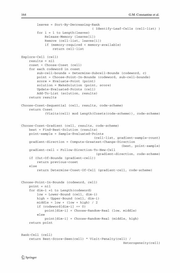
3.4 Pseudocode

We offer below pseudocode for the algorithm.

data-structures:Solution = { param0, ... , paramN-1, score}Bound = { min, max}Evaluated-Point = { solution, immediate-parent-cell}Cell = { param0-bounds, ... , paramN-bounds, visit-count,

immediate-parent-cell, evaluated-points}


user-chosen constants:cell-add-limitvisit-delayhistory-lengthgradient-sample-count

Search (eval-limit, score-tolerance, bounds, code-scheme)best-soln = nilbest-score = infinityevals-done = 0

cell-list = nilinitial-cell = Make-Cell (bounds, code-scheme, nil)Update-Rank (initial-cell)

Add-To-List (initial-cell, cell-list)

while (evals-done < eval-limit and best-score > score-tolerance)c = Choose-Best-Ranked-Cell (cell-list)evaluated-points = Explore-Cell (c)new-cells = Make-Candidate-Cells

(evaluated-points, c, code-scheme)

memory-required = Memory-In-Use () + Memory-Requirement(new-cells)

cell-list = Prune-Cells (cell-list, memory-required)Add-To-List (new-cells, cell-list)

Remove (c, cell-list)Update-Rank (c)Add-To-List (c, cell-list)

evals = evals + Length(evaluated-points)

best-evaluated = Best (evaluated-points)if (Score(best-evaluated) < best-score))

best-soln = best-evaluatedbest-score = Score (best-evaluated)

return (best-soln, best-score)

Make-Candidate-Cells (evaluated-points, parent-cell, code-scheme)new-cell-list = nilranked-points = Sort-By-Increasing-Rank (evaluated-points)for i = 1 to cell-add-limit

if (Score(ranked-points[i]) < Best-Score-Seen(parent-cell)codeword = Determine-Code-Word

(evaluated-points[i], code-scheme)bounds = Determine-Subcell-Bounds (codeword, parent-cell)new-cell = Make-Cell (bounds, code-scheme, parent-cell)Update-Rank (new-cell)Add-To-List (new-cell, new-cell-list)

return new-cell-list

Prune-Cells (cell-list, memory-required)while (memory-required > memory-available)


leaves = Sort-By-Decreasing-Rank( Identify-Leaf-Cells (cell-list) )

for i = 1 to Length(leaves)Release-Memory (leaves[i])Remove (cell-list, leaves[i])if (memory-required < memory-available)

return cell-list

Explore-Cell (cell)results = nilcoset = Choose-Coset (cell)for each codeword in coset

sub-cell-bounds = Determine-Subcell-Bounds (codeword, c)point = Choose-Point-In-Bounds (codeword, sub-cell-bounds)score = Evaluate-Point (point)solution = MakeSolution (point, score)Update-Evaluated-Points (cell)Add-To-List (solution, results)

return results

Choose-Coset-Sequential (cell, results, code-scheme)return Coset

(Visits(cell) mod Length(Cosets(code-scheme)), code-scheme)

Choose-Coset-Gradient (cell, results, code-scheme)best = Find-Best-Solution (results)point-sample = Sample-Evaluated-Points

(cell-list, gradient-sample-count)gradient-direction = Compute-Greatest-Change-Direction

(best, point-sample)gradient-cell = Follow-Direction-To-New-Cell

(gradient-direction, code-scheme)if (Out-Of-Bounds (gradient-cell))

return previous-cosetelse

return Determine-Coset-Of-Cell (gradient-cell, code-scheme)

Choose-Point-In-Bounds (codeword, cell)point = nilfor dim-i =1 to Length(codeword)

low = Lower-Bound (cell, dim-i)high = Upper-Bound (cell, dim-i)middle = low + (low + high) / 2if (codeword[dim-i] == 0)

point[dim-i] = Choose-Random-Real (low, middle)else

point[dim-i] = Choose-Random-Real (middle, high)return point

Rank-Cell (cell)return Best-Score-Seen(cell) * Visit-Penalty(cell) /

Heterogeneity(cell)


Visit-Penalty (cell)return max (1, Vists(cell) - visit-delay)

Heterogeneity (cell)historical-scores = Most-Recent-Scores (cell, history-length)return 1 + ln(1 + Variance (historical-scores))

3.5 Algorithm comparisons

The following tables compare the performance of the code algorithm to that of sev-eral other search algorithms applied to the same problem. Each algorithm is run 10times to account for variability due to inherent stochasticity. We compare our codealgorithm with a genetic algorithm, a hillclimber, and random search. To establisha benchmark for comparing algorithms of differing algorithmic complexity, we im-pose a standard limit on the number of scoring function evaluations allowed for eachalgorithm and compare their findings.

In the Tables that follow, the GA columns refer to a genetic algorithm variant,where P is the population size used, and N is the number of generations performed.The random search algorithm simply evaluates points chosen at random within thebounds. The steepest descent algorithm (hillclimber) implemented an iterative localsearch which followed a noisy empirical approximation to the gradient. At each step,the hillclimber chose an arbitrary parameter index at which to begin perturbationfrom the current best known solution. Five values within the current cell bounds forthis parameter were generated, and the parameter was then set to the sampled valuethat produced the most beneficial change in score. This process was then repeatedfor each of the remaining parameters until all had been changed. If the final pointresulting from these changes produced a new best solution, this was recorded andused as the basis for subsequent local search.

The following table summarizes the characteristics of each algorithm tested. Here,p denotes the number of parameters being optimized. The term “iteration” is used todescribe how each algorithm budgets its score evaluations. The simpler algorithmshere search only one point per iteration, while more complicated ones evaluate multi-ple points before returning their decision about the best finding for this step. Regard-less of the algorithm’s iteration scheme, however, the same hard limit on actual scoreevaluations is imposed in all cases.

Complexity of search algorithms tested

Algorithm Evaluations Per Iteration Min Memory Cost Max Memory Cost

OptimalCode O(CosetSize) O(CosetSize ∗ p) O(CosetSize ∗ p ∗ EvalLimit)GA(P,N ) O(P ) O(2 ∗ P ∗ p) O(2 ∗ P ∗ p)Hillclimber O(Perturb ∗ p) O(p) O(p)Random 1 O(p) O(p)

As the simplest search, random search has the most modest memory and evalua-tion requirements; it needs to store only the current vector of parameter values it isconsidering at any step, and never needs to evaluate multiple points. The hillclimber’s


memory requirements are comparable, as it only needs to keep track of the best solu-tion found thus far, and investigate perturbations of it. The number of perturbations(denoted Perturb) performed for each parameter while empirically approximating thegradient is chosen by the user. The GA must maintain an evolving population of P

candidate vectors that are considered when generating new solutions. At each itera-tion, P new candidate vectors are generated from the current population according tothe crossover and mutation strategies chosen by the user. A second “offspring” poolof size P is used to store these new candidates so that the standard pool is not over-written during the generation process. The P new vectors in the offspring pool areevaluated and the best of these are then merged back into the standard pool beforestarting the next iteration. The code algorithm defines an iteration to be a completeevaluation of all points in one coset of the code, so the number of evaluations per-formed per iteration is purely a function of the coding scheme chosen for the problem.The memory requirements of the code algorithm are more flexible than those of theother methods. At an absolute minimum, it is necessary to store the parameter vectorassociated with each point in the coset that is currently being evaluated. While min-imizing the memory footprint of the implementation, this robs the algorithm of his-tory. At the other extreme, we could keep a running history of every point evaluatedthus far in the search. Thus, memory usage would be bounded only by the evaluationlimit in the worst case. As discussed earlier under the heading of Memory Considera-tions, we would like to retain as much history as system memory permits, and remainwithin these bounds over arbitrarily many iterations by intelligently discarding oldhistory as the memory becomes full. For practical purposes, then, the algorithm willoperate with any memory limit specified by the user. It is advisable not to set the limitunnecessarily low, however, as the memory purging process may cause the algorithmto have to reexamine regions it would otherwise have remembered to avoid.

3.6 The seven dimensional ODE problem

In this problem we attempt to tune the set of parameters P of a system of ordinary dif-ferential equations to obtain an optimal fit to a set of training data. For each equatione in a set of training equations TE, we are given two vectors: Te = {t0, t1, . . . , te_max}and De = {d0, d1, . . . , demax}. Let the function M(e, t,p) represent the value for equa-tion e at time t , obtained by numerically integrating the ODE system with parametervalues specified by the candidate solution vector p. Our objective function is then de-fined as: f (p) = ∑

e∈TE∑|Te|

i=0(M(e,Te,i , p) − De,i)2. The system of equations and

the parameter bounds are listed below. For comparison purposes, each optimizationmethod was allowed to perform 100,000 evaluations of the objective function.

In the seven parameter ODE system below, L denotes the pathogen level in thepatient, M denotes the macrophage level in the patient, and D stands for the damageor dysfunction observed in the patient.

Equations:L′ = kpg · L · (1 − L) − kpm · M · L,

M ′ = (kmp · L + D) · M · (1 − M) − M,


D′ =(

kdma ·(

1 + tanh

(M − tma

wma

)))− kd · D,

InitialConditions:L(0) = 0.05,

M(0) = 0.001,

D(0) = 0.15,

ParameterBounds:kpg = [0,0.1],kpm = [0,1],kmp = [0,10],tma = [0,0.5],wma = [0,0.5],kdma = [0,0.02],kd = [0,0.1].

A summary of the simulated results appears in Table 1.The performance of the random search algorithm provides a benchmark against

the most naive possible search strategy. We observe that the optimal code algorithmyields the most promising results in both the best and average cases over the runs. Itsworst case solution scores better than all but the two best runs of all competing algo-rithms. Random search is the next best competitor. Good performance of the randomalgorithm suggests two properties of the scoring surface: first, that good (but perhapsnon-optimal) solutions are plentiful and scattered throughout the search space, and

Table 1 Performance results for the 7-dimensional ODE system

Run OptimalCode GA(P = 16, N = 6250) Hillclimber Random

1 0.001369 0.0344754 0.456643 0.0305824

2 0.002135 0.071979 0.437013 0.0201192

3 0.005527 0.0465479 0.226696 0.0260119

4 0.002664 0.196176 0.418331 0.0135728

5 0.001448 0.335479 0.00387431 0.0183359

6 0.001673 0.0657115 0.316007 0.025964

7 0.001386 0.0792147 0.399875 0.0059441

8 0.001440 0.0602518 0.416516 0.0100706

9 0.005316 0.0714629 0.393411 0.0214453

10 0.005042 0.023839 0.418944 0.00358366

Mean 0.002800 0.09851372 0.348731031 0.017562986

Best 0.001369 0.023839 0.00387431 0.00358366


secondly that the surface is relatively nonuniform. This is further borne out by thevery poor average case performance of the most local search, the hillclimber. This isattributable to several factors. First, it performs the least global survey of all methods,making its performance very contingent on its starting point. Secondly, the effective-ness of local search is limited in this problem, due the presence of numerous localminima. The genetic algorithm performs significantly better than the hillclimber, butmuch worse than the optimal code and random algorithms. This is largely due tothe small population size employed here, which provides for too little population di-versity to drive the search. By choosing a much larger population size, the GA cancollect a better sample of the scoring surface and will be less prone to premature con-vergence. However, the population size was deliberately chosen to correspond withthe coset size of the optimal code. Since the coding scheme used here contained 16codewords, it was considered unfair to permit the GA a greater number of samplepoints per iteration. Just as it is possible to increase the population size of the GA,it is also possible to choose an alternate (perhaps more complicated) coding scheme.While recognizing this is an unusually small population for a GA, we choose to keepsample sizes equal for fairness in comparison. Table 2 shows a larger problem wherea new coding scheme is employed and a correspondingly larger GA population istherefore used.

3.6.1 The 15-parameter quadratic

In this example the function to be minimized was: f (p) = ∑15i=1(ai − pi)

2. All ai

and pi were constrained within [0, 1]. Values for the constants ai were chosen a prioriat random within these intervals and then held fixed throughout the entire battery oftests. The values of the ai ’s are listed below:

a0 = 0.0601 a1 = 0.5290 a2 = 0.0007 a3 = 0.5887 a4 = 0.9444a5 = 0.0622 a6 = 0.1902 a7 = 0.3401 a8 = 0.8010 a9 = 0.4683a10 = 0.8855 a11 = 0.9299 a13 = 0.0718 a14 = 0.5603 a15 = 0.6151

Table 2 shows a very different profile of behavior between the algorithms. Theworst performer in Table 1, the hillclimber, is now the best. Its resulting scores sur-pass all other methods by several orders of magnitude. This is easily explained—the scoring surface of this problem (a multi-dimensional quadratic) is exceptionallysmooth. As one would expect, following a gradient is extremely effective in such aspace, so this local search method triumphs. The optimal code is now the second bestperformer. This is also intuitive; the algorithm is balancing local and global search.In this space many codewords of each coset lie away from the gradient but must stillbe explored. Once these “wasted” evaluations are done, however, the ranking proce-dure will choose to recurse into the cells which are closest to the true minimum. TheGA again finishes in third place. Once again its population size has been chosen tomatch the number of codewords used in the optimal code algorithm. The GA sufferseven more acutely from the same problem as the optimal code; it spends very manyevaluations mating solutions that lie away from the target. Better solutions do indeedcome to dominate the population, but due to our limit on the number of evaluations,


Table 2 The 15-dimensional quadratic

Run OptimalCode GA(P = 2048, N = 49) Hillclimber Random

1 0.0832361 1.83559 1.97709e-05 68.379

2 0.217762 1.68968 2.22564e-05 60.54

3 0.0772086 1.68611 1.3165e-05 68.1213

4 0.220271 2.62141 1.1364e-05 66.9669

5 0.540058 1.72501 9.60819e-06 69.3401

6 0.229307 2.22178 1.08077e-05 79.7582

7 0.169243 1.23769 3.66222e-05 55.4995

8 0.0960766 3.02225 1.51147e-05 74.71

9 0.299546 2.87475 5.29135e-06 94.2987

10 0.320636 4.24115 2.10776e-05 72.1723

Mean 0.22533443 2.315542 1.6507804e-05 70.9786

Best 0.0772086 1.23769 5.29135e-06 55.4995

it follows that increasing the population size reduces the number of generations thatcan be performed. Unsurprisingly, the random search is the worst method here, as itis outperformed by methods that are capable of exploiting either gradient or historicalinformation about the smoothness of the surface.

These results suggest that the optimal code algorithm is best suited to problemswhere local gradient information is helpful, but the existence of numerous local min-ima would stymie purely local search methods. For smooth scoring surfaces, theoptimal code algorithm is effective but less efficient than gradient searching. Con-versely, for extremely nonuniform surfaces where locality is a poor guide for search,the method would then be hampered in its attempts to wisely select promising sub-cells for refining its search.

4 Classifying parameter sets yielding different regimes

Though minimizing an objective function occurs any time one fits a model to data,one of our main objectives is to predict the correct regime for a given vector of pa-rameters. The first step is to identify originally a set of regimes that the system ofODE’s could produce both over the intermediate time range as well as long term;see also [10]. Identifying relevant behavioral regimes over the intermediate term isparticularly important, since a key objective is to intervene by changing treatmentprotocol for a happy evolution of a patient toward a satisfactory long term state.While several potential regimes may be suspected to exist a priori, not all possibleregimes will usually be known. However, each time we evaluate the model at a pa-rameter set (i.e., numerically integrate it) we either classify the resulting function inone of the known regimes or decide to create a new regime. We can thus eventu-ally expand the set of regimes as the computer simulation progresses. Comparisonof regimes involves defining a measure that compares two regimes and computesa distance between them. We decided to use a measure that matches only “quali-tatively defining features” of the functions in questions, such as notable peaks, tail


behaviour, or other qualitatively relevant traits. We shall then say that two functionsare in the same regime if they have qualitatively similar features; else they representdifferent regimes. (This measure is quite different for the more usual least squaresmetric, but it addresses better the qualitative features we seek in the model.) The al-gorithm described in the previous sections is adapted to the ODE system associatedto the immune system by partitioning the parameter set in accordance to how the pa-rameters are shared in the equations that describe the model. The model is explicitlygiven in [3]. The nature of this ODE system is such that we can identify a subset ofparameters that occur jointly in certain equations of the system, thus expecting thatinteractions of potentially any order between the parameters in this subset exist. Inlike fashion, we obtain three disjoint such subsets of parameters that partition theentire parameters set, and such that the interactions between parameters in differentsubsets are few in number and expected to be of low order. In essence we thus par-tition the parameter space into a (direct) sum of (basically independent) subspacesand apply the algorithm to each part of the partition. This reduces the dimensionalityof the search, since the interactions between groups are few in number and may bestudied separately. When we say that we apply the algorithm to the immune systemproblem we understand it being applied in the sense just described. Other problemsmay require other adjustments to the algorithm to best incorporate the special natureof the ODE systems that arise.

We now describe how we can use the algorithm in the previous section in con-junction with a multinomial logistic distribution to classify any point in the parameterspace. The outcomes of the logistic distribution are the r distinct regimes. We nowstart the algorithm. At each parameter point selected, by integrating the ODE system,we obtain the response function. We compute distances to each of the r regimes andclassify that parameter point in one of them. The code ensures that the parameterspace is optimally covered each time we select a new coset of parameter points. Aftera sufficiently large number of iterations we may notice points in the parameter spacewhere bifurcations seem to occur. In the neighborhood of such points (should theyprove of investigative interest) we can locally replicate the search just described. Werefer to [11] for detailed information on issues related to bifurcation.

To classify an arbitrary parameter point θ we use the multinomial logistic as fol-lows: think of the points in the parameter space that we evaluated and classified asdata for the logistic model. Using maximum likelihood estimation, in the usual way,estimate from this data the coefficients in the logistic function. Use the multinomiallogistic model thus created to predict that θ yields a response in regime i with prob-ability pi (with the pi summing to 1). The probabilities pi are estimated from thepredictive equations generated by the multinomial logistic model. As is commonlydone, we now classify θ in the class corresponding to regime j, where j is definedby pj = max1≤i≤r pi .

Acknowledgements We thank the referees for suggestions that enhanced both the clarity and cohesive-ness of the paper.


References

1. Bone, R.C.: Immunologic dissonance: a continuing evolution in our understanding of the systemic in-flammatory response syndrome (SIRS) and the multiple organ dysfunction syndrome (MODS). Ann.Int. Med. 125, 680–687 (1996)

2. Buchman, T.G., Cobb, J.P., Lapedes, A.S., et al.: Complex systems analysis: a tool for shock research.Shock 16, 248–251 (2001)

3. Chow, C.C., et al.: The acute inflammatory response in diverse shock states. Shock 24, 74–84 (2005)4. Clermont, G., et al.: In silico design of clinical trials: a method coming of age. Crit. Care Med. 32,

2061–2070 (2004)5. Kitano, H.: Systems biology: a brief overview. Science 295, 1662–1664 (2002)6. MacWilliams, F.J., Sloane, N.J.A.: The Theory of Error Correcting Codes. North-Holland, Amster-

dam (1978)7. Medzhitov, R., Janeway, C.J.: Innate immunity. N. Engl. J. Med. 343, 338–344 (2000)8. Mira, J.P., Cariou, A., Grall, F., et al.: Association of TNF2, a TNF-a promoter polymorphism, with

septic shock susceptibility and mortality. A multicenter study. JAMA 282, 561–568 (1999)9. Nathan, C.: Points of control in inflammation. Nature 420, 846–852 (2002)

10. Neugebauer, E.A., Willy, C., Sauerland, S.: Complexity and non-linearity in shock research: reduc-tionism or synthesis?. Shock 16, 252–258 (2001)

11. Seydel, R.: Practical Bifurcation and Stability Analysis: From Equilibrium to Chaos, 2nd edn.Springer, New York (1994)

12. Wicker, S.B.: Error Control Systems for Digital Communication and Storage. Prentice Hall, NewJersey (1995)

A linear code parameter search algorithm with applications to immunology

Documents

Transcript of A linear code parameter search algorithm with applications to immunology