Tree species distributions and local habitat variation in the Amazon: large forest plot in eastern...

Journal of Ecology

2004

92

, 214 –229

© 2004 British Ecological Society

Blackwell Publishing, Ltd.

Tree species distributions and local habitat variation in the Amazon: large forest plot in eastern Ecuador

RENATO VALENCIA*, ROBIN B. FOSTER†, GORKY VILLA, RICHARD CONDIT‡, JENS-CHRISTIAN SVENNING§, CONSUELO HERNÁNDEZ, KATYA ROMOLEROUX, ELIZABETH LOSOS¶, ELSE MAGÅRD§ and HENRIK BALSLEV§

Department of Biological Sciences, Pontificia Universidad Católica del Ecuador, Apartado 17-01-2184, Quito, Ecuador,

†

Botany Department, The Field Museum, Roosevelt Road at Lake Shore Drive, Chicago, IL 60605-2496, USA,

‡

Center for Tropical Forest Science, Smithsonian Tropical Research Institute, Unit 0948, APO AA 34002-0948, USA,

§

Department of Systematic Botany, University of Århus, Nordlandsvej 68, DK-8240 Risskov, Denmark, and

¶

Center for Tropical Forest Science, Smithsonian Institution, Suite 2207, 900 Jefferson Drive, Washington, DC 20560, USA

Summary

1

We mapped and identified all trees

≥

10 mm in diameter in 25 ha of lowland wet forestin Amazonian Ecuador, and found 1104 morphospecies among 152 353 individuals. Thelargest number of species was mid-sized canopy trees with maximum height 10–20 mand understorey treelets with maximum height of 5–10 m.

2

Several species of understorey treelets in the genera

Matisia

and

Rinorea

dominatedthe forest numerically, while important canopy species were

Iriartea deltoidea

and

Eschweilera coriacea

.

3

We examined how species partition local topographic variation into niches, and howmuch this partitioning contributes to forest diversity. Evidence in favour of topographicniche-partitioning was found: similarity in species composition between ridge andvalley quadrats was lower than similarity between two valley (or two ridge) quadrats, and25% of the species had large abundance differences between valley and ridge-top. On the otherhand, 25% of the species were generalists, with similar abundance on both valley and ridges,and half the species had only moderate abundance differences between valley and ridge.

4

Topographic niche-partitioning was not finely grained. There were no more thanthree distinct vegetation zones: valley, mid-slope, and upper-ridge, and the latter twodiffered only slightly in species composition.

5

Similarity in species composition declined with distance even within a topographichabitat, to about the same degree as it declined between habitats. This suggests patchinessnot related to topographic variation, and possibly due to dispersal limitation.

6

We conclude that partitioning of topographic niches does make a contribution to the

α

-diversity of Amazonian trees, but only a minor one. It provides no explanation for theco-occurrence of hundreds of topographic generalists, nor for the hundreds of specieswith similar life-form appearing on a single ridge-top.

Key-words

: Amazonian Ecuador, catena, habitat partitioning, topographic niche,tropical forest diversity, tropical trees, Yasuni National Park

Journal of Ecology

(2004)

92

, 214–229

Introduction

Amazonian forests are species rich. There are usually200–300 tree species co-occurring at a single site (Gentry

1982, 1992; Phillips

et al

. 1994; Sierra

et al

. 1999; Ter Steege

et al

. 2000), and these estimates are based only on treeslarger than 10 cm in stem diameter over a single hectare.The total number of species could be higher than this(Valencia

et al

. 1994). A variety of hypotheses have beenproposed to account for high diversity (Hubbell

et al

. 2001;Wright 2002), and one explanation has to do with localvariation in soil resources caused by topography. Thereis ample evidence that individual species partition

Correspondence: Richard Condit (tel. 507 212 8144; fax 507 212 8148; e-mail [email protected]).*Present address: Fundación para la Ciencia y la Tecnologia,Av. Patria 850 y 10 de Agosto, Ed. Banco de Préstamos, Piso9, Apartado Postal 17-12-000404, Quito, Ecuador.

215

A large forest plot in eastern Ecuador

© 2004 British Ecological Society,

Journal of Ecology

,

92

, 214–229

topographic ridge-valley gradients, or ‘catenas’ as they aresometimes called, and that tree species distributions areaffected by underlying geological variation as well(Lieberman

et al

. 1985; Kahn 1987; Basnet 1992; Tuomisto& Ruokolainen 1994; Ruokolainen

et al

. 1997; Clark

et al

.1999; Svenning 1999; Harms

et al

. 2001; Romero-Saltos

et al

. 2001; Phillips

et al

. 2003; Tuomisto

et al

. 2003ab).Few studies, however, quantify the degree to which speciesabundances are controlled by soil characteristics, and itthus remains possible that random forces as well playan important role in community composition (Hubbell2001). For example, many neotropical tree species aregeneralists, occurring across many soil types (Hubbell& Foster 1986; Pitman

et al

. 1999, 2001), and for thesespecies, factors controlling abundance remain unknown.

The importance of soil gradients to tree diversity isthus a quantitative proposition: some species respondstrongly to soil type, while others are generalists, andjust how much each species’ abundance is limited bysoil variation is the key. Here we attempt a quantitativeevaluation of how individual tree species respond to asoil catena with a large-scale, complete forest inventoryin Amazonian Ecuador. All trees, treelets and shrubswere located and identified over 25 ha of forest, span-ning two ridge systems. From the first census of thisplot, we have precise maps of every tree of every species,and with these we seek a quantitative description ofdiversity and how it varies from shrubs to tall trees, andof how much the tree community varies across the cat-ena. Which growth-forms are most diverse? Do speciespartition the topography finely? Or are most speciesgeneralists? To evaluate the catena, we must alsoconsider the degree to which tree species compositionchanges with topographic position as well as withgeographical distance (Borcard

et al

. 1992; Legendre1993; Ruokolainen

et al

. 1997; Condit

et al

. 2002; Phillips

et al

. 2003). We use the variation in abundance ofindividual species to evaluate how important the soilcatena might be in maintaining diversity.

Materials and methods

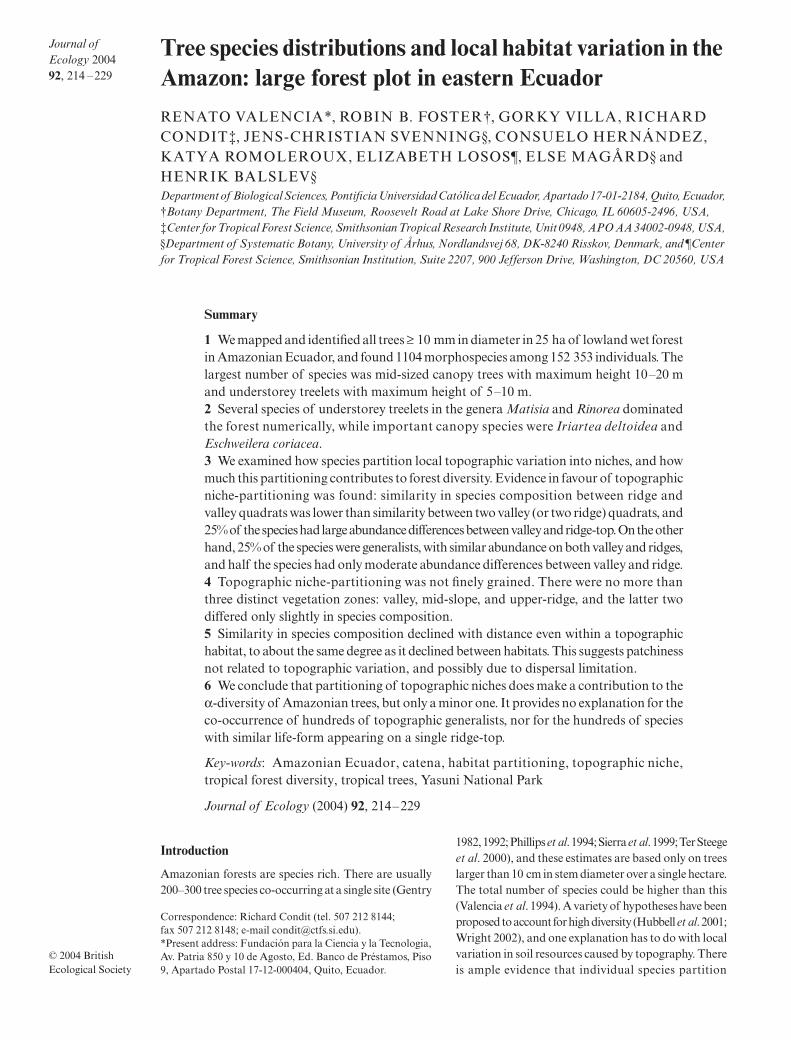
Yasuni National Park and Biosphere Reserve and theadjacent Huaorani Indian territory cover 1.6 million haof forest and form the largest protected area in AmazonianEcuador. Within the park, there are extensive oil reservesthat are ceded for prospecting and exploitation. Severaloil roads enter the park from the north, and there are afew permanent oil camps. Huaorani Indians also inhabitsmall settlements in the park, and they hunt wild meat.North of the park and the Napo River are more extensivesettlements of Quichua Indians and other Ecuadorians,people who clear forest for agriculture; some Quichuahave been colonizing oil roads close to the park. Thereis also evidence of past Native American settlementswithin the park, but whether there were ever extensiveclearings is unknown (Netherly 1997). Overall, human

influences are currently sparse, and most of Yasuni NationalPark is undisturbed wilderness covered by unbroken forest,home to the most sensitive megafauna of tropical SouthAmerica, such as jaguar (

Panthera onca

), harpy eagle(

Harpia harpyja

), giant otter (

Pteronura brasiliensis

)and white-lipped peccary (

Tayassu pecari

).The park is nearly level at about 200 m above sea level,

but crossed by numerous ridges rising 25–40 m abovethe intervening forest streams. At wider intervals, largerivers flow east to meet the Napo and the Amazon.Except for swampy areas and floodplains of the largerrivers, the vegetation is a visually homogeneous tall,evergreen, terre firme forest, lacking large disturbancesor clearings. The canopy is 10–25 m high punctuatedwith emergents to 40 and rarely 50 m tall as well as withsmall gaps created by fallen trees.

The 25-ha plot is located inside the park, at 0

°

41

′

Slatitude, 76

°

24

′

W longitude, just south of the TiputiniRiver. It is within a kilometre of the Yasuni ResearchStation, which is operated by the Pontificia UniversidadCatólica of Ecuador (Fig. 1). Access to the researchstation and thus the plot is via an oil road. There are afew Huaorani settlements on this road, north of thestation, and there has been some recent hunting nearthe research station and even inside the plot.

Soils of the Yasuni area are poorly known. Most arefluvial sediments originating in the Andes, and a geo-logical map indicates that the area south of the TiputiniRiver is a single Miocene sediment (Malo & Arguello1984). Korning

et al.

(1994) described the soils of onesite in Yasuni National Park as udult, clayey, kaoliniticand aluminium-rich. Tuomisto

et al.

(2003a) found soilsin and around the 25-ha plot to be rich in exchangeablebases compared with other Amazonian sites, with a texturedominated by silt. They concluded that two broad soiltypes cover Yasuni; our plot lies entirely within one.

At a finer scale, the 25-ha plot ranges from 216 to248 m a.s.l., and includes two ridges and an interveningvalley, plus a small section of another valley on the northboundary (Fig. 2). The valley occasionally floods, butonly for brief periods. Nothing about soil variation withinthe plot is currently known.

Rainfall and temperature are aseasonal at Yasuni.During 53 months of records at the research station,the longest rainless period was 3 weeks and the leastrainy month was August. The mean annual rainfallwas 2826 mm, and none of the 12 calendar monthsaveraged < 100 mm, although three of the 53 monthsreceived < 100 mm. Mean monthly temperatures werea high of 34

°

C and a low of 22

°

C.

A 50-ha plot was fully surveyed in 1995 by a profes-sional team. Between June 1995 and June 2000, all free-standing woody plants

≥

10 mm in stem diameter were

216

R. Valencia

et al.


Journal of Ecology

,

92

, 214–229

tagged, mapped and identified to morphospecies in thewestern half of the 50 ha. The diameter of every indi-vidual was recorded at 1.3 m above the ground, unlessthe stem was swollen or buttressed; measurements weretaken just below small swellings, or at least 0.5 m abovelarge buttresses. Regardless of the height-of-measure,we refer to these as d.b.h. (diameter at breast height).These methods are described in detail in Condit (1998).

The taxonomy of the 25-ha plot was far more dif-ficult than first anticipated, with many more speciesencountered than expected. In particular, there weremany groups with very similar species that could onlybe sorted accurately in the laboratory. A completeset of collections from the plot is now deposited inthe Herbarium of the Pontificia Universidad Católicaof Ecuador, Quito (QCH is the herbarium code), andduplicates of most of the specimens are in the FieldMuseum in Chicago (F). We have compared specimensfrom the plot with collections at Ecuador’s NationalHerbarium (QCNE), the Missouri Botanical Garden(MO), the New York Botanical Garden (NY), the Smith-sonian Natural History Museum (US) and the FieldMuseum, and 335 collections have been sent to specialists.Romoleroux

et al

. (1997) published a list of all thespecies and morphospecies and their correspondingvouchers; an updated version is now available on the web(http://www.puce.edu.ec/herbario and http://ctfs.si.edu).

There remain morphospecies for which we have seenonly one or two individuals, so a number of identi-fications remain tentative. As the taxonomic work isongoing and far from complete, we froze a data base ofspecies assignments in June 2001, and here report on it:

152 353 individual trees tagged and identified in the 25-ha plot, with 145 406 sorted into morphospecies and6947 that could not be assigned; 1104 total morpho-species, with 548 fully identified and 471 identified to genus.The number of morphospecies we have segregated hasbeen climbing slowly since, and additional taxonomicwork will probably expand the species count to 1130 orpossibly 1150.

-

We grouped species into four life-forms, defined by themaximum height they usually attain: shrubs (< 5 m),treelets (

≥

5 and < 10 m), mid-canopy trees (

≥

10 and <20 m), and tall-canopy trees (

≥

20 m). The typical max-imum height of 273 Yasuni species was obtained fromflorulas and taxonomic treatments (Croat 1978; Prance1979; Sleumer 1980; Pennington

et al

. 1981; Berg

et al

.1990; Pennington 1990; Brako & Zarucchi 1993; Rohwer1993; Vásquez 1997). Life-forms for the remaining species(all but one, which might be a liana) were assessed from ourown observations in the plot. For common species, thesecategories are reasonably accurate, but for rare species,they should be considered provisional. We believe, how-ever, that the general patterns we present will not be greatlyaffected by errors in life-form categorization.

Habitats were defined with topographic informationonly, as this was the basis for prior hypotheses abouttree distribution. The topography was based on elevation

Fig. 1 Map of Ecuador and the plot location in Amazonia. The map on the left shows the entire 50-ha region that was surveyed, 1 km × 0.5 km. The 25-ha region that was censused is the left-hand (west) half of this rectangle.

http://www.puce.edu.ec/herbario

http://ctfs.si.edu

217

A large forest plot in eastern Ecuador


Journal of Ecology

,

92

, 214–229

estimated at each point on a 20

×

20 m grid by theprofessional survey team (Fig. 2). Each 20

×

20 m quadratwas assigned three topographic attributes to assist incategorization: elevation, convexity and slope. Eleva-tion of a quadrat was defined as the mean elevationat its four corners, and convexity as the elevation of afocal quadrat minus the mean elevation of the eightsurrounding quadrats. For edge quadrats, convexitywas defined as the elevation of the centre point (10 mfrom all corners) minus the mean of the four corners;the elevation of the centre point was estimated bykriging (using Spyglass software for Macintosh). Slopewas calculated as in Harms

et al

. (2001), and is thesingle average angle from the horizontal of the entirequadrat.

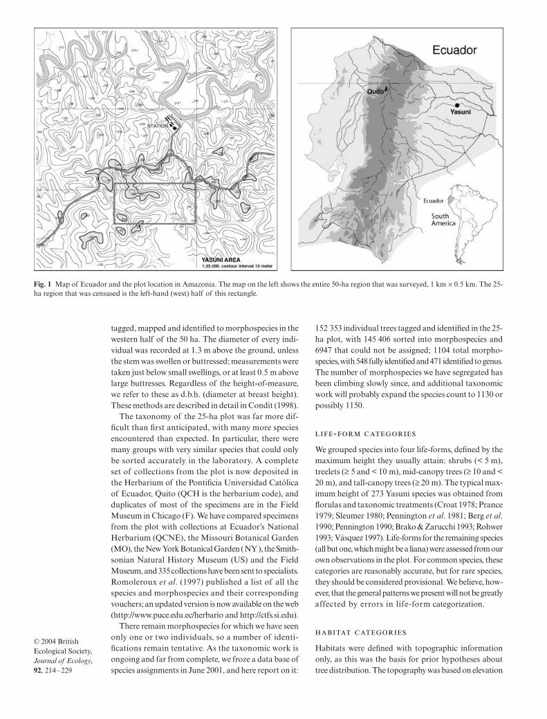
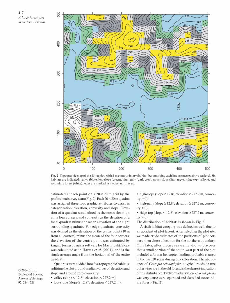
Quadrats were divided into five topographic habitats,splitting the plot around median values of elevation andslope and around zero convexity:

•

valley (slope < 12.8

°

, elevation < 227.2 m);

•

low-slope (slope

≥

12.8

°

, elevation < 227.2 m);

•

high-slope (slope

≥

12.8

°

, elevation

≥

227.2 m, convex-ity > 0);

•

high-gully (slope

≥

12.8

°

, elevation

≥

227.2 m, convex-ity < 0);

•

ridge-top (slope < 12.8

°

, elevation

≥

227.2 m, convex-ity > 0).The distribution of habitats is shown in Fig. 2.

A sixth habitat category was defined as well, due toan accident of plot layout. After selecting the plot site,we made crude estimates of the positions of plot cor-ners, then chose a location for the northern boundary.Only later, after precise surveying, did we discoverthat a small portion of the south-west part of the plotincluded a former helicopter landing, probably clearedin the past 20 years during oil exploration. The abund-ance of

Cecropia sciadophylla

, a typical roadside treeotherwise rare in the old forest, is the clearest indicationof this disturbance. Twelve quadrats where

C. sciadophylla

was very dense were separated and classified as second-ary forest (Fig. 2).

Fig. 2 Topographic map of the 25-ha plot, with 2-m contour intervals. Numbers marking each line are metres above sea level. Sixhabitats are indicated: valley (blue), low-slope (green), high-gully (dark grey), upper-slope (light grey), ridge-top (yellow), andsecondary forest (white). Axes are marked in metres; north is up.

218

R. Valencia

et al.


Journal of Ecology

,

92

, 214–229

We use tree density (individuals) and basal area to describeforest structure. Basal area was calculated by summingthe cross-sectional area of each stem at breast-height,including secondary stems that split from a main stembelow breast-height (Condit 1998). We define diversityeither as the total number of species, or the mean numberof species per unit squares (either 20

×

20 m quadratsor hectares). To correct for sample-size differencesbetween habitat, the diversity index Fisher’s

α

was used(Rosenzweig 1995; calculated from the routine given inCondit

et al

. 1998). Statistical confidence was calcu-lated using the variance across 20

×

20 m quadrats withina single habitat, or across hectares in the entire plot, basedon

t

-statistics. The quadrats in this and every analysispresented are the non-overlapping 20

×

20 m squaresbetween grid-posts set down by the survey team, ornon-overlapping square hectares composed of 25 ofthe 20

×

20 m quadrats (Condit

et al

. 1996).

To separate the effect of habitat from the effect of geo-graphical distance, we started with the similarity inspecies composition between pairs of 20

×

20 m quadrats.We used the Sørensen similarity index ‘without cover’

(Barbour

et al

. 1987), defined as where

S

12

is the number of species common to the two quadratsand

S

i

the total found in quadrat

i.

We also used the versionof Sørensen that incorporates abundance data, knownas the Sørensen index ‘with cover’ (Barbour

et al

. 1987)or the Steinhaus index. Similarity was calculated for all

quadrat-pairs in the plot. Next, the

geographical distance between each pair of quadratswas defined as the distance from quadrat centre toquadrat centre. Then mean similarity for all pairswhose distance fell in a 20-m bin (

≥

0 and < 20,

≥

20and < 40,

≥

40 and < 60, etc.) was calculated; this meanwas graphed as a function of distance. Similarity-distance graphs were drawn for quadrat-pairs withina given habitat and for pairs that included one quadratin one habitat and the second quadrat in a differenthabitat. The similarity-distance graph within a habitatshows how geographical distance affects species com-position; a habitat effect is indicated if the similarity-distance curve between habitats is lower than the curvewithin a habitat, at a given distance.

To assess similarity between pairs of habitats

i

and

j

while correcting for distance, a standardized mean

similarity was defined as Here,

SOR

ij

is the mean Sørensen similarity between quadratpairs where one quadrat is in habitat

i

and the other inhabitat

j

, but only considering cases where the distancebetween the two quadrats is 150–500 m. At this range,the impact of distance on similarity was slight. The

denominator, based on quadrat pairs from within a habitat(but never a quadrat with itself ), does the standardizing:if quadrat pairs between habitats are just as similar asquadrat pairs within a habitat, the standardized indexis 100%. Values less than 100% demonstrate habitatdifference that is independent of geographical distance.

We used a jackknife resampling approach to gener-ate confidence limits on mean similarity. A subset of312 of the 625 quadrats was drawn at random, withoutreplacement, and the similarity-distance analysis wasrepeated. We sampled without replacement becauseif replacement was allowed, quadrats would appearmore than once in each sample, and a quadrat’ssimilarity to itself provides no information. Samplingwas repeated, and the standard deviation from 100replicates was divided by √2 to generate an estimateof the standard error for all quadrats (dividing by √2because the jackknife sample was half the original); thestandard error was multiplied by 1.96 to estimate 95%confidence limits.

The most abundant species are often used to define forestcomposition, and we considered the top-10 rankingspecies in density or basal area as dominant. Abundancedifferences between two habitats for all species areillustrated with a graph of density in one habitat vs. densityin a second habitat, with one point for each species. If allspecies have identical density in two habitats, the pointsfall on a one-to-one line. The r2 from these regressionsprovide an index of habitat similarity. Density wascalculated by adding one to the total number of individualsfor a given species in a given habitat, then dividing bythe habitat’s area; this was then log-transformed. Con-fidence in density estimates and regressions was judged bybootstrapping from the 625 quadrats and calculatingdensity of each species in each habitat every time; thestandard deviation of 100 bootstrap estimates wasmultiplied by 1.96 as an estimate for 95% confidencelimits.

Confidence limits on both abundance and similaritywere thus based on bootstrapping quadrats, not indi-viduals. This means we consider a single quadrat as asampling unit, and individuals within that quadrat arenot treated as independent. Spatial autocorrelation intree distributions in many tropical forests is strongestat scales < 20 m (Condit et al. 2000), so by treating 20 ×20 m quadrats as sampling units, we remove at least partof the problem of spatial autocorrelation in assessingstatistical confidence (Harms et al. 2001).

To judge differences in species’ abundances betweenhabitats, we tallied species in three categories: those withdensity differing by < 1.5-fold, by ≥ 1.5-fold and < 5-fold,or by ≥ 5-fold. The factor 1.5 corresponds roughly tocases where 95% confidence limits on density did notoverlap; the cut-off of 5 was arbitrary, meant to indicateextreme density variation. These tallies were restricted

SS S

12

1 20 5. ( ),

+

625 6242

195 000

⋅

=

100

0 5

. ( ).

×+

SOR

SOR SORij

ii jj

219A large forest plot in eastern Ecuador

© 2004 British Ecological Society, Journal of Ecology, 92, 214–229

to species that had at least 10 individuals in all 25 ha; belowthis cut-off, confidence intervals on density were so broadthat comparisons between habitats were essentiallymeaningless. Comparisons of abundance between habitatsare uncorrected for distance, but the impact of distanceon similarity was generally only pronounced within50 m, and pooled habitat categories on which we basedcomparisons are considerably larger than this. In par-ticular, upper-ridge and valley are more than 50 m apart,and this is the habitat comparison we emphasize.

Results

There were 6094 individual trees and saplings ha−1

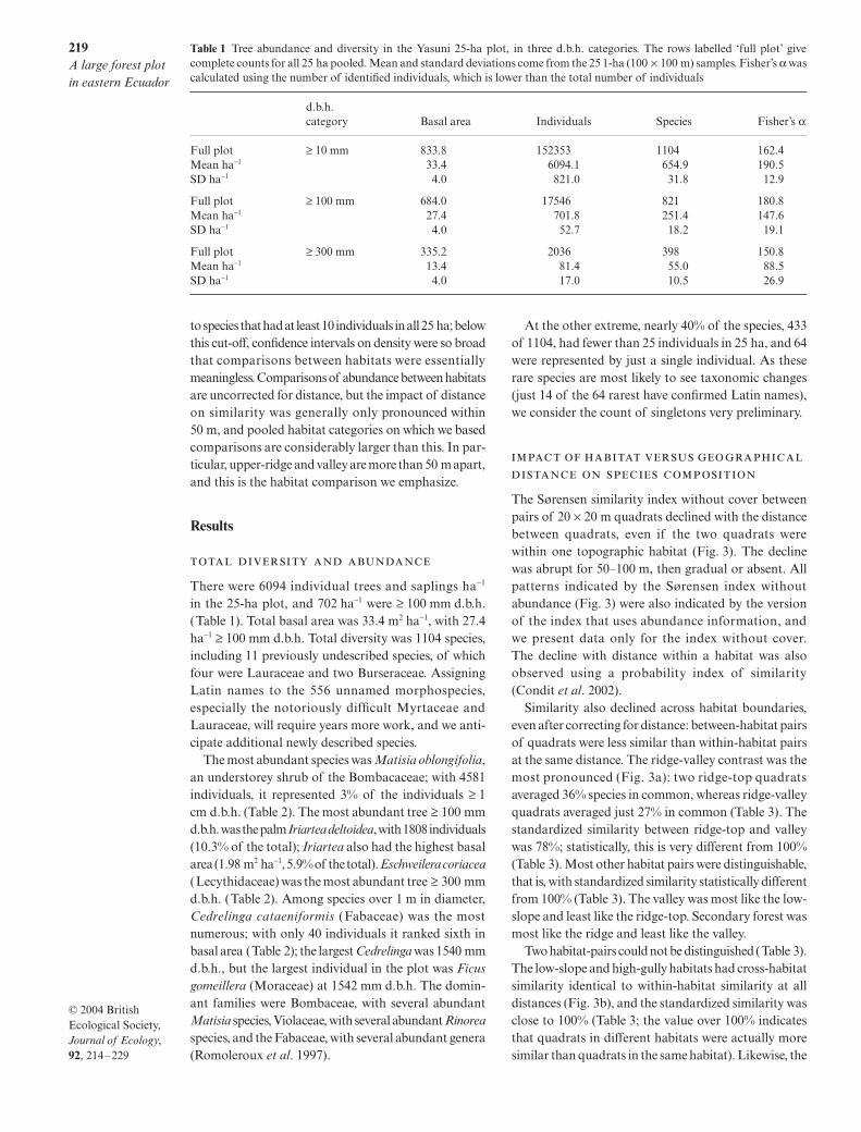
in the 25-ha plot, and 702 ha−1 were ≥ 100 mm d.b.h.(Table 1). Total basal area was 33.4 m2 ha−1, with 27.4ha−1 ≥ 100 mm d.b.h. Total diversity was 1104 species,including 11 previously undescribed species, of whichfour were Lauraceae and two Burseraceae. AssigningLatin names to the 556 unnamed morphospecies,especially the notoriously difficult Myrtaceae andLauraceae, will require years more work, and we anti-cipate additional newly described species.

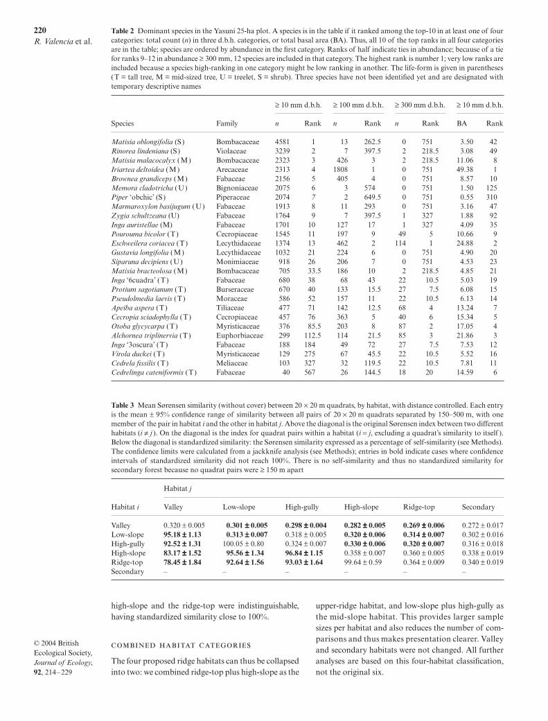
The most abundant species was Matisia oblongifolia,an understorey shrub of the Bombacaceae; with 4581individuals, it represented 3% of the individuals ≥ 1cm d.b.h. (Table 2). The most abundant tree ≥ 100 mmd.b.h. was the palm Iriartea deltoidea, with 1808 individuals(10.3% of the total); Iriartea also had the highest basalarea (1.98 m2 ha−1, 5.9% of the total). Eschweilera coriacea(Lecythidaceae) was the most abundant tree ≥ 300 mmd.b.h. (Table 2). Among species over 1 m in diameter,Cedrelinga cataeniformis (Fabaceae) was the mostnumerous; with only 40 individuals it ranked sixth inbasal area (Table 2); the largest Cedrelinga was 1540 mmd.b.h., but the largest individual in the plot was Ficusgomeillera (Moraceae) at 1542 mm d.b.h. The domin-ant families were Bombaceae, with several abundantMatisia species, Violaceae, with several abundant Rinoreaspecies, and the Fabaceae, with several abundant genera(Romoleroux et al. 1997).

At the other extreme, nearly 40% of the species, 433of 1104, had fewer than 25 individuals in 25 ha, and 64were represented by just a single individual. As theserare species are most likely to see taxonomic changes(just 14 of the 64 rarest have confirmed Latin names),we consider the count of singletons very preliminary.

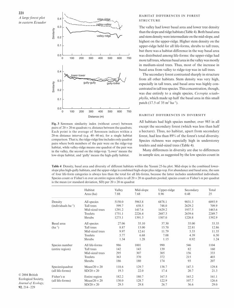
The Sørensen similarity index without cover betweenpairs of 20 × 20 m quadrats declined with the distancebetween quadrats, even if the two quadrats werewithin one topographic habitat (Fig. 3). The declinewas abrupt for 50–100 m, then gradual or absent. Allpatterns indicated by the Sørensen index withoutabundance (Fig. 3) were also indicated by the versionof the index that uses abundance information, andwe present data only for the index without cover.The decline with distance within a habitat was alsoobserved using a probability index of similarity(Condit et al. 2002).

Similarity also declined across habitat boundaries,even after correcting for distance: between-habitat pairsof quadrats were less similar than within-habitat pairsat the same distance. The ridge-valley contrast was themost pronounced (Fig. 3a): two ridge-top quadratsaveraged 36% species in common, whereas ridge-valleyquadrats averaged just 27% in common (Table 3). Thestandardized similarity between ridge-top and valleywas 78%; statistically, this is very different from 100%(Table 3). Most other habitat pairs were distinguishable,that is, with standardized similarity statistically differentfrom 100% (Table 3). The valley was most like the low-slope and least like the ridge-top. Secondary forest wasmost like the ridge and least like the valley.

Two habitat-pairs could not be distinguished (Table 3).The low-slope and high-gully habitats had cross-habitatsimilarity identical to within-habitat similarity at alldistances (Fig. 3b), and the standardized similarity wasclose to 100% (Table 3; the value over 100% indicatesthat quadrats in different habitats were actually moresimilar than quadrats in the same habitat). Likewise, the

Table 1 Tree abundance and diversity in the Yasuni 25-ha plot, in three d.b.h. categories. The rows labelled ‘full plot’ givecomplete counts for all 25 ha pooled. Mean and standard deviations come from the 25 1-ha (100 × 100 m) samples. Fisher’s α wascalculated using the number of identified individuals, which is lower than the total number of individuals

d.b.h. category Basal area Individuals Species Fisher’s α

Full plot ≥ 10 mm 833.8 152353 1104 162.4Mean ha−1 33.4 6094.1 654.9 190.5SD ha−1 4.0 821.0 31.8 12.9



220R. Valencia et al.


high-slope and the ridge-top were indistinguishable,having standardized similarity close to 100%.

The four proposed ridge habitats can thus be collapsedinto two: we combined ridge-top plus high-slope as the

upper-ridge habitat, and low-slope plus high-gully asthe mid-slope habitat. This provides larger samplesizes per habitat and also reduces the number of com-parisons and thus makes presentation clearer. Valleyand secondary habitats were not changed. All furtheranalyses are based on this four-habitat classification,not the original six.

Table 2 Dominant species in the Yasuni 25-ha plot. A species is in the table if it ranked among the top-10 in at least one of fourcategories: total count (n) in three d.b.h. categories, or total basal area (BA). Thus, all 10 of the top ranks in all four categoriesare in the table; species are ordered by abundance in the first category. Ranks of half indicate ties in abundance; because of a tiefor ranks 9–12 in abundance ≥ 300 mm, 12 species are included in that category. The highest rank is number 1; very low ranks areincluded because a species high-ranking in one category might be low ranking in another. The life-form is given in parentheses(T = tall tree, M = mid-sized tree, U = treelet, S = shrub). Three species have not been identified yet and are designated withtemporary descriptive names

Species Family

≥ 10 mm d.b.h. ≥ 100 mm d.b.h. ≥ 300 mm d.b.h. ≥ 10 mm d.b.h.

n Rank n Rank n Rank BA Rank

Matisia oblongifolia (S) Bombacaceae 4581 1 13 262.5 0 751 3.50 42Rinorea lindeniana (S) Violaceae 3239 2 7 397.5 2 218.5 3.08 49Matisia malacocalyx (M) Bombacaceae 2323 3 426 3 2 218.5 11.06 8Iriartea deltoidea (M) Arecaceae 2313 4 1808 1 0 751 49.38 1Brownea grandiceps (M) Fabaceae 2156 5 405 4 0 751 8.57 10Memora cladotricha (U) Bignoniaceae 2075 6 3 574 0 751 1.50 125Piper ‘obchic’ (S) Piperaceae 2074 7 2 649.5 0 751 0.55 310Marmaroxylon basijugum (U) Fabaceae 1913 8 11 293 0 751 3.16 47Zygia schultzeana (U) Fabaceae 1764 9 7 397.5 1 327 1.88 92Inga auristellae (M) Fabaceae 1701 10 127 17 1 327 4.09 35Pourouma bicolor (T) Cecropiaceae 1545 11 197 9 49 5 10.66 9Eschweilera coriacea (T) Lecythidaceae 1374 13 462 2 114 1 24.88 2Gustavia longifolia (M) Lecythidaceae 1032 21 224 6 0 751 4.90 20Siparuna decipiens (U) Monimiaceae 918 26 206 7 0 751 4.53 23Matisia bracteolosa (M) Bombacaceae 705 33.5 186 10 2 218.5 4.85 21Inga ‘6cuadra’ (T) Fabaceae 680 38 68 43 22 10.5 5.03 19Protium sagotianum (T) Burseraceae 670 40 133 15.5 27 7.5 6.08 15Pseudolmedia laevis (T) Moraceae 586 52 157 11 22 10.5 6.13 14Apeiba aspera (T) Tiliaceae 477 71 142 12.5 68 4 13.24 7Cecropia sciadophylla (T) Cecropiaceae 457 76 363 5 40 6 15.34 5Otoba glycycarpa (T) Myristicaceae 376 85.5 203 8 87 2 17.05 4Alchornea triplinervia (T) Euphorbiaceae 299 112.5 114 21.5 85 3 21.86 3Inga ‘3oscura’ (T) Fabaceae 188 184 49 72 27 7.5 7.53 12Virola duckei (T) Myristicaceae 129 275 67 45.5 22 10.5 5.52 16Cedrela fissilis (T) Meliaceae 103 327 32 119.5 22 10.5 7.81 11Cedrelinga cateniformis (T) Fabaceae 40 567 26 144.5 18 20 14.59 6

Table 3 Mean Sørensen similarity (without cover) between 20 × 20 m quadrats, by habitat, with distance controlled. Each entryis the mean ± 95% confidence range of similarity between all pairs of 20 × 20 m quadrats separated by 150–500 m, with onemember of the pair in habitat i and the other in habitat j. Above the diagonal is the original Sørensen index between two differenthabitats (i ≠ j ). On the diagonal is the index for quadrat pairs within a habitat (i = j, excluding a quadrat’s similarity to itself ).Below the diagonal is standardized similarity: the Sørensen similarity expressed as a percentage of self-similarity (see Methods).The confidence limits were calculated from a jackknife analysis (see Methods); entries in bold indicate cases where confidenceintervals of standardized similarity did not reach 100%. There is no self-similarity and thus no standardized similarity forsecondary forest because no quadrat pairs were ≥ 150 m apart

Habitat i

Habitat j

Valley Low-slope High-gully High-slope Ridge-top Secondary

Valley 0.320 ± 0.005 0.301 ±±±± 0.005 0.298 ±±±± 0.004 0.282 ±±±± 0.005 0.269 ±±±± 0.006 0.272 ± 0.017Low-slope 95.18 ±±±± 1.13 0.313 ±±±± 0.007 0.318 ± 0.005 0.320 ±±±± 0.006 0.314 ±±±± 0.007 0.302 ± 0.016High-gully 92.52 ±±±± 1.31 100.05 ± 0.80 0.324 ± 0.007 0.330 ±±±± 0.006 0.320 ±±±± 0.007 0.316 ± 0.018High-slope 83.17 ±±±± 1.52 95.56 ±±±± 1.34 96.84 ±±±± 1.15 0.358 ± 0.007 0.360 ± 0.005 0.338 ± 0.019Ridge-top 78.45 ±±±± 1.84 92.64 ±±±± 1.56 93.03 ±±±± 1.64 99.64 ± 0.59 0.364 ± 0.009 0.340 ± 0.019Secondary – – – – – –



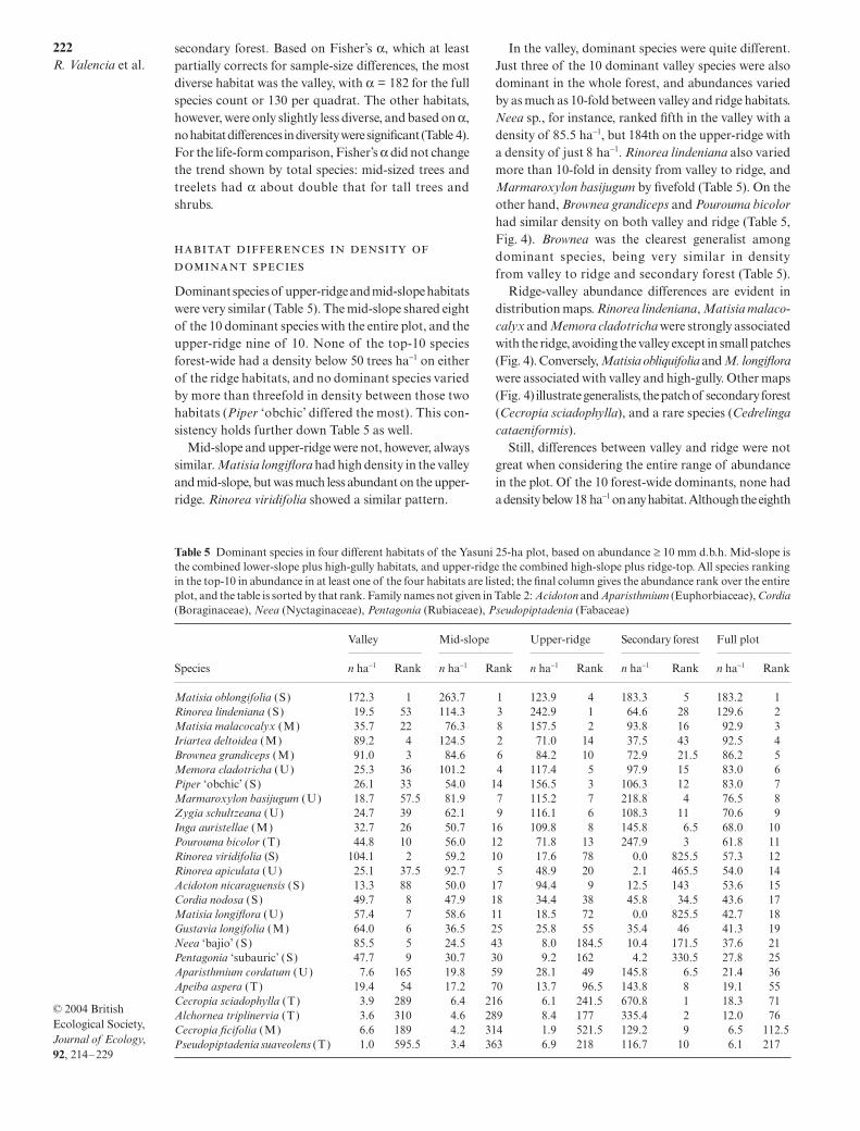
The valley had lower basal area and lower tree densitythan the slope and ridge habitats (Table 4). Both basal areaand stem density were intermediate on the mid-slope, andhighest on the upper-ridge. Higher stem density on theupper-ridge held for all life-forms, shrubs to tall trees,but there was a habitat difference in the way basal areawas distributed among life-forms: the upper-ridge hadmore tall trees, whereas basal area in the valley was mostlyin medium-sized trees. Thus, most of the increase inbasal area from valley to ridge-top was in tall trees.

The secondary forest contrasted sharply in structurefrom all other habitats. Stem density was very high,especially in tall trees, and basal area was highly con-centrated in tall tree species. This concentration, though,was due entirely to a single species, Cecropia sciado-phylla, which made up half the basal area in this smallpatch (17.5 of 35 m2 ha−1).

All habitats had high species number, over 985 in allexcept the secondary forest (which was less than halfa hectare). Thus, no habitat, apart from secondaryforest, had less than 89% of the forest’s total diversity.Species richness was especially high in understoreytreelets and mid-sized trees (Table 4).

Many differences in diversity are due to differencesin sample size, as suggested by the low species count in

Table 4 Density, basal area and diversity of different habitats within the Yasuni 25-ha plot. Mid-slope is the combined lower-slope plus high-gully habitats, and the upper-ridge is combined high-slope plus ridge-top. For abundance and basal area, the sumof four life-form categories is always less than the total for all life-forms, because the latter includes unidentified individuals.Species count or Fisher’s α over an entire region refers to all 20 × 20 m quadrats pooled; species count or Fisher’s α per quadratis the mean (or standard deviation, SD) per 20 × 20 m quadrat

Habitat Area (ha)

Valley 7.88

Mid-slope 7.68

Upper-ridge 8.96

Secondary 0.48

Total 25

Density (individuals ha−1)

All species 5150.0 5963.8 6878.1 9031.3 6093.9Tall trees 599.7 658.5 748.0 2629.2 709.9Mid-sized trees 1291.2 1417.6 1629.2 1937.5 1463.6Treelets 1751.1 2226.4 2687.3 2639.6 2249.7Shrubs 1275.1 1391.3 1507.0 1220.8 1392.9

Basal area (ha−1)

All species 27.06 35.10 37.30 35.00 33.35Tall trees 8.87 13.00 15.70 22.81 12.86Mid-sized trees 9.97 12.61 11.79 5.33 11.35Treelets 5.77 6.68 7.08 4.39 6.50Shrubs 1.34 1.28 1.15 0.92 1.24

Species number (entire region)

All life-forms 986 1001 990 546 1104Tall trees 142 143 139 82 160Mid-sized trees 295 307 305 156 333Treelets 363 370 372 215 403Shrubs 186 180 174 93 207

Species/quadrat (all life-forms)

Mean/20 × 20 118.6 129.7 138.7 147.3 129.8SD/20 × 20 19.3 22.0 17.4 20.7 21.3

Fisher’s α (all life-forms)

Entire region 182.2 180.7 167.5 165.2 161.1Mean/20 × 20 130.0 128.7 122.9 107.7 126.6SD/20 × 20 29.5 29.8 26.7 36.6 29.0

Fig. 3 Sørensen similarity index (without cover) betweenpairs of 20 × 20 m quadrats vs. distance between the quadrats.Each point is the average of Sørensen indices within a20-m distance interval (e.g. 40–60 m), for a single habitatcomparison. That is, the ridge-ridge line includes only quadratpairs where both members of the pair were on the ridge-tophabitat, while valley-ridge means one quadrat of the pair wasin the valley, the second on the ridge-top. ‘Lower’ means thelow-slope habitat, and ‘gully’ means the high-gully habitat.



secondary forest. Based on Fisher’s α, which at leastpartially corrects for sample-size differences, the mostdiverse habitat was the valley, with α = 182 for the fullspecies count or 130 per quadrat. The other habitats,however, were only slightly less diverse, and based on α,no habitat differences in diversity were significant (Table 4).For the life-form comparison, Fisher’s α did not changethe trend shown by total species: mid-sized trees andtreelets had α about double that for tall trees andshrubs.

Dominant species of upper-ridge and mid-slope habitatswere very similar (Table 5). The mid-slope shared eightof the 10 dominant species with the entire plot, and theupper-ridge nine of 10. None of the top-10 speciesforest-wide had a density below 50 trees ha−1 on eitherof the ridge habitats, and no dominant species variedby more than threefold in density between those twohabitats (Piper ‘obchic’ differed the most). This con-sistency holds further down Table 5 as well.

Mid-slope and upper-ridge were not, however, alwayssimilar. Matisia longiflora had high density in the valleyand mid-slope, but was much less abundant on the upper-ridge. Rinorea viridifolia showed a similar pattern.

In the valley, dominant species were quite different.Just three of the 10 dominant valley species were alsodominant in the whole forest, and abundances variedby as much as 10-fold between valley and ridge habitats.Neea sp., for instance, ranked fifth in the valley with adensity of 85.5 ha−1, but 184th on the upper-ridge witha density of just 8 ha−1. Rinorea lindeniana also variedmore than 10-fold in density from valley to ridge, andMarmaroxylon basijugum by fivefold (Table 5). On theother hand, Brownea grandiceps and Pourouma bicolorhad similar density on both valley and ridge (Table 5,Fig. 4). Brownea was the clearest generalist amongdominant species, being very similar in densityfrom valley to ridge and secondary forest (Table 5).

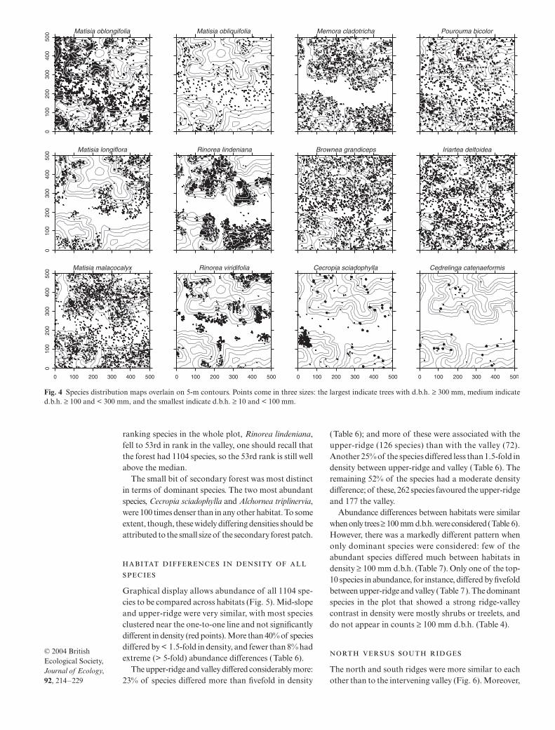
Ridge-valley abundance differences are evident indistribution maps. Rinorea lindeniana, Matisia malaco-calyx and Memora cladotricha were strongly associatedwith the ridge, avoiding the valley except in small patches(Fig. 4). Conversely, Matisia obliquifolia and M. longiflorawere associated with valley and high-gully. Other maps(Fig. 4) illustrate generalists, the patch of secondary forest(Cecropia sciadophylla), and a rare species (Cedrelingacataeniformis).

Still, differences between valley and ridge were notgreat when considering the entire range of abundancein the plot. Of the 10 forest-wide dominants, none hada density below 18 ha−1 on any habitat. Although the eighth

Table 5 Dominant species in four different habitats of the Yasuni 25-ha plot, based on abundance ≥ 10 mm d.b.h. Mid-slope isthe combined lower-slope plus high-gully habitats, and upper-ridge the combined high-slope plus ridge-top. All species rankingin the top-10 in abundance in at least one of the four habitats are listed; the final column gives the abundance rank over the entireplot, and the table is sorted by that rank. Family names not given in Table 2: Acidoton and Aparisthmium (Euphorbiaceae), Cordia(Boraginaceae), Neea (Nyctaginaceae), Pentagonia (Rubiaceae), Pseudopiptadenia (Fabaceae)

Species

Valley Mid-slope Upper-ridge Secondary forest Full plot

n ha−1 Rank n ha−1 Rank n ha−1 Rank n ha−1 Rank n ha−1 Rank

Matisia oblongifolia (S) 172.3 1 263.7 1 123.9 4 183.3 5 183.2 1Rinorea lindeniana (S) 19.5 53 114.3 3 242.9 1 64.6 28 129.6 2Matisia malacocalyx (M) 35.7 22 76.3 8 157.5 2 93.8 16 92.9 3Iriartea deltoidea (M) 89.2 4 124.5 2 71.0 14 37.5 43 92.5 4Brownea grandiceps (M) 91.0 3 84.6 6 84.2 10 72.9 21.5 86.2 5Memora cladotricha (U) 25.3 36 101.2 4 117.4 5 97.9 15 83.0 6Piper ‘obchic’ (S) 26.1 33 54.0 14 156.5 3 106.3 12 83.0 7Marmaroxylon basijugum (U) 18.7 57.5 81.9 7 115.2 7 218.8 4 76.5 8Zygia schultzeana (U) 24.7 39 62.1 9 116.1 6 108.3 11 70.6 9Inga auristellae (M) 32.7 26 50.7 16 109.8 8 145.8 6.5 68.0 10Pourouma bicolor (T) 44.8 10 56.0 12 71.8 13 247.9 3 61.8 11Rinorea viridifolia (S) 104.1 2 59.2 10 17.6 78 0.0 825.5 57.3 12Rinorea apiculata (U) 25.1 37.5 92.7 5 48.9 20 2.1 465.5 54.0 14Acidoton nicaraguensis (S) 13.3 88 50.0 17 94.4 9 12.5 143 53.6 15Cordia nodosa (S) 49.7 8 47.9 18 34.4 38 45.8 34.5 43.6 17Matisia longiflora (U) 57.4 7 58.6 11 18.5 72 0.0 825.5 42.7 18Gustavia longifolia (M) 64.0 6 36.5 25 25.8 55 35.4 46 41.3 19Neea ‘bajio’ (S) 85.5 5 24.5 43 8.0 184.5 10.4 171.5 37.6 21Pentagonia ‘subauric’ (S) 47.7 9 30.7 30 9.2 162 4.2 330.5 27.8 25Aparisthmium cordatum (U) 7.6 165 19.8 59 28.1 49 145.8 6.5 21.4 36Apeiba aspera (T) 19.4 54 17.2 70 13.7 96.5 143.8 8 19.1 55Cecropia sciadophylla (T) 3.9 289 6.4 216 6.1 241.5 670.8 1 18.3 71Alchornea triplinervia (T) 3.6 310 4.6 289 8.4 177 335.4 2 12.0 76Cecropia ficifolia (M) 6.6 189 4.2 314 1.9 521.5 129.2 9 6.5 112.5Pseudopiptadenia suaveolens (T) 1.0 595.5 3.4 363 6.9 218 116.7 10 6.1 217



ranking species in the whole plot, Rinorea lindeniana,fell to 53rd in rank in the valley, one should recall thatthe forest had 1104 species, so the 53rd rank is still wellabove the median.

The small bit of secondary forest was most distinctin terms of dominant species. The two most abundantspecies, Cecropia sciadophylla and Alchornea triplinervia,were 100 times denser than in any other habitat. To someextent, though, these widely differing densities should beattributed to the small size of the secondary forest patch.

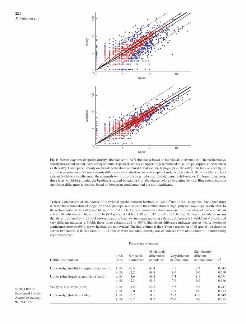
Graphical display allows abundance of all 1104 spe-cies to be compared across habitats (Fig. 5). Mid-slopeand upper-ridge were very similar, with most speciesclustered near the one-to-one line and not significantlydifferent in density (red points). More than 40% of speciesdiffered by < 1.5-fold in density, and fewer than 8% hadextreme (> 5-fold) abundance differences (Table 6).

The upper-ridge and valley differed considerably more:23% of species differed more than fivefold in density

(Table 6); and more of these were associated with theupper-ridge (126 species) than with the valley (72).Another 25% of the species differed less than 1.5-fold indensity between upper-ridge and valley (Table 6). Theremaining 52% of the species had a moderate densitydifference; of these, 262 species favoured the upper-ridgeand 177 the valley.

Abundance differences between habitats were similarwhen only trees ≥ 100 mm d.b.h. were considered (Table 6).However, there was a markedly different pattern whenonly dominant species were considered: few of theabundant species differed much between habitats indensity ≥ 100 mm d.b.h. (Table 7). Only one of the top-10 species in abundance, for instance, differed by fivefoldbetween upper-ridge and valley (Table 7). The dominantspecies in the plot that showed a strong ridge-valleycontrast in density were mostly shrubs or treelets, anddo not appear in counts ≥ 100 mm d.b.h. (Table 4).

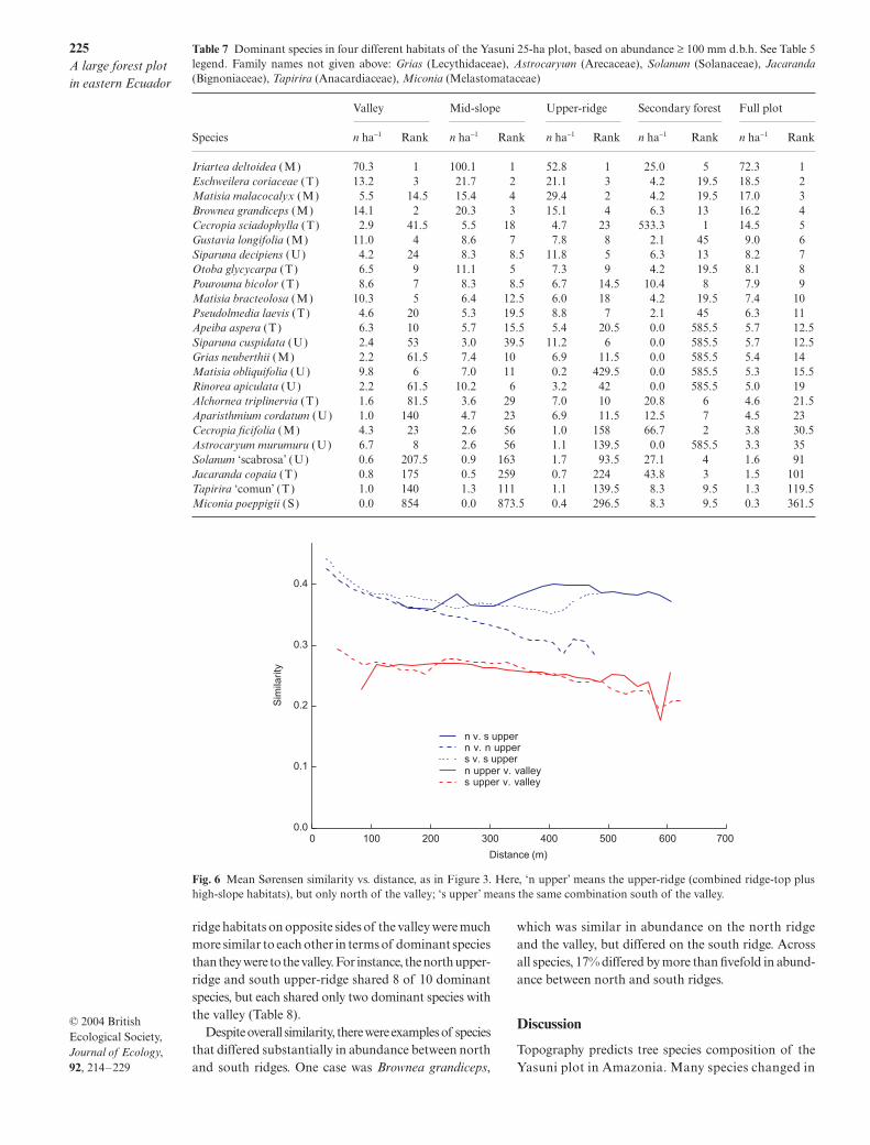
The north and south ridges were more similar to eachother than to the intervening valley (Fig. 6). Moreover,

Fig. 4 Species distribution maps overlain on 5-m contours. Points come in three sizes: the largest indicate trees with d.b.h. ≥ 300 mm, medium indicated.b.h. ≥ 100 and < 300 mm, and the smallest indicate d.b.h. ≥ 10 and < 100 mm.



Fig. 5 Scatter diagrams of species density (abundance + 1 ha−1; abundance based on individuals ≥ 10 mm d.b.h.) in one habitat vs.density in a second habitat. Axes are logarithmic. Top panel, density on upper-ridge (combined ridge-top plus upper-slope habitats)vs. the valley. Lower panel, density on mid-slope habitat (combined low-slope plus high-gully) vs. the valley. The lines on each figureare not regression lines, but mark density differences: the central line indicates equal density in each habitat; the outer (dashed) linesindicate 5-fold density differences; the intermediate (thin solid) lines indicate 1.5-fold density differences. On logarithmic axes,these lines would be straight: the bending is caused by adding 1 to abundance before calculating density. Blue points indicatesignificant differences in density, based on bootstrap confidence; red are non-significant.

Table 6 Comparison of abundance of individual species between habitats, in two different d.b.h. categories. The upper-ridgerefers to the combination of ridge-top and high-slope; mid-slope to the combination of high-gully and low-slope; north refers tothe section north of the valley, and likewise for south. The four columns under abundance give the percentage of species that hadat least 10 individuals in the entire 25 ha (854 species for d.b.h. ≥ 10 mm; 317 for d.b.h. ≥ 100 mm). Similar in abundance meansthat density differed by < 1.5-fold between a pair of habitats; moderate indicates a density difference ≥ 1.5-fold but < 5-fold; andvery different indicates ≥ 5-fold; those three columns add to 100%. Significant difference indicates species whose bootstrapconfidence intervals (95%) in two habitats did not overlap. The final column is the r 2 from a regression of all species’ log-densitiesacross two habitats; in this case, all 1104 species were included; density was calculated from abundance + 1 before beinglog-transformed

Habitat comparisond.b.h. (mm)

Percentage of species

r 2Similar in abundance

Moderately different in abundance

Very different in abundance

Significantly different in abundance

Upper-ridge (north) vs. upper-ridge (south) ≥ 10 40.5 42.4 17.1 12.3 0.743≥ 100 32.2 49.8 18.0 0.0 0.650

Upper-ridge (total) vs. mid-slope (total) ≥ 10 43.6 49.2 7.3 18.1 0.791≥ 100 42.3 49.8 7.9 0.0 0.686

Valley vs. mid-slope (total) ≥ 10 39.5 50.8 9.7 19.8 0.747≥ 100 36.0 51.7 12.3 0.0 0.612

Upper-ridge (total) vs. valley ≥ 10 25.2 51.5 23.3 37.6 0.549≥ 100 25.2 51.7 23.0 0.0 0.513



ridge habitats on opposite sides of the valley were muchmore similar to each other in terms of dominant speciesthan they were to the valley. For instance, the north upper-ridge and south upper-ridge shared 8 of 10 dominantspecies, but each shared only two dominant species withthe valley (Table 8).

Despite overall similarity, there were examples of speciesthat differed substantially in abundance between northand south ridges. One case was Brownea grandiceps,

which was similar in abundance on the north ridgeand the valley, but differed on the south ridge. Acrossall species, 17% differed by more than fivefold in abund-ance between north and south ridges.

Discussion

Topography predicts tree species composition of theYasuni plot in Amazonia. Many species changed in

Table 7 Dominant species in four different habitats of the Yasuni 25-ha plot, based on abundance ≥ 100 mm d.b.h. See Table 5legend. Family names not given above: Grias (Lecythidaceae), Astrocaryum (Arecaceae), Solanum (Solanaceae), Jacaranda(Bignoniaceae), Tapirira (Anacardiaceae), Miconia (Melastomataceae)

Species

Valley Mid-slope Upper-ridge Secondary forest Full plot

n ha−1 Rank n ha−1 Rank n ha−1 Rank n ha−1 Rank n ha−1 Rank

Iriartea deltoidea (M) 70.3 1 100.1 1 52.8 1 25.0 5 72.3 1Eschweilera coriaceae (T) 13.2 3 21.7 2 21.1 3 4.2 19.5 18.5 2Matisia malacocalyx (M) 5.5 14.5 15.4 4 29.4 2 4.2 19.5 17.0 3Brownea grandiceps (M) 14.1 2 20.3 3 15.1 4 6.3 13 16.2 4Cecropia sciadophylla (T) 2.9 41.5 5.5 18 4.7 23 533.3 1 14.5 5Gustavia longifolia (M) 11.0 4 8.6 7 7.8 8 2.1 45 9.0 6Siparuna decipiens (U) 4.2 24 8.3 8.5 11.8 5 6.3 13 8.2 7Otoba glycycarpa (T) 6.5 9 11.1 5 7.3 9 4.2 19.5 8.1 8Pourouma bicolor (T) 8.6 7 8.3 8.5 6.7 14.5 10.4 8 7.9 9Matisia bracteolosa (M) 10.3 5 6.4 12.5 6.0 18 4.2 19.5 7.4 10Pseudolmedia laevis (T) 4.6 20 5.3 19.5 8.8 7 2.1 45 6.3 11Apeiba aspera (T) 6.3 10 5.7 15.5 5.4 20.5 0.0 585.5 5.7 12.5Siparuna cuspidata (U) 2.4 53 3.0 39.5 11.2 6 0.0 585.5 5.7 12.5Grias neuberthii (M) 2.2 61.5 7.4 10 6.9 11.5 0.0 585.5 5.4 14Matisia obliquifolia (U) 9.8 6 7.0 11 0.2 429.5 0.0 585.5 5.3 15.5Rinorea apiculata (U) 2.2 61.5 10.2 6 3.2 42 0.0 585.5 5.0 19Alchornea triplinervia (T) 1.6 81.5 3.6 29 7.0 10 20.8 6 4.6 21.5Aparisthmium cordatum (U) 1.0 140 4.7 23 6.9 11.5 12.5 7 4.5 23Cecropia ficifolia (M) 4.3 23 2.6 56 1.0 158 66.7 2 3.8 30.5Astrocaryum murumuru (U) 6.7 8 2.6 56 1.1 139.5 0.0 585.5 3.3 35Solanum ‘scabrosa’ (U) 0.6 207.5 0.9 163 1.7 93.5 27.1 4 1.6 91Jacaranda copaia (T) 0.8 175 0.5 259 0.7 224 43.8 3 1.5 101Tapirira ‘comun’ (T) 1.0 140 1.3 111 1.1 139.5 8.3 9.5 1.3 119.5Miconia poeppigii (S) 0.0 854 0.0 873.5 0.4 296.5 8.3 9.5 0.3 361.5

Fig. 6 Mean Sørensen similarity vs. distance, as in Figure 3. Here, ‘n upper’ means the upper-ridge (combined ridge-top plushigh-slope habitats), but only north of the valley; ‘s upper’ means the same combination south of the valley.



abundance along the ridge-valley catena, and there areimpressive pairs of species in the genera Rinorea andMatisia that partitioned the topographic niche veryprecisely (see Fig. 4). The fact that two separate ridgeswere conspicuously more similar to each other than tothe intervening valley confirms that the abundancedifferences were caused by soil and not by unrelatedpatchiness in species distributions. The ridge-valleydifference is not surprising: catenas are fundamentalin plant ecology in general and in the tropics in par-ticular (Gartlan et al. 1986; Weaver 1991; Tuomisto &Ruokolainen 1994; Tuomisto et al. 1995; Clark et al. 1999;Svenning 1999; Webb 2000). Corresponding with speciesturnover, forest structure also changed from valley toridge; the valley had smaller-stature species, fewerindividuals, less basal area, and a lower canopy.

We initially tested five topographic sections, but theevidence did not support this many. Instead, we foundessentially three topographic habitats (two ridge, plusthe valley). We quantified the abundance differencesacross these habitats, and classified species relative tothe catena using the contrast between upper-ridge andvalley. A quarter of the species differed less than1.5-fold in density from ridge-top to valley, and thusappear to be generalists. At the opposite extreme, 15%of the species were much denser on the upper-ridge and8% were much denser in the valley; it seems reasonableto conclude that most of these species are specialiststo topographic differences. The remaining half of thespecies were more difficult to classify, as they favouredone habitat (> 1.5-fold density difference), but stilloccurred at both (< 5-fold density difference).

We conclude that at least a quarter of the species aregeneralists with respect to the catena, another quarterare specialists to ridge or valley, and a very small numberare narrowly restricted to gullies or lower ridge. Thebulk of the species fall in a grey area and cannot be clas-sified on present data; they might be generalists whosedensity varies due to dispersal limitation or other factors,or they might be specialists with some individualsoccurring in poor habitat as a sink population. More

observations or experiments would be required toestablish topographic preferences of these species. Thisillustrates limitations of estimating habitat requirementsfrom a single census, that is, of judging process frompattern. In defence of pattern analysis, though, thereare so many sites and so many species in Amazonia thatpattern analyses are all we are ever likely to have for most.

Among the dominant species, the clearest habitatspecialists were small-stature treelets or shrubs. Duqueet al. (2002) found the same pattern in the ColombianAmazon. Many other tree surveys in Amazonia arebased on trees ≥ 100 mm d.b.h., and these would miss thesmall-statured specialists at Yasuni.

We also found a distance effect on tree species com-position, even within areas of uniform topography,suggesting patchiness in distributions not related totopography. A number of species had large abund-ance differences between north and south ridge-tops,also suggesting patchiness not related to topography.Svenning (1999, 2001a) suggested that decay of similaritywithin palm assemblages is caused at least partly bylimited seed dispersal. Condit et al. (2002) tested forthe importance of dispersal limitation using a theorydescribing how dispersal should influence similarity;they found that dispersal might play some role, but thatother factors are involved in the rapid decay of simi-larity at short distances. Interestingly, habitat effecton tree species composition at Yasuni, as measured bySørensen similarity, was on a par with the distanceeffect: both led to a moderate reduction in similarity.To make predictions about forest composition at thisscale, it is equally important to know what is nearby asit is to identify the topographic habitat.

It is possible that fine-grained variation in soil withintopographic habitats provided further habitat parti-tioning, and we have begun detailed studies of soilswithin the plot that can test this hypothesis. Tuomistoet al. (2003a), however, found evidence for variationin soil chemistry and texture only at wider scales atYasuni. They concluded that there are two main soiltypes, with corresponding variation in vegetation, in

Table 8 A comparison of dominant species on the north and south ridges. The upper-ridge refers to the combination of ridge-topand high-slope. All species that had a rank in the top-10 on either north or south sections are included

Species

North upper-ridge South upper-ridge Valley

Abundance Rank Abundance Rank Abundance Rank

Rinorea lindeniana 246.0 1 233.8 1 19.5 53Matisia malacocalyx 166.1 2 140.3 4 35.7 22Matisia oblongifolia 132.8 3 104.3 8 172.3 1Piper ‘obchic’ 132.1 4 184.7 2 26.1 33Memora cladotricha 122.8 5 104.8 7 25.3 36Acidoton nicaraguensis 117.6 6 65.6 15 13.3 88Zygia schultzeana 112.3 7 116.5 6 24.7 39Marmaroxylon basijugum 104.0 8 125.0 5 18.7 57.5Brownea grandiceps 100.2 9 59.1 17 91.0 3Inga auristellae 87.0 10 143.2 3 32.7 26Guarea fistulosa 74.3 13 91.8 9 20.1 51Pourouma bicolor 60.0 16 86.4 10 44.8 10



the area of their study; the 25-ha plot fell within one.We thus doubt that we will find much partitioning dueto soil variation within the 25 ha, beyond the topo-graphic patterns described here. Maximum tree height(which we refer to as life-form) provides another deter-ministic avenue by which species can coexist (Kohyama1993, 1996), but we found hundreds of species with similarlife-form coexisting in close proximity. It appears unlikelythat this is a major diversifying force, but more preciseevaluation of growth, reproduction and height are needed(Kohyama et al. 2003). Variation in light within the forestprovides colonization-based niches (Grubb 1986; Pacala& Rees 1998; Rees et al. 2001), and the small patch ofsecondary forest that fell inside the plot demonstratesthat species composition in high light differs conspic-uously from the rest of the forest. Svenning (2000) alsodemonstrated species associations with smaller gapsin undisturbed forest at Yasuni. We have not yet eval-uated light-based niches across the entire community.

We found high tree species diversity for all life-formsin all habitats. More than 100 species occurred in indi-vidual 20 × 20 m quadrats, and 370 species of under-storey treelets coexisted on a topographically uniformridge-top c. 200 m across. We acknowledge that ourcategorization of species into growth forms is prelimin-ary, and that some of those 370 species may exist onlyas sink populations; however, it seems clear that a verylarge number of very similar species occupy homo-geneous topographic and soil conditions. We concludethat topography does not provide a niche axis that isfinely partitioned by hundreds of species; rather, it pro-vides three niches. Moreover, many of the thousand-plus species in the forest are generalists with respect totopography. Thus, although topography explains someof the tree α-diversity, its contribution is minor. Harmset al. (2001), Svenning (2001b) and Wright (2002) drewsimilar conclusions from tree distribution studies.

Abundance fluctuations of generalists and patchi-ness within topographic habitats could be due largelyto chance or to unpredictable events. Given so manygeneralist species, a description of forest dynamicscannot ignore randomness (Van der Maarel & Sykes 1993;Dewdney 1997; Bell 2001; Hubbell 2001) nor dispersallimitation (Hurtt & Pacala 1995; Silman 1996; Hubbellet al. 1999). On the other hand, there are species special-ized to topographic habitats, and a full understandingof the forest cannot ignore patchiness in soil resources(Terborgh et al. 1996; Svenning 2001a; Condit et al.2002).

Acknowledgements

We are indebted to the field workers who have mapped,tagged and identified trees since 1995. We thankespecially those who worked more than 2 years for theproject: A. Loor, J. Zambrano, M. Zambrano, G. Grefa,E. Guevara and L. Vélez. We also thank M. Bass andH. Mogollón for help in identifying species, S. Laofor data management and calculations, N. Pitman

for suggestions on data analysis and for assistance inthe field, Flemming Nørgaard for creating Figure 1,and H. Navarrete, N. Pitman and S. León for commentson the manuscript. The Mellon Foundation, the TupperFamily Foundation and the Smithsonian TropicalResearch Institute provided grants for the fieldworkand the Biological and Cultural Diversity Project of thePluvial Andean Forests (DIVA) provided financialsupport to the first author. National Science Founda-tion (US) grant DEB-0090311 supported fieldwork inthe plot, and grant DEB-9806828 supported a dataanalysis workshop for several similar plots; we wouldlike to thank the participants of this workshop for muchadvice on the ideas. This is a publication of the Center forTropical Forest Science of the Smithsonian Institution.

References

Barbour, M.G., Burk, J.H. & Pitts, W.D. (1987) TerrestrialPlant Ecology. Benjamin/Cummings, Menlo Park, California.

Basnet, K. (1992) Effect of topography on the pattern of treesin Tabonuco (Dacryodes excelsa) dominated rain forest ofPuerto Rico. Biotropica, 24, 31–42.

Bell, G. (2001) Neutral macroecology. Science, 293, 2413–2418.

Berg, C.C., Akkermans, R.W. & van Heusden, E.C. (1990)Cecropiaceae: Coussapoa and Pourouma, with an introduc-tion to the family. Flora Neotropica, 51, 1–208.

Borcard, D., Legendre, P. & Drapeau, P. (1992) Partialling outthe spatial component of ecological variation. Ecology, 73,1045–1055.

Brako, L. & Zarucchi, J.L. (1993) Catalog of the flowering plantsand Gymnosperms of Peru. Monographs in SystematicBotany from the Missouri Botanical Garden, 45, 1–1286.

Clark, D.B., Palmer, M.W. & Clark, D.A. (1999) Edaphicfactors and the landscape-scale distributions of tropicalrain forest trees. Ecology, 80, 2662–2675.

Condit, R. (1998) Tropical Forest Census Plots. Methods andResults from Barro Colorado Island, Panama and a Compari-son with Other Plots. Springer-Verlag, Berlin.

Condit, R., Ashton, P.S., Baker, P., Bunyavejchewin, S.,Gunatilleke, S., Gunatilleke, N., Hubbell, S.P., Foster, R.B.,Hua Seng, L., Itoh, A., LaFrankie, J.V., Losos, E., Manokaran,N., Sukumar, R. & Yamakura, T. (2000) Spatial patterns inthe distribution of tropical tree species. Science, 288, 1414–1418.

Condit, R., Foster, R.B., Hubbell, S.P., Sukumar, R., Leigh,E.G., Manokaran, N. et al. (1998) Assessing forest diversityon small plots: calibration using species-individual curvesfrom 50 ha plots. Forest Biodiversity: Research, Monitoring,and Modeling (eds F. Dallmeier & J.A. Comiskey), pp. 247–268. UNESCO, Paris.

Condit, R., Hubbell, S.P., LaFrankie, J.V., Sukumar, R.,Manokaran, N., Foster, R.B. et al. (1996) Species-area andspecies-individual relationships for tropical trees: a compar-ison of three 50 ha plots. Journal of Ecology, 84, 549–562.

Condit, R., Pitman, N., Leigh, E.G., Chave, J., Terborgh, J.,Foster, R.B. et al. (2002) Beta-diversity in tropical foresttrees. Science, 295, 666–669.

Croat, T.R. (1978) Flora of Barro Colorado Island. StanfordUniversity Press, Stanford, California.

Dewdney, A.K. (1997) A dynamical model of abundances innatural communities. Coenoses, 12, 67–76.

Duque, A., Sánchez, M., Cavelier, J. & Duivenvoorden, J.(2002) Different floristic patterns of woody understoreyand canopy plants in Colombian Amazonia. Journal ofTropical Ecology, 18, 499–525.



Gartlan, J.S., Newbery, D.M., Thomas, D.W. & Waterman,P.G. (1986) The influence of topography and soil phospho-rus on the vegetation of Korup Forest Reserve Cameroon.Vegetatio, 65, 131–148.

Gentry, A.H. (1982) Patterns of neotropical plant speciesdiversity. Evolutionary Biology, 15, 1–84.

Gentry, A.H. (1992) Tropical forest biodiversity: distribu-tional patterns and their conservational significance. Oikos,63, 19–28.

Grubb, P.J. (1986) Problems posed by sparse and patchilydistributed species in species-rich plant communities.Community Ecology (eds J. Diamond & T.J. Case), pp. 207–225. Harper & Row, New York.

Harms, K.E., Condit, R., Hubbell, S.P. & Foster, R.B. (2001)Habitat associations of trees and shrubs in a neotropicalforest. Journal of Ecology, 89, 947–959.

Hubbell, S.P. (2001) The Unified Neutral Theory of Biodiversityand Biogeography. Princeton University Press, Princeton,New Jersey.

Hubbell, S.P., Ahumada, J.A., Condit, R. & Foster, R.B.(2001) Local neighborhood effects on long-term survival ofindividual trees in a neotropical forest. Ecological Research,16, 859–875.

Hubbell, S.P. & Foster, R.B. (1986) Biology, chance, and historyand the structure of tropical rain forest tree communities.Community ecology (eds J. Diamond & T.J. Case), pp. 314–329. Harper and Row, New York.

Hubbell, S.P., Foster, R.B., O’Brien, S.T., Harms, K.E.,Condit, R., Wechsler, B., Wright, S.J. & Loo de Lao, S.(1999) Light gap disturbances, recruitment limitation, andtree diversity in a neotropical forest. Science, 283, 554–557.

Hurtt, G.C. & Pacala, S.W. (1995) The consequences ofrecruitment limitation: reconciling chance, history and com-petitive differences between plants. Journal of TheoreticalBiology, 176, 1–12.

Kahn, F. (1987) The distribution of palms as a function oflocal topography in Amazonian terra-firme forests. Experi-entia, 43, 251–259.

Kohyama, T. (1993) Size-structured tree populations in gap-dynamic forest – the forest architecture hypothesis for thestable coexistence of species. Journal of Ecology, 81, 131–143.

Kohyama, T. (1996) The role of architecture in enhancingplant species diversity. Biodiversity: an Ecological Perspective(eds T. Abe, S.A. Levin & M. Higashi), pp. 21–33. Springer-Verlag, Berlin.

Kohyama, T., Suzuki, E., Partomihardjo, T., Yamada, T. &Kubo, T. (2003) Tree species differentiation in growth,recruitment and allometry in relation to maximum heightin a Bornean mixed dipterocarp forest. Journal of Ecology,91, 797–806.

Korning, J., Thomsen, K., Dalsgaard, K. & Nornberg, P.(1994) Characters of three udults and their relevance to thecomposition and structure of virgin rain forest of amazo-nian Ecuador. Geoderma, 63, 145–164.

Legendre, P. (1993) Spatial autocorrelation: trouble or newparadigm? Ecology, 74, 1659–1673.

Lieberman, M., Lieberman, D., Hartshorn, G.S. & Peralta, R.(1985) Small-scale altitudinal variation in lowland tropicalforest vegetation. Journal of Ecology, 73, 505–516.

Malo, G. & Arguello, C. (1984) Proyecto Oriente, Mapa deCompilación Geológica de la Provincia Del Napo. Departa-mento de Geología, Instituto Ecuatoriano de Minería,Ministerio de Energía y Minas, Quito.

Netherly, P. (1997) Loma y ribera: patrones de asentamientoprehistórico en la Amazonía ecuatoriana. Fronteras de laCiencia, 1, 33–54.

Pacala, S.W. & Rees, M. (1998) Models suggesting fieldexperiments to test two hypotheses explaining successionaldiversity. American Naturilist, 152, 729–737.

Pennington, T.D. (1990) Sapotaceae. Flora Neotropica, 52, 1–770.

Pennington, T.D., Terence, D. & Styles, B.T. (1981)Meliaceae. Flora Neotropica, 28, 1–470.

Phillips, O.L., Hall, P., Gentry, A.H., Check, S.S.A. &Vásquez, R. (1994) Dynamics and species richness of tropicalrain forests. Proceedings of the National Academy of Sciences,91, 2805–2809.

Phillips, O.L., Vargas, P.N., Monteagudo, A.L., Cruz, A.P.,Zans, M.-E.C., Sánchez, W.G. et al. (2003) Habitat asso-ciation among Amazonian tree species: a landscape-scaleapproach. Journal of Ecology, 91, 757–775.

Pitman, N.C.A., Terborgh, J., Silman, M.R. & Núñez, V.P.(1999) Tree species distributions in an upper Amazonianforest. Ecology, 80, 2651–2661.

Pitman, N.C.A., Terborgh, J., Silman, M.R., Núñez, V.P.,Neill, D.A., Palacios, W.A. et al. (2001) Dominance anddistribution of tree species in upper Amazonian terra firmeforets. Ecology, 82, 2101–2117.

Prance, G.T. (1979) Chrysobalanaceae. Flora of Ecuador, 10,1–24.

Rees, M., Condit, R., Crawley, M., Pacala, S. & Tilman, D.(2001) Long-term studies of vegetation dynamics. Science,293, 650–655.

Rohwer, J.G. (1993) Lauraceae. Nectandra. Flora Neotropica,60, 1–332.

Romero-Saltos, H., Valencia, R. & Macía, M.J. (2001)Patrones de diversidad, distribución y rareza de plantasleñosas en el Parque Nacional Yasuní y la Reserva ÉtnicaHuaorani, Amazonía ecuatoriana. Evaluación de RecursosVegetales No Maderables En la Amazonía Noroccidental(eds J.F. Duivenvoorden, H. Balslev, J. Cavelier, C. Grandez,H. Tuomisto & R. Valencia), pp. 131–162. IBED, Universiteitvan Amsterdam, Amsterdam.

Romoleroux, K., Foster, R., Valencia, R., Condit, R., Balslev,H. & Losos, E. (1997) Especies leñosas (dap ≥1 cm) en-contradas en dos hectáreas de un bosque de la Amazoníaecuatoriana. Estudios Sobre Diversidad Y Ecología dePlantas (eds R. Valencia & H. Balslev), pp. 189–215. PontificiaUniversidad Católica del Ecuador, Quito, Ecuador.

Rosenzweig, M.L. (1995) Species Diversity in Space and Time.Cambridge University Press, Cambridge.

Ruokolainen, K., Linna, A. & Tuomisto, H. (1997) Use ofMelastomataceae and pteridophytes for revealing phyto-geographical patterns in Amazonian rain forests. Journal ofTropical Ecology, 13, 243–256.

Sierra, R., Cerón, C., Palacios, W. & Valencia, R. (1999) Elmapa de vegetación del Ecuador continental. PropuestaPreliminar de un Sistema de Clasificación de VegetaciónPara El Ecuador Continental (ed. R. Sierra), pp. 120–139.Proyecto INEFAN/GEF-BIRF y EcoCiencia, Quito, Ecuador.

Silman, M.R. (1996) Regeneration from seed in a Neotropicalrain forest. PhD thesis, Duke University, Durham, NorthCarolina.

Sleumer, H.O. (1980) Flacourtiaceae. Flora Neotropica, 22, 1–499.

Svenning, J.-C. (1999) Microhabitat specialization in a species-rich palm community in Amazonian Ecuador. Journal ofEcology, 87, 55–65.

Svenning, J.-C. (2000) Small canopy gaps influence plantdistributions in the rain forest understory. Biotropica, 32,252–261.

Svenning, J.-C. (2001a) Environmental heterogeneity, recruit-ment limitation and the mesoscale distribution of palms ina tropical montane rain forest (Maquipucuna, Ecuador).Journal of Tropical Ecology, 17, 97–113.

Svenning, J.-C. (2001b) On the role of microenvironmentalheterogeneity in the ecology and diversification of neotropicalrain-forest palms (Arecaceae). Botanical Review, 67, 1–53.

Ter Steege, H., Sabatier, D., Castellanos, H., Van Andel, T.,Duivenvoorden, J., De Oliveira, A.A. et al. (2000) An



analysis of the floristic composition and diversity ofAmazonian forests including those of the Guiana Shield.Journal of Tropical Ecology, 16, 801–828.

Terborgh, J., Foster, R.B. & Núñez, V.P. (1996) Tropical treecommunities: a test of the nonequilibrium hypothesis. Ecology,77, 561–567.

Tuomisto, H., Poulsen, A.D., Ruokolainen, K., Moran, R.C.,Quintana, C., Celi, J. et al. (2003a) Linking floristic patternswith soil heterogeneity and satellite imagery in EcuadorianAmazonia. Ecological Applications, 13, 352–371.

Tuomisto, H. & Ruokolainen, K. (1994) Distribution of Pterid-ophyta and Melastomataceae along an edaphic gradient inan Amazonian rain forest. Journal of Vegetation Science, 5,25–34.

Tuomisto, H., Ruokolainen, K., Aguilar, M. & Sarmiento, A.(2003b) Floristic patterns along a 43-km long transect in anAmazonian rainforest. Journal of Ecology, 91, 743–756.

Tuomisto, H., Ruokolainen, K., Kalliola, R., Linna, A.,Danjoy, W. & Rodríguez, Z. (1995) Dissecting Amazonianbiodiversity. Science, 269, 63–66.

Valencia, R., Balslev, H. & Paz y Miño, G. (1994) High treealpha-diversity in Amazonian Ecuador. Biodiversity andConservation, 3, 21–28.

Van der Maarel, E. & Sykes, M.T. (1993) Small-scale plantspecies turnover in a limestone grassland: the carouselmodel and some comments on the niche concept. Journal ofVegetation Science, 4, 179–188.

Vásquez, R. (1997) Flórula de Las Reservas Biológicas de Iqui-tos, Perú. The Missouri Botanical Garden Press, St Louis.

Weaver, P.L. (1991) Environmental gradients affect forestcomposition in the Luquillo Mountains of Puerto Rico.Interciencia, 16, 142–151.

Webb, C.O. (2000) Habitat associations of trees and seedlingsin a Bornean rain forest. Journal of Ecology, 88, 464–478.

Wright, S.J. (2002) Plant diversity in tropical forests: a reviewof mechanisms of species coexistence. Oecologia, 130, 1–14.

Received 7 May 2003 revision accepted 8 December 2003 Handling Editor: David Burslem

Tree species distributions and local habitat variation in the Amazon: large forest plot in eastern...

Documents

Transcript of Tree species distributions and local habitat variation in the Amazon: large forest plot in eastern...