Thermoelectric Power ve rsus Electrical Conductivity Plot for ...
Upload
yachaytechCategory
view
4download
0
UNIVERSITY OF MIAMI
COMMUNITY AND FUNCTIONAL ECOLOGY OF LIANAS
IN THE YASUNÍ FOREST DYNAMICS PLOT, AMAZONIAN ECUADOR
By
Hugo Geovanny Romero-Saltos
A DISSERTATION
Submitted to the Faculty of the University of Miami
in partial fulfillment of the requirements for the degree of Doctor of Philosophy
Coral Gables, Florida
May 2011

©2011 Hugo Romero-Saltos All Rights Reserved

UNIVERSITY OF MIAMI
A dissertation submitted in partial fulfillment of the requirements for the degree of
Doctor of Philosophy
COMMUNITY AND FUNCTIONAL ECOLOGY OF LIANAS
IN THE YASUNÍ FOREST DYNAMICS PLOT, AMAZONIAN ECUADOR
Hugo G. Romero-Saltos Approved: _________________________ _________________________ Leonel da S.L. Sternberg, Ph.D. Terri A. Scandura, Ph.D. Professor of Biology Dean of the Graduate School _________________________ _________________________ David P. Janos, Ph.D. Donald L. DeAngelis, Ph.D. Professor of Biology Professor of Biology _________________________ Jack B. Fisher, Ph.D. Professor of Biology Fairchild Tropical Botanic Garden

ROMERO-SALTOS, HUGO G. (Ph.D., Biology) Community and Functional Ecology of Lianas (May 2011) in the Yasuní Forest Dynamics Plot, Amazonian Ecuador
Abstract of a dissertation at the University of Miami. Dissertation supervised by Professor Leonel da S.L. Sternberg. No. of pages in text: (216)
I studied the community of lianas in the Yasuní Forest Dynamics Plot (YFDP), in
Amazonian Ecuador. I found that species diversity of lianas in valley habitat was higher
than in ridge habitat, but liana abundance was similar. I also found that community
structure (species composition and their abundances) of lianas in ridge was distinct from
that in valley because of the differential distribution and abundance of certain species
along the topographic gradient. In an attempt to explain this phenomenon
deterministically, I took two approaches: (1) to explore if trait expression of leaf-based
traits, wood specific gravity and stem growth rate was different among species with ridge
habitat association, species with valley habitat association, and generalist species; and (2)
to explore if frequencies of different whole-plant growth strategies in the forest
understory—defined by whether a liana was free-standing or already climbing, by its
climbing mechanism, and by its understory appearance—were different between ridge
and valley. My underlying rationale was that if certain trait expression or understory
growth strategy can be associated to a given species, or group of species, and such
species also drive the community structure difference between ridge and valley, then
ecological insight on the biological deterministic mechanisms driving the difference can
be gained. I end this one-page dissertation abstract right here and purposely leave you,
the reader, perplexed—I invite you to seek answers to the liana distribution conundrum in
the YFDP by perusing this dissertation.

iii
I dedicate this work to my loved children and wife

iv
Acknowledgements
After almost eight years, my Ph.D. program at the University of Miami came to a
good end only because many people and institutions dedicated many hours and much
money on a young Ecuadorian scientist (well, not too young anymore). I remember the
faces of most people who helped me and thank them all, but the problem is that I have
never been good with names! My friends at UM and abroad already know how close they
are to my heart and so does my family, so I will not name them here, except when they
were also scientists whose input for this dissertation was valuable. Often during this
journey, I felt the emotional support from friends and family was more important than
any academic support, although certainly some people generously gave me both.
For the sake of formality, I ought to mention the names of a few key people and
institutions:
• I am deeply grateful to Leo Sternberg, my academic advisor at UM, for his trust
and friendship. I also thank the members of my Dissertation Committee: Dave
Janos, Jack Fisher and Don DeAngelis—for me, they are all excellent scientists
and very special teachers. Needless to say, I am also very grateful to the Biology
faculty at UM from whom I learned the many nuts-and-bolts of being a scientist.
• This work would not have been possible without the help of my long-time
colleague, collaborator and friend: Esteban Gortaire. I also thank my field and lab
assistants, in particular (and in alphabetic order): Carolina Altamirano, Nataly
Charpentier, Luis Espinoza, Ronald Grefa, Carlos Padilla, Laura Salazar, and the
innumerable Waorani indians from Yasuní National Park. Pablo Loaiza, Mariana
Mites, Verónica Sáenz and Diego Torres also helped me with various tasks. I am

v
also grateful to the personnel affiliated to the 50-ha Yasuní Forest Dynamics Plot
project: Renato Valencia, Consuelo Hernández, Álvaro Pérez, and the whole team
of mappers. A special appreciation goes to Carmen Ulloa who hosted me during
my visit to the Missouri Botanical Garden.
• The following people, which include a number of international specialists, helped
me with the plant taxonomy (listed in alphabetical order): Pedro Acevedo-
Rodríguez, Pablo Alvia, Gerardo Aymard, Robyn Burnham, Peter Jörgensen, Ron
Liesner, Lúcia Lohmann, Rosa Ortiz, Álvaro Pérez, Charlotte Taylor, Hyo Won,
and Milton Zambrano. In addition, this dissertation obtained academic input from
the following people (listed in alphabetical order): Robyn Burnham, Robert
Colwell, John Cozza, Patrick and Patricia Ellsworth, Guangyou Hao, Kyle Harms,
Nathan Kraft, Eric Manzané, Nathan Muchhala, Amartya Saha, Stefan Schnitzer,
Renato Valencia, and Xin Wang.
• Funding for this dissertation and other related studies (not presented in this
dissertation) was obtained from the Center for Tropical Forest Science
(Smithsonian Tropical Research Institute), the University of Miami, the
UNESCO’s Man and Biosphere Program, and “The Romero Foundation”. The
Yasuní Research Station and the Herbarium QCA at the Pontificia Universidad
Católica del Ecuador kindly provided logistic support during field seasons.
• Ecuador’s Ministry of Environment supported this scientific study by issuing
research permits 002-IC-FL-PNY-RSO and 005-IC-FA-PNY-RSO.
Thank you all

vi
TABLE OF CONTENTS
Page
LIST OF FIGURES ........................................................................................................... ix
LIST OF TABLES ........................................................................................................... xiv
CHAPTER 1: Introduction .............................................................................................. 1
Trapped between reality and myth: a prolegomenon about Yasuní ....................... 1
Plant ecology in Yasuní .......................................................................................... 4
This dissertation: The lianas in the Yasuní Forest Dynamics Plot ....................... 12
CHAPTER 2: Liana communities in ridge and valley topographic habitats of the
Yasuní Forest Dynamics Plot, Amazonian Ecuador .................................................... 16
SUMMARY .......................................................................................................... 16
BACKGROUND AND HYPOTHESIS ............................................................... 17
METHODS ........................................................................................................... 20
Study area........................................................................................................ 20
Research design .............................................................................................. 23
Data analyses .................................................................................................. 27
RESULTS ............................................................................................................. 36
Diversity and floristics .................................................................................... 36
Abundance (liana density) and frequency ....................................................... 38
Basal area and size distribution....................................................................... 40
Multivariate analyses ...................................................................................... 41
DISCUSSION ....................................................................................................... 43
Across Yasuní comparisons ............................................................................ 43
Ridge vs. valley: a conundrum within YFDP’s terra firme forest .................. 48
Conclusion ...................................................................................................... 56
TABLES ............................................................................................................... 58
FIGURES .............................................................................................................. 63
vii
CHAPTER 3: On the relation between plant functional traits and topographic
habitat associations of lianas in a terra firme tropical rainforest, Yasuní, Amazonian
Ecuador ............................................................................................................................ 69
SUMMARY .......................................................................................................... 69
BACKGROUND AND HYPOTHESES .............................................................. 70
METHODS ........................................................................................................... 74
Study area........................................................................................................ 74
Defining species guilds of habitat association ................................................ 75
Sampling quantitative functional traits ........................................................... 77
Comparing among species guilds of habitat association ................................ 90
Correlations among traits ................................................................................ 92
RESULTS ............................................................................................................. 92
Species guilds of habitat association ............................................................... 92
Question 1: Do species guilds differ in their trait values? .............................. 94
Question 2: Do species guilds differ in their intra-specific (between
individuals) trait variation (phenotypic plasticity)? ........................................ 95
Correlations among traits ................................................................................ 96
DISCUSSION ....................................................................................................... 97
Association (or non-association) of liana species to topographic habitats ..... 97
Traits vs. topographic habitat association: did hypotheses hold? ................. 102
Traits vs. topographic habitat association: barely any pattern? .................... 104
Conclusion .................................................................................................... 113
TABLES ............................................................................................................. 114
FIGURES ............................................................................................................ 117

viii
CHAPTER 4: Growth strategies of lianas in the forest understory of ridge and
valley topographic terra firme habitats in the Yasuní Forest Dynamics Plot,
Amazonian Ecuador ..................................................................................................... 124
SUMMARY ........................................................................................................ 124
BACKGROUND AND HYPOTHESES ............................................................ 126
METHODS ......................................................................................................... 134
Study area...................................................................................................... 134
Sampling design and data analyses ............................................................... 136
Vegetation cover: densiometer measurements.............................................. 140
RESULTS AND DISCUSSION ......................................................................... 141
Free-standers vs. Climbers ............................................................................ 141
Climbing mechanisms and understory appearances in ridge versus valley:
testing the hypotheses ................................................................................... 147
Conclusion .................................................................................................... 154
TABLES ............................................................................................................. 155
FIGURES ............................................................................................................ 159
CHAPTER 5: Conclusion ............................................................................................ 163
LITERATURE CITED ................................................................................................... 166
APPENDICES ................................................................................................................ 180
Appendix 1 .......................................................................................................... 181
Appendix 2 .......................................................................................................... 193
Appendix 3 .......................................................................................................... 201
Appendix 4 .......................................................................................................... 205
Appendix 5 .......................................................................................................... 210
Appendix 6 .......................................................................................................... 215

ix
LIST OF FIGURES
Figure 2.1. Topographic map of the 50-hectare Yasuní Forest Dynamics Plot (50-ha YFDP) and its relative location in Ecuador and in South America. The thirty non-contiguous 20×20 m quadrats (1.2 ha) sampled in this study formed a perfect rectangular grid in the western 500×600 m area of the YFDP. The habitat of each 20×20 m quadrat was classified, using topographic criteria, either as ridge (red square) or as valley (blue square). Quadrats can be identified by a combination of a column code and a row code that follows the tree census protocols (e.g. “27,22” for the quadrat at column 27 and row 22). Arrows indicate those quadrats which contain valley-ridge transitional 5×5 m subquadrats. The lowest and highest altitude points in the YFDP, at approximately 215 m and 249 m respectively, are also shown. Topographic contours represent 5 m altitude increments ......................................................................................................................... 64
Figure 2.2. Mao Tau rarefaction curves with 84% confidence intervals (CI) for the
lianas with diameter ≥1 cm in the ridge (continuous lines; N=17 quadrats) and the valley (dotted lines; N=13 quadrats) habitats of the YFDP. In this type of analysis, the 84% CI represent an α=0.05. (A) Species density curve (species vs. area); given the same sampled area (0.52 ha), the valley had significantly higher species density than the ridge (CI did not overlap). (B) Species richness curve (species vs. individuals); given the same number of individuals (794 ind.), the higher number of species of the valley was not significantly different from that of the ridge (CI overlap). .................................................................... 65
Figure 2.3. Abundance and basal area of lianas (diameter ≥1 cm) in the ridge (N=17
quadrats) and the valley (N=13 quadrats) habitats of the YFDP. (A) Relative abundance (%) by 5-mm diameter classes in ridge and valley habitats; the distributions did not differ significantly (Kolmogorov-Smirnov test, D=0.106, P=0.99). Inset: Number of individuals (# ind.) censused in ridge and valley quadrats; mean density per 20×20 m quadrat was not significantly different between habitats. Error bars represent ±1 standard error of the mean. (B) Relative basal area (%) by 5-mm diameter classes in ridge and valley habitats; the distributions did not differ significantly (Kolmogorov-Smirnov test, D=0.158, P=0.96). Inset: Basal area (cm2) observed in ridge and valley quadrats; mean basal area per 20×20 m quadrat was not significantly different between habitats. Error bars represent ±1 standard error of the mean. .................................................................. 66
Figure 2.4. Non-Metric Multidimensional Scaling (NMDS) analyses using
abundance data of liana species (diameter ≥1 cm) in thirty 20×20 m quadrats (1.2 ha) established in the ridge (N=17 quadrats) and the valley (N=13 quadrats) habitats of the YFDP. Open circles represent ridge quadrats, while closed circles represent valley quadrats. The codes next to each point identify each quadrat (red for ridge, blue for valley) and arrows indicate those quadrats that contained valley-ridge transitional zones (see Figure 2.1). The distances among quadrat coordinates in the diagram represent the rank-ordered (dis-)similarities in their species composition, according to the Bray-Curtis index. How well the distances in a NMDS two-dimensional diagram match the real dis-similarities among quadrats can be assessed by the stress index and the Shephard diagrams (upper right-hand corners of the graphs). To facilitate comparison, all axes use

x
the same scale. (A) NMDS using the complete dataset (195 species, 1739 individuals; non-identified lianas excluded). (B) NMDS using a dataset of the the most common liana species, arbitrarily defined as those species with total abundance ≥5 individuals and frequency ≥2 quadrats (80 species, 1493 individuals; non-identified lianas excluded)....67
Figure 2.5. Detrended Correspondence Analyses (DCA) using abundance data of
liana species (diameter ≥1 cm) in thirty 20×20 m quadrats (1.2 ha) established in the ridge (N=17 quadrats; 20×20 m each) and the valley (N=13 quadrats) habitats of the YFDP. Open circles represent ridge quadrats, while closed circles represent valley quadrats. Both DCA diagrams use the same axes scale for ease of comparison; units are “standard deviations of species turnover”. In addition to quadrat scores (circles), the diagrams show species scores (red crosses) from the 31 most dominant species in either habitat (species acronyms in Table 2.3 and Appendix 2). The dashed rectangle in each DCA diagram depicts the quadrat scores diagram, on which the calculated axes lengths, a measure of species turnover in the system, are based. (A) DCA using the complete dataset (195 species, 1739 individuals; non-identified lianas excluded). (B) A conservative DCA using a subset of the most common liana species, arbitrarily defined as those species with total abundance ≥5 individuals and frequency ≥2 quadrats (80 species, 1493 individuals; non-identified lianas excluded). ........................................................... 68
Figure 3.1. Intra- and inter-specific averages and variation of specific leaf area
(SLA), leaf dry matter content (LDMC), leaf lamina thickness (LT), leaf length to width ratio (L:W; incl. petiole), and individual-level leaf size range (LSR) of the 43 liana species included in the functional traits analyses. Species were classified in the following species guilds on the basis of their habitat association (or non-association): ridge species (R), valley species (V), true generalist species (G), and widespread species with habitat association (W, with two subcategories: WR, with ridge association, and WV, with valley association). Variation is expressed as mean ± 1 standard deviation (SD). To compare among species guilds pairwise, non-parametric Mann-Whitney tests were used (i.e., medians were compared, but mean ± 1 SD error bars, not boxplots, were used for the figure to simplify appearance and to make the calculation of the coefficients of variation in (B) clearer). The uncorrected/Bonferroni-corrected P values of the pairwise comparisons are shown only if uncorrected P≤0.10. (A) (research question 1) For each species (filled circles with thin error bars), intra-specific (between individuals) mean ± intra-specific variation (± 1 SD); and, for each species guild (open circles with thick error bars), inter-specific mean (mean of species mean values) ± inter-specific variation (± 1 SD). Mean and SD for each species, in addition to range (minimum and maximum values) and sample size (N), are reported in Appendix 4. Species are ordered by family (for acronyms meaning, see Tables or Appendices). (B) (research question 2) For each species guild (open circles with thick error bars), mean intra-specific (between individuals) variation ± inter-specific variation, expressed as coefficients of variation (CV) to make the intra-specific variation comparable across different species. Because a coefficient of variation obviously cannot be calculated for species with N=1 individual sampled, only species with N≥2 individuals sampled were considered to test if intra-specific variation was different among species guilds. ....................................................119

xi
Figure 3.2. Intra- and inter-specific average and variation of leaf carbon (C) concentration (%), leaf nitrogen (N) concentration (%), leaf phosphorus (P) concentration (%), leaf C:N ratio, leaf N:P ratio, leaf δ13C, and leaf δ15N of the 43 liana species included in the functional traits analyses. Species were classified in the following species guilds on the basis of their habitat association (or non-association): ridge species (R), valley species (V), true generalist species (G), and widespread species with habitat association (W, with two subcategories: WR, with ridge association, and WV, with valley association). Variation is expressed as mean ± 1 standard deviation (SD). To compare among species guilds pairwise, non-parametric Mann-Whitney tests were used (i.e., medians were codmpared, but mean ± 1 SD error bars, not boxplots, were used for the figure to simplify appearance and to make the calculation of the coefficients of variation in (B) clearer). The uncorrected/Bonferroni-corrected P values of the pairwise comparisons are shown only if uncorrected P≤0.10. (A) (research question 1) For each species (filled circles with thin error bars), intra-specific (between individuals) mean ± intra-specific variation (± 1 SD); and, for each species guild (open circles with thick error bars), inter-specific mean (mean of species mean values) ± inter-specific variation (± 1 SD). Mean and SD for each species, in addition to range (minimum and maximum values) and sample size (N), are reported in Appendix 4. Species are ordered by family (for acronyms meaning, see Tables or Appendices). (B) (research question 2) For each species guild (open circles with thick error bars), mean intra-specific (between individuals) variation ± inter-specific variation, expressed as coefficients of variation (CV) to make the intra-specific variation comparable across different species. Because a coefficient of variation obviously cannot be calculated for species with N=1 individual sampled, only species with N≥2 individuals sampled were considered to test if intra-specific variation was different among species guilds. ....................................................121
Figure 3.3. Intra- and inter-specific average and variation of wood specific gravity
(WSG) and absolute growth rate by diameter categories (AGR) of the 43 liana species included in the functional traits analyses. Species were classified in the following species guilds on the basis of their habitat association (or non-association): ridge species (R), valley species (V), true generalist species (G), and widespread species with habitat association (W, with two subcategories: WR, with ridge association, and WV, with valley association). Variation is expressed as mean ± 1 standard deviation (SD). To compare among species guilds pairwise, non-parametric Mann-Whitney tests were used (i.e., medians were compared, but mean ± 1 SD error bars, not boxplots, were used for the figure to simplify appearance and to make the calculation of the coefficients of variation in (B) clearer). The uncorrected/Bonferroni-corrected P values of the pairwise comparisons are shown only if uncorrected P≤0.10. (A) (research question 1) For each species (filled circles with thin error bars), intra-specific (between individuals) mean ± intra-specific variation (± 1 SD); and, for each species guild (open circles with thick error bars), inter-specific mean (mean of species mean values) ± inter-specific variation (± 1 SD). Mean and SD for each species, in addition to range (minimum and maximum values) and sample size (N), are reported in Appendix 5. Species are ordered by family (for acronyms meaning, see Tables or Appendices). (B) (research question 2) For each species guild (open circles with thick error bars), mean intra-specific (between individuals) variation ± inter-specific variation, expressed as coefficients of variation

xii
(CV) to make the intra-specific variation comparable across different species. Because a coefficient of variation obviously cannot be calculated for species with N=1 individual sampled, only species with N≥2 individuals sampled were considered to test if intra-specific variation was different among species guilds. ....................................................123
Figure 4.1. Sixteen schematic graphical examples of whole-individual growth
strategies of climbing lianas in the low forest understory, as used in this study. The “trellises” (supports for climbing) used by the lianas are not shown. These strategies result from the combination of four climbing mechanisms (twining, tendrils, branch-twining and scrambling sensu lato) and four understory appearances defined by the presence/absence of creeping stems and the presence/absence of large branches (branches ≥1 cm in diameter) near ground-level. Our “scrambling s.l.” category includes climbers with hooks or spines and sprawlers in general. A creeping stem can either be the main stem or a branch, but creeping branches are not shown in this Figure to gain clarity (also, note that a non-creeping liana may have underground runner stems nonetheless). Root-climbers and adhesive-tendril climbers are not shown. Many aspects in the figure are not drawn to scale nor are biologically precise. Understory appearance was characterized from what could be observed up to an approximate height of 3 m. .................................160
Figure 4.2. Proportions of primary climbing mechanisms by diameter classes among
climbing lianas in ridge (N=17 20×20 m quadrats) and valley (N=13 quadrats) habitats of the YFDP. Root-climbers and adhesive-tendril climbers are not shown because they were very rare. The proportion of lianas of a given climbing mechanism in a given diameter class, in a given quadrat, was calculated with respect to the total number of climbing lianas of the given diameter class in the quadrat (but excluding unidentified lianas). Statistical differences between ridge and valley groups were evaluated via Mann-Whitney and t-tests, but because the P ranges of both tests were always similar, only Mann-Whitney results (U) are shown. Thin-lined boxplots and their corresponding open circles represent ridge quadrats, while thick-line boxplots and their corresponding filled circles represent valley quadrats. When a frequent species among the climbing lianas (“C” species of Table 4.1) had at least two individuals in a given diameter class in a given habitat, its acronym is shown in the Figure (acronyms ordered as in Table 4.1). P-values are categorized as: P≤0.001(***, extremely significant difference), 0.001<P≤0.01 (**, highly significant difference), 0.01<P≤0.05 (*, significant difference), P>0.05 (no significant difference). .....................................................................................................161
Figure 4.3. Proportions of understory appearances by diameter classes among
climbing lianas in ridge (N=17 20×20 m quadrats) and valley (N=13 quadrats) habitats of the YFDP. Root-climbers and adhesive-tendril climbers are not shown because they were very rare. The proportion of lianas of a given understory appearance in a given diameter class, in a given quadrat, was calculated with respect to the total number of climbing lianas of the given diameter class in the quadrat (but excluding unidentified lianas). Statistical differences between ridge and valley groups were evaluated via Mann-Whitney and t-tests, but because the P ranges of both tests were always similar, only Mann-Whitney results (U) are shown. Thin-lined boxplots and their corresponding open circles represent ridge quadrats, while thick-line boxplots and their corresponding filled circles

xiii
represent valley quadrats. When a frequent species among the climbing lianas (“C” species of Table 4.1) had at least two individuals in a given diameter class in a given habitat, its acronym is shown (acronyms ordered as in Table 4.1). P-values are categorized as: P≤0.001(***, extremely significant difference), 0.001<P≤0.01 (**, highly significant difference), 0.01<P≤0.05 (*, significant difference), P>0.05 (no significant difference). .......................................................................................................................162

xiv
LIST OF TABLES
Table 2.1. Diversity of lianas in ridge (N=17 20×20 m quadrats) and valley (N=13 quadrats) habitats of the YFDP. Diversity was measured using species density (the number of species in a given area), species richness (the number of species in a given number of individuals) and a Fisher’s alpha diversity index estimator. To compare species density and species richness between habitats, we used Mao Tau rarefaction curves and their associated 84% confidence intervals (CI; in parentheses). To compare Fisher’s alpha between habitats, we also used their associated 84% CI estimated at the same number of quadrats (i.e., the number of quadrats in valley). As complementary information, the average number of species per 20×20 m quadrat (± 1 standard deviation, SD), and the total number of taxa sampled on ridge and in valley are shown.................. 59
Table 2.2. Most diverse families (# species ≥3) and genera of lianas in ridge (N=17
20×20 m quadrats) and valley (N=13 quadrats) habitats of the YFDP. The number of species and genera in each family are shown for two diameter cutoffs: ≥1 cm and [≥2.5 cm]. List is primarily ordered from the most to the least species-rich family, and then from the most to least genus-rich family. The fourteen families represented by one or two species are not shown........................................................................................................ 60
Table 2.3. Relative abundance (# individuals / total # individuals in a habitat), mean
absolute abundance per quadrat (mean # individuals ± 1 standard deviation, with range in parentheses), and relative frequency (# quadrats / total # quadrats in a habitat) of the 31 most dominant liana species in ridge (N=17 20×20 m quadrats) and valley (N=13 quadrats) habitats of the YFDP. Also shown is total absolute abundance, overall mean absolute abundance per quadrat, and total absolute frequency. Dominant species were defined by either of the two following criteria: (1) species among the 20 most abundant in the whole sample (numbered 1 to 20), or only in ridge habitat or only in valley habitat; OR (2) species among the 10 most frequent in the whole sample, or only in ridge habitat or only in valley habitat. Species are ordered by decreasing total abundance, and then by decreasing total frequency. The full species list (195 spp.) is in Appendix 2. ................. 61
Table 2.4. Liana diversity (number of species, #spp.) and abundance (number of
individuals, # ind.) data from other studies in Yasuní terra firme forest selected for comparison to this study’s data (from Appendix 3). For diversity comparisons, we used species density (species-area) and species richness (species-individuals) Mao Tau rarefaction curves created for the ≥1.0 cm and ≥2.5 cm diameter cutoffs (including, but not limited to, those curves shown in Figure 2.2). For abundance comparisons, we used individuals-area “curves” (straight lines) obtained by quadrats randomization (see Methods). The values being compared are indicated with the same font (whether in black bold or red bold). ............................................................................................................. 62
Table 3.1. Liana species showing habitat association according to two kinds of
randomization tests of 17 ridge quadrats and 13 valley quadrats in the YFDP, using abundance data of the 80 most common species (those with abundance ≥5 individuals and frequency ≥2 quadrats), from the 195 species registered in total (see Chapter 2). As

xv
response variable, test 1 used overall relative abundance, while test 2 used mean relative abundance per quadrat. The tests gave Monte-Carlo probabilities (P) that served to classify a species’ habitat association (or non-association). A species was classified (CLASS.) as a ridge species (R) if Pridge ≤0.10 and frequency in the valley habitat was <6 quadrats (< ~50% of the valley quadrats). A species was classified as a valley species (V) if Pvalley ≤0.10 and frequency in the ridge habitat was <8 quadrats (<~50% of the ridge quadrats). If, for a given habitat, P≤0.10, but frequency in the other habitat was ≥6 valley quadrats or ≥8 ridge quadrats, the species was classified as a widespread species with habitat association (W, with two subcategories: WR, with ridge association, and WV, with valley association). P and frequency values that complied with these selection criteria are shown in bold, but only those species that complied with the criteria in both randomization tests, indicated by FT and with its habitat association shadowed, were included in the functional traits analyses (conservative approach). Species that were among the 31 most dominant species (see chapter 1) are indicated by D. Species acronyms (in bold) were formed by the first three letters of the genus (in UPPERCASE) and the first three letters of the epithet. Names within quotation marks are morphospecies. Family acronyms (in parentheses) were formed by a three-letter code. Species are ordered by family. .........................................................................................115
Table 3.2. Liana species showing NO habitat association to either ridge or valley
according to two kinds of randomization tests of 17 ridge quadrats and 13 valley quadrats in the YFDP, using abundance data of the 80 most common species (those with abundance ≥5 individuals and frequency ≥2 quadrats), from the 195 species registered in total (see Chapter 2). As response variable, test 1 used overall relative abundance, while test 2 used mean relative abundance per quadrat. The tests gave Monte-Carlo probabilities (P) that served to classify a species’ habitat association (or non-association). A species was classified (CLASS.) as a true generalist (G) if 0.3≤P≤0.7 (i.e., it was more or less equally represented in both habitats), independent of its frequency in either habitat. P values that complied with these selection criteria are shown in bold, but only those species that complied with the criteria in both randomization tests, indicated by FT and with its habitat association shadowed, were included in the functional traits analyses (conservative approach). Species that were among the 31 most dominant species (see chapter 1) are indicated by D. Species acronyms (in bold) were formed by the first three letters of the genus (in UPPERCASE) and the first three letters of the epithet. Names within quotation marks are morphospecies. Family acronyms (in parentheses) were formed by a three-letter code. Species are ordered by family. ........................................116
Table 4.1. Climbing mechanisms, relative abundances (%) and absolute abundances
(ABS. ABUND., # individuals) of the most frequent species in 17 ridge quadrats (R) and 13 valley quadrats (V) sampled in the YFDP (each quadrat: 20×20 m). Among the free-standing lianas, the species selected as most frequent were those occurring in at least ≈25% of either the ridge quadrats (≥4 quadrats) OR the valley quadrats (≥3 quadrats). Among the climbing lianas, the species selected as most frequent were those occurring in at least ≈50% of either the ridge quadrats (≥8 quadrats) OR the valley quadrats (≥6 quadrats). For each species, the percentage of individuals in each category was calculated with respect to the total number of individuals of the species (free-standing + climbing

xvi
individuals). In each species, the largest percentage and those within a 5% range from it appear underlined and in bold, the lowest non-zero percentage and those within a 5% range from it appear in red bold, and zero values appear as blanks. Absolute abundances of free-standing and climbing lianas, as well as habitat association (from Chapter 3), are also shown. Species were sorted by primary climbing mechanism, and then alphabetically by family and scientific name. Species acronyms (in bold) were formed by the three first letters of the genus (in UPPERCASE) and the first three letters of the epithet. The 15 species listed represented 79% of the 286 free-standing lianas found in this study (46 species/morphospecies, all identified at least to family) and 44.6% of the 1378 climbing lianas found in the 30 quadrats sampled (representing 190 species/morphospecies, all identified at least to family). The 176 unidentified/non-collected climbing lianas and the 79 lianas that were neither climbing nor free-standing were excluded from this study (see Methods). .........................................................................................................................156
Table 4.2. Proportions, per-quadrat, of primary climbing mechanisms and understory
appearances among climbing lianas in ridge (N=17 20×20 m quadrats) and valley (N=13 quadrats) habitats of the YFDP. Proportions were calculated with respect to the total number of climbing lianas in a quadrat (but excluding unidentified lianas). Mean, median [in brackets] and range (in parentheses) are shown. Statistical differences between ridge and valley groups were assessed via Mann-Whitney (U) and t-tests. To gain readability, the statistics U and t are not shown and P-values are categorized as: P≤0.001(***, extremely significant difference), 0.001<P≤0.01 (**, highly significant difference), 0.01<P≤0.05 (*, significant difference), 0.05<P≤0.10 (NS*, no significant difference, but almost), P>0.10 (NS, no significant difference). P-values of the U test and the t-test in general fell within the same range; when they did not, the P-value category of the t-test is shown below that of the U test. The rare root- and adhesive-tendril climbers are not shown. ..............................................................................................................................158

1
CHAPTER 1: Introduction
The knowledge gap between what we know about the ecology of trees versus what
we know about the ecology of lianas (woody vines) is shrinking very fast in the last few
decades, and this dissertation is part of such research impetus among the scientific
community. Because comprehensive reviews about the biology of lianas are readily
available to the reader (Putz and Mooney 1991, Bongers, Schnitzer, and Taore 2002,
Schnitzer and Bongers 2002, Pérez-Salicrup, Schnitzer, and Putz 2004, Isnard and Silk
2009, Vaughn and Bowling 2011, Paul and Yavitt 2011) and the data Chapters on their
own already have sufficient liana-related background information, the focus of the
Introduction is instead on three topics that are the foundation of this dissertation. First, I
will introduce the Yasuní forest (in eastern Amazonian Ecuador) in a general way,
including its historical aspects and the conservation challenge it currently faces. Second, I
will emphasize the importance of the 50-hectare Yasuní Forest Dynamics Plot (YFDP) by
giving an account of plant-related research conducted in Yasuní. Although such account
is not intended as a formal nor a complete academic review, I hope it will help to situate
this dissertation as an important component along the research history of the YFDP.
Third, last but not the least, I will present an overview of this dissertation, i.e. what the
over-arching question is and what specific questions I am asking.
TRAPPED BETWEEN REALITY AND MYTH: A PROLEGOMENON ABOUT YASUNÍ
For the average citizen, the Yasuní area in eastern Amazonian Ecuador just became
accessible a few decades ago when the construction of two oil company roads—the “vía
Auca” (built in the 1980´s) and the “vía Maxus” (built in the 1990´s)—started to “drill”
into terra incognita territory (Finer et al. 2009). At the time, few scientists, if any,
2
anticipated that Yasuní will be known as one of the most biodiverse forests on Earth.
Now we have realized that Yasuní and its surrounding areas, including northern Perú,
represent a biogeographic area where high species diversity of vascular plants overlaps
with high species diversity of vertebrates, resulting in relatively high alpha diversity
compared to other tropical rainforest areas (Bass et al. 2010). This huge area—in which
approximately 1.68 million hectares are “officially” protected in Ecuador by Yasuní
National Park and contiguous Waorani Ethnic Reserve, which together are known as the
Yasuní Biosphere Reserve (Finer et al. 2009)—roughly contains at least 150 species of
amphibians, 120 species of reptiles, 600 species of birds, 200 species of mammals, 500
species of fish, 3000 species of trees and 500 species of lianas (see review in Bass et al.
2010, and comments on-line). Yet, despite its biodiversity importance, biological
research in Yasuní is still young compared to other Neotropical forests. To exemplify, a
web search in Google Scholar/Biology for the term “La Selva” (the renowned biological
station in Costa Rica) in the title of an academic work gave 852 results, whereas the same
search for “Yasuní” or “Yasuni” gave only 46 results. The real number of publications in
each area is probably higher than what the these figures show, but the point is clear:
science in Yasuní is still a baby.
The history of Yasuní is quite convoluted. Historically, the deep terra firme forests of
Yasuní were inhabited by the Waorani, and their cousins the Tagaeri and Taromenane,
some of whom still live in “voluntary” (or should we say “forced”?) isolation (Finer et al.
2009). The forests along the main rivers, on the other hand, historically were inhabited by
the Zaparos, an ethnia that went almost extinct because of disease in the late 1800´s
(Finer et al. 2009) and that now has been practically absorbed by the Kichwas. The

3
Waorani represent an ethnographic group so unique that their language is unrelated to
any other (Finer et al. 2009). Less than fifty years ago, they still used to roam the vast
terra firme forest of Yasuní, mixing horticultural, foraging and hunting life habits
(Beckerman et al. 2009). In the 1960´s, it was estimated that there were no more than 500
of them, but today there are at least 2000 Waoranis (Finer et al. 2009). They have a
character of their own—they can be friendly or deadly, although, as in any human
society, there is quite a bit of variation from one person to another (Beckerman et al.
2009; and pers. obs.). Deadly revenges and raids among different clans within the
Waorani have diminished in frequency since contact (religion-driven), but they have not
by any means disappeared—the last killing incident involving supposedly “pacified”
Waoranis killing Taromenane occurred in 2003 (but rumor says they were paid by illegal
loggers to whom the very territorial Taromenane were giving big time trouble; Finer et al.
2009). Throughout the years (since 1999), I have worked with many Waorani, young and
old, men and women, and in general they have demonstrated to be dependable, smart and
quite entertaining field assistants (except for some bad experiences that, retrospectively,
were not worse than the awkward moments experienced with westernized research
assistants).
The Waoranis are nowadays one of the main players in the complex challenge to
conserve, or should we better say preserve, the forest of Yasuní. This challenge has been
in the past few years incandesced by three events: (1) the Yasuní-ITT Initiative, in which
the government of Ecuador has asked the international community (in particular the
developed countries) for money in exchange of leaving the oil from eastern Yasuní
untapped, even though therein lies the second largest oil reserve of the country (Finer et

4
al. 2009, Finer, Moncel, and Jenkins 2010, Vogel 2010); (2) the realization that the ~150-
km of the “vía Maxus” that runs deep into Yasuní, although still unpaved and of
restricted-access, is the main venue by which approximately 10,500 ± 400 kg (± 95% CI)
of bushmeat are illegally extracted every year by the ever-increasing indigenous
population settled along the road, and who have seen in the bushmeat (black) market the
opportunity to make a living (Suárez et al. 2009); and (3) the strong will of a group of
scientists for letting the world know about the incredible megadiversity of Yasuní (see
e.g., Bass et al. 2010, Marx 2010). Realistically, I personally think the long-term
conservation of Yasuní is an utopia—unless we kick out almost everyone, but the
scientists of course!
PLANT ECOLOGY IN YASUNÍ
Brief history and status quo
As in many parts of the world, plant research in Yasuní started with collecting
expeditions. The first botanical expeditions occurred in the late 1960´s, basically along or
nearby rivers, but did not really peak until the mid-1990´s when two, still active, research
stations were founded: Yasuní Research Station and Tiputini Biodiversity Station. The
appearance of these research centers occurred concomitantly with the end of the
construction of the Maxus road. The road opened the path for intense botanical
expeditions within the core of Yasuní (see Pitman 2000 for a chronological account) and
was seen as the perfect opportunity to study the diversity, distribution, demography and
associated ecological processes of the Yasuní plants in a comprehensive way. Before
then, only a few forest plots and transects had been established in the buffer zone of
Yasuní National Park where logistics permitted it (Balslev et al. 1987, Korning and
5
Balslev 1994, Cerón and Montalvo 1997). The largest plant research initiative (or at least
the most expensive) was the establishment of a permanent 50-hectare (ha) forest plot
(1000×500 m) currently known as the “50-ha Yasuní Forest Dynamics Plot” (YFDP;
Valencia et al. 2004a). At the time, the YFDP was envisioned as an ideal complement to
Barro Colorado Island´s 50-ha plot (established in 1980‒1981) which had become, and
still is, one of our most valuable assets to understand many ecological patterns and
processes in lowland tropical rainforests (Hubbell 2004).
During the past decade, many plant ecology studies have been undertaken in Yasuní.
A set of these studies has solely explored the spatial variation in diversity, distribution,
floristics, and community structure of tree, liana and palm communities at the landscape
scale within and among the main forest types of Yasuní (terra firme, floodplain and
swamp forests), sometimes reinforcing them with analyses of rarity (e.g., Montúfar 1999,
Pitman 2000, Romero-Saltos, Valencia, and Macía 2001, Burnham 2002, Tuomisto et al.
2003, Burnham 2004). These studies, in conjunction with the classic studies that studied a
handful of terra firme and flooded forest plots/transects in the outskirts of Yasuní
(Balslev et al. 1987, Korning and Balslev 1994), showed that the terra firme forest of
Yasuní has significantly higher species diversity than floodplain and swamp forests, and
that terra firme forest is the least variable of the three forest types in terms of taxa
composition (i.e., it has relatively low species turnover across the landscape). These
studies were complemented by other studies which did not only study the local landscape
variation of Yasuní but also that of other Neotropical areas in order to generate a more
comprehensive regional picture. Those studies compared among Yasuní, Manú and
Panamá (e.g., Pitman 2000, Pitman et al. 2001, Pitman et al. 2002, Condit et al. 2002),

6
between Yasuní and Bolivia (e.g., Macía and Svenning 2005), between Yasuní and
northern Perú (e.g., Vormisto et al. 2004, Montúfar and Pintaud 2006, Pitman et al.
2008), and among Yasuní, Perú and Colombia (Duque et al. 2004a, Duque et al. 2004b),
to name some examples. These studies showed that, although terra firme forests of
western Amazonia are relatively homogeneous with regard to the presence of common
dominant taxa, especially at and above genus level, it is possible to discern types of terra
firme forests within apparently homogeneous vegetation when dominant/subdominant
species abruptly change in their relative abundances concomitantly with a change (or
presumed change) in abiotic variables (e.g., topsoil, climate, topography,
geomorphology). Such phenomenon has been observed even within Yasuní terra firme
forests (Tuomisto et al. 2003), where there are not abrupt changes as, for example, the
presence of white-sand forests surrounded by forests on clay soil (like in Perú or
Colombia; see e.g., Duivenvoorden 1995).
To complement the macro-approach of the above mentioned studies, another set of
plant research projects in Yasuní have taken the miniaturist approach and have studied
local plant communities intensively, although obviously in the publications the results are
always compared to other areas in the tropics. This approach has involved either lowering
the diameter cutoff below which trees or lianas do not enter a sample (e.g., 1 cm instead
of 10 cm or 2.5 cm), or focusing on the ecology of certain species (autecology), groups of
species (e.g., taxonomic families, palms, etc.), growth stages (e.g., seedlings), non-tree
growth forms (e.g., lianas, epiphytes, herbs, etc.), or whatever other intensive approach
the local research question demanded. A few examples of this approach include: the
studies on lianas in the vicinity of the Yasuní Research Station, which intensively

7
sampled lianas independent of their diameter (Nabe-Nielsen 2001) and also included
studies on the population ecology of Machaerium cuspidatum, arguably the most
common liana species in Yasuní (Nabe-Nielsen 2002, Nabe-Nielsen and Hall 2002,
Nabe-Nielsen 2004); the studies about diversity and distribution of epiphytes (Kreft et al.
2004, Sandoya 2007); a study on reproductive and litterfall phenology on more than a
dozen tree species (Cárate 2005); a study about how environmental factors may affect the
germination of six Cecropia species (Barriga 2002); the studies on the potential effect of
hunting pressure on diaspore dispersal by vertebrates (e.g., Holbrook and Loiselle 2009);
and several in-depth studies about a variety of research topics conducted within the
YFDP and nearby areas. Given the relevance of the YFDP studies to this doctoral
dissertation, which was also conducted within the YFDP, such studies are presented
below in an independent section.
The Yasuní Forest Dynamics Plot: an account of research topics in a permanent
observatory
Since the YFDP was established in 1995 (Valencia et al. 2004a), the number of large
research projects conducted within the YFDP, many resulting in more than one
publication, have reached at least a dozen. While most projects have been devoted to pure
plant ecological research, some have used the experience gained in the YFDP to obtain
conservation/educational funding (e.g., Garwood 2008) while also allocating some funds
for basic taxonomic and ecological research (e.g., Barriga 2002, Santiana 2005, Moscoso
2010). And there have been projects that even used the YFDP, or parts of it, as habitat to
track down animals (e.g., Drosophila flies; Acurio, Rafael, and Dangles 2010). The core
of the research in the YFDP, however, has been devoted to understand the ecological
processes that, synergistically considered, may help to explain the miracle of having so

8
many plant species packed in just half-a-square-kilometer of forest (50 hectares). Indeed,
the approximately 1100 species of trees (Valencia et al. 2004a, Valencia et al. 2004c,
Valencia et al. 2004b, Valencia et al. 2009) and 250 species of lianas (see Chapter 2)
occurring in the YFDP are but a sample of the typical megadiversity of the equatorial
rainforests from western Amazonia (Bass et al. 2010). These studies strengthen the
common conservationist claim that Ecuador is one of the top five most biodiverse
countries in the world per unit of area (Mast et al. 1997), a claim that is further supported
by the approximately 4,000 formally recognized species of vascular plants occurring at
an altitude ≤500 m in Amazonian Ecuador, from which herbaceous vines and woody
vines (lianas) are represented by roughly 700 species in all (Jørgensen and León-Yánez
1999).
A set of publications from the YFDP have asked if microenvironmental
heterogeneity—usually quantified as spatiotemporal variation in topography,
light/gaps/canopy openness, and soil characteristics—plays a role in the observed
distribution of plants. The environment vs. plant distribution topic is basic but important,
and has been explored for palms (Svenning 1999a), a few common understory species of
trees and palms (Svenning 2000), trees in general (Valencia et al. 2004c, Valencia et al.
2004b, John et al. 2007), seedlings (Metz 2007), tree species in the Myristicaceae family
(Queenborough et al. 2007b), and lianas (see Chapter 2). In general, these studies have
found clear associations between microenvironmental conditions and the distribution of
many species, although the strength of such associations change depending on growth
form, plant size, and, of course, species and sample size. Given that the environment
seems to constrain, at least to some extent, where species can grow or thrive in the

9
YFDP, another set of studies have evaluated the impact of the environment on the life
history and demographic rates of particular species, taxonomical groups or growth forms.
These have included studies on the effect of the environment on the recruitment of
arborescent palms (Svenning 1999b), on the growth strategies of clonal palms (Svenning
2000), on the growth strategies of lianas (see Chapter 4), and on the population growth
rate of a common understory palm species (Geonoma macrostachys; Svenning 2002).
More complex and recent studies have gone one step further and have considered not
only the abiotic factors but also the biotic factors—in particular the “biotic
neighbourhood” (i.e., the plants growing near your focus plant) and community-level
density-dependent processes operating at the seedling stage (dispersal assembly)—in an
attempt to understand the mechanisms behind the coexistence of countless species in the
YFDP. These have been part of the doctoral dissertations of Metz (2007), focused on
seedlings, and Queenborough (2005), focused on Myristicaceae, and which are starting to
create impact through their resulting publications (so far, Queenborough et al. 2007c,
Queenborough et al. 2009, and Metz, Sousa, and Valencia 2010). (Based on data
collected in the YFDP, Queenborough also published a paper on the evolution of dioecy
in Myristicaceae; Queenborough et al. 2007a). The Metz´s studies, which still continue,
are being further supported by the long-term seed/fruit rain data from the 200-traps
system (1 m2 each) that was set up by J. Wright (STRI) and N. Garwood (Southern
Illinois University) in the year 2000. Since then, every two weeks or so, all flowers,
fruits, or any reproductive part thereof, that fall in every trap have been quantified. At
present, the database has approximately 165,000 records (every record representing an
observation of a species in a trap at a given time). The accumulated secrets behind this

10
enormous dataset still await publication, although some results from the first years,
coupled with climatic data, formed part of a doctoral dissertation (Persson 2005) and an
undergraduate thesis (Aguilar 2002).
Lately, another line of research in the YFDP has pointed out that it is illusory to
think that we will understand the mechanisms that maintain the high diversity in Yasuní
if we do not understand how the community was assembled, evolutionarily speaking. The
underlying assumption in these studies is that every species is different, i.e. they are not
ecologically equivalent entities subjected to stochastic demographic processes with
phenotypes randomly distributed throughout the forest, as in Hubbell´s neutral model
(Hubbell 2001). (The neutral model, however, has served as the perfect null hypothesis).
In the past decade, powerful tests based on the distribution of phenotypes (functional
traits) and taxa relatedness were developed to assess the relative importance of
community assembly processes such as niche differentiation (driven by competition),
habitat filtering, and neutrality (e.g., Webb 2000, Kraft et al. 2007). Sooner than later,
this trendy research reached the YFDP with the challenge of testing these models in a
natural setting where a little more than a thousand species coexist in just 50 hectares of
forest. The trait- and phylogenetic-based analyses designed to identify the main processes
driving tree community assembly in the YFDP have found a clear, although weak, signal
of habitat (environmental) filtering up to the 100×100 m spatial scale, in part related to
the topographically-defined habitats of ridge and valley in the plot (Silver, Lugo, and
Keller 1999, Kraft and Ackerly 2010). However, they have also found, somewhat
paradoxically, evidence for differentiation of functional strategies among coexisting
species (i.e., “niche partitioning” as a result of competition; this is not to be confused

11
with “topographic niche-partitioning” which is more related to habitat/environmental
filtering) and enemy-mediated density dependence at relatively small spatial scales, up to
the 20×20 m scale (Silver, Lugo, and Keller 1999, Kraft and Ackerly 2010). I cannot wait
to use the functional trait data of the lianas in the YFDP (see Chapter 3) to address
community assembly questions similar to those asked for the trees.
The increasing interest of the international community and decision-makers in the
debate about climate change, and whether tropical forests will serve as net carbon sinks
or net carbon sources (e.g., Clark 2004), prompted the questions of how much carbon is
there actually in the YFDP (the “stocks” or “reserves”), how it varies over time, and how
much and how fast it moves among different ecosystem compartments (i.e., the “fluxes”
along the soil-plant-atmosphere continuum). One of the first approaches to increase the
accuracy of carbon stocks estimates in the YFDP was to measure wood specific gravity
of as many common tree species as possible (Altamirano 2009). These local estimates
have allowed to estimate the aboveground carbon stocks in the YFDP relatively
accurately, although based only on tree data (Valencia et al. 2009). But the carbon picture
in Yasuní is far from complete. For example, belowground carbon stocks as well as
ecosystem-level fluxes are basically unknown (but pioneering work is now being
conducted by H. Muller-Landau, and Ecuador´s YFDP local team). We do not have either
any accurate assessment of how representative the carbon processes in the YFDP are of
the whole terra firme forest of Yasuní, not to mention the unknown carbon dynamics in
the other forest types in Yasuní: floodplains and swamps.
Finally, it is important to stress that one of the key reasons why the YFDP was
created was to represent the equatorial lowland north-western Amazonian forests in

12
regional or worldwide comparative studies. Thus, from time to time the data from the
YFDP becomes part of regional or global datasets assembled in order to address a variety
of questions (e.g., Condit et al. 2002, John et al. 2007, Chave et al. 2008, Metz et al.
2008, DeWalt et al. 2010, Kraft et al. 2010). Such initiatives are usually (but not
necessarily) undertaken by scientists associated to the CTFS-SIGEO worldwide network
of permanent forest plots hosted by the Smithsonian Tropical Research Institute in
Panamá (www.ctfs.si.edu), which is, in practice, a consortium of many independent
institutions, country-based universities and scientists from many parts of the world.
THIS DISSERTATION: THE LIANAS IN THE YASUNÍ FOREST DYNAMICS PLOT
This dissertation represents the first formal approach to study the ecology of lianas
(woody vines) within the 50-hectare Yasuní Forest Dynamics Plot (YFDP), in
Amazonian Ecuador. It is a study that asks simple questions, but which I think have
uttermost relevance in the attempt to build a solid foundation for future research
initiatives.
In Chapter 2, I (1) describe the liana community in the YFDP and find that various
community-level attributes of the lianas in ridge habitat (diversity, species composition,
and/or species abundances) are significantly different than those of the lianas in valley
habitat, because of the distinct distribution (differential abundance) of several species
between ridge and valley. This leads to the main over-arching question of this
dissertation: To what extent is the observed spatial distribution of plants in a forest, in
this case lianas, explained by the characteristics of the different species. To be relevant,
(1) Because the data for this dissertation were collected with the help of a small team of Ecuadorian biologists and innumerable field and lab assistants, I decided to write the data Chapters (Chapters 2, 3 and 4) in the first person plural. The data Chapters were written in a format suitable for publication in a specialized journal, with the potential authors listed as a footnote.

13
these characteristics must have an effect on the fitness of the plants, i.e. they must be
“functional” traits.
In this dissertation, I explore two groups of functional traits: one group includes
traits commonly measured in plants (specific leaf area, leaf dry matter content, leaf
morphometry [lamina thickness, length:width ratio, leaf size], leaf carbon, nitrogen, and
phosphorus concentrations, leaf 13C and 15N isotopic signatures, wood specific gravity
and stem diameter growth rate), while the second group includes traits that are particular
to lianas and specifically refer to the way a liana, as a whole, grows in the forest (whether
it is free-standing or climbing, the mechanism it uses to climb, whether is creeping or not,
and whether it has near-ground branches or not). Partly because the traits in the first
group are measured quantitatively (continuous variables), while those in the second group
are measured qualitatively (categorical variables), I explore the first group in Chapter 3
and the second group in Chapter 4.
In Chapter 3, I explore the expression of the quantitative traits in those species that
are driving the community-level differences between ridge and valley,(2) which are
basically those common species with a statistically significant habitat association to
either ridge or valley, and compare their trait expression to that of generalist species
(species that show no habitat association at all). I test a number of theory-based
hypotheses developed with the underlying idea that if trait expression is different among
species guilds of habitat association (or non-association), then there is evidence that the
inherent traits of liana species can constrain where in the forest certain species can
(2) A trait analysis using all the liana species in the community would be imprudent with the present
status of the data because many species occur at very low local abundance, and thus the number of individuals sampled for traits in such species were very low, not to mention the lack of data of some traits in many of the rare species.

14
grow—which would explain, at least partly, the observed differential distribution
between ridge and valley that some species show. Go ahead and read Chapter 3 to
discover the results.
In Chapter 4, I explore if the different strategies lianas use to grow, as whole plants,
depend on the topographic habitat. If a particular growth strategy is significantly more
common in either ridge or valley, and that growth strategy can be more or less
consistently associated to a particular liana species, or to a group of species, then it is
possible that the growth strategy exhibited by such species plays a role in determining
where in the forest such species can grow—which would explain, at least partly, the
observed community-level difference in community structure (species composition and
their abundances) between ridge and valley. Of course, the problem in this logic is that
one does not know whether the growth strategy is innate to the plant or is shaped by the
environment. To partly solve this issue, I approach the data creatively. First, I analyze
free-standing lianas (treelet-like lianas) and climbing lianas (lianas already attached to a
support) separately. Second, I describe growth strategies only among the climbing lianas
by using two whole-plant categorical variables: climbing mechanism (twining, tendrils,
branch-twining, scrambling [sensu lato], and adhesive roots/tendrils), and understory
appearance (creeping liana with large understory branches [usually stolons], creeping
liana with no large understory branches, non-creeping liana with large understory
branches, and non-creeping liana with no large understory branches). Among these
whole-plant traits, certainly climbing mechanism is phylogenetically constrained and thus
not subject to environmental influences. Note that the concept of understory appearance
is applicable only to climbing lianas. At the end, by using this approach, only the

15
understory appearance among climbing lianas has the chicken vs. egg problem, i.e. not
knowing if understory appearance is innate to the plant or is caused by the environment.
So, is there any difference among growth strategies of lianas on ridge vs. those in valley?
Find out by reading Chapter 4.
To end this dissertation, in the Conclusion chapter I come back to the over-arching
question: To what extent is the observed spatial distribution of lianas in the YFDP
forest explained by the characteristics of the different species? In an attempt to
contribute to the development of theory to answer this question, in the Conclusion I
synthesize the results from the three data Chapters. Note that the distribution problem
(why some species of lianas are differentially distributed along the ridge-valley
topographic gradient in the YFDP, a phenomenon that eventually results in the ridge
having a different species composition and/or species abundances than the valley) is
essentially different from, although still related to, the diversity problem (why so many
species coexist in such a reduced space). Throughout this dissertation, I focus more on
the first problem than on the second, which I think requires much more information than
what I presently have (e.g., dispersal processes, competition, phylogenetic relations). I
believe the Yasuní lianas will eventually give us insight about both problems.

16
CHAPTER 2: Liana communities in ridge and valley topographic habitats of the Yasuní Forest Dynamics Plot,
Amazonian Ecuador ( 3)
SUMMARY
We describe the species diversity, species composition, abundance, basal area,
floristics and community structure of the lianas in the 50-hectare Yasuní Forest Dynamics
Plot (YFDP) in Amazonian Ecuador. The general hypothesis we test is that the liana
community will change along the topographic gradient from ridge to valley (250–215 m)
that is characteristic of the YFDP terra firme forest. A modified (refined) detailed
sampling protocol was used that included the wide variety of lianas. We sampled all
lianas with diameter ≥1 cm in thirty 20×20 m quadrats established as a grid design in the
western 600×500 m area of the YFDP: 17 in ridge habitat and 13 in valley habitat. We
inventoried 1919 individual lianas in all, classified into 195 species-level taxa (155 fully
identified to species), 93 genera and 38 families. Only 10 percent of the species (19
species) contained 50 percent of the individuals, whereas nearly 50% of all species (97
species) were represented by only 1–3 individuals. The five most abundant species,
representing 30% of the individuals, were Combretum laxum (141 individuals),
Machaerium cuspidatum (135), Petrea maynensis (127), Cuervea kappleriana (96), and
Clitoria pozuzoensis (82). P. maynensis and C. kappleriana were much more common on
ridge, while C. laxum and M. cuspidatum, although widely spread in both habitats, tended
to be most abundant in valley. For lianas with diameter ≥1 cm, species density, species
(3) Potential co-authors for publication: Esteban Gortaire1, Leonel da S. L. Sternberg2 and Nataly
Charpentier. 1Escuela de Ciencias Biológicas, Pontificia Universidad Católica del Ecuador. Av. 12 de Octubre 1076 y Roca, Apartado postal 17-01-2184. Quito, Ecuador. 2Department of Biology, University of Miami. 1301 Memorial Dr., Coral Gables, Florida 33146, USA.

17
richness and Fisher’s alpha diversity index were all higher in the valley than in the ridge;
these diversity differences were statistically significant, except for species richness. On
the other hand, abundance and basal area, including their distributions by diameter
classes, were not significantly different between the two habitats, although large lianas
(diameter ≥5 cm) tended to occur more commonly in valley. A significant difference in
liana species composition between ridge and valley, as represented by species
abundances, was found even for lianas with diameter ≥2.5 cm and whether or not rare
species were included in the analyses (ANOSIM). Ridge quadrats segregated relatively
well from valley quadrats along the first axes of NMDS and DCA ordinations. DCA
analyses showed also that rare species increased the species turnover among quadrats,
particularly in valley, which we suggest is more heterogeneous than contiguous ridge
areas. Overall, these results support the hypothesis that topographic changes in the
landscape, probably correlated with biogeochemical changes, can influence liana
communities, even at relatively small spatial scales.
BACKGROUND AND HYPOTHESIS
While walking in a lowland tropical rainforest, after marveling at the tallest or widest
trees, you ought to wonder about the long woody vines, commonly known as “lianas”,
clinging on whatever support available and whose tip you rarely see. To a large extent,
the importance of lianas resides in their great capacity to exploit empty space in the forest
(see Castellanos et al. 1992) with efficient biomass investment (see Niklas 1994); branch
systems can certainly extend tens of meters in all directions, interacting with several tree
stems and crowns, while root systems probably are as spread as well, perhaps more
conspicuously in those liana species that develop roots along stolons. If abundant, lianas

18
can negatively affect their host trees via resource competition and/or via architectural
hindrance, potentially causing malformations, decrease of growth and fecundity rates,
and of course less chance for survival (e.g., Stevens 1987, Pérez-Salicrup and Barker
2000, Ingwell et al. 2010). Other important ecological roles of lianas—including their
important contribution to the diversity and abundance of woody plants in tropical lowland
rainforests (approximately 20–25% in a typical forest; Gentry 1982, Gentry 1991), how
they may affect the succession pathway in forest gaps (e.g., Schnitzer and Carson 2010),
how they contribute to the nutrient and water cycles (e.g., Restom and Nepstad 2001), or
how they may be becoming increasingly dominant in tropical forests (e.g., Phillips et al.
2002)—have progressively come to light since the modern fervor to study their ecology
started in the 1980’s (e.g., Gentry 1982, Peñalosa 1984, Putz 1984, Stevens 1987).
Today, publications about lianas have become relatively common and some extensive
reviews are available (Putz and Mooney 1991, Bongers, Schnitzer, and Taore 2002,
Schnitzer and Bongers 2002, Pérez-Salicrup, Schnitzer, and Putz 2004, Isnard and Silk
2009, Vaughn and Bowling 2011, Paul and Yavitt 2011). The reader is referred to those
reviews to further appreciate the ecological importance of lianas, as it is not our intention
here to present an updated review.
Technically speaking, what is a liana? Lianas are defined as woody (except for the
sturdy non-woody stems of monocots) terrestrial vines that climb using varied
mechanisms such as tendrils, hooks/spines/thorns, twining stems or leaves (or other
organs), adhesive adventitious roots, or simply by scrambling on top of other plants (Putz
and Mooney 1991, Schnitzer and Bongers 2002, Isnard and Silk 2009). Some lianas have
the distinctive ability to reproduce vegetatively by stem resprouting, particularly if

19
damaged (e.g., Peñalosa 1984, Caballé 1994), although liana seedlings of some species
can be very common on the forest floor as well (e.g., Metz 2007). Some liana species
may first grow upright a few meters, and then wait for the ideal conditions that will
trigger their ascent. These free-standing lianas should not be confused with treelets, just
as climbing lianas should not to be confused with climbing (hemi-)epiphytes whose roots,
as opposed to lianas, may facultatively lose connection to the ground (though there are
“intermediate” liana/hemiepiphyte growth forms, such as Marcgravia), or with the
hanging rope-like woody aerial roots (Tarzan-suitable) of some primary hemiepiphytes
that are usually stranglers (e.g., Clusia, Ficus). See Moffett (2000) for an useful overview
and discussion of these growth forms.
The present study introduces the diversity, abundance, basal area, floristics and
community structure (defined as species composition and their abundances) of the lianas
in the 50-hectare Yasuní Forest Dynamics Plot (YFDP) in northwestern Amazonia, based
on a subsample of 1.2 ha (thirty non-contiguous 20×20 m quadrats evenly dispersed as a
grid). The 50-ha YFDP is a permanent large-scale observatory of tropical plant ecology
associated to the CTFS-SIGEO worldwide plot network (Valencia et al. 2004a, CTFS
2010). It is located in Yasuní National Park, Amazonian Ecuador, a protected area of
approximately 10,000 km2 known to harbor very high levels of plant and animal alpha
diversity (Bass et al. 2010), and where lianas are certainly not the exception (Nabe-
Nielsen 2001, Romero-Saltos, Valencia, and Macía 2001, Burnham 2002, Burnham
2004). Studies on plant diversity and distribution in the YFDP have demonstrated that the
topographically-defined upper-ridge and valley habitats are the most dissimilar in terms
of tree and palm species composition (Svenning 1999a, Valencia et al. 2004c), while the

20
diversity of tree species between ridge and valley is not significantly different, although
there is a tendency towards higher diversity in valley (Valencia et al. 2004c). The valley
also has smaller basal area and density of trees per hectare than the ridge, and in fact tree
biomass on the ridge is at least 50% more than that on the valley (Valencia et al. 2004c,
Valencia et al. 2009). Because trees with a relatively large diameter are proportionally
more common on the ridge than in the valley, mean canopy height is probably higher on
ridge than in valley (Valencia et al. 2004c; see also Svenning 1999a). We expected that
all these differences in tree communities of ridge and valley habitats in the YFDP may
influence the liana community as well.
Our study, therefore, has two specific goals. First, we want to provide
comprehensive community-level information about the lianas in the YFDP from which
future studies can be built. Because this work represents the first (partial) census of lianas
in the YFDP, we have taken special care to work out the liana taxonomy, which has
utmost relevance given the long-term vegetation monitoring objective of the YFDP.
Second, we want to test the simple hypothesis that liana communities are sensitive to
topographic changes in the hilly terra firme forest of Yasuní, specifically between ridge
(broadly defined) and valley environments—no study in Yasuní has explored this
question at such small spatial scale (for studies at the landscape scale, see, Romero-
Saltos, Valencia, and Macía 2001, Burnham 2002, Burnham 2004).
METHODS
STUDY AREA
The present study was conducted from 2006 to 2008 in Yasuní National Park,
Amazonian Ecuador, in the 50-hectare Yasuní Forest Dynamics Plot (YFDP). Yasuní
21
National Park comprises near 10,000 km2 of mostly undisturbed, highly diverse, lowland
evergreen tropical rainforest (ECOLAP and MAE 2007, Bass et al. 2010). The 50-ha
YFDP (00°41' S, 76°24' W; altitudinal range: 215–250 m) was established in 1995 and is
associated to an ever expanding network of large-scale permanent plots (ca. 40 at present)
that monitor millions of trees in several tropical and temperate countries (Valencia et al.
2004a, CTFS 2010). In each plot, all trees with diameter at breast height (DBH) ≥1 cm
are censused approximately every five years. In the YFDP, three censuses of all trees
with DBH ≥1 cm have been completed in the western 25 ha, while in the eastern 25 ha
only two censuses have been completed, the first of which included trees with DBH ≥10
cm only (R. Valencia and C. Hernández, pers. comm.).
The YFDP is located on terra firme (upland) forest, with ridge formations up to 250
m altitude towards the northern, southern and eastern areas of the plot; these are
separated by a relatively wide valley or bottomland (ca. 215–225 m altitude) that, except
for swampy areas, is considered terra firme as well (Figure 2.1; Valencia et al. 2004a). A
few permanent streams crisscross the valley; they may seldom overflow and temporarily
flood part of the valley during the rainiest months. Intervening valleys are a common
physical feature of the hilly terra firme forest of Yasuní, and under low drainage
conditions, they may become swamp forests dominated by the palm tree Mauritia
flexuosa. In the YFDP, there are some small non-contiguous swampy areas (1.72 ha total;
not sampled in our study).
More than 90% of Yasuní is terra firme (upland) hilly forest growing on Ultisol soils
that are somewhat clayey, acidic and rich in iron and aluminum (Pitman 2000, Valencia
et al. 2004a). The surface soil (0–5 cm) of the terra firme is, when compared to other terra

22
firme areas in northwestern Amazonia, relatively rich in exchangeable bases (particularly
Ca, Mg, and Na) and has an average texture of approximately 50% silt, 29% sand and
21% clay (Tuomisto et al. 2003) (for more information on nutrient concentrations at
deeper levels in the Yasuní terra firme soil, as well as on swamp and floodplain soils,
refer to Lips and Duivenvoorden 2001). The biogeochemical characteristics of the
topographically distinct ridge and valley habitats of the YFDP have not been well
studied, but differences are expected. The main differences, related to the effect of
topography on the hydrological regime, should be on drainage (on average probably
lower in the valley, at least in the depressions), soil water content (on average probably
higher in the valley; see e.g. Jirka et al. 2007) and soil oxygen concentration (on average
probably lower in the valley; see e.g. Silver, Lugo, and Keller 1999). If these differences
are marked, other soil characteristics such as pH, aluminum concentration, nutrients
concentrations and organic matter concentration should also be different between ridge
and valley habitats (Tange, Yagi, and Sasaki 1998, Tuomisto et al. 2003, Kubota, Murata,
and Kikuzawa 2004). However, in a recent study no clear difference in soil nutrients was
observed between these habitats in the YFDP (John et al. 2007), although the reliability
of the soil data collected for that study has been questioned (J. Dalling pers. comm., H.
Romero-Saltos pers. obs.).
Climatic records (April 1994 to August 2009) from a weather station at the Yasuní
Research Station, located at ca. 1 km from the YFDP, provide a good overview of the
local patterns of rainfall, temperature and relative humidity, although complete 12-month
data is available for only a few years and monthly data are often incomplete (monthly
patterns described below are therefore based on months with at least 20 days of weather

23
data only). Average annual rainfall is 3047 mm (N=4 years with complete 12-month data;
range: 2699–3446 mm) while average monthly rainfall is 250 mm (N=132 months, range:
29–640 mm). Because no month had a multi-year average rainfall <100 mm, Yasuní is
considered a non-seasonal forest. However, the abundant rainfall does follow a seasonal
pattern with two rainfall peaks: the strongest in May (May’s rainfall average=394 mm)
and the second, less pronounced, in October (October’s rainfall average=243 mm). This
double-peak rainfall pattern is typical of easternmost Ecuador and is controlled by yearly
fluctuations of the Intertropical Convergence Zone with respect to the Equator (Pitman
2000). The average monthly temperature is 24.6 °C (N=127 months, range: 22.1–26.7
°C), but daily minimum and maximum temperatures can fluctuate considerably (all-time
hourly records of minimum and maximum temperatures are 14 °C and 50 °C,
respectively). Monthly average relative humidity is 86.8% (N=11 months, range: 80.0–
91.2%); the lowest hourly relative humidity ever registered was 34% while the highest
was 98.3%.
RESEARCH DESIGN
We sampled the lianas in thirty non-contiguous 20×20 m quadrats aligned as a
perfect rectangular grid in the western 600×500 m area of the 50-ha YFDP (1000×500
m). Each 20×20 m quadrat was located in the center of each square hectare (6 columns ×
5 rows), and can be uniquely identified by a combination of a column code (x-axis) and a
row code (y-axis), where each column or row is a 20 m wide forest strip (Figure 2.1).
This coding system is the same used for the tree censuses. The quadrats were purposely
established in a non-random fashion (grid) to equalize the sampling effort across the
YFDP and have a good representation of its liana diversity. Columns 02 to 22 were

24
sampled in 2006, while column 27 was sampled in 2008. In each 20×20 m quadrat, we
sampled all liana individuals with a diameter (at the largest stem width) ≥1.0 cm at a
Point of Diameter Measurement (PDM) located along the main stem following a standard
PDM location protocol (Appendix 1). At a PDM, the largest and smallest stem widths
(diameters)—irrespective of stem shape (i.e., even if the stem was terete)—were
measured with a Vernier caliper and rounded off to the nearest 0.1 mm. Terete liana
stems with a largest stem width ≥5.0 cm were only measured with diameter tape
(accuracy: ±1 mm). Adult stems surrounded with profuse and soft cork (e.g.,
Aristolochia, Chomelia, some Paullinia) were measured without the cork (i.e., the cork
was removed). The stem area at a PDM was cleaned and marked with fluorescent
orange/red spray paint, and a cross was drawn with permanent black marker on the PDM.
An aluminum tag, uniquely numbered, was loosely attached to the stem at or near the
PDM using red plastic rope proven to last many years under rainforest conditions
(Fortex® 4H). Hemiepiphytic climbers (from various families), which sometimes may
look like lianas, were not sampled, and neither were any Araceae or Cyclanthaceae
climbers. Although non-woody, the sturdy monocot vines from Smilacaceae (Smilax),
Dioscoreaceae (Dioscorea) and Arecaceae (Desmoncus) were included in the sampling,
as well as any sub-woody or herbaceous vine with a diameter ≥1 cm.
For each liana we also recorded one of the following three “growth stages”: climbing
(liana using a support), free-standing (treelet-like non-climbing liana; YFDP’s
taxonomists helped us to unequivocally distinguish them from treelets) or neither of them
(e.g., fallen branches that had rooted and leafed successfully, but were not yet climbing).

25
An individual was defined as an “apparent genet”, i.e. a stem or a group of stems
obviously connected above- or below-ground, but whose genetic relatedness to nearby
lianas of the same species, presumably physically separated, is uncertain because those
nearby individuals could either be ramets (vegetative clones) or genets (seed origin)
(Gerwing et al. 2006, Schnitzer, DeWalt, and Chave 2006, DeWalt et al. 2010). Thus,
under this definition, “apparent genets” might as well be called “apparent ramets”. An
individual was included in the sample only if its presumable original rooting point was
inside the limits of the 20×20 m quadrat at ground level. Such original rooting point,
along with any other conspicuous rooting points (those with diameter ≥1 cm), were
mapped on paper to facilitate relocation of the liana in the future.
Appendix 1 describes the two different protocols we used to locate the Point of
Diameter Measurement (PDM) along the main stem of a liana: the “Gerwing/Romero”
(G/R) protocol and the “Basal” protocol. Sometimes, if a liana had complex growth (e.g.,
creeping, looping, multiple rooting points, multiple stems), we may measure more than
one PDM for that liana (see Appendix 1). The G/R protocol was designed as a
complement to a sampling protocol for lianas published in 2006 (Gerwing et al. 2006), in
particular for the special cases not defined in that publication. We did not take into
account the most recent liana sampling protocol (Schnitzer, Rutishauser, and Aguilar
2008)—an update of the original protocol (Gerwing et al. 2006)—because it was not
available when we developed our system. To provide perspective, a graphical comparison
between our two protocols and the “Gerwing/Schnitzer” (G/S) protocol is also shown in
Appendix 1. The G/R protocol is based on a classification key that describes a liana’s
ground-level general appearance—from approximately 0 to 3 m height—with an

26
alphanumeric code. We used this protocol in 2006 (columns 02 to 22), but not in 2008
(column 27) when we instead decided to use the much simpler and practical Basal
protocol (see Appendix 1). Nevertheless, the G/R codes describing the general
appearance of a liana were used both in 2006 and 2008. Even though in column 27 we
sampled all lianas with a Basal diameter ≥1 cm (at the largest stem width), we also
always annotated whether or not a liana had a G/R diameter ≥1 cm (yes/no data); in
addition, for 217 random lianas, we measured both the G/R and Basal diameters, so that a
correction could be developed later if necessary (see Data Analyses section).
Lianas were identified by collecting botanical samples (mostly leaves only) that were
later pressed, dried, and identified in the following herbaria with the support of other
botanists (see Acknowledgements), although we always reserved the right for the final
decision on a specimen’s identity: Herbarium of the Pontifical Catholic University of
Ecuador (QCA), National Herbarium of Ecuador (QCNE), Missouri Botanical Garden
Herbarium (MO), the University of Michigan Herbarium (MICH) (done by R. Burnham),
the United States National Herbarium (US) (done by P. Acevedo-Rodríguez) , and the
University of São Paulo Herbarium (SPF) (done by L. Lohmann). Vouchers of nearly all
the species-level taxa were mounted and are formally deposited at QCA and at the
reference herbarium of the YFDP project at the Yasuní Research Station. In addition, a
representative subset of specimens was donated to QCNE and MICH, some Sapindaceae
were donated to US, and some Bignoniaceae were donated to SPF. As a further aid,
several virtual herbaria (Internet websites) with high-quality images of herbarium
specimens from western Amazonia (F, MO, NY, US, among others), were consulted to
observe species types and to confirm/solve dubious identifications. Not all lianas were

27
collected, either because of canopy inaccessibility (these lianas were codified as non-
collected/non-identified “Zzz zzz” lianas in the database) or because they were easily
identifiable, without the need of a collection, by their distinctive foliar and/or non-foliar
vegetative characters.
DATA ANALYSES
In our study, each 20×20 m quadrat was considered the unit of replication or
sampling unit, and thus the set of quadrats in a given topographic habitat (ridge or valley)
was considered a sample of such habitat. This is the appropriate statistical terminology
for our study, as opposed to colloquially refer to each quadrat as a “sample” (Sokal and
Rohlf 1995, Colwell, Mao, and Chang 2004). Given that quadrats were separated from
each other by at least 80 m (Figure 2.1), we assumed that each quadrat was statistically
independent. The 180 non-collected/non-identified “Zzz zzz” lianas were excluded from
the diversity and multivariate analyses, but were included in the abundance and basal area
analyses.
Habitat classification
The thirty quadrats were classified as 17 ridge quadrats and 13 valley quadrats
(Figure 2.1), according to the following procedure (partially based on Valencia et al.
2004c). First, using ArcGIS 9, elevation data collected at the corners of all 20×20 m
quadrats in the 50-ha YFDP were used to estimate a mean altitude and a mean slope for
each of the 30 quadrats. Second, each 20×20 m quadrat in our sample was classified
either as ridge or valley based on these means, and how they differed from median
threshold values of elevation (227.2) and slope (12.8°). A ridge quadrat was defined as
one with mean elevation ≥227.2 and any slope, or one with mean elevation <227.2 but

28
slope ≥12.8° (low ridge). A valley quadrat was defined as one with mean elevation
<227.2 m and slope <12.8°. The quadrats classified as ridge in our study include
therefore the low ridge, high ridge, high gully and ridge-top topographic habitats defined
by also using convexity/concavity measurements (Valencia et al. 2004c)
(convexity/concavity is measured with respect to the imaginary plane that crosses a
quadrat from one extreme to the other; the slope of such plane being the mean slope of
the quadrat). In studies with trees in the YFDP (Valencia et al. 2004c, Valencia et al.
2009), the use of a detailed topographic classification within the ridge area (where
convexity/concavity measurements matter) did not increase the explained variation in tree
species composition, species abundances, or biomass distribution. We assumed this is
also the case for lianas, although we acknowledge the imperfect generalization of our
simple two-habitat classification at the 20×20 m scale. This imperfect classification is
particularly evident in quadrats that contain ridge-valley transitional areas; these
quadrats, indicated with arrows in Figure 2.1, were identified as those containing ridge-
valley transition 5×5 m subquadrats, according to a detailed topographic habitat
classification at the 5×5 m scale of the whole YFDP (data not shown).
Diameter criteria for inclusion of liana individuals in analyses
For each liana, the geometric mean of the largest and smallest stem widths
(diameters) was calculated. Only those lianas with a G/R mean geometric diameter ≥1 cm
were analyzed in our study (1919 individuals out of the 2032 sampled in total). The 113
lianas excluded from the present study’s dataset include 26 lianas whose mean geometric
diameter was <1 cm (although their largest stem width was ≥1 cm) and 87 lianas from
column 27 with a “Basal” diameter ≥1 cm, but a G/R diameter <1 cm. We did not apply

29
any G/R diameter correction to the lianas that only had “Basal” diameters measured
because the difference in diameter between these two types of diameters, in the random
lianas set (see Research Design section), was minimal (y=1.024x−0.087, where y=G/R
diameter and x=“Basal” diameter; R2=0.852; N=217 lianas). The difference is minimal
probably because many lianas in the study area start branching within 40 cm from the
original rooting point, and therefore in those cases the “Basal” PDM is basically the same
as the G/R PDM (see Appendix 1).
Community descriptors
Diversity—To facilitate the comparison between our study and other studies,
diversity analyses were conducted not only for lianas ≥1 cm in diameter but also for the
sub-dataset of lianas ≥2.5 cm in diameter. Species density (the number of species in a
given area) and species richness (the number of species in a given number of individuals)
of ridge and valley habitats were measured by analyzing Mao Tau species rarefaction
curves and their confidence intervals (see Gotelli and Colwell 2001, Gotelli and Colwell
2010). We assumed that the data on species identities collected in the set of quadrats of a
given topographic habitat provided information about the α-diversity of such habitat;
thus, a rarefaction curve of a given habitat represents how α-diversity changes with
increasing area (species density) or with increasing number of individuals (species
richness) in such habitat. In addition, we also estimated Fisher’s alpha diversity indexes
(Fisher, Corbet, and Williams 1943) for the ridge and the valley liana communities, and
compared them using confidence intervals. Further, to statistically estimate the total
number of species in the whole liana community assemblage in our study area (i.e., the
50-ha YFDP), we computed the Chao2 incidence-based total species richness estimator

30
and the Michaelis-Menten function asymptote of the Mao Tau curve, based on all 30
ridge and valley quadrats. All these analyses were conducted using the freeware program
EstimateS® (Colwell 2009).
The calculation of a Mao Tau quadrat-based species rarefaction curve and its upper
and lower confidence intervals does not require randomizations of quadrat order because
the computation is analytical (Colwell, Mao, and Chang 2004, Mao, Colwell, and Chang
2005, Gotelli and Colwell 2010). In contrast, calculations of the Chao2 estimator and the
Fisher’s alpha diversity index estimator, require randomization in the order of quadrats;
thus, for these analyses, in EstimateS we set the number of randomizations, without
replacement, to 10,000 (with no random shuffling of individuals among quadrats within
species, i.e., the spatial structure of the data was kept intact, just as for the quadrat-based
species rarefaction curves).
To compare the species density between ridge and valley, the points on the two Mao
Tau rarefaction curves at which ridge and valley had the same number of quadrats (i.e., at
13 quadrats) were statistically compared. On the other hand, to compare the species
richness between both habitats, the x-axes of the quadrat-based rarefaction curves were
first re-scaled to individuals, and then the points on the two curves at which ridge and
valley had the same number of individuals were statistically compared (see Gotelli and
Colwell 2010). The statistical comparison between the point on the ridge curve and the
point on the valley curve was conducted using the traditional overlap criterion of
confidence intervals. Following the recommendation of various authors (Gotelli and
Colwell 2010, in turn based on Payton, Greenstone, and Schenker 2003), we used 84%
confidence intervals (CI)—not 95% CI—for the statistical comparison between these two

31
points. The 84% CI approximately correspond, in this type of analyses, to a type I error
probability of 0.05 (Payton, Greenstone, and Schenker 2003). Similarly, to compare the
Fisher’s alpha estimator of ridge vs. that of valley, we used the Fisher’s alpha values and
84% CI estimated for an equal number of ridge and valley quadrats (i.e., at 13 quadrats).
Abundance, basal area and liana size distributions—We calculated abundance (#
individuals) and basal area (cm2) for each 20×20 m quadrat, and then compared the ridge
and valley mean per quadrat values. After checking for normality, we used a t test to
compare the mean basal area per ridge quadrat to that per valley quadrat. To assess
whether there was a significant difference between the diameter-class distributions of
liana abundance and liana basal area in the ridge vs. the valley, we used a Kolmogorov-
Smirnov test; this analysis used relative abundances to correct for the difference in total
number of individuals sampled in each habitat. Diameter classes were defined as equal
intervals of 0.5 cm. These analyses were conducted using PAST 1.97 (Hammer, Harper,
and Ryan 2001).
To compare our liana density results to other studies from Yasuní that used different
sampling areas and diameter cutoffs, we developed expected individuals-area curves for
lianas ≥1 cm and for lianas ≥2.5 cm in diameter. These curves (straight lines) resulted
from 100 randomizations of quadrat order using abundance values of the 30 quadrats.
Multivariate (multispecies) analyses
We used three complementary and classic multivariate approaches to evaluate how
species composition and species abundances changed between ridge and valley quadrats
(ANOSIM), and along the ridge to valley topographic gradient (NMDS, DCA). ANOSIM
(ANalysis Of SIMilarities) is a non-parametric procedure that directly tests for significant

32
differences in species composition and abundances between communities (Clarke 1993).
It is roughly analogous to an ANOVA in the sense that it compares (dis-)similarity
distances (converted to ranks) between groups (i.e., ridge and valley) with distances
within groups (i.e., among quadrats within a habitat); the distances can be based on any
similarity coefficient. The other two multivariate analyses, Non-Metric Multidimensional
Scaling Analysis (NMDS) and Detrended Correspondence Analysis (DCA), are
ordination techniques mainly used to depict the underlying pattern in species composition
(and their species abundances) and, in the case of DCA, to measure the extent of species
turnover along the topographic gradient (Lepš and Šmilauer 2003). We considered
NMDS and DCA as complementary because they permitted to explore the consistency of
the patterns, independent of the underlying statistics. The 180 non-collected/non-
identified “Zzz zzz” lianas were excluded from all these analyses.
Similar to the diversity analyses, ANOSIM’s were conducted with the dataset of
lianas with diameter ≥1 cm and with the (sub-)dataset of lianas with diameter ≥2.5 cm.
This allowed us to inquire into the effect of sampling protocols (different diameter cutoff
criteria) on the observed composition of species and their abundances. NMDS and DCA
analyses, however, were only conducted with the dataset of lianas ≥1 cm in diameter
because we did not want to exclude too many species from the ordinations and from the
estimation of species turnover (via DCA). In addition, we assessed the effect of rare
species by conducting analyses with and without rare species. A rare species, within the
≥1 cm dataset and the ≥2.5 cm dataset, was arbitrarily defined as a species either
occurring in a single quadrat only (i.e., with frequency=1; frequency defined as #
quadrats where a species occurs) or having a total abundance ≤4 individuals. Therefore,

33
the datasets used for the multivariate analyses were the following: the full dataset of
lianas with diameter ≥1 cm (195 species and 1739 individuals), the dataset of the most
common species of lianas (no rare species) with diameter ≥1 cm (80 species and 1493
individuals), the dataset of lianas with diameter ≥2.5 cm (111 species and 464
individuals; for ANOSIM only), and the dataset of the most common species of lianas
with diameter ≥2.5 cm (20 species and 297 individuals; for ANOSIM only).
ANOSIM—Using the program PAST 1.97 (Hammer, Harper, and Ryan 2001), we
conducted one-way ANOSIM’s using the Bray-Curtis index as the similarity coefficient
because it is a classical ecological index that works well with abundance data (Hammer
2010, Clarke 1993), and was also the coefficient used for the Non-Metric
Multidimensional Scaling analyses (see below). The ANOSIM test statistic is R (not to be
confused with a correlation coefficient), which can have a value of up to 1 when there is
complete dissimilarity among groups (i.e., when all replicates within groups are more
similar to each other than to any of the replicates from different groups; Clarke 1993).
The significance (type I error probability) of R is computed by permuting the group
membership of quadrats; for this, we set the number of permutations in PAST to 100,000.
Because in our study there are only two groups, ridge and valley, ANOSIM basically
became a two-sample comparison (Clarke 1993, Hammer 2010).
Non-Metric Multidimensional Scaling Analyses—Non-Metric Multidimensional
Scaling Analyses (NMDS) were conducted using the program PAST 1.97 (Hammer,
Harper, and Ryan 2001, Hammer 2010). Similar to ANOSIM, NMDS does not work
directly on the species data, but on a matrix of (dis-)similarities among quadrats,
calculated by any similarity index; in this case, we used the Bray-Curtis index because it

34
works well with abundance data (Clarke 1993, Hammer 2010). In a NMDS ordination,
the distances among quadrat points (given by the axes coordinates) represent the rank-
order of their (dis-)similarities (not the dissimilarity values themselves). How well the
distances among quadrat coordinates in a NMDS diagram represent the real rank
similarities among quadrats is measured by the “stress” index, where 0 would be a perfect
fit (Lepš and Šmilauer 2003). In other words, stress is equal to 0 when there is a perfect
linear correlation between the real and the depicted similarity distances (Shephard
diagram). The iterative algorithm of a NMDS tries to find a spatial configuration of
points that would give the lowest stress, starting with a random configuration of points
(quadrats) in a multidimensional space where the number of dimensions have been a
priori defined (usually two or three; we used two in our study). In contrast to Detrended
Correspondence Analyses (see below), the units of the NMDS axes do not have any
particular meaning.
Detrended Correspondence Analyses—The Detrended Correspondence Analyses
(DCA) were conducted using CANOCO 4.5 (Jongman, ter Braak, and van Tongeren
1995, ter Braak and Šmilauer 2002, Lepš and Šmilauer 2003). The following CANOCO
options were used: species abundances were natural-log transformed (y'=ln[y+1], where
y'=transformed abundance and y=original abundance), detrending was done by segments
(# segments=26), no down-weighting for rare species was used, and Hill’s axes scaling
was applied (i.e., quadrat ordination scores were optimized to depict species turnover
distances among quadrats). As opposed to ANOSIM and NMDS, DCA works directly
with the species data, not with (dis-)similarity coefficients among quadrats. A DCA
simultaneously summarizes species to species, species to quadrat, and quadrat to quadrat

35
relations, assuming a unimodal (bell-shaped) species response to hypothetical (“latent”)
environmental variables represented by the ordination axes—the hope is that the axes will
correlate with some real environmental gradients. The latent ordination axes also provide
a broad measure of the degree of species turnover among sites (here quadrats) in the
study area; in fact, the axes units are in “standard deviations of species turnover”, which
is a name derived from the “standard deviation” (i.e., width) of a species’
multidimensional (multi-axes) unimodal response curve. In practice, if two quadrats, or
groups of quadrats, in a DCA diagram are separated by around four “standard
deviations”, they probably differ significantly in species composition or species
abundances. The amount of variation in species composition, and their abundances,
explained by an axis is described by its eigenvalue (λ), and the sum of all eigenvalues
from all extracted axes is known as total inertia (λtotal).The relative comparison between
an axis’ eigenvalue and the total inertia indicates how much of the variation is explained
by such axis.
Dominant species set
To define dominance, we used abundance (# individuals) and frequency (# quadrats
where a species occurs) data, but not basal area because large lianas were rather sparse.
Dominant species in the community were thus defined by either of the two following
criteria: (1) species among the 20 most abundant in the whole area sampled (which
corresponded to ~50% of all individuals sampled; see Results), or in the ridge only, or in
the valley only; OR (2) species among the 10 most frequent in the whole area sampled, or
in the ridge only or in the valley only.
36
RESULTS
DIVERSITY AND FLORISTICS
In the whole area sampled (thirty non-contiguous 20×20 m quadrats: 1.2 ha), we
found 195 species-level taxa (155 fully identified species [34 with “cf.”] and 40
morphospecies; hereafter, for practicality, a species-level taxon will be referred to simply
as “species”, unless the distinction between species and morphospecies becomes
necessary given the context), 93 genera and 38 families of lianas with
“Gerwing/Romero” (G/R) geometric mean diameter ≥1 cm (Appendix 2). From the total
number of individuals sampled, 84.5% were assigned an official epithet and 90.3% were
identified to genus. In the subset of lianas with G/R diameter ≥2.5 cm, there were 111
species, 71 genera and 31 families. Only four morphospecies were identified to family
level only (Appendix 2).
For all quadrats, the average number of liana species (≥1 cm in diameter) in a 20×20
m area was 27. The total number of species, genera and families found in the ridge area
(17 quadrats) were relatively similar to those in the valley (13 quadrats), for both
diameter cutoffs, ≥1 cm and ≥2.5 cm (Table 2.1). The average number of species in a
ridge quadrat vs. that in a valley quadrat did not differ significantly, independent of the
diameter cutoff (t test: P=0.76 and P=0.85 for the ≥1 cm and ≥2.5 cm diameter cutoffs,
respectively; Table 2.1). According to the Mao Tau rarefaction curves—another way to
test for a difference in alpha diversity between environments by controlling for sampling
effort of area and individuals—species density (number of species in a given area) in the
valley was significantly higher than in the ridge for lianas ≥1 cm in diameter (Table 2.1,
Figure 2.2), but not for lianas ≥2.5 cm diameter (Table 2.1); in contrast, species richness
(number of species in a given number of individuals) of ridge and valley were not

37
significantly different, independent of diameter cutoff (Table 2.1, Figure 2.2). Yet
another way to test for a difference in alpha diversity between environments is to use
diversity indexes—Fisher’s alpha in the present study. According to this diversity index,
the valley was more diverse than the ridge for lianas ≥1 cm, but not for lianas ≥2.5 cm
(Table 2.1), i.e., we found the same pattern as when using the species density rarefaction
curves.
According to the Mao Tau rarefaction curves of the 30 quadrats combined (not
shown), the estimated number of liana species and individuals (≥1 cm in diameter) in one
hectare—the size commonly used as a standard in many tropical forest inventories—was
183 (95% CI: 169–198) and 1449, respectively. The expected total number of liana
species in the study area (i.e. the 50-ha YFDP), according to the Chao2 estimator and the
Michaelis-Menten function asymptote (of the Mao Tau curve), based on data from the 30
non-contiguous quadrats, was 280 (95% CI: 240–356) and 242, respectively.
With respect to floristics, Table 2.2 presents data for the most species-rich families
and genera only, and for the ≥1 cm and ≥2.5 cm diameter cutoff datasets. For lianas with
diameter ≥1 cm, the five most speciose families were, in decreasing order, Sapindaceae,
Fabaceae, Malpighiaceae, Bignoniaceae, and Hippocrateaceae, while the families with
the greatest number of genera were mostly the same as the most speciose families,
although the ranking was different (Table 2.2). The pattern is very similar when
considering only lianas ≥2.5 cm, the main difference being that Fabaceae becomes the
most diverse family, followed by Sapindaceae (Table 2.2). It is interesting to note that
even though Sapindaceae was represented by only three genera, it was still a very
speciose family (Table 2.2). Together, the six families just mentioned represented nearly

38
half of the species and generic diversity (of lianas ≥1 cm): 49.2% and 46.2%,
respectively. Regarding genera, the five most speciose, in the dataset of lianas ≥1 cm
(data for lianas ≥2.5 cm not shown), were Paullinia, Bauhinia, Strychnos, Mikania and,
Tournefortia, representing almost a quarter (23%) of the total number of species (Table
2.2). Note that Paullinia was, remarkably, almost three times more diverse than the next
most speciose genus (Bauhinia); this was the highest relative difference in diversity
observed between any two families or genera ranked adjacently.
ABUNDANCE (LIANA DENSITY) AND FREQUENCY
We inventoried 1919 individual lianas with mean geometric G/R diameter ≥1 cm in
the thirty non-contiguous 20×20 m quadrats: 1029 lianas in 0.68 ha of ridge habitat (279
of these with diameter ≥2.5 cm: 27.1%) and 890 lianas in 0.52 ha of valley habitat (258
of these with diameter ≥2.5 cm: 29.0%). These data include 180 unidentified (non-
collected) lianas: 84 on ridge and 96 in valley. These “Zzz zzz” lianas on average
constituted 9.5% of the lianas in a quadrat (range: 0–23%).
Out of the 1919 lianas, 1554 lianas were climbing (attached to a support), 286 were
free-standing (treelet-like) lianas (half of the free-standing individuals belonged to four
species only: Cuervea kappleriana, Petrea maynensis, Callichlamys latifolia and
Bauhinia guianensis), and 79 lianas were neither climbing nor free-standing (e.g., alive
fallen branches that had rooted and leafed successfully, but were not yet climbing). The
180 unidentified “Zzz zzz” lianas mentioned above included 176 climbing lianas (usually
very tall lianas with unreachable leaves) and four lianas that were were neither climbing
nor free-standing.

39
On average, the density of lianas was 64 lianas per 20×20 m quadrat; on ridge, there
were on average 61 individuals per quadrat, while in valley there were 68, a non-
significant difference (t=1.14; P=0.26; Figure 2.3A Inset). The maximum density was
recorded in a valley quadrat (27,02: 100 individuals), while the minimum density, in a
ridge quadrat (12,22: 34 individuals). Regarding the relative abundance (%) of lianas in
5-mm class diameters, we found that the ridge and valley lianas had similar inverse J-
shaped distributions (Kolmogorov-Smirnov test, D= 0.10; P=0.99; Figure 2.3A), with the
great majority of lianas having small diameters.
To represent 50% of the total individuals sampled (cumulative distribution), the 20
most abundant species are sufficient (Table 2.3). In contrast, nearly 50% of the species
(97 out of 195 species) were represented by 1–3 individuals only, and 25% of the species
(49 species) were represented by a single individual only (Appendix 2). The five most
abundant species in the whole area (Table 2.3), representing 30% of the individuals
sampled, were Combretum laxum, Machaerium cuspidatum, Petrea maynensis, Cuervea
kappleriana, and Clitoria pozuzoensis (Table 2.3). Note the relatively small difference in
abundance among the three most abundant species, and the relatively large gap in
abundance between these top three-species and the rest. These five species were also the
most frequent (# quadrats where the species occurred) in the whole area sampled.
Generally, the most abundant and frequent species on ridge were the same as in
valley, but usually those species were not equally dominant in the two habitats (Table
2.3). At the generic level, Paullinia was the only dominant genus occurring in every
single quadrat (Appendix 2). Within the 20 most abundant species, Petrea maynensis,
Cuervea kappleriana, Salacia multiflora, Adenocalymna impressum, Tetrapterys nitida

40
and Hylenaea comosa were at least twice as abundant on ridge as in valley, while
Combretum laxum, Machaerium cuspidatum, Bauhinia rutilans, Fridericia
schummaniana, and Dicella julianii were approximately twice as abundant in valley as
on ridge (Table 2.3). A similar pattern resulted from an analysis of frequencies, except
that the apparent preference of B. rutilans, F. schummaniana, and D. julianii for valley
decreased notably, and the preference of M. cuspidatum for valley disappeared (Table
2.3).
BASAL AREA AND SIZE DISTRIBUTION
On average, a ridge quadrat had less basal area than a valley quadrat (381.4 vs. 504.0
cm2; Figure 2.3B Inset), but the difference between these means was not statistically
significant (t=1.42, P=0.17; Figure 2.3B Inset). This trend toward higher basal area in
valley quadrats is more apparent, although still insignificant, if the two high outlier
values are excluded (one from ridge and one from valley) (t=1.9, P=0.07). Further, when
we compared the mean number of large lianas (diameter ≥5 cm) per quadrat on ridge to
that in valley, a trend towards larger lianas in valley than on ridge was apparent (Mann-
Whitney U=68.5, P=0.08).
The stems of the 1919 individuals sampled in the thirty 20×20 m quadrats summed
to a total basal area of 13,036.3 cm2, i.e. there was an average basal area of 434.5 cm2 per
quadrat. Combined ridge quadrats (N=17) summed a basal area of 6484.5 cm2, while
combined valley quadrats (N=13) summed 6551.8 cm2. The basal area distribution by 5-
mm diameter classes is no different between ridge and valley (Kolmogorov-Smirnov test,
D= 0.158, P=0.956; Figure 2.3B). Yet, in the 50–55 mm class and in the 70–75 mm class,
the valley had at least twice as much basal area as the ridge (related to abundance,

41
compare Figures 3.3A and 3B). In the present study, 129 individuals from 40 liana
species had diameters ≥5 cm, and half of these species had large individuals occurring
only in valley. The two largest individuals were both Combretum laxum: one grew in the
valley quadrat 12,07 (diameter=31.5 cm) and the other one grew in the ridge quadrat
22,17 (diameter=18.3 cm). The two species that dominated the species with large
individuals (diameter ≥5 cm), and thus contributed significantly to basal area in a
quadrat, were also the two most abundant species (see Table 2.3): Combretum laxum (25
out of 141 individuals had diameters ≥5 cm) and Machaerium cuspidatum (19 out of 135
individuals had diameters ≥5 cm). Also, both species had larger individuals (diameter ≥5
cm) growing in valley than on ridge (15 out of 25 for C. laxum, and 12 out of 19 for M.
cuspidatum). The species Doliocarpus dentatus, Dioclea ucayalina and Piptadenia
anolidurus also had a few large lianas of diameter ≥5 cm: four individuals each. In the
case of D. dentatus and P. anolidurus, these four individuals were all growing in valley;
but in the case of D. ucayalina, they were all growing on ridge.
MULTIVARIATE ANALYSES
According to ANOSIM, species composition, or abundances, differed significantly
between ridge and valley for all datasets analyzed (for all lianas ≥1 cm in diameter:
R=0.34, P=1×10⁻⁵; for most common lianas ≥1 cm: R=0.35, P<1×10⁻⁵; for all lianas ≥2.5
cm: R=0.18, P=0.0028; for most common lianas ≥2.5 cm: R=0.18, P=0.0029).
Analyses using NMDS and DCA (of lianas ≥1 cm in diameter), showed ridge and
valley quadrats separated relatively well along the first axis. This reflected the
topographic (altitudinal) gradient (Figures 4 and 5). For all ordinations, Pearson
correlations between the quadrats’ first axis scores (x coordinates) and the quadrats’ mean

42
elevations were all strong and highly significant (for NMDS’s in Figures 4A and 4B:
r=−0.74, P<0.001; for DCA in Figure 2.5A: r=−0.62, P<0.001; for DCA in Figure 2.5B:
r=−0.63, P<0.001). Further, those quadrats that contained valley-ridge transitional zones,
and thus a mean elevation somewhat higher than a typical valley quadrat, were mostly
located in the center of the NMDS ordinations (quadrats with arrows in Figures 1 and 4).
In the DCA diagrams (Figure 2.5), the inclusion of the rare species in the analyses
practically doubled the variation (compare values of λtotal) and extended the axis lengths.
The percentages of total variation explained by the first two axes, based on the axes’
eigenvalues (λ) in relation to the total λ (total inertia), were 13.6% for the all-species
DCA (Figure 2.5A) and 16.8% for the most common species DCA (Figure 2.5B). Axes
lengths were all <4 “standard deviation” units, and even <3 in the most common species
DCA (Figures 5A and 5B). The inclusion of the rare species in the analysis increased the
species turnover in the valley more so obviously than in the ridge (i.e., valley quadrats in
Figure 2.5A tended to disperse more than the valley quadrats in Figure 2.5B, whereas the
ridge quadrats more or less maintained a similar dispersion).
To simplify the description of the relations between species and quadrats in the DCA
diagrams, only the species scores (x-y coordinates) of the most dominant species (Table
2.3) were plotted in Figure 2.5. In the DCA diagrams, a greater number of dominant
species seem to gravitate towards ridge quadrats than towards valley quadrats (Figure
2.5). The diagrams also show that Combretum laxum and Machaerium cuspidatum, the
two most common species, although widespread (had high frequency; Table 2.3),
apparently prefer valleys to ridges (i.e, are relatively more abundant in valley habitat)
(Figure 2.5, Table 2.3). That Adenocalymna impressum and Moutabea aculeata were

43
restricted to ridge, and that Piptadenia anolidurus and Mansoa verrucifera were
restricted to valley (Table 2.3) is also clearly reflected in the diagrams (Figure 2.5).
DISCUSSION
ACROSS YASUNÍ COMPARISONS
Diversity, abundance and floristics
The 195 species found in the present study (Appendix 2) represented 39% of the
regional (gamma) diversity of Yasuní, estimated at 500 species (Burnham 2002). In
addition, throughout the course of our study we opportunistically collected a total of 264
liana species in the YFDP area and nearby forest (246 inside the YFDP only). Out of
these 264 species, 200 were assigned an official taxonomic epithet and the rest were
morphospecies mostly identified to genus. In the YFDP area, we thus have collected
approximately half of the estimated regional (gamma) diversity. According to the Chao2
estimator and the Michaelis-Menten function asymptote of the species-area Mao Tau
curve (all 30 quadrats pooled, not shown), the total number of species in the study area,
statistically estimated, were 280 (95% CI: 240–356) and 242 species, respectively (but
see Mao, Colwell, and Chang 2005 to understand the caveats in this type of analysis).
Because these estimated values compare relatively well to the actual values, we conclude
that, through our study and its accessory collection efforts, a good compilation of the
existing liana species in the YFDP area has been achieved.
With regard to the contribution of lianas to the total diversity and abundance of
woody plants in the YFDP (trees and lianas ≥1 cm only; other woody growth forms
excluded), we estimate on a per-hectare basis an average contribution of ~22% to
diversity (183 liana spp. / [183 liana spp. + 655 tree spp.]) and ~20% to abundance (1449

44
liana ind. / [1449 liana ind. + 5830 tree ind.]), respectively (values obtained from the
rarefaction curves estimates of all 30 quadrats pooled [not shown], and the average tree
values per hectare reported by Valencia et al. 2009). Our estimates agree relatively well
with the commonplace claim that lianas typically constitute ~20–25% of the woody plant
density and species density in many tropical forests (Gentry 1982, Gentry 1991, Schnitzer
and Bongers 2002).
Although diversity values from the present study and those of the three other studies
about lianas in Yasuní (Nabe-Nielsen 2001, Romero-Saltos, Valencia, and Macía 2001,
Burnham 2002, Burnham 2004) are not directly comparable because of methodological
differences (Appendix 3), we can use Mao Tau rarefaction curves (species-area and
species-individuals; including those shown in Figure 2.2) to approximate the comparisons
(Table 2.4). The number of species in a given area (species density) and the number of
species in a given number of individuals (species richness) obtained in the present study
agree relatively well with the values reported in other studies in Yasuní, in particular
when lianas ≥2.5 cm are compared (Table 2.4). Across Ecuadorian Amazonia, to find 20
to 30 species of lianas of diameter ≥2.5 cm in 0.1 ha of mature terra firme forest is
probably commonplace. For instance, 21 species of lianas ≥2.5 cm in diameter were
found in an Amazonian pre-montane rainforest (850 m altitude) some 200 km west of the
YFDP (Romero-Saltos 1999). Because of the general agreement between the diversity
results from our study and other studies that use liana data from Yasuní (Nabe-Nielsen
2001, Burnham 2004, Duque et al. 2004a, Quisbert and Macía 2005, and Macía and
Svenning 2005), the regional comparisons that appear in those publications, although
dated, are still valid.

45
To broadly compare our liana density results to other studies from Yasuní that used
different sampling areas, we developed individuals-area curves for ≥1 cm and ≥2.5 cm
diameter cutoffs (curves not shown) and compared the density of liana individuals among
different studies using these curves (Table 2.4). The YFDP liana density estimates were
similar to the values reported in other liana studies from Yasuní terra firme forests,
although the YFDP values for 0.1 ha were somewhat higher than the other studies,
probably reflecting that our study was the only one that sampled free-standing lianas
(Table 2.4). In a regional comparison of liana density between Neotropics and
Paleotropics (DeWalt et al. 2010), we reported for Yasuní the datum of 377 lianas/ha
(diameter ≥2.5 cm) based on data from a 20×500 m transect within the YFDP
(unpublished data). However, according to our individuals-area curve, we now estimate
448 lianas/ha (diameter ≥2.5 cm) in the YFDP, a value that in fact is very close to the
average value of 446 lianas/ha (diameter ≥2.5 cm) reported for Yasuní (DeWalt et al.
2010).
Two studies present floristic information comparable to the present study. The first
study (Nabe-Nielsen 2001) sampled only 0.4 ha near YFDP, while the second study
(Romero-Saltos, Valencia, and Macía 2001) spread their terra firme 0.1 ha samples
across an area of near 140 km2. For the comparisons, we only applied a diameter cutoff
correction to our data (no other correction such as the standardization of area sampled or
number of individuals sampled was applied). Thus, the floristic comparisons below
should be considered preliminary. At the family level, it is striking that the seven most
speciose families from the present study (Table 2.2) were also the seven most speciose in
both studies (Nabe-Nielsen 2001, Romero-Saltos, Valencia, and Macía 2001). The

46
ranking of families is of course not exactly the same, but consistencies exist. In the
mature terra firme forest of Yasuní, Sapindaceae and Fabaceae are certainly always the
two most liana species-rich families when lianas ≥1 cm of diameter are sampled (in
particular Sapindaceae, given it contains Paullinia, the most species-rich liana genus;
Table 2.2). For lianas with diameter ≥2.5 cm, Fabaceae is usually the most species-rich
family in terra firme forest, followed by Bignoniaceae (as in Nabe-Nielsen 2001 and
Romero-Saltos, Valencia, and Macía 2001) or by Sapindaceae and then Bignoniaceae (as
in our study; Table 2.2). If a lower diameter cutoff is used, Asteraceae, because of its
relatively diverse genus Mikania, will usually appear among the ten most species-rich
families (Nabe-Nielsen 2001; and Table 2.2). At the genus level, the two most species-
rich genera found in the present study, Paullinia (21 spp.) and Bauhinia (8 spp.), were
also the most species-rich in another study (Romero-Saltos, Valencia, and Macía 2001),
thus assuring their place as the dominant liana genera in Yasuní.
The general consistency among Yasuní liana studies on diversity, abundance, and
floristic data (at least the floristics of the most species-rich families and genera) supports
the common hypothesis that the communities of lianas and trees in Yasuní’s terra firme
forest, and in fact in the whole western Amazonia, are relatively homogenous and
predictable (Burnham 2002, Burnham 2004, Pitman et al. 2001, Macía and Svenning
2005). This relative terra firme forest homogeneity of Yasuní is also reflected, to a certain
extent, by liana species composition and species abundances, as we discuss below (but
see ridge vs. valley discussion).

47
Species composition and species abundances
Species composition, and their relative abundances, in the 1.2 ha of terra firme forest
sampled in the present study was similar to what was observed in two other studies in
Yasuní that sampled terra firme forest (Burnham 2002 and Romero-Saltos, Valencia, and
Macía 2001), particularly with regard to the most dominant species. The two studies that
are the most comparable because of their identical diameter cutoff sampling protocol (≥1
cm) (Burnham 2002 and the present study) had five shared species among the top ten
most abundant. The five shared liana species are: Bauhinia guianensis, Clitoria
pozuzoensis, Combretum laxum, Machaerium cuspidatum, and Petrea maynensis. Most
of the rest of the species in the two top-ten datasets do still appear variously ranked
among the dominant species sets from these studies (31 species in the present study
[Table 2.3], and 35 species in Burnham 2002). The exceptions are Bauhinia rutilans and
Tontelea fuliginea (from our study), and Maripa peruviana and Clitoria javitensis (from
Burnham 2002). T. fuliginea and C. javitensis perhaps are identification issues (T.
fuliginea was just recently described by Lombardi 2006, i.e. after Burnham’s
publications, while Burnham’s C. javitensis might be what we identified as Dioclea
ucayalina). These exceptions argue in favor of a flexible concept of “oligarchy” at the
species level that accommodates local realities, as opposed to the existence of a strict set
of “oligarch” species, whose members are expected to be always present among the top
ten (Burnham 2002).
All things considered, the most important similarity among Yasuní liana studies is
the uttermost dominance of Machaerium cuspidatum, usually the most abundant species
but which ranked second in the present study, after Combretum laxum (Table 2.3). The
great importance of C. laxum in our study is a result of its great abundance and frequency

48
in the valley (Table 2.3). It is also a liana species that can grow very large in diameter (in
fact, the two widest lianas in the present study [diameters=18.3 and 31.5 cm] belonged to
this species) and certainly in length (e.g., during a forest clear-cut in Yasuní, we observed
an individual with a basal diameter of 7.5 cm and a length of 255 m, branches included).
Further, C. laxum has always been among the top 10 most abundant species in any of the
Yasuní studies, whatever the habitat sampled (terra firme, floodplain, or swamp) or
whatever the diameter cutoff used (Burnham 2002, Romero-Saltos, Valencia, and Macía
2001). Future research efforts to explain why M. cuspidatum and C. laxum have become
so dominant in the forest of Yasuní are thus justified, and at least for M. cuspidatum these
are already underway (Nabe-Nielsen 2002, Nabe-Nielsen 2004, Nabe-Nielsen and Hall
2002). Other candidate species for future population and ecophysiological studies could
be those dominant species shared between different studies (e.g., with Burnham 2002; see
above).
RIDGE VS. VALLEY: A CONUNDRUM WITHIN YFDP’S TERRA FIRME FOREST
Differences (or similarities) in diversity, abundance and basal area
In the YFDP, we observed that the diversity of liana communities changed along the
ridge to valley altitudinal (topographic) gradient. When all sampled lianas (diameter ≥1
cm) were included in the analyses, the change in diversity was reflected in species
density (Table 2.1, Figure 2.3A) and in Fisher’s alpha estimates (Table 2.1), but not in
species richness (Table 2.1, Figure 2.2B) nor in density of individuals (Figure 2.3A
Inset). When only relatively large, established, lianas were considered (diameter ≥2.5
cm), the difference in diversity between ridge and valley disappeared (Table 2.1). Thus,
the 84 species of thin lianas that did not have individuals with diameter ≥2.5 cm were

49
responsible for the difference in diversity between ridge and valley. These species were
not only thin but also were, for the most part, rare species (average abundance=3
individuals; mode=1 individual; median=2 individuals; 69 species [82%] had 1–4
individuals) that occurred more or less evenly in ridge habitat and in valley habitat (22
species were exclusive to ridge, 26 were exclusive to valley, while 36 were shared).
Small and rare plants are clearly important contributors for the high species diversity in
Yasuní.
Species richness [spp./ind.] and species density [spp./area] are mathematical ratios
related through the density of individuals [ind./area] by the following equation: [spp./ind]
= [spp./area] / [ind./area] (Gotelli and Colwell 2010). Thus, by deduction, the conclusion
of no difference in species richness between ridge and valley, [spp./ind.]ridge =
[spp./ind.]valley, is a logical contradiction because species density was not equal between
habitats but lower in the ridge than in the valley, [spp./area]ridge < [spp./area]valley, and
thus species richness should also have been lower in the ridge, [spp./ind.]ridge <
[spp./ind.]valley. This paradox is true whether or not the density of individuals [ind./area] is
different between the two habitats. Are we thus facing a Type II statistical error when we
conclude that there is no difference in species richness between ridge and valley? (i.e.,
failure to detect a significant difference, when in reality there is one). We think so,
considering that: (1) the CI of the species richness of ridge and valley (Table 2.1, Figure
2.2B) barely overlap and probably would cease to overlap if the number of comparable
individuals (=794 ind.) were to increase a little more; (2) already, the number of species
in valley at 794 individuals is notably greater than the number of species on ridge (151
spp. vs. 135 spp.; Figure 2.2B), as logically expected from the analysis of ratios above;

50
and (3) the minimum sample size recommendation for our quadrat-based rarefaction
analyses (at least 20 quadrats per habitat; Gotelli and Colwell 2010) was not possible to
apply in our study. Considering these observations, we hypothesis that additional
sampling (here we only sampled 1.2 ha total) will detect consistent differences in
diversity between ridge and valley, independent of the diversity measurement used. The
eastern area of the YFDP plot, where lianas have not been yet sampled, offers an
opportunity to test this a priori hypothesis.
Diversity and abundance patterns of lianas in our study agree and disagree at the
same time with those observed for trees (Valencia et al. 2004c) in the YFDP. A direct
comparison is not possible because, for trees, 25 continuous hectares (500×500 m) were
sampled, Mao Tau curves were not used, and the ridge’s topographic subdivisions were
not lumped into a single ridge habitat for analyses. In any case, trees in the YFDP had,
similar to what was observed in lianas, higher diversity in valley than on ridge according
to Fisher’s alpha, although this difference was not significant in trees (Valencia et al.
2004c) but was significant in lianas (Table 2.1). On average, there were fewer tree
species per quadrat and fewer tree individuals per hectare in valley than on ridge, but
whether or not these differences were significant was not reported (Valencia et al.
2004c). For lianas, on the other hand, there was not a significant difference between ridge
an valley in both the mean number of liana species per quadrat (Table 2.1) and in the
mean number of liana individuals per quadrat (Figure 2.3A). In Yasuní, at the landscape
scale (forest type), both tree and liana diversity and abundance are, on average, highest in
terra firme forest, intermediate in floodplain forest, and lowest in swamp forest—in other
words, there is concordance between tree and liana patterns (Romero-Saltos, Valencia,

51
and Macía 2001). However, at the other extreme of the spatial scale, i.e. when trees and
lianas are studied at the topographic scale within the same terra firme forest, the
comparison of diversity and abundance patterns of trees vs. those of lianas can be more of
a conundrum.
In any case, the diversity and abundance patterns of lianas and trees in ridge and
valley habitats in the YFDP may be informative for understanding tree-liana interactions
at the community scale. Here we propose a few simple testable hypotheses on this topic:
(1) Given that trees occur less densely in valley than on ridge while liana abundance
does not seem to be limited by topography, the average number of lianas per host tree
should be higher in valley.
(2) The higher abundance of lianas per host tree in valley should result in higher number
of liana species per host tree.
(3) The putative overload of lianas per host tree in the valley might cause decreased
fitness of trees there relative to the fitness of conspecific/congeneric trees in the ridge
(e.g., reduced growth, reduced fecundity, higher mortality; see e.g., Stevens 1987, Peña-
Claros et al. 2008, Ingwell et al. 2010)—this potentially strong negative effect of lianas
on host trees in the valley may partly explain why trees there tend to be smaller, and/or
have less biomass, than trees in the ridge (Valencia et al. 2004c, Valencia et al. 2009).
This conjecture can only be tested experimentally and is probably associated whith other
processes such as treefall rates (Ferry et al. 2010). To elaborate more on the evolutionary
or ecological processes responsible for the difference in diversity between ridge and
valley in the YFDP is beyond the scope of this paper, but useful approaches to this topic,

52
using data from Yasuní, can be found in some doctoral dissertations (Pitman 2000,
Queenborough 2005, Metz 2007and Kraft 2008) and their resulting publications (e.g.,
Pitman et al. 2001, Queenborough et al. 2007b, Kraft, Valencia, and Ackerly 2008, Kraft
and Ackerly 2010).
The abundance and basal area of lianas in different diameter classes did not differ
significantly between ridge and valley (Figure 2.3), suggesting that in both habitats,
lianas probably face similar mechanisms that shape their size structure. For instance, we
can anticipate that community-wide recruitment, growth, and mortality rates are probably
very similar in both habitats, producing the typical inverted J-shaped abundance
distribution commonly seen in tropical forests. An interesting exception to the broad
similarity in the physiognomy (size structure) of ridge and valley liana communities was
the slightly higher abundance of large lianas (diameter ≥5 cm) in the valley (Figure
2.3A), and the concomitant trend of higher average per-quadrat basal area there (Figure
2.3B Inset). This trend is similar to what was observed in Borneo where large lianas
tended to occur in the alluvial forest (DeWalt et al. 2006). In the present study, most of
the large individuals in valley belong to the two most common species, Combretum
laxum and Machaerium cuspidatum, and to the species Piptadenia anolidurus and
Doliocarpus dentatus. These species probably have physiological traits that allow them to
better exploit the valley environment, so they can grow faster and/or grow older (larger)
there (i.e., under higher soil moisture, low soil O2 concentration, distinct nutrient
availability, lower tree density, among other conditions; e.g., Tange, Yagi, and Sasaki
1998, Silver, Lugo, and Keller 1999, Tuomisto et al. 2003, Kubota, Murata, and
Kikuzawa 2004, Valencia et al. 2004c, Jirka et al. 2007).

53
Differences in composition of species or their specific abundances
Whereas the valley had higher species density, higher species richness, and higher
Fisher’s alpha estimates than the ridge (although the difference was only significant for
species density and Fisher’s alpha), species composition, or their abundances, differed
significantly between ridge and valley (ANOSIM). This was true independently of the
diameter cutoff criteria and whether or not rare species were included (ANOSIM). The
distinction between ridge and valley is so clear that it persists even if the analysis is
conducted with only the 20 most common species among the lianas ≥2.5 cm in diameter
(ANOSIM’s R=0.18, P=0.0029; see Results). This difference in liana species
composition (or in their abundances) between the two habitats was also observed for
trees, in particular between upper-ridge and valley (Valencia et al. 2004c). Thus, despite
the different growth mechanisms of its constituent plants, YFDP’s tree and liana
communities seem to be responding similarly to environmental mosaics. We can further
expect that the ecological processes shaping tree and liana communities are probably
similar, in particular at the seedling/sapling stage when some believe the fate of many
forest plants is decided (see Metz 2007).
In all NMDS and DCA ordinations, ridge and valley quadrats segregated relatively
well along the first axes, all of which were highly correlated (r>0.62; P<0.001) with the
altitudinal gradient (Figures 4 and 5; see Results). A meaning for the second axes is
unclear. Although the NMDS’s stress indexes of ~0.26 are relatively high (Figure 2.4;
certainly, with stress index >0.35, the placement of the sites would be effectively random;
Clarke 1993), and although the DCA’s first axis explain no more than ~11% of the total
variation in the system (Figure 2.5), it is important to emphasize that the topographic
(altitudinal) gradient (or any other variables correlated with it) represented by the first

54
axis in all these ordinations, is indeed the main underlying structure or pattern in the data.
In other words, although other factors relatively independent of topography may affect
liana species compositions (or their abundances) in the YFDP (e.g., enemy-mediated
density dependence), taken individually, no factor has as much influence as
topography—even when the effect of topography itself is relatively weak or minor (cf.
Valencia et al. 2004c, Kraft and Ackerly 2010). Trait- and phylogenetic-based analyses
designed to identify the main processes driving tree community assembly in the YFDP
have found a clear, although weak, signal of habitat (environmental) filtering up to the
100×100 m spatial scale, in part related to the topographically-defined habitats of ridge
and valley (Kraft, Valencia, and Ackerly 2008, Kraft and Ackerly 2010). However, such
analyses also have found, somewhat paradoxically, evidence for differentiation of
functional strategies among species (also known as “niche partitioning”, but not to be
confused with “topographic niche-partitioning” which is more related to
habitat/environmental filtering) and enemy-mediated density dependence up to the 20×20
m (quadrat) scale (Kraft, Valencia, and Ackerly 2008, Kraft and Ackerly 2010). What the
underlying community assembly processes are for lianas, and more interestingly how
they interplay with the tree processes, remains to be explored.
Undoubtedly, the ridge vs. valley difference in community structure of lianas was
mainly caused by differential abundances of the most common species, the majority of
which occurred in both habitats (Table 2.3). Rare species also did contribute to
differentiate the habitats, but more importantly they contributed to increase the variation
(species turnover) in the system, in particular within valley, the moister habitat (valley
quadrats in Figure 2.5A are more spread out than those in Figure 2.5B, whereas ridge

55
quadrats are more or less equally spread in both figures; compare also λtotal values).
Similarly, at the landscape scale, the variation in tree and liana community structure
(plants with diameter ≥2.5 cm) was much higher in those forests with relatively high soil
moisture—swamps and floodplains—than in the well-drained ridge (terra firme) forest
(Romero-Saltos, Valencia, and Macía 2001). Therefore, the general claim that the terra
firme forest of Yasuní is relatively homogenous (see “Across Yasuní comparisons”
section above) certainly applies best to ridge areas. Valley areas, on the other hand, seem
more physically and biologically heterogeneous, apparently having microhabitats in
which environmental conditions considered stressful to most plant species (e.g., periodic
soil saturation) make only uniquely adapted species successful. To illustrate this point,
we analyzed the distribution of singleton species (total abundance=1) in ridge and valley
quadrats (49 singleton species total) and found that the three quadrats with highest
number of singletons were all valley quadrats (27,22: five species; 17,07 and 17,22: four
species). When repeating this same analysis using those species with frequency (#
quadrats where a species occurs)=1, the result was similar: the two quadrats with the
highest number of species were valley quadrats 27,22 (8 species) and 17,22 (7 species),
whereas the rest of quadrats had four or less species only.
Statistical analyses of topographic habitat preference for the most common species in
our dataset are part of an accompanying study, but in the meantime we emphasize here
the obvious patterns (see Results). Among the 31 most dominant species, there were only
five species solely occurring in either ridge or valley, from which only one occurred
within the set of 20 most abundant species: Adenocalymna impressum, a species that in
the present study was restricted to ridge habitat (Table 2.3). Other studies in Yasuní

56
(Romero-Saltos, Valencia, and Macía 2001, Burnham 2002) also observed that A.
impressum was among the dominant species in terra firme (although in Burnham 2002, A.
impressum also occured in floodplain but was not among the most dominant in that
habitat). Another obvious pattern was that observed with the two most common species:
Combretum laxum and Machaerium cuspidatum. These species, although widespread,
were relatively more abundant in valley, the moister habitat (Table 2.3, Figure 2.5). In
another study (Burnham 2002), proportionally more lianas of these two species were also
observed in the moister habitat, floodplain, than in terra firme. The next two most
common species, Petrea maynensis and Cuervea kappleriana, in contrast, occurred much
more abundantly and frequently in ridge habitat (Table 2.3, Figure 2.5). In Burnham’s
study, P. maynensis also preferred terra firme but C. kappleriana did not. We suspect,
however, that our C. kappleriana is Burnham’s Hylenaea comosa, as the two species are
vegetatively very similar. In Burnham’s, H. comosa was the tenth most abundant species
in terra firme, based on data of climbing lianas alone, whereas in our study C.
kappleriana was the fourth most abundant species (Table 2.3), but based on data of
climbing and free-standing lianas together. C. kappleriana in our study was the most
common species among the free-standing lianas (18.9% of the 286 free-standing lianas
sampled overall), and in fact a little more than half of the individuals of this species were
free-standing.
CONCLUSION
Based on a sample of 17 ridge quadrats (20×20 m each) and a sample of 13 valley
quadrats, containing in total 1919 lianas with diameter ≥1 cm and 195 species, we have
comprehensively described the liana community in the 50-ha Yasuní Forest Dynamics

57
Plot (YFDP). We also tested the general hypothesis that the diversity, abundance and
species composition of lianas respond to the characteristic ridge-valley topographic
gradient of the plot, similar to what has been observed with trees (Valencia et al. 2004c).
We have found evidence supporting this hypothesis with respect to diversity and species
composition, but not with respect to abundance. We conclude that topographic changes in
the landscape, probably correlated with changing biogeochemical characteristics, can
influence liana communities even at relatively small spatial scales.

58
TABLES

59
Table 2.1. Diversity of lianas in ridge (N=17 20×20 m quadrats) and valley (N=13 quadrats) habitats of the YFDP. Diversity was measured using species density (the number of species in a given area), species richness (the number of species in a given number of individuals) and a Fisher’s alpha diversity index estimator. To compare species density and species richness between habitats, we used Mao Tau rarefaction curves and their associated 84% confidence intervals (CI; in parentheses). To compare Fisher’s alpha between habitats, we also used their associated 84% CI estimated at the same number of quadrats (i.e., the number of quadrats in valley). As complementary information, the average number of species per 20×20 m quadrat (± 1 standard deviation, SD), and the total number of taxa sampled on ridge and in valley are shown.
DIAMETER ≥ 1.0 cm
DIAMETER ≥ 2.5 cm
RIDGE VALLEY
RIDGE VALLEY
SPECIES DENSITY (rarefacted)a 130
(122–139) * 151 (141–161)
62 (55–68) NS 70
(61–69)
84% CI at 13 quadrats (0.52 ha)
SPECIES RICHNESS (rarefacted)a 135
(126-144) NS 151 (141–161)
68 (61–75) NS 70
(61–79)
84% CI at 794 ind.b
84% CI at 223 ind.b
FISHER’S ALPHA ESTIMATOR46.4
(42.4–50.4) * 55.3 (50.8–59.8)
32.5 (27.1–37.9) NS 35.1
(29.9–40.3)
84% CI at 13 quadrats (0.52 ha)
# SPECIES PER QUADRATmean ± 1 SD:
range:N (# quadrats):
26.9 ± 6.5
15–40 N = 17
NS
27.7 ± 7.7 12–41 N = 13
9.8 ± 3.5
4–19 N = 17
NS
10.0 ± 3.0 5–15
N = 13
In 0.68 ha: In 0.52 ha: In 0.68 ha: In 0.52 ha:
TOTAL # SPECIES 145 151
71 70
(# shared species: 101) (# shared species: 30)
TOTAL # GENERATOTAL # FAMILIES
83 35
77 35
54 26
50 23
a
Species density and species richness estimated via Mao Tau rarefaction curves and their 84% CI (rounded to whole numbers). Rarefaction curves for lianas with diameter ≥1 cm are shown in Figure 2.2.
b The abundances used as reference for this comparison are those from the valley, after excluding “Zzz zzz” lianas.
* Significant difference between ridge and valley (P≤0.05).
NS Non-significant difference between ridge and valley.

60
Table 2.2. Most diverse families (# species ≥3) and genera of lianas in ridge (N=17 20×20 m quadrats) and valley (N=13 quadrats) habitats of the YFDP. The number of species and genera in each family are shown for two diameter cutoffs: ≥1 cm and [≥2.5 cm]. List is primarily ordered from the most to the least species-rich family, and then from the most to least genus-rich family. The fourteen families represented by one or two species are not shown.
FAMILY # SPECIES IN
FAMILY
# GENERA IN
FAMILYa
GENUS NAMES (# species in parentheses, morphospecies included)
SAPINDACEAE 23 [12] 3 [3] Paullinia (21), Serjania (1), Thinouia (1)
FABACEAE 19b
[16] 7 [7] Bauhinia (8), Machaerium (3), Clitoria (2), Piptadenia (2), Acacia (1), Dalbergia (1), Dioclea (1)
MALPIGHIACEAE 18b
[10] 10 [8] Diplopterys (4), Hiraea (3), Mascagnia (2), Tetrapterys (2), Alicia (1), Dicella (1), Ectopopterys (1), Heteropterys (1), Jubelina (1), Stigmaphyllon (1)
BIGNONIACEAE 17b
[11] 9 [7] Bignonia (3), Fridericia (3), Amphilophium (2), Stizophyllum (2), Tanaecium (2), Adenocalymna (1), Callichlamys (1), Mansoa (1), Martinella (1)
HIPPOCRATEACEAE 10 [8] 7 [7] Salacia (3), Tontelea (2), Anthodon (1), Cheiloclinium (1), Cuervea (1), Hylenaea (1), Peritassa (1)
MENISPERMACEAE 9 [4] 7 [4] Abuta (2), Telitoxicum (2), Anomospermum (1), Curarea (1), Disciphania (1), Odontocarya (1), Sciadotenia (1)
DILLENIACEAE 7 [5] 5 [4] Doliocarpus (2), Tetracera (2), Davilla (1), Neodillenia (1), Pinzona (1)
CUCURBITACEAE 7 [1] 4 [1] Gurania (3), Cayaponia (2), Psiguria (1), Siolmatra (1) ASTERACEAE 7 [1] 3 [1] Mikania (5), Ichthyothere (1), Piptocarpha (1) CONVOLVULACEAE 6 [3] 2 [2] Dicranostyles (3), Maripa (3) LOGANIACEAE 6 [4] 1 [1] Strychnos (6) CONNARACEAE 5 [4] 3 [2] Connarus (2), Rourea (2), Pseudoconnarus (1) APOCYNACEAE 5 [4] 2 [2] Odontadenia (3), Forsteronia (2) VERBENACEAE 5 [2] 2 [2] Aegiphila (4), Petrea (1) BORAGINACEAE 5 [2] 1 [1] Tournefortia (5) ARISTOLOCHIACEAE 4 [2] 1 [1] Aristolochia (4) DICHAPETALACEAE 4 [2] 1 [1] Dichapetalum (4) PASSIFLORACEAE 3 [3] 2 [2] Passiflora (2), Dilkea (1) RUBIACEAE 3 [3] 2 [2] Chomelia (2), Randia (1) ACANTHACEAE 3 [1] 1 [1] Mendoncia (3) LILIACEAE 3 [0] 1 [0] Smilax (3) MARCGRAVIACEAE 3b [0] 1 [0] Marcgravia (2) POLYGONACEAE 3 [1] 1 [1] Coccoloba (3) RHAMNACEAE 3 [2] 1 [1] Gouania (3)
a Morphospecies with no genus identification excluded.
b Includes a single morphospecies with no genus identification.

61
Table 2.3. Relative abundance (# individuals / total # individuals in a habitat), mean absolute abundance per quadrat (mean # individuals ± 1 standard deviation, with range in parentheses), and relative frequency (# quadrats / total # quadrats in a habitat) of the 31 most dominant liana species in ridge (N=17 20×20 m quadrats) and valley (N=13 quadrats) habitats of the YFDP. Also shown is total absolute abundance, overall mean absolute abundance per quadrat, and total absolute frequency. Dominant species were defined by either of the two following criteria: (1) species among the 20 most abundant in the whole sample (numbered 1 to 20), or only in ridge habitat or only in valley habitat; OR (2) species among the 10 most frequent in the whole sample, or only in ridge habitat or only in valley habitat. Species are ordered by decreasing total abundance, and then by decreasing total frequency. The full species list (195 spp.) is in Appendix 2.
RIDGE VALLEY
SPECIESa,b
RE
L.
AB
UN
D.(%
)
ABUNDANCE PER
QUADRAT
RE
L.
FR
EQ
.(%)
RE
L
AB
UN
D.(%
)
ABUNDANCE PER
QUADRAT
RE
L.
FR
EQ
. (%)
TO
TA
L
AB
UN
D.
ABUNDANCE PER
QUADRAT
TO
TA
L
FR
EQ
.
1 COMbretum laxum 4.5C
2.7±3.5 (0–10) 47.1F 10.7
C 7.3±4.2 (0–13) 92.3
F 141 4.7±4.4 (0–13) 20
2 MAChaerium cuspidatum 4.9C
2.9±2.3 (0–7) 94.1F 9.6
C 6.5±4.8 (0–16) 92.3
F 135 4.5±4.0 (0–16) 28
3 PETrea maynensis 9.4C
5.7±4.3 (0–15) 88.2F 3.4
C 2.3±5.3 (0–18) 30.8 127 4.2±5.0 (0–18) 19
4 CUErvea kappleriana 7.3C
4.4±2.6 (0–10) 94.1F 2.4
C 1.6±2.5 (0–8) 46.2
F 96 3.2±2.8 (0–10) 22
5 CLItoria pozuzoensis 5.2C
3.1±2.0 (0–7) 88.2F 3.3
C 2.2±1.8 (0–6) 84.6
F 82 2.7±1.9 (0–7) 26
6 CALlichlamys latifolia 2.3C
1.4±2.9 (0–10) 29.4 3.3C
2.2±2.6 (0–9) 61.5F 53 1.8±2.7 (0–10) 13
7 BAUhinia rutilans 1.6C
0.9±1.5 (0–5) 41.2 4.0C
2.8±4.6 (0–17) 69.2F 52 1.7±3.3 (0–17) 16
8 BAUhinia guianensis 2.8C
1.7±2.5 (0–8) 58.8F 1.5
C 1.0±1.5 (0–5) 46.2
F 42 1.4±2.1 (0–8) 16
9 PAUllinia bracteosa 1.7C
1.0±1.3 (0–5) 52.9F 1.3
C 0.9±1.5 (0–5) 46.2
F 29 1.0±1.4 (0–5) 15
10 TONtelea fuliginea 1.7C
1.0±1.6 (0–6) 52.9F 1.1
C 0.8±1.6 (0–5) 23.1 27 0.9±1.6 (0–6) 12
11 SALacia multiflora 1.9C
1.2±1.4 (0–5) 58.8F 0.7 0.5±0.7 (0–2) 38.5 26 0.9±1.2 (0–5) 15
12 ADEnocalymna impressum 2.3C
1.4±3.5 (0–14) 29.4 0 0 0 24 0.8±2.7 (0–14) 5
13 LERetia cordata 1.1C
0.6±0.9 (0–2) 41.2 1.1C
0.8±1.0 (0–3) 46.2F 21 0.7±0.9 (0–3) 13
14 TETrapterys nitida 1.7C
1.0±1.8 (0–5) 29.4 0.1 0.1±0.3 (0–1) 7.7 18 0.6±1.4 (0–5) 6
15 HYLenaea comosa 1.5C
0.9±1.1 (0–4) 58.8F 0.2 0.2±0.4 (0–1) 15.4 17 0.6±0.9 (0–4) 12
16 PERitassa pruinosa 1.3C
0.8±1.2 (0–4) 41.2 0.4 0.3±0.5 (0–1) 30.8 17 0.6±1.0 (0–4) 11
17 PAUllinia microneura 1.3C
0.8±1.3 (0–4) 35.3 0.4 0.3±0.6 (0–2) 23.1 17 0.6±1.1 (0–4) 9
18 FRIdericia schummaniana 0.6 0.4±0.7 (0–2) 23.5 1.2C
0.8±1.2 (0–3) 38.5 17 0.6±1.0 (0–3) 9
19 BIGnonia aequinoctialis 1.0 0.6±1.9 (0–8) 17.6 0.8 0.5±1.5 (0–5) 15.4 17 0.6±1.7 (0–8) 5
20 DICella julianii 0.6 0.4±0.7 (0–2) 23.5 1.1C
0.8±1.5 (0–5) 30.8 16 0.5±1.1 (0–5) 8
CHEiloclinium cognatum 1.0 0.6±0.8 (0–3) 47.1F 0.6 0.4±1.0 (0–3) 15.4 15 0.5±0.9 (0–3) 10
DIChapetalum spruceanum 0.7 0.4±1.1 (0–4) 17.6 0.9C
0.6±1.0 (0–3) 38.5 15 0.5±1.0 (0–4) 8
DIOclea ucayalina 1.2C
0.7±0.9 (0–3) 47.1F 0.2 0.2±0.4 (0–1) 15.4 14 0.5±0.8 (0–3) 10
FORsteronia affinis 1.3C
0.8±1.2 (0–4) 41.2 0.1 0.1±0.3 (0–1) 7.7 14 0.5±1.0 (0–4) 8
PAUllinia ingifolia 0.4 0.2±0.4 (0–1) 23.5 1.0C
0.7±1.2 (0–4) 38.5 13 0.4±0.9 (0–4) 9
DOLiocarpus dentatus 0.2 0.1±0.3 (0–1) 11.8 1.1C
0.8±0.9 (0–3) 53.8F 12 0.4±0.7 (0–3) 9
PAUllinia dasystachya 0.3 0.2±0.4 (0–1) 17.6 1.0C
0.7±1.2 (0–4) 38.5 12 0.4±0.9 (0–4) 8
MOUtabea aculeata 1.1C
0.6±1.1 (0–3) 35.3 0 0 0 11 0.4±0.9 (0–3) 6
MANsoa verrucifera 0 0 0 1.2C
0.8±1.7 (0–6) 38.5 11 0.4±1.2 (0–6) 5
PIPtadenia anolidurus 0 0 0 1.2C
0.8±1.9 (0–6) 23.1 11 0.4±1.3 (0–6) 3
CHOmelia estrellana 0 0 0 1.1C
0.8±2.8 (0–10) 7.7 10 0.3±1.8 (0–10) 1 a Six-letter acronyms of species in bold. b
Species listed after the 20th. most abundant species (DICjul) are not necessarily the subsequent species in terms of total abundance. C Species is among the top 20 most common in that habitat. F Species is among the top 10 most frequent in that habitat (note that several species may have the same frequency).

62
Table 2.4. Liana diversity (number of species, #spp.) and abundance (number of individuals, # ind.) data from other studies in Yasuní terra firme forest selected for comparison to this study’s data (from Appendix 3). For diversity comparisons, we used species density (species-area) and species richness (species-individuals) Mao Tau rarefaction curves created for the ≥1.0 cm and ≥2.5 cm diameter cutoffs (including, but not limited to, those curves shown in Figure 2.2). For abundance comparisons, we used individuals-area “curves” (straight lines) obtained by quadrats randomization (see Methods). The values being compared are indicated with the same font (whether in black bold or red bold).
DATA FROM OTHER STUDIES (see Appendix 3) DATA FROM THIS STUDY
STUDY HABITAT SAMPLED
AREA (ha)
DIAMETER CUTOFF
(cm) # spp. # ind.
species
densitya
(# spp.)
species
richnessb
(# spp.)
individuals
densitya
(# ind.)
Nabe-Nielsen (2001)
ridge 0.1 ≥1.0 44
(mean, N=4)
94 (mean, N=4)
53 40 153
Nabe-Nielsen (2001)
ridge 0.1 ≥2.5 21
(mean, N=4)
33 (mean, N=4)
21 20 41
Romero-Saltos, Macía, and
Valencia (2001) ridge 0.1 ≥2.5
20 (mean, N=10)
37 (mean, N=10)
21 21 41
Burnham (2002) ridge & valley
0.2 ≥1.0 99
(mean, N=6)
342 (mean, N=6)
87 96 324
Burnham (2004) ridge & valley
1.2 ≥1.0 254
(total of 6×0.2 ha)
2053 (total of
6×0.2 ha) 195 NA
c 1919
a Species density and individuals density were standardized to the same area sampled in other studies.
b Species richness was standardized to the same number of individuals sampled in other studies.
c Not enough individuals sampled in this study to make a valid comparison (but note that in 1919 ind. there were 195 spp.).

63
FIGURES

64
Figure 2.1. Topographic map of the 50-hectare Yasuní Forest Dynamics Plot (50-ha YFDP) and its relative location in Ecuador and in South America. The thirty non-contiguous 20×20 m quadrats (1.2 ha) sampled in this study formed a perfect rectangular grid in the western 500×600 m area of the YFDP. The habitat of each 20×20 m quadrat was classified, using topographic criteria, either as ridge (red square) or as valley (blue square). Quadrats can be identified by a combination of a column code and a row code that follows the tree census protocols (e.g. “27,22” for the quadrat at column 27 and row 22). Arrows indicate those quadrats which contain valley-ridge transitional 5×5 m subquadrats. The lowest and highest altitude points in the YFDP, at approximately 215 m and 249 m respectively, are also shown. Topographic contours represent 5 m altitude increments.

65
Figure 2.2. Mao Tau rarefaction curves with 84% confidence intervals (CI) for the lianas with diameter ≥1 cm in the ridge (continuous lines; N=17 quadrats) and the valley (dotted lines; N=13 quadrats) habitats of the YFDP. In this type of analysis, the 84% CI represent an α=0.05. (A) Species density curve (species vs. area); given the same sampled area (0.52 ha), the valley had significantly higher species density than the ridge (CI did not overlap). (B) Species richness curve (species vs. individuals); given the same number of individuals (794 ind.), the higher number of species of the valley was not significantly different from that of the ridge (CI overlap).

66
Figure 2.3. Abundance and basal area of lianas (diameter ≥1 cm) in the ridge (N=17 quadrats) and the valley (N=13 quadrats) habitats of the YFDP. (A) Relative abundance (%) by 5-mm diameter classes in ridge and valley habitats; the distributions did not differ significantly (Kolmogorov-Smirnov test, D=0.106, P=0.99). Inset: Number of individuals (# ind.) censused in ridge and valley quadrats; mean density per 20×20 m quadrat was not significantly different between habitats. Error bars represent ±1 standard error of the mean. (B) Relative basal area (%) by 5-mm diameter classes in ridge and valley habitats; the distributions did not differ significantly (Kolmogorov-Smirnov test, D=0.158, P=0.96). Inset: Basal area (cm2) observed in ridge and valley quadrats; mean basal area per 20×20 m quadrat was not significantly different between habitats. Error bars represent ±1 standard error of the mean.

67
Figure 2.4. Non-Metric Multidimensional Scaling (NMDS) analyses using abundance data of liana species (diameter ≥1 cm) in thirty 20×20 m quadrats (1.2 ha) established in the ridge (N=17 quadrats) and the valley (N=13 quadrats) habitats of the YFDP. Open circles represent ridge quadrats, while closed circles represent valley quadrats. The codes next to each point identify each quadrat (red for ridge, blue for valley) and arrows indicate those quadrats that contained valley-ridge transitional zones (see Figure 2.1). The distances among quadrat coordinates in the diagram represent the rank-ordered (dis-)similarities in their species composition, according to the Bray-Curtis index. How well the distances in a NMDS two-dimensional diagram match the real dis-similarities among quadrats can be assessed by the stress index and the Shephard diagrams (upper right-hand corners of the graphs). To facilitate comparison, all axes use the same scale. (A) NMDS using the complete dataset (195 species, 1739 individuals; non-identified lianas excluded). (B) NMDS using a dataset of the the most common liana species, arbitrarily defined as those species with total abundance ≥5 individuals and frequency ≥2 quadrats (80 species, 1493 individuals; non-identified lianas excluded).

68
Figure 2.5. Detrended Correspondence Analyses (DCA) using abundance data of liana species (diameter ≥1 cm) in thirty 20×20 m quadrats (1.2 ha) established in the ridge (N=17 quadrats; 20×20 m each) and the valley (N=13 quadrats) habitats of the YFDP. Open circles represent ridge quadrats, while closed circles represent valley quadrats. Both DCA diagrams use the same axes scale for ease of comparison; units are “standard deviations of species turnover”. In addition to quadrat scores (circles), the diagrams show species scores (red crosses) from the 31 most dominant species in either habitat (species acronyms in Table 2.3 and Appendix 2). The dashed rectangle in each DCA diagram depicts the quadrat scores diagram, on which the calculated axes lengths, a measure of species turnover in the system, are based. (A) DCA using the complete dataset (195 species, 1739 individuals; non-identified lianas excluded). (B) A conservative DCA using a subset of the most common liana species, arbitrarily defined as those species with total abundance ≥5 individuals and frequency ≥2 quadrats (80 species, 1493 individuals; non-identified lianas excluded).

69
CHAPTER 3: On the relation between plant functional traits and topographic habitat associations of lianas in a terra firme
tropical rainforest, Yasuní, Amazonian Ecuador ( 4)
SUMMARY
In the Yasuní Forest Dynamics Plot (YFDP), in an attempt to understand why some
species of lianas seem to be associated either with ridge habitat or valley habitat, or in
fact not to be associated to a habitat at all, we analyzed the inter-specific variation and the
intra-specific variation (phenotypic plasticity) of several quantitative traits in 43 species
statistically classified into four species guilds of habitat association: 14 ridge species (R),
5 valley species (V), 20 generalist species (G) and 4 highly abundant species which
statistically showed habitat association but were also widespread in the forest (2 WR and
2 WV species). Specifically, we asked: (1) for each trait, do species guilds differ in their
trait values? and (2) for each trait, do species guilds differ in their intra-specific (between
individuals) trait variation (phenotypic plasticity)? Traits measured included wood
specific gravity [WSG], absolute diameter growth rate [AGR] by diameter classes, and
several leaf traits mostly measured from understory shade leaves (specific leaf area
[SLA], leaf dry matter content [LDMC], leaf thickness [LT], length to width ratio [L:W],
individual-level leaf size range [LSR], leaf carbon [C], nitrogen [N], and phosphorus [P]
concentrations, C:N and N:P ratios, and 13C and 15N isotopic signatures). SLA, LDMC, N
concentration and P concentration values correlated among them, in accordance to what
(4) Potential co-authors for publication: Esteban Gortaire1, Leonel da S. L. Sternberg2, Kyle Harms3,
Laura Salazar4, Carolina Altamirano1, Luis Espinoza, and Carlos Padilla1. 1Escuela de Ciencias Biológicas, Pontificia Universidad Católica del Ecuador. Av. 12 de Octubre 1076 y Roca, Apartado postal 17-01-2184. Quito, Ecuador. 2Department of Biology, University of Miami. 1301 Memorial Dr., Coral Gables, Florida 33146, USA. 3Department of Biological Sciences, Louisiana State University. 202 Life Sciences Building, Baton Rouge, LA 70803, USA. 4Albrecht-von-Haller-Institute for Plant Sciences, University of Göttingen, Untere Karspüle 2, D-37073 Göttingen, Germany.

70
is commonly predicted by theory. Among all traits analyzed, only SLA, leaf P
concentration and WSG showed two or more significant, or almost significant, pairwise
differences between inter-specific medians of trait values. Median phenotypic plasticity
basically did not differ among species guilds of habitat association for almost all traits.
The very limited sample size (number of individuals sampled per species) in the nutrient,
WSG and AGR data may have hindered the uncovering of more differential patterns. In
conclusion, although the few species guilds’ pairwise differences observed shed some
light on the underlying ecophysiological strategies that may explain the distribution of
some liana species in the YFDP, the clearest pattern was really the absence of differential
patterns for most traits among the species guilds of habitat association.
BACKGROUND AND HYPOTHESES
Living organisms thrive where, through evolution, they have become better fit. This
paradigm is clear in extreme environments where adaptations of living organisms are
obvious, but it may not be as clear along moderate environmental gradients where the
adaptations can be subtle, if at all existent. What drives the distribution of plant species in
a tropical forest? One hypothesis is that a plant species thrives where it is a good
competitor, and that the hundreds of species in a tropical rainforest coexist because the
conditions of Gause’s Competitive Exclusion Principle are constantly violated (e.g.,
Palmer 1994, Wright 2002)—otherwise, only one species would persist (Gause 1937).
Environmental homogeneity in time and space is one of such violated conditions: real
environments are not immutable and are constantly producing environmental gradients.
In a typical tropical forest, the abundance of a number of plant species strongly correlates
with such environmental gradients, particularly soil gradients related to topography (e.g.,

71
Sollins 1998). One often tends to explain such distribution patterns by alluding to the
niche concept—but the evolutionary diversification of specialized niches along
environmental gradients probably explains relatively little of the great ecological problem
of why so many woody species coexist in just a few hectares of lowland tropical
rainforest (e.g., Wright 2002, Valencia et al. 2004c).
In the 50-ha Yasuní Forest Dynamics Plot (YFDP), in Amazonian Ecuador, the
ridge-valley topographic signal is strong enough to statistically differentiate the tree, liana
and palm communities along the topographic gradient (in terms of their species
composition and/or species abundances), even if plants are sampled at the seedling stage
and despite the hyperdiversity of the site (at least 1100 species of trees, 30 species of
palms and 200 species of lianas; Svenning 1999a, Valencia et al. 2004c, Metz 2007, and
Chapter 2). This statistically significant difference between the very diverse communities
of ridge and valley is certainly driven by the differential abundances of some species
along the gradient (in particular when comparing its extremes, i.e., upper ridge vs.
valley). If abundant, such species have a stronger effect on the difference if they mostly
occur in only one habitat; if rare (but not too rare as to become uninformative), they
increase the variation in the system (Chapter 2). But why do such species partition the
gradient in the first place, while the rest of species do not? One hypothesis is that they are
the result of “niche differentiation”, i.e., because of inter-specific competition (limiting
similarity; MacArthur and Levins 1967), their traits evolved to become better adapted to
either extreme of the topographic gradient (see e.g., Wright 2002, Kraft et al. 2007).
Another hypothesis is that they are the result of “habitat filtering”, i.e., a habitat filtered
out those species that lacked a viable ecological strategy—reflected in their trait or life-

72
history attributes—to survive in it (see e.g., Kraft et al. 2007). Either way, both
hypotheses are related because niche differentiation may result in taxa that become so
well adapted to a certain habitat or habitats that they lose the ability to successfully
establish in other habitats, and thus become subject to habitat filtering. In the YFDP,
roughly 40% of the tree and palm species show a statistically significant habitat
association to either ridge or valley (Svenning 1999a, Valencia et al. 2004c), but because
most tree species also do occur, infrequently, in the least “preferred” habitat, only 25% of
the tree species are probably real topographic-habitat “specialists” (Valencia et al.
2004c). Among seedlings (mainly of trees and lianas), during yearly censuses for five
years, up to 60% of the species showed significant associations to one or two of the
following three habitats: ridge-top, mid-slope or valley (Metz 2007).
In the present study, we statistically identify the species of lianas in the YFDP that
show a clear signal of habitat association and explore if such signal can be recovered in
the expression of some quantitative functional traits measured in as many individuals of
those species as possible—if so, this may ultimately help to explain the observed spatial
distribution of the liana species in the YFDP. We compare the inter- and intra-specific
trait variation of these species to that of “generalist” species, which were also statistically
determined. For each trait measured, we specifically asked two questions:
(1) Do species guilds differ in their trait values? For this first question, we developed
two hypotheses that differed based on the assumed level of phylogenetic conservatism at
the family or genus level: (1) if the traits are assumed to be not too phylogenetically
conserved, then we hypothesized that species traits values will change considerably
within the same family and be more environmentally- than phylogenetically-controlled,

73
i.e. significant differences will be observed among species guilds, whether or not family
composition differed among habitats, and especially between guilds from contrasting
environments (ridge vs. valley); on the other hand, (2) if traits are phylogenetically
conserved at the family or genus level, then we hypothesized that species trait values will
be rather insensitive to the environment, i.e. significant differences will be observed
among species guilds only if the composition of families or genera also differed among
them. Phylogenetic conservatism, which was not directly measured in the present study,
occurs when the trait variation within family or genus clades is lower than what can be
expected by chance (see e.g., Swenson and Enquist 2007).
(2) Do species guilds differ in their intra-specific (between individuals) trait
variation (phenotypic plasticity)? For this second question, based on the premise that
plants should be adapted to the environment(s) where they occur in greatest abundance,
we developed two hypotheses: (1) generalist or widespread species of lianas, in order to
tolerate a variety of forest soils, will have, on average, higher relative intra-specific
(inter-individual) trait variation—“phenotypic plasticity”—than species mostly restricted
to a single habitat (ridge or valley species); and (2) because ridges are physically and
vegetation-wise more homogenous than valleys (Chapter 2), valley species, on average,
will have higher intra-specific variation than ridge species. We reasoned that higher
phenotypic plasticity of valley species should be advantageous to tolerate the variety of
valley types that apparently exist within the Yasuní terra firme forest (Chapter 2). The
biogeophysical heterogeneity of valleys is probably determined by distinct regimes of
soil water logging (proneness to flooding), which in turn should influence local soil-plant
water and nutrient dynamics.

74
METHODS
STUDY AREA
The present study was conducted in Yasuní National Park, Amazonian Ecuador, in
the 50-hectare Yasuní Forest Dynamics Plot (YFDP) (00°41' S, 76°24' W). Mean annual
rainfall and mean monthly temperature are approximately 3000 mm and 25 °C,
respectively. The ever abundant rainfall (mean monthly rainfall = 250 mm) follows a
seasonal pattern with two rainfall peaks occurring around May and October. More than
90% of Yasuní National Park is terra firme (upland) hilly forest on Udult Ultisols that are
somewhat clayey, acidic, and rich in iron and aluminum (Pitman 2000, Valencia et al.
2004a). The surface soil (0–5 cm) of the terra firme forest is, when compared to other
terra firme areas in northwestern Amazonia, relatively rich in exchangeable bases
(particularly Ca, Mg, and Na) and has an average texture of approximately 50% silt, 29%
sand and 21% clay (data extracted from Tuomisto et al. 2003).
The YFDP is located on terra firme (upland) forest, with ridge formations up to 250
m altitude, separated by a valley with an altitude of 215–225 m that can be considered
terra firme as well, except for some swampy areas (Valencia et al. 2004a). Some of the
streams that crisscross the valley may occasionally overflow during the rainiest months.
Intervening valleys are a common physiographic feature of the hilly terra firme forest of
Yasuní, and under low drainage conditions they may become swamp forests; in the
YFDP, there are some such swampy areas, but they are relatively small and non-
continuous (and were not sampled in the present study).
The main physical differences between ridge and valley habitats are evidently related
to the effect of topography on the hydrological regime: on average, drainage is probably
lower in the valley, soil water content is probably higher in the valley (see e.g. Jirka et al.

75
2007) and soil oxygen concentration is probably lower in the valley (see e.g., Silver,
Lugo, and Keller 1999). If these differences are marked, other soil characteristics such as
pH, Al concentration, nutrients concentrations and organic matter concentration should
be also different between ridge and valley habitats (see e.g., Tange, Yagi, and Sasaki
1998, Tuomisto et al. 2003, Kubota, Murata, and Kikuzawa 2004), but a thorough
geochemical/geophysical description of YFDP’s ridge and valley soils is not as yet
available (the YFDP soil data reported by John et al. 2007 was apparently faulty; J.
Dalling, pers. comm., H. Romero-Saltos, pers. obs.).
DEFINING SPECIES GUILDS OF HABITAT ASSOCIATION
Species guilds of habitat association (or non-association) were defined by using
habitat randomization tests of the 80 most common species of lianas (diameter ≥1 cm)
occurring in a sample of 17 ridge quadrats and 13 valley quadrats (20×20 m each),
aligned as a perfect rectangular grid in the western 600×500 m area of the 50-ha Yasuní
Forest Dynamics Plot. The points in the grid were separated by exactly 100 m (i.e., 80 m
from one quadrat edge to the next). The 80 most common species set (out of 195 species
found in total in the grid quadrats; see Chapter 2) comprised those species with total
abundance ≥5 individuals and frequency (# quadrats where a species occurs) ≥2 quadrats.
For each species, randomization tests were run using, as a response variable, two kinds of
relative abundance data: (1) a test using a species overall relative abundance in each
habitat (# individuals of a species in a habitat / total # individuals of all species in that
habitat), and (2) a test using a species mean relative abundance per quadrat in each
habitat (sum of [# individuals of a species in a quadrat / total # individuals in that
quadrat] of all quadrats in a habitat / # quadrats in that habitat). The tests were basically
76
Monte Carlo tests (sensu Gotelli and Ellison 2004) with 1000 randomizations in which
habitat categories (valley and ridge) were randomly shuffled among plots but the internal
distribution of taxa in each plot was maintained. In each simulation (randomization), the
observed relative abundance of a species was compared to its simulated distribution of
relative abundance, and whether the observed value was greater than, lower than or equal
to the simulated value was tallied. A one-tailed Monte-Carlo probability of habitat
association was then calculated, for each species, as the number of times the observed
relative abundance was less than or equal to the simulated relative abundance / 1000
(see Gotelli and Ellison 2004).
To decide if a species showed association to a habitat, we did not use the strict 0.05
probability cutoff because with it very few species showed habitat association and thus
the sample size (# species) for the subsequent trait analyses (see below) was greatly
reduced. Instead, a less conservative probability cutoff of 0.10 was used. The selection
criteria used to classify the habitat association or non-association of a species were: (1)
ridge species [R]: if Pridge ≤0.10 and frequency in valley habitat <6 quadrats (<≈50% of
the valley quadrats), (2) valley species [V]: if Pvalley ≤0.10 and frequency in ridge habitat
<8 quadrats (<≈50% of the ridge quadrats), (3) true generalist species [G]: if
0.30≤P≤0.70 and with any frequency (a 0.30–0.70 probability range was assumed to
mean that a species was more or less equally represented in both habitats), and (4)
widespread species with habitat association [W]: if Pridge ≤0.10 but frequency in valley
≥6 quadrats, the species was classified as widespread with ridge association [WR]; if
Pvalley ≤0.10 but frequency in ridge habitat ≥8 quadrats, the species was classified as
widespread with valley association [WV]. Note that a P≤0.10 for one habitat almost

77
always would correspond to a P≥0.90 for the other. Those species with P ranges between
0.10–0.30 and 0.70–0.90 were not formally classified (nor their traits analyzed) because
we assumed that their habitat association (or non-association) to ridge or valley was not
clear—these “transitional” species can be however considered as species with a trend to
be associated to one habitat over the other. To somehow compensate the liberal approach
on the probability cutoff (0.10), we applied a conservative approach to select the final set
of species for the functional traits analyses: only those species that complied with the
selection criteria in both randomization tests were selected. This resulted in 43 liana
species selected for trait analyses, out of the 80 species analyzed for habitat association,
and out of the 195 species found in total in the grid quadrats.
SAMPLING QUANTITATIVE FUNCTIONAL TRAITS
Given the nature of our research questions (see Introduction), in our study we
focused only on those traits that can be measured quantitatively at the individual-level
(i.e., traits such as dispersal syndrome are not analyzed). Although moderate destructive
sampling probably has minimal impact on individual plant fitness (Cornelissen et al.
2003), we decided to minimize the impact on the plants within the YFDP because their
long-term demographics are being carefully studied. We thus only sampled representative
individuals and collected as few leaves as possible. To understand our sampling
approach, the following background information is relevant: (1) field sampling
campaigns occurred in 2006 and 2008; (2) in order to increase sample size, sampling of
functional traits was not limited to the 30 grid quadrats, but also included two other areas:
a 20×500 m ridge-valley-ridge transect inside the YFDP (“column 07”; unpublished
dataset), and the terra firme forest around the YFDP within a radius of approximately 2

78
km (where mainly destructive sampling of wood specific gravity was undertaken); (3)
because the lianas in the 20×500 m transect were censused in 2006 and re-censused in
2008 (data unpublished), some of the lianas sampled in that transect were 2008 recruits or
had, by the second census, died; (4) functional trait data of the 43 species whose traits
were analyzed represent a subset of an unpublished liana trait dataset of approximately
200 liana species from the YFDP; (5) not all traits were collected in all the forest areas
sampled; (6) for obvious reasons, traits were not sampled in every single liana censused
in the YFDP; and (7) although we collected most data in a systematic way, sometimes
data were also gathered opportunistically (e.g., sampling sun leaves of lianas from the
crown of recently fallen trees). Detailed sampling protocols for each functional trait are
explained below.
Specific leaf area
Specific leaf area (SLA, fresh leaf area / dry mass, mm2/mg) was measured in the
2006 and 2008 field campaigns for 589 lianas (578 censused in the YFDP), representing
all the 43 species selected for trait analyses. Quadrats sampled for SLA included all the
quadrats in the grid and in the transect. In every 20×20 m quadrat, usually one individual
per species was sampled; when in taxonomic doubt, or when the species seemed to occur
at low densities locally, several individuals were sampled, but this happened rarely (mean
number of individuals sampled per species per quadrat = 1.2, mode = 1, range = 1–6). For
every individual sampled, we collected healthy leaves that had apparently recently
matured and hardened, and thus had few or no epiphylls. We usually collected two or
three leaves per individual, including the largest leaf and the smallest leaf we could locate
on the plant, if they met the health and matureness criteria above (but in 29% of the 589

79
lianas, only one leaf was sampled). Leaves collected were mostly shade leaves from the
understory because in general it was impossible to collect sun leaves from the upper
canopy. In the field, leaf dehydration was minimized by maintaining the leaves in plastic
bags, with a wet cotton ball inside, stored in a cooler with ice. Once in the lab, leaves
were scanned (in 2006) or digitally photographed (in 2008; leaves pressed with a pane of
glass), and then their fresh area was measured from the digital images using ImageJ®.
After leaves were dried for three days at a temperature of about 50–60 °C, their dry mass
was measured with a Sartorius® digital balance (±0.001 g) while they were still warm (to
minimize humidity absorption from the environment). Dry leaves were then stored for
subsequent chemical analyses of carbon, nitrogen and phosphorus (see below).
Individual-level SLA was estimated by averaging the SLA values of the leaves collected
in the same individual; these SLA’s were in general very similar to each other despite
that leaves were often different in size and that so few leaves were collected per
individual. Indeed, regression equations among SLA’s of leaves from the same liana, of
the species considered for our study, and based on lamina-based SLA, had all P<0.001,
and were: for largest leaf (x) vs. smallest leaf (y): y=0.90x+2.23, R2=0.65, N=411 leaf
pairs; for largest leaf (x) vs. extra leaf (y): y=0.90x+2.66, R2=0.77, N=127 pairs; and
finally for extra leaf (x) vs. smallest leaf (y): y=0.96x+0.54, R2=0.70, N=124 pairs. These
regressions were based on lamina-based SLA and not on whole leaf-based SLA because
whole leaf SLA was not always sampled (see below).
In 2006, fresh leaf area and dry mass were measured without petioles, rachises,
pulvini, or other similar structures (which were all discarded), so that measurements were
only based on the lamina. We took this approach because at the time we were using a

80
small flat-bed scanner. However, in 2008, when we used high-resolution digital
photography, we were able to measure both the fresh area and dry mass of the lamina (as
in 2006) and the fresh area and dry mass of the whole leaf. This allowed us to correct
lamina-based SLA (x) to whole leaf-based SLA (y) with the following equations based on
highly significant linear regressions between the two variables (R2>0.9, P<0.001):
y=0.92x+0.44 for simple leaves; y=0.87x−0.12 for pinnate/trifoliate/or similar leaves;
y=0.77x+0.85 for partly bipinnate leaves; y=1.09x−6.97 for true bipinnate leaves. These
regressions are based on data from >1000 individuals and >200 species of lianas sampled
for functional traits in the whole YFDP (unpublished), not only on data from the 43
species selected for trait analyses.
Data curation procedures, necessary to increase data quality, were mostly based on
the identification of outliers. One approach involved comparisons among the SLA values
of the few leaves collected from the same individual; because such SLA’s were usually
similar (see above), extreme outliers were easily detected by scatter-plotting. Another
approach, but only applicable for compound leaves, was to compare the SLA of the
largest leaflet, which was independently measured, to the SLA of the whole leaf; again,
because these two variables were correlated, extreme outliers were easily detected by
scatter-plotting (for the species with compound leaves in our study, the regression
equation between leaflet SLA (y) and whole leaf SLA (x) was: y=1.03x+4.71, R2=0.67,
N=103 lianas, P<0.001). Most of the strange values detected were caused by data entry
typos; the few extreme outliers that could not be explained by careful data inspection
were taken out from the analyses, which usually resulted in a reduction in the number of
leaves included in the calculation of average individual-level SLA.

81
Leaf dry matter content
Leaf dry matter content (LDMC, dry leaf mass / water-saturated fresh leaf mass,
mg/g) was only measured in the 2008 field campaign for 285 lianas (282 censused in the
YFDP), representing 41 of the 43 species selected for trait analyses. Quadrats sampled
for LDMC only included those censused in 2008: the quadrats in the transect (second
census) and five of the 30 grid quadrats (those in “column 27” of the YFDP). In every
20×20 m quadrat, usually one individual per species was sampled; when in taxonomic
doubt, or when the species seemed to occur at low densities locally, several individuals
were sampled, but this happened rarely (mean number of individuals sampled per species
per quadrat = 1.24, mode = 1, range = 1–6). The leaves collected for LDMC
measurements were the same collected for SLA measurements, i.e. usually two or three
leaves per individual, including the largest leaf and the smallest leaf we could locate on
the plant, if they met the health and matureness criteria (but in 11% of the 285 lianas,
only one leaf was sampled). Because of the storage procedure in the field (see SLA
protocol), and because most leaves were understory shade leaves growing in a forest that
receives a lot of rainfall, we did not rehydrate the leaves in the lab. Leaves were weighed
as soon as we returned from the field (fresh mass), digitally photographed (for SLA
measurements; see above), dried for three days at a temperature of about 50–60 °C, and
then weighed again (dry mass). Mass was measured to the nearest thousandth of a gram
(±0.001 g) using a Sartorius® digital balance. Individual-level LDMC was estimated by
averaging the LDMC measurements of the leaves collected in the same individual; these
LDMC’s were in general very similar to each other despite the fact that leaves were often
different in size and that so few leaves were collected per individual. Indeed, regression
equations among LDMC’s of leaves from the same liana, of the species considered for

82
our study, had all P<0.001, and were: for largest leaf (x) vs. smallest leaf (y):
y=0.98x+16.24, R2=0.82, N=253 leaf pairs; for largest leaf (x) vs. extra leaf (y):
y=0.89x+38.33, R2=0.84, N=117 pairs; and finally for extra leaf (x) vs. smallest leaf (y):
y=1.0x+5.08, R2=0.85, N=117 pairs.
As in SLA, we curated LDMC data with two approaches. One approach involved
comparisons among the LDMC values of the few leaves collected from the same
individual; because such LDMC’s were usually similar (see above), possible data errors
(extreme outliers) were easily detected by scatter-plotting. Another approach, applicable
for compound leaves only, was to compare the LDMC of the largest leaflet, which was
independently measured, to the LDMC of the whole leaf; again, because these two
variables were correlated, extreme outliers were easily detected simply by scatter-plotting
(for the species with compound leaves in our study, the regression equation between
leaflet LDMC (y) and whole leaf LDMC (x) was: y=0.52x+172.3, R2=0.50, N=103 lianas,
P<0.001). Most of the strange values detected were caused by data entry typos; the few
extreme outliers that could not be explained by careful data inspection were taken out
from the analyses, which usually resulted in a reduction in the number of leaves included
in the calculation of average individual-level LDMC.
Leaf lamina thickness
Leaf lamina thickness (LT, mm) was measured in the 2006 and 2008 field campaigns
for 589 lianas (578 censused in the YFDP), representing all the 43 species selected for
trait analyses. LT was measured in the same leaves in which SLA was measured. Leaf
lamina thickness of fresh leaves was measured in the lab using a micrometer, which can
detect differences in thickness of 1/100 mm. For compound leaves, LT was measured in

83
the largest leaflet only. LT was measured near the tip, at the middle (and between the
midrib and the lamina edge) and near the base of each leaf (or leaflet). Leaf veins were
avoided whenever possible. Individual-level LT was estimated by averaging the LT
values of the leaves collected in the same individual (an average of up to 9 measurements
if three leaves were sampled); these LT’s were in general very similar to each other
despite that leaves were often different in size and that so few leaves were collected per
individual. Indeed, regression equations among LT’s of leaves from the same liana, of the
species considered in our study, had all P<0.001, and were: for largest leaf (x) vs.
smallest leaf (y): y=0.94x+0.004, R2=0.86, N=544 leaf pairs; for largest leaf (x) vs. extra
leaf (y): y=0.92x+0.007, R2=0.86, N=141 pairs; and finally for extra leaf (x) vs. smallest
leaf (y): y=0.94x+0.008, R2=0.90, N=141 pairs.
Data curation involved comparisons among the LT values of the few leaves collected
from the same individual; because such LT’s were usually similar (see above), possible
data errors (extreme outliers) were easily detected by scatter-plotting.
Length to width ratio of whole leaf
Length (L) and width (W) of leaves were measured in the 2006 and 2008 field
campaigns for 584 lianas (573 censused in the YFDP), representing all the 43 species
selected for trait analyses. The length to width ratio (L:W) of a leaf (length/width) is
considered in the present study as a quantitative proxy for leaf shape (as if leaves were
ovoids). Leaf length and width were measured in the same leaves in which SLA was
measured. Leaf length included the petiole length. In some leaves, because of leaflets
arrangement, loss of leaflets, or loss of leaf tips, the approximate location of the leaf tip
had to be approximated. Individual-level L:W was estimated by averaging the L:W

84
values of the leaves collected from the same individual; these L:W’s were in general very
similar to each other despite that leaves were often different in size and that so few leaves
were collected per individual. Indeed, regression equations among L:W’s of leaves from
the same liana, of the species considered in our study, had all P<0.001, and were: for
largest leaf (x) vs. smallest leaf (y): y=0.91x+0.18, R2=0.72, N=539 leaf pairs; for largest
leaf (x) vs. extra leaf (y): y=0.86x+0.42, R2 = 0.74, N=141 pairs; and finally for extra leaf
(x) vs. smallest leaf (y): y=0.83x+0.44, R2=0.60, N=141 pairs.
Data curation involved comparisons among the L:W values of the few leaves
collected from the same individual; because such L:W’s were usually similar (see above),
possible data errors (extreme outliers) were easily detected by scatter-plotting.
Individual-level leaf size range
Leaf size range (LSR, cm2) at the individual level was defined as the difference in
leaf lamina area between the largest and the smallest leaves from the same liana. LSR
data were collected in the 2006 and 2008 field campaigns for 415 lianas (411 censused in
the YFDP), representing all the 43 species selected for trait analyses. LSR is considered a
proxy for within-individual variation of leaf size. Leaf size, defined as the fresh area of
the leaf lamina (Cornelissen et al. 2003), was measured by analyzing the digital images of
leaves obtained for SLA (see above). Lianas that had only one leaf sampled (169 lianas)
were obviously excluded from LSR calculations. We have not used leaf size per se as a
trait because we did not sample enough leaves to represent the average leaf size in a
liana—a maximum of only three leaves were sampled from each liana, and because they
often represented leaf size extremes, purposely sampled to estimate LSR, the leaves were
not necessarily representative of the most common size of leaves in an individual.

85
Leaf carbon and nitrogen concentrations, and their stable isotope signatures
In 2007 and 2008, mass-based concentrations (%) of carbon (C) and nitrogen (N) in
the leaves, along with relative abundances of 13C and 15N stable isotopes (δ13C and δ15N),
were measured at the University of Miami, USA. These 113 lianas (104 censused in the
YFDP), represent all the 43 species selected for trait analyses, and represent a subset of
the 589 lianas whose SLA’s were sampled and which had dry leaves in storage, but
which could not all be chemically analyzed because of funding limitations. This subset
was initially created by randomly selecting 2 individuals per species; however, because
of lumping or separation of species by the time the liana taxonomy was completed, the
end result was 1–7 individuals per species in the analyzed set of 113 lianas (mean = 2.63,
mode = 2, median = 2, only two species had 1 individual analyzed, and only six species
had 4–7 individuals analyzed).
For chemical analyses, the few leaves collected from each liana were finely ground
together as a single composite sample. The day before sample preparation, the finely
ground leaf material was dried overnight in an oven at 40 °C to get rid of as much
humidity as possible. This extra-drying of leaf material was important because, for each
liana, just about 5 mg of ground leaf material were used for analyses (exact weights were
of course recorded for subsequent calculations). The weighed leaf material was placed
into a small tin cup that was then rolled as a ball. The tin balls were loaded in an
elemental analyzer (Eurovector, Milan, Italy) coupled with a continuous flow isotope
ratio mass spectrometer (Isoprime, Elementar, Hannau, Germany). For isotopic relative
abundances, results had an accuracy of ±0.1‰ (δ units).

86
Leaf phosphorus concentration
In 2007 and 2008, mass-based concentration (%) of phosphorus (P) in the leaves was
measured at the University of Miami for the same ground leaf composite samples in
which C(%) and N(%) were measured (113 lianas, 104 censused in the YFDP,
representing all the 43 species selected for trait analyses). P was first extracted from the
leaf tissue by the following procedure: first, a given mass of dry leaf tissue (in a crucible)
was ashed at 600 °C for 6 hours (in a furnace), then the ash was digested with 5 ml of a
4% sulfuric acid solution for about 10 minutes, and finally solid impurities were filtrated
out using glass fiber filter paper and washes of 4% sulfuric acid solution (on glass
funnels). The resulting filtrate of 4% sulfuric acid solution + P (collected in graduated
test tubes) had always a fixed volume of 25 ml. Although our intention was to ash about
500 mg of leaf material for every liana, often there was not enough leaf material (only 1–
3 leaves were collected per liana) and so the weights of the dry leaf tissue (before ashing)
had considerable variation (mean±1 SD=442.2±108.7 mg, median=464, minimum=66,
maximum=612, N=113). The P concentration in the filtrate was measured using the
Method 365.1 of the U.S. Environmental Protection Agency (USEPA 1983)—ultimately
based on the classic colorimetric approach to measure P in aqueous solutions (Fiske and
SubbaRow 1925)—accommodated for flow injection analysis (FIA) using a Flow
Solution® 3000 instrument (Alpkem, OI Analytical, Texas, USA). The FIA instrument
calculated the P concentration in the acid solution in ppm (X ppm = X mg P / 1000 ml
filtrate); thus, the mass-based concentration of P (in %) was calculated as: {[mg of P in
leaf tissue] / mg of leaf tissue analyzed} × 100 = {[(X mg P / 1000 ml filtrate) × 25 ml
filtrate] / mg of leaf tissue analyzed} × 100.

87
In 2009-2010, after exploring the leaf nutrient data of >400 liana individuals and
>200 liana species analyzed in the whole YFDP (unpublished data), including data from
the 43 species selected for trait analyses, we noticed that our measured P concentration
values were, in general, probably underestimated because many lianas had very high N:P
ratios (mean±1SD=77.0±54.07, median=60.36, minimum=10.63, maximum=492.10)
when compared to N:P ratios from other studies in lowland tropical rainforests, although
in those studies very few lianas were represented (mean±1SD=14.8±7.91, median=14.21,
minimum=6.27, maximum=73.33, Wright et al. 2004). This led us to send duplicate leaf
samples for P analysis to two other university-affiliated labs in USA: the Soil and Plant
Testing Laboratory at University of Missouri Extension (41 samples sent; one [rarely
two] species per family sent) and the Agronomy Soil Testing Lab at Kansas State
University (31 samples sent, from among the 41 samples). The samples sent to either
Missouri or Kansas included 13 samples from the species selected for the present study.
The results from Missouri and Kansas were very similar (y=1.07x+0.003, R2=0.99, N=31,
where y=Kansas result and x=Missouri result), despite their different method to extract P
from the leaf tissue: in Missouri, leaves were ashed and then digested with 6N HCl
(Miller 1997, Kalra 1998), while in Kansas, leaves were not ashed but instead a wet
digest with sulfuric acid and hydrogen peroxide was used (Lindner and Harley 1942,
Thomas, Sheard, and Moyer 1967). To measure P concentration in the extract, both labs
used Inductively Coupled Plasma Atomic Emission Spectrometry (ICP). When the 41
values from Missouri/Kansas (31 of them averages between Missouri and Kansas) were
plotted against the Miami data, we noticed that for Miami P concentration values >0.15
(%), there was relatively good agreement between the Missouri/Kansas and Miami

88
measurements, meaning that when the P content in the leaf was relatively high, our
method apparently worked well. On the other hand, for Miami values <0.15%, what was
measured in Missouri/Kansas was consistently higher than what was measured in Miami,
and followed a linear relation described by the following regression equation:
y=2.318x+0.026, R2=0.82, P<<0.001, N=37, where y = Missouri/Kansas value and x =
Miami value. Given the high R2 and very low P, we decided to correct all Miami values
<0.15% with this equation, except those from samples sent to Missouri/Kansas, which of
course kept the values measured in those labs.
Carbon-nitrogen ratio and nitrogen-phosphorus ratio
The ratio of carbon concentration to nitrogen concentration (C:N) and the ratio of
nitrogen concentration to phosphorus concentration (N:P) were calculated in order to
explore differences in nutrient stoichiometry among the species guilds of habitat
association.
Wood specific gravity
Wood specific gravity (WSG, dry wood mass / fresh wood volume, g/cm3) was
measured in the 2006 and 2008 field campaigns for 157 lianas representing 39 species of
the 43 species selected for trait analyses. Because to obtain a representative wood sample
from the thin stem of most lianas may jeopardize liana survival, WSG was not measured
in YFDP lianas, but in lianas along the terra firme trails of the nearby Yasuní Research
Station. A liana was sampled only if it could be identified (or leaves could be collected
for later taxonomic identification). Wood was usually extracted from the thickest area of
the main stem, usually near the base, either by coring (large lianas, usually ≥5 cm of
diameter), by sawing (medium-sized lianas), or by cutting (very small lianas). If coring,

89
we used a small Haglöf increment borer to obtain cortex-to-pith wood cores
approximately 5 mm wide; if sawing, we used a small manual saw to obtain triangular-
shaped pieces of wood which included the pith (like a pie slice); if cutting, we used a
hand pruner and buried the cut stem in the soil hoping the liana will regrow. Stem
diameter at the point of collection was recorded (data not analyzed).
To measure WSG, the fresh volume of a wood sample was estimated, without cortex,
using the Archimedes’ principle (i.e., by sinking the fresh wood sample in a small
container of water on top of a digital scale; because the density of water is ≈1 g/cm3, the
weight reading of the scale must be basically equal to the volume of wood). Dry weight
of the wood sample was measured after drying the sample in an oven for 48 hours at 100
°C. A Sartorius® digital balance (±0.001 g) was used to make these measurements.
Stem diameter growth rate
Absolute stem growth rate (AGR, ∆ diameter between censuses / ∆ time between
censuses, mm/yr) were calculated for 606 lianas representing 42 of the 43 species
selected for trait analyses. These lianas represent a subset of the lianas initially censused
in 2006 and re-censused in 2008 in a 20×500 m transect inside YFDP (“column 07”). To
be included in the growth rate calculations, a liana had to meet the following criteria: (1)
have a geometric mean diameter ≥1.0 cm in the first census (the geometric mean
diameter is the geometric mean of the diameters of the longest and widest axes, at the
point of diameter measurement [PDM] on a liana stem; the geometric mean diameter was
the value used for growth rate calculations); (2) have the same PDM in the first and
second censuses (sometimes the original PDM would be destroyed); (3) have a growth
rate that is not an outlier (at the end, only one liana that had a growth rate of 11.91

90
mm/yr, probably a result of erroneous data recording, was excluded from the analysis);
and (4) obviously, be alive in the two censuses (“survivor”).
To explore the change in absolute growth rate as the lianas age, for every species we
separately analyzed the growth rates of the lianas in the following four diameter
categories: 1.0–1.5 cm, 1.5–2.5 cm, 2.5–5.0 cm and ≥5.0 cm (defined using first census
data). The first two categories were meant to represent young lianas that were probably
actively growing (at least those facing ideal environmental conditions), while the last
category was meant to represent old established lianas that probably were not growing as
much (or so we assumed). Just a few species had individuals represented in all diameter
categories. Because of this analysis by short-range diameter classes, we considered that
the calculation of relative stem growth rate (RGR, ∆ [ln diameter] / ∆ time, 1/yr) was not
necessary for the comparisons among species guilds. RGR is thus only reported (in an
Appendix) but not analyzed.
COMPARING AMONG SPECIES GUILDS OF HABITAT ASSOCIATION
The present study posed two research questions for each trait (see Introduction): (1)
Do species guilds differ in their trait values?, and (2) Do species guilds differ in their
intra-specific (between individuals) trait variation (phenotypic plasticity)? To answer
them, as explained above, we first classified liana species into four species guilds of
habitat association or non-association (ridge species [R], valley species [V], true
generalist species [G], and widespread species with habitat association [W]), and sampled
14 quantitative traits of as many individuals per species as possible (SLA, LDMC, LT,
L:W, LSR, C, N and P concentrations, C:N and N:P ratios, relative isotopic abundance of
13C and 15N, WSG, and AGR), and then selected 43 species for trait analyses.

91
Data analysis for research question 1: Do species guilds differ in their trait values?
To answer question 1, the following approach was taken: First, a mean value was
calculated for each of the 43 species by averaging the individual-level measured values
(themselves averages of up to three leaves) of all individuals in the species. Second, the
analysis itself consisted in comparing pairwise between species guilds via Mann-Whitney
(non-parametric) tests in which each species-level mean value was considered a replicate
(an independent statistical observation) (i.e., intra-specific [inter-individual] variation
was disregarded). Mann-Whitney was used because species-level mean values were often
not normally distributed, i.e. this statistical test compared medians, not averages, of the
distributions of species-level mean values. P values of the six possible pairwise
comparisons were Bonferroni-corrected; corrected and uncorrected P values for each
pairwise comparison are reported in Results only if uncorrected P≤0.10.
Data analysis for research question 2: Do species guilds differ in their intra-specific
(between individuals) trait variation (phenotypic plasticity)?
To answer question 2, the following approach was taken: First, to make the intra-
specific (between individuals) variation of different species comparable (relative) so that
statistical calculations can be done (e.g., the calculation of a median of intra-specific
variation for all species in a species guild; see below), the intra-specific trait variation of
each of the 43 species was expressed as a coefficient of variation (CV = standard
deviation / mean; we did not express it as a percentage). A CV was calculated even if
only two individuals had been sampled because very low numbers of sampled individuals
per species were common particularly among the C, N, P, WSG and AGR data of the
valley species (had we used the threshold of including only species with three or more
individuals for the CV calculations, almost no valley species would have been

92
represented in the analysis of these traits). Second, the analysis itself consisted in
comparing pairwise between species guilds via Mann-Whitney (non-parametric) tests in
which each CV, one per species, was considered a replicate (an independent statistical
observation). Mann-Whitney was used because CV’s were often not normally distributed,
i.e., this statistical test compared the medians, not averages, of the distributions of
species-level CV’s. P values of the six possible pairwise comparisons were Bonferroni-
corrected; corrected and uncorrected P values for each pairwise comparison are reported
in the present study only if uncorrected P≤0.10.
CORRELATIONS AMONG TRAITS
Although it was not the aim of the present study to explore in detail how traits vary
concomitantly with each other (e.g., if the aim had been to detect trade-offs), to support
some aspects of the Discussion, we nonetheless created a matrix of Pearson correlations
among all traits using data from 43 species whose traits were analyzed. For every trait,
one value per species was used as an independent statistical observation (i.e., N = number
of species); this value was the mean trait value of all measured individuals in a species.
Because P values were not corrected for multiple comparisons, we assumed that
correlations existed only if P≤0.001. The statistical program used was SPSS®.
RESULTS
SPECIES GUILDS OF HABITAT ASSOCIATION
To test for habitat association (or non-association), we focused the analyses on the
80 most common species out of the 195 found in the sample of 30 grid quadrats in the
YFDP (see Chapter 2). The 80 most common species were defined as those with at least
five individuals in all and occurring in at least two quadrats.

93
Tables 3.1 and 3.2 show the 66 species classified as ridge species (R, 18 species),
valley species (V, 13 species), widespread species with habitat association (W, four
species) and true generalist species (G, 31 species), according to the classification criteria
used (see Methods). Fourteen species (not shown) remained unclassified because they did
not show a clear signal of habitat association (or non-association) according to our
criteria. To counteract the liberal criteria of this classification process (probability
threshold of 0.10; see Methods), we used the following conservative criterion to select
the species for functional trait analyses: both statistical tests of habitat association had to
agree in order for a species to be selected (see Methods). This approach resulted in 43
species (of the 66) actually selected for the functional trait analyses, and which included:
14 R species (out of 18; Table 3.1), five V species (out of 13; Table 3.1), four W species
(out of four; Table 3.1), and 20 G species (out of 31; Table 3.2). Had we used more strict
(very conservative) criteria to select species with habitat association for analyses—or, for
that matter, to classify habitat association—only a handful of species would have been
selected; for example, using the criteria that P must be ≤0.05 in both statistical tests, and
that frequency must be <6 valley quadrats (for R species) or <8 ridge quadrats (for V
species), only nine R species and two V species would be selected (R species [acronyms]:
FORaff, ADEimp, DIOuca, HYLcom, SALmul, STRram, TETnit, MOUacu, and PETmay;
V species: MANver and DOLden; Table 3.1). The four species classified as W (CLIpoz
and CUEkap with ridge association; COMlax and MACcus with valley association; Table
3.1) are among the five most common species in the YFDP forest (the other most
common is PETmay, clearly an R species)—these four species are very widespread but
anyhow seem to “prefer” (be relatively more abundant in) one habitat over the other.

94
Although we did not conduct a formal analysis of habitat association at the family
level, in Tables 3.1 and 3.2 some trends were apparent for the most diverse families
(recall though that the analyses were conducted in a subsample of the 195 species).
Asteraceae, Bignoniaceae, Dilleniaceae and Fabaceae had species represented in at least
three of the guilds (Fabaceae in actually all of them). Other diverse families that were
also well represented across the topographic gradient, with species represented in two
guilds including the generalist guild, were Sapindaceae, Connaraceae, Malpighiaceae and
Menispermaceae; the latter three did not have valley species as such, but only generalist
or ridge species. The families Convolvulaceae (with three species) and Dichapetalaceae
(with two species) appeared only among the generalist guild. Perhaps the most striking
pattern, however, is that of the Hippocrateaceae—in this family, which is among the most
speciose in the YFDP (10 species; Chapter 2), almost all species were restricted to ridge
habitat, and there were no true valley species.
QUESTION 1: DO SPECIES GUILDS DIFFER IN THEIR TRAIT VALUES?
Descriptive statistics for each of the 43 species whose traits were analyzed are shown
in Appendices 3.1 and 3.2.
When P’s of the Mann-Whitney pairwise comparisons between species guilds were
applied a Bonferroni correction, the only trait that still showed significant pairwise
differences between species guilds was mass-based phosphorus concentration, P(%)
(Figure 3.2A). If uncorrected P’s were used, only a few comparisons of median trait
values between two species guilds would be significantly different (Puncorrected≤0.05),
while another handful of comparisons would show a trend toward a significant difference
(0.05< Puncorrected≤0.10) (Figures 3.1A, 3.2A, and 3.3A). The comparisons that showed at

95
least a trend to be significantly different (particularly if uncorrected P values were used)
appeared in the SLA, LDMC, L:W, C(%), P(%), C:N, δ15N and WSG traits, and were:
(1) R species had lower median SLA than V species (uncorrected/corrected
P=0.06/0.35; Figure 3.1A) and G species (P=0.08/0.50). In addition, V species had
higher median SLA than W species (P=0.02/0.12; Figure 3.1A).
(2) R species had higher median LDMC than G species (P=0.03/0.19; Figure 3.1A);
(3) R species had higher median L:W than G species (P=0.05/0.31; Figure 3.1A);
(4) V species had higher median C(%) than G species (P=0.06/0.37; Figure 3.2A);
(5) R species had significantly lower median P(%) than V species (P=0.005/0.03;
Figure 3.2A) and G species (P=0.003/0.02; Figure 3.2A). In addition, V species had
higher median P(%) than W species (P=0.07/0.40; Figure 3.2A).
(6) R species had higher median C:N than G species (P=0.06/0.34; Figure 3.2A);
(7) G species had higher median δ15N than W species (P=0.02/0.13; Figure 3.2A);
and,
(8) V species had lower median WSG than R species (P=0.06/0.38; Figure 3.3A) and
W species (P=0.03/0.18; Figure 3.3A).
QUESTION 2: DO SPECIES GUILDS DIFFER IN THEIR INTRA-SPECIFIC (BETWEEN
INDIVIDUALS) TRAIT VARIATION (PHENOTYPIC PLASTICITY)?
Basically, species guilds did not differ in their inter-specific median of intra-specific
trait variation. No difference was significant after probabilities were Bonferroni-
corrected. The comparisons that showed at least a trend to be significantly different
(particularly if uncorrected P values were used) appeared in the LDMC, LT, C:N, δ13C,
AGR1.0–1.5 cm and AGRall lianas traits, and were:

96
(1) G species had higher LDMC median intra-specific variation than R species
(uncorrected/corrected P=0.03/0.17; Figure 3.1B);
(2) V species had higher LT median intra-specific variation than R species
(P=0.05/0.28; Figure 3.1B) and W species (P=0.07/0.40; Figure 3.1B);
(3) R species had higher C:N median intra-specific variation than V species
(P=0.06/0.35; Figure 3.2B);
(4) V species had higher δ13C median intra-specific variation than G species
(P=0.09/0.56; Figure 3.2B); and,
(5) W species had higher AGR1.0–1.5 cm median intra-specific variation than R and G
species (P=0.05/0.32 and P=0.08/0.46, respectively; Figure 3.3B). W species also had
higher AGRall lianas median intra-specific variation than G species (P=0.08/0.49; Figure
3.3B).
CORRELATIONS AMONG TRAITS
Appendix 6 shows the Pearson correlation matrix using trait data of the 43 species
selected for trait analyses (AGR’s of the different diameter classes were excluded from
the correlation matrix because these are not independent of AGRall lianas). Because P
values were not adjusted for multiple comparisons (e.g. by using a Bonferroni
correction), we consider here that correlations existed only if P≤0.001. Thus, positive
correlations included SLA vs. N (r=0.50), N vs. P (r=0.50), N:P vs. C (r=0.58), N:P vs. N
(r=0.58), while negative correlations included SLA vs. LDMC (r=−0.51), C:N vs. SLA
(r=−0.53), C:N vs. N (r=−0.82), and C:N vs. P (r=−0.55).

97
DISCUSSION
ASSOCIATION (OR NON-ASSOCIATION) OF LIANA SPECIES TO TOPOGRAPHIC HABITATS
Criteria to define species habitat association are not written in stone
We have statistically identified species of lianas in the YFDP that (1) show a clear
signal of habitat association to either ridge (18 “R” species; Table 3.1) or valley (13 “V”
species; Table 3.1), (2) show no habitat association at all, i.e. they are true generalists (31
“G” species; Table 3.2), and (3) have a widespread distribution but yet also show
association to either ridge (two “WR” species) or valley (two “WV” species) (Table 3.1).
However, the criteria used to define species membership to these guilds were relatively
arbitrary and represented a compromise between liberal (non-strict) and conservative
approaches, as we discuss below.
First, to avoid drawing conclusions on species with very low number of individuals
sampled, the analyses were conducted with the 80 most common species of lianas only
(out of 195 species in all; see Appendix 5 of Chapter 2). This conservative approach does
not imply that rare species—which represent almost 60% of the species in the YFDP
liana community and which were defined as those with total abundance ≤4 individuals or
total frequency = 1 quadrat—cannot be associated to a given habitat. It merely means that
to decide whether a rare species is a specialist or a generalist, a larger sample size (both
in area and individuals) would be needed. Out of the 80 species, 14 (17.5%) remained
unclassified into the species guilds because they represented “transitional” species. These
“transitional” species were neither G nor R/V species, but had a tendency to occur more
abundantly in either habitat.
Second, we have defined habitat association (or non-association) of single species by
using relative abundance. There is not, however, a single definition of relative abundance

98
or, for that matter, of habitat association. For the habitat randomization tests, we used two
definitions of relative abundance for each species: overall relative abundance and mean
relative abundance per quadrat (see Methods). However, these did not always give the
same conclusion: one species could be classified as having habitat association according
to one definition, but not according to the other (Tables 3.1 and 3.2). Yet another
alternative to define habitat association would be to use presence/absence data of a
species in a quadrat (frequency data) and discard the per quadrat abundance data of a
species; such approach may balance the importance of rare vs. common species by giving
widespread but locally rare species as much weight as widespread but locally abundant
species. It would be interesting to conduct such analysis using the whole dataset of 195
species to see if results agree with those conducted here using only the 80 most common
species.
Third, instead of using the classic threshold P value of 0.05 to decide if a species
showed significant association to a habitat, we used a liberal P threshold of 0.10. This
increased the probability for a type I error—i.e., classifying a species as being associated
to a habitat, when in reality it does not—but reduced the probability of a type II error—
i.e., not classifying a species as being associated to a habitat, when in reality it does. The
0.30–0.70 probability range used to define a true generalist, which selected species more
or less evenly distributed in both habitats, could be also considered a liberal choice (a
stricter criterion would be to select a range closer to 0.50). Among the 31 species with
habitat association (Table 3.1), 11 species could be considered real habitat “specialists”
because they had test 1 and test 2 probabilities ≤0.05. All except one of these 11 species
were also among the most dominant species in the YFDP (Table 3.1), so clearly these

99
species had very low probabilities because of their large sample size (number of
individuals). As explained in Methods, to somehow counteract the liberal 0.10 P
threshold, we decided to analyze the traits of only those species (out of the 66 classified;
Tables 3.1 and 3.2) for which the conclusions of both randomization tests agreed. This
approach left us with 43 species (shadowed in Tables 3.1 and 3.2), from which 14 were R
species but only five were V species. The trait expression of these 43 species are
discussed in another section below (discussion on research question 1).
There were few V and W species, while G and R species were numerous
Why most species were G or R species, and why was it rare to be a V or W species?
We think this pattern in the number of constituent species in each species guild is giving
two clear messages, evolutionarily speaking. First, the appearance of specialized species
of lianas in environments subjected to periodic soil water saturation and associated low
soil O2 concentration (Tange, Yagi, and Sasaki 1998, Silver, Lugo, and Keller 1999, Jirka
et al. 2007), such as the valley in our study, seems a rare evolutionary event—although
nutrient availability might be actually higher in the valley than in the ridge (by
accumulation of nutrients via water-mediated erosion). Second, at the opposite extreme
of being a true specialist, it seems also hard to evolve as a widespread and very dominant
species (W species) probably because evolving the traits necessary to grow well in a
variety of environments (not to mention environmental stochasticity) must be difficult—
traits indeed cannot be infinitely flexible and so trade-offs must emerge at some point in
order for a plant species to persist (“super” plant species don’t exist).
A brief discussion on the relative abundance of the W species (except Clitoria
pozuzoensis) and of the most common true R species (Petrea maynensis) in another study

100
in Yasuní, but which sampled habitats at the forest-type scale (Burnham 2002), can be
read in Chapter 2—basically, that study found similar patterns as in our study, in
particular with regard to the apparent association of Machaerium cuspidatum and
Combretum laxum, the two most common species in the YFDP, to moister soil conditions
in the valley than in the ridge.
Hippocrateaceae species were basically R species, while Fabaceae species appeared in
all species guilds
Among the 80 most common species that were subjected to the tests of habitat
association, seven were Hippocrateaceae. From these, six could be assigned a habitat
association (or non-association): four were classified as R species, one as a WR species
(Cuervea kappleriana; statistically, really an R species), and one as a G species (Tontelea
fuliginea, but which had a stronger habitat association trend towards ridge than towards
valley) (Tables 3.1 and 3.2). The non-classified species was Cheiloclinium cognatum, a
species in between an R and a G species. Thus, among the species of Hippocrateaceae
analyzed, none were associated to valley habitat, making it the only family, among those
with highest species diversity (Chapter 1), with such an unusual pattern. Why do the
“hippocrats” find it difficult to thrive in valley? To answer this question, field
experiments in which eco-physiological measurements are monitored must be designed
(e.g., reciprocal transplant experiments), but in the meantime, our current trait data
(Figures 3.1, 3.2 and 3.3) pinpoint a few trends that hint what the underlying eco-
physiological mechanisms for the strong ridge association of hippocrats might be. These
are discussed in another section below.
In sharp contrast to Hippocrateaceae, the seven species of Fabaceae that entered in
the habitat association analyses were spread out in all four species guilds (Tables 3.1 and

101
3.2). This is not surprising as Fabaceae is indeed one of the most biologically successful
angiosperm families, the third most diverse after Asteraceae and Orchidaceae (Stebbins
1981). The innate capacity of most legumes to fix atmospheric nitrogen and the varied
climbing mechanisms of legume lianas most probably contribute to the ubiquitousness of
this plant family across the whole topographic gradient in the YFDP (along with other
characteristic traits; Stevens 2001 onwards).
Habitat association of lianas in other studies
In lowland tropical rainforests, there are not many studies that have evaluated habitat
association of lianas at the topographic scale (within the same forest). In Borneo, habitat
“associations” of lianas were studied at the forest-type scale in three very distinct forest
types—alluvial, sandstone hill, and kerangas—using the same statistical technique as in
our study but using only mean relative abundance per quadrat as a definition for relative
abundance (DeWalt et al. 2006). In that study, 71.4% of the 42 most common species of
lianas analyzed (selected from 107 species) showed habitat association to at least one
forest type. On the other hand, we found that only 43.8% of the 80 most common species
analyzed (selected from 195 species) showed habitat association to either ridge or valley
(Table 3.1). Note, however, that their study and ours did not strictly evaluate the same
species distribution phenomenon (ours assessed topographic habitat association, while
theirs assessed forest-type habitat association) and did not use the same statistical
criterion to define habitat association (ours used a P threshold of 0.10 in a one-tailed test,
while theirs used a P threshold of 0.05 in a two-tailed test). It would be interesting to test,
with the same statistical technique used in the present study, if the levels of habitat
association of lianas in Yasuní increase when analyzed at the forest-type level. The

102
Rabinowitz-type rarity analyses (Rabinowitz 1981) of the two landscape-level liana
studies of Yasuní (Romero-Saltos, Valencia, and Macía 2001 and Burnham 2002) are a
clue to what the result might be. The first study sampled terra firme, floodplain and
swamp forests, and found that, among the 83 fully identified species of lianas (diameter
≥2.5 cm) with abundance >1 individual, 53.1% were restricted to one of the three forest
types. The second study sampled terra firme and floodplain forests, and found that,
among the 191 fully identified species of lianas (diameter ≥1 cm) occurring in at least
two of 12 sites sampled, 33.5% were restricted to one of the two forest types. Note that
the criteria to exclude a species from the rarity analyses were different in these two
studies, although both criteria aimed to exclude the rarest species.
TRAITS VS. TOPOGRAPHIC HABITAT ASSOCIATION: DID HYPOTHESES HOLD?
The first approach to study whether there was any trait signal(s) associated with a
guild of species defined by their common habitat association (or non-association) was to
compare inter-specific trait medians (not means) among species guilds of the 43 liana
species whose traits were analyzed (Figures 3.1A, 3.2A, and 3.3A). We developed two
hypotheses to describe what we a priori expected (see Introduction), each predicting
something different depending on the level of phylogenetic conservatism assumed
(phylogenetic conservatism itself was not assessed in the present study; it would require
mapping of trait evolution onto phylogenetic “supertrees” of all liana taxa in the
community, see e.g., Swenson and Enquist 2007). Data indicate that there is partial
support for the second hypothesis, which was based on the premise that traits are
phylogenetically conserved and which stated that “significant differences will be
observed among species guilds only if the composition of families or genera also differed

103
among them”. The support is partial because although the composition of families and
genera was clearly not the same in the different species guilds (see Tables and Figures),
differences were not always observed in all traits analyzed—as the second hypothesis
implied—but in just a handful of traits (only seven pairwise comparisons were significant
when using uncorrected P values; Figures 3.1A, 3.2A, and 3.3A), or just in P
concentration if we apply the conservative Bonferroni correction of P values (mass-based
P(%) was clearly significantly lower in R species than in V and G species; Figure 3.2A).
The second approach to study whether there was any trait signal associated with a
guild of species defined by their common habitat association (or non-association) was to
compare inter-specific medians of relative intra-specific trait variation—“phenotypic
plasticity”—among species guilds of the 43 liana species analyzed (Figures 3.1B, 3.2B,
and 3.3B). We developed two hypotheses to describe what we a priori expected (see
Introduction), based on the premise that plants should be adapted to the environment(s)
where they occur in highest abundance: first, we expected that generalist or widespread
species will have higher phenotypic plasticity than specialist species; second, we
expected that valley species will have higher phenotypic plasticity than ridge species. Our
rationale was that a generalist or widespread species should be able to cope with a variety
of (often unpredictable) environments, while a valley species should be able to cope with
the intrinsic physical and vegetation-wise heterogeneity that valley environments seem to
have in Yasuní, which is far greater than the one observed for ridges (see Introduction,
and Chapter 2). Data analyses showed that only three of the 108 possible pairwise
comparisons (6 pairwise comparisons × 18 trait comparisons) were significant when
using uncorrected P values, and none were significant after P values were Bonferroni-

104
corrected (Figures 3.1B, 3.2B, and 3.3B). The three pairwise comparisons that were
significant when using uncorrected P values (LDMC and LT in Figure 3.1, and AGR1.0-1.5
cm in Figure 3.3) conformed, more or less, to our predictions—but they were only three of
the many statistical comparisons made and thus we conclude that there is not really
support for either hypothesis in our dataset. This is in accordance to what was observed in
a meta-analysis of leaf dry mass per unit area (LMA; Poorter et al. 2009), in which no
difference in LMA plasticity was observed between species from wet and dry
environments.
TRAITS VS. TOPOGRAPHIC HABITAT ASSOCIATION: BARELY ANY PATTERN?
Are the few observed differences, or lack thereof, giving any meaningful ecological
message on the trait-topography relation in lianas in the YFDP? We discuss below a few
of the results that might be relevant to this end.
SLA and P trends: potential explanations for the low values among R species
Our data followed the well-known correlations among SLA, LDMC, N concentration
and P concentration, although the correlations among these traits were relatively weak
(r≈0.35–0.51, Appendix 6; for a discussion on the functional meaning of these
correlations, refer to e.g., Cornelissen et al. 2003, Wright et al. 2005, Westoby and
Wright 2006, Poorter et al. 2009). The existence of these correlations assured us that the
quality of our data was sufficient, despite the low sample size in nutrient traits with
respect to the number of individuals sampled per species (Appendix 4). The interesting
aspect of our data are not these well-known correlations but the observation that median
SLA and median P concentration among the R species tended to be the lower than V and
G species, and that the direction of the differences in the species guilds’ pairwise

105
comparisons of these two traits were exactly the same (Figures 3.1A and 3.2A; see
Results). Behind these results, there is of course the concerted data trends of several
species: low SLA’s were measured in three of the four Hippocrateaceae species (all from
different genera!) and in the climbing palm Desmoncus orthacanthos (Figure 3.1A),
while low P concentrations were measured in all four Hippocrateaceae species and the
two Strychnos (Loganiaceae) species (Figure 3.2A). V species, on the other hand, tended
to have higher SLA’s and higher P concentrations than R species, although still within
the range observed in numerous G species (Figures 3.1A and 3.2A). Therefore, it seems
that the species driving the statistically significant, or almost significant, pairwise
differences in SLA and P concentration are, for the most part, the several
Hippocrateaceae species and the rather few V species.
A recent review on the functional meaning of leaf dry mass per unit leaf area (LMA)
(Poorter et al. 2009)—in which data from near 4000 plant species reported in hundreds of
studies were synthesized—is useful to interpret the SLA patterns observed in our study
because LMA is simply the inverse of SLA. Among the LMA trends emphasized in that
review (in italics below), we think the following are relevant for the present study:
(1) In general, low LMA (high SLA) has been correlated to relatively high growth
rate, in both herbaceous and woody plants. The few V species tended to have higher
SLA’s than most R species (Figure 3.1A), but the expected accompanying trend of higher
AGR in V species was not observed (Figure 3.3A) probably because our AGR estimates
come only from two censuses, two-years apart, of a 20×500 m area in the YFDP where
valley habitat was barely represented, resulting in very few number of individuals of V
species measured (except for Doliocarpus dentatus; Figure 3.3A, Appendix 5). Sampling
106
issues for AGR are further discussed below. In any case, in Chapter 2 we showed that
there is a tendency for larger lianas (larger basal area) to occur in valley than on ridge, in
particular among the V species Piptadenia anolidurus and Doliocarpus dentatus, and the
WV species Combretum laxum and Machaerium cuspidatum. Thus, all things considered,
we put forward the hypothesis that some species of lianas with a “preference” to thrive in
valley habitat get larger in valley than on ridge because of high growth rates associated
with low LMA (high SLA), in turn associated with higher leaf N and P concentrations
(Appendix 6). V species may be effectively using P obtained from a source that is
constantly renewed: the P being washed off from the ridge via downslope water-mediated
soil erosion. On the other hand, most R species had low P concentration, perhaps
reflecting low P availability in ridge soil. Reliable soil data from the YFDP is not
however available at present to confirm these speculations on soil P content in ridge and
valley soils (the YFDP soil data published by John et al. 2007 had several problems; J.
Dalling, pers. comm., H. Romero-Saltos, pers. obs.).
(2) In general, high LMA (low SLA) means leaves with high total structural
carbohydrates (TSC) and lignin (e.g., with more sclerenchyma in cell walls). R species
tended to have low SLA’s, in particular the Hippocrateaceae species and the climbing
palm Desmoncus orthacanthos (Figure 3.1A). The dry leaves of these species appear
rigid once dried probably because of their high content of TSC and lignin.
(3) In general, in species not adapted to “drought” conditions, LMA increases (SLA
decreases) toward either extreme of the soil moisture gradient: the dry extreme and the
waterlogging extreme. According to Poorter et al. (2009), this effect of soil moisture on
LMA can be explained because leaves under “drought” stress tend to expand slower, so

107
cells in the fully expanded leaves end up more tightly packed and have even thicker
walls. Keep in mind that for land plants not adapted to “drought” conditions, both
extremes of the soil moisture gradient represent stressful situations: on the one hand, very
low soil water content may surpass the permanent wilting point, while on the other hand,
very high soil water content (inundated root system) can greatly reduce root conductance,
making shoot and leaves effectively suffer from water stress because they are still under
evaporative demand. Of course, these stressful conditions will have more of an impact on
leaves developing during the stress period. In the present study, the dry extreme of the
soil moisture gradient is not plausible because average monthly rainfall in Yasuní is well
above 100 mm. Anyhow, ridge areas in general may have lower soil water content than
valley areas, thus making the probably inherent (phylogenetically conserved) high LMA
of hippocrats an advantage in ridge habitat. Regarding waterlogging, in our study there is
not a signal of decreasing SLA (increasing LMA) among the only species that may have
potentially faced waterlogging: the V species. This may be because most of the valley
quadrats that we studied in the western half of the YFDP actually have relatively good
drainage (indeed, most valleys in Yasuní, interspersed among the hills, are
physiographically considered part of terra firme forest). LMA of V species may however
increase in the individuals of these species growing in the valley area of the eastern half
of the YFDP, which certainly has lower drainage than the western side because a few
swampy areas have developed there. We will test this hypothesis when lianas in the
eastern half of the YFDP are sampled.
(4) From an ecological perspective, low-LMA (high-SLA) species tend to realize a
life strategy of fast resource acquisition and growth, while high-LMA (low-SLA) tend to

108
realize a life strategy of high resource conservation and persistence. This in turn implies
that low-LMA species will tend to be better fit under high-resource conditions
(productive habitats) whereas high-LMA species will tend to be better fit under adverse
growing conditions (e.g., in oligotrophic habitats). In the present study, there was a
tendency for V species to have high-SLA (low-LMA), but it was not significantly
different from the median SLA observed in G species, although it was still higher than
the median SLA of R species (Figure 3.1A). The large variation in SLA values among the
G species, together with the limited number of V species found, precludes any hasty
conclusion that the valley habitat in the YFDP might be more productive (i.e., that it is a
high-resource environment) than the ridge habitat.
WSG: low in V species?
Although WSG was measured in very few individuals of the already small set of V
species (0–2 individuals per species; Appendix 5), there is an apparent trend for V
species to have relatively low WSG and low LMA (high SLA) than most species in other
species guilds (Figures 3.3A and 3.1A). However, probably because of sampling
drawbacks in our dataset (see discussion below), V species did not show high AGR
(Figure 3.3A) as would be expected from theory (e.g., Swenson and Enquist 2007,
Poorter et al. 2009). In any case, the trade-offs between WSG, LMA and GR (growth
rate) that hold true for many tree species (particularly pioneer species) seem also
supported in our liana dataset, at least partially. The observed trend that larger lianas of
the species Piptadenia anolidurus and Doliocarpus dentatus occur in valley and not in
ridge habitat (see Chapter 2) are consistent with the findings of low WSG and low LMA
in these two V species (Figures 3.3A and 3.1A).

109
High phenotypic plasticity in AGR of W liana species?
In the analysis of inter-individual variation, i.e. phenotypic plasticity, the only
apparent trend that might be ecologically meaningful is that concerning higher AGR
inter-individual variation in the W species (Clitoria pozuzoensis, Cuervea kappleriana,
Combretum laxum and Machaerium cuspidatum), observed in all diameter categories
except that of lianas ≥5.0 cm (Figure 3.3B). This trend could represent a real adaptation
of these very dominant species (all of them among the top five most abundant; the fifth
being Petrea maynensis, a ridge specialist) to grow in many types of environments and
thus explain, at least partially, why they have become so dominant. However, on the
other hand, it could also simply be a sampling artifact: because there were more
individuals sampled of these species, more different microhabitats affected the growth of
the individuals positively or negatively, and thus the variation in AGR became higher.
Given their high abundance, it is possible that W species, which statistically are really
either R or V species (Table 3.1), appeared outside the habitat they “prefer” mainly as a
result of mass effects (Shmida and Wilson 1985).
In general, the main pattern was the absence of differential patterns
Although we have thoroughly discussed the potential meaning of SLA (1/LMA)
differential patterns for the apparent success of a handful of species in either ridge or
valley, by no means SLA by itself can explain the performance of lianas in the YFDP
topographic habitats. SLA is really part of a trait complex, which for the YFDP lianas we
have just started to understand. The few statistical differences that we hardly recovered
from the data get lost among the soaring message of our data: most traits did not really
show any meaningful difference among species guilds of habitat association (or non-

110
association). If most of the measured traits in our study do not seem to explain much
about why certain species of lianas are associated to one topographic habitat over the
other, or are not associated to any habitat at all, what can then explain this phenomenon?
This is a question that must be tackled from different angles.
First, it is clear that our dataset at present suffers from several drawbacks which may
be hindering any discernable relation between traits and species distributions. A
particular problem with the current data is the low number of replicates (individuals
sampled) in the C, N, P, WSG and AGR data (see Appendices). Further, AGR data comes
only from two censuses, two-years apart, conducted in a 20×500 m transect that
overlapped little with the 30 grid quadrats from which the leaf data was obtained (see
Methods), and WSG was measured entirely from individuals outside the YFDP wherever
they occurred, with no systematic sampling of ridge and valley habitats (see Methods).
These sampling incongruities in our trait data must be solved in the future in order to
obtain more conclusive patterns, if any. Yet, in dense and megadiverse tropical
rainforests, such as Yasuní, to sample trait data at the individual level is a daunting
task—in the 50-ha YFDP, among the woody plants with diameter ≥1 cm, there are
approximately 300,000 trees (≈1100 species; R. Valencia and C. Hernández, pers.
comm.) and an estimate of 70,000 lianas (≈200 species; see Chapter 2).
Second, there is certain doubt that the low number of species in the V guild
represents a large enough sample size (number of species) to draw any conclusion. Our
methodological approach to select species for trait analyses reduced the sample size of
most species guilds, in particular the V species guild. The doubt thus arises of whether
the trait “patterns” observed for the 43 species whose traits were analyzed will also hold

111
if all 66 species from Tables 3.1 and 3.2 were analyzed, or if habitat association were to
be evaluated for all 195 species registered in the 30 grid quadrats. We think, however,
that re-analyses of the relation between liana traits and species guilds of habitat
association should wait until more complete trait data is available from the YFDP and/or
when lianas in the whole 50 hectares are censused. This will enable assessment of habitat
association with other statistical techniques such as torus-translation (Harms et al. 2001)
and a detailed evaluation of how individuals in the same species can change their trait
values when faced with particular environments (we could have analyzed this in the
present study, but did not because we think traits from not enough individuals were
sampled to answer this question). Current available liana data from the YFDP come from
an area of only two hectares in the western half of YFDP “dissected” into 25 non-
contiguous 20×20 m quadrats and 25 contiguous 20×20 m quadrats (a 20×500 m
transect)—they still just represent a broad image of what is happening in the whole 50-ha
YFDP.
Third, the search for biological mechanisms that can explain the observed
distribution of liana species in the YFDP can be advanced by altogether different
approaches. For example, in a companion paper we explore the occurrence of different
“whole-plant growth strategies” of lianas—defined by climbing mechanisms, presence or
absence of creeping stems, and presence or absence of near-ground large branches—in
the ridge and valley topographic habitats of the YFDP. Another approach that can
advance our understanding of liana-environment relations is to compare traits of different
liana species but control for their different evolutionary (phylogenetic) background—this
can be done either statistically (e.g., Swenson and Enquist 2007), or by simply limiting

112
the comparisons to species within the same genus or family (e.g., Cai et al. 2007). Such
phylogenetic independent contrasts will allow to separate the effect of genetics from the
effect of the environment on species’ trait expression. Yet another comprehensive step
would be to compare not only among liana species, but between growth forms: trees vs.
lianas. We suspect that if such analyses were to be conducted with all ~1100 species of
trees and ~200 species of lianas of the YFDP forest, leaf trait differences between trees
and lianas that share a common phylogenetic background (assuming they exist) may well
be as large as the differences among different genera or families (see Wright et al. 2005),
effectively blurring any consistent difference in leaf traits between these two growth
forms, which several authors have reported for other tropical forests, but often based on a
limited sampling of the community (e.g., Kazda and Salzer 2000, Cai et al. 2009).
Finally, trait- and phylogenetically-based tests of community assembly of the liana
community at different spatial scales in the YFDP may shed light on the relative
importance of the underlying evolutionary or ecological processes that shape the
assembly of the community, such as niche differentiation, habitat filtering or stochasticity
(see e.g., Kraft et al. 2007). Such analyses have the advantage that species are not
classified into “functional groups”—or, for that matter, into “species guilds of habitat
association” as in the present study—but are instead understood as distinct entities whose
ecological strategies are described along continuum axes. In the YFDP, this type of
analyses have already been conducted with the tree community (Kraft, Valencia, and
Ackerly 2008, Kraft and Ackerly 2010) and have found that both habitat associations and
niche differentiation processes shape the tree species co-occurrence patterns: a niche
differentiation signal was found to be stronger at small spatial scales (certainly an effect

113
of competition) while a habitat filtering signal was found at all spatial scales. A study of
this nature but with lianas will represent the perfect opportunity to use the unpublished
trait data of the approximately 200 species of lianas from the YFDP that has been already
collected (although for many traits and species, the sample size is still limited)—after all,
only a third of the liana species from which we have trait data appear in the TRY global
database of plant functional traits (http://www.try-db.org).
CONCLUSION
In conclusion, although the few species guilds’ pairwise differences observed shed
some light on the underlying ecophysiological strategies that may explain the distribution
of some liana species in the YFDP, the most striking pattern was really the absence of
differential patterns for most traits among the species guilds of habitat association.
Therefore, other ecological processes unrelated with trait expression, such as dispersal
assembly, also probably influence the distribution of lianas in the ridge and valley
habitats of the Yasuní Forest Dynamics Plot.

114
TABLES

115
Table 3.1. Liana species showing habitat association according to two kinds of randomization tests of 17 ridge quadrats and 13 valley quadrats in the YFDP, using abundance data of the 80 most common species (those with abundance ≥5 individuals and frequency ≥2 quadrats), from the 195 species registered in total (see chapter 1). As response variable, test 1 used overall relative abundance, while test 2 used mean relative abundance per quadrat. The tests gave Monte-Carlo probabilities (P) that served to classify a species’ habitat association (or non-association). A species was classified (CLASS.) as a ridge species (R) if Pridge ≤0.10 and frequency in the valley habitat was <6 quadrats (< ~50% of the valley quadrats). A species was classified as a valley species (V) if Pvalley ≤0.10 and frequency in the ridge habitat was <8 quadrats (<~50% of the ridge quadrats). If, for a given habitat, P≤0.10, but frequency in the other habitat was ≥6 valley quadrats or ≥8 ridge quadrats, the species was classified as a widespread species with habitat association (W, with two subcategories: WR, with ridge association, and WV, with valley association). P and frequency values that complied with these selection criteria are shown in bold, but only those species that complied with the criteria in both randomization tests, indicated by FT and with its habitat association shadowed, were included in the functional traits analyses (conservative approach). Species that were among the 31 most dominant species (see Chapter 2) are indicated by D. Species acronyms (in bold) were formed by the first three letters of the genus (in UPPERCASE) and the first three letters of the epithet. Names within quotation marks are morphospecies. Family acronyms (in parentheses) were formed by a three-letter code. Species are ordered by family.
P ridge P valley
FAMILY Species
CLASS. TEST 1 TEST 2 TEST 1 TEST 2 RIDGE
ABUND. VALLEY ABUND.
RIDGE FREQ.
VALLEY FREQ.
APOCYNACEAE (APO)
FORsteronia acouci R 0.06 0.17 0.93 0.83 9 2 6 2 FORsteronia affinis FT,D R 0.01 0.03 0.99 0.97 13 1 7 1
ARECACEAE (ARE)
DESmoncus orthacanthos FT R 0.08 0.09 0.93 0.95 6 1 4 1 ASTERACEAE (AST)
MIKania hookeriana R 0.08 0.12 0.92 0.90 5 1 5 1 MIKania leiostachya FT V 0.96 0.98 0.04 0.06 1 6 1 4
BIGNONIACEAE (BIG)
ADEnocalymna impressum FT,D R 0.03 0.04 1.00 1.00 24 0 5 0 CALlichlamys latifolia D V 0.79 0.93 0.22 0.07 24 29 5 8 FRIdericia schummaniana D V 0.89 0.92 0.14 0.08 6 11 4 5 MANsoa verrucifera FT,D V 1.00 1.00 0.02 0.01 0 11 0 5 TANaecium affine FT V 1.00 1.00 0.04 0.08 0 5 0 3
BORAGINACEAE (BOR)
TOUrnefortia coriacea V 0.89 0.98 0.12 0.07 1 4 1 3 COMBRETACEAE (COM)
COMbretum laxum FT,D WV 1.00 1.00 0.01 0.01 46 95 8 12
CONNARACEAE (CNN)
CONnarus punctatus R 0.03 0.18 1.00 1.00 5 0 3 0 DILLENIACEAE (DIL)
DOLiocarpus dentatus FT,D V 0.99 1.00 0.01 0.004 2 10 2 7 TETracera volubilis R 0.04 0.17 1.00 1.00 7 0 3 0
FABACEAE (FAB)
BAUhinia rutilans D V 0.94 0.87 0.07 0.13 16 36 7 9 CLItoria pozuzoensis FT,D WR 0.05 0.05 0.95 0.95 53 29 15 11 DIOclea ucayalina FT,D R 0.03 0.01 0.97 0.99 12 2 8 2 MAChaerium cuspidatum FT,D WV 0.99 0.98 0.02 0.02 50 85 16 12 PIPtadenia anolidurus FT,D V 1.00 1.00 0.04 0.08 0 11 0 3
HIPPOCRATEACEAE (HIP)
ANThodon decussatum FT R 0.04 0.08 1.00 1.00 6 0 4 0 CUErvea kappleriana FT,D WR 0.01 0.003 1.00 1.00 75 21 16 6 HYLenaea comosa FT,D R 0 0.001 1.00 1.00 15 2 10 2 PERitassa pruinosa FT,D R 0.10 0.06 0.90 0.94 13 4 7 4 SALacia multiflora FT,D R 0.05 0.03 0.96 0.97 20 6 10 5
LOGANIACEAE (LOG)
STRychnos mitscherlichii FT R 0.07 0.05 0.94 0.96 5 1 4 1 STRychnos ramentifera FT R 0.03 0.02 0.97 0.99 7 1 6 1
MALPIGHIACEAE (MLP)
TETrapterys nitida FT,D R 0.03 0.04 0.97 0.97 17 1 5 1 MENISPERMACEAE (MEN)
CURarea tecunarum FT R 0.04 0.09 0.96 0.91 10 2 7 2
POLYGALACEAE (PGA)
MOUtabea aculeata FT,D R 0.01 0.02 1.00 1.00 11 0 6 0 POLYGONACEAE (PGO)
COCcoloba excelsa V 0.95 0.90 0.06 0.12 1 4 1 4
SAPINDACEAE (SPI)
PAUllinia “corteza” V 0.92 0.88 0.08 0.16 1 6 1 3 PAUllinia dasystachya D V 0.93 0.87 0.07 0.13 3 9 3 5 PAUllinia ingifolia D V 0.92 0.88 0.08 0.12 4 9 4 5
VERBENACEAE (VER)
PETrea maynensis FT,D R 0.01 0.004 0.98 1.00 97 30 15 4
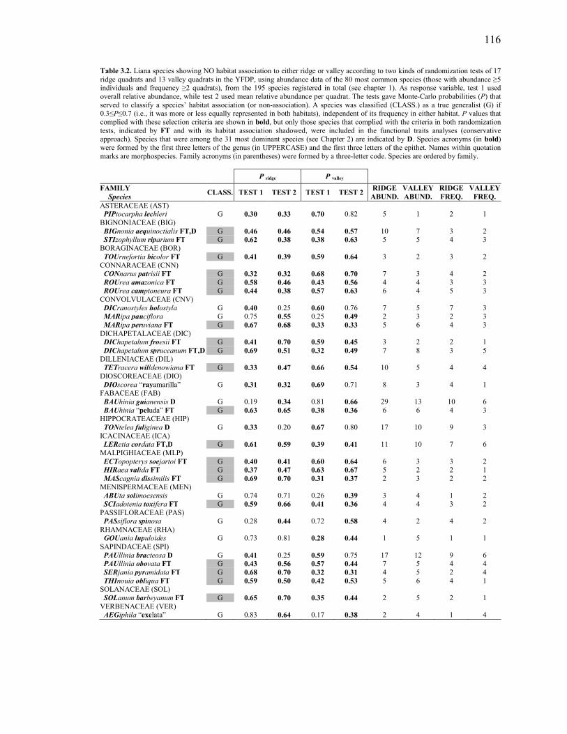
116
Table 3.2. Liana species showing NO habitat association to either ridge or valley according to two kinds of randomization tests of 17 ridge quadrats and 13 valley quadrats in the YFDP, using abundance data of the 80 most common species (those with abundance ≥5 individuals and frequency ≥2 quadrats), from the 195 species registered in total (see chapter 1). As response variable, test 1 used overall relative abundance, while test 2 used mean relative abundance per quadrat. The tests gave Monte-Carlo probabilities (P) that served to classify a species’ habitat association (or non-association). A species was classified (CLASS.) as a true generalist (G) if 0.3≤P≤0.7 (i.e., it was more or less equally represented in both habitats), independent of its frequency in either habitat. P values that complied with these selection criteria are shown in bold, but only those species that complied with the criteria in both randomization tests, indicated by FT and with its habitat association shadowed, were included in the functional traits analyses (conservative approach). Species that were among the 31 most dominant species (see Chapter 2) are indicated by D. Species acronyms (in bold) were formed by the first three letters of the genus (in UPPERCASE) and the first three letters of the epithet. Names within quotation marks are morphospecies. Family acronyms (in parentheses) were formed by a three-letter code. Species are ordered by family.
P ridge P valley
FAMILY Species
CLASS. TEST 1 TEST 2 TEST 1 TEST 2 RIDGE
ABUND. VALLEY ABUND.
RIDGE FREQ.
VALLEY FREQ.
ASTERACEAE (AST)
PIPtocarpha lechleri G 0.30 0.33 0.70 0.82 5 1 2 1 BIGNONIACEAE (BIG)
BIGnonia aequinoctialis FT,D G 0.46 0.46 0.54 0.57 10 7 3 2 STIzophyllum riparium FT G 0.62 0.38 0.38 0.63 5 5 4 3
BORAGINACEAE (BOR)
TOUrnefortia bicolor FT G 0.41 0.39 0.59 0.64 3 2 3 2 CONNARACEAE (CNN)
CONnarus patrisii FT G 0.32 0.32 0.68 0.70 7 3 4 2 ROUrea amazonica FT G 0.58 0.46 0.43 0.56 4 4 3 3 ROUrea camptoneura FT G 0.44 0.38 0.57 0.63 6 4 5 3
CONVOLVULACEAE (CNV)
DICranostyles holostyla G 0.40 0.25 0.60 0.76 7 5 7 3 MARipa pauciflora G 0.75 0.55 0.25 0.49 2 3 2 3 MARipa peruviana FT G 0.67 0.68 0.33 0.33 5 6 4 3
DICHAPETALACEAE (DIC)
DIChapetalum froesii FT G 0.41 0.70 0.59 0.45 3 2 2 1 DIChapetalum spruceanum FT,D G 0.69 0.51 0.32 0.49 7 8 3 5
DILLENIACEAE (DIL)
TETracera willdenowiana FT G 0.33 0.47 0.66 0.54 10 5 4 4 DIOSCOREACEAE (DIO)
DIOscorea “rayamarilla” G 0.31 0.32 0.69 0.71 8 3 4 1
FABACEAE (FAB)
BAUhinia guianensis D G 0.19 0.34 0.81 0.66 29 13 10 6 BAUhinia “peluda” FT G 0.63 0.65 0.38 0.36 6 6 4 3
HIPPOCRATEACEAE (HIP)
TONtelea fuliginea D G 0.33 0.20 0.67 0.80 17 10 9 3 ICACINACEAE (ICA)
LERetia cordata FT,D G 0.61 0.59 0.39 0.41 11 10 7 6
MALPIGHIACEAE (MLP)
ECTopopterys soejartoi FT G 0.40 0.41 0.60 0.64 6 3 3 2 HIRaea valida FT G 0.37 0.47 0.63 0.67 5 2 2 1 MAScagnia dissimilis FT G 0.69 0.70 0.31 0.37 2 3 2 2
MENISPERMACEAE (MEN)
ABUta solimoesensis G 0.74 0.71 0.26 0.39 3 4 1 2 SCIadotenia toxifera FT G 0.59 0.66 0.41 0.36 4 4 3 2
PASSIFLORACEAE (PAS)
PASsiflora spinosa G 0.28 0.44 0.72 0.58 4 2 4 2 RHAMNACEAE (RHA)
GOUania lupuloides G 0.73 0.81 0.28 0.44 1 5 1 1
SAPINDACEAE (SPI)
PAUllinia bracteosa D G 0.41 0.25 0.59 0.75 17 12 9 6 PAUllinia obovata FT G 0.43 0.56 0.57 0.44 7 5 4 4 SERjania pyramidata FT G 0.68 0.70 0.32 0.31 4 5 2 4 THInouia obliqua FT G 0.59 0.50 0.42 0.53 5 6 4 1
SOLANACEAE (SOL)
SOLanum barbeyanum FT G 0.65 0.70 0.35 0.44 2 5 2 1 VERBENACEAE (VER)
AEGiphila “exelata” G 0.83 0.64 0.17 0.38 2 4 1 4

117
FIGURES

118
Figure 3.1. Intra- and inter-specific averages and variation of specific leaf area (SLA), leaf dry matter content (LDMC), leaf lamina thickness (LT), leaf length to width ratio (L:W; incl. petiole), and individual-level leaf size range (LSR) of the 43 liana species included in the functional traits analyses. Species were classified in the following species guilds on the basis of their habitat association (or non-association): ridge species (R), valley species (V), true generalist species (G), and widespread species with habitat association (W, with two subcategories: WR, with ridge association, and WV, with valley association). Variation is expressed as mean ± 1 standard deviation (SD). To compare among species guilds pairwise, non-parametric Mann-Whitney tests were used (i.e., medians were compared, but mean ± 1 SD error bars, not boxplots, were used for the figure to simplify appearance and to make the calculation of the coefficients of variation in (B) clearer). The uncorrected/Bonferroni-corrected P values of the pairwise comparisons are shown only if uncorrected P≤0.10. (A) (research question 1) For each species (filled circles with thin error bars), intra-specific (between individuals) mean ± intra-specific variation (± 1 SD); and, for each species guild (open circles with thick error bars), inter-specific mean (mean of species mean values) ± inter-specific variation (± 1 SD). Mean and SD for each species, in addition to range (minimum and maximum values) and sample size (N), are reported in Appendix 4. Species are ordered by family (for acronyms meaning, see Tables or Appendices). (B) (research question 2) For each species guild (open circles with thick error bars), mean intra-specific (between individuals) variation ± inter-specific variation, expressed as coefficients of variation (CV) to make the intra-specific variation comparable across different species. Because a coefficient of variation obviously cannot be calculated for species with N=1 individual sampled, only species with N≥2 individuals sampled were considered to test if intra-specific variation was different among species guilds.
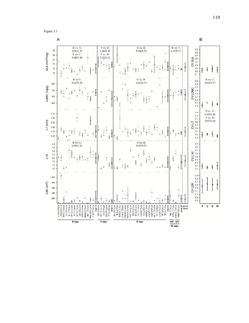
119
Figure 3.1

120
Figure 3.2. Intra- and inter-specific average and variation of leaf carbon (C) concentration (%), leaf nitrogen (N) concentration (%), leaf phosphorus (P) concentration (%), leaf C:N ratio, leaf N:P ratio, leaf δ13C, and leaf δ15N of the 43 liana species included in the functional traits analyses. Species were classified in the following species guilds on the basis of their habitat association (or non-association): ridge species (R), valley species (V), true generalist species (G), and widespread species with habitat association (W, with two subcategories: WR, with ridge association, and WV, with valley association). Variation is expressed as mean ± 1 standard deviation (SD). To compare among species guilds pairwise, non-parametric Mann-Whitney tests were used (i.e., medians were codmpared, but mean ± 1 SD error bars, not boxplots, were used for the figure to simplify appearance and to make the calculation of the coefficients of variation in (B) clearer). The uncorrected/Bonferroni-corrected P values of the pairwise comparisons are shown only if uncorrected P≤0.10. (A) (research question 1) For each species (filled circles with thin error bars), intra-specific (between individuals) mean ± intra-specific variation (± 1 SD); and, for each species guild (open circles with thick error bars), inter-specific mean (mean of species mean values) ± inter-specific variation (± 1 SD). Mean and SD for each species, in addition to range (minimum and maximum values) and sample size (N), are reported in Appendix 4. Species are ordered by family (for acronyms meaning, see Tables or Appendices). (B) (research question 2) For each species guild (open circles with thick error bars), mean intra-specific (between individuals) variation ± inter-specific variation, expressed as coefficients of variation (CV) to make the intra-specific variation comparable across different species. Because a coefficient of variation obviously cannot be calculated for species with N=1 individual sampled, only species with N≥2 individuals sampled were considered to test if intra-specific variation was different among species guilds.

121
Figure 3.2

122
Figure 3.3. Intra- and inter-specific average and variation of wood specific gravity (WSG) and absolute growth rate by diameter categories (AGR) of the 43 liana species included in the functional traits analyses. Species were classified in the following species guilds on the basis of their habitat association (or non-association): ridge species (R), valley species (V), true generalist species (G), and widespread species with habitat association (W, with two subcategories: WR, with ridge association, and WV, with valley association). Variation is expressed as mean ± 1 standard deviation (SD). To compare among species guilds pairwise, non-parametric Mann-Whitney tests were used (i.e., medians were compared, but mean ± 1 SD error bars, not boxplots, were used for the figure to simplify appearance and to make the calculation of the coefficients of variation in (B) clearer). The uncorrected/Bonferroni-corrected P values of the pairwise comparisons are shown only if uncorrected P≤0.10. (A) (research question 1) For each species (filled circles with thin error bars), intra-specific (between individuals) mean ± intra-specific variation (± 1 SD); and, for each species guild (open circles with thick error bars), inter-specific mean (mean of species mean values) ± inter-specific variation (± 1 SD). Mean and SD for each species, in addition to range (minimum and maximum values) and sample size (N), are reported in Appendix 5. Species are ordered by family (for acronyms meaning, see Tables or Appendices). (B) (research question 2) For each species guild (open circles with thick error bars), mean intra-specific (between individuals) variation ± inter-specific variation, expressed as coefficients of variation (CV) to make the intra-specific variation comparable across different species. Because a coefficient of variation obviously cannot be calculated for species with N=1 individual sampled, only species with N≥2 individuals sampled were considered to test if intra-specific variation was different among species guilds.
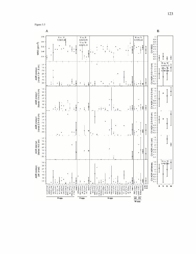
123
Figure 3.3

124
CHAPTER 4: Growth strategies of lianas in the forest understory of ridge and valley topographic terra firme habitats
in the Yasuní Forest Dynamics Plot, Amazonian Ecuador ( 5)
SUMMARY
In the Yasuní Forest Dynamics Plot (YFDP) we assessed the apparent “strategies”
that lianas with diameter ≥1 cm were using to grow in the understory of ridge and valley
topographic habitats, as observed in a sample of 17 ridge quadrats and 13 valley quadrats
(20×20 m each). An understory growth strategy was defined by the following categorical
variables: whether a liana was free-standing or already climbing, climbing mechanism
(twining, tendrils, branch-twining, scrambling or adhesive roots/tendrils) and understory
appearance (creeping or not, and having large branches or not; applicable to climbing
lianas only). We reasoned that if a particular growth strategy is significantly more
common in either ridge or valley, and that growth strategy can be more or less
consistently associated to a particular species, or to a group of species, then the growth
strategy exhibited by such species may play a role in determining where in the forest such
species can grow—which in turn would explain, at least partly, the observed community-
level difference in liana community structure (species composition and their abundances)
between ridge and valley.
We found 286 free-standing lianas (representing 46 species) and 1378 climbing
lianas (representing 190 species) with diameter ≥1 cm in the YFDP (43 species shared).
Twining and tendrilate species were the most numerous among both free-standing and
(5) Potential co-authors for pulication: Esteban Gortaire1 and Leonel da S. L. Sternberg2. 1Escuela de
Ciencias Biológicas, Pontificia Universidad Católica del Ecuador. Av. 12 de Octubre 1076 y Roca, Apartado postal 17-01-2184. Quito, Ecuador. 2Department of Biology, University of Miami. 1301 Memorial Dr., Coral Gables, Florida 33146, USA.

125
climbing lianas. Branch-twining lianas, represented only by Hippocrateaceae, were
relatively more numerous among free-standing lianas than among climbing lianas (17%
vs. 5%), suggesting that the species of Hippocrateaceae tend to be free-standing even as
old saplings. There were practically no scrambling species among the free-standing
lianas, while species with adhesive roots or adhesive tendrils were very rare. Among the
top most frequent species (frequency defined as the number of quadrats in which a
species occurs), we found that free-standing individuals were important in determining
the habitat association mainly of tendrilate and branch-twining species.
Given that the trees in the valley have slightly higher dynamism (higher mortality,
recruitment and growth rates) than the trees in the ridge (although the difference is not
significant), it is possible that small trellises for lianas are relatively more common in
valley than in ridge. If so—and based on the patterns observed in past studies—we
hypothesized that twining lianas will be relatively more abundant in ridge than in valley,
and that tendrilate lianas will show the opposite pattern. Further, because the understory
of the Yasuní forest is apparently denser than other lowland tropical rainforests, we
hypothesized that scramblers will have similar relative abundance in ridge and valley.
Finally, because more trees apparently fall in valley than in ridge, we hypothesized that
creeping lianas will be relatively more abundant in valley than in ridge. In the present
study, we found, in general, statistical support for these predictions (hypotheses),
although with varied degrees of confidence.
We conclude that understory growth strategies of lianas can help to explain the
distribution of liana species in a forest because they reflect the concomitant, time-
cumulative, effects of forest successional processes, tree dynamics (mortality, recruitment

126
and growth rates, and associated processes such as tree-fall rates) and broad forest
physiognomy (particularly the relative abundance of appropriate trellises for lianas).
BACKGROUND AND HYPOTHESES
Lowland tropical rainforests from western Amazonia, such as those in Ecuador, are
more dynamic than those in central or eastern Amazonia (e.g., Phillips et al. 2004). Tree-
fall gaps in western Amazonian forests probably create a very heterogeneous mosaic of
microhabitats (gaps and their associated successional pathways) which, however, become
diluted when the forest is observed at the landscape scale—indeed, relatively few
common tree and liana species tend to dominate western Amazonian forests (see e.g.,
Pitman et al. 2001, Romero-Saltos, Valencia, and Macía 2001, Burnham 2002, Macía and
Svenning 2005). At the plot scale, the presence of a limited set of tree and liana species
that are associated to particular habitats—such as swampy areas, valleys, ridgetops, or
secondary forests—reinforces this apparent order or predictability (Valencia et al. 2004c;
see also Chapter 3).
At very small spatial scales, lianas are perhaps the only growth form that apparently
adapts (survives) well to dynamic forest microsites which are frequently impacted by
tree-falls (review in Schnitzer and Bongers 2002). Adult lianas, in general, have several
stem anatomical characteristics that give them flexibility but also toughness, allowing
them to sustain structural strains imposed by random disturbances or, if need arises, to
quickly recover from breakage or wounds (reviews in e.g., Fisher and Ewers 1991, Putz
and Holbrook 1991, Isnard and Silk 2009). Thus, given their innate adaptability to ever-
changing environments, lianas may be especially responsive to the dynamic three-
dimensional architecture created by the fast growing, fast recruiting and fast dying trees

127
in the western Amazonian forests (e.g., Malhi et al. 2004, Phillips et al. 2004). This
“responsiveness” of lianas to local disturbance may be strong enough to influence their
distribution and abundance at the local scale (e.g., Putz 1984, Baulfor and Bond 1993,
Schnitzer 2005), in addition to the well-known environmental variables that control the
distribution and abundance of plants in general (e.g., water availability, light, nutrients,
CO2 concentration).
How can we assess if a liana species can grow successfully in different tropical
rainforest microhabitats with different degrees of architectural complexity or successional
status? The most direct approach is of course experimental and would consist of planting
liana species in architecturally distinct microhabitats while controlling for confounding
factors (e.g., Putz 1984). A second, indirect, approach would be to assume that if a liana
species under natural conditions in the forest is repeatedly not found, or rarely occurs, in
many independent replicates of an architecturally-defined microhabitat, then
(statistically) it can be concluded that the liana species in question does not grow in such
microhabitat. Both approaches seem valid, but they depend on how the concept of
“architectural complexity” of a forest microhabitat is defined. Traditionally, liana studies
have implicitly defined architectural complexity from the point of view of the lianas, i.e.
as the availability of suitable “trellises” (supports for climbing) for species guilds of
lianas defined by their common climbing mechanism, i.e. the mechanism used to attach
to a support (e.g., Putz 1984, DeWalt, Schnitzer, and Denslow 2000, Nabe-Nielsen 2001).
Per se, trellis availability has rarely, if ever, been measured directly, but instead it has
been assumed to be correlated with forest type, forest age, microhabitats in a forest, or
tree size distribution (e.g., Putz 1984, DeWalt, Schnitzer, and Denslow 2000, Nabe-

128
Nielsen 2001). Climbing mechanisms have been defined in various ways, but the most
common classification, more ecologically- than ontogenetically-based, has five categories
(originally proposed by Putz 1984): (1) climbing by extreme circumnutation, i.e. by the
continuous twining of the main stem axis or its equivalent (e.g., Forsteronia,
Apocynaceae), (2) climbing by coiling tendrils which may have diverse ontogenetic
origins (e.g., Paullinia, Sapindaceae), (3) climbing by lateral branches that twine once or
a few times around the support (e.g., Salacia, Hippocrateaceae), (4) erratically climbing
by using hooks, thorns, or spines, or simply by leaning, a broad strategy to which we
refer in this study as “scrambling sensu lato” (e.g., Machaerium, Fabaceae), and (5)
climbing by a “glue-to-your-support” strategy, i.e. by tiny adventitious adhesive roots
(e.g. Marcgravia, Marcgraviaceae) or by tendril tips that do not coil but are adhesive and
thus the liana in practice climbs as if it were a root-climber (e.g., some Bignoniaceae and
Vitaceae). Although some species have evolved more than one climbing mechanism, it is
usually feasible to determine in the field what primary or main climbing mechanism the
species is using (Putz 1984).
The characterization of climbing mechanisms along with the characterization of
trellis availability have revealed ecological trends that, along with other more general
processes (e.g., habitat filtering, niche differentiation, stochasticity, enemy-mediated
density dependence, among others), hint about the nature of the underlying factors that
determine the observed distribution and abundance of lianas at the landscape (forest-type)
or local scales. For instance, it is well known that tendrilate lianas—which can only
attach to small-diameter trellises—decrease, whereas twiners increase, as a tropical
rainforest ages (DeWalt, Schnitzer, and Denslow 2000, but see Koski 2009). This

129
phenomenon is concomitant with a reduction of liana density as the forest matures (Putz
1984, DeWalt, Schnitzer, and Denslow 2000, Letcher and Chazdon 2009, Madeira et al.
2009) which in turn, at least within the terra firme ridge forest of Yasuní, is positively
correlated with a reduction in the number of small trees (Nabe-Nielsen 2001). In the terra
firme ridge forest of Yasuní, it has also been shown that scrambling lianas prefer thinner
host trees than lianas with other climbing mechanisms, and the thicker a liana, the thicker
its host tree, independent of the liana’s climbing mechanism (Nabe-Nielsen 2001). These
and other studies (e.g., Baulfor and Bond 1993) have demonstrated that the availability of
appropriate trellises is important in determining the distribution of lianas in a forest.
In the 50-ha Yasuní Forest Dynamics Plot (YFDP), the community of lianas in ridge
habitat is different from that in valley habitat in terms of diversity and species
composition (and/or species abundances; Chapter 2). The community difference between
these two topographically-defined habitats is largely driven by those common species
that partition the topographic gradient. In Chapter 3, we statistically identified such
species and showed that the inter-specific median values of only three functional traits
were statistically different between the ridge species guild and the valley species guild:
leaf mass per area, leaf phosphorus concentration and wood specific gravity. However,
because of the nature of the habitat association analyses, such pattern was based on the
comparison of only 14 ridge species against five valley species (Chapter 3), i.e. it used
just 10% of the 195 species of lianas found in the thirty 20×20 m non-contiguous
quadrats sampled in the YFDP (Chapter 2). Clearly, the difference between ridge and
valley liana communities in the YFDP calls for more comprehensive approaches, such as
the present study.

130
In this study, in a further attempt to understand the reasons why the community of
lianas in ridge habitat is different from that in valley habitat in the terra firme forest of the
YFDP (Chapter 2), we quantify, in these two topographically-defined habitats, the
frequencies of: relatively large free-standing lianas (diameter ≥1 cm, treelet-like, i.e.
lianas that are not yet climbing), lianas that are already climbing, different climbing
mechanisms (defined above), and different “understory appearances”. Understory
appearance—a concept by imagination (Ford 2000)—is defined by whether or not a liana
has near-ground or on-ground branches (i.e., branches emerging from the main stem at a
height ≤3 m approximately) and by whether or not its main stem, and/or any of its
branches, are creeping (presence of stolons or runners).
We propose that the ability to be free-standing as an old sapling, climbing
mechanism, and understory appearance represent whole-plant functional traits that can
define the time-cumulative strategy of how a liana grew or is growing in the understory
of a forest. Such understory growth strategies may reflect relatively long-term ecological
processes that putatively affect the distribution and abundance of lianas in a forest.
Within this framework, in this study we specifically explore the following topics in the
YFDP lianas (hypotheses appear in italics):
(1) Free-standing vs. climbing lianas: We describe the community of free-standing
lianas in the YFDP and contrast it with the community of climbing lianas, including the
relative proportions of species with different climbing mechanisms in these two
communities. We also characterize the climbing mechanism and size (diameter)
distribution of each of the most frequent species (frequency = # quadrats a species occurs
in) of free-standing lianas and of climbing lianas. This allows us to explore how the

131
relative abundance of growth stages in each most frequent species of lianas played a role
in determining its habitat association (as defined in Chapter 3). This is important because
the most frequent and/or common species are the ones largely responsible for the
statistical difference in species composition, and/or their abundances, between ridge and
valley (see Chapters 1 and 2).
(2) On twining lianas: Twining lianas tend to become increasingly more common as
a forest matures (DeWalt, Schnitzer, and Denslow 2000). On average, in the terra firme
forest of the YFDP, tree biomass in the valley, compared to the ridge, has higher
(although not significantly) relative mortality rate (2.83 vs. 2.30 %/year), recruitment rate
(0.18 vs. 0.15 Mg/ha/year), and relative growth rate (2.86 vs. 2.36 %/year), although
these differences are not statistically significant (Valencia et al. 2009). Also, above-
ground biomass is at least 50% higher in ridge compared to that of valley (Valencia et al.
2009). Thus, it is possible that there is a higher abundance of young forest patches in
valley than in ridge, and thus we hypothesize that, among climbing lianas, twining lianas
should be relatively more common in ridge than in valley.
(3) On tendrilate lianas: Regarding tendrilate lianas, we set forth to explore which
of two contradictory hypotheses is best reflected in the data. First, let’s recall that trees in
valley apparently tend to die and recruit faster than in ridge (higher dynamism; Valencia
et al. 2009). If these slightly higher rates are caused in part by a slightly higher tree-fall
rate (and associated successional processes) in valley—as has been observed in other
studies in lowland Neotropical rainforests (e.g., Ferry et al. 2010), but not yet explicitly
measured in the YFDP—it is possible, among other effects, that more small trellises for
lianas exist in valley than in ridge. Thus, among climbing lianas, we hypothesize that

132
such putatively higher abundance of small trellises in valley habitat should increase the
relative abundance of tendrilate lianas in valley (e.g., Putz 1984), as indeed has been
observed in young forests (e.g., DeWalt, Schnitzer, and Denslow 2000). Second,
alternatively, tendrilate lianas may be also responding to the abundance of small trees and
shrubs, which one may think should provide sufficiently small trellises for tendrilate
lianas. In the YFDP, small trees (1≤DBH≤10 cm)—and in fact trees in general—tend to
be increasingly more abundant from valley to upper ridge (Valencia et al. 2004c; tree
data from the 30 quadrats sampled in this study confirm the positive correlation between
small trees and elevation, r=0.62, P<0.001). Thus, if small trees are important for the
occurrence of climbing tendrilate lianas, we hypothesize that tendrilate lianas should be
relatively more common in ridge than in valley, which is the opposite of what the first
hypothesis stated.
(4) On branch-twining lianas: In Yasuní, branch-twining lianas are characteristic
of only a single family: Hippocrateaceae. Therefore, the distribution of branch-twining
lianas should follow that of the species in Hippocrateaceae. In Chapters 1 and 2, we
showed that this family was, among the most species-rich, the only family whose species
mostly occurred in ridge than in valley. Thus, undoubtedly, we expect that branch-
twining lianas must be proportionally more abundant in ridge than in valley.
(5) On scrambling lianas: In Yasuní, scrambling lianas (sensu lato) tend to grow on
thinner trellises than lianas with other climbing mechanisms (Nabe-Nielsen 2001).
Scramblers in general also seem to proliferate where there is a dense, closed, arrangement
of supports, independent of their diameter (e.g., in vegetation tangles; Putz 1984). In a
lowland tropical rainforest such as Yasuní, where the understory is supposedly denser

133
than in other lowland tropical rainforests in the world (Pitman et al. 2002, S. Davies
[CTFS-STRI], pers. comm.), we hypothesized that the relative abundance of scramblers
should be similar between ridge and valley (although they might be slightly more
abundant in valley if the higher dynamism there increases the abundance of thinner
trellises).
(6) On understory appearances: Because in Yasuní creeping lianas have on
average more rooting points than non-creepers (unpublished data), they may have a better
chance to survive tree-falls than non-creepers because undamaged stem portions on the
ground may resprout if still attached to nearby and intact rooting points (e.g., Peñalosa
1984, Alvira, Putz, and Fredericksen 2004). This putative advantage of creepers in forests
with high tree mortality would be enhanced if a liana also produces near-ground branches
or on-ground branches (stolons). Of course, it could also be that creepers become more
abundant in a forest area not because they are more resilient to falling trees, but because
tree-falls keep creating creeping lianas by breaking them or slipping them off from their
host trees (cause and effect cannot be separated). In any case, in the YFDP the valley
habitat is apparently more dynamic than the ridge habitat (see above; Valencia et al.
2009), and thus, among climbing lianas, we hypothesized that creeping lianas—
particularly if they have stolons or near-ground branches—should be relatively more
abundant in valley than in ridge.
(7) On the interaction between climbing mechanism and understory
appearance: To complement the search for differential patterns between ridge and valley
habitats with respect to the frequencies of different climbing mechanisms and understory
appearances among climbing lianas, we assess if the expected differences can still be

134
detected when a given comparison is conducted with the lianas in a given combination of
climbing mechanism and understory appearance. We hope that this high-resolution
evaluation of understory growth strategies among climbing lianas will allow us to gain
understanding of the growth mechanisms behind the patterns that are expected at a lower
resolution (i.e., the hypotheses above, where we just focus on a climbing mechanism
without taking into account understory appearance, and vice versa). As a further step, we
also gain insight by broadly characterizing the size (in diameter classes) of the
individuals of the most frequent species of climbing lianas in the different combinations
of climbing mechanisms and understory appearances.
In short, we postulate in this study that the distinct environmental conditions and the
distinct tree dynamics in the ridge and valley habitats of the YFDP differentially
influence the growth strategies that lianas can use in the forest understory, which in turn
may partly explain the differences in species composition, species abundances, and
species diversity observed between these two dissimilar liana communities (Chapter 2).
METHODS
STUDY AREA
This study was conducted in Yasuní National Park, Amazonian Ecuador, within the
50-hectare Yasuní Forest Dynamics Plot (YFDP; 1000×500 m; 00°41' S, 76°24' W).
Mean annual rainfall and mean monthly temperature in the area are approximately 3000
mm and 25 °C, respectively (Chapter 2). Because mean monthly rainfall is 250 mm,
Yasuní is considered a non-seasonal forest (Chapter 2). The YFDP is associated with an
ever expanding network of large-scale permanent plots that monitor millions of trees in
several tropical and temperate countries (Valencia et al. 2004a). Yasuní National Park, of

135
approximately 10,000 km2, is known to harbor very high levels of plant and animal alpha
diversity (Bass et al. 2010), and lianas certainly are not the exception (Nabe-Nielsen
2001, Romero-Saltos, Valencia, and Macía 2001, Burnham 2002, Burnham 2004). The
YFDP is located on terra firme (upland) forest, with ridge formations (up to 250 m
altitude) towards the northern, southern and eastern areas, separated by a relatively wide
valley (ca. 215–225 m altitude). Except for a few small swampy areas in the valley, ridge
and valley are considered terra firme forest (Valencia et al. 2004c). A few permanent
streams crisscross the valley; they may occasionally overflow and temporarily flood part
of the valley during the rainiest months.
Past studies have shown that ridge and valley habitats of the YFDP are statistically
dissimilar in terms of tree, liana and palm species composition or species abundances
(Svenning 1999a, Valencia et al. 2004c, Chapter 2). While the diversity of tree species
between ridge and valley is not significantly different—although a tendency towards
higher diversity in valley exists—lianas show higher species diversity in valley than on
ridge (Valencia et al. 2004c, Chapter 2). In the valley, the average density of trees and
basal area per hectare is lower than on the ridge, whereas liana density is similar in both
habitats (Valencia et al. 2004c, Chapter 2). Because trees with relatively large diameters
occur more commonly on ridge than in valley—tree biomass is, in fact, at least 50%
higher on ridge—mean canopy height is probably higher on ridge than in valley
(Valencia et al. 2004c, Valencia et al. 2009; see also Svenning 1999a).
More than 90% of Yasuní is terra firme (upland) hilly forest growing on Ultisols
soils that are somewhat clayey, acidic and rich in iron and aluminum (Pitman 2000,
Valencia et al. 2004a). The surface soil (0–5 cm) of the terra firme is, when compared to

136
other terra firme areas in northwestern Amazonia, relatively rich in exchangeable bases
(particularly Ca, Mg, and Na) and has an average texture of approximately 50% silt, 29%
sand and 21% clay (Tuomisto et al. 2003). The biogeochemical characteristics of the
topographically distinct ridge and valley habitats of the YFDP have not been well
studied, but differences are expected. The main physical differences should evidently be
related to the effect of topography on the hydrological regime: on average, drainage is
probably lower in the valley, soil water content is probably higher in the valley (see e.g.
Jirka et al. 2007) and soil oxygen concentration is probably lower in the valley (see e.g.,
Silver, Lugo, and Keller 1999). If these differences are marked, other soil characteristics
such as pH, Al concentration, nutrient concentrations and organic matter concentration
should also be different between ridge and valley habitats (see e.g., Tange, Yagi, and
Sasaki 1998, Tuomisto et al. 2003, Kubota, Murata, and Kikuzawa 2004), but a reliable
geochemical/geophysical description of the YFDP’s ridge and valley soils is not yet
available.
SAMPLING DESIGN AND DATA ANALYSES
To evaluate the frequencies of different understory growth strategies of lianas in the
ridge and valley habitats of the YFDP—as defined by free-standing/climbing status,
climbing mechanism and understory appearance (see Introduction)—we used a subset of
1378 climbing lianas and 286 free-standing lianas, out of the total of 1919 lianas with
diameter ≥1.0 cm (195 species) sampled in 17 non-contiguous ridge quadrats and 13 non-
contiguous valley quadrats (each 20×20 m; Chapter 2). Excluded from this study were
176 climbing lianas not identified to family (usually very tall lianas with leaves that were
practically inaccessible even by climbing nearby trees) and 79 lianas that were neither

137
climbing nor free-standing (usually fallen branches with roots and leaves, but which were
not yet climbing). The 176 unidentified (and non-collected) climbing individuals were
excluded because their climbing mechanism was unknown or, even if directly observed
or inferred, could not be unequivocally matched to a taxon. The 79 lianas that were
neither climbing nor free-standing were not included because many of these lianas are
very prone to die (unpublished recensus data) and because in this study we focus on the
climbing and free-standing growth stages only.
Lianas were sampled from 2006 to 2008 following an in-house sampling protocol
that is complementary to that of Gerwing et al. (2006), but which, for a number of
reasons, is somewhat different from what was independently proposed by Schnitzer,
Rutishauser, and Aguilar (2008) also as a complement to Gerwing et al. (2006) (see
Appendix 1 of Chapter 2). Our Gerwing/Romero (G/R) protocol defines a Point of
Diameter Measurement (PDM) in a liana by codifying, alphanumerically, its “understory
appearance” (see Introduction) below an approximate height of 3 m, in addition to other
characteristics used for the application of the G/R protocol, such as the distance along the
stem from the main rooting point to the point where the first branch emerges, the
presence of thick adventitious roots, the presence of a voluble main liana stem fully
encircling a host stem, among other characteristics (see Appendix 1 of Chapter 2).
The data registered in the field for every one of the climbing and free-standing lianas
included in this study were: (1) diameter at the PDM; (2) free-standing/climbing status;
(3) PDM code in the G/R protocol (a proxy of understory appearance; see above); (4)
whether it had any understory branch(es) ≥1 cm in diameter, <1 cm in diameter, or both
(at at height <3 m approximately); and (5) its apparent climbing mechanism if easily

138
observable (see Introduction). Climbing mechanisms registered at the individual level
were later assessed for consistency within species; for data analyses, the same primary
climbing mechanism was assigned to every individual of a species, so free-standing
lianas also had their future climbing mechanism assigned. To assign an understory
appearance to every liana sampled, we used information from numerals (3) and (4)
above. The understory appearances used in this study focused on the presence/absence of
large understory branches (diameter ≥1 cm) and on the creeping/not creeping status of
liana stems (incl. branches); thus, there are four possible understory appearances, as used
in this study: creeping with large branches, creeping with no large branches, not creeping
with large branches, and not creeping with no large branches. Note that although the
concept of understory appearance can be applied to climbing or free-standing lianas (in
fact, 20 out of the 286 free-standing lianas crept a little), for the purpose of this study we
applied it to climbing lianas only. To clarify our approach towards the understanding of
understory growth strategies of climbing lianas in the YFDP, a graphical representation
of the 16 possible combinations of climbing mechanisms and understory appearances
(excepting the adhesive roots/tendrils climbing mechanism), as used in this study, is
shown in Figure 4.1. However, not shown in the Figure is the possibility, indeed
repeatedly observed in the field, that a branch, not the main stem, is the stem that creeps
(those cases were nonetheless classified along with those lianas in which the main stem
creeps).
The most frequent species of lianas among the free-standing lianas and among the
climbing lianas were selected by the following criteria: in the free-standing lianas dataset,
we selected those species occurring in at least ≈25% of either ridge quadrats (≥4

139
quadrats) or valley quadrats (≥3 quadrats), while in the climbing lianas dataset, we
selected those species occurring in at least ≈50% of either ridge quadrats (≥8 quadrats)
OR valley quadrats (≥6 quadrats). The low frequency threshold (25%) used for free-
standing lianas was chosen because of the relative paucity of free-standing lianas in the
forest. To describe size (diameter) distribution in each of the most frequent species, the
percentage of individuals in each of the following diameter classes was calculated with
respect to the total number of individuals in the species (free-standing + climbing
individuals): 1.0–1.5 cm, 1.5–2.5 cm, 2.5–5.0 cm, and ≥5.0 cm. The first two classes
were meant to represent young lianas that were probably actively growing in the forest (at
least those facing ideal environmental conditions), while the last class was meant to
represent very old established lianas (or so we assumed).
To test the hypotheses about differences in the proportion of climbing mechanisms
and understory appearances from climbing lianas in ridge vs. valley (see Introduction),
we considered a quadrat as an independent replicate. In each quadrat, the proportion of
climbing lianas having a given climbing mechanism (out of five possible; see above), a
given understory appearance (out of four possible; see above), or a given combination of
climbing mechanism and understory appearance (out of 16 possible, see Figure 4.1;
adhesive tendrils/adventitious roots climbing mechanism excluded), was calculated with
respect to total number of climbing lianas in the quadrat (excluding unidentified lianas).
For every comparison, the ridge sample (N=17 quadrats) was compared to the valley
sample (N=13 quadrats) using a two-sample t-test and a Mann-Whitney non-parametric
test; we conservatively decided to use both statistical tests for every comparison because
the data used in a given comparison were not always normally distributed.
140
To complement the analysis above, we conducted an analysis that is similar in nature
but in which climbing lianas were separated into four diameter classes: 1.0–1.5 cm, 1.5–
2.5 cm, 2.5–5.0 cm, and ≥5.0 cm. The goal was to identify the size range (in diameter) of
the lianas that were driving the postulated differences between ridge and valley in terms
of climbing mechanisms and understory appearances. As above, we considered a quadrat
as the independent replicate or sampling unit. In each quadrat, among the lianas of a
given diameter class, the proportion of lianas of a given climbing mechanism or
understory appearance was calculated with respect to the total number of climbing lianas
of the given diameter class in the quadrat (excluding unidentified lianas). Ridge vs. valley
comparisons by diameter classes in each of the 16 possible combinations of climbing
mechanism and understory appearance (Figure 4.1) were not conducted. As above, for
every comparison, the ridge sample (N=17 quadrats) was compared to the valley sample
(N=13 quadrats) using both a two-sample t-test and a Mann-Whitney non-parametric test.
Finally, for every comparison of ridge climbing lianas vs. valley climbing lianas of a
given diameter class, we also identified which frequent species contributed at least two
individuals in the datasets being compared; this way, we broadly (visually) characterized
the size distribution of the most frequent species of climbing lianas across the different
climbing mechanisms and understory appearances.
VEGETATION COVER: DENSIOMETER MEASUREMENTS
As a very broad proxy of forest successional status, we used measurements of
vegetation cover (canopy openness) made with a convex densiometer. Densiometer
readings were taken at the four corners of every 5×5 m subquadrat, each measurement
taken with the densiometer facing towards the center of a subquadrat. Thus, for each

141
20×20 m quadrat, we obtained 64 densiometer readings. By using natural statistical
breaks, we classified the densiometer data in three categories: “low” vegetation cover
(62.5–87.5% of cover), “typical” cover (87.5–93.75%), and “high” cover (93.75–100%).
Then, by assuming each densiometer reading best represented a forest area of 2.5×2.5 m
(6.25 m2), for each 20×20 m quadrat we calculated the forest area represented by the
three vegetation cover categories (out of 400 m2).
RESULTS AND DISCUSSION
We postulated that the real and presumed physical and ecological differences
between the ridge and valley habitats in the YFDP (see Introduction and Methods) must
have an effect on the growth strategies lianas use in the understory of these forest
habitats, constraining at the same time what species can grow where, and thus partly
explaining why the liana community structure (species composition and their
abundances) in ridge is different from that in valley habitat (Chapter 2). Such strategies
were defined in terms of frequencies of free-standing lianas, climbing lianas, different
climbing mechanisms and different understory appearances (see Introduction and
Methods).
FREE-STANDERS VS. CLIMBERS
General comparison
In this study, we analyzed a subset of 1664 lianas (193 species) from the dataset of
1919 lianas (195 species) with diameter ≥1 cm that were registered in 17 ridge quadrats
and 13 valley quadrats in the YFDP (each 20×20 m; Chapter 2): 286 were free-standing
lianas (46 species) and 1378 were climbing lianas (190 species). Forty-three species were
shared between free-standing and climbing lianas, i.e. three species only appeared as
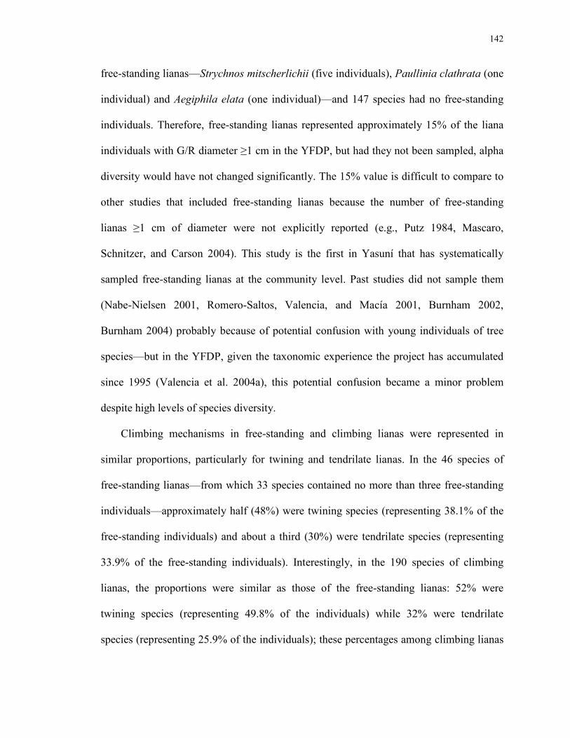
142
free-standing lianas—Strychnos mitscherlichii (five individuals), Paullinia clathrata (one
individual) and Aegiphila elata (one individual)—and 147 species had no free-standing
individuals. Therefore, free-standing lianas represented approximately 15% of the liana
individuals with G/R diameter ≥1 cm in the YFDP, but had they not been sampled, alpha
diversity would have not changed significantly. The 15% value is difficult to compare to
other studies that included free-standing lianas because the number of free-standing
lianas ≥1 cm of diameter were not explicitly reported (e.g., Putz 1984, Mascaro,
Schnitzer, and Carson 2004). This study is the first in Yasuní that has systematically
sampled free-standing lianas at the community level. Past studies did not sample them
(Nabe-Nielsen 2001, Romero-Saltos, Valencia, and Macía 2001, Burnham 2002,
Burnham 2004) probably because of potential confusion with young individuals of tree
species—but in the YFDP, given the taxonomic experience the project has accumulated
since 1995 (Valencia et al. 2004a), this potential confusion became a minor problem
despite high levels of species diversity.
Climbing mechanisms in free-standing and climbing lianas were represented in
similar proportions, particularly for twining and tendrilate lianas. In the 46 species of
free-standing lianas—from which 33 species contained no more than three free-standing
individuals—approximately half (48%) were twining species (representing 38.1% of the
free-standing individuals) and about a third (30%) were tendrilate species (representing
33.9% of the free-standing individuals). Interestingly, in the 190 species of climbing
lianas, the proportions were similar as those of the free-standing lianas: 52% were
twining species (representing 49.8% of the individuals) while 32% were tendrilate
species (representing 25.9% of the individuals); these percentages among climbing lianas

143
were very similar to those observed by Nabe-Nielsen (2001) in mature terra firme ridge
forests in Yasuní, and by Santos, Kinoshita, and Rezende (2009) in fragmented seasonal
semideciduous forest in southeastern Brazil. There were relatively more branch-twining
species among the free-standers than among the climbers, 17% vs. 5%, suggesting that
the species of Hippocrateaceae—the only family with this type of climbing mechanism in
our dataset—tend to be free-standing even as old saplings (diameter ≥1 cm). Scramblers
(sensu lato) were represented by relatively few species and individuals in both growth
stages (among free-standing lianas: two individuals, two species; among climbing lianas:
197 individuals, 18 species). Acacia tenuifolia and Piptocarpha lechleri were the two
scrambling species among the free-standers, each represented by only a single
individual—thus, in Yasuní scramblers practically never can be free-standing! (at least
not with a diameter ≥1 cm). This can be either interpreted as scramblers being very
effective in finding suitable supports while they are still very young, or as scramblers
lacking the wood ontogenetic adaptations necessary to develop as self-supporting when
young (for some biomechanical and evolutionary perspectives on this issue, see e.g.,
Kennard 1998, Gallenmüller et al. 2001, Gallenmüller, Rowe, and Speck 2004, Rowe,
Isnard, and Speck 2004, and Lahaye et al. 2005). Finally, root climbers did not exist
among free-standing lianas, and only three species existed among climbing lianas, all in
the Marcgraviaceae. This family, in addition to liana species, includes several species of
secondary woody hemiepiphytes (which superficially may look like lianas).
Most frequent and most common species among free-standers and climbers
The majority of the most common species (defined by number of individuals) in each
growth stage were also among the most frequent species (defined by number of quadrats

144
in which they occurred) (Table 4.1). Further, the 10 most abundant species among the
free-standing lianas were mostly the same as the 10 most abundant species among the
climbing lianas, although ranked differently (Table 4.1). Among climbing lianas,
Machaerium cuspidatum and Combretum laxum—both species with valley association,
but also widespread (Chapter 3)—were the two most abundant (Table 4.1). On the other
hand, among free-standing lianas, Cuervea kappleriana and Petrea maynensis—both
species with ridge association (Chapter 3)—were the two most abundant, although they
were also among the top five most abundant among climbing lianas (Table 4.1).
Callichlamys latifolia, a species with valley association (Chapter 3), and Bauhinia
guianensis, a generalist species (Chapter 3), had a higher rank position in abundance
among free-standing lianas than among climbing lianas. All things considered, we
conclude that the observed difference in community structure (species composition and
their abundances) between the whole liana communities of ridge and valley (Chapter 2)
seems also reflected among the free-standing lianas (in fact, using data from free-
standing lianas only, an ANOSIM test gave a significant difference between ridge and
valley: RANOSIM = 0.24, P<0.01, Bray-Curtis used as distance measure).
Table 4.1 illustrates a number of patterns in the occurrence and size distribution of
free-standing and climbing lianas of the most frequent species within each growth stage,
and within each habitat. First, free-standing individuals were relatively rare among the six
frequent species of twining lianas, from which only Petrea maynensis had free-standing
individuals that were as common as their climbing counterparts, in particular in the
smallest diameter class: 1.0–1.5 cm. Therefore, the strong ridge association shown by this
species (Chapter 3), one of the most dominant in the YFDP (Chapter 2), is very

145
dependent on the relatively high abundance of free-standing individuals, which constitute
36.5% of the individuals in this species, almost all with a diameter ≤2.5 cm. Second, as
opposed to what was observed with the twining species, free-standing individuals were
relatively common among the most frequent species of tendrilate and branch-twining
lianas. In fact, free-standing individuals constituted approximately half of the total
number of individuals in the following four species: Callichlamys latifolia, Bauhinia
guianensis, Cuervea kappleriana and Tontelea fuliginea. Thus, the habitat association
shown by these dominant species in the YFDP (Chapter 2) is largely influenced by the
distribution of their free-standing lianas. Third, as can be expected, it is very rare for a
free-standing liana to reach a diameter greater than 2.5 cm. Fourth, it is peculiar that,
among the most frequent species, the three species with the highest relative abundance of
climbing lianas with diameter ≥5 cm are all twining species: Combretum laxum (a valley
specialist), Doliocarpus dentatus (a valley specialist) and Dioclea ucayalina (a ridge
specialist); these very large lianas are most probably associated with very large host trees
(Nabe-Nielsen 2001) which one would expect are more common in mature forests, thus
reaffirming the trend that twining species tend to increase in abundance in mature
neotropical forests (DeWalt, Schnitzer, and Denslow 2000). Fifth, and finally, three
species did not have any free-standing liana at all: Doliocarpus dentatus (a valley
species), Dioclea ucayalina (a ridge species) and Machaerium cuspidatum (a valley
species). M. cuspidatum, in particular, merits attention because it is the most abundant
species among climbing lianas in the YFDP (Table 4.1) (or the second most abundant,
after Combretum laxum, if all the 1919 sampled lianas are considered; Chapter 2).

146
Although the lack of free-standing individuals in Machaerium cuspidatum per se is
not surprising because scrambling species were very rare among free-standing lianas in
general, this result serves as a springboard to discuss why this species became ubiquitous
in Yasuní. M. cuspidatum is a widespread and locally common species that occurs in terra
firme, floodplain and swamp forests, although it tends to be relatively more abundant in
terra firme valleys and in relatively well-drained floodplains (Nabe-Nielsen 2001,
Romero-Saltos, Valencia, and Macía 2001, Burnham 2002, Burnham 2004, Chapters 1
and 2; Table 4.1). In addition to the life-history traits emphasized by other researchers but
which may not necessarily be unique to the species (e.g., seedling shade-tolerance, high
seedling growth rate in areas with high-light intensity although with lower seedling
survivorship there, higher rate of vegetative reproduction in flood-prone soils where
seedlings mortality is high, low mortality of large adults in tall mature forest, low
mortality of juveniles in low, usually young, forest, among others; Nabe-Nielsen 2002,
Nabe-Nielsen and Hall 2002, Nabe-Nielsen 2004), we postulate that M. cuspidatum
became so successful in Yasuní simply because its specific climbing mechanism is more
effective in attaching to a variety of supports, in a variety of microenvironments, than that
of many other species. M. cuspidatum climbs by long, thin, flexible, usually leafless,
branches (modified inflorescences?) which towards their tips have many tiny hooks
pointing down and which can anchor strongly to basically any surface (pers. obs.). This is
rather an uncommon strategy among scramblers, which instead tend to produce spines or
thorns throughout the stem (e.g., Piptadenia, Dioscorea), sometimes very large (e.g.,
Celtis iguanaea), or hooks in pairs, but which are further separated along the stem and
not as small as those of M. cuspidatum (e.g., Randia). Because scramblers tend to

147
proliferate where the vegetation is dense (Putz 1984), the relatively denser understory of
the Yasuní plot, compared to other tropical rainforests in the world (Pitman et al. 2002, S.
Davies, CTFS-STRI, pers. comm.), probably also influences the success of this liana
species. The slightly higher forest dynamism of the valley compared to the ridge in the
YFDP (Valencia et al. 2009) should also influence the distribution of this species locally
if the phenomenon results in slightly higher availability of small trellises in valley, to
which scramblers show a clear tendency to attach (Nabe-Nielsen 2001).
CLIMBING MECHANISMS AND UNDERSTORY APPEARANCES IN RIDGE VERSUS VALLEY:
TESTING THE HYPOTHESES
On the basis of proven and hypothesized biogeophysical and tree dynamics
differences between ridge and valley (see Introduction and Methods), we developed a
number of hypotheses about differences in the proportion of climbing mechanisms and
understory appearances between climbing lianas occurring in ridge vs. those occurring in
valley (see Introduction). We explored these hypothesized differences for every
combination of climbing mechanism and understory appearance, for every climbing
mechanism independent of understory appearance, and for every understory appearance
independent of climbing mechanism (Table 4.2). We also explored if the expected
differences could still be detected if the comparisons had been conducted only with lianas
in different diameter classes (Figures 4.2 and 4.3, and on which the occurrence of the
most frequent species were manually “mapped” onto them; see Methods). The
hypothesized differences were formally tested via Mann-Whitney tests (non-parametric)
and t-tests (parametric) (see Methods), which almost always gave similar P values (Table
4.2), meaning that patterns were robust independent of the underlying distribution of the
data.

148
Hypothesis about twining lianas: Because of a lower occurrence of young forest
patches in ridge than in valley, we hypothesized that twining lianas should be relatively
more common in ridge than in valley.
As predicted, twining lianas were relatively less abundant in valley than in ridge,
although the trend is not strong (compare averages 0.52 vs. 0.45; Mann-Whitney’s
P=0.039, while t-test’s P=0.08; Table 4.2). With some reservations, and assuming
twining lianas are good indicators of the late successional status of a forest (DeWalt,
Schnitzer, and Denslow 2000, Schnitzer and Bongers 2002), we thus infer that the forest
on the ridge has been relatively less subjected to disturbances (e.g., tree-falls) than the
forest in the valley. This assertion is somewhat supported by densiometer readings of the
30 quadrats sampled in this study. After categorizing the data into low (relatively open),
intermediate and high forest cover (see Methods), we found that the average and median
low forest areas per valley quadrat were slightly higher than those per ridge quadrat,
although the difference was rather minimum and not significant (averages: 16.3 vs. 15.1
m2; medians: 6.3 vs. 0 m2; total area of a quadrat: 400 m2; see also Svenning 2000).
When twining lianas were decomposed into the four understory appearances, a statistical
difference between ridge and valley was not detected at any of the understory
appearances, although there is a slight trend for twining lianas to be relatively more
abundant in ridge than in valley when they are not creeping and have large branches
(Table 4.2). Similarly, when twining lianas were expanded by diameter classes, there
were no significant differences between per-quadrat ridge and valley proportions in any
of the diameter classes analyzed (Figure 4.2). When comparing the ridge and valley
proportions of non-creeping twining lianas as a whole (whether with large branches or
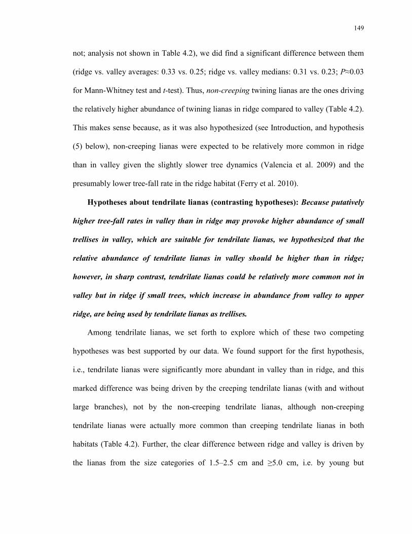
149
not; analysis not shown in Table 4.2), we did find a significant difference between them
(ridge vs. valley averages: 0.33 vs. 0.25; ridge vs. valley medians: 0.31 vs. 0.23; P≈0.03
for Mann-Whitney test and t-test). Thus, non-creeping twining lianas are the ones driving
the relatively higher abundance of twining lianas in ridge compared to valley (Table 4.2).
This makes sense because, as it was also hypothesized (see Introduction, and hypothesis
(5) below), non-creeping lianas were expected to be relatively more common in ridge
than in valley given the slightly slower tree dynamics (Valencia et al. 2009) and the
presumably lower tree-fall rate in the ridge habitat (Ferry et al. 2010).
Hypotheses about tendrilate lianas (contrasting hypotheses): Because putatively
higher tree-fall rates in valley than in ridge may provoke higher abundance of small
trellises in valley, which are suitable for tendrilate lianas, we hypothesized that the
relative abundance of tendrilate lianas in valley should be higher than in ridge;
however, in sharp contrast, tendrilate lianas could be relatively more common not in
valley but in ridge if small trees, which increase in abundance from valley to upper
ridge, are being used by tendrilate lianas as trellises.
Among tendrilate lianas, we set forth to explore which of these two competing
hypotheses was best supported by our data. We found support for the first hypothesis,
i.e., tendrilate lianas were significantly more abundant in valley than in ridge, and this
marked difference was being driven by the creeping tendrilate lianas (with and without
large branches), not by the non-creeping tendrilate lianas, although non-creeping
tendrilate lianas were actually more common than creeping tendrilate lianas in both
habitats (Table 4.2). Further, the clear difference between ridge and valley is driven by
the lianas from the size categories of 1.5–2.5 cm and ≥5.0 cm, i.e. by young but

150
established lianas and by the very old Bauhinia rutilans lianas (Figure 4.2). The cause for
this difference, as we hypothesized, might be that the availability of small trellises—
caused by higher tree-fall rates and to which tendrilate lianas are particularly sensitive
(Putz 1984, Schnitzer and Bongers 2002)—is higher in valley than in ridge, which is
something expected if trees are dying and recruiting a little faster in valley (Valencia et
al. 2009), even though the density of trees in general is lower in valley (Valencia et al.
2004c, Valencia et al. 2009). Tree-fall rates have not been empirically studied in the
YFDP, but given the indirect evidence, we expect them to be higher in valley than in
ridge, similarly to what was observed in the French Guianan forests which also, as in the
YFDP, showed a marked reduction of biomass in bottomlands (Valencia et al. 2009,
Ferry et al. 2010). The presence of small trees, which in the YFDP become increasingly
more abundant as one walks from valleys to ridgetops (Valencia et al. 2004c), has
apparently little effect on the local distribution of tendrilate lianas (see also Ewango
2010)—in other words, it is the intrinsic tree dynamics of a forest, not its static
architecture, what apparently matters.
About branch-twining lianas: Because Hippocrateaceae species are the only ones
that climb by branch-twining, and they mostly occur in ridge, branch-twining lianas
must of course be significantly more abundant in ridge than in valley.
This result was certainly anticipated based on the observed distribution of the
majority of species in Hippocrateaceae, the only family that branch-twines to climb.
Indeed, the difference in the relative proportions of branch-twiners in ridge vs. valley was
highly significant for all but one understory appearance: creeping with no large branches
(Table 4.2). This understory appearance, anyhow, is very rare among Hippocrateaceae

151
(Table 4.2), indicating that in this family creeping and the existence of large branches
(probably stolons) normally occur together. The clear significant difference between
ridge and valley in the per-quadrat proportions of branch-twiners is maintained for all
diameter classes <5 cm (Figure 4.2), although it is considerably stronger (higher P value)
for small lianas that are presumably actively climbing (1.0–1.5 cm). Thus, whatever the
underlying factors that control the distribution of Hippocrateaceae, these are acting
strongly since the plants are very small. The “preference” for ridge habitat of many
members of this family is correlated with relatively low mass-based leaf phosphorous
concentration, high leaf mass per area (low specific leaf area), high leaf dry matter
content and high wood specific gravity (see Chapter 3). In addition, Hippocrateaceae
commonly tend to be free-standing even as old saplings (see above). The conjunction of
all these traits certainly plays a role in determining the spatial distribution of
Hippocrateaceae species in the YFDP forest, but it would be interesting to explore if
these traits also occur in other Neotropical forests, and how these apparent evolutionary
adaptations came about.
Hypothesis about scramblers: Because the understory of Yasuní is apparently
denser than other tropical lowland rainforests in the world, we hypothesized that
scramblers should occur at similar relative abundances in ridge and valley, although
they might be slightly more abundant in valley because of putatively higher abundance
of small trellises there.
There is clear support for this hypothesis in our dataset (Table 4.2). In addition,
scramblers, which contained many less species than twining or tendrilate lianas (see
above), showed a tendency to occur more frequently in valley, but only among creeping

152
lianas (Table 4.2). When the ridge-valley comparisons were made by diameter classes,
there was no difference between habitats at any of the diameter classes (Figure 4.2),
meaning scramblers are widely distributed in the YFDP. In Yasuní, within ridge terra
firme forest, scramblers showed a clear tendency to attach to relatively thin trellises
(Nabe-Nielsen 2001); this is also probably true in valley habitat as well. As mentioned
already, thin trellises might be slightly more frequent in valley than in ridge because of
higher tree dynamism in valley forest (Valencia et al. 2009). Although such presumed
higher abundance of trellis availability in valley seems unimportant for the distribution of
most scramblers, it might anyhow help to explain why Machaerium cuspidatum, the most
common scrambling species, but also the most common species among climbing lianas,
occurs in greater abundance in valley than in ridge (Chapters 1 and 2).
Hypothesis about understory appearance: Either because the valley has a higher
tree-fall rate than the ridge, which may cause more lianas to creep or fall to the
ground, or because lianas that creep in general might be more resilient to falling trees
than those that do not creep, we hypothesized that creeping lianas—particularly if they
have stolons or near-ground branches—should be relatively more abundant in valley
than in ridge.
Although the average and median values shown in Table 4.2 follow what was
expected—i.e., higher proportions in valley than in ridge for creeping lianas, and higher
proportions in ridge than in valley for non-creeping lianas—the only significant
difference between ridge and valley was detected with those creeping lianas that had no
large branches (compare 0.12 in ridge vs. 0.21 in valley; Table 4.2). However, when
creeping lianas as a whole (lianas with and without large branches considered together)

153
and non-creeping lianas as a whole were compared (not shown in Table 4.2), the ridge vs.
valley differences in the average and median per-quadrat proportions became significant
(P=0.02–0.03 for all Mann-Whitney tests and t-tests) and followed the expected trends:
for creeping lianas, higher relative abundance in valley, and for non-creeping lianas,
higher relative abundance in ridge. Therefore, in general, the presence/absence of large
branches was the only variable that was insensitive to the habitat, whereas creeping/non-
creeping appearance and climbing mechanisms seemed to “react” to the environment. In
other words, lianas with large branches, whether creeping or not, were more or less
evenly distributed in the two habitats (Table 4.2). This is in a way similar to what was
observed in Costa Rica where multi-stemmed individuals of lianas showed no trend with
forest age, as opposed to trees which became significantly less multi-stemmed (at DBH
level) in old-growth forests (Letcher and Chazdon 2009). The detected ridge vs. valley
difference among the creeping lianas with no large branches was caused by the lianas in
the size range from 1.5 to 5.0 cm (Figure 4.3), and was most probably driven by the
presence of individuals from three frequent species with strong valley association (see
Chapter 3): Combretum laxum, Bauhinia rutilans and Machaerium cuspidatum (Figure
4.3). In addition, it is evident from Figure 4.3 that when lianas are young (diameter <2.5
cm), they mostly are not creeping and have no large branches, while when they become
old (diameter ≥5.0 cm), they are mostly found creeping and with large branches, although
evidently just a few liana species can reach such large size (e.g., among the most frequent
species: Combretum laxum, Dioclea ucayalina, Machaerium cuspidatum, and
Doliocarpus dentatus).

154
CONCLUSION
We postulated that distinct environmental conditions and distinct tree dynamics in
the ridge and valley habitats of the YFDP constrain the growth strategies that lianas can
use in the forest understory of these two topographically-defined habitats. Because many
liana species have clearly defined or distinct growth strategies, the interaction between
environment and growth strategy may partly explain the differences in species
composition, species abundances, and species diversity observed between these two
dissimilar liana communities (Chapter 2). We found that, in general, the growth strategy
patterns observed were in line with our predictions (hypotheses), which were literature-
based or rationally developed. We conclude that understory growth strategies of lianas,
assessed at a point in time in the long history of a forest, can help to explain the
distribution of liana species because they reflect the concomitant, and time-cumulative,
effects of forest successional processes, tree dynamics (mortality, recruitment and growth
rates, and associated processes such as tree-fall rates) and general forest physiognomy
(particularly the relative abundance of appropriate trellises for lianas).

155
TABLES

156
Table 4.1. Climbing mechanisms, relative abundances (%) and absolute abundances (ABS. ABUND., # individuals) of the most frequent species in 17 ridge quadrats (R) and 13 valley quadrats (V) sampled in the YFDP (each quadrat: 20×20 m). Among the free-standing lianas, the species selected as most frequent were those occurring in at least ≈25% of either the ridge quadrats (≥4 quadrats) OR the valley quadrats (≥3 quadrats). Among the climbing lianas, the species selected as most frequent were those occurring in at least ≈50% of either the ridge quadrats (≥8 quadrats) OR the valley quadrats (≥6 quadrats). For each species, the percentage of individuals in each category was calculated with respect to the total number of individuals of the species (free-standing + climbing individuals). In each species, the largest percentage and those within a 5% range from it appear underlined and in bold, the lowest non-zero percentage and those within a 5% range from it appear in red bold, and zero values appear as blanks. Absolute abundances of free-standing and climbing lianas, as well as habitat association (from Chapter 3), are also shown. Species were sorted by primary climbing mechanism, and then alphabetically by family and scientific name. Species acronyms (in bold) were formed by the three first letters of the genus (in UPPERCASE) and the first three letters of the epithet. The 15 species listed represented 79% of the 286 free-standing lianas found in this study (46 species/morphospecies, all identified at least to family) and 44.6% of the 1378 climbing lianas found in the 30 quadrats sampled (representing 190 species/morphospecies, all identified at least to family). The 176 unidentified/non-collected climbing lianas and the 79 lianas that were neither climbing nor free-standing were excluded from this study (see Methods).
RELATIVE ABUNDANCE (%)
BY DIAMETER CLASSES (cm) of free-standing lianas
RELATIVE ABUNDANCE (%) BY DIAMETER CLASSES (cm)
of climbing lianas
A frequent species...
1.0–1.5 1.5–2.5 2.5–5.0 ≥5.0 1.0–1.5 1.5–2.5 2.5–5.0 ≥5.0
Climbing mechanism
Species (Family)
...among free-
standing lianas?
...among climbing lianas?
R V R V R V R V
R V R V R V R V
ABS. ABUND. among
free-standing
lianas1
ABS. ABUND. among
climbing
lianas1
HABITAT
ASSOCIATION2
Main axis twining
COMbretum laxum
(Combretac.)
yes yes 3.8 8.3 1.5 0.8 0.8
6.0 9.8 6.0 22.6 9.0 12.8 7.5 11.3
20
T 113
T WV
DOLiocarpus dentatus
(Dilleniac.)
no yes
8.3 33.3 8.3 8.3 8.3 33.3
0 12 V
CLItoria pozuzoensis (Fabac.)
yes yes 4.9 1.2 11.1 2.5
12.3 9.9 22.2 17.3 13.6 4.9
16
T 65
T WR
DIOclea ucayalina (Fabac.)
no yes
7.1 28.6 28.6 7.1 28.6
0 14 R
LERetia cordata (Icacinac.)
no yes 4.8
23.8 9.5 4.8 14.3 14.3 23.8 4.8
1 20 G
PETrea maynensis (Verbenac.)
yes yes 13.6 5.9 11.9 1.7 3.4
14.4 5.1 22.0 8.5 11.0 2.5
43
T 75
T R
Tendrils CALlyclamys latifolia (Bignoniac.)
yes yes 3.8 11.5 13.5 13.5 3.8 3.8 1.9
5.8 7.7 11.5 7.7 5.8 9.6
27
T 25
T V
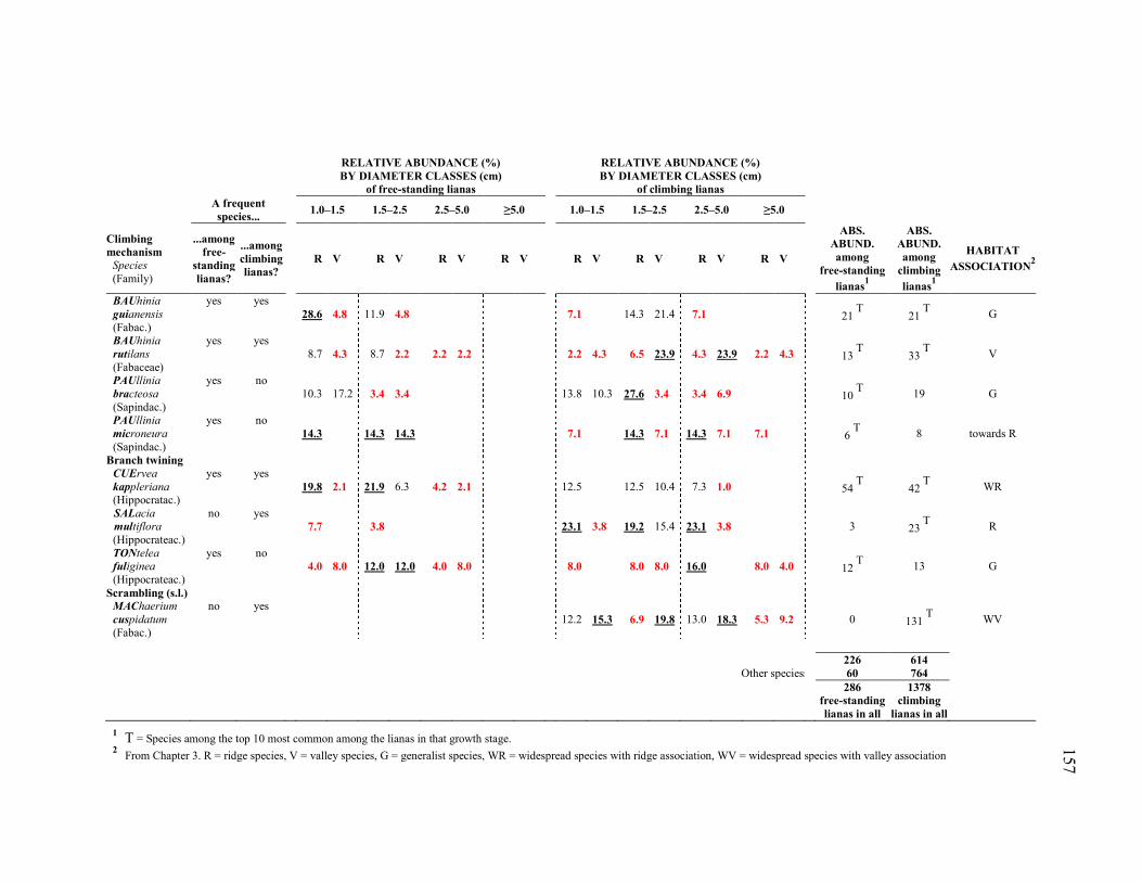
157
RELATIVE ABUNDANCE (%)
BY DIAMETER CLASSES (cm) of free-standing lianas
RELATIVE ABUNDANCE (%) BY DIAMETER CLASSES (cm)
of climbing lianas
A frequent species...
1.0–1.5 1.5–2.5 2.5–5.0 ≥5.0 1.0–1.5 1.5–2.5 2.5–5.0 ≥5.0
Climbing mechanism
Species (Family)
...among free-
standing lianas?
...among climbing lianas?
R V R V R V R V
R V R V R V R V
ABS. ABUND. among
free-standing lianas
1
ABS. ABUND. among
climbing lianas
1
HABITAT ASSOCIATION
2
BAUhinia guianensis (Fabac.)
yes yes 28.6 4.8 11.9 4.8
7.1 14.3 21.4 7.1
21
T 21
T G
BAUhinia rutilans (Fabaceae)
yes yes 8.7 4.3 8.7 2.2 2.2 2.2
2.2 4.3 6.5 23.9 4.3 23.9 2.2 4.3
13
T 33
T V
PAUllinia bracteosa (Sapindac.)
yes no 10.3 17.2 3.4 3.4
13.8 10.3 27.6 3.4 3.4 6.9
10
T 19 G
PAUllinia microneura (Sapindac.)
yes no 14.3 14.3 14.3
7.1 14.3 7.1 14.3 7.1 7.1
6
T 8 towards R
Branch twining CUErvea kappleriana (Hippocratac.)
yes yes 19.8 2.1 21.9 6.3 4.2 2.1
12.5 12.5 10.4 7.3 1.0
54
T 42
T WR
SALacia multiflora (Hippocrateac.)
no yes 7.7 3.8
23.1 3.8 19.2 15.4 23.1 3.8
3 23
T R
TONtelea fuliginea (Hippocrateac.)
yes no 4.0 8.0 12.0 12.0 4.0 8.0
8.0 8.0 8.0 16.0 8.0 4.0
12
T 13 G
Scrambling (s.l.) MAChaerium
cuspidatum
(Fabac.)
no yes
12.2 15.3 6.9 19.8 13.0 18.3 5.3 9.2
0 131
T WV
226 614 Other speciess 60 764 286 1378
free-standing
lianas in all climbing
lianas in all
1 T = Species among the top 10 most common among the lianas in that growth stage.
2 From Chapter 3. R = ridge species, V = valley species, G = generalist species, WR = widespread species with ridge association, WV = widespread species with valley association

158
Table 4.2. Proportions, per-quadrat, of primary climbing mechanisms and understory appearances among climbing lianas in ridge (N=17 20×20 m quadrats) and valley (N=13 quadrats) habitats of the YFDP. Proportions were calculated with respect to the total number of climbing lianas in a quadrat (but excluding unidentified lianas). Mean, median [in brackets] and range (in parentheses) are shown. Statistical differences between ridge and valley groups were assessed via Mann-Whitney (U) and t-tests. To gain readability, the statistics U and t are not shown and P-values are categorized as: P≤0.001(***, extremely significant difference), 0.001<P≤0.01 (**, highly significant difference), 0.01<P≤0.05 (*, significant difference), 0.05<P≤0.10 (NS*, no significant difference, but almost), P>0.10 (NS, no significant difference). P-values of the U test and the t-test in general fell within the same range; when they did not, the P-value category of the t-test is shown below that of the U test. The rare root- and adhesive-tendril climbers are not shown.
CLIMBING MECHANISM
twining tendrils branch-twining scrambling (sensu lato)
ALL CLIMBING MECHANISMS
ridge
valley ridge
valley ridge
valley ridge
valley ridge
valley
UN
DE
RS
TO
RY
AP
PE
AR
AN
CE
cree
pin
g
wit
h la
rge
bra
nch
es 0.11
[0.10] (0.02– 0.27)
NS
0.12 [0.10] (0.02– 0.21)
0.03 [0.03]
(0– 0.12)
*
0.07 [0.08] (0– 0.16)
0.03[0.02]
(0–0.11)
** *
0.01 [0] (0– 0.03)
0.02[0.02]
(0–0.11)
NS* *
0.05 [0.04] (0– 0.15)
0.20 [0.20] (0.05– 0.39)
NS
0.24 [0.25] (0.03– 0.41)
Th
e data in
this b
ox is expan
ded
b
y diam
eter classes in F
igure 4.3
no
larg
e b
ran
ches
0.07 [0.05]
(0– 0.24)
NS
0.09 [0.08] (0– 0.23)
0.03 [0.02]
(0– 0.11)
*
0.06 [0.05] (0– 0.21)
0.002[0](0–
0.02)
NS
0.004 [0] (0– 0.03)
0.02[0](0–
0.09)
* NS*
0.05 [0.04] (0– 0.16)
0.12 [0.11] (0.03– 0.28)
*
0.21 [0.21] (0.05– 0.43)
not
cre
epin
g
wit
h la
rge
bra
nch
es 0.13
[0.12] (0–
0.37)
NS
NS*
0.07 [0.07] (0– 0.13)
0.07 [0.06]
(0– 0.17)
NS
0.07 [0.07] (0– 0.14)
0.05[0.05]
(0–0.14)
*
0.02 [0.02] (0– 0.05)
0.02[0](0–
0.13)
NS
0.03 [0.03] (0– 0.11)
0.27 [0.29] (0.03– 0.53)
NS
0.20 [0.17] (0.05– 0.33)
no
larg
e b
ran
ches
0.20 [0.19] (0.05– 0.43)
NS
0.18 [0.16] (0.04– 0.41)
0.08 [0.06]
(0– 0.30)
NS
0.10 [0.09] (0.02– 0.22)
0.06[0.05]
(0–0.23)
** *
0.02 [0] (0– 0.08)
0.06[0.05]
(0–0.14)
NS
0.05 [0.05] (0– 0.10)
0.41 [0.37] (0.12– 0.73)
NS
0.35 [0.33] (0.13– 0.73)
ALL APPEARANCES
0.52 [0.55] (0.23– 0.66)
* NS*
0.45 [0.43] (0.36– 0.56)
0.21 [0.18] (0.13– 0.36)
**
0.30 [0.30] (0.20– 0.42)
0.15[0.14]
(0–0.41)
*** **
0.05 [0.04] (0– 0.14)
0.12[0.10](0.02–0.25)
NS*
0.18 [0.20] (0.05– 0.33)
1
1
The data in this box is expanded by diameter classes in Figure 4.2

159
FIGURES

160
Figure 4.1. Sixteen schematic graphical examples of whole-individual growth strategies of climbing lianas in the low forest understory, as used in this study. The “trellises” (supports for climbing) used by the lianas are not shown. These strategies result from the combination of four climbing mechanisms (twining, tendrils, branch-twining and scrambling sensu lato) and four understory appearances defined by the presence/absence of creeping stems and the presence/absence of large branches (branches ≥1 cm in diameter) near ground-level. Our “scrambling s.l.” category includes climbers with hooks or spines and sprawlers in general. A creeping stem can either be the main stem or a branch, but creeping branches are not shown in this Figure to gain clarity (also, note that a non-creeping liana may have underground runner stems nonetheless). Root-climbers and adhesive-tendril climbers are not shown. Many aspects in the figure are not drawn to scale nor are biologically precise. Understory appearance was characterized from what could be observed up to an approximate height of 3 m.

161
Figure 4.2. Proportions of primary climbing mechanisms by diameter classes among climbing lianas in ridge (N=17 20×20 m quadrats) and valley (N=13 quadrats) habitats of the YFDP. Root-climbers and adhesive-tendril climbers are not shown because they were very rare. The proportion of lianas of a given climbing mechanism in a given diameter class, in a given quadrat, was calculated with respect to the total number of climbing lianas of the given diameter class in the quadrat (but excluding unidentified lianas). Statistical differences between ridge and valley groups were evaluated via Mann-Whitney and t-tests, but because the P ranges of both tests were always similar, only Mann-Whitney results (U) are shown. Thin-lined boxplots and their corresponding open circles represent ridge quadrats, while thick-line boxplots and their corresponding filled circles represent valley quadrats. When a frequent species among the climbing lianas (“C” species of Table 4.1) had at least two individuals in a given diameter class in a given habitat, its acronym is shown in the Figure (acronyms ordered as in Table 4.1). P-values are categorized as: P≤0.001(***, extremely significant difference), 0.001<P≤0.01 (**, highly significant difference), 0.01<P≤0.05 (*, significant difference), P>0.05 (no significant difference).

162
Figure 4.3. Proportions of understory appearances by diameter classes among climbing lianas in ridge (N=17 20×20 m quadrats) and valley (N=13 quadrats) habitats of the YFDP. Root-climbers and adhesive-tendril climbers are not shown because they were very rare. The proportion of lianas of a given understory appearance in a given diameter class, in a given quadrat, was calculated with respect to the total number of climbing lianas of the given diameter class in the quadrat (but excluding unidentified lianas). Statistical differences between ridge and valley groups were evaluated via Mann-Whitney and t-tests, but because the P ranges of both tests were always similar, only Mann-Whitney results (U) are shown. Thin-lined boxplots and their corresponding open circles represent ridge quadrats, while thick-line boxplots and their corresponding filled circles represent valley quadrats. When a frequent species among the climbing lianas (“C” species of Table 4.1) had at least two individuals in a given diameter class in a given habitat, its acronym is shown (acronyms ordered as in Table 4.1). P-values are categorized as: P≤0.001(***, extremely significant difference), 0.001<P≤0.01 (**, highly significant difference), 0.01<P≤0.05 (*, significant difference), P>0.05 (no significant difference).

163
CHAPTER 5: Conclusion
In the Yasuní Forest Dynamics Plot (YFDP), I have demonstrated that the liana
community (diameter ≥1 cm) in ridge habitat is different from the community in valley
habitat in at least two respects: community structure (understood as the composition and
abundance of species) and species diversity. Why does this difference exist? If one
assumes it is the environment that controls the distribution of plants, this pattern is not
surprising given the suspected biogeochemical differences that certainly exist between
ridge and valley (from valley to ridgetop, there is an altitudinal difference of 20‒30 m).
But there is a diametrically opposite alternative: one can assume what controls the
distribution of plants are plants themselves (e.g., via competition) or the activity of
animals (e.g., via dispersal and herbivory). This classic ecological dilemma is unsolvable
because the truth, as many studies have shown, lies somewhere in the middle and it is
always relative to the system, the spatiotemporal scale under study, and the amount of
information available. Given the paucity of information about the lianas within the
YFDP, in this dissertation I tackled the problem of explaining the ridge vs. valley
difference by focusing on one specific part of the conundrum: the relationship between
the differential spatial distribution and abundance of liana species in ridge and valley
habitats and the functional traits they exhibit, or express, in these habitats. In other words,
my over-arching question was: To what extent is the observed spatial distribution of
lianas in the YFDP forest explained by the characteristics of the different species?
The functional traits sampled in the present study were classified into two groups:
quantitative traits (continuous variables) and qualitative traits (categorical variables). The
quantitative traits included those commonly measured in plants: specific leaf area (SLA),

164
leaf dry matter content (LDMC), leaf morphometry (lamina thickness, length:width ratio,
leaf size), leaf carbon (C), nitrogen (N), and phosphorus (P) concentrations, leaf 13C and
15N isotopic signatures, wood specific gravity (WSG) and stem growth rate (in diameter).
The qualitative traits, on the other hand, were particular to lianas and described the
strategy used by a liana, as a whole plant, to grow in the understory of the forest; these
included: whether a liana was growing as a free-stander or as a climber, its climbing
mechanism (twining, tendrils, branch-twining, scrambling [sensu lato], and adhesive
roots/tendrils) and its understory appearance (creeping liana with large understory
branches [usually stolons], creeping liana with no large understory branches, non-
creeping liana with large understory branches, and non-creeping liana with no large
understory branches).
I found that because the trait expression patterns of a group of related species
(species within the same family or genus) is often different from the expresssion patterns
of another group of related species, the generalization of trait expression to the whole
ridge or valley commnunities must be made cautiously. In fact, not all traits showed a
distinctive pattern between ridge and valley. In the subset of common species that had a
clear habitat association to either ridge or valley, I found that ridge species had a lower
SLA and leaf P concentration, but higher WSG, than valley species. The other traits did
not show any clear differential pattern, although there is a trend for LDMC to be higher
among ridge species (expected, given the low SLA among them). In addition, I found that
the ability to be free-standing as an old sapling (diameter ≥1 cm) is only typical of very
few liana species, while in the rest it occurs sporadically (and rarely among twining
lianas and practically never among scrambling lianas). I also found that tendrilate lianas

165
and creeping lianas were significantly more common in valley, while branch-twining
lianas and main stem-twining lianas were significantly more common on ridge. The
presence or absence of understory branches in lianas occurred randomly and did not show
any particular pattern associated with habitat.
The patterns above mentioned constitute the main “discoveries” of this doctoral
dissertation and those for which I sought to find an explanation in the Discussion sections
of the different data Chapters. I focused mostly on the role of the environment
(particularly soil characteristics and canopy openness) and the observed tree dynamics
(mortality, recruitment and growth rates), and offered some rational arguments why these
may be relevant to explain the observed distribution of lianas in the YFDP. I hope this
treatise on the lianas of the Yasuní Forest Dynamics Plot motivates more in-depth studies
about the distribution problem (why some species of lianas are differentially distributed
along the ridge-valley topographic gradient) and the diversity problem (why so many
species coexist in such a reduced space).

166
LITERATURE CITED
Acurio, A., V. Rafael, and O. Dangles. 2010. Biological invasions in the Amazonian tropical rain forest: The case of Drosophilidae (Insecta, Diptera) in Ecuador, South America. Biotropica 42:717‒723.
Aguilar, Z. 2002. Estudio de la floración a nivel de comunidad de un bosque de tierra firme en la Amazonía ecuatoriana (Tesis de Licenciatura). Quito: Pontificia Universidad Católica del Ecuador.
Altamirano, D.C. 2009. Biomasa aérea y variación de la densidad básica de la madera en especies dominantes del bosque de Yasuní, Amazonía ecuatoriana (Tesis de Licenciatura). Quito: Pontificia Universidad Católica del Ecuador.
Alvira, D., F.E. Putz, and T.D. Fredericksen. 2004. Liana loads and post-logging liana densities after liana cutting in a lowland forest in Bolivia. Forest Ecology and Management 190:73–86.
Balslev, H., J. Luteyn, B. Ollgaard, and L.B. Holm-Nielsen. 1987. Composition and structure of adjacent unflooded and floodplain forest in Amazonian Ecuador. Opera Botanica 92:37–57.
Barriga, P. 2002. Influencia del suelo y la luz en la germinacion de seis especies de Cecropia de la Amazonia ecuatoriana (Tesis de Licenciatura). Quito: Pontificia Universidad Católica del Ecuador.
Bass, M.S., M. Finer, C.N. Jenkins, H. Kreft, D.F. Cisneros-Heredia, S.F. McCracken, N.C.A. Pitman, P.H. English, K. Swing, G. Villa, A. Di Fiore, C.C. Voigt, and T.H. Kunz. 2010. Global conservation significance of Ecuador's Yasuní National Park. Plos One 5:e8767.doi:10.1371/journal.pone.0008767.
Baulfor, D.A. and W.J. Bond. 1993. Factors limiting climber distribution and abundance in a southern African forest. Journal of Ecology 81:93–99.
Beckerman, S., P.I. Erickson, J. Yost, J. Regalado, L. Jaramillo, C. Sparks, M. Iromenga, and K. Long. 2009. Life histories, blood revenge, and reproductive success among the Waorani of Ecuador. Proceeding of the United States National Academy of Sciences (PNAS) 106:8134‒8139.
Bongers, F., F.A Schnitzer, and D. Taore. 2002. The importance of lianas and consequences for forest management in west Africa. Bioterre No. spécial:59–70.
Burnham, R.J. 2002. Dominance, diversity and distribution of lianas in Yasuní, Ecuador: who is on top? Journal of Tropical Ecology 18:845–864.
Burnham, R.J. 2004. Alpha and beta diversity of lianas in Yasuní, Ecuador. Forest Ecology and Management 190:43–55.
Burnham, R.J. 2004. Alpha and beta diversity of Lianas in Yasuní, Ecuador. Forest Ecology and Management 190:43–55.

167
Caballé, G. 1994. Ramet proliferation by longitudinal splitting in the Gabonese rain forest liana Dalhousiea africana S. Moore (Papilionaceae). Biotropica 26:266–275.
Cai, Z.-Q., L. Poorter, K. Cao, and F. Bongers. 2007. Seedling growth strategies in Bauhinia species: Comparing lianas and trees. Annals of Botany 100:831–838.
Cai, Z.-Q., S.A. Schnitzer, B. Wen, Y. Chen, and F. Bongers. 2009. Liana communities in three tropical forest types in Xishuagbanna, south-west China. Journal of Tropical Forest Science 21:252–264.
Cárate, D. 2005. Ciclos fenológicos y producción de frutos de quince especies de árboles dentro de una parcela de una hectárea en el Parque Nacional Yasuní, Amazonía ecuatoriana (Tesis de Licenciatura). Quito: Pontificia Universidad Católica del Ecuador.
Castellanos, A.E., R. Duran, S. Guzmán, O. Briones, and M. Feria. 1992. Three-dimensional space utilization of lianas: A methodology. Biotropica 24:396–401.
Cerón, C. and C. Montalvo. 1997. Composición de una hectárea de bosque en la comunidad Huaorani de Quehueiri-Ono, zona de amortiguamiento del Parque Nacional Yasuní, Napo, Ecuador. P. 279–298 in Estudios biológicos para la conservación, edited by P.A. Mena. Quito: EcoCiencia.
Chave, J., R. Condit, H.C. Muller-Landau, S.C. Thomas, P.S. Ashton, S. Bunyavejchewin, L.L. Co, H.S. Dattaraja, S.J. Davies, S. Esufali, C.E.N. Ewango, K.J. Feeley, R.B. Foster, N. Gunatilleke, S. Gunatilleke, P. Hall, T.B. Hart, C. Hernández, S.P. Hubbell, A. Itoh, S. Kiratiprayoon, J.V. LaFrankie, S. Loo de Lao, J.-R. Makana, N.S. Noor, A.R. Kassim, C. Samper, R. Sukumar, H.S. Suresh, S. Tan, J. Thompson, M.D.C. Tongco, R. Valencia, M. Vallejo, G. Villa, T. Yamakura, J.K. Zimmerman, and E.C. Losos. 2008. Assessing evidence for a pervasive alteration in tropical tree communities. Plos Biology 6:e45.
Clark, D.A. 2004. Tropical forests and global warming: slowing it down or speeding it up? Frontiers in Ecology and the Environment 2:73‒80.
Clarke, K.R. 1993. Non-parametric multivariate analysis of changes in community structure. Australian Journal of Ecology 18:117–143.
Colwell, R.K. 2009. “EstimatesS: Statistical estimation of species richness and shared species from samples. Version 8.2.” (http://purl.oclc.org/estimates).
Colwell, R.K., C.X. Mao, and J. Chang. 2004. Interpolating, extrapolating, and comparing incidence-based species accumulation curves. Ecology 85:2717–2727.
Condit, R., N. Pitman, E.G. J. Leigh, J. Chave, J. Terborgh, R.B. Foster, P. Nuñez V., S. Aguilar, R. Valencia, G. Villa, H.C. Muller-Landau, E. Losos, and S.P. Hubbell. 2002. Beta-diversity in tropical forest trees. Science 295:666‒669.

168
Cornelissen, J.H.C., S. Lavorel, E. Garnier, S. Díaz, N. Buchmann, D.E. Gurvich, P.B. Reich, H. ter Steege, H.D. Morgan, M.G.A. van der Heijden, J.G. Pausas, and H. Poorter. 2003. A handbook of protocols for standardised and easy measurement of plant functional traits worldwide. Australian Journal of Botany 51:335–380.
CTFS. 2010. “Center for Tropical Forest Science, Smithsonian Tropical Research Institute.” (http://www.ctfs.si.edu/).
DeWalt, S.J., K. Ickes, R. Nilus, K.E. Harms, and D.F.R.P. Burslem. 2006. Liana habitat associations and community structure in a Bornean lowland tropical forest. Plant Ecology 186:203–216.
DeWalt, S.J., S.A. Schnitzer, J. Chave, F. Bongers, R.J. Burnham, Z. Cai, G. Chuyong, D.B. Clark, C.E.N. Ewango, J.J. Gerwing, E. Gortaire, T. Hart, G. Ibarra-Manríquez, K. Ickes, D. Kenfack, M.J. Macía, J.R. Makana, M. Martínez-Ramos, J. Mascaro, S. Moses, H.C. Muller-Landau, M.P.E. Parren, N. Parthasarathy, D.R. Pérez-Salicrup, F.E. Putz, H. Romero-Saltos, and D. Thomas. 2010. Annual rainfall and seasonality predict pan-tropical patterns of liana density and basal area. Biotropica 42:309–317.
DeWalt, S., S.A. Schnitzer, and J. Denslow. 2000. Density and diversity of lianas along a chronosequence in a central Panamanian lowland forest. Journal of Tropical Ecology 16:1–19.
Duivenvoorden, J.F. 1995. Tree species composition and rain forest-environment relationships in the middle Caquetá Area, Colombia, NW Amazonia. Vegetatio 120:91‒113.
Duque, A.J., J.F. Duivenvoorden, J. Cavelier, A. García, C. Grández, M.J. Macía, H. Romero-Saltos, and R. Valencia. 2004b. Response shape of plant genera and species along gradients in NW Amazonia. P. 87‒101 in Plant diversity scaled by growth forms along spatial and environmental gradients: A study in the rain forests of NW Amazonia (Ph.D. dissertation, Chapter 7). Amsterdam: University of Amsterdam and TROPENBOS International.
Duque, A.J., J.F. Duivenvoorden, M. Sánchez, J. Cavelier, H. Romero-Saltos, R. Valencia, M.J. Macía, C. Grández, and A. García. 2004a. Diversity and composition of woody lianas in NW Amazonia. P. 69‒84 in Plant diversity scaled by growth forms along spatial and environmental gradients: A study in the rain forests of NW Amazonia (Ph.D. dissertation, Chapter 6). Amsterdam: University of Amsterdam and TROPENBOS International.
ECOLAP and MAE. 2007. Guía del Patrimonio de Áreas Naturales Protegidas del Ecuador. Quito: Ministerio del Ambiente del Ecuador, ECOFUND, FAN, DarwinNet, IGM.
Ewango, C. 2010. The liana assemblage of a Congolian rainforest: diversity, structure and dynamics (Ph.D. dissertation). Wageningen: Wageningen University.

169
Ferry, B., F. Morneau, J.D. Bontemps, L. Blanc, and V. Freycon. 2010. Higher treefall rates on slopes and waterlogged soils result in lower stand biomass and productivity in a tropical rain forest. Journal of Ecology 98:106–116.
Finer, M., R. Moncel, and C.N. Jenkins. 2010. Leaving the oil under the Amazon: Ecuador´s Yasuní-ITT initiative. Biotropica 42:63‒66.
Finer, M., V. Vijay, F. Ponce, C.N. Jenkins, and T.R. Kahn. 2009. Ecuador´s Yasuní Biosphere Reserve: a brief modern history and conservation challenges. Environmental Research Letters 4:1‒15.
Fisher, R.A., A.S. Corbet, and C.B. Williams. 1943. The relation between the number of species and the number of individuals in a random sample of an animal population. Journal of Animal Ecology 12:42–58.
Fisher, J.B. and F.W. Ewers. 1991. Structural response to stem injury in vines. P. 99–124 in The biology of vines, edited by F. Putz and H.A. Mooney. Cambridge: Cambridge University Press.
Fiske, C.H. and Y. SubbaRow. 1925. The colorimetric determination of phosphorus. The Journal of Biological Chemistry 66:375-400.
Ford, E.D. 2000. Scientific Method for Ecological Research. Cambridge: Cambridge University Press.
Gallenmüller, F., U. Müller, N. Rowe, and T. Speck. 2001. The growth form of Croton pullei (Euphorbiaceae) - Functional morphology and biomechanics of a Neotropical liana. Plant biology 3:50–61.
Gallenmüller, F., N. Rowe, and T. Speck. 2004. Development and growth form of the neotropical liana Croton nuntians: the effect of light and mode of attachment on the biomechanics of the stem. Journal of Plant Growth and Regulation 23:83–97.
Garwood, N.C. 2008. “Biodiversity basics strengthening sustainability of the Yasuní Amazonian Rainforest, Ecuador.” Final Report of a project funded by the Darwin Initiative for the Survival of Species (2001‒2005), The Natural History Museum (United Kingdom) and Pontificia Universidad Católica del Ecuador (Ecuador).
Gause, G.F. 1937. Experimental populations of microscopic organisms. Ecology 18:173–179.
Gentry, A.H. 1982. Patterns of neotropical plant species diversity. Evolutionary Biology 15:1–84.
Gentry, A.H. 1991. The distribution and evolution of climbing plants. P. 3–49 in The biology of vines. Cambridge, New York: Cambridge University Press.
Gerwing, J.J., S.A. Schnitzer, R.J. Burnham, F. Bongers, J. Chave, S.J. DeWalt, C.E.N. Ewango, R. Foster, D. Kenfack, M. Martínez-Ramos, M. Parren, N. Parthasarathy, D.R. Pérez-Salicrup, F.E. Putz, and D.W. Thomas. 2006. A standard protocol for liana censuses. Biotropica 38:256–261.

170
Gotelli, N.J. and R.K. Colwell. 2001. Quantifying biodiversity: procedures and pitfalls in the measurement and comparison of species richness. Ecology Letters 4:379–391.
Gotelli, N.J. and R.K. Colwell. 2010. Estimating species richness. P. 39–54 in Biological diversity: Frontiers in measurement and assessment, edited by A.E Magurran and B.J. McGill. United Kingdom: Oxford University Press.
Gotelli, N.J. and A.M. Ellison. 2004. A primer of ecological statistics. Sunderland: Sinauer Associates, Inc.
Hammer, Ø. 2010. “PAST: PAleontological STatistics Reference Manual (version 1.97). Natural History Museum, Norway.” (http://folk.uio.no/ohammer/past/).
Hammer, Ø., D.A.T. Harper, and P.D. Ryan. 2001. PAST: Paleontological Statistics Software Package for Education and Data Analysis. Paleontological Electronica 4:9 pp. http://palaco-electronica.org/2001_1/past/issue1_01.htm. http://folk.uio.no/ohammer/past/.
Harms, K.E., R. Condit, S.P. Hubell, and R.B. Foster. 2001. Habitat associations of trees and shrubs in a 50-ha neotropical forest plot. Journal of Ecology 89:947–959.
Holbrook, K.M. and B.A. Loiselle. 2009. Dispersal in a Neotropical tree, Virola flexuosa (Myristicaceae): Does hunting of large vertebrates limit seed removal? Ecology 90:1449‒1455.
Hubbell, S.P. 2001. The unified neutral theory of biodiversity and biogeography. Princeton: Princeton University Press.
Hubbell, S.P. 2004. Two decades of research on the BCI Forest Dynamics Plot. P. 8‒30 in Tropical forest diversity and dynamism - Findings from a large-scale plot network. Chicago: The University of Chicago Press.
Ingwell, L.L., S.J. Wright, K.K. Becklund, S.P. Hubbell, and S.A. Schnitzer. 2010. The impact of lianas on 10 years of tree growth and mortality on Barro Colorado Island, Panama. Journal of Ecology 98:879–887.
Isnard, S. and W.K. Silk. 2009. Moving with climbing plants from Charles Darwin´s time into the 21st century. American Journal of Botany 96:1205–1221.
Jirka, S., M. McDonald, M. Johnson, T. Feldpausch, E.G. Couto, and S.J. Riha. 2007. Relationships between soil hydrology and forest structure and composition in the southern Brazilian Amazon. Journal of Vegetation Science 18:183–194.
John, R., J.W. Dalling, K.E. Harms, J.B. Yavitt, R.F. Stallard, M. Mirabello, S.P. Hubell, R. Valencia, H. Navarrete, M. Vallejo, and R.B. Foster. 2007. Soil nutrients influence spatial distribution of tropical tree species. Proceedings of the National Academy of Sciences of the United States of America 104:864–869.
Jongman, R.H.G., C.J.F. ter Braak, and O.F.R. van Tongeren, eds. 1995. Data analysis in community and landscape ecology. Cambridge: Cambridge University Press.

171
Jørgensen, P.M. and S. León-Yánez. 1999. Catalogue of the vascular plants of Ecuador. Monographs in Systematic Botany of the Missouri Botanical Garden 75:i–viii, 1–1182.
Kalra, Y., ed. 1998. Handbook of reference methods for plant analysis. Boca Raton: CRC Press.
Kazda, M. and J. Salzer. 2000. Leaves of lianas and self-supporting plants differ in mass per unit area and in nitrogen content. Plant Biology 2:268–271.
Kennard, D.K. 1998. Biomechanical properties of tree saplings and free-standing lianas as indicators of susceptibility to logging damage. Forest Ecology and Management 102:179–191.
Korning, J. and H. Balslev. 1994. Growth and mortality of trees in Amazonian tropical rain forest in Ecuador. Journal of Vegetation Science 4:77–86.
Koski, M.H. 2009. Climbing through changing forests: is liana diversity or morphology affected by forest age or precipitation? (Senior Honors Thesis). Ann Arbor: University of Michigan.
Kraft, N.J.B. 2008. Functional trait and phylogenetic-based tests of community assembly in an Amazonian forest (Ph.D. dissertation). Berkeley: University of California.
Kraft, N.J.B. and D.D. Ackerly. 2010. Functional trait and phylogenetic tests of community assembly across spatial scales in an Amazonian forest. Ecological Monographs 80:401–422.
Kraft, N.J.B., W.K. Cornwell, C.O. Webb, and D.D. Ackerly. 2007. Trait evolution, community assembly, and the phylogenetic structure of ecological communities. The American Naturalist 170:271–283.
Kraft, N.J., M.R. Metz, R.S. Condit, and J. Chave. 2010. The relationship between wood density and mortality in a global tropical forest data set. New Phytologist 1–13.
Kraft, N.J.B., R. Valencia, and D.A. Ackerly. 2008. Functional traits and niche-based tree community assembly in an Amazonian forest. Science 322:580–582.
Kreft, H., N. Köster, W. Küper, J. Nieder, and W. Barthlott. 2004. Diversity and biogeography of vascular epiphytes in Western Amazonia, Yasuní, Ecuador. Journal of Biogeography 31:1463‒1476.
Kubota, Y., H. Murata, and K. Kikuzawa. 2004. Effects of topographic heterogeneity on tree species richness and stand dynamics in a subtropical forest in Okinawa Island, southern Japan. Journal of Ecology 92:230–240.
Lahaye, R., L. Civeyrel, T. Speck, and N.P. Rowe. 2005. Evolution of shrub-like growth forms in the lianoid subfamily Secamonoideae (Apocynaceae s.l.) of Madagascar: phylogeny, biomechanics and development. American Journal of Botany 92:1381–1396.
Lepš, J. and P. Šmilauer. 2003. Multivariate analysis of ecological data using CANOCO. Cambridge: Cambridge University Press.

172
Letcher, S.G. and R.L. Chazdon. 2009. Lianas and self-supporting plants during tropical forest succession. Forest Ecology and Management 257:2150–2156.
Lindner, R.C. and C.P. Harley. 1942. A rapid method for the determination of nitrogen in plant tissue. Science 96:565–566.
Lips, J.L. and J.F Duivenvoorden. 2001. La Amazonía noroccidental: caracterización ambiental. P. 19–45 in Evaluación de productos forestales no maderables en la Amazonía noroccidental, edited by J.F. Duivenvoorden, H. Balslev, J. Cavelier, C. Grandes, H. Tuomisto, and R. Valencia. Amsterdam: IBED, Universiteit van Amsterdam.
Lombardi, J.A. 2006. A new species of Tontelea from Amazonian Peru and Ecuador, and notes on the Tontelea attenuata species group (Celastraceae, Hippocrateoideae). Brittonia 58:52–58.
MacArthur, R. and R. Levins. 1967. The limiting similarity, convergence, and divergence of coexisting species. The American Naturalist 101:377–385.
Macía, M.J. and J.-C. Svenning. 2005. Oligarchic dominance in western Amazonian plant communities. Journal of Tropical Ecology 21:613–626.
Madeira, B.G., M.M. Espírito-Santo, S.D'A. Neto, Y.R.F. Nunes, G.A. Sánchez Azofeifa, G.W. Fernandes, and M. Quesada. 2009. Changes in tree and liana communities along a successional gradient in a tropical dry forest in south-eastern Brazil. Plant Ecology 201:291–304.
Malhi, Y., T.R. Baker, O.L. Phillips, S. Almeida, E. Alvarez, L. Arroyo, J. Chave, I. Czimczik, A. Di Fiore, N. Higuchi, T.J. Killeen, S.G. Laurance, W.F. Laurance, S.L. Lewis, L.M. Mercado Montoya, A. Monteagudo, D.A. Neill, P. Nuñez Vargas, S. Patiño, J.N.M. Silva, A. Torres Lezama, R. Vásquez Martínez, J. Terborgh, B. Vinceti, and J. Lloyd. 2004. The above-ground coarse wood productivity of 104 Neotropical forest plots. Global Change Biology 10:563–591.
Mao, C.X., R.K. Colwell, and J. Chang. 2005. Estimating species accumulation curves using mixtures. Biometrics 61:433–441.
Marx, E. 2010. The fight for Yasuni. Science 330:1170‒1171.
Mascaro, J., S.A. Schnitzer, and W.P. Carson. 2004. Liana diversity, abundance, and mortality in a tropical wet forest in Costa Rica. Forest Ecology and Management 190:3–14.
Mast, R.B., C.G. Mittermeier, R.A. Mittermeier, J.V. Rodríguez-Mahecha, and A.H. Hemphill. 1997. Ecuador. P. 314‒324 in Megadiversity: Earth’s Biologically Wealthiest Nations, edited by R.A. Mittermeier, P. Robles Gil, and C.G. Mittermeier. Monterrey, Mexico: CEMEX and Conservation International.
Metz, M.R. 2007. Spatiotemporal variation in seedling dynamics and the maintenance of diversity in an Amazonian forest (Ph.D. dissertation). Berkeley: University of California.

173
Metz, M.R., L.S. Comita, Y.-Y. Chen, N. Norden, R. Condit, S.P. Hubbell, I.F. Sun, N.S. b. M. Noor, and S.J. Wright. 2008. Temporal and spatial variability in seedling dynamics: a cross-site comparison in four lowland tropical forests. Journal of Tropical Ecology 24:9‒18.
Metz, M.R., W.P. Sousa, and R. Valencia. 2010. Widespread density-dependent seedling mortality promotes species coexistence in a highly diverse Amazonian rain forest. Ecology 91:3675‒3685.
Miller, R.O., ed. 1997. Western states laboratory proficiency testing program - Soil and plant analytical methods - Version 4.00.
Moffett, M.W. 2000. What´s “up” ? A critical look at the basic terms of canopy biology. Biotropica 32:569–596.
Montúfar, R. 1999. Influencia de factores edáficos en la distribución y abundancia de diez especies de palmas en el Parque Nacional Yasuní, Amazonía ecuatoriana (Tesis de Licenciatura). Quito: Pontificia Universidad Católica del Ecuador.
Montúfar, R. and J.-C. Pintaud. 2006. Variation in species composition, abundance and microhabitat preferences among western Amazonian terra firme palm communities. Botanical Journal of the Linnean Society 151:127‒140.
Moscoso, M.A. 2010. Taxonomía y distribución de Calyptranthes Sw. (Myrtaceae) en Ecuador (Tesis de Licenciatura). Quito: Pontificia Universidad Católica del Ecuador.
Nabe-Nielsen, J. 2001. Diversity and distribution of lianas in a Neotropical rain forest, Yasuni National Park, Ecuador. Journal of Tropical Ecology 17:1–19.
Nabe-Nielsen, J. 2002. Growth and mortality rates of the liana Machaerium cuspidatum in relation to light and topographic position. Biotropica 34:319–322.
Nabe-Nielsen, J. 2004. Demography of Machaerium cuspidatum, a shade-tolerant Neotropical liana. Journal of Tropical Ecology 20:505–516.
Nabe-Nielsen, J. and P. Hall. 2002. Environmentally induced clonal reproduction and life history traits of the liana Machaerium cuspidatum in an Amazonian rain forest, Ecuador. Plant Ecology 162:215–226.
Niklas, K.J. 1994. Comparisons among biomass allocation and spatial distribution patterns of some vine, Pteridophyte, and Gymnosperm shoots. American Journal of Botany 81:1416–142.
Palmer, M.W. 1994. Variation in species richness: towards a unification of hypotheses. Folia Geobotanica & Phytotaxonomica 29:511–530.
Paul, G.S. and J.B. Yavitt. 2011. Tropical vine growth and the effects on forest succession: A review of the ecology and management of tropical climbing plants. The Botanical Review 77:11–30.

174
Payton, M.E., M.H. Greenstone, and N. Schenker. 2003. Overlapping confidence intervals or standard error intervals: What do they mean in terms of statistical significance? Journal of Insect Science 3:34. insectscience.org/3.34.
Peña-Claros, M., T.S. Fredericksen, A. Alarcón, G.M. Blate, U. Choque, C. Leaño, J.C. Licona, B. Mostacedo, W. Pariona, Z. Villegas, and F.E. Putz. 2008. Beyond reduced-impact logging: Silvicultural treatments to increase growth rates of tropical trees. Forest Ecology and Management 256:1458–1467.
Peñalosa, J. 1984. Basal branching and vegetative spread in tropical rain forest lianas. Biotropica 16:1–9.
Pérez-Salicrup, D.R. and M.G. Barker. 2000. Effect of liana cutting on water potential and growth of adult Senna multijuga (Caesalpinioideae) trees in a Bolivian tropical forest. Oecologia 124:469–475.
Pérez-Salicrup, D.R., S.A. Schnitzer, and F.E. Putz. 2004. Community ecology and management of lianas (Editorial). Forest Ecology and Management (Special Issue) 190:1–2.
Persson, V. 2005. Effects of climatic seasonality on reproductive phenology of tropical forest plants (Ph.D. dissertation). Aberdeen: The University of Aberdeen.
Phillips, O.L., T.R. Baker, L. Arroyo, N. Higuchi, T.J. Killeen, W.F. Laurance, S.L. Lewis, J. Lloyd, Malhi. Y., A. Monteagudo, D.A. Neill, P. Nuñez Vargas, J.N.M. Silva, J. Terborgh, R. Vásquez Martínez, M. Alexiades, S. Almeida, S. Brown, J. Chave, J.A. Comiskey, C.I. Czimczik, A. Di Fiore, T. Erwin, C. Kuebler, S.G. Laurance, H.E.M. Nascimento, J. Olivier, W. Palacios, S. Patiño, N.C.A. Pitman, C.A. Quesada, M. Saldias, A. Torres Lezama, and B. Vinceti. 2004. Pattern and process in Amazon tree turnover,1976-2001. Philosophical Transactions of the Royal Society of London B: Biological Sciences 359:381–407.
Phillips, O.L., R. Vásquez Martínez, L. Arroyo, T.R. Baker, T. Killeen, S.L. Lewis, Y. Malhi, A. Monteagudo Mendoza, D. Neill, P. Núñez Vargas, M. Alexiades, C. Cerón, A. Di Fiore, T. Erwin, A. Jardim, W. Palacios, M. Saldias, and B. Vinceti. 2002. Increasing dominance of large lianas in Amazonian forests. Nature 418:770–774.
Pitman, N.C.A. 2000. A large-scale inventory of two Amazonian tree communities (Ph.D. dissertation). Duke: Duke University.
Pitman, N.C.A. 2000. A large-scale inventory of two Amazonian tree communities (Ph.D. dissertation). Duke: Duke University.
Pitman, N., H. Mogollón, N. Dávila, M. Ríos, R. García-Villacorta, J. Guevara, T.R. Baker, A. Monteagudo, O.L. Phillips, R. Vásquez-Martínez, M. Ahuite, M. Aulestia, D. Cardenas, C.E. Cerón, P-A. Loizeau, D.A. Neill, P. Nuñez V., W.A. Palacios, R. Spichiger, and E. Valderrama. 2008. Tree community change across 700 km of lowland Amazonian forest from the Andean foothills to Brazil. Biotropica 40:525‒535.

175
Pitman, N.C.A., J.W. Terborgh, M.R. Silman, P. Núñez V., D.A. Neill, C.E. Cerón, W.A. Palacios, and M. Aulestia. 2002. A comparison of tree species diversity in two upper Amazonian forests. Ecology 83:3210‒3224.
Pitman, N.C.A., J.W. Terborgh, M.R. Silman, P. Núñez, D.A. Neill, C.A. Cerón, W.A. Palacios, and M. Aulestia. 2001. Dominance and distribution of tree species in upper Amazonian terra firme forests. Ecology 82:2101–2117.
Poorter, H., U. Niinemets, L. Poorter, I.J. Wright, and R. Villar. 2009. Causes and consequences of variation in leaf mass per area (LMA): a meta-analysis. New Phytologist 182:565–588.
Putz, F.E. 1984. The natural history of lianas on Barro Colorado Island, Panama. Ecology 6:1713–1724.
Putz, F.E. and N.M. Holbrook. 1991. Biomechanical studies of vines. P. 73–97 in The biology of vines. Cambridge: Cambridge University Press.
Putz, F.E. and H.A. Mooney, eds. 1991. The biology of vines. Cambridge, New York: Cambridge University Press.
Queenborough, S.A. 2005. Coexistence of the Myristicaceae in an Amazonian rain forest (Ph.D. dissertation). Aberdeen: The University of Aberdeen.
Queenborough, S.A., D.F.R.P. Burslem, N.C. Garwood, and R. Valencia. 2007a. Determinants of biased sex ratios and inter-sex costs of reproduciton in dioecious tropical forest trees. American Journal of Botany 94:67‒78.
Queenborough, S.A, D.F.R.P. Burslem, N.C. Garwood, and R. Valencia. 2007b. Habitat niche partitioning by 16 species of Myristicaceae in Amazonian Ecuador. Plant Ecology 192:193–207.
Queenborough, S.A., D.F.R.P. Burslem, N.C. Garwood, and R. Valencia. 2007c. Neighborhood and community interactions determine the spatial pattern of tropical tree seedling survival. Ecology 88:2248‒2258.
Queenborough, S.A., D.F.R.P. Burslem, N.C. Garwood, and R. Valencia. 2009. Taxonomic-scale dependence of habitat niche partitioning and biotic neighbourhood on survival of tropical tree seedlings. Proceedings of the Royal Society - Biological Sciences 276:4197‒4205.
Quisbert, J. and M.J. Macía. 2005. Estudio comparativo de la composición florística y estructura del bosque de tierra firme en dos sitios de tierras bajas de Madidi. Ecología en Bolivia 40:339–364.
Rabinowitz, D. 1981. Seven forms of rarity. P. 205–217 in Biological aspects of rare plant conservation, edited by H. Synge. New York: John Willey & Sons.
Restom, T.G. and D.C. Nepstad. 2001. Contribution of vines to the evapotranspiration of a secondary forest in eastern Amazonia. Plant and Soil 236:155–163.

176
Romero-Saltos, H. 1999. Diversidad, análisis estructural y aspectos florísticos relevantes de las lianas en una parcela de bosque muy húmedo premontano, Amazonía Ecuatoriana (Tesis de Licenciatura). Quito: Pontificia Universidad Católica del Ecuador.
Romero-Saltos, H., R. Valencia, and M.J. Macía. 2001. Patrones de diversidad, distribución y rareza de plantas leñosas en el Parque Nacional Yasuní y la Reserva Étnica Huaorani, Amazonía ecuatoriana. P. 131–162 in Evaluación de recursos vegetales no maderables en la Amazonía noroccidental, edited by J.F.H. Duivenvoorden, H. Balslev, J. Cavelier, C. Grández, H. Tuomisto, and R. Valencia. Amsterdam: IBED, Universiteit van Amsterdam.
Rowe, N., S. Isnard, and T. Speck. 2004. Diversity of mechanical architectures in climbing plants: an evolutionary perspective. Journal of Plant Growth and Regulation 23:108–128.
Sandoya, V. 2007. Diversidad y composición de epífitas vasculares en cuatro tipos de hábitats dentro del Parque Nacional Yasuní, Amazonía ecuatoriana (Tesis de Licenciatura). Quito: Pontificia Universidad Católica del Ecuador.
Santiana, J.P. 2005. La familia Bombacaceae en las tierras bajas del norte y centro de la Amazonía ecuatoriana: notas sobre su taxonomía y distribución (Tesis de Licenciatura). Quito: Pontificia Universidad Católica del Ecuador.
Santos, dos, K., L.S. Kinoshita, and A.A. Rezende. 2009. Species composition of climbers in seasonal semideciduous forest fragments of Southeastern Brazil. Biota Neotropica 9:175–188.
Schnitzer, S.A. 2005. A mechanistic explanation for global patterns of liana abundance and distribution. The American Naturalist 166:262–276.
Schnitzer, S.A. and F. Bongers. 2002. The ecology of lianas and their role in forests. Trends in Ecology and Evolution 17:223–230.
Schnitzer, S.A. and W.P. Carson. 2010. Lianas suppress tree regeneration and diversity in treefall gaps. Ecology Letters 13:849–857.
Schnitzer, S.A., S.J. DeWalt, and J. Chave. 2006. Censusing and measuring lianas: A quantitative comparison of the common methods. Biotropica 38:581–591.
Schnitzer, S.A., S. Rutishauser, and S. Aguilar. 2008. Supplemental protocol for liana censuses. Forest Ecology and Management 255:1044–1049.
Shmida, A. and M.V. Wilson. 1985. Biological determinants of species diversity. Journal of Biogeography 12:1–20.
Silver, W.L., A.E. Lugo, and M. Keller. 1999. Soil oxygen availability and biogeochemistry along rainfall and topographic gradients in upland wet tropical forest soils. Biogeochemistry 44:301–328.

177
Silver, W.L., A.E. Lugo, and M. Keller. 1999. Soil oxygen availability and biogeochemistry along rainfall and topographic gradients in upland wet tropical forest soils. Biogeochemistry 44:301–328.
Sokal, R.R. and F.J. Rohlf. 1995. Biometry: the principles and practice of statistics in biological research. New York: W.H. Freeman and Company.
Sollins, P. 1998. Factors influencing species composition in tropical lowland rain forest: does soil matter? Ecology 79:23–30.
Stebbins, G.L. 1981. Why are there so many species of flowering plants? Bioscience 31:573–577.
Stevens, G.C. 1987. Lianas as structural parasites: The Bursera simaruba example. Ecology 68:77–81.
Stevens, P.F. 2001 onwards. “Angiosperm Phylogeny Website, Version 9, June 2008.” Retrieved March 1, 2011 (http://www.mobot.org/mobot/research/apweb/).
Suárez, E., M. Morales, R. Cueva, V. Utreras Bucheli, G. Zapata-Ríos, E. Toral, J. Torres, W. Prado, and J. Vargas Olalla. 2009. Oil industry, wild meat trade and roads: indirect effects of oil extraction activities in a protected area in north-eastern Ecuador. Animal Conservation 12:364‒373.
Svenning, J.-C. 1999a. Microhabitat specialization in a species-rich palm community in Amazonian Ecuador. Journal of Ecology 87:55–65.
Svenning, J.-C. 1999b. Recruitment of tall arborescent palms in the Yasuní National Park, Amazonian Ecuador: are large treefall gaps important? Journal of Tropical Ecology 15:355‒366.
Svenning, J.-C. 2000. Growth strategies of clonal palms (Arecaceae) in a neotropical rainforest, Yasuní, Ecuador. Australian Journal of Botany 48:167–178.
Svenning, J.-C. 2000. Small canopy gaps influence plant distributions in the rain forest understory. Biotropica 32:252‒261.
Svenning, J.-C. 2002. Crown illuminaton limits the populatin growth rate of a Neotropical understory palm (Geonoma macrostachys, Arecaceae). Plant Ecology 159:185‒199.
Swenson, N.G. and B.J. Enquist. 2007. Ecological and evolutionary determinants of a key plant functional trait: wood density and its community-wide variation across latitude and elevation. American Journal of Botany 94:451–459.
Tange, T., H. Yagi, and S. Sasaki. 1998. Relationship between topography and soil properties in a hill dipterocarp forest dominated by Shorea curtisii at Semangkok Forest Reserve, Peninsular Malaysia. Journal of Tropical Forest Science (Malysia) 10:398–409.
ter Braak, C.J.F. and and P. Šmilauer. 2002. CANOCO Reference Manual and CanoDraw for Windows User´s Guide: Software for Canonical Community Ordination (version 4.5). Ithaca, New York: Microcomputer Power.
178
Thomas, R.L., R.W Sheard, and J.R. Moyer. 1967. Comparison of conventional and automated procedures for nitrogen, phosphorus, and potassium analysis of plant material using a single digestion. Agronomy Journal 59:240–243.
Tuomisto, H., A.D. Poulsen, K. Ruokolainen, R.C. Moran, C. Quintana, J. Celi, and G. Cañas. 2003. Linking floristic patterns with soil heterogeneity and satellite imagery in Ecuadorian Amazonia. Ecological Applications 13:352–371.
USEPA. 1983. “Methods for Chemical Analysis of Water and Wastes. Report number EPA-600/4-79-020.” Office of Research and Development, Environmental monitoring and support laboratory, U.S. Environmental Protection Agency , Cincinnati.
Valencia, R., R. Condit, R.B. Foster, K. Romoleroux, G. Villa, J.-C Svenning, E. Magård, M. Bass, E.C. Losos, and H. Balslev. 2004a. Yasuní Forest Dinamics Plot, Ecuador. P. 609–620 in Tropical forest diversity and dynamism: findings from a large-scale plot network, edited by E.C. Losos and E.C. Leigh Jr. Chicago: The University of Chicago Press.
Valencia, R., R. Condit, R.B. Foster, K. Romoleroux, G. Villa, J.-C Svenning, E. Magård, M. Bass, E.C. Losos, and H. Balslev. 2004a. Yasuní Forest Dinamics Plot, Ecuador. P. 609–620 in Tropical Forest Diversity and Dynamism - Findings from a Large-Scale Plot Network, edited by E.C. Losos and E.C. Leigh Jr. Chicago: The University of Chicago Press.
Valencia, R., R. Condit, H.C. Muller-Landau, C. Hernández, and H. Navarrete. 2009. Dissecting biomass dynamics in a large Amazonian forest plot. Journal of Tropical Ecology 25:473–482.
Valencia, R., R. Condit, K Romoleroux, R.B. Foster, G. Villa Muñoz, E.C. Losos, H. Balslev, J.-C. Svenning, and E. Magard. 2004b. Tree species diversity and distribution in a forest plot at Yasuní National Park, Amazonian Ecuador. P. 107‒118 in Tropical forest diversity and dynamism: findings from a large-scale plot network, edited by E.C. Losos and E.G., Jr. Leigh. Chicago: The University of Chicago Press.
Valencia, R., R.B. Foster, G. Villa, R. Condit, J.-C. Svenning, C. Hernández, K. Romoleroux, E. Losos, E. Magard, and H. Balslev. 2004c. Tree species distribution and local habitat variation in the Amazon: large forest plot in eastern Ecuador. Journal of Ecology 92:214–229.
Vaughn, K.C. and A.J. Bowling. 2011. Biology and physiology of vines. Horticultural reviews 38:1–21.
Vogel, J.H. 2010. The economics of the Yasuní initiative - Climate change as if thermodynamics mattered. London and New York: Anthem Press.
Vormisto, J., J.-C. Svenning, P. Hall, and H. Balslev. 2004. Diversity and dominance in palm (Arecaceae) communities in terra firme forests in the western Amazon basin. Journal of Ecology 92:577‒588.

179
Webb, C.O. 2000. Exploring the phylogenetic structure of phylogenetic communities: an example for rain forest trees. The American Naturalist 156:145‒155.
Westoby, M. and I.J. Wright. 2006. Land-plant ecology in the basis of the functional traits. Trends in Ecology and Evolution 21:261–268.
Wright, S.J. 2002. Plant diversity in tropical forests: a review of mechanisms of species coexistence. Oecologia 130:1–14.
Wright, I.J., P.B. Reich, J.H.C. Cornelissen, D.S. Falster, E. Garnier, K. Hikosaka, B.B. Lamont, W. Lee, J. Oleksyn, N. Osada, H. Poorter, R. Villar, D.I. Warton, and M. Westoby. 2005. Assessing the generality of global leaf trait relationships. New Phytologist 166:485–496.
Wright, I.J., P.B. Reich, M. Westoby, D.D. Ackerly, Z. Baruch, F. Bongers, J. Cavender-Bares, T. Terry Chapin, J.H.C. Cornelissen, M. Diemer, J. Flexas, E. Garnier, P.K. Groom, J. Gulias, K. Hikosaka, B.B. Lamont, T. Lee, W. Lee, C. Lusk, J.J. Midgley, M.-L. Navas, Ü Niinemets, J. Oleksyn, N. Osada, H. Poorter, P. Poot, L. Prior, V.I. Pyankov, C. Roumet, S.C. Thomas, M.G. Tjoelker, E.J. Veneklaas, and R. Villar. 2004. The worldwide leaf economics spectrum. Nature 428:821–827.

180
APPENDICES

181
APPENDIX 1
The “Gerwing/Romero” (G/R) and “Basal” protocols to locate the Point(s) of
Diameter Measurement (PDM) of a liana as used in the Yasuní Forest Dynamics Plot
(YFDP)—and how or why the G/R protocol, or similar others (Schnitzer, Rutishauser,
and Aguilar 2008), became relatively impractical.
Introductory remarks
The “Gerwing/Romero” (G/R) protocol to locate the Point(s) of Diameter
Measurement (PDM) of a liana is mostly based on the recommendations of Gerwing et
al. (2006), but complemented with instructions for those special cases whose PDM’s
were not defined in that publication. Schnitzer, Rutishauser, and Aguilar (2008)—to
whom we sent a draft of our G/R protocol in November 2006—have also defined PDM’s
for such special cases, and here we refer to their protocol as the “Gerwing/Schnitzer”
(G/S) protocol. We did not make any attempt to incorporate the G/S protocol into our
G/R protocol because it was published when our field work was almost finished, and
because we thought (and still do) that the G/R protocol has arguably better qualities
although probably is more labor-intensive (particularly because of our system of
sampling/tagging near-ground branches; see description of the G/R protocol below). As a
result, the G/R PDM’s and the G/S PDM’s may sometimes differ considerably, although
most often they coincide (see accompanying figure at the end of this Appendix, modified
with permission from the publisher ELSEVIER).
The G/S protocol was developed for the first (full) inventory of lianas in the 50-ha
Barro Colorado Island Forest Dynamics Plot in 2007, while the G/R protocol was
developed for the first (partial) inventory of lianas in the 50-ha Yasuní Forest Dynamics
Plot in 2006–2008 (this dissertation). However, the original versions of these G/R and

182
G/S protocols were developed for the censuses of lianas in the Forest Dynamics Plots in
Africa (e.g., Kenfack et al. 2005, cited in Schnitzer, DeWalt, and Chave 2006). Despite
the broad application of these similar protocols in several studies, the G/R protocol was
not used to locate PDM’s during the 2008 field campaign in the YFDP, but only to codify
the growth stage (free-standing/climbing/neither) and general appearance of a liana near
ground level (see below how the G/R protocol works). What protocol did we use instead
to locate PDM’s on lianas in 2008, and why did we reduce the application of the G/R
protocol to the description of liana appearances only? To answer these questions, a short
account of our field experience with the G/R protocol is necessary.
At the beginning of 2008—while conducting the first census of the five quadrats in
column 27 (see Methods) and the second census of the liana community in the whole
column 07 (unpublished data)—we realized that the application of the G/R protocol to
locate PDM’s was prone to two recurring problems: (1) it sometimes absurdly excluded
lianas from the sample, especially when in conjunction with a diameter cutoff criterion;
and (2) it tended to cause confusion, during a recensus, in the location of PDM’s of
ramets originating from lianas censused in the past. Let’s exemplify these problems. An
absurd exclusion from the sample occurred, for example, when we encountered two
young free-standing Bauhinia guianensis lianas, of about the same age and height (<2 m)
and growing next to each other. One had no branches at all (the leaves came out directly
from the primary stem) while the other had a single small branch appearing at <130 cm
from the rooting point. When the G/R protocol was applied, the Bauhinia with no
branches was excluded from the sample because it did not reach a diameter ≥1 cm at the
G/R PDM on the main stem (130 cm from the rooting point), while the branching

183
Bauhinia was included in the sample because it reached the 1 cm diameter cutoff at the
G/R PDM (20 cm below the branch). The inclusion of only one of the Bauhinia’s just
didn’t make sense because the two lianas looked basically the same. Regarding the
potential confusion in locating PDM’s of ramets that originate from lianas sampled in a
previous census, we recall, as an example, the case of a liana whose main stem in the first
census crept several meters from its rooting point before ascending towards the canopy.
Following the G/R protocol, the PDM was located at 130 cm above the point on the stem
that last touched the ground. By the time of the second census, this creeping stem had
broke off between the original rooting point and the PDM and two independently rooted
lianas, i.e. ramets (clones), had been created. For such a case, we thought it was most
logical to keep the old tag on one of the ramets, and to consider the other as a new
(vegetative) recruit to be censused and tagged (or should we create two new tags?). But
then the question arose as to which ramet should maintain the original tag. Again, we
thought it was logical that the liana still attached to the original rooting point should keep
the original tag, but that was not, given the circumstances, the liana with the original tag
attached (and associated PDM)—the G/R protocol had tricked us and made evident the
incongruousness between method and (our) logic.
Our solution to the complications above explained, and various others that we
painstakingly faced, was rather elementary. In 2008, instead of applying the G/R protocol
to locate PDM’s, we decided to use a much simple, practical and inclusive method: the
“Basal” protocol. This protocol simply dictates that the PDM should be located at any
point along a liana stem with minor or no growth irregularities, preferably within the first
tens of centimeters (at 20 cm if possible) from the presumable original rooting point of a

184
liana, preferably before the first branch independent of its diameter, and if possible away
from adventitious roots. When this broad Basal protocol can not be easily applied or
results in a nonsense measurement (e.g., when the diameter in the basal area of a stem is
much lower than in other stem areas and thus it is not representative, or when a liana has
multiple branches originating from almost the same point at ground level, etc.), the
“Basal” PDM should be simply located at any visible, but not deformed, representative
area of the main stem, and the arbitrary location should be explained in the datasheet.
From our experience, to decide the location of a “representative” area is usually
commonsense—i.e., there is not really a need for convoluted protocols (like the G/R or
the G/S protocols).
Because a Basal protocol—or other similar protocol—is more inclusive, it increases
the measured diversity, abundance, and basal area of a liana community, as well as the
estimated biomass (Schnitzer, DeWalt, and Chave 2006). At the YFDP, however,
measurements of basal area and estimates of biomass at the individual level, are not
apparently very affected, according to what we observed in a random sample of 217
lianas where both diameters were measured (y=1.024x−0.087, where y=G/R diameter and
x=Basal diameter; R2=0.852; see Data Analyses section). In a long-term study of forest
dynamics, like that in the 50-ha YFDP, to include more individuals in the sample is
certainly a plus because demographic rates will better reflect reality (be more accurate).
For this reason—not to mention the added benefit of unambiguity during its application
in recensuses (see example above)—we plan to continue using the “Basal” protocol for
sampling lianas in the YFDP. In general, it is after all a straightforward method, just like
the Diameter at Breast Height (DBH) is for trees. An alternative for sampling a

185
community more completely is of course the use of a lower diameter cutoff (Gerwing et
al. [2006] suggest 0.5 cm) or no diameter cutoff at all (e.g., Nabe-Nielsen 2001).
Although in certain tropical rainforests such approach can easily duplicate the number of
individuals sampled (e.g., Romero-Saltos 1999), in the Yasuní terra firme forest, liana
abundance estimates from different studies were very similar whether lianas <1 cm were
included or not (Nabe-Nielsen 2001, Burnham 2002; see Results section). In any case,
even if lianas <1 cm were abundant in the YFDP area, because of the large-scale and
detailed sampling scheme, the costs of sampling them will probably outdo the benefits.
Comparisons between YFDP and other studies that use different protocols should be
possible as long as one always measures, in addition to the Basal diameter, the diameters
at PDM’s based on the G/R or G/S protocols. Sometimes, the PDM’s of these different
protocols will coincide, in particular the G/R and G/S PDM’s. To clarify, we prepared a
Figure (shown at the end of this Appendix) based on different graphical examples of
lianas that appeared in Gerwing et al. (2006) and Schnitzer, Rutishauser, and Aguilar
(2008), and which are reproduced here with permission of the publisher ELSEVIER. The
G/R PDM’s are depicted by green lines, while the Basal PDM’s are depicted by red
lines. The alphabetical codes of branch PDM’s and other special PDM’s in these two
protocols are tagged with green uppercase letters. The G/S PDM’s are shown as black
lines, along with the black uppercase letters used by Gerwing et al. (2006) and Schnitzer,
Rutishauser, and Aguilar (2008) to identify each case. Cases I, L and N are lianas that
would not be sampled under the G/S criteria but that would be sampled under our more
inclusive G/R criteria. To exemplify the use of the G/R “liana appearance” system, below
each liana we also indicate its corresponding “appearance” code (see below).

186
The “Gerwing/Romero” (G/R) protocol: a key of liana appearances
General guidelines—To successfully apply the G/R protocol to locate the Point(s)
of Diameter Measurement (PDM) of a liana, it is necessary to keep in mind the following
guidelines:
(1) Locate on the ground the presumable original rooting point of a liana and
consider it the reference to apply the G/R PDM location criteria. Specially in prostrate
lianas, the original rooting point may not necessarily be the principal (thickest) rooting
point which sometimes may be even located several meters from the original one. In
contrast to this protocol, Gerwing et al. (2006) and Schnitzer, Rutishauser, and Aguilar
(2008) stressed that the principal, not the original, rooting point should be the one used as
a reference to apply their protocols (and if a liana is prostrate, they even proposed that the
principal rooting point should be the last substantial rooting point before the stem ascends
for the last time). However, from our own field experience (unpublished recensus data),
to use the original rooting point instead of the principal rooting point—and, actually, to
use a “Basal” PDM instead of the G/R PDM—makes it much easier to resolve potentially
confusing situations during recensuses (see above).
(2) Measure the initial reference distances (40 cm and 130 cm) from the original
rooting point and following any curvature of the stem. In fact, always follow the stem
curvature to measure any distance along a stem.
(3) Decide which stem is acting as the main stem from which the present branches
developed. This is important to apply the criteria effectively and to properly measure and
tag branches (see guideline # 9). The distinction between main stem and branches may
not be always obvious, e.g. when the oldest stems are thinner than the younger stems, or

187
when the liana has determinate growth. A thick branch that in practice has become a
continuation of the main stem, i.e. its diameter is similar to that of the main stem and is
growing in the same direction, could be effectively be considered not a branch anymore.
We however leave this decision up to the researcher’s criteria.
(4) Do not confuse leafless, aerial, vertical branches whose tips have rooted, with
true aerial roots. Node scars, present only in branches, should help to distinguish them.
(5) Remember that stolons or “runners” (creeping stems) coming out from the main
stem are, indeed, branches.
(6) Consider all reachable branches (i.e., at a person’s reach, say <3 m height) for
the application of the criteria, independent of their diameter. This contrasts with what was
suggested by Schnitzer, Rutishauser, and Aguilar (2008) who recommended that
branches under a given cutoff diameter should be ignored. We disagree with such
recommendation because a branch with diameter <1 cm will probably have a diameter ≥1
cm in the next census and may provoke confusion if the original PDM mark disappears.
This potential confusion may be avoided if, as we recommend, all branches independent
of their diameter are taken into account for the application of the criteria because then the
location of the original PDM could be approximated if the original mark is lost (unless of
course the branches fall). When a branch is taken as a reference, we recommend to mark
it (paint it) along with the PDM on the main stem.
(7) Remember that leaf petioles, no matter how long or thick, are not “branches”.
This is particularly relevant in lianas with leaves with long petioles that grow directly
from the main stem (e.g., some Bauhinia).
(8) Realize that a host stem can be any stem (live or dead), not only a tree trunk.

188
(9) For multi–stemmed lianas (including “multi–stranded” lianas), the G/R protocol
simply dictates that all all primary and secondary branches greater than the diameter
cutoff (e.g., ≥1 cm in this study) and at a person’s reach (approximately <3 m height)
should be measured and tagged. This also applies to those “strands” resulting from the
rupture of a single stem (as in some Bauhinia). A branch PDM should be located at 5–20
cm from the branching point, i.e. it is basically a “Basal” PDM. The branches should be
tagged with the same tag number as the main stem but followed by a letter or set of letters
that uniquely identifies them (i.e., A, B, C... etc. for primary branches; AA, AB... BA,
BB... CA... etc. for secondary branches; see accompanying figure). In addition, creeping
or rooted branches should be again measured as they ascend to the canopy for the last
time. For such PDM’s, in this study we added an “ –S” code to the tag (from the Spanish
word “Sube”; see accompanying figure). For long-term monitoring, we argue that liana
branches should be sampled whenever possible because some (many?) lianas tend to
produce ramets from them, especially if the branches form roots.
(10) To complement the “appearance” codes (see below), classify the lianas into
three “growth stage” categories: climbing liana, free–standing non–climbing liana
(treelet–like), or neither of them (e.g. a fallen branch that has rooted and leafed but it is
not yet climbing). If a liana that is “neither climbing nor free–standing” is also a
“ground–to–ground” liana forming an “arch”, include it in the sample and describe it as
such (as opposed to what Schnitzer, Rutishauser, and Aguilar 2008 recommend).
(11) Realize that our G/R PDM criteria are not strict and that the PDM can be moved
to a more suitable place if the researcher has logical reasons to do so (e.g., when the G/R
PDM falls on a deformed place of the stem, or in other special cases that we have failed

189
to anticipate). In such a case, an explanation in the field datasheet should suffice. The
important thing is to always mark (paint) the PDM and attach the tag next to it.
The G/R protocol—In the Gerwing/Romero (G/R) protocol, the general
“appearance” of a liana is described by a classification key, in which the codes within a
square � are the end points of the classification. It is at these end points that G/R
instructions to locate the Point(s) of Diameter Measurement (PDM) are given (in blue).
The classification of “appearances” is not perfect (foolproof), but worked well for the
great majority of lianas in the Yasuní Forest Dynamics Plot.
1 Creeping liana (i.e., a liana with often multiple rooting points, with a creeping [or almost creeping] main stem OR branch; creeping can be along the soil or along any other surface) with original rooting point clearly defined (Note: free–standing lianas with, usually short, creeping stems are included under this criterion)
11 Branches at a person’s reach; main stem with or without aerial adventitious roots
11a In the first 130 cm, main liana stem is completely aerial and has branches (creeping or not)
11a1 First branch present at less than or at 40 cm. Measure main stem at halfway between first branching point and ground level (attach main tag here). If applicable, measure also the main stem at 130 cm from the last point touching the ground as the stem finally ascends (a duplicate of the main tag, but with “M-S” code should be attached here). In addition, measure and tag every accessible branch (with diameter greater than the diameter cutoff) at 5–20 cm from the branching point; if applicable, also measure branches at 130 cm from the last point touching the ground as they ascend for the last time (a duplicate of the main branch tag, but with “-S” code should be attached here).
11a2 First branch present between 40 and 130 cm. Measure main stem at 20 cm below first branching point (attach main tag here). If applicable, measure also the main stem at 130 cm from the last point touching the ground as the stem finally ascends (a duplicate of the main tag, but with “M-S” code should be attached here). In addition, measure and tag every accessible branch (with diameter greater than the diameter cutoff) at 5–20 cm from the branching point; if applicable, also measure branches at 130 cm from the last point touching the ground as they ascend for the last time (a duplicate of the main branch tag, but with “-S” code should be attached here).
11b In the first 130 cm, main liana stem is completely aerial and does NOT have any branches. Measure main stem at 130 cm from the original rooting point (attach main tag here). If applicable, measure also the main stem at 130 cm from the last point touching the ground as the stem finally ascends (a duplicate of the main tag, but with “M-S” code should be attached here). In addition, measure and tag every accessible branch (with diameter greater than the diameter cutoff) at 5–20 cm from the branching point; if applicable, also measure branches at 130 cm from the last point touching the ground as they ascend for the last time (a duplicate of the main branch tag, but with “-S” code should be attached here).

190
11c In the first 130 cm, main liana stem is creeping at any point. Measure main stem at a representative point, preferably where the liana is thicker and the main tag is relatively visible. We suggest, if possible, to measure at 20 cm below or above the first branching point, even if that results on a tag at ground level. Do not take into account at what distance from the original rooting point such first branch is. If applicable, measure also the main stem at 130 cm from the last point touching the ground as the stem finally ascends (a duplicate of the main tag, but with “M-S” code should be attached here). In addition, measure and tag every accessible branch (with diameter greater than the diameter cutoff) at 5–20 cm from the branching point; if applicable, also measure branches at 130 cm from the last point touching the ground as they ascend for the last time (a duplicate of the main branch tag, but with “-S” code should be attached here).
12 Branches above a person’s reach, OR liana without branches
121 Without well developed, woody, aerial adventitious roots
121a In the first 130 cm, main liana stem is NOT creeping. Measure main stem at 130 cm from the original rooting point (attach main tag here). If applicable, measure also the main stem at 130 cm from the last point touching the ground as the stem finally ascends (a duplicate of the main tag, but with “M-S” code should be attached here).
121b In the first 130 cm, main liana stem is creeping at any point. Measure main stem at 130 cm from the last point touching the ground as the stem finally ascends (attach main tag here).
122 With well developed, woody, aerial adventitious roots reaching the soil
122a In the first 130 cm, main liana stem is NOT creeping. Measure main stem at 50 cm after the last aerial adventitious root (attach main tag here).
122b In the first 130 cm, main liana stem is creeping at any point. Measure main stem at 50 cm after the last aerial adventitious root (attach main tag here).
2 Non–creeping liana (not even with creeping branches) with original rooting point clearly defined
21 Branches present at less than or at 130 cm
211 First branch present at less than or at 40 cm; if the main liana stem is voluble, it does NOT circumnutate the host stem at less than or at 40 cm. Measure main stem at halfway between first branching point and ground level (attach main tag here). Measure and tag every accessible branch (with diameter greater than the diameter cutoff) at 5–20 cm from the branching point. 211V First branch present at less than or at 40 cm, and with a voluble main stem that fully circumnutates the host stem starting at less than or at 40 cm. Measure main stem at 130 cm from the original rooting point (attach main tag here). For practicality, the diameter at breast height can be measured instead. Measure and tag every accessible branch (with diameter greater than the diameter cutoff) at 5–20 cm from the branching point. 212 First branch present between 40 and 130 cm; if the main liana stem is voluble, it does NOT circumnutate the host stem at less than or at 40 cm. Measure main stem at 20 cm below first branching point (attach main tag here). Measure and tag every accessible branch (with diameter greater than the diameter cutoff) at 5–20 cm from the branching point. 212V First branch present between 40 and 130 cm, and with a voluble main liana stem that fully circumnutates the host stem starting at less than or at 40 cm. Measure main stem at 130 cm from the original rooting point (attach main tag here). For practicality, the diameter at breast height can be measured instead. Measure and tag every accessible branch (with diameter greater than the diameter cutoff) at 5–20 cm from the branching point.

191
22 Branches present at more than 130 cm
22N First branch NOT at a person’s reach
22NV (or 22N1) Main liana stem is voluble and fully circumnutates the host stem starting at less than or at 130 cm. Measure main stem at 130 cm from the original rooting point (attach main tag here). For practicality, the diameter at breast height can be measured instead.
22N2 Main liana stem reaches host stem after 130 cm, OR liana does not have a host plant
22N21 Either without any adventitious roots, OR with small adventitious roots not reaching the soil, OR with well developed and woody adventitious roots reaching the soil but growing from the main stem at less than 130 cm. Measure main stem at 130 cm from the original rooting point (attach main tag here). 22N22 With well developed and woody adventitious roots reaching the soil and growing from the main stem above 130 cm. Measure main stem at 50 cm after the last aerial adventitious root (attach main tag here).
22S First branch at a person’s reach
22SV (or 22S1) Main liana stem is voluble and fully circumnutates the host stem starting at less than or at 130 cm. Measure main stem at 130 cm from the original rooting point (attach main tag here). For practicality, the diameter at breast height can be measured instead. Measure and tag every accessible branch (with diameter greater than the diameter cutoff) at 5–20 cm from the branching point. 22S2 Main liana stem reaches host stem after 130 cm, OR liana does not have a host plant
22S21 Either without any adventitious roots, OR with small adventitious roots not reaching the soil, OR with well developed and woody adventitious roots reaching the soil but growing from the main stem at less than 130 cm. Measure main stem at 130 cm from the original rooting point (attach main tag here). Measure and tag every accessible branch (with diameter greater than the diameter cutoff) at 5–20 cm from the branching point.
22S22 With well developed and woody adventitious roots reaching the soil and growing from the main stem above 130 cm. Measure main stem at 50 cm after the last aerial adventitious root (attach main tag here). Measure and tag every accessible branch (with diameter greater than the diameter cutoff) at 5–20 cm from the branching point.
23 Liana with no branches (e.g., young liana with unbranched main stem from which leaves come out directly; or ground-to-ground lianas with no stem/leaf sprouts). Measure main stem at 130 cm from the original rooting point or, if this is not possible, at an arbitrary representative non-deformed point along the main stem where the tag is clearly visible.
3 Rooted liana whose presumable original rooting point cannot be clearly defined, and/or the location of its PDM is dificult/impossible to assign following the criteria above. Lianas that are “neither climbing nor free-standing” and that are usually creeping (e.g., a live fallen branch that has randomly rooted and leafed successfully) tend to fall in this category. Measure main stem at a non–deformed point near a rooting point, or at an arbitrary area representative of the main stem or the main branch. Measure and tag every accessible branch (with diameter greater than the diameter cutoff) at 5–20 cm from the branching point.

192
Ap
pen
dix
1 F
igu
re. G
raph
ical
com
pari
son
betw
een
the
Ger
win
g/S
chni
tzer
pro
toco
l (G
erw
ing
et a
l. 20
06, S
chni
tzer
et a
l. 20
08)
and
the
Ger
win
g/R
omer
o pr
otoc
ol u
sed
in t
he p
rese
nt s
tudy
. S
ee t
ext
for
mor
e in
form
atio
n.
Ori
gina
l fi
gure
s w
ere
mod
ifie
d w
ith
perm
issi
on f
rom
the
publ
ishe
r .

193
APPENDIX 2
Abundance (as # individuals) and frequency (as # quadrats) of all liana taxa
(families, genera, and species–level taxa [species and morphospecies]) censused in thirty
20×20 m quadrats (1.2 ha) established in the ridge (N = 17 quadrats) and the valley (N =
13 quadrats) topographic habitats of the Yasuní Forest Dynamics Plot.
The list is ordered alphabetically from family to species. Morphospecies are
indicated with a “$” code, and their names, arbitrarily created, are within quotation marks
(for practical purposes, given the high diversity of lianas present, we have decided not to
enumerate the morphospecies as “sp. 1”, “sp. 2”, etc.). Acronyms of species-level taxa
were formed by the first three letters of the genus in UPPERCASE followed (usually) by
the first three letters of the species epithet (or the morphospecies name) in lowercase. All
species-level taxa, even if the genus or family was unknown, were assigned a species-
level name. When the genus was unknown, it was codified as “Zzz”; when the family
was unknown, it was codified as “ZZZ”. Lianas that were neither identified nor collected
(180 lianas) were codified as “Zzz zzz”.
The best collections of each species-level taxon (H. Romero-Saltos’ collections)
were selected as official botanical vouchers; these are deposited at the QCA herbarium at
the Pontificia Universidad Católica del Ecuador and at the informal reference herbarium
of the YFDP project at Yasuní Research Station. However, at QCA not all specimens
were mounted because of internal herbarium regulations on specimens quality (indicated
by NM). Duplicates of some species were also donated to other herbaria (see Methods).
More than one voucher was sometimes selected to better represent the morphological
variation of a taxon.

194
The species that formed part of the set of 80 most common species—which were
arbitrarily defined as those with total abundance ≥5 individuals and total frequency ≥2
quadrats—are indicated with a “80MC” code. The species that formed part of the set of
31 most dominant species—those species among the 20 most abundant in the whole
sampled area, or in ridge habitat only, or in valley habitat only, OR those species among
the 10 most frequent in the whole area sampled, or in ridge habitat only or in valley
habitat only—are indicated with a “31MD” code (see Table 2.3).
FAMILY Species-level taxon Acronym
Vouchers (HRS #)
ridge abund.
ridge freq.
valley abund.
valley freq.
Genus
80MC? 31MD?ACANTHACEAE
11 7 9 6
Mendoncia
11 7 9 6
Mendoncia glabra Poepp. & Endl. MENgla 2443 3 3 1 1
80MC Mendoncia cf. glomerata Leonard MENglo 2593 6 5 7 5
Mendoncia sericea Leonard MENser 1823 2 1 1 1
AMARANTHACEAE
1 1 1 1
Chamissoa
1 1 1 1
Chamissoa altissima (Jacq.) Kunth CHAalt 2600 1 1 1 1
APOCYNACEAE
23 11 11 7
Forsteronia
22 11 3 3
80MC Forsteronia acouci (Aubl.) A. DC. FORaco 2282 9 6 2 2
80MC-31MD Forsteronia affinis Müll. Arg. FORaff 2632 13 7 1 1
Odontadenia
1 1 8 7
Odontadenia funigera Woodson ODOfun 1963 0 0 2 2
Odontadenia puncticulosa (Rich.) Pulle ODOpun 3661 0 0 4 4
Odontadenia stemmadeniifolia Woodson ODOste 1729 1 1 2 2
ARECACEAE
6 4 1 1
Desmoncus
6 4 1 1
80MC Desmoncus orthacanthos Mart. DESort 2085 6 4 1 1
ARISTOLOCHIACEAE
4 4 1 1
Aristolochia
4 4 1 1
Aristolochia cf. fragrantissima Ruiz ARIfra 2337 1 1 0 0
Aristolochia guentheri O.C. Schmidt ARIgue 1527 2 2 0 0
Aristolochia lagesiana Ule ARIlag 3122 0 0 1 1
Aristolochia "suavecafe" $ ARIsua 3051 1 1 0 0
ASTERACEAE
11 6 13 6
Ichthyothere
0 0 2 1
Ichthyothere scandens S.F. Blake ICHsca 3026 0 0 2 1
Mikania
6 6 10 5
Mikania guaco Bonpl. MIKgua 2646 0 0 1 1
80MC Mikania hookeriana DC. MIKhoo 1730 5 5 1 1
80MC Mikania cf. leiostachya Benth. MIKlei 2569 1 1 6 4
Mikania "cornuda" $ MIKcor 2467 0 0 1 1
Mikania "like-weber" $ MIKlik 1957 0 0 1 1
Piptocarpha
5 2 1 1
80MC Piptocarpha lechleri (Sch. Bip.) Baker PIPlec 2280 5 2 1 1
BIGNONIACEAE
77 15 85 13

195
FAMILY Species-level taxon Acronym
Vouchers (HRS #)
ridge abund.
ridge freq.
valley abund.
valley freq.
Genus
80MC? 31MD?
Adenocalymna
24 5 0 0
80MC-31MD Adenocalymna impressum (Rusby) Sandwith ADEimp 2602 24 5 0 0
Amphilophium
4 4 1 1
Amphilophium crucigerum (L.) L.G. Lohmann AMPcru 2438 1 1 0 0
Amphilophium magnoliifolium (Kunth) L.G. Lohmann
AMPmag 2907 3 3 1 1
Bignonia
10 3 10 4
80MC-31MD Bignonia aequinoctialis L. BIGaeq 3502,3710 10 3 7 2
Bignonia hyacinthina (Standl.) L.G.Lohmann BIGhya 3687 0 0 1 1
Bignonia sciuripabala (Bureau & Schum.) L.G. Lohmann
BIGsci 2812 0 0 2 1
Callichlamys
24 5 29 8
80MC-31MD Callichlamys latifolia (Rich.) K. Schum. CALlat 1580, 3140 24 5 29 8
Fridericia
7 5 16 5
Fridericia nicotianiflora (Kraenzl.) L.G. Lohmann
FRInic 2736 0 0 5 1
80MC-31MD
Fridericia schummaniana (Loes) L.G. Lohmann
FRIsch 2119 6 4 11 5
Fridericia "pelischumma" $ FRIpel 2435 1 1 0 0
Mansoa
0 0 11 5
80MC-31MD Mansoa verrucifera (Schltdl.) A.H. Gentry MANver 2214, 3108 0 0 11 5
Martinella
2 2 2 2
Martinella obovata (Kunth) Bureau & K. Schum.
MARobo 2055 2 2 2 2
Stizophyllum
5 4 7 5
Stizophyllum inaequilaterum Bureau & K. Schum.
STIina 2831 0 0 2 2
80MC Stizophyllum riparium (Kunth) Sandwith STIrip 2959 5 4 5 3
Tanaecium
1 1 8 5
80MC
Tanaecium affine (A. H. Gentry) L. G. Lohmann
TANaff 3780 0 0 5 3
Tanaecium pyramidatum (Rich.) L.G. Lohmann
TANpyr 2836 1 1 3 2
Zzz
Zzz "miriam" $ ZZZmir 1897NM 0 0 1 1
BORAGINACEAE
7 7 7 6
Tournefortia
7 7 7 6
Tournefortia angustiflora Ruiz & Pav. TOUang 2954 0 0 1 1
80MC Tournefortia bicolor Sw. TOUbic 2247 3 3 2 2
80MC Tournefortia coriacea Vaupel TOUcor 2499 1 1 4 3
Tournefortia ulei Vaupel TOUule 2238 1 1 0 0
Tournefortia "peluda" $ TOUpel 2796 2 2 0 0
COMBRETACEAE
46 8 95 12
Combretum
46 8 95 12
80MC-31MD Combretum laxum Jacq. COMlax 2151 46 8 95 12
CONNARACEAE
23 11 11 6
Connarus
12 6 3 2
80MC Connarus patrisii (DC.) Planch. CONpat 2895 7 4 3 2
80MC Connarus punctatus Planch. CONpun 2534 5 3 0 0
Pseudoconnarus
1 1 0 0
Pseudoconnarus agelaeoides (G. Schellenb.) Forero
PSEage 2228 1 1 0 0
Rourea
10 8 8 6
80MC Rourea amazonica (Baker) Radlk. ROUama 3062 4 3 4 3
80MC Rourea camptoneura Radlk. ROUcam 1645 6 5 4 3
CONVOLVULACEAE
16 11 15 6
Dicranostyles
8 8 6 4
Dicranostyles ampla Ducke DICamp 1528 1 1 0 0
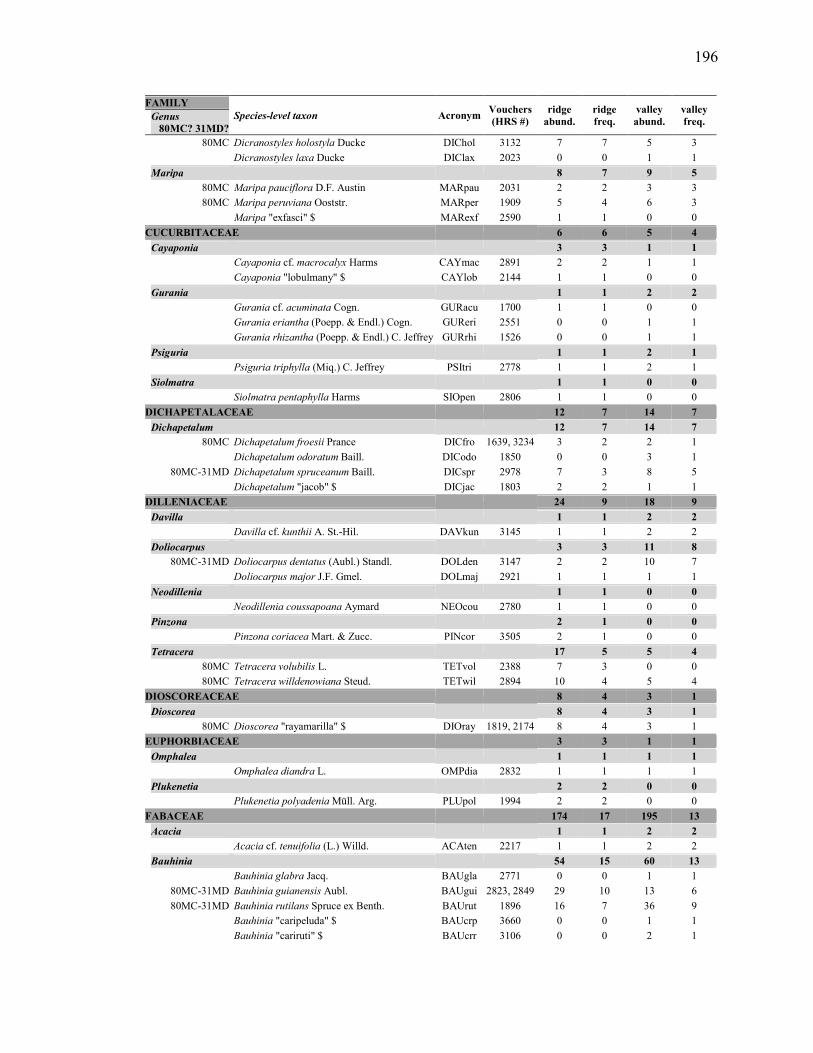
196
FAMILY Species-level taxon Acronym
Vouchers (HRS #)
ridge abund.
ridge freq.
valley abund.
valley freq.
Genus
80MC? 31MD?
80MC Dicranostyles holostyla Ducke DIChol 3132 7 7 5 3
Dicranostyles laxa Ducke DIClax 2023 0 0 1 1
Maripa
8 7 9 5
80MC Maripa pauciflora D.F. Austin MARpau 2031 2 2 3 3
80MC Maripa peruviana Ooststr. MARper 1909 5 4 6 3
Maripa "exfasci" $ MARexf 2590 1 1 0 0
CUCURBITACEAE
6 6 5 4
Cayaponia
3 3 1 1
Cayaponia cf. macrocalyx Harms CAYmac 2891 2 2 1 1
Cayaponia "lobulmany" $ CAYlob 2144 1 1 0 0
Gurania
1 1 2 2
Gurania cf. acuminata Cogn. GURacu 1700 1 1 0 0
Gurania eriantha (Poepp. & Endl.) Cogn. GUReri 2551 0 0 1 1
Gurania rhizantha (Poepp. & Endl.) C. Jeffrey GURrhi 1526 0 0 1 1
Psiguria
1 1 2 1
Psiguria triphylla (Miq.) C. Jeffrey PSItri 2778 1 1 2 1
Siolmatra
1 1 0 0
Siolmatra pentaphylla Harms SIOpen 2806 1 1 0 0
DICHAPETALACEAE
12 7 14 7
Dichapetalum
12 7 14 7
80MC Dichapetalum froesii Prance DICfro 1639, 3234 3 2 2 1
Dichapetalum odoratum Baill. DICodo 1850 0 0 3 1
80MC-31MD Dichapetalum spruceanum Baill. DICspr 2978 7 3 8 5
Dichapetalum "jacob" $ DICjac 1803 2 2 1 1
DILLENIACEAE
24 9 18 9
Davilla
1 1 2 2
Davilla cf. kunthii A. St.-Hil. DAVkun 3145 1 1 2 2
Doliocarpus
3 3 11 8
80MC-31MD Doliocarpus dentatus (Aubl.) Standl. DOLden 3147 2 2 10 7
Doliocarpus major J.F. Gmel. DOLmaj 2921 1 1 1 1
Neodillenia
1 1 0 0
Neodillenia coussapoana Aymard NEOcou 2780 1 1 0 0
Pinzona
2 1 0 0
Pinzona coriacea Mart. & Zucc. PINcor 3505 2 1 0 0
Tetracera
17 5 5 4
80MC Tetracera volubilis L. TETvol 2388 7 3 0 0
80MC Tetracera willdenowiana Steud. TETwil 2894 10 4 5 4
DIOSCOREACEAE
8 4 3 1
Dioscorea
8 4 3 1
80MC Dioscorea "rayamarilla" $ DIOray 1819, 2174 8 4 3 1
EUPHORBIACEAE
3 3 1 1
Omphalea
1 1 1 1
Omphalea diandra L. OMPdia 2832 1 1 1 1
Plukenetia
2 2 0 0
Plukenetia polyadenia Müll. Arg. PLUpol 1994 2 2 0 0
FABACEAE
174 17 195 13
Acacia
1 1 2 2
Acacia cf. tenuifolia (L.) Willd. ACAten 2217 1 1 2 2
Bauhinia
54 15 60 13
Bauhinia glabra Jacq. BAUgla 2771 0 0 1 1
80MC-31MD Bauhinia guianensis Aubl. BAUgui 2823, 2849 29 10 13 6
80MC-31MD Bauhinia rutilans Spruce ex Benth. BAUrut 1896 16 7 36 9
Bauhinia "caripeluda" $ BAUcrp 3660 0 0 1 1
Bauhinia "cariruti" $ BAUcrr 3106 0 0 2 1
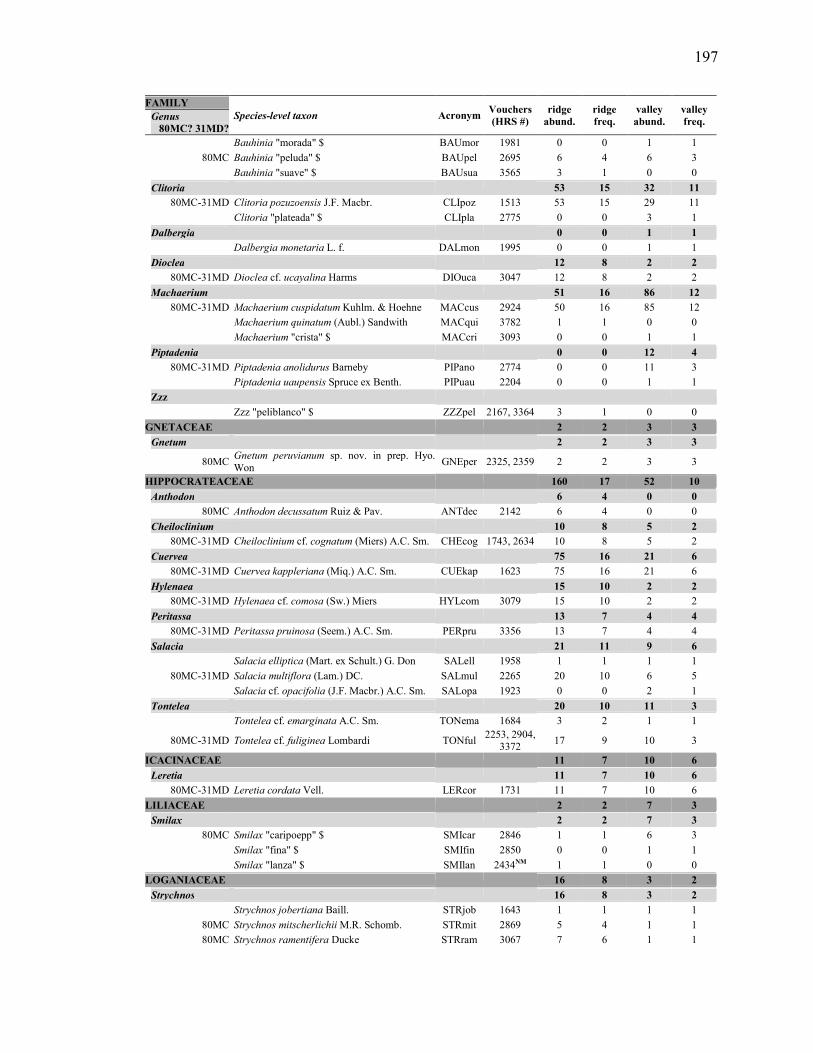
197
FAMILY Species-level taxon Acronym
Vouchers (HRS #)
ridge abund.
ridge freq.
valley abund.
valley freq.
Genus
80MC? 31MD?
Bauhinia "morada" $ BAUmor 1981 0 0 1 1
80MC Bauhinia "peluda" $ BAUpel 2695 6 4 6 3
Bauhinia "suave" $ BAUsua 3565 3 1 0 0
Clitoria
53 15 32 11
80MC-31MD Clitoria pozuzoensis J.F. Macbr. CLIpoz 1513 53 15 29 11
Clitoria "plateada" $ CLIpla 2775 0 0 3 1
Dalbergia
0 0 1 1
Dalbergia monetaria L. f. DALmon 1995 0 0 1 1
Dioclea
12 8 2 2
80MC-31MD Dioclea cf. ucayalina Harms DIOuca 3047 12 8 2 2
Machaerium
51 16 86 12
80MC-31MD Machaerium cuspidatum Kuhlm. & Hoehne MACcus 2924 50 16 85 12
Machaerium quinatum (Aubl.) Sandwith MACqui 3782 1 1 0 0
Machaerium "crista" $ MACcri 3093 0 0 1 1
Piptadenia
0 0 12 4
80MC-31MD Piptadenia anolidurus Barneby PIPano 2774 0 0 11 3
Piptadenia uaupensis Spruce ex Benth. PIPuau 2204 0 0 1 1
Zzz
Zzz "peliblanco" $ ZZZpel 2167, 3364 3 1 0 0
GNETACEAE
2 2 3 3
Gnetum
2 2 3 3
80MC
Gnetum peruvianum sp. nov. in prep. Hyo. Won
GNEper 2325, 2359 2 2 3 3
HIPPOCRATEACEAE
160 17 52 10
Anthodon
6 4 0 0
80MC Anthodon decussatum Ruiz & Pav. ANTdec 2142 6 4 0 0
Cheiloclinium
10 8 5 2
80MC-31MD Cheiloclinium cf. cognatum (Miers) A.C. Sm. CHEcog 1743, 2634 10 8 5 2
Cuervea
75 16 21 6
80MC-31MD Cuervea kappleriana (Miq.) A.C. Sm. CUEkap 1623 75 16 21 6
Hylenaea
15 10 2 2
80MC-31MD Hylenaea cf. comosa (Sw.) Miers HYLcom 3079 15 10 2 2
Peritassa
13 7 4 4
80MC-31MD Peritassa pruinosa (Seem.) A.C. Sm. PERpru 3356 13 7 4 4
Salacia
21 11 9 6
Salacia elliptica (Mart. ex Schult.) G. Don SALell 1958 1 1 1 1
80MC-31MD Salacia multiflora (Lam.) DC. SALmul 2265 20 10 6 5
Salacia cf. opacifolia (J.F. Macbr.) A.C. Sm. SALopa 1923 0 0 2 1
Tontelea
20 10 11 3
Tontelea cf. emarginata A.C. Sm. TONema 1684 3 2 1 1
80MC-31MD Tontelea cf. fuliginea Lombardi TONful
2253, 2904, 3372
17 9 10 3
ICACINACEAE
11 7 10 6
Leretia
11 7 10 6
80MC-31MD Leretia cordata Vell. LERcor 1731 11 7 10 6
LILIACEAE
2 2 7 3
Smilax
2 2 7 3
80MC Smilax "caripoepp" $ SMIcar 2846 1 1 6 3
Smilax "fina" $ SMIfin 2850 0 0 1 1
Smilax "lanza" $ SMIlan 2434NM 1 1 0 0
LOGANIACEAE
16 8 3 2
Strychnos
16 8 3 2
Strychnos jobertiana Baill. STRjob 1643 1 1 1 1
80MC Strychnos mitscherlichii M.R. Schomb. STRmit 2869 5 4 1 1
80MC Strychnos ramentifera Ducke STRram 3067 7 6 1 1

198
FAMILY Species-level taxon Acronym
Vouchers (HRS #)
ridge abund.
ridge freq.
valley abund.
valley freq.
Genus
80MC? 31MD?
Strychnos "aspera" $ STRasp 3060 1 1 0 0
Strychnos "corapeli" $ STRcor 2875 1 1 0 0
Strychnos "mate" $ STRmat 2362 1 1 0 0
MALPIGHIACEAE
60 16 35 10
Alicia
1 1 0 0
Alicia macrodisca (Triana & Planch.) W.R. Anderson
ALImac 2486NM 1 1 0 0
Dicella
6 4 10 4
80MC-31MD Dicella julianii (J.F. Macbr.) W.R. Anderson DICjul 3745 6 4 10 4
Diplopterys
7 5 6 4
Diplopterys cabrerana (Cuatrec.) B. Gates DIPcab 2244, 3148 3 2 0 0
80MC Diplopterys cf. lucida (Rich.) W.R. Anderson &
C.Cav. Davis DIPluc 2995 2 1 4 2
Diplopterys "carbon" $ DIPcar 1610NM 2 2 1 1
Diplopterys "opaca" $ DIPopa 2560NM 0 0 1 1
Ectopopterys
6 3 3 2
80MC Ectopopterys soejartoi W.R. Anderson ECTsoe 3252 6 3 3 2
Heteropterys
2 2 0 0
Heteropterys aureosericea Cuatrec. HETaur 3076 2 2 0 0
Hiraea
9 5 8 5
Hiraea affinis Miq. HIRaff 2071 2 2 1 1
80MC Hiraea fagifolia (DC.) A. Juss. HIRfag 3069 2 2 5 3
80MC Hiraea valida W.R. Anderson HIRval 2599 5 2 2 1
Jubelina
3 2 0 0
Jubelina uleana (Nied.) Cuatrec. JUBule 2709 3 2 0 0
Mascagnia
7 6 4 3
80MC
Mascagnia cf. dissimilis C.V. Morton & Moldenke
MASdis 1948 2 2 3 2
80MC Mascagnia divaricata (Kunth) Nied. MASdiv 2355 5 4 1 1
Stigmaphyllon
2 1 0 0
Stigmaphyllon sinuatum (DC.) A. Juss. STIsin 2406 2 1 0 0
Tetrapterys
17 5 2 2
Tetrapterys cf. calophylla A. Juss. TETcal 2459 0 0 1 1
80MC-31MD Tetrapterys nitida A. Juss. TETnit 1960 17 5 1 1
Zzz
Zzz "hippo" $ ZZZhip 3105 0 0 2 1
MARCGRAVIACEAE
2 2 7 4
Marcgravia
2 2 6 3
Marcgravia "micro" $ MARmic 2398 2 2 2 2
Marcgravia "tetra" $ MARtet 2503 0 0 4 1
Zzz
Zzz "diminuta" $ ZZZdim 3102NM 0 0 1 1
MENISPERMACEAE
25 10 15 8
Abuta
4 2 4 2
Abuta cf. pahnii (Mart.) Krukoff & Barneby ABUpah 2035NM 1 1 0 0
80MC Abuta cf. solimoesensis Krukoff & Barneby ABUsol 3760 3 1 4 2
Anomospermum
0 0 1 1
Anomospermum "miniterci" $ ANOmin 3112NM 0 0 1 1
Curarea
10 7 2 2
80MC Curarea tecunarum Barneby & Krukoff CURtec 2637 10 7 2 2
Disciphania
0 0 1 1
Disciphania "corazon" $ DIScor 2735NM 0 0 1 1
Odontocarya
1 1 2 1
Odontocarya "exbj" $ ODOexb 2310 1 1 2 1
Sciadotenia
4 3 4 2
80MC Sciadotenia toxifera Krukoff & A.C. Sm. SCItox 1788 4 3 4 2

199
FAMILY Species-level taxon Acronym
Vouchers (HRS #)
ridge abund.
ridge freq.
valley abund.
valley freq.
Genus
80MC? 31MD?
Telitoxicum
6 4 1 1
80MC Telitoxicum krukovii Moldenke TELkru 2785NM 5 3 1 1
Telitoxicum minutiflorum (Diels) Moldenke TELmin 2725 1 1 0 0
PASSIFLORACEAE
6 4 6 5
Dilkea
0 0 4 3
Dilkea "retuparvi" $ DILret 3001 0 0 4 3
Passiflora
6 4 2 2
Passiflora cf. ambigua Hemsl. PASamb 2436 2 2 0 0
80MC Passiflora spinosa (Poepp. & Endl.) Mast. PASspi 1521 4 4 2 2
PHYTOLACCACEAE
1 1 0 0
Seguieria
1 1 0 0
Seguieria americana L. SEGame 1753 1 1 0 0
PIPERACEAE
0 0 1 1
Piper
0 0 1 1
Piper armatum Trel. & Yunck. PIParm 3022, 3027 0 0 1 1
POLYGALACEAE
11 6 0 0
Moutabea
11 6 0 0
80MC-31MD
Moutabea aculeata (Ruiz & Pav.) Poepp. & Endl.
MOUacu 2063, 2617 11 6 0 0
POLYGONACEAE
7 5 6 5
Coccoloba
7 5 6 5
80MC Coccoloba excelsa Benth. COCexc 2765 1 1 4 4
Coccoloba cf. obovata Kunth COCobo 2336 4 3 0 0
Coccoloba "decurrente" $ COCdec 2639, 3402 2 1 2 2
RHAMNACEAE
1 1 10 4
Gouania
1 1 10 4
Gouania colombiana Suess. GOUcol 3094 0 0 3 2
80MC Gouania lupuloides (L.) Urb. GOUlup 2399NM 1 1 5 1
Gouania mollis Reissek GOUmol 2751 0 0 2 1
RUBIACEAE
5 4 10 1
Chomelia
4 3 10 1
31MD Chomelia cf. estrellana Müll. Arg. CHOest 2825 0 0 10 1
Chomelia malaneoides Müll. Arg. CHOmal 2889 4 3 0 0
Randia
1 1 0 0
Randia altiscandens (Ducke) C.M. Taylor RANalt 2043 1 1 0 0
SOLANACEAE
4 3 5 1
Markea
2 1 0 0
Markea coccinea Rich. MARcoc 2605NM 2 1 0 0
Solanum
2 2 5 1
80MC Solanum barbeyanum Huber SOLbar 1517, 1591 2 2 5 1
SAPINDACEAE
78 17 95 13
Paullinia
69 17 84 13
80MC Paullinia cf. alata G. Don PAUala 3038, 3056 2 1 4 3
Paullinia bidentata Radlk. PAUbid 2606 3 3 0 0
Paullinia cf. bilobulata Radlk. PAUbil 3394 1 1 3 2
80MC-31MD Paullinia bracteosa Radlk. PAUbra 3048 17 9 12 6
80MC Paullinia cf. capreolata (Aubl.) Radlk. PAUcap 1596, 3289 3 3 6 4
Paullinia cf. clathrata Radlk. PAUcla 2817 0 0 1 1
80MC-31MD Paullinia dasystachya Radlk. PAUdas
1734, 1816, 1898
3 3 9 5
Paullinia cf. faginea (Triana & Planch.) Radlk. PAUfag 2853 2 2 2 2
Paullinia fimbriata Radlk. PAUfim 2232 2 2 2 2
Paullinia hispida Jacq. PAUhis 2671, 3419 1 1 1 1
80MC-31MD Paullinia ingifolia Rich ex Juss. PAUing
2101, 2416, 3325
4 4 9 5
Paullinia cf. meliifolia Juss. PAUmel 2423 2 1 0 0

200
FAMILY Species-level taxon Acronym
Vouchers (HRS #)
ridge abund.
ridge freq.
valley abund.
valley freq.
Genus
80MC? 31MD?
80MC-31MD Paullinia cf. microneura Cuatrec. PAUmic 2353, 2816 13 6 4 3
80MC Paullinia cf. obovata (Ruiz & Pav.) Pers. PAUobo
1570, 2140, 2699, 2703
7 4 5 4
Paullinia cf. paullinioides Radlk. PAUpau 2844 1 1 2 2
80MC Paullinia cf. reticulata Radlk. PAUret 1581 1 1 5 3
Paullinia venosa Radlk. PAUven 2564, 2648 1 1 3 3
80MC Paullinia "cafe" $ PAUcaf
1873, 2547, 2915
4 4 6 4
80MC Paullinia "corteza" $ PAUcor
1934, 1941, 2583
1 1 6 3
Paullinia "granpari" $ PAUgra 2468, 2588 0 0 2 2
Paullinia "longteeth" $ PAUlon 2990 1 1 2 2
Serjania
4 2 5 4
80MC Serjania pyramidata Radlk. SERpyr 2559 4 2 5 4
Thinouia
5 4 6 1
80MC Thinouia obliqua Radlk. THIobl 1905, 1970 5 4 6 1
STERCULIACEAE
0 0 1 1
Byttneria
0 0 1 1
Byttneria asterotricha Mildbr. BYTast 2762NM 0 0 1 1
ULMACEAE
3 2 0 0
Celtis 3 2 0 0
Celtis iguanaea (Jacq.) Sarg. CELigu 2318 3 2 0 0
VERBENACEAE
99 15 40 9
Aegiphila 2 1 10 7
Aegiphila cordata Poepp. ex Schauer AEGcor 2504, 3276 0 0 2 1
Aegiphila cf. elata Kunth AEGela 3025NM 0 0 1 1
Aegiphila cf. mollis Kunth AEGmol 2827NM 0 0 3 2
80MC Aegiphila "exelata" $ AEGexe 2976 2 1 4 4
Petrea 97 15 30 4
80MC-31MD Petrea maynensis Huber PETmay 1673 97 15 30 4
VITACEAE
0 0 3 3
Cissus
0 0 3 3
Cissus biformifolia Standl. CISbif 2474, 3153 0 0 2 2
Cissus cf. ulmifolia (Baker) Planch. CISulm 1864 0 0 1 1
ZZZ Zzz Zzz zzz ZZZzzz
84 17 96 12

201
APPENDIX 3
Diversity and abundance of lianas in studies conducted in Yasuní, including this
study. Means were calculated from the sampling unit data shown, or copied from what
was reported in the publications. Totals per forest type are also shown. We report: forest
type (if terra firme, topographic habitat in parentheses), sampled area, diameter cutoff
used, number of species (# spp.) and number of individuals (# ind.). Data from Romero-
Saltos, Valencia, and Macía (2001) was re-analyzed excluding the 60 unidentified lianas.
The data in boxes are those being compared to our study (see Table 2.4). Studies are
ordered chronologically.
Site name
Forest type (if terra firme,
topographic habitat is also shown)
Sampled area in ha (dimensions in m)
Diameter cutoff (cm)
# spp. # ind.
Nabe-Nielsen (2001)
Sampling unit values
Yasuní 1 terra firme
(ridge) 0.2
(20×100) all lianas 96 318
Yasuní 2 terra firme
(ridge) 0.2
(20×100) all lianas 86 288
Mean values
terra firme
(ridge) 0.2
(20×100), N=2 all lianas 91 303
terra firme
(ridge) 0.1
(20×50), N=4 all lianas 62 152
terra firme
(ridge) 0.1
(20×50), N=4 ≥1.0 44 94
terra firme
(ridge) 0.1
(20×50), N=4 ≥2.5 21 33
Total values
terra firme (ridge)
0.4 (2 × (20×100))
all 138 606
Romero-Saltos, Macía, and Valencia (2001)
Sampling unit values
02 terra firme
(ridge) 0.1
(20×50) ≥2.5 24 43
04 terra firme
(ridge) 0.1
(20×50) ≥2.5 13 21
05 terra firme
(ridge) 0.1
(20×50) ≥2.5 20 41
06 terra firme
(ridge) 0.1
(20×50) ≥2.5 22 36
07 terra firme
(ridge) 0.1
(20×50) ≥2.5 21 49
15 terra firme
(ridge) 0.1
(20×50) ≥2.5 28 57
16 terra firme
(ridge) 0.1
(20×50) ≥2.5 22 31
17 terra firme
(ridge) 0.1
(20×50) ≥2.5 15 24

202
Site name
Forest type (if terra firme,
topographic habitat is also shown)
Sampled area in ha (dimensions in m)
Diameter cutoff (cm)
# spp. # ind.
18 terra firme
(ridge) 0.1
(20×50) ≥2.5 23 44
20 terra firme
(ridge) 0.1
(20×50) ≥2.5 14 21
01 floodplain 0.1
(20×50) ≥2.5 11 24
03 floodplain 0.1
(20×50) ≥2.5 20 54
10 floodplain 0.1
(20×50) ≥2.5 13 20
11 floodplain 0.1
(20×50) ≥2.5 9 21
12 floodplain 0.1
(20×50) ≥2.5 7 7
19 floodplain 0.1
(20×50) ≥2.5 13 24
21 floodplain 0.1
(20×50) ≥2.5 12 47
22 floodplain 0.1
(20×50) ≥2.5 16 30
08 swamp 0.1
(20×50) ≥2.5 10 23
09 swamp 0.1
(20×50) ≥2.5 10 24
13 swamp 0.1
(20×50) ≥2.5 1 2
14 swamp 0.1
(20×50) ≥2.5 5 7
23 swamp 0.1
(20×50) ≥2.5 11 29
24 swamp 0.1
(20×50) ≥2.5 1 1
25 swamp 0.1
(20×50) ≥2.5 4 7
Mean values
terra firme
(ridge) 0.1
(20×50), N=10 ≥2.5 20 37
floodplain
0.1 (20×50), N=8
≥2.5 13 28
swamp
0.1 (20×50), N=7
≥2.5 6 13
terra firme (ridge)
& floodplain & swamp
0.1 (20×50), N=25
≥2.5 14 27
Total values
terra firme
(ridge) 1.0
(10 × (20×50)) ≥2.5 117 367
flood plain
0.8 (8 × (20×50))
≥2.5 70 227
swamp
0.7 (7 × (20×50))
≥2.5 30 93
terra firme (ridge)
& floodplain & swamp
2.5 (25 × (20×50))
≥2.5 173 687
Burnham (2002), Burnham (2004) Sampling
unit values Monkey PC
terra firme (ridge & valley)
0.2 4×500
≥1.0 88 302

203
Site name
Forest type (if terra firme,
topographic habitat is also shown)
Sampled area in ha (dimensions in m)
Diameter cutoff (cm)
# spp. # ind.
Monkey PD terra firme
(ridge & valley) 0.2
4×500 ≥1.0 109 314
Capiron terra firme
(ridge & valley) 0.2
5×(4×100) ≥1.0 104 344
Aulestia Piraña terra firme
(ridge & valley) 0.2
5×(4×100) ≥1.0 100 433
Puente TBS terra firme
(ridge & valley) 0.2
5×(4×100) ≥1.0 105 347
Maquisapa Guacamayo
terra firme (ridge & valley)
0.2 5×(4×100)
≥1.0 86 313
TBS Floodplain floodplain 0.2
5×(4×100) ≥1.0 71 360
Caiman Durmiente floodplain 0.2
5×(4×100) ≥1.0 72 430
Yasuni Floodplain floodplain 0.2
5×(4×100) ≥1.0 87 292
ECY Floodplain floodplain 0.2
5×(4×100) ≥1.0 82 435
Laguna Nutria floodplain 0.2
5×(4×100) ≥1.0 89 441
Laguna Hoatzin floodplain 0.2
5×(4×100) ≥1.0 62 337
Mean values
terra firme
(ridge & valley) 0.2
(5×(4×100)), N=6 ≥1.0 99 342
floodplain
0.2 (5×(4×100)), N=6
≥1.0 71 382
terra firme (ridge & valley)
& floodplain
0.2 (5×(4×100)), N=12
≥1.0 88 362
Total values
terra firme
(ridge & valley) 1.2
(6 × (5×(4×100)) ≥1.0 254 2053
floodplain
1.2 (6 × (5×(4×100))
≥1.0 179 2295
terra firme (ridge & valley)
& floodplain
2.4 (12 × (5×(4×100))
≥1.0 311 4348
This study
Sampling unit values
YFDP_R_02,02 terra firme
(ridge) 0.04
(20×20) ≥1.0 24 39
YFDP_R_02,07 terra firme
(ridge) 0.04
(20×20) ≥1.0 38 92
YFDP_R_02,17 terra firme
(ridge) 0.04
(20×20) ≥1.0 25 73
YFDP_R_07,02 terra firme
(ridge) 0.04
(20×20) ≥1.0 21 43
YFDP_R_07,07 terra firme
(ridge) 0.04
(20×20) ≥1.0 20 43
YFDP_R_07,17 terra firme
(ridge) 0.04
(20×20) ≥1.0 30 72
YFDP_R_07,22 terra firme
(ridge) 0.04
(20×20) ≥1.0 33 69
YFDP_R_12,02 terra firme
(ridge) 0.04
(20×20) ≥1.0 24 61
YFDP_R_12,17 terra firme
(ridge) 0.04
(20×20) ≥1.0 26 69
YFDP_R_12,22 terra firme
(ridge) 0.04
(20×20) ≥1.0 15 34

204
Site name
Forest type (if terra firme,
topographic habitat is also shown)
Sampled area in ha (dimensions in m)
Diameter cutoff (cm)
# spp. # ind.
YFDP_R_17,02 terra firme
(ridge) 0.04
(20×20) ≥1.0 30 56
YFDP_R_17,12 terra firme
(ridge) 0.04
(20×20) ≥1.0 31 64
YFDP_R_17,17 terra firme
(ridge) 0.04
(20×20) ≥1.0 25 58
YFDP_R_22,02 terra firme
(ridge) 0.04
(20×20) ≥1.0 31 97
YFDP_R_22,17 terra firme
(ridge) 0.04
(20×20) ≥1.0 22 43
YFDP_R_22,22 terra firme
(ridge) 0.04
(20×20) ≥1.0 22 36
YFDP_R_27,17 terra firme
(ridge) 0.04
(20×20) ≥1.0 40 80
YFDP_V_02,12 terra firme
(valley) 0.04
(20×20) ≥1.0 31 96
YFDP_V_02,22 terra firme
(valley) 0.04
(20×20) ≥1.0 12 40
YFDP_V_07,12 terra firme
(valley) 0.04
(20×20) ≥1.0 31 81
YFDP_V_12,07 terra firme
(valley) 0.04
(20×20) ≥1.0 19 44
YFDP_V_12,12 terra firme
(valley) 0.04
(20×20) ≥1.0 25 52
YFDP_V_17,07 terra firme
(valley) 0.04
(20×20) ≥1.0 34 69
YFDP_V_17,22 terra firme
(valley) 0.04
(20×20) ≥1.0 29 83
YFDP_V_22,07 terra firme
(valley) 0.04
(20×20) ≥1.0 20 61
YFDP_V_22,12 terra firme
(valley) 0.04
(20×20) ≥1.0 25 56
YFDP_V_27,02 terra firme
(valley) 0.04
(20×20) ≥1.0 41 100
YFDP_V_27,07 terra firme
(valley) 0.04
(20×20) ≥1.0 26 76
YFDP_V_27,12 terra firme
(valley) 0.04
(20×20) ≥1.0 34 68
YFDP_V_27,22 terra firme
(valley) 0.04
(20×20) ≥1.0 33 64
Mean values
terra firme
(ridge) 0.04
(20×20), N= 17 ≥1.0 27 61
terra firme
(valley) 0.04
(20×20), N= 13 ≥1.0 28 68
Total values
terra firme (ridge & valley)
1.2 (30 × (20×20))
≥1.0 195 1919

205
APPENDIX 4
Leaf traits of the 43 liana species included in the functional traits analyses. The
habitat association (or non-association) of species was classified (CLASS.) as: ridge
species (R), valley species (V), generalist species (G), and widespread with habitat
association species (W, subclassified in WR: with ridge association, and WV: with valley
association) (see Methods, and Tables 3.1 and 3.2). SLA=specific leaf area, LDMC=leaf
dry matter content, LT=leaf lamina thickness, L:W=length to width ratio of whole leaf
(incl. petiole), LSR=individual-level leaf size range=lamina area of largest leaf observed
− lamina area of smallest leaf observed in the same individual, C=carbon concentration,
N=nitrogen concentration, P=phosphorus concentration, δ13C=relative abundance of the
stable isotope carbon-13 in delta units, δ15N=relative abundance of the stable isotope
nitrogen-15 in delta units, C:N=ratio of carbon concentration to nitrogen concentration,
N:P=ratio of nitrogen concentration to phosphorus concentration. Species acronyms (in
bold) were formed by the first three letters of the genus (in UPPERCASE) and the first
three letters of the epithet. Names within quotation marks are morphospecies. Family
acronyms (in parentheses) were formed by a three-letter code. Species are ordered by
family.
Values reported are: mean ± 1 standard deviation, minimum and maximum values
(in parentheses) and number of individuals sampled (N, in parentheses) (if N=2, no mean
was calculated).

206
FAMILY Species
CLASS. SLA
(mm2/mg) LDMC (mg/g)
LT (mm)
L:W (ratio)
LSR (cm2)
C (%)
N (%)
P (%)
C:N (ratio)
N:P (ratio)
δ13C δ15N
APOCYNACEAE (APO)
FORsteronia affinis
R 23±6.8
(13.9–28.5) (N=4)
species not sampled
0.08±0.01 (0.07–0.09)
(N=4)
2.6±0.7 (2.2–3.7)
(N=4)
33±17 (21–53) (N=3)
62–72.2 (N=2)
3.2–3.3 (N=2)
0.08–0.09 (N=2)
19.3–21.8 (N=2)
35.4–43.9 (N=2)
-34.6 – -31.1 (N=2)
2.27-3.59 (N=2)
ARECACEAE (ARE)
DESmoncus orthacanthos
R 9.6±3.1
(6.1–15.2) (N=6)
409.5–452.9 (N=2)
0.18±0.03 (0.13–0.21)
(N=6)
2.6±0.4 (2.2–3.4)
(N=6)
1061±152 (970–1237)
(N=3)
36.1–47.3 (N=2)
2.4–2.7 (N=2)
0.1–0.11 (N=2)
13.5–20 (N=2)
20.8–26.5 (N=2)
-33.9 – -33.3 (N=2)
3.15-6.55 (N=2)
ASTERACEAE (AST)
MIKania leiostachya
V 22.5±6
(17.1–34.9) (N=7)
175.2 (N=1)
0.17±0.03 (0.13–0.22)
(N=7)
2.6±0.5 (1.8–3.2)
(N=7)
47±23 (14–72) (N=5)
45.7±5.1 (41.1–51.6)
(N=4)
2.4±0.2 (2.1–2.6)
(N=4)
0.16±0.02 (0.15–0.18)
(N=4)
19.1±0.6 (18.6–19.8)
(N=4)
15.1±1.7 (13.8–17.5)
(N=4)
-32.2±1.6 (-34.4 – -31)
(N=4)
3.07±0.44 (2.64-3.56)
(N=4) BIGNONIACEAE (BIG)
ADEnocalymna impressum
R 14.9±4.9
(10.1–25.2) (N=10)
398.3±46.4 (345.9–438.6)
(N=4)
0.14±0.03 (0.12–0.2)
(N=10)
1.1±0.3 (0.6–1.6) (N=10)
144±120 (48–421)
(N=8)
36.9–42.4 (N=2)
3.1–3.6 (N=2)
0.13–0.16 (N=2)
11.6–11.8 (N=2)
22.5–24.3 (N=2)
-32.5 – -30.6 (N=2)
0.6-1.63 (N=2)
BIGnonia aequinoctialis
G 17.2±6.4
(7.7–27.9) (N=13)
347.3±63.7 (283.1–460.8)
(N=7)
0.11±0.02 (0.08–0.16)
(N=13)
1.1±0.2 (0.8–1.4) (N=13)
106±67 (19–229)
(N=7)
43.1±4.7 (39.8–48.5)
(N=3)
2.3±0.1 (2.2–2.5)
(N=3)
0.11±0.01 (0.1–0.12)
(N=3)
18.6±2.2 (16.2–20.6)
(N=3)
21.2±2.3 (19–23.7)
(N=3)
-30.6±1.4 (-32 – -29.2)
(N=3)
1.96±0.11 (1.89-2.09)
(N=3)
MANsoa verrucifera
V 21.4±3.7
(16.9–27.3) (N=7)
424 (N=1)
0.09±0.02 (0.08–0.12)
(N=7)
1±0.2 (0.7–1.3)
(N=7)
184±127 (46–348)
(N=4)
45.6–78.9 (N=2)
3.9–6.4 (N=2)
0.12–0.16 (N=2)
11.6–12.4 (N=2)
31.9–39.2 (N=2)
-36.8 – -33.3 (N=2)
1.91-3.96 (N=2)
STIzophyllum riparium
G 30.4±8.9
(19.4–49.8) (N=12)
310±38.1 (277.2–364.6)
(N=4)
0.08±0.02 (0.04–0.11)
(N=12)
1.1±0.2 (0.9–1.4) (N=12)
177±139 (12–435) (N=10)
43–52.4 (N=2)
3.4–3.5 (N=2)
0.16–0.17 (N=2)
12.2–15.4 (N=2)
21–21.3 (N=2)
-33.3 – -33 (N=2)
1.17-3.67 (N=2)
TANaecium affine
V 19.1±6.1
(13.5–25.6) (N=3)
245.8 (N=1)
0.13±0.03 (0.12–0.17)
(N=3)
1.2–1.3 (N=2)
48–79 (N=2)
50±5.9 (43.2–53.6)
(N=3)
3.4±0.1 (3.3–3.5)
(N=3)
0.15±0.05 (0.1–0.2)
(N=3)
14.6±2 (12.5–16.3)
(N=3)
25.4±8.2 (17.5–33.9)
(N=3)
-34.1±0.7 (-34.9 – -33.6)
(N=3)
2.52±1.8 (0.45-3.78)
(N=3) BORAGINACEAE (BOR)
TOUrnefortia bicolor
G 18.8±7.8
(11.6–32.7) (N=8)
213.9±36.4 (158–258.4)
(N=5)
0.29±0.11 (0.16–0.45)
(N=8)
2.3±0.5 (1.4–2.8)
(N=8)
67±29 (36–120)
(N=7)
41.1±1.7 (38.7–42.5)
(N=4)
2.8±0.8 (1.6–3.3)
(N=4)
0.14±0.08 (0.07–0.24)
(N=4)
16±5.4 (12.2–24)
(N=4)
24.9±15.1 (12.1–46.8)
(N=4)
-34.1±0.8 (-34.8 – -33)
(N=4)
1.99±1.17 (1.01-3.38)
(N=4) COMBRETACEAE (COM)
COMbretum laxum
WV 13.8±3.2 (9–23.7) (N=31)
422.6±59.6 (246.9–527.3)
(N=15)
0.12±0.02 (0.09–0.18)
(N=31)
3.1±0.4 (2.1–4.4) (N=31)
49±26 (16–117) (N=25)
41.6±3.8 (37.7–45.2)
(N=3)
2±0.3 (1.7–2.2)
(N=3)
0.1±0.01 (0.08–0.11)
(N=3)
21.6±4.5 (18.6–26.7)
(N=3)
21±6.4 (15.6–28.1)
(N=3)
-31.3±1 (-32.4 – -30.7)
(N=3)
1.91±1.62 (0.88-3.77)
(N=3) CONNARACEAE (CNN)
CONnarus patrisii
G 9.4±1
(8–11.5) (N=10)
472.6±78.6 (357.7–570.5)
(N=5)
0.15±0.02 (0.12–0.18)
(N=10)
1.5±0.3 (0.9–2) (N=10)
479±291 (148–839)
(N=4)
50.7±5.1 (46.5–56.3)
(N=3)
1.9±0.3 (1.6–2.2)
(N=3)
0.1±0.01 (0.08–0.1)
(N=3)
27.2±1.9 (25.1–28.8)
(N=3)
20.3±6.2 (16.3–27.5)
(N=3)
-34.6±0.8 (-35.3 – -33.7)
(N=3)
1.9±1.78 (-0.06-3.4)
(N=3)

207
FAMILY Species
CLASS. SLA
(mm2/mg) LDMC (mg/g)
LT (mm)
L:W (ratio)
LSR (cm2)
C (%)
N (%)
P (%)
C:N (ratio)
N:P (ratio)
δ13C δ15N
ROUrea amazonica
G 12.2±3.7 (7.1–20) (N=10)
542.5±95 (442.5–665.6)
(N=7)
0.18±0.03 (0.13–0.21)
(N=10)
1.3±0.4 (0.8–1.8) (N=10)
192±150 (26–432)
(N=7)
43.6±3.5 (40.5–47.3)
(N=3)
1.9±0.4 (1.5–2.3)
(N=3)
0.1±0.02 (0.07–0.12)
(N=3)
23.1±3.9 (18.9–26.5)
(N=3)
19.6±1 (18.8–20.8)
(N=3)
-34.8±1.6 (-36.6 – -33.4)
(N=3)
0.75±0.66 (0.02-1.3)
(N=3)
ROUrea camptoneura
G 16.2±4.3
(7.5–22.8) (N=10)
371±95.3 (285.5–504.6)
(N=4)
0.14±0.04 (0.1–0.25)
(N=10)
1.3±0.2 (1–1.6) (N=10)
328±295 (78–654)
(N=3)
47.3±1.5 (46.2–49)
(N=3)
2.3±0.3 (1.9–2.5)
(N=3)
0.09±0.03 (0.07–0.12)
(N=3)
21±2.7 (19–24.1)
(N=3)
27.4±10.6 (16.4–37.4)
(N=3)
-33.3±2.4 (-34.7 – -30.5)
(N=3)
2.11±0.8 (1.5-3.01)
(N=3) CONVOLVULACEAE (CNV)
MARipa peruviana
G 20.6±5.1
(15.2–30.8) (N=16)
322.3±63.3 (205.7–412.4)
(N=10)
0.13±0.02 (0.1–0.16)
(N=16)
3.6±0.3 (3.2–4) (N=16)
75±32 (36–142) (N=13)
45.7–49.4 (N=2)
2.9–3.4 (N=2)
0.09–0.17 (N=2)
13.5–17.2 (N=2)
20.5–33.3 (N=2)
-34.1 – -33.6 (N=2)
1.54-2.46 (N=2)
DICHAPETALACEAE (DIC)
DIChapetalum froesii
G 14.5±4.8
(10.3–20.1) (N=6)
369.6±26.5 (347.4–403.6)
(N=4)
0.17±0.03 (0.14–0.23)
(N=6)
2.7±0.5 (1.9–3.1)
(N=6)
78±17 (60–100)
(N=4)
54.1–61.5 (N=2)
3.4–3.6 (N=2)
0.09–0.1 (N=2)
15.7–17.1 (N=2)
35.8–38.8 (N=2)
-34.6 – -33.9 (N=2)
4.85-5.16 (N=2)
DIChapetalum spruceanum
G 13.5±2.7
(9.1–18.5) (N=17)
383±47.4 (335.2–492.6)
(N=9)
0.16±0.03 (0.1–0.22)
(N=17)
1.9±0.3 (1.3–2.4) (N=17)
279±152 (102–471)
(N=9)
43.1–60.6 (N=2)
2.4–3.7 (N=2)
0.08–0.09 (N=2)
16.2–18.2 (N=2)
30.5–39.7 (N=2)
-34.6 – -34.4 (N=2)
3.41-4.77 (N=2)
DILLENIACEAE (DIL)
DOLiocarpus dentatus
V 18.2±4.7
(11.2–25.8) (N=14)
287.3±59.5 (198.3–415.7)
(N=12)
0.17±0.03 (0.13–0.25)
(N=14)
2.6±0.3 (2.1–3.4) (N=14)
102±85 (10–273) (N=13)
45.5±10.8 (38.6–64.8)
(N=5)
1.6±0.5 (1.3–2.5)
(N=5)
0.11±0.03 (0.06–0.15)
(N=5)
29.4±3.2 (25.8–32.6)
(N=5)
16.7±7.9 (9.1–27.4)
(N=5)
-32.9±1.7 (-34.5 – -30.5)
(N=5)
0.57±0.9 (-0.31-1.64)
(N=5)
TETracera willdenowiana
G 14.6±2.7
(10.5–20.3) (N=14)
391.5±69.9 (280.1–490.6)
(N=6)
0.15±0.05 (0.11–0.31)
(N=14)
2.9±0.3 (2.5–3.4) (N=14)
112±50 (51–186) (N=10)
45.4±4.1 (40.8–48.7)
(N=3)
1.8±0.3 (1.5–2.1)
(N=3)
0.1±0.01 (0.1–0.11)
(N=3)
24.9±2.1 (22.8–27)
(N=3)
17.8±3.8 (13.4–20.2)
(N=3)
-33.6±1.7 (-35.4 – -32)
(N=3)
4.19±2.86 (2.13-7.46)
(N=3) FABACEAE (FAB)
BAUhinia "peluda"
G 19.5±4.2
(12.1–25.4) (N=14)
412.7±78.3 (326.4–559.2)
(N=7)
0.13±0.02 (0.1–0.16)
(N=14)
1.6±0.2 (1.3–2) (N=14)
56±34 (16–108) (N=12)
41.2–42.5 (N=2)
2.2–2.4 (N=2)
0.06–0.11 (N=2)
17.5–19.3 (N=2)
19.3–37.7 (N=2)
-36.4 – -35.1 (N=2)
1-3.86 (N=2)
CLItoria pozuzoensis
WR 14.8±3.4
(5.3–21.6) (N=38)
458±91.3 (311.9–702.1)
(N=17)
0.13±0.02 (0.09–0.2)
(N=38)
1.1±0.2 (0.8–2) (N=38)
284±192 (45–850) (N=25)
40.1–48.5 (N=2)
2.2–2.5 (N=2)
0.09–0.17 (N=2)
18.1–19.2 (N=2)
13–26.6 (N=2)
-34.3 – -33.2 (N=2)
0.75-1.93 (N=2)
DIOclea ucayalina
R 15.4±4.7
(8.1–24.9) (N=12)
478.9±161.8 (333.5–653.2)
(N=3)
0.09±0.02 (0.06–0.12)
(N=12)
1.2±0.2 (0.8–1.5) (N=12)
442±418 (4–1007)
(N=6)
46.1±2.8 (41.3–49)
(N=6)
2.9±0.8 (2–3.7) (N=6)
0.13±0.04 (0.07–0.16)
(N=6)
17.2±4.9 (11.2–22.4)
(N=6)
22.7±6.2 (13.7–31.2)
(N=6)
-31.2±1.8 (-34.1 – -29.2)
(N=6)
0.32±0.59 (-0.7-1.03)
(N=6)
MAChaerium cuspidatum
WV 15.3±3.2
(10.3–23.2) (N=41)
435.5±59.2 (349.6–551.8)
(N=19)
0.13±0.02 (0.09–0.17)
(N=41)
1.2±0.4 (0.8–3.8) (N=41)
302±236 (0–945) (N=28)
45.4–68.4 (N=2)
2.8–3.9 (N=2)
0.09–0.12 (N=2)
16.1–17.6 (N=2)
23.7–42 (N=2)
-32.4 – -31.4 (N=2)
-0.31-0.05 (N=2)
PIPtadenia anolidurus
V 15.4±4.4
(11.7–21.4) (N=4)
449.3 (N=1)
0.09±0.02 (0.07–0.12)
(N=4)
1.5±0.3 (1.2–1.8)
(N=4)
41–140 (N=2)
53.5–55.3 (N=2)
4.2–4.5 (N=2)
0.05–0.36 (N=2)
12–13.2 (N=2)
12.4–91.8 (N=2)
-37.7 – -33.2 (N=2)
3.32-3.76 (N=2)
HIPPOCRATEACEAE (HIP)

208
FAMILY Species
CLASS. SLA
(mm2/mg) LDMC (mg/g)
LT (mm)
L:W (ratio)
LSR (cm2)
C (%)
N (%)
P (%)
C:N (ratio)
N:P (ratio)
δ13C δ15N
ANThodon decussatum
R 16.2–20.4
(N=2) 344.6–452.9
(N=2) 0.07–0.14
(N=2) 2.7–4.5 (N=2)
14–43 (N=2)
42.2–42.9 (N=2)
1.5–2.3 (N=2)
0.06–0.09 (N=2)
19–27.8 (N=2)
24.3–25 (N=2)
-35 – -33.9 (N=2)
-0.14--0.11 (N=2)
CUErvea kappleriana
WR 13.7±5.1
(9.1–38.8) (N=33)
365.7±55.4 (272.4–491.1)
(N=15)
0.16±0.02 (0.14–0.2)
(N=33)
2.4±0.3 (1.8–2.8) (N=33)
102±46 (27–184) (N=25)
36–37 (N=2)
2.2–2.5 (N=2)
0.09–0.09 (N=2)
14.6–16.3 (N=2)
24.3–28.9 (N=2)
-35.3 – -34.1 (N=2)
-1.28-3.2 (N=2)
HYLenaea comosa
R 12.2±2.4
(8.5–18.1) (N=20)
416.5±25.4 (381.8–460.8)
(N=10)
0.14±0.02 (0.1–0.18)
(N=20)
3.1±0.5 (2.2–4.7) (N=20)
77±42 (5–165) (N=15)
43.2–65.2 (N=2)
2.3–2.5 (N=2)
0.08–0.08 (N=2)
17.5–28.5 (N=2)
28.1–32.2 (N=2)
-34.5 – -32.8 (N=2)
0.87-1.79 (N=2)
PERitassa pruinosa
R 11.7±1.8
(9.5–16.8) (N=18)
444.6±40.5 (372.1–519)
(N=9)
0.16±0.03 (0.11–0.2)
(N=18)
2.6±0.3 (2.2–3.1) (N=18)
105±47 (40–210) (N=14)
44.1–72.5 (N=2)
1.5–1.6 (N=2)
0.06–0.09 (N=2)
28.6–44.3 (N=2)
17.9–28.1 (N=2)
-36.1 – -35 (N=2)
1.05-3.05 (N=2)
SALacia multiflora
R 8.3±1.3
(5.7–11.7) (N=25)
363.1±34.2 (305.1–437.9)
(N=12)
0.3±0.04 (0.22–0.38)
(N=25)
2.4±0.3 (1.8–3.1) (N=25)
211±108 (9–422) (N=18)
45.6–47.4 (N=2)
1.2–1.5 (N=2)
0.07–0.1 (N=2)
32.4–37.1 (N=2)
15.4–17.2 (N=2)
-36.4 – -35.6 (N=2)
0.82-3.42 (N=2)
ICACINACEAE (ICA)
LERetia cordata
G 18.9±3.8 (11–25.6) (N=21)
294.4±42.9 (229.4–364.8)
(N=13)
0.18±0.03 (0.11–0.22)
(N=21)
3.2±0.4 (2.4–4.1) (N=21)
93±54 (23–228) (N=17)
37–44.5 (N=2)
2–2.6 (N=2)
0.13–0.16 (N=2)
17.2–18.1 (N=2)
12.7–20.3 (N=2)
-34.2 – -33.1 (N=2)
2.67-5.47 (N=2)
LOGANIACEAE (LOG)
STRychnos mitscherlichii
R 13.3±3.2
(8.3–16.6) (N=7)
408.2–497.8 (N=2)
0.13±0.02 (0.09–0.15)
(N=7)
2.6±0.4 (2–3.1) (N=7)
93±26 (58–121)
(N=5)
37.4±6.7 (29.8–41.7)
(N=3)
1.4±0.2 (1.3–1.7)
(N=3)
0.07±0.02 (0.05–0.08)
(N=3)
26.8±5.4 (23.1–33)
(N=3)
23.5±11.2 (16.5–36.4)
(N=3)
-33.7±0.7 (-34.2 – -32.9)
(N=3)
3.33±0.52 (3.02-3.93)
(N=3)
STRrychnos ramentifera
R 16.6±3
(10.2–22) (N=11)
419±37.8 (381.7–476.1)
(N=5)
0.11±0.02 (0.08–0.14)
(N=11)
2.7±0.5 (2.1–4.1) (N=11)
55±36 (0–99) (N=7)
57.2±15.2 (39.8–67)
(N=3)
2.5±0.7 (1.7–3) (N=3)
0.07±0.01 (0.06–0.08)
(N=3)
22.9±1.1 (21.8–24)
(N=3)
37.4±9 (27.9–45.7)
(N=3)
-34±0.3 (-34.2 – -33.7)
(N=3)
2.61±1.12 (1.69-3.86)
(N=3) MALPIGHIACEAE (MLP)
ECTopopterys soejartoi
G 22.5±9.5
(14.2–45.1) (N=9)
313±34.6 (273.1–348.2)
(N=4)
0.17±0.03 (0.13–0.22)
(N=9)
2.7±0.4 (2–3.1) (N=9)
45±19 (13–66) (N=8)
41.7 (N=1)
3.1 (N=1)
0.09 (N=1)
13.2 (N=1)
34.3 (N=1)
-33.7 (N=1)
4.21 (N=1)
HIRaea valida
G 12±2.2
(10.3–15.9) (N=5)
430.6–431.8 (N=2)
0.12±0.02 (0.1–0.15)
(N=5)
2±0.1 (1.9–2.2)
(N=5)
302–560 (N=2)
44 (N=1)
2.3 (N=1)
0.08 (N=1)
19.1 (N=1)
28 (N=1)
-35.1 (N=1)
2.66 (N=1)
MAScagnia dissimilis
G 12.5–25.9
(N=2) species not
sampled 0.17–0.22
(N=2) 2.2–2.6 (N=2)
109 (N=1)
39.4–48 (N=2)
2.5–4.7 (N=2)
0.19–0.27 (N=2)
10.2–15.5 (N=2)
13.6–17.4 (N=2)
-36.3 – -30.7 (N=2)
3.92-6.25 (N=2)
TETrapterys nitida
R 27±6.7
(18.7–46.3) (N=18)
353.9±51.3 (297.6–464.3)
(N=10)
0.11±0.02 (0.08–0.18)
(N=18)
2.4±0.3 (1.8–3) (N=18)
19±8 (7–32) (N=13)
41–50.2 (N=2)
3.5–4.7 (N=2)
0.07–0.13 (N=2)
10.6–11.7 (N=2)
35.9–48.4 (N=2)
-36.2 – -34.8 (N=2)
2.03-3.33 (N=2)
MENISPERMACEAE (MEN)
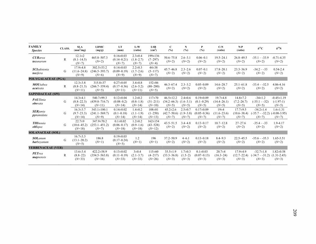
209
FAMILY Species
CLASS. SLA
(mm2/mg) LDMC (mg/g)
LT (mm)
L:W (ratio)
LSR (cm2)
C (%)
N (%)
P (%)
C:N (ratio)
N:P (ratio)
δ13C δ15N
CURarea tecunarum
R 12.1±2
(8.1–14.5) (N=7)
465.8–507.3 (N=2)
0.16±0.03 (0.14–0.21)
(N=7)
2.3±0.4 (1.8–2.7)
(N=7)
199±136 (7–297) (N=4)
50.6–75.8 (N=2)
2.6–3.1 (N=2)
0.06–0.1 (N=2)
19.5–24.1 (N=2)
26.8–49.5 (N=2)
-35.1 – -33.9 (N=2)
-0.71-4.35 (N=2)
SCIadotenia toxifera
G 17.9±4.8
(11.6–24.8) (N=9)
302.5±53.2 (246.5–393.7)
(N=6)
0.14±0.03 (0.09–0.19)
(N=9)
2.2±0.3 (1.7–2.6)
(N=9)
44±38 (5–117) (N=7)
45.7–46.8 (N=2)
2.3–2.6 (N=2)
0.07–0.1 (N=2)
17.8–20.1 (N=2)
23.3–36.9 (N=2)
-34.2 – -33 (N=2)
0.54-2.4 (N=2)
POLYGALACEAE (PGA)
MOUtabea aculeata
R 12.3±3.8
(8.8–21.3) (N=11)
315.8±37 (266.7–359.4)
(N=5)
0.27±0.05 (0.17–0.36)
(N=11)
3.4±0.8 (2.6–5.2) (N=11)
152±86 (80–280)
(N=5)
46.3–67.4 (N=2)
2.3–3.2 (N=2)
0.05–0.09 (N=2)
14.6–28.7 (N=2)
25.1–61.8 (N=2)
-33.4 – -32.5 (N=2)
4.06-4.16 (N=2)
SAPINDACEAE (SPI)
PAUllinia obovata
G 14.3±4.1
(8.8–22.3) (N=14)
540.7±99.3 (439.8–716.7)
(N=11)
0.12±0.04 (0.08–0.2)
(N=14)
1.2±0.2 (0.8–1.8) (N=14)
117±70 (31–211) (N=10)
46.5±12.2 (34.2–66.3)
(N=5)
2.4±0.6 (1.6–3.1)
(N=5)
0.19±0.09 (0.1–0.29)
(N=5)
19.7±4.8 (14.4–26.1)
(N=5)
14.8±7.2 (7.2–26.7)
(N=5)
-34±1.2 (-35.1 – -32)
(N=5)
-0.45±1.19 (-1.97-1)
(N=5)
SERjania pyramidata
G 16.3±3.7
(9.7–23.3) (N=14)
343.1±100.1 (241.1–569.7)
(N=9)
0.14±0.02 (0.1–0.18)
(N=14)
1.4±0.2 (1.1–1.9) (N=14)
108±81 (1–250) (N=13)
45.2±2.6 (42.7–50.6)
(N=7)
2.5±0.7 (1.9–3.8)
(N=7)
0.17±0.09 (0.05–0.36)
(N=7)
19±4 (11.6–23.6)
(N=7)
17.7±9.5 (10.6–38.4)
(N=7)
-34.2±1.4 (-35.7 – -32.2)
(N=7)
1.6±1.31 (-0.08-3.95)
(N=7)
THInouia obliqua
G 22.7±9
(10.6–45.2) (N=18)
347.9±70.2 (253.1–451.2)
(N=7)
0.1±0.02 (0.06–0.17)
(N=18)
1.2±0.2 (0.9–1.6) (N=18)
162±154 (43–528) (N=12)
43.5–51.5 (N=2)
3.4–4.8 (N=2)
0.13–0.17 (N=2)
10.7–12.8 (N=2)
27–27.6 (N=2)
-35.4 – -33 (N=2)
1.9-4.17 (N=2)
SOLANACEAE (SOL)
SOLanum barbeyanum
G 16.7±3.3
(13.1–20.2) (N=5)
186.8 (N=1)
0.19±0.03 (0.17–0.24)
(N=5)
1.2 (N=1)
196 (N=1)
37.2–50.9 (N=2)
4–6.1 (N=2)
0.13–0.18 (N=2)
8.4–9.3 (N=2)
22.5–45.5 (N=2)
-35.6 – -35.3 (N=2)
1.65-3.51 (N=2)
VERBENACEAE (VER)
PETrea maynensis
R 13.6±3.4 (8.8–22) (N=33)
422.2±58.9 (354.5–563.8)
(N=16)
0.13±0.02 (0.11–0.19)
(N=33)
3±0.4 (2.1–3.7) (N=33)
115±60 (4–217) (N=26)
35.5±1.9 (33.3–36.8)
(N=3)
1.7±0.3 (1.5–2) (N=3)
0.1±0.03 (0.07–0.13)
(N=3)
20.7±4 (16.3–24)
(N=3)
17.9±4.9 (12.7–22.4)
(N=3)
-32.7±1.8 (-34.7 – -31.2)
(N=3)
1.82±0.58 (1.31-2.45)
(N=3)
210
APPENDIX 5
Traits of wood specific gravity and diameter growth rate (obtained from two
censuses, census 0 and census 1, separated by approximately two years) of the 43 liana
species included in the functional trait analyses. The habitat association (or non-
association) of species was classified (CLASS.) as: ridge species (R), valley species (V),
generalist species (G), and widespread with habitat association species (W, subclassified
in WR: with ridge association, and WV: with valley association) (see Methods, and
Tables 3.1 and 3.2). WSG=wood specific gravity, AGR=absolute growth rate,
RGR=relative growth rate. Growth rates by diameter categories and for all lianas (all
diameter categories) are shown. A growth rate of “0” means no growth from census 0 to
census 1. Species acronyms (in bold) were formed by the first three letters of the genus
(in UPPERCASE) and the first three letters of the epithet. Family acronyms (in
parentheses) were formed by a three-letter code. Names within quotation marks are
morphospecies. Family acronyms (in parentheses) were formed by a three-letter code.
Species are ordered by family.
Values reported are: mean ± 1 standard deviation, minimum and maximum values
(in parentheses) and number of individuals sampled (N, in parentheses) (if N=2, no mean
was calculated).

211
AGR (mm/year) RGR (1/year)
FAMILY Species
CLASS. WSG
(g/cm3) 1.0–1.5 cm 1.5–2.5 cm 2.5–5.0 cm ≥5.0 cm ALL LIANAS 1.0–1.5 cm 1.5–2.5 cm 2.5–5.0 cm ≥5.0 cm ALL LIANAS
APOCYNACEAE (APO)
FORsteronia affinis
R 0.33±0.05
(0.27–0.39) (N=6)
0.1 (N=1)
0–0 (N=2)
no lianas no lianas 0.03±0.06
(0–0.1) (N=3)
0.01 (N=1)
0–0 (N=2)
no lianas no lianas 0±0
(0–0.01) (N=3)
ARECACEAE (ARE)
DESmoncus orthacanthos
R 0.52
(N=1) no lianas
0 (N=1)
no lianas no lianas 0
(N=1) no lianas
0 (N=1)
no lianas no lianas 0
(N=1)
ASTERACEAE (AST)
MIKania leiostachya
V species not
sampled no lianas
1.31 (N=1)
no lianas no lianas 1.31
(N=1) no lianas
0.06 (N=1)
no lianas no lianas 0.06
(N=1)
BIGNONIACEAE (BIG)
ADEnocalymna impressum
R 0.38±0.07
(0.19–0.43) (N=11)
0.05–0.53 (N=2)
no lianas no lianas no lianas 0.05–0.53
(N=2) 0–0.05 (N=2)
no lianas no lianas no lianas 0–0.05 (N=2)
BIGnonia aequinoctialis
G 0.44±0.05 (0.32–0.5)
(N=9)
0.48 (N=1)
no lianas 0.35
(N=1) no lianas
0.35–0.48 (N=2)
0.05 (N=1)
no lianas 0.01
(N=1) no lianas
0.01–0.05 (N=2)
MANsoa verrucifera
V 0.48
(N=1) 0.43–0.58
(N=2) 0.29
(N=1) no lianas no lianas
0.43±0.15 (0.29–0.58)
(N=3)
0.03–0.05 (N=2)
0.02 (N=1)
no lianas no lianas 0.04±0.02
(0.02–0.05) (N=3)
STIzophyllum riparium
G 0.44±0.04
(0.41–0.48) (N=3)
0.14 (N=1)
0–0 (N=2)
0.19 (N=1)
no lianas 0.08±0.1 (0–0.19) (N=4)
0.01 (N=1)
0–0 (N=2)
0.01 (N=1)
no lianas 0±0.01
(0–0.01) (N=4)
TANaecium affine
V 0.34–0.56
(N=2) species not
sampled species not
sampled species not
sampled species not
sampled species not
sampled species not
sampled species not
sampled species not
sampled species not
sampled species not
sampled
BORAGINACEAE (BOR)
TOUrnefortia bicolor
G 0.41
(N=1) 0.1–0.67
(N=2) no lianas
2.21–3.79 (N=2)
no lianas 1.69±1.66 (0.1–3.79)
(N=4)
0.01–0.06 (N=2)
no lianas 0.06–0.11
(N=2) no lianas
0.06±0.04 (0.01–0.11)
(N=4) COMBRETACEAE (COM)
COMbretum laxum
WV 0.55±0.14
(0.37–0.73) (N=5)
0.39±0.72 (0–2.17) (N=15)
0.75±1.04 (0–3.75) (N=21)
0.89±0.85 (0–3.07) (N=14)
1.13±1.3 (0–4.8) (N=17)
0.79±1.03 (0–4.8) (N=67)
0.03±0.05 (0–0.16) (N=15)
0.03±0.04 (0–0.14) (N=21)
0.03±0.03 (0–0.1) (N=14)
0.01±0.01 (0–0.03) (N=17)
0.03±0.04 (0–0.16) (N=67)
CONNARACEAE (CNN)
CONnarus patrisii
G 0.54±0.06
(0.44–0.63) (N=8)
3.55 (N=1)
no lianas 0.13±0.11 (0–0.19) (N=3)
no lianas 0.98±1.72 (0–3.55) (N=4)
0.27 (N=1)
no lianas 0±0
(0–0.01) (N=3)
no lianas 0.07±0.13 (0–0.27) (N=4)

212
AGR (mm/year) RGR (1/year)
FAMILY Species
CLASS. WSG
(g/cm3) 1.0–1.5 cm 1.5–2.5 cm 2.5–5.0 cm ≥5.0 cm ALL LIANAS 1.0–1.5 cm 1.5–2.5 cm 2.5–5.0 cm ≥5.0 cm ALL LIANAS
ROUrea amazonica
G species not
sampled no lianas
0.26±0.36 (0–0.77) (N=4)
no lianas no lianas 0.26±0.36 (0–0.77) (N=4)
no lianas 0.01±0.02 (0–0.04) (N=4)
no lianas no lianas 0.01±0.02 (0–0.04) (N=4)
ROUrea camptoneura
G 0.57
(N=1) 0.75
(N=1)
0.27±0.33 (0–0.74) (N=4)
no lianas 0
(N=1)
0.3±0.35 (0–0.75) (N=6)
0.06 (N=1)
0.01±0.02 (0–0.04) (N=4)
no lianas 0
(N=1)
0.02±0.02 (0–0.06) (N=6)
CONVOLVULACEAE (CNV)
MARipa peruviana
G 0.46–0.54
(N=2)
0.43±0.3 (0.19–0.77)
(N=3)
0–0.73 (N=2)
no lianas no lianas 0.4±0.33 (0–0.77) (N=5)
0.03±0.02 (0.01–0.05)
(N=3)
0–0.03 (N=2)
no lianas no lianas 0.03±0.02 (0–0.05) (N=5)
DICHAPETALACEAE (DIC)
DIChapetalum froesii
G 0.44–0.46
(N=2) 0
(N=1) 0–0.4 (N=2)
2.23 (N=1)
no lianas 0.66±1.07 (0–2.23) (N=4)
0 (N=1)
0–0.02 (N=2)
0.05 (N=1)
no lianas 0.02±0.02 (0–0.05) (N=4)
DIChapetalum spruceanum
G 0.55±0.05
(0.49–0.59) (N=3)
0–0 (N=2)
0 (N=1)
no lianas no lianas 0±0
(0–0) (N=3)
0–0 (N=2)
0 (N=1)
no lianas no lianas 0±0
(0–0) (N=3)
DILLENIACEAE (DIL)
DOLiocarpus dentatus
V 0.33–0.39
(N=2)
0.24±0.3 (0–0.77) (N=8)
0–0.38 (N=2)
0.05–1.34 (N=2)
1.44 (N=1)
0.39±0.51 (0–1.44) (N=13)
0.02±0.03 (0–0.07) (N=8)
0–0.02 (N=2)
0–0.03 (N=2)
0.02 (N=1)
0.02±0.02 (0–0.07) (N=13)
TETracera willdenowiana
G 0.46±0.04 (0.4–0.53)
(N=11)
0.34±0.67 (0–1.34) (N=4)
0.9±0.9 (0.24–1.93)
(N=3)
0.84±0.86 (0–2.02) (N=6)
1.74±3.39 (0–7.77) (N=5)
0.99±1.84 (0–7.77) (N=18)
0.03±0.05 (0–0.1) (N=4)
0.04±0.05 (0.01–0.1)
(N=3)
0.02±0.02 (0–0.05) (N=6)
0.03±0.06 (0–0.13) (N=5)
0.03±0.04 (0–0.13) (N=18)
FABACEAE (FAB)
BAUhinia "peluda"
G 0.44
(N=1) 0.67
(N=1)
1.76±2.01 (0.14–5.09)
(N=5)
1.02±1.56 (0–3.55) (N=5)
no lianas 1.32±1.67 (0–5.09) (N=11)
0.06 (N=1)
0.07±0.07 (0.01–0.19)
(N=5)
0.03±0.05 (0–0.11) (N=5)
no lianas 0.05±0.06 (0–0.19) (N=11)
CLItoria pozuzoensis
WR 0.57±0.06
(0.45–0.64) (N=7)
0.34±0.54 (0–1.78) (N=18)
0.26±0.4 (0–1.2) (N=23)
0.36±0.35 (0–0.82) (N=7)
no lianas 0.3±0.45 (0–1.78) (N=48)
0.03±0.04 (0–0.13) (N=18)
0.01±0.02 (0–0.06) (N=23)
0.01±0.01 (0–0.03) (N=7)
no lianas 0.02±0.03 (0–0.13) (N=48)
DIOclea ucayalina
R 0.43±0.17
(0.28–0.65) (N=4)
1.43±1.12 (0.14–2.22)
(N=3)
0.24 (N=1)
no lianas no lianas 1.13±1.09
(0.14–2.22) (N=4)
0.11±0.09 (0.01–0.17)
(N=3)
0.01 (N=1)
no lianas no lianas 0.08±0.09
(0.01–0.17) (N=4)
MAChaerium cuspidatum
WV 0.48±0.07 (0.39–0.6)
(N=10)
0.39±0.52 (0–1.82) (N=20)
0.45±0.56 (0–1.93) (N=29)
0.69±1.37 (0–5.96) (N=33)
1.56±2.05 (0–7.16) (N=10)
0.64±1.16 (0–7.16) (N=92)
0.03±0.04 (0–0.15) (N=20)
0.02±0.03 (0–0.08) (N=29)
0.02±0.04 (0–0.17) (N=33)
0.02±0.03 (0–0.09) (N=10)
0.02±0.04 (0–0.17) (N=92)
PIPtadenia anolidurus
V 0.31–0.38
(N=2) 0
(N=1) no lianas no lianas no lianas
0 (N=1)
0 (N=1)
no lianas no lianas no lianas 0
(N=1)

213
AGR (mm/year) RGR (1/year)
FAMILY Species
CLASS. WSG
(g/cm3) 1.0–1.5 cm 1.5–2.5 cm 2.5–5.0 cm ≥5.0 cm ALL LIANAS 1.0–1.5 cm 1.5–2.5 cm 2.5–5.0 cm ≥5.0 cm ALL LIANAS
HIPPOCRATEACEAE (HIP)
ANThodon decussatum
R 0.5
(N=1) no lianas
0.25–0.72 (N=2)
no lianas 0
(N=1)
0.32±0.37 (0–0.72) (N=3)
no lianas 0.01–0.03
(N=2) no lianas
0 (N=1)
0.01±0.02 (0–0.03) (N=3)
CUErvea kappleriana
WR 0.54±0.05
(0.46–0.58) (N=9)
0.22±0.26 (0–0.87) (N=22)
0.31±0.63 (0–3.08) (N=40)
0.55±1.59 (0–5.83) (N=13)
no lianas 0.32±0.81 (0–5.83) (N=75)
0.02±0.02 (0–0.06) (N=22)
0.01±0.03 (0–0.12) (N=40)
0.02±0.04 (0–0.16) (N=13)
no lianas 0.02±0.03 (0–0.16) (N=75)
HYLenaea comosa
R 0.5
(N=1)
0.45±0.43 (0–0.87) (N=3)
0.24±0.27 (0–0.54) (N=5)
0–0.19 (N=2)
no lianas 0.28±0.31 (0–0.87) (N=10)
0.04±0.04 (0–0.08) (N=3)
0.01±0.01 (0–0.03) (N=5)
0–0.01 (N=2)
no lianas 0.02±0.03 (0–0.08) (N=10)
PERitassa pruinosa
R 0.57
(N=1)
0.33±0.39 (0–0.72) (N=4)
0.56±0.8 (0–2.59) (N=10)
0 (N=1)
no lianas 0.46±0.69 (0–2.59) (N=15)
0.02±0.03 (0–0.05) (N=4)
0.03±0.04 (0–0.14) (N=10)
0 (N=1)
no lianas 0.03±0.04 (0–0.14) (N=15)
SALacia multiflora
R 0.5±0.08
(0.42–0.63) (N=6)
0.21±0.26 (0–0.71) (N=6)
0.79±0.49 (0–1.44) (N=10)
0.43 (N=1)
no lianas 0.56±0.49 (0–1.44) (N=17)
0.02±0.02 (0–0.06) (N=6)
0.04±0.03 (0–0.08) (N=10)
0.02 (N=1)
no lianas 0.03±0.03 (0–0.08) (N=17)
ICACINACEAE (ICA)
LERetia cordata
G 0.34±0.08
(0.26–0.51) (N=7)
0.48±0.61 (0–1.53) (N=6)
0.47±0.51 (0–1.2) (N=4)
0.26±0.23 (0–0.43) (N=3)
0–0.48 (N=2)
0.4±0.46 (0–1.53) (N=15)
0.04±0.05 (0–0.13) (N=6)
0.02±0.02 (0–0.05) (N=4)
0.01±0.01 (0–0.01) (N=3)
0–0.01 (N=2)
0.02±0.03 (0–0.13) (N=15)
LOGANIACEAE (LOG)
STRychnos mitscherlichii
R 0.52
(N=1) no lianas
0.77 (N=1)
no lianas no lianas 0.77
(N=1) no lianas
0.05 (N=1)
no lianas no lianas 0.05
(N=1)
STRrychnos ramentifera
R 0.65±0.07
(0.55–0.72) (N=6)
no lianas 0.08±0.14 (0–0.24) (N=3)
no lianas no lianas 0.08±0.14 (0–0.24) (N=3)
no lianas 0±0.01
(0–0.01) (N=3)
no lianas no lianas 0±0.01
(0–0.01) (N=3)
MALPIGHIACEAE (MLP)
ECTopopterys soejartoi
G 0.48
(N=1) 2.02
(N=1)
0.11±0.19 (0–0.34) (N=3)
0 (N=1)
no lianas 0.47±0.88 (0–2.02) (N=5)
0.17 (N=1)
0±0.01 (0–0.01) (N=3)
0 (N=1)
no lianas 0.04±0.07 (0–0.17) (N=5)
HIRaea valida
G 0.51
(N=1)
0.16±0.22 (0–0.42) (N=3)
0 (N=1)
no lianas no lianas 0.12±0.2 (0–0.42) (N=4)
0.01±0.02 (0–0.03) (N=3)
0 (N=1)
no lianas no lianas 0.01±0.02 (0–0.03) (N=4)
MAScagnia dissimilis
G species not
sampled 0
(N=1) no lianas no lianas no lianas
0 (N=1)
0 (N=1)
no lianas no lianas no lianas 0
(N=1)
TETrapterys nitida
R 0.55–0.58
(N=2)
0.13±0.2 (0–0.63) (N=10)
0.4±0.69 (0–1.2) (N=3)
no lianas no lianas 0.2±0.35 (0–1.2) (N=13)
0.01±0.02 (0–0.06) (N=10)
0.02±0.03 (0–0.05) (N=3)
no lianas no lianas 0.01±0.02 (0–0.06) (N=13)
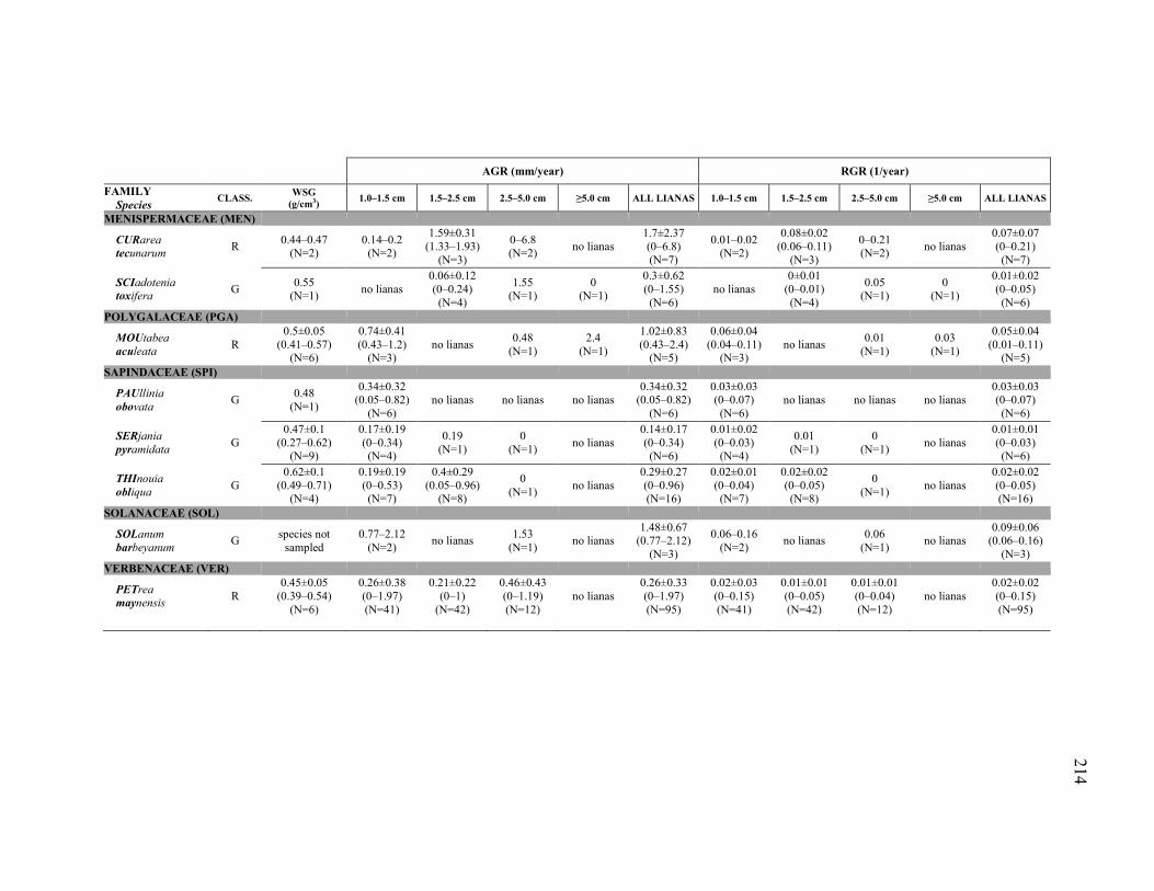
214
AGR (mm/year) RGR (1/year)
FAMILY Species
CLASS. WSG
(g/cm3) 1.0–1.5 cm 1.5–2.5 cm 2.5–5.0 cm ≥5.0 cm ALL LIANAS 1.0–1.5 cm 1.5–2.5 cm 2.5–5.0 cm ≥5.0 cm ALL LIANAS
MENISPERMACEAE (MEN)
CURarea tecunarum
R 0.44–0.47
(N=2) 0.14–0.2
(N=2)
1.59±0.31 (1.33–1.93)
(N=3)
0–6.8 (N=2)
no lianas 1.7±2.37 (0–6.8) (N=7)
0.01–0.02 (N=2)
0.08±0.02 (0.06–0.11)
(N=3)
0–0.21 (N=2)
no lianas 0.07±0.07 (0–0.21) (N=7)
SCIadotenia toxifera
G 0.55
(N=1) no lianas
0.06±0.12 (0–0.24) (N=4)
1.55 (N=1)
0 (N=1)
0.3±0.62 (0–1.55) (N=6)
no lianas 0±0.01
(0–0.01) (N=4)
0.05 (N=1)
0 (N=1)
0.01±0.02 (0–0.05) (N=6)
POLYGALACEAE (PGA)
MOUtabea aculeata
R 0.5±0.05
(0.41–0.57) (N=6)
0.74±0.41 (0.43–1.2)
(N=3) no lianas
0.48 (N=1)
2.4 (N=1)
1.02±0.83 (0.43–2.4)
(N=5)
0.06±0.04 (0.04–0.11)
(N=3) no lianas
0.01 (N=1)
0.03 (N=1)
0.05±0.04 (0.01–0.11)
(N=5) SAPINDACEAE (SPI)
PAUllinia obovata
G 0.48
(N=1)
0.34±0.32 (0.05–0.82)
(N=6) no lianas no lianas no lianas
0.34±0.32 (0.05–0.82)
(N=6)
0.03±0.03 (0–0.07) (N=6)
no lianas no lianas no lianas 0.03±0.03 (0–0.07) (N=6)
SERjania pyramidata
G 0.47±0.1
(0.27–0.62) (N=9)
0.17±0.19 (0–0.34) (N=4)
0.19 (N=1)
0 (N=1)
no lianas 0.14±0.17 (0–0.34) (N=6)
0.01±0.02 (0–0.03) (N=4)
0.01 (N=1)
0 (N=1)
no lianas 0.01±0.01 (0–0.03) (N=6)
THInouia obliqua
G 0.62±0.1
(0.49–0.71) (N=4)
0.19±0.19 (0–0.53) (N=7)
0.4±0.29 (0.05–0.96)
(N=8)
0 (N=1)
no lianas 0.29±0.27 (0–0.96) (N=16)
0.02±0.01 (0–0.04) (N=7)
0.02±0.02 (0–0.05) (N=8)
0 (N=1)
no lianas 0.02±0.02 (0–0.05) (N=16)
SOLANACEAE (SOL)
SOLanum barbeyanum
G species not
sampled 0.77–2.12
(N=2) no lianas
1.53 (N=1)
no lianas 1.48±0.67
(0.77–2.12) (N=3)
0.06–0.16 (N=2)
no lianas 0.06
(N=1) no lianas
0.09±0.06 (0.06–0.16)
(N=3) VERBENACEAE (VER)
PETrea maynensis
R 0.45±0.05
(0.39–0.54) (N=6)
0.26±0.38 (0–1.97) (N=41)
0.21±0.22 (0–1)
(N=42)
0.46±0.43 (0–1.19) (N=12)
no lianas 0.26±0.33 (0–1.97) (N=95)
0.02±0.03 (0–0.15) (N=41)
0.01±0.01 (0–0.05) (N=42)
0.01±0.01 (0–0.04) (N=12)
no lianas 0.02±0.02 (0–0.15) (N=95)

215
APPENDIX 6
Pearson (r) correlation matrix of all traits measured in the 43 species whose traits
were analyzed in the YFDP. P=2-tailed probability not corrected for multiple
comparisons. N=number of species. Traits measured were (see units in this Chapter’s
Figures or in Appendices 3.1 and 3.2): SLA=specific leaf area, LDMC=leaf dry matter
content, LT=leaf lamina thickness, L:W=length to width ratio of whole leaf (incl.
petiole), LSR=individual-level leaf size range, C=carbon concentration, N=nitrogen
concentration, P=phosphorus concentration, C:N=ratio of carbon concentration to
nitrogen concentration, N:P=ratio of nitrogen concentration to phosphorus concentration,
δ13C=relative abundance of the stable isotope carbon-13 in delta units, δ15N=relative
abundance of the stable isotope nitrogen-15 in delta units, WSG=wood specific gravity,
and AGR=absolute growth rate. Because P was not corrected for multiple comparisons
(e.g., via a Bonferroni correction), we considered that correlations existed only if
P≤0.001 (in red bold).

216
SLA LDMC LT L:W LSR C N P C:N N:P δδδδ13C δδδδ15N WSG AGR
all lianas
SLA r 1
P 2-tailed .
N 43
LDMC r −.508 1
P 2-tailed .001 .
N 41 41
LT r −.387 −.357 1
P 2-tailed .010 .022 .
N 43 41 43
L:W r −.088 −.157 .289 1
P 2−tailed .576 .327 .060 .
N 43 41 43 43
LSR r −.430 .304 .061 −.234 1
P 2−tailed .004 .053 .698 .131 .
N 43 41 43 43 43
C r .019 .176 −.155 −.031 −.051 1
P 2−tailed .903 .272 .321 .842 .747 .
N 43 41 43 43 43 43
N r .496 −.253 −.229 −.380 −.052 .342 1
P 2−tailed .001 .110 .140 .012 .741 .025 .
N 43 41 43 43 43 43 43
P r .352 −.217 −.089 −.423 −.054 −.146 .500 1
P 2−tailed .021 .173 .571 .005 .732 .350 .001 .
N 43 41 43 43 43 43 43 43
C:N r −.533 .297 .258 .345 .004 .119 −.821 −.550 1
P 2−tailed <.001 .059 .095 .024 .978 .448 <.001 <.001 .
N 43 41 43 43 43 43 43 43 43
N:P r .126 .009 −.160 .043 −.104 .580 .576 −.219 −.342 1
P 2−tailed .421 .954 .304 .783 .506 <.001 <.001 .158 .025 .
N 43 41 43 43 43 43 43 43 43 43
δδδδ13C
r .101 −.069 −.192 −.003 .030 −.140 −.134 .068 −.092 −.266 1
P 2−tailed .518 .670 .218 .987 .850 .370 .391 .664 .555 .085 .
N 43 41 43 43 43 43 43 43 43 43 43
δδδδ15N
r .110 −.290 .221 .268 .107 .110 .275 .080 −.222 .269 −.16
4 1
P 2−tailed .481 .066 .155 .083 .493 .483 .074 .610 .152 .081 .293 .
N 43 41 43 43 43 43 43 43 43 43 43 43
WSG r −.165 .205 −.028 .025 .162 −.026 −.129 −.390 .150 .011
−.222
−.011 1
P 2−tailed .316 .217 .867 .882 .325 .873 .435 .014 .362 .945 .174 .948 .
N 39 38 39 39 39 39 39 39 39 39 39 39 39
AGR all lianas
r −.113 −.256 .405 .023 −.082 .008 −.043 −.104 .084 −.017 .013 −.066 −.145 1 P 2−tailed .478 .111 .008 .885 .606 .961 .787 .513 .598 .916 .935 .679 .386 .
N 42 40 42 42 42 42 42 42 42 42 42 42 38 42
Copyright © 2022 FDOKUMEN