arX

iv:c

ond-

mat

/010

9059

v1 [

cond

-mat

.mtr

l-sc

i] 4

Sep

200

1

Trapping of Vibrational Energy in Crumpled Sheets

Ajay Gopinathan, T.A. WittenDept. of Physics and James Franck Institute, The University of Chicago, Chicago, IL 60637

S.C. VenkataramaniDept. of Mathematics, The University of Chicago, Chicago, IL 60637

(February 1, 2008)

We investigate the propagation of transverse elastic waves in crumpled media. We set up thewave equation for transverse waves on a generic curved, strained surface via a Langrangian formalismand use this to study the scaling behaviour of the dispersion curves near the ridges and on the flatfacets. This analysis suggests that ridges act as barriers to wave propagation and that modes in acertain frequency regime could be trapped in the facets. A simulation study of the wave propagationqualitatively supported our analysis and showed interesting effects of the ridges on wave propagation.

I. INTRODUCTION

Waves show distinctive behavior when they propagate through media that are strongly heterogeneous. Amongthese behaviors are localization [1], multiple propagation paths and lensing [2] . These phenomena depend stronglyon the type of wave (electromagnetic, Schroedinger, vibrational) and the type of heterogeneity.

We treat a type of heterogeneity that arises naturally in materials, but whose effect on waves has not been studied:crumpled membranes. The disorder introduced by crumpling is much different from the random disorder usuallyconsidered. Instead of a structureless disorder, crumpled sheets consist of uniform, flat facets bordered by stronglycurved and stretched borders called elastic ridges [9,10]. Vibrational waves are expected to propagate much differentlyin the facets and in the border regions. Crumpled sheets of newsprint paper are commonly used as an insulating andprotective enclosure, but we know of no characterization of their vibrational isolation or transmissions properties.

We anticipate various possible effects. We imagine oscillating a point on the membrane and investigating theresponse as a function of distance from this source as compared with a flat, uniform sheet. First, there are twonatural regimes of vibrational frequency to be considered. Low frequencies are expected to produce vibrations withwavelengths much longer than the facets or ridges of the crumpled structure. These long-wavelength waves mightshow distinctive and subtle features, yet we shall not treat them in the present paper. These waves are not expectedto depend heavily on the distinctive facet-and-ridge structure of crumpled sheets.

We shall consider instead the complementary regime of higher frequencies having wavelengths smaller than thetypical facets of the sheet. Several behaviors might be expected as compared to the uniform sheet. On the one hand,the elastic tension induced by the ridges might enhance the propagation along the network of ridges. On the otherhand, the contrasting nature of the ridges and the facets might serve as a barrier for propagation out of or into afacet. It is these phenomena that we address below.

In section II we briefly review classical thin membrane theory and gather the results we need. In section III wederive the wave equations for transverse waves on a generic curved, strained surface from a Langrangian formulation.Section IV is devoted to studying the form of the dispersion relations in the two distinct regions (ridges and facets)and also the scaling behaviour of the dispersions with thickness of the sheet. This analysis first suggests the possibilityof trapped energy in the facets with ridges serving as barriers. In section V we discuss in detail the simulations weperformed and compare them to our analytical predictions. Finally we discuss the implications of our work and thescope for future work in section VI.

II. THIN MEMBRANE THEORY

Our findings are based on the classical theory of thin membranes [3]. If the thickness is small then we may assumethat all variables may be integrated over the thickness of the membrane and it can be regarded as a two dimensionalsurface [3]. To define a surface uniquely up to overall translations and rotations it is sufficient to specify a metrictensor gαβ and a curvature tensor Cαβ satisfying Gauss’s Theorema Egregium and the Codazzi-Mainardi equations[4]. To see the physical significance of these tensors we first note that the deviation of the metric tensor from the

1

identity is simply the strain tensor

gαβ = δαβ + γαβ (1)

The sum of the eigenvalues of the strain tensor is the (2D) expansion factor and their difference is the shear angle [3].The eigenvalues of the curvature tensor are simply the inverses of the two principal radii of curvature of the surface.If we take a point ~r(x1, x2) where x1, x2 refer to the (2D) material co-ordinates of the point, the metric and curvaturetensor are given by [4]

gαβ = (∂α~r) · (∂β~r) (2)

Cαβ = n̂ · (∂α∂β~r) (3)

where ∂α denotes differentiation with respect to the material co-ordinate xα, and n̂ is the unit normal to the surfaceat that point. We now consider the forces and torques in the system necessary for mechanical equilibrium. They aregiven by the stress tensor σαβ and the torque tensor Mαβ. These are related to the deformation tensors γαβ and Cαβ ,for sufficiently small strains by [3]

σαβ =Y h

1 − ν2[γαβ + νǫαρǫβτγρτ ] (4)

Mαβ = κ[Cαβ + νǫαρǫβτCρτ ] (5)

where Y is the Young’s modulus, ν is the Poisson ratio and κ = Y h3/(12(1−ν2)) is the bending modulus of the elasticmaterial. Here h is the thickness of the sheet. ǫαβ is the two dimensional antisymmetric tensor. Summation overrepeated indices is implied. The conditions that guarantee that the strain and curvature tensors describe a physicalsurface in equilibrium are called the von Karman equations. The von Karman equations [5] may be put in a formmore suitable for our purposes as follows [6]

detCαβ = ∂α∂βγαβ −∇2 Tr γαβ (6)

∂α∂βMαβ = σαβCαβ (7)

The first equation is simply a restatement of Gauss’ theorem which helps in making sure that the curvature andmetric tensor describe a physical surface. The second von Karman (also called the stress von Karman) equation is acondition for physical equilibrium of the sheet. Finally we need expressions for the elastic energy stored in the sheet.The stretching energy is given by [6]

Es =1

2

∫

dxdy σαβγαβ (8)

and the bending energy by

Eb =1

2

∫

dxdy MαβCαβ (9)

Thus the total elastic energy of the sheet is given by

Etot =1

2

∫

dxdy [σαβγαβ + MαβCαβ ] (10)

III. THE WAVE EQUATION

Let the equilibrium configuration of the sheet be given by ~r0(x, y). This implies that ~r0(x, y) satisfies the vonKarman equations. To study tranverse waves we consider small displacements normal to the surface everywhere.

~r(x, y) = ~r0(x, y) + ǫu(x, y)n̂ (11)

where u(x, y) is a smooth function of the material coordinates x, y. Considering only transverse waves is justifiedsince it is known that in the thin limit (h ≪ 1) the transverse and in-plane modes decouple [7]. Our simulation results

2

also indicate that for small perturbations the generated modes are primarily transverse and the fraction of energy inthe in-plane modes is orders of magnitude smaller. The transverse perturbation u(x, y) leads to a change in the totalenergy of the sheet of order ǫ2. The O(ǫ) term should vanish because ~r0(x, y) is the equilibrium configuration. Usingequation (11) along with the defining equations (1)-(5) and equation (10) yields the O(ǫ2) change in energy

δE =1

2

∫

dxdy[

κ[

(uxx − u(C0xx)2)2 + (uyy − u(C0

yy)2)2]

+ 2κ(1 − ν)u2xy

+ 2κν(uxx − u(C0xx)2)(uyy − u(C0

yy)2) +hY

1 − ν2

[

γ0xx(u2

x + u2(C0xx)2 + ν(u2

y + u2(C0yy)2))

+γ0yy(u

2y + u2(C0

yy)2 + ν(u2x + u2(C0

xx)2)) + u2((C0xx)2 + (C0

yy)2 + 2νC0xxC0

yy)]]

(12)

where C0xx, C0

yy, γ0xx, γ0

yy are simply the respective components of the curvature and strain tensor in the equilibriumstate. uα is the derivative of u with respect to the material coordinate α. The O(ǫ) term is simply the stress vonKarman equation and hence vanishes as argued above. Cross terms involving C0

xy and γ0xy are absent because we have

chosen our axes to be aligned with the principal axes of the curvature and strain tensor. Here we restrict ourselvesto the case where the principal axes of the curvature and strain tensor are the same. This is true along the middle ofthe ridge [10]. The general expression is more complex but this is sufficient for our purposes. We now consider δE tobe an effective potential for the field u(x, y).

V = δE (13)

We can then define a kinetic energy term

T =1

2

∫

dxdy ρh u2t (14)

where ρ is the density of the material and ut ≡ ∂u/∂t. This leads to an effective Langrangian for the field given by

L = T − V (15)

The Euler-Lagrange equations for this system are then given by

∂L∂u

− ∂µ∂L∂uµ

+ ∂µ∂ν∂L

∂uµν= 0 (16)

The last term arises because of the presence of second derivatives of the field in the potential [8]. Using equations(12)-(15) in equation (16) gives us the local wave equation satisfied by the field u(x, y).

−ρh utt = κ∇4u − Axuxx − Ayuyy + Bu (17)

where

Ax = 2κ(C0xx)2 + 2κν(C0

yy)2 +Y h

1 − ν2(γ0

xx + νγ0yy) (18)

and similarly for Ay. The coefficient of the last term is given by

B = κ(C0xx)4 + κ(C0

yy)4 + 2κν(C0xx)2(C0

yy)2 + r[γ0xx((C0

xx)2 + ν(C0yy)2) + γ0

yy((C0yy)2 + ν(C0

xx)2)]

+ r[(C0xx)2 + (C0

yy)2 + 2νC0xxC0

yy]. (19)

where r ≡ Y h/(1−ν2). It is to be noted that all these coefficients are local, in that they depend on the curvature andstrain at the point (x, y) in the material co-ordinates. We now consider some limiting cases to understand the originof the various terms in equation (17). First we consider the case when we simply have a flat sheet with no curvatureor strain. Here Ax, Ay and B are identically zero, giving us

−ρh utt = κ∇4u (20)

which correctly describes bending waves on a sheet with thickness h, bending modulus κ and density ρ [3]. Now weconsider the case where we have a flat sheet with no curvature, κ = 0, and with some isotropic strain γ. Equation(17) then reduces to

−ρh utt =Y hγ

1 − ν∇2u (21)

which describes a stretched membrane under tension proportional to Y γ. The leading-order behaviour of the lastterm in equation (17) will be discussed in the next section.

3

IV. DISPERSION RELATIONS

A crumpled sheet consists of two distinct regions, the ridges and the flat facets that are bounded by ridges. Theridges are regions of large curvature and strain and most of the elastic energy of the sheet is stored here [9]. The flatfacets on the other hand have small curvature and strain from the ridges pulling on them [10]. In this section we lookat the dispersion relations for tranverse waves in the two regions.

A. Ridges

We take the material coordinate x to lie along the width of the ridge and y to lie along its length. We assume thatthe ridge is a region with uniform curvature and strain given by the values that they take at the midpoint. To obtainthe dispersion relations we consider a plane wave, u ∼ ei(kx−ωt), traversing the width of the ridge . Substituting thisansatz into equation (17) yields

ak4 + bk2 + c = ω2 (22)

where

a =κ

ρh(23)

b =1

ρh[2κC2

xx + 2κνC2yy + r(γxx + νγyy)] (24)

c =1

ρh[κC4

xx + rγxxC2xx + rνγyyC2

xx + rC2xx + κC4

yy + 2κνC2xxC2

yy

+ rνγxxC2yy + rγyyC2

yy + rC2yy + 2rνCxxCyy]. (25)

where r ≡ Y h/(1−ν2) as before. Considering a wave travelling in the perpendicular direction yields the same equationexcept with a x and y interchange in the coefficient b. We now consider the leading order behaviour of the abovecoefficients in the limit of very small thickness , h ≪ 1, where h is measured in units of the ridge size. For this case thescaling of the midridge curvature and strain with thickness have been worked out by Witten and coworkers [9,10,6].We have the following results for

Cxx ∼ h−1

3 (26)

Cyy ≪ Cxx (27)

γxx ∼ h2

3 (28)

γyy ∼ h2

3 (29)

Using these scaling laws along with the dispersion relation obtained above gives us the scaling behaviour of thedispersion curve

a0h2k4 + b0h

2

3 k2 + c0h−

2

3 = ω2 (30)

where a0, b0, c0 are positive real numbers independent of h. It is also to be noted that we would get the same formfor the dispersion in the perpendicular direction of propagation. The explicit form of the leading order term in thecoefficient c is

c =Y

ρ(1 − ν2)R−2 (31)

where R = C−1xx is the transverse radius of curvature of the ridge. This is significant because the above expression is

the square of the “ringing frequency” of a cylinder of radius R, which is the frequency of purely radial oscillations ofthe cylinder [7]. Thus the last term in the dispersion represents the “breathing mode” of the ridge. Equation (30)

tells us that, for large wavenumbers (k ≫ h−2

3 ), the first term dominates leading to pure bending wave behaviour.This is reasonable, since for small wavelengths (or large k) the surface is locally flat and hence we expect behaviour

like bending waves on a flat sheet. In the long wavelength regime (k ≪ h−2

3 ), the constant term dominates leading tobreathing modes of the ridge. This also prescribes a lower cutoff frequency for modes in the ridge. There is no regimewhere the second term describing sound modes dominates. Thus the crossover leads directly from the bending waveregime to the breathing mode regime.

4

0 0.2 0.4 0.6 0.8 1 1.2 1.4 1.6 1.8 2−2

−1

0

1

2

3

4

5

Log k

Log

ω2

h0

h−1/3

h−2/3

FIG. 1. Dispersion curves for the ridge (top curve) and facet (bottom curve) regions for h = 0.01. Coefficients independentof h (a0, b0 etc) have been set to 1. The lower k cutoff for the ridge region is the inverse of the ridge width (w−1

∼ h−1/3).The lower cutoff for the facet region is the inverse of the ridge length which we take as unity. Above k ≈ h−2/3 bending modesdominate in the ridge and modes in the facet can exist in the ridge too.

B. Facets

The facets have some residual strain and curvature due to the ridges. Following the treatment of Lobkovsky et al

[10] we have the following scaling relations for the curvature and strain away from the ridge.

C ∼ h1

3 (32)

γ ∼ h4

3 (33)

Using these scaling laws, we follow the same procedure as in the last section to obtain the scaling form of the dispersionrelation

a1h2k4 + b1h

4

3 k2 + c1h2

3 = ω2 (34)

Again we see two distinct regimes. For small wavelengths (k ≫ h−1

3 ), we have pure bending waves and for large

wavelengths (k ≪ h−1

3 ), we have breathing modes. Figure 1 shows the dispersion curves for both the ridges andfacets. We notice that there are modes that exist on the facets whose frequencies are too low to propagate in theridges. This prompts the question as to whether these modes can tunnel through the ridges to the other facets.

C. Skin Depth

To address the question of whether the above mentioned modes are able to penetrate the ridges we look at the skindepth of these modes in the ridge region. For a particular mode the frequency is the same in both regions ( becauseof matching at the interface ). If the frequency is less than the cutoff frequency in the ridge region, as is the case withthe modes we are looking at, then there will be an associated skin depth. This needs to be compared to the width ofthe ridge to see if these modes are trapped in the facet. Consider a mode of frequency ω0. In the ridge region we have

a0h2k4 + b0h

2

3 k2 + c0h−

2

3 = ω20 (35)

where a0, b0, c0 are just real, positive numbers independent of h. We consider the case where ω0 is just less than thecutoff frequency. Thus we take

ω20 = d0h

−2

3 (36)

where d0 < c0. Using this we may now solve for k in the ridge region. The solution is

k =[−b0 ± (b2

0 − 4a0(c0 − d0))1

2

2a0

]1

2 h−2

3 (37)

5

The requirement d0 < c0 ensures that k has a nonzero imaginary part. Thus the imaginary part of k scales as h−2

3

and hence the skin depth

ζ ∼ [Im(k)]−1 ∼ h2

3 (38)

The width of the ridge w, however scales as h1

3 [6]. Thus we find that

ζ ≪ w (39)

This implies that the modes we considered ought to remain trapped in the facet for sufficiently thin sheets. In thenext section we examine the predicted scaling behaviour and the trapping phenomenon numerically.

V. SIMULATIONS

We model the elastic sheet as a triangular lattice of springs of unstretched length a and spring constant K followingSeung and Nelson [11]. We incorporate bending rigidity by assigning an energy J(1− n̂1 · n̂2) to every pair of adjacentlattice triangles with normals n̂1 and n̂2. Sueng and Nelson showed that when the strains are small and the radii ofcurvature are large compared to the lattice constant, this model membrane bends and stretches like an elastic sheetof thickness h = a

√

8J/K with Young’s modulus Y = 2Ka/h√

3 and Poisson ratio ν = 1/3. The bending modulus is

κ = J√

3/2. This model has been extensively used to study the static scaling properties of ridges [6,10,12]. We use itin this paper to study the dynamics of wave propagation by adding a unit mass to every lattice point. This modelsthe kinetic term in our Lagrangian and assigns to the sheet, a mass per unit area.

To produce connected ridges and facets we construct a very simple shape, namely the regular tetrahedron, by joiningthe edges of a triangular sheet [6]. By using a conjugate gradient minimization routine we get the tetrahedron closeto its equlibrium position. We then add in damping and a small perturbation (a tap on one of the facets) and thenwait for the system to attain a state of equilibrium. Once equilibrium is attained we now remove the damping andperturb the system ( tapping a few lattice points at the center of a facet by giving the three central particles of thefacet equal initial velocities normal to the surface) so as to generate waves and study their propagation. To measurethe energy being carried by the waves we first define an energy that measures the deviation from the equilibriumstate.

Edev =∑ 1

2K(xi − x0

i )2 +

∑

2J(sin(θk/2) − sin(θ0k/2))2

+∑ 1

2v2

i (40)

where xi’s refer to the positions of the point unit masses, θi’s are supplements of the angles between pairs of plaquetsand vi’s are velocities of the masses. The superscript indicates the value of the variable at equilibrium. After aninitial drop (3− 4%) this energy is conserved up to 1% of its value and hence is a reasonably reliable indicator of theenergy associated with deviations.

For large initial perturbations we may also expect the initiation of in-plane waves. To avoid these waves wefirst estimate what initial impulse causes a displacement comparable to the lattice spacing, by assuming that theenergy of the impulse is transferred to stretching and bending energy in the region of the tap. For typical values(a = 1,K = 1,J = 0.05) we obtain the limiting value of the initial impulse to be 0.1. Figure 2 shows the normalizedenergy of the perturbed facet for different tap strengths both above and below the limiting value. The simulationwas done with the above mentioned parameter values for a tetrahedron of size 10a. We notice that the curves belowthe threshold lie on top of each other. Thus tapping below the threshold strength gives us robust, characteristiccurves that are independent of the initial impulse. From here on we consider only simulations where we tap below thethreshold. Looking at the stretching and bending energies in this regime also tells us that stretching contribution issmall and hence the modes are mostly transverse. We also check this fact by looking explicitly at the particle motion.

Now we consider the time dependence of the energy of the perturbed facet. Typical curves are like those in figure 2with initial impulse below the threshold. For an initial interval the energy remains close to 1. It then begins to dropoff and we see a straight line segment to the curve. The initial interval simply indicates the time it takes the fastestmode to reach the edge of the facet. The straight line segment on the other hand is presumably where all modes arecontributing giving us a constant energy flux out of the facet and hence a constant slope in the energy versus timegraph.

6

0 2 4 6 8 10 12 14 16 18 200

0.1

0.2

0.3

0.4

0.5

0.6

0.7

0.8

0.9

1

Time

Ep/E

tot

FIG. 2. Normalized energy of the perturbed facet as a function of time. Ep stands for the deviation energy of the perturbedfacet. Etot is the total deviation energy of the tetrahedron. Curves are for values of impulse 0.01 (+),0.001 (*) and 0.3 (o).Note that the first two are below the threshold (0.1) and the last one is above.

101

Thickness h

Ons

et ti

me

t 0

12

5

7

0.35 0.65 0.45 0.55

FIG. 3. Log-log plot of onset times as a function of thickness for different p. Circles (p = 0.9), Pluses (p = 0.85), Asterisks(p = 0.92). The lines are best fit to the data points. Slopes of the lines (top to bottom) are -1.55,-1.48 and -1.41 respectively.

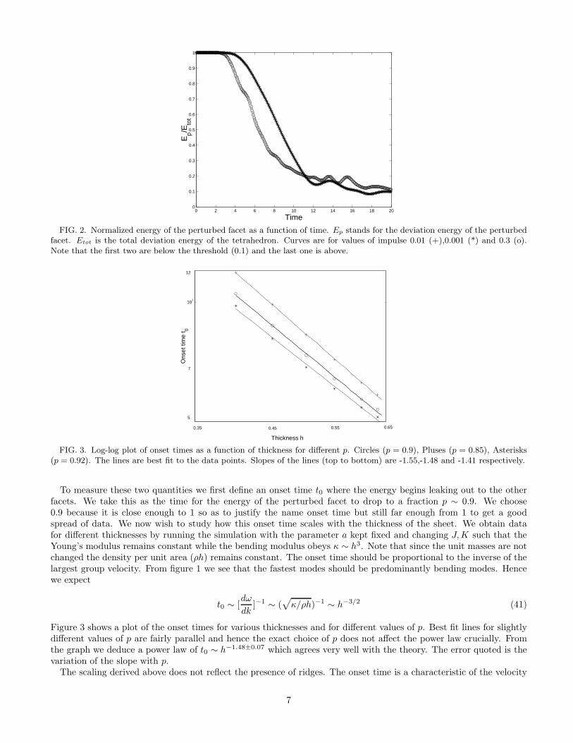
To measure these two quantities we first define an onset time t0 where the energy begins leaking out to the otherfacets. We take this as the time for the energy of the perturbed facet to drop to a fraction p ∼ 0.9. We choose0.9 because it is close enough to 1 so as to justify the name onset time but still far enough from 1 to get a goodspread of data. We now wish to study how this onset time scales with the thickness of the sheet. We obtain datafor different thicknesses by running the simulation with the parameter a kept fixed and changing J, K such that theYoung’s modulus remains constant while the bending modulus obeys κ ∼ h3. Note that since the unit masses are notchanged the density per unit area (ρh) remains constant. The onset time should be proportional to the inverse of thelargest group velocity. From figure 1 we see that the fastest modes should be predominantly bending modes. Hencewe expect

t0 ∼ [dω

dk]−1 ∼ (

√

κ/ρh)−1 ∼ h−3/2 (41)

Figure 3 shows a plot of the onset times for various thicknesses and for different values of p. Best fit lines for slightlydifferent values of p are fairly parallel and hence the exact choice of p does not affect the power law crucially. Fromthe graph we deduce a power law of t0 ∼ h−1.48±0.07 which agrees very well with the theory. The error quoted is thevariation of the slope with p.

The scaling derived above does not reflect the presence of ridges. The onset time is a characteristic of the velocity

7

Thickness h

Slo

pe m

0.65 0.4 0.45 0.55

0.13

0.3

0.2

FIG. 4. Log-log plot of slope m as a function of thickness. The line is a best fit to the data points.

0 10 20 30 40 50 600

0.1

0.2

0.3

0.4

0.5

0.6

0.7

0.8

0.9

1

Time

Ep/E

tot

FIG. 5. Normalized energy of the perturbed facet as a function of time. Ep stands for the deviation energy of the perturbedfacet. Etot is the total deviation energy. Solid line - tetrahedron. Dashed line - flat sheet.

of propagation in the facet and we would get an identical scaling law for a flat sheet. To identify the effects of theridge we consider the portion of the curve that shows the energy leaving the facet. As mentioned before there is astraight line segment to this curve where we may assume all modes are contributing. We denote the slope of this linesegment as m and study how this quantity varies with thickness. We also expect that if the slopes (m) are dominatedby the bending wave contribution then

m ∼ [dω

dk] ∼

√

κ/ρh ∼ h3/2 (42)

Figure 4 shows the expected behaviour with a power h1.46±0.1. Again this is exactly what we expect for a flat sheet.This could imply that the ridges do not affect any of the characteristics of wave propagation.

To see if this really is the case we explicitly compare curves obtained for a tetrahedron and a flat sheet underappropriate strain in figure 5. The curve for the flat sheet is obtained by using a flat triangular sheet obtained byunfolding the tetrahedron. The sheet is thus divided into four equal “facets” with the central one being perturbed.The sheet is put under strain by stretching the edges slightly and then clamping them. The magnitude of strain is setto be equal to that in the facets of the tetrahedron. The curves show the normalized energy of the same perturbedfacet in the tetrahedral and flat geometry. From figure 5 we can draw one main conclusion. The rate at which energyleaves the facet seems appreciably less in the case of the tetrahedron.

We can imagine three possible scenarios which inhibit the flow of energy from the perturbed facet. Firstly, significantreflections may occur at the ridge thus confining energy to the perturbed facet. Secondly, the energy may preferentiallypropagate through the centers of the ridges where the curvature is least, i.e. the large curvatures close to the vertices

8

0 2 4 6 8 10 12 14 16 18 200

0.1

0.2

0.3

0.4

0.5

0.6

0.7

0.8

0.9

1

Time

Ep/E

tot

FIG. 6. Normalized energy of a section of the perturbed facet as a function of time. Ep stands for the deviation energy ofthe subsection of the perturbed facet. Etot is the total deviation energy. Solid line - tetrahedron. Dashed line - flat sheet.

may inhibit propagation. Thirdly the energy may simply propagate preferentially along the ridge and not into theneighbouring facet. The first two mechanisms follow qualitatively from our analytical treatment while the third wouldinvalidate our analysis. To check for the possibility of reflections we look at the energy of a smaller triangular sectionwithin our perturbed facet. Figure 6 shows the comparison between the tetrahedral case and the flat sheet case.We immediately notice a bump in the curve for the tetrahedron indicating that energy flows back in, suggesting theoccurence of reflections.

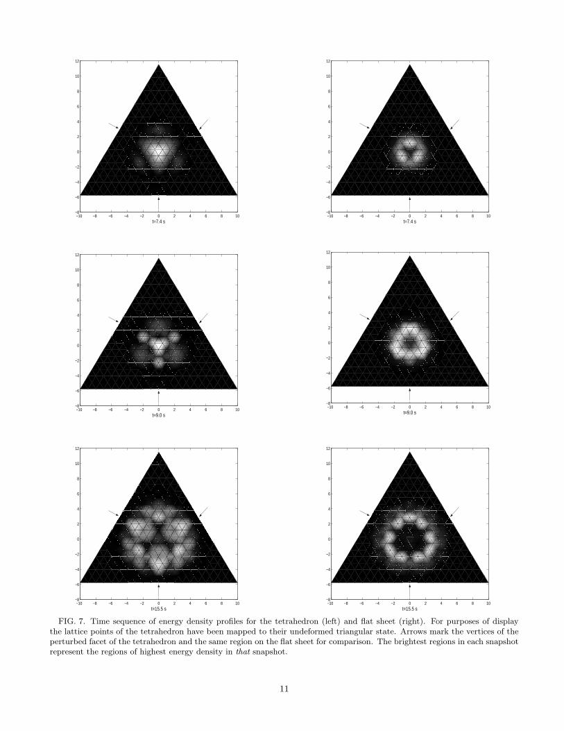
However to note the presence or absence of other features we looked explicitly at the spatial energy distribution asa function of time. Figure (7) shows a sequence of snapshots of the spatial energy distribution for the tetrahedronon the left and a flat sheet on the right. The tetrahedron has been folded out and hence the central triangular face,marked at the vertices by arrows, is the perturbed face. Ridges form the sides of this face. Arrows in the flat sheetsequence simply help to identify the same region. Note that the initial excitation is confined to the central threeparticles. We see that in the flat sheet case, the energy simply spreads outwards. In the tetrahedral case though, wenotice reflections (t = 6.5 to t = 9) and also the preferential propagation of energy through the middle of the ridges(t = 15.5 ). Thus we see the qualitative effects predicted by our analysis. However we never see the complete trappingof energy. This could be due to the limited size of the simulation as well as the difficulty in producing wavelengths inthe right regime.

VI. CONCLUSION

In this paper we have taken the first step toward understanding the dynamics of crumpled elastic sheets. We findthat the ridge structures in crumpled sheets qualitatively modify the propagation of transverse waves. Despite thestress induced by the ridges, our analysis indicates that the stretched string or drumhead modes normally associatedwith a stretched membrane are not important in a crumpled sheet. Our analysis suggested that the ridges wouldact as barriers to propagation and also that there could be modes that are trapped in the facets. These modesare unable to penetrate the ridges because the associated skin depth is much less than the ridge width in the thinlimit. Our numerical simulations gave us qualitative evidence that the above picture was right. Future work couldfocus on subjecting our predictions to a more thorough simulation analysis which could support our findings in amore quantitative fashion as well as identify the trapping of modes in the right frequency regime. It would also beinteresting to extend the analysis to cover the low frequency regime.

VII. ACKNOWLEDGEMENTS

The authors would like to thank Denis Chigirev and Vijay Patel for developing early versions of the simulationprogram used. AG would like to thank members of the Witten group and Brian DiDonna in particular for enlightening

9

−10 −8 −6 −4 −2 0 2 4 6 8 10−8

−6

−4

−2

0

2

4

6

8

10

12

t=0.0 s

−10 −8 −6 −4 −2 0 2 4 6 8 10−8

−6

−4

−2

0

2

4

6

8

10

12

t=5.0 s

−10 −8 −6 −4 −2 0 2 4 6 8 10−8

−6

−4

−2

0

2

4

6

8

10

12

t=6.5 s

−10 −8 −6 −4 −2 0 2 4 6 8 10−8

−6

−4

−2

0

2

4

6

8

10

12

t=0.0 s

−10 −8 −6 −4 −2 0 2 4 6 8 10−8

−6

−4

−2

0

2

4

6

8

10

12

t=5.0 s

−10 −8 −6 −4 −2 0 2 4 6 8 10−8

−6

−4

−2

0

2

4

6

8

10

12

t=6.5 s

10

−10 −8 −6 −4 −2 0 2 4 6 8 10−8

−6

−4

−2

0

2

4

6

8

10

12

t=7.4 s

−10 −8 −6 −4 −2 0 2 4 6 8 10−8

−6

−4

−2

0

2

4

6

8

10

12

t=9.0 s

−10 −8 −6 −4 −2 0 2 4 6 8 10−8

−6

−4

−2

0

2

4

6

8

10

12

t=15.5 s

−10 −8 −6 −4 −2 0 2 4 6 8 10−8

−6

−4

−2

0

2

4

6

8

10

12

t=7.4 s

−10 −8 −6 −4 −2 0 2 4 6 8 10−8

−6

−4

−2

0

2

4

6

8

10

12

t=9.0 s

−10 −8 −6 −4 −2 0 2 4 6 8 10−8

−6

−4

−2

0

2

4

6

8

10

12

t=15.5 s

FIG. 7. Time sequence of energy density profiles for the tetrahedron (left) and flat sheet (right). For purposes of displaythe lattice points of the tetrahedron have been mapped to their undeformed triangular state. Arrows mark the vertices of theperturbed facet of the tetrahedron and the same region on the flat sheet for comparison. The brightest regions in each snapshotrepresent the regions of highest energy density in that snapshot.

11

conversations. This work was supported in part by the National Science Foundation under Award number DMR-9975533 and in part by the National Science Foundation’s MRSEC Program under Award Number DMR-980859

[1] C. M. Soukoulis and E. N. Economou , Waves in Random Media, 9, 255 (1999).[2] R. Blandford and R. Narayan, Astrophysical journal 310, 568 (1986).[3] L. D. Landau and E. M. Lifshitz, Theory of Elasticity, (Pergamon, Oxford 1986).[4] R. S. Milman and G. D. Parker, Elements of Differential Geometry, (Prentice Hall, New Jersey 1977).[5] T. von Karman , Collected Works, (Butterworth, London 1956).[6] A. E. Lobkovsky, Phys. Rev. E. 53, 3750 (1996).[7] A. D. Pierce Elastic Wave Propagation, Pg. 205, (North-Holland 1989)[8] H. Goldstein Classical Mechanics, Pg. 66, (Addison Wesley 1980)[9] T. A. Witten and Hao Li, Europhys. Lett. 23, 51 (1993).

[10] A. E. Lobkovsky and T. A. Witten, Phys. Rev. E 55, 1577 (1997).[11] H. S. Seung and D. R. Nelson, Phys. Rev. A 38, 1005 (1988).[12] B. A. DiDonna and T. A. Witten, cond-mat 0104119.

12