Trapped Between the Falling Sky and the Rising Seas: The Imagined Terrors of the Impacts of Climate...
81
Electronic copy available at: http://ssrn.com/abstract=1548711 DRAFT: December 13, 2009 with references Trapped Between the Falling Sky and the Rising Seas: The Imagined Terrors of the Impacts of Climate Change Indur M. Goklany ABSTRACT Some advocates of drastic greenhouse gas controls claim that the costs of global warming are underestimated and that a proper accounting of the full costs raises the specter of economic and political instability, conflict and mass migration as weak governments in developing countries with low adaptive capacity are buffeted by floods, droughts, famine, and rising seas driven by global warming. No country, least of all the US, will be immune from the spillover effects. Accordingly, they argue, the costs to the US of a unilateral pursuit of GHG reductions would be justified by the benefits to the US itself. This chapter shows that the central pillar for this argument, namely, countries’, and specifically developing countries’, adaptive capacity will be low, is flawed. Specifically, it shows that under the IPCC’s warmest scenario, which projects a 1990–2085 warming of 4°C precisely because it assumes healthy economic growth worldwide, developing countries will in 2100 be twice as wealthy as the US is today, even after subtracting the costs of warming per the Stern Review’s overblown estimates. Industrialized countries will be thrice as wealthy. Moreover future societies will have superior technologies at their disposal. Accordingly, their adaptive capacities should be much higher than it is today, the costs of warming have been overestimated, and fears of economic and societal breakdown are precisely that — fears. Moreover, empirical trends suggest that warming is currently proceeding slower than the IPCC’s projections, nor is there any hint of any deterioration in climate‐sensitive indicators of human well‐being that might presage such breakdowns. Specifically, agricultural productivity has increased; hunger has declined; deaths from hunger, extreme weather events, malaria and other vector‐borne disease have dropped; and people are living longer and healthier. Regarding environmental well‐being, the Amazon and the Sahel are becoming greener, as is most of the world. Ironically, much of this improvement in human and environmental well‐being has been enabled, directly or indirectly, by technologies dependent on fossil fuels or economic surpluses generated by the use of fossil fuels and other GHG‐ generating activities.
-
Upload
independent -
Category
Documents
-
view
1 -
download
0
Transcript of Trapped Between the Falling Sky and the Rising Seas: The Imagined Terrors of the Impacts of Climate...
Electronic copy available at: http://ssrn.com/abstract=1548711
DRAFT: December 13, 2009 with references
Trapped Between the Falling Sky and the Rising Seas:
The Imagined Terrors of the Impacts of Climate Change
Indur M. Goklany
ABSTRACT
Some advocates of drastic greenhouse gas controls claim that the costs of global warming are
underestimated and that a proper accounting of the full costs raises the specter of economic
and political instability, conflict and mass migration as weak governments in developing
countries with low adaptive capacity are buffeted by floods, droughts, famine, and rising seas
driven by global warming. No country, least of all the US, will be immune from the spillover
effects. Accordingly, they argue, the costs to the US of a unilateral pursuit of GHG reductions
would be justified by the benefits to the US itself. This chapter shows that the central pillar for
this argument, namely, countries’, and specifically developing countries’, adaptive capacity will
be low, is flawed. Specifically, it shows that under the IPCC’s warmest scenario, which projects a
1990–2085 warming of 4°C precisely because it assumes healthy economic growth worldwide,
developing countries will in 2100 be twice as wealthy as the US is today, even after subtracting
the costs of warming per the Stern Review’s overblown estimates. Industrialized countries will
be thrice as wealthy. Moreover future societies will have superior technologies at their disposal.
Accordingly, their adaptive capacities should be much higher than it is today, the costs of
warming have been overestimated, and fears of economic and societal breakdown are precisely
that — fears. Moreover, empirical trends suggest that warming is currently proceeding slower
than the IPCC’s projections, nor is there any hint of any deterioration in climate‐sensitive
indicators of human well‐being that might presage such breakdowns. Specifically, agricultural
productivity has increased; hunger has declined; deaths from hunger, extreme weather events,
malaria and other vector‐borne disease have dropped; and people are living longer and
healthier. Regarding environmental well‐being, the Amazon and the Sahel are becoming
greener, as is most of the world. Ironically, much of this improvement in human and
environmental well‐being has been enabled, directly or indirectly, by technologies dependent
on fossil fuels or economic surpluses generated by the use of fossil fuels and other GHG‐
generating activities.
Electronic copy available at: http://ssrn.com/abstract=1548711
DRAFT: December 13, 2009 with references
I. INTRODUCTION
Some advocates of drastic greenhouse gas (GHG) controls claim that the costs of global
warming are underestimated and that a proper accounting of the full costs raises the specter of
economic and political instability, conflict and mass migration as weak governments in
developing countries with low adaptive capacity are buffeted by floods, droughts, famine, and
rising seas driven by global warming.
As representatives of this school of thought, Freeman and Guzman (2009), henceforth FG, make
the interesting, but ultimately unpersuasive, argument that conventional cost‐benefit analyses
of the impacts of global warming on the US underestimate the costs to the US, and that a
proper consideration of the costs would show that they have been substantially
underestimated. Accordingly, they claim, it would be in the US interest to make unilateral cuts
in greenhouse gas (GHG) emissions and, if necessary, pay the full cost of mitigation.1 They claim
that a full accounting of losses to the United States indicates that it “stands to lose in a warmer
world [, therefore] investing in mitigation, even at the risk of other nations’ free riding, is the
most rational course [for the US]. Though international cooperation should be pursued, the
reluctance of others to fully engage the problem is not a sound reason for inaction by the
United States. Whatever others do, the United States should move aggressively to reduce
global GHG emissions” (FG: 170‐171).
Central to their argument is the claim that the costs of global warming to the US are
underestimated for a variety of reasons. First, they claim, assessments of the impacts of global
warming are based on “optimism about projected temperature rise; failure to account for the
possibility of catastrophic loss; omission of cross‐sectoral impacts; exclusion of nonmarket
costs; and optimism about projected economic growth (which assumes productivity will be
unaffected by climate change)” [FG: 118]. Second, the assessments do not account adequately
for the economic spillovers on the US from the effects of global warming on other nations (e.g.,
economic downturns for trading partners due to loss of productivity from reduced availability
of food and water, severe weather events, major flooding, and large‐scale refugee crises; FG:
138‐140). Third, FG argue that the costs of global warming to the US do not account for a
number of other spillover effects that would affect national security, increase migration
1 “A more complete accounting of the costs reveals that the United States would be better off paying the full cost of mitigating its impact by itself (if doing so were possible)” FG: 101.
DRAFT: December 13, 2009 with references
pressures on the US, and increase the likelihood of the the spread of contagious disease.
Specifically, they claim global warming is a threat multiplier for national security concerns
because it “is likely to exacerbate political instability around the world as weak or poor
governments struggle to cope with its impacts” (FG: 147) from increased hunger, water and
energy shortages, and floods. FG also claim that global warming “threatens to interrupt the free
flow of trade in critical resources such as oil, gas, and other essential commodities on which the
United States depends” (FG: 147). In addition, FG argue that by increasing floods, droughts, and
extreme weather, global warming would destroy crops and livelihoods in many places making
life “impossible” in many places and leading to greater migration to the US’s shores (FG: 153).
They also claim that global warming makes the spread of contagious disease more probable
because there would be more disease in the world and countries are likely to have fewer
resources to cope with disease (FG: 157).
In this chapter, I will examine FG’s arguments that the impacts of global warming on the US are
underestimated. Part II will examine the claim that models of the impacts of global warming
suffer from a “systematic downward bias” (FG: 106). It will show that, in fact, these models are
more likely to have overestimated the negative impacts — and underestimated the positive
impacts — of global warming. Part III will address issues related to impacts from potential
catastrophes that may be caused by global warming over the next century. Part IV will address
claims that “things [related to global warming] are worse than expected.” Part V will examine
issues that FG claims are frequently overlooked, e.g., cross‐sectoral impacts, reduced access to
resources, and myriad other impacts of global warming that, acting in combination, could lead
to economic instabilities resulting in international spillovers affecting the United States. Part VI
will deal with claims regarding migration, conflicts and national security. Part VII summarises
this chapter.
A note on terminology: In most public discourse the term “climate change” is synonymous with
“global warming.” For the sake of accuracy, this paper uses “global warming” rather than
climate change when the change under discussion is warming.

DRAFT: December 13, 2009 with references
II. DO IMPACT MODELS HAVE “A SYSTEMATIC DOWNWARD BIAS”?
RG (p. 118) claim that “methodological limitations of … models almost certainly cause them to
understate the impact and cost of climate change.” They attribute this to the following “five
problems”: “optimism about projected temperature rise; failure to account for the possibility of
catastrophic loss; omission of cross‐sectoral impacts; exclusion of nonmarket costs; and … [the
assumption] that productivity will be unaffected by global warming” (RG: 118). This section will
address whether the impacts estimates are likely to have been understated.
1. Optimism about Projected Temperature Rise
Estimates of the impacts of global warming are based on a chain of linked models with the
uncertain output of each model serving as the input for the next model. The first link in this
chain are emission models which use socioeconomic assumptions extending 100 or more years
into the future to generate emission scenarios, which strains credulity. As Lorenzini and Adger
(2006: 74) noted in a paper commissioned for the Stern Review, socioeconomic scenarios
“cannot be projected semi‐realistically for more than 5–10 years at a time.” Nevertheless, in
the following I will eschew skepticism regarding the ability of mere mortals to accurately
forecast socioeconomic variables more than a few years hence.
The results of these emissions models are fed into coupled atmosphere‐ocean general
circulation models (AOGCMs) to estimate spatial and temporal changes in climatic variables
(such as temperature and precipitation) which are, then, used as inputs to simplified and often
incomplete biophysical models that project location‐specific changes in biophysical factors (e.g.,
available habitat, or crop or timber yields). Notably, the uncertainty of estimates of climatic
changes increases as the scale at which they have to be specified becomes finer. This is
particularly true for precipitation, which is a — if not the — critical determinant of natural
resources (e.g., water and vegetation) that human beings and all other living species depend on
either directly or indirectly. Next, depending on the human or natural system under
consideration, the outputs of these biophysical models may have to be fed into additional
models to calculate the social, economic, and environmental impacts on those systems. Ideally,
the outputs from this set of models should be fed back into the emissions models, thereby
closing an iterative loop of models. But models have, so far, not yet incorporated this feature.
DRAFT: December 13, 2009 with references
Another shortcoming is that since the outputs from AOGCMs drive the impact models, any
problems and uncertainties associated with the former will necessarily be transmitted to the
latter. Remarkably, end‐to‐end uncertainty estimates of the results from the series of models
are never provided, which gives many readers a false sense of confidence in the results.
A major problem with AOGCMs is that they are developed and calibrated using the surface
temperature record. But there are strong indications that the surface temperature record has
been compromised, as discussed below. Therefore, quantitative estimates made using that
record are also suspect.
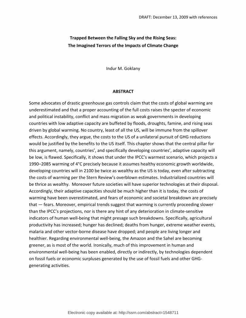
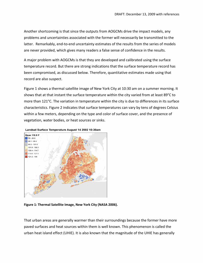
Figure 1 shows a thermal satellite image of New York City at 10:30 am on a summer morning. It
shows that at that instant the surface temperature within the city varied from at least 89°C to
more than 121°C. The variation in temperature within the city is due to differences in its surface
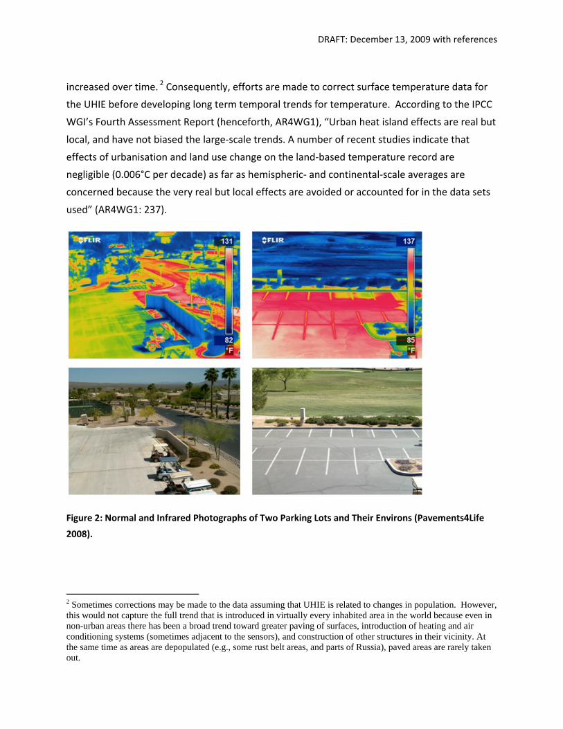
characteristics. Figure 2 indicates that surface temperatures can vary by tens of degrees Celsius
within a few meters, depending on the type and color of surface cover, and the presence of
vegetation, water bodies, or heat sources or sinks.
Figure 1: Thermal Satellite Image, New York City (NASA 2006).
That urban areas are generally warmer than their surroundings because the former have more
paved surfaces and heat sources within them is well known. This phenomenon is called the
urban heat island effect (UHIE). It is also known that the magnitude of the UHIE has generally
DRAFT: December 13, 2009 with references
increased over time. 2 Consequently, efforts are made to correct surface temperature data for
the UHIE before developing long term temporal trends for temperature. According to the IPCC
WGI’s Fourth Assessment Report (henceforth, AR4WG1), “Urban heat island effects are real but
local, and have not biased the large‐scale trends. A number of recent studies indicate that
effects of urbanisation and land use change on the land‐based temperature record are
negligible (0.006°C per decade) as far as hemispheric‐ and continental‐scale averages are
concerned because the very real but local effects are avoided or accounted for in the data sets
used” (AR4WG1: 237).
Figure 2: Normal and Infrared Photographs of Two Parking Lots and Their Environs (Pavements4Life
2008).
2 Sometimes corrections may be made to the data assuming that UHIE is related to changes in population. However, this would not capture the full trend that is introduced in virtually every inhabited area in the world because even in non-urban areas there has been a broad trend toward greater paving of surfaces, introduction of heating and air conditioning systems (sometimes adjacent to the sensors), and construction of other structures in their vicinity. At the same time as areas are depopulated (e.g., some rust belt areas, and parts of Russia), paved areas are rarely taken out.
DRAFT: December 13, 2009 with references
However, the UHIE is only one of the issues that must be confronted while developing long
term temperature trends from surface temperature data. Consider surface data from the US
Historical Climatology Network (USHCN), which is the US’s network of record.
One would think that US would have one of the more reliable surface temperature networks in
the world, yet a survey of USHCN sites indicates that the instrumental record may be
compromised because of inhomogeneities,3 and siting and maintenance issues. Many monitors
are in close proximity to asphalt roadways, parking lots, trees, other kinds of land cover, a
variety of heat sources or sinks (e.g., buildings, sewage treatment facilities, and heating and air
conditioning units, and so forth. Few, if any, of these features existed at any site from the
beginning of that site’s temperature record, nor were they introduced in one fell swoop. They
mostly accreted over time. Other sources of inhomogeneities in the data include changes in
station location (in all three dimensions); instrumentation; land use, land cover and other
factors affecting temperature readings at the micro‐ to higher‐scales; seemingly minor changes
in the height of thermometers; and operational and maintenance procedures and practices,
including the time at which temperatures are recorded, erratic or non‐uniform maintenance of
sites (such as monitor enclosures, their conditions, including the condition of the paint job, and
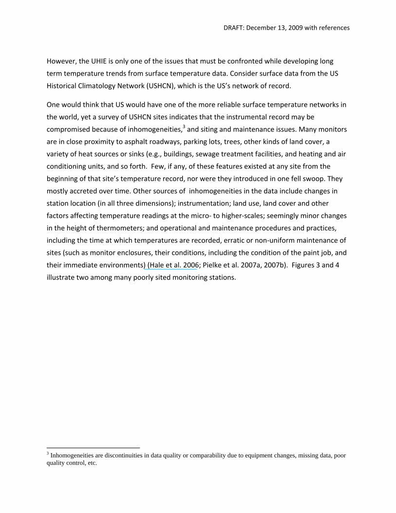
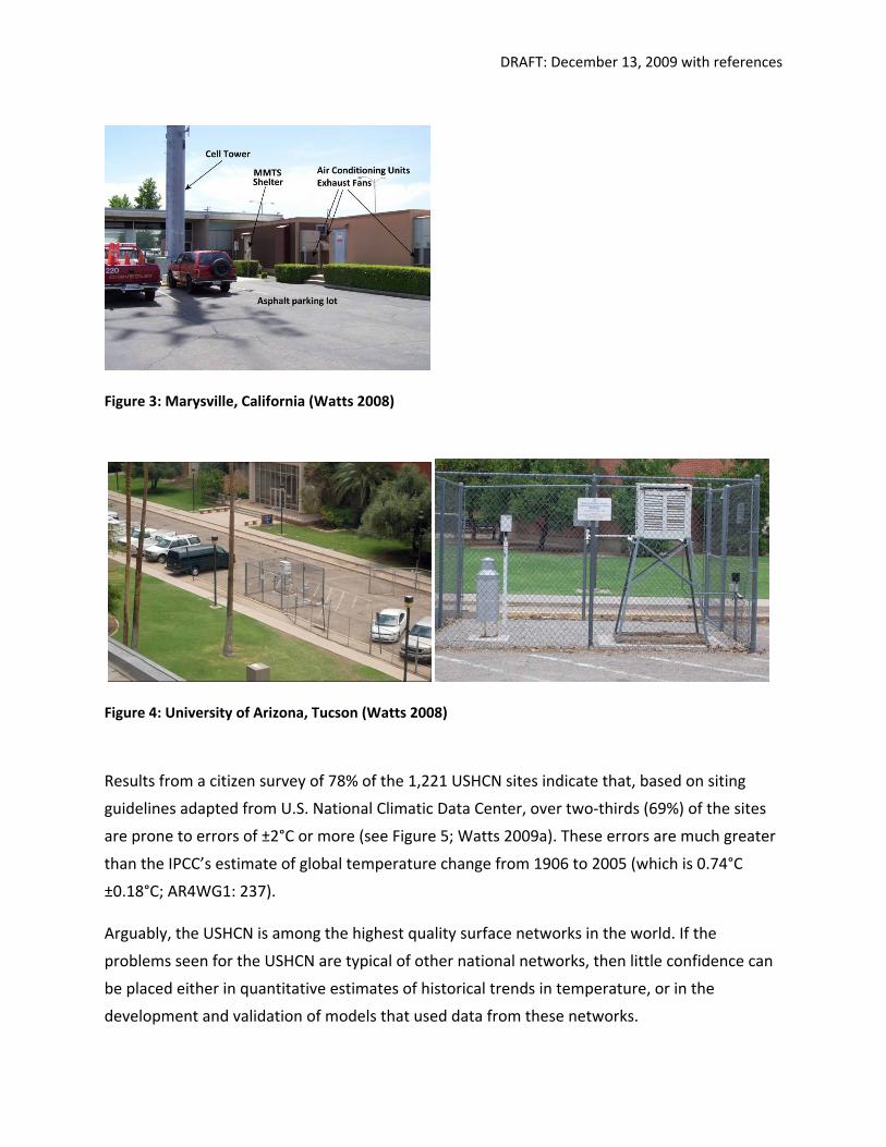
their immediate environments) (Hale et al. 2006; Pielke et al. 2007a, 2007b). Figures 3 and 4
illustrate two among many poorly sited monitoring stations.
3 Inhomogeneities are discontinuities in data quality or comparability due to equipment changes, missing data, poor quality control, etc.
DRAFT: December 13, 2009 with references
Figure 3: Marysville, California (Watts 2008)
Figure 4: University of Arizona, Tucson (Watts 2008)
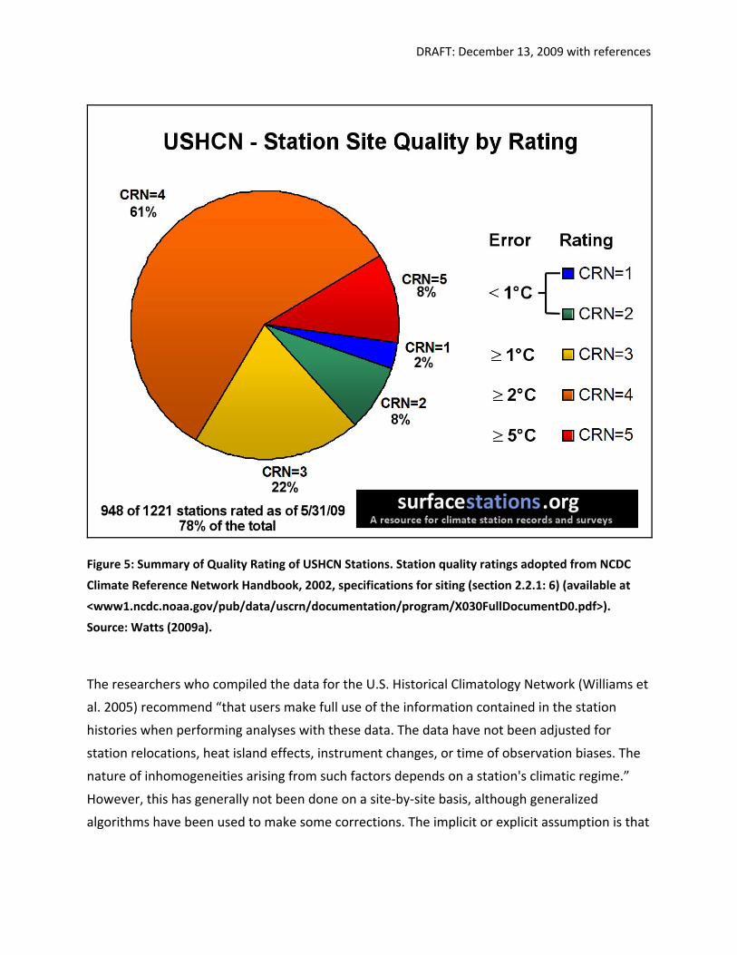
Results from a citizen survey of 78% of the 1,221 USHCN sites indicate that, based on siting
guidelines adapted from U.S. National Climatic Data Center, over two‐thirds (69%) of the sites
are prone to errors of ±2°C or more (see Figure 5; Watts 2009a). These errors are much greater
than the IPCC’s estimate of global temperature change from 1906 to 2005 (which is 0.74°C
±0.18°C; AR4WG1: 237).
Arguably, the USHCN is among the highest quality surface networks in the world. If the
problems seen for the USHCN are typical of other national networks, then little confidence can
be placed either in quantitative estimates of historical trends in temperature, or in the
development and validation of models that used data from these networks.
DRAFT: December 13, 2009 with references
Figure 5: Summary of Quality Rating of USHCN Stations. Station quality ratings adopted from NCDC
Climate Reference Network Handbook, 2002, specifications for siting (section 2.2.1: 6) (available at
<www1.ncdc.noaa.gov/pub/data/uscrn/documentation/program/X030FullDocumentD0.pdf>).
Source: Watts (2009a).
The researchers who compiled the data for the U.S. Historical Climatology Network (Williams et
al. 2005) recommend “that users make full use of the information contained in the station
histories when performing analyses with these data. The data have not been adjusted for
station relocations, heat island effects, instrument changes, or time of observation biases. The
nature of inhomogeneities arising from such factors depends on a station's climatic regime.”
However, this has generally not been done on a site‐by‐site basis, although generalized
algorithms have been used to make some corrections. The implicit or explicit assumption is that
DRAFT: December 13, 2009 with references
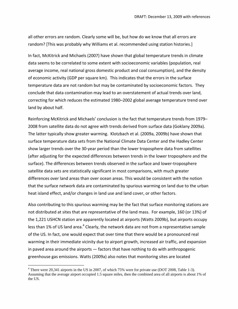
all other errors are random. Clearly some will be, but how do we know that all errors are
random? [This was probably why Williams et al. recommended using station histories.]
In fact, McKitrick and Michaels (2007) have shown that global temperature trends in climate
data seems to be correlated to some extent with socioeconomic variables (population, real
average income, real national gross domestic product and coal consumption), and the density
of economic activity (GDP per square km). This indicates that the errors in the surface
temperature data are not random but may be contaminated by socioeconomic factors. They
conclude that data contamination may lead to an overstatement of actual trends over land,
correcting for which reduces the estimated 1980–2002 global average temperature trend over
land by about half.
Reinforcing McKitrick and Michaels’ conclusion is the fact that temperature trends from 1979–
2008 from satellite data do not agree with trends derived from surface data (Goklany 2009a).
The latter typically show greater warming. Klotzbach et al. (2009a, 2009b) have shown that
surface temperature data sets from the National Climate Data Center and the Hadley Center
show larger trends over the 30‐year period than the lower troposphere data from satellites
(after adjusting for the expected differences between trends in the lower troposphere and the
surface). The differences between trends observed in the surface and lower‐troposphere
satellite data sets are statistically significant in most comparisons, with much greater
differences over land areas than over ocean areas. This would be consistent with the notion
that the surface network data are contaminated by spurious warming on land due to the urban
heat island effect, and/or changes in land use and land cover, or other factors.
Also contributing to this spurious warming may be the fact that surface monitoring stations are
not distributed at sites that are representative of the land mass. For example, 160 (or 13%) of
the 1,221 USHCN station are apparently located at airports (Watts 2009b), but airports occupy
less than 1% of US land area.4 Clearly, the network data are not from a representative sample
of the US. In fact, one would expect that over time that there would be a pronounced real
warming in their immediate vicinity due to airport growth, increased air traffic, and expansion
in paved area around the airports — factors that have nothing to do with anthropogenic
greenhouse gas emissions. Watts (2009a) also notes that monitoring sites are located
4 There were 20,341 airports in the US in 2007, of which 75% were for private use (DOT 2008, Table 1-3). Assuming that the average airport occupied 1.5 square miles, then the combined area of all airports is about 1% of the US.

DRAFT: December 13, 2009 with references
preferentially at waste water treatment plants, fire stations and other types of sites that too
are not representative of the land surface.
The above findings suggest that the amount of warming that has occurred since the 1850s may
have been overestimated, and that AOGCMs that are calibrated using the surface data may be
overestimating the sensitivity of temperature increases to carbon dioxide, or underestimating
the role of natural variability, or both. That this might be the case is supported by the fact that
contrary to the IPCC’s claim — derived from the results of several AOGCMs — that global
temperatures should increase by 0.2°C per decade under “Business as Usual”(BAU) scenarios
(AR4WG1: 12), global surface temperature data do not show any significant global warming
since 1998 (as indicated in Figure 6; Kerr 2009). This, despite the fact that since the 1990s,
emissions have grown more rapidly than were projected under any of the BAU scenarios mainly
because of the spectacular economic growth in China and India. Hence, if anything, we should
have seen an increase larger than that projected by the IPCC.
The fact that the IPCC models seem to be failing ought not come as a major surprise, since
these models have not been validated using out‐of‐sample data under conditions of high
Figure 6: Global Temperature Trends, 1999–2008. Gray line is based on the Hadley Center’s surface temperature dataset; the blue line is the data adjusted to account for the El Niño phenomenon of 1998; the orange lines indicate the linear trend line and error bars. Source: Kerr (2009).

DRAFT: December 13, 2009 with references
greenhouse gas concentrations. Just as a mathematical model for a human being (for instance)
should be able to show that he can not only breathe but walk, talk and chew gum at the same
time, for a climate model to be valid, it should be able to simultaneously forecast with
reasonable accuracy the spatial and temporal variations in a wide variety of climatic variables
including temperature, pressure and precipitation, as well as endogenously produce the
patterns and rhythms of ocean circulation (among other things). But we know from the
AR4WG1 that models are unable to do this even for “in sample” data. As it states, “Difficulties
remain in reliably simulating and attributing observed temperature changes at smaller [that is,
less than continental] scales” [AR4WG1: 10.] And this what it says about projections of climate
change:
“There is considerable confidence that climate models provide credible quantitative estimates
of future climate change, particularly at continental scales and above. This confidence comes
from the foundation of the models in accepted physical principles and from their ability to
reproduce observed features of current climate and past climate changes. Confidence in
model estimates is higher for some climate variables (e.g., temperature) than for others
(e.g., precipitation).” (AR4WG1: 600, emphasis added)
This tacitly acknowledges that confidence is low for model projections of temperature at less
than continental scales, and is even lower for precipitation — perhaps even at the continental
scale. Notably, it doesn’t provide any quantitative estimate of the confidence that should be
attached to projections of temperatures at the subcontinental scale. This lack of confidence in
temperature and precipitation results at such scales is reaffirmed by recent reports from the US
Climate Change Science Program (CCSP):
“Climate model simulation of precipitation has improved over time but is still problematic.
Correlation between models and observations is 50 to 60% for seasonal means on scales of a
few hundred kilometers.” (CCSP 2008:3).
“In summary, modern AOGCMs generally simulate continental and larger‐scale mean surface
temperature and precipitation with considerable accuracy, but the models often are not
reliable for smaller regions, particularly for precipitation.” (CCSP 2008: 52).
The IPCC does not say that “all” features of current climate or past climate changes can be
reproduced, as a good model of climate change ought to be able to do endogenously. In fact, it
notes:
DRAFT: December 13, 2009 with references
“Model global temperature projections made over the last two decades have also been in
overall agreement with subsequent observations over that period (Chapter 1).
“Nevertheless, models still show significant errors. Although these are generally greater at
smaller scales, important large scale problems also remain. For example, deficiencies remain
in the simulation of tropical precipitation, the El Niño‐Southern Oscillation and the Madden‐
Julian Oscillation (an observed variation in tropical winds and rainfall with a time scale of 30 to
90 days).” (AR4WG1: 601; emphasis added).
Notably, although the absence of global warming for the decade (1999‐2008) was not forecast
by the models that the IPCC relied on, a number of peer reviewed papers have suggested there
would be a cooling trend in the early 2000s based on their analysis of natural variability. These
include Loehle (2004 and 2009); Zhen‐Shan and Xian (2007) who in 2007 published a paper
provocatively titled, “Multi‐scale analysis of global temperature changes and trend of a drop in
temperature in the next 20 years”; Tsonis et al. (2007); Swanson and Tsonis (2009); and
Keenleyside (2008).
Time may reveal these projections to be flawed, but the fact is that currently there exists no
empirical basis for concluding that the IPCC’s temperature projections are “optimistic”, as
claimed by FG. To the contrary, such empirical evidence as exists suggests that natural
variability is a much more significant factor in temperature swings than is credited in AR4WG1,
and that the temperature sensitivity of the climate system to GHG emissions has been
overestimated, which suggest that reducing such emissions will have a lower impact on
temperature than estimated.
2. Impacts of Global Warming Are Overestimated
FG argue that models systematically underestimate the future impacts of global warming. In
this section I will show that, in fact, current modeling studies vastly overestimate the net
negative impacts (or damages) of climate change.
The major reason for this is that the magnitude of future damages depends critically on
society’s future adaptive capacity. But the methodologies used to estimate impacts
underestimate individuals’ and society’s future capacity to make self‐directed (or autonomous)

DRAFT: December 13, 2009 with references
adaptations to global warming.5 In general, this adaptive capacity is determined by a variety of
socioeconomic factors, including society’s level of economic development (as measured by GDP
per capita, which is also a surrogate for wealth or per capita income), available technologies,
and human and social capital (Goklany 2000, 2007a). Therefore, in the future, if societies
become wealthier, as is assumed under all IPCC emission and climate scenarios (Goklany
2007b), their adaptive capacity ought to be higher (Goklany 2007a). And, if history is any guide,
due to secular technological change society should have a wider array of technological options
available to them as existing technologies are perfected and new technologies come on line
(Goklany 2007a, 2009b). This ought to further bolster adaptive capacity beyond the increase
due to economic development alone (Goklany 2007a). However, some impact assessments
ignore adaptive capacity altogether, e.g., Arnell’s (2004) study of water resources (Goklany
2007b); others assume that future adaptive capacity will be the same as it was in the base year
(generally 1990 in most assessments undertaken to date), e.g., van Lieshout et al. (2004) for
malaria; yet others assume that existing technologies will become more affordable as society
becomes wealthier but do not account for new technologies that may come on line over the
next few decades, e.g., Parry et al. (2004) for agricultural production and hunger. To date, no
impact study has fully accounted for both increasing wealth and secular technological change
(Goklany 2007b). As a result they overestimate the negative impacts and underestimate the
positive impacts. Therefore, they all overestimate net damages associated with global warming,
with some studies overestimating a lot more than others.
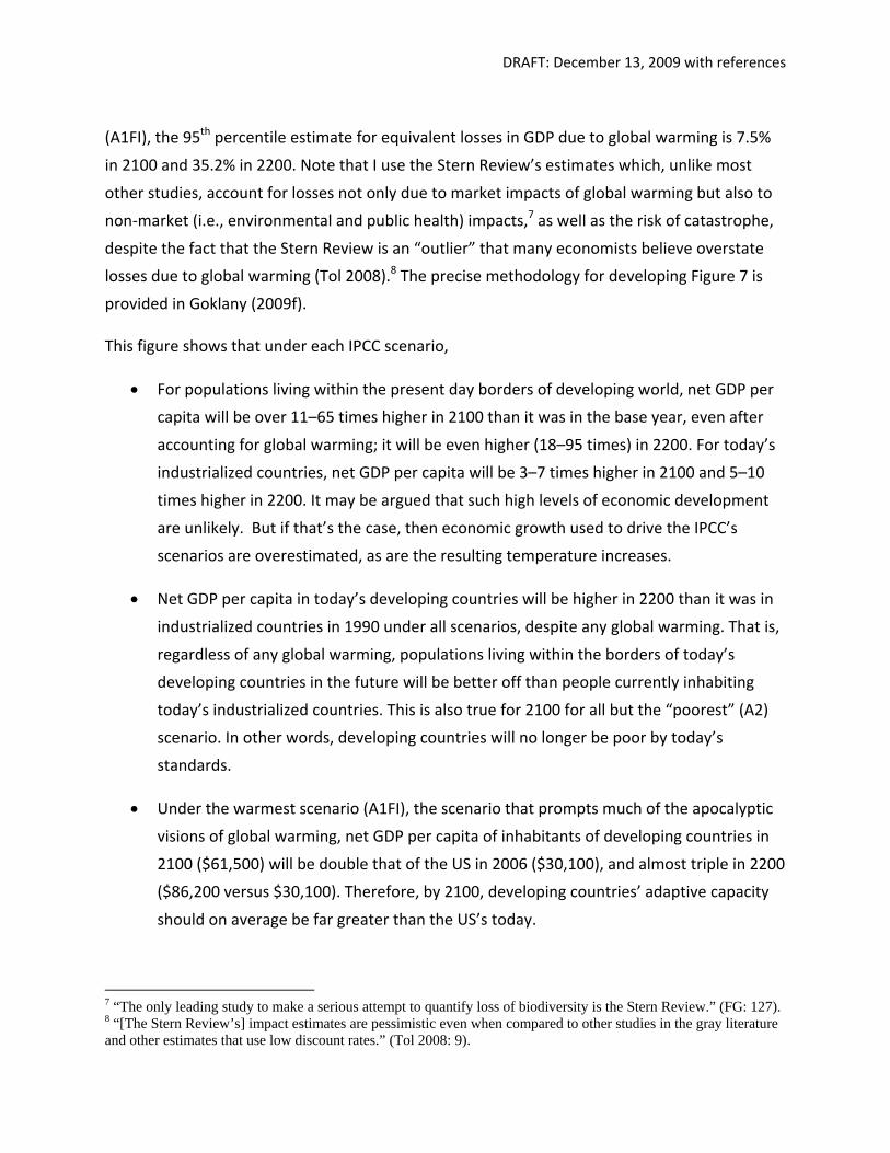
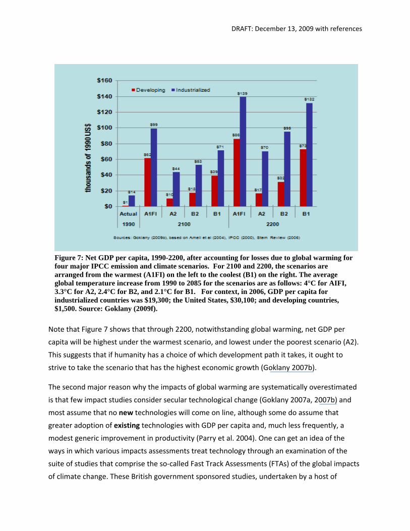
Figure 7, taken from Goklany (2009f), provides estimates of net GDP per capita — a
determinant of adaptive capacity — for four IPCC reference scenarios for areas that comprise
today’s developing and industrialized countries after accounting for any losses in GDP due to
global warming for 1990 (the base year), 2100 and 2200. For 1990, the net GDP per capita is
calculated assuming that any GDP loss due to global warming is negligible.6 For 2100 and 2200,
net GDP per capita is estimated assuming that (a) GDP per capita in the absence of global
warming will grow per the IPCC SRES scenarios and (b) adjusting it downward to account for the
costs of climate change per the Stern Review’s 95th percentile estimate. According to the Stern
Review, under the “high climate change” scenario, equivalent to the IPCC’s warmest scenario
5 Adaptations could include measures to either reduce any adverse effect of global warming or take advantage of any of its positive impacts. 6 This assumption is appropriate since the Stern Review’s estimates used 1990 as the baseline for estimating the average global temperature increase.
DRAFT: December 13, 2009 with references
(A1FI), the 95th percentile estimate for equivalent losses in GDP due to global warming is 7.5%
in 2100 and 35.2% in 2200. Note that I use the Stern Review’s estimates which, unlike most
other studies, account for losses not only due to market impacts of global warming but also to
non‐market (i.e., environmental and public health) impacts,7 as well as the risk of catastrophe,
despite the fact that the Stern Review is an “outlier” that many economists believe overstate
losses due to global warming (Tol 2008).8 The precise methodology for developing Figure 7 is
provided in Goklany (2009f).
This figure shows that under each IPCC scenario,
For populations living within the present day borders of developing world, net GDP per
capita will be over 11–65 times higher in 2100 than it was in the base year, even after
accounting for global warming; it will be even higher (18–95 times) in 2200. For today’s
industrialized countries, net GDP per capita will be 3–7 times higher in 2100 and 5–10
times higher in 2200. It may be argued that such high levels of economic development
are unlikely. But if that’s the case, then economic growth used to drive the IPCC’s
scenarios are overestimated, as are the resulting temperature increases.
Net GDP per capita in today’s developing countries will be higher in 2200 than it was in
industrialized countries in 1990 under all scenarios, despite any global warming. That is,
regardless of any global warming, populations living within the borders of today’s
developing countries in the future will be better off than people currently inhabiting
today’s industrialized countries. This is also true for 2100 for all but the “poorest” (A2)
scenario. In other words, developing countries will no longer be poor by today’s
standards.
Under the warmest scenario (A1FI), the scenario that prompts much of the apocalyptic
visions of global warming, net GDP per capita of inhabitants of developing countries in
2100 ($61,500) will be double that of the US in 2006 ($30,100), and almost triple in 2200
($86,200 versus $30,100). Therefore, by 2100, developing countries’ adaptive capacity
should on average be far greater than the US’s today.
7 “The only leading study to make a serious attempt to quantify loss of biodiversity is the Stern Review.” (FG: 127). 8 “[The Stern Review’s] impact estimates are pessimistic even when compared to other studies in the gray literature and other estimates that use low discount rates.” (Tol 2008: 9).
DRAFT: December 13, 2009 with references
Thus, the problems of poverty that warming would exacerbate (e.g., low agricultural
productivity, hunger, malnutrition, malaria and other vector borne diseases) ought to be
reduced if not eliminated by 2100, even if one ignores any secular technological change that
ought to occur in the interim. Tol and Dowlatabadi (2001), for example, show that malaria
has been functionally eliminated in a society whose annual per capita income reaches
$3,100. Therefore, even under the poorest scenario (A2), developing countries should be
free of malaria well before 2100, even assuming no technological change in the interim.
Similarly, if the average net GDP per capita in 2100 for developing countries is $10,000–
$82,000, then their farmers would be able to afford technologies that are unaffordable
today (e.g., precision agriculture) or new technologies that should come on line by then
(e.g., drought resistant seeds) (Goklany 2007c: chapter 9, 2009d: 292–93). But, since impact
assessments generally fail to fully factor in increases in economic development and
technological change, they substantially overestimate future net damages from global
warming.
DRAFT: December 13, 2009 with references
Note that Figure 7 shows that through 2200, notwithstanding global warming, net GDP per
capita will be highest under the warmest scenario, and lowest under the poorest scenario (A2).
This suggests that if humanity has a choice of which development path it takes, it ought to
strive to take the scenario that has the highest economic growth (Goklany 2007b).
The second major reason why the impacts of global warming are systematically overestimated
is that few impact studies consider secular technological change (Goklany 2007a, 2007b) and
most assume that no new technologies will come on line, although some do assume that
greater adoption of existing technologies with GDP per capita and, much less frequently, a
modest generic improvement in productivity (Parry et al. 2004). One can get an idea of the
ways in which various impacts assessments treat technology through an examination of the
suite of studies that comprise the so‐called Fast Track Assessments (FTAs) of the global impacts
of climate change. These British government sponsored studies, undertaken by a host of
Figure 7: Net GDP per capita, 1990-2200, after accounting for losses due to global warming for four major IPCC emission and climate scenarios. For 2100 and 2200, the scenarios are arranged from the warmest (A1FI) on the left to the coolest (B1) on the right. The average global temperature increase from 1990 to 2085 for the scenarios are as follows: 4°C for AIFI, 3.3°C for A2, 2.4°C for B2, and 2.1°C for B1. For context, in 2006, GDP per capita for industrialized countries was $19,300; the United States, $30,100; and developing countries, $1,500. Source: Goklany (2009f).
DRAFT: December 13, 2009 with references
authors who were intimately involved in the IPCC’s various assessment reports, were state‐of‐
the‐art at the time the IPCC’s 4AR was compiled. A dissection of their methodologies in Goklany
(2007b) shows that:
The water resources study (Arnell 2004) totally ignores adaptation, despite the fact that
many adaptations to water related problems, e.g., building dams, reservoirs, and canals,
are among mankind’s oldest adaptations, and do not depend on the development of
any new technologies (Goklany 2007b: 1034–35).
The study of agricultural productivity and hunger (Parry et al. 2004) allows for increases
in crop yield with economic growth due to greater usage of fertilizer and irrigation in
richer countries, decreases in hunger due to economic growth, some secular (time‐
dependent) increase in agricultural productivity, as well as some farm level adaptations
to deal with climate change. But these adaptations are based on currently available
technologies, rather than technologies that would be available in the future or any
technologies developed to specifically cope with the negative impacts of global warming
or take advantage of any positive outcomes (Parry et al., 2004: 57; Goklany 2007b:
1032–33). However, the potential for future technologies to cope with climate change
is large, especially if one considers bioengineered crops and precision agriculture
(Goklany 2007b, 2007c).
Nicholls (2004) study on coastal flooding from sea level rise takes some pains to
incorporate improvements in adaptive capacity due to increasing wealth. But it makes
some questionable assumptions. First, it allows societies to implement measures to
reduce the risk of coastal flooding in response to 1990 surge conditions, but not to
subsequent sea level rise (Nicholls, 2004: 74). But this is illogical. One should expect that
any measures that are implemented would consider the latest available data and
information on the surge situation at the time the measures are initiated. That is, if the
measure is initiated in, say, 2050, the measure’s design would at least consider sea level
and sea level trends as of 2050, rather than merely the 1990 level. By that time, we
should know the rate of sea level rise with much greater confidence. Second, Nicholls
(2004) also allows for a constant lag time between initiating protection and sea level
rise. But one should expect that if sea level continues to rise, the lag between upgrading
protection standards and higher GDP per capita will be reduced over time, and may
DRAFT: December 13, 2009 with references
even turn negative. That is, adaptations would be anticipatory rather than reactive,
particularly, for a richer society. Fourth, Nicholls (2004) does not allow for any
deceleration in the preferential migration of the population to coastal areas, as might be
likely if coastal flooding becomes more frequent and costly (Goklany 2007b: 1036–37).
The analysis for malaria undertaken by van Lieshout et al. (2004) includes adaptive
capacity as it existed in 1990, but does not adjust it to account for any subsequent
advances in economic and technological development. There is simply no justification
for such an assumption.
So how much of a difference in impact would consideration of both economic development and
technological change have made?
If impacts were to be estimated for 5 or so years into the future, ignoring changes in adaptive
capacity between now and then probably would not be fatal. However, the time horizon of
climate change impact assessments is often on the order of 50–100 years or more. The Fast
Track Assessments use a base year of 1990 to estimate impacts for 2025, 2055 and 2085 (Parry
2004). The Stern Review’s time horizon extends out to 2100–2200 and beyond (Stern Review
2006).
It should be noted that some of the newer impacts assessments have begun to account for
changes in adaptive capacity. For example, Yohe et al. (2006), in an exercise exploring the
vulnerability to climate change under various climate change scenarios, allowed adaptive
capacity to increase between the present and 2050 and 2100. However, they limited any
increase in adaptive capacity to “either the current global mean or to a value that is 25% higher
than the current value – whichever is higher” (Yohe et al. 2006: 4). Such a limitation would miss
most of the increase in adaptive capacity implied by Figure 7.
More recently, Tol et al. (2007)’s analyzed the sensitivity of deaths from malaria, diarrhea,
schistosomiasis, and dengue deaths to warming, economic development and other
determinants of adaptive capacity through the year 2100. Their results indicate,
unsurprisingly, that consideration of economic development alone could reduce mortality
substantially. For malaria, for instance, deaths would be eliminated before 2100 in a number of
the more affluent Sub Saharan countries (Tol et al. 2007: 702). This result is consistent with
retrospective assessments indicate that over the span of a few decades, changes in economic
DRAFT: December 13, 2009 with references
development and technologies can damp down various indicators of adverse environmental
impacts and negative indicators of human well‐being (Goklany 2009b). For example, due to a
combination of greater wealth and secular technological change, U.S. death rates due to
various climate‐sensitive water‐related diseases — dysentery, typhoid, paratyphoid, other
gastrointestinal disease, and malaria —declined by 99.6 to 100.0 percent from 1900–1970
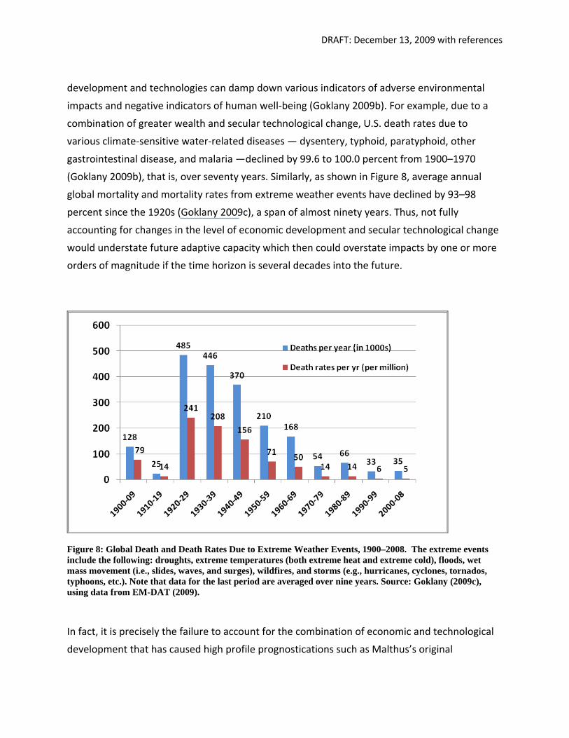
(Goklany 2009b), that is, over seventy years. Similarly, as shown in Figure 8, average annual
global mortality and mortality rates from extreme weather events have declined by 93–98
percent since the 1920s (Goklany 2009c), a span of almost ninety years. Thus, not fully
accounting for changes in the level of economic development and secular technological change
would understate future adaptive capacity which then could overstate impacts by one or more
orders of magnitude if the time horizon is several decades into the future.
Figure 8: Global Death and Death Rates Due to Extreme Weather Events, 1900–2008. The extreme events include the following: droughts, extreme temperatures (both extreme heat and extreme cold), floods, wet mass movement (i.e., slides, waves, and surges), wildfires, and storms (e.g., hurricanes, cyclones, tornados, typhoons, etc.). Note that data for the last period are averaged over nine years. Source: Goklany (2009c), using data from EM-DAT (2009).
In fact, it is precisely the failure to account for the combination of economic and technological
development that has caused high profile prognostications such as Malthus’s original
DRAFT: December 13, 2009 with references
conjecture about running out of cropland, The Limits to Growth, and The Population Bomb, to
fizzle (Goklany 2009b).
3. Impacts on Species and Biodiversity are Overestimated
Advocates of drastic greenhouse gas reductions, make much of modeled estimates which
indicate that in the future global warming could cause substantial species extinctions and
reduce biodiversity. But these estimates are projections rather than “predictions.” As noted by
Kevin Trenberth, the IPCC makes “no predictions … instead [it] proffers ‘what if’ projections of
future climate that correspond to certain emissions scenarios.”9 This distinction, however, is
often overlooked. FG, for instance, claim that, “A significant loss of biodiversity as a
consequence of climate change is very likely to occur yet is rarely included in estimates of
economic harm” (FG: 127). Note how a projection, which is not even a prediction, led to a
“very likely” result!
As justification for the claim, FG notes:
“One … study found that as global warming causes species to move northward and upward in
search of cooler climates, patterns of habitat loss emerge.118 This study found that the range
limits of species have shifted on average 6.1 kilometers toward the poles per decade.119
Utilizing these numbers, another study estimated that 15–37% of all species will be extinct by
2050 due to habitat loss attributable to ‘climatic unsuitability.’120 This finding is consistent with
the most recent IPCC report which states that “[a]pproximately 20 to 30% of plant and animal
species assessed so far (in an unbiased sample) are likely to be at increasingly high risk of
extinction as global mean temperatures exceed a warming of 2 to 3°C above pre‐industrial
levels . . . .”121 The estimates become 40–70% if temperature increases exceed 3.5°C.122” (FG:
128).
The studies cited by FG, and relied upon by the IPCC, for the most part employ “climate
envelope models” (CEMs) (also known as “bioclimatic envelope models” or “ecological niche
models”) to determine whether species will have suitable habitat available to them in order to
persist. These models employ the statistical association between current climates and present‐
day species distributions to predict future ranges and extinction risks. Essentially, these studies
9 Trenberth was referring to the results of climate models, but if one cannot predict changes in climate, how can one make predictions of its impacts?
DRAFT: December 13, 2009 with references
are predicated on a very narrow kind of climatic determinism (Siddiqi and Oliver 2005) in which
a few climatic variables (generally temperature and precipitation) determine species habitat,
range, and ultimate survival.
But there are good reasons to be skeptical of these projections. First, these models use as
climatic inputs the uncertain outputs from various AOGCMs. Moreover, envelope models
should employ geographical scales that are finer than continental scales because the ranges of
most species do not extend to entire continents. But, as noted above, the finer the scale, the
lesser the confidence in AOGCM temperature results, and lesser still the confidence in
precipitation results. To compound matters, the envelope models need to be driven by
simultaneous projections for temperature and precipitation. But again, as noted, AOGCM
results for precipitation are uncertain (CCSP 2008: 3). Second, not only is the ability of AOGCMs
to simultaneously predict these variables inadequate (CCSP 2008: 52), bioclimatic models also
have not been appropriately validated using out‐of‐sample data (see below).
Third, although envelope models employ the statistical association between current climates
and present‐day species distributions to predict future ranges and extinction risks, future
climatic conditions are, according to the IPCC, likely to be radically different. In particular,
atmospheric CO2 concentrations are projected to be much higher, and rates of plant growth,
water use efficiency, energy requirements of species, predator‐prey relationships and, possibly,
species‐area relationships should all be different from what they are today (see, e.g., Thuillier
et al. 2004; Guisan and Thuiller 2005; Schwartz et al. 2006; Araújo and Rahbek 2006). Fourth,
future outcomes may also be confounded by unanticipated evolutionary changes (Botkin et al.
2007: 229–230, 234). Fifth, species may have broader climatic tolerances than indicated by
their observed ranges (Malcolm et al. 2006). In addition, understanding of “trailing” edge
dynamics, i.e., the ability of species to persist in established locations is poor (Hampe and Petit
2005, Tamis et al. 2005).
In a review paper on bioclimatic models in BioScience, Botkin et al. (2007) note:
“Of the modeling papers we have reviewed, only a few were validated. Commonly, these
papers simply correlate present distribution of species with climate variables, then replot the
climate for the future from a climate model and, finally, use one‐to‐one mapping to replot the
future distribution of the species, without any validation using independent data (Midgley et
DRAFT: December 13, 2009 with references
al. 2002, Travis 2003, Coulston and Riitters 2005, Hannah et al. 2005, Lawler et al. 2006).
Although some are clear about some of their assumptions (mainly equilibrium assumptions),
readers who are not experts in modeling can easily misinterpret the results as valid and
validated. For example, Hitz and Smith (2004) discuss many possible effects of global warming
on the basis of a review of modeling papers, and in this kind of analysis the unvalidated
assumptions of models would most likely be ignored.” (Botkin et al. 2007: 228)
Similarly, Dormann cautions that:
“[T]he problems associated with the analysis of present distribution of species are so
numerous and fundamental that common ecological sense should caution us against putting
much faith in relying on their findings for further extrapolations” (Dormann 2007: 388).
A recent study comparing the predictive performance of sixteen bioclimatic models found that
some of the most widely used models performed poorly (Araújo and Rahbek 2006). “[T]here is
little consensus regarding the relative performance of these models …The models are based on
some problematic ecological assumptions.” Moreover, Randin et al (2008: 1557) also showed
“that local‐scale models predict persistence of suitable habitats in up to 100% of species that
were predicted by a European‐scale model to lose all their suitable habitats in the area.”
Lack of resolution in the vertical scale can also lead to errors. In a comparison of model
projections and observations for European butterflies, Luoto and Heikkinen (2008: 483) note
that:
“The inclusion of elevation range increased the predictive accuracy of climate‐only models for
86 of the 100 species. The differences in projected future distributions were most notable in
mountainous areas, where the climate–topography models projected only ca. half of the
species losses than the climate‐only models. By contrast, climate–topography models
estimated double the losses of species than climate‐only models in the flatlands regions. Our
findings suggest that disregarding topographical heterogeneity may cause a significant source
of error in broad‐scale bioclimatic modeling.”
This indicates that the modeling should be done at finer scales but, as noted, the finer the scale,
the less reliable the climate change projections.
In a test of bioclimatic models, Duncan et al. (2009) tested whether bioclimatic models
developed for five South African dung beetle species could predict the distribution of these
DRAFT: December 13, 2009 with references
species if they were transplanted to Australia. They found that for three of the five species, the
models performed poorly, suggesting that climate determinism is no more valid for the rest of
the natural world than it is for human beings. Similarly, Mittika et al. (2008) tested the ability of
a bioclimatic model developed using European data for the map butterfly for range shifts in
Finland, and found that it performed poorly.
In a recent paper on climate envelope models, recognizing the above shortcomings of
bioclimatic models, Beale et al. (2008: 14908) noted that,
“Because it is axiomatic that climate influences species distributions (8), the climate envelope
approach of matching distributions to climate is intrinsically appealing. However, the use of
such simplistic models is risky on both biological and statistical grounds: there are many
reasons why species distributions may not match climate, including biotic interactions (10),
adaptive evolution (11), dispersal limitation (12), and historical chance (13) … [T]here remains
no quantitative information that would allow assessment of how well, or even if, species
distributions match climate.”
Accordingly they undertook a test of these models using data from three “high profile studies”
(p. 14910). They found that results from such models were “no better than chance for 68 of 100
European bird species” (p. 14908), concluding that scientific studies and policies based on
indiscriminate use of results of climate envelope methods “may be misleading and in need of
revision” (p. 14908), specifically noting that a model that is “no better than a chance
association… is certainly not a model that should inform policy.” (Beale et al. 2008: 14910).
Similarly, in a study of 57 species of Spanish birds, Seoane and Carrascal (2008) found that half
of the species exhibited positive population trends “which is good news from a conservation
perspective” (p. 117) while only one‐tenth showed a significant decrease (p. 111). Species that
showed a “marked increase preferred wooded habitats, were habitat generalists and occupied
warmer and wetter areas, while moderate decreases were found for open country habitats in
drier areas” (p. 111). They conclude that:
“The coherent pattern in population trends we found disagrees with the proposed detrimental
effect of global warming on bird populations of western Europe, which is expected to be more
intense in bird species inhabiting cooler areas and habitats. Such a pattern suggests that
factors other than the increase in temperature may be brought to discussions on global
change as relevant components to explain recent changes in biodiversity… These short‐ to
DRAFT: December 13, 2009 with references
medium‐term population increases may be due to concomitant increases in productivity …
Such patterns suggest that net primary production may be brought to discussions on global
change as a relevant component to explain recent changes in biodiversity” (Seoane and
Carrascal 2008: 111, 117)
While acknowledging some of these problems, the IPCC’s 2007 WG II report (AR4WG2: 218).
had claimed that:
“these methods have nonetheless proved capable of simulating known species range shifts in
the distant (Martinez‐Meyer et al., 2004) and recent past (Araújo et al., 2005), and provide a
pragmatic first‐cut assessment of risk to species decline and extinction (Thomas et al., 2004a).”
But neither the Martinez‐Meyer et al. nor the Araújo et al. studies cited by the IPCC dealt with
periods during which CO2 concentrations were as high as are projected for the future. Martinez‐
Meyer et al.’s test of ecological niche models was based on a comparison of species
distributions under current conditions versus conditions that existed in the Last Full Glacial
Period of the Pleistocene (from 14,500–20,500 years before present, BP), a period during which
CO2 concentrations probably did not exceed 240 ppm (Ahn and Brook 2008, Figure 1) . By
contrast we are currently at 388 ppm and, if the IPCC projections are correct, could range from
730 to 1,020 ppm by 2100 (AR4WG1: 750).
Lapola et al. (2009) analyzed biome distribution in tropical South America under a range of
climate projections and a range of estimates for the effects of increased atmospheric CO2. Their
results indicate that even if the CO2 fertilization effect is halved, and is maintained in the long
term, instead of large‐scale die‐back predicted previously for Amazonia, it overwhelms the
negative effects of higher temperatures and any reductions in precipitation. On the other hand
if the dry season exceeds 4 months — projected by two of fourteen AOGCMs — then large
portions of Amazonia are replaced by tropical savanna.
Long term ecological monitoring of sites in Amazonia, however, suggests that CO2 fertilization
has indeed occurred in the forests. In a synthesis of long term ecological monitoring data
across old growth Amazonia, Phillips et al (2008) find that from approximately 1988 to 2000 not
only that the biomass of these tropical forests increased10 but that they have become more
10 Gloor et al. (2009), based on analysis of data from 135 forest plots in old growth Amazonia from 1971 to 2006 show that the observed increase in aboveground biomass is not due to an artifact of limited spatial and temporal monitoring. They conclude that biomass has increased over the past 30 years (p. 2427).
DRAFT: December 13, 2009 with references
dynamic, that is, they have more stems, faster recruitment, faster mortality, faster growth and
more lianas. These increases have occurred across regions and environmental gradients and
through time for the lowland Neotropics and Amazonia. They note that the simplest
explanation for this suite of results is that improved resource availability has increased net
primary productivity, in turn increasing growth rates, which can all be explained by a long‐term
increase in a limiting resource. They suggest that this no‐longer‐limiting resource might be CO2,
although other factors (e.g., insolation or diffuse radiation) may also play a role:
“What kind of environmental changes could have increased the growth and productivity of
tropical forests? Elsewhere we have discussed the candidate drivers in detail (Lewis et al.
2004a; Malhi & Phillips 2004; Lewis 2006). While there have been widespread changes in the
physical, chemical and biological environment of tropical trees, the only change for which
there is unambiguous evidence that the driver has widely changed and that such a change
should accelerate forest growth (Lewis et al. 2004a) is the increase in atmospheric CO2. The
undisputed long‐term increase in concentrations, the key role of CO2 in photosynthesis, and
the demonstrated effects of CO2 fertilization on plant growth rates make this the primary
candidate. However, a substantial role for increased insolation (e.g. Ichii et al. 2005) or
aerosol‐induced increased diffuse fraction of radiation (e.g. Oliveira et al. 2007) cannot be
ruled out.” (Phillips et al.: 1824).
Phillips et al.’s findings are consistent not only with Seaone ansd Carrascal’s study of Spanish
bird species but, more significantly, also with satellite data that indicate that the net primary
productivity of the Amazon increased substantially from 1982–99, a period that experienced
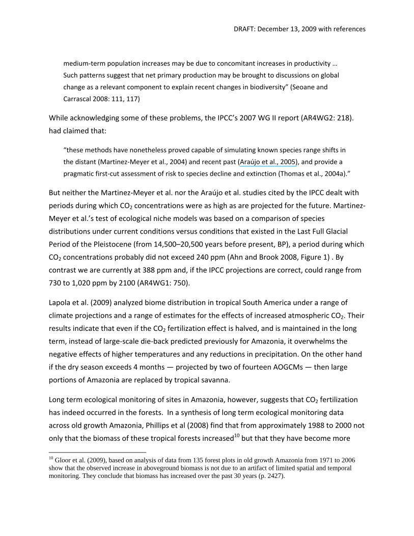
considerable global warming (see Figure 9; AR4WG1: 106; Myneni 2006: 5).
DRAFT: December 13, 2009 with references
Figure 9: Climate driven changes in global net primary productivity. Source: Myneni (2006).
Using a mixture of observations and climate model outputs, Lloyd and Farquhar (2008), find no
evidence that tropical forests are currently “dangerously close” to their optimum temperature
range. They found that increases in photosynthetic rates due to CO2 fertilization should over
forthcoming decades more than offset any decline in photosynthetic productivity due to higher
temperatures. They also found “little direct evidence that tropical forests should not be able to
respond to increases in [CO2] and argue that the magnitude and pattern of increases in forest
dynamics across Amazonia observed over the last few decades are consistent with a [CO2]‐
induced stimulation of tree growth.”
In addition, the AR4WG2 overstates its claim that Araújo et al. (2005) showed that bioclimatic
models can simulate range shifts for the recent past. In fact, Araújo et al. found that:
“Among the 74 British‐bird species that contracted during the reported period, species were
correctly projected to contract in … 50% of the models … For the remaining 42 species that
expanded during the reported period, species were correctly projected to expand in 56% of
the models ... In short, assessment of all projections indicates a performance in terms of
DRAFT: December 13, 2009 with references
predicting the direction of range shifts no better than tossing a coin.” (p. 531; emphasis
added).
To get around this problem, Araújo et al. (2005) recommend using a “consensual modeling” or
“ensemble modeling” approach. Although the theoretical basis for such an approach is unclear,
their study indicates that consensual modeling improved the correspondence between models
and observation. However, it’s not clear whether the IPCC’s AR4WG2 results were based on the
consensual or ensemble modeling approach, since neither term appears in conjunction with
species or habitat modeling in its ecosystems chapter. Certainly, it was not used in the
landmark Thomas et al. (2004) study cited by the IPCC above as providing a “pragmatic first‐cut
assessments of risk to species decline and extinction” (AR4WG2: 218). Notably this study is also
a mainstay of FG’s claims regarding the impacts of climate change on species and ecosystems
(their reference 120).
In any case, the IPCC’s claim that bioclimatic models provide a first‐cut assessment is a stretch.
And even if it does, that begs the question whether enough confidence can be attached to the
results to use them as a basis for supporting trillion dollar policies, as opposed to generating
hypotheses and testing sensitivities to different variables. This issue also needs to be addressed
with respect to results based on ensemble modeling before using them for formulating policies.
Yet another problem with Thomas et al (2004) is that it modeled extinctions based on species‐
area relationship, which is based on the assumption that the number of species that can be
supported on a piece of real estate would be reduced as the size of that real estate shrinks,
based on a power law relationship.11 However, recent studies suggest that habitat size may be a
poor predictor of extinction In a study of 785 animal species in 1,015 population networks
surveyed in 12,370 discrete habitat patches on 6 continents, Pruigh et al (2008) found that
fragment size was a poor predictor of patch occupancy. Area alone accounted for a median of
13% of the deviance in occupancy (Pruigh et al. 2008: 20770), adding that the quality of the
matrix surrounding the fragment may have a greater influence on occupancy and persistence.
In a recent paper in Science, Willis and Bhagwat (2009: 807) take note of Pruigh et al.’s study,
adding that:
11 This power-law relationship is S=cAz, where S is the number of species, A is area, and c and z are constants (Thomas et al. 2004: 145).

DRAFT: December 13, 2009 with references
“This ability of species to persist in what would appear to be a highly undesirable and
fragmented landscape has also been recently demonstrated in West Africa. In a census on the
presence of 972 forest butterflies over the past 16 years, Larsen found that despite an 87%
reduction in forest cover, 97% of all species ever recorded in the area are still present … For
reasons that are not entirely clear, these butterfly species appear to be able to survive in the
remaining primary and secondary forest fragments and disturbed lands in the West African
rainforest. However, presence or absence does not take into account lag effects of declining
populations …” [Citations deleted.]
On the other hand, the loss of terrestrial and freshwater habitat to agricultural uses in
particular, has generally been considered to be the most significant threat to global biodiversity
(Goklany 1998, Millennium Ecosystem Assessment 2005). If that is the case, changes in
cropland could either exacerbate or relieve the consequences of global warming. To the extent
higher CO2 concentrations, global warming, and human adaptive responses increase
agricultural and forest productivity and water use efficiency (Idso and Brazel 1984; Gedney et
al. 2006), the diversion of land and water to human uses would be reduced (Goklany 1998,
2003). Lower habitat loss would also conserve carbon stocks and sinks as well as migration
corridors, a mechanism to aid species adapt to changed circumstances. Levy et al. (2004), for
instance, indicate that because of increases in productivity due largely to CO2 fertilization,
under the IPCC’s A1FI (warmest) scenario the amount of global cropland could decline from
11.6% in 1990 to 5.0% in 2100, substantially increasing the amount of habitat available to the
rest of nature. Such reduction in cropland could also restore and preserve migration corridors.
Similarly, if human adaptive responses free up more water for in‐stream uses, that would
reduce pressures on freshwater species. Thus at moderate levels of global warming, the overall
pressure on biodiversity, ecosystems and species might well decline (Goklany 1998, 2001), only
to increase once again if temperatures keep escalating, although higher CO2 concentrations
may help compensate for that (Lloyd and Farquhar 2008, Saurer et al. 2004).
4. Will the Deserts Expand and the Landscape Become Bleaker?
In the previous section, I showed that empirical data indicates that Amazonia and the world as
a whole is greener today than it used to be. Notwithstanding that, one of the concerns
regarding global warming is that deserts will expand, and that earth will be a bleaker place.
Popular wisdom is that, “Desertification, drought, and despair—that's what global warming has

DRAFT: December 13, 2009 with references
in store for much of Africa” (Owen 2009). However, satellite Imagery shows that parts of the
Sahara and Sahel are greening up consistent with the trend recorded in Figure 9 (Owen 2009).
The United Nations’ Africa Report notes:
“Greening of the Sahel as observed from satellite images is now well established, confirming
that trends in rainfall are the main but not the only driver of change in vegetation cover. For
the period 1982‐2003, the overall trend in monthly maximum Normalized Difference
Vegetation Index (NDVI) is positive over a large portion of the Sahel region, reaching up to 50
per cent increase in parts of Mali, Mauritania and Chad, and confirming previous findings at a
regional scale.” (United Nations 2008: 41).
Similarly, an Australia‐wide analysis of satellite data for 1981–2006 indicates that vegetation
cover has increased average of 8% (Donohue et al. 2009).
With respect to the northern latitudes, 22% of the vegetated area in Canada was found to have
a positive vegetation trend from 1985–2006. Of these, 40% were in northern ecozones (Pouliot
et al. 2009).
III. CHERRY PICKING CATASTROPHES & TIPPING POINTS
Advocates of strict greenhouse gas controls frequently argue that, unchecked, global warming
might lead to catastrophes as various thresholds and “tipping points” are crossed. Favorite
candidates for catastrophes are a “rapid collapse” of the Greenland Ice Sheet (GIS) and West
Antarctic Ice Sheet (WAIS), which contain water equivalent to 21 meters of global sea level rise
(FG: 118); a halting of the thermohaline circulation (also known as the Atlantic meridional
overturning circulation, or MOC) which was the inspiration for the deep freeze depicted in the
movie, The Day After Tomorrow (FG: 126); and the warming‐induced melting of methane
hydrates (known as clathrates) in the Arctic which would then increase methane in the
atmosphere that would further reinforce the warming (FG: 118‐119, 126).
Much of the rationale for considering such low‐probability‐but‐potentially‐high‐consequence
events can be traced to Weitzman’s estimate that “eventually” there could be, according to the
probability density function (PDF) based on the IPCC’s climate change estimates, a 5%
probability that average global temperature increase (ΔT) will exceed 11°C and a 1% probability
DRAFT: December 13, 2009 with references
that it could exceed 20°C. However, as already discussed, these models have not been
validated, and are, in fact, failing their validation. According to these models, global
temperatures should have risen at least 0.2°C over the past decade but they have not (see
Figure 6). This indicates that the sensitivity of ΔT to increases in carbon dioxide may have been,
for whatever reason, substantially overestimated by the models and, therefore, Weitzman’s
(2008) probability estimates are overblown.
Weitzman (2008) used PDFs derived from 22 IPCC models, giving each one equal weight. These
models subscribe to the same paradigm with respect to the influence of carbon dioxide on
temperature, although they may differ on the magnitude of the temperature sensitivity. It is
also not clear that these models do not share components, assumptions, parametrization and
other features. So the 22 “models” may be more appropriately viewed as 22 variants of the
same basic model. Equally important, alternate models such as those derived in Zhen‐Shan and
Xian (2007), Tsonis et al. (2007), Swanson and Tsonis (2009), and Loehle (2004 and 2009), which
forecast a cooling period in the early 2000s, are not represented; nor are models incorporating
Svensmark’s theory of galactic cosmic rays (Knudsen and Riisager 2009), Lindzen and Choi’s
(2009) theory on feedbacks, or alternative specifications of the residence time of CO2 in the
atmosphere. If one is skeptical about these alternative models and formulations, they ought to
be given lower weights, but to ignore them is inappropriate for the purposes of developing a
PDF.
Note that while global warming studies sometimes make projections that extend to 2100 and
beyond, to the extent the results are sensitive to socioeconomic factors —and IPCC’s emissions
and climate change estimates are driven by socioeconomic assumptions — one cannot and
should not give them much credence (Lorenzini and Adger 2006: 74). In the following I will
restrain my skepticism on this score.
In this section I will first look at the evidence that the potential catastrophes listed above are
likely over the next century —a time horizon that goes well beyond what is reasonably
foreseeable — before addressing broader issues associated with the advocates’ appeal to
catastrophism.
DRAFT: December 13, 2009 with references
1. The Greenland Ice Sheet (GIS) and West Antarctic Ice Sheet (WAIS)
According to the IPCC’s WG I Summary for Policy Makers (AR4WG1: 17) neither the Greenland
nor West Antarctic Ice Sheets are in danger of melting away any time soon. Regarding the
latter, it notes:
“Current global model studies project that the Antarctic Ice Sheet will remain too cold for
widespread surface melting and is expected to gain in mass due to increased snowfall.”
With respect to the former, it also notes:
“If a negative surface mass balance were sustained for millennia, that would lead to virtually
complete elimination of the Greenland Ice Sheet and a resulting contribution to sea level rise
of about 7 m” (emphasis added).
This statement, based on thermodynamics, applies equally well to the West Antarctic Ice Sheet.
But whether one is concerned about the GIS or WAIS, what is the probability that a negative
surface mass balance can, in fact, be sustained for millennia, particularly after considering the
amount of fossil fuels that can be economically extracted and the likelihood that other energy
sources will not displace fossil fuels in the interim, given claims of “peak oil,” and that
renewable energy sources are on the verge of paying for themselves?
Notably, Willersleev et al. (2007) found that during the Eemian (~ 125,000‐130,000 yrs ago), a
period during which average global temperatures were 3‐5°C higher and sea level was 4‐6 m
higher than it is today [IPCC AR4WG1: 9], Greenland was much warmer, but still not ice free.
Second, for an event to be classified as a catastrophe, it should occur relatively quickly
precluding efforts by man or nature to adapt or otherwise deal with it. But if it occurs over
millennia, as the IPCC says, or even centuries, that gives humanity ample time to adjust, albeit
at some socioeconomic cost. But as indicated by Figure 7, if the assumptions behind the IPCC’s
projections of global warming are valid, then humanity will be much wealthier in the future
even after accounting fully for the effects of global warming, and the cost need not be
prohibitive (see below).
More importantly, if it does take centuries or millennia, the toll on human life, limb and
property may well be minor if: (1) the total amount of sea level rise (SLR) and, perhaps more
importantly, the rate of SLR can be predicted with some confidence, as seems likely in the next
DRAFT: December 13, 2009 with references
few decades considering the resources being expended on such research; (2) the rate of SLR is
slow relative to how fast populations can strengthen coastal defenses and/or relocate; and (3)
there are no insurmountable barriers to relocation, if that is the preferred response.
This would be true even had the so‐called “tipping point” already been passed and ultimate
disintegration of the ice sheet was inevitable, so long as it takes millennia for the disintegration
to be realized. In other words, the issue isn’t just whether the tipping point is reached, rather it
is how long does it actually take to tip over and for its effects to be manifested. Take, for
example, if a hand grenade is tossed into a crowded room. Whether this results in tragedy —
and the magnitude of that tragedy — depends upon how much time it takes for the grenade to
go off, the reaction time of the occupants, and their ability to respond.
Lowe, et al. (2006: 32‐33), based on a “pessimistic, but plausible, scenario in which
atmospheric carbon dioxide concentrations were stabilised at four times pre‐industrial levels,”
estimated that a collapse of the Greenland Ice Sheet would over the next 1,000 years raise sea
level by 2.3 meters (with a peak rate of 0.5 cm/yr or 0.5 m per century). If one were to
arbitrarily double that to account for potential melting of the West Antarctic Ice Sheet, that
would result in total SLR of ~5 meters in 1,000 years with a peak rate (assuming the peaks
coincide) of 1 meter per century.
A rise of 5 m/millennium would not be unprecedented. Sea level has risen 120 meters in the
past 18,000 years, an average of 0.67 meters/century or 6.7 meters per millennium. It may also
have risen as much as 4 meters/century during meltwater pulse 1A episode 14,600 years ago
(Weaver et al. 2003). Neither humanity nor, from the perspective of millennial time scales, the
rest of nature seem the worse for it. Coral reefs for example, evolved and their compositions
changed over millennia as new reefs grew while older ones were submerged in deeper water
(e.g., Cabioch et al. 2008). So while there have been ecological changes, it is unknown whether
the changes were for better or worse. For a melting of the GIS (or WAIS) to qualify as a
catastrophe, one has to show, rather than assume, that the ecological consequences would, in
fact, be for the worse. Notably, such a showing is never explicitly made. It is generally assumed
that an ecological change is necessarily worse for man and nature. This is theology, not reason.
Finally, history from the past several decades indicates that human beings can certainly cope
with sea level rise of such magnitudes if they have centuries or millennia to prepare and adjust.
In fact, if necessary, human beings could get out of the way in a matter of decades, if not years.
DRAFT: December 13, 2009 with references
Can a relocation of such a magnitude be accomplished?
Consider that the global population increased from 2.5 billion in 1950 to 6.9 billion this year.
Among other things, this meant creating the infrastructure for an extra 4.4 billion people in the
intervening 59 years (as well as improving the infrastructure for the 2.5 billion counted in the
baseline, many of whom barely had any infrastructure whatsoever in 1950). These
improvements occurred at a time when everyone was significantly poorer. (Global per capita
income today is 3.8 times what it was in 1950.12) Therefore, while relocation will, no doubt, be
costly, tomorrow’s much wealthier world ought to be able in theory to relocate billions of
people to higher ground over the next few centuries, if that were necessary. In fact, once a
decision is made to relocate, the cost differential of relocating, say, 10 meters higher rather
than a meter higher is probably marginal. It should also be noted that over millennia the
world’s infrastructure will necessarily have to be renewed or replaced dozens of times, which
effectively can help reduce premature losses of committed capital (and overall costs). For
example, the ancient city of Troy, once on the coast but now a few kilometers inland, was built
and rebuilt at least 9 times in 3 millennia.
2. Thermohaline Circulation
A popular myth about climate is that winters of Western Europe are mild relative to those of
eastern North America because of the thermohaline circulation (THC), so‐called because it is
driven by differences in the density of seawater due to changes in temperature and salinity
(salts are halides in Latin). The thermohaline circulation, sometimes called the “Great Ocean
Conveyor Belt” or “Meridional (i.e., north‐south) Overturning Circulation,” conveys heat from
the lower latitudes in warm surface waters towards the poles. The Gulf Stream (and its
tentacle, the North Atlantic Drift), which is part of this circulation, moves heat from the tropics
to the northeast Atlantic. This heat is picked up by the mid‐latitude westerlies over the Atlantic
which warm western Europe. Thus as the surface water moves north, it cools. Some of it also
forms sea ice, which increases the salinity of the remaining water. Both cooling and sea ice
formation, therefore, increase the density of the water, which then sinks toward the ocean
depths becoming part of the North Atlantic Deep Water. This deep water travels south across
the Atlantic between the New and Old Worlds toward the Antarctic and then northward into
12 This is estimated using data from Maddison (2008), and World Bank (2009d). Per capita income in 1990 International dollars increased from $2,117 in 1950 to $7,725 in 2006 per Maddison (2008), and another 3.8% from 2006 to 2007 per the World Bank.
DRAFT: December 13, 2009 with references
the Indian Ocean or north east around Australia to the Northern Pacific where, mixing with
warmer waters, it rises and generates a warm, counter‐current close to the ocean’s surface.
The counter‐current from the Pacific travels south and west through the Indonesian archipelago
where it joins the countercurrent established in the Indian Ocean. It then goes around the Cape
of Good Hope into the Atlantic, where it becomes, once again, part of the Gulf Stream.
One of the favorite doomsday scenarios about global warming is that melting of the Greenland
Ice Sheet or the permafrost or increased runoff could inject extra freshwater in the North
Atlantic which could, then, substantially halt the sinking of the water into the North Atlantic
Deep, and halt the conveyor belt sending Europe, if not the world, into a deep freeze. This was
essentially the premise behind the movie, The Day After Tomorrow. However, these fears seem
to be overblown (Wunsch 2004; Kerr 2005).
First, most of the winter warming of Western Europe seems to be due to atmospheric
circulation and seasonal release of heat stored in the ocean rather than heat transported by the
ocean circulation (Seager et al. 2002; Weaver and Hillaire‐Marcel 2004).
Second, Gregory and co‐workers (2005) compared the response of the THC to a quadrupling of
CO2 concentrations over 140 years using 11 different models.13 All the models indicated a
gradual decline in the strength of the THCs by between 10 and 50 percent. However, none
showed a rapid or complete collapse. None of the models shows a cooling anywhere that would
more than offset any resulting warming.
These points were picked up in the IPCC WG I Summary for Policy Makers, which notes
(AR4WG1: 16),
“Based on current model simulations, it is very likely that the meridional overturning
circulation (MOC) of the Atlantic Ocean will slow down during the 21st century. The multi‐
model average reduction by 2100 is 25% (range from zero to about 50%) for SRES emission
scenario A1B. Temperatures in the Atlantic region are projected to increase despite such
changes due to the much larger warming associated with projected increases in greenhouse
gases. It is very unlikely that the MOC will undergo a large abrupt transition during the 21st
century. Longer‐term changes in the MOC cannot be assessed with confidence.” [Emphasis
added.]
13 See, also, Schmittner et al. (2005), which reports that 28 projections from 9 different coupled global climate models of a scenario of future CO2 increase projected a gradual weakening of the North Atlantic THC by 25(±25)% until 2100.
DRAFT: December 13, 2009 with references
Not much has changed since then. A shut down of the MOC doesn’t look any more likely now
than it did then. Based on observations spanning 1957‐2004, Baehr et al.(2007) found “no MOC
trend over the past 50 yr.” Latif et al (2006) note that instead of a sustained THC weakening, “a
strengthening since the 1980s is observed.” Their “combined assessment of ocean hydrography
data and model results indicates that the expected anthropogenic weakening of the THC will
remain within the range of natural variability during the next several decades.” Finally, Boyer et
al. (2007) find that the “North Atlantic freshened from the 1950s to the 1990s but has since
become more saline.”
Clark et al. (2008: 316) offer the following summary:
“… all available model simulations, including those with estimates of maximum Greenland Ice
Sheet (GIS) melting rates, indicate that it is very unlikely that the MOC will undergo an abrupt
transition during the course of the 21st century … 14 coupled models simulated a 100‐year
0.1‐Sv freshwater perturbation to the northern North Atlantic Ocean—17 times the recently
estimated melt rates from the GIS—and the MOC weakened by a multimodel mean of 30%
after 100 years; none of the models simulated a shutdown. Another model simulated
greenhouse gas levels that increased to four times preindustrial values and then remained
fixed; the resulting GIS displayed a peak melting rate of about 0.1 Sv, with little effect on the
MOC. One model simulation uses the SRES A1B scenario but adds an additional 0.09‐Sv
freshwater forcing as an upper‐bound estimate of potential GIS melting. In this case, the MOC
weakened but subsequently recovered its strength, indicating that GIS melting would not
cause abrupt climate change in the 21st century.” [Citations deleted.]
Finally, if the slowing of the thermohaline circulation would only partially offset any global
warming per the IPCC’s assessment, then it could offset some of the consequences of global
warming, such as extended heat waves, hypothetical increases in climate‐sensitive diseases, or
threats to biodiversity. Thus, such a slowing down, were it to occur, is more appropriately
viewed as an “anti‐catastrophe” than a catastrophe.
To summarize, as Carl Wunsch (2004), a climatologist at MIT, put it:
“The only way to produce an ocean circulation without a Gulf Stream is either to turn off the
wind system, or to stop the Earth's rotation, or both.
“Real questions exist about conceivable changes in the ocean circulation and its climate
consequences. However, such discussions are not helped by hyperbole and alarmism. The
occurrence of a climate state without the Gulf Stream any time soon — within tens of millions
of years — has a probability of little more than zero.”
DRAFT: December 13, 2009 with references
3. Methane
Another global warming bogeyman is that warming might lead to release of methane from
methane clathrates (or hydrates) stored in the Arctic permafrost which would increase its
concentration in the atmosphere. But methane has a “global warming potential” averaged over
100 years of 25, that is, methane, ton‐for‐ton, is 25 times more powerful a greenhouse gas than
carbon dioxide (AR4WG1 Technical Summary: 33). Thus, such releases of methane would
constitute a positive feedback for global warming.
The initial concerns about methane stemmed from the fact that by the 1990s the atmospheric
concentration of methane, which had been growing rapidly, had exceeded 1,730 parts per
billion (ppb), almost twice the maximum amount measured over the past 650,000 years in ice
cores (AR4WG1: 3).
Concern of runaway methane feedback was also stoked by a number of modeling studies which
suggested rapid disintegration of the permafrost with global warming (e.g., Lawrence and Slater
2005, Zimov et al. 2006). However, in a modeling study which took into consideration the
thermal profile of the permafrost, and the fact that the melting effect of warm air surface
temperatures on the upper layers of permafrost would be countered by cooling due to colder
deeper layers of permafrost, Delisle (2007) showed that “massive releases of methane in the
near future are questionable.”
Even more compelling is that the growth in atmospheric concentrations has slowed
substantially. As noted by the IPCC AR4WG1 (p. 796):
“Recent measurements show that CH4 growth rates have declined and were negative for
several years in the early 21st century … The observed rate of increase of 0.8 ppb yr–1 for the
period 1999 to 2004 is considerably less than the rate of 6 ppb yr–1 assumed in all the [IPCC]
SRES scenarios for the period 1990 to 2000.”
The latest observations indicate that the rate of change is not increasing, and that they “are not
consistent with sustained changes … yet” (Dlugokencky et al. 2009: 4). They also indicate that
the geographical pattern and the isotopic signature of methane increases suggests that the
major sources are wetlands — probably tropical wetlands —rather than Arctic permafrost.
DRAFT: December 13, 2009 with references
Petrenko et al. (2009) examined the source of isotopic methane in a glacial ice core from West
Greenland to determine the probable source of the large increase in methane during the
abrupt warming of +10±4°C that occurred during the transition from the Younger Dryas to the
Preboreal (~11,600 years ago) (Grachev and Severinghaus 2005). They concluded that
“wetlands were the likely main driver of the [methane] increase and that clathrates did not play
a large role,” a finding they noted “is in agreement with findings from previous ice core CH4
isotopic studies” (Petrenko et al. 2009: 508). This study essentially reiterated the results of
another paper by many of the same researchers that appeared in Nature the previous year
(Fischer et al. 2008). Notably the Petrenko et al. study’s publication was accompanied by an
announcement titled, “Ancient Greenland methane study good news for planet, says CU‐
Boulder scientist” (Eureka Alert 2009).
So it seems that while methane emissions might increase if there is warming, there is no
evidence of catastrophic releases from clathrates.
4. Selective Catastrophism
The foregoing examination of the three most frequently cited sources of climate change
catastrophe indicates that there is no evidence that they are likely to occur, if at all, any time in
the foreseeable future and, possibly, not even for centuries and millennia. Moreover, the
approach embodied in FG toward potential catastrophes is fundamentally flawed in several
respects.
First, it is selective about the potential catastrophes that it chooses to focus upon. But why
consider some but not other potential catastrophes?
If one wants to develop rational policies to address speculative catastrophic events that might
(or might not) occur over the next few centuries or millennia (e.g., melting of ice sheets, or the
shutdown of the MOC), as a start one should consider the universe of potential catastrophes
and then develop criteria as to which should be addressed and which not. Rational analysis
must necessarily be based on a systematic review of catastrophes, and not on cherry picking
one’s favorite catastrophes. This means examining not only the catastrophes that additional
warming may bring, but also the catastrophes that warming may avoid. It also means
considering the possibility that over the time frame of interest (namely, centuries or millennia),
DRAFT: December 13, 2009 with references
an increasingly wealthy and technologically more sophisticated society will devise new
technologies to negate, defuse or cope with any resulting catastrophe.
Specifically, absent global warming, the Little Ice Age (LIA) might return over the next few
centuries or millennia. How can one make such a claim? For one thing, we know there was an
LIA. It has been extensively documented in history, literature, and art (Fagan 2000; Lamb 1982),
and that it ended around a century and half ago. Since it occurred in the past, history may
indeed repeat itself, particularly if one considers timeframes of the order of centuries or
millennia. Historical documentation indicates that the consequences of another ice age, Little
or not, could range from the severely negative to the positive (if that would buffer the negative
consequences of warming).
Second, so long as we are concerned about low probability events, we should also consider
equally low or higher probability events that might either forestall these catastrophes on
relatively short notice14 or negate their impacts when the time comes. Specifically, it is quite
possible — in fact, probable, considering the amounts being expended on research and
development of such technologies — that somewhere between now and 2100 or 2200,
technologies will become available that will deal with global warming much more economically
and rapidly than currently available technologies. Such technologies may include ocean
fertilization, carbon sequestration, other geo‐engineering options (e.g., deploying mirrors in
space), more efficient solar or photovoltaic technologies which would indeed pay for
themselves, unlike current versions of these technologies which, being uneconomic, need
regulation or subsidies to “compete” in the market place, except under limited circumstances.
In addition, it may include technologies that have not yet been conceived.
Similarly, there is a finite, non‐zero probability that future new and improved adaptation
technologies will substantially reduce the net adverse impacts of global warming. This has
occurred over the past century for virtually every climate‐sensitive sector that has been
studied. For example, from 1900‐1970, U.S. death rates due to various climate‐sensitive water‐
related diseases — dysentery, typhoid, paratyphoid, other gastrointestinal disease, and malaria
—declined by 99.6 to 100.0 percent (Goklany 2009b: 14). Similarly, over the centuries, poor
agricultural productivity exacerbated by drought led to massive famines in India and China,
14 If one is concerned about catastrophes that might occur or unfold over centuries or millennia, “short notice” would be on the order of a century or so.
DRAFT: December 13, 2009 with references
killing millions (Davis 2001; Becker 1997). But such famines have not recurred since the 1970s
despite any global warming, and notwithstanding the fact that populations are substantially
higher today (Goklany 2009c: 104). Similarly, by the 2000s, deaths and death rates due to
droughts, floods and other extreme weather events had dropped worldwide by 93–98% since
they peaked in the 1920s (see Figure 8).
Third, a full analysis should also consider that greenhouse gas controls may themselves cause
catastrophes. First, CO2 not only contributes to warming, it is also the key building block of life
as we know it. Human beings are 18% carbon (Mallery, undated), all of which can be traced
directly or indirectly to vegetation created by the photosynthesis of CO2. In fact, as shown in
Figure 9, according to the IPCC WG I report (2007: 106), net primary productivity (NPP) of the
global biosphere has increased in recent decades, partly due to greater warming, higher CO2
concentrations and nitrogen deposition.
Increased NPP not only means more food for humanity, it also provides a double dividend for
biodiversity and conservation. First, higher NPP means the biosphere can support greater and
wider variety of species (e.g., Lloyd and Farquhar 2008; Seoane and Carrascal 2008). Second, by
increasing agricultural and forest productivity it reduces the human demand for land, which is
the single largest threat to biodiversity today (Goklany 1998; MEA 2005). Thus, there is a finite
probability that reducing CO2 emissions would have potentially severe negative consequences
not only for the conservation of nature but also for the prospects of eliminating hunger.
There is also a finite probability that costs of GHG reductions could reduce economic growth
worldwide which, then, may reduce the adaptive capacity of developing countries, which are
generally acknowledged to be most at risk from global warming (Goklany 2000b). Even if only
industrialized countries sign up for emission reductions, there could be negative economic
consequences in developing countries because they derive a substantial share of their income
from aid, trade, tourism, and remittances from the rest of the world (see Section V). Tol (2005)
examines this possibility and although the extent to which that study fully considered these
factors (i.e., aid, trade, tourism, and remittances) is unclear, it concludes (p. 577):
“… for an emission abatement policy costing $1/tC, which is roughly the price of the Kyoto
Protocol without the USA but with Russian hot air [,] Africa and Latin America would prefer
money to be spent on development rather than on emission reduction—that is, their climate‐
change impacts fall further if money is invested in development rather than in abatement.”
DRAFT: December 13, 2009 with references
Finally, one of the problems with the argument that society should address low‐probability‐but‐
potentially‐high‐impact events is that that there is a much higher probability that the resources
expended on addressing such problems would have been squandered. This would not be a
problem but for the fact that there are opportunity costs associated with this, as demonstrated
by the above quote from Tol.
According to the 2007 IPCC Science Assessment’s Summary for Policy Makers (p. 10), “Most of
the observed increase in global average temperatures since the mid‐20th century is very likely
due to the observed increase in anthropogenic greenhouse gas concentrations.” In IPCC
parlance, “very likely” means that its authors believe there is at least a 90–95% likelihood that
anthropogenic greenhouse gas emissions (AGHG) are responsible for 50‐100% of the global
warming since 1950, assuming that “most” denotes anywhere between 50–100%. In other
words, anthropogenic GHGs are responsible for 45–95% of that warming.15
This means there is an up to 55% chance that resources expended in limiting global warming
would have been squandered to little or no effect. Since any effort to significantly reduce global
warming will cost trillions of dollars (see Nordhaus 2008: 82), that would be an unqualified
disaster, particularly since those very resources could be devoted to reducing more urgent
problems humanity faces here and now (e.g., hunger, malaria, safer water and sanitation) —
problems we know exist for sure unlike the global warming bogeymen that may well be
figments of the imagination (Goklany 2000, 2005, 2009a; Lomborg 2004, 2008)
According to estimates from the World Health Organization (2002) of the contribution of over
26 risk factors to the global burden of disease for 2000, global warming contributes less than
0.3% of the global mortality burden.16 Not surprisingly, in 2000 it ranked below the top 20
global threats to public health—behind more mundane but much more consequential problems
such as hunger (underweight), unsafe water and poor sanitation, vitamin A deficiency, poor
nutritional intake, and indoor air pollution (Goklany 2009a: 70). Looking toward the future, on
the basis of health impacts, global warming will continue to be outranked by other
environmental and health risks through the foreseeable future (Goklany 2003, 2007b, 2009a).
15 The lower number is calculated as 50% of 90%, and the higher number as 100% of 95%. 16 Although these estimates are based on suspect methodology (see Goklany 2009a: 70), by virtue of their provenance they have been very influential in the public policy debate. They were for example, picked up wholesale in a review article in Nature (Patz et al. 2005), and adopted by several influential reports, e.g., the report of the Lancet and University College London Institute for Global Health Commission (2009).
DRAFT: December 13, 2009 with references
It is critical to understand that the concern for opportunity costs is not merely theoretical. At
the 2009 World Food Summit, developed countries rejected the U.N.'s call to commit $44
billion annually for agricultural development for developing nations, which would have helped
reduce hunger for hundreds of millions. According to the Associated Press (2009), the UN Food
and Agricultural Organization's Assistant Director‐General Alexander Mueller said that
governments kept away from firm commitments to reduce hunger, “due to the economic crisis
and because they expect they will need to channel money to the developing world at next
month's summit on climate change in Copenhagen” (emphasis added).
Spending money on low probability catastrophes instead of problems we know exist for sure is
like a starving man giving up a fat juicy bird in hand while hoping that he will catch other birds
in the future even though he does not know whether those birds exist today or will exist in the
future. It is rational only if one ignores opportunity costs, and advocates’ appeal to potential
catastrophes and tipping points only serves to tip the discussion from being based on rational
analysis to one dominated by our fears.
IV. “THINGS ARE WORSE THAN EXPECTED/THOUGHT”
Proponents of drastic greenhouse gas controls frequently claim that “climate change is worse
than we thought.” (PBS 2006). The Lancet‐University College of London Commission (2009:
1,701), for example, asserts (p. 1701) that “Work done after the IPCC 2007…found that CO2
emissions growth rate increased from 1.3% to 3.3% every year, suggesting that the current
carbon cycle is generating more severe climate change sooner than expected.” Indeed, it is true
that the spectacular economic growth across Asia and elsewhere was beyond most
expectations in the 1990s, when the IPCC scenarios were formulated. But emissions increases
should not be conflated with global warming. The relevant question is whether global
temperatures and other more robust indicators of warming have risen more rapidly than
anticipated in the IPCC (2007) assessment, or if the climate sensitive indicators of well‐being
have deteriorated faster.
The IPCC assessment estimated that if emissions stayed within the range of the IPCC scenarios,
then global average temperature should increase 0.2°C per decade in the near term (AR4WG1:
12). Therefore, higher CO2 emissions should, if anything, result in higher temperature increases.
But neither the satellite (e.g., RSS 2009) nor surface temperature data (Hadley Centre 2009)
DRAFT: December 13, 2009 with references
show significant global warming since 2000, let alone an increase at a rate greater than the
IPCC’s projected 0.2°C per decade (see also Figure 6). Of equal importance is the fact that ocean
heat content has not increased significantly in recent years (Dickey et al. 2008; Levitus et al.
2008), and sea level rise has slowed since 2003 (University of Colorado 2009).
A counter argument is that several of the highest global average temperatures have occurred in
the 2000s. Whether this is the case, it is less remarkable than it seems because one would
expect warm (or cold) years to occur in bunches due to the inertia of the climate system (that
is, because of persistence).
Admittedly, the empirical trends cited above are based on short‐term trends, but so is the claim
that we should be more concerned because of a (short‐term) increase in CO2 emissions. More
importantly, the divergence over the most recent decade between the IPCC’s projections and
empirical data with regard to global temperature anomalies coupled with reductions in ocean
heat content and the rate of sea level rise at a time of unprecedented increases in CO2
emissions, suggests that the sensitivity of climate to CO2 emissions might have been
overestimated in the models relied upon by the IPCC for its projections of future warming and
its impacts, or that natural variability may be a larger influence on climate than acknowledged
by the IPCC, or both. Some argue that this could be due to natural variability and that when
natural variability swings the other way warming will return with a vengeance. See Section II.
Perhaps that will happen, but it also means that reducing GHG emissions will have a much
smaller influence than indicated by the IPCC models, and that greater attention should be
focused on adaptation.
Also, as will be discussed in greater detail below (Section V.5), contrary to prognostications of
GHG control advocates, climate sensitive indicators of human well‐being have generally
advanced over the long term despite any global warming. For instance, despite claims that
hurricanes would get more intense if not more frequent, total accumulated cyclone intensity
for a season are at historic lows (Maue 2009); instead of increasing, death tolls from extreme
weather events have continued to decline (see Figure 8); property damage from cyclones has
increased but only to the extent that more property is at risk (Pielke et al. 2008a, 2008b);
generally, agricultural productivity is higher than ever while hunger is generally lower
(notwithstanding an increase in the past couple of years because of increased demand in the
DRAFT: December 13, 2009 with references
fast developing Asian countries and diversion of crops to biofuel production) (Goklany 2007c,
FAO 2008); and the world continues to get greener (Figure 9).
V. ECONOMIC SPILLOVERS
It is generally accepted that developing countries are more at risk from global warming than
industrialized countries (see, e.g., UNEP 1993; Goklany 1995: 435). This is largely because: (a)
global warming is projected to exacerbate the problems of poverty that currently afflict many
developing countries, and (b) they lack the financial, technological and human resources
needed to cope with these problems today (Goklany 2000; Lancet Commission 2009). The
problems of poverty that are generally cited as worsening with global warming are malaria and
other vector‐borne diseases, hunger, water shortages, and vulnerability to extreme weather
events and sea level rise. The IPCC, among others, claim that global warming could, therefore,
hinder sustainable development of developing countries (AR4WG2: 13, 20). In a similar vein, FG
argue that weak or poor governments may be swamped by the impacts of climate change such
that their economic productivity would suffer, leading to economic instability which, in turn,
would result in large — and negative — economic spillovers on the United States. The economic
instability would, then, lead to political instability, breed terrorism and precipitate mass
migration with adverse consequences for US’s economic well‐being and national security (see,
e.g., FG: 134‐137).
Implicit in the claims noted above is the notion that future adaptive capacity, particularly of
developing countries, will not be much different from today. But as was discussed in Section II,
this notion is inconsistent with the socioeconomic assumptions built into the IPCC’s emissions
and climate change scenarios.
No matter, FG claim (p. 138) that because of climate change, “First, and most obviously, trade
flows will diminish.” They suggest, for example, that:
“… supply [of foreign products to the US] might be affected by severe economic and social
dislocation in South and Southeast Asia caused by flooding, drought, and extreme weather
events. Affected countries, including China and India, may be unable to maintain production
levels in the face of these impacts. This sort of disruption in supply would lead to a rise in
DRAFT: December 13, 2009 with references
prices, which would be harmful to American economic welfare” (FG: 138–39; citations have
been deleted).
Other factors that could “permanently reduce productivity levels” are a disruption of water or
energy supplies due to global warming (FG: 139). They then argue that “Climate change also
threatens to interrupt the free flow of trade in critical resources such as oil, gas, and other
essential commodities on which the United States depends” (p. 147).
The arguments made by FG seem plausible if one ignores the fact that future adaptive capacity
will most likely be substantially greater than it is today. They, moreover, rely on a surfeit of
speculation as betrayed by their repeated appeals to readers to “imagine” the numerous ways
by which global warming could lead to economic spillovers on the U.S. (emphases added):
“Consider, for example, some obvious ways in which American interests are negatively
affected by climate change abroad. Imagine major economic downturns in the most
important trading partners of the United States, including Europe and China. Now imagine
that these downturns last decades. What would be the effect on the United States? How
would the United States be affected by violent conflict in the Middle East prompted by
disputes over water resources? What if drought and disease, exacerbated by climate change,
topple already unstable governments in Africa, creating safe havens for terrorist groups? What
happens if migration pressures from Latin America increase dramatically as living conditions
there deteriorate? Or if the emergence of contagious disease in Asia (recall the SARS scare in
2003) threatens to or actually comes to the United States? None of these scenarios is
particularly farfetched. Indeed, each of them is reasonably likely. Each of them would also
have a significant economic and/or political impact on the United States. Yet the possibility of
such events is not taken into account by existing IAMs. As we show below, once one takes into
account the likely spillovers from climate change, the costs to the United States are clearly
much larger than typically portrayed.” (p. 135‐136)
“The inability to generate precise numerical estimates of the economic impact of climate
change spillovers from other states does not mean, however, that they are unlikely to occur.
Indeed, we can readily imagine a number of channels through which events elsewhere might
have an impact on the American economic system. The discussion that follows confirms the
intuition that American integration into the international economic system virtually
guarantees that broad‐based and substantial hardship abroad will lead to welfare losses in the
United States.” (p.138)
DRAFT: December 13, 2009 with references
“Imagine, for example, how supply might be affected by severe economic and social
dislocation in South and Southeast Asia caused by flooding, drought, and extreme weather
events.” (p. 138‐39)
“Imagine a highly plausible scenario in which conflicts might arise over water resources in the
Middle East or Nigeria, which affects the supply of oil to the rest of the world, including the
United States” (p. 140)
“Imagine further what would be required to address the outbreak of infectious disease in
Indonesia, a country of 222 million people and seventy one airports (seventeen of which are
international).” (p. 163)
In this section, I will examine whether these speculations are likely to transpire in the
foreseeable future, which I define, very optimistically, as 2085–2100, despite Lorenzini and
Adger’s (2006) cautionary note. As part of this examination I will explore whether future
adaptive capacity of developing nations will continue to be low, whether global warming would
overwhelm economic development in developing countries, the effect of considering cross‐
sectoral impacts, and whether current trends indicate that developing nations are experiencing
increasing impacts from disease, hunger, floods, droughts, and other extreme events, as some
fear would occur in a warming world (FG: 147.) Based on this examination, I will address
whether it is likely that global warming would in the foreseeable future cause economic
instability in developing countries which might then destabilize weak governments in
developing countries.
1. The Future Adaptive Capacity of Developing Nations
The lynchpin to FG’s above thesis is that developing nations lack the adaptive capacity to cope
with global warming. This may be true today if the impacts of global warming projected for the
future are imposed on today’s developing world because, for any given level of technology,
adaptive capacity is determined by socioeconomic conditions (Goklany 2007a). But the real
question is whether their adaptive capacity will continue to be low in the future under the
DRAFT: December 13, 2009 with references
socioeconomic conditions assumed under the scenarios used to generate future global
warming. Figure 7 provides the answer.17
It shows that even if one adjusts future GDP per capita downward to account for the Stern
Review’s upper bound estimates of the damages of global warming, today’s developing
countries will be far wealthier in the future than they are today. As the discussion surrounding
Figure 7 indicates, under the IPCC’s warmest scenario, in 2100 the net GDP per capita (a proxy
for wealth) in today’s developing countries will, on average, be double that of the US in 2006,
notwithstanding any global warming. In 2200, it will be triple that of the US in 2006. That is, by
2100, developing countries’ adaptive capacity should be far greater than the US’s today, even if
one ignores the secular technological change that ought to occur in the interim (Goklany 2007a,
2009e). Accordingly the problems of poverty that would be exacerbated by global warming
ought to be, more or less, history by then. These problems are generally not endemic to any
nation with a GDP per capita more than a third that of the US today (WRI 2009). Tol et al.
(2007) essentially confirm this in a paper that explores the sensitivity of deaths from malaria,
diarrhea, schistosomiasis, and dengue to the level of global warming, economic development,
and other determinants of adaptive capacity. Notably, their analysis ignored secular
technological change, which would have reduced deaths from such diseases earlier (Goklany
2007a). Hence, FG’s narrative that due to low adaptive capacity, global warming might cause
economic or political instability around the world due to the cumulative impact on death,
disease, extreme events and so forth, seems farfetched.
However, some may argue that global warming will prevent developing countries from reaching
the levels indicated in Figure 7. But Figure 7 takes global warming into consideration fully. In
fact, for 2100 it starts with the IPCC’s assumptions about economic growth between 1990 and
2100, and subtracts from that the most extreme estimates for the damages due to warming
using a study that itself is considered by many economists to be an outlier (Tol 2008; see, also,
Goklany 2007b: 1041, fn 11).18 Thus, this counterargument fails.
Alternatively, it may be argued that the IPCC scenarios are not credible, that they overestimate
developing countries’ future level of economic growth. That may well be the case —recall
Lorenzini and Adger’s remark that socioeconomic scenarios “cannot be projected semi‐
17 For the sake of brevity, the following discussion will focus on the warmest (A1FI) scenario, not because it’s the most likely case — see the discussion surrounding Figure 6 — but because this is the one that is most feared. 18 For 2200, Figure 7 uses assumptions that are more conservative than the Stern Review. See Goklany (2009f).
DRAFT: December 13, 2009 with references
realistically for more than 5–10 years at a time” (Lorenzini and Adger 2006: 74). But if the IPCC
scenario assumptions for economic development are too high, then so are its emissions and
climate change estimates because they are generated using those very assumptions. For
internal consistency, one cannot use one level of economic growth to estimate emissions and
climate change, but then ignore that economic growth in the estimation of future adaptive
capacity. The failure to fully account for future adaptive capacity is endemic to the current
generation of impacts assessments.
2. Cross‐Sectoral Impacts
One of the arguments FG (p. 106) make is that cross‐sectoral impacts of global warming are not
considered, that cumulatively they could be more‐than‐additive. Although this sounds
plausible, it’s unclear whether that would indeed be the case.
Consider, for example, the case of energy in England. Once upon a time a good share of its
energy was obtained from forests. Over time they got depleted, but England did not run out of
energy —it turned to coal (Clay 1984: 47–48). If an analysis had been done of the forestry
sector in the 16th and 17th centuries they would have shown that England’s economy had
exceeded “peak wood,” and would sooner or later grind to a halt. But with the benefit of
hindsight we know it did not because a new economic sector was created. Essentially the same
story was repeated on the continent. Similarly, substitutions for numerous everyday products
have occurred over time with the substitutions coming from seemingly unrelated sectors. For
example, clothing was once totally produced by the agricultural or hunting sectors, but today
much of it comes from hydrocarbons (Goklany 2009e).19 Notably, the movement toward both
coal and hydrocarbons for energy, transportation, textiles, building materials, and synthetic
fertilizers has reduced humanity’s vulnerability to climate‐sensitive natural resources, and
helped insulate their economic well‐being from climatic swings.
Moreover, as societies become wealthier, the share of GDP and employment that is dependent
on climate‐sensitive natural resource sectors — agriculture, forestry, fisheries — declines
(Goklany 1992: 18‐19). Thus, consideration of cross‐sectoral effects would reveal that over
19 Additional examples of technological substitutes for ecosystem services are provided in Goklany (2009e).
DRAFT: December 13, 2009 with references
time as societies become wealthier, they become more insulated from the effects of global
warming. That is, richer is more resilient (Goklany 1999).
Thus, appropriate consideration of cross‐sectoral impacts may reveal that their cumulative
impacts may just as easily turn out to be less‐than‐additive as it could be more‐than‐additive.
But just as no one could have forecast or modeled the above noted cross‐sectoral substitutions
a century in advance, neither can today’s models forecast them with any confidence. This is yet
another reason to be skeptical of models.
3. Global Warming and Development
On the issue of the relationship between global warming and sustainable development, the
IPCC notes that sustainable development “can reduce vulnerability to climate change, and
climate change could impede nations’ abilities to achieve sustainable development pathways”
(AR4WG2: 20). FG, on the other hand, dwell on the latter (downside) aspect of economic
development while generally ignoring the upside. This raises the issue of whether global
warming hinders sustainable development or does sustainable development make it easier to
cope with warming, and which effect, if either, is predominant?
It is possible to answer these questions using results from the British‐government sponsored
“Fast Track Assessments” (FTAs) of the global impacts of global warming (Parry 2004; Arnell et
al. 2002, 2004). From the point of view of proponents of greenhouse gas controls, these FTAs
have an impeccable provenance. Many of the FTA authors were major contributors to the
IPCC’s Third and Fourth Assessments (IPCC 2001, AR4WG2 2007). For instance, the lead author
of the FTA’s hunger assessments (Parry et al. 1999, 2004), Professor Martin Parry, was the co‐
chair of IPCC Work Group 2 during its latest (2007) assessment. Similarly, the authors of the
FTA’s water resources and coastal flooding studies were also lead authors of corresponding
chapters in the same IPCC’s Fourth Assessment Report.
The FTAs provide estimates for 2085, which is realistically beyond what is reasonably
foreseeable, for the contribution of global warming to the total populations at risk of malaria,
hunger, and coastal flooding due to sea level rise. Goklany (2009a, 2009d) converted these
estimates of populations at risk into mortality by comparing historical mortality estimates from
the World Health Organization against FTA estimates of populations at risk for the base (1990)
period. The results indicate that under the IPCC’s warmest scenario — the so‐called A1FI
DRAFT: December 13, 2009 with references
scenario, which gives an increase in average global temperatures of 4°C above 1990 levels —
global warming would contribute no more than 13% of the total mortality from malaria,20
hunger and coastal flooding in 2085 (Goklany 2009a: 71). The remaining 87% or more is due to
non‐global warming related factors.
However, had improvements in adaptive capacity been appropriately accounted for, the 87%
contribution from the latter would have been much smaller, but then so would have the 13%
share attributed to global warming (by a like amount).
FTA results also indicate that:
By 2085, global warming would reduce the global population at risk of water shortages,
although some areas would see increases (Arnell 2004; see Goklany 2009a: 72–74).21
Partly due to increases in net primary productivity because of CO2 fertilization, the
amount of habitat devoted to cropland would be reduced by global warming under the
A1FI scenario, at least through 2100 (Goklany 2007b). Since diversion of habitat to
cropland is perhaps the single largest threat to species and ecosystems (Goklany 1998;
MEA 2005), this means that global warming could actually reduce pressures on
biodiversity (Goklany 1998; 2005).
All this shows that lack of economic development would be a greater problem than global
warming, at least through 2085–2100. No less important, it is far cheaper to advance economic
development than mitigate climate change (Goklany 2003, 2005, 2009d). This is essentially
what Bjørn Lomborg’s two Copenhagen Consensus (2004, 2008) exercises also find. It is also
consistent with the Tol et al. (2007) analysis of various climate‐sensitive infectious diseases.
That analysis suggests that
“[D]eaths will first increase, because of population growth and climate change, but then fall,
because of development … As climate can only be changed with a substantial delay,
development is the preferred strategy to reduce infectious diseases even if they are
exacerbated by climate change. Development can … increase the capacity to cope with
projected increases in infectious diseases over the medium to long term.”
20 Malaria accounts for about 75% of the global burden of disease from vector-borne diseases (IPCC 2001: 463). Therefore , it serves as a good surrogate for the latter. 21 This information is not readily apparent from the abstract in Arnell (2004), but see Goklany (2009a, pp. 72-74) and Oki and Kanae (2006).
DRAFT: December 13, 2009 with references
Thus, it is most unlikely that under the IPCC’s warmest scenario, global warming will overwhelm
economic development, notwithstanding the Stern Review’s upper bound damage estimates.
Second, economic development should be given priority over reducing greenhouse gas
emissions.
4. Inconsistencies in the Economic Spillover Argument
The economic spillover argument is founded on the notion that the direct or indirect adverse
impacts of global warming on the economies of the US’s trading partners will, in turn, reduce
the US’s economic well‐being. Folded within this argument is that global warming could reduce
the US’s ability to obtain oil and other natural resources by affecting, in one way or another,
the production capacities of the world’s oil and natural resource exporters (FG: 134–39).
However, if either economic output and/or oil consumption were to be reduced, greenhouse
gas emissions and temperature estimates would also have to be lowered below what is
assumed in the IPCC scenarios. Such outcomes would be internally inconsistent with the
assumptions used to drive the IPCC scenarios. Moreover, such an adjustment would provide an
albeit involuntary measure of self‐correction to global warming.
Also, it is schizophrenic to lament the reduction of economic activity, which is a major driver of
emission estimates, even as one is arguing for substantial and unilateral emissions control.
Similarly, FG (p. 133) bemoan that “It is hard to believe, for example, that higher energy prices
… will not affect agriculture costs.”
It is also worth noting that FG (p. 147) claim that GW could affect the US’s ability to obtain oil,
natural gas and other resources. But were this to occur, it does not follow that reducing
greenhouse gas emissions would be the most economically efficient solution. It could be more
efficient to extract more of these resources from areas within U.S. jurisdiction, where these are
abundant (CRS 2009).
Yet another inconsistency is one contained in the speculation that “conflicts might arise over
water resources in the Middle East or Nigeria, which affects the supply of oil to the rest of the
world, including the United States” (FG: 140). Such a scenario is unlikely if for no reason other
than the fact that countries rich in hydrocarbons, having easy access to energy, would have no
DRAFT: December 13, 2009 with references
difficulty in resorting to desalination22 or, alternatively, importing food which is tantamount to
importing the water needed to grow it.23
5. Reality Check: Empirical Trends vs. Model Results and Other Claims
Much of FG’s discourse is based on extrapolations from the results of impact modeling studies
for periods 50–100 years or more into the future. In other cases, it is simply asserted or
imagined that some adverse consequences could occur (see below). But as noted in the
foregoing, little confidence can be placed on the model results because the socioeconomic
assumptions used to drive emissions estimates are uncertain; the AOGCMs produce results that
are not reliable for average temperature at less than continental scales even during the model
calibration period, and they are even less reliable for precipitation; the AOGCMs have
apparently overestimated temperatures for the latest decade; the biophysical and bioclimatic
models have generally not been validated; and impacts models have done a remarkably poor
job of accounting for changes in adaptive capacity.
In this subsection, I will compare recent (decades‐long) empirical trends against model
projections and assertions regarding the adverse impacts of global warming for various climate‐
sensitive aspects of human well‐being.
Hunger. FG (p. 116 , fn 62) claim: “At lower latitudes, crop productivity is expected to decrease
in any event, increasing the risk of hunger and famine.” But, in fact, the portion of the
developing world’s population suffering from chronic hunger declined from around 33% in
1969‐1971 to 16% in 2003‐2005 (FAO 2009: 11). However, it increased to about 17% in 2008
and is projected to be higher for 2009, partly due to climate change policies that subsidize
and/or mandate biofuels (FAO 2009: 11).
Disease. FG (p. 157) warn that, “The global disease burden will likely increase as a result of
climate change.” First, they argue that “the resources necessary to contain disease are likely to
be less available, making the spread of contagious disease more probable.” But the notion that
there will be fewer resources available to deal with future problems in general and contagious
22 Goklany (2007c: 362) notes that one of the barriers to desalination is that it is an energy intensive process, and that is why it is more prevalent in oil rich countries than elsewhere. Moreover the costs of desalination have been dropping. 23 Water that is used to make a product is sometimes called “virtual water” (Hoekstra 2003, p. 13).
DRAFT: December 13, 2009 with references
diseases in particular is, as indicated by Figure 7 and discussed previously, completely
inconsistent with the scenarios developed by the IPCC, even after accounting for the damages
from global warming per the Stern Review’s upper bound estimates.
FG’s second argument is that global warming will increase the probability of pathogens causing
more diseases (p. 157). They also argue that global warming impact estimates do not account
for disease due to drought and famine, among other things (p. 157). But do empirical data
show an overall increase in diseases over the past century, a period of warming?
First, average life expectancies around the world have increased from 31 years in 1900 to 47
years in the early 1950s to 69 years today (Goklany 2007c; World Bank 2009). For developing
countries life expectancies increased from 25–30 years in 1900, to 41 years in the early 1950s
and 69 years at present (Goklany 2009b). This indicates that for practical purposes, there has
been less disease in aggregate, humanity is much better able to cope with diseases, or both. In
any case, disease is less of a problem today than it used to be. In fact, in virtually every country,
“health‐adjusted” life expectancies currently exceed unadjusted life expectancies from just a
few decades ago (Goklany 2007c: 40). In other words, we are not only living longer, we are also
living healthier.
Second, contrary to what might be surmised from FG’s claim, the ranges of the most critical
climate‐sensitive infectious diseases have actually shrunk despite any long term warming that
may have occurred. Malaria, which as noted accounted for a disproportionately large share of
the global burden of vector‐borne disease, is a case in point. As indicated in Figure 10, the area
in which malaria is endemic has been reduced substantially since the start of global warming.
However, this figure does not show the rebound in malaria that occurred in the 1980s and
1990s due to a combination of poor policies (e.g., cessation of indoor spraying of DDT in many
countries), development of resistance to drugs and insecticides, and a deterioration of public
health infrastructure in many African countries coincident with a period during which their
economies deteriorated and AIDS was ascendant (Goklany 2007c: 178–181). Since then,
however, matters have, for the most part, been turned around. The Living Proof Project (2009:
3–4) reports that not only are malaria cases declining, but it is killing fewer people. For
example, between 2001 and 2006, deaths from malaria declined by 45% in Rwanda, 50% in
Cambodia, 76% in the Philippines, 80% in Eritrea and Zanzibar, and 90% in Sao Tome and
Principe.
DRAFT: December 13, 2009 with references
Third, FG’s concerns regarding droughts and famines also seem misplaced considering that
deaths and death rates from these events have declined markedly since the early 1900s (see
below).
Droughts and Water Shortages. The possibility of water shortages leading to droughts and
hunger are, understandably, recurring themes in the climate change literature (e.g., FG: 139).
Droughts, which are a manifestation of severe water shortages, have plagued humanity from
time immemorial, and deaths from droughts are probably the best indicator of the
socioeconomic impact of such water shortages. In fact, droughts were responsible for the bulk
(58%) of the global fatalities due to extreme weather events from 1900–2008 (Goklany 2009c:
104). However, long term trends in global deaths and death rates from droughts indicate that
they peaked in the 1920s. Since then they have declined by 99.97% and 99.99%, respectively
(Goklany 2009c: 104). Also, to the extent there is a concern that global warming might have
reduced access to safe water, note that between 1990 and 2006 an additional 1.6 billion people
gained such access (UN 2008: 42).
Floods and Extreme Weather Events. Data from 1900–2008, indicate that since the 1920s,
cumulative annual deaths from all extreme weather events declined globally by 93% on average
while the death rate dropped by 98% (see Figure 8; Goklany 2009c: 104). With respect to
floods, the second most deadly form of extreme weather event, deaths and death rates crested
in the 1930s. By 2000–2008, they were down by 98.7% and 99.6%, respectively (Goklany 2009c:
104). Notably, extreme weather events nowadays contribute only 0.06 percent to the global
and U.S. mortality burdens in an average year, have, by and large, declined even as all‐cause
mortality has increased (Goklany 2009c: 102).
Clearly, the direction of long term empirical trends for aggregate hunger, disease, deaths from
droughts, floods, and extreme weather events, are not consistent with what one would expect
based on FG’s narrative regarding the impacts of global warming. One factor contributing to
the divergence between real world trends and model projections may be that, as discussed
previously, the trend in average global temperature for the most recent decade is lower than
what the IPCC had projected based on its “accepted” climate models. Yet another factor may
be that the agencies responsible for anthropogenic greenhouse gas emissions are, in fact, also
responsible for the increases in human well‐being, as discussed in the next section.
DRAFT: December 13, 2009 with references
It could be argued that the current trends described above do not show a deterioration in
human well‐being because temperature change is still in a zone where the net effects of global
warming are positive, and it is only a matter of time before it does. That might, conceivably,
turn out to be the case, but how can we be confident that it will in the foreseeable future and,
if it does, that it will be due to anthropogenic greenhouse gas emissions in light of the problems
with the concatenated system of models outlined in Sections II–IV? And how can we be
confident that the moneys — and socioeconomic well‐being — expended to control
greenhouse gas emissions will provide benefits especially considering opportunity costs? In
fact, analyses that accept the FTA results as given, indicate that human well‐being is likely to
advance faster, farther and with greater certainty through the foreseeable future if climate
change policies focus on advancing development or otherwise addressing present day problems
that might be exacerbated by global warming (Goklany 2005, 2009d).
6. Fossil Fuels and Long Term Advances in Human Well‐Being
Goklany (2007c) ascribes the documented improvements since the start of the Industrial
Revolution in virtually every objective measure of human well‐being — poverty; life expectancy;
infant, child and maternal mortality; prevalence of hunger and malnutrition; child labor; job
opportunities for women; educational attainment; income —to a Cycle of Progress composed
of the mutually reinforcing, co‐evolving forces of economic growth, technological change and
freer trade. And fossil fuels have been integral to each facet of this cycle. Without the energy
generated by fossil fuels, economic development would be much lower, many of the
technologies that we take for granted and have come on line since the dawn of industrialization
(e.g., devices that directly or indirectly use electricity or fossil fuels) would have been stillborn,
and the current volume of internal and external trade would be impossible to sustain. Even
trade in services would be substantially diminished, if not impossible, without energy to
generate electricity to power lights, computers, and telecommunications.
In fact, no human activity is possible without energy. Every product we make, move or use
requires energy. Even human inactivity cannot be sustained without energy. A human being
who is merely lying around needs to replenish his energy just to keep basic bodily functions
operating. The amount of energy needed to sustain this is called the basal metabolic rate
(BMR). It takes food — a carbon product — to replace this energy. Insufficient food, which is
DRAFT: December 13, 2009 with references
defined in terms of the BMR, leads to starvation, stunting, and a host of other physical and
medical problems, and, possibly, death.
Fossil fuel powered technologies underpin much of the economic development and associated
improvements in human well‐being that have occurred since the Industrial Revolution, as
described in the following:
Hunger. Global food production has never been higher than it is today due to fertilizers,
pesticides, irrigation, and farm machinery. But fertilizers and pesticides are manufactured from
fossil fuels, and energy is necessary to run irrigation pumps and machinery.24 This entire suite
of energy‐dependent technologies also enabled the Green Revolution. And in today’s world,
willy‐nilly, energy for the most part means fossil fuels. Additional CO2 in the atmosphere has
most likely also contributed to higher food production (IPCC 2001: 254–257, 285) because it
provides carbon, the basic building block of life. Another factor critical to reining food prices
and reducing hunger worldwide is trade within and between countries which enables food
surpluses to be moved to food deficit areas (Goklany 1995, 1998). But it takes fossil fuels to
move food around in the quantities and the speed necessary for such trade to be an integral
part of the global food system, as it indeed is. Moreover, fossil fuel dependant technologies
such as refrigeration, rapid transport, and plastic packaging, ensure that more of the crop that
is produced is actually consumed. That is, they increase the overall efficiency of the food
production system, which helps lower food prices and contain hunger worldwide, while
reducing the amount of land under cultivation and helping conserve nature (Goklany 1998).
Health. Having sufficient quantity of food is the first step to a healthy population. It’s not
surprising that hunger and high mortality rates go hand in hand. In addition, even the most
mundane medical and public health technologies depend on energy, most of which is derived
from fossil fuels. Such technologies include heating for sterilization; pumping water from water
treatment plants to consumers and sewage to treatment plants; and transporting and storing
vaccines, antibiotics, and blood. In addition, energy is necessary to operate a variety of medical
equipment (e.g., x‐rays, electrophoresis, and centrifuges); or undertake a number of medical
24 “A much less recognized connection between water and energy are the vast amounts of energy used to treat, distribute, and use water. Water is heavy (1 liter weighs one kilogram), so moving it requires a lot of energy. Energy needs are particularly high for places where water is pumped from very deep wells, or where it is piped over long distances and steep terrain. Additionally, heating water is energy-intensive. In California, for example, 19% of the electricity use, 33% of the non-electricity natural gas, and 33 million gallons of diesel consumption is water-related.” (UN Global Compact 2009, p.4).
DRAFT: December 13, 2009 with references
procedures. Moreover, economic surpluses generated by greenhouse gas producing activities
in the US and other industrialized countries have helped create technologies to enable safer
drinking water and sanitation; develop solutions and treatments for diseases such as AIDS,
malaria, tuberculosis; and increase life expectancies through vaccinations and improvements in
nutrition and hygiene (Goklany 2007c).
Child Labor. Fossil fuel powered machinery has not only made child labor obsolete in all but the
poorest societies, but it allows children to be children and, equally importantly, to be more
educated in preparation for a more fulfilling and productive life (Goklany 2007c).
Equal Opportunity for Women and the Disabled. But for home appliances powered for the
most part by electricity, more women would be toiling in the home. Moreover, power tools and
machinery allow women, the disabled and the weak to work on many tasks that once would
have been reserved, for practical purposes, for able‐bodied men. It also expands their options
for employment and economic advancement.
Education. Today’s populations are much more educated and productive than previous ones in
large part due to the availability of relatively cheap fossil fuel generated electrical lighting. And
education is a key factor contributing not only to economic development and technological
innovation but also personal fulfillment (Goklany 2007c, 2009c).
Poverty. A substantial share of the income of many developing countries comes directly or
indirectly from trade, tourism, developmental aid (to the tune of at least $2.3 trillion over the
decades; Easterly 2008), and remittances ($338 billion in 2008 alone; World Bank 2009c) from
industrialized countries. Moreover, it would be impossible to sustain the amount of trade and
tourism that occurs today without fossil fuels. These factors, acting together, have helped halve
the proportion of the developing world’s population living in absolute poverty (i.e., living on
less than $1.25 per day in 2005 dollars) from 52 percent in 1981 to 25 percent in 2005 (World
Bank 2009a). Much of this would have been impossible but for the wealth generated in
industrialized countries by fossil fuel powered economic development. Ironically, higher food
prices, partly because of the diversion of crops to biofuels in response to climate change
policies, helped push 130‐155 million people into absolute poverty in 2008 (World Bank 2009b:
5). This is equivalent to 2.5–3.0% of the developing world’s population.
DRAFT: December 13, 2009 with references
Disaster Preparedness and Response, and Humanitarian Aid. Timely preparations and response
are major factors that have contributed to the reduction in death and disease that traditionally
were caused by or accompanied disasters from extreme weather events (Figure 8). Their
success hinges on the availability of fossil fuels to move people, food, medicine and critical
humanitarian supplies before and after events strike. Economic development also allowed the
US (and other developed countries) to offer humanitarian aid to developing countries in times
of famine, drought, floods, cyclones, and other natural disasters, weather related or not. Such
aid, too, would have been virtually impossible to deliver in large quantities or in a timely
fashion absent fossil fuel fired transportation.
Clearly, fossil fuels have advanced human well‐being in both industrialized and developing
countries. Not surprisingly, human well‐being has advanced across the board despite any
global warming that may have occurred since the inception of the Industrial Revolution
(Goklany 2007c, 2009b).
7. Will Global Warming Cause Economic Instability in the Developing Counties?
To summarize the foregoing, if the IPCC’s warmest emission scenario is to be given credence
and one adopts the Stern Review’s upper bound estimates of global warming damages, then
well before 2100 the adaptive capacity of developing countries should on average exceed that
of the US today. Accordingly, while global warming will have impacts on developing nations, it
seems unlikely that they will, over the foreseeable future, cause economic instability. There is
nothing in the empirical record that contradicts these findings.
VI. NATIONAL SECURITY SPILLOVERS
FG (pp. 146‐47), drawing upon reports by the Center for Strategic and International Studies and
the Center for a New American Security (2007) and Fingar (2008), amongst others, claim that
climate change is a “threat multiplier” with respect to the US’s national security (p. 146–47).
They argue that economic instability due to global warming could lead to political instability
around the world, which would adversely affect US economic interests, breed terrorism and
DRAFT: December 13, 2009 with references
spark mass migration with substantial negative consequences for US’s economic well‐being and
national security (FG: 134‐137). In their view:
“ … climate change is likely to exacerbate political instability around the world as weak or poor
governments struggle to cope with its impacts.202 In especially hard hit nations, deteriorating
economic conditions could lead to the fall of governments, creating, at worst, safe havens and,
at best, fertile recruiting grounds for terrorist groups. Floods, droughts, and conflicts over
scarce resources are projected to create refugees—‘climate migrants’—who will spill into
neighboring countries, potentially inflaming political tensions and burdening the already‐
stressed economies in these host nations.203 Climate change also threatens to interrupt the
free flow of trade in critical resources such as oil, gas, and other essential commodities on
which the United States depends. Such threats will require the United States to take costly
action to protect itself. However, even with such action, the United States almost certainly
cannot avoid all of the significant negative effects.” (FG: 147.)
They point to the vulnerability of Bangladesh, China, India, and Africa as examples (FG: 148‐
150). They argue that:
“With high risk of impact and low adaptive capacity, Africa stands to fare badly as global
temperatures increase.221 One might take the view that much of the suffering in Africa will not
affect the United States unless we are inclined to support humanitarian relief,222 yet this
overlooks the increasing strategic importance of the continent. Africa possesses critical natural
resources over which there is increasingly intense competition,223 and various countries in
Africa pose a risk to the United States as potential bases for terrorist groups.”
The above arguments all rest on the premise that global warming will lead to economic
instability which, then, will lead to political and social instabilities. But, as shown in the previous
section, the likelihood of a global warming caused economic instability is low, and, therefore, so
is the likelihood of any descent into political and social instability, terrorism, and mass
migration. In the foregoing, I also addressed claims specifically related to the impact of global
warming on drought and water shortage, floods, hunger, and disease. In this section, instead of
revisiting these issues, I will examine additional aspects related to the proposition that global
warming could lead to water wars and other conflicts, and set off mass migration.

DRAFT: December 13, 2009 with references
1. Water Wars
As noted in Section V, the FTA’s water resource analysis, despite completely ignoring
consideration of any autonomous adaptations, showed that global warming may well reduce
the net global population at risk of water shortage, although some areas might experience
greater shortage. This subsection will focus on the latter set of the world population.
Water is critical for growing crops and, worldwide, agriculture is responsible for 66% of the
freshwater withdrawals and 85% of freshwater consumption (Goklany 2002). So water
shortages, if any, are likely to have the greatest effect on agricultural production and on in‐
stream uses such as species conservation, fish, and recreation. Thus, the theory that water
shortages could lead to food shortages in some areas, which could then exacerbate other
societal problems and lead to economic and political instability, is very plausible.
Nordas and Gleditsch (2007: 631) note that, “There is, indeed, a literature that suggests a
potential for water wars (see e.g. Gleick, 1993; Renner, 1996; Klare, 2001),” but then they add:
“… other writers are very skeptical (Beaumont, 1997; Wolf, 1999). A statistical study finds that
neighboring countries that share rivers experience low‐level interstate conflict somewhat
more frequently (Gleditsch, Furlong, Hegre, Lacina, & Owen, 2006), but a companion study
finds that they also tend to cooperate more (Brochmann & Gleditsch, 2006). Yoffe, Wolf, and
Giordano (2003) argue that cooperation consistently trumps conflict in handling shared
international water resources.”
This is essentially what the Nobel Prize winning economist, Elinor Ostrom finds, namely, that
despite the potential for conflict, diverse cultures and societies have evolved institutions at
different times to manage and allocate water (as well as other resources) without resorting to
armed war (Ostrom 1990).25
There is, in fact, considerable scope for addressing water shortages short of resorting to armed
conflict. Water conservation can help defuse the desire to go to war. Measures available to
help societies cope with water stress include institutional reforms that would treat water as an
economic commodity by allowing market pricing and transferable property rights to water.
25 Similarly, with respect to fisheries, Nordas and Gleditsch (2007, p. 631) note that: “… on the issue of shared fisheries resource, also raised by the IPCC, Myers (1996: 9) notes that nations bordering on the North Atlantic have gone ‘to the edge of hostilities over cod stocks’. But of course, the so-called ‘cod wars’ or ‘turbot wars’ (Soroos, 1997) of the North Atlantic are remarkable for their lack of interstate violence. Coast guard and naval forces have been involved in these disputes, but so far not a single casualty has been reported.”
DRAFT: December 13, 2009 with references
Such reforms should stimulate broader adoption of existing but underused conservation
technologies and lead to more private‐sector investment in R&D, which would reduce water
demand by all sectors. In addition, since future societies are expected to be substantially
wealthier (see Figure 7), they should be better able to afford conservation technologies (e.g.,
technologies to enable precision agriculture or bioengineered seeds for drought resistant crops)
as and when they become available (Goklany 2007c). Other technological fixes include
desalination, the costs of which have been coming down (Goklany 2007c: 362), and recycling
used water, which is becoming more acceptable (Goklany 2009d). Moreover, importing food,
for practical purposes, “imports” the water that is used to grow that food. A variant of this
approach is to outsource food production to area that have sufficient water resources (and
arable land), as Indian and Saudi Arabian interests have started doing in Ethiopia (McCrummen
2009). Notably, a reduction of 18 percent in agricultural water consumption would, on average,
double the amount of water available for all other uses (Goklany 2005).
FG (pp. 140, 150) also raise the specter of water shortages in the Middle East and Nigeria that
could contribute or lead to conflicts and impact oil supplies. But these countries have access to
energy to desalinate seawater, and many of them already have considerable experience with
desalination. Of the more than 120 countries that employ desalination, it is most prevalent in
oil producing countries that are also short on freshwater (Goklany 2007c: 362). And, it seems
more than likely that the oil‐rich countries would be able to import food, and other resources
that they may lack. So if there is any war, terrorism or mass migration from oil producing
countries, it will not be because of global warming.
Barnaby (2009: 282), writing in Nature, informs us that:
“There are 263 cross‐boundary waterways in the world. Between 1948 and 1999, cooperation
over water, including the signing of treaties, far outweighed conflict over water and violent
conflict in particular. Of 1,831 instances of interactions over international freshwater
resources tallied over that time period (including everything from unofficial verbal exchanges
to economic agreements or military action), 67% were cooperative, only 28% were conflictive,
and the remaining 5% were neutral or insignificant. In those five decades, there were no
formal declarations of war over water.” (Emphasis added.)
Her conclusion:
DRAFT: December 13, 2009 with references
“It is time we dispelled this myth [of ‘water wars’]. Countries do not go to war over water, they
solve their water shortages through trade and international agreements… Cooperation, in fact,
is the dominant response to shared water resources.” (Barnaby 2009: 282)
In the future, as countries become wealthier, they will be better able to obtain and utilize
technologies to wring the most out of every drop of water, and recycle and reuse water
over and over again if the alternative is war.
2. Migration and Climate Refugees
The specter of mass migration (FG: 135–37), like that of water wars, may be exaggerated. It
stands to reason that migration is one option that people might use to deal with natural
disasters, but it is unlikely to be the option of choice (Perch‐Nielsen 2008: 381). It is more likely
to be an option that is exercised after all other reasonable options have been exhausted.
Therefore, the greater the adaptive capacity, the lower the likelihood of migration. Also, most
migration is probably temporary (Perch‐Nielsen 2008: 381) and local (Gilbert 2009).
Second, to the extent migration is motivated by economics, the incentive for migration from
developing countries to the developed world may go down if the relative gap between the two
groups were diminished, as they should per Figure 7. Reinforcing the reduction in migration
pressure is the fact that the marginal utility of an extra dollar should go down as people get
wealthier. This, for example, is one of the reasons why the Human Development Index uses the
logarithm of per capita income rather than per capita income as one of its components (see
Goklany 2007c: 53). Remarkably, as reported by Nature, estimates that between 200 million to
1 billion people may migrate by 2050 are "based on assumptions that are simplistic, if not
outright dodgy.” (Gilbert 2009).
It is also worth noting that implicit in FG’s fears of mass migration is the notion that
immigration fueled by mass migration would be unwelcome in host countries. But not all
people in the host countries will necessarily be xenophobes, and there is an alternate narrative.
Currently (2005–10), total fertility rates (TFRs) in 43 out of the 53 developed countries are
below replacement rates, i.e., each woman of child bearing age has less than 2.05 children (WRI
2009). The average TFR for all developed countries is 1.69. Their populations are aging.
Similarly, 22 of 169 developing countries also have TFRs below 2.05, including the heavyweight,
DRAFT: December 13, 2009 with references
China, the two Koreas, and Thailand. To the extent these countries have social security nets for
the elderly, they are already under stress (Goklany 1995: 434), and their elderly will need day‐
to‐day help to take care of themselves, but because of the low TFR the countries could become
depopulated, as is currently happening in Russia (World Bank 2009d). These countries may, in
due course of time, welcome mass immigration as the solution to these problems. Conceivably,
robots and other technologies could help meet some of the needs of the elderly, but one
suspects that even a xenophobe might prefer a human touch, even if it’s alien.
3. Conflicts
Water is not the only imagined source of conflict. Other contributing sources could include
shortages of food and other critical resources. But as discussed in Section V, the adaptive
capacity of future societies should be much higher, and it does not follow that low agricultural
production in a country would necessarily lead to food shortages. This is because there is much
more to maintaining or increasing food production than just agricultural productivity or, for
that matter, expanding land under cultivation. As noted elsewhere, food production can be
increased by reducing pre‐ and post‐harvest crop losses, and reducing food losses at every step
in the food chain from farm gate to the consumer’s plate (Goklany 1998: 948–49). More
importantly, trade and an increase in people’s purchasing power allows non‐producers and/or
consumers in even food deficit areas to import food from areas with surpluses (Goklany 1995,
1998, 2009c: 104). This combination of factors helps explain trends over the last century that
indicate major declines in hunger, and deaths due to droughts, which historically used to result
in food shortages (see Sections V.5 and V.6). Notably, deaths from droughts declined by almost
four orders of magnitude since the 1920s (Goklany 1998, 2009c: 104) and if the purchasing
power of populations increases per the IPCC’s scenarios (see Figure 7), it is likely to decline
further. The specter of famine and food shortages is farfetched.
There is also some literature that has looked at climate and conflicts. Zhang et al. (2007), in an
analysis of China during the Little Ice Age (1400 AD–1900 AD) found that there were more
conflicts during colder times in China. They note that cooling reduced agricultural production,
which then led to a successive series of social problems: inflation followed by war, famine, and
population decline. Tol and Wagner (2009), in a study of European conflicts during the second
millennium find that conflict was more intense during colder periods. However, this
DRAFT: December 13, 2009 with references
relationship weakens in the industrialized era, presumably, partly due to increased adaptive
capacity. They speculate that since the correlation is weakening, global warming would not lead
to an increase in violent conflict. On the other hand, Burke et al (2009) find that warming has
led to increased civil conflict in Africa for the 1980–2002 period.26 However, it’s unclear
whether any of these studies would be relevant and applicable to the future risk of conflict
since the socioeconomic conditions built into the IPCC scenarios are substantially different from
what existed during the historical situations studied in these papers (see Figure 7).
Nordas and Gleditsch (2007: 635) note that despite increases in arguments that the effects of
climate change are unfolding in conflicts in Africa and in Darfur in particular, the number of
state‐based armed conflicts have declined by one‐third since their peak just after the end of the
Cold War. They note that the severity of conflict, as measured by battle deaths, has declined
worldwide since World War II, and there has been a decline in the number of conflicts in sub‐
Saharan Africa in the past decade. They conclude that:
“While it is possible that climate change may lead to more conflict in the future, it has not so
far caused a reversal of the current trend towards a more peaceful world.” (Nordas and
Gleditsch 2007: 631).
Adding to this trend is the fact that the global decline in birth rates signals that there will be
fewer adolescents and young people in the future, which could mean that there would be
fewer people eager to engage in armed conflict for a variety of reasons (Urdal 2006: 624).
Also, as TFRs go down, children and young adults become scarcer and more valuable assets for
every country, and the body politic will be loathe to sacrifice them in armed conflict if alternate
arrangements can be made.
VII. CONCLUSION
FG argue that the costs of global warming to the US have been substantially underestimated,
and that a proper accounting would consider non‐market impacts, the cost of catastrophe, and
the economic and national security spillover costs on the US from the myriad impacts of global
26 This study seems to have overlooked any confounding effects from the advent of AIDS, and the increase in the youth population during the 1980s (see Urdal 2006).

DRAFT: December 13, 2009 with references
warming on other nations. Such an accounting would show that aggregate costs to the US are
sufficiently high so as to warrant unilateral GHG cuts by the US. This paper has shown that this
proposition is fundamentally flawed, with little or no empirical support.
Contrary to FG’s claims, model projections of the impacts of future global warming are not
underestimated. First, over the past decade, surface global temperatures have been more or
less flat despite IPCC model results that had projected an increase of at least 0.2°C. This may be
due to the fact that climate models, which have not been validated, have been developed and
calibrated using surface temperature data that some studies indicate might be biased upward,
for whatever reason. Such models would have a tendency to overestimate, rather than
underestimate, temperature change, and any resulting impacts of global warming.
That model results diverge from reality ought not to be a surprise. These models, as the IPCC
admits candidly, are unable to accurately reproduce average temperature at less‐than‐
continental scale, and their ability to reproduce precipitation is worse. In addition, there are
major features of the climate that they cannot reproduce endogenously. Therefore, they are, at
best, imperfect representations of the climate system. So if they are unable to reproduce the
past with much accuracy, why should one expect them to accurately foretell the future?
Second, the current crop of impact assessments ignore or underestimate the increases in
adaptive capacity that ought to occur as societies become wealthier per the IPCC’s emissions
and climate change scenarios. Even after accounting for upper bound estimates of losses in
welfare due to global warming per the pessimistic calculations of the Stern Review (which
consider not only direct impacts of warming but also losses due to non‐market impacts and the
risk of catastrophe), average net GDP per capita of industrialized countries in 2100 will be triple
that of the US in 2006 under the IPCC’s warmest scenario. For developing countries, average
net GDP per capita will be double that of the US in 2006. Therefore, because of economic
development alone, the average country’s adaptive capacity should far exceed that of the US’s
today. On top of that, future societies will have superior technologies at their disposal. But
these factors are generally overlooked or underestimated in the vast majority of impacts
assessments. As a result, not only are these assessments internally inconsistent with the
economic assumptions used to generate the IPCC’s emissions and global warming scenarios,
they substantially overestimate the net negative consequences of global warming. Historical
analogies indicate that failure to fully account for increases in adaptive capacity due to

DRAFT: December 13, 2009 with references
economic and technological development can, over decades, overestimate net negative
impacts by an order of magnitude or more.
Nevertheless, even under the IPCC’s warmest scenario (which gives a temperature increase of
4°C beyond the 1990 level in 2085) and despite insufficient consideration of advances in future
adaptive capacity, the contribution of global warming to the major problems facing humanity
and the environment would, through the foreseeable future, be small relative to that of other
factors. Specifically, global warming should (a) be responsible for less than a seventh of all
deaths from hunger, malaria, and coastal flooding, (b) reduce the global population at risk of
water shortage, and (c) increase the net primary productivity of the biosphere which should
make more habitat and food resources available to both mankind and the rest of nature. This
indicates that while global warming may be a problem, it is not a first rank problem through the
foreseeable future. Thus it does not merit extraordinary efforts, as is suggested by proponents
of drastic GHG controls, so long as today’s urgent problems remain unsolved.
FG also argue that non‐market impacts, specifically, impacts on ecosystems and species, are
generally ignored in cost‐benefit analyses of global warming, and point to several modeling
studies which indicate that it could cause major species losses and extinctions. However, these
results are based on bioclimatic models that that use as inputs the uncertain outputs of
unvalidated climate models. Equally importantly, the bioclimatic models generally have not
been validated either, and have been shown to perform poorly, particularly at the spatial scales
that are relevant to identifying species habitats and ranges.
They also ignore the fact that the models were developed using current conditions but future
CO2 concentrations and climatic conditions are going to be radically different. This alone would
affect the rates of plant growth, water use efficiency, energy requirements of species, predator‐
prey relationships and, possibly, species‐area relationships. Nor do the models consider
evolutionary changes, or that species may have broader climatic tolerances than indicated by
their observed ranges. No less important, they ignore the fact that there are other, more
important threats to habitat and species that would be modified by additional CO2 levels and
the climate. Specifically, the major current threats to ecosystems and biodiversity are diversion
of terrestrial habitat and freshwater to agriculture. But in the future, increased productivity,
partly due to higher atmospheric CO2 concentrations — a precursor to global warming — could
reduce today’s major threats by reducing human demand for cropland and timberland.
DRAFT: December 13, 2009 with references
Moreover, while model results may be used to paint a bleak ecological future, the reality is that
the earth has been largely greening, e.g., in the Amazon, the Sahel, and the Northern latitudes.
Another argument that has been made is that impacts analyses generally ignore the potential
for catastrophes. However, the potential catastrophes that are cited most frequently are
unlikely to occur this century. It would take centuries if not millennia for either the Greenland
or West Antarctic Ice Sheets to melt, if at all, and their socioeconomic impacts are likely to be
minimal, given such lead times. There is no indication that the thermohaline circulation is
weakening, but were that to occur, model projections do not indicate that any resulting cooling
would overwhelm warming. So in the presence of global warming, a slow down of the
thermohaline circulation is more appropriately considered to be an anti‐catastrophe.
Regarding catastrophic releases of methane from clathrates in the permafrost, analysis of past
abrupt warming of the order of +10±4°C that occurred around 11,600 years ago have largely
exonerated clathrates from a large role in an increase in methane concentrations.
Since these “catastrophes” are not imminent, humanity has time to develop and perfect
backstop technologies that could forestall them, and there is a good likelihood that improved
adaptation technologies will become available over the next century or more that will
substantially reduce their net adverse impacts, if any. In any case, no analysis of catastrophes is
complete if it does not include consideration of such developments.
Note that dwelling on some low probability catastrophes that may occur over centuries or
millennia while ignoring events that may be just as, if not more, likely to occur over the same
timeframe amounts to cherry picking. Since the Little Ice Age ended a century and a half ago, it
could, absent global warming, return over the next few centuries or millennia. The possibility of
recurrence of an Ice Age — Little or otherwise — and its potential consequences should be
considered in any systematic analysis of potential catastrophes. Similarly, it is cherry picking to
ignore the possibility that over the same time frame, new technologies may be created to
forestall or cope with any catastrophe so as to negate its impacts, particularly since society
ought to be wealthier and have greater technological prowess. Technologies to forestall
catastrophes may include ocean fertilization, carbon sequestration, other geo‐engineering
options (e.g., deploying mirrors in space), as well as technologies that have not yet been
conceived. These considerations should also be part of any systematic analysis of catastrophes.
DRAFT: December 13, 2009 with references
Other high consequence events that advocates of drastic greenhouse gas controls overlook and
which are no less likely to occur are that such controls may themselves cause catastrophes.
Since net primary productivity (NPP) of the global biosphere has increased in recent decades,
partly due to greater warming and higher CO2 levels, a reduction in CO2 may have negative
consequences not only for the conservation of nature but also for the prospects of eliminating
hunger. In addition, the costs of GHG reductions could reduce economic growth worldwide
which, then, may reduce the adaptive capacity of developing countries. Were this to result, it
would not be the first unintended consequence of climate change policies. We know that
subsidies for biofuels, which have been rationalized, in part, as efforts to reduce carbon
emissions, have contributed to increases in poverty, hunger, and diversion of habitat from
conservation purposes to cultivation. However, there is no evidence that these policies have
provided any benefit whatsoever to society, as opposed to having made a few producers
wealthier.
Another problem with addressing low‐probability‐but‐potentially‐high‐impact events is that
that there is a much higher probability that the resources expended on such events would have
been squandered. According to the IPCC, “Most of the observed increase in global average
temperatures since the mid‐20th century is very likely due to the observed increase in
anthropogenic greenhouse gas concentrations.” This translates into an up‐to‐55% chance that
resources expended in limiting global warming would have been squandered with little or no
reduction in average global temperatures. This would be an unqualified disaster because the
trillions that would go toward mitigation in order to reduce the already low probability of such
catastrophes could instead be used to reduce today’s urgent problems that we know exist with
100% certainty (e.g., poverty, hunger, malaria, water shortage, and diversion of land to
agriculture). These urgent problems will continue to outweigh global warming through the
foreseeable future, unless they are dealt with successfully (Goklany 2009a, 2009b). But dealing
with them successfully would be made harder if we divert our resources toward deep
greenhouse gas reductions.
FG also imagine that global warming could lead to economic and political destabilization of
some countries, thereby spawning terrorism and mass migration. FG argue that such outcomes
could have major spillover effects on the US economically and serve as threat multipliers for US
national security interests. But the fundamental premise behind these claims — that
developing nations lack the adaptive capacity to cope with the myriad impacts of global
DRAFT: December 13, 2009 with references
warming such as droughts, floods, other extreme events, hunger and disease — while true
today, is invalid in the future as indicated (in part) by Figure 7. Accordingly, it is unlikely global
warming will cause economic or political instability, or lead to terrorism and migration over the
foreseeable future.
Moreover, empirical trends indicate that threats from climate sensitive problems — deaths and
death rates from droughts, floods, other extreme events, hunger and climate sensitive diseases
— are actually declining. There is no suggestion in the empirical record that presages a
breakdown of economic or political stability due to global warming. And while one can imagine
countries going to war over water, oil and other natural resources, reality is, once again, much
more subdued because people would rather resort to trade and cooperation, and develop
institutions than engage in armed conflict. If fertility rates continue to decline worldwide as
they have been doing for the past few decades, this tendency should be further reinforced as
populations age, and societies become more averse to risking their children’s lives for such
resources.
In contrast to claims based on prognostications from unvalidated and inadequate models,
empirical data show that the critical climate‐sensitive indicators of human and environmental
well‐being have been improving over the past few decades. Specifically, long term trends
indicate that agricultural productivity has increased; hunger has declined; deaths from hunger,
malaria and other vector‐borne disease have dropped; as have deaths from extreme weather
events. As a result human beings are living longer and healthier. Regarding environmental well‐
being, the Amazon and the Sahel are becoming greener, as is most of the world. There is
nothing in these trends that gives confidence in the projections of impact models. Much of this
improvement in human and environmental well‐being has been enabled, directly or indirectly,
by technologies dependent on fossil fuels or economic surpluses generated by the use of fossil
fuels and other greenhouse gas generating activities. Thus, efforts to reduce greenhouse gas
emissions could prove to be counterproductive, just as efforts to replace gasoline with ethanol
have been.
To summarize, FG have overestimated the impacts of global warming, partly because they gave
their imagination free rein in identifying the terrors that global warming might visit upon
society, but reined in their imagination when it came to identifying solutions. Specifically, if one
is to give credence to the IPCC’s estimates of emissions and global warming, then willy‐nilly one

DRAFT: December 13, 2009 with references
has to accept that adaptive capacity in the future should be much higher than it is today. But
this undermines the claim that inability of future societies to cope would lead to disaster, and
economic and political instability.
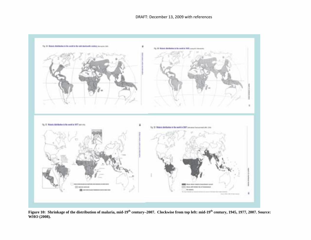
DRAFT: December 13, 2009 with references
Figure 10: Shrinkage of the distribution of malaria, mid-19th century–2007. Clockwise from top left: mid-19th century, 1945, 1977, 2007. Source: WHO (2008).
72
References:
Ahn J. and E. J. Brook (2008), Atmospheric CO2 and Climate on Millennial Time Scales During the Last Glacial Period. Science 322, 83‐85.
Araújo, M.B., R.J. Whittaker, R.J. Ladle and M. Erhard (2005): Reducing uncertainty in projections of extinction risk from climate change. Global Ecol. Biogeogr., 14, 529‐538.
Araújo, M.B. and M. New. 2007. Ensemble forecasting of species distributions. Trends in Ecology & Evolution, 22, 42‐47.
Araújo, Miguel B. and Carsten Rahbek (2006). How Does Climate Change Affect Biodiversity? Science 313: 1396–97.
Arnell NW, et al. (2002) The consequences of CO2 stabilization for the impacts of climate change. Climatic Change 53: 413‐446.
Associated Press (2009). Food summit turns down UN funding appeal. Yahoo News 16 November 2009. Available at http://news.yahoo.com/s/ap/20091116/ap_on_bi_ge/eu_un_food_summit. .
Baehr, Johanna; Helmuth Haak, Steven Alderson, et al. (2007). Timely Detection of Changes in the Meridional Overturning Circulation at 26°N in the Atlantic. Journal of Climate 20 (23): 5827–5841.
Beale, Colin M.; Jack J. Lennon; and Alessandro Gimona (2008), Opening the climate envelope reveals no macroscale associations with climate in European birds. Proceedings of the National Academy of Sciences of the United States of America, PNAS 105 (39): 14908‐14912.
Becker, Jasper (1997). Hungry Ghosts: Mao's Secret Famine. New York: Free Press.
Botkin, D.B., et al. (2007). Forecasting the Effects of Global Warming on Biodiversity. Bioscience 57 (3): 227‐236.
Boyer, T., et al. (2007). Changes in the freshwater content of the Atlantic Ocean, 1955‐2006. Geophysical Research Letters, 34, L16603, doi:10.1029/2007GL030126.
Buckley, Lauren B. and Roughgarden, Joan (2004). Biodiversity conservation: effects of changes in climate and land use. Nature 430: 1 (doi:10.1038/nature02717).
Burke, Marshall B.; Edward Miguel; Shanker Satyanath; John A. Dykema; David B. Lobel (2009). Warming increases the risk of civil war in Africa. PNAS 105: 20670–20674.
Cabioch, G., et al. (2008). Successive reef depositional events along the Marquesas foreslopes (French Polynesia) since 26 ka. Marine Geology 254: 18‐34.
CCSP (2008). Climate Models: An Assessment of Strengths and Limitations. A Report by the U.S. Climate Change Science Program and the Subcommittee on Global Change Research [Bader D.C., C. Covey, W.J. Gutowski Jr., I.M. Held, K.E. Kunkel, R.L. Miller, R.T. Tokmakian and M.H. Zhang (Authors)]. Department of Energy, Office of Biological and Environmental Research, Washington, D.C., USA, 124 pp.
Center for Strategic & Int’l Studies & Center. for a New American Security (2007). The Age of Consequences: The Foreign Policy and National Security Implications of Global Climate Change. Available at http://www.cnas.org/files/documents/publications/CSISCNAS_AgeofConsequences_November07.pdf.
Clark, Peter U.; Thomas L. Delworth, Andrew J. Weaver (2008). Freshwater Forcing: Will History Repeat Itself? Science 320: 316‐317.
Clay, C.G.A. (1984). Economic expansion and social change: England 1500‐1700, Volume 2. Cambridge University Press.
73
CNA (2007). National Security and the Threat of Climate Change. Available at http://www.securityandclimate.cna.org/.
Copenhagen Consensus (2004).
Copenhagen Consensus (2008). The Outcome of the Copenhagen Consensus. Available at http://www.copenhagenconsensus.com/Default.aspx?ID=953.
CRS (Congressional Research Service) (2009). U.S. Fossil Fuel Resources: Terminology, Reporting, and Summary. Authors: Gene Whitney, Carl E. Behrens, Carol Glover. CRS Report R40872.
Davis, Mke (2001). Late Victorian Holocausts: El Nino Famines and the Making of the Third World. London: Verso, 2001.
Delisle, G. (2007), Near‐surface permafrost degradation: How severe during the 21st century?, Geophys. Res. Lett., 34, L09503, doi:10.1029/2007GL029323.
Department of Transportation. (2008). National Transportation Statistics. Available at http://www.bts.gov/publications/national_transportation_statistics/2008/html/table_01_03.html. Visited 23 November 2009.
Dickey JO, Marcus SL, Willis JK. (2008). Ocean cooling: Constraints from changes in Earth's dynamic oblateness (J 2) and altimetry. Geophys. Res. Lett. 35, L18608, doi:10.1029/2008GL035115.
Dlugokencky, E. J., et al. (2009). Observational constraints on recent increases in the atmospheric CH4 burden. Geophysical Research Letters, 36, L18803, doi:10.1029/2009GL039780.
Donohue, Randall J.; Tim R. McVIcar; and Michael Roderick. (2009). Climate‐related trends in Australian vegetation cover as inferred from satellite observations, 1981–2006. Global Change Biology doi: 10.1111/j.1365‐2486.2008.01746.x.
Dormann, Carsten F. (2007). Promising the future? Global change projections of species distributions. Basic and Applied Ecology 8: 387—397.
Duncan, Richard P; Phillip Cassey and Tim M Blackburn (2009), Do climate envelope models transfer? A manipulative test using dung beetle introductions. Proc. R. Soc. B 276 (1661): 1449‐1457
Easterly, William (2008). Easterly on Growth, Poverty, and Aid. Library of Economics and Liberty. http://www.econtalk.org/archives/2008/02/easterly_on_gro.html. Visited 29 November 2009.
EM‐DAT. 2009. The OFDA/CRED International Disaster Database. Université Catholique de Louvain, Brussels, Belgium.Available at http://www.em‐dat.net. Data downloaded on August 24, 2009.
Eureka Alert. 2009. Ancient Greenland methane study good news for planet, says CU‐Boulder scientist. PR announcement, 23 April 2009. Available at http://www.eurekalert.org/pub_releases/2009‐04/uoca‐agm042109.php.
Fagan, Brian M. (2000). The Little Ice Age: How Climate Made History, 1300‐1850. New York: Basic Books
FAO (2009). State of Food Insecurity 2009. FAO, Rome.
FAO (Food and Agricultural Organization) (2008). State of Food Insecurity 2008. FAO, Rome.
Fingar, Thomas (2008). National Intelligence Assessment on the National Security Implications of Global Climate Change to 2030. Joint Hearing Before the House Select Comm. on Energy Independence and Global Warming and the House Permanent Select Comm. on Intelligence, available at http://globalwarming.house.gov/tools/2q08materials/files/0069.pdf.
Fischer, H., Melanie Behrens, Michael Bock, Ulrike Richter, Jochen Schmitt, Laetitia Loulergue, Jerome Chappellaz, Renato Spahni, Thomas Blunier, Markus Leuenberger & Thomas F. Stocker (2008). Changing boreal methane sources and constant biomass burning during the last termination. Nature 452: 864 ‐865.

74
Gedney, N., Cox, P.M., Betts, R.A., Boucher, O., Huntingford, C. and Stott, P.A. 2006. Detection of a direct carbon
dioxide effect in continental river runoff records. Nature 439: 835‐838.
Gilbert, Natasha (2009). Climate refugee fears questioned. Nature News. 25 June 2009, doi:10.1038/news.2009.601.
Gloor, M.: O. L. Phillips, J. J. Lloyd, et al. (2009). Does the disturbance hypothesis explain the biomass increase in basin‐wide Amazon forest plot data? Global Change Biology 15: 2418–2430.
Freeman, Jody; and Andrew Guzman (2009). Climate Change & U.S. Interests. Version 3.1, dated 09/13/2009.
Goklany, I.M. (1992). “Adaptation and Climate Change.” Paper presented at the Annual Meeting of the American Association for the Advancement of Science, Chicago, February 6‐11, 1992.
Goklany, I.M. (1998). Saving habitat and conserving biodiversity on a crowded planet. BioScience 48: 941‐953.
Goklany, I.M. (1999). “Richer is More Resilient: Dealing With Climate Change and More Urgent Environmental
Problems.” In R. Bailey, ed., Earth Report 2000, Revisiting the True State of the Planet, New York: McGraw‐Hill, pp.
155‐187.
Goklany, I.M. (2000). Potential Consequences of Increasing Atmospheric CO2 Concentration Compared to Other Environmental Problems. Technology 7S (2000): 189‐213.
Goklany, I.M. (2000b). Applying the Precautionary Principle to Global Warming (November 2000). Weidenbaum Center Working Paper No. PS 158. Available at SSRN: http://ssrn.com/abstract=250380 or doi:10.2139/ssrn.250380.
Goklany, I.M. (2001). The Precautionary Principle: A Critical Appraisal of Environmental Risk Assessment.
Washington: Cato Institute.
Goklany, I.M. (2005). “A Climate Policy for the Short and Medium Term: Stabilization or Adaptation?” Energy & Environment 16: 667‐680 (2005).
Goklany, I.M. (2007a). Integrated Strategies to Reduce Vulnerability and Advance Adaptation, Mitigation, and Sustainable Development. Mitigation and Adaption Strategies for Global Change DOI 10.1007/s11027‐007‐9098‐1 (2007).
Goklany, I.M. (2007b). Is a Richer‐but‐warmer World Better than Poorer‐but‐cooler Worlds? Energy & Environment, 18 (7 and 8): 1023‐1048.
Goklany, I.M. (2007c).
Goklany, I.M. (2009a). Global public health: Global warming in perspective. Journal of American Physicians and Surgeons 14 (3): 69‐75.
Goklany, I.M. (2009b). Have increases in population, affluence and technology worsened human and environmental well‐being? Electronic Journal of Sustainable Development, vol. 1, no.3 (2009).
Goklany, I.M. (2009c). Deaths and Death Rates from Extreme Weather Events: 1900‐2008. Journal of American Physicians and Surgeons 14 (4): 102–09.
Goklany, I.M. (2009d). Is Climate Change the "Defining Challenge of Our Age"? Energy & Environment 20(3): 279‐302.
Goklany, I.M. (2009e). Technological Substitution and Augmentation of Ecosystem Services. Draft. In: Simon A. Levin et al. (eds.), The Princeton Guide to Ecology (Princeton University Press, Princeton, 2009).
Goklany, I.M. (2009f). Discounting.
75
Grachev, Alexi M. and Jeffrey P. Severinghaus (2005). A revised +10±4 °C magnitude of the abrupt change in Greenland temperature at the Younger Dryas termination using published GISP2 gas isotope data and air thermal diffusion constants. Quaternary Science Reviews 24 ( 5‐6): 513‐519.
Green, K.C., and Armstrong, J.S. (2007). Global Warming: Forecasts by Scientists Versus Scientific Forecasts. Energy
and Environment 18: 997‐1021.
Gregory, J.M. et al. (2005). “A model intercomparison of changes in the Atlantic thermohaline circulation in
response to increasing atmospheric CO2 concentration,” Geophysical Research Letters 32: L12703,
doi:10.1029/2005GL023209.
Guisan, A., and W. Thuiller (2005). Predicting species distributions: offering more than simple habitat models.
Ecology Letters 8:993–1009.
Hale, R. C., K. P. Gallo, T. W. Owen, and T. R. Loveland. 2006. Land use/land cover change effects on temperature
trends at U.S. Climate Normals stations. Geophys. Res. Lett. 33: L11703, doi:10.1029/2.
Hampe, A. and Petit, R.J. 2005. Conserving biodiversity under climate change: the rear edge matters. Ecology
Letters 8: 461‐467.
Hoekstra, A. Y. (2003). Virtual Water: An Introduction. In: A.Y. Hoekstra, Virtual Water Trade Proceedings of the International Expert Meeting on Virtual Water Trade, February 2003 pp. 13–23. IHE Delft, Delft, The Netherlands.
Idso, S.B. and Brazel, A.J. (1984). Rising atmospheric carbon dioxide concentrations may increase streamflow.
Nature 312: 51‐53.
IPCC (2007). Climate change 2007. Impacts, adaptation, and vulnerability, Contribution of working group II to the fourth assessment report of the Intergovernmental Panel on Climate Change. In: Parry ML, Canziani OF, Palutikof JP, van der Linden PJ, eds . Cambridge University Press.
IPCC (2007). Climate Change 2007: The Physical Science Basis. Cambridge: Cambridge University Press, 2007: 12.
IPCC (Intergovernmental Panel on Climate Change) (2001). Climate change 2001. Impacts, adaptation, and vulnerability, Contribution of working group II to the fourth assessment report of the Intergovernmental Panel on Climate Change. Cambridge University Press.
Keenleyside (2008)
Kerr, R.A. (2005). “Confronting the Bogeyman of The Climate System,” Science 310 (2005); 432‐433;
Kerr, Richard A. (2009). Global warming: What Happened to Global Warming? Scientists Say Just Wait a Bit, Science 2 October 2009: Vol. 326. no. 5949: 28 – 29, DOI: 10.1126/science.326_28a.
Klotzbach: J., et al. (2009b). Corrigendum To Klotzbach Et Al 2009 – Our Conclusions Are Unchanged. Climate Science Blog..Available at http://pielkeclimatesci.wordpress.com/2009/12/03/corrigendum‐to‐klotzbach‐et‐al‐2009/
Klotzbach: J., R. A. Pielke, Sr., R. A. Pielke, Jr., J. R. Christy, and R. T. McNider (2009a), An alternative explanation for differential temperature trends at the surface and in the lower troposphere, J. Geophys. Res., 114, D21102, doi:10.1029/2009JD011841.
Knudsen, M.F. and Riisager (2009). Is there a link between earth's magnetic field and low‐latitude precipitation? Geology 37: 71‐74.
Lamb, Hubert
Lamb, Hubert H. (1982). Climate, History and the Modern World. London: Taylor & Francis.
76
Lancet and University College London Institute for Global Health Commission (The Lancet Commission). Managing the health effects of climate change. Lancet 2009;373:1693‐1733.
Lapola, D. M., M. D. Oyama, and C. A. Nobre (2009). Exploring the range of climate biome projections for tropical South America: The role of CO2 fertilization and seasonality, Global Biogeochem. Cycles, 23, GB3003, doi:10.1029/2008GB003357.
Latif, M.; C. Böning, J. Willebrand, A. Biastoch, J. Dengg, N. Keenlyside, U. Schweckendiek, G. Madec. (2006). Is the Thermohaline Circulation Changing? Journal of Climate 19 (18): 4631‐4637.
Lawrence, D. M., and A. G. Slater (2005). A projection of severe nearsurface permafrost degradation during the 21st century, Geophys. Res. Lett., 32, L24401, doi:10.1029/2005GL025080.
Levitus S, Antonov JI, Boyer TP, Locarnini RA, Garcia HE, Mishonov AV. (2008). Global ocean heat content 1955–2008 in light of recently revealed instrumentation problems. Geophysical Research Letters 36, L07608, doi:10.1029/2008GL037155, figure S11.
Levy, Marc A. et al. (2008). Assessment of Select Climate Change Impacts on U.S. National Security (Ctr. for Int’l Earth Sci. Info. Network, Working Paper 2008), available at http://www.ciesin.columbia.edu/documents/Climate_Security_CIESIN_July_2008_v1_0.ed070208.pdf.
Lindzen, Richard S.; Y‐S Choi (2009). On the determination of climate feedbacks from ERBE data. Geophysical Research Letters VOL. 36, L16705, doi:10.1029/2009GL039628.
Living Proof Project (2009). Progress Against Malaria. Available at http://www.gatesfoundation.org/livingproofproject/Documents/progress‐against‐malaria.pdf.
Living Proof Project (2009). Progress Against Malaria: Winning the Fight Against a Deadly Disease. Available at www.livingproofproject.com
Lloyd, J. and Farquhar, G.D. (2008). Effects of rising temperatures and [CO2] on the physiology of tropical forest trees. Philosophical Transactions of the Royal Society Series B 363: 1811‐1817.
Loehle, C. 2004. Climate change: detection and attribution of trends from long‐term geologic data. Ecological Modelling 171: 433‐450. Loehle, Craig. 2009. Cooling of the global ocean since 2003. Energy & Environment 20(1&2): 99‐102. Lomborg, Bjorn, ed. (2004). Global crises, global solutions. Cambridge: Cambridge University Press. Lorenzini, I., and Adger, W.N. (2006). “Critique of Treatments of Adaptation Costs in PAGE and FUND Models,” In: Warren, R. et al. (2006a). Spotlighting Impacts Functions in Integrated Assessment Models, Norwich, Tyndall Centre for Climate Change Research Working Paper 91: 72‐79.
Lowe, J.A. et al. (2006). The Role of Sea‐Level Rise and the Greenland Ice Sheet in Dangerous Climate Change: Implications for the Stabilisation of Climate. In Avoiding Dangerous Climate Change, H.J. Schellnhuber et al. (eds), Cambridge University Press, Cambridge: 29‐36.
Luoto, M. and R. K. Heikkinen (2008). Disregarding topographical heterogeneity biases species turnover assessments based on bioclimatic models. Global Change Biology 14 (3): 483 – 494. doi: 10.1111/j.1365‐2486.2007.01527.x
Maddison, Angus (2008). Statistics on World Population, GDP and Per Capita GDP, 1‐2006 AD. Available at http://www.ggdc.net/maddison/Historical_Statistics/horizontal‐file_03‐2009.xls.
Malcolm JR, Liu G, Neilson RP, Hansen L, Hannah L. 2006. Global warming and extinctions of endemic species from
biodiversity hotspots. Conservation Biology 20: 538‐548
77
Mallery, C. Undated. Elemental Composition of the Human Body. Available at http://www.bio.miami.edu/~cmallery/150/life/elements.htm.
Martinez‐Meyer, E., A.T. Peterson and W.W. Hargrove, 2004: Ecological niches as stable distributional constraints on mammal species, with implications for Pleistocene extinctions and climate change projections for biodiversity. Global Ecol. Biogeogr., 13, 305‐314.
Maue, Ryan. 2009. 24‐Month Running Sums of Global Tropical Cyclone Accumulated Cyclone Energy (ACE). Available at http://www.coaps.fsu.edu/~maue/tropical/. Visited 04 December 2009.
McCrummen, Stephanie. 2009. The ultimate crop rotation. Washington Post. 23 November 2009: A01.
McKitrick, R.R. and P.J. Michaels (2007), Quantifying the influence of anthropogenic surface processes and inhomogeneities on gridded global climate data, J. Geophys. Res., 112, D24S09, doi:10.1029/2007JD008465.
McKitrick, R.R. and P.J. Michaels. (2007). Quantifying the influence of anthropogenic surface processes and
inhomogeneities on gridded global climate data. J. Geophys. Res. 112: D24S09, doi:10.1029/2007JD008465.
McKitrick, Ross R.;and Patrick J. Michaels (2008). Background Discussion On: Quantifying the influence of anthropogenic surface processes and inhomogeneities on gridded global climate data. Available at http://www.uoguelph.ca/~rmckitri/research/jgr07/M&M.JGR07‐background.pdf. Visited 3 November 2009.
McMichael, AJ, et al. (2004). Global Climate Change. In Comparative Quantification of Health Risks: Global and Regional Burden of Disease due to Selected Major Risk Factors. Geneva: World Health Organization, 2004: 1543–1649.
Meteorological Office Hadley Centre for Climate Change (2009). Met Office Hadley Centre observations datasets 2009. http://www.cru.uea.ac.uk/cru/data/temperature/hadcrut3gl.txt (accessed May 16, 2009). The trend line for the temperature anomaly (based period 1961‐90) from January 2000 through March 2009 is essentially flat, with an R2 of 0.0003.
Millennium Ecosystem Assessment [MEA] (2005). Millennium Ecosystem Assessment Synthesis Report. Pre‐publication Final Draft, approved by MA Board on March 23, 2005. On file with author.
Mitikka, Varpu; Risto K. Heikkinen, Miska Luoto, Miguel B. Araújo, Kimmo Saarinen, Juha Po¨yry, Stefan Fronzek, (2008). Predicting range expansion of the map butterfly in Northern Europe using bioclimatic models. Biodiversity and Conservation 17: 623‐41.
Myneni, Ranga (2006). Long Term Monitoring of Vegetation Greenness from Satellites. Slide show dated 07/13/2006. Available at http://www.ias.sdsmt.edu/STAFF/INDOFLUX/Presentations/14.07.06/session1/myneni‐talk.pdf. Visited 11 November 2009.
NASA (2006). http://www.giss.nasa.gov/research/news/20060130/
Nordås, Ragnhild, and Nils Petter Gleditsch (2007). Climate Change and Conflict. Political Geography 26(6): 627‐736.
Nordhaus, W. (2008). A Question of Balance: Weighing the Options on Global Warming Policies. New haven, Yale
University Press.
Oesthook, K.J.W. The Role of Wood in World History. Environmental History Resources. Available at http://www.eh‐resources.org/wood.html.
Oki T, Kanae S. (2006). Global hydrological cycles and world water resources. Science 313:1068‐1072.
Ostrom, Elinor (1990). GOVERNING THE COMMONS The Evolution of Institutions for Collective Action. Cambridge University Press.
Owen, James. (2009). Sahara Desert Greening Due to Climate Change? National Geographic News 31 July 2009. Available at http://news.nationalgeographic.com/news/2009/07/090731‐green‐sahara.html.
78
Parry et al. 1999
Parry M, Rosenzweig C, Iglesias A, Fischer G, Livermore M. Climate change and world food security: a new assessment. Global Environmental Change‐Human and Policy Dimensions. Global Envir Change 1999; 9: S51‐S67.
Parry ML, ed. (2004). Special Issue: An Assessment of the Global Effects of Climate Change under SRES Emissions and Socio‐economic Scenarios. Global Environ Change 14: 1‐99.
Parry ML, Rosenzweig C, Iglesias I, Livermore M, and Fischer G. (2004). Effects of climate change on global food production under SRES emissions and socio‐economic scenarios. Global Environ Change 14 (1): 53–67.
Patz JA, Campbell‐Lendrum D, Holloway T, Foley JA. (2005). Impact of regional climate change on human health. Nature 438:310‐317.
Pavement4Life (2008). http://www.pavements4life.com/QDs/Environment_1HeatIsland.asp.
Pearson R.G., and Dawson T.P. (2003) Predicting the impacts of climate change on the distribution of species: are
bioclimatic envelope models useful? Global Ecology and Biogeography, 12, 361–
Perch‐Nielsen, Sabine L.,Michèle B. Bättig, Dieter Imboden (2008). Exploring the link between climate change and migration. Climatic Change 91:375–393.
Petrenko, Vasilii V.; Andrew M. Smith, Edward J. Brook, Dave Lowe, Katja Riedel, Gordon Brailsford, Quan Hua, Hinrich Schaefer, Niels Reeh, Ray F. Weiss, David Etheridge, and Jeffrey P. Severinghaus. 14CH4 Measurements in Greenland Ice: Investigating Last Glacial Termination CH4 Sources. Science 324: 506‐508
Phillips, Oliver L; Simon L Lewis, Timothy R Baker, Kuo‐Jung Chao and Niro Higuchi (2008). The changing Amazon forest. Philosophical Transactions of the Royal Society Series B 2008 363, 1819‐1827.
Pielke Sr., R.A. J. Nielsen‐Gammon, C. Davey, J. Angel, O. Bliss, N. Doesken, M. Cai., S. Fall, D. Niyogi, K. Gallo, R.
Hale, K.G. Hubbard, X. Lin, H. Li, and S. Raman. 2007a. Documentation of uncertainties and biases associated with
surface temperature measurement sites for climate change assessment. Bull. Amer. Meteor. Soc. 88 (6): 913‐928.
Pielke, Jr., R. A., Gratz, J., Landsea, C. W., Collins, D., Saunders, M., and Musulin, R. (2008a). Normalized Hurricane Damages in the United States: 1900‐2005. Natural Hazards Review, Volume 9, Issue 1: 29‐42.
Pielke, Jr., R.A., Bouwer, L., Crompton, R., Faust, E., and Höppe (2008b). Catastrophe Losses in the Context of Demographics, Climate, and Policy. Managing the Changing Landscape of Catastrophe Risk. 10th Aon Re Australia Biennal Hazards Conference, September 16‐18 2007. Queensland Australia.
Pielke, R. A., Sr., et al. 2007b. Unresolved issues with the assessment of multidecadal global land surface
temperature trends. J. Geophys. Res. 112: D24S08, doi:10.1029/2006JD008229.
Pouliot, D A; Latifovic, R; Olthof. 2009. Long term changes in vegetation from 1KM AVHRR NDVI data over Canada for the period 1985‐2006. International Journal of Remote Sensing 30 (1): 149‐168.
Prugh LR, Hodges KE, Sinclair RE, Brashares JS (2008). Effect of habitat area and isolation on fragmented animal populations. Proc Natl Acad Sci USA 105:20770–20775.
Public Broadcasting Service. California and the American Dream, Building Healthy Communities (2006). http://www.pbs.org/california/programfeature.html (accessed 3 July 2009).
Randin, Christophe F.; Robin Engler, Signe Normand et al. (2008). Climate change and plant distribution: local models predict high‐elevation persistence. Global Change Biology (2009) 15, 1557–1569, doi: 10.1111/j.1365‐2486.2008.01766.x
Remote Sensing Systems (2009). Description of MSU and AMSU Data Products. RSS version 3.2, TLT. http://www.ssmi.com/msu/msu_data_description.html (accessed May 16, 2009). The trend for the temperature

79
anomaly (based period 1979‐98) for the lower troposphere is essentially flat from January 2000 through April 2009, with an R2 of 0.0006.
Rogers, P. Assessing the Socioeconomic Consequences of Climate Change on Water Resources. Climatic Change 28:
179‐208.
Saurer, Matthias; Rolf T. W. Siegwolf and F.H. Schweingruber. (2004). Carbon Isotope Discrimination Indicates
Improving Water‐use Efficiency of Trees in Northern Eurasia over the Last 100 Years. Global Change Biology 10,
2109–2120, Doi: 10.1111/j.1365‐2486.2004.00869.x
Schmittner, A., M. Latif and B. Schneider (2005). “Model projections of the North Atlantic thermohaline circulation
for the 21st century assessed by observations,” Geophysical Research Letters 32: L23710, 10.1029/2005GL 024368.
Schwartz, M.W., Iverson, L.R., Prasad, A.M., Matthews, S.N. and O’Connor, R.J. (2006). Predicting extinctions as a
result of climate change. Ecology 87: 1611–1615.
Seager, R. et al. (2002). “Is the Gulf Stream responsible for Europe's mild winters?: Quarterly Journal of the Royal
Meteorological Society,” 128: 2563‐2586.
Seoane, Javier and Luis M. Carrascal (2008). Interspecific differences in population trends of Spanish birds are
related to habitat and climatic preferences. Global Ecology and Biogeography 17: 111–121.
Siddiqi, Akhtar H. and John E. Oliver (2005). Climate Determinism. In: John E. Oliver (ed.), Encyclopedia of World Climatology, Dordrecht, The Netherlands: Springer: 333–336.
Stern Review (2006). The Economics of Climate Change.
Swanson and Tsonis (2009).
Tamis, Wil L. M.; Maarten Van’t Zelfde, Ruud Van Der Meijden, Helias A. Udo De Haes. 2005. Changes in Vascular
Plant Biodiversity in the Netherlands in the 20th Century Explained by Their Climatic and Other Environmental
Characteristics. Climatic Change 72: 37–56.
Thuillier, W. (2004). Patterns and uncertainties of species’ range shifts under climate change. Global Change
Biology 10: 2020–2027, doi: 10.1111/j.1365‐2486.2004.00859.x
Tol, Richard S.J. (2005). Adaptation and mitigation: trade‐offs in substance and methods. Environmental Science &
Policy 8: 572–578.
Tol, R.S.J., K.L. Ebi and G.W. Yohe (2007), 'Infectious Disease, Development, and Climate Change: A Scenario Analysis', Environment and Development Economics, 12, 687‐706.
Tol, R.S.J.; Sebastian Wagner (2009). Climate change and violent conflict in Europe over the last millennium. Climatic Change DOI 10.1007/s10584‐009‐9659‐2.
Tol, Richard S. J. (2008). The Social Cost of Carbon: Trends, Outliers and Catastrophes. Economics: The Open‐Access, Open‐Assessment E‐Journal, Vol. 2, 2008‐25. http://www.economics‐ejournal.org/economics/journalarticles/2008‐25
Trenberth, Kevin (2007). Predictions of climate. Nature, Climate Feedback, June 4, 2007. Available at http://blogs.nature.com/climatefeedback/2007/06/predictions_of_climate.html.
Tsonis et al. (2007), who suggest “an alternative hypothesis, namely that the climate shifted after the 1970s event to a different state of a warmer climate, which may be superimposed on an anthropogenic warming trend.”
Tsonis, A. A., K. Swanson, and S. Kravtsov (2007). A new dynamical mechanism for major climate shifts, Geophysical Research Letters, 34, L13705, doi:10.1029/2007GL030288.
80
UN Global Compact and Pacific Institute (2009). Climate Change and the Global Water Crisis: What Businesses Need to Know and Do. Available at http://www.unglobalcompact.org/docs/issues_doc/Environment/ceo_water_mandate/UNGC‐PI_climate‐water_whitepaper_FINAL.pdf
UNEP [United Nations Environment Programme] (1993). Climate change and North‐South relations. Climate change fact sheet 109. UNEP, May 1, 1993. Available at http://unfccc.int/resource/ccsites/senegal/fact/fs109.htm. Visited May 12, 2003.
United Nations (2008). Millennium Development Goals Report 2008. United Nations, New York.
United Nations. 2008b. Africa Report: Desertification, Drought and Climate Change. Available at http://www.un.org/esa/sustdev/publications/trends_africa2008/desertification.pdf.
University of Colorado (2009). Sea level rise. http://sealevel.colorado.edu/ (accessed May 16 2009).
Urdal, Henrik (2006). A Clash of Generations? Youth Bulges and Political Violence. International Studies Quarterly (2006) 50, 607–629.
Watts, A. (2007). A hands‐on study of station siting issues for United States Historical Climatology Network
Stations. Workshop on Detecting the Atmospheric Response to the Changing Face of the Earth: A Focus on Human‐
Caused Regional Climate Forcings, Land‐Cover/Land‐Use Change, and Data Monitoring, 27‐29 August 2007
Boulder, CO, available at http://surfacestations.org/.
Watts, Anthony (2008a). Homepage, surfacestations.org, visited May 29, 2008.
Watts, Anthony (2009a). Is the U.S. Surface Temperature Record Reliable? Chicago, IL: The Heartland Institute,
2009. Available at http://www.surfacestations.org/.
Watts, Anthony (2009b). Personal communication.
Weaver, A. J. and C. Hillaire‐Marcel (2004). “Ice growth in the greenhouse: A seductive paradox but unrealistic
scenario,” Geoscience Canada 31: 77‐85;
Weaver, A.J., et al. (2003). Meltwater Pulse 1A from Antarctica as a Trigger of the Bølling‐Allerød Warm Interval. Science 14 March 2003 299: 1709‐1713 [DOI: 10.1126/science.1081002].
Weitzman, Martin L. (2008). On Modeling and Interpreting the Economics of. Catastrophic Climate Change. Page 2. Available at http://www.economics.harvard.edu/faculty/weitzman/files/modeling.pdf.
Williams, C.N., Jr., M.J. Menne, R.S. Vose, and D.R. Easterling. (2006). United States Historical Climatology Network
Daily Temperature, Precipitation, and Snow Data. ORNL/CDIAC‐118, NDP‐070. Available on‐line
[http://cdiac.ornl.gov/epubs/ndp/ushcn/usa.html] from the Carbon Dioxide Information Analysis Center, Oak
Ridge National Laboratory, U.S. Department of Energy, Oak Ridge, Tennessee.
Willerslev, Eske; Cappellini, Enrico; Boomsma, Wouter; et al. (2007). Ancient Biomolecules from Deep Ice Cores
Reveal a Forested Southern Greenland. Science 317: 111‐117.
World Bank (2009a). PovcalNet. http://iresearch.worldbank.org/PovcalNet/povDuplic.html. Visited 29 November 2009.
World Bank (2009b). Commodities at the Crossroads: Key Findings from the Global Economic Prospects 2009. http://siteresources.worldbank.org/INTGEP2009/Resources/GEP‐2009‐Booklet.pdf.
World Bank (2009c). Migration and Development Brief 11: A better‐than‐expected outcome for migration and remittance flows in 2009, but significant risks ahead. November 3, 2009. Available at http://siteresources.worldbank.org/INTPROSPECTS/Resources/334934‐1110315015165/MigrationAndDevelopmentBrief11.pdf.

81
World Bank. (2009d). World Development Indicators. Available at http://ddp‐ext.worldbank.org/ext/DDPQQ/member.do?method=getMembers&userid=1&queryId=6, downloaded 4 September 2009.
World Health Organization (2008). Global malaria control and elimination : report of a technical review. Geneva: WHO: 21‐24.
Worthy, D. E. J., E. Chan, M. Ishizawa, D. Chan, C. Poss, E. J. Dlugokencky, S. Maksyutov, and I. Levin (2009). Decreasing anthropogenic methane emissions in Europe and Siberia inferred from continuous carbon dioxide and methane observations at Alert, Canada, J. Geophys. Res., 114, D10301, doi:10.1029/2008JD011239.
Wunsch, Carl (2004). “Gulf Stream safe if wind blows and Earth turns,” Nature 428 (2004): 601.
WRI (World Resources Institute). (2009). EarthTrends. Available at http://earthtrends.wri.org/index.php.
Yohe, Gary, Elizabeth Malone, Antoinette Brenkert, Michael Schlesinger, Henk Meijd , Xiaoshi Xinge, Daniel Lee. (2006). A Synthetic Assessment of the Global Distribution of Vulnerability to Climate Change from the IPCC Perspective that Reflects Exposure and Adaptive Capacity. CIESIN, Columbia University. http://sedac.ciesin.columbia.edu/mva/ccv/.
Zhang, David D.; Peter Brecke; Harry F. Lee; Yuan‐Qing He; and Jane Zhang (2007). Global climate change, war, and population decline in recent human history. Proceedings of trhe National Academies of Sciences 104: 19214–19219.
Zhen‐Shan, L. and Xian, S. (2007). Multi‐scale analysis of global temperature changes and trend of a drop in temperature in the next 20 years. Meteorology and Atmospheric Physics 95: 115‐121.
Zimov, S. A., E. A. G. Schuur, and F. S. Chapin III (2006). Permafrost and the global carbon budget, Science, 313, 1612–1613.