Transport Properties of Chiral Carbon Nanotubes - R. Saito ...

Transport Properties of Chiral Carbon Nanotubes

Edward MiddletonStudent Number: (9995005)Supervisor: Dr Riichiro Saito

Laboratory: Kimura-Saito LaboratoryJUSST student from April 1999 to March 2000

Micro-electronic Engineering Division

Department of Electronic EngineeringThe University of Electro-Communications

February 8, 2000

Acknowledgments

I would like to acknowledge the assistance of Dr Riichiro Saito for his kind

words and enthusiasm in the project. I would further like to acknowledge the

�nancial support of the Ministry of Education through the JUSST program

in making this work possible. furthermore I would like to thank both The

University of Electro-communications and Gri�th University for their support

of the exchange program.

1

Abstract

We are exploring a group of very small structures that have extremely interesting

properties. These structures are so small that they don't adhere to the laws of

classical physics. These structures can only barely be seen with the aid of

powerful microscope such as Scanning Tunneling Microscopes STM and Atomic

Force Microscopes AFM. But many people believe they are the key to shrinking

current electronics into the quantum domain. These structures are Single Wall

Carbon Nanotubes SWCN.

Carbon nanotubes have a structure that resembles a graphene sheet roled

into a tube. The structure of SWCN's has a mirror symmetry for two-types of

nanotubes, armchair and zigzag nanotubes, and the remaining nanotubes have

a chiral symmetry.

We have investigated the transport properties of chiral SWCN. Our work

involves determining the electrical transport properties of chiral SWCN. To

do this we have developed a Green's function method based on Landauer's

formalism to calculate the conductance of arbitrary SWCN's. We have created

a program that implements this method and have used it to test a range of

structures. We have obtained good results for a number of important cases

and good partial results (number of channels) for almost all SWCN we have

tested. We have been able to verify the partial results against both the energy

dispersion relation EDR calculations and the structurally imposed upper limit.

Further work is necessary to completely resolve some outstanding problems.

Contents

1 Introduction 1

1.1 Purpose . . . . . . . . . . . . . . . . . . . . . . . . . . . . . . . . 1

1.2 Transport . . . . . . . . . . . . . . . . . . . . . . . . . . . . . . . 1

1.2.1 Interactions (Scattering) . . . . . . . . . . . . . . . . . . . 1

1.3 Classic Transport LmL' � L;W . . . . . . . . . . . . . . . . . . 3

1.4 Ballistic Transport L;W � LmL' . . . . . . . . . . . . . . . . . 4

1.5 Carbon Nanotubes . . . . . . . . . . . . . . . . . . . . . . . . . . 4

1.5.1 Discovery . . . . . . . . . . . . . . . . . . . . . . . . . . . 4

1.5.2 Lattice Structure . . . . . . . . . . . . . . . . . . . . . . . 5

1.5.3 Band structure . . . . . . . . . . . . . . . . . . . . . . . . 5

1.5.4 Graphite band structure . . . . . . . . . . . . . . . . . . . 5

1.5.5 Nanotube band structure . . . . . . . . . . . . . . . . . . 7

2 Method 11

2.1 Overview . . . . . . . . . . . . . . . . . . . . . . . . . . . . . . . 11

2.1.1 Tight-binding model . . . . . . . . . . . . . . . . . . . . . 12

2.1.2 Energy Dispersion Relation . . . . . . . . . . . . . . . . . 13

2.1.3 Direct calculation of Wave-function . . . . . . . . . . . . . 13

2.2 Basic Green's function method . . . . . . . . . . . . . . . . . . . 14

2.2.1 Wave-function at the boundary's . . . . . . . . . . . . . . 14

2.2.2 Calculating F . . . . . . . . . . . . . . . . . . . . . . . . . 17

2.3 Reduced Green's Function Method . . . . . . . . . . . . . . . . . 19

3 Results 27

3.1 Upper Limit . . . . . . . . . . . . . . . . . . . . . . . . . . . . . . 27

3.2 Energy Dispersion Relation . . . . . . . . . . . . . . . . . . . . . 27

3.3 Direct calculation of Wave-function . . . . . . . . . . . . . . . . . 29

3.4 Basic Green's function method . . . . . . . . . . . . . . . . . . . 29

3.5 Reduced Green's function method . . . . . . . . . . . . . . . . . 29

3.6 Breaking up the unit cell . . . . . . . . . . . . . . . . . . . . . . . 32

3.6.1 Cell Formulation . . . . . . . . . . . . . . . . . . . . . . . 32

3.7 Reduced Matrix Calculation . . . . . . . . . . . . . . . . . . . . . 35

3.8 Eigensolution Calculation . . . . . . . . . . . . . . . . . . . . . . 35

3.9 Tubes Tested . . . . . . . . . . . . . . . . . . . . . . . . . . . . . 35

1

3.9.1 Problems . . . . . . . . . . . . . . . . . . . . . . . . . . . 35

4 Discussion 36

4.1 Channels with Energy Dispersion Relation . . . . . . . . . . . . . 36

4.2 Conductance and Channels . . . . . . . . . . . . . . . . . . . . . 36

5 Conclusions 37

5.1 Energy Dispersion Relation . . . . . . . . . . . . . . . . . . . . . 37

5.2 Channels . . . . . . . . . . . . . . . . . . . . . . . . . . . . . . . 37

5.3 Conductance . . . . . . . . . . . . . . . . . . . . . . . . . . . . . 37

A Fortran 38

A.1 Direct Wave-function Calculation . . . . . . . . . . . . . . . . . . 38

A.1.1 Make�le . . . . . . . . . . . . . . . . . . . . . . . . . . . . 38

A.1.2 Fortran 77 source . . . . . . . . . . . . . . . . . . . . . . . 38

A.2 Basic Greens Function Method . . . . . . . . . . . . . . . . . . . 42

A.2.1 Make�le . . . . . . . . . . . . . . . . . . . . . . . . . . . . 42

A.2.2 Fortran 90 source . . . . . . . . . . . . . . . . . . . . . . . 42

A.3 Reduced Greens Function Method . . . . . . . . . . . . . . . . . 57

A.3.1 Main Make�le . . . . . . . . . . . . . . . . . . . . . . . . 57

A.3.2 Main Program Fortran 90 source . . . . . . . . . . . . . . 58

A.3.3 Library Make�le . . . . . . . . . . . . . . . . . . . . . . . 73

A.3.4 zedr1d Fortran 90 source . . . . . . . . . . . . . . . . . . 74

A.3.5 zrhmn Fortran 90 source . . . . . . . . . . . . . . . . . . . 76

A.3.6 zcalcf Fortran 90 source . . . . . . . . . . . . . . . . . . . 84

A.3.7 sortwaves Fortran 90 source . . . . . . . . . . . . . . . . . 96

A.3.8 shpsrt Fortran 90 source . . . . . . . . . . . . . . . . . . . 106

A.3.9 zgcalc Fortran 90 source . . . . . . . . . . . . . . . . . . . 108

A.3.10 Module Make�le . . . . . . . . . . . . . . . . . . . . . . . 113

A.3.11 Machine Dependent Fortran 90 source . . . . . . . . . . . 113

A.3.12 Problem Parameters Fortran 90 source . . . . . . . . . . . 114

A.3.13 CarbonNanotube Fortran 90 source . . . . . . . . . . . . 115

B Maple 129

B.1 Basic Green's function method . . . . . . . . . . . . . . . . . . . 129

B.2 Reduced Green's function method . . . . . . . . . . . . . . . . . 130

B.2.1 Chain Conductance with scattering . . . . . . . . . . . . . 130

B.2.2 Comparison of Methods . . . . . . . . . . . . . . . . . . . 132

B.2.3 Conductance of ladder . . . . . . . . . . . . . . . . . . . . 132

2

List of Figures

1.1 Transport Regimes . . . . . . . . . . . . . . . . . . . . . . . . . . 2

1.2 Momentum loss through atomic scattering . . . . . . . . . . . . . 3

1.3 Experiment showing ballistic conductance . . . . . . . . . . . . . 4

1.4 Carbon nanotube unit cell . . . . . . . . . . . . . . . . . . . . . . 6

1.5 Energy Dispersion Relation showing cut-o� energy "N . . . . . . 7

1.6 band structure of 2D graphite . . . . . . . . . . . . . . . . . . . . 8

1.7 Breakup of SWCN into Metallic and semi-conducting . . . . . . . 8

1.8 The relationship between band gap and diameter . . . . . . . . . 9

1.9 STS Conductance measurements showing band gap . . . . . . . . 10

2.1 Input boundary . . . . . . . . . . . . . . . . . . . . . . . . . . . . 15

2.2 possible waves in a structure . . . . . . . . . . . . . . . . . . . . 18

2.3 The unit cell Hamiltonian and hopping matrix for a (4; 2) SWCN 19

3.1 The two types of bonds connecting unit cells are shown. a. shows

a bonds crossing the boundary and b. shows b bonds crossing

the boundary. . . . . . . . . . . . . . . . . . . . . . . . . . . . . . 28

3.2 Energy dispersion relation n;m � 7 . . . . . . . . . . . . . . . . . 28

3.3 E�ect of impurity on chain using direct wave-function calculation 29

3.4 band structure and conductance of a 10 by 10 atom strip calcu-

lated using Green's function method . . . . . . . . . . . . . . . . 30

3.5 Analytically determined chain conductance with single scatterer . 31

3.6 Algebraicly determined conductance for a chain of 10 atoms using

Andos method (plain line) and our adaptation of Green's function

method (dotted line) . . . . . . . . . . . . . . . . . . . . . . . . . 32

3.7 Conductance for ladder determined algebraicly using adaptation

of Green's function method . . . . . . . . . . . . . . . . . . . . . 33

3.8 Conductance for tubes of n;m � 7 . . . . . . . . . . . . . . . . . 34

3

List of Tables

3.1 Relationship between Ch = (n;m) and channels upper limit. . . . 27

4

Chapter 1

Introduction

1.1 Purpose

Single wall carbon nanotubes (SWCN) are molecular structures that have in-

teresting electrical properties that suggest great potential in the development

of quantum devices. To develop electrical devices using SWCN we need to

have a precise understanding of their electrical transport properties and more

speci�cally we need to know how well they conduct electrons, and what factors

e�ect this conductance. Experimentally conductance has been measured using

scanning tunneling spectroscopy [1][2]. Electron transport has been measured

directly by placing a tube on platinum electrodes [3]. Attempts have been made

[4][5] to address both of these questions but only for simple systems (armchair

and zigzag SWCN). The intention of this work is to create a method for numer-

ically calculating the conductance of all SWCN's.

1.2 Transport

We use the word transport when describing the transfer of electrons through

mesoscopic systems to di�erentiate such transfer from the concepts of macro-

scopic (or classical) transport.

In all forms of electron transport the same interactions between electron

atoms (protons) and electric and magnetic �elds are involved however their

importance to transport is di�erent. Thus to look at transport we need to

quantify these interactions to determine the nature of the transport.

1.2.1 Interactions (Scattering)

We can quantify the e�ect of electron atom interactions in terms of two quan-

tities, the e�ect of an interaction i on changing the original momentum �mi

and the e�ect of an interaction i on changing the original phase �'i . We can

look at the electron atom interactions in terms of lengths by saying, what is the

1

Ballistic Transport

Atom Elastic Scattering Inelastic Scattering

Classic Transport

Diffusive Transport

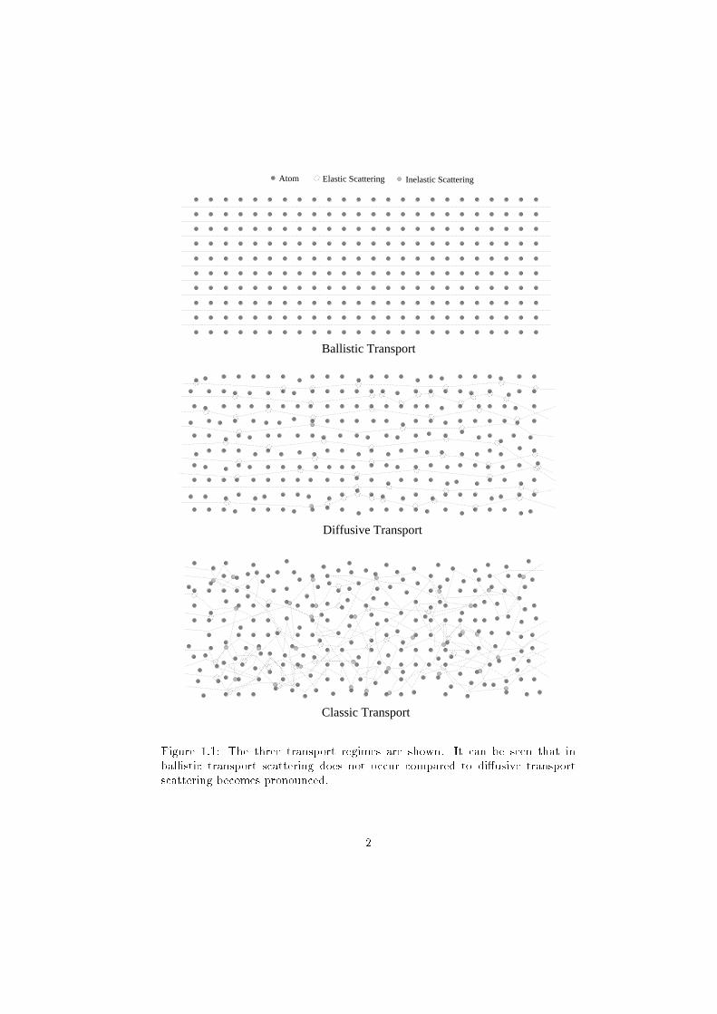
Figure 1.1: The three transport regimes are shown. It can be seen that in

ballistic transport scattering does not occur compared to di�usive transport

scattering becomes pronounced.

2

P1

P1

P2

P2

21

Atom

3

1 2 3 4 5 6 7 8 9 10

Electron

τ τ τ

0 0 0

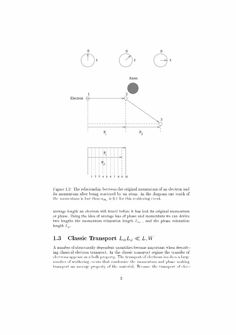
Figure 1.2: The relationship between the original momentum of an electron and

its momentum after being scattered by an atom. In the diagram one tenth of

the momentum is lost thus �miis 0:1 for this scattering event.

average length an electron will travel before it has lost its original momentum

or phase. Using the idea of average loss of phase and momentum we can derive

two lengths the momentum relaxation length Lm , and the phase relaxation

length L'.

1.3 Classic Transport LmL' � L;W

A number of structurally dependent quantities become important when describ-

ing classical electron transport. In the classic transport regime the transfer of

electrons appears as a bulk property. The transport of electrons involves a large

number of scattering events that randomize the momentum and phase making

transport an average property of the material. Because the transport of elec-

3

µ m1

20 nm

0 V 6 V

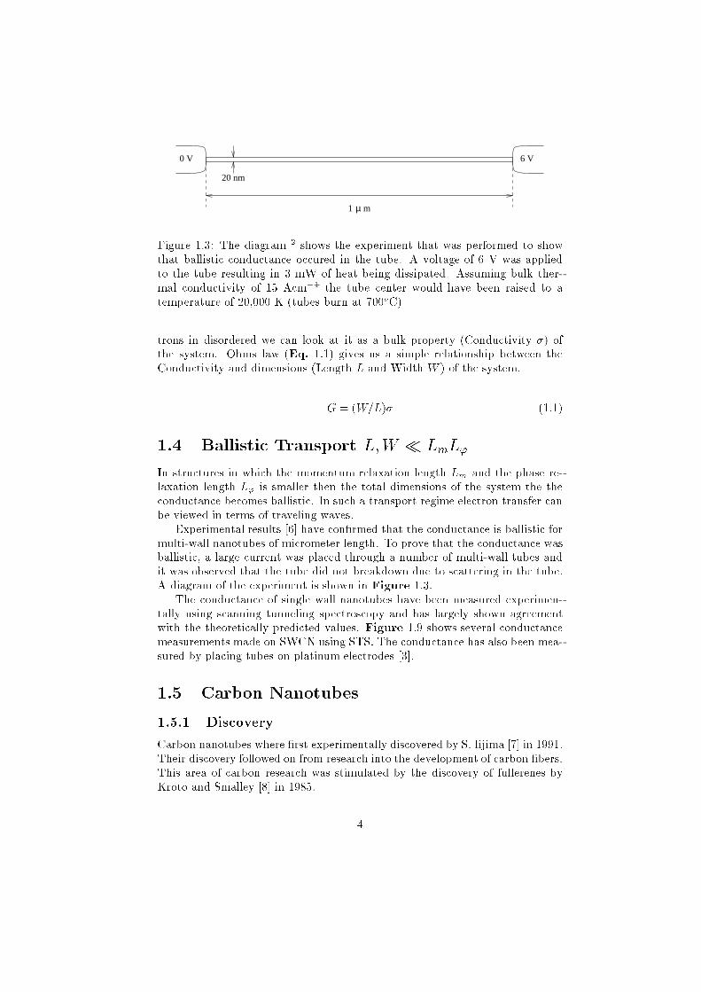
Figure 1.3: The diagram 2 shows the experiment that was performed to show

that ballistic conductance occured in the tube. A voltage of 6 V was applied

to the tube resulting in 3 mW of heat being dissipated. Assuming bulk ther-

mal conductivity of 15 Acm�1 the tube center would have been raised to a

temperature of 20,000 K (tubes burn at 700oC)

trons in disordered we can look at it as a bulk property (Conductivity �) of

the system. Ohms law (Eq. 1.1) gives us a simple relationship between the

Conductivity and dimensions (Length L and Width W ) of the system.

G = (W=L)� (1.1)

1.4 Ballistic Transport L;W � LmL'

In structures in which the momentum relaxation length Lm and the phase re-

laxation length L' is smaller then the total dimensions of the system the the

conductance becomes ballistic. In such a transport regime electron transfer can

be viewed in terms of traveling waves.

Experimental results [6] have con�rmed that the conductance is ballistic for

multi-wall nanotubes of micrometer length. To prove that the conductance was

ballistic, a large current was placed through a number of multi-wall tubes and

it was observed that the tube did not breakdown due to scattering in the tube.

A diagram of the experiment is shown in Figure 1.3.

The conductance of single wall nanotubes have been measured experimen-

tally using scanning tunneling spectroscopy and has largely shown agreement

with the theoretically predicted values. Figure 1.9 shows several conductance

measurements made on SWCN using STS. The conductance has also been mea-

sured by placing tubes on platinum electrodes [3].

1.5 Carbon Nanotubes

1.5.1 Discovery

Carbon nanotubes where �rst experimentally discovered by S. Iijima [7] in 1991.

Their discovery followed on from research into the development of carbon �bers.

This area of carbon research was stimulated by the discovery of fullerenes by

Kroto and Smalley [8] in 1985.

4

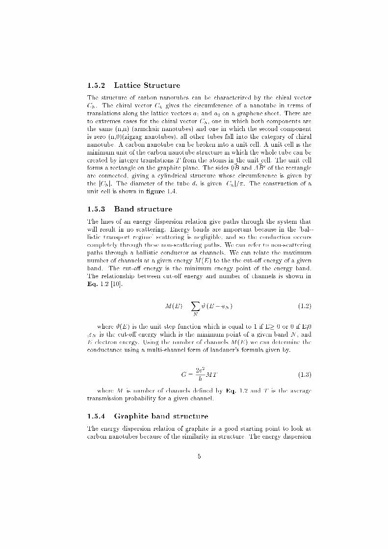
1.5.2 Lattice Structure

The structure of carbon nanotubes can be characterized by the chiral vector

Ch. The chiral vector Ch gives the circumference of a nanotube in terms of

translations along the lattice vectors a1 and a2 on a graphene sheet. There are

to extremes cases for the chiral vector Ch, one in which both components are

the same (n,n) (armchair nanotubes) and one in which the second component

is zero (n,0)(zigzag nanotubes), all other tubes fall into the category of chiral

nanotube. A carbon nanotube can be broken into a unit cell. A unit cell is the

minimum unit of the carbon nanotube structure in which the whole tube can be

created by integer translations T from the atoms in the unit cell. The unit cell

forms a rectangle on the graphite plane. The sides ~0B and ~AB0 of the rectangle

are connected, giving a cylindrical structure whose circumference is given by

the jChj. The diameter of the tube dt is given jChj=�. The construction of a

unit cell is shown in �gure 1.4.

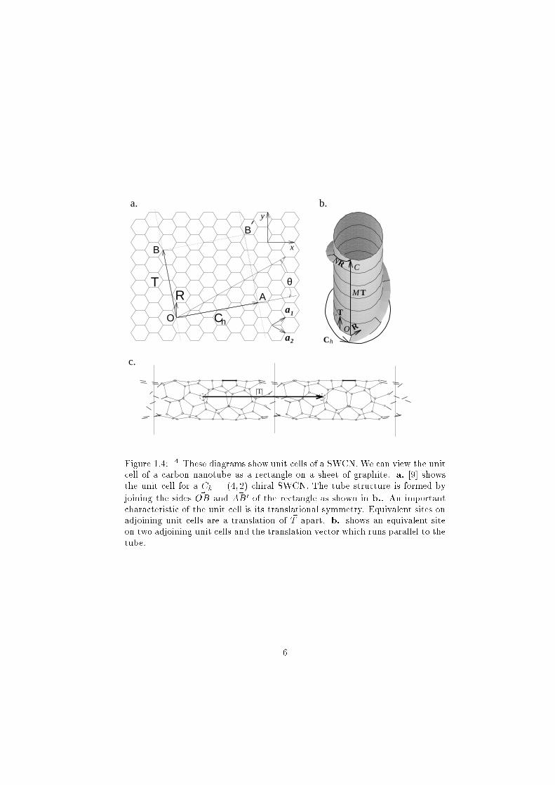
1.5.3 Band structure

The lines of an energy dispersion relation give paths through the system that

will result in no scattering. Energy bands are important because in the 'bal-

listic transport regime' scattering is negligible, and so the conduction occurs

completely through these non-scattering paths. We can refer to non-scattering

paths through a ballistic conductor as channels. We can relate the maximum

number of channels at a given energy M(E) to the the cut-o� energy of a given

band. The cut-o� energy is the minimum energy point of the energy band.

The relationship between cut-o� energy and number of channels is shown in

Eq. 1.2 [10].

M(E) =XN

# (E � "N) (1.2)

where #(E) is the unit step function which is equal to 1 if E� 0 or 0 if E<0

,"N is the cut-o� energy which is the minimum point of a given band N , and

E electron energy. Using the number of channels M(E) we can determine the

conductance using a multi-channel form of landauer's formula given by.

G =2e2

hMT (1.3)

where M is number of channels de�ned by Eq. 1.2 and T is the average

transmission probability for a given channel.

1.5.4 Graphite band structure

The energy dispersion relation of graphite is a good starting point to look at

carbon nanotubes because of the similarity in structure. The energy dispersion

5

NR

hC

C

M T

T

O R

|T|

a1

a2

O

A

B

B

T

Ch

θR

y

x

b.a.

c.

Figure 1.4: 4 These diagrams show unit cells of a SWCN. We can view the unit

cell of a carbon nanotube as a rectangle on a sheet of graphite. a. [9] shows

the unit cell for a Ch = (4; 2) chiral SWCN. The tube structure is formed by

joining the sides ~OB and ~AB0 of the rectangle as shown in b.. An important

characteristic of the unit cell is its translational symmetry. Equivalent sites on

adjoining unit cells are a translation of ~T apart. b. shows an equivalent site

on two adjoining unit cells and the translation vector which runs parallel to the

tube.

6

E

k

E(k)

εε

εε

1

2

3

4

f

N = 1 2 3 4

Figure 1.5: The diagram 6 shows the cut-o� energy for a given band N on the

energy dispersion relation. The cut-o� energy is the minimum point of and

energy band and is important because of its relation to the number of channels

M (E) at a given energy(Eq. 1.2).

relation of graphite is shown in Figure 1.6. The general character of the 2D

graphite energy dispersion relation is similar to that found in carbon nanotubes.

The energy bands in carbon nanotubes however do not always cross. This is

important because the conductance depends on the number of energy bands at

a given energy, and thus if there are no bands at given energy then conduction

does not occur at that energy.

1.5.5 Nanotube band structure

It has been found that crossing of energy bands depends on the structure of

the tube. Using periodic boundary conditions the wave vector in the circumfer-

ential direction becomes quantized. The wave vectors along the tube axis are

continuous (Ref. [9] page 56) for �nite length tubes. The energy dispersion rela-

tion becomes one-dimensional as a result of quantization in the circumferential

direction.

Metal/Semiconductor

It was found that band crossing only occurs for some chiralities (others exhibited

band gaps). The band gap shown in some nanotubes suggests they are semi-

conductors We can see in �gure 1.7 the breakup of nanatubes into metallic and

semi-conducting tubes suggested by the band structure.

Band gap

Calculations suggest that for large diameter tubes the conductance becomes

inversely proportional to the diameter as shown in �gure 1.8.

7

K Γ M K-10.0

-5.0

0.0

5.0

10.0

15.0

Ene

rgy

[eV

] π∗

ππ

π∗

K K

E

KMΓKM

[eV

]

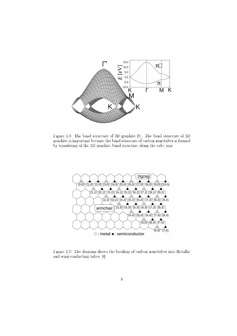
Figure 1.6: The band structure of 2D graphite [9]. The band structure of 2D

graphite is important because the band structure of carbon nanotubes is formed

by translating of the 2D graphite band structure along the tube axis.

(6,0) (7,0) (8,0) (9,0)

(4,1) (5,1) (6,1) (7,1) (8,1) (9,1)

(3,2) (4,2) (5,2) (6,2) (7,2) (8,2) (9,2)

(4,3) (5,3) (6,3) (7,3) (8,3)

(4,4) (5,4) (6,4) (7,4) (8,4)

(5,5) (6,5) (7,5)

(6,6) (7,6)

(1,0)(0,0) (2,0) (10,0)(3,0) (4,0) (5,0)

(2,1)

(3,3)

(2,2)

(1,1) (3,1)

: metal : semiconductor

armchair

zigzag

Figure 1.7: The diagram shows the breakup of carbon nanotubes into Metallic

and semi-conducting tubes [9]

8

0.0 1.0 2.0 3.0 4.0 5.0 6.0100/dt [1/A]

0.0

0.2

0.4

0.6

Eg/

t

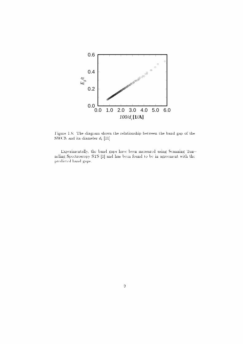
Figure 1.8: The diagram shows the relationship between the band gap of the

SWCN and its diameter dt [11]

Experimentally, the band gaps have been measured using Scanning Tun-

neling Spectroscopy STS [1] and has been found to be in agreement with the

predicted band gaps.

9

Figure 1.9: The picture shows conductance measurements that have been per-

formed using scanning tunneling spectroscopy STS [1]

10

Chapter 2

Method

2.1 Overview

In large molecular structures the atomic orbitals of individual atoms join to-

gether to become paths through the complete structure. In ballistic conductors

the movement of electrons waves along such paths results in electron transfer or

transport. We can look at electron waves in terms of schr�odingers wave equation

given bellow. Eq. 2.1.

i~@

@t= �

~2

2mr2 + V (r; t) (2.1)

Our solution method employs the single-band e�ective mass equation (ef-

fective mass equation) which is an approximation schr�odingers wave equation.

The singe-band e�ective mass equation is given bellow. The principle di�er-

ence between the time independent schr�odingers equation and the e�ective mass

equation is that the resulting wave-functions are smoothed out versions of the

actual wave-functions.

�Ec +

(i~r+ eA)

2m+U(r)

�(r) = E (r) (2.2)

To �nd the wave-functions of e�ective mass equation we discretize it over

a basis of atomic orbitals � giving a in�nite matrix form of the schr�odingers

equation.

HC = EC (2.3)

This can be expanded in terms of the three term recursion relation as

PCj�1 + (E �H0)Cj + PyCj+1 = 0 (2.4)

11

Use a Green's function method we and the appropriate boundary conditions

we can truncate this to a �nite Green's function which gives us the response of

the system. From the Green's function we can calculate the transmission coef-

�cients tij and using a multi-channel form of the landauer's formula (Eq. 2.5)

we can calculate the conduction.

G =2e2

h

n;mXi;j

jti;j j2

(2.5)

2.1.1 Tight-binding model

In the tight binding model we approximate the wave functions by a basis of

atomic orbitals, given bellow.

(r) =

nXi=1

Ci� (r) (2.6)

If the lattice points are located at points x = jan then from Bloch's equation

T~an = ei~k� ~an (2.7)

where T~an is a translation along the n th lattice vector ~an and ~k is the wave

vector. Thus Cj is periodic.

Cj�1 = �Cj (2.8)

The Hamiltonian operator is given by

H �(i~r+ eA)

2

2m+U(r) (2.9)

In order to numerically determine the r2 we must use the �nite di�erence

method which gives

r2Cj =1

a2[Cj+1 � 2Cj +Cj�1] (2.10)

Which brings us back to the recursive solution of schr�odinger

PCj�1 + (E �H0)Cj + PyCj+1 = 0

12

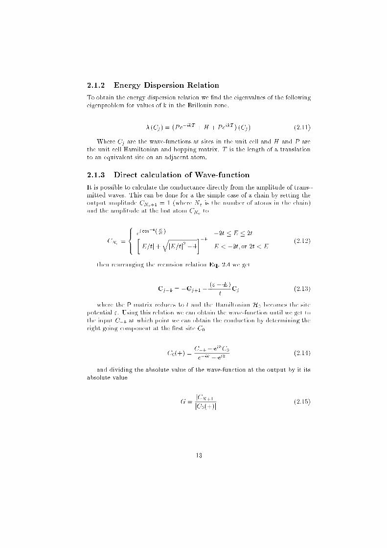
2.1.2 Energy Dispersion Relation

To obtain the energy dispersion relation we �nd the eigenvalues of the following

eigenproblem for values of k in the Brillouin zone.

� (Cj) =�Pe�ikT +H + PeikT

�(Cj) (2.11)

Where Cj are the wave-functions at sites in the unit cell and H and P are

the unit cell Hamiltonian and hopping matrix. T is the length of a translation

to an equivalent site on an adjacent atom.

2.1.3 Direct calculation of Wave-function

It is possible to calculate the conductance directly from the amplitude of trans-

mitted waves. This can be done for a the simple case of a chain by setting the

output amplitude CNc+1 = 1 (where Nc is the number of atoms in the chain)

and the amplitude at the last atom CNcto

CNc=

8><>:

ei cos�1( E2t ) �2t � E � 2t�

jE=tj+

qjE=tj

2� 1

��1

E < �2t; or 2t < E(2.12)

then rearranging the recursion relation Eq. 2.4 we get

Cj�1 = �Cj+1 �("� E)

tCj (2.13)

where the P matrix reduces to t and the Hamiltonian H0 becomes the site

potential ". Using this relation we can obtain the wave-function until we get to

the input C�1 at which point we can obtain the conduction by determining the

right going component at the �rst site C0

C0(+) =C�1 � eikC0

e�ik � eik(2.14)

and dividing the absolute value of the wave-function at the output by it its

absolute value

G =jCN+1j

jC0(+)j(2.15)

13

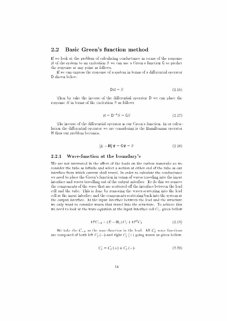
2.2 Basic Green's function method

If we look at the problem of calculating conductance in terms of the response

R of the system to an excitation S we can use a Green's function G to predict

the response at any point as follows.

If we can express the response of a system in terms of a di�erential operator

D shown below.

DR = S (2.16)

Then by take the inverse of the di�erential operator D we can place the

response R in terms of the excitation S as follows

R = D�1S = GS (2.17)

The inverse of the di�erential operator is our Green's function. In or calcu-

lation the di�erential operator we are considering is the Hamiltonian operator

H thus our problem becomes.

[E � H] = G = S (2.18)

2.2.1 Wave-function at the boundary's

We are not interested in the a�ect of the leads on the carbon nanotube so we

consider the tube as in�nite and select a section at either end of the tube as our

interface from which current shall travel. In order to calculate the conductance

we need to place the Green's function in terms of waves traveling into the input

interface and waves travelling out of the output interface. To do this we remove

the components of the wave that are scattered o� the interface between the lead

cell and the tube. This is done by removing the waves scattering into the lead

cell at the input interface and the components scattering back into the system at

the output interface. At the input interface between the lead and the structure

we only want to consider waves that travel into the structure. To achieve this

we need to look at the wave equation at the input interface cell C0, given bellow

tPC�1 + (E �H0)C0 + tP yC1 (2.19)

We take the C�1 as the wave-function in the lead. All Cj wave functions

are composed of both left Cj (�) and right Cj (+) going waves as given bellow.

Cj = Cj (+) + Cj (�) (2.20)

14

Input Boundary

Contact

Input

C1 2C-1 C

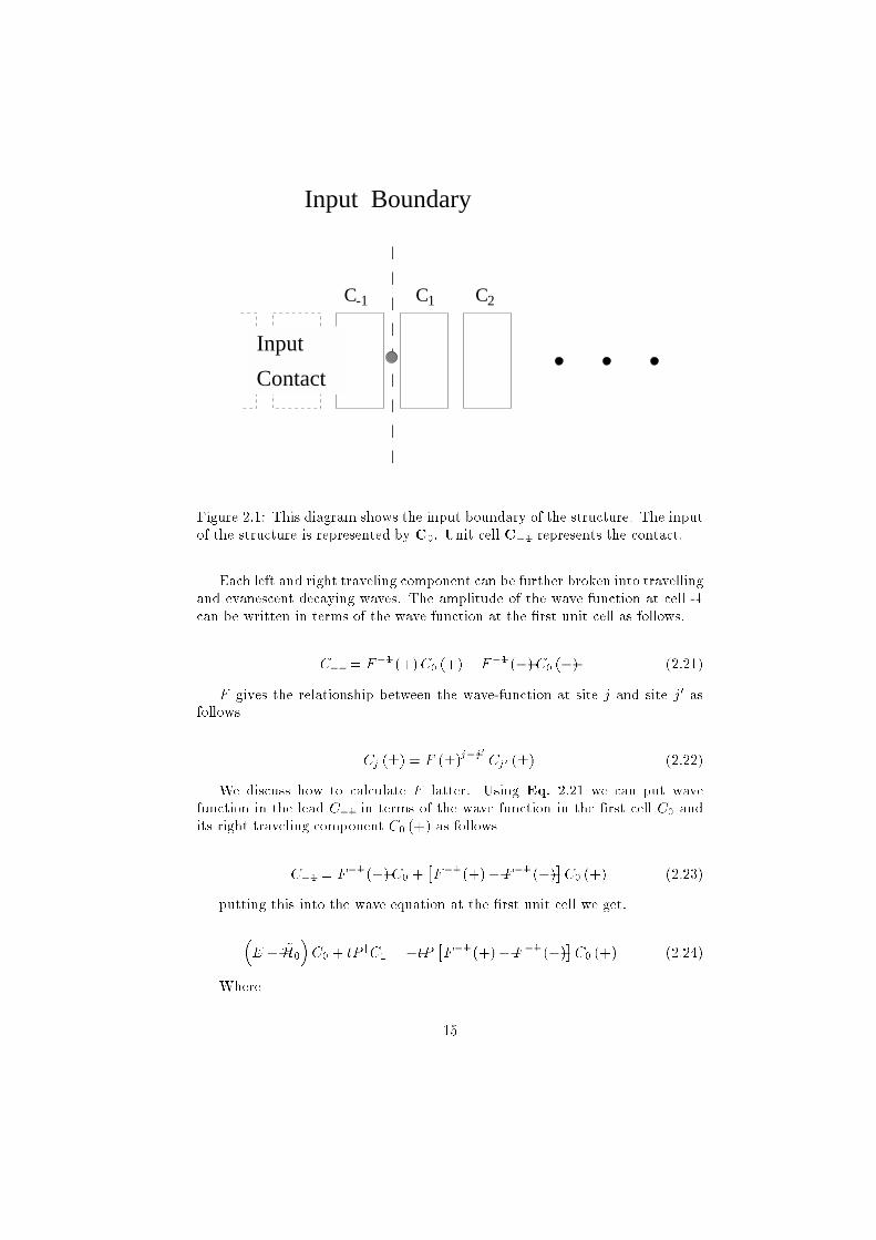
Figure 2.1: This diagram shows the input boundary of the structure. The input

of the structure is represented by C0. Unit cell C�1 represents the contact.

Each left and right traveling component can be further broken into travelling

and evanescent decaying waves. The amplitude of the wave function at cell -1

can be written in terms of the wave function at the �rst unit cell as follows.

C�1 = F�1 (+)C0 (+) + F�1 (�)C0 (�) (2.21)

F gives the relationship between the wave-function at site j and site j0 as

follows

Cj (�) = F (�)j�j0

Cj0 (�) (2.22)

We discuss how to calculate F latter. Using Eq. 2.21 we can put wave

function in the lead C�1 in terms of the wave function in the �rst cell C0 and

its right traveling component C0 (+) as follows

C�1 = F�1 (�)C0 +�F�1 (+)� F�1 (�)

�C0 (+) (2.23)

putting this into the wave equation at the �rst unit cell we get.

�E � ~H0

�C0 + tP yC1 = �tP

�F�1 (+)� F�1 (�)

�C0 (+) (2.24)

Where

15

~H = H0 � tPF�1 (�) (2.25)

and the excitation of the system is given by

�tP�F�1 (+) � F�1 (�)

�(2.26)

Which puts the wave-function at site done by removing the component of

the waves traveling from the structure back into the lead. This is done as shown

bellow.

~H0 = H0 � tPF�1 (�) (2.27)

We must also consider the wave-function at the output of the system. At

the output, we only want to consider waves that travel from the structure into

the lead. To do this we must remove the components that are re ected by the

leads back into the structure. This can be achieved quite simply by removing

the components of the wave-function in the lead that are traveling to the left.

This is done as follows. We begin with the original hamilton-ian equation for

the last unit cell.

tPCN�1 + (E �HN)CN + tP yCN+1 (2.28)

The CN+1 is composed of incident and re ected waves but we are only

interested in the incident waves because re ected waves do not contribute to

the conductance. To remove the re ected waves we use the relation given in

Eq. 2.22. We are only interested in the incident component so we take

CN+1 = F (+)CN (2.29)

Which gives us only the waves incident on the contact and thus Eq. 2.28

becomes

�E � ~HN

�CN + tPCN�1 = 0 (2.30)

where

~HN = H � tP yF (+) (2.31)

16

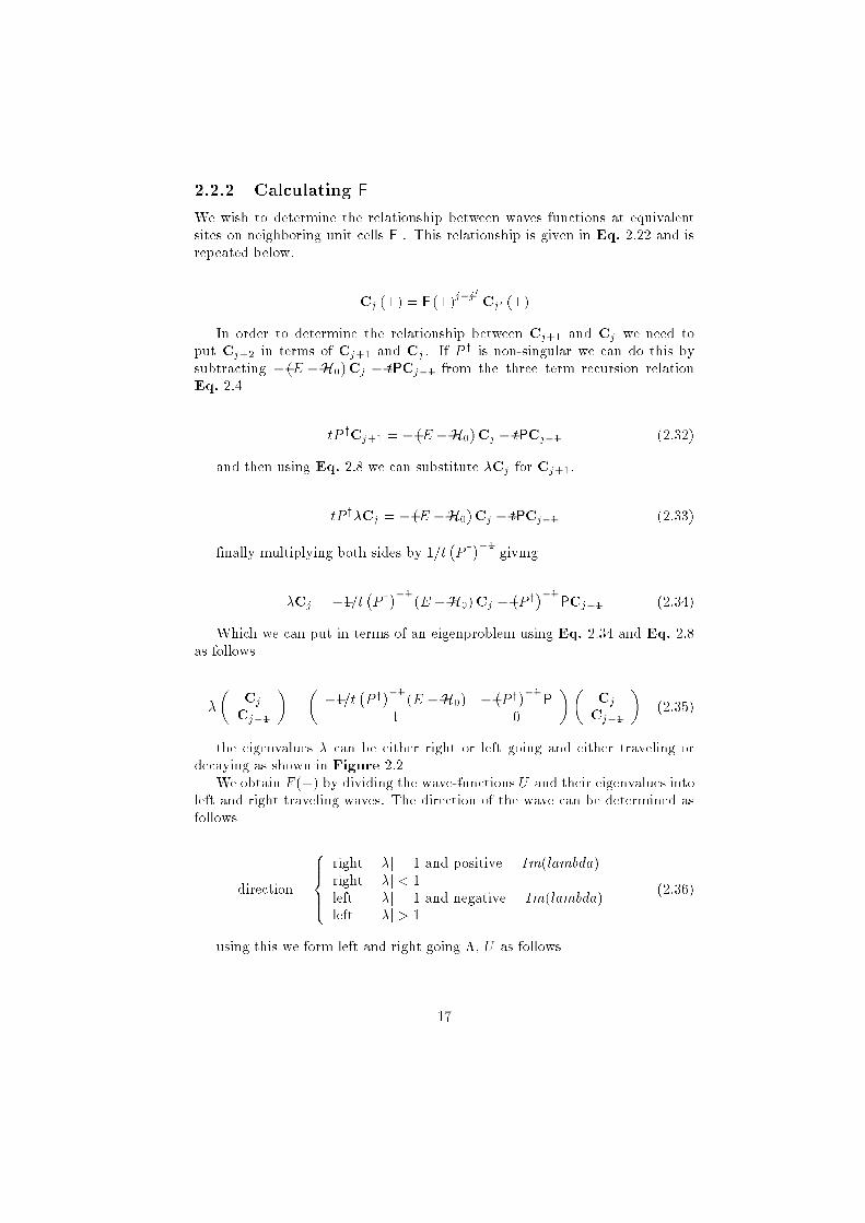
2.2.2 Calculating F

We wish to determine the relationship between waves functions at equivalent

sites on neighboring unit cells F . This relationship is given in Eq. 2.22 and is

repeated below.

Cj (�) = F (�)j�j0

Cj0 (�)

In order to determine the relationship between Cj+1 and Cj we need to

put Cj+2 in terms of Cj+1 and Cj. If P y is non-singular we can do this by

subtracting � (E �H0)Cj � tPCj�1 from the three term recursion relation

Eq. 2.4

tP yCj+1 = � (E �H0)Cj � tPCj�1 (2.32)

and then using Eq. 2.8 we can substitute �Cj for Cj+1.

tP y�Cj = � (E �H0)Cj � tPCj�1 (2.33)

�nally multiplying both sides by 1=t�P y

��1

giving

�Cj = �1=t�P y��1

(E �H0)Cj ��P y��1

PCj�1 (2.34)

Which we can put in terms of an eigenproblem using Eq. 2.34 and Eq. 2.8

as follows

�

�Cj

Cj�1

�=

��1=t

�P y

��1

(E �H0) ��P y

��1P

1 0

��Cj

Cj�1

�(2.35)

the eigenvalues � can be either right or left going and either traveling or

decaying as shown in Figure 2.2

We obtain F (+) by dividing the wave-functions U and their eigenvalues into

left and right traveling waves. The direction of the wave can be determined as

follows

direction =

8>><>>:

right j�j = 1 and positive = Im(lambda)

right j�j < 1

left j�j = 1 and negative = Im(lambda)

left j�j > 1

(2.36)

using this we form left and right going �, U as follows

17

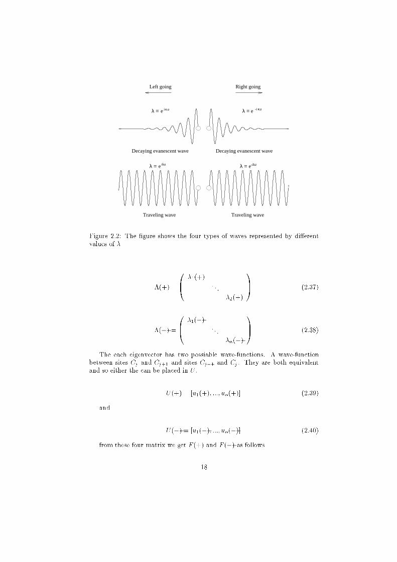
Traveling wave

Left going

Decaying evanescent wave Decaying evanescent wave

Traveling wave

Right going

-ikaeλ =

κi aeλ = eλ =

eλ = ika

κ-i a

Figure 2.2: The �gure shows the four types of waves represented by di�erent

values of �

�(+) =

0B@

�1(+). . .

�2(+)

1CA (2.37)

�(�) =

0B@

�1(�). . .

�n(�)

1CA (2.38)

The each eigenvector has two possiable wave-functions. A wave-function

between sites Cj and Cj+1 and sites Cj�1 and Cj . They are both equivalent

and so either the can be placed in U .

U (+) = [u1(+); :::; un(+)] (2.39)

and

U (�) = [u1(�); :::; un(�)] (2.40)

from these four matrix we get F (+) and F (�) as follows

18

C (E-H)C jP

tP =P = H =

j

j

j+1C

j+1

j

j

j

j

P

j-1

j-1 t

A

B

B

A

AA

BB

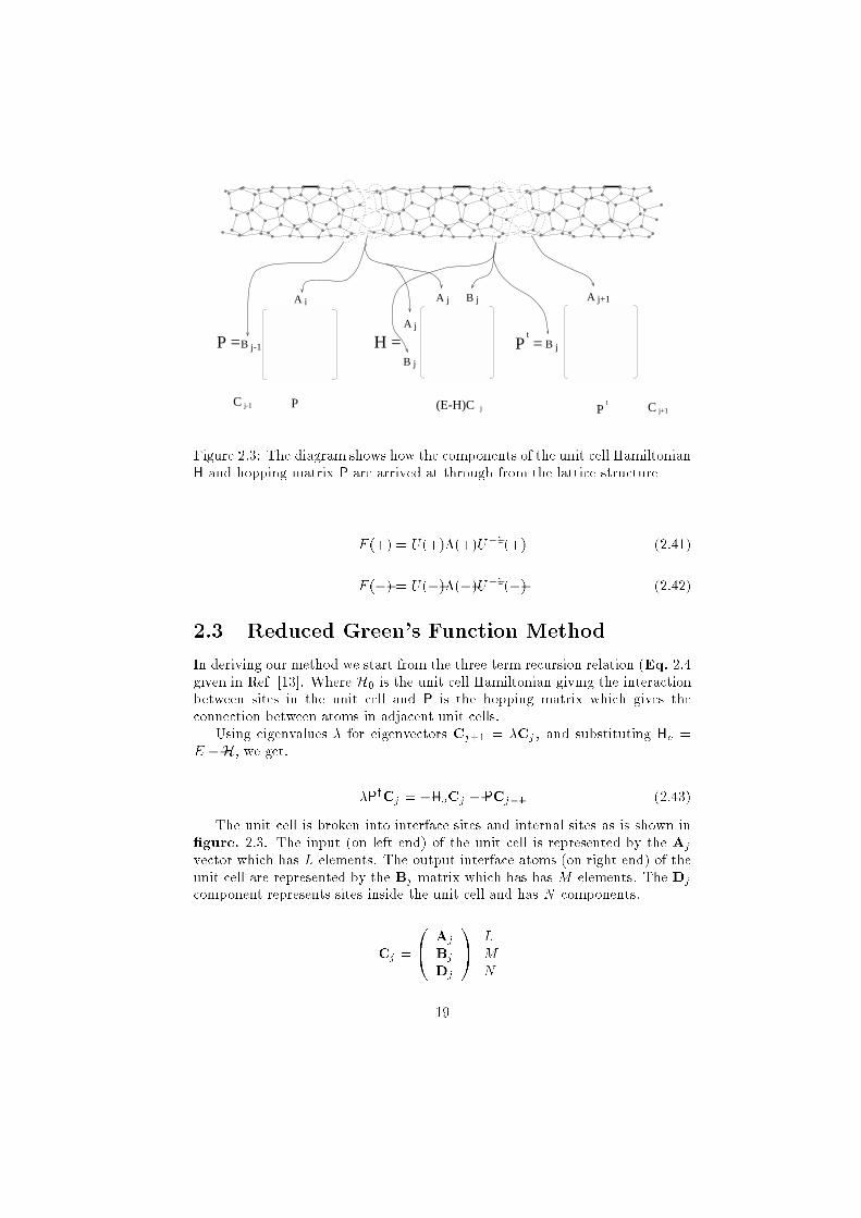
Figure 2.3: The diagram shows how the components of the unit cell Hamiltonian

H and hopping matrix P are arrived at through from the lattice structure

F (+) = U(+)�(+)U�1(+) (2.41)

F (�) = U(�)�(�)U�1(�) (2.42)

2.3 Reduced Green's Function Method

In deriving our method we start from the three term recursion relation (Eq. 2.4

given in Ref. [13]. Where H0 is the unit cell Hamiltonian giving the interaction

between sites in the unit cell and P is the hopping matrix which gives the

connection between atoms in adjacent unit cells.

Using eigenvalues � for eigenvectors Cj+1 = �Cj , and substituting Ho =

E �H, we get.

�PyCj = �HoCj � PCj�1 (2.43)

The unit cell is broken into interface sites and internal sites as is shown in

�gure. 2.3. The input (on left end) of the unit cell is represented by the Aj

vector which has L elements. The output interface atoms (on right end) of the

unit cell are represented by the Bj matrix which has has M elements. The Dj

component represents sites inside the unit cell and has N components.

Cj =

0@ Aj

Bj

Dj

1A L

M

N

19

The connection between each cell is represented in matrix form in the Hop-

ping matrix. It is broken into Aj ,Bj and Dj components. Because only the

Bj and Aj+1 elements are connected only the elements of the matrix between

these

P =

0@ 0 PAB 0

0 0 0

0 0 0

1A Py =

0@ 0 0 0

Py

AB 0 0

0 0 0

1A

From the three term recursion relation the PCj�1 results in the following

vector.

PCj�1 =

0@ 0 PAB 0

0 0 0

0 0 0

1A0@ Aj�1

Bj�1

Dj�1

1A =

0@ PABBj�1

0

0

1A

usingEq. 2.8 and thePyCj+1 term of the recursion relation we getPyCj+1 =

�PyCj which is given in block form below

�PyCj = �

0@ 0 0 0

P y

AB 0 0

0 0 0

1A0@ Aj

Bj

Dj

1A =

0@ 0

�P y

ABAj

0

1A (2.44)

The unit cell Hamiltonian H0 = (E �H0) of Eq. 2.43 is given in block form

bellow.

H0 =

0@ HAA HAB HAD

HBA HBB HBDHDA HDB HDD

1A (2.45)

Using block components Eq. 2.43 becomes

0@ 0

Py

AB�Aj

0

1A = �

0@ HAAAj +HABBj +HADDj

HBAAj +HBBBj +HBDDj

HDAAj +HDBBj +HDDDj

1A

�

0@ PABBj�1

0

0

1A � � � (a)

� � � (b)

� � � (c)

(2.46)

We want to �nd the relationship between Aj and Aj+1 and Bj and Bj+1.

To do this we need to remove the Dj component from the Eq. 2.46. To do this

we put Dj in terms of Aj and Bj. Taking row (c) of Eq. 2.46

20

0 = �HDAAj �HDBBj �HDDDj (2.47)

If HDD is non-singular then we can place Dj in terms of Aj and Bj by

adding HDDDj to both sides of Eq. 2.47 and then multiplying by the inverse

of HDD which gives

Dj = H�1

DD(�HDAAj �HDBBj) (2.48)

If the Py

AB is non-singular then we can place Aj+1 in terms of Aj , Bj using

row (b) of Eq. 2.46 given below

�Py

ABAj = �HBAAj �HBBBj �HBDDj (2.49)

by multiplying both sides by�P

y

AB

��1

to give

�Aj =�P y��1

(�HBAAj �HBBBj �HBDDj) (2.50)

and then removing the Dj component by substituting Eq. 2.48

�Aj =�P

y

AB

��1 �

HBDH�1

DDHDA �HBA

�Aj

+�P

y

AB

��1 �

HBDH�1

DDHDB �HBB

�Bj (2.51)

or

�Aj = XAj + YBj (2.52)

row (a) of Eq. 2.46 gives us

0 = �HAAAj �HABBj �HADDj � PABBj�1 (2.53)

multiplying by � we get.

0 = �HAA�Aj �HAB�Bj �HAD�Dj � PABBj (2.54)

and then removing the Dj component by substituting Eq. 2.48 we get

0 =�HADH

�1

DDHDA �HAA

��Aj +

�HADH

�1

DDHDB �HAB

��Bj � PABBj

(2.55)

21

or

0 = A�Aj + B�Bj � PABBj (2.56)

B�Bj = PABBj � A�Aj (2.57)

= PABBj � A (XAj + YBj) (2.58)

if the B matrix is non-singular (has an inverse) we can place �Bj in terms of

Aj and Bj components as follows

�Bj = B�1 (PABBj � A (XAj + YBj))

= B�1 (PABBj � AXAj � AYBj)

=��B

�1AXAj

�+ B

�1 (PAB � AY)Bj

(2.59)

�Bj = ZAj +WBj (2.60)

We can put this in terms of and eigenproblem

�

�Aj

Bj

�=

�X Y

Z W

��Aj

Bj

�

A = HADH�1

DDHDA �HAA (2.61)

B = HADH�1

DDHDB �HAB (2.62)

X =�P y��1 �

HBDH�1

DDHDA �HBA

�(2.63)

Y =�P y��1 �

HBDH�1

DDHDB �HBB

�(2.64)

Z = �B�1AX (2.65)

W = B�1 (P � AY) (2.66)

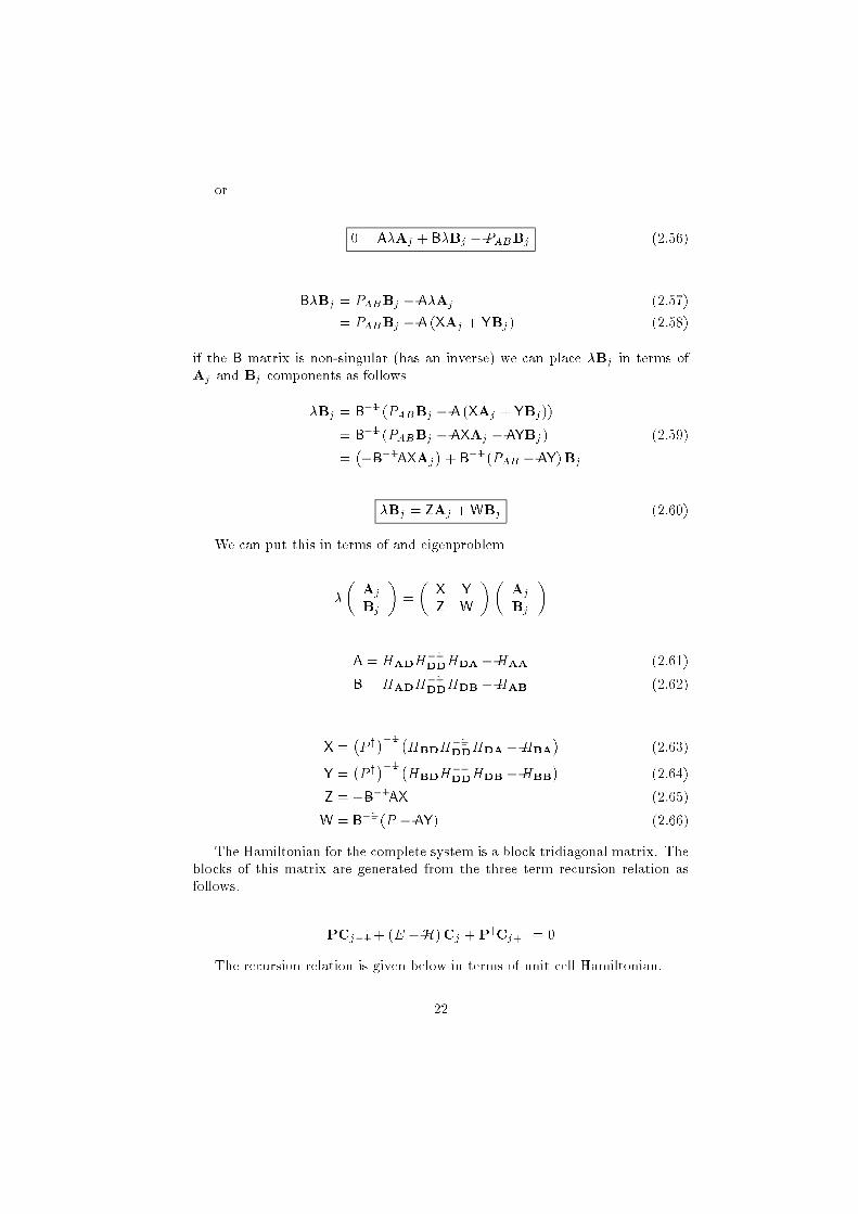
The Hamiltonian for the complete system is a block tridiagonal matrix. The

blocks of this matrix are generated from the three term recursion relation as

follows.

PCj�1 + (E �H)Cj + PyCj+1 = 0

The recursion relation is given below in terms of unit cell Hamiltonian.

22

0@ 0 P 0

0 0 0

0 0 0

1A0@ Aj�1

Bj�1

Dj�1

1A+

0@ HAA HAB HAD

HBA HBB HBDHDA HDB HDD

1A0@ Aj

Bj

Dj

1A

+

0@ 0 0 0

P y 0 0

0 0 0

1A0@ Aj+1

Bj+1

Dj+1

1A = 0 (2.67)

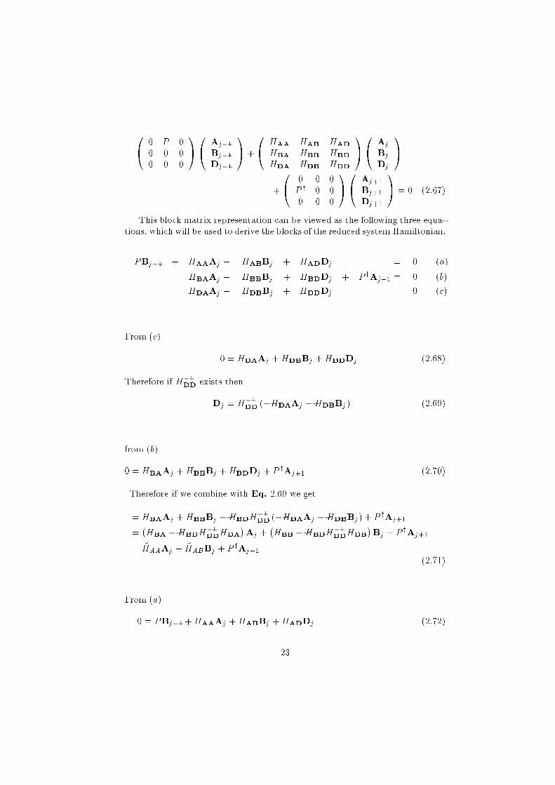
This block matrix representation can be viewed as the following three equa-

tions, which will be used to derive the blocks of the reduced system Hamiltonian.

PBj�1 + HAAAj + HABBj + HADDj = 0 (a)

HBAAj + HBBBj + HBDDj + P yAj+1 = 0 (b)

HDAAj + HDBBj + HDDDj = 0 (c)

From (c)

0 = HDAAj +HDBBj +HDDDj (2.68)

Therefore if H�1

DDexists then

Dj = H�1

DD(�HDAAj �HDBBj) (2.69)

from (b)

0 = HBAAj +HBBBj +HBDDj + P yAj+1 (2.70)

Therefore if we combine with Eq. 2.69 we get

= HBAAj +HBBBj �HBDH�1

DD(�HDAAj �HDBBj) + P yAj+1

=�HBA �HBDH

�1

DDHDA

�Aj +

�HBB �HBDH

�1

DDHDB

�Bj + P yAj+1

= �HAAAj + �HABBj + P yAj+1

(2.71)

From (a)

0 = PBj�1 +HAAAj +HABBj +HADDj (2.72)

23

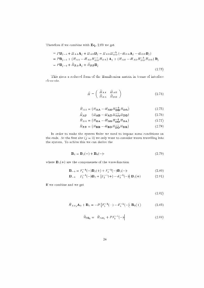
Therefore if we combine with Eq. 2.69 we get

= PBj�1 +HAAAj +HABBj +HADH�1

DD (�HDAAj �HDBBj)

= PBj�1 +�HAA �HADH

�1

DDHDA

�Aj +

�HAB �HADH

�1

DDHDB

�Bj

= PBj�1 + �HBAAj + �HBBBj

(2.73)

This gives a reduced form of the Hamiltonian matrix in terms of interface

elements.

�H =

��HAA

�HAB

�HBA�HBB

�(2.74)

�HAA =�HAA �HADH

�1

DDHDA

�(2.75)

�HAB =�HAB �HADH

�1

DDHDB

�(2.76)

�HBA =�HBA �HBDH

�1

DDHDA

�(2.77)

�HBB =�HBB �HBDH

�1

DDHDB

�(2.78)

In order to make the system �nite we need to impose some conditions on

the ends. At the �rst site (j = 0) we only want to consider waves travelling into

the system. To achive this we can derive the

B0 = B0(+) +B0(�) (2.79)

where B0(+) are the componenets of the wave-function

B�1 = F�1

b (+)B0(+) + F�1

b (�)B0(�) (2.80)

B�1 = F�1

b (�)B0 +�F�1

b (+)� F�1

b (�)�B0(+) (2.81)

If we combine and we get

(2.82)

�HAA0A0 +B0 = �P

�F�1

b (+) � F�1

b (�)�B0(+) (2.83)

~HAB0=h�HAB0

+ PF�1

b (�)i

(2.84)

24

0BBBBB@

�P�F�1

b (+)� F�1

b (�)�B0(+)

0

0...

0

1CCCCCA

=

0BBBBBB@

~HAA0~HAB0

~HBA0~HBB0

P y

P ~HAA1

. . .

. . .. . .

(2.85)

at j = Nc

ANc+1 = Fa(+)ANc(2.86)

Thus from 27

~HBANcANc

+ ~HBBNcBNc

= 0 (2.87)

~HBANc=h�HBANc

+ P yFa(+)i

(2.88)

~HBBNc= �HBBNc

(2.89)

. . .. . .

. . . ~HBBNc�1P y

P ~HAANc

~HABNc

~HBANc

~HBBNc

1CCCCCCCCA

(2.90)

~H =

0BBBBBBBBBBBBBBB@

P ~HAAj�1~HABj�1

~HBAj�1~HBBj�1

P y

P ~HAAj~HABj

~HBAj~HBBj

P y

P ~HAAj+1~HABj+1

~HBAj+1~HBBj+1

P y

1CCCCCCCCCCCCCCCA(2.91)

25

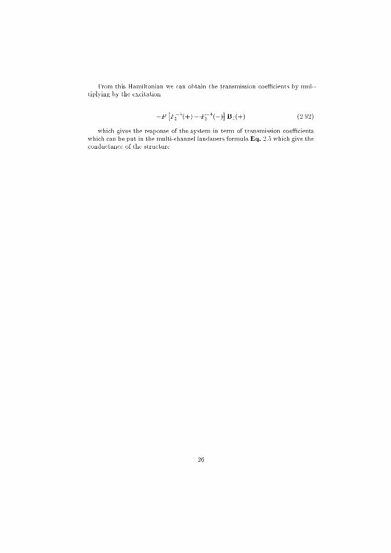
From this Hamiltonian we can obtain the transmission coe�cients by mul-

tiplying by the excitation

�P�F�1

b (+)� F�1

b (�)�B0(+) (2.92)

which gives the response of the system in term of transmission coe�cients

which can be put in the multi-channel landauers formula Eq. 2.5 which give the

conductance of the structure.

26

Chapter 3

Results

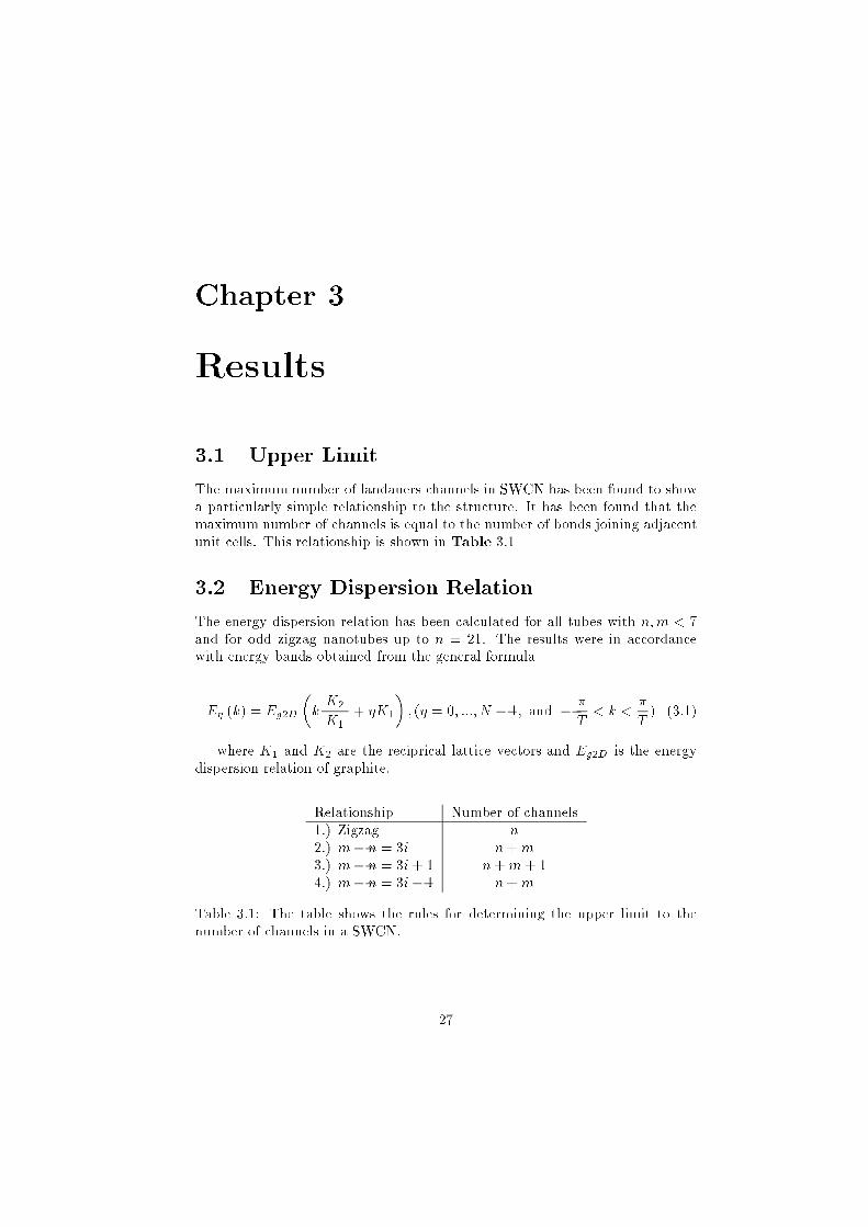
3.1 Upper Limit

The maximum number of landauers channels in SWCN has been found to show

a particularly simple relationship to the structure. It has been found that the

maximum number of channels is equal to the number of bonds joining adjacent

unit cells. This relationship is shown in Table 3.1

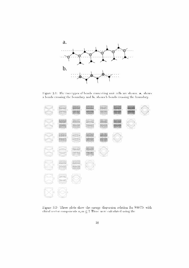
3.2 Energy Dispersion Relation

The energy dispersion relation has been calculated for all tubes with n;m < 7

and for odd zigzag nanotubes up to n = 21. The results were in accordance

with energy bands obtained from the general formula

E� (k) = Eg2D

�kK2

jK1j+ �K1

�; (� = 0; :::; N � 1; and �

�

T< k <

�

T) (3.1)

where K1 and K2 are the reciprical lattice vectors and Eg2D is the energy

dispersion relation of graphite.

Relationship Number of channels

1.) Zigzag n

2.) m� n = 3i n+m

3.) m� n = 3i + 1 n+m + 1

4.) m� n = 3i � 1 n+m

Table 3.1: The table shows the rules for determining the upper limit to the

number of channels in a SWCN.

27

a.

b.

Figure 3.1: The two types of bonds connecting unit cells are shown. a. shows

a bonds crossing the boundary and b. shows b bonds crossing the boundary.

Figure 3.2: These plots show the energy dispersion relation for SWCN with

chiral vector components n;m � 7 These were calculated using the

28

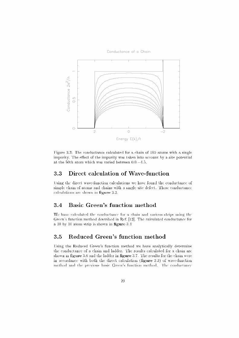
Figure 3.3: The conductance calculated for a chain of 100 atoms with a single

impurity. The e�ect of the impurity was taken into account by a site potential

at the 50th atom which was varied between 0.0 - 4.5.

3.3 Direct calculation of Wave-function

Using the direct wave-function calculations we have found the conductance of

simple chain of atoms and chains with a single site defect. These conductance

calculations are shown in �gure 3.3.

3.4 Basic Green's function method

We have calculated the conductance for a chain and various strips using the

Green's function method described in Ref. [13]. The calculated conductance for

a 10 by 10 atom strip is shown in �gure 3.4

3.5 Reduced Green's function method

Using the Reduced Green's function method we have analytically determine

the conductance of a chain and ladder. The results calculated for a chain are

shown in �gure 3.6 and the ladder in �gure 3.7. The results for the chain were

in accordance with both the direct calculation (�gure 3.3) of wave-function

method and the previous basic Green's function method. The conductance

29

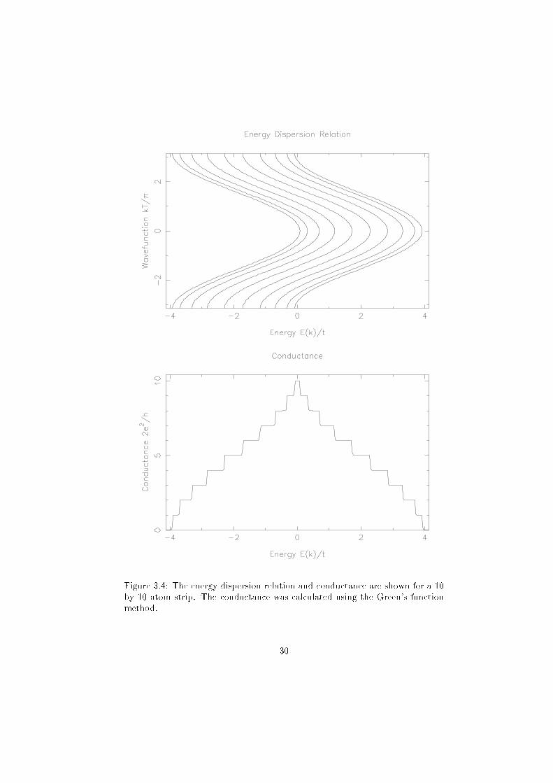
Figure 3.4: The energy dispersion relation and conductance are shown for a 10

by 10 atom strip. The conductance was calculated using the Green's function

method.

30

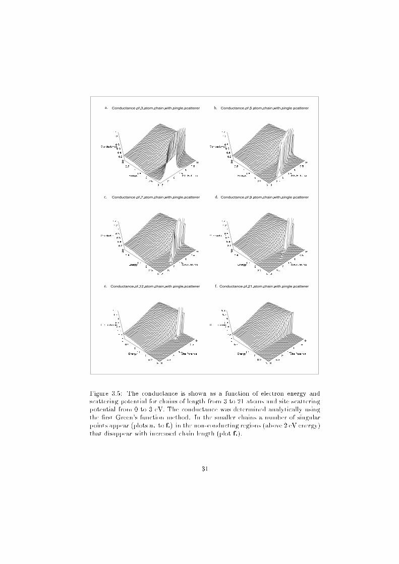
d.

a.

c.

b.

e. f.

Figure 3.5: The conductance is shown as a function of electron energy and

scattering potential for chains of length from 3 to 21 atoms and site scattering

potential from 0 to 3 eV. The conductance was determined analytically using

the �rst Green's function method. In the smaller chains a number of singular

points appear (plots a. to f.) in the non-conducting regions (above 2 eV energy)

that disappear with increased chain length (plot f.).

31

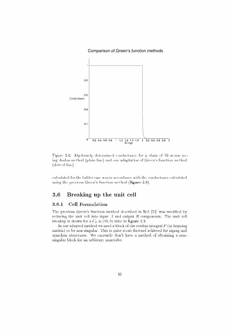
Figure 3.6: Algebraicly determined conductance for a chain of 10 atoms us-

ing Andos method (plain line) and our adaptation of Green's function method

(dotted line)

calculated for the ladder case was in accordance with the conductance calculated

using the previous Green's function method (�gure 3.4).

3.6 Breaking up the unit cell

3.6.1 Cell Formulation

The previous Green's function method described in Ref. [13] was modi�ed by

reducing the unit cell into input A and output B components. The unit cell

breakup is shown for a Ch = (10; 9) tube in �gure 2.3.

In our adapted method we need a block of the overlap integral P (or hopping

matrix) to be non-singular. This is quite strait-forward achieved for zigzag and

armchair structures. We currently don't have a method of obtaining a non-

singular block for an arbitrary nanotube.

32

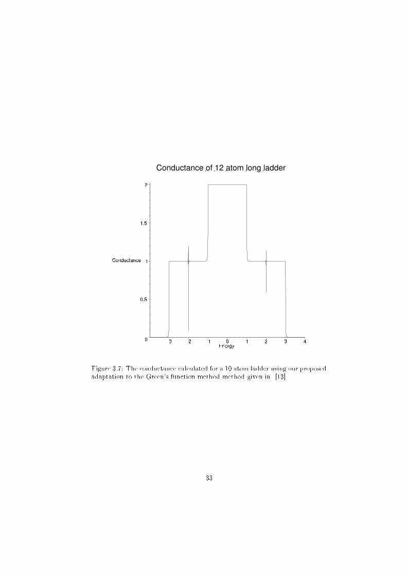
Figure 3.7: The conductance calculated for a 10 atom ladder using our proposed

adaptation to the Green's function method method given in [13]

33

Singular P matrix

Singular P matrix Singular P matrix

Singular P matrix

Singular P matrix Singular P matrix

Singular P matrix

Singular P matrix Singular P matrix Singular P matrix

Singular P matrixSingular P matrixSingular P matrixSingular P matrixSingular P matrix

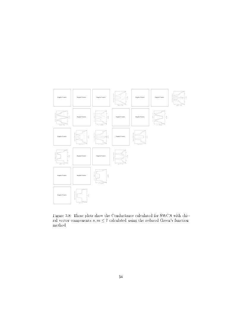
Figure 3.8: These plots show the Conductance calculated for SWCN with chi-

ral vector components n;m � 7 calculated using the reduced Green's function

method

34

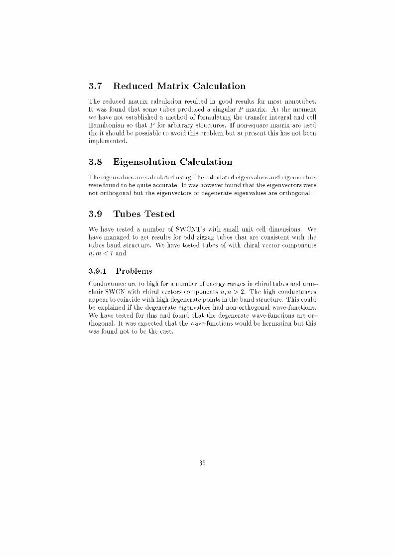
3.7 Reduced Matrix Calculation

The reduced matrix calculation resulted in good results for most nanotubes.

It was found that some tubes produced a singular P matrix. At the moment

we have not established a method of formulating the transfer integral and cell

Hamiltonian so that P for arbitrary structures. If non-square matrix are used

the it should be possiable to avoid this problem but at present this has not been

implemented.

3.8 Eigensolution Calculation

The eigenvalues are calculated using The calculated eigenvalues and eigenvectors

were found to be quite accurate. It was however found that the eigenvectors were

not orthogonal but the eigenvectors of degenerate eigenvalues are orthogonal.

3.9 Tubes Tested

We have tested a number of SWCNT's with small unit cell dimensions. We

have managed to get results for odd zigzag tubes that are consistent with the

tubes band structure. We have tested tubes of with chiral vector components

n;m < 7 and

3.9.1 Problems

Conductance are to high for a number of energy ranges in chiral tubes and arm-

chair SWCN with chiral vectors components n; n > 2. The high conductances

appear to coincide with high degenerate points in the band structure. This could

be explained if the degenerate eigenvalues had non-orthogonal wave-functions.

We have tested for this and found that the degenerate wave-functions are or-

thogonal. It was expected that the wave-functions would be hermatian but this

was found not to be the case.

35

Chapter 4

Discussion

4.1 Channels with Energy Dispersion Relation

We found the number of channels calculated to be in agreement with the number

of channels as predicted from the band structure. This sugests that the calcula-

tion of the reduced matrix is correct. The discrepency in the conductance and

the number of channels sugests that either their is a signi�gant numerical error

or that errors have occured latter in the program.

4.2 Conductance and Channels

We found that the conductance was completly consistent with the number of

channels for zigzag SWCN with odd n but only completly consitent for the case

of a (2,2) armchair tubes. Although the other SWCN were not consistent over

the entire energy range important features of the conductors were found to be

consistent. All armchair tubes tested were found to have a conductance of 2

2e2=h arround the Fermi level. For energy values far from the Fermi level the

conductance also tended to be consistent.

It is possiable that numerical instability contributes to the errors in the

conductance, however under or over ow was not observed in the calculation.

A possiable cause of instability could be the subtraction of close values which is

known to cause cancelation of values but this has not been found to be the case

except in the case of conductance far from the Fermi level and has not been

shown to contribute to degeneration of the result.

It is possiable that the calculation could be highlighting some new phenom-

ena of the calculation method or the carbon nanotubes being investigated. It is

possible that the conductance is not quantized in the ranges being viewed but

this would not explain the high values in armchair tubes which are known to

exhibit quantized conductance levels.

36

Chapter 5

Conclusions

5.1 Energy Dispersion Relation

We have calculated the energy dispersion relation for a large range of structures

and have shown that it is consistent with the band structure determined using

analytic means [9].

5.2 Channels

We have veri�ed the upper limit on the number of landauers channels. We

have managed to correctly calculate the number of landauers channels and have

found that it is consistency with the energy dispersion relation.

There are problems in correctly formulating the hopping matix P for arbi-

trary SWCN but it is beleaved that this problem can be resolved in non-square

matrix are used.

5.3 Conductance

The conductance has been calculated for a range of armchair, zigzag and chiral

nanotubes. The conductance has been found to be consistent with the energy

dispersion relaition for zigzag SWCN with odd n.

It has been found that the conductance is inconsistent with the energy dis-

persion relation for a range of values in other SWCN. The conductance becomes

very high for energy ranges of such SWCN. We have not currently established

the reason for this.

37

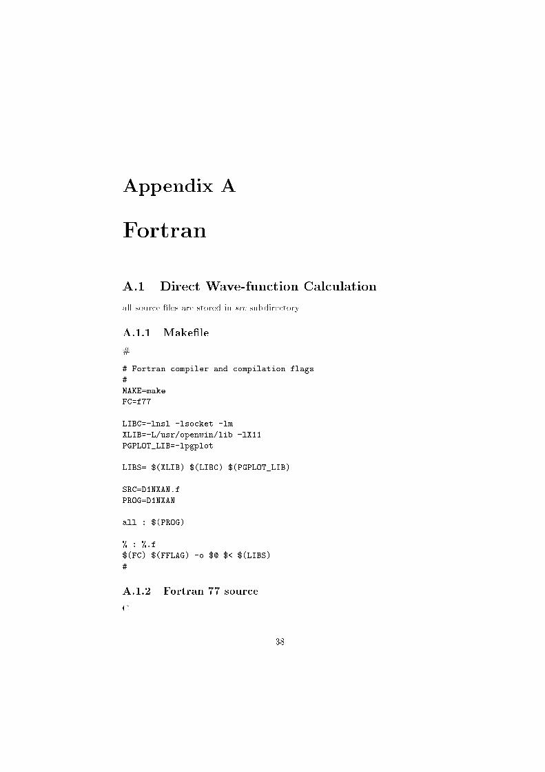
Appendix A

Fortran

A.1 Direct Wave-function Calculation

all source �les are stored in src subdirectory

A.1.1 Make�le

#

# Fortran compiler and compilation flags

#

MAKE=make

FC=f77

LIBC=-lnsl -lsocket -lm

XLIB=-L/usr/openwin/lib -lX11

PGPLOT_LIB=-lpgplot

LIBS= $(XLIB) $(LIBC) $(PGPLOT_LIB)

SRC=D1NXAN.f

PROG=D1NXAN

all : $(PROG)

% : %.f

$(FC) $(FFLAG) -o $@ $< $(LIBS)

#

A.1.2 Fortran 77 source

C

38

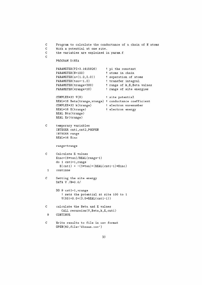
C Program to calculate the conductance of a chain of N atoms

C With a potential at one site.

C the variables are explained in param.f

C

PROGRAM D1NXA

PARAMETER(PI=3.1415926) ! pi the constant

PARAMETER(N=100) ! atoms in chain

PARAMETER(a=(1.0,0.0)) ! seperation of atoms

PARAMETER(tau=-1.0) ! transfer integral

PARAMETER(trange=300) ! range of k,E,Beta values

PARAMETER(vrange=10) ! range of site energies

COMPLEX*32 V(N) ! site potential

REAL*16 Beta(trange,vrange) ! conductance coefficient

COMPLEX*32 k(trange) ! electron wavenumber

REAL*16 E(trange) ! electron energy

REAL Bta(trange)

REAL Er(trange)

C temporary variables

INTEGER cnt1,cnt2,PGOPEN

INTEGER range

REAL*16 Einc

range=trange

C Calculate E values

Einc=(6*tau)/REAL(range-1)

do 1 cnt1=1,range

E(cnt1) = -(3*tau)+(REAL(cnt1-1)*Einc)

1 continue

C Setting the site energy

DATA V /N*0.0/

DO 9 cnt1=1,vrange

! sets the potential at site 100 to 1

V(50)=0.0+(0.5*REAL(cnt1-1))

C calculate the Beta and E values

CALL recursion(V,Beta,k,E,cnt1)

9 CONTINUE

C Write results to file in csv format

OPEN(60,file='d1nxan.csv')

39

DO 12 cnt2=1,range

WRITE(60,'(G42.33E3,$)') E(cnt2)

DO 121 cnt1=1,vrange-1

WRITE(60,"(',',G42.33E3,$)") Beta(cnt2,cnt1)

121 CONTINUE

WRITE(60,"(',',G42.33E3)") Beta(cnt2,vrange)

12 CONTINUE

CLOSE(60,status='keep')

C

C Plot the results

C

istat = PGOPEN ('?')

IF (istat .NE. 1 ) STOP

CALL PGSCRN(0, 'white', istat)

CALL PGSCRN(1, 'black', istat)

CALL PGSCH (1.50)

CALL PGENV(REAL(E(1)),REAL(E(range)),0.0,1.2,0,0)

CALL PGLAB('Energy E(k)/t',

$ 'Conductance 2e\\u2\\d/h','Conductance of a Chain')

DO 7 cnt1=1,vrange

DO 71 cnt2=1,range

Bta(cnt2)=REAL(Beta(cnt2,cnt1))

Er(cnt2)=REAL(E(cnt2))

71 CONTINUE

CALL PGLINE(range,Er,Bta)

7 CONTINUE

CALL PGEND

END

C subroutine for calculating the transmission of a chain

C of atoms with site energies V and electron wave numbers k

C the results are returned in Beta and E

subroutine recursion(V,Beta,k,E,cnt1)

include 'param.f'

C Temporary variables

INTEGER tcnt,acnt,cnt1

REAL*16 alpha

COMPLEX*32 Cnp1,Cnm1,Cn,C0p,I,den,num,kappa,X

C DO 6 tcnt =1,trange

C WRITE(*,*)E(tcnt)

40

C 6 CONTINUE

I=(0.0,1.0)

DO 5 tcnt=1,trange

C Calculate the values of k for given E value

alpha=abs(E(tcnt)/(2*tau))

IF(alpha.GT.1.0) THEN

X=CMPLX(alpha)+SQRT(CMPLX(alpha)**(2.0,0.0)-(1.,0.))

kappa=( (1.,0.)/CMPLX(a) )*LOG(X)

Cn = X**(-1)

Cnp1 = (1.,0.)

k(tcnt)=kappa

ELSE

b = E(tcnt)/(2.*tau)

k(tcnt) = (1./a)*acos(b)

Cn = exp(-I*a*k(tcnt))

Cnp1 = (1.,0.)

ENDIF

C Recursion formula

C (E - V)

C Cn-1 = -Cn+1 + ------- Cn

C t

DO 51 acnt=1,N

Cnm1= -Cnp1 - ((V(acnt)-E(tcnt))*Cn )/tau

Cnp1 = Cn

Cn = Cnm1

51 CONTINUE

C Calculate

C ik

C Cn - e Cn+1

C Co(+) = ---------------

C -ik ik

C e - e

den= Cn - Cnp1*exp(I*k(tcnt))

num= exp(-I*k(tcnt)) - exp(I*k(tcnt))

C0p=den/num

C Calculate

C |Cn|

C Beta = ---------

C |Co(+)|

41

C

Beta(tcnt,cnt1)=1/abs(C0p)

5 continue

9998 end

C

A.2 Basic Greens Function Method

A.2.1 Make�le

#

# Makefile for Ando's Method program

#

FC=f90

FFLAG=-fast -mt



#LAPACK=lib/testlib.a

LAPACK=-xlic_lib=sunperf

PGPLOT_LIB=-lpgplot -DPGPLOT

LIBS= $(LAPACK) $(XLIB) $(LIBC) $(PGPLOT_LIB)

PROGRAMS=andos

all: $(PROGRAMS)

andos: andos.F90

% : %.F90

$(FC) $(FFLAG) -o $@ $< $(LIBS)

clean: andos

$(RM) andos

#

A.2.2 Fortran 90 source

!

PROGRAM ANDOSMETHOD

42

! Description:

! The program calculates the conduction

! and band structure for strips of atoms

!

! Method:

! This program uses a method outlined in

!

! T. Ando "quantum point contacts in magnetic fields".

! Phys. Rev. B, 44 (15):8017-8027p October 1991

!

! Input files:

! None

! Output files:

! Conductance.csv - Calculated conductance values

! as comma seperated values E,C

! EnergyDispersionRelation.csv - Calculated energy

! dispersion relation as comma

! seperated values K,E_1,..,E_N

! [graphics file] - if pgplot is compiled in a

! graphics file

! Current Code Owner: Edward Middleton

! History:

! Version Date Comment

! ------- ---- -------

! 1999 20/10 Original code. Edward Middleton

! Code Description:

! Language: Fortran 90.

! Software Standards: "Coding Standard"

! Declarations:

#include 'andos.h'

IMPLICIT NONE

! External Subroutines

! Lapack Library

! (http://www.netlib.org/lapack/lug/lapack_lug.html)

! ZGEEVX - Nonsymmetric Eigenproblems

! ZGETRF - LU Factorization of a General Matrix

! ZGETRI - Inverse of an LU-Factored General Matrix

43

! PGPlot Library

! (http://astro.caltech.edu/~tjp/pgplot/contents.html)

! PGSUBP - subdivide view surface into panels

! PGSCRN - set color representation by name

! PGSCH - set character height

! PGENV - set window and viewport and draw labeled frame

! PGLAB - write labels for x-axis, y-axis, and top of plot

! PGPT - draw several graph markers

! PGLINE - draw a polyline (curve defined by line-segments)

! PGEND - close all open graphics devices

! External Functions

! PGPlot Library

! PGOPEN - open a graphics device

! Local parameters

! system specific parameter

INTEGER, PARAMETER :: dp_kind = 8 ! IEEE double-precision

! floating-point (Eight-byte)

INTEGER, PARAMETER :: sp_kind = 4 ! IEEE single-precision

! floating-point (Four-byte)

INTEGER, PARAMETER :: fbsi_kind = 4 ! four-byte signed integer

! external function

INTEGER :: PGOPEN

! Local scalars:

REAL(KIND=dp_kind) :: &

& pi,& ! pi

& rkinc,& ! k value incriment

& rkmax,& ! maximium k value

& rkmin,& ! minimium k value

& reinc,& ! e value incriment

& remax,& ! maximium energy value

& remin,& ! minimium energy value

& remargin,& ! margin for energy on edr plot

& ra,& ! atomic seperation

& rti,& ! transfer integral

& roll,& ! one lower limit

& roul ! one upper limit

#if PGPLOT

INTEGER(KIND=fbsi_kind) :: &

& iSTAT ! plot device status

44

REAL(KIND=sp_kind) ::&

& rcmax,& ! maximium conductance value

& rcmargin ! margin for C on conductance plot

#endif

COMPLEX(KIND=dp_kind) :: &

& zi,& ! imaginary number (0+i)

& zESCRATCH ! Scratch variable

INTEGER(KIND=fbsi_kind) :: &

& idn,& ! number of atoms in unit cell

& ide,& ! size of conductance eigenproblem (2 x idn)

& idc,& ! number of unit cells in Greens function

& idg,& ! size of greens function

& irange,& ! number of values to calculate

& icnt,iblk,ios,jos,& ! counters

& iINFO,& ! return status

& iLDEWRK,& ! matrix for edr eigenproblem 2 x idn

& iLDWWRK,& ! matrix for conductance eigenproblem

& ipcnt,incnt ! counters for sorting eigensolution

! Local arrays:

REAL(KIND=dp_kind), DIMENSION(:), ALLOCATABLE ::&

& rV,& ! site energy for unit cell

& rEdr,& ! row energy dispersion relation values

& rk,& ! current k value

& rE,& ! energy values to calculate conductance

& rC ! conductance values

REAL(KIND=dp_kind), DIMENSION(:,:), ALLOCATABLE ::&

& rWWRK2 ! workspace (conductance eigenproblem)

#if PGPLOT

REAL(KIND=sp_kind), DIMENSION(:), ALLOCATABLE ::&

& rPlotEdr,& ! band of dispersion relation relation

& rPlotK,& ! k values

& rPlotE,& ! E values

& rPlotC ! C values

#endif

COMPLEX(KIND=dp_kind), DIMENSION(:,:), ALLOCATABLE :: &

& zP,& ! hopping matrix (overlap integral)

& zIAP,& ! inverse adjoint of hopping matrix

& zHo,& ! Hamiltonian

& zNI,& ! Identity matrix (idn,idn)

! for edr eigenproblem

45

& zEf,& ! recursion relation

& zEdr,& ! energy dispersion relation

& zEWRK,& ! Scratch array (iLDWORK, iLDWORK)

& zEWRK2,& ! Scratch array (2 x idn, 2 x idn)

! for conductance eigenproblem

& zWef,& ! matrix for conductance eigenproblem

& zWORK,& ! work space for matrix inversion sub

& zWaveVec,& ! eigenvectors (conductance eigenproblem)

& zWWORK,& ! workspace (conductance eigenproblem)

! L and U matrix

& zLp,zLn,&

& zUp,zUn,&

& zIUp,zIUn,&

& zFp,zFn,&

& zIFp,zIFn,&

& zGfn,&

& zH,&

& zGWORK,&

& zT

COMPLEX(KIND=dp_kind), DIMENSION(:), ALLOCATABLE :: &

& zWaveEv ! eigenvalues (conductance eigenproblem)

INTEGER(KIND=fbsi_kind), DIMENSION(:), ALLOCATABLE :: &

& iPIVOT,& ! pivot matrix for matrix inversion sub

& iGPIVOT ! pivot matrix for Greens fn inversion

!

! Initalize variables

!

pi = 4.0d0 * ATAN(1.0d0) ! calculate pi

zi = (0.0,1.0) ! imaginary number (0+i)

roll = 0.9999 ! one lower limit

roul = 1.0001 ! one upper limit

write(*,"('Enter idn # of atoms in the unit cell: ',$ )")

read(*,*) idn

rti = -1.0d0 ! transfer integral

ide = 2*idn ! size of conductance eigenproblem

idc = 10 ! number of unit cells in Greens function

idg = idn*idc ! size of Green's function

46

ra = 1.0d0 ! atomic seperation

irange = 300 ! number of values to calculate

rkmax = pi/ra ! maximium k value

rkmin = -pi/ra ! minimium k value

iLDEWRK = 2*idn

iLDWWRK = 2*ide

#if PGPLOT

remargin = 0.2

rcmargin = 0.4

#endif

!

! Create the unit cells

!

ALLOCATE(zP(idn,idn),zHo(idn,idn),rV(idn),STAT=iINFO)

IF(iINFO.NE.0)THEN

GOTO 9999

END IF

rV=-4*rti

do icnt=1,idn

zP(icnt,icnt) = (1.0,0.0)

zHo(icnt,icnt) = rV(icnt) + 4*rti

end do

zHo(1,2) = -rti

zHo(2,1) = -rti

do icnt=2,idn-1

zHo(icnt,1+icnt) = -rti

zHo(1+icnt,icnt) = -rti

end do

WRITE(*,*)"H"

do icnt=1,idn

WRITE(*,'(I2,$)')INT(zHo(icnt,1:idn-1))

WRITE(*,'(I2)')INT(zHo(icnt,idn))

end do

WRITE(*,*)"P"

do icnt=1,idn

WRITE(*,'(I2,$)')INT(zP(icnt,1:idn-1))

WRITE(*,'(I2)')INT(zP(icnt,idn))

end do

!

! Calculate the energy dispersion relation

47

!

! calculate k incriment

rkinc = (rkmax-rkmin)/REAL(irange-1,KIND=dp_kind)

! calculate energy dispersion relation

OPEN(UNIT=17,FILE='EnergyDispersionRelation.csv')

ALLOCATE(zEf(idn,idn),zEdr(irange,idn),&

& zEWRK(iLDEWRK,iLDEWRK),zEWRK2(2*idn,2*idn),&

& rEdr(irange),rk(irange),STAT=iINFO)

IF(iINFO.NE.0)THEN

GOTO 9999

END IF

DO icnt = 1,irange

! calculate k value

rk(icnt) = REAL(icnt-1,KIND=dp_kind)*rkinc+rkmin

! calculate eigenfunction

zEf = zP*EXP( -zi*rk(icnt)*ra ) + zHo + &

& ADJOINT(zP)*EXP( zi*rk(icnt)*ra )

! calls lapack routine ZGEEV for

! solution of Nonsymmetric Eigenproblems

CALL ZGEEV ('N', 'N', idn, zEf, idn, zEdr(icnt,1:idn),&

& zESCRATCH, 1, zESCRATCH, 1, zEWRK, iLDEWRK, zEWRK2, iINFO)

! write results to file

rEdr=REAL(zEdr(icnt,1:idn),KIND=4)

WRITE(17,'(G42.33E3,$)') rk(icnt)

DO iblk=1,idn-1

WRITE(17,"(',',G42.33E3,$)") rEdr(iblk)

END DO

WRITE(17,"(',',G42.33E3)") rEdr(idn)

END DO

CLOSE(UNIT=17)

! maximium and minimium energy values

remin=(MINVAL(REAL(zEdr))-remargin)

remax=(MAXVAL(REAL(zEdr))+remargin)

#if PGPLOT

! plot the energy dispersion relation

48

! using the PGPLOT library

! open device

iSTAT = PGOPEN ('?')

IF (iSTAT .LE. 0 ) STOP

! initalize plot

CALL PGSUBP (1, 2)

CALL PGSCRN(0, 'white', iSTAT)

CALL PGSCRN(1, 'black', iSTAT)

CALL PGSCH (1.50)

CALL PGENV( REAL(remin,KIND=sp_kind),&

& REAL(remax,KIND=sp_kind),&

& REAL(rkmin,KIND=sp_kind),&

& REAL(rkmax,KIND=sp_kind), 0, 0)

CALL PGLAB ('Energy E(k)/t', 'Wavefunction kT/\gp',&

& 'Energy Dispersion Relation')

! plot energy dispersion relation

ALLOCATE(rPlotEdr(irange),rPlotK(irange),STAT=iINFO)

IF(iINFO.NE.0)THEN

GOTO 9999

END IF

rPlotK=REAL(rk,kind=sp_kind)

DO icnt = 1,idn

rPlotEdr=REAL(zEdr(1:irange,icnt),kind=sp_kind)

CALL PGLINE(irange,rPlotEdr,rPlotK)

END DO

DEALLOCATE(rPlotEdr,rPlotK)

#endif

DEALLOCATE(zEf,zEDR,zEWRK,zEWRK2,rEDR)

! energy incriment

reinc = (remax-remin)/REAL(irange-1,KIND=dp_kind)

ALLOCATE(&

& rE(irange),& ! energy values to calculate conductance

& rC(irange),& ! conductance values

& zIAP(idn,idn),& ! inverse adjoint of hopping matrix

& zNI(idn,idn),& ! Identity matrix (idn,idn)

& iPIVOT(idn),& ! pivot matrix for matrix inversion sub

& zWORK(idn,idn),& ! work space for matrix inversion sub

& zWef(ide,ide),& ! matrix for conductance eigenproblem

49

& zWaveVec(ide,ide),& ! eigenvectors (conductance eigenproblem)

& zWaveEv(ide),& ! eigenvalues (conductance eigenproblem)

& zWWORK(2*ide,2*ide),& ! workspace (conductance eigenproblem)

& rWWRK2(2*ide,2*ide),& ! workspace (conductance eigenproblem)

& zLp(idn,idn),&

& zLn(idn,idn),& !

& zUp(idn,idn),&

& zUn(idn,idn),& !

& zIUp(idn,idn),&

& zIUn(idn,idn),& !

& zFp(idn,idn),&

& zFn(idn,idn),& !

& zIFp(idn,idn),&

& zIFn(idn,idn),& !

& zGfn(idg,idg),& !

& zH(idg,idg),& !

& iGPIVOT(idg),& ! pivot matrix for Greens fn inversion

& zGWORK(idg,idg),& ! work space for Green's fn inversion

& zT(idn,idn)& !

& ,STAT=iINFO)

IF(iINFO.NE.0)THEN

GOTO 9999

END IF

zNI=(0.0,0.0)

DO icnt = 1,idn

zNI(icnt,icnt)=(1.0,0.0)

END DO

DO icnt = 1,irange

! calculate e value

rE(icnt)=REAL(icnt-1,KIND=dp_kind)*reinc+remin

!

! Creation of eigenfunction for matrix in (2.12)

!

! invert the adjoint of P

iPIVOT=0

zIAP=ADJOINT(zP)

CALL ZGETRF (idn, idn, zIAP, idn, iPIVOT, iINFO)

IF (iINFO .EQ. 0) THEN

CALL ZGETRI (idn, zIAP, idn, iPIVOT, zWORK, idn, iINFO)

IF (iINFO .NE. 0) THEN

print*,"ERROR: could not invert LU factorised&

50

& the adjoint of P"

goto 9999

END IF

ELSE

print*,"ERROR: could not LU factorise while &

&trying to invert the adjoint of P"

goto 9999

END IF

! create the eigenfunction

zWef(1:idn,1:idn) = (1.0/rti)*MATMUL(zP,(zHo-(rE(icnt)*zNI)))

zWef(1:idn,idn+1:ide) = -MATMUL(zIAP,zP)

zWef(idn+1:ide,1:idn) = zNI

zWef(idn+1:ide,idn+1:ide) = (0.0,0.0)

! calls lapack routine ZGEEV for

! solution of Nonsymmetric Eigenproblems

CALL ZGEEV ('N', 'V', ide, zWef, ide, zWaveEv,&

& zESCRATCH, 1, zWaveVec, ide, zWWORK, iLDWWRK,&

& rWWRK2, iINFO)


print*,"could not find eigenvalues for conductance&

&eigenproblem"

print*,"The QR algorithm failed to compute all the "

print*,"eigenvalues, and no eigenvectors have been "

print*,"computed. Elements i+1 through N of WR and WI"

print*,"(or W), where i = INFO, contain those eigenvalues"

print*,"that have converged"

goto 9999

END IF

!

! Creation and L,U from sorted eigenvalues and eigenvectors

! (2.14),(2.15)

!

! sort waves into left and right travelling

! and decaying waves

ipcnt=1;incnt=1;

zLp=(0.0,0.0);zLn=(0.0,0.0)

zUp=(0.0,0.0);zUn=(0.0,0.0)

DO iblk=1,ide

! test for travelling wave

IF(ABS(zWaveEv(iblk)) .GE. roll .AND.&

& ABS(zWaveEv(iblk)) .LE. roul) THEN

51

IF(AIMAG(zWaveEv(iblk)) .GT. 0.0d0) THEN

IF(ipcnt>idn) THEN

PRINT*,"ERROR: to many right travelling waves"

goto 9999

END IF

zLp(ipcnt,ipcnt)=zWaveEv(iblk)

! zUp(:,ipcnt)=zWaveVec(1:idn,iblk)

zUp(:,ipcnt)=zWaveVec(idn+1:2*idn,iblk)

ipcnt=ipcnt+1

ELSE IF(AIMAG(zWaveEv(iblk)) .LT. 0.0d0) THEN

IF(incnt>idn) THEN

PRINT*,"ERROR: to many left travelling waves"

goto 9999

END IF

zLn(incnt,incnt)=zWaveEv(iblk)

! zUn(:,incnt)=zWaveVec(1:idn,iblk)

zUn(:,incnt)=zWaveVec(idn+1:2*idn,iblk)

incnt=incnt+1

ELSE

! eigenvalue is one

PRINT*,"ERROR: eigenvalue is 1"

goto 9999

END IF

ELSE IF( ABS(zWaveEv(iblk)) .LT. roll) THEN

IF(ipcnt>idn) THEN

PRINT*,"ERROR: to many right decaying waves"

goto 9999

END IF

zLp(ipcnt,ipcnt)=zWaveEv(iblk)

! zUp(:,ipcnt)=zWaveVec(1:idn,iblk)

zUp(:,ipcnt)=zWaveVec(idn+1:2*idn,iblk)

ipcnt=ipcnt+1

ELSE IF( ABS(zWaveEv(iblk)) .GT. roul) THEN

IF(incnt>idn) THEN

PRINT*,"ERROR: to many left decaying waves"

goto 9999

END IF

zLn(incnt,incnt)=zWaveEv(iblk)

! zUn(:,incnt)=zWaveVec(1:idn,iblk)

zUn(:,incnt)=zWaveVec(idn+1:2*idn,iblk)

incnt=incnt+1

END IF

END DO

!

52

! Calculate F from U,L (2.19)

!

! invert the U(+) matrix

iPIVOT=0

zIUp=zUp

CALL ZGETRF (idn, idn, zIUp, idn, iPIVOT, iINFO)


CALL ZGETRI (idn, zIUp, idn, iPIVOT, zWORK, idn, iINFO)



& U(+) matrix"

goto 9999

END IF

ELSE


&trying to invert the U(+) matrix"

goto 9999

END IF

! invert the U(-) matrix

iPIVOT=0

zIUn=zUn

CALL ZGETRF (idn, idn, zIUn, idn, iPIVOT, iINFO)


CALL ZGETRI (idn, zIUn, idn, iPIVOT, zWORK, idn, iINFO)



& U(-) matrix"

goto 9999

END IF

ELSE


&trying to invert the U(-) matrix"

goto 9999

END IF

! Calculate F from equation (2.19)

zFp=MATMUL(MATMUL(zUp,zLp),zIUp)

zFn=MATMUL(MATMUL(zUn,zLn),zIUn)

! invert the F(+) matrix

iPIVOT=0

zIFp=zFp

CALL ZGETRF (idn, idn, zIFp, idn, iPIVOT, iINFO)


CALL ZGETRI (idn, zIFp, idn, iPIVOT, zWORK, idn, iINFO)


53


& F(+) matrix"

goto 9999

END IF

ELSE


&trying to invert the F(+) matrix"

goto 9999

END IF

! invert the F(-) matrix

iPIVOT=0

zIFn=zFn

CALL ZGETRF (idn, idn, zIFn, idn, iPIVOT, iINFO)


CALL ZGETRI (idn, zIFn, idn, iPIVOT, zWORK, idn, iINFO)



& F(-) matrix"

goto 9999

END IF

ELSE


&trying to invert the F(-) matrix"

goto 9999

END IF

!

! Calculate the Green's function

!

! Creation of total hamiltonian (2.29)

zGfn=0.0d0

! Block Ho

zGfn(1:idn,1:idn) = zHo - rti*MATMUL(zP,zIFn)

! Block H(n+1)

zGfn(idg-idn+1:idg,idg-idn+1:idg) = zHo - rti*MATMUL(zP,zFp)

! Copy upper off-diagional blocks Pt

DO iblk=1,(idc-1)

ios=((iblk-1)*idn+1);jos=(iblk*idn+1)

zGfn(ios:ios+idn-1,jos:jos+idn-1)= - rti*ADJOINT(zP)

END DO

54

! Copy lower off-diagional blocks P

DO iblk=1,(idc-1)

ios=(iblk*idn+1);jos=((iblk-1)*idn+1)

zGfn(ios:ios+idn-1,jos:jos+idn-1) = -rti*zP

END DO

! Copy diagional blocks H(1..n)

DO iblk=1,(idc-2)

ios=(iblk*idn+1);jos=(iblk*idn+1)

! adding the site potential

zGfn(ios:ios+idn-1,jos:jos+idn-1)=zHo

END DO

! E-H

zGfn=-zGfn

DO iblk=1,idg

zGfn(iblk,iblk)=rE(icnt)+zGfn(iblk,iblk)

END DO

! Invert (E-H)

iGPIVOT=0

zH=zGfn

CALL ZGETRF (idg, idg, zGfn, idg, iGPIVOT, iINFO)


CALL ZGETRI (idg, zGfn, idg, iGPIVOT, zGWORK, idg, iINFO)



& Green's function matrix"

goto 9999

END IF

ELSE


&trying to invert the Green's function matrix"

goto 9999

END IF

!

! Calculation of transmission matrix

!

zT=MATMUL(zGfn((idg-idn+1):idg,1:idn),MATMUL(zP,(zIFp-zIFn)))

! calculate conduction

rC(icnt)=SUM( ABS( zT**2) )

END DO

55

DEALLOCATE(zIAP,zNI,iPIVOT,zWORK,zWef)

! write answers to file

OPEN(UNIT=17,FILE='Conductance.csv')

DO icnt=1,irange

WRITE(17,'(G42.33E3,$)') rE(icnt)

WRITE(17,"(',',G42.33E3)") rC(icnt)

END DO

CLOSE(UNIT=17)

#if PGPLOT

! plot conductance

! initalize plot

rcmax=(MAXVAL(REAL(rC))+rcmargin)

CALL PGENV(REAL(remin,KIND=sp_kind),&

& REAL(remax,KIND=sp_kind),&

& 0.0, REAL(rcmax,KIND=sp_kind),0,0)

CALL PGLAB('Energy E(k)/t', 'Conductance 2e\u2\d/h',&

& 'Conductance')

! plot conductance

ALLOCATE(rPlotE(irange),rPlotC(irange),STAT=iINFO)

IF(iINFO.NE.0)THEN

GOTO 9999

END IF

rPlotE = REAL(rE,KIND=sp_kind)

rPlotC = REAL(rC,KIND=sp_kind)

CALL PGLINE(irange,rPlotE,rPlotC)

#endif

9999 CONTINUE

#if PGPLOT

! finish plot

CALL PGEND

#endif

END PROGRAM ANDOSMETHOD

!

56

A.3 Reduced Greens Function Method


A.3.1 Main Make�le

#


#

MAKE=make

RM=rm

FC=f90

FFLAG=-g

#-fast -mt -g

CPP=/usr/ccs/lib/cpp

CPPFLAGS=-I./ -DPGPLOT




PGPLOT_LIB=-lpgplot

MYMODS=-M./mods mods/CarbonNanotubes.o

MYLIBS=libs/libNOando.a

LIBS= $(LAPACK) $(XLIB) $(LIBC) $(PGPLOT_LIB)

SRC=noandos.F90

PROG=noandos

prog : mods libs $(PROG)

all : prog

mods :

cd mods; $(MAKE) all

lib :

cd libs; $(MAKE) all

%.f90 : %.F90

$(CPP) $(CPPFLAGS) $< $@

57

% : %.f90 lib mods

$(FC) $(FFLAG) $(LIBS) -o $@ $< $(MYMODS) $(MYLIBS)

-$(RM) $<

.PHONY : clean libsclean

clean : libsclean

-$(RM) noandos.f90 noandos.F90~ noandos noandos.o

libsclean :

cd libs; $(MAKE) clean

cd mods; $(MAKE) clean

#

A.3.2 Main Program Fortran 90 source

!

!

PROGRAM NOANDOS

! Description:

! Calculates the band structure and conduction

! of carbon nanotubes from their chiral vector

!

! Method:

! A Green's function is used to calculate the

! transmission coefficients which are used to

! determine the conductance through the

! multichannel version of landauer's formula

!

! Input files:

! none

! Output files:

! <n>b<m>-lattice.xyz

! the unit cell of the SWCN in xmol format

! <n>b<m>-parameters.dat

! various calculation parameters

! <n>b<m>-parameters.dat

! energy value,number of channels,conductance

! Band structure file

! wave number,energy band 1, ... ,energy band n

58

! Current Code Owner: Edward Middleton

! History:


! ------- ---- -------

! 0.1 1999/20/10 Original code. Edward Middleton

! Code Description:


! Software Standards: "Coding Standard"

! Declarations:

! Modules used:

USE MachineDependent

USE ProblemParameters

USE CarbonNanotubes

#if PGPLOT

USE PlotParameters

#endif

! Imported Type Definitions:

! Imported Parameters:

! Imported Scalar Variables with intent (in):

! Imported Scalar Variables with intent (out):

! Imported Array Variables with intent (in):

! Imported Array Variables with intent (out):

! Imported Routines:

! <Repeat from Use for each module...>

Implicit None

!Include statements

#include 'noandos.h'

#include 'libs/interfaces.h'

! Declarations must be of the form:

! <type> <VariableName> ! Description/ purpose of variable

59

! Local scalars:

REAL(KIND=realdouble) ::&

& ra,& ! lattice constant

& rtau,& ! transfer integral

& repsilon,& ! site energy

& rmargin,& ! margin of E plot

& rprint,& ! temp variable

& rimag

INTEGER(KIND=integerdefault) ::&

& iprintcnt1,& ! counters for printing values

& iprintcnt2,&

& iprintcnt3,&

& iCh(2),&

& isubcnt ! counter for energy subtraction

! Local arrays:

CHARACTER(LEN=8) ::&

& csize,&

& cn,cm ! chiral vector

COMPLEX(KIND=complexdouble), DIMENSION(:,:), ALLOCATABLE ::&

& zH,&

& zHo,&

& zEmHo,&

& zP,&

& zHt_ba,&

& zHt_bb,&

& zHt_aa,&

& zHt_ab,&

& zA,&

& zB,&

& zPs,&

& zS,&

& ztPdab,&

& zEDR,&

& zRH,&

& zFap,&

& zFan,&

& zFbp,&

& zFbn,&

& zIFbp,&

& zIFbn,&

& zG,&

& zGfn,&

60

& zDF,&

& zWORK

COMPLEX(KIND=complexdouble), DIMENSION(:,:,:), ALLOCATABLE ::&

& zT

REAL(KIND=realdouble), DIMENSION(:), ALLOCATABLE ::&

& rPRINTEDR,&

& rK,&

& rE,&

& rC,&

& rtw

REAL(KIND=realdouble), DIMENSION(:,:), ALLOCATABLE ::&

& rT,&

& rLattice

#if PGPLOT

REAL(KIND=realsingle), DIMENSION(:), ALLOCATABLE ::&

& rX,&

& rY

#endif

INTEGER(KIND=integerdefault), DIMENSION(:), ALLOCATABLE ::&

& iPIVOT

!- End of header --------------------------------------------------

! calculate energy dispersion relation

lcalc_edr=.TRUE.

lcalc_conductance=.TRUE.

! number of values to calculate for

WRITE(*,"('enter number value: ',$ )")

READ(*,*) ivalues

! transfer integral

rtau=-1.0

! get chiral vector

iCh(1)=tube_C_h(1)

iCh(2)=tube_C_h(2)

! create character parameters for filename

WRITE(cn,'(I3)') iCh(1)

WRITE(cm,'(I3)') iCh(2)

cn=ADJUSTL(cn)

61

cm=ADJUSTL(cm)

! use upper limit n+m+1 to limit ploted conductance

rcmaxlm=REAL(iCh(1)+iCh(2)+5)

! calculate some parameters form input data

ido=tube_site_number() ! no. Atoms in unit cell

idl=tube_max_channel_number() ! no. A atoms

idm=tube_max_channel_number() ! no. B atoms

idn=ido-(idl+idm) ! no. D atoms

idnc=tube_cell_number() ! no. unit cells

ide=idm+idl ! rank of eigenfunction matrix

idg=idnc*ide ! rank of Green's function matrix

! margin to added to calculated energy dispersion

! in order to determine conductance range

! remin-rmargin < range < rmax+rmargin

rmargin=0.2*ABS(rtau)

WRITE(*,"('enter complex value: ',$ )")

READ(*,*) rimag

zimag=CMPLX(0.0,rimag)

! calculate lattice points

ALLOCATE(rLattice(ido,ido),STAT=ierror)

IF(ierror .NE. 0) THEN

goto 9999

END IF

call tube_lattice(rLattice)

! Load Ho and P data from file

! allocate the hamiltonian and hopping matrix

ALLOCATE(zH(ido,ido),zP(ido,ido),STAT=ierror)

IF(ierror.NE.0)THEN

goto 9999

END IF

zH=(0.0d0,0.0d0);zP=(0.0d0,0.0d0)

call tube_matrix(rLattice,zH,zP)

! print lattice

#include 'printlat.h'

! print H and P

#include 'printparam.h'

62

! allocate matrixs

ALLOCATE(zHo(ido,ido),zS(ido,ido),STAT=ierror)


CALL EXIT(-1)

END IF

! add t components

zHo=rtau*zH

zS=rtau*zP

!

! Calculate the energy dispersion relation

!

! calculate the range of kvalues to use

rkmax=pi/tube_length_T()

rkmin=-pi/tube_length_T()

IF(lcalc_edr)THEN

ALLOCATE(zEDR(ivalues,ido),rK(ivalues),stat=ierror)

IF(ierror.NE.0)THEN

CALL EXIT(-1)

END IF

CALL ZEDR1D(zHo,zS,&

& tube_length_T(),zEDR,rK)

! Calculate the maximium and minimium values

remin=(MINVAL(REAL(zEDR,KIND=8))-rmargin)

remax=(MAXVAL(REAL(zEDR,KIND=8))+rmargin)

! Printing results to file

#include 'printedr.h'

! plot edr to edr

#if PGPLOT

#include 'plotedr.h'

#endif

ELSE IF(remin .EQ. 0.0 .AND. remax .EQ. 0.0)THEN

remin=-4

remax=4

END IF

!

63

! Calculation of Laundeaurs Conductance

!

! start of main loop

reinc = (remax-remin)/REAL((ivalues-1.0d0),KIND=realdouble)

! allocate matrix

ALLOCATE(zRH(ide,ide),zEmHo(ido,ido), STAT=ierror)


CALL EXIT(-1)

END IF

ALLOCATE(zHt_ba(idm,idm),zHt_bb(idm,idm),zHt_aa(idm,idm),zHt_ab(idm,idm)&

& ,ztPdab(idm,idm), STAT=ierror)


CALL EXIT(-1)

END IF

ALLOCATE(rE(ivalues),rC(ivalues),rtw(ivalues), STAT=ierror)


CALL EXIT(-1)

END IF

ALLOCATE(zFap(idm,idm),zFan(idm,idm), STAT=ierror)


CALL EXIT(-1)

END IF

ALLOCATE(zFbp(idm,idm),zFbn(idm,idm),zIFbp(idm,idm),&

& zIFbn(idm,idm), STAT=ierror)


CALL EXIT(-1)

END IF

ALLOCATE(zGfn(idg,idg),zDF(idm,idm),zWORK(idg,idg),&

& rT(idm,ivalues),&

& iPIVOT(idg),zT(idm,idm,ivalues), STAT=ierror)


CALL EXIT(-1)

END IF

DO iecnt = 1,ivalues

IF(.NOT. lcalc_conductance)THEN

goto 9999

END IF

! calculating E

rE(iecnt)=REAL(iecnt-1,KIND=realdouble)*reinc+remin

! Subtract Ho from E ie (IE-Ho)

64

zEmHo=-zHo

DO isubcnt=1,ido

zEmHo(isubcnt,isubcnt)=rE(iecnt)

END DO

! Calculate the reduced matrix

CALL ZRHMN(zEmHo,zS,zRH,zHt_ba,zHt_bb,zHt_aa,zHt_ab,ztPdab,&

& zWORK(1:3*max(idn,idm),1:3*max(idn,idm)))


GOTO 3000

END IF

! Calculate the F matrix's

CALL ZCALCF(zRH,zFap,zFan,zFbp,zFbn,zIFbp,&

& zIFbn,rtw(iecnt))


GOTO 3000

END IF

! Calculate the greens function between the ends of

! the system

CALL ZGCALC(zS_s,ztPdab,zHt_ab,zHt_bb,zHt_ba,zHt_aa,zFap,&

& zIFbp,zIFbn,zGfn,zDF,zWORK,iPIVOT)


GOTO 3000

END IF

! Calculation of transmission matrix from greens function

zT(:,:,iecnt)=MATMUL(zGfn((idg-idl+1):idg,1:idl),zDF)

! Calculation of Conductance from transmission matrix

rC(iecnt)=SUM( ABS( zT(:,:,iecnt)**2) )

WRITE(STDOUT,*)"E = ",rE(iecnt)," C = ",rC(iecnt)

3000 END DO

! conductance plot range

rcmax=(REAL(MAXVAL(rC))+rmargin)

! print conductance throught each transmission coefficient

IF(lcalc_conductance)THEN

#include 'printt.h'

END IF

! plot conductance throught each transmission coefficient

65

#if PGPLOT


#include 'plott.h'

END IF

#endif

! print calculated conductance


#include 'printcond.h'

END IF

! plot conductance

#if PGPLOT


#include 'plotcond.h'

END IF

#endif

! call cleanup function

9999 CONTINUE

WRITE(STDOUT,*) "FINISHED"

END PROGRAM NOANDOS

!

Printing Program Fortran 90 source

!

! print the calculated energy dispersion relation

!

OPEN(UNIT=PRINTUNIT,FILE=TRIM(cn)//'b'//TRIM(cm)//'&

&-lattice.xyz')

WRITE(PRINTUNIT,*) ido

WRITE(PRINTUNIT,*)' '

DO iprintcnt1=1,ido

WRITE(PRINTUNIT,"('C',3f10.5)") rLattice(iprintcnt1,1:3)

END DO

CLOSE(UNIT=PRINTUNIT)

!

OPEN(PRINTUNIT,FILE=TRIM(cn)//'b'//TRIM(cm)//'-parameters.dat') WRITE(PRINTUNIT,*)"ido

",ido WRITE(PRINTUNIT,*)"idl: ",idl WRITE(PRINTUNIT,*)"idm: ",idm

WRITE(PRINTUNIT,*)"idn: ",idn

IF(ido.LT.100)THENWRITE(csize,'(I2)')ido WRITE(PRINTUNIT,*)"zH"

WRITE(PRINTUNIT,'('//csize//"(I2))")transpose(INT(zH))WRITE(PRINTUNIT,*)"zP"

66

WRITE(PRINTUNIT,'('//csize//"(I2))")transpose(INT(zP)) END IF CLOSE(PRINTUNIT)

!

! print the calculated energy dispersion relation

ALLOCATE(rPRINTEDR(ido),stat=ierror)

IF(ierror.NE.0)THEN

goto 2003

END IF


&-EnergyDispersionRelation.csv')

DO iprintcnt1=1,ivalues

rPRINTEDR(1:ido)= REAL(zEDR(iprintcnt1,1:ido),KIND=4)

WRITE(PRINTUNIT,'(G42.33E3,$)') rK(iprintcnt1)

DO iprintcnt2=1,ido-1

WRITE(PRINTUNIT,"(',',G42.33E3,$)")&

& rPRINTEDR(iprintcnt2)

END DO

WRITE(PRINTUNIT,"(',',G42.33E3)") rPRINTEDR(ido)

END DO


IF(ALLOCATED(rPRINTEDR))THEN

DEALLOCATE(rPRINTEDR)

END IF

2003 CONTINUE

!

!

!

! print conduction for each transmission coefficients

!

OPEN(UNIT=PRINTUNIT,FILE=TRIM(cn)//'b'//TRIM(cm)//'-t.csv')

! write headings

WRITE(PRINTUNIT,"('Energy',$)")

DO iprintcnt1 =1,idl

DO iprintcnt2=1,idm

IF( iprintcnt1 .EQ. idm .AND. iprintcnt2 .EQ. idm)THEN

WRITE(PRINTUNIT,"(',',I3,' to ',I3)")&

& iprintcnt1,iprintcnt2

ELSE

WRITE(PRINTUNIT,"(',',I3,' to ',I3,$)")&

& iprintcnt1,iprintcnt2

END IF

END DO

END DO

67

! write conductance values


WRITE(PRINTUNIT,'(G42.33E3,$)') rE(iprintcnt1)

DO iprintcnt2 =1,idl

DO iprintcnt3=1,idm

IF( iprintcnt2 .EQ. idl&

& .AND. iprintcnt3 .EQ. idm)THEN

rprint=ABS(&

& zT(iprintcnt2,iprintcnt3,iprintcnt1)**2&

& )

WRITE(PRINTUNIT,"(',',G15.7E2)") rprint

ELSE

rprint=ABS(&

& zT(iprintcnt2,iprintcnt3,iprintcnt1)**2&

& )

WRITE(PRINTUNIT,"(',',G15.7E2,$)") rprint

END IF

END DO

END DO

END DO


!

!

! print the calculated conductance values


&-Conductance.csv')


WRITE(PRINTUNIT,"(G42.33E3,',',G42.33E3,',',G42.33E3)")&

& rE(iprintcnt1), rtw(iprintcnt1), rC(iprintcnt1)

END DO


!

Plot Program Fortran 90 source

!

!

ierror = PGOPEN (TRIM(cn)//'b'//TRIM(cm)&

& //'-EnergyDispersionRelation.eps/CPS')

IF (ierror .LE. 0 )THEN

goto 1000

68

END IF

ierror=0

CALL PGPAP (11.0, 0.66666)

CALL PGSCRN(0, 'white', ierror)

IF (ierror .NE. 0 )THEN

goto 1000

END IF

CALL PGSCRN(1, 'black', ierror)


goto 1000

END IF

CALL PGSCH (1.50)

CALL PGENV( REAL(remin,KIND=realplot),&

& REAL(remax,KIND=realplot),&

& REAL(rkmin,KIND=realplot),&

& REAL(rkmax,KIND=realplot), 0, 0)

CALL PGLAB ('Energy E(k)/t','Wavefunction kT/\gp',&

& 'Band Structure of C\dh\u=('&

& //TRIM(cn)//','//TRIM(cm)//') Carbon Nanotube')

ALLOCATE(rX(ivalues),rY(ivalues),STAT=ierror)

IF(ierror.NE.0)THEN

WRITE(STDERR,*)"ERROR: could not allocate X or Y&

& array while ploting"

goto 1000

END IF

rX(1:ivalues)=REAL(rK,KIND=realplot)

DO iplotcnt1 = 1,ido

rY = REAL(zEDR(1:ivalues,iplotcnt1),KIND=realplot)

CALL PGLINE(ivalues,rY,rX)

END DO

1000 CALL PGEND

IF(ALLOCATED(rX))THEN

DEALLOCATE(rX)

END IF

IF(ALLOCATED(rY))THEN

DEALLOCATE(rY)

END IF

!

!

! Plots the conductance and number of channels

!

69


& //'-Conductance.eps/CPS')


goto 1001

END IF

ierror=0

CALL PGPAP (11.0, 0.66666)



goto 1001

END IF



goto 1001

END IF

CALL PGSCH (1.50)

IF (rcmax .GT. rcmaxlm) THEN

rcmax = rcmaxlm

END IF

CALL PGENV( REAL(remin,KIND=4), REAL(remax,KIND=4)&

& , 0.0, REAL(rcmax,KIND=4),0,0)

CALL PGLAB('Energy E(k)/t', 'Conductance 2e\u2\d/h',&

& 'Conductance of C\dh\u=('&

& //TRIM(cn)//','//TRIM(cm)//') Carbon Nanotube')


IF(ierror.NE.0)THEN



goto 1001

END IF

rX=REAL(rE,KIND=realplot)

rY=REAL(rC,KIND=realplot)

CALL PGLINE(ivalues,rX,rY)

CALL PGSLS(2)

rY=REAL(rtw,KIND=realplot)


1001 CALL PGEND


DEALLOCATE(rX)

END IF


DEALLOCATE(rY)

END IF

70

!

!

!


& //'-t.eps/CPS')


goto 1002

END IF

ierror=0

CALL PGSUBP (idm, idl)

CALL PGPAP (11.0, 0.66666)



goto 1002

END IF



goto 1002

END IF

CALL PGSCH (1.50)


IF(ierror.NE.0)THEN



goto 1002

END IF

rX(1:ivalues)=REAL(rE(1:ivalues),KIND=realplot)

DO iplotcnt1 = 1,idm

DO iplotcnt2 = 1,idl

WRITE(ct1,'(I3)') iplotcnt1

WRITE(ct2,'(I3)') iplotcnt2

ct1=ADJUSTL(ct1)

ct2=ADJUSTL(ct2)

CALL PGENV( REAL(remin,KIND=realplot),&

& REAL(remax,KIND=realplot)&

& , 0.0,2.0,0,0)

CALL PGLAB('Energy E(k)/t', 'Conduction 2e\u2\d/h',&

& 'Conduction of t\d'&

& //TRIM(ct1)//','//TRIM(ct2)//'\u')

rY(1:ivalues)=REAL(SUM(ABS(&

& zT(iplotcnt1,iplotcnt2,1:ivalues)&

& **2)),KIND=realplot)


END DO

71

END DO

1002 CALL PGEND


DEALLOCATE(rX)

END IF


DEALLOCATE(rY)

END IF

!

72

A.3.3 Library Make�le

#


#

SHELL = /bin/sh

.SUFFIXES:

.SUFFIXES: .F90 .f90 .o

RM=rm

FC=f90

FFLAG=-g

#-fast -mt



MODS=-M../mods

LIBS=$(LAPACK) $(LIBC) $(MODS)

CPPFLAGS=-I./


RM = /usr/bin/rm

AR = /usr/ccs/bin/ar

ARFLAGS = cr

SRC=ztestsub.F90 zedr1d.F90 comp.F90 zrhmn.F90 \

shpsrt.F90 sortwav.F90 zgcalc.F90 zcalcf.F90

OBJS=ztestsub.o zedr1d.o comp.o zrhmn.o evsort.o \

sortwav.o zgcalc.o zcalcf.o shpsrt.o

all: libNOando.a

libNOando.a: $(OBJS)

$(AR) $(ARFLAGS) libNOando.a $?

%.f90 : %.F90

$(CPP) $(CPPFLAGS) $< $@

%.o : %.f90

$(FC) $(FFLAG) $(LIBS) -c $<

.PHONY : clean

73

clean:

-$(RM) libNOando.a $(OBJS) $(OBJS:.o=.f90) $(OBJS:.o=.o.d)\

$(<:.F90=.f90) $(OBJS:.o=.F90~)

#

A.3.4 zedr1d Fortran 90 source

!

SUBROUTINE ZEDR1D(zH,zP,rT,zEDR,rK)

! Description:

! this subroutine calculates the energy dispersion

! relation from the unit cell hamiltonian matrix

! and hopping matrix.

!

! Method:

! given in report

!

! Owner: Edward Middleton

!

! History:


! ------- ---- -------

! 0.1 01/09/1999 Original code. Edward Middletion

!

! Code Description:


! Software Standards: Coding Standard

!

! Parent module:

!

! Declarations:

! Modules used:



! Imported routines:




! Imported scalars:

74

Implicit None

! Include statements:

#define _ZEDR1D 1

#include 'interfaces.h'

COMPLEX(KIND=complexdouble),PARAMETER :: zi=(0.0d0,1.0d0)

COMPLEX(KIND=complexdouble),DIMENSION(:,:),INTENT(IN) ::&

& zH,zP

REAL(KIND=realdouble), INTENT(IN) :: rT

COMPLEX(KIND=complexdouble),DIMENSION(:,:),INTENT(OUT) ::&

& zEDR

REAL(KIND=realdouble),DIMENSION(:),INTENT(OUT) ::&

& rK

COMPLEX(KIND=complexdouble) ::&

& zSCRATCH,&

& zEf(ido,ido),&

& zWORK(ido*4,ido*4)


& dWORK2(ido*2,ido*2)

REAL(KIND=realdouble) :: rinc,pi

INTEGER(KIND=integerdefault) :: icnt,iINFO,iLDWORK

zEDR=(0.0d0,0.0d0);rK=(0.0d0)

iLDWORK=ido*4

rinc = (rkmax-rkmin)/(ivalues-1)

DO icnt = 1,ivalues

rK(icnt)=(icnt-1)*rinc+rkmin

zEf = zP*EXP( -zi*rK(icnt)*rT ) + zH +&

& ADJOINT(zP)*EXP( zi*rK(icnt)*rT )

CALL ZGEEV ('N', 'N', ido, zEf, ido, zEDR(icnt,1:ido),&

& zSCRATCH, 1, zSCRATCH, 1, zWORK, iLDWORK, dWORK2,&

& iINFO)

CALL QSORT(zEDR(icnt,1:ido),SIZE(zEDR(icnt,1:ido)),16,COMP)

75

WRITE(STDOUT,*) "no. ",icnt

END DO

END SUBROUTINE ZEDR1D

!

A.3.5 zrhmn Fortran 90 source

!

!+ Calculates unit cell eigenfunction and system hamiltonian blocks

SUBROUTINE ZRHMN&

& (zEmHo, zS,& ! in

& zRH, zX, zY, zZ, zW, zASs, zWORK) ! out

! Description:

! Calculates the eigenfunction for the Andos and reduced Andos

! method and the coresponding blocks of the total hamiltonian.

!

! Method:

! given in report

!


!

! History:


! ------- ---- -------


!

! Code Description:



!

! Parent module:

!

! Declarations:

! Modules used:





76



! Imported scalars:

Implicit None


#include 'zrhmn.h'


!* Subroutine arguments

! Array arguments with intent(in):


& zEmHo,& ! unit cell Hamiltonian matrix

& zS ! overlap matrix

! Array arguments with intent(out):

COMPLEX(KIND=complexdouble),INTENT(OUT) ::&

& zRH(:,:),& ! reduced Hamiltonian matrix

& zWORK(:,:),&

& zX(:,:),& ! X component of the system hamiltonian matrix

& zY(:,:),& ! Y component of the system hamiltonian matrix

& zZ(:,:),& ! Z component of the system hamiltonian matrix

& zW(:,:),& ! W component of the system hamiltonian matrix

& zASs(:,:) ! AS component of the system hamiltonian matrix

! Local Scalars:

REAL(KIND=realdouble) :: rEPSMCH,DLAMCH

INTEGER(KIND=integerdefault) :: icnt,icnt2

! Local arrays:

COMPLEX(KIND=complexdouble),DIMENSION(idn,idn) ::&

& zIEmHodd

INTEGER(KIND=integerdefault),DIMENSION(ido) ::&

& iPIVOT

COMPLEX(KIND=complexdouble),DIMENSION(idm,idm) ::&

& zIASs,&

& zIY,&

& zTEST

COMPLEX(KIND=complexdouble),DIMENSION(max(idn,idm),&

& max(idn,idm )) ::zU,zVT

REAL(KIND=realdouble),DIMENSION(max(idn,idm)) :: rSing

REAL(KIND=realdouble),DIMENSION(max(idn,idm),&

77

& max(idn,idm )) :: rW

REAL(KIND=realdouble),DIMENSION(5*max((idn),idm),&

& 5*max((idn),idm)) :: rWORK3

CHARACTER(LEN=3) :: INTSZ

REAL(KIND=realdouble) :: dEPS

!- End of header --------------------------------------------------

!------------------------------------------------------------------

![1.0] Initialize: allocate space, clear arrays etc...

!------------------------------------------------------------------

ierror=0

zRH=(0.0d0,0.0d0);zX=(0.0d0,0.0d0);zY=(0.0d0,0.0d0)

zZ=(0.0d0,0.0d0);zW=(0.0d0,0.0d0);zASs=(0.0d0,0.0d0)

zIASs=(0.0d0,0.0d0);zIY=(0.0d0,0.0d0)

zASs = ADJOINT(zS_s)

! inversion of zASs

zIASs = ADJOINT(zS_s)

! Calculate the machine epsilon

rEPSMCH = DLAMCH('E')

rSing=0.0;zU=(0.0,0.0);zVT=(0.0,0.0);zWORK=(0.0,0.0)

rWORK3=0.0

CALL ZGESVD('A', 'A', idm, idm, zIASs, idm, rSing,&

& zU(1:idm,1:idm), idm, zVT(1:idm,1:idm), idm,&

& zWORK, 3*idm, rWORK3, ierror)

IF (ierror .NE. 0) THEN

WRITE(STDERR,*)"ERROR: could not SVD AS_s submatrix"

goto 9999

END IF

rW=0.0

do icnt=1,idm

if(rSing(icnt).GT.rEPSMCH)THEN

rW(icnt,icnt)=1.0/rSing(icnt)

else

WRITE(STDERR,"('ERROR: P is singular ',$)")

WRITE(STDERR,"('(',G15.7E2,')',$)")rEPSMCH

do icnt2=1,idm

WRITE(STDERR,"(G15.7E2,$)") rSing(icnt2)

end do

WRITE(STDERR,*)

lcalc_conductance=.FALSE.

78

ierror=-1;goto 9999

END if

end do

zIASs = MATMUL(ADJOINT(zVT(1:idm,1:idm))&

& ,MATMUL(rW(1:idm,1:idm)&

& ,ADJOINT(zU(1:idm,1:idm))))

! zIASs= ADJOINT(zS_s)

! CALL ZGETRF (idm, idm, zIASs, idm, iPIVOT, ierror)

! CALL ZGETRI (idm, zIASs, idm, iPIVOT, zWORK, idm, ierror)

! zIASs=

IF(ido.EQ.idm)THEN

!--------------------------------------------

! 2.1 Andos case

!--------------------------------------------

ELSE

IF((idm*2).EQ.ido)THEN

!--------------------------------------------

! 2.2 Reduced Andos no Dj

!--------------------------------------------

! inversion of Y matrix

zIY = -zEmHo_ab


rWORK3=0.0

CALL ZGESVD('A', 'A', idm, idm, zIY, idm, rSing,&




WRITE(STDERR,*)"ERROR: could not SVD zIY matrix"

goto 9999

END IF

rW=0.0

do icnt=1,idm



else

WRITE(STDERR,"('ERROR: Y is singular ',$)")


do icnt2=1,idm


end do

WRITE(STDERR,*)

79

ierror=-1;goto 9999

END if

end do

zIY = MATMUL(ADJOINT(zVT),MATMUL(rW,ADJOINT(zU)))

#if fadsfas

CALL ZGETRF (idm, idm, zIY, idm, iPIVOT, ierror)

IF (ierror .EQ. 0) THEN

CALL ZGETRI (idm, zIY, idm, iPIVOT, zWORK, idm, ierror)


WRITE(STDERR,*)"ERROR: could not invert LU factorised Y matrix"

goto 9999

END IF

ELSE

WRITE(STDERR,*)"ERROR: could not LU factorise Y matrix"

goto 9999

END IF

#endif

! calculate the X matrix

zX = -zEmHo_aa

! calculate the Z matrix

zZ = MATMUL(zIASs,-zEmHo_ba)

! calculate the W matrix

zW = MATMUL(zIASs,-zEmHo_bb)

! calculate the A, B, W and z blocks

zRH_a = -MATMUL(zIY,MATMUL(zX,zZ))

zRH_b = MATMUL(zIY,(zS_s-MATMUL(zX,zW)))

zRH_w = zW

zRH_z = zZ

! collecting data

!

! WARNING: zX, zY, zZ, zW are used for temperary

! storage before this point and are set

! to their correct values here.

!

! The values to be used in the construct the

! complete hamiltonian matrix

!

zX = zEmHo_ba

zY = zEmHo_bb

zZ = zEmHo_aa

zW = zEmHo_ab

80

ELSE

!--------------------------------------------

! 2.3 Complete Reduced Andos

!--------------------------------------------

! calculating inverse of H_dd submatrix

zIEmHodd = zEmHo_dd


rWORK3=0.0

CALL ZGESVD('A', 'A', (idn), (idn),&

& zIEmHodd ,(idn) , rSing, zU, &

& (idn), zVT, (idn), zWORK,&

& 3*(idn), rWORK3, ierror)


WRITE(STDERR,*)"ERROR: could not SVD zEmHo_dd matrix"

goto 9999

END IF

rW=0.0

do icnt=1,(idn)



else



do icnt2=1,(idn)


end do

WRITE(STDERR,*)

ierror=-1;goto 9999

END if

end do

zIEmHodd=MATMUL( ADJOINT( zVT(1:(idn),1:(idn)) )&

& ,MATMUL( rW( 1:(idn),1:(idn) ),&

& ADJOINT( zU(1:(idn),1:(idn)) ) ) )

#if afads

CALL ZGETRF (idn, idn, zIEmHodd,&

& idn, iPIVOT, ierror)


CALL ZGETRI (idn, zIEmHodd, idn,&

& iPIVOT, zWORK, idn, ierror)


WRITE(STDERR,*)"ERROR: could not invert LU &

&factorised H_dd submatrix"

goto 9999

END IF

81

ELSE

WRITE(STDERR,*)"ERROR: could not LU factorise H_dd submatrix"

goto 9999

END IF

#endif

! Calculate X matrix

zX = MATMUL( zEmHo_ad,&

& MATMUL( zIEmHodd,zEmHo_da ) )&

& - zEmHo_aa

! Calculate Y matrix

zY = MATMUL( zEmHo_ad,&

& MATMUL( zIEmHodd,zEmHo_db ) )&

& - zEmHo_ab

! calculating inverse of Y

zIY=zY


rWORK3=0.0

CALL ZGESVD('A', 'A', idm, idm, zIY, idm, rSing,&




WRITE(STDERR,*)"ERROR: could not SVD zIY matrix"

goto 9999

END IF

rW=0.0

do icnt=1,idm



else



do icnt2=1,idm


end do

WRITE(STDERR,*)

ierror=-1;goto 9999

END if

end do

zIY = MATMUL(ADJOINT(zVT),MATMUL(rW,ADJOINT(zU)))

#if fdsa

CALL ZGETRF (idm, idm, zIY, idm, iPIVOT, ierror)

82


CALL ZGETRI (idm, zIY, idm, iPIVOT, zWORK, idm, ierror)


WRITE(STDERR,*)"ERROR: could not invert &

&LU factorised Y matrix"

goto 9999

END IF

ELSE

WRITE(STDERR,*)"ERROR: could not LU factorise Y matrix"

goto 9999

END IF

#endif

! calculate the Z block

zZ = MATMUL(zIASs,(MATMUL( zEmHo_bd,&

& MATMUL(zIEmHodd,zEmHo_da)) - zEmHo_ba ))

zRH_z = zZ

! calculate the W block

zW = MATMUL( zIASs,( MATMUL( zEmHo_bd,&

& MATMUL(zIEmHodd,zEmHo_db) ) - zEmHo_bb ))

zRH_w = zW

! calculate the A block

zRH_a = -MATMUL(zIY,MATMUL(zX,zZ))

! calculate the B block

zRH_b = MATMUL(zIY,(zS_s - MATMUL(zX,zW)))

!

! WARNING: zX, zY, zZ, zW are used for temperary

! storage before this point and are set

! to their correct values here.

!

! The values to be used in the construct the

! complete hamiltonian matrix

!

! calculate the X block of system hamiltonian

zX = zEmHo_ba&

& - MATMUL( zEmHo_bd,&

& MATMUL(zIEmHodd,zEmHo_da) )

! calculate the Y block of system hamiltonian

zY = zEmHo_bb&

83

& - MATMUL( zEmHo_bd,&

& MATMUL(zIEmHodd,zEmHo_db) )

! calculate the Z block of system hamiltonian

zZ = zEmHo_aa&

& - MATMUL( zEmHo_ad,&

& MATMUL(zIEmHodd,zEmHo_da) )

! calculate the W block of system hamiltonian

zW = zEmHo_ab&

& - MATMUL( zEmHo_ad,&

& MATMUL(zIEmHodd,zEmHo_db) )

END IF

END IF

RETURN

9999 CONTINUE

WRITE(STDERR,*) "ERROR: error while executing zrhmn"

END SUBROUTINE ZRHMN

!

A.3.6 zcalcf Fortran 90 source

!

!+ Calculates Fa(+-) and Fb(+-) for reduced Ando's method

SUBROUTINE ZCALCF&

& ( zRH, & ! in

& zFap, zFan, zFbp, zFbn, zIFbp, zIFbn, rtw) ! out

! Description:

! Calculates the relationship between states

! from a reduced structural matrix:

! i.e. the transfer relation

!

! Method:

! See Requirements document 101 section 3.1.3.

!


!

! History:


! ------- ---- -------


!

84

! Code Description:



!

! Parent module:

!

! Declarations:

! Modules used:







! Imported scalars:

Implicit None


#define _ZCALCF 1





& zRH ! reduced cell hamiltonian

! Scalar arguments with intent(out):


& rtw ! the number of traveling waves



& zFap,&

& zFan,&

& zFbp,&

& zFbn,&

& zIFbp,&

& zIFbn

85

! Local parameters:

#if test_eigenvector_for_unitary

REAL(KIND=realsingle),PARAMETER ::zeromaxval =1E-5

#endif

#if test_det_AmLI_EQ_0

REAL(KIND=realsingle),PARAMETER ::zerominval =1E-25

#endif

INTEGER(KIND=integerdefault) :: iLDWORK

! Local scalars:

REAL(KIND=realdouble) :: DLAMCH,&

& rABNRM

INTEGER(KIND=integerdefault) :: iLO,&

& iHI,&

& icnt,&

& icnt2

#if test_calculate_eigenvalues

INTEGER(KIND=integerdefault) :: itestcnt3

#endif


INTEGER(KIND=integerdefault) :: itestcnt1,itestcnt2

#endif


INTEGER(KIND=integerdefault) :: itestcnt

#endif

! Local arrays:

COMPLEX(KIND=complexdouble),DIMENSION(ide,ide) :: zVR,&

& zSCRATCH,&

& zL

COMPLEX(KIND=complexdouble),DIMENSION(ide) :: zW

COMPLEX(KIND=complexdouble),DIMENSION(ide*ide+2*ide,&

& ide*ide+2*ide)&

& :: zWORK

COMPLEX(KIND=complexdouble),DIMENSION(ide/2,ide/2) :: zLp,&

& zLn,&

& zUap,&

& zUan,&

& zUbp,&

& zUbn,&

& zIUap,&

& zIUan,&

& zIUbp,&

& zIUbn,&

86

& zTEMP


COMPLEX(KIND=complexdouble),DIMENSION(ide,ide)::zTEST3,zTEST4

#endif


COMPLEX(KIND=complexdouble),DIMENSION(2)::zDET

COMPLEX(KIND=complexdouble),DIMENSION(ide,ide)::zTEST

#endif


COMPLEX(KIND=complexdouble),DIMENSION(ide,ide)::zTEST1

#endif

REAL(KIND=realdouble),DIMENSION(ide*ide,&

& ide*ide) ::&

& rWORK2

REAL(KIND=realdouble),DIMENSION(5*ide,5*ide) ::&

& rWORK3

REAL(KIND=realdouble),DIMENSION(ide) :: rSCALE,&

& rRCONV,&

& rRCONE,&

& rSing

INTEGER(KIND=integerdefault),DIMENSION(ide) :: iPIVOT

!- End of header --------------------------------------------------

!------------------------------------------------------------------

![1.0] Initialize: allocate space, calculate eigenvalues etc...

!------------------------------------------------------------------

! initalize arrays,variables

ierror=0

iLDWORK = ide**2+2*ide

zL = zRH

zW=(0.0d0,0.0d0);zVR=(0.0d0,0.0d0);

zWORK=(0.0d0,0.0d0);rWORK2=0.0d0

! testing eigenproblem is non-singular

CALL ZGESVD('N','N',ide,ide,zL,ide,rSing,zSCRATCH,&

& 1,zSCRATCH,1,zWORK,3*ide,rWORK3,ierror)


WRITE(STDERR,*) "ERROR: convergence failed while SVD zRH"

ierror=-1;goto 9999

87

ELSEIF(MAXVAL(rSing).LT.10E-15)THEN

WRITE(STDERR,*) "ERROR: the zRH matrix it is singular"

ierror=-1;goto 9999

END IF

zL = zRH

zW=(0.0d0,0.0d0);zVR=(0.0d0,0.0d0);

zWORK=(0.0d0,0.0d0);rWORK2=0.0d0

! calculating eigenvalues and eigenvectors

CALL ZGEEVX ('P', 'V', 'V', 'B', ide, zRH, ide, zW, zSCRATCH,&

& ide, zVR, ide, iLO, iHI, rSCALE, rABNRM, rRCONE, rRCONV,&

& zWORK, iLDWORK, rWORK2, ierror)


WRITE(STDERR,*)"ERROR: could not find all &

&eigenvalues of zRH matrix"

ierror=-1;GOTO 9999

END IF


! Calculate eigenvalues from eigenvectors

zTEST3=zVR

iPIVOT=0;zWORK=(0.0,0.0)

CALL ZGETRF (ide, ide, zTEST3, ide, iPIVOT, ierror)


CALL ZGETRI (ide, zTEST3, ide, iPIVOT, zWORK, ide, ierror)


WRITE(*,*)"FAILED: test_calculate_eigenvalues&

&couldn't invert LU factored zVR"

GOTO 9993

END IF

ELSE

WRITE(STDERR,*) "FAILED: test_calculate_eigenvalues&

& could not LU factor zVR"

GOTO 9993

END IF

zTEST4=MATMUL(zTEST3,zVR)

do itestcnt3=1,ide

zTEST4(itestcnt3,itestcnt3)=(0.0,0.0)

end do

IF(MAXVAL(ABS(zTEST4)).GT.1E-15)THEN

WRITE(STDERR,*) "FAILED: test_calculate_eigenvalues wrong inverse"

! CALL EXIT(-1)

END IF

zTEST4=MATMUL(zTEST3,MATMUL(zL,zVR))

do itestcnt3=1,ide

88

zTEST4(itestcnt3,itestcnt3)=&

& zTEST4(itestcnt3,itestcnt3)-zW(itestcnt3)

end do

IF(MAXVAL(ABS(zTEST4)).GT.1E-10)THEN

WRITE(STDERR,*) "FAILED: test_calculate_eigenvalues"

CALL EXIT(-1)

ELSE

WRITE(STDOUT,*) "PASSED: test_calculate_eigenvalues"

END IF

9993 CONTINUE

#endif


! test that det(A - LI)

! is equal to zero

DO itestcnt1=1,ide

zTEST=zL

! calculate (A-LI)

DO itestcnt2 = 1,ide

zTEST(itestcnt2,itestcnt2)=&

& zL(itestcnt2,itestcnt2)-zW(itestcnt1)

END DO

! LU factorize

CALL ZGEFA (zTEST, ide, ide, iPIVOT, ierror)

IF(ierror.ne.0) THEN

WRITE(STDERR,*) "FAILED: test_det_AmLI_EQ_0 couldn't LU&

& factor (A-LI)"

! CALL EXIT(-1)

GOTO 9992

END IF

! calculate the determinant

iPIVOT=0;zWORK=(0.0,0.0)

CALL ZGEDI (zTEST, ide, ide, iPIVOT, zDET, zWORK, 10 )

zDET(1)=zDET(1)*(10.0d0**REAL(zDET(2)))

! IF(ABS(zDET(1)).LT.zerominval)THEN

IF(ABS(zDET(1)).LT. 0.0)THEN

WRITE(STDERR,*) "FAILED: test_det_AmLI_EQ_0 ",zDET(1)

CALL EXIT(-1)

GOTO 9992

ELSE

WRITE(STDOUT,*) "PASSED: test_det_AmLI_EQ_0"

END IF

END DO

9992 CONTINUE

#endif

89


! test whether eigenvectors are unitry

zTEST1=MATMUL(ADJOINT(zVR),zVR)

DO itestcnt=1,idm

zTEST1(itestcnt,itestcnt)=(0.0,0.0)

END DO

IF(MAXVAL(ABS(zTEST1)).GT.zeromaxval)THEN

WRITE(STDERR,*) "FAILED: test_eigenvector_for_unitary"

ELSE

WRITE(STDOUT,*) "PASSED: test_eigenvector_for_unitary"

END IF

9991 CONTINUE

#endif

!------------------------------------------------------------------

![2.0] Sort eigenvalues & eigenvectors into L(+-),Ua(+-) & Ub(+-)

!------------------------------------------------------------------

CALL SORTWAVES(zW,zVR,zLp,zLn,zUap,zUan,zUbp,zUbn,rtw)


ierror=-1;GOTO 9999

END IF

!-----------------------------------------------------------------------------

![3.0] Calculate Fa(+-) and Fb(+-) from L(+-), Ua(+-) and Ub(+-) (2.19)

!-----------------------------------------------------------------------------

! initalise all arrays

zFap=(0.0d0,0.0d0);zFan=(0.0d0,0.0d0);zFbp=(0.0d0,0.0d0);zFbn=(0.0d0,0.0d0)

zIFbp=(0.0d0,0.0d0);zIFbn=(0.0d0,0.0d0)

! inversion of Ua(+)

iPIVOT=0

zIUap=zUap

CALL ZGETRF (idm, idm, zIUap, idm, iPIVOT, ierror)


CALL ZGETRI (idm, zIUap, idm, iPIVOT, zWORK, idm, ierror)


WRITE(STDERR,*)"ERROR: could not invert LU factorised Ua(+) matrix"

ierror=-1

goto 9999

END IF

#if error_test

zTEMP=MATMUL(zIUap,zUap)

90

IF(MAXVAL(REAL(zTEMP)) .GT. 1.000000000001)THEN

WRITE(STDERR,*)"ERROR: accuracy of Ua(+)**-1 is bad"

WRITE(STDERR,*)" maximium value is to high"

DO icnt2=1,SIZE(zTEMP,1)

DO icnt=1,(SIZE(zTEMP,1)-1)

WRITE(*,"(',',G42.33E3,$)") REAL(zTEMP(icnt,icnt2))

END DO

WRITE(*,"(',',G42.33E3)") REAL(zTEMP(SIZE(zTEMP,1),icnt2))

END DO

ierror=-1

goto 9999

ELSEIF(MINVAL(REAL(zTEMP)) .LT. (-0.000000000001))THEN

WRITE(STDERR,*)"ERROR: accuracy of Ua(+)**-1 is bad"

WRITE(STDERR,*)" minimium value is to low"




END DO


END DO

ierror=-1

goto 9999

END IF

#endif

ELSE

WRITE(STDERR,*)"ERROR: could not LU factorise Ua(+) matrix"

ierror=-1

goto 9999

END IF

! calculation of Fa(+)=Ua(+)*L(+)*Ua(+)**-1

zFap=MATMUL(MATMUL(zUap,zLp),zIUap)

! inversion of Ua(-)

iPIVOT=0

zIUan=zUan

CALL ZGETRF (idm, idm, zIUan, idm, iPIVOT, ierror)


CALL ZGETRI (idm, zIUan, idm, iPIVOT, zWORK, idm, ierror)


WRITE(STDERR,*)"ERROR: could not invert LU factorised Ua(-) matrix"

ierror=-1

goto 9999

END IF

#if error_test

zTEMP=MATMUL(zIUan,zUan)


91

WRITE(STDERR,*)"ERROR: accuracy of Ua(-)**-1 is bad"





END DO


END DO

ierror=-1

goto 9999


WRITE(STDERR,*)"ERROR: accuracy of Ua(-)**-1 is bad"





END DO


END DO

ierror=-1

goto 9999

END IF

#endif

ELSE

WRITE(STDERR,*)"ERROR: could not LU factorise Ua(-) matrix"

ierror=-1

goto 9999

END IF

! calculation of Fa(-)=Ua(-)*L(-)*Ua(-)**-1

zFan=MATMUL(MATMUL(zUan,zLn),zIUan)

! inversion of Ub(+)

iPIVOT=0

zIUbp=zUbp

CALL ZGETRF (idm, idm, zIUbp, idm, iPIVOT, ierror)


CALL ZGETRI (idm, zIUbp, idm, iPIVOT, zWORK, idm, ierror)


WRITE(STDERR,*)"ERROR: could not invert LU factorised Ub(+) matrix"

ierror=-1

goto 9999

END IF

#if error_test

zTEMP=MATMUL(zIUbp,zUbp)


WRITE(STDERR,*)"ERROR: accuracy of Ub(+)**-1 is bad"

92





END DO


END DO

ierror=-1

goto 9999


WRITE(STDERR,*)"ERROR: accuracy of Ub(+)**-1 is bad"





END DO


END DO

ierror=-1

goto 9999

END IF

#endif

ELSE

WRITE(STDERR,*)"ERROR: could not LU factorise Ub(+) matrix"

ierror=-1

goto 9999

END IF

! calculation of Fb(+)=Ub(+)*L(+)*Ub(+)**-1

zFbp=MATMUL(MATMUL(zUbp,zLp),zIUbp)

! inversion of Ub(-)

iPIVOT=0

zIUbn=zUbn

CALL ZGETRF (idm, idm, zIUbn, idm, iPIVOT, ierror)


CALL ZGETRI (idm, zIUbn, idm, iPIVOT, zWORK, idm, ierror)


WRITE(STDERR,*)"ERROR: could not invert LU factorised Ub(-) matrix"

ierror=-1

goto 9999

END IF

#if error_test

zTEMP=MATMUL(zIUbn,zUbn)


WRITE(STDERR,*)"ERROR: accuracy of Ub(-)**-1 is bad"


93




END DO


END DO

ierror=-1

goto 9999


WRITE(STDERR,*)"ERROR: accuracy of Ub(-)**-1 is bad"





END DO


END DO

ierror=-1

goto 9999

END IF

#endif

ELSE

WRITE(STDERR,*)"ERROR: could not LU factorise Ub(-) matrix"

ierror=-1

goto 9999

END IF

! calculation of Fb(-)=Ub(-)*L(-)*Ub(-)**-1

zFbn=MATMUL(MATMUL(zUbn,zLn),zIUbn)

! inversion of Fb(+)

iPIVOT=0

zIFbp=zFbp

CALL ZGETRF (idm, idm, zIFbp, idm, iPIVOT, ierror)


CALL ZGETRI (idm, zIFbp, idm, iPIVOT, zWORK, idm, ierror)


WRITE(STDERR,*)"ERROR: could not invert LU factorised Fb(+) matrix"

ierror=-1

goto 9999

END IF

#if error_test

zTEMP=MATMUL(zIFbp,zFbp)


WRITE(STDERR,*)"ERROR: accuracy of Fb(+)**-1 is bad"



94



END DO


END DO

ierror=-1

goto 9999


WRITE(STDERR,*)"ERROR: accuracy of Fb(+)**-1 is bad"





END DO


END DO

ierror=-1

goto 9999

END IF

#endif

ELSE

WRITE(STDERR,*)"ERROR: could not LU factorise Fb(+) matrix"

ierror=-1

goto 9999

END IF

! inversion of Fb(-)

iPIVOT=0

zIFbn=zFbn

CALL ZGETRF (idm, idm, zIFbn, idm, iPIVOT, ierror)


CALL ZGETRI (idm, zIFbn, idm, iPIVOT, zWORK, idm, ierror)


WRITE(STDERR,*)"ERROR: could not invert LU factorised Fb(-) matrix"

ierror=-1

goto 9999

END IF

#if error_test

zTEMP=MATMUL(zIFbn,zFbn)


WRITE(STDERR,*)"ERROR: accuracy of Fb(-)**-1 is bad"





END DO

95


END DO

ierror=-1

goto 9999


WRITE(STDERR,*)"ERROR: accuracy of Fb(-)**-1 is bad"





END DO


END DO

ierror=-1

goto 9999

END IF

#endif

ELSE

WRITE(STDERR,*)"ERROR: could not LU factorise Fb(-) matrix"

ierror=-1

goto 9999

END IF

RETURN

9999 CONTINUE

WRITE(STDERR,*) "ERROR: error while executing zcalcf"

OPEN(UNIT=PRINTUNIT,FILE='eigenfunction-errors.out')

do icnt=1,ide

WRITE(PRINTUNIT,*) 'Eigenfunction ',icnt

WRITE(PRINTUNIT,"(G42.33E3,G42.33E3)") zVR(:,icnt)

end do


END SUBROUTINE ZCALCF

!

A.3.7 sortwaves Fortran 90 source

!

!+ sorts wavefunctions into left and right going

SUBROUTINE SORTWAVES(&

& zW,zVR,&

& zLp,zLn,zUap,zUan,zUbp,zUbn,rtw)

! Description:

96

! Sorts the wavefunctions based on their eigenvalue

! into right and left going waves

!

! Method:

! See Requirements document

!


!

! History:


! ------- ---- -------


!

! Code Description:



!

! Parent module:

!

! Declarations:

! Modules used:



IMPLICIT NONE


#define _SORTWAVES 1



& rtwbound = 1.0E-5 ! number less then rtwbound

! is considered zero

COMPLEX(KIND=complexdouble),DIMENSION(:),INTENT(INOUT) ::&

& zW

COMPLEX(KIND=complexdouble),DIMENSION(:,:),INTENT(INOUT) ::&

& zVR


& zLp,&

& zLn,&

& zUap,&

& zUan,&

& zUbp,&

97

& zUbn


& rtw


& ztemp,&

& ztemp1,&

& ztemp2(idl+idm),&

& ztemp3(idl+idm),&

& zevinv,&

& zev


& rtemp,&

& rold,&

& rtemp2(idl+idm),&

& rtemp3(idl+idm),&

& ra,&

& rb


& iold,&

& ipcnt,&

& incnt,&

& iblk,&

& istp,&

& itwc,&

& iwcnt,&

& isep,&

& itrans(idl,2),&

& itmp


& icnt1,&

& icnt2,&

& rows,&

& ideg,&

& iBlock(idl),&

& istack


& zSCRATCH,&

& zSTACK(idl+idm,idl+idm),&

& zWORK(3*(idl+idm),3*(idl+idm))


& dSING(idl+idm),&

98

& dWORK(5*(idl+idm),5*(idl+idm))

zLp=0.0d0;zLn=0.0d0;zUap=0.0d0;zUan=0.0d0

zUbp=0.0d0;zUbn=0.0d0;ierror=0

ipcnt=1;incnt=1

!

! find the number of traveling waves

!

itwc=0

DO iblk=1,ide

IF( ABS(zW(iblk)) .LT. (1.0d0+rtwbound)&

& .AND. ABS(zW(iblk)) .GT. (1.0d0-rtwbound)) THEN

itwc=itwc+1

END IF

IF(ABS(zW(iblk)) .EQ. 0.0d0) THEN

WRITE(STDERR,*) "ERROR: zero eigenvalues"

GOTO 9999

END IF

END DO

!

! check if any vectors are orthogonal

!

rtwbound = 1.0E-15

#if ORTH

DO iblk=1,ide

DO istp=iblk+1,ide

ztemp=DOT_PRODUCT(zVR(:,iblk),zVR(:,istp))

IF(ABS(ztemp).LT.rtwbound)THEN

WRITE(STDOUT,*)"eigenvector ",iblk," and ",&

& istp," are orthogonal"

END IF

END DO

END DO

#endif

!

! Check degenerate eigenvalues have orthogonal eigenvectors

!

DO icnt1=1,ide

istack=1;ideg=0

iBlock(istack)=icnt1

zSTACK(:,1)=zVR(:,icnt1)

DO icnt2=icnt1+1,ide

IF( AIMAG(zW(icnt1)) .GT. AIMAG(zW(icnt2))-1E-10&

&.AND.AIMAG(zW(icnt1)).LT.AIMAG(zW(icnt2))+1E-10&

&.AND.REAL(zW(icnt1)).GT.REAL(zW(icnt2))-1E-10&

99

&.AND.REAL(zW(icnt1)).LT.REAL(zW(icnt2))+1E-10)THEN

! count the number of degenerate eigenvalues

ideg=ideg+1

! collect all degenerate eigenvectors in stack

IF(ABS(DOT_PRODUCT(zVR(:,icnt1),zVR(:,icnt2)))&

& .GT.1E-10)THEN

istack=istack+1

iBlock(istack)=icnt2

zSTACK(:,istack)=zVR(:,icnt2)

END IF

END IF

END DO

IF(istack.GT.1)THEN

! orthogonalize eigenvectors

CALL ZGESVD('O', 'N', ide, istack,&

& zSTACK(:,1:istack), ide, dSING,&

& zSCRATCH, 1, zSCRATCH, 1, zWORK,&

& 3*ide, dWORK, ierror)


WRITE(STDERR,*)"ERROR: could not SVD &

&eigenvectors matrix"

goto 9999

END IF

END IF

! copy orthoganalized vectors back to VR

DO icnt2=1,istack

zVR(:,iBlock(icnt2))=zSTACK(:,icnt2)

END DO

END DO

IF(ideg.GT.1)THEN

! print number of degenerate eigenvectors

WRITE(STDOUT,*) ideg, " degenerate eigenvalues"

END IF

! test that orthogonalization has worked

#include 'testorth.h'

#if adfasdfd

DO icnt1=1,ide

DO icnt2=icnt1+1,ide

100

IF( AIMAG(zW(icnt1)).GT.AIMAG(zW(icnt2))-1E-10&

&.AND.AIMAG(zW(icnt1)).LT.AIMAG(zW(icnt2))+1E-10&

&.AND.REAL(zW(icnt1)).GT.REAL(zW(icnt2))-1E-10&

&.AND.REAL(zW(icnt1)).LT.REAL(zW(icnt2))+1E-10) THEN

ztemp=DOT_PRODUCT(zVR(:,icnt1),zVR(:,icnt2))

IF(ABS(ztemp).gt. 1E-10)THEN

WRITE(STDERR,*)"ERROR: eigenvector ",icnt1,"&

&is not orthogonal to ",icnt2," ",ABS(ztemp)

goto 9999

END IF

END IF

END DO

END DO

#endif

rtwbound = 1.0E-5

!

! sanity check

!

IF(MOD(itwc,2) .NE. 0) THEN

WRITE(STDERR,*) 'ERROR: odd number of traveling waves'

GOTO 9999

END IF

!

! find traveling waves

!

rtwbound = 1.0E-3

ipcnt=0;incnt=0;

! right traveling wave

DO iblk=1,ide

ztemp=(0.0,0.0);iold=1

! check if it is right traveling

IF( ( ABS(zW(iblk)) .LT. (1.0d0+rtwbound)&

& .AND. ABS(zW(iblk)) .GT. (1.0d0-rtwbound)) ) THEN

IF( AIMAG(zW(iblk)) .GT. 0.0d0 ) THEN

IF( ipcnt .EQ. idm ) THEN

WRITE(STDERR,*) 'ERROR: to many positive&

&traveling waves'

GOTO 9999

ELSE

ipcnt=ipcnt+1

! set traveling waves

itrans(ipcnt,1) = iblk

END IF

ELSE IF( AIMAG(zW(iblk)) .LT. 0.0d0 ) THEN

IF( incnt .EQ. idm ) THEN

WRITE(STDERR,*) 'ERROR: to many negative&

101

& traveling waves'

GOTO 9999

ELSE

incnt=incnt+1

! set traveling waves

itrans(incnt,2) = iblk

END IF

ELSE

WRITE(STDERR,*) 'ERROR: not possiable to&

& reach here ',zW(iblk)

GOTO 9999

END IF

END IF

END DO

!

! pair finding

!

#if PAIR

iblk=1;ipcnt=0;incnt=0;

DO WHILE(iblk.LT.ide)

IF( ( ABS(zW(iblk)) .LT. (1.0d0+rtwbound)&

& .AND. ABS(zW(iblk)) .GT. (1.0d0-rtwbound)) ) THEN

ipcnt=ipcnt+1


if(AIMAG(zW(iblk+1)) .GE. 0.0d0) THEN

iblk=iblk+1

ipcnt=ipcnt+1


iblk=iblk+1

incnt=incnt+1


iblk=iblk+1

incnt=incnt+1


END if

END IF

iblk=iblk+1

END DO

#endif

rtw=REAL(ipcnt,KIND=8)

IF((itwc/2).NE.ipcnt) THEN

102

WRITE(STDERR,*)"traveling wave count error ",&

& (itwc/2)," ",ipcnt

goto 9999

END IF

!

! find right decaying waves

!

DO iblk=1,ide

ztemp=(0.0,0.0);iold=1

! check if it is right decaying

IF( ABS(zW(iblk)) .LT. (1.0d0-rtwbound) ) THEN

IF( ipcnt .EQ. idm ) THEN

WRITE(STDERR,*) 'ERROR: to many positive &

&decaying waves'

GOTO 9999

ELSE

! set right decaying waves

ipcnt=ipcnt+1


END IF

ELSE IF( ABS(zW(iblk)) .GT. (1.0d0+rtwbound) ) THEN

IF( incnt .EQ. idm ) THEN

WRITE(STDERR,*) 'ERROR: to many negative&

& decaying waves'

GOTO 9999

ELSE

! set left decaying waves

incnt=incnt+1


END IF

END IF

END DO

!

! sort decaying waves

!

DO iblk=(itwc+1),idm

zTEMP2(iblk)=zW(itrans(iblk,1))

END DO

rTEMP2(itwc+1:idm)=ABS( zTEMP2(itwc+1:idm) )

CALL SHPSRT( rTEMP2(itwc+1:idm),zTEMP2(itwc+1:idm),&

& itrans(itwc+1:idm,1) )

DO iblk=( itwc+1 ),idm

zTEMP3(iblk)=zW( itrans(iblk,2) )

END DO

103

rTEMP3(itwc+1:idm)=ABS( zTEMP3(itwc+1:idm) )

CALL SHPSRT( rTEMP3(itwc+1:idm),zTEMP3(itwc+1:idm),&

& itrans(itwc+1:idm,2) )

! reverse the order

itrans(itwc+1:idm,2)=itrans(idm:itwc+1:-1,2)

zTEMP3(itwc+1:idm)=zTEMP3(idm:itwc+1:-1)

!

! test sorting

!

DO iblk=1,idm



END DO

rtemp2=ABS(zTEMP2*zTEMP3)

isep=0

do iblk = 1,idm

IF( ( rtemp2(iblk) .GT. (1.0d0+rtwbound)&

& .OR. rtemp2(iblk) .LT. (1.0d0-rtwbound)) ) THEN

!isep=1

end if

if(isep.eq.1)then

goto 9999

END if

END do

!

! move elements

!

DO iblk=1,idm

IF( itrans(iblk,1) > ide&

& .OR. itrans(iblk,2) > ide&

& .OR. itrans(iblk,1) <= 0&

& .OR. itrans(iblk,2) <= 0 ) THEN

WRITE(STDERR,*) "ERROR: invalid matrix reference"

ierror=-3

GOTO 9999

END IF

zLp(iblk,iblk)=zW(itrans(iblk,1))

zLn(iblk,iblk)=zW(itrans(iblk,2))

zUap(:,iblk)=zVR(1:idm,itrans(iblk,1))

zUbp(:,iblk)=zVR((idm+1):(2*idm),itrans(iblk,1))

zUan(:,iblk)=zVR(1:idm,itrans(iblk,2))

zUbn(:,iblk)=zVR((idm+1):(2*idm),itrans(iblk,2))

END DO

104

ierror=0

RETURN

9999 CONTINUE

do istp=1,idm

WRITE(*,'(2I6)') itrans(istp,1),itrans(istp,2)

END do

OPEN(UNIT=17,FILE='sort-errors.out')

WRITE(17,*) ''

WRITE(17,'(4I6)') ide,iblk,itwc,ierror

WRITE(17,*) ''

do istp=1,ide

! WRITE(17,*) ''

rtemp=ABS(zW(istp))

WRITE(17,*) "Eigenvalue ",istp

WRITE(17,'(G42.33E3,G42.33E3,G42.33E3)') zW(istp),rtemp

ztemp=(1.0d0/zW(istp)); rtemp=ABS(ztemp)

WRITE(17,'(G42.33E3,G42.33E3,G42.33E3)') ztemp,rtemp

end do

WRITE(17,*) ''

do istp=1,idm

WRITE(17,'(2I6)') itrans(istp,1),itrans(istp,2)

END do

do istp=1,ide

WRITE(17,*) 'Eigenvector ',istp

WRITE(17,"(G42.33E3,G42.33E3)") zVR(:,istp)

end do

WRITE(17,*) ''

WRITE(17,"(G42.33E3,G42.33E3)") (1+rtwbound),(1-rtwbound)

WRITE(17,*) ''

WRITE(17,*) 'positive L'

do istp=1,idm

WRITE(17,*) ''

WRITE(17,"(G42.33E3,G42.33E3)") zLp(:,istp)

end do

WRITE(17,*) ''

WRITE(17,*) 'negative L'

do istp=1,idm

WRITE(17,*) ''

WRITE(17,"(G42.33E3,G42.33E3)") zLn(:,istp)

end do

105

CLOSE(UNIT=17)

ierror=-1

END SUBROUTINE SORTWAVES

!

A.3.8 shpsrt Fortran 90 source

!

SUBROUTINE SHPSRT (X,Y,Z)

!

! Parameters:

! X = the primary array to be used in sorting (input/output).

! Y = another array, of COMPLEX(KIND=8) sorted in the same order as X (input/output)

! Z = another array, of INTEGER(KIND=4)sorted in the same order as X (input/output).

!

! Noel M. Nachtigal

! October 4, 1990

!

! Description:

! This subroutine sorts the array X using HeapSort.

! It rearranges the elements of Y and Z.

!

! Method:

! HeapSort

!

! Owner: Public Domain

!

! History:


! ------- ---- -------

! 0.1 04/10/1990 Original code. Noel M. Nachtigal

! 0.2 01/09/1999 Converted F90. Edward Middletion

!

! Code Description:



!

! Parent module:

!

! Declarations:

! Modules used:

106


#define _SHPSRT 1


REAL(KIND=realdouble),DIMENSION(:) ::&

& X

COMPLEX(KIND=complexdouble),DIMENSION(:) ::&

& Y

INTEGER(KIND=integerdefault),DIMENSION(:) ::&

& Z

!

! Local variables.

!


& N,& ! length of input vectors

& I,&

& J,&

& K,&

& L


& TMPX


& TMPY


& TMPZ

!

N=SIZE(X,1)

IF (N.LE.1) RETURN

!

L = N / 2 + 1

K = N

10 IF (L.GT.1) THEN

L = L - 1

TMPX = X(L)

TMPY = Y(L)

TMPZ = Z(L)

ELSE

TMPX = X(K)

TMPY = Y(K)

TMPZ = Z(K)

X(K) = X(1)

Y(K) = Y(1)

Z(K) = Z(1)

K = K - 1

107

IF (K.LE.1) THEN

X(1) = TMPX

Y(1) = TMPY

Z(1) = TMPZ

RETURN

END IF

END IF

I = L

J = L + L

20 IF (J.LE.K) THEN

IF (J.LT.K) THEN

IF (X(J).GT.X(J+1)) J = J + 1

END IF

IF (TMPX.GT.X(J)) THEN

X(I) = X(J)

Y(I) = Y(J)

Z(I) = Z(J)

I = J

J = J + J

ELSE

J = K + 1

END IF

GO TO 20

END IF

X(I) = TMPX

Y(I) = TMPY

Z(I) = TMPZ

GO TO 10

END SUBROUTINE SHPSRT

!

A.3.9 zgcalc Fortran 90 source

!

!+ Calculate the System Greens function and Driving function

SUBROUTINE ZGCALC&

& (ztPab,ztPdab,&

& zHt_ab,zHt_bb,zHt_ba,zHt_aa,&

& zFap,zIFbp,zIFbn,& ! in

& zGfn,zDF,zWORK,iPIVOT) ! out

! Description:

! Calculates the Greens fuction by inverting the systems

! Hamiltonian, also calculates the driving function.

!

108

! Method:

! given in report

!

! Owner: Edward

!

! History:


! ------- ---- -------


!

! Code Description:


! Software Standards: "Coding Standards"

!

! Parent module:

!

! Declarations:

! Modules used:







! Imported scalars:

Implicit None


#include 'zgcalc.h'





& ztPab,&

& ztPdab,&

& zHt_ab,&

& zHt_bb,&

& zHt_aa,&

109

& zHt_ba,&

& zFap,&

& zIFbp,&

& zIFbn



& zGfn,&

& zDF,&

& zWORK

INTEGER(KIND=integerdefault),DIMENSION(:),INTENT(OUT) ::&

& iPIVOT

! Local scalars:


& ix

CHARACTER(LEN=40) :: intlen

COMPLEX(KIND=complexdouble),DIMENSION(idl,idm) ::&

& zTEMP

!- End of header --------------------------------------------------

!

! initalize values

!

ierror=0

zGfn=(0.0d0,0.0d0)

WRITE(intlen,'(I40)') idm

! copy reduced hamiltonian elements

DO ix=1,idnc

! Copy diagional blocks Ht_aa

zGfn(&

& (ix-1)*(idl+idm)+1:ix*(idl+idm),& ! row

& (ix-1)*(idl+idm)+1:ix*(idl+idm)& ! column

& ) = zHt_aa

! Copy upper off-diagional blocks Ht_ab

zGfn(&

& (ix-1)*(idl+idm)+1:ix*(idl+idm),& ! row

& (ix-1)*(idl+idm)+idl+1:ix*(idl+idm)& ! column

& ) = zHt_ab

110

! Copy lower off-diagional blocks Ht_ba

zGfn(&

& (ix-1)*(idl+idm)+idl+1:ix*(idl+idm),& ! row

& (ix-1)*(idl+idm)+1:ix*(idl+idm)& ! column

& ) = zHt_ba

! Copy diagional blocks Ht_bb

zGfn(&

& (ix-1)*(idl+idm)+idl+1:ix*(idl+idm),& ! row

& (ix-1)*(idl+idm)+idl+1:ix*(idl+idm)& ! column

& ) = zHt_bb

END DO

! copy hopping matrix

DO ix=1,(idnc-1)

! Copy upper off-diagional blocks -tPdab

zGfn(&

& (ix-1)*(idl+idm)+idl+1:ix*(idl+idm),&

& ix*(idl+idm)+1:ix*(idl+idm)+idl&

& ) = -ztPdab

! Copy lower off-diagional blocks -tPab

zGfn(&

& ix*(idl+idm)+1:ix*(idl+idm)+idl,&

& (ix-1)*(idl+idm)+idl+1:ix*(idl+idm)&

& ) = -ztPab

END DO

! Block Htabo

zTEMP=MATMUL(ztPab,zIFbn)

CALL ZTESTSUB(idm,zTEMP,zHt_ab)

zGfn(1:idl,idl+1:idl+idm) =&

& zGfn(1:idl,idl+1:idl+idm) + MATMUL(ztPab,zIFbn)

! Block H(n+1)

zTEMP=MATMUL(ztPdab,zFap)

CALL ZTESTSUB(idm,zTEMP,zHt_ba)

zGfn(idg-idm+1:idg,(idg-idm-idl+1):(idg-idm))&

& = zGfn(idg-idm+1:idg,(idg-idm-idl+1):(idg-idm))&

& + MATMUL(ztPdab,zFap)

! add finite imaginary component

DO ix=1,idg

zGfn(ix,ix)=zGfn(ix,ix)+zimag

111

END DO

! invert the greens function

iPIVOT=0

CALL ZGETRF (idg, idg, zGfn, idg, iPIVOT, ierror)


CALL ZGETRI (idg, zGfn, idg, iPIVOT, zWORK, idg, ierror)


WRITE(STDERR,*) "ERROR: could not invert LU &

&factorised Green's function"

ierror=-1

goto 9999

END IF

ELSE

WRITE(STDERR,*) "ERROR: could not LU factorise &

&while trying to invert Green's function"

ierror=-1

goto 9999

END IF

! calculate the driving function

zDF=(-MATMUL(ztPab,(zIFbp-zIFbn)))

RETURN

9999 CONTINUE

WRITE(STDERR,*) "ERROR: error while executing zgcalc"

END SUBROUTINE ZGCALC

!

112

A.3.10 Module Make�le

#


#

MAKE=make

RM=rm

FC=f90

FFLAG=-g

#-fast -mt


all : mods

mods : MachineDependent.M CarbonNanotubes.M ProblemParameters.M\

PlotParameters.M

%.M: %.f90

$(FC) $(FFLAG) -c $< $(LIBS)

%.f90 : %.F90

$(CPP) $< $@

.PHONY : clean

clean:

-$(RM) CarbonNanotubes.f90 CarbonNanotubes.o CarbonNanotubes.M\

ProblemParameters.f90 ProblemParameters.o ProblemParameters.M \

MachineDependent.f90 MachineDependent.o MachineDependent.M \

PlotParameters.f90 PlotParameters.o PlotParameters.M

#

A.3.11 Machine Dependent Fortran 90 source

!

MODULE MachineDependent

! Global Parameters:

INTEGER, PARAMETER :: realsingle = 4

INTEGER, PARAMETER :: realdouble = 8

INTEGER, PARAMETER :: complexsingle = 4

INTEGER, PARAMETER :: complexdouble = 8

113

INTEGER, PARAMETER :: integersmall = 1

INTEGER, PARAMETER :: integermedium = 2

INTEGER, PARAMETER :: integerbig = 4

INTEGER, PARAMETER :: integerdefault = 4

INTEGER, PARAMETER :: STDERR = 0

INTEGER, PARAMETER :: STDIN = 5

INTEGER, PARAMETER :: STDOUT = 6

INTEGER, PARAMETER :: PRINTUNIT = 17

END MODULE MachineDependent

!

A.3.12 Problem Parameters Fortran 90 source

!

MODULE ProblemParameters

use MachineDependent

! Global variables:


& ido,& ! number of atoms in the unit cell

& idl,& ! number of A interface atoms

& idm,& ! number of B interface atoms

& idn,& ! number of D interface atoms

& idnc,& ! number of cells

& ide,& ! rank of eigenfunction matrix

& idg,& ! rank of total hamiltonian matrix

& ivalues,& ! number of values to calculate for

& iecnt,& ! value energy counter

& ierror ! output status


& reinc,& ! energy incriment

& rkmax, rkmin,& ! k value range

& remax,remin,& ! Energy range

& rcmax,& ! maximium conductance value

& rcmaxlm ! Maximium number of channels


& zimag ! imaginary component of diagional

LOGICAL ::&

& lcalc_conductance,&

& lcalc_edr

114

END MODULE ProblemParameters

!

A.3.13 CarbonNanotube Fortran 90 source

!

MODULE CarbonNanotubes


! Local Parameters:

REAL(KIND=realdouble),PARAMETER ::&

& pi = 3.141592

REAL(KIND=realdouble),PARAMETER ::&

& eps=1.0e-5

! Local Scalars:

! status of tube parameter

! .TRUE. has been calculated

! .FALSE. has not been calculated

LOGICAL ::&

& a_cc_def,&

& a_def,&

& C_h_def,&

& L_def,&

& l2_def,&

& a_1_def,&

& a_2_def,&

& b_1_def,&

& b_2_def,&

& d_def,&

& d_r_def,&

& N_def,&

& d_t_def,&

& R_def,&

& length_R_def,&

& chiral_angle_def,&

& T_def,&

& length_T_def,&

& lattice_def,&

& cell_number_def,&

& site_number_def,&

& max_channel_number_def


115

& C_h(2),& ! chiral vector

& l2,&

& R(2),& ! symmetry vector (table 3.3) 46p

& T(2),& ! translation vector (table 3.3) 46p

& N,&

& d,& ! d given in (table 3.3) 46p

& d_r,& ! d_r given in (table 3.3) 46p

& nn,& ! n.o. hexagons in unit cell

& nk,&

& cell_number,& ! n.o. of unit cells in tube

& site_number,&

& max_channel_number


& sq3,& ! square root of 3

& a_cc,& ! bond length of graphite

& a,& ! Lattice contant in nm

& gamma0,& ! nearest neighbor overlap integral

& c,&

& L,&

& a_1(2),&

& a_2(2),&

& b_1(2),&

& b_2(2),&

& chiral_angle,&

& length_R,&

& length_T

CONTAINS

! Define procedures contained in this module.

! procedures for getting various tube parameters

! function to determine the greatest

! common multiple of n and m

#include 'igcm.F90'

FUNCTION tube_a_cc()

REAL(KIND=realdouble) :: tube_a_cc

IF(.NOT.a_cc_def)THEN

a_cc=1.42

a_cc_def=.TRUE.

END IF

tube_a_cc=a_cc

END FUNCTION tube_a_cc

FUNCTION tube_a()

116

REAL(KIND=realdouble) :: tube_a

IF(.NOT.a_def)THEN

a=SQRT(3.0)*tube_a_cc()

a_def=.TRUE.

END IF

tube_a=a

END FUNCTION tube_a

! chiral vector

FUNCTION tube_C_h(comp)

INTEGER(KIND=integerdefault) :: tube_C_h,comp,tmp

IF(.NOT.C_h_def)THEN

WRITE(STDOUT,"('enter the chiral vector C_h = (n,m): ',$ )")

READ(STDIN,*) C_h(1),C_h(2)

IF(C_h(1).lt.C_h(2))THEN

tmp=C_h(1)

C_h(1)=C_h(2)

C_h(2)=tmp

END IF

IF(C_h(1).eq.0 .and. C_h(2) .EQ. 0)THEN

WRITE(STDERR,*) "ERROR: both chiral vectors can't be 0"

CALL EXIT(-1)

END IF

C_h_def=.TRUE.

END IF

IF(comp.EQ.1)THEN

tube_C_h=C_h(1)

ELSEIF(comp.EQ.2)THEN

tube_C_h=C_h(2)

END IF

END FUNCTION tube_C_h

FUNCTION tube_L()

REAL(KIND=realdouble) :: tube_L

IF(.NOT.L_def)THEN

L=tube_a()*SQRT(REAL(tube_l2()))

L_def=.TRUE.

END IF

tube_L=L

END FUNCTION tube_L

FUNCTION tube_l2()

INTEGER(KIND=integerdefault) :: tube_l2

IF(.NOT.l2_def)THEN

l2=tube_C_h(1)**2+tube_C_h(2)**2&

& +tube_C_h(1)*tube_C_h(2)

l2_def=.TRUE.

117

END IF

tube_l2=l2

END FUNCTION tube_l2

FUNCTION tube_cell_number()

INTEGER(KIND=integerdefault) :: tube_cell_number

IF(.NOT.cell_number_def)THEN

WRITE(*,"('enter the number of unit cells in the tube: '&

&,$ )")

READ(*,*) cell_number

cell_number_def=.TRUE.

END IF

tube_cell_number=cell_number

END FUNCTION tube_cell_number

FUNCTION tube_site_number()

INTEGER(KIND=integerdefault) :: tube_site_number

IF(.NOT.site_number_def)THEN

site_number=tube_N()*2

site_number_def=.TRUE.

END IF

tube_site_number=site_number

END FUNCTION tube_site_number

FUNCTION tube_max_channel_number()

INTEGER(KIND=integerdefault) :: tube_max_channel_number,tmp

IF(.NOT.max_channel_number_def)THEN

tmp=tube_C_h(1)-tube_C_h(2)-1

IF(tmp.eq.0)THEN

max_channel_number=tube_C_h(1)+tube_C_h(2)+1

ELSEIF(MOD(tmp,3).eq.0)THEN

max_channel_number=tube_C_h(1)+tube_C_h(2)+1

ELSE

max_channel_number=tube_C_h(1)+tube_C_h(2)

END IF

max_channel_number_def=.TRUE.

END IF

tube_max_channel_number=max_channel_number

END FUNCTION tube_max_channel_number

! unit vectors (table 3.3) p46

FUNCTION tube_a_1(comp)

REAL(KIND=realdouble) :: tube_a_1

INTEGER(KIND=integerdefault) :: comp

IF(.NOT.a_1_def)THEN

a_1(1)=SQRT(3.0)*tube_a()/2.0

118

a_1(2)=tube_a()/2.0

a_1_def=.TRUE.

END IF

IF(comp.EQ.1)THEN

tube_a_1=a_1(1)


tube_a_1=a_1(2)

END IF

END FUNCTION tube_a_1

FUNCTION tube_a_2(comp)

REAL(KIND=realdouble) :: tube_a_2


IF(.NOT.a_2_def)THEN

a_2(1)=SQRT(3.0)*tube_a()/2.0

a_2(2)=-tube_a()/2.0

a_2_def=.TRUE.

END IF

IF(comp.EQ.1)THEN

tube_a_2=a_2(1)


tube_a_2=a_2(2)

END IF

END FUNCTION tube_a_2

! reciprocal lattice vectors (table 3.3) p46

FUNCTION tube_b_1(comp)

REAL(KIND=realdouble) :: tube_b_1


IF(.NOT.b_1_def)THEN

b_1(1)=2.0*pi/( SQRT(3.0)*tube_a() )

b_1(2)=2.0*pi/tube_a()

b_1_def=.TRUE.

END IF

IF(comp.EQ.1)THEN

tube_b_1=b_1(1)


tube_b_1=b_1(2)

END IF

END FUNCTION tube_b_1

FUNCTION tube_b_2(comp)

REAL(KIND=realdouble) :: tube_b_2


IF(.NOT.b_2_def)THEN

b_2(1)=2.0*pi/( SQRT(3.0)*tube_a() )

119

b_2(2)=-2.0*pi/tube_a()

b_2_def=.TRUE.

END IF

IF(comp.EQ.1)THEN

tube_b_2=b_2(1)


tube_b_2=b_2(2)

END IF

END FUNCTION tube_b_2

FUNCTION tube_d()

INTEGER(KIND=integerdefault) :: tube_d

IF(.NOT.d_def)THEN

d=IGCM(tube_C_h(1),tube_C_h(2))

d_def=.TRUE.

END IF

tube_d=d

END FUNCTION tube_d

FUNCTION tube_d_r()

INTEGER(KIND=integerdefault) :: tube_d_r

IF(.NOT.d_r_def)THEN

IF(MOD(INT(tube_C_h(1)-tube_C_h(2)),3*tube_d()).eq.0) THEN

d_r=3*tube_d()

ELSE

d_r=tube_d()

END IF

d_r_def=.TRUE.

END IF

tube_d_r=d_r

END FUNCTION tube_d_r

FUNCTION tube_N()

INTEGER(KIND=integerdefault) :: tube_N

IF(.NOT.N_def)THEN

N=2*tube_l2()/tube_d_r()

N_def=.TRUE.

END IF

tube_N=N

END FUNCTION tube_N

! diameter

FUNCTION tube_d_t()

REAL(KIND=realdouble) :: tube_d_t

IF(.NOT.d_t_def)THEN

d_t=tube_L()/pi

120

d_t_def=.TRUE.

END IF

tube_d_t=d_t

END FUNCTION tube_d_t

FUNCTION tube_R(comp)

INTEGER(KIND=integerdefault) :: tube_R,comp,n60,p,q,j2

IF(.NOT.R_def)THEN

ichk=0

if(tube_T(1).eq.0) then

n60=1

else

n60=tube_T(1)

end if

DO p=-abs(n60),abs(n60)

DO q=-abs(tube_T(2)),abs(tube_T(2))

IF(IGCM(p,q).EQ.1)THEN

j2 = tube_T(1)*q - tube_T(2)*p

IF(j2.eq.1) THEN

j1 = tube_C_h(2)*p-tube_C_h(1)*q

IF( j1.GT.0 .and. j1.LT.tube_N() ) THEN

R(1)=p

R(2)=q

END IF

END IF

END IF

END DO

END DO

R_def=.TRUE.

END IF

IF(comp.EQ.1)THEN

tube_R=R(1)


tube_R=R(2)

END IF

END FUNCTION tube_R

FUNCTION tube_length_R()

REAL(KIND=realdouble) :: tube_length_R

IF(.NOT.length_R_def)THEN

length_R=tube_a()*SQRT(REAL(tube_R(1)**2+tube_R(2)**2&

& +tube_R(1)*tube_R(2)))

length_R_def=.TRUE.

END IF

tube_length_R=length_R

END FUNCTION tube_length_R

121

FUNCTION tube_T(comp)

INTEGER(KIND=integerdefault) :: tube_T,comp

IF(.NOT.T_def)THEN

T(1)=(2*tube_C_h(2)+tube_C_h(1))/tube_d_r()

T(2)=-(2*tube_C_h(1)+tube_C_h(2))/tube_d_r()

T_def=.TRUE.

END IF

IF(comp.EQ.1)THEN

tube_T=T(1)


tube_T=T(2)

END IF

END FUNCTION tube_T

FUNCTION tube_length_T()

REAL(KIND=realdouble) :: tube_length_T

IF(.NOT.length_T_def)THEN

length_T=SQRT(3.0)*tube_L()/tube_d_r()+eps

length_T_def=.TRUE.

END IF

tube_length_T=length_T

END FUNCTION tube_length_T

FUNCTION tube_chiral_angle()

REAL(KIND=realdouble) :: tube_chiral_angle

IF(.NOT.chiral_angle_def)THEN

chiral_angle=ATAN(SQRT(3.0)*tube_C_h(2)/&

& (2*tube_C_h(1)+tube_C_h(2)))

chiral_angle_def=.TRUE.

END IF

tube_chiral_angle=chiral_angle

END FUNCTION tube_chiral_angle

SUBROUTINE tube_lattice(lattice)

REAL(KIND=realdouble),DIMENSION(:,:) :: lattice

REAL(KIND=realdouble) :: rs,q2,q3,q4,q5,h1,h2,k,&

& x1,y1,z1,x2,y2,z2,x3,kk2

INTEGER(KIND=integerdefault) :: i,ii

IF(.NOT.lattice_def)THEN

! rs: tube radius

rs=tube_d_t()/2.0

! q2: the 'chiral' angle for R

! q3: the angle between C_h and R

! q4: a period of an angle for the A atom

122

! q5: the difference of the angle between

! the A and B atoms

q2=atan((SQRT(3.0)*REAL(tube_R(2)))/&

& REAL(2*tube_R(1)+tube_R(2)))

q3=tube_chiral_angle()-q2

q4=2.0d0*pi/REAL(tube_N())

q5=tube_a_cc()*COS((pi/6.0d0)&

& -tube_chiral_angle())/tube_L()*2.0d0*pi

! h1:

! h2: Delta z between the A and B atoms

h1=ABS(tube_length_T())/ABS(SIN(q3))

h2=tube_a_cc()*SIN((pi/6.0d0)-tube_chiral_angle())

ii=0

DO i=0,tube_N()-1

! calculate A atoms

k=int(REAL(i)*abs(tube_length_R())/h1)

x1=rs*cos(REAL(i)*q4)

y1=rs*sin(REAL(i)*q4)

z1=REAL( (REAL(i)*abs(tube_length_R())&

& -REAL(k)*h1))*sin(q3)

kk2=abs(int(z1/tube_length_T()))+1

! Check the A atom is in the unit cell 0 < z1 < t

if(z1.gt.tube_length_T()-0.02)then

z1=z1-tube_length_T()*REAL(kk2)

end if

if(z1.lt.-0.02) then

z1=z1+tube_length_T()*REAL(kk2)

end if

ii=ii+1

lattice(ii,1)=x1

lattice(ii,2)=y1

lattice(ii,3)=z1

! The B atoms

z3=(REAL(i)*abs(tube_length_R())&

& -REAL(k)*h1)*sin(q3)-h2

ii=ii+1

! Check the B atom is in the unit cell 0 < z3 < t

if((z3.ge.-0.02).and.(z3.le.tube_length_T()-0.02))then

! yes

x2 =rs*cos(REAL(i)*q4+q5)

y2 =rs*sin(REAL(i)*q4+q5)

123

z2 =REAL(REAL(i)*abs(tube_length_R())&

& -REAL(k)*h1)*sin(q3)-h2

lattice(ii,1)=x2

lattice(ii,2)=y2

lattice(ii,3)=z2

else

! no

x2 =rs*cos(REAL(i)*q4+q5)

y2 =rs*sin(REAL(i)*q4+q5)

z2 =REAL(REAL(i)*abs(tube_length_R())&

& -REAL(k+1)*h1)*sin(q3)-h2

kk=abs(int(z2/tube_length_T()))+1

if(z2.gt.tube_length_T()-0.01)then

z2=z2-tube_length_T()*REAL(kk)

end if

if(z2.lt.-0.01) then

z2=z2+tube_length_T()*REAL(kk)

end if

lattice(ii,1)=x2

lattice(ii,2)=y2

lattice(ii,3)=z2

end if

END DO

! sort x,y,z as z

do i = 1, tube_N()*2-1

do j = i+1, tube_N()*2

ich = 0

dz = lattice(i,3) - lattice(j,3)

if (abs(dz) .le. 0.001) then

th1 = atan2(lattice(i,2),lattice(i,1))

th2 = atan2(lattice(j,2),lattice(j,1))

if (th1 .gt. th2) ich = 1

end if

if (dz .ge. 0.001) then

ich = 1

end if

if (ich .eq. 1) then

tmp = lattice(i,1)

lattice(i,1) = lattice(j,1)

lattice(j,1) = tmp

tmp = lattice(i,2)


lattice(j,2) = tmp

tmp = lattice(i,3)

124


lattice(j,3) = tmp

end if

end do

end do

lattice_def=.TRUE.

END IF

END SUBROUTINE tube_lattice

! For calculating the P matrix, we output only (i,j) for

! P is connected. Note that P is NOT SYMMETRIC

! iiP is the number for the pair.

SUBROUTINE tube_matrix(inlattice,zH,zP)

REAL(KIND=realdouble),INTENT(INOUT) :: inlattice(:,:)


& lattice(SIZE(inlattice,1),SIZE(inlattice,1))

COMPLEX(KIND=complexdouble),INTENT(OUT) :: zP(:,:),zH(:,:)


& zTEST(SIZE(zP,1)/2,SIZE(zP,1)/2),&

& zWORK(SIZE(zP,1)*2,SIZE(zP,1)*2),&

& zSCRATCH


& rWORK3(SIZE(zP,1)*3,SIZE(zP,1)*3),&

& rS(SIZE(zP,1)/2),rEPSMCH

REAL(KIND=realdouble) :: dd,txyz(SIZE(lattice,1),3),t

INTEGER(KIND=integerdefault) :: i,j,iiP,iiH,MA,MB,MD,&

& ii,iii(SIZE(lattice,1)),&

& ick(SIZE(lattice,1)),&

& IP(2,SIZE(lattice,1)),&

& IH(2,SIZE(lattice,1)),&

& INFO,testcnt

lattice=inlattice

1000 iiP=0

do i=1,tube_N()*2-1

do j=i+1,tube_N()*2

! calculate the distance

dd = (&

& lattice(j,1)-lattice(i,1))**2+&

& (lattice(j,2)-lattice(i,2))**2+&

& (lattice(j,3)-lattice(i,3)-tube_length_T())**2

if ( dd .gt. 0.1d0 .and. dd .lt. tube_a()+0.1)then

! yes

125

iiP = iiP + 1

IP(1,iiP) = j

IP(2,iiP) = i

end if

end do

end do

! find A_j atom ick(i) = -1

! B_j atom ick(i) = -2

ick = 0

do i=1,iiP

ick( IP(1,i) ) = -1

ick( IP(2,i) ) = -2

end do

MA = 0

do i=1,tube_N()*2

if(ick(i).eq.-1) then

MA=MA+1

iii(MA)=i

end if

end do

MB = MA

do i=1,tube_N()*2

if(ick(i).eq.-2) then

MB=MB+1

iii(MB)=i

end if

end do

MC = MB

MB = MB - MA

do i=1,tube_N()*2

if(ick(i).eq.0) then

MC=MC+1

iii(MC)=i

end if

end do

if ((MC .ne. tube_N()*2) .or. (MA .ne. MB)) then

MC = MC - MB - MA

write(0,*) 'MA, MB, MC, N2 =',MA, MB, MC, N2

WRITE(0,*) MA

126

WRITE(0,*)' '

DO i=1,tube_N()*2

WRITE(0,"('C',3f10.5)") lattice(i,1:3)

END DO

stop 'Error Something is Strange check a program'

end if

! Now iii is the index for sorting to A, B and D

do i = 1, tube_N()*2

txyz(i,1) = lattice(i,1)



end do

do i = 1, tube_N()*2

lattice(i,1) = txyz(iii(i),1)



end do

! Then we calculate again the P matrix for the sorted x,y,z

! iiP is the number for the pair.

iiP=0

do i=1,tube_N()*2-1

do j=1,tube_N()*2

! exclude the long distant pair

! from the difference of z_i

if (abs(lattice(i,3)-lattice(j,3)-tube_length_T())&

& .le.1.6d0) then


dd = (lattice(i,1)-lattice(j,1))**2+&

& (lattice(i,2)-lattice(j,2))**2+&

& (lattice(i,3)-lattice(j,3)-tube_length_T())**2

if ( dd .lt. tube_a()+0.1)then

! yes

iiP = iiP + 1

iP(1,iiP) = i

iP(2,iiP) = j

zP(i,j)=(1.,0.)

end if

end if

end do

end do

iiH=0

127

do i=2,tube_N()*2

do j=1,i-1

! exclude the long distant pair

! from the difference of z_i

if (abs(lattice(i,3)-lattice(j,3)).le.1.6d0) then


dd = (lattice(i,1)-lattice(j,1))**2+&

& (lattice(i,2)-lattice(j,2))**2+&

& (lattice(i,3)-lattice(j,3))**2

if ( (dd.gt.0.09d0) .and. (dd.lt.2.56d0) ) then

! yes

iiH = iiH + 1

zH(j,i) = (1.,0.)

zH(i,j) = (1.,0.)

end if

end if

end do

end do

inlattice=lattice

END SUBROUTINE tube_matrix

END MODULE CarbonNanotubes

!

128

Appendix B

Maple


B.1 Basic Green's function method

> restart;with(linalg):

> Ps:=1;CTPs:=1;Ho:=-0;

>

> Ef:=matrix(2,2,[1^(-1)*Ps*(Ho-E),-(Ps^2),1,0]);

>

> eigenv:=eigenvectors(Ef);

This plot that the first eigenvalue is right traveling for >-2 and left traveling for < -

> plot({Re(eigenv[1][1](E)),Im(eigenv[1][1](E))},E=-3..2.5);

This plot shows that the second eigenvalue is right travelling for < -2 and left travelli

> plot({Re(eigenv[2][1](E)),Im(eigenv[2][1](E))},E=-2.5..3);

I was attempting to use a piecewise function to solve the problem with the eigenvalues

but instead just change the values and run the code on each set of values.

> #Lp:=piecewise(E>=-2,eigenv[1][1],E<-2,eigenv[2][1]);

> #Up:=piecewise(E>=-2,eigenv[1][3][1][1],E<-2,eigenv[2][3][1][1]);

> #Ln:=piecewise(E>=-2,eigenv[2][1],E<-2,eigenv[1][1]);

> #Un:=piecewise(E>=-2,eigenv[2][3][1][1],E<-2,eigenv[1][3][1][1]);

> # E <= -2

> Lp:=eigenv[1][1];

> Up:=eigenv[1][3][1][1];

> Ln:=eigenv[2][1];

> Un:=eigenv[2][3][1][1];

> # E > -2

> #Lp:=eigenv[2][1];

> #Up:=eigenv[2][3][1][1];

> #Ln:=eigenv[1][1];

> #Un:=eigenv[1][3][1][1];

129

> Fp:=evalm(Up*Lp*Up^(-1)):

> Fn:=evalm(Un*Ln*Un^(-1)):

> IFp:=Fp^(-1):

> IFn:=Fn^(-1):

> print("F(+)",Fp,"F(-)",Fn);

> print("F(+)^-1",IFp,"F(-)^-1",IFn);

> Eta:=band([1,(E-Ho),1],10):

> Eta[1,1]:=(E-(Ho-Ps*IFn)):

> Eta[10,10]:=(E-(Ho-CTPs*Fp)):

> Eta[5,5]:=(E-0.0):

> print("H",Eta);

> A:=evalm(-CTPs*(IFp-IFn)):

> print("A",A);

> G:=evalm(1/Eta):

> #print("G",G);

> Gnp1o:=G[10,1]:

> #print("(N+1|G|0)",Gnp1o);

> T:=(E)->evalf(abs(Gnp1o*A)^2);

> eval( abs(Gnp1o*A)^2 );

> fn1:=(E)->evalf(abs((-E+sqrt(E^2-4))*(-1/(-1/2*E-1/2*sqrt(E^2-4))+1/(-1/2*E+1/2*sqrt(E^

> fn2:=(E)->evalf(abs((E+sqrt(E^2-4))*(-1/(-1/2*E+1/2*sqrt(E^2-4))+1/(-1/2*E-1/2*sqrt(E^2

> fn:=piecewise(E<=-2,fn1,E>-2,fn2);

>

> interface(plotdevice);plotsetup(ps,plotoutput=`ChainAndosAlg.eps`,plotoptions=`noborder

>

> plotsetup(default);

> plot({fn(E)},E=-3..3,view=[-3..3, 0..1.03],axes=FRAME,title="Conductance of 10 atom cha

B.2 Reduced Green's function method

B.2.1 Chain Conductance with scattering


> iM:=1;iN:=2;

>

> Haa:=evalm(E-matrix(iM,iM,[-0]));Hab:=evalm(0-matrix(iM,iM,[-1])):

> Hba:=evalm(0-matrix(iM,iM,[-1])):Hbb:=evalm(E-matrix(iM,iM,[-0]));

> evalm(blockmatrix(2,2,[Haa,Hab,Hba,Hbb]));

>

> Ps:=matrix(iM,iM,[1]);

> CTPs:=htranspose(Ps);

> zmm:=matrix(iM,iM,[0]):

> blockmatrix(2,2,[zmm,Ps,zmm,zmm]);

> X:=evalm( -Haa );

> Y:=evalm( -Hab );

130

> Z:=evalm( inverse(CTPs)&*(-Hba) );

> W:=evalm( inverse(CTPs)&*(-Hbb) );

> A:=evalm( -inverse(Y)&*X&*Z );

> B:=evalm( inverse(Y)&*(Ps-(X&*W)) );

> Ef:=evalm(blockmatrix(2,2,[Z,W,A,B]));

> eigenv:=eigenvectors(Ef);

> Lp:=eigenv[2][1];

> Uap:=eigenv[2][3][1][1];Ubp:=eigenv[2][3][1][2];

> Ln:=eigenv[1][1];

> Uan:=eigenv[1][3][1][1];Ubn:=eigenv[1][3][1][2];

> Fap:=evalm(Uap*Lp*Uap^(-1)):

> Fan:=evalm(Uan*Ln*Uan^(-1)):

> IFap:=Fap^(-1):

> IFan:=Fan^(-1):

> Fbp:=evalm(Ubp*Lp*Ubp^(-1)):

> Fbn:=evalm(Ubn*Ln*Ubn^(-1)):

> IFbp:=Fbp^(-1):

> IFbn:=Fbn^(-1):

> print("Fa(+)",Fap,"Fa(-)",Fan);

> print("Fa(+)^-1",IFap,"Fa(-)^-1",IFan);

> print("Fb(+)",Fbp,"Fb(-)",Fbn);

> print("Fb(+)^-1",IFbp,"Fb(-)^-1",IFbn);

> Fbp:=-1+1/2*E^2-1/2*Q;IFan:=1/(-1+1/2*E^2+1/2*Q);IFbp:=1/(-1+1/2*E^2-1/2*Q);IFbn:=1/(-1

> X:=eval(Hba[1,1]);

> Y:=eval(Hbb[1,1]);

> Z:=eval(Haa[1,1]);

> W:=eval(Hab[1,1]);

> Ho:=eval(W+Ps[1,1]*IFan);

> Hn:=eval(X+CTPs[1,1]*Fbp);

> tPs:=-htranspose(Ps)[1,1];

> cPs:=-Ps[1,1];

> Eta:= matrix(10 ,10 , [ Z, Ho, 0, 0, 0, 0, 0, 0, 0, 0,

> X, Y, cPs, 0, 0, 0, 0, 0, 0, 0,

> 0, tPs, Z, W, 0, 0, 0, 0, 0, 0,

> 0, 0, X, Y, cPs, 0, 0, 0, 0, 0,

> 0, 0, 0, tPs, Z-a, W, 0, 0, 0, 0,

> 0, 0, 0, 0, X, Y, cPs, 0, 0, 0,

> 0, 0, 0, 0, 0, tPs, Z, W, 0, 0,

> 0, 0, 0, 0, 0, 0, X, Y, cPs, 0,

> 0, 0, 0, 0, 0, 0, 0, tPs, Z, W,

> 0, 0, 0, 0, 0, 0, 0, 0, Hn, Y]);

> A:=eval(-cPs*(IFbp-IFbn));

> G:=evalm(1/Eta):

> Gnp1o:=G[6,1]:

> print("(N+1|G|0)",Gnp1o);

> T:=(E)->evalf( abs(Gnp1o*A)^2 );

131

> eval( abs((Gnp1o*A))^2 );

> Q:=sqrt(-4*E^2+E^4);

> interface(plotdevice);

> plotsetup(ps,plotoutput=`ChainNOAndosAnalytic.eps`,plotoptions=`noborder,portrait,axisw

> plot3d({T(E,a)},a=0..3,E=-3..3,view=[0..3,-3..3,0..1.4], axes=FRAME,grid=[30,30],gridst

>


> plot3d({T(E,a)},a=0..3,E=-3..3,view=[0..3,-3..3,0..1.4], axes=FRAME,grid=[30,30],gridst

>

B.2.2 Comparison of Methods

> Q1:=sqrt(-4*E^2+E^4);

> T1:=(E)->abs((-E^2+Q1)*(-2+E^2+Q1)*(1/(-1+1/2*E^2-1/2*Q1)-1/(-1+1/2*E^2+1/2*Q1))/(-4*E^

> Q:=sqrt(E^2-4);

> T2:=(E)->4*abs((E+Q)*(-1/(-1/2*E+1/2*Q)+1/(-1/2*E-1/2*Q))/(-4*Q+53*E^7+70*E^6*Q-12*E^9-


> plotsetup(ps,plotoutput=`GreensChainComparison.eps`,plotoptions=`noborder,portrait,colo

> plot({T1(E),T2(E)},E=0..3,view=[0..3,0..1.1], axes=FRAME,title="Comparison of Green's f

B.2.3 Conductance of ladder

Conductance of ladder using Reduced Green's function method

clear all variables and load all packages


Initalize all variables

> epsilon:=0:Tau:=-1:iM:=2:iN:=6:slength:=8:

Initalise all matrix

> Haa:=evalm(matrix(iM,iM,[0,-1,-1,0])):

> Hab:=matrix(iM,iM,[0,0,0,0]):

> Had:=matrix(iM,iN-2*iM,[-1,0,0,-1]):

>

> Hba:=matrix(iM,iM,[0,0,0,0]):

> Hbb:=matrix(iM,iM,[0,-1,-1,0]):

> Hbd:=matrix(iM,iN-2*iM,[-1,0,0,-1]):

>

> Hda:=matrix(iN-2*iM,iM,[-1,0,0,-1]):

> Hdb:=matrix(iN-2*iM,iM,[-1,0,0,-1]):

> Hdd:=matrix(iN-2*iM,iN-2*iM,[0,-1,-1,0]):

>

> H:=evalm(blockmatrix(3,3,[Haa,Hab,Had,Hba,Hbb,Hbd,Hda,Hdb,Hdd]));

>

> Pab:=matrix(iM,iM,[1,0,0,1]):

> zmm:=matrix(iM,iM,[0,0,0,0]):

> zmn:=matrix(iM,iN-2*iM,[0,0,0,0]):

> znm:=matrix(iN-2*iM,iM,[0,0,0,0]):

132

> znn:=matrix(iN-2*iM,iN-2*iM,[0,0,0,0]):

> Pdab:=htranspose(Pab):

> P:=blockmatrix(3,3,[zmm,Pab,zmn,zmm,zmm,zmn,znm,znm,znn]);

>

> Lp:=band([0],iM):

> Ln:=band([0],iM):

> Uap:=band([0],iM):

> Uan:=band([0],iM):

> Ubp:=band([0],iM):

> Ubn:=band([0],iM):

> U:=matrix(iM*2,iM*2,[]):

We reduce the hamiltonian H and hopping matrix P

in terms of A and B components

> H_aa:=evalm(Had&*inverse((E-Hdd))&*Hda-(E-Haa)):

> H_ab:=evalm(Had&*inverse((E-Hdd))&*Hdb-Hab):

> X:=evalm(inverse(Pdab)&*(Hbd&*inverse((E-Hdd))&*Hda-Hba)):

> Y:=evalm(inverse(Pdab)&*(Hbd&*inverse((E-Hdd))&*Hdb-(E-Hbb))):

> Z:=evalm(-inverse(H_ab)&*H_aa&*X):

> W:=evalm(inverse(H_ab)&*(Pdab-H_aa&*Y)):

> Ef:=eval(blockmatrix(2,2,[X,Y,Z,W])):

> eigenv:=eigenvectors(Ef):

We get a number of equations for the eigenvalues and eigenvectors but

it can be seen from the plots below that if we consider the positive

energy values the the first two equations give right going waves and

the second two give left going waves.

> plot({Re(eigenv[1][1]),Im(eigenv[1][1]),abs(eigenv[1][1])},E=0..4,

> view=[0..4, -2..2],title="eigenvalue of right going wave",

> labels=["Energy","Eigenvalue"]);

> plot({Re(eigenv[3][1]),Im(eigenv[3][1]),abs(eigenv[3][1])},E=0..4,

> view=[0..4, -2..2], title="eigenvalue of right going wave",

> labels=["Energy","Eignevalue"]);

> plot({Re(eigenv[2][1]),Im(eigenv[2][1]),abs(eigenv[2][1])},

> E=0..1.2,view=[0..4, -2..2],title="eigenvalue of left going wave",


> plot({Re(eigenv[4][1]),Im(eigenv[4][1]),abs(eigenv[4][1])},E=0..3.5,

> view=[0..4, -2..2],title="eigenvalue of left going wave",


Which allows us to sort the eigenvalues and wavefunctions into U and L

> Lp:=matrix(2,2,[eigenv[1][1],0,0,eigenv[3][1]]):

> Uap:=matrix(2,2,[eigenv[1][3][1][1],eigenv[3][3][1][1],

> eigenv[1][3][1][2],eigenv[3][3][1][2]]):

> Ubp:=matrix(2,2,[eigenv[1][3][1][3],eigenv[3][3][1][3],

> eigenv[1][3][1][4],eigenv[3][3][1][4]]):

> Ln:=matrix(2,2,[eigenv[2][1],0,0,eigenv[4][1]]):

> Uan:=matrix(2,2,[eigenv[2][3][1][1],eigenv[4][3][1][1],

> eigenv[2][3][1][2],eigenv[4][3][1][2]]):

133

> Ubn:=matrix(2,2,[eigenv[2][3][1][3],eigenv[4][3][1][3],

> eigenv[2][3][1][4],eigenv[4][3][1][4]]):

which we can use to calculate F

> Fap:=evalm(Uap&*Lp&*inverse(Uap)):

> Fan:=evalm(Uan&*Ln&*inverse(Uan)):

> Fbp:=evalm(Ubp&*Lp&*inverse(Ubp)):

> Fbn:=evalm(Ubn&*Ln&*inverse(Ubn)):

and the inverse of F

> IFap:=inverse(Fap):

> IFan:=inverse(Fan):

> IFbp:=inverse(Fbp):

> IFbn:=inverse(Fbn):

finally we create the hamiltonian for the entire structure

> Ht_aa:=evalm(((E-Haa)-Had&*inverse(E-Hdd)&*Hda)):

> Ht_ab:=evalm(Hab-Had&*inverse(E-Hdd)&*Hdb):

> Ht_ba:=evalm(Hba-Hbd&*inverse(E-Hdd)&*Hda):

> Ht_bb:=evalm(((E-Hbb)-Hbd&*inverse(E-Hdd)&*Hdb)):

> Htabo:=evalm((Ht_ab+Pab&*IFan)):

> Htban:=evalm((Ht_ba+Pdab&*Fbp)):

> Eta:=blockmatrix(slength,slength,[Ht_aa,Htabo, zmm, zmm, zmm, zmm, zmm, zmm,

> Ht_ba,Ht_bb, Pab, zmm, zmm, zmm, zmm, zmm,

> zmm, Pdab,Ht_aa,Ht_ab, zmm, zmm, zmm, zmm,

> zmm, zmm,Ht_ba,Ht_bb, Pab, zmm, zmm, zmm,

> zmm, zmm, zmm, Pdab,Ht_aa,Ht_ab, zmm, zmm,

> zmm, zmm, zmm, zmm,Ht_ba,Ht_bb, Pab, zmm,

> zmm, zmm, zmm, zmm, zmm, Pdab,Ht_aa,Ht_ab,

> zmm, zmm, zmm, zmm, zmm, zmm,Htban,Ht_bb]):

from which we obtain the Green's function for the

structure by inverting the (E-H)

> st := time():

> G:=evalm(1/(Eta)):

> print("inversion time",time() - st);

the excitation matrix A matrix

> A:=evalm(-Pab&*(IFbp-IFbn)):

is multiply by the component of the Green's function between

the leads (0|GN) to get the transmission coefficients

> Gnp1o:=matrix(iM,iM,[G[15,1],G[15,2],G[16,1],G[16,2]]):

> ga:=evalm(Gnp1o&*A):

which gives us the conductance using the multichannel landauers formula

> T:=(E)->evalf(abs(ga[1,1])^2+abs(ga[2,1])^2+abs(ga[1,2])^2+abs(ga[2,2])^2):

> stp := time():



> plot(T(E),E=0..4,view=[0..4, 0..2.03],axes=FRAME,

> title="Conductance of 12 ladder chain"

> ,labels=["Energy","Conductance"]);

134

> print("plotting time",time() - stp);

135

Bibliography

[1] Jeroen W. G. Wild�oer Liesbeth C. Venema Andrew G. Rinzer Richard E.

Smalley Cess Dekker. "electronic structure of atomically resolved carbon

nanotubes". Nature, 391:59{62p, January 1998.

[2] Teri Wang Odom Jin-Lin Huang Philip Kim and Charles M. Lieber.

"atomic structure and electrical properties of single-wall carbon nan-

otubes". Nature, 391:62{64p, January 1998.

[3] Sander J. Tans Michel H. Devoret Hongjie Dai Andreas Thess Richard E.

Smilley L. J. Geerings and Cees Dekker. "individual single-wall carbon

nanotubes as quantum wires". Nature, 386:474{477p, April 1997.

[4] Leonor Chirco Lorin X. Benedict Steven G. Louie Marvin L. Cohen. "quan-

tum conductance of carbon nanotubes with defects". Physics Review B,

54(4):2600{2606p, July 1996.

[5] Weidong Tian and Supriyo Datta. "aharonov-bohm-type e�ect in graphene

tubules: A landauer approach". Physical Review B, 49(7):5097{5100p,

February 1994.

[6] Stefan Frank Philippe Poncharral Z.L. Wang A. de Heer. "carbon nanotube

quantum resistors". Nature, 280:1744{1746p, June 1998.

[7] Sumio Iijima. "helical microtubules of graphitic carbon". Nature, 354:56{

58p, November 1991.

[8] H.W. Kroto J.R. Heath S.C. O'Brien R.F. Curl R.E. Smalley. "". Nature,

318, November 1985.

[9] R. Saito G. Dresselhaus and M.S. Dresselhaus. "Physical Properties of

Carbon Nanotubes". Imperial College Press, 1998.

[10] Supriyo Datta. "Electronic Transport in Mesoscopic Systems". Cambridge

Studies in Semiconductor Physics and Microelectronic Engineering:3. Cam-

bridge University Press, 1995.

[11] M.S. Dresselhaus R.A. Jishi G. Dresselhaus D. Inomata K. Nakao and

Riichiro Saito. "". Molecular Materials, 4:27{40p, 1994.

136

[12] Ryo Tamura Masaru Tsukada. "conductance of nanotubes junctions and

its scaling law". Physical Review B, 55(8):4991{4998p, February 1997.

[13] T. Ando. "quantum point contacts in magnetic �elds". Physics Review B,

44(15):8017{8027p, October 1991.

137

Transport Properties of Chiral Carbon Nanotubes - R. Saito ...

Documents

Transcript of Transport Properties of Chiral Carbon Nanotubes - R. Saito ...