Transport diffusivities of fluids in nanopores by non-equilibrium molecular dynamics simulation

Hendrik Frentrupa, Carlos Avendanoa,b, Martin Horscha,c, Alaaeldin Saliha and Erich A. Mullera*aDepartment of Chemical Engineering, Imperial College London, South Kensington Campus, London SW7 2AZ, UK; bSchool ofChemical and Biomolecular Engineering, Cornell University, 120 Olin Hall, Ithaca, NY 14853, USA; cLehrstuhl fur Thermodynamik,Technische Universitat Kaiserslautern, Erwin-Schrodinger-Str. 44, 67663 Kaiserslautern, Germany

(Received 4 October 2011; final version received 27 October 2011)

We present a method to study fluid transport through nanoporous materials using highly efficient non-equilibrium moleculardynamics simulations. A steady flow is induced by applying an external field to the fluid particles within a small slab of thesimulation cell. The external field generates a density gradient between both sides of the porous material, which in turntriggers a convective flux through the porous medium. The heat dissipated by the fluid flow is released by a Gaussianthermostat applied to the wall particles. This method is effective for studying diffusivities in a slit pore as well as morenatural, complex wall geometries. The dependence of the diffusive flux on the external field sheds light on the transportdiffusivities and allows a direct calculation of effective diffusivities. Both pore and fluid particle interactions are representedby coarse-grained molecular models in order to present a proof-of-concept and to retain computational efficiency in thesimulations. The application of the method is demonstrated in two different scenarios, namely the effective mass transportthrough a slit pore and the calculation of the effective self-diffusion through this system. The method allows for a distinctionbetween diffusive and convective contributions of the mass transport.

Keywords: non-equilibrium molecular dynamics; diffusion; Lennard-Jones potential; slit pore

1. Introduction

Numerous types of nanoporous media have found theirway into membrane modules and chemical reactors forindustrial use, among them are activated carbons, zeolitestructures and metal-organic frameworks. Furthermore,there is an anticipation of significant advances inprogressive technologies such as nanofiltration, gasseparation, water purification, desalination, energy gener-ation and fuel cell technology based on engineered fluidflow through nanoporous media [1–4].

Due to the complexity of the transport phenomena andthe interactions, the potentially high number of speciesinvolved and geometric discontinuities on the nanoscale, arigorous thermodynamic treatment of microscopic masstransport continues to be a challenge. For instance,consider the classical Hagen–Poiseuille equation thatdescribes the pressure required to invoke a specific fluxthrough the cylindrical pore [5]. This equation breaksdown at the nanoscale as mass transport throughnanoporous media is governed by characteristics on themolecular level [6]. Similarly, a classical treatment of fluiddynamics, namely the continuum Navier–Stokesequations, is unsuitable at the nanoscale [7]. Models ofincreasing complexity have been devised in an attempt toaccount for these phenomena [8]; however, the modelsfail to incorporate the full molecular character of theproblem [9–11].

The aim of this work is to explore a novel approach tosimulate mass transport in porous materials. After a briefevaluation of existing simulation techniques in thefollowing section, enhancements of a suitable approachare proposed in Section 3. The benefit of this approach isits simplicity, efficiency and its applicability to a widerange of conditions and systems. This method can be usedto analyse the mobility of confined fluids, yielding a directroute to diffusivities. The methodology is applied to amodel system and the results are presented in Section 4.

2. Diffusion: theory and simulation

Mass transfer can be principally attributed to two differentmechanisms: macroscopic transport via convection andmicroscopic transport from diffusion. In pores on the scaleof a few nanometres in diameter, diffusion is the primarymechanism behind mass transport as convective contri-butions can be considered small [6].

There are several different approaches to describediffusive mass transport, ranging from theories based onstatistical mechanics to outright phenomenologicalexpressions [12–14]. It is apparent that the choice of frameof reference (i.e. the centre of mass of the fluid, the solid andso on) will have a profound outcome on the validity and theapplicability of the constituent relations [15]. This point isfrequently overlooked and fuels the fact that there is hardly

ISSN 0892-7022 print/ISSN 1029-0435 online

q 2012 Taylor & Francis

http://dx.doi.org/10.1080/08927022.2011.636813

http://www.tandfonline.com

*Corresponding author. Email: e.muller@imperial.ac.uk

Molecular SimulationVol. 38, No. 7, June 2012, 540–553

Dow

nloa

ded

by [I

mpe

rial C

olle

ge L

ondo

n Li

brar

y] a

t 04:

53 1

1 M

ay 2

012

any consensus in the literature on the topic.Notwithstanding,here we present some of the most accepted views andequations relevant to the method employed.

2.1 Self-diffusion and collective diffusion

In a bulk system of a pure substance at equilibrium, the self-diffusion is defined as a measure of the mobility of a singletagged particle in a bulk of otherwise identical particles. Thecorresponding transport property is the self-diffusioncoefficient Ds [9,16,17]. Since random thermal motion ofthe particles is the source for self-diffusion, it highly dependson temperature and density of the system. In the case ofinterest here, confinement also has a non-trivial effect on thediffusion. The calculation of Ds within a molecularensemble can be performed using Einstein’s relation orequivalently by using the Green–Kubo relations [18]:

Ds !1

2dlimt!1

d

dt

1

Nf

XNf

i!1

ri"t#2 ri"0#j j2* +

! 1

d

!1

0

1

Nf

XNf

i!1

vi"t#$vi"0#* +

dt; "1#

where ri"t# and vi"t# are the position and the velocity ofparticle i at time t, respectively, Nf is the number of fluidparticles and d is the dimensionality of the system. InEquation (1), the terms in the angular brackets denote anensemble average, either of the particle’s mean squaredisplacement (MSD) for the first expression on the right-hand side or of the velocity auto-correlation function(VACF) for the second expression. In a dense fluid, theMSDincreases linearly with time due to frequent collisions of theparticles [18]. This linear relationship relates to the self-diffusivity, describing the mobility of the particles. TheVACF originates from a more general expression fortransport properties based on statistical mechanics [19].

The diffusion of a single tagged particle in a mixture oftwo different species is called tracer diffusion. Thedistinction is due to the fact that a tagged particle in amixture will not only interact with particles of the samespecies but also with particles of a different species,implying that composition has an influence on the outcome.

It stems from the above that the motion of one particleis also correlated with the motion of the other particles ofthe same type within the system. The mobility of a particleis thus inherently a collective property and one may wishto take the velocity correlation function (VCF) of theentire system into account. Accordingly, the integrationover this VCF yields the collective self-diffusivity Dc [9]:

Dc !1

d

!1

0

1

Nf

XNf

j!1

vj"t#$XNf

i!1

vi"0#* +

dt: "2#

It should be noted that in Equation (2), there is anadditional summation as compared to Equation (1), but theVACF is still a part of this summation. Therefore, the self-diffusivity and a cross contribution Dj constitute thecollective diffusivity

Dc ! Ds % Dj: "3#

For low-density fluids, Dj is negligible and thecollective diffusivity approaches the self-diffusivity [20].

2.2 Transport diffusion

Transport diffusion refers to systems not at equilibriumwhere gradients in concentration, pressure or temperaturecause a net mass flux. This is the quantity most intimatelyrelated to macroscopic measurements such as flux throughmembranes and uptake rate in porous solvents. Themagnitude of the mass flux J is governed by the mobility ofthe substance, which is quantified using a diffusioncoefficient. In the presence of concentration gradients, i.e.under non-equilibrium conditions, the mass transport inthe continuous system is commonly described phenomen-ologically by Fick’s first law [21], which in 1D (d ! 1) is

J ! 2Dtdr

dx; "4#

where r denotes the fluid density and Dt is the transportdiffusion coefficient (also called Fickian diffusivity). Ingeneral, Ds and Dt are inherently different [22] althoughthey unfortunately share a common name. Notwithstand-ing for an infinitely diluted low-density gas, the value forDt, describing the transport diffusion, appears to approachthe self-diffusivity Ds [23]. Due to its simple formulation,the Fickian approach is wide spread in engineering.However, the formulation breaks down for certain non-ideal cases. For instance, at the interface of two separatephases in equilibrium, a considerable gradient inconcentration will not induce a net flux. In response, theperception of a gradient in chemical potential, m, being thefundamental driving force of macroscopic mass transportseems to be better founded

J D ! 2Ldm

dx: "5#

Here, the mass flux JD is related to a chemicalpotential, m, gradient via a phenomenological transportcoefficient L, often called the Onsager coefficient [23].The Onsager relation describes the transport at amicroscopic level and thus we make the distinction of aflow induced by diffusion, JD, which need not beaccompanied by a pressure gradient, as will be seen inthe latter part of this work. However, in most cases,both convective (pressure-driven) and diffusive contri-

Molecular Simulation 541

Dow

nloa

ded

by [I

mpe

rial C

olle

ge L

ondo

n Li

brar

y] a

t 04:

53 1

1 M

ay 2

012

butions are present, and the total flux J may be formallydecomposed into a diffusive flux, J D, and a convectiveflux, J C:

J ! J D % J C ! 2Ldm

dx

" #2 kc

dP

dx

" #; "6#

where kc denotes the linear phenomenological transportcoefficient for pressure-driven mass transport. Thisformulation of mass transport garnered wide-spreadsupport in the literature [20,24], but there are alsoconflicting views [25] to this distinction betweendiffusive and convective components.

The Gibbs–Duhem equation gives a direct relationshipbetween the system’s natural thermodynamic variables

Xm

i

Nidmi ! 2SdT % VdP: "7#

In a single-component system at constant temperature, itreduces to dm ! dP=r. This expression can be used tosimplify Equation (6), and one obtains

J ! 2 L% kcr$ % dm

dx

" #: "8#

Upon expanding the derivative on the right andreordering,

J ! 2 L% kcr$ % dm

dr

" #dr

dx

" #

! kBTL

r% kBTkc

& 'r

kBT

dm

dr

" #& 'dr

dx

" #; "9#

and making the assignment of

G ! r

kBT

dm

dr

" #! 1

kBT

dm

d ln r

" #; "10#

where G is a thermodynamic correction factor sometimescalled the Darken factor [17]. The Darken factor may berelated to the adsorption isotherms for inhomogeneoussystems [26,27].

When the chemical potential of a substance isexpressed in terms of the definition of activity a,m=m0 ! kBT ln a, the thermodynamic factor can beexpressed as G ! "› ln a=› ln r#T . Equivalently, in termsof fugacity f, G ! "› ln f=› ln r#T . For a low-density gas,the Darken factor approaches unity. It is convenient toexpress the flux equation in terms of a gradient in densityand therefore Equation (10) can be used in Equation (9),which yields

J ! 2 D0 % kBTkc" #G dr

dx

" #; "11#

where D0 is being defined as D0 ; kBTL=r. In the limit ofa vanishing pressure-driven mass transport coefficient, theeffective diffusivity is expected to approach the transportdiffusivity and D0G ! Dt. The aim of this study was toexplore the possibilities to use molecular simulation forthese limiting cases.

A similar formulation considers the chemical potentialgradient as the driving force behind diffusion; theMaxwell–Stefan description of diffusive mass transportfor two-component bulk diffusion (under the assumptionthat the porous medium acts as a bulk component) can beexpressed as

27m1 !kBT

!MSx2"u1 2 u2#; "12#

where !MS denotes the Maxwell–Stefan diffusivity andui "i ! 1; 2# are the average velocities of the fluid "i ! 1#and the porous material "i ! 2#. The resistance to mix isinfluenced by the composition of the ‘mixture’ and africtional drag expressed by the drag coefficient kBT=!MS.

The importance of the Maxwell–Stefan approach isthat the diffusion coefficient is actually the collective self-diffusion (Equation (2)), so this formulation is a mostnatural one to employ when attempting to relatemacroscopic transport coefficients to molecular simu-lations. However, the evaluation of Equation (2) is acomputational tour de force.

Since the definition of x2 is not meaningful fordiffusion of a single species through narrow pores, theinfluence of composition as well as geometrical factorssuch as tortuousity and porosity will be included in thedrag coefficient, and also noting that the porous material isstationary (u2 ! 0):

27m1 !kBT

!MSu1: "13#

Therefore, extending to an expression of 1D masstransport and dropping the subscripts for components, theexpression is similar to Equations (4) and (5):

J ! 2r

kBT!MS

dm

dx

" #: "14#

In summary, for the isothermal mass transfer of a purespecies through a porous medium, there is a relationshipbetween the various diffusion coefficients:

Dt – LkBT

r! D0 ! !MS ! Dc: "15#

Extension of these relations to binary mixture have beenpresented and discussed in the literature [28].

H. Frentrup et al.542

Dow

nloa

ded

by [I

mpe

rial C

olle

ge L

ondo

n Li

brar

y] a

t 04:

53 1

1 M

ay 2

012

2.2.1 Molecular dynamics simulations

The trajectories of the particles can be directly taken fromequilibrium molecular dynamics (EMD) and used inEquations (1) and (2) [29]. EMD methods are a commonroute to the self-diffusivity of a substance becausesimulation results can be compared to experimentalmeasurements from pulsed-field gradient nuclear magneticresonance and neutron scattering measurements [9].Moreover, the calculation of self-diffusivities by EMD isconvenient because the auto-correlation function, or theMSD for that matter, converges very quickly due to thepossibility of averaging over all particles. However, whencomputing the collective diffusivity, the correlationbetween the velocity of a single particle with all otherparticle velocities has to be determined and the correlationfunction converges very slowly [17]. To simulatecollective diffusivities from EMD is computationallyexpensive as several extremely long simulations need to beperformed to obtain viable results. The EMD simulationsshould also be performed in a microcanonical ensemble(NVE) in order to not alter the molecular trajectories byapplying a thermostat. Additionally, the calculation ofdiffusion coefficients by EMD is not straightforward forheterogeneous systems. These complications havespawned the development of non-equilibrium approaches.A multitude of different approaches has been devised, ofwhich the majority drive the system of interest away fromequilibrium. The gradient relaxation MD method wasintroduced by Maginn et al. [17] to study mass transport inzeolites. The approach determines the diffusivity bymonitoring the time-dependent recurrence of a non-equilibrium system to a state of equilibrium. Morespecifically, a step profile in the density of a fluid in zeolitecages was imposed and used as a starting point for atransient MD simulation. Diffusive mass transport causesthe density profile to smoothly flatten out to a state ofuniform density. The time evolution of the density profileis analysed and yields the diffusion coefficient. In anotherrelated approach, Salih [30] considered a simulation boxof an equilibrated fluid in contact through a capillary witha vacuum space. The expansion is monitored and the timeevolution in density is an analytical solution of the Fickianexpression to obtain the diffusion coefficient. Surely,many similar computer experiments of this transientnature could be envisioned to calculate the diffusivity. Theprincipal difficulty of this methodology is the limitationsof statistical reliability due to the batch-like or transientnature of the simulation.

Another subcategory of non-equilibrium techniquesincludes methods that simulate a non-equilibrium systemin a steady state. Heffelfinger and van Swol [31] proposedthe dual control volume grand canonical moleculardynamics (DCV-GCMD) method in an attempt to directlysimulate diffusive flux triggered by a gradient in chemical

potential. To this end, an elongated simulation box isdivided into three relevant compartments. Reservoircompartments are located at the right and the left end ofthe system and the flow region is located at the centrebetween the two reservoirs. Each reservoir is kept at aconstant chemical potential by inserting and deletingparticles from the reservoir. In some implementations, thesimulated fluid is composed of two species that only differin colour [31] or in one specific molecular parameter [32].By keeping high and low chemical potential regions forthe two species on opposite sites of the simulation box, theoverall system is kept at constant density. In otherinstances [24], a single component fluid is simulated andimposing a difference in chemical potential leads to onereservoir being at a higher pressure than the other, whichin turn makes a net flux occur in the flow region. While thesteady state nature of the simulation allows for animproved accumulation of statistics, the combination ofstochastic and deterministic elements within the samesimulation box poses a challenge for two reasons [33].First, the stochastically inserted particles must be given avelocity that matches the average streaming velocity,which in turn is not known a priori. Second, if the ratio ofMonte Carlo insertions and deletions to MD steps is notlarge enough, the DCV-GCMDmethod may give incorrectresults [33,27].

In the external field non-equilibrium moleculardynamics (EF-NEMD) method [29], an equilibrated MDsystem is taken out of equilibrium with an external forcefield acting on all of the fluid particles. The external fieldinduces an acceleration in a specific direction, inducing amacroscopic flux in the same direction. For smallperturbations, it is common to regard this external forcefield as equivalent to imposing a chemical potential (or apressure) gradient. It can be compared to gravityhomogeneously acting on all particles of the sample.However, the external field is an extension to theHamiltonian of the ensemble [34], and thus, it has aneffect on the interaction between particles. The effectmight not be negligible in some cases, in particular, whenconsidering the interaction between fluid and wallparticles. Moreover, some reservations to the EF-NEMDmethod are targeted towards the fact that it has not beenformally demonstrated under what conditions the equiv-alence of external field and chemical potential gradient isjustified and when those assumptions break down [33].Nonetheless, more recent publications indicate that themethod is more efficient than EMD, especially whenmixtures are under consideration [27], and shows greaterpotential for an extension to more complex systems [35].

In light of this background, the objective of thefollowing sections is to present a boundary-drivenimplementation of the EF-NEMD approach and evaluateit in the context of the theoretical framework presented atthe beginning of this section. It is intended to make the

Molecular Simulation 543

Dow

nloa

ded

by [I

mpe

rial C

olle

ge L

ondo

n Li

brar

y] a

t 04:

53 1

1 M

ay 2

012

methodology more applicable to study transport phenom-ena in porous structures.

3. Boundary-driven NEMD simulations

The implementation of theEF-NEMDschemehas numerousadvantages over the other commonly applied methods.Above all, it exceeds other methods in computationalefficiency for systems of comparable sizes [33]. Moreover,the method is purely deterministic, meaning that themolecular trajectories are not influenced by any stochasticelements that could alter the system’s dynamics, such as therandom insertion of particles. Thus, there is no obstacle toapply the approach to a plenitude of applications, forexample, to complex geometries of the porous material or tochain-like molecules such as polymers.

In this work, we modify the EF-NEMD method toconsider an external field applied only to the particles thatare in a thin slab at the boundary of the simulation box.A similar approach has previously been employed to studypressure-driven flow in protein channels [36] andturbulence on a molecular level [37]. As a result of this,the dynamics of the particles are only altered in a smallsection of the simulation box and the main interactionbetween fluid and pore structure is not affected by theexternal perturbation. The implications and consequentresults are discussed in Section 4. The following sectionwill elucidate the specifics of the simulation method.

3.1 System set-up and force fields

We consider, as a test case, a slit nanopore. The slit poregeometry has been commonly used as a model porousmedia [38–40]; thus comparison can be made with otherresults. The method, however, is general in nature and canbe extended to any morphology.

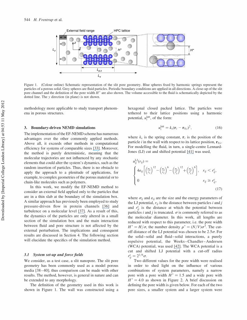
The definition of the geometry used in this work isshown in Figure 1. The wall was constructed using a

hexagonal closed packed lattice. The particles weretethered to their lattice positions using a harmonicpotential, ulatti , of the form:

ulatti ! ks"ri 2 r0;i#2; "16#

where ks is the spring constant, ri is the position of theparticle i in the wall with respect to its lattice position, r0;i.For modelling the fluid, in turn, a single-centre Lennard-Jones (LJ) cut and shifted potential [41] was used,

uLJij "rij# !

41ijsij

rij

( )122 sij

rij

( )62 sij

rcij

( )12% sij

rcij

( )6& '; rij , rcij;

0 rij $ rcij;

8>><

>>:

"17#

where sij and 1ij are the size and the energy parameters ofthe LJ potential, rij is the distance between particles i and jand rcij is the distance at which the potential betweenparticles i and j is truncated. s is commonly referred to asthe molecular diameter. In this work, all lengths arereduced with respect to this parameter, i.e. the pore widthH * ! H=s, the number density r* ! "N=V#s3. The cut-off distance of the LJ potential was chosen to be 2:5s. Forthe solid–solid and fluid–solid interactions, a purelyrepulsive potential, the Weeks–Chandler–Andersen(WCA) potential, was used [42]. The WCA potential is acut and shifted LJ potential with a cut-off radiusrcij ! 21=6s.

Two different values for the pore width were realisedin order to shed light on the influence of variouscombinations of system parameters, namely a narrowpore with a pore width H * ! 1:5 and a wide pore withH * ! 4:0 as shown in Figure 2. A brief discussion ondefining the pore width is given below. For each of the twopore sizes, a smaller system and a larger system were

External field range HPC lattice

Lx

H* H*

zx

Lp,x

Lz

Figure 1. (Colour online) Schematic representation of the slit pore geometry. Blue spheres fixed by harmonic springs represent theparticles of a porous solid. Grey spheres are fluid particles. Periodic boundary conditions are applied in all directions. A close-up of the slitpore channel and the definition of the pore width H * are also shown. The volume accessible to the fluid is schematically depicted by thedotted line. The y direction (in plane) is not shown.

H. Frentrup et al.544

Dow

nloa

ded

by [I

mpe

rial C

olle

ge L

ondo

n Li

brar

y] a

t 04:

53 1

1 M

ay 2

012

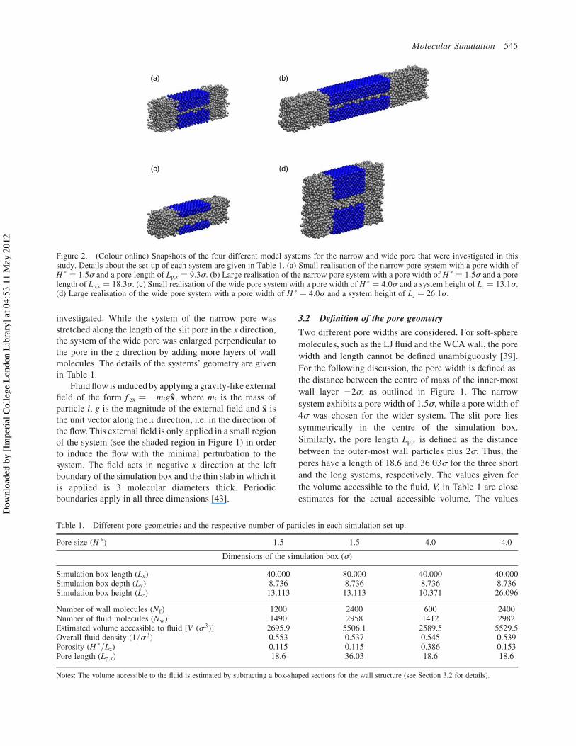
investigated. While the system of the narrow pore wasstretched along the length of the slit pore in the x direction,the system of the wide pore was enlarged perpendicular tothe pore in the z direction by adding more layers of wallmolecules. The details of the systems’ geometry are givenin Table 1.

Fluid flow is induced by applying a gravity-like externalfield of the form f ex ! 2migx, where mi is the mass ofparticle i, g is the magnitude of the external field and x isthe unit vector along the x direction, i.e. in the direction ofthe flow. This external field is only applied in a small regionof the system (see the shaded region in Figure 1) in orderto induce the flow with the minimal perturbation to thesystem. The field acts in negative x direction at the leftboundary of the simulation box and the thin slab in which itis applied is 3 molecular diameters thick. Periodicboundaries apply in all three dimensions [43].

3.2 Definition of the pore geometry

Two different pore widths are considered. For soft-sphere

molecules, such as the LJ fluid and the WCA wall, the pore

width and length cannot be defined unambiguously [39].

For the following discussion, the pore width is defined as

the distance between the centre of mass of the inner-most

wall layer 22s, as outlined in Figure 1. The narrow

system exhibits a pore width of 1:5s, while a pore width of4s was chosen for the wider system. The slit pore lies

symmetrically in the centre of the simulation box.

Similarly, the pore length Lp;x is defined as the distance

between the outer-most wall particles plus 2s. Thus, thepores have a length of 18.6 and 36:03s for the three short

and the long systems, respectively. The values given for

the volume accessible to the fluid, V, in Table 1 are close

estimates for the actual accessible volume. The values

Table 1. Different pore geometries and the respective number of particles in each simulation set-up.

Pore size (H *) 1.5 1.5 4.0 4.0

Dimensions of the simulation box (s)

Simulation box length (Lx) 40.000 80.000 40.000 40.000Simulation box depth (Ly) 8.736 8.736 8.736 8.736Simulation box height (Lz) 13.113 13.113 10.371 26.096

Number of wall molecules (Nf) 1200 2400 600 2400Number of fluid molecules (Nw) 1490 2958 1412 2982Estimated volume accessible to fluid [V (s 3)] 2695.9 5506.1 2589.5 5529.5Overall fluid density (1=s 3) 0.553 0.537 0.545 0.539Porosity (H *=Lz) 0.115 0.115 0.386 0.153Pore length (Lp;x) 18.6 36.03 18.6 18.6

Notes: The volume accessible to the fluid is estimated by subtracting a box-shaped sections for the wall structure (see Section 3.2 for details).

(a) (b)

(c) (d)

Figure 2. (Colour online) Snapshots of the four different model systems for the narrow and wide pore that were investigated in thisstudy. Details about the set-up of each system are given in Table 1. (a) Small realisation of the narrow pore system with a pore width ofH * ! 1:5s and a pore length of Lp;x ! 9:3s. (b) Large realisation of the narrow pore system with a pore width of H * ! 1:5s and a porelength of Lp;x ! 18:3s. (c) Small realisation of the wide pore system with a pore width of H * ! 4:0s and a system height of Lz ! 13:1s.(d) Large realisation of the wide pore system with a pore width of H * ! 4:0s and a system height of Lz ! 26:1s.

Molecular Simulation 545

Dow

nloa

ded

by [I

mpe

rial C

olle

ge L

ondo

n Li

brar

y] a

t 04:

53 1

1 M

ay 2

012

were calculated by subtracting the volume of the porousmedium from the entire box volume (Vest ! &"LxLz#2Lp;x"Lz 2 H *#'Ly), meaning that smooth edges of the porewall were not explicitly taken into account.

3.3 Molecular simulation details

Since the external field performs work on the system whichlater must be dissipated as heat, the temperature of thesystem must be carefully controlled by a thermostat.A Gaussian thermostat [44], i.e. an isokinetic thermostat, isapplied only to the particles belonging to the wall. Thus, theheat generated in the fluid is removed from the system viathe wall structure by the interaction between the wall andthe fluid, leaving the motion of the fluid moleculesunperturbed by the thermostat. Most off-the-shelf MDprogrammes will by default apply the thermostat to thefluid, something that will inevitably lead to spurious results.

The equations of motion for the particles in the wall aregiven by

dri"t#dt

! vi"t#;

dvi"t#dt

! f i"t#mi

2 x"t#vi"t#; "18#

subject to the constraint

dT "t#dt

! d

dt

1

kBNdof

XNw

i!1

mivi"t#$vi"t# !

! 0; "19#

where vi"t# and f i"t# denote the velocity and the total forceof particles i, respectively, kB is the Boltzmann constant,Nw is the total number of particles of the wall and Ndof isthe number of degrees of freedom. The parameter x"t# inEquation (18) is a friction coefficient that guarantees aconstant kinetic temperature T . The equations of motionare integrated using the leap-frog algorithm [44]. Sincethe fluid particles are not subject to any thermostat, theequations of motion that govern their dynamics are thesame as in Equation (18) setting x"t# ! 0 at every timestep. To achieve an increase in computational efficiency, aVerlet list of closest neighbours is employed whencalculating the forces for each time step [34]. The listsphere radius was chosen to be 1:0s.

In this work, thermodynamic and structural propertiesare expressed in reduced variables for temperature, densityand time. The quantities are defined as T * ! kBT=1, r* !Nfs3=V and t * ! t

*****************"m1=s2#

p. The LJ parameters and m,

which represents the molecular weight, can be used toexpress all other units of interest.

The central observable when investigating masstransport phenomena is the molecular flux. The flux inthe x direction can be directly measured by counting thenumber of molecules crossing the x ! 0 plane as a

function of time and in relation to the accessible area in thexy plane Ayz,

Ji !N%

i 2 N2i

trunAyz; "20#

where Ji denotes the molar flux of species i, N%i and N2

i

denote the amount of molecules of species i which havepassed the plane in the time trun in positive and negative xdirection, respectively. Alternatively, the flux could becalculated by evaluating the corresponding average ensem-ble velocity times the system density in the x direction.

Each system was equilibrated for 400,000 time stepswith no external forces applied. Then, with the externalfield applied, simulations ran for 2.5 million time stepsafter an equilibration period of 250,000 time steps. In allsimulations, the time step was chosen to be t * ! 0:01.In order to avoid phase separation within the system, thetemperature was chosen to be at a super-critical value,T * ! 1:5. The fluid densities are close to 0.5. The actualdensity of each system is not uniform and an averagedensity can only be estimated from the number ofmolecules over the volume accessible to the fluid.The values of average density are given in Table 1.Several runs were performed for each state point to give ameasure for the error to be expected from the simulations.

4. Results and discussion

The dynamics of the mass transport obviously depend onthe magnitude of the external field applied to the system.The response to the external field is also influenced by thearchitecture of the porous media. The impact of theperturbation on the mechanical and thermal equilibriumand the results for the different systems are shown inFigure 2 and are discussed in the following section.In particular, the density distribution, the kinetictemperature and the average particle velocities wereinvestigated closely and the respective quantities, whichcharacterise mass transfer, such as effective diffusivities,were calculated. Finally, a discussion on simulatingcounter fluxes follows.

4.1 Unidirectional mass transport

Due to the application of the external field, the density is notuniform in the entire system. The external force, acting in thenegative x direction, builds up a pressurised bulk on the rightof the porous structure, provoking an increase in density inthe right bulk region. The fluid is squeezed into the porousstructure andflowdevelops in the slit-pore.While the densityin the bulk region is uniform for a moderate perturbation, alinear density gradient develops within the pore. In order toquantify the differences in density, the density distributionalong the length of the pore was measured. To this end, the

H. Frentrup et al.546

Dow

nloa

ded

by [I

mpe

rial C

olle

ge L

ondo

n Li

brar

y] a

t 04:

53 1

1 M

ay 2

012

simulation box was divided into thin slabs. For each slab,the average amount of molecules was measured during thesimulation and a density profile along the x direction,the direction of flow, could be obtained. Moreover, to assessthe heat transport within the system, the kinetic temperaturewas measured in the same fashion.

Density profiles of three exemplary cases in terms ofsystem geometry are shown in Figure 3 for f ex ! 0:2 and0:51=s. Density profiles for all other conditions can betaken from the supplementary material.

4.1.1 Effective diffusivities

The simulations yield a difference in density as well as theflux triggered by this density gradient. Equation (11)establishes the relationship between the flux and a gradientin density via the effective diffusion coefficient. With thebulk densities available from the simulations, the densitygradient can be expressed as

Dr

Dx! rright 2 rleft

Lp;x

" #; "21#

where Lp;x is the length of the respective pore. Hence, thetransport equation can be expressed as follows:

Jx < 2DeffDr

Dx

" #: "22#

The dependence of Deff on the external force is plottedin Figure 4. The figure shows that the effective diffusivityis not independent of the external field applied. As isexpected, Deff increases with the magnitude of the externalfield. Also, the results for the larger and the smaller systemdeviate from each other; as entrance effects play a largerrole for the smaller system, a lower effective diffusioncoefficient for the small system is expected.

The quantity of interest, of course, is the limit ofDeff asthe force tends to zero [45], corresponding to the transportdiffusion coefficient Dt. As can be seen in Figure 4, thisquantity is independent of the size of the system, and bothsmall and large realisations of each pore width coincide.For H * ! 1:5, an effective diffusion coefficient for avanishing external force field is "Deff#jf ex!0 ! 9:55"5#,where the number in parentheses gives the uncertainty inthe last digit. ForH * ! 4:0, "Deff#jf ex!0 is equal to 18.6(1).Certainly, the coefficient changes with the available poreopening as expected. There is a compromise betweenapplying an extremely small external force, which wouldguarantee that the system remains in the linear regime(thus extrapolation to zero force would be meaningful) but

0.3

0.4

0.5

0.6

0.7

0.8

–20 –15 –10 –5 0 5 10 15 20

r [1

/s3 ]

x [s]

(a)

0.3

0.4

0.5

0.6

0.7

0.8

–20 –15 –10 –5 0 5 10 15 20

r [1

/s3 ]

x [s]

(b)

Figure 3. (Colour online) Selected density profiles along the length of the simulation box, i.e. in x direction. (a) f ex ! 0:21=s and (b)f ex ! 0:51=s. Solid red lines represent the profile for the small realisation of the arrow pore. Blue and green lines depict the small and thelarge realisation of the wide pore, respectively.

0

10

20

30

40

50

60

0 0.2 0.4 0.6 0.8

Diff

usiv

ity D

eff [

s (e

/m)1/

2 ]

fex [e/s ]

Figure 4. Effective diffusivities for the narrow and wide pore.Circles (small realisation) and squares (large realisation) denotethe narrow pore system; triangles (small realisation) anddiamonds (large realisation) denote the wide pore system. Thedashed lines are a quadratic fit to the simulation results. Errors areestimated as the deviation between several runs for the samepoint. In general, the error bars are smaller than the symbols,though.

Molecular Simulation 547

Dow

nloa

ded

by [I

mpe

rial C

olle

ge L

ondo

n Li

brar

y] a

t 04:

53 1

1 M

ay 2

012

would exhibit poor statistics due to the poorly developedflow and a large external flow which produces an efficientsimulation and smaller fluctuations but may correspond toan excessive perturbation of the system. There is no recipefor the precise magnitude of the force to be used.

For the case that is under scrutiny here, the masstransport coefficient does not only account for collectiveself-diffusion, but includes the resistance to promoting aflow. With an increasing density gradient, and thereforealso an increasing pressure difference between the twobulk sections, this resistive component also increases. Theincrease in the average fluid velocity vx points to this aswell. Thus, it can be argued that this convectivecomponent becomes canonical in the limit of f ex ! 0,and it is in this limit that the effective diffusivity equals thetransport diffusivity Dt.

4.1.2 Fluid structure

It can be seen in Figure 3 that the density profile inside thepore shows a regular undulation pattern. These undula-tions can be attributed to the uneven topology of the poresurface. The issue is related to the fact that it is not possibleto define an unambiguous pore size mentioned in Section3.2. Since the slit pore is a structured wall consisting ofsoft spheres, the surface of the slit pore is not flat but has asmooth and wavy surface. The fluid has more space toexpand where there are dents in the pore surface. What ismore, the wall molecules are not still but rather vibrateabout their lattice positions. The roughness of the poresurface was not explicitly taken into account when thedensity profile was calculated. This feature does not hinderthe analysis of the simulations since average values alongthe pore are considered.

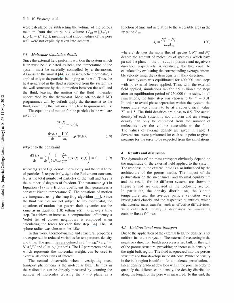
A typical set of density profiles [39] in the z directioncan be seen in Figure 5. Although the walls are softlyrepulsive, it can be seen that the fluid forms well-definedadsorbed layers and travels preferentially along the wall.This is seen more clearly in the wider pore, where the samephenomena occurs. In this case, however, the fluid in themiddle of the pore shows no structure.

Measuring the density in the bulk regions is anuncomplicated task as the available volume in these regionsis correctly defined. However, the density within the pore issubject to the complications in defining the pore width.Furthermore, at the entrance and exit of the pore, theavailable volume changes in an abrupt fashion, going frombulk to confinement. This point transitionwas not explicitlytaken into account in the density profiles as it creates thespikes in the profiles. The spikes are located at the entranceand exit of the slit pore. The average density in the bulksections was taken only from the simulations from whichthe difference in density could be calculated unambigu-ously. Figure 3(a) shows that a weak external force invokesa linear response in the density distribution at these

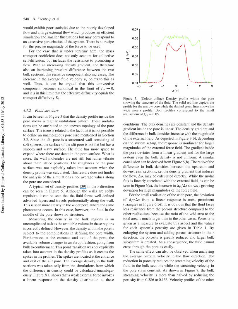
conditions. The bulk densities are constant and the densitygradient inside the pore is linear. The density gradient andthe difference in bulk densities increase with the magnitudeof the external field. As depicted in Figure 3(b), dependingon the system set-up, the response is nonlinear for largermagnitudes of the external force field. The gradient insidethe pore deviates from a linear gradient and for the largesystem even the bulk density is not uniform. A similarconclusion can be derived from Figure 6(b). The ratio of thedifference in bulk densities between the upstream anddownstream sections, i.e. the density gradient that inducesthe flow, Dr, may be calculated directly. While the molarflux is linearly correlated with the external field, as can beseen in Figure 6(a), the increase inDr=Dx shows a growingdeviation for high magnitudes of the force field.

For the small realisation of the wide pore, the deviationof Dr=Dx from a linear response is most prominent(triangles in Figure 6(b)). It is obvious that the fluid facesless resistance from the porous structure compared to theother realisations because the ratio of the void area to thetotal area is much larger than in the other cases. Porosity isgiven as a measure to evaluate this aspect and the valuesfor each system’s porosity are given in Table 1. Byenlarging the system and adding porous structure in the zdirection, the porosity is greatly reduced and larger bulksubsystem is created. As a consequence, the fluid cannotcross through the pore as easily.

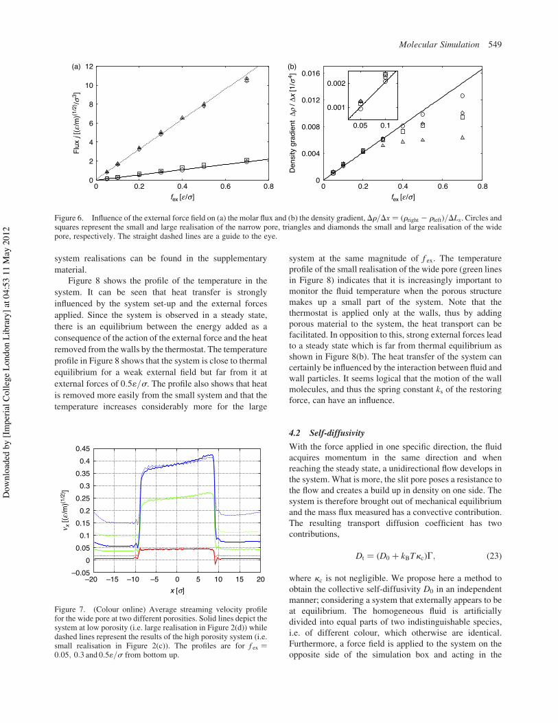
The same effect can also be observed when analysingthe average particle velocity in the flow direction. Thereduction in porosity reduces the streaming velocity of thefluid in the bulk sections while the streaming velocity inthe pore stays constant. As shown in Figure 7, the bulkstreaming velocity is more than halved by reducing theporosity from 0.386 to 0.153. Velocity profiles of the other

0.01

0.02

0.03

0.04

0.05

0.06

0.07

–3 –2 –1 0 1 2 3

r [1

/s3 ]

z [s]

Figure 5. (Colour online) Density profile within the poreshowing the structure of the fluid. The solid red line depicts theprofile for the narrow pore while the dashed green lines shows thewide pore’s profile. Both profiles correspond to the smallrealisations at f ex ! 0:05.

H. Frentrup et al.548

Dow

nloa

ded

by [I

mpe

rial C

olle

ge L

ondo

n Li

brar

y] a

t 04:

53 1

1 M

ay 2

012

system realisations can be found in the supplementary

material.Figure 8 shows the profile of the temperature in the

system. It can be seen that heat transfer is strongly

influenced by the system set-up and the external forces

applied. Since the system is observed in a steady state,

there is an equilibrium between the energy added as a

consequence of the action of the external force and the heat

removed from the walls by the thermostat. The temperature

profile in Figure 8 shows that the system is close to thermal

equilibrium for a weak external field but far from it at

external forces of 0:51=s. The profile also shows that heatis removed more easily from the small system and that the

temperature increases considerably more for the large

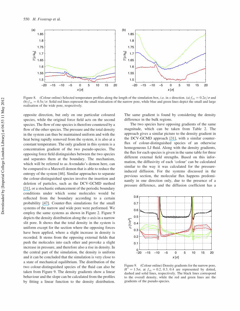
system at the same magnitude of f ex. The temperatureprofile of the small realisation of the wide pore (green linesin Figure 8) indicates that it is increasingly important tomonitor the fluid temperature when the porous structuremakes up a small part of the system. Note that thethermostat is applied only at the walls, thus by addingporous material to the system, the heat transport can befacilitated. In opposition to this, strong external forces leadto a steady state which is far from thermal equilibrium asshown in Figure 8(b). The heat transfer of the system cancertainly be influenced by the interaction between fluid andwall particles. It seems logical that the motion of the wallmolecules, and thus the spring constant ks of the restoringforce, can have an influence.

4.2 Self-diffusivity

With the force applied in one specific direction, the fluidacquires momentum in the same direction and whenreaching the steady state, a unidirectional flow develops inthe system. What is more, the slit pore poses a resistance tothe flow and creates a build up in density on one side. Thesystem is therefore brought out of mechanical equilibriumand the mass flux measured has a convective contribution.The resulting transport diffusion coefficient has twocontributions,

Dt ! D0 % kBTkc" #G; "23#

where kc is not negligible. We propose here a method toobtain the collective self-diffusivity D0 in an independentmanner; considering a system that externally appears to beat equilibrium. The homogeneous fluid is artificiallydivided into equal parts of two indistinguishable species,i.e. of different colour, which otherwise are identical.Furthermore, a force field is applied to the system on theopposite side of the simulation box and acting in the

–0.050

0.050.1

0.150.2

0.250.3

0.350.4

0.45

–20 –15 –10 –5 0 5 10 15 20

n x [(

e/m

)(1/2

) ]

x [s]

Figure 7. (Colour online) Average streaming velocity profilefor the wide pore at two different porosities. Solid lines depict thesystem at low porosity (i.e. large realisation in Figure 2(d)) whiledashed lines represent the results of the high porosity system (i.e.small realisation in Figure 2(c)). The profiles are for f ex !0:05; 0:3 and 0:51=s from bottom up.

0

2

4

6

8

10

12

0 0.2 0.4 0.6 0.8

Flux

j [(e

/m)(1

/2) /s

3 ]

fex [e/s]0 0.2 0.4 0.6 0.8

fex [e/s]

(a) (b)

0

0.004

0.008

0.012

0.016

Den

sity

gra

dien

t Δr

/ Δx

[1/s

4 ]

0.001

0.002

0.05 0.1

Figure 6. Influence of the external force field on (a) the molar flux and (b) the density gradient, Dr=Dx ! "rright 2 rleft#=DLx. Circles andsquares represent the small and large realisation of the narrow pore, triangles and diamonds the small and large realisation of the widepore, respectively. The straight dashed lines are a guide to the eye.

Molecular Simulation 549

Dow

nloa

ded

by [I

mpe

rial C

olle

ge L

ondo

n Li

brar

y] a

t 04:

53 1

1 M

ay 2

012

opposite direction, but only on one particular coloured

species, while the original force field acts on the second

species. The flow of one species is therefore countered by a

flow of the other species. The pressure and the total density

in the system can thus be maintained uniform and with the

heat being rapidly removed from the system, it is also at a

constant temperature. The only gradient in this system is a

concentration gradient of the two pseudo-species. The

opposing force field distinguishes between the two species

and separates them at the boundary. The mechanism,

which will be referred to as Avendano’s demon here, can

be compared to a Maxwell demon that is able to reduce the

entropy of the system [46]. Similar approaches to separate

the colour-distinguished species involve the insertion and

deletion of particles, such as the DCV-GCMD method

[31], or a stochastic enhancement of the periodic boundary

conditions under which some molecules would be

reflected from the boundary according to a certain

probability [47]. Counter-flux simulations for the small

systems of the narrow and wide pore were performed. We

employ the same systems as shown in Figure 2. Figure 9

depicts the density distribution along the x-axis in a narrow

slit pore. It shows that the total density in the system is

uniform except for the section where the opposing forces

have been applied, where a slight increase in density is

recorded. It stems from the opposing external fields that

push the molecules into each other and provoke a slight

increase in pressure, and therefore also a rise in density. In

the central part of the simulation, the density is uniform

and it can be concluded that the simulation is very close to

a state of mechanical equilibrium. The distribution of the

two colour-distinguished species of the fluid can also be

taken from Figure 9. The density gradients show a linear

behaviour and the slope can be calculated from the profiles

by fitting a linear function to the density distribution.

The same gradient is found by considering the densitydifference in the bulk regions.

The two species have opposing gradients of the samemagnitude, which can be taken from Table 2. Theapproach gives a similar picture to the density gradient inthe DCV-GCMD approach [31], with a similar counter-flux of colour-distinguished species of an otherwisehomogeneous LJ fluid. Along with the density gradients,the flux for each species is given in the same table for threedifferent external field strengths. Based on this infor-mation, the diffusivity of each ‘colour’ can be calculatedsimilar to the way it was calculated for the pressure-induced diffusion. For the systems discussed in theprevious section, the molecular flux happens predomi-nantly in one direction only, due to the presence of apressure difference, and the diffusion coefficient has a

1.5

1.6

1.55

1.65

1.75

1.7

1.8

1.85

–20 –15 –10 –5 0 5 10 15 20

T [e

/kB]

x [s]–20 –15 –10 –5 0 5 10 15 20

x [s]

(a)

1.5

1.6

1.55

1.65

1.75

1.7

1.8

1.85

T [e

/kB]

(b)

Figure 8. (Colour online) Selected temperature profiles along the length of the simulation box, i.e. in x direction. (a) f ex ! 0:21=s and(b) f ex ! 0:51=s. Solid red lines represent the small realisation of the narrow pore, while blue and green lines depict the small and largerealisation of the wide pore, respectively.

0

0.1

0.2

0.3

0.4

0.5

0.6

0.7

0.8

–20 –15 –10 –5 0 5 10 15 20

r [1

/s3 ]

x [s]

Figure 9. (Colour online) Density gradients for the narrow pore,H * ! 1:5s, at f ex ! 0:2; 0:3; 0:4 are represented by dotted,dashed and solid lines, respectively. The black lines correspondto the overall density, while the red and green lines are thegradients of the pseudo-species.

H. Frentrup et al.550

Dow

nloa

ded

by [I

mpe

rial C

olle

ge L

ondo

n Li

brar

y] a

t 04:

53 1

1 M

ay 2

012

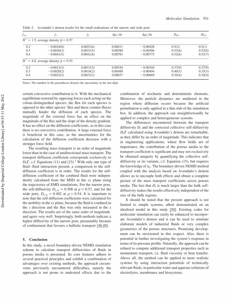
certain convective contribution to it. With the mechanicalequilibrium restored by opposing forces each acting on thecolour-distinguished species, the flux for each species isopposed to the other species’ flux and these counter-fluxesmutually hinder the diffusion of each species. Themagnitude of the external force has an effect on themagnitude of the flux and the slope of the density gradient.It has no effect on the diffusion coefficients, as in this casethere is no convective contribution. A large external forceis beneficial in this case, as the uncertainties for thecalculation of the diffusion coefficient decrease with astronger force field.

The resulting mass transport is an order of magnitudelower than in the case of unidirectional mass transport. Thetransport diffusion coefficient corresponds exclusively toD0G, c.f. Equations (11) and (23).1 With only one type offluid–fluid interaction present, a comparison to the self-diffusion coefficient is in order. The results for the self-diffusion coefficient of the confined fluid were indepen-dently calculated from the MSD in the xy plane usingthe trajectories of EMD simulations. For the narrow pore,the self-diffusivity Ds;xy ! 0:508 at r ! 0:57, and for thewide pore, Ds;xy ! 0:402 at r ! 0:54. It is important tonote that the self-diffusion coefficients were calculated forthe mobility in the xy plane, because the fluid is confined inthe z direction and the flux was only measured in the xdirection. The results are of the same order of magnitudeand agree very well. Surprisingly, both methods indicate ahigher diffusivity of the narrow pore, presumably becauseof confinement that favours a ballistic transport [48,49].

5. Conclusion

In this study, a novel boundary-driven NEMD simulationscheme to calculate transport diffusivities of fluids inporous media is presented. Its core features adhere toseveral practical principles and exhibit a combination ofadvantages over existing methods, the approach circum-vents previously encountered difficulties, namely theapproach is not prone to undesired effects due to the

combination of stochastic and deterministic elements.

Moreover, the particle dynamics are unaltered in the

region where diffusion occurs because the artificial

perturbation is only applied in a thin slab of the simulation

box. In addition, the approach can straightforwardly be

applied to complex and heterogeneous systems.The differences encountered between the transport

diffusivity Dt and the corrected collective self-diffusivity

D0G calculated using Avendano’s demon are remarkable,

as they differ by an order of magnitude. This indicates that

in engineering applications, where flow fields are of

importance, the contribution of the porous media to the

transport coefficient is significant and may not exclusively

be obtained uniquely by quantifying the collective self-

diffusivity or its variants, c.f. Equation (15), but requires

the knowledge of kc. The boundary-driven NEMDmethod

coupled with the analysis based on Avendano’s demon

allows us to uncouple both effects and obtain a complete

picture of the mass transport coefficients across porous

media. The fact that Dt is much larger than the bulk self-

diffusivity makes the results effectively independent of the

size of the bulk regions.It should be noted that the present approach is not

limited to simple systems, albeit demonstrated on an

idealised model in this study [50]. Existing codes for

molecular simulation can easily be enhanced to incorpor-

ate Avendano’s demon and it can be used to simulate

elaborate models of industrial fluids or very complex

geometries of the porous structures. Promising develop-

ment can be envisioned in this respect. Also, there is

potential in further investigating the system’s response in

terms of its pressure profile. Naturally, the approach can be

refined to compute additional transport properties such as

momentum transport, i.e. fluid viscosity or heat transfer.

Above all, the method can be applied to more realistic

systems by using interaction potentials of technically

relevant fluids, in particular water and aqueous solutions of

electrolytes, membranes and biosystems.

Table 2. Avendano’s demon results for the small realisations of the narrow and wide pore.

f ex j1 j2 dr1=dx dr2=dx D0;1 D0;2

H * ! 1:5, average density r ! 0:57

0.2 20.0018(6) 0.0021(6) 0.00411 20.00428 0.5(2) 0.5(1)0.3 20.0030(3) 0.0031(5) 0.00580 20.00586 0.53(6) 0.52(8)0.4 20.0041(5) 0.0041(6) 0.00781 20.00775 0.52(6) 0.53(7)

H * ! 4:0, average density r ! 0:55

0.2 20.0012(3) 0.0013(3) 0.00336 20.00344 0.37(9) 0.37(9)0.3 20.0020(2) 0.0018(2) 0.00489 20.00494 0.40(3) 0.35(3)0.4 20.0025(3) 0.0023(3) 0.00657 20.00669 0.39(4) 0.39(4)

Notes: The number in the parentheses denotes the uncertainty in the last digit.

Molecular Simulation 551

Dow

nloa

ded

by [I

mpe

rial C

olle

ge L

ondo

n Li

brar

y] a

t 04:

53 1

1 M

ay 2

012

Acknowledgements

The authors would like to extend their gratitude to the GermanAcademic Exchange Service (DAAD) for their financial supportthrough the DAAD postdoctoral project on ‘methods and toolsfor the non-equilibrium analysis of nanoscopic interfaces’ to MHand through a ‘research abroad fellowship’ to HF, who alsowishes to thank Prof. Joachim Gross for his continuing supportand helpful insight. Fruitful discussion with Prof. Suresh Bhatiais gratefully acknowledged. The authors would also like to thankthe German Research Foundation (DFG) for establishing thecollaborative research centre (SFB) 926 on ‘microscalemorphology of component surfaces’ (MICOS). The authorswould also like to thank the Engineering and Physical ScienceResearch Council (EPSRC) for financial support under the‘Molecular Systems Engineering’ grant (EP/E016340) andthrough a Doctoral Training Award to AS.

References[1] T. Humplik, J. Lee, S.C. O’Hern, B.A. Fellman, M.A. Baig,

S.F. Hassan, M.A. Atieh, F. Rahman, T. Laoui, R. Karnik, andE.N. Wang, Nanostructured materials for water desalination,Nanotechnology 22 (2011), 292001.

[2] J.K. Holt, H.G. Park, Y. Wang, M. Stadermann, A.B. Artyukhin,C.P. Grigoropoulos, A. Noy, and O. Bakajin, Fast mass transportthrough sub-2-nanometer carbon nanotubes, Science 312 (2006),pp. 1034–1037.

[3] P. Abgrall and N.T. Nguyen, Nanofluidic devices and theirapplications, Anal. Chem. 80 (2008), pp. 2326–2341.

[4] J.C. Rasaiah, S. Garde, and G. Hummer, Water in nonpolarconfinement: From nanotubes to proteins and beyond, Annu. Rev.Phys. Chem. 59 (2008), pp. 713–740.

[5] J. Goldsmith and C.C. Martens, Molecular dynamics simulation ofsalt rejection in model surface-modified nanopores, J. Phys. Chem.Lett. 1 (2010), pp. 528–535.

[6] S.K. Bhatia, M.R. Bonilla, and D. Nicholson,Molecular transport innanopores: A theoretical perspective, Phys. Chem. Chem. Phys. 13(2011), pp. 15350–15383.

[7] K.P. Travis, B.D. Todd, and D.J. Evans, Departure from Navier–Stokes hydrodynamics in confined liquids, Phys. Rev. E 55 (1997),pp. 4288–4295.

[8] W. Bowen and J. Welfoot, Predictive modelling of nanofiltration:Membrane specification and process optimisation, Desalination 147(2002), pp. 197–203.

[9] K.E. Gubbins, Y. Liu, J.D. Moore, and J.C. Palmer, The role ofmolecular modeling in confined systems: Impact and prospects,Phys. Chem. Chem. Phys. 13 (2011), pp. 58–85.

[10] E.J. Maginn and J.R. Elliott, Historical perspective and currentoutlook for molecular dynamics as a chemical engineering tool, Ind.Eng. Chem. Res. 49 (2010), pp. 3059–3078.

[11] D.N. Theodorou, Progress and outlook in Monte Carlo simulations,Ind. Eng. Chem. Res. 49 (2010), pp. 3047–3058.

[12] R. Krishna and J.A. Wesselingh, The Maxwell–Stefan approach tomass transfer, Chem. Eng. Sci. 52 (1997), pp. 861–911.

[13] S.K. Bhatia and D. Nicholson, Modelling self-diffusion of simplefluids in nanopores, J. Phys. Chem. B 115 (2011), pp. 11700–11711.

[14] O. Jepps, S. Bhatia, and D. Searles, Wall mediated transport inconfined spaces: Exact theory for low density, Phys. Rev. Lett. 91(2003), p. 126102.

[15] D.J. Keffer, C.Y. Gao, and B.J. Edwards, On the relationshipbetween Fickian diffusivities at the continuum and molecular levels,J. Phys. Chem. B 109 (2005), pp. 5279–5288.

[16] A. Einstein, Uber die von der molekularkinetischen Theorie derWarme geforderte Bewegung von in ruhenden Flussigkeitensuspendierten Teilchen, Annalen der Physik 322 (1905),pp. 549–560.

[17] E.J. Maginn, A.T. Bell, and D.N. Theodorou, Transport diffusivityof methane in silicalite from equilibrium and nonequilibriumsimulations, J. Phys. Chem. 97 (1993), pp. 4173–4181.

[18] P.M. Chaikin and T.C. Lubensky, Principles of Condensed MatterPhysics, Cambridge University Press, New York, NY, 1995.

[19] R. Kubo, Statistical-mechanical theory of irreversible processes.I. General theory and simple applications to magnetic andconduction problems, J. Phys. Soc. Jpn 12 (1957), pp. 570–586.

[20] D. Nicholson, The transport of adsorbate mixtures in porousmaterials: Basic equations for pores with simple geometry,J. Membrane Sci. 129 (1997), pp. 209–219.

[21] R.B. Bird, W.E. Stewart, and E.N. Lightfoot, Transport phenomena,2nd ed., Wiley, New York, 2002.

[22] J. Karger and D.M. Ruthven, Diffusion in zeolites and othermicroporous solids, Wiley-Blackwell, New York, 1992.

[23] E.L. Cussler, Diffusion: Mass transfer in fluid systems, 3rd ed.,Cambridge University Press, New York, 2009.

[24] K. Travis and K. Gubbins, Combined diffusive and viscoustransport of methane in a carbon slit pore, Mol. Simulat. 25 (2000),pp. 209–227.

[25] S. Bhatia and D. Nicholson, Hydrodynamic origin of diffusion innanopores, Phys. Rev. Lett. 90 (2003), 016105.

[26] R. Krishna, Describing the diffusion of guest molecules insideporous structures, J. Phys. Chem. C 113 (2009), pp. 19756–19781.

[27] S. Chempath, R. Krishna, and R.Q. Snurr, Non-equilibriummolecular dynamics simulations of diffusion of binary mixturescontaining short n-alkanes in faujasite, J. Phys. Chem. B 108(2004), pp. 13481–13491.

[28] Y. Wang and M.D. LeVan, Mixture diffusion in nanoporousadsorbents: Equivalence of Fickian and Maxwell-Stefanapproaches, J. Phys. Chem. B 112 (2008), pp. 8600–8604.

[29] D. Evans and O. Morriss, Non-Newtonian molecular dynamics,Comput. Phys. Rep. 1 (1984), pp. 297–343.

[30] A. Salih, Molecular simulation of the adsorption and transportproperties of carbon dioxide, methane, water and their mixtures incoal-like structures, Ph.D. diss., Imperial College London, London,UK, 2010.

[31] G.S. Heffelfinger and F. van Swol, Diffusion in Lennard-Jonesfluids using dual control volume grand canonical moleculardynamics simulation (DCV-GCMD), J. Chem. Phys. 100 (1994),pp. 7548–7552.

[32] T. Duren, F.J. Keil, and N.A. Seaton, Molecular simulation ofadsorption and transport diffusion of model fluids in carbonnanotubes, Mol. Phys. 100 (2002), pp. 3741–3751.

[33] G. Arya, H.C. Chang, and E.J. Maginn, A critical comparison ofequilibrium, non-equilibrium and boundary-driven moleculardynamics techniques for studying transport in microporousmaterials, J. Chem. Phys. 115 (2001), pp. 8112–8124.

[34] M. Allen and D. Tildesley, Computer Simulation of Liquids, OxfordUniversity Press, Oxford, 1987.

[35] M. Horsch, J. Vrabec, M. Bernreuther, and H. Hasse, Poiseuille flowof liquid methane in nanoscopic graphite channels by moleculardynamics simulation, in Proceedings of the International Sym-posium on Turbulence, Heat and Mass Transfer, Vol. 6, BegellHouse, New York, 2009, pp. 89–92.

[36] F. Zhu, E. Tajkhorshid, and K. Schulten, Pressure-induced watertransport in membrane channels studied by molecular dynamics,Biophys. J. 83 (2002), pp. 154–160.

[37] J. Castillo-Tejas, A. Rojas-Morales, F. Lopez-Medina,J.F.J. Alvarado, G. Luna-Barcenas, F. Bautista, and O. Manero,Flow of linear molecules through a 4:1:4 contraction-expansionusing non-equilibrium molecular dynamics: Extensional rheologyand pressure drop, J. Non-Newtonian Fluid Mech. 161 (2009),pp. 48–59.

[38] Q. Cai, M.J. Biggs, and N.A. Seaton, Effect of pore wall model onprediction of diffusion coefficients for graphitic slit pores,Phys. Chem. Chem. Phys. 10 (2008), pp. 2519–2527.

[39] K.P. Travis and K.E. Gubbins, Poiseuille flow of Lennard-Jonesfluids in narrow slit pores, J. Chem. Phys. 112 (2000),pp. 1984–1994.

[40] R. Cracknell, D. Nicholson, and N. Quirke, Direct moleculardynamics simulation of flow down a chemical potential gradient in aslit-shaped micropore, Phys. Rev. Lett. 74 (1995), pp. 2463–2466.

[41] J. Vrabec, G.K. Kedia, G. Fuchs, and H. Hasse, Comprehensivestudy of the vapour-liquid coexistence of the truncated and shifted

H. Frentrup et al.552

Dow

nloa

ded

by [I

mpe

rial C

olle

ge L

ondo

n Li

brar

y] a

t 04:

53 1

1 M

ay 2

012

Lennard-Jones fluid including planar and spherical interfaceproperties, Mol. Phys. 104 (2006), pp. 1509–1527.

[42] J.D. Weeks, D. Chandler, and H.C. Andersen, Role of repulsiveforces in determining the equilibrium structure of simple liquids,J. Chem. Phys. 54 (1971), pp. 5237–5247.

[43] D. Frenkel and B. Smit, Understanding Molecular Simulation,2nd ed., Academic Press, London, 1996.

[44] D. Brown and J. Clarke, A comparison of constant energy, constanttemperature and constant pressure ensembles in moleculardynamics simulations of atomic liquids, Mol. Phys. 51 (1984),pp. 1243–1252.

[45] S. Kjelstrup, D. Bedeaux, E. Johannessen, and J. Gross, Non-equilibrium thermodynamics for engineers, 1st ed., World ScientificPublishing Company, Singapore, 2010.

[46] W. Thomson, The Sorting Demon of Maxwell, Proceedings of theRoyal Institution 9 (1879), pp. 113–114.

[47] J.R. Whitman, G.L. Aranovich, and M.D. Donohue, Thermodyn-amic driving force for diffusion: Comparison between theory andsimulation, J. Chem. Phys. 134 (2011), p. 094303.

[48] F.J.A.L. Cruz and E.A. Muller, Behavior of ethylene and ethanewithin single-walled carbon nanotubes, 2: Dynamical properties,Adsorption 15 (2009), pp. 13–22.

[49] A. Barati Farimani and N.R. Aluru, Spatial diffusion of water incarbon nanotubes: From Fickian to ballistic motion, J. Phys. Chem.B 115 (2011), pp. 12145–12149.

[50] D.S. Sholl, Understanding macroscopic diffusion of adsorbedmolecules in crystalline nanoporous materials via atomisticsimulations, Acc. Chem. Res. 39 (2006), pp. 403–411.

Molecular Simulation 553

Dow

nloa

ded

by [I

mpe

rial C

olle

ge L

ondo

n Li

brar

y] a

t 04:

53 1

1 M

ay 2

012