Tracking individual fish from a moving platform usinga split-beam transducer

Nils Olav Handegard,a� Ruben Patel, and Vidar HjellvikInstitute of Marine Research, P.O. Box 1870 Nordnes, N-5817 Bergen, Norway

�Received 16 May 2003; revised 11 July 2005; accepted 11 July 2005�

Tracking of individual fish targets using a split-beam echosounder is a common method forinvestigating fish behavior. When mounted on a floating platform like a ship or a buoy, thetransducer movement often complicates the process. This paper presents a framework for trackingsingle targets from such a platform. A filter based on the correlated fish movements between pingsis developed to estimate the platform movement, and an extended Kalman filter is used to combinethe split-beam measurements and the platform-position estimates. Different methods for gating anddata association are implemented and tested with respect to data-association errors, using manuallytracked data from a free-floating buoy as a reference. The data association was improved by utilizingthe estimated velocity for each track to predict the location of the next observation. The dataassociation was more robust when estimates of platform tilt/roll were used. Other techniques toestimate position and velocity, like linear regression and smoothing splines, were implemented andtested on a simulated data set. The platform-state estimation improved the estimates for methods likethe Kalman filter and a smoothing spline with cross validation, but not for robust methods like linearregression and smoothing spline with a fixed degree of smoothing. © 2005 Acoustical Society ofAmerica. �DOI: 10.1121/1.2011410�

PACS number�s�: 43.30.Sf �KGF� Pages: 2210–2223

I. INTRODUCTION

The split-beam echosounder has become an importanttool for investigating fish behavior. It provides four-dimensional observations �range, two angles, and time�,making it possible to track objects over a period, thus obtain-ing information about fish movements in the acousticbeam.1,2 The technique has several applications, includingstudies of migratory behavior, vessel-avoidance effects, andcounting fish. Tracking objects with a split-beam echo-sounder is fairly easy for well-defined targets observed by afixed transducer, but is more difficult if the targets are weakand/or the transducer platform is unstable.

The concept of the “single echo” often arises in fisheriesacoustics. This is the echo formed by one fish in isolation.The split-beam echosounder measures the range and the an-gular direction to the target, and an algorithm for single-echodetection �SED� is used to detect these echoes, discardingany that have overlapping contributions from more than onefish. Different single-target algorithms have been tested, andit was found that algorithms based on the phase stability�measured by the standard deviation of the phase angle� re-jected multiple targets most efficiently, and a method utiliz-ing amplitude differences between the split-beam transducerelements performed well for strong targets.3

After the single targets are detected they must be com-bined into tracks. This can be achieved using an algorithmfor multiple-target tracking �MTT�. This is an automatic pro-cedure that can handle several tracks simultaneously. MTT isused in several applications, and the literature is extensive.4,5

a�

Electronic mail: nilsolav@imr.no

2210 J. Acoust. Soc. Am. 118 �4�, October 2005 0001-4966/2005/11

Any motion of the transducer complicates the trackingof fish. Data association is the process of combining thesingle echoes into useful tracks. Transducer motion makesthis more difficult and causes error in the velocity estimates.In this paper, we investigate various methods of data asso-ciation and velocity estimation under these conditions, lead-ing to improved techniques for fish tracking.

II. MATERIALS

Observations made from a free-floating buoy6 are usedto test the performance of the tracker. The buoy contains aSimrad EK60 split-beam echosounder with an ES38-12 split-beam transducer of approximately 11.5° symmetrical beamwidth between the −3 dB directions. The transducer ismounted on a cable with floats and weights to stabilize itduring operations.7 The resulting depth of the transducer is40 m. A compass is mounted on the transducer house todetermine its alongship direction.

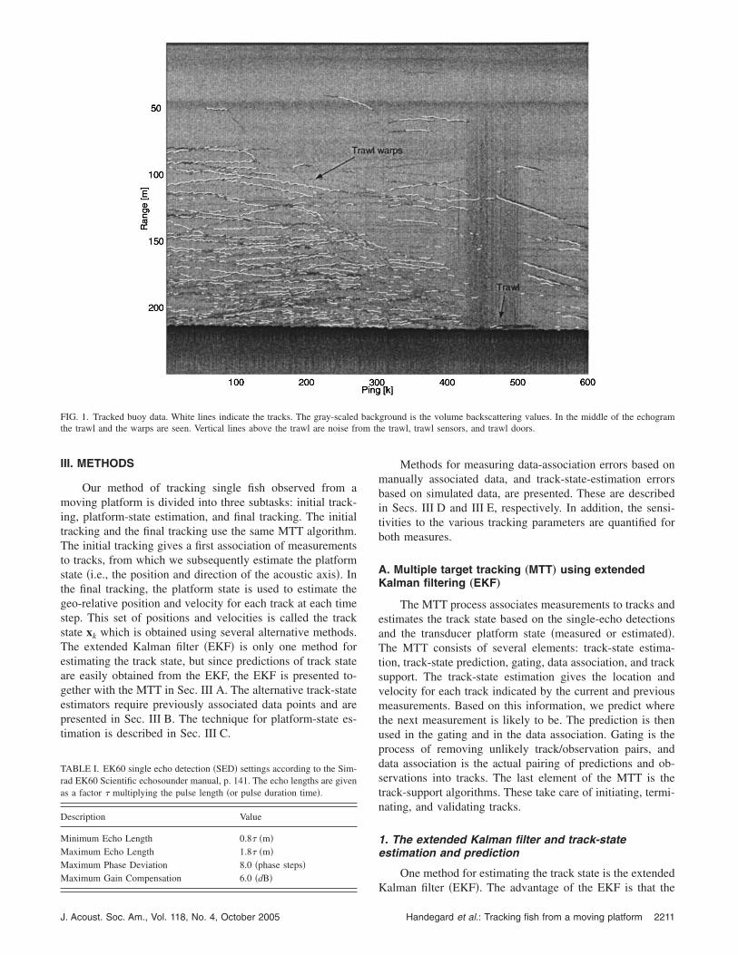
The test data set was recorded during a fish avoidancestudy in the Barents Sea in March 2001. The buoy waspassed several times by a trawling vessel, and the purpose ofthe study was to investigate the behavior of the fish �mainlycod� in response to the vessel and gear.7 Data from one suchpassing comprise the test set whose total duration is 10 min.The ping rate is 1 s−1 and the data include 5700 single-echodetections �see the echogram shown in Fig. 1�.

The EK60 Mark 1 software �Ver. 1.3.0.54� was used todetect single targets within the echo beam. The settings for

the SED algorithm are given in Table I.

© 2005 Acoustical Society of America8�4�/2210/14/$22.50

III. METHODS

Our method of tracking single fish observed from amoving platform is divided into three subtasks: initial track-ing, platform-state estimation, and final tracking. The initialtracking and the final tracking use the same MTT algorithm.The initial tracking gives a first association of measurementsto tracks, from which we subsequently estimate the platformstate �i.e., the position and direction of the acoustic axis�. Inthe final tracking, the platform state is used to estimate thegeo-relative position and velocity for each track at each timestep. This set of positions and velocities is called the trackstate xk which is obtained using several alternative methods.The extended Kalman filter �EKF� is only one method forestimating the track state, but since predictions of track stateare easily obtained from the EKF, the EKF is presented to-gether with the MTT in Sec. III A. The alternative track-stateestimators require previously associated data points and arepresented in Sec. III B. The technique for platform-state es-timation is described in Sec. III C.

FIG. 1. Tracked buoy data. White lines indicate the tracks. The gray-scaledthe trawl and the warps are seen. Vertical lines above the trawl are noise fr

TABLE I. EK60 single echo detection �SED� settings according to the Sim-rad EK60 Scientific echosounder manual, p. 141. The echo lengths are givenas a factor � multiplying the pulse length �or pulse duration time�.

Description Value

Minimum Echo Length 0.8� �m�Maximum Echo Length 1.8� �m�Maximum Phase Deviation 8.0 �phase steps�Maximum Gain Compensation 6.0 �dB�

J. Acoust. Soc. Am., Vol. 118, No. 4, October 2005

Methods for measuring data-association errors based onmanually associated data, and track-state-estimation errorsbased on simulated data, are presented. These are describedin Secs. III D and III E, respectively. In addition, the sensi-tivities to the various tracking parameters are quantified forboth measures.

A. Multiple target tracking „MTT… using extendedKalman filtering „EKF…

The MTT process associates measurements to tracks andestimates the track state based on the single-echo detectionsand the transducer platform state �measured or estimated�.The MTT consists of several elements: track-state estima-tion, track-state prediction, gating, data association, and tracksupport. The track-state estimation gives the location andvelocity for each track indicated by the current and previousmeasurements. Based on this information, we predict wherethe next measurement is likely to be. The prediction is thenused in the gating and in the data association. Gating is theprocess of removing unlikely track/observation pairs, anddata association is the actual pairing of predictions and ob-servations into tracks. The last element of the MTT is thetrack-support algorithms. These take care of initiating, termi-nating, and validating tracks.

1. The extended Kalman filter and track-stateestimation and prediction

One method for estimating the track state is the extended

ground is the volume backscattering values. In the middle of the echograme trawl, trawl sensors, and trawl doors.

backom th

Kalman filter �EKF�. The advantage of the EKF is that the

Handegard et al.: Tracking fish from a moving platform 2211

state is estimated by weighting the previous state with thenew observation, thus it is unnecessary to recalculate thewhole track. See Sec. III C for a description of alternativetrack-state estimators. The true position and velocity for tar-get i at ping k and time tk are given by the track-state vector

xk = �xk yk zk xk yk zk TSk�egc

T ,

where �xk ,yk ,zk� is the position vector, �xk , yk , zk� is the ve-locity vector, TSk is the target strength, T denotes matrixtransposition, and egc denotes the geo-referenced coordi-nate system �see Fig. 2�. The corresponding estimate isdenoted by x. In general there are several tracks i andmeasurements j for each ping k, but for easier readabilitywe have here omitted i and j from the notation. Under aconstant-velocity assumption, the track state at time tk+1

= tk+�Tk is given by

xk+1 = ���Tk�xk + w�, �1�

where ���Tk� is the matrix of the track-state transition forthe time interval �Tk and w�=w�tk� is an additive systemerror component �see Appendix A for details�. The error isassumed to be normally distributed and the target-model-covariance matrix is defined as ��=E�w�w�

T � �see Appen-dix A�.

From the estimated track state at time step k−1, we canpredict the state at step k. The predicted track state x is found

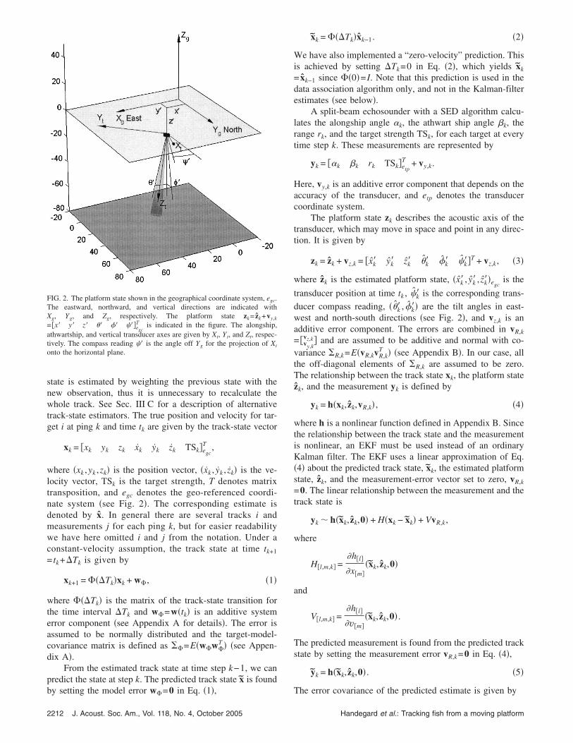
FIG. 2. The platform state shown in the geographical coordinate system, egc.The eastward, northward, and vertical directions are indicated withXg, Yg, and Zg, respectively. The platform state zk= zk+vy,k

= �x� y� z� �� �� ��egc

T is indicated in the figure. The alongship,athwartship, and vertical transducer axes are given by Xt, Yt, and Zt, respec-tively. The compass reading � is the angle off Yg for the projection of Xt

onto the horizontal plane.

by setting the model error w�=0 in Eq. �1�,

2212 J. Acoust. Soc. Am., Vol. 118, No. 4, October 2005

xk = ���Tk�xk−1. �2�

We have also implemented a “zero-velocity” prediction. Thisis achieved by setting �Tk=0 in Eq. �2�, which yields xk

= xk−1 since ��0�= I. Note that this prediction is used in thedata association algorithm only, and not in the Kalman-filterestimates �see below�.

A split-beam echosounder with a SED algorithm calcu-lates the alongship angle �k, the athwart ship angle �k, therange rk, and the target strength TSk, for each target at everytime step k. These measurements are represented by

yk = ��k �k rk TSk�etp

T + vy,k.

Here, vy,k is an additive error component that depends on theaccuracy of the transducer, and etp denotes the transducercoordinate system.

The platform state zk describes the acoustic axis of thetransducer, which may move in space and point in any direc-tion. It is given by

zk = zk + vz,k = �xk� yk� zk� �k� �k� k��T + vz,k, �3�

where zk is the estimated platform state, �xk� , yk� , zk��egcis the

transducer position at time tk , k� is the corresponding trans-

ducer compass reading, ��k� , �k�� are the tilt angles in east-west and north-south directions �see Fig. 2�, and vz,k is anadditive error component. The errors are combined in vR,k

= �vy,k

vz,k� and are assumed to be additive and normal with co-variance �R,k=E�vR,kvR,k

T � �see Appendix B�. In our case, allthe off-diagonal elements of �R,k are assumed to be zero.The relationship between the track state xk, the platform statezk, and the measurement yk is defined by

yk = h�xk, zk,vR,k� , �4�

where h is a nonlinear function defined in Appendix B. Sincethe relationship between the track state and the measurementis nonlinear, an EKF must be used instead of an ordinaryKalman filter. The EKF uses a linear approximation of Eq.�4� about the predicted track state, xk, the estimated platformstate, zk, and the measurement-error vector set to zero, vR,k

=0. The linear relationship between the measurement and thetrack state is

yk � h�xk, zk,0� + H�xk − xk� + VvR,k,

where

H�l,m,k� =�h�l�

�x�m��xk, zk,0�

and

V�l,m,k� =�h�l�

�v�m��xk, zk,0� .

The predicted measurement is found from the predicted trackstate by setting the measurement error vR,k=0 in Eq. �4�,

yk = h�xk, zk,0� . �5�

The error covariance of the predicted estimate is given by

Handegard et al.: Tracking fish from a moving platform

�x,k = ���Tk��x,k−1���Tk�T + ��,

where �x,k−1 is the estimated track-state-error covariancefrom the previous time step and �� is the track-state-

transition covariance. Initially �x,k−1=�x,0 where

�x,0 = �P0 xy2 ,P0 xy

2 ,P0 z2 ,P0 dxdy

2 ,P0 dxdy2 ,P0 dz

2 ,P0 TS2 �I . �6�

The elements of �x,0 are parameters. The estimated trackstate is found by weighting the predicted track state and theobservation by the Kalman gain, Kk,

xk = xk + Kk�yk − h�xk, zk,0�� ,

where

Kk = �x,kHkT�Hk�x,kHk

T + Vk�R,kVkT�−1.

The estimated track-state-error covariance is

�x,k = �I − KkHk��x,k,

the linearized innovation, k=yk− yk, is

k = H�xk − xk� + VvR,k,

and the linearized covariance of the innovation is

�,k = Hk�kHkT + Vk�R,kVk

T.

2. Gating and data association

The next step in the MTT algorithm is to associate theobservations with existing predictions. The challenge is toavoid associating a false prediction-observation pair, and toavoid not associating a true prediction-observation pair�track splitting�. The innovation ijk is the difference betweenthe predicted measurement from track i and the observation jat ping k; it is used in the gating and data-association algo-rithms. Innovations based on both constant and “zero-velocity” predictions are implemented and tested. Gating isthe initial step in the data association, where unlikely pairs ofpredictions and observations are removed. The distance indi-cated by the innovation is calculated, and any pair separatedby more than a set amount is deemed to be outside the gate.The gate can be specified in several ways. We have imple-mented two types. Firstly, a static gate accepts pairs within afixed ellipsoidal volume around the prediction:

dijk2 = ijkGijk

T � 1, �7�

where

G = ��G2 0 0

0 �G2 0

0 0 rG2 �

−1

. �8�

Here �G, �G, and rG act as gates in angles and range, respec-tively. Note that different gate widths may be used in theinitial and final tracking. These are indexed by numbers, i.e.,rG1 and rG2. If no measurement is associated with a giventrack at time step k, the algorithm continues the search attime step k+1. However, the volume likely to contain thenext measurement of the track is now larger, and it will

increase for each time step when no association is made.

J. Acoust. Soc. Am., Vol. 118, No. 4, October 2005

This suggests the use of a dynamic gate whose size increaseswith the prediction covariance. Such a gate requires a prioriknowledge of the detection probabilities and measurementerrors.8 In order to test the concept of a dynamic gate, sup-pose the detection probabilities are constant, so that

dijk2 = ijk �,ijk

−1 ijkT � 2 ln� cG

�,ijk� + ln ��,ijk� , �9�

where cG is a constant. The last term is a penalizing term toprevent tracks with high innovation covariance �many miss-ing pings� being preferred over those with low innovationcovariance.8

When gating is performed, a sparse matrix is obtainedcontaining the d2’s for all combinations of predictions �i� andobservations �j� for ping k that fall inside the gates. Theassociation algorithm assigns observations to predictionsbased on the elements in this matrix. Several data-associationmethods are described in the literature.8 One of the mostcommon is the global nearest neighbor �GNN� method,which assigns observations to tracks by minimizing the totalsum of distances. In this case an assignment with a higher d2

may be chosen at a given time step if the total cost is lower.This assignment problem is solved by the Bertsekas auctionalgorithm.9 We also implemented a simpler algorithm thatfirst assigns the best pairing at each time step, then the nextbest, continuing until all observations inside the gates areassigned. In this case the total sum of distances may behigher than for the GNN method. We have compared themethods with respect to their data-association errors.

3. Track support

The last part of the MTT algorithm is track support. Thisstarts, terminates, and validates the tracks. When an observa-tion is not connected to an existing track, a new one isspawned. The new track state starts with the position indi-cated by the observation, the velocity set to zero, and �x,0 asan assumed error covariance. A track is terminated at the lastping before the first sequence of MP consecutive missingpings. The track is rejected if it is less than ML �minimumtrack length�, or if the number of missing pings divided bythe track length is more than MN. The track length is simplythe number of pings from start to finish, including any miss-ing pings.

B. Other track-state estimators

In the previous section, the EKF was used both for pre-diction and estimation of the track state. Since the EKF es-timates the new track state based on the new associated mea-surements and the present track prediction only, thistechnique is well suited to be integrated with the gating anddata-association algorithms. However, after the measure-ments have been associated, other techniques can be used toestimate the position and velocity of the targets. The addi-tional techniques we have tested are the Kalman-smoothingalgorithm, linear regression, and a smoothing spline.

After estimating the tracks with the Kalman filter andcomputing the track-support functions, a Kalman smoothing

algorithm may be applied. The advantage over the Kalman-

Handegard et al.: Tracking fish from a moving platform 2213

filter algorithm is that the influence of the initial values �zerovelocity and �x,0� is avoided. This is achieved by using theKalman-filter predictions and estimates to compute the Kal-man smoothed estimate

xk = xk + Jk�xk+1 − ���Tk�xk� ,

with covariance

�ˆ

x,k = �x,k − Jk��ˆ

x,k+1 − �x,k+1�JkT,

by moving backwards through the track. Here

Jk = �x,k���tk�T�x,k−1 .

Both the Kalman filter and the Kalman smoother estimatethe position and velocity errors. However, the comparisonwith other methods is based on the position and velocityestimates only, not the errors. For the Kalman-filter estimatewe define position and velocity vectors

skKF = xk�1¯3�, uk

KF = xk�4¯6�

and for the Kalman smoothed estimate

skKS = xk�1¯3�, uk

KS = xk�4¯6�.

The linear regression and the smoothing spline methods re-quire us to map the measurements yk to Cartesian coordi-nates �egc�. This is achieved using the estimated platformstate z,

sk = g�y, z� = �x

y

z�

egc

,

where g is found from h �see Appendix B�. A constant-velocity track,

skL = s0

L + uLtk, �10�

is then fitted to sk by minimizing SS=�k�skL−sk�2

2, and s0L and

uL are found. However, a straight regression line through thesk’s may be a rather crude approximation. Therefore, we alsoused a smoothing spline, which minimizes a compromisebetween the exact fit and the smoothness of the track. This isimplemented in the R function10 smooth.spline, where thedegree of smoothness can be chosen automatically by crossvalidation, or by setting the parameter “spar” to a givenvalue. We have used both the nonparametric �cross valida-tion� and parametric �spar=0.7� methods, denoted by sk

SNP

and skSP, respectively. For details see the documentation of

smooth.spline in the R program,10 and the standard-Sliterature.11

C. Platform-state estimation

When tracking targets from vessels and buoys, the posi-tion and the direction of the acoustic beam may change fromping to ping. Knowledge of the transducer position and ori-entation is required for accurate results. There are standardnotation and sign conventions for the motion of a submergedbody.12 However, the angles defined in this section are rela-

tive to the east-west and north-south directions, not the ves-

2214 J. Acoust. Soc. Am., Vol. 118, No. 4, October 2005

sel heading, i.e., the measurements of ship or buoy motionhave to be mapped into zk before evaluating Eq. �3�. If directmeasurements of transducer position and orientation wereavailable, the initial tracking and platform-state estimationwould be unnecessary.

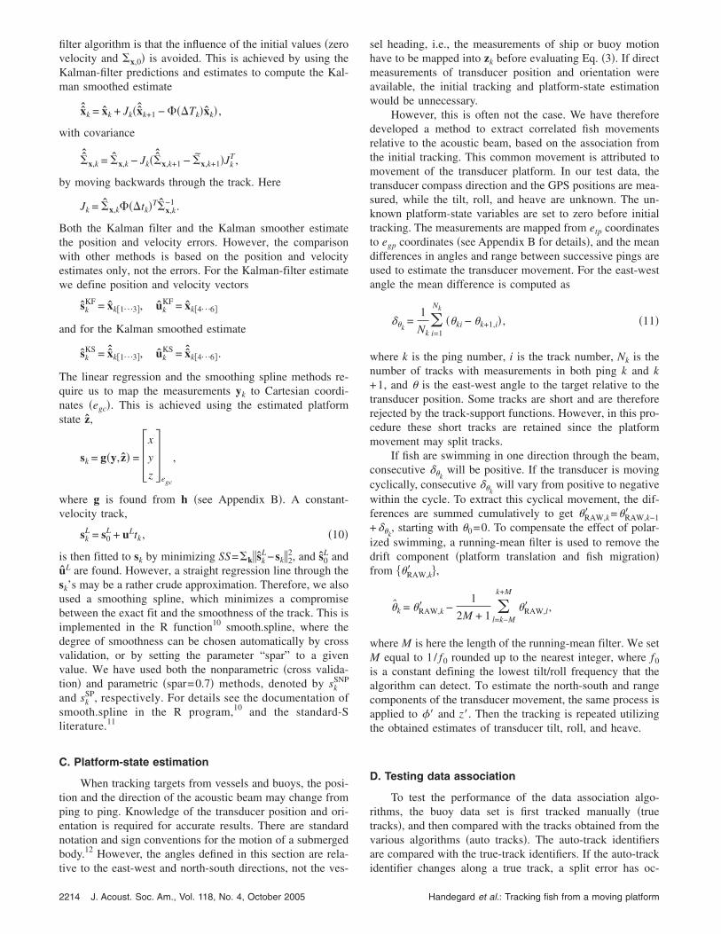
However, this is often not the case. We have thereforedeveloped a method to extract correlated fish movementsrelative to the acoustic beam, based on the association fromthe initial tracking. This common movement is attributed tomovement of the transducer platform. In our test data, thetransducer compass direction and the GPS positions are mea-sured, while the tilt, roll, and heave are unknown. The un-known platform-state variables are set to zero before initialtracking. The measurements are mapped from etp coordinatesto egp coordinates �see Appendix B for details�, and the meandifferences in angles and range between successive pings areused to estimate the transducer movement. For the east-westangle the mean difference is computed as

�k=

1

Nk i=1

Nk

��ki − �k+1,i� , �11�

where k is the ping number, i is the track number, Nk is thenumber of tracks with measurements in both ping k and k+1, and � is the east-west angle to the target relative to thetransducer position. Some tracks are short and are thereforerejected by the track-support functions. However, in this pro-cedure these short tracks are retained since the platformmovement may split tracks.

If fish are swimming in one direction through the beam,consecutive �k

will be positive. If the transducer is movingcyclically, consecutive �k

will vary from positive to negativewithin the cycle. To extract this cyclical movement, the dif-ferences are summed cumulatively to get �RAW,k� =�RAW,k−1�+ �k

, starting with �0=0. To compensate the effect of polar-ized swimming, a running-mean filter is used to remove thedrift component �platform translation and fish migration�from ��RAW,k� �,

�k = �RAW,k� −1

2M + 1 l=k−M

k+M

�RAW,l� ,

where M is here the length of the running-mean filter. We setM equal to 1/ f0 rounded up to the nearest integer, where f0

is a constant defining the lowest tilt/roll frequency that thealgorithm can detect. To estimate the north-south and rangecomponents of the transducer movement, the same process isapplied to �� and z�. Then the tracking is repeated utilizingthe obtained estimates of transducer tilt, roll, and heave.

D. Testing data association

To test the performance of the data association algo-rithms, the buoy data set is first tracked manually �truetracks�, and then compared with the tracks obtained from thevarious algorithms �auto tracks�. The auto-track identifiersare compared with the true-track identifiers. If the auto-track

identifier changes along a true track, a split error has oc-

Handegard et al.: Tracking fish from a moving platform

curred. If the true-track identifier changes along an autotrack, a connection error has occurred. The measure for tracksplitting is defined as

Jsplit�p� =�iCi

s

�i�Li − 1�, �12�

where p gives the parameter settings, Cis is the number of

changes in the auto-track identifier along the true track i, andLi is the length of the true track i. An example is given inFig. 3. The measure for false associations is similarly definedas

Jconnect�p� =�iCi

c

�i�Li − 1�, �13�

where Cic is the number of changes in the true-track identifier

along auto track i and Li is the length of auto track i. The twomeasures are combined into a single measure of the associa-tion error

Jalloc = 12 �Jsplit + Jconnect� . �14�

To test the parameter sensitivity to the data associationerror, the tracker is run with one parameter perturbed by±10% at each run. The sensitivity measure is defined as

Spa = 0.5� �J+10%Jalloc

+�J−10%

Jalloc�� �p

p�−1

, �15�

where �J+10% and �J−10% are the changes in Jalloc whenperturbing parameter p±10% , �p / p=0.1, except for MP,which is an integer. To test the sensitivity to MP, thisparameter is increased or decreased by one. A relativemeasure is still used, i.e., �p / p=1/MP0, where MP0 is theunperturbed value.

E. Testing position and velocity estimates

A simulated data set is used to test the validity of theposition and velocity estimates for each track. Different fishtrajectories are simulated, including transducer tilt/roll ef-fects. The track states estimated by the various techniquesare then compared with the known positions and velocitiesfrom the simulations. The simulated data comprise four

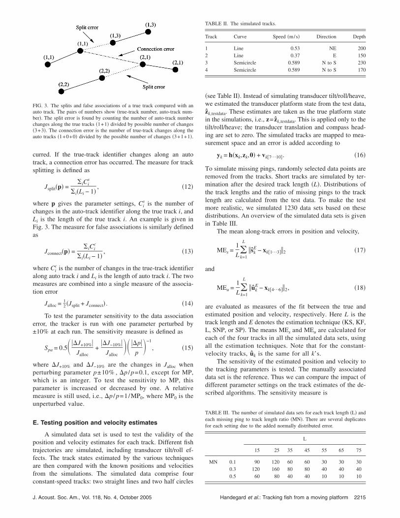
FIG. 3. The splits and false associations of a true track compared with anauto track. The pairs of numbers show �true-track number, auto-track num-ber�. The split error is found by counting the number of auto-track numberchanges along the true tracks �1+1� divided by possible number of changes�3+3�. The connection error is the number of true-track changes along theauto tracks �1+0+0� divided by the possible number of changes �3+1+1�.

constant-speed tracks: two straight lines and two half circles

J. Acoust. Soc. Am., Vol. 118, No. 4, October 2005

�see Table II�. Instead of simulating transducer tilt/roll/heave,we estimated the transducer platform state from the test data,zk,testdata. These estimates are taken as the true platform statein the simulations, i.e., z= zk,testdata. This is applied only to thetilt/roll/heave; the transducer translation and compass head-ing are set to zero. The simulated tracks are mapped to mea-surement space and an error is added according to

yk = h�xk,zk,0� + vk�7¯10�. �16�

To simulate missing pings, randomly selected data points areremoved from the tracks. Short tracks are simulated by ter-mination after the desired track length �L�. Distributions ofthe track lengths and the ratio of missing pings to the tracklength are calculated from the test data. To make the testmore realistic, we simulated 1230 data sets based on thesedistributions. An overview of the simulated data sets is givenin Table III.

The mean along-track errors in position and velocity,

MEs =1

L k=1

L

�skE − xk�1¯3��2 �17�

and

MEu =1

L k=1

L

�ukE − xk�4¯6��2, �18�

are evaluated as measures of the fit between the true andestimated position and velocity, respectively. Here L is thetrack length and E denotes the estimation technique �KS, KF,L, SNP, or SP�. The means MEs and MEu are calculated foreach of the four tracks in all the simulated data sets, usingall the estimation techniques. Note that for the constant-velocity tracks, uk is the same for all k’s.

The sensitivity of the estimated position and velocity tothe tracking parameters is tested. The manually associateddata set is the reference. Thus we can compare the impact ofdifferent parameter settings on the track estimates of the de-scribed algorithms. The sensitivity measure is

TABLE II. The simulated tracks.

Track Curve Speed �m/s� Direction Depth

1 Line 0.53 NE 2002 Line 0.37 E 1503 Semicircle 0.589 N to S 2304 Semicircle 0.589 N to S 170

TABLE III. The number of simulated data sets for each track length �L� andeach missing ping to track length ratio �MN�. There are several duplicatesfor each setting due to the added normally distributed error.

L

15 25 35 45 55 65 75

MN 0.1 90 120 60 60 30 30 300.3 120 160 80 80 40 40 400.5 60 80 40 40 10 10 10

Handegard et al.: Tracking fish from a moving platform 2215

Sps =1

�i=1M Li

i

M

k

Li

�sikE − sik

Ep�2 �19�

for the position estimates and

Spv =1

�i=1M Li

i

M

k

Li

�uikE − uik

Ep�2 �20�

for the velocity estimates. Here M is the number of tracks, Li

is the track length for track i, sikE and uik

E are the position andvelocity estimates for track i at time tk using estimation tech-nique E and the optimal parameter setting for the data asso-ciation error, and sik

Ep and uikEp are the position and velocity

estimate where parameter p is perturbed. The parameters areperturbed by ±10%, one at a time. The mean Sps and Spvare calculated for each parameter and each estimationtechnique.

IV. RESULTS

The various methods for data association and track esti-mation are examined by comparing the tracker results ob-tained, respectively, with simulated data and the test data.The questions are: how do the different data association al-

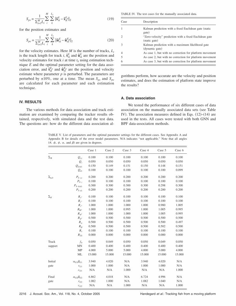
TABLE V. List of parameters and the optimal paramAppendix B for details of the error model paramet�� , � , , � , and �� are given in degrees.

Case 1 Case 2

�� Qxy 0.100 0.100Qz 0.050 0.050

Qdxdy 0.150 0.149Qdz 0.100 0.100

�x,0 P0 xy 0.200 0.200P0 z 0.100 0.100

P0 dxdy 0.300 0.300P0 dz 0.200 0.200

�R Rx� 0.100 0.100Ry� 0.100 0.100Rz� 1.000 1.000

R�� 1.000 1.000R�� 1.000 1.000R� 0.500 0.500R� 0.500 0.500R� 0.500 0.500Rr 0.100 0.100

RTS 0.000 0.000

Track f0 0.050 0.049support MN 0.400 0.400

MP 4.000 5.000ML 15.000 15.000

Initial �G1�G1 3.940 4.020gate rG1 1.000 1.000

cG1 N/A N/A

Final �G2�G2 6.862 4.018gate rG2 1.082 1.000

2216 J. Acoust. Soc. Am., Vol. 118, No. 4, October 2005

gorithms perform, how accurate are the velocity and positionestimates, and does the estimation of platform state improvethe results?

A. Data association

We tested the performance of six different cases of dataassociation on the manually associated data sets �see TableIV�. The association measures defined in Eqs. �12�–�14� areused in the tests. All cases were tested with both GNN andBPF data-association methods.

settings for the different cases. See Appendix A and/A indicates “not applicable.” Note that all angles

Case 3 Case 4 Case 5 Case 6

0.100 0.100 0.100 0.1000.050 0.050 0.050 0.0500.151 0.150 0.148 0.1510.100 0.100 0.100 0.099

0.200 0.200 0.200 0.2000.100 0.100 0.100 0.1000.300 0.300 0.298 0.3000.200 0.200 0.200 0.200

0.100 0.100 0.100 0.1000.100 0.100 0.100 0.1001.000 1.000 0.980 1.0050.995 1.000 1.005 0.9951.000 1.000 1.005 0.9950.500 0.500 0.500 0.5000.500 0.500 0.500 0.4970.500 0.500 0.502 0.5000.100 0.100 0.100 0.1000.000 0.000 0.000 0.000

0.050 0.050 0.049 0.0500.400 0.400 0.400 0.4005.000 4.000 5.000 4.00015.000 15.000 15.000 15.000

N/A 3.940 4.020 N/AN/A 1.000 1.000 N/A

1.000 N/A N/A 1.000

N/A 6.724 4.996 N/AN/A 1.082 1.040 N/A

TABLE IV. The test cases for the manually associated data.

Case Description

1 Kalman prediction with a fixed Euclidean gate �staticgate�

2 “Zero-velocity” prediction with a fixed Euclidean gate�static gate�

3 Kalman prediction with a maximum likelihood gate�dynamic gate�

4 As case 1, but with no correction for platform movement5 As case 2, but with no correction for platform movement6 As case 3, but with no correction for platform movement

eterers. N

cG2 N/A N/A 1.000 N/A N/A 1.000

Handegard et al.: Tracking fish from a moving platform

To do a fair comparison of the methods, we use theparameters that give the lowest Jalloc for each case. Theseparameters are found initially by a searching over the param-eter space, then a gradient method is used to minimize Jalloc.The resulting parameters are given in Table V. Note that MNand ML are not in the optimization since the associationmeasure does not contain a penalizing term for excludingshort tracks. If the longest track is correctly associated, theoptimal ML will be equal to the length of the longest track.The parameter estimation procedure is performed using theBPF data-association algorithm.

The split error, the connect error, and the associationerror for the six cases are given in Table VI. The GNN andBPF methods showed no difference in the data associationerror, and BPF is used since it is computationally less de-manding. The association error is lower for a static gate com-pared to a dynamic gate. Velocity prediction �cases 1 and 4�decreases the association error. Note that the optimal finalhorizontal gates ��G2 and �G2� are larger when velocity pre-diction is included �see Table V�. The platform-state estima-tion gives little improvement. When velocity prediction isused �cases 1 and 4�, the connect error increases by 25%,while the split error is reduced by 50% by the platform esti-mation.

Another way to evaluate the effect of platform-state es-

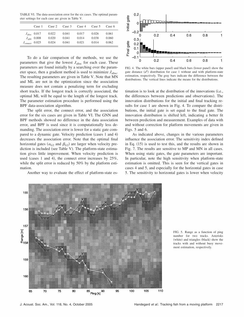
TABLE VI. The data-association error for the six cases. The optimal param-eter settings for each case are given in Table V.

Case 1 Case 2 Case 3 Case 4 Case 5 Case 6

Jalloc 0.017 0.022 0.041 0.017 0.026 0.061Jsplit 0.008 0.020 0.041 0.014 0.038 0.060

Jconnect 0.025 0.024 0.041 0.021 0.014 0.062

J. Acoust. Soc. Am., Vol. 118, No. 4, October 2005

timation is to look at the distribution of the innovations �i.e.,the differences between predictions and observations�. Theinnovation distributions for the initial and final tracking re-sults for case 1 are shown in Fig. 4. To compare the distri-butions, the initial gate is set equal to the final gate. Theinnovation distribution is shifted left, indicating a better fitbetween prediction and measurement. Examples of data withand without correction for platform movements are given inFigs. 5 and 6.

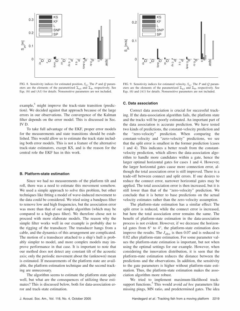
As indicated above, changes in the various parametersinfluence the association error. The sensitivity index definedin Eq. �15� is used to test this, and the results are shown inFig. 7. The results are sensitive to MP and MN in all cases.When using static gates, the gate parameters are important.In particular, note the high sensitivity when platform-stateestimation is omitted. This is seen for the vertical gates incases 4 and 5, and especially for the horizontal gates in case5. The sensitivity to horizontal gates is lower when velocity

FIG. 4. The white bars �upper panel� and black bars �lower panel� show thegate distance �d2� distribution for case 1 without and with platform-stateestimation, respectively. The gray bars indicate the difference between thedistributions. The vertical lines indicate the means for the distributions.

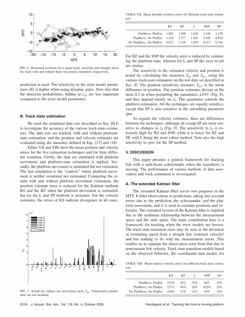
FIG. 5. Range as a function of pingnumber for two tracks. Asterisks�white� and triangles �black� show thetracks with and without buoy move-ment estimation, respectively.

Handegard et al.: Tracking fish from a moving platform 2217

prediction is used. The sensitivity to the error model param-eters �R� is higher when using dynamic gates. Note also thatthe detection probabilities, hidden in cG, are less importantcompared to the error model parameters.

B. Track state estimation

We used the simulated data sets described in Sec. III Eto investigate the accuracy of the various track-state estima-tors. The data sets are tracked, with and without platform-state estimation, and the position and velocity estimates areevaluated using the measures defined in Eqs. �17� and �18�.

Tables VII and VIII show the mean position and velocityerrors for the five estimation techniques and for three differ-ent scenarios. Firstly, the data are simulated with platformmovement, and platform-state estimation is applied. Sec-ondly, the platform movement is simulated but not estimated.The last simulation is the “control,” where platform move-ment is neither simulated nor estimated. Comparing the re-sults with and without platform movement estimation, theposition estimate error is reduced for the Kalman methodsKS and the KF when the platform movement is estimated,but for the L and SP methods it increases. For the velocityestimates, the errors of KS indicate divergence in all cases.

FIG. 7. Sensitivity indices for association error, Spa. Nonsensitive param-

FIG. 6. Horizontal positions for a single track. Asterisks and triangles showthe track with and without buoy movement estimation, respectively.

eters are not included.

2218 J. Acoust. Soc. Am., Vol. 118, No. 4, October 2005

For KF and the SNP the velocity error is reduced by estimat-ing the platform state, whereas for L and SP the error levelsare similar.

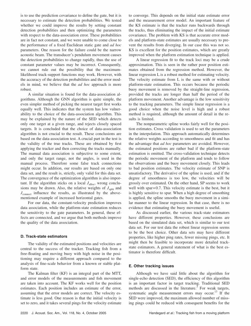
The sensitivity to the estimated velocity and position istested by calculating the measures Sps and Spv, using thevarious track-state estimators on the test data set described inSec. II. The position sensitivity measure, Sps, is the meandifference in position. The position estimates deviate at themost 0.3 m when perturbing the parameters ±10% �Fig. 8�,and they depend mainly on f0. This parameter controls theplatform estimation. All the techniques are equally sensitive,except that SP is also sensitive to the smoothing parameterspar.

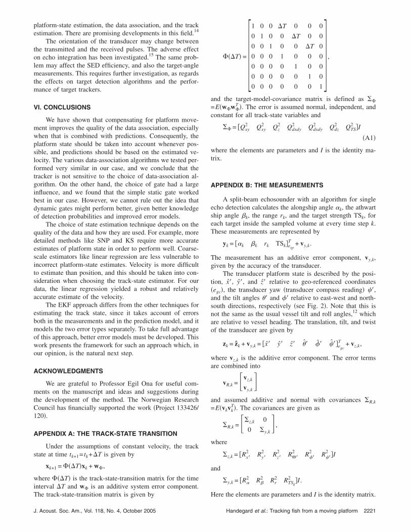
As regards the velocity estimates, there are differencesbetween the techniques, although all except SP are most sen-sitive to changes in f0 �Fig. 9�. The sensitivity to f0 is ex-tremely high for KS and SNP, while it is lower for KF andSP, with L being the most robust method. Note also the highsensitivity to spar for the SP method.

V. DISCUSSION

This paper presents a general framework for trackingfish with a split-beam echosounder when the transducer ismoving. The performance of various methods of data asso-ciation and track estimation is investigated.

A. The extended Kalman filter

The extended Kalman filter serves two purposes in theMTT. It links observations to predictions, taking into accounterrors due to the prediction, the echosounder, and the plat-form movement, and it is used to estimate positions and ve-locities. The extended version of the Kalman filter is requireddue to the nonlinear relationship between the measurementspace and the state space. The main contribution here is aframework for tracking when the error models are known.The track-state-transition error may be seen as the deviationin swimming speed from a straight line �constant velocity�and has nothing to do with the measurement errors. Thisenables us to separate the observation error from that due tononconstant fish velocity. Track state transition models basedon the observed behavior, the coordinated turn model, for

TABLE VII. Mean absolute position errors for different track-state estima-tors.

KS KF L SNP SP

PlatMove, PlatEst. 1.082 1.368 1.628 1.336 1.158PlatMove, No PlatEst. 1.929 2.577 1.303 3.295 0.829

No PlatMove, No PlatEst. 0.627 1.138 1.029 0.417 0.346

TABLE VIII. Mean relative velocity errors for different track-state estima-tors.

KS KF L SNP SP

PlatMove, PlatEst. 315% 52% 31% 68% 32%PlatMove, No PlatEst. 721% 88% 28% 815% 35%

No PlatMove, No PlatEst. 428% 51% 23% 45% 16%

Handegard et al.: Tracking fish from a moving platform

example,5 might improve the track-state transition �predic-tion�. We decided against that approach because of the largeerrors in our observations. The convergence of the Kalmanfilter depends on the error model. This is discussed in Sec.IV D.

To take full advantage of the EKF, proper error modelsfor the measurements and state transitions should be estab-lished. This would allow us to estimate the track state includ-ing both error models. This is not a feature of the alternativetrack-state estimators, except KS, and is the reason for thecentral role the EKF has in this work.

B. Platform-state estimation

Since we had no measurements of the platform tilt androll, there was a need to estimate this movement somehow.We used a simple approach to solve this problem, but othertechniques like fitting a model of wave-induced movement tothe data could be considered. We tried using a bandpass filterto remove low and high frequencies, but the association errorwas more than that of our simple algorithm �which may becompared to a high-pass filter�. We therefore chose not toproceed with more elaborate models. The reason why thesimple filter works well in our example is probably due tothe rigging of the transducer. The transducer hangs from acable, and the dynamics of this arrangement are complicated.The motion of a transducer attached to a ship’s hull is prob-ably simpler to model, and more complex models may im-prove performance in that case. It is important to note thatour method does not detect any constant tilt of the acousticaxis; only the periodic movement about the �unknown� meanis estimated. If measurements of the platform state are avail-able, the platform estimation technique and the second track-ing are unnecessary.

The algorithm seems to estimate the platform state quitewell, but what are the consequences of utilizing these esti-mates? This is discussed below, both for data-association er-

FIG. 8. Sensitivity indices for estimated position, Sps. The P and Q param-eters are the elements of the parametrized �x,0 and ��, respectively. SeeEqs. �6� and �A1� for details. Nonsensitive parameters are not included.

ror and track-state estimation.

J. Acoust. Soc. Am., Vol. 118, No. 4, October 2005

C. Data association

Correct data association is crucial for successful track-ing. If the data-association algorithm fails, the platform stateand the tracks will be poorly estimated. An important part ofthe data association is accurate prediction. We have testedtwo kinds of predictions, the constant-velocity prediction andthe “zero-velocity” prediction. When comparing theconstant-velocity and “zero-velocity” predictions, we seethat the split error is smallest in the former prediction �cases1 and 4�. This indicates a better result from the constant-velocity prediction, which allows the data-association algo-rithm to handle more candidates within a gate, hence thelarger optimal horizontal gates for cases 1 and 4. However,the larger horizontal gates cause more connection error, al-though the total association error is still improved. There is atrade-off between connect and split errors. If one desires toreduce the connect error, narrower horizontal gates may beapplied. The total association error is then increased, but it isstill lower than that of the “zero-velocity” prediction. Weconclude that it is better to base predictions on the actualvelocity estimates rather than the zero-velocity assumption.

The platform-state estimation has a similar effect: Thesplit error is reduced, while the connect error is increased,but here the total association error remains the same. Thebenefit of platform-state estimation in the data-associationprocess is not evident. However, if we decrease the horizon-tal gates from 6° to 4°, the platform-state estimation doesimprove the results. The Jalloc is then 0.07 and is reduced to0.02 after platform-state estimation. For some parameter val-ues the platform-state estimation is important, but not whenusing the optimal settings for our example. However, whenconsidering the innovation distribution, it is seen that theplatform-state estimation reduces the distance between thepredictions and the observations. In addition, the sensitivityto the gate parameters is higher without platform-state esti-mation. Thus, the platform-state estimation makes the asso-ciation algorithm more robust.

We tried to implement maximum-likelihood track-support functions.5 This would avoid ad hoc parameters like

FIG. 9. Sensitivity indices for estimated velocity, Spv. The P and Q param-eters are the elements of the parametrized �x,0 and ��, respectively. SeeEqs. �6� and �A1� for details. Nonsensitive parameters are not included.

missing pings, MN ratio, and predetermined gates. The idea

Handegard et al.: Tracking fish from a moving platform 2219

is to use the prediction covariance to define the gate, but it isnecessary to estimate the detection probabilities. We testedwhether we could improve the results by setting constantdetection probabilities and then optimizing the parameterswith respect to the data-association error. These probabilitiesare in fact not constant, and we were unable to come close tothe performance of a fixed Euclidean static gate and ad hocparameters. One reason for the failure could be the narrowacoustic beam. The transducer’s pendulum movement causesthe detection probabilities to change rapidly, thus the use ofconstant parameter values may be incorrect. Consequently,we cannot rule out the possibility that the maximum-likelihood track-support functions may work. However, withthe accuracy of the detection probabilities and the error mod-els in mind, we believe that the ad hoc approach is morerobust.

A similar situation is found for the data-association al-gorithms. Although the GNN algorithm is quite simple, theeven simpler method of picking the nearest target first worksequally well. This indicates that the system has low vulner-ability to the choice of the data-association algorithm. Thismay be explained by the nature of the SED which detectsonly one target at a given range, and rejects closely spacedtargets. It is concluded that the choice of data-associationalgorithm is not crucial to the result. These conclusions arebased on the data-association test. A crucial part in the test isthe validity of the true tracks. These are obtained by firstapplying the tracker and then correcting the tracks manually.The manual data association is subjective to some extent,and only the target range, not the angles, is used in themanual process. Therefore some false track connectionsmight occur. In addition, our results are based on only onedata set, and the result is, strictly, only valid for this data set.The convergence of the optimization algorithm is also impor-tant. If the algorithm sticks on a local Jalloc, wrong conclu-sions may be drawn. Also, the relative weights of Jsplit andJconnect influence the results, as illustrated by the above-mentioned example of increased horizontal gates.

For our data, the constant-velocity prediction improvesdata association, while the platform-state estimation reducesthe sensitivity to the gate parameters. In general, these ef-fects are connected, and we argue that both methods improvethe quality of the data association.

D. Track-state estimators

The validity of the estimated positions and velocities arecentral to the success of the tracker. Tracking fish from afree-floating and moving buoy with high noise in the posi-tioning may require a different approach compared to theanalysis of fine-scale behavior from a known or stable plat-form state.

The Kalman filter �KF� is an integral part of the MTT,and error models of the measurements and fish movementare taken into account. The KF works well for the positionestimates. Each position includes an estimate of the error,assuming that the error models are correct. The velocity es-timate is less good. One reason is that the initial velocity is

set to zero, and it takes several pings for the velocity estimate

2220 J. Acoust. Soc. Am., Vol. 118, No. 4, October 2005

to converge. This depends on the initial state estimate errorand the measurement error model. An important feature ofthe KS estimate is that the tracker runs backwards throughthe tracks, thus eliminating the impact of the initial estimatecovariance. The problem with KS is that accurate error mod-els and platform-state estimates are usually necessary to pre-vent the results from diverging. In our case this was not so.KS is excellent for the position estimates, which are greatlyimproved when the platform estimation technique is applied.

A linear regression fit to the track loci may be a crudeapproximation. This is seen in the rather poor position esti-mates obtained from the regression method. However, thelinear regression L is a robust method for estimating velocity.The velocity estimate from L is the same with or withoutplatform-state estimation. This occurs because the periodicbuoy movement is removed by the straight-line regression,provided the tracks are longer than half the period of theplatform movement. Another advantage is the low sensitivityto the tracking parameters. The simple linear regression is agood choice when the noise level is high and a robustmethod is required, although the amount of detail in the re-sults is limited.

The nonparametric spline works fairly well for the posi-tion estimates. Cross validation is used to set the parametersin the interpolation. This approach automatically determinesthe relative weights according to smoothness and fit and hasthe advantage that ad hoc parameters are avoided. However,the estimated positions are rather bad if the platform-stateestimation is omitted. The cross-validation technique detectsthe periodic movement of the platform and tends to followthe observations and the buoy movement closely. This leadsto bad position estimates. The velocity estimate of SNP isunsatisfactory. The derivative of the spline is used, and if thedegree of smoothness is too low, the velocities will begrossly over estimated. On the other hand, SP seems to workwell with spar=0.7. This velocity estimate is the best, but itis highly sensitive to spar. When a high degree of smoothingis applied, the spline smooths the buoy movement in a simi-lar manner to the linear regression. In that case, there is noevidence that estimating the buoy movement is useful.

As discussed earlier, the various track-state estimatorshave different properties. However, these conclusions arebased on the simulated data set, which is similar to our testdata set. For our test data the robust linear regression seemsto be the best choice. Other data sets may have differentproperties, like higher ping rates, fewer missing pings, etc. Itmight then be feasible to incorporate more detailed track-state estimators. A general statement of what is the best es-timator is therefore difficult.

E. Other tracking issues

Although we have said little about the algorithm forsingle-echo detection �SED�, the efficiency of this algorithmis an important factor in target tracking. Traditional SEDmethods are discussed in the literature.3 For weak targets,systematic angle measurement errors may occur.13 If theSED were improved, the maximum allowed number of miss-

ing pings could be reduced with consequent benefits for the

Handegard et al.: Tracking fish from a moving platform

platform-state estimation, the data association, and the trackestimation. There are promising developments in this field.14

The orientation of the transducer may change betweenthe transmitted and the received pulses. The adverse effecton echo integration has been investigated.15 The same prob-lem may affect the SED efficiency, and also the target-anglemeasurements. This requires further investigation, as regardsthe effects on target detection algorithms and the perfor-mance of target trackers.

VI. CONCLUSIONS

We have shown that compensating for platform move-ment improves the quality of the data association, especiallywhen that is combined with predictions. Consequently, theplatform state should be taken into account whenever pos-sible, and predictions should be based on the estimated ve-locity. The various data-association algorithms we tested per-formed very similar in our case, and we conclude that thetracker is not sensitive to the choice of data-association al-gorithm. On the other hand, the choice of gate had a largeinfluence, and we found that the simple static gate workedbest in our case. However, we cannot rule out the idea thatdynamic gates might perform better, given better knowledgeof detection probabilities and improved error models.

The choice of state estimation technique depends on thequality of the data and how they are used. For example, moredetailed methods like SNP and KS require more accurateestimates of platform state in order to perform well. Coarse-scale estimators like linear regression are less vulnerable toincorrect platform-state estimates. Velocity is more difficultto estimate than position, and this should be taken into con-sideration when choosing the track-state estimator. For ourdata, the linear regression yielded a robust and relativelyaccurate estimate of the velocity.

The EKF approach differs from the other techniques forestimating the track state, since it takes account of errorsboth in the measurements and in the prediction model, and itmodels the two error types separately. To take full advantageof this approach, better error models must be developed. Thiswork presents the framework for such an approach which, inour opinion, is the natural next step.

ACKNOWLEDGMENTS

We are grateful to Professor Egil Ona for useful com-ments on the manuscript and ideas and suggestions duringthe development of the method. The Norwegian ResearchCouncil has financially supported the work �Project 133426/120�.

APPENDIX A: THE TRACK-STATE TRANSITION

Under the assumptions of constant velocity, the trackstate at time tk+1= tk+�T is given by

xk+1 = ���T�xk + w�,

where ���T� is the track-state-transition matrix for the timeinterval �T and w� is an additive system error component.

The track-state-transition matrix is given by

J. Acoust. Soc. Am., Vol. 118, No. 4, October 2005

���T� = �1 0 0 �T 0 0 0

0 1 0 0 �T 0 0

0 0 1 0 0 �T 0

0 0 0 1 0 0 0

0 0 0 0 1 0 0

0 0 0 0 0 1 0

0 0 0 0 0 0 1

� ,

and the target-model-covariance matrix is defined as ��

=E�w�w�T �. The error is assumed normal, independent, and

constant for all track-state variables and

�� = �Qxy2 Qxy

2 Qz2 Qdxdy

2 Qdxdy2 Qdz

2 QTS2 �I

�A1�

where the elements are parameters and I is the identity ma-trix.

APPENDIX B: THE MEASUREMENTS

A split-beam echosounder with an algorithm for singleecho detection calculates the alongship angle �k, the athwartship angle �k, the range rk, and the target strength TSk, foreach target inside the sampled volume at every time step k.These measurements are represented by

yk = ��k �k rk TSk�etp

T + vy,k.

The measurement has an additive error component, vy,k,given by the accuracy of the transducer.

The transducer platform state is described by the posi-tion, x�, y�, and z� relative to geo-referenced coordinates�egc�, the transducer yaw �transducer compass reading� �,and the tilt angles �� and �� relative to east-west and north-south directions, respectively �see Fig. 2�. Note that this isnot the same as the usual vessel tilt and roll angles,12 whichare relative to vessel heading. The translation, tilt, and twistof the transducer are given by

zk = zk + vy,k = �x� y� z� �� �� ��egc

T + vz,k,

where vz,k is the additive error component. The error termsare combined into

vR,k = �vz,k

vy,k�

and assumed additive and normal with covariances �R,k

=E�vkvkT�. The covariances are given as

�R,k = ��z,k 0

0 �y,k� ,

where

�z,k = �Rx�2 Ry�

2 Rz�2 R��

2 R��2 R�

2 �I

and

�y,k = �R�2 R�

2 Rr2 RTSk

2 �I .

Here the elements are parameters and I is the identity matrix.

Handegard et al.: Tracking fish from a moving platform 2221

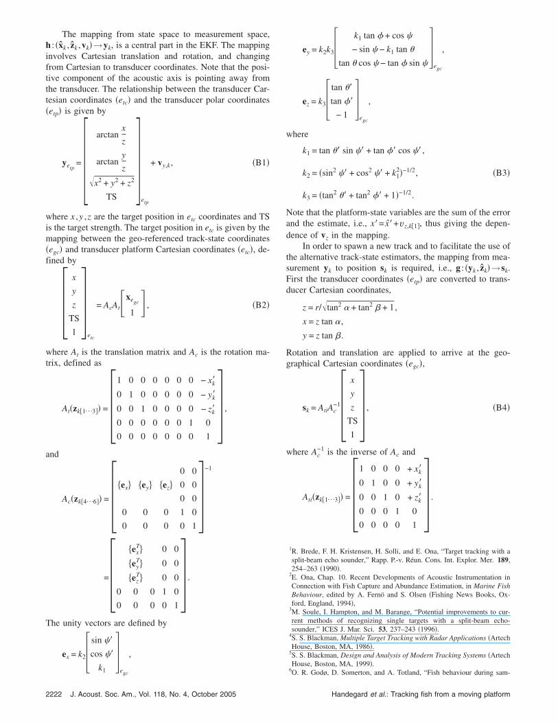
The mapping from state space to measurement space,h : �xk , zk ,vk�→yk, is a central part in the EKF. The mappinginvolves Cartesian translation and rotation, and changingfrom Cartesian to transducer coordinates. Note that the posi-tive component of the acoustic axis is pointing away fromthe transducer. The relationship between the transducer Car-tesian coordinates �etc� and the transducer polar coordinates�etp� is given by

yetp= �

arctanx

z

arctany

z

x2 + y2 + z2

TS

�etp

+ vy,k, �B1�

where x ,y ,z are the target position in etc coordinates and TSis the target strength. The target position in etc is given by themapping between the geo-referenced track-state coordinates�egc� and transducer platform Cartesian coordinates �etc�, de-fined by

�x

y

z

TS

1�

etc

= AcAt�xegc

1� , �B2�

where At is the translation matrix and Ac is the rotation ma-trix, defined as

At�zk�1¯3�� = �1 0 0 0 0 0 0 − xk�

0 1 0 0 0 0 0 − yk�

0 0 1 0 0 0 0 − zk�

0 0 0 0 0 0 1 0

0 0 0 0 0 0 0 1� ,

and

Ac�zk�4¯6�� = �0 0

�ex� �ey� �ez� 0 0

0 0

0 0 0 1 0

0 0 0 0 1�

−1

=��ex

T� 0 0

�eyT� 0 0

�ezT� 0 0

0 0 0 1 0

0 0 0 0 1� .

The unity vectors are defined by

ex = k2� sin �

cos �

k1�

e

,

gc

2222 J. Acoust. Soc. Am., Vol. 118, No. 4, October 2005

ey = k2k3� k1 tan � + cos

− sin − k1 tan �

tan � cos − tan � sin �

egc

,

ez = k3� tan ��

tan ��

− 1�

egc

,

where

k1 = tan �� sin � + tan �� cos �,

k2 = �sin2 � + cos2 � + k12�−1/2, �B3�

k3 = �tan2 �� + tan2 �� + 1�−1/2.

Note that the platform-state variables are the sum of the errorand the estimate, i.e., x�= x�+vz,k�1�, thus giving the depen-dence of vz in the mapping.

In order to spawn a new track and to facilitate the use ofthe alternative track-state estimators, the mapping from mea-surement yk to position sk is required, i.e., g : �yk , zk�→sk.First the transducer coordinates �etp� are converted to trans-ducer Cartesian coordinates,

z = r/tan2 � + tan2 � + 1,

x = z tan � ,

y = z tan � .

Rotation and translation are applied to arrive at the geo-graphical Cartesian coordinates �egc�,

sk = AtiAc−1�

x

y

z

TS

1� , �B4�

where Ac−1 is the inverse of Ac and

Ati�zk�1¯3�� = �1 0 0 0 + xk�

0 1 0 0 + yk�

0 0 1 0 + zk�

0 0 0 1 0

0 0 0 0 1� .

1R. Brede, F. H. Kristensen, H. Solli, and E. Ona, “Target tracking with asplit-beam echo sounder,” Rapp. P.-v. Réun. Cons. Int. Explor. Mer. 189,254–263 �1990�.

2E. Ona, Chap. 10. Recent Developments of Acoustic Instrumentation inConnection with Fish Capture and Abundance Estimation, in Marine FishBehaviour, edited by A. Fernö and S. Olsen �Fishing News Books, Ox-ford, England, 1994�,

3M. Soule, I. Hampton, and M. Barange, “Potential improvements to cur-rent methods of recognizing single targets with a split-beam echo-sounder,” ICES J. Mar. Sci. 53, 237–243 �1996�.

4S. S. Blackman, Multiple Target Tracking with Radar Applications �ArtechHouse, Boston, MA, 1986�.

5S. S. Blackman, Design and Analysis of Modern Tracking Systems �ArtechHouse, Boston, MA, 1999�.

6

O. R. Godø, D. Somerton, and A. Totland, “Fish behaviour during sam-

Handegard et al.: Tracking fish from a moving platform

pling as observed from free floating buoys - application for bottom trawlsurvey assessment,” ICES CM 1999/J:10 �1999�.

7N. O. Handegard, K. Michalsen, and D. Tjøstheim, “Avoidance behaviourin cod �Gadus morhua� to a bottom-trawling vessel Aquatic LivingResources 16, 265-270 �2003�.

8S. S. Blackman, in Design and Analysis of Modern Tracking Systems�Artech House, Boston, MA, 1999�, Chap. 6.

9D. Bertsekas, “The auction algorithm for assignment and other networkflow problems: A tutorial,” Interfaces 20, 133–149 �1990�.

10R Development Core Team, R: A language and environment for statisticalcomputing, R Foundation for Statistical Computing, Vienna, Austria, 2003.

11

J. M. Chambers and T. J. Hastie, Statistical Models in S �Wadsworth/

J. Acoust. Soc. Am., Vol. 118, No. 4, October 2005

Brooks Cole, Pacific Grove, CA, 1992�.12SNAME, “Nomenclature for treating the motion of a submerged body

through a fluid,” Technical Report Bulletin 1-5. Society of Naval Archi-tects and Marine Engineers, New York �1950�.

13R. Kieser, T. Mulligan, and J. Ehrenberg, “Observation and explanation ofsystematic split-beam angle measurement errors,” Aquatic LivingResources 13, 275–281 �2000�.

14H. Balk and T. Lindem, “Improved fish detection in data from split beamtransducers,” Aquatic Living Resources 13�5�, 297–303 �2000�.

15T. Stanton, “Effects on transducer motion on echo-integration techniques,”

J. Acoust. Soc. Am. 72, 947–949 �1982�.

Handegard et al.: Tracking fish from a moving platform 2223