Tracing Carbon Sources through Aquatic and TerrestrialFood Webs Using Amino Acid Stable IsotopeFingerprintingThomas Larsen1,2*, Marc Ventura2,3, Nils Andersen1, Diane M. O’Brien4, Uwe Piatkowski5,

Matthew D. McCarthy6

1 Leibniz-Laboratory for Radiometric Dating and Stable Isotope Research, Christian-Albrechts Universitat zu Kiel, Kiel, Germany, 2 Biogeodynamics and Biodiversity Group,

Centre for Advanced Studies of Blanes, Spanish Research Council (CEAB-CSIC), Blanes, Catalonia, Spain, 3 Institut de Recerca de l’Aigua, Universitat de Barcelona,

Barcelona, Catalonia, Spain, 4 Institute of Arctic Biology and Department of Biology and Wildlife, University of Alaska Fairbanks, Fairbanks, Alaska, United States of

America, 5GEOMAR, Helmholtz-Zentrum fur Ozeanforschung Kiel, Kiel, Germany, 6Ocean Sciences Department, University of California Santa Cruz, Santa Cruz, California,

United States of America

Abstract

Tracing the origin of nutrients is a fundamental goal of food web research but methodological issues associated withcurrent research techniques such as using stable isotope ratios of bulk tissue can lead to confounding results. Weinvestigated whether naturally occurring d13C patterns among amino acids (d13CAA) could distinguish between multipleaquatic and terrestrial primary production sources. We found that d13CAA patterns in contrast to bulk d13C valuesdistinguished between carbon derived from algae, seagrass, terrestrial plants, bacteria and fungi. Furthermore, we showedfor two aquatic producers that their d13CAA patterns were largely unaffected by different environmental conditions despitesubstantial shifts in bulk d13C values. The potential of assessing the major carbon sources at the base of the food web wasdemonstrated for freshwater, pelagic, and estuarine consumers; consumer d13C patterns of essential amino acids largelymatched those of the dominant primary producers in each system. Since amino acids make up about half of organismalcarbon, source diagnostic isotope fingerprints can be used as a new complementary approach to overcome some of thelimitations of variable source bulk isotope values commonly encountered in estuarine areas and other complexenvironments with mixed aquatic and terrestrial inputs.

Citation: Larsen T, Ventura M, Andersen N, O’Brien DM, Piatkowski U, et al. (2013) Tracing Carbon Sources through Aquatic and Terrestrial Food Webs UsingAmino Acid Stable Isotope Fingerprinting. PLoS ONE 8(9): e73441. doi:10.1371/journal.pone.0073441

Editor: Candida Savage, University of Otago, New Zealand

Received March 15, 2013; Accepted July 20, 2013; Published September 17, 2013

Copyright: � 2013 Larsen et al. This is an open-access article distributed under the terms of the Creative Commons Attribution License, which permitsunrestricted use, distribution, and reproduction in any medium, provided the original author and source are credited.

Funding: The study was funded by the DFG-supported Cluster of Excellence ‘‘The Future Ocean’’ (EXC 80/1, CP0937) and Carlsbergfondet (2007_01_0301). TLwas supported by Juan de la Cierva (JCI-2009-049330) and MV by the Spanish Government projects Fundalzoo (CGL2010-14841) and Invasivefish (427/2011). Thefunders had no role in study design, data collection and analysis, decision to publish, or preparation of the manuscript.

Competing Interests: The authors have declared that no competing interests exist.

* E-mail: natursyn@gmail.com

Introduction

During the last 30 years, stable isotope analysis has emerged as

one of most powerful tools for tracing organic carbon in food

webs. Analyses of total organic matter (‘‘bulk’’) have become

widespread due to the relative ease and low cost of sample

preparation and analysis. However, the potential of variable

environmental conditions to influence carbon isotopic ratios at the

base of the food web (d13C) is a serious drawback for disentanglingaquatic and terrestrial sources [1,2,3,4]. With the advent of new

continuous flow technologies, compound specific isotope analysis is

increasingly employed as a complementary tool for food web

analysis. Isotope analysis of fatty acids in conjunction with their

structural compositions are now widely used to investigate

biosynthetic sources since their molecular structure are tied to

their biosynthetic origins (e.g. [5]). However, fatty acids account

for only a small fraction of total organic carbon fluxes, and they

tend to undergo degradation and transformation during food web

passage [6]. Amino acids (AAs), in contrast, account for the large

majority of organic nitrogen, and about half of total carbon in

most organisms [7] and therefore are among the major conduits of

carbon through food chains. The main methodological drawback

of the 20 protein AAs is that they are ubiquitous in all life forms.

However, about half of the AAs can only be synthesized by

bacteria, fungi and photoautotrophs, and are therefore essential or

indispensable for animal diets. Since these essential AAs (EAAs)

typically pass from food source to consumer without alteration to

their carbon skeletons [8,9], a method for tracking their origins

and fluxes could greatly advance our understanding of nutrient

cycling and trophic relationships.

Recent research has shown that naturally occurring d13CAA

patterns contain information of both biosynthetic origin and mode

of carbon acquisition [10], and that the EAA group is particularly

diagnostic of origin [11]. These d13CAA patterns represent the sum

of the isotopic fractionations associated with the individual

biosynthetic pathways and associated branch points for each AA

(e.g. [12]). Larsen et al. [11] found that the d13CAA patterns of

terrestrial plants, bacteria and fungi were distinct and consistent,

and proposed these ‘‘stable isotope fingerprints’’ as a tool for

tracing sources of organic matter in terrestrial ecosystems.

Comparisons of d13CEAA patterns between laboratory reared

PLOS ONE | www.plosone.org 1 September 2013 | Volume 8 | Issue 9 | e73441

consumers and known diets have also indicated that stable isotope

fingerprints are passed on to consumers [11,13,14]. In spite of

these advances, it has until now been unresolved whether d13CAA

patterns can distinguish between aquatic and terrestrial primary

producers [14] and to what extent variable growth conditions for

aquatic producers may influence d13CAA patterns. The factors that

affect bulk and compound specific isotope patterns are funda-

mentally different. While bulk d13C values for a given producer

largely are determined by the ratio of carbon fixation to carbon

flux into the cell [15], d13CAA patterns are determined

downstream of the Calvin cycle by AA biosynthetic pathways

and associated branching points in the central metabolism. For

bulk d13C based studies, temporal and spatial variations of

inorganic carbon sources and other environmental conditions

therefore pose a challenge [16,17]; particularly in the highly

productive coastal benthic and estuarine habitats that are also the

zones of most organic carbon deposition in modern biogeochem-

ical cycles. A measure based on compound specific stable isotope

analysis that could distinguish between terrestrial and aquatic

sources of organic matter across varying ecological conditions

would therefore have profound implications for biological research

across a number of disciplines.

Here we investigated whether d13CAA patterns based approach-

es could transcend some of the limitations associated with bulk

d13C, by characterizing d13CAA values for a large set of different

algae and vascular plants. We tested whether these two groups

have different d13CAA patterns, and compared these with d13CAA

patterns from heterotrophic bacteria and fungi. Further, to test the

potential for d13CAA source information to be independent of

variation in bulk d13C values, we analyzed two marine primary

producers sampled from a range of different environments within

their natural habitats. Finally, to assess the practical relevance of

using d13CAA patterns as diagnostic and quantitative biomarkers in

actual ecosystems we analyzed consumers from freshwater,

pelagic, and estuarine systems.

Materials and Methods

Sampling DesignTo test whether freshwater, marine and terrestrial primary

producers have different d13CAA patterns, we collected and

cultured samples from wide variety of primary producers (micro-

and macroalgae, and terrestrial plants). In the field, we only

collected fresh and newly emerged thallus and leaves. For

microbial reference samples we obtained axenically cultured

bacteria and fungi. For testing the potential for d13CAA source

information to be independent of variation in bulk d13C values

among aquatic producers, we acquired multiple samples of the

seagrass Posidonia oceanica and the giant kelp Macrocystis pyrifera

collected from a range of different environments within their

natural habitats. For P. oceanica, the maximum photosynthetically

active radiation above their canopies ranged from 50 to 310 mmol

m22 s21 between the sampling locations and the coverage of leaf

necrosis ranged from 0 to 37.5%.M. pyrifera samples were collected

either in spring or late fall, periods of contrasting ocean conditions

that result in widely divergent bulk isotopic values [18]. Note that

our sampling was not designed for investigating the influence of

geographical region on terrestrial plants since a previous study

[14] found no systematic differences in d13CAA patterns from

greenhouse plants and those collected in boreal and mangrove

ecosystems. Finally, to assess the practical relevance of using

d13CAA patterns as diagnostic biomarkers in actual ecosystems we

analyzed consumers from three well-studied ecosystems: from a

marine pelagic ecosystem in the central North Pacific Ocean the

carnivorous fish species opah (Lampris guttatus), common dolphin-

fish (Coryphaena hippurus) and broadbill swordfish (Xiphias gladius),

from a littoral marine system (estuarine) the California mussel

(Mytilus californianus), and from oligotrophic arctic lakes the water

flea Daphinia sp. and seston.

Sample Acquisition and PreparationA detailed list of all our field samples and their locations is

provided in Table S1. Here follows a general description of

sampling locations, protocols and permits. All macroalgae (22

species), two seagrasses and two mussels were collected by the

Californian shore. The macroalgae except M. pyrifera (see below)

were collected on state tidelands for which collection without a

permit is allowed for less than ten pounds fresh weight. The

seagrass samples were provided under a permit to Joseph M. Long

Marine Laboratory, Santa Cruz. Subsamples of mussels were

obtained from recreationally harvested mussels under a permit to

Natasha Vokhshoori. The three pelagic fish samples were collected

as in Choy et al. [19] with NOAA longline observers, and

locations for the fish samples are approximate and are reported as

the centers of 565 degree cells in accordance with NOAA

confidentiality policies. Soils and the majority of terrestrial plants

(10 out of 12 species) were collected adjacent to five Alaskan

tundra lakes in which we also collected seston (5–80 mm size

particles) and Daphnia. The Alaskan samples were collected on land

owned by the Alaskan state or Bureau of Land Management

where no permission was required because we sampled on day

trips by foot or rafts leaving no permanent marks; soil samples

were collected between 2 and 8 cm below the soil surface and

amounted to ,50 g dry weight for each location; each plant

sample amounted ,1 g dry weight. No permit was required for

sacrificing Daphnia, which are not protected or endangered; they

were sampled with a zooplankton net (150–200 mm) and kept alive

until sorting at Toolik Field Station. The terrestrial plant collection

was supplemented with two species from public owned land in

Denmark where no permission was required for sampling. We

obtained five P. oceanica samples from the Catalonian shore in the

Mediterranean Sea under a permit to Teresa Alcoverro by the

Catalan Water Agency, and the five M. pyrifera samples from the

Californian shore were sampled under a permit to Melissa M.

Foley [18] by NOAA’s Monterey Bay National Marine Sanctuary.

All field samples were kept on crushed ice in coolers and stored

between 1 and 3 days before thoroughly washing them in milliQ

water (except for animal and seston samples). Seagrass leaves were

further cleaned by scraping off epiphytes with a razor blade. The

seston samples that during sampling had been collected into

500 ml bottles were in the laboratory concentrated onto GF/C

glass microfiber filters (Whatman). For analysis of animal samples,

we prepared whole tissue samples of Daphnia and muscle tissue for

mussels and fish. All samples were dried at 50uC except for animal,

seston and soil samples, which were freeze-dried. After drying the

samples were homogenized with a mortar.

Microalgae comprised of five diatoms, two cyanobacteria, two

chlorophytes, three haptophytes, and two crysophytes obtained

from existing axenic cultures at GEOMAR, Kiel, Germany or the

culture collection of algae of Goettingen University, Germany. See

Table S2 for detailed list of laboratory samples. The microalgae

were cultured between April 2010 and January 2011 at

GEOMAR in sterile 225 cm2 tissue culture flasks with vented

cap in brackish water (13.9 psu) collected from Kiel Fjord or

seawater (31.2 psu) collected at Multimar-Wattforum by the

German North Sea. Water mixed with added nutrients was sterile

filtered (Whatman celluloseacetate 0.2 mm filter) (see Table S2 for

light, temperature and nutrient regimes). In addition we collected

Amino Acid Isotope Fingerprinting

PLOS ONE | www.plosone.org 2 September 2013 | Volume 8 | Issue 9 | e73441

three non-sterile filtered water samples from Kiel Fjord February

2012 for the use of culturing of natural assemblages of microalgae

in culture tanks. Visual inspection of these samples revealed

between 60–80% dominance of diatoms. All microalgae were

harvested after 5 to 21 days during exponential growth or right

after the onset of the lag phase on either a Durapore PVDF

0.22 mm pore size filter (Sigma-Aldrich, Germany), GF/C glass

microfiber filters (Whatman) or by centrifugation in 50 ml vials at

3300 g. The algae were subsequently freeze dried, and surplus

substrates with live cultures were autoclaved.

Laboratory grown fungi and bacteria samples were either

obtained from a previous study [11] or isolated and cultured at the

Institute of Arctic Biology, University of Alaska Fairbanks from soil

or water samples collected during the Alaskan field sampling

mentioned above (see Table S2 for details). For isolating fungal

and bacterial strains, the growth media were treated with either

antibiotics (Streptomycin and Tetracycline hydrochloride) or

fungicides (Amphotericin and Nystatin, all chemicals were from

Sigma-Aldrich, St. Louis, Missouri, USA). After isolation under

sterile conditions, all bacteria samples were grown on solid media

(Bacto Agar BD, Sparks, Maryland, USA) and fungi were grown

in liquid media flasks in a shaking incubator (Innova 4230, New

Brunswick Scientific, Edison, New Jersey, USA) and harvested

after one to three weeks. We used amino acid free nutrient media

containing 15 g L21 of one of the following nutrient mixes

‘Czapek’, ‘MAG’ and ‘MMN’ (See Table S2 for temperature and

nutrient regimes). Microbial samples in liquid media were

harvested by centrifugation in 50 ml tubes (2200 g) and freeze

dried after harvesting. All substrates with viable cultures were

autoclaved after harvesting.

Elemental and Isotope AnalysisElemental content and bulk isotope ratios of plants, bacteria,

fungi, macroalgae and animals were measured at the UCSC

Stable Light Isotope Facility. Approximately 1 mg of sample was

pelletized into tin capsules and analyzed on a Carlo Erba 1108

linked to a Thermo Finningan DeltaPlus XP mass spectrometer

with an analytical standard deviation of typically,60.15%(n = 3). Elemental content and bulk isotope ratios of microalgae

were determined on 2 mg samples pelletized into tin capsules at

the UC Davis Stable Isotope Facility using a PDZ Europa ANCA-

GSL elemental analyzer interfaced to a PDZ Europa 20–20

isotope ratio mass spectrometer (Sercon Ltd., Cheshire, UK).

Isotope data are expressed in delta (d) notation as ((Rsample/

Rstandard) –1) 6 1000%, where R is the ratio of heavy to light

isotope; and the standard is Vienna Pee Dee Belemnite (VPDB) for

carbon and air for nitrogen.

For d13C analysis of individual AAs (d13CAA) we transferred

between 1.5 and 7 mg of sample to Pyrex culture tubes

(136100 mm). Samples were flushed with N2 gas, sealed, and

hydrolyzed in 1–2 ml 6 N HCl (37% HCl diluted with Milli-Q

water, Merck, Darmstadt, Germany) at 110uC in a heating block

for 20 h. After hydrolysis, samples collected on GF/C filters and

coralline algae were purified with Dowex 50WX8 cation exchange

resin according to Amelung & Zhang [20] and He et al [21]. In

the remaining samples we removed lipophilic compounds by

adding 2 ml n-hexane/DCM (6:5, v/v) to the Pyrex tubes that

were flushed shortly with N2 gas and sealed before vortexing for

30 s. The aqueous phase was then filtered through a Pasteur

pipette lined with glass wool that had been pretreated at 450uC.All samples were transferred into 4 ml dram vials before

evaporating the samples to dryness under a steam of N2 gas for

30 minutes at 110uC in a heating block. The samples were stored

at 218uC. To volatize the AAs, we followed the derivatization

procedure by Corr et al [22] methylating the dried samples with

acidified methanol and subsequently acetylating them with a

mixture of acetic anhydride, triethylamine and acetone (NACME:

N-acetyl methyl ester derivatives). As a precautionary measure to

reduce oxidation of amino acids during derivatization, we flushed

and sealed reaction vials with N2 gas prior to the methylation and

acetylation reactions. To account for carbon added during

derivatization [23] and variability of isotope fractionation during

analysis, we also derivatized and analyzed pure amino acids with

known d13C values. Nor-leucine was used as an internal standard.

Amino acid derivatives were injected with an autosampler into an

Agilent Single Taper Ultra Inert Liner (#5190-2293) that was held

at 280uC for 2 min. The compounds were separated on a Thermo

TraceGOLD TG-200MS GC column

(60 m60.32 mm60.25 um) installed on an Agilent 6890N gas

chromatograph (GC). The oven temperature of the GC started at

50uC and heated at 15uC min21 to 140uC, followed by 3uC min21

to 152uC and held for 4 min, then 10uC min21 to 245uC and held

for 10 min, and finally 5uC min21 to 290uC and held for 5 min.

The GC was interfaced with a MAT 253 isotope ratio mass

spectrometer (IRMS) via a GC-III combustion (C) interface

(Thermo-Finnigan Corporation). All samples were analyzed in

triplicate. The average reproducibility for the internal standard

nor-leucine (Nle) was 60.4% (n = 3) and the amino acid standards

ranged from 60.1% for Phe to 60.6% for Thr (n = 12–15 for

each batch). Of the amino acids we were able to analyze (see Fig.

S1 for GC-C-IRMS chromatogram) the following were defined as

non-essential for animals: alanine (Ala), asparagine/aspartic acid

(Asx), glutamine/glutamic acid (Glx), glycine (Gly), and tyrosine

(Tyr). The following were defined as essential: histidine (His),

isoleucine (Ile), leucine (Leu), lysine (Lys), methionine (Met),

phenylalanine (Phe), threonine (Thr), and valine (Val).

Calculations and Statistical AnalysesAll statistical analyses except the mixing modeling were

performed in R version 2.12.1 [24] with RStudio interface version

0.96.330. All values in the text are given as mean 6 standard

deviation. To explore patterns and group memberships in our

dataset we performed Ward’s hierarchical clustering (R-package

cluster) and principal component analysis (PCA, R-package vegan)

on d13C values of amino acids that had been normalized to their

respective sample means denoted as d13CAAn. Prior to applying

statistical analysis the data were tested for univariate normality by

visually checking whether there were departures from normality

on Q-Q plots. His and Met were excluded from the analyses due

to missing measurements caused by concentrations below detec-

tion limits. Differences in each amino acid between different

producer groups were tested with ANOVA with Tukey HSD post-

hoc tests. To examine combinations of independent variables (i.e.

d13CAA values) that best explained differences between the

categorical variables (i.e. the groups defined by the PCA and

one-way ANOVA tests) and to construct models for predicting

membership of unknown samples, we performed linear discrim-

inant function analysis (LDA, R package MASS [25]) on d13CAA

values. For calculating the probability of group membership of the

classifier samples we used a leave-one-out cross-validation

approach. To test the null hypothesis that there was no difference

in classification among the groups we applied Pillai’s trace

(MANOVA). Relative contributions of EAAs from diets to

consumers was estimated in the software FRUITS (version 0.1,

http://sourceforge.net/projects/fruits) [26] with normalized iso-

tope values. FRUITS also considers the biochemical composition

of sources and which sources are most likely to contribute the

most. FRUITS is executed with BUGS, which is a software

Amino Acid Isotope Fingerprinting

PLOS ONE | www.plosone.org 3 September 2013 | Volume 8 | Issue 9 | e73441

package for performing ‘‘Bayesian inference Using Gibbs

Sampling’’ that includes an expert system for determining an

appropriate Markov chain Monte Carlo scheme based on the

Gibbs sampling.

Results

To assess differences in d13CAA patterns we first carried out a

PCA with d13CAAn values that in contrast to a LDA does not

require categorical variables. With this analysis we found that the

samples clustered according to their major phylogenetic associa-

tions: algae, bacteria, fungi and vascular plants (Fig. 1). The first

principal component accounted for 33% of the variation, and

separated the photoautotrophs from the microorganisms. The

second principal component accounted for 27% of the variation

and separated algae from vascular plants, and fungi from bacteria.

The AAs in the PCA grouped largely according to their

biosynthetic families, with the exception that Ile grouped with

the pyruvate AAs (Ala, Leu and Val), but biosynthetically belongs

to the oxaloacetate family (Asx, Lys and Thr). The third group

consisted of the aromatic AAs, Tyr and Phe. See Table S3 for the

d13C values for each AA measured, and Table S4 for detailed

PCA results. We then tested which of the d13CAAn values were

significantly different between algae, terrestrial plants, bacteria

and fungi with ANOVA (Table S5). Seven amino acids (Ala, Phe,

Tyr, Thr, Val, Leu and Lys) were significantly different between

algae and terrestrial plants, all AAs except Glx were significantly

different between algae and bacteria, and six (Glx, Gly, Ile, Leu,

Lys and Val) were significantly different between algae and fungi

(see Table S5 for direction of the differences). The microalgal

groups (chlorophytes, chrysophytes, cyanobacteria, diatoms, and

haptophytes) only displayed subtle differences between d13CAAn

values (Table S5). For this reason we grouped them to a single

group and tested them against the two macroalgal groups. We

found the most notable difference between brown algae and

microalgae with five significantly different AAs (Ala, Asx, Ile, Lys,

Tyr).

We then applied LDA to our d13CEAA data to identify which of

the six EAAs (Ile, Leu, Lys, Phe, Thr, Val) were most important

for distinguishing between algae, bacteria, fungi and terrestrial

plants. The seagrass samples were omitted from this analysis due

to a small number of samples (the number of samples did not

exceed the number of EAAs). Bacterial, fungal, and terrestrial

plant samples classified with 99.162.6% posterior probability

within their own groups (Fig. 2, Table S6). The microalgal samples

classified with 97.368.1% probability as algae with Melosira varians

and Isochrysis galbana having the lowest probabilities (84% and

61%, respectively). All brown algae samples (Phaeophyceae)

classified with 100% probability as algae, and eight out of nine

red algae (Rhodophyta) classified with 98.663.8% probability as

algae. The ninth red algae, Osmundea spectabilis, classified as a

bacterium (54% probability) rather than an alga (46% probability).

The most important linear discriminants for separating the four

categorical variables were Lys, Phe, Leu and Val. We created a

second LDA model based on the five most informative EAAs (Ile,

Leu, Lys, Phe, Val) to assess to what extent it would be possible to

separate the three algal groups (microalgae, brown algae and red

algae) and seagrass samples from each other. Of all 27 microalgal

samples, 24 samples classified as microalgae, 10 out of 12 brown

algae classified as brown algae, 7 out of 9 red algae classified as red

algae, and all 7 seagrass samples classified as seagrass (Fig. 3, Table

S7). None of the algal samples classified as seagrass.

The second major question asked by our study was to what

extent d13CAA patterns are affected by environmental conditions.

To answer this question we analyzed seagrass (P. oceanica) and giant

kelp samples (M. pyrifera) [16] across a variety of growth conditions

(see Table S1 for details). For both species the range in d13C values

was five- to ten-fold greater for bulk than d13CAAn values (Fig. 4).

Individual d13CAAn values typically spanned between 0.4 to 0.6%compared to 2.6% and 5.2% for bulk d13C values of P. oceanica

and M. pyrifera, respectively.

Finally, we investigated how d13CEAA patterns of animals from

three different aquatic ecosystems resembled the main primary

production sources in their respective environments. For Arctic

shallow lakes in Northern Alaska, we used bacteria, microalgae

and terrestrial plants as the most likely end members for Daphnia.

The LDA model classified all the categorical variables correctly,

and the d13CEAA patterns of the five Daphnia samples resembled

microalgae with 84.0616.9% probability and bacteria with

11.9612.3% probability (Fig. 5a, Table S8). The seston sample

resembled microalgae with 96.8% probability. While three out of

four soil samples resembled plants with .97% probability, the

remaining sample resembled plants with 69% probability. In an

open pelagic system, we used microalgae, bacteria and fungi as

end members for three predatory fish species (C. hippurus, L. guttatus

and X. gladius) from the central Pacific. The three categorical

variables (algae, bacteria and fungi) were distinctly different and

the d13CEAA patterns of all three fish samples matched those of

microalgae with 100% probability (Fig. 5b, Table S8). In the

estuarine system we selected microalgae, giant kelp and bacteria as

the most likely particulate organic matter sources for the

California mussel (Mytilus californianus). The LDA model classified

all the categorical variables correctly, and the d13CEAA patterns of

Figure 1. The principal component analysis of d13CAAn valuesof different producers show a range of different isotopepatterns between bacteria, fungi, vascular plant and algae.None of the microalgal or macroalgal group clustered separately fromone another. Values in parentheses are the percentage variationaccounted by each axes. The first axis separates the photoautotrophsfrom the microbes, and the second axis separates vascular plants fromalgae, and fungi from bacteria. The fairly similar vector lengths showthat almost all amino acids were important for the variations of the twofirst ordination components. See Table S4 for analytical details.doi:10.1371/journal.pone.0073441.g001

Amino Acid Isotope Fingerprinting

PLOS ONE | www.plosone.org 4 September 2013 | Volume 8 | Issue 9 | e73441

Figure 2. Linear discriminant function analysis based on the d13CEAAvalues (Ile, Leu, Lys, Phe, Thr, Val) of bacteria, fungi, algae andterrestrial plants. In the left figure (a) displaying the scores of the first two discriminant axes, fungi and terrestrial plants each cluster separatelyfrom algae and bacteria. In the right figure (b) displaying the second and third discriminant axes, bacteria are separated apart from the algae, fungiand terrestrial plants. The dotted lines represent confidence ranges at P = 0.5. See Table S6 for details.doi:10.1371/journal.pone.0073441.g002

Figure 3. Linear discriminant function analysis with the d13CEAAvalues (Ile, Leu, Lys, Phe, Val) from the three algal groups. It separatesall seagrass samples from the three algal groups. The majority of the algal samples classified correctly within their own groups (Table S7). The dottedlines represent confidence ranges at P = 0.5; confidence ranges are only displayed in the left figure (a) because the third linear discriminant in rightfigure (b) only explained 14%.doi:10.1371/journal.pone.0073441.g003

Amino Acid Isotope Fingerprinting

PLOS ONE | www.plosone.org 5 September 2013 | Volume 8 | Issue 9 | e73441

the two mussels resembled microalgae with $99.7% probability

and brown algae with 0.3% probability (Fig. 5c, Table S8). We

used the California mussel samples to exemplify how EAA isotope

values can be used to obtain relative proportions of food sources

for a consumer. The mixing model was based on d13Cn values of

the three most informative EAAs for separating microalgae, brown

algae and bacteria: Leu, Val and Lys. For brown algae, we only

considered kelp since it is the most dominant brown alga in the

mussels’ habitat. We also included information about the relative

proportion of the three EAAs (Leu, Lys and Val) in the food

sources [27–29], and the likelihood that the mussels would

consume one food sources over another (See Appendix S1). We

found that the mussels obtained about two-third of their EAAs

from microalgae (66.7613.3%), about a quarter from kelp

(26.0611.4%) and the remaining fraction from bacteria

(7.366.0%) (Fig. 6, Appendix S1).

Discussion

Our results show that d13CAA patterns can be used as powerful

and ubiquitous tracers for discerning carbon origins in both

terrestrial and marine settings (Fig. 1). We found that d13C values

for seven out of eleven AAs were significantly different between

algae and terrestrial plants, which enabled us to create a

classification model that determined whether the AAs originated

from terrestrial or marine sources (Figs. 2 and 3). The fact that

variations in d13CAA patterns among algae were sufficiently

constrained to make a clear distinction between aquatic and

terrestrial primary producers seems remarkable, considering that

our algal samples encompassed a large number of species from

both freshwater and marine environments. Within the algal groups

that comprised two macroalgal and five microalgal domains,

brown algae stood out as having the most distinct d13CEAA

Figure 4. Bars representing the maximum range for individualamino acid d13Cn values (normalized to their means) and bulkd13C values across five giant kelp samples (Macrocystis pyrifera)or five seagrass samples (Posidonia oceanica). The bars for theamino acids represent the mean and standard deviations of either fivenon-essential (NEAA) or six essential (EAA) amino acids.doi:10.1371/journal.pone.0073441.g004

Amino Acid Isotope Fingerprinting

PLOS ONE | www.plosone.org 6 September 2013 | Volume 8 | Issue 9 | e73441

patterns (Fig. 5c, Table S5). We also found that d13CEAA patterns

of terrestrial and aquatic primary producers were different from

bacteria and fungi. While the mechanistic reasons why algae vs.

vascular plants have such unique d13CAA patterns are not

currently clear as discussed below, the strong diagnostic potential

we observe for these major classes of primary producers is

consistent with broad ability of d13CAA patterns to distinguish

between other major organism groups.

Our results also indicate that d13CEAA patterns applied as

source diagnostic isotope fingerprints may offer a partial solution

to one of the major issues for the application of stable isotopes in

ecological and biogeochemical research: confounding variable

source bulk isotope values. It has remained a persistent challenge

for isotope ecologists to disentangle confounding d13C values

caused by variations in inorganic carbon sources and other

environmental parameters. Here we show that despite substantial

shifts in bulk d13C values for the seagrass P. oceanica and the giant

kelp M. pyrifera linked to season or growth conditions, d13CAAn

values were constant within a 0.5% standard deviation (Fig. 4).

These results are consistent with the notion that d13CAA patterns

are mostly determined by major evolutionary AA metabolic

pathways of an organism [11,12,30] rather than the factors

affecting bulk d13C values such as carbon availability, growth

rates, and cell surface area [3–4]. For application in food web

studies it is particularly encouraging that d13CAAn values only

shifted by 0.5% compared to the .5% shift in bulk d13C values of

giant kelp. Another important observation is that light attenuation

and leaf necrosis for the seagrass samples did not affect d13CAAn

values notably. Light intensity and necrosis are important factors

for seagrass growth and often associated with changes in leaf

composition of phenolic compounds, carbohydrates and chloro-

phyll [31–33].

We directly tested the ability of d13CAA patterns to transfer

information about major primary producer sources through food

webs by examining d13CAA values in consumers from diverse

habitats (freshwater arctic lakes, subtropical pelagic ocean,

estuarine marine). In every habitat, the results were consistent

with the hypothesis that d13CEAA source patterns based are

conserved in passage through food webs. In the freshwater

ecosystem, the resemblance of Daphnia and seston AAs with

microalgae rather than bacteria and terrestrial plants agrees with

limnological food web studies based on bulk isotope data [34]

(Fig. 5a). However, it is interesting that neither Daphnia nor seston

were projected directly on top of the algal samples pointing to a

possible influence of microbial reworking or allochtonous input, as

has been previously suggested in Arctic lakes [35]. In the open

ocean almost all primary production derives from single-celled

algae [36], so d13CAA patterns would be expected to align with

algal sources in oceanic consumers. The d13CEAA patterns exactly

followed this prediction (Fig. 5b), which also implies that d13CEAA

diagnostic information was not substantially altered by microbial

reworking [37–40], or transformed during digestive processes [41].

Our estuarine system is much more complex, with microalgae,

giant kelp, and reworked organic matter as possible contributors to

suspended particular organic matter (POM) [18]. For the estuarine

classification of California mussels, we included bacteria in

addition to microalgae and brown algae as end members in our

model, and found that microalgae had a much higher probability

being an AA source for the mussels than kelp (Fig. 5c). Since

classification models are not suited to estimate relative proportions

of food sources, we applied a mixing model to the study with

estuarine mussels. Based on the three most informative EAAs for

separating the mussel’s most likely food sources, we found that the

mussels obtained about two-third of their EAAs from mussels,

about a quarter from kelp and the remaining fraction from

bacteria (Fig. 6, Appendix S1). Thus, our findings are consistent

with the expectation that mussels mainly feed on POM derived

from fresh phytoplankton, and that microbially reworked POM is

a minor source [42].

If algae and vascular plants share similar amino acid

biosynthetic pathways [43,44], it raises the question why they

have consistently different d13CAA patterns. It has been proposed

by Hayes [30] that growth rates potentially could affect

intramolecular isotope distribution. During the stationary growth

phase the removal of carbon from the tricarboxylic acid cycle

would be slower than in the exponential phase. This would lead to

the accumulation of 13C enriched compounds at the ends of the

biosynthetic pathways in turn delivering 13C depleted precursors

to the first steps of the pathways [30]. While we did not test this

hypothesis, the rather uniform 13CAA patterns among microalgae

with contrasting growth rates suggest that this influence is rather

small. In support of this view, we found that the Mediterranean

Figure 5. Application of source diagnostic d13CEAA patterns infood web studies across three different ecosystems. (a) Inoligotrophic arctic lakes in Alaska, Daphinia sp. and seston clusterclosely to each other, and their EAAs appear to derive predominantlyfrom microalgae although a part of their EAAs may have come fromfoods reworked by bacteria or from allochtonous sources (i.e soils). (b)In the central North Pacific Ocean the EAAs of the carnivorous fishspecies (opah; Lampris guttatus, common dolphinfish; Coryphaenahippurus, broadbill swordfish; Xiphias gladius) resembled microalgaerather than EAAs from bacteria and fungi. (c) In a complex littoralmarine system by the Californian shore, the d13CEAA fingerprints ofCalifornia mussel (Mytilus californianus) resemble microalgae and notbacteria or brown algae, i.e. kelp. In the figure legend, ‘Pr’ signifiespredicted samples. See Table S8 for analytical details.doi:10.1371/journal.pone.0073441.g005

Figure 6. A boxplot generated with the FRUITS mixing modelshowing the contribution of essential amino acids (Leu, Lys,and Val) from three diets (bacteria; n =12, kelp; n=5, micro-algae; n=27) to the California mussel (Mytilus californianus;average value of two samples). The boxes provide a 68%confidence interval (corresponding to the 16th and 84th percentiles)and the whiskers provide a 95% confidence interval. The horizontalcontinuous line indicates the average while the horizontal discontin-uous line indicates the median (50th percentile). See Appendix S1 fordetailed information.doi:10.1371/journal.pone.0073441.g006

Amino Acid Isotope Fingerprinting

PLOS ONE | www.plosone.org 7 September 2013 | Volume 8 | Issue 9 | e73441

seagrass samples had similar d13CAA patterns in spite of the

different lighting regimes and hence growth rates in their natural

habitats. Isotope fractionation at metabolic branch points may also

explain some of the observed differences in d13CAA patterns

[11,12,]. We found that algae were 13C enriched relative to plants

for the AAs belonging to the pyruvate group (Ala, Val, Leu). A

similar case of greater 13C enrichment in algae than plants was

found by Chikaraishi and Naraoka [44] for n-alkanes that like

most other lipids have pyruvate as a precursor [45]. In contrast to

the pyruvate AAs, the aromatic AAs (Tyr, Phe) were 13C depleted

in algae relative to plants. From a carbon mass balance point of

view it is possible that 13C enrichment of pyruvate AAs in algae

lead to depletion of the aromatic AAs because they are less

coupled to lipid synthesis by having phosphoenolpyruvate and

erythrose-4-phosphate as precursors. The aromatic AAs also serve

as precursors for the synthesis of numerous primary and secondary

metabolites such as alkaloids and lignins [46], which also could

have influenced 13CAA fractionation of the aromatic AAs. For

deepening our understanding of the biochemical processes leading

to the 13CAA fractionation patterns further inquiry is needed into

the overall carbon mass balance between the most abundant

hydrocarbon groups and AAs.

Taken together, our results show that d13CAA patterns can

transcend bulk isotope analyses across diverse ecological environ-

ments, and be used to understand carbon sources and transfer in

ecological research as exemplified with our classification and

mixing modeling approaches. The strong diagnostic potential for

algae and plants may be particularly powerful for applications in

complex estuarine and coastal systems, where mixed aquatic and

terrestrial inputs occur, or in freshwater environments with strong

allochtonous influence. While our findings indicate that source-

specificity of d13CEAA patterns is conserved across environmental

gradients, further controlled physiological studies are also

warranted to better understand under what circumstances these

patterns may be altered. For a broad understanding of food web

cycling of nutrients, we also stress that it is also important to

consider other major biochemical classes, such as lipids and

carbohydrates. Finally, in addition to investigating ecosystem level

transfer of carbon and nitrogen, we suggest that this fingerprinting

method can help assessing symbiotic contributions of AAs from

bacteria to animal hosts. There is mounting evidence that protein-

nitrogen assimilation is possible in the lower gut of some animals

during digestion [47–49]. Our results indicate that d13CEAA

patterns may offer a direct way to assess the importance of such

microbial AA contributions, not only in the specific animals where

this may occur, but more broadly up food chains.

Supporting Information

Figure S1 GC-C-IRMS chromatogram.

(PDF)

Table S1 Field sample characteristics.

(PDF)

Table S2 Laboratory sample characteristics.

(PDF)

Table S3 d13C values of individual amino acids.

(PDF)

Table S4 Principal component analysis output for algal,bacterial, fungal and plant samples (Figure 1).

(PDF)

Table S5 ANOVA comparison of d13CAAn values.

(PDF)

Table S6 Linear discriminant analysis output for algal,bacterial, fungal and terrestrial plant samples (Figure 2).

(PDF)

Table S7 Linear discriminant function analysis outputof aquatic primary producers (Figure 3).

(PDF)

Table S8 Linear discriminant function analysis outputfor amino acid origins of consumers (Figure 5).

(PDF)

Appendix S1 FRUITS mixing model data (Figure 6).

(PDF)

Acknowledgments

We thank Laura Elsbernd and Dr. Lennart Bach for technical assistance in

culturing algae and the following people for additional assistance: Dr. Kai

Lohbeck, Dr. Armin Form, Tanja Kluver, Dr. Birte Matthiessen, Cordula

Meyer, Franziska Werner, and Rong Bi. We also thank Dr. Teresa

Alcoverro, Guillem Roca, Dr. Melissa M. Foley, Natasha Vokhshoori, Dr.

Anela Choy, and Dr. Yiming Wang for their help in obtaining the field

samples.

Author Contributions

Conceived and designed the experiments: TL MV MDM DMO.

Performed the experiments: TL UP MDM. Analyzed the data: TL NA.

Wrote the paper: TL MDM MV DMO NA.

References

1. Boecklen WJ, Yarnes CT, Cook BA, James AC (2011) On the Use of Stable

Isotopes in Trophic Ecology. Annual Review of Ecology, Evolution, and

Systematics 42: 411–440.

2. Degens ET, Guillard RRL, Sackett WM, Hellebust JA (1968) Metabolic

fractionation of carbon isotopes in marine plankton–I. Temperature and

respiration experiments. Deep Sea Research and Oceanographic Abstracts 15:

1–9.

3. Fogel ML, Cifuentes LA, Velinsky DJ, Sharp JH (1992) Relationship of Carbon

Availability in Estuarine Phytoplankton to Isotopic Composition. Marine

Ecology Progress Series 82: 291–300.

4. Popp BN, Laws EA, Bidigare RR, Dore JE, Hanson KL, et al. (1998) Effect of

phytoplankton cell geometry on carbon isotopic fractionation. Geochimica et

Cosmochimica Acta 62: 69–77.

5. Jones WB, Cifuentes LA, Kaldy JE (2003) Stable carbon isotope evidence for

coupling between sedimentary bacteria and seagrasses in a sub-tropical lagoon.

Marine Ecology-Progress Series 255: 15–25.

6. De Troch M, Boeckx P, Cnudde C, Van Gansbeke D, Vanreusel A, et al. (2012)

Bioconversion of fatty acids at the basis of marine food webs: insights from a

compound-specific stable isotope analysis. Marine Ecology Progress Series 465:

53–67.

7. Hedges JI, Baldock JA, Gelinas Y, Lee C, Peterson M, et al. (2001) Evidence for

non-selective preservation of organic matter in sinking marine particles. Nature

409: 801–804.

8. McMahon KW, Fogel ML, Elsdon TS, Thorrold SR (2010) Carbon isotope

fractionation of amino acids in fish muscle reflects biosynthesis and isotopic

routing from dietary protein. Journal of Animal Ecology 79: 1132–1141.

9. O’Brien DM, Fogel ML, Boggs CL (2002) Renewable and nonrenewable

resources: Amino acid turnover and allocation to reproduction in lepidoptera.

Proceedings of the National Academy of Sciences of the United States of

America 99: 4413–4418.

10. Scott JH, O’Brien DM, Emerson D, Sun H, McDonald GD, et al. (2006) An

examination of the carbon isotope effects associated with amino acid

biosynthesis. Astrobiology 6: 867–880.

11. Larsen T, Taylor D, Leigh MB, O’Brien DM (2009) Stable isotope

fingerprinting: a novel method for identifying plant, fungal or bacterial origins

of amino acids. Ecology 90: 3526–3535.

12. Hayes JM (2001) Fractionation of the Isotopes of Carbon and Hydrogen in

Biosynthetic Processes. In: Cole JWVaDR, editor. Reviews in Mineralogy and

Geochemistry 43, Stable Isotope Geochemistry. Washington The Mineralogical

Society of America. 225–277.

Amino Acid Isotope Fingerprinting

PLOS ONE | www.plosone.org 8 September 2013 | Volume 8 | Issue 9 | e73441

13. Larsen T, Ventura M, O’Brien DM, Magid J, Lomstein BA, et al. (2011)

Contrasting effects of nitrogen limitation and amino acid imbalance on carbonand nitrogen turnover in three species of Collembola. Soil Biology and

Biochemistry 43: 749–759.

14. Larsen T, Wooller MJ, Fogel ML, O’Brien DM (2012) Can amino acid carbonisotope ratios distinguish primary producers in a mangrove ecosystem? Rapid

Communications in Mass Spectrometry 26: 1541–1548.15. Goericke G, Montoya JP, Fry B (1994) Physiology of isotopic fractionation in

algae and cyanobacteria. In: Lajtha K, Michener RH, editors. Stable isotopes in

ecology and environmental science. Oxford; Boston: Blackwell ScientificPublications. 187–221.

16. Cloern JE, Canuel EA, Harris D (2002) Stable carbon and nitrogen isotopecomposition of aquatic and terrestrial plants of the San Francisco Bay estuarine

system. Limnology and Oceanography 47: 713–729.17. Bouillon S, Connolly RM, Lee SY (2008) Organic matter exchange and cycling

in mangrove ecosystems: Recent insights from stable isotope studies. Journal of

Sea Research 59: 44–58.18. Foley MM, Koch PL (2010) Correlation between allochthonous subsidy input

and isotopic variability in the giant kelp Macrocystis pyrifera in central California,USA. Marine Ecology Progress Series 409: 41–50.

19. Choy CA, Popp BN, Kaneko JJ, Drazen JC (2009) The influence of depth on

mercury levels in pelagic fishes and their prey. Proceedings of the NationalAcademy of Sciences of the United States of America 106: 13865–13869.

20. Amelung W, Zhang X (2001) Determination of amino acid enantiomers in soils.Soil Biology & Biochemistry 33: 553–562.

21. He HB, Lu HJ, Zhang W, Hou SM, Zhang XD (2011) A liquidchromatographic/mass spectrometric method to evaluate 13C and 15N

incorporation into soil amino acids. Journal of Soils and Sediments 11: 731–740.

22. Corr LT, Berstan R, Evershed RP (2007) Development of N-acetyl methyl esterderivatives for the determination of d13C values of amino acids using gas

chromatography-combustion-isotope ratio mass spectrometry. Analytical Chem-istry 79: 9082–9090.

23. Silfer JA, Engel MH, Macko SA, Jumeau EJ (1991) Stable carbon isotope

analysis of amino acid enantiomers by conventional isotope ratio massspectrometry and combined gas chromatography/isotope ratio mass spectrom-

etry. Anal Chem 63: 370–374.24. R-Development-Core-Team (2012) R: A language and environment for

statistical computing. Vienna, Austria: R Foundation for Statistical Computing.25. Venables WN, Ripley BD (2002) Modern applied statistics with S. New York:

Springer. xi, 495 p.

26. Fernandes R, Rinne C, Nadeau M-J, Grootes PM (2012) Revisiting thechronology of northern German monumentality sites: preliminary results. In:

Hinz M, Muller J, Luth F (eds.). Fruhe Monumentalitat und sozialeDifferenzierung, Band 2, Verlag Dr. Rudolf Habelt GmbH.

27. Mateus H, Regenstein JM, Baker RC (1976) The amino acid composition of the

marine brown alga Macrocystis pyrifera from Baja California, Mexico. BotanicaMarina. 155–156.

28. Brown MR (1991) The amino-acid and sugar composition of 16 species ofmicroalgae used in mariculture. Journal of Experimental Marine Biology and

Ecology 145: 79–99.29. Simon M, Azam F (1989) Protein content and protein synthesis rates of

planktonic marine bacteria. Marine Ecology Progress Series 51: 201–213.

30. Hayes JM (1993) Factors controlling 13C contents of sedimentary organic

compounds: Principles and evidence. Marine Geology 113: 111–125.31. Dennison WC, Alberte RS (1982) Photosynthetic Responses of Zostera marina L.

(Eelgrass) to in Situ Manipulations of Light Intensity. Oecologia 55: 137–144.

32. Zimmerman RC, Kohrs DG, Steller DL, Alberte RS (1995) Carbon Partitioningin Eelgrass - Regulation by Photosynthesis and the Response to Daily Light-

Dark Cycles. Plant Physiology 108: 1665–1671.33. Agostini S, Desjobert J-M, Pergent G (1998) Distribution of phenolic compounds

in the seagrass Posidonia oceanica. Phytochemistry 48: 611–617.

34. Francis TB, Schindler DE, Holtgrieve GW, Larson ER, Scheuerell MD, et al.(2011) Habitat structure determines resource use by zooplankton in temperate

lakes. Ecology Letters 14: 364–372.35. Rautio M, Vincent WF (2007) Isotopic analysis of the sources of organic carbon

for zooplankton in shallow subarctic and arctic waters. Ecography 30: 77–87.36. Falkowski PG (1980) Primary productivity in the sea. New York: Plenum Press.

ix, 531 p.

37. Keil RG, Fogel ML (2001) Reworking of amino acid in marine sediments: Stablecarbon isotopic composition of amino acids in sediments along the Washington

coast. Limnology and Oceanography 46: 14–23.38. Macko SA, Estep MLF (1984) Microbial alteration of stable nitrogen and carbon

isotopic compositions of organic matter. Organic Geochemistry 6: 787–790.

39. Kaiser K, Benner R (2008) Major bacterial contribution to the ocean reservoir ofdetrital organic carbon and nitrogen. Limnology and Oceanography 53: 99–

112.40. McCarthy MD, Benner R, Lee C, Hedges JI, Fogel ML (2004) Amino acid

carbon isotopic fractionation patterns in oceanic dissolved organic matter: anunaltered photoautotrophic source for dissolved organic nitrogen in the ocean?

Marine Chemistry 92: 123–134.

41. Newsome SD, Fogel ML, Kelly L, del Rio CM (2011) Contributions of directincorporation from diet and microbial amino acids to protein synthesis in Nile

tilapia. Functional Ecology 25: 1051–1062.42. Miller RJ, Page HM (2012) Kelp as a trophic resource for marine suspension

feeders: a review of isotope-based evidence. Marine Biology 159: 1391–1402.

43. Falkowski PG, Katz ME, Knoll AH, Quigg A, Raven JA, et al. (2004) TheEvolution of Modern Eukaryotic Phytoplankton. Science 305: 354–360.

44. Chikaraishi Y, Naraoka H (2003) Compound-specific d13C analyses of n-alkanesextracted from terrestrial and aquatic plants. Phytochemistry 63: 361–371.

45. Zhou YP, Grice K, Stuart-Williams H, Farquhar GD, Hocart CH, et al. (2010)Biosynthetic origin of the saw-toothed profile in d13C and d2H of n-alkanes and

systematic isotopic differences between n-, iso- and anteiso-alkanes in leaf waxes of

land plants. Phytochemistry 71: 388–403.46. Buchanan BB, Gruissem W, Jones RL (2000) Biochemistry & molecular biology

of plants. Rockville, Md.: American Society of Plant Physiologists. xxxix, 1367 p.47. Binder HJ (1970) Amino acid absorption in the mammalian colon. Biochimica et

Biophysica Acta 219: 503–506.

48. Ugawa S, Sunouchi Y, Ueda T, Takahashi E, Saishin Y, et al. (2001)Characterization of a mouse colonic system B(0+) amino acid transporter related

to amino acid absorption in colon. American Journal of Physiology -Gastrointestinal and Liver Physiology 281: G365–G370.

49. Ford D, Howard A, Hirst BH (2003) Expression of the peptide transporterhPepT1 in human colon: a potential route for colonic protein nitrogen and drug

absorption. Histochemistry and Cell Biology 119: 37–43.

Amino Acid Isotope Fingerprinting

PLOS ONE | www.plosone.org 9 September 2013 | Volume 8 | Issue 9 | e73441

Supporting Information Appendix S1

Input data (mean ± standard deviation) of the California mussel (Mytilus californianus) for the FRUITS mixing

model.

Consumer values:

δ13

CVal δ13

CLeu δ13

CLys

Mussels (n=2) -5.53±0.12 -7.43±0.11 3.15±0.43

Food isotope values:

δ13

CVal δ13

CLeu δ13

CLys

Macrocystis (n=5) -4.31±0.63 -8.60±0.73 3.02±0.46

Microalgae (n=27) -4.87±1.33 -7.76±1.85 2.67±1.03

Bacteria (n=12) -2.37±1.35 -0.76±1.14 0.82±1.18

Food biochemical composition (relative proportions):

Val Leu Lys

Macrocystis (n=1) [8]* 0.42±0.04 0.35±0.03 0.24±0.02

Microalgae (n=14) [9] 0.31±0.01 0.40±0.02 0.29±0.02

Bacteria (n=63) [10] 0.34±0.07 0.39±0.11 0.27±0.13 *Composition derived from one sample; hence, the standard deviation was set to

an arbitrary value of 10% of the mean.

Prior information for ranking the most likely food sources was derived from the linear discriminant function analysis (Figure 5c):

[Microalgae]>[Bacteria]

[Microalgae]>[Macrocystis]

[Macrocystis]>[Bacteria]

Output data (relative proportions; mean, standard deviation (Stdev), 2.5, 50 and 97.5 percentiles (pc)) from the

FRUITS mixing model.

Estimates on food intake:

Mean Stdev 2.5 pc 50 pc 97.5 pc

Macrocystis 0.26 0.11 0.05 0.26 0.46

Microalgae 0.66 0.13 0.45 0.65 0.93

Bacteria 0.08 0.06 0.00 0.06 0.20

Estimates on fraction contribution:

Amino acid Mean Stdev 2.5 pc 50 pc 97.5 pc

Val 0.34 0.02 0.30 0.34 0.37

Leu 0.39 0.02 0.36 0.39 0.42

Lys 0.28 0.02 0.24 0.28 0.31

Estimates on food contribution:

Proxy Food Mean Stdev 2.5 pc 50 pc 97.5 pc

δ13

CVal Macrocystis 0.32 0.13 0.07 0.32 0.54

Microalgae 0.61 0.14 0.39 0.60 0.91

Bacteria 0.07 0.06 0.00 0.06 0.21

δ13

CLeu Macrocystis 0.24 0.11 0.04 0.23 0.43

Microalgae 0.69 0.13 0.47 0.68 0.94

Bacteria 0.07 0.06 0.00 0.06 0.21

δ13

CLys Macrocystis 0.23 0.11 0.04 0.22 0.42

Microalgae 0.70 0.13 0.49 0.69 0.94

Bacteria 0.07 0.06 0.00 0.05 0.23

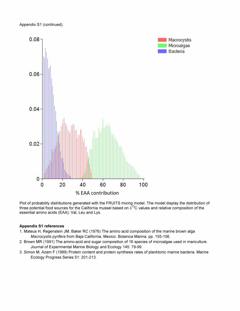
Appendix S1 (continued).

Plot of probability distributions generated with the FRUITS mixing model. The model display the distribution of

three potential food sources for the California mussel based on δ13

C values and relative composition of the essential amino acids (EAA); Val, Leu and Lys.

Appendix S1 references

1. Mateus H, Regenstein JM, Baker RC (1976) The amino acid composition of the marine brown alga

Macrocystis pyrifera from Baja California, Mexico. Botanica Marina. pp. 155-156.

2. Brown MR (1991) The amino-acid and sugar composition of 16 species of microalgae used in mariculture.

Journal of Experimental Marine Biology and Ecology 145: 79-99.

3. Simon M, Azam F (1989) Protein content and protein synthesis rates of planktonic marine bacteria. Marine

Ecology Progress Series 51: 201-213.

% EAA contribution

Supporting Figure S1 GC-C-IRMS chromatogram of the diatom Amphora coffaeiformis with the ratio of 45 to 44 voltages over time in the upper panel and voltage (mV) over time of ion masses 44 and 45, the most abundant CO2 ion forms, in the lower panel.

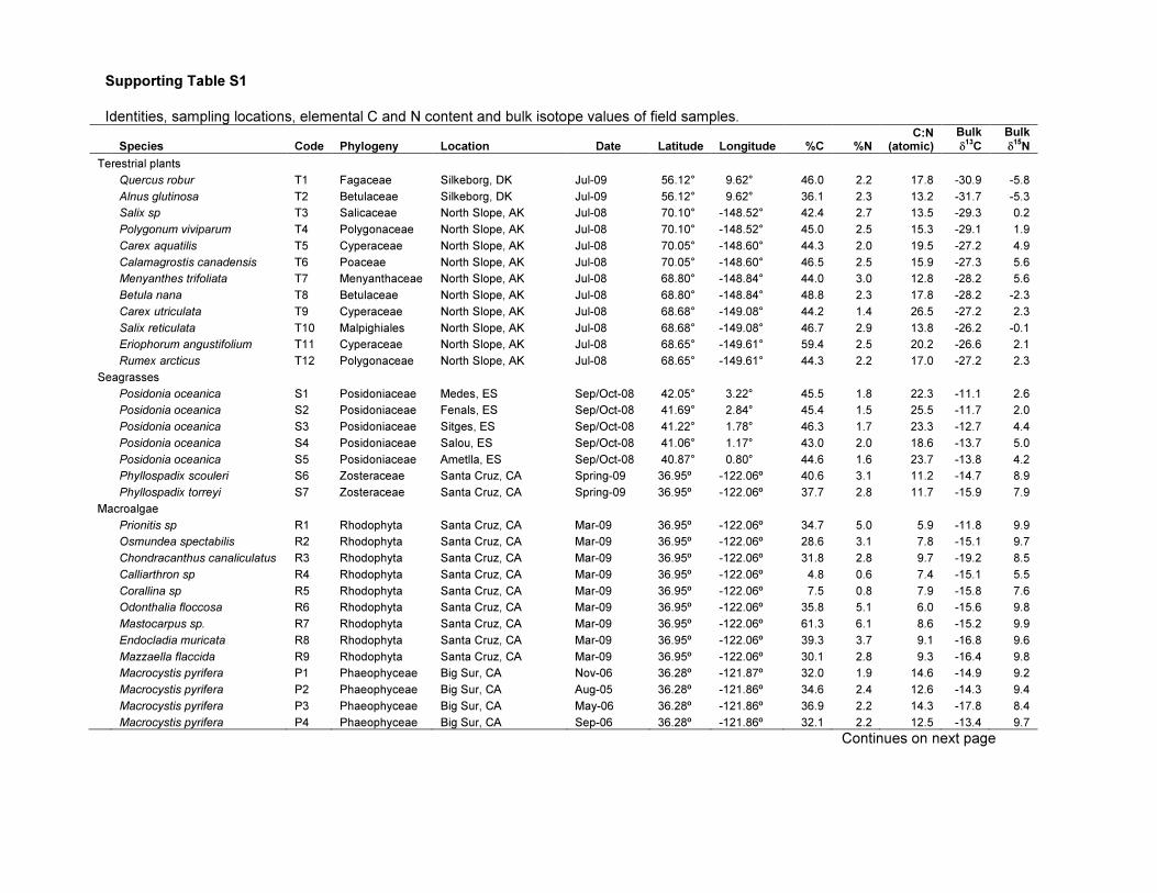
Supporting Table S1

Identities, sampling locations, elemental C and N content and bulk isotope values of field samples.

Species Code Phylogeny Location Date Latitude Longitude %C %N C:N

(atomic)

Bulk

δ13

C

Bulk

δ15

N

Terestrial plants

Quercus robur T1 Fagaceae Silkeborg, DK Jul-09 56.12° 9.62° 46.0 2.2 17.8 -30.9 -5.8

Alnus glutinosa T2 Betulaceae Silkeborg, DK Jul-09 56.12° 9.62° 36.1 2.3 13.2 -31.7 -5.3

Salix sp T3 Salicaceae North Slope, AK Jul-08 70.10° -148.52° 42.4 2.7 13.5 -29.3 0.2

Polygonum viviparum T4 Polygonaceae North Slope, AK Jul-08 70.10° -148.52° 45.0 2.5 15.3 -29.1 1.9

Carex aquatilis T5 Cyperaceae North Slope, AK Jul-08 70.05° -148.60° 44.3 2.0 19.5 -27.2 4.9

Calamagrostis canadensis T6 Poaceae North Slope, AK Jul-08 70.05° -148.60° 46.5 2.5 15.9 -27.3 5.6

Menyanthes trifoliata T7 Menyanthaceae North Slope, AK Jul-08 68.80° -148.84° 44.0 3.0 12.8 -28.2 5.6

Betula nana T8 Betulaceae North Slope, AK Jul-08 68.80° -148.84° 48.8 2.3 17.8 -28.2 -2.3

Carex utriculata T9 Cyperaceae North Slope, AK Jul-08 68.68° -149.08° 44.2 1.4 26.5 -27.2 2.3

Salix reticulata T10 Malpighiales North Slope, AK Jul-08 68.68° -149.08° 46.7 2.9 13.8 -26.2 -0.1

Eriophorum angustifolium T11 Cyperaceae North Slope, AK Jul-08 68.65° -149.61° 59.4 2.5 20.2 -26.6 2.1

Rumex arcticus T12 Polygonaceae North Slope, AK Jul-08 68.65° -149.61° 44.3 2.2 17.0 -27.2 2.3

Seagrasses

Posidonia oceanica S1 Posidoniaceae Medes, ES Sep/Oct-08 42.05° 3.22° 45.5 1.8 22.3 -11.1 2.6

Posidonia oceanica S2 Posidoniaceae Fenals, ES Sep/Oct-08 41.69° 2.84° 45.4 1.5 25.5 -11.7 2.0

Posidonia oceanica S3 Posidoniaceae Sitges, ES Sep/Oct-08 41.22° 1.78° 46.3 1.7 23.3 -12.7 4.4

Posidonia oceanica S4 Posidoniaceae Salou, ES Sep/Oct-08 41.06° 1.17° 43.0 2.0 18.6 -13.7 5.0

Posidonia oceanica S5 Posidoniaceae Ametlla, ES Sep/Oct-08 40.87° 0.80° 44.6 1.6 23.7 -13.8 4.2

Phyllospadix scouleri S6 Zosteraceae Santa Cruz, CA Spring-09 36.95º -122.06º 40.6 3.1 11.2 -14.7 8.9

Phyllospadix torreyi S7 Zosteraceae Santa Cruz, CA Spring-09 36.95º -122.06º 37.7 2.8 11.7 -15.9 7.9

Macroalgae

Prionitis sp R1 Rhodophyta Santa Cruz, CA Mar-09 36.95º -122.06º 34.7 5.0 5.9 -11.8 9.9

Osmundea spectabilis R2 Rhodophyta Santa Cruz, CA Mar-09 36.95º -122.06º 28.6 3.1 7.8 -15.1 9.7

Chondracanthus canaliculatus R3 Rhodophyta Santa Cruz, CA Mar-09 36.95º -122.06º 31.8 2.8 9.7 -19.2 8.5

Calliarthron sp R4 Rhodophyta Santa Cruz, CA Mar-09 36.95º -122.06º 4.8 0.6 7.4 -15.1 5.5

Corallina sp R5 Rhodophyta Santa Cruz, CA Mar-09 36.95º -122.06º 7.5 0.8 7.9 -15.8 7.6

Odonthalia floccosa R6 Rhodophyta Santa Cruz, CA Mar-09 36.95º -122.06º 35.8 5.1 6.0 -15.6 9.8

Mastocarpus sp. R7 Rhodophyta Santa Cruz, CA Mar-09 36.95º -122.06º 61.3 6.1 8.6 -15.2 9.9

Endocladia muricata R8 Rhodophyta Santa Cruz, CA Mar-09 36.95º -122.06º 39.3 3.7 9.1 -16.8 9.6

Mazzaella flaccida R9 Rhodophyta Santa Cruz, CA Mar-09 36.95º -122.06º 30.1 2.8 9.3 -16.4 9.8

Macrocystis pyrifera P1 Phaeophyceae Big Sur, CA Nov-06 36.28º -121.87º 32.0 1.9 14.6 -14.9 9.2

Macrocystis pyrifera P2 Phaeophyceae Big Sur, CA Aug-05 36.28º -121.86º 34.6 2.4 12.6 -14.3 9.4

Macrocystis pyrifera P3 Phaeophyceae Big Sur, CA May-06 36.28º -121.86º 36.9 2.2 14.3 -17.8 8.4

Macrocystis pyrifera P4 Phaeophyceae Big Sur, CA Sep-06 36.28º -121.86º 32.1 2.2 12.5 -13.4 9.7

Continues on next page

Table S1 continued

Species Code Phylogeny Location Date Latitude Longitude %C %N C:N

(atomic) Bulk δ13

C

Bulk

δ15

N

Macrocystis pyrifera P5 Phaeophyceae Big Sur, CA Mar-07 36.28º -121.86º 33.3 1.8 16.1 -18.7 7.2

Scytosiphon sp P6 Phaeophyceae Santa Cruz, CA Mar-09 36.95º -122.06º 32.9 2.9 9.8 -8.5 8.7

Laminaria sp P7 Phaeophyceae Santa Cruz, CA Mar-09 36.95º -122.06º 25.2 1.8 12.0 -14.3 9.9

Silvetia sp P8 Phaeophyceae Santa Cruz, CA Mar-09 36.95º -122.06º 37.5 1.5 21.3 -15.2 9.3

Petrospongium sp P9 Phaeophyceae Santa Cruz, CA Mar-09 36.95º -122.06º 30.8 1.9 13.7 -11.9 9.6

Pelvetiopsis sp. P10 Phaeophyceae Santa Cruz, CA Mar-09 36.95º -122.06º 32.2 1.8 15.2 -17.9 10.0

Ralfsia sp P11 Phaeophyceae Santa Cruz, CA Mar-09 36.95º -122.06º 34.8 2.2 13.5 -7.0 9.6

Cystoseira osmundacea P12 Phaeophyceae Santa Cruz, CA Mar-09 36.95º -122.06º 28.6 1.8 13.8 -17.0 8.8

Fish

Coryphaena hippurus ch Coryphaenidae CN Pacific Ocean Jun-10 ~25º ~-150º NA NA NA -16.3 NA

Lampris guttatus lg Lampridae CN Pacific Ocean Dec-10 ~22º ~-140º NA NA NA -19.9 NA

Xiphias gladius xg Xiphiidae CN Pacific Ocean Jan-11 ~31º ~-135º NA NA NA -21.8 NA

Mussels

Mytilus californianus gav Mytilidae Gaviota, CA Jan-11 34.47º -120.48º NA NA NA -15.0 10.3

Mytilus californianus sc Mytilidae Santa Cruz, CA Jan-11 36.95º -122.05º NA NA NA -13.3 10.8

Daphnia

Daphnia middendorffiana dL1 Daphnia North Slope, AK Jul-08 70.10° -148.52° 49.0±0.4 11.5±0.3 3.6±0.0 -26.9±0.0 NA

Daphnia middendorffiana dL2 Daphnia North Slope, AK Jul-08 70.05° -148.60° 49.0±0.3 11.5±0.1 3.7±0.1 -26.6±0.0 3.4±0.3

Daphnia tenebrosa dL3 Daphnia North Slope, AK Jul-08 68.80° -148.84° 50.3±3.8 11.0±1.0 3.9±0.3 -26.3±0.3 1.3±0.0

Daphnia pulex dL4 Daphnia North Slope, AK Jul-08 68.68° -149.08° 48.6±1.4 11.6±0.3 3.6±0.0 -25.5±0.1 1.8±0.5

Daphnia pulex dL5 Daphnia North Slope, AK Jul-08 68.65° -149.61° 49.9±1.8 12.1±0.5 3.5±0.0 -25.7±0.1 2.5±1.0

Soils

Peat soil sL1 Detrital North Slope, AK Jul-08 70.10° -148.52° 22 0.9 21.4 -27.7 2.9

Peat soil sL3 Detrital North Slope, AK Jul-08 68.80° -148.84° 32.2 1.2 22.8 -26.8 3.4

Peat soil sL4 Detrital North Slope, AK Jul-08 68.68° -149.08° 39.2 2 16.5 -26.3 0.7

Peat soil sL5 Detrital North Slope, AK Jul-08 68.65° -149.61° 38.1 1.7 19.2 -25.7 1

Seston

Seston 5 µm pL1 Plankton North Slope, AK Jul-08 70.10° -148.52° 15.5 1.1 11.9 -20.1 1.7

Seston 5 µm pL2 Plankton North Slope, AK Jul-08 70.05° -148.60° 35.6 4 7.6 -33.6 0.1

Supporting Table S2

Identities, origins, substrates, elemental C and N content and bulk isotope values of laboratory samples.

Phylogeny Code Origin Nutrient source$

Sub-strate ºC %C %N

C:N (atomic)

Bulk

δ13

C

Bulk

δ 15

N

Bacteria

Burkholderia xenovorans B1 culture collection* MAG [1,2] Agar 22 47.2 12.5 3.2 -12.5 -8.1

Methylobacterium sp B2 isolated from boreal forest* MAG Liquid 25 44.8 9.0 4.3 -13.3 -10.0

Klebsiella sp B3 isolated from boreal forest* MAG Agar 22 45.1 11.0 3.5 -22.9 -4.0

Rhodococcus spp. B4 isolated from boreal forest* Czapek Liquid 25 54.9 4.9 9.5 -22.7 5.1

Unidentified B5 isolated from tundra soil MAG Agar 22 44.2 11.2 3.4 -16.2 -0.1

Unidentified B6 isolated from tundra soil MAG Agar 22 43.6 10.6 3.5 -16.6 2.1

Unidentified B7 isolated from tundra soil MAG Agar 22 44.1 10.4 3.6 -16.2 0.4

Unidentified B8 isolated from arctic lake MAG Agar 22 44.2 10.4 3.7 -15.5 0.1

Unidentified B9 isolated from tundra soil MAG Agar 22 43.7 10.3 3.6 -22.9 -7.0

Unidentified B10 isolated from tundra soil MAG Agar 22 40.3 7.9 4.4 -17.4 -1.1

Unidentified B11 isolated from tundra soil MAG Agar 22 41.7 8.4 4.3 -17.9 0.9

Unidentified B12 isolated from arctic lake MAG Agar 22 42.5 9.9 3.7 -23.2 -2.5

Fungi

Ascomycota F1 isolated from boreal forest* Czapek Liquid 25 47.3 1.9 21.1 -25.0 2.8

Aureobasidium pullulans F2 isolated from boreal forest* MAG Liquid 25 41.5 6.0 5.9 -22.6 2.6

Bionectria orhroleuca F3 isolated from boreal forest* Czapek Agar 22 42.5 4.5 8.2 -24.6 4.0

Nectria vilior F4 isolated from boreal forest* Czapek Liquid 25 34.7 2.9 10.3 -23.6 2.8

Mortierella alpina F8 culture collection* MMN [3] Agar 22 40.5 6.0 5.8 -8.7 9.5

Unidentified F5 isolated from tundra soil MMN Liquid 25 53.6 2.3 19.8 -10.7 6.5

Unidentified F6 isolated from tundra soil MMN Liquid 25 55.0 1.6 29.4 -11.3 8.7

Unidentified F7 isolated from tundra soil MMN Liquid 25 47.9 4.0 10.3 -10.9 8.4

Unidentified F9 isolated from tundra soil MMN Liquid 25 49.9 3.3 12.9 -10.9 8.2

Microalgae

Cyanothece sp C1 GEOMAR† no nutrients added SW 29 42.9 3.7 9.9 -20.1 -1.2

Merismopedia punctata C2 GEOMAR f/2 diluted 1:4 [4,5] BW 20 20.1 3.1 5.6 -25.9 5.4

Anabaena cylindrica C3 SAG‡ no nutrients added FW 20 46.6 9.0 4.5 -19.3 -1.0

Nostoc muscorum C4 SAG no nutrients added FW 20 50.5 6.3 6.9 -19.1 3.6

Achnanthes brevipes D1 GEOMAR f/2 BW 20 28.8 1.9 13.1 -12.8 4.6

Amphora coffaeiformis D2 GEOMAR f/2 BW 20 24.7 2.2 9.6 -10.5 5.5

Melosira varians D3 GEOMAR f/2 BW 20 24.0 3.2 6.5 -14.6 4.0

Phaeodactylum tricornutum D4 SAG f/2 SW 20 18.8 3.1 5.1 -19.4 10.4

Stauroneis constricta D5 GEOMAR f/2 SW 20 24.7 1.2 17.6 -9.1 5.1

Continues on next page

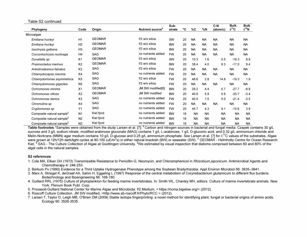
Table S2 continued

Phylogeny Code Origin Nutrient source$

Sub-strate ºC %C %N

C:N (atomic)

Bulk

δ13

C

Bulk

δ15

N

Microalgae

Emiliana huxleyi H1 GEOMAR f/2 w/o silica SW 20 NA NA NA NA NA

Emiliana huxleyi H2 GEOMAR f/2 w/o silica BW 20 NA NA NA NA NA

Isochrysis galbana H3 GEOMAR f/2 w/o silica BW 20 NA NA NA NA NA

Corcontochrysis noctivaga H4 SAG no nutrients added FW 20 NA NA NA NA NA

Dunaliella sp. K1 GEOMAR f/2 w/o silica SW 20 10.3 1.6 5.5 -16.3 8.9

Prasinocladus marinus K2 GEOMAR f/2 w/o silica BW 20 38.4 4.0 8.3 -17.0 8.4

Ankistrodesmus falcatus K3 SAG f/2 w/o silica FW 20 NA NA NA NA NA

Chlamydocapsa maxima K4 SAG no nutrients added FW 20 NA NA NA NA NA

Chlamydomonas asymmetrica K5 SAG f/2 w/o silica FW 20 48.6 2.8 14.8 -19.3 1.9

Chlamydomonas gigantea K6 SAG f/2 w/o silica FW 20 NA NA NA NA NA

Ochromonas minima X1 GEOMAR JM SW modified[6] BW 20 29.2 4.4 5.7 -27.7 -8.8

Ochromonas villosa X2 GEOMAR JM SW modified BW 20 40.6 5.9 5.9 -25.7 -3.4

Ochromonas danica X3 SAG no nutrients added FW 20 40.5 7.0 5.0 -21.4 -3.5

Chromulina sp X4 SAG no nutrients added FW 20 NA NA NA NA NA

Cryptomonas sp Y1 SAG no nutrients added FW 20 45.7 4.3 9.1 -15.6 3.9

Composite natural sample§ N1 Kiel fjord no nutrients added BW 16 NA NA NA NA NA

Composite natural sample§ N2 Kiel fjord no nutrients added BW 16 NA NA NA NA NA

Composite natural sample§ N3 Kiel fjord no nutrients added BW 16 NA NA NA NA NA

Table footnotes.*Samples were obtained from the study Larsen et al. [7]; $

Carbon and nitrogen sources in bacterial and fungal media: Czapek contains 30 g/L sucrose and 3 g/L sodium nitrate, modified arabinose gluconate (MAG) contains 1 g/L L-arabinose, 1 g/L D-gluconic acid, and 0.32 g/L ammonium chloride and

Melin-Norkrans (MMN) agar medium contains 10 g/L D-glucose and 0.25 g/L ammonium phosphate. See Larsen et al. [7] for δ13

C values of the substrates. Algae were grown at 12h/12h dark/light cycles at 80-100 (uE/m

2s) in either natural brackish (BW) or seawater (SW).

† GEOMAR - Helmholtz Centre for Ocean Research

Kiel; ‡ SAG - The Culture Collection of Algae at Goettingen University.

§We estimated by visual inspection that diatoms comprised between 60 and 80% of the

algal cells in the natural samples.

S2 references

1. Cole MA, Elkan GH (1973) Transmissible Resistance to Penicillin-G, Neomycin, and Chloramphenicol in Rhizobium japonicum. Antimicrobial Agents and Chemotherapy 4: 248-253.

2. Berkum Pv (1990) Evidence for a Third Uptake Hydrogenase Phenotype among the Soybean Bradyrhizobia. Appl Environ Microbiol 56: 3835–3841. 3. Marx A, Striegel K, deGraaf AA, Sahm H, Eggeling L (1997) Response of the central metabolism of Corynebacterium glutamicum to different flux burdens.

Biotechnology and Bioengineering 56: 168-180. 4. Guillard RRL (1975) Culture of phytoplankton for feeding marine invertebrates. In: Smith WL, Chanley MH, editors. Culture of marine invertebrate animals. New

York: Plenum Book Publ. Corp. 5. Provasoli-Guillard National Center for Marine Algae and Microbiota. f/2 Medium, < https://ncma.bigelow.org/> (2012). 6. Roscoff Culture Collection. JM SW modified, <http://www.sb-roscoff.fr/Phyto/RCC > (2012). 7. Larsen T, Taylor D, Leigh MB, O'Brien DM (2009) Stable isotope fingerprinting: a novel method for identifying plant, fungal or bacterial origins of amino acids.

Ecology 90: 3526-3535.

Supporting Table S3

Amino acid δ13

C values (‰). Each sample was analyzed in triplicate (mean±stdev). See Table S1 and S2 for sample identities. NA indicates missing values.

ID Ala Asx Glx Gly His Ile Leu Lys Met Phe Thr Tyr Val

Bacteria

B1 -11.3± 0.1 -12.9± 0.9 -11.5± 0.0 -12.9± 0.1 -8.4± 0.9 -12.0± 0.0 -12.8± 0.1 -10.4± 0.1 -18.6± 0.1 -18.8± 0.0 -5.2± 0.8 -16.8± 0.1 -13.6± 0.1

B2 -12.2± 0.0 -17.6± 0.3 -17.8± 0.0 -13.9± 0.0 -8.1± 0.7 -12.9± 0.1 -13.0± 0.0 -14.9± 0.1 -18.5± 0.2 -17.0± 0.1 -8.2± 1.4 -18.1± 0.1 -14.1± 0.1

B3 -15.9± 0.0 -21.8± 0.7 -18.3± 0.0 -21.3± 0.2 -16.0± 0.4 -18.9± 0.2 -19.9± 0.0 -20.3± 0.2 -25.7± 0.3 -24.6± 0.1 -15.0± 0.8 -22.9± 0.0 -20.8± 0.0

B4 -22.6± 0.0 -22.7± 0.4 -22.9± 0.0 -25.3± 0.1 -22.2± 0.4 -23.7± 0.1 -25.2± 0.2 -21.2± 1.1 -27.5± 0.2 -28.9± 0.1 -15.1± 0.1 -27.7± 0.2 -26.4± 0.2

B5 -14.8± 0.1 -17.4± 0.6 -16.5± 0.0 -13.8± 0.4 -8.1± 0.2 -16.1± 0.1 -17.7± 0.3 -14.8± 0.2 -20.0± 0.2 -18.3± 0.1 -8.3± 0.2 -18.0± 0.0 -17.8± 0.1

B6 -18.3± 0.1 -15.1± 0.1 -14.3± 0.1 -18.5± 0.1 -11.8± 0.2 -17.1± 0.5 -19.2± 0.1 -15.3± 0.1 -18.8± 0.2 -20.1± 0.1 -8.6± 1.3 -20.2± 0.1 -21.1± 0.0

B7 -15.3± 0.0 -15.3± 0.9 -13.9± 0.0 -14.3± 0.1 -9.8± 0.0 -15.6± 0.2 -17.4± 0.1 -12.9± 0.2 -18.5± 0.1 -18.5± 0.1 -7.4± 0.3 -18.3± 0.1 -19.0± 0.0

B8 -14.1± 0.1 -15.4± 0.7 -15.2± 0.0 -14.0± 0.3 -7.8± 0.3 -16.1± 0.2 -15.9± 0.0 -14.4± 0.1 -20.7± 0.3 -17.7± 0.0 -7.8± 0.5 -17.4± 0.2 -17.7± 0.0

B9 -18.1± 0.1 -24.2± 0.9 -21.2± 0.0 -21.7± 0.2 -16.8± 0.2 -21.2± 0.5 -24.1± 0.5 -21.5± 0.1 -27.4± 0.3 -27.0± 0.0 -16.8± 0.2 -25.2± 0.1 -25.1± 0.1

B10 -16.5± 0.0 -19.2± 0.0 -16.8± 0.1 -15.5± 0.3 -10.6± 0.4 -18.6± 0.1 -17.4± 0.1 -17.8± 0.2 NA -20.9± 0.0 -12.2± 0.3 -19.7± 0.1 -21.4± 0.0

B11 -17.2± 0.1 -18.9± 0.1 -18.5± 0.0 -16.9± 0.6 -11.8± 0.5 -18.6± 0.1 -19.0± 0.1 -18.5± 0.1 NA -21.9± 0.1 -11.6± 0.7 -20.9± 0.1 -22.1± 0.1

B12 -20.8± 0.1 -24.4± 0.0 -24.1± 0.0 -22.4± 0.4 NA± NA -24.0± 0.1 -24.2± 0.1 -24.8± 0.2 -31.6± 0.3 -28.7± 0.1 -17.9± 1.6 -25.5± 0.0 -26.0± 0.1

Collembola

cL1 -27.4± 0.1 -24.5± 1.0 -23.6± 0.1 -24.2± 0.0 -21.6± 0.2 -27.8± 0.1 -32.7± 0.2 -27.4± 0.1 -27.6± 0.1 -30.8± 0.1 -17.0± 0.0 -29.9± 0.1 -30.5± NA

cL2 -25.8± 0.1 -22.1± 1.0 -22.3± 0.1 -23.4± 0.1 -21.0± 0.4 -26.2± 0.1 -32.3± 0.2 -25.8± 0.2 -25.6± 0.2 -28.6± 0.2 -16.7± 0.2 -27.9± 0.1 -30.8± 0.2

cL3 -25.6± 0.1 -21.2± 0.1 -23.0± 0.0 -23.7± 0.1 -20.4± 0.3 -26.0± 0.2 -31.4± 0.3 -24.9± 0.1 -25.8± 0.1 -28.4± 0.0 -15.5± 0.2 -27.6± 0.1 -29.1± 0.3

cL4 -24.8± 0.1 -22.0± 0.2 -22.8± 0.1 -24.6± 0.1 -20.1± 0.2 -26.1± 0.1 -30.8± 0.1 -25.5± 0.0 -25.6± 0.1 -28.0± 0.0 -16.2± 0.2 -27.3± 0.1 -28.5± 0.0

cL5 -25.4± 0.1 -24.6± 1.0 -23.0± 0.0 -23.6± 0.1 -19.3± 0.4 -26.4± 0.0 -31.2± 0.1 -25.7± 0.0 -25.3± 0.1 -28.4± 0.1 -16.2± 0.2 -27.7± 0.0 -29.9± 0.1

Daphnia

dL1 -29.8± 0.2 -28.2± 0.8 -27.2± 0.0 -22.7± 0.4 -22.5± 0.1 -30.9± 0.1 -35.6± 0.1 -26.5± 0.1 -28.6± 0.2 -36.0± 0.1 -15.8± 0.8 -33.4± 0.1 -33.3± 0.0

dL2 -32.4± 0.3 -30.6± 0.5 -30.5± 0.0 -24.6± 0.3 -25.9± 0.6 -33.8± 0.2 -38.3± 0.2 -29.2± 0.2 -31.5± 0.2 -38.8± 0.0 -20.8± 1.3 -35.9± 0.2 -37.4± 0.1

dL3 -26.6± 0.0 -27.0± 0.2 -25.7± 0.0 -21.5± 0.1 -21.7± 0.2 -29.6± 0.1 -34.0± 0.4 -25.3± 0.2 -27.8± 0.3 -34.2± 0.1 -16.8± 0.1 -31.6± 0.2 -32.5± 0.1

dL4 -36.1± 0.2 -32.1± 0.7 -31.6± 0.0 -31.6± 0.5 -29.0± 0.2 -34.6± 0.1 -39.7± 0.1 -31.0± 0.2 -33.1± 0.2 -40.2± 0.1 -21.8± 0.1 -37.0± 0.1 -38.8± 0.0

dL5 -32.6± 0.1 -28.8± 0.1 -29.0± 0.0 -23.6± 0.2 -22.6± 0.3 -32.2± 0.0 -37.1± 0.1 -28.6± 0.1 -30.8± 0.1 -37.4± 0.1 -20.6± 0.1 -34.8± 0.0 -35.8± 0.1

Fish ch -14.3± 0.4 -17.8± 0.1 -14.6± 0.1 -7.0± 0.1 -9.6± 0.0 -18.4± 0.5 -25.4± 0.2 -16.9± 0.1 -25.4± 0.1 -26.7± 0.1 -10.1± 0.4 -25.8± 0.3 -22.1± 0.3

lg -16.1± 0.1 -17.2± 1.4 -17.4± 0.3 -8.5± 0.1 -10.1± 0.1 -20.3± 0.0 -27.1± 0.1 -18.5± 0.1 -26.7± 0.1 -27.8± 0.1 -11.3± 0.6 -26.4± 0.1 -22.7± 0.3

xg -16.5± 0.6 -16.0± 0.4 -18.2± 0.0 -5.9± 0.3 -7.4± 0.2 -20.1± 0.2 -27.7± 0.2 -18.8± 0.1 -25.6± 0.1 -27.1± 0.1 -8.7± 0.3 -26.0± 0.2 -23.2± 0.2

Fungi F1 -21.2± 0.1 -20.4± 0.1 -20.9± 0.0 -28.8± 0.3 -22.1± 0.3 -23.4± 0.1 -30.0± 0.2 -28.0± 0.4 -22.0± 0.2 -27.3± 0.0 -13.8± 0.5 -27.1± 0.1 -25.1± 0.1

F2 -16.0± 0.2 -19.7± 0.6 -20.7± 0.0 -22.8± 0.1 -20.6± 0.4 -22.3± 0.4 -27.2± 0.1 -26.5± 0.2 -24.5± 0.3 -26.5± 0.0 -11.9± 0.5 -26.6± 0.1 -21.7± 0.2

F3 -21.4± 0.1 -22.3± 0.1 -20.6± 0.1 -25.7± 0.1 NA± NA -24.8± 0.1 -31.1± 0.5 -27.6± 0.7 -25.1± 0.4 -30.2± 0.4 -14.3± 0.1 -28.8± 0.1 -26.1± 0.0

F4 -18.3± 0.0 -21.9± 0.0 -21.3± 0.1 -23.2± 0.6 -22.9± 0.3 -22.7± 0.2 -29.5± 0.1 -28.5± 0.1 -25.2± 0.6 -27.9± 0.0 -12.2± 0.1 -27.5± 0.2 -26.8± 0.2

ID Ala Asx Glx Gly His Ile Leu Lys Met Phe Thr Tyr Val

F8 -6.4± 0.1 -6.3± 0.1 -4.1± 0.0 -10.7± 0.1 -7.1± 0.4 -6.0± 0.0 -12.4± 0.1 -11.0± 0.2 -10.7± 0.3 -13.3± 0.0 -1.2± 0.1 -13.9± 0.1 -8.7± 0.1

F5 -5.5± 0.1 -6.6± 0.8 -4.9± 0.2 -8.7± 0.1 -8.3± 0.7 -8.5± 0.3 -14.7± 0.5 -12.7± 0.2 -10.3± 0.2 -14.5± 0.1 -1.9± 0.8 -14.3± 0.1 -10.3± 0.1

F6 -5.2± 0.0 -5.7± 0.5 -3.9± 0.0 -4.4± 0.2 -10.8± 0.3 -8.2± 0.4 -13.8± 0.4 -14.4± 0.6 -9.7± 0.1 -15.3± 0.1 -1.6± 0.5 -15.1± 0.1 -8.3± 0.3

F7 -4.7± 0.2 -4.5± 0.1 -4.2± 0.1 -8.1± 0.1 -9.2± 0.2 -9.5± 0.2 -17.3± 0.3 -14.2± 0.2 -12.0± 0.5 -15.5± 0.1 -3.3± 0.1 -14.6± 0.2 -10.0± 0.3

F9 -6.2± 0.1 -5.6± 0.2 -4.3± 0.0 -7.5± 0.1 -6.7± 0.3 -9.3± 0.1 -16.7± 0.1 -13.4± 0.4 -13.8± 0.5 -15.3± 0.1 -4.4± 0.0 -15.0± 0.1 -11.5± 0.0

Macroalgae R1 -9.0± 0.1 -10.9± 0.1 -14.3± 0.1 -4.2± 0.1 -12.5± 0.3 -17.3± 0.5 -20.2± 0.1 -10.9± 0.1 -15.3± 0.1 -19.2± 0.0 -6.4± 0.2 -18.9± 0.1 -19.2± 0.1

R2 -13.3± 0.2 -11.3± 0.6 -16.2± 0.0 -10.3± 0.3 NA -15.4± 0.3 -19.5± 0.2 -13.0± 0.2 NA -20.7± 0.1 -4.8± 0.6 -20.0± 0.1 -21.3± 0.3

R3 -17.3± 0.2 -16.4± 0.1 -18.6± 0.1 -14.7± 0.1 -19.4± 0.0 -21.7± 0.3 -25.8± 0.3 -16.4± 0.2 NA -25.3± 0.1 -9.2± 0.2 -23.0± 0.1 -25.4± 0.2

R4 -13.4± 0.1 -11.1± 0.2 -13.8± 0.0 -16.4± 0.1 -12.9± 0.2 -17.0± 0.1 -21.9± 0.4 -14.9± 0.2 -21.6± 0.2 -23.7± 0.0 -11.0± 1.1 -21.9± 0.1 -19.8± 0.1

R5 -15.5± 0.1 -15.4± 0.0 -17.6± 0.6 -13.7± 0.0 NA -19.5± 0.1 -22.5± 0.1 -16.4± 0.4 NA -25.3± 0.1 -15.3± 0.1 -24.2± 0.0 -22.4± 0.0

R6 -11.4± 0.1 -11.4± 0.1 -14.8± 0.0 -9.8± 0.1 -14.2± NA -16.5± 0.1 -21.0± 0.4 -13.1± 0.1 NA -21.1± 0.1 -8.7± 0.1 -19.8± 0.1 -20.7± 0.2

R7 -12.1± 0.1 -12.4± 0.5 -15.4± 0.1 -9.9± 0.0 NA -16.7± 0.2 -21.0± 0.3 -11.0± 0.1 -15.3± 0.1 -21.1± 0.3 -5.9± 0.3 -19.5± 0.4 -20.3± 0.0

R8 -14.7± 0.3 -14.5± 0.7 -16.1± 0.4 -14.5± 0.1 NA -18.0± 0.1 -23.5± 0.0 -15.8± 0.4 -17.9± NA -22.0± 0.0 -7.3± 1.1 -21.2± 0.3 -23.6± 0.0

R9 -11.9± 0.1 -13.2± 0.1 -15.6± 0.1 -10.7± 0.1 -16.4± 0.4 -20.4± 0.2 -23.4± 0.0 -13.3± 0.1 -17.3± 0.5 -22.5± 0.1 -6.8± 1.0 -20.1± 0.0 -20.9± 0.1

P1 -13.6± 0.2 -4.6± 0.3 -12.7± 0.1 -12.1± 0.1 -13.2± 0.3 -17.6± 0.2 -23.1± 0.2 -11.1± 0.1 -14.1± 0.2 -19.4± 0.1 -3.6± 0.2 -18.6± 0.1 -18.8± 0.1

P2 -10.3± 0.3 -1.9± 0.7 -11.4± 0.1 -9.6± 0.3 -12.6± 0.3 -15.2± 0.1 -21.5± 0.2 -9.1± 0.2 -13.0± 0.1 -19.1± 0.2 -1.2± 0.5 -18.2± 0.1 -17.0± 0.1

P3 -15.2± 0.3 -5.6± 0.7 -15.6± 0.1 -15.7± 0.3 NA -19.6± 0.4 -24.8± 0.1 -12.7± 0.3 -16.0± 0.4 -22.2± 0.1 -5.5± 0.1 -21.1± 0.1 -20.7± 0.0

P4 -11.9± 0.3 -2.4± 0.2 -11.6± 0.1 -10.3± 0.0 -12.0± 0.9 -16.8± 1.4 -20.0± 0.1 -9.9± 0.1 -13.1± 0.3 -18.9± 0.1 -0.4± 0.3 -18.0± 0.2 -15.7± 0.1

P5 NA± 0.4 -9.2± 0.2 -18.0± 0.1 -17.2± 0.1 -16.7± 0.5 -21.4± 0.1 -26.1± 0.2 -14.1± 0.1 -17.5± 0.1 -23.9± 0.0 -6.4± 0.2 -22.2± 0.2 -22.5± 0.1

P6 -4.5± 0.0 -4.2± 1.0 -4.7± 0.0 -2.7± 0.2 NA -6.3± 0.6 -13.3± 0.1 -1.7± 0.0 -7.2± 0.1 -12.8± 0.1 -2.6± 0.7 -12.2± 0.3 -10.4± 0.1

P7 -9.5± 0.2 -4.9± 0.1 -11.3± 0.0 -7.7± 0.2 -7.6± 0.1 -15.6± 0.1 -23.9± 0.4 -9.2± 0.4 -12.7± 0.5 -18.8± 0.1 -1.2± 0.5 -18.8± 0.1 -19.1± 0.1

P8 -10.4± 0.1 -9.0± 0.3 -12.0± 0.2 -6.9± 0.2 -14.9± 0.6 -19.5± 0.2 -25.5± 0.3 -10.7± 0.2 -17.8± 0.2 -20.4± 0.2 -0.5± 0.7 -21.9± 0.1 -19.6± 0.3

P9 -9.2± 0.2 -5.7± 1.1 -9.6± 0.0 -9.2± 0.3 NA -10.9± 0.1 -18.3± 0.4 -8.2± 0.1 NA -16.7± 0.1 0.9± 0.5 -17.0± 0.0 -14.5± 0.0

P10 -14.1± 0.1 -9.8± 0.1 -12.6± 0.1 -11.5± 0.1 NA -16.9± 0.1 -23.6± 0.2 -10.8± 0.3 -14.3± 0.1 -23.6± 0.0 5.4± 4.6 -22.9± 0.1 -21.2± 0.2

P11 -5.2± 0.0 -5.5± 0.8 -5.3± 0.0 -1.9± 0.1 -5.3± 0.5 -7.3± 0.1 -14.7± 0.3 -4.5± 0.2 -7.8± NA -12.7± NA 0.8± 0.3 -12.5± 0.0 -10.9± 0.2

P12 -14.4± 0.2 -8.7± 0.1 -17.1± 0.1 -16.2± 0.8 -15.1± 0.4 -17.6± 0.2 -25.2± 0.2 -9.1± 0.1 -14.7± 0.1 -21.2± 0.1 -8.6± 0.0 -20.4± 0.2 -22.4± 0.2

Microalgae

C1 -13.6± 0.2 -12.8± 0.2 -23.7± 0.1 -15.3± 0.6 -23.5± 0.3 -27.7± 0.2 -27.8± 0.1 -18.0± 0.0 -23.3± 0.5 -24.9± 0.3 -10.4± 0.1 -23.7± 0.1 -24.0± 0.1

C2 -22.6± 0.1 -16.2± 0.1 -26.3± 0.0 -23.1± 0.2 NA -28.9± 0.0 -36.0± 0.0 -23.8± 0.3 -23.9± 0.4 -34.6± 0.1 -19.5± 0.6 -35.0± 0.2 -32.8± 0.1

C3 -11.6± 0.1 -12.9± 1.0 -15.3± 0.0 -7.3± 0.2 NA -17.3± 0.1 -23.3± 0.3 -13.4± 0.2 NA -19.8± 0.1 -5.9± 1.0 -17.5± 0.2 -20.5± 0.2

C4 -13.1± 0.3 -12.2± 0.8 -18.9± 0.1 -11.3± 0.2 NA -20.0± 0.1 -25.8± 0.0 -13.8± 0.3 NA -24.0± 0.2 -10.1± 0.1 -22.1± 0.1 -24.2± 0.1

D1 -9.7± 0.1 -11.1± 0.4 -11.4± 0.1 -11.2± 0.2 NA -10.2± 0.1 -17.3± 0.2 -8.8± 0.5 NA -18.1± 0.3 -2.7± 0.8 -15.7± 0.1 -13.8± 0.1

D2 -7.4± 0.2 -9.1± 0.3 -7.5± 0.0 -12.0± 0.4 NA -11.5± 0.1 -18.7± 0.0 -11.1± 0.2 NA -19.6± 0.2 -2.0± 0.9 -16.0± 0.1 -16.8± 0.2

D3 -10.3± 0.1 -16.2± 1.0 -12.2± 0.0 -12.3± 0.1 NA -16.5± 0.0 -22.1± 0.5 -15.8± 0.2 -15.0± 0.2 -20.6± 0.1 -7.0± 1.6 -19.4± 0.1 -19.7± 0.0

D4 -16.0± 0.1 -17.7± 0.1 -18.9± 0.0 -12.2± 0.1 NA -16.1± 0.1 -25.5± 0.4 -15.2± 0.2 NA -23.8± 0.1 -10.8± 0.3 -21.8± 0.1 -22.9± 0.1

D5 -1.3± 0.1 -6.6± 1.0 -7.4± 0.1 5.5± 0.2 NA -10.4± 0.1 -19.3± 0.1 -8.5± 0.2 -8.2± 0.4 -16.0± 0.4 -4.6± 0.5 -14.4± 0.2 -15.5± 0.1

ID Ala Asx Glx Gly His Ile Leu Lys Met Phe Thr Tyr Val

H1 -16.3± 0.0 -15.6± 0.1 -15.9± 0.1 -13.5± 0.0 -17.8± 0.3 -18.3± 0.6 -27.2± 0.0 -15.7± 0.1 -17.9± 0.1 -23.2± 0.0 -9.1± 0.1 -22.3± 0.0 -24.9± 0.0

H2 -13.1± 0.1 -13.1± 1.0 -19.7± 0.1 -19.0± 0.1 NA -19.2± 0.2 -23.8± 0.1 -14.5± 0.1 NA -24.6± 0.0 -8.6± 0.6 -22.6± 0.1 -21.1± 0.3

H3 -16.4± 0.1 -13.3± 0.2 -16.7± 0.1 -19.6± 0.1 NA -18.3± 0.1 -31.4± 0.1 -15.4± 0.1 -19.9± 0.2 -25.0± 0.0 -8.9± 0.2 -22.7± 0.1 -26.8± 0.1

H4 -11.2± 0.0 -13.7± 0.9 -15.9± 0.0 -11.8± 0.1 NA -13.8± 0.1 -20.5± 0.1 -12.0± 0.4 NA -21.6± 0.1 -6.8± 0.3 -19.6± 0.1 -18.8± 0.0

K1 -12.1± 0.5 -13.0± 0.7 -15.6± 0.1 -7.1± 0.6 NA -15.8± 1.3 -23.7± 0.3 -13.0± 0.3 -16.9± 0.3 -19.7± 0.1 -6.7± 0.5 -16.8± 0.2 -19.2± 0.5

K2 -12.7± 0.1 -12.3± 0.9 -14.3± 0.1 -7.9± 0.1 NA -15.3± 0.5 -23.3± 0.1 -12.2± 0.0 -15.5± 0.4 -21.4± 0.0 -2.2± 0.8 -19.4± 0.1 -20.6± 0.1

K3 -4.1± 0.0 -5.7± 0.0 -10.0± 0.1 0.2± 0.1 NA -10.4± 0.1 -15.7± 0.1 -5.2± 0.1 NA -15.9± 0.1 -8.1± 0.9 -14.2± 0.0 -13.0± 0.1

K4 -5.5± 0.1 -7.5± 0.1 -10.8± 0.1 -6.6± 0.1 NA -11.4± 0.0 -16.7± 0.1 -7.7± 0.3 NA -15.7± 0.1 -4.2± 0.3 -12.5± 0.1 -15.3± 0.0

K5 -13.8± 0.1 -14.0± 0.4 -17.7± 0.1 -13.8± 0.1 NA -16.3± 0.2 -23.2± 0.3 -13.9± 0.4 NA -22.2± 0.0 -6.4± 0.3 -20.3± 0.2 -20.4± 0.1

K6 -9.6± 0.2 -13.4± 0.1 -12.1± 0.0 -10.7± 0.4 NA -11.4± 0.5 -18.4± 0.1 -10.5± 0.3 NA -18.4± 0.1 -7.1± 0.3 -16.8± 0.1 -15.9± 0.1

N1 -17.4± 0.1 -18.9± 0.0 -20.3± 0.1 -21.7± 0.4 -19.2± 0.6 -21.0± 0.1 -29.7± 0.3 -18.1± 0.0 -21.7± 0.6 -27.0± 0.1 -11.0± 0.1 -24.8± 0.2 -26.4± 0.5

N2 -17.4± 0.2 -18.2± 0.1 -20.3± 0.1 -21.9± 0.3 -20.8± 0.2 -20.6± 0.1 -29.3± 0.3 -18.0± 0.2 -19.2± 0.6 -26.8± 0.1 -11.2± 0.1 -24.5± 0.2 -27.2± 0.2

N3 -17.4± 0.2 -17.8± 0.2 -20.4± 0.0 -21.8± 0.6 -21.5± 0.2 -19.8± 0.1 -29.4± 0.2 -17.9± 0.2 -21.2± 0.4 -26.9± 0.1 -10.7± 0.1 -24.7± 0.2 -27.1± 0.1

X1 -17.2± 0.1 -16.5± 0.1 -24.5± 0.3 -14.7± 0.1 -25.4± 0.7 -26.7± 0.0 -35.1± 0.0 -20.7± 0.1 -27.3± 0.2 -31.9± 0.1 -13.6± 0.1 -29.7± 0.1 -30.2± 0.1

X2 -16.0± 0.0 -17.4± 0.9 -21.4± 0.0 -14.2± 0.2 NA -22.8± 0.2 -32.7± 0.0 -19.2± 0.1 NA -30.0± 0.1 -10.7± 0.8 -27.8± 0.1 -28.0± 0.1

X3 -16.3± 0.0 -18.3± 1.1 -18.9± 0.0 -14.5± 0.4 NA -19.3± 0.1 -25.2± 0.1 -16.4± 0.3 NA -25.5± 0.1 -9.6± 0.5 -23.3± 0.1 -23.9± 0.2

X4 -3.2± 0.2 -6.1± 0.1 -9.9± 0.4 -8.2± 0.0 NA -11.1± 0.1 -18.2± 0.0 -6.2± 0.2 NA -16.1± 0.0 -1.3± 0.2 -13.0± 0.1 -14.4± 0.1

Y1 -11.1± 0.1 -12.2± 0.1 -15.9± 0.1 -11.8± 0.1 NA -11.8± 0.5 -19.3± 0.3 -11.4± 0.2 NA -19.5± 0.1 -4.2± 0.3 -17.0± 0.1 -17.1± 0.1

Mussels gav -13.1± 0.1 -15.9± 2.1 -13.2± 0.0 -11.9± 0.1 -16.9± 0.8 -18.6± 0.1 -25.1± 0.1 -14.3± 0.1 -17.3± 0.3 -24.2± 0.1 -12.9± 0.2 -22.7± 0.1 -23.2± 0.1

sc -12.3± 0.0 -14.2± 0.1 -12.0± 0.1 -6.8± 0.0 -13.1± 0.2 -16.8± 0.0 -23.4± 0.0 -13.1± 0.0 -15.8± 0.1 -22.5± 0.1 -11.0± 0.3 -21.3± 0.1 -21.5± 0.1

Plants T1 -27.2± 0.2 -25.7± 1.3 -29.4± 0.1 -24.2± 0.1 -24.9± 0.2 -29.2± 0.1 -38.4± 0.2 -25.6± 0.2 NA -32.5± 0.4 -15.7± 0.3 -30.3± 0.1 -37.1± 0.5

T2 -24.6± 0.0 -25.5± 0.0 -29.1± 0.0 -24.5± 0.0 -32.4± 0.8 -30.7± 0.1 -39.7± 0.4 -27.9± 0.1 NA -33.9± 0.1 -16.1± 2.3 -31.5± 0.0 -36.1± 0.2

T3 -25.1± 0.1 -19.9± 0.5 -23.7± 0.1 -20.1± 0.1 -21.5± 0.6 -24.2± 0.3 -34.4± 0.2 -22.5± 0.1 NA -27.0± 0.1 -12.6± 0.3 -26.0± 0.3 -31.4± 0.3

T4 -27.0± 0.0 -23.0± 0.6 -26.5± 0.1 -23.3± 0.1 -26.0± 0.3 -27.4± 0.5 -35.3± 0.1 -23.9± 0.4 -28.9± 0.3 -28.8± 0.0 -15.8± 0.1 -28.6± 0.1 -33.3± 0.1

T5 -25.6± 0.0 -22.7± 0.1 -26.0± 0.1 -18.7± 0.1 -22.9± 0.2 -26.8± 0.4 -33.5± 0.2 -22.5± 0.1 NA -27.7± 0.0 -15.3± 0.1 -26.0± 0.0 -31.6± 0.1

T6 -26.9± 0.0 -22.0± 0.1 -26.4± 0.1 -19.3± 0.2 -27.3± 0.1 -27.1± 0.1 -34.4± 0.1 -24.9± 0.1 -25.6± 0.4 -28.9± 0.2 -9.9± 0.7 -29.3± 0.0 -32.0± 0.1

T7 -27.0± 0.1 -22.0± 0.6 -25.7± 0.1 -21.9± 0.2 -27.0± 0.3 -27.5± 0.2 -33.6± 0.1 -23.5± 0.4 -32.2± 0.3 -28.7± 0.1 -12.6± 1.0 -28.3± 0.1 -32.2± 0.1

T8 -26.2± 0.2 -19.1± 0.1 -25.9± 0.0 -20.2± 0.1 -30.1± 0.2 -25.2± 0.1 -35.2± 0.1 -23.9± 0.1 -33.0± 0.3 -27.8± 0.1 -8.6± 0.5 -28.1± 0.1 -30.6± 0.1

T9 -26.7± 0.0 -22.9± 0.1 -26.8± 0.0 -21.7± 0.1 -25.1± 0.7 -27.8± 0.1 -35.4± 0.4 -24.3± 0.3 -26.8± 0.7 -28.9± 0.1 -15.4± 0.0 -29.0± 0.1 -32.6± 0.1

T10 -24.7± 0.1 -19.4± 0.7 -23.4± 0.0 -19.4± 0.4 -23.4± 0.9 -25.1± 0.3 -34.5± 0.4 -23.2± 0.4 -28.6± 0.2 -26.4± 0.1 -11.5± 0.1 -27.0± 0.2 -30.5± 0.5

T11 -25.2± 0.4 -18.8± 0.1 -23.6± 0.0 -18.6± 0.2 -25.4± NA -23.2± 0.1 -33.0± 0.1 -21.8± 0.1 -24.5± NA -27.0± 0.1 -4.4± 0.5 -27.3± 0.1 -30.0± 0.2

T12 -27.3± 0.1 -24.1± 0.0 -26.1± 0.1 -21.1± 0.2 NA -27.6± 0.1 -37.2± 0.1 -25.6± 0.2 NA -29.9± 0.1 -18.1± 0.4 -28.7± 0.0 -34.1± 0.2

Seagrasses S1 -11.4± 0.1 -10.1± 0.2 -12.7± 0.3 -6.5± 0.1 NA -13.9± 0.0 -19.5± 0.2 -9.5± 0.2 NA -14.1± 0.1 -5.6± 0.2 -17.0± 0.1 -17.3± 0.0

S2 -12.7± 0.1 -12.2± 0.0 -15.5± 0.0 NA NA -14.5± 0.1 -20.3± 0.1 -10.3± 1.2 NA -15.1± 0.0 -5.7± 0.1 -18.2± 0.4 -18.3± 0.1

S3 -13.9± 0.2 -12.7± 0.2 -15.9± 0.1 -10.3± 0.4 NA -14.5± 0.1 -21.7± 0.0 -11.2± 0.6 NA -15.6± 0.3 -7.5± 0.2 -18.6± 0.1 -19.4± 0.0

ID Ala Asx Glx Gly His Ile Leu Lys Met Phe Thr Tyr Val

S4 -14.4± 0.2 -13.6± 0.4 -16.4± 0.1 -9.2± 0.3 NA -14.9± 0.1 -22.4± 0.5 -11.5± 0.2 NA -17.6± 0.1 -6.6± 0.3 -18.8± 0.0 -20.1± 0.1

S5 -13.8± 0.1 -14.0± 0.0 -16.9± 0.1 -9.1± 0.3 NA -15.1± 0.1 -22.5± 0.1 -11.5± 0.3 NA -16.5± 0.3 -5.7± 0.6 -18.8± 0.0 -19.5± 0.0

S6 -12.0± 0.2 -15.2± 0.8 -15.2± 0.0 -6.7± 0.3 NA -17.5± 0.1 -21.4± 0.1 -12.7± 0.1 NA -17.0± 0.1 -12.2± 0.2 -17.1± 0.2 -20.1± 0.0

S7 -16.7± 0.1 -17.7± 0.9 -17.7± 0.1 -9.3± 0.0 NA -19.8± 0.5 -23.1± 0.2 -13.0± 0.2 NA -17.6± 0.1 NA -19.3± 0.1 -21.0± 0.1

Seston

pL1 -27.2± 0.0 -24.6± 0.2 -28.6± 0.0 -24.6± 0.0 NA -33.5± 0.2 -37.5± 0.0 -26.6± 0.2 -28.9± 0.6 -36.1± 0.1 NA -33.1± 0.0 -35.7± 0.3

pL2 -31.6± 0.5 -28.8± 0.1 -34.1± 0.1 -30.7± 1.1 NA -39.0± 0.3 -42.6± 0.3 -29.6± 0.3 -31.1± 0.4 -41.3± 0.1 -23.5± 4.5 -36.3± 0.1 -41.7± 0.2

Soil

sL1 -25.2± 0.2 -20.5± 0.2 -25.1± 0.1 -19.7± 0.1 NA -28.2± 0.1 -33.6± 0.1 -25.3± 0.6 -28.0± 0.6 -29.5± 0.1 -16.6± 0.2 -27.9± 0.1 -32.6± 0.3

sL2 -23.3± 0.1 -16.3± 0.6 -22.8± 0.0 -16.5± 0.1 NA -26.7± 0.1 -31.9± 0.1 -23.2± 0.2 -25.5± 0.2 -28.4± 0.1 -17.8± 0.5 -27.4± 0.1 -30.9± 0.0

sL4 -22.7± 0.1 -21.0± 0.1 -22.4± 0.1 -16.3± 0.1 NA -24.6± 0.1 -30.9± 0.1 -23.0± 0.3 NA -27.2± 0.1 -16.2± 0.1 -26.4± 0.3 -30.0± 0.1

sL5 -21.0± 0.1 -19.7± 0.6 -21.8± 0.2 -13.7± 0.2 NA -24.2± 0.1 -29.0± 0.6 -21.2± 0.2 -25.5± 0.4 -26.4± 0.1 -15.9± 0.5 -25.0± 0.2 -28.1± 0.5

Supporting Table S4

Principal component analysis output for Fig. 1.

Importance of components PC1 PC2 PC3 PC4 PC5 PC6 PC7 PC8 PC9 PC10

Eigenvalue 3.5134 2.3968 1.506 0.87973 0.79135 0.59113 0.55969 0.33367 0.18363 0.11818

Cumulative proportion 0.3231 0.5435 0.682 0.76294 0.83572 0.89009 0.94156 0.97224 0.98913 1

Vector scores

PC1 PC2 PC3 PC4 PC5 PC6

Ala 0.08 1.09 -0.93 0.23 -0.21 0.54

Asx -1.20 0.62 0.50 -0.15 0.31 0.47

Glx 0.52 1.03 0.72 0.38 -0.49 0.05

Gly -0.96 -0.22 -0.89 0.76 -0.18 -0.61

Ile 1.12 -0.10 0.29 -0.40 -1.00 -0.27

Leu 1.39 -0.13 -0.35 -0.44 0.52 -0.19

Lys -1.02 -0.48 -0.51 -1.01 -0.18 0.02

Phe 0.49 -1.34 0.25 0.52 0.25 0.08

Thr -0.86 -0.23 1.14 0.02 0.12 -0.21

Tyr 0.54 -1.26 -0.09 0.22 -0.28 0.78

Val 1.34 0.63 -0.01 -0.01 0.60 -0.11

Sample scores

ID PC1 PC2 ID PC1 PC2 ID PC1 PC2

B1 0.86 0.14 F9 0.67 1.03 R5 0.19 0.50

B10 0.90 -0.62 H1 -0.21 -0.06 R6 -0.15 0.22

B11 0.80 -0.57 H2 -0.05 0.33 R7 -0.31 -0.01

B12 0.96 -0.28 H3 -0.40 0.10 R8 -0.05 -0.10

B2 1.34 -0.63 H4 0.17 0.13 R9 -0.43 0.22

B3 1.31 0.11 K1 -0.15 -0.44 S1 -0.09 -0.58

B4 0.62 -0.07 K2 -0.48 0.05 S3 0.07 -0.87

B5 0.81 -0.77 K3 -0.18 0.40 S4 -0.08 -0.78

B6 0.62 -0.46 K4 0.02 -0.14 S5 -0.07 -0.90

B7 0.58 -0.56 K5 0.01 -0.13 S6 0.14 -0.77

B8 0.78 -0.66 K6 0.56 0.05 T1 -0.52 -0.90

B9 0.96 -0.06 N1 0.03 0.05 T10 -0.40 -0.73

C1 -0.82 0.06 N2 0.00 -0.01 T11 -0.66 -0.70

C2 -0.84 1.13 N3 -0.02 0.02 T12 -0.22 -0.88

C3 -0.31 -0.33 P1 -0.65 0.20 T2 -0.52 -0.25

C4 -0.65 0.14 P10 -1.07 0.78 T3 -0.32 -0.93

D1 0.46 0.06 P11 0.01 0.23 T4 -0.23 -0.98

D2 0.21 0.79 P12 -0.58 -0.20 T5 -0.28 -1.21

D3 0.37 0.36 P2 -0.83 0.64 T6 -0.55 -0.77

D4 0.12 -0.29 P3 -0.70 0.34 T7 -0.36 -0.89

D5 -0.55 0.78 P4 -0.71 0.52 T8 -0.57 -0.78

F1 0.82 1.34 P6 0.10 0.34 T9 -0.31 -0.89

F2 0.83 0.73 P7 -0.97 0.52 X1 -1.14 0.79

F3 0.68 0.68 P8 -1.12 0.80 X2 -0.77 0.76

F4 0.68 0.45 P9 -0.20 0.42 X3 -0.01 0.01

F5 0.82 0.89 R1 -0.52 0.16 X4 -0.19 0.28

F6 0.96 0.28 R2 -0.23 -0.13 Y1 0.29 -0.29

F7 0.68 1.29 R3 -0.33 -0.09

F8 1.12 0.76 R4 0.24 0.80

Supporting Table S5

Comparison of δ13

CAAn values (mean ± standard deviation) between groups with the number of replicates (n) in the rightmost column. The subscript letters denote significant differences between groups at 95% confidence levels with analysis of variance tests.

Ala Asx Glx Gly Ile Leu Lys Phe Thr Tyr Val n

Overall comparison

Algae 3.4± 1.7a 4.1± 2.9

a 0.6± 1.5

a 4.0± 3.2

a -1.1± 2.0

a -7.6± 1.9

a 2.9± 1.2

a -6.1± 0.9

a 9.1± 2.9

a -4.5± 1.4

a -4.9 ± 1.2

a 47

Bacteria 1.6± 1.6b -0.7± 1.4

b 0.5± 1.5

a 0.5± 1.4

b 0.2± 0.8

ab -0.8± 1.1

b 0.8± 1.2

b -3.8± 1.2

b 6.9± 1.2

b -2.8± 0.8

b -2.4 ± 1.4

b 12

Fungi 4.0± 1.2a 3.1± 1.1

a 4.0± 1.4

b 0.1± 2.6

b 0.7± 0.8

b -5.8± 1.1

c -4.0± 1.1

c -5.0± 1.0

a 8.5± 2.1

ab -4.7± 1.0

a -0.9 ± 1.1

c 9

Plants -0.2± 1.7b 3.8± 0.8

a -0.2± 0.7

a 4.8± 1.0

a -0.9± 0.6

ab -9.5± 0.9

d 1.8± 0.8

d -3.1± 0.8

c 12.9± 2.7

c -2.5± 1.0

b -6.8 ± 0.7

d 12

Algal comparison

Microalgae 4.2± 1.6a 3.2± 2.6

a 0.3± 1.7

a 4.1± 3.8

a -0.5± 2.0

a -7.8± 1.9

a 2.7± 1.0

a -6.1± 1.0

a 8.7± 2.3

a -4.0± 1.2

a -4.9 ± 1.2

a 27

Phaeophyceae 1.8± 1.1b 6.9± 3.2

b 1.3± 0.9

a 3.1± 2.2

a -2.3± 1.9

b -8.7± 1.5

a 3.7± 1.4

b -6.2± 1.1

a 11.0± 4.0

a -5.8± 1.3

b -4.8 ± 1.3

a 11

Rhodophyta 3.2± 1.0ab

3.5± 0.9a 0.6± 1.2

a 4.8± 2.4

a -1.6± 1.4

ab -5.7± 1.1

b 2.6± 0.7

ab -5.9± 0.6

a 8.0± 2.4

a -4.5± 0.6

ab -5.1 ± 0.6

a 9

Microalgae

Chlorophytes 3.5± 1.3a 2.2± 1.3

a -0.3± 0.8

a 5.5± 2.9

a -0.3± 1.1

a -7.0± 1.4

a 2.7± 0.7

a -5.8± 0.7

a 7.4± 3.9

a -3.6± 1.2

a -4.3 ± 1.1

a 6

Chrysophytes 5.5± 1.7a 4.1± 2.6

ab 0.0± 0.5

a 5.7± 3.3

a -1.4± 1.2

ab -9.2± 2.5

a 3.0± 0.4

a -7.2± 1.1

a 9.8± 1.1

a -4.8± 1.4

a -5.5 ± 1.0

a 4

Cyanobacteria 4.8± 1.3a 6.5± 3.7

b -1.0± 1.9

a 5.7± 1.6

a -3.5± 2.8

b -8.2± 0.5

a 2.8± 1.1

a -5.8± 1.3

a 8.6± 1.1

a -4.6± 2.3

a -5.3 ± 1.1

a 4

Diatoms 4.2± 1.8a 1.9± 1.5

a 1.6± 1.7

a 2.9± 5.2

a 0.6± 1.2

a -7.6± 1.5

a 2.2± 1.5

a -6.0± 0.9

a 8.9± 2.1

a -3.8± 0.7

a -4.8 ± 1.4

a 8

Haptophytes 3.5± 1.3a 3.9± 2.2

ab 0.7± 2.3

a 1.8± 2.7

a -0.4± 1.1

a -7.9± 3.1

a 3.3± 0.6

a -5.8± 0.8

a 9.4± 1.0

a -4.0± 0.6

a -5.1 ± 2.1

a 4

Supporting Table S6 Linear discriminant function analysis output for Fig. 2. According to the MANOVA test, algae, bacteria, fungi and plants are significantly different: Pillai Trace = 3.16, F50,345 = 11.8, P<0.0001.

Coefficients of linear discriminants

LD1 LD2 LD3

Ile -0.09 0.16 0.14

Leu 0.11 -0.59 -0.46

Lys 0.74 -0.13 0.13

Phe -0.25 0.45 -0.44

Thr -0.02 0.05 0.00

Val -0.44 0.02 0.68

Proportion of trace

LD1 LD2 LD3

0.55 0.28 0.17

Posterior probabilities with cross validation of the classifier samples.

ID Actual Predicted (% probability)

Algae Bacteria Fungi Plants

C1 Algae 94.7 4.2 0 1.2

C2 Algae 100 0 0 0

C3 Algae 98.1 0 0 1.9

C4 Algae 100 0 0 0

D1 Algae 100 0 0 0

D2 Algae 99.9 0.1 0 0

D3 Algae 84.0 12 0 3.9

D4 Algae 100 0 0 0

D5 Algae 100 0 0 0

H1 Algae 91.7 0 0 8.3

H2 Algae 100 0 0 0

H3 Algae 60.9 0 0 39.1

H4 Algae 100 0 0 0

K1 Algae 99.0 0 0 1

K2 Algae 100 0 0 0

K3 Algae 100 0 0 0

K4 Algae 100 0 0 0

K5 Algae 100 0 0 0

K6 Algae 100 0 0 0

N1 Algae 99.8 0 0 0.2

N2 Algae 99.6 0 0 0.4

N3 Algae 99.6 0 0 0.4

P1 Algae 100 0 0 0

P10 Algae 100 0 0 0

P11 Algae 100 0 0 0

P12 Algae 100 0 0 0

P2 Algae 100 0 0 0

P3 Algae 100 0 0 0

P4 Algae 100 0 0 0

P6 Algae 100 0 0 0

P7 Algae 100 0 0 0

P8 Algae 100 0 0 0

P9 Algae 100 0 0 0

R1 Algae 99.8 0.2 0 0

R2 Algae 45.9 54.1 0 0

R3 Algae 99.8 0.2 0 0

R4 Algae 99.4 0.6 0 0

R5 Algae 61.5 38.5 0 0

(Table S5 continued)

Predicted (% probability)

ID Actual Algae Bacteria Fungi Plants

R6 Algae 99.2 0.8 0 0

R7 Algae 100 0 0 0

R8 Algae 88.2 5.5 0 6.3

R9 Algae 100 0 0 0

X1 Algae 100 0 0 0

X2 Algae 100 0 0 0

X3 Algae 99.9 0.1 0 0

X4 Algae 100 0 0 0

Y1 Algae 100 0 0 0

B1 Bacteria 13.3 86.7 0 0

B10 Bacteria 0 100 0 0

B11 Bacteria 0 100 0 0

B12 Bacteria 0 100 0 0

B2 Bacteria 0 100 0 0

B3 Bacteria 0 100 0 0

B4 Bacteria 6.1 93.9 0 0

B5 Bacteria 0.5 99.5 0 0

B6 Bacteria 1.2 98.8 0 0

B7 Bacteria 5.1 94.9 0 0

B8 Bacteria 0 100 0 0

B9 Bacteria 0.4 99.6 0 0

F1 Fungi 0 0 100 0

F2 Fungi 0 0 100 0

F3 Fungi 0 0 100 0

F4 Fungi 0 0 100 0

F5 Fungi 0 0 100 0

F6 Fungi 0 0 100 0

F7 Fungi 0 0 100 0

F8 Fungi 0 0 100 0

F9 Fungi 0 0 100 0

T1 Plants 0.4 0 0 99.6

T10 Plants 0 0 0 100

T11 Plants 0.1 0 0 99.9

T12 Plants 0 0 0 100

T2 Plants 0.3 0 0 99.7

T3 Plants 0 0 0 100

T4 Plants 0.1 0 0 99.9

T5 Plants 0.7 0 0 99.3

T6 Plants 0 0 0 100

T7 Plants 0.6 0 0 99.4

T8 Plants 0 0 0 100

T9 Plants 0.1 0 0 99.9

Supporting Table S7 Linear discriminant analysis output for Fig. 3. According to the MANOVA test, Microalgae, Phaeophyceae, Rhodophyta and Seagrass are significantly different: Pillai Trace=1.44, F12,147=11.24 P<0.001. Coefficients of linear discriminants

LD1 LD2 LD3

Ile 0.12 -0.08 0.46

Leu -0.49 -0.75 -0.56

Lys 0.39 0.20 -0.64

Phe -0.78 0.43 0.21

Val 0.77 0.38 0.40

Proportion of trace

LD1 LD2 LD3

0.51 0.35 0.14

Posterior probabilities of the classifier samples.

ID Actual Predicted (% probability)

Microalgae Phaeophyceae Rhodophyta Seagrass

C1 Microalgae 1.3 9.6 55.8 33.4

C2 Microalgae 97.3 0.1 2.7 0.0

C3 Microalgae 73.9 2.0 3.9 20.3

C4 Microalgae 34.4 6.5 59.0 0.0

D1 Microalgae 85.2 14.8 0.0 0.0

D2 Microalgae 96.6 0.3 3.1 0.0

D3 Microalgae 84.4 0.0 9.3 6.3

D4 Microalgae 99.6 0.1 0.3 0.0

D5 Microalgae 71.3 28.5 0.0 0.2

H1 Microalgae 91.6 0.2 2.9 5.2

H2 Microalgae 87.3 4.0 8.6 0.0

H3 Microalgae 78.8 21.1 0.0 0.1

H4 Microalgae 89.5 0.6 9.9 0.0

K1 Microalgae 92.4 7.0 0.0 0.6

K2 Microalgae 94.5 4.8 0.7 0.0

K3 Microalgae 2.0 97.9 0.1 0.0

K4 Microalgae 40.5 11.2 46.0 2.3

K5 Microalgae 98.3 0.7 1.0 0.0

K6 Microalgae 97.9 1.1 1.0 0.0

N1 Microalgae 99.5 0.2 0.2 0.0

N2 Microalgae 95.8 0.1 4.2 0.0

N3 Microalgae 98.9 0.1 1.0 0.0

X1 Microalgae 90.5 9.5 0.0 0.0

X2 Microalgae 98.0 2.0 0.0 0.0

X3 Microalgae 51.1 0.0 48.9 0.0

X4 Microalgae 2.3 97.7 0.0 0.0

Y1 Microalgae 98.2 0.3 1.5 0.0

P1 Phaeophyceae 31.9 67.8 0.1 0.2

P10 Phaeophyceae 59.2 35.4 5.4 0.0

P11 Phaeophyceae 29.2 70.8 0.0 0.0

P12 Phaeophyceae 3.8 95.8 0.4 0.0

P2 Phaeophyceae 6.9 93.0 0.0 0.0

P3 Phaeophyceae 39.2 60.6 0.2 0.0

P4 Phaeophyceae 22.3 77.5 0.2 0.0

P6 Phaeophyceae 1.7 98.3 0.0 0.0

P7 Phaeophyceae 4.7 95.3 0.0 0.0

(Table S7 continued) Predicted (% probability)

ID Actual Microalgae Phaeophyceae Rhodophyta Seagrass

P8 Phaeophyceae 0.8 99.2 0.0 0.0

P9 Phaeophyceae 75.5 24.5 0.0 0.0

R1 Rhodophyta 6.6 1.1 91.5 0.8

R2 Rhodophyta 0.0 0.0 99.9 0.0

R3 Rhodophyta 3.5 0.0 96.4 0.0

R4 Rhodophyta 98.9 0.2 1.0 0.0

R5 Rhodophyta 4.3 0.0 95.7 0.0

R6 Rhodophyta 7.4 0.0 92.5 0.0

R7 Rhodophyta 12.3 1.6 86.1 0.0

R8 Rhodophyta 7.6 0.0 79.7 12.7

R9 Rhodophyta 65.2 20.1 14.6 0.0

S1 Seagrass 0.0 0.0 0.0 100.0

S2 Seagrass 0.1 0.0 0.0 99.9

S3 Seagrass 0.0 0.0 0.0 100.0

S4 Seagrass 8.0 0.2 0.5 91.3

S5 Seagrass 0.6 0.0 0.0 99.4

S6 Seagrass 0.0 0.0 0.2 99.8

S7 Seagrass 0.0 0.0 0.0 99.9

Supporting Table S8 (for Figure 5a)

Linear discriminant analysis output for Figure 5a. According to the MANOVA test, Bacteria, Microalgae, and Plants are significantly different: Pillai Trace=1.57, F10,90=33.2, P<0.001.

Coefficients of linear discriminants. LD1 LD2

Ile 0.07 0.00

Leu -0.83 0.04

Lys 0.28 -0.50

Phe 0.08 0.62

Thr 0.06 0.08

Val 0.39 -0.37

Proportion of trace.

LD1 LD2

0.63 0.37

Posterior probabilities of the classifier samples.

ID Actual Predicted (% probability)

Bacteria Microalgae Plants

B1 Bacteria 99.8 0.2 0.0

B10 Bacteria 100.0 0.0 0.0

B11 Bacteria 100.0 0.0 0.0

B12 Bacteria 100.0 0.0 0.0

B2 Bacteria 100.0 0.0 0.0

B3 Bacteria 100.0 0.0 0.0

B4 Bacteria 100.0 0.0 0.0

B5 Bacteria 100.0 0.0 0.0

B6 Bacteria 100.0 0.0 0.0

B7 Bacteria 100.0 0.0 0.0

B8 Bacteria 100.0 0.0 0.0

B9 Bacteria 100.0 0.0 0.0

C1 Microalgae 0.0 99.6 0.4

C2 Microalgae 0.0 100.0 0.0

C3 Microalgae 0.0 99.3 0.7

C4 Microalgae 0.0 100.0 0.0

D1 Microalgae 0.0 100.0 0.0

D2 Microalgae 0.0 100.0 0.0

D3 Microalgae 0.3 97.6 2.1

D4 Microalgae 0.0 100.0 0.0

D5 Microalgae 0.0 100.0 0.0

H1 Microalgae 0.0 97.0 3.0

H2 Microalgae 0.0 100.0 0.0

H3 Microalgae 0.0 99.5 0.5

H4 Microalgae 0.0 100.0 0.0

K1 Microalgae 0.0 99.9 0.1

K2 Microalgae 0.0 100.0 0.0

K3 Microalgae 0.0 100.0 0.0

K4 Microalgae 0.0 100.0 0.0

K5 Microalgae 0.0 100.0 0.0

K6 Microalgae 0.0 100.0 0.0

N1 Microalgae 0.0 99.9 0.1

N2 Microalgae 0.0 99.7 0.3

N3 Microalgae 0.0 99.8 0.2

X1 Microalgae 0.0 100.0 0.0

X2 Microalgae 0.0 100.0 0.0

X3 Microalgae 0.0 100.0 0.0

X4 Microalgae 0.0 100.0 0.0

Y1 Microalgae 0.0 100.0 0.0

T1 Plants 0.0 0.0 100.0

T10 Plants 0.0 0.0 100.0

T11 Plants 0.0 0.0 100.0

T12 Plants 0.0 0.0 100.0

T2 Plants 0.0 0.0 100.0

T3 Plants 0.0 0.0 100.0

T4 Plants 0.0 0.0 100.0

T5 Plants 0.0 0.2 99.8

T6 Plants 0.0 0.0 100.0

T7 Plants 0.0 0.0 100.0

T8 Plants 0.0 0.0 100.0

T9 Plants 0.0 0.0 100.0

Probability of essential amino acid origins of Daphnia, seston, and soils.

ID Bacteria Microalgae Plants

dL1 0.1 99.6 0.4

dL2 12.7 84.0 3.3

dL3 1.7 97.6 0.6

dL4 30.7 57.3 12.0

dL5 14.2 81.6 4.2

pL2 0.0 96.8 3.1

sL1 0.0 0.0 100.0

sL2 0.7 2.3 97.0

sL4 0.3 0.3 99.4

sL5 13.2 18.1 68.7

Supporting Table S8 (for Figure 5b)

Linear discriminant analysis output for Figure 5b. According to the MANOVA test, Bacteria, Fungi and Microalgae are significantly different: Pillai Trace=1.71, F10,84=50.4, P<0.001.

Coefficients of linear discriminants. LD1 LD2

Ile -0.20 -0.09

Leu 0.56 0.75

Lys 0.69 -0.30

Phe -0.21 0.09

Thr -0.07 -0.12

Val -0.75 -0.40

Proportion of trace.

LD1 LD2

0.61 0.39

Posterior probabilities of the classifier samples.

ID Actual Predicted (% probability)

Bacteria Fungi Microalgae

B1 Bacteria 99.9 0.0 0.1

B10 Bacteria 100.0 0.0 0.0

B11 Bacteria 100.0 0.0 0.0

B12 Bacteria 100.0 0.0 0.0

B2 Bacteria 100.0 0.0 0.0

B3 Bacteria 100.0 0.0 0.0

B4 Bacteria 100.0 0.0 0.0

B5 Bacteria 99.9 0.0 0.1

B6 Bacteria 100.0 0.0 0.0

B7 Bacteria 99.9 0.0 0.1

B8 Bacteria 100.0 0.0 0.0

B9 Bacteria 100.0 0.0 0.0

F1 Fungi 0.0 100.0 0.0

F2 Fungi 0.0 100.0 0.0

F3 Fungi 0.0 100.0 0.0

F4 Fungi 0.0 100.0 0.0

F5 Fungi 0.0 100.0 0.0

F6 Fungi 0.0 100.0 0.0

F7 Fungi 0.0 100.0 0.0

F8 Fungi 0.0 100.0 0.0

F9 Fungi 0.0 100.0 0.0

C1 Microalgae 0.0 0.0 100.0

C2 Microalgae 0.0 0.0 100.0

C3 Microalgae 0.0 0.0 100.0

C4 Microalgae 0.0 0.0 100.0

D1 Microalgae 0.0 0.0 100.0

D2 Microalgae 0.0 0.0 100.0

D3 Microalgae 0.1 0.0 99.9

D4 Microalgae 0.0 0.0 100.0

D5 Microalgae 0.0 0.0 100.0

H1 Microalgae 0.0 0.0 100.0

H2 Microalgae 0.0 0.0 100.0

H3 Microalgae 0.0 0.0 100.0

H4 Microalgae 0.0 0.0 100.0

K1 Microalgae 0.0 0.0 100.0

K2 Microalgae 0.0 0.0 100.0

K3 Microalgae 0.0 0.0 100.0

K4 Microalgae 0.0 0.0 100.0

K5 Microalgae 0.0 0.0 100.0

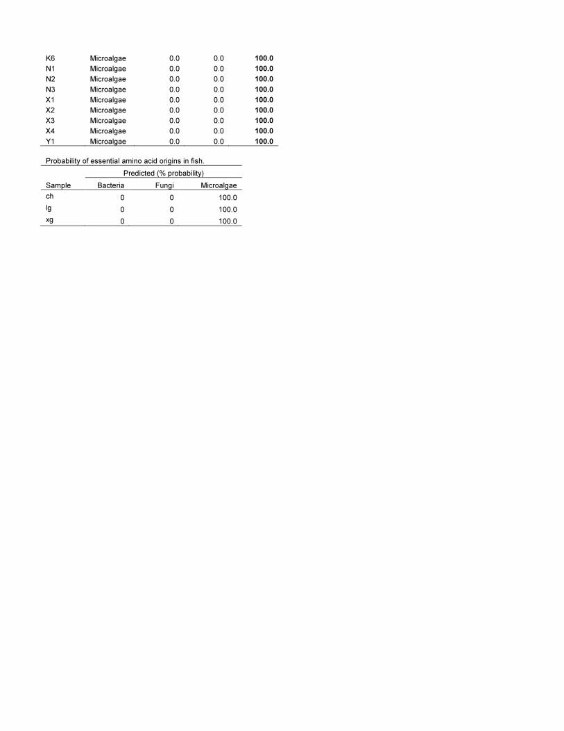
K6 Microalgae 0.0 0.0 100.0

N1 Microalgae 0.0 0.0 100.0

N2 Microalgae 0.0 0.0 100.0

N3 Microalgae 0.0 0.0 100.0

X1 Microalgae 0.0 0.0 100.0

X2 Microalgae 0.0 0.0 100.0

X3 Microalgae 0.0 0.0 100.0

X4 Microalgae 0.0 0.0 100.0

Y1 Microalgae 0.0 0.0 100.0

Probability of essential amino acid origins in fish.

Predicted (% probability)

Sample Bacteria Fungi Microalgae

ch 0 0 100.0

lg 0 0 100.0

xg 0 0 100.0

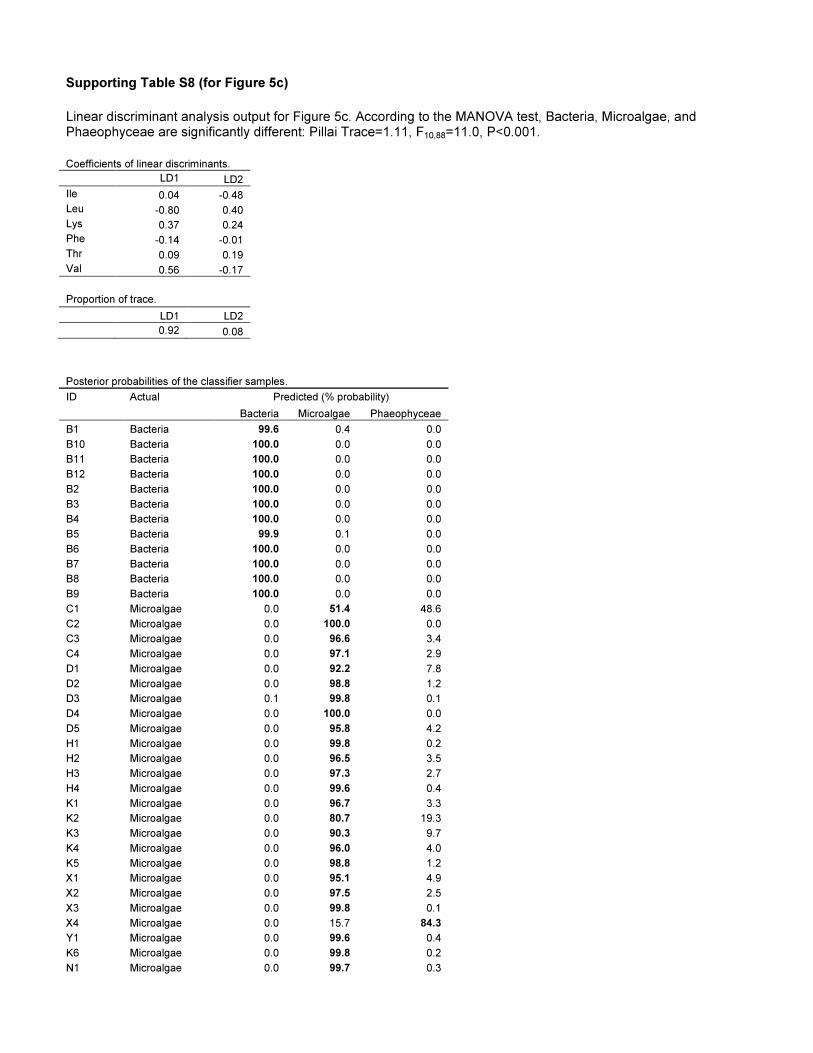
Supporting Table S8 (for Figure 5c)

Linear discriminant analysis output for Figure 5c. According to the MANOVA test, Bacteria, Microalgae, and Phaeophyceae are significantly different: Pillai Trace=1.11, F10,88=11.0, P<0.001.

Coefficients of linear discriminants. LD1 LD2

Ile 0.04 -0.48

Leu -0.80 0.40

Lys 0.37 0.24

Phe -0.14 -0.01

Thr 0.09 0.19

Val 0.56 -0.17

Proportion of trace.

LD1 LD2

0.92 0.08

Posterior probabilities of the classifier samples.

ID Actual Predicted (% probability)

Bacteria Microalgae Phaeophyceae

B1 Bacteria 99.6 0.4 0.0

B10 Bacteria 100.0 0.0 0.0

B11 Bacteria 100.0 0.0 0.0

B12 Bacteria 100.0 0.0 0.0

B2 Bacteria 100.0 0.0 0.0

B3 Bacteria 100.0 0.0 0.0

B4 Bacteria 100.0 0.0 0.0

B5 Bacteria 99.9 0.1 0.0

B6 Bacteria 100.0 0.0 0.0

B7 Bacteria 100.0 0.0 0.0

B8 Bacteria 100.0 0.0 0.0

B9 Bacteria 100.0 0.0 0.0

C1 Microalgae 0.0 51.4 48.6

C2 Microalgae 0.0 100.0 0.0

C3 Microalgae 0.0 96.6 3.4

C4 Microalgae 0.0 97.1 2.9

D1 Microalgae 0.0 92.2 7.8

D2 Microalgae 0.0 98.8 1.2

D3 Microalgae 0.1 99.8 0.1

D4 Microalgae 0.0 100.0 0.0

D5 Microalgae 0.0 95.8 4.2

H1 Microalgae 0.0 99.8 0.2

H2 Microalgae 0.0 96.5 3.5

H3 Microalgae 0.0 97.3 2.7

H4 Microalgae 0.0 99.6 0.4

K1 Microalgae 0.0 96.7 3.3

K2 Microalgae 0.0 80.7 19.3

K3 Microalgae 0.0 90.3 9.7

K4 Microalgae 0.0 96.0 4.0

K5 Microalgae 0.0 98.8 1.2

X1 Microalgae 0.0 95.1 4.9

X2 Microalgae 0.0 97.5 2.5

X3 Microalgae 0.0 99.8 0.1

X4 Microalgae 0.0 15.7 84.3

Y1 Microalgae 0.0 99.6 0.4

K6 Microalgae 0.0 99.8 0.2

N1 Microalgae 0.0 99.7 0.3

N2 Microalgae 0.0 99.9 0.1

N3 Microalgae 0.0 99.9 0.1

P1 Phaeophyceae 0.0 18.0 82.0

P10 Phaeophyceae 0.0 0.3 99.7

P11 Phaeophyceae 0.0 34.8 65.2

P12 Phaeophyceae 0.0 34.2 65.8

P2 Phaeophyceae 0.0 3.6 96.4

P3 Phaeophyceae 0.0 25.0 75.0

P4 Phaeophyceae 0.0 2.5 97.5

P6 Phaeophyceae 0.0 35.9 64.1

P7 Phaeophyceae 0.0 2.8 97.2

P8 Phaeophyceae 0.0 0.1 99.9

P9 Phaeophyceae 0.0 35.8 64.2

Probability of essential amino acid origins of mussels.

Predicted (% probability)

Sample Bacteria Microalgae Phaeophyceae

gav 0 99.8 0.2

sc 0 99.7 0.3