Semilinear Evolution Equations of Second Order via Maximal Regularity

JOURNAL OF MATHEMATICAL ANALYSIS AND APPLICATIONS 141, 49-71 (1989)
Trace Regularity of the Solutions of the Wave Equation with
Homogeneous Neumann Boundary Conditions and Data Supported away from the Boundary*
I. LASIECKA AND R. TRIGGIANI
Department of Applied Mathematics, Thornton Hall, University of Virginia, Charlottesville, Virginia 22903
Submitted by Leonard D. Berkovitz
Received October 19, 1987
Let Sz c R” be a smooth domain with boundary I? Let u be the solution of a second order hyperbolic scalar equation with homogeneous Neumann boundary conditions defined on P due to initial conditions aO, U, and to a forcing term J: The present paper studies the regularity of the map {A uO, a,} +ulr, where {,J uO, u,} E L’(Q) x H’(Q) x L*(a), Q = (0, T] x Sz, and u Ir is the Dirichlet trace of the solution. In particular, the case of compactly supported data {f; t+. U, } is considered and contrasted with corresponding results where the data do not have compact support. In this latter case, an optimal regularity result is given for the wave equation on the half-space of dimension 22. It states, contrary to expecta- tions from elliptic or parabolic theory, that U~~E H”4(C), but ~1~ 4 H34+r(Z), VE > 0, where Z = (0, T] x r. 1” 1989 Academtc Press, Inc.
1. INTRODUCTION, STATEMENT OF THE PROBLEM, AND PRELIMINARIES
Let u(x, t) be the solution of the following second order hyperbolic mixed problem of Neumann type defined on a domain Sz c R”, n typically > 1, with sufficiently smooth boundary Z7
U,,(& r) = .&(x9 8) 4x3 f) +m f) in Q=nx(O, T] (l.la)
4-G 0) = u,(x), u,(x, 0) = u,(.x) in R (l.lb)
&4(x, t)/l%,, 3 0 inZ=rx(O, T]. (l.lc)
Here, -J&‘(x, ~3) is a second order differential operator uniformly elliptic on 0, with sufficiently smooth coefficients (and symmetric principal part)
* This research was supported in part by the National Science Foundation under Grant DMS8301668.
49 0022-247X/89 $3.00
CopyrIght ~CB 1989 by Academic Press. Inc. All rights of reproductmn m any form reserved

50 LASIECKA AND TRIGGIANI
which are time independent; canonically, we have, &‘(x, 8) = A, the n-dimensional Laplacian acting on x E R”. Moreover, let v be the unit normal vector on I-, pointed outward, and a/all, the conormal derivative with respect to SZZ. Thus, if &‘(x, 13) = A, then a/an.& = a/@, the usual normal derivative.
The present article is a companion paper to our recent work [6], and intends to complement a major result of [6] by contrasting it with the results presented here, which refer to an important special class of data f, uo, #I. Both papers are part of an ongoing effort aimed at the study of (optimal) global regularity properties of hyperbolic dynamics, needed for instance in the context of present control theory studies for partial differen- tial equations.
In the present paper we address the issue of regularity of the (Dirichlet) trace u 1,. of the solution u to the Neumann problem (1.1, a, b, c) restricted to the boundary r, for given data f, uo, uI selected in suitable function spaces. More precisely, with reference to problem (l.la)-( l.lc), we are interested in the regularity of the map
if, uo, UI > -+ul,:X+ Y (1.2)
from a suitable chosen space X into the sought after (possibly) optimal space Y, corresponding to X, which contains the trace u 1 z.
For the sake of definiteness, throughout this paper we shall take’
x= L’(Q) x H’(Q) x P(Q). (1.3)
Remark 1.1. As a first step in identifying the corresponding space Y, we recall the following interior regularity result for the Neumann problem (l.la)-( l.lc): the map
{f, UOT ~,}EX=L~(Q)~H’(Q)~L~(~~)+~EC([~, T];H’(Q)) (1.4)
is continuous. Thus, an application of standard trace theory yields u lr~ C( [0, r]; H”‘(r)) continuously. Hence, for the sought after optimal space Y in (1.2) we have a first limitation from above
Y c C( [O, 7-1; fP( z-)). (1.5)
Remark 1.2. (Sharp Trace Regularity for the Corresponding Hyper- bolic Problem of Dirichlet Type). In an attempt to find a second limitation for Y, this time from below, we next consider the corresponding second
’ Other choices of the space X, e.g., X=H-‘(Q) x L’(a) xW’(S2) or X=H-‘(Q)x H2(12) x H’(0) can be. treated similarly.

TRACE REGULARITY OF THE WAVE EQUATION 51
order hyperbolic problem of Dirichfet type, which consists of Eqs. (l.la) and (1.1 b) and of the homogeneous boundary condition
u(x, t) = 0 on Z=Tx (0, T), (1.6)
replacing (1.1~) on a bounded domain Q c R”. The Dirichlet problem (l.la), (l.lb), (1.6) admits the following trace regularity result, which was established recently (in fact, even in the case of sufficiently smooth time dependent coefficients of the differential operator .&(x, a); see [7, 2,4]: the map
rL~o+~: L’(Q) x H&q x L*(Q) -+ L*(z) (1.7)
is continuous. (Actually, the space L’(0, T; L’(Q)) may replace the space L’(Q) in (1.7).) Since the interior regularity of the solution to the Dirichlet problem (l.la), (1.1 b), (1.6) is the same as that for the Neumann problem (l.la))(l.lc), i.e., is described by
{~,u~,~~}EL~(Q)xH~(SZ)XL~(SZ)-*~EC(CO, Tl;fC#W (1.4,)
with H’ in (1.4) replaced by HA now, we see that (1.7) is an independent regularity result, not obtainable by applying (formally) trace theory to the interior regularity (1.4,). In fact, (1.7) shows that the Neumann trace of the solution to the hyperbolic problem of Dirichlet type (l.la)-( l.lb), (1.6) behaves in the space variable “$ better” (in Sobolev space order) than what one would obtain by applying formally trace theory to the interior regularity (1.4,).
Remark 1.3. (A Conjecture on the Neumann Problem). On the basis of Remark 1.2, and by analogy with the more established elliptic and parabolic theory, it has been advanced that in the case of the Neumann problem (l.la)-(l.lc), we may perhaps have
if, MO3 UI> + ~1~: L*(Q) x H’(Q) x L2(Q) -+ H’(C). (1.8)
As a reinforcement, one may note that statement (1.8) is precisely that which one would obtain, if the Dirichlet trace u 1 r of the solution u to the Neumann problem (l.la)-( 1. lc) as in ( 1.4) would likewise behave “5 better” (as in the Dirichlet case (l.la), (l.lb), (1.6) described in Remark 1.2) than the regularity that we would get by formal application of trace theory to (1.4).
Our studies reveal that conjecture (1.8) is false in general, except for the one-dimensional case, where for &(x, a) = d and Q = (0, + co), the half- space, where regularity (1.7) can be verified by the well known explicit

52 LASIECKA AND TRIGGIANI
formula for the solution, or by direct computations as in Section 3. In the general case dim D > 1, the situation is much more complex and appears to depend on the geometry of 52. Thus the issue of optimal regularity of ulr in the Neumann case (l.la)-( 1.1~) is more delicate than the issue of optimal regularity of au/aq in the Dirichlet case (1. la), (l.lb), (1.6). (Indeed, the techniques employed in [7,2,4] in the Dirichlet case are not successful in the Neumann case, see [6].) This is described by the following theorem.
THEOREM 1.1. With reference to the Neumann problem ( l.la)-( 1. lc), with dim S2 > 1, the following regularity results hold true, The map
Lfi UOY u,} + uJz: L’(Q) x H’(O) x L2(sZ) -+ Y (1.9)
is continuous, where
(a) Y= H3j4-‘(Z), V E > 0, if&(x, a) = A and Q = parallelepiped,
(b) Y = H2’3(C), if JZ?(X, a) = A and Q = sphere;
(c) Y = H213(Z), if the coefficients of&(x, a) depend near the bound- ary either only on the tangential or else only on the normal direction to the boundary;
(d) Y = H”‘(C), in the general case.
The proof of parts (a) and (b) can be given by use of the same techni- ques (eigenfunction expansion for the solution followed by Fourier trans- form in time) as those employed in [S] to obtain corresponding results for the interior regularity under nonhomogeneous boundary conditions, i.e., the corresponding dual problem to (l.lak(l.lc). The proof of part (c) is given in [3] (if the coefficients of &‘(x, a) depend only on the tangential direction) and in 163 (for the normal direction case). The proof of part (d) is given in [6]; it is quite complicated and uses pseudo-differential operators techniques on the half-space.
Theorem 1.1 falls short of establishing conjecture (1.8) for dim Q > 1 and may be viewed as a starting point for the problem investigated in the present paper. In fact, we see in the next section that in the canonical case with 52 = half-space, and &(x, a) = A, conjecture (1.8) holds true provided one adds the assumption that the data {f, uo, ul} in X are compactly supported in $2 (i.e., have support bounded away from the boundary r of Q). If one drops the assumption that (f, uo, u,} have compact support in 52, then we shall show still in the canonical case of the Laplacian A over the half-space that the trace ulr to problem (l.la)-(1.1~) satisfies U]~E H3’“(L’) but ul& H3’4+E(L’), E > 0, thereby disproving the conjecture (1.8) of Remark 1.3.

TRACEREGULARITYOFTHEWAVEEQUATION 53
2. THE CASE OF THE LAPLACIAN A IN THE HALF-SPACE: STATEMENT OF MAIN RESULTS
We shall assume now that the domain Q is given by the half-space
D=R”+={(x,y):x>0,y~R”-I} (2.la)
l-= {(o,y):y~R”-I}. (2.lb)
Our main results for &9(x, a) = A in 52 in (2.1) are as follows.
THEOREM 2.1. Consider problem (l.la)-(l.lc) with &(x, a)= A, Sz as in (2.1) and u0 = u, = 0. Assume that f~ L’(Q) and, moreover, that
f has compact support contained in Sz. (2.2)
Then, for any 0 < T < 00 the trace u 1 r of the solution u satisfies
U(r=Ulx=oEH’(z). (2.3)
THEOREM 2.2. Consider problem (l.la)-( 1.1~) with d(x, 8) = A, Sz as in (2.1) and f = 0. Assume that u0 E H’(Q) and u1 E L’(sZ) and that, moreover,
u0 and uI have compact support contained in Sz. (2.4)
Then, for any 0 < T < 00, the trace u lr of the solution u satisfies
ul,=ul,=,EH’(C). (2.5)
By superposition we then obtain the following corollary of Theorems 2.1 and 2.2:
THEOREM 2.3. Consider problem (l.la)-( l.lc) with &(x, LJ) = A and Sz as in (2.1). Assume feL2(Q), ~,EH’(SZ), u, EL’(Q) and, moreover, assume that f, uO, u, have compact support in l2 as described in (2.2) and in (2.4). Then the trace u 1 r of the solution u satisfies
Ulr=ul,=,EH’(C). (2.6)
Thus, the addition of the assumption that the data have compact support in Q guarantees the conjecture (1.8). Without this assumption, we have instead.
THEOREM 2.4. Consider probfem (l.la)-( l.lc) with &01(x, 8) = A and Sz as in (2.1). Then the map
{f, uO, u, ) -+ uI r: L*(Q) x H’(Q) x L’(Q) --f H”“(C) (2.7)

54 LASIECKA AND TRIGGIANI
is continuous. Moreover, for dim Q 3 2
ulr$ H3i4+&(q, t/E > 0. (2.8)
Thus, assumptions (2.2) and (2.4) on compact support for the data are crucial in obtaining H’(C) regularity for u I,-, i.e., conjecture (1.8).
Remark 2.1. The results of Theorems 2.1 and 2.2 were first proved in [9]. There are two main differences with respect to [9] which we point out:
(i) The proofs in [9] use geometric optics techniques: more precisely Lax’s asymptotic expansion of u into a geometric optics approximation and a smooth reminder as in [ 111. By contrast, our proofs here are of a more elementary nature and more direct (and thus we believe much simpler) and are based on the application of the Laplace-Fourier transform followed by a direct estimate of an integral kernel. Our direct computations clearly display the benefit of the compact support assumption on the data (E > 0 as opposed to F = 0 in the proofs of Section 3). We also remark that our direct approach to Theorems 2.1 and 2.2 enables us to prove likewise the optimal result of Theorem 2.4.
(ii) Reference [9] first proves (by geometric optics techniques) Theorem 2.2 and then uses Theorem 2.2 to prove Theorem 2.1. Here, instead we reverse the order. We first prove (by direct methods) Theorem 2.1 and then use a finite speed of propogation argument and Theorem 2.1 to establish Theorem 2.2.
In closing, we thank J. L. Lions for bringing to our attention Ref. [9] during an exchange of correspondence in May 1984. Our proofs here of Theorems 2.1 and 2.2 were obtained soon after becoming acquainted with Ref. [9]. We are presenting them now after finally completing our paper [6], in order to combine the present results with data with compact support in the context of the general theory in [6], where the data do not have compact support (Theorem 1.1, particularly part d).
3. PROOF OF THEOREM 2.1
Step 1. Let s = CI + ifl be the Laplace transform variable corresponding to t and let iw be the Fourier transform variable corresponding to the tangential direction y. After applying the Laplace-Fourier transform to problem (1.1) we obtain
b2 + I QJ 12) qs, w, x) = fi,&, 0, x) +f(s, 0, x) ti,(s, 0, x = 0) = 0

TRACE REGULARITY OF THE WAVE EQUATION 55
whose solution is given by
z&Y, 0, x = 0) = - J& j”: exp( -Jm t).h 0,5) 4. (3.0)
By the compact support assumption off near x = 0, we have p(s, w, 4) = 0, 0 < 5 < E for some E > 0, depending on f:
Replacing “0” by “a” in the lower limit of the integral in (3.1) and applying Schwarz inequality, we obtain
Iti(s, 0, x=0)1 < 1 exp( - I Re Jm E)
IJm I[ReJm
X D
v: IPC &~,t)l*4 . c I
112
(3.1)
Step 2. To prove Theorem 2.1, it is sufficient by (3.1) to show the following proposition.
PROPOSITION 3.1. We haoe
(3.2)
for all /I3 E R’, all w E R”, and for some ct > 0 fixed, where
z=s2+ (wI*=a*-p+ IwlZ+2iclp (3.3a)
Iz(= [(a-p+ Iol2)2+4c12p2]“2 (3.3b)
> I z I l’*, Rez>O (3.4a) =
=JM= (zl+IRez( Jw’ Rez<o (3’4b)

56 LASIECKA AND TRIGGIANI
FIGURE 1
Proof of Proposition 3.1. It suffices to show (3.2) for the pair {/?, co} in theregion&‘={{~,o}:/?>O}, since the function F(o, /3) is even in /I. We divide the region into four sub-regions:
g):p2+ loI 1 (3.5a)
9, : 812 6 I u I 6 2/k fi’+ lu~2~ 1 (3.5b)
9%: 101>2p; ~2+(o12>1 (3.5c)
a,: lo1 <p/2; p’+ loI 1. (3.5d)
See Fig. 1.
We find it convenient to break the proof of Proposition 3.1 into the following two lemmas.
LEMMA 3.1. Estimate (3.2) for F(w, /?) holds true in the “good” region S&uSe, US&, given by (3Sa), (3.5c), (3.5d) (in fact, even with E=O).
Proof of Lemma 3.1. We examine each region separately.
Region 9?,,. By (3.5a) we have in go: Re z > C, for a > 1 and I /3 1, I o I < 1; hence, as desired
f’(o, B) d C, in &To.
Region g2. In region 9T2 we have by (3.5~)
) 2’2 1 = ) z ) 1’2 > ((a”+; Iw12)2+4612~2}1’4~cc5( lul, c,>o; (3.6a)

TRACE REGULARITY OF THE WAVE EQUATION 57
hence
18l+l~l ( z 1 II2
< 314 <c ‘c,’ a
in g2. (3.6b)
Moreover in .G@*
Rez=a2-f12+ Jo12>a2+3fi2>0
so that by (3.4a) and (3.6a)
~/Re~IZIzI”‘~C,IoI>,C, in %2. (3.7)
Equations (3.6b) and (3.7) together yield the desired bound (3.2) for (0, /I} E .4& simply by using the crude estimate exp { - I Re & 1 E} < 1.
Region B3. First we show that in region B?, we have
IReJl >Cc,.
In fact, if Re z B 0, then from (3.4a) and (3.3b)
JZIReJ;I>Iz11’2>C,a”2~C,>0, c, = (4012)“4.
If instead Re z < 0, then again by (3.4b)
2(Re $)‘= 4a2p2
- Re z + J(Re z)~ + 4u2j12 >CJ>C,>O,
where we have used Re z 4 ~1~ - $8’ valid in &.
Equations (3.9) and (3.10) then prove (3.8), as desired. Next, we have from (3.4b), since 1 o I < /I/2,
IzI”2= {(p’- Iw(2-a2)2+4a2p2}“4
3 CJ when b- co cap2 3 c, > 0
IPI + lOI< WJ when /I -+ ~13 1 z 1 ‘J2 WC,
GC,.
(3.8)
(3.9)
(3.10)
(3.11)
Equations (3.8) and (3.11) together prove the desired estimate (3.3) for { fi, W} in region gj, again by simply using exp { - I Re 4 I E} < 1. The proof of Lemma 3.1 is complete. 1
Remark 3.1. Note that in the proof of Lemma 3.1 we have not used the

58 LASIECKA AND TRIGGIANI
assumption that f has compact support on R, as explicitly pointed out in the statement of Lemma 3.1 that E may be taken equal to zero.
A more delicate Lemma in the “bad” region W, is
LEMMA 3.2. Estimate (3.2) for the function F(w, p) holds true in the region W,, given by (3.5b).
Proof of Lemma 3.2. We divide further the region 9, into two sub- regions as follows:
9: = {zEBl: Rez>O}
92; = (zE92,: Rez<O}.
Subregion B: . We have by (3.4a), (3.3b)
in which case by (3.2) and (3Sb)
exp( - C,B”‘&) 6 const, (3.12)
using for the first time the assumption E > 0.
Subregion 9 ; . We again have from (3.4b)
(3.13)
since 1 Re z 1 = ( a2 -B’ + 1 w 1’ I < C,/?’ in 9, and therefore from (3.2), (3.4b), (3.13)
38 F(w 8 G cm /,11/2exp {
-J&p, djjgyjq
1 . (3.14)
To show that F(o, 8) in (3.14) is uniformly bounded in B; , we fix /I, and we look for the max of F(o, /I) where I w 1 runs in [/I/2,2/?] and then establish that
sup max F(o, B) < ~0, where M, is a suitably large constant, B>M l~l~CBP~2Bl
tWBlE%-
TRACE REGULARITY OF THE WAVE EQUATION 59
To do this, we let, for fixed /I,
x=xg=p2- IwI*-a2>o, (3.15)
where 0 d x < i/l’- a2 (for /II 2 M, > $M’). Thus (3.14) can be re-written as
F(a3 B, xp) G cm 3P {xi + 4crZflZ} u4 exp (J
-JzajlE
X,+/2jTGp > z G,(x). (3.16)
We now ascertain that G,(x) is uniformly bounded for p > M, and Odx<$*- ~1’. To accomplish this, we first note that
Gp(xp = 0) < Cafll/’ exp( - Caj31’2~) 6 C, for all such fl (3.17a)
G,y(x,j = :P’ - a2) < CJ/P 6 C, for all such ,!I (3.17b)
Next we shall consider all critical points (depending ob) of G,(x). With fl fixed, it is sufficient to look at all critical points of
- - = Y&x) = (x2 + 4a2f12) exp (J
4&$E 3 G;(x) x+JxW >
which coincide with those of GB(x). Setting Y;(x) = 0, we obtain
i.e.,
x2 = 2a2e2~2 x2 + 4a2p2
x+JF-i@ 2 (a’&*) j?’
(x2 + 4a*~*)
2J?z@ (3.18a)
2 (a*E*) B’ Jm 2 (2a3c2) 03. (3.18b)
Hence
(x/B)‘> (2a3E2) fi + cc when ,L?-+Go. (3.19)
Returning to the equality in (3.18a), we obtain
x2 + 4a2a2 x2 =
x+pTGp
2a2c2b2
or
l+4a2(~~=&(f)[(~)+/@YZ]. (3.20)

60 LASIECKA AND TRIGGIANI
Using (3.19), for all /? > M, so that say xl/? > 1 we obtain from (3.20)
+2CA2 < l/j?[(x//?) + (x/B) J-1. (3.21)
Equation (3.21) combinded with x < $I’- tx2 below (3.15), gives
(l//W/B) - const, (3.22)
for x = xB possible critical points of G(x). For such potential critical points x = xB = 8’ - 1 o I2 - a’, we then obtain by (3.22)
3P 38 - = (x; + &2/j2) l/4 G c, (Zl”2
and so by (3.16)
G,dx,) G C, for any critical points xB. (3.23)
Equation (3.23) together with (3.17) completes the proof that
a% B) 6 c, in 3;.
The proof of Lemma 3.2 is complete. 1
Lemmas 3.1 and 3.2 together prove Proposition 3.1. The proof of Theorem 2.1 is complete. 1
4. PROOF OF THEOREM 2.2
Let u be the solution to problem (1.1) withfz 0, u(x, 0) = uO(x) E H’(Q), and u,(x, 0)= u~(x)EL~(Q), where we assume that
{suppu,usuppu,)c {x>O).
By finite speed of propagation (identically equal to one in this case), the solution u(t) satisfies
{supp U(f), supp k(f)} r {x>O} for all 0 < t < 6
for some 6>0, depending on supp u,usupp u,.
(4.la)
(4.lb)
Thus its trace on I’ satisfies

TRACE REGULARITY OF THE WAVE EQUATION 61
Next, let us take a smooth scalar function x(t) = x6(f) with x(O) = 1; j(O) = 1 and vanishing for t > 6. Define 4(t, X, y) by
d(f, x3 Y) = 4f3 x3 Y) - x(t) 46 x, y); dIr=O=O. (4.2)
Then &t)=ir(t)-mu--(t)ti(t); dLo=O (4.3 1
~(t)=ii(t)-~(t)u(t)-22ji(t)i4(t)-~(t)ii(r)
=h4(t)-Ll(~(t)u(t))-ji(t)u(t)-2~(t)b(t), (4.4)
since x du = d(xu), x being only time dependent. Thus we obtain the following problem in 4,
&r)=d&t)+F
a4 ax x=”
=o
41r=0=Ck4=0
F=ji,(t) u(t)--ia C(t).
By (4.1) and by construction of x(r) (i.e., x(t) = 0; t 2 6) we have
supp F(t) c (x > 0} for all t > 0.
Since u0 E H’(Q); U, E &(Q), standard regularity results give
UE Iv(Q);
hence in particular by (4.6)
FE L*(Q).
(4.5)
(4.6)
(4.7)
(4.8)
Thus for problem (4.5) we are in the exact situation described by Theorem 2.1.
Application of Theorem 2.1 to the solution of (4.5) gives
4IZEma. (4.9)
Returning to (4.2)
4lr=~lr-L5~lr=~lr, (4.10)
where we have used (4.lb). Combining (4.10) with (4.9) completes the proof of Theorem 2.2. 1
Remark 4.1. Note that the proof of Theorem 2.2 is general. It does not use the fact that the problem in question is defined on a half-space and has
409 141.1-5

62 LASIECKA AND TRIGGIANI
constant coefficients. Once we have the boundary regularity u I=E H’(Z) for the nonhomogeneous problem (l.la)-(l.lc) with u,,=ul=O and f E L’(Q) for a general elliptic operator &(x, a), we can then conclude with the same regularity UI=E H’(C) on the boundary for the same problem (l.la)-( l.lc) with f = 0 and USE H’(Q), U, E L2(s2). 1
5. PROOF OF THEOREM 2.4
We split the proof into separate propositions.
PROPOSITION 5.1. Let u be the solution to the problem (l.lak( 1.1~) with ss’(x, 8) = A, iR as in (2.1) and with u0 = u, = 0. Then the map
f + u ( r: L’(Q) + H3’4(C) (5.1)
is continuous.
Proof of Proposition 5.1. We return to (3.1) with E = 0 (we shall use the same notation as in the proof of Theorem 2.1). In order to establish (5.1) it is sufficient to show
( p 1 3’4 + 1 w 1 3’4 1 12 1 II2 ( Re ,,& ( ‘I2 ’ cu
(5.2)
for all {CD, /3} with /I > 0. From the proof of Theorem 2.1 (see Remark 3.1), it follows that in the
“good” region .G@* v B0 v B3 we have in fact
which a posteriori implies (5.2) for these regions. Thus it is sufficient to consider 9, =WT u9I?;.
Subregion .G@ : . In a: where Re z>O we have by (3.4a), (3.3b)
& I Re &I 2 (z11/2a (4~*b~)r/~> clp1/2 (5.3)
so that (5.3) implies
(5.4)

TRACE REGULARITY OF THE WAVE EQUATION 63
Then, (5.2) in 9: follows now from (5.4) and from the fact that ) o 1 < 20 in 8,.
Now let us consider 97, i.e., ZES with Re ~=a~-/?~+~w(~<O.
Subregion 9 ; . From (3.4b)
since 1 z ( ‘I2 3 C,fl’12. Then, (5.2) follows now from (5.5) and from ) w 1 d 2p. The proof of (5.2), hence of Proposition 5.1, is thus complete. 1
To complete the proof of (2.7) in Theorem 2.4 it is enough to establish
PROPOSITION 5.2. Let u be the solution to the problem (l.lat(l.lc) with &(x, 8) = A, Q as in (2.1), andf= 0. Then the map
{ ug, 24, } --) u 1 J-: H’(0) x L2(sz) -+ H”“(C)
is continuous.
Proof of Proposition 5.2. For the proof of this proposition we shall make use of the operator representation of the solution u and it is based on arguments similar to those presented in [7]. In fact, we represent u(t) via cosine and sine operators as
u(t) = s(t) u1+ C(t) u(), (5.6)
where S(t) = j& C(z) dz and C(t) are strongly continuous sine and cosine operators in L2(f2) associated to the negative self-adjoint generator A defined by
Au = Au, UC&~(A)
Let N: L2(r) * L2(52) be the operator defined as
Ng=vo (A-l)v=O in 52 (w~x)l,=o=g on r.
It is well known that
NE cY(H”(T) -+ H”+3’2(Q))
(5.7)
(5.8)

64 LASIECKA AND TRIGGIANI
for all real s and it can be verified by using Green’s Formula [ 10, 83 that
N*A,Z4=U(, for u~g(Ar), (5.9)
where A I = A -I and (N*u, u)~~(~) = (u, Nu)~~(~). Thus by (5.6) and (5.9)
u(t)lr= N”A,[S(l) z41 + C(t) u,]. (5.10)
Thus, with reference to (5.10), in order to establish Proposition 5.2, we must show that
N*A I S(t) : continuous L*(Q) -+ H3j4(Z);
N*A , C(t) : continuous H’(Q) -+ H3’4(C)
(5.11)
(5.12a)
or equivalently
N*( -A,)“2 C(t): continuous L2(LJ) --) H3’4(Z), (5.12b)
the equivalence being a consequence of the known identification (with equivalent norms)
9(( -A,)“*) - H’(O). (5.13)
To prove (5.11)-(5.12), we let 4 denote the solution of the problem
d,,=@+f in Q
dI,=7-=O, fP*,t=T=O in Sz (5.14a)
(W~)l.=o=O in C
with LI = R: the half-space as in (2.1) with f E&(Q). By variation of parameter formula we can write
&)=p(T-l)f(T)d? (5.14b) ,
and in the notation of [7, 8, IO]
By (5.1) we have
L* E 2q.2(Q) + H3’“(C)).
(5.15)
(5.16)
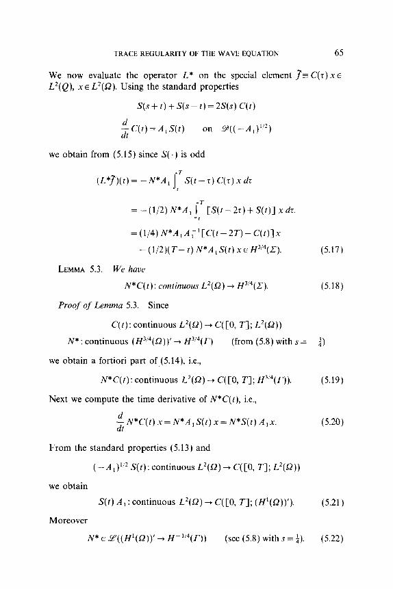
TRACE REGULARITY OF THE WAVE EQUATION 65
We now evaluate the operator L* on the special element j‘- C(r) x E L’(Q), XE L’(Q). Using the standard properties
S(s + t) + S(s - t) = 2&!?(S) C(t)
-$C(f)=A,S(f) on g(( -A,)‘12)
we obtain from (5.15) since S( .) is odd
(L*Y)(t)= -N*A, p(M) C(r)xdt t
=-(1/2)N*A,jl[~(r-2r)+S(t)lxdr. t
= (l/4) N*A,A;‘[C(t-2z--C(t)]x
-(1/2)(T-t)N*A,S(r)xEH3’4(C).
LEMMA 5.3. We have
N*C(t): contim4ous L2(Q) + H”“(,q.
Proof of Lemma 5.3. Since
C(t): continuous L’(Q) 3 C( [0, T]; L2(Q))
N* : continuous ( H3j4(Q))’ + H3j4( f) (from (5.8) with s =
we obtain a fortiori part of (5.14), i.e.,
N*C( t) : continuous L’(Q) + C( [0, T]; H314(IJ).
Next we compute the time derivative of N*C(t), i.e.,
&N*C(r)x=N*A,S(r)x=N*S(f)A,x.
From the standard properties (5.13) and
( --II~)~/’ S(t): continuous L2(0) + C([O, T]; L’(Q))
we obtain
S(t) A, : continuous L2(Q) -b C( [0, T]; (H’(Q))‘).
Moreover
(5.17)
(5.18)
(5.19)
(5.20)
(5.21)
N* E 6p((H’(Q)) --) Hp1’4(lJ) (see (5.8) with s = $). (5.22)

66 LASIECKA AND TRIGGIANI
Thus, combining (5.21) and (5.22) yields from (5.20)
$ N*C(t): continuous L2(Q) + C( [0, r]; H-‘j4(r)). (5.23)
By the Intermediate Derivative Theorem [S, pp. 19-231, we infer from (5.19) and (5.23) that for 0 6 8 < 1
DyN*C(t): continuous L’(Q) -+ L2(0, T; H3’“-‘(r)),
hence (5.24)
N*C(t): continuous L2(Q) -+ H314(0, T; L2(r)).
Then (5.19) together with (5.24) implies (5.18) and Lemma 5.3 is proved. 1
Returning to the proof of (5.11), we see that since LAKE H3’“(Z), then (5.17) and (5.18) yield
(T-t) N*A,S(t) XE H”“(Z) 7 continuously in x E L2(Q). (5.25)
As (5.25) holds for every T, we can drop the term (T- t) to infer that
N*A 1 S(t) x E H3’“(C), continuously in x E L’(Q) (5.26)
as desired, and (5.11) is proved.
Proof of (5.12). We repeat the same argument this time with ?=S’(t)x~L’(e) for XE~((--A,)“*) and obtain
N*A , C(r) x E H”“(C), continuously in x E g( ( -A, )‘I*) (5.27)
as desired. Equation (5.12) is proved.
Thus (5.10), (5.11), (5.12) prove Proposition 5.2. 1
To complete the proof of Theorem 2.4 we need to establish (2.8). To this end it is sufficient to prove
PROPOSITION 5.4. For any E > 0, there exists f, E L2(Q) such that the solution u(t) of the corresponding problem (l.la)( 1.1~) with -ol(x, 8) = A; Sz the half-space as in (2.1), with dim Sz 2 2, u0 = u, = 0, satisfies
ulr& H3’4+E(C), V& > 0.

TRACE REGULARITY OF THE WAVE EQUATION 67
Proof of Proposition 5.3. Returning to (3.0) we obtain
1 I~~~~~~~=~~12=,~~+,w,2, O” exp( - dm 5) f(s, 0~5) 4 2,
(5.28)
Moreover, we have the definition
= 5 5 Rfi R”,-’ (IPI 3’4+E+ 101 3’4+E)2 )ti(s,~,x=O)(~dwdfi. (5.29)
Hence, from (5.28), (5.29)
We begin by considering functions f(t, X, y) of the form
f(t, x> Y) =fi(t, Y) .f2@)~ L’(Q)
with
fl(4 Y) E L2W and f2(x) E L2(0, co)
(5.31a)
(5.31b)
so that if” denotes as before the Laplace-Fourier transform (Laplace in t, Fourier in y), then
fb, x2 0) =A(4 ~)fz(X). (5.31c)
Next, we specialize further f*(x). For any E > 0 given, we select fZE(x), say constructively we take’
~2ZE(X)=X-1’4+EJ-1,4+E(X), J, = Bessel function (5.32)
such that
(5.33a)
* It is a pleasure to thank M. Rao, University of Florida, for pointing this out.

68 LASIECKA AND TRIGGIANI
for ali (s, 0) satisfying
(s,o)ES,~((S,O):S=CL+i~;oO~I~*---*~l} (533b)
for tl > 0 fixed. That the function in (5.32) satisfies (5.33a), (5.33b) can be verified by [I].
Then letSbe given by (5.31a), (5.31b) withf, = fzE specialized by (5.32). Let u be the corresponding solution thus satisfying inequality (5.30). Thus using (5.30), (5.31), and (5.33a) we obtain
Li IP’ 312 t 2~
R; R;-’ Is*+ iw)*1
(by (5.334)
ss IBI 312 + 2E
>CZ I Lb> OH’
Rfi RZ-’ I~*+l~l~l lRe$~11+2E do d/L (5.34)
Next, we shall specialize the function fi in (5.34) satisfying (5.31b). TO this end we introduce first the subregion of S, characterized by
Given E > 0 we then define the function f,,(t, y) as the inverse Laplace- Fourier transform off,E(S, w) where
(5.36)
where n =dim Q3 2 by assumption. Then, clearly such fi,EEL2(C) as required by (531b). In fact, recalling (5.35), we have by Plancherel theorem
s
cc 1 =
I (~c”+‘“~~*“/*)(~~+~) d/i’ < co (5.37)

TRACE REGULARITY OF THE WAVE EQUATION 69
as desired. Next, in returning to (5.34) we shall need the relation
for 0 < c, < C, < cc, to be verified at the end (indeed, we shall need only the left-hand side inequality in (5.38)). Returning to (5.34) withfi defined by (5.36) and invoking (the left-hand side of) (5.38) we obtain
B 312 + 2~
E+“-21~2+I~121 (Redm11+2’ do d/i’
(5.39)
For n=dim Q=2, we have by (5.35)
Right-hand side of (5.39)
(5.40)
as desired. Similarly for n = dim Sz = 3 in (5.39) we obtain via polar coordinates
dw = p dp d6
Right-hand side of (5.39)
(5.41)
as desired. In higher dimensions we obtain the same result by means of spherical coordinates. It remains to verify inequality (5.38).

70 LASIECKA AND TRIGGIANI
Verzjhztion of (5.38). To verify the left-hand side of (5.38) (needed in (5.39)) we set
A=s*+ Iw(*=(a*+ [oj2-~z)+2ia/3
liJ= Is2+ lt~)*l= {(a*+ )o)2-/?2)2+4a2/?2)1~2.
Thus, using (5.35) we obtain in the region S, ,
111 d {(a*+ 1)2+4a2/12}1’2<Cc,./? in &, 1
C,= {(a*+ 1)2+4a2}1’2.
(5.41a)
(5.41b)
(5.42)
Moreover, from (3.4), ( Re fi I < ) 1 I ‘I* and hence in S, 1 using (5.42)
IRe$/<c,j?1’2 in S, I (5.43)
Hence, using again (5.42) we obtain on S,,r
P 312 + 2~ B
312 + 2~
~~2+~~~2~~Re~~~1+2E~/~~~~/~‘~2~~’2 312 + 2~
P y8’/‘+“=c”B
as desired, and the left-hand side of (5.38) is proved. Verification of the right-hand side of (5.38) uses, from (5.41b) that (* ): 11 I B 2aB. Moreover, since Re A 20 on S,,, by (5.35), we then obtain by (3.4a) and (*) that
,/Z~Re~~~~3.~“*~(2~()~‘*~“*. (5.44)
Then (* ) and (5.44) used in (5.38) yield its right-hand side inequality. The proof of Proposition 5.4 is complete. 1
Remark 5.1. We refer to [7, 33 for analogous counterexamples on the dual problem
u,t = ux.x + uyy on Q u(x, 0) =24,(x, 0) = 0 in Q
u XI,=0 = g on 2.
REFERENCES
1. G. DOETSCH, “Introduction in the Theory and Application of Laplace Transform,” Springer-Verlag, Berlin, 1979.
2. J. L. LIONS, “Controle des Systemes Distribues Singuliers,” Gauthier Villars, Paris, 1983.

TRACE REGULARITY OF THE WAVE EQUATION 71
3. I. LASIECKA, Sharp regularity results for mixed hyperbolic problems of second order, “Lecture Notes in Mathematics,” No. 1223, Springer-Verlag, Berlin, 1985, pp, 150-175.
4. I. LASIECKA, J. L. LIONS, AND R. TRIGGIANI, Nonhomogeneous boundary value problems for second order hyperbolic operators, J. Math. Pure Appl. 65 (1986), pp. 149-192.
5. J. L. LIONS AND E. MAGENES, “Nonhomogeneous Boundary Value Problems,” Vols. I, II, Springer-Verlag, Berlin.
6. I. LASIECKA AND R. TRIGGIANI, Sharp regularity theory for second order hyperbolic equations of Neumann type, Part I: Lz Nonhomogeneous data, Ann. Mat. Pwra Appl., to appear.
7. I. LASIECKA AND R. TRIAGGIANI, Regularity of hyperbolic equations under L,(O, T; L,(T))-Dirichlet boundary terms, Appl. Math. Optim. 10 (1983), 275-286.
8. I. LASIECKA AND R. TRIGGIANI, A cosine operator approach to modelling L,(O, T, L,(T))-Boundary input hyperbolic equations,” Appl. Math. Uptim. 7 (1981). pp. 35-93.
9. W. W. SYMES, A trace theorem for solutions of the wave equation and the remote determination of acoustic sources, Much. Math. Appl. Sci. 5 (1983), pp. 131-152.
10. R. TRIGGIANI, A cosine operator approach to boundary input hyperbolic systems, “Lecture Notes in Information and Control Science,” Vol. 6, pp. 380-390, Springer- Verlag, Berlin, 1978.
11. P. D. LAX, Asymptotic solutions of oscillatory initial value problems, Duke Math. J. 24 (1957), 627-646.
Copyright © 2022 FDOKUMEN