Towards Defining Evaluation Measures for Neural NetworkForecasting Models

Dr Pauline Kneale; Dr Linda See; Mr Andrew SmithSchool of Geography, University of Leeds LS2 9JT UK

P.Kneale@geog.leeds.ac.uk

Abstract. There is diversity in the use of global goodness-of-fit statistics to determine how well models forecast floodhydrographs. This paper compares the results from nine evaluation measures and two forecasting models. Theevaluation measures comprise global goodness-of-fit measures as recommended by Legates and McCabe (1999) andSmith (2000) and more flood specific measures which gauge the ability of the models to predict operational alarmlevels and the rising limb of the hydrograph. The models used in this particular study are artificial neural networkstrained with backpropagation (BPNNs) and a Time Delay Neural Network (TDNN). Networks were trained toforecast stage on the River Tyne, Northumbria, for lead times ranging from 2 to 6 hours with minimal data. Thetraining data set consisted of continuous data for one winter period and validation was undertaken using data fromwinter periods for three other years. The results showed that the TDNNs performed better than the BPNNs althoughthe evaluation measures indicate that the performance of these particular models for operational purposes is not yetsufficient. Issues regarding the creation of appropriate training data sets and sampling procedures as well as thehydrological conditions of the River Tyne need to be investigated further. A consistent set of operational evaluationmeasures and benchmark data sets must be established before comparison of neural network and physical models canbe facilitated. The combination of evaluation measures provides a good picture of the overall forecasting performanceof the models, and suggests that operators should consider a range of measures.

1. INTRODUCTION

Climate trends in Northern Europe suggest that weatherpatterns are moving towards wetter and stormierconditions. Damage due to flooding in the past fiveyears has been estimated at several billion pounds in theUK, while on an international scale, flooding poses life-threatening problems particularly in tropical andsubtropical regions. Although global warming is nowrecognised as a real threat, there has been little successin establishing protocols for the reduction of greenhousegases. Therefore, an increase in the occurrence offlooding is likely to continue into the future. Buildingnew flood defences to contain higher flows, defendingvulnerable sites and domestic and commercial insuranceclaims all have serious financial implications. For thesereasons the timely forecasting of floods is becomingmore crucial for both flood defence and catchmentmanagement purposes.

There are several integrated flood forecasting systemsavailable. These systems generally comprise severalinteracting components, which usually include arainfall-runoff forecasting model, a database for themanagement of historical and real-time data, adissemination module which issues warnings tohydrologists monitoring the catchment, and acomponent which continually evaluates and updates theforecasting outputs (Nemec, 1986). The forecastingsystems currently in operation within the EA varybetween regional offices; for example, the River FlowForecasting System (RFFS) developed by the Instituteof Hydrology and Logica UK Ltd (Moore et al., 1994)is currently used in Yorkshire and Northumbria, whilethe Wessex Radar Information Project (WRIP) is the

system employed in the South Western, Anglian andNorth West regions (Han et al., 1997). These large-scale systems generally require a substantial investmentof both time and money for their development andcontinued maintenance yet a recent assessment of theflood forecasting models used by the EA revealed thatthese systems are not yet satisfactory for use in anautomated operational environment (Marshall, 1996).

The complexity of natural systems and the number ofprocesses that continuously interact to influence riverlevels render traditional modelling based on mirroringnatural processes with process-based equations verydifficult. Where processes can be modelled numerically,there are constraints imposed by the spatial availabilityof data and the cost of collecting this data in real time.An alternative approach, which has been slowly gainingrecognition within hydrology, is the application ofartificial neural networks (ANNs) to a variety ofhydrological forecasting problems. ANNs offer thepotential for a more flexible, less assumption-dependentapproach to modelling flood processes, and they havealready been demonstrated to work successfully assubstitutes for rainfall-runoff models (Minns and Hall,1996; Smith and Eli, 1995; Abrahart and Kneale, 1997;Khondker et al., 1998). Most of the studies in theliterature make use of feedforward multi-layerperceptrons trained with backpropagation (Rumelhart etal., 1986), hereafter referred to as BPNNs. However,there are many other ANN algorithms and architecturesthat have yet to be investigated (Shepherd, 1997). TimeDelay Neural Networks (TDNNs), which are used inspeech recognition (Waibel, 1989), provide one type ofnetwork that could especially benefit flow forecastingbecause these networks can potentially find thetemporal relationship between inputs. This has

relevance for the inclusion of upstream stations, whichmust be lagged in the input data by an average traveltime when used with BPNNs. Multi-net approaches(Sharkey, 1999) offer another promising area forresearch in developing better ANN flood forecastingmodels. However, the ultimate test of their operationalfeasibility lies in their performance in real-time floodforecasting. To achieve this comparison, a set ofoperational evaluation measures for existing systemsmust be established along with a repository forbenchmark data sets. In his review of EA operationalforecasting models, Marshall (1996) highlighted thelack of a consistent evaluation system between offices,while much of the research in the literature reportsperformance using global goodness-of-fit statistics,which are rarely useful for determining how wellmodels can predict flood hydrographs.

This paper presents a set of comprehensive evaluationmeasures that can be used to compare results fromforecasting models. A set of BPNNs and TDNNs weredeveloped to forecast stage on the River Tyne,Northumbria. The networks were trained on acontinuous data set for one winter period and validatedon winter periods for three other years. Models weredeveloped to forecast lead times ranging from 2 to 6hours. The majority of the evaluation measures arebased on the ability to predict operational alarm levelsand the rising limb of the hydrograph. The data set hasbeen kept very small to see what can be done withrelatively few storms, so absolute performance resultshere are of less interest than the relative results. It ishoped that this set of measures will provide a useful toolfor comparing different models within a particular studycatchment and initiate a dialogue for the establishment

of a consistent set of operational evaluation measuresand benchmark data sets in the future.

2. STUDY AREA

The study area is the upper, non-tidal section of theTyne River, North East England as shown in Figure 1.The Tyne basin has an area of approximately 2,920km2. The lowest non-tidal stage gauge on the Tyne islocated at Bywell, upstream of Newcastle. Historic dataof stage and rainfall values are available, measured at ahandful of stations throughout the North Tynecatchment. Telemetered data at 15 minute intervals forthe years 1994 to 1998 were provided by theEnvironment Agency for Bywell and three upstreamstations on the River Tyne: Reaverhill, Rede Bridge andUgly Dub. The forecasting task is to determine ifBywell can be predicted using only information fromthe north portion of the Tyne in the hypothetical eventthat the telemetred network on the south Tyne shouldfail. The 15 minute data were converted to an hourlyresolution. Figure 2 shows the relationship between thelevels at upstream stations and Bywell, which serves toillustrate that a simple linear relationship does not existand therefore some form of nonlinear modelling isrequired.

The average travel times between stations werecalculated by plotting hydrographs of historical stormevents. They represent the typical time difference for apeak flow passing between two stage gauges. Data fromthe upstream stations were offset by the average traveltime before training with the BPNNs. However, theTDNNs did not see the lagged data in order todetermine whether these networks could model thetravel time as part of the training process.

Figure 1: Location of the Tyne River in the UK

(a)

Figure 2: Location map of the River Tyne

(b)

(c)

Figure 2: Plots of river level at Bywell against levels at (a) Reaverhill (b) Rede Bridge and (c) Ugly Dub

0.0

1.0

2.0

3.0

4.0

5.0

6.0

0.0 1.0 2.0 3.0 4.0

Level at Reaverhill (m)

Lev

el a

t Byw

ell (

m)

0.0

1.0

2.0

3.0

4.0

5.0

6.0

0.0 0.5 1.0 1.5 2.0 2.5

Level at Rede Bridge (m)

Lev

el a

t Byw

ell (

m)

0.0

1.0

2.0

3.0

4.0

5.0

6.0

0.0 0.5 1.0 1.5 2.0

Level at Ugly Dub (m)

Lev

el a

t Byw

ell (

m)

Every major river under the jurisdiction of theEnvironment Agency has between one and four floodrisk warning levels defined at a range of points alongthe river. Each warning level represents a particularlevel of risk of flood occurrence when the riverreaches that particular level. Risk is measured in termsof the human and economic consequences of theflood. The alarm levels for Bywell gauging station inthe 1990-1999 period and the interpretation of thealarm levels are shown in Table 1; the status andinterpretations were revised in 2000. These alarmlevels were used in devising the set of operationalevaluation measures.

Table 1: Alarm levels for the River Tyne at theBywell stage gauge (Source: Environment Agency)

Status Interpretation LevelAlarm First operational warning level 3.5mYellow Flooding of low lying farmland

and roads near rivers and the sea4.4m

Amber Flooding may affect isolatedproperties, roads and large areasof farmland near rivers and thesea

5.3m

Red Flooding will affect manyproperties, roads and large areasof farmland

5.8m

3. ERROR MEASURES FOR EVALUATION

Evaluation measures are frequently referred to as“goodness-of-fit” measures, since they measure thedegree to which the predicted hydrograph fits theactual hydrograph. Goodness-of-fit statistics can begrouped into two types: relative and absolute.

3.1 Relative goodness-of-fit statisticsRelative goodness-of-fit measures are non-dimensional indices, which provide a relativecomparison of the performance of one model againstanother. There are three commonly used relativegoodness-of-fit statistics:

(a) The Coefficient of Determination

( )( )

( ) ( )

2

1

2

1

2

12

−−

−−=

∑∑

∑

==

=

N

ii

N

ii

N

iii

PPOO

PPOOR (1)

where Oi is the observed value at time i, Pi is thepredicted value at time i, N is the total number ofobservations, O is the mean of O over N and P is themean of P over N. It measures the degree ofcollinearity between two sets of values. Thecoefficient has a range of 0.0 to 1.0 with a highervalue indicating a higher degree of collinearity.

(b) The Coefficient of Efficiency (Nash and Sutcliffe,1970)

( )

( )∑

∑

=

=

−

−

−=N

i

i

N

iii

OO

PO

E

1

2

1

2

1 (2)

where a value of 1.0 represents a ‘perfect’ predictionwhile a model with an index of 0.0 is no moreaccurate than predicting the mean observed value forall i. This measure was introduced by Nash andSutcliffe (1970) and is widely used in the hydrologicalliterature.

(c) The Index of Agreement

( )

∑

∑

=

=

−+−

−

−=N

iii

N

iii

OOOP

PO

d

1

2

1

2

1 (3)

which was proposed by Willmott (1981) as anadaptation of the Nash and Sutcliffe efficiency index.The alteration to the denominator seeks to penalisedifferences in the mean predicted and mean observedvalues. Inspection shows the degree of similaritybetween the coefficients of determination andefficiency. Due to the squaring of the error terms in allthree measures, they are considered to be overlysensitive to outliers in the data set.

More generic forms of both E and d can be developed,by varying the power applied to the error terms to anarbitrary, positive integer power j, denoted as Ej and djrespectively:

∑

∑

=

=

−

−

−=N

i

j

i

N

i

jii

j

OO

PO

E

1

11 (4)

( )

∑

∑

=

=

−+−

−

−=N

iii

N

iii

j

OOOP

PO

d

1

2

1

2

1 (5)

By this convention the original coefficient ofefficiency E becomes E2 and the original index ofagreement d becomes d2. Particularly useful are E1and d1 since difference terms are not inflated by theirdistance from the mean.

3.2 Absolute goodness-of-fit statistics

In contrast, absolute goodness-of-fit statistics aremeasured in the units of the flow/stage measurement.The following are commonly used absolute goodness-of-fit statistics:

(a) Root Mean Squared Error (RMSE)

( )

N

PO

RMSE

N

iii∑

=

−

= 1

2

(6)

As with the various relative statistics, the squarederror term places undue importance on the outliers inthe dataset.

(b) Mean Absolute Error (MAE)

∑=

− −=N

iii PONMAE

1

1 (7)

Taking the absolute value of the error term rather thanits square removes the bias towards outlying points inthe data set.

(c) Comparisons of Means and Standard Deviations

PO sssPOm

−=−=

??

(8)

Whilst not in themselves fully descriptive goodness-of-fit statistics, comparisons of the mean of theobserved and predicted values and their standarddeviations do provide a useful measure of theperformance of the model.

3.3 Flood Specific Evaluation Measures

The following are a list of additional evaluationmeasures that are specifically aimed at measuringflood forecasting performance:

(a) Proportion of time in the correct state of alarm

( )

( )

=

= ∑=

−

statesdifferent in are ,0

state same in the are ,1,

,1

1

ii

iiii

N

iii

PO

POPOf

POfNE

(9)

A useful model will be able to accurately predict whena river enters a higher flood risk alarm status, sincethis will allow precautionary measures to be takenearlier. Hence the lower the proportion of missed, lateor false alarms to correctly predicted alarms, the betterthe performance of the model. The score is reduced byboth a failure to predict an alarm event thatsubsequently occurs, and by false alarms for eventsthat do not occur.

The next two measures were originally suggested bySmith (2000) in his investigation of neural networkforecasting models for the River Tyne. These werefound to be useful indicators in combination with theother measures outlined above.

(b) Root Mean of the Flow Weighted Error(RM_FWE)

N

POO

FWERM

N

iiii∑

=

−

= 1_ (10)

For each data point, the absolute error between theobserved and predicted values is calculated, which isthen multiplied by the observed level. The mean ofthese flow weighted errors is then calculated in theusual manner. This way the sensitivity of the errorcalculation is increased for high flow and storm eventsand reduced for low and normal flows. However, themultiplication by observed level implies that theimportance of the accuracy of prediction is linearlyproportional to the observed level. Whilst there is noreason to suppose that a linear scale of importance isthe most appropriate, it is plausibly more appropriatethan rating importance independent of flow.

(c) Root Mean Gradient Weighted Error

1

.

_ 21

−

−−

=∑

=−

N

POOO

GWERM

N

iiiii

(11)

Whilst the RM_FWE has increased sensitivity to highflow data, it is still relatively insensitive to the errorsin the lower part of the rising limb of a hydrograph.For this reason a gradient weighted error measurementis also proposed. For each data point, the absoluteerror between the observed and predicted values iscalculated. This is multiplied by the absolutedifference between the current observed value and theprevious observed value, which is approximatelyproportional to the current gradient of the hydrograph.The mean of these flow weighted errors is thencalculated in the usual manner. In this way thesensitivity of the error calculation is increased forperiods of rapid change in levels and reduced forperiods of stable flow.

There are two disadvantages to this measure. UnlikeRM_FWE, sensitivity is reduced for any stable periodof high flow. In addition to increasing sensitivity tothe rising limb of the hydrograph, sensitivity is alsoincreased to the falling limb, which is of lessimportance for flood risk warning. It is not possible touse the true (signed) gradient since this wouldimprove scores for poorly fitting falling limbs andreduce those where the fit was good. Despite theseproblems, it may prove that the RM_GWE is a usefulmeasure in addition to the RM_FWE.

3.4 Suggested Evaluation Measures forOperational Flood Forecasting

Many of the principal measurements that are used inthe hydrological literature have been reviewed byLegates and McCabe (1999). They stronglydiscourage the use of R2 as a goodness-of-fit statistic

as well as E2 and d2, but recommend the use of E1 andd1 instead to reduce the influence of outliers andbecause E1 has the advantage that the value 0.0 has ameaning that can be directly interpreted. In additionthey recommend that a complete assessment of modelperformance should include at least one absolute errormeasure (e.g. RMSE or MAE) with anysupplementary information such as comparison ofmeans and standard deviations. In their conclusionthey stress that any individual goodness-of-fit statisticis only one tool in assessing the performance of amodel and that a range of statistics are required. Forthe development of a set of evaluation measures, therecommendations of Legates and McCabe (1999) arefollowed for both the entire data set and for dataabove the alarm level as well as including the moreflood specific evaluation measures outlined in section3.3.

4. ANN EXPERIMENTS ON THE UPPER TYNERIVERThis section provides an overview of the artificialneural network models used in this study and brieflydescribes the ANN modelling experiments for theUpper Tyne River.

4.1 Artificial Neural Network Models

ANNs are information processors, trained to representthe implicit relationships and processes that areinherent within a data set. The original inspiration forANNs was biological so much of the terminology ofANNs reflects this biological heritage. Gooddescriptions can be found in Kasabov (1996), Bishop(1995) and Lin and Lee (1996). The basic structure ofan ANN consists of a number of simple processingunits, also known as neurons or nodes. The basic roleof each node is to take the weighted sum of the inputsand process this through an activation function such asthe sigmoid. A connection or link joins the output ofone node to the input of another. Each link has a‘weight’, which represents the strength of theconnection. Collectively, the values of all the weightsin a network represent the current state of learning ofthe network, in a distributed manner. These weightsare altered during the training process to ensure thatthe inputs produce an output that is close to thedesired value. The arrangement of nodes andinterconnecting links is called the architecture. Inmany architectures, nodes are arranged in layers,whereby there are no links between nodes in the samelayers. Data enters the network through the input unitsof the input layer, are fed forward through successivehidden layers and emerge from the output units in theoutput layer of the network. This is called afeedforward network or multi-layer perceptron (MLP)(Rumelhart et al., 1986) because the flow ofinformation is in one direction only from input tooutput units.

A learning function or algorithm is used to adjust theweights of the network during the training phase.There are many learning algorithms for training a

MLP but backpropagation is one of the most common(Rumelhart et al., 1986). Backpropagation is based onthe concept of steepest gradient descent of the errorsurface. During the learning period, both the inputvector and the target output vector are supplied to thenetwork. The network then generates an error signalbased on the difference between the actual output ofthe network and the target vector. This error signal isthen used to adjust the weights of the networkappropriately. The error for a hidden processing unit isderived from the error that has been passed back fromeach processing unit in the next forward layer. Thiserror is weighted using the same connection weightsthat modified the forward output activation value, andthe total error for a hidden unit is thus the weightedsum of the error contributions from each individualunit in the next forward layer. Following training,input data are then passed through the trained networkin its non-training mode, where the presented data aretransformed within the hidden layers to provide themodelling output values.

Time Delay Neural Networks (TDNNs) are another inthe class of feedforward neural networks. They are inmany ways similar to MLPs and train using analgorithm similar to backpropagation. TDNNs aredesigned to detect temporal relationships in asuccession of inputs, independent of the absolute time,i.e. they seeks relationships between inputs in theirposition relative to each other, rather than theirposition in the data set. In backpropagation, networkswith the temporal sequence are converted to a spatialsequence.

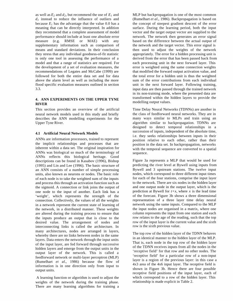
Figure 3a represents a MLP that would be used forpredicting the river level at Bywell using inputs fromBywell and 3 upstream stations. The twelve inputnodes, which correspond to three different input timesfor each of the four stations, comprise the input layerto the network. There are six nodes in the hidden layerand one output node in the output layer, which is theprediction at Bywell for t+x, where x is the lead timeof the forecast. Figure 3b shows a three dimensionalrepresentation of a three layer time delay neuralnetwork using the same inputs. Compared to the MLPthe input nodes are organised in a matrix, where onecolumn represents the input from one station and eachrow relates to the age of the reading, such that the toprow of the input layer is the current value and the sixthrow is the sixth previous value.

The top row of the hidden layer of the TDNN behavesin an identical manner to the hidden layer of the MLP.That is, each node in the top row of the hidden layerof the TDNN receives inputs from all the nodes in the‘receptive field’ for that row and no other nodes. The‘receptive field’ for a particular row of a non-inputlayer is a region of the previous layer: in this case a4x3 area of the 4x6 input layer. The receptive field isshown in Figure 3b. Hence there are four possiblereceptive field positions of the input layer, each ofwhich correspond to a row of the hidden layer. Thisrelationship is made explicit in Table 2.

(a) Conventional feedforward network

(b) Time Delay Neural Network

Figure 3: (a) Conventional feedforward and (b) time delay network architectures for forecasting river level at Bywellusing historical levels from Bywell and 3 upstream stations

t-4

t-5

t-3

t-5

t-4

t-3

t-3

t-2

t-1

t-2

t-1

Hidden Layer Output Layer

Input Layer

Bywell at t+x

etc.

The inputnodes are fullyconnected toeach hiddenlayer node

Bywell

Reaverhill

Ugly Dub

Rede Bridge

t

Bywell at t+x

Output Layer

Hidden Layer

Input Layer

t

t-1

t-2

t-3

t-4

t-5

Bywell

Reaverhill

Ugly Dub

Rede Bridge

etc.

The hidden layernodes are fully

connected to thesingle output node

etc.

All the input nodesin contained in the

dashed box arefully connected tothe nodes in the

dashed box of thehidden layer

ReceptiveField

Table 2: The relationship of rows of the hidden layerand the corresponding receptive field for the TDNN

shown in Figure 3b

Row of HiddenLayer

Row of input layer incorresponding receptivefield

1 1 to 32 2 to 43 3 to 54 4 to 6

The choice of the number of rows in the hidden layerand the size of the receptive fields must be made sothat there is exact correspondence between the numberof rows in the hidden layer and the number of possiblepositions for receptive fields in the previous layer. Thenumber of rows in a non-input layer is the time delayof the layer. The number of rows in the input layer isthe total delay length. Continuing the comparison withthe MLP, each row in the hidden layer of the TDNN isequivalent to the status of the hidden layer of the MLPat a recent point in time. (i.e. the top represents thecurrent time and each subsequent row represents thestatus of the MLP hidden layer one time step earlier).The integration function of the output node canrecognise relationships between the different rows ofthe hidden layer and hence the temporal patterns overthe entire delay length time period are considered. Theupdate function for TDNNs is similar tobackpropagation but the convergence tends to beslower and hence longer training times are needed.

4.2 Outline of Experimental RunsA series of feedforward BPNNs and TDNNs weretrained on historical data for the winter period of oneyear (Oct to Apr 1994/95) to forecast levels at Bywellfor lead times of 2, 4 and 6 hours ahead. This winterperiod was chosen because it contains the highestevent for the entire 4 year time period. This willensure that the network has seen the full range ofevents in the training data set and not be forced toextrapolate to events never seen before. The networkswere then validated using independent data from threefurther winter periods from 1995 to 1998. The neuralnetwork model inputs for all the experiments were thelevels at Bywell, Reaverhill, Rede Bridge and UglyDub. No rainfall information was available. The 15-minute data were averaged to produce hourly valuesand normalised between 0.1 and 0.9 prior to training.Neural networks were trained using backpropagationwith momentum (BPNNs) and backpropagation for atime delay neural network (TDNNs). Training wasstopped when the errors in both the training andvalidation data sets were at a minimum to avoidproblems with overfitting of the data.

5. ANN EXPERIMENTS ON THE UPPER TYNERIVER

Once the networks were trained, the validation datasets were used in predictive mode. The followinggoodness-of-fit statistics were calculated:

• RMSE (m)

• MAE (m)

• E1

• d1

• Difference of averages

• Difference of standard deviations

• False alarms

• RM_FWE (m)

• RM_GWE (m)

These measures were calculated for the entire winterperiod and for a subset of the data, which includedonly alarm levels. The exception is the false alarms,which are calculated only for the subset. Table 3 liststhe number of observations where alarm levelsequalled or exceeded 3.5 m. The goodness-of-fitstatistics are provided in Tables 4 to 6 correspondingto lead times of 2, 4 and 6 hours.

Table 3: Number of observations exceeding alarmlevels for each winter period

Winter Period Number of observations94/95 4995/96 596/97 2597/98 6

The following observations can be summarised fromTables 4 to 6:

• the results generally show an increase in RMSE,MAE, RM_FWE and FM_GWE as the lead timeincreases, which is to be expected. The TDNNsgenerally had lower values for all lead timescompared to the BPNNs indicating they arehandling the data better. The RM_FWE andRM_GWE are more difficult measures tointerpret but they clearly indicate the years inwhich higher floods occurred because thesemeasures are higher for the winter period of1995/96.

• E1 and d1 also follow the same expected patternexcept they decrease as the lead time increases.Similarly, the TDNNs generally had highervalues for all lead times compared to the BPNNs.

Table 4: Error measures for a 2 hour lead time. The top value in each row is the statistic for all data in the winterperiod while the bottom value is the statistic for a subset of the data containing only values exceeding alarm levels.

Measure BackPropagation TDNN94/95 95/96 96/97 97/98 94/95 95/96 96/97 97/98

RMSE (m) 0.06310.2044

0.10801.2108

0.16931.1878

0.12480.7103

0.07990.2939

0.10490.3487

0.12280.5808

0.11280.4954

MAE (m) 0.02520.1354

0.04971.0484

0.06370.8583

0.05720.6603

0.04940.2335

0.06640.2982

0.06800.4418

0.06750.4093

E1 0.9351 0.7937 0.8004 0.8271 0.8730 0.7248 0.7867 0.7958

d10.96760.8947

0.89800.1084

0.90150.2924

0.91410.1157

0.93550.7847

0.85780.3212

0.88990.4856

0.89350.2338

AverageDifference

-0.00280.0057

0.03121.0484

0.02620.3645

0.03240.6604

-0.03280.1034

-0.05070.2093

-0.0438-0.0078

-0.03940.1178

Std DevDifference

0.0007-0.0544

0.0240-0.4555

0.0026-0.7590

0.0164-0.1719

0.01580.1924

0.0284-0.1678

-0.0069-0.3384

0.0079-0.4135

False Alarms 0.1020 0.8000 0.6800 1.0000 0.2245 0.4000 0.4800 0.5000

RM_FWE (m) 0.21230.7594

0.24572.0157

0.32561.8603

0.28071.5455

0.27591.0614

0.24971.0752

0.29041.3235

0.26981.2132

RM_GWE (m) 0.05780.2300

0.05370.6289

0.09020.5952

0.06580.3548

0.05930.2428

0.04400.3363

0.06780.4284

0.05490.3076

Table 5: Error measures for a 4 hour lead time. The top value in each row is the statistic for all data in the winterperiod while the bottom value is the statistic for a subset of the data containing only values exceeding alarm levels.

Measure BackPropagation TDNN94/95 95/96 96/97 97/98 94/95 95/96 96/97 97/98

RMSE (m) 0.13900.5973

0.14241.8715

0.23711.8436

0.16821.2420

0.12690.5414

0.12980.6193

0.16580.9920

0.14110.8271

MAE (m) 0.05880.3274

0.05631.7645

0.08851.6008

0.07111.1516

0.07230.4634

0.07010.4333

0.07750.7774

0.07500.7551

E1 0.8487 0.7663 0.7228 0.7853 0.8139 0.7094 0.7569 0.7730

d10.92490.7606

0.88490.0673

0.86230.1232

0.89320.0698

0.90500.5976

0.85190.2299

0.87490.2845

0.88200.0776

AverageDifference

0.02060.1749

0.00311.764

0.00141.2231

0.00481.1516

-0.03160.3156

-0.04230.4271

-0.03160.3131

-0.02560.6627

Std DevDifference

0.0077-0.1862

-0.0088-0.4446

0.0039-0.8550

0.0382-0.3578

0.01550.1364

0.0505-0.3735

-0.0023-0.5421

0.0209-0.3715

False Alarms 0.1837 1.0000 0.8400 1.0000 0.3877 0.4000 0.5600 0.8333

RM_FWE (m) 0.32751.2146

0.28392.6160

0.40322.5374

0.33242.0422

0.34691.4674

0.26921.2851

0.33541.7662

0.30501.6555

RM_GWE (m) 0.08680.3832

0.06280.7711

0.10420.7002

0.07550.4402

0.07490.3648

0.05360.4756

0.08450.5616

0.06400.3641

Table 6: Error measures for a 6 hour lead time. The top value in each row is the statistic for all data in the winterperiod while the bottom value is the statistic for a subset of the data containing only values exceeding alarm levels.

Measure BackPropagation TDNN94/95 95/96 96/97 97/98 94/95 95/96 96/97 97/98

RMSE (m) 0.21211.0260

0.16441.7930

0.25501.6575

0.19331.2391

0.18160.8485

0.13561.6006

0.22551.6067

0.16771.1278

MAE (m) 0.12970.6211

0.09131.7782

0.12171.4203

0.10281.1930

0.09160.7227

0.07721.4888

0.10701.3971

0.09381.0014

E1 0.6659 0.6213 0.6188 0.6894 0.7641 0.6798 0.6644 0.7163

d10.82790.5844

0.80760.0669

0.80530.1754

0.83890.0675

0.87910.4439

0.83210.0788

0.82630.9738

0.85170.0673

AverageDifference

-0.05810.5351

-0.03301.7782

-0.04430.9923

-0.02191.1930

-0.01650.6125

-0.04391.4887

-0.0410-0.7727

-0.03910.9873

Std DevDifference

0.0497-0.2560

0.0665-0.0128

0.0147-0.8463

0.0579-0.2604

0.03040.1193

0.0136-0.4207

0.0048-0.7727

0.0414-0.4217

False Alarms 0.4694 1.000 0.9200 1.000 0.6939 1.0000 0.8800 0.8300

RM_FWE (m) 0.45791.7082

0.32972.6240

0.43872.3977

0.37552.0752

0.41021.8391

0.30102.4024

0.41442.3697

0.35181.9072

RM_GWE (m) 0.09950.4942

0.06000.7382

0.10290.6715

0.07630.4523

0.09380.4487

0.06050.7181

0.10120.6693

0.07350.4138

• the average differences are very small for theentire data set and the negative sign shows thatthe TDNNs tended to overpredict for the entiredata set. The BPNNs tended to underpredict onaverage for lead times of 2 and 4 hours and thenoverpredict as the lead time increased. For thealarm subset, both the TDNNs and the BPNNstended to underpredict. This provides a goodsource of extra information above the other globalmeasures.

• the difference in standard deviations indicates adifference in the variation of predictions relativeto the observed data. The results generallyindicated a slightly smaller variation overall but ahigher one for the alarm data set. The TDNNspredicted values with variations closer to theobserved data relative to the BPNNs.

• the false alarm rate increased with lead time andthe TDNN models generally had a lower rate offalse alarms than the BPNNs.

The combination of evaluation measures clearlyhighlights the difference between performance for theentire winter period and that for the alarm data set.Unfortunately the alarm data set is very small forBywell so the networks were heavily biased towardslow flow events. Therefore, it is not surprising thatpoor absolute results were achieved for bothforecasting models in an operational context.Interestingly, better results have been achieved whenpredicting stage at Bywell using the South Tyne Riverstations only (Kneale et al., 2000), which raises thequestion as to whether Bywell is mainly responsive tothe South Tyne flows. If this were true, then thestations on the North Tyne could not be used topredict Bywell successfully in the hypothetical eventthat the South Tyne stations fail. Alternatively, should

data sets be sampled to contain only flood hydrographevents and used in the training and independentvalidation process? In theory these will provide moremeaningful global goodness-of-fit statistics. Finally,should a better sampling scheme such asbootstrapping be used in the training process(Abrahart, 2001)? Each of these issues will beinvestigated in the next stage of the research.However, the TDNN models did show a betterperformance overall and therefore hold some promiseas to another type of neural network that could beinvestigated for rainfall-runoff modelling.

6. CONCLUSIONS

This paper has presented a set of evaluation measuresfor the purpose of comparing results from forecastingmodels including a combination of global and floodspecific goodness-of-fit measures. Backpropagationand Time Delay Neural Networks were trained toforecast stage on the River Tyne, Northumbria usingonly upstream stations on the north branch. Thenetworks were trained on a continuous data set for onewinter period and validated on winter periods for threeother years. Models were developed to forecast leadtimes ranging from 2 to 6 hours. The combination ofmeasures provided a good picture of the forecastingperformance of the models. However, theestablishment of a consistent set of operationalevaluation measures and benchmark data sets shouldbe undertaken by researchers and operational staff. Ifthere could be some general agreement on errormeasures and a set of benchmark data sets suppliedwith these error measures, it would facilitate thecomparison of the neural network and physicalmodels in the future. This will go a long way towardsaddressing a major criticism of neural network modelsin the hydrological literature, i.e. the lack of

comparison with existing operational forecastingsystems.

Clearly there are a very limited number of alarm levelevents and increasing the data set should improve theabsolute results. Nevertheless these experiments withlimited data replicate situations where new stationsare established. Issues regarding the creation ofappropriate training data sets and sampling proceduresas well as the hydrological conditions of the RiverTyne need to be investigated further. The results alsoshowed that, in general, the TDNNs perform betterthan the BPNNs and may prove a profitable algorithmfor hydrological investigations.

REFERENCES

Abrahart, R.J. (2001) “Forecasting comparison betweensplit-sample validation and single model bootstrapneural network rainfall-runoff modelling”. To bepresented at GeoComputation 2001, BrisbaneAustralia, 24-26 September 2001.

Abrahart, R.J. and Kneale, P.E. (1997) “Exploring neuralnetwork rainfall-runoff modelling”, Proceedings ofthe Sixth National Hydrology Symposium, Universityof Salford, 9.35-9.44.

Bishop, C.M. (1995) Neural Networks for PatternRecognition. Clarendon Press: Oxford.

Garrick, M., Cunnane, C. and Nash J.E. 1978. “A criterionof efficiency for rainfall-runoff models”, Journal ofHydrology, vol. 36, pp. 375-381.

Han, D., Cluckie, I.D., Wedgwood, O. and Pearse, I. (1997)“The North West Flood Forecasting System (WRIPNorth West)”, BHS Sixth National HydrologicalSymposium, University of Salford.

Kasabov N.K. (1996) Foundations of Neural Networks,Fuzzy Systems, and Knowledge Engineering. MITPress: Cambridge, Massachusetts.

Khonder, M.U.H., Wilson, G. and Klinting, A. (1998)“Application of neural networks in real time flashflood forecasting”. In Babovic, V. and Larsen, C.L.(eds.) Proceedings of the Third InternationalConference on HydroInformatics, A.A.Balkema:Rotterdam, pp. 777-782.

Kneale, P. and See, L. (1999) Developing a Neural Networkfor Flood Forecasting in the Northumbria Area of theNorth East Region, Environment Agency. FinalReport. University of Leeds: Leeds.

Kneale, P.E., See, L., Cameron, D., Kerr, P. and Merrix, R.(2000) “Using a prototype neural net forecastingmodel for flood predictions on the Rivers Tyne andWear”. British Hydrological Society, 7th NationalHydrology Symposium.

Legates, D.R. and McCabe, G.J. (1999) “Evaluating the usethe “goodness-of-fit” measure in hydrologic andhydroclimatic model validation”. Water ResourcesResearch. vol. 35, pp. 233-241.

Lin, C.T. and Lee, C.S.G. (1996) Neural Fuzzy Systems – ANeuro-Fuzzy Synergism to Intelligent Systems.Prentice Hall: Upper Saddle River

Marshall, C. (1996) Evaluation of Integrated FloodForecasting Systems, R&D Technical Report W17,Environment Agency, Bristol.

Minns, A.W. and Hall, M.J. (1996) “Artificial neutralnetworks as rainfall-runoff models”, HydrologicalSciences Journal, vol. 41, pp. 399-417.

Moore, R.J., Jones, D.A., Black, K.B., Austin, R.M.,Carrington, D.S., Tinnion, M. and Akhondi, A. (1994)

“RFFS and HYRAD: Integrated systems for rainfalland river flow forecasting in real-time and theirapplication in Yorkshire”, BHS Occasional Paper 4,University of Salford, Salford.

Nash, J.E. and Sutcliffe, J.V. (1970) “River flow forecastingthrough conceptual models, I, A discussion ofprinciples”, Journal of Hydrology, vol. 10, pp. 282-290.

Nemec, J. (1986) Hydrological Forecasting: Design andOperation of Hydrological Forecasting Systems, D.Reidel Publishing Company: Dordrecht.

Rumelhart, D.E., Hinton, G.E. and Williams, R.J. (1986)“Learning internal representation by errorpropagation”. In D.E. Rumelhart, J.L. McClelland(eds.) Parallel Distributed Processing: Explorations inthe Microstructure of Cognition, Vol.1. MIT Press:Cambridge MA, pp. 318-362.

Sharkey, A.J.C. (1999) Combining Artificial NeuralNetworks: Ensemble and Modular Multi-Net Systems.Springer-Verlag: London.

Shepherd, A.J. (1997) Second-Order Methods for NeuralNetworks. Springer-Verlag Limited: London.

Smith A. (2000) A comparison of neural network designswith regards their capability for river levelforecasting, for the Tyne River, NE England.Unpublished MSc Dissertation. School of Geography,University of Leeds: Leeds.

Smith, J. and Eli, R.N. (1995) “Neural network models ofrainfall-runoff process”, Journal of Water ResourcesPlanning and Management, vol.121, pp. 499-509.

Waibel, A. (1989) ”Modular construction of time-delayneural networks for speech recognition”, NeuralComputing, vol.1, pp. 39-36.

Willmott, C.J. (1981) “On the validation of models”,Physical Geography, vol.2, pp. 184-194.