arX

iv:0

803.

2706

v1 [

astr

o-ph

] 18

Mar

200

8DRAFT VERSIONMARCH 18, 2008Preprint typeset using LATEX style emulateapj v. 4/12/04

TOWARD A HALO MASS FUNCTION FOR PRECISION COSMOLOGY:THE LIMITS OF UNIVERSALITY

JEREMY TINKER1,2, ANDREY V. K RAVTSOV1,2,3, ANATOLY KLYPIN4, KEVORK ABAZAJIAN 5,M ICHAEL WARREN6, GUSTAVO YEPES7, STEFAN GOTTLÖBER8, DANIEL E. HOLZ6

Draft version March 18, 2008

ABSTRACTWe measure the mass function of dark matter halos in a large set of collisionless cosmological simulations

of flat ΛCDM cosmology and investigate its evolution atz. 2. Halos are identified as isolated density peaks,and their masses are measured within a series of radii enclosing specific overdensities. We argue that thesespherical overdensity masses are more directly linked to cluster observables than masses measured using thefriends-of-friends algorithm (FOF), and are therefore preferable for accurate forecasts of halo abundances. Oursimulation set allows us to calibrate the mass function atz = 0 for virial masses in the range 1011 h−1M⊙

≤ M ≤ 1015 h−1M⊙ to . 5%. We derive fitting functions for the halo mass function in this mass range fora wide range of overdensities, both atz= 0 and earlier epochs. In addition to these formulae, which improveon previous approximations by 10-20%, our main finding is that the mass function cannot be representedby a universal fitting function at this level of accuracy. Theamplitude of the “universal” function decreasesmonotonically by≈ 20− 50%, depending on the mass definition, fromz= 0 to 2.5. We also find evidence forredshift evolution in the overall shape of the mass function.Subject headings:cosmology:theory — dark matter:halos — methods:numerical— large scale structure of the

universe

1. INTRODUCTION

Galaxy clusters are observable out to high redshift (z. 1–2), making them a powerful probe of cosmology. The largenumbers and high concentration of early type galaxies makeclusters bright in optical surveys, and the high intracluster gastemperatures and densities make them detectable in X-ray andthrough the Sunyaev-Zel’dovich (SZ) effect. The evolutionof their abundance and clustering as a function of mass issensitive to the power spectrum normalization, matter con-tent, and the equation of state of the dark energy and, po-tentially, its evolution (e.g., Holder et al. 2001; Haiman et al.2001; Weller et al. 2002; Majumdar & Mohr 2003). In addi-tion, clusters probe the growth of structure in the Universe,which provides constraints different from and complemen-tary to the geometric constraints by the supernovae type Ia(e.g., Albrecht et al. 2006). In particular, the constraints fromstructure growth may be crucial in distinguishing between thepossibilities of the cosmic acceleration driven by dark energyor modification of the magnitude-redshift relation due to thenon-GR gravity on the largest scales (e.g., Knox et al. 2005).

The potential and importance of these constraints have mo-tivated current efforts to construct several large surveysofhigh-redshift clusters both using the ground-based opticaland Sunyaev-Zel’dovich (SZ) surveys and X-ray missions inspace. In order to realize the full statistical power of these sur-veys, we must be able to make accurate predictions for abun-

1 Kavli Institute for Cosmological Physics, The University of Chicago,5640 S. Ellis Ave., Chicago, IL 60637, USA

2 Department of Astronomy & Astrophysics, The University of Chicago,5640 S. Ellis Ave., Chicago, IL 60637, USA

3 Enrico Fermi Institute, The University of Chicago, 5640 S. Ellis Ave.,Chicago, IL 60637, USA

4 Department of Astronomy, New Mexico State University5 Department of Physics, University of Maryland, College Park6 Theoretical Astrophysics, Los Alamos National Labs7 Grupo de Astrofísica, Universidad Autónoma de Madrid8 Astrophysikalisches Institut Potsdam, Potsdam, Germany

dance evolution as a function of cosmological parameters.Traditionally, analytic models for halo abundance as

a function of mass, have been used for estimating ex-pected evolution (Press & Schechter 1974; Bond et al. 1991;Lee & Shandarin 1998; Sheth & Tormen 1999). Such models,while convenient to use, require calibration against cosmolog-ical simulations. In addition, they do not capture the entirecomplexity of halo formation and their ultimate accuracy islikely insufficient for precision cosmological constraints. Aprecision mass function can most directly be achieved throughexplicit cosmological simulation.

The standard for precision determination of the mass func-tion from simulations was set by Jenkins et al. (2001) andEvrard et al. (2002), who have presented fitting function forthe halo abundance accurate to∼ 10− 20%. These studiesalso showed that this function was universal, in the sensethat the same function and parameters could be used to pre-dict halo abundance for different redshifts and cosmologies.Warren et al. (2006) have further improved the calibrationto ≈ 5% accuracy for a fixed cosmology atz = 0. Severalother studies have tested the universality of the mass functionat high redshifts (Reed et al. 2003, 2007; Lukic et al. 2007;Cohn & White 2007).

One caveat to all these studies is that the theoretical countsas a function of mass have to be converted to the counts asa function of the cluster properties observable in a given sur-vey. Our understanding of physics that shapes these proper-ties is, however, not sufficiently complete to make reliable,robust predictions. The widely adopted strategy is thereforeto calibrate abundance as a function of total halo mass and cal-ibrate the relation between mass and observable cluster prop-erties either separately or within a survey itself using nuisanceparameters (e.g. Majumdar & Mohr 2004; Lima & Hu 2004,2005, 2007). The success of such a strategy, however, de-pends on how well cluster observables correlate with totalcluster mass and whether evolution of this correlation withtime is sufficiently simple (e.g., Lima & Hu 2005).

2

Tight intrinsic correlations between X-ray, SZ, and opti-cal observables and cluster mass are expected theoretically(e.g., Bialek et al. 2001; da Silva et al. 2004; Motl et al. 2005;Nagai 2006; Kravtsov et al. 2006) and were shown to ex-ist observationally (e.g., Mohr et al. 1999; Lin et al. 2004;Vikhlinin et al. 2006; Maughan 2007; Arnaud et al. 2007;Sheldon et al. 2007; Zhang et al. 2008) in the case when bothobservables and masses are defined within a certainspheri-cal radius enclosing a given overdensity. The majority of themass function calibration studies, however, have calibratedthe mass function with halos and masses measured using thefriends-of-friends (FOF) percolation algorithm. This algo-rithm is computationally efficient, straightforward to imple-ment, and is therefore appealing computationally. The rela-tion between the FOF masses and observables is, however,quite uncertain.

As we show below (see § 2.3 and Fig. 2), there is large,redshift-dependent, and asymmetric scatter between the FOFmass and mass measured within a spherical overdensity,which implies that there is also large asymmetric scatter be-tween the FOF mass and cluster observables. This does notbode well for self-calibration of such relations. Furthermore,there is no way to measure the equivalent of the FOF massin observations, which means that any calibration of the FOFmass and observables will have to rely on simulations. Anadditional issue is that halos identified with an FOF algorithmmay not have one-to-one correspondence to the objects iden-tified in observational surveys. For example, the FOF finderis known to join neighboring halos into a single object even iftheir centers are located outside each others virial radii.Suchobjects, however, would be identified as separate systems inX-ray and SZ surveys.

Although no halo-finding algorithm applied on simulationscontaining only dark matter may be perfect in identifying allsystems that would be identified in a given observational sur-vey, the spherical overdensity (SO) halo finder, which identi-fies objects as spherical regions enclosing a certain overden-sity around density peaks (Lacey & Cole 1994), has signifi-cant benefits over the FOF both theoretically and observation-ally. Most analytic halo models (see, e.g., Cooray & Sheth2002, for review) assume that halos are spherical, and thestatistics derived are sensitive to the exact halo definition.To be fully self-consistent, the formulae for halo properties,halo abundance, and halo bias, on which the calculations rely,should follow the same definition. The tight correlations be-tween observables and masses defined within spherical aper-tures means that connecting observed counts to theoreticalhalo abundances is relatively straightforward and robust.Atthe same time, the problem of matching halos to observedsystems is considerably less acute for halos identified arounddensity peaks, compared to halos identified with the FOF al-gorithm.

Thus there is substantial need for a recalibration of thehalo mass function based on the SO algorithm for a rangeof overdensities probed by observations and frequently usedin theoretical calculations (∼ 200− 2000). Such calibra-tion for the standardΛCDM cosmology is the main focusof this paper. Specifically, we focus on accurate calibra-tion of halo abundances for intermediate and high-mass halos(∼ 1011 − 1015h−1M⊙) over the range of redshifts (z∼ 0− 2)most relevant for the current and upcoming large cluster sur-veys.

The paper is organized as follows. In § 2 we describe oursimulation set and SO algorithm. In § 3 we present results for

the mass function, demonstrating how our results depend oncosmology and redshift. In § 4 we summarize and discuss ourresults.

Throughout this paperwe use masses defined within radiienclosing a given overdensity with respect to the mean densityof the Universe at the epoch of analysis.

2. METHODS

2.1. Simulation Set

Table 1 lists our set of simulations. All the simulations arebased on variants of the flat,ΛCDM cosmology. The cosmo-logical parameters for the majority of the simulations reflectthe zeitgeist of the first-year WMAP results (Spergel et al.2003). We will refer to this cosmology as WMAP1. A smallernumber of simulations have cosmological parameters closerto the three-year WMAP constraints (Spergel et al. 2007), inwhich bothΩm andσ8 are lower and the initial power spec-trum contains significant tilt ofn = 0.95. This subset of simu-lations are not of the same identical parameter set, but ratherrepresent slight variations around a parameter set we will referto globally as WMAP3.

The largest simulation by volume followed a cubic box of1280h−1Mpc size. There are fifty realizations of this simu-lation performed with the GADGET2 code (Springel 2005),which have been kindly provided to us by R. Scoccimarro.With the exception of these 1280h−1Mpc boxes, the initialconditions for all simulations were created using the stan-dard first-order Zel’dovich approximation (ZA). Crocce et al.(2006) point out possible systematic errors in the resultingmass function if first-order initial conditions are startedin-sufficiently early. Using second order Lagrange perturbationtheory (2LPT) to create initial conditions, they identify dis-crepancies between the halo mass function from their simu-lations and that of Warren et al. (2006) at the highest masses.In Warren et al. (2006), several boxes larger than 768h−1Mpcwere utilized in the analysis that are not listed in Table 1.In tests with our spherical overdensity halo finder, we find adiscrepancy between the 2LPT simulations and these simula-tions. At this point, it is not yet clear whether the discrepancyis due to the effect advocated by Crocce et al. (2006) or due toother numerical effects. We explore the issue of initial startingredshift in some detail in the Appendix A. What is clear, how-ever, is that results of these simulations systematically deviatefrom other higher resolution simulations, especially for largervalues of overdensities. We therefore do not include them inour analyses.

The first five simulations listed in Table 1 were usedin Warren et al. (2006) in their analyses. The integrationswere performed with the Hashed Oct-Tree (HOT) code ofWarren & Salmon (1993). Additionally, there are two HOTsimulations in the WMAP3 parameter set. These simulationswill be referred to in the text by their box size, inh−1Mpc,prefixed by the letter ‘H’. Simulations in the WMAP3 set willbe appended with the letter ’W’. Due to identical box sizesbetween parameter sets, H384 will refer to the WMAP1 sim-ulation, H384W will refer to the simulation with WMAP3parameters, and H384Ω will refer to the low-Ωm simulation(which we will include in the WMAP3 simulation subset).

There are six simulations using the Adaptive RefinementTechnique (ART) of Kravtsov et al. (1997), and four thatuse GADGET2 in addition to the L1280 realizations. TheL80 and L120 ART boxes modeling the WMAP1 cosmol-ogy are described in Kravtsov et al. (2004) and L250 simu-

3

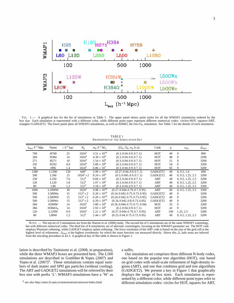
FIG. 1.— A graphical key for the list of simulations in Table 1. The upper panel shows point styles for all the WMAP1 simulations ordered by thebox size. Each simulation is represented with a different color, while different point types represent different numerical codes: circles=HOT, squares=ART,triangles=GADGET2. The lower panel plots all WMAP3 simulations, as well as H384Ω, the low-Ωm simulation. See Table 1 for the details of each simulation.

TABLE 1PROPERTIES OF THESIMULATION SET

Lbox h−1 Mpc Name ǫ h−1 kpc Np mp h−1 M⊙ (Ωm,Ωb,σ8,h,n) Code zi zout ∆max

768 H768 25 10243 3.51×1010 (0.3,0.04,0.9,0.7,1) HOT 40 0 800384 H384 14 10243 4.39×109 (0.3,0.04,0.9,0.7,1) HOT 48 0 3200271 H271 10 10243 1.54×109 (0.3,0.04,0.9,0.7,1) HOT 51 0 3200192 H192 4.9 10243 5.89×108 (0.3,0.04,0.9,0.7,1) HOT 54 0 320096 H96 1.4 10243 6.86×107 (0.3,0.04,0.9,0.7,1) HOT 65 0 3200

1280 L1280 120 6403 5.99×1011 (0.27,0.04,0.9,0.7,1) GADGET2 49 0, 0.5, 1.0 600500 L500 15 10243×2 8.24×109 (0.3,0.045,0.9,0.7,1) GADGET2 40 0, 0.5, 1.25, 2.5 3200250 L250 7.6 5123 9.69×109 (0.3,0.04,0.9,0.7,1) ART 49 0, 0.5, 1.25, 2.5 3200120 L120 1.8 5123 1.07×109 (0.3,0.04,0.9,0.7,1) ART 49 0, 0.5, 1.25, 2.5 320080 L80 1.2 5123 3.18×108 (0.3,0.04,0.9,0.7,1) ART 49 0, 0.5, 1.25, 2.5 3200

1000 L1000W 30 10243 6.98×1010 (0.27,0.044,0.79,0.7,0.95) ART 60 0, 0.5, 1.25, 2.5 3200500 L500Wa 15 5123×2 6.20×1010 (0.24,0.042,0.75,0.73,0.95) GADGET2 40 0 3200500 L500Wb 15 5123×2 6.20×1010 (0.24,0.042,0.75,0.73,0.95) GADGET2 40 0 3200500 L500Wc 15 5123×2 6.20×1010 (0.24,0.042,0.8,0.73,0.95) GADGET2 40 0 3200384 H384W 14 10243 3.80×109 (0.26,0.044,0.75,0.71,0.94) HOT 35 0 3200384 H384Ωm 14 10243 2.92×109 (0.2,0.04,0.9,0.7,1) HOT 42 0 3200120 L120W 0.9 10243 1.21×108 (0.27,0.044,0.79,0.7,0.95) ART 100 1.25, 2.5 320080 L80W 1.2 5123 2.44×108 (0.23,0.04,0.75,0.73,0.95) ART 49 0, 0.5, 1.25, 2.5 3200

NOTE. — The top set of 5 simulations are from the Warren et al. (2006) study. The second list of 5 simulations are of the same WMAP1cosmology,but with different numerical codes. The third list of 8 simulations are of alternate cosmologies, focusing on the WMAP3 parameter set. The HOT codeemploys Plummer softening, while GADGET employs spline softening. The force resolution of the ART code is based on the size of the grid cell at thehighest level of refinement.∆max is the highest overdensity for which the mass function can measured directly. Above this∆, halo mass are inferredfrom the rescaling procedure in §2.3. A graphical key of thistable is shown in Figure 1.

lation is described by Tasitsiomi et al. (2008, in preparation),while the three WMAP3 boxes are presented here. The L500simulations are described in Gottlöber & Yepes (2007) andYepes et al. (2007)9. These simulations contain equal num-bers of dark matter and SPH gas particles (without cooling).The ART and GADGET2 simulations will be referred by theirbox size with prefix ‘L’. WMAP3 simulations have a ‘W’ as

9 see also http://astro.ft.uam.es/marenostrum/universe/index.html

a suffix.Our simulation set comprises three different N-body codes,

one based on the popular tree algorithm (HOT), one basedon grid codes with small-scale refinement of high-density re-gions (ART), and one that combines grid and tree algorithms(GADGET2). We present a key in Figure 1 that graphicallydisplays the range of box sizes. Each simulation is repre-sented by a different color, while different point types refer todifferent simulation codes: circles for HOT, squares for ART,

4

and triangles for GADGET2. These point symbols and colorswill be used consistently in the figures below.

2.2. Halo Identification

The standard spherical overdensity algorithm is describedin detail in Lacey & Cole (1994). However, in our ap-proach we have made several important modifications. InLacey & Cole (1994) the centers of halos are located on thecenter of mass of the particles within the sphere. Due to sub-structure, this center may be displaced from the main peakin the density field. Observational techniques such as X-raycluster identification locate the center of the halo at the peakof the X-ray flux (and therefore the peak of density of the hotintracluster gas). Optical cluster searches will often locate thecluster center at the location of the brightest member, whichis also expected to be located near the peak of X-ray emis-sion (Lin et al. 2004; Koester et al. 2007; Rykoff et al. 2008).Thus we locate the centers of halos at their density peaks.

Our halo finder begins by estimating the local densityaround each particle within a fixed top-hat aperture with ra-dius approximately three times the force softening of eachsimulation. Beginning with the highest-density particle,asphere is grown around the particle until the mean interiordensity is equal to the input value of∆, where∆ is theoverdensity within a sphere of radiusR∆ with respect tothe mean density of the Universe at the epoch of analysis,ρm(z) ≡ Ωm(z)ρcrit(z) = ρm(0)(1+ z)3:

∆ =M∆

(4/3)πR3∆

ρm. (1)

All values of∆ listed in this paper are with respect toρm(z).Since local densities smoothed with a top-hat kernel are

somewhat noisy, we refine the location of the peak of thehalo density with an iterative procedure. Starting with a ra-dius of r = R∆/3, the center of mass of the halo is calculatediteratively until convergence. The value ofr is reduced iter-atively by 1% and the new center of mass found, until a fi-nal smoothing radius ofR∆/15, or until only 20 particles arefound within the smoothing radius. At this small aperture, thecenter of mass corresponds well to the highest density peak ofthe halo. This process is computationally efficient and elim-inates noise and accounts for the possibility that the choseninitial halo location resides at the center of a large substruc-ture; in the latter case, the halo center will wander toward thelarger mass and eventually settle on its center. Once the newhalo center is determined, the sphere is regrown and the massis determined.

All particles within R∆ are marked as members of a haloand skipped when encountered in the loop over all parti-cle densities. Particles located just outside of a halo can bechosen as candidate centers for other halos, but the iterativehalo-centering procedure will wander into the parent halo.Whenever two halos have centers that are within the largerhalo’sR∆, the halo with the largest maximum circular veloc-ity, defined as the maximum of the circular velocity profile,Vc(r) = [GM(< r)/r]1/2, is taken to be the parent halo and theother halo is discarded.

We allow halos to overlap. As long as the halo center doesnot reside withinR∆ of another halo, the algorithm identifiesthese objects as distinct structures. This is in accord withX-ray or SZ observations which would identify and count suchobjects as separate systems. The overlapping volume maycontain particles. Rather than attempt to determine which

halo each particle belongs to, or to divide each particle be-tween the halos, the mass is double-counted. No solutionto this problem is ideal, but we find that the total amount ofdouble-counted mass is only∼ 0.75% of all the mass locatedwithin halos, with no dependence on halo mass. This paral-lels the treatment of close pairs of clusters detected observa-tionally. When two X-ray clusters are found to have overlap-ping isophotal contours, each system is treated individuallyand double counting of mass will occur as well.

For each value of∆, the halo finder is run independently.Halo mass functions are binned in bins of width 0.1 in logMwith no smoothing. Errors on each mass function are obtainedby the jackknife method; each simulation is divided into oc-tants and the error on each mass bin is obtained through thevariance of the halo number counts as each octant is removedfrom the full simulation volume (cf. Zehavi et al. 2005, equa-tion [6]). The jackknife errors provide a robust estimate ofboth the cosmic variance, which dominates at low masses,and the Poisson noise that dominates at high masses (seeHu & Kravtsov 2003 for a the relative contributions of eachsource of error as a function of halo mass).

When fitting the data, we only use data points with errorbars less than 25% to reduce noise in the fitting process. Wenote that mass bins will be correlated (low-mass bins moreso than high mass ones). We do not calculate the full covari-ance matrix of each mass function, so theχ2 values obtainedfrom the fitting procedure should be taken as a general guideof goodness of fit, but not as an accurate statistical measure.However, we note that the data from multiple simulations ineach mass range will be uncorrelated, and the lack of a covari-ance matrix should not bias our best-fit values for the massfunction.

2.3. Comparison of FOF and SO halos

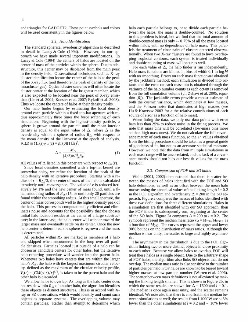
White (2001, 2002) demonstrated that there is scatter be-tween the masses of halos identified with the FOF and SOhalo definitions, as well as an offset between the mean halomasses using the canonical values of the linking lengthl = 0.2in the FOF algorithm and overdensity∆ = 200 in the SO ap-proach. Figure 2 compares the masses of halos identified withthese two definitions for three different simulations. Halos ina simulation are first identified with our SO approach, thenthe FOF finder is subsequently run, beginning at the centerof the SO halo. Figure 2a compares∆ = 200 tol = 0.2. Thesymbols represent the median mass ratiorM = M200/MFOF.2 asa function ofM200. The curves represent the upper and lower90% bounds on the distribution of mass ratios. Although themedian is near unity, the scatter is large and highly asymmet-ric.

The asymmetry in the distribution is due to the FOF algo-rithm linking two or more distinct objects in close proximityto each other. Because we allow halos to overlap, FOF willtreat these halos as a single object. Due to the arbitrary shapeof FOF halos, the algorithm also links SO objects that do notoverlap. The median mass ratio is also sensitive to the numberof particles per halo; FOF halos are known to be biased towardhigher masses at low particle number (Warren et al. 2006).The scatter between mass definitions is not alleviated by mak-ing the linking length smaller. This is shown in Figure 2b, inwhich the same results are shown for∆ = 1600 andl = 0.1.The median is once again near unity, and the scatter remainsidentical. We note also that there is an offset in the median be-tween simulations as well; the results from L1000W are∼ 5%lower than the other simulations atl = 0.2 and∼ 10% lower

5

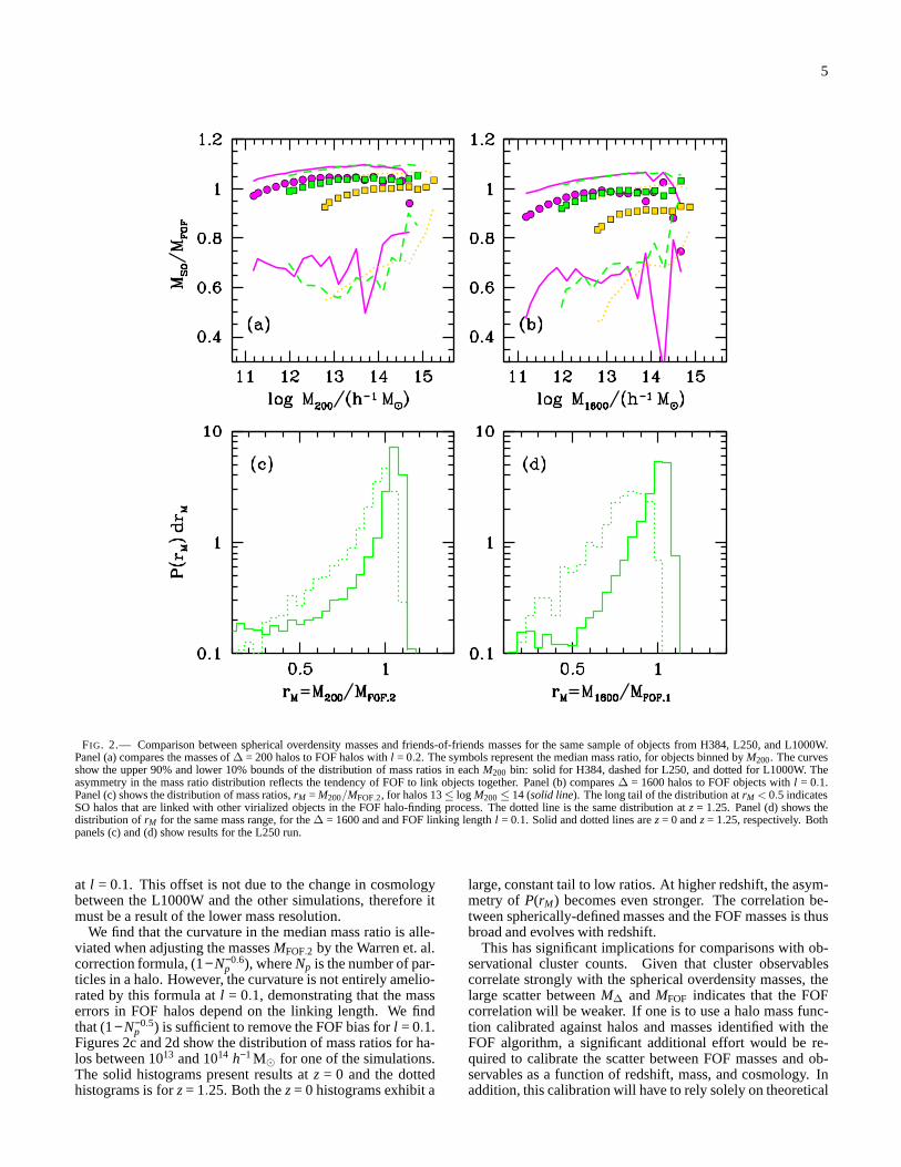
FIG. 2.— Comparison between spherical overdensity masses and friends-of-friends masses for the same sample of objects from H384, L250, and L1000W.Panel (a) compares the masses of∆ = 200 halos to FOF halos withl = 0.2. The symbols represent the median mass ratio, for objects binned byM200. The curvesshow the upper 90% and lower 10% bounds of the distribution ofmass ratios in eachM200 bin: solid for H384, dashed for L250, and dotted for L1000W. Theasymmetry in the mass ratio distribution reflects the tendency of FOF to link objects together. Panel (b) compares∆ = 1600 halos to FOF objects withl = 0.1.Panel (c) shows the distribution of mass ratios,rM = M200/MFOF.2, for halos 13≤ log M200≤ 14 (solid line). The long tail of the distribution atrM < 0.5 indicatesSO halos that are linked with other virialized objects in theFOF halo-finding process. The dotted line is the same distribution atz = 1.25. Panel (d) shows thedistribution ofrM for the same mass range, for the∆ = 1600 and and FOF linking lengthl = 0.1. Solid and dotted lines arez= 0 andz= 1.25, respectively. Bothpanels (c) and (d) show results for the L250 run.

at l = 0.1. This offset is not due to the change in cosmologybetween the L1000W and the other simulations, therefore itmust be a result of the lower mass resolution.

We find that the curvature in the median mass ratio is alle-viated when adjusting the massesMFOF.2 by the Warren et. al.correction formula, (1−N−0.6

p ), whereNp is the number of par-ticles in a halo. However, the curvature is not entirely amelio-rated by this formula atl = 0.1, demonstrating that the masserrors in FOF halos depend on the linking length. We findthat (1−N−0.5

p ) is sufficient to remove the FOF bias forl = 0.1.Figures 2c and 2d show the distribution of mass ratios for ha-los between 1013 and 1014 h−1M⊙ for one of the simulations.The solid histograms present results atz = 0 and the dottedhistograms is forz= 1.25. Both thez= 0 histograms exhibit a

large, constant tail to low ratios. At higher redshift, the asym-metry of P(rM) becomes even stronger. The correlation be-tween spherically-defined masses and the FOF masses is thusbroad and evolves with redshift.

This has significant implications for comparisons with ob-servational cluster counts. Given that cluster observablescorrelate strongly with the spherical overdensity masses,thelarge scatter betweenM∆ andMFOF indicates that the FOFcorrelation will be weaker. If one is to use a halo mass func-tion calibrated against halos and masses identified with theFOF algorithm, a significant additional effort would be re-quired to calibrate the scatter between FOF masses and ob-servables as a function of redshift, mass, and cosmology. Inaddition, this calibration will have to rely solely on theoretical

6

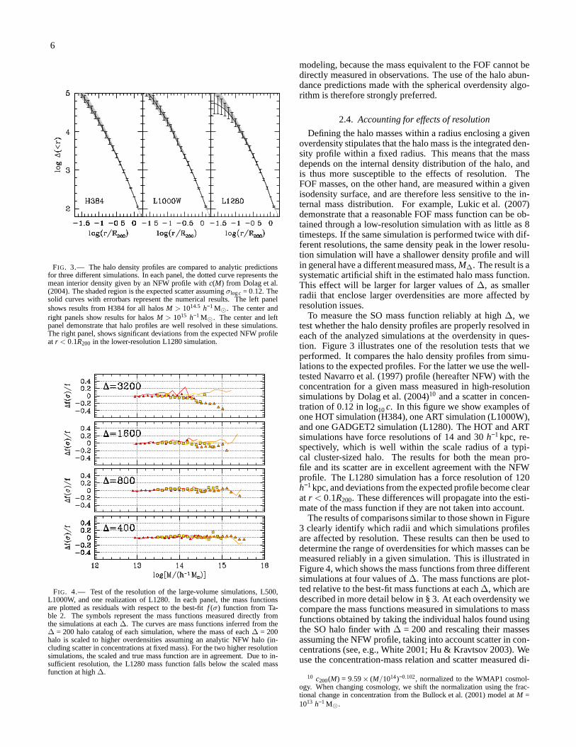
FIG. 3.— The halo density profiles are compared to analytic predictionsfor three different simulations. In each panel, the dotted curve represents themean interior density given by an NFW profile withc(M) from Dolag et al.(2004). The shaded region is the expected scatter assumingσlogc = 0.12. Thesolid curves with errorbars represent the numerical results. The left panelshows results from H384 for all halosM > 1014.5 h−1 M⊙. The center andright panels show results for halosM > 1015 h−1 M⊙. The center and leftpanel demonstrate that halo profiles are well resolved in these simulations.The right panel, shows significant deviations from the expected NFW profileat r < 0.1R200 in the lower-resolution L1280 simulation.

FIG. 4.— Test of the resolution of the large-volume simulations, L500,L1000W, and one realization of L1280. In each panel, the massfunctionsare plotted as residuals with respect to the best-fitf (σ) function from Ta-ble 2. The symbols represent the mass functions measured directly fromthe simulations at each∆. The curves are mass functions inferred from the∆ = 200 halo catalog of each simulation, where the mass of each∆ = 200halo is scaled to higher overdensities assuming an analyticNFW halo (in-cluding scatter in concentrations at fixed mass). For the twohigher resolutionsimulations, the scaled and true mass function are in agreement. Due to in-sufficient resolution, the L1280 mass function falls below the scaled massfunction at high∆.

modeling, because the mass equivalent to the FOF cannot bedirectly measured in observations. The use of the halo abun-dance predictions made with the spherical overdensity algo-rithm is therefore strongly preferred.

2.4. Accounting for effects of resolution

Defining the halo masses within a radius enclosing a givenoverdensity stipulates that the halo mass is the integratedden-sity profile within a fixed radius. This means that the massdepends on the internal density distribution of the halo, andis thus more susceptible to the effects of resolution. TheFOF masses, on the other hand, are measured within a givenisodensity surface, and are therefore less sensitive to thein-ternal mass distribution. For example, Lukic et al. (2007)demonstrate that a reasonable FOF mass function can be ob-tained through a low-resolution simulation with as little as 8timesteps. If the same simulation is performed twice with dif-ferent resolutions, the same density peak in the lower resolu-tion simulation will have a shallower density profile and willin general have a different measured mass,M∆. The result is asystematic artificial shift in the estimated halo mass function.This effect will be larger for larger values of∆, as smallerradii that enclose larger overdensities are more affected byresolution issues.

To measure the SO mass function reliably at high∆, wetest whether the halo density profiles are properly resolvedineach of the analyzed simulations at the overdensity in ques-tion. Figure 3 illustrates one of the resolution tests that weperformed. It compares the halo density profiles from simu-lations to the expected profiles. For the latter we use the well-tested Navarro et al. (1997) profile (hereafter NFW) with theconcentration for a given mass measured in high-resolutionsimulations by Dolag et al. (2004)10 and a scatter in concen-tration of 0.12 in log10c. In this figure we show examples ofone HOT simulation (H384), one ART simulation (L1000W),and one GADGET2 simulation (L1280). The HOT and ARTsimulations have force resolutions of 14 and 30h−1kpc, re-spectively, which is well within the scale radius of a typi-cal cluster-sized halo. The results for both the mean pro-file and its scatter are in excellent agreement with the NFWprofile. The L1280 simulation has a force resolution of 120h−1kpc, and deviations from the expected profile become clearat r < 0.1R200. These differences will propagate into the esti-mate of the mass function if they are not taken into account.

The results of comparisons similar to those shown in Figure3 clearly identify which radii and which simulations profilesare affected by resolution. These results can then be used todetermine the range of overdensities for which masses can bemeasured reliably in a given simulation. This is illustrated inFigure 4, which shows the mass functions from three differentsimulations at four values of∆. The mass functions are plot-ted relative to the best-fit mass functions at each∆, which aredescribed in more detail below in § 3. At each overdensity wecompare the mass functions measured in simulations to massfunctions obtained by taking the individual halos found usingthe SO halo finder with∆ = 200 and rescaling their massesassuming the NFW profile, taking into account scatter in con-centrations (see, e.g., White 2001; Hu & Kravtsov 2003). Weuse the concentration-mass relation and scatter measured di-

10 c200(M) = 9.59× (M/1014)−0.102, normalized to the WMAP1 cosmol-ogy. When changing cosmology, we shift the normalization using the frac-tional change in concentration from the Bullock et al. (2001) model atM =1013 h−1 M⊙.

7

rectly from our simulations (Tinker et. al., in preparation).The figure shows that the measured and re-scaled mass func-tions are in good agreement for∆ ≤ 800, where the scaled-up mass function is∼ 5% higher than the true mass func-tion. This error is accrued from the halos located withinR200,which can become separate halos for higher overdensities andare not accounted for in the rescaling process.

At higher overdensities, the agreement is markedly worse,especially for the lower-resolution L1280 boxes. At∆ =1600, the measured mass function is underestimated by∼

10%, increasing to∼ 20% at∆ = 3200. Therefore, for thissimulation we use the directly-measured mass function onlyat∆ ≤ 600, while at higher∆ we calculate the mass functionby mass re-scaling using halos identified with an overdensity∆ = 600. A scaling baseline of log(∆high/∆low)≤ 0.9 accruesonly. 2% error in the amplitude of the mass function at thesemasses. Thus the rescaled halo catalogs are reliable for cali-brating the halo mass function at high overdensity. This pro-cedure is used to measure high-∆ mass functions for L768(for ∆ > 800) and L1280 (for∆ > 600).

At ∆ = 200 we choose a conservative minimum value of noless than 400 particles per halo. Below this value resolutioneffects become apparent, and simulations with differing massresolutions begin to diverge. This is readily seen in the SOmass functions analyzed in Jenkins et al. (2001). At higher∆, halos are probed at significantly smaller radii, and the res-olution requirements are more stringent. Thus at higher∆

we increase the minimum number of particles such that, at∆ = 3200,Nmin is higher by a factor of 4. Exact values foreach overdensity are listed in Table 2.

3. HALO MASS FUNCTION

3.1. Fitting Formula and General Results

Although the number density of collapsed halos of a givenmass depends sensitively on the shape and amplitude of thepower spectrum, successful analytical ansatzes predict thehalo abundance quite accurately by using a universal func-tion describing the mass fraction of matter in peaks of a givenheight,ν ≡ δc/σ(M,z), in the linear density field smoothedat some scaleR = (3M/4πρm)1/3 (Press & Schechter 1974;Bond et al. 1991; Sheth & Tormen 1999). Here,δc ≈ 1.69is a constant corresponding to the critical linear overdensityfor collapse andσ(M,z) is the rms variance of the linear den-sity field smoothed on scaleR(M). The traditional nonlinearmass scaleM∗ corresponds toσ = δc. This fact has moti-vated the search for accurate universal functions describingsimulation results by Jenkins et al. (2001), White (2002), andWarren et al. (2006). Following these studies, we choose thefollowing functional form to describe halo abundance in oursimulations:

dndM

= f (σ)ρm

Md lnσ−1

dM. (2)

Here, the functionf (σ) is expected to be universal to thechanges in redshift and cosmology and is parameterized as

f (σ) = A[(σ

b

)−a+ 1

]

e−c/σ2

(3)

where

σ =∫

P(k)W(kR)k2dk, (4)

andP(k) is the linear matter power spectrum as a function ofwavenumberk, andW is the Fourier transform of the real-space top-hat window function of radiusR. It is convenient to

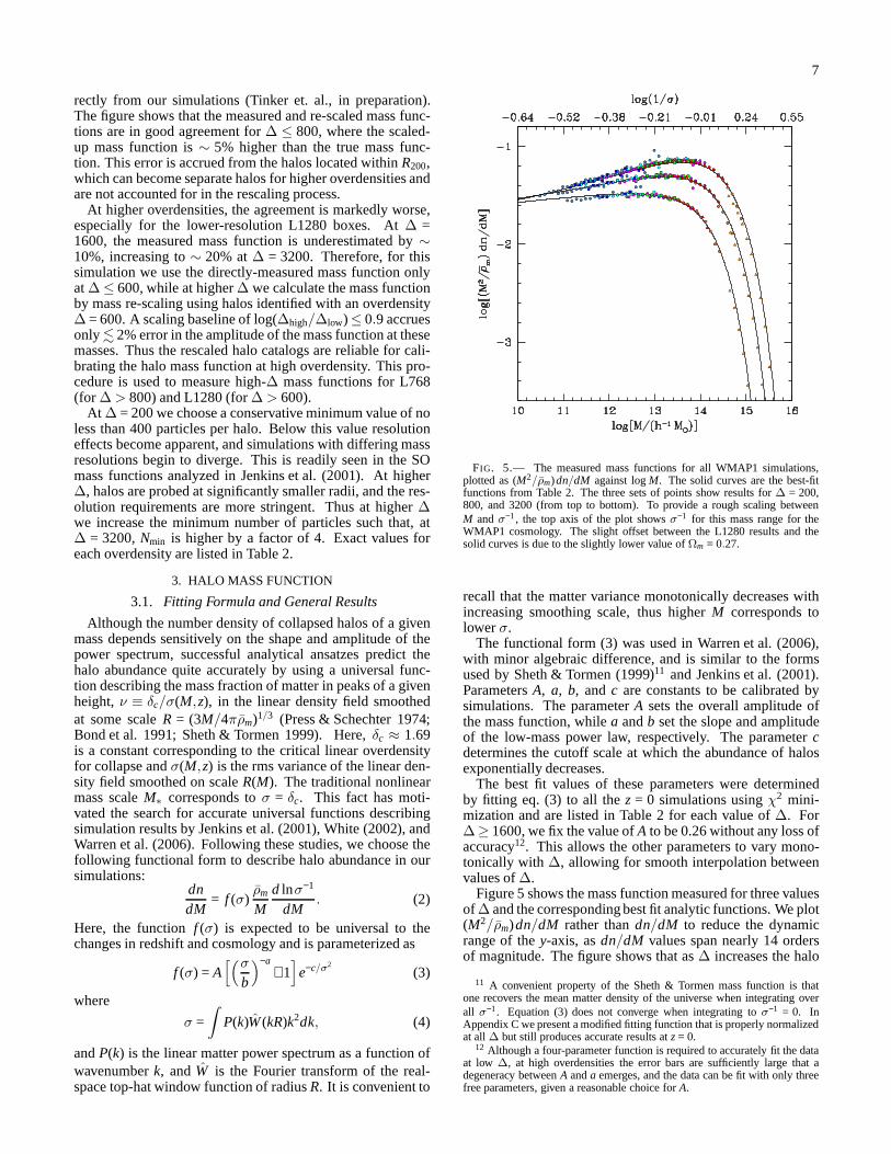
FIG. 5.— The measured mass functions for all WMAP1 simulations,plotted as (M2/ρm)dn/dM against logM. The solid curves are the best-fitfunctions from Table 2. The three sets of points show resultsfor ∆ = 200,800, and 3200 (from top to bottom). To provide a rough scalingbetweenM andσ

−1, the top axis of the plot showsσ−1 for this mass range for theWMAP1 cosmology. The slight offset between the L1280 results and thesolid curves is due to the slightly lower value ofΩm = 0.27.

recall that the matter variance monotonically decreases withincreasing smoothing scale, thus higherM corresponds tolowerσ.

The functional form (3) was used in Warren et al. (2006),with minor algebraic difference, and is similar to the formsused by Sheth & Tormen (1999)11 and Jenkins et al. (2001).ParametersA, a, b, andc are constants to be calibrated bysimulations. The parameterA sets the overall amplitude ofthe mass function, whilea andb set the slope and amplitudeof the low-mass power law, respectively. The parametercdetermines the cutoff scale at which the abundance of halosexponentially decreases.

The best fit values of these parameters were determinedby fitting eq. (3) to all thez = 0 simulations usingχ2 mini-mization and are listed in Table 2 for each value of∆. For∆≥ 1600, we fix the value ofA to be 0.26 without any loss ofaccuracy12. This allows the other parameters to vary mono-tonically with ∆, allowing for smooth interpolation betweenvalues of∆.

Figure 5 shows the mass function measured for three valuesof ∆ and the corresponding best fit analytic functions. We plot(M2/ρm)dn/dM rather thandn/dM to reduce the dynamicrange of they-axis, asdn/dM values span nearly 14 ordersof magnitude. The figure shows that as∆ increases the halo

11 A convenient property of the Sheth & Tormen mass function is thatone recovers the mean matter density of the universe when integrating overall σ

−1. Equation (3) does not converge when integrating toσ−1 = 0. In

Appendix C we present a modified fitting function that is properly normalizedat all∆ but still produces accurate results atz= 0.

12 Although a four-parameter function is required to accurately fit the dataat low ∆, at high overdensities the error bars are sufficiently largethat adegeneracy betweenA anda emerges, and the data can be fit with only threefree parameters, given a reasonable choice forA.

8

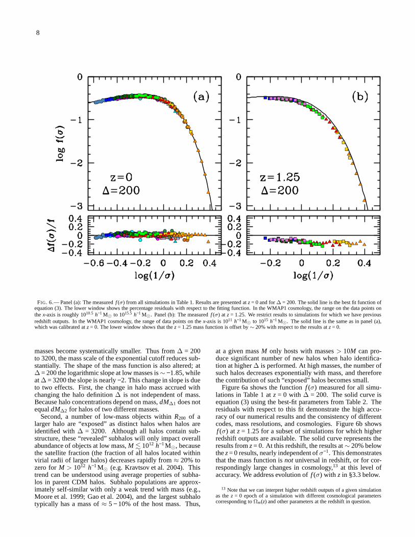
FIG. 6.— Panel (a): The measuredf (σ) from all simulations in Table 1. Results are presented atz= 0 and for∆ = 200. The solid line is the best fit function ofequation (3). The lower window shows the percentage residuals with respect to the fitting function. In the WMAP1 cosmology, the range on the data points onthex-axis is roughly 1010.5 h−1 M⊙ to 1015.5 h−1 M⊙. Panel (b): The measuredf (σ) at z = 1.25. We restrict results to simulations for which we have previousredshift outputs. In the WMAP1 cosmology, the range of data points on thex-axis is 1011 h−1 M⊙ to 1015 h−1 M⊙. The solid line is the same as in panel (a),which was calibrated atz= 0. The lower window shows that thez= 1.25 mass function is offset by∼ 20% with respect to the results atz= 0.

masses become systematically smaller. Thus from∆ = 200to 3200, the mass scale of the exponential cutoff reduces sub-stantially. The shape of the mass function is also altered; at∆ = 200 the logarithmic slope at low masses is∼ −1.85, whileat∆ = 3200 the slope is nearly−2. This change in slope is dueto two effects. First, the change in halo mass accrued withchanging the halo definition∆ is not independent of mass.Because halo concentrations depend on mass,dM∆1 does notequaldM∆2 for halos of two different masses.

Second, a number of low-mass objects withinR200 of alarger halo are “exposed” as distinct halos when halos areidentified with ∆ = 3200. Although all halos contain sub-structure, these “revealed” subhalos will only impact overallabundance of objects at low mass,M . 1012 h−1M⊙, becausethe satellite fraction (the fraction of all halos located withinvirial radii of larger halos) decreases rapidly from≈ 20% tozero forM > 1012 h−1M⊙ (e.g. Kravtsov et al. 2004). Thistrend can be understood using average properties of subha-los in parent CDM halos. Subhalo populations are approx-imately self-similar with only a weak trend with mass (e.g.,Moore et al. 1999; Gao et al. 2004), and the largest subhalotypically has a mass of≈ 5− 10% of the host mass. Thus,

at a given massM only hosts with masses> 10M can pro-duce significant number of new halos when halo identifica-tion at higher∆ is performed. At high masses, the number ofsuch halos decreases exponentially with mass, and thereforethe contribution of such “exposed” halos becomes small.

Figure 6a shows the functionf (σ) measured for all simu-lations in Table 1 atz = 0 with ∆ = 200. The solid curve isequation (3) using the best-fit parameters from Table 2. Theresiduals with respect to this fit demonstrate the high accu-racy of our numerical results and the consistency of differentcodes, mass resolutions, and cosmologies. Figure 6b showsf (σ) at z= 1.25 for a subset of simulations for which higherredshift outputs are available. The solid curve representstheresults fromz= 0. At this redshift, the results at∼ 20% belowthez= 0 results, nearly independent ofσ−1. This demonstratesthat the mass function isnot universal in redshift, or for cor-respondingly large changes in cosmology,13 at this level ofaccuracy. We address evolution off (σ) with z in §3.3 below.

13 Note that we can interpret higher redshift outputs of a givensimulationas thez = 0 epoch of a simulation with different cosmological parameterscorresponding toΩm(z) and other parameters at the redshift in question.

9

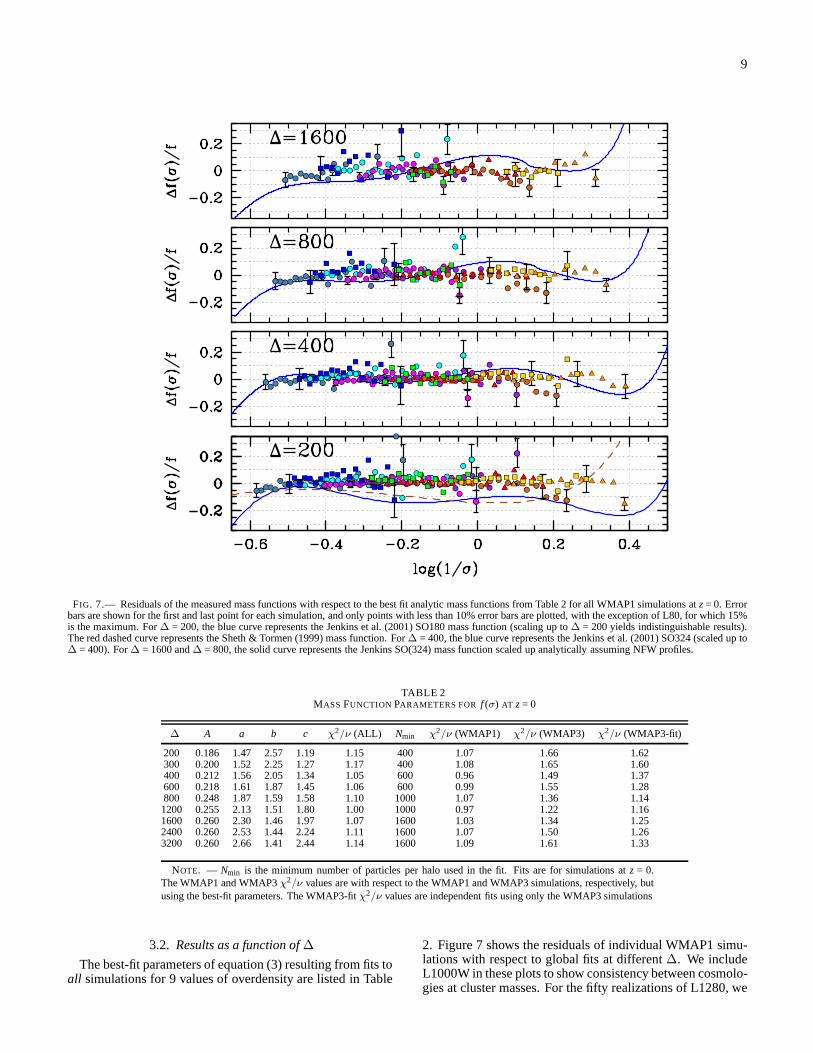
FIG. 7.— Residuals of the measured mass functions with respect to the best fit analytic mass functions from Table 2 for all WMAP1 simulations atz= 0. Errorbars are shown for the first and last point for each simulation, and only points with less than 10% error bars are plotted, with the exception of L80, for which 15%is the maximum. For∆ = 200, the blue curve represents the Jenkins et al. (2001) SO180 mass function (scaling up to∆ = 200 yields indistinguishable results).The red dashed curve represents the Sheth & Tormen (1999) mass function. For∆ = 400, the blue curve represents the Jenkins et al. (2001) SO324 (scaled up to∆ = 400). For∆ = 1600 and∆ = 800, the solid curve represents the Jenkins SO(324) mass function scaled up analytically assuming NFW profiles.

TABLE 2MASS FUNCTION PARAMETERS FOR f (σ) AT z= 0

∆ A a b c χ2/ν (ALL) Nmin χ

2/ν (WMAP1) χ2/ν (WMAP3) χ

2/ν (WMAP3-fit)

200 0.186 1.47 2.57 1.19 1.15 400 1.07 1.66 1.62300 0.200 1.52 2.25 1.27 1.17 400 1.08 1.65 1.60400 0.212 1.56 2.05 1.34 1.05 600 0.96 1.49 1.37600 0.218 1.61 1.87 1.45 1.06 600 0.99 1.55 1.28800 0.248 1.87 1.59 1.58 1.10 1000 1.07 1.36 1.141200 0.255 2.13 1.51 1.80 1.00 1000 0.97 1.22 1.161600 0.260 2.30 1.46 1.97 1.07 1600 1.03 1.34 1.252400 0.260 2.53 1.44 2.24 1.11 1600 1.07 1.50 1.263200 0.260 2.66 1.41 2.44 1.14 1600 1.09 1.61 1.33

NOTE. — Nmin is the minimum number of particles per halo used in the fit. Fits are for simulations atz = 0.The WMAP1 and WMAP3χ2/ν values are with respect to the WMAP1 and WMAP3 simulations, respectively, butusing the best-fit parameters. The WMAP3-fitχ

2/ν values are independent fits using only the WMAP3 simulations

3.2. Results as a function of∆

The best-fit parameters of equation (3) resulting from fits toall simulations for 9 values of overdensity are listed in Table

2. Figure 7 shows the residuals of individual WMAP1 simu-lations with respect to global fits at different∆. We includeL1000W in these plots to show consistency between cosmolo-gies at cluster masses. For the fifty realizations of L1280, we

10

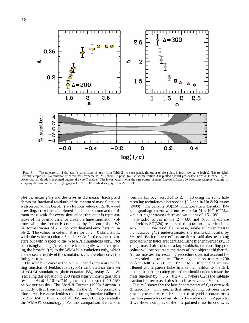
FIG. 8.— The trajectories of the best-fit parameters off (σ) from Table 2. In each panel, the order of the points is from low-∆ to high-∆ (left to right).Error bars represent 1-σ variance of parameters from the MCMC chain. In panel (a), thenormalizationA is plotted against power-law slopea. In panel (b), thepower-law amplitudeb is plotted against the cutoff scalec. The lower panel shows the rms scatter of mass functions from100 bootstrap samples, creating bysampling the simulation list. Light gray is for∆ = 200, while dark gray is for∆ = 1600.

plot the meanf (σ) and the error in the mean. Each panelshows the fractional residuals of the measured mass functionswith respect to the best-fitf (σ) for four values of∆. To avoidcrowding, error bars are plotted for the maximum and mini-mum mass scale for every simulation; the latter is represen-tative of the cosmic variance given the finite simulation vol-ume, while the former is dominated by Poisson noise. Welist formal values ofχ2/ν for our diagonal error bars in Ta-ble 2. The values in column 6 are for allz = 0 simulations,while the value in column 8 is theχ2/ν for the same param-eters but with respect to the WMAP1 simulations only. Notsurprisingly, theχ2/ν values reduce slightly when compar-ing the best-fitf (σ) to the WMAP1 simulations only, whichcomprise a majority of the simulations and therefore drive thefitting results.

The solid blue curve in the∆ = 200 panel represents the fit-ting function of Jenkins et al. (2001) calibrated on their setof τCDM simulations (their equation B3), using∆ = 180(rescaling this equation to 200 yields nearly indistinguishableresults). AtM & 1012 h−1M⊙, the Jenkins result is 10–15%below our results. The Sheth & Tormen (1999) function issimilarly offset from our results. In the∆ = 400 panel, theblue curve shows the Jenkins et. al. fitting function calibratedto ∆ = 324 on their set ofΛCDM simulations (essentiallythe WMAP1 cosmology). For this comparison the Jenkins

formula has been rescaled to∆ = 400 using the same halorescaling techniques discussed in §2.3 and in Hu & Kravtsov(2003). The Jenkins SO(324) function (their Equation B4)is in good agreement with our results forM < 1013 h−1M⊙,while at higher masses there are variations of±5–10%.

The solid curves in the∆ = 800 and 1600 panels arethe Jenkins SO(324) result scaled up to those overdensities.At σ−1 > 1, the residuals increase, while at lower massesthe rescaledf (σ) underestimates the numerical results by5− 10%. Both of these effects are due to subhalos becomingexposed when halos are identified using higher overdensity.Ifa high-mass halo contains a large subhalo, the rescaling pro-cedure will overestimate the mass of that object at higher∆.At low masses, the rescaling procedure does not account forthe revealed substructures. The change in mass from∆ = 200to ∆ = 1600 is∼ 50% at 1014 h−1M⊙. If subhalos are dis-tributed within parent halos in a similar fashion to the darkmatter, then the rescaling procedure should underestimatethemass function by∼ 0.5×0.2 = 0.1 (where 0.2 is the subhalofraction for low-mass halos from Kravtsov et al. 2004).

Figure 8 shows that the best fit parameters off (σ) vary with∆ smoothly. This means that interpolating between thesebest-fit parameters can be expected to yield accurate massfunction parameters at any desired overdensity. In AppendixB we show examples of the interpolated mass functions, as

11

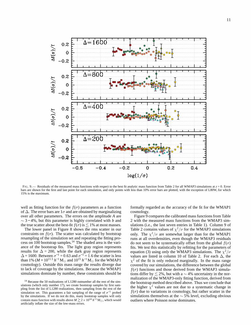
FIG. 9.— Residuals of the measured mass functions with respect to the best fit analytic mass function from Table 2 for all WMAP3simulations atz= 0. Errorbars are shown for the first and last point for each simulation, and only points with less than 10% error bars are plotted, with the exception of L80W, for which15% is the maximum.

well as fitting function for thef (σ) parameters as a functionof ∆. The error bars are 1σ and are obtained by marginalizingover all other parameters. The errors on the amplitudeA are∼ 3− 4%, but this parameter is highly correlated withb andthe true scatter about the best-fitf (σ) is . 1% at most masses.

The lower panel in Figure 8 shows the rms scatter in ourconstraints onf (σ). The scatter was calculated by bootstrapresampling of the simulation set and repeating the fitting pro-cess on 100 bootstrap samples.14 The shaded area is the vari-ance of the bootstrap fits. The light gray region representsresults for∆ = 200, while the dark gray region represents∆ = 1600. Betweenσ−1 = 0.63 andσ−1 = 1.6 the scatter is lessthan 1% (M = 1011.5 h−1M⊙ and 1015 h−1M⊙ for the WMAP1cosmology). Outside this mass range the results diverge dueto lack of coverage by the simulations. Because the WMAP1simulations dominate by number, these constraints should be

14 Because the 50 realizations of L1280 outnumber all the rest of the sim-ulations (which only number 17), we create bootstrap samples by first sam-pling from the list of L1280 realizations, then sampling from the rest of thesimulation set. This guarantees a fair sampling of the rangeof σ

−1 probedby the simulations. If we do not do this, many bootstrap samples will onlycontain mass function with results aboveM &2×1014 h−1 M⊙, which wouldartificially inflate the size of the low-mass errors.

formally regarded as the accuracy of the fit for the WMAP1cosmology.

Figure 9 compares the calibrated mass functions from Table2 with the measured mass functions from the WMAP3 sim-ulations (i.e., the last seven entries in Table 1). Column 9 ofTable 2 contains values ofχ2/ν for the WMAP3 simulationsonly. Theχ2/ν are somewhat larger than for the WMAP1runs at all overdensities, even though the WMAP3 residualsdo not seem to be systematically offset from the globalf (σ)fits. We test this statistically by refitting for the parameters ofequation (3) usingonly the WMAP3 simulations. Theχ2/νvalues are listed in column 10 of Table 2. For each∆, theχ2 of the fit is only reduced marginally. In the mass rangecovered by our simulations, the difference between the globalf (σ) functions and those derived from the WMAP3 simula-tions differ by. 2%, but with a∼ 4% uncertainty in the nor-malization of the WMAP3-only fitting function, derived fromthe bootstrap method described above. Thus we conclude thatthe higherχ2 values are not due to a systematic change inf (σ) due to variations in cosmology, but rather scatter in thesimulations themselves at the∼ 5% level, excluding obviousoutliers where Poisson noise dominates.

12

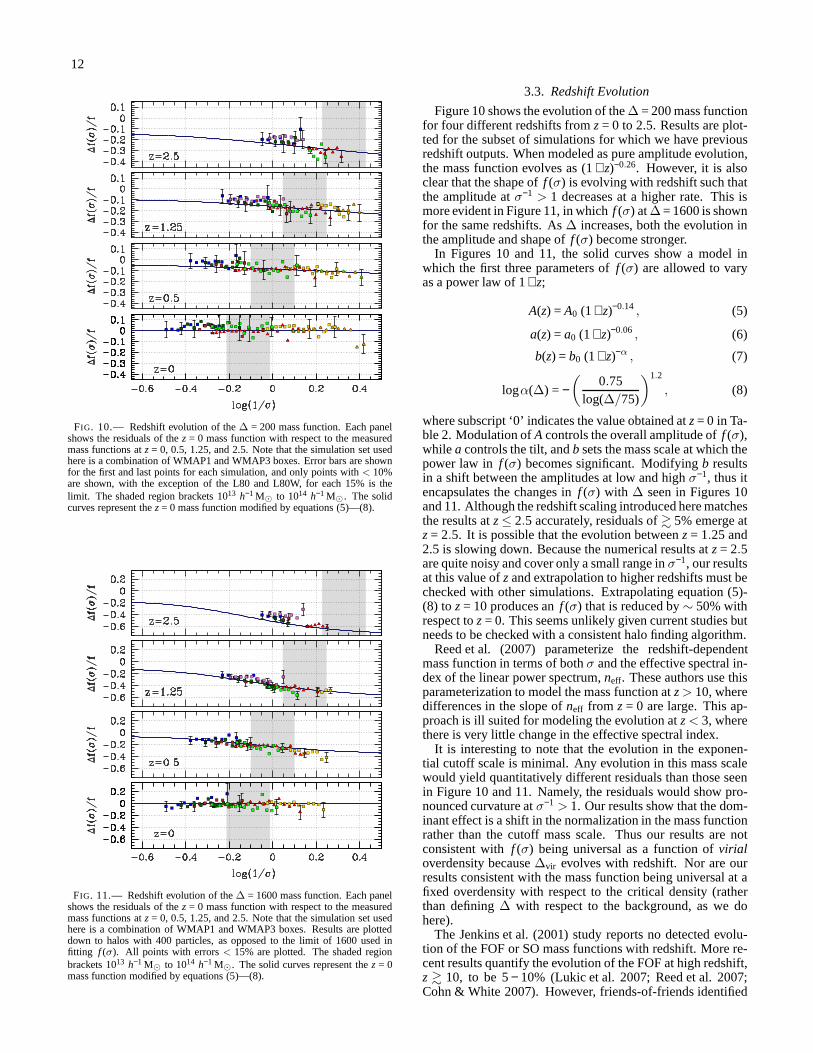
FIG. 10.— Redshift evolution of the∆ = 200 mass function. Each panelshows the residuals of thez = 0 mass function with respect to the measuredmass functions atz= 0, 0.5, 1.25, and 2.5. Note that the simulation set usedhere is a combination of WMAP1 and WMAP3 boxes. Error bars areshownfor the first and last points for each simulation, and only points with< 10%are shown, with the exception of the L80 and L80W, for each 15%is thelimit. The shaded region brackets 1013 h−1 M⊙ to 1014 h−1 M⊙. The solidcurves represent thez= 0 mass function modified by equations (5)—(8).

FIG. 11.— Redshift evolution of the∆ = 1600 mass function. Each panelshows the residuals of thez = 0 mass function with respect to the measuredmass functions atz= 0, 0.5, 1.25, and 2.5. Note that the simulation set usedhere is a combination of WMAP1 and WMAP3 boxes. Results are plotteddown to halos with 400 particles, as opposed to the limit of 1600 used infitting f (σ). All points with errors< 15% are plotted. The shaded regionbrackets 1013 h−1 M⊙ to 1014 h−1 M⊙. The solid curves represent thez = 0mass function modified by equations (5)—(8).

3.3. Redshift Evolution

Figure 10 shows the evolution of the∆ = 200 mass functionfor four different redshifts fromz= 0 to 2.5. Results are plot-ted for the subset of simulations for which we have previousredshift outputs. When modeled as pure amplitude evolution,the mass function evolves as (1+ z)−0.26. However, it is alsoclear that the shape off (σ) is evolving with redshift such thatthe amplitude atσ−1 > 1 decreases at a higher rate. This ismore evident in Figure 11, in whichf (σ) at∆ = 1600 is shownfor the same redshifts. As∆ increases, both the evolution inthe amplitude and shape off (σ) become stronger.

In Figures 10 and 11, the solid curves show a model inwhich the first three parameters off (σ) are allowed to varyas a power law of 1+ z;

A(z) = A0 (1+ z)−0.14 , (5)

a(z) = a0 (1+ z)−0.06 , (6)

b(z) = b0 (1+ z)−α , (7)

logα(∆) = −(

0.75log(∆/75)

)1.2

, (8)

where subscript ‘0’ indicates the value obtained atz= 0 in Ta-ble 2. Modulation ofA controls the overall amplitude off (σ),while a controls the tilt, andb sets the mass scale at which thepower law in f (σ) becomes significant. Modifyingb resultsin a shift between the amplitudes at low and highσ−1, thus itencapsulates the changes inf (σ) with ∆ seen in Figures 10and 11. Although the redshift scaling introduced here matchesthe results atz≤ 2.5 accurately, residuals of& 5% emerge atz= 2.5. It is possible that the evolution betweenz= 1.25 and2.5 is slowing down. Because the numerical results atz= 2.5are quite noisy and cover only a small range inσ−1, our resultsat this value ofzand extrapolation to higher redshifts must bechecked with other simulations. Extrapolating equation (5)-(8) to z= 10 produces anf (σ) that is reduced by∼ 50% withrespect toz= 0. This seems unlikely given current studies butneeds to be checked with a consistent halo finding algorithm.

Reed et al. (2007) parameterize the redshift-dependentmass function in terms of bothσ and the effective spectral in-dex of the linear power spectrum,neff. These authors use thisparameterization to model the mass function atz> 10, wheredifferences in the slope ofneff from z= 0 are large. This ap-proach is ill suited for modeling the evolution atz< 3, wherethere is very little change in the effective spectral index.

It is interesting to note that the evolution in the exponen-tial cutoff scale is minimal. Any evolution in this mass scalewould yield quantitatively different residuals than thoseseenin Figure 10 and 11. Namely, the residuals would show pro-nounced curvature atσ−1 > 1. Our results show that the dom-inant effect is a shift in the normalization in the mass functionrather than the cutoff mass scale. Thus our results are notconsistent withf (σ) being universal as a function ofvirialoverdensity because∆vir evolves with redshift. Nor are ourresults consistent with the mass function being universal at afixed overdensity with respect to the critical density (ratherthan defining∆ with respect to the background, as we dohere).

The Jenkins et al. (2001) study reports no detected evolu-tion of the FOF or SO mass functions with redshift. More re-cent results quantify the evolution of the FOF at high redshift,z & 10, to be 5− 10% (Lukic et al. 2007; Reed et al. 2007;Cohn & White 2007). However, friends-of-friends identified

13

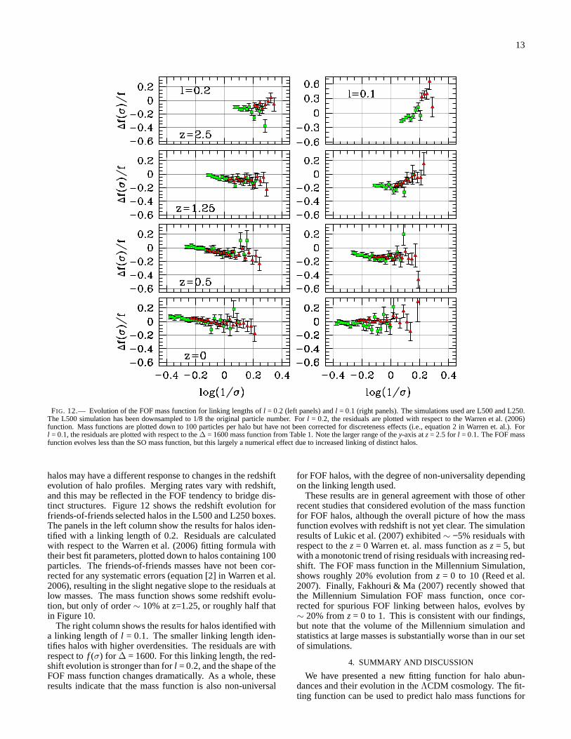
FIG. 12.— Evolution of the FOF mass function for linking lengthsof l = 0.2 (left panels) andl = 0.1 (right panels). The simulations used are L500 and L250.The L500 simulation has been downsampled to 1/8 the originalparticle number. Forl = 0.2, the residuals are plotted with respect to the Warren et al.(2006)function. Mass functions are plotted down to 100 particles per halo but have not been corrected for discreteness effects(i.e., equation 2 in Warren et. al.). Forl = 0.1, the residuals are plotted with respect to the∆ = 1600 mass function from Table 1. Note the larger range of they-axis atz= 2.5 for l = 0.1. The FOF massfunction evolves less than the SO mass function, but this largely a numerical effect due to increased linking of distincthalos.

halos may have a different response to changes in the redshiftevolution of halo profiles. Merging rates vary with redshift,and this may be reflected in the FOF tendency to bridge dis-tinct structures. Figure 12 shows the redshift evolution forfriends-of-friends selected halos in the L500 and L250 boxes.The panels in the left column show the results for halos iden-tified with a linking length of 0.2. Residuals are calculatedwith respect to the Warren et al. (2006) fitting formula withtheir best fit parameters, plotted down to halos containing 100particles. The friends-of-friends masses have not been cor-rected for any systematic errors (equation [2] in Warren et al.2006), resulting in the slight negative slope to the residuals atlow masses. The mass function shows some redshift evolu-tion, but only of order∼ 10% at z=1.25, or roughly half thatin Figure 10.

The right column shows the results for halos identified witha linking length ofl = 0.1. The smaller linking length iden-tifies halos with higher overdensities. The residuals are withrespect tof (σ) for ∆ = 1600. For this linking length, the red-shift evolution is stronger than forl = 0.2, and the shape of theFOF mass function changes dramatically. As a whole, theseresults indicate that the mass function is also non-universal

for FOF halos, with the degree of non-universality dependingon the linking length used.

These results are in general agreement with those of otherrecent studies that considered evolution of the mass functionfor FOF halos, although the overall picture of how the massfunction evolves with redshift is not yet clear. The simulationresults of Lukic et al. (2007) exhibited∼ −5% residuals withrespect to thez= 0 Warren et. al. mass function asz= 5, butwith a monotonic trend of rising residuals with increasing red-shift. The FOF mass function in the Millennium Simulation,shows roughly 20% evolution fromz = 0 to 10 (Reed et al.2007). Finally, Fakhouri & Ma (2007) recently showed thatthe Millennium Simulation FOF mass function, once cor-rected for spurious FOF linking between halos, evolves by∼ 20% fromz= 0 to 1. This is consistent with our findings,but note that the volume of the Millennium simulation andstatistics at large masses is substantially worse than in our setof simulations.

4. SUMMARY AND DISCUSSION

We have presented a new fitting function for halo abun-dances and their evolution in theΛCDM cosmology. The fit-ting function can be used to predict halo mass functions for

14

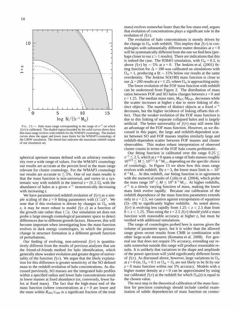
FIG. 13.— Halo mass range corresponding to the range ofσ−1 on which

f (σ) is calibrated. The shaded region bounded by the solid curves shows howthis mass range evolves with redshift for the WMAP1 cosmology. The dashedcurves show the upper and lower mass limits for the WMAP3 cosmology ofthe L80W simulation. The dotted line indicates the maximum redshift outputof our simulation set.

spherical aperture masses defined with an arbitrary overden-sity over a wide range of values. For the WMAP1 cosmologyour results are accurate at the percent level in the mass rangerelevant for cluster cosmology. For the WMAP3 cosmologyour results are accurate to. 5%. One of our main results isthat the mass function is non-universal, and varies in a sys-tematic way with redshift in the intervalz= [0,2.5], with theabundance of halos at a givenσ−1 monotonically decreasingwith increasingz.

We have parameterized redshift evolution off (σ) as a sim-ple scaling of thez = 0 fitting parameters with (1+ z)α. Wenote that if this evolution is driven by changes inΩm withz, it may be more robust to modelf (σ,z) as a function ofthe growth rate rather than 1+ z. Our simulation set does notprobe a large enough cosmological parameter space to detectdifferences due to different growth factors. However, thiswillbecome important when investigating how the mass functionevolves in dark energy cosmologies, in which the primarychange in structure formation is a different growth functionof perturbations.

Our finding of evolving, non-universalf (σ) is quantita-tively different from the results of previous analyses thatusethe friend-of-friends method for halo identification, whichgenerally show weaker evolution and greater degree of univer-sality of the functionf (σ). We argue that the likely explana-tion for this difference is greater sensitivity of the SO definedmass to the redshift evolution of halo concentrations. As dis-cussed previously, SO masses are the integrated halo profileswithin a specified radius and lower halo concentrations resultin lower masses at fixed abundance (or, conversely, fewer ha-los at fixed mass). The fact that the high-mass end of themass function (where concentrations atz = 0 are lower andthe mass withinR200/c200 is a significant fraction of the total

mass) evolves somewhat faster than the low-mass end, arguesthat evolution of concentrations plays a significant role intheevolution of f (σ).

The evolution of halo concentrations is mostly driven bythe change inΩm with redshift. This implies thatf (σ) in cos-mologies with substantially different matter densities atz= 0will be systematically different from the one we find here (per-haps closer to ourz> 1 results). There are indications that thisis indeed the case. The H384Ω simulation, withΩm = 0.2, isabove f (σ) by ∼ 5% atz = 0. The Jenkins et al. (2001) fit-ting function for∆ = 180 was calibrated on simulations withΩm = 1, producing a fit∼ 15% below our results at the sameoverdensity. The Jenkins SO(180) mass function is close toour∆ = 200 results atz= 1.25, whereΩm is approaching unity.

The lower evolution of the FOF mass function with redshiftcan be understood from Figure 2. The distribution of massratios between FOF and SO halos changes betweenz= 0 andz= 1.25. The median mass ratio,MSO/MFOF, decreases whilethe scatter increases at higherz due to more linking ofdis-tinct objects. The number of distinct objects at a fixedσ−1

decreases, but the higher incidence of linking offsets thisef-fect. Thus the weaker evolution of the FOF mass function isdue to this linking of separate collapsed halos and is largelyartificial. The better universality off (σ) may still seem likean advantage of the FOF mass function. However, as we dis-cussed in this paper, the large and redshift-dependent scat-ter between SO and FOF masses implies similarly large andredshift-dependent scatter between FOF masses and clusterobservables. This makes robust interpretation of observedcluster counts in terms of the FOF halo counts problematic.

Our fitting function is calibrated over the range 0.25 .σ−1 . 2.5, which atz= 0 spans a range of halo masses roughly1010.5 . M . 1015.5 h−1M⊙, depending on the specific choiceof cosmology. In Figure 13 we show how this mass rangeevolves with redshift. Byz= 3, the lower mass limit is∼ 105

h−1M⊙. At this redshift, our fitting function is in agreementwith the numerical results of Colín et al. (2004), which probethe mass range 105 ≤ M ≤ 109 h−1M⊙. At higher redshifts,σ−1 is a slowly varying function of mass, making the lowermass limit evolve rapidly. Because our calibration of theredshift dependence of the mass function parameters extendsonly to z= 2.5, we caution against extrapolation of equations(5)—(8) to significantly higher redshifts. As noted above,f (σ) is evolving less rapidly from 1.25< z< 2.5 than from0 < z< 1.25. Thus using thez= 2.5 f (σ) should yield a massfunction with reasonable accuracy at higherz, but must beverified with additional simulations.

The range of cosmologies probed here is narrow given thevolume of parameter space, but it is wider than the allowedrange given recent results from CMB in combination withother large-scale measures (Komatsu et al. 2008). For gen-eral use that does not require 5% accuracy, extending our re-sults somewhat outside this range will produce reasonable re-sults. It is unlikely that variations in the shape and amplitudeof the power spectrum will yield significantly different formsof f (σ). As discussed above, however, large variations inΩmatz= 0 (ie,Ωm = 0.1 orΩm = 1), are not likely to be fit by ourz= 0 mass function within our 5% accuracy. Models with ahigher matter density atz = 0 can be approximated by usingour calibratedf (σ) at the redshift for whichΩm(z) is equal tothe chosen value.

The next step in the theoretical calibration of the mass func-tion for precision cosmology should include careful exam-ination of subtle dependencies of mass function on cosmo-

15

logical parameters (especially on the dark energy equationofstate), effects of neutrinos with non-zero mass, effects ofnon-gaussianity (Grossi et al. 2007; Dalal et al. 2007), etc. Last,but not least, we need to understand the effects of baryonicphysics on the mass distribution of halos and related effects onthe mass function, which can be quite significant (Rudd et al.2008). The results of Zentner et al. (2007) indicate that themain baryonic effects can be encapsulated in a simple changeof halo concentrations, which would result in a uniform shiftof M∆ and a uniform correction tof (σ). Whether this is cor-rect at the accuracy level required remains to be demonstratedwith numerical simulations.

Our study illustrates just how daunting is the task of cal-ibrating the mass function to the accuracy of. 5%. Largenumbers of large-volume simulations are required to esti-mate the abundance of cluster-sized objects, but high dynamicrange is required to properly resolve their internal mass dis-tribution and subhalos. The numerical and resolution effectsshould be carefully controlled, which requires stringent con-vergence tests. In addition, the abundance of halos on the ex-ponential cutoff of the mass function can be influenced by thechoice of method to generate initial conditions and the start-ing redshift, as was recently demonstrated by Crocce et al.(2006, see also Appendix A). All this makes exhaustive stud-ies of different effects and cosmological parameters usingbrute force calibration of the kind presented in this paper forthe ΛCDM cosmology extremely demanding. Clever newways need to be developed both in the choice of the param-eter space to be investigated (Habib et al. 2007) and in com-

plementary studies of various effects using smaller, targetedsimulations.

We thank Roman Scoccimarro for simulations, computertime to analyze them, and discussions on initial conditions.We thank Rebecca Stanek, Gus Evrard, Martin White, andUros Seljak for many helpful discussions. We thank AlexVikhlinin, Salman Habib, and David Weinberg for useful dis-cussions and comments on the manuscript. J.T. was sup-ported by the Chandra award GO5-6120B and National Sci-ence Foundation (NSF) under grant AST-0239759. A.V.K. issupported by the NSF under grants No. AST-0239759 andAST-0507666, by NASA through grant NAG5-13274, and bythe Kavli Institute for Cosmological Physics at the Univer-sity of Chicago. Portions of this work were performed un-der the auspices of the U.S. Dept. of Energy, and supportedby its contract #W-7405-ENG-36 to Los Alamos NationalLaboratory. Computational resources were provided by theLANL open supercomputing initiative. S.G. acknowledgessupport by the German Academic Exchange Service. Someof the simulations were performed at the Leibniz Rechenzen-trum Munich, partly using German Grid infrastructure pro-vided by AstroGrid-D. The GADGET SPH simulations havebeen done in the MareNostrum supercomputer at BSC-CNS(Spain) and analyzed at NIC Jülich (Germany). G.Y. and S.G.wish to thank A.I. Hispano-Alemanas and DFG for financialsupport. G.Y. acknowledges support also from M.E.C. grantsFPA2006-01105 and AYA2006-15492-C03.

REFERENCES

Albrecht, A., Bernstein, G., Cahn, R., Freedman, W. L., Hewitt, J., Hu, W.,Huth, J., Kamionkowski, M., Kolb, E. W., Knox, L., Mather, J.C., Staggs,S., & Suntzeff, N. B. 2006, Report of the Dark Energy Task Force (astro-ph/0609591)

Arnaud, M., Pointecouteau, E., & Pratt, G. W. 2007, A&A, 474,L37Bialek, J. J., Evrard, A. E., & Mohr, J. J. 2001, ApJ, 555, 597Bond, J. R., Cole, S., Efstathiou, G., & Kaiser, N. 1991, ApJ,379, 440Bullock, J. S., Kolatt, T. S., Sigad, Y., Somerville, R. S., Kravtsov, A. V.,

Klypin, A. A., Primack, J. R., & Dekel, A. 2001, MNRAS, 321, 559Cohn, J. D. & White, M. 2007, ApJ, submitted (astro-ph/0706.0208), 706Colín, P., Klypin, A., Valenzuela, O., & Gottlöber, S. 2004,ApJ, 612, 50Cooray, A. & Sheth, R. 2002, Phys. Rep., 372, 1Crocce, M., Pueblas, S., & Scoccimarro, R. 2006, MNRAS, 373,369da Silva, A. C., Kay, S. T., Liddle, A. R., & Thomas, P. A. 2004,MNRAS,

348, 1401Dalal, N., Doré, O., Huterer, D., & Shirokov, A. 2007, PRD submitted

(astro-ph/0710.4560), 710Dolag, K., Bartelmann, M., Perrotta, F., Baccigalupi, C., Moscardini, L.,

Meneghetti, M., & Tormen, G. 2004, A&A, 416, 853Evrard, A. E., MacFarland, T. J., Couchman, H. M. P., Colberg, J. M.,

Yoshida, N., White, S. D. M., Jenkins, A., Frenk, C. S., Pearce, F. R.,Peacock, J. A., & Thomas, P. A. 2002, ApJ, 573, 7

Fakhouri, O. & Ma, C.-P. 2007, MNRAS, submited (ArXiv:0710:4567)Gao, L., White, S. D. M., Jenkins, A., Stoehr, F., & Springel,V. 2004,

MNRAS, 355, 819Gottlöber, S. & Yepes, G. 2007, ApJ, 664, 117Grossi, M., Dolag, K., Branchini, E., Matarrese, S., & Moscardini, L. 2007,

MNRAS, 382, 1261Habib, S., Heitmann, K., Higdon, D., Nakhleh, C., & Williams, B. 2007,

Phys. Rev. D, 76, 083503Haiman, Z., Mohr, J. J., & Holder, G. P. 2001, ApJ, 553, 545Holder, G., Haiman, Z., & Mohr, J. J. 2001, ApJ, 560, L111Hu, W. & Kravtsov, A. V. 2003, ApJ, 584, 702Jenkins, A., Frenk, C. S., White, S. D. M., Colberg, J. M., Cole, S., Evrard,

A. E., Couchman, H. M. P., & Yoshida, N. 2001, MNRAS, 321, 372Knox, L., Song, Y. ., & Tyson, J. A. 2005, PRL, submitted (astro-ph/0503644)Koester, B. P., McKay, T. A., Annis, J., Wechsler, R. H., Evrard, A., Bleem,

L., Becker, M., Johnston, D., Sheldon, E., Nichol, R., Miller, C., Scranton,R., Bahcall, N., Barentine, J., Brewington, H., Brinkmann,J., Harvanek,M., Kleinman, S., Krzesinski, J., Long, D., Nitta, A., Schneider, D. P.,Sneddin, S., Voges, W., & York, D. 2007, ApJ, 660, 239

Komatsu, E., Dunkley, J., Nolta, M. R., Bennett, C. L., Gold,B., Hinshaw, G.,Jarosik, N., Larson, D., Limon, M., Page, L., Spergel, D. N.,Halpern, M.,Hill, R. S., Kogut, A., Meyer, S. S., Tucker, G. S., Weiland, J. L., Wollack,E., & Wright, E. L. 2008, ApJS, submitted, (ArXiv/0803.0547)

Kravtsov, A. V., Berlind, A. A., Wechsler, R. H., Klypin, A. A., Gottlöber,S., Allgood, B., & Primack, J. R. 2004, ApJ, 609, 35

Kravtsov, A. V., Klypin, A. A., & Khokhlov, A. M. 1997, ApJS, 111, 73Kravtsov, A. V., Vikhlinin, A., & Nagai, D. 2006, ApJ, 650, 128Lacey, C. & Cole, S. 1994, MNRAS, 271, 676Lee, J. & Shandarin, S. F. 1998, ApJ, 500, 14Lima, M. & Hu, W. 2004, Phys. Rev. D, 70, 043504—. 2005, Phys. Rev. D, 72, 043006—. 2007, Phys. Rev. D, 76, 123013Lin, Y.-T., Mohr, J. J., & Stanford, S. A. 2004, ApJ, 610, 745Lukic, Z., Heitmann, K., Habib, S., Bashinsky, S., & Ricker,P. M. 2007, ApJ,

submitted, (astro-ph/0702360)Majumdar, S. & Mohr, J. J. 2003, ApJ, 585, 603—. 2004, ApJ, 613, 41Maughan, B. J. 2007, ApJ, 668, 772Mohr, J. J., Mathiesen, B., & Evrard, A. E. 1999, ApJ, 517, 627Moore, B., Ghigna, S., Governato, F., Lake, G., Quinn, T., Stadel, J., & Tozzi,

P. 1999, ApJ, 524, L19Motl, P. M., Hallman, E. J., Burns, J. O., & Norman, M. L. 2005,ApJ, 623,

L63Nagai, D. 2006, ApJ, 650, 538Navarro, J. F., Frenk, C. S., & White, S. D. M. 1997, ApJ, 490, 493Press, W. H. & Schechter, P. 1974, ApJ, 187, 425Press, W. H., Teukolsky, S. A., Vetterling, W. T., & Flannery, B. P. 1992,

Numerical recipes in C. The art of scientific computing (Cambridge:University Press, |c1992, 2nd ed.)

Reed, D., Gardner, J., Quinn, T., Stadel, J., Fardal, M., Lake, G., & Governato,F. 2003, MNRAS, 346, 565

Reed, D. S., Bower, R., Frenk, C. S., Jenkins, A., & Theuns, T.2007,MNRAS, 374, 2

Rudd, D. H., Zentner, A. R., & Kravtsov, A. V. 2008, ApJ, 672, 19Rykoff, E. S., McKay, T. A., Becker, M. R., Evrard, A., Johnston, D. E.,

Koester, B. P., Rozo, E., Sheldon, E. S., & Wechsler, R. H. 2008, ApJ, 675,1106

Scoccimarro, R. 1998, MNRAS, 299, 1097Sheldon, E. S., Johnston, D. E., Scranton, R., Koester, B. P., McKay, T. A.,

Oyaizu, H., Cunha, C., Lima, M., Lin, H., Frieman, J. A., Wechsler, R. H.,Annis, J., Mandelbaum, R., Bahcall, N. A., & Fukugita, M. 2007, ApJ,submitted (0709.1153), 709

Sheth, R. K. & Tormen, G. 1999, MNRAS, 308, 119Spergel, D. N., Bean, R., Doré, O., Nolta, M. R., Bennett, C. L., Dunkley, J.,

Hinshaw, G., Jarosik, N., Komatsu, E., Page, L., Peiris, H. V., Verde, L.,Halpern, M., Hill, R. S., Kogut, A., Limon, M., Meyer, S. S., Odegard, N.,Tucker, G. S., Weiland, J. L., Wollack, E., & Wright, E. L. 2007, ApJS,170, 377

16

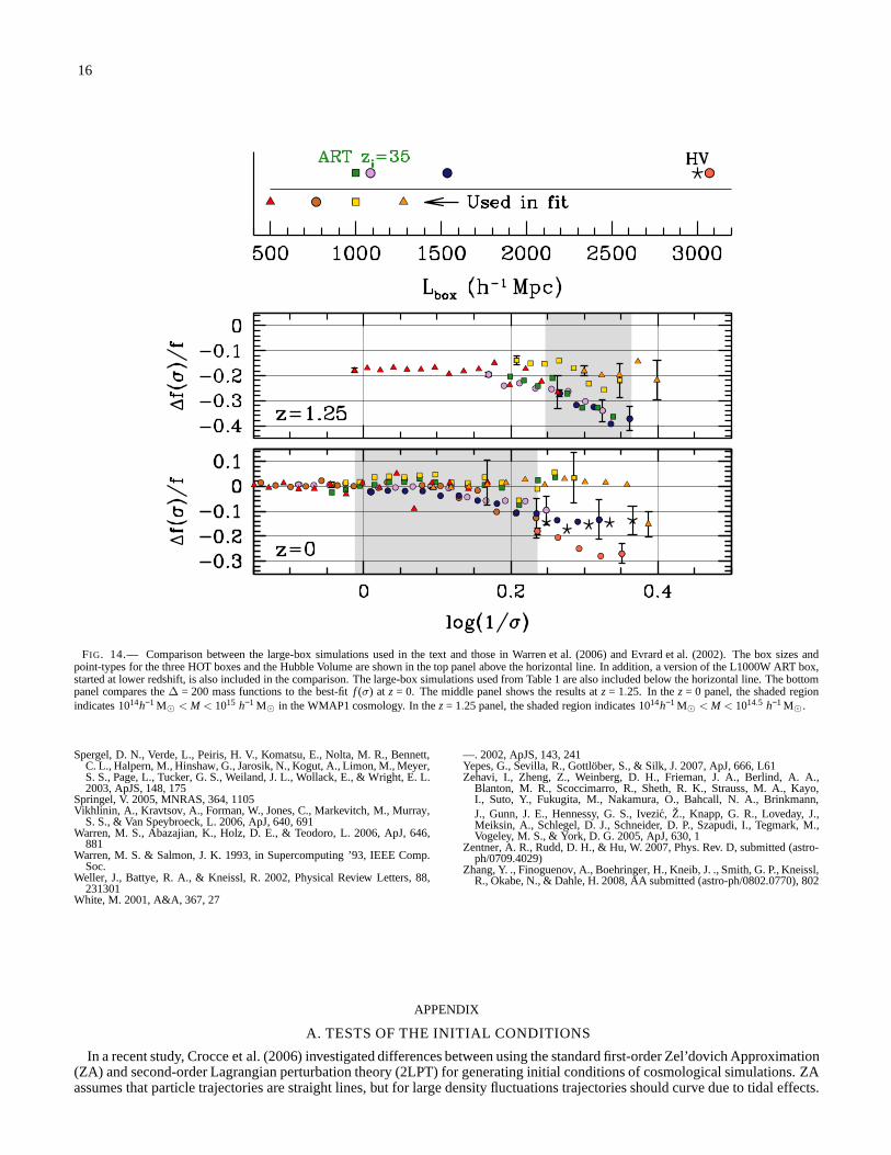
FIG. 14.— Comparison between the large-box simulations used inthe text and those in Warren et al. (2006) and Evrard et al. (2002). The box sizes andpoint-types for the three HOT boxes and the Hubble Volume areshown in the top panel above the horizontal line. In addition, a version of the L1000W ART box,started at lower redshift, is also included in the comparison. The large-box simulations used from Table 1 are also included below the horizontal line. The bottompanel compares the∆ = 200 mass functions to the best-fitf (σ) at z = 0. The middle panel shows the results atz = 1.25. In thez = 0 panel, the shaded regionindicates 1014h−1 M⊙ < M < 1015 h−1 M⊙ in the WMAP1 cosmology. In thez= 1.25 panel, the shaded region indicates 1014h−1 M⊙ < M < 1014.5 h−1 M⊙.

Spergel, D. N., Verde, L., Peiris, H. V., Komatsu, E., Nolta,M. R., Bennett,C. L., Halpern, M., Hinshaw, G., Jarosik, N., Kogut, A., Limon, M., Meyer,S. S., Page, L., Tucker, G. S., Weiland, J. L., Wollack, E., & Wright, E. L.2003, ApJS, 148, 175

Springel, V. 2005, MNRAS, 364, 1105Vikhlinin, A., Kravtsov, A., Forman, W., Jones, C., Markevitch, M., Murray,

S. S., & Van Speybroeck, L. 2006, ApJ, 640, 691Warren, M. S., Abazajian, K., Holz, D. E., & Teodoro, L. 2006,ApJ, 646,

881Warren, M. S. & Salmon, J. K. 1993, in Supercomputing ’93, IEEE Comp.

Soc.Weller, J., Battye, R. A., & Kneissl, R. 2002, Physical Review Letters, 88,

231301White, M. 2001, A&A, 367, 27

—. 2002, ApJS, 143, 241Yepes, G., Sevilla, R., Gottlöber, S., & Silk, J. 2007, ApJ, 666, L61Zehavi, I., Zheng, Z., Weinberg, D. H., Frieman, J. A., Berlind, A. A.,

Blanton, M. R., Scoccimarro, R., Sheth, R. K., Strauss, M. A., Kayo,I., Suto, Y., Fukugita, M., Nakamura, O., Bahcall, N. A., Brinkmann,J., Gunn, J. E., Hennessy, G. S., Ivezic, Ž., Knapp, G. R., Loveday, J.,Meiksin, A., Schlegel, D. J., Schneider, D. P., Szapudi, I.,Tegmark, M.,Vogeley, M. S., & York, D. G. 2005, ApJ, 630, 1

Zentner, A. R., Rudd, D. H., & Hu, W. 2007, Phys. Rev. D, submitted (astro-ph/0709.4029)

Zhang, Y. ., Finoguenov, A., Boehringer, H., Kneib, J. ., Smith, G. P., Kneissl,R., Okabe, N., & Dahle, H. 2008, AA submitted (astro-ph/0802.0770), 802

APPENDIX

A. TESTS OF THE INITIAL CONDITIONS

In a recent study, Crocce et al. (2006) investigated differences between using the standard first-order Zel’dovich Approximation(ZA) and second-order Lagrangian perturbation theory (2LPT) for generating initial conditions of cosmological simulations. ZAassumes that particle trajectories are straight lines, butfor large density fluctuations trajectories should curve due to tidal effects.

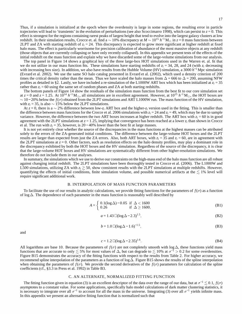
17

Thus, if a simulation is initialized at the epoch where the overdensity is large in some regions, the resulting error in particletrajectories will lead to ‘transients’ in the evolution of perturbations (see also Scoccimarro 1998), which can persist to z= 0. Thiseffect is strongest for the regions containing rarest peaksof largest height that tend to evolve into the largest galaxyclusters at lowredshift. In their simulation results, Crocce et. al. find a∼ 10% discrepancy atM ∼ 1015 h−1M⊙ in z= 0 mass functions between2LPT and ZA with starting redshift ofzi = 24. This discrepancy is expected to grow more significant athigher redshift at fixedhalo mass. The effect is particularly worrisome for precision calibration of abundance of the most massive objects at any redshift(those objects that are currently collapsing or have only recently collapsed). In this appendix we present tests of the effects of theinitial redshift on the mass function and explain why we havediscarded some of the large-volume simulations from our analysis.

The top panel in Figure 14 shows a graphical key of the three large-box HOT simulations used in the Warren et. al. fit thatwe do not utilize in our mass function fits. These simulationshave starting redshifts ofzi = 34, 28, and 24 (withzi decreasingwith increasing box size). In addition, we also have resultsfrom the Hubble Volume (HV) simulation, a 3000h−1Mpc simulation(Evrard et al. 2002). We use the same SO halo catalog presented in Evrard et al. (2002), which used a density criterion of 200times the critical density rather than the mean. Thus we havescaled the halo masses from∆ = 666 to∆ = 200, assuming NFWprofiles as detailed in §2. Lastly, we have included a re-simulation of the L1000W ART box which has been initialized atzi = 35rather thanzi = 60 using the same set of random phases and ZA at both startingredshifts.

The bottom panels of Figure 14 show the residuals of the simulation mass function from the best fit to our core simulation setat z= 0 andz= 1.25. At 1014 h−1M⊙, all simulations are in excellent agreement. However, at 1015 h−1M⊙, the HOT boxes are∼ 10−20% below thef (σ) obtained from the 2LPT simulations and ART L1000W run. The mass function of the HV simulation,with zi = 35, is also∼ 15% below the 2LPT simulations.

At z= 0, there is a∼ 2% difference between low-zi ART box and the higher-zi version used in the fitting. This is smaller thanthe difference between mass functions for the Crocce et al. 2006 simulations withzi = 24 andzi = 49, which may be due to samplevariance. However, the difference between the two ART boxesincreases at higher redshift. The ART box withzi = 60 is in goodagreement with the 2LPT simulations atz= 1.25, implying that convergence has been reached at a lowerzi than shown in Crocceet al. The run withzi = 35, however, is 20− 40% lower than the best fit at large masses.

It is not yet entirely clear whether the source of the discrepancies in the mass functions at the highest masses can be attributedsolely to the errors of the ZA-generated initial conditions. The difference between the large-volume HOT boxes and the 2LPTresults are larger than expected from just the ZA errors. Also, both ART boxes, withzi = 35 andzi = 60, are in agreement withthe 2LPT simulations atz= 0. Other factors, such as resolution effects on the halo density profiles, may play a dominant role inthe discrepancy exhibited by both the HOT boxes and the HV simulation. Regardless of the source of the discrepancy, it is clearthat the large-volume HOT boxes and HV simulations are systematically different from other higher-resolution simulations. Wetherefore do not include them in our analyses.

In summary, the simulations which we use to derive our constraints on the high-mass end of the halo mass function are all robustagainst changing initial redshift. The 2LPT simulations have been thoroughly tested in Crocce et al. (2006). The L1000WandL500 simulations, utilizing ZA withzi & 50, show consistent results with the 2LPT simulations at multiple redshifts. However,quantifying the effects of initial conditions, finite simulation volume, and possible numerical artifacts at the. 1% level willrequire significant additional work.

B. INTERPOLATION OF MASS FUNCTION PARAMETERS

To facilitate the use of our results in analytic calculations, we provide fitting functions for the parameters off (σ) as a functionof log∆. The dependence of each parameter in the mass function is reasonably well described by

A =

0.1(log∆) − 0.05 if ∆ < 16000.26 if ∆ ≥ 1600, (B1)

a = 1.43+ (log∆− 2.3)1.5, (B2)

b = 1.0+ (log∆− 1.6)−1.5, (B3)

and

c = 1.2+ (log∆− 2.35)1.6. (B4)

All logarithms are base 10. Because the parameters off (σ) are not completely smooth with log∆, these functions yield massfunctions that are accurate to only. 5% for most values of∆, but can degrade to. 10% atσ−1 > 0.2 for some overdensities.Figure B15 demonstrates the accuracy of the fitting functions with respect to the results from Table 2. For higher accuracy, werecommend spline interpolation of the parameters as a function of log∆. Figure B15 shows the results of the spline interpolationwhen obtaining the parameters off (σ). We provide the second derivatives of thef (σ) parameters for calculation of the splinecoefficients (cf., §3.3 in Press et al. 1992) in Table B3.

C. AN ALTERNATE, NORMALIZED FITTING FUNCTION

The fitting function given in equation (3) is an excellent descriptor of the data over the range of our data, but atσ−1 . 0.1, f (σ)asymptotes to a constant value. For some applications, specifically halo model calculations of dark matter clustering statistics, itis necessary to integrate over allσ−1 to account for all the mass in the universe. Integrating (3) over allσ−1 yields infinite mass.In this appendix we present an alternative fitting function that is normalized such that

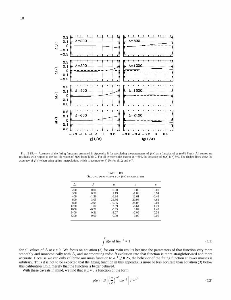
18

FIG. B15.— Accuracy of the fitting functions presented in Appendix B for calculating the parameters off (σ) as a function of∆ (solid lines). All curves areresiduals with respect to the best-fit results off (σ) from Table 2. For all overdensities except∆ = 600, the accuracy off (σ) is . 5%. The dashed lines show theaccuracy off (σ) when using spline interpolation, which is accurate to. 2% for all∆ andσ

−1.

TABLE B3SECOND DERIVATIVES OF f (σ) PARAMETERS

∆ A a b c

200 0.00 0.00 0.00 0.00300 0.50 1.19 -1.08 0.94400 -1.56 -6.34 12.61 -0.43600 3.05 21.36 -20.96 4.61800 -2.95 -10.95 24.08 0.01

1200 1.07 2.59 -6.64 1.211600 -0.71 -0.85 3.84 1.432400 0.21 -2.07 -2.09 0.333200 0.00 0.00 0.00 0.00

∫

g(σ)d lnσ−1 = 1 (C1)

for all values of∆ at z = 0. We focus on equation (3) for our main results because the parameters of that function vary moresmoothly and monotonically with∆, and incorporating redshift evolution into that function is more straightforward and moreaccurate. Because we can only calibrate our mass function toσ−1 & 0.25, the behavior of the fitting function at lower masses isarbitrary. Thus it is not to be expected that the fitting function in this appendix is more or less accurate than equation (3) belowthis calibration limit, merely that the function is better behaved.

With these caveats in mind, we find that atz= 0 a function of the form

g(σ) = B

[

(σ

e

)−d+ σ− f

]

e−g/σ2

(C2)

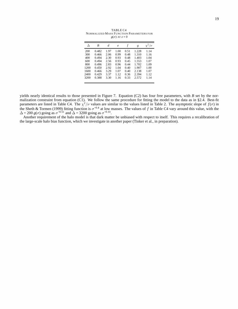
19

TABLE C4NORMALIZED MASS FUNCTION PARAMETERS FOR

g(σ) AT z= 0

∆ B d e f g χ2/ν

200 0.482 1.97 1.00 0.51 1.228 1.14300 0.466 2.06 0.99 0.48 1.310 1.16400 0.494 2.30 0.93 0.48 1.403 1.04600 0.494 2.56 0.93 0.45 1.553 1.07800 0.496 2.83 0.96 0.44 1.702 1.091200 0.450 2.92 1.04 0.40 1.907 1.001600 0.466 3.29 1.07 0.40 2.138 1.072400 0.429 3.37 1.12 0.36 2.394 1.123200 0.388 3.30 1.16 0.33 2.572 1.14

yields nearly identical results to those presented in Figure 7. Equation (C2) has four free parameters, withB set by the nor-malization constraint from equation (C1). We follow the same procedure for fitting the model to the data as in §2.4. Best-fitparameters are listed in Table C4. Theχ2/ν values are similar to the values listed in Table 2. The asymptotic slope of f (σ) inthe Sheth & Tormen (1999) fitting function isσ−0.4 at low masses. The values off in Table C4 vary around this value, with the∆ = 200g(σ) going asσ−0.51 and∆ = 3200 going asσ−0.33.

Another requirement of the halo model is that dark matter be unbiased with respect to itself. This requires a recalibration ofthe large-scale halo bias function, which we investigate inanother paper (Tinker et al., in preparation).