Topologically certified approximation of umbilics and ridges on polynomial parametric surface

ISS

N 0

249-

6399

ISR

N IN

RIA

/RR

--56

74--

FR

+E

NG

ap por t de r ech er ch e

Thème SYM

INSTITUT NATIONAL DE RECHERCHE EN INFORMATIQUE ET EN AUTOMATIQUE

Topologically certified approximation of umbilicsand ridges on polynomial parametric surface

Frédéric Cazals — Jean-Charles Faugère — Marc Pouget — Fabrice Rouillier

N° 5674

Septembre 2005

Unité de recherche INRIA Sophia Antipolis2004, route des Lucioles, BP 93, 06902 Sophia Antipolis Cedex (France)

Téléphone : +33 4 92 38 77 77 — Télécopie : +33 4 92 38 77 65

Topologically certified approximation of umbilics and ridges onpolynomial parametric surface

Frédéric Cazals ∗ , Jean-Charles Faugère † , Marc Pouget ‡ , Fabrice Rouillier §

Thème SYM — Systèmes symboliquesProjets Geometrica et Salsa

Rapport de recherche n° 5674 — Septembre 2005 — 36 pages

Abstract: Given a smooth surface, a blue (red) ridge is a curve along which the maximum (mini-mum) principal curvature has an extremum along its curvature line. Ridges are curves of extremalcurvature and encode important informations used in surface analysis or segmentation. But reportingthe ridges of a surface requires manipulating third and fourth order derivatives —whence numericaldifficulties. Additionally, ridges have self-intersections and complex interactions with the umbilicsof the surface —whence topological difficulties.

In this context, we make two contributions for the computation of ridges of polynomial para-metric surfaces. First, by instantiating to the polynomial setting a global structure theorem of ridgecurves proved in a companion paper, we develop the first certified algorithm to produce a topolog-ical approximation of the curve P encoding all the ridges of the surface. The algorithm exploitsthe singular structure of P —umbilics and purple points, and reduces the problem to solving zerodimensional systems using Gröbner basis. Second, for cases where the zero-dimensional systemscannot be practically solved, we develop a certified plot algorithm at any fixed resolution.These contributions are respectively illustrated for Bezier surfaces of degree four and five.

Key-words: Ridges, Differential Geometry, Computer Algebra.

∗ INRIA Sophia-Antipolis, Geometrica project† INRIA Rocquencourt, Salsa project‡ INRIA Sophia-Antipolis, Geometrica project§ INRIA Rocquencourt, Salsa project

Approximation certifiée des ombilics et des ridges d’une surfaceparametrée polynomiale

Résumé : Étant donnée une surface lisse, un ridge bleu (rouge) est une courbe le long de laquellela courbure principale maximum (minimum) a un extremum en suivant sa ligne de courbure. Lesridges sont des lignes d’extrêmes de courbure et codent des informations importantes utilisées ensegmentation, recalage, comparaison et analyse de surfaces. Cependant, reporter les ridges d’unesurface nécessite l’évaluation de dérivées d’ordre trois et quatre —d’où des difficultés numériques.De plus, les ridges s’auto-intersectent et interagissent de façon complexe avec les ombilics de lasurface —d’où des difficultés de nature topologique.

Dans ce contexte, ce papier propose deux contributions. D’une part, en instantiant pour les sur-faces paramétrées de façon polynomiale un théorème de structure globale des ridges établi dans unpapier joint, nous développons un algorithme produisant une approximation certifiée de la courbeP codant les ridges de la surface. Cet algorithme exploite la structure singulière de P , et reposesur la résolution de systèmes zéro dimensionnels. D’autre part, pour les cas où les systèmes zéro di-mensionnels ne peuvent être effectivement résolus, nous développons un algorithme de tracé certifiéà une résolution donné.Ces deux algorithmes sont illustrés sur des surfaces de Bézier de degrés quatre et cinq respective-ment.

Mots-clés : Ridges et Extrêmes de courbure, Géométrie Différentielle, Calcul algébrique.

Certified approximation of umbilics and ridges 3

1 Introduction

1.1 Ridges as curves on smooth surfaces

Convinced the basic principals of esthetic beauty could be revealed by mathematical principles, FelixKlein drew the so-called parabolic curves on the face of the Apollo of Belvedere [HCV52]. Eventhough such an attempt may appear as desperately optimistic, Klein’s intuition paved the alley aimingat bridging the gap between shape representations and shape perception, and several curves drawnon surfaces nowadays participate to the understanding of surfaces embedded in R3. For applicationsranging from the design of class A surfaces in the automotive industry to medical imaging, examplesuch curves are reflection lines, curvature lines or ridges. An informal introduction to these objectscan be found in the treatise [Koe90].

Given a smooth surface, a ridge consists of the points where one of the principal curvatures hasan extremum along its curvature line. Reporting ridges of a surface is a challenging task stemmingfrom the fact that ridges witness third order differential properties. First, given a surface knownanalytically or through a mesh, computing or estimating high order derivatives is a numericallya difficult task. Second, curves defined from high order properties are inherently unstable, andclassifying their transitions requires delicate singularity analysis [Por01]. Finally, ridges cannot bereported on their own since they have a complex interplay with umbilics and curvature lines, whencetopological difficulties.

1.2 Previous work

Given the previous difficulties, no algorithm reporting ridges in a certified fashion has been de-veloped as of today. Most contributions deal with sampled surfaces known through a mesh, anda complete review of these contributions can be found in [CP05]. In the following, we focus oncontributions related to parametric surfaces.

Reporting umbilics. Umbilics of a surface are always traversed by ridges, so that reporting ridgesfaithfully requires reporting umbilics. To do so, Morris [Mor90] minimizes the function k1− k2,which vanishes exactly at umbilics. Meakawa et al. [MWP96] define a polynomial system whoseroots are the umbilics. This system is solved with the rounded interval arithmetic projected poly-hedron method. This algorithm uses specific properties of the Bernstein basis of polynomials andinterval arithmetic. The domain is recursively subdivided and a set of boxes containing the umbilicsis output, but neither existence nor uniqueness of an umbilic in a box is guaranteed.

Reporting ridges. The only method dedicated to parametric surfaces we are aware of is that ofMorris [Mor90, Mor96]. The parametric domain is triangulated and zero crossings are sought onedges. Local orientation of the principal directions are needed but only provided with a heuristic.This enables to detect crossings assuming (i)there is at most one such crossing on an edge (ii)theorientation of the principal directions is correct. As this simple algorithm fails near umbilics, thesepoints are located first and crossings are found on a circle around the umbilic.

RR n° 5674

4 Cazals & Faugère & Pouget & Rouillier

1.3 Contributions

Consider a parameterized surface Φ(u,v), the parameterization being polynomial with rational coef-ficients. Let P be the curve encoding the ridges of Φ(u,v). We aim at studying P on the compactbox domain D = [a,b]× [c,d]. We know from [CFPR05] that curve P is a singular curve defined bya polynomial P with rational coefficients. Ideally, we would like to produce a topologically certifiedapproximation of P . Given a real algebraic curve, the standard way to approximate it consists ofresorting to the Cylindrical Algebraic Decomposition (CAD). Running the CAD requires computingsingular points and critical points of the curve —points with a horizontal tangent. Theoretically,these points are defined by zero-dimensional systems. Practically, because of the high degree of thepolynomials involved, the calculations may not go trough. Replacing the bottlenecks of the CAD bya resolution method adapted to the singular structure of P , we make two contributions:

1. First, we develop an algorithm producing a graph G embedded in the domain D , which isisotopic to the curve P of ridges in D . The key points are twofold:

(a) no generic assumption is required, i.e. several critical or singular points may have thesame horizontal projection;

(b) no computation with algebraic numbers is involved.

If singular and critical points can be computed —in a reasonable amount of time, the methodis effective.

2. Second, if singular or critical points cannot computed in a reasonable amount of time, wedevelop a certified plot algorithm at any fixed resolution: we subdivide D into pixels, a pixelbeing lit iff the curve intersects it.

1.4 paper overview

Notations are presented in section 2. The pre-requisites on ridges and on the main tools used byour algorithms are recalled in sections 3 and 4. The main difficulties of CAD based algorithms arediscussed in section 5. Certified topological approximation and the certified plot are developed insections 6 and 7, and illustrated in section 8. Appendix 10 provides the algebraic pre-requisites.

2 Notations

For a bivariate function f (u,v), the partial derivatives are denoted with indices, for example fuuv =∂ 3 f

∂ 2u∂ v. The quadratic form induced by the second derivatives is denoted f2(u,v) = fuuu2 +2 fuvuv+

fvvv2. The discriminant of this form is denoted δ ( f2) = f 2uv− fuu fvv. The cubic form induced by

the third derivatives in denoted f3(u,v) = fuuuu3 +3 fuuvu2v+3 fuvvuv2 + fvvvv3. The discriminant ofthis form is denoted δ ( f3) = 4( fuuu fuvv− f 2

uuv)( fuuv fvvv− f 2uvv)− ( fuuu fvvv− fuuv fuvv)

2.Let f be a real bivariate polynomial and F the real algebraic curve defined by f . A point

(u,v) ∈ C2 is called

INRIA


• a singular point of F if f (u,v) = 0, fu(u,v) = 0 and fv(u,v) = 0;

• a critical point of F if f (u,v) = 0 and fu(u,v) = 0 and fv(u,v) 6= 0 (such a point has anhorizontal tangent);

• a regular point of F if f (u,v) = 0 and it is neither singular nor critical.

If the domain D of study is a subset of R2, by fiber we refer to a cross section of this domain ata given ordinate or abscissa.

3 The implicit structure of ridges, and study points

3.1 Implicit structure of the ridge curve

As shown in [CFPR05], the ridge curve P is defined by the bivariate polynomial P(u,v). In thesame paper, we also introduce polynomials a, b, a′ and b′, together with Signridge, p2, which arefunctions of the curvatures of the surface and their first derivatives. These functions characterize thesingularities and the colors of P in the following sense [CFPR05]:

Theorem. 1 Consider a smooth parametric surface whose parameterization is denoted Φ(u,v).There exists polynomial functions P, p2 and Signridge so that the set of blue ridges union the setof red ridges union the set of umbilics has equation P = 0. In addition, for a point of this set P , onehas:

• If p2 = 0, the point is an umbilic.

• If p2 6= 0 then:

– if Signridge =−1 then the point is a blue ridge point,

– if Signridge = +1 then the point is a red ridge point,

– if Signridge = 0 then the point is a purple point.

Following the theoretical study performed in [CFPR05], the only assumption made is that thesurface admits generic ridges in the sense that real singularities of P satisfy the following condi-tions:

• Real singularities of P are of multiplicity at most 3.

• Real singularities of multiplicity 2 are called purple points. They satisfy the system Sp = {a =b = a′ = b′ = 0, δ (P2) > 0, p2 6= 0}. In addition, two real branches of P are passing througha purple point.

• Real singularities of multiplicity 3 are called umbilics. They satisfy the system Su = {p2 =0}= {p2 = 0,P = 0,Pu = 0,Pv = 0}. In addition, if δ (P3) denote the discriminant of the cubicof the third derivatives of P at an umbilic, one has:

RR n° 5674


– if δ (P3) > 0, then the umbilic is called a 3-ridge umbilic and three real branches of P

are passing through the umbilic with three distinct tangents;

– if δ (P3) < 0, then the umbilic is called a 1-ridge umbilic and one real branch of P ispassing through the umbilic.

As we shall see in section 6, these conditions are checked during the processing of the algorithm.

3.2 Study points and zero dimensional systems

A recalled in introduction, the most demanding task to certify to topology of a real algebraic curveconsists of isolating its real singular and critical points. For our problem, the singular and criticalpoints of P have a well known structure which can be exploited. More precisely: we successivelyisolate umbilics, purple points and critical points. As a system defining one set of these points alsoinclude as solution the points of the previous system, we use a localization method to simplify thecalculations (see theorem 2). The points reported at each stage are characterized as roots of a zero-dimensional system —a system with a finite number of complex solutions, together with the numberof half-branches of the curve connected to each point. In addition, points on the border of the domainof study need a special care. This setting leads to the definition of study points:

Definition. 1 Study points are points in D which are

• real singularities of P , denoted Su∪Sp , with Su = S1R∪S3R and

– S1R = {p2 = P = Pu = Pv = 0,δ (P3) < 0} (1-ridge umbilics)

– S3R = {p2 = P = Pu = Pv = 0,δ (P3) > 0} (3-ridges umbilics)

– Sp = {a = b = a′ = b′ = 0, δ (P2) > 0, p2 6= 0}= {a = b = a′ = b′ = 0, δ (P2) > 0}\Su

(purple points)

• real critical points of P in the v-direction (i.e. points with a horizontal tangent which are notsingularities of P) defined by the systemSc = {P = Pu = 0,Pv 6= 0} (critical points);

• intersections of P with the left and right sides of the box D satisfying the system

Sb = {P(a,v) = 0, v ∈ [c,d]}∪{P(b,v) = 0, v ∈ [c,d]}. Such a point may also be critical orsingular.

4 Some Algebraic tools for our method

In this section, we sketch the two algebraic methods ubiquitously called by our algorithms. Moredetails are provided in appendix 10.

INRIA


4.1 Zero dimensional systems

In our algorithms, we will need to represent solutions of zero-dimensional systems depending ontwo or more variables. We use the so called Rational Univariate Representation of the roots [Rou99],which can be viewed as a univariate equivalent to the studied system.

Given a zero-dimensional system I =< p1, . . . , ps > where the pi ∈Q[X1, . . . ,Xn], a Rational Uni-

variate Representation of V(I) has the following shape : ft (T ) = 0,X1 =gt,X1

(T )

gt,1(T ) , . . . ,Xn =gt,Xn

(T)

gt,1(T ) ,

where ft ,gt,1,gt,X1, . . . ,gt,Xn

∈Q[T ] (T is a new variable). It is uniquely defined w.r.t. a given polyno-

mial t which separates V (I) (injective on V (I)), the polynomial ft being necessarily the characteristicpolynomial of mt (the multiplication operator by the polynomial t) in Q[X1, . . . ,Xn]/I [Rou99]. TheRUR defines a bijection between the roots of the system I and those of ft preserving the multiplicitiesand the real roots :

V(I)(∩R) ≈ V( ft)(∩R)α = (α1, . . . ,αn) → t(α)

(X1(α) =gt,X1

(t(α))

gt,1(t(α)), . . . ,Xn(α) =

gt,Xn(t(α))

gt,1(t(α))) ← t(α)

There exists several ways for computing a RUR. One can use the strategy from [Rou99] whichconsists of computing a Gröbner basis of I and then to perform linear algebra operations to computea separating element as well as the full expression of the RUR. The Gröbner basis computation canalso be replaced by the generalized normal form from [MT05]. There exists more or less certifiedalternatives such as the Geometrical resolution [GLS01] (it is probabilistic since the separating ele-ment is randomly chosen and its validity is not checked, one also loose the multiplicities of the roots)or resultant based strategies such as [KOR05].

4.2 Univariate root isolation

This second tool is used to analyze fibers i.e. cross sections of D at a given ordinate or abscissa,and requires isolating roots of univariate polynomials whose coefficients are rational numbers orintervals. The method uses the Descartes rule and is fully explained in [RZ03]. The algorithmis based on a recursive subdivision of the initial interval. If exact computations with rationals areperformed, the algorithm is proved to terminate —but such computations may be costly. However,the structure of our problem is such that certifications can be achieved using interval arithmetic ratherthan an exact arithmetic. To see how, given a polynomial P = ∑n

i=0 aiui with rational coefficients,

assume we are given intervals [li,ri] enclosing the coefficients ai. Representing a rational number byan interval amounts to approximating the number, and we shall assume the intervals’ widths can bemade arbitrarily small. The specifications of the algorithm [RZ03] in the case of polynomials withintervals as coefficients are the following :

• Input :

– Pε1= ∑n

i=0[li,ri]ui a univariate polynomial with intervals [li,ri] of width less than ε1 as

coefficients. Notice that Pε1can be seen as a family of polynomials parameterized by the

choice of a (n+1)-uple (ai)i=0...n with ai ∈ [li,ri];

RR n° 5674


– [a,b] an interval for the variable u;

– a precision ε2 for the interval arithmetic computations. (This is the precision used torepresent the intervals’ boundaries.)

• Output :

– a list Li of intervals with rational bounds containing a unique real root of Pε1(that is any

polynomial of the family has a unique real root in each of these intervals);

– a list Le of interval with rational bounds where no decision was possible —i.e. theDescartes rule of sign cannot be applied because signs of interval coefficients are notdefined;

– all the elements of Li and Le are intervals contained in ]a,b[;

– a real root of Pε1in ]a,b[ is represented by an interval of Li or Le;

According to [RZ03], Le is not empty only in one of the following situations :

• there exists a polynomial in the family of polynomial Pε1which has a multiple root in ]a,b[;

• the precision ε2 of the interval arithmetic used for the computation is not sufficient;

In the present article, we need to solve two kinds of problems : isolating all the solutions ofa polynomial with rational coefficients; and isolating all the simple roots of a polynomial whosecoefficients are intervals —of arbitrary length, knowing intervals which separate the multiple rootsfrom the simple ones.

In the first case, the square free part of the polynomial is computed so that it has no multipleroot. Hence both problems become equivalent if we use interval arithmetics: we need to isolate allroots of P on the interval [a,b] containing no multiple roots of P. This can straightforwardly be donerunning the previous algorithm for Pε1

. If the list Le is empty we are done, otherwise the algorithmis run for Pε1/2 and ε2/2. The termination of this process is proved in [RZ03].

4.3 About square-free polynomials

Many computations suppose that the considered polynomials are square-free, replacing them, whenneeded, by their square-free part. In our algorithms, we use interpolation based algorithms (multi-modular, Hensel lifting, etc.) in the univariate case as well as in the bivariate case (default strategyin most computer algebra systems). One key advantage of such methods is that they detect quicklythat a polynomial is square-free by solving a simpler problem (univariate problem in the bivariatecase, computation modulo a prime number in the univariate case). In particular, this first part of thecomputation can be used to test if a polynomial is square-free or not.

In the univariate case for example, if a polynomial is square-free modulo a prime number whichdo not divide its leading coefficient, then is is square-free.

Thus, using algorithms based on interpolation strategies, the overall cost of the computations fortesting if a polynomial is square-free (or to compute its square-free part when it is not) is negligible

INRIA


compared to the rest. (With a standard variant using the Euclidean algorithm, one would perform, inaverage, O(d2) binary operations, d being the degree of the polynomial.)

In the few cases where the computation of a square-free part is non trivial, the computing timefor interpolation based methods is, in average, proportional to the size of the result and polynomialin the size (degree and coefficients sizes) of the input. For example, in the univariate case, a naivevariant will run Euclid-e’s algorithm modulo some prime numbers (O(d2) binary operations for apolynomial of degree d) until the product of these prime numbers exceeds the size of the coefficientsin the result and finally will recover the result using the Chinese remainder theorem). Since the nontrivial cases are few, these computations do not represent a blocking step in the whole algorithms ofthe present paper.

5 On the difficulty of approximating algebraic curves

The standard way to approximate algebraic curves is to resort to the CAD (Cylindrical AlgebraicDecomposition). In this section, we recall the main steps of such strategies to approximate P anddiscuss the major difficulties of algorithms like [GVN02]. In section 6 we will show how to keeptrack of the specific implicit structure of ridges [CFPR05] to optimize the process.

The CAD has been introduced in [Col75]. Basically, a CAD adapted to a set of multivariatepolynomials is a partition of the ambient space (Rn if the polynomials depends on n variables) intocells (connected subsets with a trivial topology) where the signs of the considered polynomials areall constant. Such a general method can be adapted to compute a graph reporting the topology of 2-Dor 3-D curves —see respectively [GVN02] and [GLMT04]. The following give the basic principlesof the method.

Given any implicit curve P(u,v) = 0, one consider P as a univariate polynomial in u (or v) andstudy the values of v (or u) for which the number of roots of P varies. When v varies, a root of Pmay "go to infinity" or become singular. The first case corresponds to the values of v for which theleading coefficient of P vanishes and the second case to the values of v for which the discriminantwrt u vanishes (v-coordinates of singular points and critical points wrt the projection on the v-axis).Both sets of values can be expressed as the (real) roots of a univariate polynomial c(v) which can beexplicitly computed from P. When restricted to a cylinder between the fibers over two consecutivereal roots of c(v), P(u,v) = 0 has the topology of a trivial covering. Using the CAD to approximatean algebraic curve requires mainly three stages.

In the following, we consider there is no (horizontal) asymptotes: no roots to the leading co-efficient wrt the variable u. A change of coordinate is always able to transform the curve in sucha configuration and anyways, as we will see later, one can easily avoid such an assumption whenstudying the curve in a compact box.

First stage. Produce the v-coordinates of the singular points and the critical points wrt the projec-tion on the v-axis. These v-coordinates are the real roots α1, ..,αs of the discriminant of P w.r.t. u,denoted by Critu.

RR n° 5674


Second stage. Consists of building the fiber above each v-coordinate of critical and singular points.This calculation involves polynomials whose coefficients are algebraic numbers, so as to isolate thesolutions in each fiber and at least discriminate the multiple points from the simple points. Moreformally, this requires solving:

• L-1a. Report the simple real roots of P(u,αi), i = 1..s;

• L-1b. Report the multiple real roots of P(u,αi), i = 1..s and their multiplicity;

Note that the u-coordinates of the critical and singular points are the multiple roots of the poly-nomials P(u,αi).

Third stage. Finally, the connection phase consists of connecting points from fibers. This requires:

• Finding the real roots of P(u,βi), i = 0..s, βi being any arbitrary point in ]αi,αi+1[, with theconvention α0 =−∞ and αs+1 = +∞.

• Finding the number of half branches which connect to the real roots of P(u,αi), i = 1..s inorder to connect each real root of P(u,βi), i = 0..s, to a real root of P(u,αi), i = 0..s and to areal root of P(u,αi+1), i = 0..s.

These three stages face four major difficulties.

Computing the discriminant Critu. For large polynomials, the first difficulty comes from the cal-culation of the discriminant wrt u, which may be unpractical. In section 6, we shall face this difficultyby sequentially reporting study points independently and thus decreasing strongly the degrees of theinvolved polynomials.

Isolating the roots of P(u,αi). The second difficulty comes from the isolation of the roots ofP(u,αi), αi being a real root of Critu and the computation of their multiplicities. Since αi is analgebraic number, there are three main ways to certify such a computation:

• (i) use an approximated representation of the real algebraic numbers involved such as floatingpoint numbers or intervals. It then becomes possible to isolate some of the simple real rootsof P(u,αi). Managing correctly the precision of the approximations as well as the numericalerrors during the computations, one can hope being able to isolate all the simple real roots ofP(u,αi). However, we are not aware of any general implementation of this strategy.

• (ii) use an exact representation of the real algebraic numbers involved – for example an in-terval and a polynomial to refine it to an arbitrary precision, or Thom’s coding of the roots–and apply classical algorithms with the induced arithmetic such as Sturm-habicht sequencesand sub-resultants algorithms for computing the roots of P(u,αi) [BPR03] for details. Forlarge problems, the size of the polynomials involved and the cost of exact arithmetic over realalgebraic numbers prevents this solution from being practical.

INRIA


• (iii) solve the zero-dimensional system P(u,v) = 0,Critu(v) = 0. This third strategy computesdirectly the 2D representation of the singular and critical points. On the one hand, the basiccomputations may be more difficult, but in the other hand, the operations using real algebraicnumbers are simple to perform (only evaluates polynomial at real algebraic numbers). In otherwords, one may increase the number of arithmetic operations but decrease their cost.

Genericity assumption. In order to avoid difficult computations in the cases where it is not pos-sible to compute the multiplicities of the roots at the second stage of the previous algorithm or toperform computations using the strategy (ii), most recent algorithms such as [GVN02] or [GLMT04]suppose that the curve is in generic position w.r.t. the coordinate system —which means that eachfiber P(u,αi) = 0 contains a unique critical or singular point. This implies that each polynomialP(u,αi) has one and only one multiple root. In such a situation, points of consecutive fibers corre-sponding to αi,αi+1 are easily connected through points in an intermediate witness fiber [GVN02].(One-to-one connections are made between regular points, and one is left with connections betweenthe unique critical point of each fiber αi,αi+1 with the remaining points of the intermediate fiber.)

The genericity hypothesis can be met through a linear change of variables. The algorithm de-scribed in [GVN02] or [GLMT04] provides such a generic position for the curve and this eases thecomputation of the roots of P(u,αi). In our case, the studied curves are usually in generic positionand, anyways, it is also true that a randomly chosen linear change of coordinates will put the curvein generic position with a probability one. But checking deterministically that a curve is in genericposition may be more costly than all the other operations and is required if we pretend to imple-ment a certified algorithm. For example, in [GVN02] such a test requires the computation of someprincipal Sturm-Habicht coefficients of P wrt u which is mainly as costly as using strategy (ii) forcomputing the fibers over the αi.

Moreover, one can choose not to fully certify the generic position (by performing a random linearchange of variables) and thus use strategy (i) to compute the fibers P(u,αi) = 0. This is suggest by[GVN02] but the way it is done is again not certified since they use a purely numerical function( fsolve from MAPLE software), which can not make the distinction between a cluster of 3simple roots and a triple point.

In addition, replacing a variable by a linear form in a huge bivariate polynomial may be a dif-ficult task. The sizes of the coefficients increases so that all the computations except perhaps thoseinvolving real algebraic numbers become more difficult.

All the above problems are illustrated by the example from section 8 :

• we were not able to perform the generic position test;

• we were not able to compute the roots of some P(u,αi) even under the generic position as-sumption —in which case P(u,α i) has exactly one multiple root which allows to use severaloptimization tricks.

RR n° 5674


6 Certified topological approximation

In this section, we circumvent the difficulties of the CAD and develop a certified algorithm to com-pute the topology of P .

6.1 Output specification

Definition. 2 Let G be a graph whose vertices are points of D and edges are non-intersectingstraight line-segments between vertices. Let the topology on G be induced by that of D . We saythat G is a topological approximation of the ridge curve P on the domain D if G is ambient iso-topic to P ∩D in D .

More formally, there exists a function F : D× [0,1]−→D such that:

• F is continuous;

• ∀t ∈ [0,1], Ft = F(., t) is an homeomorphism of D onto itself;

• F0 = IdD

and F1(P ∩D) = G .

Note that homeomorphic approximation is weaker and our algorithm using a cylindrical decom-position technique actually gives isotopy. In addition, our construction allows to identify singulari-ties of P to a subset of vertices of G while controlling the error on the geometric positions. We canalso color edges of G with the color of the ridge curve it is isotopic to. Once this topological sketchis given, one can easily compute a more accurate geometrical picture.

6.2 Method outline

Taking the square free part of P, we can assume P is square free. We can also assume P has no partwhich is a horizontal segment —parallel to the u-axis. Otherwise this means that a whole horizontalline is a component of P. In other words, the content of P wrt u is a polynomial in v and we canstudy this factor separately and divide P by this factor. Eventually, to get the whole topology of thecurve, one has to merge the components.

6.2.1 The algorithm

Our algorithms consists of the following five stages:

1. Isolating study points. Study point are isolated in 2D with rational univariate representations(RUR). Study points within a common fiber are identified.

2. Regularization of the study boxes. The boxes of study points are reduced so as to havethe right number of intersections between their border and P . This number is 6 for 3-ridgeumbilic, 2 for 1-ridge umbilic, 4 for a purple, 2 for others. Moreover, boxes are reduced soas to have crossings on the top and bottom sides only. Define the number of branches comingfrom the top and the bottom.

INRIA


3. Computing regular points in study fibers. In each fiber of a study point, the u-coordinatesof intersection points with P other than study points are computed.

4. Adding intermediate rational fibers. Add rational fibers between study points fibers andisolate the u-coordinates of intersection points with P .

5. Performing connections. This information is enough to perform the connections. Considerthe cylinder between two consecutive fibers, the number of branches connected from abovethe lower fiber is the same than the number of branches connected from below the higher fiber.Hence there is only one way to perform connections with non-intersecting straight segments.

6.2.2 Key points wrt CAD based algorithms

Our algorithm avoids the difficulties of CAD methods, and the following comments are in order.

Zero-dimensional systems versus the discriminant Critu. Instead of computing the v-coordinatesof all critical and singular points at once, as done by the CAD, study points are sequentially com-puted directly in 2D, together with the information required to derive the graph G .

Isolating the roots of P(u,αi). The isolation of roots of polynomials whose coefficients are alge-braic numbers does not arise since study points are isolated in 2D in the first place. We only usethe isolation of simple roots of polynomial whose coefficients are intervals. However, we do need tocharacterize the presence of multiple study points in the same fibers, an information required by theconnection process.

The connection phase without genericity assumption. Algorithms derived from the CAD haveproblems to perform the proper connection between to consecutive fibers if these fibers contain morethan one critical or singular point. We alleviate this limitation using the information on the numberof half-branches connected to the point. This number is equal to 6 for a 3-ridge umbilic, 4 for apurple point and 2 otherwise. These informations are sufficient to build the approximation G .

Complexity-wise. The advantage of the strategy is to iteratively split the problem into simplerones, and to solve the sub-problems directly in 2D. The main drawback of the method may be thearithmetic asymptotic complexity upper bounds of some of the tools we use to compute and certifythe solutions of zero-dimensional systems (see section 10).

Let F be a set of polynomials, mindeg(F) (resp. maxdeg(F)) the minimal (resp. maximal)degree of a polynomial which belongs to F . According to [Laz83], in the case of two variables,a Gröbner basis for a Degree ordering has at most mindeg(F)+ 1 polynomials of degree less than2maxdeg(F)− 1 so that modern strategies like [Fau02] will compute it in a polynomial time. Inshort, the algorithm is faster than inverting a matrix whose number of columns is bounded by thenumber of possible monomials while the number of rows is bounded by the number of polynomials.Since all the other algorithms we use are also polynomial (RUR, isolation, etc.) in their input, thefull strategies we use are still polynomial.

RR n° 5674


We would like to point out that we need to compute, certify and provide numerical approxima-tions with an arbitrary precision of the real roots of huge systems. Up to our knowledge, the toolswe used are, at least in practice, the most efficient ones with such specifications.

6.3 Step 1. Isolating study points

The method to identify these study points is to compute a RUR of the system defining them. Detailsof the method are exposed in section 10.

The less the number of solutions of a system, the easier the computation of the RUR. Hence, weuse a localization method to decompose the computation of the different types of study points —seesection 10.5. More precisely, we sequentially solve the following systems:

1. The system Su from which the sets S1R and S3R are distinguished by evaluating the sign ofδ (P3).

2. The system Sp for purple points.

3. The system Sc for critical points.

4. The system Sb for border points, that is intersections of P with the left and right sides of thebox D . Solving this system together with one of the previous identifies border points whichare also singular or critical.

Selecting only points belonging to D reduces to adding inequalities to the systems and is wellmanaged by the RUR. According to 10.5, solving such systems is equivalent to solving zero-dimensionalsystems without inequalities when the number of inequations remains small compared to the numberof variables.

The RUR of the study points provides a way to compute a box around each study point qi whichis a product of two intervals [u1

i ;u2i ]× [v1

i ;v2i ] (see section 10). The intervals can be as small as

desired.The computation of the RUR of one of these systems begins with testing if the polynomial v is

separating for the system (see 10 for the definition of a separating element). Note that if it is so, thesolution points are in generic position wrt the projection on the v-axis, that is each fiber of a pointcontains no other point of this system. In any case, we compute the square-free part of the minimalor characteristic polynomial of the multiplication by v modulus the ideal generated by the system(nothing to do when v is separating since it is the first polynomial of the RUR) : its roots are exactlyall the v-coordinates of the solutions of the system.

Until now, we only have separate informations on the different systems. In order to identify studypoints having the same v-coordinate, we need to cross these informations. First we compute isolationintervals for all the v-coordinates of all the study points together, denote I this list of intervals.If two study points with the same v-coordinate are solutions of two different systems, the gcd ofpolynomials enable to identify them:

• Initialize the list I with all the isolation intervals of all the v-coordinates of the different sys-tems.

INRIA


• Let A and B be the square free polynomials defining the v-coordinates of two different systems,and IA, IB the lists of isolation intervals of their roots. Let C = gcd(A,B) and IC the list ofisolation intervals of its roots. One can refine the elements of IC until they intersect only oneelement of IA and one element of IB. Then replace these two intervals in I by the single intervalwhich is the intersection of the three intervals. Do the same for every pair of systems.

• I then contains intervals defining different real numbers in one-to-one correspondence with thev-coordinates of the study points. It remains to refine these intervals until they are all disjoint.

Second, we compare the intervals of I and those of the 2d boxes of the study points. Let two studypoints qi and q j be represented by [u1

i ;u2i ]× [v1

i ;v2i ] and [u1

j ;u2j ]× [v1

j ;v2j ] with [v1

i ;v2i ]∩ [v1

j ;v2j ] 6= ∅.

One cannot, a priori, decide if these two points have the same v-coordinate or if a refinement ofthe boxes will end with disjoint v-intervals. On the other hand, with the list I, such a decision isstraightforward. The boxes of the study points are refined until each [v1

i ;v2i ] intersects only one

interval [w1i ;w2

i ] of the list I. Then two study points intersecting the same interval [w1i ;w2

i ] are in thesame fiber.

Finally, one can refine the u-coordinates of the study points with the same v coordinate untilthey are represented with disjoint intervals since, thanks to localizations, all the computed points aredistinct.Checking genericity conditions of section 3.1.

First, real singularities shall be the union of purple and umbilical points, this reduces to comparethe systems for singular points and for purple and umbilical points. Second, showing that δ (P3) 6= 0for umbilics and δ (P2) > 0 for purple points reduces to sign evaluation of polynomials at the rootsof a system (see section 10.5).

u

v

αi

β2i,1 u1

i,1 u2i,1 β1

i,li β2i,li

u1i,mi

u2i,mi

β1i,1

n+i,j

n−

i,j

Number of branches above

Number of branches belowv1

i

v2

i

Figure 1: Notations for a fiber involving several critical/singular points: u1(2)i, j

are used for study

points, β 1(2)i, j

for simple points.

RR n° 5674


u

v

αi+1

αi

δi

v2

i

v1

i

Figure 2: Performing connections

6.4 Step 2. Regularization of the study boxes

At this stage, we have computed all the v-coordinates α1, ...,αs of all the study points {qi, j, i =

1 . . .s, j = 1 . . .mi} by means of isolating intervals [v1i ;v2

i ], i = 1..s. We have isolated u-coordinatesof the mi study points in each fiber αi by the intervals [u1

i, j;u2i, j], j = 1..mi) and we know (section 6.3)

the number of branches which should be connected to each of them.Note that an intersection (in D) of P with a fiber v = v0 which is not a study point is a regular

point of P . Hence, the u-coordinate of this point is a simple root of the univariate polynomialP(u,v0). The first additional computation we need to do is to ensure that for each fiber P(u,αi) = 0the isolating boxes of the study points do not contain any regular point. It is sufficient to count thenumber of intersection points between P and the border of the isolating box to detect if the boxcontains or not a regular point : such a computation remains to solve 4 univariate polynomials withrational coefficients and can be done efficiently using the algorithm from section 4.2. Precisely, ifthe study point is a critical point, the isolating box contains no regular point if and only if the numberof points in the computed intersection is 2 (2 for a 1-ridge, 6 for a 3-ridge, 4 for a purple, 2 for anon-critical nor singular border point ). If the box contains a regular point, one use the RUR to refinethe isolating box and perform again the test : after a finite number of steps, each study point will berepresented by an isolating box which do not contain any regular point.

In addition, reducing boxes if necessary, we can also assume the intersections on the border ofthe isolation boxes only occur on the top or the bottom sides of the boxes (that is the sides parallelto the u-axis). This allows to compute the number of half-branches connected to the top and to thebottom of each study point. For the special case of border points, one has to compute the number ofbranches inside the domain D only.

INRIA


6.5 Step 3. Computing regular points in study fibers

We now compute the regular points in each fiber P(u,αi) = 0. Computing the regular points ofeach fiber is now equivalent to computing the roots of the polynomials P(u,αi) outside the intervalsrepresenting the u-coordinates of the study points (which contain all the multiple roots of P(u,αi)).

Denote [u1i, j;u2

i, j], j = 1..mi the intervals representing the u-coordinates of the study points onthe fiber of αi and [v1

i ,v2i ]ε an interval of length ε containing (strictly) αi and no other α j, j 6=

i. Substituting v by [v1i ,v

2i ]ε in P(u,v) gives a univariate polynomial with intervals as coefficients

we denote P(u, [v1i ,v

2i ]ε ). We apply the algorithm 4.2 for the polynomial P(u, [v1

i ,v2i ]ε ) and on the

domain ∪mij=1

[u1i, j;u2

i, j]. We know that for every vi ∈ [v1i ,v

2i ]ε the polynomial P(u,vi) has no multiple

roots on this domain. Hence the algorithm will return intervals [β 1i, j;β 2

i, j], j = 1 . . . li such that for εsufficiently small and ∀vi ∈ [αi]ε , each root of P(u,vi) belonging to [a,b]\∪mi

j=1[u1

i, j;u2i, j] is contained

in a unique [β 1i, j;β 2

i, j].We have isolated, along each fiber, a collection of points si, j, i = 1 . . .s, j = 1, . . . ,mi + li, which

are either study points or regular points of P . Each such point is isolated in a box i.e. a product ofintervals and comes with two integers (n+

i, j,n−i, j) denoting the number of branches in D connected

from above and from below.

6.6 Step 4. Adding intermediate rational fibers

Consider now an intermediate fiber, i.e. a fiber associated with v = δi i = 1 . . .s−1, with δi a rationalnumber in-between the intervals of isolation of two consecutive values αi and αi+1. If the fibersv = c or v = d are not fibers of study points, then they are added as fibers δ0 or δs.

Getting the structure of such fibers amounts to solving a univariate polynomial with rationalcoefficients, which is done using the algorithm described in section 4.2. Thus, each such fiber alsocomes with a collection of points for which ones knows that n+

i, j = n−i, j = 1. Again, each such pointis isolated in a box.

6.7 Step 5. Performing connections

We thus obtain a full and certified description of the fibers: all the intersection points with P andtheir number of branches connected. We know, by construction, that the branches of P betweenfibers have empty intersection. The number of branches connected from above a fiber is the samethan the number of branches connected from below the next fiber. Hence there is only one way toperform connections with non-intersecting straight segments. More precisely, vertices of the graphare the centers of isolation boxes, and edges are line-segments joining them.

Notice that using the intermediate fibers v = δi is compulsory if one wishes to get a graph G

isotopic to P . If not, whenever two branches have common starting points and endpoints, theembedding of the graph G obtained is not valid since two arcs are identified.

The algorithm is illustrated on Fig. 2. In addition

• If a singular point box have width δ , then the distance between the singular point and thevertex representing it is less than δ .

RR n° 5674


• One can compute the sign of the function Signridge defined in 3.1 for each regular point ofeach intermediate fiber. This defines the color of the ridge branch it belongs to. Then one canassign to each edge of the graph the color of its end point which is on an intermediate fiber.

7 Certified plot

In this section, we develop an algorithm to provide information of P when some of the calculationsrequired to certify the topology do not succeed. The information we provide consists of intersectionsbetween rational fibers in the study box and the curve. These intersections are used to define the so-called certified plot. Notice that if some calculations succeed –in particular those of umbilics andpurple points, then, the isolation boxes of these singularities can be superimposed to the certifiedplot.

For simplicity, we suppose that P is irreducible, that P(u,v) = 0 has no isolated points, whichis true under our genericity conditions of section 3.1, and that the studied domain is [0,1]× [0,1].In addition, we denote by n′ an integer such that there does not exists a connected component ofP(u,v) = 0 which is embedded in a product of intervals of length less than 1/n′.

Certified plot with n′ known. To specify the plot, we make the following:

Definition. 3 Given an integer n with n > n′, consider the n× n decomposition of the boundeddomain [0,1]× [0,1] into pixels, i.e. products of intervals of length 1/n: {[ i

n ; i+1n ]× [ j

n ; j+1n ] i =

0 . . .n−1, j = 0 . . .n−1}. Also assume each pixel has a binary attribute: lit or not.This n× n decomposition is called the certified plot of P at resolution n if a pixel is lit if and

only if P intersects the pixel. (Note that the intersection may occur only on the border or even on acorner of the pixel).

The method reduces to finding intersections between the curve P and horizontal and verticalfibers defining the pixels. The algorithm processing horizontal fibers is presented on Fig. 3. Thesame algorithm is used to process the vertical lines, i.e. computations are applied to polynomialsP(i/n,v).

INRIA


For each i = 0 . . .n:

1. Compute the square free part of P(u, i/n).

2. Isolate its roots with intervals of length less than 1/n. (As recalled in section 4.2, the algo-rithm terminates with Le = /0 since the square free part has been taken.) Let Li = {I j ; j =1 . . .mi} be the set of these intervals.

3. For each j = 1 . . .mi

(a) If I j does not intersect a fiber in the other direction, there exists k = 0 . . .n−1 such that

I j ⊂ [ kn ; k+1

n ]. The pixels containing this segment are lit (if 0 < i < n these are [ kn ; k+1

n ]×

[ i−1n ; i

n ] and [ kn ; k+1

n ]× [ in ; i+1

n ], else only one of these is in the studied domain).

(b) If I j intersects the fiber u = k/n (k = 0 . . .n−1) in the other direction then

• if P(k/n, i/n) 6= 0 then its sign enable to refine I j such that it does not intersect thefiber and one lights pixels as in step 3a —that is, we light the pixel to the right orthe left of u = k/n.

• if P(k/n, i/n) = 0 then one lights the pixels containing the point (k/n, i/n) (if thispoint is not on the border of the domain, there are 4 such pixels).

Figure 3: Processing horizontal fibers P(u, i/n)

Certified plot with n′ unknown. If n′ is not known, one can choose an arbitrary n and apply thesame strategy : only components which are embedded into products of intervals of length < 1/nmay not be represented.

8 Illustrations

We illustrate our algorithms for Bezier surfaces of degree four and five respectively. In both cases,the study domain is the domain D = [0,1]× [0,1].

8.1 Certified topology

Given a parameterized surface, recall that certifying the topology of ridges requires going throughthree stages. First, the polynomial P is computed using Maple. Second, the zero-dimensional sys-tems defining the study points are solved, together with the intersections between P and the fibers ofstudy points and intermediate fibers. Third, the connections between all these points are performedso as to produce the embedded graph G isotopic to P .

RR n° 5674


We illustrate this process on the Bezier surface whose control points are

[0,0,0] [1/4,0,0] [2/4,0,0] [3/4,0,0] [4/4,0,0][0,1/4,0] [1/4,1/4,1] [2/4,1/4,−1] [3/4,1/4,−1] [4/4,1/4,0][0,2/4,0] [1/4,2/4,−1] [2/4,2/4,1] [3/4,2/4,1] [4/4,2/4,0][0,3/4,0] [1/4,3/4,1] [2/4,3/4,−1] [3/4,3/4,1] [4/4,3/4,0][0,4/4,0] [1/4,4/4,0] [2/4,4/4,0] [3/4,4/4,0] [4/4,4/4,0]

Alternatively, this surface can be expressed as the graph of the total degree 8 polynomial h(u,v) for(u,v) ∈ [0,1]2:

h(u,v) =116u4v4−200u4v3 +108u4v2−24u4v−312u3v4 +592u3v3−360u3v2 +80u3v+252u2v4−504u2v3

+324u2v2−72u2v−56uv4 +112uv3−72uv2 +16uv.

The computation of the implicit curve has been performed using Maple 9.5 —see Maple work-sheet accompanying [CFPR05], and requires less than one minute. It is a bivariate polynomialP(u,v) of total degree 84, of degree 43 in u, degree 43 in v with 1907 terms and coefficients with upto 53 digits.

The study points Su, Sp and Sc were computed using the softwares FGB and RS (http://fgbrs.lip6.fr).These systems being in shape position —cf appendix 10.3, the RUR can be computed as shown in[Rou99]. Alternatively, Gröbner basis can be computed first using [Fau99] or [Fau02]. We testedboth methods and the computation time for the largest system Sc does not exceed 10 minutes. Table1 gives the main characteristics of these systems.

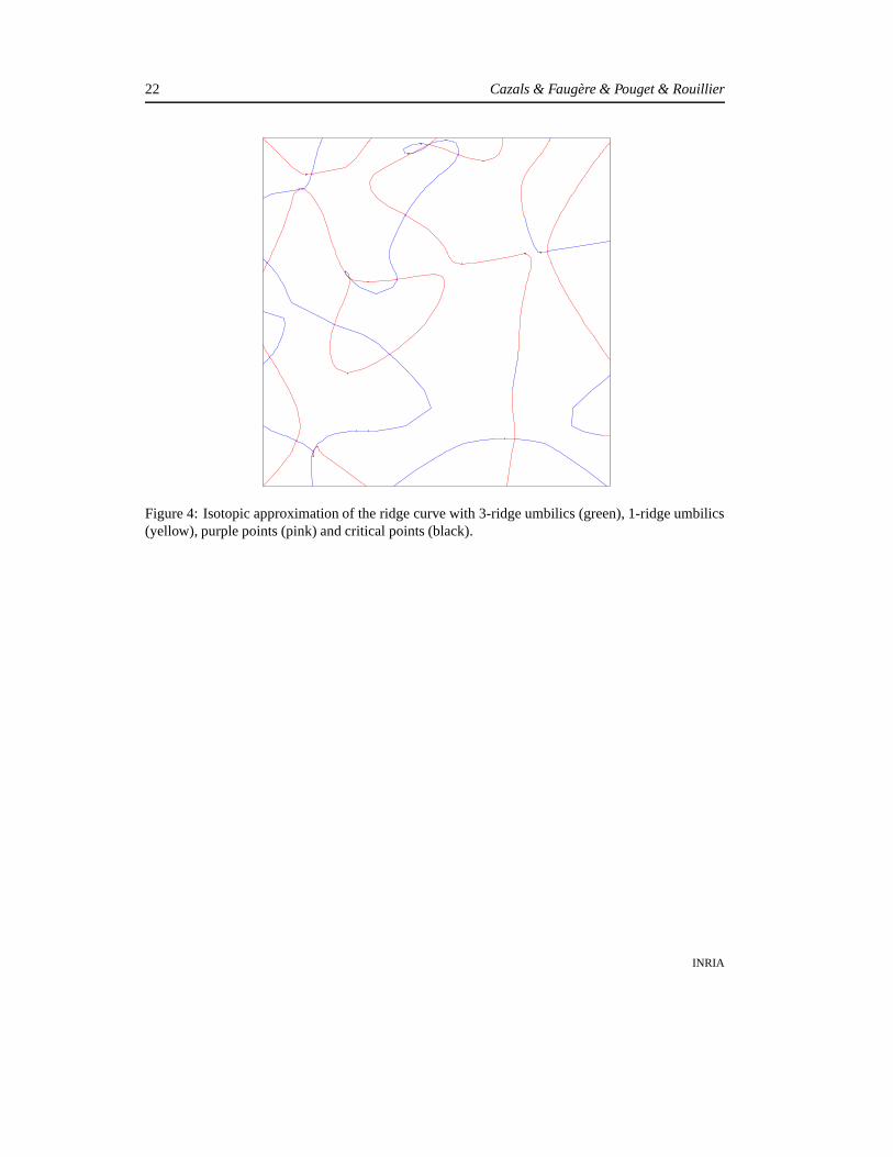
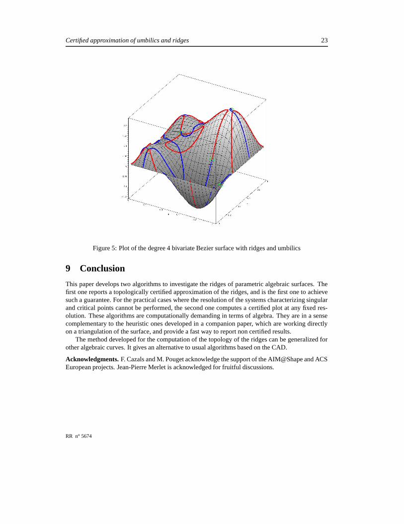
Figure 4 displays the topological approximation graph of the ridge curve in the parametric do-main D computed with the algorithm of section 6. The surface and its ridges are displayed on Fig.5. To avoid occlusion problems of lifted ridge segments by the surface, we lifted on the surface thepoints lit by the algorithm from section 7 rather than the ridge segments of Fig. 4.

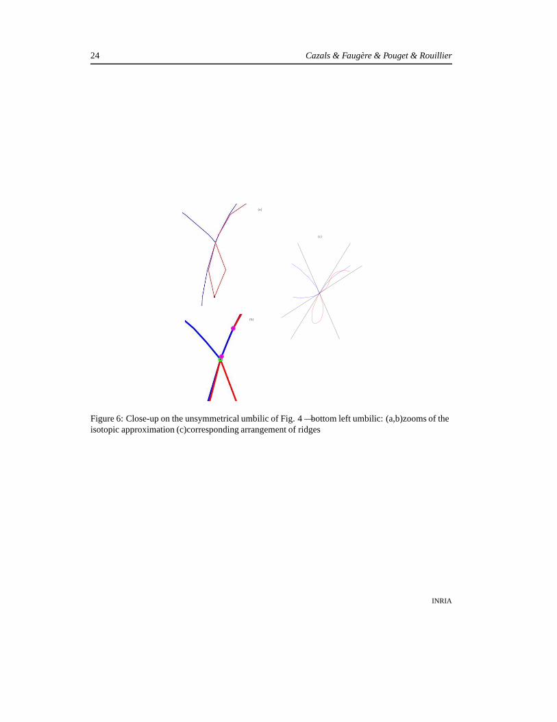
There are 19 critical points (black dots), 17 purple points (pink dots) and 8 umbilics, 3 of whichare 3-ridge (green) and 5 are 1-ridge (yellow). Figure 6 displays on the left two close-ups of thebottom left 3-ridge umbilic, and on the right a more readable sketch. One can recognize an unsym-metric umbilic, that is a 3-ridge umbilic where the three blue branches are followed by the three redones round the umbilic. The other 3-ridge umbilics are symmetric, that is branches alternate colorsround the umbilic.

System # of roots ∈ C # of roots ∈ R # of real roots ∈D

Su 160 16 8Sp 1068 31 17Sc 1432 44 19

Table 1: characteristics of zero dimensional systems

On this example, the discriminant with respect to u has degree 3594 in v and coefficients with upto 3418 digits. CAD based strategies require solving polynomials of degree 43 with coefficients in a

INRIA


field extension defined by an irreducible polynomial of degree 1431 with coefficient of 1071 digits.Up to our knowledge, none of the best existing software or libraries can perform such a computationin a reasonable time.

8.2 Certified plot

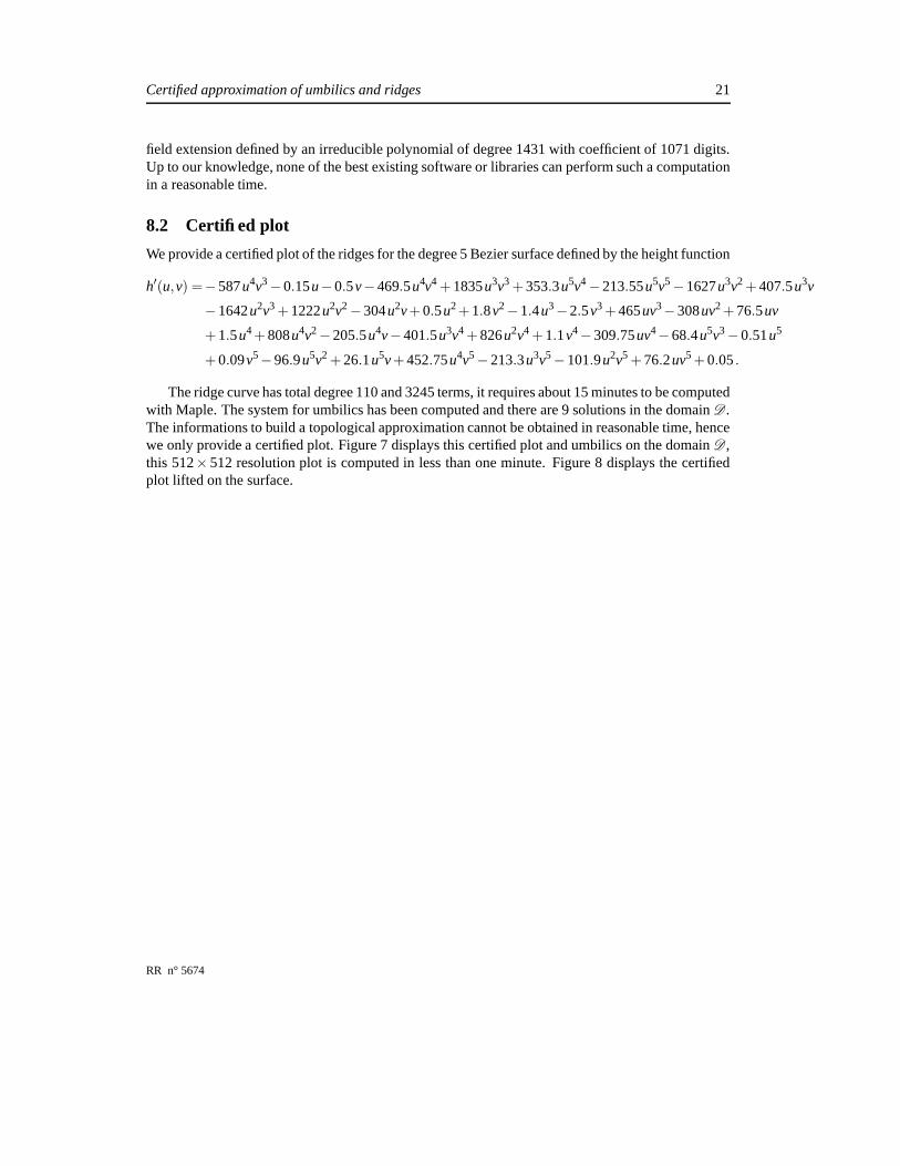
We provide a certified plot of the ridges for the degree 5 Bezier surface defined by the height function

h′(u,v) =−587u4v3−0.15u−0.5v−469.5u4v4 +1835u3v3 +353.3u5v4−213.55u5v5−1627u3v2 +407.5u3v

−1642u2v3 +1222u2v2−304u2v+0.5u2 +1.8v2−1.4u3−2.5v3 +465uv3−308uv2 +76.5uv

+1.5u4 +808u4v2−205.5u4v−401.5u3v4 +826u2v4 +1.1v4−309.75uv4−68.4u5v3−0.51u5

+0.09v5−96.9u5v2 +26.1u5v+452.75u4v5−213.3u3v5−101.9u2v5 +76.2uv5 +0.05 .

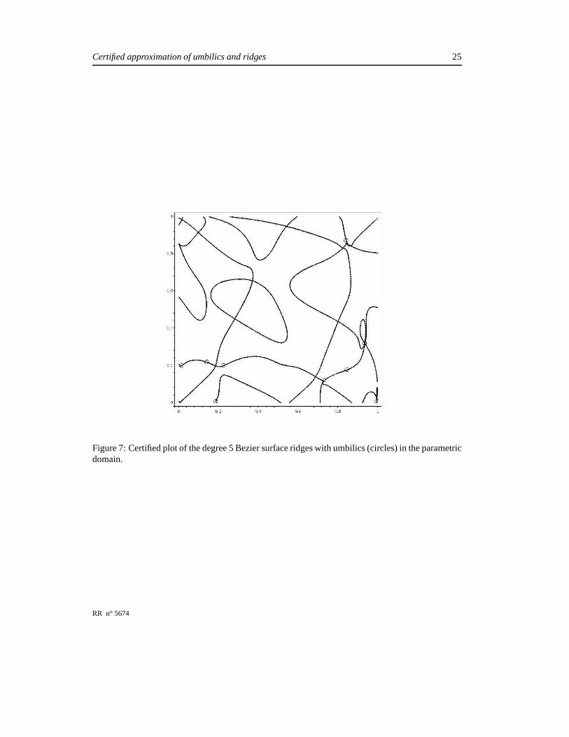
The ridge curve has total degree 110 and 3245 terms, it requires about 15 minutes to be computedwith Maple. The system for umbilics has been computed and there are 9 solutions in the domain D .The informations to build a topological approximation cannot be obtained in reasonable time, hencewe only provide a certified plot. Figure 7 displays this certified plot and umbilics on the domain D ,this 512× 512 resolution plot is computed in less than one minute. Figure 8 displays the certifiedplot lifted on the surface.

RR n° 5674


Figure 4: Isotopic approximation of the ridge curve with 3-ridge umbilics (green), 1-ridge umbilics(yellow), purple points (pink) and critical points (black).

INRIA


Figure 5: Plot of the degree 4 bivariate Bezier surface with ridges and umbilics

9 Conclusion

This paper develops two algorithms to investigate the ridges of parametric algebraic surfaces. Thefirst one reports a topologically certified approximation of the ridges, and is the first one to achievesuch a guarantee. For the practical cases where the resolution of the systems characterizing singularand critical points cannot be performed, the second one computes a certified plot at any fixed res-olution. These algorithms are computationally demanding in terms of algebra. They are in a sensecomplementary to the heuristic ones developed in a companion paper, which are working directlyon a triangulation of the surface, and provide a fast way to report non certified results.

The method developed for the computation of the topology of the ridges can be generalized forother algebraic curves. It gives an alternative to usual algorithms based on the CAD.

Acknowledgments. F. Cazals and M. Pouget acknowledge the support of the AIM@Shape and ACSEuropean projects. Jean-Pierre Merlet is acknowledged for fruitful discussions.

RR n° 5674


(a)

(b)

(c)

Figure 6: Close-up on the unsymmetrical umbilic of Fig. 4 —bottom left umbilic: (a,b)zooms of theisotopic approximation (c)corresponding arrangement of ridges

INRIA


Figure 7: Certified plot of the degree 5 Bezier surface ridges with umbilics (circles) in the parametricdomain.

RR n° 5674


Figure 8: Certified plot of the degree 5 Bezier surface ridges with umbilics lifted on the surface.

INRIA


References

[AS98] Auzinger and Stetter. An elimination algorithm for the computation of all zeros of asystem of multivariate polynomial equations. Int. Series of Numerical Math., 86:11–30,1998.

[BCL82] B. Buchberger, G.-E. Collins, and R. Loos. Computer Algebra Symbolic and AlgebraicComputation. Springer-Verlag, second edition edition, 1982.

[BPR03] S. Basu, R. Pollack, and M.-F. Roy. Algorithms in real algebraic geometry, volume 10of Algorithms and Computations in Mathematics. Springer-Verlag, 2003.

[Buc85] B. Buchberger. Gröbner bases : an algorithmic method in polynomial ideal theory.Recent trends in multidimensional systems theory. Reider ed. Bose, 1985.

[CFPR05] F. Cazals, J.-C. Faugere, M. Pouget, and F. Rouillier. The implicit structure of ridges ofa smooth parametric surface. Technical Report 5608, INRIA, 2005.

[CLO92] D. Cox, J. Little, and D. O’Shea. Ideals, varieties, and algorithms an introduction tocomputational algebraic geometry and commutative algebra. Undergraduate texts inmathematics. Springer-Verlag New York-Berlin-Paris, 1992.

[Col75] G.E. Collins. Quantifier elimination for real closed fields by cylindrical algebraic de-composition. Springer Lecture Notes in Computer Science 33, 33:515–532, 1975.

[CP05] F. Cazals and M. Pouget. Topology driven algorithms for ridge extraction on meshes.Technical Report RR-5526, INRIA, 2005.

[Fau99] J.-C. Faugère. A new efficient algorithm for computing gröbner bases ( f4). Journal ofPure and Applied Algebra, 139(1-3):61–88, June 1999.

[Fau02] Jean-Charles Faugère. A new efficient algorithm for computing gröbner bases withoutreduction to zero f5. In International Symposium on Symbolic and Algebraic Computa-tion Symposium - ISSAC 2002, Villeneuve d’Ascq, France, Jul 2002.

[FGLM93] J.C. Faugère, P. Gianni, D. Lazard, and T. Mora. Efficient computation of zero-dimensional gröbner basis by change of ordering. Journal of Symbolic Computation,16(4):329–344, Oct. 1993.

[GLMT04] G. Gatellier, A. Labrouzy, B. Mourrain, and J.-P. Técourt. Computing the topology of 3-dimensional algebraic curves. In Computational Methods for Algebraic Spline Surfaces,pages 27–44. Springer-Verlag, 2004.

[GLS01] M. Giusti, G. Lecerf, and B. Salvy. A gröbner free alternative for solving polynomialsystems. Journal of Complexity, 17(1):154–211, 2001.

[GVN02] L. Gonzalez-Vega and I. Necula. Efficient topology determination of implicitly definedalgebraic plane curves. Computer Aided Geometric Design, 19(9), 2002.

RR n° 5674


[HCV52] D. Hilbert and S. Cohn-Vossen. Geometry and the Imagination. Chelsea, 1952.

[Koe90] J.J. Koenderink. Solid Shape. MIT, 1990.

[KOR05] J. Keyser, K Ouchi, and M. Rojas. The exact rational univariate representation fordetecting degeneracies. In DIMACS Series in Discrete Mathematics and TheoreticalComputer Science. AMS Press, 2005. To appear.

[Laz83] D. Lazard. Gröbner bases, gaussian elimination, and resolution of systems of algebraicequations. In EUROCAL’ 83 European Computer Algebra Conference, volume 162 ofLNCS, pages 146–156. Springer, 1983.

[Mor90] R. Morris. Symmetry of Curves and the Geometry of Surfaces: two Explorations withthe aid of Computer Graphics. Phd Thesis, 1990.

[Mor96] R. Morris. The sub-parabolic lines of a surface. In Glen Mullineux, editor, Mathematicsof Surfaces VI, IMA new series 58, pages 79–102. Clarendon Press, Oxford, 1996.

[MT05] B. Mourrain and P. Trébuchet. Generalized normal forms and polynomial system solv-ing. In Proceedings of the International Symposium on Symbolic and Algebraic Com-putation, 2005. To appear.

[MWP96] T. Maekawa, F. Wolter, and N. Patrikalakis. Umbilics and lines of curvature for shapeinterrogation. Computer Aided Geometric Design, 13:133–161, 1996.

[Por01] I. Porteous. Geometric Differentiation (2nd Edition). Cambridge University Press,2001.

[Rou99] F. Rouillier. Solving zero-dimensional systems through the rational univariate represen-tation. Journal of Applicable Algebra in Engineering, Communication and Computing,9(5):433–461, 1999.

[RR05] N. Revol and F. Rouillier. Motivations for an arbitrary precision interval arithmetic andthe mpfi library. Reliable Computing, 11:1–16, 2005.

[RZ03] F. Rouillier and P. Zimmermann. Efficient isolation of polynomial real roots. Journalof Computational and Applied Mathematics, 162(1):33–50, 2003.

INRIA


10 Appendix: Algebraic pre-requisites

In this section, we summarize some basic results about Gröbner bases and their applications tosolving zero-dimensional systems (systems with a finite number of complex roots). The reader mayrefer to [CLO92],[BPR03].

Lets denote by Q[X1, . . . ,Xn] the ring of polynomials with rational coefficients and unknownsX1, . . . ,Xn and S = {P1, . . . ,Ps} any subset of Q[X1, . . . ,Xn]. A point x ∈ Cn is a zero of S if Pi(x) =0 ∀i = 1 . . .s. The ideal I = 〈P1, . . . ,Ps〉 generated by P1, . . . ,Ps is the set of polynomials inQ[X1, . . . ,Xn] constituted by all the combinations ∑R

k=1 PkUk with Uk ∈ Q[X1, . . . ,Xn]. Since everyelement of I vanishes at each zero of S, we denote by V(S) = V(I) = {x ∈Cn | p(x) = 0 ∀p ∈ I}(resp. VR(S) = VR(I) = V(I)

⋂

Rn) the set of complex (resp. real) zeroes of S.

10.1 Gröbner bases

A Gröbner basis of I is a computable generator set of I with good algorithmical properties (asdescribed below) and defined with respect to a monomial ordering. In this paper, one will usethe following orderings:

• lexicographic order : (Lex)

Xα11· . . . ·Xαn

n <Lex Xβ11· . . . ·Xβn

n ⇔∃i0 ≤ n ,

{

αi = βi, for i = 1, . . . , i0−1,αi0

< βi0

(1)

• degree reverse lexicographic order (DRL) :

Xα11· . . . ·Xαn

n <DRL Xβ11· . . . ·XβN

n ⇔ X((∑k αk),−αn,...,−α1) <Lex x((∑k βk),−βn,...,−β1) (2)

Lets define the mathematical object “Gröbner”:

Definition. 4 For any n-uple µ = (µ1, . . . ,µn) ∈ Nn, let denote by X µ the monomial X µ11· . . . ·X µn

n .

If < is an admissible (compatible with the multiplication) monomial ordering and P = ∑ri=0 aiX

µ(i)

any polynomial in Q[X1, . . . ,Xn], we define: LM(P,<) = maxi=0...r , < X µ(i)(leading monomial of

P w.r.t. <), LC(P,<) = ai with LM(P,<) = X µ(i)(leading coefficient of P w.r.t. <) and LT(P,<) =

LC(P,<)LM(P,<) (leading term of P wrt <).

Definition. 5 A set of polynomials G is a Gröbner basis of an ideal I wrt to a monomial ordering <if for all f ∈ I there exists g ∈ G such that LM(g,<) divides LM( f ,<).

Given any admissible monomial ordering < one can easily extend the classical Euclidean di-vision to reduce a polynomial p by another one or, more generally, by a set of polynomials F ,performing the reduction wrt to each polynomial of F until getting an expression which can not bereduced anymore. Lets denote such a function by Reduce(p,F,<) (reduction of the polynomial pwrt F). Unlike in the univariate case, the result of such a process is not canonical except if F = G isa Gröbner basis:

RR n° 5674


Theorem. 2 Let G be a Gröbner basis of an ideal I ⊂Q[X1, . . . ,Xn] for a fixed ordering <.

(i) a polynomial p ∈Q[X1, . . . ,Xn] belongs to I if and only if Reduce(p,G,<) = 0,

(ii) Reduce(p,G,<) does not depend on the order of the polynomials in the list G, thus, this is acanonical reduced expression modulo I.

Gröbner bases are computable objects. The most popular method for computing them is Buch-berger’s algorithm ([BCL82, Buc85]). It has several variants and it is implemented in most of gen-eral computer algebra systems like Maple or Mathematica. The computation of Gröbner bases usingBuchberger’s original strategies has to face to two kind of problems :

• (A) arbitrary choices : the order in which are done the computations has a dramatic influenceon the computation time; Precisely, one compute G by increasing the set of initial polyno-

mials, adding so called S-polynomials (spol<(p,q) =COF<(p,q)

LT(p) p− COF<(p,q)LT(q) q,COF<(p,q) =

LCM(LT<(p),LT<(q)) where LCM stands for “least common multiple”) until all the possibleS-polynomials of polynomials of G reduce to 0 modulo G (Reduce(spol<(p,q),G,<) = 0).

• (B) useless computations : the original algorithm spends most of its time in computing 0 (ateach step, most of the new S-polynomials do reduce to zero in a naive algorithm).

For problem (A), J.C. Faugère proposed ([Fau99] - algorithm F4) a new generation of powerful al-gorithms ([Fau99]) based on the intensive use of linear algebra techniques. In short, the arbitrarychoices are left to computational strategies related to classical linear algebra problems (matrix in-versions, linear systems, etc.). For problem (B), J.C. Faugère proposed ([Fau02]) a new criterion fordetecting useless computations

We pay a particular attention to Gröbner bases computed for elimination orderings since theyprovide a way of "simplifying" the system (an equivalent system with a structured shape). Forexample, a lexicographic Gröbner basis of a zero dimensional system (when the number of complexsolutions is finite) has always the following shape (if we suppose that X1 < X2 . . . < Xn):

f (X1) = 0f2(X1,X2) = 0...fk2

(X1,X2) = 0

fk2+1(X1,X2,X3) = 0...fkn−1+1(X1, . . . ,Xn) = 0...fkn

(X1, . . . ,Xn) = 0

.

(when the system is not zero dimensional some of the polynomials may be identically null). A wellknown property is that the zeros of the smallest (w.r.t. <) non null polynomial define the Zariski

INRIA


closure (classical closure in the case of complex coefficients) of the projection on the coordinate’sspace associated with the smallest variables.

More generally, an admissible ordering < on the monomials depending on variables [X1, . . . ,Xn]is an ordering which eliminates Xd+1, . . . ,Xn if Xi < X j ∀i = 1 . . .d, j = d +1 . . .n. The lexicographicordering is a particular elimination ordering.

Definition. 6 Given two monomial orderings <U (w.r.t. the variables U1, . . . ,Ud) and <X (w.r.t. thevariables Xd+1, . . . ,Xn) one can define an ordering which “eliminates“ Xd+1, . . . ,Xn by setting theso called block ordering <U,X as follows : given two monomials m and m′, m <U,X m′ if and only ifm|U1=1,...,Ud=1

<X m′|U1=1,...,Ud=1or (m|U1=1,...,Ud=1

= m′|U1=1,...,Ud=1and m|Xd+1=1,...,Xn=1

<U m′|Xd+1=1,...,Xn=1).

Two important applications of elimination theory are the “projections” and “localizations“. Inthe following, given any subset V of Cd (d is an arbitrary positive integer), V is its Zariski closure,say the smallest subset of Cd containing V which is the zero set of a system of polynomial equations.

Proposition. 1 Let G be a Gröbner basis of an ideal I ⊂ Q[U,X ] w.r.t. any ordering < whicheliminates X. Then G

⋂

Q[U ] is a Gröbner basis of I⋂

Q[U ] w.r.t. to the ordering induced by < onthe variables U; Moreover, if ΠU : Cn −→ Cd denotes the canonical projection on the coordinatesU, V(I∩Q[U ]) = V(G∩Q[U ]) = ΠU(V(I)).

Proposition. 2 Let I ⊂ Q[X ], f ∈ Q[X ] and T be a new indeterminate, then V(I)\V( f ) = V((I +〈T f − 1〉)

⋂

Q[X ]). If G′ ⊂ Q[X ,T ] is a Gröbner basis of I + 〈T f − 1〉 with respect to <X,T then

G′⋂

Q[X ] is a Gröbner basis of I : f ∞ := (I + 〈T f − 1〉)⋂

Q[X ] w.r.t. <X . The variety V(I)\V( f )and the ideal I : f ∞ are usually called the localization of V(I) and I by f .

10.2 Zero-dimensional systems

Zero-dimensional systems are polynomial systems with a finite number of complex solutions. Thisspecific case is fundamental for many engineering applications. The following theorem shows thatwe can detect easily that a system is zero dimensional or not by computing a Gröbner basis for anymonomial ordering :

Theorem. 3 Let G = {g1, . . . ,gl} be a Gröbner basis for any ordering < of any system S = {P1, . . . ,Ps}∈Q[X1, . . . ,Xn]

s. The two following properties are equivalent :

• For all index i = 1 . . .n, there exists a polynomial g j ∈ G and a positive integer n j such that

Xn ji

= LM(g j,<);

• The system {P1 = 0, . . . ,Ps = 0} has a finite number of solutions in Cn.

If S is zero-dimensional, then, according to theorem 3, only a finite number of monomials m ∈Q[X1, . . . ,Xn] are not reducible modulo G, meaning that Reduce(m,G,<)= m. Mathematically, asystem is zero-dimensional if and only if Q[X1, . . . ,Xn]/I is a Q-vector space of finite dimension.This vector space can fully be characterized when knowing a Gröbner basis:

RR n° 5674


Theorem. 4 Let S = {p1, . . . , ps} be a set of polynomials with pi ∈Q[X1, . . . ,Xn] ;∀i = 1 . . . s, andsuppose that G is a Gröbner basis of 〈S〉 with respect to any monomial ordering <. Then :

• Q[X1, . . . ,Xn]/I = {Reduce(p,G,<) , p ∈ Q[X1, . . . ,Xn]} is a vector space of finite dimen-sion;

• B = {t = X e11· · ·Xen

n , (e1, . . . ,en) ∈ Nn| Reduce(t,G,<) = t} = {w1, . . . ,wD} is a basisof Q[X1, . . . ,Xn]/I as a Q-vector space;

• D = ]B is exactly the number of complex zeroes of the system {P = 0, ∀P ∈ S} counted withmultiplicities.

Thus, when a polynomial system is known to be zero-dimensional, one can switch to linearalgebra methods to get informations about its roots. Once a Gröbner basis is known, a basis ofQ[X1, . . . ,Xn]/I can easily be computed (Theorem 4) so that linear algebra methods can be appliedfor doing several computations.

For any polynomial q∈Q[X1, . . . ,Xn] the decomposition q =Reduce(q,G,<)=∑Di=1 aiwi is unique

(theorem 2) and we denote by~q =[a1, . . . ,aD] the representation of q in the basis B. For example, the

matrix w.r.t. B of the linear map mq:

(

Q[X1, . . . ,Xn]/I −→ Q[X1, . . . ,Xn]/I~p 7−→ −→pq

)

can explicitly

be computed (its columns are the vectors −→qwi) and one can then apply the following well-knowntheorem:

Theorem. 5 (Stickelberger) The eigenvalues of mq are exactly the q(α) where α ∈VC(S).

According to Theorem 5, the i-th coordinate of all α ∈ VC(S) can be obtained from mXieigen-

values but the issue of finding all the coordinates of all the α ∈VC(S) from mX1, . . . ,mXn

eigenvaluesis not explicit nor straightforward (see [AS98] for example) and difficult to certify.

10.3 The Rational Univariate Representation

The Rational Univariate Representation [Rou99] is, with the end-user point of view, the simplest wayfor representing symbolically the roots of a zero-dimensional system without loosing information(multiplicities or real roots) since one can get all the information on the roots of the system bysolving univariate polynomials.

Given a zero-dimensional system I =< p1, . . . , ps > where the pi ∈Q[X1, . . . ,Xn], a Rational Uni-

variate Representation of V(I) has the following shape : ft (T ) = 0,X1 =gt,X1

(T )

gt,1(T ) , . . . ,Xn =gt,Xn

(T)

gt,1(T ) ,

where ft ,gt,1,gt,X1, . . . ,gt,Xn

∈Q[T ] (T is a new variable). It is uniquely defined w.r.t. a given poly-

nomial t which separates V (I) (injective on V (I)), the polynomial ft being necessarily the character-istic polynomial of mt (see above section) in Q[X1, . . . ,Xn]/I [Rou99]. The RUR defines a bijectionbetween the roots of I and those of ft preserving the multiplicities and the real roots :

INRIA


V(I)(∩R) ≈ V( ft )(∩R)α = (α1, . . . ,αn) → t(α)

(gt,X1

(t(α))

gt,1(t(α)), . . . ,

gt,Xn(t(α))

gt,1(t(α))) ← t(α)

For computing a RUR one has to solve two problems :

• finding a separating element t;

• given any polynomial t, compute a RUR-Candidate ft ,gt,1,gt,X1, . . . ,gt,Xn

such that if t is aseparating polynomial, then the RUR-Candidate is a RUR.

According to [Rou99], a RUR-Candidate can explicitly be computed when knowing a suitable rep-resentation of Q[X1, . . . ,Xn]/I :

• ft = ∑Di=0 aiT

i is the characteristic polynomial of mt . Lets denote by ft its square-free part.

• for any v∈Q[X1, . . . ,Xn], gt,v = gt,v(T ) = ∑d−1i=0 Tr ace(m

vti )Hd−i−1(T ), d = deg( ft) and H j(T ) = ∑ ji=0

aiTi− j

In [Rou99], a strategy is proposed for computing a RUR for any system (a RUR-Candidate and aseparating element), but there are special cases where it can be computed differently. When X1 isseparating V(I) and when I is a radical ideal, the system is said to be in shape position. In suchcases, the shape of the lexicographic Gröbner basis is always the following :

f (X1) = 0X2 = f2(X1)...Xn = fn(X1)

. (3)

As shown in [Rou99], if the system is in shape position, gX1,1 = f ′X1and we have fX1

= f and

fi(X1) = gX1,Xi(X1)/gX1,1

(X1)mod f . Thus the RUR associated with X1 and the lexicographic Gröb-

ner basis are equivalent up to the inversion of gX1,1 = f ′X1modulo fX1

. In the rest of the paper we callthis object a RR-Form of the corresponding lexicographic Gröbner basis. The RUR is well knownto be much smaller than the lexicographic Gröbner basis in general (this may be explained by theinversion of the denominator) and thus will be our priviligied object. Note that it is easy to checkthat a system is in shape position once knowing a RUR-Candidate (and so to check that X1 separatesV(I)): it is necessary and sufficient that fX1

is square-free.We thus can multiply the strategies for computing a symbolic solution : one can compute the

RR-Form Gröbner directly using [Fau99] or [Fau02] for example or by change of ordering like in[FGLM93] or a RUR using the algorithm from [Rou99]. Choosing the right strategy will be part ofour experimental section.

RR n° 5674


10.4 From formal to numerical solutions

Computing a RUR reduces the resolution of a zero-dimensional system to solving one polynomial

in one variable ( ft ) and to evaluating n rational fractions (gt,Xi

(T )

gt,1(T ) , i = 1 . . .n) at its roots (note that if

one simply want to compute the number of real roots of the system there is no need to consider therational coordinates). The next task is thus to compute all the real roots of the system (and only thereal roots), providing a numerical approximation with an arbitrary precision (set by the user) of thecoordinates.

The isolation of the real roots of ft can be done using the algorithm proposed in [RZ03] : theoutput will be a list l ft

of intervals with rational bounds such that for each real root α of ft , thereexists a unique interval in l ft

which contains α . The second step consists in refining each intervalin order to ensure that it does not contain any real root of gt,1. Since ft and gt,1 are co-primethis computation is easy and we then can ensure that the rational functions can be evaluated usinginterval arithmetics without any cancellation of the denominator. This last evaluation is performedusing multi-precision arithmetics (MPFI package - [RR05]). As we will see in the experiments, theprecision needed for the computations is poor and, moreover, the rational functions defined by theRUR are stable under numerical evaluation, even if their coefficients are huge (rational numbers),and thus this part of the computation is still efficient. For increasing the precision of the result, it isonly necessary to decrease the length of the intervals in l ft

which can easily be done by bisection orusing a certified Newton’s algorithm. Note that it is quite simple to certify the sign of the coordinates: one simply have to compute some gcds and split, when necessary the RUR.

10.5 Signs of polynomials at the roots of a system

Computing the sign of given multivariate polynomials {q1, . . . ,ql} at the real roots of a zero-dimensionalsystem may be important for many applications and this problem is not solved by the above method.Instead of "plugging" straightforwardly the formal coordinates provided by the RUR into the qi,we better extend the RUR by computing rational functions which coincide with the qi at the rootsof I. This can theoretically simply be done by using the general formula from [Rou99] : ht, j =

∑D−1i=0 Trace(m

q jti)HD−i−1(T ). One can directly compute the Trace(m

q jti) reusing the computations

already done if the (classical) RUR (without additional constraints) has already been computed andshow that as soon as l is small (at least smaller than the number of variables), it is not more costly tocompute the extended RUR than the classical one.

INRIA


Contents

1 Introduction 31.1 Ridges as curves on smooth surfaces . . . . . . . . . . . . . . . . . . . . . . . . . . 31.2 Previous work . . . . . . . . . . . . . . . . . . . . . . . . . . . . . . . . . . . . . . 31.3 Contributions . . . . . . . . . . . . . . . . . . . . . . . . . . . . . . . . . . . . . . 41.4 paper overview . . . . . . . . . . . . . . . . . . . . . . . . . . . . . . . . . . . . . 4

2 Notations 4

3 The implicit structure of ridges, and study points 53.1 Implicit structure of the ridge curve . . . . . . . . . . . . . . . . . . . . . . . . . . 53.2 Study points and zero dimensional systems . . . . . . . . . . . . . . . . . . . . . . 6

4 Some Algebraic tools for our method 64.1 Zero dimensional systems . . . . . . . . . . . . . . . . . . . . . . . . . . . . . . . . 74.2 Univariate root isolation . . . . . . . . . . . . . . . . . . . . . . . . . . . . . . . . 74.3 About square-free polynomials . . . . . . . . . . . . . . . . . . . . . . . . . . . . . 8

5 On the difficulty of approximating algebraic curves 9

6 Certified topological approximation 126.1 Output specification . . . . . . . . . . . . . . . . . . . . . . . . . . . . . . . . . . . 126.2 Method outline . . . . . . . . . . . . . . . . . . . . . . . . . . . . . . . . . . . . . 12

6.2.1 The algorithm . . . . . . . . . . . . . . . . . . . . . . . . . . . . . . . . . . 126.2.2 Key points wrt CAD based algorithms . . . . . . . . . . . . . . . . . . . . . 13

6.3 Step 1. Isolating study points . . . . . . . . . . . . . . . . . . . . . . . . . . . . . . 146.4 Step 2. Regularization of the study boxes . . . . . . . . . . . . . . . . . . . . . . . 166.5 Step 3. Computing regular points in study fibers . . . . . . . . . . . . . . . . . . . . 176.6 Step 4. Adding intermediate rational fibers . . . . . . . . . . . . . . . . . . . . . . . 176.7 Step 5. Performing connections . . . . . . . . . . . . . . . . . . . . . . . . . . . . . 17

7 Certified plot 18

8 Illustrations 198.1 Certified topology . . . . . . . . . . . . . . . . . . . . . . . . . . . . . . . . . . . . 198.2 Certified plot . . . . . . . . . . . . . . . . . . . . . . . . . . . . . . . . . . . . . . 21

9 Conclusion 23

10 Appendix: Algebraic pre-requisites 2910.1 Gröbner bases . . . . . . . . . . . . . . . . . . . . . . . . . . . . . . . . . . . . . . 2910.2 Zero-dimensional systems . . . . . . . . . . . . . . . . . . . . . . . . . . . . . . . 3110.3 The Rational Univariate Representation . . . . . . . . . . . . . . . . . . . . . . . . 32

RR n° 5674


10.4 From formal to numerical solutions . . . . . . . . . . . . . . . . . . . . . . . . . . 3410.5 Signs of polynomials at the roots of a system . . . . . . . . . . . . . . . . . . . . . 34

INRIA

Unité de recherche INRIA Sophia Antipolis2004, route des Lucioles - BP 93 - 06902 Sophia Antipolis Cedex (France)

Unité de recherche INRIA Futurs : Parc Club Orsay Université - ZAC des Vignes4, rue Jacques Monod - 91893 ORSAY Cedex (France)

Unité de recherche INRIA Lorraine : LORIA, Technopôle de Nancy-Brabois - Campus scientifique615, rue du Jardin Botanique - BP 101 - 54602 Villers-lès-Nancy Cedex (France)

Unité de recherche INRIA Rennes : IRISA, Campus universitaire de Beaulieu - 35042 Rennes Cedex (France)Unité de recherche INRIA Rhône-Alpes : 655, avenue de l’Europe - 38334 Montbonnot Saint-Ismier (France)

Unité de recherche INRIA Rocquencourt : Domaine de Voluceau - Rocquencourt - BP 105 - 78153 Le Chesnay Cedex (France)

ÉditeurINRIA - Domaine de Voluceau - Rocquencourt, BP 105 - 78153 Le Chesnay Cedex (France)

http://www.inria.frISSN 0249-6399

Topologically certified approximation of umbilics and ridges on polynomial parametric surface

Documents

Transcript of Topologically certified approximation of umbilics and ridges on polynomial parametric surface