Time, Rate and Conditioning - Rutgers Center for Cognitive ...
108
In press, Psychological Review Time, Rate and Conditioning C. R. Gallistel and John Gibbon University of California, Los Angeles and New York State Psychiatric Institute Abstract We draw together and develop previous timing models for a broad range of conditioning phenomena to reveal their common conceptual foundations: First, conditioning depends on the learning of the temporal intervals between events and the reciprocals of these intervals, the rates of event occurrence. Second, remembered intervals and rates translate into observed behavior through decision processes whose structure is adapted to noise in the decision variables. The noise and the uncertainties consequent upon it have both subjective and objective origins. A third feature of these models is their time-scale invariance, which we argue is a deeply important property evident in the available experimental data. This conceptual framework is similar to the psychophysical conceptual framework in which contemporary models of sensory processing are rooted. We contrast it with the associative conceptual framework. Pavlov recognized that the timing of the conditioned response or CR (e.g., salivation) in a well conditioned subject depended on the reinforcement delay, or latency. The longer the interval between the onset of the conditioned stimulus or CS (e.g. , the ringing of a bell) and the delivery of the unconditioned stimulus or US (meat powder), the longer the latency between CS onset and the onset of salivation. An obvious explanation is that the dogs in Pavlov’s experiment learned the reinforcement latency and did not begin to salivate until they judged that the delivery of food was more or less imminent. This is not the kind of explanation that Pavlov favored, because it lacks a clear basis in reflex physiology. Similarly, Skinner observed that the timing of operant responses was governed by the intervals in the schedule of reinforcement. When his pigeons pecked keys to obtain reinforcement on fixed interval (FI) schedules, the longer the fixed interval imposed between the obtaining of one reinforcement and the availability of the next, the longer the pigeon waited after each reinforcement before beginning to peck the key to obtain the next reinforcement. An obvious explanation is that his pigeons learned the duration of the interval between a delivered reinforcement and the next arming of the key and did not begin to peck until they judged that the opportunity to obtain another reinforcement was more or less imminent. Again, this is not the sort of explanation that Skinner favored, though for reasons other than Pavlov’s. In this paper we take the interval-learning assumption as the point of departure in the analysis of conditioned behavior. We assume that the subjects in conditioning experiments
-
Upload
khangminh22 -
Category
Documents
-
view
0 -
download
0
Transcript of Time, Rate and Conditioning - Rutgers Center for Cognitive ...

In press, Psychological Review
Time, Rate and Conditioning
C. R. Gallistel and John Gibbon
University of California, Los Angeles
and New York State Psychiatric Institute
AbstractWe draw together and develop previous timing models for a broad range ofconditioning phenomena to reveal their common conceptual foundations: First,conditioning depends on the learning of the temporal intervals between events andthe reciprocals of these intervals, the rates of event occurrence. Second, rememberedintervals and rates translate into observed behavior through decision processeswhose structure is adapted to noise in the decision variables. The noise and theuncertainties consequent upon it have both subjective and objective origins. A thirdfeature of these models is their time-scale invariance, which we argue is a deeplyimportant property evident in the available experimental data. This conceptualframework is similar to the psychophysical conceptual framework in whichcontemporary models of sensory processing are rooted. We contrast it with theassociative conceptual framework.
Pavlov recognized that the timing of theconditioned response or CR (e.g., salivation)in a well conditioned subject depended on thereinforcement delay, or latency. The longerthe interval between the onset of theconditioned stimulus or CS (e.g. , the ringingof a bell) and the delivery of theunconditioned stimulus or US (meat powder),the longer the latency between CS onset andthe onset of salivation. An obviousexplanation is that the dogs in Pavlov’sexperiment learned the reinforcement latencyand did not begin to salivate until they judgedthat the delivery of food was more or lessimminent. This is not the kind of explanationthat Pavlov favored, because it lacks a clearbasis in reflex physiology. Similarly, Skinnerobserved that the timing of operant responseswas governed by the intervals in the scheduleof reinforcement. When his
pigeons pecked keys to obtain reinforcementon fixed interval (FI) schedules, the longer thefixed interval imposed between the obtainingof one reinforcement and the availability ofthe next, the longer the pigeon waited aftereach reinforcement before beginning to peckthe key to obtain the next reinforcement. Anobvious explanation is that his pigeonslearned the duration of the interval between adelivered reinforcement and the next armingof the key and did not begin to peck untilthey judged that the opportunity to obtainanother reinforcement was more or lessimminent. Again, this is not the sort ofexplanation that Skinner favored, though forreasons other than Pavlov’s.
In this paper we take the interval-learningassumption as the point of departure in theanalysis of conditioned behavior. We assumethat the subjects in conditioning experiments

Gallistel and Gibbon 2
do in fact store in memory the durations ofinterevent intervals and subsequently recallthose remembered durations for use in thedecisions that determine their conditionedbehavior. An extensive experimental literatureon timed behavior has developed in the lastfew decades (for reviews, see Fantino,Preston & Dunn, 1993; Gallistel, 1989;Gibbon & Allan, 1984; Gibbon, Malapani,Dale & Gallistel, 1997; Killeen & Fetterman,1988; Miller & Barnet, 1993; Staddon &Higa, 1993). In consequence, it is now widelyaccepted that the subjects in conditioningexperiments do in some sense learn theintervals in the experimental protocols. Butthose aspects of conditioned behavior thatseem to depend on knowledge of thetemporal intervals are often seen asadjunctive to the process of associationformation (e.g., Miller & Barnet, 1993),which is commonly taken to be the coreprocess mediating conditioned behavior. Wewill argue that it is the learning of temporalintervals and their reciprocals (event rates)that is the core process in both Pavlovian andinstrumental conditioning.
It is our sense that most contemporaryassociative theorists no longer assume thatthe association-forming process itself isfundamentally different in Pavlovian andinstrumental conditioning. Until thediscovery of autoshaping (Brown & Jenkins,1968), a now widely used Pavlovianprocedure for teaching what used to beregarded as instrumental responses (pecking akey or pressing a lever for food), it wasassumed that there were two fundamentallydifferent association-forming processes. One,which operated in Pavlovian conditioning,required only the temporal contiguity of aconditioned and unconditioned stimulus. Theother, which operated in instrumentalconditioning, required that a reinforcer stampin the latent association between a stimulusand a response. In this older conception of
the association-froming process ininstrumental conditioning, the reinforcer wasnot itself part of the associative structure, itmerely stamped in the S-R association.Recently, however, it has been shown thatPavlovian response-outcome (R-O) oroutcome-response (O-R) associations areimportant in instrumental conditioning(Adams & Dickinson, 1981; Colwill &Rescorla, 1986; Colwill & Delamater, 1995;Mackintosh & Dickinson, 1979; Rescorla,1991). Our reading of the most recent trendsin associative theorizing is that, for these andother reasons (e.g., Williams, 1982), the twokinds of conditioning paradigms are no longerthought to tap fundamentally differentassociation-forming processes. Rather, theyare thought to give rise to differentassociative structures via a single association-forming process.
In any event, the underlying learningprocesses in the two kinds of paradigms arenot fundamentally different from theperspective of timing theory. The paradigmsdiffer only in the kinds of events that markthe start of relevant temporal intervals oralter the expected intervals betweenreinforcements. In Pavlovian paradigms, theanimal’s behavior has no effect on thedelivery of reinforcement. The conditionedbehavior is determined by the rate and timingof reinforcement when a CS is presentrelative to the rate and timing of reinforce-ment when that CS is not present. Ininstrumental paradigms, the animal’s behavioralters the rate and timing of reinforcement.Reinforcements occur at a higher rate whenthe animal pecks the key (or presses thelever, etc.) than when it does not. And thetime of delivery of the next reinforcementmay depend on the interval since a response-elicited event such as the previousreinforcement. In both cases, the essentialunderlying process from a timing perspectiveis the learning of the contingency between the

Gallistel and Gibbon 3
rate of reinforcement (or expected intervalbetween reinforcements) and some state ofaffairs (bell ringing vs. bell not ringing or keybeing pecked vs. key not being pecked, orrapid key pecking versus slow key pecking).Thus, we will not treat these conditioningparadigms separately. We will move back andforth between them.
We develop our argument around modelsthat we have ourselves elaborated, becausewe are more intimately familiar with them.We emphasize, however, that there areseveral other timing models (e.g., Church &Broadbent, 1990; Fantino et al., 1993;Grossberg & Schmajuk, 1991; Killeen &Fetterman, 1988; Miller & Barnet, 1993;Staddon & Higa, 1993). We do not imagineour own models to be the last word. In fact,we will call attention at several points todifficulties and lacunae in these models. Ourgoal is to make clear essential features of aconceptual framework that differs quitefundamentally from the framework in whichconditioning is most commonly analyzed. Weexpect that as this framework becomes morewidely used, the models rooted in it willbecome more sophisticated, more complete,and of ever broader scope.
We also use the framework to callattention to quantitative features ofconditioning data that we believe have farreaching theoretical implications, mostnotably the many manifestations of time-scale invariance. A conditioning result is timescale invariant if the graph of the result looksthe same when the experiment is repeated at adifferent time scale, by changing all thetemporal intervals in the protocol by acommon scaling factor, and the scaling factorson the data graphs are adjusted so as to offsetthe change in time scale. Somewhat moretechnically, conditioning data are time scaleinvariant if the normalized data plots aresuperimposable. Normalization takes out the
time scale. Superimposability means that thenormalized curves (or, in the limit, individualpoints) fall on top of each other. We giveseveral examples in what follows, beginningwith Figures 1A and 2. An extremelyimportant empirical consequence of the newconceptual framework is that it stimulatesresearch to test the limits of fundamentallyimportant principles like this.
CR Timing
The learning of temporal intervals in thecourse of conditioning is most directlyevident in the timing of the conditionedresponse in protocols where reinforcementoccurs at some fixed delay after a markingevent. In what follows, this delay is called thereinforcement latency, T.
Some well established facts of CR timingare:
•The CR is maximally likely at thereinforcement latency. When there is afixed latency between a marking eventsuch as placement in the experimentalchamber, the delivery of a previousreinforcement, the sounding of a tone, theextension of a lever, or the illumination ofa response key, the probability that awell trained subject will make aconditioned response increases as thetime of reinforcement approaches,reaching a maximum at the reinforcementlatency (Figures 1 and 2).
•The distribution of CR onsets and offsets isscalar: There is a constant coefficient ofvariation in the distribution of responseprobability around the latency of peakprobability, that is, the standard deviationof the distribution is proportionate to itsmode. Thus, the temporal distribution ofconditioned response initiations (andterminations) is time scale invariant:

Gallistel and Gibbon 4
scaling time in units proportional to modeof the distribution renders thedistributions obtained at differentreinforcement latencies superimposable(see Figure 1A & Figure 2).
Scalar Expectancy Theory
Scalar Expectancy Theory was developed toaccount for the above aspects of theconditioned response (Gibbon, 1977). It is amodel of what we will call the when decision,the decision that determines when the CRoccurs in relation to a time mark such as CSonset or offset or the delivery of a previousreinforcement. The basic assumptions ofScalar Expectancy Theory and thecomponents out of which the model isconstructed--a timing mechanism, a memorymechanism, sources of variability or noise inthe decision variables, and a comparisonmechanism adapted to that noise (see Figure3)-- appear in our explanation of all otheraspects of conditioned behavior. The timingmechanism generates a signal, ˆ t e , which isproportional at every moment to the elapsedduration of the animal’s current exposure to aCS. This quantity in the head is the animal’smeasure of the duration of an elapsinginterval. The timer is reset to zero by theoccurrence of a reinforcement, which marksthe end of the interval that began with theonset of the CS. The magnitude of ˆ t e at the
time of reinforcement, ˆ t T is written tomemory through a multiplicative translationvariable, k*, whose expected value {E(k*)=K*} is close to but not identically one.Thus, the reinforcement interval recorded inmemory, ˆ t * = k * ˆ t T on average, deviatesfrom the timed value by some (generallysmall) percentage, which is determined by theextent to which the expected value of K*
deviates from 1. (See Table 1 for a list of thesymbols and expressions used, together withtheir meanings.)
Figure 1. A. Normalized rate of respondingas a function of the normalized elapsedinterval, for pigeons responding on fixedinterval schedules, with inter-reinforcementintervals, T, ranging from 30 to 3,000 s.R (t) is the average rate of responding atelapsed interval t since the last reinforcement.R (T) is the average terminal rate ofresponding . (Data from Dews, 1970). Plotfrom Gibbon, 1977, used by permission ofthe publisher.) B. The time course of theconditioned double blink on a singlerepresentative trial in an experiment in whichrabbits were trained with two different USlatencies (400 & 900 ms). (Data from Kehoe,Graham-Clarke & Schreurs, 1989) C.Percent freezing as a function of the intervalsince placement in the experimental chamberafter a single conditioning trial in which ratswere shocked 3 minutes after being placed inthe chamber. (Data from Fanselow& Stote,1995 Used with authors’ permission.)

Gallistel and Gibbon 5
Figure 2. Scalar property: Time scale invariance in the distribution of CRs. A. Responding ofthree birds on the peak procedure in blocked sessions at reinforcements latencies of 30 s and 50 s(unreinforced CS durations of 90 s and 150 s, respectively). Vertical bars at the reinforcementlatencies have heights equal to the peaks of the corresponding distributions. B. The samefunctions normalized with respect to CS time and peak rate (so that vertical bars wouldsuperpose). Note that although the distributions differ between birds, both in their shape and inwhether they peak before or after the reinforcement latency (K* error), they superpose whennormalized (rescaled). {Unpublished data from Gibbon}

Gallistel and Gibbon 6
Table 1: Symbols and Expressions in SET
Symbol orExpression
Meaning
ˆ t e time elapsed since CS onset, the subjective measure of an elapsinginterval
ˆ t T magnitude of ˆ t e at time of reinforcement, the experienced durationof the CS-US interval
ˆ t * remembered duration of CS-US interval
k* scaling factor relating ˆ t * to ˆ t T : ˆ t * = k * ˆ t T
K* expected value of k*; close to but not equal to 1; fact that valuenot equal to 1 explains systematic discrepancy between averageexperienced duration and average remembered duration, the K*error
ˆ t e ˆ t * the decision variable for the when decision, the measure of howsimilar the currently elapsed interval is to the rememberedreinforcement latency
β a decision threshold
T generally, a fixed reinforcement latency. In Pavlovian delayconditioning, the CS-US interval. In a fixed interval operantschedule, the interval between reinforcements
ˆ λ csrate of reinforcement attributed to a CS, the reciprocal of theexpected interval between reinforcements
Note: In this and subsequent symbol tables, a hat on a variable indicates that it is asubjective estimate, a quantity in the head representing a physically measurable externalvariable. Variables without hats are either measurable quantities outside the head, orscaling constants (always symbolized by k’s), or decision thresholds (alwayssymbolized by β).
When the CS reappears (when a new trialbegins), ˆ t e the subjective duration of thecurrently elapsing interval of CS exposure, iscompared to ˆ t * , which is derived bysampling (reading) the remembered reinforce-ment delay in memory. The comparison takes
the form of a ratio, ˆ t e ˆ t * which we call thedecision variable. When this ratio exceeds athreshold, β somewhat less than 1, the animalresponds to the CS--provided it has hadsufficient experience with the CS to havealready decided that it is a reliable predictorof the US (see later section on the acquisition

Gallistel and Gibbon 7
or whether decision)1. The when decisionthreshold is somewhat less than 1, becausethe CR anticipates the US. If, on a given trial,reinforcement does not occur (for example, inthe peak procedure, see below), then theconditioned response ceases when this samedecision ratio exceeds a second thresholdsomewhat greater than 1. (The decision tostop responding when the reinforcementinterval is past, is not diagrammed in Figure3, but see Gibbon & Church, 1990).) In short,the animal begins to respond when itestimates the currently elapsing interval to beclose to the remembered delay ofreinforcement. If it does not get reinforced, itstops responding when it estimates thecurrently elapsing interval to be sufficientlypast the remembered delay. The decisionthresholds constitute its criteria for “close”and “past.” Its measure of closeness (orsimilarity) is the ratio between the currentlyelapsing and the remembered interval.
The interval timer in SET may beconceived as a clock system (pulse generator)feeding an accumulator (working memory),
1 The decision variable is formally a ratio ofrandom variables and is demonstrably non-normal in most cases. However, the decisionrule, te/t* > β is equivalent to te > βt* and the
right hand side of this inequality isapproximately normal when t* is normal. Whenthe threshold, β is itself variable, some non-normalilty is induced in the right hand side ofthe decision rule, introducing some positive skewin this composite variable. Gibbon and hiscollaborators (Gibbon, 1992; Gibbon, 1981b;Gibbon, Church & Meck, 1984) have discussedthe degree of non-normality in this variate inconsiderable detail. It is shown that a) themean and variance of the decision variate arereadily obtained in closed form, and b) thedegree of skew in the composite variable is notlarge relative to other variance in the system.The behavioral performance often also shows aslight positive skew consistent with the formalanalysis.
which continually integrates activity overtime. The essential feature of such amechanism is that the quantity in theaccumulator grows as a linear function oftime. By contrast, the reference memorysystem statically preserves the values of pastintervals. When accumulation is temporarilyhalted, for example in paradigms whenreinforcement is not delivered and the signalis briefly turned off and back on again after ashort period (a gap), the value in theaccumulator simply holds through the gap(working memory), and the integratorresumes accumulating when the signal comesback on.
Scalar variability, evident in the constantcoefficient of variation in the distribution ofthe onsets, offsets and peaks of conditionedresponding, is a consequence of twofundamental assumptions. The first is thatthe comparison mechanism uses the ratio ofthe two values being compared, rather than,for example, their difference. The second isthat subjective estimates of temporaldurations, like subjective estimates of manyother continuous variables (length, weight,loudness, etc.), obey Weber’s law: thedifference required to discriminate onesubjective magnitude from another with agiven degree of reliability is a fixed fraction ofthat magnitude(Gibbon, 1977; Killeen &Weiss, 1987). What this most likely implies--and what Scalar Expectancy Theory assumes--is that the uncertainty about the true valueof a remembered magnitude is proportional tothe magnitude. These two assumptions --thedecision variable is a ratio and estimates ofduration read from memory have scalarvariability--are both necessary to explainscale invariance in the distribution ofconditioned responses (Church & Gibbon,1982; Gibbon & Fairhurst, 1994).

Gallistel and Gibbon 8
Figure 3. Flow diagram for the CR timing or when decision. Two trials are shown, the firstreinforced, at T, (filled circle on time line) and the second still elapsing at e. When the first trial isreinforced, the cumulated subjective time, ˆ t T , is stored in working memory and transferred toreference memory via a multiplicative variable, k* ( ˆ t * = k * ˆ t T ). The decision to respond is basedon the ratio of the elapsing interval (in working memory) to the remembered interval (in referencememory). It occurs when this ratio exceeds a threshold (β) close to, but generally less than 1. Note
that the reciprocal of ˆ t T is equal to ˆ λ cs , the estimated rate of CS reinforcement, which plays acrucial role in the acquisition and extinction decisions described later.
It has recently become clear that much ofthe observed trial-to-trial variability in
response timing is due to the variabilityinherent in the signals derived from reading

Gallistel and Gibbon 9
durations stored in long-term memory, ratherthan from variability in the timing processthat generates inputs to memory . Even whenthere is only one such comparison duration inmemory, a comparison signal ˆ t * , derivedfrom reading that one memory variessubstantially from trial to trial. In someparadigms, the standard interval read frommemory for comparison to a currentlyelapsing interval may be based either on asingle standard (a single standard experiencedrepeatedly) or a double standard (twodifferent values experienced in randomintermixture). In the 2-standard condition, thecomparison value (expectation) recalled frommemory is equal to the harmonic mean of thetwo standards. The trial-to-trial variability intiming performance observed in this 2-standard condition is the same as in a 1-standard condition with a standard equal tothe harmonic mean of the standards in the 2-standard condition. The variability in theinput to memory is very different in the twoconditions, but the output variability is thesame. This implies that the trial-to-trialvariability in the response latencies is largelydue to noise in the memory reading operationrather than variability in the values read intomemory. (See Gallistel, in press for a fullerdiscussion of the evidence for thisconclusion.)
The Timing of Appetitive CRs
The FI Scallop
An early application of Scalar ExpectancyTheory was to the explanation of the "FIscallop” in operant conditioning. An FIschedule of reinforcement deliversreinforcement for the first response madeafter a fixed interval has elapsed since thedelivery of the last reinforcement. Whenresponding on such a schedule, animals pauseafter each reinforcement, then resumeresponding after some interval has elapsed. It
was generally supposed that the animal’s rateof responding accelerated throughout theremainder of the interval leading up toreinforcement. In fact, however, conditionedresponding in this paradigm, as in manyothers, is a two-state variable (slow, sporadicpecking versus rapid, steady pecking), withone transition per inter-reinforcement interval(Schneider, 1969). The average latency to theonset of the high-rate state during the post-reinforcement interval increases in proportionto the scheduled reinforcement interval over avery wide range of intervals (from 30s to atleast 50 min). The variability in this onsetfrom one interval to the next also increases inproportion to the scheduled interval. As aresult, averaging over many inter-reinforcement intervals results in the smoothincrease in the average rate of responding thatDews (1970) termed “proportional timing”(Figure 1A). The smooth, almost linearincrease in the average rate of responding seenin Figure 1A is the result of averaging acrossmany different abrupt onsets. It could moreappropriately be read as showing theprobability that the subject will have enteredthe high-rate state as a function of the timeelapsed since the last reinforcement.
The Peak Procedure
The fixed interval procedure only allows oneto see the subject’s anticipation ofreinforcement. The peak procedure (Catania,1970; Roberts, 1981) is a discrete-trialsmodification that enables one also to observethe cessation of responding when theexpected time of reinforcement has passedwithout reinforcement. The beginning of eachtrial is marked by the illumination of the key(with pigeon subjects) or the extension of thelever (with rat subjects). A response (keypeck or lever press) is reinforced only after afixed interval has elapsed. However, a partialreinforcement schedule is used. On sometrials, there is no reinforcement. On these

Gallistel and Gibbon 10
trials (Peak trials), the CS continues for threeor four times the reinforcement latency,allowing the experimenter to observe thecessation of the CR when the expected timeof reinforcement has passed. This procedureyielded the data in Figure 2, which come fromthe unreinforced trials.
The smoothness of the curves in Figure 2is again an averaging artifact. On any one trial,there is an abrupt onset and an abrupt offsetof steady responding (Church, Meck &Gibbon, 1994; Church, Miller, Meck &Gibbon, 1991; Gibbon & Church, 1992). Themidpoint of the interval during which theanimal responds (the CR interval) isproportionate to reinforcement latency, andso is the average duration of this CR interval.However, there is considerable trial-to-trialvariation in the onset and the offset ofresponding. The curves in Figure 2 are aconsequence of averaging across theindependently variable onsets and offsets ofresponding (Church et al., 1994). As in Figure1A, these curves are more appropriately readas giving the probability that the animal willbe responding at a high rate at any givenfraction of the reinforcement latency.
The Timing of Aversive CRs
Avoidance Responses
The conditioned fear that is manifest infreezing behavior and other indices of aconditioned emotional response is classicallyconditioned in the operational sense that thereinforcement is not contingent on theanimal’s response. Avoidance responses, bycontrast, are instrumentally conditioned inthe operational sense, because theirappearance depends on the contingency thatthe performance of the conditioned responseforestalls the aversive reinforcement. Byresponding, the subject avoids the aversivestimulus. We stress the purely operational, as
opposed to the theoretical, distinctionbetween classical and instrumentalconditioning, because, from the perspectiveof timing theory, the only difference betweenthe two paradigms is in the events that markthe beginnings of expected and elapsingintervals. In the instrumental case, theexpected interval to the next shock is longestimmediately after a response, and therecurrence of a response resets the shockclock. Thus, the animal’s response marks theonset of the relevant interval.
The timing of instrumentally conditionedavoidance responses is as dependent on theexpected time of aversive reinforcement asthe timing of classically conditionedemotional reactions, and it shows the samescale invariance in the mean, and scalarvariability around it (Gibbon, 1971, 1972). Inshuttle box avoidance paradigms, where theanimal gets shocked at either end of the box ifit stays too long, the mean latency at whichthe animal makes the avoidance responseincreases in proportion to the latency of theshock that is thereby avoided, and so doesthe variability in this avoidance latency. Asimilar result is obtained in free-operantavoidance, where the rat must press a leverbefore a certain interval has elapsed in orderto forestall for another such interval theshock that will otherwise occur (Gibbon,1971, 1972, 1977; Libby & Church, 1974).As a result, the probability of an avoidanceresponse at less than or equal to a givenproportion of the mean latency is the sameregardless of the absolute duration of theexpected shock latency (see, for example,Figure 1 in Gibbon, 1977). Scalar timing ofavoidance responses is again a consequence ofthe central assumptions in Scalar ExpectancyTheory--the use of a ratio to judge thesimilarity between the currently elapsedinterval and the expected shock latency, andscalar variability (noise) in the shock latencydurations read from memory.

Gallistel and Gibbon 11
When an animal must respond inorder to avoid a pending shock, respondingappears long before the expected time ofshock. One of the earliest applications ofSET (Gibbon, 1971) showed that this earlyresponding in avoidance procedures isnevertheless scalar in the shock delay (Figure4). According to SET, the expectation ofshock is maximal at the experienced latencybetween the onset of the warning signal andthe shock, just as in other paradigms.However, a low decision threshold leads toresponding at an elapsed interval equal to asmall fraction of the expected shock latency.The result of course is successful avoidanceon almost all trials. The low thresholdcompensates for trial-to-trial variability in theremembered duration of the warning interval.If the the threshold were higher, the subjectwould more often fail to respond in time toavoid the shock. The low threshold ensuresthat responding almost always anticipatesand thereby forestalls the shock.
Figure 4. The mean latency of the avoidanceresponse as a function of the latency of theshock (CS-US interval) in a variety of cuedavoidance experiments with rats (Anderson,1969; Kamin, 1954; Low & Low, 1962) andmonkeys (Hyman, 1969). Note that althoughthe response latency is much shorter than theshock latency, it is nonetheless proportionalto the shock latency. The straight lines aredrawn by eye {Redrawn with slight
modifications from Gibbon, 1971, bypermission of the author and publisher.}
The Conditioned Emotional Response
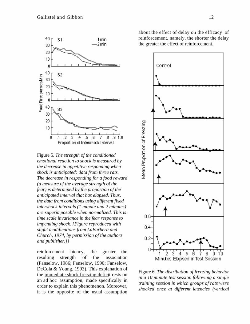
The conditioned emotional response (CER) isthe suppression of appetitive responding thatoccurs when the subject (usually a rat)expects a shock to the feet (aversivereinforcement). The appetitive response issuppressed because the subject freezes inanticipation of the shock (Figure 1C). Ifshocks are scheduled at regular intervals, thenthe probability that the rat will stop itsappetitive responding (pressing a bar toobtain food) increases as a fraction of theintershock interval that has elapsed. Thesuppression measure obtained fromexperiments employing different intershockintervals are superimposable when they areplotted as a proportion of the intershockinterval that has elapsed (LaBarbera &Church, 1974-- see Figure 5). Put anotherway, the degree to which the rat fears theimpending shock is determined by how closeit is to the shock. Its subjective measure ofcloseness is the ratio of the interval elapsedsince the last shock to the expected intervalbetween shocks--a simple manifestation ofscalar expectancy.
The Immediate Shock Deficit
If a rat is shocked immediately after beingplaced in an experimental chamber (1-5second latency), it shows very littleconditioned response (freezing) in the courseof an eight-minute test the next day. Bycontrast, if it is shocked several minutes afterbeing placed in the chamber, it shows muchmore freezing during the subsequent test. Thelonger the reinforcement delay, the more totalfreezing is observed, up to several minutes(Fanselow, 1986). This has led to thesuggestion that in conditioning an animal tofear the experimental context, the longer the
Gallistel and Gibbon 12
Figure 5. The strength of the conditionedemotional reaction to shock is measured bythe decrease in appetitive responding whenshock is anticipated: data from three rats.The decrease in responding for a food reward(a measure of the average strength of thefear) is determined by the proportion of theanticipated interval that has elapsed. Thus,the data from conditions using different fixedintershock intervals (1 minute and 2 minutes)are superimposable when normalized. This istime scale invariance in the fear response toimpending shock. {Figure reproduced withslight modifications from LaBarbera andChurch, 1974, by permission of the authorsand publisher.]}
reinforcement latency, the greater theresulting strength of the association(Fanselow, 1986; Fanselow, 1990; Fanselow,DeCola & Young, 1993). This explanation ofthe immediate shock freezing deficit rests onan ad hoc assumption, made specifically inorder to explain this phenomenon. Moreover,it is the opposite of the usual assumption
about the effect of delay on the efficacy ofreinforcement, namely, the shorter the delaythe greater the effect of reinforcement.
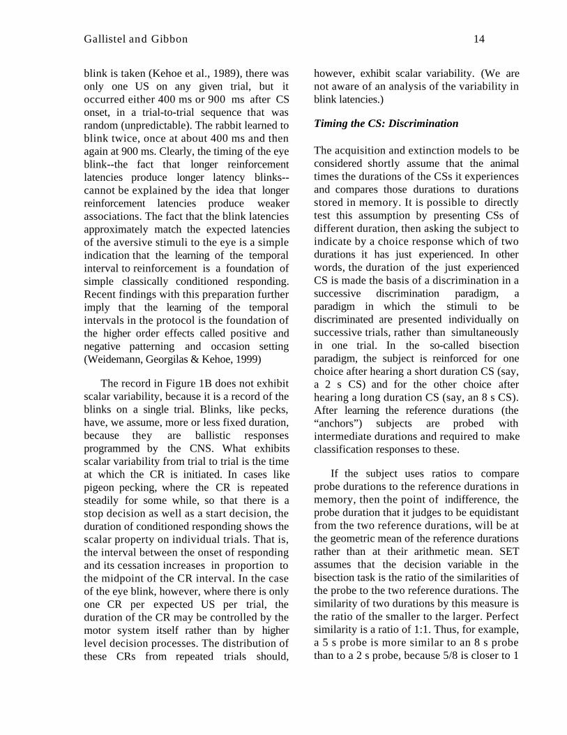
Figure 6. The distribution of freezing behaviorin a 10 minute test session following a singletraining session in which groups of rats wereshocked once at different latencies (vertical

Gallistel and Gibbon 13
arrows) after being placed in the experimentalbox (and removed 30 s after the shock). Thecontrol rats were shocked immediately afterbeing placed in a different box (a differentcontext from the one in which their freezingbehavior was observed on the test day). AfterFig. 2 in (Bevins & Ayres, 1995).
From the perspective of ScalarExpectancy Theory, the immediate shockfreezing deficit is a manifestation of scalarvariability in the distribution of the fearresponse about the expected time of shock.Bevins and Ayres (1995) varied the latencyof the shock in one-trial contextual fearconditioning paradigm and showed that thelater in the training session the shock is given,the later one observes the peak in freezingbehavior and the broader the distribution ofthis behavior throughout the session (Figure6). The prediction of the immediate shockdeficit follows directly from the scalarvariability of the fear response about themoment of peak probability (as evidenced inFigure 5). If the probability of freezing in atest session following training with a 3-minute shock delay is given by the broadnormal curve in Figure 7. (cf. freezing data inFigure 1C), then the distribution after a 3-slatency should be 60 times narrower (3-scurve in Figure 7). Thus, the amount offreezing observed during an 8-minute testsession following an immediate shock shouldbe negligible in comparison to the amountobserved following a shock delayed for 3minutes.
It is important to note that ourexplanation of the failure to see significantevidence of fear in the chamber afterexperiencing short latency shock does notimply that there is no fear associated withthat brief delay. On the contrary, we suggestthat the subjects fear the shock just as muchin the short-latency conditions as in the long-latency condition. But the fear begins and
ends very much sooner; hence, there is muchless measured evidence of fear. Because theaverage breadth of the interval during whichthe subject fears shock grows in proportionto the remembered latency of that shock, thetotal amount of fearful behavior (number ofseconds of freezing) observed is much greaterwith longer shock latencies.
Figure 7. Explanation of the immediate shockfreezing deficit by Scalar Expectancy Theory:Given the probability-of-freezing curve shownfor the 3-minute group (Figure 1C), the scaleinvariance of CR distributions predicts thevery narrow curve shown for subjectsshocked immediately (3 s) after placement inthe box. Scoring percent freezing during theeight minute test period will show much morefreezing in the 3-minute group than in the 3-sgroup (about 60 times more).
The Eye Blink
The conditioned eye blink is often regarded asa basic or primitive example of a classicallyconditioned response to an aversive US. Afact well known to those who have directlyobserved this conditioned response is that thelatency to the peak of the conditionedresponse approximately matches the CS-USlatency. Although the response is overliterally in the blink of an eye, it is so timedthat the eye is closed at the moment when theaversive stimulus is expected. Figure 1B is aninteresting example. In the experiment fromwhich this representative plot of a double
Gallistel and Gibbon 14
blink is taken (Kehoe et al., 1989), there wasonly one US on any given trial, but itoccurred either 400 ms or 900 ms after CSonset, in a trial-to-trial sequence that wasrandom (unpredictable). The rabbit learned toblink twice, once at about 400 ms and thenagain at 900 ms. Clearly, the timing of the eyeblink--the fact that longer reinforcementlatencies produce longer latency blinks--cannot be explained by the idea that longerreinforcement latencies produce weakerassociations. The fact that the blink latenciesapproximately match the expected latenciesof the aversive stimuli to the eye is a simpleindication that the learning of the temporalinterval to reinforcement is a foundation ofsimple classically conditioned responding.Recent findings with this preparation furtherimply that the learning of the temporalintervals in the protocol is the foundation ofthe higher order effects called positive andnegative patterning and occasion setting(Weidemann, Georgilas & Kehoe, 1999)
The record in Figure 1B does not exhibitscalar variability, because it is a record of theblinks on a single trial. Blinks, like pecks,have, we assume, more or less fixed duration,because they are ballistic responsesprogrammed by the CNS. What exhibitsscalar variability from trial to trial is the timeat which the CR is initiated. In cases likepigeon pecking, where the CR is repeatedsteadily for some while, so that there is astop decision as well as a start decision, theduration of conditioned responding shows thescalar property on individual trials. That is,the interval between the onset of respondingand its cessation increases in proportion tothe midpoint of the CR interval. In the caseof the eye blink, however, where there is onlyone CR per expected US per trial, theduration of the CR may be controlled by themotor system itself rather than by higherlevel decision processes. The distribution ofthese CRs from repeated trials should,
however, exhibit scalar variability. (We arenot aware of an analysis of the variability inblink latencies.)
Timing the CS: Discrimination
The acquisition and extinction models to beconsidered shortly assume that the animaltimes the durations of the CSs it experiencesand compares those durations to durationsstored in memory. It is possible to directlytest this assumption by presenting CSs ofdifferent duration, then asking the subject toindicate by a choice response which of twodurations it has just experienced. In otherwords, the duration of the just experiencedCS is made the basis of a discrimination in asuccessive discrimination paradigm, aparadigm in which the stimuli to bediscriminated are presented individually onsuccessive trials, rather than simultaneouslyin one trial. In the so-called bisectionparadigm, the subject is reinforced for onechoice after hearing a short duration CS (say,a 2 s CS) and for the other choice afterhearing a long duration CS (say, an 8 s CS).After learning the reference durations (the“anchors”) subjects are probed withintermediate durations and required to makeclassification responses to these.
If the subject uses ratios to compareprobe durations to the reference durations inmemory, then the point of indifference, theprobe duration that it judges to be equidistantfrom the two reference durations, will be atthe geometric mean of the reference durationsrather than at their arithmetic mean. SETassumes that the decision variable in thebisection task is the ratio of the similarities ofthe probe to the two reference durations. Thesimilarity of two durations by this measure isthe ratio of the smaller to the larger. Perfectsimilarity is a ratio of 1:1. Thus, for example,a 5 s probe is more similar to an 8 s probethan to a 2 s probe, because 5/8 is closer to 1

Gallistel and Gibbon 15
than is 2/5. If, by contrast, similarity weremeasured by the extent to which thedifference between two durations approaches0, then a 5 s probe would be equidistant(equally similar) to a 2 and an 8 s referent,because 8-5 = 5-2. Maximal uncertainty(indifference) should occur at the probeduration that is equally similar to 2 and 8. Ifsimilarity is measured by ratios rather thandifferences, then the probe is equally similarto the two anchors for T, such that 2/T = T/8or T=4, the geometric mean of 2 and 8.
As predicted by the ratio assumption inScalar Expectancy Theory, the probeduration at the point of indifference is in factgenerally the geometric mean, the duration atwhich the ratio measures of similarity areequal, rather than the arithmetic mean, whichis the duration at which the differencemeasures of similarity are equal (Church &Deluty, 1977; Gibbon et al., 1984; seePenney, Meck, Allan & Gibbon, in press fora review and extension to human timediscrimination) Moreover, the plots of thepercent choice of one referent or the other asa function of the probe duration are scaleinvariant, which means that the psychometricdiscrimination functions obtained fromdifferent pairs of reference durationssuperpose when time is normalized by thegeometric mean of the reference durations(Church & Deluty, 1977; Gibbon et al.,1984).
Acquisition
The acquisition of responding to the CS
The conceptual framework we propose forthe understanding of conditioning is, in itsessentials, the decision-theoretic conceptualframework, which has long been employed inpsychophysical work, and which hasinformed SET from its inception. In thepsychophysical decision-theoretic frame-
work, there is a stimulus whose strength maybe varied by varying relevant parameters. Thestimulus might be, for example, a light flash,whose detectability is affected by itsintensity, duration and luminosity. Thestimulus gives rise through an often complexcomputational process to a noisy internalsignal called the decision variable. Thestronger the stimulus, the greater the meanvalue of this noisy decision variable. Thesubject responds when the decision variableexceeds a decision threshold. The stronger thestimulus is, the more likely the decisionvariable is to exceed the decision threshold;hence the more likely the subject is torespond. The plot of the subject’s responseprobability as a function of the strength ofthe stimulus (for example, its intensity orduration or luminosity) is called thepsychometric function.
In our analysis of conditioning, theconditioning protocol is the stimulus. Thetemporal intervals in the protocol--includingthe cumulative duration of the animal’sexposure to the protocol-- are the relevantparameters of the stimulus, as are thereinforcement magnitudes, when they alsovary. These stimulus parameters determinethe value of a decision variable through a to-be-described computational process, calledrate estimation theory (RET). The decisionvariable is noisy, due to both external andinternal sources. The animal responds to theCS when the decision variable exceeds anacquisition threshold. The decision process isadapted to the characteristics of the noise.
The acquisition function in conditioning isequivalent to the psychometric function in apsychophysical task. Its rise (the increasingprobability of a response as exposure to theprotocol is prolonged) reflects the growingmagnitude of the decision variable. The visualstimulus in the example used above getsstronger as the duration of the flash is

Gallistel and Gibbon 16
prolonged, because the longer a light of agiven intensity is continued, the moreevidence there is of its presence (up to somelimit). Similarly, the conditioning stimulusgets stronger as the duration of the subject’sexposure to the protocol increases, becausethe continued exposure to the protocol givesstronger and stronger objective evidence thatthe CS makes a difference in the rate ofreinforcement (stronger and stronger evidenceof CS-US contingency).
In modeling acquisition, we try to emulatepsychophysical modeling by paying closerattention to quantitative results, rather thanpredicting only the directions of effects.However, our efforts to test models of thesimple acquisition process quantitatively arehampered by a paucity of data on acquisitionin individual subjects. Most publishedacquisition curves are group averages. Theseare likely to contain averaging artifacts. Ifindividual subjects acquire abruptly, butdifferent subjects acquire after differentamounts of experience, the averaging acrosssubjects of response frequency as a functionof trials or reinforcements will yield asmooth, gradual group acquisition curve, eventhough acquisition in each individual subjectshowed abrupt acquisition. Thus, the form ofthe “psychometric function” (acquisitionfunction) for individual subjects is not wellestablished.
Quantitative facts about the effects ofbasic variables like partial reinforcement,delay of reinforcement, and the intertrialinterval on the rate of acquisition andextinction also have not been as wellestablished as one might suppose, given therich history of experimental research onconditioning and the long-recognizedimportance of these parameters2. In recent
2This is in part because meaningful data onacquisition could not be collected before the advent of
years, pigeon autoshaping has been the mostextensively used appetitive conditioningpreparation. The most systematic data onrates of acquisition and extinction come fromit. Data from other preparations, notablyrabbit jaw movement conditioning (anotherappetitive preparation), the rabbit nictitatingmembrane preparation (aversive condition-ing) and the conditioned suppression ofappetitive responding (CER) preparation(also aversive) appear to be consistent withthese data, but do not permit as strongquantitative conclusions.
Pigeon autoshaping is a fully automatedvariant of Pavlov’s classical conditioningparadigm. The protocol for it is diagrammedin Figure 8A. The CS is the transilluminationof a round button (key) on the wall of theexperimental enclosure. The illumination ofthe key may or may not be followed at somedelay by the brief presentation of a hopperfull of food (reinforcement). Instead ofsalivating to the stimulus that predicts food,as Pavlov’s dogs did, the pigeon pecks at it.The rate or probability of pecking the key isthe measure of the strength of conditioning.As in Pavlov’s original protocol, the CR(pecking) is the same or nearly the same asthe UR elicited by the US. In this paradigm,as in Pavlov’s paradigm, the food is deliveredat the end of the CS whether or not thesubject pecks the key. Thus, it is a classicalconditioning paradigm rather than an operantconditioning paradigm. As an automatedmeans for teaching pigeons to peck keys inoperant conditioning experiments, it hasreplaced experimenter-controlled shaping. Itis now common practice to condition the
fully automated conditioning paradigms. Whenexperimenter judgment enters into the training in anon-line manner, as is the case when animals are“shaped,” or when the experimenter handles thesubjects on every trial (as in most maze paradigms),the skill and attentiveness of the experimenter is animportant but unmeasured factor.

Gallistel and Gibbon 17
pigeon to peck the key by reinforcing keyillumination whether or not the pigeon pecks(a Pavlovain procedure) and only thenintroduce the operant contingency onresponding. The discovery that pigeon keypecking--the prototype of the operantresponse--could be so readily conditioned bya classical (Pavlovian) rather than an operantprotocol has cast doubt on the traditionalassumption that classical and operantprotocols tap fundamentally differentassociation-forming processes (Brown &Jenkins, 1968).
Some well established facts about theacquisition of a conditioned response are:
• The "strengthening" of the CR withextended experience: It takes a number ofreinforced trials for an appetitiveconditioned response to emerge.
• No effect of partial reinforcement:Reinforcing only some of the CSpresentations increases the number oftrials required to reach an acquisitioncriterion in both Palovian paradigms(Figure 8B, solid lines) and operantdiscrimination paradigms (Williams,1981). However, the increase isproportional to the thinning of thereinforcement schedule--the averagenumber of trials per reinforcement (thethinning factor). Hence, the requirednumber of reinforcements is unaffectedby partial reinforcement (Figure 8B,dashed lines). Thus, the nonrein-forcements that occur during partialreinforcement do not affect the rate ofacquisition, defined as the reciprocal ofreinforcements to acquisition.
• Effect of the intertrial interval Increasingthe average interval between trialsincreases the rate of acquisition, that is, itreduces the number of reinforcements
required to reach an acquisition criterion(Figure 8B, dashed lines), hence, alsotrials to acquisition (Figure 8B, solidlines). More quantitatively, reinforce-ments to acquisition are approximatelyinversely proportional to the I/T ratio(Figures 9 and 10), which is the ratio ofthe intertrial duration (I) to the durationof a CS presentation (T, for trialduration). If the CS is reinforced ontermination (as in Figure 8A), then T isalso the reinforcement latency or delay ofreinforcement. This interval is also calledthe CS-US interval or the ISI (forinterstimulus interval). The effect of theI/T ratio on the rate of acquisition isindependent of the reinforcementschedule, as may be seen from the factthat the solid lines are parallel in Figure8B, as are also, of course, the dashedlines.
• Delay of reinforcement: Increasing thedelay of reinforcement, while holding theintertrial interval constant, retardsacquisition--in proportion to the increasein the reinforcement latency (Figure 11,solid line). Because I is held constantwhile T is increased, delaying reinforce-ment in this manner reduces the I/T ratio.The effect of delaying reinforcement isentirely due to the reduction in the I/Tratio. Delay of reinforcement per se doesnot affect acquisition (dashed line inFigure 11).
• Time scale invariance: When the inter-trial interval is increased in proportion tothe delay of reinforcement, delay ofreinforcement has no effect onreinforcements to acquisition (Figure 11,dashed line). Increasing the intertrialinterval in proportion to the increase inCS duration means that all the temporalintervals in the conditioning protocol areincreased by a common scaling factor.

Gallistel and Gibbon 18
Therefore, we call this important resultthe time scale invariance of the acquisitionprocess. The failure of partialreinforcement to affect rate of acquisitionand the constant coefficient of variation inreinforcements to acquisition (constantvertical scatter about the regression line inFigure 9) are other manifestations of timescale invariance, as will be explained.
•Irrelevance of reinforcement magnitude:Above some threshold level, the amountof reinforcement has little or no effect onthe rate of acquisition. Increasing theamount of reinforcement by increasing theduration of food-cup presentation 15-folddoes not reduce reinforcements toacquisition. In fact, the rate of acquisitioncan be dramatically increased by reducingreinforcement duration and adding thetime thus saved to the intertrial interval(Figure 12). The intertrial interval, theinterval when nothing happens, mattersprofoundly in acquisition; the duration ormagnitude of the reinforcement does not.
• Acquisition requires contingency (theTruly Random Control) When reinforce-ments are delivered during the intertrialinterval at the same rate as they occurduring the CS, conditioning does notoccur (the truly random control, alsoknown as the effect of backgroundconditioning --Rescorla, 1968). Thefailure of conditioning under theseconditions is not simply a performanceblock, as conditioned responding to theCS after random control training is notobservable even with sensitive techniques(Gibbon & Balsam, 1981). The trulyrandom control eliminates the contin-gency between CS and US while leavingthe frequency of their temporal pairingunaltered. Its effect on conditioningimplies that conditioning is driven by CS-
US contingency, not by the temporalpairing of CS and US.
• Effect of signaling 'background' rein-forcers. In the truly random controlprocedure, acquisition to a target CS doesoccur if another CS precedes (and therebysignals) the 'background' reinforcers(Durlach, 1983). These signaled rein-forcers are no longer background rein-forcers if, by a background reinforcer, onemeans a reinforcer that occurs in thepresence of the background alone.
Figure 8. A. Time lines showing the variablesthat define a classical (Pavlovian)conditioning protocol--the duration of a CSpresentation (T), the duration of the intertrialinterval (I ), and the reinforcement schedule ,S (trials/reinforcement). The US(reinforcement) is usually presented at thetermination of the CS (black dots). Forreasons shown in Figure 12, the US may betreated as a point event, an event whoseduration can be ignored. The sum of T and Iis C, the duration of the trial cycle. B. Trialsto acquisition (solid lines) and reinforcementsto acquisition (dashed lines) in pigeon

Gallistel and Gibbon 19
autoshaping, as a function of thereinforcement schedule and the I/T ratio. Notethat the solid and dashed lines come in pairs,with the members of a pair joined at the 1/1value of S, because, with that schedule(continual reinforcement), the number ofreinforcements and number of trials areidentical. The acquisition criterion was atleast one peck on three out of four consecutivepresentations of the CS. (Reanalysis of data inFig. 1 of Gibbon, Farrell, Locurto, Duncan &Terrace, 1980)
1000100101.1
1
10
100
1000B&P 79
B&J 68G&W, 71, 73
G et al 75G et al VC
G et al FC
G et al 80R et al 77
T et al 75T 76a
T 76b
W & McC 74Regression
I/T
Re
info
rce
me
nts
to
Ac
qu
isit
ion
Figure 9. Reinforcements to acquisition as afunction of the I/T ratio. (double logarithmiccoordinates). The data are from12experiments in several different laboratories,as follows: B&P 79 = Balsam & Payne,1979; B&J 68 = Brown & Jenkins, 1968;G&W,71,73 = Gamzu & Williams, 1971,1973); G et al 75 = Gibbon, Locurto &Terrace, 1975; G et al VC = Gibbon,Baldock, Locurto, Gold & Terrace, 1977Variable C; G et al FC = Gibbon et al., 1977Fixed C; G et al 80 = Gibbon et al., 1980; Ret al 77 = Rashotte, Griffin & Sisk, 1977; T etal 75 = Terrace, Gibbon, Farrell & Baldock,1975; T76a = Tomie, 1976a; T76b = Tomie,1976b; W & McC74 = Wasserman &McCracken, 1974.
Figure 10. Selected data showing the effect ofI/T ratio on the rate of eye blink conditioningin the rabbit, where I is the estimated amountof exposure to the experimental apparatus perCS trial (time when the subject was outsidethe apparatus not counted). We used 50% CRfrequency as the acquisition criterion inderiving these data from published groupacquisition curves. S&G, 1964 =Schneiderman & Gormezano(1964) 70-trialsper session, session length roughly half anhour, I varied randomly with mean of 25 s.B&T, 1965 = Brelsford & Theios (1965)single-session conditioning, Is of 45, 111, and300 s, session lengths increased with I (1.25& 2 hrs for data shown). We do not show the300 s data because those sessions lastedabout 7 hours. Fatigue, sleep, growingrestiveness, etc. may have become animportant factor. Lenvinthal, et al., 1985 =Levinthal, Tartell, Margolin & Fishman,1985, one trial per 11 minute (660-s) dailysession. None of these studies was designed tostudy the effect of I/T ratio, so the plot shouldbe treated with caution. Such studies areclearly desirable--in this and other standardconditioning paradigms.
We have presented data from pigeonautoshaping to illustrate the basic facts ofacquisition (Figures 8, 9, 11 and 12), becausethe most extensive and systematic
Gallistel and Gibbon 20
quantitative data come from experimentsusing that paradigm. However, the sameeffects (and surprising lack of effects) seemto be apparent in other classical conditioningparadigms. For example, partial reinforce-ment produces little or no increase inreinforcements to acquisition in a widevariety of paradigms (see citations in Table 2of Gibbon et al., 1980; also Holmes &Gormezano, 1970; Prokasy & Gormezano,1979); whereas, lengthening the amount ofexposure to the experimental apparatus perCS trial increases the rate of conditioning inthe rabbit nictitating membrane preparationby almost two orders of magnitude (Kehoe &Gormezano, 1974; Levinthal et al., 1985;Schneiderman & Gormezano, 1964--seeFigure 10). Thus, it appears to be generallytrue that varying the I/T ratio has a muchstronger effect on the rate of acquisition thandoes varying the degree of partialreinforcement, regardless of the conditioningparadigm used.
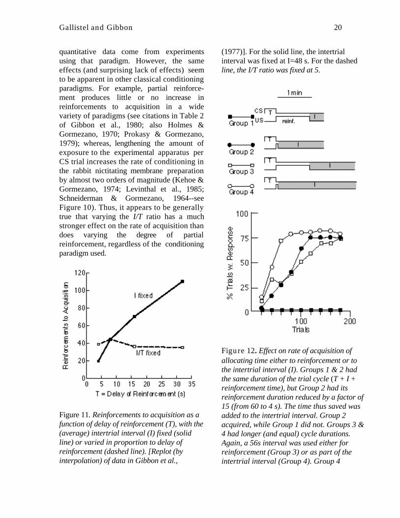
Figure 11. Reinforcements to acquisition as afunction of delay of reinforcement (T), with the(average) intertrial interval (I) fixed (solidline) or varied in proportion to delay ofreinforcement (dashed line). [Replot (byinterpolation) of data in Gibbon et al.,
(1977)]. For the solid line, the intertrialinterval was fixed at I=48 s. For the dashedline, the I/T ratio was fixed at 5.
Figure 12. Effect on rate of acquisition ofallocating time either to reinforcement or tothe intertrial interval (I). Groups 1 & 2 hadthe same duration of the trial cycle (T + I +reinforcement time), but Group 2 had itsreinforcement duration reduced by a factor of15 (from 60 to 4 s). The time thus saved wasadded to the intertrial interval. Group 2acquired, while Group 1 did not. Groups 3 &4 had longer (and equal) cycle durations.Again, a 56s interval was used either forreinforcement (Group 3) or as part of theintertrial interval (Group 4). Group 4

Gallistel and Gibbon 21
acquired most rapidly. Group 3, which hadthe same I/T ratio as Group 2, acquired nofaster than Group 2, despite getting 15 timesmore access to food per reinforcement.(Replotted from Figs. 1 & 2 in Balsam &Payne, 1979 by permission of the authors andpublisher).
It also appears to be generally true that inboth appetitive and aversive conditioningparadigms, varying the magnitude or intensityof reinforcement has little effect on the rate ofacquisition. Increasing the magnitude of thewater reinforcement in rabbit jaw-movementconditioning 20-fold has no effect on the rateof acquisition (Sheafor & Gormezano, 1972).Turning to aversive conditioning, Annau andKamin (1961) examined the effect of shockintensity on the rate at which fear-inducedsuppression of appetitive responding isacquired. The groups receiving the threehighest intensities (0.85, 1.55 & 2.91 ma) allwent from negligible levels of suppression tocomplete suppression on the second day oftraining (between trials 4 and 8). The groupreceiving the next lower shock intensity (0.49ma) showed less than 50% suppressionasymptotically. Kamin (1969a) laterexamined the effect of two levels of shockintensity on the rate at which CERs to a lightCS and a noise CS were acquired. He used 1ma, which is the usual level in CERexperiments, and 4 ma, which is a veryintense shock. The 1 ma groups crossed the50% median suppression criterion betweentrials 4 and 5, while the 4 ma groups crossedthis criterion between trials 3 and 4. Thus,varying shock intensity from the minimumthat sustains a vigorous fear response up tovery high levels has little effect on the rate ofCER acquisition.
The lack of an effect of US magnitude orintensity on the number of reinforcementsrequired for acquisition is counterintuitiveand merits further investigation in a variety of
paradigms. In such investigations, it will beimportant to show data from individualsubjects to avoid averaging artifacts. For thesame reason, it will be important not to binthe responses by session or number of trials,etc. What one wants is the real-time record ofresponding. Finally, it will be important todistinguish between the asymptote of theacquisition function and the location of itsrise, defined as, the number of reinforcementsrequired to produce, for example, a half-maximal rate of responding. At least from apsychophysical perspective, only the lattermeasure is relevant to determining the rate ofacquisition. In psychophysics, it has longbeen recognized that it is important todistinguish between the location of thepsychometric function along the x-axis (inthis case, number of reinforcements), on theone hand, and the asymptote of the function,on the other hand. The location of thefunction indicates the underlying rate orsensitivity, while its asymptote reflectsperformance factors. The same distinction isused in pharmacology: the location (doserequired for) the half-maximal responseindicates affinity, while the asymptoteindicates performance factors such as thenumber of receptors available for binding.
We do not claim that reinforcementmagnitude is unimportant in conditioning. Aswe will emphasize later on, it is a veryimportant determinant of preference. It isalso an important determinant of theasymptotic level of performance. And, if themagnitude of reinforcement varied dependingon whether the reinforcement was deliveredduring the CS or during the background, wewould expect magnitude to affect rate ofacquisition as well. A lack of effect on rate ofacquisition is observed (and, on our analysis,expected) only when there are no backgroundreinforcements (the usual case in simpleconditioning) or when the magnitude ofbackground reinforcements is the same as the

Gallistel and Gibbon 22
background reinforcements equals themagnitude of CS reinforcements (the usualcase when there is background conditioning).
Rate Estimation Theory
From a timing perspective, acquisition is aconsequences of decisions that the animalmakes about whether to respond to a CS. Ourmodels for these decisions are adapted fromGallistel's earlier account (Gallistel, 1990,1992a, b), which we will call Rate EstimationTheory (RET). In our acquisition model, thedecision to respond to the CS in the course ofconditioning is based on the animal's growingcertainty that the CS has a substantial effecton the rate of reinforce-ment. In simpleconditioning, this certainty appears to bedetermined by the subject’s estimate of themaximum possible value for the rate ofbackground reinforce-ment given itsexperience of the background up to a givenpoint in conditioning. Its estimate of theupper limit on what the rate of backgroundreinforcement may be decreases steadily asconditioning progresses, because the subjectnever experiences a background reinforcement(in simple conditioning). The subject’sestimate of the rate of CS reinforcement, bycontrast, remains stable, because the subjectgets reinforced after every so many secondsof exposure to the CS. The decision torespond is based on the ratio of these rateestimates, as shown in Figure 13. This ratiogets steadily larger as conditioning pro-gresses, because the upper limit on thebackground rate gets steadily lower. It shouldalready be apparent why the amount ofbackground exposure is so important inacquisition. It determines how rapidly theestimate for the background rate ofreinforcement diminishes.
The ratio of two estimates for rates ofreinforcement is equivalent to the ratio of twoestimates of the expected interval between
reinforcements (the interval-rate dualityprinciple). Thus, any model couched in termsof rate ratios can also be couched in terms ofthe ratios of the expected intervals betweenevents. When couched in terms of theexpected intervals between reinforce-ments,the RET model of acquisition is as follows:Because the subject never experiences abackground reinforcement in standard delayconditioning (after the hopper training), itsestimate of the interval between backgroundreinforcements gets longer in proportion tothe duration of its unreinforced exposure tothe background. By contrast, its estimate ofthe interval between reinforce-ments whenthe CS is on remains constant, because it getsreinforced after every T seconds of CSexposure. Thus, the ratio of the two expectedintervals gets steadily greater as conditioningprogresses. When this ratio exceeds a decisionthreshold, the animal begins to respond to theCS
The interval-rate duality principle meansthat the decision variables in SET and RETare the same kind of variables. Both decisionvariables are equivalent to the ratio of twoestimated intervals. Rescaling time does notaffect these ratios, which is why both modelsare time scale invariant. This time-scaleinvariance is, we believe, unique to timing-based models of conditioning with decisionvariables that are ratios of estimated intervals.It provides a simple way of discriminatingexperimentally between these models andassociative models. There are, for example,many associative explanations for the trial-spacing effect (Barela, 1999, in press), whichis the strong effect that lengthening theintertrial interval has on the rate ofacquisition (Figures 9 & 10). To ourknowledge, none of them is time-scaleinvariant. That is, in none of them is it truethat the magnitude of the trial-spacing effectis determined simply by the relative amountsof exposure to the CS and to the background

Gallistel and Gibbon 23
alone in the protocol (Figure 11). Theexplanation of the trial-spacing effect givenby Wagner’s (1981) “sometimes opponentprocess (SOP) model, for example, dependson the rates at which stimulus traces decayfrom one state of activity to another. Thesize of the predicted effect of trial spacingwill not be the same for protocols that havethe same proportion of CS exposure tointertrial interval and differ only in their timescale, because longer time scales will lead tomore decay. This time-scale dependence isseen in the predictions of any model thatassumes intrinsic rates of decay (of, forexample, stimulus traces, as in Sutton &Barto, 1990) or any model that assumes thatexperience is carved into trials (Rescorla &Wagner, 1972, for example).
Rate Estimation Theory offers a model ofacquisition that is distinct from, albeit similarin inspiration to, the model proposed byGibbon and Balsam (1981). The ideaunderlying both models is that the decisionwhether to respond to a CS in the course ofconditioning depends on a comparison of theestimated rate of CS reinforcement to theestimated rate of background reinforcement(cf. Miller’s Comparator Hypothesis -- Cole,Barnet & Miller, 1995a; Miller, Barnet &Grahame, 1992). In our current proposal,RET incorporates scalar variability in theinterval estimates, just as SET did inestimating the point within the CS at whichresponding should be seen. In RET, however,two new principles are introduced: First, therelevant time intervals are cumulated acrosssuccessive occurrences of the CS and acrosssuccessive intervals of background alone. Thetotal cumulated time in the CS and the totalcumulated exposure to the background areintegrated throughout a session and evenacross sessions, provided no change in ratesof reinforcement is detected.
Cumulations over separated occurrencesof a signal have previously been shown to berelevant to performance when no reinforcersintervene at the end of successive CSs. Theseare the "gap" (Meck, Church & Gibbon,1985) and "split trials" (Gibbon & Balsam,1981) experiments, which show that subjectsdo, indeed, cumulate successive times oversuccessive occurrences of a signal. However,the cumulations proposed in RET extendover much greater intervals (and much greatergaps) than those employed in the just citedexperiments. This raises the importantquestion of how accumulation without(practical) limit may be realized in the brain.We conjecture that the answer to thisquestion may be related to the question of theorigin of the scalar variability in rememberedmagnitudes. Pocket calculators accumulatemagnitudes (real numbers) without practicallimit, but not with a precision that isindependent of magnitude. What is fixed isthe number of significant digits, hence, thepercent accuracy with which a magnitude(real number) may be specified. The scalarnoise in remembered magnitudes gives themthe same property: a remembered magnitudeis only specified to within plus or minus acertain percentage of its “true” value, and thedecision process is adapted to take account ofthis. Scalar uncertainty about the value of anaccumulated magnitude may be inherent inany scheme that permits accumulationwithout practical limit -- for example througha binary cascade of accumulators as suggestedby Gibbon. Malapani, Dale & Gallistel(1997) Quantitative details on such a modelare in preparation by Killeen (personalcommunication). Our point is that scalaruncertainty about the value of a quantity maybe inherent in a scale invariant computationaldevice, a device capable of working withmagnitudes of any scale.

Gallistel and Gibbon 24
The second important way in which theRET model of acquisition differs from theearlier SET model is that it incorporates apartitioning process into the estimation ofrates. Partitioning is fundamental to RET,because RET starts from the observation thatwhen only a few reinforcements haveoccurred in the presence of a CS it isinherently ambiguous whether they should becredited entirely to the CS, entirely to thebackground or some to each. Thus, anyprocess that is going to make decisions basedon separate rate estimates for the CS and thebackground needs a mechanism thatpartitions the observed rates of reinforcementamong the possible predictors of those rates.The partitioning process in RET leads insome cases (e.g., in the case of “signaled”background reinforcers, see Durlach, 1983) toestimates for the background rate ofreinforcement that are not the same as theobserved estimates assumed by the Gibbonand Balsam model.
We postpone discussion of thepartitioning process until we come toconsider the phenomena of cue competition,because cue competition experimentshighlight the need for a rate partitioningprocess in any time scale invariant model ofacquisition. The only thing that one needs toknow about the partitioning process at thispoint is that when there have been noreinforcements of the background alone, itattributes a zero rate of reinforcement to thebackground. This is equivalent to estimatingthe interval between backgroundreinforcements to be infinite, but the estimateof an infinite interval between events cannever be justified by a finite period ofobservation. A fundamental idea in ourtheory of acquisition is that a failure toobserve any background reinforcementsduring the initial exposure to a conditioningprotocol should not and does not justify an
estimate of zero for the rate of backgroundreinforcement. It only justifies the conclusionthat the background rate is no higher than thereciprocal of the total exposure to thebackground so far. Thus, RET assumes thatthe estimated rate of backgroundreinforcement when no reinforcement has yetbeen observed during any intertrial interval is1 ˆ t I , where ˆ t I is the subjective measure ofthe cumulative intertrial interval (thecumulative exposure to the backgroundalone)--see Consistency Check in Figure 13.
Correcting the background rate estimatedelivered by the partitioning process in thecase where there has been no background USsadapts the decision process to the objectiveuncertainty inherent in a finite period ofobservation without an observed event. (Putanother way, it recognizes that absence ofevidence is not evidence of absence.) Notethat this correction is consistent withpartitioning in later examples in whichreinforcements are delivered in the intertrialinterval. In those cases, the estimated rate of
background reinforcement, ˆ λ b is alwaysˆ n I ˆ t I , the cumulative number of backgroundreinforcements divided by the cumulativeexposure to the background alone.
As conditioning proceeds with noreinforcers in the intertrial intervals, ˆ t I getslonger and longer, so 1 ˆ t I gets smaller andsmaller. When the ratio of the rate expectedduring the CS and the background rateexceeds a threshold, conditioned respondingappears. Thus, conditioned responding makesits appearance when
ˆ λ cs + ˆ λ bˆ λ b
> β
where β ιs the threshold or decision criterion.Assuming that the animal's estimates of

Gallistel and Gibbon 25
numbers and durations are proportional tothe true numbers and durations (i.e., thatsubjective number and subjective duration,represented by the symbols with hats, areproportional to objective number andobjective duration, which are represented bythe same symbols without hats), we have
ˆ λ cs + ˆ λ b = ncs tcs
andˆ λ b = nI tI ,
so that (by substitution) conditioningrequires that
ncs tcs
nI tI> β
Equivalently (by rearrangement), the ratioof CS reinforcers to background reinforcers,ncs nI , must exceed the ratio of thecumulated trial time to the cumulatedintertrial (background alone) time by somemultiplicative factor,
ncs
nI> β
tcs
tI(1)
It follows that, N , the number of CSreinforcements required for conditioning tooccur in simple delay conditioning must beinversely proportional to the I/T ratio. Theleft hand side of (1) is equal to N , because bythe definition of N , the conditioned responseis not observed until ncs = N . and nI isimplicitly taken to be 1 when the estimatedrate of reinforcement is taken to be 1 tI . Onthe right hand side of (1), the ratio ofcumulated intertrial interval time (cumulativeexposure to the background alone = t I ) andthe cumulated CS time (tcs) is (on average) theI/T ratio. Thus, conditioned responding to theCS should begin when
ncs > β (I T )−1 . (2)
Equation (2) means that on average, thenumber of trials to acquisition should be thesame in different protocols with differentdurations for I and T but the same I/T ratio.It also implies that reinforcements toacquisition should be inversely proportionalto the I/T ratio.
In Figure 9, which is replotted fromGibbon & Balsam (1981), data from a varietyof studies show that this inverseproportionality between reinforcements toacquisition and the I/T ratio is onlyapproximately what is in fact observed. Theslope of the best fitting line through the datain Figure 9 is -.72±.04, which is significantlyless than the value of -1 (99% confidencelimit = -.83), which means that there is alinear rather than strictly proportionalrelation. The fact that the slope is close to 1means, however, that the relation can beregarded as approximately proportional.
The derivation of a linear (rather thanproportional) relation between logN andlog(I/T) and of the scalar variability inreinforcements to acquisition (the constantvertical scatter about the regression line inFigure 9), is given in Appendix 1A.Intuitively, it rests on the following idea: N isthe CS presentation (trial) at which subjectsfirst reach the acquisition criterion. Thismeans that for the previous N-1 trials thiscriterion was not exceeded. Because there isnoise in the decision variable, for any givenaverage value of the decision variable that issomewhat less than the decision criterion,there is some probability that the actuallysampled value on a given trial will be greaterthan the criterion. Thus, there is someprobability that noise in the decision variablewill lead to the satisfaction of the acquisitioncriterion during the period when the averagevalue of the variable remains below criterion.The more trials there are during the period
Gallistel and Gibbon 26
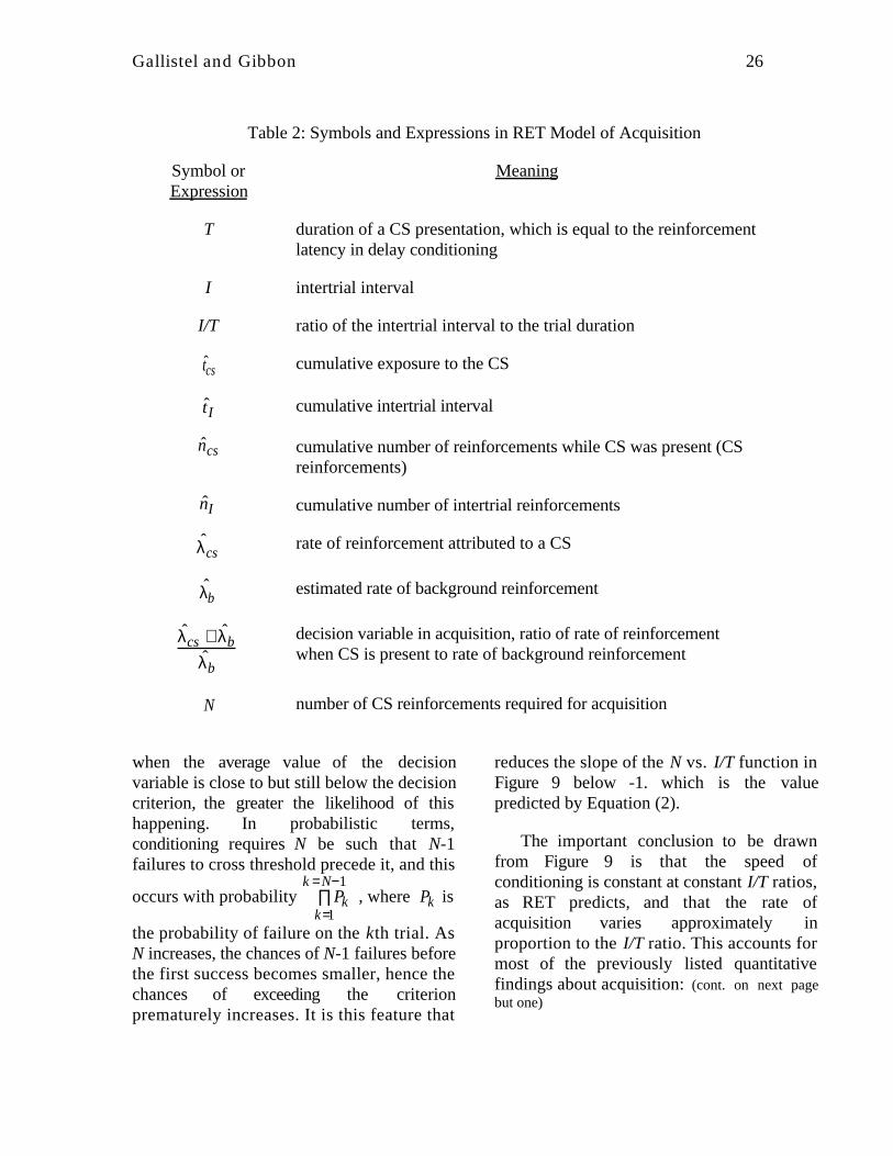
Table 2: Symbols and Expressions in RET Model of Acquisition
Symbol orExpression
Meaning
T duration of a CS presentation, which is equal to the reinforcementlatency in delay conditioning
I intertrial interval
I/T ratio of the intertrial interval to the trial duration
ˆ t cs cumulative exposure to the CS
ˆ t I cumulative intertrial interval
ˆ n cs cumulative number of reinforcements while CS was present (CSreinforcements)
ˆ n I cumulative number of intertrial reinforcements
ˆ λ csrate of reinforcement attributed to a CS
ˆ λ b estimated rate of background reinforcement
ˆ λ cs + ˆ λ bˆ λ b
decision variable in acquisition, ratio of rate of reinforcementwhen CS is present to rate of background reinforcement
N number of CS reinforcements required for acquisition
when the average value of the decisionvariable is close to but still below the decisioncriterion, the greater the likelihood of thishappening. In probabilistic terms,conditioning requires N be such that N-1failures to cross threshold precede it, and this
occurs with probability Pkk=1
k =N−1∏ , where Pk is
the probability of failure on the kth trial. AsN increases, the chances of N-1 failures beforethe first success becomes smaller, hence thechances of exceeding the criterionprematurely increases. It is this feature that
reduces the slope of the N vs. I/T function inFigure 9 below -1. which is the valuepredicted by Equation (2).
The important conclusion to be drawnfrom Figure 9 is that the speed ofconditioning is constant at constant I/T ratios,as RET predicts, and that the rate ofacquisition varies approximately inproportion to the I/T ratio. This accounts formost of the previously listed quantitativefindings about acquisition: (cont. on next pagebut one)

Gallistel and Gibbon 27
Figure 13. Functional structure (flow diagram) of the whether decision in acquisition. In simpleconditioning, reinforcements (black dots) coincide with each CS offset and there are nobackground reinforcements (no dots during intertrial intervals). Subjective duration is cumulated

Gallistel and Gibbon 28
separately for the CS ( ˆ t cs) and for the background ( ˆ t I ), as are the subjective numbers ofreinforcements ( ˆ n cs and ˆ n I .) These values in working memory enter into the partition
computation to obtain estimated rates of reinforcement for the CS ( ˆ λ cs ) and for the background
( ˆ λ b ). The rate estimates are continually updated and stored in reference memory. A rate estimatecan never be less than the reciprocal of the cumulative interval of observation. When an estimateis lower than this (typically, an estimate of a rate of 0), it is replaced by the reciprocal of the totalexposure to the background alone (Consistency Check). The decision that the CS predicts anincreased rate of reinforcement occurs when the ratio of the rate of reinforcement expected whenthe CS is present ( ˆ λ cs + ˆ λ b ) to the estimated background rate of reinforcement ( ˆ λ b ) equals or
exceeds a criterion, β.
(1) Effect of trial spacing: Increasing Iwithout increasing T results in a higher I/Tratio, hence more rapid conditioning. RETcorrectly predicts the form and magnitude ofthis effect.
(2) Effect of delay of reinforcement:Increasing T without increasing I results in alower I/T ratio, hence slower conditioning.Again, RET correctly predicts the form andmagnitude of this effect
(3) Time scale invariance: Increasing Iand T by the same factor does not change therate of conditioning. The points in Figure 9with the same I/T ratio show approximatelyequal rates of conditioning, even though theabsolute values of I and T differ substantiallyamong points at the same ratio (at the samepoint along the abscissa)--see also Figure 11.
(4) No effect of partial reinforcement:When reinforcers are omitted on somefraction of the trials, cumulative exposure tothe CS per CS reinforcement increases by theinverse of that fraction, but so doescumulative exposure to the background perCS reinforcement. For example, reinforcingonly 1/2 the trials increases the amount ofexposure to the CS per reinforcement by 2(from T to 2T). But each T seconds ofexposure to the CS is accompanied by Iseconds of exposure to the background alone.Doubling the amount of CS exposure per
reinforcement doubles the amount ofbackground-alone exposure per CSreinforcement as well. Therefore, the ratio ofthese two cumulative exposures ( tcs and tI )after any given number of reinforcementsremains unchanged. No decrement in rate ofacquisition should be seen, and none is,indeed, found. In RET, this deeply importantexperimental result is another manifestationof the time-scale invariance of conditioning,because partial reinforcement does not changethe relative amounts of CS exposure andbackground exposure per reinforcement.
(5) No effect of reinforcement magnitude:When reinforcement magnitude is increased, itincreases the estimated rate ofreinforcement3 in both the signal and in thebackground by the same factor; hence, thesechanges in reinforcement magnitudes cancel,leaving I/T unchanged. Again, noimprovement in rate of acquisition isexpected, and none is found. If there were acontrast between the magnitude ofreinforcements given during the intertrial
3Rate is now used to mean the amount ofreinforcement per unit of time, which is the product ofreinforcement magnitude and number of reinforcementsper unit of time. Later, when it becomes important todistinguish between the number of reinforcements perunit of time and the magnitudes of thosereinforcements, we will call this 'income' rather thanrate. It is the same quantity as expectancy ofreinforcement, H, in Gibbon (1977).

Gallistel and Gibbon 29
intervals and the magnitude given during theCS, then RET predicts that the ratio of thesethese contrasting reinforcement magnitudeswould strongly affect rate of acquisition.However, when there are no reinforcementsduring the intertrial intervals (the usual case)RET predicts that varying magnitude ofreinforcement will have no effect, because the“Consistency Check” stage in thecomputation of the decision variableimplicitly assumes that the yet-to-occur firstbackground reinforcement will have the samemagnitude as the reinforcements so farexperienced.
(6) Acquisition variability. The datapoints in Figure 9 show an approximatelyconstant range of vertical scatter about theregression line in log-log coordinates. In themodel of acquisition just presented, thisscalar variability in reinforcements toacquisition results from the increasingvariability in the estimate of tI , the totalaccumulated intertrial time, in comparison tothe relatively stable variability of the estimateof the average interval of CS exposurebetween reinforcements, tcs ncs . Intuitively,the estimated inter-reinforcement interval in
the presence of the CS (1 ( ˆ λ cs + ˆ λ b) )becomes increasingly stable as ncs increases,while the sampling noise in the estimate ofthe background inter-reinforcement intervalgets greater in proportion as that estimategets larger (scalar variability). Because of thescalar property, the variability in the estimateof N in Equation (2) is proportional to itssize, hence constant on the log scale. Thebasic threshold prediction and its expectedvariance are detailed in Appendix 1A.
Summary of Acquisition
Most of the presently known quantitativefacts about the rate of acquisition followdirectly from the assumption that the animalbegins to respond to the CS when the ratio of
two rate estimates exceeds a criterion: Thenumerator of the ratio is the subject’sestimate of the rate of reinforcement in thepresence of the CS. The denominator is theestimate of the background rate ofreinforcement. The ratio may be thought of asthe subject’s measure of how similar the rateof CS reinforcement is to the rate ofbackground reinforcement. In simple con-ditioning, when the background alone is neverreinforced, the denominator is the reciprocalof the cumulative duration of the intervalbetween trials, while the numerator is rate ofreinforcement when the CS is present. If thedecision ratio is taken to be a ratio ofexpected interreinforcement intervals, thenthe predictions follow from the assumptionthat conditioned responding begins when theexpected interval between backgroundreinforcements exceeds the expected intervalbetween CS reinforcements by a thresholdfactor. These are equivalent formulations (theinterval-rate duality principle).
Acquisition of a Timed Response
There is no conditioned response to the CSuntil the whether criterion has been met. Thetiming of the responses that are thenobserved is known to depend, at leasteventually, on the distribution of reinforce-ment latencies that the animal observes. It isthis dependence that is modeled by SET,which models the process leading to aconditioned response under well-trainedconditions, where the animal has decided(earlier in its training) that the CS merits aresponse (the whether decision). What theappropriate comparison interval for thatparticular response is, and what theappropriate threshold value(s) is/are. Amodel for the acquisition of an appropriatelytimed conditioned response is needed todescribe the process that makes these latterdecisions during the course of training,because SET presupposes that these

Gallistel and Gibbon 30
decisions have already been made. It modelsonly mature responding, the respondingobserved once comparison intervals andthresholds have been decided on.
It is tempting to assume that no suchdecisions are necessary, that the animal,simply samples from the distribution ofremembered intervals to obtain the particularremembered interval that constitute thedenominator of the decision ratios in SET onany one trial. This would predictexponentially distributed response latenciesin experiments where the observed CS-USintervals were exponential, and normallydistributed response latencies in cases wherethere was a single, fixed CS-US interval. Weare inclined to doubt that this assumptionwould survive detailed scrutiny of thedistributions actually observed and theirevolution over the course of training, but weare not aware of published data of this kind.Consider an experiment where the rat hascome to fear a shock that occurs at somerandom but low rate when a CS is present (asin, for example, the background conditions ofRescorla 1968). The shock delays after CSonset are exponentially distributed, and thisdistribution is so shallow that it is commonfor shocks not to occur for many minutes. Itseems unlikely that onset of the rat’s fearresponse is ever delayed by many minutesafter the onset of the CS under theseconditions, where the shock is equally likelyat any moment! But this is what one has topredict if it is assumed that the rat simplysamples from the distribution of rememberedlatencies. Also, casual observation of trainingdata from the peak procedure suggests thatthe termination of conditioned responding tothe CS when the expected reinforcementlatency has passed develops later in trainingthan does the delay of anticipatoryresponding (cf. Rescorla, 1967). This impliesthat it takes longer (more training experience)to decide on an appropriate stop threshold
than to decide on an appropriate startthreshold.
The need to posit timing-acquisitionprocesses by which the animal decides in thecourse of training on an appropriatecomparison intervals (and perhaps also onappropriate decision thresholds) becomeseven clearer when one considers morecomplex paradigms like the time-leftparadigm with one very short and one verylong standard interval. In this paradigm, thedecision to switch from the Standard side tothe Time-Left side uses the harmonic mean ofthe two standard intervals as the comparisonvalue (the denominator in the decisionvariable). However, on those trials where thesubject does not switch to the Time-Left sidebefore the moment of commitment andthereby ends up committed to the standarddelays, one observes the effects of three moretiming decisions. After the moment when theprogram has committed the subject to theStandard Side, and hence, one of the twoStandard Delays, the likelihood of respondingrises to a peak at the time of the firststandard delay (first start decision); if food isnot delivered then, it subsides (first stopdecision), to rise to a second peak at the timeof the second latency (second start decision).Thus, in this experiment, three differentreference intervals (expectations) are derivedfrom one and the same experienceddistribution (the distribution of delays on thestandard side)--one expectation for thechange-over decision, one for the decisionthat cause the early peak in responding on theStandard Side and one for the decision thatcauses the late peak. Clearly, an account isneeded of how in the course of training, theanimal decides on these three differentreference intervals and appropriatethresholds. There is no such account atpresent. Its development must await data onthe emergence of timed responding (that is,appropriate acquisition data).

Gallistel and Gibbon 31
A related issue concerns the acquisition ofthe conditioned response in trace conditioningparadigms. In these paradigms, the US doesnot occur during the CS but rather some whileafter the termination of the CS. Thus, theonset of the CS does not predict an increasein the rate of US occurrence. Rather the offsetof the CS predicts that a US will occur after afixed latency. For the acquisition of aresponse to the CS to occur under theseconditions, the animal must decide either thatthe latency from CS onset to the US is muchshorter than the US-US latency or that theonset of the CS predicts its offset, whichpredicts a US within an interval that is shortrelative to the US-US interval. As in theacquisition of a timed response, this wouldappear to require a decision process thatexamines the distribution of USs relative to atime marker.
Extinction
Associative models of conditioning are eventdriven; changes in associative strengths occurin response to events. Extinction is theconsequence of non-reinforcements, whichare problematic “events,” because a non-reinforcement is the failure of a reinforcementto occur. If there is no defined time at which areinforcement ought to occur, then it is notclear how to determine when a non-reinforcement has occurred. In RateEstimation Theory, this problem does notarise, because extinction is assumed to occurwhen a decision variable involving an elapsinginterval exceeds a decision criterion. Thedecision variable is the ratio of the currentlyelapsing interval without a reinforcement tothe expected interreinforcement interval.Before elaborating, we list some of the salientempirical facts about extinction, againstwhich different models of the process may bemeasured:
Extinction Findings
• Weakening of the CR with extendedexperience of non-reinforcement: It takesa number of unreinforced trials before theconditioned response ceases. Howabruptly it ceases in individual subjectshas not been established. That is, theform of the psychometric extinctionfunction in individual subjects is notknown.
• Partial reinforcement extinction effect(PREE): Partial reinforcement during theoriginal conditioning increases trials toextinction, the number of unreinforcedtrials required before the animal stopsresponding to the CS. However, theincrease is proportional to the thinning ofthe reinforcement schedule (Figure 14B,solid lines); hence, it does not affect thenumber of reinforcements that must beomitted to produce a given level ofextinction (Figure 14B, dashed lines).Thus, both delivered reinforcements toacquisition and omitted reinforcements toextinction are little affected by partialreinforcement.
• No effect of I/T ratio on rate of extinctionThe I/T ratio has no effect on the numberof reinforcements that must be omitted toreach a given level of extinction (Figure14B, dashed lines), hence, also no effecton trials to extinction (Figure 14B, solidlines). This lack of effect on the rate ofextinction contrasts strikingly with thestrong effect of the same variable on therate of acquisition (Figures 14A). As inthe case of acquisition, this result is bestestablished in the case of pigeonautoshaping, but it appears to begenerally true that partial reinforcementduring acquisition has little effect on thenumber of reinforcements that must be

Gallistel and Gibbon 32
omitted to produce extinction (for anextensive tabulation of such results, seeGibbon et al., 1980).
• Rates of extinction may be equal to orfaster than rates of acquisition. Afterextensive training in an autoshapingparadigm, the number of reinforcementsthat must be omitted to reach a modestextinction criterion (a decline to 50% ofthe pre-extinction rate of responding) isroughly the same as the number of
reinforcements required to reach a modestacquisition criterion (one peck in 3 out of4 CS presentations), when the I/T ratioduring acquisition is in the mostcommonly used range--see gray bandacross Figure 14A&B. If the I/T ratio issmaller than usual, then acquisition takesmany more reinforcements than must beomitted to produce extinction. Underthese conditions, the rate of extinction isfaster than the rate of acquisition.
Figure 14. Effect of the I/T ratio and the reinforcement schedule during training on acquisition andextinction of autoshaped pecking in the pigeon. A. Reproduced from Figure 8. B. Partialreinforcement during training increases trials to extinction in proportion to the thinning factor (S);hence, it has no effect on omitted reinforcements to extinction. The I/T ratio, which has a strongeffect on reinforcements to acquisition, has no effect on omitted reinforcements to extinction. Basedon data in (Gibbon et al., 1980; Gibbon et al., 1977)
• Rates of extinction are comparable to ratesof response elimination. After extensivetraining in the autoshaping paradigm, thedecline of responding in ordinary
extinction proceeds at about the same rateas the decline of responding whenresponse elimination is produced not bywithholding reinforcement of the CS but

Gallistel and Gibbon 33
rather by introducing the truly randomcontrol, that is, by shifting from a zerorate of background reinforcement to anrate of background reinforcement thatequals the rate observed when the CS ispresent (Durlach, 1986)--see Figure 15.
Figure 15. Rate of response elimination underrandom reinforcement compared to rate ofsimple extinction. Two groups (N = 6)received 15 sessions of autoshaping trainingwith a CS rate of one US per 30s, a CSduration of 12s, and a mean intertrial intervalof 132s (I/T = 10). Data shown are fromsubsequent sessions of extinction (no US’s atall), or random control (USs delivered at anaverage rate of one per 30s during bothintertrial intervals and CS presentations).{Unpublished data from Aronson, et al.}
Model
The conceptual framework we are elaboratingattributes changes in conditioned behavior todecisions based on decision variables thatgrow with the duration of relevant experience.Central to this perspective is the assumptionthat different decisions are based on differentdecision variables. Thus, the acquisition of aresponse to a CS that predicts a higher rate ofreinforcement is based on a differentcomparison than is the timing of a response
to a CS that predicts a reinforcement aftersome fixed latency. Similarly, thedisappearance of the conditioned response toa CS in the course of extinction is assumed tobe based on yet another comparison, acomparison of the cumulative amount ofunreinforced CS exposure since the last CSreinforcement with the expected amount ofCS exposure per reinforcement. In the versionof RET here presented, extinction occurswhen:
ˆ I csnoR
I ˆ R Ics=
ˆ λ csˆ λ csnoR
> β
that is, when the ratio of the estimated(subjective) interval elapsed since the lastreinforcement ( ˆ I csnoR ) to the expected
interval between CS reinforcements ( I ˆ R Ics ) is
greater than a threshold factor, β. By theprinciple of interval-rate duality, the decisionvariable may also be thought of as the ratiobetween the estimated rate of CSreinforcement up to the last reinforcement
( ˆ λ cs ) and the estimated rate since then
( ˆ λ csnoR ). The model is developed moreformally and with a treatment of varianceissues in Appendix 1B.
(1) Weakening of the CR: The decisionvariable grows in proportion to the durationof extinction, because the longer extinctionlasts, the more unreinforced exposure to theCS accumulates. Equivalently, the subject’sestimate of the rate of CS reinforcement sincethe last such reinforcement becomes an eversmaller fraction of its previous estimate. Thisexplains why it takes some number ofomitted reinforcements to produce extinction.On this view, it is a relatively prolongedinterval without reinforcement that leads toextinction rather than the “occurrence” of anon-reinforcement. ‘Occurrence’ is in scarequotes because a non-reinforcement is anevent only in the mind of the experimenter ortheoretician (and, possibly, in the mind of the

Gallistel and Gibbon 34
subject), it is not an event in the ordinaryphysical sense. ‘Relatively’ is italicized,because it is the expected interval betweenreinforcements that determines whatconstitutes a long interval without
reinforcement. Here as everywhere in ourmodels, the only intervals that matter arerelative intervals (the principle of time-scaleinvariance).
Table 3: Symbols and Expressions in RET Model of Extinction
Symbol orExpression
Meaning
ˆ I csnoR amount of CS exposure since the last reinforcement credited tothe CS
I ˆ R Ics expected interval between CS reinforcements = 1 ˆ λ cs
ˆ λ csnoRestimated rate of CS reinforcement since the last reinforcementcredited to the CS = 1 ˆ I csnoR
ˆ I csnoR
I ˆ R Ics=
ˆ λ csˆ λ csnoR
decision variable in extinction
The decision process mediating extinctionoperates in parallel with the decision processmediating acquisition, because it is a generalprocess animals employ to detect changes inthe rates of significant events. Before theexperimenter implements extinction, thesubject has been checking all along for achange in the rate of CS reinforcement, butthis check comes up negative (in favor of theno change hypothesis) until some way intothe extinction phase of the experiment.
(2) The partial reinforcement extinctioneffect, The effect of partial reinforcement ontrials to extinction, follows directly from theassumption that the decision to stopresponding is based on the ratio of thecurrently accumulating interval ofunreinforced CS exposure to the expectedamount of CS exposure per reinforcement.Thinning the reinforcement schedule duringtraining by a given factor increases the
expected amount of CS exposure perreinforcement by that factor. For example,when a 10:1 schedule of reinforcement is usedduring acquisition (an average of 10presentations of the CS per reinforcement),the expected amount of CS exposure perreinforcement is 10T rather than simply T,where T is trial duration. In our model ofextinction, the expected interval betweenreinforcement is the denominator of thedecision variable, the quantity against whichthe animal compares the currently elapsingperiod of unreinforced CS exposure. For thedecision variable to reach a criterion (fixedthreshold) value during extinction, thenumerator must increase by the same factoras the denominator. Hence, the number oftrials required to reach the extinction decisionthreshold must increase in proportion to thethinning of the partial reinforcement schedule.This increase in trials to extinction is thepartial reinforcement extinction effect.

Gallistel and Gibbon 35
Because the required amount ofunreinforced CS exposure increases inproportion to the thinning factor, the numberof reinforcements that must be omitted toreach a given level of extinction remainsconstant. In other words, there is a partialreinforcement extinction effect only if onelooks at trials to extinction (or requiredamount of unreinforced CS exposure). From atiming perspective, this is not an appropriateunit. The appropriate unit is omittedreinforcements to extinction (or the relativeamount of CS exposure). If one takes thenumber of omitted reinforcements toextinction as the appropriate unit of analysis,there is no partial reinforcement extinctioneffect (Figure 14). Notice that the predictionthat trials to extinction must increase inproportion to the thinning of thereinforcement schedule does not depend onparametric assumptions. The proportionalitybetween trials to extinction and the pre-extinction schedule of reinforcement isanother manifestation of time scaleinvariance.
If one assumes that reinforcementstrengthens and non-reinforcement weakensassociative connections, then it is paradoxicalthat partial reinforcement has no effect onreinforcements to acquisition even though therate of extinction (the amount of weakeningper nonreinforcement) may be as great orgreater than the rate of acquisition (theamount of strengthening per reinforcement).The paradox vanishes if one thinks in termsof a ratio comparison of expected intervalsbetween reinforcements. From thatperspective, partial reinforcement has noeffect on reinforcements to acquisitionbecause it extends proportionately bothexposure to the CS and exposure to thebackground, leaving their ratio unchanged.And, partial reinforcement has no effect onomitted reinforcements to extinction, because
the same number of nonreinforcementsproduces any given ratio between theexpected interreinforcement interval and theinterval without reinforcement. In both cases,the lack of an effect is a manifestation of theunderlying time-scale invariance of theconditioning process. This is obscured by theassociative analysis, because in thatframework, the focus is on “trials” (CSpresentations) rather than on the ratios ofaccumulated intervals (or, equivalently, onratios of estimated rates of reinforcement).
(3) The I/T ratio has no effect on the rateof extinction, because the currently cumulatinginterval of unreinforced CS exposure is notcompared to the expected interval betweenbackground reinforcements; it is compared tothe expected interval between CSreinforcements. The striking differencebetween the effect of the I/T ratio onacquisition and its lack of effect on extinctionfollows from a fundamental aspect of timingtheory--different decisions rest on differentcomparisons (cf. Miller’s ComparatorHypothesis --Cole et al., 1995a; Miller et al.,1992). Different decisions rest on differentcomparisons because different comparisonsare appropriate to detecting differentproperties of the animal's experience. Thebackground rate of reinforcement is theappropriate comparison when the effect of aCS on the rate of reinforcement is in question;the previous rate of CS reinforcement is theappropriate comparison when the question iswhether the rate of CS reinforcement haschanged. This is a general feature of modelingwithin a decision-theoretic framework, notjust of our models. It is taken for granted, forexample, in psychophysical modeling thatdifferent judgments about the same stimulusare based on different decision variables.
(4) Rates of extinction may be as fast orfaster than rates of acquisition, because rateof acquisition depends on the I/T ratio,
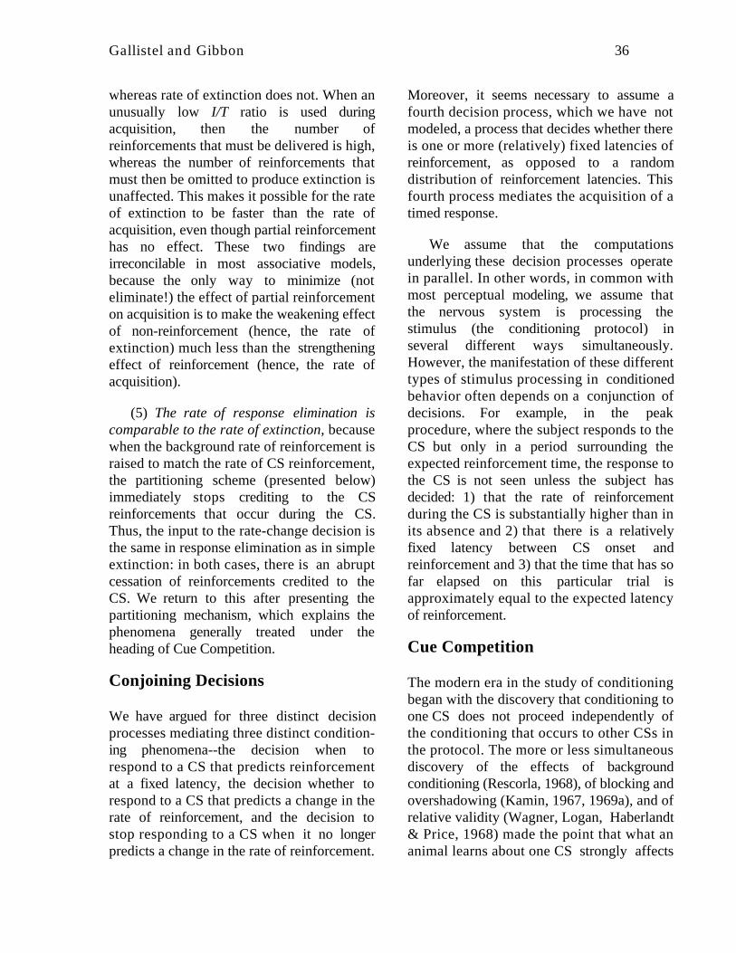
Gallistel and Gibbon 36
whereas rate of extinction does not. When anunusually low I/T ratio is used duringacquisition, then the number ofreinforcements that must be delivered is high,whereas the number of reinforcements thatmust then be omitted to produce extinction isunaffected. This makes it possible for the rateof extinction to be faster than the rate ofacquisition, even though partial reinforcementhas no effect. These two findings areirreconcilable in most associative models,because the only way to minimize (noteliminate!) the effect of partial reinforcementon acquisition is to make the weakening effectof non-reinforcement (hence, the rate ofextinction) much less than the strengtheningeffect of reinforcement (hence, the rate ofacquisition).
(5) The rate of response elimination iscomparable to the rate of extinction, becausewhen the background rate of reinforcement israised to match the rate of CS reinforcement,the partitioning scheme (presented below)immediately stops crediting to the CSreinforcements that occur during the CS.Thus, the input to the rate-change decision isthe same in response elimination as in simpleextinction: in both cases, there is an abruptcessation of reinforcements credited to theCS. We return to this after presenting thepartitioning mechanism, which explains thephenomena generally treated under theheading of Cue Competition.
Conjoining Decisions
We have argued for three distinct decisionprocesses mediating three distinct condition-ing phenomena--the decision when torespond to a CS that predicts reinforcementat a fixed latency, the decision whether torespond to a CS that predicts a change in therate of reinforcement, and the decision tostop responding to a CS when it no longerpredicts a change in the rate of reinforcement.
Moreover, it seems necessary to assume afourth decision process, which we have notmodeled, a process that decides whether thereis one or more (relatively) fixed latencies ofreinforcement, as opposed to a randomdistribution of reinforcement latencies. Thisfourth process mediates the acquisition of atimed response.
We assume that the computationsunderlying these decision processes operatein parallel. In other words, in common withmost perceptual modeling, we assume thatthe nervous system is processing thestimulus (the conditioning protocol) inseveral different ways simultaneously.However, the manifestation of these differenttypes of stimulus processing in conditionedbehavior often depends on a conjunction ofdecisions. For example, in the peakprocedure, where the subject responds to theCS but only in a period surrounding theexpected reinforcement time, the response tothe CS is not seen unless the subject hasdecided: 1) that the rate of reinforcementduring the CS is substantially higher than inits absence and 2) that there is a relativelyfixed latency between CS onset andreinforcement and 3) that the time that has sofar elapsed on this particular trial isapproximately equal to the expected latencyof reinforcement.
Cue Competition
The modern era in the study of conditioningbegan with the discovery that conditioning toone CS does not proceed independently ofthe conditioning that occurs to other CSs inthe protocol. The more or less simultaneousdiscovery of the effects of backgroundconditioning (Rescorla, 1968), of blocking andovershadowing (Kamin, 1967, 1969a), and ofrelative validity (Wagner, Logan, Haberlandt& Price, 1968) made the point that what ananimal learns about one CS strongly affects

Gallistel and Gibbon 37
what it learns about other CSs. Alternatively,the behavioral expression of what it haslearned about one CS is affected by what ithas learned about other CSs (cf. Miller’sComparator Hypothesis --Cole, Barnet &Miller, 1995b; Miller et al., 1992). Thediscovery of cue competition led to theRescorla-Wagner model (Rescorla & Wagner,1972) and to other contemporary associativemodels that explain how experience with onestimulus affects the observed conditioning toanother stimulus (e.g. Mackintosh, 1975;Miller & Matzel, 1989; Pearce, 1994; Pearce& Hall, 1980; Wagner, 1981).
Some well-established facts concerningcue interactions during acquisition are:
• Blocking and the effect of backgroundconditioning: Blocking is said to occurwhen one CS is presented alone at leastsome of the time and together with asecond CS some of the time. If the rate ofreinforcement during presentations of thefirst CS is unaffected by the presence orabsence of the second CS, then the secondCS does not get conditioned no matterhow often it is reinforced (that is, pairedwith the US).
• Overshadowing If two CSs are alwayspresented and reinforced together, aconditioned response generally developsmuch more strongly to one than to theother (Kamin, 1967, 1969a, b;Mackintosh, 1971, 1976; Reynolds,1961)--see Figure 16
• Relative validity: When one CS (called thecommon cue) occurs in combination witha second CS on some trials but incombination with a third CS on othertrials, the CS that gets conditioned is theone that can, by itself, predict theobserved pattern of US occurrences. Inother words, the relatively more valid cue
gets conditioned (Wagner et al., 1968)--see Figure 17.
• One trial overshadowing. Thecompetitive exclusion of one CS byanother CS in the overshadowing protocolis manifest after a single conditioning trial(James & Wagner, 1980; Mackintosh &Reese, 1970).
• Retroactive reversal of overshadowingand blocking. Subjects do not respond toan overshadowed CS if tested before theovershadowing CS is extinguished, butthey do respond to it if tested after theovershadowing CS is extinguished(Kaufman & Bolles, 1981; Matzel,Schachtman & Miller, 1985; --see Baker& Mercier, 1989 for review). Thus,extinction of the overshadowing CSretroactively removes the overshadowing.Sometimes, the complementary effect,retroactive blocking, is also obtained.Subsequent reinforcement of anovershadowed CS retroactively blocks theovershadowing CS (Cole et al., 1995a).Retroactive blocking is only reliablyobtained in sensory preconditioningprotocols, where the stimulus paired witha CS is another CS rather than aconventional US

Gallistel and Gibbon 38
Figure 16. Overshadowing in operantappetitive conditioning. Two pigeons weretrained to peck the key with a triangle on ared background and not the key with a circleon a green background. When tested with thefour stimulus elements (red, green, triangle,circle) separately, one bird responded entirelyto the red, while the other responded entirelyto the triangle, although both of these
elements had, of course, been paired withreinforcement throughout training. (Datafrom Reynolds, 1961). Overshadowing isoften not as complete as in this example.
. It is not generally obtained whenconventional CS-US overshadowingprotocols are used (Grahame, Barnet &Miller, 1992).
• Inhibitory conditioning: When a CSpredicts the omission of reinforcement, aconditioned response develops that ismore or less the antithesis of the“excitatory” response (e.g., avoidance ofthe CS rather than approach to it). Such aCS is said to be an inhibitory CS (or CS-).When a CS- is paired with an excitatoryCS (a CS+), the conditioned responseelicited by the CS+ is reduced orabolished. This is called the “summationtest” for conditioned inhibition.

Gallistel and Gibbon 39
Figure 17. The effect of relative validity on CER conditioning in the rat. Although foot shock (dots)is paired with both X and A on 50% of all presentations, X is the more valid predictor in GroupAX 1/2+, BX 1/2+, while A is the more valid predictor in Group AX+, BX-. When responses to theindividual stimuli are tested, only the more valid CS elicits a conditioned response (fear-inducedsuppression of appetitive responding). These are the Stage I data from Table 3 on p. 175 ofWagner, et al. (1968). Not all of the results in that paper show the all-or-nothing property that onesees in these data.
Partitioning and Predictor Minimization
In Rate Estimation Theory, cue competitionis explained by properties of the partitioningprocess, the process that credits rates ofreinforcement to the different CSs presentedduring conditioning. Among the CSs that maybe credited with some rate of reinforcement isthe background (the experimental chamber),
which is treated as simply another CS, withno special status. The properties of thepartitioning process derive largely from asimple principle--rate additivity--which isimplicit in the structure of the mechanismthat computes the rates of reinforcementcredited to each of the experimentallymanipulated stimuli (Gallistel, 1990). Someproperties of the partitioning process dependon a second principle--the principle ofparsimony (or predictor minimization). Thissecond principle comes into play only inthose cases in which the principle of rateadditivity does not determine a unique
solution to the rate estimation problem. Insuch cases, the principle of parsimony(Occam’s razor) minimizes the number ofpredictors.
The structure of the partitioning processin RET is entirely determined by these twoprinciples, because all of the explanations inRET that depend on partitioning aremathematically derivable consequences ofthem. (Figure 18 gives a flow diagram for thecomputational structure implied by these twoprinciples.) Mathematical derivations of thepredictions of these principles are given inGallistel (1990, 1992b) and a spreadsheetimplementation of the model in Gallistel(1992a). However, in order to understandpredictions of the partitioning model in thecase of most of the classic cue competitionprotocols, no mathematics are reallynecessary. To make these explanations asintuitively accessible as possible, we avoidmathematical derivation in what follows,referring the mathematically inclined to theabove citations and to Appendix 2.

Gallistel and Gibbon 40
Figure 18. The functional structure of the rate-estimating process. The principle of rate additivityreduces the rate estimation problem to a well understood problem in linear algebra, the problemof finding the solution to a system of simultaneous linear equations. The coefficients of the matrixthat defines the system of equations are the ratios of individual time totals and the pairwise timetotals (cumulative amounts of exposure to each CS in the denominators and cumulative exposureto each pairwise combination of CSs in the numerators). The raw rate vector consists of the rateestimates made by ignoring other CSs and simply dividing the cumulative exposure to eachstimulus by the number of reinforcements obtained in the presence of that stimulus. Inverting thetemporal coefficient matrix and multiplying it times the raw rate vector gives the corrected rateestimates in all cases in which there exists a unique additive solution. The determinant of thematrix is 0 when the system of simultaneous equations implied by the assumption of additivitydoes not have a solution. This happens whenever there are redundant CSs, in which case, thereare not as many independent equations as there are rates to be estimated. In such cases, potentialsolution vectors come from lower order matrices (systems of equations that ignore one or moreCS). The principle of predictor minimization determines which of the lower-order solutions istaken as the ‘correct’ solution. It selects the solution that minimizes the sum of the absolute valuesof the predicted rates. For more details, see Appendix. 2
Blocking
We begin our discussion of the partitioningmechanism with its application to blocking.In a blocking protocol, an independentlyconditioned CS is combined on some trialswith the target CS, without a change in theexpected inter-reinforcement interval.Because the rate of reinforcement when the
target CS is present does not differ from therate when the blocking CS is presented alone,the additive combination of expected ratesrequires that the reinforcement rate attributedto the target stimulus be zero (seepartitioning box in Figure 19). Hence, thetarget stimulus does not acquire the power toelicit a conditioned response no matter howoften it is paired with the reinforcer.

Gallistel and Gibbon 41
RET predicts that if US magnitude ischanged at the same time the second CS isintroduced, then a rate--or rather an income--will be attributed to that CS (Dickinson, Hall& Mackintosh, 1976). An income is a rate ofreinforcement (number of reinforcements perunit time) multiplied by a reinforcementmagnitude. If reinforcement magnitude goesup when the second CS is introduced, thenincome goes up and the newly introduced CSis credited with that increase. That is, it iscredited with the amount of income notpredicted by the first CS. If reinforcementmagnitude goes down when the new CS isintroduced, then it is credited with a negativeeffect on income. We deal with incomes atmuch greater length in a subsequent sectionon operant choice. So far, we have beenignoring reinforcement magnitude, because in
most conditioning experiments it does notvary. However, RET generalizes in astraightforward way to the case in which it isincome (rate multiplied by magnitude) thatmust be predicted rather than simply rate. Nonew assumptions are necessary. Income
simply replaces simple rate in thecalculations (systems of equations).
There is a close analogy between theexplanation of blocking in terms of ratepartitioning and its explanation in theRescorla-Wagner model, which has been themost influential associative explanation of cuecompetition. In the Rescorla-Wagner model,associative strengths combine additively and,at asymptote, the sum of the associations toa given US cannot exceed the upper limit onpossible net associative strength for that US.In the timing model, estimated rates ofreinforcement (or estimated incomes)combine additively, and their sums mustequal the observed rates of reinforcement (orincomes). However, in RET, unlike in the R-W model, the constraint holds at every pointin conditioning (not just at asymptote) and itis an external constraint (the observed rates)rather than an internal free parameter(maximum possible associative strength).Indeed, there are no free-parameters in therate estimation process: the theoreticallyposited rate estimates in the subject's headare completely determined by the observedrates of reinforcement.

Gallistel and Gibbon 42
Figure 19. The principle of rate additivity predicts blocking. Rate additivity implies the top twoequations in the Partitioning Box. Solving them gives 1/T for ˆ λ bl , which is the subjective rate ofreinforcement for the blocking stimulus. Note that any value other than this would fail to accountfor the rate of reinforcement observed on trials when the blocking stimulus is presented alone. Byadditivity, the rate of reinforcement attributed to the blocked stimulus ( ˆ λ bd ) must be the raw ratefor that stimulus, which is 1/T, minus the rate estimate for the blocking stimulus, which is also1/T. Hence, the rate of reinforcement attributed to the blocked stimulus must be 0.
Background Conditioning and theContingency Problem
In the truly random control protocol, the rateof reinforcement when the background aloneis present is the same as the rate observedwhen a transient CS, such as a tone or a light,is also present (Figure 20). The principle ofrate additivity requires that the backgroundbe credited with a rate that explains the rate
observed when it alone is present. It alsorequires that the sum of this rate and the ratecredited to the CS equal the rate observedwhen the CS is present. The unique solutionto this double constraint ascribes a zero rateof reinforcement to the CS. This explains theprofoundly important discovery thatconditioning depends on a CS-UScontingency rather than on the temporal

Gallistel and Gibbon 43
pairing of CS and US (Rescorla, 1968). InRET, the ratio of the rate of reinforcementwhen the CS is present to the rate when it is
absent (the background rate) is the measure ofcontingency. When this ratio equals 1,there is no contingency.
Figure 20. The principle of rate additivity predicts the effect of background conditioning. When therate of reinforcement during the intertrial interval equals the rate during a CS, the rate estimatefor the background equals the raw rate estimate for the CS. When the rate estimate for thebackground is subtracted from that raw rate estimate for the CS, the resulting estimate for the CSalone is 0. Thus, what matters is not whether the US is paired with the CS but whether the rate ofUS occurrence changes when the CS comes on (CS-US contingency).
Response elimination
Recall that responding to a conditioned CSmay be abolished equally rapidly either byordinary extinction, in which the CS is nolonger reinforced, or by the so-calledresponse-elimination procedure, in which theCS continues to be reinforced but the rate ofreinforcement during the intertrial interval(background reinforcement), which has been
zero, is now made equal to the rate of CSreinforcement. The partitioning process inRET has the property that the attribution offurther reinforcements to the CS ceases assoon as the rate of background reinforcementis raised to equal the rate of CSreinforcement. This is because the rateestimates at every point in conditioningdepend only on the totals accumulated up to

Gallistel and Gibbon 44
that point. Thus, it does not matter whetherthe reinforcements in the background comebefore or after the CS reinforcements. InFigure 20, the background reinforcementscome before the CS reinforcement. In Figure21, they come afterwards, as they wouldwhen response elimination begins, but theresult is the same: the three reinforcementsduring the intertrial interval have the effectof forcing the reinforcement that occursduring the CS to be credited to thebackground rather than to the CS. Becausethe commencement of backgroundreinforcement immediately robs all furtherCSs of credit for the reinforcements thatoccur in their presence, the onset of
background reinforcement marks thebeginning of an interval in which no furtherreinforcements are attributed to the CS.Thus, ordinary extinction and responseelimination are two different ways ofreducing to zero the apparent rate of CSreinforcement. From the standpoint of theextinction-producing decision process, whichcompares the currently cumulating amountof apparently unreinforced CS exposure tothe expected interval between reinforcementscredited to the CS, they are identical. Thus,the decision to stop responding to the CSoccurs after the same number of “omitted”reinforcements in both cases, whether those“omissions” are real or apparent.
Figure 21. Explanation of response elimination: When intertrial reinforcers appear,they force a corresponding proportion of previous CS reinforcements to be creditedto the background rather than to the CS. Thus, the cumulative number ofreinforcements credited to the CS stops growing as soon as the background begins to

Gallistel and Gibbon 45
be reinforced at a rate equal to the rate of CS reinforcement. Note that partitioningdepends only on the total cumulations, which are the same in this f igure and theprevious one. This is a form of path independence.
Signaling ‘Background’Reinforcements
Rate additivity also has the consequence thatso-called signaled "background" reinforcersdo not affect the estimate of the rate ofreinforcement for the chamber alone; hence,signaling background reinforcers eliminatesthe blocking effect of such reinforcers. Asignaled background reinforcer is simply areinforcer that occurs in the presence ofanother CS (the signaling CS). Because thereare never reinforcements when only thebackground is present, the background rateof reinforcement must be zero. The zeroestimate for the background rate ofreinforcement forces the reinforcers thatoccur during the signaling CS to be creditedto it (proof in Gallistel, 1990), which is whysignaled background reinforcements do notprevent the acquisition of a conditionedresponse to the target CS (Durlach, 1983;Goddard & Jenkins, 1987). Note that thisexplanation requires a substantial amount ofunreinforced exposure to the background inthe absence of any other CSs, which hasbeen shown to be necessary (Cooper,Aronson, Balsam & Gibbon, 1990). Theadvantage that Rate Estimation Theory hasover the alternative timing account ofblocking and background conditioningoffered by Gibbon and Balsam (1981) is thatit explains why signaling "background"reinforcers eliminates the blocking effect of"background" conditioning.
Overshadowing
The principle of additivity does not alwaysdetermine a unique solution to the rate
estimation problem. In overshadowingprotocols, two CSs are always presentedtogether, but the conditioned responsedevelops to one CS and not the other (Figure16), or, at least, more strongly to one than tothe other. When two CSs have alwaysoccurred together, any pair of rate estimatesthat sums to the observed rate ofreinforcement is consistent with theadditivity constraint. Suppose, for example,that a tone and a light are always presentedtogether for 5 s, at the end of whichreinforcement is always given.Reinforcement is never given when thesetwo CSs are not present, so the estimate ofthe background rate of reinforcement mustbe 0. One solution to the rate estimationproblem credits a rate of 1 reinf./5 s to thetone and 0 rate of reinforcement to the light.This solution is consistent with the principleof rate additivity. But so is the solution thatcredits 1 reinf./5 s to the light and 0 to thetone. And so is the solution that credits 0.5reinf./5s to the light and 0.5 reinf./5 s to thetone, and so is every combination of ratesthat sums to 1 reinf./5s. Thus, the principleof rate additivity does not determine aunique solution to the rate estimationproblem in cases where there are redundantCSs.
The principle of predictor minimizationeliminates redundant CSs in such a way as tominimize the number of predictors (CSs)credited with any predictive power, that is,with a non-zero rate of reinforcement. Therequirement that a solution to the rateestimation problem must minimize thenumber of predictors eliminates all thosesolutions that impute part of the observed

Gallistel and Gibbon 46
rate of reinforcement to one of the tworedundant CSs and part to the other. Thus,this principle pares the infinite populationof possible additive solutions down to onlyall-or-none solutions. In the case shown inFigure 16, there would not appear to be inprinciple any non-arbitrary way of decidingwhich of the two all-or-none solutionsshould be preferred, so it is not surprising tofind that one subject credited the trianglewhereas the other credited the redbackground. The very arbitrariness of thisoutcome suggests that the principleunderlying overshadowing is the eliminationof redundant predictors. The situation is, webelieve, analogous to the situation withambiguous figures, stimuli that support twoor more mutually exclusive percepts. Theperceptual system resolves the conflict infavor of one percept or the other, even if theresolution is arbitrary.
In other cases, there may be an auxiliaryprinciple that favors one solution overanother. There may be a priori biases (Foree& LoLordo, 1973; LoLordo, Jacobs & Foree,1982). Or, a CS that has a greater observedrange of variation (hence, higher contrastbetween its presence and its absence) mightbe preferred over a CS with a smaller rangeof variation. This would explain whymanipulating the relative intensities of thetwo CSs can determine which CS isovershadowed (Mackintosh, 1976; Kamin &Gaioni, 1974).
The principle of predictor minimizationrequires that one of two redundant CSs becredited with no rate of reinforcement.Although this was the result in Figures 16and 17, it is not always the case that thesubject fails to respond at all to theovershadowed CS. There are many cases inthe literature where there was some responseto both CSs (e.g., Kamin, 1969a;Mackintosh, 1971; Wagner et al., 1968).
Blocking is also sometimes incomplete(Ganesan & Pearce, 1988), although this is ararer finding. The explanation ofovershadowing and blocking in manyassociative models depends on the assumedvalues of salience parameters, so thesemodels can explain intermediate degrees ofovershadowing (at least qualitatively) by anappropriate choice of values for these freeparameters. The explanation ofovershadowing and blocking in RET, bycontrast, does not involve any freeparameters: the principle of predictorminimization dictates that one or the otherCS be given credit, but not both. Thus, theonly way that intermediate degrees ofovershadowing or blocking can be reconciledwith RET is to assume that the subjectsrespond to the overshadowed CS notbecause that CS is itself credited with a rateof reinforcement, but because theovershadowed CS predicts the presence ofthe overshadowing CS and theovershadowing CS is credited with a rate ofreinforcement. Many will recognize this asan appeal to something akin to what arecalled “within-compound” associations(Dickinson & Burke, 1996; Rescorla &Cunningham, 1978), which is a well-established phenomenon, often incorporatedinto associative models as well. Thisinterpretation raises the question of how onecan determine whether the response to aredundant CS is due to the primaryconditioning of that CS (a rate ofreinforcement credited to that CS) or tosecond order conditioning of that CS to theother CS. Techniques for doing this havebeen developed by Holland (1990), so thisexplanation can be tested. Of course, itwould also be desirable to understand whyone sees this phenomenon in some cases andnot others.

Gallistel and Gibbon 47
One-Trial Overshadowing
The selective imputation of the observedrate of reinforcement to only one of tworedundant CSs may occur after the first trialon which the two CSs are reinforced,because predictor minimization applieswhenever ambiguity (multiple additivesolutions) arises, and ambiguity arises thefirst time that there is a reinforcement of thejointly presented CSs. In the Rescorla-Wagner model, the overshadowing of one CSby another can only develop over repeatedtrials. Thus, experiments demonstratingovershadowing after a single trial have beenthought to favor models in which anattentional process of some kind excludesone CS from access to the associativeprocess (Mackintosh, 1975; Pearce & Hall,1980). Rate Estimation Theory explains onetrial overshadowing without recourse toselective attention. Like ordinaryovershadowing, it is an immediateconsequence of the predictor minimizationprinciple. That is, it is a consequence of theprocess for determining which stimuli getcredited with which rates of reinforcement.
Relative Validity.
The predictor minimization principle alsopredicts the relative validity effect firstdemonstrated by Wagner, et al. (1968). Theirtwo protocols had three CSs, A, B and X. Inboth protocols, the X stimulus, that is, thecommon cue, was reinforced on half thetrials. In both protocols it occurred togetherwith the A stimulus on half the trials andtogether with the B stimulus on the otherhalf. In one protocol, however, only the AXtrials were reinforced, while in the other, halfthe AX trials and half the BX trials werereinforced. Subsequently, unreinforced testtrials with each stimulus presented inisolation showed that subjects exposed to
the first protocol (only AX trials reinforced)developed a conditioned response to the Astimulus but not to the X or B stimuli.Subjects exposed to the second protocol(half of each kind of trial reinforced)developed a conditioned response to the Xstimulus but not to the A or B stimuli,despite the fact that both were reinforcedjust as frequently as the X stimulus (seeFigure 17).
Both protocols in this experiment giverise to two possible solutions, one involvingonly one CS and one involving two CSs. Thepredictor minimization principle dictates theone-CS solutions (the most valid CS). In theprotocol where both AX and BX trials arereinforced half the time, the one-CS solutioncredits all of the reinforcements to X. Thealternative to this solution credits both to Aand to B the rate of reinforcement credited toX by the one-CS solution. The predictor-minimizing machinery selects the one-CSsolution. In the other protocol, where onlyAX trials are reinforced, the one-CS solutioncredits all reinforcements to A.Alternatively, reinforcements on AX trialsmay be credited to X, but this predicts anequal rate of reinforcement on BX trials. Toexplain the absence of reinforcements on BXtrials, this solution attributes an equal andopposite rate of reinforcement to B. Thepredictor-minimizing machinery rejects thetwo-CS solution in favor of the one-CSsolution. Thus, predictor minimizationexplains both overshadowing and the effectof the relative validity of a cue. Predictorminimization is a mechanical or algorithmicimplementation of Occam’s razor.
Retroactive Reversals
Rate Estimation Theory also predicts thatthe overshadowing of one CS by another willbe reversed by subsequent extinction of theovershadowing CS. This result is a joint

Gallistel and Gibbon 48
consequence of the additivity and predictorminimization principles. Predictorminimization credits the observed rate ofreinforcement to only one CS, which leads toovershadowing in the first phase ofconditioning. When the overshadowing CS isshown by subsequent experience not topredict the rate of US occurrence previouslyimputed to it, the additive partitioning ofrates forces all the USs previously creditedto the overshadowing CS to be creditedretroactively to the overshadowed CS. Thatis, the additional experience radically altersthe solution to the rate estimation problem.
The retroactive effects of laterreinforcements have already been seen in ourexplanation of response elimination. Theyare a consequence of the path independenceof the partitioning process, its indifferenceto the order in which various CSs and CScombinations have been experienced. InRET, rate estimates depend only on theaccumulated time and number totals. It doesnot matter how they accumulated.4
4On our analysis, the only alternative to theretroactive revision of previously computed rates ofreinforcement is to conclude that the rate ofreinforcement predicted by the overshadowing CS haschanged. In the original formulation of RateEstimation Theory (Gallistel, 1990), the conclusionthat the rate had changed was prevented by a thirdconstraining principle, the “rate-inertia” principle.The rate-inertia principle is that the rate attributed toa CS is not assumed to have changed unless theanalysis for the nonstationarity of rate (the analysisthat leads to the extinction decision) decides that ithas. In the case of retroactive unblocking, there is noevidence of non-stationarity if the rates originallyimputed to the overshadowing and overshadowedstimuli are reversed. After the reversal, there is noevidence that the rates of reinforcement imputed toeach CS have changed since conditioning began.
Reversing rate estimates made underinitially ambiguous conditions is not the same asdeciding there has been a change in the rates. Thesystem concludes in effect that its earlier estimates ofthe rates were erroneous, as opposed to concluding
The reversal of overshadowing bysubsequent training with the overshadowingCS alone is difficult to explain for associativemodels that explain overshadowing in termsof the effect of cue competition on thestrength of the association to theovershadowed CS (Baker & Mercier, 1989;Barnet, Grahame & Miller, 1993a; Hallam,Matzel, Sloat & Miller, 1990; Miller et al.,1992; Miller & Grahame, 1991; Miller &Matzel, 1989). It requires that the strengthof the association to the overshadowed CSincrease in the absence of any furtherexperience with that CS. The strength of theassociation to the overshadowed CS mustincrease not simply as a consequence of thepassage of time, but rather as a consequenceof the animal’s subsequent experience withthe overshadowing CS. This violates afundamental principle of most associativemodels, which is that the only CSs whoseassociations with the US are modified on agiven trial are the CSs present on that trial(but see Dickinson & Burke, 1996; VanHamme & Wasserman, 1994). Theseconsiderations have led to the suggestion
that its earlier estimates were correct and that the ratesthemselves have now changed. The latter conclusionis prevented by the rate-inertia constraint. Thisconstraint imposes an arbitrary resolution on aninherently ambiguous state of affairs. The secondscenario--that the rates themselves have changed--isjust as consistent with the animal’s experience as isthe conclusion that previous rate accreditations wereerroneous. It may be that under some circumstances,the rate-inertia constraint does not operate, in whichcase earlier estimates will not be revised in the lightof later evidence. This would explain why retrogradeblocking is sometimes observed and sometimes not(Grahame et al., 1992). In retrograde blocking,subsequent reinforced presentations of theovershadowed CS retroactively blocks conditioningto the overshadowing CS. Generally speaking, inperceptual theory, ambiguity-resolving constraints arecontext-specific. They apply in some circumstances,but not all. A principled analysis of which contextswill and will not support retroactive blocking isclearly necessary for this to be a satisfactoryexplanation.

Gallistel and Gibbon 49
that overshadowing is not due to an effect onassociative strength but rather to a decisionprocess that translates associative strengthsinto observed responses (Baker & Mercier,1989; Cole et al., 1995a; Matzel et al.,1985). This suggestion moves associativetheory in the direction of the kind of theorywe are describing, particularly when it iscoupled to the Temporal Coding Hypothesis(Barnet, Arnold & Miller, 1991; Barnet etal., 1993a; Barnet, Grahame & Miller,1993b; Barnet & Miller, 1996; Cole et al.,1995b; Matzel, Held & Miller, 1988; Miller& Barnet, 1993), which is that the animallearns the CS-US interval, in addition to theCS-US association.
In the relative validity protocol, also, theanimal’s initial conclusions about which CSpredicts an increase in reinforcement can bereversed by subsequent, disambiguatingexperience with the CS to which it initiallyimputes the observed rates of reinforcement(Cole et al., 1995a). Here, too, the additivityand predictor minimization constraintstogether force this retroactive effect — forthe same reasons that they force subsequentexposure to an unreinforced overshadowingCS to reverse the animal’s originalconclusions as to which CS predictedreinforcement in the first place. The kind ofanalysis we propose brings the study oflearning close to the study of psychophysicsand perception, not only in that it hasexplicitly formulated decision processes, butalso in that it has principles that constrainthe interpretation of inherently ambiguousdata, thereby resolving the ambiguities.
The timing-model explanations of theeffects of background conditioning,overshadowing, and relative validity do notdepend on assumptions about the values offree parameters. They are direct results ofthe two principles that determine thestructure of the rate-estimation machinery.
By contrast, associative explanations ofthese phenomena depend on parametricassumptions. The explanation of the effectsof background conditioning and relativevalidity were central features of theinfluential paper by Rescorla and Wagner(1972), which is the most widely citedcontemporary theory of associativeconditioning. It is, however, unclear that theRescorla-Wagner model can explain botheffects using a single set of parametricassumptions (Gallistel, 1990, pp. 412-417).Attention to whether and how explanationsdepend on parametric assumptions shouldbe part of the evaluation of competingtheories of conditioning.
Inhibitory conditioning
The explicitly unpaired and featurenegative protocols
The additive partitioning of observed ratesgenerates the phenomena of conditionedinhibition, without any further assumptions.Two protocols that produce what is calledconditioned inhibition are the explicitlyunpaired protocol and the feature negativeprotocol. In the first, reinforcements occur atsome random rate except when a transientCS is present. Thus, when the CS comes on,the expected rate of reinforcement decreasesto zero. If the reinforcers are positivereinforcers, the conditioned response thatdevelops is avoidance of the CS(Wasserman, Franklin & Hearst, 1974). Inthe feature negative paradigm, one CS (theCS+) is reinforced when presented alone, butnot when presented together with the otherCS (the CS-). Thus, on those trials where theCS- comes on along with the CS+, the rate ofreinforcement decreases to zero from the ratepredicted by the CS+. In time, theconditioned response is seen to the CS+ butnot to the combination of CS+ and CS-.When the CS- is then tested in combination

Gallistel and Gibbon 50
with another separately conditioned CS+,the conditioned response elicited by thisother CS+ is reduced or eliminated (forreviews of the conditioned inhibitionliterature, see LoLordo & Fairless, 1985;Rescorla, 1969).
The additive partitioning of observedrates of reinforcement dictates that thesubjective rate of reinforcement for the CS-in the above described inhibitoryconditioning paradigms be negative, becausethe rate attributed to the sometimes co-occurring CS (the background or the CS+),which is positive, and the rate attributed tothe CS- must sum to the rate observed ratewhen the CS- is also present. Objective ratescannot be negative, anymore than amountsof money can be negative, but subjectiverates can be negative as easily as bankbalances can (or rates of deposit). Subjectiverates are quantities or signals in the brain,just as bank balances are numbers in a bookor bit patterns in a computer.
Subjective rates are used in the processof arriving at estimates of expected inter-reinforcement intervals, just as debts(negative assets) are used in arriving atestimates of net worth. Adding a negativerate estimate to a positive rate estimatereduces the estimated rate of reinforcement,which lengthens the estimated intervalbetween reinforcements, thereby weakeningor eliminating the conditioned response. Thelengthening of the expected inter-rewardinterval when the CS- comes on is whatelicits conditioned avoidance of the CS-.
On this analysis, the conditioned effectsof the CS- have nothing to do with inhibitionin the neurophysiological sense. From atiming perspective, these phenomena aremisnamed in that it seems odd to call thereduction in an expected rate ofreinforcement, or equivalently, the
lengthening of an estimated interval betweenreinforcements an instance of inhibition.Moreover, when we come to consider recentresults from backward second orderconditioning experiments, we will see thatcalling these CSs inhibitors leads toconfusion and perplexity.
The overprediction protocol
Although conditioned inhibition is normallyproduced by omitting reinforcement whenthe target CS is present, it can also beproduced by protocols in which the targetCS is reinforced every time it is presented(Kremer, 1978; Lattal & Nakajima, 1998). Inthe first phase of this protocol, two CSs areseparately presented and reinforced. In thesecond phase, they are presented togetherand accompanied by a third CS. Eachpresentation of the three CS compound isreinforced. Because estimated rates add, therate of reinforcement to be expected whentwo CSs are presented together is twice therate expected when each is presentedseparately. But only one reinforcement is infact given on the three-CS trials. There is aunique additive solution to the resultingdiscrepancy between the predicted andobserved rate, namely, that the rate ofreinforcement ascribed to the third CS beequal in magnitude to the rates ascribed toeach of the first two CSs but opposite insign. Asymptotically, λ1, λ2 = 1/T, and
λ3 = -1/T. This protocol does indeedproduces inhibitory conditioning of the thirdCS, despite the fact that it is paired withreinforcement on every occasion on which itis presented. Note that the predictorminimization principle does not come intoplay here, because there is a unique additivesolution. Predictor minimization operatesonly when there is more than one additivesolution.

Gallistel and Gibbon 51
A related protocol weakens the CR totwo independently conditioned CSs bypairing them and giving only onereinforcement per paired presentation(Kamin & Gaioni, 1974). Here, there is nothird CS to whose influence the missingreinforcements can be ascribed. Hence, therates of reinforcement ascribed to each of thetwo CSs must be reduced when they arepresented together without doubling theamount of reinforcement per presentation. Itis readily shown that when the number ofjoint presentations has grown to equal thenumber of (initial) individual presentations,λ1 = λ2 = 2/3(N/T). At that point, thepaired presentations have reduced theoriginal (pre-pairing) rates (N/T) by a third.
Backward, Secondary and TraceConditioning
Three dichotomies that figure prominently intextbook presentations of basic conditioningare the dichotomy between forward andbackward conditioning, the dichotomybetween primary and second orderconditioning, and the dichotomy betweendelay and trace conditioning. In each case,the latter type of conditioning is usuallyobserved to be less effective than the former.A recent series of brilliantly conceived andexecuted experiments in the laboratory ofRalph Miller have shown that temporalcoding is fundamental to an understanding ofthese dichotomies. Backward conditioning(US precedes CS) is less effective thanforward conditioning, not because itproduces weaker associations but becausethe subject learns that the US precedes theCS, hence, the CS does not ordinarily enablethe subject to anticipate the US. Secondaryconditioning is less effective than primaryconditioning because the subject learns thatthe second order signal will be followed at apredictable latency by the primary signal,
which, being closer in time to the US, is amore precise predictor of it. Traceconditioning is less effective than delayconditioning for the same reason: the subjectlearns that CS onset will be followed at apredictable latency by CS offset, which,being closer in time to the US, is a moreprecise predictor of it. By exploiting theseinsights, Miller and his collaborators havebeen able to arrange conditions that reverseeach of these conventional observations,making backward conditioning appearstronger than forward, second order appearas strong as primary, and trace appearstronger than delay conditioning.
Their experiments use a CER paradigmin which a CS signals impending shock, thefear of which suppresses drinking (thelicking of a water tube). On test trials, theshock is omitted so that the conditionedresponse to the CS is uncontaminated by theresponse to the shock. The latency toresume licking after the CS comes on is themeasure of the strength of the conditionedresponse.
If the shock coincides with CS offset, theprocedure is delay conditioning. If the shockoccurs some while after the offset of the CS,it is trace conditioning. If the shock onsetprecedes CS onset, the procedure isbackward conditioning. If the CS is pairedwith shock (either by delay or trace orbackward conditioning), the procedure is aprimary conditioning procedure. If the CS isnot conditioned directly to shock but ratherhas been paired with a another CS that hasalready been directly conditioned, theprocedure is secondary conditioning.Secondary conditioning is one of two formsof second order conditioning. In the otherform, called sensory preconditioning, twoneutral CSs are paired in phase one, then oneof them is paired with a US in phase two.Thus, secondary conditioning and sensory

Gallistel and Gibbon 52
preconditioning differ only in whether theCS-US phase of training comes before orafter the CS-CS phase.
One experiment (Cole et al., 1995b)looked at trace-versus-delay conditioning,backward conditioning and second orderconditioning. In the secondary-conditioningversion of the experiment, the subjects werefirst given primary conditioning, using eithera delay protocol or a trace protocol. In thedelay protocol, the CS lasted 5 s, and theshock coincided with its offset (see topprotocol in Figure 22A). In the traceprotocol, the CS also lasted 5 s, but theshock did not occur until 5 s after its offset(see second-to-top protocol in Figure 22A).
Some subjects were immediately testedfor their degree of suppression to theconditioned CS. These tests revealed theexpected difference between the results ofdelay versus trace conditioning: The trace-conditioned subjects showed less fear of theCS than the delay-conditioned subjects. Thisoutcome is doubly predicted by associativetheory, because: 1) Trace conditioning isweaker than delay conditioning, even whenthe CS-US latency is the same. This istraditionally taken to indicate that theassociations formed to stimulus traces areweaker than the associations formed whenthe stimulus is present at the moment ofreinforcement. 2) In the present case, thetrace group had a greater delay ofreinforcement (10 s versus 5 s). Prolongingthe interval from CS onset to reinforcementis traditionally thought to weaken thestrength of the association by reducing thedegree to which the stimulus onsets aretemporally paired.
The subjects that were not immediatelytested for the strength of primaryconditioning next experienced a brief phaseof backward secondary conditioning (see
final protocol in Figure 22A). During thistraining, the CS they had already learned tofear was followed by another CS, also lasting5 s. As usual, the phase of secondaryconditioning was kept brief, because theprimarily conditioned CS is not reinforcedduring secondary conditioning. From thestandpoint of the primary conditioning, thesecondary conditioning phase is a briefextinction phase; it must be kept brief toprevent extinction of the primaryconditioning.
From the standpoint of associativetheories, the group that received primarytrace-conditioning followed by backwardsecondary conditioning ought to show noconditioned responding to the second-orderCS, for two reasons: First, the primaryconditioning itself was weaker in this group,because it was trace conditioning rather thandelay conditioning. Second, the secondaryconditioning was backward conditioning.Backward pairing is commonly assumed toproduce no (or very little) conditioning.
From a timing perspective, however, thisgroup should show a strong conditionedresponse to the secondary CS, as may beseen by looking at the diagram of the threeprotocols in Figure 22A. In fact, theirresponse to the secondary CS should bestronger than the response of the group thatreceived primary delay conditioningfollowed by backward secondaryconditioning. In the latter group, theexpected interval to shock when thesecondary CS (the clicker) comes on is 0.(This may be seen in Figure 23A byfollowing the dashed vertical line from theshock in the primary conditioning phasedown to the onset of the secondary CS.)They should show little conditionedresponse for the same reason that animalsgiven simultaneous primary conditioning failto respond to the CS. By the time they.
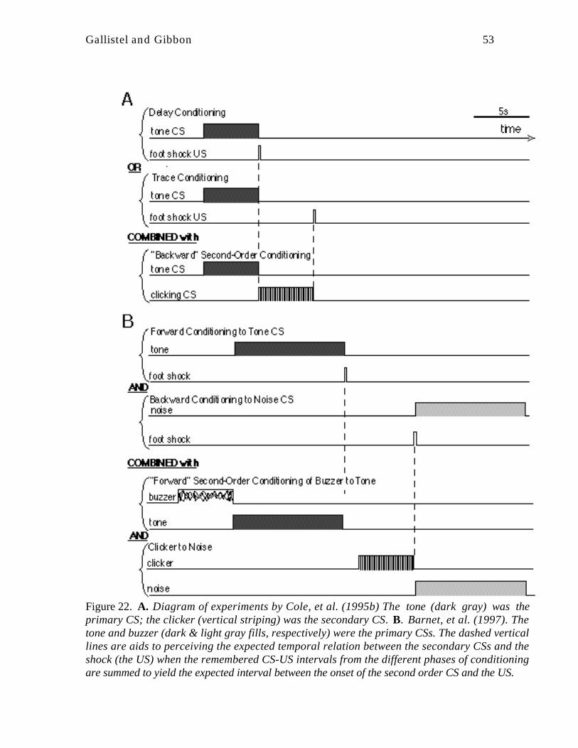
Gallistel and Gibbon 53
Figure 22. A. Diagram of experiments by Cole, et al. (1995b) The tone (dark gray) was theprimary CS; the clicker (vertical striping) was the secondary CS. B. Barnet, et al. (1997). Thetone and buzzer (dark & light gray fills, respectively) were the primary CSs. The dashed verticallines are aids to perceiving the expected temporal relation between the secondary CSs and theshock (the US) when the remembered CS-US intervals from the different phases of conditioningare summed to yield the expected interval between the onset of the second order CS and the US.

Gallistel and Gibbon 54
realize that the CS has come on, they havenothing to fear. In fact, this group showedvery little fear (very little lick suppression).But for the group that got trace conditioning,the expected interval to shock is 5 s whenthe clicker comes on. They should be afraidof the clicker and they were, despite the factthat the clicker itself was never paired withshock
The reaction to the clicker in the groupthat got primary trace conditioning followedby backward second-order conditioning wasnot significantly weaker than the reaction tothe primary CS (the tone) in the controlsubjects that got simple delay conditioning.This comparison is not entirely valid,because the clicker (the secondary CS) isgenerally found to be more potent in thiskind of conditioning than the tone used forprimary conditioning. Nonetheless, thecomparison emphasizes that the fear elicitedby combining what the animal has learnedabout the temporal relations between thethree stimuli (the tone, the clicker and theshock) during different phases ofconditioning can be a strong fear. These arenot marginal effects.
Cole, et al. (1995b) also did a sensorypreconditioning version of the experiment.Recall that in secondary conditioning theprimary protocol is given first and thesecond order second, while in sensorypreconditioning this order is reversed. Thisvariation in training order is important froman associative perspective. When the secondorder conditioning occurs before the primaryconditioning, conditioning cannot beexplained in terms of secondaryreinforcement (the idea that a CS associatedwith a US takes on the reinforcing propertiesof the US). From a timing perspective, thisvariation in procedure is of little theoretical
importance, because the learning of temporalintervals is not dependent on reinforcement.The only effect of reversing the trainingorder is that the primary conditioning phasebecomes an extinction phase for the secondorder conditioning, rather than vice versa.This is a serious consideration only if thesecond phase of conditioning (whetherprimary or second order) is prolonged. But itis not, precisely in order to avoid thisproblem. From a timing perspective, oneshould get basically the same result in thesensory-preconditioning version of thisexperiment as in the secondary conditioningversion. That was in fact the case.
Again, the strength of the fear reaction tothe clicker in the trace group was as strongas the reaction to the tone in the delaygroup, despite the fact that the tone wasdirectly paired with shock whereas theclicker was not. (Again, however, thiscomparison is somewhat vitiated by the factthat the CSs used in different roles weredeliberately not counterbalanced.) Thestrong fear reaction to the clicker wasobserved only in the group that received thesupposedly weaker form of primaryconditioning--trace conditioning. In thegroup that received the supposedly strongerform of primary conditioning, the fearreaction to the clicker was much weaker.
In these experiments, the relativestrengths of the reactions to the second orderCSs are the reverse of the relative strengthsof the reactions to the primary CSs. From anassociative perspective, these reversals areparadoxical. The reaction to the second orderCS is assumed to be mediated by the second-order and primary associations conducting inseries. The second order training was alwaysthe same in these experiments; only theprimary training differed. So, the strengthsof the reactions to the second order CSs

Gallistel and Gibbon 55
ought to be determined by the strength ofthe primary associations, which they clearlyare not.
A second experiment (Barnet et al.,1997) makes the same point. There weretwo 10-s-long CSs in the phase of primaryconditioning, one forwardly conditioned, onebackwardly conditioned (top two protocolsin Figure 22B). There was no fixed temporalrelation between these two CSs, but therewas a fixed temporal relation between eachCS and shock. Shock always occurred at theoffset of the one CS but immediatelypreceding the onset of the other CS.
In the second-order phase, two differentsecondary CSs, each 5 s in duration, wereforwardly paired with the two primary CSs(bottom two protocols in Figure 22B). Thus,the onset of one second order CS precededby 5s the onset of the forwardly conditionedprimary CS, while the onset of the othersecond order CS preceded by 5 s the onsetof the backwardly conditioned primary CS.(As in the previous experiment, there weresecondary conditioning and sensorypreconditioning versions of this experiment.)
The strengths of the fear reactions to theprimary CSs showed the usual differencebetween forward and backward conditioning,that is, reactions to the backwardlyconditioned primary CS were weaker.However, the strengths of the reactions tothe second order CSs were reversed. Thesecond order CS that predicted thebackwardly conditioned primary CS elicitedmore fear than did the second order CS thatpredicted the forwardly conditioned primaryCS.
The diagram of the temporal relationsbetween CSs and USs (Figure 22B) makesthe timing explanation of these results moreor less self-evident. What one needs to
consider is the expected interval to shock atthe onset of a CS--the comparison quantityin Scalar Expectancy Theory. In the tests ofthe primary CSs, when the forwardlyconditioned CS (the tone) comes on, theexpected interval to shock is 10s. When thebackwardly conditioned CS (the noise)comes on, however, it is 0 s. As previouslyexplained, this should result in little fear,given the decision rule specified by ScalarExpectancy Theory. On the other hand,when the secondarily conditioned buzzercomes on, which predicts the onset of thetone, the expected interval to shock is 15 s.Moreover, the onset of a still better warningstimulus--one that more precisely predictsthe shock--is expected in 5 s. When thesecondarily conditioned clicker comes on,however, the expected interval to shock isonly 5 s, and, probably more importantly,no further warning stimulus is expected,because the shock is expected before theprimarily conditioned noise. Thus, the shockis coming very soon and there will be nofurther warning.
The diagrams in Figure 22 make it clearwhy one might wish to speak of subjects’forming a temporal map during conditioning(Honig, 1981). The ability to remembertemporal intervals and to add, subtract, anddivide them--the central capabilities assumedin our timing models--gives the animalprecisely that.
A third experiment (Barnet & Miller,1996) shows the utility of the timingperspective in understanding both backwardconditioning and conditioned inhibition. Thisintricately designed experiment requires forits interpretation both Rate EstimationTheory and Scalar Expectancy Theory. Itbrings into play most of the theoreticalanalyses we have so far developed.

Gallistel and Gibbon 56
Figure 23. Schematic of experiment by Barnet and Miller (1996) in which the inhibitor CS reduces(inhibits fear), but a second-order CS, whose only connection to shock is that it predicts theinhibitor CS, nonetheless elicits (excites) fear. A consideration of the temporal relations herediagrammed makes this seeming paradox intelligible.
Recall that in Rate Estimation Theory, aCS is a conditioned inhibitor if its estimatedrate of reinforcement for that CS is negative.When a CS to which a negative subjectiverate of reinforcement is attributed ispresented together with a previouslyconditioned excitor, the negative rate ofreinforcement sums with the positive rate
attributed to the excitor. The expected rateof reinforcement is thereby reduced. Thistest--presenting the putative conditionedinhibitor together with a conditioned excitor--is called the summation test for conditionedinhibition. Recall also that in ScalarExpectancy Theory, when there is a fixedinterval between CS onset and

Gallistel and Gibbon 57
reinforcement, the expected interval toreinforcement is used to time a conditionedresponse that anticipates the reinforcement.All of these principles come into play inwhat follows.
The experiment, which is diagrammed inFigure 23, involved three training phases.The first phase forwardly conditioned anexcitor to be used in the summation test.That is, the subjects were taught to fear astimulus that predicted shock. The secondphase backwardly conditioned an inhibitorto be used in the summation test. The thirdphase paired a third CS with the so-calledinhibitor, without further shocks (secondorder conditioning of an inhibitor).
In the first phase, each presentation ofthe excitatory CS lasted 30 s and there was a1-s foot shock coincident with its offset.Thus, the expected rate of reinforcement inthe presence of this excitor was 2 shocks perminute. A prolonged phase of backwardinhibitory conditioning followed, carried outin the same chamber as the excitatoryconditioning, but with a different CS. Eachof the twelve 20-minute sessions in thisphase contained eight 30-s presentations ofthe inhibitory CS, with each presentation ofthis CS immediately preceded by a 1-sshock. The background against which theshock was presented was a flashing houselight that came on 30 s before the shock. Inthe analysis of this experiment from theperspective of Rate Estimation Theory, it isassumed that this flashing house lightconstituted the background, and that thebackwardly conditioned CS, which came onwhen the shock and the backgroundterminated, can be treated as havingsuppressed the background and, hence, therate of reinforcement predicted by it, whichwas 2 shocks per minute.
Finally, there was a phase of secondaryconditioning in which the subjects learnedthat yet another CS predicted the onset ofthe “inhibitory” CS. The reason that scarequotes now appear around inhibitory willsoon be evident. The secondary CS lastedonly 5 s, and the 30-s “inhibitory” CS cameon at its offset.
As always, the phase of secondaryconditioning was kept brief to avoidextinction of the primary conditioning. Wenote in passing, that the account ofextinction offered by Rate EstimationTheory makes it clear why this works. Inassociative theories, every non reinforcedtrial weakens the net excitatory strength ofthe CS-US associations, and the initial trialsin a series of non-reinforced trials have thegreatest weakening effect. A moderatelynumerous sequence of unreinforced trialsought, therefore, to have a big impact on the(net excitatory) strength of a CS-USassociation, but in fact such strings have nodetectable impact (Prokasy & Gormezano,1979). In the RET model of extinction, bycontrast, the first few non-reinforcedsegments of CS exposure have no effect.Extinction does not occur until the ratiobetween the interval without CSreinforcement and the expected intervalbetween CS reinforcements gets large. Untilthe subject decides that the rate ofreinforcement has changed, there is noextinction.
The secondary conditioning wasconducted in a different chamber from theprimary conditioning, as was the summationtest and the test for the subjects’conditioned response to the secondary CS.Thus, all the conditions in which shocknever occurred were run in a context thatgave the animal no reason to expect shock.

Gallistel and Gibbon 58
The summation test showed that CS thatsuppressed the flashing became aconditioned inhibitor. Presenting thisbackwardly conditioned CS together withthe excitor CS in the test phase of theexperiment diminished the subject’s fear ofthe excitor. This is the standard test forconditioned inhibition. The backwardlyconditioning experience taught the animalthat the CS suppressed an excitor. When thebackwardly conditioned CS was combinedwith another independently conditionedexcitor, it did not eliminate the fear causedby the excitor, but it did reduce it. This is tobe expected if the inhibitory power of thebackwardly conditioned CS arose from itssuppression of an excitatory “background”(the flashing light) rather than from its directsuppression of shocks themselves.
That backward conditioning shouldestablish an effective inhibitor is itselfinteresting. It shows once again that forwardtemporal pairing is not essential toconditioning. However, the theoreticallymost interesting part of this experimentcomes from the results of the test for theeffect of the secondary CS--the CS whoseonset predicted that the conditioned“inhibitor” would come on in 5 s. Thesecondary CS excited fear (manifest in astrong suppression of licking), even thoughits only connection to the shock was via aprimary CS that inhibited fear. It is thisresult that has led us to place scare quotesaround “inhibitor” and its cognates. If astimulus has an inhibitory effect on theconditioned response, then another stimulus,whose only connection to the reinforcer isthat it predicts the inhibitory stimulus,ought itself to inhibit the conditionedresponse. But it does not inhibit theconditioned response; on the contrary, itstrongly excites it.
Scalar Expectancy Theory predicts thisresult, for reasons diagrammed in Figure 23.In the backward conditioning phase, theanimal learned that the interval from theonset of the “inhibitory” CS to the onset ofshock was -1 s. In the secondaryconditioning phase, it learned that theinterval from the onset of the secondary CSto the onset of the “inhibitory” CS was 5 s.The expected interval to shock when thesecondary CS comes on should be the sumof these two intervals, which is 4 s. Thesubjects should have feared an impendingshock, and they did.
Rate Estimation Theory and ScalarExpectancy Theory are not in conflict here.Rate Estimation Theory deals only with therate of reinforcement the animal expectswhen the inhibitory CS is present. Thatexpectation is 0 shocks, because thebackwardly conditioned CS suppresses theexcitor. The rate estimation mechanism takesaccount of the analytic impossibility ofdirectly observing a negative rate. ScalarExpectancy Theory deals with a differentaspect of the animal’s decision making, thetiming of a conditioned response controlledby the expected interval to the reinforcement(the when decision, in contrast to thewhether decision). Scalar ExpectancyTheory gives (in part) a quantitativeformalization of Honig’s (1981) TemporalMap and Miller’s (Miller & Barnet, 1993)Temporal Coding Hypothesis. Intuitively,any animal with a temporal map--any animalthat has learned the temporal relationsbetween the various stimuli--will show whatBarnet and Miller (1996) found, as thediagram in Figure 23 makes clear. Theirfindings are not surprising if it is assumedthat knowledge of the temporal intervals inconditioning protocols is the foundation ofconditioned behavior.

Gallistel and Gibbon 59
In a second version of this experiment,Barnet and Miller (1996) added an extinctionphase following the backward conditioningphase. In this version, the animal was firsttaught that a shock immediately precededthe onset of the “inhibitory” CS (thebackward conditioning phase) and then thatthis was no longer true (the extinctionphase). In the extinction phase, the“inhibitory” CS was repeatedly presented inthe absence of shock--and (importantly) alsoin the absence of the flashing light thatpresaged shock (the effective backgroundstimulus for the shock experience during thebackward conditioning). From a timingperspective, the extinction phase shouldpersuade the animal that, while it once wastrue that the inhibitory CS was preceded bya shock, that is no longer true. However, thisshould not affect the animal's estimate of thepower of the backwardly conditioned CS tosuppress an excitatory background stimulus(the flashing light), because this stimuluswas absent during extinction. The extinctionexperience, if anything, confirmed that whenthe "inhibitory" CS was present, thethreatening flashing light was not present.
This second version of the experiment(the version with an interpolated extinctionphase) emphasizes the importance of thedistinction between the whether decision andthe when decision. The extinction phaseremoves the expectation that is used in theexcitatory when decision. This whendecision leads to a fear response to thesecondary CS (and the consequentsuppression of licking). But the extinctiondoes not remove the expectation that makesthe primary CS an effective conditionedinhibitor, the expectation that the primaryCS can suppress CSs that predict shock,thereby lowering the expected rate of shockreinforcement.
The results from this second version(with interpolated extinction) were asexpected from the joint application of ScalarExpectancy Theory and Rate EstimationTheory. The extinction phase did not affectthe results of the summation test. Despitethe intervening extinction phase, presentingthe “inhibitory” CS together with the excitordiminished the subjects’ fear of the excitor,thereby moderately reducing the amount oflick suppression, just as in the versionwithout an extinction phase. The extinctionphase, however, greatly reduced the animals’fear of the secondary CS. Thus, theextinction phase removed the basis for theanticipatory reaction to the secondary CS(the reaction that occurs before the primaryCS comes on), without removing the basisfor the reduction in fear caused by the actualpresence of the “inhibitory” CS.
Further versions of this basic experimentreplaced the backward conditioning of theinhibition with a phase of conventional,feature-negative inhibitory conditioning. Inthis more conventional protocol, the“inhibitory” effect of one CS was created bypairing that CS from time to time with anotherwise reinforced CS (hence, an excitor)and omitting the reinforcement on thosetrials. Historically, this is the procedure,first employed by Pavlov himself, whichgave rise to the concept of a conditionedinhibitor. The CS that predicts the omissionof reinforcement becomes a conditioned“inhibitor.”
The use of the more conventionalprocedure for establishing conditioned“inhibition” eliminates the expectation thatfigured in the previously describedprediction, because there no longer is a fixedtemporal interval between the onset of the“inhibitory” CS and the onset of thereinforcer. Scalar Expectancy Theory only
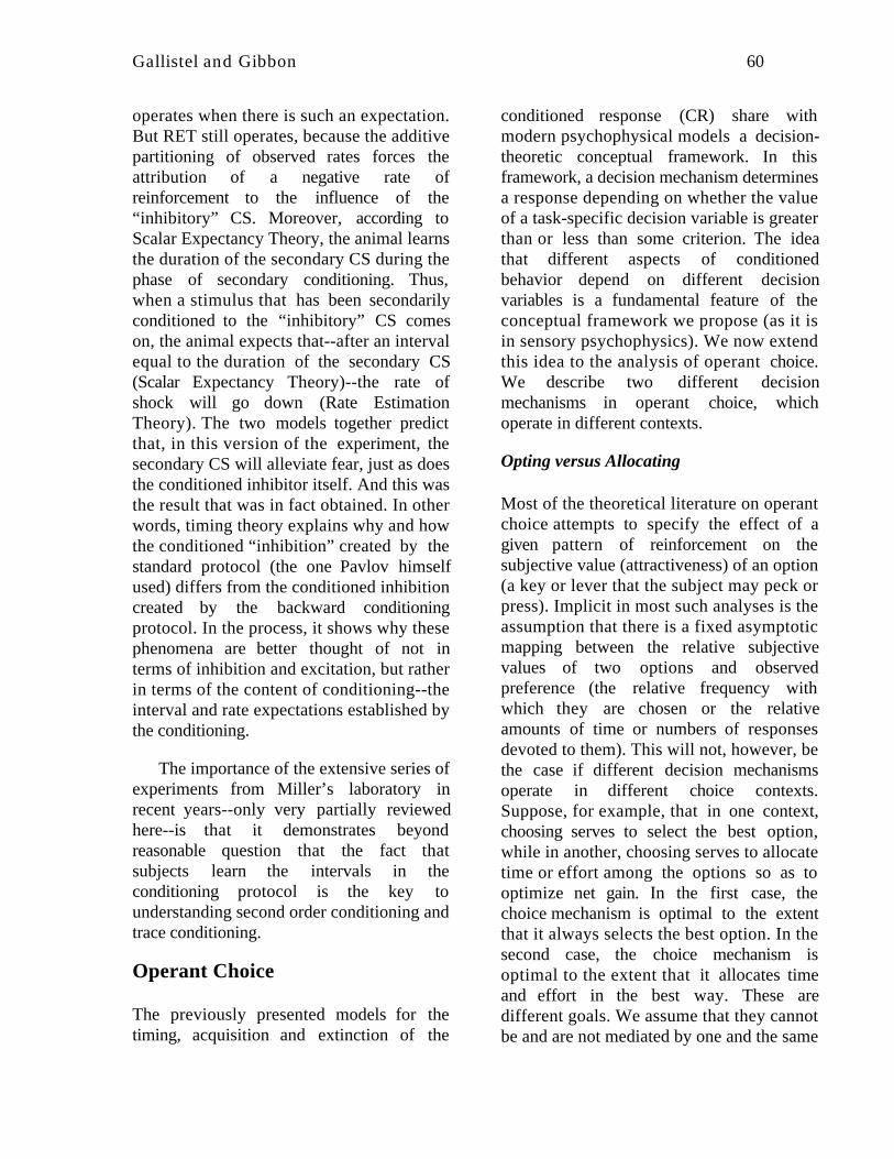
Gallistel and Gibbon 60
operates when there is such an expectation.But RET still operates, because the additivepartitioning of observed rates forces theattribution of a negative rate ofreinforcement to the influence of the“inhibitory” CS. Moreover, according toScalar Expectancy Theory, the animal learnsthe duration of the secondary CS during thephase of secondary conditioning. Thus,when a stimulus that has been secondarilyconditioned to the “inhibitory” CS comeson, the animal expects that--after an intervalequal to the duration of the secondary CS(Scalar Expectancy Theory)--the rate ofshock will go down (Rate EstimationTheory). The two models together predictthat, in this version of the experiment, thesecondary CS will alleviate fear, just as doesthe conditioned inhibitor itself. And this wasthe result that was in fact obtained. In otherwords, timing theory explains why and howthe conditioned “inhibition” created by thestandard protocol (the one Pavlov himselfused) differs from the conditioned inhibitioncreated by the backward conditioningprotocol. In the process, it shows why thesephenomena are better thought of not interms of inhibition and excitation, but ratherin terms of the content of conditioning--theinterval and rate expectations established bythe conditioning.
The importance of the extensive series ofexperiments from Miller’s laboratory inrecent years--only very partially reviewedhere--is that it demonstrates beyondreasonable question that the fact thatsubjects learn the intervals in theconditioning protocol is the key tounderstanding second order conditioning andtrace conditioning.
Operant Choice
The previously presented models for thetiming, acquisition and extinction of the
conditioned response (CR) share withmodern psychophysical models a decision-theoretic conceptual framework. In thisframework, a decision mechanism determinesa response depending on whether the valueof a task-specific decision variable is greaterthan or less than some criterion. The ideathat different aspects of conditionedbehavior depend on different decisionvariables is a fundamental feature of theconceptual framework we propose (as it isin sensory psychophysics). We now extendthis idea to the analysis of operant choice.We describe two different decisionmechanisms in operant choice, whichoperate in different contexts.
Opting versus Allocating
Most of the theoretical literature on operantchoice attempts to specify the effect of agiven pattern of reinforcement on thesubjective value (attractiveness) of an option(a key or lever that the subject may peck orpress). Implicit in most such analyses is theassumption that there is a fixed asymptoticmapping between the relative subjectivevalues of two options and observedpreference (the relative frequency withwhich they are chosen or the relativeamounts of time or numbers of responsesdevoted to them). This will not, however, bethe case if different decision mechanismsoperate in different choice contexts.Suppose, for example, that in one context,choosing serves to select the best option,while in another, choosing serves to allocatetime or effort among the options so as tooptimize net gain. In the first case, thechoice mechanism is optimal to the extentthat it always selects the best option. In thesecond case, the choice mechanism isoptimal to the extent that it allocates timeand effort in the best way. These aredifferent goals. We assume that they cannotbe and are not mediated by one and the same

Gallistel and Gibbon 61
choice mechanism. Rather, the animalinvokes different choice mechanisms,depending on what it has learned about thecontext. We call choice behavior mediated bythe first mechanism opting behavior andchoice behavior mediated by the secondmechanism allocating behavior.
The Opting Decision
The desirability of distinguishing betweenopting and allocating became apparent in thecourse of a "failed" experiment. Theexperiment was intended to be a variant ofthe well known matching paradigm in whichsubjects choose between two manipulandareinforced by concurrent variable interval(VI) schedules. These schedules makereinforcement available at a variable intervalfollowing the collection of a precedingreinforcement. Usually, the distribution ofintervals is approximately exponential.Schedules are said to run concurrently whentwo response options are presentedcontinuously and simultaneously, eachreinforced on its own schedule. Theparadigm models the situation that a foraginganimal faces when it must allocate itsforaging time among patches that differ infood density. Herrnstein (1961) discoveredthat, under these circumstances, the ratio ofthe dwell times and responses allocated tothe options during a session tended to matchthe ratio of the reinforcements obtained fromthem. The study and analysis of this"matching" phenomenon has formed asubstantial part of the experimental andtheoretical literature on operant choice in thelast four decades (Commons, Herrnstein &Rachlin, 1982; Davison & McCarthy, 1988;Herrnstein, 1991; Herrnstein & Prelec, 1991;Nevin, 1982).
In the failed version of this experiment,pigeons were first trained with the keyspresented one by one rather than together.
Six pigeons received 25 sessions of initialtraining in which each of two differentlyilluminated keys (red, green) were presented15 times per session. Each time a key waspresented, it remained on until the pigeonhad collected a reinforcement from it. Theamount of time that elapsed on any one trialbetween the illumination of the key, whichsignaled its availability as an option, and thearming of the reinforcement mechanismvaried from trial to trial in accord with theintervals programmed into a standard VIscheduling tape. The average scheduledinterval depended on which key wasilluminated; it was 20 s when the red keywas illuminated, 60 s when the green keywas. When these subjects were then shiftedto concurrent training (both keys illuminatedat the same time), they did not show adegree of preference for the richer key thatmatched its relative richness (i.e., a 3:1preference). All 6 birds preferred the richerkey exclusively; they almost never chose theleaner key. This is called overmatching.Overmatching is seldom observed whenconcurrent VI schedules constitute theoptions, and this degree of overmatching--98% to 100% choice of the richer schedule insix out of six subjects-- is without publishedprecedent. The effect of the initial training,with each key presented separately, onsubsequent preference under concurrentconditions was robust and enduring. Threeof the six subjects showed exclusivepreference for the richer key throughout 25sessions of concurrent training.
Related experiments in this seriesshowed that breaking the usually continuousconcurrent-schedules paradigm up intodiscrete trials, each trial terminating in areinforcement on one or the other of the twosimultaneously operative keys, did notproduce overmatching. On the contrary, itreliably produced some degree ofundermatching, provided that the schedule

Gallistel and Gibbon 62
on the key not being pecked elapsed in thediscrete trial procedure exactly as in thecontinuous procedure, that is, provided thatthe concurrent intervals did not begin anewwith each trial. Thus, it was presumably thepresentation of the options individuallyduring initial training, not the breaking up ofthe experience with each key into discrete 1-reinforcement trials that resulted in anexclusive preference for the richer key. Asimilar result was obtained by Edmon,Lucki, & Grisham (1980), who trainedpigeons on multiple VI schedules--a protocolin which only one schedule is available atany one time, with the different schedulessignaled by different key lights. When thesesubjects were tested with keys presentedconcurrently, they showed almost exclusivepreferences for the keys that signaled thericher of the two choices. These findings callinto question the assumption that matchingbehavior is the result of the relative strengthsof the responses.
We suggest that in the course of theinitial training, the subjects in theseexperiments learned that this was not acontext that permitted the allocation ofbehavior among concurrent options. On ourmodel, the opting mechanism mediateschoice between mutually exclusive options,options that cannot be concurrentlyexploited. Our model for the decisionprocess that operates in such contexts is thesignal-detection model for forced choicesbased on noisy decision variables. Theexpected delays of reinforcement for the twooptions are represented internally by(memory) signals with scalar samplingvariability (Figure 24). The rememberedinterval for a given option--the signalgenerated for that option when memory isconsulted--varies from one consultation ofmemory to the next. The decisionmechanism reads (samples) memory to getthe value associated with each option and it
Figure 24. The signal-detection conceptionapplied to choice behavior in an optingcontext. The signals representing theparameters of the outcome (in this case, theinterval between reinforcements) have scalarvariability (noise). To the extent that theprobability density functions for thedistributions of these signals overlap, thereis some likelihood that, on a given choicetrial, the subject will be mistaken aboutwhich is the better option. Such mistakes aredue to sampling error.
always chooses the option with the lowersampled value. The choice of the optionwith the longer interreinforcement intervaloccurs only as a result of sampling error,that is, only on trials on which the sampledsignal for the leaner option happens to beshorter than the sampled signal for the richeroption. Thus, when the distributions fromwhich the choice mechanism is sampling arewell separated, the leaner option is almostnever chosen. That is why pigeons trainedwith only one VI option available at any onetime, almost invariably chose the richer ofthe two options when they are subsequentlyoffered as concurrently exploitable options.The subjects’ choice behavior is no longermediated by the decision process used toallocate behavior among concurrentlyexploitable options, because it has learnedthat these options are not concurrentlyexploitable.

Gallistel and Gibbon 63
Computational Sources of Non-NormativeOpting
In the framework we propose, the sources ofnon-normative decision making are to besought in the idiosyncracies of the processesthat compute the decision variables. Thedecision variables in opting behavior areexpected (subjective) incomes. Thesubjective income from a singlereinforcement is the subjective magnitude ofthat reinforcement divided by its subjectivedelay. If the reinforcers are appetitive(positive reinforcement), then the optionwith the greatest average subjective incomeis prefered; if the reinforcers are aversive(negative reinforcement), then the optionwith the smallest average subjective incomeis prefered. However, the computation ofsubjective income has repeatedly beenshown to depart from the normative in twoways: 1) Only the intervals when areinforcement is pending are taken intoaccount. We call this the principle ofsubjectively sunk time. 2) When the amountand delay of reinforcement varies, theaverage subjective income is the expectationof the ratios rather than the ratio of theexpectations (Bateson & Kacelnik, 1996).The ratios in question are the ratios betweenthe magnitudes and the delays ofreinforcement. Each such ratio is an incomedatum. It is a well established experimentalfact that laboratory animals average incomedata in computing the expected subjectiveincome for an option. This is commonlycalled hyperbolic discounting or harmonicaveraging. On the one hand, this findingsupports our contention that the rate ofreinforcement (the reciprocal of the delay) isthe fundamental variable in conditioning(rather than probability of reinforcement),because, when reinforcement magnitude doesnot vary, averaging income data is equivalentto averaging rate data. On the other hand,
this way of computing the average subjectiveincome can cause the resulting subjectiveexpectation to depart arbitrarily far from thetrue expectation, so it is decidedly non-normative. This departure from whatnormative considerations would lead one toexpect is perplexing.
Subjectively Sunk Time.
The intertrial intervals when no option ispresent, the latencies to choose, and theintervals devoted to consuming (or otherwisedealing with) the reinforcements are nottaken into account in computing theexpected income (Bateson & Kacelnik, 1996;Mazur, 1991). In our model, the cumulativeinterreinforcement interval timer does notrun during these intervals; it only runs whena reinforcement is pending. We call thesesubjectively sunk times by analogy to themicroeconomic concept of a sunk cost. Asunk cost is a cost that appears to berelevant to the computation of the utility ofan alternative but in fact is not and ought tobe ignored in rational (normative) economicdecision making. A subjectively sunkinterval is an interval that is not included inthe computation of subjective income.
Subjectively sunk intervals are notnecessarily objectively sunk intervals, andthis discrepancy can lead to strongly non-normative preferences. Suppose, forexample, that the animal is repeatedlyallowed to choose between food rewards Aand B, where the magnitude of A is always1.5 times the magnitude of B, but the delayof B--the latency between choice andreceipt, that is, the time when the reward ispending-- is 0.5 times the delay of A. If theanimal chooses B, it gets its reward 50%sooner, but what it gets is only 2/3 of whatit would have got had it chosen A. Suppose,as is commonly the case, that session time isfixed and/or that the intervals during which

Gallistel and Gibbon 64
reinforcements are pending account for onlya small proportion of session time. Underthese conditions, reductions in the averageamount of time during which reward ispending are offset by increases insubjectively sunk time (intertrial intervals)during which no reward is pending, soshortening the average delay between choiceand reinforcement (the interval when areinforcement is pending) has negligibleeffect on the the objective income, that is, onthe amount of reinforcement per unit ofsession time. Under these circumstances, therational decision maker should stronglyprefer the bigger reward as opposed to theone that is delivered more quickly. Therational decision maker should not treat theintertrial intervals and the decision times assunk intervals. But, because the delay-of-reinforcement timer does not run duringthese intervals, subjects strongly prefer thequicker reward. This irrational preference forthe quicker but smaller reward has beentermed a lack of self-control brought on bythe prospect of immediate reinforcement(Rachlin, 1974, 1995). From a timingperspective, it is a consequence of theprinciple of subjectively sunk times andhyperbolic discounting.
Hyperbolic Discounting andHarmonic Averaging.
The principle that the decision variables onwhich opting is based are subjectiveincomes--subjective reinforcementmagnitudes divided by interreinforcementintervals--is equivalent to the hyperbolicdiscounting principle, which has often beenused to describe the effect of delayingreinforcement on the subjective value of thereinforcement (Fantino, 1969; Killeen, 1982;Mazur, 1984; Mazur, 1986; McDiarmid &Rilling, 1965; Rilling & McDiarmid, 1965).In Mazur's (1984) formulation
V =A
1+ kD, (3)
where V is the value of a reward (positivereinforcement), A is amount (magnitude),and D is the delay. This may be rewritten as
V =A
D+ ′ k ,with ′ k =
1
k,
which reduces to magnitude (amount)divided by interreward interval (delay) whenk' is zero (or negligibly small relative to D).
Equation (3) is a necessary modificationof the income formula when it is applied tovery short delays. Without the 1 in thedenominator the income produced by a givenamount of food would go to infinity as thedelay went to zero. Clearly, as the delaybecomes negligible, the income ought tobecome asymptotically equal to thesubjective magnitude of the food. This isaccomplished by adding the one to thedenominator. Psychologically, this may bethought of as taking into account that belowsome value, differences in the objective delayare psychologically negligible. Put anotherway, delays are scaled relative to the delaythat is perceived as immediate, that is, aslasting no longer than a single unit ofsubjective time. The irreducible unit of timemay also be thought of as the latency tobegin timing a delay (see Gibbon et al.,1984). If the reinforcement is delivered inless than this latency, then it has negligibledelay.
When an option sometimes produces onedelay and sometimes another, the expecteddelay of reinforcement that governs optingdecisions is the harmonic average (Bateson &Kacelnik, 1996, 1995; Brunner and Gibbon,1995; Brunner et al., 1994; Gibbon, Church,Fairhurst & Kacelnik, 1988; Killeen, 1968;McDiarmid & Rilling, 1965; Mazur, 1984;Schull, Mellon & Sharp, 1990). The

Gallistel and Gibbon 65
harmonic average of a series ofinterreinforcement intervals is the reciprocalof the average of the reciprocals. Thereciprocal of an interreinforcement interval isa rate (the rate-interval duality principle).Thus, this well established and surprisingway of computing the expectations thatgovern opting behavior is equivalent tocomputing the rate of reinforcementassociated with each delivery (the reciprocalof the interval by which delivery wasdelayed), averaging these rates, and thentaking the reciprocal of that average to obtainthe expected delay of reinforcement.
It does not matter whether one is pittinga variable delay against a fixed delay ofreinforcement or a probabilistic reinforce-ment against a certain reinforcement(delivered at a fixed delay). Withprobabilistic reinforcement, each occurrenceof a given option, i.e., each occurrence of agiven discriminative stimulus, is reinforcedwith some probability less than 1. From atiming perspective, this is another way ofproducing a variable interval schedule ofreinforcement. Timing theory assumes thatthe brain processes probabilisticreinforcement schedules as if the relevantvariable was the rate of reinforcement, notits probability. Thus, the hyperbolicequation that predicts the results ofexperiments titrating a fixed-delay optionagainst a VI option should also predict theresults of experiments that titrate a fixed-delay option against a probabilisticallyreinforced option, and this is, indeed, thecase (Mazur, 1989; Rachlin, Logue, Gibbon& Frankel, 1986; Rachlin, Raineri & Cross,1991).
The harmonic average of different delaysis always shorter than the arithmetic average.Thus, harmonic averaging yields theexperimentally well documented preferencefor a variable delay of reward (positive
reinforcement) over a fixed delay with thesame (objective) expectation (Autor, 1969;Davison, 1969; Fantino, 1969; Herrnstein,1964; Mazur, 1984; Pubols, 1962). As thisexample illustrates, the averaging of incomedata leads to non-normative opting behavior.The normative (correct) way to computeexpected income is to divide averagemagnitude (the expected magnitude) byaverage interrinforcement interval (theexpected delay of reinforcement). Thisquantity is the ratio of the expectations.What subjects do instead is average theincome data, that is, they compute theexpectation of the ratios (magnitude/delay).Why they do so is a mystery (cf Bateson &Kacelnik, 1996).
Matching and the Allocating DecisionMechanism
Many discussions of matching behavior--and, in particular, the controversy overmatching versus maximizing-- rest, webelieve, in part on the implicit assumptionthat rational choice should always take theform of an opting decision, that is, themechanism should always choose thesubjectively better alternative, within thelimits established by the noise in thedecision variables. Part of the fascination ofmatching behavior for students of choice andrational decision making is that it appears toviolate this principle; the animal frequentlyleaves the better alternative for the pooreralternative. It does so even when thealternatives differ greatly in richness, so thatdiscrimination failure is unlikely to be asignificant factor. We have just seen thatwhen birds are first given the VI schedules asmutually exclusive options, theysubsequently almost never confuse thepoorer with the better option, even foroptions whose expectation differs by afactor of only 3. Matching, by contrast, is

Gallistel and Gibbon 66
obtained with much greater differences thanthat (Figure 29).
It is not obvious, however, that eitherthe subject or the theorist should attend tothe average rates of reinforcement. In aconcurrent VI schedule, when the schedulingmechanism times out, the scheduledreinforcement is held for the subject tocollect whenever it next responds on themanipulandum. The longer the subject hasbeen away from a manipulandum, the morecertain it is that a reinforcer has beenscheduled on it. Thus, the longer a subjecthas stuck with one choice, the more certain itis that, at that moment, the other choice islikely to pay off. This consideration is thefoundation of the local maximizing accountsof matching behavior (Shimp, 1969). In thisaccount, the subject learns the relationbetween time away from a manipulandumand probability of immediate pay-off. Itleaves the richer option for the leaner whenit estimates the momentary probability of apay-off from the leaner option to be higherthan the momentary probability of a pay-offfrom the richer option. This account adheresto the principle that the decision mechanismalways chooses what appears to be thebetter option at the moment of choice.
Local maximizing accounts of matchingmust be distinguished from globalmaximizing accounts (Baum, 1981; Rachlin,1978; Staddon & Motheral, 1979). The latteremphasize the important point thatmatching (on concurrent variable intervalschedules and in many other situations) isthe rational way to behave in that itmaximizes overall return. Because immediatereward is reliably available at the leaneralternative if it has long gone unvisited,subjects should leave the richer alternativefor the leaner from time to time. Adaptiveadvantage is very likely the ultimate(evolutionary) cause of matching behavior.
The question is, what is the proximate causeof the decisions to leave the richer alternativefor the leaner. Global maximization is atheory about ultimate causation, whereaslocal maximization is a theory of proximate(or 'molecular') causation, as is the modelthat we propose.
Our model of the decision process inmatching rests on three well establishedexperimental findings: the stochastic natureof visit termination, the effect of relative rateof reinforcement on the likelihood of visittermination, and the effect of the overall rateof reinforcement on the likelihood of visittermination. It builds on earlier theorizingthat treats the likelihood of visit termination--hence, the rate of switching between theoptions--as the fundamental dependentvariable (Myerson & Miezin, 1980; Pliskoff,1971). Ours is a model of the decisionprocess that terminates a visit.
Leaving is stochastic. The localmaximizing account predicts that thelikelihood of the subject's switching fromone option to the other increases with theduration of its stay (the interval duringwhich it remains with one option, also calledthe dwell time). However, Heyman (1979)showed that the momentary probability of achangeover from one option to the other wasconstant; it did not vary as a function of thenumber of responses that the pigeon hadmade on the key it was currently pecking(Figure 25). This means that the rate ofswitching (the momentary likelihood of visittermination) does not change as stayduration increases. That in turn implies thatthe frequency of visits terminating at a givenduration declines by a fixed percentage foreach increment in duration. In other words,the frequency of observed departures shouldbe an exponential function of dwell time,which it is (Figure 26).

Gallistel and Gibbon 67
Figure 25. The probability of a changeover key response (a switch to the other option) as afunction of the number of responses since the last changeover. Note that probability increases littleif at all with the length of the run, despite fact that the longer the run, the more certain it is thatthere is a reinforcement waiting to be collected from the other option. Note also that the lower theprobability of switching, the longer runs last. Expected run length is the reciprocal of the switchingprobability (leaving rate) {Reproduced from Figs 3 & 4 on pp. 45 & 46 of Heyman, 1979. bypermission of author & publisher.}
The discovery that the likelihood ofleaving an option at any one momentdepends only on the average rates ofreinforcement, and not on the momentary
likelihood that the switch will be reinforced,led Heyman (1979; 1982) to suggest that thedecision process in matching was an elicited(unconditioned) Markov process, in which

Gallistel and Gibbon 68
average rates of reinforcement directlydetermine the momentary likelihoods of thesubject's leaving one option for the other.(These momentary likelihoods are hereaftercalled the leaving rates.) Heyman argued thatmatching is not conditioned in the Skinnerianor operant sense, that is, it is not shaped bythe prior consequences of such behavior in
such a situation (the law of effect); it issimply what the animal is built to do given acertain input. The suggestion that matchingis "unconditioned" behavior is very much inthe spirit of our models. In our models, aninnate (unconditioned) decision mechanismdetermines what the animal will do given theinterreinforcement intervals in its memory.
Figure 26. Dwell time distributions (frequency of stays of a given duration plotted againstduration) averaged over 6 subjects. The ordinate is logarithmic, so the linear decline seen afterthe changeover duration implies an exponential distribution of stay durations The slope of theregression line through the linear decline is proportional to the leaving rate (momentarylikelihood of a departure). The leaving rate depends on the rate of reinforcement available in thealternative schedule; hence, it is approximately 4 times greater when a VI 40 s schedule has beenpaired with a VI 20 s schedule (lower left panel) than when the same schedule has been pairedwith a VI 80 s schedule (upper right). Notice, also, that the leaving rate is unchanged on the probetrials, when a different alternative is offered. What matters is the remembered alternative rate of

Gallistel and Gibbon 69
reinforcement, not the alternative offered on the probe trial (Replotted, with recomputedregression lines, from data in Fig. 4 on p. 213 of Gibbon, 1995.)
Effects of relative and overall rates ofreward on leaving rate. Heyman (1979) alsonoted an important property of the leavingrates, namely, that they summed to aconstant. Myerson and Miezin (1980)showed that the same was true in the data ofBaum and Rachlin (1969). They furtherconjectured that the value of the constant towhich the leaving rates summed would be anincreasing function of the overallreinforcement rate (the sum of the tworeinforcement rates). As they noted, thisassumption is incorporated into Killeen's(1975) model of choice in the form of anarousal factor, which depends on the overallrate of reinforcement. These arousalassumptions make intuitive sense becausethe greater the sum of the leaving rates, themore rapidly the subject cycles through theoptions. To collect reinforcements from bothoptions at close to the rate at which theybecome available, the duration of a visitcycle (the time consumed in sampling bothoptions) must be no longer than the averageoverall interval between reinforcements. Thisinterval--the expected interval betweenreinforcements without regard to source--isthe reciprocal of the sum of the rates ofreinforcement at the different sources. Onthe other hand, it is a waste of effort to cyclebetween the options many times during oneexpected interreinforcement interval. Thusthe time taken to cycle through the optionsshould depend on the expected intervalbetween reinforcements, and it does (Figure27).
Effect of relative reward magnitude onleaving rate. Although reinforcementmagnitude has no effect on rate ofacquisition, it has a dramatic effect onpreference (Figure 28). Indeed, it has a scalar
Figure 27. Cycle duration as a function of theexpected interval between programmedreinforcement in 6 self-stimulating rats, withconcurrent and equal VI schedules of brainstimulation reinforcement. The overall rateof reinforcement changed, both betweensessions and once in each 2-hour session.The expected interreinforcement interval isthe reciprocal of the expected overall rate ofreinforcement, which is the sum of thereciprocals of the two VIs. The cycle durationincludes the changeover (travel time),(Unpublished data from Mark, 1997, Ph.D.thesis.)
effect, that is, relative stay durations arestrictly proportional to relative rewardmagnitudes. Catania (1963) reportedmatching when the relative magnitude of thereinforcements was varied rather than theirrelative rate. When the obtained rates ofreinforcement were approximately equal butthe duration of food access perreinforcement was, for example, twice asgreat on one side, pigeons spentapproximately twice as much time on theside that produced double the income. The

Gallistel and Gibbon 70
income from an option is the amount ofreward obtained from that option per unit oftime in the apparatus, not per unit of time ornumber of responses invested in that option.The latter quantity, amount of reward perunit of time invested in an option (or perresponse), is the return. The distinctionbetween income and return is crucial in whatfollows. Note that it is possible to have alarge income from a low return investmentand a small income from a high returninvestment.
The average income is the product of theaverage rate at which rewards are obtainedand the average magnitude of a reward. Putanother way, the income from an option isproportional to the rate of reinforcement ofthat option, with the reinforcementmagnitude as the constant of proportionality(scaling factor), and rate of reinforcementspecified in units of session time (not timedevoted to the option). Expected income isthe same quantity that Gibbon (1977) calledexpectancy of reinforcement and symbolizedas H, which symbol we will use here.
Catania's result implies that it is relativeincome that matters in matching behavior,not rate or probability of reinforcement.Moreover, if the same result--time-allocationratios that match income ratios--is obtainedover a wide range of relative magnitudes ofreinforcement, that is, if the effect of therelative magnitude of reinforcement isindependent of the effect of relative rate ofreinforcement, then strong conclusionsfollow: 1) Subjective rate and subjectivemagnitude are simply proportional toobjective rate and magnitude. 2) Subjectiverates and subjective magnitudes combinemultiplicatively to determine subjectiveincomes, which are the decision variablesthat determine how time is allocated amongalternatives. 3) The observed time-allocationratio is equal to the ratio of the subjective
incomes, that is, the ratio of the expectedstay durations equals the ratio of theexpectancies. These are strong conclusionsbecause they assert maximally simplerelations between observed objectivequantities (rates and magnitudes ofreinforcement and time-allocation ratios) andinferred quantities in the head (subjectiverates, subjective magnitudes and the ratios ofsubjective incomes).
Keller and Gollub (1977) varied bothrelative reinforcement magnitude (duration ofthe bird's access to the grain hopper) andrelative rate of reinforcement. They foundthat, for some training conditions at least,the time-allocation ratio was approximatelyequal to the income ratio (Figure 28B; seealso Harper, 1982, for a similar result undergroup conditions). This has not beenconsistently replicated (e.g., Logue &Chavarro, 1987; see Davison, 1988, forreview), although none of the failures toreplicate has varied both relativereinforcement magnitude and relativereinforcement rate over a large range, so it isdifficult to know how seriously to take theobserved departures from matching.
Recently, Leon and Gallistel (1998)tested the extent to which the effect ofvarying the relative rate of reinforcementwas independent of the relative magnitude ofthe reinforcers. They used brain stimulationreward and varied reinforcement magnitude,M, by varying the pulse frequency in the 0.5s trains of pulses that constituted individualreinforcements. Thus, the relative magnitudeof the reinforcement was varied withoutvarying reinforcement duration. On one side(the F side), the reward magnitude was fixed;on the other (the V side), the rewardmagnitude varied from one 10-minute trial tothe next. It varied from a level near thethreshold for performance to the saturationlevel, which is the largest possible reward

Gallistel and Gibbon 71
produceable in a given subject by stimulating through a given electrode.
The programmed relative rate of rewardvaried from 4:1 in favor of the F side to 1:4in favor of the V side. The actually obtainedrate ratio, λv/λf, varied by about 2 orders ofmagnitude, from about 10:1 in favor of the Fside to about 1:10 in favor of the V side.Thus, the experiment tested the extent towhich the ratio of times allocated to the F
and V sides remained proportional to therelative obtained rate of reward in the face oflarge differences in the relative magnitude ofreward. These large differences in themagnitudes of the rewards produced largedifferences in the extent to which the animalpreferred one side or the other at a givenrelative rate of reward.
Figure 28 A. Times allocated tocompeting levers delivering brain-stimulation rewards on concurrentvariable interval schedules to a ratmoving back and forth between them soas to exploit them both. The magnitude ofthe rewards delivered on the F side wasfixed. The magnitude of the rewards onthe V side was varied from one 10-minutetrial to the next by varying the pulsefrequency in the 0.5 s trains of rewardingpulses. Preference varies from a strongpreference for the F side to a strongpreference for the V side, depending onthe magnitude of the V reward. Thestrength of the preference is the ratio ofthe two time allocations. (Reproducedwith slight modifications from Leon &Gallistel, 1998) B. Preference for theL(eft) key over the R(ight) key in a pigeonresponding on concurrent variableinterval schedules, as a function of therelative incomes. Relative income is theproduct of the ratio of the rewardmagnitudes (underlined) and the ratio ofthe experienced rates of reward:HL HR = λL λ R( ) ML MR( ) Thepreshift data are from initial controlsessions in which the scheduled rates ofreinforcement and the reward magnitudeswere both equal. (Data from Keller &Gollub, 1977)

Gallistel and Gibbon 72
Leon and Gallistel found that changingthe relative rate of obtained reward by agiven factor changed the time-allocation ratioby about the same factor, regardless of therelative magnitudes of the reward (exceptwhen one of the reward magnitudes was
close to the threshold for performance).Over about three orders of magnitude (fromtime allocation ratios of 30:1 to 1:30), thetime allocation ratio equaled the ratio ofsubjective incomes (Figure 29).
Figure 29. The log of the time-allocation ratio plotted against the log of relative income for 6 ratsresponding for brain stimulation reward on concurrent VI schedules, with relative rate of reward,

Gallistel and Gibbon 73
λv/λf, and relative subjective reward magnitude, Mv/Mf, varying over about two orders ofmagnitude (1:10 to 10:1). The different symbols identify different sub-conditions. The gray linesrepresent the identity function , which has a slope of 1 and an intercept at the origin. (Modifiedslightly from Leon & Gallistel, 1998)
The when to leave decision. The findingsjust reviewed imply that allocating behavioris mediated by a stochastic decisionmechanism in which the leaving rate for oneoption is determined by the subjectiveincomes from it, and from the other options.Mark and Gallistel (1994) suggested a modelfor the when-to-leave decision that directlyincorporates these principles. Their modelmay be seen as a further development of amodel by Myerson and Miezin (1980). Thedecision to leave is generated by a Poissonprocess (a process formally equivalent to theprocess of emitting a particle in the course ofradioactive decay). The leaving rate(emission rate) is assumed to be determinedby the incomes from the two options, inaccord with two constraints. One constraintis that the ratio of the leaving rates equal theinverse ratio of the incomes. We formulatethis constraint in terms of expected staydurations rather than leaving rates, becausethe symbol for the leaving rate on side iwould naturally be λi , but we have alreadyused that symbol to represent thereinforcement rate on that side. Also, it isthe stay durations that are directlymeasured. Recall that the expected stayduration, E(d), is the reciprocal of the leavingrate. Therefore, the first constraint is
E(d1) E(d2) = H1 H2 (4)
The other constraint is that the sum of theleaving rates (that is, the sum of thereciprocals of the expected stay durations)be proportional to the sum of the subjectiveincomes:
1
E(d1)+
1
E(d2)
= c H1 + H2( ) (5)5
In practice, the sum of the leaving rates(departures per minute of time spent at oneor another lever) appears to be a linearlyincreasing function of the sum of theincomes (Figure 30). The slope and interceptvary appreciably between subjects. Thus, afurther test of this explanation would be todetermine whether the magnitude of thepreference observed on the probe trials inindividual subjects can be more accuratelypredicted if one separately determines foreach subject the function relating the sum ofthe leaving rates to the sum of thereinforcement rates.
Whereas Mark and Gallistel (1994) builtthe empirically derived constraints directlyinto the structure of the mechanism thatmakes the when to leave decision, Gibbon(1995) suggested a psychological mechanismfrom which these principles may be derived.He proposed that the decision to leave isbased on repetitive sampling from thepopulation of remembered incomes. (Recallthat each individual reward gives rise to aremembered income or reinforcementexpectancy, which is equal to the subjectivemagnitude of the reward divided by thesubjective duration of the interval required toobtain it.) The subject leaves the option it iscurrently exploiting whenever the incomesample for the other option is greater thanthe sample from the population for the
5The formulation of this assumption in Mark andGallistel (1994) contains a mathematical error, whichis here corrected.

Gallistel and Gibbon 74
currently exploited option. When it is not,the subject stays where it is (so-calledhidden transitions). Gibbon further assumedthat the rate at which the subject samplesfrom the populations of rememberedincomes (called its level of "arousal") isproportional to the overall income (the sumof the average incomes from the twooptions). Gibbon showed that the likelihoodthat a sample from one exponentiallydistributed population of rememberedincomes would be greater than a sample from
another such population was equal to theratio of the (scaled) rate parameters for thetwo distributions. This explains why theratio of the leaving rates equals the inverse ofthe income ratio. Also, the higher the rate ofsampling from the two populations, thesooner a sample will satisfy the leavingcondition. This explains why the duration ofa visit cycle (the sum of the expected staydurations, plus the "travel" or switchingtime) goes down as the overall rate ofreinforcement goes up.
Figure 30. The sum of the leaving rates (total departures/total time on side) as a function of theoverall reward rate for 6 rats responding for brain stimulation reward on concurrent variableinterval schedules of reinforcement. (The schedules were the same on both sides and alternated atapproximately 1-hour intervals between VI 60, VI20, and VI 6.7 s. The arrows beneath theabscissa in the upper left plot indicate the programmed overall rates of reinforcement in the
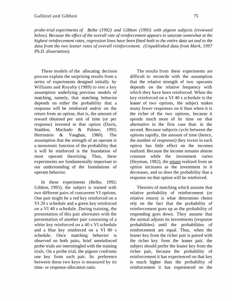
Gallistel and Gibbon 75
probe-trial experiments of Belke (1992) and Gibbon (1995) with pigeon subjects (reviewedbelow). Because the effect of the overall rate of reinforcement appears to saturate somewhat at thehighest reinforcement rates, regression lines have been fitted both to the entire data set and to thedata from the two leaner rates of overall reinforcement. (Unpublished data from Mark, 1997Ph.D. dissertation).
These models of the allocating decisionprocess explain the surprising results from aseries of experiments designed initially byWilliams and Royalty (1989) to test a keyassumption underlying previous models ofmatching, namely, that matching behaviordepends on either the probability that aresponse will be reinforced and/or on thereturn from an option, that is, the amount ofreward obtained per unit of time (or perresponse) invested in that option (Davis,Staddon, Machado & Palmer, 1993;Herrnstein & Vaughan, 1980). Theassumption that the strength of an operant isa monotonic function of the probability thatit will be reinforced is the foundation ofmost operant theorizing. Thus, theseexperiments are fundamentally important toour understanding of the foundations ofoperant behavior.
In these experiments (Belke, 1992;Gibbon, 1995), the subject is trained withtwo different pairs of concurrent VI options.One pair might be a red key reinforced on aVI 20 s schedule and a green key reinforcedon a VI 40 s schedule. During training, thepresentation of this pair alternates with thepresentation of another pair consisting of awhite key reinforced on a 40 s VI scheduleand a blue key reinforced on a VI 80 sschedule. Once matching behavior isobserved on both pairs, brief unreinforcedprobe trials are intermingled with the trainingtrials. On a probe trial, the pigeon confrontsone key from each pair. Its preferencebetween these two keys is measured by itstime- or response-allocation ratio.
The results from these experiments aredifficult to reconcile with the assumptionthat the relative strength of two operantsdepends on the relative frequency withwhich they have been reinforced. When thekey reinforced on a VI 40 s schedule is theleaner of two options, the subject makesmany fewer responses on it than when it isthe richer of the two options, because itspends much more of its time on thatalternative in the first case than in thesecond. Because subjects cycle between theoptions rapidly, the amount of time (hence,the number of responses) they invest in eachoption has little effect on the incomesrealized. Because the income remains almostconstant while the investment varies(Heyman, 1982), the return realized from anoption increases as the investment in itdecreases, and so does the probability that aresponse on that option will be reinforced.
Theories of matching which assume thatrelative probability of reinforcement (orrelative return) is what determines choicerely on the fact that the probability ofreinforcement goes up as the probability ofresponding goes down. They assume thatthe animal adjusts its investments (responseprobabilities) until the probabilities ofreinforcement are equal. Thus, when theleaner key from the richer pair is paired withthe richer key from the leaner pair, thesubject should prefer the leaner key from thericher pair, because the probability ofreinforcement it has experienced on that keyis much higher than the probability ofreinforcement it has experienced on the

Gallistel and Gibbon 76
richer key from the leaner pair (despite thefact that both keys have produced about thesame income). In fact, however, the subjectprefers the richer key from the leaner pair bya substantial margin (Belke, 1992; Gibbon,1995). The empirical results are strongly inthe opposite direction from the resultpredicted by the conventional assumptionthat the relative strength of operantsdepends on the relative probability of theirhaving been reinforced in the past.
It might be thought that the preferencefor the richer key from the leaner pair is aconsequence of a contrast effect, that is, thevalue of that key had been enhanced by thecontrast with a poorer alternative duringtraining. But this would not explain thesurprising strength of the preference. On theprobe trials, the VI 40 s key from the leanerpair is preferred 4:1 over the VI 40 s keyfrom the richer pair (Belke, 1992; Gibbon,1995). By contrast, it is only preferred 2:1to the VI 80 s key with which it is pairedduring training. Moreover, when the richerkey from the richer pair is pitted against thericher key from the leaner pair, the richerkey from the leaner pair is preferred 2:1(Gibbon, 1995), a result that is exceedinglycounterintuitive. This last result seems torule out explanations in terms of contrast.
These startling results are predicted bythe Mark and Gallistel (1994) and Gibbon(1995) models of the when to leave decision.Solving simultaneous equations (4) and (5)for the leaving rates (the reciprocals of theexpected stay durations), yields:1 E(d1) = cH2 and 1 E(d2) = cH1 . Inwords, the leaving rate for a key should beproportional to the income from the otherkey. Or, in terms of expected stay durations,the richer the other option(s), the shorter theexpected stay duration. It follows that theexpected stay duration for the VI 40 s keyfor which a VI 80 s key has been the other
option is 4 times longer than the expectedstay duration for a VI 40 s key for which aVI 20 s key has been the other option, andtwice as long as the expected stay durationfor a VI 20 s key for which a VI 40 s key hasbeen the other option. (Compare with theslopes of the regression lines in Figure 26,which are proportional to the empiricallydetermined leaving rates.)
Our explanation of the probe resultsassumes that the decision to leave a keyduring a probe trial depends not on theincome attributed to the key actually presentas an alternative on that trial but rather onthe income that has generally been availableelsewhere when the key the bird is currentlypecking was one of the options. Theparameter of the stochastic leaving decisionmaking depends on what the subjectremembers having obtained elsewhere in thepast, not on the income 'promised' by thealternative presented on the probe trial.Recall that if a subject is initially trainedwith concurrent VI keys presentedseparately--not as options that can beconcurrently exploited--then it shows anexclusive preference for the richer key whenthe keys are presented simultaneously. Thatresult and the results of these probeexperiments imply that the decisionmechanism that mediates matching isinvoked only when past experience indicatesthat two or more options may be exploitedconcurrently. Only the remembered incomesfrom the options that have actually beenexploited concurrently affect the leaving ratefor a given option. Options that have notbeen concurrently exploitable, but which arenow present, do not enter into the decisionto leave an option in order to sampleanother.

Gallistel and Gibbon 77
How the Allocating Mechanism MayProduce Exclusive Preference
An option that is never tried produces noincome. Thus, the subjective income from anoption must depend on the extent to whichthe subject samples that option, at least inthe limit. As we have already noted, thesampling rate for concurrent VI options issuch that large variations in the pattern andamount of sampling have little effect on theincomes realized from the options (Heyman,1982). This is not true, however, with manyother scheduling algorithms. For example,when reinforcements are scheduled byconcurrent ratio schedules, which deliverreinforcement after a number of responsesthat is approximately exponentiallydistributed about some mean value, then anyresponse-allocation ratio less than anexclusive preference for the richer scheduleresults in an income ratio than the response-allocation ratio. This is an analytic fact, notan empirical fact. It was first pointed out byHerrnstein and Loveland (1975), who wenton to note that, with variable ratio schedules,the response-allocation ratio can equal theincome ratio only in the limit when all of theresponses are allotted to the richer optionand, hence, all of the income is obtained fromthat option. Thus, the exclusive preferencefor the richer schedule, which is observedwith concurrent variable ratio schedules ofreinforcement, does not imply that thisbehavior is controlled by the optingmechanism rather than the allocatingmechanism. Exclusive preference for oneoptions can result from destabilizingpositive feedback between the subject’stime-allocation behavior and theinterreinforcement intervals that itexperiences. Longer interreinforecementintervals cause diminished sampling of anoption, which causes the animal toexperience still longer interreinforcement
intervals from that option, and so on, untilsampling of an option eventually goes tozero (cf Baum, 1981; Baum, 1992).
Summary
A coherent theory of operant choice can beerected on the same foundations as thetheory of Pavlovian conditioning. In bothcases, probability of reinforcement (whetherresponse reinforcement or stimulusreinforcement) is irrelevant. The behaviorallyimportant variable is the interval betweenreinforcements in the presence of theconditioned stimulus (the CS, in Pavlovianterminology, the discriminative stimulus orsecondary reinforcer, in operantterminology). Equivalently, the behaviorallyimportant variable is the rate ofreinforcement. The behaviorally importanteffect of the relevant variable is not thestrengthening of associations (or of responsetendencies). Rather, experienced intervals arestored in memory, and read from memorywhen they are needed in the computationsthat yield decision variables. Distinctdecision mechanisms mediate distinct kindsof decisions. In Pavlovian conditioning, thereare distinct mechanisms for deciding whetherto respond, when to respond, and whetherto quit responding. In operant choice, thereare distinct mechanisms for deciding whichof two mutually exclusive options to choose(opting behavior) and for allocating behavioramong concurrently exploitable options.
The decision variables in operant choiceare subjective incomes (reinforcementexpectancies), which are subjectivereinforcement magnitudes divided by thesubjective interval between reinforcements.Under concurrent conditions, where bothoptions are continuously present, the timeused in computing the income from anoption is session time (more precisely, thetime when both options are present), not the

Gallistel and Gibbon 78
time specifically devoted to (invested in) anoption. In discrete-choice paradigms, wherethe options are only intermittently availableand the choice of one option more or lessimmediately precludes the choice of theother, the intervals used to computesubjective incomes are the delays between achoice and the delivery of the reinforcement(the intervals when a reinforcement has beenchosen and is pending). Other intervals areignored in the computation of incomes; theyare subjectively sunk times.
Because reinforcement magnitude dividedby delay of reinforcement goes to infinity asthe subjective interval goes to zero, theremust be a lower bound on subjectiveintervals. This lower bound--the subjectiveinstant--establishes a scaling constant forsubjective time. This leads to theexperimentally well documented hyperbolicrelation between the amount by which areward is delayed and its subjective value.
In discrete-choice paradigms where thesubjects must compute the value of anoption that involves more than one delay ofreinforcement, they average the income valueof each reinforcement. The reinforcementexpectancy in these cases is the expectedratio of individual reward magnitudes andtheir delays rather than the ratio of theexpectancies. The rationale for this kind ofaveraging is unclear.
Contrasting ConceptualFrameworks
We have elaborated a different conceptualframework for the understanding ofconditioning. In this section, we highlight thefundamental differences between thisframework and the associative frameworkthat has so far been the basis for allinfluential models of conditioning.
Different Answers to Basic Questions
That the two conceptual frameworks arefundamentally different is apparent from aconsideration of the contrasting answersthey offer to the basic questions addressedby the material taught in an introductorycourse on learning:
1) Why does the conditioned responseappear during conditioning?
Standard answer: Because the associativeconnection gets stronger.
Timing answer: Because the decision ratiofor the whether-to-respond decisiongrows until it exceeds a decisionthreshold.
2) Why does the CR disappear duringextinction?
Standard answer: Because there is a lossof net excitatory associative strength.This loss occurs either because theexcitatory association itself has beenweakened or because a countervailinginhibitory association has beenstrengthened.
Timing answer: Because the decision ratiofor the whether-to-stop decision growsuntil it exceeds the decision threshold.
3) What is the effect of reinforcement?
Standard answer: It strengthens excitatoryassociations.
Timing answer: It marks the beginningand/or the termination of one or moreintervals-- an inter-reinforcementinterval, a CS-US interval, or both.

Gallistel and Gibbon 79
4) What is the effect of delay ofreinforcement?
Standard answer: It reduces the incrementin associative strength produced by areinforcement.
Timing answer: It lengthens theremembered inter-reinforcement interval,the remembered CS-US interval, or both.
5) What is the effect of non-reinforcement?
Standard answer: The non-reinforcement(the No-US) weakens the excitatoryassociation; or, it strengthens aninhibitory association.
Timing answer: The timer for the mostrecent interreinforcement intervalcontinues to accumulate.
6) What happens when nothing happens(during the intertrial interval)?
Standard answer: Nothing.
Timing answer: The timer for thebackground continues to accumulate.
7) What is the effect of CS onset?
Standard answer: It opens the associativewindow in the mechanism that respondsto the temporal pairing of two signals.That is, it begins a trial during which theupdating of associative strengths willoccur.
Timing answer: It starts a timer (to timethe duration of this presentation) and itcauses the cumulative exposure timers toresume cumulating.
8) What is the effect of varying the magnitudeof reinforcement?
Standard answer: It varies the size of theincrement in the excitatory association.
Timing answer: It varies the rememberedmagnitude of reinforcement.
9) Why is the latency of the conditionedresponse proportional to the latency ofreinforcement?
Standard answer: There is no widelyaccepted answer to this question inassociative theory.
Timing answer: Because the animalremembers the reinforcement latency andcompares a currently elapsing interval tothat remembered interval.
10) What happens when more than one CS ispresent during reinforcement?
Standard answer : The CSs compete for ashare of a limited increment inassociative strength; or, selectiveattention to one CS denies other CSsaccess to the associative mechanism (CSprocessing deficits); or, predicted USsloose the power to reinforce (USprocessing deficits).
Timing answer: The rate of reinforcementis partitioned among reinforced CSs inaccord with the additivity and predictor-minimization constraints.
11) How does conditioned inhibition arise?
Standard answer: The omission of anotherwise expected US (the occurrenceof a No-US) strengthens inhibitoryassociations.
Timing answer: The additive solution tothe rate-estimation problem yields anegative rate of reinforcement.

Gallistel and Gibbon 80
12.) What happens when a CS follows areinforcer rather than preceding it?
Standard answer. Nothing. Or, aninhibitory connection between CS andUS is formed.
Timing answer. A negative CS-US intervalis recorded, or, equivalently, a positiveUS-CS interval. (More precisely:subjective intervals, like objectiveintervals, are signed.)
13. How does a secondary CS acquirepotency?
Standard answer. An association formsbetween the secondary CS and theprimary CS, so that activation may beconducted from the secondary CS to theprimary CS and thence to the US via theprimary association.
Timing answer. The signed intervalbetween the secondary and primary CSis summed with the signed intervalbetween the primary CS and the US toobtain the expected interval between thesecondary CS and the US.
14) How is CS-US contingency defined?
Standard answer. By differences in theconditional probability of reinforcement
Timing answer. By the ratio of the rates ofreinforcement
15) What is the fundamental experientialvariable in operant conditioning?
Standard answer. Probability ofreinforcement
Timing answer. Rate of reinforcement
Contrasting Basic Assumptions
Central to the timing framework is theassumption that the nervous system timesthe durations of the intervals marked off bythe events in a conditioning protocol, storesrecords of these intervals in memory,cumulates successive intervals of exposureto the same conditioned stimulus, andgenerates conditioned responses through theagency of decision processes, which takestored intervals and currently elapsingintervals as their inputs. None of theseelements is found in associative analyses ofconditioning. There is no provision for thetiming of intervals. There is no provision forthe summing of intervals. There is nomemory process that stores the result of aninterval-timing process, and there are nodecision processes.
Conversely, none of the elements ofassociative models is found in timing models.There is no associative bond--no learned,signal-conducting connection--thus also nostrengthening of connections throughrepetition, hence, no associabilityparameters. There is no notion of a learningtrial, and the probability of reinforcement,whether of stimuli or responses, plays norole. Thus, the two conceptual frameworkshave no fundamental elements in common.Timing models of conditioning have more incommon with psychophysical models invision and hearing than with associativemodels in learning. Like models inpsychophysics, they focus on quantitativeaspects of the experimental data. Likemodern perceptual theories, they embodycomputational principles that resolveambiguities inherent in the input to yield anunambiguous percept (representation) of thestate of the world.
Gallistel and Gibbon 81
Elementary Acquisition Event inAssociative Models
The elementary event in the associativeconception of acquisition is a change in thestrength of a connection. Repetitions of thesame learning experience--for example,repetitions of the temporal pairing of a toneand a puff of air directed at the eye--strengthen the connection. Thus, what theassociative conception appears to require atthe neurobiological level is a mechanism foraltering the strength of a synaptic connectionbetween neurons. The enduring appeal of theassociative conception is this neurobiologicaltransparency. A second strong appeal is thestraightforwardness of its explanation for the(presumed) gradual increase in the strengthof the conditioned response. Thestrengthening of the conditioned response isnaturally seen as a consequence ofsuccessive increments in the underlyingconnection strengths.
On the other hand, the assumption of aconductive connection whose strength isincremented over successive repetitionsplaces serious obstacles in the way of anassociative explanation for the fact thatanimals learn the durations of intervals, themagnitudes of reinforcements, the intensitiesof conditioned and unconditioned stimuli,and other parameters of the experimentalprotocol The size of an increment inassociative strength is a function of morethan one aspect of the events on a giventrial--the magnitude and delay ofreinforcement, the pretrial strength of theassociation, strengths of other associationsto the same US, and so on. Because of thisconfounding of experiential variables, noneof these variables is recoverable from thecurrent strength of the connection. Put moreformally, the strength of an associativeconnection is a many-one function of
different properties of the conditioningprotocol, and many-one functions are notinvertible; you cannot get from the one backto the many.6
Elementary Acquisition Event inTiming Models
The elementary event in the timingconception of conditioning is the measuringand recording of an elapsed interval. Learningis the product of an information gatheringsystem that functions automatically. Eachrepetition of the same experience (forexample, each trial in an eye blinkconditioning experiment) lays down a newrecord (cf. Logan, 1988). The system alsokeeps running totals for the cumulativedurations of the salient stimuli. Thus, whatthe timing conception requires at theneurobiological level is a mechanism capableof cumulating and storing the values of alarge number of distinct of variables.
It is not difficult to suggest cellularmechanisms capable of storing the values ofvariables. Miall (1996) has proposednetwork models for accumulation, a centralfeature in timing models of acquisition, andfor storage and comparison processes. (Seealso Fiala, Grossberg & Bullock, 1996;Grossberg & Merrill, 1996, for networktiming models.) While these models do not
6It might, however, be possible to get from manyback to the many, that is, a manifold of associativeconnections might--with a very careful choice ofconnection-forging processes--be such that one canrecover from that manifold the values of the manyexperiential variables that created it. However, theassociative processes invoked to explain animalconditioning do not have the properties required tomake an associative manifold invertible. It is notclear that it is possible to modify the association-forming process in such a way as to make theassociative manifold invertible without eliminatingthe neurobiological transparency and straightforwardexplanantion of gradual response acquisition thataccount for much of the appeal of associative models.

Gallistel and Gibbon 82
have anything like the complexity of thesystems we have proposed, they doillustrate the feasibility in principle of aneural-net kind of representation ofaccumulated elapsed time. Enduring changesin synaptic strength could, in principle, beused to record the values of variables, albeitat the cost of sacrificing those propertiesthat make the change constitute a change inassociative strength, as traditionallyunderstood.
In sum, what timing models require is amemory functionally analogous to aconventional computer memory, amechanism for storing and retrieving thevalues of variables. While it is notimmediately apparent how to create such amemory out of the currently understoodelements of neurobiology, such a memory isboth physically possible (witness computermemory) and biologically possible. Genesprovide the proof of biological possibility;they store the values of variables for read-out in response to gene-activating stimuli.Note that genes are repositories ofinformation, not paths for signal flow. Genesare read by gene activating signals, just ascomputer memories are read by memory-activating signals. Fifty years ago thephysico-chemical mechanisms for thesegenetic operations were deeply mysterious.What timing models requireneurobiologically is a selectively activatablerepository for the values of experientiallydetermined variables. The neurobiologicallymysteriousness of this requirement is nogreater than the biochemical mysteriousnessof the gene theory’s requirement for a self-replicating molecule was in, say, 1950.
Decision Mechanisms vs . NoDecision Mechanisms
Associative models do not have decisionmechanisms that take remembered values as
their inputs and generate conditionedresponses as their outputs, whereas decisionmechanisms are central to the timingperspective. (Miller and Schachtman’s(1985) Comparator Hypothesis is anexception to this generalization, which iswhy it represents a step in the direction ofthe kind of model we argue for.) Timingmodels of conditioning share withpsychophysical models in vision and hearingthe explicit, formal specification of decisionprocesses. Associative models, by contrast,have long lacked an explicit specification ofthe process by which the strengths ofassociations translate into observed behavior(Miller & Matzel, 1989; Wasserman &Miller, 1997). The lack of decisionmechanisms in associative models goes handin hand with the lack of a mechanism forstoring and retrieving the values of variables,because decision mechanisms take the valuesof remembered variables as their inputs.
Challenges
Quite aside from its intrinsic value as anexplanatory framework that integrates awide variety of findings and suggests manynew experiments, an alternative to theassociative conceptual framework is valuablebecause it brings into clear focus severalenduring puzzles that have arisen in thestandard associative explanations ofconditioned behavior. This may stimulatethe further development of associativemodels.
Understanding partial reinforcement
The fact that partial reinforcement does notaffect the number of reinforcements toacquisition or nor reduce the number thatmust be omitted to produce extinction is apuzzle. None of the formally specifiedassociative models we are familiar with canaccount for this, because they all assume

Gallistel and Gibbon 83
that non-reinforced trials weaken the netexcitatory effects of reinforced trials.Therefore, the number of reinforced trials toreach a given level of excitatory effect oughtto increase as the schedule of reinforcementgets thinner, but it does not, or does so onlyslightly.
Also, the net excitatory effect after agiven number of reinforcements ought to beweaker the thinner the schedule ofreinforcement. Therefore, the number ofomitted reinforcements required to produceextinction ought to be reduced as theschedule of reinforcement is thinned, but it isnot, or only slightly. Gibbon (1981a)showed that, the asymptotic strength of theCS-US association in the Rescorla-Wagnertheory is:
pβl
pβ l + 1− p( )βe
, (6)
where p is the probability that the CS isreinforced, and βl and βe are the learning andextinction rate parameters. When the rates oflearning and extinction are equal, then the β's
cancel out, and (6) reduces to p. Regardless
of the values of the β's, the asymptoticstrength of the association declines as theprobability of reinforcement declines. Trials(and omitted reinforcements) to extinctionshould be reduced correspondingly, but, infact partial reinforcement increases trials toextinction and does not change omittedreinforcements to extinction.
As the extinction rate (_e) is reducedrelative to the learning rate (_l), the amountby which partial reinforcement reducesasymptotic associative strength is reduced.However, the effect remains large for anyplausible ratio of extinction rates to learningrates. The extinction rate cannot be made toomuch slower than the learning rate, because
the lower the ratio of the extinction rate tothe learning rate, the longer extinction shouldtake relative to learning, which brings us to asecond problem.
It is puzzling that the number ofreinforcements that must be omitted toproduce extinction can be substantially lessthan the number of reinforcements requiredfor acquisition. To avoid catastrophic effectsof partial reinforcement on acquisition,associative models generally assume that therate of extinction is less than the rate ofacquisition (associations get stronger fasterthan they get weaker). In that case,extinction ought to take longer thanacquisition, which is not generally the case.Indeed, by reducing the ratio of the averageintertrial interval, I, to the average trialduration, T, to 1.5/1, one can create aprotocol in which the number ofreinforcements required for acquisition ismore than twice the number of omittedreinforcements required for extinction. Atthis I/T ratio, subjects can still beconditioned on a 10:1 partial reinforcementschedule--with no more reinforcements thanare required under continuous reinforcement!These findings appear to challenge thefoundational assumption that reinforcementand nonreinforcement have opposing effectson the net excitatory effect of CS-USassociations.
It has been pointed out that the basicassumptions of associative conditioningtheories about the strengthening andweakening effects of reinforcement and non-reinforcement fail to account for themicrostructure of performance under partialreinforcement (the trial-by-trial pattern --Gormezano & Coleman, 1975; Prokasy &Gormezano, 1979; see also Capaldi &Miller, 1988). They also fail to account forthe macrostructure, when trials to extinctionare considered along side trials to acquisition.

Gallistel and Gibbon 84
Time-scale invariance
None of the formally specified associativemodels we are familiar with accounts for thetime-scale invariance of the acquisitionprocess. They all assume that delayingreinforcement reduces associability. Indeed,neurobiologically oriented associativetheories often take a narrow window ofassociability as the signature of theassociative mechanism (e.g. Gluck &Thompson, 1987; Grossberg & Schmajuk,1991; Usherwood, 1993). The problem withthe assumption that delaying reinforcementreduces associability is that delayingreinforcement has no effect if the intertrialinterval is increased proportionately. This isa manifestation of time-scale invariance:changing the relevant time intervals by somescaling factor does not affect the results.
Another basic problem for associativetheories is that conditioning depends on acontingency between the CS and the US (orthe instrumental response and thereinforcement). Associative theories, at leastthose that have influence in neurobiologicalcircles, assume that conditioning is driven bytemporal pairing. Contingency is a globalstatistical property of the animal’sexperience. Like all such properties, it istime-scale invariant. It is difficult to see howthe operation of a mechanism that isactivated by temporal pairing can be time-scale invariant, because the concept oftemporal pairing would seem to be a clearexample of a time-scale dependent concept.Defining temporal pairing in a time-scaleinvariant manner would necessitate radicalrethinking of the mechanisms that couldmediate the effects of this temporal pairing.
The inverse proportionality betweenreinforcements to acquisition and the trial-to-trial interval also lacks an explanation.
The trial-spacing effect is explainedqualitatively by the assumption that it givesmore scope for the extinction of conditioningto the background (Durlach, 1989; Rescorla& Durlach, 1987). However, Gibbon (1981)showed that the Rescorla-Wagner theorypredicted only a weak effect of intertrialinterval on reinforcements to acquisition,while predicting a strong effect of partialreinforcement--the opposite of what isobserved empirically.
We believe that other associative modelswould make the same predictions regardingthe relative potencies of these two basicvariables if they were modified so as to makepredictions regarding the effect of theintertrial interval. It is hard to say what mostassociative models, as they now stand,would predict about the relative effects ofvarying partial reinforcement and theintertrial interval on the rates of conditioningand extinction, because they cannot predictthe effect of the intertrial interval at allwithout making use of the assumption ofmultiple background “trials” during oneintertrial interval. This assumption brings upthe “trial problem.”
The trial problem
The notion of a trial is a fundamental butinsufficiently scrutinized notion in mostassociative models. A trial is a discreteinterval of time during which events occurthat cause the updating of associativeconnections. In Pavlovian conditioning, if aCS and a US both occur on a trial, it is areinforced trial; if a CS occurs but not a US,it is an unreinforced trial. In instrumentalconditioning, a trial is an interval duringwhich there is an input (a stimulus), anoutput (a response), and finally, an error-correcting feedback (reinforcement or non-reinforcement). This latter conception of atrial also applies to the many contemporary

Gallistel and Gibbon 85
associative network models that use anerror-correcting algorithm to updateassociative strengths (“supervised learningalgorithms”). The notion of a trial isintimately linked to the notion that it is theprobability of reinforcement that driveslearning, because probabilities cannot bedefined in the absence of trials.
We discern three different traditionsgoverning the identification of thetheoretician’s trial with the elements of aconditioning protocol. In one conception,which one might call the neurobiologicalconception of Pavlovian conditioning, thebeginning of a trial corresponds to the onsetof a CS and the termination of a trialcorresponds to the closing of the window ofassociability. The onset of a CS opens thewindow of associability; if a reinforcementoccurs while the window remains open, it isa reinforced trial; if a reinforcement does notoccur while the window is open, it is anunreinforced trial. Another trial does notbegin until there is a further CS onset.
In the second, more pragmaticconception of a Pavlovian trial, a trial beginswhen a CS comes on and it terminates whenthe CS goes off (or soon thereafter). If areinforcement occurs while the CS is on (orsoon thereafter), it is a reinforced trial, if itdoes not, it is an unreinforced trial.
Finally, in the instrumental tradition, atrial begins when the animal makes aresponse. The response opens a window ofassociability. If reinforcement is deliveredwhile the window is open, the associationbetween the response and the stimulipresent when it was made is strengthened. Ifreinforcement does not occur soon after theresponse is made, it is an unreinforced trial.
The trouble with the first conception isthat it is known to be empirically
indefensible. It has not been possible todefine by experiment when the window ofassociation opens nor how long it staysopen (see Rescorla, 1972, for a review ofsuch efforts). That is, it has never beenpossible to define temporal pairing in thesimple way that this traditional conceptionsuggests that it should be defined. Indeed,the time-scale invariance of the acquisitionprocess would appear to be irreconcilablewith such an assumption.
The trouble with the more pragmaticnotion of a Pavlovian trial is that it cannot beapplied in the case of backgroundconditioning, or in any of the conditioningprotocols in which there are manyreinforcements during a sustained CSpresentation. Such protocols are common inoperant paradigms, where a stimulus presentat the time of reinforcement is called asecondary reinforcer and/or a discriminativestimulus. The stimuli reinforced in operantparadigms (the stimuli projected onto thekeys that the pigeons peck) are oftencontinuously present, as for example inconcurrent schedules of reinforcement. InPavlovian conditioning, background orcontext conditioning is empirically wellestablished and theoretically important:Reinforcements that occur while an Aplysiaor a pigeon or a rat is in an experimentalchamber establish a conditioned response tothe chamber (Baker & Mackintosh, 1977;Balsam, 1985; Balsam & Schwartz, 1981;Colwill, Absher & Roberts, 1988; Rescorla,1968; Rescorla, 1972). The more frequentthe reinforcer, the stronger the backgroundconditioning (Mustaca, Gabelli, Papine &Balsam, 1991).
When the pragmatic conception of a trialis applied to a background conditioningprotocol, each experimental sessionconstitutes one trial, because the CS (thebackground) “comes on” at the beginning of

Gallistel and Gibbon 86
the session, when the subject is placed in theapparatus, and terminates with the end ofthe session, when it is removed. How to dealwith the effects of reinforcer frequency isthen problematic. To get round this problem,Rescorla and Wagner (1972) posited a trial“clock”, which carved time into purelysubjective trials. This permitted them totreat the intertrial intervals, when thebackground alone was present, as composedof sequences of multiple internally timedevent-independent trials (auto-trials, forshort), with the association between thebackground and the US strengthened orweakened accordingly as a reinforcer did ordid not happen to occur during such a“trial.” Their immensely influential analysisof the effect of background conditioning onconditioning to a transient CS depended onthis auto-trial assumption just as strongly ason the much better known assumption thatassociations to a given US compete for anasymptotically limited total associativestrength. But the authors themselves seem tohave regarded this assumption as atemporary theoretical expedient. There hasbeen no attempt to explore its consequences.We believe that such an attempt woulduncover unfortunate implications.
The problem is that in many cases, itappears necessary to assume that auto-trialsare very short (on the order of a second orless). If they are allowed to be as long asRescorla and Wagner assumed them to be forthe purposes of their analysis--two minutes--then, in many conditioning protocols, oneagain encounters the problem that a singletrial encompasses more than onepresentation of both the CS and the US.And, two CSs (or a CS and a US) that didnot in fact coincide are counted as coincidingbecause they both occurred during one auto-trial. However, if auto-trials are assumed tobe very short, then many protocols havevery large numbers of unreinforced auto-
trials. Unreinforced trials either weakenexcitatory associations (as in the Rescorla-Wagner theory), and/or they strengtheninhibitory associations, which negate thebehavioral effects of excitatory associations,and/or they reduce attention to the CS. Inany event, the numerous unreinforced trialsintroduced into the analysis by the (veryshort) auto-trials assumption would seemmake the build up of any appreciable netexcitatory effect impossible. The effects ofrare reinforced auto-trials are swamped bythe effects of the frequent unreinforced auto-trials. One is forced to assume that theeffects of non-reinforcement are extremelyweak relative to the effects of reinforcement,but then it becomes difficult to explain theresults of experiments on extinction andconditioned inhibition. These experimentsshow that conditioned inhibition can developrapidly (Nelson & Bouton, 1997) and thatextinction can occur more rapidly thanacquisition. For an indication of thedifficulty that even very complex associativetheories confront in explaining contextconditioning, see Mazur and Wagner (1982,p. 33f).
The operant conception of a trial hassimilar problems. The notion of probabilityof response reinforcement is not definable inabsence of a discrete interval of specifiedduration following the response, duringwhich a reinforcement either is or is notreceived. However, there are no data thatindicate what this interval might be. One candelay reinforcement for long intervalsprovided that intertrial intervals are madecorrespondingly long. Indeed, thephenomenon of autoshaping, as we havealready noted, calls into question thedistinction between the Pavlovian andoperant paradigms. It is not clear thatconditioning in any paradigm actuallydepends on the animal’s making a response.Conditioning in operant paradigms, as in

Gallistel and Gibbon 87
Pavlovian paradigms, appears to be drivenby the temporal relations between events,including events initiated by the subject,such as key pecks, lever presses and chainpulls. Insofar as an operant response isirrelevant in operant conditioning--orrelevant only insofar as it constitutes adistinguishable kind of event--then theoperant conception of a trial (response-initiated trials) becomes inapplicable.
If the trial notion is theoreticallyindispensable but operationally undefinable--that is, if one cannot say when a givensegment of a protocol constitutes a trial--then one must ask whether associativetheories can actually be applied to thephenomena they seek to explain. If thesemodels are to be used as a guide tomechanisms to be looked for at theneurobiological level of analysis, they aregoing to have to be more specific about whatconstitutes a trial.
Paradoxical Effects of ReinforcementMagnitude
An animal’s preference for one concurrentVI schedule of reinforcement over another isproportional to the relative magnitudes ofthe reinforcements (Catania, 1963; Keller &Gollub, 1977; Mark & Gallistel, 1993; Leon& Gallistel, 1997). The natural associativeinterpretation of this is that biggerreinforcements produce bigger increments inassociative strength and, therefore, a biggerasymptotic associative strength. In theRescorla-Wagner theory, for example, theparameter lambda, which is the asymptoticnet associative strength that a US cansupport, is generally taken to be a functionof the magnitude of reinforcement. Thatassumption has the just specifiedconsequence, at least qualitatively--greaterpreference for bigger rewards. However, ifbigger reinforcements increase the size of the
increments in associative strength, theyought to increase the rate of acquisition, butthey do not. Thus, from an associativeperspective, there is a paradox between thestrong effect of reinforcement magnitude onpreference (Figure 28) and its negligibleeffect on the rate of acquisition (Figure 12).
The No-US Problem
Extinction and conditioned inhibition requirean associative change in response to thefailure of a US to occur. For a CS to becomean inhibitor it must signal the non-occurrenceof an otherwise expected stimulus (LoLordo& Fairless, 1985; Rescorla, 1988). It isunclear how to conceptualize this within anassociative context. Both Pavlov (1928) andHull (1943) wrestled with the question ofhow the non-occurrence of a stimulus couldbe the cause of something. We do not thinkthe question has been solved in the decadessince. Dickinson (1989) refers to this as theNo-US problem.
As Dickinson (1989) points out, there isnothing inherently puzzling about a processset in motion by the failure of something tooccur. In a device like a computer, which iscapable of comparing input values againstinternally generated or stored values (that is,against an expectation in the sense that termis used in this paper), the failure of an inputto occur generates a signal from thecomparison process. This signal isproportional to the difference or ratiobetween the input magnitude (0, in the caseof failure) and the comparison magnitude(the expectation). The discrepancy signalinitiates whatever events are to beconsequent upon the failure. This is thenature of our explanation of extinction: thedecision to stop responding is based on theratio between a currently elapsingunreinforced interval and an expectedinterreinforcement interval. Indeed, an

Gallistel and Gibbon 88
expected interval between reinforcements isthe denominator in each of the decisionratios that appear in the timing analysis ofacquisition, extinction and response timing.
The basic problem is that, in associativetheory, the non-occurrence of reinforcement(the occurrence of a No-US) is generallytreated as an event. This event sets inmotion the mechanism that responds to non-reinforcement. Even if one adds to anassociative model the machinery necessaryto have an expectation (as is implicitly orexplicitly done in the Rescorla-Wagner,1972, model and many other contemporaryassociative models), it is still unclear how tomake the associative analysis go through,because an event has to have a time ofoccurrence, and there does not appear to be aprincipled way of saying when a non-reinforcement has occurred. Acquisition andextinction proceed normally whenreinforcements are delivered by random rateor Poisson scheduling mechanisms, and arandom rate of background reinforcement isgenerally used in the explicitly unpairedprotocol for the production of conditionedinhibition. In these schedules, reinforcementis no more likely at any one moment than atany other. Thus, there is no basis forexpecting the reinforcement to occur at anyparticular moment. How can the changesthat underlie extinction and inhibition be setin motion by the failure of an expectedreinforcement to occur if that reinforcementis no more likely at any one moment than atany other? It would seem that either thefailure must be deemed to happen at everymoment, or it must be deemed never tohappen. In either case, it is unclear how tomake a physically realizable, real-time modelof extinction and inhibitory conditioningwithin the associative conceptualframework, without recourse to the trialsassumption, which is itself deeplyproblematic.
Directionality
In associative models, a special class ofstimuli, reinforcing stimuli, set theassociative mechanism in motion and conferdirectionality on the associative process. Ifthere is no stimulus that can be identified asa reinforcing stimulus, then there is nothingto set the associative process in motion(nothing to cause learning) and there is noway of specifying directionality, that is, noway of saying whether one is dealing withforward or backward conditioning. Thismakes the phenomenon of sensorypreconditioning an awkward phenomenonfor associative theories to come to termswith. On the face of it--if one does notbelieve that there is a special class of stimulicalled reinforcing stimuli--then sensorypreconditioning is simply conditioning: twostimuli, say, a tone and a light, aretemporally paired and they becomeassociated. The problem arises because mosttheories of the associative process assumethat it matters which stimulus comes first,the CS or the US. If the CS comes first, it isforward conditioning. If the US comes first,it is backward conditioning. The associativemechanism itself is assumed to be sensitiveto temporal order. Different orderings of thestimuli being associated produce differentassociative effects. If they did not, then itwould not matter whether Pavlov rang thebell before or after presenting food to hisdogs, which we know to be false. However,when two neutral stimuli are paired, there isno way to specify whether one has to dowith forward or backward conditioning.
From a timing perspective, reinforcersplay no privileged role in learning per se.Like other stimuli, their onsets and offsetsmay mark either or both ends of a timedinterval. The memory of reinforcement playsa privileged role only in determining whether

Gallistel and Gibbon 89
a decision mechanism is used to determine aresponse. Neutral stimuli--stimuli that donot elicit stimulus-specific unconditionedresponses--do not evoke CRs because theyare not intrinsically important to anybehavior system (Fanselow, 1989;Timberlake & Lucas, 1989). In order for abehavior-determining decision to be made, abehavior system must operate. That is, theanimal must be motivated to make use of theconditioned stimuli in the control of itsbehavior. Reinforcers are simplymotivationally significant stimuli, stimuliwhose occurrence motivates behavior thatanticipates that occurrence. They are notimportant for learning, only for performance.
Second Order Conditioning
In the Section on Dichotomies, we reviewrecent findings from Ralph Miller’slaboratory (Cole, Barnet & Miller, 1995a, b;Barnet and Miller, 1996) on TraceConditioning versus Delay Conditioning,Backward versus Forward Conditioning,Inhibitory Conditioning, and Second OrderConditioning. These findings pose achallenge to traditional conceptions.
The challenge is to explain the reversalsin the apparent relative strengths of primaryCS-US associations when their strengths aretested directly and indirectly (Cole, Barnet& Miller, 1995a,b; Barnet & Miller, 1996).In the direct tests, when the strength of theconditioned response to the primary CS ismeasured, backwardly conditioned and traceconditioned CSs appear to have considerablyweaker associations with the US thanforwardly conditioned and delay conditionedCSs. But in the indirect tests, when thestrength of the conditioned response to CSsthat have been linked to the primary CSsthrough identical second order conditioningis measured, the backwardly conditioned andtrace conditioned primary CSs appear to
have much stronger associations with the USthan the forwardly conditioned and delayconditioned primary CSs. The results fromthe Miller lab seem to require the kind ofassumption that is the foundation of thetiming perspective, namely, that in thecourse of conditioning, the subject acquiresquantiative knowledge of the temporalrelations between events, and that it is thisquantiative knowledge and inferences drawnfrom it that determine the conditionedresponse.
Reinstatement
Associative models conceive of extinction inone of two ways: 1) as the weakening of anassociation (e.g. Pearce, 1994; Rescorla &Wagner, 1972), or, 2) as the development ofan opposing association (or negating processof some kind) whose effects cancel theeffects of the excitatory association. Thefirst assumption is almost universallyadhered to in connectionist models.However, it is now widely recognized byexperimentalists to be irreconcilable with alarge literature demonstrating thatconditioning is forever: no subsequentexperience can expunge the memories(associations/connections) implanted(strengthened) by earlier conditioning(Bouton, 1991; Bouton, 1993; Bouton &Ricker, 1994; Brooks, Hale, Nelson &Bouton, 1995; Kaplan & Hearst, 1985;Mazur, 1996; Rescorla, 1992; Rescorla,1993; Rescorla & Heth, 1975; see Rescorla,1998 for review). To be sure, subsequentexperience can lead to the disappearance ofthe conditioned response, but a variety ofreinstatement procedures show that the“associations” (the memories implantedduring earlier conditioning) remain when theconditioned response has disappeared. Thesimplest of the reinstatement procedures isto wait a while after extinction before testingfor the presence of the conditioned response.

Gallistel and Gibbon 90
The response comes back (e.g. Rescorla,1996)--the phenomenon that Pavlov (1928)dubbed spontaneous recovery. Changing thespatial context (the experimental chamber)also brings the response back (Bouton &Ricker, 1994).
Bringing back the conditioned responseafter its extinction by changing the temporaland/or spatial context is called reinstatement.The finding that it is almost always possibleto reinstate an extinguished (or even counter-conditioned) response has led specialists inconditioning to favor the view that extinctioninvolves the development of an associationwith an opposing (or canceling) effect ratherthan the weakening of the originallyconditioned association--a view favored byPavlov himself. It is not, however, clear howthis solves the problem. The problem is toexplain why reinstatement procedures makeold excitatory associations prevail overnewer inhibitory (or canceling) associations.
From the perspective of the analysis ofextinction here expounded, a preconditionfor extinction is that the animal not forgetthe path to its present estimates of the stateof the world. On this analysis, extinction is aconsequence of a decision mechanismdesigned to detect a change in the rate ofreinforcement attributed to the CS, that is, todecide whether recent experience isinconsistent with earlier experience. Thisrequires that recent experience be comparedto earlier experience. A precondition for thatcomparison is that recent experience be keptdistinct from more remote experience inmemory. To detect a change, the systemmust not represent its experience solely bymeans of a running average, which is acommon assumption in associative modelsof conditioning. It cannot use a simplerunning average of its experience todetermine its behavior, because a segment of
the recent past must be compared to theearlier past.
Devenport’s (1994) temporal weightingrule points the way to the treatment ofreinstatement phenomena from a timingperspective. The general principle indicatedby a variety of findings (e.g. Mazur, 1996) isthat animals track their experience on severaldifferent time scales. When recent experienceindicates one state of affairs but more remotealbeit more extensive experience indicates adifferent state of affairs, the animal favorsthe more recent experience so long as it isindeed recent. As that experience becomesless recent, the animal begins to base itsbehavior more on the more remote but moreextensive past. In other words, an importantvariable in determining which part of itsremembered experience dominates ananimal’s behavior is the time elapsed sincethe experience--not because of forgetting, butbecause the recency of one experiencerelative to conflicting or different experiencesis itself an important decision variable. It isused to decide which of two conflictingprevious experiences provides the moreplausible current expectation. This accountassumes that a representation of how long ithas been since a particular conditioningexperience is an important determinant ofconditioned behavior (cf. Clayton &Dickinson, 1998).
A phenomenon similar to reinstatementhas recently been demonstrated in operantchoice. Mazur (1995) showed that whenpigeons experience a change in the relativerate of reward after a long period of stability,they adjust to the change within the sessionin which they encounter it, but, at thebeginning of the next few sessions, theyshow clear reversion to the pre-change time-allocation ratio, followed by an increasinglyrapid return to the post-change time-allocation ratio. These results and

Gallistel and Gibbon 91
Devenport's theory suggest that there is yetanother decision mechanism to beinvestigated, namely, the mechanism thatdecides in effect which context should be thebasis of the animal's current behavior--anolder context, or a more recent context. This,decision will presumably depend on theanimal's previous experience with changes inrates of reinforcement, which will indicate,among other things, how long such changesmay be expected to last.
Conclusion
In a strictly behaviorist conceptualframework, conditioned behavior does notdepend on the acquisition of symbolicknowledge of the world. The conditioningexperience rewires the nervous system sothat the animal behaves more adaptively, butthe nervous system does not thereby acquireany internal structure that specifies objectiveproperties of the experience that caused therewiring. This was not only the burden ofSkinner’s (1938) argument; it was the mainpoint of Hull’s early writings (for example,Hull, 1930). Arguments of a similar naturehave been advanced much more recently bysome connectionists (Churchland &Sejnowski, 1992; Smolensky, 1986).However, much recent experimental workinvolving mutliple stimuli, multiple types ofresponses, and multiple kinds of reinforcershas demonstrated that the subjects inconditioning experiments do rememberwhich stimuli and which responses lead towhich reinforcements (Colwill, 1993;Rescorla & Colwill, 1989). Timingexperiments demonstrate that subjects alsolearn the temporal intervals in the protocols.Animal subjects have also been shown tolearn the time of day at which they wereconditioned (see Gallistel, 1990, for review)and to know which reinforcers were cached
where and how long ago (Clayton &Dickinson, 1998; Clayton & Dickinson,1999; Sherry, 1984). Clearly, then,conditioning causes changes in the internalstructure of the brain that permit the animalto recall objective properties of theconditioning experience.
We believe it is time to rethinkconditioning in the light of these findings,because the strengths of associative bonds,at least as traditionally conceived, cannotreadily serve to specify objective facts aboutthe animal’s past experience. In this review,we have attempted to show that timingtheory provides a powerful and wide-rangingalternative to the traditional conceptualframework. There is, of course, much thatremains to be explained. We believe,however, that we have covered enoughterritory to demonstrate the power andadvantages of this conceptual framework.
Timing theory brings theories ofconditioning into the same conceptual andmethodological domain as theories ofsensory processing and perception--thedomain of information processing anddecision theory. And, it invites us toconsider quantitative aspects of theconditioning data much more closely thanthey have so far been considered. Contraryto the popular impression, simple andprofoundly important quantitativeregularities are discernible in theexperimental data, for example, the time-scale invariance of the conditioning processand of the distributions of conditionedresponses.

Gallistel and Gibbon 92
ReferencesAdams, C. D., & Dickinson, A. (1981).
Instrumental responding followingreinforcer devaluation. Quarterly Journalof Experimental Psychology: Comparative& Physiological Psychology, 33B(2), 109-121.
Anderson, N. H. (1969). Variation of CS-USinterval in long-term avoidanceconditioning in the rat with wheel turn andwith shuttle tasks. Journal of Comparativeand Physiological Psychology, 68, 100-106.
Annau, Z., & Kamin, L. (1961). Theconditioned emotional response as afunction of intensity of the US. Journal ofComparative and PhysiologicalPsychology, 54, 428-432.
Autor, S. M. (1969). The strength ofconditioned reinforcers as a function offrequency and probability ofreinforcement. In D. P. Hendry (Ed.),Conditioned reinforcement, (pp. 127-162).Homewood, IL: Dorsey Press.
Baker, A. G., & Mackintosh, N. J. (1977).Excitatory and inhibitory conditioningfollowing uncorrelated presentations of theCS and US. Animal Learning and Behavior,5, 315-319.
Baker, A. G., & Mercier, P. (1989).Attention, retrospective processing andcognitive representations. In S. B. Klein &R. R. Mowrer (Eds.), Contemporarylearning theories:Pavlovian conditioningand the status of traditional learningtheory, (pp. 85-116). Hillsdale, NJ:Lawrence Erlbaum Associates.
Balsam, P. (1985). The functions of contextin learning and performance. In P. Balsam& A. Tomie (Eds.), Context and learning, (pp. 1-21). Hillsdale, NJ: LawrenceErlbaum Assoc.
Balsam, P., & Schwartz, A. L. (1981). Rapidcontextual conditioning in autoshaping.Journal of Experimental Psychology:Animal Behavior Processes, 7, 382-393.
Balsam, P. D., & Payne, D. (1979). Intertrialinterval and unconditioned stimulusdurations in autoshaping. Animal Learningand Behavior, 7, 477-482.
Barela, P. B. (1999, in press). Theoreticalmechanisms underlying the trial-spacingeffect. Journal of ExperimentalPsychology: Animal Behavior Processes.
Barnet, R. C., Arnold, H. M., & Miller, R.R. (1991). Simultaneous conditioningdemonstrated in second-order conditioning:Evidence for similar associative structurein forward and simultaneous conditioning.Learning and Motivation., 22(253-268).
Barnet, R. C., Cole, R. P., & Miller, R. R.(1997). Temporal integration in second-order conditioning and sensorypreconditioning. Animal Learning andBehavior, 25(2), 221-233.
Barnet, R. C., Grahame, N. J., & Miller, R.R. (1993a). Local context and thecomparator hypothesis. Animal Learningand Behavior, 21, 1-13.
Barnet, R. C., Grahame, N. J., & Miller, R.R. (1993b). Temporal encoding as adeterminant of blocking. Journal ofExperimental Psychology: AnimalBehavior Processes, 19, 327-341.
Barnet, R. C., & Miller, R. R. (1996).Second order excitation mediated by abackward conditioned inhibitor. Journal ofExperimental Psychology: AnimalBehavior Processes, 22(3), 279-296.
Bateson, M., & Kacelnik, A. (1995).Preferences for fixed and variable foodsources: Variability in amount and delay.Journal of the Experimental Analysis ofBehavior, 63, 313-329.
Bateson, M., & Kacelnik, A. (1996). Ratecurrencies and the foraging starling: Thefallacy of the averages revisited. BehavioralEcology, 7, 341-352.
Baum, W. M. (1981). Optimization and thematching law as accounts of instrumentalbehavior. Journal of the ExperimentalAnalysis of Behavior, 36, 387-403.

Gallistel and Gibbon 93
Baum, W. M. (1992). In search of thefeedback function for variable-intervalschedules. Journal of the ExperimentalAnalysis of Behavior, 57, 365-375.
Baum, W. M., & Rachlin, H. C. (1969).Choice as time allocation. Journal of theExperimental Analysis of Behavior., 12,861-74.
Belke, T. W. (1992). Stimulus preferenceand the transitivity of preference. AnimalLearning and Behavior, 20, 401-406.
Bevins, R. A., & Ayres, J. J. B. (1995).One-trial context fear conditioning as afunction of the interstimulus interval.Animal Learning and Behavior, 23(4), 400-410.
Bitterman, M. E. (1965). Phyleticdifferences in learning. AmericanPsychologist, 20, 396-410.
Bouton, M. B. (1991). Context and retrievalin extinction and in other examples ofinterference in simple associative learning.In L. Dachowski & C. R. Flaherty (Eds.),Current topics in animal learning, .Hillsdale, NJ: Lawrence Erlbaum Assoc.
Bouton, M. E. (1993). Context, ambiguity,and classical conditioning. CurrentDirections in Psychological Science, 3, 49-53.
Bouton, M. E., & Ricker, S. T. (1994).Renewal of extinguished responding in asecond context. Animal Learning andBehavior, 22(3), 317-324.
Brelsford, J., & Theios, J. (1965). Singlesession conditioning of the nictitatingmembrane in the rabbit: Effect of intertrialinterval. Psychonomic Science, 2, 81-82.
Brooks, D. C., Hale, B., Nelson, J. B., &Bouton, M. E. (1995). Reinstatement aftercounterconditioning. Animal Learning andBehavior, 23(4), 383-390.
Brown, P. L., & Jenkins, H. M. (1968).Autoshaping of the pigeon's key-peck.Journal of the Experimental Analysis ofBehavior, 11, 1-8.
Brunner, D., & Gibbon, J. (1995). Value offood aggregates: Parallel versus serialdiscounting. Animal Behaviour, 50, 1627-1634.
Brunner, D., Gibbon, J., & Fairhurst, S.(1994). Choice between fixed and variabledelays with different reward amounts.Journal of Experimental Psychology:Animal Behavior Processes, 20, 331-346.
Brunswik, E. (1939). Probability as adeterminer of rat behavior. Journal ofExperimental Psychology, 25, 175-197.
Capaldi, E. J., & Miller, D. J. (1988).Counting in rats: its functional significanceand the independent cognitive processeswhich comprise it. Journal of ExperimentalPsychology: Animal Behavior Processes,14, 3-17.
Catania, A. C. (1963). Concurrentperformances: a baseline for the study ofreinforcement magnitude. Journal of theExperimental Analysis of Behavior, 6,299-300.
Catania, A. C. (1970). Reinforcementschedules and psychophysical judgments.In W. N. Schoenfeld (Ed.), Theory ofreinforcement schedules, (pp. 1-42). NewYork: Appleton-Century-Croft.
Church, R. M., & Broadbent, H. A. (1990).Alternative representations of time,number, and rate. Cognition, 37
Church, R. M., & Deluty, M. Z. (1977).Bisection of temporal intervals. Journal ofExperimental Psychology: AnimalBehavior Processes, 3, 216-228.
Church, R. M., & Gibbon, J. (1982).Temporal generalization. Journal ofExperimental Psychology: AnimalBehavior Processes,, 8, 165-186.
Church, R. M., Meck, W. H., & Gibbon, J.(1994). Application of scalar timing theoryto individual trials. Journal of ExperimentalPsychology: Animal Behavior Processes,20(2), 135-155.
Church, R. M., Miller, K. D., Meck, W. H.,& Gibbon, J. (1991). Symmetrical and

Gallistel and Gibbon 94
asymmetrical sources of variance intemporal generalization. Animal Learningand Behavior, 19, 207-214.
Churchland, P. S., & Sejnowski, T. J. (1992).The computational brain: MIT Press;Cambridge, MA, US.
Clayton, N. S., & Dickinson, A. (1998).Episodic-like memory during cacherecovery by scrub jays. Nature, 395, 272-274.
Clayton, N. S., & Dickinson, A. (1999).Memory for the content of caches byscrub jays (Aphelocoma coerulescens).Journal of Experimental Psychology:Animal Behavior Processes, 25(1), 82-91.
Cole, R. P., Barnet, R. C., & Miller, R. R.(1995a). Effect of relative stimulusvalidity: Learning or performance deficit?Journal of Experimental Psychology:Animal Behavior Processes, 21, 293-303.
Cole, R. P., Barnet, R. C., & Miller, R. R.(1995b). Temporal encoding in traceconditioning. Animal Learning andBehavior, 23(2), 144-153.
Colwill, R. M. (1993). Signaling theomission of a response-contingentoutcome reduces discriminative control. ,21(4), 337-345.
Colwill, R. M., Absher, R. A., & Roberts,M. L. (1988). Context-US learning inAplysia californica. Journal ofNeuroscience, 8(12), 4434-4439.
Colwill, R. M., & Delamater, B. A. (1995).An associative analysis of instrumentalbiconditional discrimination learning. ,23(2), 218-233.
Colwill, R., & Rescorla, R. (1986).Associations in operant conditioning. In G.H. Bower (Ed.), Psychology of learningand motivation, . ???: ????
Commons, M. L., Hernnstein, R. J., &Rachlin, H. (Eds.). (1982). Quantitativeanalyses of behavior: Vol. 2. Matching andmaximizing accounts. Cambridge: M.A.:Ballinger.
Cooper, L. D., Aronson, L., Balsam, P. D.,& Gibbon, J. (1990). Duration of signalsfor intertrial reinforcement andnonreinforcement in random controlprocedures. Journal of Experimental Psychology: Animal Behavior Processes, 16, 14-26.
Davis, D. G., Staddon, J. E., Machado, A.,& Palmer, R. G. (1993). The process ofrecurrent choice. Psychological Review,100, 320-341.
Davison, M. (1988). Concurrent schedules:Interactions of reinforcer and frequencyand reinforcer duration. Journal of theExperimental Analysis of Behavior, 49,339-349.
Davison, M., & McCarthy, D. (1988). Thematching law: A research review. Hillsdale,NJ: Erlbaum.
Davison, M. C. (1969). Preference formixed-interval versus fixed-intervalschedules. Journal of the ExperimentalAnalysis of Behavior, 12, 247-252.
Devenport, L. D., & Devenport, J. A.(1994). Time-dependent averaging offoraging information in least chipmunksand golden-mantled squirrels. AnimalBehaviour, 47, 787-802.
Dews, P. B. (1970). The theory of fixed-interval responding. In W. N. Schoenfeld(Ed.), The theory of reinforcementschedules, . New York: Appleton-Century-Crofts.
Dickinson, A. (1989). Expectancy theory inanimal conditioning. In S. B. Klein & R. R.Mowrer (Eds.), Contemporary learningtheories: Pavlovian conditioning and thestatus of traditional learning theory, (pp.279-308). Hillsdale, NJ: Lawrence ErlbaumAssociates.
Dickinson, A., & Burke, J. (1996). Within-compound associations mediate theretrospective revaluation of causalityjudgements. Quarterly Journal ofExperimental Psychology. B, Comparativeand Physiological Psychology, 49, 60-80.

Gallistel and Gibbon 95
Dickinson, A., Hall, G., & Mackintosh, N. J.(1976). Surprise and the attenuation ofblocking. Journal of ExperimentalPsychology: Animal Behavior Processes,2, 213-222.
Durlach, P. J. (1983). Effect of signalingintertrial unconditioned stimuli inautoshaping. Journal of ExperimentalPsychology: Animal Behavior Processes,9, 374-389.
Durlach, P. J. (1986). Explicitly unpairedprocedure as a response eliminationtechnique in autoshaping. Journal ofExperimental Psychology: AnimalBehavior Processes, 12, 172-185.
Durlach, P. J. (1989). Role of signals forunconditioned stimulus absence in thesensitivity of autoshaping to contingency.Journal of Experimental Psychology:Animal Behavior Processes, 15, 202-211.
Edmon, E. L., Lucki, I., & Grisham, M. G.(1980). Choice Responding FollowingMultiple Schedule Training. AnimalLearning & Behavior, 8(2).
Estes, W. (1964). Probability learning. In A.W. Melton (Ed.), Categories of humanlearning, . New York: Academic.
Fanselow, M. S. (1986). Associative vstopographical accounts of the immediate-shock freezing deficit in rats: Implicationsfor the response selection rules governingspecies specific defense reactions. Learningand Motivation, 17, 16-39.
Fanselow, M. S. (1989). The adaptivefunction of conditioned defensive behavior:An ecological approach to Pavlovianstimulus-substitution theory. In R. J.Blanchard, P. F. Brain, D. C. Blanchard, &S. Parmigiani (Eds.), Ethoexperimentalapproaches to the study of behavior.(MATO ASI Series D., Vol. 48, pp. 151-166), . Boston: Kluver AcademicPublishers.
Fanselow, M. S. (1990). Factors governingone-trial contextual conditioning. AnimalLearning and Behavior, 18, 264-270.
Fanselow, M. S., DeCola, J. P., & Young, S.L. (1993). Mechanisms responsible forreduced contextual conditioning withmassed unsignaled unconditional stimuli.Journal of Experimental Psychology:Animal Behavior Processes, 19, 121-137.
Fanselow, M.S., & Stote, D. (1995) Title?Annual Meeting of the PsychonomicsSociety, Los Angeles.
Fantino, E. (1969). Conditionedreinforcement, choice, and thepsychological distance to reward. In D. P.Hendry (Ed.), Conditioned reinforcement,(pp. 163-191). Homewood, IL: DorseyPress.
Fantino, E., Preston, R. A., & Dunn, R.(1993). Delay reduction: Current status.Journal of the Experimental Analysis ofBehavior, 60, 159-169.
Fiala, J. C., Grossberg, S., & Bullock, D.(1996). Metobotropic glutamate receptoractivation in crebellar Purkinje cells assubstrate for adaptive timing of theclassically conditioned eye-blink response.Journal of Neuroscience, 16(11), 3760-3774.
Fischer, G. (1972). Maximizing and role ofcorrection method in probability learningin chicks. Journal of Comparative andPhysiological Psychology, 80, 49-53.
Foree, D. D., & LoLordo, V. M. (1973).Attention in the pigeon: Differentialeffects of food-getting versus shock-avoidance procedures. Journal ofComparative and PhysiologicalPsychology 85, 551-558.
Gallistel, C. R. (1989). Animal cognition: therepresentation of space, time and number.Annual Review of Psychology, 40, 155-189.
Gallistel, C. R. (1990). The organization oflearning. Cambridge, MA: BradfordBooks/MIT Press.
Gallistel, C. R. (1992a). Classicalconditioning as a non-stationary,multivariate time series analysis: A

Gallistel and Gibbon 96
spreadsheet model. Behavior ResearchMethods, Instruments, and Computers,24(2), 340-351.
Gallistel, C. R. (1992b). Classicalconditioning as an adaptive specialization:A computational model. In D. L. Medin(Ed.), The psychology of learning andmotivation: Advances in research andtheory, (Vol. 28, pp. 35-67). New York:Academic Press.
Gallistel, C.R. (1999, in press) Can responsetiming be explained by a decay process.Journal of the Experimental Analysis ofBehavior
Gamzu, E., & Williams, D. R. (1971).Classical conditioning of a complex skeletalresponse. Science, 171, 923-925.
Gamzu, E., & Williams, D. R. (1973).Associative factors underlying the pigeon'skeypecking in autoshaping procedures.Journal of the Experimental Analysis ofBehavior, 19, 225-232.
Ganesan, R., & Pearce, J. M. (1988). Effectof changing the unconditioned stimulus onappetitive blocking. Journal ofExperimental Psychology: AnimalBehavior Processes, 14, 280-291.
Gibbon. (1986). The structure of subjectivetime: How time flies, The psychology oflearning and motivation, (Vol. 20, pp. 105-135). San Diego: Academic Press.
Gibbon, J., Farrell, L., Locurto, C. M.,Duncan, H. J., & Terrace, H. S. (1980).Partial reinforcement in autoshaping withpigeons. Animal Learning and Behavior, 8,45-59.
Gibbon, J. (1972). Timing and discriminationof shock density in avoidance.Psychological Review, 79, 68-92.
Gibbon, J. (1977). Scalar expectancy theoryand Weber's Law in animal timing.Psychological Review, 84, 279-335.
Gibbon, J. (1981a). The contingencyproblem in autoshaping. In C. M. Locurto,H. S. Terrace, & J. Gibbon (Eds.),
Autoshaping and conditioning theory, (pp.285-308). New York: Academic.
Gibbon, J. (1981b). On the form andlocation of the psychometric bisectionfunction for time. Journal of MathematicalPsychology, 24, 58-87.
Gibbon, J. (1992). Ubiquity of scalar timingwith a Poisson clock. Journal ofMathematical Psychology, 36, 283-293.
Gibbon, J. (1995). Dynamics of timematching: Arousal makes better seemworse. Psychonomic Bulletin and Review,2(2), 208-215.
Gibbon, J., & Allan, L. (Eds.). (1984).Timing and time perception. (Vol. 423).New York: New York Academy ofSciences.
Gibbon, J., Baldock, M. D., Locurto, C. M.,Gold, L., & Terrace, H. S. (1977). Trialand intertrial durations in autoshaping.Journal of Experimental Psychology:Animal Behavior Processes, 3, 264-284.
Gibbon, J., & Balsam, P. (1981). Spreadingassociations in time. In C. M. Locurto, H.S. Terrace, & J. Gibbon (Eds.),Autoshaping and conditioning theory, (pp.219-253). New York: Academic.
Gibbon, J., & Church, R. M. (1981). Timeleft: linear versus logarithmic subjectivetime. Journal of Experimental Psychology:Animal Behavior Processes, 7(2), 87-107.
Gibbon, J., & Church, R. M. (1990).Representation of time. Cognition, 37, 23-54.
Gibbon, J., & Church, R. M. (1992).Comparison of variance and covariancepatterns in parallel and serial theories oftiming. Journal of the ExperimentalAnalysis of Behavior, 57, 393-406.
Gibbon, J., Church, R. M., Fairhurst, S., &Kacelnik, A. (1988). Scalar expectancytheory and choice between delayedrewards. Psychol. Review, 95, 102-114.
Gibbon, J., Church, R. M., & Meck, W. H.(1984). Scalar timing in memory. In J.Gibbon & L. Allan (Eds.), Timing and time
Gallistel and Gibbon 97
perception, (Vol. 423, pp. 52-77). NewYork: New York Academy of Sciences.
Gibbon, J., & Fairhurst, S. (1994). Ratioversus difference comparators in choice.Journal of the Experimental Analysis ofBehavior, 62, 409-434.
Gibbon, J., Locurto, C., & Terrace, H. S.(1975). Signal-food contingency and signalfrequency in a continuous trials auto-shaping paradigm. Animal Learning andBehavior, 3, 317-324.
Gibbon, J., Malapani, C., Dale, C. L., &Gallistel, C. R. (1997). Toward aneurobiology of temporal cognition:Advances and challenges. Current Opinionin Neurobiology, 7(2), 170-184.
Gibbon, J. R. (1971). Scalar timing and semi-Markov chains in free-operant avoidance.Journal of Mathematical Psychology, 8,109-138.
Gluck, M. A., & Thompson, R. F. (1987).Modeling the neural substrates ofassociative learning and memory: acomputational approach. PsycholologicalReview, 94(2), 176-191.
Goddard, M. J., & Jenkins, H. M. (1987).Effect of signaling extra unconditionedstimuli on autoshaping. Animal Learningand Behavior, 15(1), 40-46.
Gormezano, I., & Coleman, S. R. (1975).Effects of partial reinforcement onconditioning, conditional probabilities,asymptotic performance, and extinction ofthe rabbit's nictitating membrane response.Pavlovian Journal of Biological Science, 10,13-22.
Grahame, N. J., Barnet, R. C., & Miller, R.R. (1992). Pavlovian inhibition cannot beobtained by posttraining A-US pairings:Further evidence for the empiricalasymmetry of the comparator hypothesis.Bulletin of the Psychonomic Society, 30,399-402.
Grossberg, S., & Merrill, J. W. L. (1996).The hippocampus and cerebellum inadaptively timed learning, recognition, and
movement. Journal of CognitiveNeuroscience, 8, 257-277.
Grossberg, S., & Schmajuk, N. A. (1991).Neural dynamics of adaptive timing andtemporal discrimination during associativelearning. In G. A. Carpenter & S.Grossberg (Eds.), Pattern recognition byself-organizing neural networks, (pp. 637-674). Cambridge, MA: MIT Press.
Hallam, S. C., Matzel, L. D., Sloat, J. S., &Miller, R. R. (1990). Excitation andinhibition as a function of post-trainingextinction of the excitatory cue used inPavlovian inhibition training. Learning andMotivation, 21, 59-84.
Harper, D. G. C. (1982). Competitiveforaging in mallards: ideal free ducks.Animal Behaviour, 30, 575-584.
Herrnstein, R. J. (1961). Relative andabsolute strength of response as a functionof frequency of reinforcement. Journal ofthe Experimental Analysis of Behavior, 4,267-272.
Herrnstein, R. J. (1964). Secondaryreinforcement and rate of primaryreinforcement. Journal of the ExperimentalAnalysis of Behavior, 7, 27-36.
Herrnstein, R. J. (1991). Experiments onstable sub-optimality in individualbehavior. American Economic Review, 81, 360-364.
Herrnstein, R. J., & Loveland, D. H. (1975).Maximizing and matching on concurrentratio schedules. Journal of theExperimental Analysis of Behavior, 24,107-116.
Herrnstein, R. J., & Prelec, D. (1991).Melioration: A theory of distributedchoice. Journal of Economic Perspectives,5, 137-156.
Herrnstein, R. J., & Vaughan, W. J. (1980).Melioration and behavioral allocation. In J.E. R. Staddon (Ed.), Limits to action: Theallocation of individual behavior, (pp. 143-176). New York: Academic.

Gallistel and Gibbon 98
Heyman, G. M. (1979). A Markov modeldescription of changeover probabilities onconcurrent variable-interval schedules.Journal of the Experimental Analysis ofBehavior, 31, 41-51.
Heyman, G. M. (1982). Is time allocationunconditioned behavior? In M. Commons,R. Herrnstein, & H. Rachlin (Eds.),Quantitative Analyses of Behavior, Vol. 2:Matching and Maximizing Accounts, (Vol.2, pp. 459-490). Cambridge, Mass:Ballinger Press.
Holland, P. C. (1990). Event representationin Pavlovian conditioning: Image andaction. Cognition, 37, 105-131.
Holmes, J. D., & Gormezano, I. (1970).Classical appetitive conditioning of therabbit's jaw movement response underpartial and continuous reinforcementschedules. Learning and Motivation, 1,110-120.
Honig, W. K. (1981). Working memory andthe temporal map. In N. E. Spear & R. R.Miller (Eds.), Information processing inanimals: Memory mechanisms, (pp. 167-197). Hillsdale, NJ: Erlbaum.
Hull, C. L. (1930). Knowledge and purposeas habit mechanisms. PsychologicalReview, 37, 511-525.
Hull, C. L. (1943). Principles of behavior.New York: Appleton-Century-Crofts.
Hyman, A. (1969). Two temporalparameters of free-operant discriminatedavoidance in the rehsus monkey. Journal ofthe Experimental Analysis of Behavior, 12,641-648.
James, J. H., & Wagner, A. R. (1980). One-trial overshadowing: Evidence ofdistributive processing. Journal ofExperimental Psychology: AnimalBehavior Processes, 6, 188-205.
Kamin, L. J. (1954). Traumatic avoidancelearning: the effects of CS-US interval witha trace-conditioning procedure. Journal ofComparative and PhysiologicalPsychology, 47, 65-72.
Kamin, L. J. (1967). "Attention-like"processes in classical conditioning. In M.R. Jones (Ed.), Miami symposium on theprediction of behavior: aversivestimulation, (pp. 9-33). Miami: Univ.Miami Press.
Kamin, L. J. (1969a). Predictability,surprise, attention, and conditioning. In B.A. Campbell & R. M. Church (Eds.),Punishment and aversive behavior, (pp.276-296). New York: Appleton-Century-Crofts.
Kamin, L. J. (1969b). Selective associationand conditioning. In N. J. Mackintosh &W. K. Honig (Eds.), Fundamental issues inassociative learning, (pp. 42-64). Halifax:Dalhousie University Press.
Kamin, L. J., & Gaioni, S. J. (1974).Compound conditioned emotionalresponse conditioning with differentiallysalient elements in rats. Journal ofComparative and PhysiologicalPsychology, 87, 591-597.
Kaplan, P., & Hearst, E. (1985). Contextualcontrol and excitatory vs inhibitorylearning: Studies of extinction,reinstatement, and interference. In P. D.Balsam & A. Tomie (Eds.), Context andlearning, . Hillsdale, NJ: Lawrence ErlbaumAssociates.
Kaufman, M. A., & Bolles, R. C. (1981). Anonassociative aspect of overshadowing.Bulletin of the Psychonomic Society, 18,318-320.
Kehoe, E. J., & Gormezano, I. (1974).Effects of trials per session onconditioning of the rabbit's nictitatingmembrane response. Bulletin of thePsychonomic Society, 4, 434-436.
Kehoe, E. J., Graham-Clarke, P., & Schreurs,B. G. (1989). Temporal patterns of therabbit's nictitating membrane response tocompound and component stimuli undermixed CS-US intervals. BehavioralNeuroscience, 103, 283-295.

Gallistel and Gibbon 99
Keller, J. V., & Gollub, L. R. (1977).Duration and rate of reinforcement asdeterminants of concurrent responding.Journal of the Experimental Analysis ofBehavior, 28, 145-153.
Killeen, P. (1968). On the measurement ofreinforcement frequency in the study ofpreference. Journal of the ExperimentalAnalysis of Behavior, 11, 263-269.
Killeen, P. (1975). On the temporal controlof behavior. Psycholological Review, 82,89–115.
Killeen, P. R. (1982). Incentive theory: II.Models for choice. Journal of theExperimental Analysis of Behavior, 38,217-232.
Killeen, P. R., & Fetterman, J. G. (1988). Abehavioral theory of timing. PsychologicalReview, 94, 455-468.
Killeen, P. R., & Weiss, N. A. (1987).Optimal timing and the Weber function.Psychological Review, 94, 455-468.
Kremer, E. F. (1978). The Rescorla-Wagnermodel: Losses in associative strength incompound conditioned stimuli. Journal ofExperimental Psychology: AnimalBehavior Processes, 4, 22-36.
LaBarbera, J. D., & Church, R. M. (1974).Magnitude of fear as a function of theexpected time to an aversive event. AnimalLearning and Behavior, 2, 199-202.
Lattal, K. M., & Nakajima, S. (1998).Overexpectation in appetitive Pavlovianand instrumental conditioning. AnimalLearning and Behavior, 26(3), 351-360.
Leon, M. I., & Gallistel. (1998). Self-Stimulating Rats Combine SubjectiveReward Magnitude and Subjective RewardRate Multiplicatively. Journal ofExperimental Psychology: AnimalBehavior Processes, 24(3), 265-277.
Levinthal, C. F., Tartell, R. H., Margolin, C.M., & Fishman, H. (1985). The CS-USinterval (ISI) function in rabbit nictitatingmembrane response conditioning with very
long intertrial intervals. Animal Learningand Behavior, 13(3), 228-232.
Libby, M. E., & Church, R. M. (1974).Timing of avoidance responses by rats.Journal of the Experimental Analysis ofBehavior, 22, 513-517.
Logan, G. D. (1988). Toward an instancetheory of automatization. PsycholologicalReview, 95, 492-527.
Logue, A. W., & Chavarro, A. (1987). Effecton choice of absolute and relative values ofreinforcer delay, amount, and frequency.Journal of Experimental Psychology:Animal Behavior Processes, 13.
LoLordo, V. M., & Fairless, J. L. (1985).Pavlovian conditioned inhibition: Theliterature since 1969. In R. R. Miller & N.E. Spear (Eds.), Information processing inanimals, . Hillsdale, NJ: Lawrence ErlbaumAssociates.
Lolordo, V. M., Jacobs, W. J., & Foree, D.D. (1982). Failure to block control by arelevant stimulus. Animal Learning andBehavior, 10, 183-193.
Low, L. A., & Low, H. I. (1962). Effects ofCS-US interval length upon avoidanceresponding. Journal of Comparative andPhysiological Psychology, 55, 105901061.
Mackintosh, N. J. (1971). An analysis ofovershadowing and blocking. QuarterlyJournal of Experimental Psychology, 23,118-125.
Mackintosh, N. J. (1974). The psychologyof animal learning. New York: Academic.
Mackintosh, N. J. (1975). A theory ofattention: Variations in the associability ofstimuli with reinforcement.Psycholological Review., 82, 276-298.
Mackintosh, N. J. (1976). Overshadowingand stimulus intensity. Animal Learningand Behavior, 4, 186-192.
Mackintosh, N. J., & Dickinson, A. (1979).Instrumental (Type II) conditioning. In A.Dickinson & R. A. Boakes (Eds.),Mechanism of Learning and Motivation, .

Gallistel and Gibbon 100
Hilsdale, N.J: Lawerence ErlbaumAssociates.
Mackintosh, N. J., & Reese, B. (1970). One-trial overshadowing. Quarterly Journal ofExperimental Psychology, 31, 519-526.
Mark, T. A. (1997). The microstructure ofchoice. Unpublished Ph.D., University ofCalifornia, Los Angeles.
Mark, T. A., & Gallistel, C. R. (1994). Thekinetics of matching. Journal ofExperimental Psychology: AnimalBehavior Processes, 20, 79-95.
Matzel, L. D., Held, F. P., & Miller, R. R.(1988). Information and expression ofsimultaneous and backward associations:Implications for contiguity theory.Learning and Motivation, 19, 317-344.
Matzel, L. D., Schachtman, T. R., & Miller,R. R. (1985). Recovery of overshadowedassociation achieved by extinction of theovershadowing stimulus. Learning andMotivation, 16, 398-412.
Mazur, J. E. (1984). Tests of an equivalencerule for fixed and variable delays. Journalof Experimental Psychology: AnimalBehavior Processes, 10, 426-436.
Mazur, J. E. (1986). Fixed and rariable ratiosand delays: Further test of an equivalencerule. Journal of Experimental Psychology:Animal Behavior Processes, 12, 116-124.
Mazur, J. E. (1989). Theories ofprobabilistic reinforcement. Journal of theexperimental analysis of behavior, 51, 87-99.
Mazur, J. E. (1991). Choice withprobabilistic reinforcement: Effects ofdelay and conditioned reinforcers. Journalof the experimental analysis of behavior,55, 63-77.
Mazur, J. E. (1995). Development ofpreference and spontaneous recovery inchoice behavior with concurrent variable-interval schedules. Animal Learning andBehavior, 23(1), 93-103.
Mazur, J. E. (1996). Past experience,recency, and spontaneous recovery in
choice behavior. Animal Learning &Behavior, 24(1), 1-10.
Mazur, J. E. (1997). Choice, delay,probability, and conditionedreinforcement. Animal Learning andBehavior, 25(2), 131-147.
Mazur, J. E., & Wagner, A. R. (1982). Anepisodic model of associative learning. InM. L. Commons, R. J. Herrnstein, & A. R.Wagner (Eds.), Quantitative Analyses ofBehavior: Acquisition, (pp. 3-39).Cambridge, MA: Ballinger.
McDiarmid, C. G., & Rilling, M. E. (1965).Reinforcement delay and reinforcementrate as determinants of schedulepreference. Psychonomic Science, 2, 195-196.
McNamara, J. M., & Houston, A. I. (1992).Risk-sensitive foraging: A review of thetheory. Bulletin of Mathematical Biology,54, 355-378.
Meck, W. H. (1996). Neuropharmacology oftiming and time perception. CognitiveBrain Research, 3, 227-242.
Meck, W. H., Church, R. M., & Gibbon, J.(1985). Temporal integration in durationand number discrimination. Journal ofExperimental Psychology: AnimalBehavior Processes, 11, 591-597.
Miall, C. (1996). Models of neural timing.In M. Pastor, A. & J. Artieda (Eds.),Time, internal clocks and movement.Advances in psychology. Vol. 115, (pp.69-94). Amsterdam: North-Holland/Elsevier Science.
Miller, R. R., & Barnet, R. C. (1993). Therole of time in elementary associations.Current Directions in PsychologicalScience, 2, 106-111.
Miller, R. R., Barnet, R. C., & Grahame, N.J. (1992). Responding to a conditionedstimulus depends on the currentassociative status of other cues that werepresent during training of that specificstimulus. Journal of Experimental

Gallistel and Gibbon 101
Psychology: Animal Behavior Processes,18, 251-264.
Miller, R. R., & Grahame, N. J. (1991).Expression of learning. In L. Dachowski &C. F. Flaherty (Eds.), Current topics inanimal learning, . Hillsdale, NJ: LawrenceErlbaum Assoc.
Miller, R. R., & Matzel, L. D. (1989).Contingency and relative associativestrength. In S. B. Klein & R. R. Mowrer(Eds.), Contemporary learning theories:Pavlovian conditioning and the status oftraditional learning theory, (pp. 61-84).Hillsdale, NJ: Lawrence Erlbaum Assoc.
Miller, R. R., & Schachtman, T. R. (1985).Conditioning context as an associativebaseline: Implications for responsegeneration and the nature of conditionedinhibition. In R. R. Miller & N. S. Spear(Eds.), Information processing in animals:Conditioned inhibition, (pp. 51-88).Hillsdale, NJ: Lawrence ErlbaumAssociates, Inc.
Mustaca, A. E., Gabelli, F., Papine, M. R.,& Balsam, P. (1991). The effects ofvarying the interreinforcement interval onappetitive contextual conditioning. AnimalLearning and Behavior, 19, 125-138.
Myerson, J., & Miezin, F. M. (1980). Thekinetics of choice: an operant systemsanalysis. Psycholological Review, 87, 160-174.
Nelson, J. B., & Bouton, M. E. (1997). Theeffects of a context switch following serialand simultaneous feature-negativediscriminations. Learning & Motivation,28, 56-84.
Nevin, J. A. (1982). Some persistent issuesin the study of matching and maximizing.In M. L. Commons, R. J. Herrnstein, & H.Rachlin (Eds.), Quantitative analyses ofbehavior: vol. 2: Matching and maximizingaccounts, (pp. 153-165). Cambridge, MA:Ballinger.
Pavlov, I. V. (1928). Lectures on conditionedreflexes: The higher nervous activity of
animals (H. Gantt, Trans.). London:Lawrence & Wishart.
Pearce, J. M. (1994). Similarity anddiscrimination: A selective review and aconnectionist model. PsychologicalReview, 101, 587-607.
Pearce, J. M., & Hall, G. (1980). A modelfor Pavlovian learning: Variation in theeffectiveness of conditioned but not ofunconditioned stimuli. PsycholologicalReview, 87, 532-552.
Penney, T. B., Meck, W. H., Allan, L. G., &Gibbon, J. (in press). Human temporalbisection: mixed memories for auditoryand visual signal durations. In C. E.Collyer & D. A. Rosenbaum (Eds.),Timing of behavior: Neural, computational,and psychological perspectives, .Cambridge, MA: MIT Press.
Pliskoff, S. S. (1971). Effects of symmetricaland asymmetrical changeover delays onconcurrent performances. Journal of theExperimental Analysis of Behavior, 16,249-256.
Prokasy, W. F., & Gormezano, I. (1979).The effect of US omission in classicalaversive and appetitive conditioning ofrabbits. Animal Learning and Behavior, 7,80-88.
Pubols, B. H. (1962). Constant versusvariable delay of reinforcement. Journal ofComparative and PhysiologicalPsychology, 55, 52-56.
Rachlin, H. (1974). Self-control.Behaviorism, 2, 94-107.
Rachlin, H. (1978). A molar theory ofreinforcement schedules. Journal of theExperimental Analysis of Behavior, 30,345-360.
Rachlin, H. (1995). Self-control: Beyondcommitment. Behavioral and BrainSciences, 18, 109-121.
Rachlin, H., Logue, A. W., Gibbon, J., &Frankel, M. (1986). Cognition andbehavior in studies of choice.Psychological Review, 93, 33-45.

Gallistel and Gibbon 102
Rachlin, H., Raineri, A., & Cross, D. (1991).Subjective probability and delay. Journalof the Experimental Analysis of Behavior,55, 233-244.
Rashotte, M. E., Griffin, R. W., & Sisk, C.L. (1977). Second-order conditioning ofpigeon's keypeck. Animal Learning andBehavior, 5, 25-38.
Reboreda, J. C., & Kacelnik, A. (1991). Risksensitivity in starlings: Variability in foodamount and food delay. BehavioralEcology, 2, 301-308.
Rescorla, R. A. (1967). Inhibition of delay inPavlovian fear conditioning. Journal ofComparative and PhysiologicalPsychology, 64, 114-120.
Rescorla, R. A. (1968). Probability of shockin the presence and absence of CS in fearconditioning. Journal of Comparative andPhysiological Psychology, 66(1), 1-5.
Rescorla, R. A. (1969). Pavlovianconditioned inhibition. PsychologicalBulletin, 72, 77-94.
Rescorla, R. A. (1972). Informationalvariables in Pavlovian conditioning. In G.H. Bower (Ed.), The psychology oflearning and motivation, (Vol. 6, pp. 1-46).New York: Academic.
Rescorla, R. A. (1988). Behavioral studies ofPavlovian conditioning. Annual Review ofNeuroscience, 11, 329-352.
Rescorla, R. A. (1991). Associations ofmultiple outcomes with an instrumentalresponse. Journal of ExperimentalPsychology: Animal Behavior Processes,17, 465-474.
Rescorla, R. A. (1992). Response-independent outcome presentation canleave instrumental R-O associations intact.Animal Learning and Behavior, 20(2), 104-111.
Rescorla, R. A. (1993). The preservation ofresponse-outcome associations throughextinction. Animal Learning and Behavior,21(3), 238-245.
Rescorla, R. A. (1996). Spontaneousrecovery after training with multipleoutcomes. Animal Learning and Behavior,24, 11-18.
Rescorla, R. A. (1998). Instrumentallearning: Nature and persistence. In M.Sabourin, F. I. M. Craik, & M. Roberts(Eds.), Proceeding os the XXVIInternational Congress of Psychology: Vol.2. Advances in psychological science:Biological and cognitive aspects, (Vol. 2,pp. 239-258). London: Psychology Press.
Rescorla, R. A., & Colwill, R. M. (1989).Associations with anticipated and obtainedoutcomes in instrumental conditioning.Animal Learning and Behavior, 17, 291-303.
Rescorla, R. A., & Cunningham, C. L.(1978). Within-compound flavorassociation. Journal of ExperimentalPsychology: Animal Behavior Processes,4, 267-275.
Rescorla, R. A., & Durlach, P. J. (1987). Therole of context in intertrial interval effectsin autoshaping. Quarterly Journal ofExperimental Psychology, 39B, 35-48.
Rescorla, R. A., & Heth, C. D. (1975).Reinstatement of fear to an extinguishedconditioned stimulus. Journal ofExperimental Psychology: AnimalBehavior Processes, 104, 88-106.
Rescorla, R. A., & Wagner, A. R. (1972). Atheory of Pavlovian conditioning:Variations in the effectiveness ofreinforcement and nonreinforcement. In A.H. Black & W. F. Prokasy (Eds.), Classicalconditioning II, (pp. 64-99). New York:Appleton-Century-Crofts.
Reynolds, G. S. (1961). Attention in thepigeon. Journal of the ExperimentalAnalysis of Behavior, 4, 203-208.
Rilling, M., & McDiarmid, C. (1965). Signaldetection in fixed ratio schedules. Science,148, 526-527.
Roberts, S. (1981). Isolation of an internalclock. Journal of Experimental

Gallistel and Gibbon 103
Psychology: Animal Behavior Processes,7, 242-268
Roberts, S., & Church, R. M. (1978).Control of an internal clock. Journal ofExperimental Psychology: AnimalBehavior Processes, 4, 318-337.
Schneider, B. (1969). A two-state analysisof fixed-interval responding in the pigeon.Journal of the Experimental Analysis ofBehavior, 12, 667-687.
Schneiderman, N., & Gormezano, I. (1964).Conditioning of the nictitating membraneof the rabbit as a function of CS-USinterval. Journal of Comparative andPhysiological Psychology, 57, 188-195.
Schull, R. L., Mellon, R., & Sharp, J. A.(1990). Delay and number of foodreinforcers: Effects on choice and latencies.Journal of the Experimental Analysis ofBehavior, 53, 235-246.
Sheafor, P. J., & Gormezano, I. (1972).Conditioning the rabbit's (Oryctolaguscuniculus) jaw-movement response.Journal of Comparative and PhysiologicalPsychology, 81, 449-456.
Sherry, D. (1984). Food storage by black-capped chickadees: memory for locationand contents of caches. Animal Behavior,32, 451-464.
Shimp, C. P. (1969). Optimal behavior infree-operant experiments. PsycholologicalReview, 76, 97-112.
Skinner, B. F. (1938). The behavior oforganisms. New York: Appleton-Century-Crofts.
Smolensky, P. (1986). Informationprocessing in dynamical systems:foundations of harmony theory. In D. E.Rumelhart & J. L. McClelland (Eds.),Parallel distributed processing:foundations, (Vol. 1, pp. 194-281).Cambridge, MA: MIT Press.
Staddon, J. E. R., & Higa, J. J. (1993).Temporal learning. In D. Medin (Ed.), Thepsychology of learning and motivation. vol
27, (Vol. 27, pp. 265-294). New York:Academic.
Staddon, J. E. R., & Motheral, S. (1979). Onmatching and maximizing in operant choiceexperiments. Psychological Review, 85,436-444.
Stephens, D. W., & Krebs, J. R. (1986).Foraging theory. Princeton: PrincetonUniversity Press.
Sutton, R. S., & Barto, A. G. (1990). Time-derivative models of Pavlovianreinforcement. In M. Gabriel & J. Moore(Eds.), Learning and compuationalneuroscience: Foundations of adaptivenetworks, . Cambridge, MA:Bradford/MIT Press.
Terrace, H. S., Gibbon, J., Farrell, L., &Baldock, M. D. (1975). Temporal factorsinfluencing the acquisition and maintenanceof an autoshaped keypekc. AnimalLearning and Behavior, 3, 53-62.
Timberlake, W., & Lucas, G. A. (1989).Behavior systems and learning: Frommisbehavior to general principles. In S. B.Klein & R. R. Mowrer (Eds.),Contemporary learning theories:Instrumental conditioning theory and theimpact of biological constraints onlearning, (pp. 237-275). Hillsdale, NJ:Erlbaum.
Tomie, A. (1976a). Interference withautoshaping by prior context conditioning.Journal of Experimental Psychology:Animal Behavior Processes, 2, 323-334.
Tomie, A. (1976b). Retardation ofautoshaping: Control by contextualstimuli. Science, 192, 1244-1246.
Usherwood, P. N. R. (1993). Memories aremade of this. Trends in Neurosciences,16(11), 427-429.
Van Hamme, L. J., & Wasserman, E. A.(1994). Cue competition in causalityjudgments: The role of nonpresentation ofcompound stimulus elements. Learning &Motivation, 25, 127-151.

Gallistel and Gibbon 104
Wagner, A. R. (1981). SOP: A model ofautomatic memory processing in animalbehavior. In N. E. Spear & R. R. Miller(Eds.), Information processing in animals:memory mechanisms, (pp. 5-47).Hillsdale, NJ: Lawrence Erlbaum.
Wagner, A. R., Logan, F. A., Haberlandt, K.,& Price, T. (1968). Stimulus selection inanimal discrimination learning. Journal ofExperimental Psychology, 76(2), 171-180.
Wasserman, E. A., Franklin, S. R., & Hearst,E. (1974). Pavlovian appetitivecontingencies and approach versuswithdrawal to conditioned stimuli inpigeons. Journal of Comparative andPhysiological Psychology, 86, 616-627.
Wasserman, E. A., & McCracken, S. B.(1974). The disruption of autoshapedkeypecking in the pigeon by food-trayillumination. Journal of the ExperimentalAnalysis of Behavior, 22, 39-45.
Wasserman, E. A., & Miller, R. R. (1997).What's elementary about associativelearning? Annual Review of Psychology,48, 573-607
Weidemann, G., Georgilas, A., & Kehoe, E.J. (1999). Temporal specificity inpatterning of the rabbit nictitatingmembrane response. Animal Learning andBehavior, 27(1), 99-107.
Williams, B. A. (1981). Invariance inreinforcements to acquisition, withimplications for the theory of inhibition.Behaviour Analysis Letters, 1, 73-80.
Williams, B. A. (1982). Blocking theresponse-reinforcer association. In M. L.Commons, R. J. Herrnstein, & A. R.Wagner (Eds.), Quantitative Analyses ofBehavior: Acquisition, (pp. 427-447).Cambridge, MA: Ballinger.
Williams, B. A., & Royalty, P. (1989). Atest of the melioration theory of matching.Journal of Experimental Psychology:Animal Behavior Processes, 15(2), 99-113.

Gallistel and Gibbon 105
Appendix 1
A. Acquisition
The acquisition decsion is to respond whenever
(λCS + λb)/ λb ≥ β, (A.1)
where β is the threshold. For delay conditioning (see Figure 11) these rates are given by
λB = nI/ tI , and λCS = (n/tCS) - λB,so that the decision rule (A.1), is equivalent to
(n/tCS)/(nI/ tI) ≥ β,or,
n/nI ≥ β(tCS/tI), (A.2a)with expectation (for equality)
N/NI = β(NT/NI) = β(I/T)-1, (A.2b)which confirms that the ratio of free to CS reinforcers at acquisition must be constant for constant I/Tratios.
Acquisition Variance in Simple Delay Conditioning
Assuming nI =1, then on average N= β(I/T)-1. However, the right side of (A.2a) is a ratio of two normalvariates, a Geary z-variate (see Gibbon, 1977), which does not have a second moment. We therefore derivethe Semi-InterQuartile Range range for n (SIQR = N.75- N.5, for the symmetric Geary z) to show that
variability around the regression in Figure 6 is also proportional to β(I/T)-1, and hence constant on the logscale.
Let x = βtCS, and y = ntI,
with means,
µx = βNT, µy = N2I (A.3a)
and variances
σ2x = (γβNT)2, σ2
y = (γN2I)2, (A.3b)
reflecting the scalar property with sensitivity index, γ (the coefficient of variation).
The criterion (A.2), is met with probability α or better iff ∃(Nα) such that
P(x-y<0) = α = Φ(zα).
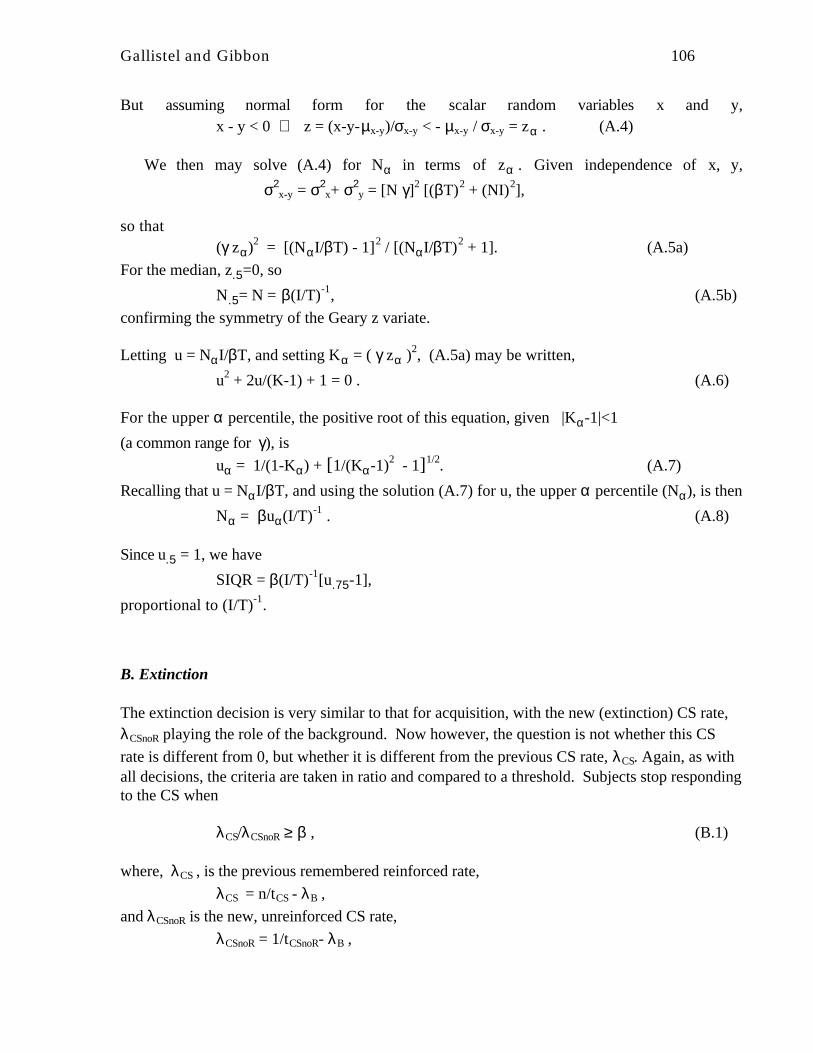
Gallistel and Gibbon 106
But assuming normal form for the scalar random variables x and y,x - y < 0 ⇔ z = (x-y-µx-y)/σx-y < - µx-y / σx-y = zα . (A.4)
We then may solve (A.4) for Nα in terms of zα . Given independence of x, y,
σ2x-y = σ2
x+ σ2y = [N γ]2 [(βT)2 + (NI)2],
so that(γ zα)2 = [(NαI/βT) - 1]2 / [(NαI/βT)2 + 1]. (A.5a)
For the median, z.5=0, so
N.5= N = β(I/T)-1, (A.5b)
confirming the symmetry of the Geary z variate.
Letting u = NαI/βT, and setting Kα = ( γ zα )2, (A.5a) may be written,
u2 + 2u/(K-1) + 1 = 0 . (A.6)
For the upper α percentile, the positive root of this equation, given |Kα-1|<1
(a common range for γ), is
uα = 1/(1-Kα) + [1/(Kα-1)2 - 1]1/2. (A.7)
Recalling that u = NαI/βT, and using the solution (A.7) for u, the upper α percentile (Nα), is then
Nα = βuα(I/T)-1 . (A.8)
Since u.5 = 1, we have
SIQR = β(I/T)-1[u.75-1],
proportional to (I/T)-1.
B. Extinction
The extinction decision is very similar to that for acquisition, with the new (extinction) CS rate,λCSnoR playing the role of the background. Now however, the question is not whether this CS
rate is different from 0, but whether it is different from the previous CS rate, λCS. Again, as withall decisions, the criteria are taken in ratio and compared to a threshold. Subjects stop respondingto the CS when
λCS/λCSnoR ≥ β , (B.1)
where, λCS , is the previous remembered reinforced rate,
λCS = n/tCS - λB ,
and λCSnoR is the new, unreinforced CS rate,
λCSnoR = 1/tCSnoR- λB ,

Gallistel and Gibbon 107
where tCSnoR is the current accumulated CS time without reinforcement, with expectation, NnoRT,
and scalar variance, (γNnoRT)2.
Since acquisition has occurred by the time extinction is instituted, λB is small, and so thedecision rule, (B.1) is approximately
ntCSnoR/tCS ≥ β . (B.2a)It is convenient to write the left side of (B.2a) as
nnoR[tCSnoR/nnoR]/[tCS/n] (B.2b)where it is clear the variates in brackets are both estimates of T. Hence taking expectations,subjects stop responding on average when
NnoR≥ β . (B.3)Thus the extinction decision is independent of I, T, or their ratio.
Extinction Variance.
An explicit form for the SIQR of NnoR is obtained similarly to acquisition. Let x = βtCS , y =ntCSnoR, with means,
µx = βNT, µy = NNnoRT, (B.4a)and variances,
σ2x = (γβNT)2, σ2
y = (γ NNnoRT)2, (B.4b)
reflecting the scalar property. The criterion (B.1), is met with probability α or better iff
∃(N*noR) such that
P(x-y<0) = α = Φ(zα).
Again assuming normal form for the scalar rv’s x and y,x - y < 0 ⇔ z = (x-y-µx-y)/σx-y < - µx-y / σx-y = zα . (B.4)
We may solve (B.4) for N*noR in terms of zα .zα = [NN*noRT - βNT]/[ (γβNT)2 + (γ NN*2
noRT)2]1/2,
so that terms in NT cancel, giving
(γzα)2 = [N*noR - β]2/[ (β2 + N*2noR] . (B.5)
Again setting u = N*noR/β, and Kα = (γzα)2, the positive, upper α solution to the quadratic (B.5)
givesN*noR = 2β uα , (B.6)
where uα = 1/(1-Kα) + [1/(Kα-1)2 - 1]1/2, as in (A.7). Thus
SIQR = 2β[u.75-1]. (B.7)
Variability is also constant, independent of the conditioning protocol.

Gallistel and Gibbon 108
Appendix 2: Rate Estimation
The general solution to the problem of computing true rates of reinforcement
λ1
λ2
Mλn
for n
predictive stimuli (CSs) under the assumption that rates of reinforcement combine additively is
λ1
λ2
Mλn
=
1t1•2
t1L
t1•n
t1t1•2
t21 L t2•n
t2M M O M
t1•n
tn
t2•n
tnL 1
−1
×
N1
t1N2
t2M
Nn
tn
,
where ti is the cumulative duration of Stimulus i, ti•j is the cumulative duration of the
conjunctions of Stimuli i and j, and Ni is the cumulative number of reinforcements delivered inthe presence of Stimulus i. When there are redundant CSs, the determinant of the matrix is zero,so a unique solution does not exist. Unique solutions are then obtained from reduced systems,which are generated from matrices of reduced rank and vectors of correspondingly reduceddimensionality. These reduced matrices and vectors are obtained by deleting one or more CSsfrom consideration. Deleting different CSs produces different solutions. Among these, thepreferred solution is the one that minimizes the sum of the absolute values of the rate estimates.When there is more than one such minimal solution, the choice among them must either be madeat random or be based on extraneous considerations, such as the relative salience of the CSs.
Acknowledgements
We are grateful to the large number of colleagues have read and critiqued parts of earlier drafts.We particularly wish to thank Gustavo Stolovitzky for helping in the derivation of acquisitionvariability, to Peter Dayan for calling attention to a serious error in the way that RET computedthe odds that two rates differed, and to Stephen Fairhurst for showing that taking variability intoaccount leads to the prediction that the slope of the function relating reinforcements toacquisition to the I/T ratio is less than 1. We thank Ralph Miller and three self-identifiedreviewers, Russ Church, Peter Killeen and John Pearce, for thorough and helpful critiques ofearlier versions. We gratefully acknowledge support from NIH Award MH41649 to JG and NSFaward IBN-930