University of Nebraska - LincolnDigitalCommons@University of Nebraska - LincolnArchitectural Engineering -- Dissertations andStudent Research Architectural Engineering

2-1-2011

A VIRTUAL SUPPLY AIRFLOW RATE METERIN ROOFTOP AIR CONDITIONING UNITSDaihong YuUniversity of Nebraska-Lincoln, daisy.yu926@gmail.com

Follow this and additional works at: http://digitalcommons.unl.edu/archengdissPart of the Acoustics, Dynamics, and Controls Commons, and the Architectural Engineering

Commons

This Article is brought to you for free and open access by the Architectural Engineering at DigitalCommons@University of Nebraska - Lincoln. It hasbeen accepted for inclusion in Architectural Engineering -- Dissertations and Student Research by an authorized administrator ofDigitalCommons@University of Nebraska - Lincoln.

Yu, Daihong, "A VIRTUAL SUPPLY AIRFLOW RATE METER IN ROOFTOP AIR CONDITIONING UNITS" (2011).Architectural Engineering -- Dissertations and Student Research. Paper 6.http://digitalcommons.unl.edu/archengdiss/6

A VIRTUAL SUPPLY AIRFLOW RATE METER IN ROOFTOP AIR

CONDITIONING UNITS

By

Daihong Yu

A THESIS

Presented to the Faculty of

The Graduate College at the University of Nebraska

In Partial Fulfillment of Requirements

For the Degree of Master of Science

Major: Architectural Engineering

Under the Supervision of Professor Haorong Li

Lincoln, Nebraska

Feb, 2011

A VIRTUAL SUPPLY AIRFLOW RATE METER IN ROOFTOP AIR

CONDITIONING UNITS

Daihong Yu, M.S.

University of Nebraska, 2011

Adviser: Haorong Li

Virtual sensing technology aims to estimate difficult to measure, expensive, or new

quantities by using multifarious mathematical models along with non-invasive and low-

cost measurements. Such embedded intelligence is a key to improving the performance of

building systems in terms of functionality, safety, energy efficiency, environmental

impacts, and costs. Considering the progress that has been achieved over many various

fields (e.g., process controls, automobiles, avionics, autonomous robots, telemedicine)

within the last two decades, numerous intelligent features have been incorporated and

enabled that would otherwise not be possible or economical.

To identify the potential opportunities and research/development needs of virtual

sensing technology in building systems,

First, this thesis reviews the major milestones of virtual sensing development in other

emerging fields and its formulation of development methodologies.

Second, the state-of-the-art in virtual sensing technology in building systems is

summarized as a starting point for its future developments and applications.

After that, a cost-effective virtual supply airflow (SCFM ) meter for rooftop air-

conditioning units (RTUs) is created by using a first-principle model in combination

with accurate measurements of virtual or virtually calibrated temperature sensors (a

virtual mixed air temperature sensor and a virtually calibrated supply air temperature

sensor) as a supplementary example. Modeling of the virtual meter, uncertainty analysis,

and experimental evaluation are performed through a wide range of laboratory testing in

the development. The study reveals that the first-principle based virtual SCFM meter

could accurately predict SCFM values for RTUs (uncertainty is ± 6.9%). This innovative

application is promising with a number of merits, such as high cost-effectiveness, ease-

of-implementation, long-term availability after one-time development, and generic

characteristics for all RTUs with gas heating.

Significant research and developments are needed before virtual sensors become

commonplace within buildings. It is believed a wealth of virtual sensing derived

applications would facilitate the sustainable management and optimize the advanced

controls in building systems. It is hoped that this study can provide a resource for future

developments.

COPYRIGHT

I hereby declare that I am the sole author of this thesis.

I authorize University of Nebraska-Lincoln, Lincoln, Nebraska, to lend this thesis to

other institutions or individuals for the purpose of scholarly research.

I authorize University of Nebraska-Lincoln, Lincoln, Nebraska, to reproduce this

thesis by photocopying or by other means, in total or in part, at the request of other

institutions or individuals for the purpose of scholarly research.

Copyright © Daihong Yu, 2011. All rights reserved.

5

5

AUTHOR’S ACKNOWLEDGEMENTS

First and foremost, I would like to gratefully acknowledge Professor Haorong Li for

his tireless guidance in my study, research, and personal development. He is knowledgeable,

perseverant, and passionate in life and career.

It is also a great honor for me to have Professor James E. Braun as the key committee

member who offered much advice and insight throughout my work on virtual sensing

technology with his patience and knowledge.

I also sincerely thank my committee members Dr. Siu Kit Lau and Dr. Tian Zhang

for their instruction and help. Thank you all!!

6

6

TABLE OF CONTENTS

Chapter 1 INTRODUCTION ................................................................................... 19

1.1 Background on virtual sensing technology in building systems ................. 19

1.2 Major milestones in virtual sensing development ...................................... 22

1.2.1 Virtual sensing in process controls ...................................................... 23

1.2.2 Virtual sensing in automobiles ............................................................ 23

1.2.3 Use of virtual sensing in other emerging fields ................................... 25

1.3 Formulation of development methodology for virtual sensing ................... 26

1.3.1 Categorization of virtual sensors ......................................................... 26

1.3.2 Approaches for developing virtual sensors ......................................... 29

1.3.3 General steps in developing virtual sensors ........................................ 31

1.4 Background on development of a virtual SCFM meter in RTUs ............... 32

1.5 Outline of the thesis .................................................................................... 35

Chapter 2 VIRTUAL SENSING TECHNOLOGY IN BUILDING SYSTEMS..... 37

2.1 Unique opportunities for virtual sensing in building systems .................... 37

2.2 State-of-the-art in virtual sensing in buildings............................................ 38

2.2.1 Virtual sensors used in building mechanical systems ......................... 40

2.2.1.1 Virtual sensors for vapor compression air conditioners ................... 40

2.2.1.2 Virtual sensors for chillers ............................................................... 50

2.2.1.3 Virtual sensors for heat pumps ......................................................... 51

7

7

2.2.1.4 Virtual sensors for air handling units ............................................... 53

2.2.2 Virtual sensors for building envelopes and occupied zones ................ 58

Chapter 3 DEVELOPMENT OF A VIRTUAL SCFM METER IN RTUS ............ 60

3.1 Modeling and evaluations of cooling-based approach................................ 62

3.1.1 Modeling of cooling-based approach .................................................. 62

3.1.2 Evaluations of cooling-based approach ............................................... 63

3.1.2.1 Experiment preparation of cooling-based SCFM meter .................. 63

3.1.2.2 Uncertainty analysis of cooling-based SCFM meter........................ 66

3.1.2.3 Experimental evaluation of cooling-based SCFM meter ................. 67

3.2 Modeling and evaluations of heating-based approach ................................ 68

3.2.1 Modeling of heating-based approach .................................................. 68

3.2.2 Evaluations of heating-based SCFM meter ......................................... 73

3.2.2.1 Experiment preparation of heating-based SCFM meter ................... 73

3.2.2.2 Uncertainty analysis of heating-based SCFM meter ........................ 74

3.2.2.3 Experimental evaluation of heating-based SCFM meter ................. 75

3.3 Comparisons and conclusions of cooling- and heating-based approaches . 76

3.4 Implementation issues ................................................................................. 78

3.4.1 Measuring and processing SAT ........................................................... 78

3.4.1.1 Background of direct measurements of SAT in RTUs .................... 78

3.4.1.2 Evaluation of direct measurements of SAT in RTUs ....................... 80

8

8

3.4.1.3 Development of a virtual calibration model for a SAT sensor in

RTUs 87

3.4.1.4 Uncertainty analysis ......................................................................... 88

3.4.2 Measuring and processing MAT ......................................................... 89

3.4.3 Implementation flowchart of the virtual SCFM meter ........................ 90

Chapter 4 FUTURE RESEARCH NEEDS AND CONCLUTION ......................... 92

4.1 Future needs for virtual sensing technology and its application in building

systems 92

4.1.1 Future needs for virtual sensing technology in building systems ........ 92

4.1.2 Future steps for development of an improved virtual SCFM meter in

RTUs 93

4.1.3 Future steps for development of an improved virtually calibrated SAT

sensor in RTUs .......................................................................................................... 94

4.2 Conclusion .................................................................................................. 95

References ................................................................................................................... 99

Appendix A ............................................................................................................... 108

Appendix B ............................................................................................................... 111

9

9

LIST OF TABLES

Table 1: Virtual sensing developments in vehicles..................................................... 25

Table 2: Virtual sensors in buildings .......................................................................... 38

Table 3: Uncertainty analysis of cooling-based SCFM meter .................................... 67

Table 4: Experimental evaluation of cooling-based SCFM meter.............................. 67

Table 5: Calculation of NTU of a heat exchanger ...................................................... 71

Table 6: Experimental designs and results of heating-based SCFM meter ................ 73

Table 7: Uncertainty analysis of heating-based SCFM meter .................................... 75

Table 8: Experimental evaluation of heating-based SCFM meter .............................. 75

Table 9: Evaluation of direct SAT measurement under both cooling and heating mode

........................................................................................................................................... 81

Table 10: Linear model coefficients for the example RTU ........................................ 88

Table 11: Uncertainty analysis of SATmfr,cal ............................................................... 89

Table 12: Correcting UA in cooling mode ............................................................... 117

Table 13: Results of evaluation of SATmfr,cal ............................................................ 119

10

10

LIST OF FIGURES

Figure 1: Virtual sensing systemized vehicle ............................................................. 25

Figure 2: A categorization scheme for virtual sensors................................................ 27

Figure 3: General steps in developing virtual sensors ................................................ 31

Figure 4: Intelligent air conditioner enabled through multiple virtual sensors ........... 41

Figure 5: Virtual refrigerant charge sensor ................................................................. 42

Figure 6: Virtual refrigerant pressure sensors ............................................................. 44

Figure 7: Virtual refrigerant flow rate sensor ............................................................. 45

Figure 8: Virtual compressor power consumption sensor .......................................... 46

Figure 9: Virtual system performance sensors............................................................ 47

Figure 10: Virtual supply air humidity sensor ............................................................ 48

Figure 11: Illustration of bypass factor analysis ......................................................... 50

Figure 12: Virtual sensors for chillers ........................................................................ 50

Figure 13: Virtual sensors for heat pump reversing and check valve leakage faults .. 52

Figure 14: Virtual mixed air temperature sensor ........................................................ 53

Figure 15: Virtual sensors for AC cooling coil ........................................................... 55

Figure 16: Virtual sensors for filters ........................................................................... 56

Figure 17: Virtual pump water flow rate sensor ......................................................... 57

Figure 18: Virtual fan air flow rate meter ................................................................... 58

Figure 19: Virtual occupant complaint sensor ............................................................ 59

Figure 20: Virtual sensor for solar radiation ............................................................... 59

Figure 21: Typical air-conditioning process ............................................................... 60

11

11

Figure 22: Illustration of machine layout in the lab .................................................... 63

Figure 23: Experimental settings in the cooling mode ............................................... 64

Figure 24: Lab sensors’ layout .................................................................................... 64

Figure 25: Heat transfer of a heat exchanger .............................................................. 68

Figure 26: Illustration of measuring grid and numbered sensors ............................... 83

Figure 27: Evaluation of measuring grid under both cooling and heating mode: (a) IP

units and (b) SI units. ........................................................................................................ 85

Figure 28: eH vs OADst in different Hstage: (a) IP units and (b) SI units. ................. 87

Figure 29: An implementation flowchart of a virtual SCFM meter in RTUs ............. 91

Figure 30: A hierarchy scheme of SoVS .................................................................... 93

Figure 31: Sensors layout of additional six air temperature sensors ........................ 112

Figure 32: Evaluation of additional six temperature sensors under both cooling and

heating mode: (a) IP units and (b) SI units. .................................................................... 114

Figure 33: The experiment evaluation procedures of the virtual calibration

methodology ................................................................................................................... 116

Figure 34: UA linear regression: (a) IP units and (b) SI units. ................................. 118

12

12

NOMENCLATURE

Roman Letter Symbols

A area, ft2

(m2)

a,c empirical coefficient

C discharge coefficient, specific heat, Btu/(lbm·°F) (kJ/(kg·K));

Cmin the smaller of Cg and Ca, Btu/(hr·°F) (kW/K)

Cmax the bigger of Cg and Ca, Btu/(hr·°F) (kW/K)

Cr a capacity ratio as Cmin /Cmax

D duct diameter, in (m); discharge dew point temperature, °C (°F)

e error between SATlab,meas and SATmfr,meas (°F, °C)

eC,eva relative error between meas,CV

and elmod,CV

eeva error between SATmfr,cal and SATexp,eva (°F, °C)

eH error between SATth,pred and SATmfr,meas (°F, °C)

eH,eva relative error between meas,HV

and elmod,HV

EAT exhaust air temperature (°F, °C)

ET entering air temperature, °C (°F)

h enthalpy, kJ/kg (Btu/lbm), heat transfer coefficient, Btu/(h·ft2·°F)

(kW/(m2·K))

H height, ft (m); pump head, fan head, inch H2O (Pa)

Hstage heating stage status

h1 enthalpy of air before the thermal equipment Btu/lbm (kJ/kg)

13

13

h2 enthalpy of air after the thermal equipment Btu/lbm (kJ/kg)

k slope of the best-fit line geometry constant, thermal conductivity,

Btu/h·ft·°F (kW/(m·K))

L length, ft (m)

LMTD logarithmic mean temperature difference

m mass of charge, lbm(kg)

m mass flow rate, lbm/min (kg/s)

MAT mixed air temperature, °C (°F)

0wbMAT

critical point of the mixed air wet bulb temperature, °F (°C)

MOAT measurement of the manufacturer-installed OAT sensor, ºF (ºC)

MRAT measurement of the manufacturer-installed RAT sensor, ºF (ºC)

MSAT measurement of the manufacturer-installed SAT sensor, ºF (ºC)

n the number of right angle bends

N number of suction strokes per unit time

NTU number of transfer units

Nu Nusselt number

OARH outside air relative humidity

OAT outside air temperature, °C (°F)

OADst

outside air damper position

P pressure

Pr Prandtl number

Q capacity, Btu/hr (kW)

14

14

Q volumetric flow rate, m3/s

RAT return air temperature, °C

Re duct Reynolds number

S suction dew point temperature, °C (°F)

SHR sensible heat ratio

SAT Supply air temperature, °C (°F)

T temperature, °C (°F)

U heat transfer coefficient, Btu/(hr·°F·ft²) (kW/(m2·K))

v specific volume, ft3/lb (m

3/ kg), kinematic viscosity, ft

2/s (m

2/s)

V displacement volume, cfm (m3), linear velocity, ft/s (m/s)

V supply airflow rate, cfm (m3/s)

w humidity ratio, speed

W width, m

W

compressor power consumption, Btu/h (kW)

X mass flow rate, power consumption, current, coefficient of

performance or compressor volumetric efficiency

ZARH zoon air relative humidity

ZAT zoon air temperature, °C (°F)

∆P pressure drop

∆Tfan supply fan temperature rise, ºF (ºC)

∆Toa-ra difference between outdoor and return-air temperature

Greek symbols

β outside fresh air ratio

15

15

heat exchanger effectiveness

η efficiency

μ dynamic viscosity of air, lbm/ft·s (N·s/m2)

ρ density, lb/ft3 (kg/m

3)

Subscripts

a air

aie air stream in the inlet of evaporator

aic air stream in the inlet of condenser

amb ambient

aoe air stream in the outlet of evaporator

aoc air stream in the outlet of condenser

B bypasing

c cooling

ca condenser air

cal calibration

ch charge

comp compressor

cond condenser

cycle refrigerant cycle

d design

db dry bulb

dis discharge

down downstream

16

16

error bias error

eva evaluation

evap evaporator

exp experimental

fan supply air fan

g gas

G grid

i inlet

lab lab-installed

ll liquid line

loss heat loss

LCV leaky check valve

LRV leaky reversing valve

mfr manufacturer

max maximum

meas measured

min minimum

model modeling

normal normal condition

o outlet

P constant pressure

pred predicted

pump heat pump

17

17

r ratio

ref refrigerant

s supply air, sensible

sc subcooling

sh superheat

sp set point

suc Suction line

th theoretical

total total value

rated nominal value at rated conditions

up upstream

v volumetric

vir virtual

wb wet bulb

wb wet bulb

Abbreviations

AHU Air handling unit

ANN Artificial Neural Networks

ARMAX auto-regressive moving-average time-series model

BF bypass factor

CAV Constant air volume

COP coefficient of performance

18

18

DDC direct digital control

DF decoupling feature

DX direct expansion

EMCS energy management control system

EER energy efficiency ratio

FDD fault detection and diagnoses

FP First principle

FXO fixed orifice

HVAC Heating, ventilation and air-conditioning system

IAQ indoor air quality

MLP Multi-layer Perceptron

NTU number of transfer units

PAFM physical airflow meter

PCA Principle Component Analysis

RTU rooftop air conditioning unit

SCFM supply airflow rate

SVM Support Vector Machine

TXV thermal expansion valve

TXV thermostatic expansion valve

VAV variable air volume

VHC virtual heating capacity

19

19

Chapter 1 INTRODUCTION

1.1 Background on virtual sensing technology in building systems

Embedded intelligence is a key to improving the performance of systems in terms of

functionality, safety, energy efficiency, environmental impacts, and costs. Consider the progress

that has been achieved with automobiles within the last two decades. Modern automobiles

incorporate many intelligent features, including anti-lock brakes, electronic stability control, tire

pressure monitoring, and feedback on fuel efficiency and the need for service. If a car is in need

of service, then a technician has access to on-board diagnostic information. In many cases, these

advanced features have been enabled through the development of virtual sensors. A virtual

sensor estimates a difficult to measure or expensive quantity using one or more mathematical

models along with lower cost physical sensors. Fifty years ago, most automobiles provided fuel

level and some warning lights using four physical sensors, on average. Today, about 40

relatively low-cost embedded physical sensors are employed along with virtual sensors to

optimize driving performance, safety, functionality, and reliability of vehicles (Healy, 2010).

In contrast, building systems rarely provide feedback on energy efficiency or the need for

service and generally do not provide optimized controls. In fact, typical information provided to

a building owner and occupants, even with a direct digital control (DDC) energy management

control system (EMCS), is not significantly better than what was provided 50 years ago.

Although the energy efficiency of individual building components has improved significantly

(e.g., the rated efficiency of new residential cooling equipment has nearly tripled), the operating

efficiency is typically degraded by 20% to 30% due to improper installation/commissioning and

inadequate maintenance/repair (CEC, 2008).

20

20

One of the reasons that building applications are slower to adopt more automation and

intelligent features than automobiles may be that they are not mass produced in factories. For

automobiles, automated features are part of an integrated design and their development costs can

be spread out over millions of vehicles. For buildings, the cost threshold for advanced features is

much higher because buildings tend to be individually engineered. Also, building systems can be

very large and complex, serving hundreds of zones with individual controllers and often requiring

thousands of sensors to adequately characterize and monitor performance. Therefore, a key to

realizing more intelligent features in buildings should be to reduce the cost threshold. Lowering

the cost of sensing through the availability of virtual sensors helps in attacking this problem with

the potential for providing high level performance monitoring information (e.g., energy

efficiency) at significantly less cost. It would also make sense if advanced features were

embedded within individual manufactured devices (air handling units, compressors, etc.) rather

than being engineered within the control system during the building design phase. In order to

realize widespread application, advanced features should be commodities rather than individual

engineering projects.

Practically every device within a building could serve as a virtual sensor in addition to

providing its intended function. For instance, a fan/motor package could incorporate a model that

provides virtual sensing for air flow rate and power consumption using only measurements of

static pressure difference and inlet temperature. A compressor could incorporate a map for

refrigerant flow rate and input power using physical measurements of inlet and outlet pressure,

along with inlet temperature. Valves or dampers could also output flow measurements based on

differential pressure and inlet temperature measurements. A ―smart‖ lighting fixture could

provide power, lighting, and heat gain outputs based on the input control signal. A ―smart‖

window could provide estimates of heat gain and even solar radiation based on low-cost

measurements and a model.

21

21

The availability of a rich set of high value sensor information would enable a level of

building optimization and improvement not previously possible. Virtual sensors for capacity and

power consumption at the device level would allow real-time monitoring of device, subsystem,

and whole-building efficiencies. This information could be used along with other virtual sensors

to enable diagnosis, tracking, and economic impact evaluation of specific faults. The virtual

sensor outputs and embedded models could also be employed within a control optimizer that

determines setpoints that minimize operating costs at each operating condition. If all devices

incorporated embedded intelligence then there would undoubtedly be a significant amount of

redundant information that could use to diagnose sensor faults (e.g., faults within devices

providing virtual sensor outputs).

Some might argue that all of the data necessary to provide monitoring, diagnostics, and

optimal control could be provided more reliably and robustly using physical sensors. However,

virtual sensors have several advantages in addition to lower cost. For example, virtual sensors

could be more easily added as retrofits in a number of important applications, such as

measurement of refrigerant flow rate or pressure. A physical sensor for refrigerant mass flow

would require opening up the system, recovering the refrigerant, installing the sensors, and then

recharging the system. The installation of refrigerant pressure sensors would require access to

threaded service ports on the equipment, which can cause refrigerant leakage over time (Li and

Braun, 2009a). The same refrigerant-side sensor information could be obtained using non-

invasive surface mounted temperature sensors along with models.

In some cases, it is very difficult to install physical sensors that can accurately measure a

desired quantity. For example, it is very difficult to obtain accurate mixed air temperature

measurements at the inlet of cooling coils or evaporators because the compactness of the mixing

chamber creates highly non-uniform flow and temperature characteristics. However, an accurate

effective mixed air temperature is readily obtained using a model and measurements obtained at

other more uniform locations (e.g., coil outlet and/or return and ventilation air streams). In other

22

22

cases, it can be impossible to measure some quantities directly. For example, it is currently not

possible to directly measure the amount of refrigerant charge within an air conditioner or heat

pump.

Virtual sensors have been developed in other fields to obtain measurements indirectly in

a cost-effective, non-invasive or/and practical manner, but are only recently the subject of

development for building systems. There is no widely accepted definition of virtual sensing. In

the context of this thesis, virtual sensing is considered to include any indirect method of

determining a measureable quantity that utilizes outputs from other physical and/or virtual

sensors along with process models and/or property relations. The primary goals of this thesis are

to review the state-of-the-art in virtual sensing in other fields and as applied to building systems,

to newly develop a virtual supply air flow (SCFM) meter in rooftop air-conditioning units

(RTUs), and to provide some perspective regarding open issues and possible next steps as a

starting point for future development and implementation. First, this chapter reviews the major

milestones of virtual sensing development in other emerging fields and its formulation of

development methodologies.

1.2 Major milestones in virtual sensing development

There has been a rapid development of virtual sensing technology over the past decade

within a number of different domains, including avionics, autonomous robots, telemedicine,

traffic, automotive, nature and building monitoring and control (Dorst, et al.1998; Hardy and

Ahmad, 1999; Hardy and Maroof, 1999; Oosterom and Babuska, 2000; Kestell, et al. 2001;

Oza,et al 2005; Srivastava, et al. 2005; Gawthrop 2005; Kabadayi, et al. 2006; Bose, et al. 2007;

Ibarg¨uengoytia, et al. 2008; Said, et al. 2009; Raveendranathan, et al. 2009; et al.). In particular,

virtual sensing has found widespread applications in process controls and automobiles, so here

focuses on these two fields in providing a brief history of notable developments.

23

23

1.2.1 Virtual sensing in process controls

―Virtual sensors‖, also termed ―soft sensors‖, have found widespread applications in

process control engineering since the early 1980s. Researchers in process control engineering

(Venkatasubramanian et al., 2003a, 2003b, 2003c; Fortuna et al, 2007; Kadlec et al., 2009) use

the term virtual sensors to characterize software that includes several interacting measurements of

characteristics and dynamics that are processed (fused) together to calculate new quantities that

need not be measured directly. Under this definition, well-known software algorithms that are

considered to be soft sensors include Kalman filters and state observers or estimators such as

electric motor velocity estimators. In process control engineering, virtual sensing is focused on

estimating system dynamics or state variables through construction of state observers.

Accordingly, virtual sensor development involves representing the whole control system using a

mathematical transient model through ordinary or partial differential equations, and then

constructing state observers or estimators to estimate non-measured states using mathematical

transformation techniques. The transformed estimators or observers are considered to be virtual

sensors.

1.2.2 Virtual sensing in automobiles

There have been a large number of virtual sensing developments for automobiles during

the past decade. Unlike applications in process control engineering where system dynamics or

transient states are of primary interest, the focus for virtual sensing in automobiles has primarily

been on determination of steady-state variables. The methods for constructing virtual sensors

have been more fragmented and component-oriented. Steady-state models represented by

algebraic equations are often used to relate the quantity that is not measured directly to one or

more quantities that are directly measured using physical sensors. These steady-state models can

be considered to be virtual sensors.

24

24

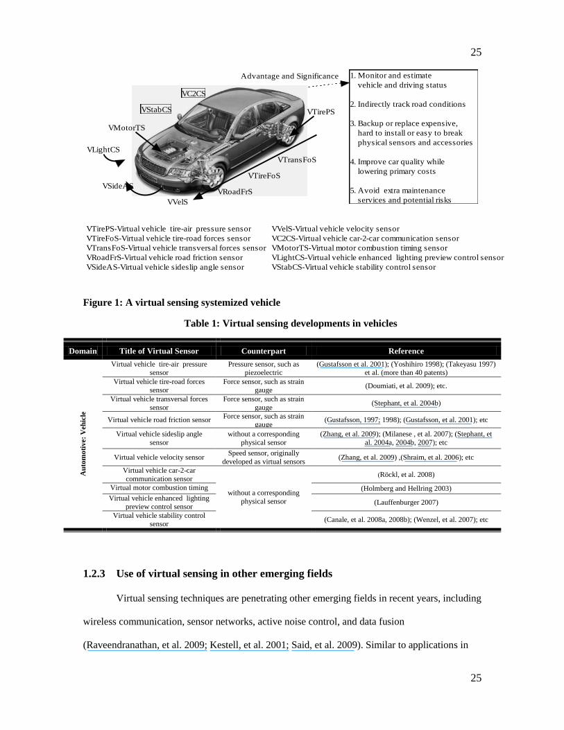
Figure 1 depicts a vehicle that employs ten virtual sensors that have been developed in

the past decade to provide increased functionality, safety, and reliability. Table 1 describes the

corresponding physical sensor and references for each virtual sensor. For example, virtual

sideslip angle and velocity of the centre of gravity sensors play important roles in reducing the

potential dangers associated with loss of control of a vehicle. These quantities would be difficult

and expensive to measure directly and are estimated using a hyperbolic tangent switching

function (Zhang, et al. 2009; Shraim, et al. 2006) that combines available vehicle information

(e.g. mass of vehicle, friction coefficient). Another example is the virtual tire pressure sensor.

Conventionally, tire air pressure is measured directly using a pressure responsive element located

within the tire. However, this construction is complicated and costly. There have been a number

of different developments related to tire pressure indication, reflected in more than 40 patents

(Gustafsson et al. 2001; Yoshihiro 1998; Takeyasu 1997). A widely studied approach utilizes a

Kalman filter to estimate tire pressure in a simple model that uses wheel speed and road friction

that are also sensed using virtual observers (Zhang, et al. 2009; Shraim, et al. 2006; Gustafsson,

1997; 1998; 2001). On-vehicle sensors alone do not provide sufficient quality and quantity of

information to fulfill all of the evolving vehicle requirements (Röckl, et al. 2008). Virtual sensors

have also been developed that utilize car-to-car communication within an intelligent automotive

system for a variety of purposes, including cooperative collision and traffic jam warnings. The

convergence of multiple virtual sensors has significantly upgraded the intelligence of automobiles

over time.

25

25

VTirePS

VTireFoS

VTransFoS

VRoadFrSVSideAS

VVelS

VC2CS

VMotorTS

VLightCS

VStabCS

1. Monitor and estimate

vehicle and driving status

2. Indirectly track road conditions

3. Backup or replace expensive,

hard to install or easy to break

physical sensors and accessories

4. Improve car quality while

lowering primary costs

5. Avoid extra maintenance

services and potential risks

Advantage and Significance

VTirePS-Virtual vehicle tire-air pressure sensor

VTireFoS-Virtual vehicle tire-road forces sensor

VTransFoS-Virtual vehicle transversal forces sensor

VRoadFrS-Virtual vehicle road friction sensor

VSideAS-Virtual vehicle sideslip angle sensor

VVelS-Virtual vehicle velocity sensor

VC2CS-Virtual vehicle car-2-car communication sensor

VMotorTS-Virtual motor combustion timing sensor

VLightCS-Virtual vehicle enhanced lighting preview control sensor

VStabCS-Virtual vehicle stability control sensor

Figure 1: A virtual sensing systemized vehicle

Table 1: Virtual sensing developments in vehicles

Domain Title of Virtual Sensor Counterpart Reference

Au

tom

oti

ve:

Veh

icle

Virtual vehicle tire-air pressure sensor

Pressure sensor, such as piezoelectric

(Gustafsson et al. 2001); (Yoshihiro 1998); (Takeyasu 1997) et al. (more than 40 patents)

patents. Virtual vehicle tire-road forces

sensor

Force sensor, such as strain

gauge (Doumiati, et al. 2009); etc.

Virtual vehicle transversal forces

sensor

Force sensor, such as strain

gauge (Stephant, et al. 2004b)

Virtual vehicle road friction sensor Force sensor, such as strain

gauge (Gustafsson, 1997; 1998); (Gustafsson, et al. 2001); etc

Virtual vehicle sideslip angle

sensor

without a corresponding

physical sensor

(Zhang, et al. 2009); (Milanese , et al. 2007); (Stephant, et

al. 2004a, 2004b, 2007); etc

Virtual vehicle velocity sensor Speed sensor, originally

developed as virtual sensors (Zhang, et al. 2009) ,(Shraim, et al. 2006); etc

Virtual vehicle car-2-car

communication sensor

without a corresponding

physical sensor

(Röckl, et al. 2008)

Virtual motor combustion timing

sensor (Holmberg and Hellring 2003)

Virtual vehicle enhanced lighting preview control sensor

(Lauffenburger 2007)

Virtual vehicle stability control sensor

(Canale, et al. 2008a, 2008b); (Wenzel, et al. 2007); etc

1.2.3 Use of virtual sensing in other emerging fields

Virtual sensing techniques are penetrating other emerging fields in recent years, including

wireless communication, sensor networks, active noise control, and data fusion

(Raveendranathan, et al. 2009; Kestell, et al. 2001; Said, et al. 2009). Similar to applications in

26

26

automobiles, the primary focus for virtual sensing developments in these emerging fields has

been on estimating steady-state variables. However, transient-state variables are also utilized in

many virtual sensing schemes, notably in active noise control which uses mechanistic models

similar in nature to the process control field. Data-driven modeling methods are more frequently

used in the fields of wireless communication, sensor networks and data fusion because the

amount of data and information in these fields are very rich. Also, researchers in these fields are

more accustomed to applying data processing techniques and less skilled in developing physical

models.

Another emerging area for adoption of virtual sensing is the building industry. The

development of virtual sensors for building components has lagged other fields, probably because

of the fragmented nature of the industry and the emphasis on initial costs. In fact, the concept and

potential for ―virtual sensing‖ has only recently been considered for building applications leading

to some initial developments (Li and Braun, 2007a; 2007b; 2009a; 2009b).

1.3 Formulation of development methodology for virtual sensing

Virtual sensors are the embodiment of virtual sensing techniques. For the sake of

simplicity, the term virtual sensor is used interchangeably with virtual sensing to present

development methodology. Although many different types of virtual sensors have been

developed, there is no widely accepted definition and no systematic virtual sensing development

methodology. It is useful to categorize virtual sensors before attempting to describe general

approaches for their development.

1.3.1 Categorization of virtual sensors

Virtual sensors can be categorized, as shown in Figure 2, according to three interrelated

criteria that affect development approaches: 1) measurement characteristics, 2) modeling

methods, and 3) application.

27

27

Modeling

methods

-based

Measurements

characteristics

-based

Virtual sensors

Application

purposes

-based

Transient-state

data -based

First-principle

(model-driven)

For backup

/replacement

Steady-state

data -based

Black-box

(data-driven)Grey-box

For

observing

Layer

-based

Basic

virtual sensor

Derived

virtual sensor

Figure 2: A categorization scheme for virtual sensors

The measurement characteristic category refers to whether the desired virtual sensor

outputs are transient or steady-state variables. A transient virtual sensor incorporates a transient

model to predict the transient behavior of an unmeasured variable in response to measured

transient inputs. This type of sensor would be necessary for feedback control or if transient

information were useful in fault identification. For performance monitoring or fault identification

it is often adequate and/or desirable to assume that the modeled process is quasi-static. In this

case, steady-state models (i.e., with no dynamic terms) are utilized. This modeling is appropriate

when the measured input quantities change slowly or the modeled process responds very

―quickly‖ to changes in inputs. Many processes in the food and biochemistry industry, like

fermentation processes, utilize transient-state virtual sensors (Rotem, et al. 2000; Kampjarvi, et al.

2008). Transient-state virtual sensors are also very common in the specialty chemistry field

(Bonne and Jorgensen 2004). However, steady-state virtual sensors represent the majority of the

applications in different fields (Qin 1997; Casali, et al. 1998; Park and Han 2000; Jos de Assis

and Maciel Filho 2000; Meleiro and Finho 2000; Radhakrishnan and Mohamed 2000;

Devogelaere, et al. 2002; James, et al. 2002.et al.).

With respect to modeling methods, virtual sensors can be divided into three types: first-

principle (model-driven), black-box (data-driven), and grey-box virtual sensors. First-principle

(physical or white-box) virtual sensors are most commonly derived from fundamental physical

28

28

laws and have parameters with some physical significance. For example, DeWolf et al. (1996)

developed a virtual slurry polymerization reactor sensor based on a Kalman filter and Prasad, et al.

(2002) applied a multi-rate Kalman filter to the control of a polymerization process. For the same

application, Doyle (1998) utilized a non-linear observer method. In contrast to first-principle

virtual sensors, black-box (data-driven) approaches utilize empirical correlations without any

knowledge of the physical process. Examples include multivariate Principle Component Analysis

(Gonzalez, 1999; Warne et al. 2004), Partial Least Squares (Frank and Friedman, 1993; Kourti,

2002), Artificial Neural Networks (Poggio and Girosi, 1990; Bishop, 1995) and so on. A grey-

box virtual sensor utilizes a combination of physical and empirical models in estimating the

output of an unmeasured process (Casali et al. 1998; Meleiro and Finho 2000; James, et al. 2002).

According to application, virtual sensors can be divided into backup/replacement and

observing virtual sensors. Backup/replacement virtual sensors are used either to back up or

replace existing physical sensors. A backup virtual sensor can provide a check on the accuracy of

an installed sensor and even enable virtual calibration. For example, the reliability of

temperature sensors is affected by incorrect installation, hostile environmental conditions, or

natural drift (ASHRAE, 2009). A replacement application is dictated by cost and reliability

considerations, such as the virtual tire-air pressure sensor studied for automobiles (Gustafsson, et

al. 2001; Yoshihiro 1998; Takeyasu 1997; et al.). A physical pressure sensor located within the

tire is expensive and exposed to high rotational speeds and vibration which over time can lead to

unreliable measurements and failure. Within automotive applications, the majority of the existing

virtual sensors either back up or replace physical counterparts. In contrast, observing virtual

sensors estimate quantities which are not observable (or measurable) directly using existing

physical sensors. For example, typically there is no physical sensor to directly determine engine

performance. Mihelc and Citron (1984) proposed a virtual engine-performance monitor for

determining the relative combustion efficiencies of each cylinder within a multiple cylinder

29

29

internal combustion engine using available information (e.g. the position of engine crankshaft).

This performance index allows evaluation of test engine fuel distribution stem and ignition

system control strategies.

Either backup/replacement or observer sensors can be used for a variety of end-use

applications, including performance monitoring, control, and fault detection and diagnostics

(FDD). FDD virtual sensors allow flagging of a fault and ―measurement‖ of the fault severity.

For instance, a virtual air flow sensor could be a cost-effective replacement for a physical sensor

and be used to directly identify a fan or heat exchanger fouling fault. Alternatively, diagnostic

fault indicators could be energy rates or other variables that have no physical sensor counterpart.

Since the early 1990s, a number of FDD virtual sensors have been studied, such as FDD virtual

sensors for a turbo generator (Gomez, et al. 1996) and an ethylene cracking process (Kampjarvi,

et al. 2008).

1.3.2 Approaches for developing virtual sensors

Transient-state virtual sensors are typically developed using measurements associated

with responses to rapid control changes (e.g. system shut-down or turn-on). The models could

be physical, grey-box, or black-box models. Transient physical or grey-box models could be sets

of linear or non-linear ordinary differential equations or time-series equations. System

identification techniques are employed to determine model order and estimate parameters.

Neural networks are sometimes employed as a black-box modeling approach for transient

representations, requiring time series data as inputs. A significant amount of training data is

typically required to train a transient neural network model. Transient training approaches need

to handle batch-to-batch data variations (Nomikos and MacGregor, 1995) that account for the

finite and varying duration of the processes, the time variance of the particular batches described

by the batch trajectory, the often high batch-to-batch variance, and the starting conditions of the

batches (Champagne, et al. 2002). An example of a grey-box transient model is an auto-

30

30

regressive moving-average time-series model with deterministic input terms (ARMAX). An

ARMAX model was proposed by Casali et al. (1998) for characterizing particle size in a grinding

plant. Meleiro and Finho (2000) presented a grey-box transient virtual sensor that is part of a self-

tuning adaptive controller of a fermentation process and that utilizes a Multi-layer Perceptron

(MLP) approach which is trained using simulated data based on a phenomenological model.

Steady-state virtual sensors are developed using measurements collected while a system

is running in an uninterrupted, continuous way. Steady-state virtual sensors use algebraic

equations rather than differential or time-series equations and respond instantaneously to time-

varying inputs to provide quasi-steady outputs. This is appropriate for many applications and can

be combined with steady-state detectors so that the outputs are only utilized under appropriate

operating conditions. Steady-state virtual sensors can use physical, grey-box, or black-box

models. Steady-state first principle models might incorporate mass balances, force balances,

energy balances, and/or rate equations that describe a mechanical, thermal, or chemical process.

Black-box models are often multi-variable polynomials or neural networks. An example of a

grey-box virtual sensor is a biomass concentration sensor developed for a biochemical batch

process (James, et al. 2002) that combines a physical model of a portion of the process with an

artificial neural network model.

Black-box models have the potential to provide a more accurate representation than a

physical or grey-box model because they have several degrees of freedom to map the measured

behavior. However, they require significantly more training data and generally do not extrapolate

well beyond the range in which they were trained. There are a number of statistical tools that can

be used during the development of black-box models for any application, including Principle

Component Analysis (PCA), or more precisely on Hotelling’s T2 (Hotelling, 1931) and Q-

Statistics (Jackson and Mudholkar, 1979). PCA is one of the most popular tools for developing

black-box models for virtual sensors (Jolliffe, 2002). Another popular method is the Self

31

31

Organizing Maps or Kohonen Map (Kohonen, 1997), which is a type of artificial neural network.

Specific examples of black-box virtual sensors that have been developed include single or multi-

regression models (Kresta, et al.1994; Park and Han, 2000), Partial Least Squares (Wold, et al.

2001), Artificial Neural Networks (ANN) (Qin and McAvoy, 1992; Bishop, 1995; Radhakrishnan

and Mohamed, 2000; Principe, et al. 2000; Hastie, et al. 2001), Neuro-Fuzzy Systems (Jang,et al.

1997; Lin and Lee, 1996) and Support Vector Machines (SVMs) (Vapnik, 1998).

1.3.3 General steps in developing virtual sensors

A number of studies have been done to define procedures for developing virtual sensors

(Park and Han, 2000; Han and Lee, 2002; Warne et al., 2004). In general, the process can be

defined in terms of three steps as illustrated in Figure 3 and described in the following paragraphs:

(i) data collection and pre-processing, (ii) model selection and training and (iii) sensor

implementation and validation.

Inp

ut

Ou

tpu

t

Model selection

and training-

Multi-approaches

for modeling

virtual sensors

Implementation

and validation-

Error analysis,

laboratory testing

and/or in-situ studies

Data collection-

Measurements; empirical coefficients

and/or user specifications

& Pre-processing-

Data filters by using

mathematic methods, e.g. PCA

Figure 3: General steps in developing virtual sensors

Proper data collection and pre-processing (pre-filtering or data outliers) is fundamental in

the development of accurate and reliable virtual sensor models. The type and range of test data

depends on the modeling approach. Transient sensors require transient test data, whereas

transient data should be filtered for steady-state modeling approaches. A ―steady-state detector‖

may be used as a pre-processor (Li and Braun 2003b, Wichman and Braun 2009) to eliminate

transient data. For black-box models, Principle Component Analysis is a popular approach for

pre-processing data in order to aid in the model selection (Serneels and Verdonck, 2008,

Stanimirova, et al. 2007 and Walczak and Massart, 1995).

32

32

Model selection and training are the most difficult and critical steps in the process of

developing a virtual sensor. There are many model types to choose from and each requires a

process of determining the proper model order, estimating parameters, and then redefining the

model selection/order. The previous section provided an overview of possible modeling

approaches. However, there is a bit of an art involved in identifying an appropriate model.

A virtual sensor could be implemented as part of a control or monitoring system or as a

standalone sensor with its own hardware, embedded software, and input/output channels. In

either case, the virtual sensor implementation needs to be tested in both laboratory and in-situ

studies to validate performance and evaluate robustness (e.g., error analysis). Statistical

approaches can be used to validate accuracy (e.g., student’s t-test Gosset, 1908). It is important to

assess the performance using independent data (Hastie et al., 2001; Weiss and Kulikowski, 1991).

With the review of virtual sensing technology development and formulization

accomplished above, the state-of-the-art in virtual sensing technology in building systems are

studied in Chapter 2 as a starting point for its future developments and applications in building

systems. In the meantime, a first-principle (FP) based virtual supply airflow (SCFM) meter for

RTUs is created using a white-box model in combination with accurate measurements of low-cost

virtual or virtually calibrated temperature sensors (virtually calibrated supply air temperature

sensor and a virtual mixed air temperature sensor) as a supplementary example of the study.

1.4 Background on development of a virtual SCFM meter in RTUs

RTUs are widely used for air conditioning retail, residential and industrial premises,

covering from small to medium sizes of spaces. The U.S. Department of Energy estimates that

RTUs including unitary air-conditioning equipments account for about 1.66 quads of total energy

consumption for commercial buildings in the United States (Westphalen and Koszalinski 2001).

Knowledge of SCFM through RTUs is certainly of great importance for a number of reasons. For

instance, low SCFM directly impairs temperature distribution and causes poor indoor air quality

33

33

(IAQ). ASHRAE standard 62.1-2007 specifies ventilation and circulation airflow rate based on

the occupancy and floor area. In some cases, low SCFM across the RTUs makes the heating

equipment to run on the high temperature limit, leading to intensive heating cycling and energy

losses.

In the last two decades, a number of studies have focused on finding good solutions for

measuring SCFM (e.g., ASHRAE 41.2, 1987; Howell and Sauer. 1990a, 1990b; Riffat. 1990,

1991; ASHRAE 110, 1995; Palmiter and Francisco, 2000; etc). In terms of physical airflow

measuring and monitoring devices, the most popular techniques are based on air dynamic

pressure measurements by using a pitot traverse or on air velocity by vane anemometer.

However, in general

A physical airflow monitoring meter (PAFM) is fragile

The main disadvantage of PAFM is its flimsy reliability. Periodical calibration is

required but rarely followed in real applications. Credibility of measurements would be

compromised dramatically after long-term use in adverse duct work surroundings.

Implementing and maintaining a PAFM are expensive

PAFMs are costly in the regards of procurement and installation, ranging from hundreds

to thousands dollars. Much more expenses emerge along for maintenance, repair or rebuild, due

to the hostile operating environment.

Additional pressure loss is incurred

In order to get accurate measurement, a high air velocity across the instrument is desired

for a spread of different airflow rate. To achieve this, a piece of duct work is throttled and it

causes additional pressure loss to the fan.

Besides, installing PAFMs in RTUs is even more unrealistic,

It is hard to install a PAFM in RTUs.

34

34

RTUs usually have compact structure and duct work. The originally efficient

configuration leaves barely any space for a physical meter. PAFMs require more space than is

available to measure the true value of SCFM.

Relative price of PAFMs over RTUs is high

The majority of light commercial RTUs falls in the range of 5 tons to 15 tons of cooling

capacity and only cost several thousand dollars. However, a decent air flow station plus

installation could cost up to one thousand dollars per unit and eat up the cost advantage of RTUs.

Despite the importance of SCFM, it is tough to justify installation of PAFMs in RTUs.

To beat the costly and vulnerable PAFMs, a low-cost but accurate virtual SCFM meter is highly

needed to solve the dilemma for RTUs. In fact, the SCFM values by indirectly using equipment

capacity in combination with temperature change across equipment (an energy balance) have

been of great concern over the past decades (ACCA, 1995). However, this method is known to be

problematic. For gas furnaces, erratic temperature measurement errors in the supply plenum exist

due to non-uniform temperature distribution and intensive thermal radiation, with the resulting

estimate of SCFM having a big potential spread (Wray et al. 2002; Yu et al. 2011). Instead, this

study develops the virtual SCFM meter which utilizes newly developed low-cost virtual or

virtually calibrated temperature sensors to access accurate SCFM values. The primary merit of

the proposed virtual SCFM meter is its cost-effectiveness and long-standing accuracy and

stability.

Utilizing the virtual SCFM meter as an innovative automated FDD application to enhance

the real-time monitoring, control and diagnosis of RTUs is promising. Badly maintained,

degraded, and improperly controlled equipment wastes about 15% to 30% of energy used in

commercial buildings (Katipamula and Brambley 2005). Based on economic evaluations (Li and

Braun 2003a) by applying the automated FDD technique for RTUs to a number of California

sites, significant savings: around 70% of the original service cost savings and $5 to $51/kW·year

35

35

operating cost savings, were observed. What is more, the payback period of the automated FDD

technique mainly derived from low-cost temperature sensors is less than one year (Li and Braun

2007a, 2007b).

1.5 Outline of the thesis

The introductory part, Chapter 1, gives the background on virtual sensing technology in

building systems. Major milestones of its notable developments in other fields and the

formulation of virtual sensor development are included. After that, background about the general

steps in developing a virtual SCFM meter in RTUs is addressed.

In Chapter 2, unique opportunities for virtual sensing in buildings are elaborated firstly.

The state-of-the-art in virtual sensing technology in building systems are presented herein

covering over thirty virtual sensors for building mechanical systems, building envelope, and

occupied zones as a starting point for its future developments and applications in building

systems.

A newly developed virtual SCFM meter for RTUs is studied in Chapter 3. The basic

mechanism of a virtual SCFM meter is briefly described at first. Modeling of the virtual meter,

uncertainty analysis, and experimental evaluation are then systematically conducted for both

cooling- and heating-based approaches by using a wide span of laboratory testing data.

Comparisons of the two approaches are made based on the involved measurements and

calculations. It reveals that the latter one excels the former one in several aspects. After that,

detailed implementation issues incorporating measuring and processing the parameters and a

graphical implementation flowchart of the heating-based virtual SCFM meter are provided. The

study concludes that the non-intrusive virtual SCFM meter can accurately predict the SCFM for

RTUs with high robustness.

36

36

Chapter 4 provides some perspective regarding open issues of implementation and

maintenance of virtual sensing technology in buildings. Meanwhile, future steps of developing an

improved virtual SCFM meter are illustrated including improving the virtual calibration method

of a SAT sensor in RTUs. After that, conclusions about the virtual sensing technology in

buildings and the virtual SCFM meter in RTUs is made.

37

37

Chapter 2 VIRTUAL SENSING TECHNOLOGY IN

BUILDING SYSTEMS

2.1 Unique opportunities for virtual sensing in building systems

Within a building’s life cycle, the majority of the human effort (~90%) is placed on initial

design, selection and purchase whereas the majority of the costs (more than 75%) occur during

operation. Problems that develop during operation are often ignored as long as comfort is

satisfied, leading to inefficient operation (Cisco, 2005). According to CEC (2008), the

widespread lack of quality system installation and maintenance can increase the actual HVAC

system energy use by 20% to 30%. A number of other investigations have shown energy penalties

from 15% to 50% due to faults or non-optimal operations (Katipamula, 2005; Liu et al. 2004). In

addition, up to 70% reduction in service costs have been estimated for improved maintenance

scheduling (Li and Braun 2007c).

One current approach for improving operational performance is to utilize a manual

process of ―continuous commissioning‖. However, this approach has disadvantages compared to

continuous monitoring and automated fault detection and diagnostics. First, it is very costly in

that it entails bringing specialized engineers to the field to perform inspection, measurement, and

evaluation. Second, it is not continuous and is only performed periodically (e.g., every 3-5 years).

There has been an increasing trend towards remote monitoring of building systems. However,

these monitoring systems do not include intelligence that could provide automated continuous

commissioning with automated diagnoses of faults and reports for building operators or service

contractors with recommendations and priorities for fixing problems.

38

38

Most of the approaches that have been developed for automated diagnostics require a

number of measurements that are typically not available within existing monitoring systems or

not accurate. For example, for light commercial RTUs with economizers, only zone temperature,

outdoor air temperature (and humidity for enthalpy economizers), discharge air temperature, and

return air temperature sensors are installed which is not sufficient for typical diagnostic methods

(Rossi and Braun, 1997; Li and Braun, 2003b). Furthermore, the return and outdoor air

temperature sensors are not typically very accurate and often result in faulty operation of the

economizer. The requirement for additional and more accurate sensors has limited the

deployment of automated diagnostics because of the additional costs.

Virtual sensing techniques could facilitate the development of more cost-effective and

robust diagnostic systems and optimal control. Recently, Li and Braun (2007a, 2007b) proposed

some virtual sensors for vapor compression cycle equipment for use as part of fault detection and

diagnosis methods. The virtual sensors use low-cost temperature sensors together with

manufacturers’ rating data to derive measurements which otherwise would be either very

expensive or impractical/impossible to obtain directly. The following section provides a review

of these virtual sensors along with examples of other developments for buildings that can be

considered to be virtual sensors.

2.2 State-of-the-art in virtual sensing in buildings

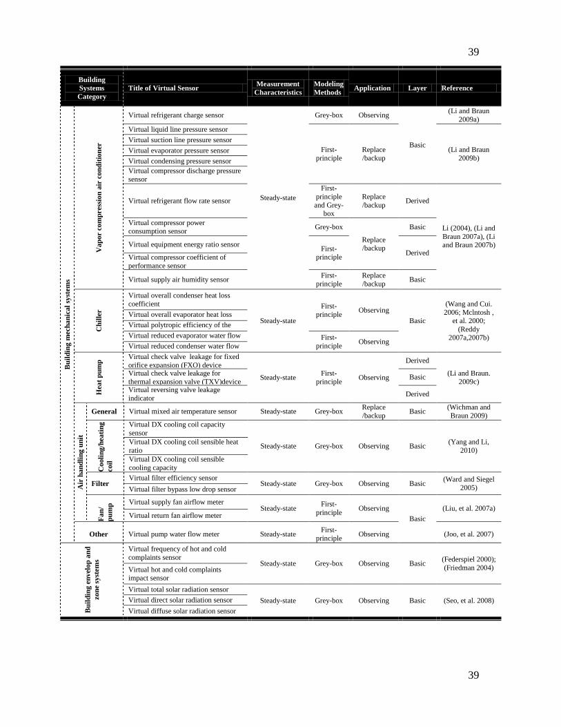
Table 2 presents a summary of virtual sensor developments with each sensor classified

according to the categories previously presented and organized regarding the type of building

system component. All of these virtual sensor developments are based on steady-state models

using either first-principle or grey-box approaches. In many cases, the authors did not explicitly

utilize the terminology virtual sensor, but the models were well developed and meet the criteria

for virtual sensors.

Table 2: Virtual sensors in buildings

39

39

Building

Systems

Category

Title of Virtual Sensor Measurement

Characteristics

Modeling

Methods Application Layer Reference

Bu

ild

ing m

ech

an

ical

syst

em

s

Va

por c

om

press

ion

air

co

nd

itio

ner

Virtual refrigerant charge sensor

Steady-state

Grey-box Observing

Basic

(Li and Braun

2009a)

Virtual liquid line pressure sensor

First-

principle

Replace

/backup

(Li and Braun

2009b)

Virtual suction line pressure sensor

Virtual evaporator pressure sensor

Virtual condensing pressure sensor

Virtual compressor discharge pressure

sensor

Virtual refrigerant flow rate sensor

First-

principle

and Grey-box

Replace

/backup Derived

Li (2004), (Li and

Braun 2007a), (Li and Braun 2007b)

Virtual compressor power

consumption sensor Grey-box

Replace /backup

Basic

Virtual equipment energy ratio sensor First-

principle Derived

Virtual compressor coefficient of

performance sensor

Virtual supply air humidity sensor First-

principle

Replace

/backup Basic

Ch

ille

r

Virtual overall condenser heat loss

coefficient

Steady-state

First-

principle Observing

Basic

(Wang and Cui.

2006; Mclntosh , et al. 2000;

(Reddy 2007a,2007b)

Virtual overall evaporator heat loss coefficient

Virtual polytropic efficiency of the

compressor

Virtual reduced evaporator water flow

detector

First-

principle Observing

Virtual reduced condenser water flow

detector

Hea

t p

um

p Virtual check valve leakage for fixed

orifice expansion (FXO) device indicator

Steady-state First-

principle Observing

Derived

(Li and Braun.

2009c)

Virtual check valve leakage for

thermal expansion valve (TXV)device indicator

Basic

Virtual reversing valve leakage

indicator Derived

Air

ha

nd

lin

g u

nit

General Virtual mixed air temperature sensor Steady-state Grey-box Replace

/backup Basic

(Wichman and

Braun 2009)

Co

oli

ng

/hea

tin

g

coil

Virtual DX cooling coil capacity

sensor

Steady-state Grey-box Observing Basic (Yang and Li,

2010)

Virtual DX cooling coil sensible heat

ratio

Virtual DX cooling coil sensible

cooling capacity

Filter Virtual filter efficiency sensor

Steady-state Grey-box Observing Basic (Ward and Siegel

2005) Virtual filter bypass low drop sensor

Fa

n/

pu

mp

Virtual supply fan airflow meter Steady-state

First-

principle Observing

Basic

(Liu, et al. 2007a) Virtual return fan airflow meter

Other Virtual pump water flow meter Steady-state First-

principle Observing (Joo, et al. 2007)

Bu

ild

ing e

nv

elo

p a

nd

zo

ne

syst

em

s

Virtual frequency of hot and cold

complaints sensor Steady-state Grey-box Observing Basic

(Federspiel 2000);

(Friedman 2004) Virtual hot and cold complaints impact sensor

Virtual total solar radiation sensor

Steady-state Grey-box Observing Basic (Seo, et al. 2008) Virtual direct solar radiation sensor

Virtual diffuse solar radiation sensor

40

40

2.2.1 Virtual sensors used in building mechanical systems

2.2.1.1 Virtual sensors for vapor compression air conditioners

Li and Braun (2007a, 2007b, 2009a, and 2009b) introduced the concept of virtual sensing

for application to buildings. Eleven virtual sensors were developed and validated for vapor

compression air conditioners with the main purpose of reducing costs for a fault detection and

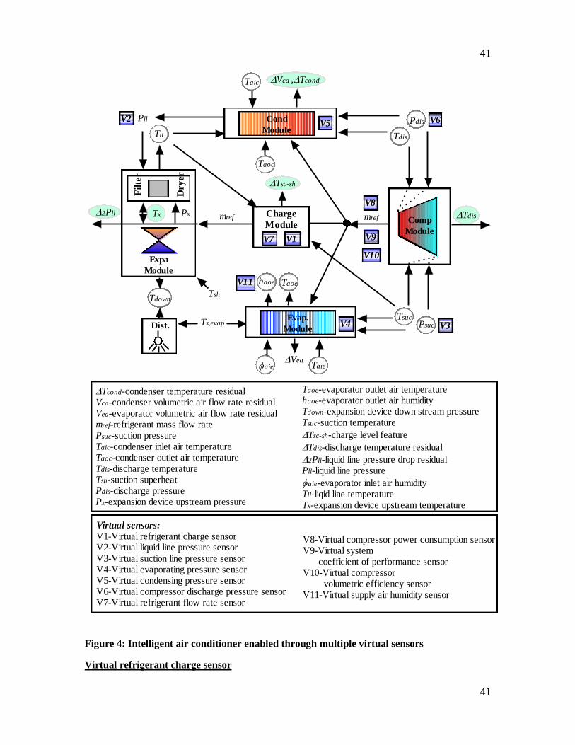
diagnostic method. Figure 4 depicts an air conditioner that employs these eleven virtual sensors.

For the most part, the virtual sensors are organized according to the four major components of a

typical vapor compression system: compressor, condenser, evaporator and expansion valve. In

addition, there is piping between these components, including a discharge line between the

compressor and condenser, a liquid line connecting the condenser to the expansion device, and a

suction line between the evaporator and compressor. The expansion device is usually located in

close proximity to the evaporator with small feeder tubes that distribute refrigerant to individual

evaporator flow circuits. The following subsections provide brief descriptions of the development

and application of the virtual sensors depicted in Figure 4.

41

41

Cond

Module

Comp

Module

Expa

Module

Dist.Evap.

Module

2Pll

Vca

Tdis

,Tcond

Tsc-sh

Tsh

Taoe

Tdown

Ts,evapTsuc

Psuc

Tx Px

Pll

Tll

Taie

mrefmref

Taic

aie

Tdis

Pdis

Taoc

Fil

ter

Dry

er

Vea

Tcond-condenser temperature residualVca-condenser volumetric air flow rate residualVea-evaporator volumetric air flow rate residualmref-refrigerant mass flow ratePsuc-suction pressureTaic-condenser inlet air temperatureTaoc-condenser outlet air temperatureTdis-discharge temperatureTsh-suction superheatPdis-discharge pressurePx-expansion device upstream pressure

Taoe-evaporator outlet air temperaturehaoe-evaporator outlet air humidityTdown-expansion device down stream pressureTsuc-suction temperature

Tsc-sh-charge level feature

Tdis-discharge temperature residual

2Pll-liquid line pressure drop residualPll-liquid line pressure

aie-evaporator inlet air humidityTll-liqid line temperatureTx-expansion device upstream temperature

Virtual sensors:

V1-Virtual refrigerant charge sensorV2-Virtual liquid line pressure sensorV3-Virtual suction line pressure sensorV4-Virtual evaporating pressure sensorV5-Virtual condensing pressure sensorV6-Virtual compressor discharge pressure sensorV7-Virtual refrigerant flow rate sensor

V8-Virtual compressor power consumption sensorV9-Virtual system coefficient of performance sensorV10-Virtual compressor volumetric efficiency sensorV11-Virtual supply air humidity sensor

V1

V2

V3V4

V5 V6

V8

V9

V11

Charge

Module

V7

haoe

V10

Figure 4: Intelligent air conditioner enabled through multiple virtual sensors

Virtual refrigerant charge sensor

42

42

Proper refrigerant charge level is critical for a vapor compression system to operate

efficiently and safely. A number of studies conducted by separate investigators (Proctor and

Downey1995; Cowan 2004) have concluded that more than 50% of the packaged air-conditioning

systems in the field have improper refrigerant charge due to improper commissioning, service, or

leakage. There is no direct measurement of refrigerant charge besides removing all of the charge

and weighing it. Charge tuning is typically accomplished in the field using manufacturers’

charge tables that are expressed in terms of measured superheat at the evaporator outlet (Tsh) and

sub-cooling at the condenser outlet (Tsc). However, these specifications are not applicable when

faults are present (e.g., low indoor airflow) or under certain operating conditions (e.g., low or

high ambient and high or low mixed-air wet-bulb temperatures). In addition, these approaches

typically specify utilization of compressor suction and discharge measurements (Psuc and Pdis) to

indirectly determine Tsh and Tsc. This requires the installation of gauges or transducers, which for

a permanent installation could be a potential source of refrigerant leakage.

Empirical coefficients: ksc, ksh

Input Output

Measurements:

Tcond,Tll,Tevap,Tsc,mtotal,rated

Refrigerantcharge level

V1-

Virtual

refrigerant

charge sensor

User specifications:

mtotal,rated

Figure 5: Virtual refrigerant charge sensor

To allow continuous monitoring of refrigerant charge using non-invasive measurements,

Li and Braun (2009a) proposed a virtual sensor (depicted in Figure 5) that uses four surface

mounted temperature measurements (condensing, liquid-line, evaporating, and suction-line

temperature) that are obtained while the system is operating at steady state. The algorithm for

estimating refrigerant charge from temperature measurements is given in equations 1 and 2:

)TT(k

k)TT(

k

1

m

mmrated,shsh

sc

shrated,scsc

chrated,total

rated,totaltotal (1)

43

43

sc

rated,totalch

k

mk (2)

Where mtotal is the total refrigerant charge, the subscript rated denotes rating operating conditions,

ksc is a constant that depends on the condenser geometry, and ksh is a constant that depends on the

evaporator geometry. The constants ksc and ksh can be estimated using a small amount of

experimental data.

The virtual refrigerant charge sensor algorithm has been validated for a range of different

systems and over a wide range of operating conditions with and without other faults. In general,

the charge predictions are within about 8% of the actual charge. The algorithm could be easily

implemented at relatively low cost as part of a permanently installed control or monitoring system

to indicate charge level and/or to automatically detect and diagnose low or high levels of

refrigerant charge.

Virtual refrigerant pressure sensors

Refrigerant pressures are useful for monitoring, control and diagnostics in a vapor

compression system. For several diagnostics algorithms, refrigerant pressures are used to

determine evaporating and condensing temperatures, liquid line sub-cooling, and suction line

superheat. However, both the hardware and installation are expensive for permanent installations.

Installation requires a brazed connection. For field installations, the refrigerant has to be

evacuated and recharged, which is costly. Moreover, if the connection is made using available

threaded service ports on the compressor, then it is likely that refrigerant will leak over time.

Virtual refrigerant pressure sensors (Li and Braun, 2009b) have significantly lower hardware and

installation costs and are non-invasive.

44

44

Input

Output

Liquid line pressureV2-Virtual liquid line

pressure sensor

V3-Virtual suction linepressure sensor

V4-Virtual evaporatingpressure sensor

Virtual refrigerant

pressure sensors

V5-Virtual condensingpressure sensor

V6-Virtual compressordischarge pressure sensor

Suction line pressure

Evaporating pressure

Condensing pressure

Compressordischarge pressure

Measurements:Condensing temperature;Evaporating temperature

Empirical coefficients

User specifications:Compressor map; rated

discharge dew-pointtemperature; rated suction

dew-point temperature

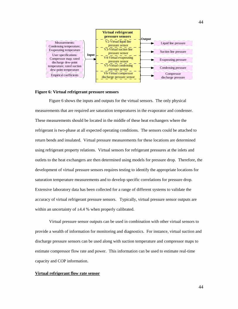
Figure 6: Virtual refrigerant pressure sensors

Figure 6 shows the inputs and outputs for the virtual sensors. The only physical

measurements that are required are saturation temperatures in the evaporator and condenser.

These measurements should be located in the middle of these heat exchangers where the

refrigerant is two-phase at all expected operating conditions. The sensors could be attached to

return bends and insulated. Virtual pressure measurements for these locations are determined

using refrigerant property relations. Virtual sensors for refrigerant pressures at the inlets and

outlets to the heat exchangers are then determined using models for pressure drop. Therefore, the

development of virtual pressure sensors requires testing to identify the appropriate locations for

saturation temperature measurements and to develop specific correlations for pressure drop.

Extensive laboratory data has been collected for a range of different systems to validate the

accuracy of virtual refrigerant pressure sensors. Typically, virtual pressure sensor outputs are

within an uncertainty of ±4.4 % when properly calibrated.

Virtual pressure sensor outputs can be used in combination with other virtual sensors to

provide a wealth of information for monitoring and diagnostics. For instance, virtual suction and

discharge pressure sensors can be used along with suction temperature and compressor maps to

estimate compressor flow rate and power. This information can be used to estimate real-time

capacity and COP information.

Virtual refrigerant flow rate sensor

45

45

Refrigerant flow rate is a very valuable measurement for performance monitoring and

diagnostics. However, it is too expensive to measure directly and can be unreliable when the

condenser exit condition is a two-phase mixture. Li and Braun (2007a) proposed two approaches

for estimating refrigerant flow rate from other measurements that are part of the virtual sensor as

illustrated in Figure 7.

Input

Measurements:Psuc,Pdis,Tamb,Tsuc

V7-

Virtual

refrigerant

flow rate

sensor

OutputRefrigerantflow rate

User specification:equation information

Method(2):Using

energy balance

Measurements:compressor

power consumption;Tdis,TsucPdis,Psuc

Method(1):Using

compressor map

Empirical coefficients

Figure 7: Virtual refrigerant flow rate sensor

The method 1 illustrated in Figure 7 uses data from a compressor manufacturer to

determine a correlation for volumetric efficiency and uses it to determine mass flow rate

according to:

sucvnormal,ref

v

NVm

(3)

Where N is the number of suction strokes per unit time, V is the displacement volume, vsuc is the

suction line refrigerant specific volume, and ηv is volumetric efficiency. Li and Braun (2002)

proposed the following empirical form for correlating volumetric efficiency

4asucamb3

2

suc

dis2

suc

dis10v )TT(a)

P

P(a

P

Paa (4)

Where the a’s are empirical coefficients, Psuc and Pdis are suction pressure and discharge pressure

that can be measured using virtual refrigerant pressures, Tsuc is suction temperature, Tamb is

compressor ambient temperature. Additionally, Taoc (when the compressor is located in the

46

46

condenser outlet air stream) or Taic (when the compressor is not directly in the condenser outlet air

stream) can be used to replace Tamb, if it is not directly measured.

Mass flow rate determined using a compressor map is only valid if the compressor is

working properly. However, a redundant mass flow measurement can be determined using the

following energy balance on the compressor (method 2)

sucdis

lossref

hh

QWm

(5)

Where lossQ is compressor heat loss rate (J/kg) is, W is measured compressor power consumption

(kW), hdis (Tdis, Pdis) and hsuc (Tsuc, Psuc) are the discharge line and suction line refrigerant enthalpy

(J/kg). This method was shown to work well for both normal and faulty compressor operation.

The map-based method is more accurate when the compressor is operating normally and

can be used to calibrate the energy-balance method. If a fault is identified for the compressor,

then the energy-balance approach can be used. Neither approach will work well if a two-phase

refrigerant condition exists at the inlet to the compressor.

Virtual compressor power consumption sensor

Compressor power consumption is a very useful index in monitoring, control and

diagnostics for vapor compression cycle systems. However, physical measurements for it would

be expensive. Figure 8 depicts a virtual compressor performance sensor that only requires

temperature measurements.

Input

Measurements:suction dew

point temperature,discharge dew

point temperature

V8-Virtual

compressor power

consumption sensor

Output

Empiricalcoefficients

Compressorpower consumption

Figure 8: Virtual compressor power consumption sensor

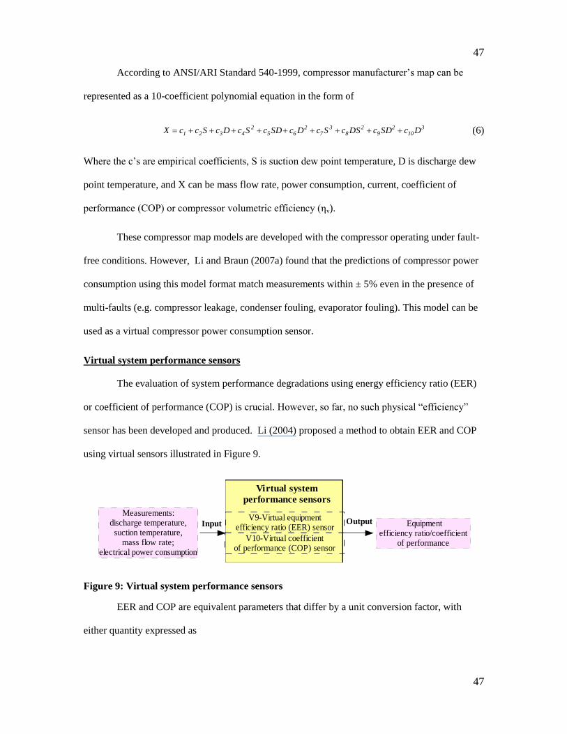
47

47

According to ANSI/ARI Standard 540-1999, compressor manufacturer’s map can be

represented as a 10-coefficient polynomial equation in the form of

3

102

92

83

72

652

4321 DcSDcDScScDcSDcScDcSccX (6)

Where the c’s are empirical coefficients, S is suction dew point temperature, D is discharge dew

point temperature, and X can be mass flow rate, power consumption, current, coefficient of

performance (COP) or compressor volumetric efficiency (ηv).

These compressor map models are developed with the compressor operating under fault-

free conditions. However, Li and Braun (2007a) found that the predictions of compressor power

consumption using this model format match measurements within ± 5% even in the presence of

multi-faults (e.g. compressor leakage, condenser fouling, evaporator fouling). This model can be

used as a virtual compressor power consumption sensor.

Virtual system performance sensors

The evaluation of system performance degradations using energy efficiency ratio (EER)

or coefficient of performance (COP) is crucial. However, so far, no such physical ―efficiency‖

sensor has been developed and produced. Li (2004) proposed a method to obtain EER and COP

using virtual sensors illustrated in Figure 9.

Input

Measurements:discharge temperature,

suction temperature,mass flow rate;

electrical power consumption

Virtual system

performance sensors

Output

V10-Virtual coefficientof performance (COP) sensor

V9-Virtual equipmentefficiency ratio (EER) sensor Equipment

efficiency ratio/coefficientof performance

Figure 9: Virtual system performance sensors

EER and COP are equivalent parameters that differ by a unit conversion factor, with

either quantity expressed as

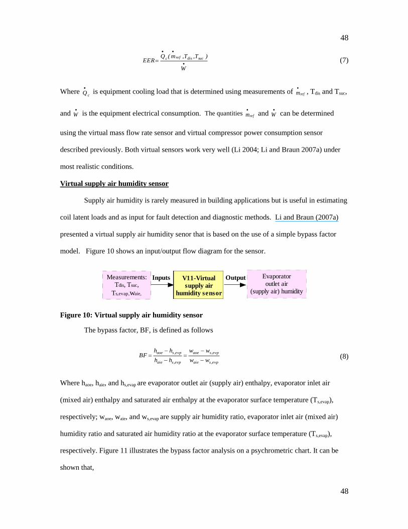
48

48

W

)T,T,m(QEER

sucdisrefc (7)

Where cQ

is equipment cooling load that is determined using measurements of refm

, Tdis and Tsuc,

and

W is the equipment electrical consumption. The quantities refm

and

W can be determined

using the virtual mass flow rate sensor and virtual compressor power consumption sensor

described previously. Both virtual sensors work very well (Li 2004; Li and Braun 2007a) under

most realistic conditions.

Virtual supply air humidity sensor

Supply air humidity is rarely measured in building applications but is useful in estimating

coil latent loads and as input for fault detection and diagnostic methods. Li and Braun (2007a)

presented a virtual supply air humidity senor that is based on the use of a simple bypass factor

model. Figure 10 shows an input/output flow diagram for the sensor.

InputsMeasurements:Tdis, Tsuc,

Ts,evap,waie,

V11-Virtual

supply air

humidity sensor

Output Evaporatoroutlet air

(supply air) humidity

Figure 10: Virtual supply air humidity sensor

The bypass factor, BF, is defined as follows

evp,saie

evp,saoe

evp,saie

evp,saoe

ww

ww

hh

hhBF

(8)

Where haoe, haie, and hs,evap are evaporator outlet air (supply air) enthalpy, evaporator inlet air

(mixed air) enthalpy and saturated air enthalpy at the evaporator surface temperature (Ts,evap),

respectively; waoe, waie, and ws,evap are supply air humidity ratio, evaporator inlet air (mixed air)

humidity ratio and saturated air humidity ratio at the evaporator surface temperature (Ts,evap),

respectively. Figure 11 illustrates the bypass factor analysis on a psychrometric chart. It can be

shown that,

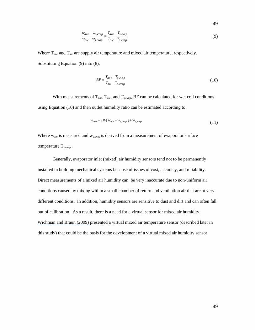
49

49

evapsaie

evapsaoe

evapsaie

evapsaoe

TT

TT

ww

ww

,

,

,

,

(9)

Where Taoe and Taie are supply air temperature and mixed air temperature, respectively.

Substituting Equation (9) into (8),

evapsaie

evapsaoe

TT

TTBF

,

,

(10)

With measurements of Taoe, Taie, and Ts,evap, BF can be calculated for wet coil conditions

using Equation (10) and then outlet humidity ratio can be estimated according to:

evap,sevap,saieaoe w)ww(BFw (11)

Where waie is measured and ws,evap is derived from a measurement of evaporator surface

temperature Ts,evap .

Generally, evaporator inlet (mixed) air humidity sensors tend not to be permanently

installed in building mechanical systems because of issues of cost, accuracy, and reliability.

Direct measurements of a mixed air humidity can be very inaccurate due to non-uniform air

conditions caused by mixing within a small chamber of return and ventilation air that are at very

different conditions. In addition, humidity sensors are sensitive to dust and dirt and can often fall

out of calibration. As a result, there is a need for a virtual sensor for mixed air humidity.

Wichman and Braun (2009) presented a virtual mixed air temperature sensor (described later in

this study) that could be the basis for the development of a virtual mixed air humidity sensor.

50

50

Figure 11: Illustration of bypass factor analysis

2.2.1.2 Virtual sensors for chillers

A number of independent studies (Wang and Cui. 2006; Mclntosh , et al. 2000; Reddy

2007a,2007b; et al. ) have focused on identifying common faults occurring in chillers using low-

cost measurements. A number of virtual sensors were developed that are listed in Figure 12.

Input

OutputOverall condenser

heat transfer conductanceVirtual overall condenserheat transfer conductance

Virtual overall evaporatorheat transfer conductance

Virtual polytropicefficiency of the compressor

Virtual sensors for chillers

Virtual reduced evaporator water flow detector

Virtual reduced condenserwater flow detector

Overall evaporatorheat transfer conductance

Polytropicefficiency of the compressor

an index of the ratio ofTevap,current and Tevap, predict

an index of the ratio ofTcond,current and Tcond, predict

Measurements:Twic,Twoc, Twie, Twoe

Tsrc,Tsre,

mcond,mevap

P1,v1,h1, P2, v2, h2

User specifications

Figure 12: Virtual sensors for chillers

The sensor outputs could be useful for monitoring and as part of a fault diagnoses scheme.

For instance, the evaporator and condenser heat transfer conductances could be used to monitor

overall performance of the heat exchangers. In order to utilize these indices for fault

identification, it would be necessary to correlate normal conductance values in terms of

operational conditions (e.g., flow rates) and to establish thresholds for faulty performance. For

water side fouling, virtual indices for relative reduction in water flow could be used directly to

indicate a change from normal performance. Compressor performance could be monitored using

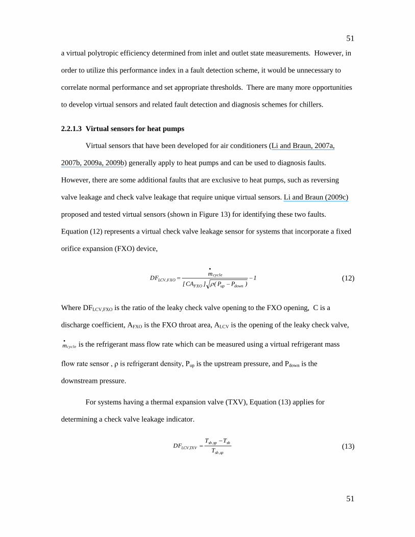
51

51

a virtual polytropic efficiency determined from inlet and outlet state measurements. However, in

order to utilize this performance index in a fault detection scheme, it would be unnecessary to

correlate normal performance and set appropriate thresholds. There are many more opportunities

to develop virtual sensors and related fault detection and diagnosis schemes for chillers.

2.2.1.3 Virtual sensors for heat pumps

Virtual sensors that have been developed for air conditioners (Li and Braun, 2007a,

2007b, 2009a, 2009b) generally apply to heat pumps and can be used to diagnosis faults.

However, there are some additional faults that are exclusive to heat pumps, such as reversing

valve leakage and check valve leakage that require unique virtual sensors. Li and Braun (2009c)

proposed and tested virtual sensors (shown in Figure 13) for identifying these two faults.

Equation (12) represents a virtual check valve leakage sensor for systems that incorporate a fixed

orifice expansion (FXO) device,

1)PP(]CA[

mDF

downupFXO

cycle

LCV,FXO

(12)

Where DFLCV,FXO is the ratio of the leaky check valve opening to the FXO opening, C is a

discharge coefficient, AFXO is the FXO throat area, ALCV is the opening of the leaky check valve,

cyclem

is the refrigerant mass flow rate which can be measured using a virtual refrigerant mass

flow rate sensor , ρ is refrigerant density, Pup is the upstream pressure, and Pdown is the

downstream pressure.

For systems having a thermal expansion valve (TXV), Equation (13) applies for

determining a check valve leakage indicator.

sp,sh

shsp,sh

TXVLCV,T

TTDF

(13)

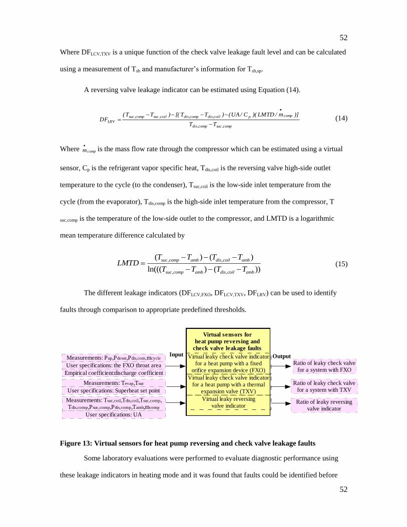
52

52

Where DFLCV,TXV is a unique function of the check valve leakage fault level and can be calculated

using a measurement of Tsh and manufacturer’s information for Tsh,sp.

A reversing valve leakage indicator can be estimated using Equation (14).

comp,succomp,dis

comppcoil,discomp,discoil,succomp,suc

LRVTT

)]m/LMTD)(C/UA()TT[()TT(DF

(14)

Where compm

is the mass flow rate through the compressor which can be estimated using a virtual

sensor, Cp is the refrigerant vapor specific heat, Tdis,coil is the reversing valve high-side outlet

temperature to the cycle (to the condenser), Tsuc,coil is the low-side inlet temperature from the

cycle (from the evaporator), Tdis,comp is the high-side inlet temperature from the compressor, T

suc,comp is the temperature of the low-side outlet to the compressor, and LMTD is a logarithmic

mean temperature difference calculated by

, ,

, ,

( ) ( )

ln((( ) ( ))

suc comp amb dis coil amb

suc comp amb dis coil amb

T T T TLMTD

T T T T

(15)

The different leakage indicators (DFLCV,FXO, DFLCV,TXV, DFLRV) can be used to identify

faults through comparison to appropriate predefined thresholds.

Virtual sensors for

heat pump reversing and

check valve leakage faults

OutputVirtual leaky check valve indicatorfor a heat pump with a fixed

orifice expansion device (FXO)

Virtual leaky check valve indicatorfor a heat pump with a thermal

expansion valve (TXV)

Virtual leaky reversingvalve indicator

Ratio of leaky check valvefor a system with FXO

Ratio of leaky check valvefor a system with TXV

Ratio of leaky reversingvalve indicator

Measurements: Pup,Pdown,Pdis,com,mcycle

User specifications: the FXO throat area

Empirical coefficient:discharge coefficient

Input

Measurements: Tevap,Tsuc

User specifications: Superheat set point

Measurements: Tsuc,coil,Tdis,coil,Tsuc,comp,Tdis,comp,Psuc,comp,Pdis,comp,Tamb,mcomp

User specifications: UA

Figure 13: Virtual sensors for heat pump reversing and check valve leakage faults

Some laboratory evaluations were performed to evaluate diagnostic performance using

these leakage indicators in heating mode and it was found that faults could be identified before

53

53

heating capacity degraded more than 5% for a system with an FXO and 3% for the same system

retrofit with a TXV.

2.2.1.4 Virtual sensors for air handling units

Virtual mixed air temperature sensor

Mixed air temperature (MAT) is a useful measurement for control and diagnostics for

economizers and vapor compression cycles. However, it can be very difficult to accurately

measure MAT because of space constraints and the use of small chambers for mixing outdoor and

return air in packaged ACs. Highly non-uniform temperature and velocity distributions at the inlet

to the evaporator can cause significant bias errors when employing single-point and averaging

temperature sensors (Avery 2002; Carling and Isakson 1999; Robinson 1999). The mixing

process changes significantly as the damper position varies with economizer operation. Wichman

(2007) suggested that a measurement grid of at least four temperature sensors mounted

symmetrically on the duct centerline provides reasonable estimates under most conditions.

However, this is a costly approach. Lee and Dexter 2005 and Tan and Dexter (2005, 2006)

proposed a method for correcting the bias error associated with a single-point sensor using CFD

simulations. However, this is also costly and difficult to implement in practice.

Input OutputMeasurements:

outside air damper position,RAT, OAT,

MAT(from a single inaccuratemixed air temperature sensor)

Mixed airtemperature

Virtual mixed

air temperature

Figure 14: Virtual mixed air temperature sensor

Wichman and Braun (2009) proposed and demonstrated a scheme for adjusting a single-

point measurement of MAT (virtual MAT sensor) that is based on in-situ measurements and self

calibration. The approach is based on correlating the bias error in terms of damper control signal

and difference between outdoor and return-air temperature. The correlation could be determined

using a self-calibration procedure with only four temperature measurements: mixed, outdoor,

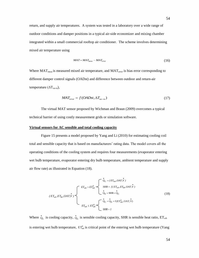
54

54

return, and supply air temperatures. A system was tested in a laboratory over a wide range of

outdoor conditions and damper positions in a typical air-side economizer and mixing chamber

integrated within a small commercial rooftop air conditioner. The scheme involves determining

mixed air temperature using

errormeas MATMATMAT (16)

Where MATmeas is measured mixed air temperature, and MATerror is bias error corresponding to

different damper control signals (OADst) and difference between outdoor and return-air

temperature (∆Toa-ra),

( , )error oa raMAT f OADst T (17)

The virtual MAT sensor proposed by Wichman and Braun (2009) overcomes a typical

technical barrier of using costly measurement grids or simulation software.

Virtual sensors for AC sensible and total cooling capacity

Figure 15 presents a model proposed by Yang and Li (2010) for estimating cooling coil

total and sensible capacity that is based on manufacturers’ rating data. The model covers all the

operating conditions of the cooling system and requires four measurements (evaporator entering

wet bulb temperature, evaporator entering dry bulb temperature, ambient temperature and supply

air flow rate) as illustrated in Equation (18).

)V,OAT,ET,ET( dbwb

0wbwb ETET

0wbwb ETET

)V,OAT,ET(Q wbC

)V,OAT,ET,ET(fSHR dbwb

CS QSHRQ

)V,OAT,ET(fQQ 0wbSC

1SHR

(18)

Where CQ

is cooling capacity, SQ

is sensible cooling capacity, SHR is sensible heat ratio, ETwb

is entering wet bulb temperature, 0wbET is critical point of the entering wet bulb temperature (Yang

55

55

and Li 2010), ETdb is entering dry bulb temperature, OAT is ambient temperature and

V is

supply air flow rate, which can be measured using a virtual air flow rate sensor.

Input

Measurements:ETdb,ETwb,

OAT,Airflow

Output

Cooling capacity

Empiricalcoefficients

Sensible cooling capacity

Sensible heat ratioVirtual DX cooling coil

sensible heat ratio

Virtual sensors for

AC with DX cooling coil

Virtual DX cooling coilcapacity sensor

Virtual DX cooing coil sensible cooling capacity

Figure 15: Virtual sensors for AC cooling coil

The performance of the virtual sensors has been evaluated using a wide range of data.

Overall predictions of cooling capacity are within 10% for both wet-coil and dry-coil conditions.

Additional work is necessary to evaluate accuracy when faults are present.

Virtual sensor for filters

Filtration in HVAC systems is often used for prevention of airborne diseases (Ottney et

al.1993) and to protect coils from fouling (Braun, 1986). There are several standards associated

with HVAC filtration efficacy, such as ASHRAE Standard 52.1, Gravimetric and Dust-Spot

Procedures for Testing Air-Cleaning Devices Used in General Ventilation for Removing

Particulate Matter (ASHRAE 1992) or ASHRAE Standard 52.2, Method of Testing General

Ventilation Air-Cleaning Devices for Removal Efficiency by Particle Size (ASHRAE 1999).

Most of the previous studies related to filtration have focused on testing of filter media, rather

than on systems having installed filtration devices. A few investigators have attempted to

establish models and test methods for determining in-situ filter efficiency that are based on

ignoring filter bypass, the air that circumvents filters due to gaps around the filter pan or filter

housing. Recently, Ward and Siegel (2005) proposed models for monitoring overall filter

efficiency (a virtual filter efficiency sensor) and the air flow bypassing the filter (virtual filter

bypass flow sensor) that are depicted in Figure 16.

56

56

Input

User specifications:Filter size,geometry of the gap

Virtual sensors

for filters

Outputfilter bypass flow

Measurements:airflow rate;pressure drop

filter efficiency

Virtual filter bypassflow drop sensor

Virtual filterefficiency sensor

Figure 16: Virtual sensors for filters

The virtual filter sensors require specification of the size and geometry of the gaps around

the filter and measurements of air flow rate and pressure drop. The flow bypassing the filter is

estimated according to

)HW

P)n5.1(2(

]HW

P)n5.1(2)

W H

L12(

W H

L12[

Q

22

22

2

33

B

(19)

Where QB is the flow rate of air bypassing the filter, ∆P is the pressure drop across the filter

which can be measured, μ is the dynamic viscosity of air, and ρ is the density of the air, L is the

length of the crack longitudinal to the flow, W is the width of the crack perpendicular to flow, H

is the height of the crack, n is the number of right angle bends in the path of bypass flow.

The method of estimating bypass flow has only validated using simulation for a variety of

common filters. Additional work is necessary to perform experimental validation using

laboratory and field studies.

Virtual water flow rate sensor

Liu et al. (2007a) proposed a pump water flow station (virtual water flow rate meter)

depicted in Figure 17 that uses pump head (Hpump), pump speed (wpump), and empirical

coefficients to determine pump performance according to

0

pump2

pump022

pump21pump1

a2

)Hwa(a4wawaQ

(20)

57

57

InputMeasurements:

pump head, pump speed

Virtual chillerefficiency sensor

Output

Pump waterflow rates

User specifications:pump performance curve

Cooling energyconsumption

Chillerefficiency

Pumpefficiency

Virtual pumpefficiency sensor

Virtual chiller energyconsumption sensor

Virtual pump water

flow rate sensors

Virtual pumpwater flow meter

Figure 17: Virtual pump water flow rate sensor

The virtual sensor could be used along with other measurements to estimate pump

efficiency, cooling energy consumption and chiller efficiency and used within a building energy

management and control system. A case study was performed in a building having a chilled

water system and demonstrated that the low-cost virtual sensor can accurately measure water

flow rate and be used along with other measurements to monitor energy consumption. In addition

to performance monitoring, the virtual flow meter could be applied for optimized pump speed

control (Liu, et al. 2007b). However, the method described in this paper is not applicable for all

pump characteristics. More work is needed to generalize the approach.

Virtual fan air flow rate meter

Joo et al. (2007) proposed a fan flow station (virtual fan air flow rate meter) for

measuring supply and/or return fan air flows and that is illustrated in Figure 18. The model for

flow rate is similar to the approach used for the pump flow sensor and is expressed as

0'

20

'2

'22

1'

1'

'

2

)(4

a

HwaawawaQ

fanfanfanfan

(21)

Where Hfan is fan head, wfan is fan speed, and the a’s are empirical coefficients that are determined

using regression applied to a fan performance curve provided by the manufacturer. The

algorithm was shown to provide accurate estimates of supply and return fan air flow rate for a

variable-air-volume (VAV) system.

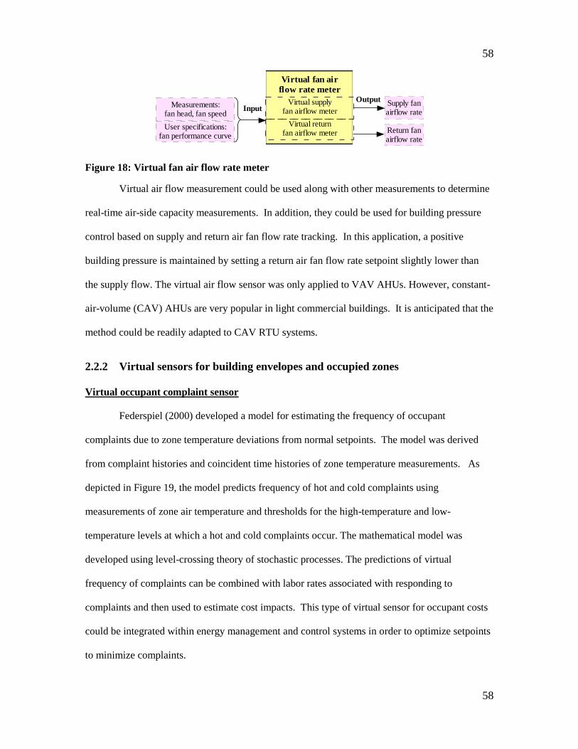
58

58

InputMeasurements:

fan head, fan speed

OutputSupply fanairflow rate

User specifications:fan performance curve

Return fanairflow rate

Virtual returnfan airflow meter

Virtual fan air

flow rate meter

Virtual supplyfan airflow meter

Figure 18: Virtual fan air flow rate meter

Virtual air flow measurement could be used along with other measurements to determine

real-time air-side capacity measurements. In addition, they could be used for building pressure

control based on supply and return air fan flow rate tracking. In this application, a positive

building pressure is maintained by setting a return air fan flow rate setpoint slightly lower than

the supply flow. The virtual air flow sensor was only applied to VAV AHUs. However, constant-

air-volume (CAV) AHUs are very popular in light commercial buildings. It is anticipated that the

method could be readily adapted to CAV RTU systems.

2.2.2 Virtual sensors for building envelopes and occupied zones

Virtual occupant complaint sensor

Federspiel (2000) developed a model for estimating the frequency of occupant

complaints due to zone temperature deviations from normal setpoints. The model was derived

from complaint histories and coincident time histories of zone temperature measurements. As

depicted in Figure 19, the model predicts frequency of hot and cold complaints using

measurements of zone air temperature and thresholds for the high-temperature and low-

temperature levels at which a hot and cold complaints occur. The mathematical model was

developed using level-crossing theory of stochastic processes. The predictions of virtual

frequency of complaints can be combined with labor rates associated with responding to

complaints and then used to estimate cost impacts. This type of virtual sensor for occupant costs

could be integrated within energy management and control systems in order to optimize setpoints

to minimize complaints.

59

59

Input

Measurements: ZAT

Virtual occupant

complaint sensorOutput

Hot and cold complaintsimpact

Virtual frequency of hotand cold complaints sensor

Virtual hot and coldcomplaints impact sensor

User specifications:High limit of building temperate;Low limit of building temperate

Frequency ofhot and cold complaints

Figure 19: Virtual occupant complaint sensor

Virtual sensor for solar radiation

Solar radiation is an important measurement for use in models that predict building loads.

However, it is expensive to measure on site and is rarely available. Recently, Seo, et al. (2008)

evaluated a number of different models for estimating solar radiation from other available

measurements and identified some simplifications that result in reasonable performance.

Performance was statistically evaluated using measured solar radiation for several locations

around the world. Figure 20 depicts virtual sensors for total, direct normal, and diffuse solar

radiation sensor based on the simplified model. The algorithms are empirical and only require

inputs of hourly cloud cover information, dry bulb temperature, relative humidity, and wind speed.

Input

Virtual sensors

for solar radiationOutput

Solarradiation

Measurements:

solar altitude,sun position, cloud cover,

relative humidity, wind speed,

dry-bulb temperature difference

Empirical coefficientsVirtual diffuse solar

radiation sensor

Virtual direct solarradiation sensor

Virtual solarradiation sensor

Diffuse solarradiation

Direct solarradiation

Figure 20: Virtual sensor for solar radiation

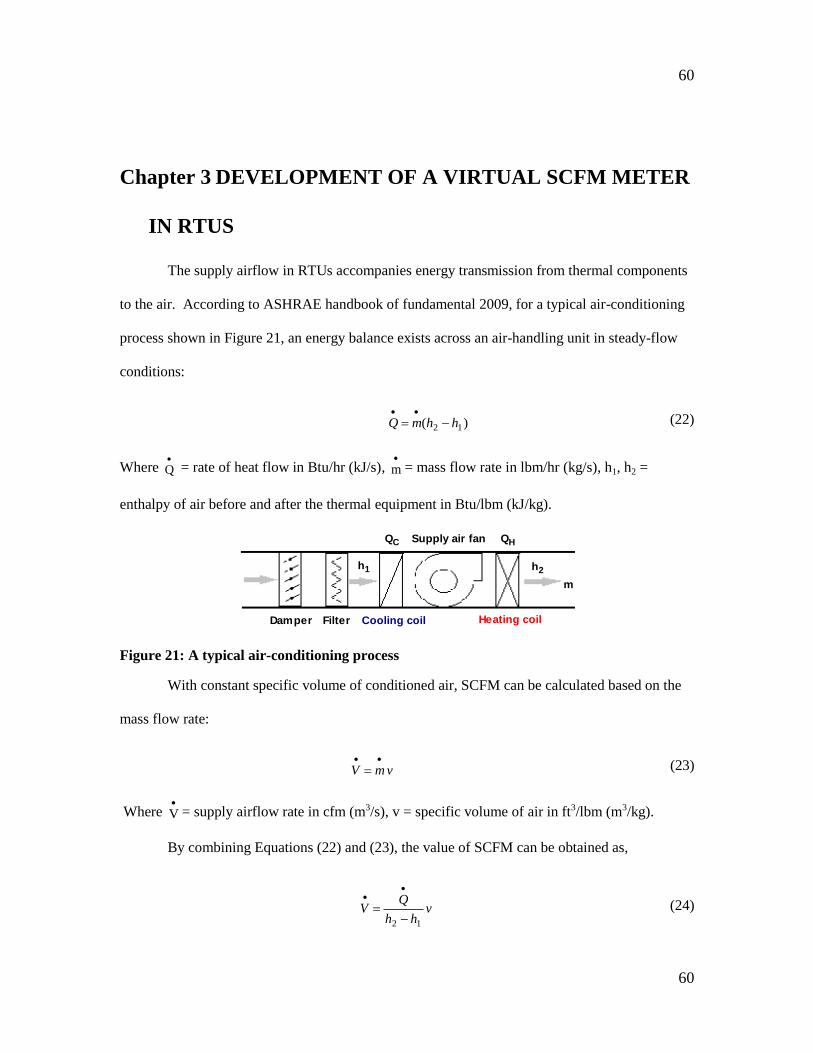
60

60

Chapter 3 DEVELOPMENT OF A VIRTUAL SCFM METER

IN RTUS

The supply airflow in RTUs accompanies energy transmission from thermal components

to the air. According to ASHRAE handbook of fundamental 2009, for a typical air-conditioning

process shown in Figure 21, an energy balance exists across an air-handling unit in steady-flow

conditions:

)( 12 hhmQ

(22)

Where

Q = rate of heat flow in Btu/hr (kJ/s),

m = mass flow rate in lbm/hr (kg/s), h1, h2 =

enthalpy of air before and after the thermal equipment in Btu/lbm (kJ/kg).

Damper Filter Cooling coil

Supply air fan

Heating coil

m

QC QH

h1 h2

Figure 21: A typical air-conditioning process

With constant specific volume of conditioned air, SCFM can be calculated based on the

mass flow rate:

vmV

(23)

Where

V = supply airflow rate in cfm (m3/s), v = specific volume of air in ft3/lbm (m3/kg).

By combining Equations (22) and (23), the value of SCFM can be obtained as,

vhh

QV

12

(24)

61

61

To avoid using expensive measurements such as relative humidity, only sensible capacity

across the cooling or heating coil is adopted in the development of a virtual SCFM meter.

Equation (25) thus can be represented by and a virtual SCFM meter prototype is obtained as,

s

p

QV v

C SAT MAT

(25)

Where s

Q

= sensible capacity in Btu/hr (kJ/s), SAT = supply air temperature in ºF (ºC), and

MAT= mixed air temperature in ºF (ºC)

For a typical RTU, cooling and heating are two opposite energy transmissions related to

SCFM and air status change. Accordingly, there are two approaches (cooling mode- and heating

mode-based approaches) to obtain the sensible capacity in Equation (25). The reliable values of

sQ

, which may involve other implicit variables, and SAT, MAT are needed in the cooling or

heating process to make the virtual SCFM meter work.

The remaining challenge is to evaluate the two candidates (cooling mode- and heating

mode-based approaches) and develop an implementation method which satisfies the following

features of a feasible virtual SCFM meter: (1) using a simple while reliable mechanism; (2)

characteristic of small uncertainty and robust against faults; and (3) easy-to-obtain parameters

or measurements.

Without the presence of simultaneous cooling and heating, individual cooling mode- and

heating mode-based approaches are studied in the next two subsections. The inputs and basic

measurements are verified and adopted from the referred literature. The critical measurements

are reiterated in detail in the section of implementation issues.

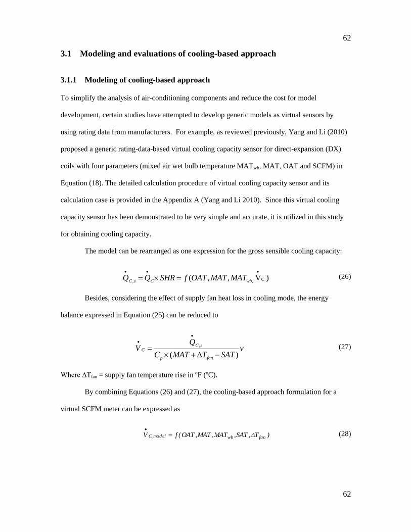
62

62

3.1 Modeling and evaluations of cooling-based approach

3.1.1 Modeling of cooling-based approach

To simplify the analysis of air-conditioning components and reduce the cost for model

development, certain studies have attempted to develop generic models as virtual sensors by

using rating data from manufacturers. For example, as reviewed previously, Yang and Li (2010)

proposed a generic rating-data-based virtual cooling capacity sensor for direct-expansion (DX)

coils with four parameters (mixed air wet bulb temperature MATwb, MAT, OAT and SCFM) in

Equation (18). The detailed calculation procedure of virtual cooling capacity sensor and its

calculation case is provided in the Appendix A (Yang and Li 2010). Since this virtual cooling

capacity sensor has been demonstrated to be very simple and accurate, it is utilized in this study

for obtaining cooling capacity.

The model can be rearranged as one expression for the gross sensible cooling capacity:

C,,( , , V )wbC s C

Q Q SHR f OAT MAT MAT

(26)

Besides, considering the effect of supply fan heat loss in cooling mode, the energy

balance expressed in Equation (25) can be reduced to

,

( )

C sC

p fan

QV v

C MAT T SAT

(27)

Where ∆Tfan = supply fan temperature rise in ºF (ºC).

By combining Equations (26) and (27), the cooling-based approach formulation for a

virtual SCFM meter can be expressed as

)T,SAT,MAT,MAT,OAT(fV fanwbelmod,C

(28)

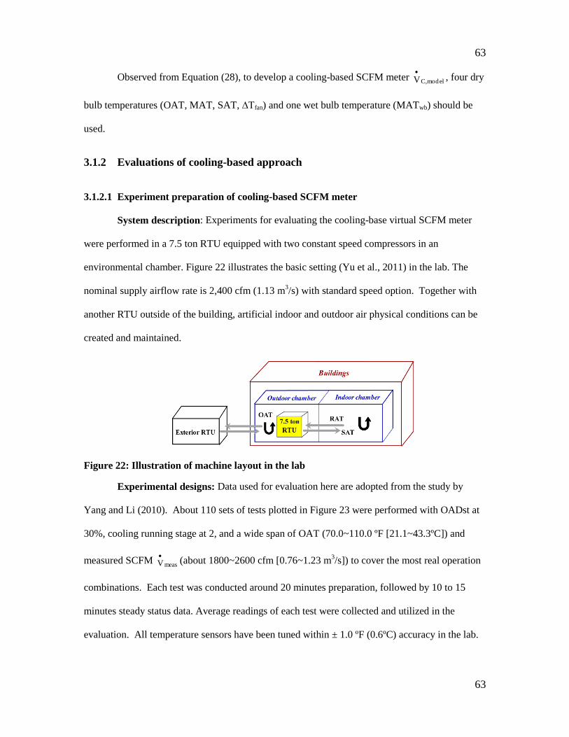
63

63

Observed from Equation (28), to develop a cooling-based SCFM meter elmod,CV

, four dry

bulb temperatures (OAT, MAT, SAT, ∆Tfan) and one wet bulb temperature (MATwb) should be

used.

3.1.2 Evaluations of cooling-based approach

3.1.2.1 Experiment preparation of cooling-based SCFM meter

System description: Experiments for evaluating the cooling-base virtual SCFM meter

were performed in a 7.5 ton RTU equipped with two constant speed compressors in an

environmental chamber. Figure 22 illustrates the basic setting (Yu et al., 2011) in the lab. The

nominal supply airflow rate is 2,400 cfm (1.13 m3/s) with standard speed option. Together with

another RTU outside of the building, artificial indoor and outdoor air physical conditions can be

created and maintained.

Figure 22: Illustration of machine layout in the lab

Experimental designs: Data used for evaluation here are adopted from the study by

Yang and Li (2010). About 110 sets of tests plotted in Figure 23 were performed with OADst at

30%, cooling running stage at 2, and a wide span of OAT (70.0~110.0 ºF [21.1~43.3ºC]) and

measured SCFM measV

(about 1800~2600 cfm [0.76~1.23 m

3/s]) to cover the most real operation

combinations. Each test was conducted around 20 minutes preparation, followed by 10 to 15

minutes steady status data. Average readings of each test were collected and utilized in the

evaluation. All temperature sensors have been tuned within ± 1.0 ºF (0.6ºC) accuracy in the lab.

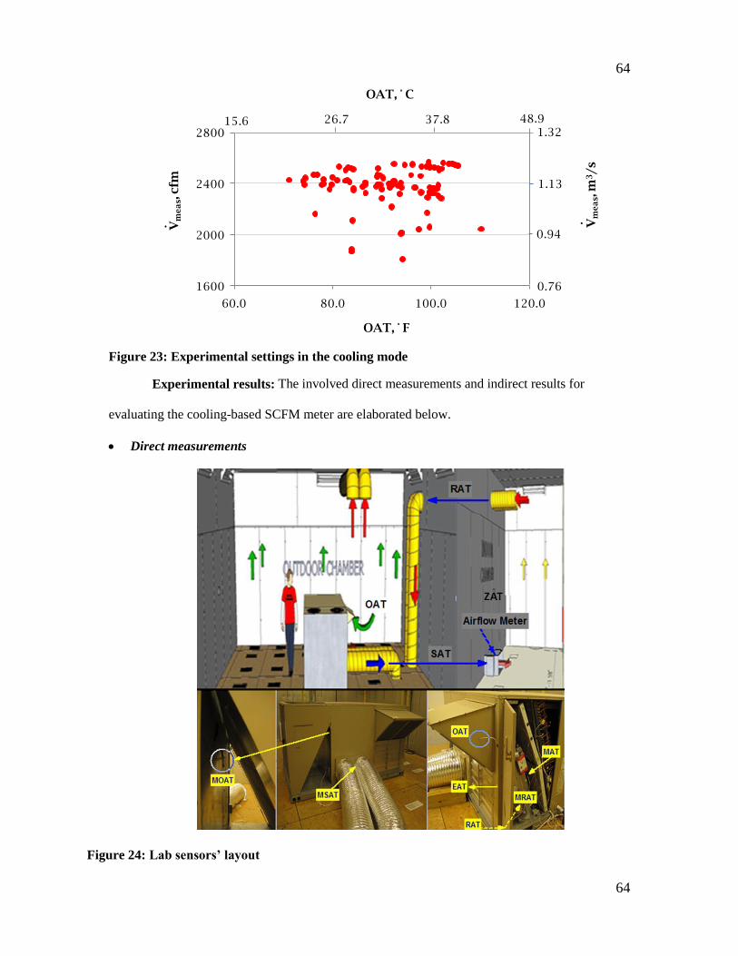
64

64

1600

2000

2400

2800

60.0 80.0 100.0 120.0

Vm

eas, c

fm

OAT, ° F

26.7

1.13

1.32

0.94

0.76

OAT, ° C

Vm

eas, m

3/s

. .

48.937.815.6

Figure 23: Experimental settings in the cooling mode

Experimental results: The involved direct measurements and indirect results for

evaluating the cooling-based SCFM meter are elaborated below.

Direct measurements

Figure 24: Lab sensors’ layout

65

65

Outside air temperature (OAT) It is found, the manufacturer-preinstalled OAT (MOAT) sensor

in Figure 24 is fixed beside the evaporator coils, and the measurements are not reliable due to improper

heat gain and poor temperature distribution. To supplement it for an accurate OAT, another air

temperature sensor with ± 0.1 ºF (0.6ºC) uncertainty is mounted at the RTU outside air inlet (Figure 24).

In this experiment, average reading of the lab-installed OAT sensor instead of MOAT sensor is used.

Supply air temperature (SAT) Based on the study by Yu et al. (2011), an manufacturer-

preinstalled SAT (MSAT) sensor (Figure 24) in RTUs could predict the true values in cooling mode.

Therefore, average reading of the MSAT sensor with ± 0.1 ºF (0.6ºC) uncertainty is adopted here.

Return air temperature (RAT) In order to calculate MAT accurately, obtaining the true value of

RAT is also important. In the lab, a RAT sensor with ± 0.1 ºF (0.6ºC) uncertainty installed right at the

return air duct outlet (Figure 24) is utilized to verify the accuracy of the manufacturer-preinstalled RAT

(MRAT) sensor. In the case, average reading of the lab-installed RAT sensor is proved trustable and then

used.

Outside air relative humidity (OARH), zone air relative humidity (ZARH) and zone air

temperature (ZAT) Besides, in an attempt to calculate the parameter of MATwb, average readings of lab-

installed OARH sensor in the outdoor chamber (Figure 22), ZARH and ZAT sensors in the indoor

chamber are collected accordingly.

Measured SCFM (measV

) An airflow station (pressure transducer) offering ± 1% full scale

accuracy is permanently mounted in supply air duct in the lab. The airflow station was calibrated by the

manufacturer before it was installed. It serves as the airflow reference measV

in this study.

Indirect results

Virtual mixed air temperature (MATvir) Since there is no pre-installed physical MAT sensor

available in our study, we adopted the method proposed by Yang and Li (2011) with an acceptable

uncertainty of ±1.0ºF (0.6ºC). The specific details are provided in Section 3.4.2 about measuring and

processing MAT.

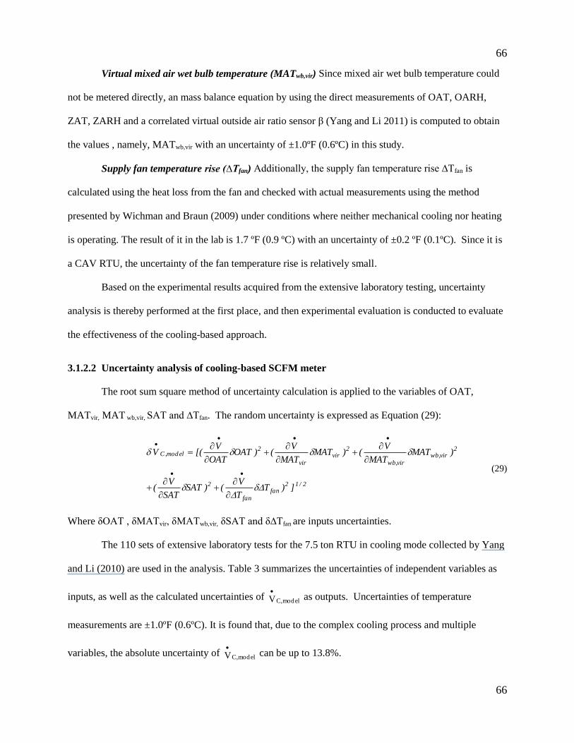
66

66

Virtual mixed air wet bulb temperature (MATwb,vir) Since mixed air wet bulb temperature could

not be metered directly, an mass balance equation by using the direct measurements of OAT, OARH,

ZAT, ZARH and a correlated virtual outside air ratio sensor β (Yang and Li 2011) is computed to obtain

the values , namely, MATwb,vir with an uncertainty of ±1.0ºF (0.6ºC) in this study.

Supply fan temperature rise (∆Tfan) Additionally, the supply fan temperature rise ∆Tfan is

calculated using the heat loss from the fan and checked with actual measurements using the method

presented by Wichman and Braun (2009) under conditions where neither mechanical cooling nor heating

is operating. The result of it in the lab is 1.7 ºF (0.9 ºC) with an uncertainty of ±0.2 ºF (0.1ºC). Since it is

a CAV RTU, the uncertainty of the fan temperature rise is relatively small.

Based on the experimental results acquired from the extensive laboratory testing, uncertainty

analysis is thereby performed at the first place, and then experimental evaluation is conducted to evaluate

the effectiveness of the cooling-based approach.

3.1.2.2 Uncertainty analysis of cooling-based SCFM meter

The root sum square method of uncertainty calculation is applied to the variables of OAT,

MATvir, MAT wb,vir, SAT and ∆Tfan. The random uncertainty is expressed as Equation (29):

2/12fan

fan

2

2vir,wb

vir,wb

2vir

vir

2elmod,C

])TT

V()SAT

SAT

V(

)MATMAT

V()MAT

MAT

V()OAT

OAT

V[(V

(29)

Where δOAT , δMATvir, δMATwb,vir, δSAT and δ∆Tfan are inputs uncertainties.

The 110 sets of extensive laboratory tests for the 7.5 ton RTU in cooling mode collected by Yang

and Li (2010) are used in the analysis. Table 3 summarizes the uncertainties of independent variables as

inputs, as well as the calculated uncertainties of elmod,CV

as outputs. Uncertainties of temperature

measurements are ±1.0ºF (0.6ºC). It is found that, due to the complex cooling process and multiple

variables, the absolute uncertainty of elmod,CV

can be up to 13.8%.

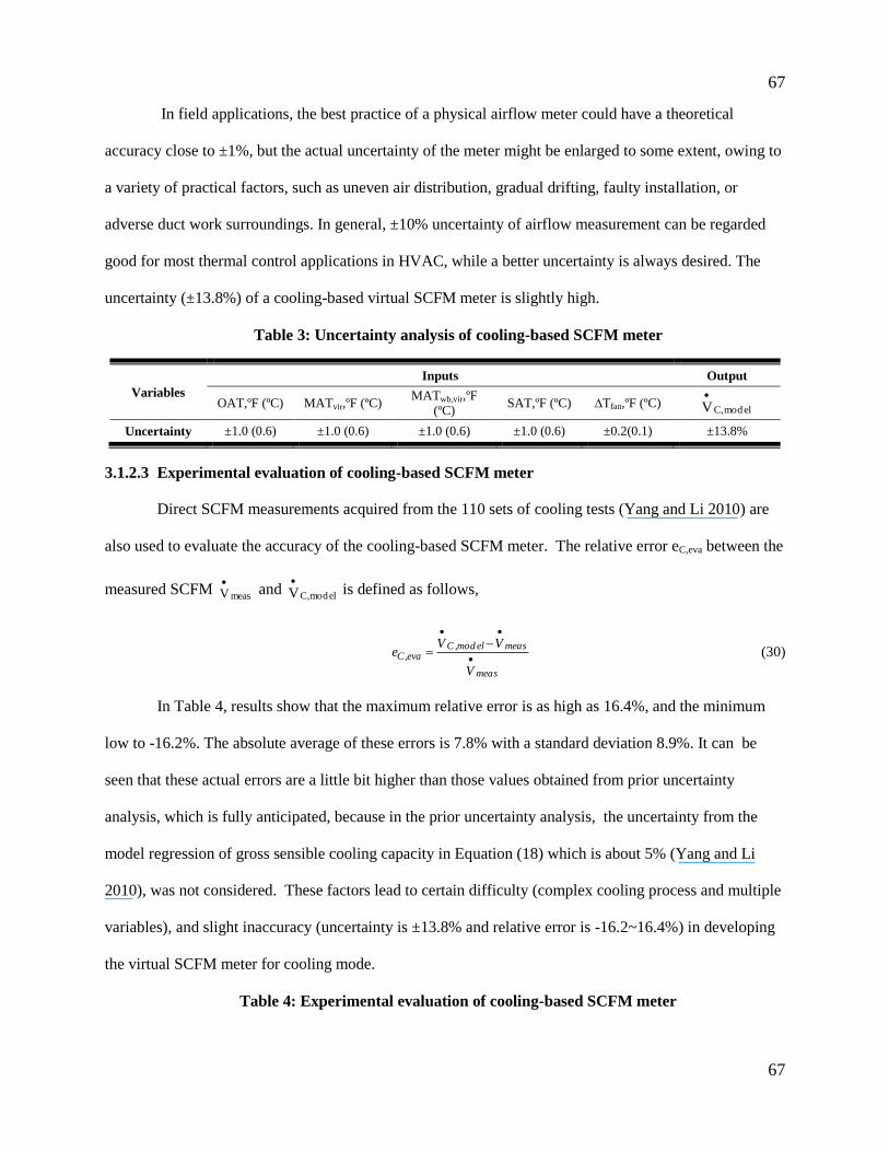
67

67

In field applications, the best practice of a physical airflow meter could have a theoretical

accuracy close to ±1%, but the actual uncertainty of the meter might be enlarged to some extent, owing to

a variety of practical factors, such as uneven air distribution, gradual drifting, faulty installation, or

adverse duct work surroundings. In general, ±10% uncertainty of airflow measurement can be regarded

good for most thermal control applications in HVAC, while a better uncertainty is always desired. The

uncertainty (±13.8%) of a cooling-based virtual SCFM meter is slightly high.

Table 3: Uncertainty analysis of cooling-based SCFM meter

Variables

Inputs

Output

OAT,ºF (ºC) MATvir,ºF (ºC) MATwb,vir,ºF

(ºC) SAT,ºF (ºC) ∆Tfan,ºF (ºC)

elmod,CV

Uncertainty

±1.0 (0.6) ±1.0 (0.6) ±1.0 (0.6) ±1.0 (0.6) ±0.2(0.1) ±13.8%

3.1.2.3 Experimental evaluation of cooling-based SCFM meter

Direct SCFM measurements acquired from the 110 sets of cooling tests (Yang and Li 2010) are

also used to evaluate the accuracy of the cooling-based SCFM meter. The relative error eC,eva between the

measured SCFM measV

and

elmod,CV

is defined as follows,

meas

measelmod,Ceva,C

V

VVe

(30)

In Table 4, results show that the maximum relative error is as high as 16.4%, and the minimum

low to -16.2%. The absolute average of these errors is 7.8% with a standard deviation 8.9%. It can be

seen that these actual errors are a little bit higher than those values obtained from prior uncertainty

analysis, which is fully anticipated, because in the prior uncertainty analysis, the uncertainty from the

model regression of gross sensible cooling capacity in Equation (18) which is about 5% (Yang and Li

2010), was not considered. These factors lead to certain difficulty (complex cooling process and multiple

variables), and slight inaccuracy (uncertainty is ±13.8% and relative error is -16.2~16.4%) in developing

the virtual SCFM meter for cooling mode.

Table 4: Experimental evaluation of cooling-based SCFM meter

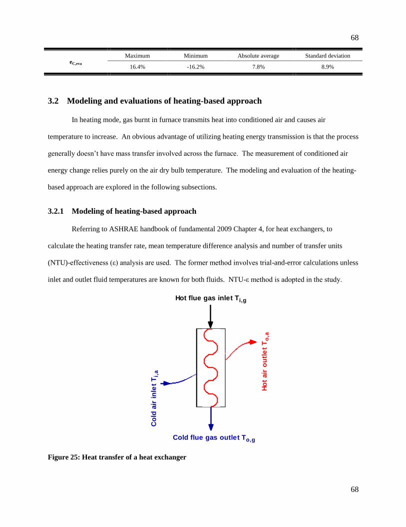
68

68

eC,eva

Maximum Minimum Absolute average Standard deviation

16.4% -16.2% 7.8% 8.9%

3.2 Modeling and evaluations of heating-based approach

In heating mode, gas burnt in furnace transmits heat into conditioned air and causes air

temperature to increase. An obvious advantage of utilizing heating energy transmission is that the process

generally doesn’t have mass transfer involved across the furnace. The measurement of conditioned air

energy change relies purely on the air dry bulb temperature. The modeling and evaluation of the heating-

based approach are explored in the following subsections.

3.2.1 Modeling of heating-based approach

Referring to ASHRAE handbook of fundamental 2009 Chapter 4, for heat exchangers, to

calculate the heating transfer rate, mean temperature difference analysis and number of transfer units

(NTU)-effectiveness (ε) analysis are used. The former method involves trial-and-error calculations unless

inlet and outlet fluid temperatures are known for both fluids. NTU-ε method is adopted in the study.

Co

ld a

ir in

let

Ti,

a

Ho

t air

ou

tle

t T

o,a

Cold flue gas outlet To,g

Hot flue gas inlet Ti,g

Figure 25: Heat transfer of a heat exchanger

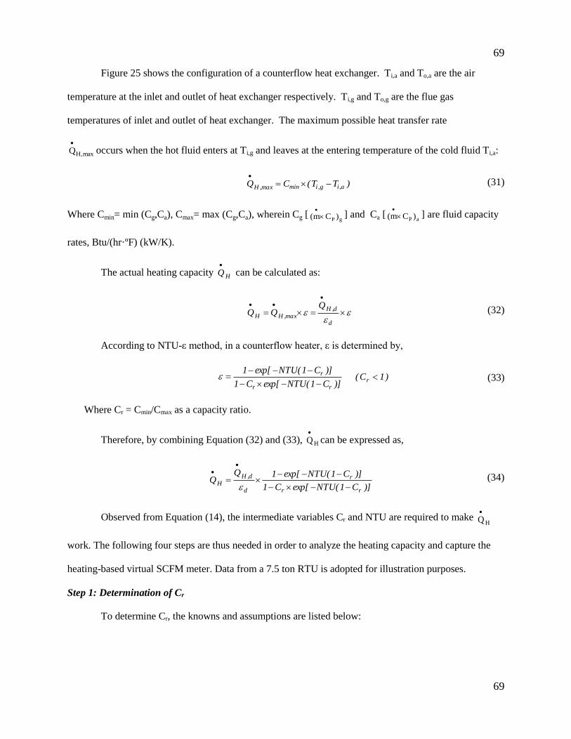
69

69

Figure 25 shows the configuration of a counterflow heat exchanger. Ti,a and To,a are the air

temperature at the inlet and outlet of heat exchanger respectively. Ti,g and To,g are the flue gas

temperatures of inlet and outlet of heat exchanger. The maximum possible heat transfer rate

max,HQ

occurs when the hot fluid enters at Ti,g and leaves at the entering temperature of the cold fluid Ti,a:

)TT(CQ a,ig,iminmax,H

(31)

Where Cmin= min (Cg,Ca), Cmax= max (Cg,Ca), wherein Cg [ gP )Cm(

] and Ca [ aP )Cm(

] are fluid capacity

rates, Btu/(hr·ºF) (kW/K).

The actual heating capacity HQ

can be calculated as:

d

d,Hmax,HH

QQQ (32)

According to NTU-ε method, in a counterflow heater, ε is determined by,

)]C1(NTUexp[C1

)]C1(NTUexp[1

rr

r

)1C( r (33)

Where Cr = Cmin/Cmax as a capacity ratio.

Therefore, by combining Equation (32) and (33), HQ

can be expressed as,

)]C1(NTUexp[C1

)]C1(NTUexp[1QQ

rr

r

d

d,HH

(34)

Observed from Equation (14), the intermediate variables Cr and NTU are required to make HQ

work. The following four steps are thus needed in order to analyze the heating capacity and capture the

heating-based virtual SCFM meter. Data from a 7.5 ton RTU is adopted for illustration purposes.

Step 1: Determination of Cr

To determine Cr, the knowns and assumptions are listed below:

70

70

The design heating capacity and design heat exchanger effectiveness are: d,HQ

= 130,000 Btu/hr (38.1

kW); d = 80%.

The design airflow rate and design flue gas flow rate are: d,aV

= 144,000 ft3/hr (2400 cfm; 1.13m

3/s),

gV

= 1,800 ft3/hr (30.0 cfm; 0.014m

3/s).

The density and specific heat of air are: ρa = 0.070lb/ft3 (1.200 kg/m

3); CP,a =0.240 Btu/(lbm·ºF) (1.005

kJ/(kg·K)).

It is a sufficient combustion process in the gas furnaces. The density and specific heat of flue gas are: ρg =

0.077lb/ft3 (1.240 kg/m

3); CP,g =0.295 Btu/(lbm·ºF) (1.230 kJ/(kg·K)).

Since with similar specific heat on both sides the flow rate on the air side is several degrees of

magnitude higher than that on the flue gas side, Cg<<Ca, then according to Cmin and Cmax definition, we

have Cmin equals Cg and Cmax equals Ca.

(1) Cmin = Cg . With flue gas flow rate known, the value of Cg can be obtained as,

gg,Pgg VCC

(35)

In this case, Cg is 40.36 Btu/(hr·ºF) (0.021 kW/K) as calculated.

(2) Cmax = Ca . With design airflow rate known, Ca can be derived from Eq. (16):

d,aa,Paa VCC

(36)

The result is Ca = 2419 Btu/(hr·ºF) (1.423 kW/K) under design conditions.

Since Ca is significantly greater than Cg, the assumption holds for wide range airflow rate and we

have,

a

g

max

minr

C

C

C

CC (37)

Step 2: Correlating NTU

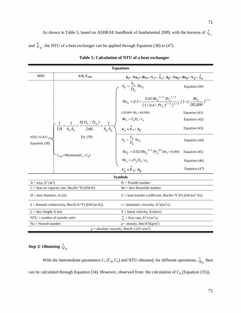
71

71

As shown in Table 5, based on ASHRAE handbook of fundamental 2009, with the knowns of aV

and gV

, the NTU of a heat exchanger can be applied through Equation (38) to (47).

Table 5: Calculation of NTU of a heat exchanger

Equations

NTU UA, Cmin ha←Nua←Rea←Va← aV

; hg←Nug←Reg←Vg← gV

aa

aa Nu

D

kh Equation (40)

gg

ga

aa Ah

1

kL2

)D/D(li

Ah

1

UA

1

Eq. (39)

Cmin=Minimum(Ca ,Cg)

2/1a

4/13/2a

3/1a

2/1a

a )000,282

Re(1[

])Pr/4.01[

PrRe62.03.0Nu

(10,000<Rea<40,000) Equation (41)

NTU=UA/Cmin

Equation (38)

aaaa v/DVRe Equation (42)

aaa A/VV

Equation (43)

gg

gg Nu

D

kh Equation (44)

4.0g

5/4gg PrRe023.0Nu (Reg>10,000) Equation (45)

gggg /DVRe Equation (46)

ggg A/VV

Equation (47)

Symbols

A = area, ft2 (m2) Pr = Prandtl number

C = heat air capacity rate, Btu/(hr·ºF) (kW/K) Re = duct Reynolds number

D = duct diameter, in (m) U = heat transfer coefficient, Btu/(hr·ºF·ft²) (kW/(m2·K))

k = thermal conductivity, Btu/(h·ft·ºF) (kW/(m·K)) v = kinematic viscosity, ft2/s(m2/s)

L = duct length, ft (m) V = linear velocity, ft/s(m/s)

NTU = number of transfer units

V = flow rate, ft3/s (m3/s)

Nu = Nusselt number ρ = density, lbm/ft3(kg/m3)

μ = absolute viscosity, lbm/ft·s ((N·s)/m2)

Step 3: Obtaining HQ

With the intermediate parameters Cr (Cg, Ca) and NTU obtained, for different operations, HQ

then

can be calculated through Equation (34). However, observed from the calculation of Cg (Equation (35)),

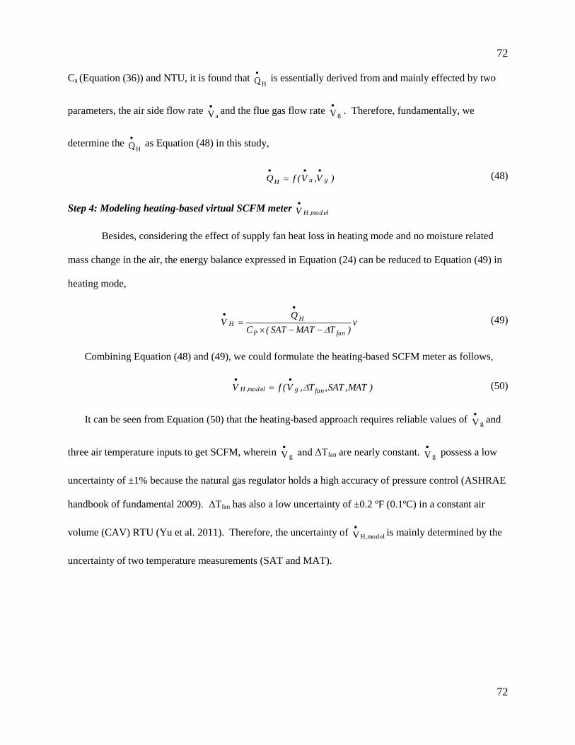
72

72

Ca (Equation (36)) and NTU, it is found that HQ

is essentially derived from and mainly effected by two

parameters, the air side flow rate aV

and the flue gas flow rate

gV

. Therefore, fundamentally, we

determine the HQ

as Equation (48) in this study,

)V,V(fQ gaH

(48)

Step 4: Modeling heating-based virtual SCFM meter elmod,HV

Besides, considering the effect of supply fan heat loss in heating mode and no moisture related

mass change in the air, the energy balance expressed in Equation (24) can be reduced to Equation (49) in

heating mode,

v

)TMATSAT(C

QV

fanP

HH

(49)

Combining Equation (48) and (49), we could formulate the heating-based SCFM meter as follows,

)MAT,SAT,T,V(fV fangelmod,H

(50)

It can be seen from Equation (50) that the heating-based approach requires reliable values of gV

and

three air temperature inputs to get SCFM, wherein gV

and ΔTfan are nearly constant.

gV

possess a low

uncertainty of ±1% because the natural gas regulator holds a high accuracy of pressure control (ASHRAE

handbook of fundamental 2009). ΔTfan has also a low uncertainty of ±0.2 ºF (0.1ºC) in a constant air

volume (CAV) RTU (Yu et al. 2011). Therefore, the uncertainty of elmod,HV

is mainly determined by the

uncertainty of two temperature measurements (SAT and MAT).

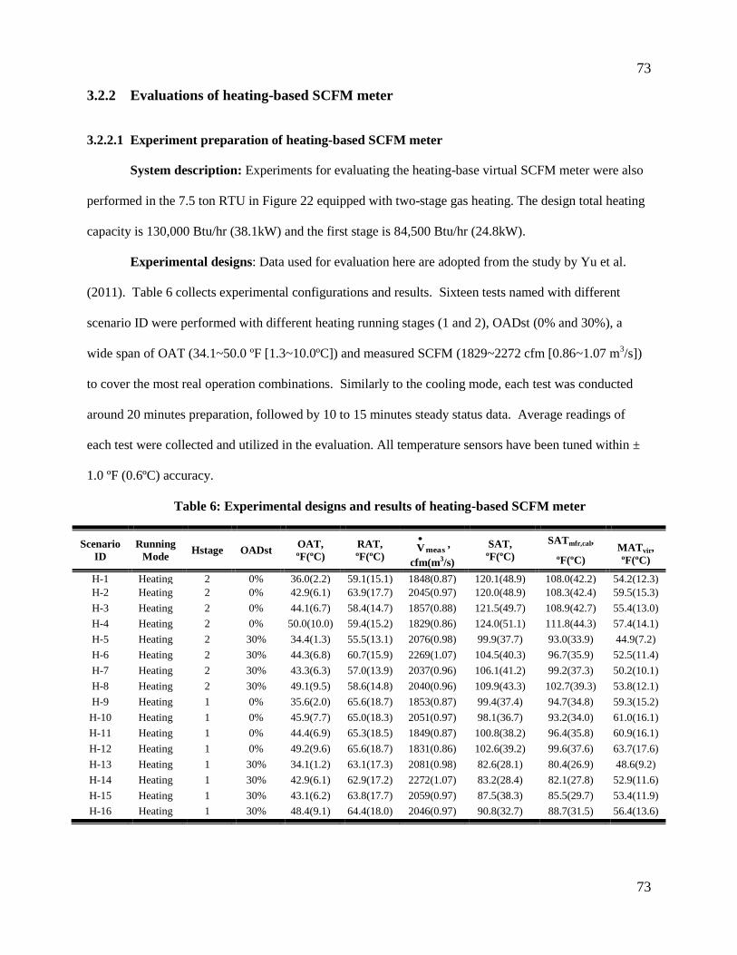
73

73

3.2.2 Evaluations of heating-based SCFM meter

3.2.2.1 Experiment preparation of heating-based SCFM meter

System description: Experiments for evaluating the heating-base virtual SCFM meter were also

performed in the 7.5 ton RTU in Figure 22 equipped with two-stage gas heating. The design total heating

capacity is 130,000 Btu/hr (38.1kW) and the first stage is 84,500 Btu/hr (24.8kW).

Experimental designs: Data used for evaluation here are adopted from the study by Yu et al.

(2011). Table 6 collects experimental configurations and results. Sixteen tests named with different

scenario ID were performed with different heating running stages (1 and 2), OADst (0% and 30%), a

wide span of OAT (34.1~50.0 ºF [1.3~10.0ºC]) and measured SCFM (1829~2272 cfm [0.86~1.07 m3/s])

to cover the most real operation combinations. Similarly to the cooling mode, each test was conducted

around 20 minutes preparation, followed by 10 to 15 minutes steady status data. Average readings of

each test were collected and utilized in the evaluation. All temperature sensors have been tuned within ±

1.0 ºF (0.6ºC) accuracy.

Table 6: Experimental designs and results of heating-based SCFM meter

Scenario

ID

Running

Mode Hstage OADst

OAT,

ºF(ºC)

RAT,

ºF(ºC) measV

,

cfm(m3/s)

SAT, ºF(ºC)

SATmfr,cal,

ºF(ºC)

MATvir,

ºF(ºC)

H-1 Heating 2 0% 36.0(2.2) 59.1(15.1) 1848(0.87) 120.1(48.9) 108.0(42.2) 54.2(12.3)

H-2 Heating 2 0% 42.9(6.1) 63.9(17.7) 2045(0.97) 120.0(48.9) 108.3(42.4) 59.5(15.3)

H-3 Heating 2 0% 44.1(6.7) 58.4(14.7) 1857(0.88) 121.5(49.7) 108.9(42.7) 55.4(13.0)

H-4 Heating 2 0% 50.0(10.0) 59.4(15.2) 1829(0.86) 124.0(51.1) 111.8(44.3) 57.4(14.1)

H-5 Heating 2 30% 34.4(1.3) 55.5(13.1) 2076(0.98) 99.9(37.7) 93.0(33.9) 44.9(7.2)

H-6 Heating 2 30% 44.3(6.8) 60.7(15.9) 2269(1.07) 104.5(40.3) 96.7(35.9) 52.5(11.4)

H-7 Heating 2 30% 43.3(6.3) 57.0(13.9) 2037(0.96) 106.1(41.2) 99.2(37.3) 50.2(10.1)

H-8 Heating 2 30% 49.1(9.5) 58.6(14.8) 2040(0.96) 109.9(43.3) 102.7(39.3) 53.8(12.1)

H-9 Heating 1 0% 35.6(2.0) 65.6(18.7) 1853(0.87) 99.4(37.4) 94.7(34.8) 59.3(15.2)

H-10 Heating 1 0% 45.9(7.7) 65.0(18.3) 2051(0.97) 98.1(36.7) 93.2(34.0) 61.0(16.1)

H-11 Heating 1 0% 44.4(6.9) 65.3(18.5) 1849(0.87) 100.8(38.2) 96.4(35.8) 60.9(16.1)

H-12 Heating 1 0% 49.2(9.6) 65.6(18.7) 1831(0.86) 102.6(39.2) 99.6(37.6) 63.7(17.6)

H-13 Heating 1 30% 34.1(1.2) 63.1(17.3) 2081(0.98) 82.6(28.1) 80.4(26.9) 48.6(9.2)

H-14 Heating 1 30% 42.9(6.1) 62.9(17.2) 2272(1.07) 83.2(28.4) 82.1(27.8) 52.9(11.6)

H-15 Heating 1 30% 43.1(6.2) 63.8(17.7) 2059(0.97) 87.5(38.3) 85.5(29.7) 53.4(11.9)

H-16 Heating 1 30% 48.4(9.1) 64.4(18.0) 2046(0.97) 90.8(32.7) 88.7(31.5) 56.4(13.6)

74

74

Experimental results: Experimental results for evaluating the heating-based virtual SCFM meter

are collected in Table 6 respectively. The methods to obtain the direct measurements (OAT, RAT, and

measV

) and the indirect results (MATvir and ∆Tfan ) are the same as the cooling mode, excepting the SAT

values:

Calibrated MSAT (SATmfr, cal) Based on the study by Yu et al. (2011), direct measurements of an

MSAT sensor are incorrect in heating mode with gas furnaces equipped in RTUs. There exists

unacceptable erratic measurement errors (e.g., in a 7.5 ton RTU, the errors are from 1.0 ºF [0.6ºC] to

12.6ºF [7.0ºC]) due to severe temperature stratification and high thermal radiation. The traditional

calibration method can hardly overcome the defect. The methodology of virtual calibration of an MSAT

sensor is innovated with good accuracy by Yu et al (2011). This method is adopted in this study and

MSAT is calibrated as SATmfr, cal in Table 4 with uncertainty ± 1.2 ºF (0.7ºC). For more information

about the virtual calibration of an MSAT sensor in RTUs, please refer to the section 3.4.2.

Based on the experimental results in the 7.5 ton RTU in the heating mode, uncertainty analysis

and experimental evaluation are thereby conducted to evaluate the effectiveness of the heating-based

approach.

3.2.2.2 Uncertainty analysis of heating-based SCFM meter

Based on Equation (50), uncertainty of heating-based approach calculation is conducted with the

independent variables of gV

, ΔTfan, SATmfr,cal and MATvir. The root sum square is used as Equation (51):

2/12vir

vir

2cal,mfr

cal,mfr

2fan

fan

2g

g

])MATMAT

V()SAT

SAT

V()T

T

V()V

V

V[(V

elmod,Helmod,Helmod,Helmod,H

elmod,H

(51)

Where δgV

, δΔTfan, δSATmfr,cal and δMATvir are inputs uncertainties.

The results of sixteen experiments in heating mode preformed in the 7.5 ton RTU are used to

analyze the uncertainty of heating-based approach. As shown in Table 7, gV

is 30.0 cfm (0.014m

3/s) for

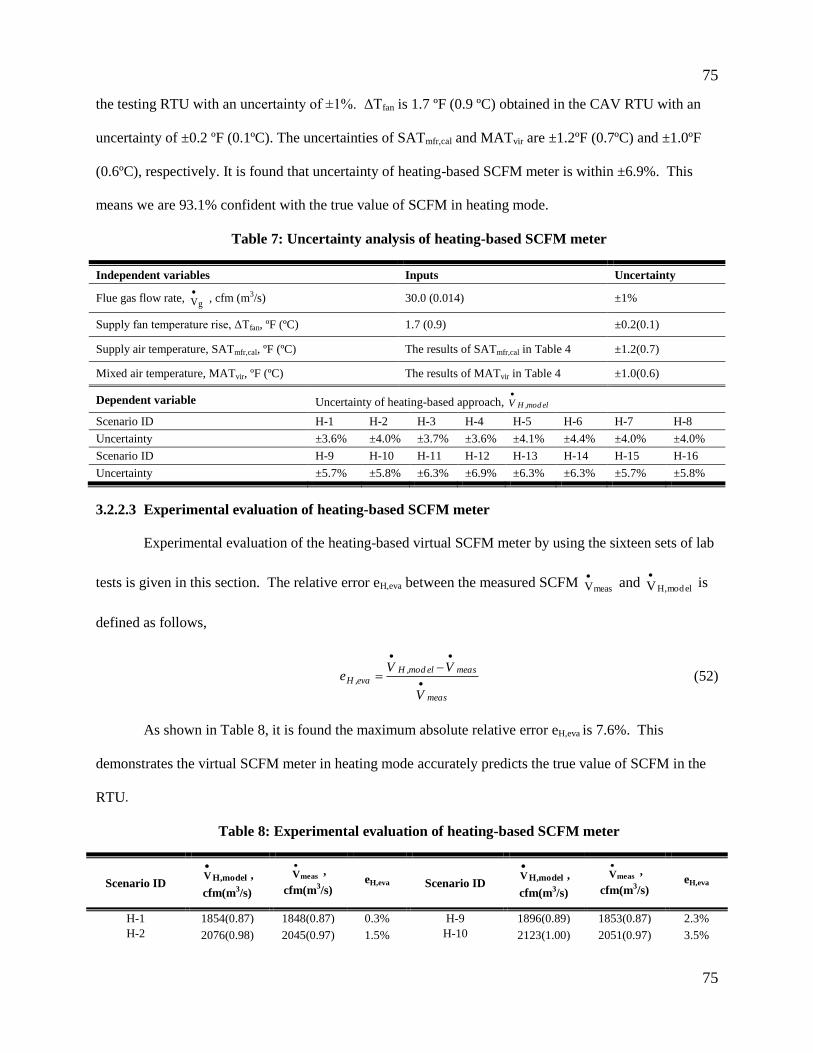
75

75

the testing RTU with an uncertainty of ±1%. ΔTfan is 1.7 ºF (0.9 ºC) obtained in the CAV RTU with an

uncertainty of ±0.2 ºF (0.1ºC). The uncertainties of SATmfr,cal and MATvir are ±1.2ºF (0.7ºC) and ±1.0ºF

(0.6ºC), respectively. It is found that uncertainty of heating-based SCFM meter is within ±6.9%. This

means we are 93.1% confident with the true value of SCFM in heating mode.

Table 7: Uncertainty analysis of heating-based SCFM meter

Independent variables

Inputs Uncertainty

Flue gas flow rate, gV

, cfm (m3/s) 30.0 (0.014) ±1%

Supply fan temperature rise, ΔTfan, ºF (ºC) 1.7 (0.9) ±0.2(0.1)

Supply air temperature, SATmfr,cal, ºF (ºC) The results of SATmfr,cal in Table 4 ±1.2(0.7)

Mixed air temperature, MATvir, ºF (ºC) The results of MATvir in Table 4 ±1.0(0.6)

Dependent variable Uncertainty of heating-based approach, elmod,HV

Scenario ID H-1 H-2 H-3 H-4 H-5 H-6 H-7 H-8

Uncertainty ±3.6% ±4.0% ±3.7% ±3.6% ±4.1% ±4.4% ±4.0% ±4.0%

Scenario ID H-9 H-10 H-11 H-12 H-13 H-14 H-15 H-16

Uncertainty ±5.7% ±5.8% ±6.3% ±6.9% ±6.3% ±6.3% ±5.7% ±5.8%

3.2.2.3 Experimental evaluation of heating-based SCFM meter

Experimental evaluation of the heating-based virtual SCFM meter by using the sixteen sets of lab

tests is given in this section. The relative error eH,eva between the measured SCFM measV

and

elmod,HV

is

defined as follows,

meas

measelmod,H

eva,H

V

VVe

(52)

As shown in Table 8, it is found the maximum absolute relative error eH,eva is 7.6%. This

demonstrates the virtual SCFM meter in heating mode accurately predicts the true value of SCFM in the

RTU.

Table 8: Experimental evaluation of heating-based SCFM meter

Scenario ID elmod,HV

,

cfm(m3/s)

measV

,

cfm(m3/s)

eH,eva Scenario ID elmod,HV

,

cfm(m3/s)

measV

,

cfm(m3/s)

eH,eva

H-1 1854(0.87) 1848(0.87) 0.3% H-9 1896(0.89) 1853(0.87) 2.3%

H-2 2076(0.98) 2045(0.97) 1.5% H-10 2123(1.00) 2051(0.97) 3.5%

76

76

H-3 1866(0.88) 1857(0.88) 0.5% H-11 1890(0.89) 1849(0.87) 2.2%

H-4 1834(0.87) 1829(0.86) 0.3% H-12 1969(0.93) 1831(0.86) 7.6%

H-5 2174(1.03) 2076(0.98) 4.7% H-13 2204(1.04) 2081(0.98) 5.9%

H-6 2399(1.13) 2269(1.07) 5.7% H-14 2443(1.15) 2272(1.07) 7.5%

H-7 2125(1.00) 2037(0.96) 4.3% H-15 2181(1.03) 2059(0.97) 5.9%

H-8 2132(1.01) 2040(0.96) 4.5% H-16 2164(1.02) 2046(0.97) 5.7%

To here, both cooling- and heating-based approaches to develop a virtual SCFM meter are

presented. Finally, the comparisons and conclusions of the two approaches are explored in the next

subsection.

3.3 Comparisons and conclusions of cooling- and heating-based approaches

Comparing the cooling and heating-based approaches, we could reach the following conclusions:

Uncertainty of elmod,CV

is much higher than the uncertainty of

elmod,HV

elmod,HV

is correlated with the inputs of gV

,ΔTfan, SATmfr,cal and MATvir, wherein

gV

and ΔTfan

are quite stable with very low uncertainties. Uncertainty of elmod,HV

is low, within ±6.9%. In contrast,

elmod,CV

is calculated by five parameters of OAT, MATvir, MATwb,vir , SAT and ΔTfan with more

difficulties of implementation and higher risk of uncertainties (±13.8 %, in this case). The heating-based

SCFM meter, with the feature of "less uncertainty", is considered simple, stable and could accurately

predict the SCFM in RTUs.

The relative error eC,eva between measV

and

elmod,CV

is high, while eH,eva in heating mode is low

Owing to the uncertainty generated by the model regression of sens,CQ

in Equation (18), as well as

the uncertainty associated with the multiple measurements of elmod,CV

in Equation (28), the relative errors

eC,eva between measV

and

elmod,CV

are high (-16.2~16.4%, in this case). However, elmod,HV

, with simple

and reliable inputs, is much close to measV

as evaluated through laboratory tests.

Robustness of elmod,HV

is better than

elmod,CV

77

77

Although the manufacturer-data based cooling capacity model proposed by Yang and Li (2010)

could work well when the system operates normally or only air side faults are present (e.g. improper

supply airflow rates), it could not work in the presence of the faults developed at refrigerant side (e.g.

low refrigerant charge). However, it is notorious that the refrigerant side of RTUs is plagued by various

common degraded faults due to its complexity (Proctor and Downey, 1995; Cowan, 2004; Li and Braun

2007a, 2007b, 2009a). This fact causes more difficulties and limitations when implementing and

accurately monitoring the cooling-based SCFM meter in practice. However, in heating mode, the gas side

is simple and its gas flow rate is accurately controlled by a sophisticated gas regulator. Although the gas

side could fail occasionally, degraded faults associated with the gas side have been rarely reported. It is

easy to identify complete failure and thus to avoid using the flow meter. With the good-fault free property,

heating-based SCFM meter performs robustly most of the time.

Relative humidity measurement of inlet air is required for cooling mode, but not for heating mode

According to Equation (28), MATwb is critical to calculate the SCFM for cooling mode. Installing

relative humidity sensor is needed to collect the measurement of wet bulb temperature. However, no

measurement on the air humidity is required in the heating-based approach. Only easy-to-obtain

measurements (dry bulb temperatures) are left in Equation (50) as unknown dependent variables. As we

know, RTUs may not have relative humidity sensors mounted by manufacturers. Comparing to

temperature sensors, relative humidity sensors are costly. Additional costs entail with procurement,

installation and maintenance of relative humidity sensors. Moreover, a relative humidity sensor is

notorious for its accuracy drifting and saturation under high humidity levels.

The above comparisons between cooling- and heating-based approaches reveals that utilizing heating

mode to develop a virtual SCFM meter is worthy of confidence. Therefore, the implementation issues of a

heating-based virtual SCFM meter, covering detailed measuring and processing the parameters and an

implementation flowchart, are introduced in the following section.

78

78

3.4 Implementation issues

This part is dedicated to provide an instruction of using this virtual SCFM meter in practice.

Except for the stable input of gV

of the heat exchanger, implementation issues of three temperature

measurements SAT, MAT and ∆Tfan, are described.

To ensure the robustness and reliability of this virtual meter, a steady-status detector presented by

Li and Braun (2003b) is referred to filter out the transient data of all temperature measurements related to

Equation (38).

3.4.1 Measuring and processing SAT

3.4.1.1 Background of direct measurements of SAT in RTUs

Accurate SAT measurements would directly influence the performance of the virtual SCFM

meter. In the field, there is a manufacturer-preinstalled SAT sensor (MSAT) widely used in most light

commercial RTUs and it is not difficult to collect the readings. However, a common practice by RTU

manufacturers is to pre-install the MSAT sensor right after the gas-fired heating coil in a compact

chamber. Owing to the following two inherent problems under this arrangement, the accuracy and

reliability of the MSAT sensor are notoriously difficult to attain in heating mode (ASHRAE fundamental,

2009):

Poor air temperature distribution

With gas-fired heating coil mounted in a crowded housing, RTUs have an extremely uneven air

temperature distribution where the onboard SAT temperature sensor is located. According to ASME PTC

19.3-1974, aspiration method involving passing a high-velocity stream of air over the temperature sensor

is improbable to be applied.

Intensive thermal radiation of gas heating

The MSAT sensor is bathed in an adverse hot air chamber. Measurements can be affected by

radiation from surrounding surfaces (ASHRAE fundamental, 2009). Strong thermal radiation from gas

79

79

burners causes a dramatic rise in air temperature measurement. Even with the shielding suggested by

Parmelee and Huebscher (1946), the radiation impact on the MSAT sensor can hardly be eliminated.

Meanwhile, the RTU’s compact structure makes it improper for shielding.

Consequently, manufacturers recommend that the MSAT sensor should be relocated to the supply

air duct on site, particularly if the supply air temperature control functions were used (Lennox, 2007).

However, relocating the MSAT sensor would run into a series of problems.

First of all, repositioning the MSAT sensor to the supply air duct could be very costly in a

situation where all other installations of a system are completed. It is greatly in excess of the original

budget planned for an economy packaged unit. Second, RTUs are usually set up right upon the roof of the

served zones in light commercial buildings (e.g., big-box retail stores), the supply air duct, if there is one,

is too short to meet the minimum requirements by manufacturers or to achieve a balanced air temperature

distribution.

As a result, a lot of building operators either do not bother to relocate the MSAT sensor, which

will cause unreliable supply air temperature related control functions, or completely disable the MSAT

sensor related functions.

Instead of repositioning the MSAT sensor to supply air duct or directly using the MSAT

measurements, we proposed an innovative virtual calibration method to solve the dilemma (Yu et al.

2011). The main merit of this method is that a general linear model to offset the MSAT errors is created

through a one-time algorithm development. This virtual calibration technique is very cost-effective,

accurate, stable, easy-to-use and generic for all RTUs with similar construction of gas furnaces and can be

implemented for long-term use.

The study begins with the evaluation of two groups of direct measurements: the single onboard

MSAT sensor-based measurement and further a measuring grid-based measurement. It is found neither

method can provide the real time true value of SAT. There are unstable changing errors in both of them,

which rules out the possibility of using regular calibration. Then, a virtual calibration algorithm for the

MSAT sensor is proposed based on lab data, and also the modeling and implementation procedures are

80

80

summarized for easy-to-use implementation. Uncertainty analysis and additional experimental evaluation

are carried out over a wide range of controlled tests later on. The study concludes that the virtually

calibrated MSAT sensor can accurately predict the true value and is adopted to develop a virtual SCFM

meter in RTUs.

3.4.1.2 Evaluation of direct measurements of SAT in RTUs

Direct measurements are conventionally used for air temperature in all kinds of forced air

systems. In this section, the 7.5 ton RTU equipped with gas heating is evaluated in terms of direct SAT

measuring of two methods: the MSAT sensor-based measurement and a measuring grid-based

measurement.

The assessment starts with the single onboard MSAT sensor under both cooling and heating

mode. To further understand the nature of inaccuracy in direct measurement, an additional method,

termed multi-sensor measuring grid, is applied. The measurements for them are performed

simultaneously in the same experimental series to ensure the consistency and comparability of the results.

To keep it simple, only the necessary experimental results and the deduction are debriefed right below.

MSAT sensor-based measurement

A group of parametric tests are implemented to the two-stage cooling and two-stage gas heating

7.5 ton RTU for the evaluation of the MSAT sensor derived measurements. Both cooling and heating

mode are offered with stage 1 and 2. OADst is modulated at 0% and 30% for the different runs, since in

cooling and heating mode, RTUs bring in minimum outside air flow for ventilation and 30% is usually

the upper limit for a minimum damper position (ASHRAE Standard 62.1, 2007). Besides the data point

given in the section 3.1.2.1 and 3.2.2.1, there is an additional lab-installed SAT sensor (SATlab,meas) to

verify the MSAT measurement in the lab. Each experiment assigned a scenario ID is conducted around 20

minutes for preparation, and followed by 10 to 15 minutes under steady status (Li and Braun 2003b).

Instant readings for each sensor are sampled every 15 seconds and the mean of the samples is then used to

represent the corresponding measurement result.

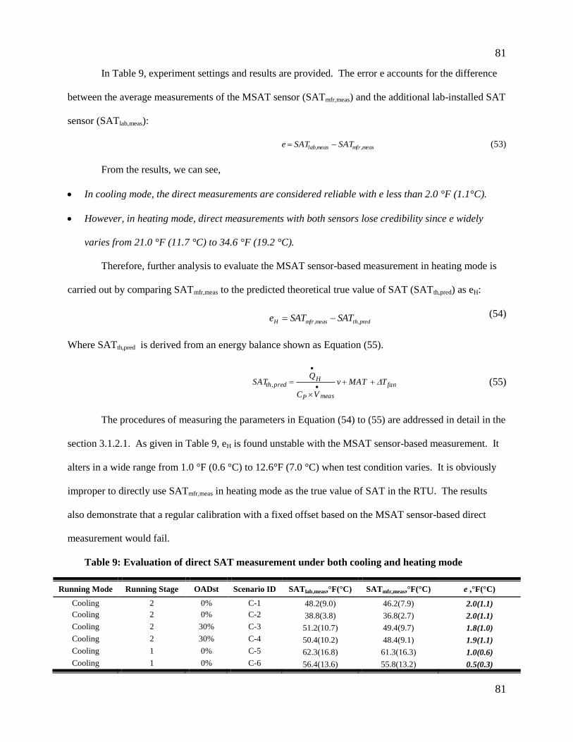
81

81

In Table 9, experiment settings and results are provided. The error e accounts for the difference

between the average measurements of the MSAT sensor (SATmfr,meas) and the additional lab-installed SAT

sensor (SATlab,meas):

meas,mfrmeas,lab SATSATe (53)

From the results, we can see,

In cooling mode, the direct measurements are considered reliable with e less than 2.0 °F (1.1°C).

However, in heating mode, direct measurements with both sensors lose credibility since e widely

varies from 21.0 °F (11.7 °C) to 34.6 °F (19.2 °C).

Therefore, further analysis to evaluate the MSAT sensor-based measurement in heating mode is

carried out by comparing SATmfr,meas to the predicted theoretical true value of SAT (SATth,pred) as eH:

pred,thmeas,mfrH SATSATe (54)

Where SATth,pred is derived from an energy balance shown as Equation (55).

fan

measP

Hpred,th TMATv

VC

QSAT

(55)

The procedures of measuring the parameters in Equation (54) to (55) are addressed in detail in the

section 3.1.2.1. As given in Table 9, eH is found unstable with the MSAT sensor-based measurement. It

alters in a wide range from 1.0 °F (0.6 °C) to 12.6°F (7.0 °C) when test condition varies. It is obviously

improper to directly use SATmfr,meas in heating mode as the true value of SAT in the RTU. The results

also demonstrate that a regular calibration with a fixed offset based on the MSAT sensor-based direct

measurement would fail.

Table 9: Evaluation of direct SAT measurement under both cooling and heating mode

Running Mode Running Stage OADst Scenario ID SATlab,meas,°F(°C) SATmfr,meas,°F(°C) e ,°F(°C)

Cooling 2 0% C-1 48.2(9.0) 46.2(7.9) 2.0(1.1)

Cooling 2 0% C-2 38.8(3.8) 36.8(2.7) 2.0(1.1)

Cooling 2 30% C-3 51.2(10.7) 49.4(9.7) 1.8(1.0)

Cooling 2 30% C-4 50.4(10.2) 48.4(9.1) 1.9(1.1)

Cooling 1 0% C-5 62.3(16.8) 61.3(16.3) 1.0(0.6)

Cooling 1 0% C-6 56.4(13.6) 55.8(13.2) 0.5(0.3)

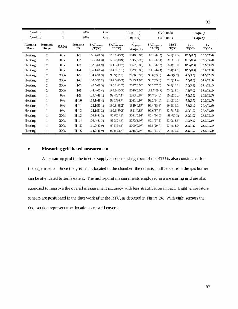
82

82

Cooling 1 30% C-7 66.4(19.1) 65.9(18.8) 0.5(0.3)

Cooling 1 30% C-8 66.0(18.9) 64.6(18.1) 1.4(0.8)

Running

Mode

Running

Stage OADst

Scenario

ID

SATlab,meas

,°F(°C)

SATmfr,meas ,

°F(°C) measV

,

cfm(m3/s)

SATth,pred ,

°F(°C)

MAT,

°F(°C)

eH ,

°F(°C)

e ,

°F(°C)

Heating 2 0% H-1 151.4(66.3) 120.1(48.9) 1848(0.87) 108.0(42.2) 54.2(12.3) 12.1(6.7) 31.3(17.4)

Heating 2 0% H-2 151.3(66.3) 120.0(48.9) 2045(0.97) 108.3(42.4) 59.5(15.3) 11.7(6.5) 31.3(17.4)

Heating 2 0% H-3 152.5(66.9) 121.5(49.7) 1857(0.88) 108.9(42.7) 55.4(13.0) 12.6(7.0) 31.0(17.2)

Heating 2 0% H-4 155.1(68.4) 124.0(51.1) 1829(0.86) 111.8(44.3) 57.4(14.1) 12.2(6.8) 31.1(17.3)

Heating 2 30% H-5 134.4(56.9) 99.9(37.7) 2076(0.98) 93.0(33.9) 44.9(7.2) 6.9(3.8) 34.5(19.2)

Heating 2 30% H-6 138.5(59.2) 104.5(40.3) 2269(1.07) 96.7(35.9) 52.5(11.4) 7.8(4.3) 34.1(18.9)

Heating 2 30% H-7 140.5(60.3) 106.1(41.2) 2037(0.96) 99.2(37.3) 50.2(10.1) 7.0(3.9) 34.4(19.1)

Heating 2 30% H-8 144.4(62.4) 109.9(43.3) 2040(0.96) 102.7(39.3) 53.8(12.1) 7.2(4.0) 34.6(19.2)

Heating 1 0% H-9 120.4(49.1) 99.4(37.4) 1853(0.87) 94.7(34.8) 59.3(15.2) 4.6(2.6) 21.1(11.7)

Heating 1 0% H-10 119.1(48.4) 98.1(36.7) 2051(0.97) 93.2(34.0) 61.0(16.1) 4.9(2.7) 21.0(11.7)

Heating 1 0% H-11 122.1(50.1) 100.8(38.2) 1849(0.87) 96.4(35.8) 60.9(16.1) 4.3(2.4) 21.4(11.9)

Heating 1 0% H-12 124.1(51.2) 102.6(39.2) 1831(0.86) 99.6(37.6) 63.7(17.6) 3.0(1.7) 21.4(11.9)

Heating 1 30% H-13 106.1(41.2) 82.6(28.1) 2081(0.98) 80.4(26.9) 48.6(9.2) 2.2(1.2) 23.5(13.1)

Heating 1 30% H-14 106.4(41.3) 83.2(28.4) 2272(1.07) 82.1(27.8) 52.9(11.6) 1.0(0.6) 23.3(12.9)

Heating 1 30% H-15 111.0(43.9) 87.5(38.3) 2059(0.97) 85.5(29.7) 53.4(11.9) 2.0(1.1) 23.5(13.1)

Heating 1 30% H-16 114.8(46.0) 90.8(32.7) 2046(0.97) 88.7(31.5) 56.4(13.6) 2.1(1.2) 24.0(13.3)

Measuring grid-based measurement

A measuring grid in the inlet of supply air duct and right out of the RTU is also constructed for

the experiments. Since the grid is not located in the chamber, the radiation influence from the gas burner

can be attenuated to some extent. The multi-point measurements employed in a measuring grid are also

supposed to improve the overall measurement accuracy with less stratification impact. Eight temperature

sensors are positioned in the duct work after the RTU, as depicted in Figure 26. With eight sensors the

duct section representative locations are well covered.

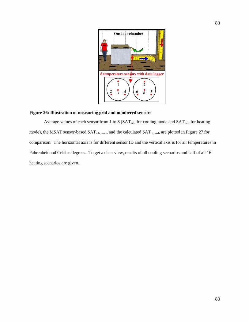
83

83

Figure 26: Illustration of measuring grid and numbered sensors

Average values of each sensor from 1 to 8 (SATG,C for cooling mode and SATG,H for heating

mode), the MSAT sensor-based SATmfr,meas, and the calculated SATth,pred, are plotted in Figure 27 for

comparison. The horizontal axis is for different sensor ID and the vertical axis is for air temperatures in

Fahrenheit and Celsius degrees. To get a clear view, results of all cooling scenarios and half of all 16

heating scenarios are given.

84

84

20

40

60

80

1 2 3 4 5 6 7 8 SAT

M,M

Tem

per

atu

re(°

F)

C-1 C-2 C-3 C-4 C-5 C-6 C-7 C-8

SATM,M

SAT

mfr,m

ea

sSensor ID

Cooling mode

55

80

105

130

155

1 2 3 4 5 6 7 8 SAT

M,M

SAT

CTe

mp

erat

ure

(°F

)

H-1 H-4 H-6 H-7 H-8 H-13 H-15 H-16

SAT

mfr,m

eas

SAT

th,p

red

Heating mode

Scenario ID

(a)

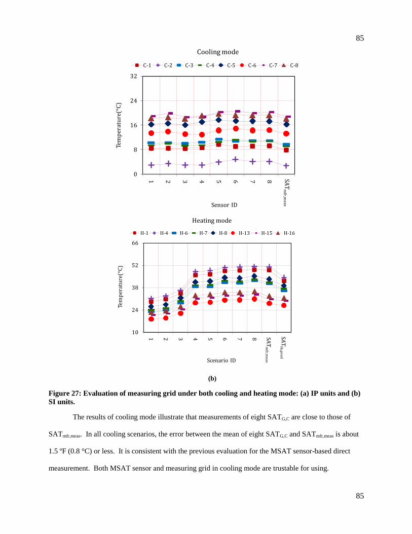
85

85

0

8

16

24

32

1 2 3 4 5 6 7 8 SAT

M,M

Tem

per

atu

re(°

C)

C-1 C-2 C-3 C-4 C-5 C-6 C-7 C-8

SATM,M

SAT

mfr,m

ea

sSensor ID

Cooling mode

10

24

38

52

66

1 2 3 4 5 6 7 8 SAT

M,M

SAT

C

Tem

per

atu

re(°

C)

H-1 H-4 H-6 H-7 H-8 H-13 H-15 H-16

SAT

mfr,m

eas

SAT

th,p

red

Heating mode

Scenario ID

(b)

Figure 27: Evaluation of measuring grid under both cooling and heating mode: (a) IP units and (b)

SI units.

The results of cooling mode illustrate that measurements of eight SATG,C are close to those of

SATmfr,meas. In all cooling scenarios, the error between the mean of eight SATG,C and SATmfr,meas is about

1.5 ºF (0.8 °C) or less. It is consistent with the previous evaluation for the MSAT sensor-based direct

measurement. Both MSAT sensor and measuring grid in cooling mode are trustable for using.

86

86

From the heating mode plot, the following points can be observed:

Temperature distribution of eight SATG,H is irregular

Combining Figure 26 and 27, relationships of eight SATG,H and their location in heating mode are

erratic. Temperature values of sensors 1 to 4 are lower than those of the corresponding sensors 5 to 8. It

is unsuitable to calculate the true value of SAT by averaging eight SATG,H.

Big temperature difference exists between SATmfr,meas and the average eight SATG,H

In scenario H-7, for example, SATmfr,meas is 106.1°F (41.2 °C) ; SATG,H sensors 1 to 8 give the

lowest reading as 74.4 °F (23.6 °C), the highest as 108.7 °F (42.6°C). It makes the differential

temperature between SATmfr,meas and the average eight SATG,H 8.9 °F (4.9 °C). In all heating scenarios,

the error between SATmfr,meas and the mean of eight SATG,H varies from 3.0 ºF (1.7 °C) to 12.2 ºF (6.8

°C) .

Various temperature difference stands between SATth,pred and the mean of eight SATG,H

The temperature difference between SATth,pred and the mean of eight SATG,H varies in different

scenarios. Like in scenario H-7, with Hstage 2 and OADst 30%, the mean of eight SATG,H is 95.2 °F

(35.1°C) while the true value SATth,pred is 99.2 °F (37.3 °C) [with 4.0 °F (2.2 °C) temperature

difference]. However, in scenario H-16 with Hstage 1 and OADst 30%, the mean of eight SATG,H is

85.9°F (29.9 °C) while the true value SATth,pred is 88.7 °F (31.5 °C) [with 2.8 °F (1.6 °C) temperature

difference]. As presented in this case, the measuring grid does not indicate the true value of SAT.

In summary, the evaluation of measuring grid further testifies that the offset error for MSAT in

heating mode varies. Controls in RTUs related to MSAT sensor direct measurements in heating mode

can be far from the intended operation and lead to inferior system performance. What is more, using

measuring grid does not help obtain the true value of SAT in RTUs. It could not be used for the

verification of the predicted true value of SAT as well. An innovative calibration algorithm is needed to

fill in the gap.

87

87

3.4.1.3 Development of a virtual calibration model for a SAT sensor in RTUs

Algorithm development

As analyzed above, direct measurement, either the single MSAT sensor-based or the measuring

grid-based cannot catch the true value of SAT. The measuring grid method in a location out of the RTU

merely provides closer but still mediocre prediction. Besides, additional construction, costs, maintenance

and sources for uncertainty are incurred by using the measuring grid. It is not a practical tool in real

applications.

Variables in the experiments thus are reinvestigated to identify the algorithm that might be useful

to predict the offset for the calibration of the MSAT sensor-based measurement.

Hstage=2

Hstage=1

0% 15% 30% 45%

OADste H

,°F

(a)

Hstage=2

Hstage=1

0% 15% 30% 45%

OADst

e H,°

C

(b)

Figure 28: eH vs OADst in different Hstage: (a) IP units and (b) SI units.

88

88

As shown in Figure 28, the error eH is a strong function of heating stages (Hstage) and OADst. A

liner model can be fitted to represent the relationship between eH, Hstage and OADst in RTUs. As shown

in Equation (56), the model can be used to estimate the calibration error (ecal) of the MSAT sensor under

certain Hstage and OADst. Verification through more lab tests is explored in later sections.

OADstHstagegOADstfOADstdHstagecHstagebae 22cal (56)

Once such an offset ecal expression is obtained for a given type of RTU, it can be utilized to

correct the MSAT sensor-based measurement for the true value in RTUs. The equation for the calibrated

MSAT sensor (SATmfr,cal) is given below:

calmeas,mfrcal,mfr eSATSAT (57)

For this 7.5 ton rooftop unit with 130,000 Btu/hr (38.1 kW) gas heating capacity, the coefficients

for the linear model are obtained with the experimental data. The results are listed in Table 10, with R-

square 0.98.

Table 10: Linear model coefficients for the example RTU

IP units Coefficient

s

a b c d f g

Value 1.0900 0.6905 2.4200 0.5484 0.1166 -8.5000

SI units Coefficient

s a b c d f g

Value 0.6056 0.3836 1.3444 0.3047 0.0648 -4.7222

Equations (56) and (57) jointly constitute the model of the virtual calibration that can be directly

transplanted to different RTUs.

3.4.1.4 Uncertainty analysis

The virtual calibration algorithm of an MSAT sensor obtains SATmfr,cal as the prediction of SAT

true value. In this section, uncertainty sensitivity of SATmfr,cal to relative HQ

,

measV

,MAT and ΔTfan is

raised. The root sum square method of uncertainty calculation is applied to the variables. The random

uncertainty is expressed in units °F (°C) as Equation (58):

2/12fan

fan

cal,mfr2cal,mfr2meas

meas

cal,mfr2H

H

cal,mfrcal,mfr ])T

T

SAT()MAT

MAT

SAT()V

V

SAT()Q

Q

SAT[(SAT

(58)

89

89

Where HQ

, measV

, MAT and fanT are sensor uncertainties.

Table 11 summarizes the uncertainties of independent variables as inputs to Equation (55), as

well as the calculated uncertainties of SATmfr,cal as outputs. As can be seen, the absolute uncertainty of

virtual calibrated SAT is lower than 1.2 °F (0.7 °C). It is in the range of acceptable error for temperature

uncertainties in the HVAC industry.

Table 11: Uncertainty analysis of SATmfr,cal

Independent variables Inputs Uncertainty

Gas heating capacity, HQ

,Btu/hr (kW) Gas heating stage 1: 84,500 (24.8)

Gas heating stage 2: 130,000 (38.1) ±2%

Measured supply air flow rate, measV

,cfm (m3/s) Default data in Table 1 ±1%

Mixed air temperature, MAT, °F (°C) Default data in Table 1 ±1.0°F (0.6 °C)

Supply fan temperature rise, ∆Tfan, °F (°C) 1.7°F (0.9 °C) ±0.2°F (0.1 °C)

Dependent variable Calibrated manufacturer-installed SAT sensor, SATmfr,cal ,°F (°C)

Scenario ID H-1 H-2 H-3 H-4 H-5 H-6 H-7 H-8

Uncertainty (°F) 1.2(0.7) 1.1(0.6) 1.2(0.7) 1.2(0.7) 1.1(0.6) 1.1(0.6) 1.1(0.6) 1.1(0.6)

Scenario ID H-9 H-10 H-11 H-12 H-13 H-14 H-15 H-16

Uncertainty (°F) 1.1(0.6) 1.1(0.6) 1.1(0.6) 1.1(0.6) 1.1(0.6) 1.1(0.6) 1.1(0.6) 1.1(0.6)

The accuracy of virtual calibrated MSAT (SATmfr,cal) in Equation (56) and (57) is further

evaluated by using energy balance under both cooling (forward) and heating (backward) mode as

elaborated in Appendix B. It demonstrates SATmfr,cal can be trusted as the true value of SAT in RTUs.

The virtual calibration method for measuring and processing MSAT measurement is adopted to develop a

virtual SCFM meter in this study.

3.4.2 Measuring and processing MAT

Accurate direct MAT measurements are notoriously difficult to obtain in RTUs due to space

constraints and the use of small chambers for mixing outdoor and return air (ANSI/ASME Standard PTC

19.3, 1974). As presented previously, Wichman and Braun (2009) proposed and demonstrated an

economical scheme for adjusting a single-point measurement of MAT (a smart MAT sensor) in RTUs

that is based on in-situ measurements and self calibration. The approach is achieved by correlating the

bias error in terms of OADst and temperature difference between outdoor and return-air. Extensive lab

90

90

testing demonstrates that the smart mixed air temperature sensor performs very well and the overall root-

mean-squared error is 0.57ºF (0.3ºC). The smart MAT sensor proposed overcomes a typical technical

barrier of using costly measurement grids or simulation software.

However, a physical MAT sensor is not typically installed in light commercial RTUs due to its

bad performance. So this smart MAT sensor cannot be implemented without adding a new MAT sensor.

To further simplify this technique, Yang and Li (2011) proposed an alternative method which eliminates

the need of a physical MAT sensor and instead constructs a virtual MAT sensor to estimate MAT using

OAT, RAT and a correlated virtual outdoor air ratio sensor β as follows,

RAT)1(OATMAT (59)

Both laboratory and field testing demonstrate an acceptable uncertainty of ±1.0 ºF (0.6 ºC). Since

there is no pre-installed physical MAT sensor available in our study, we adopted this method.

With accurate parameters accomplished, a graphical flowchart is explored accordingly to sum up

the implementation procedures of a virtual SCFM meter in RTUs.

3.4.3 Implementation flowchart of the virtual SCFM meter

The virtual SCFM meter in RTUs can be implemented through the following procedures in

Figure 29:

Step 1: Check the steady-status;

Step 2: Check the heating and cooling status;

Step 3: Check the availability of direct MSAT, OAT and RAT measurements;

Step 4: Virtually calibrate MSAT measurement; compute virtual MAT values;

Step 5: Run the virtual SCFM meter in Equation (50).

91

91

Y

Y

Y

N

N

N

Start

Steady-status

End

Hstage>0 andwithout the

presence of simultaneous cooling and heating

MSAT, OAT and RATmeasurementsare available

Stop

Virtual calibrationof SAT measurement

Compute VirtualMAT values

With the knowns of constants

Vg and Tfan, run the virtualSCFM meter in Equation(50)

Figure 29: An implementation flowchart of a virtual SCFM meter in RTUs

92

92

Chapter 4 FUTURE RESEARCH NEEDS AND

CONCLUTION

4.1 Future needs for virtual sensing technology and its application in

building systems

4.1.1 Future needs for virtual sensing technology in building systems

There is significant research and development that is needed before virtual sensors

become commonplace within buildings. In addition to the need for specific virtual sensor

developments, there is a need for standard methods to evaluate virtual sensor performance and

approaches for information management of networks of virtual sensors that can share sensor

inputs and outputs.

According to Underwood (1997), the performance of physical sensors is evaluated in

terms of range, repeatability, sensitivity and accuracy. These same performance parameters are

important for virtual sensors. However, the performance of a single virtual sensor can be

dependent on the accuracy of multiple physical sensor inputs and a model that uses those inputs

to predict the virtual sensor output. Standard approaches for calibrating and evaluating the

performance of virtual sensors over a wide range of operating conditions do not exist but are

needed. Furthermore, the model used within a virtual sensor can be based on a physical process

that changes over time due to the development of faults. As a result, virtual sensor performance

evaluations need to consider the robustness of sensor outputs with respect to the development of

physical faults.

Another important issue is information management for networks of virtual sensors that

are massively deployed within a building system. This problem can be described as

systemization of virtual sensors (SoVS), which has been an active area of research in other fields

93

93

for more than a decade (Hardy and Maroof 1999; Gu et al. 2004; Chin et. al, 2005; Bose et al.

2007). Figure 30 presents a proposed hierarchy for SoVS that could be applied to virtual sensors

in buildings. Two classes of virtual sensor are proposed: basic and derived virtual sensors. Basic

virtual sensors are created by using information from a group of physical sensors, empirical

coefficients, and user specifications. They can be viewed as extensions of physical sensors that

are used as low-cost replacements or backups for physical sensors or to estimate new quantities

that cannot be physically measured. Conversely, a derived virtual sensor is a sensor model built

in a combination with physical, basic and/or other derived virtual sensor measurements. They

could be used to provide higher level system information for performance monitoring, fault

identification and advanced control.

Basic virtual

sensors layer

Fundamental sensing and

communication hardware

and device drivers, etc

Derived virtual

sensors layer

Physical sensors system (layer)

Backup

/replacement;

Observing

A hierarchy

of

SoVS

Knowledge and

other available

information base,

such as

user specifications

and

empirical coefficients

Figure 30: A hierarchy scheme of SoVS

4.1.2 Future steps for development of an improved virtual SCFM meter in RTUs

Based on the above study of development and deployment an FP based virtual SCFM

meter in RTUs, we find that it needs further research about its model implementation and fault

diagnostics.

The FP based virtual SCFM meter relies heavily on indirect measurements of a virtually

calibrated supply air temperature (SATmfr,cal) sensor (Yu. et al. 2011a) and a virtual mixed air

temperature (MATvir) sensor (Yang and Li 2011). Owing to the drifts and other changes of data

94

94

during routine operations and during system renovation (e.g., serious damages of physical

sensors), there is often no objective measurement to reassess the virtual or virtually calibrated

sensors. Moreover, multiple parameters of the virtual meter (e.g., OAT, RAT, SAT and β)

periodically require traditional calibration or virtual calibration (Yang et al. 2011) before they can

be used since the accuracy and reliability of the fragile physical sensors often cannot be

guaranteed (e.g., exposed to hostile environment for a long time).

In the meantime, since the FP based virtual SCFM meter is proposed by utilizing an

energy balance in combination with accurate SATmfr,cal and MATvir measurements across heating

coils, it cannot be used to develop a virtual heating capacity meter inversely for further automated

FDD applications.

Therefore, further simplification of implementation and maintenance and enhancement of

fault diagnosing capability for the virtual SCFM meter in RTUs is necessary. The attempt of

using grey-box or black-box based modeling method could be one of solutions for the future

development of an improved virtual SCFM meter in RTUs.

4.1.3 Future steps for development of an improved virtually calibrated SAT sensor

in RTUs

The existing virtual calibration model for a SAT sensor proposed by Yu et al (2011) has

several deficiencies practically in the following aspects:

Low accuracy under a wide range of operating conditions

Due to the limitations of experimental configurations from Yu et al. (2011), the

correlated model of the virtual calibration method exposes greater errors (e.g., relative error is

±4.0 ˚F [2.2˚C]) under a wide range of operating conditions (e.g., OAT is lower than

35˚F[1.67˚C] and the SCFM degradation is higher than 20%) .

Poor performance in fault diagnostics

95

95

The low credibility of virtually calibrated MSAT measurements directly causes relatively

poor performance in fault diagnostics. A classic example is the FP based virtual SCFM meter,

which could raise a higher uncertainty.

Limited fault-tolerance in the presence of faults.

The current virtual calibration model for an MSAT sensor functions well only under

conditions in which the RTU performance is not significantly degraded [e.g., supply airflow rate

should not be lower than 80% of nominal SCFM level].

Therefore, to overcome the inadequacies of the existing virtual calibration method for an

MSAT sensor in RTUs, further research is needed to develop an improved calibration model with

well-designed laboratory experiments under a wider span of operation conditions and in the

presence of faults (e.g., substantially enhanced SCFM degradation of 50%).

4.2 Conclusion

Virtual sensing has the potential for providing high value information with low cost

measurements and models that has been successfully applied in other fields. The benefits for

buildings could be even greater than those for other applications because of the cost sensitivity of

the industry and the current lack of real-time information on building performance. Virtual

sensors could be embedded in practically every device within a building, providing a wealth of

component performance information that when combined would provide subsystem and overall

system level performance. In addition to smart mechanical and electrical devices (pumps, fans,

compressors, lights, etc.), structural and passive devices such as windows, skylights, walls, etc.

could have embedded intelligence for providing virtual sensor outputs for energy flows,

daylighting, etc. The widespread development and application of virtual sensors within buildings

could play a part in revolutionizing the industry and enabling the vision of intelligent and high

performance buildings that includes real-time performance monitoring, automated diagnostics,

and optimized controls.

96

96

This study has reviewed developments and approaches within other fields that could be

helpful to product developers and researchers for building applications. Some recent examples of

virtual sensors developed for buildings were presented, but for the most part the landscape for

future developments is wide open. The virtual sensors developed for buildings are based on very

simple steady-state models. More robust and accurate virtual sensors are undoubtedly possible

using dynamic models and techniques that have been applied in other fields. Ultimately,

manufacturers’ of building devices and systems must embrace the concept of embedding virtual

sensors within their products before significant progress towards intelligent buildings will be

made.

As for development of a virtual SCFM meter for RTUs, the importance and necessity of

monitoring SCFM are obvious for control effectiveness, energy conservation and IAQ in building

systems. Using direct SCFM meters in RTUs has long been retarded due to the relatively high

price and practical problems. An innovative virtual SCFM meter in RTUs only using

noninvasive temperature measurements is then proposed in this study.

Modeling and evaluations of both cooling- and heating-based approaches are studied

before selecting the algorithm. According to the guiding principles for developing a virtual

SCFM meter as the authors suggested, it is found that heating-based SCFM meter possesses the

following features: (1) using a simple while reliable mechanism; (2) characteristic of small

uncertainty and robust against faults; (3) easy-to-obtain parameters or measurements. The

otherwise hard-to-measure SAT and MAT are solved by using the existing research results.

In conclusion, the innovative methodology demonstrates that the virtual SCFM meter in

RTUs

Is robust enough against various operation conditions;

Has a good accuracy rate (uncertainty is ± 6.9%);

Is relatively easy to implement and economical for use;

97

97

Is generic for all RTUs with gas heating.

As for applications, the virtual SCFM meter can facilitate maintenance and real-time

automated FDD in RTUs by:

1. Serving as part of permanently installed control or monitoring system to indicate

the real time SCFM and automatically detect and diagnose improper readings

2. Detecting RTU air side faults such as dirty indoor filters and slipping supply fan

belt, which lead to decreased SCFM in RTUs

Besides, regarding the SAT parameter used in the virtual SCFM meter, it is found that the

single MSAT sensor-based direct measurement is conventionally used in RTUs to obtain SAT.

But the accuracy and reliability is greatly compromised in heating mode due to the severe

temperature stratification and high thermal radiation in RTUs. The single onboard MSAT sensor-

and measuring grid-based measurements are evaluated through a set of tests in a lab. The

experiments are designed to cover representative operations in both cooling and heating mode. It

is found that, although direct measurements have reasonably good accuracy in cooling mode,

there are unacceptable erratic errors in heating mode and a regular calibration can hardly

overcome the defect.

An easy-to-use virtual calibration methodology of an MSAT sensor in RTUs is then

proposed. A general linear model relying on available operation information (OADst, Hstage)

and direct temperature measurements (SATmfr,meas) is derived to acquire the various offsets.

Further experimental evaluation and uncertainty analysis are conducted to prove the performance

of this innovative method. The study indicates that the virtual calibration of an MSAT sensor in

RTUs is robust against multi-variable operating conditions, is easy to implement and economical

for use, and is generic in RTUs with the same construction of gas furnaces. Knowledge of

accurate SAT values in RTUs would also benefit to real-time automated control, FDD and other

advance applications. For instance,

98

98

It could improve the energy efficiency and obtain better reliability of the SAT

based sequencing control

It could serve as part of a permanently installed control or monitoring system to

ensure the accuracy in SAT measurement.

It could help find the heating stage failure fault in RTUs by evaluating the

differential temperature across the gas furnaces.

It also could be utilized to develop a virtual supply airflow rate meter which is

vital for improving energy management, sustaining indoor air quality, and facilitating real-time

automated control and FDD in RTU

99

99

References

ACCA. 1995. Manual S. Residential Equipment Selection. Washington, D.C.: Air Conditioning

Contractors of America.

ANSI/ARI Standard 540-1999. Positive Displacement Refrigerant Compressors and Compressor

Units, American National Standards Institute, New York, NY 10036/Air-Conditioning and

Refrigeration Institute, Atlanta, GA 30329, 2003 Ashok N. Srivastava, Nikunj C. Oza and

Julienne Stroeve. 2005. Virtual Sensors: Using Data Mining Techniques to Efficiently

Estimate Remote Sensing Spectra. IEEE TRANSACTIONS ON GEOSCIENCE AND

REMOTE SENSING, 43 (3): 590-600

ASHRAE 1999. ASHRAE Standard 52.2 . 1999. Method of Testing General Ventilation Air-

Cleaning Devices for Removal Efficiency by Particle Size. Atlanta: American Society of

Heating, Refrigerating and Air-conditioning Engineers, Inc.

ASHRAE 1992. ASHRAE Standard 52.1. 1992, Gravimetric and Dust Spot Procedures for

Testing Air Cleaning Devices Used in General Ventilation for Removing Particulate Matter.

Atlanta: American Society of Heating, Refrigerating and Air-conditioning Engineers, Inc.

ASHRAE. 2009. 2009 ASHRAE Handbook –Fundamentals. Atlanta: American Society of

Heating, Refrigerating and Air-conditioning Engineers, Inc.

ASHRAE. 1987. ASHRAE Standard 41.2-1987, Standard Methods for Laboratory Airflow

Measurement. Atlanta: American Society of Heating, Refrigerating and Air-conditioning

Engineers, Inc.

ASHRAE. 1995. ASHRAE Standard 110-1995, Method of Testing Performance of Laboratory

Fume Hoods. Atlanta: American Society of Heating, Refrigerating and Air-conditioning

Engineers, Inc.

ASHRAE. 2007. ASHRAE Standard 62.1-2007, Ventilation for Acceptable Indoor Air Quality.

Atlanta: American Society of Heating, Refrigerating and Air-conditioning Engineers, Inc.

ASME. 1974. ANSI/ASME Standard PTC 19.3-1974 (R1998), Temperature measurement

instruments and apparatus. American Society of Mechanical Engineers, New York.

Avery, G. 2002. Do averaging sensors average? ASHRAE Journal 44(12):42–43.

Bishop, C. M. 1995. Neural networks for pattern recognition. USA: Oxford University Press.

Bonne, D., and Jorgensen, S. B. 2004. Data-drivenmodeling of batch processes. In Proceedings of

7th international symposium on advanced control of chemical processes, ADCHEM.

Bose, Raja; Helal, Abdelsalam; Sivakumar, Vishak and Lim, Shinyoung. 2007. Virtual sensors

for service oriented intelligent environments. The 3rd IASTED International Conference on

Advances in Computer Science and Technology, ACST 2007: 165-170

Braun, R.H. 1986. Problem and solution to plugging of a finned-tube cooling coil in an air

handler. ASHRAE Transactions, 92(2)

Breuker, M.S. 1997. Evaluation of a statistical, rule-based detection an diagnosis method for

vapor compression air conditioners. Master's thesis, School of Mechanical Engineering,

Purdue University, West Lafayette. IN.

100

100

Breuker, M.S., and Braun, J.E. 1998a. Common faults and their impacts for rooftop air

conditioners. International Journal of Heating, Ventilating, Air Conditioning and

Refrigerating Research 4(3):303-318.

Breuker, M.S., and Braun, J.E. 1998b. Evaluating the performance of a fault detection and

diagnostic system for vapor compression equipment. International Journal of Heating,

Ventilating, Air Conditioning and Refrigerating Research 4(4):401-425.

C.P. Underwood. 1997. HVAC Control Systems: Modeling, Analysis and Design. Spon Press,

ISBN-13: 978-0419209805

Canale, M.; Fagiano, L.; Ruiz, F.; Signorile, M.C.. 2008a. On the design of linear virtual sensors

for low cost vehicle stability control. 17th IEEE International Conference on Control

Applications 2008: 1-6

Canale, M.; Fagiano, L.; Ruiz, F.; Signorile, M.C. 2008b. A study on the use of virtual sensors in

vehicle control. 47th IEEE Conference on Decision and Control: 4402-4407

Carling, P., and P. Isakson. 1999. Temperature measurement accuracy in an air-handling unit

mixing box. Proceedings of the 3rd International Symposium on HVAC, ISHVAC ‘99,

Shenzhen, China.

Casali, A., Gonzalez, G., Torres, F., Vallebuona, G., Castelli, L., & Gimenez, P. 1998.Particle

size distribution soft-sensor for a grinding circuit. Powder Technology, 99(1), 15–21.

CEC, 2008, Strategic Plan to Reduce the Energy Impact of Air Conditioners, June 2008, CEC-

400-2008-010

Champagne, M., Dudzic, M., Inc, T., & Temiscaming, Q. 2002. Industrial use of multivariate

statistical analysis for process monitoring and control. In Proceedings of the 2002 American

control conference (vol. 1).

Chastain, J.P. 1987. Pressure gradients and the location of the neutral pressure axis for low-rise

structures under pure stack conditions. Unpublished M.S. thesis. University of Kentucky,

Lexington.

Cisco, 2005, Cisco Connected Real Estate, http://www.builconn.com/downloads/CCRE-WP2.pdf

Cowan, A. 2004. Review of recent commercial rooftop unit field studies in the Pacific Northwest

and California. Northwest Power and Conservation Council and Regional Technical Forum,

October 8, Portland, OR.

Devogelaere, D., Rijckaert, M., Leon, O. G., & Lemus, G. C. 2002. Application of feedforward

neural networks for soft sensors in the sugar industry. In Proceedings of the VII Brazilian

symposium on neural networks, 2002 (SBRN 2002) (pp. 2–6).

DeWolf, S., Cuypers, R. L. E., Zullo, L. C., Vos, B. J., & Bax, B. J. 1996. Model predictive

control of a slurry polymerisation reactor. Computers and Chemical Engineering, 20, 955–

961.

Doyle, F. J. 1998. Nonlinear inferential control for process applications. Journal of Process

Control, 8(5–6), 339–353.

Engdahl, F. and Johansson, D. 2003. Optimal supply air temperature with respect to energy use in

a variable air volume system. Energy and Buildings, 36(3): 205-18.

Etheridge, D.W. 1977. Crack flow equations and scale effect. Building and Environment 12:181.

Federspiel, C. 2000. Predicting the Frequency and Cost of Hot and Cold Complaints in Buildings.

HVAC&R Research 6(4): 289-305

101

101

Fortuna, Luigi; Graziani, Salvatore; Rizzo, Alessandro; Xibilia, M. Gabriella, 2007, Soft Sensors

for Monitoring and Control of Industrial Processes, Springer-Verlag, ISBN 978-1-84628-479-

3

Frank, I. E., and Friedman, J. H., 1993. A statistical view of some chemometrics regression tools.

Technometrics, 35(2): 109–135.

Friedman, G.2004. Too Hot Too Cold Diagnosing Occupant Complaints. ASHRAE Journal,

46(1): S157-S158, S160-S163

Gawthrop, Peter J.. 2005. Virtual actuators with virtual sensors. Proceedings of the Institution of

Mechanical Engineers Part I: Journal of Systems and Control Engineering: 370-377.

Gomez, E., Unbehauen, H., Kortmann, P., and Peters, S. 1996. Fault detection and diagnosis with

the help of fuzzy-logic and with application to a laboratory turbogenerator. In Proceedings of

the 13th IFAC World Congress (Vol. N) (pp. 175–180).

Gonzalez, G. D., 1999. Soft sensors for processing plants. In Proceedings of the second

international conference on intelligent processing and manufacturing of materials,1999.

Gosset,W. S. 1908. The probable error of a mean. Biometrika, 6(1), 1–25.

Guopeng Liu, Mingsheng Liu and Gang Wang. 2007a. Development of a pump water flow

station in HVAC systems. 2007 Energy Sustainability Conference

Guopeng Liu, Mingsheng Liu, Gang Wang. 2007b. Optimized pump speed control using pump

water flow station for HVAC systems. ASHRAE Transactions, 113(2):362-367

Gustafsson, M. Drevö, U. Forssell, M. Löfgren, N. Persson, and H. Quicklund. 2001. Virtual

sensors of tire pressure and road friction. Society f Automotive Engineers (SAE), Inc.

Gustafsson, F. 1997. Slip-based estimation of tire-road friction. Automatica, 33 (6):1087-1099

Gustafsson, F. 1998. Estimation and change detection of tire-road friction using the wheel slip.

IEEE Control System Magazine, 18(4): 42-49

Han, C., and Lee, Y. H., 2002. Intelligent integrated plant operation system for six sigma. Annual

Reviews in Control, 26(1), 27–43.

Hardy, Nigel and Maroof, Aftab Ahmad. 1999. ViSIAr - a virtual sensor integration architecture.

Robotica, 17(6): 635-647

Hardy, Nigel; Ahmad, Aftab. 1999. De-Coupling for Re-Use in Design and Implementation

Using Virtual Sensors. Autonomous Robots 6:265-280

Hassan Shraim, Bouchra Ananou, Leonid Fridman, Hassan Noura and Mustapha Ouladsine.

2006. Sliding Mode Observers for the Estimation of Vehicle Parameters Forces and States of

the Center of Gravity. Proceedings of the 45th IEEE Conference on Decision & Control:

1635-1640

Hastie, T., Tibshirani, R., and Friedman, J. 2001. The elements of statistical learning: Data

mining, inference, and prediction. Springer.

Healy, W., 2010, Building Sensors and Energy Monitoring Systems, Building America Meeting

on Diagnositic Measurement and Performance Feedback for Residential Space Conditioning

Equipment, National Institute of Standards and Technology, April 26, 2010, Gaithersburg,

MD

Hotelling, H. 1931. The generalization of student’s ratio. The Annals of Mathematical Statistics,

2(3), 360–378.

102

102

Ian B.D. Mclntosh, John W. Mitchell and William A. Beckman. 2000. Fault Detection and

Diagnosis in Chillers-Part I: Model Development and Application. ASHRAE Transaction

106: 268-282

Ik-Seong Joo; Mingsheng Liu; Guopeng Liu.2007. Application of Fan Airflow Stations In Air-

Handling Units. Energy engineering, 104(2): 66-80

J. Ph. Lauffenburger, B. Bradai, A. Herbin and M. Basset. N.2007. Navigation as a Virtual Sensor

for Enhanced Lighting Preview Control. 2007 IEEE Intelligent Vehicles Symposium, Istanbul,

Turkey: 1-6

J.S.Y. Chin et. al, 2005. Virtual Appliances for Pervasive Computing: A Deconstructionist,

Ontology based, Programming-by-example Approach, the 2005 IEE. International Workshop

on Intelligent Environments.

J. Stephant, A. Charara and D. Meizel. 2004a. Experimental validation of vehicle sideslip angle

observers. 2004 IEEE Intelligent Vehicles Symposium, Parma, Italy: 150-155

J. Stephant, A. Charara and D. Meizel. 2004b. Virtual sensor: application to vehicle sideslip angle

and transversal forces. IEEE Transactions on Industrial Electronics, 51(2): 278-289

J. Stephant, A. Charara and D. Meizel. 2007. Evaluation of sliding mode observer for vehicle

sideslip angle. Control Engineering Practice.15: 803-812

Jackson, J. E., and Mudholkar, G. S. 1979. Control procedures for residuals associated with

principal component analysis. Technometrics, 21(3), 341–349.

James, S., Legge, R., and Budman, H. 2002. Comparative study of black-box and hybrid

estimation methods in fed-batch fermentation. Journal of Process Control, 12(1), 113–121.

Jang, J. S. R., Sun, C. T., and Mizutani, E. 1997. Neuro-fuzzy and soft computing. Upper Saddle

River, NJ: Prentice Hall.

Jolliffe, I. T. 2002. Principal component analysis. Springer.

Jos de Assis, A., and Maciel Filho, R. 2000. Soft sensors development for on-line bioreactor state

estimation. Computers and Chemical Engineering, 24(2), 1099–1103.

Kadlec, Petr; Gabrys, Bogdan; Strandt, Sibylle , 2009, Data-driven Soft Sensors in the process

industry, Computers and chemical engineering 33 (4): 795–814,

Kampjarvi, P., Sourander, M., Komulainen, T., Vatanski, N., Nikus, M., & Jms-Jounela, S. L.

2008. Fault detection and isolation of an on-line analyzer for an ethylene cracking process.

Control Engineering Practice, 16(1), 1–13.

Katipamula, S. and Brambley, M. R. 2005. Methods for Fault Detection, Diagnostics, and

Prognostics for Building Systems—A Review, Part I. HVAR&R Research, 11(1): 3-25.

Kestell, C.D.; Hansen, C.H.; Cazzolato, B.S. 2001. Virtual sensors in active noise control.

Acoustics Australia, 29(2): 57-62

Kohonen, T. 1997. Self-organizing maps. Secaucus, NJ, USA: Springer-Verlag New York, Inc.

Kourti, T. , 2002. Process analysis and abnormal situation detection: From theory to practice.

Control Systems Magazine, IEEE, 22 (5):10–25.

Kresta, J.V., Marlin,T. E.,&MacGregor, J. F. 1994.Development of inferential process models

using PLS. Computers and Chemical Engineering, 18(7), 597–611.

Kronvall, J. 1980. Correlating pressurization and infiltration rate data—Tests of an heuristic

model. Lund Institute of Technology, Division of Building Technology, Lund, Sweden.

103

L. Dorst, A.G. Hoekstra, J.M. van den Akker, M. Bergman, F.C.A. Groen, J.M. Lagerberg, A.

Visser, H. Yakali, L.O. Hertzberger, 1998. Evaluation Automatic Debiting Systems by

Modeling and Simulation of Virtual Sensors. IEEE Instrumentation and Measurement, 1:118-

25

Larry Palmiter and Paul Francisco. 2000. Development of a Simple Device for Field Airflow

Measurement of Residential Air Handling Equipment, Phase I and Phase II. Ecotope Final

Report for DOE 2000.

Lee, P.S., and A.L. Dexter. 2005. A fuzzy sensor for measuring the mixed air temperature in air-

handling units. Measurement 37(1):83–93.

Lennox, 2007. ―M1-7 VERSION 5.02 INTEGRATED MODULAR CONTROLLER (IMC)‖.

Lennox technical publications, 2007

Li. H. 2004. A DECOUPLING-BASED UNIFIED FAULT DETECTION AND DIAGNOSIS

APPROACH FOR PACKAGED AIR CONDITIONERS. A thesis submitted to the faculty of

Purdue University.

Li, H., and J.E. Braun. 2002. On-line models for use in automated fault detection and diagnosis

for HVAC&R equipment, in: Proceedings of the 2002 ACEEE Conference on Energy

Efficiency in Buildings, Monterey, CA, USA.

Li, H., and J.E. Braun. 2003a. A survey of field service costs for rooftop air conditioners. Internal

report, Ray W. Herrick Laboratories, Purdue University, West Lafayette, IN.

Li, H., and J.E. Braun. 2003b. An improved method for fault detection and diagnosis applied to

packaged air conditioners. ASHRAE Transactions 109(2):683-92.

Li, H. and Braun, J.E. 2007a. Decoupling Features and Virtual Sensors for Diagnosis of Faults in

Vapor Compression Air Conditioners. International Journal of Refrigeration, 30(3): 546-564

Li, H. and Braun, J.E. 2007b. A Methodology for Diagnosing Multiple-Simultaneous Faults in

Vapor Compression Air Conditioners. HVAC&R Research, 13(2): 369-395

Li, H., and J.E. Braun. 2007c. Economic Evaluation of Benefits Associated with Automated Fault

Detection and Diagnosis in Rooftop Air Conditioners. ASHRAE Transactions, 113(2): 200-

210

Li, H., and J.E. Braun. 2009a. Development, Evaluation, and Demonstration of a Virtual

Refrigerant Charge Sensor. HVAC&R Research,15(1):117-136

Li, H., and J.E. Braun. 2009b. Virtual Refrigerant Pressure Sensors for Use in Monitoring and

Fault Diagnosis of Vapor-Compression Equipment. HVAC&R Research, 15(3):597-616

Li, H., and J.E. Braun. 2009c. Decoupling features for diagnosis of reversing and check valve

faults in heat pumps International Journal of Refrigeration, 32(2009): 316-326

Li, H., Yu, D., and J. E. Braun. 2011. A Review of Virtual Sensing Technology and Application

in Building Systems. HVAC&R Research, under review

Lin, C., and Lee, C. 1996. Neural fuzzy systems: A neuro-fuzzy synergism to intelligent systems.

Upper Saddle River, NJ, USA: Prentice-Hall, Inc.

Matthias Röckl, Jan Gacnik, Jan Schomerus. 2008. Integration of Car-2-Car Communication as a

Virtual Sensor in Automotive Sensor Fusion for Advanced Driver Assistance Systems. 2008

Springer Automotive Media (FISITA) World Automotive Congress

Meleiro, L. A. C., & Finho, R. M. 2000. A self-tuning adaptive control applied to an industrial

large scale ethanol production. Computers and Chemical Engineering, 24(2–7), 925–930.

104

Milanese, Mario; Regruto, Diego; Fortina, Andrea. 2007. Direct Virtual Sensor (DVS) design in

vehicle sideslip angle estimation. 2007 American Control Conference: 3654-3658

Moustapha Doumiati, Alessandro Victorino, Ail Charara and Daniel Lechner. 2009. Virtual

sensors, application to vehicle tire-road normal forces for road safety. 2009 American Control

Conference: 3337-3343

Nomikos, P., & MacGregor, J. F. 1995. Multivariate SPC charts formonitoring batch processes.

Technometrics, 37(1), 41–59.

Oosterom, M.; Babuška, R. 2000. Virtual sensor for fault detection and isolation in flight control

systems - fuzzy modeling approach. Proceedings of the IEEE Conference on Decision and

Control, 3: 2645-2650,

Ottney, TC. 1993. Particle management for HVAC systems. ASHRAE Journal 5(l):6.

Oza, Nikunj C.;Srivastava, Ashok N.; Stroeve, Julienne. 2005. Improvements in virtual sensors:

Using spatial information to estimate remote sensing spectra. International Geoscience and

Remote Sensing Symposium (IGARSS), 8: 5606-5609

Pablo H. Ibarg¨uengoytia, Alberto Reyes, Mario Huerta and Jorge Hermosillo. 2008. Probabilistic

Virtual Sensor for On-Line Viscosity Estimation. Proceedings of the 2008 Seventh Mexican

International Conference on Artificial Intelligence: 377-382

Park, S., and Han, C. 2000. A nonlinear soft sensor based on multivariate smoothing procedure

for quality estimation in distillation columns. Computers and Chemical Engineering, 24(2–7):

871–877.

Parmelee, G.V. and Huebscher, R.G. 1946. The shielding of thermocouples from the effects of

radiation. ASHRAE Transactions, 52:183

Poggio, T., and Girosi, F. , 1990. Regularization algorithms for learning that are equivalent to

multilayer networks. Science, 247(4945): 978–982.

Prasad, V., Schley, M., Russo, L. P., & Wayne Bequette, B. 2002. Product property and

production rate control of styrene polymerization. Journal of Process Control, 12(3), 353–

372.

Principe, J. C., Euliano, N. R., and Lefebvre, W. C. 2000. Neural and adaptive systems. New

York: Wiley.

Proctor, J., and T. Downey. 1995. Heat pump and air conditioner performance. Affordable

Comfort Conference, March 26–31, Pittsburgh, PA.

Qin, S. J. 1997. Neural networks for intelligent sensors and control—Practical issues and some

solutions. Neural Systems for Control, 213–234.

Qin, S. J., and McAvoy, T. J. 1992. Nonlinear PLS modeling using neural networks. Computers

& Chemical Engineering, 16(4), 379–391.

Raveendranathan, N. Loseu, V. Guenterberg, E. Giannantonio, R. Gravina, R. Sgroi,

M. Jafari, R. Implementation of Virtual Sensors in Body Sensor Networks with the SPINE

Framework. Industrial Embedded Systems, 2009. SIES '09: 124-127

Radhakrishnan, V. R., and Mohamed, A. R. 2000. Neural networks for the identification and

control of blast furnace hot metal quality. Journal of Process Control, 10(6), 509–524.

R.H. Howell and H.J. Sauer. 1990a. Field measurements of air velocity: pitot traverse or vane

anemometer, ASHRAE Journal 32 (3): 46–52.

105

R.H. Howell and H.J. Sauer. 1990b. Airflow measurements at coil faces with vane anemometers,

ASHRAE Transactions 1990; 96(1):502-511.

Rossi, T.M. 1995. Detection, diagnosis, and evaluation of faults in vapor compression cycle

equipment. Ph.D. thesis, School of Mechanical Engineering, Purdue University, West

Lafayette, Indiana.

Rossi, T.M., and J.E. Braun. 1997. A statistical rule-based fault detection and diagnostic method

for vapor compression air conditioners. HVAC&R Research 3(1): 19-37.

Rotem, Y., Wachs, A. and Lewin, D. R. 2000. Ethylene compressor monitoring using model-

based PCA. AIChE Journal, 46(9), 1825–1836.

Robinson, K.D. 1999. Mixing effectiveness of AHU combination mixing/filter box with and

without filters. ASHRAE Transactions 105(1):88–95.

S. Kabadayi, A. Pridgen, C. Julien, 2006. Virtual Sensors: Abstracting Data from Physical

Sensors, Proceedings of the 2006 International Symposium on World of Wireless, Mobile and

Multimedia Networks, Buffalo, NY.

Said, Eyad Haj; Homaifar, Abdollah; Grossberg, Michael, 2009. Creating virtual sensors using

learning based super resolution and data fusion. IEEE Aerospace Conference Proceedings.

Schulte, R., et. al. 2005. Continuous IAQ Monitoring. ASHRAE Journal 47(5): 38-40, 42, 44, 46

Seo, Donghyun; Huang, Joe; Krarti, Moncef. 2008. Development of models for hourly solar

radiation prediction. ASHRAE Transactions, 114(1): 392-403

Serneels, S., and Verdonck, T. 2008. Principal component analysis for data containing outliers

and missing elements. Computational Statistics and Data Analysis, 52(3),1712–1727.

Shengwei Wang and Jingtan Cui. 2006. A Robust Fault Detection and Diagnosis Strategy for

Centrifugal Chillers. HVAC& R Research; 12(3):407-427.

Stanimirova, I., Daszykowski, M., and Walczak, B. 2007. Dealing with missing values and

outliers in principal component analysis. Talanta, 72(1), 172–178.

T.A. Wenzel; K.J. Burnham; M.V. Blundell; R.A. Williams. 2007. Kalman filter as a virtual

sensor: applied to automotive stability systems. Transactions of the Institute of Measurement

and Control 29(2): 95-115

T. Agami Reddy.2007a. Formulation of a Generic Methodology for Assessing FDD Methods and

Its Specific Adoption to Large Chillers. HVAC&R Research, 113(2): 334-342

T. Agami Reddy. 2007b. Development and Evaluation of a Simple Model-Based Automated

Fault Detection and Diagnosis (FDD) Method Suitable for Process Faults of Large Chillers.

ASHRAE Transactions, 113(2): 27-39

T. Gu, H. K. Pung, D. Q. Zhang, 2004. Towards an OSGibased Infrastructure for Context-aware

Applications, Pervasive Computing.

Tan, H., and A.L. Dexter. 2005. Improving the accuracy of sensors in building automation

systems. Proceedings of the 16th IFAC World Congress, Prague, Czech Republic.

Tan, H., and A.L. Dexter. 2006. Automated commissioning of a cooling coil using a smart mixed-

air temperature sensor. Proceedings of the 7th International Conference on System

Simulation in Buildings (SSB 2006), Paper P14, Liege, Belgium.

Takeyasu, Taguchi. 1997. Tire air pressure detecting device. EP783982. Nippon Denso Co.

106

U. Holmberg and M. Hellring. 2003. A simple virtual sensor for combustion timing. Journal of

dynamic systems, measurement, and control, 125(3): 462-467

Vapnik, V. N. 1998. Statistical learning theory. NewYork: Wiley.

Venkatasubramanian, V.; Rengaswamy, S.; Yin, K.; Kavuri , 2003a, A review of process fault

detection and diagnosis Part I: Quantitative model-based methods, Computers and chemical

engineering 27 (3): 293–311

Venkatasubramanian, V.; Rengaswamy, S.; Yin, K.; Kavuri , 2003b, A review of process fault

detection and diagnosis Part II: Qualitative models and search strategies, Computers and

chemical engineering 27 (3): 313–326

Venkatasubramanian, V.; Rengaswamy, S.; Yin, K.; Kavuri , 2003c, A review of process fault

detection and diagnosis Part III: Process history based methods, Computers and chemical

engineering 27 (3): 327–346

W. P. Mihelc and S. J. Citron, 1984. ―An on-line engine roughness measurement technique,‖

SAE Tech. paper 840136.

Walczak, B., and Massart, D. L. 1995. Robust principal components regression as a detection tool

for outliers. Chemometrics and Intelligent Laboratory Systems, 27(1),41–54.

Ward, Matthew and Siegel, Jeffrey. 2005. Modeling filter bypass: Impact on filter efficiency:

ASHRAE Transactions, 111(1): 1091-1100

Walker, I.S., D.J. Wilson., and M.H. Sherman. 1997. A comparison of the power law to quadratic

formulations for air infiltration calculations. Energy and Buildings 27(3).

Warne, K., Prasad, G., Rezvani, S., &Maguire, L., 2004. Statistical and computational

intelligence techniques for inferential model development: A comparative evaluation and a

novel proposition for fusion. Engineering Applications of Artificial Intelligence, 17(8), 871–

885.

Wichman, A. 2007. Evaluation of fault detection and diagnosis methods for refrigeration

equipment and air-side economizers. Masters thesis, Ray W. Herrick Laboratories, School of

Mechanical Engineering,Purdue University, West Lafayette, IN.

Weiss, S., and Kulikowski, C. 1991. Computer systems that learn: Classification and prediction

methods from statistics, neural nets, machine learning, and expert systems. San Francisco,

CA, USA: Morgan Kaufmann Publishers Inc.

Westphalen, D., and S. Koszalinski. 2001. Energy Consumption Characteristics of Commercial

Building HVAC Systems: Volume I – Chillers, Refrigerant Compressors, and Heating

Systems. Final Report to the Department of Energy (Contract No. DE-AC01-96CE23798)

Wichman, A and J.E. Braun. 2009. A Smart Mixed-Air Temperature sensor. HVAR&R Research,

15(1): 101-115

Wold, S., Sjstrm, M., and Eriksson, L. 2001. PLS-regression: A basic tool of chemometrics.

Chemometrics and Intelligent Laboratory Systems, 58(2), 109–130.

Wray, C., I. Walker, J. Siegel, and M. Sherman. 2002. Practical Diagnostics for Evaluating

Residential Commissioning Metrics. Lawrence Berkeley National Laboratory Report LBNL–

45959

Yang, M., Yu,D., Xiong,J. and Li, H. 2011, A Methodology of Virtual Calibration and Its

Applications in Building Sytems. HVAC&R Research, under review.

107

Yang, H., and Li, H. 2010. A Generic Rating-Data-Based DX Coil Modeling Method, HVAC&R

Research 16(3): 331–353

Yang, M., and Li, H. 2011. A virtual outside air ratio in packaged air conditioners. HVAC&R

Research, under review.

Yu, D., Li, H., Yu, Y., and Xiong, J. 2011. Virtual Calibration of A Supply Air Temperature

Sensor in Rooftop Air Conditioning Units. HVAC &R Research, 17(1): 31.

Yu, D., Li, H., and Yang, M. 2010. A Virtual Supply Airflow Meter for Rooftop Air

Conditioning Units. Building and environment, 46 (6): 1292-1302.

Yoshihiro, Nishikawa. 1998. Tire air pressure detecting device. EP832768, US 5982279. Denso

Corp, Nippon Soken

Zhang, Wei; Ding, Nenggen; Yu, Guizhen; Zhou, Wei. 2009. Virtual Sensors Design in Vehicle

Sideslip Angle and Velocity of the Centre of Gravity Estimation. Electronic Measurement &

Instruments, 9th International Conference 2009: 3-652

108

Appendix A

Calculation procedure of virtual cooling capacity sensor and its calculation case

(Yang and Li 2010)

1. Calculate SHR values for the 192 sets of manufacturer’ rating data, i.e., CsC

QQSHR

/,

2. Determine ),,( OATVMATfQ CwbC

function for wet-coil condition from manual data.

a. First, filter out the dry-coil condition data (i.e., SHR = 1) from the manufacturer’s

rating data, and then take the average CQ

for the remaining data with different MAT values but

with the same ),,( OATVMAT Cwb

. In fact,

CQ

at different MAT only has a slight difference.

b. Second, use the above data as regression data to obtain the two polynomial-order

regression equation (including the cross-terms), i.e.,

CQ

= –2.07941376E+02 + 2.96627293E + 00 · CV

– 5.09934779E–03 · 2

CV

–

2.80837085E+00 · OAT – 1.20456417E–02 · OAT2 + 1.13374693E+01 · MATwb–

8.90324909E–02 · MATwb2 + 3.31590430E-03 · CV

· OAT – 3.25207538E–02· CV

· MATwb +

5.95485478E–02 · OAT · MATwb.

3. Determine ),,,( OATVMATMATfSHR Cwb

function for wet-coil condition from manual

data.

a. First, using all of the manufacturer’s rating data (including the dry- and wet-coil

condition data) as regression base data to obtain the two polynomial-order regression equation

(including the cross-terms), i.e.,

109

),,,(00 OATVMATMATfSHR Cwb

, Calculated

)1],,,,[min( 00 OATVMATMATfSHR Cwb

SHR0 = 2.06138630E+00 + 4.86175823E–03 · CV

– 2.31885687E–05 · 2

CV

–

6.03107125E–03 · OAT – 3.47628104E–06 · OAT2 – 2.12623314E–02 · MATdb – 6.23810658E–

04· MATdb2 + 1.42567593E-03· MATwb – 1.70365679E–03 · MATwb

2 + 5.08243110E–06 · CV

·

OAT– 7.18371002E–05 · CV

· MATdb + 8.47359069E–05 · CV

· MATwb + 2.65979398E–05 ·

OAT· MATdb + 8.21949015E–05 · OAT · MATwb + 2.16712122E–03 · MATdb · MATwb

b. Second, calculate the relative error RelSHR0= (real SHR – Calculated SHR0) / real SHR

for all data. If the absolute ABS (RelSHR0 ) < 0.04 for all data, then SHR0 is the needed SHR, i.e.,

SHR = ),,,(00 OATVMATMATfSHR Cwb

. However, the case has the maximum RelSHR0 at

11%, so the following step (one more trial run) is needed.

c. Otherwise, select both the wet-coil data and the dry-coil data with their SHR0 (i.e.,

filter out the dry-coil condition data with their SHR0 ≥ 1) as the regression base data to obtain the

two polynomial-order regression equation (including the cross-terms), i.e.,

),,,(11 OATVMATMATfSHR Cwb

. Then calculate the relative error RelSHR1 = (real SHR –

Calculated SHR1) / real SHR for all data. If the absolute ABS(RelSHR1 ) < 0.04 for all data, then

SHR1 is the needed SHR. If not, then repeat step 3 to obtain SHRi (i > 1) until ABS(RelSHR1 ) <

0.04 where SHRi is the needed SHR. The case has the following SHR1 equation and its maximum

RelSHR1 is 7.9%, so one more trial run is needed.

SHR1 = 9.15278278E–01 + 9.81014645E–03 · CV

– 1.65320650E–05 · 2

CV

–

3.17794263E–03 · OAT + 3.91291794E–06 · OAT2 + 1.14217256E–02 · MATdb– 5.74152410E–

04 · MATdb2– 1.58296172E–02 · MATwb – 6.72975815E–04 · MATwb

2 + 3.44307387E–05 · CV

·

110

OAT + 7.48326342E–05 · CV

· MATdb – 2.08790216E–04 · CV

· MATwb + 1.86863800E–04 ·

OAT · MATdb – 1.93730853E–04· OAT · MATwb + 1.21717851E–03 · MATdb · MATwb

d. Filter out the dry-coil data with their SHR1 ≥ 1 and use the remaining data as the

regression base data to obtain the two polynomial-order regression equation (including the cross-

terms), i.e., ),,,(22 OATVMATMATfSHR Cwb

and then its corresponding RelSHR2. The

maximum RelSHR2 is 4%, so SHR2 is the needed SHR.

SHR2 = 8.13491256E–01 + 1.12900295E–02 · CV

– 1.05332286E–05 · 2

CV

–

5.14903396E–03 · OAT + 1.62786936E–05 · OAT2 + 5.17463820E–02 · MATdb –

3.97020976E–04 · MATdb2 – 6.07627777E–02 · MATwb + 4.18798335E–04 · MATwb

2 +

3.91372605E–05 · CV

· OAT + 1.20515835E–04 · CV

· MATdb – 2.98347811E–04 · CV

·

MATwb + 2.70113976E–04 · OAT · MATdb – 2.97676815E–04· OAT · MATwb + 8.76128835E–

05 · MATdb · MATwb

e. If there is no ABS(RelSHRi) < 0.04 after several runs, we can choose the SHRi whose

max value or average value of ABS(RelSHRi ) is minimal among these trial runs. Fortunately, we

generally can obtain the SHR function before the third trial run for our case calculations, that is,

SHR2 or SHR1 is the right solution.

4. Determine MAT0wb.

a. For a fixed ( OATVMAT C ,,

), the equation ),,,( OATVMATMATfSHR Cwb

is

actually a quadratic equation of MATwb, i.e.,

cMATbMATaSHR wbwb 2

, where (a, b,

c) are constants at a fixed OATVMAT C ,,

. Given SHR = 1, the MATwb0 can be easily solved

from the following equation:

012

cMATbMATa wbwb

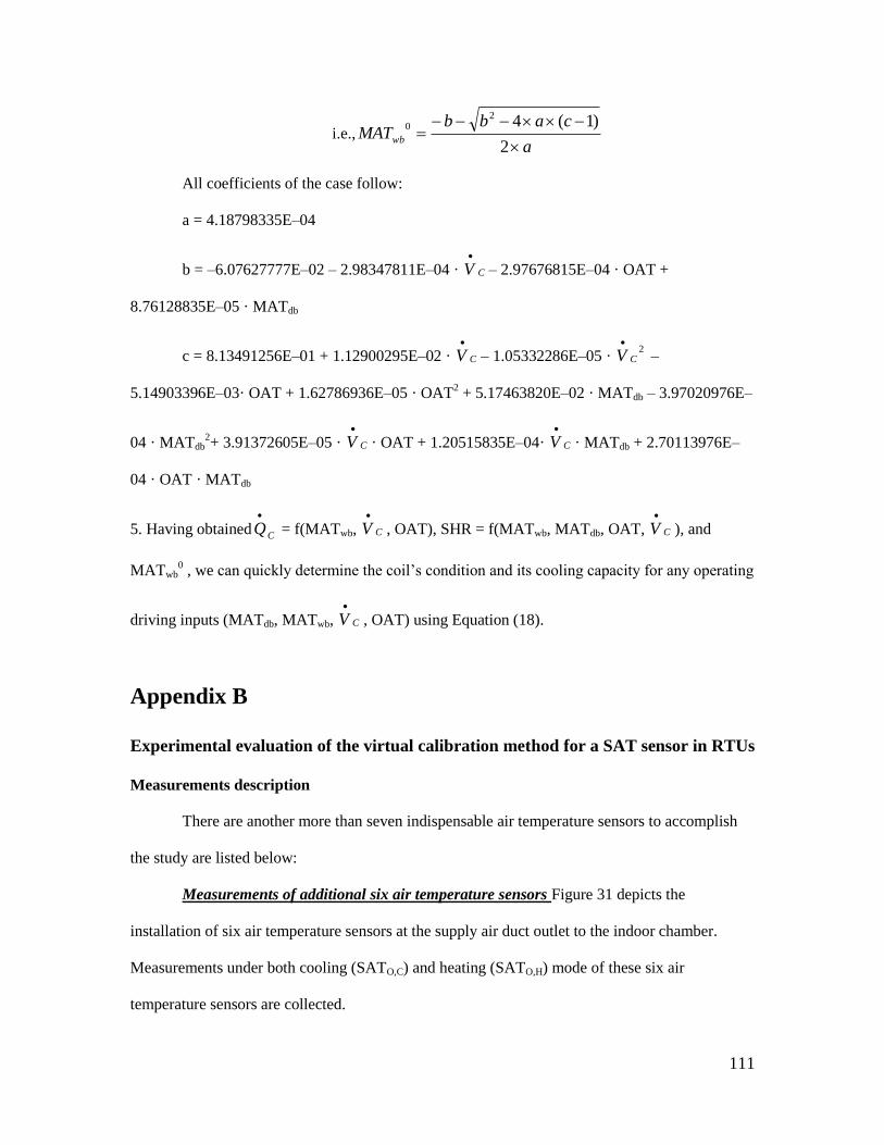
111

i.e.,a

cabbMATwb

2

)1(420

All coefficients of the case follow:

a = 4.18798335E–04

b = –6.07627777E–02 – 2.98347811E–04 · CV

– 2.97676815E–04 · OAT +

8.76128835E–05 · MATdb

c = 8.13491256E–01 + 1.12900295E–02 · CV

– 1.05332286E–05 · 2

CV

–

5.14903396E–03· OAT + 1.62786936E–05 · OAT2 + 5.17463820E–02 · MATdb – 3.97020976E–

04 · MATdb2+ 3.91372605E–05 · CV

· OAT + 1.20515835E–04· CV

· MATdb + 2.70113976E–

04 · OAT · MATdb

5. Having obtainedCQ

= f(MATwb, CV

, OAT), SHR = f(MATwb, MATdb, OAT, CV

), and

MATwb0 , we can quickly determine the coil’s condition and its cooling capacity for any operating

driving inputs (MATdb, MATwb, CV

, OAT) using Equation (18).

Appendix B

Experimental evaluation of the virtual calibration method for a SAT sensor in RTUs

Measurements description

There are another more than seven indispensable air temperature sensors to accomplish

the study are listed below:

Measurements of additional six air temperature sensors Figure 31 depicts the

installation of six air temperature sensors at the supply air duct outlet to the indoor chamber.

Measurements under both cooling (SATO,C) and heating (SATO,H) mode of these six air

temperature sensors are collected.

112

Measurement of lab-installed temperature sensor at the supply air duct outlet The

sensor is referred to as lab-installed temperature sensor at the supply air duct outlet (SATO,lab).

The function is to verify the additional six temperature sensors at the supply air duct outlet in

Figure 31.

Figure 31: Sensors layout of additional six air temperature sensors

Evaluation of SATO,C and SATO,H

Observed from Figure 32, in cooling mode, the average error between SATO,lab and the

mean of six SATO,C is less than 1ºF (0.6°C). In the meantime, in heating mode, the error between

SATO,lab and the mean of six SATO,C is lower 3 ºF (1.7°C). As expected, at the cross-section close

to the outlet, air is well mixed and temperature distribution is fairly balanced. So in this study the

mean of six SATO,C and the mean of six SATO,H are used in the verification process.

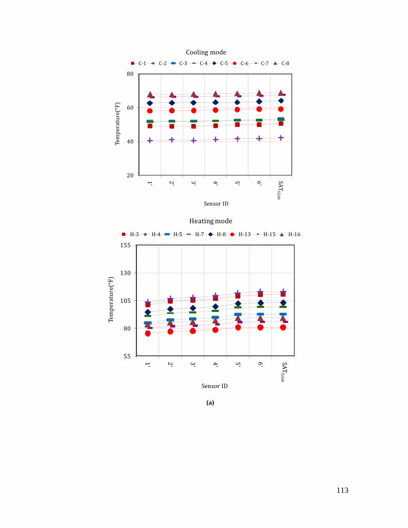
113

20

40

60

80

1'

2'

3'

4'

5'

6' lab

senso

r

Tem

per

atu

re(°

F)

Sensor ID

C-1 C-2 C-3 C-4 C-5 C-6 C-7 C-8

SAT

O,la

b

Cooling mode

55

80

105

130

155

1'

2'

3'

4'

5'

6' lab

senso

r

Tem

per

atu

re(°

F)

Sensor ID

H-3 H-4 H-5 H-7 H-8 H-13 H-15 H-16

SAT

O,lab

Heating mode

(a)

114

0

10

20

30

40

1'

2'

3'

4'

5'

6' lab

senso

r

Tem

per

atu

re(°

C)

Sensor ID

C-1 C-2 C-3 C-4 C-5 C-6 C-7 C-8

SAT

O,la

b

Cooling mode

10

20

30

40

50

1'

2'

3'

4'

5'

6' lab

senso

r

Tem

per

atu

re(°

C)

Sensor ID

H-3 H-4 H-5 H-7 H-8 H-13 H-15 H-16

SAT

O,lab

Heating mode

(b)

Figure 32: Evaluation of additional six temperature sensors under both cooling and heating

mode: (a) IP units and (b) SI units.

Experimental evaluation of virtually calibrated SAT measurement

Evaluation is presented here to validate the accuracy of virtually calibrated MSAT

measurement. There is no direct way but an indirect method to evaluate the accuracy of virtual

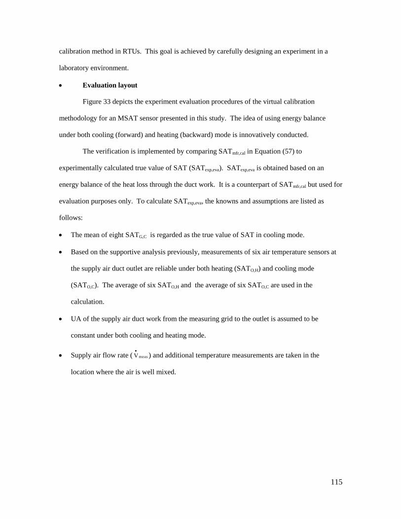
115

calibration method in RTUs. This goal is achieved by carefully designing an experiment in a

laboratory environment.

Evaluation layout

Figure 33 depicts the experiment evaluation procedures of the virtual calibration

methodology for an MSAT sensor presented in this study. The idea of using energy balance

under both cooling (forward) and heating (backward) mode is innovatively conducted.

The verification is implemented by comparing SATmfr,cal in Equation (57) to

experimentally calculated true value of SAT (SATexp,eva). SATexp,eva is obtained based on an

energy balance of the heat loss through the duct work. It is a counterpart of SATmfr,cal but used for

evaluation purposes only. To calculate SATexp,eva, the knowns and assumptions are listed as

follows:

The mean of eight SATG,C is regarded as the true value of SAT in cooling mode.

Based on the supportive analysis previously, measurements of six air temperature sensors at

the supply air duct outlet are reliable under both heating (SATO,H) and cooling mode

(SATO,C). The average of six SATO,H and the average of six SATO,C are used in the

calculation.

UA of the supply air duct work from the measuring grid to the outlet is assumed to be

constant under both cooling and heating mode.

Supply air flow rate ( measV

) and additional temperature measurements are taken in the

location where the air is well mixed.

116

Figure 33: The experiment evaluation procedures of the virtual calibration methodology

Evaluation implementation

Three main steps of evaluation in sequence are included as follows:

Step (1): Correcting UA in cooling mode

Heat loss in cooling mode (Qloss,C) through the duct work leads to the air temperature

change from the measuring grid cross-section to the outlet in the duct. Heat transfer surface (A)

and heat transfer coefficient (U) of the duct work are constants; therefore, UA could be deduced

with measV

, OAT, SATG,C and SATO,C.

Step (2): Correlating SATexp,eva

Similarly, SATexp,eva in heating mode should be acquired while UA, measV

, SATO,H and

OAT are known.

Step (3): Verification of SATmfr,cal

Finally, SATmfr,cal in heating mode is evaluated after SATexp,eva is derived from

experiments.

Step (1): Correcting UA in cooling mode

The goal here is to estimate the constant UA in the lab environment with the data points

collected in the experiment series in cooling mode. To investigate the UA, it is assumed that (1)

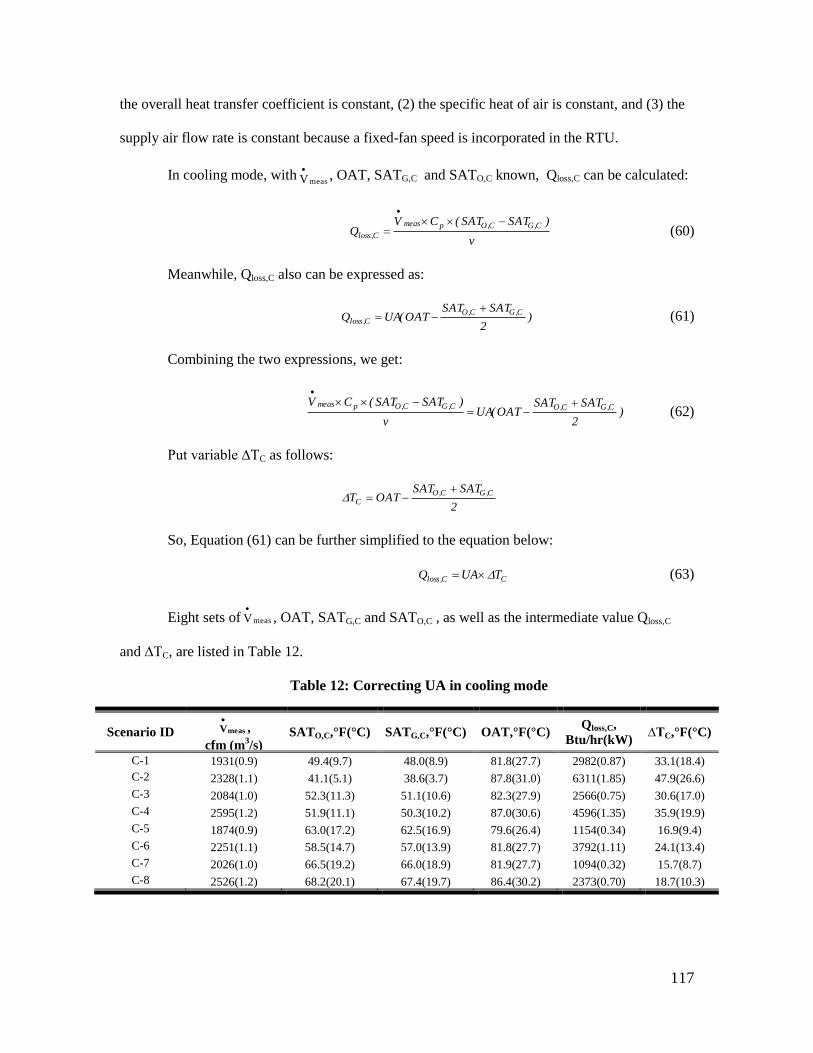
117

the overall heat transfer coefficient is constant, (2) the specific heat of air is constant, and (3) the

supply air flow rate is constant because a fixed-fan speed is incorporated in the RTU.

In cooling mode, withmeasV

, OAT, SATG,C and SATO,C known, Qloss,C can be calculated:

v

)SATSAT(CVQ

C,GC,Opmeas

C,loss

(60)

Meanwhile, Qloss,C also can be expressed as:

)

2

SATSATOAT(UAQ

C,GC,OC,loss

(61)

Combining the two expressions, we get:

)

2

SATSATOAT(UA

v

)SATSAT(CVC,GC,OC,GC,Opmeas

(62)

Put variable ∆TC as follows:

2

SATSATOATT

C,GC,OC

So, Equation (61) can be further simplified to the equation below:

CC,loss TUAQ (63)

Eight sets of measV

, OAT, SATG,C and SATO,C , as well as the intermediate value Qloss,C

and ∆TC, are listed in Table 12.

Table 12: Correcting UA in cooling mode

Scenario ID measV

,

cfm (m3/s)

SATO,C,°F(°C) SATG,C,°F(°C) OAT,°F(°C) Qloss,C,

Btu/hr(kW) ∆TC,°F(°C)

C-1 1931(0.9) 49.4(9.7) 48.0(8.9) 81.8(27.7) 2982(0.87) 33.1(18.4)

C-2 2328(1.1) 41.1(5.1) 38.6(3.7) 87.8(31.0) 6311(1.85) 47.9(26.6)

C-3 2084(1.0) 52.3(11.3) 51.1(10.6) 82.3(27.9) 2566(0.75) 30.6(17.0)

C-4 2595(1.2) 51.9(11.1) 50.3(10.2) 87.0(30.6) 4596(1.35) 35.9(19.9)

C-5 1874(0.9) 63.0(17.2) 62.5(16.9) 79.6(26.4) 1154(0.34) 16.9(9.4)

C-6 2251(1.1) 58.5(14.7) 57.0(13.9) 81.8(27.7) 3792(1.11) 24.1(13.4)

C-7 2026(1.0) 66.5(19.2) 66.0(18.9) 81.9(27.7) 1094(0.32) 15.7(8.7)

C-8 2526(1.2) 68.2(20.1) 67.4(19.7) 86.4(30.2) 2373(0.70) 18.7(10.3)

118

Figure 34 shows that Qloss,C and ∆TC have a positive linear correlation. Data points

scatter closely beside a line. The slope of the linear-regressed line, which is 115.47, can be used

as the value of UA for the duct work. In other words, UA is found as115.47 Btu/hr·°F (0.06

kW/K). As physical characteristics of the duct work, this value remains unchanged when gas

heating is operating.

Qloss,C= 115.47×∆TC

R² = 0.80

0.0

2000.0

4000.0

6000.0

8000.0

0 15 30 45 60

y (Btu/hr)

x (°F)

Qlo

ss,C

∆TC (a)

Qloss,C= 0.06×∆TC

R² = 0.80

0.0

0.6

1.2

1.8

2.4

0 8 16 24 32

y (kW

)

x (°C)

Qlo

ss,C

∆TC

(b)

Figure 34: UA linear regression: (a) IP units and (b) SI units.

Step (2): Correlating SATexp,eva

As pointed out previously, with UA, measV

, SATO,H and OAT known, SATexp,eva could be obtained by

jointly solving Equation (64) and (65),

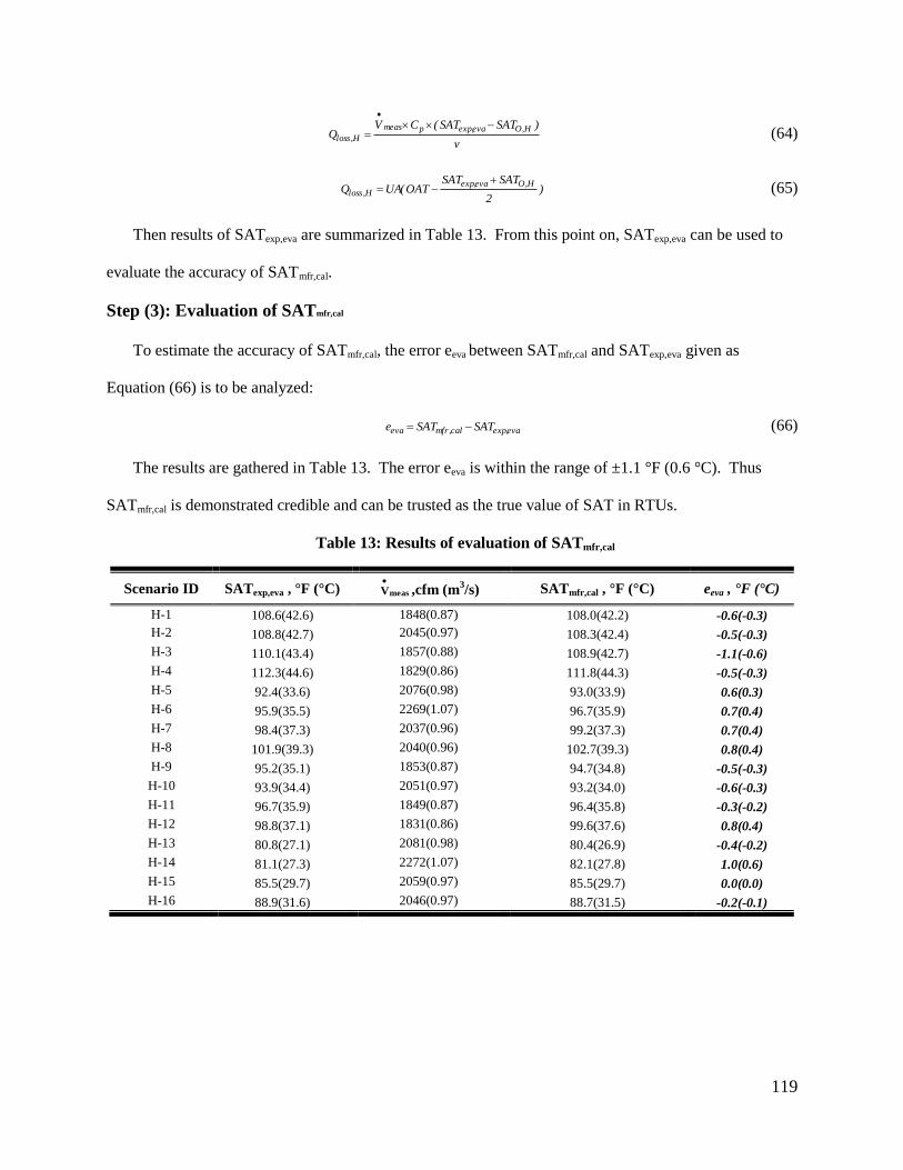
119

v

)SATSAT(CVQ

H,Oevaexp,pmeas

H,loss

(64)

)

2

SATSATOAT(UAQ

H,Oevaexp,H,loss

(65)

Then results of SATexp,eva are summarized in Table 13. From this point on, SATexp,eva can be used to

evaluate the accuracy of SATmfr,cal.

Step (3): Evaluation of SATmfr,cal

To estimate the accuracy of SATmfr,cal, the error eeva between SATmfr,cal and SATexp,eva given as

Equation (66) is to be analyzed:

evaexp,cal,mfreva SATSATe (66)

The results are gathered in Table 13. The error eeva is within the range of ±1.1 °F (0.6 °C). Thus

SATmfr,cal is demonstrated credible and can be trusted as the true value of SAT in RTUs.

Table 13: Results of evaluation of SATmfr,cal

Scenario ID SATexp,eva , °F (°C) measV

,cfm (m3/s) SATmfr,cal , °F (°C) eeva , °F (°C)

H-1 108.6(42.6) 1848(0.87) 108.0(42.2) -0.6(-0.3)

H-2 108.8(42.7) 2045(0.97) 108.3(42.4) -0.5(-0.3)

H-3 110.1(43.4) 1857(0.88) 108.9(42.7) -1.1(-0.6)

H-4 112.3(44.6) 1829(0.86) 111.8(44.3) -0.5(-0.3)

H-5 92.4(33.6) 2076(0.98) 93.0(33.9) 0.6(0.3)

H-6 95.9(35.5) 2269(1.07) 96.7(35.9) 0.7(0.4)

H-7 98.4(37.3) 2037(0.96) 99.2(37.3) 0.7(0.4)

H-8 101.9(39.3) 2040(0.96) 102.7(39.3) 0.8(0.4)

H-9 95.2(35.1) 1853(0.87) 94.7(34.8) -0.5(-0.3)

H-10 93.9(34.4) 2051(0.97) 93.2(34.0) -0.6(-0.3)

H-11 96.7(35.9) 1849(0.87) 96.4(35.8) -0.3(-0.2)

H-12 98.8(37.1) 1831(0.86) 99.6(37.6) 0.8(0.4)

H-13 80.8(27.1) 2081(0.98) 80.4(26.9) -0.4(-0.2)

H-14 81.1(27.3) 2272(1.07) 82.1(27.8) 1.0(0.6)

H-15 85.5(29.7) 2059(0.97) 85.5(29.7) 0.0(0.0)

H-16 88.9(31.6) 2046(0.97) 88.7(31.5) -0.2(-0.1)

120

121