Threshold-Coloring and Unit-Cube ContactRepresentation of Graphs

Md. Jawaherul Alam1, Steven Chaplick2, Gasper Fijavz3, Michael Kaufmann4,Stephen G. Kobourov1, and Sergey Pupyrev1

1 Department of Computer Science, University of Arizona, Tucson, AZ, USA2 Department of Applied Mathematics, Charles University, Prague, Czech Republic3 Faculty of Computer and Information Science, University of Ljubljana, Slovenia

4 Wilhelm-Schickhard-Institut fur Informatik, Universitat Tubingen, Tubingen, Germany

Abstract. In this paper we study threshold coloring of graphs, where the ver-tex colors represented by integers are used to describe any spanning subgraphof the given graph as follows. Pairs of vertices with near colors imply the edgebetween them is present and pairs of vertices with far colors imply the edge isabsent. Not all planar graphs are threshold-colorable, but several subclasses, suchas trees, some planar grids, and planar graphs without short cycles can always bethreshold-colored. Using these results we obtain unit-cube contact representationof several subclasses of planar graphs. Variants of the threshold coloring problemare related to well-known graph coloring and other graph-theoretic problems. Us-ing these relations we show the NP-completeness for two of these variants, anddescribe a polynomial-time algorithm for another.

1 Introduction

Graph coloring is among the fundamental problems in graph theory. Typical applica-tions of the problem and its generalizations are in job scheduling, channel assignmentsin wireless networks, register allocation in compiler optimization and many others [15].In this paper we consider a new graph coloring problem in which we assign colors (in-tegers) to the vertices of a graph G in order to define a spanning subgraph H of G. Inparticular, we color the vertices of G so that for each edge of H , the two endpoints arenear, i.e., their distance is within a given “threshold”, and for each edge of G \H , theendpoints are far, i.e., their distance greater than the threshold; see Fig 1.

The motivation of the problem is twofold. First, such coloring can be used for theFrequency Assignment Problem [10], which asks for assigning frequencies to transmit-ters in radio networks so that only specified pairs of transmitters can communicate witheach other. Second, such coloring can be used in the context of the geometric prob-lem of unit-cube contact representation of planar graphs. In such a representation ofa graph, each vertex is represented by a unit-size cube and each edge is realized by acommon boundary with non-zero area between the two corresponding cubes. Findingclasses of planar graphs with unit-cube contact representation was recently posed as anopen question by Bremner et al. [2]. In this paper we partially address this problem asan application of our coloring problem in the following way. Suppose a planar graphG has a unit-cube contact representation where one face of each cube is co-planar; see

arX

iv:1

302.

6183

v5 [

cs.D

M]

16

May

201

3

1

1

N

N N

N

FF

F

F

N

1

2

1

0

1

3

312

d

b

e

f

c

(a) (b)

d e f

cb

a

ed f

cb

a

ab c

d e fa

Fig. 1. (a) A planar graph G and its unit-cube contact representation where the bottom faces ofall cubes are co-planar, (b) a spanning subgraph H of G with a (4, 1)-threshold-coloring and itsunit-cube contact representation. Far edges are shown dashed, near edges are shown solid.

Fig. 1(a). Assume that we can define a spanning subgraphH ofG by our particular ver-tex coloring. We show that it is possible to compute a unit-cube contact representationof H by lifting the cube for each vertex v by the amount equal to the color of v (wherethe size or side-length of the cubes are roughly equal to the threshold); see Fig. 1(b).

1.1 Problem Definition

An edge-labeling of graph G = (V,E) is a mapping ` : E → {N,F} assigning labelsN or F to each edge of the graph; we informally name edges labeled with N as thenear edges, and edges labeled with F as the far edges. Note that such an edge labelingof G defines a partition of the edges E into near and far edges. By abuse of notation thepair {N,F} also denotes this partition.

Let r ≥ 1 and t ≥ 0 be two integers and let [1 . . . r] denote a set of r consecutiveintegers. For a graph G = (V,E) and an edge-labeling ` : E → {N,F} of G, a (r, t)-threshold-coloring of G with respect to ` is a coloring c : V → [1 . . . r] such that foreach edge e = (u, v) ∈ E, e ∈ N if and only if |c(u) − c(v)| ≤ t. We call r and tthe range and the threshold. Note that the set of near edges defines a spanning subgraphH = (V,N) ofG, whereH is a spanning subgraph of graphG if it contains all verticesof G. H is a threshold subgraph of G if there exists such a threshold-coloring.

A graph G is total-threshold-colorable if for every edge-labeling ` of G there existsan (r, t)-threshold-coloring of G with respect to ` for some r ≥ 1, t ≥ 0. Informallyspeaking, for every partition of edges of G into near and far edges, we can producevertex colors so that endpoints of near edges receive near colors, and endpoints of faredges receive colors that are far apart. A graph G is (r, t)-total-threshold-colorable if

2

it is total-threshold-colorable for the range r and threshold t. In this paper we focus onthe following problem variants:

Problem 1. (Total-Threshold-Coloring Problem) Given a graphG, isG total-threshold-colorable, that is, is every spanning subgraph of G a threshold subgraph of G?

The problem is closely related to the question about whether a particular spanninggraph H of G is threshold-colorable.

Problem 2. (Threshold-Coloring Problem) Given a graphG and a spanning subgraphH , is H a threshold subgraph of G for some integers r ≥ 1, t ≥ 0?

Another interesting variant of the threshold-coloring is the one in which we specifythat the graph G is the complete graph. In this case we call H an exact-threshold graphif H is a threshold subgraph of the complete graph G for some integers r ≥ 1, t ≥ 0.

Problem 3. (Exact-Threshold-Coloring Problem) Given a graph H , is H an exact-threshold graph?

In the final variant of the problem we assume that the threshold and the range arethe part of the input:

Problem 4. (Fixed-Threshold-Coloring Problem) Given a graph G, a spanning sub-graph H , and integers r ≥ 1, t ≥ 0, is H (r, t)-threshold-colorable?

1.2 Related Work

Many problems in graph theory deal with coloring or assigning labels to the vertices ofa graph; many graph classes are defined based on such coloring and labeling; see [1] foran excellent survey. To the best of our knowledge, total-threshold-colorability definesa new class of graphs. Here we mention two closely related classes: threshold graphsand difference graphs. Threshold graphs are ones for which there is a real number Sand for every vertex v there is a real weight av such that (v, w) is an edge if and onlyif av + aw ≥ S [14]. A graph is a difference graph if there is a real number S and forevery vertex v there is a real weight av such that |av| < S and (v, w) is an edge if andonly if |av − aw| ≥ S [11]. Note that for both classes the threshold (real number S)defines edges between all pairs of vertices, while in our setting the threshold definesonly the edges of a graph G, which is not necessarily a complete graph. Both thresholdand difference graphs can be characterized in terms of forbidden induced subgraphs. Forour problem such a characterization is unknown. For details on threshold and differencegraphs, see [14].

Another related graph coloring problem is the distance constrained graph labeling.Here the goal is to findL(p1, . . . , pk)-labeling of the vertices of a graph so that for everypair of vertices at distance at most i ≤ k we have that the difference of their labels isat least pi. The most studied variant is L(2, 1)-labeling [6, 9]. In [9] it was shown thatminimizing the number of labels in L(2, 1)-labeling is NP-complete, even for graphswith diameter 2. Further, it shown that it is also NP-complete to determine whether alabeling exists with at most k labels for every fixed integer k ≥ 4 [5].

3

graphclasses

Cycle Tree FanTriangularGrid

SquareGrid

HexagonalGrid

Octagonal-SquareGrid

Square-TriangleGrid

Planar Graphw/o Cyclesof size ≤ 9

thresholdcoloring

r = 5,t = 1

r = 2,t = 0

r = 5,t = 1

No Open r = 5,t = 1

r = 5,t = 1

No r = 8,t = 2

unit-cubecontact

Yes No No Open Yes Yes Yes Open No

Table 1. Results on the Total-Threshold-Coloring Problem. “No” entries in the last row followfrom the fact that graphs with vertices of high degrees cannot have unit-cube representation [2].

A threshold-coloring of a planar graph can be used to find a contact representa-tion of the graph with cuboids (axis aligned boxes) in 3D. Thomassen [16] shows thatany planar graph has a proper contact representation by cuboids in 3D. In a contactrepresentation of a graph, the vertices are represented by cuboids (or other polygonalshapes) and the edges are realized by a common boundary of the two correspondingcuboids. A contact representation is proper if for each edge the corresponding commonboundary has non-zero area. Felsner and Francis [4] prove that any planar graph has a(non-proper) contact representation by cubes.

Bremner et al. [2] proves that the same result does not hold when using only unitcubes. Our results on threshold-coloring of planar graphs translates to results on classesof planar graphs that can be represented by contact of unit cubes.

1.3 Our Contribution

1. We study the Total-Threshold-Coloring Problem for various subclasses of pla-nar graphs. In particular, we show that several subclasses of planar graphs arethreshold-colorable (e.g., trees, hexagonal grids, planar graphs without any cyclesof length ≤ 9) and several subclasses are not (e.g., triangular grid, 4-3 grid). Ourresults are summarized in Table 1.

2. As an application of the threshold-coloring problem, we address the problem ofcontact representation of planar graphs with unit cubes. Given a planar graph, weinvestigate whether each of its subgraphs has a contact representation with unitcubes. We show how we can use the threshold-coloring for computing unit-cubecontact representations for some subclasses of planar graphs. For some other sub-classes, we gave algorithms to directly compute unit-cube contact representationwithout using threshold-coloring. Thus we answer some of the open problemsfrom [2] for some subclasses of planar graphs. The last column of Table 1 sum-marizes these results.

3. Finally we study the relation of the various threshold-coloring problems with othergraph-theoretic problems. Specifically, we show that the Threshold-Coloring Prob-lem and the Fixed-Threshold-Coloring Problem are NP-complete by reductions

4

from a graph sandwich problem and the classical vertex coloring problem, respec-tively. We also show that the Exact-Threshold-Coloring Problem can be solvedin linear time since it is equivalent to the proper interval graph recognition problem.

2 Threshold-Coloring and Other Graph Problems

We begin by showing the connections between threshold-colorability and some classi-cal graph-theoretical and graph coloring problems.

2.1 Vertex Coloring Problem

Let G = (V,E) be a graph. We call G k-vertex-colorable if there exists a coloringc : V → [1 . . . k] such that for any edge (u, v) ∈ E, c(u) 6= c(v), that is, u and vhave different colors. Given an input graph G and an integer k > 0, the vertex coloringproblem asks whether there exists a k-vertex-coloring of G.

Lemma 1. Let G = (V,E) be a graph and let k be a positive integer. Define an edge-labeling ` : E → {N,F} that assigns each edge the label F , that is, for each edgee ∈ E, `(e) = F . Then G has a k-vertex-coloring if and only if there exists a (k, 0)-threshold-coloring of G with respect to `.

Proof. Let c : V → [1 . . . k] define a mapping of the vertices ofG to the colors [1 . . . k].Then c is a k-vertex-coloring of G⇔ for each edge e = (u, v) ∈ E, c(u) 6= c(v)⇔for each edge e = (u, v) ∈ E, |c(u) − c(v)| > 0⇔ c is a (k, 0)-threshold-coloring ofG with respect to `. ut

Corollary 1. The Fixed-Threshold-Coloring Problem is NP-complete.

2.2 Proper Interval Representation Problem

An interval representation [1] for a graph G = (V,E) is one where each vertex vof G is represented by an interval I(v) of R such that for any edge (u, v) ∈ E, theintervals I(u) and I(v) have a non-empty intersection, that is, I(u) ∩ I(v) 6= ∅. Aproper interval representation [1] for G is an interval representation of G where nointerval properly contains another. A proper interval graph is one that has a properinterval representation. Equivalently, a proper interval graph is one that has an intervalrepresentation with unit intervals. The problem of proper interval representation for agraph G asks whether G has a proper interval representation. The problem has beenstudied extensively [3, 12], and it still attracts attention [13].

Lemma 2. A graph is an exact-threshold graph if and only if it is a proper intervalgraph.

Proof. Let graph H = (V,E) be an exact-threshold graph. This implies that there areintegers r ≥ 1, t ≥ 0 and a mapping c : V → [1 . . . r] such that for any pair u, v ∈ V ,(u, v) ∈ E ⇔ |c(u) − c(v)| ≤ t⇔ |c(u) − c(v)| < t + ε with 0 < ε < 1 since c(u)

5

and c(v) are integers. We can find an interval representation of H with unit intervals asfollows. Choose an arbitrary ε such that 0 < ε < 1. Define for each vertex v of H aninterval I(v) of unit length where the left-end has x-coordinate c(v)/(t + ε). Then forany two vertices u and v of H , I(u) and I(v) has a non-empty intersection if and onlyif | c(u)t+ε −

c(v)t+ε | ≤ 1 ⇔ |c(u) − c(v)| ≤ (t + ε) ⇔ |c(u) − c(v)| ≤ t since c(u) and

c(v) are integers. Then l(u) and l(v) has non-empty intersection if and only if (u, v) isan edge of H . Thus these intervals yield an interval representation of H .

Conversely, if H has an interval representation Γ with unit intervals, we can findan exact (r, t)-threshold-coloring of H for some integers r ≥ 1, t ≥ 0. Scale Γ by asufficiently large factor t such that each end-point of some interval in Γ has a positiveinteger x-coordinate (after possible translation in the positive x direction). Let r be thex-coordinate of the right end-point of the rightmost interval in this scaled representa-tion. Define a coloring c : V → [1 . . . r] where for each vertex v of H , c(v) equals thex-coordinate of the left end-point of the interval for v. Also define the threshold as thescaling factor t. It is easy to verify that c is indeed an (r, t)-threshold-coloring. ut

Since recognition of proper interval graphs can be done in linear time [3, 12, 13],we have

Corollary 2. The Exact-Threshold-Coloring Problem can be solved in linear time.

2.3 Graph Sandwich Problem

The graph sandwich problem is defined in [8] as follows.

Problem 5. Given two graphs G1 = (V,E1) and G2 = (V,E2) on the same vertex setV , where E2 ⊆ E1, and a property Π , does there exist a graph H = (V,E) on thesame vertex set such that E2 ⊆ E ⊆ E1 and H satisfies property Π?

Here E1 and E2 can be thought of as universal and mandatory sets of edges, withE sandwiched between the two sets. We are interested in a particular property for thegraph sandwich problem: “proper interval representability”. A graph satisfies properinterval representability if it admits a proper interval representation.

Lemma 3. Let G = (V,EG) and H = (V,EH) be two graphs on the same vertex setV such that EH ⊆ EG. Then the threshold-coloring problem for G with respect to theedge partition {EH , EG − EH} is equivalent to the graph sandwich problem for thevertex set V , mandatory edge set EH , universal edge set EH ∪ (V × V − EG) andproper interval representability property.

Proof. LetEU denote the universal edge setEH∪(V ×V −EG) for the graph sandwichproblem. Suppose there exists a graph H∗ = (V,E∗) such that EH ⊆ E∗ ⊆ EU andH∗ has a proper interval representation. Then by Lemma 2, there exist two integersr ≥ 0 and t ≥ 0 and a coloring c : V → [1 . . . r] such that for any pair u, v ∈ V ,|c(u) − c(v)| ≤ t if and only if (u, v) ∈ E∗. We now show that c is in fact a desiredthreshold-coloring for G. Consider an edge e = (u, v) ∈ EG. If e ∈ EH then e ∈ E∗

since EH ⊆ E∗ and hence |c(u) − c(v)| ≤ t. On the other hand if e ∈ (EG − EH),

6

e /∈ EU = EH ∪ (V × V − EG) and therefore e /∈ E∗ since E∗ ⊆ EU . Hence|c(u)− c(v)| > t.

Conversely, if there exists integers r ≥ 1 and t ≥ 0 such that there is an (r, t)-threshold-coloring c : V → [1 . . . r] of G with respect to the edge partition {EH , EG−EH}, then define an edge set E∗ as follows. For any pair u, v ∈ V , (u, v) ∈ E∗ ifand only if |c(u) − c(v)| ≤ t. Clearly the graph H∗ = (V,E∗) has an exact (r, t)-threshold-coloring and hence by Lemma 2, H∗ has a proper interval representation.Furthermore for any edge e = (u, v) ∈ EH , |c(u) − c(v)| ≤ t and hence e ∈ E∗.Thus EH ⊆ E∗. Again if e ∈ E∗ then |c(u) − c(v)|let. Therefore either e ∈ EH ore /∈ EG ⇒ e ∈ (V × V − EG). Hence e ∈ (EH ∪ (V × V − EG)) = EU . ThusE∗ ⊆ EU . Therefore E∗ is sandwiched between the mandatory and the universal set ofedges and H∗ has a proper interval representation. ut

Golumbic et al. [7] proved that the graph sandwich problem is NP-complete for theproper-interval-representability property. Hence we have

Corollary 3. The Threshold-Coloring Problem is NP-complete.

Summarizing the results in this section, we have the following theorem.

Theorem 1. The Threshold-Coloring Problem and the Fixed-Threshold-Coloring Prob-lem are NP-complete while the Exact-Threshold-Coloring Problem can be solved inlinear time.

3 Total-Threshold-Coloring of Graphs

In this section we address the Total-Threshold-Coloring Problem: is a given graph Gtotal-threshold-colorable, that is, can every spanning subgraph of G be represented byappropriately coloring the vertices of G?

First note that not every graph (not even every planar graph) is total-threshold-colorable. Suppose that G = K4, and we would like to represent a subgraph wherefour of the edges remain and span a 4-cycle, while the other two edges are removed(edge-partitioning {N,F}). Assume that there exists an (r, t)-threshold-coloring withcolors c1, c2, c3, c4 for vertices v1, v2, v3, v4 respectively. Without loss of generality as-sume c4 is the highest color and (v1, v4) ∈ F , hence also (v2, v3) ∈ F . Also assumec3 ≥ c2 and consequently c4− c2 ≥ c3− c2. The left side of the inequality should be atmost t, and the right side strictly greater than t, which cannot be accomplished by anychoice of the range and the threshold.

Next we investigate several subclasses of planar graphs. For each of them we eithergive an algorithm to find an (r, t)-threshold-coloring of any graph in that class withrespect to each edge-partition for some r ≥ 1, t ≥ 0; or we give an example of a graphin that class and the edge-partition for which there is no threshold-coloring.

3.1 Paths, Cycles, Trees, Fans

For paths and trees there is a trivial coloring with threshold t = 0 and two colors.Choose an arbitrary vertex as the root and color it 0. Color 1 all vertices with an odd

7

Fig. 2. Threshold-coloring of trees, cycles, and fans.

F

F FN

N N

N

NN

(a)

N N N N

N

N N

F

F

F

F

(b)

Fig. 3. Graphs which are not total-threshold-colorable.

number of far edges on the shortest path to the root. Color 0 all vertices with an evennumber of far edges to the root. Then all vertices connected by a near edge of G get thesame color, and vertices connected by a far edge get different colors; see Fig. 2(a).

For cycles and fans there is a coloring scheme with threshold t = 1 and five colors.A fan is obtained from a path P by adding a new vertex v connected to all vertices ofthe path. We use colors {−2,−1, 0, 1, 2} to color a fan. The vertices of P are coloredby −1 and 1, and v is colored by 0. After this initial coloring some of the far edges(u, v), u ∈ P might have |c(u) − c(v)| = 1. We fix it by changing the color of u from1 to 2 or from −1 to −2; see Fig. 2(c). It is easy to see that the same algorithm can beapplied to color a cycle; see Fig. 2(b).

3.2 Triangular Grid

In a triangular grid (planar weak dual of a hexagonal grid) all faces are triangles andinternal vertices have degree 6. It is easy to show that a triangular grid is not total-threshold-colorable. Consider the graph with vertices v0, v1, v2, u0, u1, u2, where eachvertex ui is adjacent to vi+1 and vi+2 (mod 3); see Fig. 3(a). LetF = {(v0, v1), (v1, v2),(v2, v0)}, and let N contain the remaining 6 edges. Assume that there exists a (r, t)-threshold-coloring c. Without loss of generality, let c(v0) < c(v1) < c(v2). Now onone hand c(v2) − c(v0) > 2t and on the other c(v2) − c(v0) ≤ |c(v2) − c(u1)| +|c(u1)− c(v0)| ≤ 2t, which is impossible. This also proves that outerplanar graphs arenot total-threshold-colorable in general.

3.3 Hexagonal Grid

In a hexagonal grid all faces are 6-sided and internal vertices have degree 3 (planar weakdual of the triangular grid). Here we show that the hexagonal grid is total-threshold-

8

colorable with r = 5 and t = 1. We begin with a simple lemma about (5,1) color space.For convenience, we use colors {−2,−1, 0, 1, 2}.

Lemma 4. Let P2 = {v0, v1, v2} be a path of length 2. Then for any edge-labelingof P2 and a fixed color k ∈ {−2,−1, 1, 2}, there is a threshold-coloring c of P2 withthreshold t = 1, where c(v0) = 0, c(v2) = k and c(v1) ∈ {−2,−1, 1, 2}.

Proof. Depending on whether the edge (v0, v1) is near or far, choose c(v1) to be 1 or2. If the label of (v1, v2) disagrees with the colors of v1 and v2 then we change the signof c(v1). ut

Lemma 5. Any hexagonal grid is (5, 1)-total-threshold-colorable.

Proof. The coloring is done in two steps. In the first step we assign color 0 for a set ofindependent vertices of G as shown in Fig. 4(a), where the colored vertices are white.Note that no two white vertices have a shortest path of length less than 3.

In the second step we find a coloring of the remaining black vertices, using onlyfour colors {−2,−1, 1, 2}. Let w1 be a white vertex. We randomly choose one of itsblack neighbors b1, and assign a color for b1 based on the label of edge (w1, b1). Nowvertex b1 has two white vertices w2 and w3 within distance 2. Using Lemma 4 we can(uniquely) extend the coloring of b1 to w2 (symmetrically, to w3) so that additionalblack vertex b2 gets a color. Again, the coloring of b2 can be extended to its nearestwhite neighbor. We continue such a propagation of colors, see Figs. 4(b) and 4(c) whereprocessed black vertices and edges are shown dashed red. One can easily see that theprocess will color a row of hexagons with alternate upper and lower legs.

To complete the coloring ofGwe choose a white vertex in the next row of hexagonsand initiate a similar propagation process. For example, one can use vertices w and bshown in Fig. 4(c). ut

3.4 Octagonal-Square Grid

Lemma 6. Any octagonal-square grid is (5, 1)-total-threshold-colorable.

(a) (b) (c)

Fig. 4. Total-threshold-coloring of the hexagonal grid. (a) White vertices get color 0, black ver-tices get one of the colors −2,−1, 1, 2. (b) A color assignment to b1 can be extended to verticesw2 and w3 based on the labels of the red dashed edges. (c) The process assigns colors for the redvertices.

9

(a) (b) (c)

Fig. 5. Total-threshold-coloring of the octagonal-square grid.

Proof. We use colors {−2,−1, 0, 1, 2} and threshold t = 1 to find a coloring; the proofis similar to the proof of Lemma 5. We start by partitioning the vertices of the graphinto white and black as shown in Fig. 5(a), and we assign color 0 to the white ones.Then we choose a white vertex w and its black neighbor b as in Fig. 5(b), and we assigncolors {−2,−1, 1, 2} to the “row” of black vertices. It is easy to see that the coloringof rows can be done independently; see Fig. 5(c). ut

3.5 Square-Triangle Grid

We prove that the graph in Fig. 3(b) is not total-threshold-colorable. Assume to thecontrary that c is a (r, t)-threshold-coloring. Without loss of generality let c(v0) <c(u0). Since (v1, u0) is a far edge and (v0, x), (u0, x) are near we have c(v0) < c(x) <c(u0). Similar argument shows that c(v1) < c(v0) < c(x) < c(u0) < c(u1). Then ifx < y, we have c(v1)+ t < c(x) and c(x)+ t < c(y), which implies c(v1)+2t < c(y).This makes it impossible to find a color for v2 near to both v1 and y. Similarly if x > ythen it is impossible to color u2.

Theorem 2 summarizes the results in this section.

Theorem 2. Paths, cycles, trees, fans, the hexagonal grid and the octagonal-squaregrid are total-threshold-colorable. The triangular grid and triangle-square grid are nottotal-threshold-colorable.

4 Planar Graphs without Short Cycles

In the cases where we have counter-examples of total-threshold-colorability (e.g., K4

and the triangular grid) we have short cycles, which can be used to force groups ofvertices to be simultaneously near and far. In this section we show that if we considergraphs without short cycles, we can prove total-threshold-colorability.

Theorem 3. Let G be a planar graph without cycles of length ≤ 9. Then G is (8, 2)-total-threshold-colorable5.

5 Equivalently, the girth (that is, the shortest cycle) of G should be ≥ 10.

10

The outline of our proof for Theorem 3 is as follows. We first find some small treestructures T that are “reducible”, in the sense that for any edge-labeling of T and anygiven fixed coloring of the leaves of T to the colors {0, 1, . . . , 7}, there is a (8, 2)-threshold-coloring of T . For a contradiction assume that there is a planar graph withgirth≥ 10 having no (8, 2)-threshold-coloring. We consider the minimal such graphG,and by a discharging argument prove that G contains at least one of these reducible treestructures. This contradicts the minimality of G. We start with some technical claims.

Extending a coloring. Let Pn be a path with vertices v0, . . . , vn. Given an edge-labelingof Pn and the color c0 of v0 we call a color cn legal if there exists a (8, 2)-threshold-coloring c of Pn, so that c(v0) = c0 and c(vn) = cn.

Claim 1 Let P1 be a path of length 1. Then at least one of the colors 1 or 6 is legal(irrespective of the edge label and the color c0).

Proof. One only needs to observe that color 1 is close to 0, 1, 2, 3, and is far from4, 5, 6, 7, i.e. the distance between colors is at most 2 or strictly more than 2, respec-tively. The result follows by symmetry. ut

Claim 2 Let P2 be a path of length 2. Then 3 is legal unless c0 = 3 and {N,F} ={{e1}, {e2}}, i.e. the edges e1 and e2 are labeled differently. Symmetrically, 4 is legalunless c0 = 4 and {N,F} = {{e1}, {e2}}.

Proof. By symmetry we only give the proof for the case c2 = 3. If N = {e1, e2} thenwe choose c(v1) to be the average of c0 and c2, rounding if necessary. If F = {e1, e2},then one of 0, 7 is a good choice for c(v1), as both 0,7 are far from c2 = 3, and at leastone is far from c0. In the remaining case we may assume that c0 6= 3. If c0 < 3, thenset c(v1) = 0 or c(v1) = 5 in case e2 ∈ F or e2 ∈ N , respectively. If c0 > 3, then setc(v1) = 6 or c(v1) = 1 in case e2 ∈ F or e2 ∈ N , respectively. ut

Claim 3 Let P3 be a path of length 3. Then 1, 3, 4, and 6 are all legal (irrespective ofthe edge label and the color c0).

Proof. By symmetry it is enough to find appropriate coloring extensions for whichc(v3) = 1 and c(v3) = 3. For the latter, choose c1 = c(v1) 6= 3, according to c0 andthe label of e1. Now by Claim 2 this choice of c1 can be extended to the remaining partof P3, so that c(v3) = 3. The goal c(v3) = 1 splits into two subcases. If c0 6= 3, 4, thenby Claim 2 both 3 and 4 are possible color choices for c(v2). One is close and the otheris far from 1. In case c0 is either 3 or 4, then again by Claim 2 both 1 and 6 are possiblechoices for c(v2). Again, the former is close and the latter is far from 1. ut

A star is a subdivision of the graphK1,n, and its center is the single vertex of degree≥ 3. Let T be a star. A prong of T is a path from a leaf to the center of T , and a prongwith k edges is called a k-prong, we say that it has length k.

Claim 4 Let T be a subdivision of K1,3 with prongs of length 1, 2, and 3, respectively.Assume that the leaves of T are assigned colors, so that the leaf u on the 1-prong iscolored with either 1 or 6. Then we can extend this partial coloring to the whole T .

11

Fig. 6. Two additional types of reducible configurations, T1 and T2.

Proof. Let v be the center of T . Given c(u), we can choose c(v) ∈ {3, 4} so that thelabeling condition on the 1-prong is satisfied. If this choice cannot be extended to thelonger prongs, then the leaf of the 2-prong is also colored with either 3 or 4, see Claim2. But then the choice c(v) ∈ {1, 6} which satisfies the labeling condition on the 1-prong can be extended to the remaining prongs. ut

Reducible configurations. A configuration is a tree T , and is reducible if every assign-ment of colors to the leaves of T can be, for every possible edge-labeling of T , extendedto a (8, 2)-threshold-coloring c of the whole T .

Claim 5 A path P4 of length 4 is a reducible configuration.

Proof. Let v be a neighbor of a leaf in P4. By Claim 1 and Claim 3 either c(v) = 1 orc(v) = 6 extends to the remaining uncolored vertices. ut

Now Claim 5 implies that longer paths are reducible as well. Let us turn our atten-tion to stars.

Claim 6 (A) Let T be a star with at most 1 prong of length 1 and the remaining prongshave length 3. Then T is reducible.

(B) Let T be a star with at most 3 prongs of length 2 and the remaining prongs havelength 3. Then T is reducible.

Proof. In both cases let v denote the center of the star. In order to establish (A) let c(v)be either 1 or 6, which is appropriate for the 1-prong (such a choice exists by Claim1). By Claim 3 the coloring c(v) can be extended to the remaining 3-prongs. For (B)we may assume that neither 3 nor 4 can be extended to all three 2-prongs. By Claim 2both colors 3 and 4 are used at leaves of the 2-prongs. Now, by Claim 1 at least one ofc(v) = 1 or c(v) = 6 extends to the third 2-prong, and hence also to the remaining 2-and 3-prongs, by Claim 2 and Claim 3. ut

Claim 7 There exist two additional types T1 and T2 of reducible configurations shownin Fig. 4.

Proof. Let us first consider the T1 configuration. By Claim 1 one of 1,6 is appropriatefor the color of x, with respect to color a and type of edge e. If b ∈ {3, 4}, then choosec(y) from 1, 6, and if b 6∈ {3, 4} then choose c(y) from {3, 4}. By Claim 2 this works.

12

Let us now turn to T2. If e is a near edge, we might as well contract e (which impliesboth x and y will receive the same color), and reduce to Claim 6(B).

Hence we shall assume e is a far edge. Assume first that coloring vertex x with both1 and 6 extends to the left 2-prong at x. If c(x) = 1 and c(y) = 4 does not extend to theright 2-prongs at y, we may assume b = 4. If c(x) = 6 and c(y) = 3 does not extendto the right 2-prongs at y, we may assume c = 3. In this case setting c(x) = 1 andc(y) = 6 extends to the right.

By Claim 1 we may assume that only one of c(x) = 1 or c(x) = 6 extends to theleft 2-prong at x, without loss of generality the former. Now a 6= 3 and a 6= 4, and bothc(x) = 3 and c(x) = 4 extend left. A choice of c(x) = 1, c(y) = 4 does not extend tothe right 2-prongs at y only if, say, b is equal to 4. But now at least one of c(y) = 1 orc(y) = 6 extends to the right 2-prongs, and such a choice can be complemented withc(x) = 4 or c(x) = 3, respectively. ut

Discharging. A minimal counterexample is the smallest possible (in terms of order) pla-nar graph G without cycles of length ≤ 9 which is not (8, 2)-total-threshold-colorable.A minimal counterexample G does not contain reducible configurations. Further G isconnected and has no vertices of degree 1. As G is also not a cycle (such a cycle shouldbe of length ≥ 9 and should not contain a P4), and is therefore homeomorphic to a(multi)graph of minimal degree ≥ 3.

Let us fix its planar embedding determining its set of faces F (G). Let us defineinitial charges: initial charge of a vertex v, γ0(v), is equal to 4 deg(v) − 10, and theinitial charge of a face f , γ0(f), is equal to deg(f)− 10. A routine application of Eulerformula shows that the total initial charge is −20.

As all faces have length ≥ 10, every face is initially non-negatively charged. Weshall not alter the charges of faces.

The following table shows initial charges of vertices according to their degree:

degree deg(v) 2 3 4 5 6 7 · · ·initial charge γ0(v) −2 2 6 10 14 18 · · ·

The discharging procedure will run in two phases, by γi(v) we shall denote thecharge of vertex v after Phase i of discharging. Informally, Phase 1 shall see that verticesof degree 2 do not have negative charges, and Phase 2 will leave only vertices of degree3 with a possible negative charge.

Let u, v be vertices of G. We say that u and v are 2-adjacent, if G contains a u− v-path whose (possible) internal vertices all have degree 2. In Phase 1 we redistributecharge according to the following rule:

Rule 1: every vertex v of degree ≥ 3 sends charge 1 to every vertex u of degree 2, forwhich v and u are 2-adjacent.

In Phase 2 we shall apply the following rule:

Rule 2: If u and v are adjacent with γ1(u) > 0, γ1(v) < 0 then u sends charge 1 to v.

As every vertex u of degree 2 (we also call them 2-vertices) is 2-adjacent to exactlytwo vertices of bigger degree, we have γ1(u) = 0 in this case. For a vertex v of degree

13

≥ 3, the discharging in Phase 1 decreases the charge of v by the number of 2-verticeswhich are 2-adjacent to v.

Let v be a vertex of degree≥ 3. A prong at v is a v−x-path whose other end-vertexx is of degree ≥ 3 and has internal vertices of degree 2.

Claim 8 Let v be a vertex of degree ≥ 3. Then the number of 2-vertices that are 2-adjacent to v is at most 2 · deg(v)− 3.

Proof. By Claim 5 each prong at v contains at most two vertices of degree 2. If theshortest prong at v has length 1, then Claim 6 implies that at least one other prong haslength≤ 2. If the shortest prong at v has length 2, then by Claim 6 we have at least fourprongs that are of length ≤ 2, and the result follows. ut

Now Claim 8 serves as the lower bound for vertex charges after Phase 1, and in turnprepares us for the Phase 2 of discharging.

Claim 9 (A) Let v be a vertex of degree 3. If γ1(v) < 0, then γ1(v) = −1 and theprongs at v have lengths 1, 2 and 3, respectively.

(B) Let v be a vertex of degree 3. If γ1(v) = 0, then the prongs at v have either lengths1, 1, 3 or 1, 2, 2.

(C) Let v be a vertex of degree 3 with its prongs of length 1, 1, and 2. Then γ1(v) = 1.(D) Let v be a vertex of degree 3 with all 3 prongs of length 1. Then γ1(v) = 2.(E) If v is a vertex of degree ≥ 4, then γ2(v) ≥ 0, and also γ2(v) is not smaller than

the number of 1-prongs at v.

Proof. Let us first prove (E). Choose a vertex v with deg(v) ≥ 4. For every prongof length 3, v sends 2 units of charge in Phase 1. For every shorter prong v sends atmost 1 unit of charge in either Phase 1 or Phase 2. The total charge sent out of v inboth of the phases is by Claim 6 and Claim 8 at most 2 deg(v) − 2. Hence γ2(v) ≥(4 deg(v)− 10)− (2 deg(v)− 2) = 2deg(v)− 8 ≥ 0.

The other cases merely stratify vertices of degree 3 according to the number of their2-neighbors of degree 2. ut

Now Claim 9(E) states that every vertex v of degree ≥ 4 satisfies γ2(v) ≥ 0.Similarly, if a 3-vertex u is adjacent to a vertex v whose degree is at least 4, then alsoγ2(u) ≥ 0. This fact follows from either Claim 9(A) and (E) (in case γ1(u) < 0), orfrom either Claim 9(C) or (D) (if γ1(v) > 0) as in this case u cannot send excessivecharge in Phase 2.

Claim 10 No vertex v has γ2(v) < 0 and γ1(v) < 0.

Proof. Let v be a vertex satisfying both γ2(v) < 0 and γ1(v) < 0. By Claim 9 deg(v) =3 and v has prongs of length 1, 2, 3. Let u be the only neighbor of v of degree 6= 2. Sincev has received no charge from u in Phase 2 we have both deg(u) = 3 and γ1(u) ≤ 0.By Claim 9 the prongs of u are of lengths 1, 2, 3 or 1, 1, 3 or 1, 2, 2. Hence G containsone of configurations shown in Fig. 4.

Now observe that these are reducible, as each matches one of T1 or T2 types ofreducible configurations Claim 7. ut

14

Fig. 7. Negatively charged vertex v after both phases induces a reducible configuration.

Fig. 8. Negatively charged vertex v after Phase 2, its charge was positive after Phase 1.

Claim 11 No vertex v has γ2(v) < 0 and γ1(v) ≥ 0.

Proof. If γ1(v) = 0, then also γ2(v) = 0, as Rule 2 does not reduce charge of adischarged vertex. By Claim 9(E) vertices of degree ≥ 4 do not have negative chargeafter Phase 2.

Hence we may assume that v has degree 3, γ1(v) > 0, and γ2(v) < 0. By Claim9(C) and (D) every neighbor u of v satisfies either deg(u) = 2 or deg(u) = 3 andγ1(u) < 0. There are exactly two possible cases and they are shown in Fig. 4. It isenough to see that there exists a color choice c(v) which can be extended in the 2-prongand/or stars centered at neighbors of v.

Let us first settle the option shown in the right. By Claim 1 at least one of c(v) = 1or c(v) = 6 extends to the top 2-prong, and this choice also extends to the two copiesof T , see Claim 4. The left case is even easier, as both choices c(v) = 1 and c(v) = 6extend to the three copies of T , again by Claim 4. ut

Now Claim 10 and Claim 11 imply that no vertex has negative charge after Phase 2of the discharging procedure. As the total charge remains negative and the faces cannothave negative charges we have a contradiction, which completes the proof of Theo-rem 3.

5 Unit-Cube Contact Representations of Graphs

Lemma 7. If G has a unit-cube contact representation Γ so that one face of each cubeis co-planar in Γ , then any threshold subgraph ofG also has a unit-cube representation.

Proof. Let H = (V,EH) be a threshold subgraph of G = (V,EG) and let c : V →[1 . . . r] be an (r, t)-threshold-coloring ofGwith respect to the edge-partition {EH , EG−EH}. We now compute a unit-cube contact representation of H from Γ using c.

15

(a)

b

c

d

e

g

h

o

n

p

f

mi

j

k

l

a

b

c

d

e

f

g

h l

k

j

i

p

o

n

m

a

b

c

d

e

f

g

h

i

j

k

l p

o

n

m

a

b

c

d

e

f

g

h

i

j

k

l

m

n

o

p

a

b

c

d

e

f

g

h

i

j

k

l

m

n

o

p

a

b

c

d

e

f

g

h

i

j

k

l

m

n

o

p

a

b

c

d

e

f

g

h

i

k

l

n

m

o

p

a

b

c

d

e

f

g

h

i

k

j

l

m

n

o

p

q

r

s

t

u

v

q

r

s

t

u

vj

(b) (c) (d)

a

Fig. 9. Unit-cube contact representations for square, triangular, hexagonal and octagonal-squaregrids (top-view).

Assume (after possible rotation and translation) that the bottom face for each cube inΓ is co-planar with the plane z = 0; see Fig. 1(a). Also assume (after possible scaling)that each cube in Γ has side length t + ε, where 0 < ε < 1. Then we can obtain aunit-cube contact representation of H from Γ by lifting the cube for each vertex v byan amount c(v) so that its bottom face is at z = c(v); see Fig. 1(b). Note that for anyedge (u, v) ∈ EH , the relative distance between the bottom faces of the cubes for u andv is |c(u)−c(v)| ≤ t < (t+ε); thus the two cubes maintain contact. On the other hand,for each pair of vertices u, v with (u, v) /∈ EH , one of the following two cases occurs:(i) either (u, v) /∈ EG and their corresponding cubes remain non-adjacent as they werein Γ ; or (ii) (u, v) ∈ (EG −EH) and the relative distance between the bottom faces ofthe two cubes is |c(u)− c(v)| ≥ (t+ 1) > (t+ ε), making them non-adjacent. ut

Corollary 4. Any subgraph of hexagonal and octagonal-square grid has a unit-cubecontact representation.

Proof. This follows from the fact that each of these grids has a unit-cube contact repre-sentation [Fig. 9(c)–(d)] and is total-threshold-colorable [Lemmas 5, 6]. ut

Unfortunately, triangular grids are not always threshold-colorable, while for squaregrids, the status of the threshold-colorability is unknown. Thus we cannot use the resultof Lemma 7 to find unit-cube contact representations for the subgraphs of square andtriangular grids, although there are nice unit-cube contact representations for these gridswith co-planar faces; see 9(a)–(b). Instead of using the threshold-coloring approach, wenext show how to directly compute a unit-cube contact representation via geometricalgorithms. Specifically, we describe such geometric algorithms for unit-cube contactrepresentations for any subgraph of hexagonal and square grids.

Lemma 8. Any subgraph of a hexagonal grid has a unit-cube contact representation.

Proof. This claim follows from Corollary 4. Furthermore since hexagonal grids aresubgraphs of square grids, this result can also be proven as a corollary of Lemma 9.

16

(b)(a)

(c) [Top−view]

(d) [Side−view]

Fig. 10. Construction of unit-cube representation for any subgraph of a hexagonal grid.

However here we give an alternative proof by designing a geometric algorithm to con-struct unit-cube contact representation for subgraphs of hexagonal grids.

Let G be a subgraph of a hexagonal grid G∗, as in Fig. 10(a). We first construct aunit-cube representation ofG∗, where the base of each gray cube has z-coordinate 0 andthe base of each white cube has z-coordinate 1; see Fig. 10(b). Call this representationΓ ∗. We now obtain a representation of G from Γ ∗ as follows. First, we delete the cubescorresponding to the vertices of G∗ that are not in G. Now to delete the edges in G∗

not in G, we note that G∗ is bipartite. Let A be a partite set of G. Then we can deletea set of edges by only removing the contact from cubes corresponding to vertices in A.Suppose v is a vertex in A and R is the corresponding cube. Without loss of generality,assume that R is a white cube. Then R has (at most) three contacts: one with a whitecube w and two other with two gray cubes g1, g2. To get rid of the contact with w, wejust shift R a small distance 0 < ε < 0.5 away from w; see Fig. 10(c). On the otherhand, to get rid of the contact with exactly one of g1 and g2, we shift R away from thatcube until it looses the contact, while to get rid of both the adjacencies, we shift R asmall distance 0 < ε < 0.5 upward; see Fig. 10(d). ut

Lemma 9. Any subgraph of a square grid has a unit-cube contact representation.

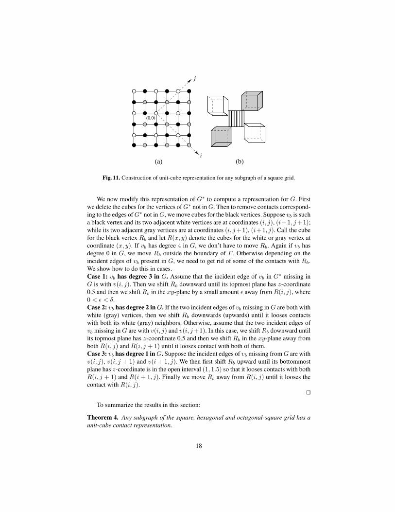
Proof. Let G be a subgraph of a square grid G∗. We first construct a unit-cube rep-resentation of G∗. Note that G∗ is a bipartite graph and suppose A and B are its twopartite sets; see Fig. 11(a). We first place cubes for the vertices of the set A (whiteand gray vertices in the figure). Consider the (i, j) coordinate system on these ver-tices, as illustrated in Fig. 11(a), with the center (0, 0) taken arbitrarily. Consider avertex v of A with the coordinate (i, j) in this coordinate system. We call v a whitevertex when i + j is even; otherwise v is a gray vertex. We place the cube for v inthe range [x(i, j), x(i, j) + 1] × [y(i, j), y(i, j) + 1] × [z(i, j), z(i, j) + 1]; wherex(i, j) = [δi + (2 − δ)j], y(i, j) = [(2 − δ)i − δj], 0 < δ < 0.5 and z(i, j) = 0.5if v is a white vertex, otherwise z(i, j) = 0. Each black vertex has two adjacent whiteand two adjacent gray vertices and we place its unit cube between the cubes for fouradjacent vertices with z-coordinate 0.25; see Fig. 11(b).

17

��������������������

��������������������

j

i

(0,0)

(b)(a)

Fig. 11. Construction of unit-cube representation for any subgraph of a square grid.

We now modify this representation of G∗ to compute a representation for G. Firstwe delete the cubes for the vertices ofG∗ not inG. Then to remove contacts correspond-ing to the edges ofG∗ not inG, we move cubes for the black vertices. Suppose vb is sucha black vertex and its two adjacent white vertices are at coordinates (i, j), (i+1, j+1);while its two adjacent gray vertices are at coordinates (i, j+1), (i+1, j). Call the cubefor the black vertex Rb and let R(x, y) denote the cubes for the white or gray vertex atcoordinate (x, y). If vb has degree 4 in G, we don’t have to move Rb. Again if vb hasdegree 0 in G, we move Rb outside the boundary of Γ . Otherwise depending on theincident edges of vb present in G, we need to get rid of some of the contacts with Rb.We show how to do this in cases.Case 1: vb has degree 3 in G. Assume that the incident edge of vb in G∗ missing inG is with v(i, j). Then we shift Rb downward until its topmost plane has z-coordinate0.5 and then we shift Rb in the xy-plane by a small amount ε away from R(i, j), where0 < ε < δ.Case 2: vb has degree 2 inG. If the two incident edges of vb missing inG are both withwhite (gray) vertices, then we shift Rb downwards (upwards) until it looses contactswith both its white (gray) neighbors. Otherwise, assume that the two incident edges ofvb missing inG are with v(i, j) and v(i, j+1). In this case, we shiftRb downward untilits topmost plane has z-coordinate 0.5 and then we shift Rb in the xy-plane away fromboth R(i, j) and R(i, j + 1) until it looses contact with both of them.Case 3: vb has degree 1 inG. Suppose the incident edges of vb missing fromG are withv(i, j), v(i, j + 1) and v(i + 1, j). We then first shift Rb upward until its bottommostplane has z-coordinate is in the open interval (1, 1.5) so that it looses contacts with bothR(i, j + 1) and R(i + 1, j). Finally we move Rb away from R(i, j) until it looses thecontact with R(i, j).

ut

To summarize the results in this section:

Theorem 4. Any subgraph of the square, hexagonal and octagonal-square grid has aunit-cube contact representation.

18

6 Conclusion and Open Problems

We introduced a new graph coloring problem, called threshold-coloring, that generatesspanning subgraphs from an input graph where the edges of the subgraph are impliedby small absolute value difference between the colors of the endpoints. We showed thatany spanning subgraph of trees, some planar grids, and planar graphs without cycles oflength ≤ 9 can be generated in this way; for other classes like triangular and square-triangle grids, we showed that this is not possible. We also considered different variantsof the problem and noted relations with other well-known graph coloring and graph-theoretic problems. Finally we use the threshold-coloring problem to find unit-cubecontact representation for all the subgraphs of some planar grids. The following is a listof some interesting open problems and future work.

1. Some classes of graphs are total-threshold-colorable, while others are not. There aremany classes for which the problem remains open; see Table 1 for some examples.A particularly interesting class is the square grid: does any subgraph of a squaregrid have a threshold-coloring?

2. Theorem 3 implies that any planar graph without cycles of length ≤ 9 is total-threshold-colorable. On the other hand, all our examples of non-threshold-colorablein Fig. 3(a) contain triangles. Can we reduce this gap by identifying the minimumcycle-length (girth) in a planar graph that guarantees total-threshold-colorability?

3. Can we efficiently recognize graphs that are threshold-colorable?4. Is there a good characterization of threshold-colorable graphs?5. The triangular and square-triangular grid are not total-threshold-colorable and we

cannot use threshold-colorability to find unit-cube contact representations; can wegive a geometric algorithm (such as those in Section 5 for square and hexagonalgrids) to directly compute such representations?

Acknowledgments: We thank Torsten Ueckerdt, Carola Winzen and Michael Bekosfor discussions about different variants of the threshold-coloring problem.

References

1. A. Brandstadt, V. B. Le, and J. P. Spinrad. Graph classes: a survey. Society for Industrialand Applied Mathematics, 1999.

2. D. Bremner, W. Evans, F. Frati, L. Heyer, S. Kobourov, W. Lenhart, G. Liotta, D. Rappaport,and S. Whitesides. On representing graphs by touching cuboids. In Graph Drawing, pages187–198, 2012.

3. C. M. H. de Fegueiredo, J. Meidanis, and C. P. de Mello. A linear-time algorithm for properinterval graph recognition. Information Processing Letter, 56(3):179–184, 1995.

4. S. Felsner and M. C. Francis. Contact representations of planar graphs with cubes. InSymposium on Computational geometry, pages 315–320, 2011.

5. J. Fiala, T. Kloks, and J. Kratochvıl. Fixed-parameter complexity of λ-labelings. DiscreteApplied Mathematics, 113(1):59–72, 2001.

6. J. Fiala, J. Kratochvıl, and A. Proskurowski. Systems of distant representatives. DiscreteApplied Mathematics, 145(2):306 – 316, 2005.

19

7. M. C. Golumbic, H. Kaplan, and R. Shamir. On the complexity of DNA physical mapping.Advances in Applied Mathematics, 15(3):251–261, 1994.

8. M. C. Golumbic, H. Kaplan, and R. Shamir. Graph sandwich problems. Journal of Algo-rithms, 19(3):449–473, 1995.

9. J. R. Griggs and R. K. Yeh. Labelling graphs with a condition at distance 2. SIAM Journalon Discrete Mathematics, 5(4):586–595, 1992.

10. W. Hale. Frequency assignment: Theory and applications. Proceedings of the IEEE,68(12):1497–1514, 1980.

11. P. L. Hammer, U. N. Peled, and X. Sun. Difference graphs. Discrete Applied Mathematics,28(1):35–44, 1990.

12. P. Hell, R. Shamir, and R. Sharan. A fully dynamic algorithm for recognizing and represent-ing proper interval graphs. In European Symposium on Algorithms, pages 527–539, 1999.

13. V. B. Le and D. Rautenbach. Integral mixed unit interval graphs. In Computing and Combi-natorics, pages 495–506, 2012.

14. N. V. R. Mahadev and U. N. Peled. Threshold Graphs and Related Topics. North Holland,1995.

15. F. Roberts. From garbage to rainbows: Generalizations of graph coloring and their applica-tions. Graph Theory, Combinatorics, and Applications, 2:1031–1052, 1991.

16. C. Thomassen. Interval representations of planar graphs. Journal of Combinatorial Theory,Series B, 40(1):9 – 20, 1986.

20