Threshold-Based Mechanisms to Discriminate Transient from Intermittent Faults

Threshold-Based Mechanisms to DiscriminateTransient from Intermittent Faults

Andrea Bondavalli, Member, IEEE, Silvano Chiaradonna,

Felicita Di Giandomenico, and Fabrizio Grandoni

AbstractÐThis paper presents a class of count-and-threshold mechanisms, collectively named �-count, which are able to

discriminate between transient faults and intermittent faults in computing systems. For many years, commercial systems have been

using transient fault discrimination via threshold-based techniques. We aim to contribute to the utility of count-and-threshold schemes,

by exploring their effects on the system. We adopt a mathematically defined structure, which is simple enough to analyze by standard

tools. �-count is equipped with internal parameters that can be tuned to suit environmental variables (such as transient fault rate,

intermittent fault occurrence patterns). We carried out an extensive behavior analysis for two versions of the count-and-threshold

scheme, assuming, first, exponentially distributed fault occurrencies and, then, more realistic fault patterns.

Index TermsÐFault discrimination, threshold-based identification, transient and intermittent faults, modeling and evaluation, fault

diagnosis.

æ

1 INTRODUCTION

MOST computer system applications are expected tohave a ªreasonablyº continuous service, ranging from

a few minutes' wait after a crash, to a few seconds/milliseconds downtime as often required in controllers ofcritical systems. This means that, when a fault occurs, someaction has to be taken to get the system operating again. Theextent of such actions depends on the nature of the fault andon the characteristics of the system. In [1], [2], physicalfaults are classified as permanent or temporary. Permanentfaults lead to errors whenever the relevant component isactivated; the only way to handle such faults is to removethe component. Temporary physical faults can be distin-guished into internal faults (usually known as intermittent)and external faults (transient). The former are caused bysome internal part going outside its specified behavior.After their first appearance, they usually exhibit a relativelyhigh occurrence rate and, eventually, tend to becomepermanent. On the other hand, transient faults cannot betraced to a defect in a particular part of the system and,normally, their adverse effects rapidly disappear. Sincemost malfunctions derive from transient faults [2], if theydo not occur too frequently, removing the affectedcomponent would not be the best solution for most systems.Trying to keep operative a component that has been hit bytransient faults is particularly worthwhile in the design ofunattended dependable systems (e.g., aerospace applica-

tions), where the components should be kept in the systemuntil the throughput benefit of keeping the faulty compo-nent on-line is offset by the greater probability of multiple(hence, catastrophic) faults. In any case, the effects of thefaults need to be dealt with: Simply retrying or restartingmay be enough in commercial systems, while, in moredemanding applications, on-line error masking and/or astate recovery of the faulty component before restart may berequired.

The importance of distinguishing transient faults so thatthey can be dealt with specifically is testified to by the widerange of solutions proposed, although with reference tospecific systems (see Section 6). One commonly usedmethod, for example, in several IBM mainframes, is tocount the number of error events: Too many events in agiven time frame would signal that the component needs tobe removed.

This paper presents a family of mechanisms based on acount-and-threshold scheme, collectively named �-count,designed to discriminate intermittent and permanent faultsagainst low rate, low persistency transient faults. Mostsimilar solutions in the literature apply to general purposemainframe systems, well-equipped with system crash logs,which give detailed information for use in (complex)postmortem analysis. Our goal is to develop mechanismssimple enough to 1) be studied in depth by standardanalytical means and 2) be implementable as small, low-overhead and low-cost modules, suitable even for em-bedded, real-time, dependable systems. The behavior of abasic version of �-count is presented in [3] with reference toa fault model restricted to the exponential distribution offault occurrences. We now present a single-thresholdscheme and a better performing double threshold scheme.To characterize the latter's enhanced behavior, moresignificant performance parameters have been used. Weperform a two step analysis: First, we make the usualassumptions about exponential fault distribution; then, we

230 IEEE TRANSACTIONS ON COMPUTERS, VOL. 49, NO. 3, MARCH 2000

. A. Bondavelli is with the Department of systems and Information Science,University of Firenze, Via Lombroso 6/17, Firenze, Italy.E-mail: [email protected].

. S. Chiaradonna is with CNUCE-CNR, Via Alfieri No. 1, 56010 Ghezzano-Pisa, Italy. E-mail: [email protected].

. F. Di Giandomenico and F. Grandoni are with IEI-CNR, Via Alfieri No. 1,56010 Ghezzano-Pisa, Italy.E-mail: {digiandomenico, grandoni}@iei.pi.cnr.it.

Manuscript received 23 Nov. 1998; accepted 5 Oct. 1999.For information on obtaining reprints of this article, please send e-mail to:[email protected], and reference IEEECS Log Number 106368.

0018-9340/00/$10.00 ß 2000 IEEE

make more accurate fault hypotheses to better represent the

real-life behavior of intermittent and transient faults. The

extended fault hypotheses increased the model's analytical

aspects, without impairing the easy analyzability of the

mechanism.The rest of the paper is organized as follows: Section 2

introduces the general model of the system, together with

hypotheses on the component's behavior and the perfor-

mance figures for the fault discrimination mechanism. In

Section 3, the basic single-threshold scheme is presented

and analyzed under the simplistic exponentially distributed

faults assumption. Section 4 is devoted to modeling and

evaluating the basic scheme under more realistic distribu-

tions of fault occurrences. Section 5 introduces and analyzes

a double-threshold scheme aimed at facilitating a trade-off

between conflicting goals in the design of the basic scheme.

In Section 6, the literature is briefly reviewed and some

comparisons with heuristics shown. Finally, conclusions are

drawn in Section 7.

2 SYSTEM MODEL

The description of our mechanisms will be given with

reference to a model, where the system is partitioned into

components enclosed in well-defined boundaries (which

constitute the field replaceable units of the system), thus

establishing the finest resolution for error detection and

fault diagnosis. Besides the fault discrimination mechanism,

the system includes:

. An error detection subsystem which evaluates whethera component is behaving correctly or not. Errordetection results in signals, which for the purposesof this paper are assumed to have binary values. Weuse this signal stream to feed the fault discriminationmechanism. Computing systems are normallyequipped with several low-level error detectiondevices (e.g., overflow checking, divide-by-zero,program code signatures, watchdog timers). Errornotification may also be generated by testingprograms or be a subproduct of other mechanismsthe system is equipped with (e.g., of the errorprocessing mechanisms properly geared with sup-plemental error signaling tools or of distributedagreement algorithms augmented with disagree-ment indications).

. A fault passivation subsystem, which is in charge ofprocessing the signals produced by the faultdiscrimination mechanism.

Hereafter, it will be assumed that, when an error in a

system component is detected, the effect of the error is

removed by the time the component is used again. This

obviously raises the issue of the cost of such an assumption.

Error treatment itself (or its cost) can be neglected in some

cases (e.g., when stateless components are used or in

redundant computations where the entire state of the

components is subject to a vote and the correct value can

be recovered from the result of this vote), but may be very

onerous in other cases.

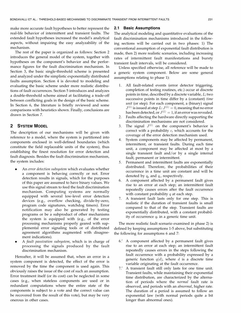
2.1 Basic Assumptions

The analytical modeling and quantitative evaluations of the

fault discrimination mechanisms introduced in the follow-

ing sections will be carried out in two phases: 1) The

conventional assumption of exponential fault distribution is

made, then 2) more realistic scenarios, including increasing

rates of intermittent fault manifestations and bursty

transient fault intervals, will be considered.Unless specified otherwise, all reference will be made to

a generic system component. Below are some general

assumptions relating to phase 1):

1. All fault-related events (error detector triggering,completion of testing routines, etc.) occur at discretepoints in time, described by a discrete variable,L; twosuccessive points in time differ by a (constant) timeunit (or step). For each component, a (binary) signalJ �L� is issued at stepL: J �L� � 0, meaning that no errorhas been detected, orJ �L� � 1, if an error was revealed.

2. Faults affecting the hardware directly supporting thediscrimination mechanisms are not considered.

3. The signal J �L� on the component's behavior iscorrect with a probability c, which accounts for thecoverage of the error detection mechanism used.

4. System components may be affected by permanent,intermittent, or transient faults. During each timeunit, a component may be affected at most by asingle transient fault and/or by a single internalfault, permanent or intermittent.

5. Permanent and intermittent faults are exponentiallydistributed. Therefore, the probabilities of theiroccurrence in a time unit are constant and will bedenoted by qp and qi, respectively.

6. A component affected by a permanent fault givesrise to an error at each step; an intermittent faultrepeatedly causes errors after the fault occurrencewith constant probability q at each step.

7. A transient fault lasts only for one step. This isrealistic if the duration of transient faults is smallcompared to that of the step. Transient faults areexponentially distributed, with a constant probabil-ity of occurrence qt in a generic time unit.

The more realistic fault scenario examined in phase 2) is

defined by keeping assumptions 1-5 above, but substituting

the following for assumptions 6 and 7:

6.0 A component affected by a permanent fault givesrise to an error at each step; an intermittent faultrepeatedly causes errors in the steps following thefault occurrence with a probability expressed by ageneric function q�d�, where d is a discrete timevariable originating at the fault occurrence.

7.0 A transient fault still only lasts for one time unit.Transient faults, while maintaining their exponentialtime distribution, are characterized by the alterna-tion of periods where the normal fault rate isobserved, and periods with an abnormal, higher rate.The duration of a period is assumed to follow anexponential law (with normal periods quite a bitlonger than abnormal ones).

BONDAVALLI ET AL.: THRESHOLD-BASED MECHANISMS TO DISCRIMINATE TRANSIENT FROM INTERMITTENT FAULTS 231

2.2 Figures of Interest and Notation Summary

Informally, our fault discrimination mechanisms aim to

balance two conflicting requirements:

1. To signal, as quickly as possible, all componentsaffected by permanent or intermittent faults (here-after faulty components or FCs). In fact, gatheringinformation to discriminate between transient andintermittent faults takes time, thus giving rise to alonger fault latency. This increases the chances ofcatastrophic failure and also increases the require-ments on the error processing subsystem in fault-tolerant systems.

2. To avoid signaling components other than FCs(hereafter, healthy components or HCs). Depriving thesystem of resources that can still do valuable workmay be even worse than relying on a faultycomponent.

The performance of the mechanisms with respect to the

above goals will be evaluated through:

1. the average D or the Cumulative DistributionFunction (CDF) FD of XD, the total elapsed timesteps between a (permanent or intermittent) faultoccurrence in a component u and the signaling of uas faulty; in this time interval, u is maintained in useand relied upon.

2. NU , the fraction of component life (with respect toits expected life as determined by the expectedoccurrence of a permanent/intermittent fault) inwhich a healthy component u is not actually used inthe system. NU is a measure of the penalty inflictedby the discrimination mechanism on the utilizationof HCs.

Table 1 shows the symbols used for the main parameters,together with their definitions. The default values for qt,qp � qi are derived by considering the case when the moduleto be diagnosed is a processor or computer executing acyclic task at a repetition rate of 100 times per hour. The ratefor intermittent-permanent faults is assumed to be 10ÿ4

faults/hour, thus qp � qi � 10ÿ4=100 � 10ÿ6. We assumethat transient faults are 10 times more frequent thanpermanent faults, i.e., qt � 10ÿ5. The probability that theerror detection subsystem gives wrong signals is assumedto be no worse than that of transient faults as, otherwise,there would be no gain in the dependability of the overallsystem. The default value of the parameter c is thus set to1ÿ 10ÿ5.

3 A BASIC THRESHOLD-BASED FILTERING

MECHANISM AND ITS ANALYSIS

3.1 �-Count, an On-Line Single Threshold-BasedFault Identification Mechanism

As in several well-known threshold schemes (see Section 6for a brief review), our first basic mechanism, the single-

threshold �-count, gathers all signals related to the correct-ness of a given component from any available errordetector, weighing down signals as they get older, to decidethe point in time when keeping a system component on-lineis no longer beneficial.

A simple, but nevertheless satisfactory, formulation ofthe filtering function � is the following:

��L� � ��Lÿ1� �K if J �L� � 0

��Lÿ1� � 1 if J �L� � 1

(0 � K � 1

��0� � 0;

�1�


TABLE 1Symbols and Definitions

where L is the discrete time variable defined in Section 2.1and � is a score associated with each not-yet-removedcomponent to keep track of the errors experienced by thatcomponent.

When the value of ��L� exceeds a given threshold �T , thecomponent is diagnosed as affected by a permanent or anintermittent fault. This event produces an �-signal, which issent to the fault passivation subsystem. The values to assignto the parameters K and �T so that the strategy works bestdepend on the expected frequency of permanent, inter-mittent, and transient faults and on the probability c ofcorrect judgments of the error signaling mechanism used.Note that d�T e represents the minimum number ofconsecutive errors sufficient to consider a component asbad enough for removal, while K represents the ratio inwhich � is decreased after a time step without error signals,thus setting the time window where memory of previouserrors is retained.

The filtering function � may be given different formula-tions from (1) above when searching for particularperformances. For example, the additive expression belowassociates a constant decrement to each errorless computa-tion, while, in (1), the decrement is proportional to thecurrent count.

��L� ��Lÿ1� � 1 if J�L� � 1

��Lÿ1� ÿ dec ifJ �L� � 0 AND ��Lÿ1� ÿ dec > 0;

0 � dec

0 if J �L� � 0 AND ��Lÿ1� ÿ dec � 0:

8>>>>>>><>>>>>>>:�2�

With this function, the decay time of the current value isproportional to the value itself, while, in form (1), itdepends (roughly) only on the parameter K. This wouldresult in different optimal settings for the mechanism'sparameters and also in differences in behavior; however,the modeling and the analysis will be worked out for form(1) only since it is straightforward to adapt the methodsused here to form (2) and, of course, to other variants of the� function as well.

3.2 Analysis of the Single-Threshold �-Count

The first phase of the evaluation of the single-threshold �-count is now carried out, using hypotheses 1 to 7(Section 2.1). Because of the assumption of exponentialfault distributions, it is trivial to see that an FC will alwayseventually be identified as such. Unfortunately, the sameargument means that we cannot rule out that an HC mightbe wrongly signaled as faulty. Besides these asymptoticresults, the behavior of the mechanism has been modeledby Stochastic Activity Networks (SAN) [4]. Two SANs havebeen derived: The first, modeling the mechanism acting ona faulty component, is used to compute an approximationof the average delay D to the identification of an FC; thesecond, modeling the mechanism acting on a healthycomponent, allows the approximate evaluation of theaverage unused fraction of an HC life NU . A faultycomponent is affected, by definition, either by a permanentor by an intermittent fault. The estimation of the number of

steps needed to recognize a permanent fault is trivial: Theprobability of J �L� � 1 is very close to 1 (it is 1 � c), therefore,the expected time to the threshold crossing is approxi-mately bounded by d�T e, considering that the value of �will generally be greater than 0 when the permanent faultoccurs. Hence, we have only modeled the case ofintermittent faults, which requires a longer identificationtime. As required by SAN models, a discrete approximationof the real valued variable � is used. In the followingsections, the approximate values are chosen to lead to aconservative evaluation of the performance parameters.

The SAN models are presented in the next twosubsections and evaluated in Section 3.3. As for the modelspresented later, the details of the modeling are notnecessarily a prerequisite for appreciating the results ofsubsequent evaluations.

3.2.1 Model of the Single-Threshold �-Count Acting on a

Faulty Component

F SAN-1 (Fig. 1) represents the behavior of the single-threshold �-count acting on the FC u when affected by anintermittent fault. Inside F SAN-1, � is represented by itsapproximation variable � inf � �; � inf will then reach �Tin an average number of steps D higher than, or equal to,the average number of steps which would be required bythe real �. Moreover, to better enforce D to be an upperbound, we assume that, at the first occurrence of apermanent/intermittent fault, � inf � 0, while, in general,� inf will take positive, albeit small, values.

F SAN-1 has three places: 1) not remov (a token heremeans that u is not yet flagged as faulty); 2) remov (a tokenhere marks the actual identification of u as an FC, with theattending emission of the �-signal ); 3) alpha state (used tomaintain the current value of � inf). The exponentiallydistributed timed activity (with rate 1) next step representsthe receipt of a signal; it has two cases: case 1, representingthe occurrence of J �L� � 1, and case 2, representing that ofJ�L� � 0.

In order to allow the steady-state evaluation of the SAN,an additional timed activity, next miss, has been inserted. Itrepresents the (dummy) restart of �-count upon the issuingof the �-signal; next miss is also exponentially distributedwith rate 1. The two output gates incr and decr perform thebasic steps for computing � inf . When � inf reaches thevalue �T , the gate incr deposits a token in the place removand sets to 0 the value of � inf in order to restart innext miss.

The probabilities associated with case 1 and case 2 in thenext step transition are expressed as:

P �Case 1� � �q � qt�c� �1ÿ q ÿ qt��1ÿ c�P �Case 2� � �q � qt��1ÿ c� � �1ÿ q ÿ qt�c:

The first term of the first expression represents a failureof u (either an activation of the intermittent or an occurrenceof a transient fault, with probability q � qt) which isdetected by the error signaling mechanism (withprobability c); while the second term represents theincorrect detection of a failure. The second expression hasa symmetric explanation.


The value of D is determined by the ratio between thesteady-state probabilities that one token is in the places

not remov and remov, respectively, which is equal to theratio between the mean time spent in the two places. Since

the activities next step and next miss have the same rate

(equal to 1), the latter ratio corresponds to the averagenumber of visits to the place not remov before going to the

place remov, i.e., the average number of steps to the

identification of the FC.

3.2.2 Model of the Single-Threshold �-Count Acting on a

Healthy Component

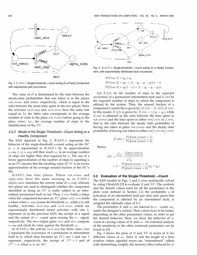
The SAN depicted in Fig. 2, H SAN-1, represents thebehavior of the single-threshold �-count acting on the HC

u. � is represented in H SAN-1 by its approximation� sup � �; � sup will then reach �T in an average number

of steps not higher than that required by �. The use of a

lower approximation of the number of steps to signaling uas an FC ensures that the resulting value of NU is an excess

approximation of the average unused fraction of the HC'slife.

H SAN-1 has four places. Places not remov andalpha state have the same meaning as in F SAN-1

(alpha state maintains the current value of � sup), whereastwo places are used to distinguish whether the component

identified as being an FC is really subject to an inter-

mittent/permanent fault or not. Place f rem holds a tokenwhen the component becomes an FC, place notf rem holds

a token when � sup crosses the threshold �T , while u is stillhealthy. Activities next step and next miss, which are

exponentially distributed timed activities with rate 1,

represent, as in the previous SAN, the receipt of a signaland the restart of �ÿ count upon issuing the �ÿ signal,

respectively. The two output gates incr and decr compute� sup and check its value against the threshold �T .

In H SAN-1, the activity next step has three cases. Case

1 represents the occurrence of a permanent or intermittent

fault in u, which thus becomes an FC; case 2 and case 3

represent, respectively, the receipt of J �L� � 1 and of

J �L� � 0 when u is an HC.

P �Case 1� � qp � qiP �Case 2� � qtc� �1ÿ qp ÿ qi ÿ qt��1ÿ c�P �Case 3� � qt�1ÿ c� � �1ÿ qp ÿ qi ÿ qt�c:

Let E life be the number of steps to the expectedoccurrence of a permanent/intermittent fault and E util bethe expected number of steps in which the component isutilized by the system. Then, the unused fraction of acomponent's useful life is given by �E lifeÿE util�=E life.In this model, E life is given by: E life � 1=�qi � qp�, whileE util is obtained as the ratio between the time spent innot remov and the time spent in either notf rem or f rem,that is, the ratio between the steady state probability ofhaving one token in place not remov and the steady stateprobability of having one token in either notf rem or f rem:

E util � P �#not remov � 1�P �#not remov � 0� :

Hence,

NU �1

qi�qp ÿP �#not remov�1�P �#not remov�0�

1qi�qp

� 1ÿ P �#not remov � 1�P �#not remov � 0� �qi � qp�:

3.3 Evaluation of the Single-Threshold �-Count

The SAN models in Figs. 1 and 2 were analytically solvedby using UltraSAN [5] to evaluate D and NU . The symbolsand the default values used for all the parameters in theplots were defined in Section 2.2; the probability q ofactivation of an intermittent fault per time unit, given thatthe component is affected by an intermittent fault, isassigned the (default) value of 0.1.

The parameters K and �T are internal to �ÿ count, i.e.,under the designer's control. Their values have to be tuned,depending on the other parameters values, in order to getthe desired behavior. Here, we show the behavior of �-count at varying values of K and �T . An extended analysisof the sensitivity to the other (external) parameters can befound in [3].

Fig. 3 shows the plots of D and NU in terms of K fordifferent values of �T . Since K sets the length of a timewindow where signaled errors are ªrememberedº (albeitwith diminishing weight), the memory effect induced by K


Fig. 2. H SAN-1: Single-threshold �-count acting on a Healty Compo-

nent, with exponentially distributed fault occurences.

Fig. 1. F SAN-1: Single-threshold �-count acting on a Faulty Component

with exponential fault occurrence.

clearly has contrasting consequences on the delay to faultidentification, D, and on the utilization loss, NU . Highvalues of K, causing a slow decay of the �-count, make itquicker to catch an intermittent fault, i.e., give low valuesof the delay. However, this is at the cost of a higherutilization loss since there is more chance that enoughtransient faults add up to the �-count over the threshold.The opposite occurs at low values of K. With regard tothe threshold height �T , a symmetrical behavior isobserved: Higher values require more error signals (andmore time) to trigger the �-count output, thus improvingNU while lengthening D.

More specifically, note that, at low values of K, the delayD markedly improves as K increases, up to a region arounda value KD (0.99 in the case of Fig. 3); for K > KD,variations of D become smaller and smaller. In addition, Dbecomes less sensitive to the threshold height �T in theregion above KD.

The curves plotted for NU highlight the effect of thediscrete increment of �. The curves appear as grouped intwo sets, those with �T less or equal to 2 and those with �Thigher than 2, which depart from each other (for low valuesof K). The reason is that, in the first case, two errorssignaled in the window are sufficient to single out thecomponent, while, when �T � 2, three errors are usuallynecessary.

NU gets its best values for low values of K. The curvesshow a continuous, but slow, increase up to a region arounda value KNU and, for K > KNU , NU becomes worse andworse. If KD < KNU , values of K in the interval �KD;KNU �determine values for both the delay and the utilization losswhich cannot be significantly further improved. Thus, itappears that, if no indications of their relative importanceare given, values for K should be chosen in such an

interval. However, the existence of this interval dependson other parameters as well. For example, as shown inFig. 4, D is heavily influenced by the intermittent faultactivation parameter q: The lower q is (i.e., the longer theexpected time between intermittent fault activation), thehigher KD is.

Since a low NU and a low D are conflicting goals, thedefinition of the ªbest behaviorº for �-count and, thus, theproper tuning of its parameters, entails defining theirrelative importance. Thus, even in cases where the rangefor values to be assigned to K can be identified, aspreviously discussed, it still has to be decided whether Dor NU should be optimized: The former case requires lowvalues of �T , while high values optimize the latter one.More generally, parameters for a specific system can betuned once the system designer has given constraints on thedesired behavior of the mechanism, e.g., ªD must beoptimized while NU must take values lower than a giventhreshold.º

4 SINGLE-THRESHOLD �-Count UNDER MORE

ACCURATE DISTRIBUTIONS OF FAILURES

The previous analysis of the single-threshold �-count wasaimed at understanding the influence of the internalparameters on the performance measures. To make it easierto grasp the essentials of the mechanism's behavior, simpleapproximations to the fault process (i.e., exponentialdistribution) have been used. However, the constant rateassumption is not the best as far as intermittent faults areconcerned as, in most cases, they tend to become morefrequent after the first occurrence and may turn intopermanent faults. Transient faults may occasionally occur


Fig. 3. Effect of the internal parameters K;�T on the delay figure D and the utilization loss NU.

with an abnormal frequency (e.g., during a storm). In this

section, the original fault model will be refined to account

for the above phenomena.First, the activation rate of intermittent faults is con-

sidered as increasing in time after the first occurrence, that

is, assumption 6' of Section 2.1 will replace here

assumption 6. Since this change only affects the behavior

of faulty components, only the delay in identifying an FC

will be reevaluated. It will be given in terms of the

Cumulative Distribution Function FD�d� of the number of

steps XD to the FC identification. The fault probability, of

course, is given by a time-dependent function q�d� instead

of the constant-valued parameter q previously used.Second, a piecewise exponential distribution of transient

faults is introduced, where short, higher-frequency fault

bursts emerge from the ªnoise floorº of the normal transient

fault rate, that is, assumption 7' of Section 2.1 will replace

here assumption 7. In the presence of bursts, the evaluation

of D by using the simple exponential model leads to a

conservative estimation since the occurrence of bursts can

only speed up the process of spotting a faulty component.

The figures relative to HCs will be reevaluated in the

following: The constant transient fault probability qt is here

substituted by the two values qta, qtb which hold in the

ªnormalº periods and in the ªburstyº ones, respectively.The modifications of the fault model will be introduced

one at a time to simplify both the analysis and the

comprehension of their effects. In the next two subsections,

the detailed SAN models, obtained by modifying those

previously presented to take into account the above

changes, are described.

4.1 Another Model of the Single-Threshold �-CountActing on an FC

F SAN-2, depicted in Fig. 5, which represents the behaviorof single-threshold �-count acting on a faulty component, isderived from F SAN-1 by adding the place count, holdingthe running number of time units d, and the gate next m,described below. This allows the use of time-dependentprobabilities at the cost of increasing the number of states ofthe model and the time and computational effort needed toobtain the solution. In order to cope with this potential stateexplosion problem, �-count is analyzed in a finite timeinterval of length Max d, i.e., for 0 � d �Max d steps fromthe fault's occurrence, even though the identification of theFC has still to be achieved at that point. F SAN-2 isdescribed in terms of its differences with respect toF SAN-1.

The place count is initialized to 1 and is updated bythe two output gates incr and decr. When count holdsMax d� 1 tokens, the gates incr or decr, depending on thecase, deposit a token in the place remov and set to 0 thevalue of � inf for a restart in next miss. Upon the firing ofnext miss, the gate next m resets to 1 the number of tokensin count and not remov in order to restart the network. Theexpressions for the probabilities of the two cases ofnext step are derived from those used in F SANÿ 1 bysubstituting the constant-valued q with a time-dependentfunction q�d�, implemented as a marking-dependent ex-pression q�#count�.

The values of FD�d� for d �Max d are obtained asfollows: Consider that, whenever �-count succeeds inidentifying the FC in at most Max d steps, the placecount contains exactly XD tokens, so, let V be a variabledefined as


Fig. 4. Values of D and NU as a function of K for a few values of the intermittent fault manifestation probability, q.

V � #count if #remov � 10 if #remov � 0

�from the steady-state evaluation of FV �d�, the CDF of V , itfollows:

FD�d� � FV �d� ÿ FV �0�1ÿ FV �0� :

Note that V may also take the value Max d� 1. Thisaccounts for the probability that the identification of theFC u is not performed within Max d steps from theoccurrence of the fault.

4.2 Another Model of the Single-Threshold �-CountActing on an HC

The behavior of the single-threshold �-count acting on anHC considering more realistic distributions of occurrencesof transient faults is modeled by H SAN-2, depicted in Fig. 6,which is an extension of H SAN-1. H SAN-2 represents thealternation of normal periods, whose duration is indicatedby the random variable Ta, where the probability of anoccurrence of a transient fault per time unit is qta, and ofabnormal periods, having random lengths Tb, characterizedby a higher probability qtb. The switch between periodshappens with rates �ab and �ba. Extending this model toaccount for many different periods is straightforward.

There are basically three differences between this net andH SAN-1: 1)two places, norm freq and abnorm fr and twotransitions, T norm and T burst, have been added torepresent the alternation of normal and abnormal periods,2) the expressions for the probabilities of case 2 and case 3of next step have been modified using qta or qtb instead of qt,depending on the marking of norm freq and abnorm fr,3) gate end m has been given the additional task of settingto 1 the number of tokens in norm freq and to 0 that ofabnorm fr. From H SAN-2, an upper bound NU to theutilization loss of the component is obtained, just like inH SAN-1.

4.3 Evaluation of the Single-Threshold �-CountUsing the New Models

The solution of the SAN models yields the values of FD�d�and NU . The measure 1-FD�d�, indicating the probability ofnot identifying an FC component within d steps, has beenplotted instead of FD�d� to help better show the effects ofdifferent time functions for the probability q�d�.

A function commonly recognized to fit the real lifebehavior of intermittent faults is the (discrete) Weibulldistribution [2], [6]. Thus, although the SAN model

(described in Section 4.1) representing the behavior of �-count on an FC allows the use of arbitrary functions ofdiscrete time, the Weibull discrete-time hazard function willbe adopted in the following evaluations, i.e.:

q�d� � 1ÿ �1ÿ qw�d�ÿ�dÿ1�� ; d > 0; � � 1; 0 < qw < 1:

To allow a significant comparison with the exponentialdistribution used in Section 3, the parameters qw and � for afamily of Weibull distributions are chosen so that the sameexpected number of intermittent faults is obtained for bothdistributions in a fixed initial time interval (namely, anaverage of six fault manifestations in 60 steps).

In the following evaluation, the expected duration of abursty interval, Tb, will be in the range 10-50 steps (i.e., fromsix to 30 minutes), while the expected duration of a normalinterval, Ta, will be given the two values 2,400 and 220,000steps (corresponding to 24 hours and about three months,respectively).

The default values for the internal parameters K and �Tare 0.99 and 2.0, respectively. Other parameters, common tothe exponential model (e.g., qp � qi , c, etc.), take the defaultvalues defined in Section 2.2 unless otherwise specified. Thevalues of the remaining parameters are specified in therelevant figures.

The effects of an increasing intermittent fault rate on thedelay to FC identification, represented by 1ÿ FD�d�, areshown in Fig. 7. Plots of 1ÿ FD�d� for a few values of � andqw are reported. Note first that the crossover, around d � 60,of the Weibull plots with the exponential plot (representedby � � 1) is due to the assumption on the averages of bothdistributions. It is apparent that the exponential modeloverevaluates the probability of spotting a faulty compo-nent at the left of the crossover and, on the other hand,gives lower estimates for larger values of the detectiondelay. In fact, in Fig. 7, one full order-of-magnitudedifference between the exponential curve and the Weibullwith � � 1:4 is observed for d � 100. It can thus beconcluded that, whenever real intermittent faults getactivated with increasing rate, the accuracy of the enhancedmodel improves significantly.

Fig. 8 shows the influence of burstiness on the utilizationloss NU . Fig. 8a, where NU is plotted against Tb and qtb,highlights that the presence of transient fault burstssignificantly worsens the utilization loss caused by wronglytagging an HC as faulty with respect to the exponentialdistribution. In the figure, the transient fault probabilitiesqta and qtb are given value pairs such that the resulting time


Fig. 6. H SAN-2: Single-threshold �-count acting on a Healthy

Component, with transient fault bursts.

Fig. 5. F SAN-2: Single-threshold �-count acting on an FC under time-

dependent error rates of intermittent faults.

averages equal the default qt (i.e., 10ÿ5), to allow a directcomparison with the exponentially distributed behavior(shown by the curve labeled qtb � 10ÿ5). The departure fromthe exponential behavior grows, as expected, with increas-ing qtb, e.g., for qtb three orders of magnitude over thedefault value, NU gets more than one order of magnitudeworse. This is remarkable considering that the average faultprobability is kept constant and that the burst length is atiny fraction of the normal interval. With regard tovariations in bursty intervals, higher values of Tb, implyinga higher number of transient faults during those intervals,lead to higher values of NU ; this influence obviouslydecreases with decreasing values of qtb.

In Fig. 8b, the utilization loss NU is evaluated against �Tand qtb. As already discussed in the pure exponential case,

higher values of the threshold �T have to be set to achieve

lower values of NU . The situation gets worse in the

presence of bursts: For any value of �T , the higher qtb is,

the higher the utilization loss is. A measure of this effect can

be observed by comparing the dashed curves labeled with

qtb � 5 � 10ÿ3 and qt � 7:2 � 10ÿ5, plotted for distributions

with the same mean. On the other hand, given a target

value for NU (10ÿ3 is chosen as an example in Fig. 8b), a

corresponding value for �T can be determined to attain it.

The curves show that increasing values of �T are required

by increasing values of qtb. Of course, the curve labeled with

qt � 10ÿ5, corresponding to the exponential distribution,

intercepts the lowest value for �T . Unfortunately, however,

higher values of �T lead to higher values of the identifica-

tion delay D, with consequent higher risks in running the

system while relying on a faulty component. The dilemma

ªNU vs. D,º already faced at the end of Section 3.3, is, in

fact, exacerbated by the presence of fault bursts, to the

extent that it may be difficult to find a satisfying trade-off in

the original �-count mechanism. The next sections describe

a solution based on the idea of decoupling the effects of the

threshold mechanism by adopting a double-threshold

scheme.

5 A DOUBLE-THRESHOLD SCHEME

5.1 �-Count Using Two Thresholds

Consider now a new �-count scheme, where a component u

is kept in full service as long as its score � is lower than a

first threshold �L. When the value of � grows bigger than

�L, u will be restricted to running application programs

solely for diagnostic purposes, that is, its behavior will only

be monitored by the error signaling subsystem, and the

associated �-count mechanism will continue to operate. In

other words, u is considered as a ªsuspectº and, as such, its

results are not delivered to the user or relied upon by the

system. If � continues to grow, it eventually crosses a

second threshold �H , with �H > �L: Then, the component u

is diagnosed as being affected by a permanent/intermittent

fault and the �-signal is issued, as in the original �-count, to

the fault passivation subsystem. When, instead, �, after

some wandering in the ��H ÿ �L� ªlimbo,º becomes lower

than or equal to �L,1 then the ªsuspectº component will be

brought back into full service.With this scheme, the lower threshold can be kept at a

low level to limit the detection delay XD, while the

probability of throwing away good components hardly

increases. In fact, occasional fault bursts may anomalously

raise an HC's �-count, forcing the component into a

nonutilization period, but the probability of an irrevocable

elimination can be kept as low as desired by setting a

suitably high value for �H .2 An adverse effect of this

scheme is the need to treat errors that show up in the units

confined in the limbo. In fact, to continue observing their

behavior, they need to be treated exactly like the on-line

components, thus putting their share of burden on the

error-processing subsystem.The models to be used in the analysis of the double-

threshold mechanism, under assumptions 1-5 and 6', 7' of

Section 2.1, are introduced below.

5.2 Double-Threshold �-Count Acting on an HC

H SAN-3 (Fig. 9) models the behavior of the double-

threshold �-count acting on an HC. H SAN-3 is an

extension of H SAN-2; as in the latter, a bursty fault

behavior is modeled and the computation of an upper

bound NU of the utilization loss of a healthy component is

allowed.There are basically four differences between H SAN-3

and H SAN-2:

1. The place susp (initially set to 0) has been added torepresent the alternation of periods in which thecomponent is ªsuspectº (one token in susp) withthose where the component is used and suppliesresults to the user (no token in susp);

2. The gate incr has been given the additional task ofsetting to 1 the number of tokens in susp when thevalue of � reaches the first threshold �L;

3. The gate decr has been given the additional task ofsetting to 0 the number of tokens in susp when thevalue of � becomes lower than the first threshold �L;

4. Gate end m has been given the additional task ofsetting to 0 the number of tokens in susp (when thecomponent is tagged as faulty).

The unused fraction of a component's useful life is

determined as in Section 3.2.2; here, however, E util is the

expected number of steps in which the HC is not suspected,

i.e., used and relied upon; it is determined by the following

expression:

E util � P �#not remov � 1 AND #susp � 0�P �#not remov � 0� :

Then:


1. In practice, a threshold value �L0 with �L0 � �L may be moreappropriate here to put a degree of hysteresis in the mechanism with thegoal of avoiding frequent ªbouncingº between the ªactiveº and ªsuspectedºstates.

2. An infinite value would, in fact, keep all units running, whether inªlimboº or not.

NU �1

qi�qp ÿP �#not remov�1 AND #susp�0�

P �#not remov�0�1

qi�qp

� 1ÿ P �#not remov � 1 AND #susp � 0�P �#not remov � 0� �qi � qp�:

5.3 Double-Threshold �-Count Acting on an FC

The behavior of the double-threshold �-count acting on an

FC, considering time-dependent error rates of intermittent

faults, is modeled using F SAN-3 (see Fig. 10), a SAN

derived from F SAN-2 (described in Section 4.1), which

allows lower bounds to be computed for the number of

steps the FC is kept in full service after the permanent/

intermittent fault occurrence. As with F SAN-2, the analysis

has been limited to a finite time interval spanning Max d

time units.There are three main differences between F SAN-3 and

F SAN-2:

1. The place count notsusp (initially set to 1 since, in thefirst step, the component is assumed to be in aªnonsuspectº state) counts the steps in which the FCis not suspected. It holds the number of stepselapsed with � inf < �L before the identification ofFC as faulty or Max d if Max d steps went by,whichever event occurs first;

2. Gates incr and decr have been given the additionaltask of incrementing the number of tokens incount notsusp when � inf < �L. The gate incr

deposits a token in the place remov when the valueof � inf reaches the value �H ;

3. Gate next m has been given the additional task ofresetting to 1 the number of tokens in count notsusp.

F SAN-3 allows a lower bound of FD�d� to be computed for

d �Max d. Actually, the CDF FD�d� of XD is defined as

FD�d� � P �XD � d� � P �XD � djYD �Max d��P �YD �Max d� � P �XD � djYD > Max d��P �YD > Max d�;

where YD is the number of steps for � inf to reach �H . The

approximation, obtained by considering

FD�d� � P �XD � djYD �Max d� � P �YD �Max d�for d �Max d

;

clearly gives values always lower than the actual CDF.To obtain a closed expression for FD�d� in terms of the

SAN values, consider that, whenever �-count succeeds in

identifying the FC in at most Max d steps, the place count

contains exactly YD tokens, while the place count notsusp

contains exactly XD tokens. Let V and W be auxiliary

variables defined as:


Fig. 7. Influence of increasing intermittent fault rate on the delay to FC identification.


Fig. 8. Influence of burstiness on utilization loss.

V � #count if #remov � 1

0 if #remov � 0

�W �

#count notsuspif #remov � 1 AND #count

�Max d

0 otherwise

8>><>>:and FW �d� be the CDF of the variable W , FV �d� the CDF of

the variable V . Clearly:

P �XD � djYD �Max d� � FW �d� ÿ FW �0�1ÿ FW �0� for d �Max d

and

P �YD �Max d� � FV �Max d� ÿ FV �0�1ÿ FV �0� :

To check how strict the lower bound thus obtained is, we

can compute P �YD > Max d� as well:

P �YD > Max d� � FV �Max d� 1� ÿ FV �Max d�1ÿ FV �0� :

5.4 Evaluation of the Double-Threshold �-Count

The SAN models described in the previous two sections

were analytically evaluated by UltraSAN and estimations

for the measures NU and FD�d� were derived. The basic

parameter settings are still those presented in Section 2.2 if

not otherwise specified. The values of new parameters

relating to the double-threshold �-count are indicated

directly in the figures.To understand the added features of the double-thresh-

old scheme over the original single-threshold �-count,

consider the typical procedure that a system designer

might follow to set up the internal parameters of the

mechanism. Given the external parameters, i.e., the fault

rates and their characterizations, in the single-threshold

case a near-optimal value of K can be determined from

Fig. 3, which is likely to be around KD. A figure like Fig. 8

can then be generated, where NU and D are plotted against

the remaining internal parameter �T . As can be seen, setting

a target value for, say, NU , forces the value for D, leaving

the designer with no leeway. The settings of NU and D

should thus be traded off each other, according to their

relative importance in the system design.

The performance figures resulting from the applicationof the single-threshold �-count are then compared withthose obtained from the double-threshold variant. Here-after, the range ��L; �H � is always assumed to include thevalue of �T . A suitable setting for parameters �H and �L hasto be chosen. Since high values of the single threshold �Tgive low values of NU , Fig. 8 could be used to find asuitable value for �T which fits the target NU , which canthen be assigned to the higher threshold �H . The value to beassigned to �L has to lead to a good trade-off between arelatively slight negative influence on the utilization factorof an HC and a satisfactorily low value for the probabilityof keeping an FC on-line. This is what is shown in Figs. 11and 12.

Fig. 11 shows the effects of the variation of the lowerthreshold on the utilization loss NU of an HC. To give aquantitative measure of the expected increase in NU ,because of nonutilization periods spent by HCs in ªlimbo,ºa comparison with the single-threshold case with �T � �His made. Four pairs of plots have been depicted; each pairhas a plot relative to the single-threshold mechanism andthe other relative to the double-threshold case, for differentvalues of �H and �T . The pairs ��T ; qtb� were chosen (on thebasis of Fig. 8b) to give values of NU around 10ÿ3, whichare considered significant for typical applications. In eachplot pair, the difference between the two curves displayshow much HC utilization is lost. For �L � �T � �H , themechanism is reduced to the single threshold, i.e., thedifference is zero. Clearly, this difference increases withdecreasing values of �L. The interesting fact is that theworsening of NU remains negligible with values of thelower threshold going as low as 1.1. Around this value, thecurves exhibit a pronounced knee, which is not surprisingsince the elemental increment in �-count is, in fact, 1. Afirst-approximation choice for �L is then around 1.1. In anycase, at even lower values of �L, there is no dramatic loss,e.g., for �T � 3 (and qtb � 10ÿ3) at �L � 0:5, the utilizationloss is around 4 � 10ÿ3: With such a low �L setting, mostpermanent/intermittent faults would result in the neutra-lization of the affected component with virtually no delay.

Having set all the internal parameters, we only need tocheck whether the probability of keeping an unreliablecomponent on-line is now low enough. This can be seenfrom Fig. 12, where FD�d� is plotted against d for different�L, with �H � 3.

A refinement step can now be made by looking at thebenefits to be gained by further shrinking �L: The benefitsof a smaller value may be weighed against the price to be


Fig. 9. H SAN-3: Double-threshold �-count acting on an HC, with

transient fault bursts.

Fig. 10. F SAN-3: Double-threshold �-count acting on an FC under

time-dependent error rates of intermittent faults.

paid in terms of NU that can be evaluated from Fig. 11; thestep can be repeated until a good trade-off is found.

Since lower values for the threshold give lower delay D,in the comparison between the two �-count schemes, withreference to D, the better performing single-threshold is thatwhere �T � �L. In Fig. 12, where �H � 3, the plot relative to�T � 2 and the one relative to �L � 2 show that the double-threshold incurs a loss, in terms of FD�d�, with respect to thesingle-threshold. This loss is the consequence of the

nonzero probability that an FC comes back into full serviceafter first surpassing �L. However, such a ªbetterº behaviorregarding FD�d� of the single-threshold is purely specula-tive, as it implies worsening NU : From Fig. 11, the twoschemes have comparable values of NU if �T has the samevalue as �H . In Fig. 12, however, when �T � �H , thedouble-threshold �-count fares much better: the lower thevalue of �L, the higher the improvement in the value ofFD�d�. For example, if d � 40, the probability of having


Fig. 11. Comparison of the effects of the double-threshold and the single-threshold on the utilization loss NU.

Fig. 12. Effects of the double-threshold and the single-threshold on the delay indicator FD�d�.

recognized an FC is about 0.5 for the single-threshold with�T � 3, while, for the double-threshold with �H � 3 and�L � 1:1, it is approximately 0.88. In Fig. 11 for the samesetting of �H , �L, and �T , the loss of utilization of an HC isnegligible.

6 RELATED WORK

We now consider some transient fault discriminatingtechniques from the literature. These can be broadlyclassified into two groups: A) techniques designed tosupport human intervention and B) algorithm-based,automatic mechanisms. We will relate some of them with�-count for the sake of simple comparisons.

6.1 Group A

In [7], a trend analysis of system error logs is applied whichattempts to predict future hard failures by distinguishingintermittent faults (bound to turn into solid failures) fromtransient faults. The authors conclude, ªFault prediction ispossible.º

In [8], some heuristics, collectively named DispersionFrame Technique, for fault diagnosis and failure predictionare developed and applied (off-line) to system error logstaken from a large Unix-based file system. The heuristicsare based on the interarrival patterns of the failures (whichmay be time-varying). For example, there is the 2-in-1 rule,which warns when the time of interarrival of two failures isless than one hour, and the 4-in-1 rule, which fires whenfour failures occur within a 24-hour period.

In [9], error rate is used to build up error groups. Simpleprobabilistic techniques are then recursively applied to thequite detailed information given by the error recordstructure to seek similarities (correlations) among records,which may point to common causes (permanent faults) of apossibly large set of errors. The procedure is applied toevent logs gathered from IBM 3081 and CYBER machines.

Because of the detailed error reports available fromsystem logs, the procedures in this group can makesophisticated analyses and may allow more precise diag-noses or permanent failure predictions. However, they arenormally applied off-line, they are seldom expressed inalgorithmic form, and their complexity does not help theperformance analysis. By contrast, the choice for �-count isto forego elaborate inferences on the health of the system, infavor of the higher predictability of a simple mechanism,possibly operating on-line. Despite its simplicity, �-countcould be used as a basic tool to implement approximateversions of the above heuristics. For example, a 2-in-1-likerule [8] can be obtained using the single-threshold �-count by setting �T to 1�� and K to �1=x, where x isthe time window (or trigger frame) within which twofailures are considered too many, and �, 0 < � < 1, is aparameter to represent the accuracy of the approximationto the 2-in-1 rule. By assigning to K the value computedwith the above formula, when a second error hits thecomponent u after less than x time units, the threshold�T will be exceeded since, at the preceding time unit, thevalue of � associated with u is greater than �. With thesame assumptions as above, it is clear that the parametersof the single-threshold �-count that satisfy the relation

��Ky � 1�Ky � 1�Ky � 1 ��T make up an approximation ofthe 4-in-1 rule [8] where, in this case, 4 � y is the triggerframe.

6.2 Group B

In TMR MODIAC, the architecture proposed in [10], twofailures experienced in two consecutive operating cycles bythe same hardware component that is part of a redundantstructure make the other redundant components consider itas definitively faulty.

In IBM machines, the idea of thresholding the number oferrors accumulated in a time window has long beenexploited. In the earlier examples, as in [11], whichdescribes the automatic diagnostics of IBM 3081, the ideais used to trigger the intervention of a maintenance crew; inlater models, as in ES/9000 Model 900 [12], a retry-and-threshold scheme is adopted to deal with transient errors.

In [13], error detectors and error-handling strategies aregiven ample reviews in recognition of their importance totolerating transient faults. An ªerror-handling controllerºgets its inputs from the error detectors to implementtransient fault tolerance; its operation encompasses asses-sing each fault, labeling it as transient if it occurs less thanK times in a given time window.

In [14], if, after a fault, a channel of the core FTP can berestarted, then it is brought back into operation; ªhowever,it is assigned a demerit in its dynamic health variable; thisvariable is used to differentiate between transient andintermittent failures.º

In [15], a list of ªsuspectº processors is generated duringthe redundant executions; a few schemes are then sug-gested for processing this list, e.g., assigning weights toprocessors that participate in the execution of a job and failto produce a matching result and taking down fordiagnostics those whose weight exceeds a certain threshold.

All of these solutions implement schemes simpler than�-count. In fact, when given suitable parameters, theirfunctionalities may easily be obtained by an �-countinstance, e.g., the approach proposed in [10] can beemulated by the single-threshold �-count with K � 0 and�T � 2.

7 CONCLUSIONS

We have introduced a family of mechanisms, collectivelynamed �-count, to discriminate intermittent and permanentfaults against low rate, low persistency transient faults.They are characterized above all by: 1) tunability throughinternal parameters, to warrant wide adaptability to avariety of system requirements; 2) generality with respect tothe system in which they are intended to operate, to ensurewide applicability; 3) simplicity of operation to allow highanalyzability through analytical models. The behavior of �-count has been extensively studied, in terms of performancefigures, for use in the framework of the whole system'sdesign. Fault hypotheses more adherent to real-life faultbehavior than the conventional exponential distributionhave been assumed; their effect on the basic mechanism ledto the introduction of the double-threshold scheme.

A practical application of the ideas presented in thispaper is being pursued in the context of the Esprit GUARDS


project [16]. Mechanisms inspired by the �-count schemehave been included in the design of the GUARDS genericarchitecture for real-time, dependable systems. Each ªchan-nelº of the redundant architecture is equipped with adistributed implementation of �-count for the managementof the status of each channel and of the whole system, inorder to reach consensus on the necessary reconfigurationactions. Three different prototypes are currently beingdeveloped by each end-user project partner.

Other uses of �-count, taken as a system building block,can be devised. For example, consider an N-modularredundant fault-tolerant structure, where instances of �-count are employed in each module for its original goal. Ahigher level diagnosis layer could be added, which wouldmonitor the �-count values of all modules by looking forcorrelated errors: A common pattern of rising counts onseveral dials might, for instance, be an alarming symptom.

Finally, �-count can discriminate between different typesof event streams, provided they exhibit sufficiently differentcharacteristic rates. Many other uses of the mechanisms aretherefore possible. In the field of dependable systems, �-count could be used to track errors per se (i.e., not to huntfaults), to decide whether or not to trigger a costly errorprocessing protocol, which would normally require time-consuming system restart and state restoration procedures.

The practical efficacy of all the mechanisms based onthresholds depends on proper settings of the thresholds.Practitioners have long been used to tuning their systemsusing expertise and trial-and-error. Our effort aims to givethe designer well-defined tools, to exert such actions in asystematic, predictable, and repeatable way. In our evalua-tions, and in showing how to tune the parameters, we haveused fault statistics reported in the current literature. Thetuning for a specific system can be carried out by applyingthe procedures described in this paper, using the actualfault parameters.

ACKNOWLEDGMENTS

This work has been supported, in part, by the CEC in theframework of the ESPRIT 20716 GUARDS project in whichthe authors are involved through PDCC. The authors wouldlike to acknowledge all the project team for fruitfuldiscussions.

REFERENCES

[1] J.C. Laprie, ªDependabilityÐIts Attributes, Impairments andMeans,º Predictably Dependable Computing Systems, B. Randell,J.C. Laprie, H. Kopetz, and B. Littlewood, eds., pp. 1-28, Springer-Verlag, 1995.

[2] D.P. Siewiorek and R.S. Swarz, Reliable Computer SystemÐDesignand Evaluation. Digital Press, 1992.

[3] A. Bondavalli, S. Chiaradonna, F. Di Giandomenico, and F.Grandoni, ªDiscriminating Fault Rate and Persistency to ImproveFault Treatment,º Proc. 27th IEEE FTCSÐInt'l Symp. Fault-TolerantComputing, pp. 354-362, 1997.

[4] W.H. Sanders and J.F. Meyer, ªA Unified Approach for SpecifyingMeasures of Performance, Dependabiliy and Performability,ºDependable Computing for Critical Applications, A. Avizienis andJ. Laprie, eds., vol. 4 of Dependable Computing and Fault-TolerantSystems, pp. 215-237, Springer-Verlag, 1991.

[5] W.H. Sanders, W.D. Obal, M.A. Qureshi, and F.K. Widjanarko,ªThe UltraSAN Modeling Environment,º Performance Evaluation J.,vol. 24, pp. 89-115, 1995.

[6] H.E. Ascher, T.-T.Y. Lin, and D.P. Siewiorek, ªModification of:Error Log Analysis: Statistical Modeling and Heuristic TrendAnalysis,º IEEE Trans. Reliability, vol. 41, pp. 599-601, 1992.

[7] M.M. Tsao and D.P. Siewiorek, ªTrend Analysis on System ErrorFiles,º Proc. 13th IEEE FTCSÐInt'l Symp. Fault-Tolerant Computing,pp. 116-119, 1983.

[8] T.-T.Y. Lin and D.P. Siewiorek, ªError Log Analysis: StatisticalModeling and Heuristic Trend Analysis,º IEEE Trans. Reliability,vol. 39, pp. 419-432, 1990.

[9] R.K. Iyer, L.T. Young, and P.V.K. Iyer, ªAutomatic Recognition ofIntermittent Failures: An Experimental Study of Field Data,º IEEETrans. Computers, vol. 39, pp. 525-537, 1990.

[10] G. Mongardi, ªDependable Computing for Railway ControlSystems,º Proc. DCCA-3ÐDependable Computing for Critical Appli-cations, pp. 255-277, 1993.

[11] N.N. Tendolkar and R.L. Swann, ªAutomated Diagnostic Meth-odology for the IBM 3081 Processor Complex,º IBM J. Research andDevelopment, vol. 26, pp. 78-88, 1982.

[12] L. Spainhower, J. Isenberg, R. Chillarege, and J. Berding, ªDesignfor Fault-Tolerance in System ES/9000 Model 900,º Proc. 22ndIEEE FTCSÐInt'l Symp. Fault-Tolerant Computing, pp. 38-47, 1992.

[13] J. Sosnowski, ªTransient Fault Tolerance in Digital Systems,º IEEEMicro, vol. 14, pp. 24-35, 1994.

[14] J.H. Lala and L.S. Alger, ªHardware and Software Fault Tolerance:A Unified Architectural Approach,º Proc. 18th IEEE FTCSÐInt'lSymp. Fault-Tolerant Computing, pp. 240-245, 1988.

[15] P. Agrawal, ªFault Tolerance in Multiprocessor Systems withoutDedicated Redundancy,º IEEE Trans. Computers, vol. 37, pp. 358-362, 1988.

[16] D. Powell, J. Arlat, L. Beus-Dukic, A. Bondavalli, P. Coppola, A.Fantechi, E. Jenn, C. RabeÂjac, and A. Wellings, ªGUARDS: AGeneric Upgradable Architecture for Real-Time DependableSystems,º IEEE Trans. Parallel and Distributed Systems, vol. 10,pp. 580-599, 1999.

Andrea Bondavalli (M-97) received his Laurea'degree in computer science from the Universityof Pisa in 1986. In the same year, he joinedCNUCE-CNR, where he holds the position ofªprimo ricercatoreº working in the DependableComputing System Group. From April 1991 toFebruary 1992, he was a guest member of thestaff at the Computing Laboratory of the Uni-versity of Newcastle upon Tyne (United King-dom). Since 1989, he has been working on

several European ESPRIT projects, such as BRA PDCS, BRA PDCS2,20716 GUARDS, 27439 HIDE, and various national projects ondependable computing. He has also served as a program committeemember for international conferences and symposia and as a reviewerfor conferences and journals. His current research interests include thedesign of dependable real-time computing systems, software andsystem fault tolerance, the integration of fault tolerance in real-timesystems, and the modeling and evaluation of dependability attributeslike reliability, availability, and performability. He is a member of theIEEE and the IEEE Computer Society and the AICA Working Group onªDependability in Computer Systems.º

Silvano Chiaradonna graduated in computerscience from the University of Pisa in 1992,working on a thesis in cooperation with CNUCE-CNR. Since 1992, he has been working ondependable computing and participated in Eur-opean ESPRIT BRA PDCS2 and ESPRIT 20718GUARDS projects. He was a fellow student atIEI-CNR and has also been serving as areviewer for international conferences. His cur-rent research interests include the design of

dependable computing systems, software and system fault tolerance,and the modeling and evaluation of dependability attributes like reliabilityand performability.


Felicita Di Giandomenico graduated in com-puter science from the University of Pisa in1986. Since February 1989, she has been aresearcher at the Institute IEI of the ItalianNational Research Council. During these years,she has been involved in a number of Europeanand national projects in the area of dependablecomputing systems. She spent nine months(from August 1991 to April 1992) visiting theComputing Laboratory of the University of New-

castle upon Tyne (United Kingdom) as a guest member of the staff. Shehas served as a program committee member for internationalconferences, and as a reviewer for conferences and journals. Hercurrent research activities include the design of dependable real-timecomputing systems, software implemented fault tolerance, issuesrelated to the integration of fault tolerance in real-time systems, andthe modeling and evaluation of dependability attributes, mainly reliabilityand performability.

Fabrizio Grandoni received his Laurea' degreein computer science from the University of Pisa.He then spent several years in the R&Ddepartments of large industrial companies,studying array computer architectures for radarsignal processing and working on the theory ofself-diagnostic systems, where he coauthoredthe widely referenced BGM model. In 1980, hejoined the research staff of IEI-CNR, where he ispresently working in the Dependable Computing

Systems Group. In 1980, he was active in the MuTEAM dependablemultimicroprocessor project, whose results were awarded three pre-sentations at FTCS-11. He then worked on Byzantine Agreementalgorithms, on distributed traffic management in wide-area networks,and in such Esprit projects as Delta-4 and GUARDS. His currentresearch interests include the design of dependable real-time computingsystems, and software and system fault tolerance.


Threshold-Based Mechanisms to Discriminate Transient from Intermittent Faults

Documents

Transcript of Threshold-Based Mechanisms to Discriminate Transient from Intermittent Faults