Three-Dimensional Resolution Doubling in Wide-Field FluorescenceMicroscopy by Structured Illumination

Mats G. L. Gustafsson,* Lin Shao,y Peter M. Carlton,y C. J. Rachel Wang,z Inna N. Golubovskaya,z

W. Zacheus Cande,z David A. Agard,y{ and John W. Sedaty

*Department of Physiology and Program in Bioengineering, yThe Keck Advanced Microscopy Laboratory and the Department ofBiochemistry and Biophysics, University of California, San Francisco, California; zDepartment of Molecular & Cell Biology, University ofCalifornia, Berkeley, California; and {Howard Hughes Medical Institute

ABSTRACT Structured illumination microscopy is a method that can increase the spatial resolution of wide-field fluorescencemicroscopy beyond its classical limit by using spatially structured illumination light. Here we describe how this method can beapplied in three dimensions to double the axial as well as the lateral resolution, with true optical sectioning. A grating is used togenerate three mutually coherent light beams, which interfere in the specimen to form an illumination pattern that varies bothlaterally and axially. The spatially structured excitation intensity causes normally unreachable high-resolution information tobecome encoded into the observed images through spatial frequency mixing. This new information is computationally extractedand used to generate a three-dimensional reconstruction with twice as high resolution, in all three dimensions, as is possible in aconventional wide-field microscope. The method has been demonstrated on both test objects and biological specimens, and hasproduced the first light microscopy images of the synaptonemal complex in which the lateral elements are clearly resolved.

INTRODUCTION

Light microscopy, and particularly fluorescence microscopy,

is very widely used in the biological sciences, because of

strengths such as its ability to study the three-dimensional

interior of cells and organisms, and to visualize particular

biomolecules with great specificity through fluorescent la-

beling. Its major weakness is its moderate spatial resolution,

which is fundamentally limited by the wavelength of light.

The classical wide-field light microscope has another

weakness in that it does not gather sufficiently complete in-

formation about the sample to allow true three-dimensional

imaging—the missing-cone problem (1). The manifestation

of the missing cone problem in the raw data (which are ac-

quired as a sequence of two-dimensional images, referred to

as sections, with different focus) is that each section of the

data contains not only in-focus information from the corre-

sponding section of the sample, but also out-of-focus blur

from all other sections. Three-dimensional reconstructions

from conventional microscope data presently have to rely on

a priori constraints, such as the nonnegativity of the density

of fluorescent dye, to attempt to compensate for the missing

information (1).

Confocal microscopy (2,3) in principle alleviates both

problems: by physically blocking the out-of-focus light using

a pinhole, it provides true three-dimensional imaging and at

the same time extends resolution somewhat beyond the

conventional limit, both axially and laterally (2,3). The im-

provement of lateral resolution, however, only takes place if

such a small pinhole is used that much in-focus light is dis-

carded together with the unwanted out-of-focus light (4). In

practice, it is rarely advantageous to use such a small pinhole:

given the weak fluorescence of typical biological samples

and the low sensitivity of detectors normally used in confocal

microscopes, the detrimental loss of in-focus signal usually

outweighs any resolution benefits. Confocal microscopes are

therefore often operated with wider pinholes, producing a

lateral resolution that is comparable to that of the conven-

tional microscope.

It has been demonstrated that it is possible to double the

lateral resolution of the fluorescence microscope without any

loss of light, using spatially structured illumination light to

frequency-mix high resolution information into the passband

of the microscope (5–8). The method, structured illumination

microscopy (SIM), also reaches higher effective lateral res-

olution than confocal microscopy (5). This strong resolution

enhancement has so far only been experimentally demon-

strated in two dimensions on thin samples (5–8). A slightly

different form of laterally structured illumination has been

used specifically to provide axial sectioning, but without

strong effect on lateral resolution (9,10), and purely axial

intensity structures have been used to encode high-resolution

axial information (11). Three-dimensional resolution en-

hancement by SIM has been outlined theoretically (8,12,13),

but to our knowledge no experimental demonstrations have

been published.

In this article we demonstrate a modified form of structured

illumination microscopy that provides true three-dimensional

imaging without missing-cone problem, with twice the spa-

tial resolution of the conventional microscope in both the

axial and lateral dimensions.

doi: 10.1529/biophysj.107.120345

Submitted August 24, 2007, and accepted for publication November 6, 2007.

Address reprint requests to M. G. L. Gustafsson, Tel.: 415-514-4385; E-mail:

mats@msg.ucsf.edu.

Editor: Enrico Gratton.

� 2008 by the Biophysical Society

0006-3495/08/06/4957/14 $2.00

Biophysical Journal Volume 94 June 2008 4957–4970 4957

THEORY

The resolution properties of a linear, translation-invariant

optical system are described by its point spread function

(PSF) H(r), the real-space blurred image formed by the

system when the object is a point source. The observed data

D(r) is a convolution of the emitting object (the distribution

of fluorescent emission) E(r) with the PSF:

DðrÞ ¼ ðE5HÞðrÞ: (1)

By the convolution theorem, the Fourier transform of this

convolution is a pointwise product: DðkÞ ¼ EðkÞHðkÞ ¼EðkÞOðkÞ; where tildes (;) indicate the Fourier transform

of the corresponding real-space quantities, and OðkÞ ¼ HðkÞis the optical transfer function. The complex value O(k)

describes how strongly, and with what phase shift, the spatial

frequency k of the object is transferred into the measured data.

The classical resolution limit manifests itself in the fact that

the OTF has a finite support, outside of which it is zero. The

OTF support—the observable region of reciprocal space—

thus defines which spatial frequencies the microscope can

detect. The OTF support of the conventional microscope is a

toruslike region (Fig. 1, a and b); the ‘‘hole’’ of the torus is the

‘‘missing cone’’ of information near the kz axis. (The kz

direction of reciprocal space corresponds to the axial (z)

direction in real space.) Extending the resolution, in a true

sense, is equivalent to finding a way to detect information

from outside of this observable region. That apparently self-

contradictory task is possible because the structure of interest

to the microscopist is not actually the emission E(r) but rather

the object structure: the density distribution of fluorescent dye

S(r). If an object is excited by an illumination intensity I(r),

the resulting emission rate distribution is

EðrÞ ¼ SðrÞIðrÞ; (2)

where all proportionality constants, such as absorption cross

section and quantum yield, have been suppressed for clarity.

(Eq. 2 describes normal linear fluorescence; discussion of

nonlinear fluorescent responses and their use for resolution

purposes will be deferred to Discussion). The Fourier transform

of the pointwise product in Eq. 2 is a convolution: EðkÞ ¼ðS5IÞðkÞ. If IðrÞ is spatially varying, then IðkÞ is nontrivial

(i.e., not a delta function), and the convolution operation

becomes nonlocal; in particular the convolution can make the

observed data within the observable region of EðkÞ depend

on normally unobservable components of SðkÞ from other

parts of reciprocal space. That information is then observable

in principle, but must be extracted.

Extracting that information is nontrivial for general illu-

mination patterns, but becomes simple if a few conditions are

satisfied. First, the illumination pattern should be a sum of a

finite number of components, each of which is separable into

an axial and a lateral function,

Iðrxy; zÞ ¼ +m

ImðzÞJmðrxyÞ; (3)

where rxy denotes the lateral coordinates (x,y). Second, each

of those lateral functions Jm should be a simple harmonic

wave (i.e., contain only a single spatial frequency). Thirdly,

one of two conditions should be met: either the axial

functions Im are also purely harmonic, or, when the three-

dimensional data are acquired as a sequence of two-dimen-

sional images with different focus, the illumination pattern is

maintained fixed in relation to the focal plane of the micro-

scope, not in relation to the object. The latter condition is

what we will discuss in this article, because it allows a broader

choice of the axial function Im.

The significance of the last condition can be understood by

first considering the alternative arrangement where the illu-

mination pattern is kept fixed in relation to the object during

acquisition. In that case, Eqs. 1–3 apply directly and lead to

the following convolution integral for the measured data:

FIGURE 1 Enlargement of the observable region of reciprocal space

through structured illumination. (a–e) Observable regions for (a and b) the

conventional microscope, and for structured illumination microscopy using

two illumination beams (c), and three illumination beams in one (d) or three

(e) sequential orientations. (f) The three amplitude wave vectors correspond-

ing to the three illumination beam directions. All three wave vectors have the

same magnitude 1/l. (g–h) The resulting spatial frequency components of

the illumination intensity for the two-beam (g) and three-beam (h) case. The

dotted outline in panel h indicates the set of spatial frequencies that are

possible to generate by illumination through the objective lens; compare

with the observable region in panel a. An intensity component occurs at each

pairwise difference frequency between two of the amplitude wave vectors.

(i, j): xz (i) and xy (j) sections through the OTF supports in panel b (shown in

white), panel c (light shaded), panel d (dark shaded), and panel e (solid). The

darker regions fully contain the lighter ones.

4958 Gustafsson et al.

Biophysical Journal 94(12) 4957–4970

DðrÞ ¼ ðH5EÞðrÞ ¼ ½H5ðS IÞ�ðrÞ

¼ +m

ZHðr� r9ÞSðr9ÞImðz9ÞJmðr9xyÞdr9: (4)

In the above integral, primed coordinates r9 refer to the

specimen reference frame, unprimed coordinates r refer to

the data set reference frame (in particular, the axial coordinate

z refers to the physical displacement of the specimen slide

relative to the objective lens), and the difference coordinates,

r– r9, refer to the reference frame of the objective lens. It is

seen that the point spread function H depends on the differ-

ence coordinates r– r9. If we now consider holding the light

pattern fixed relative to the objective lens’s focal plane during

focusing, that means that Im will depend not on the specimen-

frame’s primed coordinate z9 but rather on the objective-lens-

frame’s difference coordinate z– z9, the same coordinate as

the point spread function H depends on. Therefore the axial

part of each illumination component multiplies the point

spread function, not the object S, in the convolution integral:

DðrÞ ¼ +m

ZHðr� r9ÞImðz� z9ÞSðr9ÞJmðr9xyÞdr9

¼ +m

½ðH ImÞ5ðS JmÞ�ðrÞ: (5)

As a result, if we let Dm denote the mth term of the above

sum, its Fourier transform will take the form

DmðkÞ ¼ OmðkÞ½SðkÞ5JmðkxyÞ�; (6)

where Om ¼ O5Im is the Fourier transform of H Im.

It was assumed above that Jm is a simple harmonic,

JmðrxyÞ ¼ eið2ppm�rxy1umÞ; (7)

which implies that JmðkxyÞ ¼ dðkxy � pmÞeium . Substituted

into Eq. 6, this implies that the observed data can be written

as

DðkÞ ¼ +m

DmðkÞ ¼ +m

OmðkÞeium Sðk� pmÞ; (8)

a sum of a finite number of copies of the object information S;each moved laterally in reciprocal space by a distance pm,

filtered (and band-limited) by a transfer function Om, and

phase-shifted by a phase um. In summary, each lateral

frequency component m of the illumination structure corre-

sponds to a separate optical transfer function Om, which is

given by a convolution of the conventional detection OTF

with the axial illumination structure of the mth pattern

component, and applies to a component of object information

that has been translated in reciprocal space by the lateral

wave vector pm of that pattern component.

As seen in Eq. 8, a single raw data image is a sum of several

different information components, one for each index m. To

restore the data, these information components must be

separated. This can be done by acquiring additional data sets

with different known values of the phases um. Changing the

phase values by phase shifts dum alters the coefficients

eium in Eq. 8 from eium0 to eiðum01dumÞ; leading to a linearly

independent combination of the unknown information com-

ponents. Each phase-shifted image thus supplies one inde-

pendent linear equation in N unknowns (where N is the

number of frequency components in Eq. 8). If data are ac-

quired with at least N different phases, the number of equa-

tions is at least equal to the number of unknowns, allowing

the N information components to be separated by applying a

simple N3N matrix. (Of course, a badly chosen set of phases

{um} could lead to an ill-conditioned or even singular matrix,

but the natural choice of equally spaced phases on the 0–2p

interval produces a well-conditioned separation matrix,

which in fact performs a discrete Fourier transform of the data

with respect to the phase-shift variable.)

In practice, the situation is usually simplified further in

several ways. A physical light intensity is a real-valued

function; the exponentials in Eq. 7 must therefore occur in

pairs with opposite pm, corresponding to information from

symmetrically located regions of reciprocal space. Because

the Fourier transform aðkÞ of any real-valued function a(r)

(such as the object structure) has the symmetry property that

að�kÞ is the complex conjugate of aðkÞ, only one informa-

tion component from each such pair has to be calculated; the

values within the other component follow by symmetry.

Secondly, if the set of different lateral spatial frequencies pm

of the illumination pattern is, in fact, the fundamental fre-

quency and harmonics of a periodic pattern, then all the

spatial frequencies are multiples of the fundamental: pm ¼mp. If, furthermore, the phase-shifting of the illumination

takes place by spatially translating a rigid pattern, then the

phase-shifts dum are also multiples of a fundamental phase-

shift: dum¼mdu. For patterns with reflection symmetry, the

same applies to the starting phases, um0 ¼ mu0, and thus for

the total phase: um ¼ mu. In this situation, which was the

case in our experiments, we can rewrite Eq. 8 as

DðkÞ ¼ +m

OmðkÞeimuSðk� mpÞ: (9)

It is seen from Eq. 9 that the measured data gains new (i.e.,

normally unobservable) information in two ways: the support

of each transfer function Om is extended axially, compared to

the conventional OTF O, through the convolution with the

axial function Im; and the translation by mp moves new

information laterally into the support of Om.

Because the Om and pm are known, the separated infor-

mation components can be computationally moved back (by

a distance pm) to their true positions in reciprocal space, re-

combined into a single extended-resolution data set, and re-

transformed to real space. This procedure will be discussed in

more detail in Methods.

The total effective observable region with this method is

given by the support of the convolution of the conventional

OTF O with the total illumination structure I. The maximal

3D Structured-Illumination Microscopy 4959

Biophysical Journal 94(12) 4957–4970

resolution increase in a given dimension is therefore equal to

the maximum illumination spatial frequency in that dimen-

sion. Since the set of spatial frequencies that can be generated

in the illumination is limited by diffraction in exactly the

same way as the set of frequencies that can be observed (if the

illumination and observation takes place through the same

optical system), the maximum possible spatial frequency

in the illumination equals the conventional resolution limit

of the detection (except scaled by the ratio of emission

and excitation wavelengths). The maximum resolution ex-

tension possible in this manner is therefore a factor of

ð1=lexc11=lemÞ=ð1=lemÞ ¼ 11lem=lexc; slightly more than

two, in each dimension. This is true axially as well as laterally.

The next section describes a specific choice of illumination

patterns that allows most of the information within this dou-

bled resolution limit to be acquired in a modest number of

exposures.

Three-beam illumination

In the two-dimensional structured-illumination microscope

described previously (5), the sample was illuminated by two

beams of light, which interfered to form a sinusoidal light

intensity pattern 1 1 cos(p � x), which has only three Fourier

components (Fig. 1 g) (i.e., only three terms, m ¼ {�1, 0,

11}, in Eqs. 3–9). If the same illumination pattern were ap-

plied in three-dimensional microscopy, the resulting observ-

able region would consist of three shifted copies of the

conventional three-dimensional OTF (Fig. 1 c). That region

yields twice the normal lateral resolution, but suffers from the

same missing cone problem as the conventional OTF, making

three-dimensional reconstructions difficult. One way around

this problem would be to use a coarser illumination pattern,

i.e., a shorter pattern wave vector p, which would result in the

three OTF components moving closer together and over-

lapping each other’s missing cones (9,10). That approach,

however, sacrifices lateral resolution. This tradeoff between

filling in missing-cone information and maintaining resolution

can be avoided by using a modified illumination structure. In

the three-dimensional structured illumination microscope

used in this article, the fluorescent sample is illuminated with

three mutually coherent beams of excitation light (Fig. 1 f). In

general, a coherent superposition of plane waves with wave

vectors kj produces a total light intensity

IðrÞ}����+

j

Ejeikj �r����

2

¼ +j

E�j e�ikj�r

!� +

q

Eqeikq �r

!

¼ +j;q

E�j � Eqeiðkq�kjÞ�r

!; (10)

which consists of one spatial component at each pairwise

difference vector kq–kj between any two of the plane-wave

propagation vectors. Interference between the three illumi-

nation beams thus produces a three-dimensional excitation

intensity pattern that contains seven Fourier components, one

at each difference vector between the three illumination wave

vectors (Fig. 1 h). The observable region that becomes

accessible with this illumination pattern is the convolution

of the seven-dot illumination structure of Fig. 1 h with the

conventional OTF support in Fig. 1, a and b, resulting in the

region shown in Fig. 1 d. This region fills in the missing cone

while maintaining the full factor of two of lateral resolution

extension, and at the same time doubles the axial resolution.

It extends lateral resolution only in one direction, but the

procedure can of course be repeated with the illumination

pattern rotated to other directions. Fig. 1 e shows the

observable region using three pattern orientations. Whereas

the observable region for a single pattern orientation has

‘‘dimples’’ at the missing cones of the side bands (Fig. 1 d),

these dimples are effectively filled in once multiple pattern

orientations are used (Fig. 1 e).

Only five lateral spatial frequencies (kx values) occur

in Fig. 1 h, two of them shared by pairs of intensity com-

ponents. Thus only five transfer functions Om(k), with m ¼{�2,�1,0,1,2}, contribute to the region in Fig. 1 d. Each Om

is formed by convolution of the conventional OTF with an

axial function ImðkzÞ that corresponds to an axial profile

through Fig. 1 h at the corresponding kx position. Three of

these profiles, I�2; I0; and I2; each consists simply of a delta

function at kz ¼ 0, but the two remaining profiles I�1 and I1

each contain two delta functions (located at kz ¼ 6kz1 ¼6ð1� cosðbÞÞn=lexc; where b is the angle between each

side beam direction and the optic axis). Accordingly, each of

the three transfer functions O�2, O0, and O2 is identical to the

conventional OTF in Fig. 1 a; these are the three bands that

are also seen in Fig. 1 c. The remaining transfer functions

O�1 and O1, on the other hand, each consist of two copies of

the conventional OTF, offset by a distance 6kz1 above and

below the kz ¼ 0 plane (Fig. 1 d).

In the above discussion, and in Fig. 1, the illumination was

assumed to be fully coherent. In practice, it can be attractive

to introduce a slight spatial incoherence into the illumination

light. One reason to do so is to help suppress stray interfer-

ence fringes caused by scattering off dust particles, etc.,

which could otherwise cause artifacts; a separate reason is to

confine the interference effects to a finite axial extent around

the focal plane. For the experiments in this article, the three

illumination beams were generated from a slightly spatially

incoherent beam using a diffraction grating. The incoherence

leads to a slight modification of the transfer functions in Fig.

1. The illumination light emanated from a circular source

(actually the end face of a multimode optical fiber, see

Methods); three uniformly spaced images of this source,

corresponding to the –1, 0, and 11 diffraction orders of the

grating, were projected onto the back focal plane (pupil) of

the objective lens (Fig. 2 a). The source was spatially inco-

herent: each point of the source was effectively mutually

incoherent with all other points of the source. Each point in

any of the three source images in the pupil is therefore mu-

tually coherent only with the corresponding point in the other

4960 Gustafsson et al.

Biophysical Journal 94(12) 4957–4970

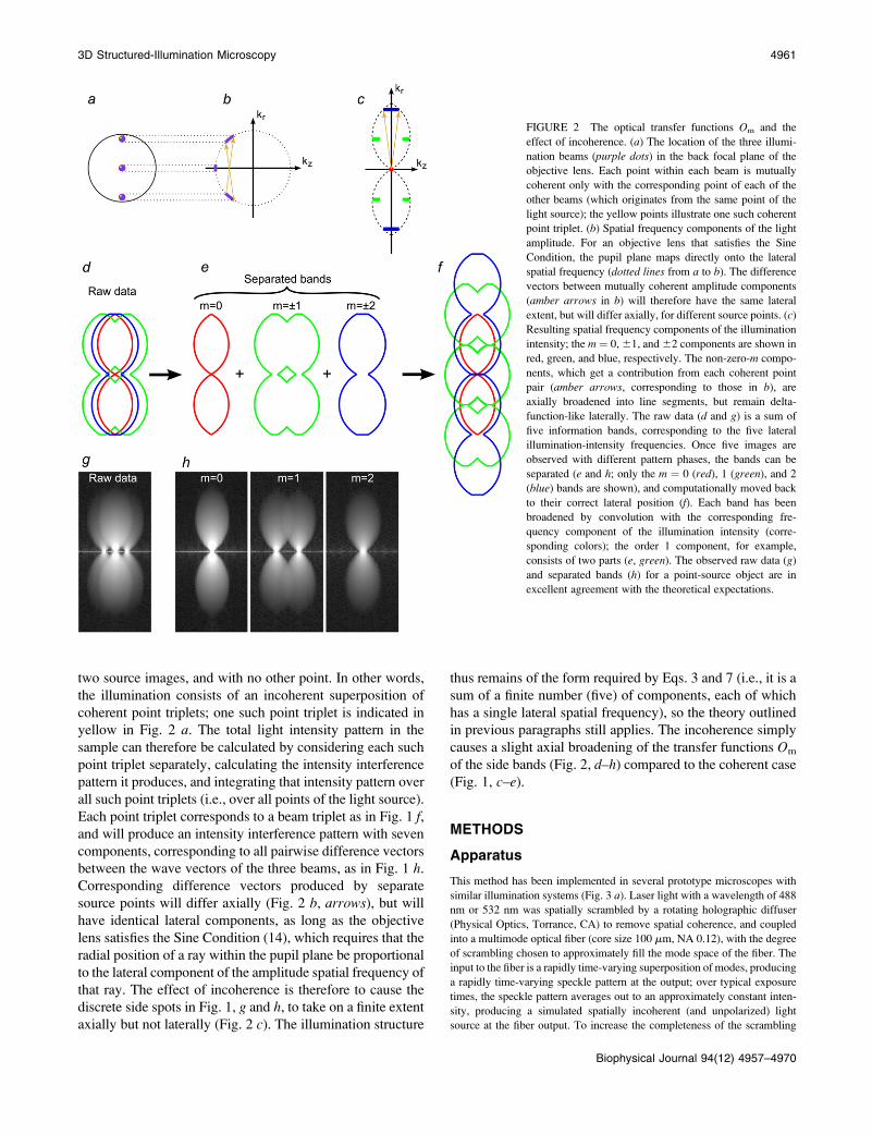
two source images, and with no other point. In other words,

the illumination consists of an incoherent superposition of

coherent point triplets; one such point triplet is indicated in

yellow in Fig. 2 a. The total light intensity pattern in the

sample can therefore be calculated by considering each such

point triplet separately, calculating the intensity interference

pattern it produces, and integrating that intensity pattern over

all such point triplets (i.e., over all points of the light source).

Each point triplet corresponds to a beam triplet as in Fig. 1 f,and will produce an intensity interference pattern with seven

components, corresponding to all pairwise difference vectors

between the wave vectors of the three beams, as in Fig. 1 h.

Corresponding difference vectors produced by separate

source points will differ axially (Fig. 2 b, arrows), but will

have identical lateral components, as long as the objective

lens satisfies the Sine Condition (14), which requires that the

radial position of a ray within the pupil plane be proportional

to the lateral component of the amplitude spatial frequency of

that ray. The effect of incoherence is therefore to cause the

discrete side spots in Fig. 1, g and h, to take on a finite extent

axially but not laterally (Fig. 2 c). The illumination structure

thus remains of the form required by Eqs. 3 and 7 (i.e., it is a

sum of a finite number (five) of components, each of which

has a single lateral spatial frequency), so the theory outlined

in previous paragraphs still applies. The incoherence simply

causes a slight axial broadening of the transfer functions Om

of the side bands (Fig. 2, d–h) compared to the coherent case

(Fig. 1, c–e).

METHODS

Apparatus

This method has been implemented in several prototype microscopes with

similar illumination systems (Fig. 3 a). Laser light with a wavelength of 488

nm or 532 nm was spatially scrambled by a rotating holographic diffuser

(Physical Optics, Torrance, CA) to remove spatial coherence, and coupled

into a multimode optical fiber (core size 100 mm, NA 0.12), with the degree

of scrambling chosen to approximately fill the mode space of the fiber. The

input to the fiber is a rapidly time-varying superposition of modes, producing

a rapidly time-varying speckle pattern at the output; over typical exposure

times, the speckle pattern averages out to an approximately constant inten-

sity, producing a simulated spatially incoherent (and unpolarized) light

source at the fiber output. To increase the completeness of the scrambling

FIGURE 2 The optical transfer functions Om and the

effect of incoherence. (a) The location of the three illumi-

nation beams (purple dots) in the back focal plane of the

objective lens. Each point within each beam is mutually

coherent only with the corresponding point of each of the

other beams (which originates from the same point of the

light source); the yellow points illustrate one such coherent

point triplet. (b) Spatial frequency components of the light

amplitude. For an objective lens that satisfies the Sine

Condition, the pupil plane maps directly onto the lateral

spatial frequency (dotted lines from a to b). The difference

vectors between mutually coherent amplitude components

(amber arrows in b) will therefore have the same lateral

extent, but will differ axially, for different source points. (c)

Resulting spatial frequency components of the illumination

intensity; the m ¼ 0, 61, and 62 components are shown in

red, green, and blue, respectively. The non-zero-m compo-

nents, which get a contribution from each coherent point

pair (amber arrows, corresponding to those in b), are

axially broadened into line segments, but remain delta-

function-like laterally. The raw data (d and g) is a sum of

five information bands, corresponding to the five lateral

illumination-intensity frequencies. Once five images are

observed with different pattern phases, the bands can be

separated (e and h; only the m ¼ 0 (red), 1 (green), and 2

(blue) bands are shown), and computationally moved back

to their correct lateral position (f). Each band has been

broadened by convolution with the corresponding fre-

quency component of the illumination intensity (corre-

sponding colors); the order 1 component, for example,

consists of two parts (e, green). The observed raw data (g)

and separated bands (h) for a point-source object are in

excellent agreement with the theoretical expectations.

3D Structured-Illumination Microscopy 4961

Biophysical Journal 94(12) 4957–4970

(the space of independent speckle patterns being averaged), a section of the

fiber was vibrated mechanically during exposure. The light exiting the fiber

was collimated and directed to a fused silica linear transmission phase

grating, which diffracted the beam into a large number of orders. A beam

block in an intermediate pupil plane discarded all diffraction orders except

orders 0 and 61; these three orders together received ;70% of the power

incident on the grating. The grating was designed so that the intensity of

order 0 was 70–80% of that of orders 61; this unequal intensity ratio was

picked to slightly strengthen the highest-lateral-frequency information

components (m¼62, blue in Fig. 2). The three beams were refocused so that

each formed an image of the fiber end-face in the back focal plane of the

objective lens. The beams produced as diffraction orders 11 and �1 were

focused near opposing edges of the back focal plane aperture, and order 0 at

its center (Fig. 2 a). The diameter of each fiber image was typically between

5% and 10% of the pupil diameter. The objective lens (1003 PlanApo 1.4

NA) recollimated the beams and made them intersect each other in the ob-

jective lens’s focal plane, where they interfered to form an illumination

intensity pattern with both axial and lateral structure (Fig. 3 b). The illumi-

nation intensity pattern in the focal plane of the objective lens can equiva-

lently be thought of as a demagnified image of the grating. Fluorescence light

emitted by the sample was gathered by the same objective lens and deflected

by a dichroic mirror to a cooled charge-coupled device camera; scattered

excitation light was rejected by an emission filter (580–630 and 500–530 nm

band pass for 532- and 488-nm excitation, respectively) in front of the

camera. Three-dimensional datasets were acquired by translating the sample

holder axially relative to the objective lens by using a piezoelectric translator

under closed-loop control from a capacitive position sensor. The orientation

and phase of the illumination pattern were controlled by rotating and later-

ally translating the grating. For this purpose, the grating was mounted on a

piezoelectric translator, which in turn was mounted on a motorized rotation

stage. The piezoelectric translator was controlled in closed loop using a

custom-made capacitive distance sensor, which consisted of one convex

electrode on one side of the grating holder, and one hollow cylindrical

counter electrode that surrounded the grating holder, each flanked by a guard

electrode. The counter electrode was rigidly attached to the optical table and

served as a fixed reference, so that the position of the grating in the direction

of its pattern wave vector could be controlled with nanometer precision and

reproducibility without placing any unusual requirements on the precision or

stability of the rotation stage bearings. The corresponding pattern-control

precision in sample space is even tighter than this, by a factor of the mag-

nification from sample plane to grating plane (typically ;100).

To interfere with maximum contrast, the illumination beams in the sample

must be s-polarized relative to each other, which corresponds to the beams

diffracted by the grating being linearly polarized perpendicularly to the plane

of diffraction. This polarization state was maintained at all orientations by a

wire-grid linear polarizer (Moxtek, Orem, UT) that co-rotated with the

grating. For pattern directions that are not parallel or perpendicular to the

dichroic mirror, the often large retardance of a standard dichroic mirror could

drastically alter the polarization state of the beams; we typically use custom

multiband dichroic coatings operated in transmission (Chroma Technology,

Rockingham, VT), which by design had small enough retardance at the laser

wavelengths that the effect on pattern contrast was negligible. The coatings

were deposited on 3.2-mm-thick optically flat substrates to preserve the

wavefront quality in the reflected imaging beam. The flatness of these mirrors

was checked interferometrically after mounting.

For ideal imaging, the grating face should be in an image plane, that is,

perfectly conjugate to the camera. To optimize this parameter, the Fourier

components of the illumination pattern were plotted as a function of z, by

measuring, at each focus setting, the changes in overall emission of a single

fluorescent bead as the pattern was phase-shifted. Guided by such mea-

surements, the axial position of the grating stage was adjusted to make the

plane of maximum pattern modulation (see Fig. 3 b) coincide with the focal

plane (defined as the plane with peak intensity of the bead image). This

parameter only needs to be aligned once (for a particular objective and

wavelength), although it can be affected by spherical aberration if imaging

deep into samples with ill-matched refractive index.

Optimal resolution is achieved when the illumination side beams traverse

the objective pupil near its edges. To optimize for different objectives (with

different pupil diameters) and wavelengths (with different diffraction angles

at the grating) therefore requires changing either the grating, or the magni-

fication between the grating plane and sample plane. We have implemented

the latter approach, by mounting intermediate lenses (or combinations of

lenses and mirrors) on interchangeable kinematic base plates, to allow quick

switching between prealigned configurations for specific wavelengths and

objectives. Prealignment includes the focusing step described in the previous

paragraph. A configuration optimized for one wavelength typically allows

operation at shorter wavelengths as well (albeit at slightly lower resolution

compared to a system optimized for the shorter wavelength). An alternative

solution would be to use zoom optics.

Sample preparation

Drops of fluorescent polystyrene microspheres (Invitrogen, Carlsbad, CA)

diluted in water were allowed to dry on cover glasses, and mounted in Laser

Liquid 5610 (R.P. Cargille Laboratories, Cedar Grove, NJ).

HL60 cells were grown and differentiated into a neutrophil-like state as

described (15), briefly stimulated with their target chemoattractant formyl-

methionyl-leucyl-phenylalanine, allowed to adhere to cover glasses, fixed

with formaldehyde, labeled for actin with rhodamine phalloidin (Invitrogen),

and mounted in 96% glycerol, 4% n-propyl gallate.

HeLa cells were grown on cover glasses, fixed with glutaraldehyde,

quenched against autofluorescence with sodium borohydride, immuno-

fluorescently labeled with anti-a-tubulin primary antibodies (DM1A,

FIGURE 3 (a) Simplified diagram of the structured illumination appara-

tus. Scrambled laser light from a multimode fiber is collimated onto a linear

phase grating. Diffraction orders –1, 0 and 11 are refocused into the back

focal plane of an objective lens. The beams, recollimated by the objective

lens, intersect at the focal plane in the sample, where they interfere and

generate an intensity pattern with both lateral and axial structure (b). The

finite axial extent of the pattern is related to the axial broadening of its spatial

frequencies (Fig. 2 c). Emission light from the sample is observed by a

charge-coupled device (CCD) camera via a dichroic mirror (DM).

4962 Gustafsson et al.

Biophysical Journal 94(12) 4957–4970

Sigma-Aldrich, St. Louis, MO) followed by Alexa-488-labeled secondary

antibodies (Invitrogen), and mounted in glycerol (16).

Maize meiocytes, released from anthers fixed with 4% paraformaldehyde

in buffer A (15 mM PIPES-NaOH (pH 6.8), 80 mM KCl, 20 mM NaCl,

2 mM EDTA, 0.5 mM EGTA, 0.2 mM spermine, 0.5 mM spermidine, 1 mM

DTT, 0.32 M sorbitol), were treated briefly with cellulase and macerozyme,

and permeabilized with 0.02% Triton X-100 in buffer A (17). The meiocytes

were prepared for indirect immunofluorescence as described (18). Cells were

stained with AFD1 antibody (19) and ASY1 antibody, kindly provided by

C. Franklin (20), which were detected with Cy3- and Alexa-488-conjugated

secondary antibodies, respectively. Slides were mounted in ProLong Gold

antifade medium (Invitrogen).

For electron microscopy, flattened spreads of pachytene chromosomes

were prepared from maize meiocytes according to published protocols (21),

and stained with silver nitrate.

Acquisition

Three-dimensional data were acquired with five pattern phases (u in Eq. 9)

spaced by 2p/5, three pattern orientations spaced 60� apart, and a focus step

of 122 or 125 nm. The axial range of the acquired data was typically made to

extend somewhat (.0.5 mm) above and below the region of interest. The

order of acquisition was to vary the phase most rapidly, then the focusing,

and the pattern rotations most slowly, thus generating a full focus/phase stack

for each orientation before proceeding to the next orientation. This order

avoids placing any angular-reproducibility requirements on the rotation

stage, and allows modest thermal drift to be measured and corrected (see

Parameter Fitting below).

Point-spread function (PSF) data was acquired similarly, including the

five phases but only one pattern orientation, on a sample consisting of a

single fluorescent microsphere. The axial range of PSF data sets was similar

to that of typical image data.

To allow fair comparisons without any questions about relative exposure

times or photobleaching, conventional-microscopy data sets for comparison

purposes were produced from the raw SIM data by summing the images

acquired at different phases of the illumination pattern. Summing over the

phase produces an image that corresponds to uniform illumination, because

the imaging process is linear and the illumination patterns themselves (Eq. 7)

add up to uniform illumination with the standard choice of pattern phases

(regularly spaced on the 0–2p interval).

The time required for acquisition varies between the different prototypes,

and of course with data set size and exposure time. One system that uses an

electron-multiplying charge-coupled device camera read out at 10 MHz can

acquire a data set comprising 80 sections of 512 3 512 pixels, each at five

phases and three orientations, with 100-ms exposure times, in 140 s. The

acquisition time is limited by the exposure time (a total of 120 s in that

example), which can be decreased by increasing the illumination intensity.

Because of the inherent parallelism of wide-field microscopy, as opposed to

point scanning, the illumination intensity could be increased by many orders

of magnitude without becoming limited by saturation.

The illumination intensity pattern (Fig. 3 b) was measured by recording

the integrated emission intensity from a subresolution microsphere as a

function of pattern phase and sample focus, and converting phase into lateral

position using the known period of the pattern.

Transfer functions

A three-dimensional point spread function data set was three-dimensionally

Fourier-transformed and separated into the terms DmðkÞ ¼ OmðkÞeium0 Sðk�mpÞ of Eq. 9, using the phase-shift method described in Theory. Because the

factor S is constant for a point source sample, and OmðkÞ ¼ O�mðkÞ by

symmetry, D1mðkÞ and D�mðkÞ are identical except for the phase factor eium0 .

That phase factor, which is irrelevant as it depends on the arbitrary position of

the bead, was estimated by comparing D1mðkÞ with D�mðkÞ; and removed.

Hence the measured Dm is effectively a measurement of Om. To decrease

noise, each Om was rotationally averaged around the kz axis and set to zero

outside of its known support.

The actual object, a fluorescent bead, was of course not a true point source

but had a nonzero diameter (typically 115–120 nm); this fact was usually

ignored, but can be compensated for by dividing the measured Om, before

rotational averaging, by Ssphðk� mpÞ; where Ssph ðkÞ is the Fourier trans-

form of a solid sphere with a diameter equal to the nominal diameter of the

bead. (Explicitly, SsphðkÞ ¼ aðpdjkjÞ where aðxÞ ¼ sinðxÞ=x3 � cosðxÞ=x2

and d is the bead diameter.) For such division to be well behaved, the first

zero of SsphðkÞ must lie well outside the extended OTF support, which is the

case for the beads used here (albeit barely).

Transfer functions need only be determined once for each combination of

objective lens and wavelength, and can be applied to all subsequent data sets

acquired on the same microscope under the same conditions.

Parameter fitting

All processing calculations were done in three dimensions where not other-

wise noted. As a precaution against edge-related artifacts, the raw data were

typically preprocessed by slightly intermixing opposing lateral edges (the

outermost ;10 pixels).

For each pattern orientation, the Fourier transform of the raw data is a sum

in the form of Eq. 9. The terms DmðkÞ ¼ OmðkÞeium0 Sðk� mpÞ of that sum

(for the starting phase of the pattern) were separated as described in Theory.

The central information component D0 is produced three times, once for each

pattern orientation; this redundancy was exploited to detect thermal drift, by

cross-correlating the three versions of D0 in real space. The measured drift

was removed by a compensating real-space shift of the data for orientations

1 and 2 relative to orientation 0, through multiplying by the corresponding

phase gradients in frequency space. Drift within each orientation was not

compensated for, but could be corrected sectionwise if known. The position

offsets for each section could be estimated either by fitting a smooth curve to

the three measured time-points of three-dimensional drift, or by using sec-

tionwise two-dimensional (or sub-volume-wise three-dimensional) cross-

correlations to get additional time points for a more precise curve fit.

The precise values of the pattern wave vector p, the starting phase um0,

and the modulation depths cm were determined from the data by comparing

the different information components in the regions of frequency space

where they overlap. The modulation depths cm are scale factors that are taken

to multiply each Om, to allow for the possibility that the contrast of each

frequency component of the pattern may be subtly different in the image data

than when the Om were measured. A single starting phase um0 was assumed

to be valid for each pattern orientation m, that is, the pattern phase was as-

sumed to be reproducible over the time required to acquire data for one

pattern orientation. Specifically, for m ¼ 1 and m ¼ 2 separately, and using

a predicted value of p, Dmðk1mpÞO0ðkÞ was cross-correlated with

D0ðkÞOmðk1mpÞ. Because each Dm contains a factor of Om from the

physical observation process, the two expressions being compared would be

expected to contain the same values SðkÞO0ðkÞOmðk1mpÞ at each point kwithin the overlap of their supports (for the correct shift vector p), except for

noise and a constant factor cmeium0 . The cross correlation was done in three

steps: first a standard fast-Fourier-transform-based cross-correlation in fre-

quency space (yielding values only at discrete frequency-space pixels), then

parabolic interpolation to locate the peak of that cross-correlation to subpixel

accuracy, and finally refinement through an optimization in which subpixel

frequency-space shifts were applied in the form of real-space phase gradi-

ents. The location of the cross-correlation peak yields the shift vector p; the

parameters cm and um0 are found by complex linear regression of

Dmðk1mpÞO0ðkÞ against D0ðkÞOmðk1mpÞ for that value of p. Explicitly,

the values of the two data sets at each pixel ki within the overlap constitute a

pair (ai,bi) of complex numbers, which in the absence of noise and errors

would be proportional to each other: bi¼ s ai. The proportionality constant s

(which here equals cmeium0 ) is estimated by complex linear regression as

+ða�i biÞ=+jaij2. (Linear regression is not strictly the optimal estimator: it

would be optimal if only bi contained noise, but in our situation both ai and bi

3D Structured-Illumination Microscopy 4963

Biophysical Journal 94(12) 4957–4970

are noisy.) In the following, the factors cmeium0 are considered absorbed into

the Om, for simplicity of notation.

Reconstruction

Once the parameters were determined, the different information components

Dm were combined through a generalized Wiener filter,

~SðkÞ ¼+d;m

O�mðk 1 mpdÞDd;mðk 1 mpdÞ

+d9;m9

jOm9ðk 1 m9pd9Þj21 w

2 AðkÞ; (11)

where ~SðkÞ is the estimate of the true sample information SðkÞ; the sums are

taken over the three pattern orientations d and the five component orders m at

each orientation, pd is the pattern wave vector (i.e., direction and inverse

period) of pattern orientation d, w2 is the Wiener parameter (which was taken

to be a constant and adjusted empirically), and A(k) is an apodization

function (typically a three-dimensional triangle function, which decreases

linearly from unity at the origin to zero at the surface of an oblate spheroid

that approximates the extended OTF support).

Eq. 11 was implemented in the following (somewhat nonintuitive) way:

each unshifted information component Dd;mðkÞwas separately multiplied by

a filter function O�mðkÞAðk� mpdÞ= +jOm9ðk1m9pd9 � mpdÞj2 1 w2� �

; and

the filtered results were then padded with zeros (to provide space for shifting

information by the vectors pd, or equivalently to decrease the real-space pixel

size to accommodate the increased resolution), transformed to real space,

multiplied by the complex phase gradient e2pimpd�r (which represents the

frequency-space shift by mpd), and added together, to produce the final re-

construction. In this calculation, the transfer function values were calculated

from the rotationally averaged measured Om by interpolation. The pixel-size

reduction is usually done laterally by a factor of two; larger factors, and axial

as well as lateral reduction, can be used to produce smoother reconstructions.

This order of operations produces noticeably better results than the

straightforward approach of first multiplying Dd;mðkÞ by O�mðkÞ; shifting the

product by mpd, combining according to Eq. 11, and retransforming to real

space. The reason has to do with edge artifacts. Because the shift vectors mpd

do not in general fall on integral pixels of the discrete frequency space, the

shifts are implemented as multiplications by the corresponding phase gra-

dients f ðrÞ ¼ e2pimpd�r in real space. Multiplying by f(r) corresponds in

frequency space to a convolution by its discrete Fourier transform f(k), which

is a discrete delta function d(k � mpd) if mpd falls on a frequency-space

pixel, but a nontrivial sinc-like function otherwise. Convolution by that

function effectively ‘‘smears’’ the information in the kx, ky, and kz directions.

This smearing is not necessarily a problem in itself, but can become dele-

terious if the smeared information is amplified during subsequent processing.

In the straightforward approach sketched above, the product SðkÞjOmðkÞj2 is

divided by the Wiener filter denominator +jOm9j2 1 w2 after it is shifted by

the vector mpd. The three-dimensional transfer functions Om9 are strongly

peaked at the origin (in fact singular in the continuum limit, in the case of O0),

and their squares of course even more so. Dividing by the Wiener denom-

inator thus boosts spatial frequencies that lie far from the origin, and from the

pattern frequencies mpd, relative to spatial frequencies that are close to those

points. Boosting those frequencies greatly amplifies any information that was

smeared into such regions by the shift operation, and this amplified smear can

lead to artifacts in the reconstruction. In the processing order used here, on

the other hand, the sample information is divided by the Wiener denominator

before the shift is executed, so that there is no amplification of smeared in-

formation.

Only the information components with nonnegative m were calculated

explicitly; the negative-m components, which are related to the positive-m

counterparts by complex-conjugate symmetry, were supplied simply by

discarding the imaginary part of the final reconstruction in real space.

Reconstruction (including data transfer and parameter fitting) of a data set

comprising 72 axial sections of 400 3 400 pixels (each at five phases and

three pattern orientations), which produces an 800 3 800 3 72 voxel re-

construction, required 138 s on a computer with two dual-core 2.2 GHz

Opteron processors. On a well-characterized and reproducible system it may

be possible to decrease processing time significantly by eliminating much of

the parameter fitting.

RESULTS

An example of a measured three-dimensional OTF data set is

shown in Fig. 2, g and h. Panel g shows a kx-kz view of a

rotationally averaged three-dimensional Fourier transform of

raw three-dimensional data acquired on a point source sam-

ple with a fixed, arbitrary phase of the illumination pattern.

The data represent a sum of contributions from all the dif-

ferent information components, as described by Eq. 8 and

illustrated schematically in Fig. 2 d. Similar data for five

different phases of the illumination pattern allowed separa-

tion of five information components (Fig. 2 h). With suffi-

cient reproducibility of the phase shifts, focus steps and

illumination intensity, separation can be near-perfect, with

negligible contamination of each information components by

others. As seen by comparison of Fig. 2, e and h, the quali-

tative shape of each information component is in complete

accordance with theoretical predictions, including the

broadening due to spatial incoherence.

To demonstrate resolution performance, a planar cluster of

red-fluorescent microspheres of nominal diameter 121 nm

was imaged with the three-dimensional structured illumina-

tion method, and compared to three-dimensional conven-

tional wide-field data (Fig. 4). As seen in the axial (xz) view

(Fig. 4 d), the structured illumination method is indeed able to

suppress the out-of-focus blur, above and below the focal

plane, which is a dominant element in the conventional mi-

croscope data (Fig. 4 c). At the same time, the in-focus xyviews (Fig. 4, a and b) illustrate the striking improvement in

lateral resolution. (In comparing these panels, it should be

kept in mind that the conventional data have not benefited

from the linear filtering that is inherent in the SIM processing.

Linear filtering is unsuitable for three-dimensional conven-

tional microscopy data due to the missing-cone problem. A

comparison of two-dimensional SIM to raw and linearly fil-

tered conventional data has been published elsewhere (22).)

Two microspheres are resolved as a pair at a separation of 125

nm, to be compared to the absolute resolution limit of the

conventional microscope, which is ;207 nm at this red ob-

servation wavelength (lem ¼ 605 6 25 nm).

To quantify the resolution, the apparent full width at half-

maximum (FWHM) of isolated green-fluorescent micro-

spheres of nominal diameter 115 nm was measured in a

separate data set acquired with lem ¼ 520 6 17.5 nm and

lexc¼ 488 nm, using a 1003 1.4 NA PlanApo objective lens,

and with the side beams centered at 92% of the pupil radius.

To allow accurate measurements, the lateral and axial pixel

dimensions of this data set were decreased during processing

by an extra factor of two compared to normal operation.

4964 Gustafsson et al.

Biophysical Journal 94(12) 4957–4970

Measurements on 100 microspheres, histogrammed in Fig. 4 e,

yielded a mean FWHM of 103.9 nm laterally and 279.5 nm

axially, with standard deviations of 1.5 nm and 2.9 nm, re-

spectively. For comparison, the theoretical frequency-space

resolution limits for three-dimensional SIM with these pa-

rameters are ;(92 nm)�1 and (265 nm)�1 in the lateral and

axial directions, respectively, and the true FWHM of a 115-

nm solid sphere is 515ðffiffiffi3p

=2Þ nm ¼ 99.6 nm.

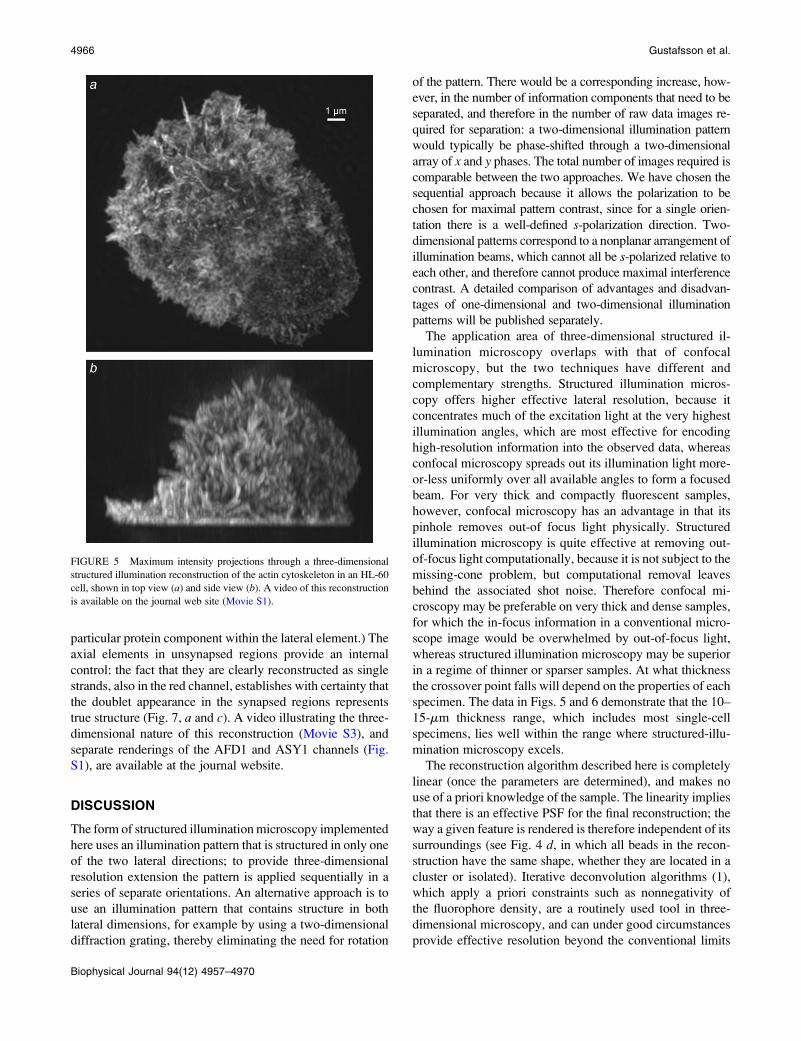
Fig. 5 and Supplementary Material, Data S1, Movie S1

show a structured illumination reconstruction of a biological

sample with complex three-dimensional structure, the actin

cytoskeleton in an HL60 cell which had been induced to dif-

ferentiate into a neutrophil-like state. The cell was exposed to a

low concentration of a bacterial peptide, formyl-methionyl-

leucyl-phenylalanine, which is a chemotactic target for neu-

trophils; this stimulated the cell to ruffle into a complex

three-dimensional shape. The images in Fig. 5 are maximum-

intensity projections through the entire volume of the cell.

As seen, the method yields a true three-dimensional recon-

struction, largely devoid of out-of-focus blur.

As a biological resolution test, we imaged the microtubule

cytoskeleton in HeLa cells (Fig. 6, Movie S2). Individual

microtubules can be followed throughout the cell volume.

Two parallel microtubules are well resolved as separate at a

distance of 125 nm (Fig. 6 b, inset) while entirely unresolved

in the conventional microscopy image generated from the

same data (Fig. 6 a, inset). To estimate the resolving power

on biological specimens, 20 microtubules were chosen at

random and their axial and lateral FWHM were measured; the

average FWHM was 120 nm laterally and 309 nm axially.

Fig. 7 shows an example of a biologically significant

structure that cannot be resolved by conventional means: the

synaptonemal complex (SC), which mediates pairing and

recombination of homologous chromosomes during meiosis

I (23). Maize meiocytes were immunofluorescently labeled in

red and green against the proteins AFD1 and ASY1, re-

spectively. Both proteins are associated with the axial/lateral

element of the SC, which forms an axis along each chro-

mosome (set of sister chromatids) before pairing, and aligns

as two parallel strands (the lateral elements), on either side of

a central element, after pairing and synapsis is complete (Fig.

7 b). The center-to-center distance between the lateral ele-

ments has been measured by electron microscopy to be ;140

nm in maize (24). With our preparation protocol, the epitope

for the ASY1 antibody becomes inaccessible for antibody

binding after synapsis, hence the lateral elements of synapsed

parts of the SC are labeled in red only, whereas unsynapsed

parts of the SC are labeled in both red and green. Separate

three-dimensional structured illumination data sets were ac-

quired in red and green, reconstructed, and merged (Fig. 7 a).

The nucleus shown was in the late zygotene stage of meiosis,

when synapsis is nearly complete. In synapsed regions, the

two lateral elements can be clearly resolved as separate and

traced through the nucleus (Fig. 7 a, c, and e), which is not

possible with conventional microscopy (Fig. 7 d and (19)).

The apparent center-center distance between the lateral ele-

ments in our reconstructions is ;170–180 nm, in reasonable

agreement with the published values based on electron mi-

crographs. (Perfect agreement is not necessarily expected,

given our gentler preparation protocol and labeling of a

FIGURE 4 A cluster of red-fluorescent microspheres of nominal diameter 0.12 mm, imaged with (a and c) conventional microscopy, and (b and d) structured

illumination microscopy. (a and b) Single in-focus x,y sections illustrating the improvement of lateral resolution. (c and d) Single x,z sections, at the y position

indicated by horizontal lines in panel a, illustrating removal of out-of-focus blur above and below the plane of focus. (e) Histograms of the apparent lateral and

axial full width at half-maximum (FWHM) of individual green-fluorescent beads observed by three-dimensional SIM.

3D Structured-Illumination Microscopy 4965

Biophysical Journal 94(12) 4957–4970

particular protein component within the lateral element.) The

axial elements in unsynapsed regions provide an internal

control: the fact that they are clearly reconstructed as single

strands, also in the red channel, establishes with certainty that

the doublet appearance in the synapsed regions represents

true structure (Fig. 7, a and c). A video illustrating the three-

dimensional nature of this reconstruction (Movie S3), and

separate renderings of the AFD1 and ASY1 channels (Fig.

S1), are available at the journal website.

DISCUSSION

The form of structured illumination microscopy implemented

here uses an illumination pattern that is structured in only one

of the two lateral directions; to provide three-dimensional

resolution extension the pattern is applied sequentially in a

series of separate orientations. An alternative approach is to

use an illumination pattern that contains structure in both

lateral dimensions, for example by using a two-dimensional

diffraction grating, thereby eliminating the need for rotation

of the pattern. There would be a corresponding increase, how-

ever, in the number of information components that need to be

separated, and therefore in the number of raw data images re-

quired for separation: a two-dimensional illumination pattern

would typically be phase-shifted through a two-dimensional

array of x and y phases. The total number of images required is

comparable between the two approaches. We have chosen the

sequential approach because it allows the polarization to be

chosen for maximal pattern contrast, since for a single orien-

tation there is a well-defined s-polarization direction. Two-

dimensional patterns correspond to a nonplanar arrangement of

illumination beams, which cannot all be s-polarized relative to

each other, and therefore cannot produce maximal interference

contrast. A detailed comparison of advantages and disadvan-

tages of one-dimensional and two-dimensional illumination

patterns will be published separately.

The application area of three-dimensional structured il-

lumination microscopy overlaps with that of confocal

microscopy, but the two techniques have different and

complementary strengths. Structured illumination micros-

copy offers higher effective lateral resolution, because it

concentrates much of the excitation light at the very highest

illumination angles, which are most effective for encoding

high-resolution information into the observed data, whereas

confocal microscopy spreads out its illumination light more-

or-less uniformly over all available angles to form a focused

beam. For very thick and compactly fluorescent samples,

however, confocal microscopy has an advantage in that its

pinhole removes out-of focus light physically. Structured

illumination microscopy is quite effective at removing out-

of-focus light computationally, because it is not subject to the

missing-cone problem, but computational removal leaves

behind the associated shot noise. Therefore confocal mi-

croscopy may be preferable on very thick and dense samples,

for which the in-focus information in a conventional micro-

scope image would be overwhelmed by out-of-focus light,

whereas structured illumination microscopy may be superior

in a regime of thinner or sparser samples. At what thickness

the crossover point falls will depend on the properties of each

specimen. The data in Figs. 5 and 6 demonstrate that the 10–

15-mm thickness range, which includes most single-cell

specimens, lies well within the range where structured-illu-

mination microscopy excels.

The reconstruction algorithm described here is completely

linear (once the parameters are determined), and makes no

use of a priori knowledge of the sample. The linearity implies

that there is an effective PSF for the final reconstruction; the

way a given feature is rendered is therefore independent of its

surroundings (see Fig. 4 d, in which all beads in the recon-

struction have the same shape, whether they are located in a

cluster or isolated). Iterative deconvolution algorithms (1),

which apply a priori constraints such as nonnegativity of

the fluorophore density, are a routinely used tool in three-

dimensional microscopy, and can under good circumstances

provide effective resolution beyond the conventional limits

FIGURE 5 Maximum intensity projections through a three-dimensional

structured illumination reconstruction of the actin cytoskeleton in an HL-60

cell, shown in top view (a) and side view (b). A video of this reconstruction

is available on the journal web site (Movie S1).

4966 Gustafsson et al.

Biophysical Journal 94(12) 4957–4970

(25). Such methods could also be applied to SIM data, and

could be expected to provide similar benefits, at the expense

of making the reconstruction of a given structure depend on

its surroundings. In this article we have avoided all use of

constraints, to eliminate any possibility of confusion between

actual measurement of new high-resolution information by

SIM, and extrapolation beyond the measured information

based on constrained deconvolution.

As described above, structured illumination can be thought

of as generated by interference of two or more mutually co-

herent beams. There are two main approaches to generating

such beams: through diffractive beam splitting with a mask,

grating, or other patterned device (5,6,8–10), which was used

in this article, or by reflective beam splitting (7,26,28). Each

method has advantages and disadvantages. Reflective beam

splitting has an advantage for multicolor applications in that

FIGURE 6 The microtubule cytoskeleton in HeLa cells. Axial maximum-intensity projections, using conventional microscopy (a) and structured-

illumination microscopy (b), through a 244-nm-thick subset of the data (two sections). (Insets) two parallel microtubules spaced by 125 nm (arrows) are well

resolved in the structured illumination reconstruction, but unresolved by conventional microscopy. The image contrast of the inset in a has been adjusted, for

easier comparison. (c) Cross-eyed stereo view of projections through the structured-illumination reconstruction. The data value of each voxel controlled both

the brightness and the opacity of that voxel in the rendering. A video of this reconstruction is available on the journal web site (Movie S2).

3D Structured-Illumination Microscopy 4967

Biophysical Journal 94(12) 4957–4970

the positions of the illumination beams in the pupil plane can

be made independent of their wavelength, whereas with

diffractive beam splitting the distance of a beam from the

pupil center is typically proportional to its wavelength and

can therefore be strictly optimized only for one wavelength at

a time. (Multiwavelength data sets can still be taken, by op-

timizing for the longest wavelength, with only minor per-

formance penalties at the shorter wavelength channels (see

Fig. 7).) On the other hand, reflective beam splitting has a

severe disadvantage in that it typically causes the beams to be

separated spatially and handled by separate optical compo-

nents (mirrors, etc.); any nanometer-scale drift of any such

component translates directly into a phase error in the data.

With diffractive beam splitting, by contrast, all beams typi-

FIGURE 7 The synaptonemal complex (SC) in a maize meiocyte nucleus during the late zygotene stage of meiosis. Fixed meiocytes were immunofluo-

rescently labeled for the axial/lateral element components AFD1 (red fluorescence, here displayed as magenta) and ASY1 (green) of the synaptonemal

complex. Under the fixation conditions used, the ASY1 epitope is inaccessible to the antibodies when synapsis is complete; the synapsed regions therefore

fluoresce only in red, whereas the unsynapsed regions fluoresce in both green and red. In fully synapsed chromosomes, the lateral elements align as two parallel

strands separated by ;170 nm. (a) Maximum-intensity projection through a three-dimensional structured-illumination reconstruction of an entire nucleus (data

set thickness, 8 mm). Separate renderings of the AFD1 and ASY1 channels of this image are available on the journal website (Fig. S1). (b) Transmission

electron micrograph of a silver-stained chromosome-spread preparation of a maize pachytene meiocyte, showing the three elements of the SC surrounded by

the paired chromosomes. (LE, lateral elements; CE, central element; Ch, chromatin.) (c) Magnification of the cyan-boxed region, maximum-intensity-projected

through 1.5 mm of the sample thickness, showing a transition from unpaired to paired SC (arrows). (d and e) Magnifications of the white-boxed region of the

specimen, imaged with conventional microscopy (d) or structured illumination microscopy (e). Panels d and e show maximum-intensity projections of only

three axial sections, representing 375 nm of sample thickness, to avoid unnecessary blur in the conventional image. The lateral elements in synapsed regions,

which are unresolvable by conventional microscopy (d), are well resolved by structured illumination microscopy (a, c, and e), and the twisting of the two

strands around each other can be clearly followed (e, compare with b). A video of this reconstruction is available on the journal web site (Movie S3).

4968 Gustafsson et al.

Biophysical Journal 94(12) 4957–4970

cally traverse the same optical components in an essentially

common-path geometry, which decreases the sensitivity to

component drift by several orders of magnitude. In addition,

reflective beam splitting typically requires separate mirror

sets for each pattern orientation, which becomes increasingly

bulky as the number of pattern orientations increases; for this

reason the approach has so far only been implemented for one

(26,28) or two (7) pattern orientations, which is insufficient

for isotropic resolution, and can force a tradeoff between

resolution and anisotropy (7).

Since live microscopy is an area of much current excite-

ment, it is important to consider to what extent three-

dimensional SIM can be applied to live samples. The prin-

ciples are fully compatible with living samples, assuming that

a water-immersion objective lens is used to avoid unneces-

sary aberrations. Apart from the usual limits to total exposure

set by photobleaching and phototoxicity, the only additional

limitation relates to motion. The current algorithm treats the

sample as an unchanging three-dimensional structure, and

could therefore produce artifacts if substantial motion were to

occur within the sample during data acquisition. As im-

plemented here, three-dimensional SIM uses 15 raw images

per axial section, and spaces the axial sections by typically

125 nm to provide Nyquist sampling relative to its axial

resolution of ,300 nm. This corresponds to 120 exposures

per mm of data volume thickness; a data set of a thick three-

dimensional sample can thus entail .1000 raw images. Even

with a high-speed camera and rapid pattern generation

hardware, such data sets could take seconds or minutes to

acquire, a timescale during which many biological systems

will undergo internal movements many times larger than the

resolution scale of SIM. Sensitivity to motion can be de-

creased somewhat by using an acquisition order in which all

images of a certain focal plane (for all pattern orientations as

well as phases) are acquired before refocusing; in that mode,

the time frame during which motion must be avoided may be

decreased from that of the full data set to the time required to

record a sample thickness corresponding to the axial extent of

pattern modulation (see Fig. 3 b). Both limitations—motion

and photobleaching/phototoxicity—become proportionately

less stringent for thinner samples. Live imaging at SIM res-

olution should be quite feasible on a class of thin samples.

At the thin limit, some structures could be treated as two-

dimensional, including any sample viewed in total internal

reflection mode and some structures such as lamellipodia that

are naturally thinner than the conventional depth of field.

SIM is fully compatible with the total internal reflection

mode, as has recently been demonstrated in one dimension

(26). With appropriate hardware, it should be possible to

acquire time-sequence data of such samples by two-dimen-

sional SIM at frame rates in the Hz range.

The algorithm described assumes that the three-dimen-

sional data include the entire emitting object. If the data

contain strong light that originates from beyond the edges of

the imaged volume, artifacts could be expected to arise. We

have reconstructed such data sets without major problems,

using the processing order and other precautions outlined in

Methods, but whenever possible we include the whole object

of interest in the data set, and ideally a few out-of-focus

sections above and below, to avoid this issue.

The method described in this article assumes a normal,

linear relationship between the illumination intensity and the

fluorescent emission rate, and achieves approximately a factor

of two of resolution extension. It is known that two-dimen-

sional wide-field resolution can be extended much further if

the sample can be made to respond nonlinearly to illumination

light (22,27,28). That concept, nonlinear structured illumi-

nation microscopy, can in principle be applied to the three-

dimensional method described here in much the same way as

it is used in two dimensions, and could enhance axial as well

as lateral resolution. The main limitation is that the require-

ment for photostability of the fluorophores, already signifi-

cant in two dimensions, would increase in proportion to the

number of sections. The same concern, of dividing the avail-

able phototolerance over the sections when going from two-

dimensional to three-dimensional imaging, may also affect

other recent methods that have demonstrated very high res-

olution in two dimensions, such as PALM/FPALM/STORM

(29–31). Highly nonlinear point-scanning methods such as

STED (32) may be less subject to this effect, especially if using

multiphoton excitation, to the extent that photodegradation

can be confined to a small axial range near the focal plane.

The axial resolution of the conventional microscope is

worse than the lateral resolution by a factor of approximately

three (for high-NA objective lenses). The same anisotropy

also applies to three-dimensional SIM as described here,

which extends resolution by the same factor in all dimensions.

However, the structured illumination concept is compatible

with the opposing-objective-lens geometry of I5M, which

allows access a much greater axial resolution (33). A

straightforward combination of three-dimensional SIM and

I5M, called I5S, can yield nearly isotropic three-dimensional

imaging resolution in the 100-nm range (34).

In conclusion, three-dimensional structured-illumination

microscopy can produce multicolor three-dimensional imag-

ing reconstructions of fluorescently-labeled specimens with a

lateral resolution, approaching 100 nm, which is unavailable

in practice with conventional methods of three-dimensional

light microscopy. At the same time it can provide axial res-

olution ,300 nm, and remove out-of-focus blur determin-

istically. We believe that it has an important role to play in

cell biology.

SUPPLEMENTARY MATERIAL

To view all of the supplemental files associated with this

article, visit www.biophysj.org.

We thank Lukman Winoto, Sebastian Haase, and the late Melvin Jones for

contributions to hardware and software; Orion Weiner for preparing the

3D Structured-Illumination Microscopy 4969

Biophysical Journal 94(12) 4957–4970

HL-60 cells; Emerick Gallego, Yuri Strukov, and Lifeng Xu for assistance

with cell culture; and C. Franklin for providing the ASY1 antibody.

This work was supported in part by the David and Lucile Packard

Foundation, the Keck Laboratory for Advanced Microscopy, the Sandler

Family Supporting Foundation, the National Institutes of Health (grant No.

GM25101 to J.W.S., grant No. GM31627 to D.A.A., and grant No.

GM48547 to W.Z.C.), the Burroughs Wellcome Fund’s Interfaces in

Science Program, and the National Science Foundation through the Center

for Biophotonics, a National Science Foundation Science and Technology

Center that is managed by the University of California, Davis, under

Cooperative Agreement No. PHY 0120999.

REFERENCES

1. Agard, D. A., Y. Hiraoka, P. Shaw, and J. W. Sedat. 1989. Fluores-cence microscopy in three dimensions. Methods Cell Biol. 30:353–377.

2. Pawley, J. B. 2006. Handbook of Biological Confocal Microscopy.Plenum Press, New York.

3. Diaspro, A. 2002. Confocal and Two-Photon Microscopy: Founda-tions, Applications, and Advances. Wiley-Liss, New York.

4. Wilson, T. 1995. The role of the pinhole in confocal imaging system.In Handbook of Biological Confocal Microscopy. J. B. Pawley, editor.Plenum Press, New York.

5. Gustafsson, M. G. L. 2000. Surpassing the lateral resolution limit by afactor of two using structured illumination microscopy. J. Microsc.198:82–87.

6. Heintzmann, R., and C. Cremer. 1998. Laterally modulated excitationmicroscopy: improvement of resolution by using a diffraction grating.Proc. SPIE. 3568:185–195.

7. Frohn, J. T., H. F. Knapp, and A. Stemmer. 2000. True optical reso-lution beyond the Rayleigh limit achieved by standing wave illumina-tion. Proc. Natl. Acad. Sci. USA. 97:7232–7236.

8. Gustafsson, M. G. L., D. A. Agard, and J. W. Sedat. 2000. Doublingthe lateral resolution of wide-field fluorescence microscopy using struc-tured illumination. Proc. SPIE. 3919:141–150.

9. Neil, M. A. A., R. Juskaitis, and T. Wilson. 1997. Method of obtainingoptical sectioning by using structured light in a conventional micro-scope. Opt. Lett. 22:1905–1907.

10. Neil, M. A. A., R. Juskaitis, and T. Wilson. 1998. Real time 3Dfluorescence microscopy by two beam interference illumination. Opt.Commun. 153:1–4.

11. Bailey, B., D. L. Farkas, D. L. Taylor, and F. Lanni. 1993. Enhance-ment of axial resolution in fluorescence microscopy by standing-waveexcitation. Nature. 366:44–48.

12. Gustafsson, M. G. L., D. A. Agard, and J. W. Sedat. Method andapparatus for three-dimensional microscopy with enhanced resolution.US Patent RE38,307E. Filed 1995, reissued 2003.

13. Frohn, J. T., H. F. Knapp, and A. Stemmer. 2001. Three-dimensionalresolution enhancement in fluorescence microscopy by harmonicexcitation. Opt. Lett. 26:828–830.

14. Hecht, E. 1990. Optics, 2nd Ed. Addison-Wesley, Reading, Massachusetts.

15. Weiner, O. D., M. C. Rentel, A. Ott, G. E. Brown, M. Jedrychowski,M. B. Yaffe, S. P. Gygi, L. C. Cantley, H. R. Bourne, and M. W.Kirschner. 2006. Hem-1 complexes are essential for Rac activation,actin polymerization, and myosin regulation during neutrophil chemo-taxis. PLoS Biol. 4:e38.

16. Mitchison Laboratory protocols on fluorescence procedures for theactin and tubulin cytoskeleton in fixed cells. Http://mitchison.med.harvard.edu/protocols/gen1.html.

17. Dernburg, A. F., J. W. Sedat, and R. S. Hawley. 1996. Direct evidenceof a role for heterochromatin in meiotic chromosome segregation. Cell.86:135–146.

18. Golubovskaya, I. N., L. C. Harper, W. P. Pawlowski, D. Schichnes,and W. Z. Cande. 2002. The pam1 gene is required for meiotic bouquetformation and efficient homologous synapsis in maize (Zea mays L.).Genetics. 162:1979–1993.

19. Golubovskaya, I. N., O. Hamant, L. Timofejeva, C.-J. R. Wang, D.Braun, R. Meeley, and W. Z. Cande. 2006. Alleles of afd1 dissectREC8 functions during meiotic prophase I. J. Cell Sci. 119:3306–3315.

20. Armstrong, S. J., A. P. Caryl, G. H. Jones, and F. C. Franklin. 2002.Asy1, a protein required for meiotic chromosome synapsis, localizes toaxis-associated chromatin in Arabidopsis and Brassica. J. Cell Sci.115:3645–3655.

21. Gillies, C. B. 1981. Electron microscopy of spread maize pachytenesynaptonemal complexes. Chromosoma. 83:575–591.

22. Gustafsson, M. G. L. 2005. Nonlinear structured-illumination micros-copy: wide-field fluorescence imaging with theoretically unlimitedresolution. Proc. Natl. Acad. Sci. USA. 102:13081–13086.

23. Page, S. L., and R. S. Hawley. 2004. The genetics and molecularbiology of the synaptonemal complex. Annu. Rev. Cell Dev. Biol. 20:525–558.

24. Gillies, C. B. 1973. Ultrastructural analysis of maize pachytenekaryotypes by three dimensional reconstruction of the synaptonemalcomplexes. Chromosoma. 43:145–176.

25. Carrington, W. A., R. M. Lynch, E. D. Moore, G. Isenberg, K. E.Fogarty, and F. S. Fay. 1995. Super-resolution three-dimensionalimages of fluorescence in cells with minimal light exposure. Science.268:1483–1487.

26. Chung, E., D. Kim, Y. Cui, Y.-H. Kim, and P. T. C. So. 2007. Two-dimensional standing wave total internal reflection fluorescence mi-croscopy: superresolution imaging of single molecular and biologicalspecimens. Biophys. J. 93:1747–1757.

27. Heintzmann, R., T. M. Jovin, and C. Cremer. 2002. Saturated patternedexcitation microscopy—a concept for optical resolution improvement.J. Opt. Soc. Am. A. 19:1599–1609.

28. Schwentker, M. A., H. Bock, M. Hofmann, S. Jakobs, J. Bewersdorf,C. Eggeling, and S. W. Hell. 2007. Wide-field subdiffraction RE-SOLFT microscopy using fluorescent protein photoswitching. Microsc.Res. Tech. 70:269–280.

29. Betzig, E., G. H. Patterson, R. Sougrat, O. W. Lindwasser, S. Olenych,J. S. Bonifacino, M. W. Davidson, J. Lippincott-Schwartz, and H. F.Hess. 2006. Imaging intracellular fluorescent proteins at nanometerresolution. Science. 313:1642–1645.

30. Hess, S. T., T. P. Girirajan, and M. D. Mason. 2006. Ultra-highresolution imaging by fluorescence photoactivation localization mi-croscopy. Biophys. J. 91:4258–4272.

31. Rust, J. M., M. Bates, and X. Zhuang. 2006. Sub-diffraction-limitimaging by stochastic optical reconstruction microscopy (STORM).Nat. Methods. 3:793–795.

32. Klar, T. A., S. Jakobs, M. Dyba, A. Egner, and S. W. Hell. 2000.Fluorescence microscopy with diffraction resolution barrier bro-ken by stimulated emission. Proc. Natl. Acad. Sci. USA. 97:8206–8210.

33. Gustafsson, M. G. L., D. A. Agard, and J. W. Sedat. 1999. I5M: 3Dwidefield light microscopy with better than 100 nm axial resolution.J. Microsc. 195:10–16.

34. Shao, L., B. Isaac, S. Uzawa, D. A. Agard, J. W. Sedat, andM. G. L. Gustafsson. 2008. I5S: Wide-field light microscopy with100-nm-scale resolution in three dimensions. Biophys. J. 94:4971–4983.

4970 Gustafsson et al.

Biophysical Journal 94(12) 4957–4970