Three-dimensional limit analysis of rigid blocks assemblages. Part II: Load-path following solution...

International Journal of Solids and Structures 42 (2005) 5161–5180

www.elsevier.com/locate/ijsolstr

Three-dimensional limit analysis of rigid blocksassemblages. Part II: Load-path following

solution procedure and validation

A. Ordu~na *, P.B. Lourenco

Department of Civil Engineering, University of Minho, Azurem, 4800-058 Guimaraes, Portugal

Received 7 July 2004; received in revised form 8 February 2005Available online 17 March 2005

Abstract

A novel solution procedure for the non-associated limit analysis of rigid blocks assemblages is proposed. This pro-posal produces better solutions than previously proposed procedures and it is also able to provide an insight into thestructural behaviour prior to failure. The limit analysis model proposed in Part I of this paper and the solution proce-dure are validated through illustrative examples in three-dimensional masonry piers and walls. The use of limit analysisfor three-dimensional problems incorporating non-associated flow rules and a coupled yield surface is novel in theliterature.� 2005 Elsevier Ltd. All rights reserved.

Keywords: Limit analysis; Non-associated flow rule; Rigid block; Non-linear optimisation

1. Introduction

In the first part of this paper (Orduna and Lourenco, 2005), a complete limit analysis formulation forrigid block assemblages was presented. In this formulation, it was accepted that the rigid blocks interactthrough quadrilateral interfaces without tensile strength and cohesion, that the non-associated Coulombcriterion governs the shearing failure, and that the compressive stresses are limited. In the developmentof this model, the plastic torsion on frictional interfaces was studied, and a piecewise linear yield functionfor rectangular interfaces was proposed together with a model for the hinging yield mode.

0020-7683/$ - see front matter � 2005 Elsevier Ltd. All rights reserved.doi:10.1016/j.ijsolstr.2005.02.011

* Corresponding author. Present address: Faculty of Civil Engineering, University of Colima, km 9, Colima-Coquimatlan way28400, Mexico. Tel./fax: +52 312 316 1167.

E-mail address: [email protected] (A. Ordu~na).

mailto:[email protected]

5162 A. Ordu~na, P.B. Lourenco / International Journal of Solids and Structures 42 (2005) 5161–5180

The standard material model (with associated flow rules) introduces important theoretical simplificationsto limit analysis. The most significant result, perhaps, is the uniqueness of the ultimate load factor, definedas the ratio between the variable loads causing the collapse and their nominal values. Besides, non-standardmaterials were studied since the early limit analysis development stages; see for instance Palmer, 1966. Morerecent investigations include those of Corigliano and Maier (1995), Boulbibane and Weichert (1997) and DeSaxce and Bousshine (1998). A constant in all these investigations is the lack of unique solutions for limitanalysis problems in the presence of non-associated flow rules.

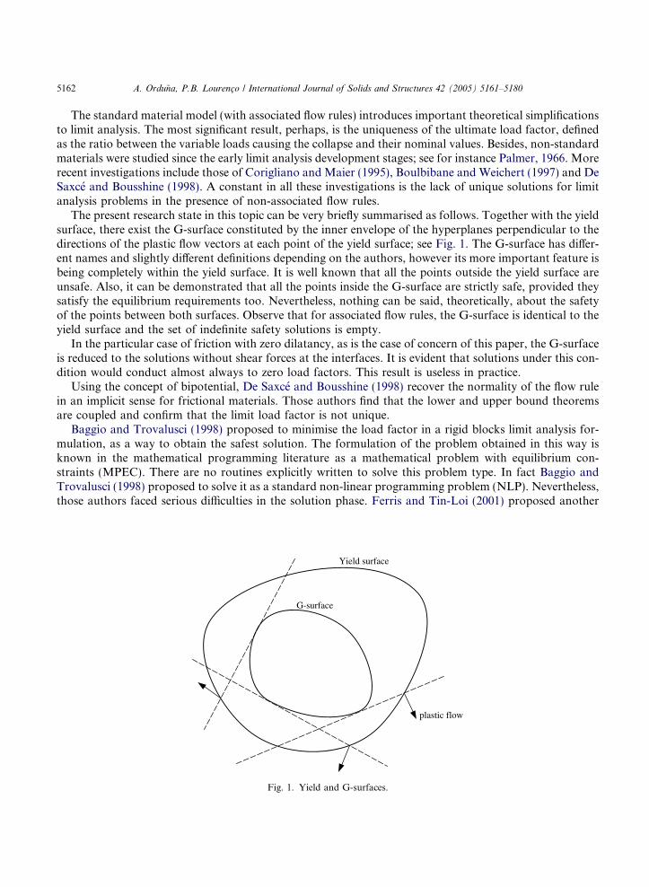
The present research state in this topic can be very briefly summarised as follows. Together with the yieldsurface, there exist the G-surface constituted by the inner envelope of the hyperplanes perpendicular to thedirections of the plastic flow vectors at each point of the yield surface; see Fig. 1. The G-surface has differ-ent names and slightly different definitions depending on the authors, however its more important feature isbeing completely within the yield surface. It is well known that all the points outside the yield surface areunsafe. Also, it can be demonstrated that all the points inside the G-surface are strictly safe, provided theysatisfy the equilibrium requirements too. Nevertheless, nothing can be said, theoretically, about the safetyof the points between both surfaces. Observe that for associated flow rules, the G-surface is identical to theyield surface and the set of indefinite safety solutions is empty.

In the particular case of friction with zero dilatancy, as is the case of concern of this paper, the G-surfaceis reduced to the solutions without shear forces at the interfaces. It is evident that solutions under this con-dition would conduct almost always to zero load factors. This result is useless in practice.

Using the concept of bipotential, De Saxce and Bousshine (1998) recover the normality of the flow rulein an implicit sense for frictional materials. Those authors find that the lower and upper bound theoremsare coupled and confirm that the limit load factor is not unique.

Baggio and Trovalusci (1998) proposed to minimise the load factor in a rigid blocks limit analysis for-mulation, as a way to obtain the safest solution. The formulation of the problem obtained in this way isknown in the mathematical programming literature as a mathematical problem with equilibrium con-straints (MPEC). There are no routines explicitly written to solve this problem type. In fact Baggio andTrovalusci (1998) proposed to solve it as a standard non-linear programming problem (NLP). Nevertheless,those authors faced serious difficulties in the solution phase. Ferris and Tin-Loi (2001) proposed another

G-surface

Yield surface

plastic flow

Fig. 1. Yield and G-surfaces.

A. Ordu~na, P.B. Lourenco / International Journal of Solids and Structures 42 (2005) 5161–5180 5163

solution strategy in order to minimise the load factor taking advantage of routines explicitly written forsolving mixed complementarity problems (MCP), which is a problem type akin to the MPEC. The maindisadvantage of the approach consisting on minimising the load factor is that the resulting ultimate loadfactor can severely underestimate its true value.

In this paper, a novel solution procedure is proposed for the non-associated limit analysis of rigid blocksassemblages. This procedure follows, in an approximate manner, the loading history on the structure. Theprocedure is useful in providing a good understanding of the structural behaviour before and at failure.And, more important, the procedure provides better solutions than minimising the load factor. Finally,both the limit analysis model and the solution procedure are validated through three illustrative examples.It is noted that the solution of three-dimensional limit analysis problems involving non-associated flow andcoupled failure surfaces seems to be novel in the literature.

2. The limit analysis problem

Eqs. (1)–(6) are the conditions that a limit analysis solution with non-associated flow rule must fulfil.Eq. (1) combines the compatibility and flow rule conditions. Here, ~N 0 is a matrix, which columns con-tain the flow directions corresponding to each yield mode; the vector d~k contains the flow multipliers forthe yield modes; ~C is the compatibility matrix and the vector d~u contains the displacement rates for allthe blocks in the model. Eq. (2) is a scaling condition for the displacement rates that ensures the exis-tence of non-zero but finite values. Here, ~F v is the vector of variable loads applied on the centroid ofeach block. Eq. (3) is the equilibrium condition. Here, ~F c is the constant loads vector; a is the load fac-tor, measuring the amount of variable load applied on the structure, and ~Q is the vector of generalisedstresses at the interfaces. Eq. (4) guarantees that the yield functions, ~u, are not violated. Eq. (5) ensuresthat the plastic flow multipliers are non-negative, which means that flow implies energy dissipation. Fi-nally, Eq. (6) guarantees that plastic flow cannot occur unless the stresses have reached the yield surface.A more detailed description of the limit analysis mathematical problem is addressed in Ordu~na andLourenco (2005).

~N 0d~k � ~Cd~u ¼~0 ð1Þ

~FT

v � d~u� 1 ¼ 0 ð2Þ

~F c þ a~F v � ~CT~Q ¼~0 ð3Þ

~u 6~0 ð4Þ

d~k P~0 ð5Þ

~uT � d~k ¼ 0 ð6Þ

This set of equations represents a case known in the mathematical programming literature as a mixed com-plementarity problem (MCP) (Ferris and Tin-Loi, 2001). In general, there is no unique solution for thisproblem in the presence of non-associated flow rules. If the load factor is minimised, as proposed by Baggioand Trovalusci (1998), the solution can severely underestimate the ultimate load factor, as it will be shownby the validation examples of the present paper.


3. The load-path following solution procedure

In this section a load-path following procedure is proposed using the available solution tools. This pro-cedure uses the same limited information as classic limit analysis (no stiffness or softening parameters areneeded) and, at the same time, provides an insight into the structural behaviour prior to failure. Neverthe-less, the most important feature of this procedure is that it provides better solutions, in terms of both failuremechanism and load factor, than the traditional proposal of minimising the load factor.

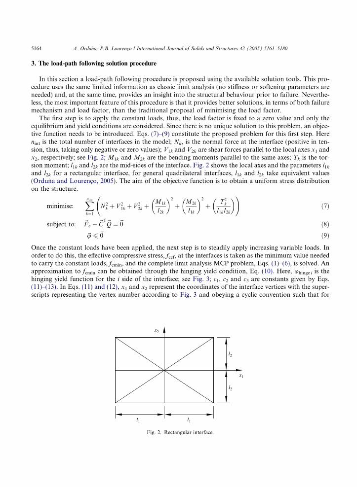
The first step is to apply the constant loads, thus, the load factor is fixed to a zero value and only theequilibrium and yield conditions are considered. Since there is no unique solution to this problem, an objec-tive function needs to be introduced. Eqs. (7)–(9) constitute the proposed problem for this first step. Herenint is the total number of interfaces in the model; Nk, is the normal force at the interface (positive in ten-sion, thus, taking only negative or zero values); V1k and V2k are shear forces parallel to the local axes x1 andx2, respectively; see Fig. 2; M1k and M2k are the bending moments parallel to the same axes; Tk is the tor-sion moment; l1k and l2k are the mid-sides of the interface. Fig. 2 shows the local axes and the parameters l1kand l2k for a rectangular interface, for general quadrilateral interfaces, l1k and l2k take equivalent values(Orduna and Lourenco, 2005). The aim of the objective function is to obtain a uniform stress distributionon the structure.

minimise:Xnintk¼1

N 2k þ V 2

1k þ V 22k þ

M1k

l2k

� �2

þ M2k

l1k

� �2

þ T 2k

l1kl2k

� � !ð7Þ

subject to: ~F c � ~CT~Q ¼~0 ð8Þ

~u 6~0 ð9Þ

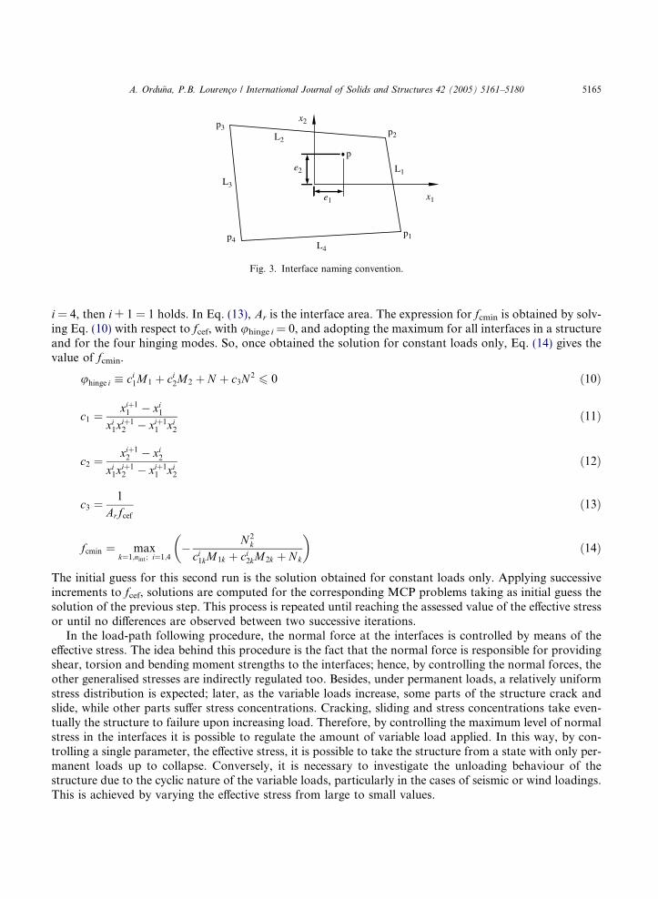
Once the constant loads have been applied, the next step is to steadily apply increasing variable loads. Inorder to do this, the effective compressive stress, fcef, at the interfaces is taken as the minimum value neededto carry the constant loads, fcmin, and the complete limit analysis MCP problem, Eqs. (1)–(6), is solved. Anapproximation to fcmin can be obtained through the hinging yield condition, Eq. (10). Here, uhinge i is thehinging yield function for the i side of the interface; see Fig. 3; c1, c2 and c3 are constants given by Eqs.(11)–(13). In Eqs. (11) and (12), x1 and x2 represent the coordinates of the interface vertices with the super-scripts representing the vertex number according to Fig. 3 and obeying a cyclic convention such that for

l1 l1

l2

l2

x2

x1

Fig. 2. Rectangular interface.

x1

x2

p1

p2p3

p4

L1

L2

L3

L4

e2

e1

p

Fig. 3. Interface naming convention.


i = 4, then i + 1 = 1 holds. In Eq. (13), Ar is the interface area. The expression for fcmin is obtained by solv-ing Eq. (10) with respect to fcef, with uhinge i = 0, and adopting the maximum for all interfaces in a structureand for the four hinging modes. So, once obtained the solution for constant loads only, Eq. (14) gives thevalue of fcmin.

uhinge i � ci1M1 þ ci2M2 þ N þ c3N 26 0 ð10Þ

c1 ¼xiþ11 � xi1

xi1xiþ12 � xiþ1

1 xi2ð11Þ

c2 ¼xiþ12 � xi2

xi1xiþ12 � xiþ1

1 xi2ð12Þ

c3 ¼1

Arfcefð13Þ

fcmin ¼ maxk¼1;nint ; i¼1;4

� N 2k

ci1kM1k þ ci2kM2k þ Nk

� �ð14Þ

The initial guess for this second run is the solution obtained for constant loads only. Applying successiveincrements to fcef, solutions are computed for the corresponding MCP problems taking as initial guess thesolution of the previous step. This process is repeated until reaching the assessed value of the effective stressor until no differences are observed between two successive iterations.

In the load-path following procedure, the normal force at the interfaces is controlled by means of theeffective stress. The idea behind this procedure is the fact that the normal force is responsible for providingshear, torsion and bending moment strengths to the interfaces; hence, by controlling the normal forces, theother generalised stresses are indirectly regulated too. Besides, under permanent loads, a relatively uniformstress distribution is expected; later, as the variable loads increase, some parts of the structure crack andslide, while other parts suffer stress concentrations. Cracking, sliding and stress concentrations take even-tually the structure to failure upon increasing load. Therefore, by controlling the maximum level of normalstress in the interfaces it is possible to regulate the amount of variable load applied. In this way, by con-trolling a single parameter, the effective stress, it is possible to take the structure from a state with only per-manent loads up to collapse. Conversely, it is necessary to investigate the unloading behaviour of thestructure due to the cyclic nature of the variable loads, particularly in the cases of seismic or wind loadings.This is achieved by varying the effective stress from large to small values.


The proposed procedure is summarised here:

(1) Solve the constant loads problem, Eqs. (7)–(9) with fcef = 1.(2) Increasing fcef. Calculate fcmin by using Eq. (14). Make f0 = fcmin. Establish the maximum effective

stress fcmax to stop the calculations and perform the following loop:
For i = 1,2, . . .fi = ffi�1
solve Eqs. (1)–(6) with fcef = fiif fi P fcmax, stop

(3) Decreasing fcef. Make f0 = fcmax and perform the following loop:
For i = 1,2, . . .fi = fi�1/fsolve Eqs. (1)–(6) with fcef = fiif fi 6 fcmin, stop
Here f is a factor to exponentially increase or decrease the effective stress for successive calculations. Thisparameter must be larger than one, and recommended values, according to the authors experience, are1.1 6 f 6 1.4. The examples shown in this paper were solved by means of a programme made using theGAMS modelling environment (Brooke et al., 1998).

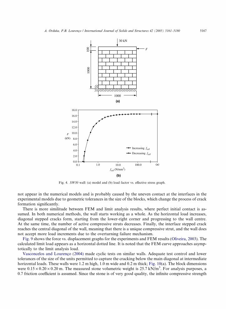
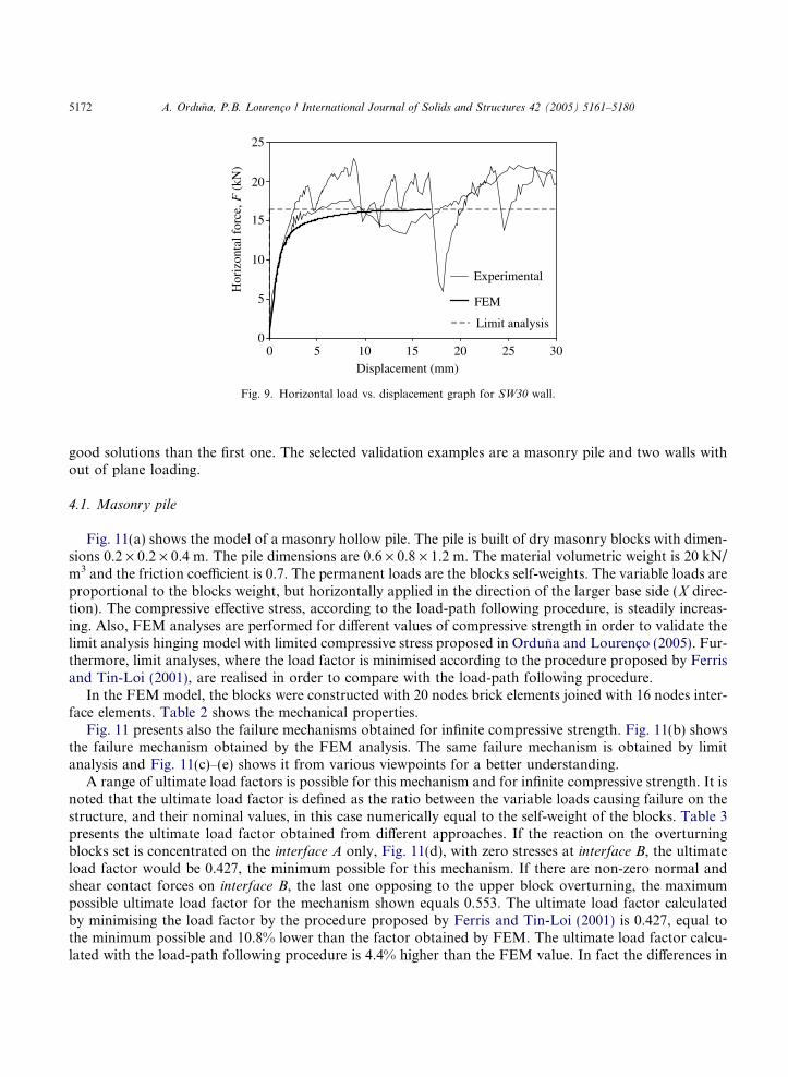
In order to illustrate the application and the kind of results obtained by the load-path following procedure,a two-dimensional model is presented. The two-dimensional limit analysis approachwas presented in Ordunaand Lourenco (2003) and the model is the SW30 shear wall presented in that paper. The wall corresponds to aseries of tests performed by Oliveira (2003) on shear walls made of dry jointed, stone block masonry underdifferent levels of vertical load and monotonically increasing lateral load; Fig. 4(a). The wall size was1000 · 1000 mm, with a thickness of 200 mm. The mean compressive strength, measured on prisms of threeand four dry laid stone blocks, was 57.1 N/mm2. The corresponding effective compressive stress calculatedaccording to Eqs. (15) and (16) is 23.7 N/mm2. These expressions have been borrowed from reinforced con-crete limit analysis theory (Nielsen, 1999) and here fc is the uniaxial compressive strength of the material inN/mm2 and me is the effectiveness factor. The measured friction coefficient value was 0.66 (Oliveira, 2003).The SW30 series consisted of two specimens with 30 kN of vertical load. Fig. 4(b) is the graph obtainedfor this wall with the load-path following procedure. It is observed that the increasing and decreasing fcefprocedures lead to the same results, apart of a small difference for low values of fcef, which is of no concern.

fcef ¼ mefc ð15Þ

me ¼ 0:7� fc200

ð16Þ

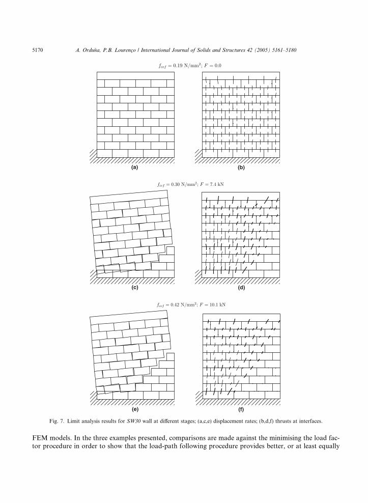
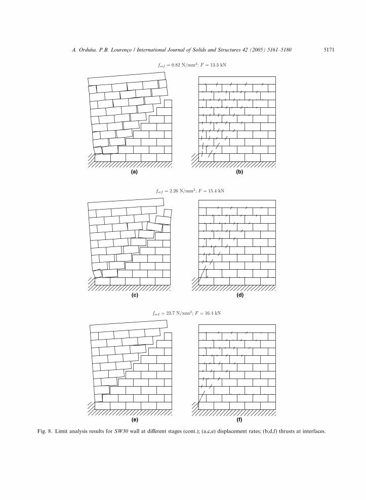
More interesting is to see how the load-path following procedure can resemble the intermediate stages ofthe structural behaviour. Fig. 5 contains pictures of the SW30 walls during testing. Fig. 6 shows the min-imum (compressive) stress distributions on the incremental deformed mesh of a finite element method(FEM) analysis performed for the same wall (Oliveira, 2003). This analysis was done with the DIANA code(DIANA, 1999) and the material model of Lourenco and Rots (1997). Table 1 presents the mechanicalproperties used in the analysis, where E and m are the Young�s and Poisson moduli, respectively, cvol isthe volumetric weight, kn and ks are the normal and tangential stiffness, respectively, l and w are the frictioncoefficient and dilatancy angle, respectively. The tensile strength and cohesion at the interfaces were as-sumed equal to zero. Finally, Figs. 7 and 8 present the displacement rates and thrusts at the interfacesfor selected stages of the load-path following procedure, using limit analysis (increasing fcef).

In the experimental results, and before the development of the final mechanism, sliding in some bedjoints at the upper-left part of the wall is evident through the head joints openings. The same sliding does

1000

1000

100 F

30 kN

(a)

F(kN)

0.0

2.0

4.0

6.0

8.0

10.0

12.0

14.0

16.0

18.0

0.1 1.0 10.0 100.0

fcef (N/mm2)

Increasing fcef

Decreasing fcef

(b)

Fig. 4. SW30 wall: (a) model and (b) load factor vs. effective stress graph.


not appear in the numerical models and is probably caused by the uneven contact at the interfaces in theexperimental models due to geometric tolerances in the size of the blocks, which change the process of crackformation significantly.

There is more similitude between FEM and limit analysis results, where perfect initial contact is as-sumed. In both numerical methods, the wall starts working as a whole. As the horizontal load increases,diagonal stepped cracks form, starting from the lower-right corner and progressing to the wall centre.At the same time, the number of active compressive struts decreases. Finally, the interface stepped crackreaches the central diagonal of the wall, meaning that there is a unique compressive strut, and the wall doesnot accept more load increments due to the overturning failure mechanism.

Fig. 9 shows the force vs. displacement graphs for the experiments and FEM results (Oliveira, 2003). Thecalculated limit load appears as a horizontal dotted line. It is noted that the FEM curve approaches asymp-totically to the limit analysis load.

Vasconcelos and Lourenco (2004) made cyclic tests on similar walls. Adequate test control and lowertolerances of the size of the units permitted to capture the cracking below the main diagonal at intermediatehorizontal loads. These walls were 1.2 m high, 1.0 m wide and 0.2 m thick; Fig. 10(a). The block dimensionswere 0.15 · 0.20 · 0.20 m. The measured stone volumetric weight is 25.7 kN/m3. For analysis purposes, a0.7 friction coefficient is assumed. Since the stone is of very good quality, the infinite compressive strength

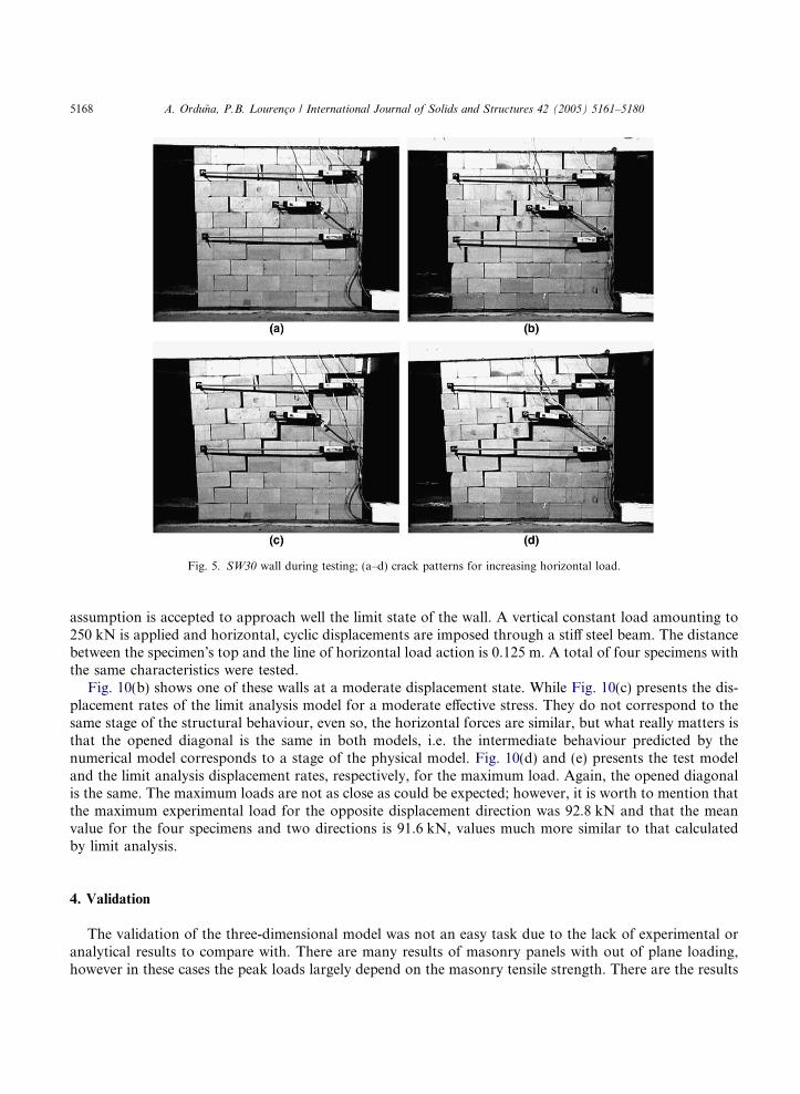
Fig. 5. SW30 wall during testing; (a–d) crack patterns for increasing horizontal load.


assumption is accepted to approach well the limit state of the wall. A vertical constant load amounting to250 kN is applied and horizontal, cyclic displacements are imposed through a stiff steel beam. The distancebetween the specimen�s top and the line of horizontal load action is 0.125 m. A total of four specimens withthe same characteristics were tested.

Fig. 10(b) shows one of these walls at a moderate displacement state. While Fig. 10(c) presents the dis-placement rates of the limit analysis model for a moderate effective stress. They do not correspond to thesame stage of the structural behaviour, even so, the horizontal forces are similar, but what really matters isthat the opened diagonal is the same in both models, i.e. the intermediate behaviour predicted by thenumerical model corresponds to a stage of the physical model. Fig. 10(d) and (e) presents the test modeland the limit analysis displacement rates, respectively, for the maximum load. Again, the opened diagonalis the same. The maximum loads are not as close as could be expected; however, it is worth to mention thatthe maximum experimental load for the opposite displacement direction was 92.8 kN and that the meanvalue for the four specimens and two directions is 91.6 kN, values much more similar to that calculatedby limit analysis.

4. Validation

The validation of the three-dimensional model was not an easy task due to the lack of experimental oranalytical results to compare with. There are many results of masonry panels with out of plane loading,however in these cases the peak loads largely depend on the masonry tensile strength. There are the results

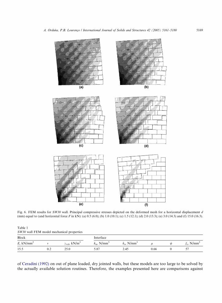
Fig. 6. FEM results for SW30 wall. Principal compressive stresses depicted on the deformed mesh for a horizontal displacement d(mm) equal to (and horizontal force F in kN): (a) 0.5 (6.0); (b) 1.0 (10.1); (c) 1.5 (12.1); (d) 2.0 (13.3); (e) 3.0 (14.3) and (f) 15.0 (16.3).

Table 1SW30 wall FEM model mechanical properties

Block Interface

E, kN/mm2 m cvol, kN/m3 kn, N/mm3 ks, N/mm3 l w fc, N/mm2

15.5 0.2 25.0 5.87 2.45 0.66 0 57


of Ceradini (1992) on out of plane loaded, dry jointed walls, but these models are too large to be solved bythe actually available solution routines. Therefore, the examples presented here are comparisons against

(a) (b)

(c) (d)

(e) (f)

Fig. 7. Limit analysis results for SW30 wall at different stages; (a,c,e) displacement rates; (b,d,f) thrusts at interfaces.


FEM models. In the three examples presented, comparisons are made against the minimising the load fac-tor procedure in order to show that the load-path following procedure provides better, or at least equally

(a) (b)

(c) (d)

(e) (f)

Fig. 8. Limit analysis results for SW30 wall at different stages (cont.); (a,c,e) displacement rates; (b,d,f) thrusts at interfaces.


FEM

Limit analysis

Experimental

Displacement (mm)0 5 10 15 20 25 30

0

5

10

15

20

25

Hor

izon

tal f

orce

, F (

kN)

Fig. 9. Horizontal load vs. displacement graph for SW30 wall.


good solutions than the first one. The selected validation examples are a masonry pile and two walls without of plane loading.

4.1. Masonry pile

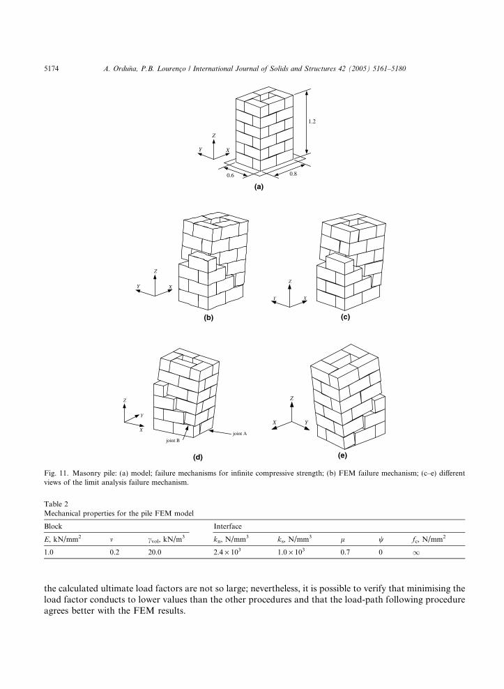
Fig. 11(a) shows the model of a masonry hollow pile. The pile is built of dry masonry blocks with dimen-sions 0.2 · 0.2 · 0.4 m. The pile dimensions are 0.6 · 0.8 · 1.2 m. The material volumetric weight is 20 kN/m3 and the friction coefficient is 0.7. The permanent loads are the blocks self-weights. The variable loads areproportional to the blocks weight, but horizontally applied in the direction of the larger base side (X direc-tion). The compressive effective stress, according to the load-path following procedure, is steadily increas-ing. Also, FEM analyses are performed for different values of compressive strength in order to validate thelimit analysis hinging model with limited compressive stress proposed in Orduna and Lourenco (2005). Fur-thermore, limit analyses, where the load factor is minimised according to the procedure proposed by Ferrisand Tin-Loi (2001), are realised in order to compare with the load-path following procedure.

In the FEM model, the blocks were constructed with 20 nodes brick elements joined with 16 nodes inter-face elements. Table 2 shows the mechanical properties.

Fig. 11 presents also the failure mechanisms obtained for infinite compressive strength. Fig. 11(b) showsthe failure mechanism obtained by the FEM analysis. The same failure mechanism is obtained by limitanalysis and Fig. 11(c)–(e) shows it from various viewpoints for a better understanding.

A range of ultimate load factors is possible for this mechanism and for infinite compressive strength. It isnoted that the ultimate load factor is defined as the ratio between the variable loads causing failure on thestructure, and their nominal values, in this case numerically equal to the self-weight of the blocks. Table 3presents the ultimate load factor obtained from different approaches. If the reaction on the overturningblocks set is concentrated on the interface A only, Fig. 11(d), with zero stresses at interface B, the ultimateload factor would be 0.427, the minimum possible for this mechanism. If there are non-zero normal andshear contact forces on interface B, the last one opposing to the upper block overturning, the maximumpossible ultimate load factor for the mechanism shown equals 0.553. The ultimate load factor calculatedby minimising the load factor by the procedure proposed by Ferris and Tin-Loi (2001) is 0.427, equal tothe minimum possible and 10.8% lower than the factor obtained by FEM. The ultimate load factor calcu-lated with the load-path following procedure is 4.4% higher than the FEM value. In fact the differences in

Fig. 10. Vasconcelos shear wall: (a) geometry; (b) test at d = 11.2 mm and F = 81.6 kN; (c) displacements rates at fcef = 6.6 N/mm2

and F = 76.1 kN; (d) test at d = 23.7 mm and F = 86.6 kN and (e) displacements rates at fcef =1 and F = 95.2 kN.


0.6 0.8

1.2

XY

Z

(a)

XY

Z

(b)

XY

Z

(c)

joint A joint B

X

Y

Z

(d)

X Y

Z

(e)

Fig. 11. Masonry pile: (a) model; failure mechanisms for infinite compressive strength; (b) FEM failure mechanism; (c–e) differentviews of the limit analysis failure mechanism.

Table 2Mechanical properties for the pile FEM model

Block Interface

E, kN/mm2 m cvol, kN/m3 kn, N/mm3 ks, N/mm3 l w fc, N/mm2

1.0 0.2 20.0 2.4 · 103 1.0 · 103 0.7 0 1


the calculated ultimate load factors are not so large; nevertheless, it is possible to verify that minimising theload factor conducts to lower values than the other procedures and that the load-path following procedureagrees better with the FEM results.

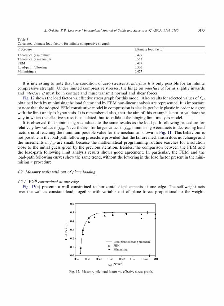
Table 3Calculated ultimate load factors for infinite compressive strength

Procedure Ultimate load factor

Theoretically minimum 0.427Theoretically maximum 0.553FEM 0.479Load-path following 0.500Minimising a 0.427


It is interesting to note that the condition of zero stresses at interface B is only possible for an infinitecompressive strength. Under limited compressive stresses, the hinge on interface A forms slightly inwardsand interface B must be in contact and must transmit normal and shear forces.

Fig. 12 shows the load factor vs. effective stress graph for this model. Also results for selected values of fcefobtained both by minimising the load factor and by FEM non-linear analysis are represented. It is importantto note that the adopted FEM constitutive model in compression is elastic–perfectly plastic in order to agreewith the limit analysis hypothesis. It is remembered also, that the aim of this example is not to validate theway in which the effective stress is calculated, but to validate the hinging limit analysis model.

It is observed that minimising a conducts to the same results as the load path following procedure forrelatively low values of fcef. Nevertheless, for larger values of fcef, minimising a conducts to decreasing loadfactors until reaching the minimum possible value for the mechanism shown in Fig. 11. This behaviour isnot possible in the load-path following procedure provided that the failure mechanism does not change andthe increments in fcef are small, because the mathematical programming routine searches for a solutionclose to the initial guess given by the previous iteration. Besides, the comparison between the FEM andthe load-path following limit analysis results shows good agreement. In particular, the FEM and theload-path following curves show the same trend, without the lowering in the load factor present in the mini-mising a procedure.

4.2. Masonry walls with out of plane loading

4.2.1. Wall constrained at one edge

Fig. 13(a) presents a wall constrained to horizontal displacements at one edge. The self-weight actsover the wall as constant load, together with variable out of plane forces proportional to the weight.

Loa

d Fa

ctor

, α

1E-2

fcef (N/mm2)

1E-1 1E+0 1E+1 1E+2 1E+3 1E+40.0

0.1

0.2

0.3

0.4

0.5

0.6

Load-path following procedureFEMMinimising

Fig. 12. Masonry pile load factor vs. effective stress graph.

1.053

0.6300.071

XY

Z

(a)

XY

Z

(b)

X Y

Z

(c)

XY

Z

(d)

X Y

Z

(e)

YX

Z

(f)

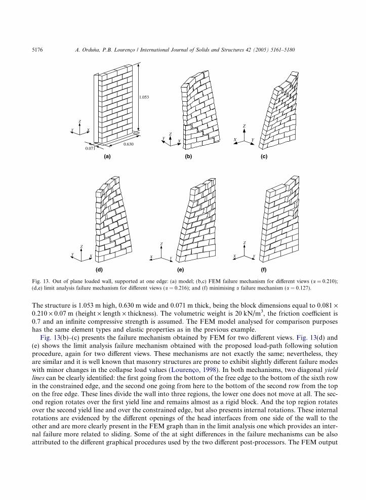
Fig. 13. Out of plane loaded wall, supported at one edge: (a) model; (b,c) FEM failure mechanism for different views (a = 0.210);(d,e) limit analysis failure mechanism for different views (a = 0.216); and (f) minimising a failure mechanism (a = 0.127).


The structure is 1.053 m high, 0.630 m wide and 0.071 m thick, being the block dimensions equal to 0.081 ·0.210 · 0.07 m (height · length · thickness). The volumetric weight is 20 kN/m3, the friction coefficient is0.7 and an infinite compressive strength is assumed. The FEM model analysed for comparison purposeshas the same element types and elastic properties as in the previous example.

Fig. 13(b)–(c) presents the failure mechanism obtained by FEM for two different views. Fig. 13(d) and(e) shows the limit analysis failure mechanism obtained with the proposed load-path following solutionprocedure, again for two different views. These mechanisms are not exactly the same; nevertheless, theyare similar and it is well known that masonry structures are prone to exhibit slightly different failure modeswith minor changes in the collapse load values (Lourenco, 1998). In both mechanisms, two diagonal yieldlines can be clearly identified: the first going from the bottom of the free edge to the bottom of the sixth rowin the constrained edge, and the second one going from here to the bottom of the second row from the topon the free edge. These lines divide the wall into three regions, the lower one does not move at all. The sec-ond region rotates over the first yield line and remains almost as a rigid block. And the top region rotatesover the second yield line and over the constrained edge, but also presents internal rotations. These internalrotations are evidenced by the different openings of the head interfaces from one side of the wall to theother and are more clearly present in the FEM graph than in the limit analysis one which provides an inter-nal failure more related to sliding. Some of the at sight differences in the failure mechanisms can be alsoattributed to the different graphical procedures used by the two different post-processors. The FEM output


is produced following the small displacements hypothesis, while the output of the limit analysis results isproduced in a large displacements basis. This means that in the FEM output the blocks are deformedbut the displacement on each point agrees with the calculations. In the limit analysis output, the blocks pre-serve their shapes but the displacements are accurate only at the block centroids.

(a) (b)

(c) (d)

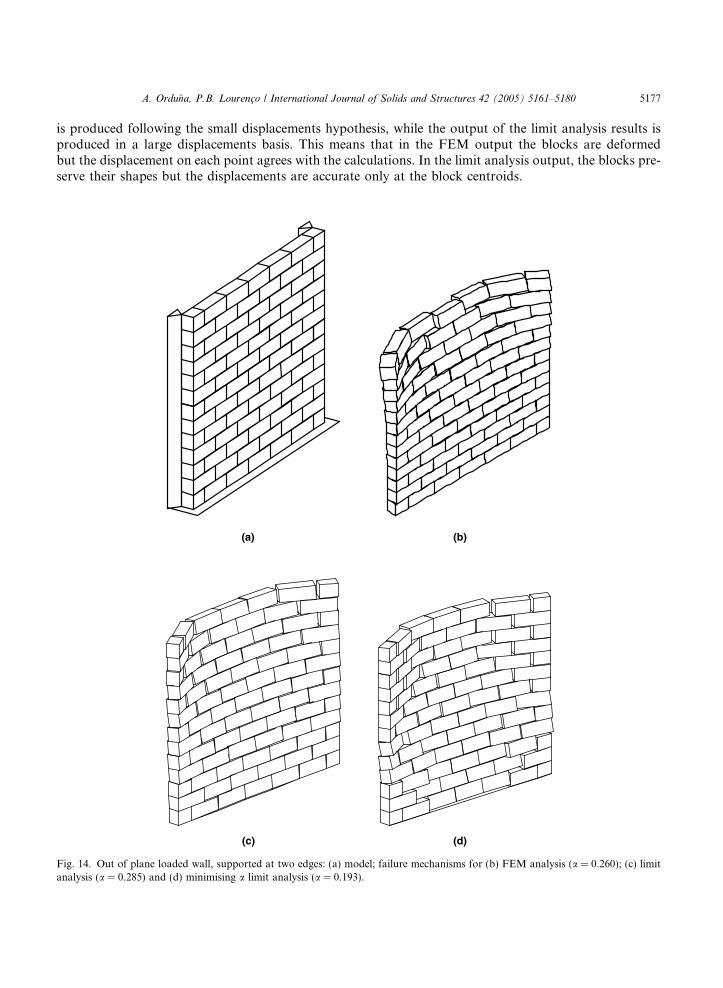
Fig. 14. Out of plane loaded wall, supported at two edges: (a) model; failure mechanisms for (b) FEM analysis (a = 0.260); (c) limitanalysis (a = 0.285) and (d) minimising a limit analysis (a = 0.193).


The limit analysis ultimate load factor is similar to the FEM value. This confirms the agreement betweenthe results obtained by the two different methods. Fig. 13(f) presents the failure mechanism obtained mini-mising the load factor by the procedure proposed by Ferris and Tin-Loi (2001). This mechanism is verydifferent from the previous ones, featuring a general overturning with localised block rotations near theconstrained edge. Moreover, the calculated ultimate load factor is unrealistically small, it differs 40% fromthe FEM value.

4.2.2. Wall constrained at two edges

The wall model presented in Fig. 14(a) has the same properties of the wall in the previous subsectionexcept that it is twice wide, 1.260 m, and it is constrained at both vertical edges. The loading is also com-posed by the self-weight as constant part and by horizontal, out of plane forces numerically equal to theblocks weights as variable part.

Fig. 14(b)–(d) presents the failure mechanisms obtained by FEM, limit analysis through the proposedload-path following procedure and limit analysis by minimising a, respectively. The former two mecha-nisms are not equal; nevertheless, they present clear similarities. In both mechanisms, the central part bendsaround horizontal, longitudinally directed axes with the curvature in the same direction as the variableload, and the external parts, near the supports, bend around vertical axes. These deflections increase fromvery small at the base to clearly visible magnitudes at the top of the wall. The mechanism resulting from theminimising a procedure is different. In the central part, it has a hinge at the base and the bending curvaturearound horizontal axes is contrary to the load direction. The mechanism also presents vertical bending nearthe supports, but with visible magnitude almost from the base until the top of the wall.

The ultimate load factor calculated by the load-path following procedure is 9.5% higher than the result-ing from the FEM analysis, which, for engineering purposes, is still an acceptable difference. The ultimateload factor calculated by minimising a is 25.8% lower than the FEM one, and significantly disagrees withthe obtained by the other two procedures.

5. Discussion

The results shown in the previous section present two general trends. Firstly, the load-path followingprocedure always gives slightly larger ultimate load factors than the FEM calculations. This general trendcan be attributed to the fact that the piecewise linear yield function used in the limit analysis interface modeloverestimates the strengths for a number of stress states (Orduna and Lourenco, 2005). Livesley (1992)pointed out the importance of a good interface modelling in the case of three-dimensional limit analysisand, therefore, an improvement of the proposed yield function seems possible. A drawback regarding thisissue is the lack of experimental results already mentioned. Nevertheless, the good agreement between limitanalysis and FEM results in three different structural models validates also, in an indirect manner, theassumptions made in the yield function development (Orduna and Lourenco, 2005).

The second trend observed in the results of Section 4 is that the ultimate load factor calculated by mini-mising a is always lower than the one obtained by FEM, reaching this difference 40% in one case. Also, thefailure mechanisms obtained by minimising a disagree with those of the FEM, at least in two of three cases,while the load-path following procedure mechanisms are more consistent with the FEM ones. For this rea-son, it has been stated that the load-path following procedure produces better solutions both in terms ofultimate load factor and failure mechanism than minimising the load factor. Within a direct method the-oretical perspective, minimising the load factor seems to be the better and safer choice. Nevertheless, thelack of taking into account the loading history in the limit analysis approach can have a significant impacton the result in the presence of non-associated flow rules. From a practical engineering viewpoint, and con-sidering that the safety assessment is generally based on the maximum reliable strength that a structure can


develop, minimising the load factor can conduct to severe and unacceptable underestimations. The mini-mising a procedure results shown in Fig. 12 suggest that before to arrive to the last load factor, with infiniteeffective stress, it is necessary to pass by intermediate mechanisms with larger load factors, in fact similar tothat resulting from the load-path following procedure. Therefore, the minimising a results can be regarded,in some cases, as residual strength mechanisms that are generally not useful in the practical assessment ofstructures.

It is theoretically possible to find all the solutions to the limit analysis MCP, Eqs. (1)–(6), by means of aprocedure similar to that proposed by Tin-Loi and Tseng (2003) for linear complementarity problems. Nev-ertheless, the choice of the most reliable solution must involve the selection of those solutions that are di-rectly reachable from the set of stress states that are possible under gravitational loads only and satisfyingthe equilibrium and yield conditions, through a continuous stress path with the same requirements, andwithout having to apply larger load factors than the ultimate load factor. The proposed load-path followingprocedure is capable of using an initial solution from the set of stress states due to permanent loads only,and take the model until failure due to variable loads. The proposal in this paper is to start from the solu-tion to Eqs. (7)–(9) although, in reality only Eqs. (8) and (9) are necessary. As already stated, Eq. (7) has theobjective to obtain an initial uniform stress distribution, but it can be dropped. In the future, it would be ofinterest to investigate the different solutions that can be obtained, starting from distinct points of the set ofgravitational loads only stress states.

6. Conclusions

In the limit analysis theory, the associated flow hypothesis allows for important mathematical simplifi-cations and conducts to three elegant and equivalent formulations, namely the static, kinematic and mixedformulations. Nevertheless, masonry, among other cementitious materials, cannot be properly representedby fully associated flow rules. In particular, the sliding failure mode is non-associated because it features adilatancy angle significantly lower than the friction angle (the dilatancy angle is taken as zero in this paper).The lack of normality in the flow rules invalidates the simplifications made in classic limit analysis and ren-ders the mixed formulation as the only possibility. Moreover, the presence of non-associated flow rules hasa more critical consequence: theoretically, there is no unique solution to the limit analysis problem. Theproposal consisting in minimising the load factor can conduct to overconservative results, as shown in thispaper. For this reason, a novel load-path following procedure has been proposed. This procedure producesbetter results and, in addition, provides an insight into the behaviour of structures through the load historyuntil failure with the same limited input data required by standard limit analysis. The procedure has notheoretical foundations at this stage. Nevertheless, this fact does not invalidate the remarkably good resultsobtained. Many cases exist where an accident or the intuition of the analyst have suggested new proceduresand only later a theoretical justifications has been found. The excellent results for masonry structuresshown in this paper may be due to the fact that, in the proposed model, the strengths of all failure modesdepend on the normal stress. Thus, limiting the amount of normal stress is a natural way to control all thematerial strengths. The generalisation of this procedure to arbitrary yield functions can constitute a way tosolve the non-associated limit analysis problem.

The validation examples have shown that both the limit analysis three-dimensional coupled model pre-sented in Orduna and Lourenco (2005) and the load-path following procedure produce results in agreementwith the more precise finite element method. Also, the comparisons of the two-dimensional models againstexperimental evidence, show that the predicted intermediate and failure behaviours agree well with the ob-served experimental behaviours. This agreement validates in particular the performance of the load-pathfollowing procedure. In three dimensions, comparisons against experimental evidence are desirable; never-theless, there is a lack of such evidence on dry joints models in the literature. Moreover, it has been found


that experiments on dry joint models are extremely sensible to the initial contact conditions on the joints;therefore, special care must be taken in the geometrical and construction tolerances in the model buildingprocess in order to produce results comparable with other methods or experiments.

Acknowledgments

The first author wishes to thank the scholarship made available to pursue his Ph.D. studies by the Cons-ejo Nacional de Ciencia y Tecnologıa of Mexico. The work was also partially supported by project SAPI-ENS 33935-99 funded by Fundacao para a Ciencia e Tecnologia of Portugal.

References

Baggio, C., Trovalusci, P., 1998. Limit analysis for no-tension and frictional three-dimensional discrete systems. Mech. Struct. Mach.26 (3), 287–304.

Boulbibane, M., Weichert, D., 1997. Application of shakedown theory to soils with non associated flow rules. Mech. Res. Commun. 24(5), 513–519.

Brooke, A., Kendrick, D., Meeraus, A., Raman, R., Rosenthal, R.E., 1998. GAMS a User�s Guide. Tech. rep., GAMS DevelopmentCorporation, Washington, DC, USA.

Ceradini, V., 1992. Modelling and experimenting for historic masonry study (in Italian). Ph.D. Thesis. Faculty of Architecture ofRome, La Sapienza.

Corigliano, A., Maier, G., 1995. Dynamic shakedown analysis and bounds for elastoplastic structures with nonassociative, internalvariable constitutive laws. Int. J. Solids Struct. 32 (21), 3145–3166.

De Saxce, G., Bousshine, L., 1998. Limit analysis theorems for implicit standard materials: application to the unilateral contact withdry friction and the non-associated flow rules in soils and rocks. Int. J. Mech. Sci. 40 (4), 387–398.

DIANA, 1999. DIANA User�s Manual Release 7.2. TNO Building and Construction Research, Delft, The Netherlands.Ferris, M., Tin-Loi, F., 2001. Limit analysis of frictional block assemblies as a mathematical program with complementarity

constraints. Int. J. Mech. Sci. 43, 209–224.Livesley, R.K., 1992. A computational model for the limit analysis of three-dimensional masonry structures. Meccanica 27, 161–172.Lourenco, P.B., 1998. Sensitivity analysis of masonry structures. In: Proc. 8th Canadian Masonry Symp. Jasper, Canada, pp. 563–574.Lourenco, P., Rots, J., 1997. A multi-surface interface model for the analysis of masonry structures. J. Eng. Mech. 123 (7), 660–668.Nielsen, M., 1999. Limit Analysis and Concrete Plasticity, second ed. CRC.Oliveira, D.V., 2003. Experimental and Numerical Analysis of Blocky Masonry Structures under Cyclic Loading. Ph.D. Thesis.

University of Minho, Guimaraes, Portugal. Available from: <http://www.civil.uminho.pt/masonry>.Orduna, A., Lourenco, P., 2003. Cap model for limit analysis and strengthening of masonry structures. J. Struct. Eng. 129 (10), 1367–

1375.Orduna, A., Lourenco, P., 2005. Three-dimensional limit analysis of rigid blocks assemblages. Part I: Torsion failure on frictional

interfaces and limit analysis formulation. Int. J. Solids Structures, in press, doi:10.1016/j.ijsolstr.2005.02.010.Palmer, A.C., 1966. A limit theorem for materials with non-associated flow laws. J. de Mecanique 5 (2), 217–222.Tin-Loi, F., Tseng, P., 2003. Efficient computation of multiple solutions in quasibrittle fracture analysis. Comput. Meth. Appl. Mech.

Eng. 192 (11–12), 1377–1388.Vasconcelos, G. F.M., Lourenco, P.B., 2004. Experimental assessment of the behaviour of unreinforced masonry walls subject to in

plane cyclic actions (in Portuguese). In: 6th National Congress on Seismology and Seismic Engineering. Guimaraes, Portugal, pp.531–542.

http://www.civil.uminho.pt/masonry

http://dx.doi.org/10.1016/j.ijsolstr.2005.02.010

Three-dimensional limit analysis of rigid blocks assemblages. Part II: Load-path following solution...

Documents

Transcript of Three-dimensional limit analysis of rigid blocks assemblages. Part II: Load-path following solution...