The copyright of this thesis vests in the author. No quotation from it or information derived from it is to be published without full acknowledgement of the source. The thesis is to be used for private study or non-commercial research purposes only.

Published by the University of Cape Town (UCT) in terms of the non-exclusive license granted to UCT by the author.

Univers

ity of

Cap

e Tow

n

AN INVESTIGATION OF FIRM SPECIFIC AND MACROECONOMIC VARIABLES AND THEIR

INFLUENCE ON EMERGING MARKET STOCK RETURNS

DAVID MOORE

Prepared under the supervision of Professor Paul Van Rensburg and presented to the School of Management Studies in fulfilment

of the requirements for the degree of

MASTER OF BUSINESS SCIENCE (Special Field: Finance)

University of Cape Town ©

Univers

ity of

Cap

e Tow

n

Abstract

This paper aims to expand on the growing area of asset pricing research in developed markets by extending such analyses to those nations considered to be emerging. Of late the accuracy of a

previously established cornerstone of asset pricing theory, namely the Capital Asset Pricing Model (CAPM) has been questioned. The discovery of numerous firm related anomalies that have predictive

power over the cross sectional variation of share returns in excess of that explained by established market proxy models has served to fuel interest and speculation as to the true robustness and

exploitability of such influences. These firm specific influences have been termed 'style characteristics' .

This study employed the use of the DataStream International Emerging Market Index for the

extraction of all firm specific and return data. In addition to the considered 'style' characteristics this study explores the broader systematic effects associated with changes in key macroeconomic variables. Informed by prior research, variables found to be of historical significance to the behaviour of the cross section of emerging market returns are included in this analysis. A collection of 50 style characteristics and 15 macroeconomic factors are tested over sample period spanning the 151 of

January 1997 to the 31 51 of December 2006 comprising a total of 1273 shares from 20 emerging nations.

Returns are adjusted for risk using both CAPM and APT formulations and the ability of the 'style' factors to explain the cross-sectional variation of returns tested in a univariate setting as in Van

Rensburg and Robertson (2003). Significant factors identified in the tests of unadjusted returns are endorsed by the results of the risk adjusted analyses. A correlation analysis is run thereafter in order to limit redundancy with a cluster analysis to follow in order to identify groups of factors with similar

explanatory power. Factors are classified into the following groups; (1) Size, (2) Value, (3) Liquidity and (4) Miscellaneous. Of the 46 tested a final list of 14 significant style effects were documented the nature of which seem to concur with the majority of developed and developing market research. In order to assess the stationarity of the 15 candidate macroeconomic variables, Augmented Dickey Fuller tests were run on the chosen factors in order to identify testable factors as in Van Rensburg

(1999). A variant of the Fama and Macbeth (1973) methodology is then employed on the 11 stationary factors identified to firstly ascertain the sensitivity of each listed share to all macroeconomic influence and thereafter be tested in a similar univariate setting as to the style factors. Five macroeconomic factors with a strong commodity focus are found to be reasonably significant at

the five percent level; however upon further analysis the ability of such factors to be considered priced risk factors is refuted.

The final 15 style characteristics are then tested to develop a muItifactor model so as to ascertain the robustness of such factors in a more complex setting. The analysis yielded a model comprising a total

of nine factors with a strong value orientation in agreement with previous univariate tests. Finally, a more robust stepwise variant of the expected return modelling technique examined by Haugen and Baker (1996) is employed. A total of five timing models are used to derive a range of style based, macroeconomic based and hybrid expected return formulations. All style models exhibited a distinct value orientation; with Book-to-Market Value and Return on Capital employed the most frequently identifiable factors. The independent macroeconomic models showed little promise; however the hybrid models-style formulations supplemented with macroeconomic influences, more specifically the Gold Price, Oil Price and long tenn US interest rates served to measurably improve explanatory power. These models have varied significance with only one specification showing potential investable exploitability.

Univers

ity of

Cap

e Tow

n

Declaration

I, David Moore, hereby declare that the work on which this thesis is based is my own original work

(except where acknowledgements indicate otherwise) and that neither the whole work nor any part of

it has been, is being, or is to be submitted for another degree in this or any other University. I

empower the University to reproduce for the purpose of research either the whole or any portion of

the contents in any manner whatsoever.

August 2008

Univers

ity of

Cap

e Tow

n

Acknowledgements

The author would like to acknowledge the supervision and guidance of Professor Paul van Rensburg

of the University of Cape Town. Furthennore the able assistance of the staff of the Finance

Department in the School of Management Studies at the University of Cape Town with special

mention owing to Mr Ryan Kruger whose aid contributed to the timely completion of this thesis.

The author also acknowledges the School of Management Studies at the University of Cape Town for

pennission to use the Finance Research Laboratory for data collection and analysis.

Finally, the author thanks the Postgraduate Funding Office of the University of Cape Town for the

Entrance Merit Scholarship.

Univers

ity of

Cap

e Tow

n

Contents

Abstract .................................................................................................................................................... i.

Declaration ........................................... .................................................................................................... ii

Acknowledgements .................................................................................................................................. iii

Contents .............................................. ..................................................................................................... iv

List of Tables ......................................................................................................................................... viii

List of Figures ......................................................................................................................................... ix

1. Introduction ................................................................................................................................... 1

1.1. Introduction .......................................................................................................................... 1

1.2. Motivationfor research ....................................................................................................... 4

1.3. Contribution ......................................................................................................................... 6

1.4. Thesis organisation. .......................................... .................................................................... 7

2. Theoretical Overview ..................................................................................................................... 1

2.1. Introduction ........................................... ............................................................................... 1

2.2. Market Effieciency and the Efficient Market Hypothesis ............................................ .......... 1

2.3. Market Effieciency ............................................................................................................... 2

2.4. Asset Pricing and the Capital Asset Pricing Model (CAPM) ............................................... 7

2.5. The Joint Hypothesis Problem ............................................................................................ 11

2.6. Arbitrage Pricing TheOlY (APT) ................................................. ........................................ 11

3. Literature Review ........................................................................................................................... 1

3.1. Introduction .......................................................................................................................... 1

3.2. A briefreview ofUSjindings ........................................... ..................................................... 2

3.2.1. An Explanation ofCAPM style anomalies .............................................. ............................... 3

3.3. The CAPM and APT in Emerging Markets ............................................... ............................ 6

3..!. Stl),e Anomoalies in Emerging Markets ............................................... ................................. 6

Univers

ityof

Cape Tow

n

3.4.1. Earlier Seminal Work ............................................................................................................ 6

3.4.2 More Recent Studies ............................................................................................................ 10

3.4.3 Testingfor Clusters offactors in emerging markets ............................................................ 10

3.4.4 Assesing Market Risk in Emerging Markets ........................................................................ 14

3.5. Macroeconomic Shocks and Share Returns .......................................................................... 18

3.5.1 Developed Market Research ................................................................................................. 18

3.5.2 Research in Emerging Markets ........................................................................................ 20

4. Data alld Descriptive Statistics ...................................................................................................... 1

4.1. Introduction ..... ..................................................................................................................... I

4.2. Data ...................................................................................................................................... 1

4.2.1. Stock returns data ..................................................................................... ............................ 2

4.2.2. Adjustments to the stock returns data ................................................................................... 3

4.2.3. Firm-specific attribute data ................................................................................................ 10

4.2.4. Descriptive statistics ..... ...................................................................................................... 16

4.3. Summary and conclusion .............................................................................. ...................... 19

5. Specijicatioll of 11ldex Models alld Ullivariate Style Allalysis ...................................................... I

5.1. Introduction .......................................................................................................................... I

5.2. Testing the Single- and Multi-index models .......................................................................... 2

5.2.1 Data and Methodology ......................................................................................................... 2

5.2.2. Theoretical Concerns and Critical Assumptions .................................................................. 5

5.3. Results ......................... .......................................................................................................... 6

5.4. Univariate Testing of Style Factors ...................................................................................... 8

5.4.1. Data and methodology ............................................................................ .............................. 8

5.4.2. Tests of Unadjusted returns .................................................................................................. 8

5.4.3. Tests of Risk-adjusted returns: CAPM .................................................................................. 9

5.4.4. Tests of Risk-adjusted returns: APT .... ............................................................................... 10

5.4.5. Comparison between unadjusted and risk-adjusted results ...... .......................................... 12

5.4.6. Primmy Adjustment to list of firm-specific characteristics ................................................ 12

5.4.7. Analysis of primary list of signnificant characteristics ...................................................... 13

5.4.8. Style Consistency ................................................................................................................ 16

5.5. Results ........... ...................................................................................................................... 17

5.5.1. Univariate Testing: Unadjusted and Risk Adjusted Results ............................................... 17

5.5.2. Identification of Significant Clusters: Unadjusted Returns ................................................ 24

5.5.3. Monthly Payoffs of Significant Factors .............................................................................. 25

Univers

ity of

Cap

e Tow

n

5.5.4 Analysis of Cumulative Monthly Payoffs ............................................................................ 32

5.6 Style Consistency ................................................................................................................ 38

5.6.1 Sign Test ............................................................................................................................. 38

5.6.2 Testfor Randomness ............................................ ............................................................... 39

5.7 Summmy and Conclusion ............................................. ...................................................... 40

6. Univariate Analysis of Macroeconomic Influences on Return Behaviour ............................... 1

6.1. Introduction .......................................................................................................................... 1

6.2. Identification of Candidate Factors ............................................... ....................................... 3

6.2.1 Prior Research .............................................. ........................................................................ 3

6.2.2 Explanation of Candidate Factors ............................................... ......................................... 4

6.3. Adjustments to Candidate Factors prior to testing ............................................... ................ 4

6.3.1. Stationarity ........................................................................................................................... 4

6.3.2. Correlation amongst Stationary factors ............................................................................... 5

6.3.3. Results ............................................... .................................................................................... 6

6.4. Univariate Testing of Macroeconomic Factors .................................................................. 12

6.4.1 Data and Methodology ....................................................................................................... 12

6.4.2 Tests of Unadjusted Returns ............................................................................................... 13

6.4.3 Results ....................................................................................................................... .......... 15

6.5 Further Analysis ................................................................................................................. 26

6.5.1 Preliminary Commentary ................................................................................................... 26

6.5.2 Macroecnomic Factors as priced risk factors .................................................................... 26

6.6. Summary and Conclusion ................................................................................................... 28

7. Multivariate Style Analysis, Timing, and Expected Return Models ............................................... 1

7.1. Introduction .......................................................................................................................... 1

7.2. Multivariate cross-sectional Regressions ............................................................................. 3

7.2.1. Introduction .......................................................................................................................... 3

7.2.2. Methodology ............................................ ............................................................................. 3

7.2.3. Results ............................................... .................................................................................... 5

7.3. Multi/actor Expected Return Models .... ................................................................................ 7

7.3.1. Data and Methodology ......................................................................................................... 7

7.3.1. 1. Problems with Haugen and Baker (1996) ............................................................................ 9

7. 3. 1. 2. Haugen and Baker (1996 - a revised methodology ........................................................... 10

Univers

ity of

Cap

e Tow

n

7.4. Expected Return Model Construction .......................................... ....................................... 12

7.4.1 Firm-Specific Models ................................................ .......................................................... 12

7.4.2 Macro-Economic Models ................................................ .................................................... 12

7.4.3 Combined Models ................................................ ............................................................... 14

7.4.4 Results ............................................... .................................................................................. 15

7.5. Summary and conclusion ............................................. ....................................................... 23

8. Summary, Conclusion, and Suggested Extensions ..................................................................... 1

8.1. Introduction ... ....................................................................................................................... I

8.2. Summary o/results ............................................................................................................... 2

8.3. Final conclusion and suggested extensions .......................................................................... 7

References ............................................................................................................................................... 1

List of Appendices ................................................................................................................................ 22

Univers

ity of

Cap

e Tow

n

List of Tables

4. Data and Descriptive Statistics ....................................................................................................... 1

Table 4.1. Firm-specific Attributes ................................................................................................. 12

Table 4.2. Grouping of Firm Specific Attributes ............................................................................. 14

Table 4.3. Descriptive Statistics of the Firm-specific Attributes .................................................... 17

5. Specification of Index Models and Univariate Style Analysis ........................................................ 1

Table 5.1. Statistical Significance of Single- and Multi-index Models ............................................. 6

Table 5.2.Significance of Attributes: Unadjusted Returns ............................................................. 18

Table 5.3. Significance of Attributes: CAPM (EMl) Adjusted Returns .......................................... 19

Table 5.4 Significance of Attributes: CAPM (WMl) Adjusted Returns ........................................... 20

Table 5.5 Final List of Significant Uncorrelated Attributes ........................................................... 31

6. Univariate Analysis of Macroeconomic influences on return behaviour in Emerging Markets .... 1

Table 6.1. Initial List of Candidate Macroecnomic Variables ......................................................... 1

Table 6.2. Results of Level Unit Root Tests ...................................................................................... 6

Table 6.3. Results of First Differenced Unit Root Tests ................................................................... 7

Table 6.4. Final List of Stationary Macroeconomic Factors ............................................... ........... II

Table 6.5 Significance of Candidate Macroeconomicfactors in return prediction. ....................... 15

7. Multivariate Style Analysis incorporating Macroeconomic Influences and Expected Return Models

......................................................................................................................................................... 1

Table 7.1. Results of Multivariate Cross-Sectional Regressions ...................................................... 5

Table 7.2. Constructed Expected Return Models: Style (Full Sample) ........................................... 15

Table 7.3. Constructed Expected Return Models: Style (Restricted Sample) ................................. 17

Table 7.4. Constructed Expected Return Models: Macroeconomic Variables ............................... 19

Table 7.5. Constructed Expected Return Models: Style and Macroeconomic Variables ............... 21

Univers

ity of

Cap

e Tow

n

List of Figures

4. Data and Descriptive Statistics ...................................................................................................... 1

Figure 4.1. Graphical Depiction of changing liquidity of listedjirms over sample period. ............ 8

5. Specification ofIndex Models and Univariate Style Analysis ........................................................ 1

Figure 5.1. Tree Diagram representing the Clusters of Monthly Payoffs: Unadjusted Returns.. 21

Figure 5.2. Tree Diagram representing the Clusters of Monthly Payoffs: CAP M (EMI) Adj.Returns ... ......................................................................................................................................................... 22

Figure 5.3. Tree Diagram representing the Clusters of Monthly Payoffs: CAPM (WMI) AdjReturns .. ........................................................................................................................................................ 23

Figure 5.4. Correlation Matrix of Significant Style Factors ........................................................... 27

Figure 5. 5. Correlation Matrix of Monthly Payoffs: Size .................................................. .............. 28

Figure 5.6. Correlation Matrix of Monthly Payoffs: Value (1) ...................................................... 28

Figure 5.7. Correlation Matrix of Monthly Payoffs: Value (2) ...................................................... 29

Figure 5.8. Correlation Matrix of Monthly Payoffs: Liquidity .............................................. ......... 29

Figure 5.9. Correlation Matrix of Monthly Payoffs:Miscellaneous ............................................... 30

Figure 5.10. Cumulative Monthly Payoffs: Size ............................................................................. 32

Figure 5.11. Cumulative Monthly Payoffs: Value (1) ..................................................................... 33

Figure 5.12. Cumulative Monthly Payoffs: Value (2) ..................................................................... 34

Figure 5.13. Cumulative Monthly Payoffs: Liquidity ..................................................................... 35

Figure 5.14. Cumulative Monthly Payoffs:Miscellaneous ............................................................. 36

Figure 5.15 Consistency of Direction ofSignficant Attribute Monthly Payoffs ............................. 38

Figure 5.16 Testing the Randomess of Monthly Payoffs ................................................................ 39

6. Univariate Cross-sectional Analysis of Macroeconomic influences on return behaviour in ........... .

Emerging Markets .......................................................................................................................... I

Figure 6.1. Correlation Matrix of Final List of Stationary Macroecnonomic Variables ................. 9

Figure 6.2. Graph of Cumulative Returns on Macroeconomic Commodities versus Returns on the DataStream International Emerging Market Index ........................................................................ 18

Figure 6.3. Graph of Cumulative Changes in US interest rates versus the Cumulative Returns upon the DataStream International Emerging Markets Index ............................... ....................................... 19

Figure 6.4. Scatter Plot of Mean Monthly Emerging Market Stock Return versus Monthly Beta Exposure to the CRBIndex ... ...................................................................................................... ..... 20

Figure 6.5. Scatter Plot of Mean Monthly Emerging Market Stock Return versus Monthly Beta Exposure to the Gold Price ($US/ounce) ...................................................... ................................. 21

Figure 6.6. Scatter Plot of Mean Monthly Emerging Market Stock Return versus Monthly Beta Exposure to the Brent Crude Oil Price ($US/barrel) ..................................................................... 22

Figure 6. 7. Scatter Plot of Mean Monthly Emerging Market Stock Return versus Monthly Beta Exposure to the Platinum Price ($US/ounce) ........................................... ...................................... 23

Figure 6.8. Scatter Plot of Mean Monthly Emerging Market Stock Return versus Monthly Beta Exposure to the US 10 year Gilt ................................................... .................................................. 24

Univers

ity of

Cap

e Tow

n

7. Multivariate Style Analysis incorporating Macroeconomic Influences and Expected Return Models

....................................................................................................................................................... 1

Figure 7.1. Cumulative Monthly Payoffs to Multivariately Significant Factors ............................. 5

Univers

ity of

Cap

e Tow

n

-1-Introduction

"The recent Finance literature seems to produce many long-term return anomalies. Subjected to

scrutiny, however, the evidence does not suggest that market efficiency should be abandoned.

Consistent with the market efficiency hypothesis that the anomalies are chance results, apparent

overreaction of stock prices to information is about as common as under reaction."

-Fama (1998, p. 304)

1.1 Introduction

The pursuit of wealth has been central to the ambitions of man for centuries, however to be

classified as wealthy is to be segregated into an elite class, a categorisation that the vast

majority will never attain. This is so because in order to obtain substantial wealth and returns

one has to bear the burden of the risk of failure, which even fewer are able to do successfully.

Establishing what is considered an adequate risk to bear for an associated return on a vested

interest is critical in the accumulation of wealth. Until the arrival of what may be termed

'Modem Finance' in the mid twentieth century such a question was extremely difficult to

answer.

Markowitz (1952: 1959) defined the relationship between risk and return and described the

concept of mean-variance efficiency as being able to determine the optimal investment

opportunity for the prospective investor. No longer was return maximisation the rule of

thumb for the investor in choosing amongst hislher opportunity set. Sharpe (1964) built on

these theoretical foundations and formulated a model, the Capital Asset Pricing Model

(CAPM) that was purported to describe the risk: return relationship in a market classified as

efficient. This formulation was the pioneering work in the pricing of assets and defined the

risk of any asset as its covariance with all other assets in the market, later termed the 'market

portfolio' .

However, in formulating this model Sharpe made many stringent assumptions that narrowed

its general applicability and so created many sceptics in the world of finance and economics

as to its accuracy. Amongst the first was the work of Roll (1976) who argued that the return

on any asset may be sensitive to not just one factor but III fact many.

Univers

ity of

Cape T

own

The theory of 'one price' and Arbitrage was born, alluding to the fact that similar assets with

similar risk exposures must be offering the same expected return. If they were not short

selling would generate a riskless profit which would contravene market efficiency.

The APT has somewhat less rigorous assumptions than the CAPM which serves as both a

strength and a weakness of the approach. Indeed the APT is more generalised than the

CAPM by virtue of its relaxed assumptions; however it also provides no theoretical

foundation by which to select its priced factors. The chosen factors are often sample-specific

and hold little economic interpretative value detracting from the soundness of the approach in

an empirical setting.

The CAPM itself even with its sweeping assumptions has struggled somewhat to hold up as

an accurate generalised asset pricing model. The inferred risk: return relationship posited by

Markovitz and that which forms the foundation of the CAPM has been found wanting when

tested empirically. Often the generated Beta estimate has shown little or no relation to

returns with evidence of other unexplained sources of variation seemingly defining the

manner in which returns are generated (Fama and French, 1992 inter alia).

It is with these 'other' sources of variation that this paper is most concerned. Firm specific

variables, information that describes in detail the financial well being and future prospects of

the firm are believed to be the next paradigm in explaining the variation in share returns.

These variables also termed 'style effects' or 'style characteristics' have been studied

extensively in developed markets-Blume (1980), Banz and Reinganum (1981), Fama (1991)

and the like have found numerous style factors with the power to describe part of the cross

sectional variation in share returns. However, there exists far less research in an emerging

market context, a gaping hole which this paper aims to fill.

The environment in which firms operate, or rather the macroeconomy with its habit of

periodic fluctuation from boom to recession is another area incorporated into the study of

pricing share returns. Although much work on macroeconomic shocks and stock market

movements does exist in both developed and emerging market contexts, this paper's ambition

is to re-assess their cross sectional explanatory impact on a broad sample of emerging shares

and possibly use them to create a hybrid forecasting model that includes both firm-specific

and macroeconomic influences.

Univers

ity of

Cap

e Tow

n

Introduction 1: 2

This paper is closely aligned to the work of Van Rensburg and Robertson (2003) and Van

Rensburg and Janari (2004) who draw upon similar characteristics-based approaches to those

used by Fama and Macbeth (1973) to identify generalised sources of explanatory power over

a broad sample of emerging market stocks. The ten year sample of stocks over the period (1 st

of January 1997 to the 31 st of December 2006) is drawn from the DataStream International

Emerging Market Index comprising a total of twenty six emerging nations.

All data used in this study is sourced from the DataStream International Database and

presented in Chapter Four and later expanded upon in Chapter Six. DataStream itself is a

public domain and updates all relevant information once such data has been made public;

therefore this study remains free from look-ahead bias. Survivorship bias however is

prevalent in this paper-with prior research citing its influence to be less than considerable it

fails to present a major cause for concern. Once sufficient data pruning and manipUlation is

complete a range of testing procedures is employed that seeks to isolate sources of

explanatory power that were previously unexplained by the CAPM and APT formulations.

To begin in Chapter Five, share returns will be adjusted for risk and the associated return

over each month will then be run in a univariate cross-sectional regression against the

sourced firm specific characteristics at the beginning of that same month in order ascertain

the payoff of the exposure to such style factors. Results are scrutinised from a statistical

standpoint and those characteristics deemed of suitable significance are studied further.

A similar analysis is performed on the candidate macroeconomic factors in Chapter Six,

whereby their relation to emerging market stock returns is investigated. Prior to testing,

suitable data transformations are performed in order to ensure testability as conducted in Van

Rensburg (1999) and Fama and Macbeth (1973). Results are once again checked for

statistical rigour, with those significant variables progressing to the next stage of the analysis.

Finally, Chapter Seven attempts at crafting an accurate predictive model using previously

identified firm-specific characteristics, macroeconomic variables and thereafter a

combination of both in a multi-factor setting are documented. A stepwise variant of the

methodology of Haugen and Baker (1996) provides the essential framework for expected

return model construction, with the aim being the development an optimal exploitable

formulation able to accurately predict share price movements.

Univers

ity of

Cap

e Tow

n

Introduction 1: 3

A summation of the paper's aims and ultimate outcomes is presented with all relevant

concerns expressed regarding the present study and the potential for further analysis in a

similar context.

The remainder of this chapter is set out as follows: Section 1.2 considers the author's

motivation for this research and Section 1.3 discusses the proposed contribution.

1.2 Motivation for Research

Firm specific characteristics such as size, book-to-market and the like provide investors with

important information. Based on these attributes shrewd investors can earmark certain

equities that exhibit such traits, construct portfolios that are sufficiently well diversified and

so in the near future earn abnormal returns through close monitoring and adjusting of their

respective holdings. This concept is defined as 'style timing' and is already common place in

developed markets due to the volumes of research undertaken on firm characteristics and

their associated impact on returns.

In emerging markets however, such anomalous behaviour hasn't been sufficiently

documented and so the implementation of a full style based investment strategy may be

considered somewhat premature. This study'S primary objective is to expand on the current

literature on the topic increasing the range of firm specific measures to be tested across a

more recent and up to date sample of emerging market nations. The hope is that this more

comprehensive study will serve to identify the precise firm specific variables that influence

the return behaviour before and after CAPM and APT based risk adjustment of emerging

market equities and in so doing form the basis to enhance investment techniques in markets

whose behaviour aside from being termed volatile is not well documented.

A sample of over twenty emerging nations has ~een gathered, drawn from the three major

emerging regions across the globe namely Africa, Latin America and Asia. Data constraints

have served to minimize the representation of the African region; however the sample as it

stands is sufficiently broad to constitute a comprehensive study.

Furthermore, the influence of broader macroeconomic factors on share returns is an

additional unexplored realm in the context of emerging market asset pricing. Previous

Univers

ity of

Cap

e Tow

n

Introduction 1: 4

research in developed markets have shown a degree of co-movement between

macroeconomic factor and stock markets, however emerging market research by K won

(1997), Gjerde and S<ettem (1999) and others is somewhat more country specific than their

developed market counterparts, an area which this study aims to expand upon through the

employment of a significantly more diversified sample. Fluctuations in interest rates,

commodity prices and various other broad market characteristics are investigated. The

second objective of this study is therefore to ascertain whether or not these variables, or

rather shocks in these variables are able to provide significant, previously undocumented

evidence of an ability to predict the cross section of share price movements.

The third objective of this study is to create a multi factor predictive model that is able to

forecast share return using the estimated historical payoffs to style factors only,

macroeconomic factors only and then a combination of both style and macroeconomic

factors. Stemming from such analysis a well considered and detailed explanation of the

results in the context of the less known emerging markets is to follow with potential avenues

for future analyses also discussed.

1.3 Contribution

The aim of this paper is to make a value added contribution to asset pricing research in

emerging equity markets. As discussed asset pricing theory is closely linked to the concept

of market efficiency. This paper attempts to ascertain the relative efficiency of emerging

equity markets through the implementation and assessment of a number of hypothetical

pricing models and their ability to predict share returns based on historical information.

This testing of return predictability, as formalised in the work of Fama (1991) in the context

of this thesis, aims to employ both firm-specific or style factor and macroeconomic

influences to attempt to forecast share returns. By defying conventional work that defines a

share's beta to the market as the lone priced risk factor, this study aims to establish whether

the above style and macroeconomic effects are able to provide additional risk-based

explanations concerning return variation over and above those posited by the CAPM and

APT.

Univers

ity of

Cap

e Tow

n

Introduction 1: 5

A significantly broad sample of emerging market nations is tested comparable to the largest

studies like that of Rouwenhorst (1999) who included twenty emerging market countries. A

list of forty-six style factors and fifteen macroeconomic variables were selected. Selection of

variables was based on a combination of evidence from prior research and through

hypothesized economic relationships as mentioned in Kennedy (2003) in order to avoid any

potential data-snooping bias. The combination of a sample with large scope and numerous

testable factors will hopefully provide the maximum likelihood for the discovery of

significant relationships that may lend themselves to having some predictive power.

Both style and macroeconomic effects are tested independently for explanatory power over

the cross section of share returns. The influence of each set of characteristics is then

compared in light of their ability to formulate models able to predict the cross section of

returns. Significant characteristics are then jointly tested in order to form a hybrid model that

seeks to optimize explanatory power.

Notably, research of this nature is in no way as well documented or complete as that found in

developed markets. There are notable gaps in certain areas of the dataset and this is

somewhat of a cause for concern for the inferences to follow on the models to be output.

(Appendix A.2) The author is indeed conscious of these pitfalls and made and documented

any necessary data refinements in order to ensure accurate and robust testing and result

generation.

All considered the finding of significant, exploitable style and macroeconomic effects in

markets about which substantial knowledge has not yet been accumulated may in fact have

far reaching consequences. Practical application of such constructed models in industry may

provide assistance to equity analysts and portfolio managers alike in the areas of efficient

portfolio selection and portfolio evaluation.

1.4 Thesis Organisation

This paper compnses a total of eight chapters. Chapter 2 provides the reader with an

overview of modem finance investment theory in order to more suitably contextualise the

study at hand. Well established theoretical foundations such as mean variance analysis, the

Capital Asset Pricing Model and Arbitrage Pricing Theory are assessed in conjunction with

Univers

ityof

Cape T

own

Introduction 1: 6

market efficiency. Critiques of the aforementioned theories In terms of style and

macroeconomic influences are then documented in the context of both developed and

developing markets.

A closer look at these so called 'style' and 'macroeconomic' influences then follows in

Chapter 3 focused on prior work in global markets. Style effects such as Size, Value and

Liquidity evident in developed markets are mentioned and compared to the results of

comparative analyses in emerging nations to assess the pervasiveness of such effects across

all markets. Thereafter the chapter considers the broader influence of a range of developed

market macroeconomic variables and their ability to explain the cross sectional variation in

returns in both developed and developing markets.

Chapter Four outlines the majority of the dataset that aims to be tested in this study. Stock

Return and firm specific datasets are identified and modified sufficiently in order form the

basis of the testing procedures to follow in Chapter Five, Six and Seven of this paper. All

relevant data sources are discussed in detail with proposed data manipulations documented

and potential biases prevalent considered.

Chapter Five assesses the ability of constructed Single and Multi-Index models to explain the

time-series variation in share returns. The models are constructed using identified market

proxies and predictive factors with the single index model following a CAPM formulation

and the multi-index model a predefined APT specification. Both unadjusted and risk­

adjusted stock returns (CAPM and APT risk) are used in replicating the methodology of

Fama and Macbeth (1973) whereby chosen firm-specific attributes' cross sectional

explanatory power is assessed. Those monthly payoffs of those factors identified as having

some predictive power over returns are then further scrutinized using a correlation matrix in

order to remove the redundancy. Tests of style consistency and randomness then follow in

order to ascertain the robustness of such influences.

Chapter Six introduces a range of developed market macroeconomic influences that have

historically shown some relation to returns. As in Van Rensburg (1999) variables are

adjusted for stationarity using the Augmented Dickey Fuller Test. Those factors found to

exhibit stationarity are then correlated with each other and a number of global market

influences in order to gauge their explanatory ability. Thereafter the remaining factors are

univariately tested following the method employed in Fama and Macbeth (1973) which tests

the historic exposures to these factors in explaining the cross sectional variation in share

Univers

ity of

Cap

e Tow

n

Introduction 1: 7

returns. Careful consideration follows in ascertaining whether or not these factors are in fact

'priced' risk factors.

Chapter Seven seeks to construct a multi factor style-characteristics model in which all the

factors remain significant in the multivariate framework. Thereafter the applicability of the

previously documented influences is further explored through the crafting of a range of

expected return models based on a series of autoregressive formulations. A variant of the

methodology of Haugen and Baker (1996) is employed whereby a stepwise procedure is

implanted in an attempt to attain model that is able to use controlled monthly slopes to

forecast share returns.

Chapter Eight then presents a summary of the results evident in Chapters Five to Seven. A

final conclusion is composed and some potential extensions and areas for further research

considered

Univers

ity of

Cap

e Tow

n

-2-

Theoretical Overview

"It is, of course, possible that the apparent empirical failures of the CAP M are due to bas proxies for

the market portfolio ... The true market portfolio will cast aside the average return anomalies of

existing tests and reveal that fJ suffices to explain expected return. "

-Fama and French (1996, p. 1596)

2.1 Introduction

The accurate determination of security prices and their associated returns has been a

fascination in the minds of experts and novices alike whenever the investment decision arises.

Knowing that returns and prices follow defined patterns provides a degree of comfort to the

investor in reducing uncertainty and creating the chance for prosperous trading. However,

the true nature of the behaviour of stocks is still somewhat elusive with no one to date able to

make investment decisions with absolute certainty based solely on public information.

The aim of this chapter is to present an overview of the key theoretical aspects relating to

market efficiency and asset pricing theory in order to set the tone for the empirical

investigation to follow. Firstly a discussion of what constitutes informational efficiency in

financial markets is presented, after which the testing of established hypotheses is discussed

at length. Asset pricing theory relating to the CAPM (Capital Asset Pricing Model) is then

introduced with theoretical explanations for inconsistencies in the model's predictive power

subsequently presented. Alternative asset pricing models are then examined and 'style' IS

more comprehensively defined with a brief summation and conclusion to end the chapter.

Univers

ity of

Cap

e Tow

n

Theoretical Overview 2: 2

2.2 Market Efficiency and the Efficient Market Hypothesis

Fama (1970) alludes to the fact that the market should be an efficient allocative mechanism

and so provide investors with appropriate signals so as to bring about correct resource

allocation. In order to have this trait markets are assumed to "fully reflect" all available

information and thereby termed 'efficient'. A number of models are specified to more

rigorously define this admirable trait that markets are thought to exude.

Expected Return or "Fair Game" models are specified as follows:

Where E is the expected value operator

Pj.t is the price of security j at time t

Pj.t .... 1 is the price of security j at time t+ 1 (with reinvestment of any intermediate cash

income from the security)

rj.t-i-I is the single-period return (Pj.t+ I - pj.JI Pj,l

<Dt is a general symbol for the set of information which is assumed to be 'fully

reflected' in the price at time t

~ is an indication that Pj,l+ I and rj,l+ I are random variables at time t+ 1

It is worth noting here that it is implicitly assumed that the conditions of market equilibrium

can be represented in terms of expected returns.

Simply put, all information in <Dt is fully reflected and utilised when determining equilibrium

expected returns. Furthermore, such a theoretical standpoint has critical empirical

implications whereby if this justification holds there can be no form of trading system or

method based on <Dt that can generate returns in excess of equilibrium. This can be

represented as follows:

Univers

ity of

Cap

e Tow

n

Theoretical Overview 2: 3

Where Xj,t+ 1 is the excess profit on security j at time t+ 1, then:

E(~l+l I <D/) = 0

Hence, by definition, the sequence {~J is a fair game with respect to the information series J,

{<D t }. Now let:

Where Zj.t-d is the excess return on security j at time t+ 1, then:

E(2j~l+l I <DJ = 0

Consequently, the sequence {2j~J is also a fair game with respect to the information series

{<D t } •

Fama (1970) shows that regardless of the trading system employed provided all trades are

made on the basis of prices being fully reflective of all information, the expected excess

return on any stock will always be zero.

Two variations of the above model that have more significant implications concerning

empirical testing are the Submartingale and Random Walk Models.

The Submartingale Model as defined in Fama (1970) states that the expected price of a stock

in the following period considering the information available in the current period is greater

than or equal to the price in the current period. In the appropriate notation:

In terms of returns, the equivalent statement may be specified as follows:

The Random Walk Model is also mentioned in Fama (1970) but originally considered by

Kendall (1953) describing stock price movements as random and unpredictable. Fama

(1970) expanded on work by Kendall (1953) and formalised what characterises a random

Univers

ity of

Cap

e Tow

n

Theoretical Overview 2: 4

walk as being the instance when the returns on shares have both their marginal and

conditional probability distributions being one in the same. This is specified as follows:

Expanding on the notion of prices 'fully reflecting' available information, this model

addresses the very nature by which prices become fully reflective. It is assumed that

successive price changes are independent and identically distributed so constituting a random

walk. The Random Walk model is therefore just an extension of the Expected Return or 'Fair

Game' model in that it provides a more detailed justification of the market environment and

overall pattern of return generation.

Fama (1970) uses the fair game model and its special cases, the random walk and

submartingale models, to empirically evaluate the Efficient Market Hypothesis (EMH).

2.3 Market Efficiency

Fama (1970) defines a number of sufficient conditions for market efficiency as follows:

(i) no transaction costs for trading securities

(ii) all available information is costlessly available to market participants, and

(iii) all market participants agree on the implications of current information for the

current price and distributions of future prices of each security.

With such conditions in place a market is deemed efficient, with prices fully reflective of all

available information. However, such a strong form condition holds little weight in a real

world market environment. An alternative more logical condition is suggested by Jensen

(1978) who stated that prices reflect all available information to the point where marginal

costs are equal to the associated marginal benefits of acting upon such information. Indeed,­

many variants of the core axiom may be offered which may indeed be reasonable, however

with every variation so cognisance of these adjustments must be taken prior to interpreting

any results as being efficient.

Univers

ity of

Cap

e Tow

n

Theoretical Overview 2: 5

Tests of Market Efficiency:

As is the case with any hypothesis, its true worth is gauged when it is rigorously applied and

tested in some manner or form either empirically or theoretically. Tests of market efficiency

have been sub-categorised into three groups in order to estimate at what point the information

breaks down and the hypothesis falters.

Weakform Tests

Weak form tests or tests of return predictability, attempt to establish whether in fact past

returns are effective predictors of future return behaviour. This area of testing explores the

cross section of stock returns and seeks to find predictable patterns therein in order to

generate accurate forecasts of future returns. Anomalies such as firm size and book-to­

market effects fall under this ambit of return predictability with seasonal traits in stock

returns such as the Monday or January effect also classified under the same ambit of research.

In addition to these results certain other methodological characteristics were found that have

ramifications for the integrity of results generated. Lo and MacKinlay (1988) and Conrad

and Kaul (1988) find evidence of more profound return variation in portfolios rather than

individual stocks with the diversification benefits of portfolios cited as the chief cause.

Furthermore, French and Roll (1986) discover that returns are far more variable when the

market is open, also inferring that neither pricing errors nor the resultant noise trading that

results are not sufficient causes for differences in trading and non-trading variances.

Fama (1991) concludes that the predictability of returns from past information is indeed a

plausible outcome. Recent studies as indicated find apparent patterns in returns in both short

and long term investment horizons, with longer term relationships being somewhat more

striking and of interest to academics and practitioners alike.

Semi Strong Form Tests

Also termed 'event studies' these tests attempt to measure the speed at which information is

incorporated into stock prices. The tests simply infer that there exists no prediction error in

prices post the publication of financial information. Therefore, no abnormal returns can be

earned as prices adjust immediately to reflect new information, as per equation 2.5:

Univers

ity of

Cap

e Tow

n

Theoretical Overview 2: 6

The methodology provides a clean means of measuring the precise rate at which prices adjust

so giving a clear indication of the degree of efficiency in markets. Such tests are the least

plagued by the joint hypothesis problem, discussed infra, and according to Fama (1991), "".

are the cleanest evidence we have on efficiency."

Strong Form Tests

Strong form tests or tests of private information, attempt to establish the almost assumed

merits of insider trading. Simply put such examinations seek to ascertain whether or not

corporate insiders are able to generate consistent abnormal returns through acting on

information that is privy only to their eyes by virtue of their close association with the firm.

More recent evidence, post 1970, has found signs of market inefficiency on account of insider

trading. However, these consistent abnormal returns generated may not be primarily the

result of such illegal trades but more so due to inaccurate model specification. Both Banz

(1981) and Seyhan (1986) present convincing arguments that support inefficiency on account

of the employed model being a poor predictor of the risk-return relationship.

As is most apparent from at least two of the above three tests, tests of market efficiency and

their associated results are in fact highly sensitive to the testing procedure. More specifically,

tests of market efficiency are in fact joint tests of the soundness of the methodology

employed. This quandary is termed the joint hypothesis problem and will be discussed in

more detail in a later section.

2.4 Asset Pricing and the CAPM

In early work by Markowitz (1952) he puts forward the first theoretical justification for a

defined relationship between risk and return that later forms the basis for the construction of

now widely used asset pricing models. The notion of investors being solely concerned with

return maximisation is rejected, with the undesirable factor defined as 'risk' negating such a

rule. Risk is noted as the 'variability in returns' or dispersion of security returns around their

Univers

ity of

Cap

e Tow

n

Theoretical Overview 2: 7

mean. It is this variance that through comparison with the associated level of expected return

is shown to form the basis of investment appraisal.

Investors will be pleased if they acquire investments that offer the highest level of return and

are of minimum variance or lowest risk. From this a simple rule of thumb is derived whereby

investors base decisions on a combination of expected return and risk. Simply put, investors

prefer higher returns to lower returns given a level of risk and prefer less risk to more risk for

a certain level of expected return.

From this Markowitz (1952) rigorously defined what he termed efficient assets or efficient

portfolios of assets. These have the characteristic of being 'mean-variance efficient',

providing the highest level of return for an associated level of risk. He embraces the concept

of diversification which entails the holding of groups of securities that are uncorrelated with

each other in a portfolio, so enabling investors to earn higher returns for the same level of

risk. Diversification serves to create a defined number of mean-variance efficient portfolios

which are collectively termed Markowitz's 'efficient frontier'. The frontier represents all

possible combinations of stocks that yield maximum returns for a given level of risk and so

allow investors to locate thereupon on the basis of their degree of aversion towards risk.

The Capital Asset Pricing Model

This theoretical foundation is the basis for work by Sharpe (1964) and many others that

attempted to establish a model for the pricing of assets in the market. In this work Sharpe

(1964) postulates a similar' efficient frontier' but adds the concept of a risk free asset to the

opportunity set available to the investor. This addition serves to create the framework for the

Capital Asset Pricing Model, which is often termed the Sharpe-Lintner-Mossin CAPM due to

the similarity in the work of the researchers at the time of study.

Deriving the CAPM

The CAPM attempts to model prices through a theoretical construct that draws upon the

principle relationships between risk and return as laid down by Markowitz (1952). The

model has certain core assumptions that serve to simplify the behaviour of capital markets.

These assumptions have been critiqued for being flawed in that they are excessive

abstractions from reality, however it can be considered a reasonable starting point in model

formation. The CAPM in addition to adhering to the assumptions of Markowitz (1952) has

the following additional considerations:

Univers

ity of

Cap

e Tow

n

Theoretical Overview 2: 8

• Investors follow mean-variance analysis when evaluating investments, are rational

and exhibit risk aversion

• There are numerous investors, each with an individual holding which is of minimal

size thus negating their influence on the market

• Investors are able to borrow and lend at the risk free rate

• No transaction costs or taxes are present - markets are frictionless

• Assets are infinitely divisible and may be held in any proportion in the portfolio

• Assets are considered tradable at market prices

• Investors have homogenous expectations of returns, co variances, etc

With these assumptions it is possible to establish what combination of assets investors will

choose to hold in expected return/risk space. By virtue of the assumption of riskless lending

and borrowing, investors can now hold various combinations of the risk free and risky assets

in accordance with their degree of risk aversion. Graphically these combinations are grouped

into a construct named the Capital Market Line, which is further developed upon when the

concept of the 'market' portfolio is introduced.

The CML models the expected return of a portfolio of risky assets:

Where E(rp) is the expected return on the portfolio of risky assets

E(r m) is the expected return on the market portfolio

rjis the risk-free rate of return

(Jp is the standard deviation of the portfolio of risky assets

(Jm is the standard deviation of the market portfolio

Investors maximise their utility by holding in combination the riskless asset and the portfolio

of assets at the point of tangency between the CML and the Markowitz efficient frontier,

namely the 'market' portfolio. This portfolio is one in which all risky assets are included in

proportion of their market value and so is therefore fully diversified.

Univers

ity of

Cap

e Tow

n

Theoretical Overview 2: 9

As stated in Markowitz (1952), diversification carries the benefit of reducing unsystematic

risk to zero until all that remains in systematic risk. Therefore, the total risk measures of

variance and standard deviations are no longer the preferred measures of risk as they contain

diversifiable risk. Only an asset's systematic risk, more precisely its co-movement with the

market portfolio is its true measure of risk in equilibrium. As there is no reward for bearing

unsystematic risk, rational investors will seek to gauge risk solely on the grounds of

systematic risk. The CAPM formulation considers only systematic risk in its computation of

the expected return on a portfolio given the return on the market portfolio and the risk free

rate.

The CAPM relationship is also termed the Security Market Line (SML) and is depicted as

follows:

Where E(rp) is the expected return on the portfolio of risky assets

E(r m) is the expected return on the market portfolio

rjis the risk-free rate of return

b i is the security's covariance with the market standardised by the expected variance

of the market portfolio's returns

As can be seen this formulation builds on the CML through re-specifying the associated

measure of risk from total to systematic risk.

The CAPM is an equilibrium asset pricing model, and through the use of mean-variance

efficiency, the following conditions are expected to hold when in equilibrium:

(i) Beta (b), the sensitivity of security i to the market portfolio, the sole measure of

systematic risk needed to explain return behaviour.

(ii) There is a positive premium for the burden of Beta (b) risk

Univers

ity of

Cap

e Tow

n

Theoretical Overview 2: 10

As can be seen, (ii) is justified as being an endorsement of the CAPM provided the

relationship in (i) holds.

As previously mentioned, the CAPM is constrained in its applicability by virtue of the harsh

assumptions that establish its theoretical foundation. However, irrespective of these limiting

axioms, it should still be acknowledged as the first effective model detailing the behaviour of

capital market returns in equilibrium.

Empirical Testing using the CAPM

The CAPM is a model that is focused on expected or ex ante returns. In reality expected

returns are not directly observable, however actual or ex post returns are directly measurable.

Therefore in order to translate the CAPM into a practical model the use of a Single Index

model is employed in order move from expected to actual returns.

Such a model would be specified as follows:

(r;,1 -If ,l) = a, + f3, ('m.t - 'f.t) + G,,1

Where 'u is the observed realised return on asset i at time t

'm.t is the observed realised return on the appropriate market index at time t

'it is the risk-free rate of return at time t

ai is the excess systematic return on asset i, unaccounted for by beta

fJi is the sensitivity of the excess return on asset i to the excess return on the market

In order to employ such a model as a proxy for the CAPM, two additional assumptions must

hold namely, returns must be stationary over time and the chosen index must be an accurate

reflection of the true, unobserved market portfolio.

2.5 The Joint Hypothesis problem

In testing the efficiency of any market it has been established that some form of Asset Pricing

Model needs to be employed as a computational guide. Therefore, if one were to employ the

use of an erroneous, miss-specified asset pricing model assertions regarding the efficiency of

the tested market would be flawed.

Univers

ity of

Cap

e Tow

n

Theoretical Overview 2: 11

Roll (1977) inferred that market efficiency is in fact not directly testable due to this problem.

On account of the composition of the market portfolio being unknown, empirical studies

employ the use of a seemingly adequate proxy, be it an index or some alternative construction

to act as an aggregate for the market. Roll (1977) states that if this market proxy doesn't

represent all stocks in the true market portfolio and is mean variance efficient when in fact

the true market portfolio is to the contrary or vice versa, no form of accurate testing may be

carried out. He states that the only testable hypothesis is that the market portfolio is mean­

variance efficient.

An inaccurate market proxy for the market portfolio will serve to contribute to the incorrect

estimation of the beta. Flawed beta estimates will serve to generate flawed returns and so

make any attempt at inferring the presence of an efficient market somewhat flawed.

2.6 The Arbitrage Pricing Model (APT)

The CAPM assumptions are onerous and whilst providing tractable solutions and very

appealing linear relationship between risk and return, the model as a whole is found wanting

when applied empirically. The Arbitrage Pricing Theory of Capital Asset Pricing (APT) was

developed by Stephen Ross as an alternative to the CAPM. The APT has fewer restrictive

assumptions and is more general in terms of its scope, allowing for the formulation of

multiple risk factors to describe return behaviour. However, as the APT is not a full proof

alternative to the CAPM as it has considerable flaws of its own.

Deriving the APT

The following assumptions establish the theoretical framework within which the APT

functions.

(i) Perfectly competitive markets and frictionless trading (no transaction costs nor

taxes)

(ii) Investors are characterised by non-satiation (prefer more wealth to less wealth)

(iii) Investors have homogenous beliefs as to the return generating process being as

follows:

Univers

ity of

Cap

e Tow

n

K

~,I = E(~)+ 'Lb"kh,l +&,,1 k=l

Where rit is the realised return on asset i at time t

E(ri.J is the expected return on asset i at time t

At is the f(h risk factor that impacts on asset i at time t

b i .k is the sensitivity of the return on asset i to factor k

cit, is the unexplained residual return on asset i at time t

Theoretical Overview 2: 12

In this model all securities are affected by a set of common factors, with bi representing the

direction and magnitude ofthe security's sensitivity to each factor.

Risk in the APT is once again measured in terms of a systematic or undiversifiable measure

for every security. In the context of the APT, systematic risk is defined as the co movement

of security returns with a set of common factors instead of a market portfolio-Sharpe (1964).

Through diversification, much like the CAPM the APT assumes a return on a zero­

investment portfolio with zero systematic risk is zero in equilibrium. The model can

therefore be restated in a fully diversified form:

K

E(rp) = Ao + 'Lbp,kAk k=l

Where ;.0 is the expected return on a portfolio p with zero sensitivity to all factors i.e. the

risk-free rate of return

;.k is the risk premium associated with any of the common factors!

bpk is the sensitivity of the return on portfolio p to factor k

However, the APT does have one significant shortcoming in that it doesn't specify the

identity of the priced risk factors. It is also common place for the number and nature of these

risk factors to change over time in response to a variable economic environment.

Considering these above statements there exists a large amount of room for specification

error when formulating and applying the model empirically.

Univers

ity of

Cap

e Tow

n

Theoretical Overview 2: 13

Estimating the Factors for the APT

There are two main methods employed to determine the priced factors for the APT. The first

is termed 'factor analysis' and entails the derivation of factors as statistical constructs based

on the degree of correlation present with asset returns. The chief concern with using this

approach as expressed by McElroy and Burmeister (1988) is- "The primary economic

difficulty with the factor analysis approach is that the factors do not have any clean economic

interpretations because they cannot be directly associated with macroeconomic variables."

This critique however is somewhat nullified by Van Rensburg and Slaney (1997) who

employ a factor analytic procedure upon JSE shares and sub indices. Sub Indices, which

relate to component sectors on the exchange, provide the interpretable substance that

previous approaches lack, with those that have the highest loadings being used to formulate a

generalised model

The alternative method employed in order to obtain the priced factors for the APT is termed

the 'pre-specified variable' approach. This method selects variables for inclusion based on

their overall economic relevance and significance with respect to the sample under scrutiny.

More often than not certain macroeconomic variables are selected to be included in the model

such as inflation and changes in interest rates. This approach, although seemingly more

intuitive and general also has a number of short comings. As alluded to by Robertson (2002),

there exists no theoretical foundation by which to specifY such a model-it is seemingly

sample specific and at the discretion of the researcher. The vagueness that exists serves to

cast doubt on the model in an empirical setting. A model that is so changeable across varied

samples is prone to the generation of spurious relationships with the associated factors being

1ll essence meaningless an occurrence formalised in a study by F ama (1991) as factor

dredging.

Similar to the CAPM, the APT model is a statement about ex ante (expected) returns. When

moving from expected to realised returns, the Multi-index model is therefore employed:

(rl,1 - rj,t) = a I + 13 jaclorl,1 (rjaCIOrl,1 - rj,l) + 13 jaclor2,1 (rjacfor2,1 - rj,t) + ...

+13 jactorK,1 (rjactorK,1 - rj,l) + ci,1

Univers

ity of

Cap

e Tow

n

Theoretical Overview 2: 14

The assumptions of the APT state that the expected value of a1

is zero for all securities. The

Multi-index model however holds that the realised value of a1

should average out to zero for

a sample of historical observed returns. Again, the sample a1

values should be independent

from one sample period to the next.

As can be seen from above the vast majority of literature on the APT is concerned with

attempting to ascertain the optimal approach for the accurate specification of the priced

factors. Many researchers have indeed found the APT formulation to yield improved results

to that of the CAPM, however as previously mentioned such a formulation is prone to the

generation of spurious relations and priced factors with no meaning. Therefore, one should

be wary in preferring anyone asset pricing model to another - both the pros and cons of the

various approaches should be considered on a relative basis in light of results generated.

Univers

ity of

Cap

e Tow

n

-3-

Literature Review

"The search for truth is more precious than its possession. "

-Albert Einstein (1879-1955)

3.1 Introduction

The term emergmg market is bandied about often these days, with the preCIse

definition and context often left vague and unbounded. In order to provide focus to such a

term Antoine W. van Agtmael of the International Finance Corporation of the World Bank in

the late twentieth century explained an emerging, or developing, market economy as being

defined as an economy with low-to-middle per capita income. It is purported that such

countries in fact constitute approximately 80% of the global population, representing about

20% of the world's economies. Emerging as a word has connotations of some form of

dynamic, which holds true as an emerging market as a country is one often embarking on an

economic reform program that will lead it to stronger and more responsible economIC

performance levels, as well as transparency and efficiency in capital markets.

Financial Market Liberalisation in an Emerging Context

Emerging Markets by virtue of their very definition are dynamic nations, somewhat more

volatile than the more established countries of the globe. Increased financial liberalisation

concerning the implementation of improved trading regulations, opening of markets to

foreign investment and fastening of numerous other control mechanisms have had significant

implications in altering the behaviour of emerging markets.

As put forward in a study be Bakeart and Harvey (2000), there is significant doubt as to the

degree of merit associated with the increased involvement of foreigners in emerging markets

from a domestic perspective. Foreign speculators are blamed for increasing the inherent

market volatility of emerging nations due to their habit of frequent surprise withdrawals that

leave markets reeling. Such behaviour serves to stunt growth in such markets and hamper the

implementation of effective trade liberalisation processes.

Univers

ity of

Cape Tow

n

Literature Review 3: 2

Furthermore, the effects of such capital market liberalisations on the viability of emerging

nations from the perspective of institutional and fund investor is somewhat hazy as a result.

Greater market integration on a global scale serves to increase the cross correlations between

those markets considered emerging and the more established developed nations. This

increased co-movement implies reduced benefits from the pursuance of an internationally

diversified investment strategy and so downplay the attractiveness of opportunities in

emerging markets as alternative portfolio allocations.

3.2 A Brief Review of findings in the US and developed markets

Evidence of style based anomalies has been somewhat abundant in studies conducted in

financial markets that are considered adequately controlled and regulated such as the US.

The size effect or small firm effect is common in developed markets as identified by

Reinganum (1980), Banz (1981), Banz and Reinganum (1981), Keirn (1985), Kleidon and

Marsh (1982), Fama (1991), Fama and French (1992). Furthermore, Stattman (1980) and

Rosenberg, Reid and Lanstein (1985) find evidence of a 'value' or book to market effect later

endorsed by the studies of Fama (1991), Fama and French (1992) and Chan and Lakonishok

(2000). In addition a positive dividend yield effect is also alluded to in work by Litzenberger

and Ramaswamy (1979), Blume (1980) and Keirn (1985). Jegadeesh and Titman (1993)

document a relative strength strategy related to the momentum of stocks returns and Bhandari

(1988) finds a significant debt-equity effect.

Fama and French (1996) also study the impact of earnings to price, cash flow to price and

sales growth on returns finding little significance refuting the results of Basu (1977) who

found a considerable price to earnings effect. Du Bhondt and Thaler (1985) uncover a pattern

of reversal in long term returns.

These style characteristics as with any academic assertion have not been wholeheartedly

assimilated into the world of finance, at least not without some close scrutiny.

Chan and Chen (1988) infer that incorrect beta estimation can serve to create spurious size

effects as in Banz (1981), who himself along with Kleidon and Marsh (1982) acknowledges

the inherent instability of the effect over time. Roll (1981) cites autocorrelation and

Univers

ity of

Cape T

own

Literature Review 3: 3

infrequent trading as the root causes of identified small firm effects with Jegadeesh (1992)

seeking a risk adjusted explanation of the size anomaly. However in testing the validity of

these anomalous return effects, support for their existence has mounted. Chan, Lakonishok,

Jegadeesh (1995) rule out selection bias as being a cause of the value effect with La Porta and

Lakonsihok (1997) considering expectational errors in the anticipation of announcements the

root cause.

Ultimately from a practical perspective, the identification of these style anomalies are only

valuable if one is able to make significant, even abnormal gains through investment strategies

focused on these specific firm attributes. Mutual Fund managers and the like can form well

defined portfolios comprising of small stocks or low PIE's and so exploit a more favourable

return generating process. However, as documented in Banz (1981), Kleidon and Marsh

(1982) not all of these effects are consistent over time even in a developed market context

providing the investor with somewhat of a quandary.

Studies of such anomalies have been somewhat lacking in an emerging market context,

perhaps due to lack of data availability or even fading interest. In recent time however a

number of credible studies have been performed that serve to identify these characteristic

anomalies in less regulated emerging financial markets. With this in mind a review of

pertinent literature in such markets termed emerging would be most apt, aiding in the

preliminary determination of the investment potential of such locations.

3.2.1 Explanations of CAPM style anomalies

3.2.2.1 Arguments for investor irrationality

The assumption of the investing agent being a perfectly consistent rational actor has been

called into question as investors are subject to bouts of irrational behaviour that influence

fellow investors who are seemingly rational, which in tum serves to change the underlying

dynamic of the market.

In Basu (1977) a significant PIE effect is discovered whereby stocks with low PIE's

outperform those with high PIE's on a risk adjusted basis. This phenomenon is explained by

considering the overreaction of investors to changing market prospects. Investors tend to

overestimate the attractiveness of high PIE stocks based on their future earnings forecasts and

Univers

ity of

Cap

e Tow

n

Literature Review 3: 4

underestimate the viability of low PIE stocks. Therefore the price of High PIE stocks are bid

up becoming overvalued, while those of low PIE stocks are biased downwards and ultimately

undervalued. Investors exaggerated expectations of earnings growth in High PIE stocks

result in great losses when the desired growth rates are not achieved and rapid selling off

takes place resulting in a downturn in performance of high PIE stocks. Simultaneously, low

PIE stocks which have been undervalued are now more attractive and so, through increased

buying, results in improved returns in excess of expectations.

Chan and Lakonishok (2000) also state that it is often the case that investors behave in

extremes, they either under or over react to different situations. The prevalence of the value

premium is discussed and how in fact such an anomaly came into being. It is perceived that

investors became excessively excited in the wake of the arrival of new improved technologies

and so over extrapolated the performance of growth stocks into the future. Over-investment

served to bid prices of growth stocks up stamping out any potential gains to be had whilst

value stocks fell out of favour, prices fell and returns rose creating a sustainable value

premium in the long run. Therefore, it is plausible to assert that such unconventional

behaviour by investors serves to create such return anomalies and sustains them over an

extended period.

3.2.2.2 Arguments for investor rationality

There are two arguments to be considered here, firstly that investors are indeed rational and

that it is mere misspecification of the selected asset pricing model that creates such style

anomalies on account of size and other such effects being proxies for unexplained risk

factors. This view is supported through empirical testing by Fama and French (1992) - and -

Ball (1978). All find that beta is inadequate in explaining the commonplace risk return

relationship in modem finance theory. However there are a number of hypotheses to the

contrary that seem to refute such a postion.

3.2.2.3 Arguments for methodological bias

This addresses the concern the anomaly studies have either inaccurate, mined data or employ

faulty methodologies in attempting to model return behaviour.

Chan and Chen (1988) cite the improper estimation of risk in terms of beta as the ultimate

cause of the firm size anomaly in the tested sample. A risk adjusted explanation of the size

Univers

ity of

Cap

e Tow

n

Literature Review 3: 5

effect is provided through the use of a multi factor APT instead of the single factor CAPM

employed in Banz (1981). Therefore, incomplete methodologies contrive to explain the

exposition of such anomalies.

Another methodological concern is expressed by Chan, Lakonishok, Jegadeesh (1995) who

focus on selection bias and its impact on style based analysis. Selection bias relates to the

chosen sample to be used in analysis being somewhat restricted and bias with regards to its

composition. Such a dataset will contribute to the generation of spurious correlations and so

produce seemingly significant results that are in fact not a true reflection of the behaviour of

the population. Chan, Lakonishok, Jegadeesh (1995) seek to explain the differing returns

between value and growth stocks as being the result of selection bias. A comparison of the

CRSP and Compustat databases over a range of sample periods indicate a number of

discrepancies between the respective data sources, however the identified value anomaly still

persists and so a dispute of the value premium is unfounded on the grounds of selection bias

in the context of developed markets.

3.3 The CAPM and APT in an Emerging Market context

Tests of the CAPM and APT in an Emerging Market context have been relatively scarce

since the formulation of such models and the defining of certain countries as emerging. The

chief reason for the lack of substantial literature in this regard is mainly due to problems with

sourcing of adequate data. Information on emerging market nations has been quite scarce up

until the late nineties making rigorous study difficult. Furthermore, many emerging nations

have restrictions on foreign ownership and various trade regulations concerning outsiders -

this suggests that even if research is to be undertaken the practicality of such studies would be

limited.

3.4 Style Anomalies in Emerging Markets

3.4.1 Earlier Seminal Work

Tests of well established asset pricing models such as the CAPM in an emerging market

context have provided somewhat varied results. In earlier work by Claessens, Dasgupta and

Univers

ity of

Cap

e Tow

n

Literature Review 3: 6

Glen (1995), nineteen emerging countries were studied and a number of anomalies were

found that serve to undermine the theoretical construct that is the CAPM. Strong evidence

favouring the influence of both firm size and trading volume on the predictability of stock

returns is most evident. Dividend yield and earnings to price ratios are somewhat less

significant, however it is not the strength of the relationships found that is of most interest but

the signs of each relation. A positive size effect and a negative price to book effect are

discovered in direct contrast to studies by Fama and French (1992), Reinganum (1981), Banz

(1981) on more developed US markets.

These results however are not entirely convincing. The model used to estimate such relations

serves to aggregate the data over the sample period detracting from the effectiveness of any

lagged specification or dynamic intent regarding style timing. The constructed aggregation

technique employed seems to exaggerate identifiable relations in terms of both size and value

effects and so introduce a degree of bias. Furthermore, the multivariate analysis employed

contains factors that are excessively collinear inhibiting the interpretation of the generated

regression coefficients.

However, in a similar study by Patel (1997) using a methodology comparable to that of

Reinganum (1981) and Jaffe, Keirn and Westerfield (1989) construct portfolios based on

price to book, price to earnings or size in measuring return predictability in eleven of twenty

two identified markets. Firms in the lower half and lowest third of these portfolios are found

to produce statistically significant excess returns over a recalculated total return index,

concurring with results in conventional, developed markets. In addition the authors pose

some pertinent questions as to the impact of changes in the regulatory environment and the

implications on the robustness of certain firm specific effects. Apparent weaknesses in

methodology cited in the paper include no adjustment being made for thin trading and the use

of averaged portfolio betas. These factors may result in potential estimation bias and so

detract from the credibility of the results.

In a more recent study, Rouwenhorst (1999) employs a similar portfolio construction

methodology across a wider sample of twenty candidate countries and finds results that

cohere with developed markets at a country-specific level. In addition to the size and value

effects discovered it is asserted that emerging market equities exhibit a significant degree of

price momentum. Furthermore it asserted that risk premia cannot be explained by exposures

to the global market, with the associated low correlations between country return factors

Univers

ity of

Cap

e Tow

n

Literature Review 3: 7

indicating that premIUms are locally/country orientated. Momentum portfolios are

constructed based on prior six month returns in line with Jegadeesh and Titman (1993) and

contribute to explaining additional anomalous return behaviour.

In a multivariate setting ranked factor portfolios diversified across the twenty markets are

regressed against the MSCI world excess market return and the Fama-French (1998) High

minus Low Book-to-Market portfolio in order to gauge global risk exposure. Sizeable excess

returns are observed for all three factors concerned, with Size and Book-to-Market being the

most statistically sound. More importantly for practitioners are the associated low pair-wise

correlations between countries and regions. Potential for the construction of well diversified,

successful style portfolios that are part emergent maybe a feasible outcome of such research.

From a methodological perspective, weighted portfolio construction is cited as somewhat

preferable to the cross sectional regression approach of Fama and Macbeth (1973),

specifically in an emerging market context. Short selling restrictions in many emerging

market nations make the above mentioned unconstrained approach less viable so lending

support to the defined portfolio construction method employed. Concern is also expressed

with regards to the estimation of pre-ranking betas in the context of the markets studied. As

is well documented, emerging markets are inherently volatile and so these pre-ranking betas,

if estimated in error will have low correlation to post-ranking returns.

Liquidity is an additional style characteristic that is becoming evident in increasingly more

cross-sectional return studies and is most relevant in emerging markets where investor

uncertainty is far higher. Rouwenhorst (1999) studies share turnover as a proxy for liquidity

and forms ranked portfolios in this regard to test for any anomalous behaviour. Unlike in

Claessens, Glen and Dasgupta (1998) where a positive relation was found between seventeen

of nineteen countries studied, Rouwenhorst (1999) found that there was little significant

difference in returns of high and low turnover stocks. However, when stocks were grouped

into the earlier established factor portfolios - size, value and momentum, - turnover effects

became significant. It is discovered that data inclusion techniques create considerable sample

bias that serve to generate such spurious relations and so amplify the impact of liquidity on

return behaviour as in Lo and Wang (1997).

Fama and French (1998) test the pervasiveness of the value premIUm across a range of

international markets including those considered emerging. Constructing book to market,

Univers

ity of

Cap

e Tow

n

Literature Review 3: 8

earnings to price, cash to price and dividend to price portfolios it is found that both single and

multi factor asset pricing models were unable to explain value premia for global and country

specific analyses. The study sources data from the MSCI database which accounts fully for

firms that may have delisted over the sample period so negating the impact of survivorship

bias. In an emerging market context the identified value premium is found to be significant

and positive, again in direct contrast with Claessens, Dasgupta and Glen (1996) who find a

reversal of such an effect. Further confirmation of developed market studies Banz (1981),

etc. arose with the authors finding a statistically significant small firm effect. A shortened

sample period and the high volatility of emerging market returns are cited as cautions with

regards to excessive interpretation of asset pricing tests in emerging markets.

In a more focused study Chui and Wei (1998) analyse return behaviour III five Asian

emerging markets. Firms are initially grouped into three distinct size portfolios which are

then subdivided into nine groupings of stocks based on book to market ratios. The authors

find no distinct relation between returns and market beta; however significant anomalous

behaviour is found to be evident. Endorsing broader studies such as Rouwenhorst (1999),

Fama and French (1998), both size and book to market effects are found to effective in

explaining return variation across the majority of the sample.

Summary of results from 1995-1999

Up till now evidence from emerging market style analyses have been somewhat conventional

with little unexplained divergence from that of established market studies. The early work of

Claessens, Dasgupta and Glen (1996) found relationships that seemingly defied convention,

however the integrity of their analysis was later disputed by comparative studies. Patel

(1997), Rouwenhorst (1999) and Fama and French (1998) all find significantly negative size

and positive book to market effects. The above authors cite methodological differences and

data sorting as the chief reason for conflict with earlier work. Fama and French (1998)

identify the excessive inclusion of outliers and lack of portfolio formation as explanations for

conflicting results. The use of a slightly reduced sample, differing sample periods and the

inherent volatility associated with emerging markets are other plausible justifications.

Univers

ity of

Cap

e Tow

n

Literature Review 3: 9

3.4.2 More Recent Studies

In Serra (2000) weekly data is used to analyse similar risk factors and firm attributes across

twenty one emerging markets. Correction for excessive serial correlation amongst factors,

the presence of outliers and heteroskedastistic behaviour were adjusted for accordingly.

Market by market cross sectional regressions yielded somewhat surprising results, with only

a single factor relation being correctly anticipated. Size, book to market, earnings to price

and a constructed momentum measure all have relationships conflicting with established

developed market literature.

The generation of such unexpected regression results may be indicative of the presence of

significant co-movement between priced factors. Results do improve after firm attributes are

lagged; however the significance of the regenerated t-statistics is reduced considerably. A

small sample size in comparison with Claessens, Dasgupta and Glen (1996), Rouwenhorst

(1999) and the like coupled with the possible inclusion of overly influential observations -

Fama and French (1998) are further plausible explanations for the conflicting relationships

generated.

Van der Hart, Slagter and Van Dijk (2002) attempt to determine optimal stock selection

strategies through the use of an initially larger but subsequently well revised sample of

emerging markets. After making adjustments to the sample for survivorship bias and

insufficient market capitalisation the typical style characteristics were tested in portfolios

rebalanced monthly and held for periods of six months.

Bekaert and Urias (1996, 1999) and De Roon, Nijman and Werker (2001) find that short

selling restrictions are indeed relevant in an emerging market context. As a result Van der

Hart, Slagter and Van Dijk (2002) employ a comparison between a 'winner' portfolio (one

with conventionally favoured style attributes) and an equally weighted world index (EWI) in

measuring excess returns. A zero cost strategy was also employed to aid in comparability

with earlier research.

Earnings to Price strategies are found to generate significant excess returns comparable to

Rouwenhorst (1999) in a univariate setting. Momentum effects are again discovered,

Univers

ity of

Cap

e Tow

n

Literature Review 3: 10

however the magnitude of their returns are considerably smaller than those uncovered in

earlier studies of developed markets such as Jegadeesh and Titman (1993) and Rouwenhorst

(1998). Surprisingly no small firm premiums were found as in Rouwenhorst (1999) and Patel

(1998) with the authors citing the differences in data refinement as a potential contributing

factor. Other strategies tested included liquidity and mean reversion which both produced

unconvincing results. More interesting was the significance of the results based on analyst's

earnings revisions which generated sound excess returns above that of the EWI and in a

typical zero cost strategy.

A variation of the methodology employed by Lakonishok et al. (1994) and Chan et al. (1996)

then followed tested a number of the more successful developed market stock selection

strategies in a multivariate setting. Earnings to price, book to market, past six/twelve month

returns (momentum), and earnings revisions for the current and next fiscal year (revisions)

were appropriately normalised with the combination yielding superior excess returns.

Furthermore, Van der Hart et al endorse the findings of Rouwenhorst (1999), Serra (2000)

with low cross correlations between countries indicative of the likely benefits of international

di versification.

The robustness of this anomalous return behaviour in such context is later tested in Barry,

Goldreyer, Lockwood and Rodriguez (2002), wherein skewness and selection bias are sighted

as common pitfalls of analyses performed in emerging markets. An extended sample of

thirty five emerging nations is used which are then grouped into portfolios and rebalanced

annually. Again a pervasive book-market effect is found, however the size effect is found to

be less robust. The work of Brown, Marsh and Kleidon (1983) in developed market studies

portray a degree of scepticism with respect to size effects, inferring that the size anomaly is

inherently volatile and on occasion reverses.

Aydogan and Gursoy (2000) studied a total of nineteen emerging markets in order to test for

the prevalence of price to earnings and price to book return anomalies. Price to Earnings is

transformed into its reciprocal for computational ease and returns looking forward are then

established for three, six and twelve month time horizons. All firms are then pooled in the

formation of earnings to price portfolios which are ranked in ascending order and subdivided

into quintiles.

Univers

ity of

Cap

e Tow

n

Literature Review 3: 11

A closely aligned methodology to that of Fama and Macbeth (1973) is employed to gauge the

explanatory power of such firm specific characteristics within an international CAPM

framework. The standard beta coefficient is found to be insignificant, a progressive trend in

both developed and emerging markets as per Fama and French (1992), Harvey (1991) - and

Rouwenhorst (1999). In addition earnings to price and price to book are found to exhibit

their expected relationships and do indeed have an influence of forecasting future returns.

However, the statistical significance of the respective coefficients is found somewhat wanting

especially over short term horizons detracting from the viability of the formulation of an

investment strategy in light of the undertaken research. More promisingly though is the

repeat finding of low correlations amongst sample countries when compared to their

developed counterparts further suggesting the likely benefits from strategic international

diversification.

De Groot and Verschoor (2002) perform a similar style based analysis on Asian emerging

market countries to that of Chui and Wei (1998). The study extends the sample period

analysed into more recent times providing coverage for significant economic events as

documented by the authors. The methodology employed by Fama and Macbeth (1973) is

implemented on an individual security basis with no portfolio construction deemed necessary.

Strong pervasive size and book to market effects are found across the security returns in the

chosen sample. Furthermore, the market to book variable is found to be relatively more

prominent in the Asian context, a sign of value firms out performance and of possible interest

to regional fund managers in the formulation of prospective investment strategies.

In a more focused study by Naranjo and Porter (2007) the benefits of including emerging

markets in internationally diversified momentum strategies is scrutinised. Monthly country

neutral relative strength portfolios are constructed ranked according to return from

Thomson's Datastream (TDS) database for the period 1990-2004. Subsequent adjustments

are then made for thin trading and survivorship bias leaving a sample of forty countries which

includes eighteen that are considered emerging. Sizeable excess returns are generated from

the employment of such momentum strategies in emerging markets which coheres with that

of Rouwenhorst (1998) however the statistical significance of these effects is restricted to

five of the eighteen emerging markets in sample. Standard single factor risk adjusted models

with both country and global orientation are tested and provide little aid in explaining these

abnormal returns. Furthermore in line with Serra (2000), evidence of a lack of co-movement

Univers

ity of

Cap

e Tow

n

Literature Review 3: 12

in share returns amongst emerging markets in country neutral portfolios is discovered. It also

shown that diversification benefits extend to the holding of developed and emerging markets

in combination rather than just assorted developed markets. It is ultimately determined that

higher abnormal returns are generated from the pursuance of such diversified momentum

strategies in an international setting.

Kargin (2002) uses a somewhat unique return generating methodology in testing for the

presence of a number of style effects in an emerging market context. Value, Earnings to

Price and Momentum are the chief effects tested through the use of a modified valuation

model similar to that of Edwards and Bell (1961). This simple prediction method is then

benchmarked against an investment strategy that involves having an equally weighted

position across the sample. Significant excess returns are generated which are not unduly

hampered by the presence of transaction costs. Ultimately, significant value effects are

identified for those stocks seemingly undervalued irrespective of the low returns and high

volatility that characterise emerging markets.

Gyung-Jan, Marthe and Shawky (2002) consider the impact of liquidity on stock price

behaviour. In an emerging market context liquidity is found to exhibit a strong, positive

relationship with share price performance. This relation is purported to be as a result of

increased stock market liberalisation and its associated impact on economic growth which in

tum positively influences liquidity. A sample of twenty seven emerging markets is studied

from 1992 to 1999 sourced from the Emerging Markets Database. It is found that returns are

positively related to liquidity as proxied by the turnover ratio, trading volume and a turnover­

volatility multiple. These results expand on the results of earlier studies by Claessens,

Dasgupta and Glen (1996) and Rouwenhorst (1999) in producing more definitive outcomes.

Desrosiers, Kortas, L-Her, Plante and Roberge (2004) analyse the potential gains to be earned

from correctly timing the identified style anomalies. MSCI index data was used for a sample

of twenty six emerging markets spanning a ten year period ending in 2004. Initially fixed

investment strategies were implemented with relative strength and relative value strategies

based on price to book and price momentum being pursued. They were found to generate

considerably large positive excess returns in portfolio however these ignored the cyclical

nature these style characteristics exhibit.

Univers

ity of

Cap

e Tow

n

Literature Review 3: 13

A statistically significant negative correlation was found between the two strategies

prompting interest as to the most effective timing in the implementation of either strategy.

The strategy is based on the relative risk aversion of the investor, which in tum is conditioned

upon the success or failure of prior outcomes (Thaler and Johnson, (1990). Therefore after a

fall in prices, a relative value strategy is pursued and subsequently after a rise in prices a

relative strength strategy would be followed. The strategy which is revised monthly serves to

produce a significant market risk adjusted return of 1.46% per month. This study shows

promising signs of the benefits of style rotation in an emerging market context and aids in

endorsing the current study'S motivations and ambitions.

3.4.3 Testing for clusters of factors in emerging markets

In an emerging market context there does seem to exist areas of similar variability across

certain nations. In the study performed by Van Rensburg & Acres (2006) it was found that

there is a significant degree of clustering in terms of return behaviour amongst countries that

are in close geographical proximity.

The cluster analysis, a technique that groups similar objects and which is described later in

this paper, provided evidence of distinct differences in the behaviour of developed market

countries relative to that of emerging nations. The emerging nations studied total twenty four

countries, nineteen of which are included in this study. Two distinct clusters are formed,

capturing firstly the variation of developed markets and secondly that variability inherent to

emerging markets.

A principal components methodology was employed thereafter upon the monthly payoffs of

the emerging market country indices in order to better assess the sources of variation in such

a context. Such a methodology is preferred as it tends to produce uncorrelated factors and

accounts for a greater percentage of variation of the chosen variables. After the above

analysis is conducted it is found that emerging nations that are in close geographical

proximity tend to exhibit similar degrees of variation. More specifically there exist three

distinct regions of similarity, namely the Asian/Eastern region, Latin American and European

Regions.

Such results do indeed serve to provide an enhanced perspective regarding market risk. The

distinct clusters discovered that segregate variation and the associated low correlations across

Univers

ity of

Cap

e Tow

n

Literature Review 3: 14

developed and emerging nations serve to indicate great potential for the pursuance of a well

diversified investment strategy.

3.4.4 Assessing the Market Risk in Emerging Markets

The chief aims of exploratory tests in this context would be to more fully explain the nature

of emerging markets in general in terms of their co-movement with one another and the

degree of similarity amongst each listed stock. Such a procedure serves to adequately define

and assess any evidence of a multi factor structure in the aforementioned markets and

hopefully serve as the basis for the more intricate model construction in the form of an APT

specification to aid in risk adjustment to follow later.

As alluded to in previous chapters there are significant flaws in the formulation and

application of an APT in the context of risk assessment and asset pricing. The most common

pitfall being that the factor analytic approach employed gives rise to factors that are shallow

statistical constructs having no worthwhile economic interpretation. McElroy and Burmeister

(1988) suggest the use of macroeconomic factors in the formulation of an APT model in

order create a valid linkage between defined macroeconomic events and the technique of

asset pricing.

An alternative to the use of an APT is the employment of a multi-security market line (SML)

approach. This approach entails the use of numerous single factor tests in order assess the

risk in the market. However the integrity of such an approach is called into question in the

work of Van Rensburg and Slaney (1997) who identify multi factor index models as being of

greater explanatory and predictive significance than using the SML approach. They employ

an analysis termed principal components in an effort to construct the desired model, and after

subsequent rotations attain adequate proxies for inclusion into a multifactor model.

The rationale for the construction of such predictive models is quite interesting within in an

emerging market context. With greater financial market liberalisation the stigma of isolation

and the mystery associated emerging markets is being slowly whittled down. The relaxing of

international trade barriers and increased globalisation serve to increase the co-movement in

such nations termed emerging with that of the developed market. The two most widely

advocated techniques for performing such a risk assessment are termed Cluster and Principal

Components Analysis; however as will be noted such methods do have defined limitations

especially in the present context.

Univers

ity of

Cap

e Tow

n

Literature Review 3: 15

Prior Analyses in Emerging Markets

Cluster Analysis

"Techniques for cluster analysis seek to separate a set of data into groups or clusters. Data

ideal for such an analysis would yield clusters so obvious that they could be picked out, at

least in small scale cases, without the need for complicated mathematical techniques and no

precise definition of the term 'cluster'." For comprehensive reviews of such a technique see

Cormack (1971).

However as previously mentioned such an analysis is best performed on a small scale in

order to generate understandable, distinguishable results. This study's sample data is

however considerably large so making such an analysis of reduced value in detecting sources

of common variation amongst objects in the dataset.

In Van Rensburg and Acres (2006) cluster and factor analyses are performed on the monthly

returns generated by the International Classification Benchmark (I CB) market (level 1)

indices of the 48 countries under consideration and the monthly returns generated by the

FTSE World, FTSE Developed and FTSE Emerging Market indices. The emerging nations

considered are comparable to those included in the present study therefore making the results

generated worthy of close scrutiny.

The cluster analysis performed provided clear evidence of the variation in developed markets

being diametrically opposed to that of emerging nations. Aside from a few dispersions two

distinct clusters were discovered and named the 'developed market indices' and the

'emerging market indices'. The clustering distances were found to be far smaller amongst

developed indices when compared with those of emerging indices indicating the potential for

a strategy of diversification firstly amongst emerging nations themselves and secondly across

developed and emerging markets.

Factor Analytic Techniques: Principal Components Analysis

The second testing procedure employed in an exploratory context concerns a principal

components methodology. There is somewhat of a distinction between that which is defined

as principal components analysis and principal factor analysis. Principal components

analysis states that all variability in any given item should be used in analysis whilst principal

factor analysis considers the variability in an item that is common to another item.

Univers

ity of

Cap

e Tow

n

Literature Review 3: 16

The method of Principal Components Analysis or PCA draws on the concept of covariance in

explaining the patterns in returns. The process involves mean adjustment and the generation

of a covariance matrix which is then used as a basis for the computation of eigenvectors and

eigenvalues which aid in the identification of both the direction and magnitude of relations

that characterise the dataset.

Ultimately the chief ambitions of factor analytic techniques are: (1) to reduce the number of

variables and (2) to detect structure in the relationships between variables, i.e. to classify

variables.

Previous findings

Multicollinearity occurs when sets of data exhibit an above average correlation. Furthermore,

singularity is when such datasets are perfectly correlated and as such indicate redundancies

amongst variables and so serve to warrant their respective exclusion from the analysis. In

order to identify any of these redundancies a correlation matrix of share returns is generated

for this initial reason prior to conducting the principal component analysis.

Once more the work of Van Rensburg & Acres (2006) provides much needed insight into the

nature of variation in emerging markets. The principal components analysis performed in the

above study endorsed the findings of the cluster analysis once more finding a distinct

difference in variation in developed and emerging markets.

Of interest aside from the expected grouping of developed and emerging nations are the

clusters found within the above groups. Countries from specific global regions are found to

cluster together and exhibit significant co-movement. Distinct regions such as Latin

American, Europe and the Far East are the sub-clusters most evident. These findings agree

with those of Rouwenhorst (1999) and Desrosiers (2004) which support the significance of

country factors over above that of industry factors in being a chief determinant of return

behaviour in emerging markets.

Remarks

There are a number of considerations that serve to inhibit the applicability of such cluster and

factor analytic techniques on the dataset at hand. The sheer scope of the data makes the

Univers

ity of

Cap

e Tow

n

Literature Review 3: 17

interpretation of any such analysis difficult. Furthennore, previous research has indicated

that sector analysis in such a context is largely fruitless. Therefore, two different market

proxies are identified that may potentially serve to explain both variation inherent to

emerging nations and that which is evident on a more global scale. Single and multi-index

models are built and the explanatory power of these variables tested rigorously. The next

section describes the model specification in more detail and thereafter the results are

reviewed and interpreted.

3.5 Macroeconomic Factors

From the previous section it is evident that there are a significant number of localised finn­

specific factors that have a role in explaining the variation of share returns in both emerging

and developed market context. This considered, the next valid question to be asked would be

whether or not there exists more generalised influences that affect all firms irrespective of

their own specific traits. In both developed and emerging markets there is in fact research

that serves to document such influences as fluctuations in domestic and global markets, more

specifically the variation of certain key macroeconomic variables. It is purported that a

number of well considered macroeconomic variables do in fact have explanatory power over

the stock returns in the markets concerned.

3.5.1 Developed Market Research

Research in developed markets has aided in the identification of numerous influences on

share returns that are macroeconomic in their nature. Fama (1981), Chen, Roll and Ross

(1986), Pearce and Roley (1988), Chen (1991) perfonned studies that aim to assess the

impact of changes in the macroeconomic environment on asset prices and identified many

candidate factors as having explanatory power such as rates of production, unemployment,

the yield spread, interest rates and inflation.

In the paper by Chen, Roll and Ross (1986) several macroeconomic variables are identified

as having some measure of explanatory power on US stock returns. Using a variation of the

methodology of Fama and Macbeth (1973) they proceed to assess the explanatory power of

certain macroeconomic variables on share returns through the estimation of measures that

gauge the defined stocks exposure to such external influences.

Univers

ity of

Cap

e Tow

n

Literature Review 3: 18

Of the variables tested the spread between long and short term interest rates, industrial

production, changes in the risk premium and to a lesser extent measures of inflation are found

to exhibit significant explanatory power. In later work by Pearce and Roley (1988) an

expansion of the analysis concerning measures of inflation and their associated impact on

stock returns is evident. It is found that firm-characteristics that are related to inflation serve

to determine the impact of unanticipated inflation on a stock's rate of return.

Friedman (1988) considered a different selection of macroeconomic variables in his study.

Using both quarterly and annual data he attempted to gauge the relationship between the

Money Supply (M1 and M2) and real stock prices in the US market. He discovered both a

wealth and a substitution effect, with the real quantity of money defined relative to income

being positively related to the real stock price, the result posited as being an direct result of

increased wealth. However this positive relation is not entirely consistent with a reversal of

such a relationship evident in the US market over the studied sample period. Humpe and

Macmillian (2005) in a more recent study employ co-integration techniques and find a similar

positive but statistically insignificant relationship between the M1 Money Supply and stock

price movement. Interestingly enough they find a similar but negative relationship for M1 in

Japanese markets somewhat endorsing earlier work by Friedman (1988).

Interestingly, the results of Chen, Roll and Ross (1986) refute the significance of oil prices

and exposure to innovations in real per capita consumption having a bearing on the

determination of the movement of share returns. However such a study must be considered

in light of recent work by Sadorsky (1999) who states that the dynamics of oil prices have

changed substantially since the mid-eighties and so of late have a more influential role to play

in the prediction of stock returns. Evidence is found that that both oil prices and oil price

volatility as measured by the GARCH model are found to have significant influence on both

economic activity and stock price movements respectively.

3.5.2 Research in Emerging Markets

Research in emerging markets is less prevalent than that of their developed counterparts. A

number of studies do exist whereby macroeconomic variables specific to a particular country

are tested against that country's stock market returns, however few or none exist that test

variables of a more developed/global nature on a large sample of different emerging nations

Univers

ity of

Cap

e Tow

n

Literature Review 3: 19

which is an ambition of this study. Comparative literature is listed below that is of some

relevance to the current study.

Gjerde and Srettem (1999) investigate the influence of a number of macroeconomIC

influences well documented in developed markets upon the small open economy of Norway.

They employ a Vector Autoregressive approach (V AR) in order to model the impact of the

selected variables. They discover that much like in the US and Japan, unfavourable increases

in the real interest rate have a significant negative impact on stock returns. Oil Prices are

found to have considerable explanatory power over stock returns as found in developed

markets (Sadorsky, (1999). This relation however may be sample specific and not applicable

to a wide array of emerging nations as the Norwegian economy is fairly oil dependent.

In an article by K won (1997) the impact of a larger set of macroeconomic variables are tested

upon the Korean Stock Exchange (KSE). Industrial Production, inflation, interest rates, bond

yields, oil price and money supply (M1) are amongst some of the factors tested using three

time series regression models over the sample period January 1980 to December 1992. Of

the factors tested the term structure of interest rates, production index, foreign exchange rates,

oil price and money supply are found to be of some significance. Not found to be significant

are variables that capture inflation and risk premium, a notably different outcome to that of

developed market research by Pearce and Roley (1988), Chen (1991) and the like.

A broader sample totalling twenty emerging nations is tested in Bilson, Brailsford, and

Hooper (200 1) using both a global and localised macroeconomic model. The authors note

that there is little comparative research in this regard aside from Harvey (1995a) who

employed the use of proxies that model global macroeconomic variation such as world

inflation, world GDP, world oil prices and trade-weighted world exchange rate. The broad

sample of emerging markets studied exhibited only minimal exposure to these above

mentioned factors. The difference in the rationale for the construction of both models is

grounded in the hypothesised level of integration of emerging markets with the rest of the

world. For a global model to be of significance one would be inferring a high level of

integration amongst emerging and developed nations due in part to successful liberations.

Ultimately the model specified included a number oflocal factors such as money supply,

goods prices, real activity and exchange rates. A global factor proxy namely the return on a

value-weighted world market index was also included. Some local factors are found to be of

Univers

ity of

Cap

e Tow

n

Literature Review 3: 20

significant explanatory power with Money Supply eMl), exchange rate and the return on the

world market index being most noteworthy. The significance of this global index adds

weight to the hypothesis of greater world market integration and serves to stimulate greater

interest in the current study.

Univers

ity of

Cap

e Tow

n

-4-

Data and Descriptive Statistics

4.1 Introduction

This chapter presents the core of the dataset that is to be used in testing throughout this study.

The data used is comprised of stock returns, a collection of firm specific variables and set of

macroeconomic variables. These three datasets are used in conjunction in a cross-sectional

setting later in the paper. Here they are presented separately to improve clarity and

understanding of the sample selected. The nature and scope of the first two datasets, namely

the stock return and firm specific series are discussed in this chapter. A discussion of the

macroeconomic data employed follows in Chapter Six of this thesis.

4.2 Data

All of the return and firm specific data were obtained from DataStream International

available from the Finance Research Laboratory at the University of Cape Town (School of

Management Studies). Data Analysis is conducted mainly in Econometrics Views (E­

Views), with certain additional analyses more easily performed in Microsoft Excel and

Statistica software packages.

This study employed the use of the DataStream Emerging Markets Index for the extracting of

various firm specific and return data. l As of the 1 st of April 2007 the index had listed a total

of 1538 companies from 26 emerging nations across the globe. Certain countries and their

associated companies are excluded from this study on the basis of excessive trade regulations

hampering the exploitation of any potential investment opportunities - Refer to Appendix

A.6.

1 The use of this dataset was endorsed through correspondence with Professor Geert Rouwenhorst whose paper entitled "Local Return Factors in Emerging Markets" employed the use of data from the same database albeit over a differing sample period.

Univers

ity of

Cap

e Tow

n

Data and Descriptive Statistics 4: 2

Furthermore, there is also the problem of certain emerging nations having severely limited

data. Sufficiently large amounts of missing data points, few listed shares over the sample

period and insignificant representation with respect to total market capitalization justified

their exclusion.

After such exclusions the number of countries is reduced to a total of 20 with a revised total

of 1290 firms in the sample. Data on the emerging market countries is relatively sparse up

until the late nineties from which time it becomes more complete and of sufficient detail for

the purposes of this study.

4.2.1 Stock Returns data

Return data for the firms of the selected countries listed on the DataStream Emerging

Markets Index was obtained for the period 1 January 1995 to 31 December 2006. The

defined sample period runs from 1 January 1997 until the 31 December 2006 with the data

collected for the prior two years used to construct measures such as price momentum for

testing in a cross-sectional setting.

In order to allow for the comparability of results generated, all relevant price and index data

was converted into US dollars with the use of spot exchange rates supplied by DataStream

International. This conversion aids in mitigating the prevalence of non-uniformity in the

construction of the relative return indices across the emerging markets studied.

In order to gauge the relative size of the firms listed upon the DataStream International

Emerging Markets Index, the cumulative market value of the total number of listed

companies is expressed as a percentage of the total market capitalization of the chosen

sample for the month ended 31 December 2006. Refer to Appendix A.l for the associated

graphical representation. Of the 1290 companies to be studied that are listed on the

Emerging Markets Index, seventeen are excluded for the purpose of this representation on

account of insufficient data for the chosen period. From Appendix A.l it can be seen that

the biggest 100 companies listed in the index represent approximately 50% of the total

market capitalization. On the 31 st of December 2006, the final month in the sample period,

the 1273 firms with available data have a total market capitalization of $US 3,299 billion.

Univers

ity of

Cap

e Tow

n

Data and Descriptive Statistics 4: 3

4.2.2 Adjustments to be made to stock returns data

There exist a number of sources of bias in any cross sectional study that may serve to

hamper the interpretation of the results generated. Some of the common concerns

identified by authors in the field are presented below with their possible impact on the

integrity of the study at hand.

Data-Snooping Bias

When engaging in a detailed study, researchers often employ the results of previous studies

as a benchmark or guideline in order to validate their own methodology and subsequent

outcomes. As in MacKinlay (1988), Black (1993), Haugen and Baker (1996), when

researchers scrutinize the characteristics of a data source along with the generated results

associated with such data and furthermore attempt to construct predictive models based on

past trends, data snooping will be evident. Tests of these new models that are grounded

upon characteristics believed to be evident in the data analyzed can lead to the generation of

results that add little value, further emphasizing existing discoveries in a static, isolated

environment. In order to prevent this occurring, different data sources and varied time

periods should be employed in order to make the research more dynamic and practical.

The dataset employed in this study can be regarded as 'fresh' as no study of equivalent

rigor has been applied in an emerging market context using a like data source.

Survivorship Bias

As previously mentioned, the number of firms in the sample increases chronologically over

the sample period from 1997 where data is most sparse to 2006 where the integrity of the

data is at a maximum. Therefore this study is subject to Survivorship Bias as posited by

Banz and Breen (1986) with more recent work on the topic by Kothari, Shanken and Sloan

(1995).

Both Banz and Breen (1986) and Kothari, Shanken and Sloan (1995) cite survivorship bias

as having a significant impact on the interpretability of possible return relationships

discovered. Non-survivors, namely firms that de-list over the sample period do so either as

a result of underperformance or due to merger and acquisition. As a result of such a

Univers

ity of

Cap

e Tow

n

Data and Descriptive Statistics 4: 4

reduction in the sample the predicted performance of those remaining firms is upwardly

biased when compared with an appropriate benchmark as only the 'winner' firms now

make up the sample. Many modem databases attempt to backfill such data, however more

often than not only larger more successful firms are backfilled further exaggerating the bias

already prevalent.

However, the ramification of such bias is somewhat less onerous that it seems as inferred

by Davis (1994). Davis (1994) collects data from Moody's Industrial Manuals which are of

a high level of completeness and so are free from both look ahead and survivorship bias.

Using a random sample of one hundred firms he is able to find relationships that have been

inferred from the overwhelming majority of previous studies that have themselves been

subject to survivorship bias, therefore providing sufficient evidence to counter those

arguments that suggest the overall significance of such a bias.

Non-Synchronous Trading

This phenomenon occurs mainly due to the fact that not all shares are frequently traded and

a fair number are relatively illiquid. The problem arises when shares trade during a month

but not at the close of a month. Under the Efficient Market Hypothesis it is inferred that

prices reflect all available information, however this may not be the case for those shares

that did not trade at the end of the month. The shares that traded during the month but not

at the end may not reflect all information by the mere fact that they haven't traded for a

certain period and so haven't been able assimilate all relevant information. When this

occurs, the computing of the associated returns from such stock is subject to a degree of

bias since the information content of the price may not be reflective of the current period.

Therefore, one can infer that the less frequently traded a share, the greater the potential for

such a bias to exist.

This issue of either thin or irregularly traded shares is addressed further by Haugen and

Baker (1996) with their "bid-ask bounce" problem. Stocks trade at bid or asked prices, and

returns are generally measured from close-to-close. Assume that the underlying market

value of a stock does not change during a month, t, and that the last trade of the month was

at the bid. Assume furthermore that the stock continues to remain constant in price during

month t+ 1. There is roughly an even chance that it will close at the asked price at the end

Univers

ity of

Cap

e Tow

n

Data and Descriptive Statistics 4: 5

of t-l or t+ 1. Thus, with no change in the bid-asked spread, the measured return will either

be zero, or negative, for t, and either zero, or positive, for t+ 1. So returns measured over

closing prices may appear to be negatively auto correlated, even when they are not. Thus,

the existence of bid-asked bounce can lead a researcher to falsely conclude that last period's

return has predictive power, even when successive stock returns are completely

uncorrelated.

By virtue of this study employing the use of monthly data of well traded, large

capitalization stocks the influence of non-synchronous trading is somewhat less of a

concern.

Look Ahead Bias

Haugen and Baker (1996) also identify certain biases that may unduly influence the

integrity of certain firm specific variables. The chief concern with regards to the presence

of bias in financial information is termed' Look Ahead Bias'.

Such a phenomenon occurs when certain financial ratio data that are time related, such as

dividends or earnings yields are reported after the fact. When employing the use of an

earnings yield as a predictive factor there will be bias present if such a factor is calculated

with a figure that wasn't available at the date of prediction. The yield figure computed will

have its explanatory power exaggerated on account of the delayed earnings figure reflecting

a greater degree of assimilated market information on account of the lag in the time period.

DataStream International sources all its relevant financial data from the Published Accounts

of the companies concerned. It reports and subsequently updates information only once

such information has become public knowledge. Therefore, this study can be said to be

relatively free from look-ahead bias based on such a reporting methodology being in

operation.

More on Liquidity:

Dimson (1979) agrees with prevalence of bias in the estimation of relationships amongst

infrequently traded shares. In line with Fisher (1966), it is purported that the tendency of

Univers

ity of

Cap

e Tow

n

Data and Descriptive Statistics 4: 6

share prices to be reported at the end of periods the trades of which are infrequent result in

any index constructed from such prices to exhibit significant serial correlation. This

manifests itself as positive serial correlation which results in the variance of returns being

downwards biased. In addition such illiquid shares also have a reduced covariance with the

market further hampering accurate risk and return inference.

As is most obvious, liquidity plays an important role in any study of share prices and their

associated return behaviour. Excessively illiquid stocks produce confounding results that

are inaccurate and devoid of both practical and statistical application. Therefore a remedy

for such bias is essential. Ibbotson (1975), Dimson (1974b) and Schwert (1977) proposed

the introduction of lagged market returns as additional independent variables, whilst Marsh

(1979), Schwert (1977) and Franks, Boyles and Hech (1977) calculated returns on a trade­

to-trade basis regressing them over corresponding periods of variation in the market. These

methods however were not a general means of solving the problem of thin trading and so

Dimson (1979) attempts to correct for the bias through the employment of an aggregate

coefficients approach. Such a method generated an unbiased estimate for beta as the sum

of the slope coefficients in a regression of security returns on lagged, matching and leading

market returns. Findings suggest that such a methodology in fact served to mitigate the

bias induced on account of infrequent trading.

Alternatively, a possible solution would be to set some form of arbitrary benchmark based

on the liquidity of stocks and adjust the sample accordingly in line with such criteria. Such

is the case in Van Rensburg and Slaney (1997) whereby stocks with zero traded volume for

more than 20 weeks out of 520 weeks available in the sample period are simply excluded.

Naturally, the rigour of such criteria must be considered in line with its ramifications on

overall sample size and its effect on the testing procedure of the study at hand. This is the

case in Van Rensburg and Janari (2005) whereby a liquidity threshold was applied initially

that reduced the sample to a size not appropriate for the testing procedure to be employed.

Such a threshold has no sound theoretical foundation and is simply an arbitrary level that in

context seemed most apt. Therefore, the prescription of such a trimming technique cannot

be considered pervasive across similar studies and if improperly implemented may serve to

materially taint the nature of the sample under scrutiny with a possible consequence being

the generation of spurious relationships.

Univers

ity of

Cap

e Tow

n

Data and Descriptive Statistics 4: 7

In the case of the present study liquidity is deemed not to be of significant concern as the

vast majority of the firms scrutinized are relatively large, well established firms in their

respective nations. Also, indices such as the DataStream Emerging Markets Index have

their constituent firms' selected based on domicile and market capitalization and are

constructed in such a manner as to mitigate the prevalence of infrequent trading and

illiquidity.

To validate the above facts the sample was assessed via the construction of a turnover ratio

filter. For each share in every month, the average number of shares traded daily for the

month is divided by the number of ordinary shares outstanding at the end ofthe month prior

to yield what is termed a 'turnover ratio', as in Van Rensburg and Robertson (2003).

Shares for which this computed figure is less than 0.01 % are regarded as being thinly

traded and are candidates for omission from the sample for that particular month.

As can be seen from the graphical depiction below, the mean and median values of the

'trading volume ratio' are well in excess of the minimum threshold for illiquidity indicating

that on average the vast majority of the 1290 firms in the sample are sufficiently liquid.

This graph uses unwinsorised series data as reducing the prevalence of outliers may also

trim sufficiently illiquid stocks and so introduce an element of bias concerning the nature of

the firms in the sample.

Univers

ity of

Cap

e Tow

n

D~w and De5l.Oriplivc Slati~lics 4: g

G ral'itical [)epic!io" of the changing liquitlity "r Ii>l~d Ii rm. over the <am ple period

Figure J,I Tho KT"ph be"m ,00'" lnc- dunging m"gniluM of 11,. y, .,ly m, an and ",o<li"" ,'ahJo or Ihe

Tradillg V oiu"" Ralio ""ro" [he '"mpie rcriod. Data d,-piclcd here is un" in,end, tor 11" pM;",I , I ~97 "n<l

1 'i9~_ A CCHl>lanll'UliQ wa, depicted Ie.- i"'prN'cd ,mdor<lIlndin g and ,,·pre>enlalion. os If>" (ru< "",an ' -ain",

0.00<'5

o.em

Trend in Trading Volume Ratio IJ~"U3ry 1997 to De c~mber

2006)

0.[' ]'0 r ---- .. -·--

I--Meolian -- Meo, V . ... LiquK'1j Thro<ookli

Up.)n closer examination it is found that the number of firms thm laillo meet the spccilied

liqUidity totals One hundred and thin)' in the fir,t ye~r of the chosen s~mp1c period and by

the end falls 10 just over a hundr~d_

Ih<!refore the balanc<! of eviden<;e suggests that the current sampk is of a suiliciently liquid

nature as to wmTant the omiSSIOn of any pre<:ise trading filter rules and so form a solid basis

for the remaimler or the study_ Aller minor adjustments for liquidity a total of 1273 lisled

)inns wer<! included in 5<lmple_

Univers

ity of

Cap

e Tow

n

Data and Descriptive Statistics 4: 9

Adjustment based on data integrity

As previously documented data on emerging markets is somewhat sparse and relatively

incomplete when compared to their developed counterparts. This study is no exception,

with certain adjustments needing to be made on account of a number of abnormalities being

discovered post data sourcing.

The DataStream International Index is a value weighted index that tracks approximately

1538 stocks across twenty six emerging nations. Stocks are listed, de-listed and then re­

listed frequently whether as a result of financial difficulty or the general volatility inherent

to emerging capital markets. This dynamic nature of the index allows for discrepancies to

crop up in both price and return information sourced from such regions. Therefore, the

dataset was adjusted accordingly by removing all those firms that in months after deli sting

have remained on the index at last recorded prices and generate associated zero returns.

The removal of these firms is critical as they may serve to dampen or possibly create

spurious relationships in the regressions to follow in Chapters Five and Six.

After all adjustments were considered on the grounds of inadequate liquidity and data

integrity a total of 1273 firms from twenty emerging nations remained over the sample

period extending from the 1 st of January 1997 to 31 st December 2006.

Outliers and their Influence:

The presence of outliers amongst the collected returns data gives rise to additional grounds

for alteration. According to Barnett and Lewis (1984) an 'outlier' is defined to be an

observation in a set of data that appears to be inconsistent with the remainder of that set of

data. They emphasize that 'appears to be inconsistent' is a crucial subjective consideration

made by the observer with the chief concern being whether such observations are in fact

members of the main population.

The inclusion of outliers in any form of regressIOn procedure can have disastrous

consequences. Such extreme observations shift the fit of the ordinary least squares

regression line and in so doing tend to explain considerably less of the variation amongst

observations. Furthermore these influential observations bias both the sensitivities and the

Univers

ity of

Cap

e Tow

n

Data and Descriptive Statistics 4: 10

magnitude of the coefficients of the respective independent variables so making any form

of inference with respect to both the nature and impact of proposed relationships wildly

inconclusive.

A suitable method of accommodation for such contaminants is defined as 'winsorisation'.

A two step winsorisation procedure is employed in this study in order to mitigate the effects

of these outliers in later statistical tests to be performed on this dataset. The procedure

entails the calculating of the mean and standard deviation of the returns data in the sample

and then the systematic excluding of those observation that are in excess of three standard

deviations greater than the mean. Once this step is accomplished, a new mean and standard

deviation is calculated and the originally excluded observations returned to the dataset

being bounded to three standard deviations either side of the new mean.

As mentioned above the integrity of the data improves over the sample period. Not every

single firm is listed throughout the period under study. In the first month of the sample

period there exists return data for 720 firms which increases considerably over the ten year

period to 1264 firms in the final month. Refer to Appendix A2 where the precise

breakdown of the number of companies in the sample with return information for the last

month of each twelve month sample period is presented.

4.2.3 Firm-Specific Attribute data

Firm-Specific data relates to the detailed financial information that serves to characterize

the nature, condition and prospects of companies. These measures can be grouped and

classified according to precisely how they describe the firm. They can be accounting line

items such as Total Assets, financial ratios like Price: Earnings or technical indicators that

communicate the dynamic nature of the firm such as Price Momentum. They also fall

under various other pseudonyms, collectively being called 'style characteristics' as a result

of the descriptive ability they posses with regards to the behaviour of stock returns.

Here again the data for 1273 firms were sourced from DataStream International from the

period 1st January 1995 to the 31 st December 2006, with the two additional years being

sourced prior to the commencement of the sample period for the construction of a number

of the style characteristics.

Univers

ity of

Cap

e Tow

n

Data and Descriptive Statistics 4: 11

The collection of firm specific variables constructed and chosen for inclusion in this study

includes those that are most commonly significant in similar emerging market and

developed market studies. The set of characteristics was selected in order to sufficiently

represent the broad firm attributes such as size, value, growth, liquidity and momentum. In

addition the characteristics were chosen so as to remove double-counting and the inclusion

of attributes that are highly correlated with others which in regression may exhibit strong

signals of multicollinearity.

The methods employed in constructing these measures along with their designated code can

be found in Table 1 and 2 below. Many of the firm attributes are sourced directly from

DataStream International with the remainder being constructed using DataStream

International data.

Outliers are once more appropriately adjusted for using a similar winsorisation procedure to

that employed on the stock return data. Such a procedure serves to remove those extreme

observations that may alter the nature of generated relationships without reducing the

overall sample size.

Univers

ity of

Cap

e Tow

n

Data and Descriptive Statistics 4: 12

Table 4.1 Firm-specific Attributes

The table below shows the list of firm-specific attributes tested and their respective codenames used in this

thesis. The data were extracted from DataStream International.

CODE USED

A Tum

BTMV

CFtP

CFtTD

DY

DtMVE

Diffdivtp6

Diffdivtp12

Diffdivtp24

EPS

12 EPS

24 EPS

6 EPS

EY

1CBT

LnMV

LnP

MOM 12M

MOM IBM

MOM 1M

MOM 24M

MOM 3M

MOM 6M

MTBV

I STYLE CHARACTERISTIC

Asset Turnover

Book to Market Value

Cashtlow to Price

Cashtlow to Total Debt

Dividend Yield

Total Debt to Market Value of Equity

6 month change in Dividend to Price

12 month change in Dividend to Price

24 month change in Dividend to Price

Earnings per Share

12 month difference in EPS

24 month difference in EPS

6 month difference in EPS

Earnings Yield

Interest Cover Before Tax

Ln of Market Value

Ln of Price

12-month Momentum in Returns

18-month Momentum in Returns

I-month Momentum in Returns

24-month Momentum in Returns

3-month Momentum in Returns

6-month Momentum in Returns

Market Value to Book Value

Univers

ity of

Cap

e Tow

n

MVTrade

MVTradeMV

MVTMV 1

MVTMV 3

MVTMV 6

MVTMV 12

NS

P

Payout

PC

PE

Quick

ROCE

ROE

SalestP

TDtTA

TLtTA

TV

VO

VO

VO 3

VO 6

VO 12

Data and Descriptive Statistics 4: 13

Market Value Traded

Market Value Traded to Market Value

I-month growth in Market Value Traded to Market Value

3-month growth in Market Value Traded to Market Value

6-month growth in Market Value Traded to Market Value

12-month growth in Market Value Traded to Market Value

Number of Shares in Issue

Price

Payout Ratio

Price to Cash

Price Earnings Ratio

Quick Assets Ratio

Return on Capital Employed

Return on Equity (published)

Sales-to-Price ratio

Total Debt to Total Assets

Total Loan Capital to Total Assets

Trading Volume Ratio

Absolute Trading Volume

I-month growth in Trading Volume

3-month growth in Trading Volume

6-month growth in Trading Volume

12-month growth in Trading Volume

Univers

ity of

Cap

e Tow

n

Data and Descriptive Statistics 4: 14

Table 4.2 Grouping of Firm Specific Attributes

The table below shows the corresponding groups into which all the listed finn specific attributes from Table

4.1 (a) have been sorted. Each group models a certain behavioural aspect regarding the nature and overall

description of the finn.

STYLE GROUP CODE USED STYLE CHARACTERISTIC

MOMENTUM MOM 12M 12-month Momentum in Returns

MOM IBM 18-month Momentum in Returns

MOM 1M I-month Momentum in Returns

MOM 24M 24-month Momentum in Returns

MOM 3M 3-month Momentum in Returns

MOM 6M 6-month Momentum in Returns

LIQUIDITY MVTMV I I-month growth in Market Value Traded to Market Value

MVTMV 3 3-month growth in Market Value Traded to Market Value

MVTMV 6 6-month growth in Market Value Traded to Market Value

MVTMV 12 12-month growth in Market Value Traded to Market Value

VO I I-month growth in Trading Volume

VO 3 3-month growth in Trading Volume

VO 6 6-month growth in Trading Volume

VO 12 l2-month growth in Trading Volume

TV Trading Volume Ratio

SIZE LnMV Ln of Market Value

ICBT Interest Cover Before Tax

MVTrade Market Value Traded

MVTradeMV Market Value Traded to Market Value

VO Absolute Trading Volume

NS Number of Shares in Issue

VALUE BTMV Book to Market Value

CFtP Cashtlow to Price

Univers

ity of

Cap

e Tow

n

Data and Descriptive Statistics 4: 15

CFtTD Cashflow to Total Debt

DY Dividend Yield

DtMVE Total Debt to Market Value of Equity

EPS Earnings per Share

EY Earnings Yield

PC Price to Cash

Payout Payout Ratio

PE Price Earnings Ratio

Quick Quick Assets Ratio

SalestP Sales-to-Price ratio

TDtTA Total Debt to Total Assets

TLtTA Total Loan Capital to Total Assets

GROWTH 12 EPS 12 month difference in EPS

24 EPS 24 month difference in EPS

6 EPS 6 month difference in EPS

Diffdivtp6 6 month difference in Dividends to Price

Diffdivtpl2 12 month difference in Dividend to Price

Diffdivtp24 24 month difference in Dividends to Price

RaCE Return on Capital Employed

ROE Return on Equity (published)

A Tum Asset Turnover

Univers

ity of

Cap

e Tow

n

Data and Descriptive Statistics 4: 16

4.2.4 Descriptive Statistics

In order to gain a better understanding of the nature of the firm specific data used in this

analysis, all significant descriptive statistical measures were calculated for each attribute

and reported in Table 4.3. The statistics are computed across the entire sample period

January 1997 to December 2006 after the two step winsorisation procedure has been

completed.

Deakin (1976) examines the distributional properties of a number of financial ratios so as to

establish whether or not they can be used for statistical inference. All eleven examined,

some of which are also included in this study, are found to have non-normal distributions

even after logarithmic and root transformations are employed. Therefore, the distributions

of these ratios are somewhat skew with Frecka and Hopwood (1983) citing outliers as the

probable cause and their subsequent removal as plausible solution.

For each one of the attributes considered in this study the associated median value is in fact

lower in magnitude than the corresponding mean value, indicating definite right (positive)

skewness. As many of the measures have a non-negative bound this skewness is expected

and should not pose any problems for the majority of the tests on these attributes in this

paper as a normal distribution is not a specific requirement.

Univers

ity of

Cap

e Tow

n

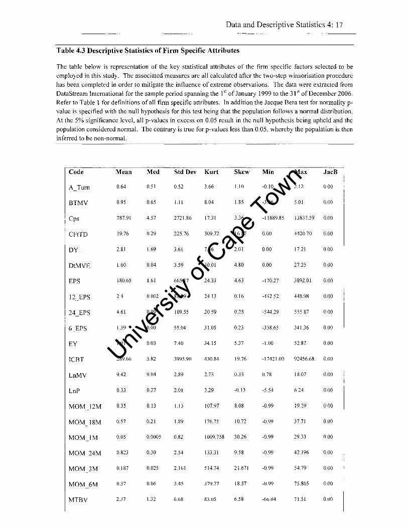
Data and Descriptive Statistics 4: 17

Table 4.3 Descriptive Statistics of Firm Specific Attributes

The table below is representation of the key statistical attributes of the firm specific factors selected to be employed in this study. The associated measures are all calculated after the two-step winsorisation procedure

has been completed in order to mitigate the influence of extreme observations. The data were extracted from

DataStream International for the sample period spanning the 151 of January 1999 to the 31 51 of December 2006. Refer to Table 1 for definitions of all firm specific attributes. In addition the Jacque Bera test for normality p­

value is specified with the null hypothesis for this test being that the population follows a normal distribution. At the 5% significance level, all p-values in excess on 0.05 result in the null hypothesis being upheld and the

population considered normal. The contrary is true for p-values less than 0.05, whereby the population is then

inferred to be non-normal.

Code Mean Med Std Dev Kurt Skew Min Max JacB

A Tum 0.64 0.51 0.52 3.66 1.10 -0.\0 2.12 000

BTMV 0.95 0.65 \.II 8.04 1.85 -3.06 5.01 0.00

Cps 787.91 4.57 2721.86 17.31 3.36 -11889.85 \3837.59 0.00

CFtTD 19.76 0.29 225.76 309.72 16.87 0.00 4420.70 0.00

DY 2.81 1.69 3.61 7.46 2.01 0.00 17.21 0.00

DtMVE 1.60 0.04 3.59 30.01 4.80 0.00 27.25 0.00

EPS 180.65 1.61 665.17 24.33 4.63 -170.27 3892.01 0.00

12 EPS 2.4 0.002 81.99 24.13 0.16 -442.52 448.98 0.00

24 EPS 4.61 0.09 109.55 20.59 0.25 -544.29 555.87 0.00

6 EPS 1.39 0.00 55.04 31.05 0.23 -338.65 341.36 000

EY 1.91 0.03 7.40 34.15 5.37 -1.00 52.87 0.00

lCBT 289.66 3.82 3995.90 430.84 19.76 -17421.00 92456.68 000

LnMV 9.42 9.04 2.89 2.73 0.33 0.78 1807 0.00

LnP 0.33 0.27 2.01 3.29 -0.13 -5.54 6.24 0.00

MOM 12M 0.35 0.13 1.13 107.97 808 -0.99 19.29 000

MOM IBM 0.57 0.21 1.89 176.75 10.72 -0.99 37.71 000 -

MOM 1M 0.05 0.0005 0.82 1009.758 30.26 -0.99 29.33 0.00 -

MOM 24M 0.823 0.30 2.54 133.31 9.58 -0.99 42.196 0.00

MOM 3M 0.187 0.025 2.161 514.74 21.671 -0.99 54.79 0.00

MOM 6M 0.37 0.06 3.45 379.77 18.57 -0.99 75.805 0.00

MTBV 2.37 1.32 6.68 83.05 6.58 -66.04 71.51 0.00

Univers

ity of

Cap

e Tow

n

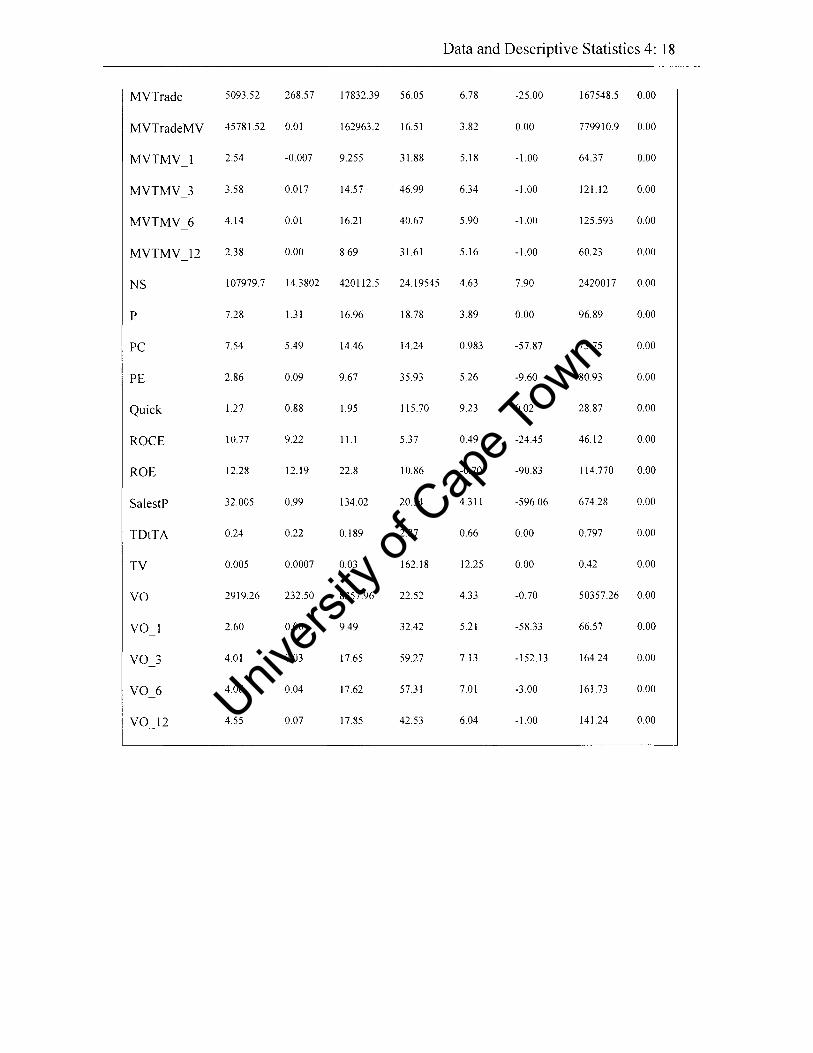
Data and Descriptive Statistics 4: 18

MVTrade 5093.52 268.57 17832.39 56.05 6.78 -25.00 167548.5 0.00

MVTradeMV 45781.52 0.01 162963.2 16.51 3.82 0.00 779910.9 0.00

MVTMV 1 2.54 -0.007 9.255 31.88 5.18 -1.00 64.37 0.00

MVTMV 3 3.58 0.017 14.57 46.99 6.34 -1.00 121.12 0.00

MVTMV 6 4.14 0.01 16.21 40.67 5.90 -1.00 125.593 0.00

MVTMV 12 2.38 0.00 8.69 31.61 5.16 -1.00 60.23 0.00

NS 107979.7 14.3802 420112.5 24.19545 4.63 7.90 2420017 0.00

P 7.28 1.31 16.96 18.78 3.89 0.00 96.89 0.00

PC 7.54 5.49 14.46 14.24 0.983 -57.87 73.75 0.00

PE 2.86 0.09 9.67 35.93 5.26 -9.60 80.93 0.00

Quick 1.27 0.88 1.95 115.70 9.23 0.02 28.87 0.00

ROCE 10.77 9.22 11.1 5.37 0.49 -24.45 46.12 0.00

ROE 12.28 12.19 22.8 10.86 -0.70 -90.83 114.770 0.00

SalestP 32.005 0.99 134.02 20.34 4.311 -59606 674.28 0.00

TDtTA 0.24 0.22 0.189 2.87 0.66 0.00 0.797 0.00

TV 0.005 0.0007 0.03 162.18 12.25 0.00 0.42 0.00

VO 2919.26 232.50 8357.96 22.52 4.33 -0.70 50357.26 0.00

VO 2.60 0.00 9.49 32.42 5.21 -58.33 66.57 0.00

VO 3 4.01 0.03 17.65 59.27 7.13 -152.13 164.24 0.00

VO 6 4.06 0.04 17.62 57.31 7.01 -3.00 161.73 0.00

VO 12 4.55 0.07 17.85 42.53 6.04 -1.00 141.24 0.00 -

Univers

ity of

Cap

e Tow

n

Data and Descriptive Statistics 4: 19

4.3 Summary and Conclusion

This chapter introduces the majority of the selected dataset used for testing in this paper.

The dataset presented comprised of stock return and firms specific data. A number of

adjustments were made to both stock return and firm specific data in order aid in testability

and result generation. Stock Returns were assessed for thin trading, however this was

found to be less of a concern than in previous studies. Subsequent adjustments were in fact

made to remove shares with insufficient return information and those with observations of

excessive magnitude. In all a total of 17 shares were removed providing a final sample of

1273 stocks.

The nature of the data and its respective source is assessed and inherent biases identified

properly documented. It is evident that this study is free from Look-Ahead and Data­

Snooping Bias, however it is nevertheless subject to Survivorship Bias.

Furthermore, in order to properly mitigate the effect of outliers present the process of

winsorisation is employed. Under this procedure both stock return and firm specific data

observations are restricted to a number of deviations around their mean value in order to

safeguard against spurious observations impacting negatively on results. A limit of 100%

is imposed on all stock return information.

Descriptive Statistics of all firm specific variables are presented that show evidence of

distinct positive skewness amongst the majority of variables. Such an anomaly is of little

consequence in light ofthe testing methods employed in Chapters Five, Six and Seven. Univers

ity of

Cap

e Tow

n

5.1 Introduction

-5-

Specification of Index Models and

Univariate Style Analysis

In the prior research reviewed in chapter three of this paper there is considerable

evidence that justifies the existence of certain firm specific anomalous characteristics that

explain return behaviour in an emerging market context. These so-called anomalies are

found to explain variation that is seemingly unexplained by the CAPM, considered the

metaphorical pillar in the theory of asset pricing. This chapter seeks to test empirically for

the presence of such return anomalies across the currently selected sample.

This study possesses a number of distinguishing features that distinguish it from prior

studies. Firstly, the broadness of the sample rivals any previous study performed on

'emerging' nations. Secondly, the array of firm specific variables analysed in this study is

far greater than those of earlier studies and so will hopefully serve to broaden the

understanding of return behaviour in such markets.

Ultimately the aim of this chapter is to undertake a univariate cross-sectional style analysis

and in so doing identify style-based factors with significant explanatory power. These style

anomalies, in order to be classified as such, need to be able to explain the variation in

returns before and after adjustments made for systematic risk. The methodology employed

follows that of Fama and Macbeth (1973) where the pooled time-series regression

coefficients and t-statistics are assessed.

Firstly though two forms of index models are specified in order gauge the degree of

systematic risk in the aforementioned markets. Both the single and multi index models

Univers

ity of

Cap

e Tow

n

Specification oflndex Models and Univariate Testing 5: 2

constructed employ well researched market proxIes that can be considered satisfactory

benchmarks for the chosen sample.

The remainder of the chapter is comprised of section 5.2 which outlines the raw returns and

the building and testing of the index models. Section 5.3 presents the results and a discussion

of the tested index models. Section 5.4 then provides a detailed outline of the univariate

testing procedure to be undertaken on the specified sample with the subsequent results

presented in Section 5.5 with Section 5.6 indicating the outcome of the style consistency

assessment. Section 5.7 summarizes and concludes.

5.2. Testing the Single and Multi index models

5.2.1 Data and Methodology

Single Index Models

Monthly return data for all selected stocks listed on the DataStream International Emerging

Markets Index over the sample period 1 January 1997 to 31 December 2006 is used in testing

the of the Single Index Model. All returns from across the several emerging nations

documented are converted to US dollars for ease of comparison and final interpretation.

As discussed in Roll (1976) any test of market efficiency is ajoint test ofthe accuracy of both

the asset pricing model used and the selected market proxy. In this study the chosen market

proxies are the DataStream International Emerging Markets Market Index and DataStream

International World Index. These indices are well documented and due to the relative

sparseness of information in an emerging market context are the most appropriate

benchmarks to be used in this study. The correlation between these indices is approximately

0.623 indicating that there is indeed variation that may be specific to emerging nations that is

unexplained on a global scale and vice versa.

The DataStream International Emerging Markets index as previously mentioned comprises

twenty six emerging nations being somewhat of a more localised proxy that omits the

influence of the more developed markets on return behaviour in an emerging context. The

Univers

ity of

Cap

e Tow

n

Specification oflndex Models and Univariate Testing 5: 3

DataStream International World Index is far broader being made up of a large sample of both

developed and developing countries. The inclusion of such an Index may provide unexpected

explanatory assistance in terms of emerging market return patterns and possibly identify

aforementioned signs of the greater integration of financial markets across the globe.

The 3 month or 90 day US Treasury Bill is used as a proxy for the risk free rate in computing

excess returns for each individual stock and both the DataStream International Emerging

Markets Market Index and DataStream International World Index.

A variation of the market model employed by Sharpe (1964) is used in this study in order to

gauge the commonality in variation amongst listed emerging market stocks. The model

specified below is in 'excess return' format as it aids in testing the statistical significance of

those sources of variation seemingly unexplained by the co-movement of stocks with some

market proxy, more specifically the abnormal return.

Excess monthly returns for the period 1 January 1997 to 31 December 2006 for each of the

1273 stocks included in the sample are regressed firstly against the monthly excess returns of

the DataStream Emerging Markets proxy. Thereafter, the realised returns are then regressed

with the DataStream World Market proxy.

The return generating process is specified as follows:

Where,

Rit - Rf

~i

Rmt - Rf

realised returns on assets i in period t

the constant term

the estimated beta coefficient of asset i

the returns on a 'market portfolio' in period t (in this case

proxied by the DataStream International Emerging Markets

Index and thereafter by the DataStream International World

Index)

random error term

Univers

ity of

Cap

e Tow

n

Specification ofIndex Models and Univariate Testing 5: 4

If a share was not listed or returns data was not available for part of the ten-year period, a

regression equation is still estimated using the returns data that are available.

Each regressIOn yields an R2, an R2 -adjusted, a p-value statistic, and a time-series of

residuals.

Multi Index Model

Once more monthly return data for all selected stocks listed on the DataStream International

Emerging Markets Index over the sample period 1 January 1997 to 31 December are

converted to US dollars as is the convention. A multifactor model is employed in order to

attempt to better explain the variation of returns in such a volatile setting.

The regression equation takes the form

Where,

Rit- Rf

~iemi

realised returns on assets i in period t

the constant term

beta coefficient showing sensitivity to the EMI

represents the realised return on DataStream International

Emerging Markets Index (EMI) in period t

beta coefficient showing sensitivity to the WMI

represents the realised return on DataStream International

W orId Markets Index (WMI) in period t

The Multi-index model uses the two market proxies in combination as explanatory variables

with the US 3 month Treasury bill rate being once again used as a proxy for the risk-free rate.

Each regressIOn yields an R2, an R2 -adjusted, a p-value statistic, and a time-series of

residuals.

Univers

ity of

Cap

e Tow

n

Specification oflndex Models and Univariate Testing 5: 5

Further testing is then performed in order to test the effectiveness of both models in terms of

explaining the unknown variation in each setting. These 'second lever tests follow the same

procedure as those previous except that in this case the respective residuals of each model are

used as dependent variables for competing models. Therefore, the multi-index model's

residuals are regressed on the explanatory variables for each of the two separate single-index

models and then each of the single index model's residuals regressed on the explanatory

variables of the multi-index model.

Once more each regression yields an R2, an R2 -adjusted, a p-value statistic, and a time-series

of residuals.

5.2.2 Theoretical Concerns and Critical Assumptions

There are certain key assumptions of any form of regression model that need to be adhered to

in order to obtain significant and interpretable results. The model is constrained to those

critical assumptions that underpin any statistically sound regression analysis:

• The predictors must be linearly independent, i.e. one must not be able to express any

predictor as a linear combination of another

• The error terms or residuals must be normally distributed

• The error terms must be independent and random i.e. E(Eit, Ejt) = 0 for all t where i i- j

• The variance of the error terms must be constant

If such assumptions are violated there can be significant implication with regards to the

accuracy of the coefficients generated. Heteroscedasticity occurs when successive error

terms are correlated with one another, whilst multicollinearity is evident where numerous

explanatory variables are correlated with one another and so disturb accurate result

generation (evident in a multi factor setting). The implications of either being present are

somewhat dire - as beta coefficients are estimated in error either under or over estimates of

their true value with associated high standard errors and insignificant t-stats. In the case of

the current study normality is not cited as a concern, with the associated Jarque Bera statistics

indicating that all the examined residuals resemble that of a normal distribution. Due to the

structure of data collection, namely consecutive months, there is cause for concern that

Univer

iof

Cape T

own

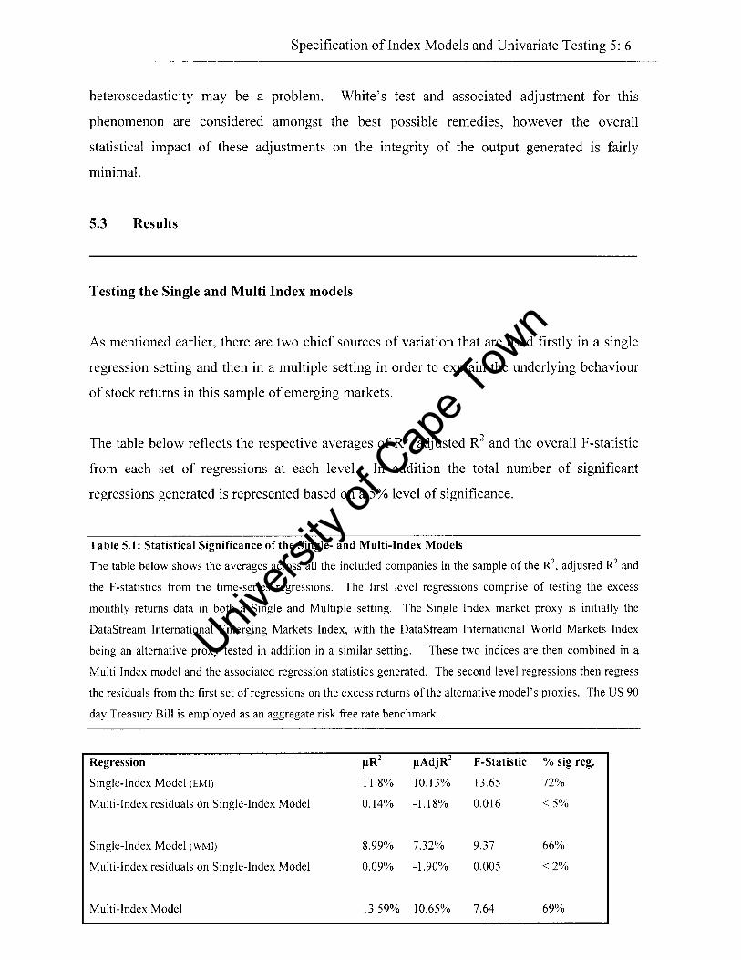
Specification ofIndex Models and Univariate Testing 5: 6

heteroscedasticity may be a problem. White's test and associated adjustment for this

phenomenon are considered amongst the best possible remedies, however the overall

statistical impact of these adjustments on the integrity of the output generated is fairly

minimal.

5.3 Results

Testing the Single and Multi Index models

As mentioned earlier, there are two chief sources of variation that are used firstly in a single

regression setting and then in a multiple setting in order to explain the underlying behaviour

of stock returns in this sample of emerging markets.

The table below reflects the respective averages of R2, adjusted R2 and the overall F-statistic

from each set of regressions at each level. In addition the total number of significant

regressions generated is represented based on a 5% level of significance.

Table 5.1: Statistical Significance of the Single- and Multi-Index Models

The table below shows the averages across all the included companies in the sample of the R2, adjusted R2 and

the F -statistics from the time-series regressions. The first level regressions comprise of testing the excess

monthly returns data in both a Single and Multiple setting. The Single Index market proxy is initially the

DataStream International Emerging Markets Index, with the DataStream International World Markets Index

being an alternative proxy tested in addition in a similar setting. These two indices are then combined in a

Multi Index model and the associated regression statistics generated. The second level regressions then regress

the residuals from the first set of regressions on the excess returns of the alternative model's proxies. The US 90

day Treasury Bill is employed as an aggregate risk free rate benchmark.

Regression /lR2 /lAdjR2 F -Statistic % sig reg.

Single-Index Model (EM I) 11.8% 10.13% 13.65 72%

Multi-Index residuals on Single-Index Model 0.14% -1.18% 0.016 <5%

Single-Index Model (WMI) 8.99% 7.32% 9.37 66%

Multi-Index residuals on Single-Index Model 0.09% -1.90% 0.005 <2%

Multi-Index Model 13.59% 10.65% 7.64 69%

Univers

ity of

Cap

e Tow

n

Specification ofIndex Models and Univariate Testing 5: 7

Single-Index residuals(EMI) on Multi-Index Model

Single-Index residuals(WMI) on Multi-Index Model

First Level Tests:

2.56% 1.43%

5.71% 4.57%

0.70

2.72

9%

43%

As can be seen from the table above, the multi-index model has the highest R2 (13.59%) and

adjusted R2 (10.65%), indicating that even when additional explanatory variables are added

the forgone degrees of freedom do not sufficiently hamper the statistical power of the model.

Furthermore not only does the multi-index model explain more of the nature of the behaviour

of the excess stock returns, it also has a comparatively similar number of significant

regressions (890 of the 1273) compared to 929 and 851 of the Single-Index models using the

emerging and world market index proxies respectively.

Second Level Tests:

The second level tests aim to establish whether or not the competing model explains some of

the unexplained variation of its rival. From the table above it is evident that the multi-index

model explains only a very small portion of the variation unexplained by either of the single­

index models, 2.56% and 5.71% respectively. It is however evident that the multi-index

model does in fact explain additional variation not explained by either of the single factor

formulations, resulting the multi-index formulation being of greater superiority.

In addition the tests of the multi-index residuals on the single-index models yield even less

convincing results. Both of the single-index models and their associated market proxies

explain very little of the variation in the residuals of the multi-index model, 0.14% and

0.09%. When these tests are then adjusted for degrees of freedom both R2 values become

negative, a clear indication of a poorly fitted model.

Univers

ity of

Cap

e Tow

n

Specification ofIndex Models and Univariate Testing 5: 8

5.4 Univariate Style Testing of Factors

This next section aims to test all of the identified firm-specific characteristics mentioned in

Table 4.1. The analysis tests the attributes over the entire sample period using time-series

cross-sectional regressions against two types of return data, unadjusted and risk adjusted

return data.

5.4.1 Data and Methodology

The data employed for this analysis is as described in Chapter Four of this study. The

monthly returns data were adjusted as discussed in Chapter Four and comprised a total of

1273 listed stocks sourced from the DataStream International Emerging Markets Index for

the sample period 1 January 1997 to 31 December 2006. A range of fifty firm specific

attributes are sourced and constructed. The cross-sectional distribution of each style

characteristic in each month is then standardised in order to enhance the comparability of the

slope coefficients output from the regressions to follow. In technical terms, standardisation

involves the adjusting of each distribution in such a way that it yields a mean of zero and a

standard deviation of one.

In order to accommodate the effect of systematic risk as modelled by the CAPM and APT,

appropriate market proxies, factor proxies and a risk free rate are sourced. As per the

previous section, single and multi index models were constructed in order to measure the

impact of the systematic component of risk.

The sections that follow describe the tests performed on firstly the unadjusted returns and

secondly on those adjusted for risk via the respective models.

5.4.2 Tests of Unadjusted Returns

This section aims to test the significance of the style characteristics listed in Chapter Four on

returns that have undergone no adjustment for systematic risk. The methodology of Fama

Univers

ity of

Cap

e Tow

n

Specification ofIndex Models and Univariate Testing 5: 9

and Macbeth (1973) is followed closely, with the model upon which the Ordinary Least

Squares (OLS) regressions are to be run specified as follows:

Where,

r = realized return on share i for month t + 1 1,1+1

r 0,1+1 = constant intercept term

hl+l = cross-sectional slope coefficient estimated from the regression

AI = standardised value of the attribute of the share at end of each month t

E: = residual error 1,1+1

The return characteristic at the beginning of every month is therefore regressed against the

realised return on the share over that period. Such an analysis is repeated for every month in

the sample and so provides a chronological series of coefficients that represent the 'payoff' of

each firm specific attribute. Statistical tests in the form of the Students t-test are then applied

to the generated coefficients in order to ascertain their overall significance. Coefficients that

fail such a testing criterion are deemed to be statistically indifferent from zero and so provide

no basis for any form of inference.

5.4.3 Tests of Risk Adjusted Returns: CAPM - Single Index Model

This section adjusts aggregate share returns for market or systematic risk through the

formulation of an appropriate model with defined market proxies. The aim of this risk­

adjusting procedure is to explain the variation that is inherent in return data which is

unexplained by the specified single factor models. The tests to follow attempt to discern

whether or not the chosen firm-specific attributes are in any way able to explain this

unexplained variation that is seemingly unsystematic in its nature.

Two independent single factor models are specified usmg the DataStream International

Emerging Markets Index and DataStream International World Markets Index as their

respective market proxies.

Univers

ity of

Cape T

own

Specification ofIndex Models and Univariate Testing 5: 10

The return generating process is specified as follows:

Where,

R jt - Rf

~j

Rmt - Rf

realised returns on assets i in period t

the constant term

the estimated beta coefficient of asset i

the returns on a 'market portfolio' in period t (in this case

proxied by the DataStream International Emerging Markets

Index and thereafter by the DataStream International World

Index)

random error term (captures variation unexplained by ~j )

Therefore, in order to gauge the variation that is unexplained by the above model, one should

combine those sources of disturbance that are not defined as systematic. Through the

summation of the Uj and the random error term Cjt one is able to quantify patterns in the

returns data that are at present unexplained and hence specify an appropriate model that has

been appropriately adjusted for risk.

Therefore the associated risk adjusted return is calculated as follows:

A similar univariate cross sectional analysis is now performed on these risk adjusted returns

with (Uj + Cj.t+1 ) being substituted as the new dependent variable. The regression equations

take the form:

Univers

ity of

Cap

e Tow

n

Specification ofIndex Models and Univariate Testing 5: 11

In this instance &1.1+1 represents the random error term from risk adjustment whilst e,,t+1 is the

error term for this new regression equation. From the regression a time series of slope

coefficients, t-stats and beta values are estimated in order to statistically test for the

significance of the chosen factors.

5.4.4 Tests of Risk Adjusted Returns: APT - Multi Index Model

The third and final test employs the use of the previously specified multi-factor model to

establish whether significance is still evident after risk adjustment. As is the case with the

two single factor risk adjustment procedures time series regressions are run over the period 1 st

January 1997 through to the 31 st December 2006.

Model Specification:

Where,

Rit - Rf

~iemi

realised returns on assets i in period t

the constant term

beta coefficient showing sensitivity to the EMI

represents the realised return on DataStream International

Emerging Markets Index (EMI) in period t

beta coefficient showing sensitivity to the WMI

represents the realised return on DataStream International

W orId Markets Index (WMI) in period t

The risk-adjusted returns are then calculated through the summation of those sources of

variation that are unexplained by the fitted model. This is equivalent to the adding of each Ui

with the associated error term Ci,t serving to create a time series of returns that are adjusted for

a significant component of systematic risk.

As is the case with the previous tests, the multifactor risk adjusted return is calculated using

the following procedure:

Univers

ity of

Cap

e Tow

n

Specification ofIndex Models and Univariate Testing 5: 12

A similar series of cross sectional univariate tests are then performed on these risk adjusted

returns employing the regression model specified below:

In this instance c,,/+1 represents the random error term from risk adjustment whilst e,,/+1 is the

error term for this new regression equation. From the regression a time series of slope

coefficients, t-stats and beta values are estimated in order to statistically test for the

significance of the chosen factors.

5.4.5 Comparison between adjusted and unadjusted results

In comparing the results from the three sets of unvariate cross sectional analyses certain

consideration must be taken as to the manner in which the risk adjusted returns were in fact

computed. As the associated betas for all the risk adjusted tests were calculated from the data

set upon which the style characteristics are being analysed, there is less of a chance that the

style characteristics will be evident when tested upon these adjusted returns relative to the

unadjusted figures. Therefore, it can be construed that if certain factors are indeed of

significant explanatory power they should be evident in a risk-adjusted setting. The risk­

adjusted tests can be seen as somewhat of a robustness check on the pervasiveness of the

identified factors.

5.4.6 Primary Adjustment to list of firm specific characteristics

The first step in analysing the full list of firm specific characteristics is that of ascertaining

each of the tested factors statistical significance. From the monthly time series of cross

sectional regressions run, associated average Student t-statistics are computed and assessed

for significance.

Factors are tested at the five percent level of significance a

procedure:

0.05 using the following

Univers

ity of

Cap

e Tow

n

Ho: ~I = 0

HI:~I:fO

T stat = mean (y)/se (y)

T -critical: tan-I = t 005 119 = ± 1.65 , . ,

Specification ofIndex Models and Univariate Testing 5: 13

The result of such testing serves to narrow down the list of characteristics run on the

unadjusted returns from fifty to a final list of twenty eight statistically significant attributes,

As an aside, it is worth noting that the style factor 'PIE' was omitted from the list upon

discovering flaws in the datasource,

5.4.7 Analysis of primary list of significant characteristics

The total list of firm specific characteristics was chosen in line with previous studies to be as

comprehensive as possible whilst at the same time concerned with ensuring relevance.

However in aiming to be sufficiently comprehensive it is inevitable that there will be factors

that are similar and exhibit common variation. Such behavioural occurrences will serve to

make the isolation and interpretation of each firm-specific effect troublesome, therefore some

form of trimming procedure is necessary. The implementation of cluster and correlation

analyses aims to mitigate the prevalence of such a problem through detailed examination of

the monthly payoffs output.

The monthly payoffs of each of the factors form the subject of the suggested cluster and

correlation analyses. The initial step in the procedure is the performance of the cluster

analysis. By cluster analysing the characteristics identified as being significant, one is able to

assess the degree of similarity between each factor and their relative ability in explaining

return variation. However, clusters do not only form on account of there being like variation

amongst factors. It may happen that certain factors group together with certain others on

account of them being totally dissimilar to all those in the analysis. This phenomenon if

Univers

ity of

Cap

e Tow

n

Specification oflndex Models and Univariate Testing 5: 14

present may detract from the pervasiveness of the clusters and so therefore a detailed

correlation analysis is performed to enhance the identification of co-moving factors.

The precise methodology employed for the aforementioned cluster analysis follows that as

described in Ward (1963). This method is somewhat different from the alternatives such as

Single and Complete Linkage as it considers the analysis of variance when establishing

clusters. The procedure entails the computing of the total sum of the squared deviations from

each observation from the mean of the cluster to which it belongs. At each and every stage of

the analysis the combination of every possible cluster is considered and those unions that

result in the minimum increase in the error sum of squares are combined into clusters. It is

also generally found that such a clustering method serves to create narrow clusters as a result

of the well defined clustering criterion.

The distance measure selected for such an analysis is additional important consideration. As

the interest of this research is to ascertain the co-movement of such factors and their

associated ability to explain share return variation, the Pearson Correlation Coefficient is

selected as the appropriate distance measure for the cluster analysis. The coefficient takes the

following form:

n

LCrx,t -~)Crv,t -r;) p = -,-t~-,-I ______ _

x,Y n-l

Where Px.y is the correlation coefficient between each of the time series ofthe monthly

payoffs of each of the significant style characteristics.

rx:u is tth monthly characteristic payoff derived from the univariate testing procedure

~.Y is the mean monthly characteristic payoff for the time series of returns derived

from the same univariate testing procedure

n is the number of monthly payoffs in the time series

Once the above procedure is completed a sufficient number of clusters that map similar

variation should be generated and form the foundation for further model building.

Univers

ity of

Cap

e Tow

n

Specification oflndex Models and Univariate Testing 5: 15

In performing a correlation analysis on the full set of monthly payoffs, the true relationships

amongst the firm characteristics is forthcoming. A correlation matrix is generated for each of

the identified clusters employing the use of the Pearson Correlation Coefficient the

computation of which was discussed earlier in this chapter.

The correlation matrices output are then further scrutinised on statistical grounds. Factors

that exhibit a high degree of co-movement with others are then compared based on their t­

statistics output from the preceding cross sectional univariate style tests on the unadjusted

returns. In the event of two factors exhibiting a high degree of correlation, only that factor

with the higher t-statistic is included in the study. For the purposes of this section upon

discussion with Van Rensburg, a high correlation is arbitrarily defined as any value in excess

of 0.7 or less than -0.7.

Subsequently, the remaining factors are then analysed for any signs of co-movement. Once

more the above procedure is followed to prune the list of significant characteristics to those

whose impact on return variation can be sufficiently isolated.

Prior to any such trimming procedures being performed the Price Earnings firm specific

factor was excluded from the analysis on account of its spurious negative data entries.

Instead of this factor Earnings Yield is used a proxy to gauge the desired value effect.

Univers

ity of

Cap

e Tow

n

Specification oflndex Models and Univariate Testing 5: 16

5.4.8 Style Consistency

In order to gauge the potential for possible style modelling, the direction of the monthly

payoffs to the refined list of significant firm specific characteristics is assessed.

5.4.8.1 Consistency in direction of monthly payoffs

This first method employed aims to attempt to ascertain the proportion of times that the

payoff is either positive or negative.

The proportion of the number of times the monthly payoffs are positive or negative is found

in the range between 0 and 100%. Those payoffs that have value closest to either one of the

aforementioned bounds are considered to have a more consistent direction. In order to

evaluate these ratios a non-parametric Sign Test is run with the null hypothesis that the

payoffs are positive in 50% of the months and negative in the 50% of the months.

5.4.8.2 Tests for Randomness in the monthly payoffs

This second method aims to test for randomness in the payoffs by attempting to ascertain the

frequency with which the actual directions of the payoffs change over the sample period. The

null hypothesis for the test states that each of the sequence of monthly payoffs is random,

with the alternative looking for non-randomness. The test statistic is usually defined as the

number of runs (R) - the number of groups of payoffs exhibiting consistent direction, with

the rejection region specified on the basis of the number of observations in differing

categories, in this case the number being either positive or negative. However as the sample

being analysed is of sufficient size the sampling distribution of R becomes approximately

normal and so allows for more conventional data analysis.

Univers

ity of

Cap

e Town

Specification oflndex Models and Univariate Testing 5: 17

5.5 Results

5.5.1 Univariate Testing: Unadjusted and Risk-Adjusted results

The results of the univariate cross sectional style tests on both the unadjusted and risk­

adjusted returns are presented in the tables below. Each table contains the full list of fifty

selected factors ranked in descending order of the absolute value of their t-statistic. Also

presented for each factor is the average of the time series of slope coefficients generated over

the full sample period. See Appendix B for a full output of slope coefficients and t-statistics.

Table 5.1 presents the full list of style factors tested on the unadjusted returns. Table 5.2 and

5.3 display the results of the same set of factors run for the risk-adjusted returns. Upon

examination it becomes evident that a large number of these tested style characteristics are

indeed significant. Furthermore, many of these factors remain significant post risk

adjustment indicative of their pervasiveness in explaining emerging market return variation.

However, there are a number of factors that diverge from the unadjusted results once risk

adjustment has been completed, with the magnitude of their payoffs and direction of

relationship substantially different.

Subsequently, the cluster analysis run on the factors found to be significant in univariate

testing against unadjusted returns as presented in Figure 5.1. Thereafter the cluster analyses

run on the both sets of risk adjusted return data are presented in for comparative purposes in

Figures 5.2 and 5.3. Univ

ersity

of C

ape T

own

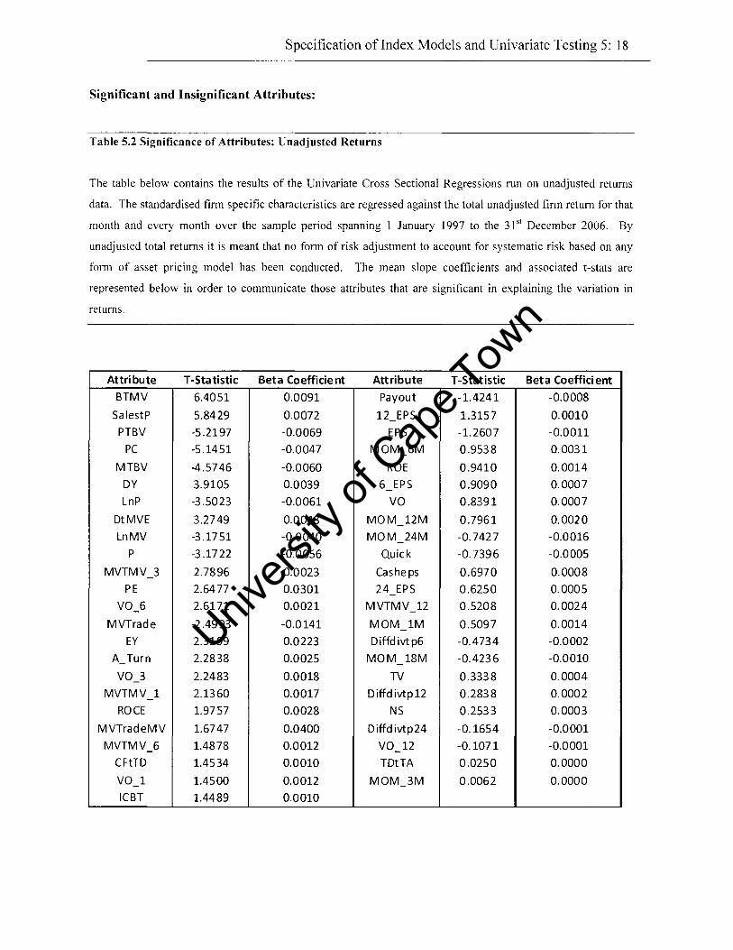
Specification ofIndex Models and Univariate Testing 5: 18

Significant and Insignificant Attributes:

Table 5.2 Significance of Attributes: Unadjusted Returns

The table below contains the results of the Univariate Cross Sectional Regressions run on unadjusted returns

data. The standardised firm specific characteristics are regressed against the total unadjusted finn return for that

month and every month over the sample period spanning 1 January 1997 to the 31 st December 2006. By

unadjusted total returns it is meant that no form of risk adjustment to account for systematic risk based on any

form of asset pricing model has been conducted. The mean slope coefficients and associated t-stats are

represented below in order to communicate those attributes that are significant in explaining the variation in

returns.

Attribute T-Statistic Beta Coefficient Attribute T-Statistic Beta Coefficient

BTMV 6.4051 0.0091 Payout -1.4241 -0.0008

SalestP 5.8429 0.0072 12_EPS 1.3157 0.0010

PTBV -5.2197 -0.0069 EPS -1.2607 -0.0011

PC -5.1451 -0.0047 MOM_6M 0.9538 0.0031

MTBV -4.5746 -0.0060 ROE 0.9410 0.0014

DY 3.9105 0.0039 6_EPS 0.9090 0.0007

LnP -3.5023 -0.0061 VO 0.8391 0.0007

DtMVE 3.2749 0.0048 MOM 12M 0.7961 0.0020

LnMV -3.1751 -0.0040 MOM_24M -0.7427 -0.0016

P -3.1722 -0.0056 Quick -0.7396 -0.0005

MVTMV_3 2.7896 0.0023 Casheps 0.6970 0.0008

PE 2.6477 0.0301 24_EPS 0.6250 0.0005

VO_6 2.6171 0.0021 MVTMV 12 0.5208 0.0024

MVTrade -2.4993 -0.0141 MOM_1M 0.5097 0.0014

EY 2.3199 0.0223 Diffdivtp6 -0.4734 -0.0002

A_ Turn 2.2838 0.0025 MOM_18M -0.4236 -0.0010

VO 3 2.2483 0.0018 TV 0.3338 0.0004

MVTMV_1 2.1360 0.0017 D iffd ivtp 12 0.2838 0.0002

ROCE 1.9757 0.0028 NS 0.2533 0.0003

MVTradeMV 1.6747 0.0400 Diffdivtp24 -0.1654 -0.0001

MVTMV_6 1.4878 0.0012 VO_12 -0.1071 -0.0001

CFtTD 1.4534 0.0010 TDtTA 0.0250 0.0000

VO 1 1.4500 0.0012 MOM_3M 0.0062 0.0000

ICBT 1.4489 0.0010

Univers

ity of

Cap

e Tow

n

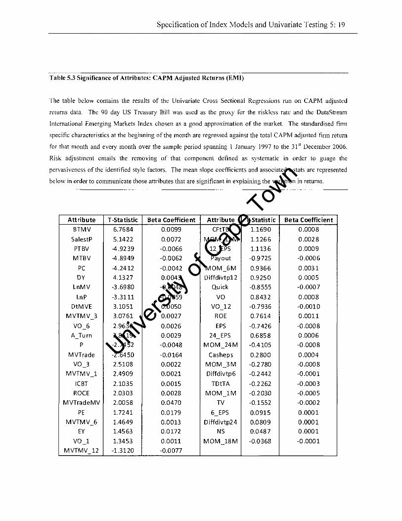
Specification ofIndex Models and Univariate Testing 5: 19

Table 5.3 Significance of Attributes: CAPM Adjusted Returns (EMI)

The table below contains the results of the Univariate Cross Sectional Regressions run on CAPM adjusted

returns data. The 90 day US Treasury Bill was used as the proxy for the riskless rate and the DataStream

International Emerging Markets Index chosen as a good approximation of the market. The standardised firm

specific characteristics at the beginning of the month are regressed against the total CAPM adjusted firm return

for that month and every month over the sample period spanning I January 1997 to the 31 51 December 2006.

Risk adjustment entails the removing of that component defined as systematic in order to guage the

pervasiveness of the identified style factors. The mean slope coefficients and associated t-stats are represented

below in order to communicate those attributes that are significant in explaining the variation in returns.

Attribute T -Sta tistic Beta Coefficient Attribute T-Statistic Beta Coefficient

BTMV 6.7684 0.0099 CFtTD 1.1690 0.0008

SalestP 5.1422 0.0072 MOM_12M 1.1266 0.0028

PTBV -4.9239 -0.0066 12 EPS 1.1136 0.0009

MTBV -4.8949 -0.0062 Payout -0.9725 -0.0006

PC -4.2412 -0.0042 MOM_6M 0.9366 0.0031

DY 4.1327 0.0043 D iffdivtp12 0.9250 0.0005

LnMV -3.6980 -0.0048 Quick -0.8555 -0.0007

LnP -3.3111 -0.0059 VO 0.8432 0.0008

DtMVE 3.1051 0.0050 VO_12 -0.7936 -0.0010

MVTMV 3 3.0761 0.0027 ROE 0.7614 0.0011

VO_6 2.9630 0.0026 EPS -0.7426 -0.0008

A_Turn 2.8519 0.0029 24 EPS 0.6858 0.0006

P -2.7452 -0.0048 MOM_24M -0.4105 -0.0008

MVTrade -2.6450 -0.0164 Casheps 0.2800 0.0004

VO_3 2.5108 0.0022 MOM_3M -0.2780 -0.0008

MVTMV 1 2.4909 0.0021 Diffdivtp6 -0.2442 -0.0001

ICBT 2.1035 0.0015 TDtTA -0.2262 -0.0003

ROCE 2.0303 0.0028 MOM_1M -0.2030 -0.0005

MVTradeMV 2.0058 0.0470 TV -0.1552 -0.0002

PE 1.7241 0.0179 6_EPS 0.0915 0.0001

MVTMV_6 1.4649 0.0013 D iffdivtp2 4 0.0809 0.0001

EY 1.4563 0.0172 NS 0.0487 0.0001

VO 1 1.3453 0.0011 MOM_18M -0.0368 -0.0001

MVTMV_12 -1.3120 -0.0077

Univers

ity of

Cap

e Tow

n

Specification ofIndex Models and Univariate Testing 5: 20

Table 5.4 Significance of Attributes: CAPM Adjusted Returns (WMI)

The table below contains the results of the Univariate Cross Sectional Regressions run on CAPM adjusted

returns data. The 90 day US Treasury Bill was used as the proxy for the riskless rate and the DataStream

International World Markets Index chosen as a good approximation of the market. The standardised firm

specific characteristics at the beginning of the month are regressed against the total CAPM adjusted firm return

for that month and every month over the sample period spanning 1 January 1997 to the 31 sl December 2006.

Risk adjustment entails the removing of that component defined as systematic in order to guage the

pervasiveness of the identified style factors. The mean slope coefficients and associated t-stats are represented

below in order to communicate those attributes that are significant in explaining the variation in returns.

Attribute T -Statistic Beta Coefficient Attribute T-Statistic Beta Coefficient

BTMV 5.6899 0.0106 Quick -1.3351 -0.0011

MTBV -5.2452 -0.0071 D iffd ivtp12 1.3006 0.0008

PTBV -5.1141 -0.0076 MOM_6M 1.2806 0.0043

SalestP 4.9531 0.0072 MVTMV 12 -1.2118 -0.0064

PC -4.2464 -0.0046 MOM 12M 1.1364 0.0030

DY 3.5359 0.0041 VO_1 0.9292 0.0008

LnMV -3.4823 -0.0050 24_EPS 0.9095 0.0008

LnP -3.4298 -0.0064 EPS -0.8196 -0.0009

DtMVE 2.9358 0.0052 CFtTD 0.6528 0.0005

MVTrade -2.8670 -0.0175 D iffd ivtp2 4 0.6455 0.0004

P -2.7712 -0.0052 MVTMV 6 0.5569 0.0005

MVTMV 3 2.7128 0.0024 ROE 0.4568 0.0007

A Turn 2.6530 0.0030 6 EPS 0.3889 0.0003

VO_6 2.5975 0.0023 TV 0.3849 0.0005

PE 2.2541 0.0236 Casheps 0.3725 0.0005

ICBT 2.0059 0.0014 VO_12 -0.3409 -0.0004

MVTMV_1 1.9782 0.0018 NS 0.2167 0.0003

VO_3 1.9501 0.0018 MOM 24M -0.2056 -0.0004

12_EPS 1.8307 0.0016 Diffdivtp6 -0.1314 -0.0001

ROCE 1.7767 0.0025 MOM IBM 0.1257 0.0003

MVTradeMV 1.7383 0.0482 TDtTA -0.1223 -0.0002

MOM 1M -1.4952 -0.0044 MOM_3M 0.1147 0.0004

EY 1.4153 0.0178 VO 0.1004 0.0001

Payout -1.3609 -0.0010

Univers

ityof

Cape T

own

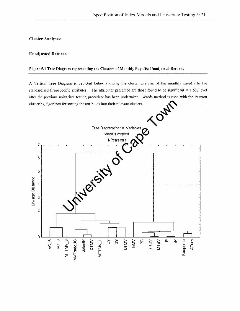
Specification oflndex Models and Univariate Testing 5: 21

Cluster Analyses:

Unadjusted Returns

Figure 5.1 Tree Diagram representing the Clusters of Monthly Payoffs: Unadjusted Returns

A Vertical Tree Diagram is depicted below showing the cluster analysis of the monthly payoffs to the

standardised firm-specific attributes. The attributes presented are those found to be significant at a 5% level

after the previous univariate testing procedure has been undertaken. Wards method is used with the Pearson

clustering algorithm for sorting the attributes into their relevant clusters.

7

6

5

Q) () c i!l 4 en is Q) OJ 3 eu

.::.::. c

:.:J

2

I I I o

<01 (') (') en 1 >' ::::> a a Q)

> > ~ '0 I-- eu

"-I--~ ~ ~

Tree Diagram for 18 Variables

Ward's rrethod

1-Pearson r

I I

~ r l I I n.. > ..- >- >- > > () iii ~ >1 W 0 ~ ~ n.. Q) I-- I-- E ro 0 ~ co

I--en I--~

I 1 1 n

> > n.. n.. a. c co co .J:: E "-

::J I-- I-- Q)

~ n.. ~ a. eu ()

e:::

Univers

ity of

Cap

e Tow

n

Specification ofIndex Models and Univariate Testing 5: 22

CAPM (Emerging Market Index) Adjusted Returns

Figure 5.2 Tree Diagram representing the Clusters of Monthly Payoffs: CAPM (EMI) Adjusted Returns

A Vertical Tree Diagram is depicted below showing the cluster analysis of the monthly payoffs to the

standardised firm-specific attributes. The attributes presented are those found to be significant at a 5% level

after the previous univariate testing procedure has been undertaken. Wards method is used with the Pearson

clustering algorithm in sorting the attributes into their relevant clusters.

6

5

a.> 4 (J c ~ III

i:S 3 a.> en ro

.0<:. c

:.:::i 2

o I ~ CD1 C') C') (f) £, > 1 >1 ::> ::2: 0 0 Kl a.> I-> > ::2: "0 Zij 0 I- ro ....

I- > ::2: ::2:

Tree Diagram for 19 Variables

Ward's method

1-Pearson r

L I

nn > ;1 >- > > I-::2: 0 ::2: ::2: al a; l- .£;; U

::2: al "0 I-ro .... I-

> ::2: ::2:

I U 0..

I 1 1 n

> > 0.. 0.. c.. c al al .£;; E ....

:::J l- I- a.> I-0.. ::2: c.. « ro

(J

0:::

Univers

ity of

Cap

e Tow

n

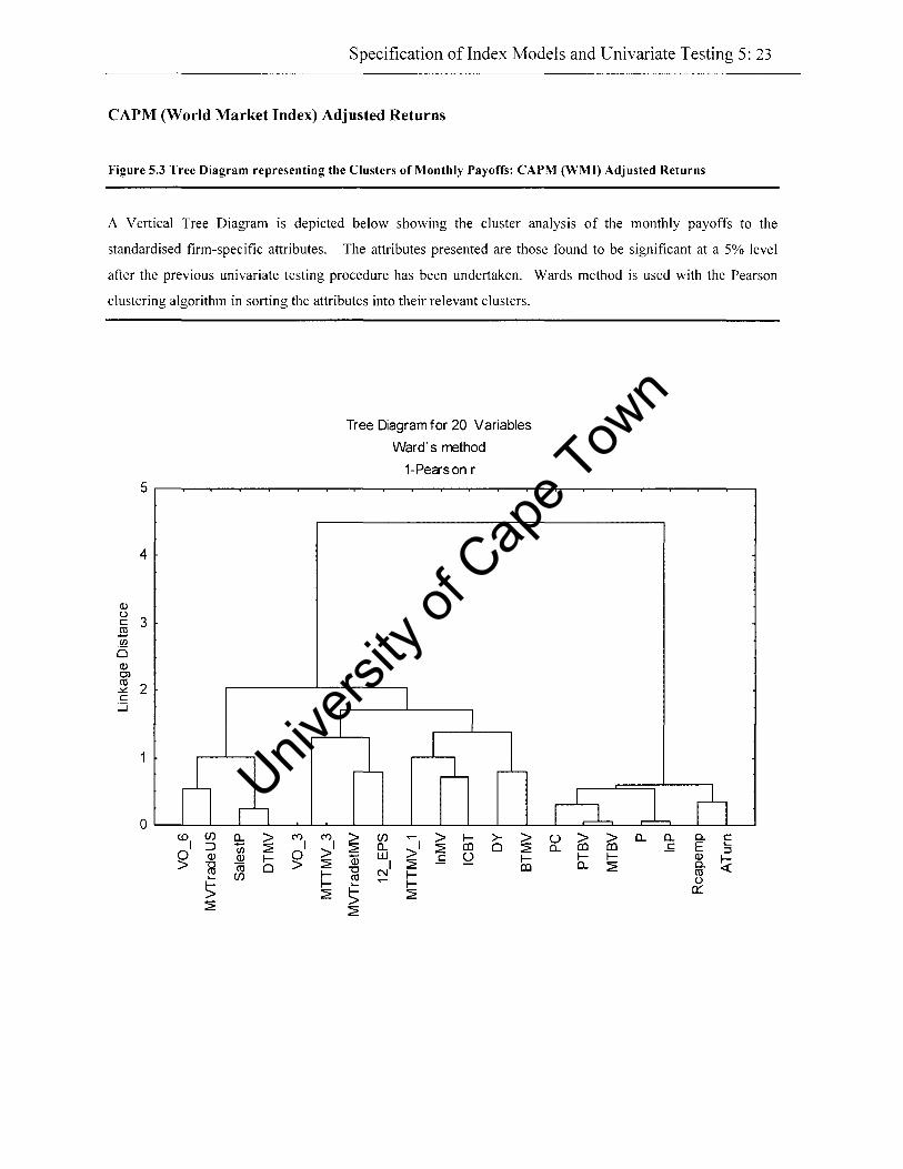
Specification oflndex Models and Univariate Testing 5: 23

CAPM (World Market Index) Adjusted Returns

Figure 5.3 Tree Diagram representing the Clusters of Monthly Payoffs: CAPM (WMI) Adjusted Returns

A Vertical Tree Diagram is depicted below showing the cluster analysis of the monthly payoffs to the

standardised firm-specific attributes. The attributes presented are those found to be significant at a 5% level

after the previous univariate testing procedure has been undertaken. Wards method is used with the Pearson

clustering algorithm in sorting the attributes into their relevant clusters.

5

4

a> t)

3 c .!!l .~ 0 a> OJ ro

2 .::.::. c

:.:J

I

o n i'l <01 C/) a.. > (") (")

::J iii ~ I >1 ~ ~ a> a> I-

~ ro 0 ~ C/) I-

> I-~

~

Tree Diagram for 20 Variables

Ward's method

1-Pearson r

I I

1 1 -.L

> C/) ;1 > I- >- > ~ a.. ~ co 0 ~ a:; W .s U l-'0 I ~ co ro N I-L.. l-

> ~

~

I ~n I J-. u > > a.. a.. Q. c a.. co co .s E L..

:::J I- I- a>

~ a.. ~ Q. ro t)

0::

Univers

ity of

Cap

e Tow

n

Specification ofIndex Models and Univariate Testing 5: 24

5.5.2 Identification of significant clusters: Unadjusted Returns

The cluster analysis yielded few, well defined clusters worthy of scrutiny. Due to Ward's

Method (1963) being very efficient in clustering it is documented that the groupings output

may in fact be somewhat narrow and omit certain factors from an expected cluster. The

classification of significant factors into the previously identified clusters is somewhat

subjective with groupings defined whilst taking into account previous literary findings.

1. Size and Value Combination

Size

Logarithm of Market Value (lnMV), Price (P), Logarithm of Price (LnP)

Value

Price to Cash (PC), Price to Book Value (PTBV), Market to Book Value (MTBV),

Return on Capital Employed (RaCE) and Asset Turnover (A Tum)

2. Value and Performance

Earnings Yield (EY), Dividend Yield (DY), Book to Market Value (BTMV), Market

Value to Market Value Traded (MTTMV _1)

3. Liquidity

Six month change in Volume in Traded (VO_6), Market Value Traded to Market

Value over Three months (MTTMV _3), Three month change in Traded Volume

(Va 3)

4. Miscellaneous:

Sales to Price Ratio (SalestP), Debt to Market Value (DTMV) and Market Value

Traded (MVTrade)

The additional cluster analyses run on the two differing sets of adjusted returns are used to

gauge the respective robustness of the clusters identified from analysing unadjusted returns.

Univers

ity of

Cap

e Tow

n

Specification ofIndex Models and Univariate Testing 5: 25

It is worth noting that certain factors fail to remain significant post risk adjustment, however

more importantly the same general clusters are again identifiable.

5.5.3 Monthly Payoffs of Significant Factors

As a result of the clusters of significant characteristics being somewhat pervasive across

unadjusted and risk-adjusted returns, the remainder of this chapter will focus on the

unadjusted return factors and their associated dataset.

In order to simplify the list of firm specific characteristics, correlation matrices were

generated for each of the clusters identified.

Univers

ity of

Cap

e Tow

n

""",,,," ,a," , "

-"mL~

,,,", ,ft

." ,w". " " , .• ,," "'.,.

'>S "'l"WP

[~L"'!l"lU'IU[ U,"'JJS"l"G "'[I UIOJJ poo.,"CtS •. [ •. " "l"P [IV "900Z .[~l"""a" I (01 L661 h.,"nuq ~ I [lOu>d ' ldU["s >1[1 01 SOl"!'" P",'[~U" "l"P "~.l ·ptLlIO.t.l~,"q {OJE" 41'"

lX"l ' l"[," U1 p'10.lJ"J "'" , sol W L '0" m 'J.j">J~ JO L' 0 JO ooll"I',HO' " ~U[HqI4~' " lllqUll" """[1 ",[()llI-"'I[HIlJ '1)l"Wl~V"'l ~'"Iq " 1[1[," lX' 1 '111[," PI'''1 U[ l', jP'l)"" ' .LP

(,'0- ""'I) "'1 ,[() (,'0 UOl[1 j.IO'''~ J" UOlI"I'·L!O) " ~u I1I q I4X. '"lnquw" >S04.l '"l"P ,unj'J P'llS" rptlU" '41 uo P>lUWjl>l[ 'Jnp'O<lJd ~U I1'''1 '1m.,"," un >1[1 u 1 lU"'~jLU~" >II 01

PUI10J ,"ll1qulW "y""ds-uU~1 P"[pJ"PU"IS "1[1 OJ sJJo {oct (['[lUOu[ >1[1 J" l"II"U~j .'[U" 'IU' ''~U'''" oos"'''J JO <UWU[ U()[I"I"ll'" ' l, [dl,"" " " "'''1>11 "1'lPl '41 LII p>lU"""J

'JOl'~,~ '1 'IS H'.'lI! II~!S JO '!Jl" I~ "ol1"I'JJO,) t·~ 'Jllt!J

9Z :" ifU)l'::>.L ::>l1l)"U ,\)Un PU1l SjJJX' I"J XJPU] JO U(l)W~!J)::>;xJS

Univers

ity of

Cap

e Tow

n

Specification (1 I- I n\lex 1\ lrxlds and C nivanalc Tc,(in g 5: 27

figure 5.5 C orrel ati" " M alr;\ [If Munthl}' Pay offs: S ize

Pr.",mN below j, a matr ix or PCdN'" C!'lH iatioo CodJjci.nts b"m'."n the month l) pa}"rr, oT to. 'landarcii""J lirm"p.cilic ch.raCleri'.!;c, g<n<rm.d fl'n"" {he univariate cross·,ecLi(Htai T.~'T."io\" on the

unadj"".d return, dar,,- All d"la is ,oLLreed from LlataSl r<am Inle,"ali"·n.1 and re ldt., to the p..-iod J"nuary

1997 to il<cemh.r 20015 I he am ibut"' Ji.'r1a)d I><low ,,,. tOos. til"! ciusle"d together using ""'ard', method

and tlla! wert found to k s i ~ni li<anl al u,ing [he S""knt l-1esl "I Ih. 3% 1<-.1 ofsignific"rxe. Corre lmio", in

.,e." 0[ 11.' and -0., ar. ilighlighl.d "ccord ingl}'_

" LII!'

p

0.,1 1

n, 3 7

~ig " rl' 5.6 Correiat;n" 'htri> nr M [lnthl}, r.}"f[,: V " Iu~ ( I )

Pre>Cnlcd belo", i, " ",""i,. OL Po",_,on Corrolati on Co<m"i<nl< bet" .. n the month ly p"yofJs of tl ..

,tanua,di",d firm'_'recific "ha,act.ri " ic, g<n.,-,,, . d ITom til< univori"te oross·,,,,tional regressions on til<

unadju_'loo ,Num, dat._ All data i, ",,\lreed ITom OalaStream Intemationa l and relm., to til< pe,iod January

1997 to December 21)')(', n,. amibliles displayed below are tho,.. that cluslerod together u;ing '''iard-, ''''lilo,"

,'OJ that ,wI'e [mUlct to be sign ificant dl u; ing the Student t·le,t at tn. 5!'o 10'01 or ,ignir."aJ,,,e_ Corrolat ion, in

exec" ofO. 7 "oJ -(I.' "re h i ~h lig htd according ly_

JlTflV

1'e

PTBV

iIJK£

Univers

ity of

Cap

e Tow

n

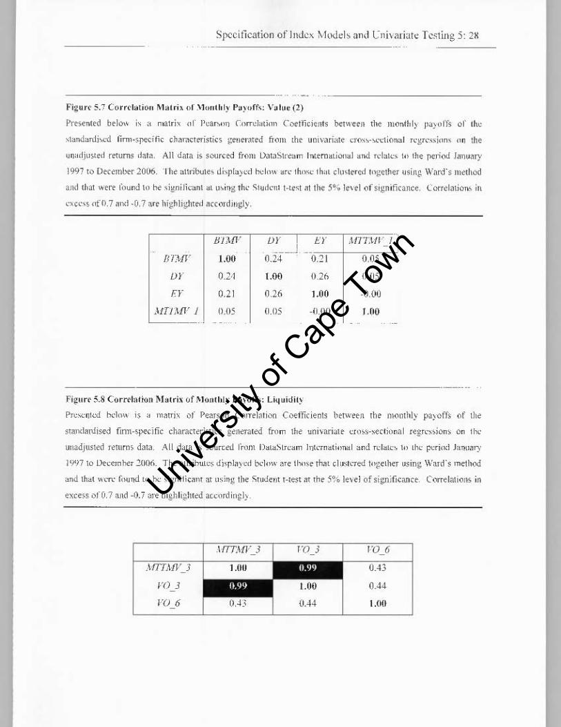
S pccification of Illlkx 1\ ll>del s and Cl1j\mi~tt T ~"ljng 5: 2X

Fig" r< S.' Corr<t~tioll M~lri, 01 .\J""lh Iy PO) "ff" Yo 1"0 (2)

Pr"'nled belO\. is " malrix or Pear",,,, C(>lTel,,(i{ll1 C<:>eHiei ents betw • • n tl" monUd) lla}o lTs 01' lhe

slandaTdj""d firm·speci!ic en''"''''t ... i'1i" gen.rat.d from 'he univJri"t' cro"·,,,·ctional TegTe"j"n< "0 the

uo"dj"".d return, (ht •. All data is soorced from l.lJtJSlr'am I",ern"ional .nd Telale, to Ihe r<Jiod J.n".ry

1997 to December 20()6. rh, alt,.ib,M; displa}cd I>c lo" .TC· Iho", I h" L e i"'lored togethe, using Ward's method

and d,at were l"und 10 t>< ,ignilicanl al ,,,ing the SludeHI Hest .t ti" 5 ~" 10\ el of ,ignificanc,. Correlation; in

exec" "ro. 7 .nd ·0.7 "'. highlighted .coordin::ly.

H1MF m !

t."Y Mn:W'"-' i [17:.1[1"" 1.00 0.24 0.21 0.05

m 0.2,1 1.00 02h o,m

FT 0.21 0,26 1.00 -0,00

JfTiMI' j (U)S (L1I5 -o.!){) /.00

Figure 5.S Correlation M.trix of Jl.loJlthl.I' P~.I'off>: Li~ uidilj

PTcscolcd t".-ilm is " 1l1.ni\ of Pe.fSon COlTelati"" C<:>etficient, betw •• n tho momhly pa)of[, of lh'

, t. ,,,l.,Uis. d fmn-'p"cific characteristics generated from 11" uni,ariale ero,,-,"c(ional r.gre"ion , on 11".­

unadjnsled returns data All data i, >ourttLl ["",m DaLaSITcam Illlcrn.liona l and TdaLe' 10 the pcri{Kl lanu.ry

1'i'!7 10 Utc"," he, ~1~1'i. The aLiTjhuLe, di'pl"ycd Ix'low . re tI~". thot ellNe,ed tog' Ll'" usin~ W"rd', method

and lh.l weTC' [ound to he , igni lic.nt "t ,,,ing the Student He'1"tthe 3% le,.1 of ,i::nificance C,,",.lalions in

exc. " of 0, 7 "nd -0. i are highlighted ",cord in gl}

1'0 J

1'0 6

Univers

ity of

Cap

e Tow

n

Specificalion oflnJ~x MoJels unJ Cnivari~t~ T~s\ing 5: 29 ------------~-------

fig ure S,9 Currd.lin" M.lri, nr Munlh I) P~}'uff." M h,'ell.neou,

P"'tln.d below is , ",o'rix "I' rea",m Corre l .... i"n c()(:ftlci.n~ b"tween th" monthl; payoffs nf {he

"",,,jardi,od flrm_'peci lie ch,.-.c(cri,(ie, generaled fr~m {he 'lni,,..i"te oross-"otio"al "gr",""" "" lhe

uniKlju,lcd return , d:l1" . .'\11 dm" i, ,,,ucoed hom D"taSu""m lnt"'latinno l arld rtlat" to the pcri(><l J,,"u",}

1997 W Deoeml-..c 2006, Th' anribures disployed be low arc tho," ,h"t olu,lcreJ together ",ing W:ll-d', me{hnd

o"d that Wert j')UIlJ to be ,igni""on ' "t ",ing the S,ud. ntt-test:li {he 5% 1 .. ,. 1 ofsigni/i,onc" C~rrelatiDIl' in

nee," of O. 7 .nd -0.7 ore highlighTed "ccocdingly,

;\WTrmkd

Sal,.,I'IP ().52 1.00

From the above figures it can r,." seen that many oflhe belw~~n factor cOlTel~lions UlT low,

however th~re arc a number that havc com"lation ligures in "xc~ss oflh~ 0.7 oound imposed

and so should be e>:c\oocd to mitigak possib le reJunJancies, Therefore the g~nmltion of the

abo,-e matriccs SCfvCS to aid in the simplilicalion of\b~ tinal characteristics list.

Univers

ity of

Cap

e Tow

n

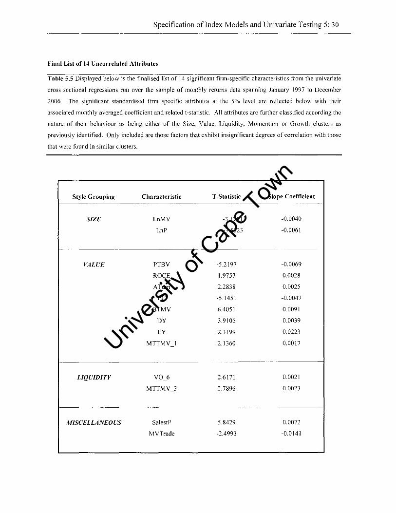
Specification ofIndex Models and Univariate Testing 5: 30

Final List of 14 Uncorrelated Attributes

Table 5.5 Displayed below is the finalised list of 14 significant finn-specific characteristics from the univariate

cross sectional regressions run over the sample of monthly returns data spanning January 1997 to December

2006. The significant standardised finn specific attributes at the 5% level are reflected below with their

associated monthly averaged coefficient and related t-statistic. All attributes are further classified according the

nature of their behaviour as being either of the Size, Value, Liquidity, Momentum or Growth clusters as

previously identified. Only included are those factors that exhibit insignificant degrees of correlation with those

that were found in similar clusters.

Style Grouping Characteristic T -Statistic Slope Coefficient

SIZE LnMV -3.1751 -0.0040

LnP -3.5023 -0.0061

VALUE PTBV -5.2197 -0.0069

RaCE 1.9757 0.0028

ATurn 2.2838 0.0025

PC -5.1451 -0.0047

BTMV 6.4051 0.0091

DY 3.9105 0.0039

EY 2.3199 0.0223

MTTMV 1 2.1360 0.0017

LIQUIDITY va 6 2.6171 0.0021

MTTMV 3 2.7896 0.0023

MISCELLANEOUS SalestP 5.8429 0.0072

MVTrade -2.4993 -0.0141

Univers

ity of

Cap

e Tow

n

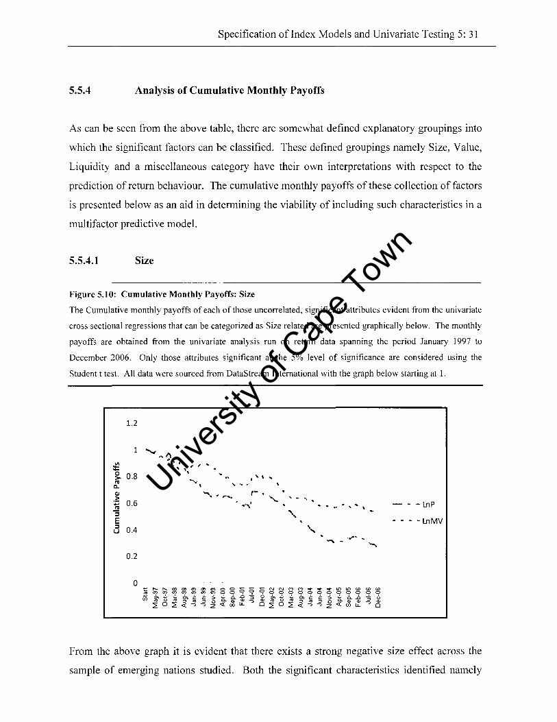
Specification of Index Models and Univariate Testing 5: 31

5.5.4 Analysis of Cumulative Monthly Payoffs

As can be seen from the above table, there are somewhat defined explanatory groupings into

which the significant factors can be classified. These defined groupings namely Size, Value,

Liquidity and a miscellaneous category have their own interpretations with respect to the

prediction of return behaviour. The cumulative monthly payoffs of these collection of factors

is presented below as an aid in determining the viability of including such characteristics in a

multi factor predictive model.

5.5.4.1 Size

Figure 5.10: Cumulative Monthly Payoffs: Size

The Cumulative monthly payoffs of each of those uncorrelated, significant attributes evident from the univariate

cross sectional regressions that can be categorized as Size related are presented graphically below. The monthly

payoffs are obtained from the univariate analysis run on return data spanning the period January 1997 to

December 2006. Only those attributes significant at the 5% level of significance are considered using the

Student t test. All data were sourced from DataStream International with the graph below starting at 1.

1.2

1

VI :t: 0 0.8 > " .... , IU c.. <II .~ 0.6 ... IU

, - .... '\.

- - - LnP ... .... , ~ \

"3 E - - - - LnMV ::J 0.4 u

0.2

o

From the above graph it is evident that there exists a strong negative size effect across the

sample of emerging nations studied. Both the significant characteristics identified namely

Univers

ity of

Cap

e Tow

n

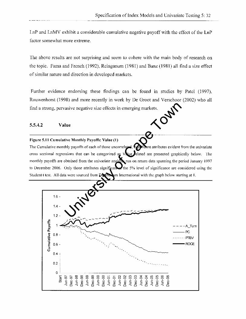
Specification ofIndex Models and Univariate Testing 5: 32

LnP and LnMV exhibit a considerable cumulative negative payoff with the effect of the LnP

factor somewhat more extreme.

The above results are not surprising and seem to cohere with the main body of research on

the topic. Fama and French (1992), Reinganum (1981) and Banz (1981) all find a size effect

of similar nature and direction in developed markets.

Further evidence endorsing these findings can be found in studies by Patel (1997),

Rouwenhorst (1998) and more recently in work by De Groot and Verschoor (2002) who all

find a strong, pervasive negative size effects in emerging markets.

5.5.4.2 Value

Figure 5.11 Cumulative Monthly Payoffs: Value (I)

The Cumulative monthly payoffs of each of those uncorrelated, significant attributes evident from the univariate

cross sectional regressions that can be categorized as Value related are presented graphically below. The

monthly payoffs are obtained from the univariate analysis run on return data spanning the period January 1997

to December 2006. Only those attributes significant at the 5% level of significance are considered using the

Student t test. All data were sourced from DataStream International with the graph below starting at 1.

1.6 -

- - - - A_Turn

--Fe

------. PfBV

0.6 -ROCE

0.4 1

0.2 ~

I

0 I - t- t- O) 0) 0> 0> 0 0 .- .- N N r0 r0 ~ ~ lCl lCl <D <D Co 0> 0> 0> 0> ~ 0> 9 0 9 0 9 0 0 0 0 0 0 0 0 0

U5 C U C U c U c U c U c U C U C U C U C U ~ Q) ~ Q) ~ Q) ~ Q) ~ Q) ~ Q) ~ Q) ~ Q) ~ Q) ~ Q) -, 0 -, 0 -, 0 -, 0 -, 0 -, 0 -, 0 -, 0 -, 0 -, 0

Univers

ity of

Cap

e Tow

n

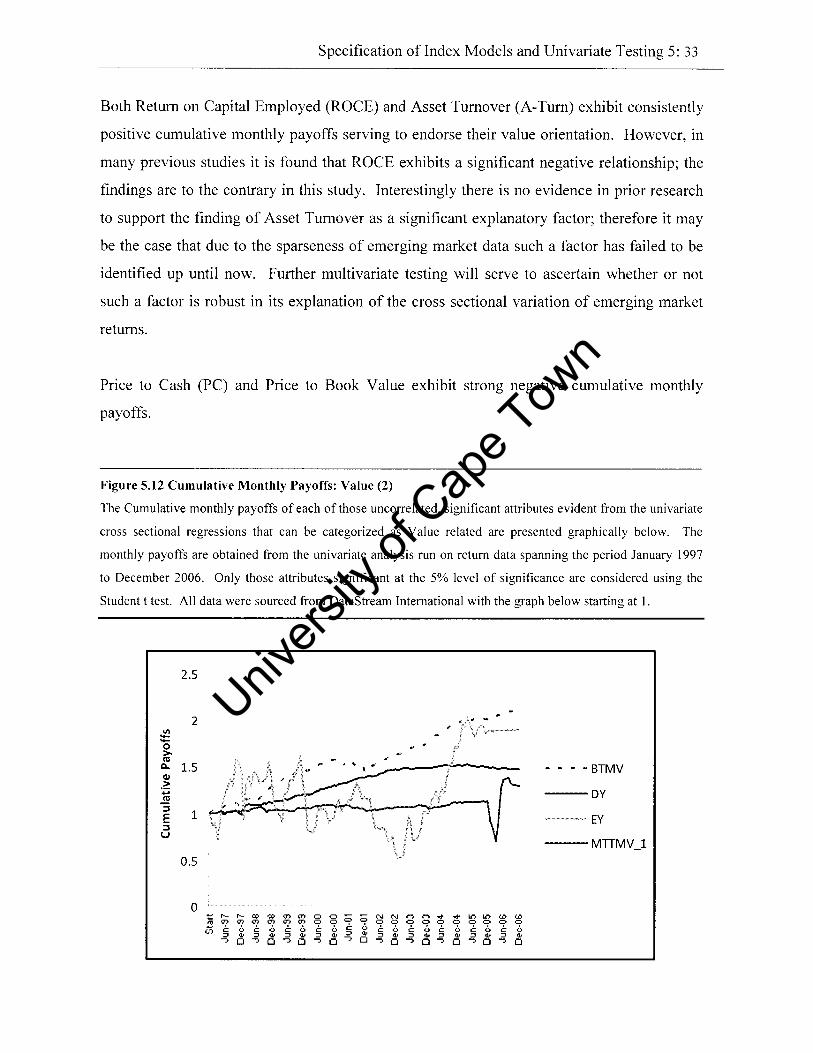
Specification ofIndex Models and Univariate Testing 5: 33

Both Return on Capital Employed (ROCE) and Asset Turnover (A-Tum) exhibit consistently

positive cumulative monthly payoffs serving to endorse their value orientation. However, in

many previous studies it is found that ROCE exhibits a significant negative relationship; the

findings are to the contrary in this study. Interestingly there is no evidence in prior research

to support the finding of Asset Turnover as a significant explanatory factor; therefore it may

be the case that due to the sparseness of emerging market data such a factor has failed to be

identified up until now. Further multivariate testing will serve to ascertain whether or not

such a factor is robust in its explanation of the cross sectional variation of emerging market

returns.

Price to Cash (PC) and Price to Book Value exhibit strong negative cumulative monthly

payoffs.

Figure 5.12 Cumulative Monthly Payoffs: Value (2)

The Cumulative monthly payoffs of each of those uncorrelated, significant attributes evident from the univariate

cross sectional regressions that can be categorized as Value related are presented graphically below. The

monthly payoffs are obtained from the univariate analysis run on return data spanning the period January 1997

to December 2006. Only those attributes significant at the 5% level of significance are considered using the

Student t test. All data were sourced from DataStream International with the graph below starting at 1.

2.5

2 VI ::: 0 > III Q. 1.5 CII .~ +-' .!!! ::J

1 E >

::J U

0.5

0 :;; r-- r-- 0) 0) "'" "'" 0 0

"'" "'" "'" '" "'" '" '=' '=' if, C /.:, C /.:, C /.:, C /.:,

" ... " ... " ... " ... ..." 0 ..." 0 ..." 0 ..." 0

;:; ;:; N N M M .... '=' 0 '=' 0 '=' C /.:, C /.:, C /.:, C

" ... " ... " ... " ..." 0 ..." 0 ..." 0 ..."

.... Ii') Ii') 0 '=' '=' /.:, C /.:, ... " ...

0 ..." 0

~ "" -=- '=' C /.:,

" ... ..." 0

- BTMV

---DY

EY

---MTTMV_l

Univers

ity of

Cap

e Tow

n

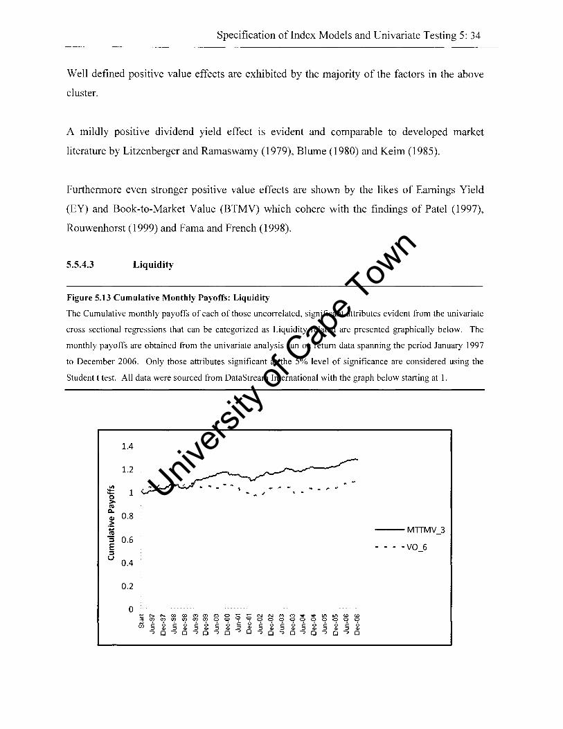
Specification ofIndex Models and Univariate Testing 5: 34

Well defined positive value effects are exhibited by the majority of the factors in the above

cluster.

A mildly positive dividend yield effect is evident and comparable to developed market

literature by Litzenberger and Ramaswamy (1979), Blume (1980) and Keirn (1985).

Furthermore even stronger positive value effects are shown by the likes of Earnings Yield

(EY) and Book-to-Market Value (BTMV) which cohere with the findings of Patel (1997),

Rouwenhorst (1999) and Fama and French (1998).

5.5.4.3 Liquidity

Figure 5.13 Cumulative Monthly Payoffs: Liquidity

The Cumulative monthly payoffs of each of those uncorrelated, significant attributes evident from the univariate

cross sectional regressions that can be categorized as Liquidity related are presented graphically below. The

monthly payoffs are obtained from the univariate analysis run on return data spanning the period January 1997

to December 2006. Only those attributes significant at the 5% level of significance are considered using the

Student t test. All data were sourced from DataStream International with the graph below starting at I.

1.4

1.2

~ 1 g. III

c.. 0.8 .~ .... ..!!! ::::l 0.6 E ::::l U

0.4

0.2

0 ~

r- r- oo

"" "" "" (f, C b C ::> '" ::>

J 0 J

00 "" "" <=> 0 S "" "" "" <=> 0

b C b C /,;, C

'" ::> '" ::> '" ::> 0 J 0 J 0 J

.. .. ,. ... ~ - ..

---MlTMV_3

-VO_6

S '" '" M M ... ... Ii> "'> ,.., ,.., 0 <=> 0 <=> 0 0 <=> 0 0 0

b .: /,;, .: /,;, c /,;, .: /,;, c b '" ::> '" ::> ... ::> '" ::> ... ::> ... 0 J 0 J 0 J 0 J 0 J 0

Univers

ity of

Cap

e Tow

n

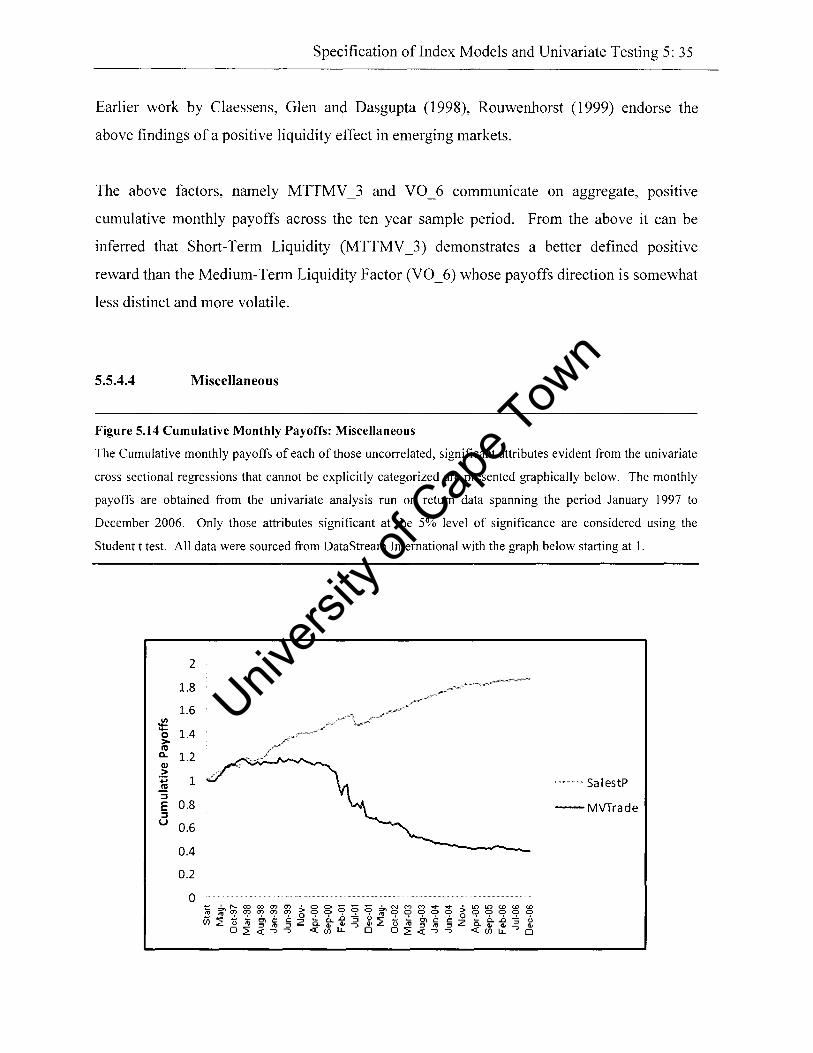
Specification ofIndex Models and Univariate Testing 5: 35

Earlier work by Claessens, Glen and Dasgupta (1998), Rouwenhorst (1999) endorse the

above findings of a positive liquidity effect in emerging markets.

The above factors, namely MTTMV _3 and VO_6 communicate on aggregate, positive

cumulative monthly payoffs across the ten year sample period. From the above it can be

inferred that Short-Term Liquidity (MTTMV _3) demonstrates a better defined positive

reward than the Medium-Term Liquidity Factor (VO _ 6) whose payoffs direction is somewhat

less distinct and more volatile.

5.5.4.4 Miscellaneous

Figure 5.14 Cumulative Monthly Payoffs: Miscellaneous

The Cumulative monthly payoffs of each of those uncorrelated, significant attributes evident from the univariate

cross sectional regressions that cannot be explicitly categorized are presented graphically below. The monthly

payoffs are obtained from the univariate analysis run on return data spanning the period January 1997 to

December 2006. Only those attributes significant at the 5% level of significance are considered using the

Student t test. All data were sourced from DataStream International with the graph below starting at 1.

2

1.8 ..... """

1.6 III :;

1.4 0 > "' Q. 1.2 Q)

.~ 1 .... . SalestP ..!!! ::J

E 0.8 --MVTrade ::J u 0.6

0.4

0.2

0

Univers

ity of

Cap

e Tow

n

Specification ofIndex Models and Univariate Testing 5: 36

The above factors are found to be significant however their precise logical classification into

any such style grouping is somewhat difficult. Sales to Price (SalestP) is by its very nature

value orientated and with such a theoretical supposition in mind can be seen to exhibit an

expected positive payoff over the chosen sample period. It is however rather strange that

such a factor with is purported value orientation does not co-move more with those factors

identified in the value clusters.

MVTrade can have a number of logical theoretical foundations. As it measure trading

activity it can be considered to be somewhat of a gauge for liquidity in the market. However,

as larger trades are generally associated with larger firms, MVTrade may also exhibit

overtones of some form of size effect. From the above graphical depiction it appears to

capture the some of the effect of liquidity crises evident in emerging markets in the late

nineties and early twenty first century with the same downward trend also cohering with a

definite size effect already identified in an emerging market context.

Univers

ity of

Cap

e Tow

n

Specification oflnuex lI-loJels and Univariate hsting 5: 37

5.6 Styk Consis l"ncy

fig"," 5. 15 Consi'{~nc~' of Oir~'tion of SignificanT Attribute. MOnlhl~ Pa~orr.

TI", diagram Ixlo,," ",lee",n" tl", proporti<m of to. numlxr of tim es that .ach of tho monthly taotor, payoff;;

"'-ere posi{i,-c comp,..ed to when the~ are n<gmi\'e, As before tho monthly payoff' are obtained from tll< ero;;,

"""iona l univariOl< rcye."ion' ow, 11", , amp le period ' p,,,,,, ing. ja" uar~ t997 {o t)co~mber 2006. All f""to"

p<e,,-,n{<d below "'~ ll",,~ foun d 10 ,{"{ iSl i,at ly sign if ",anL using. {he SluLknt;; t distribution Those mtribuk' that

fir. found h", •• 'aitll'.' clo,.;r L(l tl", hound.,; ~i lh~r {)% or If)()'!·' in eilher di rection ar. CLlnsi<ie'ed to m(lr.

con,ist.nt "itll re,l"'ct to sign, A da'll«l line is di 'playe<1 at the 5D% lewl with soli<lli "es in<liO:iling {he 5~;'

le,'el (lr , ignificance r", tho testing pr<"edu "" All data were extnloted !Tom DataSrream Internationol.

• Po~tr.-.

, > > , > c > , < , > ~ c > , 0 , ~ >' • > , ,

~ > > , c 0 <

, , , , c , > , , , • , , > , ,

I he abo\'e figure provides a helpful illustration of tlK: consistency in direction of the monthly

payoffs. A payoff with onc direction closer 10 either ()')-1, or 100% is considere(i 10 he or

gre~ter consistency th,,,, one which is loc,lleJ "-found the 50% mark . Eleven or thc above

<:harJ<:lerislics ~re founu to exhibit con;;i;;tency filtio;; slgni1icanl atlhe 5% le ,'el when tested

using the binomial formulat;on of the non-parametric Sign Test.

Univers

ity of

Cap

e Tow

n

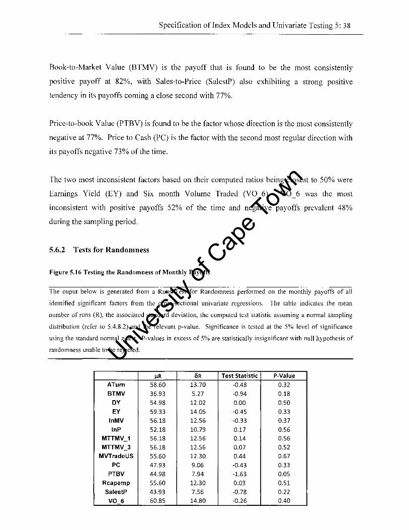
Specification ofIndex Models and Univariate Testing 5: 38

Book-to-Market Value (BTMV) is the payoff that is found to be the most consistently

positive payoff at 82%, with Sales-to-Price (SalestP) also exhibiting a strong positive

tendency in its payoffs coming a close second with 77%.

Price-to-book Value (PTBV) is found to be the factor whose direction is the most consistently

negative at 77%. Price to Cash (PC) is the factor with the second most regular direction with

its payoffs negative 73% of the time.

The two most inconsistent factors based on their computed ratios being closest to 50% were

Earnings Yield (EY) and Six month Volume Traded (VO _ 6). VO 6 was the most

inconsistent with positive payoffs 52% of the time and negative payoffs prevalent 48%

during the sampling period.

5.6.2 Tests for Randomness

Figure 5.16 Testing the Randomness of Monthly Payoffs

The ouput below is generated from a Runs Test for Randomness performed on the monthly payoffs of all

identified significant factors from the cross-sectional univariate regressions. The table indicates the mean

number of runs (R), the associated standard deviation, the computed test statistic assuming a normal sampling

distribution (refer to 5.4.8.2) and the relevant p-value. Significance is tested at the 5% level of significance

using the standard normal z-test. P-values in excess of 5% are statistically insignificant with null hypothesis of

randomness unable to be rejected.

~R cSR Test Statistic P-Value

ATurn 58.60 13.70 -0.48 0.32

BTMV 36.93 5.27 -0.94 0.18

DY 54.98 12.02 0.00 0.50

EY 59.33 14.05 -0.45 0.33

InMV 56.18 12.56 -0.33 0.37

InP 52.18 10.79 0.17 0.56 MTTMV_1 56.18 12.56 0.14 0.56 MTTMV_3 56.18 12.56 0.07 0.52

MVTradeUS 55.60 12.30 0.44 0.67

PC 47.93 9.06 -0.43 0.33

PTBV 44.98 7.94 -1.63 0.05

Rcapemp 55.60 12.30 0.03 0.51

SalestP 43.93 7.56 -0.78 0.22

va 6 60.85 14.80 -0.26 0.40

Univers

ity of

Cap

e Tow

n

Specification ofIndex Models and Univariate Testing 5: 39

From the above output it can be inferred that very few of the identified firm-specific

characteristics exhibit a consistent unchanging direction. All of the generated p-values of the

factors with the exception of the PTBV factor are in excess of 5% indicative of statistically

significant randomness in the variation of the factors monthly payoffs. As mentioned only

the PTBV factors had a p-value of approximately 5% meaning that the rejection of the null

hypothesis is acceptable and so the factor is sufficiently consistent to doubt that it changes

randomly. These findings are important as they provide some insight into the success of the

formulation of style timing models later in this paper.

5.7 Summary and Conclusion

The aim of the first half of this chapter was to investigate the overall risk structure of the

selected sample of emerging market nations for the period 1 st January 1997 to 31 December

2006. The tests conducted found that to a certain extent the behaviour of stock returns in

emerging nations exhibit a degree of commonality with a collective of such nations, namely

the DataStream International Emerging Markets Index. Furthermore, co-movement on an

international scale is also evident, more specifically with the DataStream International World

Index.

Cluster Analysis and Principal Components methodologies were then posited as potential

approaches for attempting to understand the variation inherent in emerging capital markets.

Attempts to perform such analyses on the given dataset were deemed not feasible on account

of its sheer magnitude as both testing procedures are most accurate when performed on a

small scale. However, the results of previous studies such as Van Rensburg and Acres (2006)

performed in a similar context shed some much needed light on the behaviour of emerging

capital markets. Distinct clusters for emerging and developed markets were discovered

which served as the basis for the selection of adequate proxies for the index-models later

formulated. No defined sector behaviour was found to be evident in such a context, however

emerging nations in close geographical proximity tended to have a significant degree of co­

movement in their returns.

Univers

ity of

Cap

e Tow

n

Specification ofIndex Models and Univariate Testing 5: 40

An explanation of the Time-Series variation in share returns is then attempted through the

formulation of both Single and Multi-Index models. Considering the results of prior research

in an emerging market context and the increasing trend in capital market integration,

adequate proxies were chosen accordingly. First level tests found the Multi-Index model to

have the greatest degree of explanatory power superior to either of the Single-Index models

producing an average R2 across the all the companies of 13.59% compared to 11.8% and

8.99% respectively. The number of significant regressions is also noteworthy - both the

Single-Index models and Multi-Index models generate a healthy number of significant

regressions (all in excess of 60% of the total run). The Second level tests regress the

residuals against the rival model's independent variables; however they provide little

additional evidence to further explain the nature of the underlying variation in stock returns.

Adjusted R2 that are close to or less than zero and the number of total regressions being

significant not reaching above 5% in three of the four test run emphasize the futility of

modelling.

On aggregate both the Single and Multi-Index models are relatively poor in their explanatory

power and provide minimal insight into the explaining of the time series of share returns in

emerging markets. One must consider the possibility that incorrect proxies were in fact

employed in such a setting, however due to the data constraints that characterize emerging

nations in particular, it is believed that the chosen proxies were the best available at the time

of testing.

The next part of the chapter aims to investigate the ability of the firm-specific attributes to

explain the cross sectional variation in share returns. In each month of the sample period the

forward stock returns of each of the included companies are regressed in a univariate manner

against the all 50 firm specific attributes. The averaged cross sectional regression

coefficients that output are then assessed for significance using the Students t -test. This

testing procedure serves to narrow the list down to only those characteristics that are most

significant in explaining the variation in share returns. Less than twenty attributes remain

after this procedure is conducted.

In order to assess the robustness of these factors, they are tested in the same manner against

returns that are risk adjusted using the two market proxies mentioned earlier in the chapter.

Univers

ity of

Cap

e Tow

n

Specification oflndex Models and Univariate Testing 5: 41

Once more the Students t test is performed with the significant factors identified being very

much similar to those evident from the test against the unadjusted returns.

A Cluster Analysis is then performed on the monthly payoffs of the factors identified to be

significant from the tests run on the unadjusted returns and risk-adjusted returns. The

clustering method used namely Ward's method is known to generate very narrow but

significant clusters. This considered, it is fairly difficult to identify generalised factor

groupings-however a number of logical classifications were identified. The factors could be

found to group in the following clusters (1) Size and Value, (2) Value, (3) Liquidity and a

Miscellaneous collection of factors.

In order to remove highly correlated factors that capture similar variation a correlation

analysis was performed on all factors that fell into the well defined clusters mentioned above.

If two factors were found to be excessively correlated, that factor having a lower t-statistic in

the previous univariate cross-sectional regressions was excluded.

As a result of this pruning procedure a final list of 14 firm-specific characteristics was

identified. The majority of these factors seem to cohere with the results of prior research;

however the lack of significant momentum effects is somewhat unexpected. Significant Size,

Value and Liquidity effects are however prevalent and comparable with previous studies in

an emerging market context. Interestingly, Asset Turnover, a factor that is found to be

considerably significant in this study has not been identified in previous research.

The monthly payoffs of each firm-specific attribute are then assessed for the consistency of

their direction. The more consistent the payoff direction the more interpretable the factor

becomes in terms of formulating a defined investment strategy based the results generated. A

number of the factors are indeed found to be either significantly positive or negative,

however there are many that have inconsistent direction which detracts from the potential of

being able to time the direction of such payoffs and so exploit profit taking opportunities.

Univers

ity of

Cap

e Tow

n

Specification oflndex Models and Univariate Testing 5: 42

Further testing for the changeability of the direction of such payoffs is performed using a

Runs test. It is found that the majority of the factors exhibit random behaviour with only a

few exhibiting consistent predictable trends.

It is common knowledge that Univariate Testing is limited by the fact that only one

independent variable is tested at a time against a chosen dependent variable. The problem

with such a procedure is that the significance of the explanatory power of such factors may

not in fact hold up when the number of independent variable exceeds one. Therefore in order

to ascertain how pervasive these identified factors truly are testing in a multivariate setting

will be forthcoming in chapters to follow.

Univers

ity of

Cap

e Tow

n

-6-

A Univariate Analysis of Macroeconomic influences on return behaviour in Emerging Markets

6.1 Introduction

The prevIOUS chapter identified numerous style characteristics found to have

significant explanatory power over the cross sectional variation of returns of firms in so

called emerging markets. Given these defined style anomalies that aid in our understanding

of market behaviour, one is curious to determine whether or not there may be additional

attributes or variables of a less firm-specific orientation that have some form of explanatory

power. The aim of this chapter is to explore the impact of firm exposures to certain

macroeconomic variables and changes therein in being able to further explain the cross

section of returns.

6.2 Identification of Candidate Macroeconomic Variables

6.2.1 Prior Research

The majority of prior research into macroeconomic influences on the return pattern of shares

has been considerably country-specific in its focus. The early developed market research by

Chen, Roll and Ross (1986), Pearce and Roley (1988), Friedman (1988) and Chen (1991)

place more emphasis on the local, endemic macroeconomic factors and their relative impact

on domestic share returns. Variables such as inflation, industrial production, interest rates,

money supply and unemployment are common factors cited to have potential explanatory

power.

Univers

ity of

Cap

e Tow

n

A Univariate Analysis of Macroeconomic Influences on return behaviour in emerging markets 6: 2

Research of such type is considerably more sparse in an emerging market context. Studies by

Gjerde and Srettem (1999), K won (1997) and Sadorsky (1999) retain the localised focus that

is characteristic of the majority of developed market studies. Gjerde and Srettem (1999), find

that both changes in the real interest rate and oil price movements negatively related to stock

market movement, partly endorsed by Sadorsky (1999) who communicates that shocks to the

price of oil post 1986 do in fact have a significant impact on returns on the S&P 500. Kwon

(1997) looks at the Korean market specifically and finds that factors such as the rate of

foreign exchange, oil price and money supply exhibit significant relations which vary in sign

in accordance to the type of sub-industry analysed but nevertheless provide additional support

for macroeconomic influence on market movements.

However, research by Harvey (1995a) and the later work of Bilson, Brailsford, and Hooper

(2001) focus on a broader sample of emerging nations and consider variables with a more

global orientation than that of prior research. Bilson et al (2001) studies the influence of gold

prices, exchange rates and money supply and find only moderate evidence to suggest any

form of relation.

With this prior work in both developed and emerging nations in mind, an initial list was

drawn up based on some of the hypotheses and conclusions previously asserted in the

aforementioned papers. Notably this study aims to assess the impact of more globally

orientated (mainly US) factors on the performance of emerging stock markets. This

considered a preliminary list of factors was drawn up that encompass key sources of variation

in the majority of economies across the globe

Table 6.1 Initial list of Candidate Macroeconomic Variables

The table below presents the full list of fifteen macroeconomic variables hypothesised to have potential in

explaining the variation of share returns in emerging markets. They are presented with their respective code and

a brief description of their nature. All data were sourced from DataStream International database.

Full Name and Description Code

CRB Commodities Index CRBINDEX

Gold Price SUS/ounce GOLDPRICE

Oil Brent Crude $US/Barrel OILBRENTCR

Platinum Price SUS/ounce PLATINUM

3-month US Bankers Acceptance rate USBA3M

Univers

ity of

Cap

e Tow

n

A Univariate Analysis of Macroeconomic Influences on return behaviour in emerging markets 6: 3

Rand{R) SUS exchange rate RANDDOLLAR

US Export Index USEXPIND

Yield on lOyr US Govt. Bond USGLTlOYR

US Money Supply (Ml) USMONSUPP

US Producer Price Index USPPI

US Prime Rate USPRIME

US Short Term Interest Rate USSHTRM

Yield on 3-month US Treasury Bill USTBILL3M

US Unemployment Rate USUNEMP

Chinese Yuan SUS exchange rate YUANDOLLAR

6.2.2 Explanation of Macroeconomic Factors

The list above combines the two pervading themes in the reviewed research and so has a

strong term structure and commodity focus. The majority of the factors are easily recognised

and understandable, being either commodity prices or interest rates. A number however are

not common knowledge, namely the CRB Commodities Index, US Export Index and the US

Short Term Interest Rate.

The CRB Commodities Index is a broad based commodities index also termed the NYFE

Commodity Research Bureau Index. It is described as a three dimensional index as it

averages prices across seventeen commodity futures whilst also incorporating the average

commodity prices historically. The constituents of the index are as follows: Cattle (live),

Cocoa, Coffee, Copper, Com, Cotton, Crude Oil, Gold, Heating Oil, Hogs (live), Natural

Gas, Orange Juice, Platinum, Silver, Soybeans, Sugar and Wheat.

The US export index is offered by the US Department of Labour and is a broad commodity

based index comprised of a variety of goods. The index is has some exposure to agricultural

products however its major focus is non-agricultural items such as industrial, capital and

consumer products.

The US Short Term Interest Rate is the 3-month Eurodollar rate, i.e. the interest rate on

United States Dollar three month deposits in London. It is sourced from the OECD, namely

the Organisation for Economic Co-Operation and Development.

Univers

ity of

Cap

e Tow

n

A Univariate Analysis of Macroeconomic Influences on return behaviour in emerging markets 6: 4

6.3 Adjustments to candidate variables prior to testing

Certain adjustments were carried out on the complete list of 15 macroeconomic variables

prior to performing the Univariate analysis.

6.3.1 Stationarity

Each of the variables was tested for stationarity using the Augmented Dickey-Fuller (ADF)

test. The aim of this test is to identify and mitigate the potential for spurious correlations that

occurs when attempting to gauge the relationship between two data series that are non­

stationary. The Augmented Dickey-Fuller (ADF) test differs from the simple Dickey Fuller

unit root test as it considers correlation at higher order lags through a parametric correction

that assumes the testable series follows an AR(p) process so adding (P) lagged difference

terms to explanatory side of the regression equation.

Each series to be tested (Yt)using the ADF procedure is specified as follows in lagged form:

Where,

p and 0 are parameters to be estimated, with a = p - 1

.':t represents optional exogenous regressors, in this case a constant and trend term

In order for such a test to have true statistical significance the testing procedure must consider

the nature or the manner that the data itself is generated. With regards to the current dataset

of macroeconomic data, both a constant intercept and a term that proxies trend over time are

included in the specification of the test procedure. The intercept term serves to model a

random walk which is deemed suitable for all data that has a mean not equal to zero. The

term capturing the trend over time is indicative of macroeconomic data which frequently

contains an underlying pattern of increase or decrease over time.

Each of the series was tested against the null hypothesis of non-stationarity, with the Dickey

Fuller test seeking subsequent rejection of the null to imply stationary series. Originally it

Univers

ity of

Cap

e Tow

n

A Univariate Analysis of Macroeconomic Influences on return behaviour in emerging markets 6: 5

was found by Dickey and Fuller (1979) that the calculated test statistic does not in fact follow

the conventional Student's t-distribution which served to restrict the applicability of the test.

However, work by MacKinnon (1991, 1996) implements a larger set of simulations than

those generated by the original authors. The outcome of this additional work results In

calculation of Dickey-Fuller critical values and p-values for many differing sample sizes.

The testing procedure is conducted through the computation of the ADF test statistic for each

respective series under scrutiny.

t= af ." I' se ((1)

The test is run so that an increasing number of lagged difference terms are included until the

distribution of the error term of the tested equation becomes random. The maximum number

of lags is set at twelve with the Akaike Information Criterion used to determine which of the

successively smaller lags are to be eliminated. The computed test statistic is then compared

to the Dickey Fuller critical values at the 95% level of significance. Those factors that are

not able to reject the null hypothesis are logarithmically transformed and subsequently

retested. Any other factors still not found to be significant are first differenced and once

again tested for significance. Factors still insignificant after the above transformations are

omitted on the basis of non-stationarity and don't form part of the testing procedure.

6.3.2 Correlation amongst Stationary Macroeconomic Factors

In order to further assess the explanatory power of the reduced list of macroeconomic factors

a correlation matrix of the thirteen considered stationary is generated. Factors that are highly

correlated are considered to have a similar underlying pattern of variation and so the

inclusion of such in further analysis of return predictability would be rendered somewhat

fruitless.

In addition to the testing of correlation amongst the chosen factors, two broad market proxies

were included as a robustness check. The decision of including both return indices, namely

the DataStream Emerging Markets Index and DataStream International World Markets Index

in the correlation matrix is to serve as a preliminary assessment of the relative explanatory

power such factors have on a global scale. Macroeconomic variables that exhibit correlations

Univers

ity of

Cap

e Tow

n

A Univariate Analysis of Macroeconomic Influences on return behaviour in emerging markets 6: 6

greater than 0.7 or less than -0.7 are considered highly correlated, an arbitrary level used

consistently throughout this paper. If two candidate variables do in fact exhibit such co­

movement they are considered to model similar variation and so if both were to be included

the final list of factors would be prone to double counting. Therefore, variables are excluded

if they are found to have a coefficient in excess of the proposed bounds.

6.3.3 Results:

Adjustments for Stationarity

Level Tests:

The results of the Augmented Dickey Fuller test served to identify that all the candidate

variables exhibited a non-stationary trend and so were not fit for inclusion in the proposed

analysis without sufficient adjustment.

Table 6.2 Results of Level Unit Root Tests

Presented in the table below is the output for the Augmented Dickey Fuller (ADF) test run on the fifteen

candidate macroeconomic variables. ADF test statistics, their associated p-values and the number of lagged

differences are included. All the variables were tested at the 95% significance level with rejection of the null

hypothesis inferring a series that exhibits a constant mean and variance, namely the property termed

• stationarity' . All data were sourced from the DataStream International Database.

Variable ADF Statistic p-values Lagged differences

CRBINDEX 0.16 0.9931 2

GOLDPRICE -0.03 0.9954 6

OILBRENTCR -2.66 0.2532 12

PLATINUM -1.90 0.6474 0

RANDDOLLAR -1.34 0.8766 0

USBA3M -2.59 0.2849 7

USEXPIND -0.81 0.9608 7

USGLTlOYR -2.45 0.3380 0

USMONSUPP -2.06 0.s585 1

USPPI -1.71 0.7427 3

USPRIME 0.97 0.9899 0

USSHTRM -0.84 0.9605 0

USTBILL3M -2.42 0.3673 8

USUNEMP -2.01 0.5898 12

Univers

ity of

Cap

e Tow

n

A Univariate Analysis of Macroeconomic Influences on return behaviour in emerging markets 6: 7

1 YUANDOLLAR 2.421 0.9999 1 01

As is evident from the above output, no level macroeconomic variables exhibit stationarity

and so are not suitable for testing without this trait being evident.

Logarithmic Transformations:

As none of the above level tests were able to find any of the potential macroeconomIC

variables stationary, each of the insignificant variables was re-tested subsequent to

logarithmic transformation. See Appendix C.l for results.

First Differenced Tests:

Each of the initial factors was then first differenced and the ADF statistics and associated

critical values recomputed. Factors that weren't found to significant after first differencing

were then logarithmically transformed and re-tested. The results are presented in the table

below:

Table 6.3 Results of First Differenced Unit Root Tests

Presented in the table below is the output for the Augmented Dickey Fuller (ADF) test run on the fifteen

candidate macroeconomic variables which have been first differenced. ADF test statistics, their associated p­

values and the number of lagged differences are included. All the variables were tested at the 95% significance

level with rejection of the null hypothesis inferring a series exhibit a constant mean and variance, namely the

attribute termed 'stationarity'. All data were sourced from the DataStream International Database.

Variable ADF Statistic p-values lags

DLCRBINDEX -5.94 0.0000 2

DLGOLDPRICE -6.09 0.0000 5

DLOILBRENTCR -12.63 0.0000 0

DLPLATINUM -10.67 0.0000 0

DLRANDDOLLAR -10.38 0.0000 0

DLUSBA3M -2.22 0.4728 7

DLUSEXPIND -3.51 0.0410 6

DLUSGLTlOYR -9.66 0.0000 1

DLUSMONSUPP -12.22 0.0000 0

Univers

ity of

Cap

e Tow

n

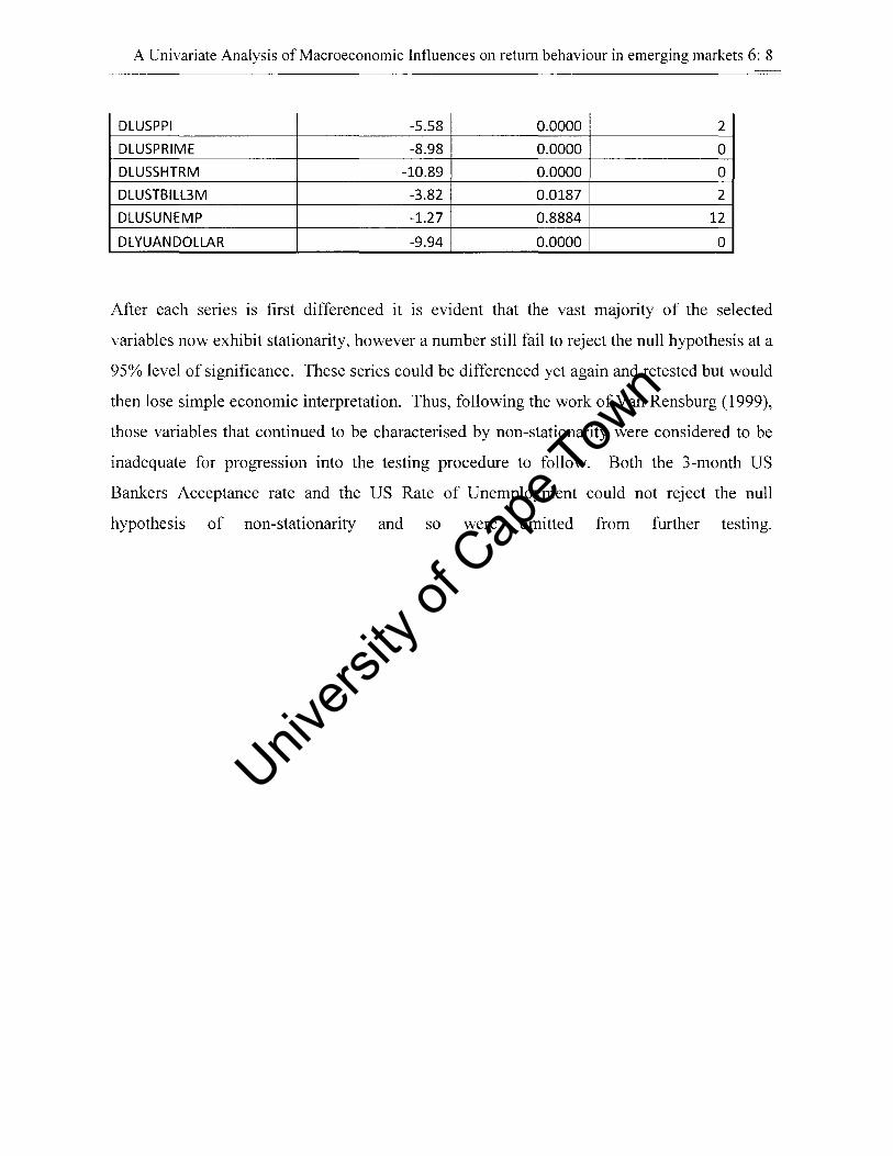
A Univariate Analysis of Macroeconomic Influences on return behaviour in emerging markets 6: 8

DLUSPPI -5.58 0.0000 2

DLUSPRIME -8.98 0.0000 0

DLUSSHTRM -10.89 0.0000 0

DLUSTBILL3M -3.82 0.0187 2

DLUSUNEMP -1.27 0.8884 12

DLYUANDOLLAR -9.94 0.0000 0

After each senes is first differenced it is evident that the vast majority of the selected

variables now exhibit stationarity, however a number still fail to reject the null hypothesis at a

95% level of significance. These series could be differenced yet again and retested but would

then lose simple economic interpretation. Thus, following the work of Van Rensburg (1999),

those variables that continued to be characterised by non-stationarity were considered to be

inadequate for progression into the testing procedure to follow. Both the 3-month US

Bankers Acceptance rate and the US Rate of Unemployment could not reject the null

hypothesis of non-stationarity and so were omitted from further testing.

Univers

ity of

Cap

e Tow

n

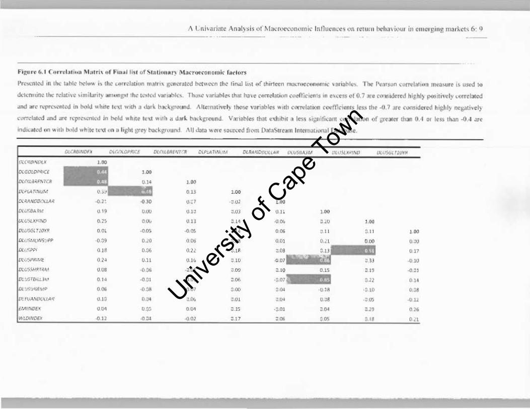
i\ L ni' ariato An . l} si , of "!ocrO<'<:O nomi, !ntlu. ncel on rolUI n l>C"h~ , io." il' om"r gmg ma,.~Cl< 6: <)

-----------------

I';l!"'"~ ~. I ("''''",1., ;,,0 .... "Irl\ "r II~ , .. I 11\4 ijl !:I 4 " U,.,,"~ "Ia~ ..... <o" o".k f'~lo""

l'n"""tetJ " Ilhe Lohle hel .. ,. .. dlc <.,r~lalion m"h"' ~ 1I""~C<l b<:(,,""n mc tin;o,] to" " r(h'n«n "':.'"''« ''''''".''' " , i:thl",. Tht p.,,"'son co.....,[;oh.". '"~u"..., i. ,,""" 10

drtcnoune the ",131"" "milJli.) """ "'VI''''' (,'.,,,,1 y.,,;ohl,~ Th"", .'lIriahIe< th31 h" 'e M"eI.lion co"",,;"",, '" e\<eS:!l 01 O. 7 ~r" r''''s","fl'd hi~hl) p<>!Ii1'''''I~ rom-lJled

""1:1 "'" A'p", ...... too tn bold .. hOle le,1 ",,,h •• IIo,k h ... , ~!!",; .. d. AIIe..".tiYo'I\ lho>.e .... n ahies " ,d, """"latlQft ,...,ITki .. u, Ins th .. -4 7 art Nus-deled hlghl) negati . el)

com-bd,-d :mel:lre rrpr~I.:.lln I:>old .. hn .. leX! ",Ih d d,.l b;.dpou,,<i- Vanabl .. that e" ubll a I ... ,i::<,i11<:1ln <0.....,1.., ,0)0 of ;:ru, .. moo 0 I Ot less 11>.", 4 .4 ...,

indm.,.-d "" .. "b bt,ld wh"e ,~'" , ... u I'j:hl IV"Y b;\o;~P""nd ,\ 1) dol . .. .. e .0UJ<ed f,<'m D: .. aS ... am 1",..., .. "),,.1 o,.,lOloo.~.

LI-~WOI' c(('()(CiI'~l ",,,.Mflw", <'iP"''''''"Y~ l)lIt .. ,:=~, ... Pt~5Mj'" ~~V.ll.~"''>I' <>:;J!(,<11<1»<

",r''''~1Jl'' •• ",W,_"i

"'''U,'MLA ••• ' x' .... n,.·t!M 0.11 ,." '" ""-"",',,,u.. .... l: .. ,,:1 -, .W •• "';nl""" '" 0 .• \)." '.m !l. ll .. " IXC'_"-X."''''' o.:l ,. on '" _0. '" ; ,,0 ' .00 OW5<:-'("O(,' 0.01 _O.OS ~ . ,.,. .. , II l .ll ,w DI., .... <·,"'~H' " 0,l9 O,lo " ;,08 0.0> 0,/ 1 ,W 0,"'"

Dl.i.,~'" '" D,lt 0,1. ; ,1. 0.17

,~' ... _Ii"" '" ". 0,1 1 ' " ,.W _,do m.U _'_IH.Of"", 0." <. ·: .01 '.D'l '_ '0 0_15 : I I -0.: 1

O" J<r", ,,.,., 0, t. <" '" '.06 O.ll '" '" 'J.< ·,,~ .w ,. '" ". ; .00 ,~ -Q." '" '" ' " "",""",,,,,,q .n '" ,-"" "" ,-'" Q,., ~m .(I.ll

i MJ,M'H o. 0" ,. :: ." -;-"1 ,. ::.l' O.li

WlDIlWO .n ". " .. ::11 ,. ,. ". M

Univers

ity of

Cap

e Tow

n

~~~ff ~ '.~:; I ~i~~,~~

a.a.i.;:a ~ ~l~~5~ ", .. ,,::il l o',-[E:" _ ~;:j -". .. s:""':;~'"' i' ·l;t~l.''' ::r -"",. '" ",.E:=-i '"

"",oobbo ,. 1' 1 ;a~~: i __ ON __ '" ;_"'''_ ~

.. ~w .. ~w_ -"", ,, ~ c

"~;;''' ,... " ... ,;;;:!l ... . ~-,'-;-ss .. ~ ; ~~§.~~ ; .... _ .. .. g ::l:

oboe",,,, II )!;l:eli·'" • _"_<>' 0 "'" _ _ .:." _ Ow"'" <> • ".,. . ~ - -- - .

~;;. ~,... =

~·ti ·'!i; §~g~~.; co. ~:l_ ...

"'11" I I >~ " > f!;;;::;. g =~>;l:f :: _ e-~q~.; " ~"il!l;:!::1 ~. ,,,--.,, -",:;!O,- . ;:;' ::!",:,;~,,~, ;:;

,...<><'0.0 ,.. 1··1 ~a';,~~ ~ ~ 9::e<:1j8 n~~1i;: c ,~

2..- ir '" ' '" ::>if~"o n i_1M ';;: '" "..,CT..,,,. -, r::::~:rs<S" ~ e!.. ;:;:::t '"

00.0. _ 1·1 !}g:~i" ~ --';1:8 , ,, ;:ro'~ >< ww :J'I'''''Q K

a,~~! l ~ I ~ ~. ~ ~ ~ ,,= ... ., "

~~~.~~ n - !il .., _ = " ., . II !3.~ .... '"

beg !.~30·;J g " " ... . -'" -"'0; .-: a;:j!;"o- .., tiaii:a[ ~ ~r",-o " ,. ' i/ " • 0 • '" :. -. -

• 1' 1 i~?' ~ a- -... , ~g 1t . , ! - .

" ", , !!~~~ s' o -~- a ::. !O • • • ",. ,... a ~a'B-~ g ~ .:;;" ;;

~ ~ l ~ ~ "i-IS;;; " .. . .=" " .. ,. -,,~ga i

·t ~ .. .. i" ~

a. 0

Univers

ity of

Cap

e Tow

n

A Univariate Analysis of Macroeconomic Influences on return behaviour in emerging markets 6: 11

The correlation matrix generated served to endorse the exclusion of certain macroeconomic

variables based on their inability to exhibit stationarity. When analysing the correlation of

certain factors versus broad market indices such as the DataStream International Emerging

Markets Index and the DataStream International World Markets Index it is found they exhibit

little similarity. If a macroeconomic influence which is global in its nature is not able to

affect such broad market indices there is little chance of such a factor being able to

significantly influence the movement of individual stock returns. Therefore, the following

factors were excluded from further analysis based on low correlations (less than 0.05) with

the respective indices: US Three Month Bankers' Acceptance Rate, US Prime Rate, US

Unemployment Rate and Chinese Yuan US$ Exchange Rate.

It was decided to keep certain commodities in the final list of factors in hope of them having

explanatory power due to firm-specific orientation. The final list of eleven factors is

presented in Table 6.4 below:

Table 6.4 Final list of Macroeconomic factors

The table below presents the final list of macroeconomic factors eligible for testing in the univariate analysis to

follow. Each factor is listed with its reference code and full name, there are a total of thirteen factors in total.

All date were sourced from DataStream International database. Please note that in all factors are first

differenced with a number undergoing logarithmic transformations in order to successfully be tested as

stationary.

Code Full Name and Description

DLCRBINDEX CRB Commodities Index

DLGOLDPRICE Gold Price SUS/ounce

DLOILBRENTCR Oil Brent Crude SUS/Barrel

DLPLATINUM Platinum Price SUS/ounce

DLRANDDOLLAR Rand(R) SUS exchange rate

DLUSEXPIND US Export Index

DLUSGLTlOYR Yield on lOyr US Govt. Bond

DLUSMONSUPP US Money Supply (Ml)

DLUSPPI US Producer Price Index

DLUSSHTRM US Short Term Interest Rate

DLUSTBILL3M Yield on 3-month US Treasury Bill

Univers

ity of

Cap

e Tow

n

A Univariate Analysis of Macroeconomic Influences on return behaviour in emerging markets 6: 12

6.4 Univariate Testing of Macroeconomic factors

The aim of this next section is to test all those significant macroeconomic factors identified in

6.3 and presented in Table 6.4. The analysis is similar to the testing procedure followed in

testing the finn-specific attributes is Chapter 5 section 5.5 of this study with some

methodological alteration. The analysis tests the significance of the macroeconomic factors

over the entire sample period using a 'rolling' time-series cross-sectional regression

procedure that serves to generate both the sensitivity and payoff of factor against two types of

return data, unadjusted and risk adjusted return data.

6.4.1 Data and Methodology

The data employed for this analysis is as described in Chapter Four of this study. The

monthly returns data were adjusted accordingly as alluded to Chapter Four and comprised of

a total of 1273 listed stocks sourced from the DataStream International Emerging Markets

Index for the sample period 1 January 1997 to 31 December 2006. A total of eleven

candidate macroeconomic factors are compiled for testing. The list was compiled in section

6.2 of this Chapter, and consists of only those variables considered adequate for such

statistical testing.

The macroeconomic variables are then tested against the returns on the sample of emerging

market finns as mentioned in Chapter Four in a cross sectional setting. Each of the candidate

variables are logarithmically transfonned and first differenced as per the Augmented Dickey

Fuller test in order to exhibit stationarity.

6.4.2 Tests of Unadjusted Returns

This section aims to test the significance of the macroeconomic factors listed in table 6.4 on

returns that have undergone no adjustment for systematic risk. A version of the methodology

of Fama and Macbeth (1973) is used to test for significance.

Univers

ity of

Cap

e Tow

n

A Univariate Analysis of Macroeconomic Influences on return behaviour in emerging markets 6: 13

U sing the list of pre-specified variables the following model is used to model individual stock

returns.

r,.1+1 = Y 0,1+1 + Y 1,1+1 AI + E: i,I+1 (6.2)

Where,

r,,I+1 = realized retUl11 on share i for year t + 1

Y 0)+1 = constant intercept tenn

Y1.t+1 = cross-sectional slope coefficient estimated from the regression

AI = value of the variable at end of each year t

E: = residual error 1.1+1

The version of Fama and Macbeth (1973) aims to generate individual sensitivities of each

stock in the broad sample of emerging markets to the final list of candidate macroeconomic

variables. In this paper the procedure is constrained to the emerging market stocks over the

sample period at hand which spanned from the 15t January 1997 to 31 5t December 2006. The

procedure begins by estimating the sensitivity (beta) of each of the emerging market stocks

versus the final list of candidate macroeconomic variables over the first three years of the

sample period, more specifically the period 15t January 1997 to 31 5t December 1999. This in­

sample thirty six month period serves to provide the historical basis for the generation of

monthly sensitivities of emerging market returns to each of the candidate factors for the

remainder of the sample period.

The in-sample betas are then taken to be each stocks exposure to the respective

macroeconomic factors over the remainder of the sample period spanning the 15t January

2000 to 31 5t December 2006, the out-sample period. The historical betas are then winsorised

in order remove the detrimental effect of outliers on the robustness of the testing procedures

to follow. Univariate regressions of each factor versus stock returns in a cross sectional

setting are then run to generate a set monthly payoffs, or risk premia that represent the

potential reward for each stocks exposure to a respective macroeconomic factor. These

payoffs are then tested for statistical significance using the Student's T -test. This study is

Univers

ity of

Cap

e Tow

n

A Univariate Analysis of Macroeconomic Influences on return behaviour in emerging markets 6: 14

subject to a degree of look-ahead bias by virtue of the method employed in out-sample beta

estimation. It is understood that betas do in fact vary over time, however due to the nature of

macroeconomic data and that each and every stock has some general exposure to such

influences continuously it is deemed that such a bias will have little effect on the overall

results produced and the assertions made thereupon.

Fama and Macbeth (1973) suggest that in order to control for the errors in variables problem

that may arise from the above testing procedure the stocks should be grouped into portfolios.

However this proposed adjustment fails to fully nullify the impact of estimation error on the

generation of the regression slope coefficients. In this study no portfolio construction

methodology is employed however flaws inherent to both the data and methodology are

understood and considered when interpreting any results.

Furthermore, an important consideration to account for when testing any broad sweeping

macroeconomic factors over a large sample period against share returns is trend. Nations

develop and become more productive over time and experience varied levels of economic

growth. This growth begins to manifest itself in both macroeconomic indicators and to some

extent in the prosperity of certain business operations.

Therefore, over a period of time macroeconomic variables may become inflated whilst share

returns exhibit similar increases in performance. From the perspective of the researcher it is

essential to consider a nations general economic growth and the element of bias it may serve

to introduce when attempting infer that certain macroeconomic variables have explanatory

power over share price performance. Each of the aforementioned macroeconomic variables

are depicted graphically over time compared to the returns of the selected stocks in the

sample in order to assess the likelihood of any bias.

Univers

ity of

Cap

e Tow

n

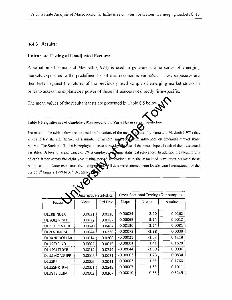
A Univariate Analysis of Macroeconomic Influences on return behaviour in emerging markets 6: 15

6.4.3 Results:

Univariate Testing of Unadjusted Factors:

A variation of Fama and Macbeth (1973) is used to generate a time senes of emerging

markets exposures to the predefined list of macroeconomic variables. These exposures are

then tested against the returns of the previously used sample of emerging market stocks in

order to assess the explanatory power of those influences not directly firm-specific.

The mean values of the resultant tests are presented in Table 6.5 below

Table 6.5 Significance of Candidate Macroeconomic Variables in return prediction

Presented in the table below are the results of a variant of the method posited by Fama and Macbeth (1973) that

serves to test the significance of a number of general macroeconomic influences on emerging market share

returns. The Student's T- test is employed to assess the significance of the mean slope of each of the preselected

variables. A level of significance of 5% is employed to gauge statistical relevance. In addition the mean return

of each factor across the eight year testing period is provided with the associated correlation between these

returns and the factor exposures also being output. All data were sourced from DataStream International for the

period 15t January 1999 to 31 5t December 2006.

Descriptive Statistics Cross-Sectional Testing (Out-sample)

Factor Mean Std Dev Slope T-stat p-value

DLCRBINDEX 0.0021 0.0126 0.00024 2.40 0.0162

DLGOLDPRICE 0.0022 0.0182 0.00065 3.24 0.0012

DLOILBRENTCR 0.0040 0.0484 0.00136 2.64 0.0081

DLPLATINUM 0.0044 0.0230 -0.00072 -2.88 0.0039

DLRANDDOLLAR 0.0014 0.0200 -0.00021 -1.52 0.1218

DLUSEXPIND 0.0002 0.0015 0.00001 1.41 0.1579

DLUSGLTlOYR -0.0014 0.0249 -0.00044 -2.59 0.0096

DLUSMONSUPP 0.0008 0.0031 -0.00003 -1.73 0.0834

DLUSPPI 0.0009 0.0041 0.00003 1.35 0.1760

DLUSSHRTRM -0.0001 0.0545 -0.00007 -1.63 0.1011

DLUSTBILL3M -0.0002 0.0307 -0.00010 -0.65 0.5149

Univers

ity of

Cap

e Tow

n

A Univariate Analysis of Macroeconomic Influences on return behaviour in emerging markets 6: 16

From the above analysis it is apparent that a number of global macroeconomic factors do in

fact exhibit some statistical power in explaining some portion of the variation in share

returns. At the 5% level of significance it is evident that the vast majority of factors with a

commodity focus are found to have some form of significant explanatory power.

The correlations provided serve to explain the strength of the predictive power that Fama and

Macbeth's (1973) modified methodology has identified. The remainder of this chapter

attempts to assess which variables are in fact the most noteworthy in a return based setting

and with the aid of statistical and technical analyses goes on to suggest specific variables for

potential inclusion in the multifactor predictive model to be discussed later in the chapter.

Graphical Depiction of Macroeconomic Variables:

The following graphs depict the relationship between changeable global macroeconomIC

factors and variation in the returns of the DataStream International Emerging Markets Index.

Certain commodities and changing interest rates are amongst the most highly significant of

the list of candidate factors, refer to figures 6.7 and 6.8. Graphical representations of their

movement over time are presented in the chapter with the remainder to be found in Appendix

D.

Furthermore in order to more accurately assess whether or not such macroeconomic factors

are in fact priced according to the degree of exposure experienced by emerging market firms,

the mean monthly returns on each factor are regressed against the respective beta exposures.

Those factors found to be most significant in section 6.4.1 are presented in graphs 6.9-6.15.

Refer to appendix D for the remainder of the ouput. Univ

ersity

of C

ape T

own

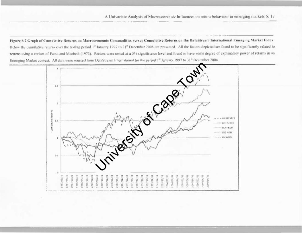
A Uni ,ari"IC Analy,is of r.,.·I"cro ocOt\()1llic IntllLcncc.1 On rcwm t>.:hndl)lIr it! cJ1\~rgit!1? marl_!> 6: 17

I'·igure ".~ G'~rh of ( ·.'not.rI.t 1t~I~r", Qn MM"r""'onon,ir (omR,odi li ......... ~, C.,nul,li. ~ R. lurn. o. Ih. II. laSIr~.m I "'.·r~ ... ,ul r • ..,r~i,,~ Mar~rl Imk.

Iklll" Ih,· ,·umul,hvc ""w", ,,"~ ,he ""'11"1> jl<"'~.,J I' hllu:lJj 1 QQ7 ",] I" Dcrr."h..,- lOO6 <lI. pr<=mcd. All II", (""WI> .Jcpi"ro art fo,,,,6 t,. b<- ,ifn'ftr: .. "I~ rdaltd ,,,

r<1wm u>m!l n .",i"", "f f .lm.l ;lnd ~lacb.:1h ( I Q7ji. r """,..."..,... ,<>1, ... ..Il .. 5'. ';!I',il"·"'''·. Inri "".I (,,1IDIl ,,, ha,,· >£>Inc dt8'"« of txrl"""lol)· po"., off",on, ,n an

ErneTj!'1ljl MOKI<. .. c(lQlt.\l. All d:u \OUt ,o.".ed I ...... [hI:.!>"."", Int.rn>l.jon>l f(IT Iht prriod I" JdmlOIJ) I'IQ7 h' j I' D<",""",,~ 2006

,

"

, J

r' " ',. ,

" , i , ,. , ,. ~ ! ,. ,.

~ ! ! ! ! Ii: ! ! I Ii: ; , , , ~-, , , , , ,

,-- -_ . . _--t ;;

,. ~ ~ ~ !

, , ! ~ , , , , , , , , , \

~ , ! ,

i ! ~

,. ," , , \ '. \

, " I\ ,

! I I ! ! !

... '''- '''" -<W'''''.'

- - - - -_.. . . . . . -

Univers

ity of

Cap

e Tow

n

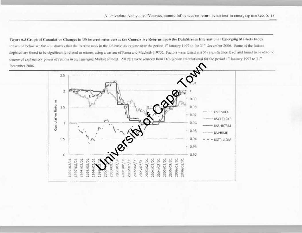
'"i~"ro 1>..\ Cn'l'b " I ( "m"bl i, t Ch"m:~~ I" I)" h"~roll r~l .. "0'"'' 11 •• Cu,"~J~li,.. "~1~ '.' "1''''' Iht r)~ I~S. r •• '" I ",~ """'i,,,.~, f. "'tr~," ~ M "~~h lI"k'

Prc."~,,od bel"" ,." ,be .<lJu"n" .. , ~' ,,,.,,,,''' ; ... , .. ~, •• " ... in .h< IJ~ ha'''' tIOi<krl;" '" OH'r lbe pNioo 1~ Jam",,) I Y'l7 10 ~'" 3 I" LA..:tmbcT 2001'>. :';'"m( 01 'hr r"",,,,_,

<l'1'ltlod a'" f<>uno.! ,,, be """f",.",I} ",1.,,-.1 10 ' .... u"" ",ins .... ,;.'" "r r.,,,,,, anti MadlClh (197J)_ F;o,:,,,,. "tn: lcs",d ., a ~'. ~il:'lif"a'IC'" Inti a,1<I rooOO I" hnr "''''''

do::.;r.~ or "rb""",~ 1''''''' OfT",U"" 'n ~11 Em"'l!'n~ M""'", ... lnl~" An da1~ "t'e """,<o:d lrom l>lrl.S1, .. m 1 .... ., ... ,;"",,1 f<M' Ilw 1""'""'" I ri J.,,,,,,,,, 1<197 '0 31 ~

Decnnbeo- 2006.

, ; i

! § "

" ,

•

0.'

0 -• N 0 -. , m m -

.,"

" .. ~

- --• ,g • " -" ~ , • m m m m m - - -

,.. · . ,.. ,

'"' (

r.-. -.-._-_._-

- ------,~ • .~ • • . "" • -" -• - • N • • • • "" • • m 8 8 --N

m 0 0 0 m m 0 0 0 0 0 -- N N N N N

.., ". • 011

0.18 rMI I"' C1r~

0,17 U>GlTlOV~

0.% . - USSHRIRM 0,15 • .•. _- USPH,l ME

.

" 0,14 - - • USTnlLL 3M

0,93 f _._ .. - _ .. _ ...... _- . . __ . ... _...J 0,92 ---------0 • 0 • 0 • 0 0 • " " , :l • N N N N 11 0 • • • • 0

" . , , - • • • 0 • 0 0 0 0 0 0 0 0 0

0 0 0 0 0 0 0 0 0 N N N N N N - N N

i ..J

Univers

ity of

Cap

e Tow

n

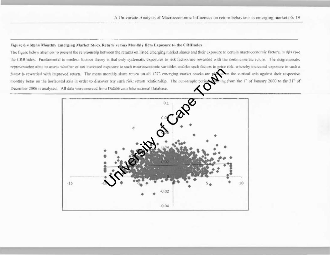
l'igu r~ loA ,~I . , ,, , ~1 (t" U' h I:., .. x ' . ~ ,\ lar~.1 !:>hotk 11.,-,.," ,e"'., MOlln.l) OCIa [ ' I""' '''"'' I" 'h~ e RII h"I,',

"111< r.gur~ ""kll'- .Il,mph 1(> 1"-':0<1'0 'Ilt rd,.."""h,p bel"Nn tho ",I"",. on I", td """"gin~ m'",,",4 sJt.l n:s al>lllhclr ~~po",re III <c" .. I~ '""w " " "",mi~ r.,,,,,,,, in ,hi, e_

lit< CRR I",I", f und.-om, .... 1 '0 m~'n rUlol ""'lheOl) i\ 111:>1 onl> s}>ltm,ue ~,.,....""'-s 10 .. oJ. f.CI ...... OW , ..... ,ud.'d "ill' Ih< to "')U,<"'u"'c «'urn ·rho ,1"'W"mmalic

Irpn.".,nLauo" arm, 10 ""'on. " h.,htr '" n<)l ,oc'nfot'd "'.,.... ...... ·10 '''''h maer .... cOI1(Imic ."","'1." ,."abb .,,<h (JoI I""'~' I"""'c , ''''''. """,,,hy "",,,,.,,,01 "'"","U'" 10 !oUch ~

f .... '" J' ,e .. -..r<k<1 .. nh in'p''''td ' tI,.-n, T1lc n1ll"" IOIoMhl> ,h..., n-h'nJ ", • • 11 I.~n ,-.""'Wng ma-r kd .... cb "", pl' ~lcd on the ' '' " ''''.1 ~,i, "Pin" 'bei, r . ......... ""~

n1(lnrhl)" bela, 00 Ih. h","i1Al1l~11 ,,~ iS 'n OI<"'\kr I" 01,,,,,,<, Ill ') """I, n>l.._ ,,"I .... r<'"1a60n.hip. I "" o"'·':lml~c po.",ud .p:Ir>nlllll Imm ,IIc I· 01 );ol1U'''1' 2000 10 W J I ~ or

l.Iec<'lnber lOOt. i, ~n.'I)..c..I All 01:110 "c~ .. ""cc"" ('"'0 0 ..... -"1=1111 In .... noalio ... l Tho ... b.""

---"

O.M • • •

'" • • • • •

• • • • • ••• • •

. " . ~ • ' . " • ~ " •

."

Univers

ity of

Cap

e Tow

n

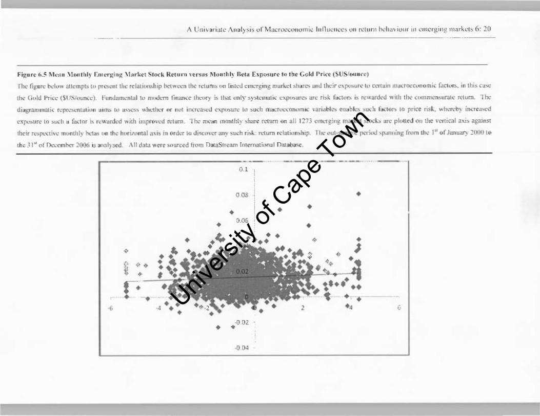
F;.g.rc fo.~ M'~l " \ l"" r!tly I :n ,or~I~~ \ lu rke. S • ...., k Il. ... " " """' ~1 0 • • h~ Ikra [ ., !,,,,, ,,re'o r ~. Cokl I' r l". (~USl"".«' 1

11>< fiJl.~n: b<1"" ~n"'hf'1> 11-, pt,.".nl d,e ",l:Ili,.",hil' btrw«'1III>< ldurn. un IrJc-J c·n.,rgmg nl"r~1 .h""" . nJ .heir ".''''I>"'~ 10 c>'~I"u' flI"""",,COf,omi( tIC''''''. i" .hi. <.>c

iii< ( ;"IJ I'JI<c I\USlu"","c). r"n<ialncnlal ", m"u,,", lin"",. ,1-0.,,-,,)' is lhal ""I)' 'y>l.'n .. l .. ~"f"-'>'m'" ... ~ ,i>~ (...:." ..... "'''Drdo.-J .. IIh .1 .. , ( ... no,,,,,,ural~ ,,1um. 'Iix-

diopllmnJ81i, "'pr= ...... ,, '" ",,11> I" ",>.:» .. 1 .. ,1 .. , • • " "'~ ;"",,'a,,'" ~'fIU'>u", lu ''''''' ,nacru,;<OJ>umO< "I~''''C> ... ,. b ..... . ""), (...: ...... 10 ",iet nsl , wh.'R.~ ;",'J~.."ro

c.'j'k»UJ\' 10 .l.ICh _ liaiD' '" "'''':!rd<:d " ilb ""P" '''''' ",'u,n. 'Iix- Oil ..... ,nor~ hl) >haT .. Mum on alJ 1173 "n"~!'Jng ",~rl.eI ,u: .. :l> u'" 1'1011(1 0" lite n'l1iral lL>;,> ag;I'ftSl

.helr n"'I"""M: mu.n" I)· "'1~' ' ''' ,,"e h"""...ral ~"> ill .. nkr '0 d ,,,,,,,,:, any .nch ml ,durn ",laI",n>h,p. I h., our'"",mr'" ",,",Ill 'f'.UU';"g (",m 'h~ lu

<If Jan""'1- ~OOO 1<1

lire ,11" or Ilo. ... ·nnlx-r 2006 IS _"I)wd ,\11 d.,~, .. ..-t ><>ore«l from n....sUtMII In.ematl,.,al n ,lI"'-.

-- -- -_. __ . " ,~ •

• • • • ~.OG •

• • • ~ • •

• ~.

• ~ ... .. • • • , "

." • •

.~

Univers

ity of

Cap

e Tow

n

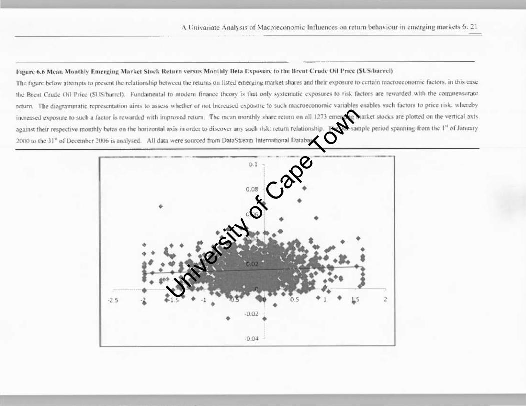
-----------"l~u ... 1>.1> ~I.~ n MUlI.hly f tt,. ,~ln .: ,\I ark~. s.""~ 11.," .. ,, " ,·~"u, MOil ' hly !Wla hl~"u,,' 10 Il,. 11 • .-01 (;,000" 0 ,1 1'''0. (Sl.SJba,'rd l

Th. r,~ur~ b<1",.- >'kmrl> ,,, I"':":'" the ",la,,,,,,,II.,, "'~"""u , I", r<IUI.1> Ull l,,,cd ~I~;"~ ma,k~l "' .... and ,b.ir t'jX>SII" 10 ,.n3IQ m~""""'''' "":lOTS. in this ."'"

Ihe fI,en' Crude OJI 1'"", \1'1 JS "","",I). Fw.d:>OP",1,o1 '" ",0..1,,,, lin ... ". Lhe"')' i. lllal ""~ ,}.l<orgti< "'p<>$u,.., 10 ".~ r:l(10" "'. k".",dw ,,,,h the .·OIlUpW>Wl ... •

M W"Tl. Tht d"'.ll'3mm. ' ,( "'111<''''''''''.' aim. '" ",,,,,,., "1 .... 1,,,. ,,' I." incn-.."..,j npo:.urc Iu !oUch n • .eNC'COOO,pIC ,ar,abl<'S .... bln • ..-1, f;x10" 10 price risk.. " -hOfcby

ir.:.~.»C'd ' .'[105'''' 10 ,,,,,h . , .. , ... i., "' .... rdo.'II """ i"'p",,~ ,<iurn. T hor "",an IIlOnLhl)" .!o.vT reiurn on all lIn .. n..;.ng mmfl1 ~...o.. or" pl<>llC1l "" ,h. '"t'I1lcal ,,;,

again>! lI>:i. "'''Ik"''1, ..... on",Ilhly ,,"a$ 0" , ... tw::."OIIoa' .,i. '" <order 10 d;""".-cr ""~ "",h ri.~ .dum .... + ... "'n.h,p , !c ,"'Ho3lnl'''' pero<)(l ~U"f\g ji"", .1tt . " " f .""""1) ::rooo It, IItt )." "ro.cetuh<:r ~U\J6 oS ~,,~lys.td ,\11 da<a ".." sourced from Dao~'>lr<':Im ' '''~mal '''l1a l I>ol'~_

-B

• • -.

•

•

"

t),liG

• -IW2

-0.04

--•

• • •

•

• • • •

• , Univers

ity of

Cap

e Tow

n

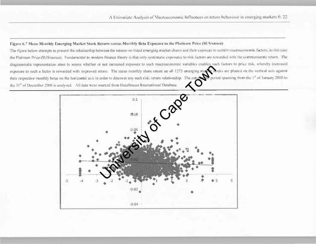
r ig~"e ~, "1 ~k~" Mon,_ I,- [ ,. erK'''K Ma rk. , ~ I\H'~ k ... ,,,, Hr. ,,, M""'hly Ikra ['t""UO" ' " Ihe 1'1.";n"m " ..... . (Sl , ""~n" <)

n.. ti~",~ bel"" :>11< mplS ' 0) prOSt'" 'he ..... uoud"p beN' •• n rbe '''UIIl' '''' Ii".d .n~~,ng ....,-~ .. ,h."" .,Nl rl.: " ~, ... " ....... '" <,na," ,,,,,, ... >.:,"'~'miL r ... ' ....... III ,hi, , .......

rh. Plalm.,m Prin ($US.ou","). FumJ..r ... ,u,,1 '0 ",' odem I;n.oncr m.ory " tho! .mll' >Jf'>I, .... "'" nr""'''''' '0 . i,\ I.", .. , "'" ","~rJ..ll ""I, .he ""nn":nS,,",,,' ,,~um_ on,,· <b"l-!"'",malic T<p«.c,,,.UOn 4in,s IO"~ ,,'h .. her or 001 l/ICTm.cd ""1''''''''. 10 ",,' h m,,«o<COllom'" Y4tiabl", cn;,hl,., ' .... h f.", ,,.,,, pn" ri'~ ... Iu,by incn'=<l

~po .. ,,~ 10 .",h A f ... ,o, i> ""ArlIcd """ ''''POO' cd ,""urn. n, Ill'''''' """"hly sIu.-~ «tum 00 ;011 1273 ..... '!;'''! ",."'" ,~"h "". pll)ll<:d "" ,h, ",n "", ni. "!;'1m"

th.i ..... 1'<'<1I ....... rhlr btras on 'h' horllOOll,d ;L>.i~ in ord ... '0 "''!Co . .. all} such r ill.; ,"'lIm .d :n;',""" p 11..- ""' .... mpl, 1'<~,,1d 'p.M'''!: ITum ,he I· .. , lllllUlll}' :roOO 10

,Ir. 31~ of 1I",,,,nh,:. ~OO6 '" .".,) ",d '\11 d.r.a " "'~ """",'<1 .,,"" 1IaIa.~I"""O In,cnollio ... I II.:llllM",

--"

1):08 -'

~ , , '" ! ,

,

'. , , ,

t , t , . , • ., , , , •• "

, -{1.0! , , -0_04

Univers

ity of

Cap

e Tow

n

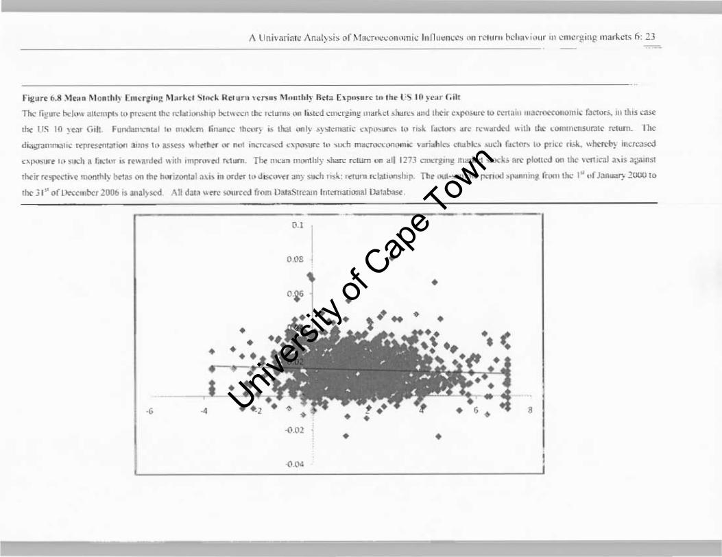
f il.:~n ~,8 .'Inn M" .,lIIy ('~~'lh' ~ M",~., S l<><~ 1'1., um I C,.., ~. M" nd,ly Rolu [ , p"'OF. ,,, I~. l 'S 10 ,.0'" (; ilt

TOC r.~"'r be),,,,, .. no"'ph ", "'C""'" Ihe nl."",,,,h'I' be"",n ,t.: n1",". on I",-cd c"lI.",¥in~ m.rl.ol , 1..0'0 .nd Ihei, c'po'lSUf"(' 10 r,."I"Iai" ,,'~I;'I"()«OIlomi< f~rtor" i" Ihis < .....

~ .. US HI j'.'" C., h. f "'MIo ... ,,n .. 1 ,,, "".1<.:", li, .. no< ,he.") "" ,ha, only " .".o" .. ,i. np""ur ... I" ".k loe"'" .fC fC .... 'Jrd "ilb Ihr ,0001ln,""UI':>I. Mum. UK"

d~l!:"'nll: .. ". 'q>l<'StI'''''''''' 3"", II> as,.,~ ", hrth., , .. n.~ i .... ""T"C~>Cd nl""'U<C ,,, ,,,,,h m ........... """" ... vo. i.h l...,. .... ~k:> ...,01, ('.'Of"> I" ",icc ,bL.. "","",I» metroS<"<!

nl'''''''''' '" .. ",h R 1 ... 1", .. 1. " Rnl.ot '" i,h ,n,l'«" til "'....... TI .. mron m""'hly -.ban: .<lurn "" .11 1273 ""'e'P"!! n""Lc1 .,.o<~ ~f"(' pl",""(1 on lhe w rl ital ,,-,io 3l:o~'nSI

t ... if fO"""' '' . mor,,"!) Mias on 110. 1o,. ,~0t1I31 UI~ In ord ... In oJ..."" ... ~Il) "",h risk: 'aun> .<I"' '' .... h,(I. Th. '~d ...... "'pl< 1"" "'" ., .. n"m!!- (rom ,hi.: 1~ ,,( J;mWl) ZOOO to

the 3 I ~ of u.....,,,,bcr 200b ii anal)~ AU d;U3 "' ..... wwud {roln V",aStr~3m 1lI!<."I1l.u,omd Uo labaoo

, .. 0,081 •

• •

, • •

i

Univers

ity of

Cap

e Tow

n

A Univariate Analysis of Macroeconomic Influences on return behaviour in emerging markets 6: 24

6.5 Further Analysis:

6.5.1 Preliminary Commentary

As is evident from both the statistical and technical analyses performed, there is sufficient

evidence to believe that there are indeed more global, less company specific factors that have

the ability to explain the cross-sectional variation in emerging market share returns.

The returns on precious commodities such as gold, platinum, oil and the like are found in

regression to be significantly correlated with emerging market returns. Student t statistics of

2.40 for the CRB index (a broad based commodities index), 3.24 for the Gold Price

($US/ounce), 2.64 for Brent Crude ($US/barrel) and -2.88 for Platinum ($US/ounce) provide

a sound basis for inferring a definitive relation between independent and dependent variables.

More technically, post 1997-1999 (Asian Crisis), commodities and their associated

appreciations and depreciations in value have seemed to track closely with emerging firm

performance, refer to figure 6.8 above.

US interest rates, the drivers of economic activity on the continent are found to be far less

significant in their statistical relation with the performance of emerging market firms. The

yield of the US Government Bond (-2.59) is the sole US interest rate that exhibits some form

of relation to emerging market returns. Figure 6.9 serves to reinforce the inadequacy of such

factors being return predictors.

6.5.2 Macroeconomic Factors as priced risk factors

In order for such statistical relationships to possess some worth, the relative exposure of

emerging market firms to changes in the values of the selected macroeconomic factors need

to be priced. The greater the exposure that an emerging market firm has to a candidate

macroeconomic variable the greater the anticipated return as a result of the increased risk

burden. This relationship should hold in the event of the factor being a suitable proxy for

pricing risk, however upon closer examination it is evident that these factors do not in fact

exhibit this hypothesised relation.

Figures 6.10 through to 6.19 track the systematic risk of the candidate macroeconomic factors

in relation to their returns on an monthly basis over the seven year period spanning 15t

January 2000 to the 31 5t December 2006.

Univers

ity of

Cap

e Tow

n

A Univariate Analysis of Macroeconomic Influences on return behaviour in emerging markets 6: 25

The graphical depictions serve to communicate that such macroeconomic influences do not

per se reward an investor for increased exposure to their subsequent variation. The candidate

variables follow distinctive trends, for which their sensitivities are quite closely correlated.

However changes in the value of these factors are not picked up by the sensitivity measure

that communicates the risk exposure to the investor. Therefore such macroeconomic

influences are merely periodic influences on return behaviour and not consistently price-able

risk factors that are able to predict returns.

In light of these above relations the next goal would be to harness this knowledge of similar

behaviour and use this as a basis for constructing a model that is able to forecast share returns

in upcoming time horizons. However, as it is presumed that these factors lack predictive

power the construction of such models should serve to endorse the views expressed in this

chapter based on results generated thus far.

6.6 Summary and Conclusion

The aim of this chapter was to supplement the risk analysis of the previous section which

identified numerous priced firm specific risk factors through the consideration of more global

influences on return behaviour, namely adjustments in the macro economy. A similar sample

period was used spanning from the 15t January 1997 to 31 5t December 2006.

Previous work in developed markets endorsed the ability of such macroeconomic influences

being more than adequate in explaining a degree of the variation in listed stock's returns.

Work by Chen, Roll and Ross (1986), Pearce and Roley (1988) et al has found a semblance

of significance in analysing shocks to the macro economy and their associated impact on

share performance.

As is the case with much research in the context of emerging markets, there is little or none

available. Therefore, such a section is somewhat groundbreaking in terms of attempting to

gauge the likelihood of global factors having an impact on the behaviour developing market

performance. With the aid of prior developed market research a shortlist of 15 macro­

economic variables was selected for testing in emerging markets.

The variables were first tested for Stationarity using the Augmented Dickey-Fuller Test. The

level tests run found that none of the chosen variables were in fact stationary and contrary to

Univers

ity of

Cap

e Tow

n

A Univariate Analysis of Macroeconomic Influences on return behaviour in emerging markets 6: 26

the requirements of linear regressIOn had a variable mean and vanance so making any

immediate analysis futile. As performed by Van Rensburg and Slaney (1997) the variables

are then logarithmically transformed in order to remove trends inherent to the data and to

create coefficients that are interpretable as percentage changes. The factors are then first­

differenced and then re-tested. Of the initial list of fifteen factors two were omitted on

account of them exhibiting non-stationarity.

The final list of factors is then correlated together to detect for similar factors with similar

variation and so remove any repetition or double counting. Once this is completed a final list

of eleven candidate macroeconomic variables is available for testing.

The factors are tested for significance using a variant of the methodology employed in Fama

and Macbeth (1973). A three year in-sample regression period (1 st January 1997 to 31

December 1999) is used to obtain historical estimates of each stock's sensitivity to the final

list of macroeconomic variables. These sensitivities or betas are then tested over the out­

sample period spanning the 1 st of January 2000 to the 31 st December 2006 in order to assess

their ability as priced risk factors.. The betas are regressed against the forward returns of the

same emerging market sample in order assess predictive power. A time series of cross

sectional estimates of each factors associated risk premium is then tested using a t-test for

mean to ascertain whether or not there is significant difference from zero. Factors found to

exhibit distinct positive relation include the Gold Price ($US per ounce), CRB Commodities

Index and the Brent Crude Oil Price ($US per barrel), with the negative relations shown by

the price of Platinum ($US per ounce) and the 10 year US Gilt. As is evident of the factors

tested those more closely aligned with commodities and term structure were found to be of

most interest.

However, the viability of the significant factors identified is less than satisfactory when

seeking an explanation for risk based on the computed exposures. The majority of factors fail

to be identified as priced risk factors, whereby the increased exposure of emerging firms to

such variables lack the associated rewards in terms of additional returns. The factors

themselves seem to experience peaks and troughs over time that are somewhat independent

of the relative returns and performance of emerging market firms. Therefore, the suitability

of such factors to be included in a multifactor model for the purposes of return prediction

must be questioned.

Univers

ity of

Cap

e Tow

n

A Univariate Analysis of Macroeconomic Influences on return behaviour in emerging markets 6: 27

The next chapter will incorporate aspects from both this and previous chapters in building a

multifactor model that considers both firm-specific and macroeconomic influence in

attempting to explain and extrapolate future share returns. Cognisance of the findings of this

chapter will be taken and recalled when interpreting the proposed models that are to follow.

Univers

ity of

Cap

e Tow

n

-7-Multivariate Style Analysis incorporating Macroeconomic Influences and

Expected Return Models

7.1 Introduction

The previous chapters of this thesis have aimed to test the influence of certain company

specific and broader macroeconomic variables on emerging market share returns. Chapter

Five which focused on firm-specific variables found a number of value orientated clusters

able to explain share returns in developing countries. Chapter Six expanded the analysis to a

more global scale and found that a number of macroeconomic factors, especially changes in

the prices of certain commodities are in fact able to provide a certain amount of insight as to

the behaviour of stock returns.

The analyses in the Chapters above however provide limited usefulness as they are presented

largely in isolation. Univariate studies do indeed provide valuable information as to which

independent variables have a major influence in explaining the variation of the dependent

variable, however the construction of forecasting models based on such isolated influences

would be excessively narrow in both their scope and accuracy for the purposes of prediction.

Furthermore, to constrain modelling to either firm specific or macroeconomic influences in

separation may also serve to negate possible combinations of explanatory variables that could

lend themselves to the better crafting of a predictive model.

Therefore the first aim of this Chapter is to construct a multifactor model from the final list of

14 firm specific factors identified previously. In such a model one seeks to have the

maximum number of explanatory factors whilst still maintaining the statistical significance of

the multivariate analysis. A range of timing models are then employed in order to find an

optimal predictive formulation for a multifactor expected return model by applying the

methodology of Haugen and Baker (1996) III a stepwise fashion.

Univers

ity of

Cap

e Tow

n

Multivariate Style Analysis incorporating Macroeconomic Influences and Expected Return Models 7: 2

Second, the 10 candidate macroeconomic variables identified in Chapter Six are also tested in

a multi factor setting. The exposures of each share to each macroeconomic influence in

sample are first computed using a variant of the methodology of Fama and Macbeth (1973)

over a specified out-sample period. A similar set of timing models is then employed in the

creation of multi factor expected return models in order to gauge the share return forecasting

ability of the selected factors.

Finally, all firm specific and macroeconomic variables are combined in one testing procedure

in order to find an optimum model that employs both firm specific and broader market

influences in the prediction of share returns. Once more similar timing models are used to

formulate the desired expected return models in adherence with the variant of the

methodology of Haugen and Baker (1996). Firm specific attributes and macroeconomic

variables with t-statistics greater than 1.00 from the univariate tests on unadjusted returns are

included in the analysis. All regressions performed are Ordinary Least Squares (OLS)

regressions.

Such a multivariate testing procedure incorporates the influence of a vast array of

independent influences in a few statistical tests. According to Michaud (1999) there exists a

distinct trade-off in such a modelling procedure. He explains that whilst the analyst may in

fact increase the in-sample explanatory power through the inclusion of more than a one

independent variable, excessive inclusion may also serve to have a detrimental effect on the

out-sample forecast power. Therefore, one must be weary of developing models of too large

a size if one seeks to employ such models in forecasting future undertakings.

The remainder of the Chapter is set out as follows: Section 7.2 defines the data and

methodology for the multivariate cross-sectional regressions with the results following,

Section 7.3 - 7.4 presents the multi factor expected return models and Section 7.5

summarises and concludes.

Univers

ity of

Cap

e Tow

n

Multivariate Style Analysis incorporating Macroeconomic Influences and Expected Return Models 7: 3

7.2 Multivariate cross-sectional regressions

7.2.1 Introduction

The section aims to test the unadjusted monthly return data against all those firm-specific

characteristics identified as significant as identified in Chapter Five. In doing so it is the

ambition of this testing procedure to create a multi factor predictive model. Once more the

distribution of each firm-specific attribute is standardised to a mean of zero and standard

deviation of one in order to enable comparability amongst the magnitudes of slopes

generated. As before all data is sourced from DataStream International and modified

accordingly as described in Chapter Four.

7.2.2 Methodology

In order to create the desired multi factor model a defined stepwise procedure is followed. To

begin the most significant characteristic evident in the univariate tests run in Chapter Five is

cross-sectionally regressed against the forward monthly returns. Thereafter the second most

significant characteristic is added and a two-factor cross-sectional regression is run with the

monthly regression specified as follows:

Where,

I~ t+1 is the realised return on share i in month t+ 1

r 0 t+1 is the constant intercept term

At and Bt are the selected standardised factors

ht+1 and ht+1 are the respective cross-sectional coefficients

£1.1+1 represents the residual error term

Univers

ity of

Cap

e Tow

n

Multivariate Style Analysis incorporating Macroeconomic Influences and Expected Return Models 7: 4

Yu+! and Y2,1+! the respective cross-sectional coefficients are then tested for statistical

significance. Their mean values are tested using a Student t-test in order to assess whether or

not they are in fact significantly different from zero and so have an impact on the dependent

variable. If the results of the test find both characteristics to be significant then the next most

significant attribute is regressed in combination with these first two. Once more the time­

series of monthly slopes is assessed for significance. If again the mean values of the slopes

of the attributes are found to be significant the process continues as before.

However, if at any time during the testing procedure the attribute with the lowest t-statistic is

found to be insignificant when alpha = 0.05 this characteristic is to be removed from the

regression. The regression is then run again with the variable omitted, with any additional

variables that are insignificant removed until such time as all variables are found to be of

sufficient significance. The procedure follows on in this manner until all of the final 18

variables have been tested in such a multiple setting.

Univers

ity of

Cap

e Tow

n

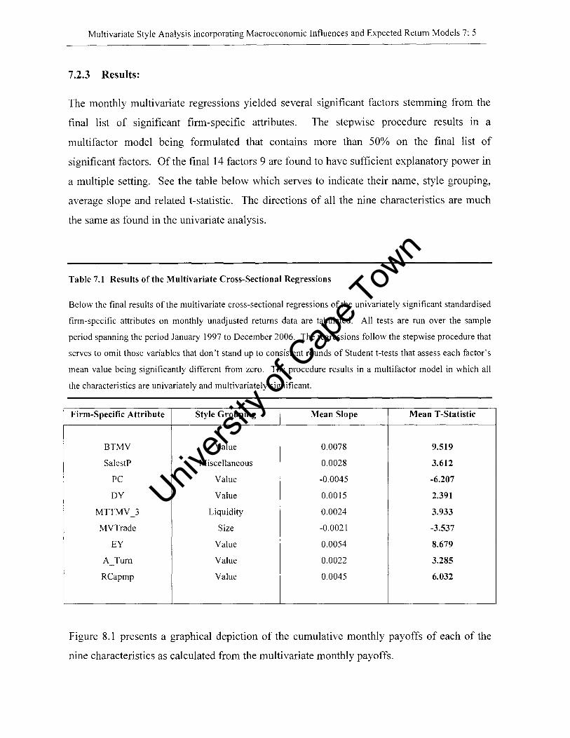
Multivariate Style Analysis incorporating Macroeconomic Influences and Expected Return Models 7: 5

7.2.3 Results:

The monthly multivariate regressions yielded several significant factors stemming from the

final list of significant firm-specific attributes. The stepwise procedure results in a

multifactor model being formulated that contains more than 50% on the final list of

significant factors. Of the final 14 factors 9 are found to have sufficient explanatory power in

a multiple setting. See the table below which serves to indicate their name, style grouping,

average slope and related t-statistic. The directions of all the nine characteristics are much

the same as found in the univariate analysis.

Table 7.1 Results of the Multivariate Cross-Sectional Regressions

Below the final results of the multivariate cross-sectional regressions of the univariately significant standardised

firm-specific attributes on monthly unadjusted returns data are tabulated. All tests are run over the sample

period spanning the period January 1997 to December 2006. The regressions follow the stepwise procedure that

serves to omit those variables that don't stand up to consistent rounds of Student t-tests that assess each factor's

mean value being significantly different from zero. The procedure results in a multifactor model in which all

the characteristics are univariately and multivariately significant.

Firm-Specific Attribute Style Grouping Mean Slope Mean T -Statistic

BTMV Value 0.0078 9.519

SalestP Miscellaneous 0.0028 3.612

PC Value -0.0045 -6.207

DY Value 0.0015 2.391

MTTMV 3 Liquidity 0.0024 3.933

MVTrade Size -0.0021 -3.537

EY Value 0.0054 8.679

A Tum Value 0.0022 3.285

RCapmp Value 0.0045 6.032

Figure 8.1 presents a graphical depiction of the cumulative monthly payoffs of each of the

nine characteristics as calculated from the multivariate monthly payoffs.

Univers

ity of

Cap

e Tow

n

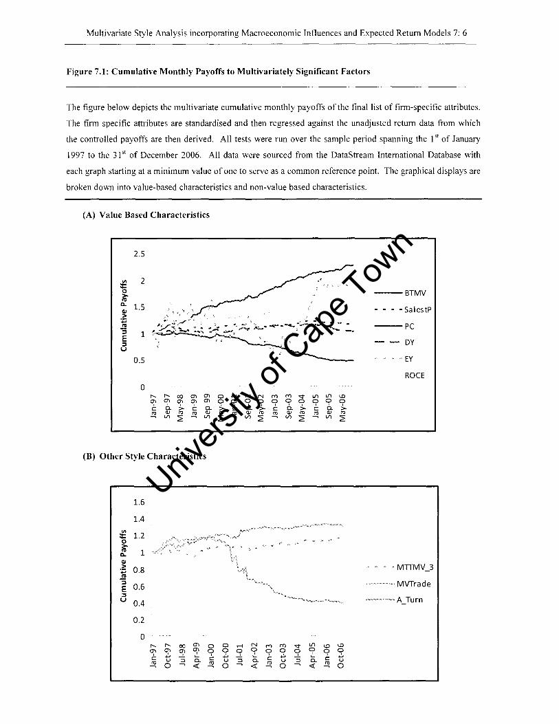
Multivariate Style Analysis incorporating Macroeconomic Influences and Expected Return Models 7: 6

Figure 7.1: Cumulative Monthly Payoffs to MuItivariately Significant Factors

The figure below depicts the multivariate cumulative monthly payoffs of the final list of firm-specific attributes.

The firm specific attributes are standardised and then regressed against the unadjusted return data from which

the controlled payoffs are then derived. All tests were run over the sample period spanning the 151 of January

1997 to the 31 51 of December 2006. All data were sourced from the DataStream International Database with

each graph starting at a minimum value of one to serve as a common reference point. The graphical displays are

broken down into value-based characteristics and non-value based characteristics.

(A) Value Based Characteristics

2.5

III 2 :t: 0 > ra

0.. 1.5 Q/

.2 ... 12 :J 1 E :J u

0.5

0 r-.. r-.. co en en 0 .--t en en en ~ en 0 9 C: 6. >. e 6. >. e ro QJ ro ro QJ ro ro -. Vl ~ -. Vl ~ -.

(B) Other Style Characteristics

1.6

1.4 III

1.2 :t: 0 > ra 1 0.. Q/

.2 0.8 ... 12 :J

0.6 E :J u 0.4

0.2

0 r-.. r-.. co en 0 0 .--t

~ ~ ~ ~ 9 0 0 ..!.. ..!. e ..... l- e u :::J Q. u :J ro 0 -. « ~ 0 -. -.

.--t N ('() ('() '<t 0 0 0 0 0 6. >. C: 6. >. QJ ro ro QJ ro Vl ~ -. Vl ~

" ~. « » o-' "

N ('() ('() '<t

~ 9 0 2 I

e ..... Q. u :J « ro 0 -.

Lfl Lfl 0 0 c 6. ro QJ -. Vl

" "

Lfl <.D 9 9 l- e Q. « ro -.

<.D 0 >. ro ~

<.D

9 ..... u 0

---BTMV

- Salestp

---PC

DY

. EY

ROCE

~ MTTMV_3

MVTrade

-.. A_Turn

Univers

ity of

Cap

e Tow

n

Multivariate Style Analysis incorporating Macroeconomic Influences and Expected Return Models 7: 7

7.3 Multifactor Expected Return Models

In order to assess the true explanatory power of those factors said to both firm specific and

more general in their nature, a series of expected return models are generated that aim to test

the return forecast accuracy.

7.3.1 Data and Methodology

Similar monthly returns, firm specific attribute and macroeconomic data to that used in the

previous chapters are employed here in model construction. However, in this section

unstandardised, winsorised firm specific data is used as no comparisons between each and

every univariate factor is necessary.

Firstly, to obtain a history of payoffs to the candidate factors multivariate cross sectional

regressions are run that include all factors simultaneously. The analysis takes the following

form:

Where,

K

1~,1+1 =YO,I+1 + LYk,l+IF;,k,1 +£,,1+1 k=1

';,1+1 = return to stock i in month t + 1,

Y k ,1+1 = estimated regression coefficient of factor k in month t + 1

F;,k,l = exposure to factor k for stock i at the end of month t

The historical payoffs to each factor form the basis for the generating of out-of-sample

predictions in future time horizons. Haugen and Baker (1996) make use of the 12 months

prior payoffs as a means of producing a forecasted return for the current month (month t).

In addition to trailing twelve-month moving average model employed by Haugen and Baker

(1996), this paper analyses four additional timing models. The first of the timing models

OM) employs the previous month's payoff to provide an estimate of the current month's

payoff. The second of the timing models (3M) uses the past three month's payoffs and a

means of predicting the current month's payoff, with the third (6M) timing model using the

Univers

ity of

Cap

e Tow

n

Multivariate Style Analysis incorporating Macroeconomic Influences and Expected Return Models 7: 8

previous six months historical payoffs and the fourth (18M) using eighteen months prior

payoffs to ascertain the payoff in the current month. This estimation procedure can be

considered the second step in the three step process.

In the final step the monthly payoffs generated previously for month (t+ 1) are combined with

the specified values of each attribute for each share i at the end of month t in order to

generate a forecast return for share i in each and every month:

Where,

K

E(1~,1+1) = YO,I+1 + IE(h,l+I)F;,k" k=1

= forecast return to share i in month t + 1

= estimated payoff to attribute k in month t + 1

A model is only effective if it servers to adequately perform the function it was designed to

carry out, in this case accurately forecast share returns. The effectiveness with which the

constructed expected return models are able to predict returns is assessed using the

Information Coefficient or Ie as mentioned by Grinold (1989). The IC is a measure of

similarity, more specifically a monthly cross-sectional correlation between the forecast and

actual returns.

h h

I(y, - Iy,! h)(y, - y)

1=1 1=1 1=1

Where,

)'\ and YI are the forecast and realised returns for the shares for month t,

h is the number of forecasts in month t and,

h

I YI ! hand yare the respective means of the forecast and realised returns. 1=1

Univers

ity of

Cap

e Tow

n

Multivariate Style Analysis incorporating Macroeconomic Influences and Expected Return Models 7: 9

According to Grinold and Kahn (1995) the IC measure is considered to be a measure that is

able to gauge the level of the manager's skill in being able to generate a model that can

accurately forecast returns. An IC measure close to or in excess of 0.1 is considered high and

serves to indicate that such a model may in fact have exploitable ability in using such pre­

specified factors to predict returns of stocks into the future.

An additional measure is used in this chapter to assess the suitability of the expected return

models generated. The Information Ratio or IR also from the work Grinold and Kahn (1995)

serves to test the robustness of the IC result by incorporating the inherent variation present in

the IC measure into the analysis.

Ie IR=­

{he

The above expresses the mean monthly IC over the standard deviation of the monthly IC. It

serves to take into account the volatility for each of the monthly IC statistics in order to

ensure that the computed and ranked IC's are in fact truly significant.

7.3.1.1 Problems with Haugen and Baker (1996)

As is apparent from the methodology outlined above, a multi factor model is created by

simply including all the testable variables in the expected return model. This process fails to

determine the optimal forecasting model since it fails to scrutinize the incremental

explanatory effect of adding a greater number of independent variables into the regression

equation. In order to create a more accurate model, the original methodology of Haugen and

Baker (1996) is tweaked somewhat in order to assess the impact on explanatory power of

each and every variable as it is included in the model.

7.3.1.2 Haugen & Baker (1996) - a revised methodology

As in Van Rensburg and Janari (2005), a stepwise variant of Haugen and Baker (1996) is

applied. The list of candidate factors eligible for testing was compiled from the original list

of univariate tests run in Chapter Five. All factors present in the univariate tests that had a t-

Univers

ity of

Cap

e Tow

n

Multivariate Style Analysis incorporating Macroeconomic Influences and Expected Return Models 7: 10

statistic of in excess of 1.00 were considered for the analysis to follow so as to allow the for

the chance an insignificant variable tested univariately may hold some explanatory power in a

multi factor setting. As previously the value of each specific attribute is considered a measure

of the stock's exposure to the factor.

The procedure commences using each of the timing models considered, namely 12M, 6M,

3M, 1M and 18M. The process is characterised by two distinct phases. Phase One follows a

univariate testing methodology much the same as those in previous chapters whereby the

tested factors are used to predict slopes. Phase Two expands the analysis to a multivariate

form whereby a set of controlled slopes is then estimated.

At each step S, the aim is to create an optimal model that exhibits the best average monthly

IC using the full range of independent variables V I to V s-l in combination with an added

independent variable N.

Step 1 aims to establish a univariate expected return model through the running of the same

univariate cross sectional regressions performed in Chapter Five of this paper. The distinct

difference here is that the data set in non-standardised. Furthermore, the dataset is scrutinized

once again for outliers and winsorised sufficiently to reduce the influence of extreme

observations. The testing procedure is as follows:

1~,t+1 = Y 0,1+1 + Y N,I+IN,,I + ci,1+1

Where,

N,,t represents the value of the attribute of share i at end of each month t,

Y \' t+1 is the cross-sectional coefficient,

';,1+1' YOHI' and c',t+1 are the same as in the univariate regressions and represent the realised

return on share i for month (t + 1), the constant intercept term, and the residual error

respectively.

From the above regressions, a set of monthly payoffs for each of the attributes is calculated.

These derived monthly payoffs are then used to form the basis of prediction for each of the

attributes' monthly slopes with respect to the model employed.

Univers

ity of

Cap

e Tow

n

Multivariate Style Analysis incorporating Macroeconomic Influences and Expected Return Models 7: 11

Specified as:

Where,

= forecast return to share i in month t + 1

E(ys.l+]) = predicted payoff to attribute N in month t + 1

Upon establishing a forecast of each share's return based on its predictive payoff to the

attributes concerned, the accuracy of the forecast is assessed through comparison with the

realised return. An Ie ratio is computed to quantify the predictive accuracy of each of the

tested attributes. The tested attribute that exhibits the largest average Ie across all months in

the sample period assumes the place of VI and is the first attribute to remain in the model.

Step 2, follows a similar procedure however here the setting is no longer univariate.

Multivariate cross-sectional regressions are run with two independent variables, SI being that

independent variable chosen to remain in the model from Step 1 and each of the remaining

attributes to be included as the second independent variable (N). The most next most

significant attribute according to its average cumulative Ie value is then included and takes

the place of V 2

Specified as follows:

r,,1+] =YO,I+] +Yn,l+]~,I,1 +YN,I+]N1,1 +&1,1+]

At step 2, V I is omitted from the list of remaining attributes to be tested in order to find the

next best characteristic.

The cross-sectional regression run as expected give rise to a set of controlled monthly slopes

for the tested independent variables (YI+]) . As more variables are included, the set of

controlled slopes for V I adjusts. The timing model employed is then used to predict the

monthly controlled slopes for each of VI and N.

The forecast of the monthly return on share i at the end of month t considering the predicted

monthly payoffs to the attributes for month (t + 1) can be indicated as follows:

Univers

ity of

Cap

e Tow

n

Multivariate Style Analysis incorporating Macroeconomic Influences and Expected Return Models 7: 12

K-l

E('~,I+l) = YO,I+1 + IE(Yr'k,l+I)Vk,I,1 +E(YS,I+l)N1,l k=l

The same procedure is repeated until the cumulative average IC across the selected sample

period is at a maximum, with the procedure ending when the next included variable causes a

reduction in the average IC value. If such a decline in the IC occurs, that variable which

caused the decrease is removed from the model and that which remains constitutes the

optimal model formulation. Therefore, the model could at minimum include just V I as an

independent variable based on the next computed IC value due the inclusion ofN, or could

have V n independent variables where V n represent that last added variable that did not reduce

the average IC value.

7.4 Expected Return Model Construction

In previous chapters in this study both firm specific effects and broader macroeconomic

influences were tested for their significance in explaining the variation in emerging market

stock returns. In order to test both influences forecasting power, a number of expected return

models are specified.

7.4.1 Firm Specific Models:

The first rounds of models constructed contain only those firm-specific factors mentioned in

Chapters Four and Five of this paper. They are tested using all the predefined timing models,

namely 1M, 3M, 6M, 12M and IBM over both the entire and restricted sample periods. Such

sample restrictions were imposed due to emerging market data being somewhat sporadic in

its distribution, with only the most recent data being of a desired level of completion. The

sample is restricted to the seven year period (l5t January 2000 to 31 5t December 2006). This

analysis is performed to act as both a check on the robustness of the full-sample results and to

possibly identify trends that have only of late become exploitable.

7.4.2 Macro Economic Models:

The second round of test aim to test the macroeconomic factors identified in Chapter 6 of this

paper for their ability to forecast emerging market share returns. As alluded to in the

previous Chapter, it is doubtful that these factors will in fact prove to be significant in their

relation to returns however they are tested nevertheless in order to provide further evidence to

justify previous findings.

Univers

ity of

Cap

e Tow

n

Multivariate Style Analysis incorporating Macroeconomic Influences and Expected Return Models 7: 13

Methodology:

In testing the predictive power of these variables, another variant of the methodology posited

by Fama and Macbeth (1973) is employed.

Using the list of pre-specified variables the following model is used to model individual stock

returns.

rU+I = Y 0,1+1 + Y 1,1+1 AI + E ;,1+1

Where,

'~,I+I = realized return on share i for year t + 1

YO,l+1 = constant intercept term

YU+I = cross-sectional slope coefficient estimated from the regression

AI = value of the variable at end of each year t

E = residual error JJ+I

The version of Fama and Macbeth (1973) employed can be defined as a 'rolling' beta

regression methodology. In this paper the procedure is constrained to the emerging market

stocks over the sample period at hand which spanned from the 15t January 1997 to 31 5t

December 2006. The procedure begins by estimating the sensitivity (beta) of each of the

emerging market stocks versus the final list of candidate macroeconomic variables over the

first three years of the sample period, more specifically the period 15t January 1997 to 31 5t

December 1999. This rolling thirty six month period serves to provide the historical data in

order to generate monthly sensitivities of emerging market returns to each of the candidate

factors for the remainder of the sample period.

Thereafter the regression 'rolls' forward whereby the range of the second to the thirty seventh

month is regressed and the updated beta estimates per stock are generated. The procedure is

repeated until a set of updated beta estimates are generated for the out-sample period

spanning the 15t of January 2000 to the 31 5t of December 2006. These exposures are then

collectively used for further testing for predictive significance in the methodology of Haugen

Univers

ity of

Cap

e Tow

n

Multivariate Style Analysis incorporating Macroeconomic Influences and Expected Return Models 7: 14

and Baker (1996). Once more a range of timing models are employed in order to measure

both the short and long term predictive capability of these macroeconomic exposures to

emerging market stock returns.

7.4.3 Combined Models:

Finally, the influence of both firm-specific and macroeconomic variables are jointly tested in

order to assess whether through their combination a more effective expected return modelling

formation is able to developed. Such a combination is tested with similar timing models over

the jointly applicable sample period. In this instance the out sample testing period running

from the 1 st of January 2000 to the 31 st of December 2006 is used as it is common in both

firm specific and macroeconomic datasets.

Univers

ity of

Cap

e Tow

n

Multivariate Style Analysis incorporating Macroeconomic Influences and Expected Return Models 7: 15

7.4.4 ftesults

ftesuIts of stepwise Haugen & Baker (1996) - Style

Table 7.2 Constructed Expected Return Models: Style (Full Sample)

The methodology of Haugen and Baker (1996) is followed in a stepwise procedure in order to formulate a series

of expected return models the aim of which is to forecast emerging market share returns. The first step of the

process begins by using only one non-standardised explanatory variable. Unlike Haugen and Baker (1996), an

array of timing models are used in order to attempt to construct the optimum model. Eighteen, Twelve, Six,

Three and previous month moving average models are used in order to estimated the controlled slopes for the

attributes under consideration. The forecasting ability of each model is gauged through the use of the IC or

Information Coefficient of Grinold (1989). That attribute that displays the highest average IC over the tested

sample period remains in the model and is then tested once more with all the other candidate factors. The

second attribute to remain in the model is that which has the highest average IC when tested alongside that

factor that remained in the first step. This stepwise procedure continues until the multifactor expected return

model derived at a stage displays a lower cumulative average IC than that of the previous stage. The

Information Ratio is that of Qian and Hua (2004) which is calculated as the mean monthly IC divided by the

standard deviation of the IC over the sample period. The mean IC and IR generated for each step are displayed

for each of the timing models below. The data were extracted from DataStream International.

Full Sample (1st January 1997 to 31s1 December 2006): Style Characteristics

Timing Mean IR (Qian and Variables

Model Monthly IC Hua, 2004)

1M 0.0408 0.8852 LNMV DY MOM 6M PTBV va 3 RaCE BTMV va 6 - - -

PC

3M 0.0463 1.0390 BTMV RaCE DY MOM 6M PC LNMV MVTRADE EPS

va 6 A TURN PTBV

6M 0.0444 l.l740 LNMV MVTRADE BTMV PTBV PC EPS DY

MVTRADEMV

12M 0.0456 1.2113 BTMV MVTRADE MOM 6M PC ICBT MTBV DY

IBM 0.0468 1.2551 BTMV MVTRADE DY MOM 6M lCBT

From the above table it is evident that five timing models used provide a number of different

forecasting models with a range of explanatory factors. Expected Return models fitted to the

full sample period failed to return statistically significant results. For such tests a mean Ie of

0.1 is considered good, with such a model having a degree of explanatory power and so being

Univers

ity of

Cap

e Tow

n

Multivariate Style Analysis incorporating Macroeconomic Influences and Expected Return Models 7: 16

somewhat exploitable in a market based environment. All five models fail to generate a

mean Ie remotely close to the desired threshold, with the IBM model achieving the highest

value of 0.0468. Models ranged in size from as small as five factors to a maximum of eleven

independent variables.

There are a number of considerations that may in fact lend themselves to explaining the

insignificance of such models in explaining emerging market share returns. The sheer

magnitude and variety of the tested sample, 19 countries from six continents a total of 1290

firms makes finding an accurate general forecasting model a somewhat onerous task.

Furthermore, both data availability and the integrity thereof has been a cause for concern in

many emerging market based study as in this one. Data pre-dating the year 2000 is sparse

and sporadic in its nature and so fails to lend itself to the subject of detailed financial

research, refer to Appendix A.2. Furthermore, the inclusion of certain anomalous countries

such as Venezuela, Pakistan et al about which little is known and wherein financial and

governmental regulation is rife serves to further exacerbate the problem of identifying a

general and reliable forecasting model.

In order account for some of the pitfalls mentioned above, an out-sample period running from

the 15t of January 2000 to the 31 5t of December 2006 was specified and the above style

characteristics retested.

Univers

ity of

Cap

e Tow

n

Multivariate Style Analysis incorporating Macroeconomic Influences and Expected Return Models 7: 17

Table 7.3 Constructed Expected Return Models: Style (Restricted Sample)

The methodology of Haugen and Baker (1996) is followed in a stepwise procedure in order to formulate a series

of expected return models the aim of which is to forecast emerging market share returns. The first step of the

process begins by using only one non-standardised explanatory variable. Unlike Haugen and Baker (1996), an

array of timing models are used in order to attempt to construct the optimum model. Eighteen, Twelve, Six,

Three and previous month moving average models are used in order to estimated the controlled slopes for the

attributes under consideration. The forecasting ability of each model is gauged through the use of the IC or

Information Coefficient of Grinold (1989). That attribute that displays the highest average IC over the tested

sample period remains in the model and is then tested once more with all the other candidate factors. The

second attribute to remain in the model is that which has the highest average IC when tested alongside that

factor that remained in the first step. This stepwise procedure continues until the multifactor expected return

model derived at a stage displays a lower cumulative average IC than that of the previous stage. The

Information Ratio is that of Qian and Hua (2004) which is calculated as the mean monthly IC divided by the

standard deviation of the IC over the sample period. The mean IC and IR generated for each step are displayed

for each ofthe timing models below. The data were extracted from DataStream International.

Restricted Sample (1st January 2000 to 31't December 2006): Style Characteristics

Timing Mean IR (Qian and Variables

Model Monthly IC Hua, 2004)

1M 0.0634 1.8538 BTMV MTBV ROCE MOM 6M PTBV CTTD

3M 0.0708 2.1366 BTMV ROCE LNP 12 EPS

6M 0.0767 1.7943 BTMV MVTRADE MOM 6M MVTRADEMV MTBV PC

LNMV

12M 0.0846 1.7444 BTMV ROCE MOM 6M MVTRADEMV PC EPS LNP

VO 3 P

IBM 0.0833 2.3279 BTMV ROCE MOM 6M A TURN 12 EPS DTMV ICBT P - - -

PC

It is evident from the results presented above in table 7.11 that such sample restriction did

indeed have a profound effect on the significance of the forecasting models generated. Of the

five timing models retested over the sample period 1 sl of January 2000 to 31 sl of December

2006, the lowest mean IC is that of the 1M model (0.0634) which is superior to all models

specified for the full sample. The IBM model has the highest mean IC of 0.0833 with a total

of nine factors.

Univers

ity of

Cap

e Tow

n

Multivariate Style Analysis incorporating Macroeconomic Influences and Expected Return Models 7: 18

Such sample modification serve to endorse the hypothesis that emerging market data in the

late twentieth century lacked completeness and so made the search for predictable

relationships an onerous one. Whilst the above models are an improvement in terms of their

explanatory power they still fail to be of sufficient exploitable significance in a market

environment with their mean IC's still below the accepted benchmark of 0.1.

In order to supplement this analysis, those macroeconomic factors thought to be of

significance when the explanation of firm returns is concerned as studied in Chapter Six of

this paper are retested as additional explanatory factors in a similar Haugen and Baker (1996)

stepwise routine.

Univers

ity of

Cap

e Tow

n

Multivariate Style Analysis incorporating Macroeconomic Influences and Expected Return Models 7: 19

Results of stepwise Haugen and Baker (1996) - Macroeconomic Variables

Table 7.4 Constructed Expected Return Models: Macroeconomic Variables

The methodology of Haugen and Baker (1996) is followed in a stepwise procedure in order to formulate a series

of expected return models the aim of which is to forecast emerging market share returns. The first step of the

process begins by using only one non-standardised explanatory variable. Unlike Haugen and Baker (1996), an

array of timing models are used in order to attempt to construct the optimum model. Eighteen, Twelve, Six,

Three and previous month moving average models are used in order to estimated the controlled slopes for the

attributes under consideration. The forecasting ability of each model is gauged through the use of the IC or

Information Coefficient of Grinold (1989). That attribute that displays the highest average IC over the tested

sample period remains in the model and is then tested once more with all the other candidate factors. The

second attribute to remain in the model is that which has the highest average IC when tested alongside that

factor that remained in the first step. This stepwise procedure continues until the multi factor expected return

model derived at a stage displays a lower cumulative average IC than that of the previous stage. The

Information Ratio is that of Qian and Hua (2004) which is calculated as the mean monthly IC divided by the

standard deviation of the IC over the sample period. The mean IC and IR generated for each step are displayed

for each of the timing models below. A variation of Fama and Macbeth (1973) was used to estimate updating

monthly sensitivities of the emerging market stocks to the candidate list of macroeconomic variables. The

method used a thirty six month rolling period to generate the sensitivities out-sample, such a procedure serves to

present estimates for a eighty four month out-sample testing period. The data were extracted from DataStream

International.

Sample (lst January 2000 to 31st December 2006): Macroeconomic Factors

Timing Mean IR (Qian and Variables

Model Monthly IC Hua, 2004)

1M 0.0201 0.5257 OILBRENTCR USMONSUPP RAND DOLLAR

USHRTRM USGLTlOYR

3M 0.0199 0.6813 CRBINDEX

6M 0.0183 0.3802 GOLDPRICE RANDDOLLAR

12M 0.0352 0.6473 RAND DOLLAR CRBINDEX USEXPIND GOLDPRICE

USMONSUPP PLATINUM USGL Tl OYR

IBM 0.0316 0.6415 USGLTlOYR GOLDPRICE USEXPIND USMONSUPP

Univers

ity of

Cap

e Tow

n

Multivariate Style Analysis incorporating Macroeconomic Influences and Expected Return Models 7: 20

As displayed in table 7.11, attempts at creating a multivariate model capable of predicting

emerging market stock returns based solely on their exposure to macroeconomic variables is

somewhat optimistic. The five macroeconomic timing models employed range in size from

as little as three factors to a maximum of seven. As was the case with the style based models

previously tested, all timing formulations fail to provide sound forecasting ability with all

mean Ie's below the accepted threshold of 0.1, the largest being the 12M model which

generated a value of 0.0352. However this model's IR is less significant being the only the

second highest out of the five models tested. This discrepancy may be a direct result of the

sparseness of the dataset examined, with earlier data being less complete resulting in tested

models providing less robust results when run thereupon.

Once more the relative sparseness and incomplete nature of emerging market data coupled

with the inclusion of a number of either overly or poorly regulated country indices in sample

are cited as potential explanations for the fitted models inconclusive performance. In this

instance the reduced size of the out-sample period employed for testing is a further factor that

may in fact hamper any potential predictive powers any tested factors could exhibit.

However, as the previously tested style factors were found to be significant in explaining

emerging market share returns over the out-sample period it is queried whether or not the

inclusion of the above candidate macroeconomic factors will in fact add to the explanatory

power of the model specified. Therefore, the methodology of Haugen and Baker (1996) is

implemented once more over a combination of style and macroeconomic factor in order to

attain a model of best fit. Univers

ity of

Cap

e Tow

n

Multivariate Style Analysis incorporating Macroeconomic Influences and Expected Return Models 7: 21

Results of stepwise Haugen and Baker (1996) - Style and Macroeconomic Variables

Table 7.5 Constructed Expected Return Models: Style and Macroeconomic Variables

The methodology of Haugen and Baker (1996) is followed in a stepwise procedure in order to formulate a series

of expected return models the aim of which is to forecast emerging market share returns. The first step of the

process begins by using only one non-standardised explanatory variable. Unlike Haugen and Baker (1996), an

array of timing models are used in order to attempt to construct the optimum model. Eighteen, Twelve, Six,

Three and previous month moving average models are used in order to estimated the controlled slopes for the

attributes under consideration. The forecasting ability of each model is gauged through the use of the IC or

Information Coefficient of Grinold (1989). That attribute that displays the highest average IC over the tested

sample period remains in the model and is then tested once more with all the other candidate factors. The

second attribute to remain in the model is that which has the highest average IC when tested alongside that

factor that remained in the first step. This stepwise procedure continues until the multifactor expected return

model derived at a stage displays a lower cumulative average IC than that of the previous stage. The

Information Ratio is that of Qian and Hua (2004) which is calculated as the mean monthly IC divided by the

standard deviation of the IC over the sample period. The mean IC and IR generated for each step are displayed

for each of the timing models below. A variation of Fama and Macbeth (1973) was used to estimate updating

monthly sensitivities of the emerging market stocks to the candidate list of macroeconomic variables. The

method used to make testable the macroeconomic variables is characterised by a thirty six month rolling period

that generates the sensitivities out-sample, such a procedure serves to present estimates for a eighty four month

out-sample testing period. The data were extracted from DataStream International.

Sample (1st January 2000 to 3rt December 2006): Style and Macroeconomic Factors

Timing Mean IR (Qian and Variables

Model Monthly IC Hua,2004)

1M 0.0781 1.7429 BTMV MTBV ROCE USMONSUPP PTBV MOM 6M

CTTO PLATINUM 12 EPS CRBINDEX

3M 0.0714 1.9668 BTMV ROCE LNP USMONSUPP

6M 0.0767 1.7943 BTMV MVTRADE MOM 6M MVTRADEMV MTBV PC

LNMV

12M 0.0861 1.7742 BTMV ROCE MOM 6M MVTRADEMV PC EPS LNP

VO 3 P GODLPRICE USGLTIOYR

IBM 0.0947 1.8669 BTMV ROCE MOM 6M A TURN 12 EPS USPPI - - -

OILBRENTCR DTMV PC MTBV GOLDPRICE DY VO 3

LNP RANDDOLLAR P USGL T1 OYR CTTD

Univers

ity of

Cap

e Tow

n

Multivariate Style Analysis incorporating Macroeconomic Influences and Expected Return Models 7: 22

Table 7.12 communicates the results of the combined Style and Macroeconomic specification

following the refined methodology first employed in its original for by Haugen and Baker

(1996).

It is most notable that this joint specification over the reduced sample period spanning the 15t

of January 2000 to the 31 st December 2006 shows models with improved return

predictability. The five timing models range between four and eighteen factors, with all five

having below par statistical power in prediction. However, one model specification in

particular, the IBM timing model produces a mean IC very similar to 0.1, 0.0947 to be

preCIse. Coupled with it having the top ranked IR equalling 1.8699 it can be inferred that

this model shows potential having a semblance of predictive power over a broad range of

emerging market nations and stocks respectively.

One should however also take heed in considering the model a truly accurate predictive

formulation. Consideration must be taken of the constrained testing period evident in the

above scenario. Timing models of significant historical depth will generate very few

observations over the reduced out sample period and so may serve to exaggerate forecasting

ability. A seven year out-sample period and the results generated there from may contain

significant bias, with certain sample specific factors exhibiting predictive power over that

distinct period but being less robust as time passes.

Univers

ity of

Cap

e Tow

n

Multivariate Style Analysis incorporating Macroeconomic Influences and Expected Return Models 7: 23

7.5 Summary and Conclusion

As mentioned this chapter aims to continue on from work done is Chapters Five and Six and

construct a number of multi factor models. Firstly, a multifactor style characteristic model

derived from the final list of candidate style factors determined in Chapter Five is

constructed. In order to create a robust model with more than a single independent variable, a

defined testing procedure is followed. It would not be sufficient to just include all style

factors as in such specifications the model may indeed provide a greater overall explanatory

power, but attempts to isolate the true explanatory sources is onerous and clouded by the

excessive number of factors in regression.

To begin a multifactor regression is run on the final list of standardised characteristics by

regressing the most significant characteristic (in the previous univariate tests) against the

forward returns in a cross sectional setting. Variables are included in the model one by one if

they are able to add to the overall significance of the model. Once a variable is added and

either that same variable or another becomes the least significant and fails to hold up to the

Student t-test for mean significance the procedure of adding variables is halted and that

variable is removed from the regression. The process of adding variables then restarts until

final characteristic is considered for inclusion in the regression. Thereafter those variables

that remain are the multi factor specification.

The procedure in this instance results in a model with a total of nine style characteristics.

They are Book to Market Value (Value), Sales to Price (Value), Price to Cash (Value),

Dividend Yield (Value), 3-month Market Value Traded to Market Value (Liquidity), Market

Value Traded (Size), Earnings Yield (Value), Asset Turnover (Size) and Return on Capital

Employed (Value). The above formulation has a strong value orientation with Book to

Market Value, Earnings Yield and Return on Capital Employed collectively having the

largest and most significant positive monthly payoffs.

The methodology of Haugen and Baker (1996) is then applied in order to assess the return

predictability of such factors through the construction of a number of expected return models.

A variant of the above methodology is applied in order to increase the robustness of the

generated results as in Van Rensburg & Janari (2005). The stepwise procedure implemented

employs five differing timing models and so forms the basis for the formulation of five

Univers

ity of

Cap

e Tow

n

Multivariate Style Analysis incorporating Macroeconomic Influences and Expected Return Models 7: 24

differing expected return models. Only previously tested style attributes that have an

univariate t-statistic in excess of 1.00 are considered for this procedure. The expected return

models generated over the full sample period are found to be somewhat insignificant as their

mean IC's fail to achieve the predictability threshold of 0.1. As emerging market data is

somewhat sparse in the late nineties the sample was restricted accordingly so as to include

only that data deemed to be more complete and testable. The sample was reduced to seven

years with such manipulations able to significantly improve the relevance of the candidate

style characteristics in explaining emerging market stock returns.

Secondly, the macroeconomic variables tested in Chapter Six of this paper were considered

for inclusion in a multi factor predictive model. In order to make such variables testable, a

variant of the methodology of Fama and Macbeth (1973) was employed that computed

changing monthly stock exposures to such factors through the use of a thirty six month

rolling period regression. This procedure generated a seven year out-sample period from the

1 st of January 2000 to the 31 st of December 2006.

The methodology of Haugen and Baker (1996) is once again applied in testing the predictive

capability of such macroeconomic sensitivities. Besides the twelve month trailing moving

average used by the original authors, the additional timing models used to gauge the

significance of the style characteristics are once again employed. None of the models

provide statistically significant results that lend themselves to being forecasting models of

some practical ability.

Finally, a joint test is performed whereby both style characteristics and macroeconomIC

variables are combined to generate a hybrid multifactor model. Such an analysis aims to

ascertain whether or not the combination of local firm specific factors and broader more

global macroeconomic data is able to better explain the variation in emerging market stock

returns.

The stepwise variant of the methodology of Haugen and Baker (1996) using the five different

timing models is employed to test the forecasting ability of the combination. As the

macroeconomic exposures are constrained to the out-sample period for which they were

computed, the combination is run over the same period, namely-1 5t of January 2000 to 31 st of

December 2006. The timing models aid in generating expected return models that range

from five to fourteen factors. Of the five models only one is found to have a mean IC

Univers

ity of

Cap

e Tow

n

Multivariate Style Analysis incorporating Macroeconomic Influences and Expected Return Models 7: 25

comparable to 0.1 and therefore a semblance of return predictability. The best model

includes the following factors: (1) Book-to-Market Value, (2) Return on Capital Employed,

(3) Prior six month momentum, (4) Asset Turnover, (5) Prior twelve month change in

earnings per share, (6) US Producer Price Index, (7) Price of Oil (Brent Crude in $US/barrel),

(8) Debt to Market Value of Equity, (9) Price to Cash Ratio, (10) Gold Price ($US per

ounce), (11) Dividend Yield, (12) Prior three months change in traded volume, (13) The

logarithm of Price, (14) Rand/Dollar exchange rate, (15) The Price per share, (16) The Yield

on the 10 year US Gilt and (17) Cash to Total Debt Ratio. Inference based on such a hybrid

model should be made with considerable caution due to the disputable data integrity of

emerging market firms, a constrained out-sample testing period and unreliability of

constituent countries and firm's regulations and reporting procedures.

This section has aimed to provide evidence that both style and macroeconomic influences are

able to explain the variation of share returns in a broad emerging market context. Unlike

developed market research, little evidence is found that supports these hypotheses. Certain

influences, be they firm specific or macroeconomic show some predictive power, however

the true meaning and explanation behind these effects is still to be understood.

Univers

ity of

Cap

e Tow

n

-8-

Summary, Conclusion and Areas for further research

8.1 Introduction

The chief aim of this thesis is the detailed investigation of asset pricing in emerging markets,

i.e. to identify both the firm-specific and broader macroeconomic factors which significantly

influence the cross-sectional variation of listed stock returns. The significant question to

follow from this ambition - are emerging markets efficient and do they price assets correctly?

If this is not the case, then the next question would ask if the reasons for share mis-pricings

are in fact identifiable, or more specifically attributable to certain characteristics that certain

firms or markets exude? Finally, the most onerous of queries relates to whether these

identifiable attributes are able to be exploited by investors.

More specifically, these questions can be narrowed down into the three main objectives of

this paper, (1) to determine whether style factors are in fact better able to explain the

variation in share returns compared to conventional asset pricing models, (2) to assess the

likelihood of broader macroeconomic influences on stock markets and to establish their

predictive power upon returns; and (3) to form multi factor predictive style, macroeconomic

and hybrid models that are able to forecast share returns based on historical payoffs to the

most significant factors.

The chapter is comprised of two sections: Section 8.2 summarises and concludes the main

findings in light of the objectives above, and Section 8.3 concludes the thesis and mentions

possible areas of refinement and suggests areas for further research.

Univers

ity of

Cap

e Tow

n

Summary, Conclusion and Area for further research 8: 2

8.2 Summary and Conclusion

This study employs the use of the DataStream Emerging Markets Index for the extracting of

various firm specific and return data.2 As of the 1 st of April 2007, the index had listed a total

of 1538 companies from 26 emerging nations across the globe. Certain countries and their

associated companies are excluded from this study on the basis of excessive trade regulations

hampering the exploitation of any potential investment opportunities, insufficient or

incomplete data, too few listed shares over the sample period and insufficient representation

in terms of overall market capitalisation. The problem of thin trading was analysed and

found not to be of significant threat to the integrity of the outcomes of analyses to follow.

After such sample refinements the total number of countries was reduced to twenty which

comprised 1273 listed shares having a cumulative market capitalisation of $US 3,299 billion

with the top 100 firms accounting for approximately 50% of this total capitalisation.

All return data and the forty six style characteristics are either constructed from or

downloaded from the DataStream International database over the sample period 1 st of January

1997 to the 31 st of December 2006. The study is free from look-ahead bias on account of

DataStream only updating information once it is publicly available. Furthermore, there is no

element of data-snooping bias present in-study as an analysis of such rigour is yet to be

performed on such an emerging market sample. The study is however subject to survivorship

bias.

Risk based explanations for the variations of share returns in emerging markets were then

sought. Single and Multi-Index Models are constructed in order to attempt to explain the

time-series variation of returns. Firstly, the DataStream International Emerging Markets

Index was used as the market proxy for the single index model with the DataStream World

Market Index next to be tested in a single index setting. Subsequently, the aforementioned

indices were then combined for the multi-index model formulation. The computed R2 and

adjusted R2 across the respective models indicates that the multi-index model is marginally

supenor in explaining the variation in returns, however with only 69% of regressions

2 The use of this dataset was endorsed through correspondence with Professor Geert Rouwenhorst whose paper

entitled "Local Return Factors in Emerging Markets" employed the use of data from the same database albeit over a differing sample period.

Univers

ity of

Cap

e Tow

n

Summary, Conclusion and Area for further research 8: 3

significant compared to 72% of the single index model which serves to somewhat blur the

distinction as to which model is ultimately superior in describing the structural influences of a

broad sample of emerging market shares. The residual variation unexplained by each model

is cross-tested in a similar manner between both index model formulations with either

model's explanatory power over the other's unclassified variation found to be statistically

insignificant.

Following the above risk-adjustment, testing of the sourced firm-specific attributes begins.

All forty-six style factors are standardised for comparative purposes and then regressed in a

cross-sectional format against emerging market share returns. The regressions are run on

unadjusted, CAPM adjusted and APT adjusted returns in order to gauge the ability of the

attributes to explain the cross sectional variation of share returns and as a test of robustness

check on identified explanatory factors. The significance of the payoffs of the tested

variables is assessed using the Student-t test. Cluster Analyses of the significant factor

payoffs are then performed for unadjusted and risk-adjusted testing procedure outputs in

order to detect groups of factors with similar explanatory power. Furthermore, to remove

double counting and the prevalence of repetition, a correlation matrix is generated on the tests

of unadjusted returns to aid in pruning out factors of excessive likeness.

The testing procedures run over the both the unadjusted and adjusted returns served to yield

very similar statistically significant factors indicating their robustness in explaining return

variation. Following the correlation analysis a final list of 14 significant style factors is

generated. A strong value and size influence is evident as indicated by factors such as the

logarithm of Price (Size), the logarithm of Market Value (Size), Book-to-Market Value

(Value), Price-to-Cash (Value) and Price-to-Book Value (Value) being amongst the most

statistically significant.

Such influences cohere with the vast majority of both developed and developing literature

concerning market efficiency with the emerging market studies of Patel (1997), Rouwenhorst

(1999), Fama and French (1998) and Serra (2000), who all find strong a strong prevalence of

a negative size and positive value effect, however few find as many varied forms of these

effects as evident in this study. Short Term Liquidity is also found to be relevant in

predicting emerging market return movements; however data concerns and lower statistical

significance are cause for concern when attempting to exploit such anomalies. The factors

can be classified into the following broad groups or clusters: (1) Size, (2) Value, (3) Liquidity

Univers

ity of

Cap

e Tow

n

Summary, Conclusion and Area for further research 8: 4

and (4) Miscellaneous. The consistency and direction of the calculated payoffs is then

assessed in order to establish the integrity of the inferred relationship. From the analysis

undertaken it is apparent that few of the so called significant factors are consistent in the

direction of their payoff which may result in the interpretation of timing models constructed

on the basis of these anomalous factors to be somewhat less than ideal in terms of forecast

accuracy. However, from the univariate testing procedure employed it is evident that there

are indeed a number of identifiable firm-specific factors that are able to aid in explaining the

variation in emerging share returns.

Having identified a number of firm-specific factors as having some explanatory power, the

analysis then moves to consider a list of macroeconomic variables and their potential

influence on emerging stock market returns in a similar setting. The variables chosen are

dominated by commodity prices and numerous short and long term interest rates in line with

similar work by Gjerde and Srettem (1999), Sadorsky (1999) and Bilson, Brailsford, and

Hooper (2001) who test and find similar factors to be significant. Augmented Dickey Fuller

tests as performed in Van Rensburg and Slaney (1997) are performed on logarithmically

transformed first differenced variables in order to establish the stationarity of the chosen

factors. A correlation analysis followed to aid in pruning those variables that show little

influence on broad emerging and global indices resulting in a final list of eleven

macroeconomic factors to be considered for testing.

In testing such macroeconomic factors, a version of the methodology used in Fama and

Macbeth (1973) was employed over an in-sample period spanning the 151 of January 1997 to

31 51 December 1999 in order to estimate the sensitivity of each emerging market stock to the

respective macroeconomic variable on a monthly basis. The in-sample betas were then

regressed out-sample over the period 151 of January 2000 to the 31 51 of December 2006 in a

cross sectional univariate setting and their explanatory power over the cross section of

emerging market returns assessed using the Student-t test. Of the final list of eleven factors

tested only the monthly payoffs or risk premia of five are found to be of notable significance.

Fluctuation in the price of Gold and Platinum in dollars per ounce, the CRB Index and they

yields on certain US government bonds issues are factors identified as having a measure of

explanatory power over the cross sectional variation of emerging market stock returns.

Through graphical depiction and with some further consideration it is quite plausible that

such macroeconomic factors are not per se priced risk factors, i.e. a greater exposure to such

Univers

ity of

Cap

e Tow

n

Summary, Conclusion and Area for further research 8: 5

a factor will not necessarily provide greater reward - the factors performance may in fact be

to a degree somewhat independent of attempts at increased investment exposure. However as

a number are statistically significant one must in fact consider that such broader market

influences may indeed have some forecasting ability.

Ultimately the real assessment of such identifiable factors that purport to explain mispricing

in so called efficient markets is in the establishment and scrutiny of predictive models that

attempt to forecast share returns on the basis of these related factors.

To begin a multivariate analysis of the aforementioned style factors was run in order to assess

whether those factors identified previously in univariate testing were in fact robust in their

explanatory power. The procedure begins by including the most significant variable evident

from the previous univariate tests. Variables are included one at a time in a multi factor

regression versus forward returns until the inclusion of an additional variable causes the least

significant variable to show an insignificant mean of the time series of its controlled slope.

Upon this outcome that variable is removed and the testing procedure continued until all such

factors are tested in such a manner. The analysis yielded a multifactor model with a total of

nine factors, namely; (1) Book-to-Market Value (2) Sales-to-Price, (3) Price-to-Cash, (4)

Dividend Yield, (5) Three month change in Market Value to Market Value Traded, (6)

Market Value Traded, (7) Earnings Yield, (8) Asset Turnover and (9) Return on Capital

Employed. As evident from the univariate analyses the Book-to-Market Value factor is of

greatest significance with the highest cumulative monthly payoff of all the factors present in

the model.

Finally, expected return models are constructed using a stepwise variant of the methodology

employed by Haugen and Baker (1996). The expected return models are constructed using

three models, (i) Style factors only, (ii) Macroeconomic factors only, and (iii) A Hybrid

formulation combining both Style and Macroeconomic factors in an effort to improve

explanatory power of the generated forecasting model. Firstly, non-standardised firm­

specific factors having a t-statistic of greater than 1.00 are examined over the full sample

period spanning the 1 st of January 1997 to the 31 st of December 2006 using not only the

twelve-month trailing moving average of attribute payoffs employed by Haugen and Baker

(1996) but further one, three, six and eighteen month trailing averages. The model's

forecasting power is assessed using the Information Coefficient (IC) and the Information

Ratio (IR). The five timing models give rise to expected return models of between five and

Univers

ity of

Cap

e Tow

n

Summary, Conclusion and Area for further research 8: 6

eleven factors, however none are found to be of significant forecasting ability with mean IC's

well below the desired threshold of 0.1.

The integrity of emerging market data in the late nineties may be considered poor (refer

Appendix A) and therefore cited as a potential cause for the apparent insignificance in

explanatory power of models tested over the specified time period. Such a data anomaly in

part justifies that the timing models be re-tested over a restricted sample running from the 1 st

of January 2000 to the 31 st of December 2006. The results generated are considerably more

promising with mean IC value of all expected return models rising, the highest value being

the twelve month model with a mean IC of 0.0846. However, even with such a considerable

improvement such models are still statistically inadequate to be regarded as exploitable in a

real-world investment setting. Therefore, the macroeconomic variables previously

considered in univariate analysis are tested for their ability firstly to provide independent

forecasting power over emerging market return, and then subsequently they are added in

analysis to the style factors in an attempt to create a more optimal hybrid expected return

model.

To test the macroeconomIC variables usmg the appropriate timing models previously

employed the updated monthly payoff of each share to each macroeconomic variable needed

to be computed. Once more a variation of Fama and Macbeth (1973) was used whereby a

rolling thirty six month in-sample period beginning the 1 st of January 1997 to the 31 st of

December 2006, would in cross sectional regression serve to establish such updated

exposures over an out-sample period 1 st of January 2000 to the 31 st of December 2006.

These exposures were then entered into the stepwise variant of Haugen and Baker (1996) in

order to ascertain their return forecasting ability. The variables however lacked any

considerable forecasting ability with the largest mean IC value of 0.352 well below 0.1. Such

variables held little value independently, but perhaps combining them to form combined style

and macroeconomic expected return models would yield better results.

The inclusion of such macroeconomic variables into a combined analysis resulted in a testing

procedure that considered a total of 36 variables of both specific and broad influence. Such

an amalgamation of factors did indeed provide a marginal improvement in the forecasting

ability of the specified expected return models. The mean IC of the original eighteen month

trailing average model improved from 0.0833 to 0.0947 indicating a somewhat slight but

nevertheless significant improvement in forecasting ability. This model proved to have the

Univers

ity of

Cap

e Tow

n

Summary, Conclusion and Area for further research 8: 7

highest mean IC and contained the following factors; (1) Book-to-Market Value, (2) Return

on Capital Employed, (3) Prior six month momentum, (4) Asset Turnover, (5) Prior twelve

month change in earnings per share, (6) US Producer Price Index, (7) Price of Oil (Brent

Crude in $US/barrel), (8) Debt to Market Value of Equity, (9) Price to Cash Ratio, (10) Gold

Price ($US per ounce), (11) Dividend Yield, (12) Prior three months change in traded

volume, (13) The logarithm of Price, (14) Rand/Dollar exchange rate, (15) The Price per

share, (16) The Yield on the 10 year US Gilt and (17) Cash to Total Debt Ratio.

While such hybrid formulations were in fact able to improve the forecasting ability of the

constructed expected return models, they still fail in statistical significance with investment

based thereupon lacking any exploitable ability.

8.3 Final Conclusion and Areas for Further research

Emerging equity markets are associated with a certain degree of mystery and fear of the

unknown. Professionals will often advocate the combination of various emerging market

offerings in portfolio with more developed market holding on the basis of diversification,

however such inclusion is often done blindfolded and considered somewhat of a gamble.

This paper aims to assist and shed a little more light on some hypothesised return drivers of a

broad sample of emerging market nations.

This thesis aimed to identify both firm-specific characteristics and more general

macroeconomic influences that have some form of relationship and explanatory power of the

cross section of emerging market share returns. A number of firm-specific and

macroeconomic variables were identified as anomalies that have their monthly payoffs

significant in both a univariate and multivariate setting. To ascertain their true worth, both

sets of characteristic's ability to forecast share returns were tested at first independently and

then in a hybrid combination through the construction of a number of expected return models.

Unfortunately, such models fail to provide conclusive evidence that indicates their ability to

accurately forecast emerging market share returns.

There has been considerable evidence in both developed and developing markets of the

existence of these anomalous effects, both firm-specific and macroeconomic. However, no

definitive account exists that accurately explains their existence. Previously accepted asset

Univers

ity of

Cap

e Tow

n

Summary, Conclusion and Area for further research 8: 8

pricing model theories such as the CAPM which make use of a sole market proxy as an

explanation for the risk: return trade-off are one again disproved with this study indicating

the presence of additional price risk factors over and above that a seemingly sufficient market

proxy. However, although such results are found that do cohere with previous literature, one

must not get carried away without considering the potential biases to which a form of data

analysis is prone.

The emergmg market dataset employed is cause for concern from the outset. Data

manipulations to remove outliers, erroneous data entries, incomplete information and account

for the presence for biases such as thin trading were necessary. A broad analysis of the data

availability for the chosen sample does raise cause for concern when noticing the somewhat

obvious trend of the decreasing sparseness of data overtime as the sample is viewed from

start to end. An additional concern would be reflected in the selected data source and it's

method of backfilling data. Such a procedure leaves the analysis vulnerable to survivorship

bias, a prejudice that has conflicting perceptions on its impact on the robustness of generated

results. Data-mining or the over analysis of a specified sample of data may lend itself to

generating anomalous results not by virtue of the fact that they are actually present but in part

due to the researcher wanting them to exist. Although such biases may hamper the production

of superbly accurate results, every possible measure is taken that the final outcomes

generated are in fact considered in light of the aforementioned concerns.

This study has indeed produce a number of expected but also unexpected results, partly due

to the extensiveness of analyses performed and partly due to the fact that minimal previous

work in such a context has been undertaken. In order to better assess the robustness of the

generated outcomes application of the proposed predictive methods needs to be extended to

further time horizons that are not only unknown but also more detailed in the rigour and

completeness of their recorded data. The testing for instance of the formulated expected

return models in a range of different sample periods and the subsequent comparison of such

results would indeed to serve to communicate whether or not the study of such anomalous

factors has any benefit.

From a practical perspective, a study of this nature aside from making an attempt at shedding

much needed light on markets not studied in rigour to those termed developed should in fact

Univers

ity of

Cap

e Tow

n

Summary, Conclusion and Area for further research 8: 9

be able to have some industry application. As previously asserted the realms of portfolio

management, equity analysis and investment performance appraisal cited similarly in work

by Fama and French (1993) would be the ideal context in which such research should be

value adding. However, it is in the area of real-world application that this study had further

potential.

Two main pitfalls hamper the ability of such an analysis to bear fruit in a real world context.

Barriers to trade are first and foremost the most considerable obstacle worth mentioning.

Numerous countries included in the tested sample were included for the sake of completeness

and due to the fact they have well recorded historical datasets. However, many Asian and

Latin American nations have considerable barriers to foreigners trading on their markets.

Such restricted accessibility severely hampers the potential for such a predictive modelling

procedure to bear fruit in industry. However, as markets become less regulated and the

arrival of the global village becomes part and parcel of every nations policy, perhaps such

broad based trading will in the end be able to generate some form of competitive reward.

The second consideration not accounted for in this study is the issue of trading costs. This

thesis omits the presence of trading costs which form a substantial portion of any investor's

outflows when managing his or her portfolio. The characteristics of a portfolio in terms of its

style and macroeconomic exposure change over time in response to overall market

movements, therefore for an investor to actively pursue a defined style based strategy

frequent re-balancing of stocks held needs to occur in order for the portfolio to remain

focused. Such portfolio adjustment is brought about through trading in and out of positions

which will result in exposure to substantial transaction costs, the magnitude of which will be

directly dependent on the frequency of the rebalancing. In addition, due to the fact of the

tested model incorporating 1273 firms from many different nations across the globe,

consistent trading in such a wide range of markets may present the investors with trading

costs more substantial that the potential benefit from pursuing the strategies investigated

herein.

Ultimately, this thesis has provided insight into some of the potential factors that may serve

to influence the decisions of investors who have a keen interest in emerging equity markets.

Although not all results have been statistically significant, nevertheless they have postulated

potential economic relationships and aided in providing some clarity as to their existence.

Future studies with the aid of more up to date information, analytical techniques and perhaps

Univers

ity of

Cap

e Tow

n

Summary, Conclusion and Area for further research 8: 10

some changes in the stance of certain nations to becoming so called 'team players' in the

game of global integration may serve to provide further insight into those markets termed

emergmg.

Univers

ity of

Cap

e Tow

n

Reference List

Agrawal, A., Tandon, K., 1994. Anomalies or illusions? Evidence from stock markets in

eighteen countries. Journal of International Money and Finance 13(1), 83-106.

Amihud, Y., Mendelson, H., 1986. Asset pricing and the bid-ask spread. Journal of Financial

Economics 17(2), 223-250.

Aydogan, K., Gursoy, G., 2001. PIE and PBV ratios as predictors of stock returns m

emerging equity markets. Emerging Markets Quarterly. 4, 60-67.

Bakeart, G., Harvey, C., 2000. Foreign Speculators in Emerging Markets. The Journal of

Finance 55(2).

Bakeart, G., Harvey, c., 2003. Emerging Markets Finance. The Journal of Empirical

Finance 10, 3-55.

Ball, R., 1978. Anomalies in relationships between securities' yields and yield surrogates.

Journal of Financial Economics, 6(2), 103-126.

Banz, R., 1981. The relationship between return and the market value of common stock.

Journal of Financial Economics 9(1),3-18

Banz, R., Breen, W., 1986. Sample dependant results using accounting and market data: some

evidence. Journal of Finance 41 (4), 779-794.

Banz, R., 1981. The relationship between return and the market value of common stock.

Journal of Financial Economics 9(1),3-18.

Barnett, V., Lewis, T., 1984. Outliers in Statistical Data. Second Edition. Wiley, New York.

Univers

ity of

Cap

e Tow

n

Barry, C., Goldreyer, E., Lockwood, L., Rodriguez, M., 2002. Robustness of size and value

effects in emerging markets, 1985-2000. Emerging Market Review, 3,1-30.

Basu, S., 1977. Investment Performance in common stocks in relation to their price-earnings

ratios: a test of the efficient market hypothesis. Journal of Finance 32(3), 663-682.

Bilson, c., Brailsford, T., Hooper, V., 2001. Selecting Macroeconomic variables as

explanatory factors of emerging market stock returns. Pacific Basin Finance Journal 9, 401-

426.

Black, F., 1972. Capital market equilibrium with restricted borrowing. Journal of Business,

45(3),444-455.

Black, F., 1993. Beta and return. Journal of Portfolio Management, 20(1),8-18.

Black, F., Fisher, L., Jensen, M., Scholes, M., 1972. The capital asset pricing model: some

empirical tests, in: Jensen, M. (Ed), Studies in the theory of capital markets, 79-121. Praeger:

New York.

Blume, M., 1980. Stock Returns and dividend yields: some more evidence. Review of

Economics and Statistics 62, 567-577.

Campbell, J., 1985. Stock Returns and the Term Structure. Working Paper No. 1626.

National Bureau of Economic Research.

Chan, K., Chen, N., 1988. An unconditional asset-pricing test and the role of firm size as an

instrumental variable for risk. Journal of Finance, 43(2),309-325.

Chan L., Jegadeesh N., Lakohishok, J., 1995. Evaluating the performance of value versus

glamour stocks: the impact of selection bias. Journal of Financial Economics 38(3), 269-286.

Chan, L., Karceski, J., Lakonishok, J., 2000. New paradigm or the same old hype in equity

investing? Financial Analysts Journal 56(4), 23-37.

Univers

ity of

Cap

e Tow

n

Chen, N., Roll R., Ross S., 1986. Economic Forces and the Stock Market. The Journal of

Business, 59(3), 383-403.

Chen, N. 1991. Financial Investment Opportunities and the Macroeconomy. The Journal of

Finance, 46(2), 529-554.

Chui, A., Wei, K., 1998. Book-to-market, firm size and turn-of-the-year effect: Evidence

from Pacific-Basin Emerging Markets. Pacific Basin Finance Journal, 6, 275-293.

Claessens, S., Dasgupta, S., Glen, J., 1998. The cross-section of stock returns: evidence from

the emerging markets. Emerging Markets Quarterly, 2, 4-13.

Conrad, J., Kaul, G., 1988. Time-Variation in Expected Returns. Journal of Business. 61 (4)

Cormack, R., 1971. A review of classification. Journal of the Royal Statistical Society, Series

A, 134,321-367

Davis, J., 1994. The cross section of realised stock returns: the pre-COMPUSTAT evidence.

Journal of Finance, 49(5),1579-1593.

De Bondt, W., Thaler, R., 1985. Does the stock market overreact? Journal of Finance 40(3),

793-805.

De Bondt, W., Thaler, R., 1987. Further evidence of investor overreaction and stock market

seasonality. Journal of Finance 42(3),557-581.

De Groot, C., Verschoor, W., 2002. Further evidence on Asian Stock Return Behaviour.

Emerging Markets Review 3, 179-193.

De Roon, F., Nijman, T., Werker, J., 2001. Testing for Mean-Variance Spanning with Short

Sales Constraints and Transaction Costs: The Case of Emerging Markets. The Journal of

Finance, 56(2),721-742.

Univers

ity of

Cap

e Tow

n

Deakin, E., 1976. Distributions of financial accounting ratios: some empirical evidence.

Accounting Review 51 (1), 90-96.

Desrosiers, S., Kortas, M., L-Her, J., Plante, J., Roberge, M., 2004. Style Timing III

Emerging Markets. Working Paper, Cass Business School,

A vailable:http://www.cass.city.ac. uk/emg/seminars/Papers/Desrosiers _ Kortas _ L'Her _Plante_

Roberge.pdf

Dickey, D., Fuller, W., 1979. Distribution of Estimators for Autoregressive Time Series with

a Unit Root. Journal of the American Statistical Association, 74,427-431

Dimson, E., 1979. Risk measurement when shares are subject to infrequent trading. Journal

of Financial Economics 7, 197-226

Dimson, E., Marsh, P., 1999. Murphy's law and market anomalies: the size premium may

have gone in reverse, but the size effect lives on. Journal of Portfolio Management 25(2), 53-

69

Edwards, E., Bell, P., 1961. The Theory and Measurement of Business Income. Book.

University of California Press.

Fama, E., 1970. Efficient capital markets. Journal of Finance 25(2).383-417.

Fama, E., 1981. Stock returns, real activity, inflation and money. American

Economic Review, 71. 545-565.

Fama, E., 1991. Efficient capital markets II. Journal of Finance 46(5),1575-1618.

Fama, E., French, K., 1992. The cross-section of expected stock returns. Journal of Finance

47(2), 427-467.

Univers

ity of

Cap

e Tow

n

Fama, E., French, K., 1998. Value versus growth: the international evidence. Journal of

Finance 53(6), 1975-1998.

Fama, E., Macbeth, J., 1973. Risk, return, and equilibrium: empirical tests. Journal of

Political Economy 71 (May-June), 607

Fama, E., French, K., 1996, Multifactor Explanations of Asset Pricing Anomalies. Journal of

Finance, LI(1), 55-84.

Fisher, L., 1966. Some new stock market indexes. Journal of Business 39(212), 191-225.

Frecka, T., Hopwood, W., 1983. The effects of outliers on the cross-sectional distributional

properties of financial ratios. Accounting Review 58(1), 115-128.

Friedman, M., 1988. Money and the Stock Market. The Journal of Political Economy, 96(2)

221-245.

French, K., Roll, R., 1986. Stock Return Variances: The Arrival of Information and the

Reaction of Traders. The Journal of Financial Econonomics. 17(1). 5-26.

Gjerde, 0., Scettem, F., 1999. Causal relations among stock returns and macroeconomic

variables in a small open economy. Journal of International Financial Markets, Institutions

and Money 9,61-74

Gompers, P., Metrick, A., 1998. Institutional investors and equity prices. NBER Working

Paper 6723.

Gyung-Jan, S., Marthe,. A ., Shawky, H., 2002. Liquidity and Stock Returns in Emerging

Equity Markets. Emerging Markets Review 4, 1-24.

Halfeld, M., 2000. A Fundamental analysis of Brazilian Stock Returns. Emerging Markets

Quarterly, 4(4)

Univers

ity of

Cap

e Tow

n

Harvey, C., 1991. The world price of co-variance risk. Journal of Finance. 46, p.lll-155.

Harvey, c., 1995. Predictable risk and returns in emerging markets. Review of Financial

Studies 8, 773-816.

Haugen, R., Baker, N., 1996. Commonality in the determinants of expected stock returns.

Journal of Financial Economics 41,401-439.

Humpe, A., Macmillian, P., 2005. Can Macroeconomic variables explain long term stock

market movements? A comparison of the US and Japan. CMDA (Centre for Dynamic

Macroeconomic Analysis) Working Paper number 0720.

Ibbotson, R., 1975. The performance of common stock new issues. Journal of Financial

Economics 2, 235-272.

Ibrahim, M., Hassanudeen, A., 2003. Macroeconomic Variables and the Malaysian Equity

Market: A view through rolling subsamples. The Journal of Economic Studies 30(1), 6-27.

Jaffe, J., Keirn, D., Westerfield, R., 1989. Earnings yield, market values, and stock returns.

Journal of Finance 44, 135-148.

Jegadeesh, N., Titman, S., 1993. Returns to Buying Winners and Selling Losers: Implications

for Stock Market Efficiency. Journal of Finance 48, 65-91.

Jensen, M., 1978. Some anomalous evidence regarding market efficiency. Journal of

Financial Economics, 6, 95-102.

Jensen, G., Johnson, R., Mercer, J., 1998. The inconsistency of the small-firm and value stock

premiums. Journal of Portfolio Management (Winter), 27-36.

Jun, S., Marathe, A., Shawky, H., 2003. Liquidity and stock returns in emerging equity

markets. Emerging Markets Review 4, 1-24.

Univers

ity of

Cap

e Tow

n

Kargin, V., 2002. Value investing m emergmg markets: risks and benefits. Emerging

Markets Review 3, 233-244.

Keirn, D., 1985. Dividend yields and stock returns: implications of abnormal January returns.

Journal of Finance 14(3),473-489.

Kendall, K., 1953. The analysis of economic time series, part 1: prices. Journal of the Royal

Statistical Society, 96, 11- 25.

Kennedy, P., 2003. A Guide to Econometrics. MIT Press: Cambridge, MA.

Brown, P., Kleidon, A., Marsh, T., 1983. New Evidence on the nature of Size Related

Anomalies on Stock Prices. The Journal of Financial Economics 12, 33-56.

Kothari, S., Shanken, J., Sloan, R., 1995. Another look at the cross-section of expected stock

returns. Journal of Finance 50(1), 185-223.

Kouwenberg, R., Salomans, R., 2005. The Value Premium in Emerging Markets and Local

Macroeconomic Conditions. Unpublished Paper

K won, S., Bacon, F., 1997. The effect of macroeconomic variables on stock market returns

in developing markets. Multinational Business Review 5(2), 63-85.

La Porta, R., Lakonishok, J., Shleifer, A., Vishny, R., 1997. Good News for Value Stocks:

Further Evidence on Market Efficiency. The Journal of Finance 52(2). 859-874

Litzenberger, R., Ramaswamy, K., 1979. The effect of personal taxes and dividends on

capital asset prices: theory and empirical evidence. Journal of Financial Economics 7(June),

163-195.

Lo, A., MacKinlay, A., 1988. Stock market prices do not follow random walks: evidence

from a simple specification test. The Review of Financial Studies, 1 (1),41-66.

Univers

ity of

Cap

e Tow

n

MacKinlay, A., 1995. Multifactor models do not explain deviations from the CAPM. Journal

of Financial Economics 38(1), 3-28.

Markowitz, H., 1952. Portfolio selection. Journal of Finance 7(1), 77-91.

Markowitz, H., 1959. Portfolio selection - efficient diversification of investments. John

Wiley & Sons: New York.

Marsh, P. 1979. Equity Rights issues and the efficiency of the UK Stock Market. The

Journal of Finance. 34(4), 839-862

McElroy, M., Bunneister, E., 1988. Arbitrage pncmg theory as a restricted nonlinear

regression model. Journal of Business and Economic Statistics 6(1), 29-42.

Merton, R., 1987. A simple model of capital market equilibrium with incomplete

infonnation. Journal of Finance 42(3),483-510.

Michaud, R., 1993. Are long-short equity strategies superior? Financial Analysts Journal

49(6), 44-49.

Naranjo, A., Porter, B., 2007. Including emergmg markets m international momentum

strategies. Emerging Markets Review (2007)

Patel, S., 1998. Cross-sectional variation in emerging markets equity returns, January 1988-

March 1997. Emerging Markets Quarterly 2,57-70.

Pearce, D., Roley, Y., 1988. Finn Characteristics, Unanticipated Inflation, and Stock

Returns. The Journal of Finance 43(4), 965-981.

Qian, E., Hua, R., 2004. Active risk and information ratio. Journal of Investment

Management 2(3).

Univers

ity of

Cap

e Tow

n

Reilly, F., Brown, K., 2000. Investment Analysis and Portfolio Management, Sixth Edition.

Harcourt College Publishers: South-Western.

Reinganum, M., 1981 a. Abnormal returns m small firm portfolios. Financial Analysts

Journal 37(2), 52-56.

Reinganum, M., 1981 b. Misspecifications of capital asset pncmg: empirical evidence

anomalies based on earnings yields and market values. Journal of Financial Economics 9(1),

19-46.

Reinganum, M., 1983. The anomalous stock market behaviour of small firms in January:

empirical tests for tax-loss selling effects. Journal of Financial Economics 12, 89-104.

Reinganum, M., Smith, J., 1983. Investor preference for large firms: new evidence on

economies of size. Journal of Industrial Economics 32(2),213-227.

Ritter, J., 1988. The buying and selling behaviour of individual investors at the tum of the

year. Journal of Finance 43(July), 701-717.

Roll, R., 1977. A critique of the asset pricing theory's tests. Journal of Financial Economics

4, 129-176.

Roll, R., 1981. A possible explanation of the small firm effect. Journal of Finance 3 6(4),

879-888.

Roll, R., Ross, S., 1994. On the cross-sectional relation between expected returns and betas.

Journal of Finance 49,101-121.

Rosenberg, B., Reid, K., Lanstein, R., 1985. Persuasive evidence of market inefficiency.

Journal of Portfolio Management II (3), 9-17.

Ross, S., 1976. The arbitrage theory of capital asset pricing. Journal of Economic Theory

13 (2), 341-360.

Univers

ity of

Cap

e Tow

n

Rosenberg, B., Reid, K., Lanstein, R., 1985. Persuasive evidence of market inefficiency.

Journal of Portfolio Management 11 (3), 9-17.

Rouwenhorst, K Geert, 1999, Local Return Factors m Emerging Markets, Journal of

Finance. LIV(4), 1439-1464.

Sadorsky, P., 1999. Oil Price stocks and stock market activity. Energy Economics 21,449-

469.

Schwert, G., 1977. Stock exchange seats as capital assets. Journal of Financial Economics 4,

51-78.

Schwert, G., 1983. Size and stock returns, and other empirical regularities. Journal of

Financial Economics 12, 3-12

Sharpe, W., 1964. Capital asset prices: a theory of market equilibrium under conditions of

risk. Journal of Finance 19(3), 425-442.

Sharpe, W., 1975. Likely gams from market timing. Financial Analysts Journal

(Marchi April), 60-69.

Serra, A., 2000, Country and industry factors in returns: evidence from emerging markets'

stocks, Emerging Markets Review 1(2), 127-151.

Serra, A., 2003, The Cross-Sectional Determinants of Returns: Evidence from Emerging

Markets' Stocks, Journal of Emerging Market Finance 2(2), 123.

Seyhun, H., 1986. Insiders' profits, costs of trading, and market efficiency. The Journal of

Financial Economics, 16, 189-212.

Stattman, D., 1980. Book values and stock returns. The Chicago MBA: A Journal of Selected

Papers 4, 25-45.

Univers

ity of

Cap

e Tow

n

Thaler, R.H., Johnson, E.J., 1990. Gambling with the House Money and Trying to Break

Even: The Effects of Prior Outcomes on Risky Choice. Management Science 36 (6), 643-

660.

van der Hart, J., Slagter, E., van Dijk, D., 2003, Stock selection strategies in emerging

markets. Journal of Empirical Finance 10, 105-132.

Van Rensburg, P. 2002. Market Segmentation on the Johannesburg Stock Exchange II,

Journalfor studies in Econometrics and Economics, 26(1), 83-89

Van Rensburg, P., 2001. A decomposition of style-based risk on the JSE. Investment Analysts

Journal 54(4), 45-60.

Van Rensburg, P., Robertson, M., 2002. Style characteristics and the cross-section of JSE

returns. Investment Analysts Journal 57, 7-16.

Van Rensburg, P., Slaney, K., 1997. Market segmentation on the Johannesburg Stock

Exchange. Journal of Studies in Economics and Econometrics 21(3),1-23.

Van Rensburg, P and Janari, E., 2005. An investigation into Style based effect on the

Australian Stock Exchange. Master's Thesis. University of Cape Town.

Van Rensburg, P (1999). Macroeconomic Identification of Candidate APT factors on the

Johannesburg Stock Exchange. The Journal of Studies in Economics and Econometrics

23(2), 27-53.

Van Rensburg, P and Acres, D., 2006. The behavior of style anomalies in worldwide indices:

A Univariate and Multivariate Analysis. Master's Thesis. University of Cape Town.

Univers

ity of

Cap

e Tow

n

List of Appendices

Appendix A .............................................................................................................................................. 1

A.l. Cumulative Size offirms listed on the DataStream Emerging Markets Index as a Percentage of Total Market Capitalisation on the 31st of December 2006 .................................................. ............ 2

A.2. Attribute Availability for the Last Month of Each Twelve-month Periodfrom the ]H of Janumy 1997 to the 3151 of December 2006 .................................................. ................................................. 3

A.3.Complete list of Firm of Specific Attributes .............................................................................. 4

A.4 Grouiping of Firm Specific Attributes ............................................. ........................................... 6

A.5. Construction and Classification of Firm Specific Measures .............................................. ....... 8

A.6. List of Countries comprising the DataStream International Emerging Markets Index ........... 11

A.7. List of Sample Constituents .......................................... ........................................................... 13

A.8. Descriptive Statistics of Firm Specific Attributes ............................................. ....................... 26

A.9. Definitions of DataStream International Items ....................................................................... 28

Appendix B .............................................................................................................................................. 1

B.l. Signficance of Attributes: CAPM Adjusted Returns (EMl) ....................................................... I

B.2.Signfiicance of Attributes: CAPM Adjusted Returns (WMI) ...................................................... 2

B.3. Cluster Analysis: CAPM (Emerging Market Index) Adjusted Returns ..................................... 3

B.4. Cluster Analysis: CAPM (World Market Index) Adjusted Returns ........................................... 4

B.5. Signficance of Attributes: APT Adjusted Returns (EMI and WMI) ........................................... 5

B.6. Correlation Matrix of Significant Style Factors ............................................... ......................... 6

Appendix C .............................................................................................................................................. 1

CI.Augmented Dickey Fuller Tests ................................................................................................. 1

C2 ScatterPlot of Mean MonthlyEmerging Market Stock Return versus Monthly Beta Exposure to US Export Index ....................................................................................................................................... 2

C3 ScatterPlot of Mean MonthlyEmerging Market Stock Return versus Monthly Beta Exposure to Rand/US Dollar Exchange Rate ...................................................................................................... 3

C4 ScatterPlot of Mean MonthlyEmerging Market Stock Return versus Monthly Beta Exposure to alterations to US Money Supply (Ml) ............................................................................................. 4

C5 ScatterPlot of Mean MonthlyEmerging Market Stock Return versus Monthly Beta Exposure to US Producer Price Inflation .............................................. ..................................................................... 5

C 6 ScatterPlot of Mean MonthlyEmerging Market Stock Return versus Monthly Beta Exposure to US Short Term Interest Rates ................................................................................................................. 6

C 7 ScatterPlot of Mean MonthlyEmerging Market Stock Return versus Monthly Beta Exposure to US Three Month Treaswy Bill ................................................... ............................................................ 7

Univers

ity of

Cap

e Tow

n

Appendix D .............................................................................................................................................. 1

D.1. Expected Return Model Constructed from a I-Month Moving Average Timing Model-Style (Full ~~~ ............................................................................................................................................. 1

D.2. Expected Return Model Constructed from a 3-Month Moving Average Timing Model-Style (Full Sample) ............................................... .............................................................................................. 2

D.3. Expected Return Model Constructed from a 6-Month Moving Average Timing Model-Style (Full Sample) ............................................... .............................................................................................. 3

D.4. Expected Return Model Constructed from a 12-Month Moving Average Timing Model-Style (Full Sample) .. ........................................................................................................................................... 4

D.5. Expected Return Model Constructed from a 18-Month Moving Average Timing Model-Style (Full Sample) ............................................... .............................................................................................. 5

D.6. Expected Return Model Constructed from a I-Month Moving Average Timing Model-Style (Restricted Sample) .......................................................................................................................... 6

D.7. Expected Return Model Constructed from a 3-Month Moving Average Timing Model-Style (Restricted Sample) .......................................................................................................................... 7

D.8. Expected Return Model Constructed from a 6-Month Moving Average Timing Model-Style (Restrcited Sample) .......................................................................................................................... 8

D.9. Expected Return Model Constructed from a 12-Month Moving Average Timing Model-Style (Restricted Sample) .......................................................................................................................... 9

D.10.Expected Return Model Constructed from a 18-Month Moving Average Timing Model-Style(Restricted Sample) ............................................... ............................................................ ...... 10

D. 11. Expected Return Model Constructed from a I-Month Moving Average Timing Model-Macroeconomic Variables ............................................. ................................................................. 1 I

D. 12. Expected Return Model Constructed from a 3-Month Moving Average Timing Model-Macroeconomic Variables ............................................. ................................................................. 12

D. 13. Expected Return Model Constructed from a 6-Month Moving Average Timing Model-Macroeconomic Variables ............................................. ................................................................. 13

D. 14. Expected Return Model Constructed from a 12-Month Moving Average Timing Model-Macroeconomic Variables ... ........................................................................................................... 14

D. 15. Expected Return Model Constructed from a 18-Month Moving Average Timing Model-Macroeconomic Variables ............................................. ................................................................. 15

D. 16. Expected Return Model Constructed from a I-Month Moving Average Timing Model-Style and Macroeconomic Variables ............................................. ................................................................. 16

D. 1 7. Expected Return Model Constructed from a 3-Month Moving Average Timing Model-Style and Macroeconomic Variables ............................................. ................................................................. 17

D. 18. Expected Return Model Constructed from a 6-Month Moving Average Timing Model-Style and Macroeconomic Variables ............................................. ................................................................. 18

D. 19. Expected Return Model Constructed from a 12-Month Moving Average Timing Model-Style and Macroeconomic Variables ............................................. ...................................................... ........... 20

D.20. Expected Return Model Constructed from a 18-Month Moving Average Timing Model-Style and Macroeconomic Variables ............................................. ................................................................. 22

Univers

ity of

Cap

e Tow

n

Appendix A

Univers

ity of

Cap

e Tow

n

Appendix A.l

Cumulative Size of firms listed on the DataStream Emerging Markets Index as a Percentage of Total Market Capitalization on 31st of December 2006

The graph below shows the cumulative market capitalization of the constituents of the DataStream International

Emerging Market Index included in the sample for this study. A total of seventeen firms of the chosen sample

are excluded on account of insufficient data for the one month period analyzed. The total market capitalization

of the firms comprising the altered index amounts to approximately US$ 3299 billion.

c: o :;; n! N

iii -a. n! U

~ o I--o ~

101 201 301 401 501 601 701 801 901 1001 1101 1201

Number of Companies

100%

90%

80%

70%

60%

50%

40%

30%

20%

10%

0%

Univers

ity of

Cap

e Tow

n

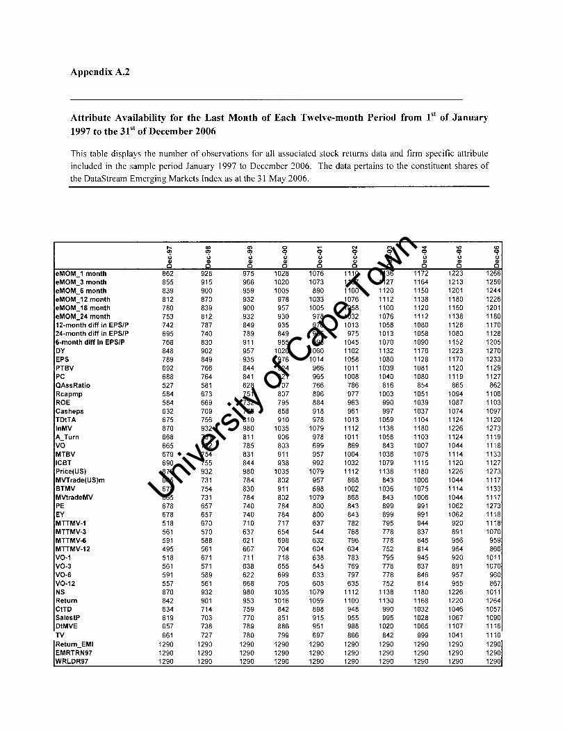
Appendix A.2

Attribute Availability for the Last Month of Each Twelve-month Period from 1st of January 1997 to the 31 st of December 2006

This table displays the number of observations for all associated stock returns data and firm specific attribute included in the sample period January 1997 to December 2006. The data pertains to the constituent shares of

the DataStream Emerging Markets Index as at the 31 May 2006.

eMOM_1 month eMOM_3 month eMOM_6 month eMOM_12 month eMOM_18 month eMOM_24 month 12-month diff in EPS/P 24-month diff in EPS/P 6-month diff in EPS/P DY EPS PTBV PC QAssRatio Rcapmp ROE Casheps TDtTA InMV A_Turn VO MTBV ICBT Price(US) MVTrade(US)m BTMV MVtradeMV PE EY MTTMV-1 MTTMV-3 MTTMV-6 MTTMV-12 VO-1 VO-3 VO-6 VO-12 NS Return CtTD SalestP DtMVE TV Return_EMI EMRTRN97 WRLDR97

..... en cJ (II

c 862 855 839 812 780 753 742 695 768 848 789 692 688 527 584 584 632 675 870 668 665 679 690 870 665 678 665 678 678 518 561 591 495 518 561 591 557 870 842 634 619 657 661

1290 1290 1290

co a;> '-' (II

c 928 915 900 870 839 812 787 740 830 902 849 766 764 581 673 669 709 756 932 751 732 754 755 932 731 754 731 657 657 670 570 588 561 671 571 589 561 932 901 714 703 738 727

1290 1290 1290

en a;> '-' (II

c 975 966 959 932 900 932 849 789 911 957 935 844 841 628 751 732 773 810 980 811 785 831 844 980 784 830 784 740 740 710 637 621 667 711 638 622 668 980 953 759 770 789 780

1290 1290 1290

0 0

cJ (II

c 1028 1020 1005 978 957 930 935 849 955

1020 976 924 921 707 807 795 858 910

1035 906 803 911 938

1035 802 911 802 784 784 717 654 698 704 718 655 699 705

1035 1016 842 851 886 799

1290 1290 1290

.... 0

cJ (II

c 1076 1073 890

1033 1005 978 976 935 998

1060 1014 966 965 766 896 884 918 978

1079 978 699 957 992

1079 957 698

1079 800 800 637 544 632 604 638 545 633 605

1079 1059 898 915 951 697

1290 1290 1290

N 0 cJ (II

c 1110 1107 1100 1076 1058 1032 1013 975

1045 1102 1058 1011 1008 786 977 963 961

1013 1112 1011 869

1004 1032 1112 868

1002 868 843 843 782 768 796 634 783 769 797 635

1112 1100 948 955 988 866

1290 1290 1290

M q '-' (II

c 1136 1127 1120 1112 1100 1076 1058 1013 1070 1132 1080 1039 1040 816

1003 990 997

1059 1138 1058 843

1038 1079 1138 843

1036 843 899 899 795 778 778 752 795 778 778 752

1138 1130 990 995

1020 842

1290 1290 1290

-.t 0 cJ (II

c 1172 1164 1150 1138 1120 1112 1080 1058 1090 1176 1128 1081 1080 854

1051 1039 1037 1104 1180 1103 1007 1075 1115 1180 1006 1075 1006 991 991 944 837 845 814 945 837 846 814

1180 1168 1032 1028 1065 999

1290 1290 1290

'" q '-' (II

c 1223 1213 1201 1180 1150 1138 1128 1080 1152 1223 1170 1120 1119 865

1094 1087 1074 1124 1226 1124 1044 1114 1120 1226 1044 1114 1044 1062 1062 920 891 956 954 920 891 957 955

1226 1220 1046 1067 1107 1041 1290 1290 1290

<D q '-' (II

c 1266 1259 1244 1226 1201 1180 1170 1128 1205 1270 1233 1129 1127 862

1106 1103 1097 1120 1273 1119 1118 1133 1127 1273 1117 1133 1117 1273 1118 1118 1070 959 866

1011 1070

960 867

1011 1264 1057 1090 1116 1110 1290 1290 1290

Univers

ity of

Cap

e Tow

n

Appendix A.3

Complete list of Firm-specific Attributes

The table below shows the complete list of 50 finn-specific attributes to be tested and their respective codenames used in this thesis. The data were extracted from DataStream International.

CODE USED STYLE CHARACTERISTIC

A Tum Asset Turnover

BTMV Book to Market Value

CFtP Cash flow to Price

CFtTD Cashflow to Total Debt

DY Dividend Yield

DtMVE Total Debt to Market Value of Equity

Divtp6m 6 month difference in Dividend to Price

Divtpl2m 12 month difference in Dividend to Price

Divtp24m 24 month difference in Dividend to Price

EPS Earnings per Share

12 EPS 12 month difference in EPS

24 EPS 24 month difference in EPS

6 EPS 6 month difference in EPS

EY Earnings Yield

ICBT Interest Cover Before Tax

LnMV Ln of Market Value

LnP Ln of Price

MOM 12M 12-month Momentum in Returns -

MOM IBM 18-month Momentum in Returns

MOM 1M I-month Momentum in Returns

Univers

ity of

Cap

e Tow

n

MOM 24M 24-month Momentum in Returns

MOM 3M 3-month Momentum in Returns

MOM 6M 6-month Momentum in Returns

MTBV Market Value to Book Value

MVTrade Market Value Traded

MVTradeMV Market Value Traded to Market Value

MVTMV I I-month growth in Market Value Traded to Market Value

MVTMV 3 3-month growth in Market Value Traded to Market Value

MVTMV 6 6-month growth in Market Value Traded to Market Value

MVTMV 12 12-month growth in Market Value Traded to Market Value

NS Number of Shares in Issue

P Price

Payout Payout Ratio

PC Price to Cash

PE Price Earnings Ratio

Quick Quick Assets Ratio

RaCE Return on Capital Employed

ROE Return on Equity (published)

SalestP Sales-to-Price ratio

TDtTA Total Debt to Total Assets

TLtTA Total Loan Capital to Total Assets

TV Trading Volume Ratio

va Absolute Trading Volume

va I I-month growth in Trading Volume -

va 3 3-month growth in Trading Volume

va 6 6-month growth in Trading Volume

va 12 12-month growth in Trading Volume

Univers

ity of

Cap

e Tow

n

Appendix A.4

Grouping of Firm Specific Attributes The table below shows the corresponding groups into which all the listed firm specific attributes from Table

4.1 (a) have been sorted. Each group models a certain behavioural aspect regarding the nature and overall

description of the firm.

STYLE GROUP CODE USED STYLE CHARACTERISTIC

MOMENTUM MOM 12M 12-month Momentum in Returns -

MOM IBM 18-month Momentum in Returns

MOM 1M I-month Momentum in Returns

MOM 24M 24-month Momentum in Returns

MOM 3M 3-month Momentum in Returns

MOM 6M 6-month Momentum in Returns

LIQUIDITY MVTMV I I-month growth in Market Value Traded to Market Value

MVTMV 3 3-month growth in Market Value Traded to Market Value

MVTMV 6 6-month growth in Market Value Traded to Market Value

MVTMV 12 12-month growth in Market Value Traded to Market Value

VO I I-month growth in Trading Volume

VO 3 3-month growth in Trading Volume

VO 6 6-month growth in Trading Volume

VO 12 12-month growth in Trading Volume

TV Trading Volume Ratio

SIZE LnMV Ln of Market Value

ICBT Interest Cover Before Tax

MVTrade Market Value Traded

MVTradeMV Market Value Traded to Market Value

VO Absolute Trading Volume

NS Number of Shares in Issue

Univers

ity of

Cap

e Tow

n

VALUE BTMV Book to Market Value

CFtP Cashflow to Price

CFtTD Cashflow to Total Debt

DY Dividend Yield

DtMVE Total Debt to Market Value of Equity

EPS Earnings per Share

EY Earnings Yield

PC Price to Cash

P Price

Payout Payout Ratio

PE Price Earnings Ratio

Quick Quick Assets Ratio

SalestP Sales-to-Price ratio

TDtTA Total Debt to Total Assets

TLtTA Total Loan Capital to Total Assets

GROWTH 12 EPS 12 month difference in EPS

24 EPS 24 month difference in EPS

6 EPS 6 month difference in EPS

RaCE Return on Capital Employed

Divtp6m 6 month difference in Dividend to Price

Divtp12m 12 month difference in Dividend to Price

Divtp24m 24 month difference in Dividend to Price

ROE Return on Equity (published)

A Tum Asset Turnover

Univers

ity of

Cap

e Tow

n

Appendix A.S

Construction and Classification of Return and Firm Specific Measures

The table below represents the full list of 50 firm specific attributes and the respective manner in which each of the measures was constructed if not satisfactorily quoted by the DataStream International Database.

Code Name of Measure Formula

A Tum Asset Turnover [Total Sales/Total Assets]

BTMV Book to Market Value 1/[Market to Book Value]

CFtP Cashtlow to Price [Cashtlow:Price]

CFtTD Cashtlow to Total Debt [Cashtlow:Total Debt]

DY Dividend Yield [Dividend Yield]

DtMVE Total Debt to Market Value of Equity [Total Debt/Market Value of Equity]

Divtp6m 6 month difference in Dividend to Price [Div(t)-Div(t-6)] / PI(t)

Divtp12m 12 month difference in Dividend to Price [Div(t)-Div(t-12)] / PI(t)

Divtp24m 24 month difference in Dividend to Price [Div(t)-Div(t-24)] / pet)]

EPS Earnings per Share [Earnings per Share]

12 EPS 12 month difference in EPS [E(t)-E(t-12)] / PI(t)

Univers

ity of

Cap

e Tow

n

24 EPS 24 month difference in EPS [E(t)-E(t-24)] / PI(t)

6 EPS 6 month difference in EPS [E(t)-E(t-6)] / pet)]

EY Earnings Yield lIPE

ICBT Interest Cover Before Tax [Interest Cover Before Tax]

LnMV Ln of Market Value LN[MV]

LnP Ln of Price LN[P]

MOM 12M 12-month Momentum in Returns [RI(t)-RI(t-12)] / RI(t-12)

MOM IBM 18-month Momentum in Returns RI(t)-RI(t-18)] / RI(t-18)

MOM 1M I-month Momentum in Returns [RI(t)-RI(t-I)] / RI(t-l)

MOM 24M 24-month Momentum in Returns RI(t)-RI(t-24)] / RI(t-24)

MOM 3M 3-month Momentum in Returns RI(t)-RI(t-3)] / RI(t-3)

MOM 6M 6-month Momentum in Returns RI(t)-RI(t-6)] / RI(t-6)

MTBV Market Value to Book Value [Market to Book Value]

MVTrade Market Value Traded [VO*P]

Univers

ity of

Cap

e Tow

n

MVTradeMV Market Value Traded to Market Value [VO*P]/[MV* I 000]

MVTMV I I-month growth in Market Value Traded [MVTMV(t)-MVTMV(t-1 )] /

to Market Value MVTMV(t-l)

MVTMV 3 3-month growth in Market Value Traded [MVTMV(t)-MVTMV(t-3)] /

to Market Value MVTMV(t-3)

MVTMV 6 6-month growth in Market Value Traded [MVTMV(t)-MVTMV(t-6)] / to Market Value MVTMV(t-6)

MVTMV 12 12-month growth III Market Value [MVTMV(t)-MVTMV(t-12)] /

Traded to Market Value MVTMV(t-12)

NS Number of Shares in Issue [Number of Ordinary Shares in Issue]

p Price [Price]

Payout Payout Ratio [Dividend paid/Price]

PC Price to Cash [Price/Cash]

PE Price Earnings Ratio [Price per Share/Earnings per Share]

Quick Quick Assets Ratio [Quick Assets Ratio]

ROCE Return on Capital Employed [Return on Capital Employed]

ROE Return on Equity [Return on Equity]

Univers

ity of

Cap

e Tow

n

SalestP Sales-to-Price ratio [Sales per Share/Price per Share]

TDtTA Total Debt to Total Assets [Total Debt]/[Total Assets]

TLtTA Total Loan Capital to Total Assets [Total Loan Capital]/[Total Assets]

TV Trading Volume Ratio [(Turnover by Volume)/(Number of

Shares)t_d

VO Absolute Trading Volume [Turnover by Volume]

VO I I-month growth in Trading Volume [VO(t)-VO(t-I)] / VO(t-l)

VO 3 3-month growth in Trading Volume [VO(t)-VO(t-3)] / VO(t-3)

VO 6 6-month growth in Trading Volume [VO(t)-VO(t-6)] / VO(t-6)

VO 12 12-month growth in Trading Volume [VO(t)-VO(t-12)] / VO(t-12)

Univers

ity of

Cap

e Tow

n

Appendix A.6

List of Countries comprising the DataStream International Emerging Markets Index

Below is a complete list of all countries comprising the DataStream International Emerging Markets Index.

Their relative contribution to the overall market capitalization of the index is provided with the number of listed

stocks selected for inclusion as at the 31 December 2006 available on the 31 May 2007. A number of countries

were excluded from the index on account of insufficient information and/or significant trade restrictions that prevent free and frequent trade by foreigners. The countries to be excluded are China, Cyprus, Romania,

Russia and Turkey.

Name of Country Proportion of Market Number of Stocks listed on index Capitalization as at 31 December 2006

Argentina 0.71% 50

Brazil 14.36% 99

Colombia 1.01% 50

China - 50

Chile 3.53% 50

Cyprus - 50

Sri Lanka 0.16% 50

Czech Republic 1.25% 29

Hungary 0.94% 42

Indonesia 2.87% 101

India 15.16% 50

Israel 2.80% 50

Korea 16.65% 100

Mexico 7.42% 88

Malaysia 4.49% 90

Peru 0.84% 49

Philippines 1.41% 50

Pakistan 1.01% 50

Poland 3.21% 50

Romania - 50

Univers

ity of

Cap

e Tow

n

Russia - 50

South Africa 7.93% 70

Taiwan 10.94% 70

Thailand 3.00% 50

Turkey - 50

Venezuela 0.29% 50

Univers

ity of

Cap

e Tow

n

Appendix A.7

List of Sample Constituents

The table below list all the constituents of the DataStream International Emerging Markets Index. The full, unadjusted sample includes a total of 1290 companies from 26 companies. All data were sourced from DataStream International.

ARGENTINA BRAZIL

ACINDAR 'B' AES TIETE ON 1000 LOCALIZA ON

AGROMETAL 'B' AES TIETE PN 1000 LOJAS AMERIC ON 1000

ALPARGATAS ALL AMER LAT ON LOJAS AMERIC PN 1000

ALTO PALERMO 'B' ALL AMER LAT PN LOJAS RENNER ON

ALUAR 'B' AMBEV ON 1000 M DIASBRANCO ON

AUTOPISTAS DEL SOL AMBEV PN 1000 METALURGICA GERDAU PN

BANCO GALICIA 'B' AMPRA ENERG ON 1000 MMX MINER ON

BANCO MACRO 'B' ARACRUZON NATURA ON

BANCO RIO 'B' ARACRUZ PNB NETPN

BBVA BANCO FRANCES 'B' ARCELOR BRASIL ON NOSSA CAIXA ON

BOLDT'B' BANCO BRASIL ON PARMALAT ON

CAMUZZI GAS PAMPEANA 'B' BANCO ITAU.HLDG.FINCAON PARMALAT PN

CAPEX 'A' BANCO ITAU.HLDG.FINCAPN PERDIGAO ON

CAPUTO 'B' BRADESCO ON PETROBRAS ON

CARBOCLOR 'B' BRADESCO PN PETROBRAS PN

CARLOS CASADO 'B' BRADESPAR ON PORTO SEGURO ON

CELULOSA 'B' BRADESPAR PN SABESP ON 1000

CENTRAL PUERTO 'B' BRAS CAN RES ON SADIA PN

COMERCIAL DEL PLATA 'B' BRASIL TELCOM PARTP.ON 1000 SIDER.NACIONAL ON

CRESUD 'B' BRASIL TELCOM PARTP.PN 1000 SOUZA CRUZ ON

DISB.DE GAS CUYANA 'B' BRASIL TELECOM ON 1000 SUBMARINO ON

DYCASA 'B' BRASIL TELECOM PN 1000 SUL AM.NAC.SEG.ON

ENDESA COSTANERA 'B' BRASKEM PNA SUZANO PAPEL PNA

FERRUM 'B' CCR RODOVIAS ON TAM ON

GAS NATURAL 'B' CEMIG ON 1000 TAM PN

GPO.CONCIO.DEL OESTE 'B' CEMIG PN 1000 TELE NRLES.PARTP.ON

GRUPO FINCO.GALICIA 'B' CESP PNB 1000 TELE NRLES.PARTP.PN

HIPOTECARIO'D' COMGAS ON 1000 TELEMAR NRLES.ON

IMPORT&EXPORT PATAG.'B' CMPH.BRASL.DISTB.ON 1000 TELEMAR NRLESPNA

INDUPA 'B' CMPH.BRASL.DISTB.PN 1000 TELESP ON

IRSA 'B' COPASAON TELESP PN

LEDESMA 'B' COPEL ON 1000 TIM PART ON 1000

MASSUH 'B' COPEL PNB 1000 TIM PART PN 1000

METROGAS 'B' COPESULON TRACTEBEL ON

MINETTI(J) 'B' COSAN ON UNIBANCO HOLDING ON

MIRGOR 'C' CPFL ENERGIA ON UNIBANCO ON

MOLINOS RIO PLATA 'B' CYRELA REAL T ON UNIBANCO PN

PAMPA HOLDING ELEKTRO ON 1000 USIMINAS ON

PETROBRAS ENGAPRTPN.'B' ELETROBRAS ON 1000 USIMINAS PNA

QUES 'B' ELETROBRAS PNB 1000 VALE DO RIO DOCE ON

QUICKFOOD 'B' EMBRAERON VALE DO RIO DOCE PNA

Univers

ity of

Cap

e Tow

n

RIGOLLEAU 'B' EMBRATEL PAR ON 1000 VCP PN

SAN LORENZO 'B' EMBRATEL PAR PN 1000 VIVO ON

SAN MIGUEL 'B' ENERGIAS BR ON VIVO PN

SIDERAR 'A' GERDAU ON WEGON

SOCOTHERM GERDAU PN WEGPN

TELECOM ARGN.'B' GOLPN

TELEFONICA DE ARGN.'B' GUARARAPES ON

TRANSENER 'B' GUARARAPES PN

TSPA.GAS DEL SUR 'B' ITAUSA ON

ITAUSA PN

KLABIN NEW PN

LIGHT ON 1000

COLOMBIA CHINA CHILE

AIRES AIR CHINA 'H' AES GENER

BBVACOL ALUMINUM CORP.OF CHINA 'H' AGUAS 'A'

BCOLOMBIA ANGANG STEEL 'H' ALMENDRAL

BOGOTA ANHUI CONCH CEMENT 'H' ANDINA 'A'

CARBOCAR BANK OF CHINA 'H' ANDINA 'B'

CARTON BANK OF COMMS.'H' ANTARCHILE

CARULLA BEIJING CAP.INTL.ARPT. 'H' BANMEDICA

CEMARGOS BYD 'H' BBVACL

CHOCOLATES CHINA BLUE CHEMICAL 'H' BCI

CINECO CHINA COAL ENERGY 'H' BICECORP

CLiCOLSANI CHINA COMMS.CON.'H' BSANTANDER

COLINVERS CHINA CON.BANK 'H' CAP

COLSANITAS CHINA COSCO HDG.'H' CAPITALES

COLTEJER CHINA INTL.MARINE 'B' CCT

COMPUTEC CHINA LIFE INSURANCE 'H' CEMENTOS

CORFICOLCF CHINA MERCHANTS BANK 'H' CENCOSUD

EDATEL CHINA MERCHANTS PRDEV. 'B' CERVEZAS

ETB CHINA OILFIELD SVS. 'H' CGE

EVERFIT CHINA SHENHUA EN.CO.'H' CGEDISTRO

EXITO CHINA SHIP.CTNRLlNES 'H' CHILE

FABRICATO CHINA SHIPPING DEV. 'H' CMPC

GASNATURAL CHINA TELECOM 'H' COLBUN

GRUPOAVAL CHINA VANKE 'B' CONCHATORO

IMUSA DATANG INTLPWRGNRTN. 'H' COPEC

INCASTILLA DONGFENG MOTOR GP.CO.'H' CORPBANCA

INTERBOLSA GUANGSHEN RAILWAY 'H' CRISTALES

INVERARGOS GUANGZHOU R&F PROPS.'H' CTC'A'

ISA HARBIN POWER EQUIT. 'H' D&S

MARLY HUANENG POWER INTL. 'H' ENDESA

MINEROS HUNAN NONFR.METALS 'H' ENERSIS

OCCIDENTE INDL.& COML.BKOF CHINA 'H' ENTEL

ODINSA JIANGSU EXPRESSWAY 'H' FALABELLA

PAZRIO JIANGXI COPPER 'H' GASCO

PFBBVACOL MAANSHAN IRON & STL.'H' lAM

Univers

ity of

Cap

e Tow

n

PFBCOLOM PETROCHINA 'H' INVERCAP

PFCORFICOL PICC PROPERTY & CL TY.'H' LA POLAR

PFVILLAS PING AN INSURANCE 'H' LAN

POPULAR SHANGHAI ELEC.GP.CO.'H' MASISA SHANGHAI JIN JIANG INTL.

PROMIGAS HTLS.'H' MINERA

SANTANDER SHAI.ZHENHUA PORT MCH. 'B' MOLYMET

SDCORFICOL SINOPEC 'H' PASUR

SDPFCORFIC SINOPEC SHAI.PETROCHEM. 'H' PEHUENCHE

SETAS SINOTRANS 'H' QUINENCO

SURAMINV THE CHINA COMMS.SVS.'H' RIPLEY

TABLEMAC TSINGTAO BREWERY 'H' SANTANGRUP

TERPELSUR YANTAI CHANGYU PION.wINE 'B' SM-CHILE 'B'

TRASMETANO YANZHOU COAL MINING 'H' SONDA

VALOREM ZHEJIANG EXPRESSWAY 'H' SQM'A'

VALSIMESA ZIJIN MINING GROUP 'H' SQM'B'

VILLAS ZTE'H' VAPORES

CYPRUS SRI LANKA CZECH REP. A & P ENTERPRISES ACL CABLES CENTRAL EUR.MEDIA (PRA)

A TSOKKOS HOTELS AITKEN SPENCE CESKA ZBROJOVKA

A ZORPAS & SONS AITKEN SPENCE HTL. CEZ

ALLIANCE INTL.REIN. AMANA TAKAFUL CS NAMORNI PLAVBA APOLLO INVESTMENT FUND PUBLIC ASIAN HOTELS AND PROPS. ECM REAL ESTATE

AQUA SOL HOTELS ASIRI JC PAPIRNY VETRNI

ARISTO DEVELOPERS ASSOCIATED MOTORWAYS JC PL YNARENSKA

ASPIS HDGPUB.CO.L TD. CAL TEX LUBRICANTS JM PL YNARENSKA

ATHINA CYPRUS INV. CAPITAL DEV.INV. K-T-V INVEST

ATLANTIC INSURANCES CARGILLS KOMERCNI BANKA

BANK OF CYPRUS CARSONS CUMBERBATCH LAZNE TEPLICE

BLUE ISLAND CENTRAL FINANCE PARAMO

CAC PAPANTONIOU CEYLON COLD STORES PEGAS NONWOVENS

CHRISTIS DAIRIES CEYLON TEA PHILIP MORRIS

CLR CAPITAL CEYLON THEATRE PRAZSKA ENERGETIKA

CLR INV.FUND CEYLON TOBACCO PRAZSKE SLUZBY CONSTANTINOU BROS HTLS. PUBLIC COLOMBO DOCKYARD RM S HOLDING

CYPRUS AIRWAYS COMMERCIAL BK.OF CEYLON SC PL YNARENSKA

CYPRUS CEMENT CTC EAGLE INSURANCE SETUZA

CYPRUS TRADING CORP. DFCC BANK SLEZAN FRYDEK-MIS

CYTRUSTEESINVESTMENTS DIALOG TELEKOM SM PL YNARENSKA

DEMETRA INVS. DIPPED PRODUCTS SPOLANA

DIMCO DISTILLERIES SPOLEK CHUO HAUTE VYR

DODONI PRTF.INVS.PCL. HATTON NATIONAL BK. SSZ

DOME INVESTMENTS HAYLEYS TELEFONICA 02 CR

ELMA HOLDINGS PCL. HA YLEYS MGT KNITTING TOMA

FROU FROU BISCUITS HOTEL DEVELOPERS UNIPETROL

HELLENIC BANK HOTEL SERVICES ZC PL YNARENSKA

INTERFUNDINVESTMENT JAMES FINLAY ZENTIVA

KEO JOHN KEELLS HOLDINGS

LAIKI INVESTMENTS LANKA 10C

Univers

ity of

Cap

e Tow

n

LANITIS DEVELOPMENT PUBLIC LANKA ORIX LEASING

LEPTOS CAL YPSO HTLS. MILLERS

LOGICOM NATIONAL DEV.BANK

LOUIS NATIONS TRUST BANK

MALLOUPAS & PAPAS PCL. NESTLE LANKA

MARFIN POPULAR BANK PELWATTE SUGAR INDS.

MINERVA INSURANCE CO. PROPERTY DEV.

MUSCITA ALUMINIUM INDS. RICHARD PIERIS

OPTIONS CASSOULIDES SAMPATH BANK

ORFANIDES PUBLIC COMPANY SEYLAN BANK

PANDORA INVS. SHALIMAR ESTATES

PETROLINA HOLDINGS SINGER SRI LANKA

SFS GROUP SRI LANKA TELECOM

SUPHIRE HOLDINGS PUBLIC THE LANKA HOSPITAL

UNIVERSAL BANK THE LION BREWERY CEYLON

VASSILIKO CEMENT TOKYO CEMENT

VISION INTL.PEOPLE GROUP TOUCHWOOD INVESTMENTS

WHITE KNIGHT HOLDINGS TRANS ASIA HOTEL

WOOLWORTH(CYPRUS) PROPS. UNITED MOTORS

HUNGARY INDIA

AGRIMPEX 'N' ABB (INDIA) LANCOINFRATECH

ALLAM I NYOMDA ACC LARSEN & TOUBRO

BIF ADITYA BIRLA NUVO MAHANAGAR TEL.NIGAM

BOOKLINE ASHOK LEYLAND MAHINDRA & MAHINDRA

BORSODCHEM ASIAN PAINTS MNGL.REF.& PETROCHEM.

CSEPEL HOLDING BAJAJAUTO MAR UTI UDYOG

DANUBIUS HOTEL & SPA BANK OF BARODA MOTOR INDUSTRIES

ECONET HU BANK OF INDIA NATIONAL ALUMINIUM

EGIS BF UTILITIES NESTLE INDIA

ELMU BHARAT ELECTRONICS NEYVELL LIGNITE

EMASZ BHARAT FORGE NICHOLAS PI RAMAL INDIA

EXBUS BHARAT HEAVY ELS. NTPC

FHB BHARAT PETROLEUM OIL & NATURAL GAS

FIRST HUNGENPRTF. BHARTI AIRTEL ORIENTAL BK.OF COMMERCE

FORRAS FORRAS/OE CAIRN INDIA PANTALOON RET.(lNDIA)

FORRAS FORRASfT CANARA BANK PARSVNATH DEVELOPERS

FOTEX CENTURY TEXTILE & INDS. PATNI COMPUTER SYSTEMS

FREESOFT CIPLA PUNJAB NATIONAL BANK

GARDENIA CONTAINER CORP OF INDIA RANBAXY LABS.

GRAPHISOFT CROMPTON GREAVES RELIANCE CAPITAL

GRAPHISOFT PARK DABUR INDIA RELIANCE COMMUNICATIONS

HUMET DR. REDDY'S LABORATORIES RELIANCE ENERGY

INTER-EUROPA BANK ESSAROIL RELIANCE INDUSTRIES

KARTONPACK FINANCIAL TECH.(INDIA) RELIANCE PETROLEUM

KONZUM GAIL (INDIA) SATYAM COMPUTER SERVICES

LlNAMAR HUNGARY GLAXOSMITHKLlNE PHARMS. SESA GOA GLENMARK

MAGYAR TKOMTELECOMPLC PHARMACEUTICALS SIEMENS

MOL MAGYAR OLAJ-ES GAZIPARI GMRINFRASTRUCTURE STATE BANK OF INDIA

GENESIS GRASIM INDUSTRIES STEEL AUTHORITY OF INDIA

OTP BANK GUJARAT AMBUJA CEMENTS STERLITE INDS.(INDIA)

Univers

ity of

Cap

e Tow

n

PANNON VAL TO HCL TECHNOLOGIES SUN PHARMACEUTICALS

PANNONFLAX HDFC BANK SUN TV

PANNONPLAST HERO HONDA MOTORS SUZLON ENERGY

PHYLAXIA PHARMA HINDALCO INDUSTRIES TATA CONSULTANCY SVS.

QUESTOR HINDUSTAN COPPER TATAMOTORS

RABA HINDUSTAN LEVER TATAPOWER

RICHTER GEDEON HINDUSTAN PETROLEUM TATASTEEL

SYNERGON HINDUSTAN ZINC TECH MAHINDRA SZEKESFEHERVARI HUTOIPAR FEVITAN HOUSING DEVELOPMENT FIN. ULTRATECH CEMENT

TISZAI VEGYI KOM I-FLEX SOLUTIONS UNION BANK OF INDIA

TVNETWORK ICICI BANK UNITECH

ZWACK UNICUM INDIABULLS FINL.SVS. UNITED PHOSPHORUS

INDIAN HOTELS UNITED SPIRITS

INDIAN OIL UTI BANK

INDIAN OVERSEAS BANK VIDEOCON INDUSTRIES

INDIAN PETROCHEM. VIDESH SANCHAR NIGAM

INFOSYS TECHNOLOGIES WIPRO

INFR.DEV.FINANCE CO. ZEE ENTERTAINMENT ENTS.

ITC

JAIPRAKASH ASSOCIATES

JINDAL STEEL & POWER

JSWSTEEL

KOTAK MAHINDRA BANK

INDONESIA ISRAEL KOREA

ANEKA TAMBANG CDI. AFRICA AMOREPACIFIC

APEXINDO PRATAMA DUTA AFRICA ISRAEL PROPERTIES ASIANA AIRLINE

ASTRA AGRO LESTARI ALONY HETZ PR.& INVS. CHElL INDUSTRIES

ASTRA INTERNATIONAL AZORIM CJ

BAKRIE & BROTHERS BEZEQ DAEGU BANK

BAKRIE TELECOM BIOCANCELL THERAPEUTICS DAELIM INDUSTRIAL

BANK CENTRAL ASIA BLUE SQUARE ISR DAEWOO ENGR.& CON.

BANK DANAMON INDONESIA CLAL INDUSTRIES DAEWOO INTERNATIONAL

BANK INTL.INDONESIA BII CLAL INSURANCE ENTS.HDG. DAEWOO SECURITIES DAEWOO SHIPBLDG.MAR.

BANK MANDIRI DELEK AUTOMOTIVE SYSTEMS ENGR.

BANK NEGARA INDONESIA DELEKGROUP DAISHIN SECURITIES

BANK NIAGA DELEK REAL ESTATE DONGBUINSURANCE

BANK NISP DISCOUNT BK. DONGKUK STEEL MILL

BANK PAN INDONESIA DISCOUNT INVESTMENTS DOOSAN

BANK PERMATA ELBIT IMAGING DOOSAN HVY.INDS.AND CON.

BANK RAKYAT INDONESIA ELBIT SYSTEMS DOOSANINFRACORE

BANK UOB BUANA ELECTRA 1 GS ENGR. & CON.

BERLIAN LAJU TANKER FIBI1 GS HOLDINGS

BIMANTARA CITRA FRUTAROM HALLA CLIMATE CONTROL

BUM I RESOURCES GTC HANA FINANCIAL GROUP

CIPUTRA DEVELOPMENT GAZIT HANAROTELECOM

ENERGI MEGA PERSADA GAZITGLOBE HANJIN HEAVY INDUSTRIES

EXCELCOMINDO PRATAMA HAREL INSURANCE INVS. HANJIN SHIPPING

GUDANG GARAM HOUSING & CONSTRUCTION HANKOOK TIRE

Univers

ity of

Cap

e Tow

n

HM SAMPOERNA ICL HANWHA

HOLCIM INDONESIA IDB DEVELOPMENT HANWHA CHEMICAL

INDAH KIAT PAPER & PULP IDB HOLDINGS HITE BREWERY

INDOCEMENT TP INDUSTRIAL BLDG. HONAM PETROCHEMICAL

INDOFOOD SUKSES MAKMUR INTERNATIONAL 1 HYNIX SEMICONDUCTOR

INDOSAT INTERNATIONAL 5 HYUNDAI AUTONET

INTL.NICKEL INDONESIA ISRAEL CORPORATION HYUNDAIDEPARTMENTSTORE

KALBE FARMA JERUSALEM ECONOMIC HYUNDAI DEV.

LlPPO BANK KOOR INDUSTRIES HYUNDAI ENGR& CON.

LlPPO KARAWACI LEUMI HYUNDAI HEAVY INDUSTRIES

MEDCO ENERGI INTL. MA INDUSTRIES HYUNDAI MERCHANT MARINE

MOBILE 8 TELECOM MENORAH MIVTACH HYUNDAI MIPO DOCKYARD

PANIN LIFE MIGDAL INS & FIN HLDG HYUNDAI MOBIS

PERUSAHAAN GAS NEGARA MIZRAHI TEFAHOT BANK HYUNDAIMOTOR

PLAZA INDONESIA NICE HYUNDAI MOTOR PF.2

PP LONDON SUMATRA ORMAT INDUSTRIES HYUNDAI SECURITIES

RAMAYANA LESTARI OS EM INVESTMENT HYUNDAI STEEL

SARI HUSADA PARTNER COMMUNICATIONS INDUSTRIAL BANK OF KOREA

SEMEN GRESIK PAZ OIL KANGWON LAND

SMART PHOENIX INSURANCE 1 KCC

TAMBANG BATUBARA BUKIT ASAM POALIM BANK KIA MOTORS

TELKOM PROPERTY & BUILDING KOOKMIN BK.

TEMPO SCAN PACIFIC STRAUSS-ELITE KOREA ELECTRIC POWER

TRUBA ALAM MANUNGGAL SUPER SOL KOREA EXCHANGE BANK

UNILEVER INDONESIA TADIRAN COMMS. KOREA EXPRESS

UNITED TRACTORS TEVA PHARMACEUTICAL KOREA GAS

KOREA INVESTMENT HDG.

KOREA ZINC

KOREAN AIR LINES

MEXICO

KOREAN REINSURANCE ALFA 'A' IDEAL 'B-1'

KT ALSEA IMSA

KT&G AMX'A' INVEX '0'

KT FREETEL AMX'L' IXEGF '0'

LGPHILIPS LCD ARA KIMBER 'A'

LG ARCA 'B' KIMBER 'B'

LG CARD ASUR 'B' LAMOSA

LG CHEM AXTEL 'CPO' LIVE POL 'C-1'

LG DACOM BACHOCO 'B' LlVEPOL1

LG ELECTRONICS BAFAR 'B' MASECA 'B'

LG HHLD. & HL THCR BEVIDES 'B' MEXCHEM

LG TELECOM BIMBO 'A' MOVILA 'B'

LOTTE CHILSUNG CABLE 'CPO' NAFTRAC 02

LOTTE CONF. CEL OMA'B'

LOTTE SHOPPING CEMEX 'CPO' PASA 'B'

LS CABLE CERAMIC 'B' PENOLES

MACQUARIE KOREA INFRFD. CICSA 'B1' PINFRA

MIRAE ASSET SECURITIES CIE 'B' POSADAS 'A'

NHN CINTRA 'A' QCPO

Univers

ity of

Cap

e Tow

n

NONG SHIM CMOCTEZ RCENTRO 'A'

ORION COCA-COLA FEMSA 'L' SAB

PACIFIC COMERCI 'UBC' SANMEX 'B'

POSCO CONTAL SARE 'B'

PUSAN BANK DESC 'A' SIMEC 'B'

S-OIL DESC 'B' SORIANA 'B'

SAMSUNG ELEKTRA TELECOM 'A l'

SAMSUNG EL TO.MECH. FEMSA 'UB' TELMEX 'A'

SAMSUNG ELECTRONICS FEMSA 'UBD' TELMEX'L'

SAMSUNG EL TNPF. FRAGUA 'B' TLEVISA 'CPO'

SAMSUNG ENGINEERING GAP'B' TVAZTCA 'CPO'

SAMSUNG FIRE & MAR.IN. GBM'O' URBI

SAMSUNG HEAVY INDS. GCARSO'A1' VALLE 'B'

SAMSUNG SDI GCC VITRO 'A'

SAMSUNG SECURITIES GEO'B' VZT

SAMSUNG TECHWIN GEUPEC 'B' WALMEX'V'

SEOUL BROADCASTING SY. GFAMSA 'A'

SHINHAN FINLGROUP GFINBUR '0'

SHINSEGAE GFNORTE '0'

SK GIGANTE

SK NETWORKS GISSA

SKTELECOM GMARTI

S1 GMD'B'

TONG YANG INVESTMENT BK. GMEXICO 'B'

WOONGJIN COWA Y GMODELO 'C'

WOORI FINANCE HOLDINGS GMODERN

WOORI INV. SECS. GNP

YUHAN GPH 1

GPROFUT

GRUMA 'B'

HERDEZ

HOMEX

ICA

ICH 'B'

MALAYSIA PERU

AFFIN HOLDINGS MMC ACEROS CAP

AIR ASIA MULPHA INTERNATIONAL ALI CORP CAP

AMCORPGROUP NESTLE (MALAYSIA) ATACOCHA CAP

AMINVESTMENT GROUP ORIENTAL HOLDINGS ATACOCHA INVERSION

AMMB HOLDINGS PETRONAS DAGANGAN BACKUS 'A'

ASIATIC DEVELOPMENT PETRONAS GAS BACKUS 'B'

ASTRO ALL ASIA NETWORKS PLUS EXPRESSWAYS BACKUS INVERSION

BATU KAWAN POS MAL.&SVS.HDG. BANCO INTERBANC CAP

BERJAYA SPORTS TOTO PPB GROUP BUENAVENTURA CAP

BINTULU PORT HOLDINGS PPB OIL PALMS CASAGR CAP

BRITISH AMER.TOB(M) PROTON HOLDINGS CEMENTOS LIMA CAP

BUMIPUTRA-COMMERCE HLDG. PUBLIC BANK CEMENTOS LIMA INVN

BURSA MALAYSIA PUNCAK NIAGA HOLDINGS CEMENT.PCMY.CAP

CARLSBERG BREWERY MAL RESORTS WORLD CEPER B CAP

Univers

ity of

Cap

e Tow

n

DIGI.COM RHB CAP. CERVESUR CAP

DRB-HICOM ROAD BUILDER HOG. COCESUR CAP

EON CAPITAL SARAWAK ENTER. CIA.MNA.CERRO CORRIDOR

FRASER & NEAVE HLDG. SHELL REFINING CREDITO CAP

GAMUDA SIME DARBY EDEGEL

GENTING SIME UEP PROPERTIES EDELNOR CAP

GOLDEN HOPE PL TN. SP SETIA EL BROCAL CAP

GREEN PACKET STAR PUBLICATION (MAL.) ENERSUC1

GUINNESS ANCHOR TA ANN HOLDINGS FERREYROS CAP

HIGHLANDS & LOWLANDS TELEKOM MALAYSIA GESTIONES RECPS.DE ATVS.

HONG LEONG BANK TENAGA NASIONAL GRANA Y MONTERO

HONG LEONG FINL.GP. TIME DOTCOM HORIZONTE CAP

1GB TITAN CHEMICALS IEQSA

IJM TOP GLOVE INPACBC1

INDUSTRIAL CONC.PRDS. TRANSMILE GROUP INTEGRA 'C' CAP

101 UEM BUILDERS LUZ DEL SUR CAP

101 PROPERTIES UEMWORLD MAPFRE PERU VIDA CAP

KFC HOLDINGS (MALAYSIA) UMW HOLDINGS MILPO CAP

KLCC PROPERTY HOLDINGS UNITED PLANTATIONS MINERA CORONA CAP

KNM GROUP YTL MINSUR INVERSION

KUALA LUMPUR KEPONG YTL CEMENT PERUANO SUIZA CAP

KULIM MALAYSIA YTLPOWER PODERC1

KUMPULAN GUTHRIE ZELAN BERHAD PROFUTURO CAP

KURNIAASIA RELAPAC1

LAFARGE MALAYAN CEMENT SAN JUAN CAP

LlNGKARAN TRANS KOTA SCOTIABANK PERU

LION DIVERSIFIED HOG. SCOTIABANK PERU PF.

MAGNUM SIDERC1

MALAKOFF SOLUCION

MALAYAN BANKING STHN.PERU COPPER INV.1

MALAYSIA AIRPORTS HDG. TELEFONICA DEL PERU 'B'

MALA YSIAN AIRLINE SY. TMOVILC1

MALAYSIAN BULK CARRIERS VOLCAN 'A'

MALAYSIAN OXYGEN VOLCAN 'B'

MALAYSIAN PACIFIC INDS. VOLCAN INVERSION

MALAYSIAN PLANTATIONS

MAXIS COMMUNICATION

MEDIA PRIMA

MISC BHD.

PHILIPPINE PAKISTAN POLAND

ABOITIZ EQUITY VENT. ABBOTT LABS.(PAK.) AGORA

ABS-CBN BCAST. ADAMJEE INSURANCE ASSECO POLAND ALLIANCE GLOBAL GP. SUSP -SUSP.19/02/07 ALLIED BANK BANK BPH

ASIAN TERMINALS ARIF HABIB SECURITIES BANK MILLENNIUM

AYALA ASKARI COMMERCIAL BANK BANK ZACHODNI WBK

AYALA LAND ATTOCK PETROLEUM BARLINEK

BANCO DE ORO BANK AL HABIB BIOTON

BANK OF THE PHILP. ISLE. BANK AL-FALAH LIMITED BORYSZEW

BENPRES HOLDINGS BANK OF PUNJAB BOS

Univers

ity of

Cap

e Tow

n

CHINA BANKING BESTWA Y CEMENT BRE BANK

DIGITAL TELECOM. o G CEMENT BUDIMEX

DMCI HOLDINGS DAWOOD HERCULES CCC

EQUITABLE PCI BANK EFU GENERAL INSURANCES CERSANIT

FILINVEST DEV. ENGRO CHEMICAL CIECH

FILINVEST LAND FAUJI FERTILIZER COMARCH

FIRSTGEN FAUJI FERTILIZER BIN QAS DOM DEVELOPMENT

FIRST METRO INV. FAYSAL BANK DZPOLSKA

FIRST PHILP.HDG. GLAXOSMITHKLlNE PAK. ECHO INVESTMENT

GLOBE TELECOM HABIB METRO BANK EMPIK MEDIA & FASHION

HOLCIM PHILPS. HUB POWER FAMUR

INTL.CTNRTERM.SVS. IBRAHIM FIBRES FORTIS BANK POLSKA

JG SUMMIT HOG. ICI PAKISTAN GETIN HOLDING

JOLLIBEE FOODS INDUS MOTORS GRUPA LOTOS

MANILA ELECTRIC 'A' KARACHI ELECTRIC SUPP. GRUPA ZYWIEC

MANILA ELECTRIC 'B' KOT ADDU POWER GTC

MANILA WATER LAKSON TOBACCO HANDLOWY

MEGAWORLD LUCKY CEMENT IMPEXMETAL

METROPOLITAN BK.& TST. MCB BANK ING BANK SLASKI BSK

PAXYS NAT.BANK OF PAKISTAN KETY

PETRON NATIONAL REFINERY KGHM

PHILEX MINING NESTLE PAKISTAN KOELNER

PHILP. LONG DSNTEL. NISHAT MILLS KREDYT B PBI

PHILIPPINE NAT.BK. OIL & GAS DEVELOPMENT KRUSZWICA

PHILIPPINE SAVINGS BANK PACKAGES LPP

PHIL TRUST BANK PAK SUZUKI MOTOR MULTIMEDIA POLSKA

PILIPINO TELEPHONE PAKISTAN OILFIELDS NETIA

PNOC ENERGY DEV. PAKISTAN PETROLEUM ORBIS

PNOC EXPLORATION 'B' PAKISTAN SERVICES PBG REPUBLIC CEMENT INFREQUENTLY TRADED PAKISTAN STATE OIL PEKAO

RIZAL COML.BKG. 'A' PAKISTAN TOBACCO PFLEIDERER GRAJEWO

ROBINSONS LD. PIAC PKNORLEN

SAN MIGUEL 'A' PICIC PKO BANK

SAN MIGUEL 'B' PRIME COMMERCIAL BANK POLlMEXMS

SECURITY BANK PTCLA POLISH OIL AND GAS

SM DEVELOPMENT 'A' SHELL PAKISTAN PROKOM SOFTWARE

SM INVESTMENTS SONERI BANK PULAWY

SM PRIME HOLDINGS SUI NORTHERN GAS STALPRODKUT

TANDUAY HOLDINGS SUI SOUTHERN GAS SWIECIE

UNION BK.OF THE PHILPS. UNILEVER PAKISTAN TELEKOMUNIKACJA POLSKA

UNIVERSAL ROBINA UNITED BANK TVN

ROMANIA RUSSIA SOUTH AFRICA

AEROSTAR BACAU AEROFLOT ABSA GROUP

AMONIL SLOBOZIA ANK BASHNEFT AECI

ANTIBIOTICE lAS I BAL TIKA BREW. AFRICAN BANK INVS.

APCAROM BUZAU COMSTAR-UNITED TELSMS. AFRICAN OXYGEN

ARMATURA CLUJ NAPOCA GAZPROM AFN.RAINBOW MRLS.

ARTROM SLATINA GAZPROM NEFT ALEXANDER FORBES

AZOMURES TG MURES IRKUTSKENERGO ALLIED EL TNPTG.PREF

Univers

ity of

Cap

e Tow

n

BANCA COMERCIALA CARPATI CA LUKOIL OAO ANGLO PLATINUM

BANCA TRANSILVANIA CLUJ MAGNIT ANGLO PLATINUM PF

BERMAS SUCEAVA MAGNITOGORSK MTL. ANGLOGOLD ASHANTI

BIOFARM MECHEL ASPEN PHMCR.

CARBOCHIM CLUJ NAPOCA MMC NORILSK NICKEL AVENG

CHIMOPAR SA BUCARESTI MOBILE TELESYSTEMS OJSC BARLOWORLD

CNTEE TRANSELECTRICA MOSCOW CITY TEL BIDVEST GROUP MOSCOW MUN.BK.-BK.OF

COM ELF BISTRITA MOSCOW CAXTON CTP PUBLISH PRINT MOSCOW UNITED ELECTRIC

COMPASIBIU NETWORK CO. DISCOVERY

ELECTROPUTERE CRAIOVA MOSENERGO DISTELL GROUP

FLAMINGO INTL.BUCURESTI N TAGIL IRON&STEEL WORKS EDGARS CONS. STORES

IMPACT BUCARESTI NOVATEK ELLERINE

LOULIS NOVOLIPETSK FERROUS EXXARO RESOURCES

MAILLIS ROMANIA ORENBURGNEFT FIRSTRAND

MECANICA CEAHLAU POLYUS GOLD FOSCHINI

MECHEL TARGOVISTE PURNEFTEGAZ GOLD FIELDS

OIL TERMINAL ROSBANK GRINDROD

OL TCHIM RM VALCEA ROSNEFT OJSC GROWTHPOINT PROPS.

PETROLEXPORTIMPORT ROSTELECOM HARMONY GOLD MNG.

POLICOLOR BUCARESTI SBERBANK OF RUSSIA HIGHVELD STL.& VNM.

PRODPLAST BUCAREST SBERBANK RUSSIA PREF. HOSKEN CONS.INV.

RAFINARIA ASTRA SEVENTH CONTINENT ILLOVO SUGAR

ROLAST PITESTI SEVERSTAL IMPALA PLATINUM

ROMANIAN BK.DEVELOPMENT SILVINIT IMPERIAL

ROM PETROL REFINERY SISTEMA JSFC INVESTEC

ROM PETROL WELL SER. SISTEMA-HALS JD GROUP

S C KANDIA-EXCELENT SLAVNEFT MEGIONNEFTEGAZ JOHNNIC COMMS.

SANTIERUL NAVAL ORSOVA SURGUTNEFTEGAS KUMBA IRON ORE

SC VRANCART SURGUTNEFTEGAZ PF. LIBERTY

SIF 1 BANAT CRISANA TATNEFT LIBERTY GROUP

SIF 2 MOLDOVA TRANSNEFT PREF. MASS MART

SIF 3 TRANSILVANIA UDMURTHEFT MEDI CLINIC

SIF 4 MUNTENIA UNIFIED ENERGY SYS. METROPOLITAN HOG.

SIF 5 OL TENIA URALKALlY MITTAL STEEL SA.

SILCOTUB ZALAU URALSVY AZINFORM MTN GROUP

SINTEZA ORADEA VIMPELCOM MURRAY & ROBERTS

SNP PETROM VSMPO MUTUAL & FEDERAL IN.

SSIF BROKER CLUJ WBD FOOD OJSC NAMPAK

TURBOMECANICA WHOLESALE GNRTN.CO.-2 NASPERS

TURHOTREST.MAREA NEAGRA WHOLESALE GNRTN.CO.-3 NEDBANK GROUP

UAMTORADEA WHOLESALE GNRTN.CO.-4 NETWORK HEAL THCARE

UCM RESITA WHOLESALE GNRTN.CO.-5 NORTHAM PLATINUM

ZENTIVA BUCURESTI WHOLESALE GNRTN.CO.-6 PICK N PAY STORES

PIK N PAY

PRETORIA POR.CMT.

REMGRO

TAIWAN

REUNERT ACER SILICONWARE PRECN.

Univers

ity of

Cap

e Tow

n

RMB ADVANCED SEMICON.ENGR. SINOPAC FINL.HDG.

SANLAM ADVANTECH TAISHIN FINL.HLDG.

SANTAM ASIA CEMENT TAIWAN CEMENT

SAPPI ASUSTEK COMPUTER TAIWAN COOPERATIVE BANK

SASOL AU OPTRONICS TAIWAN FERTILIZER

SHOPRITE CATCHER TECHNOLOGY TAIWAN MOBILE

SPAR GROUP CATHAY FINL.HLDG. TAIWAN SEMICON.MNFG.

STANDARD BK.GP. CHANG HWA COML.BANK TATUNG

STEINHOFF INTL. CHI MEl OPTOELECTRONICS UN I-PRESIDENT ENTS.

SUN INTERNATIONAL CHINA AIR LINES UNITED MICRO EL TN.

TELKOM CHINA DEV.FINL.HLDG. VIA TECHNOLOGIES

TIGER BRANDS CHINA STEEL WALSIN LlHWA

TONGAAT HLT.GP. CHINATRUST FINL.HLDG. WINBOND EL TN.

TRUWORTHS INTL. CHUNGHWA PICTURE TUBES WISTRON

WESTERN AREAS CHUNGHWA TELECOM. YUANTA CORE PAC.SECS.

WOOLWORTHS HDG. COMPAL COMMUNICATIONS YULON MOTOR

COM PAL ELECTRONICS

DELTA ELECTRONICS

E SUN FINL.HLDG.

EVA AIRWAYS

EVERGREEN MAR.

FAR EASTERN TEXTILE

FAR EASTONE TELECOM.

FIRST FINANCIAL HLDG.

FORMOSA CHEMS.& FIBER

FORMOSA PETROCHEM.

FORMOSA PLASTICS

FOXCONNTECHNOLOGY

FUBON FINL.HLDG.

FUHWA FINL.HLDG.

HIGH TECH COMPUTER

HON HAl PRECN.INDS.

HUA NAN FINANCIAL HLDG.

INNOLUX DISPLAY

INOTERA MEMORIES

INVENTEC

LARGAN PRECISION

LITE-ON TECHNOLOGY

MEDIATEK

MEGA FINANCIAL

MOTECH INDUSTRIES

NAN YA PCB

NAN YA PLASTICS

NANYA TECHNOLOGY

NOVATEK MICROEL.

POU CHEN

POWERCHIP SEMICON.

POWERTECH TECHNOLOGY

PRESIDENT CHAIN STORE

PROMOS TECHS.

QUANTA COMPUTER

Univers

ity of

Cap

e Tow

n

SHIN KONG FINL.HLDG.

THAILAND TURKEY VENUZUELA

ADVANCE AGRO ACIBADEM BANCO CARIBE 'A'

ADVANCED INFO SER. AKBANK BANCO DE VENEZUELA

AIRPORTS OF THAILAND AKCANSA BANCO EXTERIOR

AROMATICS THAILAND AKSIGORTA BANCO HIPOTECARIO ACTIVO

BANGKOK BANK ANADOLU CAM SANA YII BANCO OCCIDENTAL

BANGKOK DUSIT MED.SVS. ANADOLU EFES BANCO PROVINCIAL

BANGKOK EXPRESSWAY ANADOLU HAYAT EMEKLlLlK BANESCO BANCO UNIVERSAL

BANK OF AYUDHYA ARCELIK CANTV

BANPU PUBLIC ASYA KATILIM BANKASI CEMEX'1'

BECWORLD AYGAZ CEMEX '2'

BIG C SUPERCENTRE BIM BIRLESIK MAGAZALAR CENTRAL BANCO UNIVERSAL

BUMRUNGRAD HOSPITAL BSH EV ALETLERI SANVETC. CERAMICA CARABOBO

CAL-COMP ELECTRONICS CARREFOURSA GRUBU 'A' CORIMON 'A'

CENTRALPATTANA CIMSA CIMENTO CORPN.BANCA

CHAROEN POKPHAND FOODS COCA COLA ICECEK CORPNGPO.QUIM.

CP SEVEN ELEVEN DENIZ BANK CORPN.INDL.DE ENGA.

DELTA ELECTRONICS DOGAN HOLDING DOMG.Y CIA CARACAS

ELECTRICITY GENERATING DOGAN YAYIN HOLDING ECONOINVEST CAPITAL 'A'

GLOW ENERGY ECZACIBASI ILAC ECONOINVEST CAPITAL 'B'

HANA MICROELECTRONIC ENKAINSAAT ELECTRICIDAD DE CARACAS

IRPC EREGLI DEMIR CELIK ENVASES VENEZOLANOS

ITALIAN-THAI DEVELOPMENT FINANSBANK FABRICA NACDE CEMENT.

KASIKORNBANK FORD OTOMOTIVE SANA Y FONDO DE VALORES INMBS.

KHON KAEN SUGAR FORTIS BANK GRUPO ZULIANO

KRUNG THAI BANK GARANTI BANKASI HL BOULTON & COMPANY

LAND AND HOUSES HURRIYET GAZETECILIK INMUEBLES BOLSA DE VLRS.

MCOT IS GAYRIMENKUL INMUEMBLES Y VALORES

MINOR INTERNATIONAL KENTGIDA INVESTMENT TACOA 'A'

PRECIOUS SHIPPING KOC HOLDINGS INVESTMENT TACOA 'B'

PTT MIGROS TURK MANPA

PTT CHEMICAL PUBLIC NUH CIMENTO MANTEX

PTT EXPLORATION &.PRDN. PETKIMAS MERCANTIL SERV.FINCO.'A'

RATCHABURI ELECTRICITY PETROL OFISI MERCANTIL SERV.FINCO.'B'

RA YONG REFINERY SABANCI HOLDING PROAGRO

SHIN SELCUK ECZA DEPOSU PRODUCTOS EFE

SIAM CEMENT T SISE CAM PROTINAL

SIAM CITY BANK TESCO KIPA KITLE RON SANTA TERESA

SIAM CITY CEMENT TOFAS SIVENSA

SIAM COMMERCIAL BANK TRAKYACAM SUDAMTEX 'A'

SIAM COMMERCIAL BKPF. TUPRAS SUDAMTEX 'B'

SIAM MAKRO TURK EKONOMI BANKASI SUELOPETROL 'B'

THAI AIRWAYS INTL. TURK HAVA YOLLARI TERMINALES MARACAIBO

THAI OIL TURKCELL TORDISCA

THAI PLASTIC CHM. TURKIYE IS BANK 'C' VENASETA 'A'

THAI UNION FROZEN PRDS. TURKIYE KALKINMA VENASETA 'B'

THANACHART CAPITAL TKIVAKIFLEAR BANKASI VENCRED

Univers

ity of

Cap

e Tow

n

THORESEN THAI AG. ULKER GIDA VENEPAL 'A'

TMB BANK YAPI KREDI BK. VENEPAL 'B'

TPIPOLENE YAPI KREDI FINANSAL VENEZOLANO DE CREDITO

TRUE CORPORATION YAZICILAR HOLDING VENGAS

Appendix A.S

Table 4.3 Descriptive Statistics of Firm Specific Attributes

The table below is representation of the key statistical attributes of the firm specific factors selected to be employed in this study. The associated measures are all calculated after the two-step winsorisation procedure

has been completed in order to mitigate the influence of extreme observations. The data were extracted from

DataStream International. Refer to Table 1 for definitions of all firm specific attributes. In addition the Jacque

Bera test for normality p-value is specified with the null hypothesis for this test being that the population

follows a normal distribution. At the 5% significance level, all p-values in excess on 0.05 result in the null hypothesis being upheld and the popUlation considered normal. The contrary is true for p-values less than 0.05,

whereby the population is then inferred to be non-normal.

Code Mean Med Std Dev Kurt Skew Min Max JacB

A Tum 0.64 0.51 0.52 3.66 1.10 -0.10 2.12 000

BTMV 0.95 0.65 1.11 8.04 1.85 -3.06 5.01 0.00

Cps 787.91 4.57 2721.86 17.31 336 -11889.85 13837.59 0.00

CFtTD 19.76 0.29 225.76 309.72 16.87 000 4420.70 000

DY 2.81 1.69 3.61 7.46 2.01 0.00 17.21 0.00

DtMVE 1.60 0.04 3.59 30.01 4.80 0.00 27.25 0.00

EPS 180.65 1.61 665.17 24.33 4.63 -170.27 3892.01 0.00

12 EPS 2.4 0.002 81.99 24.13 0.16 -442.52 448.98 0.00

24 EPS 4.61 0.09 109.55 20.59 0.25 -544.29 555.87 0.00

6 EPS IJ9 000 55.04 31.05 0.23 -338.65 34IJ6 0.00

EY 1.91 0.03 7.40 34.15 537 -1.00 52.87 0.00

ICBT 289.66 3.82 3995.90 430.84 19.76 -17421.00 92456.68 0.00

LnMV 9.42 9.04 2.89 2.73 033 0.78 18.07 0.00

LnP 033 0.27 2.01 3.29 -0.13 -5.54 6.24 0.00

MOM 12M 035 0.13 1.13 107.97 8.08 -0.99 19.29 0.00 -

MOM IBM 0.57 0.21 1.89 176.75 10.72 -0.99 37.71 0.00 -

Univers

ity of

Cap

e Tow

n

MOM 1M 0.05 0.0005 0.82 1009.758 30.26 -0.99 29.33 0.00 -

MOM 24M 0.823 0.30 2.54 133.31 9.58 -0.99 42.196 0.00

MOM 3M 0.187 0.025 2.161 514.74 21.671 -0.99 54.79 0.00 -

MOM 6M 0.37 0.06 3.45 379.77 18.57 -0.99 75.805 0.00

MTBV 2.37 1.32 6.68 8305 6.58 -66.04 7l.51 0.00

MVTrade 5093.52 268.57 17832.39 56.05 6.78 -25.00 167548.5 000

MVTradeMV 4578l.52 0.01 162963.2 16.51 3.82 0.00 779910.9 0.00

MVTMV 1 2.54 -0.007 9.255 31.88 5.18 -1.00 64.37 0.00 -

MVTMV 3 3.58 0.017 14.57 46.99 6.34 -1.00 12Ll2 0.00

MVTMV 6 4.14 0.01 16.21 40.67 5.90 -LOO 125.593 0.00

MVTMV 12 2.38 0.00 8.69 31.61 5.16 -l.00 60.23 000 -

NS 107979.7 14.3802 420112.5 24.19545 4.63 7.90 2420017 0.00

P 7.28 1.31 16.96 18.78 3.89 0.00 96.89 0.00

PC 7.54 5.49 14.46 14.24 0.983 -57.87 73.75 0.00

PE 2.86 0.09 9.67 35.93 5.26 -9.60 80.93 0.00

Quick l.27 0.88 l.95 115.70 9.23 0.02 28.87 0.00

ROCE 10.77 9.22 ILl 5.37 0.49 -24.45 46.12 0.00

ROE 12.28 12.19 22.8 10.86 -0.70 -90.83 114.770 000

SalestP 32.005 0.99 134.02 20.34 4.311 -596.06 674.28 0.00

TOtTA 0.24 0.22 0.189 2.87 0.66 0.00 0.797 0.00

TV 0.005 0.0007 0.03 162.18 12.25 0.00 0.42 0.00

VO 2919.26 232.50 8357.96 22.52 4.33 -0.70 50357.26 0.00

VO 1 2.60 0.00 9.49 32.42 5.21 -58.33 66.57 0.00 -

VO 3 4.01 0.03 17.65 59.27 7.13 -152.13 164.24 0.00

VO 6 4.06 0.04 17.62 57.31 7.01 -3.00 16l.73 0.00 -

VO 12 4.55 0.07 17.85 42.53 6.04 -l.00 14l.24 0.00 -

Univers

ity of

Cap

e Tow

n

Appendix A.9

Definitions of DataStream International Items

Definitions of DataStream International Items Definitions of DataStream International items used to construct the finn-specific attributes tested in this paper. The DataStream International code is listed in brackets after the item. The definitions are based on the DataStream International Online Definitions.

Book Value per Share (1308)

Calculated on an issue basis, using that portion of share capital and reserves (excluding preference

capital) minus intangibles attributable to the issue, divided by the year-end number of shares in that

issue. It is adjusted for subsequent rights and scrip issues.

Borrowing Ratio (733)

Total debt divided by equity capital and reserves minus total intangibles.

Borrowings Repayable Within 1 Year (309)

Bank overdrafts, loans and other short-term borrowing. The current portion of long-tenn loans is

included.

Capital Gearing (731)

Preference capital plus total debt, divided by total capital employed plus short term borrowings minus

total intangibles minus future income tax benefits.

Cash Earnings per Share (792)

Earned for ordinary plus deferred tax and operating provisions, divided by the number of shares in

Issue.

Cash Flow Margin (719)

Cash earnings as a percentage of sales.

Depreciation (136)

This includes provisions for amounts written off, and depreciation of tangible fixed assets.

Amortisation of intangible assets is included only if a separate breakdown is not disclosed in the

annual report.

Dividend Yield (DY)

Univers

ity of

Cap

e Tow

n

The dividend per share as a percentage of the share price. The underlying dividend is based on an

anticipated annual dividend over the following twelve months and for that reason may be calculated

on a rolling twelve-month basis, or as the "indicated" annual amount, or it may be a forecast. The

dividend yield is based on gross dividends (including tax credits) where available. Special or once-off

dividends are generally excluded.

Dividends Paid (434)

Ordinary and preference dividends paid during the period, often representing the previous year's final

and current year's interim dividends.

Dividends per Share (DPS)

Dividend per share on a twelve-month rolling basis, taking interim dividends into account.

Earnings per Share (EPS)

The latest annualised rate that may reflect the last financial year or be derived from an aggregation of

interim period earnings. Where the interim announcements are irregular or lacking in detail, the

current earnings per share (EPS) may be a forecast provided by local sources.

Interest Cover Before Tax (ICBT)

Earnings before interest and tax (adjusted operating profit plus total non-operating income) divided by

interest paid.

Market Value (MY)

The share price multiplied by the number of ordinary shares in issue. The amount in issue is updated

whenever new tranches of stock are issued or after a capital change. For companies with more than

one class of equity capital, the market value is expressed according to the individual issue. Market

value is displayed in millions of units of local currency.

Market Value to Book Value (MTBV)

Market value divided by the net tangible assets.

Net Profit Margin (717)

Profits after tax (adjusted) divided by total sales.

Univers

ity of

Cap

e Tow

n

Number of Shares (NS)

The number of shares used in the calculation of earnings per share. The year-end number of shares is

used.

Operating Profit Margin (713)

Operating profit (adjusted for exceptional items) divided by total sales.

Payout Ratio (POUT)

The ratio of dividends per share to the net earnings per share (adjusted) for the last financial period.

Price (P)

The latest price available to DataStream International from the appropriate market in primary units of

currency. It is the previous day's closing price from the default exchange. The 'current' prices taken

at the close of market are stored each day. These stored prices are adjusted for subsequent capital

actions, and this adjusted figure then becomes the default price. Prices are generally based on 'last

trade' or an official price fixing. For stocks which are listed on more than one exchange within the

country, default prices are taken from the primary exchange of that country (note that this is not

necessarily the 'home' exchange of the stock).

Price/Cashflow Ratio (PC)

Current price divided by cash earnings per share for the appropriate financial year, adjusted for capital

changes.

Quick Assets Ratio (742)

Total current assets minus total stock and work in progress, divided by total current liabilities.

Return on Capital Employed (707)

Pre-tax profit (excluding associates) adjusted for exceptional items plus total interest charges, divided

by total capital employed plus borrowings repayable within one year minus total intangibles.

Return on Equity (published) (1506)

Earned for ordinary, divided by equity capital and reserves minus total intangibles.

Univers

ity of

Cap

e Tow

n

Total Assets (392)

The sum of tangible fixed assets, intangible assets, investments (including associates), other assets,

total stocks & work in progress, total debtors & equivalent and cash & cash equivalents.

Common adjustments:

• deferred tax, if shown as an asset, is offset against deferred tax liability

• goodwill carried in reserves is transferred to intangible assets

• advances on work in progress, if disclosed as a liability by the company, has been offset

against stocks and work in progress

Total Cash and Equivalent (375)

For industrials, this includes cash, bank balances, short-tenn loans and deposits, and investments

shown under current assets. For banks and finance companies, it includes cash and balances with

other banks, money at call and short notice, treasury bills and tenn deposits maturing under one

month. Placements with banks are excluded.

Total Current Assets (376)

Includes stocks, work in progress, trade and other debtors, cash and equivalent, and any other current

assets. Trade accounts receivable after one year are included.

Total Current Liabilities (389)

Includes current provisions, trade and other creditors, borrowings repayable within one year, and any

other current liabilities. Trade accounts payable after one year are included. Where the balance sheet

is stated before profit appropriation, the as reported figure for current liabilities is increased by the

amount of proposed dividends outstanding at balance sheet date.

Total Debt (1301)

The total of all long and short tenn borrowings, including any subordinate debt and 'debt-like' hybrid

finance instruments.

Total Debtors and Equivalent (370)

The total of balances outstanding which are due to the organisation in the nomlal course of trading.

Accounts receivable after one year are included in this item.

Univers

ity of

Cap

e Tow

n

Total Intangibles (344)

This includes research and development, goodwill, patents, trade marks, deferred charges, fomlation

expenses and concessions. The figure may differ from that reported due to the fact that deferred

charges may have been shown as part of 'other assets' and goodwill on acquisition may have been

deducted from share capital and reserves.

Total Loan Capital (321)

The total loan capital repayable after one year. It includes debentures, bonds, convertibles, notes,

leasing finance, and 'debt-like' hybrid financial instruments.

Total Return (RI)

Theoretical growth in value of a share holding over a specified period, assuming that dividends are re­

invested to purchase additional units of an equity at the closing price applicable on the ex-dividend

date.

Total Sales (104)

The amount of sales of goods and services to third parties relating to the normal industrial activities of

the company. It is net of sales related taxes and excludes any royalty income, rental income, and other

operating income.

Turnover by Volume (VO)

The number of shares traded for a stock for a particular month. The figure is always expressed in

thousands. For stocks which are traded on more than one exchange within the country, default

volumes are taken from the primary exchange of that country (note that this is not necessarily the

"home' exchange of the stock). Univers

ity of

Cap

e Tow

n

Appendix B

Univers

ity of

Cap

e Tow

n

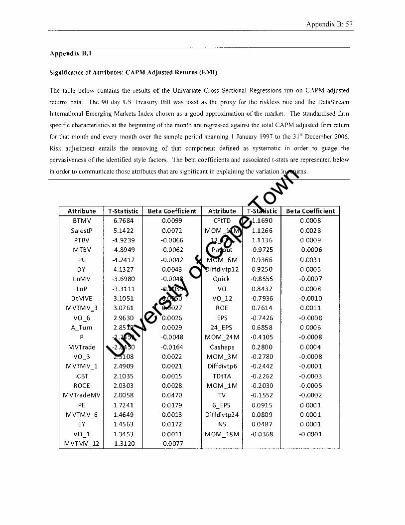
Appendix B: 57

Appendix B.t

Significance of Attributes: CAPM Adjusted Returns (EMI)

The table below contains the results of the Univariate Cross Sectional Regressions run on CAPM adjusted

returns data. The 90 day US Treasury Bill was used as the proxy for the riskless rate and the DataStream

International Emerging Markets Index chosen as a good approximation of the market. The standardised firm

specific characteristics at the beginning of the month are regressed against the total CAPM adjusted firm return

for that month and every month over the sample period spanning 1 January 1997 to the 31 sl December 2006.

Risk adjustment entails the removing of that component defined as systematic in order to guage the

pervasiveness of the identified style factors. The beta coefficients and associated t-stats are represented below

in order to communicate those attributes that are significant in explaining the variation in returns.

Attribute T -Sta tistic Beta Coefficient Attribute T-Statistic Beta Coefficient

BTMV 6.7684 0.0099 CFtTD 1.1690 0.0008

SalestP 5.1422 0.0072 MOM_12M 1.1266 0.0028

PTBV -4.9239 -0.0066 12_EPS 1.1136 0.0009

MTBV -4.8949 -0.0062 Payout -0.9725 -0.0006

PC -4.2412 -0.0042 MOM_6M 0.9366 0.0031

DY 4.1327 0.0043 o iffdivtp12 0.9250 0.0005

LnMV -3.6980 -0.0048 Quick -0.8555 -0.0007

LnP -3.3111 -0.0059 VO 0.8432 0.0008

DtMVE 3.1051 0.0050 VO 12 -0.7936 -0.0010

MVTMV_3 3.0761 0.0027 ROE 0.7614 0.0011

VO_6 2.9630 0.0026 EPS -0.7426 -0.0008

A Turn 2.8519 0.0029 24 EPS 0.6858 0.0006

P -2.7452 -0.0048 MOM_24M -0.4105 -0.0008

MVTrade -2.6450 -0.0164 Casheps 0.2800 0.0004

VO 3 2.5108 0.0022 MOM 3M -0.2780 -0.0008

MVTMV 1 2.4909 0.0021 Diffdivtp6 -0.2442 -0.0001

ICBT 2.1035 0.0015 TDtTA -0.2262 -0.0003

ROCE 2.0303 0.0028 MOM_1M -0.2030 -0.0005

MVTradeMV 2.0058 0.0470 TV -0.1552 -0.0002

PE 1.7241 0.0179 6_EPS 0.0915 0.0001

MVTMV 6 1.4649 0.0013 o iffdivtp2 4 0.0809 0.0001

EY 1.4563 0.0172 NS 0.0487 0.0001

VO 1 1.3453 0.0011 MOM_18M -0.0368 -0.0001

MVTMV 12 -1.3120 -0.0077

Univers

ity of

Cap

e Tow

n

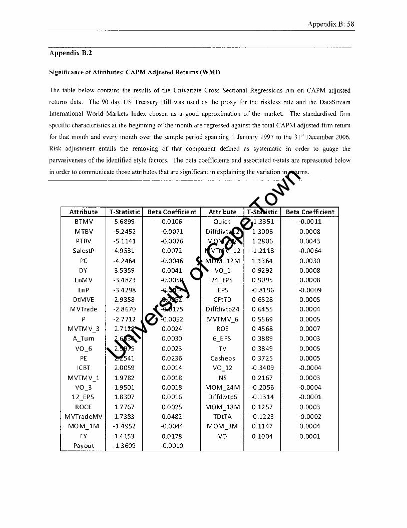
Appendix B: 58

Appendix B.2

Significance of Attributes: CAPM Adjusted Returns (WMI)

The table below contains the results of the Univariate Cross Sectional Regressions run on CAPM adjusted

returns data. The 90 day US Treasury Bill was used as the proxy for the riskless rate and the DataStream

International World Markets Index chosen as a good approximation of the market. The standardised firm

specific characteristics at the beginning of the month are regressed against the total CAPM adjusted firm return

for that month and every month over the sample period spanning 1 January 1997 to the 31 51 December 2006.

Risk adjustment entails the removing of that component defined as systematic in order to guage the

pervasiveness of the identified style factors. The beta coefficients and associated t-stats are represented below

in order to communicate those attributes that are significant in explaining the variation in returns.

Attribute T-Statistic Beta Coefficie nt Attribute T -Stat istic Beta Coefficient

BTMV 5.6899 0.0106 Quick -1.3351 -0.0011

MTBV -5.2452 -0.0071 Diffdivtp12 1.3006 0.0008

PTBV -5.1141 -0.0076 MOM 6M 1.2806 0.0043

SalestP 4.9531 0.0072 MVTMV 12 -1.2118 -0.0064

PC -4.2464 -0.0046 MOM_12M 1.1364 0.0030

DY 3.5359 0.0041 va 1 0.9292 0.0008

LnMV -3.4823 -0.0050 24_EPS 0.9095 0.0008

LnP -3.4298 -0.0064 EPS -0.8196 -0.0009

DtMVE 2.9358 0.0052 CFtTD 0.6528 0.0005

MVTrade -2.8670 -0.0175 D iffd ivtp2 4 0.6455 0.0004

P -2.7712 -0.0052 MVTMV 6 0.5569 0.0005

MVTMV_3 2.7128 0.0024 ROE 0.4568 0.0007

A Turn 2.6530 0.0030 6 EPS 0.3889 0.0003

va 6 2.5975 0.0023 TV 0.3849 0.0005

PE 2.2541 0.0236 Casheps 0.3725 0.0005

ICBT 2.0059 0.0014 va 12 -0.3409 -0.0004

MVTMV 1 1.9782 0.0018 NS 0.2167 0.0003

va 3 1.9501 0.0018 MOM_24M -0.2056 -0.0004

12_EPS 1.8307 0.0016 Diffdivtp6 -0.1314 -0.0001

RaCE 1.7767 0.0025 MOM_18M 0.1257 0.0003

MVTradeMV 1.7383 0.0482 TDtTA -0.1223 -0.0002

MOM_1M -1.4952 -0.0044 MOM 3M 0.1147 0.0004

EY 1.4153 0.0178 va 0.1004 0.0001

Payout -1.3609 -0.0010

Univers

ity of

Cap

e Tow

n

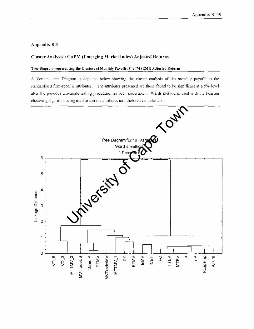
Appendix B: 59

Appendix B.3

Cluster Analysis: CAPM (Emerging Market Index) Adjusted Returns

Tree Diagram representing the Clusters of Monthly Payoffs: CAPM (EMf) Adjusted Returns

A Vertical Tree Diagram is depicted below showing the cluster analysis of the monthly payoffs to the

standardised firm-specific attributes. The attributes presented are those found to be significant at a 5% level

after the previous univariate testing procedure has been undertaken. Wards method is used with the Pearson

clustering algorithm being used to sort the attributes into their relevant clusters.

6

5

C]) 4 I,) c 2 en 0 3

C]) OJ ro ~ c ::i 2

I

1

a .~ <01 ("') ("') (f) ~ > I >' ::> ~ 0 0 lfi C]) f-> > ~ '0

~ 0 f- ro f- ~ ~

~

Tree Dagramfor 19 Variables

Ward's rrethod

1-Pearson r

I

nn > ..- >- > > f-~ >1 0 ~ ~ en a> f- .f; t) '0 ~ en ro f-'- f-

> ~ ~

I t) 0..

I 1 1 n

> > 0.. 0.. 0.. E en en .f; E ::l f- f- C])

~ 0.. ~ 0.. ro I,)

0:::

Univers

ity of

Cap

e Tow

n

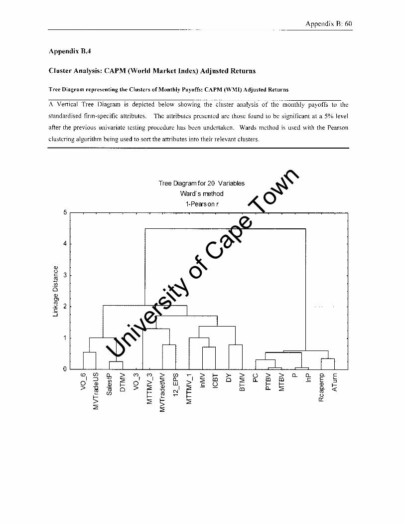
Appendix B: 60

Appendix B.4

Cluster Analysis: CAPM (World Market Index) Adjusted Returns

Tree Diagram representing the Clusters of Monthly Payoffs: CAPM (WMI) Adjusted Returns

A Vertical Tree Diagram is depicted below showing the cluster analysis of the monthly payoffs to the

standardised firm-specific attributes. The attributes presented are those found to be significant at a 5% level

after the previous univariate testing procedure has been undertaken. Wards method is used with the Pearson

clustering algorithm being used to sort the attributes into their relevant clusters.

5

4

Q) u

3 c ~ e/)

(5 Q) OJ ro

2 .::.::. c

:.:J

I

o n II COl (J) ~ > C"') C"')

::) ~ I >1 e/) 0 Q) Q) I-- 0 > > ~ ~ co 0 I--I- (J)

> I--~

~

Tree Diagram for 20 Variables

Ward's method

1-Pearson r

I I

1 I 1 J-

> (J) ~ > I-- >- > ~ 0.. >1 ~ en 0 ~ ....... w .£ U I--Q) I ~ 'D N I--

en ro l- I--

> ~

~

1 ~n I .-L u > > 0.. 0.. 0.. C

0.. en en .£ E l-::J

I-- I-- Q) !;: 0.. ~ 0.. ro u

0:::

Univers

ity of

Cap

e Tow

n

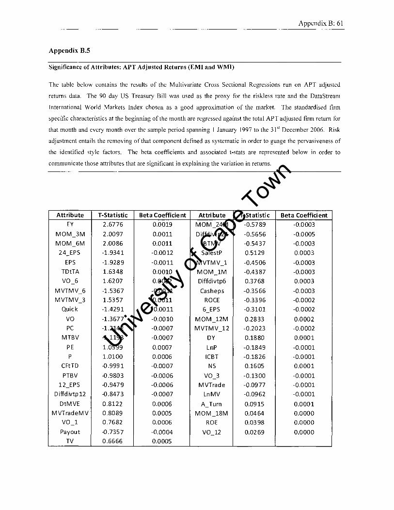
Appendix B: 61

Appendix B.S

Significance of Attributes: APT Adjusted Returns (EMI and WMI)

The table below contains the results of the Multivariate Cross Sectional Regressions run on APT adjusted

returns data. The 90 day US Treasury Bill was used as the proxy for the riskless rate and the DataStream

International World Markets Index chosen as a good approximation of the market. The standardised firm

specific characteristics at the beginning of the month are regressed against the total APT adj usted firm return for

that month and every month over the sample period spanning I January 1997 to the 31 sl December 2006. Risk

adjustment entails the removing of that component defined as systematic in order to guage the pervasiveness of

the identified style factors. The beta coefficients and associated t-stats are represented below in order to

communicate those attributes that are significant in explaining the variation in returns.

Attribute T-Statistic Beta Coefficient Attribute T -St atisti c Beta Coefficient

EY 2.6776 0.0019 MOM_24M -0.5789 -0.0003

MOM_3M 2.0097 0.0011 D iffd ivt p24 -0.5656 -0.0005

MOM_6M 2.0086 0.0011 BTMV -0.5437 -0.0003

24_EPS -1.9341 -0.0012 SalestP 0.5129 0.0003

EPS -1.9289 -0.0011 MVTMV_1 -0.4506 -0.0003

TDtTA 1.6348 0.0010 MOM_1M -0.4387 -0.0003

VO_6 1.6207 0.0012 Diffdivtp6 0.3768 0.0003

MVTMV_6 -1.5367 -0.0011 Casheps -0.3566 -0.0003

MVTMV 3 1.5357 0.0011 ROCE -0.3396 -0.0002

Quick -1.4291 -0.0011 6 EPS -0.3101 -0.0002

VO -1.3677 -0.0010 MOM_12M 0.2833 0.0002

PC -1.2142 -0.0007 MVTMV 12 -0.2023 -0.0002

MTBV -1.1193 -0.0007 DY 0.1880 0.0001

PE 1.0599 0.0007 LnP -0.1849 -0.0001

P 1.0100 0.0006 ICBT -0.1826 -0.0001

CFtTD -0.9991 -0.0007 NS 0.1605 0.0001

PTBV -0.9803 -0.0006 VO_3 -0.1300 -0.0001

12_EPS -0.9479 -0.0006 MVTrade -0.0977 -0.0001

D iffd ivtp 12 -0.8473 -0.0007 LnMV -0.0962 -0.0001

DtMVE 0.8122 0.0006 A Turn 0.0915 0.0001

MVTradeMV 0.8089 0.0005 MOM_18M 0.0464 0.0000

VO 1 0.7682 0.0006 ROE 0.0398 0.0000

Payout -0.7357 -0.0004 VO_12 0.0269 0.0000

TV 0.6666 0.0005

Univers

ity of

Cap

e Tow

n

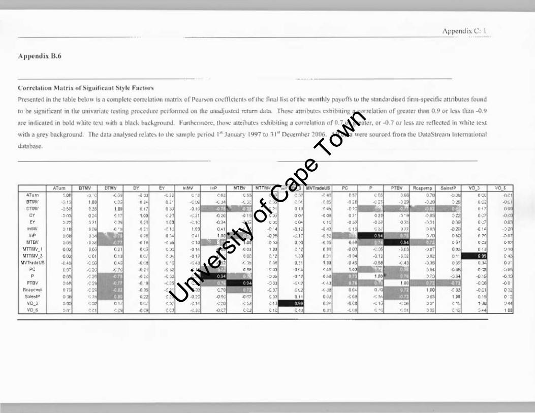
_________________________________ ,A,",~l\di" C I

l 'orrc,", IUO' ~I>II fI' .. , 1>1~1" ,j,~ " , :. ,~ It h.""". I'r~"",'rd in Iht I~bl~ t>el"" ;s 3 ~ompk1~ wm:I<>1"'" ,,,,rri,, of "'~.r"'" m ... mnchl, of 'oc final Ii •• ol"l h., m"nlh l~ J)iI} " n, '" ,h. "~ncl.l'dl!Cd 1;'''''$I'«,fk Min"",,,,, found

10 br >ij: n,fi",,"1 In .IIt UI""ari31~ 'o:!IlIn~ rro~~~,u~ I'<'lf"""c<l OIl II", un.:.djLl>I..-.J ""urn ~a\a Th" ... · ",,"bull.", <. h lb,,,,,~ ~ <,,,,,I,m,,,, uf ~"tr "'on 0.9 or I, .. , lhan -0.11

. .. mdKatrd In bold " lUte It ... " ,,10 I blad ""~ll9"'Uld F ... htnuono. ,b""" alm b .. ", "" "b,,;ng a ron.I.I I"~ "f 0.7 ." ~n'''1~r, or .{l.7 0, I,," , ...... ,"'l« IN in " biIC , .. "

with a ~ bacl-pOWld. Th~ dal~ a, ... I~ ",la!~ to) ,Il\: .... mple period I ~ J:aIlWf) I W 7 10 1'" n.,,,,ml>tr 2006 \ 11 d.na w~'" SO....-otd fron. ,h,- I).o",~""a", Irn<rnallonal

<ialAba>c .

. ~ ,~

" " .~ .. "'" ~TT~'I 1

Univers

ity of

Cap

e Tow

n

Appendix C: 1

Appendix C

Univers

ity of

Cap

e Tow

n

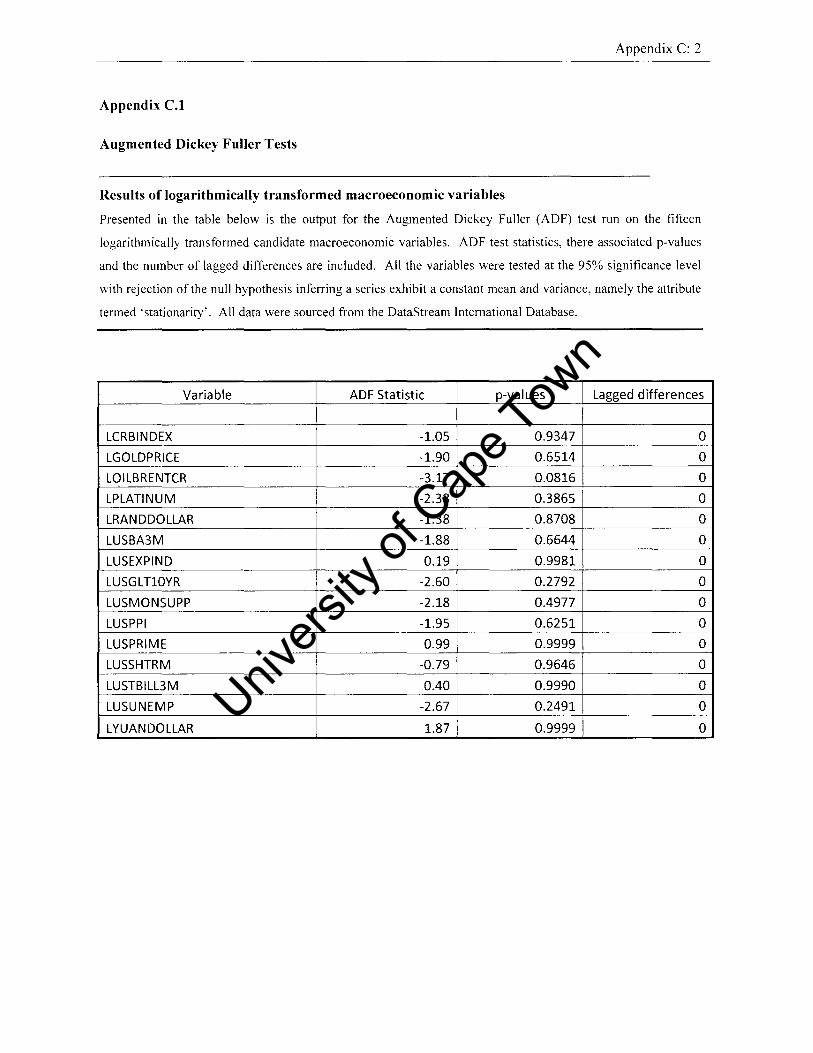
Appendix C: 2

Appendix C.l

Augmented Dickey Fuller Tests

Results of logarithmically transformed macroeconomic variables

Presented in the table below is the output for the Augmented Dickey Fuller (AD F) test run on the fifteen

logarithmically transformed candidate macroeconomic variables. ADF test statistics, there associated p-values

and the number of lagged differences are included. All the variables were tested at the 95% significance level

with rejection of the null hypothesis inferring a series exhibit a constant mean and variance, namely the attribute

termed 'stationarity'. All data were sourced from the DataStream International Database.

Variable ADF Statistic p-values Lagged differences

LCRBINDEX -1.05 0.9347 0

LGOLDPRICE -1.90 0.6514 0

LOILBRENTCR -3.17 0.0816 0

LPLATINUM -2.38 0.3865 0

LRANDDOLLAR -1.38 0.8708 0

LUSBA3M -1.88 0.6644 0

LUSEXPIND 0.19 0.9981 0

LUSGLTlOYR -2.60 0.2792 0

LUSMONSUPP -2.18 0.4977 0

LUSPPI -1.95 0.6251 0

LUSPRIME 0.99 0.9999 0

LUSSHTRM -0.79 0.9646 0

LUSTBILL3M 0.40 0.9990 0

LUSUNEMP -2.67 0.2491 0

LYUANDOLLAR 1.87 0.9999 0 Univ

ersity

of C

ape T

own

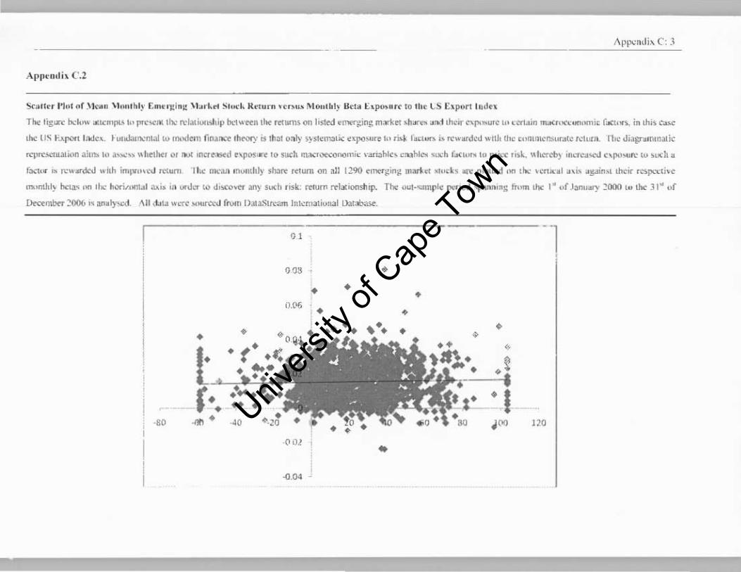
ApP"mh C: 3

App~Dlli, ('.2

Sr~II~r 1'1'" .. r ,\k~" "'~'lhI .. ' r,."'l!l ftj( \lao'l." St",'1. R~t "", "~<>'" ,\1 0,,(.1) Ilda £.p""." 10 II,,, LS [.porl I uM.

Tho tig...: hook," "''''n'pl.$~' pr<:'<'I. lit.: ",I31i""" ",, bo.1"'~R lho: return. OR IistM ~"""',:.iR~ mne! >It", .. ~",1 ,he'r C'I""U'C (" , 'Cr1:!In _,,'«""""';< rae"",,_ ;n thi' .,.....,

lhe.' U<; ............ 111<1"", f "1"J .. "t.:olal ~u ,,\lId ... n jinano;e .~~. i1 "'31 oaly '}Sl~m:llic ~XPO"'''' (0, ri>1 f.n ..... i> "' ...... <iN .. nl. (he c"IIl(I"'Iti"r~(C ",h.c", n," .Jiagnumnalk

"-'''''''''~31ion aiu'b 10 a"",,,, " I,ellot, 0, .... ,ncre_d ~'p"", .. e to .. ""II ma,.,,,,,,..,,,,,m'c \'ar.,hl~, """hi"" <""h (.oCl"" lP P"':'" ,j>~, "load» ,n.'f<:~"'-' "'1"""'" 'u ,,,,,h K

fXl'" ,. rcWiII'dc:d wilh ;ml"'''oo ,eI"m 'II", OI"a" m",,,~I)· .h:!re ,elum on;tll 1290 e""",,:;nl: m ...... ,,"ch "'" ph~"'d "" tit.: "<n, .. 1 ~'I> ~yin" lh<or ""J>CC';"" ''''>nthl} be,"< ,on 11-0; horit,.n~1 "' .. ;11 .... .Jer (0 d,>C()vcr an)' .""h rl.k, reourn relatlons'" p, TIl< "ul1''''',npl~ .,...,00 .... "'"'"' ITt"" lhc: I~ "f JanuiU)' 2000 II, the.' J 1~ "f

Dcnmbn':'ODb ... ".""",1. "II (l.,la "'= .. ",n:cd from I );uaSm:lrh hIl.'m.,lIunal lJatab. .....

" "l ,

"" • • • •

i),{>6 • + • • • • •

." , 00 l~O

'" .. . ~ Univ

ersity

of C

ape T

own

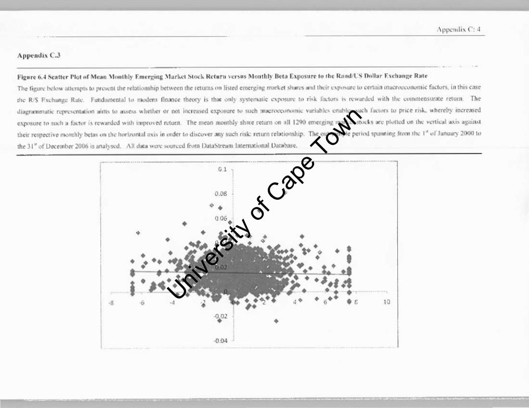
.'~ • • ~ t>A Sc.rr • • I'IGI "r M~~n \lo ~"h ly """0'):'''1 \b.I..o' ;', ,,,,1. II.N . ", ,~" •• M"n' h~' Btl" ["1"'''''' ,,, ,h. Ib,,,r_t ~ f). ,II~ r ,. ,.h~,, ~. R.,.

Th. tig"'" hdm. ~rr"n.",. ~, I"c"""DI Iht •• I;>1i"nsh,p fx<""'D rh. r~"rru. on )i,,0<1 .mo.gi"ll m."' .. ,." ........ ,d ,""i. ~'r""'''c ~, c'",Un ,D.,' ..... """,,,,,,,,. f.'I" .... in Ihi' ."'.

"u' R. S F""h.ngoo R.I~ Fo",SJ,ntnlal hi nlU<itnl lin,",,,, ,h"",)' i, Ih'" onl~ .ysr.",,"ic ''''P'''''''' II> . i,k r'''1"", " "' ..... Jc"" ""h lit .. ""nmto."""" ,tI"n,. Th.

Ji"!:".;nm., ... f1:J1I\:"""oI,,," '''''', ,,, ...... """ " h~l", or DOl ;,oc ..... std .xp..:>5""" 10,uch m""rn<..,nom" v".;.bk:, ~"""h.", ,..:h r"", ..... II> PI'" "\l... ,,"""'I.» ,ocr=O<I

.""',.u"" II> .och • Tao."" i! •• " .,dc-d ... rI" ''''f'Il"."<I .... 1"n' I", no""" moo,hly ... ". Irlum Of( .11 1290 "''''go", m.rt.", !"d s "'" pl,nl<.-d un lhe """i,,,,1 . ," ".-;<WrY

Ib.,r lnJIC'ttive "",",hI)' 1ltto< " n ,h .. 10"';,,, .... ,,1 ~'I> in ,"00 ,,, d..cu ..... "ny .uch , .. k. ottum .... Iau'"'oh'p Tho< ouH:Olnp~ lIOn,," $I"I"' ''''g fn'''' ,he I" or J""ullC) 2!MlO 10

til. ) I • or [Jonmb..- 2006 "an31~,,""'. "U ,I""" W"", ,.,,,,u-d {"m, I>.oU;'lrt-dD' Irr .. " .... i"""l u.,~b.ls •.

,M_ ....• ___ ... M. , !

• •

• • • • • • i . # ••

. , • " •

Univers

ity of

Cap

e Tow

n

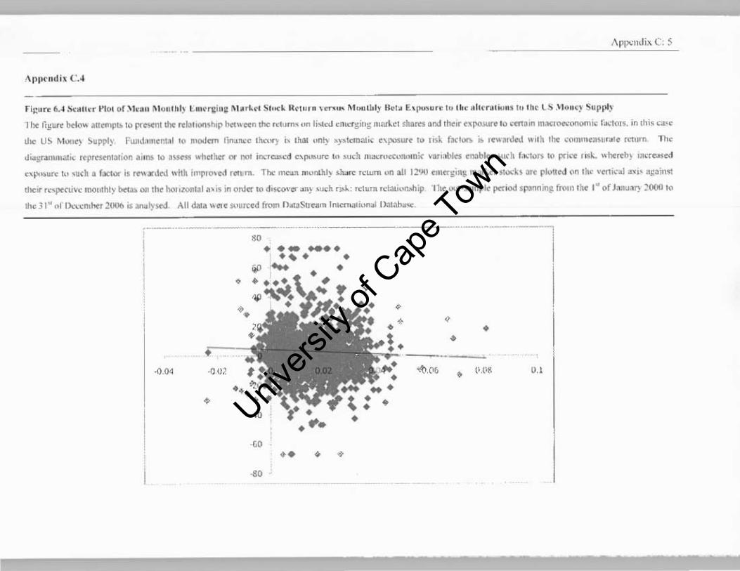
Appo:mli x C S

fil:"n 6A s.:.nn 1"<>1 of .'1eM" M')II thl)· ,,_,.,,1,,; Ma'~c' St.",k Re,u r_ , .... '" M""U.ly 0 .1. E.. llO>u 'e , .. I~< .h" "'''~J.' , .. tb. L~ .1 1 0~.~ SuPriY

1 ht r.~u ... """'" .11""pti> '0 prOWIlI d...: ... 1~"O<lSh'p betw~n the "~· .• m' on Ii" .... ellli."I"gl"g marl ... shares 000 th." txl'<»l .... 10 "cn~.n m""'oe'."O<lO<l,i< r"",rus. in ,hi, u«

~I<. U~ Mo","> ~uppl~ fun,b'n."",1 '0 ",Ot!.", lin.""., ''''"Ill)" ;,; lhal on~ >)",,'<In:ll;< r\p<>Sw< to ,isl f;!flO<!> i> ""·~,,*,1 ""I~ Iht , .. om,,,,n,"r.o1e ""ITm The

~;'gr.>"""aJi< '<prrsemanon a llM 10 ~~ wh .. !Ier or ..... i .... "TC1'><."d c:\1"'M'''' 10 ""oh lllal;roe<'U\(Mni< ..... '.11>105 <MblH l<Ifh f .... 1ors '" prke IIsl. "ht"b) m<r ..... ed

e.'''' ....... to ,ueh • IX1 ... is ,,,,,",,1to,1 w~h i"'pro.ed ,en.m. The """'" mor.Jd~ shan: ,el1lnl on all 12<)11 ""C'tgi~ ,narM! S10<."~ I = plwtd 0" 111< '·C'tIic;,J "'''- "l'.ain'<l

dl<.rr '<"'1'«""" ,,",mhl)· t!o:Ia. 00 ,h. hoi ,zool,1 a . i~ i" ONC't to d'KO\ .... .tR\ "'ok rclo., ,,"ium ,d3IJoruh ip .,n" OUI·.lllnpk ptflod $p;1nn in@.fmm III< I ~ of J3lIu",", WOO to

!he J I" "r ')',,:.:",ht, :wot. il anol)·std All <Wa ..... ,,,,.re.d from O>t,Stmtm In'CffilI,wnai .~...,.

'" ....... . ~. . ----l - . •

• •

• "' •

•• • •

Univers

ity of

Cap

e Tow

n

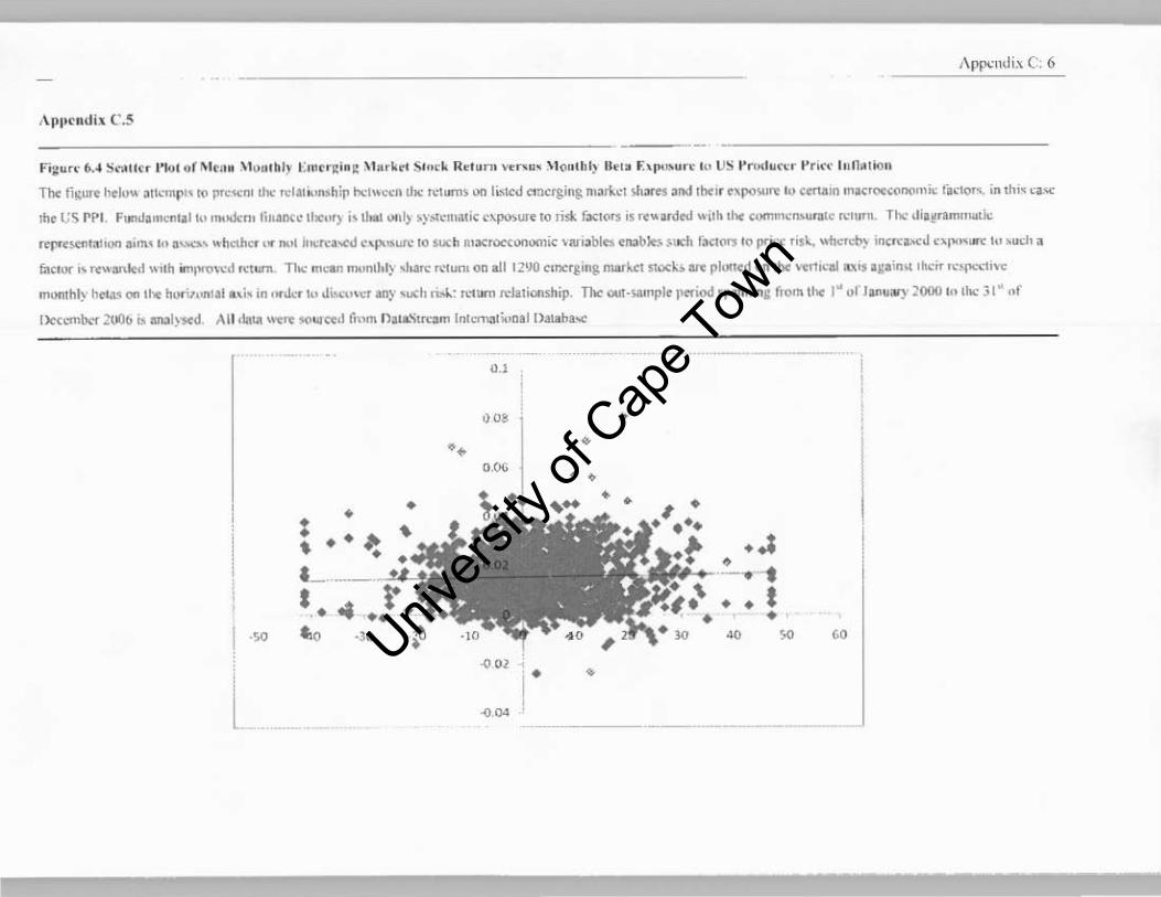
"pP<'l\tli.~ C; 6

."ij;u r< ~A S ... un \ '\0)( .... M~ .. ~l o),,'bJ, ~;m .. ~I.~ M~,~.' S.o.k R"un> , ... ,u, \1{lII(bl~ II ... ['I"'""n'" us t· ...... lu.·~" " " ... Inl1>o1lon

Til< jiglO'. h.l"" a .. "". .... t(I prc",,,, ,ho; .cI" ~".;hip ho;h.cen Ibe M u"" 00 1".cJ roncrging n,:ukel lobar .. "lid IIx" •. 'r<>~ ." ,orum ml<'0«<1,,,,,,,k r.",,,,,, ;n 'hI< us<:

lh._ US prl. FI ... d.m ....... 1 ,,, " .. okn, Ilro,I'It." 11.c.,,> 1.110.1 001) 'y"''''''aI'. C>.pO>"'.lO Ii'" rael(ITS IS r .... , dod "dh lhe' wmn'~JI>""'c "''',,~. Tho; "i.~"'mm"'k:

,..,. ....... ""00 ,,11"< ." ''''''''' .. hClh .. ". ""I n>Ckl..oo •• .,.",Uf\O 10 such n,ae,ONooomic ' -alll bl"" .""b~ ~lI<h f"",(ITS 10 pr"" ml. "h,'n'b~ inc",.,..,d e~I'''''''' ,,, • ..m a

mc' '''' "T."·an .... "" 'h iml><O"''' .. "urn. Tho; mcan monllol) "'oar. ",",uno on all 1290 ."""l'''8 rnarkl sroc~ 1ft plort.d (In IIx .~"'1II1U" 'I:.;n" lheir ""1"""""" m""lhl~ b ... ~. "" lhe' hUfi""I.1 I, i. ,n ,,, ....... ," do.c.""r an) ,uch """, "."'" rdalloosillp Tbc 001-"""1'1. prriod "" .... oml: 1T0m lhe' I~ (lr Janu.y WOO ,,, lhe 31 ~ "r

[l«cmtx..- 2oot.", an:ol!'$<'d. All (~""'" ~ur«d Cmm n...stmuu [n(ernali.,na[ [),aLob .. ",

"' "" • '. • ,.w • •

• • • • '! ..1 • • • • .. • • • w 4 , ~ ~ '" ".,

l • • .~

Univers

ity of

Cap

e Tow

n

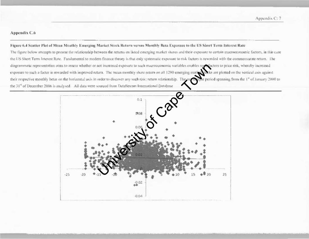
~ ig~re ~.4 ~r.U~r I'I.}! M M"". ~l o u!~ I~ I:'n. , ·~jf" M~ . ~ •• SUI"k Ikh, m ,.,...~. M"B.hl~· 1Ie!~ "'1'0"' '' ' '' d ,e US ilbor' ·I .. · .. " I,, '~m ' Ih .e

Til< jig"'" loci"" """mpls 10 ",.-sen' ,he ,.bl1looub,p br." ..... n d .. ,.mn,. 00 10M.! c"'~rg"q; 'n.ff~<I ',,"0,,", ... N1 Ilk' " nf'O"". '" •• "~In ,"""'<O«'.'OIn;c farTo,"" io Ih l< r~"

'he Us. !'.hort Tom> hn~~ Ra,. r undaooffuJllO modem fin.nruhwo) ;. IhKl onll ' }",I<"'''''' eA[IU .... '" 10 tL,~ r~cl""" ", .. ;ord.d w~h 1tJ" «Inuu.n~nr"'. mum. J he

dl.""mmau" "'1"","".1000 alml '" ,"SClo5 .. I,(OI,C"! 01 1001 'nr",,,,,td <.po""'" 10 "",II n1~o;rtJ"'OllOJluc ~1II"i"bk, cn .... lc. SI"''' f...:'"'' UI puc. , ,",. "ho,dI" "",,.,....,J

<'Pm .... '0 .ucb ~ fllC1o. IS "'w~,lIed ""h ,n'proved n."!UtI,. T"" lru""oU. nk.nlhl)" slo.Irc ""um 00 all 1190 ."""I.:m!; tn;>t~CI slocks are pl ...... cd on the .... ,10".1 ... " '1:.l.In.1

Ihoi! "''1'''"'1, .... mon.hl) OOili on II ... "">rim,n.il a". in .1RlN It. d.>cu,,,,,, :my ,,,,,h " "': Mum rd"'oorubip. Th. ou,·sampLe ~riN $1»1"'''13 (run ...... I ~ "r I .. ,WI) ~OOO In

.ho 31 ~ of 1.Ic«,."i>tr 2006 i, at ... I)..ro AU d ... we ..... ,urccd fruln f"lau'i!r •• m In •• "",,;,. ... 1 OKl.b.""

._._-_.-ro .1

"'" l • • O~ • •

" Univers

ity of

Cap

e Tow

n

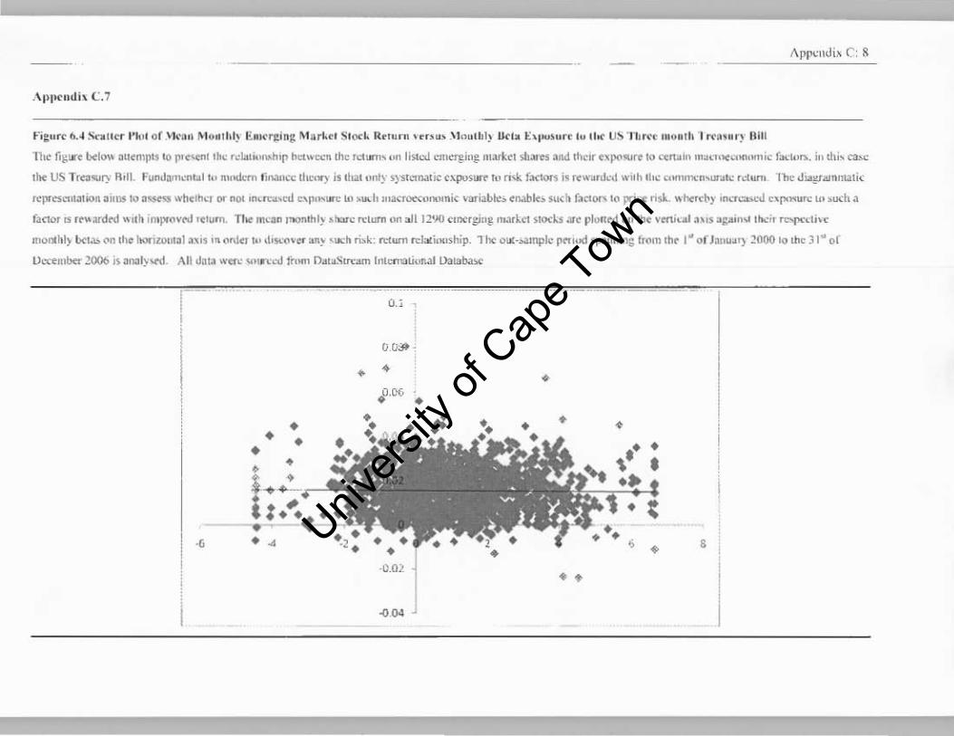
i\pr':l\di~ C: 8

Fitu .... b. ~ s. .. " ... 1'10,1 of lkaoL MO" II,I) 1'..lCl'1:in~ Mart.d Sl o<~ n~t" .... , ·~ .. u, _\ I "utll l~ Ikl •• :'I"" un ,,, II ... U~ 'Ill ""~ IMO_tl, "' "".,M.')' Rill

11", fi~In ""I"" .u~nll)(11O 1)1~ .... t Ih<" ",laI~II"",,Ir bct"'",.-n the I'd ... " "n listed e,ucrr-iog ,u"n.ct slI"' .... and thclr ~'I"""''''' to ~n"l" m",'''''''''''''",l1~ fa"'"",- ill d", """"

tM US T .. n ... " R,IL r u"J;vllc·,u,,1 ~l n".w.-m lin.ul"" tl"","}" i. Ih ... tlnly systematie c~po'i"" to "'" factors i. r~,,"..,Jc-d ","h .he "'""""'''" .... ''' tctw-" Th~ sI..graln", .. ".

"'",<:s"'rt.:ltion ~illlll to ~<$t"SII "'h~IhcI or "01 '''<f..--~,td "'1''''''''' Il, .... :h lIIacr"""tnlOmie 'mlab"'~ ~""" .. ~ ouch fan ...... 1(1 pri<~ n$l.. " .. ht.c~)· '''~ ~'P""'"'' If' .""h a

rO<1or IS •• " ardrd "'I" improwd rcturn. Th" Inc~" 1""""'1, ~h;u-c ",Ium on al l 1190 c",.tJ;ln~ n""L<1 'lor'" :IIC plo" rd 0Il1h~ VC1\Iul 3", "j;aln" lI>.:iT ""f>«1i.c

mOIll"I} 1><1 .... on the ""'iWln~l.xl' I~ onieT I" d'SlO'<1 "n~ • ....-h ri>k: retwn ,d illi,KlShip_ 1 he o:.l->:llnpl,· r"'oc! $p:llloin; from .ht I" of Janu.'l 2000 10 Ih~ J I" of

l)c<~mber 2006 i~ ~n:lI}>rtl All da13 W"" "" n <d ""'" n.,.S""~m l"I""n~oJI.11 ll:lla""'"

0 .•

(j(jJt •

• • • J'rx, •

, ••

Univers

ity of

Cap

e Tow

n

Appendix D

Univers

ity of

Cap

e Tow

n

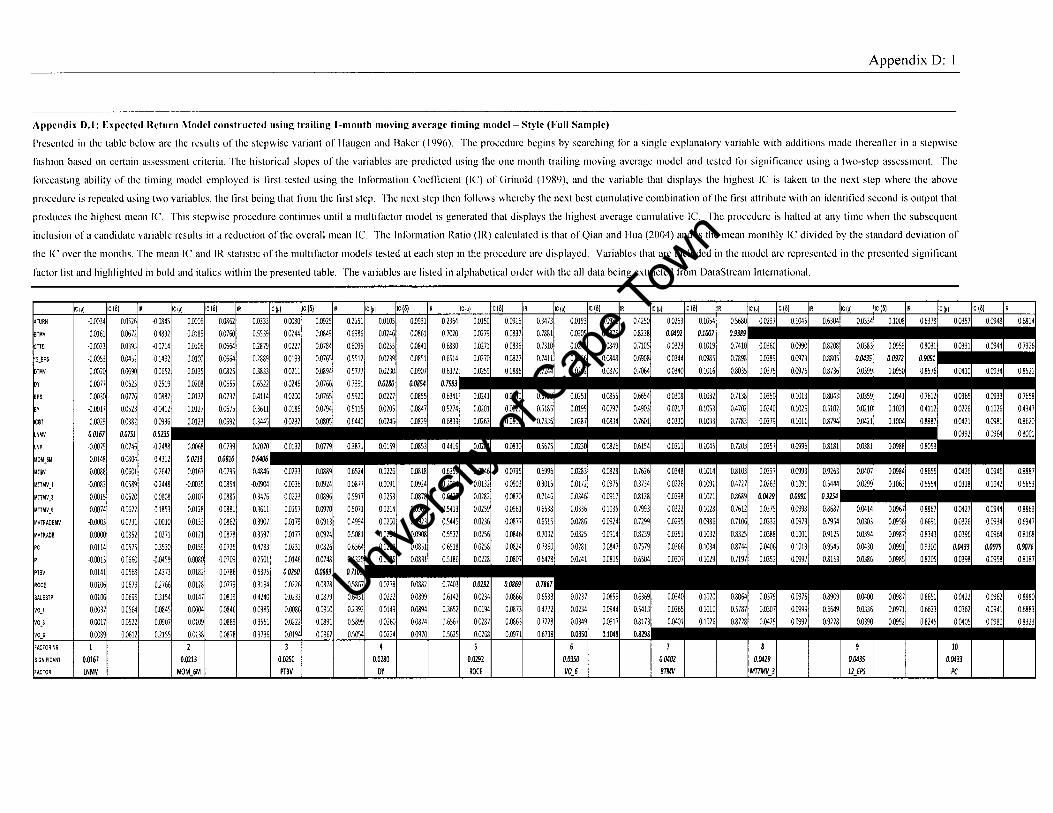
Appendix D: 1

Appendix D.1: Expected Return Model constructed using trailing I-month lIloving average timing lIlodel- Style (Full Sample)

Prescnted in the table below are the results of the stepwise variant of llaugcn and Baker (1996). The procedure begins by searching for a single explanatory variable with additions made therealler in a stepwise

filshion based on certain assessment criteria. The historical slopes of the variables arc predicted using the one month trailing moving average model and testcd for significance using a two-stcp assessment. The

fl)recasting ability of thc timing model employed is first tested using the InflJrlllation Coefficient (IC) of Grinold (1989), and the variable that displays the highest IC is taken to the next step where the above

procedure is repeated using two variables, the first being that from thc first step. The next step then follows whereby the next best cumulative combination of the first attribute with an identified second is output that

produces the highest mean Ie. This stepwisc procedure continues until a multifilctor model is generated that displays the highest average cumulative Ie. The procedure is halted at any time when the subsequcnt

inclusion ofa candidate variable results in a reduction of the overall mean Ie. The InflJrlllation Ratio (lR) calculated is that of Qian and !lua (2004) and is the mean monthly IC divided by the standard deviation of

the Ie over the months. The mean IC andlR statistic of the multi factor models tested at each step in the procedure arc displayed. Variables that arc included in the model arc representcd in the presented significant

factor list and highlighted in bold and italics within the presented table. The variables are listed in alphabetical order with the all data being extracted from DataStream International.

Univers

ity of

Cap

e Tow

n

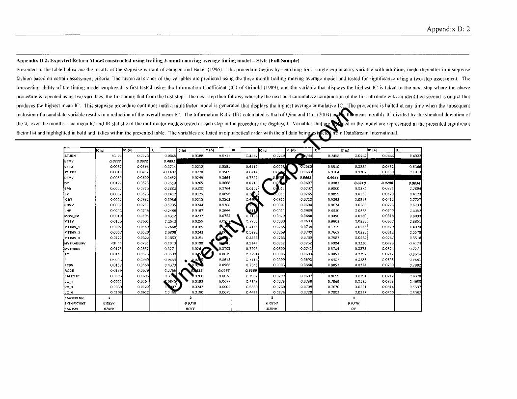
Appendix 0: 2

Appendix 1).2: Expected Return Model constructed using trailing 3-month moving average timing model- Style (Full Sample)

Presented in the table below are the results of the stepwise variant of Ilaugen and l3aker (1996). The procedure begins by searching for a single explanatory variable with additions made therealler in a stepwise

iilshion based on certain aSseSSl11l:nt criteria. The historical slopes of the variables arc predicted using the three month trailing moving average model and tested f()r signiiicance using a two-step assessmcnt. The

forecasting ability of the timing model employed is iirst tested using the Inilmnation CoefJicient (lC) of Urinold (1989), and the variable that displays the highcst Ie is taken to the next step where the above

procedure is repeated using two variables, the lirst being that from the Jirst step. The next step then follows whereby the next best cumulative combination orthe Jirst attribute with an identiJied second is output that

produces the highest mean Ie. This stepwise procedure continues until a multi factor model is generated that displays the highest average cumulative Ie. The procedurc is halted at any time when the subsequcnt

inclusion ofa candidate variable results in a reduction orthe overall mean Ie. The Inf"i.mnation Ratio (lR) calculated is that of Qian and !-Iua (2004) and is the mean monthly IC divided by the standard deviation of

the Ie over the months. The mean Ie and IR statistic of the multi factor models tested at each step in the procedure are displayed. Variables that arc included in thc model arc represented in the presented signiJicant

factor list and highlighted in bold and italics within the presented table. The variables are listed in alphabetical order with the all data being extracted from DataStream International.

IC I~I IC (6) IR IC I~I I,c (6) IR IC I~I IC (6) IIR IC I~I IC (6) IR

ATURN 5E-05 0.0526 -0.0845 0.01881 0.0712 0.4697 0.0259 0.07341 0.7458 0.0164 0.0833 0.4303

BTMV 0.0237 0.0672 0.4892

CTTD 0.0057 0.0393 -0.0714 0.0212 0.0581 0.6119 0.0293 0.0680 0.8510 0.0224 0.0732 0.6366

12_EPS 0.0010 0.0452 -0.1492 0.0228 0.0569 0.6714 0.0319 0.0689 0.9164 0.0287 0.0680 0.8013

DTMV 0.0059 0.0690 0.0652 0.0249 0.0664 0.7377 0.0350 0.0661 0.9951

DY 0.0122 0.0523 0.2519 0.0265 0.0668 0.8210 0.0314 0.0697 0.9083 0.0310 0.0700 0.9034

EPS 0.0057 0.0776 0.0882 0.0200 0.0764 0.6162 0.0315 0.0707 0.9060 0.0274 0.0774 0.7894

EY -0.0007 0.0523 -0.0412 0.0129 0.0696 0.3689 0.0311 0.0765 0.8859 0.0153 0.0679 0.4123

leBT 0.0027 0.0382 0.0936 0.0215 0.0563 0.6499 0.0311 0.0710 0.9098 0.0268 0.0712 0.7727

LNMV 0.0092 0.0751 0.5235 0.0244 0.0766 0.7568 0.0301 0.0694 0.8674 0.0283 0.0775 0.8233

LNP 0.0043 0.0746 -0.2488 0.0187 0.0666 0.6115 0.0311 0.0689 0.8920 0.0278 0.0730 0.8353

MOM_8M 0.0019 0.0804 0.4312 0.0237 0.0754 0.7198 0.0329 0.0688 0.9490 0.0280 0.0818 0.8093

MTBV 0.0120 0.0601 0.2642 0.0255 0.0552 0.7733 0.0300 0.0693 0.8802 0.0286 0.0687 0.8351

MTIMV_1 0.0002 0.0589 -0.2448 0.0169 0.0711 0.4165 0.0268 0.0734 0.7719 0.0165 0.0829 0.4024

MnMV_J 0.0037 0.0520 0.0808 0.0243 0.0606 0.5892 0.0269 0.0709 0.7669 0.0223 0.0812 0.5578

MTTMV_6 0.0112 0.0622 0.1853 0.0191 0.0685 0.4455 0.0263 0.0733 0.7587 0.0234 0.0787 0.5518

MVTRADEMV -9E-05 0.0731 0.0010 0.0188 0.0741 0.5148 0.0307 0.0752 0.8884 0.0236 0.0823 0.6123

MVTRADE 0.0175 0.0852 0.0271 0.0261 0.0705 0.7293 0.0300 0.0741 0.8704 0.0275 0.0824 0.7271

PC 0.0145 0.0575 0.3530 0.0253 0.0619 0.7791 0.0306 0.0693 0.8852 0.0297 0.0712 0.8614

P 0.0043 0.0660 -0.0459 0.0225 0.0615 0.7116 0.0309 0.0690 0.8903 0.0287 0.0695 0.8481

PTav 0.0157 0.0568 0.4373 0.0242 0.0566 0.7348 0.0303 0.0668 0.8853 0.0274 0.0709 0.7982

ROCE 0.0139 0.0679 0.2766 0.0318 0.0692 0.9189

SALESTP 0.0093 0.0695 0.3154 0.0266 0.0678 0.7982 0.0299 0.0697 0.8659 0.0291 0.0717 0.8328

VO_1 0.0051 0.0564 -0.0845 0.0192 0.0677 0.4848 0.0273 0.0738 0.7869 0.0185 0.0808 0.4653

VO_3 0.0039 0.0522 0.0907 0.0242 0.0606 0.5889 0.0269 0.0708 0.7670 0.0221 0.0814 0.5537

va 6 0.0108 0.0612 0.2155 0.0190 0.0679 0.4425 0.0273 0.0728 0.7893 0.0227 0.0790 0.5382

FACTOR NR. 1 2 3 4

SIGNIFICANT 0.0237 0.0318 0.0350 0.0310

FACTOR BTMV ROCE DTMV DY

Univers

ity of

Cap

e Tow

n

Appendix D: 3

Appl'lHlix 1>.3: Expected Return !\Iodel constructed usin~ trailin~ 6-month moving avera~e tilnin~ model- Style (Full Sample)

Presented in the table below arc the results of the stepwise variant of llaugen and Baker (1996). The procedure begins by searching for a single explanatory variable with additions made thereafier in a stepwise

filshion based on certain assessment criteria. The historical slopcs of the variables arc predicted lIsing the six month trailing moving average model and tested filr significance using a two-step assessment. The

filrecasting ability of the timing model employed is first tested using the lnfllflllation eocntcicn t (Ie) of Grinold (1989), and the variable that displays the highest IC is taken to the next step where the above

procedure is repeated using two variables, the first being that from the first step. The next step thell follows whereby the next best cumulative combination of the first attribute with an identified second is output that

produces the highest mean IC This stepwise procedure continues until a l11ultifactor l110del is generated that displays the highest average cumulative IC. The procedure is halted at any time when the subsequent

inclusion ofa candidate variable results in a reduction of the overallmeanlC The Information Ratio (IR) calculated is that ofQian and \lua (2004) and is the mcanmonthly Ie divided by the standard deviation of

the IC over the months. The mean Ie and IR statistic of the multif~1etor models tested at each step in the procedure are displayed. Variables that arc included in the model arc represented in the presented significant

factor list and highlighted in bold and italics within the presented table. The variables arc listed in alphabetical order with the all data being extracted from DataStream International.

Univers

ity of

Cap

e Tow

n

Appendix D: 4

Appcndix D ... : Expected Return !\Iudel cunstrueted using trailing 12-month moving average timing model- Stylc (Full Sample)

Presented in the table below are the results of the stepwise variant of Ilaugen and Baker (1996). The procedure begins by scarching Ill[ a single explanatory variable with additions made thercancr in a stepwise

fashion based on certain assessment criteria. The historical slopes of the variables arc predicted using the twelve month trailing moving average model and tested Il)r signilicance using a two-step assessment. The

liJrecasting ability of the timing model employed is lirst tested using the Information Coefficient (Ie) of Cirinold (1989), and the variable that displays the highest IC is taken to the ncxt stcp where the above

procedure is repeated using two variables, the first being that from the first step. The next step thcn follows whereby the next best cumulative combination of the first attribute with an identified second is output that

produces the highest mean Ie. This stepwise procedure continues until a multi factor model is generatcd that displays the highest average cUlllulative Ie. The procedure is halted at any time when the subsequent

inelusion of a candidate variable results in a reduction of the overall mean Ie. The Infi)fJnation Ratio (IR) calculated is that of Qian and Ilua (2004) and is the mean monthly Ie divided by the standard deviation of

the Ie over the months. The Illean Ie and IR statistic of the multi factor models tested at each step in the procedure arc displayed. Variables that arc included in the model are represented in the presented significant

factor list and highlighted in bold and italics within the presented table. The variables arc listed in alphabetical order with the all data being extracted from DataStream International

ATURN

BTMV

eTTD

12_EPS

DTMV

DY

EPS

EY

ICST

LNMV

LNP

MOM_8M

MTBV

MTTMV_'

MTTMV_3

MTTMV_6

MVTRADEMV

MVTRAOE

PC

PlBV

RaCE

SALESTP

VO_,

VO_J

VO.

FACTOR NR.

SIGNIFICANT

FACTOR

IC(Il)

-0.0025

0.0303

-0.0002

-0.0021

0.0055

0.0154

0.0051

0.0050

-0.0056

0.0073

0.0027

00023

0.0066

0.0002

0.0042

0.0028

0.0043

0.0246

0.0152

0.0053

0.0148

0.0072

0.0221

0.0001

0.0038

0.0003

0.0303

BTMV

IC t6)

0.0526

0.0634

0.0388

0.0456

0.0688

0.0502

0.0741

0.0473

0.0361

0.0770

0.0732

0.0784

0.0603

0.0604

0.0509

0.0606

0.0748

0.0823

0.0565

0.0630

00565

0.0683

0.0671

0.0571

0.0513

0.0601

IR IC (Jl) IC (6) IR IC (Jl) IC (6) IR IC (Jl) IC (6) IR ICM IC (6) IR ICM IC (6) IR

-0.0658 .... ° .• °'.8.° ••• ° .• °'.1.9 ••• °11.'.43.° ••• °.°.34.3 ••• ° •. °.86.9 ••• ° •. 811'.46 ••• °11.°.3.86, •• ° •. °.8.'6, •• ° •. ii98.1.'~ •• 0 .• 03.9.3 ••• 0 .• 0'.6.8 ••• 0 •. 9.85.3 ••• 01i·04.0.' ••• 0.0Il'.63 ••• II·oiio.60~ 0.9288,.

-0.0172 0.0294 0.0581

-0.0602 0.0310 0.0591

0.1818 0.0259 0.0646

0.5085 0.0340 0.0551

0.1701 0.0280 0.0661

0.1524 0.0229 0.0686

-0.1742 0.0275 0.0579

0.2443 0.0257 0.0672

0.0970 0.0241 0.0644

0.0974 0.0313 0.0655

0.2018 0.0293 0.0547

0.0101 0.0307 0.0717

0.1125 0.0149 0.0730

0.0942 00218 0.0617

0.1518 00346 0.0675

0.6926 0.0398 0.0744

0.4692 0.0330 0.0577

0.1787 0.0277 0.0584

0.4543 0.0314 0.0564

0.2268 0.0288 0.0625

0.6353 0.0358 0.0572

0.0175 0.0293 0.0691

0.0995 0.0148 0.0731

00210 0.0240 0.0597

0.0398

MVTRADE

0.8472 0.0366 0.0783 0.9460 0.0416 0.0844 1.0900 0.0426 0.0826 1.0905 0.0447 0.0829 1.1449

0.9113 0.0362 0.0727 0.9690 0.0387 0.0780 1.0455 0.0401 0.0766 1.0584 0.0421 0.0791 1.1098

0.7932 0.0336 0.0837 0.8938 0.0387 0.0837 1.0381 0.0399 0.0821 1.0478 .... 0.1I04I1'II' ••• 01l.0.8Iii8 ••• III.ll111.3 1.0418 0.0403 0.0753 1.1047 0.0449 0.0785 1.2268 0.0474 0.0770 1.2655,.

0.8560 0.0392 0.0775 1.0532 0.0418 0.0790 1.1290 0.0422 0.0786 1.1146 0.0433 0.0804 1.1477

0.6453 0.0316 0.0808 0.7866 0.0322 0.0783 0.8142 0.0343 0.0793 0.8452 0.0322 0.0826 0.8007

0.8281 0.0409 0.0720 1.0846 0.0452 0.0765 1.2054 ............. 111 •••• l1li ........ l1li11. 0.7904 0.0329 0.0808 0.8849 0.0389 0.0804 1.0525 0.0401 0.0793 1.0608 0.0425 0.0797 1.1295

0.7459 0.0358 0.0739 0.9675 .... 0 •. 0.40Il, ••• 0 •. 0.'6.1 ••• I •. I.o'.9 ••• 0 •. 0.4iiI8 ••• °

11.°11'.55, •• 1 •. 1.1.'5, •• ° •. 04.4.3 ••• 0 .• o'ii4.' ••• I .• 18.'.1

0.9840 0.0440 0.0775 1.1992,-

0.8927 0.0411 0.0719 1.1063 0.0433 0.0766 1.1714 0.0447 0.0755 1.1846 0.0471 0.0767 1.2504

0.8032 0.0347 0.0879 0.8790 0.0378 0.0817 0.9554 0.0383 0.0764 0.9597 0.0393 0.0759 0.9823

0.4021 0.0287 0.0729 0.7120 0.0345 0.0772 0.8639 0.0383 0.0747 0.9258 0.0394 0.0765 0.9561

0.5436 0.0332 0.0783 0.8359 0.0368 0.0808 0.9324 0.0382 0.0792 0.9416 0.0393 0.0791 0.9754

0.9389 ... l1li°.11°3.'11' •• l1li°11°.'8.3 .... 111.°1115.8 ••• °11.°.4°.1 ••• °11.°.8.°6 ••• 111.°.9.6' .... ° •. °.4.4.1 ••• ° •.• °'118.' ••• 1..1'114.' ••• °.110411111' .... °11.°.8°.4 ••• 111.1.°'.° 1.0812,.

1.0016 0.0431 0.0749 1.1580 0.0448 0.0790 1.2147 0.0462 0.0790 1.2288 0.0470 0.0797 1.2525

0.8374 0.0372 0.0709 1.0043 0.0421 0.0753 1.1480 0.0438 0.0751 1.1653 0.0460 0.0765 1.2281

0.9518 0.0411 0.0732 1.1045 0.0424 0.0769 1.1515 0.0443 0.0767 1.1746 0.0467 0.0777 1.2413

0.8668 0.0358 0.0816 0.9546 0.0407 0.0846 1.0859 0.0420 0.0851 1.1008 0.0435 0.0861 1.1388

1.0522 0.0401 0.0736 1.0551 0.0418 0.0769 1.1178 0.0436 0.0749 1.1442 0.0452 0.0756 1.1860

0.7581 0.0372 0.0858 0.9536 0.0389 0.0792 0.9822 0.0400 0.0750 0.9997 0.0408 0.0751 1.0162

0.4018 0.0286 0.0733 0.7101 0.0343 0.0773 0.8590 0.0382 0.0747 0.9239 0.0392 0.0766 0.9532

0.5957 0.0335 0.0780 0.8414 0.0367 0.0805 0.9275 0.0380 0.0789 0.9357 0.0391 0.0787 0.9675

0.0440

MOM 6M

4

0.0452

IC8T

0.0474

DY

0.0471

MTBV Univers

ity of

Cap

e Tow

n

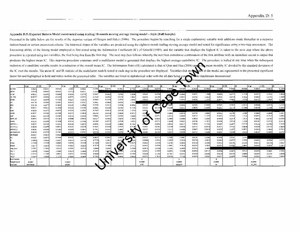
Appendix 0: 5

Appendix 1).5: Expected Return Model eonstructed using trailing IS-month moving average timing modcl- Style (Full Sample)

Presented in the table below arc the results of the stepwise variant of Ilaugen and l3aker (1996). The procedure begins by searching for a single explanatory variable with additions made therealler in a stepwise

lilshion based on certain assessment criteria. Thc historical slopes of the variables arc predicted using the eighteen month trailing moving average model and tested II.)r significance using a two-step assessment. The

I(lr\:easting ability of the timing model employed is lirst tested using the Information ('oerticient (1(') of Grinold (1989), and the variable that displays the highest 1(' is taken to the next step where the above

procedure is repeated using two variables, the lirst being that Irom the first step. The next step then 1()lIows whereby the next best cumulative combination of the first attribute with an identilied second is output that

produces the highest mean Ie. This stepwise procedure continues until a multi factor model is generated that displays the highest average cumulative Ie. The procedure is halted at any time when the subsequent

inclusion of a candidate variable results in a reduction of the overall mean Ie. The Information Ratio (lR) calculatcd is that of Qian and !lua (2004) and is the mcan monthly IC divided by the standard deviation of

the IC over the Illonths. Thc mcanlC and IR statistic of the Illultifactor models tested at each step in the procedure arc displayed. Variables that arc included in the model are represented in the presented signilicant

factor list and highlighted in bold and italics within the presented table. The variables arc listed in alphabetical order with the all data being extracted from DataStream International

Univers

ity of

Cap

e Tow

n

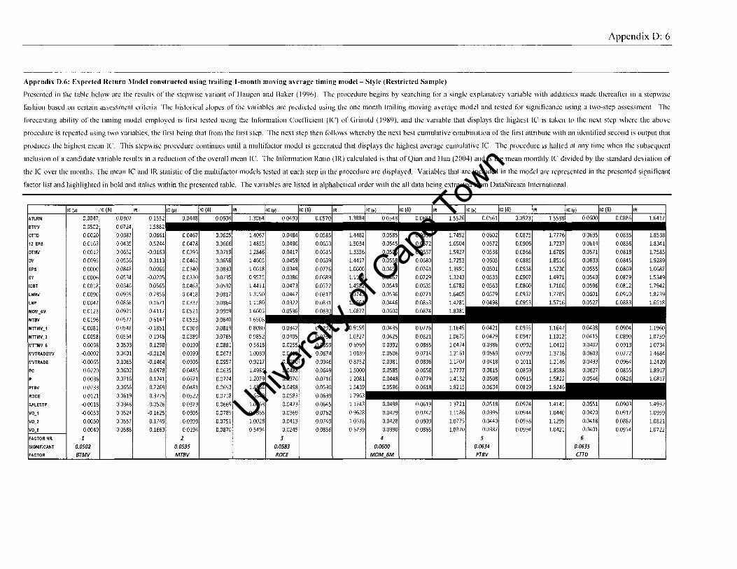
Appendix D: 6

Appendix D.C,: Expected I{eturn !\Iodel constructed using trailing I-month moving average timing model- Style (Restricted Sample)

Presented in the table below arc the resuits of the stepwise variant of Ilaugen and Baker (1996). The procedure begins by searching for a single explanatory variable with additions made therealkr in a stepwise

fashion based on certain assessment criteria. The historical slopes of the variables arc predicted using the one month trailing moving average model and tested for signilicance using a two-step assessment. The

f(lrecasting ability of the timing model employed is lirst tested using the Inlimnation Coeflicient (IC) of Urinold (1989), and the variable that displays the highest Ie is taken to the next step where the above

procedure is repeated using two variables, the lirst being that Irolll the lirst step. The next step then lilliows whereby the next best eUlllulative coillbination of the lirst attribute with an idcntilied second is output that

produces the highest mean Ie. This stepwise procedure continues until a multi factor model is generated that displays the highest average cUlllulative Ie. The procedure is halted at any tilllc when the subscquent

inclusion of a candidate variable results in a reduction of the overall mean Ie. The Inli)[fnation Ratio (IR) calculated is that of Qian and liun (2004) and is the mean monthly Ie divided by the standard deviation of

the Ie over the months. The Illean Ie and IR statistic of the Illultifactor models tested at each step in the procedure are displayed. Variables that are ineluded in the model arc represented in the presented signilicant

factor list and highlighted in bold and italics within the presented table. The variables arc listed in alphabetical order with the all data being extracted Irolll DataStream International.

0.0502

8TMV

0.0348

0.0524

0.0557

0.0588

0.0535

MT8V

0.0583

ROCE

0.0634

PT8V

0,0635

CTTD

Univers

ity of

Cap

e Tow

n

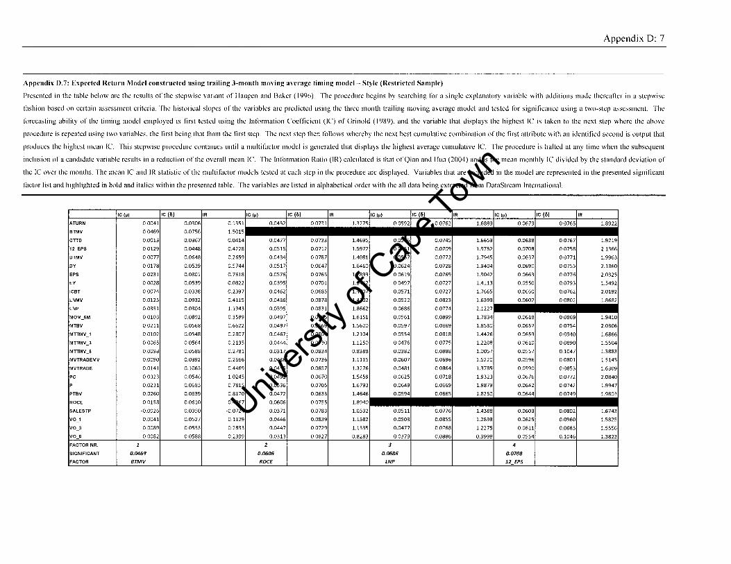
Appendix 0: 7

Appendix D.7: Expected Return Model constructed usin!: trailin!: 3-month movin!: avera!:c timin!: modcl- St)'lc (I{estricted Sample)

Presented in the table below arc the results of the stepwise variant of Ilaugen and Baker (1996). The procedure begins by searching illr a single explanatory variable with additions made therealier in a stepwise

I(lshion based on certain assessment criteria. The historical slopes of the variables arc predicted using the three month trailing moving average model and tested li)r signillcance using a two-step assessment. The

forecasting ability of the timing model employed is Ilrst tested using the Information Coertlcient (IC) of Grinold (1989). and the variable that displays the highest IC is taken to the next step where the above

procedure is repeated using two variables. the tirst being that Irom the tirst step. The next step then lilliows whereby the next best cumulative combination of the tirst allribute with an identilied second is output that

produces the highest mean Ie. This stepwise procedurc continues until a multi factor model is generated that displays the highest average cumulative Ie. The procedure is halted at any time when the subsequent

inclusion of a candidate variable results in a reduction of the overall mean Ie. The InliJr1nation Ratio (lR) calculated is that of Qian and Hua (2004) and is the mean monthly IC divided by the standard deviation of

the IC over the months. The mean IC and IR statistic ofthe multifaclor models tested at each step in the procedure arc displayed. Variables that are included in the model are represented in the presented signi!lcant

factor list and highlighted in bold and italics within the presented table. The variables arc listed in alphabetical order with the all data being extracted from DataStream International.

IC I~I IC (6) IR IC (~I IC (6) IR IC (~I IC (6) IR IC (~I IIC (6) IR

ATURN 0.0041 0.0306 0.1351 0.0452 0.0731 1.3275 0.0592 0.0762 1.6889 0.0673 0.0765 1.8922

BTMV 0.0469 0.0756 1.5015

cnD 0.0013 0.0367 0.0414 0.0477 0.0733 1.4695 0.0546 0.0745 1.6653 0.0638 0.0767 1.9219

12_EPS 0.0129 0.0448 0.4228 0.0515 0.0712 1.5972 0.0651 0.0709 1.9752 0.0708 0.0758 2.1366

DTMV 0.0077 0.0648 0.2659 0.0434 0.0787 1.4081 0.0567 0.0772 1.7945 0.0637 0.0771 1.9963

DY 0.0178 0.0539 0.5744 0.0517 0.0647 1.6460 0.0624 0.0728 1.9404 0.0690 0.0755 2.1360

EPS 0.0231 0.0801 0.7618 0.0576 0.0765 1.7899 0.0619 0.0769 1.9042 0.0663 0.0776 2.0325

EY 0.0028 0.0539 0.0822 0.0395 0.0701 1.1442 0.0497 0.0727 1.4113 0.0550 0.0793 1.5492

ICBT 0.0074 0.0338 0.2397 0.0462 0.0685 1.4707 0.0571 0.0727 1.7665 0.0660 0.0762 2.0192

LNMV 0.0125 0.0932 0.4115 0.0436 0.0878 1.4102 0.0522 0.0823 1.6399 0.0602 0.0802 1.8682

LNP 0.0351 0.0804 1.1943 0.0595 0.0831 1.8662 0.0686 0.0774 2.1227

MOM_6M 0.0103 0.0892 0.3589 0.0497 0.0856 1.6151 0.0561 0.0899 1.7834 0.0618 0.0869 1.9410

MTBV 0.0211 0.0568 0.6622 0.0497 0.0669 1.5620 0.0597 0.0669 1.8530 0.0657 0.0754 2.0306

MnMV_1 0.0102 0.0548 0.2807 0.0467 0.0807 1.2104 0.0554 0.0818 1.4426 0.0659 0.0940 1.6866

MnMV_3 0.0065 0.0564 0.2195 0.0444 0.0730 1.1250 0.0476 0.0775 1.2208 0.0610 0.0890 1.5504

MnMV_6 0.0098 0.0588 0.2781 0.0317 0.0834 0.8388 0.0382 0.0888 1.0057 0.0557 0.1047 1.3883

MVTRADEMV 0.0090 0.0392 0.2666 0.0436 0.0736 1.1115 0.0607 0.0696 1.5220 0.0596 0.0801 1.5145

MVTRADE 0.0141 0.1065 0.4469 0.0455 0.0857 1.3276 0.0481 0.0864 1.3785 0.0590 0.0853 1.6309

PC 0.0323 0.0546 1.0245 0.0492 0.0670 1.5459 0.0625 0.0718 1.9323 0.0676 0.0772 2.0840

P 0.0231 0.0685 0.7815 0.0536 0.0705 1.6793 0.0649 0.0669 1.9879 0.0642 0.0742 1.9947

PTBV 0.0260 0.0639 0.8170 0.0472 0.0633 1.4646 0.0594 0.0665 1.8250 0.0644 0.0749 1.9803

ROCE 0.0158 0.0610 0.4967 0.0606 0.0755 1.8940

SALESTP -0.0026 0.0350 -0.0724 0.0371 0.0783 1.0532 0.0511 0.0776 1.4388 0.0603 0.0802 1.6743

VO_1 0.0041 0.0527 0.1129 0.0446 0.0839 1.1582 0.0503 0.0855 1.2898 0.0625 0.0960 1.5825

VO_3 0.0089 0.0553 0.2833 0.0447 0.0729 1.1335 0.0477 0.0768 1.2275 0.0611 0.0885 1.5556

VO 6 0.0082 0.0588 0.2399 0.0313 0.0827 0.8283 0.0379 0.0886 0.9998 0.0554 0.1046 1.3823

FACTOR NR. 1 2 3 4

SIGNIFICANT 0.0469 0.0606 0.0686 0.0708

FACTOR BTMV ROCE LNP 12 EPS

Univers

ity of

Cap

e Tow

n

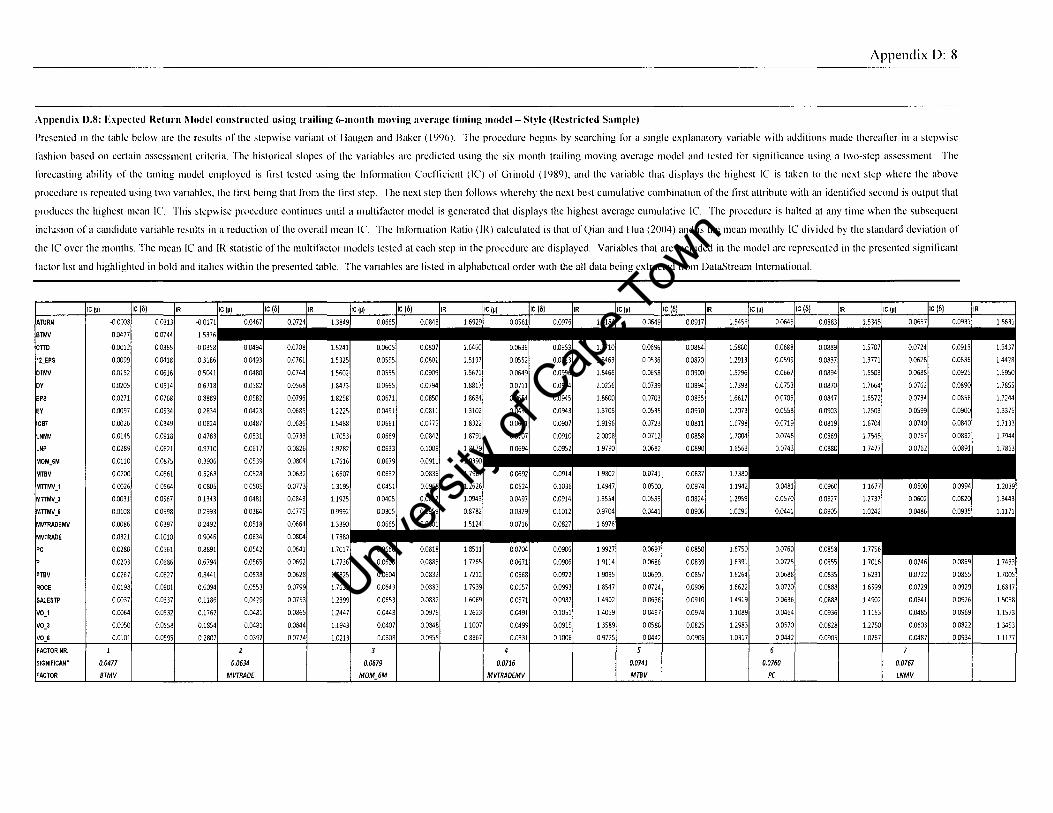
Appendix 0: 8

Appendix D.8: Expected Return l\Iodel constructed using trailing 6-month moving average timing model- Style (Restricted Sample)

Presented in the table below arc the results of the stepwise variant of Ilaugcn and Baker (1996). The procedure begins by searching fllr a single explanatory variable with additions madc thcreafter in a stepwise

lilshion based on certain assessment criteria. The historical slopes of the variables arc prcdieted using the six month trailing moving average model and testcd Illr signilieance using a two-step assessmcnt. The

Illrccasting ability of the timing model cmployed is lirst tested using thc Inlllrlnation Coefficient (IC) of Grinold (1989), and the variable that displays the highest IC is taken to the next stcp where the above

procedure is repeated using two variables. the lirst being that Irom the lirst step. The next step then follows whereby the next best cumulative combination of the lirst attributc with an identified second is output that

produces the highest mean Ie. This stepwise procedure continues until a multinlctor model is generated that displays the highest average cumulative Ie. The procedure is halted at any time when the subsequent

inclusion of a candidate variable results in a reduction of the overall mean Ie. Thc Information Ratio OR) calculated is that of Qian and Ilua (2004) and is the mean monthly IC divided by the standard deviation of

the IC over the months. The mean IC and IR statistic of the multi factor models tested at each step in the procedure arc displayed. Variables that are included in the model are represented in the presented significant

lilctor list and highlighted in bold and italics within the presented table. The variables are listed in alphabetical order with the all data being extracted from DataStream International.

Univers

ity of

Cap

e Tow

n

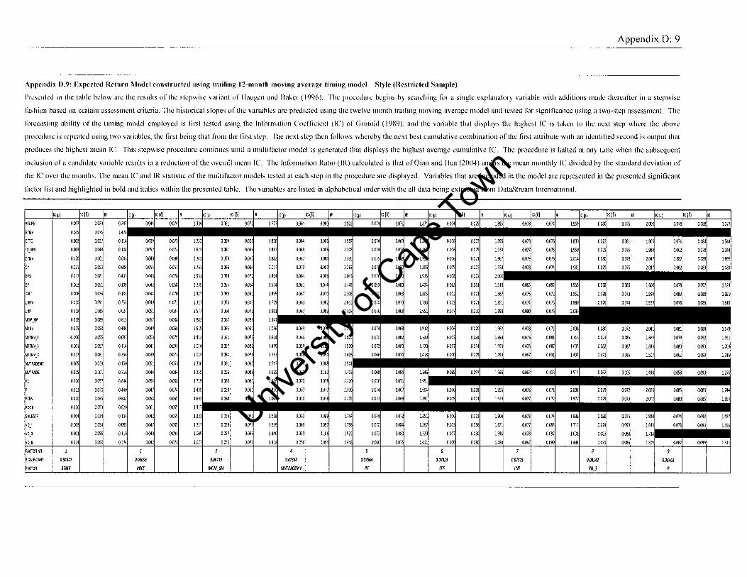
Appendix D: 9

Appendix D.9: Expected Return Model constructed using trailing 12-month moving average timing model- Style (Restricted Sample)

Presented in the table below are the results of the stepwise variant of Ilaugen and Baker (1996). The procedure begins by searching for a single explanatory variable with additions made thereafter in a stepwise

filshion based on certain assessment criteria. The historical slopes of the variables arc predicted using the twelve month trailing moving average model and tested for significance using a two-step assessment. The

forecasting ability of the timing model employed is first tested using the Information Coefficient (Ie) of Grinold (1989), and the variable that displays the highest Ie is taken to the next step where the above

procedure is repeated using two variables, the first being that from the lirst step. The next step then Illllows whereby the next best cumulative combination of the first attribute with an identified second is output that

produces the highest mean Ie. This stepwise procedure continues until a multif~lctor model is generated that displays the highest average cumulative Ie. The procedure is halted at any time when the subsequent

inclusion ofa candidate variable results in a reduction of the overall mean Ie. The Information Ratio (IR) calculated is that ofQian and IIua (2004) and is the mean monthly Ie divided by the standard deviation of

the Ie over the months. The mean Ie and IR statistic of the multifaetor models tested at each step in the procedure arc displayed. Variables that arc included in the model are represented in the presented significant

factor list and highlighted in bold and italics within the presented table. The variables arc listed in alphabetical order with the all data being extracted from DataStream International.

Univers

ity of

Cap

e Tow

n

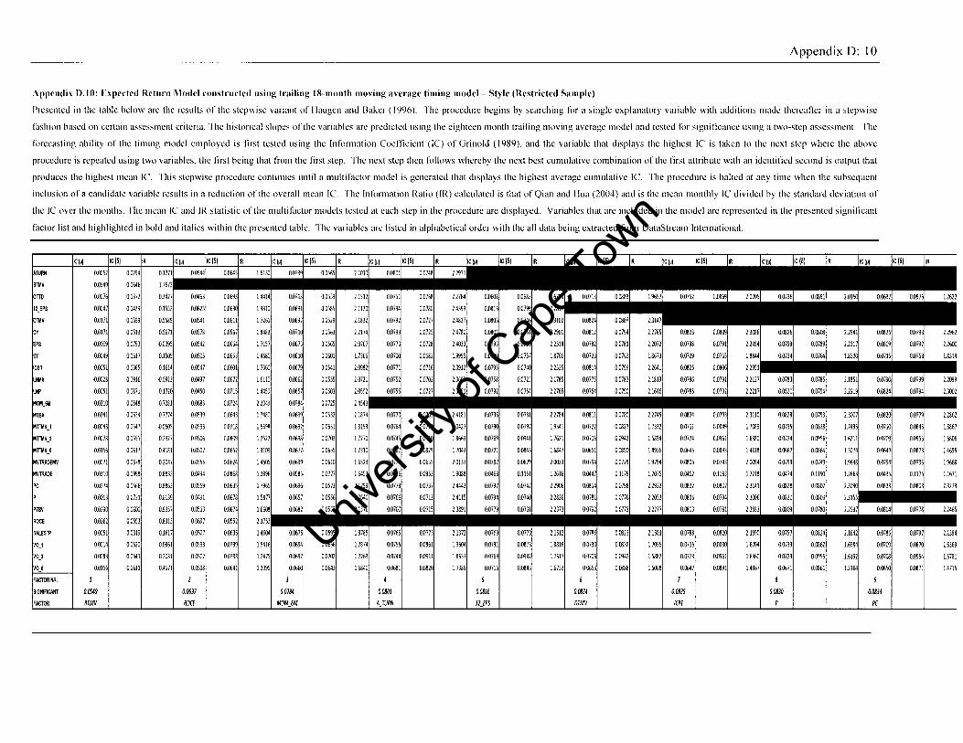
Appendix D: 10

Appendix D.IO: Expel'led Return I\lodrll'onstructed using trailing HI-month moving average timing modcl- Style (Restricted Sample)

Presented in the table below are the results of the stepwise variant of lIaugen and Baker (1996). The procedure begins by searching for a single explanatory variable with additions made therealkr in a stepwise

fashion based on certain assessment criteria. The historical slopes of the variables arc predicted using the eightcen month trailing moving average model and tested for signilicance using a two-step assessmcnt. Thc

1()recasting ability of the timing model employed is lirst tcsted using thc Inl"lJrmation Coeflicient (IC) of Grinold (1989), and the variable that displays the highest Ie is taken to thc next step where the abovc

procedure is repeated using two variables, the !irst being thatl[om the lirst step. The next step then 1"l)lIows whereby the next best cumulative combination of the !irst attribute with an identilied sccond is output that

produces the highcstl1lean Ie. This stepwisc proccdurc continues until a l1Iultifactor 11I0del is generated that displays the highest average cUl1lulative IC. The procedure is halted at any til1le when the subsequent

inclusion ofa candidate variable results in a reduction of the overalll1lean Ie. The Inl"lJr1nation Ratio (IR) calculated is that ofQian and lIua (2004) and is the meanl1lonthly IC divided by the standard deviation of

the IC over the 11I0nths. The mean IC and IR statistic of the multi factor models tested at each step in the procedure arc displayed. Variables that arc included in the model arc represented in the presented signilicant

factor list and highlighted in bold and italics within the presented table. The variables arc listed in alphabetical order with the all data being extracted 1[0111 DataStream International.

0.0549

81MV

0.0697

ROCE

0.0784

MOMJM

0.0816

11)P5

0.0814

DIMV

0.0815

IC81

0.0830 0.0833

PC

18319

2.2099

23002

2.2862

1.6867

15806

1.4695

1.9668

1.1671

2.1394

1.6369

1.5781

14715

Univers

ity of

Cap

e Tow

n

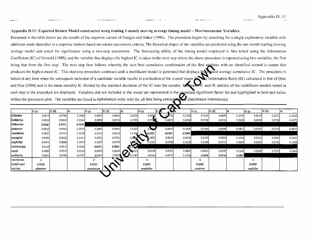
Appendix 0: II

Appendix D.II: Expected Return Model constructed using trailing I-month moving average timing model- Macroeconomic Variables

Presented in the table below are the results of the stepwise variant of Haugen and Baker (1996). The procedure begins by searching for a single explanatory variable with

additions made thereafter in a stepwise fashion based on certain assessment criteria. The historical slopes of the variables are predicted using the one month trailing moving

average model and tested for significance using a two-step assessment. The forecasting ability of the timing model employed is first tested using the Information

Coefficient (IC) of Grinold (1989), and the variable that displays the highest IC is taken to the next step where the above procedure is repeated using two variables, the first

being that from the first step. The next step then follows whereby the next best cumulative combination of the first attribute with an identified second is output that

produces the highest mean Ie. This stepwise procedure continues until a multifactor model is generated that displays the highest average cumulative Ie. The procedure is

halted at any time when the subsequent inclusion ofa candidate variable results in a reduction of the overall mean Ie. The Information Ratio OR) calculated is that ofQian

and Hua (2004) and is the mean monthly IC divided by the standard deviation of the IC over the months. The mean IC and IR statistic of the multifactor models tested at

each step in the procedure are displayed. Variables that are included in the model are represented in the presented significant factor list and highlighted in bold and italics

within the presented table. The variables are listed in alphabetical order with the all data being extracted from DataStream International

0.0721

0.0543

0.0711 0.0131

0.0520 0.0021

0.0686 0.0137

0.0541 0.0151

0.0533 0.0028

·0.0032 0.0784 0.0065

2

0.0126 0.0151

oi/brentcr usmonsupp

0.2287

0.0201

randdollar

0.0757 0.0206

4

0.0206

usshrtrm

0.0202

usgltlOyr

Univers

ity of

Cap

e Tow

n

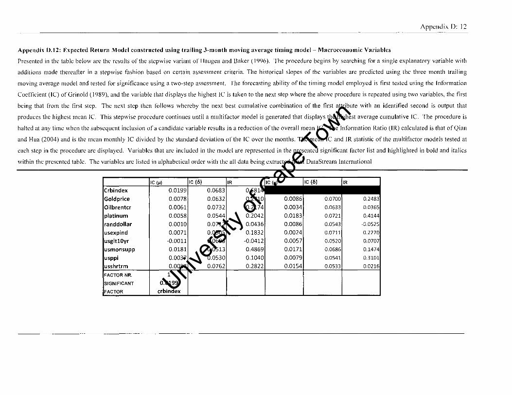
Appendix 0: 12

Appendix 0.12: Expected Return Model constructed using trailing 3-month moving average timing model- Macroeconomic Variables

Presented in the table below are the results of the stepwise variant of Haugen and Baker (1996). The procedure begins by searching for a single explanatory variable with

additions made thereafter in a stepwise fashion based on certain assessment criteria. The historical slopes of the variables are predicted using the three month trailing

moving average model and tested for significance using a two-step assessment. The forecasting ability of the timing model employed is first tested using the Information

Coefficient (IC) of Grinold (1989), and the variable that displays the highest IC is taken to the next step where the above procedure is repeated using two variables, the first

being that from the first step. The next step then follows whereby the next best cumulative combination of the first attribute with an identified second is output that

produces the highest mean Ie. This stepwise procedure continues until a multi factor model is generated that displays the highest average cumulative Ie. The procedure is

halted at any time when the subsequent inclusion ofa candidate variable results in a reduction of the overall mean IC. The Information Ratio (IR) calculated is that ofQian

and Hua (2004) and is the mean monthly IC divided by the standard deviation of the IC over the months. The mean IC and IR statistic of the multifactor models tested at

each step in the procedure are displayed. Variables that are included in the model are represented in the presented significant factor list and highlighted in bold and italics

within the presented table. The variables are listed in alphabetical order with the all data being extracted from DataStream International

Crbindex

Goldprice 0.0078 0.0632

Oilbrentcr 0.0061 0.0732 0.2174 0.0034

platinum 0.0058 0.0544 0.2042 0.0183 0.0721

randdollar 0.0010 0.0712 0.0436 0.0086 0.0543

0.0071 0.0505 0.1832 0.0024 0.0711

-0.0011 0.0693 -0.0412 0.0057 0.0520

0.0181 0.0513 0.4869 0.0171 0.0686

0.0037 0.0530 0.1040 0.0079 0.0541

0.0087 0.0762 0.2822 0.0154 0.0533

1

0.0199 crbindex Univ

ersity

of C

ape T

own

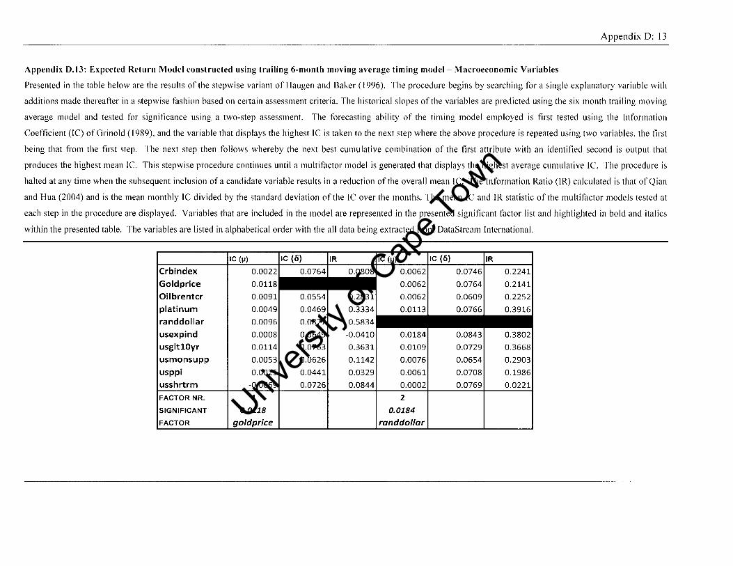
Appendix 0: 13

Appendix D.I3: Expected Return Model constructed using trailing 6-month moving average timing model- Macroeconomic Variables

Presented in the table below arc the results of the stepwise variant of Haugen and Baker (1996). The procedure begins by searching for a single explanatory variable with

additions made thereafter in a stepwise fashion based on certain assessment criteria. The historical slopes of the variables are predicted using the six month trailing moving

average model and tested for significance using a two-step assessment. The forecasting ability of the timing model employed is first tested using the Information

Coefficient (lC) of Grinold (1989), and the variable that displays the highest IC is taken to the next step where the above procedure is repeated using two variables, the first

being that from the first step. The next step then follows whereby the next best cumulative combination of the first attribute with an identified second is output that

produces the highest mean Ie. This stepwise procedure continues until a multi factor model is generated that displays the highest average cumulative Ie. The procedure is

halted at any time when the subsequent inclusion ofa candidate variable results in a reduction of the overall mean Ie. The Information Ratio (lR) calculated is that ofQian

and Hua (2004) and is the mean monthly IC divided by the standard deviation of the IC over the months. The mean IC and IR statistic of the multifactor models tested at

each step in the procedure are displayed. Variables that are included in the model are represented in the presented significant factor list and highlighted in bold and italics

within the presented table. The variables are listed in alphabetical order with the all data being extracted from DataStream International.

Crbindex 0.2241

Goldprice 0.2141

Oilbrentcr 0.2252

platinum 0.0049 0.0469

randdollar 0.0096 0.0877

usexpind 0.0008 0.0649 -0.0410 0.0184 0.0843 0.3802

usgltlOyr 0.0114 0.0763 0.3631 0.0109 0.0729 0.3668

usmonsupp 0.0053 0.0626 0.1142 0.0076 0.0654 0.2903

usppi 0.0025 0.0441 0.0329 0.0061 0.0708 0.1986

usshrtrm -0.0069 0.0726 0.0844 0.0002 0.0769 0.0221

FACTOR NR. 1 2

SIGNIFICANT 0.0118 0.0184

FACTOR randdollar Univ

ersity

of C

ape T

own

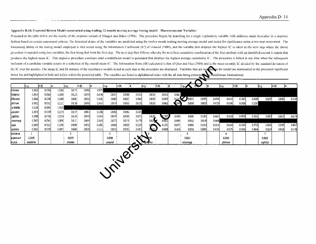
Appendix D: 14

Appl'ndix Dol": Expeeted Heturn Model constructed using trailing 12-month moving aH'rage timing model-l\lacroel°()lwmic Variahles

Presented in the table bdow arc the results of the stepwise variant of Ilaugen and Baker (1996). The procedure begins by searching for a single explanatory variable with additions made thereaficr in a stepwise

I~lshion based on certain assessment criteria. The historical slopes of the variables are prcdidcd using the twelve month trailing moving average model and tested for signilicance using a two-step assessment. The

forecasting ability of thc timing model employed is first tested using the Information Coefficient (lC) of Grinold (1989)0 and the variable that displays the highest IC is taken to the next step where the above

procedure is repeated using two variables, the first being that Irom the first step. The next step then f(lilows whereby the next best cumulative combination of the first attribute with an identilied second is output that

produces the highest mean Ie. This stepwise procedure continues until a multil~ldor model is generated that displays the highest average cumulative Ie. The procedure is haltcd at any time when the subsequent

inclusion of a candidate variable rcsults in a reduction of the overall mean Ie. The Information Ratio (lR) calculated is that of Qian and lIua (2004) and is the mean monthly IC divided by the standard deviation of

the IC over the months. The mcan Ie and IR statistic of the multil~lctor models tested at each step in the procedure are displayed. Variables that are included in the model are represented in the presented signilicant

factor list and highlighted in bold and italics within the presented table. The variables are listed in alphabetical order with the all data being extracted Irom DataStream International.

Univers

ity of

Cap

e Tow

n

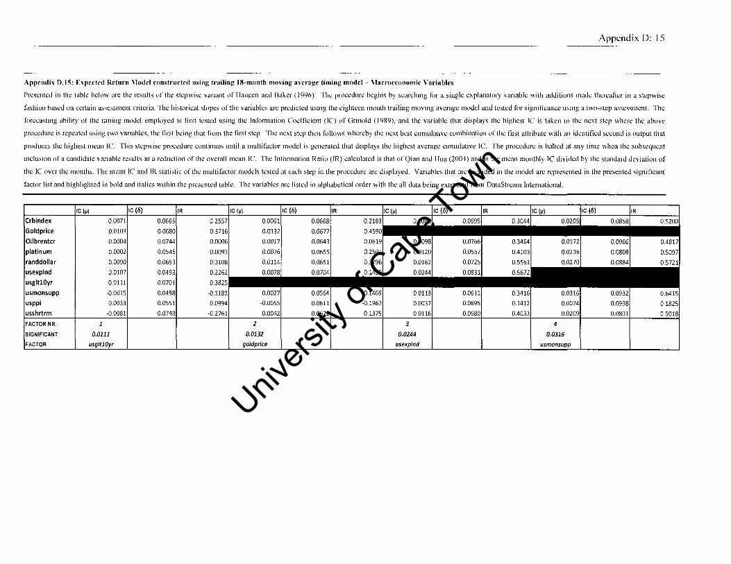
Appendix 0: 15

Appendix D.IS: Expectcd Return Model constructed using trailing 18-month moving average timing model-Macrocconomic Variables

Presented in the table below arc the results of the stepwise variant of Ilaugen and Baker (1996). The procedure begins by searching lix a single explanatory variable with additions made therealler in a stepwise

1~lshion based on certain assessment criteria. The historical slopes of the variables arc predicted using the eighteen month trailing moving average model and tested I(lr signilicance using a two-step assessment. The

I()[ecasting ability of the timing model employed is lirst tested using the Information eoeflicient (Ie) of Grinold (I 'l89), and the variable that displays the highest Ie is taken to the next step where the above

procedure is repeated using two variables, the lirst being that from the tirst step. The next step then I(lliows whereby the next best cumulative combination of the tirst attribute with an identilied second is output that

produces the highest mean Ie. This stepwise procedure continues until a multi factor model is generated that displays the highest average cumulative Ie. The procedure is halted at any time when the subsequent

inclusion of a candidate variable results in a reduction of the overall mean Ie. The Information Ratio (IR) calculated is that of Qian and Ilua (2004) and is the mean monthly Ie divided by the standard deviation of

the Ie over the months. The l11ean Ie and IR statistic of the multi factor models tested at each step in the procedure arc displayed. Variables that arc included in the model arc represented in the presented significant

factor list and highlighted in bold and italics within the presented table. The variables are listed in alphabetical order with the all data being extracted from DataStream International.

Oilbrentcr

platinum

randdollar

usexpind

usgltlOyr

usmonsupp

usppi

FACTOR

-0.0015

0.0033

-0.0081

0.0111

usgltlOyr

2

0.0132

goldprice

3

0.0244

usexpind

0.0766

0.0557

0.0725

0.0831

0.0611

0.0695

0.0680

4

0.0316

usmonsupp

0.0801

0.1825

0.5018

Univers

ity of

Cap

e Tow

n

Appendix 0: 16

Appendix D.16: Expected Return I\lodcl constructed usinJ!; trailinJ!; I-month movinJ!; average timing model- Style and Macroeconomic Variables

Presented in the table below are the results of the stepwise variant of Ilaugen and Baker (1996). The procedure begins by searching for a single explanatory variable with additions made therealler in a stepwise

fashion based on certain assessment criteria. The historical slopes of the variables are predicted using the one month trailing moving average model and tested for significance using a two-step assessment. The

Illrecasting ability of the timing model employed is first tested using the Infllrlnation Coeflicient (Ie) of Grinold (1989), and the variable that displays the highest IC is taken to the next step where the above

procedure is repeated using two variables, the first being that Irom the lirst step. The next step then Illilows whereby the next best cumulative combination of the first attribute with ml identified second is output that

produces the highest mean Ie. This stepwise procedure continues until a multi factor model is generated that displays the highest average cumulative Ie. The procedure is halted at any time when the subsequent

inclusion ofa candidate variable results in a reduction of the overalimeanlC. The Inlllrlnation Ratio (lR) calculated is that of Qian and lIua (2004) and is the mean monthly IC divided by the standard deviation of

the Ie over the months. The mean IC and IR statistic of the multi factor models tested at each step in the procedure arc displayed. Variables that are included in the model are represented in the presented significant

factor list and highlighted in bold and italics within the presented table. The variables are listed in alphabetical order with the all data being extracted from DataStream International.

Univers

ity of

Cap

e Tow

n

Appendix D: 17

Appcndix 1).16: (continued) Expcctcdl~eturn I\lodel constructed using trailing I-month moving average timing model- Style and Macrocc()nomic Variables

Presented in the table below arc the results of the stepwisc variant of Ilaugen and Baker (1996) The procedure begins by searching for a singlc explanatory variable with additions made thcreallcr in a stepwise

lilshion bascd on certain assessment criteria. The historical slopes of thc variables arc predicted using the one month trailing moving average model and tcstcd for signilicance using a two-step assessmcnt. Thc

I(lreeasting ability of the timing model employed is lirst tcstcd using the Information Coeflicient (Ie) of Grinold (1989). and the variable that displays the highest IC is taken to the next step where the above

proccdurc is rcpeated using two variables, the lirst being that Irom the lirst step. The next step then Illilows whereby the next best cumulative combination of the tirst attribute with an identilied second is output that

produccs the highest mean Ie. This stepwise procedure continues until a multi factor model is generated that displays the highcst average cumulative Ie. Thc procedurc is halted at any timc when the subsequent

inclusion of a candidate variable rcsults in a reduction of the overall mean Ie. The Information Ratio (IR) calculated is that of Qian and Iiua (2004) and is the mcan monthly Ie divided by the standard deviation of

the Ie over the months. The mean Ie and IR statistic of the multi factor l110dels tcstcd at cach step in the procedure are displayed. Variables that are included in the model are represented in the presented significant

factor list and highlighted in bold and italics within the presented table. The variables are listed in alphabetical order with the all data being extracted frol11 DataStreal11 International.

Univers

ity of

Cap

e Tow

n

Appendix 0: 18

Appendix D,17: Expccted Returu i\lodell'onstructed using trailing 3-month moving averagc timing model- Style and i\lacroeconomic Variables

Presented in the table below arc the results of the stepwise variant of Ilaugen and Baker (1996). The procedure begins by searching for a single explanatory variable with additions made therealier in a stepwise

lilshion based on certain assessment criteria. The historical slopes of the variables arc predicted using the three month trailing moving average model and tested for significance using a two-step assessment. The

forecasting ability of the timing model employed is lirst tested using the Information Coenicient (Ie) of Grinold (1989), and the variable that displays the highest IC is taken to the next step where the above

procedure is repeated using two variables, the lirst being that Irom the lirst step. The next step then follows whereby the next best cumulative combination of the lirst attribute with an identilied second is output that

produces the highest mean IC This stepwise procedure continues until a multi factor model is generated that displays the highest average cumulative Ie. The procedure is halted at any time when the subsequent

inelusion ofa candidate variable results in a reduction of the overall mean IC The Information Ratio (IR) calculated is that of Qian and I-iua (2004) and is the mean monthly IC divided by the standard deviation of

the IC over the months. The meanlC and IR statistic of the multi factor models tested at each step in the procedure are displayed. Variables that are ineluded in the model are represented in the presented signilicant

factor list and highlighted in bold and italics within the presented table. The variables are listed in alphabetical order with the all data being extracted Irom DataStream International.

ATURN

BTMV

eTTD

12_EPS

DTMV

DY

EPS

EY

leBT

LNMV

LNP

MOM_6M

MTBV

MTTMV_'

MTTMV_3

MTTMV_6

MVTRAOEMV

MVTRAOE

PC

PTBV

ROCE

SALESTP

vo_, VO_3

VO_6

Crblndex Goldprlce

Oilbrentcr platinum randdollar usexpind usgltlOyr

usmonsupp usppi usshrtrm

FACTOR NR.

SIGNIFICANT

FACTOR

Ie (IJ) Ie (6) IR

0.0041 0.0306

0.0469

0.0013

0.0129

0.0077

0.0178

0.0231

0.0028

0.0074

0.0125

0.0351

0.0103

0.0211

0.0102

0.0065

0.0098

0.0090

0.0141

0.0323

0.0231

0.0260

0.0158

·0.0026

0.0041

0.0089

0.0082

0.0199

0.0078

0.0061

0.0058

0.0010

0.0071

-0.0011

0.0181

0.0037

0.0087

0.0469

BTMV

0.0756

0.0367

0.0448

0.0648

0.0539

0.0801

0.0539

0.0338

0.0932

0.0804

0.0892

0.0568

0.0548

0.0564

0.0588

0.0392

0.1065

0.0546

0.0685

0.0639

0.0610

0.0350

0.0527

0.0553

0.0588

0.0683

0.0632

0.0732

0.0544

0.0712

0.0505

0.0693

0.0513

0.0530

0.0762

IC (.,.) IC (6) IR IC (.,.) IC (6) IR IC M IC (6) IR

0.1351 0.0452 0.0731 1.3275 0.0592 0.0762 1.6889 0.0673 0.0765 1.8922

1.5015 .. 1I1I .... IIII .. II .. IIIIII .... IIIIIIII .. IIII ...... II .... iI .. lI .. iI .. IIII .. II .. IlIlIlIi~ 0.0414

0.4228

0.2659

0.5744

0.7618

0.0822

0.2397

0.4115

1.1943

0.3589

0,6622

0.2807

0.2195

0.2781

0.2666

0.4469

1.0245

0.7815

08170

0.4967

-0.0724

0.1129

0.2833

0.2399

0.6814

0.2710

0.2174

0.2042

0.0436

0.1832

-0.0412

0.4869

0.1040

0.2822

0.0477

0.0515

0.0434

0.0517

0,0576

0.0395

0.0462

0.0436

0.0595

0.0497

0.0497

0.0467

0.0444

0.0317

0.0436

0.0455

0.0492

0.0536

0.0472

0.0606

0.0371

0.0446

0.0447

0.0313

0.0461

0.0448

0.0394

0.0460

0.0369

0.0233

0.0417

0.0432

0.0393

0.0399

0.0606

ROCE

0.0733

0.0712

0.0787

0.0647

0.0765

0.0701

0,0685

0,0878

0.0831

0.0856

0,0669

0.0807

0.0730

0.0834

0.0736

0.0857

0.0670

0.0705

0.0633

0.0755

0.0783

0.0839

0.0729

0.0827

0.0771

0,0716

0.0724

0.0743

0.0798

0.0924

0.0749

0.0763

0.0691

0.0719

1.4695 0.0546 0.0745 1.6653 0.0638 0.0767 1.9219

1.5972 0.0651 0.0709 1.9752 0.0708 0.0758 2.1366

1.4081 0.0567 0.0772 1.7945 0.0637 0.0771 1.9963

1.6460 0.0624 0.0728 1.9404 0.0690 0.0755 2.1360

1.7899 0.0619 0.0769 1.9042 0.0663 0.0716 2.0325

1.1442 0.0497 0.0727 1.4113 0.0550 0.0793 1.5492

1.4707 0.0571 0.0727 1.7665 0.0660 0.0762 2.0192

1.4102 0.0522 0.0823 1.6399 0.0602 0.0802 1.8682

1.8662 0.0686 0.0774 2.1227 "1I1I1I.1I1I1I1I.1I1I"11~ 1.6151 0.0561 0.0899 1.7834 0.0618 0.0869 1.9410

1.5620 0.0597 0.0669 1.8530 0.0657 0.0754 2.0306

1.2104 0.0554 0.0818 1.4426 0.0659 0.0940 1.6866

1.1250 0.0476 0.0775 1.2208 0.0610 0.0890 1.5504

0.8388 0.0382 0.0888 1.0057 0.0557 0.1047 1.3883

1.1115 0.0607 0.0696 1.5220 0.0596 0.0801 1.5145

1.3276 0.0481 0.0864 1.3785 0.0590 0.0853 1.6309

1.5459 0.0625 0.0718 1.9323 0.0676 0,0772 2.0840

1.6793 0.0649 0.0669 1.9879 0.0642 0.0742 1.9947

1.4646"lIlIIio •. o.5.94'lIlIlo .• 06.6.5.IIII'.·8.2.5.0 .lIlIIio.o.64i4'lIlIiio .• 07.4.9.IIII'.·9ii8.0.3 1.8940,.

1.0532 0.0511 0,0776 1.4388 0.0603

1.1582 0.0503 0.0855 1.2898 0.0625

1.1335 0.0477 0.0768 1.2275 0.0611

0.8283 0.0379 0.0886 0.9998 0.0554

1.4744 0.0625 0,0756 1.9294 0.0681

1.4323 0.0574 0.0770 1.7884 0.0661

1.2722 0.0543 0.0751 1.6985 0.0639

1.4708 0.0594 0.0746 1.8519 0.0667

1.2036 0.0528 0.0736 1.6474 0.0616

0.7318 0.0445 0.0976 1.0869 0.0617

1.3303 0.0570 0.0749 1.7625 0.0643

1.2851 0.0622 0.0770 1.7286 0.0715

1.1414 0.0533 0.0745 1.4940 0.0616

1.2791 0.0516 0.0731 1.6135 0,0597

0.0686

LNP

0.0715

usmonsupp

0.0802

0.0960

0.0885

0.1046

0.0793

0.0782

0.0784

0.0784

0.0757

0.0988

0.0775

0.0776

0.0767

0.0782

1.6743

1.5825

1.5556

1.3823

2.0880

2,0310

1.9687

2.0601

1.8934

1.3760

1.9755

1.9668

1.6810

1.8449

Univers

ity of

Cap

e Tow

n

Appendix 0: 19

Appendix D.18: Expected Return Model constructed using trailing 6·month moving average timing model- Stylc and Mauocconomic Variablcs

Prescntcd in thc table below ure the results of thc stepwisc variunt of Ilaugen and l3akcr (1996). Thc procedurc begins by searching for a single explanatory variablc with additions madc therealler in a stepwise

fashion bascd on certain assessment critcria. The historical slopes of the variables arc predictcd using the six month trailing moving avcrage model and tested for significance using a two-step assessment. The

f()recasting ability of thc timing model employed is first testcd using the Information Cocflicicnt (lC) of Grinold (1989). and thc variablc that displays the highest IC is taken to the ncxt step where the above

proeedurc is repeated using two variablcs, thc first being that from the first step. The next stcp thcn f()llows whereby the next best cumulative combination of the first attributc with an identified second is output that

produces the highest mean Ie. This stcpwisc proccdurc continues until a multif~lctor model is gcncrated that displays the highest averagc cumulative Ie. Thc procedurc is halted at any timc whcn the subscqucnt

inclusion ofa candidate variablc results in a reduction ofthc overall mcan IC. The Information Ratio (lR) calculated is that ofQian and llua (2004) and is thc mean monthly IC dividcd by thc standard deviation of

the IC over the months. The mean IC and IR statistic of the multi factor models tested at each step in the procedure arc displayed. Variables that are included in the model are represented in the presented significant

factor list and highlighted in bold and italics within the presented table. The variables are listed in alphabetical order with the all data being extracted from DataStream International.

Univers

ity of

Cap

e Tow

n

Appendix D: 20

Appendix D.19: Expected Return I\lodcl constructed using trailing l2-month moving average timing model- Style and Macroeconomic Variables

Presented in the table below arc the results of the stepwise variant of Ilaugen and Baker (1996). The procedure begins by searching for a single explanatory variable with additions made thereafter in a stepwise

filshion based on certain assessment criteria. The historical slopes of the variables arc predicted using the twelve month trailing moving average model and tested for significance using a two-step assessment. The

forecasting ability of the timing model employed is first tested using the Inf()[Jnation Coefficient (lC) of Grinold (1989), and the variable that displays the highest IC is taken to the next step where the above

procedure is repeated using two variables, the first being that from the first step. The next step then f{)lIows whereby the next best cumulative combination of the first attribute with an identified second is output that

produces the highest mean Ie. This stepwise procedure continues until a multi factor model is generated that displays the highest average cumulative Ie. The procedure is halted at any time when the subsequent

inclusion ofa candidate variable results in a reduction ofthc overall mean Ie. The Information Ratio (lR) calculated is that of Qian and \lua (2004) and is the mcanmonthly IC dividcd by the standard deviation of

the IC over the months. The mean IC and IR statistic of the multifilctor models tested at each step in the procedure are displayed. Variables that arc included in the model arc represented in the presented significant

factor list and highlighted in bold and italics within the presented table. The variables arc listed in alphabetical order with the all data being extracted from DataStream International.

ATURN

BTMV

CTID 12_EPS

DTMV

DY

EP'

EY

ICST

LNMV

lNP

MOM_8M

MTBV

MTIMV_1

MTTMV_l

MTTMV_6

MVTRAOEMV

MVTRAOE

PC

PTBV

ROCE

SALESTP

VO_1

VO_3

VO_6

Crblndex

Goldprice

Oilbrentcr platinum

randdollar usexpind

usgltlOyr

usmonsupp

usppl

usshrtrm FACTOR NR

SIGNIFICANT

FACTOR

Ie (IJ) Ie (6) IR

0.0074 0.0287

0.0455 0.0755

00034

0.0033

0.0198

00206

0.0123

0.0035

0.0056

0.0104

0.0188

0.0177

0.0149

-0,0055

0,0014

0.0133

0.0053

00248

0.0261

0.0132

0.0199

0.0260

0.0037

-00033

00012

0.0141

0.0062

0.0074

0.0066

0.0031

0.0105

0.0073

0.0080

0.0053

-0.0043

-0.0011

0.0455

BTMV

0.0370

0.0431

0.0612

0.0498

0.0815

0.0510

0.0356

0.0913

00849

00863

0.0581

0.0548

0.0571

0.0606

0.0394

0.1005

0.0573

0.0698

00653

00592

0.0340

00543

0.0564

0.0599

0.0708

0.0661

00748

0.0552

00694

0.0499

0.0706

0.0543

0.0552

0.0729

IC (~) IC (5) IR

0.2473 0.0439 0.0742

1.4783

0.1139

0.1038

0.6457

0.6837

04033

0.1086

0.1829

0.3558

0.6266

0.6153

0.4839

-0.0873

0.1139

03563

0.1502

0.7164

0.8436

0.4396

0.6418

0.8198

0.1141

-0.0848

0.1100

03737

0.2265

0.2605

0.2288

0.1111

0.3525

0.2273

0.2724

0.0899

-0.1705

-0.0457

0.0393

0.0519

0.0400

0.0552

0.0483

0.0424

0.0440

0.0400

0.0505

0.0571

0.0494

0.0534

0.0409

0.0390

0.0513

0.0444

0.0543

0.0471

0.0539

0.0606

00418

0.0467

00405

0.0416

0.0366

0.0456

0.0409

0.0444

0.0441

0.0390

0.0490

0.0466

0.0391

0.0409

0.0606

RDCE

0.0721

0.0732

0.0800

0.0573

0.0784

0.0681

0.0704

0.0727

00866

0.0877

0.0684

0.0748

0.0914

0.0729

0.0633

0.0839

00678

00735

0.0652

0.0646

0.0692

0.0846

0.0910

0.0714

0.0840

00774

0.0852

0.0713

0.0793

0.0856

0.0640

0.0690

0.0711

0.0718

IC (~) IC (6) IR IC (1-1) IC (6) IR ICM IC (6) IR IC (~) IC (6) IR

1.3338 0.0609 00718 1.7772 0.0643 00885 1.9024 0.0743 0.0708 18740 0.0744 0.0751 1.8946

1.2519 0.0595 0.0662 1.8277 0.0642 0.0863 1.9874 0.0738 0.0686 1.8468 0.0759 0.0716 1.8964

1.6228 0.0611 0.0656 1.8866 0.0682 0.0862 2.1283 0.0738 0.0730 1.8684 0.0763 0.0755 1.9304

1.3414 0.0588 0.0650 1.8816 0.0666 0.0845 2.1352 0.0751 0.0683 1.9393 0.0763 0.0709 1.9673

1.7608 0.0663 0.0645 2.0774 0.0719 0.0818 2.2666 0.0732 0.0699 1.8860 0.0749 0.0725 1.9303

1.5312 0.0580 0.0722 1.8235 0.0641 0.0880 2.0433 0.0756 0.0701 1.9345 0.0781 0.0714 1.0005

1.2346 0.0550 0.0636 1.5744 0.0606 0.0743 1.7476 0.0593 0.0801 1.4239 0.0632 0.0810 1.5177

1.4268 0.0594 0.0609 1.8550 0.0669 0.0794 2.1062 0.0697 0.0680 1.8054 0.0721 0.0706 1.8671

1.3131 0.0562 0.0651 1.7788 0.0631 0.0818 2.0133 0.0697 0.0698 1.7985 0.0718 0.0713 1.8513

15767 0.0600 0.0719 1.9009 00669 0.0828 2.1375 00756 0.0680 1.9511 0.0775 0.0704 1.9978

18824 0.0672 0.0819 1.1413 •• ~~' •• ~~ •• ~~ •• ~~' •• !Ii~ •• illiiI •• IlliIi!l~ •• ~~ ••• ~~ 1.6154 0.0647 00606 2.0361 00695 0.0778 2.2033 0.0740 0.0679 1.9116 00760 0.0696 1.9623

1.4118 0.0609 0.0734 1.6342 0.0665 0.0883 1.8253 0.0696 0.0819 1.6205 0.0734 0.0843 1.6930

1.0138 0.0572 0.0857 1.4390 0.0593 0.1063 1.5200 0.0733 0.0797 1.5202 0.0768 0.0805 1.5978

1.0132 0.0536 0.0727 1.3931 0.0547 0.0941 1.4255 .... oil·oil6.'8 ••• 0 •. oil7.44 ••• 1114il'~9 ••• D .• 06.9117 ••• oil'ii07.9~3 ••• 111.4ii8.97 1.3363 0.0606 0.0632 1.5474 0.0736 0.0679 1.9007 ~

1.2547 0.0557 0.0890 1.5548 0.0598 0.1024 1.7028 0.0680 0.0937 1.6457 0.0647 0.0971 1.5662

1.7191 0.0648 0.0612 2.0261 0.0703 0.0776 2.2200 0.0756 0.0707 1.9506 ••••••• l1li ••••• 14901 0.0588 0.0611 1.8562 0.0672 0.0772 2.1362 0.0737 0.0665 1.9037 0.0758 0.0692 1.9559

1.6917 .... 0 •. 0.6ii3~9 •• lIo •. oii6.27 ••• , •. OjjjO'ii, ••• 0 .• 06.9.8 ••• 0 •. 0.7.84, •• '.'.04.' ••• 0.0.73.' ••• 0 .• 06.8.9 ••• 1.8.9.06, •• 0 •. 0.7.49 ••• 0 •. 0.70.7 ••• 1..9'ii8.7 1.9169 11 1.2206 0.0535 00719 15380 0.0602 0.0893 1.7438 0.0742 0.0717 1.8515 0.0763 0.0728 1.9042

1.2167 0.0592 0.0755 1.5594 00651 0.0968 1.7358 0.0697 0.0835 1.5666 0.0727 0.0859 1.6215

1.0048 0.0572 0.0856 1.4398 0.0593 01062 1.5219 0.0732 0.0797 1.5196 0.0767 0.0805 1.5963

1.0770 0.0546 0.0733 1.4179 0.0556 0.0936 1.4481 0.0657 00747 1.4106 0.0697 0.0796 1.4883

1.2145 00562 0.0690 1.7841 0.0617 0.0900 1.9717 0.0719 0.0704 1.8415 0.0719 0.0749 1.8616

1.4853 0.0607 0.0685 1.9100 0.0669 0.0850 2.1222 0.0737 00681 1.8899 0.0759 0.0711 1.9453

1.3308 0.0579 0.0680 1.8171 0.0651 0.0843 2.0617 0.0708 0.0694 1.8167 0.0728 0.0716 1.8661

1.4476 0.0596 0.0638 1.8745 0.0671 0.0795 2.1231 0.0718 0.0653 1.8405 0.0715 0.0707 1.8546

1.4551 0.0621 0.0665 1.9461 0.0684 0.0837 2.1623 0.0752 00693 1.9217 0.0770 0.0726 1.9681

1.0567 0.0475 0.0858 1.2650 0.0557 0.1120 1.4817 0.0612 01081 1.3752 0.0585 0.1058 1.3727

1.5811 0.0625 0.0636 19609 0.0697 0.0816 2.1957 0.0736 0.0686 18899 0.0757 0.0713 1.9415

1.4048 0.0498 0.0736 1.4638 0.0503 0.0976 1.5562 0.0495 0.0889 13240 0.0513 0.0910 1.3680

1.1499 0.0564 0.0682 1.6095 0.0667 0.0815 1.9141 0.0656 0.0782 1.5933 0.0677 0.0794 1.6416

1.3460 0.0595 0.0635 1.8757 0.0660 0.0833 2.0996 0.0732 0.0674 1.8787 0.0752 0.0709 1.9289

3 5

0.0671 0.0736 0.0756

MOM 6M MVTRADfMV PC

0.0781

fPS

Univers

ity of

Cap

e Tow

n

Appendix 0: 21

Appendix 1>.19 (continued) Expected Return Model constructed usin!: trailin!: 12-month movin!: average timin!: model- Style and Macroeconomic Variables

Presented in the table below arc the results of the stepwise variant of Ilaugen and Baker (1996). The procedure begins by searching for a single explanatory variable with additions made therealler in a stepwise

1;lshion based on certain assessment criteria. The historical slopes of the variables arc predicted using the twelvc month trailing moving average model and tested 1()r signilicance using a two-step assessment. The

1()recasting ability of the timing model employed is tirst tested using the Information Coefticient (IC) of Grinold (1989), and the variable that displays the highest IC is taken to the next step where the above

procedure is repeated using two variables, the lirst being that l[om the lirst step. The next step then liJllows whereby the next best cumulative combination of the lirst attribute with an identified second is output that

produces the highest mean Ie. This stepwise procedure continues until a l11ultifactor model is generated that displays the highest average cumulative Ie. The procedure is halted at any time when the subsequent

inclusion ofa candidate variable results in a reduction of the overallmcan Ie. The Information Ratio (lR) calculated is that ofQian and !lua (2004) and is the mean monthly IC divided by the standard deviation of

the IC over the months. The mean IC and IR statistic of the multi factor models tested at eaeh step in the procedure arc displayed. Variables that are included in the model are represented in the presented significant

factor list and highlighted in bold and italics within the presented table. The variables are listed in alphabetical order with the all data being extracted from DataStream International.

0.0798

lIVP

0.0834 0.0846

P

0.0858

Goldpricf!

0.0862

usgftlOyr

Univers

ity of

Cap

e Tow

n

Appendix 0: 22

Appendix 1).20 Expected Retnrn I\lodel constrncted IIsing trailing IS-month moving average timing modcl- Style and l\Iacroeconomic Variahles

Presented in the table below arc the results of the stepwise variant of I [augen and Baker (1996). The procedure begins by searching [()r a single explanatory variable with additions made therealter in a stepwise

fashion based on certain assessment criteria. The historical slopes of the variables arc predicted using the eigtheen month trailing moving average model and tested for significance using a two-step assessment. The

[()recasting ability of the timing model employed is first tested using the In[()[Ination Coefficient (lC) of Grinold (1989). and the variable that displays the highest IC is taken to the next step where the above

procedure is repeated using two variables, the first being that [rom the first step. The next step then follows whereby the next best cumulative comhination of the first attribute with an identified second is output that

produces the highest mean IC This stepwise procedure continues until a multi[~lctor model is generated that displays the highest average cumulative Ie. The procedure is halted at any time when the subsequent

inclusion of a candidate variahle results in a reduction of the overall mean IC The In[()[I1Jation Ratio (IR) calculated is that of Qian and I [ua (2004) and is the mean monthly [e divided by the standard deviation of

the [e over the months. The mean [e and IR statistic of the mu[tifaetor models tested at each step in the procedure arc displayed. Variables that are included in the model arc represented in the presented significant

factor list and highlighted in bold and ita[ies within the presented table. The variables arc listed in a[phabetiea[ order with the all data being extracted from DataStream International.

Univers

ity of

Cap

e Tow

n

Appendix D: 23

Appendix D.20 (continued) Expected Return Model constructed usinl: trailinl: IS-month moving average timing modcl- Style and Macroeconomic Variables

Presented in the table below arc the rcsults of the stepwise variant of Ilaugen and Baker (1996). The procedure begins by searching Illr a single explanatory variable with additions made thereallcr in a stepwise

lilshion based on certain assessment criteria. The historical slopes of the variables arc predicted using the eigthecn month trailing moving average model and tested lilr significance using a two-step assessment. The

lilrecasting ability of the timing model employed is first tested using the Inlllrlnation Coerticient (IC) of Grinold (1989), and the variable that displays the highest Ie is taken to the next step where the above

procedure is repeated using two variables, the lirst being thatlrom the lirst step. The next step then Illllows whereby the next best cumulative combination ofthc tirst attribute with an identified second is output that

produces the highest mean Ie. This stepwise procedure continues until a multitilctor model is generated that displays the highest average cumulative Ie. Thc procedure is halted at any time when the subsequent

inclusion of a candidate variable results in a reduction of the overall mean Ie. The Intllrlnation Ratio (lR) calculated is that of Qian and Hua (2004) and is the mean monthly IC divided by the standard deviation of

the IC over the months. The mean IC and IR statistic of the multi factor models tested at each step in the procedure arc displayed. Variables that arc included in the model arc represented in the presented significant

factor list and highlighted in bold and italics within the presented table. The variables arc listed in alphabetical order with the all data being extracted from DataStream International.

Ie (~I Ie t6) IR Ie (1-11 Ie (6) IR rC(1-I1 Ie (6) IR ICIIl) Ie (6) IR Ie (1-11 Ie (6) IR Ie (6) IR

_~ _______ -.J ___ ~-.mm_..mm~-.m~~_

0.0837

Oilbr~ntcr

0.0847

DTMV

0.0852

PC

0.0858

MTBV

0.0866 0.0871

DY

Univers

ity of

Cap

e Tow

n

Appendix D: 24

Appendix D.20 (continued) Expected Return l\Iodel constructed usinl( trailinl( IS-month movinl( averal(e timing model- Style and l\Iacroeconomic Variables

Presented in the table below arc the results of the stepwise variant of Ilaugen and Ilaker (1996). The procedure begins by searching for a single explanatory variable with additions made thereafter in a stepwisc

lilshion based on certain assessment criteria. The historical slopes of the variables are predicted using the eigtheen month trailing moving average model and tested I(Jr signilicance using a two-step assessment. The

I(lrecasting ability of the timing model employed is lirst tested using the Inl(mnation Coenicient (Ie) of Grinold (1989). and the variable that displays the highest Ie is taken to the next step whcre the above

procedure is repeated using two variables. thc lirst being that Irom thc lirst stcp. The next step then follows whereby the ncxt best cumulative combination of the first attribute with an identified second is output that

produces the highest mcan Ie. This stcpwise procedure continues until a multifaetor model is gencrated that displays the highcst average cumulative Ie. Thc procedure is haltcd at any time whcn the subsequcnt

inclusion ofa candidate variable results in a reduction of the overall mean Ie. The Information Ratio (lR) calculated is that ofQian and lIua (2004) and is the mcanmonthly Ie divided by the standard deviation of

the Ie over the months. The mean IC and IR statistic of the multifactor models tested at each stcp in the procedure are displayed. Variables that arc included in the model are represented in the presented signiticant

factor list and highlighted in bold and italics within the prcsented tablc. The variables are listed in alphabetical order with the all data being extracted from DataStream International.

Univers

ity of

Cap

e Tow

n