Thesis (Mohsen Yoosefzadeh Najafabadi) - The Atrium

Using Advanced Proximal Sensing and Genotyping Tools Combined

with Bigdata Analysis Methods to Improve Soybean Yield

By

Mohsen Yoosefzadeh Najafabadi

A Thesis

Presented to

The University of Guelph

In partial fulfillment of requirements

for the degree of

Doctor of Philosophy

In

Plant Agriculture

Guelph, Ontario, Canada

© Mohsen Yoosefzadeh Najafabadi, July, 2021

ABSTRACT

USING ADVANCED PROXIMAL SENSING AND GENOTYPING TOOLS COMBINED WITH BIGDATA ANALYSIS METHODS TO IMPROVE SOYBEAN YIELD

Mohsen Yoosefzadeh Najafabadi Advisor:

University of Guelph, 2021 Dr. Milad Eskandari

Improving yield potential in major food-grade crops such as soybean (Glycine max L.) is

the most sustainable way to address the growing global food demand and its security

concerns. Selections for high-yielding cultivars have been mainly focused on the yield

performance per se but not necessarily on secondary related-traits associated with yield.

Recent substantial advances in proximal sensing have provided plant breeders with

affordable and efficient tools for evaluating a large number of genotypes for important

agronomic traits, including yield, at early growth stages. Nevertheless, the implementation

of large datasets generated by proximal sensing such as hyperspectral reflectance in

cultivar development programs is still challenging due to the essential need for intensive

knowledge in computational and statistical analyses. Therefore, this thesis was aimed to:

(1) investigate the potential use of soybean hyperspectral reflectance, hyperspectral

reflectance indices (HVI), and yield components such as number of nodes (NP), number

of non-reproductive nodes (NRNP), number of reproductive nodes (RNP), and number of

pods (PP) per plant for predicting the final seed yield using different machine learning

(ML) algorithms, (2) select the top-ranking hyperspectral reflectance and HVI in predicting

soybean yield and fresh biomass (FBIO) using recursive feature elimination (RFE)

strategy, (3) implement genetic optimization algorithm and the improved version of the

strength Pareto evolutionary algorithm 2 (SPEA2) to optimize yield components and HVI

for maximizing soybean seed yield and FBIO, and (4) study the genetics of soybean yield

and its secondary related-traits in order to discover genomic regions underlying the traits

by using genome-wide association study (GWAS). In this study, different ML algorithms

such as ensemble stacking (E-S), ensemble bagging (EB), and deep neural network

(DNN) were tested to evaluate their efficiency in predicting soybean yield and FBIO

production using a panel of 250 genotypes evaluated in four environments. Also, for the

first time, we implemented ML algorithms in GWAS to detect the associated QTL with

soybean yield components. The results of this study may provide a perspective for

geneticists and breeders regarding the use of ML algorithms in phenomics and genomics

that will result in the selection of superior soybean genotypes.

iv

DEDICATION

To the soul of my grandfather,

HeidarAli Yoosefzadeh Najafabadi

and

Mohammad Ghorbani

v

ACKNOWLEDGEMENTS

It is a huge genuine pleasure to express my sincere appreciation to my advisor, Dr. Milad

Eskandari, for accepting me as a student to pursue a Ph.D. degree at the University of Guelph. I

appreciated all support and help that I received from Dr. Milad Eskandari during my Ph.D.

Also, I would like to thank my advisory committee: Dr. Istvan Rajcan, Dr. Dan Tulpan, Dr. Hugh

Earl, and Dr. John Sulik, for their contribution to my project development and throughout my

studies. I would like to acknowledge the technical assistance of Dr. Sepideh Torabi, Mr. Bryan

Stirling, Mr. John Kobler, Mr. Robert Brandt, and all the soybean breeding crew at the University

of Guelph, Ridgetown Campus. Thanks to the University of Guelph, Grain Farmers of Ontario,

and SeCan for their financial support to this project.

I would like to thank my examination committee: Dr. Zenglu Li, Dr. Helen Booker, Dr. John Cline,

Dr. Istvan Rajcan, and Dr. Milad Eskandari, for their careful consideration of this thesis and their

inputs on my work

Special thanks to my friends, Dr. Davoud Torkamaneh, Dr. Soren Seifi, and Dr. Mohsen Hesami,

for their support and help during my Ph.D. I cannot imagine myself without their help in all aspects

of my life.

Finally, very special thanks to my family, especially my partner, Maryam Vazin, for giving me all

courage and love to accomplish my Ph.D. journey. My dear family, none of those steps would

have been possible without your help and support. Thank you for your patience and

understanding.

vi

TABLE OF CONTENTS

Abstract ....................................................................................................................... ii

Dedication ...................................................................................................................iv

Acknowledgements .................................................................................................... v

Table of Contents .......................................................................................................vi

List of Tables............................................................................................................... xi

List of Figures .................................................................................................................... xiii

Chapter 1: Introduction and Literature Review .......................................................... 1

1.1 Introduction ................................................................................................ 1

1.2 Literature Review ..................................................................................... 12

1.2.1 Introduction of soybean ........................................................................ 12

1.2.2 Importance of soybean ..................................................................... 12

1.2.3 Yield enhancement from cultivar development ................................. 13

1.2.4 Yield components ............................................................................. 13

1.2.5 Spectral reflectance .......................................................................... 15

1.2.6 Hyperspectral vegetation indices (HVI) ............................................. 16

1.2.7 Application of HVI for predicting yield ............................................... 18

1.2.8 Measuring other traits through spectral reflectance .......................... 19

1.2.9 Genome-wide association studies (GWAS) ...................................... 20

1.2.10 Conventional Statistical methods used in GWAS ............................. 23

1.2.11 Artificial Intelligence Techniques ...................................................... 34

1.2.12 Optimization algorithm ...................................................................... 35

1.2.13 Application of AI-mediated GWAS analysis in plants ........................ 36

1.2.14 Evaluating thresholds in AI-mediated GWAS analysis ...................... 37

vii

1.3 Thesis Hypothesis and Objectives ........................................................... 40

1.3.1 Hypotheses .......................................................................................... 40

1.3.2 Objectives ......................................................................................... 40

Chapter 2: Application of Machine Learning Algorithms in Plant Breeding: Predicting Yield from Hyperspectral Reflectance in Soybean ........................................................... 42

1.4 Abstract .................................................................................................... 43

1.5 Introduction .............................................................................................. 44

1.6 Materials and Methods............................................................................. 49

1.6.1 Experimental locations and plant materials ...................................... 49

1.6.2 Phenotypic evaluations ..................................................................... 50

1.6.3 Data pre-processing and statistical analyses ....................................... 51

1.6.4 Variable selection ................................................................................. 53

1.6.5 Data-driven modeling ........................................................................... 53

1.6.6 Quantification of machine learning performance .................................. 55

1.6.7 Visualizing and analyzing ..................................................................... 56

1.7 Results ..................................................................................................... 56

1.7.1 Yield Statistics and Spectral Profiles .................................................... 56


1.7.3 Growth stage comparison .................................................................... 58

1.7.4 Comparative analysis of the developed models ................................... 58

1.8 Discussion ............................................................................................... 60

1.9 Acknowledgments .................................................................................... 65

Chapter 3: Using Ensemble bagging and Depp Neural Network Algorithms and Evolutionary Optimization Algorithms for Estimating Soybean Yield and Fresh Biomass Using Hyperspectral Vegetation Indices .......................................................................... 88

viii

2.1 Abstract .................................................................................................... 89

2.2 Introduction .............................................................................................. 90

2.3 Materials and Methods............................................................................. 96

2.3.1 Plant Material .................................................................................... 96

2.3.2 Test sites and experimental designs ................................................. 96

2.3.3 Data acquisition .................................................................................... 97

2.3.4 Data pre-processing and statistical analyses ....................................... 98

2.3.5 Hyperspectral vegetation index (HVI) extraction .................................. 99


2.3.7 Yield and FBIO prediction model calibration and validation ............... 100

2.3.8 Optimization process (SPEA2 algorithm) ........................................... 102

2.3.9 Quantification of model performance and error estimations ............... 103

2.4 Results ................................................................................................... 103

2.4.1 Yield, FBIO, and HVI properties ......................................................... 103

2.4.2 Correlation analysis of HVI vs. soybean yield and FBIO .................... 104

2.4.3 Comparative analysis of the EB and DNN algorithms ........................ 105

2.4.4 Variable Selection .............................................................................. 105

2.4.5 The DNN-SPEA2 optimization algorithm ............................................ 106

2.5 Discussion ............................................................................................. 106

Chapter 4: Application of Machine Learning and Genetic Optimization Algorithms for Modeling and Optimizing Soybean Yield Using its Component Traits .......................... 137

3.1 Abstract .................................................................................................. 138

3.2 Introduction ............................................................................................ 139

3.3 Material and methods ............................................................................ 145

ix

3.3.1 Plant material and experimental design .......................................... 145

3.3.2 Phenotypic evaluations ...................................................................... 146

3.3.3 Data pre-processing, correlation coefficient, and statistical analyses 146

3.3.4 Data-driven modeling ......................................................................... 147

3.3.5 Optimization process via GA .............................................................. 148

3.3.6 Quantification of model performance and error estimations ............... 149

3.3.7 Visualizing and statistical analyzing ................................................... 150

3.4 Results ................................................................................................... 151

3.4.1 Pearson correlation analyses and individual ML evaluations ............. 151

3.4.2 Model performance and evaluation .................................................... 152

3.4.3 Optimization of the soybean seed yield using E-B-GA ....................... 153

3.5 Discussion ............................................................................................. 153

3.6 Acknowledgments .................................................................................. 158

Chapter 5: Identification of genomic regions underlying soybean yield and its components using conventional and machine learning mediated Genome-Wide Association Studies ......................................................................................................... 184

4.1 Abstract .................................................................................................. 184

4.2 Introduction ............................................................................................ 185

4.3 Materials and Methods........................................................................... 190

4.3.1 Population and experimental design ............................................... 190

4.3.2 Phenotyping .................................................................................... 190

4.3.3 Genotyping ..................................................................................... 191

4.3.4 Statistical analyses ......................................................................... 192

4.3.5 Analysis of population structure ...................................................... 193

4.3.6 Association studies ......................................................................... 193

x

4.3.7 Variable Importance measurement ................................................. 195

4.3.8 Data-driven model processes ......................................................... 195

4.3.9 Functional annotation of candidate SNPs ....................................... 196

4.3.10 Visualization ................................................................................... 196

4.4 Results ................................................................................................... 197

4.4.1 Phenotyping evaluations ................................................................. 197

4.4.2 Genotyping evaluations .................................................................. 197

4.4.3 Population structure and kinship ..................................................... 198

4.4.4 GWAS analysis ............................................................................... 198

4.4.5 Identification of candidate genes within QTL .................................. 201

4.5 Discussion ............................................................................................. 203

Chapter 6: General Discussion and Future Directions .......................................... 237

4.6 General Discussion ................................................................................ 237

4.7 Future Directions ................................................................................... 241

References .............................................................................................................. 244

xi

LIST OF TABLES

Table 1.1 The summary of the most recently published papers on the application of GWAS on different plant species. ............................................................................ 26

Table 1.2 The summary of all published papers on using Artificial Intelligence-mediated Genome-Wide Association Studies (GWAS) analysis in soybean. .......................... 37

Table 2.1. The ID, name, and pedigree of the tested genotypes. ................................. 66

Table 2.2 Combined analyses of variances for yield in the tested population across four environments. ......................................................................................................... .72

Table 2.3 Reflectance band ranking using the Recursive Feature Elimination (RFE) strategy at R4 soybean growth stage. ..................................................................... 74

Table 2.4 Reflectance band ranking using the Recursive Feature Elimination (RFE) strategy at R5 soybean growth stage. ..................................................................... 75

Table 2.5 Confusion matrix based on the performance of RF, MLP, SVM, and Ensemble-Stacking model in predicting the soybean yield using full and selected variables in R5 soybean growth stage.............................................................................................. 76

Table 3.1 Summary of the selected hyperspectral vegetation indices (HVI) used in this study. ..................................................................................................................... 113

Table 3.2 Analysis performance of random forest (RF), radial basis function (RBF), and support vector regression (SVR) algorithms for soybean yield prediction using yield component traits. ................................................................................................... 115

Table 3.3 Analysis performance of random forest (RF), radial basis function (RBF), and support vector regression (SVR) algorithms for soybean fresh biomass (FBIO) prediction using yield component traits. ................................................................. 122

Table 4.1 Analysis performance of Random Forest (RF), Multilayer Perceptron (MLP), and Radial Basis Function (RBF) algorithms, and the Ensemble-Bagging (E-B) strategy for soybean yield prediction using yield component traits such as The number of nodes per plant (NP), number of non-Reproductive nodes per plant (NRNP), number of reproductive nodes per plant (RNP), number of pods per Plant (PP), and ratio of number of pods to number of nodes per plant (P/N). ................................. 159

Table 4.2 Optimizing the number of nodes per plant (NP), number of non-Reproductive nodes per plant (NRNP), number of reproductive nodes per plant (RNP), number of pods per Plant (PP), and ratio of number of pods to number of nodes per plant (P/N) according to the E-B-GA for maximizing soybean seed yield. ............................... 177

xii

Table 5.1 The list of detected QTL for soybean maturity using different GWAS methods in the tested soybean population. .......................................................................... 211

Table 5.2 The list of detected QTL for soybean yield using different GWAS methods in the tested soybean population. .............................................................................. 214

Table 5.3 The list of detected QTL for soybean total number of nodes per plant (NP) using different GWAS methods in the tested soybean population. .................................. 217

Table 5.4 The list of detected QTL for soybean total number of non-reproductive nodes per plant (NRNP) using different GWAS methods in the tested soybean population. .............................................................................................................................. 221

Table 5.5 The list of detected QTL for soybean total number of reproductive nodes per plant (RNP) using different GWAS methods in the tested soybean population. .... 223

Table 5.6 The list of detected QTL for soybean total number of pods per plant (PP) using different GWAS methods in the tested soybean population. .................................. 224

xiii

LIST OF FIGURES

Figure 1.1 The genetic and environmental interaction of secondary traits that are related to the soybean yield. ................................................................................................. 4

Figure 1.2 The scheme of the relationship of yield components and their determining factors. .................................................................................................................... 15

Figure 1.3 The region of each reflectance bands used for constructing HVI. SRa1: Simple ratio (845 nm), SRa2: Simple ratio (905 nm), RARSa: Ratio analysis of reflectance spectra chlorophyll a, NDVI: Normalized difference vegetation index, GNDVI: Green normalized difference vegetation index, RARSc: Ratio analysis of reflectance spectra chlorophyll c, RARSb: Ratio analysis of reflectance spectra chlorophyll b, BNDVI: Blue normalized difference vegetation index, and NPQI: Normalized pheophytinization index ........................................................................................... 17

Figure 1.4 Schematic flowchart of implementing variable importance in AI-mediated GWAS analysis. ...................................................................................................... 39

Figure 2.1 The distribution of soybean genotypes in each yield class. ......................... 78

Figure 2.2 A schematic representation of the machine learning algorithms used in this study to classify the soybean yield using reflectance bands: A) Multilayer Perceptron, B) Support Vector Machine, and D) Random Forest. .............................................. 79

Figure 2.3 The scheme of data collection and machine learning algorithm development and validation. OP: Optimizing parameters; MLP: Multilayer Perceptron; SVM: Support Vector Machine; RF: Random Forest; E-S: Ensemble- stacking strategy. . 80

Figure 2.4 The variation of yield across four environments. ......................................... 81

Figure 2.5 The minimum, mean, and maximum values of each reflectance band were measured for 245 soybean genotypes evaluated at (A) R4 and (B) R5 growth stages at four different field environments. ......................................................................... 82

Figure 2.6 The importance value of selected variables based on the Recursive Feature Elimination (RFE) strategy for soybean reflectance bands measured at R4 (A) and R5 (B) soybean growth stages. ..................................................................................... 83

Figure 2.7 The soybean yield classes vs. the 395 nm reflectance band at R5 growth stages. ..................................................................................................................... 84

Figure 2.8 The accuracy of RF, MLP, SVM, and E-S algorithms for predicting soybean yield using full and RFE selected variables (-VS) measured at R4 (A) and R5 (B) soybean growth stages in four environments. The mean performance was shown as × in each figure. MLP: Multilayer Perceptron; SVM: Support Vector Machine; RF:

xiv

Random Forest; E-S: Ensemble- stacking strategy; RFE: Recursive Feature Elimination. .............................................................................................................. 85

Figure 2.9 Performance and error evaluation of RF, MLP, SVM and E-S model in soybean yield prediction using full and selected reflectance bands from R4 growth stage (VS: variable selection). .................................................................................................. 86

Figure 2.10 Performance of RF, MLP, SVM, and the E-S algorithms for soybean yield prediction using all and selected variables (-VS) from the R5 growth stage. The mean performance is indicated with as × in each figure. MLP: Multilayer Perceptron; SVM: Support Vector Machine; RF: Random Forest; E-S: Ensemble- stacking strategy; RFE: Recursive Feature Elimination. ...................................................................... 87

Figure 3.1 The schematic view of the Deep Neural Network (DNN) algorithm. .......... 129

Figure 3.2 The schematic diagram of the Improved version of the strength Pareto evolutionary algorithms-2 (SPEA2) as multi-objective optimization algorithm. ...... 130

Figure 3.3 The experimental workflow of algorithm selection and validation to predict the soybean fresh biomass (FBIO) and seed yield using hyperspectral vegetation indices (HVI). DNN; deep neural network, EB; ensemble bagging. ................................... 131

Figure 3.4 The variation of A) yield and B) fresh biomass (FBIO) across four environments. ........................................................................................................ 132

Figure 3.5 Pearson correlation analysis of hyperspectral vegetation indices (HVI), soybean seed yield, and fresh biomass (FBIO). The colour coded heatmap scale is provided................................................................................................................. 133

Figure 3.6 Violin plots representing the coefficient of determination (R2), mean absolute errors (MAE), and root mean square error (RMSE) of yield (A, B, and C) and fresh biomass (D, E, and F) performance of the deep neural network (DNN) algorithm and ensemble-bagging (EB) strategy for soybean yield and fresh biomass prediction using hyperspectral vegetation indices (HVI). ................................................................. 134

Figure 3.7 The importance of the tested hyperspectral vegetation indices (HVI) based on the recursive feature elimination (RFE) strategy for predicting soybean seed yield and fresh biomass (FBIO). ........................................................................................... 135

Figure 3.8 Optimized hyperspectral vegetation indices (HVI) values in soybeans with maximized seed yield and fresh biomass (FBIO). ................................................. 136

Figure 4.1 The schematic diagram of the genetic algorithm as the single objective evolutionary optimization algorithm. ...................................................................... 178

xv

Figure 4.2 The experimental workflow of algorithm selection and validation for predicting the soybean seed yield. The number of nodes per plant (NP), number of non-reproductive nodes per plant (NRNP), number of reproductive nodes per plant (RNP), number of pods per plant (PP), ratio of number of Pods to number of Nodes per plant (P/N), and genetic algorithm (GA). ........................................................................ 179

Figure 4.3 Pearson correlation analysis of soybean yield component traits at α=0.05. The number of nodes per plant (NP), number of non-reproductive nodes per plant (NRNP), number of reproductive nodes per plant (RNP), number of pods per plant (PP), and ratio of number of Pods to number of Nodes per plant (P.N). The colour coded heatmap scale is provided. .................................................................................... 180

Figure 4.4 Model training accuracy for Random Forest (RF), Multilayer Perceptron (MLP), and Radial Basis Function (RBF) algorithms by adding variables based on the correlation results. The number of nodes per plant (NP), number of non-reproductive nodes per plant (NRNP), number of reproductive nodes per plant (RNP), number of pods per plant (PP), and ratio of number of Pods to number of Nodes per plant (P/N). .............................................................................................................................. 181

Figure 4.5 (A) coefficient of determination (R2), (B) the Root Mean Square Error (RMSE) and (C) the Mean Absolute Errors (MAE) performance of Random Forest (RF), Multilayer Perceptron (MLP), and Radial Basis Function (RBF) algorithms, and the Ensemble-Bagging (E-B) strategy for soybean yield prediction using yield component traits. The mean performance is indicated with an + sign in each Figure. ............. 182

Figure 4.6 The schematic view of the Radial basis function (RBF) algorithm. ............ 183

Figure 5.1 LD decay distance in the tested 227 soybean genotypes. ........................ 228

Figure 5.2 The distribution of seed yield (A), maturity (B), NP (C), NRNP (D), RNP (E), and PP (F) in 227 soybean genotypes across four environments. The estimated heritability is provided for each of the six traits. RNP: Total number of reproductive nodes per plant, NRNP: The total number of non-reproductive nodes per plant, NP: The total nodes per plant, PP: The total number of pods per plant. ...................... 229

Figure 5.3 The distributions and Pearson correlations among the soybean seed yield, maturity, and yield component traits. RNP: Total number of reproductive nodes per plant, NRNP: The total number of non-reproductive nodes per plant, NP: The total nodes per plant, PP: The total number of pods per plant. The heat map scale for values is provided by colour for the panel. ............................................................ 230

Figure 5.4 Structure and kinship plots for the 227 soybean genotypes. The x-axis is the number of genotypes used in this GWAS panel, and the y axis is the membership of each subgroup. G1-G7 stands for the subpopulation. ........................................... 231

xvi

Figure 5.5 Genome-wide Manhattan plots for GWAS studies of A) maturity and B) seed yield in soybean using MLM, FarmCPU, RF, and SVR methods, from top to bottom, respectively. .......................................................................................................... 232

Figure 5.6 Genome-wide Manhattan plots for GWAS studies of A) the total number of nodes (NP) and B) the total number of non-reproductive nodes (NRNP) in soybean using MLM, FarmCPU, RF, and SVR methods, from top to bottom, respectively. 233

Figure 5.7 Genome-wide Manhattan plots for GWAS studies of A) The total number of reproductive nodes (RNP) and B) the total number of pods (PP) in soybean using MLM, FarmCPU, RF, and SVR methods, from top to bottom, respectively. .......... 234

Figure 5.8 Genome-wide Manhattan plots for GWAS studies of plant height in soybean using MLM, FarmCPU, RF, and SVR methods, from top to bottom, respectively. 235

Figure 5.9 The average effects of reference allele and alternative allele from the detected SNP’s peak for seed yield (A), maturity (B), NP (C), NRNP (D), RNP (E), and PP (F) in 227 soybean genotypes across four environments. RNP: Total number of reproductive nodes per plant, NRNP: The total number of non-reproductive nodes per plant, NP: The total nodes per plant, PP: The total number of pods per plant ....... 236

1

Chapter 1: Introduction and Literature Review

1.1 Introduction

The human population is growing roughly by 1.2% per year, creating a dire need

for increasing the yield production of major crops by more than 50% by 2050 to address

global demand for food security and supplying the needs of over 9 billion people

(Alexandratos and Bruinsma, 2012). Some of the suggested ways for increasing total

yield in major crops, such as soybean (Glycine max L.), are cultivating more lands, better

use of chemical fertilizers and pesticides, and increasing yield potential (Godfray et al.,

2010). Because of the limitation in the availability of farmlands and environmental

concerns associated with using chemical fertilizers and pest and disease controllers,

increasing yield potential is considered as the most reliable and sustainable way of

producing enough food for the fast-growing world’s population (Blaikie and Brookfield,

2015).

Soybean is the world’s most widely grown leguminous crop and an important source

of protein and oil for food and feed (Liu et al., 2008). Soybean is also an important source

of healthy plant-based food products in the human diet with significant health benefits due

mainly to its nutritional and pharmaceutical properties. As a result, global demand for

soybean is increasing significantly. However, the current annual genetic gains in yield

potential are not able to cope with the pace of increasing food demand. One of the main

2

reasons for this steady genetic gain can be inefficient selection criteria used in breeding

programs to select desirable genotypes with increased yield potential.

In general, soybean breeders have used classical phenotypic selection approaches

to evaluate and exploit total seed yield as the main selection criterion for identifying

higher-yielding genotypes. Therefore, over the past several decades, soybean yield has

increased by 21-32 kg per hectare per year (Wilcox 2001). However, genetic gains for

yield were reported to be low, in general, and inconsistent across different environments

(Aparicio et al., 2002). The final seed yield in soybean is the ultimate outcome of the

whole crop growth and development process, in which several morphological and

physiological traits and, therefore, many genes with major and minor effects play

important roles, directly or indirectly (Slafer, 2003). Therefore, one potential way to

increase the genetic gain for yield and facilitate the development of new cultivars with

higher yield potential is to use more efficient selection criteria through analytical breeding

strategies.

An analytical breeding strategy is an alternate breeding approach that focuses on

the improvement of components of complex traits such as plant growth and development

rates and yield components (Richards, 1982a). This strategy can be used for improving

yield potential in a crop by setting selection criteria up on morpho-physiological traits

related to yield and, therefore, make the selection more efficient (Reynolds, 2001). The

limited application of analytical approaches in plant breeding programs for improving yield

3

in major crops have been due partly to lack of or expensive technology to estimate

secondary related traits to yield or limited knowledge about the genetic controls of the

tested traits (Richards, 1982a).

Yield improvements in plants depend on phenology, yield components, adaptive

traits for abiotic and resistance to biotic stresses (Mondal et al., 2016). Yield potential in

soybean can be determined by the following main yield components: the number of nodes

per plant (NP), number of non-reproductive nodes per plant (NRNP), number of

reproductive nodes per plant (RNP), number of pods per plant (PP), and the ratio of

number of pods to number of nodes per plant (P/N) (Pedersen and Lauer, 2004). Seed

size is determined by the rate of seed growth and duration of seed filling, which are mainly

influenced by genetic factors with high heritability (Pedersen and Lauer, 2004). The

number of pods and number of seeds can be regulated by manipulating the crop growth

rate and can be affected by environmental stresses during critical growth stages (He et

al., 2017). Therefore, in order to increase the yield potential in developed cultivars,

improving crop growth rate and minimizing the negative effect of environmental factors

would be of paramount importance (Figure 1.1).

4

Figure 0.1 The genetic and environmental interaction of secondary traits that are related

to the soybean yield.

Measuring yield-related traits in large breeding populations are usually time and

labor-intensive. Therefore, creating and providing researchers with new tools and

techniques to estimate and measure some of these traits in easier and faster ways can

facilitate the breeding process. Spectral reflectance indices (SRI), as one of the high-

throughput phenotyping (HTP) tools, is a new area of research that can be exploited as

an efficient selection tool for improving yield potential and biomass (Araus et al., 2001) in

plant breeding programs. SRI includes a range of formulas, typically based on a sum,

difference, or ratio of two or more wavelengths, that are indicative of important functions

in plant species (Araus et al., 2001; Aparicio et al., 2002; Royo et al., 2003). Spectral

5

reflectance estimated from a canopy is based on this principle that specific traits of a

given plant are associated with the absorption of specific wavelengths of the

electromagnetic spectrum (Ferguson and Rundquist, 2018). Canopy spectral reflectance

is associated with overall leaf area and other photosynthetic components, pigment

composition, and physiological factors of plants (Merlier et al., 2015). Several

physiological parameters, such as environmental stresses, which are more prevailing in

the rainfed area, have also been assessed by spectral reflectance (Araus et al., 2001;

Reynolds, 2001).

The most commonly used hyperspectral vegetation indices (HVI) are the simple

ratio (SR) and normalized difference vegetative index (NDVI) (Araus et al., 2002). Green

biomass, leaf area index, green leaf area index, and a fraction of photosynthetically active

radiation have been reported to be positively correlated with SRI (Wiegand and

Richardson, 1990; Price and Bausch, 1995). Adequate discrimination between high and

low-yielding genotypes of soybeans was reported by using the NDVI (Ma et al., 2001).

According to other studies, Serrano et al. (2000) reported that SR could give a reliable

prediction of wheat yield under different nitrogen levels. Raun et al. (2001) reported that

50% of the yield variability was explained by NDVI in winter wheat under various nitrogen

treatments. Prediction accuracy for grain yield in wheat was increased significantly by

using spectral reflectance indices (Rutkoski et al., 2016b). To conclude, the use of high

throughput phenotyping tools such as HVI can increase the intensity and accuracy of

6

selection as well as response to selections while decreasing phenotyping time and costs

(Muhammed, 2005).

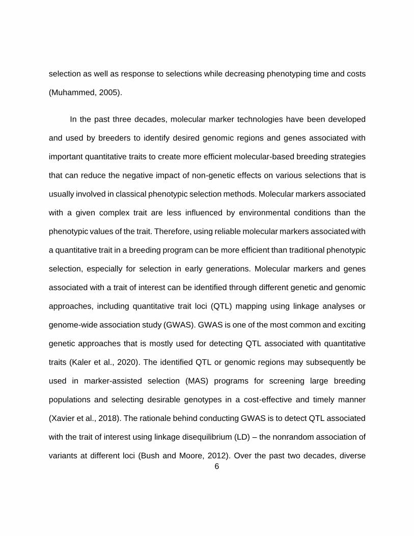
In the past three decades, molecular marker technologies have been developed

and used by breeders to identify desired genomic regions and genes associated with

important quantitative traits to create more efficient molecular-based breeding strategies

that can reduce the negative impact of non-genetic effects on various selections that is

usually involved in classical phenotypic selection methods. Molecular markers associated

with a given complex trait are less influenced by environmental conditions than the

phenotypic values of the trait. Therefore, using reliable molecular markers associated with

a quantitative trait in a breeding program can be more efficient than traditional phenotypic

selection, especially for selection in early generations. Molecular markers and genes

associated with a trait of interest can be identified through different genetic and genomic

approaches, including quantitative trait loci (QTL) mapping using linkage analyses or

genome-wide association study (GWAS). GWAS is one of the most common and exciting

genetic approaches that is mostly used for detecting QTL associated with quantitative

traits (Kaler et al., 2020). The identified QTL or genomic regions may subsequently be

used in marker-assisted selection (MAS) programs for screening large breeding

populations and selecting desirable genotypes in a cost-effective and timely manner

(Xavier et al., 2018). The rationale behind conducting GWAS is to detect QTL associated

with the trait of interest using linkage disequilibrium (LD) – the nonrandom association of

variants at different loci (Bush and Moore, 2012). Over the past two decades, diverse

7

statistical procedures have been developed and used in order to accelerate

computational analyses and improve statistical powers in GWAS in the face of testing

genomewide sets of multiple hypotheses (Tibbs Cortes et al.). These models include, but

are not limited to, the mixed linear model (MLM), multiple loci linear mixed model (MLMM),

compressed mixed linear model (CMLM), enriched compressed mixed linear model

(ECMLM), settlement of MLM under progressively exclusive relationship (SUPER), and

fixed and random model circulating probability unification (FarmCPU) (Tibbs Cortes et al.;

Bush and Moore, 2012). In addition, multiple methods have been proposed for

determining the genome-wide significance levels and thresholds, including the Bonferroni

correction and false discovery rate (FDR) (Bush and Moore, 2012; Kaler et al., 2020). The

application of GWAS was widely studied in different plant species such as: wheat (Eltaher

et al., 2021), maize (Li et al., 2021), soybean (Lin et al., 2020), and sorghum (Somegowda

et al., 2021), and the primary objective of all these studies was to accelerate the breeding

processes using GWAS-derived molecular markers for the indirect selection of superior

genotypes with improved phenotypic values. However, these studies showed that the

successful use of GWAS in uncovering genetic markers governing quantitative traits

relied on selecting appropriate GWAS approaches coupled with accurate experimental

design (Mohammadi et al., 2020).

There are several barriers on the application of conventional statistical methods in

GWAS, using for identifying genomic regions associated with complex traits (Szymczak

et al., 2009). One of the major challenges associated with using the conventional

8

statistical procedures is the “large p, small n” problem that happens in GWAS when these

methods are applied to datasets in which the number of markers (i.e., single nucleotide

polymorphisms (SNPs)) is significantly larger than the number of genotypes (Kaler et al.,

2020; Mohammadi et al., 2020; Xavier and Rainey, 2020). Also, as LD needs to be

considered between a large number of SNPs, conventional statistical methods such as

linear regression may not be well sophisticated for analyzing genome-wide datasets

(Szymczak et al., 2009). It is well documented that current conventional GWAS methods

are only powerful to detect common SNPs with large main effects that can reach the level

of significancy (Lee et al., 2020). Therefore, current conventional GWAS approaches are

underpowered for discovering minor effect SNPs associated with the target traits (Zhou

et al., 2019). Since the successful implementation of GWAS is highly dependent on the

population structure and covariates within the population, using conventional statistical

methods in GWAS requires large and diverse populations in order to detect the QTL with

minor effects (Zhou et al., 2019). Since using very large breeding populations is

expensive in breeding programs, the need for using advanced/sophisticated statistical

models integrated into GWAS is desirable for a better identification of reliable QTL in plant

crops with a narrow genetic basis.

The availability of a large number of plant genetic sequences and phenotyping can

be considered as big data, since they satisfy the following three V’s property: volume,

velocity, and variety. The term big data is referred to the presence of a large dataset that

requires an extensive computational cost to reveal associations, trends, and patterns that

9

may be present in a dataset (Gupta et al., 2020). With the exponential growth of data

using advanced omics-based approaches, efficient analysis of plant datasets using big

data techniques remains a challenge for plant science researchers (Fischer et al., 2020;

Kim et al., 2020b). Efficient analyses of large datasets is significantly dependent on

multiple processes involved in data collection, data processing, and different

management challenges that are identified in the context of big data (Labrinidis and

Jagadish, 2012; Nasser and Tariq, 2015). Data collection and processing challenges

include, but are not limited to, various factors such as volume, variety, velocity, veracity,

volatility, quality, discovery, and dogmatism (Nasser and Tariq, 2015; Al-Abassi et al.,

2020). Therefore, dealing with big datasets such as high-density SNP arrays in GWAS or

hyperspectral reflectance data requires intensive computation and the use of flexible and

efficient mathematical approaches such as artificial intelligence algorithms.

Artificial intelligence (AI) refers to the application of computer technologies to build

intelligent models with minimal human intervention (Hamet and Tremblay, 2017). AI is

broadly used in different areas such as medicine (Topol, 2020), engineering (Sha et al.,

2020), environmental science (Maganathan et al., 2020), and social science (Edelmann

et al., 2020). Recently, in the context of plant science, large investments have been made

for using AI technologies, such as machine learning (ML) algorithms (Correia et al., 2020).

ML is a subset of AI that can be defined as the development of mathematical models that

can learn and educate themselves using available datasets and make decisions

(Alpaydin, 2020). The application of ML algorithms can be considered as an alternative

10

approach to current conventional statistical procedures for analyzing SNP markers in a

data-driven manner. In general, ML algorithms are divided into three main categories:

supervised, unsupervised, and reinforcement learning (Zhang, 2020), which can be used

for analyzing different datasets. Supervised machine learning algorithms can be

employed with labeled datasets, while unsupervised learning algorithms are used to

observe patterns present in unlabeled datasets (Butler et al., 2018).

Regarding the application of different ML algorithms in the area of plant science,

supervised learning methods have drawn the most attention due to the availability of

labeled datasets such as phenotypic data for traits of interest (Chandra et al., 2020). The

development of the predictive classification models using supervised learning algorithms

involves the following five main steps: (a) the determination of the source, type, quality,

and quantity of input training data from an appropriate database (Zhang, 2020), (b) the

use of appropriate feature extraction methods to represent the input data, (c) the training

of the predictive models, (d) the evaluation of the predictive performance on the test

dataset, and (e) the investigation of the importance of features selected for the target trait

(Chandra et al., 2020; Zhang, 2020). The successful use of different ML algorithms for

analyzing high-throughput data was reported in different areas of plant sciences such as

breeding (Yoosefzadeh-Najafabadi et al., 2021b; Yoosefzadeh-Najafabadi et al., 2021c),

biotechnology (Niazian and Niedbała, 2020), genetic engineering (Hesami et al., 2020a),

physiology (Yamamoto, 2019), and precision agriculture (Chlingaryan et al., 2018). More

specifically, the effective use of ML algorithms was reported in omics-based technologies

11

such as genomics (Dumschott et al., 2020; Mahood et al., 2020), phenomics (Esposito et

al., 2020), metabolomics (Tugizimana et al., 2020), transcriptomics (Mahood et al., 2020),

and proteomics (Yadav and Singla, 2020).

Most of the studies on using HVI for predicting phenotypic performance have been

carried out with a small number of genotypes and very specific wavelengths of the

spectrum. As a result, investigation on the use of HVI in a breeding program as a potential

indirect selection criterion has been restricted. The practical use of spectral reflectance

as an indirect selection tool requires the identification of appropriate HVI and growth

stage(s) to detect genotypic differences for grain yield and biomass. Therefore, the

appropriate use of genotyping approaches combined with accurate phenotyping

approaches such as whole reflectance bands or HVI can help to increase prediction

accuracy and enhance genetic gains by improving the genetic background and shortening

breeding cycles.

12

1.2 Literature Review

1.2.1 Introduction of soybean

Soybean (Glycine max L.) is an annual, self-pollinated species that belongs to the

Leguminosae family (Schmutz et al., 2010). This species originated from wild soybean

Glycine soja, with 2n = 40, exhibit normal meiotic chromosome pairing, generate viable,

and fertile hybrids(Kim et al., 2010). Although the exact region of origin of soybean is still

unknown, southern and northeastern parts of China and several other Asian regions are

all candidate sources because G. soja grows naturally in far eastern China, Russia,

Japan, and Korea (Hyten et al., 2006).

1.2.2 Importance of soybean

Soybean consists of not only significant protein and oil contents but also several

phytochemicals such as isoflavones and phenolic compounds (Kim et al., 2012). Also,

soybean contains flavonoids (Wang and Murphy, 1994), which are suitable for reducing

the risk of osteoporosis, heart/cardiovascular diseases, and cancer (Crozier et al., 2009).

Furthermore, phenolic components are abundant in the seed of soybean (e.g., coumaric

acid, caffeic acid, and chlorogenic acid) (Kim et al., 2006), which are very useful for

human health because of their antioxidant activities (Tyug et al., 2010). According to the

fiber of the soybean, they limit high levels of blood sugar and maintain the level under the

threshold (Fabiyi, 2006). Therefore, soybean is known as a critical source for human

13

health benefits because of the pharmacological values and nutritional elements. Thus,

increasing the yield of soybean is of paramount importance.

1.2.3 Yield enhancement from cultivar development

Specht et al. (1999) reported that the genetic gain from soybean cultivar

development varies from region and the time period studied. In another study, Boerma

(1979) compared 18 southern cultivars released from 1942 to 1973 and indicated an

annual yield increase of 13.7 kg ha-1. Although Canadian researchers working with very

early maturing cultivars (0, 00, and 000) reported no genetic gain in yield from 1934 to

1976, yield gain from 1976-1992 was 30 kg ha-1 year-1 thanks to the introduction of cold-

tolerant cultivars in 1976 (Voldeng et al., 1997). In Canada, yields of short-season

soybean cultivars have increased by 0.5% year –1 (Morrison et al., 2000).

1.2.4 Yield components

Several types of research have tried to describe yield improvement in plants via

introducing specific yield components. There is a significant annual increase in seed size

averaging 0.1 g year –1 in soybean that is related to the increase in the yield of this

valuable plant (Parry et al., 2010). However, other studies indicated that the relative

importance of seed number and seed size in explaining greater yield in the cultivar

development process might depend on cultivar and their interaction with the environment

(Okamoto et al., 1995; Cui and Yu, 2005; Kim et al., 2006). Also, there is a positive

14

correlation between soybean yield and pod number (Fabiyi, 2006). Seed number per plant

was reported to be a significant contributor to yield gain in Northeast China (Huang et al.,

2010). More recent studies demonstrated that yield improvement was much more strongly

related to seed number per area than seed size (De Bruin and Pedersen, 2009). The

authors also reported that greater seed number per area appeared to be related to larger

seeds per pod, although other yield components were not examined. Comprehensive

research from China indicated that greater yield occurred via increases in nodes per plant,

pods per plant, and seed per pod (Cui and Yu, 2005). The seed number per plant is

determined by the sequential influences of node number per plant, reproductive node

number per plant, and pod number per plant, all of which being formed during the R1-R6

period (Board et al., 2003; Cui and Yu, 2005; Board et al., 2010; Connor et al., 2011).

Based on the controversy of results from different studies, it appears that yield

improvement can occur through various yield component mechanisms that most of them

are not clearly explored yet (Figure 1.2).

15

Figure 0.2 The scheme of the relationship of yield components and their determining

factors.

1.2.5 Spectral reflectance

Hyperspectral reflectance has been used by researchers to measure different plant

characteristics. Hyperspectral reflectance is based on the principles of light reflectance

and absorbance in the canopy (Kumar and Silva, 1973). The range of visible light from

400 to 700 nm is absorbed by the epidermis and palisade mesophyll due to the presence

of chloroplast and plant pigments that use the light to drive photosynthesis (Woolley,

1971; Kumar and Silva, 1973). Chlorophyll a, chlorophyll b, and plant pigments absorb

light to drive photosynthesis (Ji et al., 2006). Near-infrared (NIR) light is reflected in the

band 700-1300 nm, which is not mainly absorbed by the plant to drive photosynthesis, so

16

when it hits the spongy mesophyll in the plant, it is reflected out of the plant (Woolley,

1971). One of the most vital portions of the plant reflectance cure is the red edge because,

in this region, plant pigments stop absorbing light and begin to reflect it (Cabrera‐Bosquet

et al., 2012). Generally, with these measurements of the light that is reflected by the plant

canopy, chlorophyll content, biomass, yield, abiotic stress, and disease can be estimated

(Ford et al., 1983; Karmakar and Bhatnagar, 1996; Kandel et al., 2016).

1.2.6 Hyperspectral vegetation indices (HVI)

Most applications using HVI measurements rely on ratios of reflectance values

measured from various wavelengths (Figure 1.3). One of the most used reflectance

measurements to estimate total green biomass is NDVI (Deering, 1978; Tudcer et al.,

1978). NDVI estimates biomass by using a relationship between the NIR reflectance and

the reflectance of red light as follows; NDVI= (NIR-Red) / (NIR +Red). In order to achieve

a good perspective of using reflectance indices, Aparicio et al. (2000) used a simple ratio

SR = (NIR/ Red) and NDVI, to estimate grain yield. Based on that study, SR accounted

for 52% and NDVI 59% of the yield variation under dryland conditions. NDVI reflectance

was used to model total yield for the growing season for forage sorghum and accounting

for 80% of the yield variation (Tagarakis et al., 2017). In another study, Royo et al. (2007)

used multiple reflectance wavebands and indices, such as the 550nm, 680nm, water

index (WI), as well as the NDVI and SR to predict grain yield in wheat and indicated that

reflectance at 680 nm explained 24% to 47% of yield phenotypic variation, while water

17

index accounted for 17% to 32 % of the variation in yield. Also, the SR was more useful

in predicting yield accounting for 19% to 35% of the yield variation. However, Ray et al.

(2013) reported that both NDVI and SR failed to predict grain yield accurately in

environments with decreased biomass. Other studies such as Fitzgerald et al. (2010)

used NDVI to select up to 80% of the 20% highest yielding varieties in recombinant inbred

lines (RILs) under irrigation. This study, same as Weber et al. (2012), showed that yield

estimation might be useful for the estimation of yield at early growth stages. Regarding

using HVI in wheat, it can be understood that reflectance measurements were taken at

early grain fill and milk stage in wheat were most informative in estimating yield than those

taken closer to maturity (Aparicio et al., 2000; Brown-Guedira et al., 2000; Board et al.,

2010; Weber et al., 2012).

Figure 0.3 The region of each reflectance bands used for constructing HVI. SRa1: Simple

ratio (845 nm), SRa2: Simple ratio (905 nm), RARSa: Ratio analysis of reflectance

18

spectra chlorophyll a, NDVI: Normalized difference vegetation index, GNDVI: Green

normalized difference vegetation index, RARSc: Ratio analysis of reflectance spectra

chlorophyll c, RARSb: Ratio analysis of reflectance spectra chlorophyll b, BNDVI: Blue

normalized difference vegetation index, and NPQI: Normalized pheophytinization index

1.2.7 Application of HVI for predicting yield

According to the previous study, Marti et al. (2007) investigated wheat yield and

biomass at the milk stage by using NDVI that accounted for 77% of the variation in

biomass and 75% of the variation in wheat yield. Fitzgerald et al. (2010) used NDVI as a

selection tool in wheat breeding to select 20-80% of the top 20% best performing varieties

in a three-year study. In another study, Royo et al. (2007) reported that reflectance

measurements taken at the milk stage of wheat development were the most accurate

predictive for yield. Also, Aparicio et al. (2000) used reflectance measurements to

characterize the yield of durum wheat in both irrigated and dryland plots, and they found

that dryland plots explained more of the phenotypic difference in yield when compared to

irrigated treatments. Therefore, they used water stress indexes created from reflectance

measurements to estimate the effects of water stress on wheat yields and were able to

explain up to 87% of the phenotypic variation in yield. However, Weber et al. (2012)

applied a partial least squares model for estimating corn yield from reflectance spectra

but were only able to account for 40% of the phenotypic variation in yield, which would

limit the effectiveness of the tool for selection due to the large portion of unexplained

19

variation. On the contrary, Sakamoto et al. (2013) used reflectance data from satellites to

estimate corn yields and accounted for approximately 75% of the yield variation at a

regional level. Ma et al. (2001) were the first to use spectral reflectance measurements

to quantify grain yield in soybean, using historical lines with known yield differences and

found that by measuring NDVI taken at the R5 growth stage explained from 45% to 80%

of the phenotypic variation in soybean yield, depending on environment and year (Ma et

al., 2001). They suggested that measurements taken at R5 were the most informative

and reduced the effects of soil reflectance on the measurement (Ma et al., 2001). Also,

Christenson et al. (2016) obtained similar results when examining soybean for differences

in spectral reflectance as a predictor of grain yield. Their models explained 44% of the

variation in yield when derived from individual waveband measurements and 58% of the

yield variation when the model was based on reflectance indexes.

1.2.8 Measuring other traits through spectral reflectance

Light in the NIR region does not drive cellular function but has been shown to be

related to plant water content (Fukushima, 1981). Cellular structure in the plant leaf also

affects the path of light as it travels through the palisade mesophyll cells where most

photosynthesis occurs. When the light reaches the spongy mesophyll, the remaining

photosynthetic active light is absorbed, and the NIR is scattered and reflected due to the

air in the leaves (Kumar and Silva, 1973).

20

Spectral reflectance has been used to identify disease symptoms in crops (Adee,

2015). Muhammed (2005) used reflectance to estimate the fungal disease severity of

wheat, accounting for 95% of the variation between disease estimates and observed

ratings. Furbank and Tester (2011) used reflectance to quantify powdery mildew in wheat

and reported that this measurement could identify 95% of infected plants and 78% of

healthy plants. According to another study, Vigier et al. (2004) used spectral reflectance

to estimate Sclerotia stem rot in soybean. Nutter Jr et al. (2002) used spectral reflectance

to estimate the initial infection of soybean with soybean cyst nematode (SCN), yield,

protein, and oil. By using reflectance at 810nm, they could account for 48% of the initial

SCN population in the soil, which was shown to negatively influence the yield. Bajwa et

al. (2017) used spectral reflectance to characterize SCN severity in soybean, and they

used models with individual wavelengths and spectral indices to estimate disease

severity. Based on their results, reflectance models identify 94% of healthy plants but

were less successful at predicting diseased plants. Fletcher et al. (2014) examined

charcoal root rot in soybean relationship with spectral reflectance, and they reported an

overall decrease in reflectance with increased disease pressure across all wavebands,

with reflectance in the NIR most correlated to pathogen content in the plant.

1.2.9 Genome-wide association studies (GWAS)

Association mapping, also known as LD mapping, has been brought up to

investigate the traits down to the sequence level by exploiting the variation and extent of

21

LD within the population (Nordborg and Tavaré, 2002). Association mapping is divided

into two categories, which are candidate-gene association mapping and GWAS analysis.

Candidate-gene association is usually adopted if candidate genes for targeted traits are

available. On the other hand, GWAS, also known as a genome scan, searches the whole

genome comprehensively for causal genetic variation. Due to insufficient DNA markers

in early association studies, the candidate-gene association was used to identify SNPs

controlling the targeted traits (Bao et al., 2014). The occurrence of high throughput DNA

sequencing technology provides a platform for GWAS. GWAS was conducted in soybean

to identify markers linked to iron deficiency chlorosis (Mamidi et al., 2011), chlorophyll

(Hao et al., 2012), flowering time, maturity dates, and plant height (Zhang et al., 2015c).

An important factor to be considered when using GWAS is the extent of LD. LD

refers to the degree of non-random association of alleles at different loci. LD is affected

by numerous factors, including recombination events, drift, selection, reproduction mode,

and population admixture (Flint-Garcia et al., 2003; Gaut and Long, 2003). The factors

such as inbreeding, small population size, low recombination rate, population admixture,

natural and artificial selection lead to an increase in LD. Other factors, including

outcrossing, high recombination rate, and high mutation rate, lead to a decrease in LD

(Gupta et al., 2005). The two most commonly used statistics to describe LD are r2 and D’.

The r2 is considered as the square of the Pearson’s correlation coefficients between two

loci, and the D’ statistic is the partially normalized D value based on the observed

haplotype frequency (Hill and Robertson, 1968). The structure of LD across the genome

22

determines the resolution of association mapping. Soybean has a low level of genome-

wide LD decay rates and r2 decays to less than 0.10 at a genetic map distance of more

than 2.5 centimorgan (cM) (Hyten et al., 2007). The LD extends from 90 to 574 kb in G.

max due to domestication and increased self-fertilization (Hyten et al., 2007). A high

marker density is required in the regions with low LD for GWAS (Hwang et al., 2014). One

of the major uses of LD is to study marker-trait association in plant genomics research.

Compared to traditional linkage analysis, LD-based association mapping provides a more

precise location of QTLs. Mapping a QTL within a narrow chromosome region is possible

through LD, but not by linkage analysis because recombination within a narrow

chromosome region is not always available in a mapping population (Mackay, 2001).

Also, regression analysis is used to measure the LD between a marker and a QTL;

significant regressions indicate the association between the marker and phenotype

(Remington et al., 2001). The regression analysis can also be conducted by testing the

association between marker haplotypes and phenotype. A significant association

between the marker haplotypes and phenotypic effects provides more powerful evidence

for the presence of a QTL (Hayes and Goddard, 2001). However, GWAS are confronted

by the problem of spurious association due to population structure and kinship

relatedness. To control the false association error rate, some statistical models have been

proposed. General linear model (GLM)-based methods including structured association

(Pritchard and Donnelly, 2001), genomic control (Devlin and Roeder, 1999), family-based

tests of association (Thomson, 1995), and principal component analysis (Price, 2006),

23

were initially used. Mixed linear model (MLM)-based methods such as the unified mixed-

model method (Yu et al., 2005), compressed MLM (Zhang et al., 2010), efficient mixed-

model association (Zhou and Stephens, 2012), and multi-locus mixed model (Segura et

al., 2012) have been used to correct for genetic relatedness and population structure and

have successfully increased the computational speed and reliability.

1.2.10 Conventional Statistical methods used in GWAS

1.2.10.1 Single-SNP test

In order to facilitate comparisons between inheritance effects of genotypes, the

conventional single-SNP testes should be established. As an example, assume G and A

as the mutant wild-type alleles, respectively, from a diploid plant. A recessive model

makes a comparison between GG with AG+AA. An additive or co-dominant model will

consider GA in between AA and GG, while a dominant model reduces the comparisons

among AA, AG, and GG to between GG + AG and AA (Sun et al., 2020a). Therefore,

different models can make a significant difference in the result of GWAS (Emily, 2018).

As one of the common recommendations, it is necessary to screen the SNPs in the

population by using the co-dominant model and, then, conduct an GWAS test by

implementing all genetic models with the use of the SNPs with significant effects (Emily,

2018). After selecting an appropriate genetic model, different statistical tests such as

Fisher’s exact test, the odds ratio test, the analysis of variance (ANOVA), the chi-squared

test, the t-test, and Cochran–Armitage’s trend test can be used for the single-SNP tests

24

(Nakaoka and Inoue, 2009; Sun et al., 2020a). Each of the statistical tests is well

explained in Sun et al. (2020a). Linear models such as MLM, CMLM, ECMLM, and

SUPER are usually implemented as single-SNP tests in GWAS without the necessity of

determining the genetic models. It is possible to add systematic genetic differences and

covariates in the linear models for removing the spurious associations produced by

sampling errors and biases in study design. However, the statistical power of the test will

be decreased by allocating additional degrees of freedom (Sun et al., 2020a).

1.2.10.2 Multi-SNP test

Since complex traits are controlled by various QTL, single-SNP tests fail to extract

the joint effects of multiple alleles (Yang et al., 2012). Therefore, multi-SNP tests are

required to enhance the accuracy of GWAS analyses. However, the main problem of

multi-SNP tests arises from “large p, small n” datasets (Yang et al., 2012). One of the

probable solutions is the use of Bayesian, penalized, or stepwise approaches to provide

SNP tagging (Sun et al., 2020a). SNP tagging is the process of selecting a subset of

SNPs that store the maximum information from the full set of SNPs based on their LD

values (Sun et al., 2020a). LD values are used for detecting SNPs with the same

information and overlapping effects on the target traits (Yang et al., 2012). While different

methods have been developed based on the level of LD between two given SNPs, the

consistency of tagging between methods has low power and, therefore, those methods

need to be selected carefully for GWAS analyses in different plant species and from a

25

study to another (Ding and Kullo, 2007). The major drawback for stepwise regression in

GWAS is that this method is mostly overfitted, and the heritability estimations through this

method are not accurate (Harrell Jr, 2015; Sun et al., 2020a). Bayesian methods,

including Bayesian penalized regressions (Banerjee et al., 2018; Sun et al., 2020a) and

Bayesian variable selection (Banerjee et al., 2018; Zhao et al., 2019), have the advantage

of being sensitive to SNPs with small effect because they are free from the multiple testing

problem (Stephens and Balding, 2009; Zhao et al., 2019). However, Bayesian methods

also need prior knowledge, such as the distribution of the effect of the trait of interest and

probability of SNPs that are associated with it in the tested population (Stephens and

Balding, 2009).

1.2.10.3 Application of GWAS analysis in plants

Genome-wide association studies are currently considered as the common step to

discover QTL associated with the traits of interest. However, more and more research is

required to investigate the transferability and reproducibility of GWAS results across

different genetic backgrounds and environments (Mohammadi et al., 2020). The recent

application of GWAS in different plant species such as soybean, wheat, dry bean, and

maize is represented in Table 1.1. Many of the previous studies have reported

inconsistent QTL using GWAS for complex traits in different genetic backgrounds and

across different environments (Table 1.1). Over the past decade, thousands of QTL were

identified using different conventional GWAS methods (MacArthur et al., 2017). However,

26

a limited number of detected QTL are currently used for marker-assisted selection in plant

breeding programs due mainly to their inconsistent effects on the traits (Mohammadi et

al., 2020).

Table 0.1 The summary of the most recently published papers on the application of GWAS on different plant species.

Plant Species

Purpose Trait(s) studied

Methods

Marker types used

Number of markers used

Main findings

Reference

Soybean

Detection of genomic regions controlling storage protein subunits

Glycinin (11S), β-conglycinin (7S), sum of glycinin and β-conglycinin (SGC), the ratio of glycinin to β-conglycinin (RGC)

CMLM

SNP 207,608

Three stable QTL detected for glycinin (11S), one for β-conglycinin (7S), one for SGC, and one for RGC.

Zhang et al. (2021b)

Discovery of genomic regions underlying important diseases in soybean

Resistance to the root‐knot nematode

CMLM SNP 44,992

Four SNPs were associated with root-knot nematode and located in the same region of chromosome 13

Alekcevetch et al. (2021)

Identification of genomic regions related to

Sucrose CMLM SNP 33,149

Five quantitative trait nucleotides (QTNs)

Sui et al. (2020)

27

soluble sugar

associated with sucrose concentration were detected in two or more environments.

Detection of genomic regions associated with the soybean fatty acids

Oleic acid content

GLM MLM, CMLM FAST-LMM

SNP 2,311,337

There were not detected any environmentally stable QTL.

Liu et al. (2020)

A better understanding of the major determinants of soybean yield by using single and multi-locus GWAS methods

Seed weight

SLM MLM

SNP 61,166

Nine SNPs were detected through two MLMs in at least three environments or at least through MLM in at least three environments as well one of SLMs in one environment.

Karikari et al. (2020)

Identification of genomic regions associated with the seed sulfur amino acids content

Cysteine and methionine content

MLM

SNP 56,000 Nine QTL reported.

Malle et al. (2020)

Wheat

Selection of genetic loci conferring

Resistance to leaf rust

MLM SNP 12,931 Seven QTL for leaf rust and six QTL

Zhang et al. (2021a))

28

fungus resistance

and stripe rust

for stripe rust were identified in multiple environments.

Genetic improvement of root system architecture to improve water and nutrient use efficiency of crops to increase their productivity under stress soil conditions

Total root length (TRL), total root number (TRN), root growth angle (RGA), average root length (ARL), bulk root dry weight (RDW), individual root dry weight (IRW), bulk shoot dry weight (SDW), presence of six seminal roots per seedling (RT6) and root shoot ratio (RSR).

MLM SNP 10,789

Eight QTL for TRN, six for SDW, six for IRW, three for TRL, three for RT6, two for RDW, one QTL for RGA, ARL, and RSR were detected.

Alemu et al. (2021)

Facilitating the incorporation of nematode resistance sources into new high-

Resistance to cereal cyst nematode

MLM SNP 9,427

Seven additive QTL were identified, and these QTL explain a maximum of 9.42%

Dababat et al. (2021)

29

yielding cultivars

phenotypic variation.

Understanding the genetic basis of salt tolerance for breeding and selecting new salt-tolerant cultivars.

Plant height, spike number, spike length, grain number, thousand kernels weight, yield, and biological mass

MLM SNP 387,657

Eleven QTLs were associated with plant height, spike number, spike length, grain number, thousand kernels weight, yield, and biological mass under different salt treatments

Hu et al. (2021)

Identification of genetic loci associated with grain yield traits, and quality traits.

Protein content, Starch content, Moisture, and Zeleny sedimentation value

SLM SNP 9,290

Two SNPs on chromosome 6A and one SNP on chromosome 1B were significantly associated with quality trait moisture, as well as one SNP located on chromosome 5B associated with starch content in the seeds.

Tsai et al. (2020)

Identification of genomic

Resistance to Karnal

MLM SNP 6,382

Fifteen significant SNPs on

Singh et al. (2020)

30

regions conferring resistance to bunt and smut Diseases.

Bunt (KB) disease

chromosomes 2D, 3B, 4D, and 7B that were associated with KB resistance in an individual year

Dry Bean

Improving consumer acceptance and sustainability in cooked beans

Flavor intensity, beany, earthy, starchy, bitter, seed-coat perception, and cotyledon texture

BLINK MLM

SNP 31,273 Six SNPs across three chromosomes for flavor intensity, five SNPs associated with beany across four chromosomes, three SNPs across two chromosomes for earthy, one SNP for starchy, one SNP for bitter, three SNPs across two chromosomes for seed-coat perception, and two SNPs across two chromosomes for cotyledon texture were identified

Bassett et al. (2021)

Identifying genomic

Root surface

GLM CMLM

SNP 3,783,033

2542 and 408 significant

Wu et al. (2021)

31

regions associated with drought resistance on root traits

area, root average diameter, root volume, total root length, taproot length, lateral root number, root dry weight, lateral root length, special root weight/length, using seed germination pouches under drought conditions were evaluated for root traits

SNPs were detected by GLM and CMLM, respectively. 389 associated SNPs were detected by both models.

Genome rigon associated with resistance to anthracnose in climbing beans.

Resistance to anthracnose race 73

MLM SNP 78,754 Significant SNPs (S07_8,726,264 and S04_527,782) were found associated with resistance on chromosome four and seven

Maldonado-Mota et al. (2020)

Detection of genomic region controlling

White mold MLM FAST-MLM

SNP 9070 Fifteen QTL associated to white mold were identified

Compa et al. (2020)

32

white mold on dry bean.

Maize

Detection of genomic regions controlling the dry matter accumulation and partitioning.

Organ’s dry matter, dry matter, and organ’s dry matter partition coefficient

MLM SNP 779,855 Twenty-two, Twenty, and fourteen SNPs were detected for the leaf dry matter, total aboveground dry matter, and sheath dry matter, of the V3 stage, respectively. Moreover, 27, 25, 22, and 21 SNPs were identified for the leaf dry matter, total aboveground dry matter, sheath dry matter, and stalk dry matter of the V6 stage, respectively.

Lu et al. (2021)

Detection of genomic regions controlling Northern Maize Leaf Blight (NCLB).

NCLB resistance

MLM SNP 955,690 Twenty-two SNPs related to NCLB were detected which most of them (17 SNPs) were located in the same chromosome.

Rashid et al. (2020)

Detection of genomic regions

Fusarium ear rot resistance

MLM SNP 560,000 Thirty-four SNPs related to Fusarium

Yao et al. (2020)

33

controlling Fusarium ear rot.

ear rot were detected

Detection of genomic regions controlling stemborer.

Egg-induced parasitoid attraction

GLM ML

SNP 316,127 101 MTAs related to terpene biosynthesis, JA-defence pathway, benzoxazinone synthesis, and resistance genes were identified.

Tamiru et al. (2020)

Detection of genomic regions controlling grain drying rate (GDR)

GDR MLM SNP 217,933 Seven SNPs and six candidate genes related to the GDR were discovered

Jia et al. (2020)

Detection of genomic regions controlling odor and aroma

Odor and aroma components

MLM SNP 49,585 Eighty SNPs and 64 genomic regions related to the 15 ubiquitous volatiles were detected.

Alves et al. (2020)

Detection of genomic regions controlling the architecture of corn husk tightness

Husk layer number (HLN), husk length (HL), husk width (HW), husk thickness (HT), and husk tightness (HTI)

MLM SNP 1,253,814

Twenty-seven candidate genes related to HTI involved in husk morphogenesis, husk senescence, and cell signal transduction were detected.

Jiang et al. (2020a)

34

1.2.11 Artificial Intelligence Techniques

Recently, several studies recommended that there is a significant need to improve

the methodology of GWAS that would be suitable for a wide range of research disciplines

(Tibbs Cortes et al.; Lee et al., 2020; Sun et al., 2020a). Improving the GWAS

methodologies can be done by using any of the ML approaches in different plant species.

In these machine learning algorithms, SNPs and the phenotypic traits of interest will be

considered as input and output variables, respectively.

1.2.11.1 Machine Learning (ML) Algorithms

ML algorithms are emerging computational strategies in plant science studies with

an unprecedented capacity for analyzing complex nonlinear and multivariable systems,

which are frequently observed in plant biological processes (Hesami and Jones, 2020a).

The successful application of ML in different fields of plant science has been extensively

Detection of genomic regions controlling the white spot

White spot resistance

MLM SNP 355,972 Nine SNPs related to white spot, which of five of them co-localized on previously reported QTLs were identified.

Rossi et al. (2020)

BLINK: bayesian-information and Linkage-disequilibrium Iteratively nested keyway; MLM: mixed linear model; CMLM: Compressed mixed linear model; SLMs: Two single-locus models; SNP: Single-nucleotide polymorphism; FAST-LMM: Factored spectrally transformed linear mixed models; GWAS: Genome-wide association studies; QTL: Quantitative trait loci (QTL) : QTN: Quantitative trait nucleotides; MTAs: Marker-trait associations.

35

reviewed by Silva et al. (Silva et al., 2019). In general, ML can be considered as a group

of algorithms that are used to understand underlying patterns present in big datasets

(Dias and Torkamani, 2019). In different areas of plant science (e.g., phenomics,

genomics, and transcriptomics), ML concepts can be organized into four groups: (i)

identification, (ii) classification, (iii) quantification, and (iv) prediction (Wang et al., 2020).

These four groups are categorized as a sequence of feature extraction steps where the

dataset growingly provides more information. In GWAS, two approaches should be

satisfied to obtain optimum results: reliability and accuracy (Eraslan et al., 2019).

Reliability relates to the degree to which assessments of the same parameters achieved

under various conditions generate similar outcomes. Indeed, reliability refers to the

magnitude of the error assessment in the observed assessments to the inherent variation

in the ‘true’ sample (Eraslan et al., 2019). Accuracy refers to the closeness of a predicted

value to the actual data, which is greatly affected by the raters of experience levels

(Eraslan et al., 2019). Generally, by removing the raters fatigue, reducing bias, and using

appropriate feature extraction techniques, both the accuracy and reliability of the ML

algorithms can be greatly improved (Hesami and Jones, 2020a).

1.2.12 Optimization algorithm

Recent studies have used a genetic algorithm (GA) to reduce computational

volumes (Arab et al., 2018). GA, as the best-known optimization algorithm, causes to

achieve the optimal solutions with minimal computing. On the other hand, plant

36

phenomics challenges must satisfy various objective functions by considering different

constraints. However, GA, as a single-objective algorithm, cannot optimize multi-objective

functions, simultaneously (Bozorg-Haddad et al., 2016). Therefore, the multi-objective

algorithm has been required for the optimization of outputs. Classical optimization

methods consist of multi-criterion decision-making methods providing the converting

model of the multi-objective optimization problem to a single-objective optimization

problem by emphasizing one particular Pareto-optimal solution at a time. Considering this

method for multiple solutions, it has to be applied so many times for finding various

solutions at each simulation run (Bozorg-Haddad et al., 2016). The Non-dominated

Sorting Genetic Algorithm-II (NSGA-II) and SPEA2 have been known as the common

evolutionary multi-objective optimization algorithms, attempting to find the solution

domain for discovering Pareto-optimal solutions within a multi-objective centered scheme

(Wang et al., 2011). Based on our knowledge, there is a lack of comprehensive study in

linking ML algorithms to optimization algorithms such as genetic algorithm (GA) and

SPEA2 for modeling and optimizing a complex system of yield components and HVI in

order to predict maximum potential yield, as an optimal solution.

1.2.13 Application of AI-mediated GWAS analysis in plants

To the best of our knowledge, only a few studies were conducted regarding the use

of ML algorithms in GWAS for detecting the QTL associated with traits of interest (Table

1.2). These studies were focused on using the random forest algorithm to detect SNP

37

markers associated with some quantitative traits. However, the potential use of different

ML algorithms for improving the statistical power of GWAS in the area of plant science is

still unknown. Therefore, further research and study is required to select the optimal

GWAS method suitable for each plant species and the traits of interest based on their

genetic bases and environmental dependency.

1.2.14 Evaluating thresholds in AI-mediated GWAS analysis

In AI-mediated GWAS analyses, the significance levels or thresholds for identifying

SNPs-trait associations are estimated using variable importance methods, which are

different from statistical methods that are used for estimating p-values in conventional

GWAS (Szymczak et al., 2009). The main advantage of using variable importance, rather

than p-values, for individual SNP-trait GWAS tests, consists in the ability of these

Table 0.2 The summary of all published papers on using Artificial Intelligence-mediated Genome-Wide Association Studies (GWAS) analysis in soybean.

Purpose Trait(s) studied Methods Marker types used

Number of

markers used

Reference

Genetic architecture of yield-related traits

Grain yield; Number of pods; number of nodes; number of days to maturity; number of pods to nodes ratio

Random forest

SNP 4,240 Xavier and Rainey (2020)

Explore minor QTL by using

soybean branching Random Forest boosting

SNP 42,080 Zhou et al. (2019)

QTL: Quantitative trait loci; SNP: Single-nucleotide polymorphism.

38

approaches to consider the interaction effects between SNPs (Szymczak et al., 2009;

Asif et al., 2020). Conventional GWAS are appropriate approaches for detecting SNPs

with large main effects on complex traits; however, they are underpowered for the

simultaneous consideration of a wide range of interconnected biological processes and

mechanisms that shape the phenotype of complex traits (Lee et al., 2020). Recent studies

showed that SNPs with high importance scores are not necessarily the SNPs with

significant p-values resulted from single SNP analyses (Arshadi et al., 2009; Grömping,

2009; Szymczak et al., 2009; Ziliak, 2017; Di Leo and Sardanelli, 2020). Therefore, using

variable importance values in ML algorithms for identifying SNP-trait associations may

improve the power of AI-mediated GWAS for discovering variant-trait association with

higher resolution (Szymczak et al., 2009). The variable importance methods based on

linear and logistic regressions, support vector machines, and random forests are well

established in the literature (Grömping, 2009; Wu and Liu, 2009b; Chun and Keleş, 2010;

Williamson et al., 2020; Yoosefzadeh-Najafabadi et al., 2021b). The schematic use of

variable importance is depicted in Figure 2. Tang et al. (2009) have introduced a new

genetic-level importance measure based on scaled variable importance for SNPs, where

the importance value of each SNP was defined as the mean or maximum importance of

all SNPs in an GWAS panel (Tang et al., 2009). Here, we recommend the use of a

percentage scale for estimating variable importance. Since there is no confirmed way for

defining the significant threshold in using AI-mediated GWAS, the global empirical

threshold can be implemented for providing the empirical distribution of the null

39

hypothesis (Churchill and Doerge, 1994; Doerge and Churchill, 1996). In an AI-mediated

GWAS method, Xavier and Rainey (2020) estimated the global empirical threshold for

genetic dissection of soybean yield components based on fitting the algorithm, storing the

highest variable importance, repeating the process 1000 times, and eventually selecting

the SNPs based on a confidence level α=0.05. One of the limitations of this method is

that the number of repetitions and the level of significance (α) should be optimized based

on: the genetic background of the target plant species, the number of molecular markers,

the distribution of the phenotypic data for the target trait, and the number of data points.

Figure 0.4 Schematic flowchart of implementing variable importance in AI-

mediated GWAS analysis.

40

1.3 Thesis Hypothesis and Objectives

1.3.1 Hypotheses

1) The variation of yield in the population, among the soybean genotypes, can be partially

explained by the secondary yield-related traits.

2) Some of the secondary yield related traits can be employed to be used as inputs for

different machine learning algorithms to predict complex traits such as yield at early

growth stages.

3) Optimization algorithms can be used in soybean breeding programs to estimate the

optimum values of secondary yield related traits in cultivars with maximized yield and

fresh biomass.

4) The phenotypic variations of yield and its related traits are partially explained by genetic

variation among the soybean genotypes, which can be detected to some extent using

appropriate genetic and genomic tools.

1.3.2 Objectives

1) Study the relationship between seed yield and some of important secondary traits in a

panel of 250 soybeans in the field.

41

2) Investigate the potential use of soybean yield components and hyperspectral

reflectance for predicting the final seed yield using individual machine learning algorithms

as well as ensemble learning methods.

3) Link the best machine learning algorithm with optimization algorithm to estimate the

optimal values of the yield components and hyperspectral vegetative indices in soybean

genotypes with maximized yield.

4) Discover genomic regions associated with the target traits using genome wide

association study (GWAS) based on conventional statistical methods and machine

learning algorithms.

42

Chapter 2: Application of Machine Learning Algorithms in

Plant Breeding: Predicting Yield from Hyperspectral

Reflectance in Soybean

Published in Frontiers in Plant Science Journal

Mohsen Yoosefzadeh-Najafabadi,1 Hugh Earl,1 Dan Tulpan,2 John Sulik,1 Milad

Eskandari1

1. Department of Plant Agriculture, University of Guelph, Guelph, ON N1G 2W1, Canada

2. Department of Animal Bioscience, University of Guelph, Guelph, ON N1G 2W1,

Canada

*Corresponding author. Email: [email protected]

Yoosefzadeh-Najafabadi, M., Earl, H. J., Tulpan, D., Sulik, J., & Eskandari, M. (2021). Application of machine learning algorithms in plant breeding: predicting yield from hyperspectral reflectance in soybean. Frontiers in plant science, 11, 2169. https://doi.org/10.3389/fpls.2020.624273

https://doi.org/10.3389/fpls.2020.624273

43

1.4 Abstract

Recent substantial advances in high-throughput field phenotyping have provided

plant breeders with affordable and efficient tools for evaluating a large number of

genotypes for important agronomic traits at early growth stages. Nevertheless, the

implementation of large datasets generated by high-throughput phenotyping tools such

as hyperspectral reflectance in cultivar development programs is still challenging due to

the essential need for intensive knowledge in computational and statistical analyses. In

this study, the robustness of three common machine learning (ML) algorithms, Multilayer

Perceptron (MLP), Support Vector Machine (SVM), and Random Forest (RF), were

evaluated for predicting soybean (Glycine max) seed yield using hyperspectral

reflectance. For this aim, hyperspectral reflectance data for the whole spectra ranged

from 395 to 1005 nm, were collected at the R4 and R5 growth stages on 250 soybean

genotypes grown in four environments. The Recursive Feature Elimination (RFE)

approach was performed to reduce the dimensionality of the hyperspectral reflectance

data and select variables with the largest importance values. The results indicated that

R5 is more informative stage for measuring hyperspectral reflectance to predict seed

yields. The 395 nm reflectance band was also identified as the high ranked band in

predicting the soybean seed yield. By considering either full or selected variables as the

input variables, the ML algorithms were evaluated individually and combined-version

using the Ensemble-Stacking (E-S) method to predict the soybean yield. The RF

44

algorithm had the highest performance with a value of 84% yield classification accuracy

among all the individual tested algorithms. Therefore, by selecting RF as the

metaClassifier for E-S method, the prediction accuracy increased to 0.93, using all

variables, and 0.87, using selected variables showing the success of using E-S as one of

the ensemble techniques. This study demonstrated that soybean breeders could

implement E-S algorithm using either the full or selected spectra reflectance to select the

high-yielding soybean genotypes, among a large number of genotypes, at early growth

stages.

1.5 Introduction

The world population is projected to exceed nine billion individuals by 2050, which

will require significant improvements in the yield of major crops that contribute to global

food security (Tilman et al., 2009; Foley et al., 2011; Alexandratos and Bruinsma, 2012;

Dubey et al., 2019). Increasing the yield is the primary goal of most plant breeding

programs for major crops, such as soybean (Glycine max), which is the world’s most

widely grown leguminous crop and an important source of protein and oil for food and

feed (Hartman et al., 2011). In the area of plant breeding, however, measuring primary

traits, such as yield, which is under influenced by a combination of quantitative and

qualitative traits, in large breeding populations consisting of several thousand genotypes

is time and labor-consuming (Araus and Cairns, 2014; Cai et al., 2016; Xiong et al., 2018).

Breeding for yield is known as a highly complex and non-linear process due to the genetic

45

and environmental factors (Collins et al., 2008). Therefore, breeding approaches that are

established based on secondary traits (e.g., yield component traits and reflectance

bands), which are strongly correlated with the primary trait, enable plant breeders to

efficiently recognize promising lines at early growth stages (Ma et al., 2001; Jin et al.,

2010; Montesinos-López et al., 2017b).

The combination of high-throughput genotyping and phenotyping technologies have

enabled plant breeders to make their early growth stage selections more accurate while

it reduced the evaluation time and cost in their breeding programs (Rutkoski et al., 2016a).

Although there has been significant progress in high-throughput genotyping in recent

years with a direct impact on current plant breeding challenges (Araus and Cairns, 2014;

Tardieu et al., 2017; Araus et al., 2018), acquisition of high-throughput field phenotyping

is still a bottleneck in most breeding programs (Furbank and Tester, 2011; Araus et al.,

2018).

Remote sensing of spectral reflectance is considered as an efficient high-throughput

phenotyping tool (Araus and Cairns, 2014; Tardieu et al., 2017), which aims to measure

the spectral reflectance efficiently at several plant growth and development stages in

large breeding populations (Rutkoski et al., 2016a). It is well documented that the spectral

properties are genotype-specific and influenced by the anatomy, morphology, and

physiology of plants (Kycko et al., 2018; Schweiger et al., 2018) and, therefore, can be

used for screening plant genotypes with different agronomic potentials.

46

Analyzing large datasets consisting of spectral reflectance data requires intensive

computational and statistical analyses, which is still challenging in many plant breeding

programs (Lopez-Cruz et al., 2020). Nowadays, machine learning algorithms have drawn

attention from researchers to develop model-based breeding methods that can improve

the efficiency of breeding processes (Hesami et al., 2020b). Recently, one of the most

common artificial neural networks (ANNs), the Multilayer Perceptron (MLP) developed by

Pal and Mitra (1992a), has been broadly used for modeling and predicting complex traits,

such as yield, in different breeding programs (Geetha, 2020). MLP can be considered as

a non-linear computational method employed for various tasks such as classification and

regression of complex systems (Chen and Wang, 2020; Hesami et al., 2020d). This

algorithm is able to detect the connection and relationship between the input and output

(target) variables and quantify the inherent knowledge existing in the datasets (Ghorbani

et al., 2016; Hesami et al., 2020d). This algorithm includes several highly interconnected

processing neurons that can be used in parallel to detect a solution for a specific problem

(Ghorbani et al., 2016; Geetha, 2020). Support vector machines (SVMs), developed by

Vapnik (2000), are known as one of the powerful and easy to use machine learning

algorithms that can recognize patterns and behavior of non-linear relationships (Auria and

Moro, 2008; Su et al., 2017). Some of the advantages of SVMs over MLP are linked to

the complexity of the networks. SVMs usually use a large number of learning problem

formulations leading to solving a quadratic optimization problem (Feng et al., 2020b;

Hesami et al., 2020d). In theory, SVM has to be better performance because of using

47

structural risk minimization inductive principles rather than the empirical risk minimization

inductive principle (Belayneh et al., 2014). In addition to MLP and SVM, Random Forest

(RF - (Breiman, 2001)) is another method for data modeling with a computational efficient

training phase and very high generalization accuracy. RF has been broadly used in areas

such as object recognition (Lepetit et al., 2005), skin detection (Khan et al., 2010), plant

phenomics (Falk et al., 2020), and genomics (Mokry et al., 2013).

Machine learning algorithms are subject to overfitting, mainly because of limited

training data and dependent on single predictive models (Ali et al., 2014; Feng et al.,

2020b). Ensemble techniques, in which a group of algorithms are exploited to combine

all the possible predictions for the ultimate prediction used to address this shortage

(Dietterich, 2000). By using ensemble models, the predictive performances were

improved for yield prediction in Alfalfa (Feng et al., 2020b), Nicosia wastewater treatment

plant (Nourani et al., 2018), and plant lncRNAs (Simopoulos et al., 2018). Boosting,

bagging, and stacking are three of the most commonly used ensemble models (Dietterich,

2000; Feng et al., 2020b). The bagging method was first introduced by Breiman (1996)

as a variance reduction approach for different algorithms such as decision trees or other

algorithms that employed variable selection and fitting in a linear model (Galar et al.,

2011). Boosting algorithms have been introduced by Schapire (1999) to serve as the

alternative for the bagging method (Drucker and Cortes, 1996). Unlike bagging methods,

which are parallel ensemble techniques, boosting methods are known as sequential

ensemble techniques of base models by exploiting the dependencies of each algorithm

48

(Dietterich, 2000; Feng et al., 2020b). Many studies reported the successfulness of using

bagging-RF and stochastic gradient boosting in predicting the yield of different crops (Pal,

2007; Gandhi et al., 2016; Aghighi et al., 2018; Zhang et al., 2019b). Bagging and

boosting ensemble techniques commonly combine homogeneous algorithms for

interpretation, while stacking methods tend to use heterogeneous algorithms and adjust

the difference between them to increase precision (Dietterich, 2000; Zhou, 2012; Feng et

al., 2020b).

The successful use of machine learning algorithms for predicting the performance

of different agronomic traits, including yield, are reported in Alfalfa (Feng et al., 2020b),

Senecio species (Carvalho et al., 2013), grassland (Feilhauer et al., 2017; Rocha et al.,

2018), and chrysanthemum (Hesami et al., 2019b). However, the application of machine

learning algorithms for predicting soybean yield from hyperspectral reflectance data is still

unexplored and required comprehensive studies. Ensemble-based methods have

successfully been applied to improve the prediction accuracies in artificial intelligence and

computer vision (Ali et al., 2014; Feng et al., 2018; Ju et al., 2018; Feng et al., 2020b)

and, therefore, they may improve the accuracy of the yield prediction in this study. Thus,

the main objectives of this study are: (1) to investigate the potential use of hyperspectral

reflectance for predicting soybean yield, (2) to identify appropriate time-point of soybean

growth stages for collecting hyperspectral reflectance to maximize yield prediction

accuracy, and (3) to have a comparative study of individual and ensemble machine

learning algorithms to improve the accuracy of predicting yield. The results of this study

49

might help soybean breeders to increase the efficiency of selecting superior lines by

estimating the final yield at early growth stages using spectral reflectance combined with

machine learning approaches.

1.6 Materials and Methods

1.6.1 Experimental locations and plant materials

The research was conducted at the University of Guelph, Ridgetown Campus, in

2018 and 2019. A panel of 250 soybean genotypes was grown under field condition at

two locations: Ridgetown (42°27'14.8"N 81°52'48.0"W, 200m above sea level) and

Palmyra (42°25'50.1"N 81°45'06.9"W, 195 m above sea level), in Ontario, Canada during

two consecutive growing seasons in 2018 and 2019.

The soybean genotypes used in this study were the core germplasms of the

soybean breeding program at the University of Guelph, Ridgetown that have been

collected in the past 35 years and used for genetic studies and cultivar developments.

The ID, name and pedigree of the tested genotypes were presented in Table 2.1. The

experiments were conducted using randomized complete block designs (RCBD) with two

replications in four environments (two locations × two years). Overall, there were 500

soybean plots per environment and 1000 soybean plots per year. In order to reduce the

possible spatial variability in the field, each experiment was analyzed by nearest-neighbor

analysis (NNA) as one of the error control strategies by using double covariate analysis

50

(Stroup and Mulitze, 1991; Bowley, 1999; Katsileros et al., 2015a). Each plot consisted

of five rows, each 4.2 m long with a row spacing of 43 cm. The seeding rate was 57 seeds

per m2. At the end of the season, the three inside rows were machine harvested for

estimating total seed yields (T ha-1).

1.6.2 Phenotypic evaluations

1.6.2.1 Yield collection

Soybean seed yield (T ha-1) was measured using three out of five harvested rows

for each plot and adjusted to a 13% moisture level and maturity data. The best linear

unbiased prediction (BLUP) as a mixed model was used to calculate the average seed

yield production for each soybean genotype across different environments (Goldberger,

1962).

1.6.2.2 Hyperspectral reflectance data collection

In this study, the focus was on the spectral reflectance bands that are typically

classified as the visible (VIS) and near-infrared (NIR) spectral components (Albetis et al.,

2017). Canopy hyperspectral reflectance measurements were collected during the

soybean growth and development stages at R4, where pods are 1.91 cm long at one of

the four uppermost nodes, and R5, where seeds are 0.31 cm long in pods at one of the

four uppermost nodes (Pedersen et al., 2004). The data were collected was based on the

51

variations that were existed at R4 and R5 among genotypes across different

environments.

Each soybean genotype's hyperspectral reflectance properties were collected using

a UniSpec-DC Spectral Analysis System (PP Systems International, Inc. 110 Haverhill

Road, Suite 301 Amesbury, MA 01913, USA). The machine covers 250 reflectance bands

between 350 nm and 1100 nm with a bandwidth of 3 nm. The field-of-view of the sensor

was approximately 25° and covered a sample area of 0.25 m2. Dark reference was used

for calibrating the dual channels, and Spectralon panels were used to characterize

incoming solar radiation. For each plot, three measurements were recorded at the same

spot in order to reduce the noise, and their average, calculated by the BLUP model, was

used as the reflectance band datapoint. All of the measurements were performed as close

to solar noon as possible – the data for each stage were collected in one day, from 11:00

AM to 2:00 PM, to minimize the signal noise associated with the environment. The

hyperspectral reflectance of each location measured at one day with one device.

1.6.3 Data pre-processing and statistical analyses

The existence of noise during hyperspectral reflectance measurement is inevitable,

typically caused by sensors and electronic fluctuations (Ozaki et al., 2006). Therefore, it

would be critical to have a pre-processing step for the collected data in order to increase

the accuracy of the study. The hyperspectral data and yield of 250 soybean genotypes

were pre-processed such as normalizing, cleaning, and formatting using the R software

52

(version 3.6.1) to remove potential noises that randomly occur across the whole spectra

resulting in misinterpretations. After checking the quality of reflectance bands and

detecting outliers by using principal component analysis (PCA) for each genotype, 245

genotypes were selected for further analyses (Serneels and Verdonck, 2008). As a result

of sensor-specific artifacts, reflectance bands at the two edges of the hyperspectral

reflectance spectrum, 350-395 nm and 1005-1100 nm were removed from the original

data because of the missing data and noises. The collected contiguous hyperspectral

reflectance data was also reduced from 395-1005 nm with a 3 nm interval to a 10 nm

interval leading to a total of 62 variables. Data scaling and centering were applied in order

to improve reflectance properties in the pre-processing and the pre-treatment steps

(Rossel, 2008). For each reflectance band variable, the Savitzky–Golay filter was applied

for improving the signal-to-noise ratio (Savitzky and Golay, 1964).

As shown in Figure 2.1, the measured soybean yield was divided into four classes

with equal numbers (~) of data points in ascending order: Low (0–24.99% of total yield),

Medium-Low (25–49.99% of total yield), Medium-High (50-74.99% of total yield), and

High (75 –100% of total yield) yield. The way that the yield was classified was based on

ordering genotypes from low to high yield and select 25% of genotypes that had the lowest

yield, 25% medium-low, medium-high, and high. While 62 reflectance bands were

considered as input variables, the classified yield was chosen as the output variable.

Overall, the following statistical model was used in this study:

53

𝑌𝑖𝑗 = 𝜇 + 𝑓(𝑠) + 𝐺𝑖 + 𝐸𝑗 + 𝐺𝐸𝑖𝑗 + 𝜀𝑖𝑗 , 𝑖 = 1, … , 𝑘; 𝑗 = 1, … , 𝑛 (Eq 2.1)

Where Yij stands for the trait of interest (soybean seed yield and hyperspectral

reflectance) as a function of an intercept μ, f(s) stands for the spatial covariate, Gi is the

random genotype effect, Ej stands for the fixed environment effect, GEij is the

genotype×environment interaction effect, and εij stands for the residual effect.

1.6.4 Variable selection

Feature or variable selection is usually applied before developing the machine

learning algorithms for reducing the data dimensionality, specifically in the small training

datasets. One of the common approaches for variable selection is the Recursive Feature

Elimination (RFE) approach, which is easy to configure and effectively select the most

relevant variables that predict the output (Chen and Jeong, 2007). Therefore, the RFE

was run to indicate the initial variable importance scores and eliminate the reflectance

band variables with the lowest importance score. Afterward, the process was recursively

repeated until the ranking was indicated for all the reflectance bands. The package caret

(Kuhn, 2008) in R software version 3.6.1 was used for running RFE.

1.6.5 Data-driven modeling

Three of the most commonly used algorithms in the literature, Multilayer Perceptron

(MLP), the Support Vector Machine (SVM), and Random Forest (RF) (Filippi and Jensen,

2006; Chen et al., 2007; De Castro et al., 2012; Makantasis et al., 2015; Šestak et al.,

54

2019; Zhang et al., 2019a), were chosen and used for predicting the soybean yield. Figure

2.2-A shows the MLP algorithm including an input layer, one or more hidden layers, and

an output layer of completely interconnected neurons. Each neuron unit produces an

output based on a sigmoid function derived from a linear combination of outputs from a

previous layer (Wang et al., 2009). SVM (Figure 2.2-B) is a set of related supervised

learning methods that can recognize patterns used for classification analyses (Suykens

and Vandewalle, 1999; Shao et al., 2012). The objective of SVM is to use hyperplanes

for determining the optimal separation of yield classes. The Random Forest (RF)

approach generates a series of trees representing a subset n of independent

observations (Figure 2.2-C). A detailed description of these machine learning algorithms

can be found in Taillardat et al. (2016) and Meinshausen (2006). All of the relevant

parameters in each machine learning algorithm was optimized based on the input

variables.

We employed an ensemble method based on a stacking strategy (E-S) to improve

the prediction performance. The results from individual algorithms were collected and

combined together via the stacking procedure described in Dietterich (2000), where an

algorithm with the highest accuracy performance was selected as the metaClassifier for

this ensemble model. The Weka software version 3.9.4 (Hall et al., 2009) was used for

running all machine learning algorithms and the ensemble method.

55

1.6.6 Quantification of machine learning performance

In this study, the five-fold cross-validation strategy (Siegmann and Jarmer, 2015)

with ten repetitions was used to measure the classification quality of all the tested ML

algorithms (Figure 2.3). In order to evaluate each algorithm, the values of precision (Eq

2.2), recall (Eq 2.3) as a measure of sensitivity, F-Measure (Eq 2.4), and Matthews

Correlation Coefficient (MCC, Eq 2.5) for validation dataset were measured using the

following formulas:

Precision =𝑇𝑃

𝑇𝑃+𝐹𝑃 (Eq 2.2)

Recall =𝑇𝑃

𝑇𝑃+𝐹𝑁 (Eq 2.3)

F − Measure = 2 ×Precision×Recall

Precision+Recall (Eq 2.4)

MCC =𝑇𝑃×𝑇𝑁−𝐹𝑃×𝐹𝑁

√(𝑇𝑃+𝐹𝑃)(𝑇𝑃+𝐹𝑁)(𝑇𝑁+𝐹𝑃)(𝑇𝑁+𝐹𝑁) (Eq 2.5)

where TP stands for the number of true positives, TN is the number of true

negatives, FP stands for the number of false positives, and FN is the number of false

negatives.

56

1.6.7 Visualizing and analyzing

The Microsoft Excel software (2016), ggplot2 (Wickham, 2011), and ggvis (Dennis,

2016) packages in the R software version 3.6.1 were used to conduct statistical analyses

such as BLUP calculation, preprocessing data, and visualize the results.

1.7 Results

1.7.1 Yield Statistics and Spectral Profiles

In the current study, the average yield of 245 soybean genotypes, evaluated in four

environments, ranged from 2.58 to 5.71 t ha-1 with a mean and standard deviation of 4.22

and 0.57 t ha-1, respectively. The variation of yield among genotypes across different

environment was shown in Figure 2.4. Also, the ANOVA table for yield was presented in

Table 2.2. The heritability of yield was estimated as 0.24. The minimum, mean, and

maximum values of each reflectance bands evaluated for all the genotypes across the

four environments at the R4 and R5 growth stages are reported in Figure 2.5. At both

growth stages, while the reflectance values showed small ranges of variation among the

genotypes between 395 nm and 695 nm, the bands greater than 705 nm showed large

variations within the population.

57


The importance values of all 62 reflectance band variables for predicting yield were

estimated using the RFE strategy for the R4 (Table 2.3) and R5 (Table 2.4) growth stages.

For the R4 growth stage, the 1005 nm and the 605 nm bands had the highest and lowest

importance values (%) for classifying the soybean yield, respectively. Based on RFE

analysis, 56 of the reflectance bands were selected for training the algorithm, as shown

in Figures 2.6-A. At the R5 growth stage, the highest and lowest importance values (%)

were found at 395 nm and the 725 nm bands, respectively. Out of 62 reflectance bands,

21 reflectance bands were selected to train the algorithms based on RFE strategy, which

were considered selected variables (-VS) for further analyses. Among the 21 selected

reflectance bands, three bands were in the violet, six in the blue, two in the green, eight

in the red, and two were in the near-infrared (NIR) regions of the spectrum (Figure 2.6-

B). By using RFE for the R4 growth stage dataset, the top five high importance reflectance

bands were located in the violet and NIR regions of the spectra. However, for R5, the

violet and red regions had the top five high importance reflectance bands (Table 2.2 and

2.3). The violet region, specifically the 395 nm band, had the highest importance values

in both growth stages. The plotting of the soybean yield vs. reflectance values at 395 nm

(R5 growth stage) illustrated that the values for 395 nm in the high yielding class ranged

from 0.009 to 0.016 which lower than values for the low yielding class, ranged from 0.020

to 0.029 (Figure 2.7). The difference between the reflectance values of high and low

yielding classes was statistically significant at the significance level of 0.05 (data were not

58

shown). Among all the tested bands, the 395 nm band measured at R5 was considered

as the best solo reflectance band for discriminating soybeans for their yield potential.

1.7.3 Growth stage comparison

In order to investigate which of the growth stages is better for collecting reflectance

data and predicting the soybean yield, the reflectance bands collected at each soybean

growth stage were analyzed using the three machine learning algorithms. The average

classification accuracy for validation dataset ranged between 12% and 43% using the R4

data and between 12% and 99% using the R5 data, which indicated that the R5 soybean

growth stage is, in general, a better stage for collecting reflectance data if the goal is to

predict the yield (Figure 2.8). Therefore, R5 was selected for further machine learning

algorithm analyses. The results of individual and ensemble machine learning algorithms

using R4 data are available in Figure 2.8 and Figure 2.9.

1.7.4 Comparative analysis of the developed models

All three algorithms (RF, MLP, and SVM), as well as the E-S model, were trained

using both full (62 bands) and selected (21 bands) variables at R5, and the summaries of

the confusion matrices were presented in Table 2.5. Regarding the comparative analyses

of individual algorithms using all variables, RF, MLP, and SVM had the highest to lowest

MCC values equal to 0.84, 0.76, and 0.66, respectively (Figure 2.10-A). For the selected

variables, the MCC values for RF and MLP declined to 0.80 and 0.73, respectively, while

59

the value for SVM slightly increased to 0.73. The E-S method outperformed all the

individual algorithms obtaining an MCC value of 0.93, using all variables, and 0.87, using

selected variables (Figure 2.10-A). In general, among all the individual tested algorithms,

the RF algorithm had the highest performance with the values of 84% and 80% yield

classification accuracy using all variables and selected variables, respectively.

When using full variables, the precision values for RF, MLP, and SVM were 0.91,

0.83, and 0.82, respectively. However, by using selected variables, the precision values

for RF and MLP declined to 0.87 and 0.78, respectively, while the SVM performance was

improved (0.87) when compared against all variables (Figure 2.10-B). The E-S model had

a precision of 0.96 using all variables and 0.90 using selected variables. Using all

variables, the highest recall value was obtained for RF with a value of 0.84, followed by

MLP and SVM with the values of 0.83 and 0.68, respectively. However, the recall value

of SVM increased to 0.72 using selected variables. The recall values of RF and MLP

declined when selected variables were used (Figure 2.10-C). E-S had the highest recall

values, with 0.94 and 0.90 for full and selected variables, respectively.

To have a better interpretation of precision and recall values, the F-Measure was

evaluated for each and every algorithm. Using all variables, the F-Measures of RF, MLP,

and SVM were estimated to be 0.87, 0.81, and 0.71, respectively (Figure 2.10-D). F-

Measure values were decreased for RF (0.84) and MLP (0.80) using selected variables.

However, for SVM algorithm, the F-Measure value was increased to 0.77 by using

60

selected variables. The E-S algorithm outperformed all the individual machine learning

algorithms by having an F-Measure value of 0.94, using all variables, and 0.90, using

selected variables.

1.8 Discussion

One of the objectives of this study was to find the best growth stage for collecting

reflectance data suitable for predicting soybean yields. In this study, the hyperspectral

reflectance data were collected at the reproductive stages of R4 and R5, in which pods

and seeds are developed. R4 and R5 are known as critical growth and development

stages in soybean since stresses can impose significant impacts on the yield at these

stages and, therefore, soybean genotypes with different levels of tolerance to stresses

can be discriminated from one another at these stages (Sweeney et al., 2003). For

example, the results of a study by Eck (1987) showed that imposing soybeans to water

deficit stress during the R1 to R3 growth stages reduce seed yields up to 9-13%.

However, imposing the same soybeans to water deficit stress during R4 to R5 reduced

seed yields up to 46%. Water deficit stress can less influence the total seed yield when

occurring anytime beyond the R5 growth and development stage. Therefore, measuring

hyperspectral reflectance at R4 and R5 would be more informative for predicting the

soybean yield classes since the final yield production has been to some extent

established at these two stages for all the genotypes. Our results indicated that R5 is a

better stage to measure reflectance bands for predicting the yield.

61

Ma et al. (1996) reported significant correlations between leaf photosynthetic rates

and leaf greenness at R4 and R5, while this correlation was not significant at R6. In

soybean, the leaf photosynthetic rate can be changed significantly during the growth

stages that, in turn, can empower different genotypes to recover the yield losses caused

by temporary environmental stresses (Ferris et al., 1998; Siebers et al., 2015). Studies

showed that environmental stresses at R5 can damage the soybean yield greater than

that at R4 (Fehr et al., 1981) since the plants have less time to recover for yield before

physiological maturity. It can be hypothesized that predicting yield of genotypes with

different genetic potential by using reflectance bands that are measured at R5 is more

reliable since the final yield productions have already been established, to some extent,

for all the genotypes. The current study showed that the reflectance bands collected at

R5 are more reliable and informative for predicting yield than the data collected at R4

because of the level of accuracy.

Several studies reported the strong correlation between reflectance bands and yield

in different crop plants such as alfalfa (Kayad et al., 2016; Feng et al., 2020b), wheat

(Prey and Schmidhalter, 2019), maize (Lane et al., 2020), rice (Wan et al., 2020), and

sugarcane (Verma et al., 2020). The visible reflectance bands can be split into three main

categories, red (650-700 nm), green (550 nm), and violate-blue (390 – 499 nm)

(Hennessy et al., 2020). Most studies were emphasized the importance of red spectral

bands, or combined used of red and red edge bands as one solid index in predicting the

total yield (Jolly et al., 2005; Filippa et al., 2018a; Lykhovyd, 2020; Phan et al., 2020;

62

Tiwari and Shukla, 2020). In this study, we identified the 395 nm as the high ranked

reflectance band in classifying the soybean seed yield. The waveband centered at 395

nm belongs to the blue region of the spectral which is correlated with carotenoid,

anthocyanins, and chlorophyll absorptions (Merzlyak et al., 2003; Richter et al., 2016).

Carotenoid plays a pivotal role in discrimination of senescent leaves (Richter et al., 2016;

Hennessy et al., 2020). The importance of 395 nm band in soybean yield prediction at R5

growth stage can refer to the fact that soybean at R5 growth stage initiates the

senescence and decay of chlorophyll resulting in better discrimination of the genotypes

with different capacities. However, there is no report on the solid effect of the 395 nm

reflectance band in the physiological process of soybean or any other plants.

In order to have accurate yield prediction and avoid model overfitting, machine

learning algorithms may benefit from using a variable selection process to reduce the

dimensionality of the data to an appropriate level (Hennessy et al., 2020). Existing

variable selection methods can be categorized based on their applications, complexities,

and accuracy (Zheng et al., 2020). One of the most commonly used variable selection

methods is the RFE approach that provides an acceptable performance with moderate

computational exertions (Guyon et al., 2002; Granitto et al., 2006). The successful use of

RFE to reduce the number of input variables has been reported in many studies (Granitto

et al., 2006; Chen and Jeong, 2007; Feng et al., 2020b). The efficiency of using selected

variables for predicting classified soybean yield over full reflectance band variables was

evaluated using the RFE method. Using RFE method might decrease the value of the

63

parameters such as precision, recall, MCC, and F-Measure to avoid overfitting (Loughrey

and Cunningham, 2004). This is a small price to pay, especially if the decrease in

performance is not significant. Among all the tested individual machine learning

algorithms, RF had the highest performance using either full or selected variables. This

high performance may come from the nature of the RF algorithm, in which trees are

trained using multiple random subsamples of the original dataset. This feature gives RF

this ability to generate better and more stable predictions for new instances not

necessarily included in the training dataset (Liaw and Wiener, 2002).

MLP was another machine learning algorithm that was exploited in this study. MLP

was previously applied in different areas such as weed science (Tamouridou et al., 2017)

or drought tolerance (Etminan et al., 2019), but not in soybean for yield prediction. This

study found MLP to be the second-best machine learning algorithm for predicting the

soybean yield. Previous studies reported a high likelihood of overfitting for neural network

algorithms (Lawrence and Giles, 2000; Murakoshi, 2005). For MLP, common parameters

such as the number of hidden layers, the number of neurons in each layer, or training

time can be used to control overfitting; however, the degree of overfitting would vary

throughout the input variables (Lawrence and Giles, 2000).

SVM is also one of the most common machine learning algorithms that have been

broadly used in different areas such as plant tissue culture (Hesami and Jones, 2020b),

image classification (Lin et al., 2011), genes classification (Duan et al., 2005), and drug

64

disambiguation (Björne et al., 2013). SVM has been used when scientists had to deal with

large numbers of features and high sparsity (Nguyen and De la Torre, 2010). Although

the prediction accuracy of the SVM algorithm was lower than the values for RF and MLP

in this study, its performance was slightly increased when the selected variables were

used. An increase in SVM performance using selected variables was also reported in

previous studies (Su and Yang, 2008; Tan et al., 2010; Alirezanejad et al., 2020). It might

be due to this fact that selecting relevant variables can improve the performance of SVM

through ameliorating its feature interpretability, computational efficiency, and

generalization performance (Nguyen and De la Torre, 2010; Roy et al., 2015).

In order to see we can improve the prediction accuracy in this study through the

combined use of the machine learning algorithms, RF, MLP, and SVM were used in

constructing E-S, and RF was chosen as the metaClassifier for this ensemble algorithm.

By using the E-S approach, we improved the prediction accuracy using either full or

selected variables. A successful use of the E-S method has recently been reported for

predicting the yield in alfalfa (Feng et al., 2020b). When using the E-S approach, it is

necessary to include self-sufficient, independent, and diverse ML algorithms in the

analyses (Araya et al., 2017; Feng et al., 2020b), which have a minimum dependency

from one another and sufficient powers to predict the dependent variable, soybean yield

classes in this study (Araya et al., 2017; Feng et al., 2020b). The above criteria are

important to be considered when individual ML algorithms are selected to combine in a

given E-S analysis. In this study, RF, MLP, and SVM are selected as individual algorithms

65

to be used in the E-S analyses because of their independent prediction methods as well

as having different training approaches. By using the E-S approach, the prediction

accuracy increased to 0.93, using all variables, and 0.87, using selected variables

showing the success of using E-S as one of the ensemble techniques.

1.9 Acknowledgments

The authors would like to acknowledge the technical assistance of Dr. Sepideh

Torabi, Mr. Bryan Stirling, Mr. John Kobler, Mr. Robert Brandt, and all the soybean

breeding crew at the University of Guelph, Ridgetown Campus.

66

Table 0.1. The ID, name, and pedigree of the tested genotypes.

ID Name Pedigree

G1 AR 03 JewelxB152

G2 AR 04 Elignxa81-151014

G3 AR 05 Elgin87 xA3127

G4 AR 06 KG 60xA2943

G5 AR 07 (Conrad )xRact8502

G6 AR 08 T8508xOac86-07

G7 AR 09 M83-91x(t8508)

G8 AR 10 T8508 x9292

G9 AR 11 Rcat 8802 xS26-06

G10 AR 12 Rcat8703xs26-06

G11 AR 13 RC8802xANGORA

G12 AR 15 TABBYxSTURDY

G13 AR 02 T8112x(B152)

G14 1983.40.001 B152x(Hw8039)

G15 1990.101.001 9303xT8505

G16 1990.119.001 TABBYxSTURDY

G17 1992.103.001 HS88-4907xRCAT9108

G18 1992.84.001 AP1989xCALICO

G19 1994.49.123 A2615xS2492

G20 1994.52.834 S2492xBOBCAT

G21 1994.53.164 S2492xOACBAYFIELD

G22 1994.68.102 U91-2527xS2492

G23 1994.76.336 BL-JACK21xCALICO

G24 1995.74.256 S2492xYB30J

G25 1995.94.653 J251xRcat9404

G26 1996.113.656 S14H4xIvory

G27 1997.132.120 Rcat9507xLegacy 90a.03

G28 1997.64.87 sw3308xs1520

G29 1998.102.86 Ivoryx92B 91

G30 2000.144.02 IA1008 x LN955414

G31 2000.144.175 ph9718xivory

G32 2001.138.2.13 IA1008xRcat9910(Pro3002)

G33 2001.178.12 RG9xRcat9905

G34 2001.196.1.18 IA1008xRcat9910(pro3002

G35 2002.188.14.01 OackentxPS73

G36 2002.196.31.1 Pro30-05xOackent

67

G37 2002.218.24.01 pro3170xpro3005

G38 2003.165.14.26 Pro30-02xRcat0204

G39 2003.168.19.05 harwichxrcat2004

G40 2004.173.001 colbyxKatrina

G41 2004.181.156 IA2068xKatrina

G42 2004.193.3.02 ColbyxPinehurst

G43 2004.199.18.01 PinhurstxA01-4509031

G44 2004.202.19.04 OackentxPinehurst

G45 2004.230.15.01 PinehurstxRuthven

G46 2005.163.23.4 dh410xpinehurst

G47 2005.164.001 T0142xrc0412scn

G48 2005.167.9.06 OacKentxDH410

G49 2005.170.001 Katrinaxuo1290300

G50 2005.173.16.90 Rcat9507xKatrina

G51 2005.183.9.06 RuthvenxA03-741001

G52 2005.185.6.01 Rcat0412xA03-741001

G53 2005.207.36.06 Pinehurstxpin*Champion*Palme

G54 2006.167.47 A04-54307xM98-227065

G55 2006.169.001 M98227065xcobly

G56 2006.177.001 s12a5xm9822065

G57 2006.188.662 LD01-7323scnxCobly

G58 2006.190.792 PinhurstxLD01-7323scn

G59 2006.197.1062 LD01-7323scnxLG00-6925

G60 2006.198.1143 LD01-7323scnxMn0902scn

G61 2006.201.1381 BelmontxLD01-7323scn

G62 2007.200.566 katrinaxa04543037

G63 2007.201.14 m00378032xkatrina

G64 2007.206.40.01 a05112034xkatrina

G65 2007.208.595 hdgoshenxa04543037

G66 2007.211.867 sv9003mfa/6xhdgoshen

G67 2008.160.145 StarfieldxSc2307

G68 2008.160.159 StarfieldxSc2307

G69 2008.160.85 StarfieldxSc2307

G70 2008.169.519 Dh410xRcat0702

G71 2009.131.368 GoshenxDh410

G72 2009.139.398 DH410x100Rc13iso

G73 2009.140.687 S23T5xrcat0802

G74 2009.142.713 S23T5xDH410

68

G75 2009.142.736 S23T5xDh410

G76 2009.144.776 S23t5xOacmarvel

G77 2009.144.784 s23t5xMarvel

G78 2009.144.791 s23t5xmarvel

G79 2009.153.10.01 DH410x100rc13iso

G80 2009.153.10.02 DH410x100rc13iso

G81 2013.122.3283 rcat0908xs15-c2

G82 2009.176.3.01 s23t5x100rc13isoflavon

G83 2010.121.173 Rcat0905nxMerion

G84 2010.122.313 MerionxSc4009n

G85 2010.122.394 MerionxS23T5

G86 2010.125.621 OacMerionXS23T5

G87 2010.126.508 MerionxS18R6

G88 2010.127.568 Rcat0905nxS18R6

G89 2010.128.5.01 Sc4009xSc2407

G90 2010.137.1185 NaturexS23T5

G91 2010.141.1727 Sc4009x0x902

G92 2010.145.2020 s18R6xOx902

G93 2010.146.13.04 Rcat0905nxOx802

G94 2010.146.22.02 Rcat0905nxOx802

G95 2010.149.2191 S23T5xOx802

G96 2010.149.2193 S23T5xOx802

G97 2010.155.771 S23T5xOac08-22C

G98 2010.162.07.02 S18R6xRcat0902

G99 2010.162.16.02 S18R6xRcat0902

G100 2010.162.2.02 S18R6xRcat0902

G101 2010.162.21.03 S18R6xRcat0902

G102 2010.162.8.05 S18R6xRcat0902

G103 2011.121.44 ThamesxMfa0931L

G104 2011.123.04 ThamesDH4202

G105 2011.123.105 ThamesxDh4202

G106 2011.123.109 ThamesxDh4202

G107 2011.132.608 ThamesxRc0901n

G108 2011.133.633 rc1002nxDFh4173

G109 2011.134.10.03 Rc0901nxSc4110

G110 2011.134.3.01 Rcv0901nxSc4110light

G111 2011.139.828 S18r6xOacHuron

G112 2011.140.5.02 HdgoshenxS12r6

69

G113 2011.140.5.03 hdcGoshenxs18r6

G114 2011.140.696 OacMerionxS18R6

G115 2011.140.700 HDCGoshen xS18R6

G116 2011.147.1183 RC1002xDh4173

G117 2011.151.801 rc1002nxs18r6

G118 2011.157.20.07 RCAT 1004 x DH 4202

G119 2011.157.20.19 RCAT 1004 x DH 4202

G120 2011.157.22.11 RCAT 1004 x DH 4202

G121 2011.157.22.22 RCAT 1004 x DH 4202

G122 2011.157.22.19 RCAT 1004 x DH 4202

G123 2011.157.22.23 RCAT 1004 x DH 4202

G124 2011.157.23.02 RCAT 1004 x DH 4202

G125 2011.157.23.09 RCAT 1004 x DH 4202

G126 2011.157.23.18 RCAT 1004 x DH 4202

G127 2011.161.1885 Rc1004nxOacHuron

G128 2011.185.3.01 DH410xAr0616508

G129 2012.121.71 RCAT0908 x XC2211

G130 2012.121.84 Thames x XC 2211

G131 2012.131.1227 MERSEA x RCAT 1003

G132 2012.139.2053 OAC BROOKE x XC2211

G133 2012.140.02 SC 3809 x SC 4110N

G134 2012.142.4 SC 3809 x S18-R6

G135 2012.142.2289 OAC BROOKE x RCAT 1003

G136 2012.142.2300 OAC BROOKE x S18-R6

G137 2012.142.2352 OAC BROOKE x S18-R6

G138 2012.142.2362 OAC BROOKE x RCAT 1003

G139 2012.144.2579 brookexu09129007

G140 2012.145.2700 OAC BROOKE x AR09191003

G141 2012.145.2889 brookexar09191003

G142 2012.150.3179 rcat1005xsc4110n

G143 2012.150.3207 rcat1005xsc4110n

G144 2012.152.2490 RCAT 1005 x S23-T5

G145 2012.152.3313 RCAT 1005 x S23-T5

G146 2012.155.3478 rcat1005xrcat1002

G147 2012.160.18 RCAT 1001 x S18-R6

G148 2012.157.3617 RCAT 1001 x XC2211

G149 2012.160.3833 RCAT 1001 x S18-R6

G150 2012.160.3848 RCAT 1001 x S18-R6

70

G151 2012.161.3906 RCAT 1001 x S23-T5

G152 2012.173.5556 kenjiangdou43 x XC2211

G153 2013.13.139.1302 SC 7512 x DH 4175

G154 2013.123.134 Rcat0908 x Rcat Dover

G155 2013.135.1015 Sc7512n x OX111

G156 2013.135.1039 Sc7512n x OX111

G157 2013.136.1078 Sc7512n xS23-T5

G158 2013.136.1105 Sc7512n xS23-T5

G159 2013.136.1108 Sc7512n xS23-T5

G160 2013.145.1704 SC8412n x DH4175

G161 2013.174.2655 S21c-3 x SC3809

G162 RG10 Ems1640

G163 RG14 mapleGlenxEms1640

G164 RG2 clipxEllp2

G165 RG23 Clp-1xEllp-3

G166 rg25 Clp-1xEllp-3

G167 RG26 (an145-66x4475)x

G168 rg27 Rcat9203x(an145-70x

G169 rg2a Clp-1xEllp-2

G170 e4457 EmsC1640

G171 e4475 Ems-C1640

G172 RG7 Ems-Eglin87

G173 RG8 Ems-C1640

G174 RG9 ems-Elgin87

G175 c1640 EmsCentury

G176 RG-ellp2 ems-Elgin87

G177 RG-ellp3

G178 P01

G179 P02

G180 P03

G181 P04

G182 P05

G183 P06

G184 P07

G185 P08

G186 P09

G187 P10

G188 P11

71

G189 P12

G190 P13

G191 P14

G192 P15

G193 12.172.5413 Kemnjiangdoou43xIa2022

G194 P16 yel n.l

G195 P17

G196 P18

G197 P19

G198 P20

G199 P21

G200 LG15-1913

G201 LG15-2951

G202 LG15-4124

G203 LG15-2959

G204 LG15-4075

G205 LG15-1578

G206 LG12-18131

G207 LG14-13101

G208 14.143.883 LD 073419 x RCAT 1004N

G209 13.139.1321 SC7512N x DH4175

G210 13.137.1183 SC7512N x S18-R6

G211 13.142.1431 SC8412N x SC23-T5

G212 13.137.1174 SC7512N x S18-R6

G213 13.137.1177 SC7512N x S18-R6

G214 13.136.1127 SC7512N x S23-T5

G215 13.139.1264 SC7512N x DH4175

G216 13.135.1038 SC7512N x OX111

G217 13.139.1270 SC7512N x DH4175

G218 13.131.790 RCAT5311N x SC3809

G219 13.135.1035 SC7512N x OX111

G220 13.137.1155 SC7512N x S18-R6

G221 13.136.1119 SC7512N x S23-T5

G222 13.130.670 RCAT5311N x S18-R6

G223 13.137.1160 SC7512N x S18-R6

G224 13.139.1302 SC7512N x DH4175

G225 13.174.2711 S21-C3 x SC3809

G226 13.125.390 RCAT0908 x DH4175

72

G227 13.141.1384 SC7512N x SC6011N

G228 13.132.833 RCAT5311N x DH4175

G229 13.178.3049 S21-C3 x RCAT1106N

G230 13.132.827 RCAT5311N x DH4175

G231 13.145.1708 SC8412N x DH4175

G232 13.170.2359 M05-357149 x RCAT1106N

G233 13.131.742 RCAT5311N x SC3809

G234 13.135.1016 SC7512N x OX111

G235 13.148.1910 SC8412N x RCAT1106N

G236 13.129.540 RCAT5311N x S23-T5

G237 13.123.145 RCAT0908 x S18-R6

G238 13.136.1091 SC7512N x S23-T5

G239 13.135.1077 SC7512N x 0X111

G240 13.137.1153 SC7512N x S18-R6

G241 13.129.576 RCAT5311N x S23-T5

G242 13.123.132 RCAT0908 x S18-R6

G243 13.134.938 RCAT5311N x RCAT1106N

G244 13.131.713 RCAT5311N x SC3809

G245 13.148.1875 SC8412N x RCAT1106N

G246 13.136.1113 SC7512N x S23-T5

G247 13.148.1913 SC8412N x RCAT1106N

G248 13.141.1341 SC7512N x SC6011N

G249 13.136.1081 SC7512N x S23-T5

G250 13.136.1117 SC7512N x S23-T5

73

Table 0.2 Combined analyses of variances for yield in the 250 soybean genotypes across four tested environments (Ridgetown2018, Ridgetown2019, Palmyra2018, and Palmyra2019).

Fixed

Effect Num DF Adj MS F-Value P-Value

Maturity 1 95069527 238.23 0.000 Environment 3 380200802 777.64 0.000

Random

Effect Adj MS P-Value

Replication 146345973 0.000 Genotype 1850778 0.000

Genotype × Environment 490786 0.001

74

Table 0.3 Reflectance band ranking using the Recursive Feature Elimination (RFE)

strategy at R4 soybean growth stage.

Reflectance band (nm) Ranking Reflectance band (nm) Ranking

1005 1 775 32

395 2 655 33

945 3 675 34

755 4 665 35

985 5 825 36

995 6 485 37

705 7 695 38

745 8 475 39

965 9 615 40

955 10 465 41

715 11 515 42

975 12 625 43

905 13 685 44

725 14 565 45

885 15 575 46

875 16 535 47

895 17 645 48

765 18 545 49

845 19 635 50

915 20 555 51

865 21 415 52

735 22 505 53

925 23 595 54

855 24 455 55

805 25 585 56

795 26 445 57

935 27 425 58

835 28 435 59

815 29 525 60

405 30 495 61

785 31 605 62

75

Table 0.4 Reflectance band ranking using the Recursive Feature Elimination (RFE)

strategy at R5 soybean growth stage.

Reflectance band (nm) Ranking Reflectance band (nm) Ranking

395 1 965 32

665 2 845 33

675 3 865 34

655 4 905 35

405 5 915 36

685 6 515 37

645 7 695 38

435 8 885 39

445 9 875 40

635 10 895 41

475 11 585 42

485 12 925 43

495 13 935 44

415 14 575 45

625 15 955 46

425 16 715 47

455 17 755 48

465 18 535 49

765 19 975 50

615 20 555 51

775 21 985 52

795 22 995 53

815 23 525 54

805 24 545 55

785 25 565 56

505 26 945 57

605 27 705 58

825 28 1005 59

855 29 745 60

595 30 735 61

835 31 725 62

76

Table 0.5 Confusion matrix based on the performance of RF, MLP, SVM, and Ensemble-Stacking model in predicting the

soybean yield using full and selected variables in R5 soybean growth stage.

Full Variable Selected Variable

Algorithm

Low Medium-Low

Medium-High

High Algorithm

Low Medium-Low

Medium-High

High

RF Low 58 3 0 0 RF Low 57 4 0 0 Medium-Low

6 53 2 0

Medium-Low

5 54 2 0

Medium-High

0 3 47 12

Medium-High

0 3 46 13

High 0 0 5 56

High 0 0 9 52

MLP Low 54 7 0 0 MLP Low 52 9 0 0 Medium-Low

2 56 3 0

Medium-Low

5 55 1 0

Medium-High

0 3 56 3

Medium-High

0 2 54 6

High 0 0 6 55

High 0 0 7 54

SVM Low 33 24 4 1 SVM Low 37 21 2 0 Medium-Low

7 39 15 0

Medium-Low

7 40 14 0

Medium-High

0 13 37 12

Medium-High

0 10 38 14

High 0 2 15 44

High 0 2 14 47

E-S Low 57 4 0 0 E-S Low 53 8 0 0 Medium-Low

4 57 0 0

Medium-Low

7 49 5 0

Medium-High

0 0 54 8

Medium-High

0 5 51 6

High 0 0 6 55

High 0 0 8 53

77

RF: Random Forest, MLP: Multilayer perceptron, SVM: Support Vector Machine, and E-S: Ensemble-stacking strategy. Number of true and false instances were provided for each yield class.

78

Figure 0.1 The distribution of soybean genotypes in each yield class. All classes had the

same number of datapoints.

79

Figure 0.2 A schematic representation of the machine learning algorithms used in this

study to classify the soybean yield using reflectance bands: A) Multilayer Perceptron, B)

Support Vector Machine, and D) Random Forest. In all the tested machine learning

algorithms, hyperspectral reflectance was considered as input and soybean yield was

considered as output variables. All the algorithms were optimized based on the used

parameters. Each tested machine learning algorithm has its own parameters and

objective functions that all were considered in the analysis.

80

Figure 0.3 The scheme of data collection and machine learning algorithm development

and validation. OP: Optimizing parameters; MLP: Multilayer Perceptron; SVM: Support

Vector Machine; RF: Random Forest; E-S: Ensemble- stacking strategy. Hyperspectral

reflectance was considered as input and yield was considered as output variable. Then,

the dataset divided into training and testing based on 5-fold cross validation strategy. All

the tested machine learning algorithms were trained based on training dataset and their

efficiencies were tested using testing dataset. The appropriate algorithm was selected

based on the comparative analysis of different machine learning algorithms in predicting

soybean seed yield using hyperspectral reflectance data.

81

Figure 0.4 The boxplot variation of yield across four environments. The current boxplot

is based on yield raw data of each genotype collected from the four tested environments.

82

Figure 0.5 The minimum, mean, and maximum values of each reflectance band from 390

nm to 1005 nm were measured for 245 soybean genotypes evaluated at (A) R4 and (B)

R5 growth stages at four different field environments. R4 growth stage is known as the

pod elongation stage and R5 is the beginning of the seed development stage.

83

Figure 0.6 The importance value of selected variables based on the Recursive Feature

Elimination (RFE) strategy for soybean reflectance bands measured at R4 (A) and R5 (B)

soybean growth stages.

84

Figure 0.7 The soybean yield classes vs. the 395 nm reflectance band at R5 growth stages.

85

Figure 0.8 The accuracy of RF, MLP, SVM, and E-S algorithms for predicting soybean

yield using full and RFE selected variables (-VS) measured at R4 (A) and R5 (B) soybean

growth stages in four environments. The mean performance was shown as × in each

figure. MLP: Multilayer Perceptron; SVM: Support Vector Machine; RF: Random Forest;

E-S: Ensemble- stacking strategy; RFE: Recursive Feature Elimination.

86

Figure 0.9 Performance and error evaluation of RF, MLP, SVM and E-S model in soybean

yield prediction using full and selected reflectance bands from R4 growth stage (VS:

variable selection).

87

Figure 0.10 Performance of RF, MLP, SVM, and the E-S algorithms for soybean yield

prediction using all and selected variables (-VS) from the R5 growth stage. The mean

performance is indicated with as × in each figure. MLP: Multilayer Perceptron; SVM:

Support Vector Machine; RF: Random Forest; E-S: Ensemble- stacking strategy; RFE:

Recursive Feature Elimination.

88

2 Chapter 3: Using Ensemble bagging and Depp Neural

Network Algorithms and Evolutionary Optimization

Algorithms for Estimating Soybean Yield and Fresh

Biomass Using Hyperspectral Vegetation Indices

Published in Remote Sensing Journal

Mohsen Yoosefzadeh-Najafabadi,1 Dan Tulpan,2 and Milad Eskandari1

1. Department of Plant Agriculture, University of Guelph, Guelph, ON N1G 2W1,

Canada


Canada


Yoosefzadeh-Najafabadi, M., Tulpan, D., & Eskandari, M. (2021). Using Hybrid Artificial Intelligence and Evolutionary Optimization Algorithms for Estimating Soybean Yield and Fresh Biomass Using Hyperspectral Vegetation Indices. Remote Sensing, 13(13), 2555.

89

2.1 Abstract

Recent advances in high-throughput field phenotyping combined with sophisticated big

data analysis methods have provided plant breeders with unprecedented tools for a better

pre-diction of important agronomic traits, such as yield and fresh biomass (FBIO), at early

growth stages. This study is aimed to demonstrate the potential use of 35 selected

hyperspectral vegetation indices (HVI), collected at the R5 growth stage, for predicting

soybean seed yield and FBIO. Two artificial intelligence algorithms, ensemble-bagging

(EB) and deep neural network (DNN), were used to predict soybean seed yield and FBIO

using HVI. Considering HVI as input variables, the coefficient of determination (R2) of

0.76 and 0.77 for yield and 0.91 and 0.89 for FBIO was obtained using DNN and EB,

respectively. In this study, we also used hybrid DNN-SPEA2 to estimate the optimum HVI

values in soybeans with maximized yield and FBIO productions. In addition, to identify

the most informative HVI in predicting yield and FBIO, the feature recursive elimination

method was used, and the top ranking HVI were determined to be associated with red,

670 nm, and near-infrared, 800 nm, regions. Overall, this study introduced hybrid DNN-

SPEA2 as a robust mathematical tool for optimizing and using informative HVI for

estimating soybean seed yield and FBIO at early growth stages, which can be employed

by soybean breeders for dis-criminating superior genotypes in large breeding populations.

90

2.2 Introduction

Soybean [Glycine max (L.) Merr.] is one of the most economically important crops in the

world that is used for food, feed, and industrial products (Colletti et al., 2020). Increasing

soybean yield has always been the main priority in breeding programs in order to keep

pace with the needs of a fast-growing global population (Dubey et al., 2019). In addition,

high attention has been paid to increase soybean fresh biomass (FBIO) due to its

biorefinery properties (De Pretto et al., 2018). It would be a significant investment for

farmers to make a profit not only from yield but also from FBIO. Therefore, the

simultaneous improvement in both yield and FBIO production in soybean seems to be

necessary to meet the various demands in the near future. Improving yield and biomass

that are considered as complex quantitative traits controlled by several genetic and

environmental factors (Collins et al., 2008) requires significant time and financial

investment in breeding programs. Pre-harvest prediction of soybean yield and FBIO will

enabled plant breeders to accurately select promising genotypes in large breeding

populations at early growth stage while reducing the cost and time in their cultivar

development programs (Rutkoski et al., 2016b).

Due to recent advances in the high throughput, non-destructive phenotyping tools such

as hyperspectral reflectance, the prediction of complex traits is now available at low cost

in early growth stages (Araus et al., 2018). Pre-harvest soybean yield and FBIO prediction

91

are not only important for global food security and industrial policy making but also for

field management practices (Pantazi et al., 2016; Maimaitijiang et al., 2020). Different

approaches have been applied for crop yield and FBIO prediction, such as crop modeling

and hyperspectral reflectance (Schut et al., 2018; Maimaitijiang et al., 2020).

Proximal and remote sensing of spectral reflectance are known as non-destructive, non-

invasive phenotyping approaches for measuring the spectral properties of plants at low

cost in large breeding populations (Araus and Cairns, 2014; Rutkoski et al., 2016b;

Montesinos-López et al., 2017b; Tardieu et al., 2017). These methods are considered

proximal when the spectral properties are collected in crops’ proximities (Araus and

Cairns, 2014). The use of proximal/remote sensing for discriminating among genotypes

with different potential is well documented in different crops such as wheat (Montesinos-

López et al., 2017b), alfalfa (Feng et al., 2020b), rice (Zha et al., 2020), sorghum (Lobell

et al., 2020), and soybean (Yoosefzadeh-Najafabadi et al., 2021b). The use of spectral

properties of crops for predicting complex traits is genotype-specific and depends on the

nature of the complex trait (Kycko et al., 2018; Schweiger et al., 2018). Therefore, it is

necessary to evaluate and specify the possibilities of using spectral properties to predict

complex traits for each plant species (Yoosefzadeh-Najafabadi et al., 2021b).

Several vegetation indices are generated from the spectral reflectance and commonly

used for estimating important agronomic traits such as plant height, biomass, resistance

to different diseases, and yield in different plant species, including wheat (Hassan et al.,

92

2018), barley (Bendig et al., 2014), cotton (Duan et al., 2017), and sorghum (Watanabe

et al., 2017). The normalized difference vegetation index (NDVI), for example, is known

as an important spectral vegetation index, which is broadly used for monitoring seasonal

growth developments in plants and estimating canopy biomass, photosynthesis rate, leaf

area index, and yield formation (Jolly et al., 2005; Filippa et al., 2018b). Depending on

bands used for calculating NDVI, different types of NDVI have been established (Feng et

al., 2020b). The spectral vegetation indices are generally species-specific and site-

specific. Therefore, one of the major obstacles in their applications is their low prediction

powers on morphological and physiological processes if they are not calibrated for the

target plant species (Araus et al., 2018). In addition, analyzing large hyperspectral

reflectance data sets requires intensive computational and statistical analyses, which is

still challenging in many plant breeding programs (Lopez-Cruz et al., 2020). To address

the latest issue, machine learning (ML) algorithms are considered as reliable and efficient

computational approaches for predicting complex traits (Nezami-Alanagh et al., 2018;

Feng et al., 2020b; Hesami et al., 2020d).

The functionality of ML algorithms is based upon developing empirical relationships

between the target and input variables (Zhang et al., 2019b; Feng et al., 2020b).

Therefore, several ML algorithms were implemented for predicting yield in many crops,

including artificial neural networks (Rodriguez-Galiano et al., 2015), support vector

regression (Gandhi et al., 2016), and random forests (Yoosefzadeh-Najafabadi et al.,

93

2021b). The successful use of ML algorithms has been documented in several plant

species such as chrysanthemum (Hesami et al., 2020d), alfalfa (Feng et al., 2020b),

wheat (Bhojani and Bhatt, 2020), soybean (Yoosefzadeh-Najafabadi et al., 2021b;

Yoosefzadeh-Najafabadi et al., 2021c), and maize (Jin et al., 2016).

As one of the important subsets of ML, deep learning (DL) can automatically learn from

a large hierarchical representation of the data by using complex non-linear functions that

are trained from the outputs of the previous layers (You et al., 2017; Maimaitijiang et al.,

2020). Convolutional neural networks (CNN), deep neural networks (DNN), and long-

short term memory (LSTM) are the three most commonly used DL methods that are

broadly used in remote sensing (Benedetti et al., 2018), medical applications (Shen et al.,

2017), and human activity recognition (Ravi et al., 2016). Although few studies have

exploited DL for crop yield prediction (Yu et al., 2016; Maimaitijiang et al., 2020), the

implication of hyperspectral vegetation indices (HVI) for predicting soybean yield and

FBIO has not been exploited.

Using only one ML algorithm, especially when the training dataset is small and limited,

may result in some level of overfitting in the ultimate prediction (Ali et al., 2014; Feng et

al., 2020b). In order to address this problem and improve the prediction performance of

individual ML algorithms, different methods have been proposed (Ribeiro and dos Santos

Coelho, 2020). One of these effective methods is the ensemble method, in which the

prediction performance of different ML algorithms is combined to estimate the final

94

prediction (Dietterich, 2000). The principle of ensemble methods is built upon the divide-

and-conquer paradigm (Ribeiro and dos Santos Coelho, 2020). This idea is usually

implemented to find an optimal solution to the proposed problem (Divina et al., 2018). The

successful application of ensemble methods to predict complex traits using related traits

is well documented in maize (Jin et al., 2016), alfalfa (Feng et al., 2020b), and sugarcane

(Fernandes et al., 2017). The three most commonly used ensemble algorithms are

boosting, bagging, and stacking (Dietterich, 2000; Feng et al., 2020b). Bagging was first

introduced by Breiman (1996) as a variance reduction method for several ML algorithms

such as radial basis function and random forest (Galar et al., 2011). The bagging method

is based on the parallel ensemble algorithm, while boosting was introduced by Schapire

(1999) as a sequential ensemble model of base algorithms by using the dependencies of

each ML algorithm (Dietterich, 2000; Feng et al., 2020b). Although boosting and bagging

methods are commonly used for the combined homogeneous ML algorithms, stacking

methods are mostly exploited for heterogeneous ML algorithms and adjust the difference

between algorithms to increase the ultimate prediction accuracy (Dietterich, 2000; Zhou,

2012; Feng et al., 2020b).

In addition to the use of ensemble and DL methods for predicting yield and FBIO at early

growth stages using HVI, it would be valuable to determine the optimum values of the

HVI in genotypes with maximized yield and FBIO production. Therefore, the

implementation of optimization algorithms can be beneficial to cultivar development

95

programs. The successful use of optimization algorithms was explored in some areas of

plant science such as plant tissue cultures (Hesami et al., 2019b; Hesami and Jones,

2020a) but not yet in the field of plant breeding. In order to concurrently maximize two or

more traits, multi-objective evolutionary optimization algorithms can be employed for

finding the optimal level of inputs for different objective functions (Dao and Guo, 2020b).

One of the most commonly used multi-objective optimization algorithms is the improved

version of the strength Pareto evolutionary algorithm 2 (SPEA2) (Zhao et al., 2016). To

the best of our knowledge, this study is the first report of using the SPEA2 algorithm for

optimizing HVI that can be used for selecting soybean genotypes with high yield and FBIO

production potential within a breeding program. The main objectives of this study were:

(1) investigating the potential benefit of using HVI for predicting soybean yield and FBIO;

(2) the comparative analysis of the EB strategy and DNN algorithm to improve yield and

FBIO prediction accuracies; and (3) introducing DNN-SPEA2 algorithms as a reliable tool

for optimizing the HVI values associated with soybean genotypes with maximized yield

and FBIO production. The outcome of this study can provide soybean breeders with new

effective methods for selecting genotypes with high yield potential and FBIO production

at early growth stages in large breeding populations.

96


2.3.1 Plant Material

In this study, phenotypic data were collected using 250 soybean genotypes, which are

the core germplasms of the soybean breeding program at the University of Guelph,

Ridgetown, and are used for sustainable cultivar development and genetic studies. The

ID, name and pedigree of the tested genotypes were presented in Table 2.1.

2.3.2 Test sites and experimental designs

The soybean genotypes were cultivated under the field condition at Ridgetown

(42°27'14.8"N 81°52'48.0"W, 200m above sea level) and Palmyra (42°25'50.1"N

81°45'06.9"W, 195 m above sea level) in 2018 and 2019 in Ontario, Canada. The

experiments were conducted using randomized complete block designs (RCBD) with two

replications in four environments (two locations and two years), consisting of 2000

research plots in total. Each plot consisted of five rows, 4.2 m long each and 40 cm

spacing between each row, and the seedling rate was 50-57 seeds per m2. All phenotypic

data were adjusted using nearest neighbor analysis (NNA) to remove the possible spatial

variation in the field (Stroup and Mulitze, 1991; Bowley, 1999; Katsileros et al., 2015a).

97

2.3.3 Data acquisition

2.3.3.1 Field data collection

Seed yield (kg ha-1) for each plot was measured by harvesting three middle rows and

adjusted to 13% moisture and maturity data. The above-ground biomass samples (g m-2)

for each plot were collected from the first and last rows at the beginning seed (R5) growth

stage (Fehr et al., 1971) in 1.0 m sections per row that were randomly selected among

designated sections. The best linear unbiased prediction (BLUP) was implemented in

order to estimate the average phenotyping plots of maturity and yield for each soybean

genotype (Goldberger, 1962).

2.3.3.2 Hyperspectral reflectance data collection

In each plot, the hyperspectral reflectance properties were acquired at the R5 growth

stage using UniSpec-DC Spectral Analysis System (PP Systems International, Inc. 110

Haverhill Road, Suite 301 Amesbury, MA 01913 USA). The device covers 250 reflectance

bands ranging between 350–1100 nm with a bandwidth of 3 nm. The sensors were able

to cover a sample area of 0.25 m2 due to their 25° field-of-view properties. The “proximal

sensing” method was used for measuring hyperspectral reflectance due to the proximity

of the sensor to the canopy. For calibrating and reducing the incoming solar radiation, the

dark reference and the Spectralon panels were used for the dual and basal channels,

respectively. Also, all hyperspectral reflectance data were collected as close to solar noon

98

as possible for minimizing the signal noise associated with the environment. The

hyperspectral reflectance of each location measured at one day with one device.

2.3.4 Data pre-processing and statistical analyses

Several random noises occurring across the whole spectra can lead to misinterpretation

of the results. This is mainly caused by electronic and sensor fluctuations (Ozaki et al.,

2006). Therefore, three hyperspectral reflectance measurements were conducted for

each plot at one spot in order to reduce the possible noises, and the BLUP values were

calculated for hyperspectral reflectance bands. Also, hyperspectral reflectance data at

the upper (1005-1100 nm) and lower (350-395 nm) edges of the spectra were eliminated

from the original data because of the missing data and noises. Data centering, scaling,

and a Savitzky–Golay filter were applied for improving spectral properties and signal-to-

noise ratio (Savitzky and Golay, 1964; Rossel, 2008). All the pre-processing procedures

were conducted using the R software, version 3.6.1.

Overall, the following statistical model was used in this study:


Where Yij stands for the trait of interest (soybean seed yield, maturity, and hyperspectral

vegetation indices) as a function of an intercept μ, f(s) stands for the spatial covariate, Gi

99

is the random genotype effect, Ej stands for the fixed environment effect, GEij is the

genotype×environment interaction effect, and εij stands for the residual effect

2.3.5 Hyperspectral vegetation index (HVI) extraction

In order to reduce the hyperspectral data dependency, the vegetation indices were used

to predict the soybean yield and FBIO instead of using the original reflectance bands.

Therefore, 34 vegetation indices were selected based on the published papers (Table

3.1), each characterizing two spectral bands. The used vegetation indices were

categorized into the two most well-known indices, the normalized difference vegetation

index (NDVI) and the simple ratio index (SRI). In this study, the 34 vegetation indices

were considered as the input variables and yield or FBIO was tagged as the target

variable. The Pearson correlation coefficients among input and output variables was

evaluated in order to estimate the relevancy of each HVI to the soybean yield and FBIO.


One of the important approaches to determine the relationship between input and output

variables is sensitivity analysis (Huang et al., 2016). Several methods were developed

and used as sensitivity analysis in different field of studies such as predicting crash

frequency (Huang et al., 2016), crash injury severity prediction (Zeng and Huang, 2014),

computer science (Gal and Greenberg, 2012), and plant science (Yoosefzadeh-

Najafabadi et al., 2021a). Recently developed sensitivity analysis method of variable or

100

feature selection techniques are usually used to determine important input variables in

predicting given target traits. In this study, recursive feature elimination (RFE), as one of

the most common wrapper methods, was applied for estimating the importance of

selected HVI for predicting yield and FBIO. Due to its easy to configure property (Chen

and Jeong, 2007), RFE has the ability to effectively extract important variables in a short

time. More detail about the RFE can be found in Yoosefzadeh-Najafabadi et al. (2021b).

All the RFE analyses were carried out through the caret package (Kuhn, 2008) in R

software, version 3.6.1.

2.3.7 Yield and FBIO prediction model calibration and validation

2.3.7.1 Ensemble method (Ensemble-Bagging algorithm)

Three of the most common used ML algorithms, i.e., the radial basis function (RBF),

support vector regression (SVR), and random forest (RF), were selected as the base

learners for the ensemble method. RBF is a neural network algorithm, which applies

approximate multivariate functions to predict the output variable using multi-dimensional

input variables (Orr, 1996; Wilamowski and Jaeger, 1996). SVR is a regression version

of the support vector machine algorithm that uses hyperplanes to discover the optimal

separation of values in output variables (Vapnik, 1995). In SVR, the input and output

variables are transformed based on kernel functions from the original space to a support

vectors space, and the linear function is used to eliminate errors between the insensitive

101

loss function and the training data (Ye et al., 2009; Feng et al., 2020b). The third ML

algorithm used in this study was RF, which is based on generating a series of trees

representing a subset of independent observations (Liaw and Wiener, 2002), and

estimates the final prediction by averaging the production of all determined trees (Hesami

and Jones, 2020a). We implemented an EB based on the bagging strategy to improve

the prediction performance of individual algorithms as described by Ye et al. (2009). For

this aim, we combined all the prediction performance of the tested ML algorithms and

selected the one with the highest performance as the MetaClassifier for the EB. Each

parameter in the tested ML algorithms was tuned and adjusted based on the input/output

variables. All ML and EB analyses were conducted using the workbench for machine

learning (Weka) software version 3.9.4 (Hall et al., 2009).

2.3.7.2 Deep Neural Network (DNN)

Thanks to recent advances in the performance of complex computational procedures,

several DNN approaches have been introduced with multiple processing hidden layers

(Du and Xu, 2017). The DNN algorithm has the ability to learn the multivariate mapping

function between the output and input variables. The scheme of the used DNN algorithm

is illustrated in Figure 3.1. In this study, the multilayer perceptron (MLP) as one of the

feed-forward neural networks was used to predict the soybean yield and FBIO at an early

growth stage using HVI. The structure and function of MLP were explained in detail by

Pal and Mitra (1992b). In brief, MLP contains input, output, and hidden layers of M

102

interconnected neurons. Each layer in the MLP algorithm has full connections to the next

layer, so the output of layer M would be the input of the M +1 layer (Dao and Guo, 2020a).

In this study, optimizing MLP parameters was conducted using GUI editors in Weka

software version 3.9.4. In general, there were four hidden layers with 17 nodes in each

layer, a learning rate of 0.3 and a momentum of 0.2 (Figure 3.1).

2.3.8 Optimization process (SPEA2 algorithm)

Multi-objective optimization algorithms are usually implemented for two or more than two

outputs that sometimes are in conflict with each other. SPEA2 is a sophisticated

optimization algorithm that can be successfully implemented for finding the optimum

Pareto front solutions (Figure 3.2). In this study, based on the best algorithms for soybean

yield and FBIO predictions, we used SPEA2 to find the optimum levels of HVI for

maximizing yield and FBIO as objective functions. The main steps of SPEA2 were

summarized in Figure 3.2. To achieve the best results, population size along with three

of the most important parametric mechanisms in the SPEA2 algorithm (i.e., crossover,

selection, and mutation operations) were determined (Maheta and Dabhi, 2014). The

overall population size, generation number, uniform crossover, and mutation rate were

respectively set to 400, 1000, 0.8, and 0.6. The two-point crossover method was used to

select elite populations for crossover and obtain the appropriate fitness. More details

about the SPEA2 environmental selection methods and fitness assignment can be found

in (Zitzler et al., 2001).

103

2.3.9 Quantification of model performance and error estimations

In order to quantify the performance of EB and DNN for predicting soybean yield and

FBIO using HVI, the 250 soybean genotypes were randomly split into testing and training

sets by using five k-fold cross-validations (80-20% splits) with ten repetitions (Figure 3.3),

and root mean square error (RMSE, Eq 3.2), mean absolute errors (MAE, Eq 3.3), and

coefficient of determination (R2, Eq 3.4) were measured as follows:

𝑅𝑀𝑆𝐸 = √∑(Y′−𝑌)2

𝑛 (Eq 3.2)

𝑀𝐴𝐸 =∑ |Y′

𝑖−𝑌𝑖|𝑛𝑖=1

𝑛 (Eq 3.3)

𝑅2 =𝑆𝑆𝑇−𝑆𝑆𝐸

𝑆𝑆𝑇 (Eq 3.4)

where, Y′ and Y are the predicted and measured values, respectively, n is the

number of observations, SST stands for the sum of squares for total, and SSE stands for

the sum of the squares for error.

2.4 Results

2.4.1 Yield, FBIO, and HVI properties

In this study, the average FBIO of the 250 soybean genotypes grown in four environments

had the range of 1366.9 to 2548.5 g m-2 with a mean and standard deviation of 1948.9

104

and 336.36 g m-2, respectively. The average yield of the 250 soybean genotypes ranged

from 2.38 to 5.71 t ha-1 with a mean of 4.19 t ha-1 and a standard deviation of 0.58 t ha-1.

The distributions of soybean yield and FBIO production for each genotype across the four

environments are shown in Figure 3.4. In general, the variation in the yield was larger

than for the FBIO among soybean genotypes across the environments.

2.4.2 Correlation analysis of HVI vs. soybean yield and FBIO

The linear associations of HVI with yield and FBIO was measured using Pearson

correlation coefficients (Figure 3.5). The highest positive correlation was between yield

and maturity with a value of 0.94. All HVI showed significant correlations with both

soybean yield and fresh biomass. Among all the tested HVI, three of them had positive

correlations, and 31 HVI showed negative correlations with both soybean yield and FBIO.

While S14 showed the highest positive correlation (0.71) with yield, the highest negative

correlation was found to be between N5 and yield (-0.84). S1 showed the lowest positive

correlation with the soybean yield (0.60), and the lowest negative correlation was with N1

(-0.15). Regarding the correlation of HVI with soybean FBIO, S9 had the highest positive

correlation (0.75), and N5 had the highest negative correlation (-0.90). The lowest positive

and negative correlations with FBIO were found with S1 (0.62) and N1 (-0.18). Since all

the tested HVI were significantly correlated with soybean yield and FBIO, all HVI was

used as the input variables in EB and DNN algorithms.

105

2.4.3 Comparative analysis of the EB and DNN algorithms

One of the objectives of this study was to compare the efficacy of EB and DNN algorithms

for predicting soybean yield and FBIO from HVI data collected at the R5 growth stage.

Among all the tested ML algorithms used for establishing the EB method, the SVR

algorithm outperformed the other algorithms (Table 3.2 and 3.3) and, therefore, was

selected as the MetaClassifier for the EB strategy. The results of this study showed that

the EB method had a slightly, but not significantly, higher R2 values (0.77) over DNN

(0.76) in predicting yield from HVI (Figure 3.6-A), with the lowest RMSE and MAE values

of 224.97 and 149.28 kg ha-1, respectively (Figure 3.6-B, C). Regarding the FBIO

prediction results, the highest R2 was obtained using DNN with the value of 0.91 (Figure

3.6-D). The DNN algorithm also had the lowest RMSE and MAE values of 102.66 and

80.09 g m-2, respectively (Figure 3.6-E, F).

2.4.4 Variable Selection

In this study, RFE as one of the common variable selection methods was used in order

to select the top 10 important HVI in predicting the yield and FBIO. The results (Figure

3.7) showed that N5 had the highest importance value in predicting both yield (11.24) and

FBIO (12.49), followed by the RNDVI, S8, N2, and S6 indices as the most important HVI

in explaining soybean yield and FBIO. While the least important HVI for predicting yield

was S1 (0.014), N10 (0.70) was the least important HVI for predicting FBIO. The

106

prediction accuracy of both EB and DNN for predicting the soybean seed yield and FBIO

using the selected 10 HVI was found not to be significantly lower than what were obtained

using all the 35 HVI (data was not shown).

2.4.5 The DNN-SPEA2 optimization algorithm

The DNN algorithm, with the highest prediction accuracies for predicting both soybean

yield and FBIO from HVI, was selected and linked to the SPEA2 optimization algorithm

for estimating the optimized values of HVI in soybean genotypes with maximized yield,

4445.2 kg ha-1, and FBIO, 2254.8 g m-2 (Figure 3.8).

2.5 Discussion

Several studies have reported significant associations between HVI and the two important

agronomic traits of yield and FBIO production in several crop species such as sorghum

(Galli et al., 2020), corn (Mladenova et al., 2017), rice (Zhou et al., 2017), potato (Bala

and Islam, 2009), and wheat (Aparicio et al., 2000). In this study, we also confirmed

significant correlations between HVI and both yield and FBIO by evaluating 250 soybean

genotypes across four environments. All the tested HVI was extracted based on the

previous studies and their correlations with the tested variables (yield and FBIO). Also,

we attempted to select the tested HVI from different spectral regions (e.g., blue, green,

red, red-edge, and near-infrared regions) to investigate the potential use of different

107

spectral regions in predicting soybean seed yield and FBIO. Among all the tested HVI,

N5 had the highest negative correlation with both yield and FBIO. The N5 index consists

of two specific wavelengths, 800 nm and 670 nm (Tucker, 1979). The 670 nm band

located in the red region of the spectral was previously introduced as one of the most

important reflectance bands in agricultural studies (Ollinger, 2011; Mariotto et al., 2013;

Thenkabail et al., 2013; Hennessy et al., 2020). This reflectance band has shown strong

correlation with the chlorophyll contents in plants, which is considered as one of the most

pivotal components in determining the ultimate yield and FBIO production (Blackburn,

2007). The 800 nm band is placed within the near-infrared region of the spectrum (G.

Jones et al., 2010; Hennessy et al., 2020) and has been previously reported to be involved

in characterizing the structure of the leaves in plants. More specifically, this band is

associated with different levels of liquid water in the inter-cellular spaces of leaves

(Knipling, 1970). Changes in the balance of water and air in the inter-cellular space in

leaves have significant impact on ultimate yield and FBIO production (CABRERA‐

BOSQUET et al., 2011). Based on our previous report (Yoosefzadeh-Najafabadi et al.,

2021b), the red region, which is ranged mostly from 655 to 675 nm, had the highest

association with the soybean yield formation. In this study, we found the importance of

red wavelength in predicting FBIO as well. Therefore, N5 can be considered as one of

the most informative indices for predicting the final yield and FBIO production in soybean,

hence, for discriminating genotypes with different genetic potential for the two traits.

108

Among all the tested HVI, the S14 and S9 indices had the highest positive correlations

with yield and FBIO, respectively. The S14 index, introduced by Mutanga and Skidmore

(2004), has consisted of only red-edge reflectance bands. The S9 index, which was

proposed by Chappelle et al. (1992), is built upon both red and red-edge reflectance

regions. The red-edge reflectance bands have been reported to have strong correlations

with the chlorophyll contents and used as an explanatory indicator for senescence and

stress in plants (Gholizadeh et al., 2016; Hennessy et al., 2020). Several studies reported

the efficiency of using red and red-edge regions in discriminating plant characteristics

such as yield (Mehdaoui and Anane, 2020), biomass (Guerini Filho et al., 2020), and

disease (Fernández et al., 2020).

The potential yield and FBIO production of a given genotype can be estimated by the

level of chlorophyll and the senescence rate, especially at the later development stages

(Babar et al., 2006). In this study, the hyperspectral reflectance data were collected at the

R5 growth and development stage, in which pods and seeds are developing, and plants

have initiated the senescence from the lower leaves. These special properties of the two

indices can explain their high positive correlations with yield and FBIO. Also, RFE analysis

indicated the high importance score for N5 in predicting soybean yield and FBIO. N5

consisted of two reflectance bands, 670 and 800 nm, which were placed in red and near-

infrared regions, respectively. A previous study also obtained the high importance score

for the near-infrared regions and red regions in predicting soybean yield classes,

109

specifically the high yielding class (Yoosefzadeh-Najafabadi et al., 2021a). Here, the

efficiency of using these two reflectance bands in predicting soybean yield and FBIO was

verified as single hyperspectral vegetation index.

In general, qualitative traits can be analyzed using conventional statistical methods

(Homack, 2001; Rutherford, 2001); however, estimating complex quantitative traits such

as yield and FBIO from HVI data sets in large breeding populations require more

sophisticated statistical methods such as machine or deep learning algorithms (Vapnik,

2013). Recently, the use of ML algorithms was successfully reported in many crop

species such as soybean (Yoosefzadeh-Najafabadi et al., 2021b), wheat (Montesinos-

López et al., 2017a), chrysanthemum (Hesami et al., 2019b), alfalfa (Feng et al., 2020b),

and rice (Gandhi et al., 2016). However, in some cases, the potential issue of overfitting

through using individual ML algorithms is inevitable (Yeom et al., 2020). To overcome this

shortcoming, different ensemble algorithms have been introduced, in which the outcomes

of different ML algorithms are combined for better predictive performance (Yang et al.,

2010). In this study, the RBF, SVR, and RF algorithms were used as individual ML

algorithms to construct the ensemble strategy based on the bagging principles, and SVR

with the highest accuracy was selected as the MetaClassifier.

The superior accuracy performance of SVR, compared to other ML algorithms tested in

this study, can be due to the use of structural than empirical risk minimization inductive

principles (Belayneh et al., 2014; Hesami et al., 2020d).

110

In addition to EB, the DNN algorithm was also used to predict soybean yield and FBIO

production using HVI. Recently, DNN algorithms have attracted the attention from several

researchers in different areas such as object detection (Mahalingam and Subramoniam,

2020), image processing (Nigam et al., 2020), disease detection (Kukana, 2020), and

various engineering areas (Alam and Mukhopadhyay, 2019). The DNN algorithms are

commonly used in non-linear problems because they are easy to implement and can

overcome the adverse effect of data dimensionality (Goodfellow et al., 2016). Although

there are some ambiguities around considering MLP as a type of DNN, several studies

reported MLP as a subset of DNN (Bisong, 2019; Ge et al., 2019; Dao and Guo, 2020a).

In this study, the DNN algorithm outperformed the EB algorithm since DNN has the ability

to learn the weights between nodes through unsupervised learning instead of generating

weights randomly in the initialization stage (Makantasis et al., 2015). After that, DNN tries

to adjust weights during the learning process. This property can improve the prediction

accuracy of DNN in compared to other ML algorithms.

One of the most important objectives for plant breeders is to improve the discrimination

ability among plant genotypes with different yield and FBIO potentials in large breeding

populations, directly or indirectly (Slinkard et al., 2000). Direct selection methods are

focused on selecting the superior genotypes based on the average performance of the

target trait across many locations and over several years, while indirect selections are

based upon selecting for high heritable secondary traits that are strongly associated with

111

the target trait (Jin et al., 2010). Therefore, efficient plant breeding programs are

established based on combined direct and indirect selection strategies in order to

maximize the accuracy of the selections (Ma et al., 2001; Jin et al., 2010; Montesinos-

López et al., 2017b).

In order to move toward efficient breeding, it is important to have an estimation of the

optimized level of each secondary trait in superior genotypes. This goal can be

accomplished by using optimization algorithms such as the improved strength Pareto

evolutionary algorithm (SPEA2). SPEA2 is used for multi-objective optimization problems

to figure out the Pareto-optimal set (Zitzler et al., 2001). In this study, the DNN as the

superior algorithm in predicting the soybean yield and FBIO production was linked to

SPEA2 to optimize the HVI for maximizing yield and FBIO production (Figure 3.8). The

successful use of SPEA2 was reported in different areas such as engineering (Shigang

and Qian, 2007), material science (Zaloga et al., 2020), and economics (King et al., 2010),

but not in plant science.

To the best of our knowledge, this is the first report of using SPEA2 in the plant science

area. The advantages of SPEA2, over other multi-objective optimization algorithms, is

based on its improved fitness assignment scheme that results in understanding of the

number of individuals that dominant or are dominated by others in the data sets (Zitzler

et al., 2001). This technique empowers SPEA2 to optimize all HVI, precisely, in soybean

genotypes with maximized yield and FBIO production. By having this information,

112

soybean breeders may be able to design the “ideotype” genotypes with optimum values

for hyperspectral vegetation indices, which are potentially high seed yield and FBIO

genotypes. This approach may be used in large breeding populations, whereas selection

strategies are based on the latter criteria.

113

Table 2.1 Summary of the selected hyperspectral vegetation indices (HVI) used in this study.

Index Category Abbreviation Formula Reference

Normalized difference vegetation index (NDVI)

N1 [584nm – 471nm]/[584nm + 471nm]

(Van Der Meij et al., 2017)

N2 [689nm − 521nm]/[689nm + 521nm]

(Van Der Meij et al., 2017)

N3 [760nm − 550nm]/[760nm + 550nm]

(Zhao et al., 2015)

N4 [740nm − 667nm]/[740nm + 667nm]

(Yu et al., 2014)

N5 [800nm − 670nm]/[800nm + 670nm]

(Tucker, 1979)

N6 [750nm − 705nm]/[750nm + 705nm]

(Gitelson and Merzlyak, 1994)

N7 [750nm − 710nm]/[750nm + 710nm]

(Wu et al., 2009)

N8 [780nm − 710nm]/[780nm + 710nm]

(Kooistra et al., 2013)

N9 [750nm − 710nm]/[750nm + 710nm]

(Mutanga and Skidmore, 2004)

N10 [732nm − 717nm]/[732nm + 717nm]


N11 [820nm − 720nm]/[820nm + 720nm]

(Thenkabail et al., 2000)

N12 [750nm − 735nm]/[750nm + 734nm]


Normalized difference red edge (NDRE)

NDRE [790nm − 720nm]/[790nm + 720nm]

(Rodriguez et al., 2006)

Green normalized difference vegetation index (GNDVI)

GNDVI [750nm − 550nm]/[750nm + 550nm]

(Gitelson et al., 1996)

Renormalized difference vegetation index (RDVI)

RDVI [800nm – 670nm]/[800nm + 670nm]

(Roujean and Breon, 1995)

Simple ratio index (SRI)

S1 [565nm/533nm] (Tian et al., 2011a) S2 [750nm/550nm] (Datt, 1999) S3 [760nm/550nm] (Zhao et al., 2015) S4 [810nm/560nm] (Xue et al., 2004) S5 [734nm/629nm] (Yu et al., 2014) S6 [810nm/660nm] (Zhu et al., 2008) S7 [700nm/670nm] (McMurtrey Iii et al.,

1994) S8 [800nm/670nm] (Chen et al., 2010) S9 [675nm/700nm] (Chappelle et al.,

1992) S10 [800nm/680nm] (Sims and Gamon,

2002) S11 [752nm/690nm] (Datt, 1999)

114

S12 [750nm/700nm] (Datt, 1999) S13 [750nm/705nm] (Gitelson and

Merzlyak, 1994) S14 [706nm/755nm] (Mutanga and

Skidmore, 2004) S15 [747nm/708nm] (Gupta et al., 2003) S16 [750nm/710nm] (Zarco‐Tejada and

Miller, 1999) S17 [741nm/717nm] (Gupta et al., 2003) S18 [735nm/720nm] (Gupta et al., 2003) S19 [738nm/720nm] (Gupta et al., 2003)

115

Table 2.2 Analysis performance of random forest (RF), radial basis function (RBF), and support vector regression (SVR) algorithms for soybean yield prediction using yield component traits.

Algorithm MAE (Kg ha-1) RMSE (Kg ha-1) Coefficient of determination (R2)

RF 194.4164392 264.3694044 0.851041562

RF 153.6659487 225.8010471 0.868714008

RF 196.0085792 255.6093528 0.825276419

RF 128.2046264 162.9308531 0.898963613

RF 190.9728488 292.831912 0.771887352

RF 161.2443396 206.7116935 0.880600038

RF 237.3928162 378.5903199 0.786487711

RF 174.5036521 230.900251 0.870352877

RF 167.7280337 228.6508868 0.821401288

RF 156.1771348 219.7076022 0.8658249

RF 152.5430389 228.1215753 0.852017326

RF 195.607481 266.2181885 0.821569354

RF 196.9190055 324.9220828 0.81987753

RF 199.3637476 255.9968455 0.820151912

RF 176.6348179 249.9933007 0.807212658

RF 164.6068529 233.8554832 0.841945295

RF 197.7039414 253.489436 0.801026804

RF 176.9438476 297.3525796 0.795019998

RF 162.9480293 262.3442671 0.860342859

RF 149.6396158 189.241463 0.884526328

RF 165.5872226 210.4387478 0.841994732

116

RF 214.2586298 331.5895186 0.777967825

RF 140.8431341 193.2645868 0.917992395

RF 177.3601749 246.9138108 0.833648229

RF 187.8457237 258.4256551 0.820404094

RF 173.4347837 225.0137528 0.885411206

RF 172.26188 246.0583511 0.853459052

RF 137.8932001 181.087718 0.865382502

RF 144.5719989 216.6240212 0.878340108

RF 230.0856937 345.8972946 0.767554612

RF 203.8437002 288.4935979 0.820017696

RF 159.8103711 204.2963386 0.882240097

RF 147.2445154 208.7225649 0.868152667

RF 190.816143 316.930276 0.801753073

RF 159.0294133 199.275656 0.851906349

RF 187.0878757 254.7363732 0.791581404

RF 169.7205721 236.6627781 0.80833428

RF 150.2662134 186.5224665 0.889374882

RF 169.5110898 234.2206669 0.871887243

RF 211.0291434 321.450775 0.795012935

RF 147.178802 208.1800056 0.846933853

RF 160.1442493 213.4685974 0.881260499

RF 158.9773195 216.8433078 0.88888212

RF 176.2874827 254.0229866 0.798749809

RF 212.6379021 309.14105 0.816370719

117

RF 191.7389196 258.0168978 0.84423525

RF 185.521718 298.2415012 0.769271068

RF 163.5115468 237.5566316 0.827595832

RF 149.2701387 195.7500659 0.869894049

RF 159.155492 230.8599248 0.878819171

RBF 166.482403 228.1225591 0.895936303

RBF 141.8539799 209.7292324 0.88755794

RBF 177.4770866 244.498738 0.82952697

RBF 124.4508702 159.3585312 0.89595357

RBF 171.7851253 284.0133451 0.786188535

RBF 151.7472256 199.2448359 0.889020262

RBF 191.3819275 332.3332549 0.843649759

RBF 156.3124725 217.4039771 0.875875273

RBF 151.2263493 194.6464191 0.870931493

RBF 161.1456794 250.2351497 0.819443301

RBF 140.899325 199.494637 0.891653504

RBF 166.5171916 237.9066547 0.861616795

RBF 174.9630045 298.9875977 0.865127154

RBF 161.806343 204.3550293 0.894761192

RBF 179.6671577 265.7072244 0.773685629

RBF 134.2890418 185.6078136 0.898262776

RBF 168.361031 213.8865503 0.855724035

RBF 158.4137791 264.0797234 0.841063207

RBF 184.1080335 319.0615869 0.781863737

118

RBF 138.1787432 172.1319603 0.906035473

RBF 152.0514538 193.1760534 0.867119796

RBF 194.512439 322.1013565 0.794374653

RBF 120.8858254 177.1896796 0.939188454

RBF 162.7073572 219.3045294 0.867315056

RBF 148.6239503 193.105992 0.899124255

RBF 173.313671 258.5462006 0.846279147

RBF 158.3618457 216.1436186 0.863422465

RBF 127.727618 171.1289184 0.880682997

RBF 138.5087609 204.2425557 0.892393716

RBF 196.2541738 313.6464364 0.811598164

RBF 205.8598625 302.3590182 0.788980354

RBF 145.7107933 184.4297027 0.891108606

RBF 136.1508379 183.6820335 0.899823637

RBF 160.0521048 285.9294767 0.855288111

RBF 156.3711753 205.2928041 0.846959883

RBF 170.555398 232.3567345 0.818863266

RBF 147.6561911 193.3014557 0.876408845

RBF 137.9913619 184.7867974 0.898873668

RBF 155.1976974 236.2798182 0.87229602

RBF 213.0368675 323.5050865 0.792917032

RBF 144.3900282 232.0029736 0.809041754

RBF 156.9787925 207.3934681 0.885506922

RBF 152.2256617 215.5828163 0.886302241

119

RBF 162.1911342 232.7485089 0.833034657

RBF 183.7689879 284.8704314 0.858339365

RBF 170.7591561 266.4940022 0.844392614

RBF 177.8848472 294.979878 0.776937776

RBF 152.0130877 203.8784441 0.867692657

RBF 130.3557598 184.9497011 0.883528797

RBF 149.8517638 207.0613214 0.907388731

SVR 169.3193869 254.1831811 0.885709051

SVR 143.898444 240.3086238 0.864607456

SVR 142.4505225 206.9095853 0.87389928

SVR 114.4171545 144.973302 0.924872394

SVR 166.8015806 284.2797896 0.797220479

SVR 153.5666945 216.5995898 0.876691842

SVR 193.1655022 370.7254871 0.827227033

SVR 145.0688545 195.9714909 0.88310517

SVR 136.4520851 156.2586138 0.900808865

SVR 121.9551875 188.203529 0.922553602

SVR 124.3239525 167.8495522 0.90322418

SVR 156.5492272 248.6340724 0.863947409

SVR 195.5975833 337.4621718 0.822087889

SVR 143.1263626 189.1334368 0.919921051

SVR 135.6829301 199.0177349 0.870698029

SVR 136.1574023 198.3776151 0.891903584

SVR 141.7515528 187.6667512 0.889041454

120

SVR 158.7693144 280.4770581 0.827082577

SVR 177.7295967 305.6477374 0.817503223

SVR 133.7576242 173.0237627 0.909123355

SVR 139.1392941 184.7319337 0.853130677

SVR 176.753526 322.1107671 0.820168626

SVR 147.404754 223.3131383 0.920919747

SVR 131.2783698 207.6305114 0.885816755

SVR 142.6487192 200.9875299 0.904211457

SVR 162.7484641 234.0043982 0.889078699

SVR 132.0442351 173.6694425 0.893865214

SVR 108.1486884 133.1067669 0.919326768

SVR 146.1375347 243.512773 0.857081408

SVR 183.566601 330.771371 0.820460837

SVR 170.727708 270.4687548 0.846223367

SVR 139.5506019 171.9184397 0.902174143

SVR 137.2469409 189.3853443 0.911677959

SVR 164.9731378 312.6570646 0.836422846

SVR 126.275367 189.2158338 0.866987442

SVR 155.070386 232.0514709 0.801329204

SVR 111.3052048 164.7640341 0.918301307

SVR 127.1567767 169.4266582 0.912551468

SVR 145.8161745 214.4679096 0.924900433

SVR 194.4827625 333.1412181 0.803457764

SVR 131.0953209 193.3740054 0.870683683

121

SVR 142.4606988 189.964346 0.902140386

SVR 160.7865427 251.4286331 0.869249999

SVR 131.2447093 212.147326 0.842390416

SVR 175.7521504 300.192103 0.861305686

SVR 152.4749077 232.9133883 0.902423577

SVR 158.2806367 279.7614942 0.808935637

SVR 145.2068802 198.8333128 0.877670785

SVR 134.5474211 210.7963702 0.853422246

SVR 140.6517059 225.3313258 0.903992522

Coefficient of determination (R2), the Root Mean Square Error (RMSE) and the Mean Absolute Errors

(MAE)

122

Table 2.3 Analysis performance of random forest (RF), radial basis function (RBF), and support vector regression (SVR) algorithms for soybean fresh biomass (FBIO) prediction using yield component traits.

Algorithm MAE (g m-2) RMSE (g m-2) Coefficient of determination (R2)

RF 119.7975 148.1414 0.916044

RF 110.2672 143.6928 0.898237

RF 106.1645 128.2284 0.921452

RF 100.1349 122.8048 0.921412

RF 114.0916 149.9142 0.892765

RF 107.7502 133.5622 0.919392

RF 136.5886 169.8279 0.876284

RF 100.7597 119.4719 0.942066

RF 117.6463 151.569 0.884445

RF 111.8181 141.0908 0.912701

RF 111.1065 139.9799 0.909079

RF 136.6951 171.3069 0.855634

RF 104.9303 133.872 0.926967

RF 118.5584 143.4742 0.906125

RF 111.8948 147.6642 0.899771

RF 102.8167 133.2284 0.916527

RF 136.285 164.3982 0.871049

RF 110.7273 155.2275 0.897836

RF 105.2721 125.9429 0.930583

RF 99.7785 125.3235 0.9298

RF 107.0931 137.8202 0.902705

123

RF 108.8778 123.8896 0.929514

RF 100.4996 125.6673 0.935775

RF 111.8781 145.5287 0.905015

RF 127.3078 167.4374 0.876435

RF 116.4748 142.3661 0.915979

RF 110.5773 147.9834 0.901971

RF 107.1008 135.1511 0.900116

RF 95.47278 130.8587 0.921422

RF 119.3775 140.1423 0.922016

RF 115.9131 146.6371 0.905605

RF 99.82979 131.4242 0.922448

RF 103.365 131.1631 0.928199

RF 134.2205 162.0426 0.879752

RF 110.6957 140.9505 0.895337

RF 115.0112 151.9779 0.87949

RF 117.3989 158.8426 0.87588

RF 114.9733 148.3849 0.902559

RF 110.7049 129.3245 0.939484

RF 107.2785 123.5176 0.928689

RF 93.96014 116.238 0.92401

RF 107.2756 137.4207 0.925565

RF 100.7429 125.7191 0.934332

RF 106.1249 127.1983 0.906393

RF 139.2655 178.2483 0.874327

124

RF 119.7131 161.2743 0.893249

RF 111.7995 145.2406 0.902386

RF 113.734 146.0043 0.896196

RF 107.7184 132.2833 0.900077

RF 105.6949 122.2875 0.947621

RBF 93.41103 111.7797 0.955225

RBF 85.39414 105.082 0.944757

RBF 90.18155 117.7106 0.934235

RBF 96.75184 113.9804 0.932339

RBF 101.2754 124.0534 0.928459

RBF 92.50441 107.5343 0.94863

RBF 92.11284 112.781 0.944444

RBF 91.78491 120.0431 0.940552

RBF 111.0718 129.6541 0.917957

RBF 91.79651 116.6371 0.944356

RBF 89.14871 109.7135 0.945941

RBF 103.2617 126.511 0.930062

RBF 85.02968 102.755 0.959404

RBF 94.90637 109.8189 0.951969

RBF 108.4197 137.7227 0.908208

RBF 91.10199 105.8473 0.948014

RBF 102.8248 121.6717 0.929701

RBF 92.63952 115.423 0.942842

RBF 101.0645 135.147 0.919571

125

RBF 89.66994 108.9033 0.94932

RBF 102.3873 126.6338 0.917349

RBF 99.13121 123.9217 0.930152

RBF 82.53234 96.3069 0.968263

RBF 88.80952 113.4791 0.942513

RBF 100.7627 120.4183 0.93747

RBF 107.001 132.0483 0.929261

RBF 96.08942 120.468 0.931921

RBF 91.81762 107.4533 0.936132

RBF 90.18858 115.8784 0.938099

RBF 82.88174 99.21514 0.962078

RBF 101.9572 132.5091 0.918576

RBF 92.25789 112.8294 0.940787

RBF 83.43907 98.93 0.959095

RBF 91.12766 107.1789 0.950698

RBF 100.9256 124.7097 0.919113

RBF 112.9048 134.8489 0.905831

RBF 91.7331 114.089 0.936687

RBF 86.9929 101.501 0.95771

RBF 96.0831 119.6358 0.948123

RBF 94.80073 113.9383 0.940324

RBF 94.31312 118.9435 0.919788

RBF 90.85541 109.2606 0.955173

RBF 93.25251 119.6226 0.940368

126

RBF 92.96258 110.9872 0.928293

RBF 106.8059 128.2234 0.941275

RBF 97.1596 131.7042 0.931538

RBF 91.41567 111.6411 0.942668

RBF 98.10604 118.6544 0.931507

RBF 94.0315 111.2507 0.928674

RBF 86.83321 101.8235 0.963055

SVR 94.51651 111.0089 0.956204

SVR 85.07574 102.711 0.948514

SVR 94.43239 114.0867 0.944061

SVR 93.3968 106.9398 0.945375

SVR 103.4971 119.4833 0.934489

SVR 101.4538 116.8256 0.939164

SVR 86.59942 103.3951 0.960111

SVR 98.85259 121.1884 0.939179

SVR 112.0184 129.8826 0.919976

SVR 84.17188 98.64961 0.962204

SVR 92.37943 114.9125 0.941388

SVR 97.06402 111.2485 0.943611

SVR 100.243 117.3712 0.945837

SVR 91.51115 107.2708 0.954769

SVR 98.83634 115.3385 0.9366

SVR 94.36231 107.5964 0.947994

SVR 104.8689 121.624 0.927531

127

SVR 92.11001 108.4468 0.948885

SVR 109.8608 129.485 0.924026

SVR 89.07842 106.8196 0.950056

SVR 103.1966 122.565 0.921943

SVR 99.622 112.3747 0.943951

SVR 92.36352 110.1389 0.957031

SVR 90.81369 107.6235 0.948475

SVR 105.0717 127.2379 0.931516

SVR 100.7682 115.0609 0.947694

SVR 91.94235 112.9972 0.94265

SVR 95.84098 108.0575 0.934759

SVR 95.55339 112.6115 0.942497

SVR 91.08859 109.7267 0.952543

SVR 92.61422 107.3912 0.947799

SVR 97.09481 115.4407 0.938544

SVR 90.89481 108.9887 0.949821

SVR 96.53723 112.7428 0.947326

SVR 94.41556 112.9802 0.934302

SVR 101.7897 121.7234 0.919102

SVR 87.64503 108.7332 0.94324

SVR 100.2869 113.4994 0.94792

SVR 89.21886 102.1397 0.963119

SVR 104.0221 118.7827 0.933476

SVR 93.67412 107.9619 0.934338

128

SVR 98.18517 115.7734 0.949085

SVR 99.43682 119.8233 0.947145

SVR 100.7466 119.1365 0.920744

SVR 110.8865 130.4639 0.934299

SVR 84.74723 99.74755 0.963307

SVR 100.5082 120.4548 0.934576

SVR 101.529 119.2003 0.935642

SVR 100.1418 110.516 0.931083

SVR 85.23452 103.0854 0.960316

Coefficient of determination (R2), the Root Mean Square Error (RMSE) and the Mean Absolute Errors

(MAE)

129

Figure 2.1 The schematic view of the Deep Neural Network (DNN) algorithm. the green

boxes indicated the HVI as input variables and the orange box indicated the yield and

fresh biomass as output variables. The red circles indicated thee designed neurons for

DNN algorithms.

130

Figure 2.2 The schematic diagram of the Improved version of the strength Pareto

evolutionary algorithms-2 (SPEA2) as multi-objective optimization algorithm.

131

Figure 2.3 The experimental workflow of algorithm selection and validation to predict the

soybean fresh biomass (FBIO) and seed yield using hyperspectral vegetation indices

(HVI). DNN; deep neural network, EB; ensemble bagging. HVI were considered as input

and yield as well as FBIO were considered as output variables. Then, the dataset divided

into training and testing based on 5-fold cross validation strategy. All the tested machine

learning algorithms were trained based on training dataset and their efficiencies were

tested using testing dataset. The appropriate algorithm was selected based on the

comparative analysis of different machine learning algorithms in predicting soybean seed

yield using hyperspectral reflectance data.

132

Figure 2.4 The boxplot variation of A) yield and B) fresh biomass (FBIO) across four

environments. The current boxplot is based on yield and FBIO data of each genotype

collected from the four tested environments.

133

Figure 2.5 Pearson correlation analysis of hyperspectral vegetation indices (HVI),

soybean seed yield, and fresh biomass (FBIO). The colour coded heatmap scale is

provided.

134

Figure 2.6 Violin plots representing the coefficient of determination (R2), mean absolute

errors (MAE), and root mean square error (RMSE) of yield (A, B, and C) and fresh

biomass (D, E, and F) performance of the deep neural network (DNN) algorithm and

ensemble-bagging (EB) strategy for soybean yield and fresh biomass prediction using

hyperspectral vegetation indices (HVI).

135

Figure 2.7 The importance of the tested hyperspectral vegetation indices (HVI) based on

the recursive feature elimination (RFE) strategy for predicting soybean seed yield and

fresh biomass (FBIO).

136

Figure 2.8 Optimized hyperspectral vegetation indices (HVI) values in soybeans with

maximized seed yield and fresh biomass (FBIO).

137

3 Chapter 4: Application of Machine Learning and Genetic

Optimization Algorithms for Modeling and Optimizing

Soybean Yield Using its Component Traits

Published in PLOS ONE Journal

Mohsen Yoosefzadeh-Najafabadi,1 Dan Tulpan,2 Milad Eskandari1

1. Department of Plant Agriculture, University of Guelph, Guelph, ON N1G 2W1,

Canada


Canada


Yoosefzadeh-Najafabadi, M., Tulpan, D., & Eskandari, M. (2021). Application of machine learning and genetic optimization algorithms for modeling and optimizing soybean yield using its component traits. Plos one, 16(4), e0250665. https://doi.org/10.1371/journal.pone.0250665

https://doi.org/10.1371/journal.pone.0250665

138

3.1 Abstract

Improving genetic yield potential in major food grade crops such as soybean (Glycine

max L.) is the most sustainable way to address the growing global food demand and its

security concerns. Yield is a complex trait and reliant on various related variables called

yield components. In this study, the five most important yield component traits in soybean

were measured using a panel of 250 genotypes grown in four environments. These traits

were the number of nodes per plant (NP), number of non-reproductive nodes per plant

(NRNP), number of reproductive nodes per plant (RNP), number of pods per plant (PP),

and the ratio of number of pods to number of nodes per plant (P/N). These data were

used for predicting the total soybean seed yield using the Multilayer Perceptron (MLP),

Radial Basis Function (RBF), and Random Forest (RF), machine learning (ML)

algorithms, individually and collectively through an ensemble method based on bagging

strategy (E-B). The RBF algorithm with highest Coefficient of Determination (R2) value of

0.81 and the lowest Mean Absolute Errors (MAE) and Root Mean Square Error (RMSE)

values of 148.61 kg ha-1, and 185.31 kg ha-1, respectively, was the most accurate

algorithm and, therefore, selected as the metaClassifier for the E-B algorithm. Using the

E-B algorithm, we were able to increase the prediction accuracy by improving the values

of R2, MAE, and RMSE by 0.1, 0.24 kg ha-1, and 0.96 kg ha-1, respectively. Furthermore,

for the first time in this study, we allied the E-B with the genetic algorithm (GA) to model

the optimum values of yield components in an ideotype genotype in which the yield is

139

maximized. The results revealed a better understanding of the relationships between

soybean yield and its components, which can be used for selecting parental lines and

designing promising crosses for developing cultivars with improved genetic yield

potential.

3.2 Introduction

Soybean (Glycine max L. Merrill) is the world’s most widely grown leguminous crop and

an important oil and protein source for food and feed (Hashiguchi and Komatsu, 2017).

Because of its nutritional and pharmaceutical properties, soybean is also considered as

an important source of healthy plant-based food products in the human diet. While the

global demand for soybean is increasing significantly (Miransari, 2016), the current

average annual genetic gain for yield seem not to be able to cope with the growing

demand (Wilson, 2012). One of the probable main reasons for this low genetic gain is the

inefficient selection criteria that are currently used in breeding programs for selecting

genotypes with desirable genetic yield potentials (Ramasubramanian and Beavis, 2020).

Despite the major advances in molecular technologies and their potential

implications in breeding programs, generating reliable phenotypic data and analyzing big

datasets have been remained the major bottlenecks (Rebetzke et al., 2019). Plant

breeding programs, including soybeans, are continuously relying on the evaluation of

yield and important agronomic traits for making selections and defining commercial

140

products (Yuan et al., 2002). If a trait is under controlled by a few major genes, and so

with limited environmental effects, designing molecular marker tools would be sufficient

for selecting desirable genotypes in a given breeding population (Tester and Langridge,

2010). However, for complex traits such as yield, which are highly influenced by the

environment and controlled by numerous genes with minor effects, the dissection of traits

underlying the yield can be beneficial for selecting genotypes with improved genetic

potentials (Araus and Cairns, 2014). In general, soybean breeders have made extensive

use of the classical phenotypic selection approaches to evaluate and exploit total seed

yield as the main selection criterion in their cultivar development programs (Araus and

Cairns, 2014; Qiu et al., 2018). However, genetic gains for yield have generally been low

and inconsistent across different environments (Araus and Cairns, 2014). The general

low genetic gains for yield can be to a large extent because of the nature of this trait, in

which several secondary traits drive the final production directly or indirectly (Wilson,

2012). Thus, one possible way to increase the yield genetic gains in new cultivars is to

improve their yield component traits (Tester and Langridge, 2010; Araus and Cairns,

2014; Rebetzke et al., 2019).

Yield formation in plant species is mostly governed by yield component traits

(Richards, 2000; Kenga et al., 2006; Robbins and Staub, 2009). Traits such as the

number of nodes per plant (NP), number of non-reproductive nodes per plant (NRNP),

number of reproductive nodes per plant (RNP), and number of pods per plant (PP) are

141

considered as the major yield components in soybean (Specht et al., 1999). Therefore,

the increase in yield production can be regulated by selecting the soybeans with greater

performance in their yield components (Specht et al., 1999; Kumudini et al., 2001).

Several studies have been conducted to describe yield improvement in plants via

improving yield components (Jiang et al., 2020b; Majhi et al., 2020; Sah et al., 2020;

Xavier and Rainey, 2020). For example, positive correlations between soybean yield and

the number of pods (Jin et al., 2010) were reported to be the most significant contributor

to yield gain in Northeast China (Liu et al., 2005). By considering yield components,

soybean breeders can model and predict optimum conditions in which the highest yield

production can achieve (Ma et al., 2001). However, developing reliable prediction models

built upon several yield component traits requires dealing with large datasets that are

generated from the evaluation of large breeding populations across multi-environments.

Due to the essential need for advanced skills in computational and mathematical

analyses, exploiting large datasets in many public breeding programs is still a bottleneck.

Machine Learning (ML) algorithms, as one of the reliable and efficient computational

approaches, were successfully implemented in different fields of study, such as traffic

crash frequency modeling (Zeng et al., 2016a; Zeng et al., 2016b), environmental science

(Maganathan et al., 2020), engineering (Sha et al., 2020), and medicine (Lee et al., 2020).

Previously, Zeng et al. (2016b) developed neural network, as one of the ML algorithms

for exploring the non-linear relationship between risk factors and crash frequency. They

142

reported the successfulness of using neural network algorithms to eliminate the overfitting

and deal with lack-box characteristic (Zeng et al., 2016b). Also, several studies reported

the efficiency of ML algorithms in better detection of genomic regions associated with a

trait of interest (Duan et al., 2005; Szymczak et al., 2009; Lee et al., 2020).

One of the recent agriculture trends is the use of ML algorithms for analyzing big

data (Liakos et al., 2018; Yoosefzadeh-Najafabadi et al., 2021b). Emerging ML algorithms

in agriculture have created new opportunities to quantify and understand the intensive

data process in agriculture (Crane-Droesch, 2018; Liakos et al., 2018). In a simple form,

ML algorithms can be defined as machines with the ability to learn without explicitly

programmed (McQueen et al., 1995; Liakos et al., 2018). Theoretically, each algorithm is

involved in a specific learning process from training data to perform a task of clustering,

predicting, and classifying new datasets using the knowledge attained during the learning

process (Crane-Droesch, 2018). Various ML algorithms have been developed and can

be implemented for complex interactions between features (McQueen et al., 1995; Araus

and Cairns, 2014; Liakos et al., 2018; Niazian and Niedbała, 2020). Multilayer Perceptron

(MLP), for example, is known as the common neural network algorithm that is widely used

in different areas such as plant sciences (Yoosefzadeh-Najafabadi et al., 2021b), remote

sensing (Zhang et al., 2018a), environmental sciences (Wang and Gao, 2018), and

engineering (Yilmaz and Kaynar, 2011). Like other neural network algorithms, MLP is built

upon many neurons in which each neuron has its own specific weight (Bhojani and Bhatt,

143

2020). In any case that one neuron is insufficient to explain the algorithm, MLP will be

useful by providing multi-neurons (Araghinejad, 2013; Deore et al., 2020). Radial Basis

Function (RBF) is another ML algorithm commonly used in plant sciences (Heddam et

al., 2011; Chouhan et al., 2018; Hesami et al., 2019a). RBF is reported to be successful

for predictions wherever relevant features are used (Hesami et al., 2019a). However, its

performance for predicting soybean yield from its components is still unknown. Random

Forest (RF) is another algorithm that its performance was evaluated in this study. RF has

drawn many researchers’ attention because of adequate performances in various fields,

including plant science (De Castro et al., 2018; Yoosefzadeh-Najafabadi et al., 2021b),

animal science (Alsahaf et al., 2018; Tulpan, 2020), human science (Acharjee et al.,

2017), and remote sensing (Pal, 2005).

One of the major impediments of using individual ML algorithms is the high

probability of overfitting in single predictive algorithms (Feng et al., 2020b). To overcome

this obstacle, the ensemble techniques can be employed (Dietterich, 2000). Ensemble

techniques are known as the most influential development in the application of ML

algorithms (Seni and Elder, 2010), in which combined algorithms are exploited to improve

prediction accuracies by reducing overfitting rates (Dietterich, 2000; Seni and Elder, 2010;

Feng et al., 2020b). Three commonly used ensemble algorithms are stacking, boosting,

and bagging methods that are used according to the nature of the dataset and the

individual ML algorithms that are used (Seni and Elder, 2010). The success of using

144

ensemble techniques was reported in different areas such as plant science

(Yoosefzadeh-Najafabadi et al., 2021b), engineering (Aanonsen et al., 2009), and

computer sciences (Wang et al., 2012).

In soybean cultivar development programs, an optimum selection among important

yield components can significantly improve the yield genetic gain. Therefore, the

implementation of optimization methods in this field is of particular interest. Optimization

algorithms for improving important traits are becoming more and more attractive in plant

science (Hesami et al., 2019a; Hesami and Jones, 2020c). Genetic Algorithm (GA) is

known as one of the most well-known single objective optimization methods designed

and developed by Holland (1992), as a searching algorithm based on natural selection.

GA searching algorithm is based on Darwin’s notion that more stable organisms across

different environments survive better than the others (Yun et al., 2020).

Although the successful uses of ML ensemble methods have been reported in

different agriculture-related fields (Feng et al., 2020b; Hesami and Jones, 2020c; Hesami

et al., 2020c; Hesami et al., 2020d; Yoosefzadeh-Najafabadi et al., 2021b), the potential

use of these algorithms to predict soybean yield using yield components remains

unknown. Therefore, this study aimed to investigate the potential use of soybean yield

components for predicting the final seed yield using individual ML algorithms as well as

ensemble learning methods. In addition, linking the best machine learning algorithm with

GA for estimating the optimized values of the yield components for maximizing the

145

soybean yield was investigated. The outcomes of this study can pave the way to

understand the importance of soybean yield components in determining the total seed

yield and implement the proposed pipeline for making the genotypic selection more

accurate.

3.3 Material and methods

3.3.1 Plant material and experimental design

Two hundred and fifty soybean genotypes were grown under field conditions at two

locations: Palmyra (42°25'50.1"N 81°45'06.9"W, 195 m above sea level) and Ridgetown

(42°27'14.8"N 81°52'48.0"W, 200m above sea level), in Ontario, Canada in 2018-2019.

The population used in this study was selected from the core germplasms of soybean

breeding programs at the University of Guelph, Ridgetown campus that have been

created over 35 years and used for cultivar development and genetic studies. The full

description of the tested genotypes was presented in Table 2.1. The experiment was

conducted using randomized complete block designs (RCBD) with two replications in four

environments (two locations × two years), consisting of 2000 phenotypic plots in total.

Each plot consisted of five rows, each 4.2 m long and 40 cm spacing between each row.

The seeding rates used in this study were 50-57 seeds per m2.

146

3.3.2 Phenotypic evaluations

Seed yield (t ha-1) of each plot was measured by harvesting three middle rows and

adjusting to a 13% moisture level and maturity. At the R8 full maturity stage, soybean

yield components, including NP, NRNP, RNP, and PP, were hand-measured by randomly

selected ten plants from each phenotypic plot for each genotype in each environment.

Also, the PP to NP ratio (P/N) for each genotype was calculated using the following

equation:

𝑃/𝑁 =PP

NP (Eq 4.1)

where PP indicates the number of pods per plant, and NP indicates the total number of

nodes per plant.

3.3.3 Data pre-processing, correlation coefficient, and statistical analyses

All the phenotypic plot-based data were adjusted for spatial variations within the fields

using nearest neighbor analysis (NNA) as one of the spatial error control methods to

reduce and minimize the possible error in the field data (Stroup and Mulitze, 1991;

Katsileros et al., 2015b). The yield components were collected for 250 soybean

genotypes from 2000 plots across four environments. The average value of each yield

component for each genotype was estimated through the best linear unbiased prediction

(BLUP) as a mixed model (Robinson, 1991). For BLUP analysis, the environment factor

147

was selected as a fixed effect, and the genotype factor was considered as a random

effect. Afterward, all 250 data-points were used for constructing training and testing

datasets. In this study, all the yield component traits such as NP, NRNP, RNP, PP, and

P/N were considered as input variables for predicting the soybean yield as the output

variable. In order to improve the prediction accuracy of input variables, data scaling and

centering were applied for the pre-processing and pre-treatment steps (Rossel, 2008).

Before performing ML algorithms, the principal component (PC) analysis was applied to

identify outliers; however, no outlier was detected. The Pearson coefficient of correlations

between seed yield and yield components were estimated using the R software version

3.6.1.

3.3.4 Data-driven modeling

MLP, RBF, and RF are the most commonly used ML algorithms with distinct functions

and abilities that are used for predicting yield in plant crop species (Bhojani and Bhatt,

2020; Feng et al., 2020b; Geetha, 2020). The MLP, as one of the most common feed-

forward neural networks, consists of input, hidden, and output layers of interconnected

neurons (Gardner and Dorling, 1998). RBF is another type of neural network that used

approximate multivariate functions (Orr, 1996). RBF has the same functionality as that of

MLP but in an effective way for using in more than one dimension (Wilamowski and

Jaeger, 1996). RF is also another commonly used ML algorithm that generates combined

trees representing n number of independent observations (Liaw and Wiener, 2002). The

148

final prediction in RF is determined based on the average predictions of all possible

independent trees (Feng et al., 2020b). In order to improve the prediction performance of

individual ML algorithm, an ensemble method was proposed based on the bagging

strategy (E-B). The steps for the E-B analyses are as follows: (1) applying and training

MLP, RBF, and RF, independently; (2) selecting the best ML algorithm, based on the

validation set, as the metaClassifier for the E-B; and (3) combining the prediction results

in order to improve the prediction accuracy of the soybean yield (Feng et al., 2020a). All

the used parameters in each algorithm were optimized based on the training dataset. The

Weka software version 3.9.4 (Hall et al., 2009) was used to run all the tested ML

algorithms and the E-B method for analyzing training and validation sets.

3.3.5 Optimization process via GA

For optimizing the values of NP, PP, RNP, NRNP, and P/N in a theoretical maximized

yield ideotype genotype, the best ML algorithm was linked to the genetic algorithm (GA).

In order to have the best implement of GA, some parameters such as mutation rate,

crossover fraction, and the number of chromosomes should be determined. For that,

optimum values of the mentioned parameters are estimated by the trial and error

methods. In brief, a chromosome is known as a set of variables that define as a possible

solution to the problem. In this study, all the possible combinations of the yield component

traits were considered as different chromosomes to form the maximum soybean yield

production. All proposed chromosomes are constructed from the initial population, which

149

is the first step in the GA optimization process (Hesami and Jones, 2020c). Crossover in

GA is the process of creating a new generation of chromosomes by mixing the existing

chromosomes (Wang, 2003). In this study, the possible crossover between two

chromosomes, each containing a combination pattern of the yield components, was

evaluated by using a two-point crossover, which is known as one of the common

crossover fractions. Mutation is another parameter in GA, which is used to control the

local minima in the population (Wang, 2003). By using a mutation rate, the possibility of

having similar chromosomes will be decreased, and therefore, the possible local minima

are decreased (Hesami and Jones, 2020c). In this study, the mutation and crossover

rates as well as the number of chromosomes were set to 0.1, 0.7, and 100, respectively

(Figure 4.1). Also, the Roulette wheel was used for selecting elite populations for

crossover to obtain the appropriate fitness. In order to achieve the generation number,

the generational practice was iteratively implemented. The lower and upper bounds of the

dataset were considered as the constraints in the optimization process (Figure 4.1).

3.3.6 Quantification of model performance and error estimations

The original dataset consists of 250 observations was randomly divided into training and

validation sets based on the five k-fold cross-validation method (Siegmann and Jarmer,

2015) with ten repetitions (Figure 4.2). To quantify the performance of the ML algorithms

for predicting soybean seed yield from the yield components, the following statistical

measurements between independent reference values (Y) and estimated values (Y′)

150

were applied: The Root Mean Square Error (RMSE, Eq 4.2) and the Mean Absolute Errors

(MAE, Eq 4.3) of the validation set.

𝑅𝑀𝑆𝐸 = √∑(Y′−𝑌)2

𝑛 (Eq 4.2)

𝑀𝐴𝐸 =∑ |Y′

𝑖−𝑌𝐼|𝑛𝑖=1

𝑛 (Eq 4.3)

where Y′ stands for predicted value, Y is the field measured value, and n is the number

of observations for a given genotype.

The analyses of the goodness of fit between observed and the predicted values

were performed using the coefficient of determination (R2, Eq 4.4). While we provide their

definitions below, more comprehensive descriptions and definitions can be found in

(Taylor, 1997; Cacuci et al., 2005; Farifteh et al., 2007):

𝑅2 =𝑆𝑆𝑇−𝑆𝑆𝐸

𝑆𝑆𝑇 (Eq 4.4)

where SST stands for the sum of squares for total, and SSE stands for the sum of the

squares for error.

3.3.7 Visualizing and statistical analyzing

The results were visualized using the Microsoft Excel software (2019), ggvis (Chang and

Wickham, 2016), and ggplot2 (Wickham et al., 2016) packages in the R software version

151

3.6.1. All statistical computational procedures such as calculating BLUP and

preprocessing data were also conducted using MASS (Ripley et al., 2013) package in R

software.

3.4 Results

3.4.1 Pearson correlation analyses and individual ML evaluations

Based on the field data analyses, the average yield of 250 soybean genotypes was

estimated to be between 2.58 to 5.71 t ha-1 with a mean and standard deviation of 4.22

and 0.57 t ha-1, respectively.

The potential benefits of using each soybean yield component for predicting the

soybean seed yield was quantified using the Pearson coefficients of correlation among

all the measured traits. Based on the correlation coefficients, all the yield components,

except NRNP, were positively correlated with soybean seed yield. The linear correlation

between soybean seed yield and PP (r = 0.71) was found to be the strongest followed by

its correlation with NP (r =0.68), RNP (r =0.67), and P/N (r =0.64). The negative

correlation between soybean seed yield and NRNP was estimated as r = -0.29 (Figure

4.3).

Based on the results of correlation analyses, the top correlated variables were

iteratively added to the algorithms and updated the algorithm training performances until

152

all variables were included. The R2 values of each model were then calculated (Figure

4.4). Among all the tested ML algorithms, the R2 reached its maximum value of 0.81 in

RBF taking into account PP, NP, and RNP. No changes in R2 value were detected after

adding P/N and NRNP in the RBF algorithm. The maximum R2 value of 0.80 was obtained

for both RF and MLP when all the yield components are added into the algorithms (Figure

4.4).

3.4.2 Model performance and evaluation

The full analysis of ML algorithms are presented in the Table 4.1. Among the three tested

ML algorithms, RBF had the highest value for R2 (0.81) and the lowest values for MAE

(148.61 kg ha-1) and RMSE (185.31 kg ha-1) (Figure 4.5 A-C). The R2 values for MLP and

RF were the same (0.80); however, they had different values for MAE and RMSE. In

comparison with the MLP algorithm, RF had the lower MAE and RMSE with 156.28 kg

ha-1 and 194.75 kg ha-1, respectively (Figure 4.5 A-C). MLP had the highest MAE (172.98

kg ha-1), and RMSE (211.57 kg ha-1) among the ML algorithms. In addition to individual

evaluations of the three ML algorithms, an ensemble learning was also developed, which

outperformed all the individual machine learning algorithms, attaining an R2 value of 0.82.

The E-B method had the acceptable RMSE and MAE with a value of 184.35 kg ha-1 and

148.37 kg ha-1, respectively (Figure 4.5 A-C). In general,the R2 value of E-B increased

by 0.1, while the values of MAE and RMAS decreased by 0.24 kg ha-1 and 0.96 kg ha-1,

153

respectively, in comparison with RBF as the most accurate individual ML algorithm

identified in this study.

3.4.3 Optimization of the soybean seed yield using E-B-GA

The aim of the current study, not only was to predict soybean seed yield using yield

components, but also to estimate the optimum values of these traits, i.e., NP, PP, RNP,

NRNP, and P/N, to maximize the final yield production in a given genotype. The results

of the optimization process using GA, as the single objective evolutionary optimization

algorithm, are presented in Table 4.2. Theoretically, the highest soybean seed yield

production of 5.64 t ha-1 can be achieved in an ideotype soybean genotype in which the

values of NP, NRNP, RNP, PP, and P/N are 17.32, 3.07, 14.25, 48.98, and 2.83,

respectively.

3.5 Discussion

One of the objectives of this study was to investigate the potential use of soybean yield

components such as NP, PP, RNP, NRNP, and P/N for predicting the final seed yield

production. Many studies reported the reliance of the final yield production on the

performance of several yield-related traits (Ciampitti and Vyn, 2012; Dutamo et al., 2015;

O’Connor et al., 2018; Cao et al., 2020; Xavier and Rainey, 2020). In soybean, PP and

NP are considered as major players in determining the final seed yield (Egli, 2005; 2013;

154

Xavier and Rainey, 2020). In the current study, PP showed the highest linear correlation

with the total seed yield. The direct impact of the number of pods per plant on the final

soybean yield is also reported by Bastidas et al. (2008)]. Among all the tested yield

component traits in this study, NP showed the second-highest linear correlation with total

seed yield and showed a positive correlation with PP. Many studies reported that the

variations in the number of nodes per plant is usually accounted for the changes in the

number of pods per plant (Egli, 2005; Bastidas et al., 2008; Egli, 2013; Wei and Molin,

2020). A negative correlation between the total soybean seed yield and NRNP was found

in this study. It is in agreement with previous studies claimed that increasing the number

of non-reproductive nodes decreases the reproductive potential of soybean seed yield

(Egli, 2013; Du et al., 2019). The results of linear correlation analyses in this study

illustrated the importance of individual yield component traits in determining the total

soybean seed yield.

Conventional statistical methods such as ANOVA and simple regression methods

are typically recommended for small datasets with limited dimensions (Homack, 2001;

Rutherford, 2001). However, soybean yield is a complex trait under controlled by different

continuous variables called yield component traits. Therefore, more sophisticated

methods are required for analyzing large data sets with high dimensions (Vapnik, 2013).

The successful uses of ML algorithms for analyzing big data with multi-collinearity among

the variables have recently been reported in many plant species such as soybean

155

(Yoosefzadeh-Najafabadi et al., 2021b), alfalfa (Feng et al., 2020b), chrysanthemum

(Hesami et al., 2019b), wheat (Montesinos-López et al., 2017a), and lime (Jafari and

Shahsavar, 2020). The prediction performance of a given machine learning algorithm

refers to the power of the model in predicting the values of a dependent variable when

non-representative samples, or samples from a different population, are used as the test

population (Rocha et al., 2018). The prediction performance of an ML algorithm is

estimated using its R2, RMSE, and MAE values (James et al., 2013; Kuhn and Johnson,

2013; Rocha et al., 2018). In this study, the three common ML algorithms, RBF, MLP,

and RF, were used to predict the soybean seed yield using its components and their

prediction performance were estimated. RBF was found to be the most accurate ML

algorithm for predicting the soybean seed yield from its component traits. In general, yield

components in soybean are traits with low heritability that are influenced by environmental

factors. The environmental factors can bring some levels of instability/noise in the results

of all the ML analyses (Xavier et al., 2016a). However, the structure of RBF (Figure 4.6)

gives some level of robustness against the adversarial noises, compared to other tested

ML algorithms (Chenou et al., 2019; Langenberg et al., 2019). The specific structure of

RBF is the use of the transfer function of input variables to hidden layer name radial basis

function (Orr, 1996; Bawazeer et al., 2021). This function plays an important role in

reducing noises of input variables resulted in more accurate prediction performance

(Jiang et al., 2016).

156

Although RF and MLP had the same R2 values, the MAE and RMSE values were

lower in RF. MLP, as one of the neural network algorithms, is highly susceptible to

possible instabilities/noises caused by non-heritable factors. The MAE and RMSE values

of this algorithm were the highest among all the tested ML algorithms that may indicate

the sensitivity of the algorithm to noises. As a result, using this algorithm may not

recommend for analyzing phenotypic data that are largely affected by environmental

factors. RF with the R2, MAE, and RMSE values of 0.80, 156.28 kg ha-1, and 194.75 kg

ha-1, respectively, was selected as the second-best ML algorithm for predicting soybean

seed yield in this study. Although the difference between RF and RBF in terms of R2

values was not statistically significant (data are not shown), they were statistically different

for their MAE and RMSE values. The performance of the RF algorithm relies on

processing large dimensional data based on generalized error estimation (Rodriguez-

Galiano et al., 2015; Zhang et al., 2020). Also, there is no assumption requirement for RF

about the distribution of data (Melesse et al., 2020), and this algorithm can isolate outliers

in a small region of the variable space resulted in acceptable performance against

nonlinear environmental effects (De'ath and Fabricius, 2000; Melesse et al., 2020).

In addition to individual comparison of the three tested ML algorithms, we developed

a bagging ensemble model by combining the results of RBF, MLP, and RF in this study.

Since the RBF had the highest performance in predicting the soybean seed yield, this

algorithm was chosen as the metaClassifier for developing the E-B algorithm. Using the

157

E-B model, a slight improvement was obtained in predicting the total soybean seed yield

from its component traits. Diversity and sufficiency are two of the most important

principles in selecting base learners for an ensemble model (Feng et al., 2020a). It means

that the dependency among the used ML algorithms in the ensemble model should be

minimized, while each based learner should have an acceptable predicting capability as

well (Araya et al., 2017; Zhang et al., 2019b). Therefore, we selected different ML

algorithms as the base learners for the E-B with different training data mechanisms. Also,

the performance of the E-B was optimized by implementing RBF as the metaClassifier

for this model. The effectiveness of using ensemble models was reported in different plant

species such as chrysanthemum (Hesami et al., 2020a), sorghum (Kosmowski and

Worku, 2018), wheat (Tian et al., 2011b), alfalfa (Feng et al., 2020a), and brassicas (Qi,

2012). This study demonstrates the benefit of using the RBF-based E-B approach to

improve the soybean yield prediction accuracy using yield components.

Selecting high-yielding lines has always been one of the major goals in plant

breeding programs that can be performed using either direct or indirect selection

approaches (Slinkard et al., 2000). Selecting superior genotypes based on the yield

component traits can be considered as an indirect method. An analytical breeding

strategy is an alternate breeding approach that is focused on the improvement of

components of complex traits such as plant growth and development rates or yield

components (Acevedo and Aleppo, 1991) rather than the traits per se. This strategy can

158

improve genetic yield potential in varieties by setting up selection criteria on yield

components and making the selection more efficient (Reynolds, 2001). In order to move

toward analytical breeding, it would be important to have the optimized level of each yield

component traits in target populations. Genetic algorithm is commonly used in finding

optimized solutions by searching problems through biological parameters such as

selection, crossover, and mutation (Dasgupta et al., 2013; Hesami and Jones, 2020c).

After selecting E-B as the combined algorithm with the highest prediction ability in this

study, GA was linked into this algorithm to estimate the optimum values of the yield

component traits (Table 1). The effectiveness of using the GA algorithm for estimating

optimized solutions was reported previously in plant tissue culture (Hesami et al., 2019b),

plant physiology (Halim and Ismail, 2013), and remote sensing (Wu et al., 2017).

3.6 Acknowledgments

The authors are grateful to the past and current members of Eskandari laboratory at the

University of Guelph, Ridgetown Campus, including Dr. Sepideh Torabi, Mr. Bryan

Stirling, Mr. John Kobler, and Mr. Robert Brandt for their technical support. We would also

like to thank Mrs. Maryam Vazin for her assistance with the field data collection.

159

Table 3.1 Analysis performance of Random Forest (RF), Multilayer Perceptron (MLP), and Radial Basis Function (RBF) algorithms, and the Ensemble-Bagging (E-B) strategy for soybean yield prediction using yield component traits such as The number of nodes per plant (NP), number of non-Reproductive nodes per plant (NRNP), number of reproductive nodes per plant (RNP), number of pods per Plant (PP), and ratio of number of pods to number of nodes per plant (P/N).

Algorithm MAE (Kg ha-1) RMSE (Kg ha-1) Coefficient of determination (R2)

RF 178.7628 221.3154 0.766184

RF 149.9257 190.1973 0.824873

RF 195.2948 244.9381 0.783472

RF 158.4371 186.9633 0.545133

RF 162.9635 197.5527 0.820895

RF 141.4723 177.8491 0.892779

RF 136.1359 175.7995 0.87027

RF 190.0622 232.3531 0.692505

RF 138.5809 176.5637 0.804284

RF 159.3969 182.2693 0.812292

RF 148.2689 182.6683 0.900656

RF 167.9388 207.3602 0.800588

RF 154.2294 187.3587 0.714045

RF 168.8059 206.1508 0.836931

RF 143.3354 185.6513 0.825753

RF 164.4261 193.7816 0.726271

RF 145.82 168.8407 0.930298

160

RF 148.9438 205.5292 0.75625

RF 157.872 203.142 0.736331

RF 146.8995 196.8535 0.724496

RF 177.6075 222.6089 0.87656

RF 143.2936 185.0717 0.747739

RF 130.328 159.4461 0.889543

RF 133.714 171.697 0.890703

RF 188.8504 218.2928 0.708521

RF 161.8679 196.3354 0.825907

RF 153.3627 191.2781 0.772181

RF 160.157 205.1084 0.857359

RF 200.2354 236.3703 0.61441

RF 127.769 169.0819 0.995297

RF 182.285 220.6546 0.856008

RF 149.9078 177.8497 0.749269

RF 148.4835 184.1446 0.738688

RF 142.302 187.7328 0.871173

RF 163.3174 214.4299 0.909112

RF 196.0316 242.842 0.709007

RF 150.1975 188.1803 0.807753

RF 150.36 186.1467 0.867454

RF 142.3568 173.0309 0.768005

161

RF 140.9918 177.5659 0.818197

RF 148.6688 186.3253 0.786482

RF 148.4959 186.2586 0.863586

RF 138.4413 164.3384 0.81034

RF 170.5698 214.3142 0.829237

RF 165.9738 204.0655 0.76936

RF 175.2973 212.9283 0.732842

RF 154.5922 199.6483 0.779811

RF 164.71 213.779 0.868679

RF 141.0413 191.7986 0.829673

RF 163.0976 191.7426 0.738629

RF 148.0027 178.9045 0.836692

RF 181.4252 223.3686 0.784269

RF 152.5579 189.5512 0.82343

RF 170.461 207.7199 0.734849

RF 141.7312 176.5751 0.735335

RF 157.3465 200.8962 0.869518

RF 145.9078 187.7716 0.875962

RF 181.4088 213.8097 0.688733

RF 136.9581 170.6061 0.817263

RF 128.4578 167.8907 0.833361

RF 134.8502 184.0278 0.898587

162

RF 153.402 200.3877 0.797845

RF 141.3659 173.3029 0.876889

RF 135.4279 167.1626 0.757907

RF 158.5733 183.4167 0.813396

RF 182.4223 227.7454 0.929062

RF 156.8169 202.0108 0.752552

RF 189.7572 230.0217 0.610582

RF 147.8972 184.1388 0.844133

RF 150.5905 210.643 0.790229

RF 170.2709 212.5736 0.735781

RF 166.4571 199.5631 0.883256

RF 139.4238 178.0832 0.800048

RF 157.0009 196.2237 0.860542

RF 135.3621 169.3442 0.844932

RF 178.0886 222.583 0.77273

RF 144.9649 185.4615 0.691444

RF 174.6506 210.4431 0.764172

RF 163.1946 200.6054 0.807037

RF 115.3843 153.158 0.890578

RF 168.763 193.9537 0.838

RF 159.3417 214.9731 0.646471

RF 160.0949 202.2082 0.783883

163

RF 181.7538 218.347 0.737263

RF 151.244 185.6695 0.820413

RF 166.8557 192.8271 0.893896

RF 132.159 169.5062 0.70914

RF 131.7293 160.3757 0.893691

RF 133.2249 174.1565 0.762251

RF 193.9929 236.8308 0.816991

RF 165.0995 197.0843 0.769782

RF 140.4964 183.8125 0.936378

RF 154.0391 182.249 0.869982

RF 109.9387 158.5995 0.917128

RF 163.8293 201.346 0.657122

RF 139.5893 181.1232 0.857129

RF 154.5968 191.6562 0.713304

RF 155.9699 193.7374 0.783702

RF 203.071 239.3553 0.486035

RF 150.6367 193.4698 0.698959

MLP 172.7595 217.5933 0.780432

MLP 200.6261 252.9527 0.801682

MLP 169.3347 218.3947 0.857704

MLP 166.7933 203.4841 0.602116

MLP 144.2937 190.6019 0.848869

164

MLP 143.857 170.3943 0.753572

MLP 126.8736 164.798 0.705991

MLP 231.2917 284.9384 0.828591

MLP 226.1779 268.8094 0.831738

MLP 231.1072 269.5651 0.791386

MLP 201.0398 246.1417 0.881213

MLP 167.2376 197.22 0.866975

MLP 158.2354 201.3958 0.737549

MLP 190.92 218.587 0.86469

MLP 148.1788 186.9506 0.842144

MLP 146.7581 191.6821 0.756363

MLP 137.9938 157.613 0.755116

MLP 208.8802 241.2391 0.786219

MLP 159.0894 209.0648 0.815781

MLP 145.0941 203.2909 0.744231

MLP 187.699 229.2773 0.86999

MLP 216.459 261.1971 0.756014

MLP 135.9898 177.9439 0.864208

MLP 235.367 262.5487 0.804906

MLP 164.5036 187.6228 0.774705

MLP 169.4086 217.1101 0.850425

MLP 135.6038 160.3304 0.853235

165

MLP 174.78 196.1875 0.716394

MLP 161.6382 196.0674 0.706674

MLP 98.44332 122.9621 0.842102

MLP 186.9764 245.0146 0.822978

MLP 109.0222 137.5278 0.770514

MLP 166.0958 207.0647 0.796704

MLP 202.1948 229.1342 0.828122

MLP 201.4795 242.5588 0.786087

MLP 235.1983 288.2606 0.73038

MLP 153.1835 184.1012 0.82238

MLP 155.4043 194.6755 0.769831

MLP 261.0962 304.2983 0.783093

MLP 152.1932 183.7509 0.828472

MLP 161.1597 212.5492 0.778382

MLP 118.8771 164.4517 0.768988

MLP 132.8556 157.3079 0.77531

MLP 190.1359 233.156 0.862115

MLP 167.8941 207.3835 0.783019

MLP 168.872 205.7792 0.74932

MLP 151.1987 195.7471 0.780283

MLP 170.4522 198.8213 0.914687

MLP 146.5039 196.3535 0.828794

166

MLP 130.429 157.1896 0.831685

MLP 148.6512 188.2507 0.825356

MLP 173.4913 212.3744 0.806248

MLP 168.5609 211.869 0.793968

MLP 166.3879 196.8307 0.774842

MLP 145.2993 188.9879 0.716266

MLP 149.7417 188.7923 0.889262

MLP 132.4694 158.6575 0.902521

MLP 169.8295 205.7533 0.7742

MLP 195.2361 240.853 0.809339

MLP 165.2936 188.3967 0.720568

MLP 137.1391 179.4708 0.711557

MLP 343.7492 391.8631 0.813609

MLP 133.5503 162.2748 0.866505

MLP 131.7657 164.7783 0.748885

MLP 136.6483 178.058 0.847794

MLP 177.7942 216.2273 0.755567

MLP 144.0417 175.1276 0.844891

MLP 195.2948 251.2979 0.622138

MLP 143.8909 180.552 0.887983

MLP 156.2171 211.643 0.807022

MLP 197.7098 233.4665 0.766644

167

MLP 168.9159 202.061 0.905567

MLP 202.618 246.1472 0.824288

MLP 209.1927 254.7927 0.846966

MLP 171.9806 214.3512 0.841538

MLP 156.5163 195.6712 0.827064

MLP 189.4516 219.3236 0.68501

MLP 202.7257 239.2442 0.807838

MLP 222.0311 249.4734 0.86223

MLP 164.8277 187.0467 0.892593

MLP 163.8334 198.9956 0.856719

MLP 142.352 190.0295 0.739342

MLP 185.9694 234.6922 0.834398

MLP 207.9813 253.4011 0.761064

MLP 242.326 292.8608 0.854342

MLP 142.567 174.978 0.707284

MLP 175.0444 203.6102 0.753441

MLP 154.5905 180.7022 0.88873

MLP 175.7215 230.6778 0.810041

MLP 181.9961 221.9387 0.834332

MLP 204.4311 253.3968 0.780615

MLP 121.9059 150.4393 0.959347

MLP 176.2471 203.9698 0.838498

168

MLP 220.3621 245.4573 0.918385

MLP 143.5251 185.0442 0.704066

MLP 193.3929 247.4376 0.858957

MLP 133.1788 169.0064 0.751028

MLP 141.1103 169.8037 0.83664

MLP 215.6617 270.1576 0.505873

MLP 257.6033 296.671 0.715667

RBF 183.6138 233.221 0.742965

RBF 154.2808 193.7745 0.820005

RBF 143.5776 212.9047 0.830351

RBF 151.1534 180.7979 0.579802

RBF 142.3292 173.993 0.855718

RBF 143.5067 172.3785 0.900257

RBF 129.8851 170.7283 0.879767

RBF 158.327 188.5379 0.80311

RBF 137.4389 169.0885 0.818078

RBF 142.8674 173.7702 0.834642

RBF 155.428 208.4045 0.859551

RBF 127.8367 167.6985 0.868803

RBF 155.2717 187.98 0.72971

RBF 159.2594 196.2965 0.851342

RBF 145.7332 186.4238 0.823136

169

RBF 140.1722 181.7567 0.762889

RBF 136.9643 158.6364 0.935984

RBF 161.9318 197.444 0.771353

RBF 150.1286 189.948 0.789082

RBF 157.2294 215.6805 0.706224

RBF 163.7579 213.0716 0.881643

RBF 136.7781 173.1275 0.781717

RBF 129.7098 171.1569 0.869125

RBF 138.8365 175.307 0.875032

RBF 151.6126 178.6148 0.795283

RBF 158.8418 199.1415 0.843254

RBF 126.6348 157.6121 0.840598

RBF 142.4766 187.3825 0.710544

RBF 200.4364 229.3553 0.677522

RBF 103.9961 129.3797 0.931323

RBF 141.2857 169.9702 0.921905

RBF 140.7124 168.8831 0.782043

RBF 137.1646 168.7338 0.782994

RBF 133.134 164.1681 0.922924

RBF 178.4739 230.8923 0.768754

RBF 190.426 233.797 0.74503

RBF 133.7204 171.3819 0.808639

170

RBF 154.9224 196.7903 0.871257

RBF 150.331 172.045 0.775318

RBF 135.5637 166.4849 0.843777

RBF 142.8767 181.9715 0.795573

RBF 127.5752 161.77 0.895073

RBF 136.9867 169.1653 0.743812

RBF 168.7578 204.0289 0.854152

RBF 162.0003 197.4827 0.784401

RBF 176.6895 222.8623 0.717401

RBF 159.6183 206.0398 0.759635

RBF 151.3934 177.5788 0.911078

RBF 154.743 200.9931 0.818175

RBF 141.6372 172.916 0.801914

RBF 153.4421 198.3745 0.813678

RBF 162.2073 196.0599 0.836618

RBF 161.3724 199.8997 0.812045

RBF 170.6379 199.1354 0.762521

RBF 153.5326 187.0526 0.690971

RBF 144.5773 181.9399 0.892574

RBF 129.3503 166.7908 0.908665

RBF 150.9481 183.4863 0.77557

RBF 143.3755 182.2115 0.812386

171

RBF 101.1158 132.3554 0.909606

RBF 116.2528 159.9406 0.929833

RBF 150.3993 196.5136 0.812119

RBF 142.125 168.2098 0.870993

RBF 133.3209 165.6612 0.743889

RBF 148.696 170.7859 0.844676

RBF 177.7905 215.8261 0.755023

RBF 150.9376 181.0354 0.808973

RBF 181.3793 239.2106 0.597383

RBF 125.9981 158.3065 0.885233

RBF 159.148 207.9001 0.79668

RBF 168.702 209.1337 0.734244

RBF 150.6802 180.0562 0.913315

RBF 130.665 168.7718 0.834703

RBF 176.3399 211.3994 0.845549

RBF 130.1258 164.8486 0.855814

RBF 158.3807 194.6542 0.82766

RBF 149.738 187.2562 0.688145

RBF 155.8235 196.5279 0.806485

RBF 135.5634 172.8242 0.850478

RBF 118.5061 150.6716 0.892534

RBF 163.792 192.0888 0.85329

172

RBF 162.8707 206.0287 0.677389

RBF 153.2241 183.6246 0.827782

RBF 169.817 207.3453 0.768112

RBF 148.8906 178.6115 0.838454

RBF 151.5278 177.2087 0.8991

RBF 117.3948 152.5232 0.75611

RBF 143.7546 174.0319 0.882123

RBF 107.5289 157.072 0.81195

RBF 189.9371 224.5631 0.831525

RBF 150.3458 190.7095 0.783228

RBF 124.2933 153.913 0.949476

RBF 168.0047 193.4269 0.85032

RBF 123.3812 159.9852 0.923831

RBF 145.5034 182.8422 0.692957

RBF 153.3721 185.3318 0.851531

RBF 150.0027 190.8469 0.69351

RBF 134.2136 167.6947 0.835008

RBF 187.8876 233.8888 0.529072

RBF 136.4447 181.0933 0.734279

E-B 183.2795 226.4269 0.760125

E-B 158.7388 197.9632 0.811211

E-B 138.9816 195.5484 0.85706

173

E-B 157.427 184.4039 0.566074

E-B 153.1076 182.1446 0.842777

E-B 135.9 166.1241 0.909051

E-B 125.8501 166.0372 0.883882

E-B 153.9751 185.6232 0.806269

E-B 132.8204 162.7451 0.830713

E-B 152.0976 182.3546 0.809535

E-B 152.3521 197.8197 0.870155

E-B 132.6661 172.5216 0.861593

E-B 152.6118 179.918 0.734378

E-B 157.1289 191.2173 0.858173

E-B 151.6467 187.7465 0.821321

E-B 156.2297 189.5207 0.739623

E-B 134.4548 158.9776 0.93652

E-B 156.8858 189.8088 0.789772

E-B 151.1254 189.4081 0.793575

E-B 137.703 194.9087 0.727458

E-B 167.3076 221.0777 0.877

E-B 136.2339 170.8039 0.787356

E-B 128.6773 170.656 0.873827

E-B 138.0543 176.1757 0.874227

E-B 154.1638 183.4862 0.783918

174

E-B 154.8244 193.3933 0.844108

E-B 136.871 164.7964 0.832547

E-B 158.5593 200.0827 0.671116

E-B 192.5827 218.3656 0.707427

E-B 102.409 127.7135 0.934456

E-B 132.2051 170.6688 0.927864

E-B 140.9156 168.9344 0.777631

E-B 136.3336 165.9878 0.789646

E-B 133.3576 164.0796 0.922245

E-B 182.7726 231.2405 0.76968

E-B 195.9902 236.992 0.744964

E-B 137.6149 174.0405 0.810837

E-B 143.9593 189.4716 0.870914

E-B 148.7182 172.3549 0.771355

E-B 134.8865 168.0054 0.839248

E-B 150.7692 193.0609 0.771416

E-B 126.5058 159.9068 0.898655

E-B 129.4275 161.363 0.76353

E-B 168.6478 203.2126 0.855768

E-B 156.2701 198.9763 0.776954

E-B 173.3665 215.7703 0.732595

E-B 157.8172 200.3769 0.777714

175

E-B 152.7948 199.1369 0.900538

E-B 146.3063 194.6961 0.819759

E-B 135.8349 165.4279 0.814491

E-B 148.6061 193.467 0.811268

E-B 164.4626 209.4214 0.817501

E-B 166.5085 208.0148 0.800263

E-B 160.7459 193.2639 0.769775

E-B 152.2019 182.9039 0.707946

E-B 147.0838 185.9628 0.888372

E-B 125.6281 164.7244 0.914783

E-B 153.7599 186.1348 0.769928

E-B 146.1042 184.4388 0.808546

E-B 99.57982 134.1271 0.918512

E-B 123.7468 182.1538 0.911804

E-B 149.7901 193.9552 0.815593

E-B 140.4084 171.2181 0.860484

E-B 132.9433 163.8346 0.750176

E-B 144.8486 165.7402 0.857833

E-B 182.0624 223.981 0.737045

E-B 138.1152 166.9749 0.834598

E-B 182.5969 228.1908 0.618374

E-B 135.1193 164.8735 0.87525

176

E-B 155.9421 203.3862 0.800791

E-B 170.2542 205.8841 0.742724

E-B 145.8695 175.8282 0.913357

E-B 139.8621 179.9638 0.807157

E-B 170.7393 207.0985 0.850856

E-B 140.3855 177.5433 0.839968

E-B 146.8663 190.462 0.827966

E-B 152.8863 192.7258 0.685114

E-B 152.4733 194.3408 0.802668

E-B 131.9154 172.8414 0.858238

E-B 120.0153 152.5974 0.893512

E-B 168.0297 196.0895 0.847438

177

Table 3.2 Optimizing the number of nodes per plant (NP), number of non-

Reproductive nodes per plant (NRNP), number of reproductive nodes per plant (RNP),

number of pods per Plant (PP), and ratio of number of pods to number of nodes per

plant (P/N) according to the E-B-GA for maximizing soybean seed yield.

Input variables Predicted Yield

(t ha-1) NP NRNP RNP PP P/N

17.32 3.07 14.25 48.98 2.83 5.64

178

Figure 3.1 The schematic diagram of the genetic algorithm as the single objective

evolutionary optimization algorithm. The mutation and crossover rates as well as the

number of chromosomes were set to 0.1, 0.7, and 100, respectively. Also, the Roulette

wheel was used for selecting elite populations for crossover to obtain the appropriate

fitness. In order to achieve the generation number, the generational practice was

iteratively implemented. The lower and upper bounds of the dataset were considered as

the constraints in the optimization process

179

Figure 3.2 The experimental workflow of algorithm selection and validation for predicting

the soybean seed yield. The number of nodes per plant (NP), number of non-reproductive

nodes per plant (NRNP), number of reproductive nodes per plant (RNP), number of pods

per plant (PP), ratio of number of Pods to number of Nodes per plant (P/N), and genetic

algorithm (GA). Yield components were considered as input and yield was considered as

the output variable. Then, the dataset divided into training and testing based on 5-fold

cross validation strategy. All the tested machine learning algorithms were trained based

on training dataset and their efficiencies were tested using testing dataset. The

appropriate algorithm was selected based on the comparative analysis of different

machine learning algorithms in predicting soybean seed yield using hyperspectral

reflectance data.

180

Figure 3.3 Pearson correlation analysis of soybean yield component traits at α=0.05. The

number of nodes per plant (NP), number of non-reproductive nodes per plant (NRNP),

number of reproductive nodes per plant (RNP), number of pods per plant (PP), and ratio

of number of Pods to number of Nodes per plant (P.N). The colour coded heatmap scale

is provided.

181

Figure 3.4 Model training accuracy for Random Forest (RF), Multilayer Perceptron (MLP),

and Radial Basis Function (RBF) algorithms by adding variables based on the correlation

results. The number of nodes per plant (NP), number of non-reproductive nodes per plant

(NRNP), number of reproductive nodes per plant (RNP), number of pods per plant (PP),

and ratio of number of Pods to number of Nodes per plant (P/N).

182

Figure 3.5 (A) coefficient of determination (R2), (B) the Root Mean Square Error (RMSE)

and (C) the Mean Absolute Errors (MAE) performance of Random Forest (RF), Multilayer

Perceptron (MLP), and Radial Basis Function (RBF) algorithms, and the Ensemble-

Bagging (E-B) strategy for soybean yield prediction using yield component traits. The

mean performance is indicated with an + sign in each Figure.

183

Figure 3.6 The schematic view of the Radial basis function (RBF) algorithm.

184

4 Chapter 5: Identification of genomic regions underlying

soybean yield and its components using conventional and

machine learning mediated Genome-Wide Association

Studies

4.1 Abstract

Soybean [Glycine max (L.) Merr.] is the largest oilseed crop in the world, which has shown

relatively low historical genetic gain for seed yield over the past several decades. It is

conceivable that a better understanding of the genetic architecture of soybean yield

components may facilitate increasing the rate of genetic gain of this important trait.

Genome-wide association study (GWAS) is currently one of the few approaches for

discovering genomic regions associated with traits of interest. However, insufficient

statistical power is the limiting factor in using conventional GWAS for characterizing

quantitative traits, especially in plant species with narrow genetic bases. Machine learning

algorithms implemented in GWAS have shown great potential for detecting plausible

genetic and biological correlations for complex traits such as soybean yield and its

components. In this study, we evaluated the potential use of two most commonly used

machine learning algorithms of support vector machine (SVR) and random forest (RF) in

185

GWAS, along with two conventional methods of mixed linear models (MLM) and fixed

and random model circulating probability unification (FarmCPU), for identifying genomic

regions associated with soybean yield components. Important soybean yield component

traits, including the number of reproductive nodes per plant (RNP), number of non-

reproductive nodes per plant (NRNP), number of nodes per plant (NP), and number of

pods per plant (PP) along with yield and maturity were evaluated using data on a genomic

panel consisting of 227 soybean genotypes evaluated across four environments. Our

results indicated high correlations between soybean yield and its components. SVR-

mediated GWAS outperformed RF, MLM and FarmCPU in discovering the most relevant

quantitative trait loci (QTL) associated with maturity, yield and its components supported

by the functional annotation of candidate gene analyses. Most of the QTL and/or their

associated candidate genes identified by SVR-mediated GWAS were previously reported

as associated with the traits of interest in different genetic backgrounds. The results of

this study indicate that sophisticated mathematical approaches such as ML algorithms

may improve the efficiency of GWAS for identifying QTL suitable for genomic-based

breeding programs.

4.2 Introduction

Soybean (Glycine max [L.] Merr.) is known as one of the most important strategic crops

with substantial economic value (Rębilas et al., 2020). Soybean is widely used for food,

186

feed, fiber, biodiesel, and green manure (Temesgen and Assefa, 2020). Despite the

importance of genetic improvement in soybean yield, the soybean germplasm has in

general a narrow genetic basis, especially within North American germplasm, which has

resulted in limited enhancement of the genetic gain, historically (Xavier and Rainey,

2020). Therefore, there is a great need for analytical breeding to explore the optimum

genetic potential of soybean (Suhre et al., 2014; Mangena, 2020).

Analytical breeding strategy as an alternate breeding approach requires a better

understanding of the factors, or individual traits, responsible for the development, growth,

and yield (Richards, 1982b). This strategy considers highly correlated secondary traits

with the trait of interest as the selection criteria that can make empirical selection more

efficient for improving the genetic gain (Richards, 1982b; Reynolds, 2001; Xavier and

Rainey, 2020). The application of the analytical approaches in plant breeding programs

has been limited due mainly to lack of sufficient resources, as they are time and labor-

consuming (Richards, 1982b; Xavier et al., 2018). Therefore, breeders are restricted to

evaluating secondary traits in a small number of genotypes, which results in the limitation

of the knowledge in the genome-to-phenome analysis process (Robinson et al., 2009;

Kahlon et al., 2011; Nico et al., 2019).

Yield potential in soybean is mainly determined by the following yield component

traits: the total number of pods, nodes, reproductive nodes, non-reproductive nodes, and

pods per plant (Reynolds, 2001; Pedersen and Lauer, 2004; Xavier et al., 2018; Xavier

187

and Rainey, 2020; Yoosefzadeh-Najafabadi et al., 2021c). Among the above traits, the

total number of nodes and pods play more important roles in seed yield production than

others (Robinson et al., 2009; Yoosefzadeh-Najafabadi et al., 2021c). Several studies

reported a steady increase in the total number of nodes and the total number of pods in

soybean cultivars from 1920 to 2010 (Kahlon et al., 2011; Suhre et al., 2014; Xavier and

Rainey, 2020). These findings may highlight the importance and potential use of the

phenotypic and genotypic information on these traits, along with yield per se, as selection

criteria in cultivar development programs (Ma et al., 2001).

Genetic studies of soybean yield component traits can accelerate the breeding

process more accurately (Xavier and Rainey, 2020). Genome-Wide Association Studies

(GWAS), as one of the common genetic approaches, can be implemented on diverse

populations to detect the quantitative trait loci (QTL) associated with the soybean yield

component traits (Kaler et al., 2020). Associated QTL can be used for screening large

soybean populations in a short time with less elaborate efforts (Xavier et al., 2018).

Several GWAS algorithms have been developed for genetic studies, such as mixed linear

models (MLM), multiple loci linear mixed model (MLMM), and fixed and random model

circulating probability unification (FarmCPU) (Kaler et al., 2020). However, due to the

narrow genetic base of some plant species, including soybean, the conventional

approaches may not have enough statistical power to detect reliable QTL (Kaler et al.,

2020; Mohammadi et al., 2020; Xavier and Rainey, 2020). Therefore, the development of

188

more sophisticated statistical methods is required in order to establish effective GWAS

methods for plant species with a narrow genetic base.

Current GWAS methods are based on the conventional statistical methods that are

useful for studying less complex traits in plant species with broader genetic bases (Lipka

et al., 2015; Pasaniuc and Price, 2017). Machine learning (ML) algorithms as powerful

and reliable mathematical methods can be considered as an alternative to conventional

statistical methods for performing GWAS, which are efficient for studying more complex

traits in plants with narrow genetic base (Xavier and Rainey, 2020). Recently, the use of

ML algorithms has been reported in different areas such as plant science (Hesami et al.,

2020d; Yoosefzadeh-Najafabadi et al., 2021b), animal science (Tulpan, 2020), human

science (Chen and Verghese, 2020), engineering (Kim et al., 2020a), and computer

science (Jordan and Mitchell, 2015). The application of ML algorithms in GWAS was

previously investigated in humans by Szymczak et al. (2009). They explained a possible

use of different ML algorithms such as artificial neural networks (ANN), Bayesian network

analysis (BNA), and random forests (RF) in GWAS for human disease studies (Szymczak

et al., 2009). One of the most common used ML algorithms is RF developed by Breiman

(2001), which generates a series of trees from the independent samples for better

prediction performance (Meinshausen, 2006). The latter algorithm has been widely used

in plant genomics (Ogutu et al., 2011), phenomics (Yoosefzadeh-Najafabadi et al.,

2021b), proteomics (Jamil et al., 2020), and metabolomics (Sun et al., 2020b).

189

The first and only use of the RF-mediated GWAS in soybean, for detecting the

genomics association in soybean yield component traits, was reported by Xavier and

Rainey (2020). Support vector machine (SVM) is another common algorithm that can

detect behavior and patterns of nonlinear relationships (Auria and Moro, 2008; Su et al.,

2017; Hesami and Jones, 2020a). Theoretically, SVM should have high performance due

to the use of structural risk minimization instead of the empirical risk minimization

inductive principles (Belayneh et al., 2014; Yoosefzadeh-Najafabadi et al., 2021b). There

is a significant number of reports on the successful using of SVM in prediction problems

(Duan et al., 2005; Denton and Salleb-Aouissi, 2020; Hesami et al., 2020d; Tulpan, 2020;

Yoosefzadeh-Najafabadi et al., 2021b). Support vector regression (SVR) is known as the

regression version of SVM. There are also reports on the successful use of SVR for

addressing plant prediction problems (Awad and Khanna, 2015), which was the first

instance that SVR was used in genetic association studies.

In this study we aimed to: (1) gain a better understanding of the genetic relationships

between soybean yield and its component traits, and (2) investigate the potential use of

RF and SVM algorithms in GWAS for discovering QTL underlying soybean yield

components as compared to conventional GWAS methods of MLM and FarmCPU. The

results of this study will help soybean breeders to have a better perspective of exploiting

ML algorithms in GWAS studies, and may offer them new genomic tools for screening

190

high yielding genotypes with improved genetic gain based on genomic regions associated

with yield components.


4.3.1 Population and experimental design

An GWAS panel of 250 soybean genotypes was grown at the University of Guelph,

Ridgetown Campus in two locations, Palmyra (42°25'50.1"N 81°45'06.9"W, 195 m above

sea level) and Ridgetown (42°27'14.8"N 81°52'48.0"W, 200m above sea level) in Ontario,

Canada, in two consecutive years, 2018 and 2019. The panel used in this study consisted

of the main germplasm of the soybean breeding program at the University of Guelph,

Ridgetown Campus, that has been established over 35 years for cultivar development

and genetic studies. The randomized complete block design (RCBD) with two replications

was used for all four environments. In general, there were 500 and 1000 research plots

per environment and year, respectively. Each plot consisted of five 4.2 m long rows with

57 seeds per m2 seeding rate.

4.3.2 Phenotyping

In this experiment, soybean seed yield (t ha-1) for each plot was estimated by harvesting

three middle rows and adjusting it to 13% moisture level and maturity data. Soybean seed

yield components, including the total number of reproductive nodes per plant (RNP), the

191

total number of non-reproductive nodes per plant (NRNP), the total nodes per plant (NP),

and the total number of pods per plant (PP), were measured using 10 randomly selected

plants from each plot. The maturity was recorded as the number of days from planting to

physiological maturity (R7, (Fehr and Caviness, 1971) for each genotype.

4.3.3 Genotyping

Upon collecting young trifoliate leaf tissue for each soybean genotype from the first

replication of the trail from one plant at the Ridgetown in 2018, each sample was stored

in a 2 mL screw-cap tube. The samples were stored at -80°C after freeze-drying it for 72

hours, using the Savant ModulyoD Thermoquest (Savant Instruments, Holbrook, NY). By

using the DNA Extraction Kit (SIGMA®, Saint Louis, MO), DNA was extracted for soybean

genotypes, and the quantity of DNAs has checked via Qubit® 2.0 fluorometer (Invitrogen,

Carlsbad, CA). For genotyping-by-sequencing (GBS) of soybean genotypes, DNA

samples were sent to Plate-forme D’analyses Génomiques at Université Laval (Laval,

Quebec, Canada). The GWAS panel was genotyped via a GBS protocol based on the

enzymatic digestion with ApeKI (Kaur et al., 2017). Single-nucleotide polymorphisms

(SNPs) were called by the Fast GBS pipeline (Torkamaneh et al., 2017), along with the

Gmax_275_v2 reference genome was used during the GBS stage. Markov model was

used to impute the missing loci (34%), and a minor allele frequency less than 0.05 was

used to remove the markers below the threshold. In general, after checking the quality of

reading sequence and removing SNPs with more than 50% heterozygosity, 23 genotypes

192

were eliminated from the experiment and 17,958 high-quality SNPs from 227 soybean

genotypes used for genetic analysis.

4.3.4 Statistical analyses

The best linear unbiased prediction (BLUP) as one of the common linear mixed models

(Goldberger, 1962) was used to estimate the genetic values of each soybean genotype.

Also, R package lme4 (Bates et al., 2014) was used to analyze yield and yield

components with ‘environment’ as a fixed effect and ‘genotype’ as a random effect. To

control for the possible soil heterogeneity among the plots within a given replicate/block

and reduce the associated experimental errors, nearest-neighbor analyses (NNA) was

used as one of the common error control methods (Stroup and Mulitze, 1991; Bowley,

1999; Katsileros et al., 2015a). Outliers were determined in the raw dataset based on the

protocols proposed by Bowley (1999) and treated the same as missing data points in the

analysis. Overall, the following statistical model was used in this study:


Where Yij stands for the trait of interest (soybean seed yield and yield component traits)

as a function of an intercept μ, f(s) stands for the spatial covariate, Gi is the random

genotype effect, Ej stands for the fixed environment effect, GEij is the genotype x

environment interaction effect, and εij stands for the residual effect.

193

The heritability was calculated for soybean seed yield and yield components using

lme4 open-source R package (Bates et al., 2007) based on the following equation:

𝐻2 =Ϭ𝐺

2

Ϭ𝐺2 + Ϭ𝐸

2 (Eq 5.2)

where Ϭ2G stands for the genotypic variance, and Ϭ2

E is the environmental variance.

4.3.5 Analysis of population structure

A total of 17,958 high-quality SNPs from 227 soybean genotypes were used to conduct

population structure analysis using fastSTRUCTURE (Raj et al., 2014). Five runs were

conducted for K set from 1 and 15 to estimate the most appropriate number of

subpopulations by using the K tool from the fastSTRUCTURE software.

4.3.6 Association studies

Since different GWAS methods may capture different genomic regions (Yang et al.,

2018), MLM and FarmCPU are the two most common GWAS methods compared with

the RF and SVM as the two most common machine learning algorithms that are used in

this study. MLM and FarmCPU were implemented by using GAPIT package (Lipka et al.,

2012), and RF, as well as SVM, were conducted through the Caret package (Kuhn et al.,

2020) in R software version 3.6.1. A brief description of each of the GWAS methods is

provided below:

194

Mixed Linear Model (MLM): This GWAS is based on the likelihood ratio between

the full model, consisting of the marker of interest, and the reduced model, which is known

as the model without the marker of interest (Wen et al., 2018).

Fixed and random model circulating probability unification (FarmCPU): This

GWAS takes the advantages of using MLM as the random model, and stepwise

regression as the fixed model iteratively (Liu et al., 2016). False discovery rate (FDR) is

used for setting the threshold both in the FarmCPU and MLM models (Benjamini and

Hochberg, 1995).

Random Forest (RF): This machine-learning algorithm was first implemented by

Xavier and Rainey (2020) in a soybean GWAS study. This method is known as the

powerful non-parametric regression approach that is derived from aggregating the

bootstrapping in various decision trees (Breiman, 2001). In this experiment, a 1000-set of

decision trees constructed the forest, and the GWAS analysis was done by measuring

the importance of each feature (Botta et al., 2014), which was an SNP in this study.

Support vector regression (SVR): This machine learning algorithm is known as

one of the common supervised learning methods in prediction problems (Cortes and

Vapnik, 1995). This algorithm is based on constructing a set of hyperplanes that can be

useful in regression problems (Fletcher, 2009). The association statistics in this algorithm

can be achieved by estimating the feature importance that was previously proposed by

195

Weston et al. (2001). In this experiment, SNP markers were selected as inputs, and the

traits were selected as target variables for estimating the feature importance.

4.3.7 Variable Importance measurement

As one of the common indices for tree-based algorithms, the impurity index was chosen

as the metric of the feature importance for the RF algorithm. Regarding the SVR

algorithm, the variable importance method for SVR Weston et al. (2001) was implemented

in this dataset. For both algorithms, the importance of each SNP was scaled based on 0

to 100 percent scale. Since there is no confirmed way of defining the significant threshold

in the tested algorithms, the global empirical threshold that provides the empirical

distribution of the null hypothesis (Churchill and Doerge, 1994; Doerge and Churchill,

1996) was used for establishing threshold in this study. The global empirical threshold

was estimated based on fitting the ML algorithm, storing the highest variable importance,

repeating 1000 times, and select the SNPs based on α=0.05.

4.3.8 Data-driven model processes

In order to estimate the feature importance in RF and SVR algorithms, a five-fold cross-

validation strategy (Siegmann and Jarmer, 2015) with ten repetitions was applied on the

dataset. All of the tested machine learning algorithms were optimized for their parameters

for this dataset accordingly.

196

4.3.9 Functional annotation of candidate SNPs

For each tested GWAS model, the flanking regions of each QTL was determined using

LD decay distance (Figure 5.1), and then potential candidate genes were retrieved using

the G. max cv. William 82 reference genome, gene models 2.0 in SoyBase

(https://www.soybase.org). After listing potential candidate genes in defined windows

around each significant SNP, at the peak of each QTL, Gene Ontology annotation, Go

term enrichment (https://www.soybase.org), and the report from previous studies were

used as the criteria to select and report the most relevant candidate genes associated

with the identified QTL. The Electronic Fluorescent Pictograph (eFP) browser for soybean

(www.bar.utoronto.ca) was also used to generate additional information such as tissue-

and developmental-stage dependent expression (based on transcriptomic data from

Severin et al. (2010)) about the identified candidate genes.

4.3.10 Visualization

All of the visualizations in this study were conducted using the ggplot2 package

(Wickham, 2011) in R version 3.6.1 software and Microsoft Excel software (2016).

https://www.soybase.org/

https://www.soybase.org/

197

4.4 Results

4.4.1 Phenotyping evaluations

The tested GWAS panel of 227 soybean genotypes showed significant variations among

the genotypes for seed yield, maturity, and yield component traits. The distribution of the

phenotypic measures for the traits across the four environments is presented in Figure

5.2. The highest heritability was observed for maturity with an estimate of 0.78 followed

by 0.34, 0.33, 0.31, and 0.30 for NP, RNP, NRNP, and PP, respectively (Figure 5.2). The

lowest heritability was estimated for yield with a value of 0.24 (Figure 5.2). Soybean seed

yield and PP showed the highest variability across the environments (Figure 5.2).

The linear correlations among all the measured traits were estimated using the

coefficients of correlation (r). Based on the results (Figure 5.3), all the traits were positively

correlated with each other, except the NRNP that was negatively associated with yield,

maturity, RNP, NP, and PP. NP showed the highest correlation with the RNP (r= 0.97)

and NRNP (r= -0.63). The trait with highest correlation with yield was found to be RNP

with the coefficient value of 0.86 (Figure 5.3).

4.4.2 Genotyping evaluations

For the tested GWAS panel, high-quality SNPs were obtained from 210M single-end Ion

Torrent reads were proceeded with Fast-GBS.v2. From a total of 40,712 SNPs, 17,958

198

SNPs were polymorphic and mapped to 20 soybean chromosomes. The minimum and

maximum number of SNPs were 403 and 1780 on chromosomes 11 and 18, respectively.

Overall, the average number of SNPs across all the 20 chromosomes was 898, with the

mean density of one SNP for every 0.12 cM across the genome.

4.4.3 Population structure and kinship

The structure profile for the tested population is presented in Figure 5.4. The result of

genotypic evaluations suggested that the tested GWAS panel was composed of four to

seven subpopulations. Therefore, we chose to conduct the structure analysis using K=7

as the appropriate K for the structure profile of the tested GWAS panel (Figure 5.4). In

order to reduce the confounding, the kinship was also estimated between genotypes of

the GWAS panel.

4.4.4 GWAS analysis

The average value for soybean maturity in the tested GWAS panel was 106 days with a

standard deviation of 5 days (Figure 5.3). Association analysis by the MLM method

identified nine associated SNP markers located on chromosomes 2 and 19 (Figure 5.5-

A). Using FarmCPU, a total of nine associated SNP markers were located on

chromosomes 2, 19, and 20 (Figure 5.5-A). By using the RF method, the total of three

SNP markers on chromosomes 3, 16, and 17 were associated with the soybean maturity,

199

whereas SVR-mediated GWAS detected 11 associated SNP markers located on

chromosomes 2, 6, 10, 16, 19, and 20 (Figure 5.5-A).

SVR-mediated GWAS detected five QTL directly related to the reproductive period

and R8 full maturity (Table 5.1). The average soybean seed yield in the GWAS panel was

3.5 t ha-1 with a standard deviation of 0.45 (Figure 5.3). Using MLM, FarmCPU, RF, and

SVR approach, we identified two, three, five, and 18 SNP markers associated with the

yield, respectively (Figure 5.5-B). The SNP markers identified by MLM and FarmCPU

were located on chromosomes 6 and 8. Using the RF-mediated GWAS method,

associated SNP markers were located on chromosomes 4, 7, 12, and 17. By using the

SVR-mediated GWAS method, the SNP markers were located on chromosomes 3, 4, 6,

7, 15, 19, and 20 (Figure 5.5-B). This method identified also eight QTL directly related to

seed yield, seed weight, and seed set (Table 5.2). However, other tested GWAS methods

could not detect any QTL directly associated with seed yield (Table 5.2).

The average NP in the tested GWAS panel was 15.21 nodes with a standard

deviation of 0.77 nodes (Figure 5.3). By using the MLM and FarmCPU methods, one and

two associated SNP markers were detected, respectively (Figure 5.6-A). Four and ten

associated SNP markers were detected by NP using RF and SVR methods, respectively.

SVR-mediated GWAS was the only method that detected three QTL directly related to

the NP (Table 5.3). The average NRNP was 3.33 nodes with a standard deviation of 0.28

nodes (Figure 5.3). A total of two, three, five, and ten associated SNP markers were

200

detected using the MLM, FarmCPU, RF, and SVR methods, respectively (Figure 5.6-B).

The detected SNP markers using the SVR method were located on chromosomes 4, 7,

18, 19, and 20, whereas SNP markers identified through RF were located on

chromosomes 1, 4, 7, 18, and 19 (Figure 5.6-B). Chromosomes number 4, 8, and 15 were

identified as carrying SNP markers with NRNP using FarmCPU. The MLM method

identified SNP markers located on chromosomes 8 and 15, which most of the detected

QTL being related to seed weight, seed protein, water use efficiency, first flower, and

soybean cyst nematode (Table 5.4).

The average RNP was 11.89 nodes with a standard deviation of 0.98 nodes (Figure

5.3). Based on the results of MLM and FarmCPU methods, four associated SNP markers

with RNP were located on chromosomes 8 and 19. Using the RF method, four associated

SNP markers were identified on chromosomes 8, 9, 15, and 20. Using the SVR method,

11 SNP markers were associated with RNP located on chromosomes 4, 7, 8, 15, 18, 19,

and 20 (Figure 5.7-A). Regardless of the type of GWAS methods used in this study, we

found SNP markers associated with the trait on chromosome 8. The position of the

associated SNP marker on chromosome 8 was identical both in SVR and RF (462.3 Kbp)

and MLM and FarmCPU (481.6 Kbp). The list of detected QTL for RNP is presented in

Table 5.5. The average value for PP in the tested GWAS panel was 45.02 pods with a

standard deviation of 8.54 pods. We did not detect any SNP marker associated with PP

using the MLM and FarmCPU methods. However, by using the RF method, four SNP

201

markers were found to be associated with PP and located on chromosomes 7, 10, 19,

and 20 (Figure 5.7-B). Twelve associated SNP markers were found by SVR that were

located on chromosomes 6, 9, 10, 11, 15, 18, and 19 (Figure 5.7-B). The GWAS of

chromosome 10 with PP were found both in RF and SVR with 4.6 cM distance far from

each other. In PP, MLM and FarmCPU did not detect any related QTL for this trait, while

SVR-mediated GWAS was identified seven QTL directly related to the pod number (Table

5.6).

In order to test the possibility of detecting same SNP markers in plant height,

maturity, and yield, plant height was analyzed using MLM, FarmCPU, RF, and SVR

methods. Using MLM and FarmCPU methods, four associated SNP markers were

detected for plant height located on chromosomes 10 and 12, while RF detected three

SNP markers located on chromosomes 2 and 16. SVR-mediated GWAS was able to

detect three SNP markers associated with plant height, which located on chromosomes

1 and 11 (Figure 5-8). None of the detect SNP markers for plant height were detect in

yield, maturity, and the tested yield component traits.

4.4.5 Identification of candidate genes within QTL

In the GWAS panel, the 150-kbp flanking regions of each SNP’s peak were considered

for identifying candidate genes within QTL (Figure 5.1). For maturity, three SNP peaks

(Chr2_695362, Chr2_720134, and Chr19_47513536) had the highest allelic effect than

202

other detected SNP peaks (Figure 5.9-A). On the basis of the gene annotation and

expression within QTL, Glyma.02g006500 (GO:0015996) and Glyma.19g224200

(GO:0010201) were identified as the strong candidate genes for maturity, which encode

chlorophyll catabolic process and phytochrome A (PHYA) related genes, respectively.

Glyma.02g006500 (GO:0015996) was exactly detected in the SNP peak position of

Chr2_695362, whereas Glyma.19g224200 (GO:0010201) was 119 Kbp far from the

detected SNP peak of Chr19_47513536. In yield, the SNP peak with the position of

Chr7_1032587 had the highest allelic effect in comparison with other detected SNP peaks

(Figure 5.9-B). Within a 77 Kbp above from the detected SNP peak (Chr7_1032587),

Glyma.07G014100 (GO:0010817) was identified, which encodes the regulation of

hormone levels, as the strongest candidate genes in yield.

For NP, two SNP peaks (Chr7_1032587 and Chr7_1092403) had the highest allelic

effect among all detected SNP peaks (Figure 5.9-C). SNP peak position of Chr7_1032587

was detected in common for yield, NP, and NRNP. Glyma.07G205500 (GO:0009693) and

Glyma.08G065300 (GO:0042546) were detected as the strongest candidate genes both

in NP and NRNP, which encode UBP1-associated protein 2C and cell wall biogenesis,

respectively. Both detected gene candidates were exactly at the associated SNP peaks

of Chr7_1032587 and S08_5005929.

Regarding SNP peaks associated with RNP, the highest allelic effects were found

in SNP peaks of Chr9_40285014 and Chr15_34958361 (Figure 5.9-E).

203

Glyma.15G214600 (GO:0009920) and Glyma.15G214700 (GO:0009910), which encode

cell plate formation involved in plant-type cell wall biogenesis and acetyl-CoA biosynthetic

process, as strong candidate genes in NRNP. Glyma.15G214600 (GO:0009920) and

Glyma.15G214700 (GO:0009910) were 127 and 90 Kbp far from the detected SNP peak

of Chr15_3495836, respectively. In PP, the highest allelic effects were found in SNP

peaks of Chr7_15331676, Chr11_5245870, and Chr18_55469601 (Figure 5.9-F).

Glyma.07G128100 (GO:0009909) was the strongest candidate genes for PP, which

encodes regulation of flower development. Glyma.07G128100 (GO:0009909) was

detected exactly in the SNP peak position of Chr7_15331676.

4.5 Discussion

One of the objectives of this study was to have a better understanding of the roles of

soybean yield component traits in the production of total seed yield and how these traits

can be used for facilitating the development of high-yielding soybeans. The genetic

dissection of soybean yield component traits in order to develop genetic and genomics

toolkits can be useful for designing breeding population and selection criteria aiming at

improving yield genetic gains in new cultivars (Cooper et al., 2009; Hu et al., 2020; Xavier

and Rainey, 2020). For this aim, a wide range of analyses, including Pearson correlation,

normality and distribution plots, GWAS both in combined and separate environments, and

functional annotation of candidate genes and QTL, were performed in this study. The

204

collective evaluation of the mentioned analysis contributes to building the wide

perspectives of the genetic architecture of the soybean yield component traits. One of the

important factors for genetic studies is to evaluate the phenotypic variation within

genotypes and environments. High phenotypic variation was observed for yield and PP,

while maturity and NP had the lowest phenotypic variation across the tested

environments. These findings are in line with the results of previous research on yield

component traits (Kahlon and Board, 2012; Xavier and Rainey, 2020). The heritability and

correlation analyses showed that NP had the highest heritability and significant linear

correlations with RNP and PP. Also, PP had the highest correlation with yield among all

the tested soybean yield components. The number of nodes and pods in soybean are

known as the two of the key soybean yield components that play an important role in

determining the final soybean seed yield (Herbert and Litchfield, 1982; Kahlon and Board,

2012; Xavier and Rainey, 2020). However, studies showed the low heritability rates for

soybean yield components, especially NP and PP (Xavier et al., 2016a; KUSWANTORO,

2017; Sulistyo and Sari, 2018; Xavier and Rainey, 2020). The nature of these traits can

explain low heritability rates as they are mostly affected by environmental factors (Price

and Schluter, 1991). Although heritability indicates the strength of the relationship

between phenotype and genetic variation of the particular trait, it does not indicate the

value of the trait for genetic study (Cassell, 2009). Different low heritable traits are highly

correlated with significant economic traits (Cassell, 2009). In soybean, yield can be

205

considered as the most important economic trait that is highly determined by yield

components. Therefore, any genetic and environmental studies around yield components

can open the possibility of overall yield improvement in major crops such as soybean.

GWAS is known as one of the most important genetic toolkits for detecting QTL

associated with quantitate traits (Kaler et al., 2020). There are several statistical methods

implemented in GWAS for improving the detection of associated SNP markers with the

trait of interest. While conventional GWAS are appropriate approaches for detecting SNP

markers with large main effects on complex traits, they are, however, underpowered for

the simultaneous consideration of a wide range of interconnected biological processes

and mechanisms that shape the phenotype of complex traits (Lee et al., 2020). Therefore,

using variable importance values in ML algorithms for identifying SNP-trait associations

may improve the power of ML-mediated GWAS for discovering variant-trait association

with higher resolution (Szymczak et al., 2009). The variable importance methods based

on linear and logistic regressions, support vector machines, and random forests are well

established in the literature (Grömping, 2009; Wu and Liu, 2009a; Williamson et al., 2020;

Yoosefzadeh-Najafabadi et al., 2021b). Among all the tested GWAS methods in this

study, SVR-mediated GWAS was the best method to detect SNP markers with high allelic

effects associated with the tested traits. The advantage of SVR-mediated GWAS over

conventional GWAS models can be explained by the presence of a nonlinear relationship

between input and output variables, which is used to build an algorithm with accurate

206

prediction ability (Kaneko, 2020). Therefore, genomic regions could be better detected by

SVR-mediated GWAS because of its ability to consider the interaction effects between

SNPs rather than p-values for individual SNP-trait GWAS tests.

None of the detected QTL by MLM, FarmCPU, and RF were reported to be

associated directly with soybean maturity. However, using SVR-mediated GWAS, five

QTL were detected on chromosomes 16 and 19 specifically related to the soybean

maturity. Those QTL were previously reported by Sonah et al. (2015) and Copley et al.

(2018) in separate studies. Also, the SNP peak position of Chr19_47513536 detected by

SVR-mediated GWAS had the highest allelic effect among all the detected SNP’s peak

in soybean maturity, which is in line with Sonah et al. (2015). For soybean seed yield, five

QTL detected by SVR-mediated GWAS were reported previously (Hu et al., 2014; Copley

et al., 2018), while none of the detected QTL from other tested GWAS methods was

previously reported for this trait. There was no previous study on the genetic structure of

NRNP and RNP, therefore, all the detected QTL in this study are presented for the first

time. For PP, conventional GWAS methods were not able to detect any associated QTL.

However, using SVR-mediated GWAS, a total of seven QTL were detected to be related

to pod numbers based on previous studies (Zhang et al., 2015a). It would be necessary

to emphasize that the average allelic effects of all detected QTL presented in Figure 5.8

was not directly estimated by the tested GWAS methods. The RF and SVR-mediated

GWAS methods do not specifically provide an allele effect therefore, the aim of this study

207

was mostly focused on detecting the associated genes and QTL underlying the soybean

yield, maturity, and yield components.

The results of candidate gene identifications within identified QTL by SVR-mediated

GWAS analyses reveled important information. For example, from all the detected genes

using SVR-mediated GWAS for maturity, candidate gene Glyma.02g006500

(GO:0015996) is a protein ABC transporter 1, that is annotated as a chlorophyll catabolic

process and located exactly in the SNP peak position Chr02_695362. ATP-binding

cassette (ABC) transporter genes play conspicuous roles in different plant growth and

developmental stages by transporting different phytochemicals across endoplasmic

reticulum (ER) membranes (Hwang et al., 2016). Because of the central roles of ABC

transporters in transporting biomolecules such as phytohormones, metabolites, and

lipids, they play important roles in plant growth and development as well as maturity

(Block and Jouhet, 2015; Hwang et al., 2016). Moreover, recent studies revealed that ER

uses fatty acid building blocks made in the chloroplast to synthesize Triacylglycerol

(TAG). Therefore, ABC transporter genes are important for the normal accumulation of

Triacylglycerol (TAG) during the seed-filling stage and maturity (Kim et al., 2013; Block

and Jouhet, 2015). Additionally, Glyma.19g224200 (GO:0010201) in E3 locus, which was

previously discovered by Buzzell (1971) and molecularly characterized as a phytochrome

A (PHYA) gene (Watanabe et al., 2009), was detected through the SVR-mediated GWAS.

Phytochromes, through PHYTOCHROME INTERACTING FACTOR (PIF), regulate the

208

expression of some specific genes encoding rate-limiting catalytic enzymes of different

plant growth regulators (e.g., abscisic acid, gibberellins, auxin) and, therefore, play crucial

roles in plant maturity (Legris et al., 2019). In addition, PHYB is inactivated after imbibition

shade signals, which repress PHYA-dependent signaling in the embryo that results in the

maturity of seeds by preventing germination (Casal, 2013; De Wit et al., 2016). This is

obtained by regulating the balance between abscisic acid and gibberellin. Subsequently,

abscisic acid transports from the endosperm to the embryo by ABC transporter (De Wit

et al., 2016).

Regarding NRNP, candidate gene Glyma.07G205500 (GO:0009693- UBP1-

associated protein 2C) that annotated as ethylene biosynthetic process was located

exactly in the SNP peak position of Chr7_37469678, was detected by SVR-mediated

GWAS. An interaction screen with the heterogeneous nuclear ribonucleoprotein (hnRNP)

results in the production of oligouridylatebinding protein 1 (UBP1)-associated protein

(Lambermon et al., 2002). It has been well documented that this protein plays important

roles in several physiological processes such as responses to abiotic stresses (Li et al.,

2002), leaf senescence(Kim et al., 2008), floral development (Streitner et al., 2008), and

chromatin modification (Liu et al., 2007). In addition, previous studies showed that the

production of productive or non-reproductive nodes is completely accompanied by the

upregulation or downregulation of this protein (Bäurle and Dean, 2008; Na et al., 2015).

In addition, Glyma.08G065300 (GO:0042546- MADS-box transcription factor) that is

209

associated with cell wall biogenesis, was located in the SNP position of Chr8_5005929.

The genes of the MADS-box family can be considered as the main regulators for cell

differentiation and organ determination (Lee et al., 2013). The floral organ recognition

MADS-box family has been categorized into A, B, C, D, and E classes. Among these

classes, class E was shown to be associated with reproductive organ development

(Hussin et al., 2021). Indeed, activation or repression of this transcription factor leads to

the development of nodes to productive or non-productive nodes (Ditta et al., 2004; Gao

et al., 2010; Liu et al., 2013).

Gene expression data provided by Severin et al. (2010) noted that 20 candidate

genes for PP that were detected using the SVR-mediated GWAS were expressed in

flowers, 1 cm pod (7 DAF), pod shell (10-13 DAF), pod shell (14-17 DAF) and seeds. In

PP, most of the genes detected by SVR-mediated GWAS are associated with auxin influx

carrier or auxin response factors (ARFs), gibberellin synthesis, and response to

brassinosteroid (Yin et al., 2018; Lin et al., 2020). Song et al. (2020) and Li et al. (2018a)

also reported that some genes related to PP were associated with embryo development,

stamen development, ovule development, cytokinin biosynthesis, and response

gibberellin that we also identified in our study. Soybean seed yield significantly depends

on seed number and seed size (Rotundo et al., 2009; Liu et al., 2010). These two factors

are determined from fertilization to seed maturity. Therefore, soybean seed development

can be divided into three stages or phases: pre-embryo or seed set, embryo growth or

210

seed growth, and desiccation stages or seed maturation phases (Weber et al., 2005;

Ruan et al., 2012). In Arabidopsis, a complex signaling pathway and regulatory networks,

including sugar and hormonal signaling, transcription factors, and metabolic pathway,

have been reported to be involved in seed development (Le et al., 2010; Orozco-Arroyo

et al., 2015). Several key genes and transcription factors (e.g., LEAFY COTYLEDON 1

(LEC1), LEC2, FUSCA3 (FUS3), AGAMOUS-LIKE15 (AGL15), ABSCISIC ACID

INSENSITIVE 3 (ABI3), YUCCA10 (YUC10), ARFs) have been determined to control

several downstream plant growth regulators pathways to the seed development (Sun et

al., 2010; Pelletier et al., 2017; Lepiniec et al., 2018). Indeed, a high ratio of abscisic acid

to gibberellic acid can regulate seed development (Wang et al., 2016; Figueiredo and

Köhler, 2018). The downregulation of FUS3 obtains this through repressing GA3ox1 and

GA3ox2 and activating ABA biosynthesis (Weber et al., 2005). In soybean, RNA seq

analysis for the seed set, embryo growth, and early maturation stages of developing

seeds in two soybeans with contrasting seed size showed cell division and growth genes,

hormone regulation, transcription factors, and metabolic pathway are involved in seed

size and numbers (Du et al., 2017).

211

Table 4.1 The list of detected QTL for soybean maturity using different GWAS methods in the tested soybean population.

GWAS

Method Chromosome Peak SNP position Detected QTL

Environment a Reference

MLM 2

2212910 Sclero 3-g31 NA (Moellers et

al., 2017)

8233782 Seed Weight 6-g1 NA (Sonah et

al., 2015)

FarmCPU

2

2212910 Sclero 3-g31 NA (Moellers et

al., 2017)

8233766 Seed Weight 6-g1 NA (Sonah et

al., 2015)

20 37765851 WUE 2-g53 NA (Kaler et

al., 2017)

RF

3 2978272

Leaflet area 1-g2.1 NA (Fang et al.,

2017)

Leaflet width 1-g4.1 NA (Fang et al.,

2017)

Leaflet area 1-g2.2 NA (Fang et al.,

2017)

Leaflet width 1-g4.2 NA (Fang et al.,

2017)

Salt tolerance 1-g12 NA (Kan et al.,

2015)

16 5730281

Plant height 6-g17 NA (Zhang et

al., 2015b)

Plant height 1-g17 NA (Zhang et

al., 2015b)

First flower 4-g63 NA (Mao et al.,

2017)

212

17 34757372 SDS root retention 1-g6 NA (Bao et al.,

2015)

SVR

2

695362

Seed linolenic 2-g1 NA (Leamy et

al., 2017)

Seed linolenic 2-g2 NA (Leamy et

al., 2017)

720134

SDS 1-g12.1 2 (Wen et al.,

2014)

SDS 1-g12.2 2 (Wen et al.,

2014)

Ureide content 1-g2 2 (Ray et al.,

2015)

827374 SDS 1-g12.3 NA (Wen et al.,

2014)

10

1595239 Shoot Cu 1-g8 NA (Dhanapal

et al., 2018)

1689395 Seed oil 5-g3 NA (Sonah et

al., 2015)

16

2438652

Reproductive period 4-

g16 NA (Zhang et

al., 2015b)

R8 full maturity 9-g2 NA (Zhang et

al., 2015b)

2460921

Reproductive period 2-

g16 NA (Zhang et

al., 2015b)

R8 full maturity 2-g2 NA (Zhang et

al., 2015b)

19

47513536 R8 full maturity 4-g1 NA (Sonah et

al., 2015)

47513572 First flower 4-g81 NA (Mao et al.,

2017) a Detected in separate environments (1: 2018Ridgetown, 2:2019Ridgetwon, 3:2018Palmyra,

4:2019Palmyra, NA: Not found in any environment).

213

MLM: Mixed Linear Model, FarmCPU: Fixed and random model circulating probability

unification, RF: Random Forest, SVR: Support Vector Regression

214

Table 4.2 The list of detected QTL for soybean yield using different GWAS methods in the tested soybean population.

GWAS Method Chromosome Peak SNP position Detected QTL Environment a

Reference

MLM 5 34391386

Ureide content 1-g16.1 NA (Ray et al.,

2015)


2015)

FarmCPU 5 34391386


2015)


2015)

RF 7 1032587 WUE 2-g18 NA (Kaler et

al., 2017)

SVR 3

36309302

First flower 4-g10 NA (Mao et

al., 2017)

First flower 3-g2 NA (Hu et al.,

2014)

Seed weight 4-g3 NA (Hu et al.,

2014)

Seed yield 4-g2 NA (Hu et al.,

2014)

R8 full maturity 3-g3 NA (Hu et al.,

2014)

37617293

Plant height 3-g17 NA (Contreras-

Soto et al.,

2017)

Leaflet shape 1-g1.1 NA (Fang et

al., 2017)


al., 2017)

215


al., 2017)

Seed set 1-g32.1 NA (Fang et

al., 2017)


al., 2017)

7

44488152 Seed yield 4-g4 NA (Hu et al.,

2014)

1032587 WUE 2-g18 NA (Kaler et

al., 2017)

15 34958361 SCN 5-g35 NA (Li et al.,

2016)

19 41385139

Seed weight 5-g20 NA (Zhang et

al., 2016)

Seed weight 4-g18 NA (Hu et al.,

2014)

Seed yield 4-g5 NA (Hu et al.,

2014)

Shoot Zn 1-g28.1 NA (Dhanapal

et al.,

2018)


et al.,

2018)


et al.,

2018)


et al.,

2018)


et al.,

2018)

216

a Detected in separate environments (1: 2018Ridgetown, 2:2019Ridgetwon, 3:2018Palmyra,

4:2019Palmyra).



NA

217

Table 4.3 The list of detected QTL for soybean total number of nodes per plant (NP) using different GWAS methods in the tested soybean population.

GWAS

Method

Chromosom

e

Peak SNP

position

Detected QTL Environmen

t a

Referenc

e

FarmCPU 19 40131952

Pubescence density 1-

g17

NA (Chang

and

Hartman,

2017)

Seed weight 9-g5.1 NA (Copley et

al., 2018)

RF

4 1205787 Shoot Ca 1-g10 NA (Dhanapal

et al.,

2018)

6

50570624


al., 2017)


al., 2017)


al., 2017)


al., 2017)


al., 2017)


al., 2017)

50570473


al., 2017)


al., 2017)


al., 2017)

218

Pod number 1-g3 NA (Fang et

al., 2017)

Seed palmitic 2-g2 NA (Fang et

al., 2017)

Seed long-chain faty acid

1-g22 NA (Fang et

al., 2017)

SVR

6

50570624


al., 2017)


al., 2017)


al., 2017)


al., 2017)


al., 2017)


al., 2017)

50570473


al., 2017)


al., 2017)


al., 2017)


al., 2017)

Seed palmitic 2-g2 NA (Fang et

al., 2017)

Seed long-chain faty acid

1-g22 NA (Fang et

al., 2017)

7 1032587 WUE 2-g18 NA (Kaler et

al., 2017)

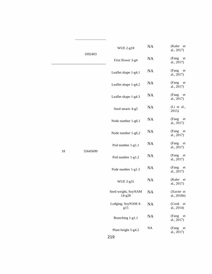
219

1092403

WUE 2-g18 NA (Kaler et

al., 2017)

First flower 3-g4 NA (Fang et

al., 2017)

18 55645699


al., 2017)


al., 2017)


al., 2017)

Seed stearic 4-g5 NA (Li et al.,

2015)

Node number 1-g6.1 NA (Fang et

al., 2017)


al., 2017)

Pod number 1-g1.1 NA (Fang et

al., 2017)


al., 2017)

Pode number 1-g1.3 NA (Fang et

al., 2017)

WUE 3-g31 NA (Kaler et

al., 2017)

Seed weight, SoyNAM

14-g28 NA (Xavier et

al., 2016b)

Lodging, SoyNAM 4-

g15 NA (Cook et

al., 2014)

Branching 1-g1.1 NA (Fang et

al., 2017)

Plant height 5-g4.2 NA (Fang et

al., 2017)

220


al., 2017)

Shoot p 1-g30

NA (Dhanapal

et al.,

2018)

19 47350110 Node number 1-g2.3 NA (Fang et

al., 2017) a Detected in separate environments (1: 2018Ridgetown, 2:2019Ridgetwon, 3:2018Palmyra,

4:2019Palmyra, NA: Not found in any environment).



221

Table 4.4 The list of detected QTL for soybean total number of non-reproductive nodes per plant (NRNP) using different GWAS methods in the tested soybean population.


Reference

MLM 15 10193796

Seed protein 6-g2 NA (Zhang et

al., 2018b)

Seed Arg 1-g4 NA (Zhang et

al., 2018b)

Seed coat luster 1-g1.3 NA (Fang et

al., 2017)

FarmCPU 15 10193796

Seed protein 6-g2 NA (Zhang et

al., 2018b)

Seed Arg 1-g4 NA (Zhang et

al., 2018b)

Seed coat luster 1-g1.3 NA (Fang et

al., 2017)

RF

1 54647498 First flower 4-g2 NA (Mao et al.,

2017)

7 329800

Phytoph 2-g32 NA (Qin et al.,

2017)

Phytoph 2-g7 NA (Qin et al.,

2017)

18 12945778 SCN 4-g14 NA (Vuong et

al., 2015)

19 40218800 Seed weight 9-g5.1 NA (Copley et

al., 2018)

SVR

7 1032587 2 WUE 2-g18 2 (Kaler et

al., 2017)

19 40218800 Seed weight 9-g5.1 NA (Copley et

al., 2018) a Detected in separate environments (1: 2018Ridgetown, 2:2019Ridgetwon, 3:2018Palmyra,

4:2019Palmyra).

222



223

Table 4.5 The list of detected QTL for soybean total number of reproductive nodes per plant (RNP) using different GWAS methods in the tested soybean population.


Reference

RF

9 40285014

Shoot Fe 1-g8.1 NA (Dhanapal

et al., 2018)


et al., 2018)


et al., 2018)

Shoot Fe 1-g9 NA (Dhanapal

et al., 2018)


et al., 2018)


et al., 2018)

Soybean mosaic virus 2-g5 NA (Che et al.,

2017)

15 34958361 SCN 5-g35 NA (Li et al.,

2016)

SVR

7 1032587 WUE 2-g18 NA (Kaler et

al., 2017)

15 34958361 1 SCN 5-g35 1 (Li et al.,

2016) a Detected in separate environments (1: 2018Ridgetown, 2:2019Ridgetwon, 3:2018Palmyra, 4:2019Palmyra).

MLM: Mixed Linear Model, FarmCPU: Fixed and random model circulating probability unification, RF: Random

Forest, SVR: Support Vector Regression

224

Table 4.6 The list of detected QTL for soybean total number of pods per plant (PP) using different GWAS methods in the tested soybean population.

GWAS

Method

Chromoso

me

Peak SNP

position Detected QTL

Environme

nt a

Referenc

e

RF

7 15331676 Seed weight, SoyNAM 14-g11 NA (Xavier

et al.,

2016b)

19 42300695


al., 2017)

Lodging, SoyNAM 4-g17 NA (Cook et

al., 2014)

SVR

9 39366957


al., 2017)


al., 2017)


al., 2017)

Seed thickness 2-g4 NA (Fang et

al., 2017)

9 39372117

Seed Thr 2-g1 NA (Li et al.,

2018b)

Seed Ser 2-g1 NA (Li et al.,

2018b)

Seed Tyr 2-g2 NA (Li et al.,

2018b)

Seed Lys 2-g2 NA (Li et al.,

2018b)

Seed leu 2-g2 NA (Li et al.,

2018b)

Seed ile 2-g2 NA (Li et al.,

2018b)

225

Seed Ala 2-g2 NA (Li et al.,

2018b)

Seed Gly 2-g2 NA (Li et al.,

2018b)

11 5245870

Ureide content 1-g29 NA (Ray et

al., 2015)


al., 2017)

18

55645699 Leaflet shape 1-g4.1 NA (Fang et

al., 2017)

55469601


al., 2017)


al., 2017)

Seed stearic 4-g5 NA (Li et al.,

2015)


al., 2017)


al., 2017)


al., 2017)


al., 2017)


al., 2017)

WUE 3-g31 NA (Dhanapa

l et al.,

2015a)

Seed weight, SoyNAM 14-g28 NA (Xavier

et al.,

2016b)

226

Lodging, SoyNAM 4-g15 NA (Cook et

al., 2014)

Branching 1-g1.1 NA (Fang et

al., 2017)


al., 2017)


al., 2017)

Shoot p 1-g30 NA (Dhanapa

l et al.,

2018)

Seed yield, SoyNAM 7-g19 NA (Cook et

al., 2014)

R8 full maturity, SoyNAM 13-

g19 NA (Cook et

al., 2014)


al., 2017)

19

43077182

Seed weight 9-g5.2 NA (Copley

et al.,

2018)

Seed weight 5-g21 NA (Copley

et al.,

2018)


al., 2017)


al., 2017)

47235604


al., 2017)

Seed palmitic 1-g19 NA (Priolli et

al., 2015)

227

47350110

Leaf carotenoid content 1-g14 NA (Dhanapa

l et al.,

2015b)

Ureide content 1-g50.3 NA (Ray et

al., 2015)

Ureide content 1-g50.4 NA (Ray et

al., 2015)

47224293 Node number 1-g2.3 NA (Fang et

al., 2017)

a detected in separate environments (1: 2018Ridgetown, 2:2019Ridgetwon, 3:2018Palmyra, 4:2019Palmyra).

MLM: Mixed Linear Model, FarmCPU: Fixed and random model circulating probability unification, RF: Random

Forest, SVR: Support Vector Regression

228

Figure 4.1 LD decay distance in the tested 227 soybean genotypes.

229

Figure 4.2 The distribution of seed yield (A), maturity (B), NP (C), NRNP (D), RNP (E),

and PP (F) in 227 soybean genotypes across four environments. The estimated

heritability is provided for each of the six traits. RNP: Total number of reproductive nodes

per plant, NRNP: The total number of non-reproductive nodes per plant, NP: The total

nodes per plant, PP: The total number of pods per plant.

230

Figure 4.3 The distributions and Pearson correlations among the soybean seed yield,

maturity, and yield component traits. RNP: Total number of reproductive nodes per plant,

NRNP: The total number of non-reproductive nodes per plant, NP: The total nodes per

plant, PP: The total number of pods per plant. The heat map scale for values is provided

by colour for the panel.

231

Figure 4.4 Structure and kinship plots for the 227 soybean genotypes. The x-axis is the

number of genotypes used in this GWAS panel, and the y axis is the membership of each

subgroup. G1-G7 stands for the subpopulation.

232

Figure 4.5 Genome-wide Manhattan plots for GWAS studies of A) maturity and B) seed

yield in soybean using MLM, FarmCPU, RF, and SVR methods, from top to bottom,

respectively.

233

Figure 4.6 Genome-wide Manhattan plots for GWAS studies of A) the total number of

nodes (NP) and B) the total number of non-reproductive nodes (NRNP) in soybean using

MLM, FarmCPU, RF, and SVR methods, from top to bottom, respectively.

234

Figure 4.7 Genome-wide Manhattan plots for GWAS studies of A) The total number of

reproductive nodes (RNP) and B) the total number of pods (PP) in soybean using MLM,

FarmCPU, RF, and SVR methods, from top to bottom, respectively.

235

Figure 4.8 Genome-wide Manhattan plots for GWAS studies of plant height in soybean

using MLM, FarmCPU, RF, and SVR methods, from top to bottom, respectively.

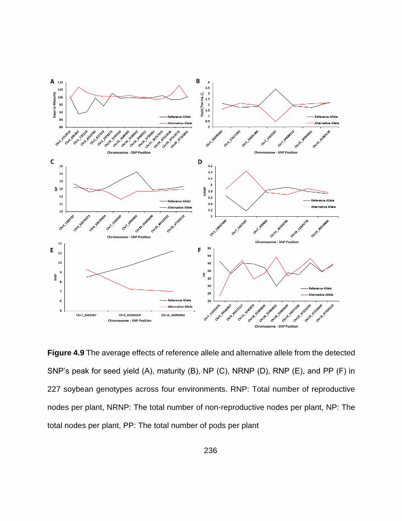
236

Figure 4.9 The average effects of reference allele and alternative allele from the detected

SNP’s peak for seed yield (A), maturity (B), NP (C), NRNP (D), RNP (E), and PP (F) in

227 soybean genotypes across four environments. RNP: Total number of reproductive

nodes per plant, NRNP: The total number of non-reproductive nodes per plant, NP: The

total nodes per plant, PP: The total number of pods per plant

237

Chapter 6: General Discussion and Future Directions

4.6 General Discussion

As the global demand for soybean is increasing significantly, there is a dire need to

accelerate and develop different breeding strategies for this strategic crop to meet the

increasing demand. One of the breeding strategies is the analytical breeding strategy,

which focuses on improving yield components such as maturity, NP, NRNP, RNP, and

PP rather than the yield per se. However, measuring yield-related traits in a large plant

breeding population is still a challenge for plant breeders. In addition, breeding for multiple

traits simultaneously requires previous knowledge about the physiological and genetic

structure of each target trait. Due to recent advances in high throughout phenotyping,

genotyping, and big data analysis methods, breeders can develop different pipelines for

selecting superior genotypes at early growth stages in a less costly manner.

One of the objectives of this thesis was to demonstrate the best soybean growth

stage for measuring hyperspectral reflectance and evaluating the three most commonly

used ML algorithms (SVM, MLP, and RF) along with introducing the E-S method in

predicting the soybean yield using reflectance variables. The soybean R5 growth stage

was identified as a better stage than R4 for measuring hyperspectral reflectance. In

addition to using 62 reflectance bands as the full variables, the RFE method was used to

reduce the dimensionality of the data. Therefore, 21 most important bands were selected

238

as reflectance variables. Using both full and selected reflectance variables, RF

outperformed all individual algorithms. Therefore, RF was selected as the metaClassifier

for E–S. E–S had the highest prediction accuracy as one of the ensemble approaches

compared to an individual ML algorithm. Therefore, E–S was recommended as a reliable

and appropriate ML algorithm for predicting the soybean yield using reflectance variables.

This study provides an applicable pipeline for using hyperspectral reflectance data and

suitable ML algorithms for the development of high-yielding soybeans, which can be used

in large soybean breeding programs for selecting high-yielding soybeans at pre-

harvesting stages. The developed methodology in this thesis can open a new window in

using spectral reflectance for selecting high-yielding genotypes in different crops.

Having reliable estimations of the optimum values for highly heritable secondary traits

such as HVI that are strongly associated with yield and FBIO can guide breeders to

construct efficient breeding programs focused on designing and selecting “ideotype”

genotypes for their target traits. In this thesis, we demonstrated the significant correlations

of several HVI, including the red region, especially the 670 nm and 800 nm wavelengths

in the NIR region, with soybean seed yield and FBIO production. We also developed EB

and DNN algorithms as reliable tools for predicting the soybean seed yield and FBIO from

HVI data collected at early growth stages. Furthermore, for the first time, we linked DNN

to the SPEA2 to estimate the optimum values of HVI in soybean genotypes with

maximized yield and FBIO. These optimum values of HVI are suggested to be validated

239

in new and independent breeding populations before being used by soybean breeders in

their cultivar development programs for selecting high-yielding genotypes with high FBIO

potential.

Efficient breeding approaches for improving the genetic potential of complex traits

such as yield in soybean can be developed based on secondary traits that govern the

final performance of the complex trait. Thus, in order to increase the genetic yield potential

in soybean, breeders can select soybean genotypes with improved yield component

traits. However, measuring yield components in a large soybean breeding program is

time-consuming and labor-intensive, which limits the implication of this approach in

cultivar development programs. Another objective of this study was to evaluate the

potential use of yield component traits for estimating final seed yield in soybean using

different ML and E-B algorithms. The results showed that RBF is a reliable solo ML

algorithm for predicting the soybean seed yield from its component traits. However, an E-

B algorithm that was built by combining the three ML and using RBF as its metaClassifier

outperformed all individual ML algorithms, therefore, it is recommended for predicting the

soybean seed yield exploiting yield component traits. In this study, for the first time, we

coupled E-B algorithm with GA in order to estimate optimum values of yield component

traits in a theoretical genotype in which the yield is maximized using the real field data.

The results are promising but it is recommended that they be evaluated in new and

independent breeding populations before their routine use in cultivar development

240

programs for selecting high-yielding potential genotypes. This information can also be

used, in combination with molecular marker technology, for developing genomic-based

toolkits that can be used for selecting genotypes with improved genetic yield potential at

early generations.

A better understanding of the genetic architecture of the yield component traits in

soybean may enable breeders to establish more efficient selection strategies for

developing high-yielding cultivars with improved genetic gains. Major yield components

such as maturity, NP, NRNP, RNP, and PP play important roles in determining the overall

yield production in soybean. This study verified the importance of those traits, using

correlation and distribution analyses, in determination of the total soybean seed yield.

Furthermore, by testing different conventional and ML-mediated GWAS methods, SVR-

mediated GWAS outperformed all the other methods.

Therefore, SVR-mediated GWAS is recommended as an alternative to conventional

GWAS methods because it exhibited the greatest power for detecting genomic regions

associated with complex traits such as yield and its components in soybean, and possibly

other crop species. To the best of our knowledge, this study is the first attempt in which

SVR was used for GWAS analyses in plants. In order to verify the causal relationship

between identified QTL and the target phenotypic traits, we identified candidate genes

within each QTL using gene annotation procedures and information. The results

demonstrated the efficiency of SVR-mediated GWAS in detecting the strong QTL that can

241

be used in marker-assisted selection. Further investigation is recommended to confirm

the efficiency of SVR-mediated GWAS in detecting associated genomic regions in other

plant species.

4.7 Future Directions

Breeding for complex traits requires different environments to validate and test the

stability of the complex trait. In this study, soybean yield, hyperspectral reflectance, and

yield components were measured in four environments consisting of two locations grown

over two years. It would be valuable to test the developed pipelines in more environments

to test the stability of the results across environments.

Each ML algorithm has its own function and parameters to be optimized based on

the given problem. However, some algorithms may respond well to specific problems. For

instance, we demonstrated the efficiency of ensemble bagging and stacking in predicting

soybean seed yield using hyperspectral reflectance and yield components, respectively.

However, the use of all the tested ML algorithms is new in the plant breeding area, and it

would be valuable to have a deep understanding of the use of other ML algorithms to

predict complex traits using secondary related traits.

Breeding for multiple traits concurrently would be a challenge in a breeding program

since each trait has its limitation and interaction with other traits. Therefore, understanding

242

the optimum value of each trait in a given population would be valuable to set up a

breeding strategy efficiently. Optimization algorithms would be helpful to estimate the

optimum value of each trait for maximizing the complex trait. However, each optimization

algorithm has its merits and demerits. This thesis evaluates the two most well-known

optimization algorithms, each from a separate optimization group: GA, as single-objective

optimization algorithms, and SPEA2, as a multi-objective evolutionary optimization

algorithm. Although both tested optimization algorithms had an acceptable performance

in finding solutions for a given soybean population, it would be valuable to conduct an

experiment and test different optimization algorithms and provide comprehensive

optimization pipelines for plant breeders.

One of the aims of this study was to estimate the optimum value of each yield

component and HVI in soybeans with maximized seed yield and FBIO production. This

result can be used for establishing a recurrent selection program in which the yield

component traits are gradually accumulated and optimized for sustainable improvement

of seed yield and its genetic gain.

In order to detect genomic regions associated with traits of interest, four GWAS

methods were used in this study. Also, in order to verify the associated genomic regions,

candidate genes and QTL were estimated using different databases. Although associated

genomic regions were detected using the tested GWAS methods, it would be more

243

valuable to conduct gene expression experiments and validate findings not only based

on DNA variants but also through gene expression analysis methods.

Markers associated with some of the detected QTL might be useful for MAS

program. We recommend evaluating and validating the detected QTL in this study in

larger and different breeding populations.

244

References

Aanonsen, S.I., Nævdal, G., Oliver, D.S., Reynolds, A.C., and Vallès, B. (2009). The ensemble Kalman filter in reservoir engineering--a review. Spe Journal 14(03), 393-412.

Acevedo, E., and Aleppo, S. (1991). Improvement of winter cereal crops in Mediterranean environments: Use of yield, morphological and physiological traits. Breeding for drought resistance in wheat 12, 188.

Acharjee, A., Prentice, P., Acerini, C., Smith, J., Hughes, I.A., Ong, K., et al. (2017). The translation of lipid profiles to nutritional biomarkers in the study of infant metabolism. Metabolomics 13(3), 25.

Adee, E. (2015). Effects of seed treatment on sudden death syndrome symptoms and soybean yield. Kansas Agricultural Experiment Station Research Reports 1(2), 3.

Aghighi, H., Azadbakht, M., Ashourloo, D., Shahrabi, H.S., and Radiom, S. (2018). Machine learning regression techniques for the silage maize yield prediction using time-series images of landsat 8 OLI. IEEE Journal of Selected Topics in Applied Earth Observations and Remote Sensing 11(12), 4563-4577.

Al-Abassi, A., Karimipour, H., HaddadPajouh, H., Dehghantanha, A., and Parizi, R.M. (2020). "Industrial big data analytics: challenges and opportunities," in Handbook of Big Data Privacy. Springer), 37-61.

Alam, M., and Mukhopadhyay, D. (Year). "How secure are deep learning algorithms from side-channel based reverse engineering?", in: Proceedings of the 56th Annual Design Automation Conference 2019), 1-2.

Albetis, J., Duthoit, S., Guttler, F., Jacquin, A., Goulard, M., Poilvé, H., et al. (2017). Detection of Flavescence dorée grapevine disease using unmanned aerial vehicle (UAV) multispectral imagery. Remote Sensing 9(4), 308.

Alekcevetch, J.C., de Lima Passianotto, A.L., Ferreira, E.G.C., Dos Santos, A.B., da Silva, D.C.G., Dias, W.P., et al. (2021). Genome-wide association study for resistance to the Meloidogyne javanica causing root-knot nematode in soybean. Theoretical and Applied Genetics, 1-16.

Alemu, A., Feyissa, T., Maccaferri, M., Sciara, G., Tuberosa, R., Ammar, K., et al. (2021). Genome-wide association analysis unveils novel QTLs for seminal root system architecture traits in Ethiopian durum wheat. BMC genomics 22(1), 1-16.

Alexandratos, N., and Bruinsma, J. (2012). World agriculture towards 2030/2050: the 2012 revision.

Ali, I., Cawkwell, F., Green, S., and Dwyer, N. (Year). "Application of statistical and machine learning models for grassland yield estimation based on a hypertemporal satellite remote sensing time series", in: 2014 IEEE Geoscience and Remote Sensing Symposium: IEEE), 5060-5063.

245

Alirezanejad, M., Enayatifar, R., Motameni, H., and Nematzadeh, H. (2020). Heuristic filter feature selection methods for medical datasets. Genomics 112(2), 1173-1181.

Alpaydin, E. (2020). Introduction to machine learning. MIT press. Alsahaf, A., Azzopardi, G., Ducro, B., Hanenberg, E., Veerkamp, R.F., and Petkov, N.

(2018). Prediction of slaughter age in pigs and assessment of the predictive value of phenotypic and genetic information using random forest. Journal of animal science 96(12), 4935-4943.

Alves, M.L., Bento-Silva, A., Gaspar, D., Paulo, M., Brites, C., Mendes-Moreira, P., et al. (2020). Volatilome–Genome-Wide Association Study on Wholemeal Maize Flour. Journal of Agricultural and Food Chemistry 68(29), 7809-7818.

Aparicio, N., Villegas, D., Araus, J., Casadesus, J., and Royo, C. (2002). Relationship between growth traits and spectral vegetation indices in durum wheat. Crop science 42(5), 1547-1555.

Aparicio, N., Villegas, D., Casadesus, J., Araus, J.L., and Royo, C. (2000). Spectral vegetation indices as nondestructive tools for determining durum wheat yield. Agronomy Journal 92(1), 83-91.

Arab, M.M., Yadollahi, A., Eftekhari, M., Ahmadi, H., Akbari, M., and Khorami, S.S. (2018). Modeling and Optimizing a New Culture Medium for In Vitro Rooting of G× N15 Prunus Rootstock using Artificial Neural Network-Genetic Algorithm. Scientific reports 8(1), 9977.

Araghinejad, S. (2013). Data-driven modeling: using MATLAB® in water resources and environmental engineering. Springer Science & Business Media.

Araus, J., Casadesus, J., and Bort, J. (2001). "Recent tools for the screening of physiological traits determining yield. Application of Physiology in Wheat Breeding".).

Araus, J., Slafer, G., Reynolds, M., and Royo, C. (2002). Plant breeding and drought in C3 cereals: what should we breed for? Annals of botany 89(7), 925-940.

Araus, J.L., and Cairns, J.E. (2014). Field high-throughput phenotyping: the new crop breeding frontier. Trends in plant science 19(1), 52-61.

Araus, J.L., Kefauver, S.C., Zaman-Allah, M., Olsen, M.S., and Cairns, J.E. (2018). Translating high-throughput phenotyping into genetic gain. Trends in plant science 23(5), 451-466.

Araya, D.B., Grolinger, K., ElYamany, H.F., Capretz, M.A., and Bitsuamlak, G. (2017). An ensemble learning framework for anomaly detection in building energy consumption. Energy and Buildings 144, 191-206.

Arshadi, N., Chang, B., and Kustra, R. (Year). "Predictive modeling in case-control single-nucleotide polymorphism studies in the presence of population stratification: a case study using Genetic Analysis Workshop 16 Problem 1 dataset", in: BMC proceedings: Springer), 1-5.

246

Asif, H., Alliey-Rodriguez, N., Keedy, S., Tamminga, C.A., Sweeney, J.A., Pearlson, G., et al. (2020). GWAS significance thresholds for deep phenotyping studies can depend upon minor allele frequencies and sample size. Molecular psychiatry, 1-8.

Auria, L., and Moro, R.A. (2008). Support vector machines (SVM) as a technique for solvency analysis.

Awad, M., and Khanna, R. (2015). "Support vector regression," in Efficient learning machines. Springer), 67-80.

Babar, M., Reynolds, M., Van Ginkel, M., Klatt, A., Raun, W., and Stone, M. (2006). Spectral reflectance to estimate genetic variation for in‐season biomass, leaf chlorophyll, and canopy temperature in wheat. Crop science 46(3), 1046-1057.

Bajwa, S.G., Rupe, J.C., and Mason, J. (2017). Soybean disease monitoring with leaf reflectance. Remote Sensing 9(2), 127.

Bala, S., and Islam, A. (2009). Correlation between potato yield and MODIS‐derived vegetation indices. International Journal of Remote Sensing 30(10), 2491-2507.

Banerjee, S., Zeng, L., Schunkert, H., and Söding, J. (2018). Bayesian multiple logistic regression for case-control GWAS. PLoS genetics 14(12), e1007856.

Bao, Y., Kurle, J.E., Anderson, G., and Young, N.D. (2015). Association mapping and genomic prediction for resistance to sudden death syndrome in early maturing soybean germplasm. Molecular Breeding 35(6), 1-14.

Bao, Y., Vuong, T., Meinhardt, C., Tiffin, P., Denny, R., Chen, S., et al. (2014). Potential of association mapping and genomic selection to explore PI 88788 derived soybean cyst nematode resistance. The Plant Genome 7(3).

Bassett, A., Kamfwa, K., Ambachew, D., and Cichy, K. (2021). Genetic variability and genome-wide association analysis of flavor and texture in cooked beans (Phaseolus vulgaris L.). Theoretical and Applied Genetics, 1-20.

Bastidas, A., Setiyono, T., Dobermann, A., Cassman, K.G., Elmore, R.W., Graef, G.L., et al. (2008). Soybean sowing date: The vegetative, reproductive, and agronomic impacts. Crop Science 48(2), 727-740.

Bates, D., Mächler, M., Bolker, B., and Walker, S. (2014). Fitting linear mixed-effects models using lme4. arXiv preprint arXiv:1406.5823.

Bates, D., Sarkar, D., Bates, M.D., and Matrix, L. (2007). The lme4 package. R package version 2(1), 74.

Bäurle, I., and Dean, C. (2008). Differential interactions of the autonomous pathway RRM proteins and chromatin regulators in the silencing of Arabidopsis targets. PLoS One 3(7), e2733.

Bawazeer, S.A., Baakeem, S.S., and Mohamad, A.A. (2021). New Approach for Radial Basis Function Based on Partition of Unity of Taylor Series Expansion with Respect to Shape Parameter. Algorithms 14(1), 1.

Belayneh, A., Adamowski, J., Khalil, B., and Ozga-Zielinski, B. (2014). Long-term SPI drought forecasting in the Awash River Basin in Ethiopia using wavelet neural

247

network and wavelet support vector regression models. Journal of Hydrology 508, 418-429.

Bendig, J., Bolten, A., Bennertz, S., Broscheit, J., Eichfuss, S., and Bareth, G. (2014). Estimating biomass of barley using crop surface models (CSMs) derived from UAV-based RGB imaging. Remote Sensing 6(11), 10395-10412.

Benedetti, P., Ienco, D., Gaetano, R., Ose, K., Pensa, R.G., and Dupuy, S. (2018). $ M^ 3\text {Fusion} $: A Deep Learning Architecture for Multiscale Multimodal Multitemporal Satellite Data Fusion. IEEE Journal of Selected Topics in Applied Earth Observations and Remote Sensing 11(12), 4939-4949.

Benjamini, Y., and Hochberg, Y. (1995). Controlling the false discovery rate: a practical and powerful approach to multiple testing. Journal of the Royal statistical society: series B (Methodological) 57(1), 289-300.

Bhojani, S.H., and Bhatt, N. (2020). Wheat crop yield prediction using new activation functions in neural network. Neural Computing and Applications 32, 13941–13951.

Bisong, E. (2019). "The Multilayer Perceptron (MLP)," in Building Machine Learning and Deep Learning Models on Google Cloud Platform. (Berkeley, CA, USA: Springer), 401-405.

Björne, J., Kaewphan, S., and Salakoski, T. (Year). "UTurku: drug named entity recognition and drug-drug interaction extraction using SVM classification and domain knowledge", in: Second Joint Conference on Lexical and Computational Semantics (* SEM), Volume 2: Proceedings of the Seventh International Workshop on Semantic Evaluation (SemEval 2013)), 651-659.

Blackburn, G.A. (2007). Hyperspectral remote sensing of plant pigments. Journal of experimental botany 58(4), 855-867.

Blaikie, P., and Brookfield, H. (2015). Land degradation and society. Routledge. Block, M.A., and Jouhet, J. (2015). Lipid trafficking at endoplasmic reticulum–chloroplast

membrane contact sites. Current opinion in cell biology 35, 21-29. Board, J., Kang, M., and Bodrero, M. (2003). Yield components as indirect selection

criteria for late-planted soybean cultivars. Agronomy journal 95(2), 420-429. Board, J., Kumudini, S., Omielan, J., Prior, E., and Kahlon, C. (2010). Yield response of

soybean to partial and total defoliation during the seed-filling period. Crop science 50(2), 703-712.

Boerma, H. (1979). Comparison of Past and Recently Developed Soybean Cultivars in Maturity Groups VI, VII, and VIII1. Crop Science 19(5), 611-613.

Botta, V., Louppe, G., Geurts, P., and Wehenkel, L. (2014). Exploiting SNP correlations within random forest for genome-wide association studies. PloS one 9(4), e93379.

Bowley, S. (1999). A hitchhiker's guide to statistics in plant biology. Guelph, Ont.: Any Old Subject Books.

Bozorg-Haddad, O., Azarnivand, A., Hosseini-Moghari, S.-M., and Loáiciga, H.A. (2016). Development of a comparative multiple criteria framework for ranking pareto

248

optimal solutions of a multiobjective reservoir operation problem. Journal of Irrigation Drainage Engineering 142(7), 04016019.

Breiman, L. (1996). Bagging predictors. Machine learning 24(2), 123-140. Breiman, L. (2001). Random forests. Machine learning 45(1), 5-32. Brown-Guedira, G., Thompson, J., Nelson, R., and Warburton, M. (2000). Evaluation of

Genetic Diversity of Soybean Introductions and North American Ancestors Using RAPD and SSR Markers Joint contribution of the USDA-ARS, and Illinois Agric. Exp. Stn. Crop Science 40(3), 815-823.

Bush, W.S., and Moore, J.H. (2012). Genome-wide association studies. PLoS Comput Biol 8(12), e1002822.

Butler, K.T., Davies, D.W., Cartwright, H., Isayev, O., and Walsh, A. (2018). Machine learning for molecular and materials science. Nature 559(7715), 547-555.

Buzzell, R. (1971). Inheritance of a soybean flowering response to fluorescent-daylength conditions. Canadian Journal of Genetics and Cytology 13(4), 703-707.

CABRERA‐BOSQUET, L., Albrizio, R., Nogues, S., and Araus, J.L. (2011). Dual Δ13C/δ18O response to water and nitrogen availability and its relationship with yield in field‐grown durum wheat. Plant, Cell & Environment 34(3), 418-433.

Cabrera‐Bosquet, L., Crossa, J., von Zitzewitz, J., Serret, M.D., and Luis Araus, J. (2012).

High‐throughput phenotyping and genomic selection: The frontiers of crop breeding converge. Journal of integrative plant biology 54(5), 312-320.

Cacuci, D.G., Ionescu-Bujor, M., and Navon, I.M. (2005). Sensitivity and uncertainty analysis, volume II: applications to large-scale systems. CRC press.

Cai, G., Yang, Q., Chen, H., Yang, Q., Zhang, C., Fan, C., et al. (2016). Genetic dissection of plant architecture and yield-related traits in Brassica napus. Scientific reports 6, 21625.

Cao, S., Xu, D., Hanif, M., Xia, X., and He, Z. (2020). Genetic architecture underpinning yield component traits in wheat. Theoretical and Applied Genetics, 1-13.

Carvalho, S., Macel, M., Schlerf, M., Moghaddam, F.E., Mulder, P.P., Skidmore, A.K., et al. (2013). Changes in plant defense chemistry (pyrrolizidine alkaloids) revealed through high-resolution spectroscopy. ISPRS journal of photogrammetry remote sensing 80, 51-60.

Casal, J.J. (2013). Photoreceptor signaling networks in plant responses to shade. Annual review of plant biology 64, 403-427.

Cassell, B.G. (2009). Using heritability for genetic improvement. Chandra, A.L., Desai, S.V., Guo, W., and Balasubramanian, V.N. (2020). Computer vision

with deep learning for plant phenotyping in agriculture: A survey. arXiv preprint arXiv:2006.11391.

Chang, H.-X., and Hartman, G.L. (2017). Characterization of insect resistance loci in the USDA soybean germplasm collection using genome-wide association studies. Frontiers in plant science 8, 670.

249

Chang, W., and Wickham, H. (2016). ggvis: Interactive Grammar of Graphics. R package version0 4.

Chappelle, E.W., Kim, M.S., and McMurtrey III, J.E. (1992). Ratio analysis of reflectance spectra (RARS): an algorithm for the remote estimation of the concentrations of chlorophyll a, chlorophyll b, and carotenoids in soybean leaves. Remote sensing of environment 39(3), 239-247.

Che, Z., Liu, H., Yi, F., Cheng, H., Yang, Y., Wang, L., et al. (2017). Genome-Wide Association Study Reveals Novel Loci for SC7 Resistance in a Soybean Mutant Panel. Frontiers in Plant Science 8(1771). doi: 10.3389/fpls.2017.01771.

Chen, J.-C., and Wang, Y.-M. (2020). Comparing Activation Functions in Modeling Shoreline Variation Using Multilayer Perceptron Neural Network. Water 12(5), 1281.

Chen, J.H., and Verghese, A. (2020). Planning for the Known Unknown: Machine Learning for Human Healthcare Systems. The American Journal of Bioethics 20(11), 1-3.

Chen, L., Huang, J., Wang, F., and Tang, Y. (2007). Comparison between back propagation neural network and regression models for the estimation of pigment content in rice leaves and panicles using hyperspectral data. International Journal of Remote Sensing 28(16), 3457-3478.

Chen, P., Haboudane, D., Tremblay, N., Wang, J., Vigneault, P., and Li, B. (2010). New spectral indicator assessing the efficiency of crop nitrogen treatment in corn and wheat. Remote Sensing of Environment 114(9), 1987-1997.

Chen, X.-w., and Jeong, J.C. (Year). "Enhanced recursive feature elimination", in: Sixth International Conference on Machine Learning and Applications (ICMLA 2007): IEEE), 429-435.

Chenou, J., Hsieh, G., and Fields, T. (Year). "Radial Basis Function Network: Its Robustness and Ability to Mitigate Adversarial Examples", in: 2019 International Conference on Computational Science and Computational Intelligence (CSCI): IEEE), 102-106.

Chlingaryan, A., Sukkarieh, S., and Whelan, B. (2018). Machine learning approaches for crop yield prediction and nitrogen status estimation in precision agriculture: A review. Computers and electronics in agriculture 151, 61-69.

Chouhan, S.S., Kaul, A., Singh, U.P., and Jain, S. (2018). Bacterial foraging optimization based radial basis function neural network (BRBFNN) for identification and classification of plant leaf diseases: An automatic approach towards plant pathology. IEEE Access 6, 8852-8863.

Christenson, B.S., Schapaugh, W.T., An, N., Price, K.P., Prasad, V., and Fritz, A.K. (2016). Predicting Soybean Relative Maturity and Seed Yield Using Canopy Reflectance. Crop Science 56(2), 625-643.

250

Chun, H., and Keleş, S. (2010). Sparse partial least squares regression for simultaneous dimension reduction and variable selection. Journal of the Royal Statistical Society: Series B (Statistical Methodology) 72(1), 3-25.

Churchill, G.A., and Doerge, R.W. (1994). Empirical threshold values for quantitative trait mapping. Genetics 138(3), 963-971.

Ciampitti, I.A., and Vyn, T.J. (2012). Physiological perspectives of changes over time in maize yield dependency on nitrogen uptake and associated nitrogen efficiencies: A review. Field Crops Research 133, 48-67.

Colletti, A., Attrovio, A., Boffa, L., Mantegna, S., and Cravotto, G. (2020). Valorisation of By-Products from Soybean (Glycine max (L.) Merr.) Processing. Molecules 25(9), 2129.

Collins, N.C., Tardieu, F., and Tuberosa, R. (2008). Quantitative trait loci and crop performance under abiotic stress: where do we stand? Plant physiology 147(2), 469-486.

Connor, D.J., Loomis, R.S., and Cassman, K.G. (2011). Crop ecology: productivity and management in agricultural systems. Cambridge University Press.

Contreras-Soto, R.I., Mora, F., de Oliveira, M.A.R., Higashi, W., Scapim, C.A., and Schuster, I. (2017). A genome-wide association study for agronomic traits in soybean using SNP markers and SNP-based haplotype analysis. PloS one 12(2), e0171105.

Cook, D.E., Bayless, A.M., Wang, K., Guo, X., Song, Q., Jiang, J., et al. (2014). Distinct copy number, coding sequence, and locus methylation patterns underlie Rhg1-mediated soybean resistance to soybean cyst nematode. Plant physiology 165(2), 630-647.

Cooper, M., van Eeuwijk, F.A., Hammer, G.L., Podlich, D.W., and Messina, C. (2009). Modeling QTL for complex traits: detection and context for plant breeding. Current opinion in plant biology 12(2), 231-240.

Copley, T.R., Duceppe, M.-O., and O’Donoughue, L.S. (2018). Identification of novel loci associated with maturity and yield traits in early maturity soybean plant introduction lines. BMC genomics 19(1), 1-12.

Correia, D.L., Bouachir, W., Gervais, D., Pureswaran, D., Kneeshaw, D.D., and De Grandpré, L. (2020). Leveraging artificial intelligence for large-scale plant phenology studies from noisy time-lapse images. IEEE Access 8, 13151-13160.

Cortes, C., and Vapnik, V. (1995). Support vector machine. Machine learning 20(3), 273-297.

Crane-Droesch, A. (2018). Machine learning methods for crop yield prediction and climate change impact assessment in agriculture. Environmental Research Letters 13(11), 114003.

Crozier, A., Jaganath, I.B., and Clifford, M.N. (2009). Dietary phenolics: chemistry, bioavailability and effects on health. Natural product reports 26(8), 1001-1043.

251

Cui, S., and Yu, D. (2005). Estimates of relative contribution of biomass, harvest index and yield components to soybean yield improvements in China. Plant Breeding 124(5), 473-476.

Dababat, A., Arif, M.A.R., Toktay, H., Atiya, O., Shokat, S., Gul, E., et al. (2021). A GWAS to identify the cereal cyst nematode (Heterodera filipjevi) resistance loci in diverse wheat prebreeding lines. Journal of Applied Genetics, 1-6.

Dao, D.-N., and Guo, L.-X. (2020a). New hybrid between SPEA/R with deep neural network: application to predicting the multi-objective optimization of the stiffness parameter for powertrain mount systems. Journal of Low Frequency Noise, Vibration and Active Control 39(4), 53–68.

Dao, D.-N., and Guo, L.-X. (2020b). New hybrid SPEA/R-deep learning to predict optimization parameters of cascade FOPID controller according engine speed in powertrain mount system control of half-car dynamic model. Journal of Intelligent & Fuzzy Systems 39(Preprint), 53–68.

Dasgupta, K., Mandal, B., Dutta, P., Mandal, J.K., and Dam, S. (2013). A genetic algorithm (ga) based load balancing strategy for cloud computing. Procedia Technology 10, 340-347.

Datt, B. (1999). A new reflectance index for remote sensing of chlorophyll content in higher plants: tests using Eucalyptus leaves. Journal of Plant Physiology 154(1), 30-36.

De'ath, G., and Fabricius, K.E. (2000). Classification and regression trees: a powerful yet simple technique for ecological data analysis. Ecology 81(11), 3178-3192.

De Bruin, J.L., and Pedersen, P. (2009). Growth, Yield, and Yield Component Changes among Old and New Soybean Cultivars All rights reserved. No part of this periodical may be reproduced or transmitted in any form or by any means, electronic or mechanical, including photocopying, recording, or any information storage and retrieval system, without permission in writing from the publisher. Agronomy journal 101(1), 124-130.

De Castro, A.-I., Jurado-Expósito, M., Gómez-Casero, M.-T., and López-Granados, F. (2012). Applying neural networks to hyperspectral and multispectral field data for discrimination of cruciferous weeds in winter crops. The Scientific World Journal 2012.

De Castro, A.I., Torres-Sánchez, J., Peña, J.M., Jiménez-Brenes, F.M., Csillik, O., and López-Granados, F. (2018). An automatic random forest-OBIA algorithm for early weed mapping between and within crop rows using UAV imagery. Remote Sensing 10(2), 285.

De Pretto, C., Giordano, R.d.L.C., Tardioli, P.W., and Costa, C.B.B. (2018). Possibilities for producing energy, fuels, and chemicals from soybean: a biorefinery concept. Waste and Biomass Valorization 9(10), 1703-1730.

252

De Wit, M., Galvão, V.C., and Fankhauser, C. (2016). Light-mediated hormonal regulation of plant growth and development. Annual review of plant biology 67, 513-537.

Deering, D.W. (1978). Rangeland reflectance characteristics measured by aircraft and spacecraft sensors. Ph. D Dissertation. Texas A&M Universtiy.

Dennis, T. (2016). Using R and ggvis to Create Interactive Graphics for Exploratory Data Analysis. Data Visualization: A Guide to Visual Storytelling for Libraries, 149.

Denton, S.M., and Salleb-Aouissi, A. (2020). A Weighted Solution to SVM Actionability and Interpretability. arXiv preprint arXiv:2012.03372.

Deore, B., Kyatham, A., and Narkhede, S. (Year). "A novel approach to ensemble MLP and random forest for network security", in: ITM Web of Conferences: EDP Sciences), 03003.

Devlin, B., and Roeder, K. (1999). Genomic control for association studies. Biometrics 55(4), 997-1004.

Dhanapal, A.P., Ray, J.D., Singh, S.K., Hoyos-Villegas, V., Smith, J.R., Purcell, L.C., et al. (2015a). Genome-wide association study (GWAS) of carbon isotope ratio (δ 13 C) in diverse soybean [Glycine max (L.) Merr.] genotypes. Theoretical and Applied Genetics 128(1), 73-91.

Dhanapal, A.P., Ray, J.D., Singh, S.K., Hoyos-Villegas, V., Smith, J.R., Purcell, L.C., et al. (2015b). Association mapping of total carotenoids in diverse soybean genotypes based on leaf extracts and high-throughput canopy spectral reflectance measurements. PloS one 10(9), e0137213.

Dhanapal, A.P., Ray, J.D., Smith, J.R., Purcell, L.C., and Fritschi, F.B. (2018). Identification of Novel Genomic Loci Associated with Soybean Shoot Tissue Macro and Micronutrient Concentrations. The plant genome 11(2), 170066.

Di Leo, G., and Sardanelli, F. (2020). Statistical significance: p value, 0.05 threshold, and applications to radiomics—reasons for a conservative approach. European radiology experimental 4(1), 1-8.

Dias, R., and Torkamani, A. (2019). Artificial intelligence in clinical and genomic diagnostics. Genome medicine 11(1), 1-12.

Dietterich, T.G. (Year). "Ensemble methods in machine learning", in: International workshop on multiple classifier systems: Springer), 1-15.

Ding, K., and Kullo, I.J. (2007). Methods for the selection of tagging SNPs: a comparison of tagging efficiency and performance. European Journal of Human Genetics 15(2), 228-236.

Ditta, G., Pinyopich, A., Robles, P., Pelaz, S., and Yanofsky, M.F. (2004). The SEP4 gene of Arabidopsis thaliana functions in floral organ and meristem identity. Current biology 14(21), 1935-1940.

Divina, F., Gilson, A., Goméz-Vela, F., García Torres, M., and Torres, J.F. (2018). Stacking ensemble learning for short-term electricity consumption forecasting. Energies 11(4), 949.

253

Doerge, R.W., and Churchill, G.A. (1996). Permutation tests for multiple loci affecting a quantitative character. Genetics 142(1), 285-294.

Drucker, H., and Cortes, C. (Year). "Boosting decision trees", in: Advances in neural information processing systems), 479-485.

Du, J., Wang, S., He, C., Zhou, B., Ruan, Y.-L., and Shou, H. (2017). Identification of regulatory networks and hub genes controlling soybean seed set and size using RNA sequencing analysis. Journal of Experimental Botany 68(8), 1955-1972.

Du, J., and Xu, Y. (2017). Hierarchical deep neural network for multivariate regression. Pattern Recognition 63, 149-157.

Du, Y., Zhao, Q., Li, S., Yao, X., Xie, F., and Zhao, M. (2019). Shoot/root interactions affect soybean photosynthetic traits and yield formation: a case study of grafting with record-yield cultivars. Frontiers in plant science 10, 445.

Duan, K.-B., Rajapakse, J.C., Wang, H., and Azuaje, F. (2005). Multiple SVM-RFE for gene selection in cancer classification with expression data. IEEE transactions on nanobioscience 4(3), 228-234.

Duan, T., Zheng, B., Guo, W., Ninomiya, S., Guo, Y., and Chapman, S.C. (2017). Comparison of ground cover estimates from experiment plots in cotton, sorghum and sugarcane based on images and ortho-mosaics captured by UAV. Functional Plant Biology 44(1), 169-183.

Dubey, A., Kumar, A., Abd_Allah, E.F., Hashem, A., and Khan, M.L. (2019). Growing more with less: Breeding and developing drought resilient soybean to improve food security. Ecological Indicators 105, 425-437. doi: https://doi.org/10.1016/j.ecolind.2018.03.003.

Dumschott, K., Schmidt, M.H.-W., Chawla, H.S., Snowdon, R., and Usadel, B. (2020). Oxford Nanopore Sequencing: New opportunities for plant genomics? Journal of Experimental Botany.

Dutamo, D., Alamerew, S., Eticha, F., and Assefa, E. (2015). Genetic variability in bread wheat (Triticum aestivum L.) germplasm for yield and yield component traits. Journal of Biology, Agriculture and Healthcare 5(17), 140-147.

Eck, H.V. (1987). Plant water stress at various growth stages and growth and yield of soybeans. Field crops research v. 17(no. 1), pp. 1-16-1989 v.1917 no.1981.

Edelmann, A., Wolff, T., Montagne, D., and Bail, C.A. (2020). Computational Social Science and Sociology. Annual Review of Sociology 46.

Egli, D. (2005). Flowering, pod set and reproductive success in soya bean. Journal of Agronomy and crop science 191(4), 283-291.

Egli, D. (2013). The relationship between the number of nodes and pods in soybean communities. Crop Science 53(4), 1668-1676.

Eltaher, S., Baenziger, P.S., Belamkar, V., Emara, H.A., Nower, A.A., Salem, K.F., et al. (2021). GWAS revealed effect of genotype× environment interactions for grain yield of Nebraska winter wheat. BMC genomics 22(1), 1-14.

https://doi.org/10.1016/j.ecolind.2018.03.003

254

Emily, M. (2018). Power comparison of Cochran-Armitage trend test against allelic and genotypic tests in large-scale case-control genetic association studies. Statistical methods in medical research 27(9), 2657-2673.

Eraslan, G., Avsec, Ž., Gagneur, J., and Theis, F.J. (2019). Deep learning: new computational modelling techniques for genomics. Nature Reviews Genetics 20(7), 389-403.

Esposito, S., Carputo, D., Cardi, T., and Tripodi, P. (2020). Applications and Trends of Machine Learning in Genomics and Phenomics for Next-Generation Breeding. Plants 9(1), 34.

Etminan, A., Pour-Aboughadareh, A., Mohammadi, R., Shooshtari, L., Yousefiazarkhanian, M., and Moradkhani, H. (2019). Determining the best drought tolerance indices using artificial neural network (ANN): Insight into application of intelligent agriculture in agronomy and plant breeding. Cereal Research Communications 47(1), 170-181.

Fabiyi, E. (2006). Soyabean processing, utilization and health benefits. Pakistan Journal of Nutrition 5(5), 453-457.

Falk, K.G., Jubery, T.Z., Mirnezami, S.V., Parmley, K.A., Sarkar, S., Singh, A., et al. (2020). Computer vision and machine learning enabled soybean root phenotyping pipeline. Plant Methods 16(1), 5. doi: 10.1186/s13007-019-0550-5.

Fang, C., Ma, Y., Wu, S., Liu, Z., Wang, Z., Yang, R., et al. (2017). Genome-wide association studies dissect the genetic networks underlying agronomical traits in soybean. Genome biology 18(1), 1-14.

Farifteh, J., Van der Meer, F., Atzberger, C., and Carranza, E.J.M. (2007). Quantitative analysis of salt-affected soil reflectance spectra: A comparison of two adaptive methods (PLSR and ANN). Remote Sensing of Environment 110(1), 59-78. doi: https://doi.org/10.1016/j.rse.2007.02.005.

Fehr, W., and Caviness, C. (1971). Burmood DT, Penington J S. Development description of soybean, Glycine max (L) Mer. Crop Science 11, 929-931.

Fehr, W., Caviness, C., Burmood, D., and Pennington, J. (1971). Stage of development descriptions for soybeans, Glycine Max (L.) Merrill 1. Crop science 11(6), 929-931.

Fehr, W., Lawrence, B., and Thompson, T. (1981). Critical Stages of Development for Defoliation of Soybean 1. Crop Science 21(2), 259-262.

Feilhauer, H., Somers, B., and van der Linden, S. (2017). Optical trait indicators for remote sensing of plant species composition: Predictive power and seasonal variability. Ecological Indicators 73, 825-833.

Feng, L., Li, Y., Wang, Y., and Du, Q. (2020a). Estimating hourly and continuous ground-level PM2. 5 concentrations using an ensemble learning algorithm: The ST-stacking model. Atmospheric Environment 223, 117242.

https://doi.org/10.1016/j.rse.2007.02.005

255

Feng, L., Zhang, Z., Ma, Y., Du, Q., Williams, P., Drewry, J., et al. (2020b). Alfalfa Yield Prediction Using UAV-Based Hyperspectral Imagery and Ensemble Learning. Remote Sensing 12(12), 2028.

Feng, P., Ma, J., Sun, C., Xu, X., and Ma, Y. (2018). A novel dynamic Android malware detection system with ensemble learning. IEEE Access 6, 30996-31011.

Ferguson, R., and Rundquist, D.J.P.a.b. (2018). Remote sensing for site-specific crop management. (precisionagbasics), 103-118.

Fernandes, J.L., Ebecken, N.F.F., and Esquerdo, J.C.D.M. (2017). Sugarcane yield prediction in Brazil using NDVI time series and neural networks ensemble. International Journal of Remote Sensing 38(16), 4631-4644.

Fernández, C.I., Leblon, B., Haddadi, A., Wang, K., and Wang, J. (2020). Potato late blight detection at the leaf and canopy levels based in the red and red-edge spectral regions. Remote Sensing 12(8), 1292.

Ferris, R., Wheeler, T., Hadley, P., and Ellis, R. (1998). Recovery of photosynthesis after environmental stress in soybean grown under elevated CO2. Crop Science 38(4), 948-955.

Figueiredo, D.D., and Köhler, C. (2018). Auxin: a molecular trigger of seed development. Genes & development 32(7-8), 479-490.

Filippa, G., Cremonese, E., Migliavacca, M., Galvagno, M., Sonnentag, O., Humphreys, E., et al. (2018a). NDVI derived from near-infrared-enabled digital cameras: Applicability across different plant functional types. Agricultural and Forest Meteorology 249, 275-285.

Filippa, G., Cremonese, E., Migliavacca, M., Galvagno, M., Sonnentag, O., Humphreys, E., et al. (2018b). NDVI derived from near-infrared-enabled digital cameras: Applicability across different plant functional types. Agricultural and Forest Meteorology 249, 275-285. doi: https://doi.org/10.1016/j.agrformet.2017.11.003.

Filippi, A.M., and Jensen, J.R. (2006). Fuzzy learning vector quantization for hyperspectral coastal vegetation classification. Remote Sensing of Environment 100(4), 512-530.

Fischer, C., Pardos, Z.A., Baker, R.S., Williams, J.J., Smyth, P., Yu, R., et al. (2020). Mining big data in education: Affordances and challenges. Review of Research in Education 44(1), 130-160.

Fitzgerald, G., Rodriguez, D., and O’Leary, G. (2010). Measuring and predicting canopy nitrogen nutrition in wheat using a spectral index—The canopy chlorophyll content index (CCCI). Field Crops Research 116(3), 318-324.

Fletcher, R.S., Smith, J.R., Mengistu, A., and Ray, J.D. (2014). Relationships between microsclerotia content and hyperspectral reflectance data in soybean tissue infected by Macrophomina phaseolina. American Journal of Plant Sciences 5(25), 3737-3744.

Fletcher, T. (2009). Support vector machines explained. Tutorial paper., Mar, 28.

https://doi.org/10.1016/j.agrformet.2017.11.003

256

Flint-Garcia, S.A., Thornsberry, J.M., and Buckler IV, E.S. (2003). Structure of linkage disequilibrium in plants. Annual review of plant biology 54(1), 357-374.

Foley, J.A., Ramankutty, N., Brauman, K.A., Cassidy, E.S., Gerber, J.S., Johnston, M., et al. (2011). Solutions for a cultivated planet. Nature 478(7369), 337.

Ford, D.M., Shibles, R., and Green, D. (1983). Growth and Yield of Soybean Lines Selected for Divergent Leaf Photosynthetic Ability1. Crop Science 23(3), 517-520.

Fukushima, D. (1981). Soy proteins for foods centering around soy sauce and tofu. Journal of the American Oil Chemists’ Society 58(3), 346-354.

Furbank, R.T., and Tester, M. (2011). Phenomics–technologies to relieve the phenotyping bottleneck. Trends in plant science 16(12), 635-644.

G. Jones, T., Coops, N.C., and Sharma, T. (2010). Employing ground-based spectroscopy for tree-species differentiation in the Gulf Islands National Park Reserve. International Journal of Remote Sensing 31(4), 1121-1127.

Gal, T., and Greenberg, H.J. (2012). Advances in sensitivity analysis and parametric programming. New York, NY, USA: Springer Science & Business Media.

Galar, M., Fernandez, A., Barrenechea, E., Bustince, H., and Herrera, F. (2011). A review on ensembles for the class imbalance problem: bagging-, boosting-, and hybrid-based approaches. IEEE Transactions on Systems, Man, and Cybernetics, Part C (Applications and Reviews) 42(4), 463-484.

Galli, G., Horne, D.W., Collins, S.D., Jung, J., Chang, A., Fritsche‐Neto, R., et al. (2020). Optimization of UAS‐based high‐throughput phenotyping to estimate plant health and grain yield in sorghum. The Plant Phenome Journal 3(1), e20010.

Gandhi, N., Armstrong, L.J., Petkar, O., and Tripathy, A.K. (Year). "Rice crop yield prediction in India using support vector machines", in: 2016 13th International Joint Conference on Computer Science and Software Engineering (JCSSE): IEEE), 1-5.

Gao, X., Liang, W., Yin, C., Ji, S., Wang, H., Su, X., et al. (2010). The SEPALLATA-like gene OsMADS34 is required for rice inflorescence and spikelet development. Plant Physiology 153(2), 728-740.

Gardner, M.W., and Dorling, S. (1998). Artificial neural networks (the multilayer perceptron)—a review of applications in the atmospheric sciences. Atmospheric environment 32(14-15), 2627-2636.

Gaut, B.S., and Long, A.D. (2003). The lowdown on linkage disequilibrium. The Plant Cell 15(7), 1502-1506.

Ge, Y., Wang, Q., Wang, L., Wu, H., Peng, C., Wang, J., et al. (2019). Predicting post-stroke pneumonia using deep neural network approaches. International journal of medical informatics 132, 103986.

Geetha, M. (2020). Forecasting the Crop Yield Production in Trichy District Using Fuzzy C-Means Algorithm and Multilayer Perceptron (MLP). International Journal of Knowledge and Systems Science (IJKSS) 11(3), 83-98.

257

Gholizadeh, A., Mišurec, J., Kopačková, V., Mielke, C., and Rogass, C. (2016). Assessment of red-edge position extraction techniques: A case study for norway spruce forests using hymap and simulated sentinel-2 data. Forests 7(10), 226.

Ghorbani, M.A., Zadeh, H.A., Isazadeh, M., and Terzi, O. (2016). A comparative study of artificial neural network (MLP, RBF) and support vector machine models for river flow prediction. Environmental Earth Sciences 75(6), 476.

Gitelson, A., and Merzlyak, M.N. (1994). Quantitative estimation of chlorophyll-ausing reflectance spectra: experiments with autumn chestnut and maple leaves. Journal of Photochemistry and Photobiology B: Biology 22(3), 247-252.

Gitelson, A.A., Kaufman, Y.J., and Merzlyak, M.N. (1996). Use of a green channel in remote sensing of global vegetation from EOS-MODIS. Remote sensing of Environment 58(3), 289-298.

Godfray, H.C.J., Beddington, J.R., Crute, I.R., Haddad, L., Lawrence, D., Muir, J.F., et al. (2010). Food security: the challenge of feeding 9 billion people. science 327(5967), 812-818.

Goldberger, A.S. (1962). Best linear unbiased prediction in the generalized linear regression model. Journal of the American Statistical Association 57(298), 369-375.

Goodfellow, I., Bengio, Y., Courville, A., and Bengio, Y. (2016). Deep learning. MIT press Cambridge.

Granitto, P.M., Furlanello, C., Biasioli, F., and Gasperi, F. (2006). Recursive feature elimination with random forest for PTR-MS analysis of agroindustrial products. Chemometrics and Intelligent Laboratory Systems 83(2), 83-90.

Grömping, U. (2009). Variable importance assessment in regression: linear regression versus random forest. The American Statistician 63(4), 308-319.

Guerini Filho, M., Kuplich, T.M., and Quadros, F.L.D. (2020). Estimating natural grassland biomass by vegetation indices using Sentinel 2 remote sensing data. International Journal of Remote Sensing 41(8), 2861-2876.

Gupta, P.K., Rustgi, S., and Kulwal, P.L. (2005). Linkage disequilibrium and association studies in higher plants: present status and future prospects. Plant molecular biology 57(4), 461-485.

Gupta, R., Tanwar, S., Tyagi, S., and Kumar, N. (2020). Machine learning models for secure data analytics: A taxonomy and threat model. Computer Communications 153, 406-440.

Gupta, R., Vijayan, D., and Prasad, T. (2003). Comparative analysis of red-edge hyperspectral indices. Advances in Space Research 32(11), 2217-2222.

Guyon, I., Weston, J., Barnhill, S., and Vapnik, V. (2002). Gene selection for cancer classification using support vector machines. Machine learning 46(1-3), 389-422.

258

Halim, A.H., and Ismail, I. (Year). "Nonlinear plant modeling using neuro-fuzzy system with Tree Physiology Optimization", in: 2013 IEEE Student Conference on Research and Developement: IEEE), 295-300.

Hall, M., Frank, E., Holmes, G., Pfahringer, B., Reutemann, P., and Witten, I.H. (2009). The WEKA data mining software: an update. ACM SIGKDD explorations newsletter 11(1), 10-18.

Hamet, P., and Tremblay, J. (2017). Artificial intelligence in medicine. Metabolism 69, S36-S40.

Hao, D., Chao, M., Yin, Z., and Yu, D. (2012). Genome-wide association analysis detecting significant single nucleotide polymorphisms for chlorophyll and chlorophyll fluorescence parameters in soybean (Glycine max) landraces. Euphytica 186(3), 919-931.

Harrell Jr, F.E. (2015). Regression modeling strategies: with applications to linear models, logistic and ordinal regression, and survival analysis. Springer.

Hartman, G.L., West, E.D., and Herman, T.K. (2011). Crops that feed the World 2. Soybean—worldwide production, use, and constraints caused by pathogens and pests. Food Security 3(1), 5-17.

Hashiguchi, A., and Komatsu, S. (2017). "Chapter 6 - Proteomics of Soybean Plants," in Proteomics in Food Science, ed. M.L. Colgrave. Academic Press), 89-105.

Hassan, M.A., Yang, M., Rasheed, A., Jin, X., Xia, X., Xiao, Y., et al. (2018). Time-Series Multispectral Indices from Unmanned Aerial Vehicle Imagery Reveal Senescence Rate in Bread Wheat. Remote Sensing 10(6), 809.

Hayes, B., and Goddard, M. (2001). Prediction of total genetic value using genome-wide dense marker maps. Genetics 157(4), 1819-1829.

He, J., Jin, Y., Du, Y.-L., Wang, T., Turner, N.C., Yang, R.-P., et al. (2017). Genotypic Variation in Yield, Yield Components, Root Morphology and Architecture, in Soybean in Relation to Water and Phosphorus Supply. Frontiers in plant science 8, 1499.

Heddam, S., Bermad, A., and Dechemi, N. (2011). Applications of radial-basis function and generalized regression neural networks for modeling of coagulant dosage in a drinking water-treatment plant: comparative study. Journal of Environmental Engineering 137(12), 1209-1214.

Hennessy, A., Clarke, K., and Lewis, M. (2020). Hyperspectral Classification of Plants: A Review of Waveband Selection Generalisability. Remote Sensing 12(1), 113.

Herbert, S., and Litchfield, G. (1982). Partitioning Soybean Seed Yield Components 1. Crop science 22(5), 1074-1079.

Hesami, M., Alizadeh, M., Naderi, R., and Tohidfar, M. (2020a). Forecasting and optimizing Agrobacterium-mediated genetic transformation via ensemble model-fruit fly optimization algorithm: A data mining approach using chrysanthemum databases. Plos One 15(9), e0239901.

259

Hesami, M., Condori-Apfata, J.A., Valderrama Valencia, M., and Mohammadi, M. (2020b). Application of Artificial Neural Network for Modeling and Studying In Vitro Genotype-Independent Shoot Regeneration in Wheat. Applied Sciences 10(15), 5370. doi: 10.3390/app10155370.

Hesami, M., and Jones, A.M.P. (2020a). Application of artificial intelligence models and optimization algorithms in plant cell and tissue culture. Applied Microbiology and Biotechnology 104, 1-37.

Hesami, M., and Jones, A.M.P. (2020b). Application of artificial intelligence models and optimization algorithms in plant cell and tissue culture. Applied Microbiology and Biotechnology 104. doi: 10.1007/s00253-020-10888-2.

Hesami, M., and Jones, A.M.P. (2020c). Application of artificial intelligence models and optimization algorithms in plant cell and tissue culture. Applied Microbiology and Biotechnology. doi: 10.1007/s00253-020-10888-2.

Hesami, M., Naderi, R., and Tohidfar, M. (2019a). Modeling and Optimizing Medium Composition for Shoot Regeneration of Chrysanthemum via Radial Basis Function-Non-dominated Sorting Genetic Algorithm-II (RBF-NSGAII). Scientific Reports 9(1), 1-11.

Hesami, M., Naderi, R., and Tohidfar, M. (2020c). Introducing a hybrid artificial intelligence method for high-throughput modeling and optimizing plant tissue culture processes: the establishment of a new embryogenesis medium for chrysanthemum, as a case study. Applied Microbiology and Biotechnology 104(23), 10249-10263.

Hesami, M., Naderi, R., Tohidfar, M., and Yoosefzadeh-Najafabadi, M. (2019b). Application of adaptive neuro-fuzzy inference system-non-dominated sorting genetic Algorithm-II (ANFIS-NSGAII) for modeling and optimizing somatic embryogenesis of Chrysanthemum. Frontiers in plant science 10, 869.

Hesami, M., Naderi, R., Tohidfar, M., and Yoosefzadeh-Najafabadi, M. (2020d). Development of support vector machine-based model and comparative analysis with artificial neural network for modeling the plant tissue culture procedures: effect of plant growth regulators on somatic embryogenesis of chrysanthemum, as a case study. Plant Methods 16(1), 1-15.

Hill, W., and Robertson, A. (1968). Linkage disequilibrium in finite populations. Theoretical and Applied Genetics 38(6), 226-231.

Holland, J.H. (1992). Adaptation in natural and artificial systems: an introductory analysis with applications to biology, control, and artificial intelligence. MIT press.

Homack, S.R. (2001). "Understanding What ANOVA Post Hoc Tests Are, Really", in: Annual Meeting of the Southwest Educational Research Association. (New Orleans, LA, USA).

260

Hu, D., Zhang, H., Du, Q., Hu, Z., Yang, Z., Li, X., et al. (2020). Genetic dissection of yield-related traits via genome-wide association analysis across multiple environments in wild soybean (Glycine soja Sieb. and Zucc.). Planta 251(2), 39.

Hu, P., Zheng, Q., Luo, Q., Teng, W., Li, H., Li, B., et al. (2021). Genome-wide association study of yield and related traits in common wheat under salt-stress conditions. BMC Plant Biology 21(1), 1-20.

Hu, Z., Zhang, D., Zhang, G., Kan, G., Hong, D., and Yu, D. (2014). Association mapping of yield-related traits and SSR markers in wild soybean (Glycine soja Sieb. and Zucc.). Breeding science 63(5), 441-449.

Huang, H., Zeng, Q., Pei, X., Wong, S., and Xu, P. (2016). Predicting crash frequency using an optimised radial basis function neural network model. Transportmetrica A: transport science 12(4), 330-345.

Huang, X., Wei, X., Sang, T., Zhao, Q., Feng, Q., Zhao, Y., et al. (2010). Genome-wide association studies of 14 agronomic traits in rice landraces. Nat Genet 42. doi: 10.1038/ng.695.

Hussin, S.H., Wang, H., Tang, S., Zhi, H., Tang, C., Zhang, W., et al. (2021). SiMADS34, an E-class MADS-box transcription factor, regulates inflorescence architecture and grain yield in Setaria italica. Plant Molecular Biology 105(4), 419-434.

Hwang, E.-Y., Song, Q., Jia, G., Specht, J.E., Hyten, D.L., Costa, J., et al. (2014). A genome-wide association study of seed protein and oil content in soybean. BMC genomics 15(1), 1.

Hwang, J.-U., Song, W.-Y., Hong, D., Ko, D., Yamaoka, Y., Jang, S., et al. (2016). Plant ABC transporters enable many unique aspects of a terrestrial plant's lifestyle. Molecular plant 9(3), 338-355.

Hyten, D.L., Choi, I.-Y., Song, Q., Shoemaker, R.C., Nelson, R.L., Costa, J.M., et al. (2007). Highly variable patterns of linkage disequilibrium in multiple soybean populations. Genetics 175(4), 1937-1944.

Hyten, D.L., Song, Q., Zhu, Y., Choi, I.-Y., Nelson, R.L., Costa, J.M., et al. (2006). Impacts of genetic bottlenecks on soybean genome diversity. Proceedings of the National Academy of Sciences 103(45), 16666-16671.

Jafari, M., and Shahsavar, A. (2020). The application of artificial neural networks in modeling and predicting the effects of melatonin on morphological responses of citrus to drought stress. Plos one 15(10), e0240427.

James, G., Witten, D., Hastie, T., and Tibshirani, R. (2013). An introduction to statistical learning. Springer.

Jamil, I.N., Remali, J., Azizan, K.A., Muhammad, N.A.N., Arita, M., Goh, H.-H., et al. (2020). Systematic Multi-Omics Integration (MOI) Approach in Plant Systems Biology. Frontiers in Plant Science 11.

261

Ji, J., Scott, M., and Bhattacharyya, M. (2006). Light is Essential for Degradation of Ribulose‐1, 5‐Bisphosphate Carboxylase‐Oxygenase Large Subunit During Sudden Death Syndrome Development in Soybean. Plant Biology 8(5), 597-605.

Jia, T., Wang, L., Li, J., Ma, J., Cao, Y., Lübberstedt, T., et al. (2020). Integrating a genome-wide association study with transcriptomic analysis to detect genes controlling grain drying rate in maize (Zea may, L.). Theoretical and Applied Genetics 133(2), 623-634.

Jiang, S., Zhang, H., Ni, P., Yu, S., Dong, H., Zhang, A., et al. (2020a). Genome-Wide Association Study Dissects the Genetic Architecture of Maize Husk Tightness. Frontiers in plant science 11, 861.

Jiang, Y., Lindsay, D.L., Davis, A.R., Wang, Z., MacLean, D.E., Warkentin, T.D., et al. (2020b). Impact of heat stress on pod‐based yield components in field pea (Pisum sativum L.). Journal of Agronomy and Crop Science 206(1), 76-89.

Jiang, Y., Wei, G., Sun, X., and Zhang, Y. (Year). "Predicting Noisy Data with an Improvement RBF Neural Network for Surrogate Models", in: 2016 4th International Conference on Machinery, Materials and Computing Technology: Atlantis Press).

Jin, J., Liu, X., Wang, G., Mi, L., Shen, Z., Chen, X., et al. (2010). Agronomic and physiological contributions to the yield improvement of soybean cultivars released from 1950 to 2006 in Northeast China. Field Crops Research 115(1), 116-123.

Jin, Z., Zhuang, Q., Tan, Z., Dukes, J.S., Zheng, B., and Melillo, J.M. (2016). Do maize models capture the impacts of heat and drought stresses on yield? Using algorithm ensembles to identify successful approaches. Global change biology 22(9), 3112-3126.

Jolly, W.M., Nemani, R., and Running, S.W. (2005). A generalized, bioclimatic index to predict foliar phenology in response to climate. Global Change Biology 11(4), 619-632.

Jordan, M.I., and Mitchell, T.M. (2015). Machine learning: Trends, perspectives, and prospects. Science 349(6245), 255-260.

Ju, C., Bibaut, A., and van der Laan, M. (2018). The relative performance of ensemble methods with deep convolutional neural networks for image classification. Journal of Applied Statistics 45(15), 2800-2818.

Kahlon, C.S., and Board, J.E. (2012). Growth dynamic factors explaining yield improvement in new versus old soybean cultivars. Journal of crop improvement 26(2), 282-299.

Kahlon, C.S., Board, J.E., and Kang, M.S. (2011). An analysis of yield component changes for new vs. old soybean cultivars. Agronomy Journal 103(1), 13-22.

Kaler, A.S., Dhanapal, A.P., Ray, J.D., King, C.A., Fritschi, F.B., and Purcell, L.C. (2017). Genome‐wide association mapping of carbon isotope and oxygen isotope ratios in diverse soybean genotypes. Crop Science 57(6), 3085-3100.

262

Kaler, A.S., Gillman, J.D., Beissinger, T., and Purcell, L.C. (2020). Comparing different statistical models and multiple testing corrections for association mapping in soybean and maize. Frontiers in plant science 10, 1794.

Kan, G., Zhang, W., Yang, W., Ma, D., Zhang, D., Hao, D., et al. (2015). Association mapping of soybean seed germination under salt stress. Molecular Genetics and Genomics 290(6), 2147-2162.

Kandel, Y.R., Wise, K.A., Bradley, C.A., Tenuta, A.U., and Mueller, D.S. (2016). Effect of planting date, seed treatment, and cultivar on plant population, sudden death syndrome, and yield of soybean. Plant Disease 100(8), 1735-1743.

Kaneko, H. (2020). Support vector regression that takes into consideration the importance of explanatory variables. Journal of Chemometrics, e3327.

Karikari, B., Wang, Z., Zhou, Y., Yan, W., Feng, J., and Zhao, T. (2020). Identification of quantitative trait nucleotides and candidate genes for soybean seed weight by multiple models of genome-wide association study. BMC plant biology 20(1), 1-14.

Karmakar, P., and Bhatnagar, P. (1996). Genetic improvement of soybean varieties released in India from 1969 to 1993. Euphytica 90(1), 95-103.

Katsileros, A., Drosou, K., and Koukouvinos, C. (2015a). Evaluation of nearest neighbor methods in wheat genotype experiments. Communications in Biometry and Crop Science 10, 115-123.

Katsileros, A., Drosou, K., and Koukouvinos, C. (2015b). Evaluation of nearest neighbor methods in wheat genotype experiments. Commun. Biom. Crop Sci 10, 115-123.

Kaur, P., Bayer, P.E., Milec, Z., Vrána, J., Yuan, Y., Appels, R., et al. (2017). An advanced reference genome of Trifolium subterraneum L. reveals genes related to agronomic performance. Plant Biotechnology Journal 15(8), 1034-1046.

Kayad, A.G., Al-Gaadi, K.A., Tola, E., Madugundu, R., Zeyada, A.M., and Kalaitzidis, C. (2016). Assessing the spatial variability of alfalfa yield using satellite imagery and ground-based data. PLoS One 11(6), e0157166.

Kenga, R., Tenkouano, A., Gupta, S., and Alabi, S. (2006). Genetic and phenotypic association between yield components in hybrid sorghum (Sorghum bicolor (L.) Moench) populations. Euphytica 150(3), 319-326.

Khan, R., Hanbury, A., and Stoettinger, J. (Year). "Skin detection: A random forest approach", in: 2010 IEEE International Conference on Image Processing: IEEE), 4613-4616.

Kim, C.Y., Bove, J., and Assmann, S.M. (2008). Overexpression of wound‐responsive RNA‐binding proteins induces leaf senescence and hypersensitive‐like cell death. New Phytologist 180(1), 57-70.

Kim, E.-H., Ro, H.-M., Kim, S.-L., Kim, H.-S., and Chung, I.-M. (2012). Analysis of isoflavone, phenolic, soyasapogenol, and tocopherol compounds in soybean [Glycine max (L.) Merrill] germplasms of different seed weights and origins. Journal of agricultural and food chemistry 60(23), 6045-6055.

263

Kim, E., Kim, S., Chung, J., Chi, H., Kim, J., and Chung, I. (2006). Analysis of phenolic compounds and isoflavones in soybean seeds (Glycine max (L.) Merill) and sprouts grown under different conditions. European Food Research and Technology 222(1-2), 201.

Kim, G.B., Kim, W.J., Kim, H.U., and Lee, S.Y. (2020a). Machine learning applications in systems metabolic engineering. Current opinion in biotechnology 64, 1-9.

Kim, K.D., Kang, Y., and Kim, C. (2020b). Application of Genomic Big Data in Plant Breeding: Past, Present, and Future. Plants 9(11), 1454.

Kim, M.Y., Lee, S., Van, K., Kim, T.-H., Jeong, S.-C., Choi, I.-Y., et al. (2010). Whole-genome sequencing and intensive analysis of the undomesticated soybean (Glycine soja Sieb. and Zucc.) genome. Proceedings of the National Academy of Sciences 107(51), 22032-22037.

Kim, S., Yamaoka, Y., Ono, H., Kim, H., Shim, D., Maeshima, M., et al. (2013). AtABCA9 transporter supplies fatty acids for lipid synthesis to the endoplasmic reticulum. Proceedings of the national academy of sciences 110(2), 773-778.

King, R.A., Deb, K., and Rughooputh, H. (2010). Comparison of NSGA-II and SPEA2 on the multiobjective environmental/economic dispatch problem. University of Mauritius Research Journal 16(1), 485-511.

Knipling, E.B. (1970). Physical and physiological basis for the reflectance of visible and near-infrared radiation from vegetation. Remote sensing of environment 1(3), 155-159.

Kooistra, L., Suomalainen, J., Iqbal, S., Franke, J., Wenting, P., Bartholomeus, H., et al. (Year). "Crop monitoring using a light-weight hyperspectral mapping system for unmanned aerial vehicles: first results for the 2013 season", in: Proceedings of 2013 Workshop on UAV-based Remote Sensing Methods for Monitoring Vegetation, Cologne, Germany), 5158.

Kosmowski, F., and Worku, T. (2018). Evaluation of a miniaturized NIR spectrometer for cultivar identification: The case of barley, chickpea and sorghum in Ethiopia. PloS one 13(3), e0193620.

Kuhn, M. (2008). Building predictive models in R using the caret package. Journal of statistical software 28(5), 1-26.

Kuhn, M., and Johnson, K. (2013). Applied predictive modeling. Springer. Kuhn, M., Wing, J., Weston, S., Williams, A., Keefer, C., Engelhardt, A., et al. (2020).

Package ‘caret’. The R Journal. Kukana, P. (Year). "Hybrid Machine Learning Algorithm-Based Paddy Leave Disease

Detection System", in: 2020 International Conference on Smart Electronics and Communication (ICOSEC): IEEE), 512-519.

Kumar, R., and Silva, L. (1973). Light ray tracing through a leaf cross section. Applied Optics 12(12), 2950-2954.

264

Kumudini, S., Hume, D.J., and Chu, G. (2001). Genetic improvement in short season soybeans. Crop science 41(2), 391-398.

KUSWANTORO, H. (2017). Genetic variability and heritability of acid-adaptive soybean promising lines. Biodiversitas Journal of Biological Diversity 18(1).

Kycko, M., Zagajewski, B., Lavender, S., Romanowska, E., and Zwijacz-Kozica, M. (2018). The Impact of Tourist Traffic on the Condition and Cell Structures of Alpine Swards. Remote Sensing 10(2), 220.

Labrinidis, A., and Jagadish, H.V. (2012). Challenges and opportunities with big data. Proceedings of the VLDB Endowment 5(12), 2032-2033.

Lambermon, M.H., Fu, Y., Kirk, D.A.W., Dupasquier, M., Filipowicz, W., and Lorković, Z.J. (2002). UBA1 and UBA2, two proteins that interact with UBP1, a multifunctional effector of pre-mRNA maturation in plants. Molecular and Cellular Biology 22(12), 4346-4357.

Lane, H.M., Murray, S.C., Montesinos‐López, O.A., Montesinos‐López, A., Crossa, J., Rooney, D.K., et al. (2020). Phenomic selection and prediction of maize grain yield from near‐infrared reflectance spectroscopy of kernels. The Plant Phenome Journal 3(1), e20002.

Langenberg, P., Balda, E., Behboodi, A., and Mathar, R. (Year). "On the Robustness of Support Vector Machines against Adversarial Examples", in: 2019 13th International Conference on Signal Processing and Communication Systems (ICSPCS): IEEE), 1-6.

Lawrence, S., and Giles, C.L. (Year). "Overfitting and neural networks: conjugate gradient and backpropagation", in: Proceedings of the IEEE-INNS-ENNS International Joint Conference on Neural Networks. IJCNN 2000. Neural Computing: New Challenges and Perspectives for the New Millennium: IEEE), 114-119.

Le, B.H., Cheng, C., Bui, A.Q., Wagmaister, J.A., Henry, K.F., Pelletier, J., et al. (2010). Global analysis of gene activity during Arabidopsis seed development and identification of seed-specific transcription factors. Proceedings of the National Academy of Sciences 107(18), 8063-8070.

Leamy, L.J., Zhang, H., Li, C., Chen, C.Y., and Song, B.-H. (2017). A genome-wide association study of seed composition traits in wild soybean (Glycine soja). BMC genomics 18(1), 1-15.

Lee, J.H., Ryu, H.-S., Chung, K.S., Posé, D., Kim, S., Schmid, M., et al. (2013). Regulation of temperature-responsive flowering by MADS-box transcription factor repressors. Science 342(6158), 628-632.

Lee, S., Liang, X., Woods, M., Reiner, A.S., Concannon, P., Bernstein, L., et al. (2020). Machine learning on genome-wide association studies to predict the risk of radiation-associated contralateral breast cancer in the WECARE Study. PloS one 15(2), e0226157.

265

Legris, M., Ince, Y.Ç., and Fankhauser, C. (2019). Molecular mechanisms underlying phytochrome-controlled morphogenesis in plants. Nature communications 10(1), 1-15.

Lepetit, V., Lagger, P., and Fua, P. (Year). "Randomized trees for real-time keypoint recognition", in: 2005 IEEE Computer Society Conference on Computer Vision and Pattern Recognition (CVPR'05): IEEE), 775-781.

Lepiniec, L., Devic, M., Roscoe, T., Bouyer, D., Zhou, D.-X., Boulard, C., et al. (2018). Molecular and epigenetic regulations and functions of the LAFL transcriptional regulators that control seed development. Plant reproduction 31(3), 291-307.

Li, C., Zou, J., Jiang, H., Yu, J., Huang, S., Wang, X., et al. (2018a). Identification and validation of number of pod‐and seed‐related traits QTL s in soybean. Plant Breeding 137(5), 730-745.

Li, J., Kinoshita, T., Pandey, S., Ng, C.K.-Y., Gygi, S.P., Shimazaki, K.-i., et al. (2002). Modulation of an RNA-binding protein by abscisic-acid-activated protein kinase. Nature 418(6899), 793-797.

Li, S., Zhang, C., Yang, D., Lu, M., Qian, Y., Jin, F., et al. (2021). Detection of QTNs for kernel moisture concentration and kernel dehydration rate before physiological maturity in maize using multi-locus GWAS. Scientific reports 11(1), 1-10.

Li, X., Tian, R., Kamala, S., Du, H., Li, W., Kong, Y., et al. (2018b). Identification and verification of pleiotropic QTL controlling multiple amino acid contents in soybean seed. Euphytica 214(6), 1-14.

Li, Y.-h., Reif, J.C., Ma, Y.-s., Hong, H.-l., Liu, Z.-x., Chang, R.-z., et al. (2015). Targeted association mapping demonstrating the complex molecular genetics of fatty acid formation in soybean. BMC genomics 16(1), 1-13.

Li, Y.h., Shi, X.h., Li, H.h., Reif, J.C., Wang, J.j., Liu, Z.x., et al. (2016). Dissecting the genetic basis of resistance to soybean cyst nematode combining linkage and association mapping. The plant genome 9(2), plantgenome2015.2004.0020.

Liakos, K.G., Busato, P., Moshou, D., Pearson, S., and Bochtis, D. (2018). Machine learning in agriculture: A review. Sensors 18(8), 2674.

Liaw, A., and Wiener, M. (2002). Classification and regression by randomForest. R news 2(3), 18-22.

Lin, F., Wani, S.H., Collins, P.J., Wen, Z., Li, W., Zhang, N., et al. (2020). QTL mapping and GWAS for identification of loci conferring partial resistance to Pythium sylvaticum in soybean (Glycine max (L.) Merr). Molecular Breeding 40, 1-11.

Lin, Y., Lv, F., Zhu, S., Yang, M., Cour, T., Yu, K., et al. (Year). "Large-scale image classification: Fast feature extraction and SVM training", in: CVPR 2011: IEEE), 1689-1696.

Lipka, A.E., Kandianis, C.B., Hudson, M.E., Yu, J., Drnevich, J., Bradbury, P.J., et al. (2015). From association to prediction: statistical methods for the dissection and selection of complex traits in plants. Current Opinion in Plant Biology 24, 110-118.

266

Lipka, A.E., Tian, F., Wang, Q., Peiffer, J., Li, M., Bradbury, P.J., et al. (2012). GAPIT: genome association and prediction integrated tool. Bioinformatics 28(18), 2397-2399.

Liu, B., Liu, X., Wang, C., Li, Y., Jin, J., and Herbert, S. (2010). Soybean yield and yield component distribution across the main axis in response to light enrichment and shading under different densities. Plant, Soil and Environment 56(8), 384-392.

Liu, C., Teo, Z.W.N., Bi, Y., Song, S., Xi, W., Yang, X., et al. (2013). A conserved genetic pathway determines inflorescence architecture in Arabidopsis and rice. Developmental cell 24(6), 612-622.

Liu, F., Quesada, V., Crevillén, P., Bäurle, I., Swiezewski, S., and Dean, C. (2007). The Arabidopsis RNA-binding protein FCA requires a lysine-specific demethylase 1 homolog to downregulate FLC. Molecular cell 28(3), 398-407.

Liu, X., Huang, M., Fan, B., Buckler, E.S., and Zhang, Z. (2016). Iterative usage of fixed and random effect models for powerful and efficient genome-wide association studies. PLoS genetics 12(2), e1005767.

Liu, X., Jin, J., Herbert, S., Zhang, Q., and Wang, G. (2005). Yield components, dry matter, LAI and LAD of soybeans in Northeast China. Field Crops Research 93(1), 85-93.

Liu, X., Jin, J., Wang, G., and Herbert, S.J. (2008). Soybean yield physiology and development of high-yielding practices in Northeast China. Field Crops Research 105(3), 157-171. doi: https://doi.org/10.1016/j.fcr.2007.09.003.

Liu, X., Qin, D., Piersanti, A., Zhang, Q., Miceli, C., and Wang, P. (2020). Genome-wide association study identifies candidate genes related to oleic acid content in soybean seeds. BMC plant biology 20(1), 1-14.

Lobell, D.B., Di Tommaso, S., You, C., Yacoubou Djima, I., Burke, M., and Kilic, T. (2020). Sight for sorghums: Comparisons of Satellite-and ground-based sorghum yield estimates in mali. Remote Sensing 12(1), 100.

Lopez-Cruz, M., Olson, E., Rovere, G., Crossa, J., Dreisigacker, S., Mondal, S., et al. (2020). Regularized selection indices for breeding value prediction using hyper-spectral image data. Scientific Reports 10(1), 1-12.

Loughrey, J., and Cunningham, P. (Year). "Overfitting in wrapper-based feature subset selection: The harder you try the worse it gets", in: International Conference on Innovative Techniques and Applications of Artificial Intelligence: Springer), 33-43.

Lu, X., Wang, J., Wang, Y., Wen, W., Zhang, Y., Du, J., et al. (2021). Genome-Wide Association Study of Maize Aboveground Dry Matter Accumulation at Seedling Stage. Frontiers in Genetics 11, 1679.

Lykhovyd, P. (2020). Sweet corn yield simulation using normalized difference vegetation index and leaf area index. Journal of Ecological Engineering 21(3).

https://doi.org/10.1016/j.fcr.2007.09.003

267

Ma, B., Dwyer, L.M., Costa, C., Cober, E.R., and Morrison, M.J. (2001). Early prediction of soybean yield from canopy reflectance measurements. Agronomy Journal 93(6), 1227-1234.

Ma, B., Morrison, M.J., and Dwyer, L.M. (1996). Canopy light reflectance and field greenness to assess nitrogen fertilization and yield of maize. Agronomy Journal 88(6), 915-920.

MacArthur, J., Bowler, E., Cerezo, M., Gil, L., Hall, P., Hastings, E., et al. (2017). The new NHGRI-EBI Catalog of published genome-wide association studies (GWAS Catalog). Nucleic acids research 45(D1), D896-D901.

Mackay, T.F. (2001). The genetic architecture of quantitative traits. Annual review of genetics 35(1), 303-339.

Maganathan, T., Senthilkumar, S., and Balakrishnan, V. (Year). "Machine Learning and Data Analytics for Environmental Science: A Review, Prospects and Challenges", in: IOP Conference Series: Materials Science and Engineering: IOP Publishing), 012107.

Mahalingam, T., and Subramoniam, M. (2020). ACO–MKFCM: An Optimized Object Detection and Tracking Using DNN and Gravitational Search Algorithm. Wireless Personal Communications 110(3), 1567-1604.

Maheta, H.H., and Dabhi, V.K. (Year). "An improved SPEA2 Multi objective algorithm with non dominated elitism and Generational Crossover", in: 2014 International Conference on Issues and Challenges in Intelligent Computing Techniques (ICICT): IEEE), 75-82.

Mahood, E.H., Kruse, L.H., and Moghe, G.D. (2020). Machine learning: A powerful tool for gene function prediction in plants. Applications in Plant Sciences 8(7), e11376.

Maimaitijiang, M., Sagan, V., Sidike, P., Hartling, S., Esposito, F., and Fritschi, F.B. (2020). Soybean yield prediction from UAV using multimodal data fusion and deep learning. Remote Sensing of Environment 237, 111599.

Majhi, P.K., Mogali, S.C., and Abhisheka, L. (2020). Genetic variability, heritability, genetic advance and correlation studies for seed yield and yield components in early segregating lines (F3) of greengram [Vigna radiata (L.) Wilczek]. International Journal of Chemical Studies 8(4), 1283-1288.

Makantasis, K., Karantzalos, K., Doulamis, A., and Doulamis, N. (Year). "Deep supervised learning for hyperspectral data classification through convolutional neural networks", in: 2015 IEEE International Geoscience and Remote Sensing Symposium (IGARSS): IEEE), 4959-4962.

Maldonado-Mota, C., Moghaddam, S., Schröder, S., Hurtado-Gonzales, O., McClean, P., Pasche, J., et al. (2020). Genomic regions associated with resistance to anthracnose in the Guatemalan climbing bean (Phaseolus vulgaris L.) germplasm collection. Genetic Resources and Crop Evolution, 1-11.

268

Malle, S., Eskandari, M., Morrison, M., and Belzile, F. (2020). Genome-wide association identifies several QTLs controlling cysteine and methionine content in soybean seed including some promising candidate genes. Scientific reports 10(1), 1-14.

Mamidi, S., Chikara, S., Goos, R.J., Hyten, D.L., Annam, D., Moghaddam, S.M., et al. (2011). Genome-wide association analysis identifies candidate genes associated with iron deficiency chlorosis in soybean. The Plant Genome 4(3), 154-164.

Mangena, P. (2020). Phytocystatins and their Potential Application in the Development of Drought Tolerance Plants in Soybeans (Glycine max L.). Protein and Peptide Letters 27(2), 135-144.

Mao, T., Li, J., Wen, Z., Wu, T., Wu, C., Sun, S., et al. (2017). Association mapping of loci controlling genetic and environmental interaction of soybean flowering time under various photo-thermal conditions. BMC genomics 18(1), 1-17.

Mariotto, I., Thenkabail, P.S., Huete, A., Slonecker, E.T., and Platonov, A. (2013). Hyperspectral versus multispectral crop-productivity modeling and type discrimination for the HyspIRI mission. Remote Sensing of Environment 139, 291-305.

Marti, J., Bort, J., Slafer, G., and Araus, J. (2007). Can wheat yield be assessed by early measurements of normalized difference vegetation index? Annals of Applied biology 150(2), 253-257.

McMurtrey Iii, J., Chappelle, E., Kim, M., Meisinger, J., and Corp, L. (1994). Distinguishing nitrogen fertilization levels in field corn (Zea mays L.) with actively induced fluorescence and passive reflectance measurements. Remote Sensing of Environment 47(1), 36-44.

McQueen, R.J., Garner, S.R., Nevill-Manning, C.G., and Witten, I.H. (1995). Applying machine learning to agricultural data. Computers and electronics in agriculture 12(4), 275-293.

Mehdaoui, R., and Anane, M. (2020). Exploitation of the red-edge bands of Sentinel 2 to improve the estimation of durum wheat yield in Grombalia region (Northeastern Tunisia). International Journal of Remote Sensing 41(23), 8986-9008.

Meinshausen, N. (2006). Quantile regression forests. Journal of Machine Learning Research 7(Jun), 983-999.

Melesse, A.M., Khosravi, K., Tiefenbacher, J.P., Heddam, S., Kim, S., Mosavi, A., et al. (2020). River Water Salinity Prediction Using Hybrid Machine Learning Models. Water 12(10), 2951.

Merlier, E., Hmimina, G., Dufrêne, E., Soudani, K.J.J.o.P., and Biology, P.B. (2015). Explaining the variability of the photochemical reflectance index (PRI) at the canopy-scale: Disentangling the effects of phenological and physiological changes. 151, 161-171.

269

Merzlyak, M.N., Solovchenko, A.E., and Gitelson, A.A. (2003). Reflectance spectral features and non-destructive estimation of chlorophyll, carotenoid and anthocyanin content in apple fruit. Postharvest biology and technology 27(2), 197-211.

Miransari, M. (2016). "11 - Soybean production and N fertilization," in Abiotic and Biotic Stresses in Soybean Production, ed. M. Miransari. (San Diego: Academic Press), 241-260.

Mladenova, I.E., Bolten, J.D., Crow, W.T., Anderson, M.C., Hain, C.R., Johnson, D.M., et al. (2017). Intercomparison of soil moisture, evaporative stress, and vegetation indices for estimating corn and soybean yields over the US. IEEE Journal of Selected Topics in Applied Earth Observations and Remote Sensing 10(4), 1328-1343.

Moellers, T.C., Singh, A., Zhang, J., Brungardt, J., Kabbage, M., Mueller, D.S., et al. (2017). Main and epistatic loci studies in soybean for Sclerotinia sclerotiorum resistance reveal multiple modes of resistance in multi-environments. Scientific reports 7(1), 1-13.

Mohammadi, M., Xavier, A., Beckett, T., Beyer, S., Chen, L., Chikssa, H., et al. (2020). Identification, Deployment, and Transferability of Quantitative Trait Loci from Genome-Wide Association Studies in Plants. Current Plant Biology, 100145.

Mokry, F.B., Higa, R.H., de Alvarenga Mudadu, M., de Lima, A.O., Meirelles, S.L.C., da Silva, M.V.G.B., et al. (2013). Genome-wide association study for backfat thickness in Canchim beef cattle using Random Forest approach. BMC genetics 14(1), 47.

Mondal, S., Rutkoski, J.E., Velu, G., Singh, P.K., Crespo-Herrera, L.A., Guzmán, C., et al. (2016). Harnessing Diversity in Wheat to Enhance Grain Yield, Climate Resilience, Disease and Insect Pest Resistance and Nutrition Through Conventional and Modern Breeding Approaches. 7(991). doi: 10.3389/fpls.2016.00991.

Montesinos-López, O.A., Montesinos-López, A., Crossa, J., de los Campos, G., Alvarado, G., Suchismita, M., et al. (2017a). Predicting grain yield using canopy hyperspectral reflectance in wheat breeding data. Plant methods 13(1), 4.

Montesinos-López, O.A., Montesinos-López, A., Crossa, J., los Campos, G., Alvarado, G., Suchismita, M., et al. (2017b). Predicting grain yield using canopy hyperspectral reflectance in wheat breeding data. Plant methods 13(1), 4.

Morrison, M.J., Voldeng, H.D., and Cober, E.R. (2000). Agronomic changes from 58 years of genetic improvement of short-season soybean cultivars in Canada. Agronomy Journal 92(4), 780-784.

Muhammed, H.H. (2005). Hyperspectral crop reflectance data for characterising and estimating fungal disease severity in wheat. Biosystems Engineering 91(1), 9-20.

Murakoshi, K. (2005). Avoiding overfitting in multilayer perceptrons with feeling-of-knowing using self-organizing maps. BioSystems 80(1), 37-40.

270

Mutanga, O., and Skidmore, A.K. (2004). Narrow band vegetation indices overcome the saturation problem in biomass estimation. International journal of remote sensing 25(19), 3999-4014.

Na, J.-K., Kim, J.-K., Kim, D.-Y., and Assmann, S.M. (2015). Expression of potato RNA-binding proteins StUBA2a/b and StUBA2c induces hypersensitive-like cell death and early leaf senescence in Arabidopsis. Journal of experimental botany 66(13), 4023-4033.

Nakaoka, H., and Inoue, I. (2009). Meta-analysis of genetic association studies: methodologies, between-study heterogeneity and winner's curse. Journal of human genetics 54(11), 615-623.

Nasser, T., and Tariq, R. (2015). Big data challenges. J Comput Eng Inf Technol 4: 3. doi: http://dx. doi. org/10.4172/2324 9307(2).

Nezami-Alanagh, E., Garoosi, G.-A., Landín, M., and Gallego, P.P. (2018). Combining DOE with neurofuzzy logic for healthy mineral nutrition of pistachio rootstocks in vitro culture. Frontiers in plant science 9, 1474.

Nguyen, M.H., and De la Torre, F. (2010). Optimal feature selection for support vector machines. Pattern recognition 43(3), 584-591.

Niazian, M., and Niedbała, G. (2020). Machine Learning for Plant Breeding and Biotechnology. Agriculture 10(10), 436.

Nico, M., Miralles, D.J., and Kantolic, A.G. (2019). Natural post-flowering photoperiod and photoperiod sensitivity: Roles in yield-determining processes in soybean. Field Crops Research 231, 141-152.

Nigam, A., Tiwari, A.K., and Pandey, A. (2020). Paddy leaf diseases recognition and classification using PCA and BFO-DNN algorithm by image processing. Materials Today: Proceedings 33, 4856–4862.

Nordborg, M., and Tavaré, S. (2002). Linkage disequilibrium: what history has to tell us. TRENDS in Genetics 18(2), 83-90.

Nourani, V., Elkiran, G., and Abba, S. (2018). Wastewater treatment plant performance analysis using artificial intelligence–an ensemble approach. Water Science and Technology 78(10), 2064-2076.

Nutter Jr, F., Tylka, G., Guan, J., Moreira, A., Marett, C., Rosburg, T., et al. (2002). Use of remote sensing to detect soybean cyst nematode-induced plant stress. Journal of Nematology 34(3), 222.

O’Connor, K., Hayes, B., and Topp, B. (2018). Prospects for increasing yield in macadamia using component traits and genomics. Tree genetics & genomes 14(1), 7.

Ogutu, J.O., Piepho, H.-P., and Schulz-Streeck, T. (Year). "A comparison of random forests, boosting and support vector machines for genomic selection", in: BMC proceedings: Springer), S11.

http://dx/

271

Okamoto, A., Hanagata, H., Kawamura, Y., and Yanagida, F. (1995). Anti-hypertensive substances in fermented soybean, natto. Plant foods for human nutrition 47(1), 39-47.

Ollinger, S.V. (2011). Sources of variability in canopy reflectance and the convergent properties of plants. New Phytologist 189(2), 375-394.

Orozco-Arroyo, G., Paolo, D., Ezquer, I., and Colombo, L. (2015). Networks controlling seed size in Arabidopsis. Plant reproduction 28(1), 17-32.

Orr, M.J. (1996). "Introduction to radial basis function networks". (Edinburgh, UK: Technical Report, center for cognitive science, University of Edinburgh).

Ozaki, Y., McClure, W.F., and Christy, A.A. (2006). Near-infrared spectroscopy in food science and technology. Hoboken, NJ, USA: John Wiley & Sons.

Pal, M. (2005). Random forest classifier for remote sensing classification. International Journal of Remote Sensing 26(1), 217-222.

Pal, M. (2007). Ensemble learning with decision tree for remote sensing classification. World Academy of Science, Engineering and Technology 36, 258-260.

Pal, S.K., and Mitra, S. (1992a). Multilayer perceptron, fuzzy sets, classifiaction. Pal, S.K., and Mitra, S. (1992b). Multilayer perceptron, fuzzy sets, classifiaction. IEEE

Transactions on neural networks 3, 683-697. Pantazi, X.E., Moshou, D., Alexandridis, T., Whetton, R.L., and Mouazen, A.M. (2016).

Wheat yield prediction using machine learning and advanced sensing techniques. Computers and Electronics in Agriculture 121, 57-65.

Parry, M.A., Reynolds, M., Salvucci, M.E., Raines, C., Andralojc, P.J., Zhu, X.-G., et al. (2010). Raising yield potential of wheat. II. Increasing photosynthetic capacity and efficiency. Journal of experimental botany 62(2), 453-467.

Pasaniuc, B., and Price, A.L. (2017). Dissecting the genetics of complex traits using summary association statistics. Nature Reviews Genetics 18(2), 117-127.

Pedersen, P., Kumudini, S., Board, J., and Conley, S. (2004). Soybean growth and development. Iowa State University, University Extension Ames, IA.

Pedersen, P., and Lauer, J.G. (2004). Response of soybean yield components to management system and planting date. Agronomy Journal 96(5), 1372-1381.

Pelletier, J.M., Kwong, R.W., Park, S., Le, B.H., Baden, R., Cagliari, A., et al. (2017). LEC1 sequentially regulates the transcription of genes involved in diverse developmental processes during seed development. Proceedings of the National Academy of Sciences 114(32), E6710-E6719.

Phan, P., Chen, N., Xu, L., and Chen, Z. (2020). Using Multi-Temporal MODIS NDVI Data to Monitor Tea Status and Forecast Yield: A Case Study at Tanuyen, Laichau, Vietnam. Remote Sensing 12(11), 1814.

Prey, L., and Schmidhalter, U. (2019). Simulation of satellite reflectance data using high-frequency ground based hyperspectral canopy measurements for in-season

272

estimation of grain yield and grain nitrogen status in winter wheat. ISPRS Journal of Photogrammetry and Remote Sensing 149, 176-187.

Price, A.H. (2006). Believe it or not, QTLs are accurate! Trends in plant science 11(5), 213-216.

Price, J.C., and Bausch, W.C. (1995). Leaf area index estimation from visible and near-infrared reflectance data. Remote Sensing of Environment 52(1), 55-65.

Price, T., and Schluter, D. (1991). On the low heritability of life‐history traits. Evolution 45(4), 853-861.

Priolli, R.H.G., Campos, J., Stabellini, N., Pinheiro, J., and Vello, N. (2015). Association mapping of oil content and fatty acid components in soybean. Euphytica 203(1), 83-96.

Pritchard, J.K., and Donnelly, P. (2001). Case–control studies of association in structured or admixed populations. Theoretical population biology 60(3), 227-237.

Qi, Y. (2012). "Random forest for bioinformatics," in Ensemble machine learning. Springer), 307-323.

Qin, J., Song, Q., Shi, A., Li, S., Zhang, M., and Zhang, B. (2017). Genome-wide association mapping of resistance to Phytophthora sojae in a soybean [Glycine max (L.) Merr.] germplasm panel from maturity groups IV and V. PLOS ONE 12(9), e0184613. doi: 10.1371/journal.pone.0184613.

Qiu, R., Wei, S., Zhang, M., Li, H., Sun, H., Liu, G., et al. (2018). Sensors for measuring plant phenotyping: A review. International Journal of Agricultural and Biological Engineering 11(2), 1-17.

Raj, A., Stephens, M., and Pritchard, J.K. (2014). fastSTRUCTURE: variational inference of population structure in large SNP data sets. Genetics 197(2), 573-589.

Ramasubramanian, V., and Beavis, W.D. (2020). Factors affecting Response to Recurrent Genomic Selection in Soybeans. BioRxiv.

Rashid, Z., Sofi, M., Harlapur, S.I., Kachapur, R.M., Dar, Z.A., Singh, P.K., et al. (2020). Genome-wide association studies in tropical maize germplasm reveal novel and known genomic regions for resistance to Northern corn leaf blight. Scientific reports 10(1), 1-16.

Raun, W.R., Solie, J.B., Johnson, G.V., Stone, M.L., Lukina, E.V., Thomason, W.E., et al. (2001). In-season prediction of potential grain yield in winter wheat using canopy reflectance. Agronomy Journal 93(1), 131-138.

Ravi, D., Wong, C., Lo, B., and Yang, G.-Z. (Year). "Deep learning for human activity recognition: A resource efficient implementation on low-power devices", in: 2016 IEEE 13th international conference on wearable and implantable body sensor networks (BSN): IEEE), 71-76.

Ray, D.K., Mueller, N.D., West, P.C., and Foley, J.A. (2013). Yield trends are insufficient to double global crop production by 2050. PloS one 8(6), e66428.

273

Ray, J.D., Dhanapal, A.P., Singh, S.K., Hoyos-Villegas, V., Smith, J.R., Purcell, L.C., et al. (2015). Genome-wide association study of ureide concentration in diverse maturity group IV soybean [Glycine max (L.) Merr.] accessions. G3: Genes, Genomes, Genetics 5(11), 2391-2403.

Rebetzke, G., Jimenez-Berni, J., Fischer, R., Deery, D., and Smith, D. (2019). High-throughput phenotyping to enhance the use of crop genetic resources. Plant Science 282, 40-48.

Rębilas, K., Klimek-Kopyra, A., Bacior, M., and Zając, T. (2020). A model for the yield losses estimation in an early soybean (Glycine max (L.) Merr.) cultivar depending on the cutting height at harvest. Field Crops Research 254, 107846.

Remington, D.L., Thornsberry, J.M., Matsuoka, Y., Wilson, L.M., Whitt, S.R., Doebley, J., et al. (2001). Structure of linkage disequilibrium and phenotypic associations in the maize genome. Proceedings of the National Academy of Sciences 98(20), 11479-11484.

Reynolds, M. (2001). Application of physiology in wheat breeding. Cimmyt. Ribeiro, M.H.D.M., and dos Santos Coelho, L. (2020). Ensemble approach based on

bagging, boosting and stacking for short-term prediction in agribusiness time series. Applied Soft Computing 86, 105837.

Richards, R. (1982a). Breeding and selecting for drought resistance in wheat. Drought resistance in crops with emphasis on rice, 303-316.

Richards, R. (1982b). Breeding and selecting for drought resistant wheat. p. 303–316. Drought resistance in crops with emphasis on rice. IRRI, Manila, Philippines. Breeding and selecting for drought resistant wheat. p. 303–316. In Drought resistance in crops with emphasis on rice. IRRI, Manila, Philippines., -.

Richards, R. (2000). Selectable traits to increase crop photosynthesis and yield of grain crops. Journal of experimental botany 51(suppl_1), 447-458.

Richter, R., Reu, B., Wirth, C., Doktor, D., and Vohland, M. (2016). The use of airborne hyperspectral data for tree species classification in a species-rich Central European forest area. International journal of applied earth observation and geoinformation 52, 464-474.

Ripley, B., Venables, B., Bates, D.M., Hornik, K., Gebhardt, A., Firth, D., et al. (2013). Package ‘mass’. Cran R 538.

Robbins, M.D., and Staub, J.E. (2009). Comparative analysis of marker-assisted and phenotypic selection for yield components in cucumber. Theoretical and applied genetics 119(4), 621-634.

Robinson, A.P., Conley, S.P., Volenec, J.J., and Santini, J.B. (2009). Analysis of high yielding, early‐planted soybean in Indiana. Agronomy Journal 101(1), 131-139.

Robinson, G.K. (1991). That BLUP is a good thing: the estimation of random effects. Statistical science 6(1), 15-32.

274

Rocha, A., Groen, T., Skidmore, A., Darvishzadeh, R., and Willemen, L. (2018). Machine learning using hyperspectral data inaccurately predicts plant traits under spatial dependency. Remote sensing 10(8), 1263.

Rodriguez-Galiano, V., Sanchez-Castillo, M., Chica-Olmo, M., and Chica-Rivas, M. (2015). Machine learning predictive models for mineral prospectivity: An evaluation of neural networks, random forest, regression trees and support vector machines. Ore Geology Reviews 71, 804-818.

Rodriguez, D., Fitzgerald, G., Belford, R., and Christensen, L. (2006). Detection of nitrogen deficiency in wheat from spectral reflectance indices and basic crop eco-physiological concepts. Australian Journal of Agricultural Research 57(7), 781-789.

Rossel, R.A.V. (2008). ParLeS: Software for chemometric analysis of spectroscopic data. Chemometrics intelligent laboratory systems 90(1), 72-83.

Rossi, E.S., Kuki, M.C., Pinto, R.J., Scapim, C.A., Faria, M.V., and De Leon, N. (2020). Genomic-wide association study for white spot resistance in a tropical maize germplasm. Euphytica 216(1), 1-15.

Rotundo, J.L., Borrás, L., Westgate, M.E., and Orf, J.H. (2009). Relationship between assimilate supply per seed during seed filling and soybean seed composition. Field crops research 112(1), 90-96.

Roujean, J.-L., and Breon, F.-M. (1995). Estimating PAR absorbed by vegetation from bidirectional reflectance measurements. Remote sensing of Environment 51(3), 375-384.

Roy, K., Kar, S., and Das, R.N. (2015). "Statistical methods in QSAR/QSPR," in A primer on QSAR/QSPR modeling. Springer), 37-59.

Royo, C., Alvaro, F., Martos, V., Ramdani, A., Isidro, J., Villegas, D., et al. (2007). Genetic changes in durum wheat yield components and associated traits in Italian and Spanish varieties during the 20th century. Euphytica 155(1-2), 259-270.

Royo, C., Aparicio, N., Villegas, D., Casadesus, J., Monneveux, P., and Araus, J. (2003). Usefulness of spectral reflectance indices as durum wheat yield predictors under contrasting Mediterranean conditions. International Journal of Remote Sensing 24(22), 4403-4419.

Ruan, Y.-L., Patrick, J.W., Bouzayen, M., Osorio, S., and Fernie, A.R. (2012). Molecular regulation of seed and fruit set. Trends in plant science 17(11), 656-665.

Rutherford, A. (2001). Introducing ANOVA and ANCOVA: a GLM approach. London, UK: Sage.

Rutkoski, J., Poland, J., Mondal, S., Autrique, E., Párez, L.G., Crossa, J., et al. (2016a). Canopy temperature and vegetation indices from high-throughput phenotyping improve accuracy of pedigree and genomic selection for grain yield in wheat. G3: Genes, Genomes, Genetics, g3. 116.032888.

275

Rutkoski, J., Poland, J., Mondal, S., Autrique, E., Pérez, L.G., Crossa, J., et al. (2016b). Canopy temperature and vegetation indices from high-throughput phenotyping improve accuracy of pedigree and genomic selection for grain yield in wheat. G3: Genes, Genomes, Genetics 6(9), 2799-2808.

Sah, R., Chakraborty, M., Prasad, K., Pandit, M., Tudu, V., Chakravarty, M., et al. (2020). Impact of water deficit stress in maize: Phenology and yield components. Scientific reports 10(1), 1-15.

Sakamoto, T., Gitelson, A.A., and Arkebauer, T.J. (2013). MODIS-based corn grain yield estimation model incorporating crop phenology information. Remote Sensing of Environment 131, 215-231.

Savitzky, A., and Golay, M.J. (1964). Smoothing and differentiation of data by simplified least squares procedures. Analytical chemistry 36(8), 1627-1639.

Schapire, R.E. (Year). "A brief introduction to boosting", in: Ijcai), 1401-1406. Schmutz, J., Cannon, S.B., Schlueter, J., Ma, J., Mitros, T., Nelson, W., et al. (2010).

Genome sequence of the palaeopolyploid soybean. nature 463(7278), 178. Schut, A.G., Traore, P.C.S., Blaes, X., and Rolf, A. (2018). Assessing yield and fertilizer

response in heterogeneous smallholder fields with UAVs and satellites. Field Crops Research 221, 98-107.

Schweiger, A.K., Cavender-Bares, J., Townsend, P.A., Hobbie, S.E., Madritch, M.D., Wang, R., et al. (2018). Plant spectral diversity integrates functional and phylogenetic components of biodiversity and predicts ecosystem function. Nature ecology evolution 2, 976–982.

Segura, V., Vilhjálmsson, B.J., Platt, A., Korte, A., Seren, Ü., Long, Q., et al. (2012). An efficient multi-locus mixed-model approach for genome-wide association studies in structured populations. Nature genetics 44(7), 825.

Seni, G., and Elder, J.F. (2010). Ensemble methods in data mining: improving accuracy through combining predictions. Synthesis lectures on data mining and knowledge discovery 2(1), 1-126.

Serneels, S., and Verdonck, T. (2008). Principal component analysis for data containing outliers and missing elements. Computational Statistics & Data Analysis 52(3), 1712-1727.

Serrano, L., Filella, I., and Penuelas, J. (2000). Remote sensing of biomass and yield of winter wheat under different nitrogen supplies. Crop science 40(3), 723-731.

Šestak, I., Zgorelec, Ž., Perčin, A., Mesić, M., and Galić, M. (2019). "Prediction of soybean leaf nitrogen content using proximal field spectroscopy", in: 54th Croatian & 14th International Symposium on Agriculture (Vodice, Croatia).

Severin, A.J., Woody, J.L., Bolon, Y.-T., Joseph, B., Diers, B.W., Farmer, A.D., et al. (2010). RNA-Seq Atlas of Glycine max: a guide to the soybean transcriptome. BMC plant biology 10(1), 1-16.

276

Sha, W., Guo, Y., Yuan, Q., Tang, S., Zhang, X., Lu, S., et al. (2020). Artificial Intelligence to Power the Future of Materials Science and Engineering. Advanced Intelligent Systems 2(4), 1900143.

Shao, Y., Zhao, C., Bao, Y., and He, Y. (2012). Quantification of nitrogen status in rice by least squares support vector machines and reflectance spectroscopy. Food Bioprocess Technology 5(1), 100-107.

Shen, D., Wu, G., and Suk, H.-I. (2017). Deep learning in medical image analysis. Annual review of biomedical engineering 19, 221-248.

Shigang, F., and Qian, A. (2007). Multi-objective reactive power optimization using SPEA2. High Voltage Engineering 33(9), 115-119.

Siebers, M.H., Yendrek, C.R., Drag, D., Locke, A.M., Rios Acosta, L., Leakey, A.D., et al. (2015). Heat waves imposed during early pod development in soybean (G lycine max) cause significant yield loss despite a rapid recovery from oxidative stress. Global change biology 21(8), 3114-3125.

Siegmann, B., and Jarmer, T. (2015). Comparison of different regression models and validation techniques for the assessment of wheat leaf area index from hyperspectral data. International journal of remote sensing 36(18), 4519-4534.

Silva, J.C.F., Teixeira, R.M., Silva, F.F., Brommonschenkel, S.H., and Fontes, E.P. (2019). Machine learning approaches and their current application in plant molecular biology: A systematic review. Plant Science 284, 37-47.

Simopoulos, C.M., Weretilnyk, E.A., and Golding, G.B. (2018). Prediction of plant lncRNA by ensemble machine learning classifiers. BMC genomics 19(1), 316.

Sims, D.A., and Gamon, J.A. (2002). Relationships between leaf pigment content and spectral reflectance across a wide range of species, leaf structures and developmental stages. Remote sensing of environment 81(2-3), 337-354.

Singh, S., Sehgal, D., Kumar, S., Arif, M., Vikram, P., Sansaloni, C., et al. (2020). GWAS revealed a novel resistance locus on chromosome 4D for the quarantine disease Karnal bunt in diverse wheat pre-breeding germplasm. Scientific reports 10(1), 1-11.

Slafer, G. (2003). Genetic basis of yield as viewed from a crop physiologist's perspective. Annals of Applied Biology 142(2), 117-128.

Slinkard, A., Solh, M., and Vandenberg, A. (2000). "Breeding for yield: the direct approach," in Linking Research and Marketing Opportunities for Pulses in the 21st Century. (Dordrecht, The Netherlands: Springer), 183-190.

Somegowda, V.K., Rayaprolu, L., Rathore, A., Deshpande, S.P., and Gupta, R. (2021). Genome-Wide Association Studies (GWAS) for Traits Related to Fodder Quality and Biofuel in Sorghum: Progress and Prospects. Protein and Peptide Letters.

Sonah, H., O'Donoughue, L., Cober, E., Rajcan, I., and Belzile, F. (2015). Identification of loci governing eight agronomic traits using a GBS‐GWAS approach and

277

validation by QTL mapping in soya bean. Plant biotechnology journal 13(2), 211-221.

Song, J., Sun, X., Zhang, K., Liu, S., Wang, J., Yang, C., et al. (2020). Identification of QTL and genes for pod number in soybean by linkage analysis and genome-wide association studies. Molecular Breeding 40(6), 1-14.

Specht, J., Hume, D., and Kumudini, S. (1999). Soybean yield potential—a genetic and physiological perspective. Crop science 39(6), 1560-1570.

Stephens, M., and Balding, D.J. (2009). Bayesian statistical methods for genetic association studies. Nature Reviews Genetics 10(10), 681-690.

Streitner, C., Danisman, S., Wehrle, F., Schöning, J.C., Alfano, J.R., and Staiger, D. (2008). The small glycine‐rich RNA binding protein AtGRP7 promotes floral transition in Arabidopsis thaliana. The Plant Journal 56(2), 239-250.

Stroup, W., and Mulitze, D. (1991). Nearest neighbor adjusted best linear unbiased prediction. The American Statistician 45(3), 194-200.

Su, C.-T., and Yang, C.-H. (2008). Feature selection for the SVM: An application to hypertension diagnosis. Expert Systems with Applications 34(1), 754-763.

Su, Q., Lu, W., Du, D., Chen, F., Niu, B., and Chou, K.-C. (2017). Prediction of the aquatic toxicity of aromatic compounds to tetrahymena pyriformis through support vector regression. Oncotarget 8(30), 49359.

Suhre, J.J., Weidenbenner, N.H., Rowntree, S.C., Wilson, E.W., Naeve, S.L., Conley, S.P., et al. (2014). Soybean yield partitioning changes revealed by genetic gain and seeding rate interactions. Agronomy Journal 106(5), 1631-1642.

Sui, M., Wang, Y., Bao, Y., Wang, X., Li, R., Lv, Y., et al. (2020). Genome‐wide association analysis of sucrose concentration in soybean (Glycine max L.) seed based on high‐throughput sequencing. The Plant Genome 13(3), e20059.

Sulistyo, A., and Sari, K. (Year). "Correlation, path analysis and heritability estimation for agronomic traits contribute to yield on soybean", in: IOP Conference Series: Earth and Environmental Science), 012034.

Sun, S., Dong, B., and Zou, Q. (2020a). Revisiting genome-wide association studies from statistical modelling to machine learning. Briefings in Bioinformatics.

Sun, S., Wang, C., Ding, H., and Zou, Q. (2020b). Machine learning and its applications in plant molecular studies. Briefings in Functional Genomics 19(1), 40-48.

Sun, X., Shantharaj, D., Kang, X., and Ni, M. (2010). Transcriptional and hormonal signaling control of Arabidopsis seed development. Current opinion in plant biology 13(5), 611-620.

Suykens, J.A., and Vandewalle, J. (1999). Least squares support vector machine classifiers. Neural processing letters 9(3), 293-300.

Sweeney, D.W., Long, J.H., and Kirkham, M. (2003). A single irrigation to improve early maturing soybean yield and quality. Soil Science Society of America Journal 67(1), 235-240.

278

Szymczak, S., Biernacka, J.M., Cordell, H.J., González‐Recio, O., König, I.R., Zhang, H., et al. (2009). Machine learning in genome‐wide association studies. Genetic epidemiology 33(S1), S51-S57.

Tagarakis, A.C., Ketterings, Q.M., Lyons, S., and Godwin, G. (2017). Proximal sensing to estimate yield of brown midrib forage sorghum. Agronomy Journal 109(1), 107-114.

Taillardat, M., Mestre, O., Zamo, M., and Naveau, P. (2016). Calibrated ensemble forecasts using quantile regression forests and ensemble model output statistics. Monthly Weather Review 144(6), 2375-2393.

Tamiru, A., Paliwal, R., Manthi, S.J., Odeny, D.A., Midega, C.A., Khan, Z.R., et al. (2020). Genome wide association analysis of a stemborer egg induced “call-for-help” defence trait in maize. Scientific reports 10(1), 1-12.

Tamouridou, A.A., Alexandridis, T.K., Pantazi, X.E., Lagopodi, A.L., Kashefi, J., Kasampalis, D., et al. (2017). Application of multilayer perceptron with automatic relevance determination on weed mapping using UAV multispectral imagery. Sensors 17(10), 2307.

Tan, M., Wang, L., and Tsang, I.W. (Year). "Learning sparse svm for feature selection on very high dimensional datasets", in: ICML).

Tang, R., Sinnwell, J.P., Li, J., Rider, D.N., de Andrade, M., and Biernacka, J.M. (Year). "Identification of genes and haplotypes that predict rheumatoid arthritis using random forests", in: BMC proceedings: BioMed Central), 1-5.

Tardieu, F., Cabrera-Bosquet, L., Pridmore, T., and Bennett, M. (2017). Plant phenomics, from sensors to knowledge. Current Biology 27(15), R770-R783.

Taylor, J. (1997). Introduction to error analysis, the study of uncertainties in physical measurements.

Temesgen, D., and Assefa, F. (2020). Inoculation of native symbiotic effective Sinorhizobium spp. enhanced soybean [Glycine max (L.) Merr.] grain yield in Ethiopia. Environmental Systems Research 9(1), 1-19.

Tester, M., and Langridge, P. (2010). Breeding technologies to increase crop production in a changing world. Science 327(5967), 818-822.

Thenkabail, P.S., Mariotto, I., Gumma, M.K., Middleton, E.M., Landis, D.R., and Huemmrich, K.F. (2013). Selection of hyperspectral narrowbands (HNBs) and composition of hyperspectral twoband vegetation indices (HVIs) for biophysical characterization and discrimination of crop types using field reflectance and Hyperion/EO-1 data. IEEE Journal of Selected Topics in Applied Earth Observations and Remote Sensing 6(2), 427-439.

Thenkabail, P.S., Smith, R.B., and De Pauw, E. (2000). Hyperspectral vegetation indices and their relationships with agricultural crop characteristics. Remote sensing of Environment 71(2), 158-182.

279

Thomson, G. (1995). Mapping disease genes: family-based association studies. American journal of human genetics 57(2), 487.

Tian, Y., Yao, X., Yang, J., Cao, W., Hannaway, D., and Zhu, Y. (2011a). Assessing newly developed and published vegetation indices for estimating rice leaf nitrogen concentration with ground-and space-based hyperspectral reflectance. Field Crops Research 120(2), 299-310.

Tian, Y., Zhao, C., Lu, S., and Guo, X. (2011b). Multiple classifier combination for recognition of wheat leaf diseases. Intelligent Automation & Soft Computing 17(5), 519-529.

Tibbs Cortes, L., Zhang, Z., and Yu, J. Status and prospects of genome‐wide association studies in plants. The Plant Genome, e20077.

Tilman, D., Socolow, R., Foley, J.A., Hill, J., Larson, E., Lynd, L., et al. (2009). Beneficial biofuels—the food, energy, and environment trilemma. Science 325(5938), 270-271.

Tiwari, P., and Shukla, P. (2020). "Artificial Neural Network-Based Crop Yield Prediction Using NDVI, SPI, VCI Feature Vectors," in Information and Communication Technology for Sustainable Development. Springer), 585-594.

Topol, E.J. (2020). Welcoming new guidelines for AI clinical research. Nature medicine 26(9), 1318-1320.

Torkamaneh, D., Laroche, J., Bastien, M., Abed, A., and Belzile, F. (2017). Fast-GBS: a new pipeline for the efficient and highly accurate calling of SNPs from genotyping-by-sequencing data. BMC bioinformatics 18(1), 5.

Tsai, H.-Y., Janss, L.L., Andersen, J.R., Orabi, J., Jensen, J.D., Jahoor, A., et al. (2020). Genomic prediction and GWAS of yield, quality and disease-related traits in spring barley and winter wheat. Scientific reports 10(1), 1-15.

Tucker, C.J. (1979). Red and photographic infrared linear combinations for monitoring vegetation. Remote sensing of Environment 8(2), 127-150.

Tudcer, C.J., Elgin Jr, J.H., and McMurtrey, J.E. (1978). Monitoring Corn and Soybean Crop Development by Remote Sensing Techniques.

Tugizimana, F., Engel, J., Salek, R., Dubery, I., Piater, L., and Burgess, K. (2020). "The disruptive 4IR in the life sciences: Metabolomics," in The Disruptive Fourth Industrial Revolution. Springer), 227-256.

Tulpan, D. (2020). 311 A brief overview, comparison and practical applications of machine learning models. Journal of Animal Science 98(Supplement_4), 44-45.

Tyug, T.S., Prasad, K.N., and Ismail, A. (2010). Antioxidant capacity, phenolics and isoflavones in soybean by-products. Food chemistry 123(3), 583-589.

Van Der Meij, B., Kooistra, L., Suomalainen, J., Barel, J.M., and De Deyn, G.B. (2017). Remote sensing of plant trait responses to field-based plant-soil feedback using UAV-based optical sensors. Biogeosciences 14(3), 733.

280

Vapnik, V. (2000). The nature of statistical learning theory. SpringerVerlag New York. Inc., New York, NY, USA.

Vapnik, V. (2013). The nature of statistical learning theory. Springer science & business media.

Vapnik, V.N. (1995). The nature of statistical learning. Theory. Verma, A.K., Garg, P.K., Hari Prasad, K., and Dadhwal, V.K. (2020). Modelling of

sugarcane yield using LISS-IV data based on ground LAI and yield observations. Geocarto International 35(8), 887-904.

Vigier, B.J., Pattey, E., and Strachan, I.B. (2004). Narrowband vegetation indexes and detection of disease damage in soybeans. IEEE Geoscience and Remote Sensing Letters 1(4), 255-259.

Voldeng, H., Cober, E., Hume, D., Gillard, C., and Morrison, M. (1997). Fifty-eight years of genetic improvement of short-season soybean cultivars in Canada. Crop Science 37(2), 428-431.

Vuong, T., Sonah, H., Meinhardt, C., Deshmukh, R., Kadam, S., Nelson, R., et al. (2015). Genetic architecture of cyst nematode resistance revealed by genome-wide association study in soybean. BMC genomics 16(1), 1-13.

Wan, L., Cen, H., Zhu, J., Zhang, J., Zhu, Y., Sun, D., et al. (2020). Grain yield prediction of rice using multi-temporal UAV-based RGB and multispectral images and model transfer–a case study of small farmlands in the South of China. Agricultural and Forest Meteorology 291, 108096.

Wang, H.-j., and Murphy, P.A. (1994). Isoflavone content in commercial soybean foods. Journal of agricultural and food chemistry 42(8), 1666-1673.

Wang, H., Khoshgoftaar, T.M., and Napolitano, A. (2012). Software measurement data reduction using ensemble techniques. Neurocomputing 92, 124-132.

Wang, J., Zhang, X., Cheng, L., and Luo, Y. (2020). An overview and metanalysis of machine and deep learning-based CRISPR gRNA design tools. RNA biology 17(1), 13-22.

Wang, L., Hu, X., Jiao, C., Li, Z., Fei, Z., Yan, X., et al. (2016). Transcriptome analyses of seed development in grape hybrids reveals a possible mechanism influencing seed size. BMC genomics 17(1), 1-15.

Wang, L., Wang, T.-g., and Luo, Y. (2011). Improved non-dominated sorting genetic algorithm (NSGA)-II in multi-objective optimization studies of wind turbine blades. Applied Mathematics Mechanics 32(6), 739-748.

Wang, S.-C. (2003). "Genetic algorithm," in Interdisciplinary Computing in Java Programming. Springer), 101-116.

Wang, Y., and Gao, W. (2018). Prediction of the water content of biodiesel using ANN-MLP: An environmental application. Energy Sources, Part A: Recovery, Utilization, and Environmental Effects 40(8), 987-993.

281

Wang, Y., Wang, F., Huang, J., Wang, X., and Liu, Z. (2009). Validation of artificial neural network techniques in the estimation of nitrogen concentration in rape using canopy hyperspectral reflectance data. International Journal of Remote Sensing 30(17), 4493-4505.

Watanabe, K., Guo, W., Arai, K., Takanashi, H., Kajiya-Kanegae, H., Kobayashi, M., et al. (2017). High-throughput phenotyping of sorghum plant height using an unmanned aerial vehicle and its application to genomic prediction modeling. Frontiers in plant science 8, 421.

Watanabe, S., Hideshima, R., Xia, Z., Tsubokura, Y., Sato, S., Nakamoto, Y., et al. (2009). Map-based cloning of the gene associated with the soybean maturity locus E3. Genetics 182(4), 1251-1262.

Weber, H., Borisjuk, L., and Wobus, U. (2005). Molecular physiology of legume seed development. Annu. Rev. Plant Biol. 56, 253-279.

Weber, V., Araus, J., Cairns, J., Sanchez, C., Melchinger, A., and Orsini, E. (2012). Prediction of grain yield using reflectance spectra of canopy and leaves in maize plants grown under different water regimes. Field Crops Research 128, 82-90.

Wei, M.C.F., and Molin, J.P. (2020). Soybean Yield Estimation and Its Components: A Linear Regression Approach. Agriculture 10(8), 348.

Wen, Y.-J., Zhang, H., Ni, Y.-L., Huang, B., Zhang, J., Feng, J.-Y., et al. (2018). Methodological implementation of mixed linear models in multi-locus genome-wide association studies. Briefings in bioinformatics 19(4), 700-712.

Wen, Z., Tan, R., Yuan, J., Bales, C., Du, W., Zhang, S., et al. (2014). Genome-wide association mapping of quantitative resistance to sudden death syndrome in soybean. BMC genomics 15(1), 1-11.

Weston, J., Mukherjee, S., Chapelle, O., Pontil, M., Poggio, T., and Vapnik, V. (Year). "Feature selection for SVMs", in: Advances in neural information processing systems), 668-674.

Wickham, H. (2011). ggplot2. Wiley Interdisciplinary Reviews: Computational Statistics 3(2), 180-185.

Wickham, H., Chang, W., and Wickham, M.H. (2016). Package ‘ggplot2’. Create Elegant Data Visualisations Using the Grammar of Graphics. Version 2(1), 1-189.

Wiegand, C.L., and Richardson, A.J. (1990). Use of spectral vegetation indices to infer leaf area, evapotranspiration and yield: I. Rationale. Agronomy Journal 82(3), 623-629.

Wilamowski, B.M., and Jaeger, R.C. (Year). "Implementation of RBF type networks by MLP networks", in: Proceedings of International Conference on Neural Networks (ICNN'96): IEEE), 1670-1675.

Williamson, B.D., Gilbert, P.B., Simon, N.R., and Carone, M. (2020). A unified approach for inference on algorithm-agnostic variable importance. arXiv preprint arXiv:2004.03683.

282

Wilson, R.F. (2012). The role of genomics and biotechnology in achieving global food security for high-oleic vegetable oil. Journal of oleo science 61(7), 357-367.

Woolley, J.T. (1971). Reflectance and transmittance of light by leaves. Plant physiology 47(5), 656-662.

Wu, C., Niu, Z., Tang, Q., Huang, W., Rivard, B., and Feng, J. (2009). Remote estimation of gross primary production in wheat using chlorophyll-related vegetation indices. Agricultural and Forest Meteorology 149(6-7), 1015-1021.

Wu, L., Chang, Y., Wang, L., Wu, J., and Wang, S. (2021). Genetic dissection of drought resistance based on root traits at the bud stage in common bean. Theoretical and Applied Genetics, 1-15.

Wu, Y., and Liu, Y. (2009a). Variable selection in quantile regression. Statistica Sinica, 801-817.

Wu, Y., and Liu, Y. (2009b). Variable selection in quantile regression. Statistica Sinica 19(2), 801.

Wu, Y., Miao, Q., Ma, W., Gong, M., and Wang, S. (2017). PSOSAC: particle swarm optimization sample consensus algorithm for remote sensing image registration. IEEE Geoscience and Remote Sensing Letters 15(2), 242-246.

Xavier, A., Jarquin, D., Howard, R., Ramasubramanian, V., Specht, J.E., Graef, G.L., et al. (2018). Genome-wide analysis of grain yield stability and environmental interactions in a multiparental soybean population. G3: Genes, Genomes, Genetics 8(2), 519-529.

Xavier, A., Muir, W.M., and Rainey, K.M. (2016a). Assessing predictive properties of genome-wide selection in soybeans. G3: Genes, Genomes, Genetics 6(8), 2611-2616.

Xavier, A., Muir, W.M., and Rainey, K.M. (2016b). Impact of imputation methods on the amount of genetic variation captured by a single-nucleotide polymorphism panel in soybeans. BMC bioinformatics 17(1), 1-9.

Xavier, A., and Rainey, K.M. (2020). Quantitative Genomic Dissection of Soybean Yield Components. G3: Genes, Genomes, Genetics 10(2), 665-675.

Xiong, Q., Tang, G., Zhong, L., He, H., and Chen, X. (2018). Response to Nitrogen Deficiency and Compensation on Physiological Characteristics, Yield Formation, and Nitrogen Utilization of Rice. Frontiers in Plant Science 9(1075). doi: 10.3389/fpls.2018.01075.

Xue, L., Cao, W., Luo, W., Dai, T., and Zhu, Y. (2004). Monitoring leaf nitrogen status in rice with canopy spectral reflectance. Agronomy Journal 96(1), 135-142.

Yadav, A.K., and Singla, D. (2020). VacPred: Sequence-based prediction of plant vacuole proteins using machine-learning techniques. Journal of Biosciences 45(1), 1-9.

Yamamoto, K. (2019). Distillation of crop models to learn plant physiology theories using machine learning. PloS one 14(5), e0217075.

283

Yang, J., Ferreira, T., Morris, A.P., Medland, S.E., Madden, P.A., Heath, A.C., et al. (2012). Conditional and joint multiple-SNP analysis of GWAS summary statistics identifies additional variants influencing complex traits. Nature genetics 44(4), 369-375.

Yang, J., Yeh, C.-T.E., Ramamurthy, R.K., Qi, X., Fernando, R.L., Dekkers, J.C., et al. (2018). Empirical comparisons of different statistical models to identify and validate kernel row number-associated variants from structured multi-parent mapping populations of maize. G3: Genes, Genomes, Genetics 8(11), 3567-3575.

Yang, P., Hwa Yang, Y., B Zhou, B., and Y Zomaya, A. (2010). A review of ensemble methods in bioinformatics. Current Bioinformatics 5(4), 296-308.

Yao, L., Li, Y., Ma, C., Tong, L., Du, F., and Xu, M. (2020). Combined genome‐wide association study and transcriptome analysis reveal candidate genes for resistance to Fusarium ear rot in maize. Journal of integrative plant biology 62(10), 1535-1551.

Ye, Y., Chen, L., Wang, D., Li, T., Jiang, Q., and Zhao, M. (2009). SBMDS: an interpretable string based malware detection system using SVM ensemble with bagging. Journal in computer virology 5(4), 283.

Yeom, S., Giacomelli, I., Menaged, A., Fredrikson, M., and Jha, S. (2020). Overfitting, robustness, and malicious algorithms: A study of potential causes of privacy risk in machine learning. Journal of Computer Security 28(1), 35-70.

Yilmaz, I., and Kaynar, O. (2011). Multiple regression, ANN (RBF, MLP) and ANFIS models for prediction of swell potential of clayey soils. Expert systems with applications 38(5), 5958-5966.

Yin, Z., Qi, H., Mao, X., Wang, J., Hu, Z., Wu, X., et al. (2018). QTL mapping of soybean node numbers on the main stem and meta-analysis for mining candidate genes. Biotechnology & Biotechnological Equipment 32(4), 915-922.

Yoosefzadeh-Najafabadi, M., Earl, H.J., Tulpan, D., Sulik, J., and Eskandari, M. (2021a). Application of machine learning algorithms in plant breeding: predicting yield from hyperspectral reflectance in soybean. Frontiers in plant science 11, 2169.

Yoosefzadeh-Najafabadi, M., Earl, H.J., Tulpan, D., Sulik, J., and Eskandari, M. (2021b). Application of Machine Learning Algorithms in Plant Breeding: Predicting Yield From Hyperspectral Reflectance in Soybean. Frontiers in Plant Science 11(2169). doi: 10.3389/fpls.2020.624273.

Yoosefzadeh-Najafabadi, M., Tulpan, D., and Eskandari, M. (2021c). Application of machine learning and genetic optimization algorithms for modeling and optimizing soybean yield using its component traits. Plos one 16(4), e0250665.

You, J., Li, X., Low, M., Lobell, D., and Ermon, S. (Year). "Deep gaussian process for crop yield prediction based on remote sensing data", in: Thirty-First AAAI conference on artificial intelligence).

284

Yu, B., Lam, H., Shao, G., and Liu, Y. (2005). Effects of salinity on activities of H+-ATPase, H+-PPase and membrane lipid composition in plasma membrane and tonoplast vesicles isolated from soybean (Glycine max L.) seedlings. Journal of environmental sciences (China) 17(2), 259-262.

Yu, K., Gnyp, M., Gao, J., Miao, Y., Chen, X., and Bareth, G. (Year). "Using Partial Least Squares (PLS) to Estimate Canopy Nitrogen and Biomass of Paddy Rice in China’s Sanjiang Plain", in: Proceedings of the Workshop on UAV-based Remote Sensing Methods for Monitoring Vegetation, edited by: Bendig, J. and Bareth, G., Kölner Geographische Arbeiten, Cologne), 99-103.

Yu, N., Li, L., Schmitz, N., Tian, L.F., Greenberg, J.A., and Diers, B.W. (2016). Development of methods to improve soybean yield estimation and predict plant maturity with an unmanned aerial vehicle based platform. Remote Sensing of Environment 187, 91-101.

Yuan, J., Njiti, V., Meksem, K., Iqbal, M., Triwitayakorn, K., Kassem, M.A., et al. (2002). Quantitative trait loci in two soybean recombinant inbred line populations segregating for yield and disease resistance. Crop science 42(1), 271-277.

Yun, Y., Chuluunsukh, A., and Gen, M. (2020). Sustainable closed-loop supply chain design problem: A hybrid genetic algorithm approach. Mathematics 8(1), 84.

Zaloga, A., Burakov, S., Yakimov, I., Gusev, K., and Dubinin, P. (Year). "Multi-population evolutionary algorithm SPEA2 for crystal structure determination from X-ray powder diffraction data", in: IOP Conference Series: Materials Science and Engineering: IOP Publishing), 012102.

Zarco‐Tejada, P.J., and Miller, J.R. (1999). Land cover mapping at BOREAS using red edge spectral parameters from CASI imagery. Journal of Geophysical Research: Atmospheres 104(D22), 27921-27933.

Zeng, Q., and Huang, H. (2014). A stable and optimized neural network model for crash injury severity prediction. Accident Analysis & Prevention 73, 351-358.

Zeng, Q., Huang, H., Pei, X., and Wong, S. (2016a). Modeling nonlinear relationship between crash frequency by severity and contributing factors by neural networks. Analytic methods in accident research 10, 12-25.

Zeng, Q., Huang, H., Pei, X., Wong, S., and Gao, M. (2016b). Rule extraction from an optimized neural network for traffic crash frequency modeling. Accident Analysis & Prevention 97, 87-95.

Zha, H., Miao, Y., Wang, T., Li, Y., Zhang, J., Sun, W., et al. (2020). Improving unmanned aerial vehicle remote sensing-based rice nitrogen nutrition index prediction with machine learning. Remote Sensing 12(2), 215.

Zhang, C., Pan, X., Li, H., Gardiner, A., Sargent, I., Hare, J., et al. (2018a). A hybrid MLP-CNN classifier for very fine resolution remotely sensed image classification. ISPRS Journal of Photogrammetry and Remote Sensing 140, 133-144.

285

Zhang, H., Hao, D., Sitoe, H.M., Yin, Z., Hu, Z., Zhang, G., et al. (2015a). Genetic dissection of the relationship between plant architecture and yield component traits in soybean (Glycine max) by association analysis across multiple environments. Plant Breeding 134(5), 564-572.

Zhang, J., Song, Q., Cregan, P.B., and Jiang, G.-L. (2016). Genome-wide association study, genomic prediction and marker-assisted selection for seed weight in soybean (Glycinemax). Theoretical and Applied Genetics 129(1), 117-130.

Zhang, J., Song, Q., Cregan, P.B., Nelson, R.L., Wang, X., Wu, J., et al. (2015b). Genome-wide association study for flowering time, maturity dates and plant height in early maturing soybean (Glycine max) germplasm. BMC genomics 16(1), 1-11.

Zhang, J., Song, Q., Cregan, P.B., Nelson, R.L., Wang, X., Wu, J., et al. (2015c). Genome-wide association study for flowering time, maturity dates and plant height in early maturing soybean (Glycine max) germplasm. BMC genomics 16(1), 217.

Zhang, J., Wang, X., Lu, Y., Bhusal, S.J., Song, Q., Cregan, P.B., et al. (2018b). Genome-wide Scan for Seed Composition Provides Insights into Soybean Quality Improvement and the Impacts of Domestication and Breeding. Molecular Plant 11(3), 460-472. doi: 10.1016/j.molp.2017.12.016.

Zhang, N., Pan, Y., Feng, H., Zhao, X., Yang, X., Ding, C., et al. (2019a). Development of Fusarium head blight classification index using hyperspectral microscopy images of winter wheat spikelets. Biosystems Engineering 186, 83-99.

Zhang, P., Yan, X., Gebrewahid, T.-W., Zhou, Y., Yang, E., Xia, X., et al. (2021a). Genome-wide association mapping of leaf rust and stripe rust resistance in wheat accessions using the 90K SNP array. Theoretical and Applied Genetics, 1-19.

Zhang, P., Yin, Z.-Y., Jin, Y.-F., and Chan, T.H. (2020). A novel hybrid surrogate intelligent model for creep index prediction based on particle swarm optimization and random forest. Engineering Geology 265, 105328.

Zhang, S., Du, H., Ma, Y., Li, H., Kan, G., and Yu, D. (2021b). Linkage and association study discovered loci and candidate genes for glycinin and β-conglycinin in soybean (Glycine max L. Merr.). Theoretical and Applied Genetics, 1-15.

Zhang, X.-D. (2020). "Machine learning," in A Matrix Algebra Approach to Artificial Intelligence. Springer), 223-440.

Zhang, Z., Ersoz, E., Lai, C.-Q., Todhunter, R.J., Tiwari, H.K., Gore, M.A., et al. (2010). Mixed linear model approach adapted for genome-wide association studies. Nature genetics 42(4), 355.

Zhang, Z., Jin, Y., Chen, B., and Brown, P. (2019b). California almond yield prediction at the orchard level with a machine learning approach. Frontiers in plant science 10, 809.

Zhao, B., Ma, B.L., Hu, Y., and Liu, J. (2015). Characterization of nitrogen and water status in oat leaves using optical sensing approach. Journal of the Science of Food and Agriculture 95(2), 367-378.

286

Zhao, F., Lei, W., Ma, W., Liu, Y., and Zhang, C. (2016). An improved SPEA2 algorithm with adaptive selection of evolutionary operators scheme for multiobjective optimization problems. Mathematical Problems in Engineering 2016.

Zhao, Y., Zhu, H., Lu, Z., Knickmeyer, R.C., and Zou, F. (2019). Structured genome-wide association studies with Bayesian hierarchical variable selection. Genetics 212(2), 397-415.

Zheng, W., Zhu, X., Wen, G., Zhu, Y., Yu, H., and Gan, J. (2020). Unsupervised feature selection by self-paced learning regularization. Pattern Recognition Letters 132, 4-11.

Zhou, W., Bellis, E.S., Stubblefield, J., Causey, J., Qualls, J., Walker, K., et al. (2019). Minor QTLs mining through the combination of GWAS and machine learning feature selection. BioRxiv, 712190.

Zhou, X., and Stephens, M. (2012). Genome-wide efficient mixed-model analysis for association studies. Nature genetics 44(7), 821.

Zhou, X., Zheng, H., Xu, X., He, J., Ge, X., Yao, X., et al. (2017). Predicting grain yield in rice using multi-temporal vegetation indices from UAV-based multispectral and digital imagery. ISPRS Journal of Photogrammetry and Remote Sensing 130, 246-255.

Zhou, Z.-H. (2012). Ensemble methods: foundations and algorithms. Boca Raton, FL, USA: CRC press.

Zhu, Y., Yao, X., Tian, Y., Liu, X., and Cao, W. (2008). Analysis of common canopy vegetation indices for indicating leaf nitrogen accumulations in wheat and rice. International Journal of Applied Earth Observation and Geoinformation 10(1), 1-10.

Ziliak, S. (2017). P values and the search for significance. Nature Methods 14(1), 3-4. Zitzler, E., Laumanns, M., and Thiele, L. (2001). SPEA2: Improving the strength Pareto

evolutionary algorithm. TIK-report 103. doi: doi:10.3929/ethz-a-004284029.

Thesis (Mohsen Yoosefzadeh Najafabadi) - The Atrium

Documents

Transcript of Thesis (Mohsen Yoosefzadeh Najafabadi) - The Atrium