THESIS - Home | ops.univ-batna2.dz
128
People’s Democratic Republic of Algeria Ministry of Higher Education and Scientific Research University A. MIRA - BEJAIA Faculty of Exact Sciences Department of Computer Science THESIS Presented by MOHAMMED AMINE MERZOUG To obtain the degree of DOCTOR OF SCIENCE Specialty: Computer Science Option: Cloud Computing Title LOCALIZED ADAPTIVE ROUTING IN WIRELESS SENSOR NETWORKS Defended on: 30/04/2019 Before the jury composed of: ABDELOUHAB ALOUI Assoc. Professor Univ. of Bejaia President AHMED MOSTEFAOUI Assoc. Professor Univ. of BFC, France Reviewer ABDERRAHMANE BAADACHE Assoc. Professor Univ. of Algiers 1 Examiner ABDELMALEK BOUDRIES Assoc. Professor Univ. of Bejaia Examiner HAMOUDI KALLA Full Professor Univ. of Batna 2 Examiner HAMOUMA MOUMEN Assoc. Professor Univ. of Batna 2 Examiner Academic Year: 2018/2019
-
Upload
khangminh22 -
Category
Documents
-
view
1 -
download
0
Transcript of THESIS - Home | ops.univ-batna2.dz

People’s Democratic Republic of AlgeriaMinistry of Higher Education and Scientific Research
University A. MIRA - BEJAIA
Faculty of Exact SciencesDepartment of Computer Science
THESISPresented by
MOHAMMED AMINE MERZOUG
To obtain the degree of
DOCTOR OF SCIENCESpecialty: Computer Science
Option: Cloud Computing
Title
LOCALIZED ADAPTIVE ROUTING IN WIRELESSSENSOR NETWORKS
Defended on: 30/04/2019 Before the jury composed of:
ABDELOUHAB ALOUI Assoc. Professor Univ. of Bejaia PresidentAHMED MOSTEFAOUI Assoc. Professor Univ. of BFC, France ReviewerABDERRAHMANE BAADACHE Assoc. Professor Univ. of Algiers 1 ExaminerABDELMALEK BOUDRIES Assoc. Professor Univ. of Bejaia ExaminerHAMOUDI KALLA Full Professor Univ. of Batna 2 ExaminerHAMOUMA MOUMEN Assoc. Professor Univ. of Batna 2 Examiner
Academic Year: 2018/2019

THESIS presented byMOHAMMED AMINE MERZOUG
to obtain the degree of
Doctor of ScienceSpecialty: Computer Science
Localized Adaptive Routing in Wireless SensorNetworks
Research Units:1. Department of Computer Science, Faculty of Exact Sciences, University of Bejaia, 06000 Bejaia, Algeria,2. Department of Computer Science and Complex Systems (DISC), AND Team, FEMTO-ST Institute, UMR
CNRS 6174, University of Burgundy Franche-Comte, 25200 Montbeliard, France.
Defense date: 30/04/2019

Praise be to Allah, The Lord of the worlds,and Peace and Blessings be upon our Prophet Muhammad PBUH,
his Family and Companions,and those who follow his guidance.

”And lower to them the wing of humility out of mercy and say, My Lord, have mercy upon themas they brought me up [when I was] small.” Quran [17:24]
To the memory of my Beloved Precious Mother who passed away when I was writing thismanuscript. She was very proud of me, may Allah SWT, in his infinite mercy, forgive her sinsand grant her Jannah Al-Firdous.
To my Dear Father, may Allah SWT protect him and lengthen his life,
To my Brothers and Sisters, especially the little Maria,
To all my Family.

ACKNOWLEDGMENTS
”And We have enjoined upon man [care] for his parents. His mother carried him, [increasingher] in weakness upon weakness, and his weaning is in two years. Be grateful to Me and to
your parents; to Me is the [final] destination.” Quran [31:14]
Now that the stress is starting to fade away, and the light at the end of the thesis tunnel is emerging,I chose to take some time alone to remember all I have been through these last couple of years and all thepeople who helped me during this period of my life. Actually, in these moments of relief and appreciation,I would like to start by expressing my profound thanks and my sincere gratitude to my esteemed supervisor,Dr. Ahmed Mostefaoui, Associate Professor at the University of Burgundy Franche-Comte. I am deeplyindebted to him for his time and his unwavering guidance and support. In fact, I would like to thank himfirst and foremost for his trust in my abilities and for the chance of working with him and his research team.For me, Dr. Ahmed is more than a thesis director, I consider him as a member of my family. He showedme how to step out of my comfort zone, and taught me to embrace fear and challenge my limits. Just whenyou think, you have finished, Dr. Ahmed will show you how one can dig deep down and find more. Mydiscussions with him, his constructive criticism, and more particularly his insight helped me become if Imay say, not only a better researcher and computer scientist but also a better person. No matter what I say,I cannot thank Dr. Ahmed enough. May Allah SWT bless him and his entire family.
I also would like to take this opportunity to thank the research team with whom I have and am still working,particularly Prof. Azzedine Boukerche, Full Professor at the University of Ottawa, and Dr. Samir Chouali,Associate Professor at the University of Burgundy Franche-Comte. It is a true honor to work under theinvaluable guidance of Professor Boukerche. I warmly and particularly thank the University of Bejaia foraccepting my application and allowing me to work under the supervision of a foreign thesis director. I, aswell, would like to thank the University of Burgundy Franche-Comte, especially the FEMTO-ST Instituteand the DISC Department, for welcoming me with kindness and open arms.
I sincerely thank the jury members who offered their precious time and kindly accepted to evaluate mythesis and attend its defense.
I offer my special thanks to my favorite teacher Prof. Tahar Bensebaa, Full Professor at the Universityof Annaba. Actually, thanks to him, I discovered the beauty and fascination of the world of algorithms,programming, and optimization. To be honest, this whole journey would not have been possible also withoutthe help of my dear brother and training partner Ali Beddiaf. Thank you so much, Ali. There is no way I canforget my dear friends; Abdelghani Boubram, Abderrezak Benyahia, Amine Barkat, Chafiq Titouna, ToufikBaroudi, and the list goes on and on. A big thank you to my friend Omar Barkat. You are a great source ofinspiration and motivation. I thank my friends in France; Amir Haroun, Andre Naz, and Ridha Ouaguelal.Thank you so much, guys, for opening your hearts and houses, and thank you so much for the warmth ofyour welcome and hospitality. My special thanks go also to my dear Nigerien friend Issa Abdoua. Thankyou so much, man, for all the great funny moments we had in Montbeliard, and in France in general. Thiswork would not have been possible without the support of many other people. So, I gratefully acknowledgeand thank all those who have in one way or another helped me attain my current position of AssistantProfessor and contributed to the completion of this humble work.
To those whose names do not appear in this manuscript, I wholeheartedly apologize and say thank you.
Sincerely,Mohammed A.
v


LIST OF PUBLICATIONS
Journal Articles
• Mohammed Amine Merzoug, Azzedine Boukerche, Ahmed Mostefaoui, and SamirChouali. Spreading Aggregation: A Distributed Collision-free Approach for Data Ag-gregation in Large-Scale Wireless Sensor Networks. Journal of Parallel and Dis-tributed Computing,125:121–134, March 2019.
• Mohammed Amine Merzoug, Azzedine Boukerche, and Ahmed Mostefaoui. Ef-ficient Information Gathering from Large Wireless Sensor Networks. ComputerCommunications, 132:84–95, November 2018.
• Ahmed Mostefaoui, Azzedine Boukerche, Mohammed Amine Merzoug, and Mah-moud Melkemi. A Scalable Approach for Serial Data Fusion in Wireless SensorNetworks. Computer Networks, 79:103–119, March 2015.
Conference Articles
• Mohammed Amine Merzoug, Azzedine Boukerche, and Ahmed Mostefaoui. SerialIn-network Processing for Large Stationary Wireless Sensor Networks. In Proceed-ings of the 20th ACM International Conference on Modeling, Analysis and Simula-tion of Wireless and Mobile Systems, MSWiM’17, Miami, Florida, USA, November21-25, 2017, pages 153–160.
• Mohammed Amine Merzoug, Ahmed Mostefaoui, and Samir Chouali. Dis-tributed Collision-free Data Aggregation Approach for Wireless Sensor Networks. In13th IEEE International Conference on Distributed Computing in Sensor Systems,DCOSS’17, Ottawa, Ontario, Canada, June 5-7, 2017, pages 175–182.
vii


CONTENTS
ACKNOWLEDGMENTS v
LIST OF PUBLICATIONS vii
TABLE OF CONTENTS ix
LIST OF FIGURES xiii
LIST OF TABLES xvii
LIST OF DEFINITIONS xix
LIST OF ACRONYMS xxi
1 INTRODUCTION 1
1.1 Thesis context . . . . . . . . . . . . . . . . . . . . . . . . . . . . . . . . . . 1
1.2 Motivations . . . . . . . . . . . . . . . . . . . . . . . . . . . . . . . . . . . . 3
1.3 Assumptions and thesis objective . . . . . . . . . . . . . . . . . . . . . . . . 5
1.4 Contributions . . . . . . . . . . . . . . . . . . . . . . . . . . . . . . . . . . . 6
1.5 Thesis structure . . . . . . . . . . . . . . . . . . . . . . . . . . . . . . . . . 6
2 WIRELESS SENSOR NETWORKS 9
2.1 Generalities . . . . . . . . . . . . . . . . . . . . . . . . . . . . . . . . . . . . 9
2.1.1 Architecture . . . . . . . . . . . . . . . . . . . . . . . . . . . . . . . . 9
2.1.2 Applications classification . . . . . . . . . . . . . . . . . . . . . . . . 10
2.1.3 Examples of application areas . . . . . . . . . . . . . . . . . . . . . 10
2.1.4 Main design constraints . . . . . . . . . . . . . . . . . . . . . . . . . 11
2.2 Query processing in WSNs . . . . . . . . . . . . . . . . . . . . . . . . . . . 11
2.2.1 Parallel structure-based querying . . . . . . . . . . . . . . . . . . . . 12
2.2.2 Parallel structure-free querying . . . . . . . . . . . . . . . . . . . . . 13
2.2.3 Serial structure-based querying . . . . . . . . . . . . . . . . . . . . . 13
ix

x CONTENTS
2.2.4 Serial structure-free querying . . . . . . . . . . . . . . . . . . . . . . 14
2.3 Boundary traversal in WSNs . . . . . . . . . . . . . . . . . . . . . . . . . . . 15
2.3.1 Basic concepts . . . . . . . . . . . . . . . . . . . . . . . . . . . . . . 15
2.3.2 Boundary traversal algorithms . . . . . . . . . . . . . . . . . . . . . 16
2.3.2.1 Curved-stick . . . . . . . . . . . . . . . . . . . . . . . . . . 18
2.3.2.2 Rolling-ball . . . . . . . . . . . . . . . . . . . . . . . . . . . 18
3 PEELING ALGORITHM 21
3.1 Introduction . . . . . . . . . . . . . . . . . . . . . . . . . . . . . . . . . . . . 21
3.2 Background and general idea . . . . . . . . . . . . . . . . . . . . . . . . . . 22
3.3 Proposed approach: peeling algorithm . . . . . . . . . . . . . . . . . . . . . 23
3.3.1 Hole-free topologies . . . . . . . . . . . . . . . . . . . . . . . . . . . 25
3.3.2 Hole topologies . . . . . . . . . . . . . . . . . . . . . . . . . . . . . . 29
3.3.2.1 Hole gate nodes identification . . . . . . . . . . . . . . . . 30
3.3.2.2 Hole gate nodes rules . . . . . . . . . . . . . . . . . . . . 30
3.3.3 Starting node determination . . . . . . . . . . . . . . . . . . . . . . . 33
3.4 Proof of correctness . . . . . . . . . . . . . . . . . . . . . . . . . . . . . . . 35
3.5 Peeling efficiency and robustness enhancement . . . . . . . . . . . . . . . 37
3.6 Peeling performance assessment . . . . . . . . . . . . . . . . . . . . . . . . 39
3.6.1 Evaluation metrics . . . . . . . . . . . . . . . . . . . . . . . . . . . . 39
3.6.2 Simulation parameters . . . . . . . . . . . . . . . . . . . . . . . . . . 40
3.6.3 Simulation results . . . . . . . . . . . . . . . . . . . . . . . . . . . . 41
3.6.3.1 Single query performance . . . . . . . . . . . . . . . . . . 41
3.6.3.2 Network lifetime . . . . . . . . . . . . . . . . . . . . . . . . 42
3.6.3.3 Collisions impact . . . . . . . . . . . . . . . . . . . . . . . . 43
3.6.3.4 PA versus EPA . . . . . . . . . . . . . . . . . . . . . . . . . 45
3.7 Conclusion . . . . . . . . . . . . . . . . . . . . . . . . . . . . . . . . . . . . 46
4 SPREADING AGGREGATION 47
4.1 Introduction . . . . . . . . . . . . . . . . . . . . . . . . . . . . . . . . . . . . 47
4.2 Background and general idea . . . . . . . . . . . . . . . . . . . . . . . . . . 48
4.3 Proposed approach: spreading aggregation . . . . . . . . . . . . . . . . . . 49
4.3.1 Brief description of SA . . . . . . . . . . . . . . . . . . . . . . . . . . 50
4.3.2 Connectivity maintenance during network traversal . . . . . . . . . . 51
4.3.3 Aggregation launch by non-boundary nodes . . . . . . . . . . . . . . 53
4.3.4 Cycles detection and removal . . . . . . . . . . . . . . . . . . . . . . 55

CONTENTS xi
4.4 Proof of correctness . . . . . . . . . . . . . . . . . . . . . . . . . . . . . . . 61
4.5 Spreading performance assessment . . . . . . . . . . . . . . . . . . . . . . 65
4.5.1 Evaluation metrics . . . . . . . . . . . . . . . . . . . . . . . . . . . . 65
4.5.2 Simulation parameters . . . . . . . . . . . . . . . . . . . . . . . . . . 65
4.5.3 Simulation results . . . . . . . . . . . . . . . . . . . . . . . . . . . . 66
4.5.3.1 Spreading algorithm versus tree-based aggregation . . . . 66
4.5.3.2 Spreading algorithm versus serial approaches . . . . . . . 69
4.6 Conclusion . . . . . . . . . . . . . . . . . . . . . . . . . . . . . . . . . . . . 71
5 GEOMETRIC SERIAL SEARCH 73
5.1 Introduction . . . . . . . . . . . . . . . . . . . . . . . . . . . . . . . . . . . . 73
5.2 Background and general idea . . . . . . . . . . . . . . . . . . . . . . . . . . 74
5.3 Proposed approach: geometric serial search . . . . . . . . . . . . . . . . . 75
5.3.1 Internality of nodes . . . . . . . . . . . . . . . . . . . . . . . . . . . . 76
5.3.2 Disconnectivity of unmarked nodes . . . . . . . . . . . . . . . . . . . 76
5.3.3 GSS overview . . . . . . . . . . . . . . . . . . . . . . . . . . . . . . 79
5.3.4 Looping avoidance mechanism . . . . . . . . . . . . . . . . . . . . . 83
5.4 GSS performance assessment . . . . . . . . . . . . . . . . . . . . . . . . . 84
5.4.1 Evaluation metrics . . . . . . . . . . . . . . . . . . . . . . . . . . . . 84
5.4.2 Simulation parameters . . . . . . . . . . . . . . . . . . . . . . . . . . 85
5.4.3 Simulation results . . . . . . . . . . . . . . . . . . . . . . . . . . . . 85
5.4.3.1 GSS versus serial information gathering techniques . . . . 86
5.4.3.2 GSS versus tree-based information gathering . . . . . . . 88
5.5 Conclusion . . . . . . . . . . . . . . . . . . . . . . . . . . . . . . . . . . . . 91
6 GENERAL CONCLUSION AND FUTURE WORKS 93
BIBLIOGRAPHY 97


LIST OF FIGURES
2.1 Example of holes and boundaries in a wireless sensor network. . . . . . . . 16
2.2 Anti-void routing. . . . . . . . . . . . . . . . . . . . . . . . . . . . . . . . . . 17
2.3 Curved-stick boundary traversal started by BTI. . . . . . . . . . . . . . . . . 18
2.4 Rolling-ball boundary traversal triggered by node N1. . . . . . . . . . . . . . 19
3.1 Boundary and non-boundary nodes in a wireless network. . . . . . . . . . . 22
3.2 Curved-stick network traversal started by node N1. . . . . . . . . . . . . . . 23
3.3 Peeling process. . . . . . . . . . . . . . . . . . . . . . . . . . . . . . . . . . 24
3.4 Peeling disconnectivity issue. (a) The node in the middle ensures the con-nectivity of Ω. (b) If this node marks itself as visited (i.e., no longer par-ticipates in the traversal process), Ω will be partitioned, leading to missedunvisited nodes. . . . . . . . . . . . . . . . . . . . . . . . . . . . . . . . . . 25
3.5 Bridge and non-bridge nodes. . . . . . . . . . . . . . . . . . . . . . . . . . . 26
3.6 Peeling connectivity maintenance. (a) Bridge nodes maintain the connec-tivity of Ω. (b) The process continues, at each moment, on the boundary ofΩ. . . . . . . . . . . . . . . . . . . . . . . . . . . . . . . . . . . . . . . . . . 26
3.7 Example of artificial holes. (a) Once node N2 is marked as visited, it createsan artificial hole. (b) Artificial holes lead to looping. (c) Links crossing theboundary and causing artificial holes (dashed line) must be deactivated. . . 27
3.8 Example of peeling misbehavior (caused due to the use of bridge nodesconcept). . . . . . . . . . . . . . . . . . . . . . . . . . . . . . . . . . . . . . 29
3.9 Example of hole selection by HGN. . . . . . . . . . . . . . . . . . . . . . . . 29
3.10 Rules applied by HGNs. (a) Before performing HGN rules. (b) After chang-ing the boundary of Ω. . . . . . . . . . . . . . . . . . . . . . . . . . . . . . . 31
3.11 Nested holes. (a) Peeling the network without using HCP packets. (b) Peel-ing the network using HCP packets. . . . . . . . . . . . . . . . . . . . . . . 32
3.12 Network boundary nodes determination. . . . . . . . . . . . . . . . . . . . . 34
3.13 Peeling linearity phenomenon. . . . . . . . . . . . . . . . . . . . . . . . . . 38
3.14 Peeling one query performance: number of transmissions. . . . . . . . . . . 42
3.15 Peeling one query performance: average response time. . . . . . . . . . . . 42
3.16 Peeling one query performance: total energy consumption. . . . . . . . . . 43
xiii

xiv LIST OF FIGURES
3.17 Peeling performance: network lifetime. . . . . . . . . . . . . . . . . . . . . . 43
3.18 Peeling query response time while enabling and disabling MAC functions. . 44
3.19 PA and EPA one query performance: number of transmissions. . . . . . . . 44
3.20 PA and EPA one query performance: average response time. . . . . . . . . 45
3.21 PA and EPA one query performance: total energy consumption. . . . . . . . 45
4.1 Illustration of SA: starting from the launcher node, the traversal mechanismextends the visited region as a ”stain” until reaching the entire network (andthis independently of the topology as shown in the rest of the chapter). . . . 48
4.2 Rolling-ball network traversal launched by node N0. . . . . . . . . . . . . . . 50
4.3 Disconnectivity of Ω during network traversal. Nodes N1, N3, N7, and N8are left unvisited. . . . . . . . . . . . . . . . . . . . . . . . . . . . . . . . . . 52
4.4 Network traversal with the use of the linking nodes concept. . . . . . . . . . 52
4.5 Shrunken rolling-ball setting and enlargement. . . . . . . . . . . . . . . . . 53
4.6 Example of cycles. Looping due to the use of linking nodes concept. . . . . 55
4.7 Initial boundary marking via IBS Packet issued by boundary-QL (node N2). 56
4.8 Left and right sets creation by portal node Ni. . . . . . . . . . . . . . . . . . 59
4.9 Disjoint boundary scan using DBS Packet issued by portal node Ni. . . . . 59
4.10 Cycle removal using LC packet broadcasted by portal node Ni. . . . . . . . 60
4.11 Transmissions required by Spreading and Tree-based approaches to ag-gregate data. . . . . . . . . . . . . . . . . . . . . . . . . . . . . . . . . . . . 67
4.12 Time required by Spreading and Tree-based approaches to aggregate data. 67
4.13 Energy required by Spreading and Tree-based approaches to aggregatedata. . . . . . . . . . . . . . . . . . . . . . . . . . . . . . . . . . . . . . . . . 68
4.14 Spreading Aggregation versus serial approaches. Comparison in terms ofrequired transmissions for data aggregation. . . . . . . . . . . . . . . . . . . 69
4.15 Spreading Aggregation versus serial approaches. Comparison in terms ofrequired time for data aggregation. . . . . . . . . . . . . . . . . . . . . . . . 70
4.16 Spreading Aggregation versus serial approaches. Comparison in terms ofrequired energy for data aggregation. . . . . . . . . . . . . . . . . . . . . . 71
5.1 Boundary-first network traversal. . . . . . . . . . . . . . . . . . . . . . . . . 74
5.2 Optimal rolling-ball network traversal. . . . . . . . . . . . . . . . . . . . . . . 75
5.3 Query launch by internal non-boundary nodes. . . . . . . . . . . . . . . . . 77
5.4 Disconnectivity example. . . . . . . . . . . . . . . . . . . . . . . . . . . . . . 78
5.5 Example of actual-cuts. Considering node N10 as QL, nodes N7, N8, N9,and N10 are actual-cuts, while the others are not (they can leave the traver-sal process). . . . . . . . . . . . . . . . . . . . . . . . . . . . . . . . . . . . 78

LIST OF FIGURES xv
5.6 Example of potential-cuts. Exactly, as depicted in this figure, N3 is apotential-cut that has no idea about the overall network topology and henceit does not know if it is an actual-cut. . . . . . . . . . . . . . . . . . . . . . . 79
5.7 (a) Example of looping caused by the use of PCNs concept. (b) Applianceof cycle removal process. . . . . . . . . . . . . . . . . . . . . . . . . . . . . 83
5.8 GSS versus serial approaches. Comparison in terms of required commu-nications (sent packets). . . . . . . . . . . . . . . . . . . . . . . . . . . . . . 87
5.9 GSS versus serial approaches. Comparison in terms of information gath-ering time. . . . . . . . . . . . . . . . . . . . . . . . . . . . . . . . . . . . . . 88
5.10 GSS versus serial approaches. Comparison in terms of information gath-ering energy. . . . . . . . . . . . . . . . . . . . . . . . . . . . . . . . . . . . 89
5.11 GSS versus Tree-based aggregation. Comparison in terms of requiredcommunications (sent packets). . . . . . . . . . . . . . . . . . . . . . . . . . 89
5.12 GSS versus Tree-based aggregation. Comparison in terms of informationgathering time. . . . . . . . . . . . . . . . . . . . . . . . . . . . . . . . . . . 90
5.13 GSS versus Tree-based aggregation. Comparison in terms of informationgathering energy. . . . . . . . . . . . . . . . . . . . . . . . . . . . . . . . . . 91


LIST OF TABLES
3.1 Peeling simulation configuration and parameters . . . . . . . . . . . . . . . 40
3.2 Peeling average nodes’ degree. . . . . . . . . . . . . . . . . . . . . . . . . . 41
4.1 Spreading simulation configuration and parameters . . . . . . . . . . . . . . 66
4.2 Spreading average nodes’ degree. . . . . . . . . . . . . . . . . . . . . . . . 66
5.1 GSS simulation configuration and parameters . . . . . . . . . . . . . . . . . 86
5.2 GSS average nodes’ degree. . . . . . . . . . . . . . . . . . . . . . . . . . . 86
xvii


LIST OF DEFINITIONS
1 Definition: Hole . . . . . . . . . . . . . . . . . . . . . . . . . . . . . . . . . . 15
2 Definition: Curved stick starting point . . . . . . . . . . . . . . . . . . . . . . 18
3 Definition: Boundary Node (BN) . . . . . . . . . . . . . . . . . . . . . . . . . 22
4 Definition: Network Boundary Node (NBN) . . . . . . . . . . . . . . . . . . . 23
5 Definition: Unvisited sub-network . . . . . . . . . . . . . . . . . . . . . . . . 25
6 Definition: BRidge Node (BRN) . . . . . . . . . . . . . . . . . . . . . . . . . 26
7 Definition: Potential Boundary Node (PBN) . . . . . . . . . . . . . . . . . . 27
8 Definition: Alive Neighborhood . . . . . . . . . . . . . . . . . . . . . . . . . 28
9 Definition: Potential Hole Boundary Node (PHBN) . . . . . . . . . . . . . . 29
10 Definition: Hole Gate Node (HGN) . . . . . . . . . . . . . . . . . . . . . . . 30
11 Definition: Boundary of Ωi . . . . . . . . . . . . . . . . . . . . . . . . . . . . 36
12 Definition: Cyclic Node (CN) . . . . . . . . . . . . . . . . . . . . . . . . . . . 38
13 Definition: Linking-Node (LN) . . . . . . . . . . . . . . . . . . . . . . . . . . 51
14 Definition: Portal Node (PN) . . . . . . . . . . . . . . . . . . . . . . . . . . . 56
15 Definition: Internal and external Nodes . . . . . . . . . . . . . . . . . . . . . 76
16 Definition: Actual-cut node (ACN) . . . . . . . . . . . . . . . . . . . . . . . . 77
17 Definition: Potential-cut node (PCN) . . . . . . . . . . . . . . . . . . . . . . 78
xix


LIST OF ACRONYMS
L(i, j) Communication link between node Ni and N j 5Q j Query intended for the whole WSN 75, 77,
79, 80R Communication range of nodes 5, 18,
19, 51,53, 57,63, 76
X Left set of detected cycle 58–61Y Right set of detected cycle 58–61Γ Set of all currently visited nodes 49, 61Ω Set of all currently unvisited nodes xiii, xiv,
25–31,33,35–38,49,51, 52,54, 55,57, 58,60–62,77, 78,83, 84
N Set of all nodes in the network 5, 25,36, 37,49, 52,61, 62,64, 75
Vi Neighbors set of node Ni 5, 22,78, 79,81–83
Wi Active neighbors set of node Ni 78, 83n Number of nodes in the network 5, 37,
61, 73L Set of all links in the network 5
ACN Actual-Cut Node (Definition 16) xix,78–82,84
BN Boundary Node (Definition 3) xix, 22,23, 29
xxi

xxii LIST OF ACRONYMS
BRN BRidge Node (Definition 6) xix,25–29,34–38
BS Back Set of detected cycle 31–33BTI Boundary Traversal Initiator xiii, 18
CN Cyclic Node (Definition 12) xix, 38CS Curved-Stick (boundary traversal tool) 16–18
DBS Disjoint-Boundary Scan Packet xiv, 51,58–61,70, 71,87
DFS Depth-First Search 13, 39,41, 43,69, 70,86–88
EPA Enhanced Peeling Algorithm (enhanced ver-sion of first proposed approach)
6, 7,21, 38,39, 45,46
FS Front Set of detected cycle 30–33
GAR Greedy Anti-void Routing 16–19GBT Greedy-Boundary Traversal 15, 48,
69, 70,86, 87
GSS Geometric Serial Search (third proposed ap-proach)
6–8,73–76,79,83–92,94, 95
HCP Hole Control Packet xiii,32–34
HGN Hole Gate Node (Definition 10) xiii, xix,29–36
HLN Hole Left Neighbor 29–34HRN Hole Right Neighbor 29, 30,
32, 33
IBS Initial-Boundary Scan Packet xiv, 50,51, 55,56, 59,61, 71

LIST OF ACRONYMS xxiii
LC Link-Cut Packet xiv, 51,59, 60
LN Linking Node (Definition 13) xix, 52
NBN Network Boundary Node (Definition 4) xix, 23,29, 34
PA Peeling Algorithm (first proposed approach) 6–8,21–23,32,35–39,41, 43,45, 46,69, 70,74, 86,87, 94,95
PBN Potential Boundary Node (Definition 7) xix, 27,28, 34
PCN Potential-Cut Node (Definition 17) xv, xix,78–84
PHBN Potential Hole Boundary Node (Definition 9) xix, 29,30
PN Portal Node (Definition 14) xix, 55PSB Parallel Structure-Based 1–3, 6,
7, 11–13
PSF Parallel Structure-Free 1–3, 6,7, 13
QL Query Launcher xiv, 5,13, 15,23, 24,39, 40,49–51,53–58,62, 63,65, 78
SA Spreading Aggregation (second proposedapproach)
xiv,6–8,47–50,61,63–68,70, 71,74, 75,86, 87,94, 95
SN Starting Node 23–25

xxiv LIST OF ACRONYMS
SSB Serial Structure-Based 1–3, 6,7, 13
SSF Serial Structure-Free 1–3, 6,7, 14,15, 79,84, 89–91
WQR Window Query Region 95, 96WSN Wireless Sensor Network 1, 2,
6, 7,9–11,13–16,21,24, 39,46–48,64,65, 70,73, 84,85, 88,92–95
1INTRODUCTION
1.1/ THESIS CONTEXT
Typically, a Wireless Sensor Network (WSN) is composed of hundreds to several thou-sands of smart autonomous sensor nodes which are randomly deployed in an area of
interest. Using their sensing, computing and wireless communication capabilities, sensornodes respond to the application/end-user needs by collecting and reporting the requiredenvironmental information (such as temperature, movement, etc.) to a specific morepowerful node known as the base station or simply the sink [1, 2]. Actually, regardlessof its inefficiency, raw data gathering from sensor nodes is practically not a purpose onits own. Rather than collecting all raw data at the sink, usually, the objective is to get alower/upper value or to derive an estimate of a parameter of interest as fast and effectivelyas possible [3,4] (e.g., minimum, maximum, average reading [5], alive nodes count, targetlocation [6–8], etc.). To achieve this end and attain time/energy efficiency, out-of-networkdata gathering (raw data collection) has been disregarded and much research has beenfocused on finding in-network approaches which involve sensor nodes in processing andconsider the network as a distributed database [3,9].
Given its interesting features and advantages, in-network processing has been estab-lished as a very efficient technique in WSNs, and numerous approaches have been pro-posed in this regard [9]. In fact, based on how the different tasks (such as processing,communications, etc.) are performed by sensor nodes, the in-network approaches pro-posed in the literature can be categorized into two major classes: parallel concurrentand serial incremental. In turn, actually, both parallel and serial approaches can also bedivided into structure-based and structure-free. These four approaches, which we referto in this manuscript respectively as PSB, PSF, SSB, and SSF are briefly presented inthe following along with some of their advantages and drawbacks.
• Parallel structure-based approaches (PSB), which are also known as in-networkcentralized approaches, operate in three separate phases: structure construction,query dissemination, and data processing [3, 9, 10]. For example, at first, a span-
1

2 CHAPTER 1. INTRODUCTION
ning tree rooted at the sink must be created. Once the whole network is covered,queries can then be spread throughout the tree ordering nodes to perform a certainprocessing on data. After query dissemination phase, data processing starts fromleaf nodes and goes up towards the root/sink. In fact, before sending the result tothe upper level, each node aggregates its children’s data with its own reading.
Besides the fact that these approaches are not scalable and, consequently, arenot suitable for large-scale deployments, they suffer from several other drawbacksamong which we briefly cite: overuse of the network resources, mainly throughcommunications. Generation of a high degree of collisions, especially in large-scaleand dense networks. Creation of the energy depletion hole problem by relying thetraffic on nodes that are close to the sink/root [11, 12]. Finally, low resilience tofailures in nodes and links, as any link or node failure will require maintenanceor complete reconstruction of the entire tree-structure, in particular, if the brokenlink or node is near the root. These drawbacks become very costly in large-scaledeployments.
• Parallel structure-free approaches (PSF): actually, in large-scale WSNs, the twolast limitations of PSB approaches cited above can have a deeply negative im-pact on the overall performance of information gathering. To overcome these draw-backs, parallel structure-free approaches, also known as in-network distributed ap-proaches, were proposed as an interesting alternative [3, 9, 13–15]. In such ap-proaches, each node maintains a local estimate of the unknown parameter. Thisestimate is refined successively (iteratively) through one-hop communications untilconvergence to the right value (which is attained when the difference between twoconsecutive estimates is less than the predefined convergence threshold). In theseapproaches, since all communications are one-hop, nodes do not need to have anyknowledge about the current network topology. Furthermore, since at the end (afterconvergence) each node holds the desired estimate, there is no need for a cen-tral base station, as there is no need for any kind of routing. Finally, given theirstructure-free nature, these approaches are very robust against failures in links andnodes [16,17].
Even though PSF approaches are independent of any rooting structure, they re-main dependent on the network topology. For instance, whether in large-scaleor in sparse deployments (e.g., linear topologies), the convergence of the unknownparameter can require a lot of iterations, leading thus to a huge communicationoverhead. Knowing that communications are the most energy-consuming task inWSNs [1], this limitation of PSF approaches can seriously compromise the wholenetwork lifetime. What is worse is the fact that concurrent communications be-tween nodes not only increase collisions but also considerably augment the queryresponse time [18].
• Serial structure-based (SSB) and serial structure-free (SSF) approaches: inWSNs, a serial in-network processing algorithm browses nodes one by one andcan perform different tasks such as: creating a schedule among nodes, query-ing or gathering data from nodes, supplying nodes with data, etc. Actually, as isthe case for parallel techniques, we distinguish two possible approaches: serialstructure-based and serial structure-free. While in SSB approaches, the query issequentially processed from node to node following a preset path (that crosses ev-ery node in the network), in SSF approaches, the visiting path is gradually built and

1.2. MOTIVATIONS 3
each visited node must be able of autonomously choosing the next hop. In bothapproaches, the information gathering process stops when all nodes in the networkhave been visited (i.e., contributed to the query), and the final node in the path holdsthe answer to the query [19,20].
Similar to the PSB approaches case, using a predefined path contributes to thevulnerability of serial structure-based techniques to topology changes and failuresin links/nodes. For instance, if at some point the next predefined hop is unavailable,the traversal process will inevitably stop at the currently explored node.
On the other hand, compared with PSB and PSF, or even with SSB approaches, se-rial structure-free algorithms achieve superior performances. In a nutshell, amongothers, the main features that differentiate serial structure-free algorithms fromtheir counterparts are (1) compactness, (2) collision-freeness, and (3) structure-independency. First of all, one of the main reasons behind the bad performanceof PSB approaches is their mode of operation. As previously mentioned, theseapproaches operate in three separate phases: structure construction, query dis-semination, and data processing. Performing these three tasks separately not onlyincreases energy consumption but also delays the response time. With regard toSSF algorithms, energy and time are considerably saved through the combinationof the three previous phases into one step. While the path is being gradually laidout throughout the network, at the same time, the query is disseminated and datais processed. Second, in SSF algorithms, the desired task is executed sequen-tially by each node while the network is gradually traversed. In other words, onlyone node is allowed to communicate at any given moment in time. Hence, serialalgorithms are inherently collision-free1 and no elaborated MAC layer is neededin these algorithms. Consequently, a considerable improvement can be made interms of responsiveness. As regards tree-based approaches, the network, in thiscase, is traversed in a parallel fashion. So, from a theoretical point of view, we cansay that this feature would give an advantage to tree-based approaches and en-hances their response time. In reality, however, the parallel traversal creates a lotof collisions, which considerably wastes time and dissipates energy, especially inlarge-dense networks. In fact, even the tree construction process is deeply affectedby collisions. Finally, the main concern in structure-based approaches is topologychanges because rebuilding or fixing a structure that covers a large dense networkis a very time and energy-consuming task. Unlike structure-based approaches, SSFalgorithms do not rely on any pre-established structure (no path is built in advance).Instead, each time a query is issued, a new path will be gradually built by each tra-versed node. This characteristic makes SSF algorithms more resistible to topologychanges and links/nodes failures.
1.2/ MOTIVATIONS
Apart from the theoretical foundations of serial approaches (i.e., convergence proofs inthe case of a parameter/function estimation) which have been provided and discussedin [19–21], several other practical issues of serial approaches still remain to be addressedand deserve additional research efforts, especially in large-scale and randomly deployed
1They do not generate any communication collisions because all communications in the network areserial.

4 CHAPTER 1. INTRODUCTION
networks. As a matter of fact, the operation of serial approaches requires the constructionof a Hamiltonian path; that is, a path that passes through all nodes in the network and vis-its each one of them just once [20]. Yet, previous research has made implicit assumptionsand supposed that such a path exists [20,22], which is not true for every configuration. Infact, even when a Hamiltonian path exists in a network of wireless nodes, finding it con-stitutes an NP-Complete problem [23]. Furthermore, constructing such a path graduallyin a decentralized fashion while ensuring scalability can generate a prohibitive overhead,particularly in sparse and large-scale networks. For instance, to overcome this obstacle,the authors in [24] used space-filling curves to derive a path that is not necessarily Hamil-tonian (nodes can be visited more than once). This serial approach, although it performswell in dense and regular networks, cannot, in fact, handle irregular network topologies,especially those with communication holes. In more specific words, this approach doesnot ensure that all connected nodes in the network will contribute to the query, hence,it does not ensure query completeness, which is very harmful to sensitive applicationswhere query accuracy is an essential requirement.
To recapitulate, we can say that despite the fact that serial approaches outperform par-allel ones in medium and large-scale network deployments, they still raise challengingresearch issues, primarily in the way the visiting path must be constructed. Actually, theperformance of a serial approach benefits from a shorter visiting path, and vice versa.In this manuscript, the motivations that drive us is the design of novel serial structure-free algorithms that can draw shorter visiting paths (in comparison with state-of-the-artapproaches), and exhibits better performance (i.e., less energy and time consumption)while satisfying the three following requirements:
• Robustness: using a pre-constructed path makes the serial approach very vulnera-ble to failures in links and nodes and completely unable to handle topology changes,as is the case for tree-based and itinerary-based approaches [24]. Actually, in sucha scenario, when selecting the next hop, the currently traversed node has no choicebut to follow the predefined path. Hence, for example, if the next predeterminedhop is unresponsive, the node in question will have no alternative except to stop theaggregation/querying operation.
In order for the proposed approach to support topology changes and be robustagainst link and node failures, it has to be structure-free, and the visiting path mustbe gradually constructed at each traversed node. In other words, instead of at-tributing a next hop to each node, the currently traversed node must be capable ofautonomously selecting the next hop.
• Scalability: in order to be highly scalable and support a very large number of nodes(which is a fundamental requirement in large-scale deployments), the proposed ap-proach has to be localized; that is, when selecting the next query hop, the currentlytraversed node must rely only on its local one-hop neighbors table, and no otheradditional information must be needed.
• Completeness: provided that the network is connected, the proposed approachhas to be able to traverse any possible topology (e.g., with or without holes, regularor irregular topologies, etc.) and ensure that all nodes are queried (aggregate thedata of all nodes). This requirement is fundamental in many practical applications,particularly sensitive ones where the aggregation result must involve all nodes ofthe network.

1.3. ASSUMPTIONS AND THESIS OBJECTIVE 5
These requirements were not supported by the previous serial approaches. For instance,as mentioned above, the itinerary-based approach in which the visiting path is predefinedthrough the use of space-filling curves [24] does not ensure the completeness require-ment in some network deployments with holes (an example of such a case has beenprovided in [25]). In fact, even predefined paths with backtracking possibilities presenta weak robustness in face of link and node failures [26]. On the other hand, as con-firmed by the numerous performance evaluation studies we have conducted, other serialapproaches like the one presented in [25] have the advantage of ensuring the aforemen-tioned requirements, at the expense of drawing longer visiting paths.
1.3/ ASSUMPTIONS AND THESIS OBJECTIVE
We consider networks composed of a finite set of n connected stationary wireless nodes,denotedN such thatN = N1, N2, . . . , Nn. All nodes in the network are assumed to havethe same communication range2, denoted R [27, 28]. The finite set of possible wirelessnon-oriented links between nodes is denoted by L such that L = L(i, j) | i , j ∧ Ni, N j ∈
N ∧ distance(Ni, N j) ≤ R . We assume that all links are bidirectional; that is to say, iflink L(i, j) belongs to L, then this implies that L( j, i) also belongs to L. In other words, itis assumed that nodes located within the communication range of each others can com-municate. We suppose that each node is aware of (1) its own location information viaa positioning system such as GPS or by means of any other efficient localization tech-nique [29–34] and (2) its direct (one-hop) neighbors and their corresponding locations.For each node Ni, the neighbors set is defined as Vi = N j | L(i, j) ∈ L.
We consider the query mode (also known as the push mode [1]), in which the end-user/application sends a query to the network and waits for a response. In thismanuscript, we refer to the node that issues queries (triggers serial aggregation process)as the Query Launcher (QL), and we assume that this node can be located anywhere inthe deployment field (i.e., it can be a boundary or non-boundary node).
Our objective is to start from any node and be able to traverse the entire network usingone single packet. The latter must jump sequentially from node to node and browsethe network while reducing communications to the extent possible. That is, minimizingor avoiding the visit of any node more than once. Also, in order to reduce communications,the next hop of the packet must be determined locally by each traversed node using onlyits local pre-collected one-hop neighbors table (no extra communications or collaborationbetween nodes should be required). In simple words, the problem that we are tryingto solve can be boiled down to a distributed graph traversal. We recall that perfectly, anetwork with n connected nodes should be traversed using exactly n− 1 communications.Thus, theoretically, the path must cross every node precisely once. But, realistically, notevery graph or network contains such optimal Hamiltonian path [20], and even if it does,determining that path constitutes an NP-complete problem [23].
2In practice, the communication range of nodes can be set to a pessimistic value (e.g., the worst casecommunication range in the network).

6 CHAPTER 1. INTRODUCTION
1.4/ CONTRIBUTIONS
In this manuscript, we propose three efficient serial structure-free algorithms that fulfillall the requirements mentioned in Section 1.2 (i.e., robustness, scalability, and complete-ness). Actually, as for any distributed localized algorithm [35, 36], we have proven thecorrectness of the proposed algorithms. More precisely, we provide in this manuscriptproofs which demonstrate that our proposed solutions (1) terminate and do not loop end-lessly and (2) visit all connected nodes in the network (i.e., ensure query completeness).In addition to the theoretical proofs, we have conducted several series of simulations inorder to assess/compare our proposed serial algorithms and highlight their good per-formances. The comparisons have been made with different state-of-the-art algorithms(PSB, PSF, SSB, and SSF approaches). The obtained simulation results confirm the ef-ficiency of our three proposals and also validate their adequacy for large-scale networkdeployments.
The first proposed algorithm, called Peeling Algorithm (PA) [18], is a serial data fusionapproach based on boundary traversal. In reality, the peeling term comes from the factthat the traversal must start from the external boundary of the network; then gradually,this external boundary (layer) of nodes is removed (marked as visited), hence revealinga new internal layer which will be peeled in its turn, and so on. More precisely, thesink node must first determine the starting point (node) of the peeling process, which isany node located on the external boundary of the network. Once found, the visit of nodesbegins from this node through the use of a graph-free boundary traversal algorithm, calledCurved-Stick [37, 38] (Section 2.3.2.1). Actually, we have also proposed an enhancedversion of the peeling algorithm, called Enhanced Peeling Algorithm (EPA). This modifiedversion has been specifically tailored for non-uniform network deployments.
The second proposed algorithm, called Spreading Aggregation (SA) [39, 40], is a serialdata aggregation approach that starts information gathering by simply setting a rollingball [41] (Section 2.3.2.2) and letting it sequentially explore the network. Unlike the Peel-ing technique [18], in SA, any node can issue queries without the need for external bound-ary determination. In fact, in this boundary-based SSF approach, even a non-boundarynode can launch queries by simply creating and launching a shrunken rolling-ball. Thelatter gets gradually enlarged at each hop until gaining its optimal shape.
The third proposed approach, called Geometric Serial Search (GSS) [42, 43], is a serialprocessing technique that does not require any control packets. As a matter of fact, inthis algorithm, just one data packet that can be issued by any node moves from node tonode and traverses the entire network. As confirmed by the obtained simulation results,in most of the cases, GSS approximates the optimal traversal path, which means thatGSS scales well in large networks and significantly saves energy and time. For example,for a network of 500 nodes, GSS requires approximately 510 hops to visit each and everynode.
1.5/ THESIS STRUCTURE
This manuscript is divided into six chapters, as follows:
• Chapter 1: thesis context, motivations, thesis objective, contributions, and thesis structure.• Chapter 2: query processing, boundary traversal, and generalities about WSNs.

1.5. THESIS STRUCTURE 7
• Chapter 3: peeling algorithm (first contribution).• Chapter 4: spreading aggregation (second contribution).• Chapter 5: geometric serial search (third contribution).• Chapter 6: general conclusion and future works.
Chapter 1 (current chapter) discusses the considered problem, the motivations that drivethis work, the considered assumptions (network and communication models, ...), thesisobjective, and the main contributions proposed to solve the treated problem.
Chapter 2 introduces the necessary background and preliminaries required to understandthe considered problem as well as its solving. More specifically, this chapter provides abrief introduction about Wireless Sensor Networks and their major challenges/issues.Furthermore, in addition to presenting and describing boundary traversal techniques inWSNs (which are the building block of our three proposed approaches), this chapter alsogives the operation, strengths, and weaknesses of the four main types of aggregationtechniques proposed in the literature, namely, SSF, SSB, PSF, and PSB approaches.
Chapters 3, 4, and 5 present respectively our three contributions (namely; Peeling algo-rithm, Spreading Aggregation and Geometric Serial Search) and details their principle ofoperation through algorithms and simple illustrative figures. These chapters also depictand interpret the obtained simulation results. More specifically:
• In Chapter 3, we present our novel serial approach, called Peeling Algorithm (PA),along with its second version, called Enhanced Peeling Algorithm (EPA), which hasbeen specifically designed for non-uniform networks [18]. In this chapter, we alsoprovide proofs that these two algorithms (1) terminate and do not loop indefinitely,and (2) ensure query completeness by visiting all connected nodes. In order to as-sess its performance, we have conducted several series of experiments and com-pared PA with state-of-the-art parallel structure-based, parallel structure-free, andserial approaches. The obtained results, presented in this chapter, confirm theefficiency of our peeling approach and also assert the effectiveness of EPA in non-uniform large-scale deployments.
• In Chapter 4, we present our second serial processing approach, called SpreadingAggregation (SA) [39, 40]. Actually, as is the case for PA, this approach has beenalso specifically designed to support very large WSNs. In addition to its structure-free and localized design, the proposed approach (i.e., SA) has been proven tofulfill the third design requirement cited in Section 1.2 (i.e., completeness). Moreprecisely, in this chapter, as we did with the peeling approach, we formally prove thecorrectness of SA; i.e., it terminates and visits all connected nodes without fallinginto looping. We also provide the results of the conducted simulations. The latterhighlight the very good scalability and efficiency of the proposed approach in termsof time and energy in comparison with other serial approaches, especially in verylarge-scale network deployments.
• In Chapter 5, we present our third scalable SSF approach that lays out veryshort visiting paths and reduces communications to the maximum extent possi-ble [42, 43]. The proposed approach, called Geometric Serial Search (GSS), hasbeen purposely designed to support very large, medium, or even small-scale WSNs.The proposed approach is totally localized and does not require any control pack-ets. Actually, as the conducted evaluations (presented in this chapter) confirm, GSS

8 CHAPTER 1. INTRODUCTION
yields shorter visiting paths when compared with state-of-the-art approaches, andalways approximates the optimal number of communications required to traverse anetwork of n nodes (i.e., n − 1 packets). Furthermore, similar to PA and SA, GSScombines path construction, query diffusion, and data fusion (while exploring thenetwork, nodes are queried and their answers are simultaneously gathered). Theevaluations studies we have conducted confirm that GSS is very scalable and hasbetter performance in terms of energy and time reduction. The conducted evalua-tions also assert that GSS ensures aggregation completeness and query accuracy.
In the end, Chapter 6 concludes the manuscript and suggests some possible future di-rections.

2WIRELESS SENSOR NETWORKS
2.1/ GENERALITIES
A wireless sensor network (WSN) is composed of several wireless sensor devicesdeployed in order to autonomously collect and transmit environmental information to
one or more collection points called sinks or base stations. The self-configuration andoperation features, which eliminate the need for human intervention, make WSNs a veryinteresting solution for information gathering applications, especially in harsh conditionswhere traditional approaches are very expensive or impossible. In this first section (2.1),which represents a brief introduction to wireless sensor networks, we will discuss thearchitecture, applications types, some areas of application, and some design constraintsof these networks. In the next two sections (2.2 and 2.3), we give the operation, strengths,and weaknesses of the four main data processing techniques proposed in the literaturefor WSNs and present the concept of boundary traversal in WSNs which is the mainingredient of our proposed approaches.
2.1.1/ ARCHITECTURE
In a WSN, we distinguish two types of nodes: sensor nodes (data sources) and sinknodes (data destination). A typical sensor node is composed of four basic compo-nents [1, 2, 44]: (1) acquisition unit responsible for capturing physical quantities fromthe surrounding environment (temperature, humidity, pressure, vibrations, sound, image,etc.), (2) data processing and storage unit, (3) wireless communication unit and (4) en-ergy unit. Depending on the application for which it was designed, a sensor node can alsohave additional units, such as a localization system and a unit responsible for moving thenode. Sensor nodes are very limited in terms of resources, especially energy, so the mainobjective is to maximize their lifetime. As regards the sink, this node is usually much morepowerful and has no energy constraints. Actually, in addition to its ordinary role of datagathering point, the sink has the ability to query information from sensor nodes.
9

10 CHAPTER 2. WIRELESS SENSOR NETWORKS
2.1.2/ APPLICATIONS CLASSIFICATION
Based on how data is reported to the base station, WSN applications can fall into fourcategories: event-driven, time-driven, query-driven, or hybrid applications.
• In event-driven applications, sensor nodes send their data to the base station only ifa specific event occurs (a threshold has been exceeded in sensor measurements).For instance, in a forest fire detection system, sensor nodes alarm the sink as soonas the temperature exceeds a certain threshold.
• In time-driven applications, sensor nodes periodically collect and send data to thebase station. The acquisition period depends on the application and can vary froma few seconds to a few hours or even days. A good example of this class of appli-cations is environmental data collection (agriculture, scientific experiments, etc.).
• In query-driven applications, sensor nodes send information only after an explicitrequest from the base station. The end-user can request information from cer-tain specific regions (window queries) or from the whole network. In other words,in these applications, the network is seen as a distributed database that can bequeried via the base station. Sensor nodes receive queries, execute them, andreturn the response to the base station.
• Hybrid applications combine any of the three modes described above. For example,a combination between an event-driven and time-driven applications.
2.1.3/ EXAMPLES OF APPLICATION AREAS
Among the areas where WSNs can be very useful are the military, security, domotics,environment, and health domains. In the following, we will succinctly present some ex-amples of applications in these different areas.
• Military applications: the rapid deployment, self-organization and fault tolerance arefeatures that make WSNs a very effective tool in the military field. More specifically,wireless sensors can be quickly deployed to help military units monitor strategicor hard-to-reach areas such as battlefields. They can provide information regardingthe location, number, and movement of soldiers and vehicles. They can also detectchemical or biological agents.
• Security applications: deploying wireless motion sensors constitutes a very efficientdistributed alarm system that can be used to detect intrusions into an area of inter-est. Since there is no critical point (single point of failure), disabling this systemwould not be easy.
• Domotic applications: wireless sensors can be used to monitor homes and con-tribute to their comfort by transforming them into intelligent environments whoseparameters (temperature, humidity, brightness, etc.) can automatically adapt to thebehavior of individuals.
• Environment applications: wireless sensor nodes allow, without disturbing, a betterobservation and tracking of wild animals life and movement. They can also effi-ciently detect natural disasters such as forest fires, storms, floods, volcanoes, etc.

2.2. QUERY PROCESSING IN WSNS 11
For example, detecting a possible start of fire provides a faster and more effectiveextinguishing operation.
• Health applications: the use of wireless sensors can provide continuous patientmonitoring. For instance, wireless sensors can detect abnormal behaviors (crying,falling, screaming, etc.) in the case of elderly or disabled people.
2.1.4/ MAIN DESIGN CONSTRAINTS
The design of WSNs face different constraints such as scalability, longevity, and robust-ness. The following points briefly describe each of these essential requirements.
• Scalability : the number of deployed sensor nodes can be of the order of hundredsor even thousands [1, 2]. Such a large number of sensor nodes generates a lot oftransmissions and can create a lot of communication collisions. Thus, solutions andalgorithms proposed for WSNs must be able to efficiently deal with any large numberof nodes without overloading the network or exhausting its limited resources.
• Longevity : the definition of the lifetime of a WSN depends on its application. It canbe defined as the duration until the first or last node dies. It can also be definedas the duration until a proportion of nodes die (x% of nodes has exhausted theirbatteries). For a WSN to remain alive for a long period of time without humanintervention, energy consumption becomes a fundamental issue. Maximizing thelife of sensor nodes means reducing their energy consumption.
• Fault tolerance: sensor nodes can fail due to physical damage (crushed by animals,during deployment, etc.), environmental interferences, or more frequently energydepletion. The failure of certain sensor nodes must not affect the functionality of thenetwork. For instance, in critical hostile environments like battlefields, fault tolerancemust be high because sensor nodes can be easily destroyed.
2.2/ QUERY PROCESSING IN WSNS
In this section, we present the principle of tree-based data aggregation, as well as someof the recent serial aggregation techniques proposed in the literature. In fact, in WSNs,information gathering from sensor nodes can be fulfilled using four different approaches;namely, parallel structure-based, parallel structure-free, serial structure-based, and serialstructure-free. This section explains in detail the operation principles of each of theseapproaches, points out their strengths and weaknesses and provides examples of eachtype.
We mention that most of the approaches presented here in this section have been im-plemented and compared against our three proposed data aggregation approaches. Inactual fact, the non-considered approaches have been mainly excluded because whetherthey do not ensure completeness (query accuracy) or because of their blatant inefficiencyin terms of energy/time.

12 CHAPTER 2. WIRELESS SENSOR NETWORKS
2.2.1/ PARALLEL STRUCTURE-BASED QUERYING
As their name clearly states, the operation of PSB approaches relies on structures (suchas trees, clusters, etc.) that must have the sink as a root and must encompass all nodesin the network [3, 9, 10, 45–47]. As regards their mode of operation, these approachesare carried out in three distinct phases: structure establishment, query diffusion, and datafusion. Initially, the whole network must be covered by the desired structure; a spanningtree rooted at the sink for instance. Once this is done and the tree has been successfullybuilt, queries can then be disseminated to all nodes of the tree ordering them to reportthe result of a certain processing that must be performed on their raw captured data. Atlast, once being interrogated, leaf nodes trigger data aggregation by simply forwardingtheir readings to their corresponding parents. From that point on, each non-leaf interme-diate node waits to receive the result of each of its children nodes, fuses them with itsown reading, and forwards the obtained result to its corresponding parent. This fusionoperation is repeated until the root/sink is reached.
Besides the fact that PSB approaches are not scalable, and consequently not suitablefor very large-scale dense deployments [18,25], they suffer from several other limitationsand drawbacks, among which we mention:
• Structure construction/maintenance: in these approaches, it is mandatory tobuild a structure that covers the whole network and provides each node with a path(next-hop) over which packets can be transmitted to the root. Constructing and re-pairing a distributed structure in a wireless collision-prone environment require anon-negligible time and energy. Several other issues need to be addressed. Forinstance, the tree must be balanced in terms of depth and in terms of node de-grees. An unbalanced structure increases collisions and leads to an unbalancedenergy consumption among nodes [48]. The energy depletion hole problem canalso occur when nodes located near the root are overused to relay the traffic. Incertain sensitive practical applications, the participation of all nodes is very crucial.Imagine a non-connected node with very sensitive data to report. Finally, in order tobe reliable, the structure needs maintenance over time, which means more energyand time need to be spent.
• Robustness: PSB approaches are very vulnerable to topology changes and re-quire maintenance or even complete re-construction in case of link/node failures.Actually, when a topology change occurs near the root, it leads to an important in-formation loss, which can be very costly in terms of time and energy in large-scalenetworks.
• Collisions and resources overuse: given their concurrent nature, PSB ap-proaches generate a lot of collisions during their three different phases, which con-siderably affects their performance in terms of energy conservation and delay timereduction, particularly in dense networks [18, 25]. In addition to collisions, operat-ing in three separate phases also increases energy consumption and delays theresponse time. This becomes worse in very large deployments.
• Query launcher singularity: in these approaches, the root is the only point ableto query the network. The creation of several trees over a resource-constrainednetwork can quickly kill the latter. Besides, if the root changes its location whetherintentionally or not, this can render the whole structure useless.

2.2. QUERY PROCESSING IN WSNS 13
2.2.2/ PARALLEL STRUCTURE-FREE QUERYING
In these diffusion-based approaches, no routing is necessary [3, 9, 13–15]. In order tointerrogate the network, the sink launches a query by broadcasting a packet to its one-hop neighbors. Upon receiving the query for the first time, each node rebroadcasts it toits immediate neighbors. After query spreading, each node exchanges raw data with itsimmediate one-hop neighbors. Actually, this last step depends on the used approach.In flooding approaches, each node exchanges data with all nodes in the network (via itsimmediate neighbors). In consensus-based approaches, each node keeps exchangingdata in an iterative way with its one-hop neighbors until convergence (i.e., until reachingthe desired result). In both approaches, in the end, each node in the network will acquirethe answer of the query.
Due to their non-reliance on any routing structure and their use of one-hop diffusionamong nodes, PSF approaches are very robust to topology changes [16, 17]. Nonethe-less, these approaches are not suitable for WSNs because they excessively use the net-work resources and require a significant execution time [18, 25]. In parallel approaches,nodes perform their assigned tasks concurrently. So, from a theoretical perspective, thiscan be seen as an asset because it can presumably enhance the response time. Never-theless, as shown by recent research [18,25], even when a sophisticated MAC protocol isutilized [49], parallel information gathering creates a lot of collisions, which considerablydissipates energy and wastes time, especially in large-dense networks.
2.2.3/ SERIAL STRUCTURE-BASED QUERYING
As is the case for PSB approaches, using a predefined path contributes to the vulnerabilityof SSB approaches. For instance, if at some point the next designated hop is unavailable,the traversal process will inevitably stop at the currently explored node. In the following,we will briefly describe two examples of these approaches, namely, Space-Filling Curve-based and Depth-First Searches.
• Depth-First Search (DFS) [26]: the distributed version of this straightforward well-known approach expands the path, as far as possible, towards the unvisited nodes,and when it gets stuck at a certain hop (i.e., when all neighbors of the currentlytraversed node have been visited), it backtracks to the parent of that node and soforth. In fact, this basic technique constructs a path for each launched query and re-quires 2 ∗ (n−1) communications to interrogate a network of n nodes and report theanswer to the QL/sink. Among the main drawbacks of this technique, we cite thevery poor robustness in front of node/link failures during the backtracking process.
• Space-Filling Curve-based Search [24]: this serial data aggregation technique,as its name implies, uses space-filling curves to lay out an itinerary through the net-work. When compared with DFS, this approach performs better in dense regulartopologies and can traverse a sensor network more efficiently in terms of commu-nications [24]. Nonetheless, besides its poor scalability and its weak robustnessagainst topology changes (link and node failures, . . . ), it cannot handle irregularnetwork topologies with communication holes. An example in which space-fillingcurve-based approach fails to ensure full network exploration and thus fails to ag-gregate all the data present in the network can be found in [25].

14 CHAPTER 2. WIRELESS SENSOR NETWORKS
We mention that this approach was not considered (implemented) in the conductedsimulations because it does not ensure aggregation completeness.
2.2.4/ SERIAL STRUCTURE-FREE QUERYING
In SSF approaches, a path passing through every node in the network must be graduallybuilt, and each traversed node must be able of autonomously choosing the next hop. Moreprecisely, the query launcher sends its reading to the next autonomously determinedhop. The latter, first, fuses the received data with its own reading, second, autonomouslydetermines the next hop, and finally sends the result to that node and so on. In the end,after complete network traversal, the result owned by the last node in the path is sent tothe query launcher via an independent geographic routing.
SSF approaches have proven their effectiveness and shown interesting results in termsof avoiding collisions, reducing communications, and saving energy and time. Actu-ally, recent research has confirmed the outperformance of SSF approaches in large-deployments and demonstrated that latency is not an intrinsic drawback as intuitivelyexpected. The following points summarize the major advantages of SSF approaches:
• Completeness: SSF approaches can be proven to ensure the traversal of anypossible topology (e.g., irregular hole-topologies, regular hole-free topologies, etc.).This feature makes SSF approaches very suitable for many practical sensitive ap-plications in which the expected result must involve all nodes of the network.
• Localizability: SSF approaches are highly scalable and can support a very largenumber of nodes because they have a localized distributed nature. As previouslymentioned, in these approaches, the next hop determination is done only throughthe use of the one-hop neighbors’ table of the currently traversed node.
• Structure-independency: as indicated by their name, SSF approaches do not relyon any predefined itinerary; each time a query is launched, a new path is drawn.Creating the path on the fly gives SSF approaches huge advantages over the otherapproaches. First, it allows them to rapidly query networks. Second, it makesthem maintenance-free, more robust against links/nodes failures and other topol-ogy changes, and thus very suitable for large dense WSNs and their specificities.Finally, queries can be issued from different spots and not just from the root/sinkas is the case for other approaches. Actually, any node whatever its location caninterrogate the network without wasting time and creating/fixing any structure. Thischaracteristic is essential in multi-owner-multi-user WSNs in which many nodes canbe in charge of distributing management commands and/or updating configurationparameters [50].
• Compactness: in serial approaches, queries are disseminated and processed atthe same time. This merge significantly reduces the amount of sent packets, con-serves energy and enhances query responsiveness. If we assume the existence ofa path that passes exactly once by each node, then n − 1 packets are sufficient toquery a network of n nodes and collect their answers.
• Collision-freeness: given the fact that only one node can transmit at any giveninstant in time, SSF approaches are collision-free. The total absence of collisions

2.3. BOUNDARY TRAVERSAL IN WSNS 15
facilitates communications, saves energy and improves query responsiveness. Ac-tually, since SSF approaches do not witness any collisions, no sophisticated MAClayer is required in these approaches. This interesting feature can further improvethe network traversal time.
In the remaining of this section, we will briefly present one of the recent SSF approachesproposed in the literature, namely Greedy and Boundary Traversal (GBT) [25]. This serialaggregation approach operates in two alternating phases: greedy forwarding and bound-ary traversal. In the beginning, during the greedy forwarding phase, the path is extended,as much as possible, towards the unvisited nodes. The idea here consists of starting fromthe sink and, at each step, adding the nearest unvisited node to the sink/QL to the path.When there are no more unvisited neighbors left at some hop (i.e., when the currently tra-versed node has no unvisited one-hop neighbors), the second boundary traversal phasebegins looking for other possible unvisited nodes in the network. If a non-visited nodehas been found, the alternative greedy traversal phase will be resumed. This way, GBTswitches between the two phases until visiting all nodes. In the end, after browsing theentire network, the boundary traversal phase will produce a cycle, indicating thus the endof the information gathering process.
2.3/ BOUNDARY TRAVERSAL IN WSNS
Since the key idea and essential ingredient of our serial data aggregation approaches isboundary traversal, the aim of this section is to provide an overview of this concept. Morespecifically, in this section, we explain the principle of operation of the boundary traversalalgorithms used throughout the manuscript. In addition to this, we also cover the basicconcepts of communication holes, boundaries, and boundary nodes in WSNs.
2.3.1/ BASIC CONCEPTS
In a wireless network, a boundary can be either the boundary of a hole inside the networkor the external boundary of the network. Fig. 2.1 gives an illustrative example of holesand boundaries in a wireless network. For instance, the orange regions in the networkdeployment of Fig. 2.1 represent four holes. Note that the boundary of the network andthat of holes are both composed of a set of nodes called boundary nodes. For example,the boundary of hole 1 is composed of the boundary nodes N1 , N2 , N3 , and N4.
We define a hole within a wireless network, as follows:
Definition 1: Hole
In a wireless connected network, a hole is a closed region empty of nodes anddelimited by the non-intersecting links of at least four nodes.
For instance, in Fig. 2.1, hole 1 is delimited by the following non-intersecting links: L(1,2),L(2,3), L(3,4), and L(4,1).
According to the localization of nodes inside the network, we can define three categoriesof nodes: (a) boundary nodes, (b) network boundary nodes and (c) internal non-boundarynodes. In order to identify the boundary nodes in a wireless network, several definitions

16 CHAPTER 2. WIRELESS SENSOR NETWORKS
Figure 2.1: Example of holes and boundaries in a wireless sensor network.
have been proposed in the literature [18, 38, 41]. We underline that our three proposedserial approaches utilize different definitions of boundary nodes. To ease the manuscriptreading, the details and definition utilized by each of our approaches will be provided inits corresponding chapter.
It is worth mentioning that the identification of network boundary nodes is not a processthat can be done locally by each node as is the case for the identification of boundarynodes (where each node can rely only on its one-hop neighbors to perform this task).
2.3.2/ BOUNDARY TRAVERSAL ALGORITHMS
The main role of a boundary traversal algorithm is to sequentially visit all nodes of aboundary, one by one. In fact, originally, in WSNs, boundary traversal has primarily beenstudied in the context of data routing around communication holes and has been pro-posed as a solution for this void problem encountered in geographic routing [41]. Forinstance, as demonstrated in Fig. 2.2, in order to reach the destination Nd, node N1 whichis a local minimum1 creates a virtual disc (rolling-ball) and spins it counterclockwise. Thefirst touched neighbor, i.e., node N2, in turn, spins the received disc and determines thenext hop. This process is repeated at each visited node until the greedy routing is re-sumed or until the whole boundary is traversed.
According to the requirements set beforehand (Section 1.2), the boundary traversal solu-tion to be utilized in our approaches must adhere to the following criteria. First, in order toensure a complete network search, the considered boundary traversal algorithm must notskip any boundary node in its path, and must also maintain the traversal process on thesame boundary. Second, in order to achieve time and energy efficiency, the used bound-ary traversal technique must be localized (i.e., does not require any additional knowledgeexcept the pre-collected one-hop information).
To the best of our knowledge, in the literature, two major categories of boundary traver-
1N1 is the nearest node to the destination Nd (among its one-hop neighbors).

2.3. BOUNDARY TRAVERSAL IN WSNS 17
Figure 2.2: Anti-void routing.
sal algorithms have been proposed: (a) graph-based approaches such as GPSR [51],GOAFR [52], etc., and (b) graph-free approaches such as GAR which employs a Rolling-Ball [41], and CS which uses a Curved-Stick [38]. In order to traverse boundaries andavoid holes, graph-based approaches, as their name suggests, require the constructionand maintenance of the underlying planar graph, and hence they require an extra over-head. To be precise, graph-based boundary traversal approaches require the construc-tion of a planar graph that represents the same connectivity as the network graph (i.e.,without altering the network connectivity, all crossing links must be removed). Actually,whilst graph-based approaches generate an important overhead due to the construc-tion/maintenance of planar graphs, graph-free approaches are of a localized memory-less2 nature (which fulfills our scalability requirement specified in Section 1.2). Further-more, graph-free approaches have been theoretically proven to ensure boundary traver-sal whatever the boundary configuration [37, 38, 41] (which satisfies our completenessrequirement specified in Section 1.2).
Based on what has been said, in this thesis, we totally disregard the first category ofalgorithms (obviously because of their graph construction/maintenance overhead) andadopt graph-free techniques (to implement our approaches) because they are much moresuitable for our case; they fulfill our requirements, and serve our objective of (1) proposinga localized approach and (2) ensuring network traversal completeness. In other words,what attracts us to graph-free approaches is not just their localized nature but also thefact that they have been theoretically proven to ensure boundary traversal, which allowsus to guarantee the exploration of all nodes.
To the extent of our knowledge, in the literature, only two distributed localized graph-freeboundary traversal approaches have been proposed, namely the curved-stick (CS) [38]and the rolling-ball (GAR) [41]. In the following, we describe these two well-known algo-rithms.
2They do not rely on any local storage (any additional information) except the one-hop neighbors tablesof the concerned nodes.

18 CHAPTER 2. WIRELESS SENSOR NETWORKS
Boundary
Curved Stick
N i N i+1
SP i SP i+1
BTI
N i-1
SP i-1
Figure 2.3: Curved-stick boundary traversal started by BTI.
2.3.2.1/ CURVED-STICK
The authors in [38] proposed a curved stick boundary traversal algorithm that is (as itsname indicates) based on a curved-stick that can be swept clockwise or counterclock-wise. More specifically, in this graph-free approach, the process of boundary traver-sal must always start from a boundary node, called BTI (Boundary Traversal Initiator ),which is responsible for setting (initiating) the curved-stick (Fig. 2.3). Initially, as shownin Fig. 2.3, the curved stick (arc with radius R) is hinged at the BTI inside the boundaryto be crossed. From this position, the BTI sweeps the curved stick counterclockwise untila neighbor is hit (node Ni−1). The latter which is selected as next hop (and hence willreceive the traversal packet), in turn, must compute the new starting point of the curved-stick (point SP i−1), sweep it to determine its next hop, and so forth. The same process isrepeated by each traversed node until visiting the whole targeted boundary.
Note that each traversed node must start sweeping the curved-stick from its correspond-ing starting point defined as follows:
Definition 2: Curved stick starting point
The starting point SPi of a node Ni is the intersection point between the twocircles, of radius R, centered at Ni and Ni−1 (previous hop of Ni), such that SPi islocated in the left side of the oriented line→ NiNi−1.
This localized boundary traversal technique has been shown to be very efficient in termsof saving energy and time, and deriving shorter routing paths around communicationholes [37, 38]. More details about the curved-stick, in particular, the ones related to itsproof of correctness, can be found in [37,38].
2.3.2.2/ ROLLING-BALL
With regard to GAR [41], its operation is identical to that of CS [38] except a rolling-ball isused instead of the curved-stick. More precisely, this approach uses a virtual void3 circle(of R/2 radius) that is hinged at a node (owned by one node) and must be empty of anyother node. Fig. 2.2 shows a rolling-ball hinged at node N1 with c1 ∈ IR2 as its center andR/2 as its radius (where R is the communication range of nodes [27, 28]). As depicted in
3It does not contain any node, neither initially, nor at any given time.

2.3. BOUNDARY TRAVERSAL IN WSNS 19
Figure 2.4: Rolling-ball boundary traversal triggered by node N1.
Fig. 2.4, in order to traverse a given boundary, this circle, called rolling-ball and hinged ata boundary node (node N1), is spun counterclockwise. The first hit neighbor (node N2),which is chosen as next hop, repeats the same operation and so on. All nodes hit byeither the curved-stick or rolling-ball are identified as boundary nodes. We also note thatfor both the curved-stick and rolling-ball, the clockwise direction can be used.
The rolling-ball radius value of R/2 is justified by the fact that when the current boundarynode, holding the rolling-ball, spins the latter, it must be ensured that it hits neighbors.If the rolling-ball, hinged at the current node, does not touch any node, this necessarilymeans that the current node is isolated and does not have neighbors. This property hasbeen used to formally demonstrate that GAR ensures boundary traversal. For the rest ofthis manuscript, we will use the term ”optimal” when referring to this value of the rolling-ball radius (i.e., R/2). In the same context, we underline that the ball’s emptiness is anessential requirement for a valid boundary traversal. In other terms, in order to guaranteea correct boundary detection/traversal, the rolling-ball must be, initially and all the time,empty of active nodes.
Finally, we recall that the operation of our proposed serial approaches has been built onboundary traversal in order to ensure their completeness (i.e., ensuring the traversal ofall nodes in the network). Furthermore, we underline that in order to achieve a good per-formance, in particular, scalability, the distributed localized nature of the utilized boundarytraversal algorithm must be maintained throughout the network exploration process. Inthe next chapter, we will start by presenting our first querying approach called the PeelingAlgorithm.


3PEELING ALGORITHM
3.1/ INTRODUCTION
In WSNs, serial data aggregation approaches, in which a parameter of interest is es-timated through a serial set of communications between nodes, have shown their ef-
fectiveness over both, parallel structure-based and parallel structure-free approaches.Nevertheless, they still suffer from two major drawbacks: (i) they require the constructionof a path that must cross every node in the network exactly once, which is known to be anNP-Complete problem [23] and (ii) they experience a poor scalability, which is an impor-tant concern in large-scale WSNs. In this chapter, we tackle these issues by proposinga novel serial localized approach, called Peeling Algorithm (PA) [18]. In this approach,a packet travels serially from node to node carrying with it the parameter estimate, andeach visited node can locally determine the next hop of the packet while not needing tostore any information about the network topology. This unique feature allows a very goodscalability of PA. In this chapter, we also present a second algorithm, called EnhancedPeeling Algorithm (EPA) [18]. More specifically, we will discuss the implementation de-tails of PA and EPA, provide their proofs of correctness and report their performanceevaluation results. Actually, the extensive OMNeT++ simulation experiments, we haveconducted, indicate clearly that our proposed algorithms outperform the existing ones.
Briefly, this chapter is structured in six sections, as follows. The next section (3.2) in-troduces the preliminaries and background required throughout the chapter. Section 3.3presents and details the operation of the proposed localized approach through illustrativeexamples, while Section 3.4 provides its proof of correctness. In Section 3.5, we presentand discuss the EPA approach. Section 3.6 presents and comments on the performanceevaluation results of both PA and EPA. Finally, Section 3.7 concludes the chapter.
21

22 CHAPTER 3. PEELING ALGORITHM
Hole 1
1
8
2
7
Hole Boundary Nodes Network Boundary Nodes
Nodes
3
45 6
Hole 2
Figure 3.1: Boundary and non-boundary nodes in a wireless network.
3.2/ BACKGROUND AND GENERAL IDEA
This section presents the essential ingredients required for the proper opera-tion/understanding of our peeling approach PA, namely the adopted definitions of bound-ary nodes and network boundary nodes. This section also succinctly presents the utilizedboundary traversal algorithm (namely the curved-stick), and the general idea of the pro-posed peeling algorithm.
The localized distributed nature of PA imposes that each node, upon receiving the query,must execute a defined set of rules that are selected according to the localization ofnodes inside the network. As previously mentioned in Section 2.3.1 (boundary traversalbasic concepts), in a wireless network, three categories of nodes can be distinguished:(a) boundary nodes, (b) network boundary nodes and (c) the rest of nodes in the network,i.e., non-boundary nodes (Fig. 3.1). Before defining each category of nodes, let us firstrecall what is a hole in the world of wireless networks. Actually, a hole is an empty closedregion delimited by the non-intersecting links of at least four nodes (see Section 2.3.1and Definition 1 for more details). For example, the grey regions in the network of Fig. 3.1represent two holes. The boundary of Hole 1 is formed by nodes N1, N2, N3, N4, N5, N6,N7, and N8.
In the same context, we recall that in order to identify boundary nodes, several definitionscan be applied [18,38,41]. The definition that we propose in PA is the following:
Definition 3: Boundary Node (BN)
A node N is said to be a boundary node in the direction ∠NiNN j, iff it has at leasttwo angularly adjacent neighbors Ni and N j, so that Ni cannot communicate withN j or the angle ∠NiNN j ≥ π.
We mention that we assume that all one-hop neighbors (Vi set) of a node Ni are orderedcounterclockwise. Hence, two consecutive one-hop neighbors of Ni are said to be angu-larly adjacent. For instance, in Fig. 3.1, node N1 has two angularly adjacent neighbors;N8 and N2, that cannot communicate, so N1 is facing a hole in this direction. Similarly,the two angularly adjacent neighbors of node N8; N7 and N1 are forming an angle greaterthan π, hence node N8 is facing a hole in this direction, and this, despite the fact thatthese two neighbors can communicate. We note that all (grey and yellow) shaded nodes

3.3. PROPOSED APPROACH: PEELING ALGORITHM 23
Figure 3.2: Curved-stick network traversal started by node N1.
in Fig. 3.1 are boundary nodes.
Definition 4: Network Boundary Node (NBN)
In a wireless connected network, the network boundary nodes are defined asthe set of BNs such that the polygon formed from the corresponding set of links,considered as straight non-intersecting line segments, contains all nodes of thenetwork.
For example, the NBN set of Fig. 3.1 is composed of all the dark shaded nodes. Inour proposed approach (detailed in Section 3.3), the serial visiting (i.e., peeling) pro-cess must begin from a NBN node. However, the identification of such a node is notstraightforward and cannot be done locally by each node as is the case for boundarynodes. In Section 3.3.3, we present the distributed localized algorithm that we proposeto determine whether a node is NBN or not. Once the starting point of the peeling hasbeen determined, the network can then be peeled layer-by-layer starting from that point(Section 3.3).
We mention that as a network traversal tool, PA makes use of the boundary traversalalgorithm described in Section 2.3.2.1. Actually, as shown in Fig. 3.2, this localized dis-tributed algorithm [38] utilizes a curved-stick that hinged at a node (N1) and swept coun-terclockwise until a neighbor is hit (N2). The latter, which is selected as next hop, in turn,computes the new starting point of the curved-stick, sweeps it to determine its next hop,and so forth. A more detailed description of the curved stick can be found in Section 2.3.2.
3.3/ PROPOSED APPROACH: PEELING ALGORITHM
In this section, we present our proposed serial approach, named Peeling Algorithm (PA).We first begin by sketching the overall peeling behavior through illustrative examples indifferent network topologies. We then provide details of the mechanism utilized to selectthe peeling starting point/node.
The proposed approach operates in three steps, as follows:

24 CHAPTER 3. PEELING ALGORITHM
(a)
Starting Node (SN)
Ω Ω
Visited Nodes
(b)
Ending Node
(c)
QIN
(d)
QIN
Figure 3.3: Peeling process.
• First, the Query Launcher (QL), called also the Query Initiator Node (QIN) sendsthe query packet to a node, named Starting Node (SN), which is located on theexternal boundary of the network (Fig. 3.3 (a)). The determination of the startingnode of the peeling will be described in details in Section 3.3.3.
• Second, from this node (i.e., SN), the boundary traversal of the unvisited nodesstarts, leading at each step to visit a node located on the external boundary of thenetwork, which is changing over time (shaded region in Fig. 3.3 (b)). The processstops when the immediate one-hop neighbors of the currently traversed node haveall been visited. (Fig. 3.3 (c)).
• Finally, by means of any efficient geographic routing mechanism [1], the query resultis sent from the last node in the path to the QL ((Fig. 3.3 (d)).
The key idea of the peeling approach is to serially visit the network, node by node, usingthe curved-stick [38]. The latter guarantees that whenever the traversal process startsfrom a boundary node, it remains on the same boundary.
In order to find the next appropriate hop, every node must maintain a flag for each of itsneighbors. This flag indicates whether the corresponding neighbor has been visited bythe query process or not. Thus, each node, upon receiving the query, will know whichof its neighbors have been visited, and hence will not consider them when it selects thequery next hop.
We note that thanks to the broadcasting nature of wireless communications, the processof updating the flags does not require any communications or overhead other than thequery packet itself. In fact, in this communication model of WSNs [1], when a node sendsa packet, all nodes within its transmission range will hear it and hence can receive it.This interesting feature is used in our approach to update, without any additional cost, thevisiting flags of each node.
The initial boundary from which the proposed peeling algorithm starts is the boundary of

3.3. PROPOSED APPROACH: PEELING ALGORITHM 25
(a)
Starting Node (SN)
Ω
(b)
Starting Node (SN)
Ω
Ending Node
Figure 3.4: Peeling disconnectivity issue. (a) The node in the middle ensures the con-nectivity of Ω. (b) If this node marks itself as visited (i.e., no longer participates in thetraversal process), Ω will be partitioned, leading to missed unvisited nodes.
the unvisited sub-network, defined as follows:
Definition 5: Unvisited sub-network
We define the current unvisited sub-network, denoted by Ω, as the set of allcurrently unvisited nodes.
3.3.1/ HOLE-FREE TOPOLOGIES
Initially, we have Ω = N and the starting node SN is located on the external boundaryof Ω. Then, at each step of the process, the currently traversed node marks itself asvisited (i.e., removed from Ω), and in turn selects the next unvisited neighbor located onthe boundary of Ω. Consequently, the external boundary of Ω changes in each step ofthe peeling process1. This rule is reapplied by each node receiving the query until visitingall nodes in the network.
We underline that although the clockwise direction can be used, in this chapter, as il-lustrated in Fig. 3.3, we adopt only the counterclockwise (trigonometric) direction of thepeeling.
The network traversal process described above, whereas it behaves very efficiently indense and hole-free topologies, does not nevertheless ensure query completeness forany network topology. A simple example in which this process fails is when a node thatconnects two parts of the network marks itself as visited (Fig. 3.4 (a)). Actually, oncethis node is being marked as visited, the unvisited region connectivity will no longer beensured, leading thus to missed unvisited nodes as shown in Fig. 3.4 (b).
To prevent such a scenario from happening and preserve the connectivity of Ω, certainnodes have to be maintained alive (involved in the traversal) despite the fact that theyhave been visited. To this end, the notion of bridge nodes has been introduced.
1The term ”peeling” comes from the fact that, at each step, the visited node is removed from the externalboundary of Ω.
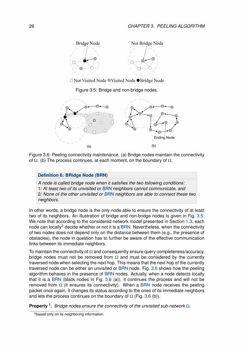
26 CHAPTER 3. PEELING ALGORITHM
Bridge Node Not Bridge Node
Visited NodeNot Visited Node Bridge Node
Figure 3.5: Bridge and non-bridge nodes.
(a)
Ω
Ending Node
(b)
Figure 3.6: Peeling connectivity maintenance. (a) Bridge nodes maintain the connectivityof Ω. (b) The process continues, at each moment, on the boundary of Ω.
Definition 6: BRidge Node (BRN)
A node is called bridge node when it satisfies the two following conditions:1/ At least two of its unvisited or BRN neighbors cannot communicate, and2/ None of the other unvisited or BRN neighbors are able to connect these twoneighbors.
In other words, a bridge node is the only node able to ensure the connectivity of at leasttwo of its neighbors. An illustration of bridge and non-bridge nodes is given in Fig. 3.5.We note that according to the considered network model presented in Section 1.3, eachnode can locally2 decide whether or not it is a BRN. Nevertheless, when the connectivityof two nodes does not depend only on the distance between them (e.g., the presence ofobstacles), the node in question has to further be aware of the effective communicationlinks between its immediate neighbors.
To maintain the connectivity of Ω and consequently ensure query completeness/accuracy,bridge nodes must not be removed from Ω and must be considered by the currentlytraversed node when selecting the next hop. This means that the next hop of the currentlytraversed node can be either an unvisited or BRN node. Fig. 3.6 shows how the peelingalgorithm behaves in the presence of BRN nodes. Actually, when a node detects locallythat it is a BRN (black nodes in Fig. 3.6 (a)), it continues the process and will not beremoved from Ω (it ensures its connectivity). When a BRN node receives the peelingpacket once again, it changes its status according to the ones of its immediate neighborsand lets the process continues on the boundary of Ω (Fig. 3.6 (b)).
Property 1. Bridge nodes ensure the connectivity of the unvisited sub-network Ω.2based only on its neighboring information.
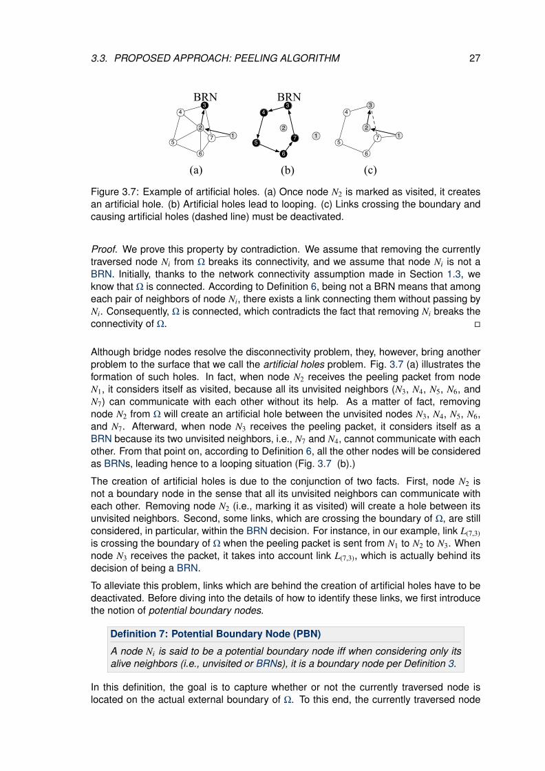
3.3. PROPOSED APPROACH: PEELING ALGORITHM 27
1 2
3 4
5
6
7
(a)
1 2
3 4
5
6
7
(b)
BRN
1 2
3 4
5
6
7
(c)
BRN
Figure 3.7: Example of artificial holes. (a) Once node N2 is marked as visited, it createsan artificial hole. (b) Artificial holes lead to looping. (c) Links crossing the boundary andcausing artificial holes (dashed line) must be deactivated.
Proof. We prove this property by contradiction. We assume that removing the currentlytraversed node Ni from Ω breaks its connectivity, and we assume that node Ni is not aBRN. Initially, thanks to the network connectivity assumption made in Section 1.3, weknow that Ω is connected. According to Definition 6, being not a BRN means that amongeach pair of neighbors of node Ni, there exists a link connecting them without passing byNi. Consequently, Ω is connected, which contradicts the fact that removing Ni breaks theconnectivity of Ω.
Although bridge nodes resolve the disconnectivity problem, they, however, bring anotherproblem to the surface that we call the artificial holes problem. Fig. 3.7 (a) illustrates theformation of such holes. In fact, when node N2 receives the peeling packet from nodeN1, it considers itself as visited, because all its unvisited neighbors (N3, N4, N5, N6, andN7) can communicate with each other without its help. As a matter of fact, removingnode N2 from Ω will create an artificial hole between the unvisited nodes N3, N4, N5, N6,and N7. Afterward, when node N3 receives the peeling packet, it considers itself as aBRN because its two unvisited neighbors, i.e., N7 and N4, cannot communicate with eachother. From that point on, according to Definition 6, all the other nodes will be consideredas BRNs, leading hence to a looping situation (Fig. 3.7 (b).)
The creation of artificial holes is due to the conjunction of two facts. First, node N2 isnot a boundary node in the sense that all its unvisited neighbors can communicate witheach other. Removing node N2 (i.e., marking it as visited) will create a hole between itsunvisited neighbors. Second, some links, which are crossing the boundary of Ω, are stillconsidered, in particular, within the BRN decision. For instance, in our example, link L(7,3)is crossing the boundary of Ω when the peeling packet is sent from N1 to N2 to N3. Whennode N3 receives the packet, it takes into account link L(7,3), which is actually behind itsdecision of being a BRN.
To alleviate this problem, links which are behind the creation of artificial holes have to bedeactivated. Before diving into the details of how to identify these links, we first introducethe notion of potential boundary nodes.
Definition 7: Potential Boundary Node (PBN)
A node Ni is said to be a potential boundary node iff when considering only itsalive neighbors (i.e., unvisited or BRNs), it is a boundary node per Definition 3.
In this definition, the goal is to capture whether or not the currently traversed node islocated on the actual external boundary of Ω. To this end, the currently traversed node

28 CHAPTER 3. PEELING ALGORITHM
has to consider only its alive neighbors and see, according to Definition 3, whether it islocated on a boundary (i.e., external boundary of Ω). Consequently, if a node is a PBN,it cannot create an artificial hole. On the opposite case, i.e., when a node is not a PBN,there is a risk of artificial hole formation.
Moreover, some links may cross the current boundary of Ω, as is the case of link L(7,3) inFig. 3.7 (a). To handle this situation, we introduce the following definition:
Definition 8: Alive Neighborhood
We denote by Vi(Ω) = N j | N j ∈ Vi ∧ N j ∈ Ω the current alive neighborhood ofnode Ni.
Based on Vi(Ω), the currently traversed node Ni can determine which links among Vi(Ω)’slinks are crossing the boundary of Ω. For instance, in our example of Fig. 3.7, node N2can easily determine that link L(7,3) is crossing the current boundary of Ω. Hence, when anode Ni receives the peeling packet from the previous hop Nprev, and find out that it is nota PBN and that there exist some links crossing the current boundary of Ω, it executes thetwo following steps:
• Construct two sets. The first one contains all nodes involved in the crossing linksthat are on the right side of the segment [Ni, Nprev]. The second set is formed bythe other nodes. In our example, the two sets are: N7 and N3.
• Send the peeling packet with this additional information about the two sets.
Upon receiving the peeling packet, the neighbors of the currently traversed node mustperform the following step. Each node checks first to which set it belongs. If it belongsto one of these two sets, then, it deactivates (deletes) its links with the nodes belongingto the other set. For example, as shown in Figure 3.7 (c), node N3 will deactivate its linkwith N7, and vice versa. Consequently, node N3 will not identify itself as a BRN, avoidingthus the previously observed looping situation. We underline that this link deactivationconcerns only the current executed query.
Property 2. PBN rules do not raise artificial holes.
Proof. Let us suppose that the currently traversed node is Ni, the previous hop is Nprev,and that an artificial hole has been created. We note that this assumption implies thatNprev has necessarily been marked as visited, otherwise an artificial hole cannot be cre-ated. In more details, we have two cases to consider; Nprev is a PBN or a non-PBN.
• Nprev is a PBN: according to Definition 7, this implies that nodes in VNprev(Ω) do notform a closed region, which contradicts the assumption of existence of a hole (cf.Definition 1).
• Nprev is not a PBN: also according to Definition 7, this implies the existence of a pathconnecting all alive neighbors of Nprev without passing through it. However, Nprev waslocated on the boundary of Ω and consequently, there exists a link belonging to thecreated hole and crossing this boundary. This is in contradiction with PBN rulesbecause such a link would have necessarily been deactivated. Consequently, ahole cannot exist, which is in contradiction with the initial assumption.
Therefore, in all cases, an artificial hole cannot exist.
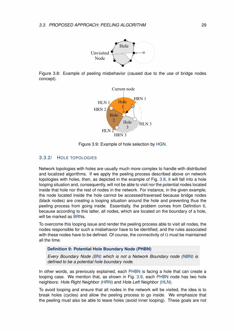
3.3. PROPOSED APPROACH: PEELING ALGORITHM 29
Hole Unvisited
Node
Figure 3.8: Example of peeling misbehavior (caused due to the use of bridge nodesconcept).
Hole 3
Hole 2
Hole 1
HRN 1
HRN 2
HRN 3 HLN 2
HLN 1
HLN 3
Current node
Figure 3.9: Example of hole selection by HGN.
3.3.2/ HOLE TOPOLOGIES
Network topologies with holes are usually much more complex to handle with distributedand localized algorithms. If we apply the peeling process described above on networktopologies with holes, then, as depicted in the example of Fig. 3.8, it will fall into a holelooping situation and, consequently, will not be able to visit nor the potential nodes locatedinside that hole nor the rest of nodes in the network. For instance, in the given example,the node located inside the hole cannot be accessed/traversed because bridge nodes(black nodes) are creating a looping situation around the hole and preventing thus thepeeling process from going inside. Essentially, the problem comes from Definition 6,because according to this latter, all nodes, which are located on the boundary of a hole,will be marked as BRNs.
To overcome this looping issue and render the peeling process able to visit all nodes, thenodes responsible for such a misbehavior have to be identified, and the rules associatedwith these nodes have to be defined. Of course, the connectivity of Ω must be maintainedall the time.
Definition 9: Potential Hole Boundary Node (PHBN)
Every Boundary Node (BN) which is not a Network Boundary node (NBN) isdefined to be a potential hole boundary node.
In other words, as previously explained, each PHBN is facing a hole that can create alooping case. We mention that, as shown in Fig. 3.9, each PHBN node has two holeneighbors: Hole Right Neighbor (HRN) and Hole Left Neighbor (HLN).
To avoid looping and ensure that all nodes in the network will be visited, the idea is tobreak holes (cycles) and allow the peeling process to go inside. We emphasize thatthe peeling must also be able to leave holes (avoid inner looping). These goals are not

30 CHAPTER 3. PEELING ALGORITHM
obvious to meet, especially with a localized serial algorithm. To solve this issue, weintroduce the following definition:
Definition 10: Hole Gate Node (HGN)
We define the Hole Gate Node of a hole as the first PHBN node of this hole toreceive/possess the peeling packet.
The HGN notion has a twofold role: (a) it allows the peeling process to discover holes (andvisit any potential inner nodes), and (b) it guarantees that the peeling can leave holes. Tomeet these two requirements, while still using a serial boundary traversal algorithm, someparticular links in Ω have to be deactivated. In other terms, the boundary of Ω must bemodified without altering its connectivity.
3.3.2.1/ HOLE GATE NODES IDENTIFICATION
According to Definition 10, two steps are necessary for a node to identify itself as HGN:
• First, it must determine whether it is facing a hole or not (Definition 3). For instance,the node of Fig. 3.9 is facing three holes. We underline that each node can locallyperform this step (thanks to its neighboring information).
• Second, once this node is aware that it is located on the boundary of a hole, it candetermine if it is the HGN of this hole when it receives the peeling packet. Moreprecisely, if the peeling packet arrives at the currently traversed node from a nodethat does not belong to the same hole, the currently traversed node is certainly thefirst visited node of the hole and consequently, it is the HGN of this latter. Otherwise,the hole has already got an HGN. We note that this second step can be performedlocally and does not require any extra-information other than the one-hop informa-tion.
In the case where the currently traversed node is facing more than one hole, the selec-tion of the hole to be explored is made according to the counterclockwise direction. Forinstance, in Fig. 3.9, the peeling packet came to the currently traversed node from hole 1,which means that hole 1 has already got an HGN and consequently, hole 2 will be theone to be explored next.
3.3.2.2/ HOLE GATE NODES RULES
Upon receiving the peeling packet from the previous hop Nprev, if node Ni detects that it isan HGN, it executes the four following steps:
1. Creates two sets from its immediate neighbors.
• The first set, called Front Set (FS), contains all neighbors located in the sectordefined by the angle ∠NprevHGNHLN. In the example of Fig. 3.10, all greynodes belong to this set, including the HRN.
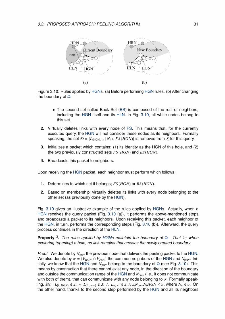
3.3. PROPOSED APPROACH: PEELING ALGORITHM 31
(a) (b)
HoleCurrent Boundary
HRN
HLN HGN
New Boundary
HRN
HLN HGN
Figure 3.10: Rules applied by HGNs. (a) Before performing HGN rules. (b) After changingthe boundary of Ω.
• The second set called Back Set (BS) is composed of the rest of neighbors,including the HGN itself and its HLN. In Fig. 3.10, all white nodes belong tothis set.
2. Virtually deletes links with every node of FS. This means that, for the currentlyexecuted query, the HGN will not consider these nodes as its neighbors. Formallyspeaking, the set D = L(HGN, i) | Ni ∈ FS (HGN) is removed from L for this query.
3. Initializes a packet which contains: (1) its identity as the HGN of this hole, and (2)the two previously constructed sets FS (HGN) and BS (HGN).
4. Broadcasts this packet to neighbors.
Upon receiving the HGN packet, each neighbor must perform which follows:
1. Determines to which set it belongs; FS (HGN) or BS (HGN).
2. Based on membership, virtually deletes its links with every node belonging to theother set (as previously done by the HGN).
Fig. 3.10 gives an illustrative example of the rules applied by HGNs. Actually, when aHGN receives the query packet (Fig. 3.10 (a)), it performs the above-mentioned stepsand broadcasts a packet to its neighbors. Upon receiving this packet, each neighbor ofthe HGN, in turn, performs the corresponding steps (Fig. 3.10 (b)). Afterward, the queryprocess continues in the direction of the HLN.
Property 3. The rules applied by HGNs maintain the boundary of Ω. That is; whenexploring (opening) a hole, no link remains that crosses the newly created boundary.
Proof. We denote by Nprev the previous node that delivers the peeling packet to the HGN.We also denote by σ = VHGN ∩ VPrev the common neighbors of the HGN and Nprev. Ini-tially, we know that the HGN and Nprev belong to the boundary of Ω (see Fig. 3.10). Thismeans by construction that there cannot exist any node, in the direction of the boundaryand outside the communication range of the HGN and Nprev (i.e., it does not communicatewith both of them), that can communicate with any node belonging to σ. Formally speak-ing, @Ni | Li, HGN < L ∧ Li, prev < L ∧ Li, n ∈ L ∧ ∠NprevNiHGN ≤ π, where Nn ∈ σ. Onthe other hand, thanks to the second step performed by the HGN and all its neighbors

32 CHAPTER 3. PEELING ALGORITHM
Previous Node
1
2
34
10
11
12
1314 15
16
17
18
59
87
6
False HGN
True HGN
Deactivated links
Hole 1
Hole 2(a)
(b)1
2
34
10
11
12
1314 15
16
17
18
Dectivated links
Hole 1
Hole 2
Hole Control Packet (HCP)
9
87
6
5
Figure 3.11: Nested holes. (a) Peeling the network without using HCP packets. (b) Peel-ing the network using HCP packets.
(i.e., links deletion), there cannot exist any link between the FS and BS sets. In addition,by construction, there cannot exit a link between the HLN and HRN (otherwise, a holecannot exit). Finally, there cannot exist a link crossing the new boundary including Nprev,HGN, and HLN.
The peeling approach described above has ensured query completeness on the numer-ous network configurations that have been randomly generated in our performance eval-uation study (cf. Section 3.6). All alive connected nodes were visited. Nevertheless, froma theoretical point of view, we have constructed by hand, some particular topologies inwhich this version of PA fails to ensure query completeness. Fig. 3.11 (a) illustrates anexample of such topologies. In this figure, when node N1 receives the query, it considersitself as the HGN of hole 1 and applies the corresponding rules. That is, link L(1, 17) isdeleted and the query is oriented towards node N2. Similarly, when node N4 receives thequery, it considers itself as the HGN of the hole located to the left, deletes link L(4, 5), andthen sends the query to node N10. Consequently, all nodes located on the boundary ofhole 2 will be lost and can never be visited.
This false HGN detection comes from the fact that node N4 treats a single hole (hole 1)as being two different holes. To solve this problem, an additional rule must be executedby the HGNs. Actually, before performing steps 2, 3 and 4 described above, the HGNsends a control packet, named Hole Control Packet (HCP), which travels along the hole

3.3. PROPOSED APPROACH: PEELING ALGORITHM 33
in question, and visits all nodes located on its boundary. Eventually, due to its nature, theHCP will get back to the HGN (Fig. 3.11 (b)). In fact, the HCP packet plays a twofold role:
• First, it informs all nodes located on the boundary of the hole that this latter hasan HGN. Consequently, these nodes will not consider this hole later on when theyreceive the query packet.
• Second, the HCP packet allows nodes to detect if their local stored holes constitutethe same hole. For instance, node N4 will know that its left and right holes areactually one single hole that has already got an HGN. This way, N4 will not consideritself as the HGN of this hole and will allow the peeling process to continue aftercontributing to it.
In the same context, later on, when the query packet gets to node N5, it will identifyitself as the HGN of hole 2, and consequently will apply the corresponding rules.That is, sending a HCP packet inside this hole and deleting the link with its rightneighbor (Fig. 3.11 (b)).
Property 4. The rules applied by HGNs do not partition the set of unvisited nodes Ω.
Proof. Let us assume that the deleted links partition Ω and let us try to arrive at a contra-diction. Further, let us suppose that there exists only one link between FS and BS sets(i.e., link connecting HGN and HRN). Actually, in this case, our initial assumption meansthat after links deletion, no path can connect the nodes of FS and BS sets. Which, thanksto the HCP packets sent by the HGN of the hole contradicts the existence of another pathconnecting HGN with HRN. Also, by construction, each hole has one and only one HGN.Consequently, there exists a path, passing through the HLN, connecting the HGN to ev-ery node in the hole, in particular, the HRN. In other words, the HGN and the HRN areconnected through the hole. In addition to that, based on (1) the fact that the BS and theFS are internally connected (i.e., nodes inside them are connected), and (2) the fact thatHGN and HRN belong respectively to the BS and FS, we can deduce that the FS and BSare connected. This contradicts the initial assumption.
The overall peeling algorithm, executed by each node receiving the query packet, is de-picted in Algorithm 1.
3.3.3/ STARTING NODE DETERMINATION
As previously mentioned, the peeling approach must start from a node that is located onthe external boundary of the network. To this end, in this section, we propose a distributedlocalized technique able to efficiently identify the network boundary nodes. Actually, thisapproach is inspired from the work presented in [37, 38], and its key idea is to try toreach a virtual node located outside the network area using a geographic greedy routing(Fig. 3.12).
In more details, a packet aiming to reach the virtual node is initiated by the sink/querylauncher. Actually, at first, the query launcher Ni sets the location of the virtual nodeand sends the created packet to its one-hop neighbor N j which is the closest to the setvirtual node (among Ni itself and all its neighbors). Knowing the virtual node location(from the received packet), every node in the path repeats this process until the packet

34 CHAPTER 3. PEELING ALGORITHM
Hole
Virtual Node
Sink
Last Local Minimum
Figure 3.12: Network boundary nodes determination.
Algorithm 1 Peeling Algorithm.Require: Receive peeling packet from previous hop.1: if (current node not visited for this query) then2: Contribute to this query;
3: Mark itself as visited for this query;
4: if (current node is HGN) then5: // If current node is located on more than one unexplored hole (Fig. 3.9)6: Select the first counterclockwise hole among local unexplored holes;
7: Send an HCP packet inside the selected hole;
8: Upon receiving the HCP packet back, select the HLN as next hop;
9: else10: if (current node is not PBN and crossing links exist) then11: Add necessary information to the peeling packet; // cf. artificial holes.12: end if13: Select next hop among unvisited and BRN neighbors;
14: end if15: else16: Select next hop among unvisited and BRN neighbors;
17: end if18: Determine the current node status; // BRN or not?19: Send peeling packet to next hop;
falls into a local minimum situation (i.e., the packet cannot be delivered to the next hopas the current node is the closest one to the virtual node). From this node, also calledthe local minimum node, the recovery process is launched using the curved-stick bound-ary traversal approach [38] (Section 2.3.2.1). This process is repeated until the currentlyselected node is closer to the virtual node than the local minimum node. From this mo-ment, the greedy forwarding is used again, and so on. For instance, in Fig. 3.12, plainarrows represent greedy communications and hollow ones represent boundary traversal(curved-stick) communications.
Following this approach and knowing that the virtual node is unreachable by construction,the packet will make a cycle and get back to the last local minimum node, denoted by Nl.
Property 5. The last local minimum node Nl is a network boundary node (NBN).
Proof. Initially, all nodes in the network are connected (connectivity assumption made inSection 1.3). Also, given the fact that (1) the curved-stick ensures boundary traversal [38],and (2) the greedy rule selects the closest node to the virtual node, we conclude that the
3.4. PROOF OF CORRECTNESS 35
last local minimum node Nl has the shortest distance to the virtual node among all nodesin the network. Hence, Nl is located on the network boundary.
Once a node has been identified as a network boundary node (NBN); e.g., the grey nodein Fig. 3.12, the process of identifying all the other NBNs in the network can be triggeredfrom this node using the curved-stick boundary traversal algorithm. In fact, upon receivingthe curved-stick packet, each node (which is necessarily a NBN) must locally update itslist of local holes (i.e., mark the external boundary of the network as explored), and thisin order to avoid considering the external boundary of the network as a hole boundary.
It is worth emphasizing that the process of NBNs determination must be done only onceand it is not necessary to repeat it each time the network is queried unless of course, thenetwork topology has changed.
3.4/ PROOF OF CORRECTNESS
In this section, we provide proofs that demonstrate the peeling algorithm correctness.More precisely, we first prove that our approach terminates and does not fall into looping.In other words, we prove that PA generates a finite set of hops. Second, we prove that PAensures query completeness (i.e., visits all nodes in the network).
The main facts on which the proof of correctness of PA is built are: (a) iteratively shrink-ing Ω while maintaining its connectivity (Property 1), (b) avoiding looping situations thatcan be caused by the creation of artificial holes (Property 2), and (c) transforming Ω (us-ing the HGN rules) from a connected sub-network with holes (cycles) to a one withoutholes (Properties 3 and 4).
Formally, PA iteratively constructs (shrinks) the set Ωi, following the recurrent relationshipdefined as follows:
Ω0 = N ,
Ωi+1 = Ωi − Nv,
where Nv is the first traversed node which is not a BRN during the scan of Ωi. For instance,in Fig. 3.11(b), if we denote the sub-network of nodes N1 to N18 by Ωk, then:
Ωk+1 = Ωk − N1,Ωk+2 = Ωk+1 − N2,Ωk+3 = Ωk+2 − N3,Ωk+4 = Ωk+3 − N9,Ωk+5 = Ωk+4 − N8,
. . .
Lemma 1:
At each iteration i, PA finds a non-BRN node Nv.
36 CHAPTER 3. PEELING ALGORITHM
Proof. Let us suppose that at step i, node Nv does not exist. In fact, since the curved-stick ensures boundary traversal, this assumption means that all the traversed nodes areBRNs. In other words, the traversed nodes form a hole. This, however, contradicts thenon-existence of holes (cycles) guaranteed by the HGN rules. Therefore, we concludethat at each step i, Nv exists.
Based on the previous lemma, we have:
Theorem 1:
PA generates a finite sequence of hops H =⋃k
i=0 Ni (i.e., PA terminates).
Proof. Initially, PA starts with a finite set Ω0 = N . Then, at each iteration i, Lemma 1ensures that a non-BRN node Nv exists. This means that the number of nodes in Ω isstrictly decreasing at each iteration:
∀ | N | > i > j > 0, | Ωi | < | Ω j |
Since PA starts with a finite set of nodes, then, it exits a k such that Ωk+1 = ∅. Hence, weprove that H is finite and PA terminates.
We define the set of external boundary nodes of Ωi, denoted by B(Ωi), as follows:
Definition 11: Boundary of Ωi
The boundary of Ωi is a cyclic sequence of unvisited or BRN nodes such thatthe closed region bounded by this non-self-intersecting polygonal sequence con-tains all the nodes of Ωi.
Lemma 2:
At each iteration i, the next visited node Nv belongs to B(Ωi). That is, Nv islocated on the boundary of the current sub-network Ωi.
Proof. We know that, initially, the peeling algorithm starts from a node that is located onthe boundary of Ω0. Based on this and given the fact that the curved-stick is a bound-ary traversal tool [38], each traversed non-BRN node Nv will be certainly located on theboundary of Ωi. This can be proven as follows. In fact, initially, the peeling algorithmkeeps scanning the nodes located on the boundary of Ω0 until it hits a non-BRN node Nv.That is, initially, Nv is located on the boundary of Ω0 and the property is true for i = 0.Now, let us suppose that the property is true for i and let us try to show that it remains assuch for i + 1. First, since the property is true for i, this means that the currently removednode Nv is located on the boundary of Ωi. Second, as previously mentioned, using thecurved-stick as a traversal algorithm guarantees that the next hop Nw of Nv is located onthe boundary of Ωi. Consequently, it is clear that this next hop Nw is also located on theboundary of Ωi+1. In fact, if Nw is not a bridge node (non-BRN) then it can be removedfrom Ωi+1 (marked as visited). Otherwise, starting from Nw, PA will keep scanning theboundary of Ωi+1 until it finds a non-bridge node that can be marked as visited. Hence,we conclude that the property is also true for i + 1.

3.5. PEELING EFFICIENCY AND ROBUSTNESS ENHANCEMENT 37
Theorem 2:
The sequence of hops H , generated by PA, contains all nodes of the network(i.e., H = N).
Proof. To prove that PA visits all nodes in the network, let us assume that H (set gen-erated at the end of network traversal) is different than N (set of all connected nodes inthe network) and then let us seek to derive a contradiction. First, let us denote by Nv,each traversed non-BRN node that will be removed from Ω without altering its connec-tivity. Second, let us denote by Nm, one of the unvisited nodes that might be missed byPA (Nm , Nv, ∀ v). Third, let us consider an unsigned integer j (0 < j < n) such that Nm
belongs to Ω j and does not belong to Ω j+1. That is, Nm has been missed at iteration j.Actually, since at iteration j, PA hits only nodes that are located on the boundary of Ω j
and does not miss any one of them (Lemma 2 and Theorem 1); therefore, Nm cannot, inany case, be located on the boundary of Ω j. Thus, Nm belongs to Ω j+1. This, however,contradicts the initial assumption which says that Nm does not belong to Ω j+1 (Nm < Ω j+1).Consequently, we conclude that PA guarantees network traversal completeness in spiteof the considered topology.
To recapitulate, thanks to Theorems 1 and 2, we have the guarantee that, regardlessof the considered network topology (irregular or regular, large-scale or sparse, with orwithout holes,etc.), the proposed peeling algorithm terminates (does not fall into looping)and ensures query completeness/accuracy.
3.5/ PEELING EFFICIENCY AND ROBUSTNESS ENHANCEMENT
As confirmed by the simulation results presented in the next section, the proposed peelingapproach performs very efficiently in uniformly dense networks. Nevertheless, we havenoted that in sparse networks with different densities, some nodes/links (because of theirpositions as BRNs) participate more often in the query evaluation than others. An exam-ple of such topologies is given in Fig. 3.13 (a), which illustrates one peeling round (greynodes have been marked as visited, black nodes are bridges, and white ones have notbeen visited yet). Actually, in this example, it is clear that bridge nodes will be accessedmore frequently than the others. For instance, if the peeling process continues until theend, the bridge black nodes and their related links will be accessed/used five times. Sucha situation occurs because the peeling algorithm does not consider the visited nodes(which are not bridges). In other words, PA keeps only one alive path of bridges and usesit all the time.
As a matter of fact, this path linearity phenomenon brings with it several drawbacks andissues. First, it increases the communications required to accomplish a query. Second,and more importantly, it contributes somehow to the vulnerability of the peeling process.For instance, when a link in such a linear path of bridges is broken, the unvisited regionwill be partitioned despite the existence of other paths that can be formed by the alreadyvisited nodes. Actually, in such a scenario, since the current version of the peeling al-gorithm does not consider this solution or any other one, the peeling packet will be sentback to the previous hop and a false peeling termination will be detected.

38 CHAPTER 3. PEELING ALGORITHM
BRN Linearity
(a): First Round
(b): Second Round
Cyclic Node
Ω
Ω
Figure 3.13: Peeling linearity phenomenon.
Repairing the connectivity of Ω (when it is partitioned due to the unavailability of a path)is a very challenging issue that deserves much research efforts. We mention that in thepresent section, our goal is just alleviating the impact of path linearity phenomenon onthe peeling process. To this end, we have added a new rule that must be performed bycertain specific nodes defined, as follows:
Definition 12: Cyclic Node (CN)
A node Ni is said to be cyclic, iff it conforms to the following two conditions:(a) it is a BRN (bridge node) and (b) it has received the peeling packet from twodifferent directions.
In other words, as illustrated in Fig. 3.13 (b), the peeling process must pass, at leasttwice, by a cyclic bridge node Ni. Actually, when the peeling process gets back to a cyclicnode (i.e., has accomplished a cycle), it defines a closed unvisited region (Fig. 3.13 (b)).The objective of the new rule that must be performed only by cyclic nodes is to peelthis closed region before continuing the process somewhere else. This, as shown byFig. 3.13 (b), means that each cyclic node must re-orient the peeling process towards theclosed unvisited region. This way, the new applied rule ensures that the peeling processremains inside the region in question until visiting all its nodes. Eventually, once thedesired region has been completely visited, the cyclic node in question will change itsstatus from bridge to visited node and forwards the peeling packet.
Clearly, from a theoretical standpoint, the new applied rule noticeably reduces the serialpath length, which considerably enhances the peeling performance. Yet, to confirm thispoint, in our experiments, in addition to PA, we have also implemented this improvement,calling it Enhanced Peeling Algorithm (EPA). For instance, applying the new rule to thenetwork of Fig. 3.13 leads to more than 8% of communications reduction. Further, as itwill be shown in the next section (3.6), this reduction is more substantial in large-scalenetwork deployments.

3.6. PEELING PERFORMANCE ASSESSMENT 39
3.6/ PEELING PERFORMANCE ASSESSMENT
In order to evaluate the performance of our proposed peeling algorithms, we have con-ducted several series of simulations using OMNeT++ [53] and its WSNs frameworkCastalia [54]. For comparison purposes, in addition to PA and EPA, we have also im-plemented the three following approaches:
1/ Tree-based querying: in this approach, called also centralized in-network query-ing [3], a tree rooted at the sink must be constructed. In fact, in the resulting tree, eachnode can have one or several children but must have only one parent, except for leafnodes which will have no children and the sink which must have no parent. Once the treeis created and all nodes in the network are connected to it, query processing can be per-formed following two phases. The first phase is dedicated to query dissemination throughthe tree (starting from the sink). More specifically, upon receiving the query, each inter-mediate node forwards the query to its children. When the query arrives at leaf nodes,the latter trigger the second phase by sending their readings to their corresponding par-ents. From this point on, upon receiving data from its children, each intermediate nodeaggregates these measurements with its own reading and sends the result to its parent,and so on. This process stops when all data is received by the sink.
2/ Iterative querying: in this approach, called also distributed in-network query-ing [14,15], the QL can launch a query by simply broadcasting a packet to its immediateneighbors. Upon receiving the query, each node re-broadcasts it and starts exchangingits own estimate with those of its immediate neighbors. More precisely, at each iteration ofthe process, the local estimate of each node is updated with the weighted data receivedduring the previous iteration, and so on. This process terminates when each node detectsthat the difference in values between two consecutive terms of the estimated parameteris smaller than a certain predetermined threshold.
3/ Depth-First Search: this well-known serial technique [26] constructs for each querya path that stems from the QL and extends, as much as possible, toward the unvisitednodes. In other words, DFS explores the network as far as it can, and when it gets stuck,it backtracks (looking for other possible unvisited nodes). To be able to do so, each nodemust be aware of its unvisited neighbors as well as the identity of its parent. We recallthat DFS requires 2∗ (n−1) hops to explore a network of n connected nodes and get backto the sink/QL.
3.6.1/ EVALUATION METRICS
Note that, regardless of the considered network configurations, all the implemented ap-proaches have been proven to ensure query completeness (all nodes contribute to thequery). In the same context, note also that, except DFS, we have not considered anyother serial approaches such as space-filling curves algorithm [24], because they do notsatisfy this requirement (they do not guarantee query accuracy).
For a single query, in addition to completeness, the other considered comparison metricsare:
• Required communications: total number of packets (transmissions) used to querythe network and aggregate data (i.e., control and data packets).

40 CHAPTER 3. PEELING ALGORITHM
Table 3.1: Peeling simulation configuration and parameters
Parameter Value(s)
Field dimensions (m2) 1000 x 1000Nodes number 100, 150, 200, . . . , 500Nodes deployment UniformNodes transmission range (m) 150Nodes initial energy (J) 100Query launcher location RandomQuery packet size (byte) 50Radio type CC2420Radio data rate (kbps) 250MAC protocol CSMA/CASensed values interval [0, 0.4]Convergence threshold (for Iterative approach) 10−2
• Response time: time that elapses between the instant when the QL issues a queryand the instant when it receives the corresponding answer.
• Consumed energy: total energy consumed by the network during the querying pro-cess. In fact, in order to estimate the energy required by each node to transmit andreceive packets, we have used the energy consumption model proposed in [55].The radio in this model dissipates Eelec = 50 nJ/bit to run the transmitter or receivercircuitry and εamp = 100 pJ/bit/m2 for the transmitter amplifier. Thus, to transmit ak-bit packet a certain distance d using this model, the radio consumes:
ET X(k, d) = k ∗ Eelec + k ∗ d2 ∗ εamp
and to receive this same packet, the radio consumes:
ERX(k) = k ∗ Eelec.
In addition to these metrics, we consider the number of queries a network can supportbefore one of its nodes runs out of energy. This metric represents the network lifetime interms of supported queries.
3.6.2/ SIMULATION PARAMETERS
The considered simulation parameters are summarized in Table 3.1. Note that the sensedvalues interval, which impacts only the iterative querying approach (described above),has been set to [0, 0.4]. Actually, as explained below in Section 3.6.3.1, the length ofthis interval has been purposely set to a small value in order to not penalize the iterativeapproach. In the same context, we mention that the sensed values, taken from the choseninterval, are normalized uniform random values.
As regards Table 3.2, it shows the average degree of nodes in the different deployments;i.e., the average number of neighbors of each node. More precisely, in this table, the first

3.6. PEELING PERFORMANCE ASSESSMENT 41
Table 3.2: Peeling average nodes’ degree.
100 150 200 250 300 350 400 450 5008 12 16 20 25 29 33 37 42
line represents the number of nodes in the network, whereas the second one representsthe corresponding average degree.
3.6.3/ SIMULATION RESULTS
For each query configuration (i.e., network deployment and query launcher location), wehave run the studied approaches and recorded the obtained results. Actually, the resultspresented below represent the mean values of 30 runs on each configuration.
3.6.3.1/ SINGLE QUERY PERFORMANCE
Figures 3.14, 3.15, and 3.16 summarize the obtained single query evaluation results.These curves clearly confirm the effectiveness of serial approaches over centralized (i.e.,parallel tree-based) and iterative (i.e., parallel structure-free) ones. Although the improve-ment is minor in sparse network configurations, it becomes more noticeable when thenetwork density increases. For instance, in terms of communications, PA is about 6 timesbetter than the iterative approach and 4 times better than the centralized one. As a matterof fact, even though the centralized approach allows concurrent transmissions, the gen-erated collisions (during tree construction, query answering, etc.) prevent this approachfrom exhibiting better performance. The obtained results also reveal that the iterative ap-proach (because of its intrinsic iterative behavior) is more costly in comparison with theother approaches. Actually, we have concluded (from other results not reported in thismanuscript) that when the standard deviation between sensed data is important and thenetwork is large, the iterative approach will need more iterations to reach convergence.In fact, this happens particularly when nodes with important differences in sensed dataare located far away from each other.
We note that, in all the studied approaches, the three considered metrics increase with theincrease of the number of nodes in the network. This trend, however, is less pronouncedin serial approaches, which means that they are more scalable than the centralized anditerative techniques.
Now, if we consider only the studied serial approaches (PA versus DFS), the obtainedresults clearly display the outperformance of our algorithm in terms of communications,time, and energy consumption. This improvement, while minor in sparse configurations(from 100 to 150 nodes), becomes more significant in dense networks (from 70% to 90%).Actually, this is primarily due to the fact that our approach is localized and structure-free(only one-hop information is required and no predetermined visiting path needs to befollowed). As regards DFS, in fact, its bad performance comes mainly from its costlymandatory backtracking process.

42 CHAPTER 3. PEELING ALGORITHM
0
500
1000
1500
2000
2500
3000
100 150 200 250 300 350 400 450 500
Num
ber
of T
ransm
issio
ns
Number of Nodes
IterativeCentralized
DFSPeeling
Figure 3.14: Peeling one query performance: number of transmissions.
0
5
10
15
20
25
30
100 150 200 250 300 350 400 450 500
Sin
gle
Qu
ery
Re
sp
on
se
Tim
e (
in s
)
Number of Nodes
IterativeCentralized
DFSPeeling
Figure 3.15: Peeling one query performance: average response time.
3.6.3.2/ NETWORK LIFETIME
In these series of simulations, we measure the effect of the different studied approacheson the overall network lifetime. To this end, prior to deployment, we have provided eachnode with the same initial energy provision of 5J. Then, we have run the consideredapproaches by launching a query every 2 minutes. The network is assumed to be deadwhen any of its nodes (i.e., the first node) runs out of energy. Fig. 3.17 plots the recordednumber of supported queries. In fact, as this figure shows, the obtained results confirmthe effectiveness of our peeling approach in terms of prolonging the network lifetime andsupporting more queries compared with the other approaches. More specifically, the

3.6. PEELING PERFORMANCE ASSESSMENT 43
0
5
10
15
20
25
30
35
40
45
100 150 200 250 300 350 400 450 500
En
erg
y C
on
su
mp
tio
n (
in J
)
Number of Nodes
IterativeCentralized
DFSPeeling
Figure 3.16: Peeling one query performance: total energy consumption.
0
100
200
300
400
500
600
100 150 200 250 300 350 400 450 500
Ne
two
rk L
ife
tim
e (
# o
f Q
ue
rie
s)
Number of Nodes
IterativeCentralized
DFSPeeling
Figure 3.17: Peeling performance: network lifetime.
improvements are nearly 500%, 300% and 50% in comparison, respectively, with theiterative, centralized, and DFS approaches.
3.6.3.3/ COLLISIONS IMPACT
As previously mentioned, one of the main interesting features of serial approaches isthat they do not generate collisions. Actually, in these approaches, all transmissionsare sequential and at any moment in time, only one node is allowed to send data. Toquantify the effect of this collision-free feature on query responsiveness, in this section,we compare the studied serial approaches (i.e., PA and DFS) while enabling and disabling

44 CHAPTER 3. PEELING ALGORITHM
0
2
4
6
8
10
100 150 200 250 300 350 400 450 500
Sin
gle
Qu
ery
Re
sp
on
se
Tim
e (
in s
)
Number of Nodes
DFS with MACDFS without MACPeeling with MAC
Peeling without MAC
Figure 3.18: Peeling query response time while enabling and disabling MAC functions.
0
200
400
600
800
1000
100 150 200 250 300 350 400 450 500
Nu
mb
er
of
Tra
nsm
issio
ns
Number of Nodes
DFS
PA
EPA
Figure 3.19: PA and EPA one query performance: number of transmissions.
the MAC layer. We recall that the considered MAC is the CSMA/CA protocol provided byCastalia [54] (Table 3.1).
The obtained results confirm that disabling the MAC layer does not affect either the re-quired number of communications nor the consumed energy, but actually, impacts thequery response time (Fig. 3.18). More specifically, a clear time improvement can be at-tained when no MAC layer is utilized, especially in dense networks (about six times ofimprovement). The reality of this enhancement being more noticeable in large-scale de-ployments validates the appropriateness of serial approaches for this kind of networks.However, the only downside here is that the MAC layer can be disabled only in the casewhere just one query is present in the network.
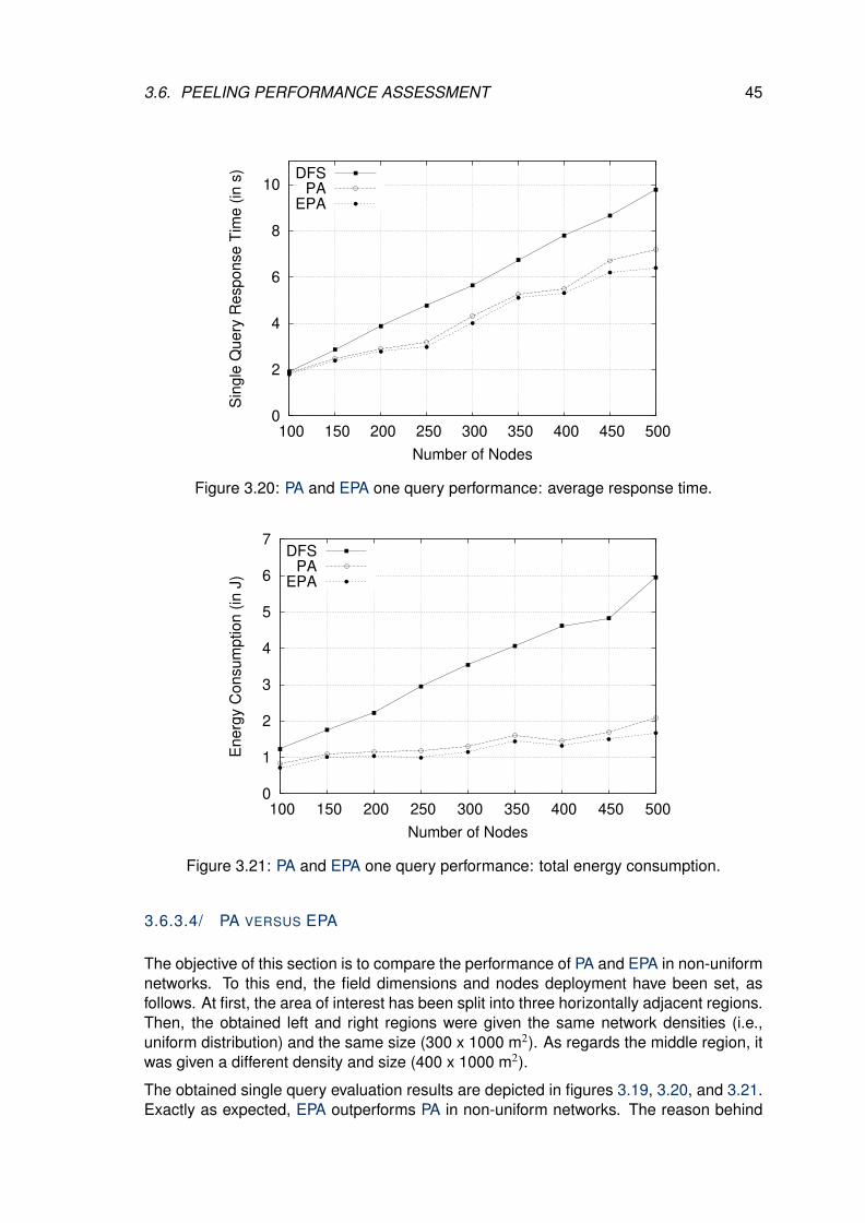
3.6. PEELING PERFORMANCE ASSESSMENT 45
0
2
4
6
8
10
100 150 200 250 300 350 400 450 500
Sin
gle
Qu
ery
Re
sp
on
se
Tim
e (
in s
)
Number of Nodes
DFSPA
EPA
Figure 3.20: PA and EPA one query performance: average response time.
0
1
2
3
4
5
6
7
100 150 200 250 300 350 400 450 500
En
erg
y C
on
su
mp
tio
n (
in J
)
Number of Nodes
DFSPA
EPA
Figure 3.21: PA and EPA one query performance: total energy consumption.
3.6.3.4/ PA VERSUS EPA
The objective of this section is to compare the performance of PA and EPA in non-uniformnetworks. To this end, the field dimensions and nodes deployment have been set, asfollows. At first, the area of interest has been split into three horizontally adjacent regions.Then, the obtained left and right regions were given the same network densities (i.e.,uniform distribution) and the same size (300 x 1000 m2). As regards the middle region, itwas given a different density and size (400 x 1000 m2).
The obtained single query evaluation results are depicted in figures 3.19, 3.20, and 3.21.Exactly as expected, EPA outperforms PA in non-uniform networks. The reason behind

46 CHAPTER 3. PEELING ALGORITHM
this (as previously explained) is that EPA uses the notion of cyclic nodes to optimize thevisiting peeling path. The improvement is about 4% in sparse configurations and about10% in dense ones, which validates the effectiveness of EPA in large-scale and non-uniform networks.
We mention that the obtained results (not shown here in this manuscript) also confirmthat PA and EPA have almost the same performance when the network deployment isuniform.
3.7/ CONCLUSION
In WSNs, serial query processing approaches have shown their effectiveness in termsof reducing communications and energy consumption. Nevertheless, besides the factthat query completeness was not ensured (i.e., visiting all nodes in the network) [24],previous research works have not explicitly addressed the key issue of constructing thevisiting path [20,22]. In this chapter, we have tackled these important issues by proposinga serial localized approach, named the Peeling Algorithm (PA) [18]. The main advantageof this proposed approach is that it does not require any additional knowledge other thanwhat is traditionally available in WSNs. That is to say, PA is a one-hop approach that doesnot require any information about the network topology. In this chapter, we have formallyproven that PA ensures query completeness and is free of looping. In addition to this,the obtained simulation results have clearly highlighted the effectiveness of PA in termsof reducing communications and energy/time consumption.
Despite its good performance and efficiency, PA still raises several research challengesthat deserve further investigations. Among these issues, we mention that the perfor-mance of PA can be further enhanced by reducing the traversal path length. In fact, thisis precisely the aim of the next chapter.

4SPREADING AGGREGATION
4.1/ INTRODUCTION
Recently, numerous works have shown that serial aggregation in large WSNs is scal-able and very efficient, in terms of avoiding collisions and conserving energy and,
more importantly, in terms of reducing response time [18, 25]. In this chapter, a novelserial data aggregation approach, called Spreading Aggregation (SA), is proposed withthe aim of shortening the traversal path and further reducing communications [39, 40].First, given the fact that it is not based on a pre-established itinerary, SA is maintenance-free and does not require any communications in this regard. Each time an aggregationprocess is launched, a new path is built, which decreases vulnerability to failure in linksand nodes and allows the approach to handle topology changes. Second, SA is a local-ized approach that relies only on the one-hop neighbors’ table of each node to graduallyconstruct the path, which makes it very scalable. A third interesting feature of SA is themerge of path construction and data processing. While the path is progressively con-structed, data is simultaneously aggregated, saving a considerable amount of time andenergy. In addition to all that, SA also saves energy and time due to its collision-freenature. In fact, in SA, only one packet is present in the entire network at any given time.
In this chapter, we formally prove the correctness of SA (i.e., free of looping and ensuresthe traversal of all connected nodes). Furthermore, the extensive OMNeT++ simulations,we performed, confirm that the proposed approach reduces communications, scales wellin large networks, and conserves time and energy. The obtained results also show thatSA outperforms state-of-the-art serial approaches.
Briefly, this chapter is structured in five sections, as follows. The next section (4.2) in-troduces the preliminaries and background required throughout the chapter. Section 4.3presents and details the operation of the proposed approach, while Section 4.4 providesits proof of correctness. Section 4.5 presents and comments on the evaluation results.Finally, Section 4.6 concludes the chapter.
47
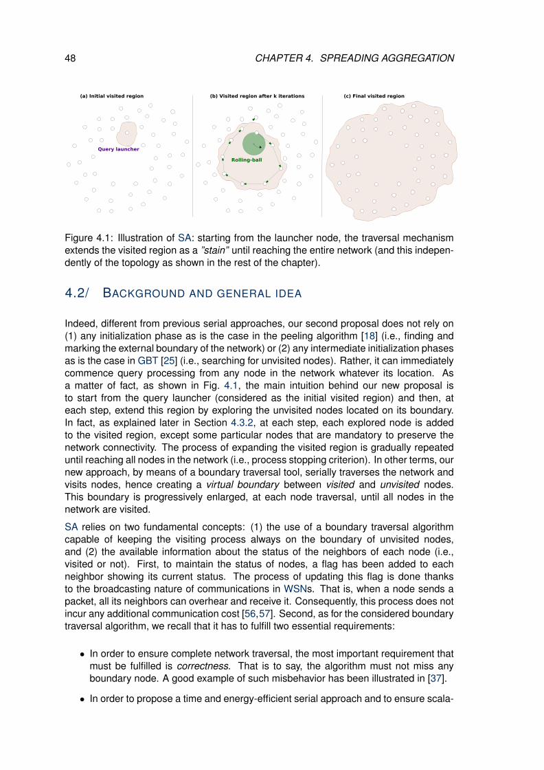
48 CHAPTER 4. SPREADING AGGREGATION
Figure 4.1: Illustration of SA: starting from the launcher node, the traversal mechanismextends the visited region as a ”stain” until reaching the entire network (and this indepen-dently of the topology as shown in the rest of the chapter).
4.2/ BACKGROUND AND GENERAL IDEA
Indeed, different from previous serial approaches, our second proposal does not rely on(1) any initialization phase as is the case in the peeling algorithm [18] (i.e., finding andmarking the external boundary of the network) or (2) any intermediate initialization phasesas is the case in GBT [25] (i.e., searching for unvisited nodes). Rather, it can immediatelycommence query processing from any node in the network whatever its location. Asa matter of fact, as shown in Fig. 4.1, the main intuition behind our new proposal isto start from the query launcher (considered as the initial visited region) and then, ateach step, extend this region by exploring the unvisited nodes located on its boundary.In fact, as explained later in Section 4.3.2, at each step, each explored node is addedto the visited region, except some particular nodes that are mandatory to preserve thenetwork connectivity. The process of expanding the visited region is gradually repeateduntil reaching all nodes in the network (i.e., process stopping criterion). In other terms, ournew approach, by means of a boundary traversal tool, serially traverses the network andvisits nodes, hence creating a virtual boundary between visited and unvisited nodes.This boundary is progressively enlarged, at each node traversal, until all nodes in thenetwork are visited.
SA relies on two fundamental concepts: (1) the use of a boundary traversal algorithmcapable of keeping the visiting process always on the boundary of unvisited nodes,and (2) the available information about the status of the neighbors of each node (i.e.,visited or not). First, to maintain the status of nodes, a flag has been added to eachneighbor showing its current status. The process of updating this flag is done thanksto the broadcasting nature of communications in WSNs. That is, when a node sends apacket, all its neighbors can overhear and receive it. Consequently, this process does notincur any additional communication cost [56,57]. Second, as for the considered boundarytraversal algorithm, we recall that it has to fulfill two essential requirements:
• In order to ensure complete network traversal, the most important requirement thatmust be fulfilled is correctness. That is to say, the algorithm must not miss anyboundary node. A good example of such misbehavior has been illustrated in [37].
• In order to propose a time and energy-efficient serial approach and to ensure scala-
4.3. PROPOSED APPROACH: SPREADING AGGREGATION 49
bility for large-scale deployments, the other requirement that must be fulfilled by theused boundary traversal algorithm is localizability. This means that the boundarytraversal algorithm must rely only on the local information available at each node(node’s position and that of its one-hop neighbors).
In this chapter, the rolling-ball [41] has been selected as a network traversal tool because,as it has been demonstrated in [37, 38], it can visit more nodes than the curved-stick.Actually, while this is a drawback in data routing context1, it can be seen as an advantagein the case of data aggregation since the prime objective in this context is to visit/querynodes as quickly as possible. The rolling-ball details can be found in Section 2.3.2.
The proposed spreading approach because of its localized nature on one hand and therequirements mentioned in Section 1.2 (particularly completeness) on the other hand,raises several research issues that this chapter covers in details. For instance, the mainproblem in our case was how to start query processing (or more precisely network traver-sal) from a non-boundary or inner node (i.e., a node that cannot hold an empty validrolling-ball)? To this end, as shown later in the chapter, we have developed an adaptiverolling-ball mechanism that is able to cope with this difficulty (Section 4.3.3). Furthermore,starting from any node in the network, the proposed network traversal mechanism has tobe designed to be able to effectively deal with all kind of network configurations; i.e., han-dle all possible topologies that a random deployment can generate including those withcommunication holes.
4.3/ PROPOSED APPROACH: SPREADING AGGREGATION
In this section, we present our second serial data fusion approach, called SpreadingAggregation (SA), and explain its operation through algorithms and illustrative examples.
At first, all nodes in the network are considered unvisited. That is, the set of unvisitednodes, denoted Ω, is equal to the set of nodes (Ω = N) and the set of visited nodes, de-noted Γ, is empty (Γ = ∅). To start the serial aggregation process, the QL sets a rolling-ballon one of its boundaries and lets it serially visit the network. As illustrated in Fig.4.2, therolling-ball (aggregation packet) launched by N0 moves in a localized fashion from node tonode, while marking them as visited. To find the next appropriate hop, each node must beaware of the status of its neighbors; visited or not (e.g., node N21). As a matter of fact, aspreviously mentioned, the broadcast nature of wireless communications renders this op-eration effortless; i.e., all of a node’s neighbors can clearly hear the communication whena rolling-ball is delivered to the next hop; consequently, they will know the status of thatnode. We underline that because nodes have to listen for a packet that is not addressedto them (idle listening), a low power listening mechanism (LPL) can be utilized [56, 57].Actually, since only one packet is present in the entire network at any given point in time,no sophisticated MAC protocol is required.
In the end, once the rolling-ball has successfully browsed the entire network, the last nodein the path can send the obtained result (aggregated data) to the QL using any efficientgeographic routing.
1The curved-stick outperforms the rolling-ball in the context of anti-void data routing and derives shorterpaths around holes.

50 CHAPTER 4. SPREADING AGGREGATION
Figure 4.2: Rolling-ball network traversal launched by node N0.
Although the approach described above is localized, it faces, however, two major is-sues: (i) ensuring the connectivity of unvisited nodes while traversing the network, and(ii) launching the aggregation from a non-boundary QL (i.e., a node on which a validempty rolling-ball cannot be hinged). We examine these two issues respectively in sub-section 4.3.2 and 4.3.3. In the last subsection 4.3.4, we present the technique proposedto solve the looping issue created by the connectivity maintenance solution proposed insubsection 4.3.2. Before getting into the details of our approach, and in order to ease thechapter understanding, in the next subsection, we give a quick overview of SA.
4.3.1/ BRIEF DESCRIPTION OF SA
In the beginning, all nodes including the QL must be aware/create their lists of bound-aries2. These lists are used later in the algorithm to detect and remove cycles. In orderto launch a query, the node in question, called QL, checks whether it is a boundary nodeor not3, and acts accordingly. First, let us begin by briefly describing the steps performedstarting from a boundary QL, then, the ones carried out starting from a non-boundary QL.
A boundary QL starts by placing a rolling-ball on one of its boundaries and after thatsending an IBS (Initial-Boundary Scan) packet to mark this initial boundary. The aimbehind using the rolling-ball to traverse and mark the initial boundary, node by node, isto help find any possible cycles in the network. Once this step is done, the QL launchesquery processing by again spinning the rolling-ball counterclockwise (inside the initialboundary) and selecting the first hit one-hop neighbor as next hop. Upon receiving theaggregation packet, each node in the network repeats the same process of spinning thereceived ball and selecting a next recipient. Actually, in addition to these two steps, eachnode determines whether it can leave the querying process, or must remain involved init if it is necessary for the network connectivity (Section 4.3.2). Furthermore, to preventlooping around communication holes (Section 4.3.4), each node upon receiving the ball
2A boundary is defined by a right neighbor, a left neighbor, and a Boolean indicating whether the boundaryhas been traversed by the rolling-ball.
3A boundary node is able of holding at least one valid empty rolling-ball and its list of boundaries mustcontain at least one item.

4.3. PROPOSED APPROACH: SPREADING AGGREGATION 51
checks if it has an unmarked disjoint boundary (that is, a boundary that has not beenexplored by the IBS packet sent by the QL). If this is the case, a cycle has been detectedand the current owner of the rolling-ball (called in this situation portal node) must startcycle-removal by first sending a DBS (Disjoint-Boundary Scan) packet responsible formarking the disjoint boundary. We mention that the role of both IBS and DBS packet is toallow nodes to detect cycles. In fact, after receiving the rolling-ball DBS packet back, theportal node removes the found cycle by (1) cutting some specific links with its one-hopneighbors, and (2) sending an LC (Link-Cut) packet to those neighbors ordering them todo the same.
Since a non-boundary QL is unable of initiating/launching an empty optimal rolling-ballwith radius R/2, it sets a smaller empty rolling-ball and launches it in the network (Sec-tion 4.3.3). This shrunken non-optimal rolling-ball performs like the optimal one by grad-ually spreading the visited region. The only difference is that the non-optimal ball getsenlarged if possible at each hop. As a matter of fact, in order to guarantee the correct-ness of our approach, the objective is to reach the optimal value (i.e., create a boundary)as quickly as possible. Once the optimal radius of the rolling-ball is reached, the traver-sal process continues on the boundary of the unvisited region as previously described.The algorithm ends at a node when the neighbors of the latter have all left the traversalprocess.
4.3.2/ CONNECTIVITY MAINTENANCE DURING NETWORK TRAVERSAL
The distributed network traversal algorithm, shown in Fig. 4.2, performs efficiently indense deployments but fails to visit all nodes in the case of sparse networks. Morespecifically, this serial aggregation technique fails when the unvisited nodes, which aremandatory for the connectivity of other unvisited nodes, mark themselves as visited andno longer participate in the traversal. For example, in Fig. 4.3, nodes N4 and N5 aremandatory for the connectivity of Ω. If they consider themselves as visited, data ag-gregation will not be complete. We recall that the traversal termination is detected at anode when the neighbors of this latter have all been marked as visited (e.g., node N6 inFig. 4.3). To solve the partitioning problem, a new status has been introduced, namelylinking nodes. A linking node is defined as follows:
Definition 13: Linking-Node (LN)
A node is said to be a Linking-Node if at least two of its one-hop unvisited orlinking neighbors cannot communicate without its help.
In other words, a linking node is the only connection point or path between at least two ofits immediate unvisited or linking neighbors. In Fig. 4.3 nodes N4, N5, and N7 are linkingnodes, while the others are not. We note that by considering the network model describedin Section 1.3, a node can locally (based only on its one-hop neighborhood information)decide whether or not it is a linking node.
To ensure the connectivity of Ω and consequently guarantee aggregation completeness,linking nodes must remain involved in the traversal. As Fig. 4.4 shows, when the ownerof the rolling-ball detects locally that it is a linking node, it marks itself as such and selectsthe next hop (linking or unvisited neighbor). When a linking node receives the aggrega-tion packet again, it does not contribute to the query but changes its status to visited orremains as a linking node and so forth.

52 CHAPTER 4. SPREADING AGGREGATION
Figure 4.3: Disconnectivity of Ω during network traversal. Nodes N1, N3, N7, and N8 areleft unvisited.
Figure 4.4: Network traversal with the use of the linking nodes concept.
Lemma 3:
Linking nodes ensure the connectivity of Ω.
Proof. This lemma can be proven by contradiction, as follows. First, at the beginning,we have Ω = N and thanks to the network connectivity assumption made in Section 1.3,we know that Ω is connected. Second, let us assume that the removal of the currentlyexplored node Ni from the traversal process disconnects Ω. Third, let us suppose that thisnode Ni is not a linking node. In fact, according to Definition 13, being a non-linking nodemeans that for each pair of neighbors of Ni, there is a path of nodes that can connectthem without passing by Ni. Therefore, we conclude that Ω can be connected withoutconsidering node Ni, which contradicts the hypothesis that assumes that excluding Ni
from the traversal process disconnects Ω.
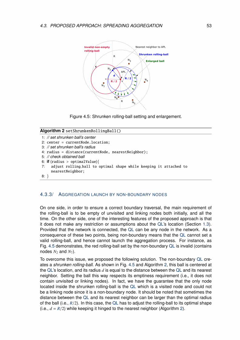
4.3. PROPOSED APPROACH: SPREADING AGGREGATION 53
Figure 4.5: Shrunken rolling-ball setting and enlargement.
Algorithm 2 setShrunkenRollingBall()1: // set shrunken ball’s center2: center = currentNode.location;3: // set shrunken ball’s radius4: radius = distance(currentNode, nearestNeighbor);5: // check obtained ball6: if (radius > optimalValue)7: adjust rolling ball to optimal shape while keeping it attached to
nearestNeighbor;
8:
4.3.3/ AGGREGATION LAUNCH BY NON-BOUNDARY NODES
On one side, in order to ensure a correct boundary traversal, the main requirement ofthe rolling-ball is to be empty of unvisited and linking nodes both initially, and all thetime. On the other side, one of the interesting features of the proposed approach is thatit does not make any restriction or assumptions about the QL’s location (Section 1.3).Provided that the network is connected, the QL can be any node in the network. As aconsequence of these two points, being non-boundary means that the QL cannot set avalid rolling-ball, and hence cannot launch the aggregation process. For instance, asFig. 4.5 demonstrates, the red rolling-ball set by the non-boundary QL is invalid (containsnodes N2 and N7).
To overcome this issue, we proposed the following solution. The non-boundary QL cre-ates a shrunken rolling-ball. As shown in Fig. 4.5 and Algorithm 2, this ball is centered atthe QL’s location, and its radius d is equal to the distance between the QL and its nearestneighbor. Setting the ball this way respects its emptiness requirement (i.e., it does notcontain unvisited or linking nodes). In fact, we have the guarantee that the only nodelocated inside the shrunken rolling-ball is the QL which is a visited node and could notbe a linking node since it is a non-boundary node. It should be noted that sometimes thedistance between the QL and its nearest neighbor can be larger than the optimal radiusof the ball (i.e., R/2). In this case, the QL has to adjust the rolling-ball to its optimal shape(i.e., d = R/2) while keeping it hinged to the nearest neighbor (Algorithm 2).
54 CHAPTER 4. SPREADING AGGREGATION
Algorithm 3 checkReceivedRollingBall()1: if (rolling ball is optimal) // radius == R/22: call Algorithm 7;
3: 4: else 5: // rolling-ball is shrunken (radius < R/2)6: enlarge rolling ball;
7: if (rolling ball is optimal) 8: call Algorithm 7;
9: 10: else 11: // rolling-ball is still shrunken12: change status to VISITED or LINKING NODE;
13: spin rolling ball;
14: sendAggregationPacket(next hop);15: 16:
Lemma 4:
A non-boundary QL cannot be a linking-node.
Proof. We recall that being non-boundary means that node Ni cannot hold an optimalrolling-ball. To illustrate our point, let us first assume that the only nodes present in thenetwork are node Ni and its one-hop neighbors. Second, let us imagine that this non-boundary node Ni has set an optimal rolling-ball on the external network boundary. Morespecifically, the rolling-ball is owned by node Ni but is hinged at its farthest (most distant)neighbor (to ensure its emptiness of any other neighbor). Under those circumstances,being non-boundary means that if node Ni rolls the ball starting from its farthest neighborand ending at this same neighbor, then node Ni will not be hit by the ball. This last state-ment also means that a path of one-hop neighbors exists surrounding node Ni, preventingthe rolling-ball from touching it. That is, for each pair of neighbors of Ni, a path exists thatconnects them without passing by Ni. Consequently, according to Definition 13, we con-clude that a non-boundary QL can never be a linking-node.
Once the shrunken (or optimal) rolling-ball has been set, the non-boundary QL marksitself as visited (Lemma 4) and forwards the aggregation packet to its nearest neighbor(Algorithm 4). This latter, upon receiving the packet (Algorithm 6), checks the receivedball (Algorithm 3). In the case of an optimal rolling-ball, the neighbor simply continuesthe aggregation process by calling Algorithm 7 (explained later). Otherwise, as shownin Fig. 4.5, first, the nearest neighbor of the QL enlarges the received ball as much aspossible. Afterward, it again checks the rolling-ball. If it became optimal, it executesAlgorithm 7, otherwise, it (1) changes its status to visited or linking node, (2) spins theshrunken ball, and (3) delivers the packet to the first hit unvisited neighbor (node N3 inFig. 4.5). The same process is applied by any subsequent traversed node. That is, eachnode that receives the aggregation packet checks the received ball and acts accordingly.It is worth highlighting that in order to remain in the same boundary and ensure networktraversal, the received shrunken-ball must be enlarged as much as possible by its ownerbefore being spun to choose the next hop.
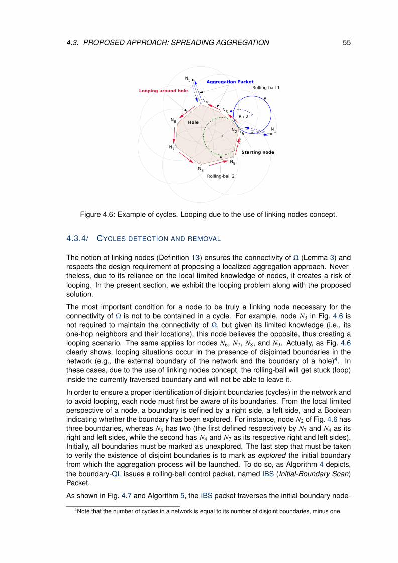
4.3. PROPOSED APPROACH: SPREADING AGGREGATION 55
Figure 4.6: Example of cycles. Looping due to the use of linking nodes concept.
4.3.4/ CYCLES DETECTION AND REMOVAL
The notion of linking nodes (Definition 13) ensures the connectivity of Ω (Lemma 3) andrespects the design requirement of proposing a localized aggregation approach. Never-theless, due to its reliance on the local limited knowledge of nodes, it creates a risk oflooping. In the present section, we exhibit the looping problem along with the proposedsolution.
The most important condition for a node to be truly a linking node necessary for theconnectivity of Ω is not to be contained in a cycle. For example, node N3 in Fig. 4.6 isnot required to maintain the connectivity of Ω, but given its limited knowledge (i.e., itsone-hop neighbors and their locations), this node believes the opposite, thus creating alooping scenario. The same applies for nodes N6, N7, N8, and N9. Actually, as Fig. 4.6clearly shows, looping situations occur in the presence of disjointed boundaries in thenetwork (e.g., the external boundary of the network and the boundary of a hole)4. Inthese cases, due to the use of linking nodes concept, the rolling-ball will get stuck (loop)inside the currently traversed boundary and will not be able to leave it.
In order to ensure a proper identification of disjoint boundaries (cycles) in the network andto avoid looping, each node must first be aware of its boundaries. From the local limitedperspective of a node, a boundary is defined by a right side, a left side, and a Booleanindicating whether the boundary has been explored. For instance, node N2 of Fig. 4.6 hasthree boundaries, whereas N6 has two (the first defined respectively by N7 and N4 as itsright and left sides, while the second has N4 and N7 as its respective right and left sides).Initially, all boundaries must be marked as unexplored. The last step that must be takento verify the existence of disjoint boundaries is to mark as explored the initial boundaryfrom which the aggregation process will be launched. To do so, as Algorithm 4 depicts,the boundary-QL issues a rolling-ball control packet, named IBS (Initial-Boundary Scan)Packet.
As shown in Fig. 4.7 and Algorithm 5, the IBS packet traverses the initial boundary node-
4Note that the number of cycles in a network is equal to its number of disjoint boundaries, minus one.

56 CHAPTER 4. SPREADING AGGREGATION
Figure 4.7: Initial boundary marking via IBS Packet issued by boundary-QL (node N2).
Algorithm 4 - Spreading Aggregation Initialization.1: To trigger serial data aggregation, the QL calls the following method:2: void initializeAggregation()3: if (currentNode.isBoundaryNode())4: set a rolling ball on any boundary;
5: send IBS Packet(); // to mark initial boundary6: 7: else 8: // current node is not a boundary node9: setShrunkenRollingBall(); // Algorithm 2
10: currentNode.status = VISITED; // Lemma 411: sendAggregationPacket(nearestNeighbor);12: 13:
by-node and orders them to locally mark the boundary in question as explored. Once theinitial boundary has been successfully marked, the determination of disjoint boundariescan be done locally by each node. Simply, if the currently traversed node (including theQL) has an unexplored boundary, then this latter is certainly a disjoint boundary (cycle)that must be opened, and the node in question is a portal node responsible for this cycleremoval.
Definition 14: Portal Node (PN)
A node is said to be a Portal Node if it has at least two disjoint boundaries.
In the case of a non-boundary QL as described earlier in Section 4.3.3 (aggregationlaunch by non-boundary nodes) and shown here in this section in Algorithm 4, insteadof issuing an IBS packet, the non-boundary QL sets a shrunken rolling-ball, marks itselfas visited, and delivers the ball to its nearest neighbor by broadcasting an aggregationpacket. Upon receiving the aggregation packet, each neighbor of the QL executes thesteps described in Algorithm 6. Note that no initial boundary needs to be marked inthe case of non-boundary QL in Algorithm 4. In fact, in this case, a new boundary will be
4.3. PROPOSED APPROACH: SPREADING AGGREGATION 57
Algorithm 5 receive IBS Packet()1: mark locally the currently traversed boundary as explored;2: if (currentNode is not the QL)3: forward IBS Packet to next hop;
4: 5: else 6: // current node is the QL7: if (previous hop is not the expected node)8: // initial boundary not totally explored9: forward IBS Packet to next hop;
10: 11: else 12: // initial boundary has been totally explored13: call Algorithm 7;14: 15:
Algorithm 6 receiveAggregationPacket()1: if (currentNode is not destination)2: // overhear aggregation packet3: updates locally the status of source node according to the received packet
(i.e., mark it as VISITED or LINKING NODE);
4: 5: else 6: // current node is the destination7: update locally the status of source node according to the received packet
(i.e., mark it as VISITED or LINKING NODE);
8: aggregate data(); // if visited for the first time9: checkRollingBall(); // Algorithm 3
10:
created in the network. Therefore, during the aggregation process, any other encounteredunexplored boundary is disjoint and must be opened by the rolling-ball owner.
We underline that due to the limited knowledge of nodes, and given the radius of theoptimal rolling-ball (R/2, where R is the communication range of nodes), the owner of thislatter cannot be aware of all nodes surrounding the ball, and hence, cannot locally detectthe existence of cycles. However, this is not the case for the shrunken rolling-ball. In fact,because of its small size, its owner is well aware of all nodes that surround it, along withtheir corresponding statuses (visited or linking nodes).
Lemma 5:
Shrunken rolling-ball does not loop.
Proof. This lemma means that at each iteration, the shrunken rolling-ball finds a non-linking node Nk that can be removed from Ω. To prove this point, let us assume thatthe shrunken ball is owned by node Ni. Actually, given the fact that the shrunken radius”d” is smaller than the optimal one (d < R/2), the farthest distance between each pairof neighbors of Ni which surround the shrunken ball and prevent it from being optimal issmaller than the communication range of nodes R (2 ∗ d < R, where 2 ∗ d is the shrunkenball diameter). Consequently, we conclude that each pair of neighbors of Ni surrounding

58 CHAPTER 4. SPREADING AGGREGATION
Algorithm 7 continueAggregationProcess()1: spin rolling ball;2: if (next hop is undefined)3: // aggregation ends here; no other nodes to visit4: currentNode.status = VISITED;
5: send result to QL; // using geographic routing6: return;
7: 8:9: if (not currentNode.isPortalNode())
10: // current node has no disjoint boundaries11: change status to VISITED or LINKING NODE;
12: sendAggregationPacket(next hop);
13: 14: else 15: // current node is a portal node16: create right and left sets;
17: send DBS Packet(); // to mark disjoint boundary18:
the shrunken ball can directly communicate with each other. Hence, even if we supposethat a cycle can occur in this case, determining and removing that cycle can be donelocally by each node without recourse to control packets.
In the case of an optimal rolling-ball, the idea of avoiding looping around cycles consistsof opening any encountered disjoint boundary by portal nodes. More specifically, asshown in Algorithm 7, in the case where the currently traversed node is not portal (i.e.,has no disjoint boundaries), this node changes its status to visited or linking node, andforwards the aggregation packet. On the other hand, a portal node must execute thethree following steps (upon receiving the aggregation packet) in order to break the cycle:
Step 1 - Creation of the left and right sets. The portal node Ni divides the set of itsimmediate neighbors into two subsets: left and right sets.
• Left set (X ⊂ Ω): this set contains all neighbors located in the sector defined by theangle ∠Nleft,Ni,Nprev (see Fig. 4.8). Where Nleft is the left side of the unexploreddisjoint boundary, and Nprev is the previous hop from which node Ni has receivedthe aggregation packet. In Fig. 4.8, all orange nodes belong to the left set X. Notethat Nprev (if it has not been visited), as well as Ni, and Nleft belong to X.
• Right set (Y ⊂ Ω): this second set is composed of the rest of neighbors of nodeNi including the right side of the unexplored boundary. In Fig. 4.8, all blue nodesbelong to Y.
Step 2 - Disjoint boundary scan: after having created the left and right sets, the portalnode issues a rolling-ball control packet named DBS (Disjoint-Boundary Scan) packet,which traverses the unexplored boundary node by node (see Fig. 4.9 and Algorithm 8).Similar to the IBS, DBS packet marks the disjoint boundary as explored and allows nodesto determine whether their local stored boundaries constitute the same boundary. Forinstance, in Fig. 4.9, DBS packet informs node Nx that the boundary defined by Ny as its

4.3. PROPOSED APPROACH: SPREADING AGGREGATION 59
Figure 4.8: Left and right sets creation by portal node Ni.
Figure 4.9: Disjoint boundary scan using DBS Packet issued by portal node Ni.
right side, and the one defined by Nz as its right side, are actually the same boundary.Hence, when node Nx later receives the aggregation packet, it will not consider these twoboundaries as disjoint.
Step 3 - Cycle removal: after receiving the DBS packet back, the portal node (whichbelongs to the left set X) virtually deletes its links with every node of the right set Y (Algo-rithm 8). In other words, the portal node Ni will not consider nodes of Y as its neighbors.Formally, the set of links that need to be deleted from L is D = L(i, j) | N j ∈ Y(Ni). Oncethe appropriate links have been removed, the portal node changes its status to visitedor linking node, and broadcasts an LC (Link-Cut) packet to its immediate neighbors. Tofinish the cycle break process, each neighbor of the portal node performs the followingsteps upon receiving the LC packet (Algorithm 9). First, it determines the set to which itbelongs (X or Y). Then, it virtually deletes its links with every node of the other set (when-ever such a link exists). Fig. 4.10 gives an example of disjoint boundary opening (cycleremoval). Once the cycle has been broken, the aggregation process continues from theleft side of the opened boundary (i.e., Nleft).
Property 6. Portal nodes ensure cycles removal from Ω.

60 CHAPTER 4. SPREADING AGGREGATION
Figure 4.10: Cycle removal using LC packet broadcasted by portal node Ni.
Algorithm 8 receive DBS Packet()1: locally mark the currently traversed boundary as explored;2: if (currentNode is not the portal node)3: forward DBS Packet to next hop;
4: 5: else 6: // current node is the portal node7: if (previous hop is not the expected node)8: // disjoint boundary not totally explored9: forward DBS Packet to next hop;
10: 11: else 12: // disjoint boundary has been totally explored13: cut links with nodes of right set;
14: change status to VISITED or LINKING NODE;
15: send LC Packet();16: 17:
Algorithm 9 receive LC Packet()1: update locally the status of source node according to the received packet(i.e., mark it as VISITED or LINKING NODE);
2: determine membership set; // right or left3: cut links with nodes of the other set;4: if (currentNode is destination)5: aggregate data(); // if visited for the first time6: call Algorithm 7;
7:
Proof. Let us assume that Ni, which is a portal node, has detected the existence of acycle C1 in Ω. Before removing C1, initially thanks to the issued DBS packet we are surethat two paths exist connecting the left set X and the right set Y of C1. The first path iscomprised of direct communication links between the nodes of X and those of Y, whilethe second is composed of Nle f t and each node located on the disjoint boundary untilNright (i.e., nodes visited by DBS packet). After removing C1 from Ω thanks to the cycle

4.4. PROOF OF CORRECTNESS 61
removal process performed by portal node Ni and its corresponding neighbors (threesteps described above), no direct communication links can exist between the left andright set of C1. Consequently, the only path that remains connecting X with Y is the DBSpacket path. In addition to that, it is worth mentioning that using the rolling-ball guaranteesthat portal node Ni and its previous-hop Nprev belong to the boundary of Ω. This formallymeans that: @N j | L j,i < L ∧ L j,prev < L ∧ L j,k ∈ L such that Nk ∈ Vi ∩ Vprev (i.e.,Nk belongs to the set of common neighbors of Ni and Nprev). Thus, by construction, therecannot exist a node N j such as (1) N j cannot communicate with Ni and Nprev, but (2) cancommunicate with Nk.
Property 7. Portal nodes do not partition Ω.
Proof. This property can be proven by contradiction. First, let us assume that cutting thedirect communication links between X and Y during cycle removal process disconnectsΩ. Second, let us assume that only one direct communication link exists that connects Xand Y, which is L(i, right) (the link between portal node Ni and right side of disjoint boundaryNright). In such a scenario, the first assumption means that there is no other path that con-nects X and Y except L(i, right), which thanks to the DBS packet sent beforehand contra-dicts the existence of another path connecting Ni with Nright. Given the fact that (1) nodesbelonging to X or those belonging to Y are internally connected (thanks to Lemma 3 andthe connectivity assumption made in Section 1.3) and (2) Ni and Nright belong respectivelyto X and Y, we deduce that X and Y can be connected thanks to the DBS packet path,and hence without requiring the deleted direct links between them. This contradicts theassumption that suggests that links cut, during cycle removal process, disconnects Ω. Inaddition to what has been said, thanks to the use of IBS and DBS packets, we have theguarantee that each disjoint boundary (cycle) has only one portal node.
4.4/ PROOF OF CORRECTNESS
In this section, we prove the correctness of the proposed algorithm. More specifically,we prove that SA visits all connected nodes in the network, without falling into looping.Proving that SA visits all nodes is based on (1) the use of a proven boundary traversalalgorithm and (2) the fact that the network is initially connected (Ω = N) and its con-nectivity is maintained throughout the data aggregation process (Lemmas 3 and 4, andProperty 7). In contrast, the proof that SA does not loop and terminates is based on thefact that all possible cycles in Ω (which can be generated because of the use of linkingnodes notion) are detected and properly removed (Lemmas 4 and 5, and Property 6).
Initially, all nodes in the network are marked as unvisited. Therefore, we have the set ofunvisited nodes Ω equal to the set of nodes N and the set of visited nodes Γ is empty(Ω = N and Γ = ∅). To accomplish data aggregation, SA iteratively visits nodes by gradu-ally filling up Γ and emptying Ω. The traversal of the network can be expressed formallyvia the following recurrent formula:Γ0 = ∅ and Ωn = N ,
Γi+1 = Γi + Nk and Ω j−1 = Ω j − Nk : i f i < n and j > 0
where n is the number of nodes in the network and Nk is the first traversed non-linkingnode that can be removed from the current set of unvisited/linking nodes Ω j without alter-

62 CHAPTER 4. SPREADING AGGREGATION
ing its connectivity. For example, in Fig. 4.4, initially, we have:
Γ0 = ∅ and Ω8 = N = N1,N2,N3,N4,N5,N6,N7,N8. The traversal of N is done through thefollowing respective iterative filling of Γ0 and emptying of Ω8:
Γ1 = Γ0 + N2 and Ω7 = Ω8 − N2
Γ2 = Γ1 + N6 and Ω6 = Ω7 − N6
Γ3 = Γ2 + N8 and Ω5 = Ω6 − N8
Γ4 = Γ3 + N7 and Ω4 = Ω5 − N7
Γ5 = Γ4 + N5 and Ω3 = Ω4 − N5
Γ6 = Γ5 + N4 and Ω2 = Ω3 − N4
Γ7 = Γ6 + N3 and Ω1 = Ω2 − N3
Finally, Γ8 = Γ7 + N1 = N and Ω0 = Ω1 − N1 = ∅.
To prove that the proposed algorithm always generates, at its termination, a finite set ofvisited nodes Γn that is equal to the set of nodes in the network N , and at the sametime it also produces an empty set of unvisited nodes Ω0, we will proceed in the followingmanner. First, we will consider the case of non-boundary QL. More precisely, we considerthe case of shrunken rolling-ball. Next, we will move to the optimal rolling-ball, which ofcourse includes the case of boundary-QL.
As mentioned before, we initially have a set of unvisited nodes Ωn composed of all nodesof the network, and we have an empty set of visited nodes Γ0. Thanks to Lemma 4, thenon-boundary QL cannot, in any case, be a linking-node, and hence it is not necessaryfor the connectivity of Ωn. Consequently, in all cases, regardless of its location in thenetwork, the non-boundary QL can be removed from Ωn and added to Γ0:
Γ1 = Γ0 + QL and Ωn−1 = Ωn − QL
Given the fact that the non-boundary QL is always removed from Ωn and added to Γ0ensures the main requirement of the rolling-ball (which is the permanent emptiness fromany node) and guarantees a correct boundary traversal process. Once the non-boundaryQL has been excluded from the traversal process (Algorithm 4), the rolling-ball will bedelivered to its nearest neighbor. Hence, this latter will have a new boundary in whichthe received rolling-ball can be released. We emphasize that the ball given to the nearestneighbor of the non-boundary QL can be shrunken or optimal (Algorithms 6 and 3). Aspreviously mentioned, we will consider only the first case. The optimal rolling-ball scenariowill be treated later on in this section.
When the shrunken rolling-ball leaves the non-boundary QL, it moves in a localized fash-ion from node to node, and if possible, it becomes enlarged at each hop. We underlinethat the traversed nodes by the shrunken rolling-ball can be marked as visited or linkingnodes, and as previously shown, the existence of linking nodes in Ω means the potentialpresence of cycles. Nonetheless, thanks to Lemma 5, we have the assurance that theshrunken rolling-ball does not generate looping situations.
Theorem 3:
After a certain number of iterations (i ≥ 1), shrunken rolling-ball gains its shapeand becomes optimal.
Proof. Let us suppose that while traversing the network with the use of a shrunken rolling-

4.4. PROOF OF CORRECTNESS 63
ball, the latter cannot be enlarged. In such a case, the fact that the shrunken-ball (likethe optimal one) traverses the boundary of Ωn−i signifies that all nodes that have beenexplored are linking nodes that form a cycle. According to Lemma 5, this is not true;at each iteration, a non-linking node Nk exists. This means that, at each iteration, thenumber of nodes in Ω j strictly decreases by one, and the number of nodes in Γi strictlyincreases by one:
| Ω j−1 | < | Ω j | and | Γi+1 | > | Γi | such as j > 0 and i < n.
Therefore, we deduce that, at each iteration, the shrunken-ball creates more space foritself by finding a non-linking node Nk that can be removed from Ω j. Given the fact that (1)the shrunken-ball does not generate looping cases, and (2) it can be enlarged, in the end,after a certain number of iterations i, the shrunken-ball can gain its shape and becomesoptimal.
After having treated the case of shrunken rolling-ball, and proved that it does not loopand produces a finite set of hops, we move to the case of optimal-ball to prove that italso does not loop. Next, we will prove that SA ensures the exploration of all nodes.But before this, it is worth mentioning that the shrunken rolling-ball, like the optimal one,ensures boundary traversal and does not miss any non-linking node in its way. The formalproofs demonstrating that the rolling-ball ensures boundary traversal can be found in [41].
Lemma 6:
Optimal rolling-ball does not loop.
Proof. To prove this by contradiction, let us assume that at some point during networktraversal, the optimal-ball cannot find a non-linking node Nk. This means that the rolling-ball has become stuck between at least two disjoint boundaries, and is jumping (looping)from a linking node to another inside one of the boundaries. This assumption can besimply denied because it contradicts the fact that portal nodes guarantee a proper de-tection/removal of cycles (disjoint boundaries) from Ωn−i. More precisely, according toProperty 6, we deduce that, at each iteration i, the optimal-ball finds a non-linking nodeNk. That is, after each iteration, the number of nodes in Ωn−i will be strictly decreased byone, and the number of nodes in Γi will be strictly increased by one:
| Ωn−(i+1) | < | Ωn−i | and | Γi+1 | > | Γi | such as i < n.
Theorem 4:
SA does not loop.
Proof. First, thanks to Lemma 5 and Theorem 3, we have the assurance that theshrunken-ball does not loop. Actually, regardless of the considered scenario, theshrunken-ball progressively gets enlarged and will eventually gain its optimal form. Sec-ond, if we consider the rolling-ball in its optimal shape, then, according to Lemma 6,we have the guarantee that it does not loop and at each iteration, it finds a non-linkingnode. Based on what has been said and given the fact that in SA, the ball can be eithershrunken or optimal, and its radius can never be larger than R/2, we conclude that SAdoes not loop and generates a finite set of hops.

64 CHAPTER 4. SPREADING AGGREGATION
Lemma 7:
At each iteration i ≥ 1, the currently visited node Nk belongs to the boundary ofΩn−i.
Proof. In the case of a shrunken-ball, the non-boundary QL (located inside the ball) can-not be in any case a linking node (Lemma 4), hence creating a boundary for its near-est neighbor to exploit (launch the ball inside it). Therefore, in both cases (optimal andshrunken-ball), the algorithm is triggered by a boundary node. Based on this and giventhe fact that the rolling-ball is a boundary traversal tool [41], each visited non-linking nodeNk will be certainly located on the boundary of Ωn−i. To prove this, let us assume that thisproperty is true for i and let us demonstrate that it remains as such for i + 1. First, sayingthat the property is true for i means that the currently traversed node Nk is located onthe boundary of Ωn−i. Second, as previously mentioned, the used rolling-ball boundarytraversal algorithm guarantees that the next hop Nsucc of Nk is located on the boundary ofΩn−i [41]. Consequently, it is clear that this next hop Nsucc is also located on the boundaryof Ωn−(i+1). More precisely, if Nsucc is not a linking node (i.e., can be marked as visited)then:
Γi+1 = Γi + Nsucc and Ωn−(i+1) = Ωn−i − Nsucc
Otherwise, starting from Nsucc, the rolling-ball has to continue its boundary browsing ofΩn−(i+1) until it finds a non-linking node that can be marked as visited. Hence, we concludethat the property is also true for i + 1.
Theorem 5:
SA visits all nodes in the network.
Proof. First, thanks to the assumption made in Section 1.3, we have the guarantee thatthe initial network is connected (Ωn = N). Second, thanks to Lemmas 3 and 4, we havethe guarantee that for both shrunken and optimal-ball, the notion of linking-nodes ensuresthe connectivity of Ω j. Third, according to Property 7, we know that the cycle removalprocess (which takes place only in the case of optimal-ball) does not partition Ω j. Toprove that SA visits all nodes in the network, let us assume that the set Γi generated atthe end of network traversal is different than the set of nodes N (i.e., i , n) and then letus seek to find a contradiction. First, let us denote by Nk the first traversed non-linkingnode that can be removed from Ω j without altering its connectivity (Lemmas 3 and 4,and Property 7). Second, let us denote by Nm, one of the unvisited nodes that might bemissed by SA (i.e., Nm , Nk, ∀ k). Third, let us consider an unsigned integer j (0 < j < n)such that Nm belongs to Ω j and does not belong to Ω j−1. That is, Nm has been missedat iteration j. In actual fact, since at iteration j, the rolling-ball touches only nodes thatare located on the boundary of Ω j and does not miss any one of them (Lemma 7 andTheorem 4), Nm cannot, in any case, be located on the boundary of Ω j. In other words,given the fact that the use of the rolling-ball guarantees that there cannot exist a node Nm
that can be missed, Nm must surely belong to Ω j−1. However, this contradicts the initialassumption, which says that Nm does not belong to Ω j−1 (Nm < Ω j−1). Consequently, weconclude that SA guarantees network traversal completeness in spite of the consideredtopology.
4.5. SPREADING PERFORMANCE ASSESSMENT 65
To recapitulate, according to Theorems 4 and 5 and regardless of the network topology(irregular or regular, large-scale or sparse, with or without holes, etc.), we conclude thatSA ensures query completeness/accuracy and terminates without looping indefinitely.
4.5/ SPREADING PERFORMANCE ASSESSMENT
As it has been previously mentioned, in this manuscript, OMNeT++ and its WSNs frame-work Castalia [53,54] have been opted for as a performance evaluation tool. This choiceis motivated, among others, by the fact that Castalia offers a realistic wireless channel(e.g., interference, mobility of nodes, path loss, etc.) and radio models (e.g., realisticmodeling of RSSI and carrier sensing, probability of reception based on SINR, packetsize, modulation type, etc.), and also a realistic node behavior, especially pertaining toradio access. Besides the proposed spreading approach, the following aggregation tech-niques have been implemented: tree-based aggregation [3], Depth-First Search [26],Peeling Algorithm [18], and Greedy-Boundary Traversal [25]. We note that all the con-sidered serial techniques have been formally proven to ensure complete exploration ofnodes, regardless of the network topology.
4.5.1/ EVALUATION METRICS
In addition to the completeness criterion, the three other metrics with which all parallel andserial approaches cited above have been evaluated are energy, time and communicationefficiency.
• Energy: this metric, which represents the most precious resource in WSNs, mea-sures the total energy spent by the network during data aggregation. To allow eachnode to estimate the energy required to transmit and receive packets, the modelproposed by Heinzelman et al. [55] has been considered. In this energy consump-tion model, in order to send a packet of a k-bit size a certain distance x, the radioconsumes ET X(k, x) = Eelec ∗ k + εamp ∗ k ∗ x2. And to receive this same packet, itconsumes ERX(k) = Eelec ∗ k. Where Eelec = 50 nJ/bit is the energy required to runthe transmitter/receiver circuitry, and εamp = 100 pJ/bit/m2 is the energy consumedby the transmitter amplifier.
• Time: this evaluation metric measures the time required to aggregate all the datapresent in the network. That is, the time that passes between the moment data ag-gregation is triggered and the moment the desired result is delivered to the sink/QL.For instance, in the conducted simulations, nodes have been ordered to find theaverage temperature of the whole network.
• Transmissions: this last metric represents the total number of packets issued bythe network in order to aggregate data (including control and data packets).
4.5.2/ SIMULATION PARAMETERS
To evaluate the scalability of SA and the other considered techniques, simulations havebeen conducted in different network size and density scenarios. More specifically, the de-

66 CHAPTER 4. SPREADING AGGREGATION
Table 4.1: Spreading simulation configuration and parameters
Parameter Value(s)
Field dimensions (m2) 1000 x 1000Nodes number 100, 150, 200, . . . , 500Nodes deployment UniformNodes transmission range (m) 150Nodes initial energy (J) 100Query launcher location RandomQuery packet size (byte) 50Radio type CC2420Radio data rate (kbps) 250MAC protocol CSMA/CA
Table 4.2: Spreading average nodes’ degree.
100 150 200 250 300 350 400 450 5006 9 12 15 18 21 25 27 31
ployment field has been fixed to 1000 x 1000 meters throughout simulations. As regardsthe network, initially, 100 sensor nodes have been randomly deployed, and then, 50 othersensor nodes were progressively added, to a maximum of 500 nodes. Table 4.1 summa-rizes the simulation parameters and Table 4.2 shows the average degree of nodes (i.e.,the average number of neighbors of each node). To be more specific, the first line of Ta-ble 4.2 depicts the number of nodes in the network, whereas the second one representsthe corresponding average degree.
4.5.3/ SIMULATION RESULTS
In this section, the obtained simulation results are compared and evaluated. Actually,for the sake of clarity, and given the obvious difference between the results of serial andparallel approaches (particularly in terms of energy consumption), we first start by plottingand comparing the results of our spreading algorithm with those of the implemented tree-based approach [3]. Next, we will plot the same results of our approach and comparethem with the implemented serial techniques, namely: Depth-First Search [26], PeelingAlgorithm [18], and Greedy-Boundary Traversal [25]. We mention that in both cases,all results, whether those relating to required transmissions, time or energy, are plottedagainst the number of nodes specified in Table 4.1.
4.5.3.1/ SPREADING ALGORITHM VERSUS TREE-BASED AGGREGATION
Fig. 4.11 plots the number of packets that our proposed serial technique of SpreadingAggregation (SA), and the tree-based approach [3] (denoted here as T-BA), have bothissued to accomplish data aggregation. Concerning Fig. 4.12 and Fig. 4.13, they respec-tively plot the time and energy that each of these two approaches has taken in order toaggregate data and deliver the response to the sink.

4.5. SPREADING PERFORMANCE ASSESSMENT 67
200
400
600
800
1000
1200
1400
1600
1800
2000
100 150 200 250 300 350 400 450 500
Num
ber
of sent packets
Number of nodes
SAT-BA
Figure 4.11: Transmissions required by Spreading and Tree-based approaches to aggre-gate data.
2
3
4
5
6
7
8
9
10
11
12
100 150 200 250 300 350 400 450 500
Aggre
gation tim
e (
seconds)
Number of nodes
SAT-BA
Figure 4.12: Time required by Spreading and Tree-based approaches to aggregate data.
In actual fact, for both approaches (SA and T-BA), the considered transmissions include(1) transmissions used to construct the tree or respectively traverse the network, (2) trans-missions used to query the network, and (3) transmissions used to deliver the processeddata to the sink. As previously mentioned, structure construction, query diffusion and dataprocessing in tree-based approaches are three independent phases. First, the networkmust be properly covered with a spanning tree (to ensure query accuracy all nodes mustbe attached to the tree). Then, after being queried via the constructed tree, sensor nodesstart data processing and response delivery to the sink/root. Conversely, in our serialapproach, these three phases are all merged into one unique phase. At the same time,

68 CHAPTER 4. SPREADING AGGREGATION
0
2
4
6
8
10
12
14
16
18
100 150 200 250 300 350 400 450 500
Aggre
gation e
nerg
y (
Joule
s)
Number of nodes
SAT-BA
Figure 4.13: Energy required by Spreading and Tree-based approaches to aggregatedata.
while gradually traversing the network, sensor nodes are queried and the proper treat-ment is applied to data. This compact performance considerably minimizes the numberof packets that need to be issued, conserves energy, and improves processing time.
As Fig. 4.13 confirms, there is a big gap between T-BA and SA in terms of energyconsumption. Actually, given their parallel and non-collision-free nature, tree-based ap-proaches do not consume energy only to construct/maintain the tree, disseminate queriesand report the processed data to the sink, but also to re-transmit collided packets. Withrespect to aggregation time, due to their parallel concurrent operation, tree-based ap-proaches should defeat serial algorithms, even with a large number of issued packets.Nonetheless, as Fig. 4.12 demonstrates, because of collisions essentially among otherreasons, this is not the case; in fact, SA presents better results than T-BA in terms ofaggregation time reduction.
To illustrate the difference between serial and tree-based approaches in terms of requiredtransmissions, let us consider a sensor network composed of n wireless nodes. If weassume that each node in tree-based approaches is involved in the query diffusion phase(i.e., it forwards the received query), this means that n packets will be broadcast. On theother hand, during the data or query processing phase, n additional packets will be sent,because obviously during this phase each node is obliged to forward a packet. Therefore,without taking into account the packets used to construct or probably maintain the tree,and without counting the retransmissions of collided packets, we can say that in total,2∗n packets need to be issued to accomplish data aggregation in tree-based approaches.We emphasize that building and fixing a distributed structure in a wireless environmentthat is prone to errors and interference, is not a straightforward task, and non-negligibletime and overhead must certainly be spent to accomplish this process. Regarding serialapproaches, if we consider the same network composed of n wireless nodes, and if weassume that these approaches can lay out an itinerary that crosses each node once atany given moment in time, then, without generating any collisions or requiring a separate

4.5. SPREADING PERFORMANCE ASSESSMENT 69
0
100
200
300
400
500
600
700
800
900
1000
100 150 200 250 300 350 400 450 500
Num
ber
of sent packets
Number of nodes
DFSGBT
PASA
OPT
Figure 4.14: Spreading Aggregation versus serial approaches. Comparison in terms ofrequired transmissions for data aggregation.
structure construction phase or maintenance, only n − 1 packets need to be issued todiffuse a query and process data.
To recapitulate, besides their bad scalability, their inadequacy for dense large-scale net-works, and their robustness and imbalance issues, tree-based approaches suffer primar-ily from collisions. First, due to their parallel concurrent mode of operation, tree-basedapproaches undergo a lot of communication collisions, especially in dense deployments.The retransmissions of collided useless packets waste a noticeable amount of energyand time, and negatively affect these approaches. Second, apart from collisions, tree-based approaches also suffer from the problem of unbalanced energy consumption. Thisissue takes place due to the creation of an unbalanced spanning tree in the first place, orbecause sensor nodes that are located near the sink/root are excessively used to passthe traffic [12]. Third, a distributed tree is a set of pre-established itineraries that are frag-ile and very sensitive to node and link failures. Therefore, the implementation of a treemaintenance operation is a requirement that can fix the problem from one side, but canbe very expensive in terms of energy and time from the other side, especially in denselarge-scale networks.
4.5.3.2/ SPREADING ALGORITHM VERSUS SERIAL APPROACHES
Fig. 4.14 shows the number of packets issued to accomplish data aggregation by theproposed approach, Depth-First Search (DFS) [26], Peeling Algorithm (PA) [18], andGreedy-Boundary Traversal (GBT) [25]. We mention that for all four serial approaches,the counted transmissions include path construction, query diffusion, and result deliveryto the sink. Fig. 4.14 also plots the number of packets that an optimal theoretical serial al-gorithm (denoted as OPT) would have issued to aggregate data if it existed. Actually, thenumber of packets required by both DFS and the optimal theoretical algorithm OPT havebeen plotted to measure the effectiveness of the evaluated serial algorithms in terms of

70 CHAPTER 4. SPREADING AGGREGATION
1
2
3
4
5
6
7
8
9
10
100 150 200 250 300 350 400 450 500
Aggre
gation tim
e (
seconds)
Number of nodes
DFSGBT
PASA
Figure 4.15: Spreading Aggregation versus serial approaches. Comparison in terms ofrequired time for data aggregation.
transmissions. The curve of a good serial approach must be located between those ofOPT and DFS.
We recall that the optimal algorithm OPT necessitates n−1 packets to traverse and aggre-gate data from a network of n connected nodes. Nevertheless, as previously mentioned,such an optimal Hamiltonian path does not exist in every network; even if it does, findingthis path constitutes an NP-complete problem [20]. DFS, because of its backtracking na-ture, requires double the number of OPT, i.e., 2∗(n−1) packets to aggregate and deliver theresult to the sink. The number of transmissions required by the other serial approaches(i.e., SA, PA, and GBT) cannot be expressed using a mathematical expression.
As demonstrated by Fig. 4.14, SA outperforms all the other serial approaches and neces-sitates a number of transmissions that is closer to the optimal number of OPT. However, insparse low-density networks, DFS slightly outperforms SA. In reality, this is due to the factthat in low-density deployments, it is more likely that the network contains more disjointboundaries (i.e., more cycles). In such a scenario, the bad performance of SA stems fromthe excessive use of DBS packets sent to scan the disjoint boundaries. So, the presenceof disjoint boundaries in the network results in a greater expenditure of control packets bySA. But, in contrast, a denser network will contain fewer holes and disjoint boundaries,and will improve the performance of SA. Note that when the number of nodes increases,SA approximates the optimal number of transmissions, and the difference between SAand DFS becomes more and more noticeable. For instance, in the case of 500 nodes,the improvement is over 40%.
Fig. 4.15 and Fig. 4.16 respectively show the time and energy required to aggregatedata by all the considered serial approaches. If these latter are compared together interms of data delivery time, one can say that, due to their sequent behavior, a serial dataaggregation algorithm will need more time to finish when it necessitates a larger numberof transmissions, and vice versa (provided that the issued packets have approximate oridentical sizes). As depicted in Fig. 4.15, since SA necessitates the smallest number of

4.6. CONCLUSION 71
0
0.2
0.4
0.6
0.8
1
1.2
1.4
1.6
100 150 200 250 300 350 400 450 500
Aggre
gation e
nerg
y (
Joule
s)
Number of nodes
DFSGBT
PASA
Figure 4.16: Spreading Aggregation versus serial approaches. Comparison in terms ofrequired energy for data aggregation.
transmissions, it performs better than all the other serial algorithms and aggregates datamore rapidly.
As shown in Fig. 4.16, SA also performs better than the other serial approaches in termsof energy consumption. Actually, in WSNs, energy is consumed by the various tasks car-ried out by nodes (chiefly, sensing, computing, and communicating). So, if one considerssimple sensing systems and plain aggregation queries, communications dominate andbecome the most energy consuming task [1], and thus, the energy consumed by serialalgorithms will be mainly related to the number of issued transmissions. That is, the morea serial algorithm requires packets, the more it will consume energy (provided that theissued packets have identical or approximate sizes). Since SA necessitates the lowestnumber of packets compared with the other serial algorithms, it is superior from the pointof view of energy consumption.
4.6/ CONCLUSION
In this chapter, we presented a new serial algorithm called Spreading Aggregation (SA).The attractiveness of this in-network data processing technique comes from several fac-tors. First, SA is maintenance-free and collision-free; hence, it does not require anytransmissions in these regards. Second, SA is a path-free localized approach that reliesonly on the limited knowledge of each node to progressively traverse the network. Inother terms, for each query, a new path will be laid out, which decreases the vulnerabilityto topology changes and link/node failures. Third, as in any other serial approach, SAfuses path construction, query dissemination, and data processing. That is to say; whilecrossing the network, sensor nodes are simultaneously queried, and their answers arecollected. The conducted OMNeT++ simulations confirm that SA is scalable and veryefficient in terms of energy conservation and response time reduction. The simulationresults also assert that SA ensures aggregation completeness, and therefore query ac-

72 CHAPTER 4. SPREADING AGGREGATION
curacy. In addition to simulations, the proposed approach has been theoretically provento visit all connected nodes in the network and to terminate without looping indefinitely.
Despite the efficiency of the proposed approach compared with tree-based aggregationand state-of-the-art serial algorithms, some other issues still remain to be addressed,such as robustness against node/link failures, imprecision of nodes’ locations, etc. Inaddition to this, the performance of the proposed approach can be further enhanced byeliminating the use of control packets (i.e., IBS and DBS packets). This will be the objectof the next chapter.
5GEOMETRIC SERIAL SEARCH
5.1/ INTRODUCTION
Considering large WSNs and comparing data aggregation approaches in terms of scal-ability, robustness, completeness, and time/energy effectiveness, recent research
has asserted the superiority of serial structure-free approaches over serial structure-based ones, and over both parallel structure-free and parallel structure-based tech-niques [18,25,39,40]. But, in spite of the fact that serial structure-free approaches excelin large and medium-scale networks, their underlying path-construction algorithms arenot optimal and can be improved by reducing the involved communications and furthershortening the visiting path. To respond to this need, this chapter presents GeometricSerial Search (GSS); a new serial structure-free algorithm specifically designed to ef-ficiently gather information from large wireless resource-constrained networks [42]. Inaddition to its completeness (i.e., visiting all nodes), collision-free nature, high scalability,energy/time efficiency, and robustness against topology changes (failures in links/nodes,...), the main advantage distinguishing GSS is that it considerably reduces communica-tions and always approaches the optimal number of hops (i.e., n −1). More precisely, inGSS, no control packets or complex data structures are required, instead, one packethops from node to node and explores the entire network. While gradually finding its waythrough the network, this packet interrogates nodes and collects their responses at thesame time. The followed path is not established in advance, can stem from any node inthe network, and requires only the one-hop neighborhood information of each traversednode to be gradually drawn. The obtained OMNeT++ simulation results presented in thischapter demonstrate the efficiency of GSS and confirm all the previously cited claims.
This chapter is sectioned into four parts, as follows. Section 5.2 introduces the necessarypreliminaries required throughout the chapter (to understand the considered problem aswell as its solving). Section 5.3 details the proposed solution (i.e., GSS) through algo-rithms and simple illustrative figures. Section 5.4 depicts and interprets the obtainedOMNeT++ simulation results. In the end, Section 5.5 concludes the chapter.
73
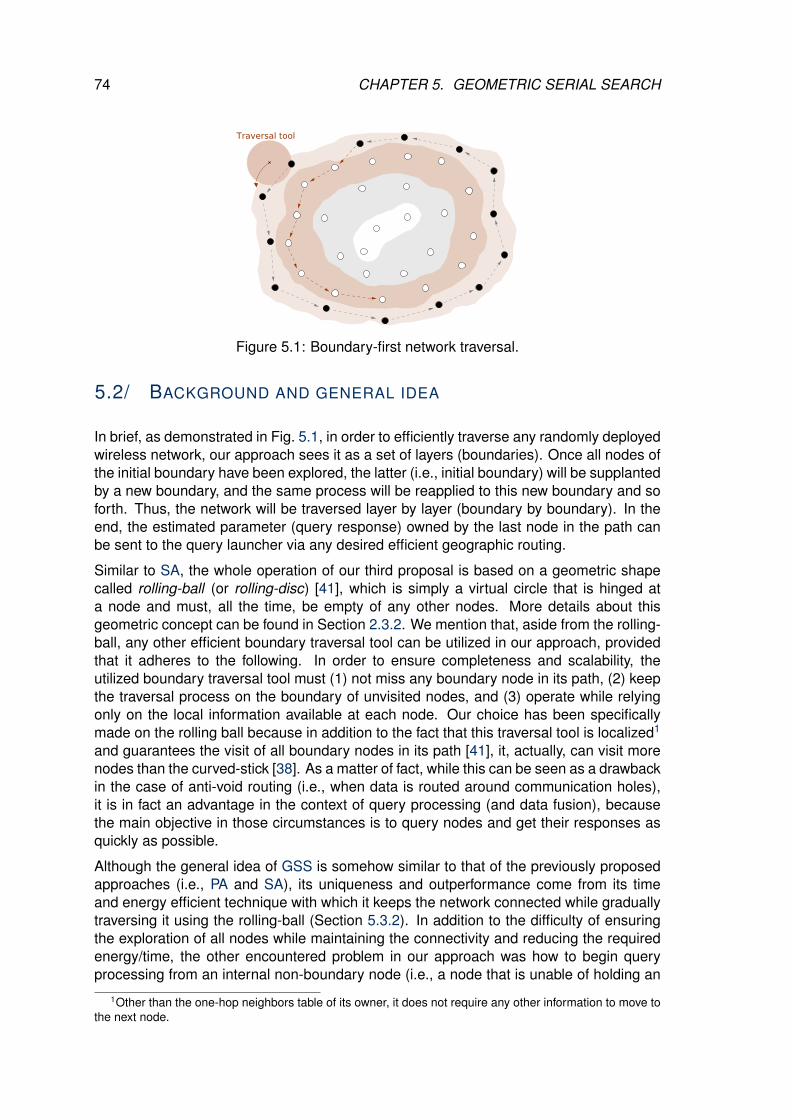
74 CHAPTER 5. GEOMETRIC SERIAL SEARCH
Figure 5.1: Boundary-first network traversal.
5.2/ BACKGROUND AND GENERAL IDEA
In brief, as demonstrated in Fig. 5.1, in order to efficiently traverse any randomly deployedwireless network, our approach sees it as a set of layers (boundaries). Once all nodes ofthe initial boundary have been explored, the latter (i.e., initial boundary) will be supplantedby a new boundary, and the same process will be reapplied to this new boundary and soforth. Thus, the network will be traversed layer by layer (boundary by boundary). In theend, the estimated parameter (query response) owned by the last node in the path canbe sent to the query launcher via any desired efficient geographic routing.
Similar to SA, the whole operation of our third proposal is based on a geometric shapecalled rolling-ball (or rolling-disc) [41], which is simply a virtual circle that is hinged ata node and must, all the time, be empty of any other nodes. More details about thisgeometric concept can be found in Section 2.3.2. We mention that, aside from the rolling-ball, any other efficient boundary traversal tool can be utilized in our approach, providedthat it adheres to the following. In order to ensure completeness and scalability, theutilized boundary traversal tool must (1) not miss any boundary node in its path, (2) keepthe traversal process on the boundary of unvisited nodes, and (3) operate while relyingonly on the local information available at each node. Our choice has been specificallymade on the rolling ball because in addition to the fact that this traversal tool is localized1
and guarantees the visit of all boundary nodes in its path [41], it, actually, can visit morenodes than the curved-stick [38]. As a matter of fact, while this can be seen as a drawbackin the case of anti-void routing (i.e., when data is routed around communication holes),it is in fact an advantage in the context of query processing (and data fusion), becausethe main objective in those circumstances is to query nodes and get their responses asquickly as possible.
Although the general idea of GSS is somehow similar to that of the previously proposedapproaches (i.e., PA and SA), its uniqueness and outperformance come from its timeand energy efficient technique with which it keeps the network connected while graduallytraversing it using the rolling-ball (Section 5.3.2). In addition to the difficulty of ensuringthe exploration of all nodes while maintaining the connectivity and reducing the requiredenergy/time, the other encountered problem in our approach was how to begin queryprocessing from an internal non-boundary node (i.e., a node that is unable of holding an
1Other than the one-hop neighbors table of its owner, it does not require any other information to move tothe next node.

5.3. PROPOSED APPROACH: GEOMETRIC SERIAL SEARCH 75
Figure 5.2: Optimal rolling-ball network traversal.
empty valid rolling-ball)? As shown later in this chapter (Section 5.3.1), we have proposedan efficient distributed technique that is able to effectively deal with this difficulty.
5.3/ PROPOSED APPROACH: GEOMETRIC SERIAL SEARCH
In all our three proposed query processing techniques, initially, for any query Q j to beissued by node Ni, all nodes are considered as unmarked (did not contribute to Q j yet).Formally speaking, the initial set of unmarked nodes for Q j is equal to the set of all nodesin the network and its initial set of marked nodes is empty:
Ωn(i, j) = N ∧ Γ0(i, j) = φ.
In fact, similar to SA, in GSS, in order to trigger network querying, node Ni marks itselfand launches a rolling-ball:
Ωn−1(i, j) = Ωn(i, j) − Ni ∧ Γ1(i, j) = Γ0(i, j) + Ni
The launched ball rolls in a localized fashion over nodes and marks each one of them(Fig. 5.2). The details of the difference between GSS and SA (and which one is the mosteffective) will be revealed throughout this chapter.
Note that, here also, as it has been already mentioned in the previous chapter, in orderto autonomously determine the ball’s next-hop, each traversed node must be aware ofthe status of its neighbors (marked or not). To do so, when the rolling-ball is delivered(broadcast) by the current node, all of its neighbors can ”hear” this notification and canthus update the status of their neighbors accordingly. This interesting feature of wirelesscommunications preserves the localized nature of GSS and does not incur any overhead.Note also that the existence of one query in the entire network does not require anyelaborated MAC layer. However, since nodes are obliged to overhear the communicationsof each other, a low power listening (LPL) MAC protocol must be considered [56,57].
In GSS, in the end, once the rolling-ball has successfully explored the whole network, thelast visited node forwards the obtained response to the query launcher via any efficient

76 CHAPTER 5. GEOMETRIC SERIAL SEARCH
geographic routing. We point out that the ball stops rolling when the currently traversednode has no unmarked neighbors. In other words, the traversal’s ending point is a nodeof which all the neighbors have been marked (Fig. 5.2).
In the following, we will provide details of our third approach. First, in Section 5.3.1, weshow how GSS is able to launch queries from non-boundary nodes (i.e., nodes unableof holding a valid empty rolling-ball). Second, in Section 5.3.2, we present the new effi-cient solution we propose to preserve the connectivity during network search. Third, InSection 5.3.3, we summarize the operation of GSS. Finally, in Section 5.3.4, we explainthe mechanism we propose to detect and remove the looping situations created by the(localized) connectivity maintenance technique proposed in Section 5.3.2.
5.3.1/ INTERNALITY OF NODES
The fact that from one side the query launcher can be any node, and from the other side,the rolling-ball must be initially empty2 [41] means that nodes can be divided into twocategories: internal and external.
Definition 15: Internal and external Nodes
Given a set of wireless nodes with R as their communication range, a node Ni issaid to be external (resp. internal), if at least one rolling-ball (resp. no rolling-ball)with radius R/2 can be attached to it.
In simple words, external nodes can hold a rolling-ball (and hence can launch queries),while internal ones cannot. To solve this issue and give internal nodes the ability tolaunch queries, we propose a straightforward technique that consists of finding anotherstarting point for Q j. The objective is to rapidly find the closest external node to theinternal query launcher Ni without compromising the localizability (fewer transmissionsmeans less time/energy consumption). Several techniques can be utilized (see Sec-tions 3.3.3 and 4.3.3). In this chapter, we propose a new approach that aims the externalnetwork boundary to find an external node (potential starting point for Q j). To explain thispoint, let us suppose that all nodes are aware of the fact that their deployment area is arectangle defined by two points. In this scenario, to find the shortest path to the exter-nal boundary, internal node Ni starts by determining its closest perpendicular projection(Fig. 5.3). Once found, node Ni sends an initialization packet to the nearest neighborto this point. Upon receiving this packet, each node N j checks whether it is externalor internal, and acts accordingly (Algorithm 10). Note that the initialization packet stopstraveling towards the external network boundary as soon as it finds an external node (e.g.,communication hole depicted in Fig. 5.3).
5.3.2/ DISCONNECTIVITY OF UNMARKED NODES
As it has been previously demonstrated in Chapter 4, combining the rolling-ball traversalwith the concept of excluding (marking) each visited node is not an effective solution.Indeed, when cut-nodes mark themselves and leave the traversal, they lead to the dis-connectivity of Ωk(i, j) and thus to the incompleteness (inaccuracy) of Q j. For instance,
2In order to guarantee a correct boundary detection, the rolling-ball must be empty of active nodes bothinitially and all the time.

5.3. PROPOSED APPROACH: GEOMETRIC SERIAL SEARCH 77
Figure 5.3: Query launch by internal non-boundary nodes.
Algorithm 10 GSS Setup1: To launch a query, node Ni executes the following if-else statement:2: if (currentNode.isExternal()) then3: call Algorithm 11;4: else5: // currentNode is internal6: find nearest projection P (Fig. 5.3);7: find nearest neighbor N j to P;8: sendInitPacket(N j);9: end if
10:11: Upon receiving initPacket, node N j calls Algorithm 10;
in Fig. 5.4, once N3 is marked, it leads to data aggregation stopping at N4 (the uniqueneighbor of N4, which is N3, has been removed).
To avoid the partitioning of Ω and eliminate any early termination of queries, in addition tothe concept of unmarked and marked nodes, two new states must be introduced, namelythe potential and actual-cuts. Whilst marked nodes are inactive and do not collaboratein any way, the rest of the nodes (i.e., unmarked, potential and actual-cuts) are seen asactive. To facilitate the understanding, in the following, we begin by defining actual-cutsand explaining the reason behind their use. Later on, we will explain what are potential-cuts and what is their role.
Definition 16: Actual-cut node (ACN)
An actual-cut Ni in a connected network is a node whose removal (marking)disconnects the set of all alive active nodes Ωk(i, j) into two or more sub-sets.
For example, node N10 of Fig. 5.5 is an actual-cut that must remain involved in the processgiven its importance for the connectivity of Ω. Once no longer needed (i.e., after the visitof N9 or N11), this actual-cut marks itself to indicate its exclusion. The rolling-ball traversalcombined with the concept of actual-cuts is sufficient to traverse any connected wirelessnetwork. Nevertheless, the main issue faced here is determining the actual-cuts. As amatter of fact, actual-cuts identification is not a straightforward operation, especially while

78 CHAPTER 5. GEOMETRIC SERIAL SEARCH
Figure 5.4: Disconnectivity example.
Figure 5.5: Example of actual-cuts. Considering node N10 as QL, nodes N7, N8, N9, andN10 are actual-cuts, while the others are not (they can leave the traversal process).
trying to preserve the localizability and save both energy and time. In other words, basedonly on its one-hop neighbors’ information, a node Ni cannot apply Definition 16 and saywhether it is an actual-cut or not (Fig. 5.6). An intuitive way out of this dilemma is nodescollaboration. This technique, however, requires extra packets, time and energy. Thesolution we propose in this chapter does not require any overhead and actually dependsonly on the rolling ball. In addition to its initial traversal role, the latter contributes to theprocess of actual-cuts identification as a probing packet. Before getting into the details,let us first explain the notion of potential-cuts which is the building block of the proposedsolution.
Definition 17: Potential-cut node (PCN)
A potential-cut Ni in a connected network is a node whose removal (marking)disconnects the set of its alive active one-hop neighbors Wi into two or moresub-sets.
A potential-cut is simply the unique possible connection between at least two of its activedirect neighbors. For example, node N10 of Fig. 5.5 is a potential-cut, as well as node N3in Fig.5.4, 5.5 and 5.6. Note that each node Ni can locally3 decide whether or not is apotential-cut. As regards the relationship PCN-ACN, an ACN is perforce a PCN, but theopposite is not true (i.e., a PCN is not necessarily an ACN).
3Based on itsWi ⊂ Vi.

5.3. PROPOSED APPROACH: GEOMETRIC SERIAL SEARCH 79
Figure 5.6: Example of potential-cuts. Exactly, as depicted in this figure, N3 is a potential-cut that has no idea about the overall network topology and hence it does not know if it isan actual-cut.
We remind that our aim is an SSF approach that excludes control packets and countsexclusively on the rolling-ball and theVi of each traversed node. To this end, as previouslymentioned, the solution we propose to determine the actual-cuts in Ωk assigns a twofoldrole to the rolling ball. We describe it briefly: upon receiving the rolling-ball, if node Ni isa potential-cut (Definition 17), it changes its status as so and forwards the rolling-ball asusual. Being given the boundary traversal of the rolling-ball, it will surely return to nodeNi. Once it got the rolling-ball back, Ni does not contribute to Q j but chooses to whether:(1) mark itself and leave the traversal, (2) declare itself as an actual-cut, or (3) stay as apotential-cut. For instance, in Fig. 5.6, based on which side the rolling-ball has returnedto N3, this node can properly determine its new status. Concretely speaking, if the ballreturns from the same side (i.e., N5), N3 is an actual-cut; there is no other path connectingits neighbors. Otherwise, N3 is not an actual-cut.
5.3.3/ GSS OVERVIEW
Algorithm 11 summarizes the operation of our proposal. In fact, GSS can be split intotwo major steps: (1) rolling-ball owned for the first time, or (2) rolling-ball has alreadybeen owned. This last case, in turn, can be divided into two sub-cases: (a) the re-visitedcurrent owner of the rolling-ball is no longer a potential-cut, or (b) is still a potential-cut(Algorithm 11). These three scenarios are detailed in the following:
• First of all, when a node Ni receives a rolling-ball for the first time, it starts by con-tributing to its corresponding query. Then, this node changes its status from un-marked to one of the following statuses: marked, ACN, or PCN. At last, node Ni
rolls the ball and delivers it to the chosen new owner.
• Second, in the case where the rolling-ball has already been received before by anode that is no longer PCN, the latter simply changes its status to marked andforwards the rolling-ball. Note that the fact that node Ni is no longer a PCN signi-fies also that this node cannot be either an ACN (relationship PCN-ACN). In Algo-rithm 11 (statement 16), in order to check whether the currently traversed node isPCN or not, we do not check its local status (currentOwner.status), but insteadwe re-apply Definition 17 (isPCN() method).

80 CHAPTER 5. GEOMETRIC SERIAL SEARCH
Algorithm 11 Boundary-First Search1: The starting point of Q j, which must be external, performs the following steps:2: contribute to Q j;
3: change its status to MARKED or PCN;
4: forwardRollingBall(newOwner);
5:6: Upon receiving the rolling-ball, currentOwner executes which follows:7: // case 1: rolling-ball owned for the first time.8: if (currentOwner.status == UNMARKED) then9: contribute to Q j;
10: change its status to MARKED, PCN or ACN;
11: forwardRollingBall(newOwner);
12: return;13: end if14:15: // case 2: rolling-ball has already been owned.16: if (not currentOwner.isPCN()) then17: // currentOwner is no longer PCN18: currentOwner.status = MARKED;
19: forwardRollingBall(newOwner);
20: else21: if (currentOwner.status == ACN) then22: call Algorithm 13;
23: else24: // currentOwner.status == PCN25: call Algorithm 12;
26: end if27: end if
• Finally, in the case where the rolling-ball has already been received before by a nodethat is still PCN, the latter needs to check its local status to determine whether it is anACN or PCN. Because having already received the ball and being PCN according toisPCN() method means that the current node can be either PCN or ACN. Once thestatus has been determined, the last step consists of executing the proper piece ofcode. Algorithm 12 and Algorithm 13 summarize respectively the instructions thatneed to be followed by the PCNs and ACNs.
When the rolling-ball returns to a PCN, it brought with it valuable information, allowinghence this node to properly determine whether it can become ACN, remain PCN or leavethe process by marking itself. As a matter of fact, a PCN decides about its new status notonly according to the set from which the rolling-ball has returned but also according to itsone-hop neighbors status. The behavior of a PCN Ni when it re-owns the rolling-ball issummarized in the following paragraph (Algorithm 12).
A potential-cut is a node that may or may not partition the set of unmarked nodes. Themain objective behind the use of this concept (i.e., potential-cuts) is the efficient determi-nation of actual-cuts in Ωk (time and energy-efficiency). So, first, when a PCN Ni receivesback the rolling-ball, the first performed step by this node is checking whether or not itis an ACN (isACN() method in Algorithm 12). If so, Ni changes its status as such andforwards the rolling-ball to the new owner. As it has been previously cited, a node is anACN when it is PCN only to guarantee the connectivity of other ACNs (i.e., without itsACN neighbors, this node is not a PCN and can be marked). In the opposite case, i.e., if

5.3. PROPOSED APPROACH: GEOMETRIC SERIAL SEARCH 81
Algorithm 12 PCN code1: if (currentOwner.isACN()) then2: currentOwner.status = ACN;3: forwardRollingBall(newOwner);
4: return;5: end if6:7: switch (oldOwner.status)8: case MARKED: 9: if (rolling-ball has returned from same set X and X , φ)
10: currentOwner.status = ACN;
11: 12: break;13: 14:15: case PCN: 16: if (rolling-ball has returned from same set X)17: currentOwner.status = ACN;
18: 19: else 20: cut link with oldOwner;
21: change status to MARKED or PCN;
22: sendCycleRemovalPacket(oldOwner);
23: return;24: 25: 26: 27:28: forwardRollingBall(newOwner);
Ni is not an ACN according to the previous rule, the execution of Algorithm 12 continuesaccording to the status of the old owner (of the rolling-ball) and other criteria, as follows:
• First, in the case where the old owner of the ball is a marked inactive node, thereare only two possible scenarios; the currently traversed node Ni which is a PCNcan become an ACN or will keep the same status (of being PCN). The first scenariotakes place when (1) the rolling-ball returns to Ni from the same set X ⊂ Vi towhich it was sent, and (2) X still contains alive active neighbors (X , φ). In sucha scenario, it is obvious that node Ni is essential for the connectivity of X. Con-sequently, Ni changes its status to ACN and forwards the rolling-ball. The secondopposite scenario happens (1) when the rolling-ball returns to Ni from the same setX ⊂ Vi to which it was delivered, but X is empty and no longer contains any aliveactive neighbors (X = φ), or (2) when the rolling-ball returns from a different setY ⊂ Vi. In both cases, node Ni keeps its old status (i.e., PCN) and forwards therolling-ball.
• Second, in the case where the old owner of the ball is a PCN, two possible scenarioscan be distinguished; the currently traversed node Ni which is also a PCN canbecome an ACN or there is a cycle that needs to be broken. The first scenariohappens when the rolling-ball returns to Ni from the same setX ⊂ Vi to which it wasintended. Note that here there is no need to check whether or not X still containsalive active neighbors (for sure X , φ because the old owner is an alive active node).

82 CHAPTER 5. GEOMETRIC SERIAL SEARCH
Algorithm 13 ACN Code1: switch (oldOwner.status)2: case MARKED: 3: if (set for which currentOwner is ACN == φ)4: currentOwner.status = PCN;
5: 6: break;7: 8:9: case PCN:
10: if (rolling-ball has returned from a different set Y)11: cut link with oldOwner;
12: change status to MARKED or PCN;
13: sendCycleRemovalPacket(oldOwner);
14: return;15: 16: 17:18: case ACN: 19: if (rolling-ball has returned from a different set Y)20: currentOwner.status = PCN;
21: 22: break;23: 24: 25:26: forwardRollingBall(newOwner);
In this first scenario, the currently traversed node Ni, which is fundamental for theconnectivity of set X, changes its status from PCN to ACN and as usual forwardsthe rolling-ball. The second alternative scenario (i.e., that is when the rolling-ballreturns to node Ni from a different set Y ⊂ Vi) creates a looping case that must beproperly treated and removed (next Section; 5.3.4).
Note that the previous two points have talked only about the cases where the old ownerN j can be a marked or PCN node but did not mention the third case in which N j can be anACN. Actually, the reason behind this is the fact that even when the old owner is an ACN,this does not signify that the currently traversed node Ni is also an ACN. As demonstratedin Algorithm 12, when the old owner N j is an ACN but the current owner Ni is not, thelatter simply remains as a PCN and delivers the rolling-ball.
Being an ACN does not mean that node Ni will stay as so throughout the whole process.In fact, similarly to PCNs, when the rolling-ball returns to an ACN, the latter determinesto whether (1) stay an ACN, (2) return to its initial state of being PCN, or finally (3) markitself to indicate its non-involvement. The new status of an ACN node is determinedaccording to its one-hop neighbors’ statuses (including the old owner) and the set fromwhich the rolling-ball has returned to it. The actions performed by an ACN, upon receivingthe rolling-ball, are described in Algorithm 13.

5.3. PROPOSED APPROACH: GEOMETRIC SERIAL SEARCH 83
Figure 5.7: (a) Example of looping caused by the use of PCNs concept. (b) Appliance ofcycle removal process.
5.3.4/ LOOPING AVOIDANCE MECHANISM
The concept of potential-cuts (Definition 17) keeps Ω connected and contributes to thelocalizability of GSS. Nonetheless, since this concept relies onWi (which is a very limitedknowledge), sometimes, it creates looping scenarios. In order to better explain the loopingissue and the proposed solution, let us consider Fig. 5.7(a). In this example, accordingto Algorithm 11, node N3 which is the query launcher changes its status to PCN andforwards the rolling-ball to N2 ∈ X (X ⊂ W3 represents the connected subset of one-hopactive neighbors of N3 to which node N2 belongs; X = N2). The launched ball travels allaround the initial boundary and gets back to N3. Note that the latter which is still PCN hasreceived the ball from another PCN (N4 ∈ Y , X). This, actually, means that there arenot only N3 and N4 that are PCNs but, in fact, a whole path of PCNs that connects thesetwo nodes throughout the boundary. In such a situation, the rolling-ball will definitely getstuck, and will keep traversing the same boundary and re-marking each touched node asPCN (Fig. 5.7(a)).
In general, the looping issue occurs when (1) the rolling-ball is forwarded by a node Ni
to a node Nk which belongs to a set X ⊂ Vi, but returns to Ni from N j which belongsto a different set Y ⊂ Vi, and (2) Ni and N j are both PCNs. To break this kind ofcycles, as demonstrated by Algorithm 12, each node Ni which detects the existence ofa cycle performs the following instructions (Fig. 5.7(b)). First of all, node Ni virtually

84 CHAPTER 5. GEOMETRIC SERIAL SEARCH
deletes its link with the old owner N j. In other terms, Ni will no longer consider N j as aneighbor. Second, after having done this, Ni changes its status (to marked or remainsas a PCN) and broadcasts a cycle removal packet which orders the old owner N j andthe other nodes in range to virtually delete links responsible for this cycle creation. Oncethe looping issue has been properly removed, the old owner N j updates its status andcontinues the process by delivering the ball to the next hop (Fig. 5.7(b)). Note that giventhe fact that another path exists connecting Ni and N j, deleting links during the cycleremoval process does not partition Ω. Note also that the main condition for a PCN to bean ACN is not to be contained in a cycle. For instance, in Fig. 5.7, node N1, which is aPCN, can never be an ACN because it belongs to a cycle, and thus it is not required tomaintain the connectivity of Ω.
5.4/ GSS PERFORMANCE ASSESSMENT
As it has been previously discussed in Chapters 3 and 4, in order to conduct the evalu-ations and assess the proposed solutions, we have opted for OMNeT++ [53]. Actually,among the different WSN frameworks proposed for this simulator, the selection has beenmade on Castalia [54], because besides its realistic radio/channel models (e.g., realisticmodeling of RSSI and carrier sensing, interference, path loss, etc.), it also gives nodes arealistic behavior particularly with regard to medium access. We recall that we have usedthe well-known energy consumption model proposed by [55]. More specifically, in orderto send a packet of k-bit size for a certain distance x, node Ni consumes ET X(k, x) Joulesand consumes ERX(k) Joules to receive this same packet, such that:
ET X(k, x) = Ec ∗ k + εamp ∗ k ∗ x2
ERX(k) = Ec ∗ k
where Ec and εamp are respectively the energy required to run the transmitter/receiver,and the energy needed to run the transmitter amplifier.
For comparison and evaluation purposes, in addition to the proposed SSF technique(i.e., GSS), we have implemented several other aggregation approaches among which,in the present chapter, we consider the Peeling Algorithm [18], Spreading Aggrega-tion [39], Greedy Boundary Traversal [25], Depth-First Search [26], and Tree-based Ag-gregation [3]. Note that whatever the network topology, all the considered serial tech-niques in this section have been proven to ensure full network browsing. We, actually, didnot implement the serial approach named space-filling curve-based search (describedin Section 2.2) [24] nor the one called PEGASIS proposed in [22] because they do notensure complete network traversal, which harm query completeness. On the other hand,apart from tree-based aggregation, no other parallel technique (such as the flooding orconsensus-based aggregation) has been considered because, in addition to Chapter 3,many other works have already shown their ineffectiveness in terms of communications,time and energy, especially in large deployments [18,25].
5.4.1/ EVALUATION METRICS
Besides the completeness metric, the four other criteria that were utilized to evaluate GSSand the other considered aggregation approaches are communications, time, energy, and

5.4. GSS PERFORMANCE ASSESSMENT 85
scalability.
• The communication criterion, which represents the number of packets issued togather information from all sensor nodes, directly affects the three other ones (i.e.,time, energy, and scalability). More precisely, the less an aggregation approachspends packets, the more efficient it is, and vice versa.
• The measured time criterion represents the delay that elapses between the momentwhen information gathering has been launched by the query initiator and the instantwhen the response is received by that node. The goal is always to have a very lowlatency.
• The energy criterion represents the sum of energy spent by all nodes in the networkto gather and deliver the required information. We recall that the energy consumedby each node has been estimated using the model proposed in [55] (describedearlier).
Energy is the most precious resource in WSNs, preserving it is the main aim ofevery approach proposed for this kind of networks.
• In order to assess the scalability of GSS and the other implemented aggregationtechniques, different network size and density scenarios have been considered inthe conducted simulations. At first, only 100 wireless nodes were randomly placedin a 1000 x 1000 meters field. Then, gradually, at each step, 50 new wireless nodeswere randomly inserted in the field, to a maximum of 500 nodes.
We point out that GSS has not been evaluated only in the aforementioned ran-dom configurations, but also in different communication range and different networksize and topology (e.g., linear, ring, different grids, regular networks with and with-out holes, irregular topologies, etc.). All the network configurations we generatedwhether manually or randomly have been successfully and efficiently browsed byGSS.
5.4.2/ SIMULATION PARAMETERS
Table 5.1 and Table 5.2 list respectively the different simulation parameters considered inthe present chapter, and the average degree of nodes in the different deployments. Thefirst line of Table 5.2 depicts the number of nodes in the network whereas the second onerepresents the corresponding average number of neighbors of each node.
5.4.3/ SIMULATION RESULTS
In the following two subsections, the obtained simulation results of the considered aggre-gation approaches are compared and evaluated. For the sake of reading ease and figuresclarity, we begin by plotting and comparing the results of our proposal with only those ofthe implemented serial approaches (Section 5.4.3.1). Afterward (in Section 5.4.3.2), weplot the results of GSS and compare them with mainly the implemented tree-based ap-proach. We point out that in both sections, communication, time and energy results havebeen plotted against the number of nodes specified in Table 5.1.

86 CHAPTER 5. GEOMETRIC SERIAL SEARCH
Table 5.1: GSS simulation configuration and parameters
Parameter Value(s)
Field dimensions (m2) 1000 x 1000Nodes number 100, 150, 200, . . . , 500Nodes deployment UniformNodes transmission range (m) 150Nodes initial energy (J) 100Query launcher location RandomQuery packet size (byte) 50Radio type CC2420Radio data rate (kbps) 250MAC protocol CSMA/CA
Table 5.2: GSS average nodes’ degree.
100 150 200 250 300 350 400 450 5006 9 12 15 18 21 25 27 31
5.4.3.1/ GSS VERSUS SERIAL INFORMATION GATHERING TECHNIQUES
Fig. 5.8 depicts the transmissions that have been spent to fulfill information gather-ing by the different implemented serial approaches, namely GSS (proposed approach),PA (Peeling Algorithm) [18], SA (Spreading Aggregation) [39], GBT (Greedy-BoundaryTraversal) [25], DFS (Depth-First Search) [26], and finally OPT (Optimal Algorithm). Thelatter represents an imaginary optimal serial algorithm4 that spends n−1 transmissions tobrowse and query a network of n wireless connected nodes. In fact, both DFS and OPTare staples when it comes to serial approaches comparison. In exact words, the resultsof these two algorithms serve as an evaluation gauge for the efficiency of serial fusionapproaches in terms of communications. An efficient serial algorithm must lay betweenOPT and DFS.
The calculated number of transmissions plotted in Fig. 5.8 includes path construction,query diffusion, data fusion, and result delivery to the query launcher. We underline thatwhile the transmissions required by DFS and OPT can be expressed mathematically, theones required by whether GSS, PA, SA, or GBT cannot because of the adaptive localizednature of these approaches. Recall that due to its inherent backtracking behavior, DFSconsumes 2∗(n−1) packets to query n wireless connected nodes and deliver the responseto the query launcher (i.e., double the packets required by OPT).
When compared to DFS, GBT, PA, and SA from the standpoint of communications, theproposed approach is much more efficient. The obtained results depicted in Fig. 5.8affirm the outperformance of GSS and its very low communication requirement. As amatter of fact, the denser the wireless network, the lower the consumption of GSS interms of packets will be. This, however, does not mean that GSS loses its effectivenessin small-sized networks. In fact, the performance result of GSS is very close to that ofOPT even in low-density sparse networks. For instance, GSS needs approximately 120
4Laying out a Hamiltonian path that does not exist in every network topology is an NP-complete prob-lem [20].

5.4. GSS PERFORMANCE ASSESSMENT 87
0
100
200
300
400
500
600
700
800
900
1000
100 150 200 250 300 350 400 450 500
Re
qu
ire
d t
ran
sm
issio
ns
Nodes
DFSGBTGSS
PASA
OPT
Figure 5.8: GSS versus serial approaches. Comparison in terms of required communica-tions (sent packets).
hops to explore a network of 100 wireless nodes, and 510 hops to traverse 500 nodes.
In sparse low-density networks, GSS is slightly different than OPT because the loop-ing scenarios created by potential-cuts have a high probability of occurrence (see Def-inition 17 and Fig.5.7). In such situations, due to the limited knowledge of nodes, therolling-ball must travels all around the current boundary to inform the currently visitednode about the existence or absence of a cycle. We recall that the optimality of GSSstems mainly from the originality of the idea we proposed to overcome the limited knowl-edge of nodes and to preserve the connectivity of the network. Concretely speaking,the trick was assigning a twofold role to the rolling ball. In addition to its main traver-sal mission, the latter was given a probing role, which considerably contributes to savingcommunications, time and energy. As Fig. 5.8 demonstrates, despite the certain pres-ence of cycles in low-density networks, GSS is not drastically affected as is the case forthe other serial approaches. As a matter of fact, in sparse networks, DFS which is a non-sophisticated serial approach outperforms PA, SA, and GBT. This is due, as previouslymentioned, to the fact that in low-density deployments, it is more likely that the networkcontains more cycles, and hence requires more communications to get traversed. Forinstance, the bad performance of SA in sparse networks comes from the excessive useof DBS packets aimed to detect the existence of potential cycles. The presence of cy-cles results in greater packets expenditure by SA, PA, and GBT. A denser deployment,in contrast, yields fewer holes and hence fewer cycles, which improves the performanceof these approaches. Actually, when the number of nodes increases, SA, PA, and GBTapproximates the optimal number of transmissions, and the difference between them andDFS becomes more noticeable. For example, in the 500-nodes deployment, SA, PA, andGBT require almost third the communications consumed by DFS, while GSS requires al-most half the transmissions of DFS (the difference between GSS and DFS is almost 50%in all the considered network sizes).
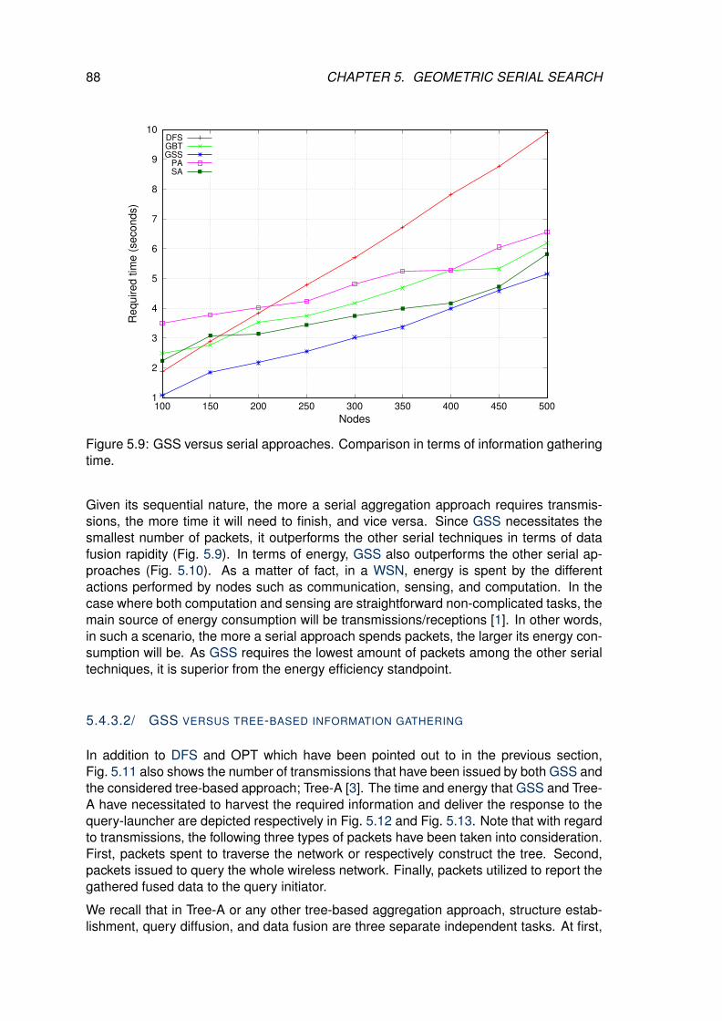
88 CHAPTER 5. GEOMETRIC SERIAL SEARCH
1
2
3
4
5
6
7
8
9
10
100 150 200 250 300 350 400 450 500
Re
qu
ire
d t
ime
(se
co
nd
s)
Nodes
DFSGBTGSS
PASA
Figure 5.9: GSS versus serial approaches. Comparison in terms of information gatheringtime.
Given its sequential nature, the more a serial aggregation approach requires transmis-sions, the more time it will need to finish, and vice versa. Since GSS necessitates thesmallest number of packets, it outperforms the other serial techniques in terms of datafusion rapidity (Fig. 5.9). In terms of energy, GSS also outperforms the other serial ap-proaches (Fig. 5.10). As a matter of fact, in a WSN, energy is spent by the differentactions performed by nodes such as communication, sensing, and computation. In thecase where both computation and sensing are straightforward non-complicated tasks, themain source of energy consumption will be transmissions/receptions [1]. In other words,in such a scenario, the more a serial approach spends packets, the larger its energy con-sumption will be. As GSS requires the lowest amount of packets among the other serialtechniques, it is superior from the energy efficiency standpoint.
5.4.3.2/ GSS VERSUS TREE-BASED INFORMATION GATHERING
In addition to DFS and OPT which have been pointed out to in the previous section,Fig. 5.11 also shows the number of transmissions that have been issued by both GSS andthe considered tree-based approach; Tree-A [3]. The time and energy that GSS and Tree-A have necessitated to harvest the required information and deliver the response to thequery-launcher are depicted respectively in Fig. 5.12 and Fig. 5.13. Note that with regardto transmissions, the following three types of packets have been taken into consideration.First, packets spent to traverse the network or respectively construct the tree. Second,packets issued to query the whole wireless network. Finally, packets utilized to report thegathered fused data to the query initiator.
We recall that in Tree-A or any other tree-based aggregation approach, structure estab-lishment, query diffusion, and data fusion are three separate independent tasks. At first,
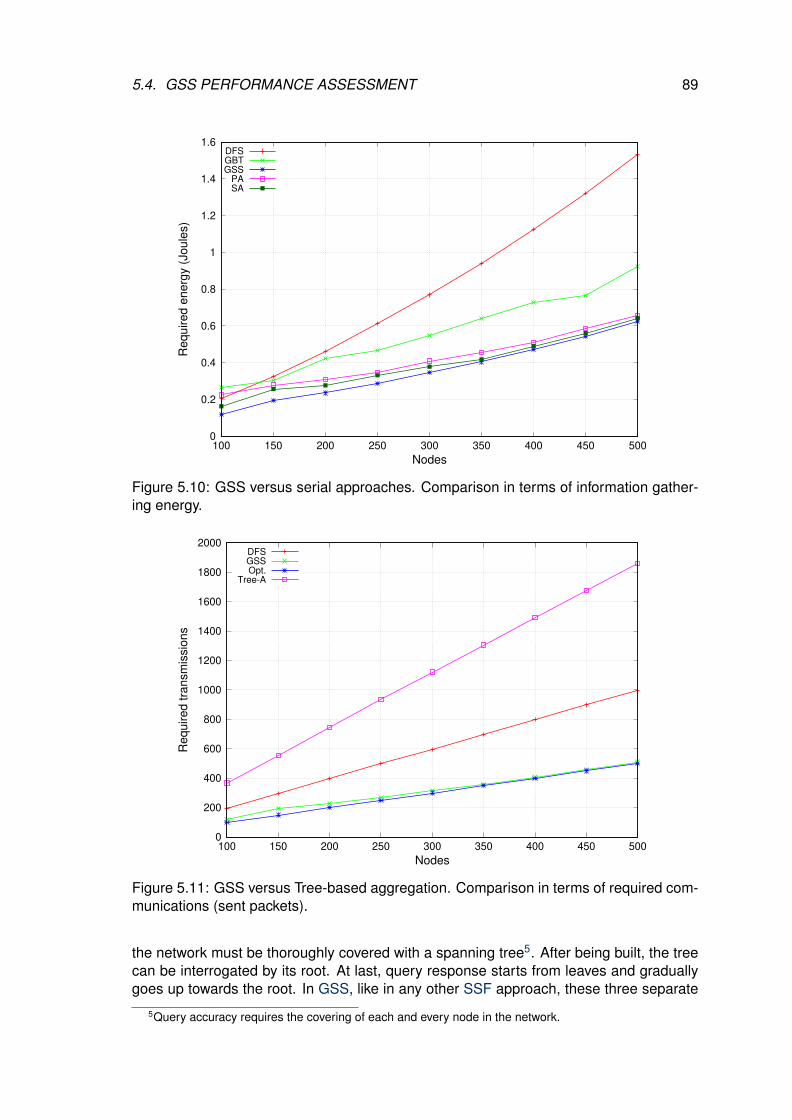
5.4. GSS PERFORMANCE ASSESSMENT 89
0
0.2
0.4
0.6
0.8
1
1.2
1.4
1.6
100 150 200 250 300 350 400 450 500
Re
qu
ire
d e
ne
rgy (
Jo
ule
s)
Nodes
DFSGBTGSS
PASA
Figure 5.10: GSS versus serial approaches. Comparison in terms of information gather-ing energy.
0
200
400
600
800
1000
1200
1400
1600
1800
2000
100 150 200 250 300 350 400 450 500
Re
qu
ire
d t
ran
sm
issio
ns
Nodes
DFSGSSOpt.
Tree-A
Figure 5.11: GSS versus Tree-based aggregation. Comparison in terms of required com-munications (sent packets).
the network must be thoroughly covered with a spanning tree5. After being built, the treecan be interrogated by its root. At last, query response starts from leaves and graduallygoes up towards the root. In GSS, like in any other SSF approach, these three separate
5Query accuracy requires the covering of each and every node in the network.

90 CHAPTER 5. GEOMETRIC SERIAL SEARCH
0
2
4
6
8
10
12
100 150 200 250 300 350 400 450 500
Re
qu
ire
d t
ime
(se
co
nd
s)
Nodes
DFSGSS
Tree-A
Figure 5.12: GSS versus Tree-based aggregation. Comparison in terms of informationgathering time.
operations have been all melted down into a single phase. Simultaneously, as the networkis being progressively browsed, nodes are interrogated and their data is collected. Thiscompactness feature of SSF approaches allows them to significantly reduce the requiredtransmissions, time, and energy.
The big difference between GSS and Tree-A in regards to energy dissipation can be ex-plained as follows. Actually, in addition to the separate indispensable (1) building/fixingof the spanning tree, (2) query dissemination, and (3) response delivery, given its con-current collision-prone behavior, Tree-A also consumes a lot of energy to retransmit thelost collided packets, especially in dense deployments. As regards information gatheringtime, intuitively, even with a larger number of transmitted packets, Tree-A is supposed tobeat all serial approaches thanks to its parallel concurrent performance. In reality, how-ever, this is not the case. Due to what has been already mentioned, GSS shows a betterresponse than Tree-A (Fig.5.12).
In a generic tree-based aggregation technique, the number of packets required to accom-plish data fusion can be calculated as follows. Actually, without considering the retrans-missions of collided packets and without considering tree construction or any probablemaintenance operation of this structure, 2 ∗ n packets need to be sent to fulfill data gath-ering from a network of n wireless nodes. More specifically, in query diffusion phase,n packets will be broadcast because all nodes are involved in this stage. During datafusion and query processing phase, n other packets will be issued because each nodemust forward a packet to the upper level except the root. As previously mentioned in Sec-tion 2.2, constructing or even maintaining a distributed logical structure over a wirelesserror/interference-prone environment is a complicated task that requires a considerabletime and energy. On the other hand, in addition to the fact that SSF approaches aremaintenance-free, do not generate any collisions, and do not require any initial separate

5.5. CONCLUSION 91
0
2
4
6
8
10
12
14
16
18
100 150 200 250 300 350 400 450 500
Re
qu
ire
d e
ne
rgy (
Jo
ule
s)
Nodes
DFSGSS
Tree-A
Figure 5.13: GSS versus Tree-based aggregation. Comparison in terms of informationgathering energy.
structure building phase, the existence of an optimal itinerary (that crosses each nodeonce) means that only n − 1 packets are needed to accomplish the desired informationcollection.
Apart from their balance and robustness issues, the main drain in tree-based approachesstems from collisions and retransmissions. Actually, packet collisions considerably affectthese approaches in terms of time and energy, especially in dense large-scale wirelessnetworks (Fig.5.12 and 5.13). Besides the fact that retransmissions significantly wastetime and energy, they are themselves subject to error and collisions, which deeply affectthese approaches. The problem of unbalanced energy consumption is also consideredas one of the main issues in tree-based aggregation approaches [12]. This phenomenonoccurs primarily because wireless nodes located nearby the root are heavily solicitedto forward the upward traffic. The unbalanced energy consumption issue can also takeplace when the initially created tree is not balanced. Finally, in tree-based approaches,structure-maintenance is indispensable because a spanning tree is nothing but a bunchof pre-set paths that are very fragile to failures and topology changes. The maintenancesolution can handle those problems at the expense of being very costly in terms of timeand energy, particularly in very large deployments.
5.5/ CONCLUSION
Serial structure-free (SSF) approaches have proven their efficiency in several aspects buthave also shown their deficiency in front of path construction complexity. This chapter hasthoroughly addressed this issue by presenting Geometric Serial Search (GSS); a novelscalable SSF approach specifically fashioned to effectively gather information from large
92 CHAPTER 5. GEOMETRIC SERIAL SEARCH
and medium-scale WSNs. The main contribution of this approach is its reliance on a newefficient localized path construction algorithm that requires fewer communications to de-rive short near-optimal visiting itineraries. Actually, the only input of this algorithm is theneighbors’ table of each traversed node, and the only tool used to traverse networks is apacket which has figuratively the shape of a rolling ball. To ensure a full network search,this packet, which can be issued by any node, sees wireless networks as a set of bound-aries (layers). While progressively finding its non-predefined track across boundaries, therolling ball simultaneously queries and collects the encountered nodes answers. In addi-tion to its inherent collision-free nature, high scalability, robustness, and energy/time effi-ciency, the extensive conducted OMNeT++ tests have confirmed that GSS constantly ap-proaches the optimal targeted number of transmissions. The performed OMNeT++ simu-lations have also confirmed that GSS avoids indefinite looping and ensures the traversalof all nodes regardless of the network topology.
As future directions, we are interested in exploiting GSS in other areas of WSNs suchprocessing topological and spatial window queries. We also plan to address some otherissues such as the effect of imprecise nodes’ locations on GSS and to what extent is thisapproach robust in face of failures in links/nodes and other topological changes.

6GENERAL CONCLUSION AND FUTURE
WORKS
The issue of querying large wireless sensor networks through data aggregation is cru-cial because of both the limited energy supply of nodes and the query time latency.
Strictly speaking, in WSNs, tasks such as data processing and query result delivery to thesink can be performed in two different ways: concurrently or sequentially. Likewise, andaccordingly, the numerous research works proposed in the literature as solutions for thequerying problem can be categorized into four classes [3,10,20,24,25,46,47]: (1) paral-lel structure-based approaches with a pre-constructed logical infrastructure (a spanningtree for instance), (2) parallel structure-free or iterative approaches in which the query re-sult is iteratively carried out through one-hop communications, (3) serial structure-basedapproaches in which the query answer is sequentially obtained via a pre-constructeditinerary that passes through every node in the network, and (4) serial structure-free ap-proaches which gradually build paths, and at the same time, interrogate nodes and gathertheir answers (i.e., each time a new query is launched, a new path is drawn for it).
Targeting large-scale or even medium network deployments, recent research has shownthat compared with the other three approaches cited above, serial structure-free aggre-gation is scalable and very efficient in terms of collisions avoidance, communication re-duction, energy conservation, and, more importantly, in terms of responsiveness. Forinstance, parallel structure-based approaches operate in three separate phases: (i) struc-ture construction (e.g., trees, clusters, ...), (ii) query dissemination, and (iii) data aggre-gation. First, a spanning tree is created over the network. Once the whole network iscovered, a query can then be diffused throughout the tree to all nodes in the network.Finally, data aggregation starts from leaf nodes and goes up towards the root/sink. Per-forming these three phases separately increases energy consumption and delays theresponse time, particularly in very large-scale networks. Conversely, serial structure-freeapproaches save energy and time because they combine the three previous phases intoone phase. While the path is gradually constructed at each hop with the help of local in-formation (i.e., a localized nature), the query is being disseminated and data aggregationis taking place at the same time. Furthermore, in opposition to parallel or serial structure-
93

94 CHAPTER 6. GENERAL CONCLUSION AND FUTURE WORKS
based approaches in which only the sink/root is able to request information from sensornodes, in serial structure-free approaches, queries can be launched from any node in thenetwork. This is, in fact, a fundamental need for emergent multi-owner-multi-user WSNswhere several nodes can be responsible for updating configuration parameters and/ordistributing management commands [50]. In addition to all this, as serial approachesinvolve only one communication at each moment in time, they can therefore avoid colli-sions, improving hence their performance in terms of energy conservation and delay timereduction. This is not the case for parallel approaches; they generate a lot of collisionsduring structure construction, query diffusion, and data aggregation, particularly in densenetworks [25], even when sophisticated MAC protocols are used [49].
As confirmed by the evaluation studies we have conducted, despite their interesting fea-tures/advantages and outperformance in comparison with other approaches, state-of-the-art serial structure-free processing techniques still suffer from several deficiencies amongwhich we mainly cite path construction. More exactly, recent serial approaches requirean additional cost to construct their non-optimal and relatively long traversal paths. Infact, the major challenges encountered when designing an efficient serial aggregationapproach are (1) ensuring the exploration of all nodes in the network whatever the con-sidered topology, and (2) reducing the needed time and energy. To achieve the latterobjective, two points must be taken into consideration. First, finding the shortest possiblevisiting path (a short path enhances the overall performance and vice versa), and second,avoiding extra communications by counting only on the local knowledge of each traversednode to explore the network.
In this work, in order to respond to these interesting and challenging questions, andin order to provide an efficient information gathering mechanism for wireless resource-constrained networks, our primary objective was developing scalable serial algorithmsthat shorten the traversal path and reduce communications to the maximum extent possi-ble. The objective was attaining the optimal number of hops, i.e., n− 1 packets to traversea network of n nodes; no extra overhead or control packets must be required. In additionto that primary goal, our second aim was the algorithms ability to explore any connectednetwork and to visit all of its nodes regardless of the topology in hand (regular/irregular,large/sparse, with/without holes, etc.). Concretely speaking, in this manuscript, we pro-posed three novel serial processing approaches, called Peeling Algorithm (PA), Spread-ing Aggregation (SA), and Geometric Serial Search (GSS), which have been specificallydesigned to be scalable and support very large numbers of nodes. The obtained simula-tion results confirm that the proposed algorithms outperform state-of-the-art approachesin terms of deriving shorter visiting paths, and in terms of time and energy consumptionreduction. The simulation results we obtained also confirm the very good scalability of ourthree proposals. In addition to these interesting experimental results, we provided in thismanuscript formal proofs that demonstrate the correctness of the proposed approaches;i.e., they terminate and are able of visiting all connected nodes without falling into looping.
First, Peeling Algorithm (PA) [18], which as its name hints, peels the network layer-by-layer starting from the external boundary. In other words, the exploration of nodes startsby progressively removing (marking as visited) the external boundary (layer) of the net-work and hence disclosing a new internal unexplored layer which will be removed (peeled)in its turn, and so forth. Initially, in order to find the peeling starting point (i.e., any nodelocated on the network external boundary), the query launcher (which can also be anynode in the network) collaborates with other nodes. Once the network external boundaryhas been determined and the starting point has been found, the network peeling can start

95
from this node using the graph-free boundary traversal algorithm called curved-stick [38].Being costly in terms of energy and time, if executed with each new query, the processof network external boundary determination can considerably harm the overall peelingperformance. However, this is not the case, this process is executed only once duringnetwork setup (unless, of course, we have unstable topologies with continuous changes).
Our second approach; Spreading Aggregation (SA) [39, 40] starts information gatheringby simply placing a rolling ball [41] (launching a single packet) and letting it sequentiallyhop over nodes and aggregate their data. The next hop of the querying/aggregationpacket is determined locally by each traversed node using only its one-hop neighborhoodinformation. No network topology information needs to be known by nodes nor colli-sions are generated as only one node is communicating at any given time. In addition tothis, unlike the peeling technique [18], in SA, there is no necessity for network externalboundary determination. As a matter of fact, in SA, non-boundary nodes can be querylaunchers by simply utilizing a shrunken rolling-ball. The latter visits nodes and gets pro-gressively enlarged if possible at each hop until eventually it gains its optimal shape andcontinues the ordinary traversal process. As confirmed by the numerous OMNeT++ sim-ulation results we obtained, Spreading Aggregation is highly scalable and very effective interms of communication, energy, and time consumption reduction. The obtained resultsalso confirm the superiority of SA over state-of-the-art serial and parallel approaches,particularly in very large-scale network deployments.
Finally, in spite of the fact that PA and SA excel in large and medium-scale networks,their path-construction mechanisms are not optimal and can be improved by reducingthe involved communications and further shortening the visiting path. Geometric SerialSearch (GSS) [42, 43]; our third approach, came to respond to this need by totally ex-cluding control packets and relying only on one packet that jumps from node to nodeand explores the entire network. In fact, while progressively traversing the network, thispacket simultaneously interrogates nodes and harvests their query responses. Pathscreated by GSS are not constructed in advance, can commence from any node in thenetwork, and necessitates only the one-hop neighbors’ table of each explored node to betraced. As a matter of fact, in addition to its completeness1, collision-freeness, scalability,energy/time efficiency, and robustness2, GSS considerably reduces communications andlays out very short traversal paths by always approaching the optimal number of hops(i.e., n − 1 packets to explore n nodes). The obtained OMNeT++ simulation results pre-sented in this manuscript demonstrated the efficiency of GSS as an information gatheringtechnique for large wireless resource-constrained networks and confirmed all the pointscited above.
To summarize, serial localized processing algorithms explore nodes one-by-one and areable of performing a multitude of tasks including scheduling nodes, querying or gather-ing data from nodes, supplying nodes with data, etc. As future research directions, weare interested in exploiting localized serial processing in other areas of WSNs such astopological aggregation and spatial window querying. In the latter example, instead ofaddressing queries to the entire network, the end-user indicates the region to be inter-rogated by specifying a rectangular shape (or any other geometric form) called WindowQuery Region (WQR). For instance, through the below query, the end-user will obtain theaverage temperature, maximum humidity, minimum light, and finally the number of sensornodes in the region bounded by a rectangle defined by two points.
1Ability to explore all nodes is a fundamental requirement in many sensitive practical applications.2Resilience to topology changes (failures in links/nodes, ...).
96 CHAPTER 6. GENERAL CONCLUSION AND FUTURE WORKS
SELECT AVG(temperature), MAX(humidity), MIN(light), COUNT()
FROM sensors as s
WHERE s.location WITHIN [(75, 75), (320, 630)]
The idea behind serial window querying is to reach the WQR by means of any efficientgeographic routing protocol. Once the desired WQR has been reached, the queryingprocess starts by sequentially collecting the answers of all nodes located inside that re-gion. Finally, the obtained query result has to be sent to the sink/query launcher using thesame geographic routing protocol that has been utilized in the beginning. Even thoughthis technique seems to be simple, it is in reality hard to design because it must be ableto handle any network deployment, especially those with communication holes. In otherterms, the proposed approach has to be able to deal with the so-called void problemand guarantee query accuracy by visiting all nodes located inside the WQR in question.In fact, we have started a research work on this matter and the preliminary results areencouraging and very promising.
As other perspectives, some other issues of localized serial processing algorithms can bealso addressed such as (1) the effect of imprecise nodes’ locations on serial aggregationin general and on our proposed approaches in particular. (2) To what extent are serialstructure-free approaches robust in face of failures in links/nodes and other topologicalchanges.

BIBLIOGRAPHY
[1] Azzedine Boukerche. Algorithms and protocols for wireless sensor networks, vol-ume 62. John Wiley & Sons, 2008.
[2] Ian F. Akyildiz and Mehmet Can Vuran. Wireless sensor networks, volume 4. JohnWiley & Sons, 2010.
[3] Ramesh Rajagopalan and Pramod K. Varshney. Data-aggregation techniques insensor networks: A survey. IEEE Communications Surveys and Tutorials, 8(1-4):48–63, 2006.
[4] Soummya Kar, Jose M. F. Moura, and Kavita Ramanan. Distributed parameter esti-mation in sensor networks: Nonlinear observation models and imperfect communi-cation. IEEE Trans. Information Theory, 58(6):3575–3605, 2012.
[5] Angelia Nedic, Alexander Olshevsky, Asuman E. Ozdaglar, and John N. Tsitsiklis.On distributed averaging algorithms and quantization effects. IEEE Trans. Automat.Contr., 54(11):2506–2517, 2009.
[6] Amir Beck, Petre Stoica, and Jian Li. Exact and approximate solutions of sourcelocalization problems. IEEE Trans. Signal Processing, 56(5):1770–1778, 2008.
[7] Jianyong Lin, Wendong Xiao, Frank L. Lewis, and Lihua Xie. Energy-efficient dis-tributed adaptive multisensor scheduling for target tracking in wireless sensor net-works. IEEE Trans. Instrumentation and Measurement, 58(6):1886–1896, 2009.
[8] Engin Masazade, Ruixin Niu, Pramod K. Varshney, and Mehmet Keskinoz. Energy-aware iterative source localization for wireless sensor networks. IEEE Trans. SignalProcessing, 58(9):4824–4835, 2010.
[9] Bahador Khaleghi, Alaa M. Khamis, Fakhreddine Karray, and Saiedeh N. Razavi.Multisensor data fusion: A review of the state-of-the-art. Information Fusion,14(1):28–44, 2013.
[10] Xiang-Yang Li, Yajun Wang, and Yu Wang. Complexity of data collection, aggrega-tion, and selection for wireless sensor networks. IEEE Trans. Computers, 60(3):386–399, 2011.
[11] Xiaobing Wu, Guihai Chen, and Sajal K. Das. Avoiding energy holes in wireless sen-sor networks with nonuniform node distribution. IEEE Trans. Parallel Distrib. Syst.,19(5):710–720, 2008.
[12] Anfeng Liu, Peng-Hui Zhang, and Zhi-Gang Chen. Theoretical analysis of the life-time and energy hole in cluster-based wireless sensor networks. J. Parallel Distrib.Comput., 71(10):1327–1355, 2011.
97

98 BIBLIOGRAPHY
[13] Soummya Kar and Jose M. F. Moura. Distributed consensus algorithms in sen-sor networks with imperfect communication: Link failures and channel noise. IEEETrans. Signal Processing, 57(1):355–369, 2009.
[14] Boris N. Oreshkin, Mark Coates, and Michael G. Rabbat. Optimization and analysisof distributed averaging with short node memory. IEEE Trans. Signal Processing,58(5):2850–2865, 2010.
[15] Stacy Patterson, Bassam Bamieh, and Amr El Abbadi. Convergence rates of dis-tributed average consensus with stochastic link failures. IEEE Trans. Automat. Contr.,55(4):880–892, 2010.
[16] Lin Xiao, Stephen P. Boyd, and Seung-Jean Kim. Distributed average consensuswith least-mean-square deviation. J. Parallel Distrib. Comput., 67(1):33–46, 2007.
[17] Satish M. Srinivasan and Azad H. Azadmanesh. Survivable data aggregation in mul-tiagent network systems with hybrid faults. IEEE Trans. Computers, 62(10):2054–2068, 2013.
[18] Ahmed Mostefaoui, Azzedine Boukerche, Mohammed Amine Merzoug, and Mah-moud Melkemi. A scalable approach for serial data fusion in wireless sensor net-works. Computer Networks, 79:103–119, 2015.
[19] Robert D. Nowak. Distributed EM algorithms for density estimation and clustering insensor networks. IEEE Trans. Signal Processing, 51(8):2245–2253, 2003.
[20] Michael Rabbat and Robert D. Nowak. Quantized incremental algorithms fordistributed optimization. IEEE Journal on Selected Areas in Communications,23(4):798–808, 2005.
[21] Angelia Nedic and Dimitri P. Bertsekas. Incremental subgradient methods for non-differentiable optimization. SIAM Journal on Optimization, 12(1):109–138, 2001.
[22] Stephanie Lindsey, Cauligi S. Raghavendra, and Krishna M. Sivalingam. Data gath-ering algorithms in sensor networks using energy metrics. IEEE Trans. Parallel Dis-trib. Syst., 13(9):924–935, 2002.
[23] Michael R. Garey and David S. Johnson. Computers and Intractability: A Guide tothe Theory of NP-Completeness. W. H. Freeman, 1979.
[24] Swapnil Patil, Samir R. Das, and Asis Nasipuri. Serial data fusion using space-filling curves in wireless sensor networks. In Proceedings of the 1st Annual IEEECommunications Society Conference on Sensor and Ad Hoc Communications andNetworks, SECON’04, Santa Clara, CA, USA, October 4-7, 2004, pages 182–190.
[25] Azzedine Boukerche, Ahmed Mostefaoui, and Mahmoud Melkemi. Efficient and ro-bust serial query processing approach for large-scale wireless sensor networks. AdHoc Networks, 47:82–98, 2016.
[26] Shimon Even and Guy Even. Graph Algorithms, Second Edition. Cambridge Uni-versity Press, 2012.
[27] Azzedine Boukerche and Xin Fei. A coverage-preserving scheme for wireless sensornetwork with irregular sensing range. Ad Hoc Networks, 5(8):1303–1316, 2007.

BIBLIOGRAPHY 99
[28] Azzedine Boukerche, Xin Fei, and Regina Borges de Araujo. An optimal coverage-preserving scheme for wireless sensor networks based on local information ex-change. Computer Communications, 30(14-15):2708–2720, 2007.
[29] Azzedine Boukerche, Horacio A. B. F. Oliveira, Eduardo F. Nakamura, and AntonioA. F. Loureiro. Localization systems for wireless sensor networks. IEEE WirelessCommun., 14(6):6–12, 2007.
[30] Horacio A. B. F. Oliveira, Azzedine Boukerche, Eduardo F. Nakamura, and AntonioA. F. Loureiro. An efficient directed localization recursion protocol for wireless sensornetworks. IEEE Trans. Computers, 58(5):677–691, 2009.
[31] Jing Wang, Ratan K. Ghosh, and Sajal K. Das. A survey on sensor localization.Journal of Control Theory and Applications, 8(1):2–11, 2010.
[32] Guang Tan, Hongbo Jiang, Shengkai Zhang, Zhimeng Yin, and Anne-Marie Ker-marrec. Connectivity-based and anchor-free localization in large-scale 2d/3d sensornetworks. TOSN, 10(1):6:1–6:21, 2013.
[33] Mort Naraghi-Pour and Gustavo Chacon Rojas. A novel algorithm for distributedlocalization in wireless sensor networks. TOSN, 11(1):1:1–1:25, 2014.
[34] Fu Xiao, Wei Liu, Zhetao Li, Lei Chen, and Ruchuan Wang. Noise-tolerant wirelesssensor networks localization via multinorms regularized matrix completion. IEEETrans. Vehicular Technology, 67(3):2409–2419, 2018.
[35] Jukka Suomela. Survey of local algorithms. ACM Comput. Surv., 45(2):24:1–24:40,2013.
[36] Eduardo F. Nakamura, Antonio A. F. Loureiro, Azzedine Boukerche, and Albert Y.Zomaya. Localized algorithms for information fusion in resource-constrained net-works. Information Fusion, 15:2–4, 2014.
[37] Ahmed Mostefaoui, Mahmoud Melkemi, and Azzedine Boukerche. Routing throughholes in wireless sensor networks. In 15th ACM International Conference on Model-ing, Analysis and Simulation of Wireless and Mobile Systems, MSWiM’12, Paphos,Cyprus, October 21-25, 2012, pages 395–402.
[38] Ahmed Mostefaoui, Mahmoud Melkemi, and Azzedine Boukerche. Localized routingapproach to bypass holes in wireless sensor networks. IEEE Trans. Computers,63(12):3053–3065, 2014.
[39] Mohammed Amine Merzoug, Azzedine Boukerche, Ahmed Mostefaoui, and SamirChouali. Spreading aggregation: A distributed collision-free approach for data aggre-gation in large-scale wireless sensor networks. J. Parallel Distrib. Comput., 125:121–134, 2019.
[40] Mohammed Amine Merzoug, Ahmed Mostefaoui, and Samir Chouali. Distributedcollision-free data aggregation approach for wireless sensor networks. In 13th IEEEInternational Conference on Distributed Computing in Sensor Systems, DCOSS’17,Ottawa, ON, Canada, June 5-7, 2017, pages 175–182.
[41] Wen-Jiunn Liu and Kai-Ten Feng. Greedy routing with anti-void traversal for wirelesssensor networks. IEEE Trans. Mob. Comput., 8(7):910–922, 2009.

100 BIBLIOGRAPHY
[42] Mohammed Amine Merzoug, Azzedine Boukerche, and Ahmed Mostefaoui. Efficientinformation gathering from large wireless sensor networks. Computer Communica-tions, 132:84–95, 2018.
[43] Mohammed Amine Merzoug, Azzedine Boukerche, and Ahmed Mostefaoui. Serialin-network processing for large stationary wireless sensor networks. In Proceedingsof the 20th ACM International Conference on Modeling, Analysis and Simulation ofWireless and Mobile Systems, MSWiM’17, Miami, FL, USA, November 21-25, 2017,pages 153–160.
[44] Ian F. Akyildiz, Weilian Su, Yogesh Sankarasubramaniam, and Erdal Cayirci. Wire-less sensor networks: a survey. Computer Networks, 38(4):393–422, 2002.
[45] Elena Fasolo, Michele Rossi, Jorg Widmer, and Michele Zorzi. In-network aggrega-tion techniques for wireless sensor networks: a survey. IEEE Wireless Commun.,14(2):70–87, 2007.
[46] Hongyu Gong, Luoyi Fu, Xinzhe Fu, Lutian Zhao, Kainan Wang, and Xinbing Wang.Distributed multicast tree construction in wireless sensor networks. IEEE Trans. In-formation Theory, 63(1):280–296, 2017.
[47] Long Cheng, Jianwei Niu, Chengwen Luo, Lei Shu, Linghe Kong, Zhiwei Zhao, andYu Gu. Towards minimum-delay and energy-efficient flooding in low-duty-cycle wire-less sensor networks. Computer Networks, 134:66–77, 2018.
[48] Panayiotis Andreou, Andreas Pamboris, Demetrios Zeinalipour-Yazti, Panos K.Chrysanthis, and George Samaras. ETC: energy-driven tree construction in wire-less sensor networks. In 10th International Conference on Mobile Data Manage-ment, MDM’09, Taipei, Taiwan, May 18-20, 2009, pages 513–518.
[49] Qiang Ma, Kebin Liu, Zhichao Cao, Tong Zhu, Xin Miao, and Yunhao Liu. Oppor-tunistic concurrency: A MAC protocol for wireless sensor networks. IEEE Trans.Parallel Distrib. Syst., 26(7):1999–2008, 2015.
[50] Daojing He, Sammy Chan, Mohsen Guizani, Haomiao Yang, and Boyang Zhou. Se-cure and distributed data discovery and dissemination in wireless sensor networks.IEEE Trans. Parallel Distrib. Syst., 26(4):1129–1139, 2015.
[51] Brad Karp and Hsiang-Tsung Kung. GPSR: greedy perimeter stateless routing forwireless networks. In Proceedings of the 6th Annual International Conference onMobile Computing and Networking, MOBICOM’00, Boston, MA, USA, August 6-11,2000, pages 243–254.
[52] Fabian Kuhn, Roger Wattenhofer, and Aaron Zollinger. Worst-case optimal andaverage-case efficient geometric ad-hoc routing. In Proceedings of the 4th ACM In-ternational Symposium on Mobile Ad Hoc Networking and Computing, MobiHoc’03,Annapolis, MD, USA, June 1-3, 2003, pages 267–278.
[53] OMNeT++: Simulation Environment. https://www.omnetpp.org, October 2018.
[54] Castalia: Wireless Sensor Network Simulator. https://github.com/boulis/Castalia,October 2018.

BIBLIOGRAPHY 101
[55] Wendi B. Heinzelman, Anantha P. Chandrakasan, and Hari Balakrishnan. Anapplication-specific protocol architecture for wireless microsensor networks. IEEETrans. Wireless Communications, 1(4):660–670, 2002.
[56] Joseph Polastre, Jason L. Hill, and David E. Culler. Versatile low power media accessfor wireless sensor networks. In Proceedings of the 2nd International Conference onEmbedded Networked Sensor Systems, SenSys’04, Baltimore, MD, USA, November3-5, 2004, pages 95–107.
[57] Wei Ye, John S. Heidemann, and Deborah Estrin. Medium access control with co-ordinated adaptive sleeping for wireless sensor networks. IEEE/ACM Trans. Netw.,12(3):493–506, 2004.


Mohammed A. Merzoug — University of Bejaia 2019.Contact: [email protected]
Document generated with LATEX and:1. The LATEX style for Ph.D. Thesis created by S. Galland — http://www.multiagent.fr/ThesisStyle2. The tex-upmethodology package suite — http://www.arakhne.org/tex-upmethodology/

Localized adaptive routing in wireless sensor networks
Abstract a wireless sensor network is made up of a set of small units, called sensor nodes, which can
communicate with one another via direct radio communications or by relays. Sensor nodes are deployed in
order to monitor a particular area of interest by sampling and collecting data (e.g., temperature, humidity,
pressure, etc.). The collected information is subsequently sent to a fusion station for analysis purposes. The
application areas of these networks are numerous in different domains such as military applications, domotics,
health, etc. In reality, the specificities of wireless sensor networks bring many new possibilities but also pose
many challenges in terms of deployment (limited energy resources, self-organization, etc.), coverage
(monitored space), communication (total absence of any network infrastructure), and finally data collection and
processing. In the context of this thesis, we are particularly interested in the general problem of data routing
and fusion in this kind of networks. In fact, due to the inherent constraints of wireless sensor networks (primarily
the very limited energy resources), this task remains particularly arduous despite the numerous works in the
literature.
Keywords wireless sensor networks; distributed algorithms; localized routing; data fusion; query processing.
كيةــشعار اللاسلــكات الاستــي شبــلي فــمحيفي ـــيه تكــتوج
ى ـادرة علـشعار، القـد الإستـماة عقـيرة، المسـدات الصغـن الوحـموعة مـن مجـكية مـكة الاستــشعار اللاسلـكون شبـتت ملــخص
راقبة ـشعار لمـد الاستـعقشر ـتن. رةـير المباشـرة أو غـكية المباشـالات اللاسلـالاتص بواسطةض ـضها البعـع بعـواصل مـالت
ال ـإرسبعـد ذلك م ـيت (.الخط، ــوبة، الضغـرارة، الرطـة الحـدرج)ع البيانات ـوجم ناتـذ العيـريق أخـن طـينة عـطقة معـمن
يـديدة فـكات عـذه الشبـبيق لهــالات التطـمج .ليلــراض التحـلأغ اجـوالإدمميع ــطة التجــى محـمعة إلــلومات المجـالمع
شعار ــكات الاستـيات شبـوصـخص ،الواقعي ـف .الخ، حةـزلية، الصــنيات المنــالتق كرية،ـبيقات العسـثل التطـتلفة مــالات مخـمج
علق ـما يتـة فيـديات خاصـن التحـديد مــالع تطــرح تــوقـس الــي نفـنها فــديدة، ولكــكانات الجـن الامـديد مـلب العـكية تجــاللاسل
ية ـياب التام لأي بنـالغ)الات ـالاتص ،(راقبةـاحة المـالمس)طية ــالتغ ،(ذاتي ، الخـظيم الــدودة، التنـة المحـوارد الطاقـم)ر ــبالنش
امة ــكلة العـاص بالمشـكل خـتمون بشـحن مهـ، نفي سياق هذه الأطروحة .تهاـع البيانات ومعالجـيرا جمـوأخ ،(كةـتية للشبـتح
كات ـي شبـتأصلة فـروضة والمــيود المفـبب القـ، بسالحقيقة يـف .كاتـن الشبـنوع مـذا الـي هـالبيانات ف جـيه ودمــلتوج
رغم ـلى الـغاية عـلل بةـصعلية ـذه العمـقى هــتب ،(ايةـدودة للغـاقة المحـوارد الطـ، مقام الأولـي المـف)كية ــشعار اللاسلـالاست
.جزةــثية المنــمال البحــن الأعـديد مــن العـم
.علاماتــالجة الاستــمع ؛ج البياناتــدم؛ ليــيه محـوجـت ؛وزعةـيات مـوارزمـخ ؛كيةـشعار اللاسلـكات الاستـشب دالةـمات الـالكل
Routage localisé et adaptatif dans les réseaux de capteurs sans fil
Résumé un réseau de capteurs sans fil est constitué d’un ensemble de petites unités, appelées nœuds capteurs,
pouvant communiquer les unes avec les autres via des communications radio directes ou par relais. Les nœuds
capteurs sont déployés afin de surveiller une zone d’intérêt particulière par le prélèvement et la collecte de
données (e.g., température, humidité, pression, etc.). Les informations ainsi collectées sont envoyées par la suite
à une station de fusion à des fins d’analyse. Les domaines applicatifs de ces réseaux sont nombreux dans
différents domaines tels que les applications militaires, la domotique, la santé, etc. En réalité, les spécificités des
réseaux de capteurs sans fil amènent de nombreuses possibilités nouvelles mais posent également de
nombreux défis en termes de déploiement (ressources énergétiques limitées, auto-organisation, etc.), de
couverture (espace surveillé), de communication (absence totale de toute infrastructure réseau), et enfin de
collecte et d’exploitation de données. Dans le cadre de cette thèse, nous nous intéressons plus particulièrement
à la problématique générale de routage et de fusion de données dans ce genre de réseaux. En effet, en raison
des contraintes inhérentes aux réseaux de capteurs sans fil (principalement les provisions énergétiques très
limitées), cette tâche demeure particulièrement ardue malgré les nombreux travaux dans la littérature.
Mots-clés réseaux de capteurs sans fil; algorithmes distribués; routage localisé; fusion de données; traitement
de requêtes.