thesis - doi@nrct

THESIS

SIDELOBE REDUCTION IN PEANO-GOSPER FRACTAL

ARRAYS USING GENETIC ALGORITHMS

META POLPASEE

GRADUATE SCHOOL, KASETSART UNIVERSITY 2007

10.144

57/KU

.the.2

007.40

3

เมื่อ 26

/07/25

65 21:

33:54

10.144

57/KU

.the.2

007.40

3

เมื่อ 26

/07/25

65 21:

33:54

THESIS

SIDELOBE REDUCTION IN PEANO-GOSPER FRACTAL ARRAYS

USING GENETIC ALGORITHMS

META POLPASEE

A Thesis Submitted in Partial Fulfillment of

the Requirements for the Degree of

Master of Engineering (Electrical Engineering)

Graduate School, Kasetsart University

2007

10.144

57/KU

.the.2

007.40

3

เมื่อ 26

/07/25

65 21:

33:54

10.144

57/KU

.the.2

007.40

3

เมื่อ 26

/07/25

65 21:

33:54

ACCKNOWLEDGEMENT

The author would like to thank Associate Professor Nuttaka Homsup for his

advice and assistance, in adjusting and correcting the contents and for serving as his

major advisor. The author is deeply grateful for Assistant Professor Waroth Kuhirun

who gave useful suggestions for this research. The author wishes to express his

appreciation to Mr. Terapass Jiranorawiss for his kindly support in giving useful

suggestions. Finally, I would like to dedicate all my works to my family who

encourages me and gives me a chance to experience in the world of living and

learning

Meta Polpasee

February 2007

10.144

57/KU

.the.2

007.40

3

เมื่อ 26

/07/25

65 21:

33:54

i

TABLE OF CONTENTS

Page TABLE OF CONTENTS i

LIST OF TABLES ii

LIST OF FIGURES iii

INTRODUCTION 1

LITERATURE REVIEWS 17

MATERIAL AND METHOD 20

Materials 20

Method 20

RESULT AND DISCUSSIONS 26

CONCLUSION AND RECOMMENDATION 59

LITERATURE CITED 60

CURRICULUM VITAE 64

10.144

57/KU

.the.2

007.40

3

เมื่อ 26

/07/25

65 21:

33:54

ii

LIST OF TABLES

Table Page 1 Comparison of the sidelobe levels in dB of the genetically

optimized stage 3 Peano-Gosper fractal arrays with different parameters for both approaches.

58 10.144

57/KU

.the.2

007.40

3

เมื่อ 26

/07/25

65 21:

33:54

iii

LIST OF FIGURES

Figure Page

1 Cantor Set 4

2 Koch Curve 5

3 Sierpinski gasket 5

4 Sierpinski carpet 6

5 Example of Binary Encoding 11

6 Example of Permutation Encoding 11

7 Example of Value Encoding 12

8 Graph of fitness 13

9 Example of Rank Selection (Before and After) 14

10 Example of Crossover 14

11 Example of Mutation 15

12 The Geometry for planar arrays of isotropic sources 17

13 Linear plot of power pattern and its associated lobes 18

14 The Peano-Gosper curve initiator 20

15 The Peano-Gosper curve generator 21

16 The first three stages in the construction of self-avoiding Peano-Gosper curve. The initiator is show as the dashed line superimposed on the stage 1generator. The generator (unscaled ) is shown again in (b) as the dashed curve superimposed on the stage 2Peano-gosper curve

22

17 Flow Chart of Methodologies case 1 24

18 Flow Chart of Methodologies case 1 25

19 The Peano-Gosper fractal arrays configurations and their relative current excitation for the stages of growth 1, 2 and 3, respectively

26

10.144

57/KU

.the.2

007.40

3

เมื่อ 26

/07/25

65 21:

33:54

iv

LIST OF FIGURES (cont’d)

Figure Page 20 Element location for the (a) stage 1, (b) stage 2, and (c) stage 3

Peano-Gosper fractal arrays. A uniform spacing of dmin is assumed0 between consecutive arrays elements which is the same for each stage, minimum spacing is λ/2, maximum current excitation is one

27

21 Evolution diagram of Genetically Optimized a Stage3: Peano-Gosper Fractal Array minimum spacing is λ/2, maximum current excitation is one

28

22 Plot of the normalized stage 3 Peano-Gosper fractal array, genetically optimized array factor versus (a) φ for θ = 90° and (b) θ for φ = 90° where minimum distance equal λ/2 and maximum current excitation equal one

28

23 The normalized radiation pattern in dB for stage 3 of Peano-Gosper fractal array from Figure 20c with a minimum spacing is λ/2, maximum current excitation is one and main beam steered to θ = 0 degrees and φ = 90° degrees. (a)Radiation Pattern, and (b) Top View

29

24 Element location for the (a) stage 1, (b) stage 2, and (c) stage 3 Peano-Gosper fractal arrays. A uniform spacing of dmin is assumed between consecutive arrays elements which is the same for each stage, minimum spacing is λ/2, maximum current excitation is ten.

31

25 Evolution diagram of Genetically Optimized a Stage3: Peano-Gosper Fractal Array, minimum spacing is λ/2, maximum current excitation is ten.

32

26 Plot of the normalized stage 3 Peano-Gosper fractal array, genetically optimized array factor versus (a) φ forθ = 90° and (b) θ for φ = 90° where minimum distance equal λ/2 and maximum current excitation equal ten.

32

27 Top view of the normalized radiation pattern in dB for stage of Peano-Gosper fractal array of isotropic elements from Figure 24c with a minimum spacing is λ/2, maximum current excitation is ten and main beam steered to θ = 0 degrees and for φ = 90° degrees.

33

10.144

57/KU

.the.2

007.40

3

เมื่อ 26

/07/25

65 21:

33:54

v



Peano-Gosper fractal arrays. A uniform spacing of dmin is assumed between consecutive arrays elements which is the same for each stage, minimum spacing is λ, maximum current excitation is one.

35

29 Evolution diagram of Genetically Optimized a Stage3: Peano-Gosper Fractal Array, minimum spacing is λ, maximum current excitation is one.

36

30 Plot of the normalized stage 3 Peano-Gosper fractal array, genetically optimized array factor versus (a) φ for θ = 90° and (b) θ for φ = 90° where minimum distance equal λ and maximum current excitation equal one

36

31 The normalized radiation pattern in dB for stage 3 of Peano-Gosper fractal array from Figure 28c with a minimum spacing is λ, maximum current excitation is one and main beam steered to θ = 0 degrees and φ = 90° degrees. (a)Radiation Pattern, and (b) Top View

37

32 Element location for the (a) stage 1, (b) stage 2, and (c) stage 3 Peano-Gosper fractal arrays. A uniform spacing of dmin is assumed between consecutive arrays elements which is the same for each stage, minimum spacing is λ, maximum current excitation is ten

39

33 Evolution diagram of Genetically Optimized a Stage3: Peano-Gosper Fractal Array, minimum spacing is λ, maximum current excitation is ten.

40

34 Plot of the normalized stage 3 Peano-Gosper fractal array, genetically optimized array factor versus (a) φ for θ = 90° and (b) θ for φ = 90° where minimum distance equal λ and maximum current excitation equal ten.

40

35 The normalized radiation pattern in dB for stage 3 of Peano-Gosper fractal array from Figure 32c with a minimum spacing is λ, maximum current excitation is ten and main beam steered to θ = 0 degrees and φ = 90° degrees. (a)Radiation Pattern, and (b) Top View.

41

10.144

57/KU

.the.2

007.40

3

เมื่อ 26

/07/25

65 21:

33:54

vi



Peano-Gosper fractal arrays. A uniform spacing of dmin is assumed between consecutive arrays elements which is the same for each stage, minimum spacing is λ/2, maximum current excitation is one

43

37 Evolution diagram of Genetically Optimized a Stage3: Peano-Gosper Fractal Array, minimum spacing is λ/2, maximum current excitation is one.

44

38 Plot of the normalized stage 3 Peano-Gosper fractal array, genetically optimized array factor versus (a) φ for θ = 90° and (b) θ for φ = 90° where minimum distance equal λ/2 and maximum current excitation equal one.

44

39 The normalized radiation pattern in dB for stage 3 of Peano-Gosper fractal array from Figure 36c with a minimum spacing is λ/2, maximum current excitation is one and main beam steered to θ = 0 degrees and φ = 90° degrees. (a)Radiation Pattern, and (b) Top View.

45

40 Element location for the (a) stage 1, (b) stage 2, and (c) stage 3 Peano-Gosper fractal arrays. A uniform spacing of dmin is assumed between consecutive arrays elements which is the same for each stage, minimum spacing is λ/2, maximum current excitation is ten.

47

41 Evolution diagram of Genetically Optimized a Stage3: Peano-Gosper Fractal Array, minimum spacing is λ/2, maximum current excitation is ten

48

42 Plot of the normalized stage 3 Peano-Gosper fractal array, genetically optimized array factor versus (a) φ for θ = 90° and (b) θ for φ = 90° where minimum distance equal λ/2 and maximum current excitation equal ten.

48

43 The normalized radiation pattern in dB for stage 3 of Peano-Gosper fractal array from Figure 40c with a minimum spacing is λ/2, maximum current excitation is ten and main beam steered to θ = 0 degrees and φ = 90° degrees. (a)Radiation Pattern, and (b) Top View.

49

10.144

57/KU

.the.2

007.40

3

เมื่อ 26

/07/25

65 21:

33:54

vii



Peano-Gosper fractal arrays. A uniform spacing of dmin is assumed between consecutive arrays elements which is the same for each stage, minimum spacing is λ, maximum current excitation is one.

51

45 Evolution diagram of Genetically Optimized a Stage3: Peano-Gosper Fractal Array, minimum spacing is λ, maximum current excitation is one.

52

46 Plot of the normalized stage 3 Peano-Gosper fractal array, genetically optimized array factor versus (a) φ for θ = 90° and (b) θ for φ = 90° where minimum distance equal λ and maximum current excitation equal one.

52

47 The normalized radiation pattern in dB for stage 3 of Peano-Gosper fractal array from Figure 44c with a minimum spacing is λ, maximum current excitation is one and main beam steered to θ = 0 degrees and φ = 90° degrees. (a)Radiation Pattern, and (b) Top View.

53

48 Element location for the (a) stage 1, (b) stage 2, and (c) stage 3 Peano-Gosper fractal arrays. A uniform spacing of dmin is assumed between consecutive arrays elements which is the same for each stage, minimum spacing is λ, maximum current excitation is ten.

55

49 Evolution diagram of Genetically Optimized a Stage3: Peano-Gosper Fractal Array, minimum spacing is λ, maximum current excitation is ten.

56

50 Plot of the normalized stage 3 Peano-Gosper fractal array, genetically optimized array factor versus (a)φ for θ = 90° and (b) θ for φ = 90° where minimum distance equal λ and maximum current excitation equal ten.

56

51 The normalized radiation pattern in dB for stage 3 of Peano-Gosper fractal array from Figure 48c with a minimum spacing is λ, maximum current excitation is ten and main beam steered to θ = 0 degrees and φ = 90° degrees. (a)Radiation Pattern, and (b) Top View.

57

10.144

57/KU

.the.2

007.40

3

เมื่อ 26

/07/25

65 21:

33:54

SIDELOBE REDUCTION IN PEANO-GOSPER FRACTAL ARRAYS USING GENETIC ALGORITHMS

INTRODUCTION

In recent years, engineers have exploited nature-based concepts in antenna

designs. The Fractal Array is a class of antenna arrays which are designed using

fractal geometry. What is fractal geometry? The first application of fractals in the

field of antenna engineering was reported by Kim and Jaggard. Broadband antenna

arrays with low sidelobe levels can be possibly generated using fractal geometry.

Although the strategic arrangement of antenna array elements can generate low

sidelobe level, reducing sidelobe levels is a very difficult problem. The antenna arrays

with low sidelobe levels can be synthesized using many analytical methods including

the Chebyshev method and Taylor method. In the synthesis of multi-element antenna

arrays, genetic algorithm, a global optimization and widely used technique can search

thorough a large solution space.

Genetic Algorithms is an optimization method based upon the theory of

natural selection. The theory concern with natural selection chromosome crossover,

and gene mutation over a large population of antennas in order to find the most

suitable solutions. The process can be used for creating and collecting the minimum

or maximum solution. Genetic Algorithm is useful for optimizing. The algorithm is

well suited for a large optimization problem because there is no limitation for the

number of optimized variables.

The objectives of this research are listed as following:

The objective of this research is to investigate a type of nature - based antenna

array design. The design is to strategically position antenna elements on the Peano -

Gosper Fractal Array using Genetic Algorithms for optimizing overall sidelobe level.

This thesis shows some examples of fractal arrays optimized by reducing sidelobe

level.

10.144

57/KU

.the.2

007.40

3

เมื่อ 26

/07/25

65 21:

33:54

2

The scopes of study of this research are conducted based on the following:

1. To create a source code for solving optimization problems on MATLAB.

2. To develop a GA code for optimizing (minimizing) sidelobe level of

fractal Antenna Arrays.

3. To optimize sidelobe level of various Fractal Antenna Arrays using

Genetic Algorithm.

10.144

57/KU

.the.2

007.40

3

เมื่อ 26

/07/25

65 21:

33:54

LITERATURE REVIEW

In most modern communication systems, high performance antennas, one of

the critical parts, are required. The main objective in designing antennas is to optimize

(improve) the performance of antennas. There are numerous concepts we can exploit

for optimizing antenna performance; two of which are fractal geometry and genetic

algorithm, a nature-based optimization technique.

1. Background of Fractal

1.1. Fractal Geometries

“Fractal” was coined by B.B Mandelbrot, a French mathematician. He

originally introduced “Fractal” in his book, “The Fractal Geometry of Nature”.

“Fractal”, derived from a Latin word, “fractus” literally means “broken” or “fracture”.

In our context, a Fractal is a geometrical object which holds a property called, “Self-

Similarity”. This means that parts of the whole structure are similar to the whole.

Fractal geometry was originated to describe complex shapes in nature that

cannot be easily characterized using classical Euclidean geometry. Mathematicians

who played a major role in developing fractal geometry are, for example, Cantor

(1872), Peano (1890), Hilbert (1891), Koch (1904), Sierpinski (1916), Julia (1918).

However, applications in engineering of fractal geometry had not been found until the

pioneering work of Mandelbrot (1970). Since 1980s, fractal have been investigated in

physics and engineering. Kim and Jaggard reported the first application of fractal

geometry in designing antennas. Fractal Geometry and electromagnetic theory were

amalgamated for a new methodology to design of low sidelobe level arrays based on

the theory of random fractals.

Fractals which are generated by an iterative algorithm comprising of

dilations and translations of an initial set are said to be deterministic. Several

examples of deterministic fractals will be described in next section.

10.144

57/KU

.the.2

007.40

3

เมื่อ 26

/07/25

65 21:

33:54

4

1.2. Examples of fractal geometry

The Cantor set

The Cantor set is shown in Figure 1. It can be generated by an iterative

procedure. At stage 0, begin with and interval [0, 1] called C0. Remove the open

middle third (1/3, 2/3) from C0 to obtain C1 = [0,1/3 ],[ 2/3 ,1]. At stage 1, Remove

the open middle third from each remaining intervals to obtain C2=[0,1/9 ],[ 2/9 , 1/3

],[ 2/3 , 7/9 ],[ 8/9 ,1]. For further stages, iterate the previous step. To obtain Cn+1,

remove the open middle third of the remaining intervals of Cn. As n approaches ∞, we

obtain a set of points called the Cantor Set.

Figure 1 Cantor Set

Koch curve

Another example of fractals is The Koch Curve, shown in Figure 2. It can

be generated by an iterative procedure. At stage 0, begin with a straight line. At stage

1, divide it into three equal segments and replace the middle segment by the two

remaining sides of an equilateral triangle of the same length as the segment being

removed. For further stages, iterate the previous procedure. As the procedure

continues infinite times, the remaining structure is so-called “Koch curve”.

10.144

57/KU

.the.2

007.40

3

เมื่อ 26

/07/25

65 21:

33:54

5

Stage 1

Stage 2

Stage 3

Figure 2 Koch Curve

The Sierpinski gasket

The Sierpinski gasket triangle is an example of deterministic fractals. It

hold a property, which is common to all other fractals, called self-similarity; for

whatever part of the triangle we take, if we magnify it, we will find exactly the same

triangle in it. The Sierpinski gasket for various stages is shown in Figure 3. The

procedure for generating the Sierpinski gasket is as follows. At stage 0, begin with an

equilateral triangle. Then use the midpoints of each side as the vertices of a new

triangle, which we then remove from the equilateral triangle. For further stages, use

the midpoints of each side as the vertices of a new triangle, which we then remove

from each of the remaining triangles in the previous stage.

Figure 3 Sierpinski gasket

10.144

57/KU

.the.2

007.40

3

เมื่อ 26

/07/25

65 21:

33:54

6

The Sierpinski carpet

The Sierpinski carpet is an example of deterministic fractals. The

Sierpinski carpet is essentially the generalized version of the Cantor set into two

dimensions. To generate the Sierpinski carpet, begin with a square, subdivide it into

nine smaller congruent squares of which we remove the open central square, then

subdivide the eight remaining squares into nine smaller congruent squares in each of

which we remove the open central square. As the procedure continues infinite times,

we obtain the Sierpinski carpet.

Figure 4 Sierpinski carpet

Some of the properties of fractals are qualitatively linked to the features

of antennas associated with the fractals geometries using them. It is envisaged that the

above description of these properties would shed light into a better understanding of

such connection. In the following sub-section a brief introduction is provide on the

use of fractal in science and engineering, and antenna engineering in particular.

10.144

57/KU

.the.2

007.40

3

เมื่อ 26

/07/25

65 21:

33:54

7

1.3. Fractal in Antenna Engineering

The primary motivation of fractal antenna engineering is to extend

antenna design and synthesis concepts beyond Euclidean geometry. This thesis

concerns antenna array synthesis using fractal geometry to obtain antenna arrays with

special features. It is widely known that properties of antenna arrays are dominated

by the arrangement of antenna elements and their relative current excitation rather

than by the structure of each individual element. Since the array spacing between

adjacent elements in terms of wavelength depends on the operating frequency, most

of the conventional antenna arrays have limited bandwidth. It has been found that the

concept of self-similarity property of fractals can help improve design of such arrays.

2. Genetic Algorithms overview

Evolution computing was introduced in the 1960s by I. Rechenberg in his

work “Evolution strategies”. His idea was then developed by other researchers. The

Genetic Algorithms were invited and developed by Prof. John Holland and his

students over the course at the University of Michigan between 1960s and 1970s.

Subsequently, it has been made widely popular by one of his students, Prof. David

Goldeg (at the University of Illinois), who was able to solve a difficult problem

involving the control of gas-pipeline transmission for his dissertation. The genetic

algorithm (GA) is robust, stochastic search method, modeled based on the principles

of genetics and mimic the natural process of selection (Darwinian Theory of

evolution). The theories of evolution and nature selection were first proposed by

Charles Darwin, to explain his observation of plants and animals in the nature of the

world. Darwin observed that variations are introduced into a population with each

new generation, the less-fit individuals tend to die off in the competition for food, and

this survival of the fittest principle leads to improvements in the species.

Some of the advantages of a GA include that it

- Optimizes with continuous or discrete variable

- Doesn’t require derivative information,

- Simultaneously searches from a wide sampling of the cost surface,

- Deals with a large number of variables,

10.144

57/KU

.the.2

007.40

3

เมื่อ 26

/07/25

65 21:

33:54

8

- Is well suited for parallel computers,

- Optimizes variable with extremely complex cost surface(they can jump out

a local minimum),

- Provide a list of optimum variable, not just a single solution,

- May encode the variable so that optimization is done with the encoded

variable

- Work with numerically generated data , experimental data, or analytical

function

Outline of the Genetic Algorithm 1. Generate a random population of n chromosomes which are suitable

solutions.

2. Establish a method to evaluate the fitness f(x) of each chromosome x in the

population

3. Create a new population by repeating the following steps until the new

population is complete

Selection - Select from the population according to some fitness scheme.

Crossover - New offspring formed by a crossover with the parents

Mutation - With a mutation probability mutate new offs-pring at each locus

(position in chromosome).

4. Create new population from the newly generated population by repeating

step 3.

10.144

57/KU

.the.2

007.40

3

เมื่อ 26

/07/25

65 21:

33:54

9

A list of some of the commonly encountered Genetic Algorithms terms

relating to the optimization problem is presented below

• Population

• Parent

• Child

• Generation

• Chromosome

• Fitness

Set of trial Member of the current generation Member of the next Successively created populations Coded form of a trial solution vector (string) consisting of genes made of alleles Positive number assigned to an individual representing a measure of fitness

10.144

57/KU

.the.2

007.40

3

เมื่อ 26

/07/25

65 21:

33:54

10

2.1. Biological Background

Chromosomes

All living organisms consist of cells. In each cell there is the same set of

chromosomes. Chromosomes are strings of DNA and serve as a model for the whole

organism. A chromosome consists of genes, blocks of DNA. Each gene encodes a

particular protein. Basically, each gene encodes a trait, for example eye color.

Possible settings for a trait (e.g. blue, brown) are called alleles. Each gene has its own

position in the chromosome. This position is called locus. A complete set of genetic

material (all chromosomes) is called genome. A particular set of genes in genome is

called the genotype.

Reproduction

During reproduction, the first thing that occurs is recombination (or cross-

over). Genes from the parents combine in some way to create a whole new

chromosome. The newly created offspring can then be mutated. Mutation means that

the elements of DNA are a bit changed. These changes are mainly caused by errors in

copying genes from parents.

Fitness

The fitness of an organism is measured by the success of the organism in

its life.

Evolution

Evolution is a process that results in changes in a population over many

generations by cross-over and mutation

2.2. Genetic Operators

The genetic operators and their significance can now be explained. The

description will be in terms of a traditional GA without any problem-specific

modifications. The operators that will be discussed include Encoding, selection,

crossover, mutation, fitness scaling and inversion.

10.144

57/KU

.the.2

007.40

3

เมื่อ 26

/07/25

65 21:

33:54

11

Encoding of a chromosome

A Chromosome should in some way contain information about solution

that it represents.

(a) Binary Encoding

One way of encoding is a binary string. The chromosome could look

like this:

Figure 5 Example of Binary Encoding

Each bit in the string can represent a character of the solution or it

could represent whether or not a character is present. Another possibility is that the

chromosome could contain just 4 numbers where each number is represented by 4 bits

(the highest number therefore being 15.)

(b) Permutation Encoding

Permutation encoding can be used in scheduling problems, such as the

traveling salesman problem or a task ordering problem. Every chromosome is a string

of numbers, which represents number in a sequence. In the TSP each number would

represent a city to be visited.

Figure 6 Example of Permutation Encoding

10.144

57/KU

.the.2

007.40

3

เมื่อ 26

/07/25

65 21:

33:54

12

(c) Value Encoding

Direct value encoding can be used in problems where some

complicated value, such as real numbers, is used and where binary encoding would

not suffice. While value encoding is very good for some problems, it is often

necessary to develop some specific crossover and mutation techniques for these

chromosomes.

Figure 7 Example of Value Encoding

Figure 7 exhibits some examples of chromosomes encoded by value

encoding. Gene A in chromosome 1 could represent a particular task and B could

represent another. N in chromosome 2 could represent north and S could represent

south. And thus, in this case, chromosome 2 represents a sequence of directions in

which a person travels in a maze.

Selection

As mentioned earlier, chromosomes must be selected properly from the

population to be parents for crossover. The problem is how to select these

chromosomes properly. There are many selection methods. Examples are Roulette

wheel selection, steady state selection.

(a) Roulette Wheel Selection

Simple reproduction allocates offspring strings using a roulette wheel

with slots sized according to fitness. The probability of chromosomes to be selected

from the population pool of chromosomes is proportional to their fitness. The fitter

the chromosome, the greater chance it will be selected. However, it is not guaranteed

that the fittest chromosome will survive in the next generation.

10.144

57/KU

.the.2

007.40

3

เมื่อ 26

/07/25

65 21:

33:54

13

chromosome 1chromosome 2chromosome 3chromosome 4

Figure 8 Graph of fitness

(b) Steady State Selection

In every generation, steady-state selection genetic algorithm performs

selection in the following way. Only a few chromosomes with high fitness are

selected for creating new offspring. Some chromosomes with low fitness are replaced

by the new offspring. The rest of population will survive in the next generation.

(c) Rank Selection

The Roulette selection method of selection will have problems when

the fitnesses of chromosomes are significantly different. For example, if the fitness of

the fittest chromosome occupies 90% of the entire roulette wheel area then other

chromosomes in the population pool will have an extremely small chance of being

selected.

Rank selection at first ranks the chromosomes in the population pool

from their fitness. For a rank selection of N chromosomes, the first N fittest

chromosomes get selected.

10.144

57/KU

.the.2

007.40

3

เมื่อ 26

/07/25

65 21:

33:54

14

Before:

Chromosome Fitness

101001001100110 10 010010001100110 19 100011110110100 3

After:

Chromosome Fitness

010010001100110 19 101001001100110 10 100011110110100 3

Figure 9 Example of Rank Selection (Before and After)

Crossover

After selection process, crossover operates on selected genes from parent

chromosomes and creates new offspring. The simplest way to do that is to choose

randomly a crossover point and copy everything before this point from the first parent

and then copy everything after the crossover point from the other parent.

Crossover can be illustrated as follows:

Figure 10 Example of Crossover

There are some other ways to perform crossover. For example we can

select more than one crossover point. In this situation, crossover would be more

10.144

57/KU

.the.2

007.40

3

เมื่อ 26

/07/25

65 21:

33:54

15

complicated and depend mainly on the encoding of chromosomes. However, specific

crossover can help improve the performance of genetic algorithm.

Mutation

Mutation is actually a variation operator, which changes the information

contained in the genome of a parent according to a given probability distribution. In

the case of bit strings, this is realized by random negation (bit mutation, mutation rate)

of single bits. Mutation is intended to prevent falling of all solutions in the population

into a local optimum of the solved problem. Mutation operation randomly changes the

offspring created by crossover. In case of binary encoding we can switch a few

randomly chosen bits from 1 to 0 or from 0 to 1. Mutation can be then illustrated as

follows:

Figure 11 Example of Mutation

10.144

57/KU

.the.2

007.40

3

เมื่อ 26

/07/25

65 21:

33:54

16

3. Antenna Arrays Theory

The radiation pattern of a single element is relatively wide and each element

provides low value of directivity (gain). In many applications, it is necessary to design

antennas with very directive characteristics (very high gains) to meet the demands of

long distance communication. This can only be accomplished by increasing the

electrical size of the antenna.

Enlarging the dimensions of single elements often leads to more directive

characteristics. Another way to enlarge the dimensions of the antenna, without

necessarily increasing the size of the individual elements, is to form an assembly of

radiating elements in an electrical and geometrical configuration. This new antenna,

formed by multi elements, is referred to as an array. In most cases, the elements of

array are identical. This is not necessary, but it is often convenient, simpler, and more

practical. The individual elements of an array may be of any form (wires, apertures,

etc.).

The total field of the array is determined by vector addition of the field

radiated by individual elements. This is assumes that the current in each element is the

same as that of isolated element (neglecting Coupling). This is usually not the case

and depends on the separation between the elements. To provide very directive

patterns, it is necessary that fields form the elements of the array interfere

constructively (add) in the desired directions and interfere destructively (cancel each

other) in the remaining space. Ideally this can be accomplished, but practically it is

only approached. In an array of identical elements, there are at least five controls that

can be used to shape the overall of pattern of the antenna. These are:

1. the geometrical configuration of the overall array (linear, circular,

rectangular, spherical)

2. the relative displacement between the elements

3. the excitation amplitude of individual elements

4. the excitation phase of the individual elements

5. the relative pattern of the individual elements

10.144

57/KU

.the.2

007.40

3

เมื่อ 26

/07/25

65 21:

33:54

17

3.1. Array Factor of Planar

θ

ϕyd

xd

Figure 12 The Geometry for planar arrays of isotropic sources.

Array factor of 2-D (Planar) Array Expressed in term of Ψ

v or n) by

setting 0=nβ , the array factor of an N-element antenna array contained in the x-y

plane may be written as :

),()(),(1

))((

1

)(yx

N

n

yxjn

N

n

rjn AFeIeIAFAF nynx ΨΨ===Ψ= ∑∑

=

Ψ+Ψ

=

Ψ•vvv

ϕθ (3.1.1)

),()ˆ(1

))((

1

)(yx

N

n

ynxnjkn

N

n

nrkjn nnAFeIeInAF nynx ==== ∑∑

=

+

=

• )v

(3.1.2)

Where Ψ

v is a vector whose component along the x-axes and y-axes

are xΨ and yΨ , respectively, and n) is a unit vector whose component along x-axes and

y-axes are xn and yn , respectively.

∑∑=

Ψ•

=

Ψ• ====ΨN

n

njn

N

n

rjn eInAFeInAFAF

1

)(

1

)( )ˆ()ˆ()(v)vvv

(3.1.3)

The function has the following properties:

1. The visible region is 1ˆ =≤+ nnn yx)) or kyx =Ψ≤Ψ+Ψ

vvv

2. The visible region of the function

∑∑=

−•

=

Ψ−Ψ• ===−=Ψ−ΨN

n

nnrkjn

N

n

rjn

neInAFeInnAFAF1

))((

1

))((00

00 )ˆ()ˆˆ()())vvvvvv

is

( ) ( ) 1ˆˆ 000=−≤−+− nnnnnn yyxx

)))) or ( ) ( ) kyyxx =Ψ≤Ψ−Ψ+Ψ−Ψvvvvv

00

10.144

57/KU

.the.2

007.40

3

เมื่อ 26

/07/25

65 21:

33:54

18

3. )()( Ψ−=Ψvv

AFAF and )()( nAFnAF )) −=

4. )()( 21 nAFnaAF )) = where a is a scalar quantity and )(1 nAF ) and )(2 nAF ) are

the arrays factors in term of n) with the minimum spacing 1min dd = and

12 add = , respectively.

Where nI represents the excitation amplitude of the n th element to be

controlled and represents the angle of maximum radiation. In this thesis, excitation

amplitude of each element is changed by using genetic algorithms. In this case, fitness

function is the lowest of sidelobe.

3.2. The mainlobe and sidelobes

According to the beampattern in Figure 13, the highest peak in the

mainlobe while the smaller peaks are Sidelobe. The beampattern may be interpreted

as the spatial filter response of an array. Thus the mainline is similar to the passband

in a spatial bandpass filter, which only passes signals in these directions. Similar to

filter design in digital signal processing, we would like the beam to approach the delta

pulse or equally an infinitely thin beam. But from array processing theory, this is

impossible using an array with finite spatial extension. The location of mainlobe peak

tells in which direction we get maximum response with the array. Another measure

used to characterize the mainlobe is the mainlobe width or the beamwith. Here we

define it to be the full width of the mainlobe at 6dB below the mainlobe peak on the

Figure 13 Linear plot of power pattern and its associated lobes.

10.144

57/KU

.the.2

007.40

3

เมื่อ 26

/07/25

65 21:

33:54

19

Beampattern From the angular array pattern, we can measure at which

angle 2φ the mainlobe has dropped 6dB. The beamwidth is then φ for consistency and

usually measured in degrees. The Sidelobe in the beampattern is equal to the stopband

in a bandpass filter. As is known from window filter design, the Sidelobe can not be

completely rejected using a finite aperture. But the Sidelobe can be suppressed a

certain degree by adjusting the amplitude weights and elements positions. The

sidelobe region or equally the stopband, is conveniently defined as the area in the

plane outside the first zero crossing of the mainlobe. The sidelobe level is used as a

measure on the height of the highest sidelobe peak in the sidelobe region and usually

given in dB. The height of the highest sidelobe relative to the mainlobe measures an

array’s ability to reject unwanted noise and signals, and focus on particular

propagating signals.

10.144

57/KU

.the.2

007.40

3

เมื่อ 26

/07/25

65 21:

33:54

MATERIAL AND METHODS

Material

1. MATLAB™ (Matrix Laboratory) version 6.5

2. Personal computer (AMD Athlon™ XP 3800 Dual Core+ 1.67 GHz

processor 1GB of RAM) for testing the proposed Matlab code.

Method

Our primary purpose is to synthesize an antenna with low sidelobes. To

achieve the goal we use the concept of genetic algorithm and fractal geometry. We

develop two Matlab codes to synthesize antenna arrays with low sidelobes in two

approaches as follow:

1.1. Generate the Peano-Gosper fractal array for the stage of growth 3.

Generate an initial population of chromosomes representing the relative current

excitation of the stage 3 Peano-Gosper fractal array. Then, apply genetic algorithm for

optimizing the stage 3 Peano-Gosper fractal array with low sidelobes

1.2. Generate the Peano-Gosper fractal array generator (the Peano-Gosper

fractal array for the stage of growth 1). Generate an initial population of chromosomes

representing the relative current excitation of the Peano-Gosper fractal array

generator. Then, apply genetic algorithm for optimizing the stage 3 Peano-Gosper

fractal array with low sidelobes

1. Procedure to construct the Peano-Gosper Curve

1. Start with the same initiator as the Peano curve shown in Figure 5.1

Figure14 The Peano-Gosper curve initiator

10.144

57/KU

.the.2

007.40

3

เมื่อ 26

/07/25

65 21:

33:54

21

2. At Stage 1, replace the initiator with generator shown in figure 5.2

3. At Stage 2, turn the generator counterclockwise as shown in Figure 5.2 until

the link between both ends in aligned in the same direction as of each line segment of

the generator(s) in the previous stage. Scale the generator until the size of the links at

both ends is the same as that of each line segment of generator. Replace each line

segment of the generated curve at the previous stage with an appropriately scaled

version of the generator.

Figure15 The Peano-Gosper curve generator

4. Repeat step 3 for further stages (stage 3)

10.144

57/KU

.the.2

007.40

3

เมื่อ 26

/07/25

65 21:

33:54

22

(a) (b)

(c)

Figure16 The first three stages in the construction of self-avoiding Peano-Gosper

curve. The initiator is shown as the dashed line superimposed on the stage

1generator. The generator (unscaled) is shown again in (b) as the dashed

curve superimposed on the stage 2Peano-gosper curve

10.144

57/KU

.the.2

007.40

3

เมื่อ 26

/07/25

65 21:

33:54

23

2. Case study In this work, the objective of this research is to synthesize antenna arrays

using the concept of genetic algorithm and fractal geometry. We apply fractal

geometry to strategically place antenna elements on the Peano-gosper fractal array

and genetic algorithm to synthesize the antenna array optimized by reducing overall

sidelobe level.

For approach 1, we represent a relative current excitation on 344 elements of

the stage 3 Peano-Gosper fractal array by a 344 binary (decimal) gene chromosome

whereas for approach 2, we code a relative current excitation on 8 elements of the

Peano-Gosper fractal array generator.

For each generation (iteration), for both approaches, we generate 64

chromosomes in the population for each individual generation. Rank selection is

chosen for the selection process; the first 50% of the fittest chromosomes are selected.

The 50% less fit chromosomes die off. All selected chromosomes are grouped in

couples. Hence, the first 50% of the fittest chromosomes consists of 32 pairs of

chromosomes (32 couple of parents). A couple of parents consists of two consecutive

ranked chromosomes. In the crossover process, the crossover point is placed at the

midpoint of each individual chromosome. Each couple of parents creates 2 offspring.

For mutation, 10% of the population is randomly selected. For each chromosome,

randomly select a gene to mutate. The genetic algorithm iterates for 100 generations

(iterations).

10.144

57/KU

.the.2

007.40

3

เมื่อ 26

/07/25

65 21:

33:54

24

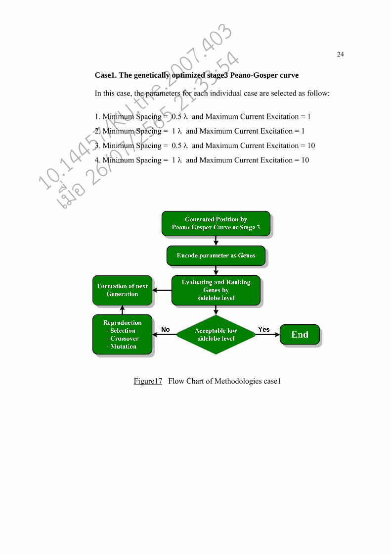
Case1. The genetically optimized stage3 Peano-Gosper curve

In this case, the parameters for each individual case are selected as follow:

1. Minimum Spacing = 0.5 λ and Maximum Current Excitation = 1

2. Minimum Spacing = 1 λ and Maximum Current Excitation = 1



Figure17 Flow Chart of Methodologies case1

10.144

57/KU

.the.2

007.40

3

เมื่อ 26

/07/25

65 21:

33:54

25

Case 2 The genetically optimized stage1 Peano-Gosper curve and create

higher order stage arrays (stage 3).

In this case, the parameters for each individual case are selected as follow:





Evaluating(Stage3) and Ranking Genes by

sidelobe level

EndReproduction

- Selection- Crossover- Mutation

Acceptable low sidelobe level

YesNo

Generated Position by Peano-Gosper Curve at Stage 1

Encode Parameter (Current Excitation)

as Genes

Generated Peano-Gosper Fractal Array

at Stage 3

Formation of next Generation

Figure18 Flow Chart of Methodologies for case 2

10.144

57/KU

.the.2

007.40

3

เมื่อ 26

/07/25

65 21:

33:54

26

RESULT AND DISCUSSION

1. Peano-Gosper Fractal Arrays Synthesis Using Genetic Algorithms

Figure19 The Peano-Gosper fractal arrays configurations and their relative current

excitation for the stages of growth 1, 2 and 3, respectively

Simulation results of the Peano-Gosper fractal arrays subjected to different

parameters are presented as follow:

1.1 The genetically optimized stage3 Peano-Gosper fractal array

a. Minimum distance equal λ/2 and Maximum of current excitation equals 1

Consider the genetically optimized stage 3 Peano-Gosper fractal array

with minimum spacing of λ/2 and maximum current excitation of 1. Figure 20

exhibits the Peano-Gosper fractal array for the stages of growth 1, 2 and 3,

respectively. Figure 21 exhibits the sidelobe level of the Peano-Gosper fractal arrays

for the stage of growth 3 versus generation. In addition, Figure 22 shows the plot of

the normalized stage 3 Peano-Gosper fractal array, genetically optimized array factor

versus (a) φ for (a)θ = 90° and (b) θ for φ = 90° where minimum distance equals λ/2

and maximum current excitation equals one.

10.144

57/KU

.the.2

007.40

3

เมื่อ 26

/07/25

65 21:

33:54

27

1

2

2

2

2

2

2

1

12

22

22

2

22

22

22

22

22

2

22

22

22

22

2

22

22

2

22

2

22

22

22

2

22

2

22

22

1

(a) Stage 1 (b) Stage 2

11 1

00

11

00 1 0

011 1

11

01

001

10

110

1 00 0

11

10

01 0

10

10

110

1 01

01

0 10

10

10

1 0 100

1 00 1 1

010 1

00

11

1100

1 0011

11

011

11 1

0 1 100

0 11

101

10 0

11

10

111

01

11

0111

11 1

01

10 0

11

11

101 1

1101

11

11

111

10

101

1 10

11

110

000

0 01

110

0 0110

00

100

01 0

00

110

1 10 0 1

100 0

1 10

10

01

0 0 010

1 10

00

011

01

000

10 1

0 01

11

00

1 10

00

111

10 0

10

11 1

01

10

01 0 1

111 0

11

10

111

01

011

0 10 0

11

01

00 0

01

01

101

1 01

110

1 1110

011

0 00

110

10 1

01

10 1 1

001 0

01

110

1 11 0

01

01

001

0 11

10

(c) Stage 3 with Genetic Algorithms

Figure 20 Element location for the (a) stage 1, (b) stage 2, and (c) stage 3 Peano-

Gosper fractal arrays. A uniform spacing of dmin is assumed between

consecutive arrays elements which is the same for each stage, minimum

spacing is λ/2, maximum current excitation is one.

10.144

57/KU

.the.2

007.40

3

เมื่อ 26

/07/25

65 21:

33:54

28

0 20 40 60 80 100-18.5

-18

-17.5

-17

-16.5

Generation

Side

lobe

Lev

el

Figure 21 Evolution diagram of Genetically Optimized a Stage3: Peano-Gosper

Fractal Array, minimum spacing is λ/2, maximum current excitation is

one

0 10 20 30 40 50 60 70 80 90-80

-60

-40

-20

0

Theta(degree), φ = 90

Arra

y Fa

ctor

(dB)

(a)

0 50 100 150 200 250 300 350-80

-60

-40

-20

0

Phi(degree), θ = 90

Arra

y Fa

ctor

(dB)

(b)

Figure 22 Plot of the normalized stage 3 Peano-Gosper fractal array, genetically

optimized array factor versus (a) φ for θ = 90° and (b) θ for φ = 90°

where minimum distance equals λ/2 and maximum current excitation

equal one

10.144

57/KU

.the.2

007.40

3

เมื่อ 26

/07/25

65 21:

33:54

29

(a)

(b)

Figure 23 The normalized radiation pattern in dB for stage 3 of Peano-Gosper fractal

array from Figure 20c with a minimum spacing is λ, maximum current

excitation is one and main beam steered to θ = 0 degrees and φ = 90°

degrees. (a)Radiation Pattern, and (b) Top View

10.144

57/KU

.the.2

007.40

3

เมื่อ 26

/07/25

65 21:

33:54

30

b. Minimum distance equal λ and Maximum of current excitation equal 10


with minimum spacing of λ and maximum current excitation of 10. Figure 24 exhibits

the Peano-Gosper fractal array for the stages of growth 1, 2 and 3, respectively.

Figure 25 exhibits the sidelobe level of the Peano-Gosper fractal arrays for the stage

of growth 3 versus generation. In addition, Figure 26 shows the plot of the normalized

stage 3 Peano-Gosper fractal array, genetically optimized array factor versus (a) φ for

(a)θ = 90° and (b) θ for φ = 90° where minimum distance equals λ and maximum

current excitation equals ten.

10.144

57/KU

.the.2

007.40

3

เมื่อ 26

/07/25

65 21:

33:54

31

1

2

2

2

2

2

2

1

12

22

22

2

22

22

22

22

22

2

22

22

22

22

2

22

22

2

22

2

22

22

22

2

22

2

22

22

1


9 1 8

3 3

2 6

8 3 4 6

1 8 2 2

10 2

6 4

8 6 7

8 9

2 7 8

0 9 4 1

0 7

1 5

4 2 3

9 7

8 1

2 3 1

1 6 6

5 2

6 9 3

2 7

4 0

0 0 2 3 3

3 5 9 9 6

21010 6

5 4

2 1

8 9 3 7

3 1 0 2 5

7 5

3 6 2

8 8 2

10 1 0 8 9

7 4 9

9 3 6

4 1 4

5 8

9 6

3 9 4

8 3

1 6

7 8 7 6

8 5 1

810

8 5 8

1 2

9 8

10 4 2 6

8 9 8 3

9 8

8 2

10 3 0

6 5

5 4 8

3 10 4

4 9

8 8 5

2 1 3

4 6 2

2 7 1

9 5 8 9 6

2 7

1 2 5

8 1 1

4 5

8 1 8

7 7 1 3 5

1 3 4 10

4 10 0

9 7

4 8

4 1 2 2 9

1 3 7

4 3

1 3 4

1 0

8 1 3

4 4 4

8 4 0

5 3

1 6

0 5 6

7 7

3 6 9

2 5 5

9 4

9 4 1

6 6

5 5

8 2 10 1

1 7 9 8

4 0

1010

5 0 1

9 4

8 7 4

2 7 3 7

3 4

5 1

2 7 4

6 1

4 3

1 3 1

7 1 5

4 5 9

5 7 1 7 0

0 3 6

8 8 4

9 5 9

2 0 2

7 1

510 8 1

4 9 2 1

1 6

4 1 7

3 7 1 5

7 6

9 3

8 4 9

0 8 6

3 3

(c) Stage 3




spacing is λ/2, maximum current excitation is ten.

10.144

57/KU

.the.2

007.40

3

เมื่อ 26

/07/25

65 21:

33:54

32

0 20 40 60 80 100-18.5

-18

-17.5

-17

-16.5

Generation

Side

lobe

Lev

el


Fractal Array, minimum spacing is λ/2, maximum current excitation is ten.

0 10 20 30 40 50 60 70 80 90-80

-60

-40

-20

0


Arra

y Fa

ctor

(dB)

(a)

0 50 100 150 200 250 300 350-80

-60

-40

-20

0


Arra

y Fa

ctor

(dB)

(b)



where minimum distance equal λ/2 and maximum current excitation

equal ten.

10.144

57/KU

.the.2

007.40

3

เมื่อ 26

/07/25

65 21:

33:54

33

(a)

(b)


array from Figure 24c with a minimum spacing is λ/2, maximum current

excitation is ten and main beam steered to θ = 0 degrees and φ = 90°

degrees.(a) Radiation Pattern, and (b) Top view.

10.144

57/KU

.the.2

007.40

3

เมื่อ 26

/07/25

65 21:

33:54

34

c. Minimum distance equal λ and Maximum of current excitation equal one

Consider the genetically optimized stage 3 Peano-Gosper fractal array with

minimum spacing of λ and maximum current excitation of 1. Figure 28 exhibits the

Peano-Gosper fractal array for the stages of growth 1, 2 and 3, respectively. Figure 29

exhibits the sidelobe level of the Peano-Gosper fractal arrays for the stage of growth 3

versus generation. In addition, Figure 30 shows the plot of the normalized stage 3

Peano-Gosper fractal array, genetically optimized array factor versus (a) φ for (a)θ =

90° and (b) θ for φ = 90° where minimum distance equals λ and maximum current

excitation equals one.

10.144

57/KU

.the.2

007.40

3

เมื่อ 26

/07/25

65 21:

33:54

35

1

2

2

2

2

2

2

1

12

22

22

2

22

22

22

22

22

2

22

22

22

22

2

22

22

2

22

2

22

22

22

2

22

2

22

22

1


00 1

11

00

11 0 0

000 1

11

00

111

00

010

0 01 1

00

01

10 0

01

10

010

1 11

01

1 00

11

10

0 1 101

0 01 0 1

101 1

00

01

0011

0 0110

00

000

01 0

0 0 011

1 11

111

00 1

00

01

011

11

11

1010

10 1

10

01 1

10

10

101 0

0000

01

10

111

11

000

1 11

10

011

011

0 00

011

1 0110

10

110

10 0

10

010

0 10 1 1

010 1

1 11

10

00

1 1 110

1 10

01

000

01

101

10 1

0 10

01

01

0 11

00

111

00 1

10

11 1

01

11

00 1 1

110 1

11

10

000

01

000

0 00 1

00

10

01 1

00

10

101

1 10

000

0 1000

100

1 11

011

10 1

00

10 0 1

001 0

00

000

0 01 1

01

11

100

0 01

11

(c) Stage 3




spacing is λ, maximum current excitation is one.

10.144

57/KU

.the.2

007.40

3

เมื่อ 26

/07/25

65 21:

33:54

36

0 20 40 60 80 100-17.5

-17

-16.5

-16

-15.5

-15

Generation

Side

lobe

Lev

el


Fractal Array, minimum spacing is λ, maximum current excitation is one.

0 10 20 30 40 50 60 70 80 90-80

-60

-40

-20

0


Arra

y Fa

ctor

(dB)

(a)

0 50 100 150 200 250 300 350-80

-60

-40

-20

0


Arra

y Fa

ctor

(dB)

(b)



where minimum distance equal λ and maximum current excitation equal

one.

10.144

57/KU

.the.2

007.40

3

เมื่อ 26

/07/25

65 21:

33:54

37

(a)

(b)




degrees. (a)Radiation Pattern, and (b) Top View

10.144

57/KU

.the.2

007.40

3

เมื่อ 26

/07/25

65 21:

33:54

38

d. Minimum distance equal λ and Maximum of current excitation equal ten

Consider the genetically optimized stage 3 Peano-Gosper fractal array with

minimum spacing of λ and maximum current excitation of 10. Figure 32 exhibits the

Peano-Gosper fractal array for the stages of growth 1, 2 and 3, respectively. Figure 33

exhibits the sidelobe level of the Peano-Gosper fractal arrays for the stage of growth 3

versus generation. In addition, Figure 34 shows the plot of the normalized stage 3

Peano-Gosper fractal array, genetically optimized array factor versus (a) φ for (a)θ =

90° and (b) θ for φ = 90° where minimum distance equals λ and maximum current

excitation equals ten.

10.144

57/KU

.the.2

007.40

3

เมื่อ 26

/07/25

65 21:

33:54

39

1

2

2

2

2

2

2

1

12

22

22

2

22

22

22

22

22

2

22

22

22

22

2

22

22

2

22

2

22

22

22

2

22

2

22

22

1


9 1 2

3 3

2 6

8 3 4 6

1 8 2 2

10 2

4 4

8 6 7

8 9

2 3 8

0 9 4 1

0 7

1 5

4 2 7

9 7

8 1

2 3 1

1 6 6

5 2

6 9 3

2 7

4 0

0 0 2 3 3

3 5 9 9 6

21010 6

5 4

2 1

8 9 3 7

3 1 0 2 5

7 5

3 6 2

8 8 2

10 1 0 8 9

7 4 9

9 3 6

4 1 4

5 8

9 6

3 9 4

8 7

1 6

7 8 7 6

8 5 1

810

8 5 8

1 2

9 8

10 4 2 6

8 9 8 3

9 8

8 8

10 3 0

6 5

5 4 8

3 10 6

4 9

8 8 5

2 1 3

4 6 2

2 7 1

9 5 8 9 6

2 3

1 2 5

8 1 1

6 5

2 1 8

7 7 1 3 5

1 3 4 10

4 10 0

9 7

4 8

4 1 2 2 9

1 3 7

4 3

1 3 4

1 0

8 1 3

4 4 6

8 410

5 3

1 4

0 5 6

7 7

3 6 9

2 5 5

9 4

9 4 1

6 6

5 5

8 2 10 1

1 7 9 8

4 0

1010

5 0 1

1 4

8 7 4

2 7 3 7

7 4

5 1

2 7 4

6 1

4 3

1 3 1

7 1 5

4 5 9

5 7 1 3 0

0 3 6

8 8 4

9 5 9

2 0 2

7 1

510 8 1

4 9 2 1

1 6

4 1 7

3 7 1 5

7 6

9 3

8 4 9

10 8 6

3 3

(c) Stage 3




spacing is λ, maximum current excitation is ten.

10.144

57/KU

.the.2

007.40

3

เมื่อ 26

/07/25

65 21:

33:54

40

0 20 40 60 80 100-19.5

-19

-18.5

-18

-17.5

-17

-16.5

Generation

Side

lobe

Lev

el


Fractal Array, minimum spacing is λ, maximum current excitation is ten.

0 10 20 30 40 50 60 70 80 90-80

-60

-40

-20

0


Arra

y Fa

ctor

(dB)

(a)

0 50 100 150 200 250 300 350-80

-60

-40

-20

0


Arra

y Fa

ctor

(dB)

(b)




ten.

10.144

57/KU

.the.2

007.40

3

เมื่อ 26

/07/25

65 21:

33:54

41

(a)

(b)




degrees. (a)Radiation Pattern, and (b) Top View.

10.144

57/KU

.the.2

007.40

3

เมื่อ 26

/07/25

65 21:

33:54

42

1.2. The genetically optimized stage1 Peano-Gosper curve and create higher order stage arrays (stage 3).

a. Minimum distance equal λ/2 and Maximum of current excitation

equal one


and create higher order stage arrays (stage 3) with minimum spacing of λ/2 and

maximum current excitation of 1. Figure 36 exhibits the Peano-Gosper fractal array

for the stages of growth 1, 2 and 3, respectively. Figure 37 exhibits the sidelobe level

of the Peano-Gosper fractal arrays for the stage of growth 3 versus generation. In

addition, Figure 38 shows the plot of the normalized stage 3 Peano-Gosper fractal

array, genetically optimized array factor versus (a) φ for (a)θ = 90° and (b) θ for φ =

90° where minimum distance equals λ/2 and maximum current excitation equals one.

10.144

57/KU

.the.2

007.40

3

เมื่อ 26

/07/25

65 21:

33:54

43

0

1

0

1

1

1

1

101

0

1

11

1

1

01

01

11

1

11

01

11

11

10

1

11

11

10

11

1

11

10

1

11

1

11

01

11

1

11

0

11

11

1


01 0

11

11

11 0 1

111 1

10

11

111

10

111

1 11 0

11

11

11 0

11

11

110

1 11

11

1 01

11

11

1 0 111

1 11 0 1

111 1

10

11

1111

0 1111

11

011

11 1

1 0 111

1 11

011

11 1

10

11

111

10

11

1111

01 1

11

11 0

11

11

110 1

1111

10

11

111

10

111

1 11

01

111

110

1 11

111

0 1111

11

011

11 1

10

111

1 11 0 1

111 1

1 01

11

11

1 0 111

1 11

01

111

11

011

11 1

1 01

11

11

1 01

11

111

01 1

11

11 0

11

11

11 0 1

111 1

10

11

111

10

111

1 11 0

11

11

11 0

11

11

110

1 11

111

0 1111

110

1 11

111

01 1

11

11 0 1

111 1

10

111

1 11 0

11

11

110

1 11

11

(c) Stage 3




spacing is λ/2, maximum current excitation is one.

10.144

57/KU

.the.2

007.40

3

เมื่อ 26

/07/25

65 21:

33:54

44

0 20 40 60 80 100-16.3

-16.25

-16.2

-16.15

-16.1

Generation

Side

lobe

Lev

el


Fractal Array, minimum spacing is λ/2, maximum current excitation is one.

0 10 20 30 40 50 60 70 80 90-80

-60

-40

-20

0


Arra

y Fa

ctor

(dB)

(a)

0 50 100 150 200 250 300 350-80

-60

-40

-20

0


Arra

y Fa

ctor

(dB)

(b)

Figure 38. Plot of the normalized stage 3 Peano-Gosper fractal array, genetically



equal one.

10.144

57/KU

.the.2

007.40

3

เมื่อ 26

/07/25

65 21:

33:54

45

(a)

(b)





10.144

57/KU

.the.2

007.40

3

เมื่อ 26

/07/25

65 21:

33:54

46

b. Minimum distance equal λ/2 and Maximum of current excitation equal ten








90° where minimum distance equals λ/2 and maximum current excitation equals ten.

10.144

57/KU

.the.2

007.40

3

เมื่อ 26

/07/25

65 21:

33:54

47

2

3

3

1

72

8

1

23

31

72

8

33

31

72

83

33

1

72

83

33

17

2

83

33

1

72

8

33

31

72

8

33

3

17

28

1


23 3

17

28

33 3 1

728 3

33

17

283

33

172

8 33 3

17

28

33 3

17

28

333

1 72

83

3 31

72

83

3 3 172

8 33 3 1

728 3

33

17

2833

3 1728

33

317

28 3

3 3 172

8 33

317

28 3

33

17

283

33

17

2833

31 7

28

33 3

17

28

333 1

7283

33

17

283

33

172

8 33

31

728

333

1 72

833

3 1728

33

317

28 3

33

172

8 33 3 1

728 3

3 31

72

83

3 3 172

8 33

31

728

33

317

28 3

3 31

72

83

3 31

72

833

31 7

28

33 3

17

28

33 3 1

728 3

33

17

283

33

172

8 33 3

17

28

33 3

17

28

333

1 72

833

3 1728

333

1 72

833

31 7

28

33 3 1

728 3

33

172

8 33 3

17

28

333

1 72

81

(c) Stage 3

Figure 40. Element location for the (a) stage 1, (b) stage 2, and (c) stage 3 Peano-



spacing is λ/2, maximum current excitation is ten.

10.144

57/KU

.the.2

007.40

3

เมื่อ 26

/07/25

65 21:

33:54

48

0 20 40 60 80 100-16.3

-16.25

-16.2

-16.15

Generation

Side

lobe

Lev

el


Fractal Array, minimum spacing is λ/2, maximum current excitation is ten.

0 10 20 30 40 50 60 70 80 90-80

-60

-40

-20

0


Arra

y Fa

ctor

(dB)

(a)

0 50 100 150 200 250 300 350-80

-60

-40

-20

0


Arra

y Fa

ctor

(dB)

(b)




equal ten.

10.144

57/KU

.the.2

007.40

3

เมื่อ 26

/07/25

65 21:

33:54

49

(a)

(b)





10.144

57/KU

.the.2

007.40

3

เมื่อ 26

/07/25

65 21:

33:54

50

c. Minimum distance equal λ and Maximum of current excitation equal one


and create higher order stage arrays (stage 3) with minimum spacing of λ and






90° where minimum distance equals λ and maximum current excitation equals one.

10.144

57/KU

.the.2

007.40

3

เมื่อ 26

/07/25

65 21:

33:54

51

1

0

1

1

1

1

1

0

10

11

11

1

10

11

11

11

01

1

11

11

01

11

1

11

01

1

11

1

10

11

11

1

10

1

11

11

0


10 1

11

11

10 1 1

111 1

01

11

111

01

111

1 10 1

11

11

10 1

11

11

101

1 11

11

0 11

11

11

0 1 111

1 10 1 1

111 1

01

11

1110

1 1111

10

111

11 1

0 1 111

1 10

111

11 1

01

11

111

01

11

1110

11 1

11

10 1

11

11

101 1

1111

01

11

111

01

111

1 10

11

111

101

1 11

110

1 1111

10

111

11 1

01

111

1 10 1 1

111 1

0 11

11

11

0 1 111

1 10

11

111

10

111

11 1

0 11

11

11

0 11

11

110

11 1

11

10 1

11

11

10 1 1

111 1

01

11

111

01

111

1 10 1

11

11

10 1

11

11

101

1 11

110

1 1111

101

1 11

110

11 1

11

10 1 1

111 1

01

111

1 10 1

11

11

101

1 11

10

(c) Stage 3




spacing is λ, maximum current excitation is one.

10.144

57/KU

.the.2

007.40

3

เมื่อ 26

/07/25

65 21:

33:54

52

0 20 40 60 80 100-16.4

-16.3

-16.2

-16.1

-16

Generation

Side

lobe

Lev

el


Fractal Array, minimum spacing is λ, maximum current excitation is one.

0 10 20 30 40 50 60 70 80 90-80

-60

-40

-20

0


Arra

y Fa

ctor

(dB)

(a)

0 50 100 150 200 250 300 350-80

-60

-40

-20

0


Arra

y Fa

ctor

(dB)

(b)




one.

10.144

57/KU

.the.2

007.40

3

เมื่อ 26

/07/25

65 21:

33:54

53

(a)

(b)





10.144

57/KU

.the.2

007.40

3

เมื่อ 26

/07/25

65 21:

33:54

54

d. Minimum distance equal λ and Maximum of current excitation equal

ten








90° where minimum distance equals λ/2 and maximum current excitation equals ten.

.

10.144

57/KU

.the.2

007.40

3

เมื่อ 26

/07/25

65 21:

33:54

55

2

4

5

6

8

9

4

4

24

56

89

4

64

56

89

46

45

6

89

46

45

68

9

46

45

6

89

4

64

56

89

4

64

5

68

94

4


24 5

68

94

64 5 6

894 6

45

68

946

45

689

4 64 5

68

94

64 5

68

94

645

6 89

46

4 56

89

46

4 5 689

4 64 5 6

894 6

45

68

9464

5 6894

64

568

94 6

4 5 689

4 64

568

94 6

45

68

946

45

68

9464

56 8

94

64 5

68

94

645 6

8946

45

68

946

45

689

4 64

56

894

645

6 89

464

5 6894

64

568

94 6

45

689

4 64 5 6

894 6

4 56

89

46

4 5 689

4 64

56

894

64

568

94 6

4 56

89

46

4 56

89

464

56 8

94

64 5

68

94

64 5 6

894 6

45

68

946

45

689

4 64 5

68

94

64 5

68

94

645

6 89

464

5 6894

645

6 89

464

56 8

94

64 5 6

894 6

45

689

4 64 5

68

94

645

6 89

44

(c) Stage 3




spacing is λ, maximum current excitation is ten.

10.144

57/KU

.the.2

007.40

3

เมื่อ 26

/07/25

65 21:

33:54

56

0 20 40 60 80 100-16.3

-16.28

-16.26

-16.24

-16.22

Generation

Side

lobe

Lev

el


Fractal Array, minimum spacing is λ, maximum current excitation is ten.

0 10 20 30 40 50 60 70 80 90-80

-60

-40

-20

0


Arra

y Fa

ctor

(dB)

(a)

0 50 100 150 200 250 300 350-80

-60

-40

-20

0


Arra

y Fa

ctor

(dB)

(b)


optimized array factor versus (a) φ forθ = 90° and (b) θ for φ = 90°


ten.

10.144

57/KU

.the.2

007.40

3

เมื่อ 26

/07/25

65 21:

33:54

57

(a)

(b)

Figure 51 Top view of the normalized radiation pattern in dB for stage of Peano-

Gosper fractal array of isotropic elements from Figure 48c with a

minimum spacing is λ, maximum current excitation is ten and main beam

steered to θ = 0 degrees and for φ = 90° degrees.

10.144

57/KU

.the.2

007.40

3

เมื่อ 26

/07/25

65 21:

33:54

58

Regarding to Figures 19 to 51, comparison of the sidelobe levels in dB of the

genetically optimized stage 3 Peano-Gosper fractal array with different parameters for

both approaches is summarized in Table 1.

Table 1 Comparison of the sidelobe levels in dB of the genetically optimized stage 3

Peano-Gosper fractal arrays with different parameters for both approaches.

Approach Minimum distance Maximum current excitation

Sidelobe Level

1 0.5 1 -18.05

1 0.5 10 -18.04

1 1 1 -17.10

1 1 10 -19.04

3 0.5 1 -16.22

3 0.5 10 -16.29

3 1 1 -16.35

3 1 10 -16.29

10.144

57/KU

.the.2

007.40

3

เมื่อ 26

/07/25

65 21:

33:54

CONCLUSION AND RECOMMENDATION

In this thesis, the optimization of antenna arrays is presented. For both

approaches, antenna elements are strategically arranged uniformly on the Peano-

Gosper fractal array. However, the relative current excitation also affects the

performance of the Peano-Gosper fractal array. Then, we run genetic algorithm for

optimizing the Peano-Gosper fractal array for 100 generations (iterations). It is

empirically found that genetic algorithm can reduce the sidelobe levels to acceptable

levels.

Although genetic algorithm performs well in optimization, its drawback is,

like other optimization techniques, that its optimization process is time-consuming.

Hence, our future work will focus on improving the speed of genetic algorithm to

optimize antenna array synthesis.

10.144

57/KU

.the.2

007.40

3

เมื่อ 26

/07/25

65 21:

33:54

LITERATURE CITED

Balanis, C 2005. Antenna Theory: Analysis and Design. John Wiley and Sons, Inc.

New York.

Bogard, J. N., D. H. Werner, and P. L. Werner 2004. A Comparison of the Peano-

Gosper Fractile Array with the Regular Hexagonal Array. Microwave and

Optical Technology Letters, Vol. 43, No. 6: 524-526.

Bondarenko, N. and Y.V. Mikhailova, 2005. Radiation Pattern Synthesis for Arrays

Based on Soerpinski Gasket. KORUS'2005.

Bray, M., G., D. H. Werner, D. W.Boeringer and D. W. Machuga 2002. Optimization

of Thinned Aperiodic Linear Phased Arrays Using Genetic Algorithms to

Reduce Grating Lobes During Scanning. IEEE Transactions on Antennas

and Propagation, Vol. 50, No.11: 2919-2924.

Falconer, K. 2003. Fractal Geometry Mathematical Foundations and Applications

2nd Edition, Wiley.

Hansen, R.C. 2003. Phased Array Antennas. John Wiley and Sons, Inc. New York.

Haupt, R. L. 2003. Thinned Arrays Using Genetic Algorithms. IEEE Transactions

on Antennas and Propagation, Vol. 42, No.8 : 2008-2018.

Haupt, R. L. 1995. An Introduction to Genetic Algorithms for Electromagnetics IEEE

Antennas and Propagation Magazine, Vol. 37, No.2: 7-15

Haupt, R. L. and S. E. Haupt. 2003. Practical Genetic Algorithms. John Wiley and

Sons, Inc. New York.

Johnson, M. and Y. Rahmut-Samii 1997. Genetic Algorithms in Engineering

Electromagnetics. IEEE Antennas and Propagation Magazine, Vol. 39,

No.4: 7-15, Aug.

10.144

57/KU

.the.2

007.40

3

เมื่อ 26

/07/25

65 21:

33:54

61

Kim, Y. and D. L. Jaggard 1986. The Fractal Random Array. Proceeding of the

IEEE, Vol. 74, 9: 1278-1280

Kraus, J., D. Ronald and J. Marhefka, 2003. Antennas for All Applications.

McGraw-Hill

Kuhirun, W. 2003. A New Design Methodology for Modular Broadband Arrays

based on Fractal Tailings. Ph.D. Thesis, the Pennsylvania State University at

University Park USA.

Kuhirun, W., T..Jariyanorawiss, M. Polpasee, and N. Homsup 2004. Solving for

Current Distribution Using Gauss-Seidel Iteration and Multigrid Method.

Proceedings of the International Conference in ECTI, Thailand.

Mandelbrot, B.B. 1983. The Fractal Geometry of Nature. John Wiley and Sons,

Inc. New York.

Massa, A., M. Donelli, Francesco G.B. De Nataale, Salvatore Caorsi and Andrea

Lommi 2004. Planar Antenna Array Control With Genetic Algorithms and

Adaptive Array Theory. IEEE Transactions on Antennas and Propagation,

Vol. 52, No.11: 2919-2924.

Petko, J. S. and D. H. Wener 2005. The Evolution of Optimal Linear Polyfractal

Arrays Using Genetic Algorithms. IEEE Transactions on Antennas and

Propagation, Vol. 53, No.11: 3604-3615.

Polpasee, M. and N. Homsup 2006. Optimize Directivity Pattern for Arrays by Using

Genetic Algorithms Based on Planar Fractal Arrays. Proceedings of the

International Conference in ISCIT, Thailand.

Polpasee, M. and N. Homsup 2006. Optimized low sidelobe level of Peano-Gosper

Fractal Arrays Synthesis Using Genetic Algorithms. Proceedings of the

International Conference in ECTI, Thailand.

10.144

57/KU

.the.2

007.40

3

เมื่อ 26

/07/25

65 21:

33:54

62

Polpasee, M. and N. Homsup 2006. Peano-Gosper Fractal Array Synthesis Using

Genetic Algorithms. Ocean 2006 IEEE Asia Pacific, Singapore

Polpasee, M.,W. Kuhirun and N. Homsup 2005. Analysis of Fractal Arrays Generated

using a 3x3 Subarray Generator. Proceedings of the International

Conference in ISCIT, China.

Polpasee, M., N. Homsu and W. Kuhirunp 2005. Analysis of Fractal Arrays

Generated using a 3x3 Subarray Generator. Proceedings of the International

Conference in ECTI, Thailand.

Soltankarimi, F., J. Nourinia and Ch.Ghobadi 2004. Sidelobe Level Optimization in

Phased Array Antennas Using Genetic Algorithm. ISSSTA 2004.

Villegas, F. J., T. Cwik, Y. Rahmat-Samii and Majid Manteghi 2004. A Parallel

Electromagnetic Genetic-Algorithm Optimization(EGO) Application for Patch

Antenna Design. IEEE Transactions on Antennas and Propagation, Vol.

52, No.9: 2424-2435.

Vinoy, K.J. 2002. Fractal Shaped Antenna Elements for Wide-and-Multi Band

Wireless Application. Ph.D. Thesis, The Pennsylvania State University at

University Park USA.

Virunha, P., M. Polpasee and N. Homsup 2006. Optimized Directivity of Square-

Planar Fractal Arrays Using Genetic Algorithms. Ocean 2006 IEEE Asia

Pacific, Singapore.

Wener, D. H., K.C. Anusko and P.L. Werner 1999 The Generation of Sum and

Difference Patterns Using Fractal SubArrays Microwave And Optical

Technology Letters, Vol. 22, No. 1: 524-526.

Wener, D. H., and R. Mittra 2000. Frontiers in Electromagnetics. IEEE Press.

10.144

57/KU

.the.2

007.40

3

เมื่อ 26

/07/25

65 21:

33:54

63

Wener, D. H., R. L.Haupt and P. L. Werner 1999. Fractal Antenna Engineering: The

Theory and Design of Fractal Antenna Arrays. IEEE Antennas and

Propagation MAgazine, Vol. 41, No.5: 37-59.

Wener, D. H and P. L. Werner, 1999. A General Class of Self-Scalable and Self-

Similar Arrays.

Wener, D. H., W. Kuhirun, and P. L. Werner 2004. Fractile Arrays: A New Class of

Tiled Arrays With Fractal Boundaries. IEEE Transactions on Antennas and

Propagation, Vol. 52, No.8: 2008-2018.

Wener, D. H., W. Kuhirun, and P. L. Werner 2005. The Peano-Gosper Fractal Array.

IEEE Transactions on Antennas and Propagation, Vol. 51, No.8: 2063-

2072.

Yan, K. and Y. Lu, 1997. Sidelobe Reduction in Array-Pattern Synthesis Using

Genetic Algorithm. IEEE Transactions on Antennas and Propagation, Vol.

45, No.7: 1117-1122.

Zhu, J., A. Hoorfar and N. Engheta 2004. Peano Antennas. IEEE Antennas and

Wireless Propagation Letters. Vol.3.

10.144

57/KU

.the.2

007.40

3

เมื่อ 26

/07/25

65 21:

33:54

CURRICULUM VITAE NAME Mr. Meta Polpasee

BIRTH DATE December 1, 1980

BIRTH PLACE Bangkok, Thailand

EDUCATION YEAR INSTITUTION DEGREE/DIPLOMA

2002 Kasetsart University B.Eng. (Electrical)

PUBLICATION

Polpasee, M. ,N.Homsup And P. Virunha “Optimize Directivity Pattern for

Arrays by Using Genetic Algorithms Based on Planar Fractal Arrays”

in Proceedings of the International Conference in ISCIT, Bangkok,

May 2007

Polpasee, M. and N.Homsup “Peano-Gosper Fractal Array Synthesis Using

Genetic ALgorithms” Ocean 2006 IEEE Asia Pacific, Singapore, May

2006

Virunha, P., M.Polpasee and N.Homsup “Optimized Directivity of Square-

Planar Fractal Arrays Using Genetic Algorithms” Ocean 2006 IEEE

Asia Pacific, Singapore, May 2006

Polpasee, M. and N.Homsup “Optimized low sidelobe level of Peano-Gosper

Fractal Arrays Synthesis Using Genetic Algorithms” in Proceedings

of the International Conference in ECTI, Ubonratchathani, May 2006

Polpasee, M, W. Kuhirun and N.Homsup "Analysis of Fractal Arrays

Generated using a 3x3 Subarray Generator", in Proceedings of the

International Conference in ISCIT, China , Oct 2005.

Polpasee, M, N.Homsup and W.Kuhirun "Analysis Fractal Array based on

3x3 Sub Array Generator, Pattaya, in Proceedings of the International

Conference in ECTI, Pattaya, May 2005.

10.144

57/KU

.the.2

007.40

3

เมื่อ 26

/07/25

65 21:

33:54

Kuhirun, W., T.Jariyanorawiss, M.Polpasee, and N.Homsup, "Solving for

Current Distribution Using Gauss-Seidel Iteration and Multigrid

Method" in Proceedings of the International Conference in ECTI,

Pattaya, May 2004.

10.144

57/KU

.the.2

007.40

3

เมื่อ 26

/07/25

65 21:

33:54

thesis - doi@nrct

Documents

Transcript of thesis - doi@nrct