Jibamitra Ganguly

Second Edition

Thermodynamics in Earth and Planetary Sciences

Springer Textbooks in Earth Sciences,Geography and Environment

The Springer Textbooks series publishes a broad portfolio of textbooks on EarthSciences, Geography and Environmental Science. Springer textbooks providecomprehensive introductions as well as in-depth knowledge for advanced studies.A clear, reader-friendly layout and features such as end-of-chapter summaries, workexamples, exercises, and glossaries help the reader to access the subject. Springertextbooks are essential for students, researchers and applied scientists.

More information about this series at http://www.springer.com/series/15201

Jibamitra Ganguly

Thermodynamics in Earthand Planetary SciencesSecond Edition

123

Jibamitra GangulyDepartment of GeosciencesUniversity of ArizonaTucson, AZ, USA

ISSN 2510-1307 ISSN 2510-1315 (electronic)Springer Textbooks in Earth Sciences, Geography and EnvironmentISBN 978-3-030-20878-3 ISBN 978-3-030-20879-0 (eBook)https://doi.org/10.1007/978-3-030-20879-0

1st edition: © Springer-Verlag Berlin Heidelberg 20082nd edition: © Springer Nature Switzerland AG 2020This work is subject to copyright. All rights are reserved by the Publisher, whether the whole or partof the material is concerned, specifically the rights of translation, reprinting, reuse of illustrations,recitation, broadcasting, reproduction on microfilms or in any other physical way, and transmissionor information storage and retrieval, electronic adaptation, computer software, or by similar or dissimilarmethodology now known or hereafter developed.The use of general descriptive names, registered names, trademarks, service marks, etc. in thispublication does not imply, even in the absence of a specific statement, that such names are exempt fromthe relevant protective laws and regulations and therefore free for general use.The publisher, the authors and the editors are safe to assume that the advice and information in thisbook are believed to be true and accurate at the date of publication. Neither the publisher nor theauthors or the editors give a warranty, expressed or implied, with respect to the material containedherein or for any errors or omissions that may have been made. The publisher remains neutral with regardto jurisdictional claims in published maps and institutional affiliations.

This Springer imprint is published by the registered company Springer Nature Switzerland AGThe registered company address is: Gewerbestrasse 11, 6330 Cham, Switzerland

A theory is the more impressive the greaterthe simplicity of its premises, the moredifferent kind of things it relates, and themore extended its area of applicability.Therefore the deep impression that classicalthermodynamics made upon me. It is the onlyphysical theory of universal content which Iam convinced will never be overthrown,within the framework of applicability of itsbasic concepts.

Albert Einstein

Dedicated to the Pioneers who led the wayand Students, Colleagues and Mentorswho helped me along the way

Preface to the Second Edition

The first edition of the book was written when I had to carry a full load ofteaching, maintain well-funded research programs and carry out many otheractivities that are typically expected of someone holding an academic position inUSA. There was hardly any free time to write a book of this nature, and conse-quently writing of the book became a stressful undertaking. This, however, is acommon situation with active scientists who write books. After my retirement afew years ago that allowed me considerable freedom of how I use my time, I feltthat I should work on the book again for a second edition that would give me theopportunity to correct many typographical errors that I have spotted in themeanwhile (these were corrected in the Chinese translation that was published in2015), improve the clarity of presentation in several places and add new materials.In the last category, I have added a new chapter on Statistical Thermodynamicsand also significant amount of new materials in many of the existing chapters;most of these additions are in Chaps. 4 – 8, 10, 12, 13 and Appendices A and C.Additionally, there is a new Appendix (D) containing solutions of selected prob-lems that are marked by asterisks in the chapters. Answers and hints for solutionshave been provided for the problems for which solutions are not included in thisAppendix. As in the first edition, I have inserted the problems into appropriateplaces within the text that the problems relate to instead of following the usualpractice of collecting them at the end of each chapter.

I am thankful to Dr. Manga Venkateswara Rao for helpful discussions andreviews of selected chapters.

In the Introduction of their ground breaking work on paleothermometry usingStatistical Thermodynamics in 1951, Harold Urey and co-workers remarked:

Geologists have drawn many conclusions from the purely qualitative evi-dence of geological studies in regard to the past climatic conditions on theearth. These deductions are based upon a great variety of evidence, and theability of the geologists to deduce as much as they have in regard to theseconditions excites the wonder and admiration of all the uninitiated whoexamine their work even casually.

Although this statement is about the geologists’ early contribution to paleocli-mate studies, it also applies, at least in my judgment, to geologists’, and in a broader

ix

sense Earth scientists’ contributions to a variety of large-scale problems. However,as in the paleoclimate studies, one of the most important developments in Geo-logical and related aspects of Planetary sciences has been the integration ofquantitative analysis using thermodynamics with the “qualitative evidence” that theGeologists are used to dealing with and their ability to extract major new insightsfrom that to address large-scale natural processes.

Hopefully, the extent and scope of application of thermodynamics to thequantitative analysis of complex natural processes would continue to grow.

Tucson, AZ, USAMarch 2019

Jibamitra Ganguly

x Preface to the Second Edition

Preface to the First Edition

When the knowledge is weak and the situation iscomplicated, thermodynamic relations are really themost powerful

Richard Feynman

Thermodynamics has played a major role in improving our understanding of naturalprocesses and would continue to do so for the foreseeable future. In fact, a course inthermodynamics has now become a part of Geosciences curriculum in manyInstitutions despite the fact that a formal thermodynamics course is taught in everyother department of physical sciences, and also in departments of ChemicalEngineering, Materials Sciences, and Biological Sciences. The reason thermody-namics is taught in a variety of departments, probably more so than any othersubject, is that its principles have wide ranging applications but the teachingof thermodynamics also needs special focus depending on the problems in a par-ticular field.

There are numerous books in thermodynamics that have usually been writtenwith particular focus to the problems in the traditional fields of Chemistry, Physics,and Engineering. In recent years, several books have also been written thatemphasized applications to Geological problems. Thus, one may wonder why thereis yet another book in thermodynamics. The primary focus of the books that havebeen written with Geosciences audience in mind has been chemical thermody-namics or Geochemical thermodynamics. Along with expositions of fundamentalprinciples of thermodynamics, I have tried to address a wide range of problemsrelating to geochemistry, petrology, mineralogy, geophysics, and planetary sci-ences. It is not a fully comprehensive effort but is a major attempt to develop a corematerial that should be of interest to people with different specialties in the Earthand Planetary Sciences.

The conditions of the systems in the Earth and Planetary Sciences to whichthermodynamics have been applied cover a very large range in pressure-temperaturespace. For example, the P-T conditions for the processes at the Earth’s surface are1 bar, 25 °C, whereas those for the processes in the deep interior of the Earth are atpressures of the order of 106 bars and temperatures of the order of 103 °C.The pressures for processes in the solar nebula are 10−3–10−4 bars. The extreme

xi

range of conditions encompassed by natural processes requires variety of manipu-lations and approximations that are not readily available in the standard textbooks onthermodynamics. Earth scientists have made significant contributions in these areasthat have been overlooked in the standard texts since the expected audience of thesetexts rarely deal with the conditions that Earth scientists have to. I have tried tohighlight the contributions of Earth scientists that have made possible meaningfulapplications of thermodynamics to natural problems.

In order to develop a proper appreciation of thermodynamic laws and thermo-dynamic properties of matter, it is useful to look into their physical picture byrelating them to the microscopic descriptions. Furthermore, in geological problems,it is often necessary to extrapolate thermodynamic properties of matter way beyondthe conditions at which these have been measured, and also to be able to estimatethermodynamic properties because of lack of adequate data to address a specificproblem at hand. These efforts require an understanding of the physical or micro-scopic basis of thermodynamic properties. Thus, I have occasionally digressed tothe discussion of thermodynamics from microscopic viewpoints, although theformal aspects of the subject of thermodynamics can be completely developedwithout appealing to the microscopic picture. On the other hand, I have not spenttoo much effort to discuss how the thermodynamic laws were developed, as thereare many excellent books dealing with these topics, but rather focused on exploringthe implications of these laws after discussing their essential contents. In severalcases, however, I have chosen to provide the derivations of equations in consid-erable detail in order to convey a feeling of how thermodynamic relations aremanipulated to derive practically useful relations.

This book has been an outgrowth of a course on thermodynamics that I havebeen teaching to graduate students of Earth and Planetary Sciences at the Universityof Arizona for over a decade. In this course, I have meshed the development of thefundamental principles with applications, mostly to natural problems. This may notbe the most logical way of presenting the subject, but I have found it to be aneffective way to keep the interest of the students alive, and answer “why am I doingthis?” In addition, I have put problems within the text in appropriate places, and inmany cases posed the derivation of some standard equations as problems, with hintswherever I felt necessary based on the questions that I have received from mystudents when they were given these problems to solve.

I have tried to write this book in a self-contained way, as much as possible. Thus,the introductory chapter contains concepts from mechanics and quantum chemistrythat were used later to develop concepts of thermodynamics and an understandingof some of their microscopic basis. The Appendix B contains a summary of someof the mathematical concepts and tools that are commonly used in classicalthermodynamics.

Selected sections of the book have been reviewed by a number of colleagues:Sumit Chakraborty, Weji Cheng, Jamie Connolly, Mike Drake, Charles Geiger,Ralph Kretz, Luigi Marini, Denis Norton, Giulio Ottonello, Kevin Righter,Surendra Saxena, Rishi Narain Singh, Max Tirone, and Krishna Vemulapalli.

xii Preface to the First Edition

I gratefully acknowledge their help but take full responsibility for the errors thatmight still be present. In addition, feedbacks from the graduate students, who tookmy thermodynamics course, have played an important role in improving the clarityof presentation, and catching errors, not all of which were typographical. I will begrateful if the readers draw my attention to errors, typographical or otherwise, thatmight have still persisted. All errors will be posted on my web page that can beaccessed using the link http://www.geo.arizona.edu/web/Ganguly/JG_page.html.

I started writing the book seriously while I was in the Bayerisches Geoinstitüt,Bayreuth, and University of Bochum, both in Germany, during my sabbatical leavein 2002–2003 that was generously supported by the Alexander von HumboldtFoundation through a research prize (forschungspreis). I gratefully acknowledge thesupport of the AvH foundation, and the hospitality of the two institutions, espe-cially those of the hosts, Profs. Dave Rubie and Sumit Chakraborty. Researchgrants from the NASA Cosmochemistry program to investigate thermodynamic andkinetic problems in the planetary systems provided significant incentives to exploreplanetary problems, and also made my continued involvement in thermodynamicsthrough the period of writing this book easier from a practical standpoint. I am alsovery grateful for these supports.

I hope that this book would be at least partly successful in accomplishing its goalof presenting the subject of thermodynamics in a way that shows its power in thedevelopment of quantitative understanding of a wide variety of geological andplanetary processes.

And finally, as remarked by the noted thermodynamicist, Kenneth Denbigh(1955)

Thermodynamics is a subject which needs to be studied not once but severaltimes over at advancing levels

October 2007Tucson, Arizona, USA

Jibamitra Ganguly

Preface to the First Edition xiii

Contents

1 Introduction . . . . . . . . . . . . . . . . . . . . . . . . . . . . . . . . . . . . . . . . . . 11.1 Nature and Scope of Thermodynamics . . . . . . . . . . . . . . . . . . 11.2 Irreversible and Reversible Processes . . . . . . . . . . . . . . . . . . . 31.3 Thermodynamic Systems, Walls and Variables . . . . . . . . . . . . 41.4 Work . . . . . . . . . . . . . . . . . . . . . . . . . . . . . . . . . . . . . . . . . . 51.5 Stable and Metastable Equilibrium . . . . . . . . . . . . . . . . . . . . . 91.6 Lattice Vibrations . . . . . . . . . . . . . . . . . . . . . . . . . . . . . . . . . 101.7 Electronic Configurations and Crystal Field Effects . . . . . . . . . 14

1.7.1 Electronic Shells, Subshells and Orbitals . . . . . . . . . 141.7.2 Crystal or Ligand Field Effects . . . . . . . . . . . . . . . . 16

1.8 Some Useful Physical Quantities and Units . . . . . . . . . . . . . . 18References . . . . . . . . . . . . . . . . . . . . . . . . . . . . . . . . . . . . . . . . . . . . 19

2 First and Second Laws . . . . . . . . . . . . . . . . . . . . . . . . . . . . . . . . . . 212.1 The First Law . . . . . . . . . . . . . . . . . . . . . . . . . . . . . . . . . . . . 222.2 Second Law: The Classic Statements . . . . . . . . . . . . . . . . . . . 242.3 Carnot Cycle: Entropy and Absolute Temperature Scale . . . . . 262.4 Entropy: Direction of Natural Processes and Equilibrium . . . . . 292.5 Microscopic Interpretation of Entropy: Boltzmann Relation . . . 312.6 Black Hole and Generalized Second Law of

Thermodynamics . . . . . . . . . . . . . . . . . . . . . . . . . . . . . . . . . . 352.7 Entropy and Disorder: Mineralogical Applications . . . . . . . . . 36

2.7.1 Configurational Entropy . . . . . . . . . . . . . . . . . . . . . 372.7.2 Vibrational Entropy . . . . . . . . . . . . . . . . . . . . . . . . 422.7.3 Configurational Versus Vibrational Entropy . . . . . . . 43

2.8 First and Second Laws: Combined Statement . . . . . . . . . . . . . 472.9 Condition of Thermal Equilibrium: An Illustrative

Application of the Second Law . . . . . . . . . . . . . . . . . . . . . . . 492.10 Limiting Efficiency of a Heat Engine and Heat Pump . . . . . . . 50

2.10.1 Heat Engine . . . . . . . . . . . . . . . . . . . . . . . . . . . . . . 502.10.2 Heat Pump . . . . . . . . . . . . . . . . . . . . . . . . . . . . . . . 522.10.3 Heat Engines in Nature . . . . . . . . . . . . . . . . . . . . . . 53

References . . . . . . . . . . . . . . . . . . . . . . . . . . . . . . . . . . . . . . . . . . . . 56

xv

3 Thermodynamic Potentials and Derivative Properties . . . . . . . . . . . 573.1 Thermodynamic Potentials . . . . . . . . . . . . . . . . . . . . . . . . . . . 573.2 Equilibrium Conditions for Closed Systems: Formulations

in Terms of the Potentials . . . . . . . . . . . . . . . . . . . . . . . . . . . 603.3 What Is Free in Free Energy? . . . . . . . . . . . . . . . . . . . . . . . . 623.4 Maxwell Relations . . . . . . . . . . . . . . . . . . . . . . . . . . . . . . . . 633.5 Thermodynamic Square: A Mnemonic Tool . . . . . . . . . . . . . . 643.6 Vapor Pressure and Fugacity . . . . . . . . . . . . . . . . . . . . . . . . . 653.7 Derivative Properties . . . . . . . . . . . . . . . . . . . . . . . . . . . . . . . 68

3.7.1 Thermal Expansion and Compressibility . . . . . . . . . . 683.7.2 Heat Capacities . . . . . . . . . . . . . . . . . . . . . . . . . . . . 70

3.8 Grüneisen Parameter . . . . . . . . . . . . . . . . . . . . . . . . . . . . . . . 733.9 P–T Dependencies of Coefficient of Thermal Expansion

and Compressibility . . . . . . . . . . . . . . . . . . . . . . . . . . . . . . . . 763.10 Summary of Thermodynamic Derivatives . . . . . . . . . . . . . . . . 77References . . . . . . . . . . . . . . . . . . . . . . . . . . . . . . . . . . . . . . . . . . . . 77

4 Third Law and Thermochemistry . . . . . . . . . . . . . . . . . . . . . . . . . . 794.1 The Third Law and Entropy . . . . . . . . . . . . . . . . . . . . . . . . . 79

4.1.1 Observational Basis and Statement . . . . . . . . . . . . . . 794.1.2 Third Law Entropy and Residual Entropy . . . . . . . . 81

4.2 P-T Dependence of Heat Capacity Functions . . . . . . . . . . . . . 824.3 Non-lattice Contributions to Heat Capacity and Entropy

of Pure Solids . . . . . . . . . . . . . . . . . . . . . . . . . . . . . . . . . . . . 874.3.1 Electronic Transitions . . . . . . . . . . . . . . . . . . . . . . . 874.3.2 Magnetic Transitions . . . . . . . . . . . . . . . . . . . . . . . . 89

4.4 Unattainability of Absolute Zero . . . . . . . . . . . . . . . . . . . . . . 914.5 Thermochemistry: Formalisms and Conventions . . . . . . . . . . . 92

4.5.1 Enthalpy of Formation . . . . . . . . . . . . . . . . . . . . . . 924.5.2 Hess’s Law . . . . . . . . . . . . . . . . . . . . . . . . . . . . . . 944.5.3 Gibbs Free Energy of Formation . . . . . . . . . . . . . . . 944.5.4 Thermochemical Data . . . . . . . . . . . . . . . . . . . . . . . 95

References . . . . . . . . . . . . . . . . . . . . . . . . . . . . . . . . . . . . . . . . . . . . 98

5 Critical Phenomenon and Equations of States . . . . . . . . . . . . . . . . 1015.1 Critical End Point . . . . . . . . . . . . . . . . . . . . . . . . . . . . . . . . . 1015.2 Near- and Super-Critical Properties . . . . . . . . . . . . . . . . . . . . 105

5.2.1 Divergence of Thermal and Thermo-PhysicalProperties . . . . . . . . . . . . . . . . . . . . . . . . . . . . . . . . 105

5.2.2 Critical Fluctuations . . . . . . . . . . . . . . . . . . . . . . . . 1075.2.3 Super- and Near-Critical Fluids . . . . . . . . . . . . . . . . 109

5.3 Near-Critical Properties of Water and Magma-HydrothermalSystems . . . . . . . . . . . . . . . . . . . . . . . . . . . . . . . . . . . . . . . . 109

xvi Contents

5.4 Equations of State . . . . . . . . . . . . . . . . . . . . . . . . . . . . . . . . . 1135.4.1 Gas . . . . . . . . . . . . . . . . . . . . . . . . . . . . . . . . . . . . 1145.4.2 Solid and Melt . . . . . . . . . . . . . . . . . . . . . . . . . . . . 121

References . . . . . . . . . . . . . . . . . . . . . . . . . . . . . . . . . . . . . . . . . . . . 128

6 Phase Transitions, Melting, and Reactions of StoichiometricPhases . . . . . . . . . . . . . . . . . . . . . . . . . . . . . . . . . . . . . . . . . . . . . . . 1316.1 Gibbs Phase Rule: Preliminaries . . . . . . . . . . . . . . . . . . . . . . . 1316.2 Phase Transformations and Polymorphism . . . . . . . . . . . . . . . 133

6.2.1 Thermodynamic Classification of PhaseTransformations . . . . . . . . . . . . . . . . . . . . . . . . . . . 133

6.3 Landau Theory of Phase Transition . . . . . . . . . . . . . . . . . . . . 1366.3.1 General Outline . . . . . . . . . . . . . . . . . . . . . . . . . . . 1366.3.2 Derivation of Constraints on the Second Order

Coefficient . . . . . . . . . . . . . . . . . . . . . . . . . . . . . . . 1406.3.3 Effect of Odd Order Coefficient on Phase

Transition . . . . . . . . . . . . . . . . . . . . . . . . . . . . . . . . 1406.3.4 Order Parameter Versus Temperature: Second

Order and Tricritical Transformations . . . . . . . . . . . . 1416.3.5 Landau Potential Versus Order Parameter:

Implications for Kinetics . . . . . . . . . . . . . . . . . . . . . 1426.3.6 Some Applications to Mineralogical and

Geophysical Problems . . . . . . . . . . . . . . . . . . . . . . . 1446.4 Reactions in the P-T Space . . . . . . . . . . . . . . . . . . . . . . . . . . 146

6.4.1 Conditions of Stability and Equilibrium . . . . . . . . . . 1466.4.2 P-T Slope: Clapeyron-Clausius Relation . . . . . . . . . . 148

6.5 Temperature Maximum on Dehydration andMelting Curves . . . . . . . . . . . . . . . . . . . . . . . . . . . . . . . . . . . 149

6.6 Extrapolation of Melting Temperature to High Pressures . . . . . 1536.6.1 Kraut-Kennedy Relation . . . . . . . . . . . . . . . . . . . . . 1536.6.2 Lindemann-Gilvarry Relation . . . . . . . . . . . . . . . . . . 155

6.7 Calculation of Equilibrium P-T Conditions of a Reaction . . . . 1566.7.1 Equilibrium Pressure at a Fixed Temperature . . . . . . 1566.7.2 Effect of Polymorphic Transition . . . . . . . . . . . . . . . 160

6.8 Evaluation of Gibbs Energy and Fugacity at High PressureUsing Equations of States . . . . . . . . . . . . . . . . . . . . . . . . . . . 1646.8.1 Birch-Murnaghan Equation of State . . . . . . . . . . . . . 1656.8.2 Vinet Equation of State . . . . . . . . . . . . . . . . . . . . . . 1656.8.3 Redlich-Kwong and Related Equations of State

for Fluids . . . . . . . . . . . . . . . . . . . . . . . . . . . . . . . . 1666.9 Schreinemakers’ Principles . . . . . . . . . . . . . . . . . . . . . . . . . . 168

6.9.1 Enumerating Different Types of Equilibria . . . . . . . . 1686.9.2 Self-consistent Stability Criteria . . . . . . . . . . . . . . . . 170

Contents xvii

6.9.3 Effect of an Excess Phase . . . . . . . . . . . . . . . . . . . . 1716.9.4 Concluding Remarks . . . . . . . . . . . . . . . . . . . . . . . . 171

References . . . . . . . . . . . . . . . . . . . . . . . . . . . . . . . . . . . . . . . . . . . . 172

7 Thermal Pressure, Earth’s Interior and Adiabatic Processes . . . . . 1757.1 Thermal Pressure . . . . . . . . . . . . . . . . . . . . . . . . . . . . . . . . . 176

7.1.1 Thermodynamic Relations . . . . . . . . . . . . . . . . . . . . 1767.1.2 Core of the Earth . . . . . . . . . . . . . . . . . . . . . . . . . . 1777.1.3 Magma-Hydrothermal System . . . . . . . . . . . . . . . . . 180

7.2 Adiabatic Temperature Gradient . . . . . . . . . . . . . . . . . . . . . . . 1827.3 Temperature Gradients in the Earth’s Mantle

and Outer Core . . . . . . . . . . . . . . . . . . . . . . . . . . . . . . . . . . . 1847.3.1 Upper Mantle . . . . . . . . . . . . . . . . . . . . . . . . . . . . . 1847.3.2 Lower Mantle and Core . . . . . . . . . . . . . . . . . . . . . 186

7.4 Isentropic Melting in the Earth’s Interior . . . . . . . . . . . . . . . . 1897.5 The Earth’s Mantle and Core: Linking Thermodynamics

and Seismic Velocities . . . . . . . . . . . . . . . . . . . . . . . . . . . . . 1937.5.1 Relations Among Elastic Properties and Sound

Velocities . . . . . . . . . . . . . . . . . . . . . . . . . . . . . . . . 1937.5.2 Radial Density Variation . . . . . . . . . . . . . . . . . . . . . 1957.5.3 Transition Zone in the Earth’s Mantle . . . . . . . . . . . 198

7.6 Horizontal Adiabatic Flow at Constant Velocity . . . . . . . . . . . 2017.6.1 Joule-Thompson Experiment and Coefficient . . . . . . 2017.6.2 Entropy Production in Joule-Thompson

Expansion . . . . . . . . . . . . . . . . . . . . . . . . . . . . . . . 2047.7 Adiabatic Flow with Change of Kinetic and Potential

Energies . . . . . . . . . . . . . . . . . . . . . . . . . . . . . . . . . . . . . . . . 2057.7.1 Horizontal Flow with Change of Kinetic Energy:

Bernoulli Equation . . . . . . . . . . . . . . . . . . . . . . . . . 2067.7.2 Vertical Flow . . . . . . . . . . . . . . . . . . . . . . . . . . . . . 207

7.8 Ascent of Material Within the Earth’s Interior . . . . . . . . . . . . 2097.8.1 Irreversible Decompression and Melting of Mantle

Rocks . . . . . . . . . . . . . . . . . . . . . . . . . . . . . . . . . . 2107.8.2 Thermal Effect of Volatile Ascent: Coupling Fluid

Dynamics and Thermodynamics . . . . . . . . . . . . . . . 213References . . . . . . . . . . . . . . . . . . . . . . . . . . . . . . . . . . . . . . . . . . . . 214

8 Thermodynamics of Solutions . . . . . . . . . . . . . . . . . . . . . . . . . . . . . 2178.1 Chemical Potential and Chemical Equilibrium . . . . . . . . . . . . 2178.2 Partial Molar Properties . . . . . . . . . . . . . . . . . . . . . . . . . . . . . 2228.3 Determination of Partial Molar Properties . . . . . . . . . . . . . . . . 224

8.3.1 Binary Solutions . . . . . . . . . . . . . . . . . . . . . . . . . . . 2248.3.2 Multicomponent Solutions . . . . . . . . . . . . . . . . . . . . 226

8.4 Fugacity and Activity of a Component in a Solution . . . . . . . . 229

xviii Contents

8.5 Determination of Activity of a Component UsingGibbs-Duhem Relation . . . . . . . . . . . . . . . . . . . . . . . . . . . . . 232

8.6 Molar Properties of a Solution . . . . . . . . . . . . . . . . . . . . . . . . 2348.6.1 Formulations . . . . . . . . . . . . . . . . . . . . . . . . . . . . . 2348.6.2 Entropy of Mixing and Choice of Activity

Expression . . . . . . . . . . . . . . . . . . . . . . . . . . . . . . . 2368.7 Ideal Solution and Excess Thermodynamic Properties . . . . . . . 236

8.7.1 Thermodynamic Relations . . . . . . . . . . . . . . . . . . . . 2368.7.2 Ideality of Mixing: Remark on the Choice of

Components and Properties . . . . . . . . . . . . . . . . . . . 2388.8 Solute and Solvent Behaviors in Dilute Solution . . . . . . . . . . . 239

8.8.1 Henry’s Law . . . . . . . . . . . . . . . . . . . . . . . . . . . . . 2408.8.2 Raoult’s Law . . . . . . . . . . . . . . . . . . . . . . . . . . . . . 242

8.9 Speciation of Water in Silicate Melt . . . . . . . . . . . . . . . . . . . . 2458.10 Standard States: Recapitulations and Comments . . . . . . . . . . . 2488.11 Stability of a Solution . . . . . . . . . . . . . . . . . . . . . . . . . . . . . . 250

8.11.1 Intrinsic Stability and Instability of a Solution . . . . . 2518.11.2 Extrinsic Instability: Decomposition of a Solid

Solution . . . . . . . . . . . . . . . . . . . . . . . . . . . . . . . . . 2548.12 Spinodal, Critical and Binodal (Solvus) Conditions . . . . . . . . . 255

8.12.1 Thermodynamic Formulations . . . . . . . . . . . . . . . . . 2558.12.2 Upper and Lower Critical Temperatures . . . . . . . . . . 262

8.13 Effect of Coherency Strain on Exsolution . . . . . . . . . . . . . . . . 2648.14 Spinodal Decomposition . . . . . . . . . . . . . . . . . . . . . . . . . . . . 2668.15 Solvus Thermometry . . . . . . . . . . . . . . . . . . . . . . . . . . . . . . . 2688.16 Chemical Potential in a Field . . . . . . . . . . . . . . . . . . . . . . . . . 269

8.16.1 Formulations . . . . . . . . . . . . . . . . . . . . . . . . . . . . . 2698.16.2 Applications . . . . . . . . . . . . . . . . . . . . . . . . . . . . . . 271

8.17 Osmotic Equilibrium . . . . . . . . . . . . . . . . . . . . . . . . . . . . . . . 2768.17.1 Osmotic Pressure, Reverse Osmosis . . . . . . . . . . . . . 2768.17.2 Natural Salinity Gradients and Power Generation . . . 2778.17.3 Osmotic Coefficient . . . . . . . . . . . . . . . . . . . . . . . . 2798.17.4 Determination of Molecular Weight of a Solute . . . . 280

References . . . . . . . . . . . . . . . . . . . . . . . . . . . . . . . . . . . . . . . . . . . . 281

9 Thermodynamic Solution and Mixing Models: Non-electrolytes . . . 2839.1 Ionic Solutions . . . . . . . . . . . . . . . . . . . . . . . . . . . . . . . . . . . 283

9.1.1 Single Site, Sublattice and Reciprocal SolutionModels . . . . . . . . . . . . . . . . . . . . . . . . . . . . . . . . . . 284

9.1.2 Disordered Solutions . . . . . . . . . . . . . . . . . . . . . . . . 2889.1.3 Coupled Substitutions . . . . . . . . . . . . . . . . . . . . . . . 2899.1.4 Ionic Melt: Temkin and Other Models . . . . . . . . . . . 290

Contents xix

9.2 Mixing Models in Binary Systems . . . . . . . . . . . . . . . . . . . . . 2919.2.1 Guggenheim or Redlich-Kister, Simple Mixture

and Regular Solution Models . . . . . . . . . . . . . . . . . 2919.2.2 Subregular Model . . . . . . . . . . . . . . . . . . . . . . . . . . 2949.2.3 Darken’s Quadratic Formulation . . . . . . . . . . . . . . . 2959.2.4 Quasi-chemical and Related Models . . . . . . . . . . . . . 2989.2.5 Athermal, Flory-Huggins and NRTL

(Non-random Two Liquid) Models . . . . . . . . . . . . . 3019.2.6 Van Laar Model . . . . . . . . . . . . . . . . . . . . . . . . . . . 3039.2.7 Associated Solutions . . . . . . . . . . . . . . . . . . . . . . . . 306

9.3 Multicomponent Solutions . . . . . . . . . . . . . . . . . . . . . . . . . . . 3099.3.1 Power Series Multicomponent Models . . . . . . . . . . . 3109.3.2 Projected Multicomponent Models . . . . . . . . . . . . . . 3119.3.3 Comparison Between Power Series and Projected

Methods . . . . . . . . . . . . . . . . . . . . . . . . . . . . . . . . . 3129.3.4 Estimation of Higher Order Interaction Terms . . . . . 3139.3.5 Solid Solutions with Multi-site Mixing . . . . . . . . . . . 3149.3.6 Concluding Remarks . . . . . . . . . . . . . . . . . . . . . . . . 314

References . . . . . . . . . . . . . . . . . . . . . . . . . . . . . . . . . . . . . . . . . . . . 315

10 Equilibria Involving Solutions and Gaseous Mixtures . . . . . . . . . . . 31910.1 Extent and Equilibrium Condition of a Reaction . . . . . . . . . . . 31910.2 Gibbs Free Energy Change and Affinity of a Reaction . . . . . . 32110.3 Gibbs Phase Rule and Duhem’s Theorem . . . . . . . . . . . . . . . . 323

10.3.1 Phase Rule . . . . . . . . . . . . . . . . . . . . . . . . . . . . . . . 32310.3.2 Duhem’s Theorem . . . . . . . . . . . . . . . . . . . . . . . . . 326

10.4 Equilibrium Constant of a Chemical Reaction . . . . . . . . . . . . . 32710.4.1 Definition and Relation with Activity Product . . . . . 32710.4.2 Pressure and Temperature Dependencies of

Equilibrium Constant . . . . . . . . . . . . . . . . . . . . . . . 32910.5 Solid-Gas and Homogeneous Gas Speciation Reactions . . . . . . 331

10.5.1 Condensation of Solar Nebula . . . . . . . . . . . . . . . . . 33110.5.2 Surface-Atmosphere Interaction in Venus . . . . . . . . . 33410.5.3 Metal-Silicate Reaction in Meteorite Mediated

by Dry Gas Phase . . . . . . . . . . . . . . . . . . . . . . . . . . 33610.5.4 Effect of Vapor Composition on Equilibrium

Temperature: T Versus Xv Sections . . . . . . . . . . . . . 33810.5.5 Volatile Compositions and Oxidation States

of Natural Systems . . . . . . . . . . . . . . . . . . . . . . . . . 34210.6 Equilibrium Temperature Between Solid and Melt . . . . . . . . . 348

10.6.1 Eutectic and Peritectic Systems . . . . . . . . . . . . . . . . 34810.6.2 Systems Involving Solid Solution . . . . . . . . . . . . . . 350

10.7 Azeotropic Systems . . . . . . . . . . . . . . . . . . . . . . . . . . . . . . . . 353

xx Contents

10.8 Reading Solid-Liquid Phase Diagrams . . . . . . . . . . . . . . . . . . 35610.8.1 Eutectic and Peritectic Systems . . . . . . . . . . . . . . . . 35610.8.2 Crystallization and Melting of a Binary Solid

Solution . . . . . . . . . . . . . . . . . . . . . . . . . . . . . . . . . 35810.8.3 Intersection of Melting Loop and a Solvus . . . . . . . . 35910.8.4 Ternary Systems . . . . . . . . . . . . . . . . . . . . . . . . . . . 361

10.9 Natural Systems: Granites and Lunar Basalts . . . . . . . . . . . . . 36310.9.1 Granites . . . . . . . . . . . . . . . . . . . . . . . . . . . . . . . . . 36310.9.2 Lunar Basalts . . . . . . . . . . . . . . . . . . . . . . . . . . . . . 365

10.10 Pressure Dependence of Eutectic Temperature andComposition . . . . . . . . . . . . . . . . . . . . . . . . . . . . . . . . . . . . . 366

10.11 Reactions in Impure Systems . . . . . . . . . . . . . . . . . . . . . . . . . 36910.11.1 Reactions Involving Solid Solutions . . . . . . . . . . . . . 37010.11.2 Reactions Involving Solid Solutions and Gaseous

Mixture . . . . . . . . . . . . . . . . . . . . . . . . . . . . . . . . . 37810.12 Retrieval of Activity Coefficient from Phase Equilibria . . . . . . 38110.13 Equilibrium Abundance and Compositions of Phases . . . . . . . 383

10.13.1 Closed System at Constant P-T . . . . . . . . . . . . . . . . 38310.13.2 Closed System at Constant V-T . . . . . . . . . . . . . . . . 39010.13.3 Minimization of Korzhinskii Potential . . . . . . . . . . . 393

References . . . . . . . . . . . . . . . . . . . . . . . . . . . . . . . . . . . . . . . . . . . . 395

11 Element Fractionation in Geological Systems . . . . . . . . . . . . . . . . . 39911.1 Fractionation of Major Elements . . . . . . . . . . . . . . . . . . . . . . 399

11.1.1 Exchange Equilibrium and DistributionCoefficient . . . . . . . . . . . . . . . . . . . . . . . . . . . . . . . 399

11.1.2 Temperature and Pressure Dependence of KD . . . . . . 40111.1.3 Compositional Dependence of KD . . . . . . . . . . . . . . 40211.1.4 Thermometric Formulation . . . . . . . . . . . . . . . . . . . 405

11.2 Trace Element Fractionation Between Mineral and Melt . . . . . 40611.2.1 Thermodynamic Formulations . . . . . . . . . . . . . . . . . 40611.2.2 Illustrative Applications . . . . . . . . . . . . . . . . . . . . . . 41111.2.3 Estimation of Partition Coefficient . . . . . . . . . . . . . . 412

11.3 Metal-Silicate Fractionation: Magma Ocean and CoreFormation . . . . . . . . . . . . . . . . . . . . . . . . . . . . . . . . . . . . . . . 41611.3.1 Pressure Dependence of Metal-Silicate Partition

Coefficients . . . . . . . . . . . . . . . . . . . . . . . . . . . . . . 41811.3.2 Pressure Dependence of Metal-Silicate Distribution

Coefficients . . . . . . . . . . . . . . . . . . . . . . . . . . . . . . 421

Contents xxi

11.3.3 Pressure Dependencies of Ni Versus Co Partition-and Distribution-Coefficients: Depth of TerrestrialMagma Ocean . . . . . . . . . . . . . . . . . . . . . . . . . . . . 423

11.4 Effect of Temperature and f(O2) on Metal-Silicate PartitionCoefficient . . . . . . . . . . . . . . . . . . . . . . . . . . . . . . . . . . . . . . 424

References . . . . . . . . . . . . . . . . . . . . . . . . . . . . . . . . . . . . . . . . . . . . 426

12 Electrolyte Solutions and Electrochemistry . . . . . . . . . . . . . . . . . . . 42912.1 Chemical Potential . . . . . . . . . . . . . . . . . . . . . . . . . . . . . . . . 43012.2 Activity and Activity Coefficients: Mean Ion Formulations . . . 43112.3 Mass Balance Relation . . . . . . . . . . . . . . . . . . . . . . . . . . . . . 43212.4 Standard State Convention and Properties . . . . . . . . . . . . . . . . 432

12.4.1 Solute Standard State . . . . . . . . . . . . . . . . . . . . . . . 43212.4.2 Standard State Properties of Ions . . . . . . . . . . . . . . . 434

12.5 Equilibrium Constant, Solubility Product and Ion ActivityProduct: Survival of Marine Carbonate Organisms . . . . . . . . . 435

12.6 Ion Activity Coefficients and Ionic Strength . . . . . . . . . . . . . . 43712.6.1 Debye-Hückel and Related Methods . . . . . . . . . . . . 43712.6.2 Mean-Salt Method . . . . . . . . . . . . . . . . . . . . . . . . . 439

12.7 Multicomponent High Ionic Strength and High P-TSystems . . . . . . . . . . . . . . . . . . . . . . . . . . . . . . . . . . . . . . . . 441

12.8 Activity Diagrams of Mineral Stabilities . . . . . . . . . . . . . . . . . 44412.8.1 Method of Calculation . . . . . . . . . . . . . . . . . . . . . . 44512.8.2 Illustrative Applications . . . . . . . . . . . . . . . . . . . . . . 448

12.9 Electrochemical Cells, Nernst Equation and f(O2)Measurement by Solid Electrolyte . . . . . . . . . . . . . . . . . . . . . 45212.9.1 Electrochemical Cell and Half-Cells . . . . . . . . . . . . . 45212.9.2 Emf of a Cell and Nernst Equation . . . . . . . . . . . . . 45312.9.3 Oxygen Fugacity Measurement Using Solid

Electrolyte Sensor . . . . . . . . . . . . . . . . . . . . . . . . . . 45412.9.4 Standard Emf of Half-Cell and Full-Cell

Reactions . . . . . . . . . . . . . . . . . . . . . . . . . . . . . . . . 45612.10 Hydrogen Ion Activity in Aqueous Solution: pH

and Acidity . . . . . . . . . . . . . . . . . . . . . . . . . . . . . . . . . . . . . . 45612.11 Eh-pH Stability Diagrams . . . . . . . . . . . . . . . . . . . . . . . . . . . 45712.12 Chemical Model of Sea Water . . . . . . . . . . . . . . . . . . . . . . . . 462References . . . . . . . . . . . . . . . . . . . . . . . . . . . . . . . . . . . . . . . . . . . . 465

13 Surface Effects . . . . . . . . . . . . . . . . . . . . . . . . . . . . . . . . . . . . . . . . 46713.1 Surface Tension and Energetic Consequences . . . . . . . . . . . . . 46713.2 Surface Thermodynamic Functions and Adsorption . . . . . . . . . 46913.3 Temperature, Pressure and Compositional Effects on

Surface Tension . . . . . . . . . . . . . . . . . . . . . . . . . . . . . . . . . . 47213.4 Langmuir Isotherm . . . . . . . . . . . . . . . . . . . . . . . . . . . . . . . . 474

xxii Contents

13.5 Crack Propagation . . . . . . . . . . . . . . . . . . . . . . . . . . . . . . . . . 47713.6 Equilibrium Shape of Crystals . . . . . . . . . . . . . . . . . . . . . . . . 47813.7 Contact and Dihedral Angles . . . . . . . . . . . . . . . . . . . . . . . . . 48113.8 Dihedral Angle and Interconnected Melt or Fluid Channels . . . 486

13.8.1 Connectivity of Melt Phase and Thin Melt Filmin Rocks . . . . . . . . . . . . . . . . . . . . . . . . . . . . . . . . 488

13.8.2 Core Formation in Earth and Mars . . . . . . . . . . . . . . 48813.9 Surface Tension and Grain Coarsening . . . . . . . . . . . . . . . . . . 49113.10 Effect of Particle Size on Solubility and Melting . . . . . . . . . . . 49413.11 Coarsening of Exsolution Lamellae . . . . . . . . . . . . . . . . . . . . 50013.12 Nucleation . . . . . . . . . . . . . . . . . . . . . . . . . . . . . . . . . . . . . . 503

13.12.1 Theory . . . . . . . . . . . . . . . . . . . . . . . . . . . . . . . . . . 50313.12.2 Microstructures of Metals in Meteorites . . . . . . . . . . 504

13.13 Effect of Particle Size on Mineral Stability . . . . . . . . . . . . . . . 506References . . . . . . . . . . . . . . . . . . . . . . . . . . . . . . . . . . . . . . . . . . . . 510

14 Statistical Thermodynamics Primer . . . . . . . . . . . . . . . . . . . . . . . . 51314.1 Boltzmann Distribution and Partition Function . . . . . . . . . . . . 51314.2 Thermodynamic Properties . . . . . . . . . . . . . . . . . . . . . . . . . . 51514.3 Expressions of Partition Functions . . . . . . . . . . . . . . . . . . . . . 51814.4 Heat Capacity of Solids . . . . . . . . . . . . . . . . . . . . . . . . . . . . . 52514.5 Chemical Equilibria and Stable Isotope Fractionation . . . . . . . 527

14.5.1 General Treatment of Chemical Reaction . . . . . . . . . 52914.5.2 Stable Isotope Fractionation: Theoretical

Foundation . . . . . . . . . . . . . . . . . . . . . . . . . . . . . . . 53014.5.3 Stable Isotope Fractionation: Some Geochemical

Applications . . . . . . . . . . . . . . . . . . . . . . . . . . . . . . 536References . . . . . . . . . . . . . . . . . . . . . . . . . . . . . . . . . . . . . . . . . . . . 541

Appendix A: Rate of Entropy Production and Kinetic Implications . . . . 543

Appendix B: Review of Some Mathematical Relations. . . . . . . . . . . . . . . 557

Appendix C: Estimation of Thermodynamic Properties of Solids . . . . . . 567

Appendix D: Solutions of Selected Problems. . . . . . . . . . . . . . . . . . . . . . . 585

References . . . . . . . . . . . . . . . . . . . . . . . . . . . . . . . . . . . . . . . . . . . . . . . . . . 593

Author Index . . . . . . . . . . . . . . . . . . . . . . . . . . . . . . . . . . . . . . . . . . . . . . . . 597

Subject Index. . . . . . . . . . . . . . . . . . . . . . . . . . . . . . . . . . . . . . . . . . . . . . . . 605

Contents xxiii

Commonly Used Symbols

(Usual meanings, unless specified otherwise)

aai or a(i)a Activity of a component i in a phase aCp & C0

P Isobaric-molar and isobaric-specific heat capacity,respectively

Cv Heat capacity at constant volume

Da=bi

Partition coefficient of i between the phases a and b

Da=bi ¼ ðXa

i =Xbi Þ

dZ An exact differential or total derivative of ZdY An inexact differential@X A partial derivative of Xfai , fiðaÞ Fugacity of a component i in a phase af Reduced partition function ratio (RPFR)F Helmholtz free energyF0 Faraday constantG, Gm Total and molar Gibbs free energyG�

i ; Goi Gibbs free energy of i in the standard (*) and pure (o) state,

respectivelyDGmix; DGxs Gibbs free energy of mixing and excess (xs) Gibbs free energy

mixing of a solution, respectivelyDrG; DrG� Gibbs energy change and standard state (*) Gibbs energy

change of a reactionDGf;e; DGf;o Gibbs free energy of formation of a compound from the

constituent elements and oxides, respectivelyGx

f Gibbs free energy of formation of a solute ion in ahypothetical “solute standard state” at unit molality in anelectrolyte solution (Chap. 12.4.1)

gi Partial molar Gibbs free energy of the component i in asolution

g Acceleration due to gravityH, Hm Total and molar enthalpy of a solution, respectivelyH�

i ; Hoi Enthalpy of i in the standard (*) and pure (o) state, respectively

DHmixðalso DHxsÞ Enthalpy of mixing of a solution

xxv

DHf;e &DHf;o Heat of formation of a compound from elements and oxides,respectively

DrH Enthalpy change of a reactionhi; h

0i

Partial and specific (′) molar enthalpy of the component i in asolution

h Planck constant, unless specified as heightK Equilibrium constant of a reactionkT Isothermal bulk moduluskS Adiabatic bulk modulusKH; K0

H Henry’s law constant in fugacity-composition andactivity-composition relations, respectively, of a dilutecomponent

kB Boltzmann constant (1.38065 � 10−23 J/K)KD(i-j) Distribution coefficient of the components i and j between a

pair of phasesKT, ks Isothermal and adiabatic bulk modulus, respectivelyL Avogadro’s number (6.02217 � 1023 mol−1)mi Molality of a component in a solutionN Total number of molesni Number of moles of the component iQeq Equilibrium activity ratio of a reaction (¼K)Q Canonical partition function in Chap. 14q Molecular partition functionR Gas constant (8.314 J/mol-K)S, Sm Total, molar entropy of a solution, respectivelyS�i ; S

oi Entropy of the component i in the standard and pure state,

respectivelyDSmix; DSxs Entropy of mixing and excess (xs) entropy of mixing of a

solutionDrS Entropy change of a reactionsi Partial molar entropy of the component i in a solutionTc Temperature of a critical pointTc(sol) Critical temperature of mixing of a solutionU; u0 Internal energy and specific internal energy (′), respectivelyV, Vm Total and molar volume of a solution, respectivelyvi or Vi Partial molar volume of the component in a solutionDVmixðalso DVxsÞ Volume of mixing of a solutionDrV Volume change of a reactionWþ ; dwþ Total and infinitesimal work done by a system, respectivelyW�; dw� Total and infinitesimal work done on a system, respectivelydxþ ; dx� Infinitesimal non-PV work done by and on a system,

respectivelyXi or X(i) Atomic or mole fraction of the component i in a solutionxpi Atomic fraction of i in the sublattice p of a solution

xxvi Commonly Used Symbols

yi Partial molar property of a component i in a solution with atotal property Y (e.g., vi: partial molar volume of thecomponent i in a solution with a total volume V)

a Coefficient of thermal expansionbT Isothermal bulk modulusbS Adiabatic bulk moduluscai Activity coefficient of a component i in a phase ac Dihedral angle in Chap. 13Ci Concentration of component i per unit surface area of an

interfacek Lagrangian multiplierlai ; l

�i & loi Chemical potential of i in a phase a, in the standard state, and

in the pure state, respectivelylJT Joule-Thompson coefficientl Reduced mass of a diatomic moleculep0 Shear modulusCth Thermodynamic Grüneisen parameterU, / Fugacity and Osmotic coefficient, respectivelyr Surface tension; also rate of entropy productionr0 Symmetry number in rotational partition function

Commonly Used Symbols xxvii

Physical and Chemical Constants

Avogadro’s number L ¼ 6:022 1023ð Þ mol�1

Boltzmann constant kB ¼ 1:38065 10�23ð Þ J K�1

Faraday constant F0 ¼ 9:6485 104� �

Cmol�1

C: Coulomb ¼ J=Vð ÞGas constant R ¼ 8:314 Jmol�1K�1

¼ 1:9872 cal mol�1 K�1

¼ 83:14 bar cm3mol�1K�1

Planck constant h ¼ 6:62607 10�34ð Þ J sAcceleration of gravityat the Earth’s surface

g ¼ 9:80665 m s�2

xxix

Some Commonly Used Physical Quantities:SI Units and Conversions

Quantity SI unit Some conversions

Force Newton (N): kg m s−2 1 N ¼ 105 dyne

Pressure Pascal (Pa): N m−2

¼ kg m�1s�21 bar ¼ 105 Pa1 atmosphere ¼ 1:01325 bar ¼ 760 mm of Hg

1 GPa GigapascalÞ ¼ 10 kbar kilobarsð Þ ¼ 104 bar�

Energy Joule (J): Nm¼ kg m2 s�2

1 cal ¼ 4:184 J

1 J ¼ 107 ergs ¼ 10 cm3 bar ¼ 1 Pa m3

1 eV electron voltð Þ=atom ¼ 96:475 kJ=mol ¼ 23:058 kcal=mol1 eV ¼ 1:602 10�19ð Þ J

watt(W)

J s−1

Length meter (m) 1 cm ¼ 104 lm micronð Þ1 nm nanometerð Þ ¼ 10 A angstromð Þ1 inch ¼ 2:54 cm

xxxi

About the Author

Jibamitra Ganguly was educated in India and theUniversity of Chicago, where he received his Ph.D.degree in Geophysical Sciences. This was followed bypost-doctoral research at the Yale University and theUniversity of California, Los Angeles, and appointmentto a faculty position at the University of Arizona, wherehe is currently a Professor Emeritus of Geosciences.The author has made major contributions in a widerange of areas in the Earth and Planetary sciencesrelating to phase equilibria, thermodynamics, anddiffusion kinetics that reflect an effective blend ofexperimental and theoretical studies with observationaldata. Besides the first edition of this book, the authorhas written a book entitled Mixtures and MineralReactions (co-author: S. K. Saxena) and edited avolume entitled Diffusion, Atomic Ordering and MassTransport, all published by Springer-Verlag. In additionProf. Ganguly is also the author of a book on the lifeand work of the Indian astrophysicist, Meghnad Saha(Meghnad Saha: His Science and Persona ThroughLetters and Writings), published by the Indian NationalScience Academy. In addition Prof. Ganguly is also theauthor of a book on the life and work of the Indianastrophysicist, Meghnad Saha (Meghnad Saha: HisScience and Persona Through Letters and Writings),published by the Indian National Science Academy. Heis a Fellow of the Mineralogical Society of America andthe American Geophysical Union, and a recipient of theAlexander von Humboldt research prize.

xxxiii

1Introduction

It must be admitted, I think, that the laws ofthermodynamics have a different feel from mostof the other laws of the physicist.

P. W. Bridgman

In this introductory chapter, I discuss the nature of thermodynamics and the type ofproblems that may be treated by the subject. I also collect together several intro-ductory concepts regarding the nature of processes that are addressed by thermo-dynamics, concept of work from mechanics that lie at the foundation ofthermodynamics, and several atomistic concepts that are important for developinginsights into the thermal and energetic properties of matter, which are treated bythermodynamics at a macroscopic level. Finally, this chapter is concluded with abrief discussion of units and conversion factors.

1.1 Nature and Scope of Thermodynamics

Thermodynamics deals with the problem of conversion of one form of energy toanother. Classical thermodynamics emerged primarily during the nineteenth cen-tury. Thus, the development of fundamental concepts of classical thermodynamics,like those of Mechanics and Electricity and Magnetism, precedes the developmentof modern concepts of the atomic or microscopic states of matter. There is also anon-classical arm of thermodynamics, known as irreversible thermodynamics,which is primarily a modern development. The laws of classical thermodynamicswere formulated by deduction from experimental observations on macroscopicscales. Consequently, the thermodynamic laws are empirical in nature, and athermodynamic system in which the laws are supposed to hold consists of a largenumber of atoms or molecules, of the order of Avogadro’s number (1023). We, of

© Springer Nature Switzerland AG 2020J. Ganguly, Thermodynamics in Earth and Planetary Sciences,Springer Textbooks in Earth Sciences, Geography and Environment,https://doi.org/10.1007/978-3-030-20879-0_1

1

course, know now that all macroscopic properties of a system (such as pressure,temperature, volume etc.) have their origin in the motions and interactions of theatoms or molecules comprising the system. Thermodynamics, by itself, does notprovide any fundamental insight as to the origin of thermodynamic laws andthermodynamic properties of matter.

The treatment of macroscopic properties in terms of statistical average of theappropriate properties of a large number of microscopic entities (atoms or mole-cules) constitutes the subject of classical Statistical Mechanics. While it providesanalytical relationships between macroscopic properties and microscopic motionsin a system, actual calculation of macroscopic properties from such relationships isa very difficult task. This is because of our lack of precise knowledge of theenergetic properties of the microscopic entities, and computational difficulties.However, considerable progress has been made in both directions in recent yearsleading to what has become known as the Molecular Dynamics or MD simula-tions. These simulations represent a merger of statistical and classical mechanics,and hold great potential in predicting the thermodynamic and other macroscopicproperties through considerations of microscopic interactions, and in refining ourknowledge of the energetic properties in the atomic scale through comparison of thepredicted and observed macroscopic properties. In addition, because of the enor-mous improvements in computational abilities, significant progress has also beenmade in the calculation of thermodynamic properties using quantum chemicalapproaches that have been briefly discussed in the Appendix C.

The fundamental concepts of classical thermodynamics have followed primarilyfrom considerations of the problem of conversion of heat into mechanical workand vice versa, which inspired the great ‘Industrial Revolution’. These have led toformal relationships among the macroscopic variables, and to descriptions of theequilibrium state of a macroscopic system under various sets of imposed conditions.(When a system achieves equilibrium consistent with the imposed conditions, allproperties in the macroscopic scale not only remain unchanged, but also do nothave any tendency to change with time as long as these conditions are not dis-turbed). Thermodynamics tells us that the macroscopic equilibrium state of a sys-tem depends only on the externally imposed conditions, such as pressure,temperature, volume, and is totally independent of the initial condition or thehistory of the system. Historically, this represented a major point of departure fromthe viewpoint of Newtonian mechanics that seeks to predict the evolutionary courseof a system on the basis of its initial conditions.

Classical thermodynamics is a subject of great power and generality, and hasinfluenced the development of important concepts in physical, chemical, biologicaland geological sciences, as well as in practical aspects of engineering. But itdemands a moderate mathematical knowledge that is within the easy reach of aserious (or even not so serious) student of science or engineering. At the same time,thermodynamics has a rigorously logical structure that is often quite subtle. Theseaspects make the subject of thermodynamics apparently easy to learn, but yetdifficult to completely appreciate in terms of its implications.

2 1 Introduction

There are three laws at the foundation of thermodynamics, which are known asthe first law, second law and third law, but most of the subject has been built on thefirst two laws. The second law of thermodynamics represents a supreme example oflogical deduction of a revolutionary physical principle from systematic analysis ofsimple experimental observations. Because the basic concepts of thermodynamicsare independent of any microscopic models, they have been unaffected by thedevelopments in the microscopic description of matter—the validity of the lawswere not threatened by discovery of errors in the microscopic models, nor thedevelopments in thermodynamics took a quantum jump with exciting new dis-coveries in the microscopic domain.

1.2 Irreversible and Reversible Processes

Consider a gas inside a rigid cylinder fitted with a movable piston. Let Pint be theinternal pressure of the gas and Pext the pressure exerted on the gas from outsidethrough the piston. If Pint > Pext then the gas will expand, and vice versa. Supposenow that the gas is allowed to expand rapidly to a particular volume, Vf. During thisrapid of expansion the gas will be in chaotic motion, which will be visible even bymacroscopic observation. Now let the gas be rapidly compressed back to its initialvolume, Vi. After a while, the state of the gas will be the same as what it was at thebeginning of the cyclic process, but the intermediate states during compressionwill bedifferent from those during expansion. This is an example of an Irreversible Process.

Now imagine that the expansion of the gas from Vi to Vf is carried out in smallincremental steps, as illustrated in Fig. 1.1, and that at each step the gas is held for asufficiently long time to allow it to achieve equilibrium with the external pressure. Ifthe process is reversed following the same procedure, then the state of the gas at agiven position of the piston, say P3, will be the same during both expansion andcontraction, but not during the stage between two specific steps, say P3 and P4.However, the size of the steps can be made arbitrarily small, at least conceptually,so that the state of the gas during expansion is recovered during compression at anyarbitrary position of the piston. This is an example of a Reversible or Quasi-staticProcess. Thus, reversible process is a process that is carried out at a sufficiently slow

Gas

P4P3P2P1

piston

Cylinder

Fig. 1.1 Illustration of stepwise compression and expansion of gas within a rigid cylinder

1.1 Nature and Scope of Thermodynamics 3

rate such that the properties of the system at any state during the process differ byinfinitesimal from those of its equilibrium state. The process is called reversiblesince a very small (i.e. infinitesimal) change in the external condition causes thesystem to reverse its direction of change.

All natural processes are irreversible, but a natural process may take place suf-ficiently slowly to approximate a reversible process. By this we mean that the time(Dt) over which a significant change of state of the system takes place is largecompared to the time the system takes to achieve equilibrium, which is often referredto as the relaxation time, s. The latter has a wide range of values, depending on thenature of the system and the perturbation produced in the system by the changingstate conditions. As an example, for the problem of expansion of gas consideredabove, it can be shown that s * V1/3/C, where V is the volume of the cylinder and Cis the velocity of sound in the gas (Callen 1985), whereas for mineralogical reactionsin geological or planetary processes, s is often as high as millions of years.

1.3 Thermodynamic Systems, Walls and Variables

Any arbitrary but well defined part of the universe, subject to thermodynamicanalysis, constitutes a thermodynamic system. The rest of the universe is called thesurrounding. A system is separated from the surrounding by a wall. We can rec-ognize the following types of systems.

Open System: A system which can exchange both energy and matter with thesurrounding across its boundaries or walls.

Closed System: A system which can exchange energy with the surrounding, butnot matter.

Isolated Systems: A system which can exchange neither energy nor matter withthe surrounding.1

In order to make the existence of different systems possible, thermodynamicshad also to device different types of wall, which are as follows.

Diathermal or non-adiabatic Wall: A wall that is impermeable to mass transfer,but permits transfer of heat through conduction. A closed system, in the sensedefined above, is surrounded by diathermal wall.

Adiabatic Wall: A wall that does not permit either mass or heat transfer across it.Ignoring the effects due to fields (e.g. gravitational field), a system surrounded byan adiabatic wall can be affected from outside only through expansion or com-pression by moving the wall. The type of internally evacuated double wall used tomake dewars for liquid nitrogen or helium is an example of an almost adiabaticwall. If we ignore the effects due to the fields, a system surrounded by a rigidadiabatic wall constitutes an isolated system.

1Some authors (e.g. Callen: Thermodynamics) use the term ‘closed system’ in the same sense as an‘isolated system’ as defined here.

4 1 Introduction

Semi-permeable Wall: This type of wall permits selective transfer of matter, andare also called semi-permeable membrane. For example, platinum and palladiumare well known to be permeable to hydrogen, but not to oxygen or water (thisproperty of the metals are made use of in some clever designs in experimentalpetrology to control oxygen partial pressure, e.g. Eugster and Wones 1962).

As we would see later, the thermodynamic walls play very important roles in thederivation of conditions that determine the evolution of a system towards theequilibrium state (see Lavenda 1978 for an insightful discussion). The thermody-namic potentials are defined only for the equilibrium states. Thus, one is faced withthe paradoxical situation of determining the behavior of the potentials as a systemevolves toward an equilibrium state, since the potentials are not defined for thenon-equilibrium states. To resolve this problem, Constantin Carathéodory (1873–1950), a German mathematician of Greek origin, introduced the concept of com-posite systems, in which the subsystems are separated from one another by specifictypes of walls. Each subsystem is at equilibrium consistent with the restrictionimposed by the internal and external walls, and thus has defined values of ther-modynamic potentials. The internal walls separating the subsystems are thenreplaced by different types of walls and the system is now allowed to come to a newequilibrium state that is consistent with the new restrictions. This procedure reducesthe problem of evolution of a system to one of a succession of equilibrium states.We would see several examples of the application of the concept of “compositesystem” later.

The thermodynamic variables are broadly classified into two groups, extensiveand intensive. The values of the extensive variables depend on the extent or size ofthe system. They are additive, i.e. the value of an extensive variable E for an entiresystem is the sum of its values, Es, for each subsystem (E = REs). Volume, heat,mass are familiar examples of extensive variables. The value of an intensivevariable for a system, on the other hand, is independent of the size of the system.Familiar examples are pressure, temperature, density etc. These properties are notadditive, and if the system is at equilibrium, then the value of an intensive variableat any point of the system is the same as in any other point.

For every extensive variable (E), it is possible to find a conjugate intensivevariable (I) such that the product of the two variables has the dimension of energy.For example, for E = volume (V), conjugate I = pressure (P); for E = Area (A),conjugate I = surface tension (r); for E = length (L), conjugate I = Force (F) etc.

1.4 Work

As defined in Mechanics, the mechanical work is the result of displacement of anobject by the application of a force. If the applied force, F, is in a direction that isdifferent from the direction of displacement, then one needs to consider the com-ponent of the applied force in the direction of displacement to calculate the work.If F is constant through a displacement DX along x, then the work (W) done by the

1.3 Thermodynamic Systems, Walls and Variables 5

force is simply given by the product of Fx and DX, where Fx is the component of Falong x. In other words,

W ¼ F:DX ¼ FDX cos h; ð1:4:1Þ

where h is the angle between the directions of applied force and displacement(Fig. 1.2). If the force is variable, then the work performed by a force on an objectin displacing it from x1 to x2 along x is given by

W ¼Zx2

x1

Fxdx ð1:4:2Þ

(If the displacement is along a curved path, then the work is given by the integralalong the curved path; such integrals are known as line integrals.) In order tointegrate Fx dx, Fx must be known as a function of x. It should be noted that if anapplied force does not displace an object, it does not perform any work. Thus, aperson pushing against a strong rigid wall does not perform any work by pushingagainst it for a long time; he or she simply gets tired. On the other hand, if there isno external force resisting the displacement, then there is no applied force either,and thus no work is performed.

If the angle between the direction of the applied force and displacement of anobject is greater than 90° and less than 270°, then the force performs a negativework on the object, since F(cosh) < 0 for h values within this range. An example ofnegative work by a force that we would encounter later in this book is that per-formed by the gravitational force, mg, when an object is lifted upwards, where m isthe mass of the object and g is the acceleration of gravity (force is mass timesacceleration). Since the gravitational force is directed downwards, the anglebetween the directions of force and displacement is 180° (Fig. 1.1). Thus, the workperformed by the force of gravity is mg(cos(180°))Dh = −mgDh (Dh > 0).

In thermodynamics we speak of system and surrounding. A system can performwork on the surrounding or the surrounding can perform work on a system.We would use the symbols W+ and W− to indicate the works performed by andon a chosen system, respectively. Obviously, in a given process, W+ = −W−.

F

FX

Displacement

mg

Fig. 1.2 Illustration of work done by a force (F) on an object when it is displaced along ahorizontal direction. The gravitational force, mg, is directed downwards, and performs a negativework on an objected when it is displaced upwards

6 1 Introduction

Of particular interest in thermodynamics is the work related to the change in vol-ume of a system. For example, consider a gas contained in a cylinder that is fittedwith a movable piston (Fig. 1.1). Now, if P is the pressure exerted by the gas on thecylinder walls, then the force exerted by the gas on the piston is P times the area ofthe piston, A (i.e. F = PA). Now if this pressure exceeds the external pressure, Pex,on the piston, then the gas would expand. If the expansion is very rapid, then thegas will be in turbulence, and thus its pressure would be non-uniform, in which casewe can no longer calculate the work done by the gas as a result of expansion.However, if the gas expands sufficiently slowly so that it has a uniform pressurethroughout, and the piston is displaced against the external pressure from a positionx1 to x2, then the work performed by the gas is given by

Wþ ¼Zx2

x1

ðPgAÞdx ð1:4:3Þ

But (Adx) is the infinitesimal change of gas volume, dV. Thus, for the displacementof the piston through the slow expansion of gas,

Wþ ¼Zv2

v1

PgdV ð1:4:4Þ

In a differential form, dw+ = PgdV, where the symbol d denotes an imperfectdifferential (see Appendix B), and thus the work done on the gas, dw = −PgdV.The value of the integral of an imperfect differential not only depends on the initialand final states of integration, but also on the path connecting these states. Thus, ingeneral, the amount of work depends on the path followed to achieve a specificchange of state. This concept is schematically illustrated in Fig. 1.3. The workperformed by the gas on expansion from A to B along the solid line is given by the

B

V

P

A Net work

Fig. 1.3 Illustration of the P-V work done by a gas on expansion and contraction along specifiedpaths. In expanding from A to B along the solid line, the gas performs a work that is given by thearea under the solid line AB between the vertical dashed lines. When the gas returns from B to Aalong the dotted line, the work done on the gas is given by the area under the dotted curve boundedby the vertical dashed lines

1.4 Work 7

line integral of PdV carried out along the solid line, that is by the area under thesolid line bounded by the two vertical lines, whereas the work performed on the gaswhen it returns to A from B along the dotted line is given by the line integral ofPdV carried out along the dotted line. Thus the net work performed by the gas inthe cyclic process is given by the area bounded by the solid and dotted lines.

Equation (1.4.4) is valid regardless of the shape of the container (the interestedreader is referred to Fermi 1956, for a proof). It is also valid, as emphasized byZemansky and Dittman (1981), whether or not there is (a) any friction between thepiston and the cylinder wall and (b) any non-mechanical irreversible process in thesystem, as long as pressure within the gas is uniform. Friction constitutes a part ofthe external force resisting the expansion of the gas. Now when the gas is com-pressed, the force exerted on the piston from outside has to overcome the resistancedue to Pg and the friction of the piston. In this case, the infinitesimal work done onthe gas (which we have chosen to be the system) is given by dw = −PexdV.However, if we want to use only Pg to calculate the work done on gas both duringexpansion and compression, then Pg and Pex must be effectively equal, whichrequires an effectively frictionless condition.

Provided that there is negligible frictional resistance, the infinitesimal work doneon a system due to a change of its volume, whether it is expansion or compression,can be expressed in terms of the (uniform) pressure P within the system, accordingto

dw� ¼ �PdV ð1:4:5Þ

When the gas expands, dV > 0, and therefore dw < 0, that is negative work isperformed on the system (or positive work is performed on the surrounding),whereas when the gas is on compression, dV < 0, and thus, dw > 0, that ispositive work is performed on the system.

In addition to work done by the expansion of a substance, which is commonlyreferred to as the PV work, there are other kinds of work resulting from other typesof displacements against appropriate conjugate forces. For example, electrical workis performed by a charge as it moves through a potential difference, which may beutilized to drive a motor, and gravitational work is performed on a body as it islifted against the force of gravity. Similarly, one can speak of work of magneti-zation, work against surface tension etc. All forms of work are important in ther-modynamics, and the main problem is in the correct identification of the conjugatedisplacements and forces. However, the PV work has played a far greater role in thedevelopment of the fundamental concepts in thermodynamics. We would, thus,collectively denote the non-PV work by the symbol x, using the plus and minussymbols in the same sense as in the PV work.*Problem 1.1 Consider a mole of an ideal gas which has an equation of statePV = RT, where R is the gas constant (8.314 J mol−1K−1 = 1.987 cal mol−1K−1)and T is the absolute temperature. Now express in terms of P and T, the reversible

*Solution to a Problem marked by an asterisk is given in the Appendix D

8 1 Introduction

work done by the volume change associated with the change in the state of gasbetween A(P1, T1) and D(P2, T2) along two different paths, ABD and ACD(Fig. 1.4). You would get different answers for the work computed along these twodifferent paths, even though the terminal states of integration are the same.

*Problem 1.2 Consider that the object in Fig. 1.2 is displaced horizontally on arough surface. Is the work done by the force of friction, fs, positive or negative?Write an expression for this work.

1.5 Stable and Metastable Equilibrium

Classical thermodynamics deals exclusively with equilibrium states of systemsconsistent with the imposed conditions. But what is an equilibrium state? We woulddiscuss later formal thermodynamic criteria for describing the equilibrium states fordifferent types of imposed conditions, but here we give a general description ofstable and metastable equilibrium using familiar physical examples which are easyto appreciate.

Consider an example of a ball rolling down a mountain slope (Fig. 1.5). A ballrolls down the slope because it seeks progressively lower potential energy levels.However, the ball may get caught behind a small undulation on the slope (position a),or it may roll all the way down to the bottom (position b). When the ball is caught inposition (a), it is said to be in a state ofmetastable equilibrium. It is a stable state ofthe ball not for all times, but for as long as the barrier remains or the position of theball is not subjected to sufficient perturbation that could move it past the barrier. If thebarrier is removed (say by erosion), the ball will eventually roll down the slope until it

P

B

DC

A

T

Fig. 1.4 Schematic illustration of the change of the state of a gas from A to D along two differentpaths in the P-T space, A ! B ! D and A ! C ! D

a

c

b

Fig. 1.5 Illustration of a metastable, b unstable and c stable or steady state positions of a ball

1.4 Work 9

reaches the bottom or gets caught in another barrier, but it will never move back on itsown to its original position at (a) from a lower height.

The position of the ball at (b) on the hill slope represents an unstable state. Theball is said to be in stable equilibrium only when it has reached the lowestpotential energy state among all the states that are accessible to it, if it is providedwith enough energy to overcome barriers between different states. In our example,the state of the ball on a flat surface at the bottom of the hill could be viewed as ofstable equilibrium. A steady state is a condition that does not represent the lowestenergy state, but which does not change with time either.

1.6 Lattice Vibrations

The thermodynamic properties of molecules and crystals are related to the vibra-tional properties of the atoms around the equilibrium lattice sites. Here we discusssome elementary concepts of molecular and lattice vibrations that would be founduseful in the discussion of thermodynamic properties of crystalline materials in thelater sections.

A molecule is, in general, subject to translational, rotational and vibrationalmotions, each of which contributes to the total energy of a molecule. Almost allatomic mass is concentrated in a tiny nucleus, the mass of the electrons beingnegligible. In atomic mass units (amu) the mass of an electron is 0.000549, whereasthose of proton and neutron are 1.0073 and 1.0087, respectively. The radius of thenucleus is of the order of 10−13 cm, whereas the overall dimension of a molecule isof the order of 10−8 cm. Consequently, one may consider that the atomic masses ofthe molecules are concentrated at individual points. Thus, we talk about mass pointof a molecule (or of mass points of a system consisting of many molecules). Inorder to locate the instantaneous position of a mass point in space, we need threecoordinates. The number of coordinates required to locate all mass points of asystem is known as the number of degrees of freedom. Thus in a system con-sisting of N atoms, there are 3 N degrees of freedom.

The vibrational and rotational motions of a molecule constitute its internalmotions. It is now well-known from quantum mechanics that the energies associ-ated with the translational and internal motions of a molecule do not change con-tinuously, but change in discontinuous steps. Thus, the energy spectrum of amolecule consists of a set of quantized energy levels. The separation D of theneighboring quantized energy levels of a molecule follows the order D(vibra-tional) > D(rotational) > D(translational). The separation of translational energylevels is, however, so close that for many purposes the translational energy can bethought to be continuous. The rotational energy is kinetic in nature, whereas thevibrational energy consists of both kinetic and potential components. The potentialpart arises from the relative positions of the atoms in a molecule during vibration,whereas the kinetic part arises from the velocity of atomic motion during the sameaction.

10 1 Introduction

The simplest model of a vibrating diatomic molecule is that of a harmonicoscillator, in which the restoring force, F, is proportional to the displacement, x,from the equilibrium position according to F = −Kx, which is known as theHooke’s law, and where K is a force constant. Since force equals the negativegradient of potential energy, u (i.e. F ¼ �du/dx) the harmonic oscillator modelleads to the following parabolic expression of potential energy as function of x,

uðxÞ ¼ 1=2Kx2; ð1:6:1Þ

relative to that at the equilibrium position (x = 0) of the atoms. It follows fromquantum mechanics that the vibrational energy levels, Ev, of a diatomic moleculebehaving as a harmonic oscillator obeys the relation

EvðnÞ ¼ nþ 1=2ð Þhm ð1:6:2Þ

where n denotes successive integers (quantum numbers), h is the Planck’s constant(h = 6.626 � 10−34 J s) and m is the vibrational frequency. The quantity 1/2 hm iscalled the zero-point energy, because it represents the energy when n = 0, and is aconsequence of the ‘uncertainty principle’ in quantum mechanics (see Sect. 14.3 forfurther discussion). The vibrational frequency of a specific oscillator is determinedby the force constant and the masses of the vibrating atoms, and it typically has avalue of 1012–1014 per second. Thus, according to the above expression, thevibrational energy levels of a harmonic oscillator are equally spaced above the zeropoint level. The harmonic oscillator model of potential energy and vibrationalenergy levels of a hypothetical diatomic molecule is illustrated in Fig. 1.6.

The harmonic oscillator model is, however, not a generally satisfactory model foratomic vibrations in a molecule or a crystal. In reality, the vibration is anharmonicthat leads to an asymmetry of the potential energy curve and decrease of the spacinginterval between vibrational energy levels with increasing quantum number. As anexample, we show in Fig. 1.7 the potential energy curve for hydrogen moleculealong with the vibrational energy levels. Because of the anharmonicity effect, the

6Displacement

Pote

ntia

l ene

rgy

½(hν)

n = 4

3

2

1

-6 -4 -2 0 2 4

Fig. 1.6 Potential energycurve and vibrational energylevels of a diatomicmolecule behaving asharmonic oscillator

1.6 Lattice Vibrations 11

restoring force becomes very weak and eventually becomes zero at large amplitudeof vibration, leading to the dissociation of a molecule. If it were not for anhar-monicity, there would be no dissociation. The thermal expansion of matter, of whichdissociation is the extreme case, takes place by the displacements of the meanpositions of the vibrating atoms in a crystal. If the potential energy changes along aparabolic curve according to the harmonic oscillator model, then the mean positionwill remain the same, preventing any thermal expansion. Similarly, diffusion of anatom within a solid would be impossible, except by quantum mechanical tunneling,if the potential energy well remains parabolic.

The effect of anharmonicity of vibration on the spacing of the energy levels isaccounted for by adding additional terms to the right hand side of Eq. (1.6.2). Inspite of its limitations, harmonic oscillator model has been frequently used, as weshall see later, to develop atomistic model of thermodynamic properties. The modelgives reasonably good results at low temperatures where the potential energy curveapproximately follows a parabolic form. This is known as quasi-harmonicapproximation, as illustrated in Fig. 1.6.

The quantum of vibrational energy, hm, is called a phonon. Thermodynamicproperties of a crystal can, in principle, be calculated from averages of vibrationalenergies, and for this purpose one needs to know a distribution function, g(m), whichgives the number of oscillators at a specific frequency of vibration (Fig. 1.8). Thefunction g(m) is known as the phonon density of states. The number of oscillatorswithin a frequency range of m1 to m2 is given by the integral of g(m)dm between thefrequency limits, or the product g(m)Dm when the frequency interval is small.

r(Ǻ)

E (kJ/mol)

Fig. 1.7 Experimental (solid line) and calculated (dotted and dashed lines) potential energy curveof H2 molecule, with the dashed line representing harmonic approximation. The horizontal linesrepresent the quantized energy levels. The harmonic approximations of vibrational energy levelsare compared with the ones for the first five quantum numbers. From McMillan (1985). Withpermission from Mineralogical Society of America

12 1 Introduction

The individual vibrations in a crystalline lattice are correlated. This correlationleads to a collective motion that produces travelling waves through a crystal. Thesetravelling waves are called lattice modes, and have two branches that are known asoptic modes and acoustic modes (Fig. 1.8). The lattice vibrations of all crystalshave 3 acoustic and 3N − 3 optic branches, where N is the number of atoms in theprimitive unit cell. The optic modes interact with light waves whereas the acousticmodes interact with sound waves. The optic modes are of high frequencies and are,thus, excited mostly at high temperatures, whereas the acoustic modes are of rel-atively lower frequency and are, thus, excited mostly at low temperatures.

The earliest theory of lattice vibration is due to Einstein (1907), who introducedthe fundamental idea of phonon or quantization of the energy of elastic waves in asolid. He assumed that atoms in a crystal vibrate around their individual equilibriumpositions with the same frequency, and independently of one another. This fre-quency or the so-called Einstein frequency, mE, lies between the optic and acousticfrequencies of a crystal. Debye (1912) advanced Einstein’s theory by consideringthat the density of states, g(m), increases smoothly as a function of vibrationalfrequency, but up to an upper cut-off limit, which is now called the Debye fre-quency, mD. This is roughly the behavior of the acoustic branch of the phonondensity of states. Further and more formal exposition of Einstein and Debye the-ories has been given in Sect. 14.4.

In the spirit of Einstein and Debye theories, one often speaks of Einstein andDebye temperatures, HE and HD, respectively. These are dimensionless quanti-ties, and are defined as the product of (h/2pkB) and the respective frequencies,where h and kB are the Plank constant and Boltzmann constant, respectively, that is,

HE ¼ hmE2pkB

ð1:6:3Þ

and

HD ¼ hmD2pkB

ð1:6:4Þ

g(ν)

Δν ν

Acousticbranch

Opticbranch

Fig. 1.8 Schematic illustration of phonon density of states of a crystal. The quantity g(m)Dmapproximately equals the number of oscillators within a small frequency interval Dm

1.6 Lattice Vibrations 13

1.7 Electronic Configurations and Crystal Field Effects

1.7.1 Electronic Shells, Subshells and Orbitals

According to the quantum theory, electrons in an atom revolve around a nucleus(consisting of protons and neutrons) in quantized or discrete energy levels. Theenergy levels are grouped together in shells and subshells according to quantummechanical principles, as briefly reviewed below.

(a) A shell for electron energy levels is characterized by its principal quantumnumber, n, as K shell for n = 1, M shell for n = 2, L shell for n = 3, andN shell for n= 4.

(b) Within each shell, there are subshells that are characterized by the l or theazimuthal quantum numbers, which have integral values. For a given value ofn, there are subshells with integral numbers of 0 to (n − 1). Thus, in the K shell,there is only one l subshell with value of 0, in the L shell, there are twol subshells with values of l = 0 and l = 1, in the M shell (n = 3) there are threel subshells with values of 0, 1 and 2, and so on (Note that the number ofl subshells within a shell is the same as the value of the principal quantumnumber n that characterizes the shell).

(c) There is one electronic orbital in the s subshell (l = 0), and it is sphericallysymmetric, whereas the p subshell (l = 1) has three, d(l = 2), has five andf (l = 3) has seven electronic orbitals. The p, d and f electronic orbitals havedirectional properties. The directional properties of the d-orbitals are illustratedin Fig. 1.9. The electronic orbitals within a subshell are characterized by themagnetic quantum number, ml. For a given value of l, the magnetic quantumnumbers have values of 0, ±1, ±2, … ± l. For example, for the p subshell,

dxy dyz dxz

22 yxd − 2zd

z

x

y

x

z

y

x

z

y

z

x

y

x

z

y

Fig. 1.9 The spatialorientations of the fived-orbitals that areenergetically degenerate in aspherically symmetricenvironment; the form of thedz2 orbital can be generatedby rotation about the z axis.From Fyfe (1964)

14 1 Introduction

which has a value of 1 for the l quantum number, the ml values are 0, +1 and−1, thus giving rise to three p orbitals. It can be easily seen that the totalnumber of electronic orbitals in a subshell equals 2l + 1.

(d) An electron has a spin quantum number, ms, of +½ or −½. (One may imaginean electron to be spinning on its own axis and at the same time rotating about anucleus in a manner analogous to the rotation of the Earth or a planet on its ownaxis and around the sun; the two types of spins are conventionally indicated asupward and downward pointing arrows, " and #). According to the Pauliexclusion principle, no two electrons can have exactly the same quantum state,i.e. the same values of the n, l, ml and ms quantum numbers. Consequently, anelectronic orbital cannot be occupied by more than two electrons. When thereare two electrons in an orbital (and thus have the same values of n, l and ml

quantum numbers), they must have opposite spins, +½ and −½. Since a sub-shell has 2l + 1 electronic orbitals, the total number of electrons in a subshell is� 2(2l + 1)

(e) When the electronic orbitals are degenerate, as in a free atom or ion, then theelectrons are distributed among the orbitals such that there is a maximumnumber of unpaired spins. This is known as the Hund’s rule. For example, in afree Fe2+ ion, there are 6 electrons in the 3d subshell, all of which have exactlythe energy. According to Hund’s rule, there must two electrons with oppositespin in one d orbital (resulting in a net spin of 0), whereas each of the four otherd orbitals will have only one electron, all with the same spin. The electronicconfiguration of an atom or ion is reported as n(subshell)m for all n and sub-shells, where m is the number of electrons in the subshell. Thus, for example,the electronic configuration of Fe is 1s22s22p63s23p63d8.

The quantum mechanical classification of shell, subshell and orbitals are sum-marized below.

Shell Subshell No. of orbitals

l = 0 to (n − 1) 2l + 1

K (n = 1) 1s (l = 0) 1

L (n = 2) 2s (l = 0) 1

2p (l = 1) 3

M (n = 3) 3s (l = 0) 1

3p (l = 1) 3

3d (l = 2) 5

N (n = 4) 4s (l = 0) 1

4p (l = 1) 3

4d (l = 2) 5

4f (l = 3) 7

1.7 Electronic Configurations and Crystal Field Effects 15

1.7.2 Crystal or Ligand Field Effects

The degeneracy of the electronic orbitals could be removed by interaction with thesurrounding negatively charged ions or dipoles within a crystal. For transition metalions with unfilled d orbitals, this removal of degeneracy of the d orbitals in asubshell leads to phenomena that have interesting thermodynamic consequences.The simplest analysis of the effect of the surrounding polyhedron on the d-orbitalsof a central cation, which is adequate for our purpose, is provided by what is knownas the crystal field theory, which was developed by Bethe (1929) and Van Vleck(1935). In this theory, the cation has orbitals with directional properties (Fig. 1.9),but the surrounding ions or ligands are considered to be orbital-less point charges orpoint dipoles. The nature of splitting of d-orbitals of a cation is dictated by thesymmetry of the surrounding polyhedron, as schematically illustrated in Fig. 1.10for regular octahedron, tetrahedron, dodecahedron and cube. The d-orbitals aredivided into two groups, t2g, which consists of the dxy, dyz and dzx orbitals, and eg,which consists of the dx2�y2 and dz2 . When the polyhedra are distorted, then there isfurther removal of d-orbital degeneracies depending on the nature of distortion(Fig. 1.11). Additionally, the degeneracy of the orbitals is removed if there are

Fig. 1.10 Crystal field splitting of the d-orbitals (with the same principal quantum number) of acentral atom in different types of regular coordinating polyhedra: (a) cubic (8); (b) dodecahedral (12);(c): tetrahedral (4); (d): spherical; (e) octahedral (6), where the parenthetical numbers indicatecoordination numbers. From Burns (1993)

16 1 Introduction

more orbitals than the number of electrons in a symmetrical non-linear molecule.This is known as the Jahn-Teller effect. In all cases the splitting is such that if alld-orbitals have the same number of electrons, then there is no net change of energy.For example, in a regular octahedron there are three d-orbitals in a lower energystate, which is 2/5D below the initial energy level, and two d-orbitals in a higherenergy state, which is 3/5D above the initial energy level, where D represents themagnitude of splitting between the eg. and t2g orbitals. Thus, if each d-orbital hasone electron, then the net change of energy is 3(−2/5D) + 2(3/5D) = 0. The mag-nitude of crystal-field splitting of d-orbitals can be determined by optical absorptionspectroscopy.

More sophisticated theories are the ligand field theory in which the ligands arealso considered to have orbitals, and the molecular orbital theory, in which theeffect is evaluated through construction of molecular orbitals as linear combinationof the atomic orbitals. Relatively simple but authoritative discussion of these the-ories can be found in Orgel (1966). All theories make use of the symmetry prop-erties of the polyhedron surrounding a cation.

When the crystal- or ligand-field becomes strong, the magnitude of the d-orbitalsplitting increases. Thus, if a mineral is compressed, then the value ofD is expected toincrease. In the pure crystal field analysis of the problem, D / R−5, where R is thedistance between a transition metal ion and the surrounding anion. When the mag-nitude of D exceeds a threshold value, the lowering of energy (stabilization effect)achieved by having electrons with unpaired spins is overcompensated by the increaseof energy (destabilization effect) due to electron occupancies of the higher energy

Fig. 1.11 Removal of the degeneracies of the eg. and t2g orbitals by the distortion of regularoctahedral and cubic sites. (a): regular octahedron; (b): trigonally distorted octahedron; (c):tetrahedrally elongated octahedron; (d): distorted 6-coordinated site as in the M1 and M2 sites ofpyroxene and olivine; (e): regular cube; (f): distorted cube (e.g. dodecahedral site of garnet). FromBurns (1993)

1.7 Electronic Configurations and Crystal Field Effects 17

orbitals, after each lower energy orbitals have acquired an unpaired electron. Underthis condition, there would be spin pairing in the lower energy orbitals. This type oftransition from the high spin to low spin state of transitionmetal ion is expected to takeplace in the high pressures of the Earth’s interior. Linn et al. (2007) found Fe2+ inferropericlase, (Fe,Mg)O, to undergo a gradual transition from the high-spin tolow-spin state over a P-T range corresponding to conditions in the Earth’s lowermantle (1000 km or 38.6 GPa, 1900 K to 2200 km or 97.3 GPa, 2300 K).

Problem 1.3 (a) Common natural garnets can be described by the chemical for-mula X3Y2Si3O12 where X and Y represent, respectively, a dodecahedral site witheight oxygen coordination and an octahedral site with six oxygen coordination. Thecommon X-site cations are Fe2+, Mg, Ca and Mn2+ whereas Y-site cations are Al,Fe3+ and Cr3+. What explains the absence of Mn3+ in the Y site in spite of the factthat Fe3+, which is the neighboring metal cation in the Periodic Table, substitutes inthe Y site in an oxidized environment? (b) From the point of view of ionic radius,both Fe3+ and Cr3+ are almost equally favorable in the octahedral site of garnet(radius ratio with respect to 4-coordinated oxygen is 0.467 for Fe3+ and 0.445 forCr3+, whereas the cation/oxygen radius ratio should be between 0.414 and 0.732 fora 6-coordinated cation, according to Pauling’s rules). But considering other factors,which one would you expect to be more favorable in this site (favorable meanslowering of energy)?Hint: Consider the electronic configurations of the ions. (b) Answer: Cr3+ (explainwhy).

1.8 Some Useful Physical Quantities and Units

There are different types of units for a given physical or chemical quantity that havebeen used in the thermodynamics, and other branches of physical science. The unitsrecommended by IUPAC (International Union of Pure and Applied Chemistry) arethose of the International System of Units (Système International d’unités) or SIunits, which originated in France. It is founded on seven mutually independent baseunits of seven base quantities, such as length (meter: m), mass (kilogram: kg), time(seconds: s) etc., and derived units of quantities related to the base quantities. Webriefly review here some of the quantities and their units in the SI system that areuseful in thermodynamics, along with the conversions to other units that have alsobeen used from time to time.

Momentum (M): Since it is a product of mass and velocity, in the SI system themomentum has the unit of (kg)(m/s) or kg m s−1.

Force (F): Force is defined as the rate of change of momentum, d(M)/dt. Thus,the unit of force in the SI unit is (kg m s−1)(s−1) or kg m s−2, which is known as aNewton (N). In the non-relativistic domain, mass (m) is constant so thatF = m(dv/dt) = ma, where v is the velocity and a is acceleration.

18 1 Introduction

Pressure: Pressure is force per unit area (A). Thus, the unit of pressure in the SIsystem is N/m2 or kg-m−1s−2, which is known as the Pascal (Pa), and is related toanother commonly used pressure unit, namely bar, as 1 Pa = 10−5 bar(1 atmosphere = 1.01325 bars). The gigapascal (GPa) that is now commonly usedas a pressure unit in the Earth Science literature is related to kilobar (kb), which isthe most frequently used pressure unit in the earlier literature, as 1 GPa = 10 kb(Giga: 109; kilo: 103).

Energy: Energy is given by the product of force and displacement. Thus, the SIunit of energy is Nm (kg m2 s−2), which is the energy required to displace a mass of1 kg through a distance of 1 m. A Nm is known as Joule (J), which is related toother energy units used in thermodynamics as follows.

1 thermochemical cal (cal) ¼ 4:184 J

1 J = 10 cm3bar

1 eV ¼ 1:602� 10�19 J (eV: electron volt):

Note that the product of cm3bar represents energy. This can be easily understood byrewriting cm3bar as cm3(Force/A), since bar is a measure of pressure. Thus, cm3barhas the dimension of force times the displacement (cm3/A), which is the dimension ofenergy.

References

Bethe H (1929) Termauf spalltung in Kristallen. Ann Physik 3:133–208Burns RG (1993) Mineralogical applications of crystal field theory. Cambridge, p 551Callen HB (1985) Thermodynamics and an introduction to thermostatics. Wiley, New York

Chichester Brisbane Toronto Singapore, p 493Debye P (1912) Zur Theorie der spezifischen wärmen. Ann der Physik 39:789–839Einstein A (1907) Die Plancksche Theorie der Strahlung und de Theorie der spezifischen Warmen.

Annal der Physik 22:180–190Eugster HP, Wones DR (1962) Stability relations of the ferruginous biotite, annite. J Petrol 3:

82–125Fermi E (1956) Thermodynamics, Dover, p 160Fyfe WS (1964) Geochemistry of Solids – An Introduction, McGraw HillLavenda BH (1978) Thermodynamics of irreversible processes. Dover, New York, p 182Linn J-F, Vanko G, Jacobsen SD, Iota V, Struzhkin VV, Prakapenka VB, Kuzentsov A, Yoo C-S

(2007) Spin transition zone in the Earth’s mantle. Science 317:1740–1743McMillan P (1985) Vibrational spectroscopy in mineral sciences, In: Kieffer SW and

Navrotsky A (eds) Reviews in Mineralogy, vol 14, Mineralogical Society of America,Washington DC, pp 9–63

Orgel LE (1966) An introduction to transition-metal chemistry – Ligand-field theory. Methuen,p 184

Van Vleck JH (1935) Valence strength and magnetism of complex salts. J Chem Phys 3:807–813Zemansky MW, Dittman RH (1981) Heat and thermodynamics. McGraw-Hill, New York, p 543

1.8 Some Useful Physical Quantities and Units 19

2First and Second Laws

Die Energie der Welt ist konstant (The energy of theUniverse is constant) Die Entropie der Welt strebteinem maximum zu (The entropy of the Universeincreases to a maximum)

Clausius (ca. 1867)

The above statements by Rudolf Clausius (1822–1888) are cosmological expres-sions of the first and second laws of thermodynamics that resulted from the failureof engineering efforts to develop machines that could (a) create energy and (b) alsoconvert energy to work without any limitation.

The first law of thermodynamics, which is based on the works of James PrescottJoule (1818–1889), Julius Robert von Mayer (1814–1878) and Herman vonHelmholtz (1821–1894) during the period 1842–1848, addresses the question ofenergy change in a system interacting with the surrounding, but not subjected tomass flow. One can look upon the total energy of a system as the sum of its externaland internal energies. The former results from the position and motion of the systemas a whole (potential and kinetic energies, respectively), whereas the latter is anintrinsic property of the internal state of matter comprising the system. (In sometreatments, only the kinetic energy of the system is considered to be the externalenergy, but in this section we will consider both kinetic and potential energies of thesystem as its external energies).

It was known in Mechanics, which preceded the development of Thermodynam-ics, that in a purely mechanical system (i.e. a system not subjected to heating orfriction), the external energy is conserved. Thus, when an object is thrown upwards ina gravitational field the sum of its potential and kinetic energies is conserved at everystage of its motion. This conservation principle was first recognized by Leibnitz in1963 (Leibnitz is also a co-founder of the subject of calculus, along with Sir Isaac

© Springer Nature Switzerland AG 2020J. Ganguly, Thermodynamics in Earth and Planetary Sciences,Springer Textbooks in Earth Sciences, Geography and Environment,https://doi.org/10.1007/978-3-030-20879-0_2

21

Newton). Thermodynamics brings into this picture of conservation of external energyin mechanics, the principle of conservation of internal energy of an isolated system.

The first law of thermodynamics introduced the concept of the conversion ofone from energy to the other, specifically of work to heat and vice versa, and ruledout the possibility of constructing a device, often referred to as the perpetual motionmachine of the first kind, which could create energy (without involving nuclearreaction). However, it did not impose any restriction on the efficiency of trans-formation of one form of energy into another. The second law of thermodynamicsimposes definite limitation on the conversion of heat into work. There is,however, no restriction on the conversion of work into heat. The second law wasdeveloped almost simultaneously with the first law on the basis of the works ofWilliam Thompson (also known as Lord Kelvin, 1824–1907), Rudolf Clausius(1822–1888) and Sadi Carnot (1796–1832). It led to the introduction of a newproperty, namely the entropy, which always increases with time in an isolatedsystem as a consequence of processes taking place within the system. This idea wasin apparent conflict with the dominant scientific idea of the time, the Newtonian orclassical mechanics. In the latter, the equations of motion are symmetrical withrespect to time, which implies that if a system evolves from one configuration S1return to another configuration S2 with time, then it should also be possible for thesystem to S1. The second law of thermodynamics was indeed one of the greatestscientific revolutions, and as noted by Feynman (1963), it was rather unique in thesense that it came through an engineering effort instead of a fundamental inquiryabout the nature of physical laws.

2.1 The First Law

If two stationary systems, which are in mutual contact, can exchange energy, thenthe gain in the internal energy of one system must be compensated by the loss in theinternal energy of the other. Thus, the net change of internal energies of the twosystems, which together constitute an isolated system, is zero. If the boundarybetween the two systems is impermeable to mass transfer, then energy can betransferred between the two systems only by means of (a) work done by one on theother, and (b) heat transfer from one to the other.

With the above background, the first law of thermodynamics can be stated asfollows. (a) The internal energy, U, of a system depends only on the state of thesystem, and (b) the change in the internal energy of a closed system is the sum of theenergies absorbed by the system from its surrounding in the form of heat andwork, i.e.

DU ¼ QþW� ð2:1:1Þ

where DU is the difference between internal energies of the system in its terminaland initial states, Q is the heat absorbed by the system from the surrounding and W−

is the work done by the surrounding on the system, which is the same as the work

22 2 First and Second Laws

absorbed by the system.1 ΔU has a positive value when the system gains energy anda negative value when it loses energy. At the outset note that it is the change ininternal energy rather than internal energy itself that is addressed by the first law.

The principle of conservation of energy is so deeply rooted in science that if itseemed to fail, a search is made to find a new form of energy. Indeed, Wolfgang Pauli(1900–1958) was led to propose the existence of an electrically neutral particlepossessing little or no mass but a definite energy, in order to preserve the energybalance in the nuclear reaction that is known as b decay, which obeyed the massbalance, but not the energy balance. In this nuclear process, a neutron is transformedinto a proton, or vice versa, by emission of a b-particle according to neu-tron ! proton + b−-particle (electron) or proton ! neutron + b+-particle (posi-tron). Wolfgang Pauli in 1938 suggested that the “missing energy” that was requiredto preserve energy conservation between the initial nucleus and the transformationproducts was carried by a new particle that interacted extremely weakly with the otherparticles and thus escaped detection. This particle is called neutrino, a name given bythe great Italian physicist Enrico Fermi (1901–1954), and which in Italian means verylittle neutral body. (Confirmation of Pauli’s prediction of the existence of neutrino25 years later led to the Nobel prize in Physics to Frederick Reines and Clyde Cowan.Both Fermi and Pauli also received Nobel prize in Physics for other contributions).

Since U depends only on the state of the system, Eq. (2.1.1) implies that eventhough the individual values of Q and W depend, in general, on the path alongwhich the state of a system has changed, the sum of Q and W is independent of thepath, and depends only on the initial and final states of the system. Thus,

ZB

A

dU ¼ZB

A

dqþ dW�ð Þ ð2:1:2aÞ

The integrals on both sides are line integrals along the same path connecting thetwo states, A and B, or since U is a state function (which implies dU is an exactdifferential, see Appendix B.2)

IdU ¼ 0 ¼

Id qþ dW�ð Þ ð2:1:2bÞ

where the symbolH

denotes line integral around a closed loop, beginning andending in the same state. If a system is contained within an adiabatic enclosure, then(DU) = W−, in which case the amount of work done on (or performed by) thesystem is independent of the path. In other words, w becomes a state function, sothat dw(Q = 0) becomes an exact differential (i.e. dw = dw). Thus, the change in

1Since, according to Einstein’s theory of relativity, internal energy can be created at the expense ofmass through nuclear reaction (according to the famous relation E = mc2, where c is the velocityof light and m is the rest mass), Eq. (2.1.1) must be restricted to systems that are not subjected tonuclear reaction. Alternatively, we can think of ΔU as the change of internal energy due toabsorption of heat and work and the change of energy due to a change of the rest mass, Δmc2.

2.1 The First Law 23

the internal energy of a system between two states, which is a unique quantity, canbe measured by knowing the adiabatic work performed on the system to achieve thesame change of state. Without knowing or inquiring anything about the microscopicnature of internal energy, we can give a thermodynamic and measurable definitionof the change of internal energy of a system when it moves from one state toanother as the work done on the system when the same change of state is broughtabout by an adiabatic process.

Most often, we are concerned with P-V work (i.e. the work related to the changeof volume). As discussed earlier (Sect. 1.4), there are also various other forms ofwork. Recalling that the differential form of all these ‘other’ forms of reversiblework performed by the system have been denoted by dx, we have dw− (i.e. thedifferential of the total work done on a system) = −PdV + dx−, and consequently,

dU ¼ dq� PdVþ dx� ð2:1:3Þ

(When asked to state the first law, it is not very uncommon for a student to havesome confusion if the sign before PdV should be positive or negative. To avoid theconfusion, one should remember that when a system is compressed (that is dV isnegative), it gains energy. This is possible only if there is a negative sign beforePdV. Conversely, when a system expands (dV > 0), it performs work on the sur-rounding and thus loses energy. Again this condition is satisfied with a negativesign before PdV).

The first law also establishes the mechanical equivalent of heat. It is evidentfrom Eq. (2.1.1) that the internal energy of a closed system can be changed, asreflected by its change of temperature, without the intervention of work by simplybringing it into contact with another system at a different temperature. Here themode of energy transfer is purely heat conduction. The amount of work that must beperformed on the same system adiabatically to achieve the same change of internalenergy or temperature constitutes the mechanical equivalent of heat. The amount ofheat necessary to raise the temperature of 1 g of water by 1 K is arbitrarily definedas a calorie. The same thermal effect on a gram of water can be achieved adia-batically by performing on it 4.184 J of work. Thus 1 cal = 4.184 J (Recall thatjoule is the MKS unit of work resulting from the application of a force of oneNewton (kg m/s2) through a displacement of one meter).

2.2 Second Law: The Classic Statements

The second law can be stated in a variety of ways, all of which are, of course,equivalent. The classic statements of the second law, which are due to WilliamThompson (1824–1907), who is also known as Lord Kelvin, and Rudolf Clausius(1822–1888), are as follows.

24 2 First and Second Laws

Kelvin Statement: A transformation whose only final result is to transforminto work heat extracted from a source which is at the same temperaturethroughout is impossible.

Clausius Statement: A transformation whose only final result is to transferheat from a body at a given temperature to a body at a higher temperature isimpossible.

As such, these statements do not convey any impression of the revolutionarynature of the second law. The latter emerges only through a careful analysis ofeither statement that leads to the development of the concept of entropy and itsproperty of unidirectional change with respect to time for natural processes in anisolated system.

Before going into entropy, let us first discuss the meaning of the Kelvin state-ment. Consider an ideal gas in contact with a heat bath at a uniform temperature.The resulting expansion of the gas would deliver work on the surrounding. Now anideal gas has the unique property that its internal energy depends only on itstemperature. Consequently, for the isothermal expansion, DU = 0, so thatQ = −W− = W+ (i.e. work done by the system), where Q ¼ R

dq. Here heatabsorbed from a source at a uniform temperature is completely converted into work.However, this is not the only final result. At the end of the process, the gas is leftwith a larger volume than at the beginning. The Kelvin statement would have beenviolated if it were possible to return the gas to its initial volume without theintervention of a heat sink. In order to return the gas to its initial volume, some heatmust be withdrawn from the gas by bringing it into contact with a heat bath at alower temperature. In this case, the final result would consist of conversion of heatinto work plus a definite amount of dissipation or wastage of heat.

If it were not for the validity of the ‘Kelvin statement’, it would have beenpossible to construct a ‘perpetual motion machine’, often referred to as the per-petual motion machine of the second kind, which will perform work endlessly bywithdrawing heat from its surrounding environment which is at uniform tempera-ture and has virtually inexhaustible amount of energy. Failure of all efforts toconstruct a perpetual motion machine constitutes the experimental evidence insupport of Kelvin’s postulate.

The Clausius statement says that heat by itself cannot flow from a lower to ahigher temperature. In a hot summer day, an air conditioner withdraws heat from ahouse and dissipates it into the atmosphere. But there is no way we can make theheat flow from a house to the surrounding atmosphere which is at a higher tem-perature without paying money to the power company. The validity of the Clausiusstatement also implies validity of the Kelvin statement. Thus, if in the aboveexample of expansion of gas, the heat dissipated into the heat sink could havereturned by itself to the heat source, we would have had complete conversion of thenet heat withdrawn from the source into work. This would have been a violation ofthe Kelvin statement. The problem of thermal pollution of environment (which istreated as a heat sink) in the modern industrialized society is a direct consequenceof the second law of thermodynamics.

2.2 Second Law: The Classic Statements 25

2.3 Carnot Cycle: Entropy and Absolute TemperatureScale

Once it was realized that there must be two heat baths at two different temperatures,one acting as a heat source and the other as a heat sink, in order for a system toperform work using a cyclic process, the French engineer Sadi Carnot (1796–1832)set out to analyze the efficiency of conversion of heat to mechanical work in a cyclicprocess that is commonly referred to as the Carnot cycle. We would first see howthe analysis of the properties of Carnot cycle led to the development of the conceptof entropy, discuss some ramifications and mineralogical applications of this con-cept, and then discuss the limiting efficiency of conversion of heat to work thatfollowed from Carnot’s analysis.

The Carnot cycle consists of two isothermal and two adiabatic steps, asillustrated in Fig. 2.1, all four steps being sufficiently slow to be effectivelyreversible (it can be shown that the magnitude of P-V slope of an adiabatic stepmust be greater than that of an isothermal step involving the same body). Thesequence of the steps is as follows.

(a) An isothermal expansion of a gas from A to B by withdrawing an amount ofheat Q2 from a heat bath at an uniform temperatureH2 defined by an empiricaltemperature scale;

(b) further expansion from B to C under adiabatic condition as a result of whichthe gas cools from H2 to a temperature H1 defined by the same empiricalscale;

A

B

C

D

P

V

Θ2

Θ1

Q2

Q1

Isothermal (Θ2)

Adiabatic

Insulator

A

D

C

B

Insulator

Insulator

C

A

Q2 Θ2

Q1 Θ1

Θ2

Θ1

Θ2

Θ1

Fig. 2.1 Schematic illustration of the Carnot cycle in the P-V space. The dotted and solid linesindicate isothermal and adiabatic paths, respectively. The path A ! B ! C represents continuousreversible expansion whereas the path C ! D ! A represents continuous reversible compression.In the right panel, the shaded boxes represent heat baths. Heat is transferred into the materialwithin the cylinder only through the bottom

26 2 First and Second Laws

(c) isothermal compression from C to D by delivering an amount of heat Q1 to aheat bath at temperature H1, with which the gas is now in contact; and finally

(d) further adiabatic compression until the gas reaches the initial temperature H2.

From a systematic treatment of the postulate of Kelvin, it can be shown (e.g.Denbigh 1981, pp. 27–29) that for a reversible cycle operating between two heatbaths, the ratio of the heat withdrawn to heat delivered by a body operating thereversible cycle depends only on the temperature of the two heat baths, i.e.Q2/Q1 = f(h2, h1). Furthermore, it is possible to define a temperature scale such thatthe functional relation has the specific form Q2/Q1 = h2/h1 so that

Q2

h2¼ Q1

h1; ð2:3:1Þ

This temperature scale is called the thermodynamic temperature scale. Stated inwords, the above equation says that it is possible to define a temperature scale suchthat the ratio of heat withdrawn to the thermodynamic temperature of the heat bathequals the ratio of heat delivered to the thermodynamic temperature of the heat sink.The ratio Q2/Q1 is independent of the property of the body that operates the Carnotcycle.

The temperature scale that is used in thermodynamics is known as the Kelvintemperature scale in which temperature is denoted by the symbol T. The name isin recognition of the contribution of Lord Kelvin towards its development. Thetemperature measured using the Kelvin scale not only satisfies Eq. (2.3.1) but hasthe same step size for a degree as in the already established Celsius or centigradescale. Specifically, the Kelvin and centigrade scales are related according toT K = T °C + 273.15, where T °C is the temperature measured in the centigradescale (A numerical value of temperature, say 400°, in the two scales is written as400 K and 400 °C). The Kelvin scale was developed by assigning a temperature of273.16 K to the triple point of water at which liquid water, ice and vapor in the pureH2O system are in thermodynamic equilibrium. This specific value for the triplepoint was chosen to make the degree step size, which is the only arbitrary aspect ofthe thermodynamic temperature scale, exactly the same as in the centigrade scale(The latter objective could have been achieved by assigning an appropriate tem-perature to some other state of a substance, but the triple point of pure water waschosen because of the relative ease with which it can be reproduced in thelaboratory).

Let us now evaluate the quantityHdq=T for the Carnot cycle (cc), where

Hdq is

the heat absorbed in the (reversible) cyclic process. We have

2.3 Carnot Cycle: Entropy and Absolute Temperature Scale 27

IdqT

� �cc¼

ZB

A

dqT2

þZD

c

dqT1

¼ Q2

T2� Q1

T1

ð2:3:2Þ

(Note that Q1 is the heat given off by the system in the isothermal process C ! D,so that −Q1 is the heat absorbed by the system in the same process). But, accordingto Eq. (2.3.1), the right hand quantity is zero, so that

IdqT

� �cc¼ 0 ð2:3:3Þ

It can be shown that the above result holds for any reversible cyclic process andnot just for the special type of reversible cyclic process depicted by Carnot cycle,that is consisting of two isothermal and two adiabatic steps (see, for example,Denbigh 1981). Thus, in general

IdqT

� �rev¼ 0 ð2:3:4Þ

This equation should be contrasted with the fact that, in general,Hdq 6¼ 0. Thus, we

find that in a reversible process, the inexact differential dq can be transformed intoan exact differential by multiplication with an integrating factor 1/T. This propertyof (dq/T)rev was first discovered by Clausius, who designated it by the specialsymbol dS, where S was called the entropy of a system. Thus,

dS ¼ dqT

� �rev

ð2:3:5Þ

The above expression constitutes the thermodynamic definition of entropy.Expressed in words, the entropy change associated with a change of state of asystem is given by the heat absorbed by the system divided by its temperature whenthe same change of state is brought about reversibly. To appreciate this statement,let us consider a schematic illustration, Fig. 2.2, which shows two states, A and B,of the same system in the P-V space. The states can be connected by an isothermalreversible path R, and multitude of irreversible paths, one of which is the path I. Letus say that the heat absorbed by the system on moving from A to B along theirreversible path I is QI, whereas that absorbed for the same change along thereversible path R is QR. Now suppose that the system has changed from state A andB along the path I. Equation (2.3.5) implies that the entropy change of the system inthis transformation is not equal to QI/T, but is given by QR/T. Regardless of howthe actual transformation is carried out from the state A to the state B, the entropychange associated with that transformation is always QR/T.

28 2 First and Second Laws

An alternative approach to the development of the concept of entropy is that dueto the Greek mathematician Constantin Carathéodory (1873–1950), who demon-strated mathematically, and without recourse to any hypothetical cyclic process, theexistence of an integrating factor that can convert the inexact differential dq to anexact or perfect differential (For an exposition of Carathéodory’s work in Englishlanguage, see Margenau and Murphy 1955, and Chandrasekhar 1957).

2.4 Entropy: Direction of Natural Processesand Equilibrium

We now explore the role played by the state function entropy in (a) establishingformal criterion for the direction of spontaneous or natural processes, and(b) defining the state of thermodynamic equilibrium. For this purpose, we accept awell-known result that for a general cyclic process in a closed system

IdqT

� 0; ð2:4:1Þ

the equality holding only when the process is reversible (see Denbigh 1981 orFermi 1956 for proof).

Referring to Fig. 2.2, let us now consider a cyclic process in which the state of asystem has changed isothermally from A ! B along the irreversible path I, andreturned to the state A isothermally along the reversible path R. Now the overallcyclic process is irreversible since a part of it is irreversible. Consequently, wehave, according to Eq. (2.4.1)

I

B

QI

QRRA

P

V

Fig. 2.2 Schematic illustration of two paths, R and I, joining two states of a system, A and B, inthe P-V plane at isothermal condition. QR and QI are the heat absorbed by the system for thechange of state along the paths R and I, respectively. The path R is assumed to be reversible, and Iis assumed to be irreversible

2.3 Carnot Cycle: Entropy and Absolute Temperature Scale 29

IdqT

¼ZB

A

dqT

� �Iþ

ZA

B

dqT

� �

R

\0 ð2:4:2Þ

By definition, the last integral equals (SA − SB) (Eq. 2.3.5). Thus,

ZB

A

dqT

� �IþðSA � SBÞ\0 ð2:4:3Þ

or

ZB

A

dqT

� �I� ðSB � SAÞ\0; ð2:4:4Þ

and, consequently,

SB � SA [ZB

A

dqT

ð2:4:5Þ

Combining Eqs. (2.3.5) and (2.4.5), we can now write the following generalexpression for any arbitrary process in a closed macroscopic system:

dS� dqT; ð2:4:6Þ

where the equality holds only when the process is reversible (i.e. when equilibriumis achieved). This is the commonly used statement of the second law, and con-stitutes one of the most revolutionary expressions in the history of science, as wewould appreciate by exploring its physical implications.

If the closed system under consideration is in an adiabatic enclosure, thendq = 0. Thus, for a system that is closed with respect to both mass and heat transfer(that is an adiabatically closed system), dS � 0. Now, recall that an isolatedsystem does not exchange either energy (in the form of work and heat) or mass withthe surrounding. Thus, we can state that

ðdSÞisolated � 0 ð2:4:7Þ

or

dSdt

� �isolated

� 0 ð2:4:8Þ

that is, in an isolated macroscopic system, entropy can never decrease; it eitherincreases due to irreversible processes within the system, or stay the same when

30 2 First and Second Laws

equilibrium is achieved. (However, note that for the entropy of a system to increase,it is only necessary for it to be adiabatically closed instead of being isolated, whichis more restrictive, since the transfer of energy in the form of reversible work doesnot affect the entropy of a system).

The entropy of a system can decrease if heat is withdrawn from it and deliveredto another system. But the entropy of the two systems together, which constitute anisolated system, must either increase or remain the same. Extending this approachto its extreme, we can view the Universe as the ultimate isolated system. Thus theentropy of the Universe must always increase due to the spontaneous processestaking place inside it. The famous astrophysicist, Sir Arthur Eddington (1882–1944), thus, called entropy as the arrow of time: the future is the direction ofincreasing entropy of the Universe. Given two snapshots of a macroscopic system,entropy provides us with the only non-subjective criterion by which one can tellwhich of the two represents the later stage in the time evolution of the system.

Equation (2.4.6) may be recast as

dS ¼ dqT

þðdSÞint¼ ðdSÞext þðdSÞint¼ ðdSÞext þr; dSð Þint¼ r� 0

ð2:4:9Þ

where the first and second terms on the right indicate, respectively, the entropychange of the system due to heat exchange with the surrounding (dq: heat absorbedfrom the surrounding; (dS)ext: entropy absorbed from the external environment) andthe entropy created by irreversible processes within the system. Examples of irre-versible processes contributing to the internal entropy production, (dS)int, arechemical reactions, heat and chemical diffusions, viscous dissipation. The ramifi-cations of entropy production in irreversible processes constitute the field ofIrreversible Thermodynamics, some aspects of which have been discussed in theAppendix A.

Problem 2.1 Show that Eq (2.4.7) is equivalent to the statement (dS)U,V � 0 for aclosed system subjected only to P-V work.

2.5 Microscopic Interpretation of Entropy: BoltzmannRelation

The second law of thermodynamics introduced a new description of natural pro-cesses. That is, (a) successive states attained by spontaneous processes in an iso-lated and macroscopic system are characterized by progressively increasing valuesof a quantity known as entropy, and (b) regardless of its initial state, the final goalof an isolated system is unique, being defined by its state of maximum entropy. Thisindependence of the final state of a macroscopic system on its initial condition, andthe idea of existence of a system property that cannot be reversed or repeated during

2.4 Entropy: Direction of Natural Processes and Equilibrium 31

a natural process in an isolated system were completely foreign to the spirit of thecontemporary science. A microscopic or fundamental picture was, therefore, neededfor the property of entropy to understand what it is physically that must alwaysincrease during a spontaneous process in an isolated system.

In the late 19th century, the Austrian Physicist, Ludwig Boltzmann (1844–1906)took this giant step, and developed the relationship between the entropy of amacroscopic system and its microscopic states (and, thus, in effect, anticipated theexistence of atoms). His work led to a proper appreciation of the physical natureand the domain of validity of the second law of thermodynamics. Boltzmannshowed that every macroscopic state, v, of a system is associated with a certainnumber of microscopic states, X(v), and that the entropy of the given macroscopicstate, S(v), is proportional to lnX(v). Subsequently, Planck (1858–1947; NobelPrize: 1918), who was one of the founders of quantum mechanics, modified theBoltzmann relation to the following form

SðvÞ ¼ kB lnXðvÞ ð2:5:1Þ

where kB is known as the Boltzmann constant (kB = 1.381 � 10−23 J K−1). Thusthe above equation is sometimes referred to as the Boltzmann-Planck relation, butmore commonly simply as the Boltzmann relation. This equation is engraved inBoltzmann’s tombstone in Vienna, Austria (Box 2.7.1).

To understand the meaning of the above equation, let us consider two boxes, oneconsisting of six black balls and the other of six white balls, each sitting in a cavitywithin a box (Fig. 2.3). All balls and cavities are of equal size and balls of a givencolor are indistinguishable among themselves. The boxes are now brought intophysical contact, placed on a vibrator, and the barrier between the boxes isremoved. Let us now imagine that the boxes are covered so that the balls are notvisible to the naked eye, but we have some way of knowing if a ball has moved intothe ‘wrong’ box as a result of the vibration. That is we can say, if there is one blackball to the right (hence, one white ball to the left), or two black balls to the right(hence, two white balls to the left), and so on, but we have no way of knowing

Fig. 2.3 Illustration of microscopic states associated with a given macroscopic state. The tworight panels show two of the 36 possible configurations (microscopic states) that are possible forthe single macroscopic state of one ball in the “wrong” position

32 2 First and Second Laws

exactly which of the available cavities in a given box are occupied by the white orblack balls. The state of a box with a certain number of “wrong balls” is itsmacroscopic state, whereas a state with a specific arrangement of the balls withinthe cavities constitutes a microscopic state. If all balls can move and occupy thecavities with equal ease (which means that all microscopic states are equallyaccessible), then for the state of one black ball to the right, and correspondingly,one white ball to the left, there are 36 possible positions of the balls within the twoboxes. In other words, for the macroscopic state of one white ball and one black ballin the ‘wrong’ positions, there are 36 microscopic configurations. According toEq. (2.5.1), the entropy of this macroscopic state is S(one wrong pair) = kBln(36).If there are two white balls to the left and two black balls to the right, then thenumber of microscopic states in each box is 15, and hence the total number ofmicroscopic states is 15 � 15 = 225, so that S(two wrong pairs) = kBln(225).

A simple way to calculate the number of distinguishable configurations within agiven box, when all configurations corresponding to a given macroscopic state, v,are equally probable is given by the combinatorial formula

X1ðvÞ ¼ N!n!ðN� nÞ! ; ð2:5:2Þ

where N is the total number of sites and n is the number of wrong balls within theparticular box (note that rearrangement of balls of the same type does not lead toconfigurations that are distinguishable). The total number of distinguishable con-figurations, X(v), for the two boxes is given by X(v) = X1(v)X2(v). The aboverelation yields the number of configurations for random distribution over themicroscopic states since all configurations are assumed to be equally probable.

We can say that the larger the number ofmicroscopic configurations accessible to amacroscopic state of a system, the larger is the degree of microscopic disorder of thatparticular state of the system. Thus, the Boltzmann interpretation of entropy has led tothe popular statement that the entropy of a state of a system is a measure of thedegree of disorder of that state. Higher the disorder, the larger is the entropy. Itshould, however, be emphasized that this connection between entropy and order isstrictly valid for an isolated system. A system that is not isolated may develop orderedstructures without necessarily decreasing its entropy. For further discussion of thisinteresting topic, the reader is referred to Nicolis and Prigogine (1989).

Using Eq. (2.5.2), one finds that there are 924 total microscopic configurationscorresponding to all possible macroscopic states (1(W)-l: 36 states; 2(W)-l: 225states, and so on, where 1(W)-l means 1 wrong ball in the left box, and thus 1 wrongball in the right box, and so on). If all microscopic states are equally accessible, thenthe probability of finding a random distribution of the balls (three white and threeblack balls in each box,X = 400) after the boxes have been vibrated for a sufficientlylong time, is 400/924 = 0.43, that of finding of 2 (or 4) balls in the wrong positionwithin each box is 225/924 = 0.24, that offinding 1 (or 5) ball(s) in thewrong positionin each box is 36/924 = 0.04, and that of finding 6 balls in the wrong (or right)positions in each box is 1/924 = 0.001. Thus, we are much more likely to find the

2.5 Microscopic Interpretation of Entropy: Boltzmann Relation 33

system of two boxes of balls to be in a state of random distribution than in any otherstate after the balls have been allowed to move around for a sufficiently long period oftime. After the random distribution is achieved, the system will time to time reverseback to the states of lower entropies in proportion to the probabilities of the states.Thus, the statement of second of law that the entropy of an isolated system is maxi-mumwhen equilibrium is achieved is valid in a statistical sense. Also the progressionof entropy towards the maximum value (corresponding to the random distribution) isnot completely monotonic. The entropy fluctuates with time, and it is the entropyof the system averaged over a certain period of time that increases with time, asillustrated in Fig. 2.4. Larger the size of the system, smaller is the time scale overwhichwe need to consider the average entropy value that must increase with time, andlower is the probability of the system of returning to its initial state. Thus, for amacroscopic system under macroscopic scale of observation, the entropy increaseswith time if it is isolated from the surrounding.

Figure 2.5, which is modified from Reif (1967), shows a computer simulation ofentropy fluctuations as a function of time. There are 40 particles in a box, and at thebeginning of the simulations, there were 21 particles in the left-half and 19 in theright-half, as illustrated in the left panel. Each particle was given an initial positionand velocity, and it is assumed that a collision between any pair of particles does notlead to any loss of kinetic energy and momentum (this is known as elastic collision).The particle positions were tracked at periodic intervals so that the elapsed time isgiven by t = sj, where j is a frame index of the sequential snap shots (1, 2, 3…) and sis the time between two successive frames. The right panel shows the number ofparticles in the left-half as function of j, which is a proxy for time. The averagenumber of particles in the left half of the box for 30 frames is 20, which is theexpected value for maximum entropy corresponding to the most disordered state, butthere are obviously fluctuations around this value in several frames.

The important relations according to, and related to, the first and second laws aresummarized in the box below, in which the expressions of dU and dS apply tosystems with fixed masses of all chemical components:

S

time

(b)(a)

time

S

Fig. 2.4 Change of entropy of an isolated system with time: (a) fluctuations of entropy at themicroscopic level; (b) progressive increase of the average value over a certain period, such asshown by the box in (a), towards a maximum value

34 2 First and Second Laws

dU ¼ dqþ dw� ðdw� : work done on the systemÞdS ¼ dqrev

Tðdq: heat absorbed by the systemÞ

dS ¼ dqT

þr; rðInternal entropy productionÞ� 0

SðvÞ ¼ kBlnXðvÞ; X ðvÞ : number of microscopic states

related to themacroscopic state v

2.6 Black Hole and Generalized Second Lawof Thermodynamics

In discussing the first law of thermodynamics as a law of conservation of energy(Sect. 2.1), it was pointed out that the classic statement of the law requires amodification to account for the fact that, according to the special theory of relativity,energy can be created at the expense of mass. Coming now to the Clausius

Fig. 2.5 Computer simulation of particle distribution as a function of time. The initial distributionis shown in the left, with 21 particles in the left side and 19 particles in the right side of a box. Allcollisions were assumed to be elastic, and the initial positions and velocities of the particles werespecified. The time evolution of the number of particles in the left half of the box is shown in theright panel. The elapsed time t = sj, where j is a frame index and s is the time between twosuccessive frames. Modified from Reif (1967)

Box (2.5.1)

2.5 Microscopic Interpretation of Entropy: Boltzmann Relation 35

statement of the second law that the entropy of the universe always increases to amaximum, we ask what happens to the entropy of the universe when an ordinarymass falls into a black hole? This question is said to have been posed by a youngphysics student and later a distinguished physicist, Jacob David Bekenstein (1947–2015), to his famous physics professor John Archibald Wheeler (1911–2008).

To an observer, the entropy of the visible universe decreases as entropy-bearingobjects from the latter falls and disappears into a black hole that is not amenable toobservation from outside. Thus, in order for the second law to be valid, the entropyof the black hole must increase by a magnitude that more than compensates for thedecrease of entropy in the visible universe. Bekenstein (1973) showed that theentropy of a black hole is proportional to its surface area and the latter increases as aresult of annihilation of matter by a black hole from the exterior region. Also theincrease of surface area of the black hole is such that it more than compensates forthe loss of entropy of the visible universe. This led to the Bekenstein’s GeneralizedSecond Law of thermodynamics:

The sum of black hole entropy, SBH, and the ordinary entropy of matter (andradiation field) in the visible universe, SVU, cannot decrease, or

D SBH þ SVUð Þ� 0 ð2:6:1Þ

In a landmark paper (Hawkins 1974) almost immediately following Bekenstein’swork, the legendary physicist Stephen Hawking (1942–2018) showed that a blackhole emits thermal radiation (now referred to as Hawking Radiation), leading to areduction of its surface area as a result of decrease of mass. However, it has beenfound that the entropy increase associated with the Hawking radiation more thancompensates for the entropy decrease due to the reduction of the surface area of ablack hole, thus upholding the validity of the GSL (Bekenstein 1975; Hawkins1976).

2.7 Entropy and Disorder: Mineralogical Applications

There are various sources of microscopic disorder in a substance that contribute toits entropy. In a crystalline substance, the two most important sources of micro-scopic disorders are those due to the existence of multitude of configurational andvibrational states that are consistent, respectively, with the composition and energyof the crystal, as discussed below. We would first discuss the configurational dis-order, which is easier to understand, and the associated entropy, which is commonlyreferred to as configurational entropy.

36 2 First and Second Laws

2.7.1 Configurational Entropy

2.7.1.1 Random Atomic Distribution: Complete Disorder

Consider, for example, a solid of solution of olivine (MgX, Fe1−X)2SiO4, in whichMg and Fe occupy the octahedral lattice sites. There are two types of geometricallydistinct octahedral sites or sublattices in olivine, known as M1 and M2 sites, whichare present in equal number in a mole of a crystal. However, at temperatures ofcommon geological interests, these sites are not distinguished by Mg2+ and Fe2+

ions in that there is equal population of either type of atoms in both sites (i.e.xFe(M1) = xFe(M2) and xMg(M1) = xMg(M2), where xi stands for the atomicfraction of i in the specified site). Thus, we can say, at least for the purpose ofcalculation of configurational entropy of olivine, that effectively there is just onetype of site over which Fe2+ and Mg2+ ions are distributed in olivine as long as theabove condition is valid. Now, for a given composition of olivine, the Mg and Fe2+

ions (we will henceforth drop the superscript 2+) can be distributed in a variety ofways over these octahedral sites without changing their fractional amounts (just asthe in the example of multiple arrangements of black and white balls within a boxfor any specification of the content of a box).

In order to calculate the configurational entropy of a ferromagnesian olivine ofspecified composition, X (e.g. atomic fraction of Mg, or XMg � X = 0.2), we needto evaluate the number of microscopic configurations associated with this com-position, and then apply the Boltzmann relation, Eq. (2.5.1). Assuming, for sim-plicity, that the distribution of Fe and Mg are random over the available octahedralsites, we can apply Eq. (2.5.2) to calculate X(X). However, since we are dealingwith very large number atoms (of the order of 1023 that are present in molarquantities), the factorial terms in Eq. (2.5.2) become very cumbersome in theirstandard forms, but can be easily evaluated by using what is known as Sterling’sapproximation for the factorial of large numbers (see Appendix B.7),

lnN! ¼ NlnN� N ð2:7:1Þ

Now let nMg stand for the number of Mg atoms and nFe for the number of Fe atomsand N for the total number of atoms so that N = nMg + nFe. We can then write fromEq. (2.5.2)

ln XðXÞconfðrÞ ¼ lnN!� lnðnMgÞ!� lnðnFeÞ!¼ ½NlnN� N� � ½nMg lnðnMgÞ � nMg� � ½nFe lnðnFeÞ � nFe�

ð2:7:2Þ

where X(X)conf(r) means the number of (distinguishable) geometric configurationsfor random distribution of atoms corresponding to a specific bulk composition, X.Substituting N for (nFe + nMg), we obtain

2.7 Entropy and Disorder: Mineralogical Applications 37

ln XðXÞconfðrÞ ¼ ðnFe þ nMgÞ lnN� nMg ln nMg � nFe ln nFe

¼ �nFe lnnFeN

� �� nMg ln

nMg

N

� �

¼ �nFe lnXFe � nMg ln XMg

ð2:7:3Þ

Expressing ni in the above equation as N(ni/N) = NXi, we now have

ln XðXÞconfðrÞ ¼ �N XFe ln XFe þXMg ln XMg� � ð2:7:4Þ

Now for a mole of olivine crystal, (MgXFe1−X)2SiO4, the number (N) of Fe plusMg is 2L, where L is the Avogadro’s number. Thus, substituting Eq. (2.7.4) into theBoltzmann relation, Eq. (2.5.1), we have

SðXÞcontin ¼ �kBð2LÞ XMg ln XMg þXFe ln Xre� �

Noting that kBL = R, where R is the gas constant, we finally obtain

SðXÞconfðrÞ ¼ �2R XMg ln XMg þXFe ln XFi� � ð2:7:5Þ

per mole of olivine with formula unit written as (Mg,Fe)2SiO4. For the general caseof random mixing of several types of atoms or ions within a particular type ofcrystallographic site or sublattice, the above relation can be generalized as

SðXÞconfðrÞ ¼ �vRPiXi ln Xi ð2:7:6Þ

where m is the total number of moles of all mixing units that are distributed ran-domly over the available crystallographic sites. Note that the total number of molesof mixing units equals the number of moles of the available sites in a crystal sinceall sites are effectively filled. The qualification “effectively” is due to the fact thatthere are always some equilibrium vacancies within a crystallographic site.A specific type of vacancy may be treated as a component and included in the aboveequation. But since the mole fraction of vacancy is very small, of the order of 10−4

or less, the vacancy terms make negligible contribution to the configurationalentropy, and are thus usually dropped.

2.7.1.2 Ordering with Random Atomic Distribution Within EachSublattice

If the distributions of Fe and Mg are not uniform between the two sublattices inolivine, i.e. xi

M1 6¼ xiM2 where xi is the atomic fraction of i in the specified site, then

we need to distinguish the two types of sites for the purpose of calculation ofconfigurational entropy. In this case, since XT = XM1XM2, we have

38 2 First and Second Laws

SconfðrÞ ¼ kB lnXT ¼ kBðlnXM1 þ lnXM2Þ¼ SconfðrÞðM1Þþ SconfðrÞðM2Þ ð2:7:7Þ

where the last two terms stand for the configurational entropies in the specific sites.Note here the additive property of entropy. The total configurational entropy ofthe system is the sum of the configurational entropies of the subsystems. Combiningthe last two equations

SconfðrÞ ¼ �R mM1

XxM1i ln xM1

i

� �� R mM2

XxM2i ln xM2

i

� �ð2:7:8Þ

where mM1 and mM2 are the number of moles of M1 and M2 sites per mole of olivineformula, as written. Note that in a mole of olivine crystal written as (Mg,Fe)2SiO4,there are one mole of M1 and one mole of M2 sites, so that mM1 = mM2 = 1 per moleof (Mg,Fe)2SiO4, and also since M1 and M2 are present in equal proportion,XFe(total) = ½[xFe

M2 + xFeM1].

In general, then, we have, for random of mixing of atoms in a multisite solidsolution

SconðrÞ ¼ �R msð1ÞX

xsð1Þi ln xsð1Þi þ msð2ÞX

xsð2Þi ln xsð2Þi þ . . .h i

ð2:7:9Þ

where mS(i) is the number of moles of s(i) sublattice per mole of a crystal over whichthe mixing units are distributed, it being assumed that the distribution within (notbetween) each type of site is random.

2.7.1.3 Solved Problem: Change of Configurational Entropy Dueto Random Mixing of Gases

Consider that a mole of an inert gas such as Ar (atomic No. 18) is separated within abox from three moles of another inert gas such as Xe (atomic No. 54) by animpermeable partition, with Ar in the left compartment (L) and Xe in the rightcompartment (R). Now the partition is replaced by one that permits the transport ofboth gas atoms, which eventually leads to a random distribution of the two gaseswithin the box, without changing the total number of moles of gas in each com-partment. What is the change of entropy of the system?

According to Boltzmann relation (Eq. 2.5.1), S(initial) = 0 since X = 1. Theentropy of the system after the replacement of the partition and attainment ofrandom distribution within the box may be calculated in two different but equiv-alent ways: (a) we can calculate the configurational entropies of each compartmentseparately, and then add these to obtain the total configurational entropy of the box,or (b) we can treat the box as not having any compartment since both compartmentsbecome equivalent after attainment of random distribution of the two gases withinthe box.

For the entire system, we have XAr = 0.25 and XXe = 0.75. Thus, after randomdistribution is achieved, XAr(L) = XAr(R) = 0. 25 and XXe(L) = XXe(R) = 0.75.

2.7 Entropy and Disorder: Mineralogical Applications 39

Now using the approach (a):

SconfðrÞ ¼ SconfðrÞðLÞ� þ SconfðrÞðRÞ

� ¼ �R½0:25 lnð0:25Þþ 0:75 lnð0:75Þ� � 3R½0:25 lnð0:25Þþ 0:75 lnð0:75Þ�¼ �4R½0:25 lnð0:25Þþ 0:75 lnð0:75Þ�¼ 18:701 J/K

Alternatively, using the approach (b), we obtain directly:

SðrandomÞ ¼ �4R½0:25 lnð0:25Þþ 0:75 lnð0:75Þ�

since there are four moles of gas in the system. Thus, the change of entropy,ΔS = Sconf(r) − S(initial), is given by ΔS = 18.701 − 0 = 18.701 J/K. The changeof entropy due to mixing, as in the above example, is known as the entropy ofmixing, and is commonly denoted as ΔS(mix) (note that the mixing need not berandom).

Instead of Ar and Xe, if the two gases were two isotopes of a gas, for example,16O and 18O, the entropy of mixing is still the same. The entropy of randommixing does not depend on the extent of difference in the properties of themixing units, as long as the mixing units are non-interacting and are not identical.For mixing of identical particles or chemical species, ΔS(mix) = 0 since rear-rangements of different atoms of the same type do not lead to different arrangementsthat are distinguishable.

Problem 2.2 The mineral albite, NaAlSi3O8, has four non-equivalent tetrahedralsites that are occupied by Al and Si. These sites are labelled as T1(O), T1(m), T2(O)and T2(m). At low temperature (<650 °C), albite has an ordered distribution of Al andSi in that Al substitutes preferentially in the T1(O) site, whereas Si substitutes pref-erentially in the other tetrahedral sites (this structural form of albite is calledlow-albite). On the other hand, at higher temperature, the distribution ofAl and Si tendto become random. Assuming that the Al and Si distribution in ‘low albite’ is com-pletely ordered and that in ‘high albite’ is completely random (i.e. equal occupancy ofAl and Si in all T sites), calculate the DSconf(r) when ‘low albite’ transforms to ‘highalbite. Then continue to Problem 6.3 when you have gone up to that level.

Answer: 18.70 J/mol-K.

2.7.1.4 Constrained Random Atomic Distribution Withina Sublattice

If the distribution within a sublattice is not random, then XS(i) has to be calculatedtaking into account the restriction on the distribution of atoms. A problem of the

40 2 First and Second Laws

latter type is encountered in connection with the distribution of Al and Si over thetetrahedral sites of a crystal because the distribution should avoid an energeticallyunfavorable configuration Al-O-Al (known as the ‘aluminum avoidance principle’)that will be sometimes encountered if the distribution of Al and Si are completelyrandom (Loewenstein 1954). As an example, let us consider the configurationalentropy of an orthopyroxene solid solution in the system MgSiO3-Al2O3. Here thecharge balanced substitution is (MgSi)6+ ⟺ (2Al)6+, with Mg occupying twonon-equivalent crystallographic sites, M1 and M2, and Si occupying twonon-equivalent tetrahedral sites, A and B. Al enters both M1 and M2 octahedralsites, but only the B tetrahedral site.

The distribution of Al and Si in each M site may be assumed to be random, inwhich case the configurational entropy arising from the mixing of Mg and Al withinthe M1 and M2 sites is given by Eq. (2.7.6). However, the calculation of Sconf due tothe mixing of Al and Si in the tetrahedral B site needs to account for the effect ofexclusion of Al-O-Al linkage. That is, we need to calculate Sconf in the tetrahedral Bsite for random mixing of Al and Si, but with the constraint that Al-O-Al linkages areavoided in the pyroxene structure which consists of a single tetrahedral chain. Thisproblemwas first addressed by Ganguly and Ghose (1979) who deduced that the totalnumber of sites that are available to the interchange of Al and Si in the pyroxenestructure, subject to the “aluminum avoidance principle”, is (NB − AlB + 1), whereNB is the total number of B sites and AlB is the total number of Al within the B sites.Thus, according to Eq. (2.5.2)

XBconfðAl� avoidÞ ¼ NB � AlB þ 1

� �!

AlB! NB � 2AlB þ 1� �

!ð2:7:10Þ

Now let the total number of B sites be a times the number of the Al atoms in thesite, so that N = aAlB. Using Sterling’s approximation for the factorial of largenumbers (Eq. 2.7.1), we then obtain

SBconfðAl� avoidÞ ¼ kB ln XBconfðAl� avoidÞ

¼ kBAlB ða� 1Þ ln AlBða� 1Þþ 1

� � ln AlBða� 2Þþ 1� �

þ kB ln AlBða� 1Þþ 1� � ln AlBða� 2Þþ 1

� �ð2:7:11Þ

Now the fraction of Al in the B site, xAlB , is AlB/NB. Thus, kB(Al

B) = kB(NBxAl

B ) sothat, if NB equals the Avogadro’s number (i.e. if there is one mole of B site), thenkB(Al

B) = RxAlB . Also since AlB is very large, we can easily drop the term +1 within

the square brackets of the above equation. Thus,

SBconfðAl� avoidÞ ¼ RxBAl½ða� 1Þ lnða� 1Þ � ða� 2Þ lnða� 2Þ� ð2:7:12Þ

2.7 Entropy and Disorder: Mineralogical Applications 41

Note that by definition a = 1/xAlB . The Sconf and molar entropy of orthopyroxene

solid solution, as calculated by Ganguly and Ghose (1979) from the site occupancydata of Al, Mg and Si, are shown in Fig. 2.6, in which the results of calculations forcompletely random mixing in the M1, M2 and B sites are compared with those thatconsider conditional random mixing in the B site, as expressed by the aboveequation.

2.7.2 Vibrational Entropy

As discussed in Sect. 1.6, a crystal may be viewed as a collection of atomic oscillatorswith quantized vibrational energy levels. For a given energy of a crystal, the

X(Al2O3)

X(Py: Opx)

Random

Al-avoidance

T = 1300 K

S(J/mol-K)

Fig. 2.6 Configurational entropy of aluminous orthopyroxene solid solution, in which Alsubstitutes in both octahedral and tetrahedral B sites according to VI(Mg)IV(Si) $ VI(Al)IV(Al).The distribution of Mg and Al in the octahedral sites is assumed to be completely random whereasthat of Si and Al in the tetrahedral B sites is assumed to be either completely random or randombut subject to the Al-avoidance principle. X(Py:Opx) is the mole fraction of an aluminousend-member component, Mg3Al2Si3O12, in orthopyroxene that is treated as a solid solution of thiscomponent with Mg4Si4O12. From Ganguly and Ghose (1979)

42 2 First and Second Laws

oscillators can be distributed in a number of ways over the vibrational energy levels.As an example, let us consider a collection of 7 oscillators (a, b, c, d, e, f and g), eachwith a frequency of m, and 3 vibrational energy levels (E1, E2 and E3) with thefollowing distribution of the oscillators: 2 in level E1, 3 in level E2 and 2 in level E3.Three examples of such distribution are illustrated in Fig. 2.7. The number of possiblearrangements of the oscillators for a specific distribution is given by

Xvib ¼ N!n1!n2!n3!

; ð2:7:13Þ

where N is the total number of oscillators, and ni is the number of oscillators in theenergy level Ei. Thus, for the above distribution of oscillators, there are 210 possiblearrangements or configurations (7!/(2!3!2!)). However, the total number of possiblearrangements of the oscillators that we have calculated above is without anyrestriction on the energy of the crystal. In practice, each arrangement of the oscillatorsmust be such that the total energy of the crystal is conserved. The most probabledistribution of oscillators over the quantized vibrational energy levels is the one thatmaximizes the function Xvib subject to the energy conservation constraint (recall thatthe energy of each oscillator is given by (n + ½)hm - see Eq. 1.6.2). Just as theconfigurational entropy is the result ofmultitude of possible distribution of atoms overthe available lattice sites subject to the conservation of the bulk composition of acrystal, as discussed above, the vibrational entropy is the result of the multitude ofarrangements of the atomic oscillators over the quantized vibrational energy levelssubject to the constraint of energy conservation. The method of calculation ofvibrational entropy is discussed in Chap. 14 dealing with statistical thermodynamics.

2.7.3 Configurational Versus Vibrational Entropy

The requirement that the entropy or the overall state of disorder of a solidmust increasewith increasing temperature commonly leads to progressive disordering or random-ization of the distribution of atoms among the non-equivalent crystallographic sites in asolid, such as noted in the Problem 2.2 for the temperature dependence of thedistribution of Al and Si among the tetrahedral sites of albite, NaAlSi3O8. Anotherexample is orthopyroxene, (Fe,Mg)SiO3, in which Fe and Mg occupy two types of

a,b a,c

f,g f,g

b,d.ec,d,e

f,e

c,d,g

a,cE3

E2

E1

Fig. 2.7 Some examples of the distribution of seven oscillators over three energy levels, E1, E2,E3, such that there are two oscillators in E1, three in E2 and two in E3

2.7 Entropy and Disorder: Mineralogical Applications 43

octahedral or six coordinated sites, M1 andM2, with a preference of Fe for theM2 siteand that of Mg for the M1 site. The site preferences decrease with increasing tem-perature, that is the distribution of Fe and Mg between the two types of sites pro-gressively approach the state of random distribution, although complete randomdistribution is never achieved (the temperature needed to achieve the state of randomdistribution lies beyond the melting temperature of orthopyroxene).

An interesting exception to the common trend of progressive configurationaldisordering with increasing temperature is found in the temperature dependence ofthe state of Fe-Mg ordering between the M1 and M2 sites of olivine. The results ofexperimental study (Redfern et al. 2000; Heinemann et al. 2006) and theoreticalcalculations (Chatterjee et al. 2011) of the temperature dependence ofintra-crystalline Fe-Mg distribution coefficient, KD, are illustrated in Fig. 2.8. HereKD is defined as

lnKD

104/T(K)

1727 727 394 227 127 60 oC

Fe prefers M1Fe prefers M2

Fig. 2.8 Temperature dependence of the Fe-Mg distribution coefficient, KD, between the M1 andM2 sites of olivine, (Fe,Mg)M1(Fe,Mg) M2SiO4. KD is defined as the (Fe/Mg)M1/(Fe/Mg)M2 ratio.Upper panel: Experimental data of Heinemann et al. (2006), circles, and Redfern et al. (2000),squares. Lower panel: theoretical calculations using structural data from Heinemann (circles) andRedfern (squares). Modified from Chatterjee et al. (2011)

44 2 First and Second Laws

KD ¼ ðFe=MgÞM1

ðFe=MgÞM2 ð2:7:14Þ

For completely random distribution of Fe and Mg between the M1 and M2 sites,KD = 1 (ln KD = 0).

The experimental data of Redfern et al. (2000) show that after achieving a state ofcomplete disorder as the temperature increased to *600 °C, Fe partitioned prefer-entially into the M2 site (and correspondingly Mg to M1 site) with continuedheating. This leads to progressive configurational ordering and hence lowering ofconfigurational entropy (Sconf) as temperature increases above 600 °C. The data ofHeinemann et al. (2006), on the other hand, show KD to be nearly independent oftemperature within their investigated temperature range of *15–900 °C and aresimilar to the subsequent theoretical predictions. Since the overall state of disordermust increase with increasing temperature, we then have @S=@T � (@S=@TÞvib þ(@S=@TÞconf [ 0 with (@S=@TÞconf � 0:

As another example of the role of vibrational entropy in increasing the overalldisorder even when there is a decrease of configurational disorder, consider thephenomenon of spontaneous crystallization of supercooled water, as discussed byDenbigh (1981). A supercooled water is metastable, and would eventually crys-tallize to ice. Since ice has a more ordered arrangement of H2O molecules thanwater, there is a decrease of configurational entropy. Thus, it may seem that aspontaneous natural process in an isolated system has led to a decrease of entropy,in contradiction to the second law (this is sometimes referred to as the Bridgmanparadox, after the name of Percy Williams Bridgman (1882–1961; Nobel prize:1946) who first posed this problem, presumably to test the understanding of thesecond law). However, it is not so. There is a more than compensating gain in thevibrational entropy in the transformation from water to ice as the latter has muchlarger number of vibrational energy levels over which the vibrational modes can bedisordered without changing the total energy of the ice.

Box (2.7.1): Boltzmann’s Struggle and (Posthumous) TriumphThe description of the equilibrium state of an isolated system as a state ofmaximum disorder of its microscopic entities was due to what is known asBoltzmann’s H-theorem. According to this theorem, which Boltzmannproposed in 1872, the elementary entities of a gas will fill a confined spaceafter it is released from one corner, and stay in that state indefinitely. Thetheorem faced challenge from leading contemporary scientists mainly for tworeasons: (a) it appealed to atoms, the existence of which was not provedduring Boltzmann’s time (and which many thought to be merely the productof “overactive imagination” rather than real physical entities), and (b) it wasin apparent conflict with Newtonian mechanics, which predicts timereversibility in the evolution of a system, that is if a state A evolves to a stateB, then with the progress of time the reverse must also be possible. In

2.7 Entropy and Disorder: Mineralogical Applications 45

deriving the H-theorem, Boltzmann also made a questionable assumption thatthe atoms comprising a gas are at all times distributed independently of oneanother, which implies no interaction among them, and his approach wasstatistical in nature describing the behavior of the average property of the gasparticles. Boltzmann’s theorem faced strong challenge from another con-temporary Austrian Physicist, Josef Loschmidt, but the strongest challengeseems to have been posed by the work of the famous French mathematician,Henri Poincaré (1854–1912). In a work that is known as the recurrencetheorem, Poincaré proved that a group of three particles moving in a confinedspace and obeying Newton’s laws of motion would repeatedly return veryclose to their initial configuration. This initiated a bitter debate betweenBoltzmann and the German mathematician Ernst Zermelo, who argued thatPoincaré’s theorem is valid for any number of particles, and therefore theH-theorem must be invalid. Boltzmann responded by showing that thenumber of particles even in a moderate volume of gas is so large that the timescale of recurrence would exceed the age of the universe, and thereforerecurrence would not be observed in a macroscopic system. However, thisbitter debate took a toll on Boltzmann’s psyche, and depressed with thefeeling that he had failed to discover a law that is valid universally and that solittle of his works seemed to have been accepted by the leading scientists andmathematicians of his time, Boltzmann took his own life in 1906 while onvacation with his family in Duino, near Trieste, Italy (it is speculated thatBoltzmann might have suffered from bipolar disease). We now know that oneof the two greatest developments of modern physics, namely quantummechanics, is indeed statistical in nature, and that atoms are not products of“overactive imagination”, and also that physical laws, including Newtonianmechanics, are often valid within certain domains, rather than universally.There is now a revival of interest among mathematicians about theH-theorem, to see if it is still valid for systems with large number of particleswithout Boltzmann’s assumption of their completely non-interacting behaviorat all times. But since no one has yet found a violation of Boltzmann’stheorem for a macroscopic system, and his ideas are so much in tune withmodern developments in physics, mathematicians no longer see the problem,as the mathematician Shinbrot (1987) puts it, as “how to prove Boltzmannwrong but how to prove him right”. An excellent but quite non-technicalaccount of the modern developments can be found in the referred article byShinbrot.

46 2 First and Second Laws

2.8 First and Second Laws: Combined Statement

We can now combine the first and second laws as follows. According to the firstlaw, we have for a closed system

dU ¼ dqþ dW� ð2:8:1Þ

If the process is reversible, then according to the second law,

dS ¼ dqT

� �rev

ð2:8:2Þ

Furthermore, for a reversible process,

dW� ¼ �PdVþ dx�ð Þrev; ð2:8:3Þ

Tombstone of Ludwig Boltzmann, Viena, Austria

2.8 First and Second Laws: Combined Statement 47

where P is the pressure within the system itself, and (dx−)rev is the reversible workother than P-V work absorbed by the system, i.e. performed by the surrounding onthe system (recall that if the process is not reversible then P is the external pressureon the system). Thus, for a reversible process, we can write the following combinedstatement of the first and second laws for systems with fixed mass of all chemicalspecies

dU ¼ TdS� PdVþ dx�ð Þrev ð2:8:4Þ

This equation embodies the definitions of absolute temperature and pressure aspartial derivatives terms of internal energy of a closed system:

T ¼ @U@S

� �V;x

; P ¼ � @U@V

� �S;x

ð2:8:5Þ

From Eq. (2.8.4), we may write for a system with fixed masses of all chemicalspecies and restricted only to P-V work,

U ¼ UðS;VÞ; ð2:8:6Þ

This equation constitutes a fundamental relation of thermodynamics. As wewould see later, a number of practically useful thermodynamic potentials can bederived from this fundamental relation.

Problem 2.3 Show that the reversible work performed by a system on the sur-rounding upon changing its state from condition A to condition B is greater than theirreversible work performed by it for the same change of state, i.e.

dwþð Þrev [ dWþð Þirrev ð2:8:7Þ

Hint: Use first law for both processes, and the fact that dU is an exact differential.Then use the second law, i.e. TdS > (dq)irrev.

*Problem 2.4 Seven moles of a perfect gas expand adiabatically against noexternal restraint. The initial P-T condition is 5 bars, 300 K, and the final pressureis 0.5 bars. Calculate DT, DV, DU, Q, and W+ (i.e. the work done by the body),making use of the knowledge that the internal energy of an ideal gas depends onlyon temperature. (Hint: pay close attention to the language of the problem; also readSect. 1.4 for calculating work)

48 2 First and Second Laws

2.9 Condition of Thermal Equilibrium: An IllustrativeApplication of the Second Law

As an illustration of how the second law of thermodynamics leads to the deter-mination of the direction of spontaneous change and condition of equilibrium, let usconsider a “composite system” (Fig. 2.9), which is isolated from the surrounding,and consists of two subsystems, 1 and 2 that are initially separated by an adiabaticwall so that no heat can flow from one subsystem to another. (The important roleplayed by “composite systems” in the derivation of thermodynamic condition ofequilibrium has been discussed in Sect. 1.3.) Each subsystem has a uniform tem-perature, but the temperature in one is different from that in the other. Thus, eachsubsystem is in internal equilibrium and therefore the overall system is in equi-librium consistent with the restrictions imposed by the walls. Consequently, eachsubsystem and the overall system have definable thermodynamic properties.

Now consider that the internal adiabatic wall is replaced by a thin but rigiddiathermal wall that permits heat transfer. It is well known from common experi-ence that heat will flow from higher to lower temperature until a uniform tem-perature is established throughout the system. We want see if this ‘commonknowledge’ readily follows from the second law.

For the convenience of derivation, we want to maintain uniform temperaturewithin each body, even if heat is flowing from one to the other. This can beaccomplished by making the diathermal wall to be poorly conducting so that theheat transfer across the partition is much slower than that needed for the attainmentof thermal equilibrium within each body or subsystem.

Let S be the total entropy of the system and S1 and S2 the entropies of thesubsystems. We assume that the entropy of the wall is negligible compared to thetotal entropy of the system. In that case, since the composite system is isolated fromthe surrounding, and entropy is additive (Eq. 2.7.7), we have S = S1 + S2. Alsosince the composite system is isolated from the surrounding, the sum of the internalenergies of the two subsystems, i.e. U1 + U2, must remain constant, so thatdU1 = −dU2. Thus, for a constant value of U, the entropy change of the compositesystem with respect to a change in the internal energy of one of the subsystems, sayU1, is given by

Q ↔Subsystem 1 Subsystem 2

Q, W, ni

Fig. 2.9 Cross-sectional view of heat transfer across a rigid, impervious and weakly diathermalwall separating two subsystems (1 and 2). The composite system is isolated from the surrounding

2.9 Condition of Thermal Equilibrium: An Illustrative Application … 49

@S@U1

¼ @S1 þ @S2@U1

¼ @S1@U1

� @S2@U2

¼ 1T1

� 1T2

ð2:9:1Þ

(We write partial derivatives in the above equation since the volume of each sub-system has been held constant.) Now, since each part of the system is considered tobe rigid, we have dU1 = dq1 − PdV1 = dq1. Thus,

@S ¼ dq11T1

� 1T2

� �ð2:9:2Þ

But since according to the second law, dS � 0 for an isolated system, we havefrom the above relation

dq1T2 � T1ð ÞT1T2

� 0 ð2:9:3Þ

Thus, if T2 > T1, then the heat absorbed by the system 1, dq1, must be positive (i.e.heat must flow from 2 to 1), and vice versa. This process will continue as long asthere is any finite temperature difference between the two bodies. At equilibrium∂S = 0, and consequently T2 = T1.

Problem 2.5 Show that in the above problem, dS1 = dq1/T even though the pro-cess is irreversible.

Hint: From the first law, and the fact that U is a state function, show that(dq1)rev = (dq1)irrev.

2.10 Limiting Efficiency of a Heat Engine and Heat Pump

2.10.1 Heat Engine

A heat engine is an engineering device that withdraws heat from a heat source andconverts it into mechanical work. Thermodynamic restriction (second law) requiresthat some heat must be wasted (i.e. delivered to a heat sink) in the process ofconversion of heat to work and continued operation of the heat engine (Fig. 2.10).The conversion factor or efficiency, η, of such a device is defined by the ratio of themechanical work performed by it to the amount of heat that it absorbed, which has aprice tag. Thus,

g ¼ Wþ

Q2ð2:10:1Þ

50 2 First and Second Laws

Thermodynamic considerations permit an evaluation of the maximum possibleconversion of heat to work by considering that attainable in a reversible cyclicprocess (i.e. in a Carnot cycle), since the work performed by a system in a rever-sible process is greater than what it can perform in an irreversible (i.e. real) process(Eq. 2.8.7).

Application of the first law to a reversible cyclic process yields

DU ¼ 0 ¼ ðQ2 � Q1ÞþW� ¼ ðQ2 � Q1Þ �Wþ ; ð2:10:2Þ

where (Q2 − Q1) is the net heat absorbed by the system, Q2 being the heat absorbedfrom a source and Q1 being the heat delivered to a sink. Both Q2 and Q1 are treatedas positive quantities (Note that while the relation ΔU = 0 = Q + W− is true for anytype of cyclic process, the relation Q = Q2 − Q1 is valid only when the cyclicprocess is extremely slow or reversible so that the isothermal expansion andisothermal compression are the only reasons for the change of heat content in thesystem. For example, if the process is not sufficiently slow to maintain a constanttemperature in the body then heat could be lost by thermal diffusion). Thus,

gmax ¼Wþð ÞrevQ2

¼ Q2 � Q1

Q2¼ 1� Q1

Q2ð2:10:3Þ

However, for a reversible process Q1/Q2 = T1/T2 (Eq. 2.3.1) so that

gmax ¼ 1� T1

T2� Th � Tc

Thð2:10:4Þ

where the subscripts h and c stand for ‘hot’ (high temperature), and ‘cold’ (lowtemperature), respectively. Thus, the limiting efficiency or conversion factor of aheat engine operating between two heat baths, each maintained at a constanttemperature, depends only on the temperatures of the heat baths.

In the design of a real engine, the property of interest is not necessarily theefficiency of conversion of energy to work, but the efficiency of power output that

HotEnvironment(Th)

EngineeringUnit

ColdEnvironment(Tc)

Q2

Q2Q1

Q1

Work (W–)

Work (W+)

Fig. 2.10 Schematic illustration of the operation of a heat engine (solid lines) and heat pump(dashed lines) between two environments at two different temperatures. Q2 and Q1 stand for theheat extracted and heat delivered, respectively. W+ and W− are, respectively, the work done andwork absorbed by the engineering unit

2.10 Limiting Efficiency of a Heat Engine and Heat Pump 51

generates profit after paying for the cost of fabrication and maintenance. Here oneconsiders an endoreversible engine in which the processes of heat transfer to andfrom the engine are the only irreversible processes. It can be shown (Callen 1985),using the above result on maximum efficiency of a Carnot engine, that the maxi-mum efficiency of power output, eerp from an endoreversible engine is given by

eerp ¼ 1� Tc

Th

� �1=2

ð2:10:5Þ

It is interesting to note that the above expression is independent of the conduc-tivities of the materials through which heat is transferred into and out of the heatengine. The efficiencies of large power plants closely match the limiting efficienciesgiven by the above expression.

2.10.2 Heat Pump

The operation of a heat pump is just the opposite to that of a heat engine in that itwithdraws heat from a cold source and delivers heat to a hot sink. Familiarexamples are the devices that keep the interior of a refrigerator cool by withdrawingheat from inside it and delivering heat to the room (just feel the temperature at theback of refrigerator), or an air-conditioning unit that keeps the inside of aroom/house cool by withdrawing heat from inside and delivering heat to theatmosphere, or a heating unit that keeps a house warm during winter by performingjust the reverse operation. In order for a heat pump to perform the desired action oftransferring heat from a cold to a hot environment, work needs to be performed onthe heat pump (which is to be purchased from a power company), as illustrated inFig. 2.10. An appropriate measure of the efficiency of the performance of a heatpump which is supposed to cool an environment would be the ratio of heatextracted from that environment to the work performed on the pump. We wouldcall this refrigeration efficiency, er. It is easy to see from Eq. (2.8.7) that the workabsorbed by a system (i.e. performed on a system) in order for it to achieve a givenchange of state is less when the work is performed along a reversible path thanwhen it is performed in an irreversible path (if we multiply both sides of Eq. (2.8.7)by −1, then it becomes −(dw+)rev < −(dw+)irrev or (dw−)rev < (dw−)irrev). Thus,since W− = Q1 − Q2, as shown above (Eq. 2.10.2), the maximum value ofrefrigeration efficiency is given by

erð Þmax¼Q2

W�ð Þrev¼ Q2

Q1 � Q2; ð2:10:6Þ

Dividing both the numerator and denominator by Q1 and substituting the relationQ1/Q2 = T1/T2, we obtain

52 2 First and Second Laws

erð Þmax¼Tc

Th � Tcð2:10:7Þ

On the other hand, if the purpose of the heat pump is to extract heat from a coldenvironment and deliver heat inside a hotter environment (e.g. keeping a housewarm in winter), as illustrated by the dashed lines in Fig. 2.10, the performanceefficiency of the heating unit, eh, should be measured by the amount of heatdelivered to the amount of work performed on it. In that case we have, followingthe above train of arguments,

ehð Þmax¼Th

Th � Tcð2:10:8Þ

It is obvious that the performance efficiency of a heat pump (whether it is supposedto cool or heat) decreases as the cold environment, from which heat is to beextracted, gets cooler, if the temperature of the hot environment remains the same.

There are four common sources of irreversibility in heat engines (Kittel andKroemer 1980): (a) part of the heat withdrawn from the high temperature sourcemay get conducted directly to the heat sink, for example through the cylinder wallcontaining the heat engine, (b) there may be thermal resistances to the flow of heatto and from the heat engine, (c) part of the work produced by it may get convertedto heat by friction, and (d) gas may expand irreversibly within the pump.

Problem 2.6 A house is kept cool at a temperature of 75 °F by an air-conditioneron a hot summer day when the outside temperature is 110 °F. In order to do this,the air-conditioner needs to withdraw heat at the rate of 740 kJ/min. Calculate theminimum power that must be consumed by the air-conditioner. Note that unit ofpower is watt or J/s.

Hint: The minimum power in watt consumed by the air-conditioner is the same asthe minimum rate of work in J/s done on it. The latter may be calculated from theratio of the rate of heat withdrawn from outside and the maximum efficiency of theair-conditioner.

Answer: 807.3 W.

2.10.3 Heat Engines in Nature

At this point, it should be interesting to discuss two Carnot-type heat engines innature that drive convection in the Earth’s mantle and hurricane. Figure 2.11schematically illustrates the nature of a convecting cycle. We note that unlike theCarnot cycle depicted in Fig. 2.1, there are no isothermal paths in the convectingcycle since lateral temperature gradients must be present in order to drive the con-vection. However, we can reduce the convecting cycle into one that involves two

2.10 Limiting Efficiency of a Heat Engine and Heat Pump 53

isothermal paths at the source and sink, which are represented by A′B′ and C′D′,respectively (dashed lines), such that the P-V area defined by ABCD, which repre-sents the work done by the system, is the same as that defined by A′B′ C′D′.

The earth’s mantle below a thermal boundary layer or lithosphere is convectingefficiently and is generally believed to have nearly adiabatic or isentropic temper-ature gradient, as discussed in a later Sect. 7.3. The convection involves defor-mation of mantle material. As discussed by Stacey (1992), the mechanical powerrequired for the deformation is derived from the convection itself. However, themechanical power is dissipated into the convecting medium and gets returned to theheat source. Thus, using Eq. (2.10.1), the efficiency of the convecting heat engine(che) in the mantle (work done divided by the effective heat input) is given by

gche ¼Wþ

Q2 �Wþ ¼ Wþ =Q2

1�Wþ =Q2ð2:10:9Þ

From Eqs. (2.10.3) and (2.10.4), the maximum value of W+/Q2 is given by(Th − Tc)/Th. Substituting this relation in the last equation, we obtain the expres-sion of maximum efficiency as (Stacey 1992)

gcheðmaxÞ ¼ Th � Tc

Tcð2:10:10Þ

Note that the maximum efficiency expressed by the last equation differs from that inEq. (2.10.4). The latter gives the efficiency of a reversible Carnot engine and has Th

instead of Tc in the denominator. Thus, in principle, ηche could be greater than 1.However, as pointed out by Stacey (1992), it should not be concluded that theefficiency of a convecting “mantle engine” actually exceeds the reversible ther-modynamic engine, but that the dissipation of mechanical work into the sourcehelps increase the mechanical power.

B′

A′

V→

D

AB

CQ1

Variable T

Adiabat

Constant T

Q2

C′

D′P

→

Fig. 2.11 Schematic illustration of the reduction of a cyclic process that involves two variabletemperature paths (A ! B, C ! D) into a cyclic process involving two isothermal paths (dashedlines, A′ ! B′, C′ ! D′). The area enclosed by ABCD, which represents the work done by thevariable temperature cyclic process, is the same as that enclosed by A′B′C′D′

54 2 First and Second Laws

Figure 2.12 shows hurricane as a Carnot engine, whose storm center lies alongthe left edge (Emanuel 2006). The stage A to B indicates nearly isothermalexpansion in contact with the surface of ocean which is effectively an infinite heatreservoir. At B, where the surface wind is strongest, the air turns abruptly upwardsas a nearly adiabatic flow until it reaches the point C. Between C and D, heat isisothermally radiated to space as infrared radiation. Finally, adiabatic compressionfrom D to A brings the cycle to completion. As shown by Emanuel (2003, 2006),the wind speed of the hurricane is given by

t2 ¼ Th � Tc

Tc

� �E; ð2:10:11Þ

where E is a measure of the thermodynamic disequilibrium between ocean andatmosphere that allows convective heat transfer. Here again, note that Tc instead ofTh appears in the denominator. This is due to the added contribution from dissi-pative heating.

It is evident from the above expression that the thermodynamic efficiency term,that is the term within the parentheses, has small effect on the wind velocity of ahurricane; for example, an increase of ocean temperature by 5 K would raise thewind velocity by only *2%. The main effect on t comes from the thermodynamic

Fig. 2.12 Representation of hurricane as a Carnot type heat engine. AB and CD are nearlyisothermal heat source (ocean) and heat sink (space), respectively. BC and CD are the adiabaticlimbs, representing expansion and compression, respectively. The storm center is at the left edge.From Emanuel (2006). With permission from the American Institute of Physics

2.10 Limiting Efficiency of a Heat Engine and Heat Pump 55

disequilibrium term E that can be shown to increase with increasing greenhousegases and water vapor that increases with global warming. The increase of Esaturates at ocean surface temperature of 35–38 °C (Emanuel, pers.com).

References

Bekenstein JD (1973) Black holes entropy. Phys Rev D 7:2333–2346Bekenstein JD (1975) Statistical black-hole thermodynamics. Phys Rev D 12:3077–3085Callen HB (1985) Thermodynamics and an introduction to thermostatics. Wiley, New York,

Chichester, Brisbane, Toronto, Singapore, p 493Chandrasekhar S (1957) An introduction to stellar structure. DoverChatterjee S, Bhattacharyya S, Sengupta S, Saha-Dasgupta T (2011) Crossover of cation

partitioning in olivines: a combination of ab initio and Monte Carlo study. Phys Chem Min38:259–265

Denbigh K (1981) The principles of chemical equilibrium. DoverEmanuel K (2003) Tropical cyclones. Ann Rev Earth Planet Sci 31:75–104Emanuel K (2006) Hurricane: tempests in a greenhouse. Phys Today 59:74–75Fermi E (1956) Thermodynamics. Dover, p 160Feynman R (1963) The Feynman lectures on physics, vol 1. Addison WesleyGanguly J, Ghosh SK (1979) Aluminous orthopyroxene: order-disorder, thermodynamic

properties, and petrological implications. Contrib Mineral Petrol 69:375–385Hawkins SW (1974) Black-hole explosions. Nature 248:30–31Hawkins SW (1976) Black-holes and thermodynamics. Phys Rev D 13:191–197Heinemann R, Kroll H, Kirfel A, Barbier B (2006) Order and anti-order in olivine I: Structural

response to temperature. Eur J Mineral 18:673–689Kittel C, Kroemer H (1980) Thermal physics. Freeman, San Francisco, p 473Loewenstein W (1954) The distribution of aluminum in the tetrahedra of silicates and aluminates.

Amer Min 39:92–96Margenau H, Murphy GM (1955) The mathematics of physics and chemistry. Van Nostrand,

Toronto, New York, LondonNicolis G, Prigogine I (1989) Exploring complexity. W.H. Freeman, New York, p 313Redfern SAT, Artioli G, Rinaldi R, Henderson CMB, Knight KS, Wood BJ (2000) Octahedral

cation ordering in olivine at high temperature. II: an in situ neutron powder diffraction study onsynthetic MgFeSiO4 (Fa50). Phys Chem Min 27:630–637

Reif F (1967) Statistical physics: Berkeley physics course, vol 5, pp 398Shinbrot M (1987) Things fall apart: no one doubts the second law, but no one’s proved it - yet.

The Sciences:32–38Stacey FD (1992) Physics of the earth. Brookfield Press, Brisbane, Australia, p 513

56 2 First and Second Laws

3Thermodynamic Potentialsand Derivative Properties

From an operational standpoint, it is convenient to have thermodynamic statefunctions that can be minimized to obtain the equilibrium state of a system undercondition of fixed temperature and pressure or a combination of one these intensivevariables and an extensive variable. These state functions are Gibbs free energy(G), Helmholtz free energy (F) and Enthalpy (H). As we would see later, theequilibrium state of a system under a prescribed set of conditions that involve atleast one intensive variable is obtained by minimizing one of these state functions,depending on which variables have been specified (such as constant P and T, orconstant V and T or constant S and T). These state functions are, thus, often referredto as the thermodynamic potentials, by analogy with our common knowledge thata stable state of a system is obtained by minimizing an appropriate potential. Thesethermodynamic potentials are often introduced in an ad hoc fashion in terms of Uand/or S (see Box 3.1.1). However, these can be derived in a systematic way fromthe fundamental relation U = U(S, V), by a mathematical technique known asLegendre transformation, as shown below. In this section, we would alwaysassume that the system under consideration has fixed masses of all chemicalspecies.

3.1 Thermodynamic Potentials

Following Callen (1985), let us consider a simple geometric example to illustrate theprinciple of Legendre transformation. Figure 3.1 shows a curve in the Y–X plane,which can be represented by an equation Y = Y(X) (e.g. Y = X1 + X1

2 + X13 + …).

One can now draw a family of closely spaced tangents to the curve as shown in thefigure. This specific family of tangents can be represented in terms of the intercept as afunction of slope by an equation of the form I = I(P), where I is the intercept on Y axisand P is the slope at a point (X, Y) on the curve. The original curve can be recoveredfrom the equation I = I(P); it is simply a curve that is tangent to the family of straight

© Springer Nature Switzerland AG 2020J. Ganguly, Thermodynamics in Earth and Planetary Sciences,Springer Textbooks in Earth Sciences, Geography and Environment,https://doi.org/10.1007/978-3-030-20879-0_3

57

lines represented by I = I(P). The equations Y = Y(X) and I = I(P) are, thus, alter-native descriptions of the same curve. It is simply a matter of convenience dictated bya specific purpose as to how one wants to represent the curve.

The mathematical technique by which an equation of the form Y = Y(X) istransformed to I = I(P) is known as Legendre transformation. The function I iscalled the Legendre transform of the function Y. It is easy to see from the equationof a straight line that

I ¼ Y� dYdX

X ð3:1:1Þ

If we have a function Y = Y(X1, X2,… Xn), then the partial Legendre transformof Y with respect to the variable Xi, keeping all other variables constant, is given by

IXi ¼ Y� @Y@Xi

� �Xj 6¼i

Xi ð3:1:2Þ

where the subscript Xj6¼i implies that all variables except Xi are kept constant in thepartial differentiation. The variables can be chosen one at a time or in variouscombinations. A Legendre transform of Y with respect to the variables X1 and X2 issimply

IX1;X2 ¼ Y� @Y@X1

� �Xi 6¼X1

X1 � @Y@X2

� �Xi 6¼X2

X2 ð3:1:3Þ

For brevity, we will henceforth denote the partial derivative of a function Y withrespect to a variable Z at constant x as Y0

z

� �x.

For the function U = U(V, S), there are 3 possible Legendre transforms, whichare as follows (the total number of Legendre transforms of the function Y equals2n − 1, where n is the number of independent variables).

Y

X

Y = Y(X)

I = I(P)

Fig. 3.1 Illustration of the concept of expressing a curved line, Y = Y(X), in a two dimensionalspace in terms of a family of closely spaced tangents to the curve

58 3 Thermodynamic Potentials and Derivative Properties

Ivð Þs¼ U� U0v

� �sV ¼ Uþ PV ð3:1:4Þ

Isð Þv¼ U� U0s

� �vS ¼ U� TS ð3:1:5Þ

and

Iv;s ¼ U� U0sS� U0

vV ¼ U� TSþ PV ð3:1:6Þ

where (Iv)s means the partial Legendre transform with respect to the variable V atconstant S, and similarly for (Is)v. These new auxiliary functions (Iv)s, (Is)v and Iv,sare called Enthalpy (H), Helmholtz’s free energy (F) and Gibbs free energy (G),respectively. These are obviously state functions since they represent combinationsof state functions. Summarizing, we now have three important, and as we would seelater, practically useful state functions defined as

H ¼ Uþ PV

F ¼ U� TS

G ¼ H� TS

¼ Fþ PV

ð3:1:1Þ

It will be shown later that these relations also hold if the restriction of the systemas one of fixed masses of all chemical species is removed.

Differentiation of the expression of H yields

dH ¼ dUþ PdVþVdP: ð3:1:7Þ

But since dU = TdS − PdV for a reversible process in a closed system that isrestricted only to P–V work, we have

dH ¼ TdSþVdP: ð3:1:8Þ

Thus, we have introduced the intensive variable P as an independent variable in therepresentation of the new function H. Similarly, by differentiating F and G, andsubstituting the expression of dU for a reversible process, we can derive

dF ¼ �PdV� SdT; ð3:1:9Þ

and

dG ¼ VdP� SdT ð3:1:10Þ

Box

3.1 Thermodynamic Potentials 59

These important differentials of the auxiliary state functions for a closed systemare summarized within a box along with the fundamental differential of U for areversible process.

dU ¼ TdS� PdV

dH ¼ TdSþVdP

dF ¼ �PdV� SdT

dG ¼ VdP� SdT

ð3:1:2Þ

Note that the above differential expressions of H, F and G are valid for a reversibleprocess in a closed system that is restricted to only P–Vwork. If we are to include othertypes of work, then dU = TdS − PdV + (dx−)rev (Eq. 2.7.4), and consequently theterm (dx−)rev must be added to the right hand side of the last three equations.

3.2 Equilibrium Conditions for Closed Systems:Formulations in Terms of the Potentials

In conjunction with the second law, the thermodynamic potentials developed abovecan be used to define the directions of spontaneous change and conditions ofequilibrium under various types of conditions. As an illustration, let us seek thecondition of equilibrium at constant P–T condition in a closed system that isrestricted only to P–V work. Under these conditions, the appropriate function todeal with is Gibbs free energy, G, since it is a function only of P and T for thesystem under consideration. Using the relation G = U + PV − TS (Box 3.1.1), wehave, at constant P–T

dG ¼ dUþ PdV� TdS ð3:2:1Þ

Now, when restricted only to P–V work

dU ¼ dqþ dw� ¼ dq� PdV: ð3:2:2Þ

(Recall from 1.4 that the relation dw− = −PdV does not necessarily imply areversible process, but requires uniformity of pressure throughout the system. If theprocess is irreversible, then P may be either internal or external pressure, dependingon whether the system is under expansion or compression, but it is the samepressure in the last two equations.) Combining these equations, we obtain

Box

60 3 Thermodynamic Potentials and Derivative Properties

(@G)P,T = (dq − PdV) + PdV − TdS = dq − TdS. According to the second law,dS � dq/T, the equality holding only at equilibrium. Consequently,

@Gð ÞP;T � 0; ð3:2:3Þ

In other words, in a system restricted only to P–V work and held at constant P and T,the direction of any spontaneous change is such that it reduces the Gibbs free energy.In general, dG = 0 is satisfied when G has reached either a maximum or a minimumvalue, but since G must decrease by a spontaneous change at constant P–T condition,G must be at minimum when equilibrium is achieved. If we now permit non-PVwork, then we must add the term dx− to the right hand side of Eq. (3.2.2). Conse-quently, we have

@Gð ÞP;T � dx� ð3:2:4Þ

or

�ð@GÞP;T � � dx� � dxþ

Pursuing the above analysis and using the second law relation dS � dq/T or(dq − TdS) � 0, we can derive a further set of relations for systems (a) restrictedonly to P–V work and (b) exposed to other types of work. All these results aresummarized in the Box (3.2.1), emphasizing the fact that all are consequences ofthe second law. The state functions U, H, F and G are also called thermodynamicpotentials, since for a system restricted only to P–V work, the direction of spon-taneous change of a system is dictated by the change of one of these functions,depending on the imposed conditions, toward a minimum. We are commonlyconcerned, especially in geological problems, with the equilibrium properties atconstant P, T condition in systems restricted commonly only to PV work, andtherefore seek to minimize the Gibbs free energy of the system. However, there arespecial situations in geological and planetary problems in which we hold differenttypes of variables constant, other than the combination of variables discussedabove. Determination of equilibrium conditions for those cases requires mini-mization of new types of potentials. We return in Sect. 10.13 to the derivation ofthose potentials through Legendre transformations.

Problem 3.1 Prove that at constant T and V, the direction spontaneous change isdictated by the condition

ð@FÞT;V\0 ð3:2:5Þ

until F reaches a minimum, in which case (@F)T,V = 0.

3.2 Equilibrium Conditions for Closed Systems: Formulations … 61

Box 3.2.1 Change of the thermodynamic potentials of a closed system undervarious sets of imposed conditions, as dictated by the second law. The arrowsindicate the fact that all the relations in terms of S, G, H, U and F on the twosides are consequences of the second law.

3.3 What Is Free in Free Energy?

For a finite change of state of a closed system from A to B at constant T and V, wehave from the relations summarized in the preceding box

�ZB

A

@Fð ÞT;V¼ FðAÞ � FðBÞ�ZB

A

dxþ ð3:3:1Þ

Now, the last integral, which denotes the non-PV work performed by the system,must be positive in order to be useful. This requires that F(A) > F(B). Thus, theuseful non-PV work performed by the system by changing its state from A to B atconstant T, V condition must be either less or equal to the decrease of the ther-modynamic potential, F. Helmholtz (1821–1894), thus, coined the term free energyfor the function F in order to emphasize that the energy released by decreasing F isthe maximum amount of energy that is free or available to be transformed intouseful work by a closed system under constant T, V condition. Subsequently, theterminology has been modified to call F as Helmholtz free energy in order todistinguish it from G, which came to be known as Gibbs free energy since, asshould be obvious from the relation in the Box (3.2.1), that the decrease of G alsorepresents the maximum energy that can be transformed into useful work, otherthan the P–V work, by a closed system at constant P–T condition. In some modern

62 3 Thermodynamic Potentials and Derivative Properties

usage, the adjective free is often dropped, and H and G are simply referred to asHelmholtz energy and Gibbs energy, respectively.

3.4 Maxwell Relations

Since each of the differentials dU, dH, dF and dG are exact, one can derive thefollowing relations for a closed system restricted only to PV work (i.e. dx = 0)from the equations summarized in the Box (3.1.2) through the application ofEuler’s reciprocity relation (Eq. B.3.3). The expressions are listed sequentiallybeginning with the exact differential property of dU.

Box 3.4.1

@T@V

� �S¼ � @P

@S

� �V

ð3:4:1Þ

@T@P

� �S¼ @V

@S

� �P

ð3:4:2Þ

@P@T

� �V¼ @S

@V

� �T

ð3:4:3Þ

@V@T

� �P¼ � @S

@P

� �T

ð3:4:4Þ

These relations are commonly known asMaxwell relations. There are also otherMaxwell relations that follow from the total or exact differentials of U, H, F and Gin open system, but the ones above are the most useful relations in classical ther-modynamics. Note that the above Maxwell relations connect the derivatives of theextensive variables S and V and those of their conjugate intensive variables T and Pin various combinations, but excluding the derivative of an extensive variable withrespect to its own conjugate intensive variable. The importance of the Maxwellrelations lies in the fact that a required derivative relation, which we want tocalculate and for which data are not available, may be replaced by another relationfor which data are available, or which may be combined with other parameters in anequation to reduce it to a tractable form. Furthermore, these relations can be used tocross-check the internal consistency of data. We would encounter many examplesof this type of operations later.

3.3 What Is Free in Free Energy? 63

3.5 Thermodynamic Square: A Mnemonic Tool

At this point, the large numbers of thermodynamic relations that have been pre-sented so far are likely to seem exasperating to most students who are not giftedwith extraordinary memory. To help alleviate this problem, Max Born (1882–1970;Nobel prize: 1954), developed a simple mnemonic diagram, which is sometimesreferred to as the thermodynamic square, for recalling the exact differentials of U,F, G and H, the associated Maxwell relations, and conditions of equilibrium undervarious sets of imposed conditions (He presented this mnemonic method in alecture in 1929. This lecture was attended by Professor Tisza of M. I. T., and themnemonic method appeared in a well-known book called Thermodynamics (JohnWiley) written by one of Tisza’s students, Herbert B. Callen).

The construction and use of the square, which is illustrated in Fig. 3.2, can besummarized as follows. Write the thermodynamic potentials that are minimized toachieve equilibrium (i.e. F, G, H and U) in descending alphabetical order on thefour sides of a square, beginning with the top side and proceeding in a clockwisefashion. Then insert the variables that affect G (i.e. P and T) at the corners on theright hand side of the square (that is the side containing G) and the variables thataffect U (i.e. S and V) at the corners of the left hand side of the square (i.e. the sidecontaining U), as shown, and write the +ve sign on the two top corners, and −vesign on the two bottom corners of the square. Note that the conjugate intensive andextensive variables at the corners of the square are linked by the diagonals (S islinked with the conjugate intensive variable T, and V is linked with the conjugateintensive variable P). This arrangement can be ensured by writing the variables inthe same alphabetical order, ascending from the bottom (S ! V, P ! T) to the topside. The square is complete, and we can state the operating principles to derivedifferent thermodynamic equalities. However, it is best to discover the operatingprinciples by recalling the often used relations involving G, namely G = H − TS,dG = −SdT + VdP and (@G)P,T = 0 at equilibrium (for a system restricted to P–Vwork), and finding out the schemes which recover these relations from the square.

F

G

H

U

V T

PS

++

--

Fig. 3.2 Illustration ofthermodynamic square. Thesymbols have usual meanings

64 3 Thermodynamic Potentials and Derivative Properties

Now consider how the relation G = H − TS can be recovered from the square bypicking the potential moving clockwise from G, i.e. H, then going to the end of theside containing H and picking the symbol at the corner, i.e. −S, and multiplying it bythe one at the other end of the associated diagonal, i.e. T. This scheme of operation canbe applied to H to obtain H = U + VP; to U to obtain U = F + TS and reorganizedinto the more familiar form F = U − TS; to F to obtain F = G − PV or the morefamiliar equation G = F + PV.

Next, see how the relation dG = −SdT + VdP is recovered from the diagram bymoving to the other side of the square from G (i.e. the side with U), picking thevariables at the two ends of this side (−S and V), and multiplying each one by thedifferential of the conjugate variable connected by the diagonal lines (−S ! dT,V ! dP). Following similar steps, one obtains dH = VdP + TdS; dU = TdS − PdVand dF = −SdT − PdV.

Next, we want to obtain the directions of spontaneous change and conditions ofequilibrium of a closed system restricted only to PV work under various sets ofimposed conditions by noting that for such a system (@G)P,T � 0, i.e. the potentialto minimize is the one labelled to the side containing the variables that are heldconstant. Thus, we have (@H)S,P � 0, (@U)S,V � 0, (@F)V,T � 0.

In order to determine the scheme for recovering the Maxwell relations, first notethat from the expression dG = VdP − SdT, we have (applying the reciprocityrelation - see Appendix B.3) (@V/@T)P = −(@S/@P)T. The two sides of the equalitysign represent two similar operations on opposite sides, in which only the sign ofthe variable at the numerator is important. Now apply the analogous operations tothe other sides, and you will have the Maxwell relations given by Eqs. (3.4.1)–(3.4.4). For example, what is the equivalent of (@V/@S)P? Applying similar oper-ation on the opposite side of the square, we have (@T/@P)S.

3.6 Vapor Pressure and Fugacity

At any temperature, every substance has a finite equilibrium vapor pressure, whichwe would refer to simply as the vapor pressure of the substance. When a condensedsubstance is introduced into a sufficiently evacuated container, it generates aquantity of vapor such that, when equilibrium is achieved, the pressure exerted bythe vapor equals the vapor pressure of the condensed substance at the specifictemperature. A volatile substance has a high vapor pressure whereas a non-volatilesubstance has a very low vapor pressure. At room temperature, alcohol has a highvapor pressure, a moth-ball has a moderate vapor pressure and a rock-formingmineral has extremely low vapor pressure. These are familiar concepts from ele-mentary chemistry.

Consider now the phase diagram of pure H2O (Fig. 3.3). The lines separating thefields of ice and liquid from vapor indicate, respectively, the vapor pressure of iceand liquid (water) as functions of temperature. At the triple point at 0.0061 bars,0.01 °C, the vapor pressures of ice and water are the same. If we extrapolate the

3.5 Thermodynamic Square: A Mnemonic Tool 65

vapor pressure curves of ice and liquid beyond the triple point, we find that in thefield of stability of liquid, the vapor pressure of liquid is lower than that of ice, andvice versa. At the triple point, where ice and liquid are in equilibrium, the vaporpressures of these two phases are exactly the same. Thus, instead of Gibbs freeenergy, we can describe the stability conditions of ice and liquid in terms of theirvapor pressures. However, this alternative description of the relative stabilities andequilibrium conditions of phases in terms of their vapor pressures is correct only aslong as the vapor behaves as a perfect gas. When it does not, one needs to make acorrection to the vapor pressure to describe relative stability of phases. This “cor-rected” vapor pressure is known as fugacity. The concept of fugacity as an alter-native measure to Gibbs free energy to describe stability or escaping tendency ofphases was introduced by G. N. Lewis (1875–1946) in 1901.

Fugacity bears the same formal relation to G as the vapor pressure of a perfectgas. For one mole of a perfect gas, which obeys the relation V = RT/P, we have, atconstant temperature, dG = VdP = RTdlnP. By analogy, fugacity, f, of a puresubstance has been related to G at constant temperature according to

dG ¼ RTdlnf ¼ RTdlnðPUÞ ð3:6:1Þ

where U is called the fugacity coefficient. Also, since at sufficiently low pressure allgases approach the perfect gas behavior, the fugacity must obey the limiting relation

P ! 0; f ¼ P ð3:6:2Þ

or

P ! 0; U ¼ 1 ð3:6:3Þ

Equations (3.6.1) and (3.6.2) constitute the fundamental definition of the fugacity.

Vapor

Ice C (221 bars,374 °C)

LiquidP

T

(0.006 bars,0.01 °C)

Fig. 3.3 Schematic phase diagram of H2O showing the triple point (that is the point ofequilibrium coexistence of ice, liquid and vapor) at 0.006 bars, 0.01 °C, and the critical end point,C, on the liquid-vapor coexistence line at 221 bars, 374 °C (see Chap. 5.1 for the discussion aboutcritical phenomenon)

66 3 Thermodynamic Potentials and Derivative Properties

Consider now the line separating the fields of water and ice. At any point alongthis line, GH2OðiceÞ ¼ GH2OðliquidÞ. But it is also correct to say that at any suchpoint, fH2O(ice) = fH2O(liquid), and if the gas behaved as a perfect gas, thenPH2O(ice) = PH2O(liquid).

An expression for the pressure dependence of fugacity can be easily derived bydifferentiating both sides of the first equality of Eq. 3.6.1 with respect to P, whichyields

@ ln f@P

� �T¼ 1

RT@G@P

� �T¼ V

RTð3:6:4Þ

The fugacity of a gas at a given pressure and temperature can be measured from aknowledge of the difference between its volume, V, and that of an ideal gas, Videal,at the specified condition, as follows.

For a mole of gas, let Vm ¼ VmðidealÞþu so that we have from the lastexpression

ðVmðidealÞþuÞdP ¼ RTdlnf

Thus, at constant T, using the P–V–T relation for a mole of ideal gas (i.e.Vm(ideal) = RT/P)

ZP0

P�

RTP

þu

� �dP ¼ RT

ZfðP0Þ

fðP�Þ

d ln f ð3:6:5Þ

or

RT ln P0 � RT ln P� þZP0

P�u dP ¼ RT ln fðP0Þ � RT ln fðP�Þ ð3:6:6Þ

From Eq. (3.6.2), as P* ! 0, f(P*) = P*, in which case the second term on theright becomes RTlnP*, and consequently we have for one mole of a gas

RT ln P0 � RT ln P� þZP0

0

u dP ¼ RT ln fðP0Þ � RT ln P�

3.6 Vapor Pressure and Fugacity 67

or

RT ln fðP0Þ ¼ RT ln P0 þZP0

0

u dP

¼ RT ln P0 þZP0

0

Vm � RTP

� �dP

ð3:6:7Þ

Tunell (1931) suggested that the last equation should be used as the definition offugacity, since the desired properties of fugacity (Eqs. 3.6.1 and 3.6.2) that weresought by Lewis follow from this definition. However, this approach is rarelyfollowed probably because it is a complex definition, and it does not convey thephysical insights of Lewis’ approach in developing the concept of fugacity.

3.7 Derivative Properties

We present here a set of useful functions, which are known as isobaric heatcapacity, CP, constant volume or isochoric (constant density) heat capacity, CV, theisobaric expansivity (or the coefficient of thermal expansion), a, isothermal andisentropic compressibilities, bT and bs respectively. These functions representpartial derivatives of the thermodynamic state functions, as discussed below, andare experimentally measurable.

3.7.1 Thermal Expansion and Compressibility

The coefficient of thermal expansion (a), and the isothermal (bT) and isentropic (bS)compressibilities are defined by

a ¼ 1V

@V@T

� �P

ð3:7:1Þ

bT ¼ � 1V

@V@P

� �T

ð3:7:2Þ

bS ¼ � 1V

@V@P

� �S

ð3:7:3Þ

The bulk modulus is the inverse of compressibility (in other words, bulk modulusis the incompressibility), and is commonly designated by the symbols kT and kS for

68 3 Thermodynamic Potentials and Derivative Properties

the isothermal and isentropic conditions, respectively. The isentropic properties areusually referred to as adiabatic properties, since according to the Second Law,a reversible adiabatic process implies an isentropic process. Here the implicitassumption is that pressure has changed sufficiently slowly for the system toeffectively maintain equilibrium.

The normalizing factors 1/V in the above equations represent the instantaneousvolume, as illustrated in Fig. 3.4. A commonly used alternative form of defining aand b uses the normalizing factor 1/V (P, 298 K) and 1/V (1 bar, T), respectively,instead of the instantaneous volume V. However, the normalizing volumes are notV (1 bar, 298 K) in either case.

Note that since volume always decreases with increasing pressure, (@V/@P)T < 0,and consequently there is a negative sign in front of this derivative in Eq. (3.7.3) sothat the compressibility and bulk modulus are positive quantities. On the other hand,the volume of a substance does not always increase with increasing temperature.Anharmonicity of vibration is responsible for the usual phenomenon of expansion ofvolume with increasing temperature, as discussed in 1.6, but a substance can alsoexhibit zero and even negative thermal expansion. Design of ceramic materials thatcan withstand thermal shock requires extremely small values of a. A review of suchmaterials, which are of great interest in the ceramic industry, may be found inHummel (1984). Examples of materials that show negative thermal expansion areZrW2O8 (Mary et al. 1996), b-quartz and several other minerals that have beendiscussed by Welche et al. (1998). Heine et al. (1999) have shown that a negativethermal expansion in a framework structure is a consequence of the geometric effectof rotation of the rigid octahedral and tetrahedral units such as SiO4 and AlO6 aroundthe bridging oxygens at high temperature, resulting in a reduction of the unit celldimension. This concept is illustrated in Fig. 3.5. In practical applications, a com-pound with negative a may be mixed with an appropriate amount of a compoundwith positive a to yield a composite material with effectively zero thermal expansion.Such materials can be heated in an oven without mechanical failure, except thatcaused by poor fabrication.

VT

at P = P1∂P

∂V

V(P1,T)

P1

V (1 bar, T)

Fig. 3.4 Illustration of the volumetric parameters used to define compressibility at an arbitrarypressure P1 according to Eq. (3.7.2). Both V(P1, T) and V(1 bar, T) are used as normalizing factors

3.7 Derivative Properties 69

3.7.2 Heat Capacities

The average heat capacity, Cav, is defined as the ratio of the heat energy absorbedby a system, Q, to the associated temperature rise, DT. The instantaneous heatcapacity at temperature T is the limiting value of this ratio. Thus, (C)av = Q/DT or(C)@T = dq/dT. However, since dq is an inexact differential, the heat absorbed by asystem for a specific change of temperature depends on the manner the temperaturechange is brought about. It is, therefore, customary to define two types of limitingheat capacities, Cp and Cv, the first relating to temperature change at constantpressure, and the second to temperature change at constant volume.

CP ¼ dq@T

� �P

ð3:7:4aÞ

Cv ¼ dq@T

� �v

ð3:7:4bÞ

From Eqs. (3.1.7) and (3.1.8), for a reversible process at constant pressure, dH =dU + PdV = TdS. Also, from the first law, dU + PdV = dq. Thus, for a reversibleprocess at constant pressure, dq = dH = TdS, so that

CP ¼ @H@T

� �P¼ T

@S@T

� �P

ð3:7:5Þ

Fig. 3.5 Illustration of the origin of negative thermal expansion by the rotation of rigidpolyhedral units around the points of linkage. The unit cell is shown by dashed lines. Note thereduction of the unit cell size as a result of rotation. From Welche et al. (1998)

70 3 Thermodynamic Potentials and Derivative Properties

Problem 3.2 Prove that in a system restricted to P–V work, the following relationshold for a reversible process

CV ¼ @U@T

� �V¼ T

@S@T

� �V

ð3:7:6Þ

(Prove both equalities)

*Problem 3.3 Consider a mole of CO2, which has an average heat capacity (Cp) ofaround 35 J/mol K between 300 and 200 K; the gas is allowed to expand reversiblyagainst a frictionless piston from an initial state at 30 bars, 300 K to a final pressureof 1 bar within a thick metal cylinder that has a Cp of 85 J/mol-K and is thermallyinsulated from the surrounding. The effect of pressure on thermodynamic propertieswithin the above pressure range is negligible. Assuming CO2 to behave as an idealgas and that its mass is negligible compared to that of the container, calculate (a) thefinal temperature of the gas, (b) the work done by the gas, given that the internalenergy of an ideal gas depends only on its temperature, and (c) the entropy changeof the system (gas + cylinder).Hint: (a) First show that (dH)system = d(U + PV) = (VdP)gas for the stated condi-tions. Then use the relation between H and Cp, and go from there to calculate Tfinal.(b) Calculate W+(gas) through its relationship with DU, according to the first law,under adiabatic condition.Answers: (a) Tf = 215 K; (b) W+(gas) = 2276 J/mol; (c) (DS)sys = −26.8 J/mol.

One can derive an important relation between Cp and Cv by starting with therelation S = S(T, V), which yields

dS ¼ @S@T

� �VdTþ @S

@V

� �TdV ð3:7:7Þ

Differentiating both sides of this expression with respect to T at constant P, we have

@S@T

� �P¼ @S

@T

� �Vþ @S

@V

� �T

@V@T

� �P

ð3:7:8Þ

From Eqs. (3.7.5) and (3.7.6), the first two terms in the above equation equals Cp/Tand CV/T, respectively, whereas, using Maxwell relation (Box 3.4.1) and theproperty of implicit function (Appendix, Eq. B.4.3)

@S@V

� �T¼ @P

@T

� �V¼ �

@P@V

� �T

@T@V

� �P

ð3:7:9Þ

3.7 Derivative Properties 71

(here the first equality is a Maxwell relation and the second equality follows fromthe property of implicit function). Using the definitions of a and bT (Eqs. 3.7.1 and3.7.2, respectively), the above relation yields (@S/@V)T = a/b, so that Eq. (3.7.8)reduces to

CP ¼ CV þ a2VTbT

¼ CV þ a2VTkT

ð3:7:10Þ

It follows that for one mole of an ideal gas (which obeys the relation PV = RT),

CP � CV ¼ R ð3:7:11Þ

The derivation of this relation is left to the reader as an exercise.The heat capacity of a solid derived from atomistic lattice theories and mea-

surements of the vibrational properties is CV, as discussed in Sects. 4.2 and 14.4,whereas phase equilibrium calculations require CP. Equation (3.7.10) permits con-version of CV to CP. The latter is also the quantity determined by calorimetricmeasurements. Saxena (1988) applied Eq. (3.7.10) to derive CV, a and kT fromcalorimetric CP data of enstatite (Mg2SiO4) and forsterite (Mg2SiO4) as a function oftemperature. He expressed these quantities in terms of polynomial functions of T as

CV ¼ Co þC1T�1 þC2T

�2 þC3T�3

a ¼ a0 þ a1Tþ a2T�1 þ a3T

�2

kT ¼ k0 þ k1Tþ k2T�1 þ k3 lnT

The constants of these functions were treated as floating variables that wereadjusted by a non-linear optimization program to yield Cp values in a wide range oftemperature that have the best match with the measured CP versus T data. Thevalues of a and kT calculated from the optimized values of the constants in the lasttwo equations are in good agreement with their measured values. This approachwas also utilized in the development of a thermodynamic data base (Saxena et al.1993).

The isothermal and adiabatic compressibilities are related to the two types ofheat capacities, CP and CV, according to

bSbT

¼ kTkS

� �¼ CV

CPð3:7:12Þ

This result can be derived as follows. From the definitions of bT and bs (Eqs. 3.7.2and 3.7.3, respectively),

72 3 Thermodynamic Potentials and Derivative Properties

bSbT

¼@V@P

� �S

@V@P

� �T

¼ �@V@P

� �S

VbTð3:7:13Þ

(Note that in deriving the above relation, the normalizing volume must be the samefor both bS and bT). Now, writing the total differential of V with respect to P and T,and differentiating both sides with respect to P at constant S, we have

@V@P

� �S¼ @V

@P

� �Tþ @V

@T

� �P

@T@P

� �S

ð3:7:14Þ

It is shown later (Eq. 7.2.3) that the last parenthetical term on the right equals(VTa)/CP. Thus, using the definitions of a and b (Eqs. 3.7.1, 3.7.2 and 3.7.3), theabove expression reduces to

@V@P

� �S¼ �VbT þðaVÞ VTa

CP

� �ð3:7:15Þ

Consequently, from Eq. (3.7.13)

bSbT

¼ 1� a2VTbTCP

; ð3:7:16Þ

which, on combination with Eq. (3.7.10), leads to Eq. (3.7.12). It is easy to showfrom the above equation that

kTkS

¼ 1� a2kTTqC0

Pð3:7:17Þ

where C0P is the isobaric specific heat capacity.

3.8 Grüneisen Parameter

From Eq. (3.7.10), one obtains

CP

CV¼ 1þ aT

VakTCV

� �ð3:8:1Þ

The quantity within the parentheses is a dimensionless parameter, and is known asthe thermodynamic Grüneisen parameter or ratio, Cth, named after Grüneisen(1926) who first introduced it from consideration of vibrational properties, asdiscussed below. Using Eq. (3.7.12), we also find that

3.7 Derivative Properties 73

Cth ¼ VakTCV

¼ VakSCP

ð3:8:2Þ

Now, since CP/CV = kS/kT, we have, combining the last two equations,

kSkT

¼ 1þCthaT ð3:8:3Þ

The thermodynamic Grüneisen parameter relates thermal and elastic properties in adimensionless form, and has a restricted range of values for solids, usually between1 and 2, and between 1.1 and 1.5 for the entire Earth (Stacey and Davis 2004), eventhough the individual terms in its expression may vary considerably. Figure 3.6shows the variation of Grüneisen parameter of some silicates and oxides that are ofinterest in the Earth sciences as a function of temperature. Anderson (1995) foundthe assumption of constancy of qCth for a solid to be a better approximation thanthat of the constancy of Cth itself. This property was utilized to approximate thevalue of Cth of materials in the Earth’s interior, as for example, by Jeanloz (1979).

Fig. 3.6 Variation of Grüneisen parameter or ratio of some silicates and oxides that are of interestin the Earth sciences as a function of temperature normalized to the Debye temperature, hD. FromAnderson (1995)

74 3 Thermodynamic Potentials and Derivative Properties

In the original development, Grüneisen assumed that the volume dependence ofthe frequency of the i th vibrational mode can be expressed as

@ ln mi@ lnV

¼ �ci

where ci is a constant, and is commonly referred to as “mode gamma”. It can beshown that if all vibrational modes have the same volume dependence, and thisrelation is independent of temperature, then the above equation leads to theexpression of thermodynamic Grüneisen parameter, Eq. (3.8.2) (see, for example,Poirier 1991).

From Eq. (3.8.2) we can derive an expression that is of interest for the purposeof direct determination of the Grüneisen parameter in the laboratory and also for thecalculation of adiabatic temperature gradient in the Earth’s interior. Substituting thederivative expressions of the individual terms in this equation, we have

Cth ¼ VakTCV

¼ �V

@V@T

� �P

@P@V

� �T

T@S@T

� �V

ð3:8:4Þ

Using now the property of implicit function (Eq. B.4.3),

@V@T

� �P

@P@V

� �T¼ � @P

@T

� �V

ð3:8:5Þ

Thus,

Cth ¼ VT

@P@T

� �V

@T@S

� �V¼ V

T@P@S

� �V

ð3:8:6Þ

Using Maxwell relation (Eq. 3.4.1) for the last derivative term, we have

Cth ¼ �VT

@T@V

� �S¼ � @ lnT

@ lnV

� �S

ð3:8:7Þ

Replacing (@lnV)S by −(@P/kS)S, which follows from the definition of ks (Eq. 3.7.3and the relation bS = 1/kS), we obtain

Cth ¼ ks@lnT@P

� �S

ð3:8:8Þ

3.8 Grüneisen Parameter 75

Boehler and Ramakrishna (1980) utilized the above expression to determine Cth

by noting the temperature change of a sample due to sudden change of pressure in apiston-cylinder apparatus. It was assumed that there was no significant heat lossfrom the sample within the time scale of measurement of temperature change, andfurthermore that there was no significant entropy production during the rapidchange of pressure. Note that the effects of heat loss (which is equivalent to entropyloss) and internal entropy production would compensate one another, at least partly.

Using the hydrostatic relation dP = qgdZ, Eq. (3.8.8) can be recast as

@ lnT@Z

� �S¼ Cthg

ðks=qÞ ð3:8:9Þ

As we would see in the next section, the parenthetical quantity in the denominator isrelated to seismic velocities. Thus, this equation is of fundamental importance inrelating seismic velocities, temperature gradient and Grüneisen parameter in theEarth’s interior.

Problem 3.4 The Grüneisen parameter can be considered as the change of pressureof a crystal of constant volume with respect to a change of its internal energydensity (i.e. density per unit volume). In other words,

Cth ¼ @P@ U=Vð Þ

� �V¼ V

@P@U

� �V

ð3:8:10Þ

Derive Eq. (3.8.7) from this relation. This establishes the equivalence of the twodefinitions of Grüneisen parameter according to Eqs. (3.8.10) and (3.8.2). Note,incidentally, that the restricted range of values of Cth implies that pressure andinternal energy density of a crystal change similarly.

3.9 P–T Dependencies of Coefficient of ThermalExpansion and Compressibility

In principle, the isobaric thermal expansion coefficient of a substance, a, depends onpressure and its isothermal compressibility, bT, depends on temperature. The pressuredependence of a and the temperature dependence of bT are, however, interrelatedthrough the fact that dV is an exact differential. From V = f(P, T), we have

dV ¼ @V@P

� �TdPþ @V

@T

� �PdT ð3:9:1Þ

or, using Eqs. (3.7.1) and (3.7.2),

dV ¼ �VbTdPþ aVdT ð3:9:2Þ

Since dV is an exact differential, the right hand side of this expression satisfies thereciprocity relation (Eq. B.3.3). Thus,

76 3 Thermodynamic Potentials and Derivative Properties

� @bT@T

¼ @a@P

ð3:9:3Þ

Consequently, one can obtain the temperature dependence of bT if the pressuredependence of a is known accurately, and vice versa. When both bT = f(T) anda = f(P) are known experimentally or retrieved from modeling relations that dependon them, the internal consistency of the data should be checked by usingEq. (3.9.3). Unfortunately, all thermodynamic data bases in the literature do notpass this test.

3.10 Summary of Thermodynamic Derivatives

Lumsden (1952) provided a summary of expressions, in a tabular form, of partialderivatives involving P, T, V, U, H, S, G, F in various combinations. These expres-sions, which are given in Table 3.1, constitute a convenient and useful referencesource. Note that the in the left hand set of derivatives, either P or T is held constant,whereas in the right hand, the conjugate extensive quantities, V or S, are held constant.

References

Anderson OL (1995) Equations of state of solids for geophysics and ceramic science. OxfordUniversity Press, New York, Oxford, p 405

Boehler R, Ramakrishnan J (1980) Experimental results on the pressure dependence of theGrüneisen parameter: a review. J Geophys Res 85:6996–7002

Table 3.1 Summary of expressions of partial derivatives of thermodynamic quantities

X Y Z @Y@X

� �Z

X Y Z @Y@X

� �Z

T V P aV T P V a/b

T S P Cp/T T S V Cp/T − a2V/b

T V P CP − aPV T U V CP − a2VT/b

T H P CP T H V CP − a2VT/b + aV/b

T F P −aPV − S T F V −S

T G P −S T G V aV/b − S

P V T −bV T P S CP/aVT

P S T −aV T V S −bCP/aT + aV

P U T bPV − aVT T U S bPCP/aT − aPV

P H T V − aVT T H S CP/aT

P F T bPV T F S bPCP/aT − aPV − S

P G T V P G S CP/aT − S

b � bT

3.9 P–T Dependencies of Coefficient of Thermal Expansion … 77

Callen HB (1985) Thermodynamics and an introduction to thermostatics. Wiley, New York,Chichester, Brisbane, Toronto, Singapore, p 493

Grüneisen E (1926) The state of a solid body. Handbuch der Physik, vol 1, Springer, Berlin,pp 1–52 Engl. Transl. NASA RE 2-18-59W (1959)

Heine V, Welche PRL, Dove MT (1999) Geometrical origin and theory of negative thermalexpansion in framework structures. Am Ceram Soc 82:1759–1767

Hummel FA (1984) A review of thermal expansion data of ceramic materials, especially ultra-lowexpansion compositions. Interceram 33:27–30

Jeanloz R (1979) Properties of iron at high-pressures and the state of the core. J Geophys Res84:6059–6069

Lumsden J (1952) Thermodynamics of alloys. Institute of Metals, LondonMary TA, Evans JSO, Vogt T, Sleight AW (1996) Negative thermal expansion from 0.3 to 1050 K

in ZrW2O8. Science 272:90–92Poirier J-P (1991) Introduction to the physics of the earth. Cambridge, p 264Saxena SK (1988) Assessment of thermal expansion, bulk modulus, and heat capacity of enstatite

and forsterite. J Phys Chem Solids 49:1233–1235Saxena SK, Chatterjee N, Fei Y, Shen G (1993) Thermodynamic data on oxides and silicates.

Springer, BerlinTunell G (1931) The definition and evaluation of the fugacity of an element or compound in the

gaseous state. J Phys Chem 35:2885–2913Welche PRL, Heine V, Dove MT (1998) Negative thermal expansion in beta-quartz. Phys Chem

Miner 26:63–77

78 3 Thermodynamic Potentials and Derivative Properties

4Third Law and Thermochemistry

The bulk of thermodynamics has been developed on the basis of the first two laws.The third law plays a much lesser role in the development of the subject. Itsprincipal application lies in the development of the concept of absolute entropy of asubstance, and its calculation through the heat capacity function. The latter, how-ever, constitutes a major step in the development of the field of thermochemistry.The third law was developed primarily by Nernst (1864–1941; Nobel prize: 1920)and proposed in 1905. In this section, we discuss the observational basis andmodern statement of the third law and its implication for the calculation of absoluteentropy of a substance. This is followed by a general discussion of thermochem-istry, and calculation of changes of thermochemical properties of reactions that arerequired for phase equilibrium calculations discussed in Chaps. 6 and 10.

4.1 The Third Law and Entropy

4.1.1 Observational Basis and Statement

From analysis of available data on changes of Gibbs energy, ΔrG, and enthalpy,ΔrH, of reactions involving pure phases, Nernst concluded that at temperatures nearabsolute zero, ΔrG and ΔrH of reactions among pure phases do not have anysignificant temperature dependence. This observation has its root in the early worksof Thomsen, Berthelot and Richard around 1900. Thus, since at T = 0, ΔrG =ΔrH − TΔrS = ΔrH, the ΔrG versus T and ΔrH versus T curves not only must beessentially flat, but also coincident near T = 0, as shown schematically in Fig. 4.1.(It is easy to see that as T ! 0, ∂(ΔrH)/∂T ! 0 since this derivative equals ΔrCp

and Cp of all substances tend to zero as T ! 0.) Now since (∂G/∂T) = −S, Nernstproposed that the vanishingly small slope of ΔrG versus T near T = 0 implies thatfor all reactions among pure phases ΔrS ! 0 as T ! 0. This is known as theNernst postulate. Planck (1858–1947) took Nernst statement a step further by

© Springer Nature Switzerland AG 2020J. Ganguly, Thermodynamics in Earth and Planetary Sciences,Springer Textbooks in Earth Sciences, Geography and Environment,https://doi.org/10.1007/978-3-030-20879-0_4

79

suggesting that the simplest way this postulate could be valid is to have the entropyof all substance go to zero as T ! 0.

If we now look at the Boltzmann expression of entropy, S = kBlnX (Eq. 2.5.1),the statement that the entropy of every substance is 0 at T = 0 implies that X = 1 atT = 0; in other words, there is only one microscopic or dynamical state in which thesystem can exist at T = 0. Now consider a solid solution of two components. As wehave discussed earlier, there are usually multitude of atomic configurations in whichthe solid solution of a fixed composition can exist without significantly changing itsoverall energy. Planck’s modification of Nernst statement that S = 0 at T = 0implies that there is only one configurational state at this temperature for a solidsolution. However, a solid solution may have different configurational states atT = 0 that have effectively the same energy. Consequently, a solid solution mayhave non-zero configurational entropy at T = 0. This analysis also applies to a solidof an end-member component if it has defects. This is because defects may beconsidered as another component in the solid, which leads to a configurationalentropy of mixing between the end member component and the defects since acertain number of defects may be distributed within a crystal in a large number ofways even at T = 0, without affecting the overall energy of the solid. An example ofa solid with lot of defects is the mineral wüstite, which has an ideal defect-freestoichiometry of FeO, but is always found as Fe1−xO, with x > 0, as a result ofvacancies (point defects) in the cation sites. These considerations led Lewis (1875–1946) to restrict the Plank statement of zero entropy of a substance at absolute zeroto pure and perfect crystalline solids. In summary then, the third law of thermo-dynamics can be stated as follows:

The entropy of a pure and perfect crystalline substance vanishes at absolutezero.

There is still a lingering problem with elements that have more than one isotope.It may be possible to have alternative configurational states or distributions ofisotopes within the crystal structure of an element that are energetically equivalenteven at T = 0. In general, it may be possible to have different configurational andvibrational states that are energetically equivalent even at absolute zero. But asnoted by Fermi (1956), the number of such equivalent states has to be very large in

Δ rG

Δ rH

T 0

GorH

Fig. 4.1 Schematic variation of Gibbs free energy and enthalpy change of a reaction, DrG andDrH respectively, as a function of temperature near absolute zero

80 4 Third Law and Thermochemistry

order to cause a significant deviation from the above statement of the third law,since S = kBlnX and kB = 1.38 � 10−23 J/mol-K. Such a situation may be theo-retically possible, but extremely unlikely to exist in nature.

4.1.2 Third Law Entropy and Residual Entropy

The thermodynamic formalisms that developed from the first and second lawsalways deal with the relative values or changes of the thermodynamic potentialswith respect to some reference state, instead of their absolute values at any givencondition. Thus, for example, we do not speak in terms of absolute value of U or H,but instead speak of DU and DH. The third law of thermodynamics relieves entropyfrom this restriction of being a ‘relative’ quantity, so to speak. Because of the thirdlaw one can now calculate the absolute entropy of a substance at a specific con-dition, as follows.

From the relationship between S and CP (Eq. 3.7.5), we have

SðT0Þ � SðT ¼ 0Þ ¼ZT0

0

CP

TdT

Using now the third law, S(T = 0) = 0, we get entropy as an absolute quantity as

SðT0Þ ¼ZT0

0

CP

TdT ð4:1:1Þ

Such absolute entropy values, which are calculated from the heat capacity data byinvoking the third law, are usually referred to as the third law entropies.

One may wish to determine the entropy of a substance at absolute zero withoutinvoking the third law. However, since absolute zero is unattainable (see Sect. 4.4),and measurements at temperatures very close to the absolute zero are very difficult,entropy at absolute zero has to be determined by extrapolation from data at highertemperature. Upon such extrapolation, one may get a positive entropy of a sub-stance at T = 0. This is known as the residual entropy, which is due to thepersistence of many alternative microscopic or dynamical states of the system up tothe lowest temperature of measurement. These states may converge essentially to aunique state or to a limited number of states that are too small to have any sig-nificant effect on entropy at absolute zero, but the extrapolation of the highertemperature trend of S versus T relation to T = 0 may not reflect the effect ofreduction of the configurational states as a function of temperature.

As an example of the problem of residual entropy, let us consider the entropy ofCO that was calculated by Clayton and Giauque (1932) from heat capacity mea-surements down to 14.36 K. They found that the extrapolated entropy of CO atT = 0 is 1.0 cal/mol-deg. The source of this residual entropy lies in the orientationaldisorder of carbon monoxide. A carbon monoxide molecule can exist in two dif-ferent orientations, namely, CO and OC, both of which have almost exactly the

4.1 The Third Law and Entropy 81

same energy. Now since each molecule of carbon monoxide can exist in one of twoorientations with effectively equal probability, the molecules in a mole of carbonmonoxide can exist in a large number of orientations that is given by 2L

(i.e. 2 � 2 � 2 � 2 … up to L terms), where L is the Avogadro’s number. Thus,the entropy due to complete orientational disorder is S(orientation) =kBlnX(orientation) = kBln2

L = (kBL)ln2, where X(orientation) stands for thenumber of orientational configurations in one mole of carbon monoxide. Now sinceLkB = R, S(orientation) = 1.38 cal/mol, which is very close to the residual entropyof carbon monoxide.

4.2 P-T Dependence of Heat Capacity Functions

Evaluation of the integral in Eq. (4.1.1) to calculate the third law entropy of a solidrequires a knowledge of CP as a function of temperature from T = 0 to T. Usually,CP is expressed in terms of a polynomial function of T, such as the one givenbelow, that fits the CP values measured in a calorimeter at different temperatures orretrieved from other sources.

CP ¼ aþ bTþ c=T2; ð4:2:1Þ

This polynomial function is known as the Maier-Kelley equation (Maier andKelley 1932) that has been used widely. Use of a CP function of this form toevaluate the third law entropy according to Eq. (4.1.1) runs into obvious mathe-matical problem because of the (a/T)dT term in the integral expression. Also, sincea polynomial function can have awkward behavior when extrapolated beyond therange of conditions encompassed by the experimental data that are fitted todetermine the parameters of the function, it is important to understand the con-straints on the behavior of CP function imposed by physical theory.

The starting point of any discussion on the heat capacity of solid is the work ofEinstein, who derived, just one year after his “miraculous year” of 1905, a rela-tionship between CV and lattice vibrations, which are the principal mechanisms ofheat absorption in solids. He assumed that (a) a crystal is a collection of harmonicoscillators (see Sect. 1.6), and (b) all oscillators vibrate with the same frequency.Debye in 1912 modified Einstein’s theory to allow for the fact that atoms in acrystal do not vibrate about their respective mean positions with a single frequency,but instead vibrate with a range or dispersion of frequencies (Fig. 1.8), say from m1to a maximum frequency of mD that is known as the Debye frequency. The dis-tribution of the frequencies, that is the number of lattice vibrations at each fre-quency within the range m1 to mD, depends on the temperature. As the temperatureincreases, the distribution of frequencies moves to the upper end. According to theDebye model, at some temperature called the Debye temperature, hD (Eq. 1.6.4),virtually all frequencies will be close to mD. The Einstein and Debye models havebeen discussed in numerous text books on Thermodynamics and Solid Sate Physics(see, for example; Swalin 1962; Denbigh 1981; Kittel and Kroemer 1980). Here wesummarize the main results on the limiting behavior of the Debye theory and return

82 4 Third Law and Thermochemistry

to this topic in Sect. 14.4. A comprehensive discussion of these models can befound in Ghose et al (1992).

According to the Debye theory,

(a) As T ! 0, CV / T3, which is known as the “Debye T to the power thirdlaw”, and

(b) As T becomes very high, CV ! 3R per mole of a monatomic solid. If the solid ispolyatomic, then CV ! 3nR, where n is total number of atoms in a molecule ofthe solid. For example, for the mineral fayalite, Fe2SiO4, CV = 3(7)R = 174.6 J/K per mole of the mineral in the high temperature limit if the latticevibrators can be considered to be harmonic oscillators. This value agrees almostexactly with that calculated from vibrational data (Ghose et al. 1992). The hightemperature limiting behavior of CV (in the harmonic model) is often referred toas the Dulong-Petit limit (the name comes from the observationmade byDulongand Petit in 1819 about the heat capacity values of solid elements).

Since CP ¼ CV þ a2VTkT (Eq. 3.7.10),

as T ! 0;CP ¼ CV / T3; ð4:2:2Þ

while, as T becomes very large,

CP ! 3ðnÞRþ a2VTkT: ð4:2:3Þ

Figure 4.2 shows the measured heat capacity of solid argon versus T3 below8 K, which is in excellent agreement with the prediction from Debye model.Figure 4.3 shows a comparison of the measured CP and CV data for Cu with theexpected limiting behaviors. As discussed in Sect. 1.6, thermal expansion of a solid

T3 (K3)

mJ/

K-m

ol

Fig. 4.2 Low temperature heat capacity of solid Argon versus T3 showing conformation to theprediction from Debye theory. From Kittel and Kroemer (1980)

4.2 P-T Dependence of Heat Capacity Functions 83

is a consequence of anharmonicity of lattice vibrations that cause displacements ofthe mean positions of atoms. This anharmonic effect is incorporated in the rela-tionship between Cp and Cv through the a2VkT term. The departure of Cv from the3nR or the Dulong-Petit limit is a consequence of the temperature dependence ofthe vibrational frequencies (mi) at constant volume that may be determined fromspectroscopic data on the pressure and temperature dependencies of vibrationalfrequencies (Mammone and Sharma 1979; Gillet et al. 1991). The expression of(∂mi/∂T)v in terms of (∂mi/∂T)P and (∂mi/∂P)T is given in Problem 4.3 (the derivationof the expression being left as an exercise to the reader, but with hints). Thedifference between Cv and the 3nR limit and that between CP and Cv are sometimesreferred to as intrinsic and extrinsic anharmonic effects, respectively (Gillet et al.1991).

More often than not, a polynomial fit of experimentally determined CP versus Tdata do not satisfy, on extrapolation beyond the temperature range of measure-ments, the high and low temperature limiting behaviors that follow from theEinstein-Debye theory of lattice vibrations. The extrapolated high temperaturebehaviors of some of the polynomial functions used in the literature are shown inFig. 4.4. Several polynomial functions with different degrees of success have been

Intrinsic Anharmonicity

2VTkT α

Fig. 4.3 Heat capacity of Cu as function of temperature, illustrating the difference between CP

and CV, anharmonicity, the Dulong Petit limit (3R), and the form of the heat capacity function.Note the low temperature dependence of heat capacity according to the Debye T3 law. Modifiedfrom Zemansky and Dittman (1981). With permission from Mc-Graw Hill

84 4 Third Law and Thermochemistry

proposed in the geological literature to remedy this problem (see Ganguly andSaxena 1987). One such function, which is due to Fei and Saxena (1987) is asfollows.

CP ¼ 3nRð1þK1T�1 þK2T

�2 þK3T�3Þþ ðAþBTÞþ/; ð4:2:4Þ

where / represents collectively the contributions from anharmonicity, cation dis-order and electronic effects (see below). It is retrieved by fitting the CP versus T databeyond the 3nR limit. The behavior of the above expression for forsterite is alsoshown in Fig. 4.4.

Born and von Kármán (1912) developed a theory of heat capacity that is muchmore exact than the Debye theory. (Max Born (1882–1970) received Nobel Prize in1954 for his pioneering research in quantum mechanics.) However, the applicationof the Born-von Kármán theory, which is known as lattice dynamical theory ofheat capacity, was hindered by the fact that it requires knowledge of the phonondensity of states (see Sects. 1.6 and 14.4) that had to await major technicaladvancements (i.e. inelastic neutron scattering) in solid state physics. A compro-mise between the Debye theory and lattice dynamical theory was developed byKieffer (1979) that led to the successful prediction of heat capacities of a largenumber of structurally complex rock-forming minerals from their elastic constantsand spectroscopic (infra-red and Raman) data. Direct calorimetric measurements ofCp versus T relations are very demanding and time consuming. Furthermore, thesemeasurements can be carried out only in a very limited number of laboratories

T (K)

3R

CP/

n(J

-mol

-K)

500 900 1300 1700 2100

18

22

26

30 1

32

4

Fig. 4.4 Comparison of the temperature dependence of CP of forsterite (Mg2SiO4) as calculatedfrom different CP functions that are fitted to calorimetric data within the temperature range *298–1000 K. (1): Maier Kelley equation, (2) Eq. (4.2.5), (3) Berman and Brown equation (1985),(4) Haas and Fisher equation (Robie et al. 1978). The CP data have been normalized by the numberof atoms per formula unit. The dashed line represents 3R + a2VTkT. From Ganguly and Saxena(1987)

4.2 P-T Dependence of Heat Capacity Functions 85

around the world. The Kieffer model has, thus, gained wide popularity in themineralogical literature since it made possible calculation of heat capacities ofminerals with much greater success than that from Debye theory, but avoiding thehigh technical demand of lattice dynamical calculations.

Briefly, Kieffer model is a “hybrid model” in that it combines the formal spiritsof Einstein and Debye models to treat the high and low frequency lattice modes,respectively. The high-frequency lattice modes obtained from spectroscopic dataare assumed to be dispersionless, as in the Einstein model, whereas the acousticmodes, obtained from the experimentally measured elastic constant data, and thelowest frequency optic modes are assumed to follow specific models of dispersion,which is a Debye-like approach (Fig. 1.8). For a comprehensive review of latticedynamical and Kieffer theories, and their mineralogical applications, the reader isreferred to Ghose et al. (1992).

The pressure dependence of Cp can be derived as follows from the relationshipbetween Cp and H (Eq. 3.7.5) and switching the order of differentiation

@CP

@P

� �T¼ @

@P@H@T

� �P

� �T

¼ @

@T@H@P

� �T

� �P

ð4:2:5Þ

Now differentiating both sides of Eq. (3.1.8) with respect to P and using Maxwellrelation (Eq. 3.4.4)

@H@P

� �T¼ T

@S@P

� �TþV ¼ �T

@V@T

� �PþV ð4:2:6Þ

which, upon substitution in Eq. (4.2.5), yields

@CP

@P

� �T¼ @

@T�T

@V@T

� �PþV

� �¼ �T

@2V

@T2

� �P

ð4:2:7Þ

For solids with positive thermal expansion, which is the usual case, the thermalexpansion increases with increasing temperature (i.e. the second derivative termabove is positive) and hence Cp of solids with positive thermal expansion shoulddecrease with pressure (because it involves T, the first term on the right is usually thedominant term). The calculated temperature and pressure effects on the Cp of peri-clase (MgO), as calculated from the lattice dynamical model of Jacobs et al. (2013) byTirone (2015), are illustrated in Fig. 4.5 (the behavior of Cv beyond 1000 K at 1 barseems anomalous).

86 4 Third Law and Thermochemistry

4.3 Non-lattice Contributions to Heat Capacityand Entropy of Pure Solids

4.3.1 Electronic Transitions

Besides lattice vibrations, heat may be absorbed by a solid by means of electronicand magnetic transitions. Electronic transitions are important for metals, but areusually negligible for non-metals. For metals the electronic transitions becomeimportant at high and low temperatures. At high temperatures, sufficient number ofelectrons may be excited to the conduction band to enable significant heatabsorption. At sufficiently low temperatures, the energy absorption by electrons,although small, becomes a significant component of the small amount of total heatabsorption by a metal.

Combining the form of temperature dependence of CV on T due to electronictransition, which follows from quantum theory, with the lattice effect, the CV versusT for metals at T � HD (where HD is the Debye temperature, Eq. 1.6.4) is givenby

Cv ¼ aT3 þ cT ð4:3:1Þ

where a and c are constants. Since at low temperature CP � CV, both a and c canbe simultaneously retrieved by regressing the CP/T against T2 at low temperatures.This procedure yields the values a and c as respectively the slope and intercept ofthe linear relation between CP/T versus T2. An example of Cp/T versus T2 relationfor metal is shown in Fig. 4.6. Anderson (2000) has shown that at the conditions ofthe Earth’s core, the electronic contribution to the heat capacity of Fe, which is theprimary constituent of the core, is very significant. His calculated Cv versus Trelation is shown in Fig. 4.7.

Fig. 4.5 Pressure andtemperature dependence ofheat capacity, as calculated byTirone (2015) from the latticevibration model of Jacobset al. (2013). With permissionfrom Oxford University press

4.3 Non-lattice Contributions to Heat Capacity and Entropy of Pure Solids 87

Transition metal ions in silicates may absorb a small, but not insignificantamount of heat by electronic transitions between d-orbitals that split under theinfluence of a crystal field (see Sect. 1.7). An electron from a lower d-orbital maybe excited to a higher orbital provided that it does not violate the Pauli exclusionprinciple and does not change the number of unpaired electrons, in accordance withthe Hund’s rule (Sect. 1.7.1). This type of electronic effect on heat capacity hasbeen studied by Dachs et al. (2007) in fayalite, Fe2SiO4.

Cp/T

T2

Fig. 4.6 Cp/T versus T2 (K2) of metallic silver near T = 0 K. The slope and intercept of the linearrelation yield the parameters a and c in Eq. (4.3.1). The electronic heat capacity is given by theterm cT. From Kittel (2005). With permission from Wiley

Fig. 4.7 Vibrational andelectronic heat capacities ofe-iron as function oftemperature. The temperatureat the core-mantle boundary isshown as CMB. FromAnderson (2000)

88 4 Third Law and Thermochemistry

4.3.2 Magnetic Transitions

The magnetic contribution is a quantum mechanical effect arising from the orbitalmotions and spins of the unpaired electrons. Usually, it is the spin of the unpairedelectrons that constitute the dominant magnetic contribution to the entropy of acompound. The magnetic contribution can be significant for crystals with transitionmetal ions, which have unpaired electrons in the outer d-orbitals. Figure 4.8 showsthe k-shaped magnetic contribution to the heat capacity of Fe-end member of theolivine solid solution series, namely fayalite (Fe2SiO4) (Dachs et al. 2007). If CP ofa solid containing a transition metal ion is extrapolated to T = 0 K according toDebye relation from measurements above the magnetic transition, then the third lawentropy calculated from this CP versus T relation would be erroneous. In theabsence of calorimetric data through the temperature range of magnetic transition,one may, to a very good approximation, estimate the entropy effect due to thistransition and add that to the entropy calculated from the extrapolated Cp versus Trelation to get a better estimate of the correct third law entropy. The estimationprocedure is discussed below.

Electrons in an atom have rotary motion or spin that leads to spin quantumstates. Using arguments from quantum theory, it can be shown that the number ofspin quantum states (Xspin) of an atom equals (2S + 1) where S is the total spin ofall electrons. Since the spin of an electron is ± ½, and the spin of a paired electronis zero (+½ −½ = 0), S = ½(Nu), where Nu is the number of unpaired electrons.Consequently, Xspin = 2(Nu/2) + 1 = Nu + 1.

When the energy differences among the spin quantum states become smallcompared to the thermal energy, kT, all spin quantum states become equallyprobable leading to a (spin quantum) disordering, and thus a contribution to theentropy of the crystal. We may call this spin quantum configurational entropy.

Forsterite - Fayalite

T (K)

Cp

(J/K

-mol

)

Fig. 4.8 Molar isobaric heat capacities of end-member olivines, forsterite (Fo: Mg2SiO4) andfayalite (Fa: Fe2SiO4), as determined in a calorimeter. The lamda-shaped feature in the Cp offayalite is due to magnetic transition of Fe2+. PPMS stands for a commercially designedcalorimeter by Physical Properties Measurement System, whereas low-TAC stands for lowtemperature adiabatic calorimetry. From Dachs et al. (2007). With permission from Elsevier

4.3 Non-lattice Contributions to Heat Capacity and Entropy of Pure Solids 89

However, at sufficiently low temperature, the energy difference among the spinquantum states become significant compared to kT, which leads to selective pop-ulation of the states with lower energies.

The entropy change due to the disordering of a crystal over the available spinquantum states from a completely ordered state can be calculated from the Boltz-mann relation. If there are n unpaired ions in a crystal, each with Nu unpairedelectrons, then from (Eq. 2.5.1)

DSmag ¼ k lnXspin ¼ k ln Nu þ 1ð Þn¼ nk ln Nu þ 1ð Þ ð4:3:2Þ

Thus, if n equals the Avogadro’s number L, so that nk = R, then

DSmag ¼ R ln Nu þ 1ð Þ ð4:3:3Þ

per mol of the ion with unpaired spin.As an example, let us calculate the DSmag for fayalie. Since Fe2+ has the elec-

tronic configuration 1s22s22p63s23p63d6, it has unpaired electron spins only in the3d orbitals. In the high spin configuration, which is the state of Fe2+ except undervery high pressure, the distribution of the electrons among the five 3d orbitals is("#) (") (") (")("), where an upward pointing arrow indicates a single electron(unpaired spin) and an upward plus downward pointing arrows indicate two elec-trons with opposite spins in the same orbital. Thus, in the high spin state there are 4unpaired electrons, and consequently DSmag = Rln(5) = 13.38 J/K per mol of Fe2+.However, since a mole of fayalite has 2 mol of Fe2+, DSmag =2(13.38) = 26.76 J/K per mole of fayalite. This constitutes 17.7% of total entropyof fayalite at 298 K, and is only slightly above DSmag(calorimetric) which consti-tutes 17.2% of the total entropy at the same temperature (Dachs et al. 2007). (Theelectronic entropy that arises from the heat capacity change due to the excitation ofelectrons from a lower to higher d-orbital, as discussed in the previous section, is3.3% of the total entropy.) With increasing forsterite content in the olivine solidsolution, the transition temperature for magnetic ordering, known as the Neeltemperature, shifts progressively to lower temperature and is accompanied by areduction of DSmag contribution to the total entropy.

In Lanthanides and actinides, the unpaired d electrons are shielded from inter-action with neighboring ions in a crystal structure by completely filled outermosts-orbitals. For these ions, the number of magnetic quantum states is given by2J + 1, where J is a quantum number representing the total angular momentumvector of the ion. The reader is referred to Ulbrich and Waldbaum (1976) for furtherdiscussion of the subject.

90 4 Third Law and Thermochemistry

4.4 Unattainability of Absolute Zero

Nernst discovered that more a substance cools, the more difficult it becomes to coolit further. From the point of view of the relationship between temperature andentropy or order, it means that more ordered the state of a substance gets, the moredifficult it becomes to remove the remaining disorder so that, as proposed byNernst, the attainment of a state of complete order that characterizes the condition atabsolute zero becomes an infinitely difficult task.

To understand the problem associated with the attainment of absolute zero,consider a substance with an entropy S(T) at temperature T in the S-T space, asillustrated in Fig. 4.9. One can think of cooling the substance by a combination of(a) isothermal removal of entropy and (b) isentropic (adiabatic) cooling. These twosteps can be achieved, respectively, by isothermal magnetization and adiabaticdemagnetization of the substance. (In isothermal magnetization, the electrons aremade to spin preferentially in one direction than in the other, thus reducing theentropy of the substance. In adiabatic (isentropic) demagnetization, the magneticfield is removed producing greater disorder of electron spins. The increase ofentropy due to spin disorder is compensated by cooling of the material so that theentropy remains constant.) Now, since according to the third law S = 0 only atT = 0, there is no way to carry out the steps (a) and (b) repeatedly so that the stateof the substance intersects either the T-axis or the S-axis at a non-zero value, andthen bring the substance to the origin (S = T = 0). From the geometric constructionshown in Fig. 4.9, the state of S = T = 0 cannot be reached by a finite number of

S

T

a

b

Fig. 4.9 Schematicillustration of cooling of asubstance by successive stepsinvolving isothermal removalof entropy and isentropiccooling. The paths illustratedby the dashed lines areimpossible, as these violatethe third law

4.4 Unattainability of Absolute Zero 91

steps of the types of (a) and (b). Similar problem arises with any other cyclicprocess that can be devised to lower the temperature of the substance. Thus, thethird law of thermodynamics has led to the notion that exactly absolute zero isphysically unattainable. However, the third law only precludes attainment ofabsolute zero by a cyclic process, such as described above. The possibility remainsthat the thermodynamic barrier to the attainment of absolute 0 may one day bebroken by a non-cyclic process.

(The quest for lower and lower temperature has led to the attainment of tem-perature below 170 nK, thus producing a new state of matter known as theBose-Einstein condensate. In this state the occupancy of the lowest energy state ina system of identical particles that are not subject to the Pauli Exclusion Principlerapidly increases with decreasing temperature below a certain critical temperature.This state was predicted by Albert Einstein on the basis of the seminal work ofSatyendra Nath Bose (1894–1974) on quantum statistics of photons. The experi-mental achievement of Bose-Einstein condensation in 1995, nearly 70 years afterEinstein’s prediction, led to Nobel prizes to physicists Carl Weinman, Eric Cornelland Wolfgang Ketterle in 2001).

4.5 Thermochemistry: Formalisms and Conventions

4.5.1 Enthalpy of Formation

Since absolute enthalpy cannot be measured, the enthalpy data of an electricallyneutral compound are reported as its enthalpy of formation from the constituentoxides or elements, which we will denote as DHf,o and DHf,e, respectively. Consider,for example, the mineral calcite, CaCO3. The DHf,o and DHf,e for calcite denote theenthalpy changes of the reactions (a) CaO + CO2 = CaCO3 and (b) Ca +C(graphite) + 3/2O2-gas = CaCO3, respectively, i.e.

DHf;oðCaCO3Þ ¼ HðCaCO3Þ � HðCaOÞþH(CO2Þ½ �

and

DHf;e CaCO3ð Þ ¼ H(CaCO3Þ � ½HðCaÞþHðC : graphiteÞþ 3=2H(CO2 � gasÞ�:

The enthalpy change of a reaction, DrH, equals the difference between the enthalpy offormation of the product and reactant compounds from either oxides or elements, i.e.DrH = RHf,o(products) − RHf,o(reactants) = RHf,e(products) − RHf,e(reactants), aslong as a uniform convention is adopted in choosing the forms of elements (forexample, graphite instead of diamond for the element C). This is because of the factthat enthalpy is a state function, and therefore the change of enthalpy in going fromone state to another is independent of the means by which the change of state isachieved. Consider, for example, the reaction

92 4 Third Law and Thermochemistry

CaOþCO2 ! CaCO3ðcalcite : CcÞ ð4:5:aÞ

for which we can construct the following cyclic process involving decomposition ofthe oxides to elements and formation of calcite from the latter.

ð4:5:1Þ

Because H is a state function, we write DrHa = DH1 + DH2 + DH3 + DH4..Since the step 3 does not constitute any reaction, DrH3 = 0. For the other steps, wecan write DrH1 = −DHf,e(CaO), DrH2 = −DHf,e(CO2) and DrH4 = DHf,e(CaCO3).Thus,

DrHa ¼ DHf;eðCaCO3Þ � DHf;eðCaOÞ � DHf;eðCO2Þ

Values for heats of formation can be found in books of thermochemical properties,such as those referred to in Sect. 4.5.4.

It should be noted in the above example that we have chosen graphite and notdiamond, and molecular oxygen and not atomic oxygen to refer the enthalpies offormation of CaO and CO2 from the elements. The physical states of elements thatthe enthalpies of formation of compounds are referred to are known as the refer-ence forms or reference states of the elements. The DHf of an element in itsreference state is taken to be zero. The choice of the reference states of elements is amatter of convention that is agreed upon by the thermochemists. Except forphosphorous, the reference forms of the elements are those forms that are stable at1 bar and the specified temperature. Earlier choice of reference form of P con-formed to this standard practice, that is red triclinic variety from 298.15 to 704 Kand ideal diatomic gas from 704 to 1800 K (e.g. Robie et al. 1978), but it is nowchanged to the metastable white P up to 317.3 K (there is a transition from a to bphase at 195.4 K), liquid P from 317.3 to 1180.01 K and ideal diatomic gas athigher temperature. This change of reference state of crystalline P is due to the factthat white P is the most reproducible form. It should be easy to see that as long as auniform convention is maintained, the choice of reference forms of elements doesnot have any effect on the calculation of enthalpy change of a reaction, which isultimately the quantity of common interest in thermochemical calculations.

If an element is not in its reference form at 1 bar, T, then its enthalpy and Gibbsenergy of formation are calculated from the reference form. Thus, while the DHf,e of

Box

4.5 Thermochemistry: Formalisms and Conventions 93

graphite at 1 bar, 298 K or 1 bar, 500 K is zero because graphite is the stable(and hence the reference) form of the element C at these conditions, the DHf,e ofdiamond at 1 bar, T equals the enthalpy change of the reaction C(graphite) =C(diamond). Thus, at 1 bar, 298 K, DHf,e(diamond) = 1.895 kJ/mol. The DHf,e ofO2 and H2 gases at 1 bar, and, say, 300 K are zero because these are the stableforms of oxygen and hydrogen at these conditions. In thermochemical tables, thereference forms of an element within different temperature ranges are clearly stated,and the enthalpy and Gibbs energy of formation from the elements of these formsare listed as zero.

4.5.2 Hess’s Law

Even before the formulation of the first law of thermodynamics, Germain HenriHess (1802–1850) observed that the heat evolved in a chemical reaction is thesame, whether the reaction was carried out directly, or through a series of inter-mediate steps. We know that this statement must be true for the enthalpy change ofthe reaction, as discussed above for the decomposition of CaCO3 to CaO and CO2.The reason that Hess found the heat of a reaction to be independent of the inter-mediate steps is simply because he conducted his experiments at a fixed pressure of1 bar, and at constant pressure DrQ = DrH, which depends only on the initial andfinal states. It is easy to check the validity of this relation from the application of thefirst law to chemical reaction, as follows.

For any reaction at a constant pressure, the change in the internal energy is givenby Up − Ur = (Qp − Qr) − P(Vp − Vr), where the subscripts p and r stand,respectively, for the products and reactants, regardless of the number of interme-diate steps. Thus, at constant pressure DrQ = (Up + PVp) − (Ur + PVr). But sinceH = U + PV, we have at constant pressure, DrQ = DrH.

4.5.3 Gibbs Free Energy of Formation

The Gibbs free energy of formation of a compound from the component elements(DGf,e) or oxides (DGf,o) is estimated according to thermodynamic relation amongG, H and S. Thus, DGf,e = DHf,e − TDSf,e, and similarly for DGf,o. However, morecommonly one utilizes a combination of the enthalpy of formation from the ele-ments or oxides and the third law entropy. For example, DGf,e = DHf,e − TDS. Thishas been called the apparent Gibbs free energy of formation (from element oroxide) or sometimes simply just the Gibbs free energy of formation, although thelast nomenclature is not quite appropriate. In practice, however, it does not matter ifone uses the true or apparent Gibbs free energy of formation of a compound, as longas all compounds in a given system are treated similarly, because the relative Gibbsfree energies of different isochemical assemblages are not affected by the choice ofeither method.

94 4 Third Law and Thermochemistry

4.5.4 Thermochemical Data

Thermochemical properties of minerals and other substances are measured directlyin different types of calorimeters and solid state electrochemical cells, and are alsoretrieved from experimentally determined phase equilibrium relations that representconsequences of the thermochemical properties of the phases. The modernapproach is to combine the directly measured data with the phase equilibriumconstraints, and derive by appropriate optimization techniques an internally con-sistent set of thermochemical data for mineral phases and fluids. By “internallyconsistent” we mean that the retrieved thermochemical properties are mutuallycompatible so that the phase relations calculated from these properties are consis-tent with the available experimental constraints that are considered to be reliable.(In the materials sciences, this is often referred to as the CALPHAD approach, afterthe name of a consortium and a journal CALPHAD that is an acronym forCalculations of Phase Diagrams.) Using this global approach, several internallyconsistent data sets have been developed for Earth and Planetary materials such asthose by Berman (1988), Johnson et al. (1992), Saxena et al. (1993), Gottscahlk(1997), Holland and Powell (2011), Chatterjee et al. (1998), Fabrichnaya et al.(2004) and Stixrude and Lithgow-Bertelloni (2005a, b, 2011) (the pioneering studybeing that by Helgeson et al. (1978) which is now superseded by Johnson et al.(1992)). Each data set is internally consistent, but is not necessarily consistent withone another. This means that combination of data from different sets may lead towrong prediction of new phase relations. The data sets of Saxena et al. (1993),Fabrichnaya et al. (2004), Holland and Powell (2011) and Stixrude andLithgow-Bertelloni (2011) are especially suited for applications to high pressurephase equilibrium that are appropriate for the Earth’s mantle.

The success of a specific data base to correctly produce phase equilibriumrelations only implies that the Gibbs free energy values within the data base areinternally consistent within a certain P-T range. The Gibbs energy values aretypically computed at desired P-T conditions by using their tabulated values atsome reference conditions (typically 1 bar, 298 K) and the heat capacity, thermalexpansion and compressibility data given within the specific data base. However,the success of a data base with phase equilibrium calculations does not necessarilyimply that the individual thermochemical and thermophysical properties (viz.thermal expansivity, compressibility, heat capacity, enthalpy and entropy) arecorrect. A variety of petrological and geophysical calculations, however, requirereliable data for these individual properties and it has been found that some of theseproperties exhibit behavior at the deep mantle and core conditions of the Earth thatare incompatible with physical constraints (see, for example, Stacey 2005; Broshet al. 2008; Tirone 2015). For example, one may find negative thermal expansionfor phases for which such behavior can be excluded, thermal maximum of Cp,

4.5 Thermochemistry: Formalisms and Conventions 95

increase of Cp with increasing P, in violation of thermodynamic restriction(Eq. 4.2.7), etc. A root cause of these problems can be traced to problems with theadopted equation of states to deal with very high P-T conditions corresponding tothe states of the Earth’s lower mantle and core (see discussion in Sect. 5.4.2.2).

In addition to the above, there are also empirical and microscopic methods ofestimating thermochemical properties, some of which have been discussed in theAppendix C. A detailed discussion of the methods that relate microscopic propertiesat the atomic level to macroscopic thermodynamic properties is beyond the scope ofthis book, but the interested readers are referred to Kieffer and Navrotsky (1985),Tossell and Vaughn (1992), Gramaccioli (2002) and the most recent review byOttonello (2018).

In solid electrochemical cells, one directly measures the free energies of for-mation of oxides as function of temperature (e.g. O’Neill 1988). Also, from thetemperature dependence of ΔfG one obtains the entropy and enthalpy values(∂G/∂T = −S, H = G + TS). The basic principles of electrochemical cells havebeen briefly discussed in Sect. 12.9.

In a calorimeter, one measures the change of heat (i.e. calor in Latin) associatedwith a change of state of a substance, such as dissolution and phase change orchemical reaction, which is made to take place within a well-insulated chamber.The quantities measured are Cv, Cp, and heats of chemical reactions. The latter maybe measured directly, or through a thermochemical cycle when the reaction is tooslow to be amenable to direct measurement. The enthalpies of formation of mostbinary oxides from elements have been determined directly by combustioncalorimetry that involves burning metal wires or powders in an oxygen atmosphere.Comprehensive reviews of calorimetric methods, especially in the context of Earthmaterials, can be found in Navrotsky (1997, 2002) and Geiger (2001).

The idea of a thermochemical cycle that is employed to determine the enthalpychange of a slow reaction can be illustrated by considering the reaction MgO(periclase: Per) + SiO2 (quartz: Qtz) = MgSiO3 (enstatite: Enst). The enthalpychange of this reaction is the DHf,o of MgSiO3. This reaction is too slow to beamenable to direct calorimetric measurements, but the reaction enthalpy can bedetermined using the following thermochemical cycle.

ð1Þ MgO ðcrystalÞþ Solvent ! solution DHsð1Þð2Þ SiO2 ðcrystalÞþ Solvent ! solution DHsð2Þð3Þ MgSiO3 ðcrystalÞþ Solvent ! solution DHsð3Þ

where DHs(i) represents the heat change associated with a specific dissolution step(i) in a calorimeter. (Because the pressure is maintained constant (at 1 bar), the heatchange equals DH, as shown in Sect. (4.5.2)). The solution is kept very dilute inorder to prevent interactions among the dissolved species and the phases are dis-solved sequentially in the same solvent. The dissolution process may be eitherexothermic (heat is evolved) or endothermic (heat is absorbed), the latter being thecase for most silicates.

96 4 Third Law and Thermochemistry

Now DHf,o(MgSiO3) is the enthalpy change of the reaction

MgOþ SiO2 ¼ MgSiO3: ð4:5:bÞ

This enthalpy change can be represented by a thermochemical cycle

ð4:5:2Þ

so that

DHf;o MgSiO3ð Þ ¼ DHsð1ÞþDHsð2Þ � DHsð3Þ: ð4:5:1Þ

The DHf,e of a ternary compound can be obtained from its DHf,o and theenthalpy of formation from elements of the component binary oxides according to

DHf;eðternary comp:Þ ¼ DHf;oðternary comp:ÞþRDHf;eðbinary oxideÞ ð4:5:2Þ

The enthalpy change of a polymorphic transition can bemeasured from the differenceof heat of solution of the two phases in a solvent. For example, DrH of theolivine-wadsleyite (a-Mg2SiO4 (Ol) = b-Mg2SiO4 (Wad)) and of wadsleyite-ringwoodite (b-Mg2SiO4 (Wad) = c-Mg2SiO4 (Ring)), which represent major phasetransitions within the Earth’s mantle at 400 and 400 km depths, was determined byAkaogi et al. (2007) from the difference in the enthalpies of solution of the two poly-morphs in a lead borate (2PbO.B2O3) solvent at 1 bar, 973 K. (Lead borate is a veryeffective solvent for many rock forming and mantle minerals at a temperature of 973 K(Kleppa 1976), and has been used widely to determine the heats of formation of thesephases.) The enthalpy of solution values are: DHs(a) = 169.35 ± 2.38 kJ/mol,DHs(b) = 142.19 ± 2.65 kJ/mol and DHs(c) = 129.31 ± 1.96 kJ/mol. These valuesyield DrH (a = b) = DHs(a) - DHs(b) = 27.2 ± 3.6 and similarly DrH (b = c) =12.9 ± 3.3 kJ/mol. It is left to the reader to figure out the relationship between the DrHand DHs of the polymorphs by constructing the appropriate thermochemical cycles.

It should be noted that while conventional thermochemical tables (JANAF,Holland and Powell 2011; Fabrichnaya et al. 2004) provide enthalpy data ofcompounds in terms of formation values from the elements or oxides, usually theformer, ab initio quantum chemical calculations yield the enthalpies of both com-pounds and their constituent elements. Such calculations have now progressed to alevel to yield reliable thermochemical values for complex materials such as rockforming minerals (e.g. Ottonello 2018). If the data from the thermochemical tables

Box

4.5 Thermochemistry: Formalisms and Conventions 97

need to be combined with the results of ab initio calculations to calculate theenthalpy change of a reaction, one must first convert the ab initio enthalpy values toDHf,e (i.e. enthalpy of formation from elements) using the enthalpies of element thathave been calculated following the same protocol.

Problem 4.1 The heats of solution of MgSiO3 (orthoenstatite) and componentoxides in a lead borate (2PbO.B2O3) solvent, as determined in a calorimeter at1 bar, 970 K, are as follows (Charlu et al. 1975).

DHsol0nðMgSiO3Þ ¼ 36:73� 0:54 kJ/mol; DHsol0nðMgOÞ ¼ 4:94� 0:33 kJ/mol;

DHsol’n(SiO2) = −5.15 ± 0.29 kJ/mol, where the uncertainties represent 1r (stan-dard deviation) values.

From these data, calculate the heat of formation from both oxides and elementsof orthoenstatite at 1 bar, 970 K, along with their respective standard deviations.Look up the additional data that you may need in a thermochemical Table (e.g.Saxena et al. 1993).

Answer DHf,ox = −36.94(0.696) kJ/mol(1r); DHf.elem = −1472.3 kJ/mol usingdata from Saxena et al. (1993)

Problem 4.2 Following the derivation for Eq. (4.2.7), show that

@Cv

@V

� �T¼ T

@2P

@T2

� �v

*Problem 4.3 The “intrinsic anharmonic parameter” of a vibrational mode i isdefined as the dependence of lnmi (mi: frequency) on temperature at constantvolume, and may be determined, according to the following relation, from thespectroscopic data on the pressure and temperature dependencies of mi.

@lnmi@T

� �V¼ akT

@lnmi@P

� �Tþ @lnmi

@T

� �P

Derive this relation.

Hint: Consider lnmi to be a function of P and T, and then take its total derivative.Evaluate the term ð@P=@TÞV using the property of implicit function (seeAppendix B.4).

References

Akaogi M, Takayama H, Kojitani H, Kawaji H, Atake T (2007) Low-temperature heat capacities,entropies and enthalpies of Mg2SiO4 polymorphs, and a-b-c and post-spinel phase relations athigh pressure. Phys Chem Miner 34:169–183

Anderson OL (2000) The Grüneisen ratio for the last 30 years. Geophys J Int 143:279–294

98 4 Third Law and Thermochemistry

Berman RG (1988) Internally consistent thermodynamic data for minerals in the systemN2O-K2O-CaO-MgO-FeO-Fe2O3-Al2O3-SiO2-TiO2-H2O-CO2. J Petrol 29:445–552

Berman RG, Brown TH (1985) Heat capacity of minerals in the system Na2O-K2O-CaO-MgO--FeO-Fe2O3-Al2O3-SiO2-TiO2-H2O-CO2: Presentation, estimation and high temperatureextrapolation. Contrib Mineral Petrol 89:168–183

Born M, von Kármán T (1912) Über Schwingungen in Raumgittern. Physik Zeit 12:297–309Brosh E, Shneck RZ, Makov G (2008) Ecplicit Gibbs free energy equation of state for solids.

J Phys Chem Solids 69:1912–1922Charlu TV, Newton RC, Kleppa OJ (1975) Enthalpies of formation at 970 K of compounds in the

system MgO-Al2O3-SiO2 from high temperature solution calorimetry. Geochim CosmochimActa 39:1487–1497

Chatterjee ND, Krueger R, Haller G, Olbricht W (1998) The Bayesian approach to the internallyconsistent thermodynamic data base: theory, database and generation of phase diagrams.Contrib Miner Petrol 133:149–168

Clayton JO, Giauque WF (1932) The heat capacity and entropy of carbon monoxide. Heat ofvaporization. Vapor pressure of solid and liquid. Free energy to 500 K from spectroscopic data.J Am Chem Soc 54:2610–2626

Dachs E, Geiger C, von Seckendorff V, Grodzicli M (2007) A low temperature calorimetric studyof synthetic (forsterite + fayalite) {(Mg2SiO4 + Fe2SiO4)} solid solutions: an analysis ofvibrational, magnetic, and electronic contributions to the molar heat capacity and entropy ofmixing. J Chem Thermo 39:906–933

Debye P (1912) Zur Theorie der spezifischen wärmen. Ann der Physik 39:789–839Denbigh K (1981) The principles of chemical equilibrium, 4th Edition, DoverFabrichnaya O, Saxena SK, Richet P, Westrum EF (2004) Thermodynamic data, models, and

phase diagrams in multicomponent oxide systems. SpringerFei Y, Saxena SK (1987) An equation of state for the heat capacity of solids. Geochim Cosmochim

Acta 51:251–254Fermi E (1956) Thermodynamics, Dover, p 160Ganguly J, Saxena SK (1987) Mixtures and mineral reactions. Springer, Berlin, Heidelberg, New

York, Paris Tokyo, p 291Geiger CA (2001) Thermodynamic mixing properties of binary oxide and silicate solid solutions

determined by direct measurements: the role of strain. In: Geiger CA (ed) Solid solutions insilicate and oxide systems. EMU notes mineral 3, Eőtvős Univ Press, pp 71–100

Ghose S, Choudhury N, Chaplot SL, Rao KR (1992) Phonon density of states and thermodynamicproperties of minerals. In: Saxena SK (ed) Advances in physical geochemistry, vol 9. Springer,New York Berlin Heidelberg, pp 283–314

Gillet P, Richet P, Guyot F (1991) High temperature thermodynamic properties of forsterite.J Geophys Res 96:11805–11816

Gottschalk M (1997) Internally consistent thermodynamic data for rock-forming minerals in thesystem SiO2-TiO2-Al2O3-Fe2O3-CaO-MgO-FeO-K2O-Na2O-H2O-CO2. Eur J Miner 9:175–223

Gramaccioli CM (ed) (2002) Energy modelling in minerals. EMU notes in mineralogy, vol 4,Eötvös University Press, Budapest, p 425

Helgeson HC, Delany JM, Nesbitt HW, Bird DK (1978) Summary and critique of thethermodynamic properties of rock-forming minerals. Amer J Sci 278-A:1–229

Holland TJB, Powell R (2011) An improved and extended internally consistent thermodynamicdataset for phases of petrological interest, involving a new equation of state for solids. J MetGeol 29:333–383

Jacobs MHG, Schmid-Fetzer R, van der Berg AP (2013) An alternative use of Kieffer’s latticedynamic model using vibrational density of states for constructing thermodynamic databases.Phys Chem Miner 40:207–227

References 99

Johnson JW, Oelkers EH, Helgeson HC (1992) SUPCRIT92: a software package for calculatingthe standard molal thermodynamic properties of minerals, gases, aqueous species, andreactions from 1 to 50000 bar and 0 to 1000 C. Comput Geosci 18:889–947

Kieffer SW (1979) Thermodynamics and lattice vibrations of minerals: 1. Mineral heat capacitiesand their relationships to simple lattice vibrational models. Rev Geophys Space Phys 17:1–19

Kieffer SW, Navrotsky A (1985) Editors: Microscopic to macroscopic, Reviews in mineralogy 14,Mineralogical Society of America, p 428

Kittel C (2005) Introduction to solid state physics. Wiley, New Jersey, p 704Kittel C, Kroemer H (1980) Thermal physics. Freeman, San Francisco, p 473Kleppa OJ (1976) Mineralogical applications of high temperature reaction calorimetry. In:

Sterns RGJ (ed) The Physics and chemistry of minerals. Wiley, pp 369–388Maier CG, Kelley KK (1932) An equation for the representation of high temperature heat content

data. J Am Chem Soc 54:3242–3246Mammone JF, Sharma SK (1979) Pressure and temperature dependence of Raman spectra of rutile

structure oxides. Year Book Carnegie Inst Washington 78:369–373Navrotsky A (1997) Progress and new directions in high temperature calorimetry. Phys Chem

Miner 24:222–241Navrotsky A (2002) Thermochemistry, energetic modelling, and systematics. In: Gramaciolli CM

(ed) Energy modelling in minerals, vol 14. European Mineralogical Union. Eötvös UniversityPress, Budapest, Hungary, pp 5–26

O’Neill HStC (1988) Systems Fe-O and Cu-O: Thermodynamic data for the equilibria Fe-“FeO”,Fe-Fe3O4, “FeO”-Fe3O4, Fe3O4-Fe2O3, Cu-Cu2O, and Cu2O-CuO from emf measurements.Am Miner 73:470–486

Ottonello G (2018) Ab initio reactivity of Earth’s materials. Rivista del Nuovo Cimento 41:225–289

Robie RA, Hemingway BS, Fisher JR (1978) Thermodynamic properties of minerals and relatedsubstances at 298.15 K and 1 bar (105 pascals) pressure and at higher temperatures. US GeolSurv Bull 1452, p 456

Saxena SK, Chatterjee N, Fei Y, Shen G (1993) Thermodynamic data on oxides and silicates.Springer

Stacey FD (2005) High pressure equations of state and planetary interiors. Rep Prog Phys 68:341–383

Stixrude L, Lithgow-Bertelloni C (2005a) Thermodynamics of mantle minerals–I. Physicalproperties. Geophys J Int 162:610–632

Stixrude L, Lithgow-Bertelloni C (2005b) Thermodynamics of mantle minerals–II. Phaseequilibria. Geophys J Int 184:1180–1213

Stixrude L, Lithgow-Bertelloni C (2011) Thermodynamics of mantle minerals–II. Phase equilibriaGeophys J Int 184:1180–1213

Swalin RA (1962) Thermodynamics of solids. Wiley, New York, London, Sydney, Toronto, p 387Tirone M (2015) On the use of thermal equations of state and the extrapolation at high temperature

and pressure for geophysical and petrological applications. Geophys J Int 202:55–66Tossell JA, Vaughn DJ (1992) Theoretical geochemistry: application of quantum mechanics in the

earth and mineral sciences. Oxford, Oxford, New York, p 514Ulbrich HH, Waldbaum DR (1976) Structural and other contributions to the third-law entropies of

silicates. Geochim Cosmochim Acta 40:1–24Zemansky MW, Dittman RH (1981) Heat and thermodynamics. McGraw-Hill, New York, p 543

100 4 Third Law and Thermochemistry

5Critical Phenomenon and Equationsof States

Consider the familiar phase diagram of H2O in the P-T space, showing the sta-bilities of ice, liquid water and water vapor (Fig. 5.1). Formally, a phase is definedto be a substance that is spatially uniform on a macroscopic scale and is physicallydistinct and separable from the surrounding. Along any of the three lines, the twophases that are on either side coexist in stable equilibrium. However, note that theline separating the fields of liquid water and water vapor ends at a point, C, whichhas the coordinate of 220.56 bars, 647.096 K (373.946 °C). This point is a criticalend point. Thus, the critical end point in the phase diagram of H2O is the terminusof the curve along which liquid and vapor can coexist. As a mixture of liquid andvapor is moved along the coexistence curve to higher temperature and pressureconditions, the properties of the two phases progressively approach one another andthe distinction between their properties completely vanishes at the critical end point.

The thermodynamic and transport properties of a fluid changes very rapidly asthe P-T conditions approach the critical end point. These sharp changes of prop-erties have important geological and industrial consequences that we would explorein this chapter. In addition, the pressure-temperature condition of the critical pointof a fluid has important implications in the formulation of its equation of state.

5.1 Critical End Point

If the P-T condition change between the fields of liquid and vapor along a path thatdoes not intersect the vapor-liquid coexistence curve, such as the curve (p-q-r) inFig. 5.1, the property of the phase will change continuously, and at no point willthere be a coexistence of liquid and vapor; there will be either a liquid or asupercritical phase or a vapor. This is unlike the case when the P-T path intersectsthe liquid-vapor coexistence curve, in which case there is a discontinuous change ofproperties (e.g. volume). On further compression of a gas after it is compressed tothe pressure of the liquid-vapor coexistence curve, there is progressive conversion

© Springer Nature Switzerland AG 2020J. Ganguly, Thermodynamics in Earth and Planetary Sciences,Springer Textbooks in Earth Sciences, Geography and Environment,https://doi.org/10.1007/978-3-030-20879-0_5

101

of gas to liquid without any change of pressure (the effect of compression iscompensated by the decrease of volume), thus permitting the coexistence of bothliquid and vapor phases. Analogous situation prevails if the temperature is changedat a constant pressure in that when the temperature reaches the coexistence curve,there is progressive conversion of one phase to the other without any change oftemperature. The heat that is supplied or withdrawn becomes compensated by theheat change associated with phase transformation.

The P-T space beyond the critical end point is conventionally divided, fordescriptive purposes, into domains of supercritical liquid (P > Pc, T < Tc), super-critical vapor (T > Tc, P < Pc) and supercritical fluid (T > Tc, P > Pc), as illustratedin Fig. 5.1, where Pc and Tc denote the pressure and temperature of the critical endpoint. However, there is no discontinuous transition of properties between any twoadjacent domains.

The existence of a critical temperature was discovered by Thomas Andrews in1869. In the course of determining the effect of temperature and pressure on theproperties of carbon dioxide, Andrews found that CO2 gas would transform to aliquid if the pressure on the gas was increased but only as long as the temperaturewas kept below 304 K (31 °C). However, beyond this temperature, it was impos-sible to convert CO2 gas to liquid by further compression. The critical P-T con-ditions of CO2, are now accepted to be 72.8 bar, 304.2 K.

Notice that no critical end point exists on the other coexistence curves in thephase diagram of water. The distinction between the properties of liquid and vaporphases is purely quantitative in nature. In both cases, the water molecules aredistributed randomly but the interactions between the molecules in the gas isweaker than those in the liquid. On the other hand, the distinction between liquidwater and ice and between ice and vapor is qualitative in nature since ice has acrystal structure with symmetry properties. This observation brings out an

Vapor

rIce

C (221 bars, 374 oC) Liquid

SC Vapor

SC Liquid SC fluid

P

T

(0.006 bars, 0.01 oC)

p

q

Fig. 5.1 Schematic phase diagram of H2O showing the critical end point of the vapor-liquidcoexistence curve and the domains of supercritical (SC) phases. Note that the horizontal andvertical dashed lines are not phase boundaries, but depict descriptive regimes

102 5 Critical Phenomenon and Equations of States

important point about the condition for the existence of a critical end point, that is,such a point can exist only on the coexistence curve of two phases that havequantitative, but not qualitative difference of properties. Thus, for example, therecan be no critical end point on the solid-liquid phase boundary.

Before delving further into the thermodynamics of critical phenomenon, wedigress briefly to discuss the nature of fluids in some natural systems. Fluids underconditions of terrestrial metamorphic processes, which are rich in H2O and CO2,had been at the supercritical conditions. The critical point of ocean water wasexperimentally determined to be 403–405 °C, 285–302 bars (Sourirajan and Ken-nedy 1962; Bischoff and Rosenbauer 1983); it is different from that of pure waterbecause of its salinity. Koschinsky et al. (2008) reported temperatures of fluidsemanating from hydrothermal veins on the Mid-Atlantic Ridge system that fall onor above (as high as 407 °C) the critical point of sea water.

The interiors of Jupiter and Saturn consist of three layers, namely, molecularhydrogen plus helium and metallic hydrogen plus helium envelopes followed bydense cores (ice + rock) (Guillot 1999). With increasing pressure, the moleculargaseous species become a supercritical fluid with progressively increasing density(the critical points of H2 and He are at 33.2 K, 13.0 bar and 5.2 K, 2.3 bar,respectively), and finally transforms, at pressures above 30 GPa, to a liquid metallicstate across a phase transition boundary. Such pressures (and much higher, of theorder of Mbar) are attained within the interiors of Jupiter and Saturn.

Let us now consider the P-V diagram showing the isothermal expansions ofliquid and gas states, such as those of H2O (Fig. 5.2). Above the point marked Pc,Vc, which is the critical end point, there is only one phase, the volume of which

c

Vc

L V

T1T2

T4

P

V

Pc

a bd

Super cooled gas

Super heatedliquid

q

Tc

L + V

Fig. 5.2 Schematic P-V diagram of a substance with a critical point at Pc, Vc, Tc. Ti indicates anisotherm with Tc as the isotherm at the critical temperature. L and V stand for liquid and vapor,respectively, which are stable at the two sides of the thick solid curve a-b.At any point under the curvea-b, the liquid and vapor phases coexist in stable equilibrium at afixed temperature, and their volumesare given by the points of intersection of the isotherm with the curve a-b. However, the liquid andsolid phases may persist metastably up to the points of intersection of an isotherm with the dashedcurve c-d. Between c and d, there must be two phases, liquid and vapor, at any temperature

5.1 Critical End Point 103

changes continuously with change of pressure. But below this point, there are twophases, liquid and vapor, which are stable on the left and right sides, respectively,of the heavy curve a-b that touches the critical point. The P-V curves for both liquidand gas, which are shown by solid lines, satisfy the inequality (∂P/∂V)T < 0, butcontinue a short distance beyond their respective stability fields, and end at thedashed curve c-d. These distances, which have terminal points at (∂P/∂V)T = 0,mark the fields of (metastable) superheated liquid and supercooled gas. The line c-dis the schematic locus of the points at which ∂P/∂V = 0. Note that at any tem-perature below Tc, the P-V curves of the stable liquid and stable gas intersect theheavy line a-b at the same pressure. This is a pressure on the liquid-vapor coex-istence curve (Fig. 5.1) corresponding to the specified temperature. Within the areabounded by the dashed line c-d, which also touches the critical point, a singlehomogeneous phase is unstable. Instead there are two phases, liquid and gas, therelative proportion of which change with compression. Between a-b and c-d, ahomogeneous phase, either gas or liquid is metastable. This means that the “wrongphase” can survive due to kinetic barrier associated with the transformation to thethermodynamically stable phase.

Since the critical point is a point on the curve c-d, it is obvious that at the criticalpoint

@P@V

� �T¼ 0 ð5:1:1Þ

Comparing the isotherms Tc and T4, we find that the critical point is the point ofmerger of the minimum and maximum on an isotherm. The convergence of aminimum and a maximum on an isotherm denotes the transition from the conditionof ∂2P/∂V2 > 0 (condition for a minimum) to ∂2P/∂V2 < 0 (condition for a maxi-mum). Thus, at the critical point, we must have ∂2P/∂V2 = 0. It can also be shownthat at the critical point ∂3P/∂V3 < 0 (Landau and Lifshitz 1958).

P-V relations at the critical point:

@P@V

� �T¼ @2P

@V2

� �T¼ 0

@3P

@V3

� �T\0

ð5:1:1Þ

One can imagine that a single expression could be found to fit the experimental P-Vdata of both liquid and gas at a fixed temperature, as shown by connecting the P-Vcurves of these phases at T4 by a dotted line inside the curve c-d. The Gibbs energy ofthe two phases in equilibrium at a fixed P-T condition must be the same. This con-dition imposes a geometric restriction on the nature of the wavy part of an isotherm.

Box

104 5 Critical Phenomenon and Equations of States

Consider, for example, the isotherm T4, which intersects the horizontal line con-necting the stable liquid and gas phases at the point q. The requirement that the Gibbsenergies of the liquid and gas connected by the horizontal line must be the sameimplies that the magnitudes of the areas between the wavy part of the isotherm T4 andthe horizontal line on two sides of the point q must be the same. This requirementensures that the change ofGibbs energy along thewavy linewithin a-b (which is givenby

RVdP between the end points of the horizontal line through q) is zero.

If we now consider the isobaric T-V relation of liquid and gas, we will havequalitatively the same picture as illustrated in Fig. 5.2, except that the volumewould increase with increasing temperature. Thus, at TC, we would also have

@T@V

� �P¼ 0 ð5:1:2Þ

The second and third derivative properties are analogous to those in the P-Vrelation, as summarized in Box (5.1.1).

5.2 Near- and Super-Critical Properties

5.2.1 Divergence of Thermal and Thermo-Physical Properties

The fact that ∂P/∂V = ∂T/∂V = 0 at the critical point has important consequencesabout the behavior of CP, bT, and aT at and near the critical condition. From thedefinitions of a and bT (Eqs. 3.7.1 and 3.7.2, respectively), it is easy to see that nearthe critical end point, both a and bT tend to + ∞. (We discussed in 3.7 that forsome solids aT < 0, but there are no critical point bounding the stability fields ofsuch solids). The qualitative behavior of CP near the critical end point can bederived as follows. From Eq. 3.7.10, the difference between CP and CV is given bythe term a2VT/bT, which, on substitution of the expressions of a and bT yields

a2VTbT

¼ �T

@V@T

� �2

P

@V@P

� �T

ð5:2:1Þ

Using now the property of an implicit function (Eq. B.4.4), we have (∂V/∂T)P =−(∂V/∂P)T/(∂T/∂P)V, which on substitution in the above equation and rearrange-ment of terms, yields

CP � CV ¼ a2VTbT

¼T

@P@T

� �2

V

@P@V

� �T

ð5:2:2Þ

5.1 Critical End Point 105

As T ! TC, the denominator after the second equality tends to zero (Eq. 5.1.1),and consequently, (CP − CV) ! ∞. Also, since all the terms after the first equalityare positive quantities, (CP − CV) ! +∞ as the critical temperature is approached.This implies that CP ! +∞ whereas CV remains finite, but diverges weakly, asT ! TC.

In summary, as T ! TC,

a ! þ1bT ! þ1Cp ! þ1CV: finite

ðweak divergenceÞ

ð5:2:1Þ

The divergence of the fluid properties near a critical end point, however, is notlimited to those discussed above. Obviously, other fluid properties that are related toone or more of the above divergent properties must also exhibit divergence near acritical point. Thus, for example, sound speed in a fluid must tend to zero asT ! Tc since it is related to bT according to Csound = (1/qbT)

1/2, where q is thefluid density. For comprehensive discussions of the behavior of various fluidproperties near the critical end point, the readers are referred to Sengers and LeveltSengers (1986) and Johnson and Norton (1991). The latter specifically considers theproperties H2O that are of great importance in the study of hydrothermal systems.Sengers and Levelt Sengers (1986) have discussed the criteria for strong and weakdivergence of properties near the critical point. According to these criteria, bT andCp diverge strongly, in accordance with the above analysis, whereas bs and Cv

diverge weakly.The divergence of a property near the critical end point is typically expressed in

terms of an appropriate exponent of (T − Tc). For example, the divergence of thebulk modulus is expressed as

bT ¼ T� Tcð Þ�c ð5:2:3Þ

The exponents of (T − Tc) used to describe the temperature dependence of prop-erties near a critical point are known as the critical exponents.

Box

106 5 Critical Phenomenon and Equations of States

5.2.2 Critical Fluctuations

Classical thermodynamics correctly predicts that the properties like CP, a, bTshould diverge near the critical end point, but it fails to correctly predict the ana-lytical form of the divergence. This problem, however, has no significant conse-quence except at conditions very near the critical point. There are enormousfluctuations of properties near the critical end point, which cannot be predicted byclassical thermodynamics (see Callen 1985, for further discussion). For example,there are huge density fluctuations of water at or very close to the critical end point,as illustrated in Fig. 5.3, which renders water milky or opaque due to the scatteringof light. This phenomenon is known as critical opalescence and is due to thevariation of refractive index of the liquid as a result of its density fluctuations atlength scales comparable to the wave length of light. However, a fraction of adegree change of temperature restores the water to its normal transparent state.

The reason behind the fluctuations of properties near the critical end point maybe understood by considering the shape of Gibbs energy versus volume curve atpoints on the coexistence curve at and near this point within the framework of aclassical theory of phase transition that is due to the great physicist Lev Landau(1908–1968; Nobel prize 1962), and is commonly referred to as the Landau theory(see Sect. 6.3). According to this theory, the G versus V curve has two equallydepressed minima at any point on the vapor-liquid coexistence curve which grad-ually merge as the critical end point is approached, leading finally to a broadminimum (Fig. 5.4). The two equally depressed minima of the Gibbs energy

Fig. 5.3 Density fluctuationsof water near the criticalpoint. From CEA (1998)

5.2 Near- and Super-Critical Properties 107

corresponds to the two equally stable physical states of the system. At any point oneither side of the coexistence curve, there is one global and one local minimum (thatis one minimum of G is lower than the other), the former corresponding to the onestable physical state of the system. The single minimum of G at the critical endpoint implies that there is only one truly stable state for the system at the criticalcondition, but since the minimum is very broad, the system can exist in severalstates of different densities without any significant effect on the overall Gibbsenergy. Similar picture is valid at near-critical condition. In other words, the densityor the physical state of the system at or very near the critical condition can fluctuateover a significantly large length scale because of the broadness of the Gibbs energyminimum. Since the difference in the Gibbs energy between near-equilibrium andexact equilibrium states at or very near-critical condition is very minute, there is notenough driving force to push the near-equilibrium states to the exact minimum ofGibbs energy.

The treatment of the problem of fluctuations near the critical condition is beyondthe scope of classical thermodynamics, but the problem was successfully treated,including the long-range correlated behavior of the fluctuations, by Kenneth Wil-son, a high energy physicist (Nobel prize, 1982), through what is known as the“renormalization group theory”. This theory also correctly predicts the experimentalvalues of critical exponents that classical theory fails to do, and also shows theinter-relationships among these exponents.

P

T

c

S

VG

V

G

V

G

G

V

G

Vl

L

gas

Vg

Fig. 5.4 Schematic illustration of the change of form of G versus V curve (a) along a coexistenceline of liquid and vapor, ending at a critical point, c, (b) at metastable extension of the coexistencecurve, and (c) in the field of stability of gas

108 5 Critical Phenomenon and Equations of States

5.2.3 Super- and Near-Critical Fluids

Supercritical fluids (SCF) have some properties that make them attractive for use asmedia to manipulate chemical reactions in industrial processes, and also make theirgeochemical evolution markedly different from that of the subcritical fluid, asfound, for example, in the chemical properties of hydrothermal fluid emanatingfrom some vents on the Mid-Atlantic Ridge system (Koschinsky et al. 2008).A useful review of the subject can be found in Savage et al. (1995). The diffusivityof a species in the supercritical fluid lies between that in a liquid and in a gas.Consequently, reactions that are diffusion controlled in the liquid become faster inthe SCF. (The term diffusion controlled means that diffusion is the slowest step inthe overall reaction process; hence the reaction rate cannot be faster than the dif-fusion rate). The solubility of a compound can also substantially increase ordecrease in passing from a subcritical to a supercritical condition. The enhancedsolubility of reactants could greatly accelerate the reaction rate in the SCF. Thepartial molar volume of a solute at very high dilution diverges as the critical point isapproached. The partial molar properties have been discussed formally in 8.2, butfrom a physical standpoint we may view partial molar volume of a solute as itseffective molar volume in a solution. The divergence of partial molar volume isusually towards negative infinity, especially when the size of the solute atom ormolecule is smaller than that of the solvent, but the divergence to positive infinity isalso possible (Savage et al. 1995). The properties of SCF vary with density, whichis very sensitive to temperature and pressure changes near the critical point.

The near-critical (NC) water also has much better solubility than water at lowertemperatures for both organic and ionic species. This makes NC-water a goodnon-pollutant solvent and reaction medium that may be used effectively in indus-trial processes, and also as a great solvent for scavenging base metals from rocksleading to the formation of ore deposits. The fluctuations of the properties of waternear the critical condition also cause sharp fluctuations in the solubility of com-ponents, such as B(OH)3

=, which probably explains the oscillatory zoning inminerals like tourmaline, as discussed by Norton and Dutrow (2001), that are foundin the carapace of Geysers.

5.3 Near-Critical Properties of Waterand Magma-Hydrothermal Systems

In a series of papers, Norton and co-workers (e.g. Norton and Knight 1977; Johnsonand Norton 1991; Norton and Dutrow 2001; Norton and Hulen 2001) have dis-cussed the properties of water at and near the critical point, and their implicationsfor the evolution of magma-hydrothermal systems. Norton and Knight (1977)

5.2 Near- and Super-Critical Properties 109

showed that convective heat flux dominates over the conductive heat transfer atpermeability values greater than 10−18 m2. The convective heat flux by a fluid, J(conv), is given by the product of the mass flux (i.e. mass of fluid crossing a unitarea per unit time) and the heat content per unit mass of the fluid. These twoquantities are given by qftf/ and C0

pT, respectively, where qf is the fluid density, tfis the fluid velocity, C0

p is the specific heat capacity of the fluid and / is the rockporosity. The quantity tf/ is known as the Darcy velocity of the fluid. Thus,

JðconvÞ ¼ ðqftf/Þ C0pT

� �ð5:3:1Þ

As discussed by Norton (2002), the magnitude of convective fluid velocity isrelated directly to the magnitude of lateral gradient of fluid density and inversely toits viscosity, m. Using chain rule, the lateral gradient of fluid density is given by

@qf@x

¼ @qf@T

� �@T@x

� �ð5:3:2Þ

The first derivative on the right can be expressed in terms of the coefficient ofthermal expansion, a, as −(qfaf). This relation follows from the definition of a(Eq. 3.7.1) and making the substitutions V = m/q and dV = −(m/q2)dq. Thus,

@qf@x

¼ �ðqfafÞ@T@x

� �ð5:3:3Þ

Norton and Knight (1977) showed that while a and Cp of water diverge to +∞near the critical point, the viscosity of water rapidly decreases as the critical point isapproached and reaches a minimum near the critical condition, as illustrated inFig. 5.5. More updated properties of water near the critical condition have beenpresented by Johnson and Norton (1991), but the general picture remains valid.Thus, because of the large increase in the magnitude of the lateral density gradientas a result of the large increase of af, and conspicuous drop of viscosity, themagnitude of convective fluid velocity rapidly increases as the critical point of H2Ois approached. This effect, coupled with the property of divergence of CP to +∞ atthe critical point leads to tremendous enhancement of the convective heat flux byfluid as its P-T condition evolves toward the critical point, as should be evidentfrom Eq. (5.3.1). (In a dynamical natural system, however, there are moderationeffects to fluid flow and its thermal evolution towards the critical point).

Numerical simulations of heat transfer show that near-critical conditions areindeed realized near the margin of a shallow granitic intrusion in the earth’s crustand in portions of the immediately overlying rock (Norton and Hulen 2001). This isillustrated (Fig. 5.6) in a numerical simulation of pressure versus enthalpy evolutionof H2O near the margin and in the lithocap of a granite pluton (Norton and Hulen2001; Norton, pers.com.). In this simulation, the dots within a trajectory of fluidevolution represent time steps, with the time gap between any two successive dots

110 5 Critical Phenomenon and Equations of States

T (oC)

Fig. 5.5 Properties of waternear the critical point. Thenear coincidence of themaxima of the coefficient ofthermal expansion, a, andisobaric heat capacity, Cp, andthe minimum of viscosity, m,causes rapid increase ofconvective heat flux by wateras the critical point isapproached. From Norton andKnight (1977). Withpermission from AmericanJournal of Science

lithocap

Pluton

Fig. 5.6 Pressure versus Enthalpy changes of water as a function of time at three locations withinand around a granite pluton. The location 1 is within the pluton, and the locations 2 and 3 are in thelithocap, as shown in the inset. The separation between two successive dots within the fluidevolution trajectory represents a 50 ky time step. The dashed lines represent density of H2O. Notehow the temperature of H2O at locations 1 and 2 evolve towards the critical point, CP. FromNorton and Hulen (2001); modified by Norton (pers.com.). With permission from Elsevier

5.3 Near-Critical Properties of Water and Magma-Hydrothermal Systems 111

being 50 ky. For the location 1 near the margin of the pluton, the fluid achievesnear-critical condition after *250 ky and persists at such condition for *50 ky.During this period, energy is very rapidly advected away by the fluid from thepluton to the overlying rock. Near critical condition also persists for *50 ky atthe location 2 in the lithocap. In addition to the very rapid dispersal of energy, thesolubilities of various chemical species in fluid are likely to be markedly differentduring the period over which the fluid remains at super-critical condition than whenits P-T condition is significantly removed from it. We also note incidentally, asshould be evident from Eq. (5.3.3) and emphasized by Norton (2002), that con-vective flows would initiate along steep margins of a pluton where the magnitude oflateral temperature gradient, and hence of density gradient, is very high (note thatbuoyancy force depends on the change of fluid density in a horizontal direction).

Figure 5.7 shows the variation of a(H2O) as function of time at a point slightlyto the right of the point 3 in the inset of Fig. 5.6, as calculated by Norton andDutrow (2001). The strong oscillatory behavior of a between 70,000 and130,000 years is due to the fluctuations of state conditions as the fluid evolvesthrough conditions near the critical point during the above time frame, and reflectsthe extreme sensitivity of a to changes of state conditions near the critical point.Monitoring the fluctuations of a in the numerical simulation serves to display thefluctuations of state conditions that result from feedback relations among thethermal transport processes and the force field that drives the fluid velocity (seeNorton and Dutrow 2001, for further discussion).

Fig. 5.7 Oscillations in the coefficient of thermal expansion, a, of water near the critical point in amagma hydrothermal system. The oscillations are due to opening and closing of fractures in therock and extreme sensitivity of a to small variations of pressure. From Norton and Dutrow (2001).With permission from Elsevier

112 5 Critical Phenomenon and Equations of States

5.4 Equations of State

An equation of state (EoS) usually refers to the relation among V, P and T of asubstance. The ideal gas equation, PV = nRT is the simplest example of such anequation. Equations of states have variety of applications in the evaluation ofthermodynamic behavior of substances at different state conditions. For example, inorder to evaluate the Gibbs energy of a substance at high pressure from a lowerpressure datum, one needs to integrate the relation dG = VdP at a constant tem-perature (recall that dG = −SdT + VdP) for which V needs to be known as afunction of pressure at the temperature of interest. This integration is especiallyimportant in geological and planetary problems where we need to perform phaseequilibrium calculations at high pressure involving solid, melt and gas phases.A polynomial fit of the measured P-V-T relation is good for interpolation of thedata, but by its very nature, a polynomial relation can produce physically unac-ceptable behavior (such as increase of volume with increasing pressure) onextrapolation beyond the range of experimental data. This is illustrated in Fig. 5.8by fitting the V-P relation of olivine as a function pressure by a polynomial functionand extrapolating it beyond the range of experimental data. Therefore, the experi-mental data need to be fitted by equations that have justifiable theoretical basis. Wediscuss below the development of some of the equations of state for gas, solid andsilicate melt that have been found useful in the treatment of geological andgeophysical problems.

0.75

0.80

0.85

0.90

0.95

1.00

0 10 20 30 40 50 60

P(GPa)

V/Vo

Polynomial Fit

2nd order B-M EoS

Fig. 5.8 Fits to the experimentally determined P-V data of forsterite (Source San Carlos, Arizona)by a polynomial function (solid line), and by 2nd order Birch-Murnaghan equation of state (dashedline), and extrapolations to higher pressures. Note that although the polynomial function fits theexperimental data better than the 2nd order B-M equation of state (EoS), it has physicallyunacceptable extrapolation to higher pressure. The slight mismatch between the experimental dataand the fit by 2nd order B-M EoS suggests that the 3rd order B-M equation is a better model forthese data. The polynomial function: V/Vo = 1.0002 − 0.0073P + 8 � 10−5P2 with P in GPa. Ko

for B-M EoS: 87.67 GPa. Experimental data are from Robert Downs (pers.com.)

5.4 Equations of State 113

5.4.1 Gas

5.4.1.1 Van der Waals and Reduced Equations of State

The ideal gas EoS, PV = nRT, which followed from the works of Robert Boyle(1627–1691), Jacques Charles (1776–1856), Amedeo Avogadro (1776–1856) andJoseph Louis Gay Lussac (1778–1850), worked well in representing the P-V-Trelation of many gases at low pressure, usually up to a few bars. However, it doesnot hold even in a crude way at significantly higher pressures. This is because idealgas equation does not consider atomic or molecular interactions within a gas, northe finite size of these entities. Also, calculation of the P-V relation of an ideal gasdoes not lead to the qualitative features shown in Fig. 5.2 in that it is devoid of anyisotherm like Tc which shows a critical point (where both first and secondderivatives of P with respect to volume are zero), and any isotherm like T4 whichshows a domain containing a maximum and a minimum. Lack of these propertiesimplies that an ideal gas would not liquify—it would compress indefinitely. Theinter-molecular attraction reduces the pressure that a gas can exert, and the finitesize of gaseous molecules or atoms reduce the space available to the gas within anenclosure. However, at sufficiently low pressure, the density of a gas becomes toolow for the volume excluded by the gaseous molecules (or atoms) as well theintermolecular attraction to have any significant effect. Thus, all non-ideal gasequations should reduce to the ideal gas form as P ! 0.

The earliest and the simplest form of non-ideal EoS for gas is due to J. D. vander Waals (1837–1923), who derived it as part of his doctoral dissertation, and isknown as the van der Waals equation. It accounts, in a simple way, for the effects ofmolecular interaction and size, and is expressed as

P ¼ nRTV� nb

� n2a

V2 ; ð5:4:1aÞ

where n is the number of moles, and a and b are constants. The constant b is thevolume excluded by the molecules in a mole of gas so that (V − nb) is the effectivefree volume available to the gas within a container of volume V, whereas theconstant a is related to the intermolecular attraction. Notice that in the aboveequation, the intermolecular attraction reduces the pressure that a gas could exert, asexpected. The above equation can also be written in terms of molar volume, Vm, as

P ¼ RTVm � b

� a

V2m

ð5:4:1bÞ

The van der Waals equation produces the qualitative features of P-V relationshown in Fig. 5.2. In addition, it is possible to express the constants a and b for agas in terms of its critical parameters. This is done by setting the first and second

114 5 Critical Phenomenon and Equations of States

derivatives of pressure with respect to volume equal to zero at the critical condition,which yield two relations between the constants a and b in terms of Tc and Vc thatcan be solved to yield

Tc ¼ 8a27bR

;

Vc ¼ 3nb orVmðcÞ ¼ 3b

On substitution in Eq. (5.4.1b), these relations yield

Pc ¼ a

27b2ð5:4:2aÞ

so that

PcVmðcÞRTc

¼ 38

ð5:4:2bÞ

Substitution of these relations in the van der Waals EoS, and rearrangement ofterms yield an equation of state in terms of the ratios P/Pc, V/Vc and T/Tc. Thesedimensionless variables are called reduced variables, Pr, Vr and Tr, respectively.

PPc

¼ Pr;TTc

¼ Tr;VVc

¼ Vr ð5:4:3aÞ

In terms of these reduced variables, van der Waals equation can be written as

Pr þ 3

V2r

� �3Vr � 1ð Þ ¼ 8Tr ð5:4:3bÞ

This equation, which is known as the reduced van der Waals equation of state,shows that for all gases that follow van der Waals equation, the relationship amongthe reduced variables is unique since these variables are dimensionless. Thus, usingEq. (5.4.3b), one can specify any two reduced variables for a van der Waals gas toobtain the third one, and from that determine its P-V-T relation if the criticalproperties are known.

5.4.1.2 Principle of Corresponding States and CompressibilityFactor

The representation of the P-V-T relations of gases in terms of the reduced variablesis known as the law of corresponding states, the implicit idea being that thebehavior of all gases expressed in this form should be very similar, as suggested bythe reduced van der Waals equation of state, Eq. (5.4.3b). This law was first

5.4 Equations of State 115

proposed by van der Waals in 1881. To examine the deviation from ideal gasbehavior, and also to see the validity of the corresponding state approach, it iscustomary to define a dimensionless ratio, Z, as

Z ¼ PVm

RTð5:4:4Þ

This ratio is known as the compressibility factor, which obviously has a value ofunity for an ideal gas. Figure 5.9, which is modified from Su (1946), shows the Z vsPr relation at several values of Tr for a number of gases. The solid lines are not least

Z

Pr

Fig. 5.9 Plot of the dimensionless compressibility factor, Z (=PVm/RT) versus reduced pressure,Pr, at different values of the reduced temperature, Tr for a number of gases which closely obey vander Waals equation of state. The solid lines show the average behavior of seven hydrocarbons.Modified from Su (1946) by Kondepudi and Prigogine (1998). With permission from AmericanChemical Society

116 5 Critical Phenomenon and Equations of States

squares fits to the data but the average behavior of seven hydrocarbons. The overallaverage deviation of the data in Fig. 5.9 from the solid lines is 1%. Thus, it isevident that P-V-T relations of the gases with Z between 1.0 and 0.2 closely followthe law of corresponding states.

5.4.1.3 Redlich-Kwong and Related Equations of State

As more data on the high pressure behavior of gases became available, the reducedvan der Waals equation of state failed to adequately represent their behavior. Theproblem is especially severe at high pressures that are of geological interest. Thisfailure of van der Waals equation is illustrated in Fig. 5.10 by considering theproperties of water at 0.1, 1 and 10 kbar pressures. Burnham et al. (1969) deter-mined the P-V-T relation of water up to 10 kbar and 1000 °C. An isothermalcombination of P-V data from this study was used to calculate the temperatureaccording to Eq. (5.4.3b) and compared with the experimental temperature. Thegross deviation of the actual behavior from the van der Waals type behavior isevident.

Despite its failure to predict P-V-T relation of gases at high pressure, the van derWaals equation forms the basis of a more successful two parameter EoS, which isdue to Redlich and Kwong (1949), and is as follows.

P ¼ RTVm � b

� a

Vm½Vm þ b� ffiffiffiT

p ; ð5:4:5Þ

A modified form of the Redlich-Kwong (RK) EoS was first introduced by Hol-loway (1977) in the geological literature, and since then a number of modificationsof this EoS have been proposed by different workers to model P-V-T relations of

100

300

500

700

900

100 300 500 700 900T(C), Expt

T(C

), va

n de

r Waa

ls

0.1 kb 1 kb

10 kb

Fig. 5.10 Comparison of temperatures calculated from reduced van der Waals equation of state(Eq. 5.4.3) with the experimental temperatures for H2O of given volumes at 0.1, 1.0 and 10.0 kbpressures. The dashed line represents the line of perfect agreement between the calculated andexperimental temperatures. The P-V-T data for H2O are from Burnham et al. (1969)

5.4 Equations of State 117

gases to high P-T conditions. Most of these modifications, which are commonlyreferred to as modified Redlich-Kwong orMRK equation of states, treat the a and bterms as specific functions of temperature and pressure, respectively, instead ofconstants. For example, Halbach and Chatterjee (1982) expressed a and b as

aðTÞ ¼ A1 þA2Tþ A3

Tð5:4:6aÞ

bðPÞ ¼ 1þB1PþB2P2 þB3P3

B4 þB5PþB6P2ð5:4:6bÞ

where the A and B parameters are constants. They derived values of these constantsfrom the experimentallymeasured P-V-T data of H2O up to 10 kb, 1000 °C (Burnhamet al. 1969), and thereby predicted the PVT properties of H2O up to 200 kb, 1000 °C.As illustrated in Fig. 5.11, the predicted volumes of H2O are in excellent agreementwith those derived from shock wave measurements at very high pressure.

Evaluation of the Gibbs free energy of a substance at a certain pressure, P2, fromthat at P1 requires evaluation of the integral of VdP between the limits P2 and P1.Since we typically have P as f(V) instead of the reverse, the integration is carriedout by the standard method of integration by parts so that

RVdP can be evaluated

fromRPdV (evaluation of Gibbs free energy at high pressures using equations of

states, P = f(V, T), is discussed in Sect. 6.8). Recognizing the difficulty of ana-lytical integration of PdV when the parameter b in an MRK formulation becomes acomplex function of P, Holland and Powell (1991) proposed the following methodof treatment of a modified Redlich-Kwong equation of state. They found that if theterm b is held constant, then the measured volume diverges from that predicted byan MRK equation above a threshold pressure Po, and that this divergence can berepresented by an equation of the form

Fig. 5.11 Comparison of theshock wave data of H2O(small squares) with theprediction from the MRKequation of state developedby Halbach and Chatterjee(1982). From Chatterjee(1991)

118 5 Critical Phenomenon and Equations of States

Vm ¼ Vmrkm þ c

ffiffiffiffiffiffiffiffiffiffiffiffiffiffiffiffiffiðP� PoÞ

pþ dðP� PoÞ

h ið5:4:7Þ

where c and d are functions of temperature, and Vmrk is the volume calculated froman MRK equation of state with constant b. Holland and Powell (1991) called thiscompensated Redlich-Kwong or CORK, and showed that this form works well inthe P-T range of 1 bar to 50 kbar and 100–1600 °C.

Holland and Powell (1991) expressed the parameters a, b, c, d in terms of someconstants with specific values and the critical temperature, Tc, and critical pressure,Pc, so that these parameters can be used for different types of gases, which conformto the principle of corresponding states.

a ¼ aoT5=2c

Pcþ a1

T3=2c

PcT

with ao = 5.45963 � 10−5, a1 = −8.63920 � 10−6 with the unit of a inkJ2 kbar−1 mol−2. This relation can be used to explicitly express the parameter a asa function of temperature for any gas by substituting its Tc and Pc values. Evalu-ation of Gibbs free energy of gas at high pressure using the CORK formulation isdiscussed in Sect. 6.8.3.

For gaseous mixtures, Redlich and Kwong (1949) proposed the followingmixing rules:

a ¼Xi

Xj

XiXjaij ð5:4:8aÞ

and

b ¼Xi

Xibi ð5:4:8bÞ

where Xi is the mole fraction of the gaseous species i and aij is a cross coefficient,the nature of which depends on the nature of the gas molecules, whether these arepolar (e.g. H2O) or non-polar (e.g. CO2). For unlike nonpolar molecules, aij rep-resents the geometric mean of the a parameters, i.e.

aij ¼ aiaj� �1=2 ð5:4:9Þ

For a mixture involving polar molecules, the cross coefficient should contain termsthat account for the formation of complexes. Thus, for example, for the geologicallymost important fluids H2O and CO2, the cross coefficient can be expressed as(Flowers 1979)

aij ¼ ðaoH2OaoCO2

Þ1=2 þ 0:5R2T5=2K ð5:4:10Þ

5.4 Equations of State 119

where K is the equilibrium constant (to be discussed later in Sect. 10.4) of thereaction

H2OþCO2 ¼ H2CO3

5.4.1.4 Virial and Virial-Type EoS

Since all gases must behave ideally at sufficiently low pressures, one may expressthe compressibility factor Z (Eq. 5.4.4) as a function of P such that Z = 1 as P ! 0.As an example,

ZðP;TÞ ¼ 1þBPþCP2 þDP3 þ . . . ð5:4:11Þ

This type of equation is known as Virial equation of state. The coefficients of P inthe above equation have theoretical significance in terms of statistical mechanics inthat the terms B, C, D etc. represent successive contributions to N-body interactions(two, three, four etc.) to the deviation from ideal gas behavior. These interactionscan, in principle, be calculated from models of molecular interactions, and thereinlies one of the appeals of Virial EoS.

The virial equations of state fail for many gases of geological interest, especiallyat high pressure. Saxena and Fei (1987) found that an EoS of the same form as thevirial EoS to be quite successful in fitting the PVT data of gases at high pressures, ifthe unity in the above equation is replaced by a temperature dependent term A(T),and the coefficients of P (i.e. B, C, D etc.) are treated as functions of pressure.

ZðP;TÞ ¼ AðTÞþBPþCP2 þDP3 þ . . . ð5:4:12Þ

With EoS of this form, which we would refer to as the Virial-type EoS, it isnecessary to break up the data for a given fluid species into different pressureregimes, and then treat the data within each pressure regime separately. Saxena andFei (1987) were successful in treating the data for a number of molecular species byconsidering three pressure regimes, <1 kbar, 1–10 kbar and >10 kbar, each with itsown values of the coefficients. This virial-type EoS will, of course, fail at very lowpressures since it does not reduce to the ideal gas law as P ! 0.

Belonoshko and Saxena (1991, 1992) estimated the volumes of several geologi-cally important fluid species, H2O, CO2, CH4, CO, O2, H2O, at P-T conditions up to1 Mbar and 4000 K by molecular dynamic (MD) simulation. They treated the resultsfrom theMD simulation as if these were experimental data (“computer experiments”)and combined these with the available (conventional) experimental data at lower P-Tconditions to develop an EoS for dense fluids. They found that the entire set of dataabove 5 kbar can be fitted quite well by a simple virial-type EoS of the form

P ¼ aV

þ b

V2 þ cVm ð5:4:13Þ

120 5 Critical Phenomenon and Equations of States

where

a ¼ a1 þ a2T

1000

� �� 104

b ¼ b1 þ b2T

1000

� �� 106

c ¼ c1 þ c2T

1000

� �� 109

and a1, a2, b1, b2, c1, c2, and m are constants, with the units of a, b and c beingbar-cm3, bar-(cm3)2 and bar-(cm3)m, respectively. The above equation is anextension of an EoS that was proposed by Tait (1889) and revived, nearly hundredyears later, by Spiridonov and Kvasov (1986). The values of the constants in theabove equation for fluid species of common geological interest, namely, H2O, CO2,CH4, CO, O2 and H2, are given by Belonoshko and Saxena (1992), and are validwithin specified range of pressure (5 kbar-1 Mbar) and temperature (700–4000 Kfor H2O and 400–4000 K for other species). Use of these values along with V incm3/mol yields P in bars. Upon comparing the volumes of dense fluids calculatedfrom their EoS parameters with the available experimental data, these authorsconcluded that their EoS with the associated parameters reproduce experimentaldata with a maximum error of 5–6%.

Pitzer and Sterner (1994) developed equations of state for H2O and CO2 that arecontinuously valid over extremely wide range of pressure, 0–10 GPa, and tem-perature from below the critical temperature to 2000 K. A particular advantage oftheir equation of state is that, because of the continuity of P-V-T relation overextremely large range, these EoS can be differentiated and integrated to yield otherthermodynamic quantities without the need to avoid some specific P-T conditions atwhich the functions become discontinuous. For example, calculation of fugacity ofa species at a pressure P′ requires evaluation of the integral

RVdP between a very

low pressure, at which fugacity becomes equal to pressure, to P′ (Eq. 3.6.9). In thiscase, it is advantageous to have P-V relation that is continuous over the desiredrange of pressure. If there is a discontinuity, as in the case of Belonoshko-SaxenaEoS, then the integral needs to be broken up into different pressure ranges withineach of which a P-V relation is valid and continuous. Detail discussion of thePitzer-Sterner EoS is beyond the scope of this section, but the EoS is linked to anonline fugacity calculator for water.

5.4.2 Solid and Melt

The equations of state discussed in this section were initially derived for solids, buthave been found to be useful also for melts. We first discuss the Birch-Murnaghanequation of state in detail because of its historical importance in geophysics and the

5.4 Equations of State 121

wide ranging applications that have been made for this EoS. This is followed byshorter exposition and discussion of further developments.

5.4.2.1 Birch-Murnaghan Equations

Using the finite strain theory developed by Murnaghan (1937), Birch (1952)showed that the strain, 2 and volume V or density q are related according to

Vo

VðPÞ ¼qðPÞqo

¼ 1� 2 2ð Þ3=2¼ 1þ 2fð Þ3=2 ð5:4:14Þ

where the subscript o refers to the zero pressure condition, and f (= −2) wasintroduced as a more convenient variable, being always positive for compression.For compression, Vo/V(P) > 0 and this requires f > 0.

In order to relate pressure and volume at constant temperature, we need to dealwith Helmholtz free energy, F, which relates these two variables according toP = − (∂F/∂V)T (Eq. 3.1.9). Using chain rule, we then relate P to f as

P ¼ � @F@V

� �T¼ � @F

@f

� �T

@f@V

� �T

ð5:4:15Þ

Rewriting Eq. (5.4.14) as V/Vo = (1 + 2f)−3/2 and differentiating both sides atconstant temperature, we get

@VVo

� �T¼ � 3

ð1þ 2fÞ5=2@f

so that

@f@V

� �T¼ � 1

3Voð1þ 2fÞ5=2 ð5:4:16Þ

We now need to find an expression for the first derivative term on the right handside of Eq. (5.4.15) to be able to express P in terms of volume or density. Birch(1952) expressed F as a polynomial function of compression, f,

F ¼ af2 þ bf3 þ cf4 þ . . . ð5:4:17Þ

(Note the unusual nature of this power series expression in that it does not contain aconstant a constant term and a first order term in f, say Fo and bf respectively. Wewould show at the end of this section how these two terms vanish). Assuming thatthe terms higher than second order in f are insignificant, a condition that wouldprevail for small values of f (i.e. small compression), we have

122 5 Critical Phenomenon and Equations of States

@F@f

� �T¼ 2af ð5:4:18Þ

The next step is to express a and f in terms of the volume or density of thesubstance. This is the most tricky step in the derivation of final expression for theequation of state. With this objective in mind, we first rewrite Eq. (5.4.14) asV(P)/Vo = (1 + 2f)−3/2 and expand the right hand side in a binomial series1 to yield,for small values of f,

VVo

¼ ð1� 3fÞ

so that

DVVo

¼ �3f ð5:4:19Þ

where ΔV = V − Vo.Now, from the definition of isothermal bulk modulus, kT, (Eq. 3.7.2, with

kT = 1/bT), we have,

limP!0 kT � kT;o ¼ �VoDPDV

� �T

¼ �VoPDV

ð5:4:20Þ

where kT,o is the isothermal bulk modulus at zero pressure (in other words, it is theinverse of the slope of the V versus P curve at a fixed temperature at P = 0: seeFig. 3.4). Note that in the above equation, we have replaced ∂P by ΔP = P − 0 = Pand ∂V by ΔV. This is because within a small interval, the derivatives can berepresented by finite differences. On substitution of the expression of P, as given byEq. (5.4.15), into the above equation,

kT;o ¼ Vo

DV@F@f

� �T

@f@V

� �T

ð5:4:21Þ

For small compression, the first derivative term on the right is given by Eq. (5.4.18)whereas the second one can be obtained from Eq. (5.4.19) as (∂f/∂V) = −1/3(Vo).(Here we are talking about “small compression” since we are dealing with kT,o.)Substitution of these relations into Eq. (5.4.21), and replacing f by −ΔV/3Vo

according to Eq. (5.4.19), we obtain the important relation

1When n is a real number, the term (1 + x)n can be expressed, according to binomial series, as

ð1þ xÞn ¼ 1þ nxþ nðn�1Þ2! x2 þ nðn�1Þðn�2Þ

3! x3 þ � � � �

5.4 Equations of State 123

a ¼ 92

kT;oVo� �

; ð5:4:22Þ

(Note that in deriving this equation, we used (∂f/∂V) = −1/3(Vo), which is validonly for small compression. The expression of (∂f/∂V) in Eq. (5.4.16) is notrestricted to small compression, but it obviously reduces to −1/3(Vo) when thisrestriction is imposed).

Combination of Eqs. (5.4.18) and (5.4.22) yields

@F@f

� �T¼ 9kT;oVof ð5:4:23Þ

Substitution of this equation and Eq. (5.4.16) into Eq. (5.4.15) yields

P ¼ 3kT;of 1þ 2fð Þ5=2; ð5:4:24Þ

Expressing now f and (1 + 2f) in terms of q/qo according to Eq. (5.4.14), we obtainthe desired relation between pressure and density at a fixed temperature:

P ¼ 3kT;o

2

qqo

� �7=3

� qqo

� �5=3" #

; ð5:4:25Þ

This is known as the second-order Birch-Murnaghan (B-M) EoS, since it wasobtained by truncating the expression of Helmholtz free energy, F, after the secondpower of compression, f (Eq. 5.4.17). Figure 5.8 shows the fit to the P-V data ofolivine using the 2nd order B-M equation of state, and extrapolation to higherpressure.

If the polynomial of F is truncated after the cubic term, then one obtains, aftereven more tedious manipulations, the so-called third-order B-M EoS, as

P ¼ 3kT;o2

qqo

� �7=3

� qqo

� �5=3" #

1þ nqqo

� �2=3

�1

" #( ); ð5:4:26Þ

where

n ¼ 34ðk0T;o � 4Þ;

with k′T,o being the pressure derivative of the bulk modulus at P = 0(i.e. (∂ko/∂P)T). Both second and third order EoS have been used extensively in thegeophysical literature.

124 5 Critical Phenomenon and Equations of States

It is easy to see, upon comparing the last two equations, that the third-order B-Mequations of state reduces to the second-order form when k′T,o = 4. Thus, when aset of compressibility data are fitted by the second-order EoS, one should check thevalue of ko′ obtained from the fitted relation. If it deviates significantly from 4, thenthe second order form is an inadequate model to fit the data, even when it fits theexperimental data adequately, and is likely to yield erroneous volume data onextrapolation.

The justification of the polynomial expression of the Helmholtz energy(Eq. 5.4.17) used by Birch can be seen as follows. If F is expressed according to aTaylor series expansion (Appendix B.6) around f = 0, then

F ¼ Fo þ bfþ af2 þ bf3 þ cf4 þ . . .;

or

@F@f

¼ bþ 2afþ 3bf2 þ 4cf3. . . ð5:4:27Þ

where Fo = F(f = 0) and the coefficients of f are constants (being related to thesuccessively higher order derivatives of F with respect to f). (Note that the aboveapproach of F was also used for G in the development of the celebrated Landautheory of phase transition discussed in Sect. 6.3.1). Now for f = 0, we havedF/df = b. However, since F must be at a minimum under equilibrium condition,we must have b = 0 at equilibrium. Thus, F − Fo = af2 + bf3 + cf4 + …. Theappearance of an Fo term in the expression of F does not alter the result for (dF/df)that is needed to develop the expression of P in terms of V or q (Eq. 5.4.15), sinceFo is a constant. However, strictly speaking what Birch wrote as the Helmholtz freeenergy, F, is in fact (F − Fo).

5.4.2.2 Further Developments for High P-T Conditions

The Birch-Murnaghan EoS does not seem to work well for compressions exceeding25%. For example, it leads to negative thermal expansion for periclase (MgO), animportant constituent of the Earth’s lower mantle, at 160 GPa pressure (Belmonte2017). (Note that while negative thermal expansivity is possible for certain types ofstructures, as discussed in the Sect. 3.7.1, it can be completely ruled out for peri-clase). Thus, with the domain of activity of Earth scientists now extending to muchhigher compression levels to address properties of the deep mantle and the Earth’score, there is an urgent need for an EoS that works better than Birch-Murnaghan atvery high P-T conditions and does not lead to physically unacceptable behavior (seeFig. 7.7 to appreciate the P-T regime). Some of the later but by no meansexhaustive advancements in this direction are discussed in this section. (Equationsof state based on lattice dynamic theories have not been discussed since thedevelopment of the theoretical formalisms to appreciate these developments isbeyond the scope of this book).

5.4 Equations of State 125

An important later development is the work of Vinet et al. (1986, 1987) whoargued that although the nature of interatomic interactions in different types ofsolids can be widely different, which would seem to preclude a common descriptionof their energetic properties, the isothermal equations of states of various classes ofsolids can still be expected to follow a universal form. They derived this universalform by considering interactions at the atomic level, and showed that it works betterthan the popular Birch-Murnaghan EoS, especially when the compression exceeds25% of the initial volume. Thus, there now seems to be a shift of preference fromB-M to Vinet EoS in the geophysical community dealing with very high pressurebehavior of rocks and melt (e.g. Anderson and Isaak 2000). Likewise theBirch-Murnaghan EoS, there are also different orders of the EoS due to Vinet et al.However, a third order form seems to be adequate to represent V-P properties ofmaterials of geological and geophysical interest. With η = V/Vo, the third orderVinet EoS can be expressed as follows.

PðgÞ ¼ 3ko

ð1� g1=3Þg2=3

exp32ðk0o � 1Þð1� g1=3Þ

ð5:4:28Þ

Here Vo, ko and k0o are volume, bulk modulus and pressure derivative of bulkmodulus, respectively, at zero pressure and a fixed temperature.

The Vinet equation was derived by using a specific form of internal energy interms of interatomic energy at zero pressure and interatomic distances at zero andhigh pressures, and taking its partial derivative with respect to V at T = 0 (recall thatdU = TdS – PdV– see Sect. 2.7– so that at T = 0, ∂U/∂V = −P). Vinet et al. (1987)subsequently argued that the above EoS can also be used at higher temperature bymaking the reference parameters (Vo, ko and k

0o) functions of temperature and showed

several successful applications of the EoS to Au, NaCl and Xe to *1300 K.As discussed above (Eq. 5.4.15), the appropriate thermodynamic potential to use

to derive an expression of pressure at T > 0 by differentiating it with respect tovolume is the Helmholtz free energy, F. Thus, the Vinet EoS would hold at hightemperature as long as F can be adequately expressed according to the form of theexpression of internal energy used in its derivation (recall that the Birch-MurnaghanEoS was also derived by assuming a specific form of F, Eq. 5.4.17). The requiredform of F(V, T) that is analogous to the form of U in Vinet EoS is as follows(Tirone 2015):

FðV;TÞ ¼ FoðTÞ½1þ aðTÞ�e�aðTÞ ð5:4:29Þ

where Fo(T) is the Helmholtz energy at zero pressure at T and a(T) is a constant atT. It remains to be seen to what extent such a form of F remains valid.

Ghiorso (2004) showed that there is a region in the P-T space that is sometimesaccessed by silicate melts at which the Vinet EoS suffers from the problem ofmathematical singularity. He has, thus, proposed a new EoS that does not suffer

126 5 Critical Phenomenon and Equations of States

from the limitation of singular behavior of the Vinet EoS, and applied that to treatthe thermodynamic properties of silicate melt.

Stacey (2005) provided a comprehensive analysis of the problems with theavailable equations of state of solids and proposed a new EoS for solids that is amodified form of an EoS proposed by Rydberg, and called it “Generalized RydbergEquation”. This EoS seems to have a larger P-T range of validity than the VinetEoS.

Brosh et al. (2007) proposed a formulation of G(P, T) by combing the pressureeffect on G due to cold compression with G(Po, T), where Po is a reference pressuresuch as 1 bar at which Gibbs energy data are available, and some other parameters.The Brosh formulation is not a conventional EoS formulation in the sense that itdoes not provide an explicit P-V-T relation, but it serves the purpose of suchformulation as it yields G(P, T) values for solid phases that are needed for phaseequilibrium calculations, and V, S, Cp, a, b can be retrieved from G(P, T) bydifferentiation. This formulation seems quite promising and Saxena and Eriksson(2015) have used it to calculate phase diagram for Fe-S system at 328 GPa and3000–6000 K (and discussed its implications for the composition and thermalstructure of the inner and outer cores of the Earth) without encountering anyunphysical behavior of the derivative properties of G; the experimental constraintson the thermodynamic properties of the phases in the Fe-S system extend up to200 GPa.

Helffrich and Connolly (2009) carried out a mathematical analysis to under-stand the reason behind the problem of negative thermal expansion of phases thatis encountered at high pressure upon the use of Birch-Murnaghan relation. Theyfound that it is a consequence of the usual assumption of linear decrease of Kʹwith T that has been used in the high temperature application of the Murnaghanand Birch-Murnaghan EoS. They suggested a remedy to this problem by using aspecific form of exponential decrease of K′ with T with an asymptotic limit ofK′ = 0. This modification restores the applicability of the widely usedBirch-Murnaghan EoS to mid-Earth condition or the core-mantle boundary(*165 GPa; Fig. 7.7) in that the EoS does not produce any physically unac-ceptable behavior.

Holland and Powell (2011) used a modified form of the Tait equation of state (seeSect. 5.4.1.4) that is valid for 298 K and added to it what is known as a thermalpressure term to make it suitable for high temperature applications. The concept ofthermal pressure has been discussed in Sect. 7.1, but briefly it is the pressure changeresulting from change of temperature at constant volume. Thus, the P-V relation inthe EoS proposed by Holland and Powell (2011) has the following form: P(V)T =P(V)T= 298K (Tait) + (DP)thermal, where the last term is given by the integral

R ðakTÞdT(see Eq. 7.1.3) over 298 K to the desired temperature. Holland and Powell (2011)argued that the term akT versus T should have the same form as Cv versus T, rising toa constant value above a certain temperature (Fig. 4.3). This expectation seems to besatisfied in several cases (e.g. Fig. 7.1), but Wang and Reeber (1996) argued on

5.4 Equations of State 127

theoretical grounds, coupled with analysis of some of the available thermophysicaldata, that it is akTV rather than akT that should be expected to remain roughlyindependent of temperature beyond a threshold value and that akT should ultimatelydecrease with T at high temperature, such as for MgO (Fig. 7.1). Tirone (2015)showed examples of anomalous behavior of the Cp function calculated from thewidely used thermodynamic database of Holland and Powell (2011) that was partlybuilt on their modified Tait EoS and has been highly successful for phase equilibriumcalculations of common petrological interest (<2 GPa).

Problem 5.1 It was discussed above that the use of Birch-Murnaghan EoS leads tonegative thermal expansion for MgO at 160 GPa. What would be the consequenceof this anomalous thermal expansion behavior for pressure effect on the entropy ofMgO?

Answer: Positive (but why?)

References

Anderson OL, Isaak DG (2000) Calculated melting curves for phases of iron. Amer Mineral85:376–385

Belmonte D (2017) First principles thermodynamics of minerals at HP-HT conditions: MgO as aprototypical mineral. Minerals 7:1–35

Belonoshko AB, Saxena SK (1991) A molecular dynamics study of thepressure-volume-temperature properties of supercritical fluids: II. CO2, CH4, CO and H2.Geochim Cosmochim Acta 55:3191–3208

Belonoshko AB, Saxena SK (1992) Equations of state of fluids at high temperature and pressure(Water, Carbon Dioxide, Methane, Carbon Monoxide, Oxygen, and Hydrogen) In: Saxena SK(ed) Advances in physical geochemistry, vol 9, Springer, New York, Berlin, Heidelberg,pp 79–97

Birch F (1952) Elasticity and the constitution of the Earth’s interior. J Geophys Res 57:227–286Bischoff JL, Rosenbauer RJ (1983) Critical point and two-phase boundary of the seawater, 200–

500 °C. Earth Planet Sci Let 68:172–180Brosh E, Makov G, Shneck RZ (2007) Application of CALPHAD to high pressures. CALPHAD

31:173–185Burnham CW, Hollaway JR, Davis NF (1969) Thermodynamic properties of water at 1,000 °C

and 10,000 bars. Geol Soc Am Special Paper 132:96Callen HB (1985) Thermodynamics and an introduction to thermostatics. Wiley, New York

Chichester Brisbane Toronto Singapore, p 493CEA (1998) Supercritical fluids. http:/www-drecam.cea.fr/drecam/spec/publi/rapport98. Commis-

sariat A L’Energie Atomique: Département de Recherche sur l’Etat Condensé les Atomes et lesMolécules

Chatterjee ND (1991) Applied mineralogical thermodynamics. Springer, Berlin, Heidelberg, NewYork, p 321

Flowers GC (1979) Correction to Hollway’s (1977) adaptation of the modified Redlich-Kwongequation of state for calculation of the fugacities of molecular species in supercritical fluids ofgeologic interest. Contrib Mineral Petrol 69:315–318

Ghiorso MS (2004) An equation of state of silicate melts. I. Formulation of a general model. Am JSci 304:637–678

128 5 Critical Phenomenon and Equations of States

Guillot T (1999) A comparison of the interiors of Jupiter and Saturn. Planet Space Sci 47:1183–1200Halbach H, Chatterjee ND (1982) An empirical Redlich-Kwong-type equations of state of water to

1000 °C and 200 kbar. Contrib Mineral Petrol 79:337–345Helffrich G, Connolly JAD (2009) Physical contradictions and remedies using simple polythermal

equations of state. Amer Mineral 94:1616–1619Holland TJB, Powell R (1991) A compensated-Redlich-Kwong (CORK) equation for volumes and

fugacities of CO2 and H2O in the range 1 bar to 50 kbar and 100–1600 °C. Contrib MineralPetrol 109:265–271

Holland TJB, Powell R (2011) An improved and extended internally consistent thermodynamicdataset for phases of petrological interest, involving a new equation of state for solids. J MetGeol 29:333–383

Holloway JR (1977) Fugacity and activity of molecular species in supercritical fluids. In:Fraser DG (ed) Thermodynamics in geology. Reidel, Dordrecht, Holland, pp 161–181

Johnson JW, Norton DL (1991) Critical phenomena in hydrothermal systems: state, thermodynamic,electrostatic, and transport properties of H2O in the critical region. Am J Sci 291:541–648

Kondepudi D, Prigogine I (1998) Modern Thermodynamics: from heat engines to dissipativestructures. John Wiley, New York, p 486

Koschinsky A, Garbe-Schönberg D, Schmidt K, Gennerich H-H, Strauss H (2008) Hydrothermalventing at pressure-temperature conditions above the critical point of seawater, 5oS on theMid-Atlantic Ridge. Geology 36:615–618

Landau LD, Lifschitz EM (1958) Statistical physics. Pergamon, London, Paris, p 484Murnaghan FD (1937) Finite deformations of an elastic solid. Amer J Math 59:235–260Norton DL (2002) Equation of state: H2O-system. In: Marini L, Ottonello G (eds) Proceedings of

the Arezzo Deminar on Fluids Geochemistry, DIPTERIS University of Genova. pp 5–17Norton DL, Dutrow BL (2001) Complex behavior of magma-hydrothermal processes: role of

supercritical fluid. Geochim Cosmochim Acta 65:4009–4017Norton DL, Hulen JB (2001) Preliminary numerical analysis of the magma-hydrothermal history

of the Geysers geothermal system, California, USA. Geothermics 30:211–234Norton DL, Knight JE (1977) Transport phenomena in hydrothermal systems: cooling plutons.

Am J Sci 277:937–981Pitzer KS, Sterner SM (1994) Equations of state valid continuously from zero to extreme pressures

for H2O and CO2. J Chem Phys 101:3111–3115Redlich O, Kwong JNS (1949) On the thermodynamics of solutions. V. An equation of state.

Fugacities of gaseous solutions. Chem Rev 44:223–244Savage PE, Gopalan S, Mizan TL, Martino CN, Brock EE (1995) Reactions at supercritical

conditions: applications and fundamentals. Amer Inst Chem Eng J 41:1723–1778Saxena SK, Fei Y (1987) Fluids at crustal pressures and temperatures I. Pure species. Contrib

Mineral Petrol 95:370–375Saxena SK, Eriksson G (2015) Thermodynamics of Fe-S at ultra-high pressure. CALPHAD

51:202–205Sengers JV, Levelt Sengers JMH (1986) Thermodynamic behavior of fluids near the critical point.

Ann Rev Phys Chem 37:189–222Sourirajan S, Kennedy GC (1962) The system H2O-NaCl at elevated temperatures and pressures.

Amer J Sci 260:115–141Spiridonov GA, Kvasov IS (1986) Empirical and semiempirical equations of state for gases and

liquids. Tev Thermophys Prop Matter 57(1):45–116 (in Russian)Stacey FD (2005) High pressure equations of state and planetary interiors. Rep Prog Phys 68:341–383Su G-J (1946) Modified law for corresponding states for real gases. Ind Eng Chem 38:803–806Tait PS (1889) On the virial equation for molecular forces, being part IV of a paper on the

foundations of the kinetic theory of gases. Proc Roy Soc Edinb 16:65–72Tirone M (2015) On the use of thermal equations of state and the extrapolation at high temperature

and pressure for geophysical and petrological applications. Geophys J Internat 202:55–66

References 129

Vinet P, Ferrante J, Smith JR, Ross JH (1986) A universal equation of state for solids. J Phys CSolid State Phys 19:L467–L473

Vinet P, Smith JR, Ferrante J, Ross JH (1987) Temperature effects on the universal equation ofstate of solids. Phys Rev B 35:1945–1953

Wang K, Reeber RR (1996) A model for evaluating and predicting high-temperature thermalexpansion. J Material Res 11:1800–1803

130 5 Critical Phenomenon and Equations of States

6Phase Transitions, Melting,and Reactions of StoichiometricPhases

In this chapter we discuss briefly the phenomenon of solid state phase transitions inwhich one substance transforms to a different one of the same composition butdifferent symmetry property, with or without redistribution of atoms within thedifferent crystallographic sites or change of ordering state. This is followed by thedevelopment of thermodynamic formulations for calculations of equilibrium con-ditions of heterogeneous reactions involving phases of fixed compositions or stoi-chiometric phases. The analogous problems involving solutions are discussed later(Chap. 10) after the development of the formalisms that are required to treat thethermodynamic properties of solutions.

6.1 Gibbs Phase Rule: Preliminaries

Any discussion of phase transformation or phase equilibrium should be preceded bya discussion of what is known as the Gibbs Phase Rule, or simply the Phase Rule,which determines the number of intensive variables that can be varied indepen-dently in a system, the latter being anything under observation. The derivation ofphase rule is presented in Sect. 10.3, but here we state what it is, and emphasize themain points about its properties and applications so that these points are not lost inthe formalities of derivation. Besides, an appreciation of phase rule is needed for theconcepts developed in this chapter.

A phase is defined to be a substance that is spatially uniform at the macroscopicscale and is physically distinct from its surroundings in a system. A homogeneousliquid, or a gas or a mineral (but not different grains of the same mineral) constitutedifferent phases. In the sense of Phase Rule, the number of components has aspecial meaning in that it is the smallest number of chemical species that is requiredto express the compositions of all the phases in the system. The choice of thecomponents, however, is not unique, and is usually a matter of convenience, but bydefinition, the number of components in a system is unique. As an example, let us

© Springer Nature Switzerland AG 2020J. Ganguly, Thermodynamics in Earth and Planetary Sciences,Springer Textbooks in Earth Sciences, Geography and Environment,https://doi.org/10.1007/978-3-030-20879-0_6

131

consider an assemblage of three phases, albite (NaAlSi3O8), jadeite (NaAlSi2O6)and quartz (SiO2). Here we need only two components to express the compositionsof all three phases. There are, however, three different ways to choose the twocomponents, viz., (a) NaAlSi2O6 and SiO2, (b) NaAlSi3O8 and NaAlSi2O6, and(c) NaAlSi3O8 and SiO2. We can use any of these sets of two components toexpress the compositions of all three phases by appropriate linear combinations, buttwo is the minimum number of chemical species that are needed to express thecompositions of all three phases. One can, of course, express the compositions ofthree phases by linear combinations of the oxides Na2O, Al2O3 and SiO2, but theseare not components in the sense of Phase Rule since it involves more species thanthe minimum needed to express the compositions of all phases in the system.

With the above definition of components, and assuming that (a) the system is atequilibrium (that requires uniformity of temperature and lack of any tendency ofchemical mass transfer) and (b) all phases are subjected to a uniform pressure, thePhase Rule is stated as follows:

F ¼ C � Pþ 2; ð6:1:1Þ

where F stands for degrees of freedom in the system, which means the number ofintensive variables that can be varied independently, P stands for the number ofphases and C stands for the number of components. In the assemblage of albite,jadeite and quartz, there are only two intensive variables, namely pressure (P) andtemperature (T) that can affect the stability of the phases. But from the phase rule,F = 1 (since P = 3 and C = 2), which means that we can vary either pressure ortemperature, but not both, as long as all three phases are present in the system, andare in equilibrium; the variation of one intensive variable depends on that of theother. This is also stated by saying that the reaction albite = jadeite + quartz isunivariant, and this is why the equilibrium stability fields of albite and of jadeiteplus quartz must be separated by a line, and not by a domain, in the P-T space, aslong as none of the minerals have additional components in solid solution, such asanorthite (CaAl2Si2O8) that dissolves in albite to form plagioclase feldspar ordiopside (CaMgSi2O6) that dissolves in jadeite to form jadeitic clinopyroxene.Figure 6.1 shows the experimentally determined location of the univariant equi-librium. The stabilities of albite and of jadeite plus quartz are confined within twodifferent divariant P-T fields within which both P and T may be varied indepen-dently within certain limits. Note that when we are dealing with the stability ofalbite alone, F = 2 because C = 1 (we need only one component, NaAlSi3O8, toexpress the composition of stoichiometric albite).

132 6 Phase Transitions, Melting, and Reactions …

6.2 Phase Transformations and Polymorphism

Transformations of a compound between structures of different crystallographicsymmetries or states of matter are known as phase transformations. The phe-nomenon of the existence of different crystallographic structures for the samecompound (e.g. kyanite, sillimanite and andalusite) is known as polymorphism. Inthis section we would first discuss classification of phase transformations, and thena special class of phase transformation, namely that accompanied by a change ofordering parameters in solid.

6.2.1 Thermodynamic Classification of PhaseTransformations

There are different types of classification of phase transformation in solids.A comprehensive review of these classifications can be found in Oganov et al.(2002). We discuss here the classification proposed by Ehrenfest (1933) on thebasis of changes of thermodynamic properties at the transition condition. Accordingto this scheme, a phase transformation is said to be first order, second order orhigher order depending on whether the discontinuities first appear in the first,second or higher derivatives of the Gibbs energy, G, with respect to pressure and

P

T ( oC)

(GPa

)

Fig. 6.1 P-T location of the univariant equilibrium High-Albite = Jadeite + Quartz, asdetermined experimentally by Holland (1980). The filled symbols indicate growth of high-albiteat the expense of jadeite plus quartz, whereas the open symbols indicate the reverse reaction.High-albite is a high temperature polymorph of albite in which Al and Si are disordered over fourtetrahedral positions

6.2 Phase Transformations and Polymorphism 133

temperature at the transition condition. Thus, in a first order transformation, dis-continuities appear in entropy and volume, which are first derivatives of G withrespect to temperature and pressure, respectively (@G/@T = −S; @G/@P = V),whereas in a second order transition, the first derivatives are continuous but dis-continuities appear in their derivatives (or in the second derivatives of G), that is inCP, a and b, at the transition condition (Fig. 6.2). Since at equilibrium ΔH = TΔS,the discontinuity in entropy in the first-order transition also implies discontinuouschange of enthalpy. At the first order transition temperature Cp becomes infinite,since Cp = ΔH/ΔT, and the absorption or liberation of heat does not cause anychange of temperature until the transition is complete. No transformation of higherthan second order has yet been established, but possible examples have been dis-cussed by Pippard (1957).

A second order transition may change to a first order transition with the changeof state conditions. The point in the P-T space where this transition from the secondto the first order behavior takes place is known as the tricritical point. An ordinarycritical point (see Sect. 5.1) cannot exist in a second order phase transition since itseparates phases of two different symmetries, but a tricritical point is somewhatanalogous to an ordinary critical point in that the first derivative properties of G(volume, enthalpy and entropy) change discontinuously on one side of the pointacross the phase boundary, and change continuously beyond the termination of thisboundary at the tricritical point.

Most polymorphic transformations that we commonly encounter, such askyanite/sillimanite/andalusite (Al2SiO5), calcite/aragonite (CaCO3), quartz/coesite/stishovite (SiO2), graphite/diamond (C), are first order in nature. Proven second ordertransformations in the sense of Ehrenfest’s original description of a discontinuity ofthe second derivative of Gibbs energy at the transition point, while the first derivativesare continuous, are extremely rare. Superconducting transition of tin at zero magneticfield, which shows a finite discontinuity of CP between normal and superconductingtin (Keesom and van Laar 1938) at the transition temperature, represents an exampleof this very rare type of phase transition. Carpenter (1980) suggested that the phasetransformation of omphacite (sodic clino-pyroxene solid solution) from P2/n toC2/c space group is likely to be second order.

Phase transformations sometimes show a k-shaped behavior of CP around thetransition temperature, as illustrated in Fig. 6.3 for the transition of SiO2 froma-quartz (trigonal) to b-quartz (hexagonal). This type of transition is neitherfirst-order nor second-order. Because of the shape of the CP function, these arecalled lambda transitions. Some other examples of lambda transitions are the onsetof ferromagnetism in paramagnetic substances, onset of ferroelectricity and onset ofsuperfluidity in liquid helium.

134 6 Phase Transitions, Melting, and Reactions …

Gm

S m, V

mC

ηP

T

∞

Fig. 6.2 Schematic illustration of the nature of change of some thermodynamic properties asfunction of temperature in first- and second-order phase transitions. (A) Change of Gibbs freeenergies of two phases related by first-order transition. (B), (C) Change of first-derivatives of Gm

(i.e. Sm and Vm) and of a second derivative of Gm, namely CP, at the first-order and second-orderphase transitions. (D) Change of a long range order parameter, η, for the two types of transitions

6.2 Phase Transformations and Polymorphism 135

6.3 Landau Theory of Phase Transition

6.3.1 General Outline

In a second order phase transformation, one or more properties of the phases changesmoothly between the low temperature and high temperature forms. For example,the state of atomic ordering or the orientation of an atomic group or the unit cellparameters or the atomic positions may change continuously between the lowtemperature and high temperature phases. Lev Landau (1908–1968, Nobel prize;1962) in 1937 developed an important phenomenological theory, which is com-monly referred to as the Landau theory, to deal with the Gibbs energy change of thephases involved in these types of phase transitions. This theory has been applied tomany mineralogical problems, especially by the Cambridge school of mineralogy(e.g. Carpenter 1985; Salje 1990; Putnis 1992). A brief outline of the basic structureof the theory is discussed below. For more expanded treatments, the interestedreaders should consult the above references and Landau and Lifschitz (1958).

In the Landau theory, one defines an order parameter, η, such that it has a valueof zero for the high temperature and a non-zero positive or negative value for thelow temperature phase. In a second order phase transition η increases or decreasessmoothly from zero as the temperature decreases below the transition temperature,Ttr. For example, in an AB alloy, (e.g. CuZn or brass), which becomes completelydisordered at Ttr, one can define a configurational order parameter to describe thedistribution of the atoms among the lattice sites a and b as

g ¼ XaA � Xa

B ð6:3:1Þ

where X defines the atomic fraction of the specified species in the lattice site a. Letus say that a is the site preferred by the atom A when the phase is ordered (in whichcase b is the lattice site preferred by the atom B). If the phase is completely

Fig. 6.3 Change of heatcapacity, CP, of quartzthrough alpha/beta transitionshowing a k type behavior.From Richet (2001). Withpermission fromAcademic/Plenum publishers

136 6 Phase Transitions, Melting, and Reactions …

disordered, XAa = XB

a , in which case η = 0. If the phase is completely ordered, thenXAa = 1 and XB

a = 0, so that η = 1. For an intermediate state of ordering η hasvalues between 0 and 1. Note that η depends on the average compositions of thelattice sites in the crystal, which may be different from the composition within asmall domain within the crystal lattice. Thus, η is a long range order parameter.Landau theory deals only with long range order parameters, and thus falls in theclass of mean field theory in that it deals with the average or mean behavior andignores local fluctuations. It fails very close to the transition condition where localfluctuations are large. This domain of large fluctuations is known as the Ginzberginterval. (Ginzberg received Nobel prize in Physics in 2003 for his theoreticalcontribution, in collaboration with Landau, to the understanding of the supercon-ducting state. The Ginzberg-Landau theory has its origin in Landau’s approach tosecond order phase transformation).

Landau assumed that near a transition point where η = 0, the Gibbs energy maybe expressed as a power series of η as

GðgÞ ¼ Go þ agþAg2 þBg3 þCg4 þDg5 þ . . . ð6:3:2aÞ

whereGo = G(η = 0). This expression ofGibbs energy is often referred to as theLandaupotential. (One would notice that this expression is formally similar to the power seriesexpansion of Helmholtz free energy, F, around the state of zero strain (Eq. 5.4.17)thatwas used to derive theBirch-Murnaghan equation of state in Sect. 5.4.2). It should beeasy to see that the Landau potential represents a Taylor series expansion of G aroundη = 0 (Appendix B.6), and thus the coefficients of η represent successively higherorder derivatives of G with respect to η (e.g. a = @G/@η, A = @2G/@η2, and so on).Consequently, since a second order transition point represents a singularity, the abovepower series expansion of G cannot be carried out to arbitrarily high orders since the nth order coefficient of η requires that G is differentiable up to that order. The powerseries form of G is also often expressed as

G(gÞ ¼ Go þ agþ 12A0g2 þ 1

3B0g3 þ 1

4C0g4 þ 1

5D0g5 þ . . . ð6:3:2bÞ

in order to get rid of the numerical coefficients when G is differentiated with respectto η. For example, dG/dη = a + 2Aη + 3Bη2 + … = a + Aʹη + Bʹη2 + ….

Landau derived constraints on the values of the coefficients of η on the basis ofthe thermodynamic stability criteria of the high temperature (η = 0) and the lowtemperature (η 6¼ 0) phases, and the stability of the transition point itself. For adetailed discussion of these procedures, the reader is referred to Landau and Lifs-chitz (1958). We present below some of the important results and later illustrate bysimple examples how the property of a coefficient of η could be constrained fromthe stability conditions, and also how a non-zero value of an odd order coefficientmakes second order phase transition impossible.

The main results about the properties of the expansion coefficients and theirrelationship with the order of phase transitions are as follows.

6.3 Landau Theory of Phase Transition 137

(a) The linear term, i.e. a, must vanish. This conclusion follows from the fact thatat η = 0, (@G/@η) = a, but the stability of the completely disordered phase (i.e.minimum of G) requires this derivative to be zero.

(b) The second order coefficient A has the property that it must be positive andnegative respectively above and below a specific temperature, Ti, and con-sequently must vanish at Ti. In other words

A ¼ a T�Tið Þ; with a[ 0 ð6:3:3Þ

(c) If the expression of G contains an odd order term, i.e. B, D etc., then the phasetransition must be first order (which is characterized by two values of theorder parameter at the transition condition, one being 0).

(d) A first order transition is possible even when the expression of G has onlyeven order terms if the second order coefficient A > 0, the fourth ordercoefficient C < 0, and there is a sixth order term, Eη6, with E > 0 i.e.G(η) = Go + Aη2 + Cη4 + Eη6 with A & E > 0, C < 0, E > 0.

(e) A second order transition requires the power series expansion of G to haveonly even order terms. However, assuming that an expansion of G up to 5 thorder is adequate, the fourth order coefficient, C, must be positive for thetransition to be of second order, i.e. G(η) = Go + Aη2 + Cη4, C > 0.

(f) For the last two cases, a G versus η curves for η < 0 is a mirror image of thatwith > 0 with the same values of the expansion coefficients.

(g) If the odd coefficients are zero, and the fourth order coefficient C = 0, whichrepresents the intermediate case between the first order (C < 0) and second order(C > 0) transitions, then we have a tricritical condition. In this case, a positivesixth order term (i.e. E > 0) is required to obtain aminimumofGas a functionofη:

G(P,T,gÞ ¼ Go þAg2 þEg6;E[ 0 ð6:3:4Þ

(As remarked before (Sect. 6.2.1), a tricritical point marks the transitionbetween a first order and a second order transformations).

(h) For second order and tricritical phase transition, Ti equals the transitiontemperature, Ttr, itself, whereas for first order phase transition, Ti could begreater than Ttr.

Although all coefficients in the power series expansion of G are, in principle,function of temperature at a given pressure, it is usually found to be adequate totreat only the second order coefficient, A, as a function of temperature, according tothe form of Eq. (6.3.3). In the same spirit, only A is usually considered to beaffected by pressure change. There is, however, no theoretical requirement on thenature of pressure dependence of A. The simplest alternative is to assume that Avaries linearly with pressure.

A crystal may have more than one type of order parameter. For example, themineral albite, NaAlSi3O8, undergoes a displacive transition from a monoclinic(C2/m: high temperature) to triclinic (C�1: low temperature) symmetry at low

138 6 Phase Transitions, Melting, and Reactions …

temperature. In alkali feldspar of composition (Na0.69K0.31)AlSi3O8 this transitiontakes place at *415–450 K (Salje 1988). But the distribution of Al and Si over thefour types of tetrahedral sites, namely (T1(O), T1(m), T2(O) and T2(m)), alsochanges with decreasing temperature, with Al being progressively more ordered tothe T1(O) site. Thus, there are two order parameters involved in two types ofprocesses. However, these two processes are not independent because both affectthe unit cell dimension of the crystal. It is possible to incorporate different orderparameters describing different types of processes, and their couplings, in theLandau potential. Comprehensive discussions of this topic can be found in Salje(1988) and Putnis (1992). As an example, the Gibbs energy of albite incorporatingthe displacive and (Al, Si) ordering effects can be expressed as the sum of twopower series in terms of two ordering parameters, ηd and ηconf, and their couplings,as follows (Putnis 1992)

G gd;gconfð Þ ¼ Go þ A1 gconfð Þ2 þC2 gconfð Þ4 þE1 gconfð Þ6 þ . . .h i

þ A2 gdð Þ2 þC2 gdð Þ4 þE2 gdð Þ6 þ . . .h i

þ k gcontð Þ gdð Þ

ð6:3:5Þ

It can be shown (Salje 1988; Putnis 1992) that as a consequence of the orderparameter coupling, there is only one phase transition in which both orderparameters participate, instead of two phase transitions, and the stability field of thelower temperature triclinic form is expanded relative to what it would have been inthe absence of Al-Si disordering.

Using mathematical arguments from group theory, Landau derived someimportant results on the relationships between the symmetry properties of the lowand high temperature phases in a second order transition. The derivation of theresults is discussed in Landau and Lifschitz (1958). The main results are summa-rized below.

(a) For a second order transition, the symmetries of the two phases must beinterrelated, with the high temperature phase having all the symmetry elementsof the lower temperature phase and some extra elements as well. In grouptheoretical language, the symmetry group of the low temperature phase mustbe a sub-group of the symmetry group of the higher temperature phase. Thereis no requirement of any relation between the symmetry groups of the twophases in the first order transition.

(b) A second order phase transformation is possible when the number of sym-metry elements of the low temperature phase is half those of the high tem-perature phase, and is impossible when the reduction factor is three.

Notice that the symmetry arguments do not tell if a second order phase trans-formation will take place, but provide the permissive criterion for such phasetransformations, and tell us when a second order phase transformation isimpossible.

6.3 Landau Theory of Phase Transition 139

6.3.2 Derivation of Constraints on the Second OrderCoefficient

For the purpose of illustration of the point that the thermodynamic stability con-ditions indeed impose restrictions on the properties of the coefficients in theexpansion of G in terms of η (Eq. 6.3.2), let us derive the property of the coefficientA in a solid that undergoes a second order transition. Now for a second ordertransition there are only even order terms in the expression of G, and the termshigher than the fourth order are negligible. Thus, since G must be at a minimumwhen equilibrium is achieved at a P-T condition, we have from Eq. (6.3.2a)

@G@g

� �P;T

¼ 2Agþ 4Cg3 ¼ 0 ð6:3:6Þ

and

@2G@g2

� �P;T

¼ 2Aþ 12Cg2 [ 0 ð6:3:7Þ

For the coefficient A, it is easy to see that A > 0 for the high temperature phase(η = 0) in order to satisfy Eq. (6.3.7). For the low temperature phase (η 6¼ 0), thefirst stability condition leads to the relation 2Cη2 = −A, which on substitution inEq. (6.3.7) leads to—4A > 0. Consequently A < 0 at T < Ttr. Now since A > 0 atT > Ttr, and A < 0 at T < Ttr, we must have A = 0 at T = Ttr, thus conforming toEq. (6.3.3)

6.3.3 Effect of Odd Order Coefficient on Phase Transition

To see how the presence of odd order coefficient in the G versus η relation leads to afirst order transition (i.e. two η values at the minimum of G), let us assume, for thesake of simplicity, that expansion up to 4th order is adequate to represent G as afunction of η near the transition temperature. At equilibrium, we have at the tran-sition temperature Ttr,

dGdg

¼ 0 ¼ 2Agþ 3Bg2 þ 4Cg3

or

4Cg2 þ 3Bgþ 2A ¼ 0

140 6 Phase Transitions, Melting, and Reactions …

which yields

g ¼ �3B� ð9B2 � 32ACÞ1=28C

ð6:3:8Þ

Thus, there are two solutions for η at the transition temperature. Since one of thesolutions must be η = 0 (a property required for the high temperature phase), wehave AC = 0. Consequently, the other solution is η = −3B/(4C).

6.3.4 Order Parameter Versus Temperature: Second Orderand Tricritical Transformations

It is now instructive to derive the dependence of the order parameter on temperaturenear the transition temperature in second order and tricritical transitions. CombiningEqs. (6.3.3) and (6.3.6), we have for a second order transition (for which Ti = Ttr)

g ¼ a2C

ðTtr � TÞh i1=2

ð6:3:9Þ

If the order parameter is so defined that it has a maximum value of unity, we canwrite η = 1 at T = 0, so that

Ttr ¼ 2Ca

ð6:3:10Þ

in which case Eq. (6.3.9) reduces to

g ¼ 1� TTtr

� �1=2

ð6:3:11Þ

Now for a tricritical transition, we recall that the odd order coefficients and thefourth order coefficient (C) are zero, and E > 0 (Eq. 6.3.4). Thus, the minimizationof G in Eq. (6.3.2a) with respect to η and substitution of Eq. (6.3.3) yields a(T – Ttr) + 3Eη4 = 0. Consequently,

g ¼ a3E

ðTtr � TÞh i1=4

ð6:3:12Þ

Again if the value of η is unity in the most ordered state (T = 0), then

Ttr ¼ 3Ea

ð6:3:13Þ

6.3 Landau Theory of Phase Transition 141

in which case

g ¼ 1� TTtr

� �1=4

ð6:3:14Þ

Within the framework of Landau theory, it is thus possible to determine the natureof the phase transition by following the behavior of the order parameter, η, asfunction of T. The exponents of (1 − T/Ttr) in the above expressions of η are knownas critical exponents. The variation of η as function of (T/Ttr) for the second orderand tricritical transitions are illustrated in Fig. 6.4. For the first order transition, theillustrated variation is schematic.

6.3.5 Landau Potential Versus Order Parameter: Implicationsfor Kinetics

The variation of (G − Go) as a function of η for a second order transition isschematically illustrated in Fig. 6.5a. The schematic variations of (G − Go) for firstorder transitions are illustrated in Fig. 6.5b, c, the former referring to the case inwhich there are only even order terms in the expansion of G, whereas the latterreferring to that with odd order coefficients (case (e) and (c), respectively, inSect. 6.3.1). In Figs. 6.5a, b, the parameter η for a phase in a given state of ordering(i.e. compositions of sublattices) can have either positive or negative values of thesame magnitude, depending on how it is defined, g ¼ Xa

A � XaB or the reverse.

0.6 0.7 0.8 0.9 1T/Ttr

0

0.2

0.4

0.6

0.8

Ord

erPa

ram

eter

2 nd Order

1 st Order

n1

Tricritical

Fig. 6.4 Variation of an order parameter as a function of T/Ttr for second order, tricritical and firstorder phase transitions, where Ttr is the transition temperature in the respective cases. The secondorder and tricritical properties have been calculated according to Eqs. (6.3.11) and (6.3.14),respectively, whereas the variation of the order parameter in the first order transition is schematic,showing two different ordering states, η = η1 and η = 0 at the transition temperature. It is assumedthat power series expansion of Gibbs energy as a function of η is valid to T/Ttr = 0.6

142 6 Phase Transitions, Melting, and Reactions …

The G versus η curves in Figs. 6.5a, b are, thus, symmetric (i.e. G for η < 0 is amirror image of that for η > 0) because of the presence of only even order terms inthe power series expansion of G as function of η (Eq. 6.3.2). Figure 6.5c is,however, asymmetric since it contains only odd order terms in the power seriesexpression of G versus η. In this case η is so defined as to have positive value for anordered state, and η < 0 denotes an anti-ordered or physically inaccessible phase.

Note that at the transition temperature of a first order transition (Fig. 6.5b, c),there is a minimum of G at η = 0 and an equally depressed minimum at η 6¼ 0.Thus, there are two stable phases with two different states of ordering at the tran-sition temperature. On the other hand, in the second order transition, there is onlyone minimum at Ttr since there is only one stable phase at the transition temper-ature. The form of the Gibbs energy curves lead to different kinetic pathways for the

= 0

T = Ttr

T > Ttr

T < Ttr

= 0

T = Ttr

T = Ttr

T > Ttr

T > Ttr

T < Ttr

T < Ttr

∆G ∆G(a)

(c)

(b)

Fig. 6.5 Schematic illustrations of the change of DG, defined as (G − Go), in the second order(a) and first order (b), (c) phase transitions. The symmetry of the curves in (a) and (b) is due to thepresence of only even order terms in the power series expansion of G as function of the orderparameter, η, whereas the asymmetry of the curves in (c) is due to the presence of odd order termsin the expression of G. In (a) and (b), the parameter η can have zero and either positive or negativevalues for a phase in a given state of ordering, depending on how it is defined. In (c), η > 0 for anordered phase. Note that at the transition temperature (Ttr) of a first order transition, (b) and (c), Ghas two equally depressed minima, one at η = 0 and the other at η 6¼ 0, implying two equallystable phases, whereas in a second order transition (a) G has only one minimum: at η = 0 for T �Ttr, and at η 6¼ 0 for T � Ttr, implying the presence of only one stable phase at all temperatures.From Carpenter (1985). With permission from Mineralogical Society of America

6.3 Landau Theory of Phase Transition 143

two types of transition. To illustrate this point, let us consider that a solid whichundergoes first order transition is being cooled from a temperature above Ttr, andthat η > 0 at T < Ttr. If the cooling rate is sufficiently slow for the solid to achievethe equilibrium ordering state as a function of temperature, then the ordering stateof the solid at any temperature will be determined by the minimum of G corre-sponding to that temperature. Now when the solid is cooled to slightly below thetransition temperature, between Ttr and Ti (Fig. 6.5b, c), it should transform to anew ordered state with η (>0) determined by the minimum of Gibbs energy.However, small fluctuations in the ordering state of the solid will cause the Gibbsenergy to rise, which in turn would prevent the fluctuations to grow any further.Only when the fluctuations exceed a critical value would the Gibbs energy decreaseby further growth of the fluctuations, and thereby lead to the formation of theequilibrium ordered state. This process is known as homogeneous nucleation.Nucleation can also be heterogeneous by having nuclei of the equilibrium phasederived from an external source or stabilized at discontinuities (see Sect. 13.11 forexposition of nucleation theory). But at any rate, first order phase transformationresulting from sudden or discontinuous change of ordering state requires nucleationand growth. On the other hand, no such Gibbs energy barrier exists in the secondorder phase transformation by order-disorder process. Therefore, a second orderphase transformation does not require nucleation (in a sense these properties of firstorder and second order phase transformations resulting from changes of orderingstate are analogous to nucleation and spinodal decomposition related to phaseseparation or unmixing, which is discussed in Sect. 8.14).

6.3.6 Some Applications to Mineralogical and GeophysicalProblems

The Landau coefficients can be determined from laboratory measurements of athermodynamic property such as enthalpy, H, as function of order parameter. Forexample, if G is expressed according to Eq. (6.3.2a) with the coefficient A given byA = a(T − Ttr) (Eq. (6.3.3)), and other parameters are insensitive to temperature,then

S ¼ � @G@T

¼ So � ag2 ð6:3:15Þ

where So = S(η = 0). Now if we are dealing with a second order transition, thenassuming that expansion of G up to the fourth order term is adequate, as is usuallythe case, we have, using Ho = H(η = 0) and A = a(T − Ttr)

H ¼ GþTS ¼ Ho þ Ag2 þCg4� �� Tðag2Þ

¼ Ho � aTtrg2 þCg4

ð6:3:16Þ

144 6 Phase Transitions, Melting, and Reactions …

Now, since C = aTtr/2 (Eq. 6.3.10), the above equation reduces to

HðgÞ ¼ Ho � aTtrg2 þ a

2Ttrg

4; ð6:3:17Þ

which enables determination of the coefficient ‘a’ from a knowledge of Ttr andexperimental data on the variation of H as a function of η, and hence of (S − So)from Eq. (6.3.15). The function (G(η) − Go) is then determined from the relationG(η) − Go = (H(η) − Ho) − T(S(η) − So).

As a specific example, let us consider the calorimetric data on the relationshipbetween the enthalpy of calcite and orientational disorder of CO3 groups (Redfernet al. 1989), which is illustrated in Fig. 6.6. Analysis of the experimental data on ηversus T shows that it conforms to Eq. (6.3.14) (Putnis 1992), which means that theorder-disorder transition is tricritical. Consequently, as discussed above(Sect. 6.3.1), C = 0, and the sixth order coefficient E is needed in the power seriesexpansion of G versus η. Thus, since in this case, E = aTtr/3 (Eq. 6.3.13), we havefollowing the above procedure

HðgÞ � Ho ¼ �aTtrg2 þ a

3Ttrg

6 ð6:3:18Þ

Using the data in Fig. 6.6, we then have

Hðg ¼ 1Þ � Hðg ¼ 0Þ ¼ �10000 J/mol

¼ �aTtr þ a3Ttr

where Ttr = 1260 K. Thus, a = 11.9 J mol−1 K−1, from which one can retrieve(S(η) − So) and (G(η) − Go), following the above procedure.

HkJ

/mol

T (K )

Fig. 6.6 Effect of orientational disorder of CO3 groups as function of temperature and enthalpy ofcalcite, as determined by drop calorimetry. DH is the enthalpy of calcite with an ordering stateηrelative to that in the completely disordered state (η = 0). From Redfern et al. (1989)

6.3 Landau Theory of Phase Transition 145

It is possible for the melting curve of a solid to have a tricritical point where thedP/dT slope becomes zero. Thermodynamic analysis of such melting behavior withinthe framework of Landau theory, yields a quadratic dependence of temperature onpressure, as follows (Aitta 2006).

T ¼ Ttc � Ttc � Toð Þ PPtc

� 1

� �2

for P\Ptc ð6:3:19Þ

where the subscript tc indicate tricritical condition and To is the iron meltingtemperature at zero (*atmospheric) pressure. In the absence of direct determinationof the tricritical conditions, the values of Ptc and Ttc of a solid may be constrainedfrom the available melting data at lower pressure, if the existence of tricritical pointcan be justified. Aitta (2006) argued that the melting curve for iron, which is theprimary component of the core of the Earth (see Sect. 7.3.2) and other rock-ironplanetary bodies, may have a tricritical point. And assuming that they do, shemodeled a selection of the available data to constrain the tricritical parameters usingthe above equation to yield Ttc = 8500 K and Ptc = 800 GPa. Here the goodagreement between the model melting curve and twelve experimental data of iron inthe range of 0–250 GPa constitutes a permissible criterion of the validity of theassumption for the existence of a tricritical melting condition. The calculated ironmelting curve (Aitta 2006) yields a temperature 6290 (±80) K at the pressure of theinner core boundary of the Earth, which is 329 GPa (Fig. 7.7, in Chap. 7). Thisshould be considered to be the upper limit of temperature at the inner core boundarysince there are dissolved impurities in the molten iron in the outer core that have theeffect of lowering the solidification temperature of iron at a given pressure (seeSect. 7.3.2). Quite similar iron melting temperature at the inner core boundarypressure was also calculated by Komabayashi (2014) from thermodynamic data ofsolid and molten iron assessed from the available melting data at 0–200 GPa.

6.4 Reactions in the P-T Space

6.4.1 Conditions of Stability and Equilibrium

Let us consider a univariant reaction among stoichiometric phases. The reactioncauses discontinuous changes of S and V. Let DrG, DrS and DrV denote the changesof the specified thermodynamic properties caused by the reaction. As a simpleexample, let us consider the reaction

NaAlSi3O8 Albite: Abð Þ ¼ NaAlSi2O6 Jadeite: Jdð Þþ SiO2 Quartz: Qtzð Þ;

which is illustrated in Fig. 6.1. At any point within the depicted field of stability ofalbite, G(Ab) < (G(Jd) + G (Qtz)), whereas at any point within the field of stabilityof Jd + Qtz, G(Ab) > (G(Jd) + G (Qtz)). In general, within the field of stability ofthe reactants (i.e. the phases that are written in the left hand side of a reaction),

146 6 Phase Transitions, Melting, and Reactions …

Xi

riG(RiÞ\Xj

pjG(PjÞ ð6:4:1Þ

where Ri is a reactant phase and ri is its stoichiometric coefficient, and Pj is aproduct phase with a stoichiometric coefficient pj. The reverse relation holds in thefield of stability of the product phases (i.e. phases that are written on the right handside of a reaction). These inequality relations follow from the fact that at a givenP-T condition, a system restricted only to P-V work evolves in the direction oflower Gibbs free energy (Eq. 3.2.3).

A schematic G versus P relation at constant temperature of the phases albite andjadeite plus quartz is illustrated in Fig. 6.7. The slope of a G versus P curve mustalways be positive since @G/@P = V, which is a positive quantity. When albite is inequilibrium with jadeite plus quartz in the P-T space, G(Ab) = G(Jd) + G(Qtz). Ingeneral, when equilibrium is achieved between the product and reactant assem-blages in the P-T space, the following condition must be satisfied.X

j

pjðGPjÞ �Xi

riGðriÞ|fflfflfflfflfflfflfflfflfflfflfflfflfflfflfflfflfflfflfflffl{zfflfflfflfflfflfflfflfflfflfflfflfflfflfflfflfflfflfflfflffl}DrG

¼ 0 ð6:4:2Þ

The quantity on the left hand side is called the Gibbs free energy change of areaction, DrG. Conventionally, it is written as total G of the product minus that ofthe reactant. If DrG < 0, the reaction proceeds to the right (i.e. in the direction of theproduct assemblages) and vice versa.

G

T = Constant

Ab

Jd + Qtz

PPeq

Fig. 6.7 Schematic illustration of the G versus P relation at a constant temperature for albite andjadeite + quartz, conforming to the stability relations shown in Fig. 6.1. Peq is the equilibriumpressure at the chosen pressure. The free energy of a stable assemblage is shown by a solid line

6.4 Reactions in the P-T Space 147

6.4.2 P-T Slope: Clapeyron-Clausius Relation

To deduce the P-T slope of an equilibrium boundary at which there are discon-tinuous changes of entropy and volume, we write, using Eq. (3.1.10)

dDrG ¼ �DrSdTþDrVdP ð6:4:3Þ

Now, since at equilibrium DrG = 0, we have along the equilibrium boundary,dDrG = 0, and consequently,

dPdT

¼ DrSDrV

ð6:4:4Þ

This relation is known as the Clapeyron-Clausius relation.

Problem 6.1 Equation (6.4.4) is not applicable to a second-order phase transitionssince for that case DrS = DrV = 0, which causes a 0/0 indeterminacy. A differentrelation is needed to express the P-T slope of second order transitions. Show thatthis relation is

dPdT

¼ DaDb

ð6:4:5Þ

Hint: Begin by expressing V = f(P, T), and writing the total differential of V.

Similarly, using S instead of V, show that

dPdT

¼ DrCp

TDrðVaÞ ð6:4:6Þ

These are known as Ehrenfest relations, after the physicist Paul Ehfrenfest (1880–1933), who first derived these relations.

Problem 6.2 Draw a schematic G versus T diagram at constant pressure, analogousto Fig. 6.7, to depict the relative stabilities of albite and jadeite plus quartz. Payattention to the thermodynamic restriction on the sign of G-T slope.

Problem 6.3 Using the result from the Problem 2.2, calculate the change in slopeof the univariant reaction Albite = Jadeite (NaAlSi2O6) + Quartz due to the phasetransition of albite from low-albite to high-albite that is smeared around 600 °C.Assume that the disordering of Al and Si does not have any significant effect on themolar volume of albite (a justifiable assumption) and the phase transition of albitetakes place at a discrete temperature of 600 °C. Sketch a qualitative phase diagramin the P-T space that is consistent with the effect of free energy change of albite (dueto low- to high-albite transition) on the phase relations.

148 6 Phase Transitions, Melting, and Reactions …

Hint: Consider any point on the metastable extension of low-Ab = Jd + Qtz in thehigh-albite field (i.e. beyond 600 °C), and determine the sign of ΔrG for thehigh-Ab equilibrium at that point.

Problem 6.4 In Eq. (6.4.4), ΔrS and ΔrV are, in general, functions of P and T.Thus, in order to calculate the slope of an equilibrium boundary at a given P-Tcondition of equilibrium (say, P′, T′), one needs to calculate ΔrS and ΔrV at thatspecific P-T condition. These properties can be calculated from the entropy andvolume data at 1 bar, 298 K, and the thermal expansion and compressibility datafrom following relations:

DrS(P0;T0Þ ¼ DrSþ þZT0

298

DrCp

T

� �1bar

dT�ZP01

DrðaVÞT0dP ð6:4:7aÞ

DrV(P0;T0Þ ¼ DrVþ þZT0

298

DrðaVÞ1bardT�ZP01

DrðbVÞT0dP ð6:4:7bÞ

where the superscript + denotes the properties at 1 bar, 298 K. Derive the aboverelations.

6.5 Temperature Maximum on Dehydration and MeltingCurves

Devolatilization, in particular dehydration and melting reactions, are of extraordinaryimportance in the understanding of geological processes at pressures in the lowercrust and the Earth’s mantle. These played critical role in the release of volatileswhich are structurally bound in minerals and the melting behavior of rocks in theEarth’s interior. The release of volatiles have many important consequences for theproperties of rocks in the Earth’s interior such as their rheological and transportproperties, and the melting temperatures. In fact, there would be no volcanism in thesubduction zone environment (circum-Pacific “ring of fire”) if it were not for thedramatic effect of water in lowering the melting temperatures of minerals and rocks.

The entropy change of a dehydration reaction is always positive. However, whilethe volume change of a dehydration reaction is positive at low pressures, it becomesnegative at high pressures. This is because of the fact that the compressibility ofH2O is much greater than the overall compressibility of the reactant solid phases.As a consequence, the volume of the dehydration products becomes less than that ofthe reactant solids after a threshold pressure is exceeded, as schematically illustratedin Fig. 6.8. This leads to the change in sign of ΔrV from positive at low pressure tonegative at high pressure, and consequently a “bending backward” phenomenon ofthe dehydration boundary in the P-T space. The dehydration boundaries of severalimportant minerals, as calculated and experimentally constrained by Bose and

6.4 Reactions in the P-T Space 149

Ganguly (1995), are illustrated in Fig. 6.9. The progressive change in the P-T slopeof dehydration reactions with increasing pressure causes release of water fromhydrous minerals at much shallower depths than it would have been otherwise asthese get buried deep into the Earth’s interior during geological processes (e.g.subduction of the oceanic lithosphere) with major consequences for such phe-nomenon as volcanism (Bose and Ganguly 1995) and probably also for seismicityin the subduction zone environment (Hacker et al. 2003).

The melting temperatures of solids are expected to exhibit similar temperaturemaximum as the dehydration temperatures, and for similar thermodynamic reasons.The entropy change of melting of a solid or a group of solids is always positive, butthe volume change of melting is positive at low pressure and negative above athreshold pressure because of the greater compressibility of the melt compared tothat of the solid. This property is very well illustrated by the melting behavior of Cs(Fig. 6.10a). The melting behavior of the most predominant rock type in the Earth’supper mantle, namely that of peridotite, is shown in Fig. 6.10b. In the latter case,the change in the slopes of solidus and liquidus1 is a consequence of the changingcomposition of the melt and residual matrix as well as their compressibilities.However, it is noteworthy that there is a melting temperature maximum where wemust have ΔVm = V(melt) − V(“melting” solid) = 0. (By “melting solid” we implythe portion of solid that underwent melting, since in a multi-phase system the entireassemblage of solid does not melt at a discrete temperature.) As a consequence,melt that might form in the deep interior of the Earth could become heavier than thesurrounding mantle, and would thus stay trapped in the interior.

V > 0

V(reactant)

V(product)

P

V < 0

V

Fig. 6.8 Schematic illustration of the volumetric behavior of the reactant and product phases in adehydration reaction as a function of pressure. Here V(product) and V(reactant) are the totalvolumes of the product and reactant phases, respectively, as written in a reaction, i.e.V(product) = RmpiPi, and V(reactant) = RmriRi, with the reaction being of the form mr1R1 +mr2R2 + … $ mp1P1 + mp2P2 + …

1In a multiphase system, melting is, in general, spread over a temperature interval. The temperatureat which the melting begins is known as the solidus whereas that at which melting goes tocompletion is known as the liquidus. Between the solidus and liquidus, the composition of meltand residual solid matrix, as well as the assemblage of phases in the latter, change as a function oftemperature.

150 6 Phase Transitions, Melting, and Reactions …

It is of incidental interest here to discuss the possibility of presence and entrap-ment of melt at the base of upper mantle that is defined by the 410 km discontinuity.Presence of water is known to lower the melting temperature of minerals. It has beensuggested that enough free water may be present at the base of the upper mantle ofthe Earth to induce partial melting of the mantle rock (Huang et al. 2005). However,such a melt layer can be gravitationally stable only if the melt has a greater densitythan the surrounding mantle rock as a consequence of the pressure effect on ΔVm, asdiscussed above. To address this problem, Sakamaki et al. (2006) determined thedensity of anhydrous and hydrous melt derived from partial melting of mantle rock(peridotite) as function of pressure at 1600 °C, which is the inferred approximatetemperature at 410 km discontinuity. Their results, which are illustrated in Fig. 6.11,suggest that magma with dissolved water content of less than *6 wt%, should begravitationally stable just above 410 km discontinuity. The presence of a melt layeris consistent with seismic anomaly observed above this discontinuity.

(Ta, Fo)

(Ta, V)

(A, Fo)(Ta)

(Ta, Atg)

(A, V)

(A)

(Ta, En)

CoesQtz

Fig. 6.9 Dehydration boundaries of the minerals talc and antigorite (serpentine) as individualphases and by reaction between them or with other phases. Ta: Talc (Mg3Si4O10(OH)2); Atg:Antigorite (Mg3 Si2O5(OH)2); En: Enstatite (MgSiO3); Fo: Forsterite (Mg2SiO4); A: Phase A(Mg7Si2O8(OH)6); V: Vapor (H2O). Note the “back-bending” of the dehydration boundaries athigh pressure. The parenthetical phases shown in italics indicate those absent from an equilibriumin the sub-system consisting of the phases Ta, Atg, En, Fo, A and V. Modified from Bose andGanguly (1995). With permission from Elsevier

6.5 Temperature Maximum on Dehydration and Melting Curves 151

T,o C

P, kb

NaKRbLi

Cs

SolidusT,o C

P, GPa

Liquidus

(a) (b)

Fig. 6.10 Melting temperature as a function of pressure for (a) several alkali metals (modified fromNewton et al. 1962) and (b) a mantle peridotite, known as KLB-1 (from Iwamori et al. 1995, withpermission fromElsevier). In (a), note themelting temperaturemaxima of Cs. The rise of temperatureafter amaximum is due to phase transformation of Cs to a denser polymorph. In (b), the melting takesplace over a temperature interval between solidus and liquidus. The experimental data are indicated

Fig. 6.11 Density versus pressure relations of peridotitic mantle, and of dry and hydrous partial meltswith different quantities of dissolvedwater. PREMstands for the PreliminaryReferenceEarthModel ofDziewonski and Anderson (1981). From Sakamaki et al. (2006). With permission from Nature

152 6 Phase Transitions, Melting, and Reactions …

6.6 Extrapolation of Melting Temperature to HighPressures

Because of experimental difficulties associated with the determination of meltingtemperatures at very high pressures, Earth scientists often have to estimate meltingtemperature at the desired pressures on the basis of the available data on meltingtemperatures at lower pressures. Since the melting curve is nonlinear, suchextrapolations require theoretical understanding of how melting temperature of asolid is related to its physical properties for which data are available. Severalmethods have been proposed for extrapolation of melting temperature of stoi-chiometric solids to high pressures. Two such methods, which are used widely inthe Earth science community, are discussed below.

6.6.1 Kraut-Kennedy Relation

Kraut and Kennedy (1966) discovered that for metals, Tm changes linearly if it isplotted against the compression of the solid, ΔVs/Vo, instead of pressure, whereΔVs = Vo − Vs(P), with Vo being the volume of the solid at the ambient condition(Fig. 6.12). This is often referred to as the Kraut-Kennedy melting law, and isstated as

TmðPÞ ¼ Tom þC

DVs

Voð6:6:1Þ

where Tmo is the melting temperature at the atmospheric condition (P * 0), and C is

a constant. Kennedy and co-workers (Kennedy and Vaidya 1970; Leudemann andKennedy 1968; Akella and Kennedy 1971) subsequently discovered that this linearrelation holds for metals except for the soft metals like Pb, which have a relativelylarge value (*3) of the Grüneisen parameter at low pressure (Akella et al. 1972);for the ionic solids Tm versus ΔV/Vo relation is concave downwards while for thevan der Waals solids it is concave upwards, usually when the compression exceeds6 and 10%, respectively, of the volume at 1 bar (Vo).

Libby (1966) and Mukherjee (1966) independently showed that the Kraut-Kennedy melting law follows from the Clapeyron-Clausius relation as a specialcase. To see this, let us re-write the Clapeyron-Clausius relation (Eq. 6.4.4) for thepressure dependence of melting temperature as

dTm ¼ DVm

DSmdP

¼ DVm

DSm

dPdVs

� �dVs

ð6:6:2Þ

6.6 Extrapolation of Melting Temperature to High Pressures 153

where DVm and DSm are the volume and entropy changes of melting, respectively,VS is the volume of the solid, and dP and dVS refer to the property changes alongthe melting curve. If we now assume that these property changes are approximatelythe same as those under isothermal condition, then from Eq. (3.7.2).

dPdVs

� @P@Vs

� �T¼ � kT

Voð6:6:3Þ

Combining the last two equations,

dTm � � DVmkTDSmVo

� �dVSð ÞT ð6:6:4Þ

Assuming the term within the parentheses to be constant, we can write

ZTmðPÞ

TmðP0Þ

dTm � � DVmkTDSmVo

� � ZVsðPÞVsðP0Þ

dVSð ÞT ð6:6:5Þ

or

TmðPÞ � TmðP0Þ þ DVmkTDSm

� �VðP0Þ � VðPÞ½ �T

Vo; ð6:6:6Þ

Fig. 6.12 Meltingtemperature versuscompression of some metalsshowing linear relations. Vo isthe solid volume at 1 barpressure. From Anderson(1995), based on the data byKennedy and Vaidya (1970)

154 6 Phase Transitions, Melting, and Reactions …

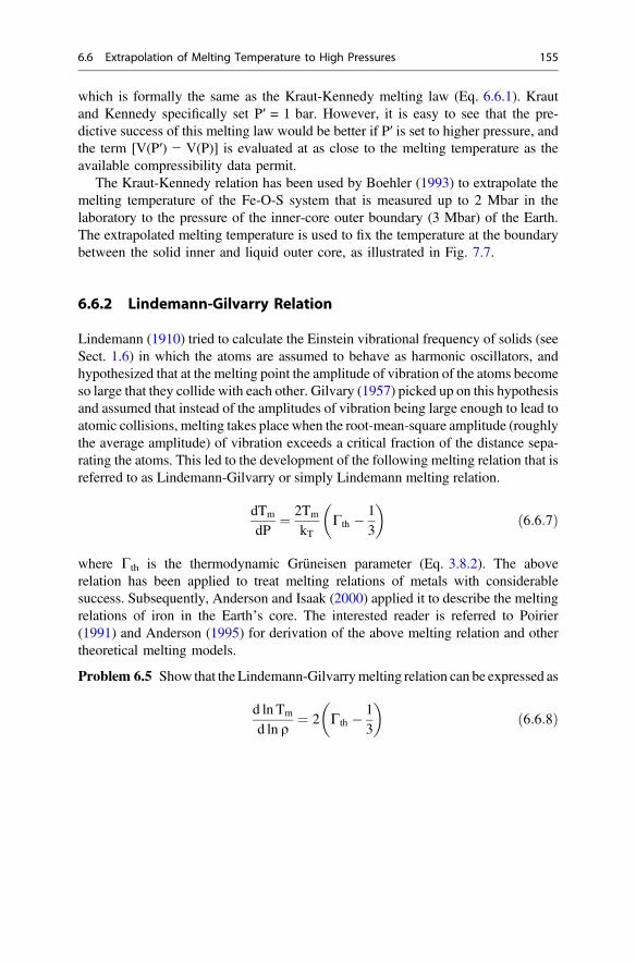
which is formally the same as the Kraut-Kennedy melting law (Eq. 6.6.1). Krautand Kennedy specifically set P′ = 1 bar. However, it is easy to see that the pre-dictive success of this melting law would be better if P′ is set to higher pressure, andthe term [V(P′) − V(P)] is evaluated at as close to the melting temperature as theavailable compressibility data permit.

The Kraut-Kennedy relation has been used by Boehler (1993) to extrapolate themelting temperature of the Fe-O-S system that is measured up to 2 Mbar in thelaboratory to the pressure of the inner-core outer boundary (3 Mbar) of the Earth.The extrapolated melting temperature is used to fix the temperature at the boundarybetween the solid inner and liquid outer core, as illustrated in Fig. 7.7.

6.6.2 Lindemann-Gilvarry Relation

Lindemann (1910) tried to calculate the Einstein vibrational frequency of solids (seeSect. 1.6) in which the atoms are assumed to behave as harmonic oscillators, andhypothesized that at the melting point the amplitude of vibration of the atoms becomeso large that they collide with each other. Gilvary (1957) picked up on this hypothesisand assumed that instead of the amplitudes of vibration being large enough to lead toatomic collisions, melting takes place when the root-mean-square amplitude (roughlythe average amplitude) of vibration exceeds a critical fraction of the distance sepa-rating the atoms. This led to the development of the following melting relation that isreferred to as Lindemann-Gilvarry or simply Lindemann melting relation.

dTm

dP¼ 2Tm

kTCth � 1

3

� �ð6:6:7Þ

where Cth is the thermodynamic Grüneisen parameter (Eq. 3.8.2). The aboverelation has been applied to treat melting relations of metals with considerablesuccess. Subsequently, Anderson and Isaak (2000) applied it to describe the meltingrelations of iron in the Earth’s core. The interested reader is referred to Poirier(1991) and Anderson (1995) for derivation of the above melting relation and othertheoretical melting models.

Problem 6.5 Show that the Lindemann-Gilvarrymelting relation can be expressed as

d lnTm

d ln q¼ 2 Cth � 1

3

� �ð6:6:8Þ

6.6 Extrapolation of Melting Temperature to High Pressures 155

6.7 Calculation of Equilibrium P-T Conditionsof a Reaction

6.7.1 Equilibrium Pressure at a Fixed Temperature

If P and T are the variables that we wish to control, then at equilibrium any reactionmust satisfy the relation DGr(Pe, Te) = 0, where Pe, Te are the equilibriumpressure-temperature condition of the reaction. As above, we will use the symbol Dr

to denote the change of a specified property between the reactant and product.Conventionally, one writes DrY =

PY(product) −

PY(reactant). As an example,

let us consider the reaction

An Gr Ky Qtz

3CaAl2Si2O8 ¼ Ca3Al2Si3O12 þ 2Al2SiO5 þ SiO2ð6:7:aÞ

which is a very important reaction for the determination of pressure of metamorphicrocks (see Sect. 10.11; An: anorthite, Gr: grossularite garnet; Ky: kyanite; Qtz:quartz). As long as the minerals are confined to the stoichiometric end membercompositions, as written, the change of Gibbs free energy, ΔrG, of this reaction atany P-T condition is written as ΔrG(P, T) = G(Gr) + 2G(Ky) + G(Qtz) − 3G(An).

Now let us suppose that we know the thermochemical properties of the phasesinvolved in a reaction at a P, T condition at which the reaction is not at equilibrium.In order to calculate the equilibrium pressure (Pe) at T′, we need to develop anexpression of ΔrG as a function of P at constant temperature, and solve for Pe at T′by imposing the equilibrium property, i.e. ΔGr(Pe, T′) = 0. To this end, we write,making use of the property (@G/@P)T = V

DrGðPe;T0Þ ¼ DrGðP;T0Þ þZPeP

ðDrVÞT0dP ¼ 0 ð6:7:1Þ

This equation can be solved for Pe if ΔrV is known as a function of P at T′. Themathematical strategy for calculating the last integral from an equation of state thatexpresses P as a function of V (instead of V as a function of P) is discussed inSect. 6.8. It should be noted, however, that when we deal with a reaction involvingonly solid phases, such as the reaction (6.7.a) above, ΔrV does not change sig-nificantly for a change of pressure of several thousand bars. This is because of thefact that minerals have similar compressibilities so that the change of volume withpressure of the products and reactants substantially cancel out. In such cases, wewould introduce very little error by taking ΔrV out of the integration sign, andsolving for Pe at T′.

In thermochemical tables, one commonly finds the enthalpy of formation ofcompounds from elements or oxides at 1 bar, 298 K, and third law entropies ofcompounds at 1 bar, 298 K along with their CP-s as functions of temperature. Inorder to use these data to solve Eq. (6.7.1), we express ΔrG(Pe, T′) as

156 6 Phase Transitions, Melting, and Reactions …

DrGðPe; T0Þ ¼ DrGð1; T 0Þ þ

ZPe

1

DrVðP; T 0ÞdP

¼ DrHð1; T 0Þ � T 0DrSð1; T 0Þ þZPe

1

DrVðP; T 0ÞdPð6:7:2Þ

ΔrH(1, T′) and ΔrS(1, T′) are related to their respective 1 bar, 298 K values, denotedby ΔrH

+ and ΔrS+, according to (Eq. 3.7.5).

DrHð1;T0Þ ¼ DrHþ þZT0

298

DrCpdT ð6:7:3Þ

and

DrSð1;TÞ ¼ DrSþ þZT0

298

DrCp

TdT ð6:7:4Þ

Substituting the last two equations into Eq. (6.6.2), rearranging the terms andimposing the condition of equilibrium, ΔrG(Pe, T′) = 0, yields

DrHþ � T0DrSþ þZT0

298

DrCPdT� TZT0

298

DrCP

TdTþ

ZPe1

ðDrVðP;T0Þ dP24

35 ¼ 0

ð6:7:5Þ

where the superscript + denotes properties at 1 bar, 298 K. Note that the first twoterms do not constitute ΔrG

+ since ΔrS+ is multiplied by T′ instead of 298.

As discussed in Sect. 4.5.1), the ΔrH+ is calculated from the enthalpy of for-

mation (ΔHf) values of the product and reactant phases from either elements oroxides according to

DrHðP;TÞ ¼ RDHf;eðproductsÞ � RHf;eðreactantsÞ¼ RDHf;oðproductsÞ � RHf;oðreactantsÞ

Note that Eq. (6.7.5) can also be used to retrieve ΔrH+ and ΔrS

+ from experimentaldata for a univariant equilibrium. This is done by calculating the term within thesquare brackets at several P-T conditions along the equilibrium boundary, andregressing it against T. The slope and intercept of the linear regression yield ΔrS

+

and -ΔrH+, respectively.

6.7 Calculation of Equilibrium P-T Conditions of a Reaction 157

6.7.1.1 Solved Problem: Depth of Diamond Formation

“Diamonds are for ever”, but from what depths within the Earth were the diamondstransported?

The diamonds are recovered from eclogite and peridotites xenoliths that representfragments of the Earth’s mantle, which were ripped off by the CO2-rich kimberlitemagmas during their explosive ascent towards the Earth’s surface in early geologicperiods (mostly Cretaceous, but some also Pre-Cambrian). The lower limit for thedepth of origin of diamond may be estimated by comparing the P-T condition ofgraphite-diamond transition boundary with the paleo-geotherms in diamond pro-ducing areas. Instead of using experimental data for the graphite-diamond transitionboundary, here we calculate this boundary, as an illustration of the application ofEq. (6.7.5) to relatively simple phase equilibrium calculation.

We first represent the graphite-diamond transition as a reaction

C(graphite) ¼ C(diamond) ð6:7:bÞ

From the thermochemical data in Robie et al. (1978), we have

Hf;eðD: 1 bar, 298 KÞ ¼ 1895 kJ/mol

Cp ¼ aþ bTþ cT2 þ dT�0:5 þ eT�2J/K-mol

with

a ¼ 98:445; b ¼ �3:6554 10�2� �

; c ¼ 1:2166 106� �

; d ¼ �1:6590 103� �

;

e ¼ 1:0977 10�5� �

for diamond,

and

a ¼ 63:160; b ¼ �1:1468 10�2� �

; c ¼ 6:4807 105� �

; d ¼ �1:0323 103� �

;

e ¼ 1:8079 10�5� �

for graphite:

Chatterjee (1991) summarized the volumetric data for the two phases as

VðD: 1 bar;TÞ ¼ 0:3409þ 0:2015 10�5� �

Tþ 0:984 10�9� �

T2 J/bar-mol

VðG: 1 bar, TÞ ¼ 0:5259þ 1:2284 10�5� �

Tþ 2:165 10�9� �

T2 J/bar-mol

bðD: 298 KÞ ¼ 0:18 10�6� �

bar�1

bðG: 298 KÞ ¼ 3:0 10�6� �

bar�1ðboth b being independent of pressure)

Since graphite is the stable form of element at 1 bar, T, it is taken to be the referenceform of the element at 1 bar, T, and accordingly,ΔHf,e(G: 1 bar, T) = 0. Thus,ΔrH ofthe above the reaction (6.7.b) at 1 bar, 298 K (i.e. ΔrH

+) is given by ΔHf,e(D: 1 bar,298 K) = 1895 kJ/mol. The ΔrCp term for this reaction can be written as

158 6 Phase Transitions, Melting, and Reactions …

DrCp ¼ DaþDbTþDcT2 þDdT�0:5 þDeT�2

where Δa = a(D) − a(G) = 35.285, and so on.It is easy to see that the sum of the first four terms in Eq. (6.7.5) yields ΔrG(1,T),

which we can now evaluate by substituting the values of ΔrH+, ΔrS

+ and carryingout the required integrations of the ΔrCp. As an example, this procedure yields

DtGð1 bar; 1373 KÞ ¼ 7666:83 kJ:

Using the data for molar volume as function of temperature at 1 bar, we have

DrVð1 bar; 1373 KÞ ¼ �0:201 J/bar-mol

Now, since (@V/@P)T = −V(1 bar, T)bT, (Eq. 3.7.2 and follow-up discussion), wehave

VðP;T0Þ ¼ I� Vð1 bar;T0ÞZ

bT0 ðPÞdP ð6:7:6Þ

where I is an integration constant. We now assume that bT′ (P) = b298(P), which is aconstant, according to the data summarized above. Thus,

V P;T0ð Þ ¼ I� V 1 bar;T0ð Þb298P

The integration constant is evaluated by substituting V(1 bar, T′) for V(P, T′) andP = 1 bar on the right hand side so that

V P; T0ð Þ ¼ V 1; T0ð Þ þV 1; T0ð Þb298 � V 1; T0ð Þb298P ð6:7:7Þ

(Note that the second term on the right is multiplied by 1 bar so that it has the unitof cm3/mol or J/bar-mol). Using the last equation, we have

ZP1

VðP;T0Þ dP ¼ Vð1;T0Þ þ b298Vð1;T0Þ½ �P0 � b298Vð1;T0ÞðP0Þ22

so that

ZPe1

DrVðP;T0Þ dP ¼ DrVð1;T0Þ þDr b298Vð1;T0Þh i½ �Pe � Dr b298Vð1;T0Þh iðPeÞ22

ð6:7:8Þ

Substitution of this equation into Eq. (6.7.5) and rearrangement of terms yields aquadratic equation

6.7 Calculation of Equilibrium P-T Conditions of a Reaction 159

�Dr b298V(1,T0Þh i

2P2e þ Dr b298V(1,T

0Þh iþDrV(1,T0Þ½ �Pe þDrG(1,T

0Þ ¼ 0

ð6:7:9Þ

where ΔrG(1, T′) stands for the first four terms in Eq. (6.7.5).The solution of the last equation by the usual method of solving a quadratic

equation yields two values of Pe, one of which is physically unreasonable. Forexample, at 1300 K, the two values of Pe are 46.6 and 208.5 kb, corresponding,respectively, to the use of minus and plus sign before the square root term of thesolution. The larger value corresponds to a depth of *600 km which is too deepfor the generation of kimberlite magma and transport of material to the surface.Furthermore, calculations of the P-T condition of xenoliths in kimberlite indicatethat these were transported from a depth of no greater than of *200 km (e.g.Ganguly and Bhattacharya 1987). Thus, we accept the lower value of Pe to definethe equilibrium graphite-diamond transition. (When the equation of equilibriuminvolves higher power of Pe due to a more complex dependence of V on P, then thesolution of Pe needs to be obtained numerically).

The results for calculation of Pe versus T relation are illustrated in Fig. 6.13 alongwith the paleogetherm of a diamond bearing locality in the southern part of India. Thepaleogeotherm was calculated by Ganguly et al. (1995) on the basis of the inferred P-Tconditions of xenoliths (crosses) in diamond bearing kimberlites of Proterozoic age(*1 Ga) and heat flow data. The geotherm and the graphite-diamond transitionboundary intersect at a pressure of 48 kb that corresponds to a depth of *150 km. Thegeotherm is also quite similar to those in other diamond producing kimberlite localities,especially South Africa (Ganguly and Bhattacharya, 1987). Thus, diamonds weretransported from a depth of at least *150 km from within the Earth’s interior.

6.7.2 Effect of Polymorphic Transition

The equilibrium (6.7.a) is subject to the effect of polymorphic transition (which is atransition between different crystallographically distinct forms of the same com-pound) as it is extended to temperature beyond the field of stability of kyanite.Many reactions of geological interest involve phases that undergo polymorphictransitions. Another example of such a reaction is

Talc Enst Qtz=Coes

MgSi4O10ðOHÞ2 ¼ 3MgSiO3 þ SiO2 þH2Oð6:7:cÞ

The equilibrium boundary of this reaction across the quartz-coesite transition isillustrated in Fig. 6.9. The general procedure for accounting for the effect of poly-morphic transition is developed below using the equilibrium (6.7.c) as an example.

Let us suppose that we know the equilibrium boundary of the above reaction inthe quartz field, and want to calculate the equilibrium boundary in the coesite field

160 6 Phase Transitions, Melting, and Reactions …

using the thermochemical data for quartz-coesite transition. The breakdown reac-tion of talc in the coesite field can be expressed as a linear combination of that in thequartz field and quartz-coesite polymorphism as follows.

Talc = 3 Enst + Qtz + H2O (1)

Qtz = Coes (2)

----------------------------------------------------------------

Talc = 3 Enst + Coes + H2O (3)

Thus, in general

DrG3ðP; TÞ ¼ DrG1ðP; TÞþDrG2ðP; TÞ

Now, let P1 and P3 be the equilibrium pressures of reactions (1) and (3), respec-tively, at a temperature T′ (Fig. 6.14). The Gibbs energy change of reaction (3) atP1, T′ is then given by

Graphite

Proterozoic Geotherm(1 Ga)

Archean Geotherm

Diamond

Fig. 6.13 Comparison of graphite/diamond equilibrium boundary with the geotherm calculatedby Ganguly et al. (1995) for the southern Indian shield area where diamonds are found in mantlexenoliths brought up by kimberlite eruptions during the proterozoic period. This comparisonshows that diamonds form at depths of at least 150 km within the Earth’s interior. The crossesrepresent calculated P-T conditions of mantle xenoliths on the basis of mineral chemistry. Thegeotherm was calculated to satisfy the xenolith and heat flow data

6.7 Calculation of Equilibrium P-T Conditions of a Reaction 161

0

ΔrG3(P1,T′) = ΔrG1(P1,T′) + ΔrG2(P1,T′)

= ΔrG2(P1,T′)

ð6:7:10Þ

The Gibbs energy change of reaction (3) at P3, T′ can be expressed as

DrG3ðP3;T0Þ ¼ DrG3ðP1;T0Þ þZP3P1

ðDrV3ÞT0dP ¼ 0 ð6:7:11Þ

The last equality is due to the fact that P3 represents the equilibrium pressure of thereaction (3) at T′. Combining the last two equations, we finally have

DrG2ðP1;T0Þ þZP3P1

ðDrV3ÞT0dP ¼ 0 ð6:7:12Þ

This equation can be solved for P3 at different T′ values to obtain the equilibriumdehydration boundary of talc in the coesite field (P3 vs. T) using the data for Gibbsenergy change of quartz to coesite transition, if the volume change for the reaction(3) is known as a function of pressure and temperature. Of course, this procedure isneeded when thermochemical data of talc is not available. If it is, then the equi-librium dehydration boundary of talc in the coesite field can be calculated bysolving the general equation of equilibrium, Eq. (6.7.5).

In the last expression, the first term on the left may be replaced by the ΔrV termfor the polymorphic reaction as follows. If P2 is the equilibrium pressure of thepolymorphic transition at Tʹ (Fig. 6.14), then

T

(1)

(2)

(3)

Talc Enst + SiO2 + H2O

Coesite

Quartz

P1

P2

P3

P

Fig. 6.14 Schematic illustration the P-T parameters defined for calculation of the effect ofpolymorphic transition on an equilibrium boundary of a reaction. The actual data for the reactionchosen here are illustrated in the inset of Fig. 6.9

162 6 Phase Transitions, Melting, and Reactions …

ð6:7:13Þ

Since volumetric data of solids are more accurate than their Gibbs energy data, it ispreferable to take advantage of the last expression to calculate P3 versus T relationaccording to Eq. (6.7.12).

Problem 6.6 The volume change of reaction (3) can be expressed asDrV3 ¼ DrVS

3 þVH2O, where DrVS3 is the solid volume change of the reaction, i.e.

DrVS3 ¼ 3VEnst þVCoes � VTlc. Now, assuming that DrVS

3 is insensitive to pressurechange between the limits of integration of Eq. (6.7.13), calculate the equilibriumpressure for the talc dehydration reaction in the coesite field at 800 °C, using thefollowing data: DrVS

3 ¼ �1:750 J=bar, ΔGo(Qtz ! Coes) = 4200 J at 800 °C andthe corresponding pressure at the qtz-coesite boundary (29.6 kb) and the virial-typeequation of state of water by Belonoshko and Saxena (1992), as given byEq. (5.4.13). Fitting of the V-P relation of water at 800 °C calculated from thisequation yields V = 39.286(P)−0.286 where P is kb.

(a) ExpressRPCPQ

VH2O� �

TdP (PC and PQ: equilibrium pressures at T in the coesite field

and the quartz field, respectively) using the method in Sect. 6.8, and solve for PC bysuccessive approximations, satisfying Eq. (6.7.12). (b) Also, use the V-P relationabove to solve for PC.

Answer: (a) 40.0 kb and (b) 41.2 kb.

Problem 6.7 Suppose that you have the Gibbs energy change of a reaction, ΔrG, at1 bar, 298 K, but not ΔrH and ΔrS, and in addition you have the CP data of allphases involved in the reaction. The CP function is expressed as CP = a + bT +c/T2.Derive an analytical expression to calculate ΔrG at any arbitrary temperature at1 bar, using the available data, and the relation @G/@T = −S. Complete all inte-grations. (Note: By adding the integral term from Eq. (6.7.1) to your derivedexpression for ΔrG(1 bar, T), you obtain an expression for ΔrG(P, T), which youcan use, instead of Eq. (6.7.2) to calculate equilibrium P at T.

Hint: First express S as a f(T) using the CP versus T relation.

*Problem 6.8 In quantum chemical calculations of pressure of first order phasetransition at a fixed temperature, it is quite common to see calculation of U versus Vrelation of the two phases that are convex downwards and take the common tangentto the two curves to determine the transition pressure (Fig. 6.15). What is the(a) rationale behind this practice and (b) restriction on the temperature at which the

6.7 Calculation of Equilibrium P-T Conditions of a Reaction 163

calculated transition pressure holds? Also what thermodynamic potential should beused in place of U to calculate the transition pressure at any temperature followingthe “common tangent” approach?

6.8 Evaluation of Gibbs Energy and Fugacity at HighPressure Using Equations of States

In many Equations of states, such as Redlich-Kwong, Birch-Murnaghan and Vinet,as discussed above, P is expressed as a function of volume, instead of the reverse,and these equations cannot be re-arranged to yield V(P) that can be used directly tocalculate the integral

RVdP, which relates the Gibbs free energies between two

different pressures. Also, this integral is needed to calculate the change of logf,where f is the fugacity, for a given change of pressure.

We can use a P(V) EoS to evaluateRVdP from the relation d(PV) = PdV +

VdP, so that ZVdP ¼

Zd(PV)�

ZPdV ð6:8:1Þ

If we evaluate the first integral between the limits P1 (lower limit) and P2 (upperlimit), then the corresponding limits of the second integral are [P1, V(P1)] and [P2,V(P2)], and those of the last integral are V(P1) and V(P2) (for brevity, we write V1

for V(P1) and V2 for V(P2)). Thus, we have

ZP2P1

VdP ¼ ½P2VðP2Þ � P1VðP1Þ� �Zv2v1

PdV ð6:8:2Þ

We derive below the expressions for the integral on the right for some commonlyused EoS for solid and fluid.

U

V

I

II

Fig. 6.15 Schematicillustration of U versus Vrelation of two polymorphicphases, I and II

164 6 Phase Transitions, Melting, and Reactions …

6.8.1 Birch-Murnaghan Equation of State

If the P-V relation is described by the third-order Birch-Murnaghan EoS (Eq. 5.4.23),then we can write

P ¼ aVo

V

� �7=3

� Vo

V

� �5=3" #

1þ nVo

V

� �2=3

�1

" #( )ð6:8:3Þ

where

a ¼ 3ko2

; and n ¼ 34

k0o � 4� �

(To recapitulate, ko is the bulk modulus at P = 0, T, and k′o is the pressurederivative of ko.) From this P-V relation, we obtain

ZV2

V1

PdV¼ 32aV5=3

o ð1� nÞ 1

V2=3

� �V2

V1

� 12anV3

o1

V2

� �V2

V1

þ 34aV7=3

o ð2n� 1Þ 1

V4=3

� �V2

V1

ð6:8:4Þ

For the second order B-M EoS, we have the special case of the above expressionwith n = 0.

6.8.2 Vinet Equation of State

Writing c ¼ 3=2ðk0o � 1Þ, we can express the Vinet EoS (Eq. 5.4.29) as

P ¼ 3ko1� g1=3

g2=3exp c 1� g1=3

h ið6:8:5Þ

where η = V/Vo. Now since dV = Vodη,ZPdV ¼ 3koVo

Z1� g1=3

g2=3exp c 1� g1=3

h idg ð6:8:6Þ

Using y = (1 − η1/3) so that dη = −3η2/3dy.ZPdV ¼ �9koVo

Zyecydy

Definite integral of this expression yields

6.8 Evaluation of Gibbs Energy and Fugacity at High Pressure … 165

Zv2v1

PdV ¼ �9koVoecy

c2ðcy� 1Þ

� �y2y1

ð6:8:7Þ

in which, summarizing, y = 1 − η1/3 = 1 − (V/Vo)1/3, and c ¼ 3=2ðk0o � 1Þ.

6.8.3 Redlich-Kwong and Related Equations of Statefor Fluids

Using the P-V relation of Redlich-Kwong equation of state, as given by Eq. (5.4.5),we obtain

ZV2

V2

PdV ¼ RT lnðV� bÞþ a

bffiffiffiT

p lnðbþVÞ

V

� �� �V2

V1

ð6:8:8Þ

where, for brevity, we have used V for the molar volume, which is written as Vm inEq. (5.4.5). In the modified Redlich-Kwong (MRK) equation of states, a and b areusually treated as functions of temperature and pressure, respectively (e.g.Eqs. 5.4.6a, b). Obviously, the above integral cannot be used when b is a functionof pressure. The integration needs to be carried out numerically.

As discussed in Sect. (5.4.1.3), recognizing the problem with the analyticalintegration of MRK when b is a function of pressure, Holland and Powell (1991)proposed a compensated Redlich-Kwong (CORK) equation of state in which b istreated as a constant. They found that the error resulting from treating b as aconstant can be accounted for by introducing a correction or compensation termwith a general form given by Eq. (5.4.7). Denoting the terms within the squarebrackets of this equation as a correction volume, Vcor, we have

ZP2P1

VdP ¼ZP2P1

VmrkdPþZP2P1

VcordP ð6:8:9Þ

The first integral on the right can be evaluated by combining Eqs. (6.8.2) and(6.8.8). The second integral on the right is given by

ZP2P1

VcordP ¼ 2c3ðP� PoÞ3=2 þ d

2ðP� PoÞ2

� �P2P1

ð6:8:10Þ

Thus, for the compensated Redlich-Kwong (CORK) equation of state proposedby Holland and Powell (1991), we finally obtain

166 6 Phase Transitions, Melting, and Reactions …

ZP2P1

VdP¼ P2Vmrk2 � P1V

mrk1

� � RT lnðVmrk � bÞþ a

bffiffiffiT

p lnbþVmrk

Vmrk

� �� �Vmrk2

Vmrk1

þ 2c3ðP� PoÞ3=2 þ d

2ðP� PoÞ2

� �P2P1

ð6:8:11Þ

where Vmrk is the molar volume calculated from a modified Redlich-Kwongequation of state with the term a calculated at the temperature of interest and btreated as a constant.

Problem 6.9 Using the equation of state (EoS) of fluids by Belonoshko andSaxena, as given by Eq. (5.4.13), calculate

(a) the Gibbs free energy and fugacity of H2O at 10 kb, 720 °C, using theexperimentally derived values (Burnham et al. 1969) of G (5 kb, 720 °C) =−27,903 J/mol, f(5 kb, 720 °C) = 3964 bars, V(5 kb, 720 °C) = 1.3569 cm3/gmand V(10 kb, 720 °C) = 1.0903 cm3/gm

(b) fugacity coefficient of water at 10 kb, 720 °C(c) see Problem 8.5.

Partial Answers: G(10 kb, 720 °C) = −17,267 J/mol; f(10 kb, 720 °C) =14,376 bars).

Hint: To calculate G(10 kb, 720 °C), evaluateRVdP from the EoS according to

the method of integration by parts (Eq. 6.8.2); also see Sect. 3.6 for calculation offugacity. The units of the constants a, b, and c are bar-cm3, bar-cm6 and bar-cm3m,respectively.

Comment: The experimentally determined values of G and f at 10 kbar, 720 °Care − 17,071 J/mol and 14,723 bars, respectively (Burnham et al. 1969), which arein good agreement with the values derived from the EoS data of Belonoshko andSaxena (1992). These authors have also presented an equation for calculating thefugacity of different geologically important volatile species in the system C-O-H at5 kb, T, which may be used to calculate the fugacity values at any other pressureusing their EoS, which is valid for P > 5 kb).

Problem 6.10 The estimated P-T conditions of formation of the Archean granulitesin the southern part of India plot much above the steady state geotherm in the samearea that is illustrated in Fig. 6.13. Thus the granulites had formed by some kind ofa transient thermal perturbation. One of the proposed mechanisms of such thermalperturbation is basaltic magma under-plating of the terrane, where the heat given offby the cooling magma body from its liquidus condition raised the temperature of thecrustal rocks. At 10 kb pressure, the average temperature of the granulites

6.8 Evaluation of Gibbs Energy and Fugacity at High Pressure … 167

is *750 °C, which is *400 °C higher than the temperature at the ambient geo-therm, and the liquidus temperature of basalt is 1300 °C. Assuming that the heatcapacity (CP) of both the crustal rocks and basaltic magma/rock are *103 J/kg-K,and the heat of fusion (DHf) of basalt is 4(105) J/kg, calculate the mass of thesupposed under-plated basalt relative to that of granulite.

(Presence of under-plated magma body, if it is sufficiently large, can be detected bygeophysical methods).

Answer: mass of basalt/mass of granulite *0.42.

6.9 Schreinemakers’ Principles

The Schreinemakers’ principles constitute a set of rules that enable us to organizethe possible equilibria in a system in a self-consistent manner. The principlesrequire systematic application of the Phase Rule, keeping track of some simple factsabout self-consistency in the stability analysis of phases, such as an assemblage ofthe phases A and B must lie within the fields of stability of both A and B.

Let us consider a system consisting of 6 phases, namely, talc (Ta), antigorite (Atg),enstatite (En), forsterite (Fo), phase A (A) and vapor (V). (The phase A is one ofseveral dense hydrous magnesium silicate phases that have been discovered in thelaboratory experiments at high P-T conditions. These are given alphabetical names,A, B, C etc., and are generally referred to as DHMS phases.) The univariant reactionrelations among these phases in the P-T space, as determined by a combination ofexperimental data and theoretical considerations, including the Schreinemakers’principles, are illustrated in Fig. 6.9 (Bose and Ganguly 1995). We will discussSchreinemakers’ principles by referring to this Figure. It should, however, be noted atthe outset that phase relations may also be depicted using intensive variables otherthan P and T. Schreinemakers principles are equally applicable to those cases. Anexample can be found later in the Sect. 12.8.1 (Fig. 12.7). For simplicity, but withoutlosing any generality, we have not included quartz and coesite in the system, althoughthe phase diagram shows equilibria involving these phases (Ta = En + SiO2

(Qtz/Coes) + V and Qtz = Coes). Only three components, MgO, SiO2, H2O arerequired to describe the compositions of all the phases, assuming that each phase isrestricted to their respective pure end-member states.

6.9.1 Enumerating Different Types of Equilibria

If the number of components in a reaction is C, then according to the Phase Rule,the reaction is univariant if it has (C + 1) number of phases. However, sometimes aspecific reaction may involve a smaller number of components than there are in thegeneral system. In that case, the reaction becomes univariant with smaller number

168 6 Phase Transitions, Melting, and Reactions …

of phases than those that involve all the components of the general system. Anexample is the reaction Qtz = Coes. It is univariant since it involves only onecomponent, SiO2, even though the phases in the general system may requireadditional components such as MgO and H2O. Such univariant equilibria thatinvolve lesser number of phases than those that contain all the components of thegeneral system are called degenerate equilibria. We will return to the properties ofthis type equilibrium later.

We now ask the following question. How many univariant equilibria may befound in a system in which the number of phases is P and that of components is C.The question can be easily answered by using combinatorial principle, as follows.

Number of univariantð Þ equilibria� P!ðCþ 1Þ!ðP� C� 1Þ!

with the equality holding when all equilibria are non-degenerate. When P = 6 andC = 3, as in the chosen illustrative system, we have No. (Univariant equilibria) � 15.

Similarly, the number of invariant points� P!ðCþ 2Þ!ðP� C� 2Þ!

so that there are a maximum of 6 invariant points in the system. All of theseinvariant points are, of course, not of geological interest. Only two invariant pointsare shown in Fig. 6.9.

For book keeping purposes in the Schreinemakers analysis, an equilibrium isdesignated by writing the phases absent from the equilibrium within parentheses.Thus, the two invariant points in Fig. 6.9 are labeled (Ta) and (A). Each univariantequilibrium intersecting at (Ta) lacks talc plus an additional phase. Similarly, eachunivariant equilibrium intersecting at (A) lacks the phase A and an additional phase.There are five univariant equilibria radiating from each invariant point. If there areX number of phases at an invariant point, then there are a maximum of X number ofunivariant equilibria radiating from that point. All univaraint reactions around aninvariant point can be written out in chemically balanced forms by using linearalgebraic method (e.g. Korzhinskii 1959).

Let us now consider a system of five phases, namely, Ta, En, Qtz, Coes and V.The phase relations are shown within a box in the lower right hand portion ofFig. 6.9. Here again, the overall system consists of three components, MgO, SiO2,H2O. Thus, each non-degenerate univariant equilibrium must consist of 4 phases.Two of these are Ta = En + Qtz + V (Coes) and Ta = En + Coes + V (Qtz),which intersect to generate an invariant point consisting of five phases. If all uni-variant equilibria in the system are non-degenerate, then there must be threeadditional equilibria radiating from the invariant point, each being characterized bythe absence of one phase from the set present at the point. However, the univariantreaction Qtz = Coes is characterized by the absence of three phases, (Ta), (En) and(V), from the set present at the invariant point. Thus, this equilibrium is considered

6.9 Schreinemakers’ Principles 169

to be triply degenerate, which means that for the book keeping purpose, it is takento be equivalent to three non-degenerate univariant equilibria. Thus, all univariantreactions radiating from the invariant point have been accounted for, and hencethere can be no other balanced univariant reaction in this part of the system.

6.9.2 Self-consistent Stability Criteria

If there is a reaction A + B = C + D, then any univariant reaction that involves thephases A and B (in either the same side or the two sides of the reaction) must lie inthe half-plane defined by the A + B side of the first reaction. We would refer to thisdomain as the A-B half-plane. The concept of half-plane is illustrated in Fig. 6.16.Consider, for example, the reaction (Ta, Atg) in the top right part of Fig. 6.9. Thestable parts of all reactions involving the phases A and En, namely the stable partsof the reactions (Ta, Fo) and (Ta, V), lie in the half-plane defined by the A + Enside of the reaction (Ta, Atg). Similarly, the stable parts of all reactions involving Foand V lie in the half-plane defined by the Fo + V side of the reaction (Ta, Atg). Thearrangement of all reactions in Fig. 6.9 satisfies this “half-plane constraint”. Thereason behind this topological restriction is a simple stability argument. If the stablepart of the reaction (Ta, Fo) is on the Fo + V half-plane, then the phase A and En inthis reaction would react to form Fo + V. The half-plane concept can be stated in adifferent and general way as follows.

The phases that are absent from any equilibrium must not appear as products ofthe reactions bounding the sector which contains the stable part of that equilib-rium. Consider, for example, the equilibrium (Ta, Fo) in the top left part of Fig. 6.9.

A + B

C + D

T

P

A – B half-plane:Field of all reactions involving A and B

C-D half-plane:Field of all reactions involving C and D

Fig. 6.16 Illustration of half-plane concept in Schreinemakers’ analysis. The stable (solid line)and metastable (dashed line) portions of a univariant reaction A + B = C + D divide the P-T spaceinto A-B and C-D half-planes. The dot represents an invariant point. All reactions involving A andB lie in the A-B half-plane. Similarly, all reactions involving C and D lie in the C-D half-plane

170 6 Phase Transitions, Melting, and Reactions …

The phases Ta and Fo do not appear as products of the reactions (Ta, V) and(Ta, Atg) that bound the sector containing the stable part of the reaction (Ta, Fo).

The fact that an assemblage of phases cannot be stable beyond the field ofstability of any of its subsets (self-consistent stability criteria) requires that thestable part of a non-degenerate univariant reaction must be truncated at an invariantpoint. However, the stable part of a degenerate reaction may sometimes extendthrough an invariant point since such extension does not necessarily violate theself-consistent stability criteria. In the example chosen above, the degeneratereaction Qtz = Coes extends through the invariant point as it does not violate anystability criterion.

If a univariant reaction, say 1, can be expressed as a linear combination of twoother equilibria, say 2 and 3, then the metastable extension of the reaction 1 must liewithin the field defined by the stable parts of the reactions 2 and 3. Consider, forexample, the reaction (Ta, En) in Fig. 6.9. It can be expressed as a linear combi-nation of the reactions (Ta, Fo) and (Ta, Atg). Thus, the metastable extension of thereaction (Ta, En) past the invariant point (Ta) lies within the field bounded by thestable parts of the reactions (Ta, Fo) and (Ta, Atg).

6.9.3 Effect of an Excess Phase

In geological problems, we often encounter some phases that are present in excesssuch that these are not completely consumed by any reaction. An example is quartzin metapelite. Although quartz is involved in numerous reactions, it is nevercompletely consumed. If a phase, say A, is present in excess, then all univaraintequilibria characterized by the absence of that phase, (A, …), become unstable.Consequently, the invariant points to which these equilibria connect also becomeunstable. However, if an equilibrium characterized by the absence of an excessphase is degenerate, then that equilibrium becomes stable. The proof of this the-orem is given by Ganguly (1968).

6.9.4 Concluding Remarks

The configuration of the phase relations derived only by the application ofSchreinemakers principle is self- consistent, but not unique, and sometimesmeaningless without additional constraints on the slopes and positions of at leastsome of the equilibria. For example, the reaction topology shown in Fig. 6.9 maybe rotated by any arbitrary angle without violating the above principles. One needsto use additional information about the slopes and positions of at least some of thereactions to derive a meaningful configuration. A detailed analysis of possibleself-consistent Schreinemakers’ topologies in a system of C + 3 phases, withapplications to geologically important systems, is given by Cheng and Greenwood(1990).

6.9 Schreinemakers’ Principles 171

The main utility of Schreinemakers’ principles lies in the fact that once somereasonable constraints about some of the reactions are available, a meaningfultopology may be derived leading to new insights about geological and planetaryprocesses. In addition, it provides a “route map” for experimental investigations ofa complex system (e.g. Ganguly 1968, 1972). It allows one to choose the criticalequilibria for experimental investigation that bring out the important properties of aphase diagram, and to search for conditions where other equilibria, which are yet tobe determined experimentally, are to be found as the phase diagram topology getsrefined. For example, referring to Fig. 6.9, if the reaction (Ta, V) is determinedexperimentally, then we know where to look for the reaction (Ta, Fo) in theexperimental studies.

As an example of the practical utility of interactive Schreinemakers analysis, wenote that the arrangement of univariant reactions around the invariant point (Ta)was derived by this approach along with constraints on the slopes of the reactionsthat could be deduced from the available thermodynamic data and some experi-mental information. The reaction (Ta, Atg) was determined experimentally by Luth(1995). This reaction was found to intersect the antigorite breakdown reactionAtg = En + Fo + V, as calculated by Bose and Ganguly (1995), at *70 kbarpressure, generating the invariant point (Ta). Since the invariant point (Ta) con-sisted of five phases, it was evident that there must be three additional univariantreactions, if all are non-degenerate, radiating from the invariant point. These uni-variant reactions were deduced by algebraic method, and their spatial dispositionswere inferred by the application of Schreinemakers’ principles and thermodynamicconstraints on the P-T slopes.

It was found that the P-T profile of the leading age of an old slab (� 50 Myr)subducting with a velocity of >3 cm/year intersects the reaction (Ta, V). Thus,instead of dehydrating, the mineral antigorite, which is a major water bearing phaseon the leading edge of a slab, delivers all the water to the phase A, enablingtransportation of water into the deep mantle. This important discovery of thepossible transport pathway of water into the deep mantle by Bose and Ganguly(1995) is an example of the important geological insight that may be gained throughthe application of Schreinemakers’ principles, coupled with experimental andthermodynamic data.

References

Aitta A (2006) Iron melting curve with a tricritical point. J Stat Mechanics: Theory andExperiment 2006:P12015

Akella J, Kennedy GC (1971) Melting of gold, silver, and copper—proposal for a newhigh-pressure calibration scale. J Geophys Res 76:4969–4977

Akella J, Ganguly J, Grover R, Kennedy GC (1972) Melting of lead and zinc to 60 kbar. J PhysChem Solids 34:631–636

Anderson OL (1995) Equations of state of solids for geophysics and ceramic science. Oxford,New York, p 405

172 6 Phase Transitions, Melting, and Reactions …

Anderson OL, Isaak DG (2000) Calculated melting curves for phases of iron. Amer Mineral85:376–385

Belonoshko AB, Saxena SK (1992) Equations of state of fluids at high temperature and pressure(Water, Carbon Dioxide, Methane, Carbon Monoxide, Oxygen, and Hydrogen) In: Saxena SK(ed) Advances in physical geochemistry, vol 9, Springer, New York, Berlin, Heidelberg,pp 79–97

Boehler R (1993) Temperatures in the Earth’s core from melting-point measurements of iron athigh pressures. Nature 363:534–536

Bose K, Ganguly J (1995) Experimental and theoretical studies of the stabilities of talc, antigoriteand phase A at high pressures with applications to subduction processes. Earth Planet Sci Lett136:109–121

Burnham CW, Hollaway JR, Davis NF (1969) Thermodynamic properties of water at 1,000o C and10,000 bars. Geol Soc Amer Special Paper 132:96

Carpenter MA (1980) Mechanism of exsolution in sodic pyroxene. Contrib Mineral Petrol 71:289–300

Carpenter MA (1985) Order-disorder transformation in mineral solid solution. In: Kieffer SW,Navrotsky A (eds) Microscopic to macroscopic: atomic environments to mineral thermody-namics. Rev Mineral 14:187–224

Chatterjee ND (1991) Applied mineralogical thermodynamics. Springer, Berlin, Heidelberg,New York, p 321

Cheng W, Greenwood HJ (1990) Toplogical construction of nets in ternary (n + 3)-phasemultisystems, with applications to Al2O3-SiO2-H2O and MgO-SiO2-H2O. Canad Mineral28:305–320

Dziewonski AM, Anderson DL (1981) Preliminary reference earth model. Phys Earth Planet Inter25:297–356

Ehrenfest P (1933) Phaseumwandlungen im üblichen und erweiterten Sinn klassifiziert nach deentsperechenden Singularitäten des thermodynamischen Potentials. Proc Amsterdam Acad36:153

Ganguly J (1968) Analysis of the stabilities of chloritoid and staurolite, and some equilibria in thesystem FeO-Al2O3-SiO3-H2O-O2. Amer J Sci 266:277–298

Ganguly J (1972) Staurolite stability and related parageneses: theory, experiments and appliations.J Petrol 13:335–365

Ganguly J, Bhattacharya PK (1987) Xenoliths in proterozoic kimberlites from southern India:petrology and geophysical implications. In: Nixon PH (ed) Mantle xenoliths, pp 249–266

Ganguly J, Singh RN, Ramana DV (1995) Thermal perturbation during charnockitization andgranulite facies metamorphism in southern India. J Metamorphic Geol 13:419–430

Gilvary JJ (1957) Temperatures in the Earth’s interior. J Atm Terrestr Phys 10:84–95Hacker BR, Peacock SM, Abers G, Holloway SD (2003) Subduction factory 2. Are

intermediate-depth earthquakes in subducting slabs linked to metamorphic dehydrationreactions? J Geophys Res 108:11–15

Holland TJB (1980) Reaction Albite = Jadeite + Quartz determined experimentally in the range600 to 1200 C. Amer Min 65:129–134

Holland TJB, Powell R (1991) A compensated-Redlich-Kwong (CORK) equation for volumes andfugacities of CO2 and H2O in the range 1 bar to 50 kbar and 100–1600 °C. Contrib MineralPetrol 109:265–271

Huang X, Xu Y, Karato S-I (2005) Water content in the transition zone from electricalconductivity of wadselyite and ringwoodite. Nature 434:746–749

Iwamori H, McKenzie D, Takahashi E (1995) Melt generation by isentropic mantle upwelling.Earth Planet Sci Lett 134:253–266

Kennedy GC, Vaidya SN (1970) The effect of pressure on the melting temperature of solids.J Geophys Res 75:1019–1022

Kesson WH, van Laar PH (1938) Measurements of the atomic heats of tin in the superconductiveand non-superconductive states. Physica 5:193–201

References 173

Komabayashi T (2014) Thermodynamics of melting relations in the system Fe-FeO at highpressure: Implications for oxygen in the Earth’s core. J Geophys Res Solid Earth 119:4164–4177

Korzhinskii DS (1959) Physicochemical basis of the analysis of the paragenesis of minerals.Consultants Bureau, New York, p 142

Kraut E, Kennedy GC (1966) New melting law at high pressures. Phys Rev 151:668–675Landau LD, Lifschitz EM (1958) Statistical physics. Pergamon, London, Paris, p 484Leudemann HD, Kennedy GC (1968) Melting curves of lithium, sodium, potassium and rubidium

to 80 kilobars. J Geophys Res 73:2795–2805Libby WF (1966) Melting points at high compression from zero compression properties through

Kennedy relation. Phys Rev Lett 17:423–424Lindemann FA (1910) Uber der berechnung molecularer Eigenfrequenzen. Zeit Phys 11:609–612Luth R (1995) Is phase A relevant to the Earth’s mantle? Geochim Cosmochim Acta 59:679–682Mukherjee K (1966) Clapeyron’s equation and melting under high pressures. Phys Rev Lett

17:1252–1254Newton RC, Jayaraman A, Kennedy GC (1962) The fusion curves of the alkali metals up to 50

kilobars. J Geophys Res 67:2559–2566Oganov AR, Brodholt JP, Price GD (2002) Ab initio theory of phase transitions and

thermochemistry of minerals. In: Gramaccioli CM (ed) Energy modelling in minerals,European Mineralogical Union Notes in Mineralogy, vol 4, Eötvös University Press, Budapest,pp 83–160

Pippard AB (1957) Elements of classical thermodynamics for advanced students in physics.Cambridge University Press, London

Poirier J-P (1991) Introduction to the physics of the earth. Cambridge, p 264Putnis A (1992) Introduction to mineral sciences. Cambridge, p 457Redfern SAT, Salje E, Navrotsky A (1989) High temperature enthalpy at the orientational

order-disorder transition in calcite: implications for the calcite/aragonite phase equilibrium.Contrib Mineral Petrol 101:479–484

Richet P (2001) the physical basis of thermodynamics with applications to chemistry. KulwarAcademic/Plenum Publishers, New York, p 442

Robie RA, Hemingway BS, Fisher JR (1978) Thermodynamic properties of minerals and relatedsubstances at 298.15 K and 1 bar (105 pascals) pressure and at higher temperatures. US GeolSurv Bull 1452:456

Sakamaki T, Suzuki A, Ohtani E (2006) Stability of hydrous melt at the base of the Earths’ uppermantle. Nature 439:192–194

Salje EKH (1988) Structural phase transitions and specific heat anomalies. In: Salje EKH(ed) Physical properties and thermodynamic behaviour in minerals, NATO, pp 75–118

Salje EKH (1990) Phase transitions in ferroelastic and co-elastic crystals. Cambridge, UK

174 6 Phase Transitions, Melting, and Reactions …

7Thermal Pressure, Earth’s Interiorand Adiabatic Processes

Unwary readers should take warning that ordinarylanguage undergoes modification to a high-pressureform when applied to the interior of the Earth; a fewexamples of equivalents follow: certain (highpressure form) – dubious (ordinary meaning),undoubtedly (high pressure form) – perhaps(ordinary meaning) …

Francis Birch

In this chapter we discuss several applications of the basic thermodynamic relationsdeveloped so far to problems relating to the properties and processes in the Earth’sinterior, from shallow crustal level to the outer core, as well as adiabatic flowprocesses that have applications to a variety of processes in different naturalenvironments. The most important source of our information about the deep interiorof the Earth, which is physically inaccessible, is the velocity of seismic waves asthese pass through the materials that constitute the interior. However, interpretationof the seismic wave velocities in terms of the density structure and mineralogicalconstitution of the Earth’s interior requires an understanding of the link betweenseismic velocities and thermodynamic properties, which is also discussed in thischapter. The processes in the deep interior of the Earth, such as decompression andmelting of rocks and rise of mantle plumes, take place under effectively adiabaticcondition. These topics are discussed in this chapter from two different viewpoints,namely the adiabatic processes take place under equilibrium condition so that theseare isentropic and that the adiabatic decompression is an irreversible process thatleads to entropy production.

© Springer Nature Switzerland AG 2020J. Ganguly, Thermodynamics in Earth and Planetary Sciences,Springer Textbooks in Earth Sciences, Geography and Environment,https://doi.org/10.1007/978-3-030-20879-0_7

175

7.1 Thermal Pressure

7.1.1 Thermodynamic Relations

The thermal pressure is defined as the pressure change associated with temperaturechange at a constant volume. The expression for thermal pressure can be derived asfollows. The P-V-T relation of a substance can be expressed in the functional formf(P,V,T) = 0. This type of function, which is known as an implicit function, leads tothe relation (see Appendix B.4)

@P@T

� �V¼ �

@P@V

� �T

@T@V

� �P

¼ �@V@T

� �P

@V@P

� �T

ð7:1:1Þ

Using Eqs. (3.7.1) and (3.7.2), the ratio of derivatives on the right equals-a/bT. Thus, we have,

@P@T

� �V¼ a

bT¼ akT ð7:1:2Þ

or

DPth ¼ZT2

T1

ðakTÞdT ð7:1:3Þ

where DPth stands for thermal pressureBoth a and kT are affected by temperature changes, but the value of akT of a

solid seems to be fairly insensitive to temperature change above its Debye tem-perature, hD, in many cases (Anderson 1995; also see Sect. 5.4.2.2 for furtherdiscussion about deviation from this relation; the concept of Debye temperature isexplained in Sect. 1.6). The behavior of akT for a few compounds of geophysicalinterest is illustrated in Fig. 7.1. Thus, the thermal pressure of a solid due totemperature change above the Debye temperature may be approximated byassuming a constant value of akT, as

DPth ¼ PðTÞ � P hDð Þ ¼ akT T� hDð Þ ð7:1:4Þ

where P(hD) is the pressure at the Debye temperature. We discuss below twoexamples of the application of the concept of thermal pressure in Geophysical andGeological problems (an additional example has been discussed in Sect. 5.4.2.2).

176 7 Thermal Pressure, Earth’s Interior and Adiabatic Processes

*Problem 7.1 Making some assumptions, the thermal pressure can be related tothe thermodynamic Grüneisen parameter, Cth (see Sect. 3.8), as follows:

DPth ¼ CthDUV

ð7:1:5Þ

This is the well-known Mie-Grüneissen equation of state. Derive this relationstarting with Eq. (7.1.3) and using the thermodynamic Grüneisen parameter asdefined by Eq. (3.8.2).

7.1.2 Core of the Earth

The Earth’s core represents 32% of its mass and is about half of its radius. It isgenerally accepted from geophysical data and observations of meteorite samplesthat the core of the Earth is made primarily of iron, with a molten outer and a solidinner components. The radii of the outer limits of the inner and outer cores are at1221 and 3480 km, respectively, corresponding to depths of 5155 and 2885 km. Inthis section, we examine if we should expect some light alloying elements to bedissolved in the core of the Earth.

Anderson (1995) calculated the q versus P relations of three polymorphs of ironat 300 K, a (bcc: body centered cubic), e (hcp: hexagonal close pack) and c (fcc:face centered cubic) for which sufficient data are available, and compared the resultswith the q versus P relation constrained for the core by the Preliminary ReferenceEarth Model or PREM (Dziewonski and Anderson 1981) that is deduced from thegeophysical data. The results are shown in Fig. 7.2a.

Fig. 7.1 The behavior ofakT for a few compounds ofgeophysical interest as afunction of temperaturenormalized to the Debyetemperature, hD. FromAnderson (1995)

7.1 Thermal Pressure 177

Phase diagram for the P-T stabilities of the different iron polymorphs (Anderson2000; Saxena and Dubrovinsky 2000), developed on the basis of the availableexperimental data, suggests that of the three polymorphs for which q versus Prelations are shown in Fig. 7.2a, only e-iron could be stable at the core pressure.However, its density at 300 K and the pressure of the solid inner core (dashedcurves) is much higher than the density of inner core in the PREM. At least a part ofthis discrepancy is due to the fact that the temperature of the inner core is *5000 K(Fig. 7.7). The adjustment of density of the e-iron can be carried out if the coef-ficient of thermal expansion of iron is known at core pressures. Alternatively, wecan adjust the pressure at a fixed density by adding the thermal pressure resultingfrom the difference between the core temperature and 300 K, taking advantage ofthe fact the akT is rather insensitive to temperature above the Debye temperature.

Using Eq. (7.1.3), and assuming a temperature of 5500 ± 500 K for theinner/outer core boundary, Anderson (1995) calculated DPth * 58 ± 5.2 GPa.Figure 7.2b was generated by him from Fig. 7.2a, using DPth = 60 GPa to illustratethe density versus pressure relation of iron polymorphs at the temperature of Earth’score. It is found that the density of e-iron is still significantly higher than the PREMdensity of the inner core. Thus, it seems very likely that there are light alloyingelements in the inner core. For several reasons, a primary candidate seems to be S(Anderson 1989; Li and Fei 2003). The phase diagram of iron at the core pressure isstill uncertain. If some other polymorph of iron other than the e (hcp) phase is stableat the core pressure, then its density should be higher than that of the latter, therebymaking the case for light alloying elements even stronger.

Fig. 7.2 Density versus pressure relation of different polymorphs of iron at (a) 300 K and(b) after correction for thermal pressure, and comparison with the Preliminary Reference EarthModel (PREM) of Dziewonski and Anderson (1981). The thermal pressure arises from thedifference between the temperature at the Earth’s core and 300 K. The density jump in the PREMis due to the transition from liquid inner to solid outer core. From Anderson (1995)

178 7 Thermal Pressure, Earth’s Interior and Adiabatic Processes

Box 7.1: A Brief Overview of the Earth’s Interior The interior of the Earthis subdivided into four major components, Crust, Mantle, Outer Core andInner core, on the basis of the observed discontinuities in the velocities ofseismic body waves, which are known as the P (or longitudinal) and S (orshear) waves. The S waves cannot pass through liquid.

The major subdivisions of the Earth’s interior are illustrated in Fig. B.7.1.The core consists primarily of iron, and the outer core is known to be in a liquidstate as it does not transmit S-waves. The mantle of the Earth, which is essen-tially made up of minerals belonging to the system MgO-FeO-CaO-Al2O3-SiO2, is subdivided into upper and lower mantles, which are separated by atransition zone. Within the latter, the velocities of both P and S waves changemuch more rapidly relative to their changes in the upper and lower mantle.

There is a *200 km thick layer (with irregular upper boundary) above thecore-mantle boundary, generally referred to as D″ (D double prime) layer,defined by seismic discontinuities and within which the seismic properties areanisotropic.

Crust

Mantle

Core

Depth(km)

Inner Core (solid)

Fig. B.7.1 From Winter (2001)

7.1 Thermal Pressure 179

In the upper mantle, there is a narrow zone between 60 and 220 km, withinwhich both P and S waves slow down relative to the velocities above andbelow. This is known as the Low velocity zone, which may consist of a smallamount of melt. The most abundant minerals in the upper and lower mantlesare olivine, (Mg,Fe)2SiO4, and perovskite, (Mg,Fe)SiO3, respectively.

There is a sharp temperature jump from the lower mantle to the outer core(Fig. 7.7) and possibly also between the upper and lower mantle through thetransition zone. These narrow zones connecting two different thermal regimesare known as thermal boundary layers. The acceleration due to gravity, g,is nearly constant at *10 m/s2 from the surface down to the core/mantleboundary (range 9.8–10.6 m/s2), after which it decreases almost linearly to 0at the center. Pressure at the core of the Earth is 3.64 Mbar. At thecore/mantle boundary, the density changes from 5.56 to 9.90 g/cm3.

7.1.3 Magma-Hydrothermal System

We next consider the problem of thermal pressure associated with the cooling andcrystallization of a tonalite magma, and its consequences. Tonalite is a granitic rockthat is made primarily of quartz and feldspar, but the percentage of plagioclasefeldspars, NaAlSi3O8–CaAl2Si2O8 solid solution, is much higher than that of alkalifeldspars, (Na,K)AlSi3O8. This problem was analyzed by Knapp and Norton(1981), who calculated, using experimental data of Burnham and Davis (1971), thethermal pressure that would be generated when a tonalite magma with 4 wt%dissolved H2O intrudes a country rock and begins to crystallize. All magmas thatare rich in quartz and feldspar components have approximately this level of dis-solved H2O when they intrude into rocks in the Earth’s crust (The dissolution ofH2O in water involves dissociation according to H2O + O2− = 2(OH)−1, where theO2− is a polymerized oxygen in the magma (see Sect. 8.9). Thus, the specifiedamount of H2O represents the amount that the magma had dissolved, and not theamount of molecular water actually present in the magma after dissociation).

The P-T phase diagram of the system is shown in Fig. 7.3. There are four fields:(a) a field of only liquid above the liquidus curve, (b) a field of XLS(crystals) + magma just below the liquidus curve, (c) a narrow field of XLS +magma + fluid, which we would refer to as the three-phase field, and (d) a field ofcompletely crystalline tonalite rock plus H2O fluid below the solidus curve (A solidusis the temperature at which melting begins in a multiphase assemblage whereas theliquidus is the temperature at which the melting of the assemblage goes to comple-tion). As the magma cools below the liquidus, it begins to crystallize, but withoutgiving off any water until the temperature of the magma falls within the three-phasefield. At this point, the residual melt becomes saturated with H2O because of itsdiminishing mass while the mass of dissolved H2O remains constant. Thus, any

180 7 Thermal Pressure, Earth’s Interior and Adiabatic Processes

further cooling leads to the exsolution or expulsion of H2O from the melt. Completecrystallization of the system takes place when it cools below the solidus temperature.

Figure 7.3 also shows the contours of thermal pressure in each field, as calcu-lated by Knapp and Norton (1981) and Norton (personal communication). Exceptfor the dashed contours below the solidus, which are for H2O, all thermal pressurecontours are for the assemblage of the stable phases in a particular field. It isinteresting to note that within the three-phase field, the thermal pressures arenegative, and are, on the average around −100 bars per degree. This negativethermal pressure is a consequence of the progressive expulsion of dissolved H2Ofrom the magma with decreasing temperature, which leads to an increase of volumefor the system of XLS + magma + fluid, and thus a negative value of the coefficientof thermal expansion, a, for the composite system.

The P-T paths of ascending magmas of constant volume, with 4 wt% dissolvedH2O (Knapp and Norton 1981), are illustrated in Fig. 7.4. The initial paths withinthe two phase field show large pressure drop reflecting moderately large positivevalues of the thermal pressure. Once within the three phase field, there is increase ofpressure within the system as it cools because of negative thermal pressure, but theincrease is small until a pressure of 1 kb is reached. Beyond this point, there is rapid

Fig. 7.3 Phase diagram of tonalite with 4 wt% H2O. The system is completely crystalline attemperatures below the solidus and completely molten at those above the liquidus. Crystallizationbegins after the magma cools below the liquidus, and is completed when the temperature at fixedpressure decreases to that of the solidus. Below the solidus, the system consists of a tonalite rockand exsolved H2O. The narrow band just above the solidus defines a domain within which crystalsand melt coexists with a H2O fluid (labeled as XLS + MAGMA + FLUID). Above this narrowband, we have crystals + fluid until the liquidus condition. The solid contours indicate the netthermal pressure, (∂P/∂T)V, for the stable assemblage in a given field. The dashed contours arethermal pressures of H2O. From Knapp and Norton (1981) with modifications by Norton(pers.com)

7.1 Thermal Pressure 181

increase of pressure due to cooling of the three phase system because of fairly largemagnitude of negative thermal pressure (Fig. 7.3). As a consequence, the system isdriven away from the solidus curve which delays its complete freezing.

The continued buildup of overpressure within the three phase system, combinedwith the effect of thermal expansion of trapped water, which is already present inthe country rock, as a consequence of heating by the intrusive body leads to thedevelopment of extensive fracture networks within the country rock. Magmaticfluids that scavenge ore forming metals from the magma become focused in thesefractures (Norton 1978), and thus lead to the formation of ore deposits. Further-more, intrusion of the magma that is prevented from complete freezing due to thebuildup of overpressure leads to the formation of dike and sill like bodies.

7.2 Adiabatic Temperature Gradient

This is a topic of considerable geological and geophysical interest, and provides theframework for our understanding the thermal gradient in the Earth’s mantle andcore, and in magma chambers. From the second law (Eq. 2.4.6), an adiabaticprocess (dq = 0) under reversible condition is an isentropic process. Thus, for

P (k

b)

T oC

Fig. 7.4 P-T paths (lines with arrows) at constant volume of cooling tonalitic magma systems with4 wt% water, as determined by the thermal pressure of the system within the fields of stabilities ofdifferent phase assemblages (see this figure). Within the two phase field (solid (s) + liquid (l)),cooling leads to sharp pressure drop because of the large positive values of the thermal pressure. Asthe magma cools into the three phase field, pressure goes up with further cooling because of negativevalues of the thermal pressure, and especially sharply when the pressure exceeds 1 kb. Theparenthetical numbers beside the initial locations of the different magma systems indicate their initialT (°C), P (kb) coordinates. From Knapp and Norton (1981)

182 7 Thermal Pressure, Earth’s Interior and Adiabatic Processes

equilibrium condition, the problem of deriving an expression for the adiabatictemperature gradient reduces to finding an expression for (∂T/∂P)S. This is easilyachieved by writing the total differential of S in terms of T and P, and imposing thecondition that dS = 0, as follows.

dS ¼ @S@T

� �PdTþ @S

@P

� �TdP ð7:2:1Þ

The first parenthetical term equals CP/T (Eq. 3.7.5), whereas, using Maxwellrelation (Eq. 3.4.4), the second parenthetical term equals -(∂V/∂T)P. Using thedefinition of the coefficient of thermal expansion, a (Eq. 3.7.1), the last term equals-aV. Thus, the above equation reduces to

dS ¼ CP

T

� �dT� ðaVÞdP ð7:2:2Þ

so that, for isentropic condition (dS = 0),

@T@P

� �S¼ VTa

CPð7:2:3Þ

Dividing both numerator and denominator by the molecular weight (or the weightedmean molecular weight if the system consists of several phases), M, and noting thatV/M = 1/q, where q is the density, and using the symbol C0

p for the specific heatcapacity Cp/M, we have

@T@P

� �S¼ Ta

qC0p

ð7:2:4Þ

For a vertical column of material under hydrostatic condition, for which dP =gdZ, where g is the acceleration of gravity and Z is the depth (+ve downwards), wethen have

@T@Z

� �S¼ gTa

C0p

ð7:2:5aÞ

or

@ ln T@Z

� �S¼ ag

C0p

ð7:2:5bÞ

An expression for (∂lnT/∂Z)S was derived earlier, Eq. (3.8.9), in terms of thethermodynamic Grüneisen parameter, Cth. It is left to the reader to verify that thelast equation is equivalent to Eq. (3.8.9).

7.2 Adiabatic Temperature Gradient 183

Equation (7.2.5) is usually used to calculate the temperature change with pres-sure in an efficiently convecting system. By definition, an isentropic temperaturegradient represents the equilibrium adiabatic temperature gradient in a verticalcolumn of material. Thus, when the actual temperature gradient in a mediumexceeds the isentropic gradient, it tends to convect in order to bring the temperaturegradient to the latter condition. If the material properties of the system are such thatthese offer little resistance to convection, then the actual temperature gradient in themedium should be only slightly superadiabatic (Fig. 7.5). This is because themedium would convect to bring about the equilibrium temperature distributionwhen there is only a small departure from equilibrium. Thus, the isentropic tem-perature gradient represents a good approximation of the actual temperature gra-dient in an efficiently convecting medium.

7.3 Temperature Gradients in the Earth’s Mantleand Outer Core

7.3.1 Upper Mantle

It is generally accepted that Earth’s mantle below *200 km depth and the outercore are convecting very efficiently so that the temperature gradients in theseregimes are only slightly super-adiabatic. Furthermore, the conductive heat lossfrom these domains is very slow so that these may be assumed to be undereffectively adiabatic conditions. One could, thus, approximate the temperaturegradients in the sub-lithospheric mantle (i.e. below *200 km depth) and in the

Adiabatic gradient

Super-adiabatic gradient

Z

T

r

Fig. 7.5 Schematic illustration of adiabatic and super-adiabatic gradients. Z is depth increasingdownwards. r is the radius of the Earth increasing upwards. Convection tends to establish anisentropic gradient which is equivalent to the adiabatic gradient since at equilibrium dS = 0 whendq = 0

184 7 Thermal Pressure, Earth’s Interior and Adiabatic Processes

outer core by their respective isentropic gradients. These temperature gradients areoften referred to as mantle- and core-adiabats, respectively.

Figure 7.6 shows two steady state geotherms in the crust and shallow uppermantle in the oceanic and continental environments, as calculated by Turcotte andSchubert (1982). The temperature profile below *200 km, which is the same inboth environments, corresponds to the adiabatic gradient (Eq. 7.2.5). There are, ofcourse, regional variations of the geotherms but the general feature is the same.Efficient mantle convection below 200 km or so maintains the temperature gradientclose to the isentropic gradient. The top part, where there is rapid temperaturechange as a function of depth, represents a thermal boundary layer. Here thedominant mode of heat transfer is conduction. The surface temperature is assumedto have remained fixed at 298 K.

We can calculate an approximate average value of the isentropic or adiabaticgradient in the upper mantle using the following average values of the mantle rocksthat consist typically of 60 vol% olivine, 20 vol% orthopyroxene, 10 vol% garnetand 10 vol% clinopyroxene: a = 5.2 � 10−5 K−1, C0

p = 1.214 kJ-kg−1-K−1,g = 10 m-s−2. To have dimensional compatibility, we first change the unit of C0

p bynoting that 1 J = 1 N m = 1 (kg-m-s−2) (m), so that C0

p = 1214 m2-s−2-K−1. Sub-stitution of these values in Eq. (7.2.5) yields

ð@T=@ZÞs ¼ 0:64 K=km

at T = 1600 K (The average thermochemical properties are calculated from the datain Saxena et al. 1993).

Continental

Oceanic

Adiabat

Conductiongeotherms

Z (K

m)

T(K)Fig. 7.6 Steady stategeotherms in the crust andshallow upper mantle in theoceanic and continentalenvironments, as calculatedby Turcotte and Schubert(1982). The temperatureprofile below *200 km,which is the same in bothenvironments, corresponds tothe adiabatic (isentropic)gradient (Eq. 7.2.5). Thereare, however, significantregional variations of thegeotherms

7.3 Temperature Gradients in the Earth’s Mantle and Outer Core 185

7.3.2 Lower Mantle and Core

A number of workers have tried to determine the adiabatic temperature profile in thelower mantle. Here we discuss the work of Brown and Shankland (1981) whocalculated the isentropic thermal profile using geophysical data. They first calculatedentropies of the mantle minerals from seismic velocities, inferred densities at themantle conditions, and assigned values of temperatures. The relationship amongentropy and the other variables are given by a modified version of the Debye theoryof lattice vibrations (the general idea of Debye theory is discussed Sects. 4.2 and14.5). Brown and Shankland (1981) assigned a temperature to the 660 km seismicdiscontinuity that defines the top of the lower mantle, calculated the entropy, andthen found the temperature at a greater depth that yields the same entropy. Theycalculated several isentropic temperature profiles, but preferred the one based on a1600 °C temperature at the 660 km discontinuity as this temperature seems mostcompatible with the P-T condition of the phase transition (spinel to perovskite) thatis generally accepted to be the major reason for the observed seismic discontinuity.The upper mantle adiabat calculated by Brown and Shankland (1981) using 1600 °Ctemperature at 670 km depth is shown in Fig. 7.7.

1000

2000

3000

4000

5000

6000

1000 2000 3000 4000 5000 6000Z (km)

T (K

)

Adiabat

AdiabatSolidus

Lower Mantle

OuterCore

Inner Core

38.6 86.9 245.9147.2 320.4 360.5

P (GPa)

Fig. 7.7 Adiabatic temperature profiles in the Earth’s outer core and lower mantle, and solidustemperature of the upper mantle. The mantle adiabat is from Brown and Shankland (1981) usingT = 1873 K at the 670 km discontinuity. The upper mantle solidus is from Boehler (1993): uppercurve: extrapolation of experimental data in diamond cell up to 2 GPa; lower curve: extrapolationof experimental data in multianvil apparatus up to 1.6 GPa. The outer core profiles are calculatedby fixing temperature of 4850 ± 200 K at the inner core/outer core boundary, as suggested byBoehler (1993) on the basis of his experimental data on the melting temperature in the Fe-Osystem up to 200 GPa. Extrapolations of the adiabats to the core/mantle boundary yieldtemperature discontinuity of*895 ± 140 K. The temperatures of the core-mantle boundary givenby the mantle and core adiabats are 2450 and 3345 ± 140 K, respectively. The smoothing of thediscontinuity by a dotted line is schematic. The numbers on the upper horizontal axis are pressuresin GPa at the depths shown on the lower horizontal axis

186 7 Thermal Pressure, Earth’s Interior and Adiabatic Processes

We now calculate the adiabatic thermal profile of the outer core usingEq. (7.2.5). For this purpose, we need to account for the variation of g as a functionof depth in the outer core, and also for the significant variation of material prop-erties. The g varies from 1068 cm/s2 at the core-mantle boundary to 440 cm/s2 atthe inner core-outer core boundary. The g versus Z data for the outer core tabulatedin the PREM (Dziewonski and Anderson 1981) can be fitted almost exactly by thepolynomial relation g = 15.458 − 0.001Z − 2(10−07)Z2, with Z in km and g inm/s2. Thus, assuming a and C0

p to be constants, integration of Eq. (7.2.5b) yields

ln TðZ2Þ ¼ ln TðZ1Þþ aC0p

ð15:458ÞZ� 5ð10�4ÞZ2 � 2ð10�7ÞZ3

3

� �ð7:3:1Þ

Brown and Shankland (1981) showed that a of outer core varies between 13.2(10−6)/K at the core-mantle (C/M) boundary and 7.9(10−6)/K at the outer core-innercore (Oc/Ic) boundary. The C0

p data can be calculated from their inferred values ofCV value of outer core of 27.66 J/mol-K and Gruneisen parameter (Cth) of the outercore. They found the latter to vary from 1.66 at the top to 0.94 to the bottom of theouter core. The relationship among Cp, Cv and C is given by Eq. (3.8.1) as Cp =Cv(1 + aTCth). A finite difference scheme needs to be used to calculate the thermalprofile of the outer core according to the above equation in order to allow for thevariation of a and C0

p. For this purpose, the outer core is divided into a series ofsmall concentric shells, and the temperature profile within each shell is calculatedusing the properties at the lower limit of the shell, beginning with the inner core(Ic)-outer core (Oc) boundary.

The temperature at the Ic/Oc boundary is fixed by the melting temperature of ironin the presence of postulated impurities in the core that seem to be primarily O and S.In the absence of direct experimental determination of melting temperature of iron atsuch high pressure (*3 Mbar), a number of attempts have been made over manyyears to estimate the temperature by extrapolation from lower pressure data. Also,there are very significant differences among the lower pressure data because ofexperimental difficulty of detecting the onset of melting. All these estimates haveresulted in a scatter of melting temperature of iron between 4000 and 8000 K at3 Mbar pressure. Perhaps the most reliable experimental data are by Boehler (1993),who determined the melting temperature in the system Fe-FeO with 30 wt% of theoxide component at static pressure up to 2 Mbar in a laser heated diamond cellassemblage. From extrapolation of his data, Boehler (1993) suggests a temperature of4850 ± 200 K at the Ic/Oc boundary (The extrapolation between 2 and 3 Mbarpressure is based on the Kraut-Kennedy melting relation that is discussed inSect. 6.6.1). On the other hand, Saxena and Eriksson (2015) suggested a maximumtemperature of *4200 (±500) K for the Ic/Oc boundary on the basis of calculatedphase relation in the Fe-S system at the pressure of the boundary (3.28 MPa). For thepurpose of this discussion of the thermal profile in the outer core, we fix the tem-perature at the Ic/Oc boundary using Boehler’s data for the Fe-O system. Changingthe boundary temperature by a few hundred degrees does not significantly change the

7.3 Temperature Gradients in the Earth’s Mantle and Outer Core 187

gradient of the thermal profile. Thus, if a different temperature at the Ic/Oc interfaceseems to be more appropriate later, then the calculated thermal profile in the outercore may be linked to it if the revised temperature is within a few hundred degrees ofwhat has been used in this calculation.

The adiabatic temperature profile of the outer core calculated by fixing thetemperature at the Ic/Oc boundary at Boehler’s suggested value is illustrated inFig. 7.7. The lower mantle and core adiabats intersect the C/M boundary at 2450and 3345 (±140) K, respectively, causing a temperature jump of 895 (±140) K.A sharp temperature jump at C/M boundary causes major heat flux (which isproportional to the temperature gradient) out of the Earth’s core, thereby leading tocrystallization and growth of the inner core. The latent heat released by the crys-tallization, however, helps restore the temperature of the outer core. Heat con-duction across the core-mantle boundary would, however, somewhat smoothen thetemperature discontinuity, as schematically illustrated in Fig. 7.7.

It has been reported (Murakami et al. 2004; Oganov and Ono 2004) that theperovskite phase, which constitutes the bulk of the lower mantle, undergoestransformation to a denser phase, known as the post-perovskite phase(orthorhombic, space group Cmcm), at *125 GPa (*2700 km depth) at temper-ature on the lower mantle adiabat. The transition boundary has a large positiveslope which implies that the post-perovskite phase has lower entropy than theperovskite phase (see Sect. 6.4). Consequently, the temperature on the adiabat inthe post-perovskite field must increase to restore the isentropic condition. This willreduce the magnitude of temperature jump at the core-mantle boundary. Addi-tionally, dissolution of other light alloying elements such as S and C in the corecould reduce the melting temperature at the Ic/Oc boundary (e.g. Saxena andEriksson 2015) and thus the temperature jump at the core-mantle boundary.

The zone over which temperature changes between two adjacent thermaldomains maintained at different temperatures is commonly referred to as a thermalboundary layer (TBL). Sharp thermal boundary layers may develop instabilities, ifcertain dynamical and physical conditions are satisfied. Seismic evidence andnumerical simulations (e.g. Olson 1987; Kellogg 1997) strongly suggest formationof thermal plumes in the TBL at the core-mantle boundary (another TBL that couldbe a source of mantle plumes is at the boundary between the upper and lowermantle). These thermal plumes ascend nearly adiabatically within the Earth andplay very important roles in the mantle dynamics. Extensive volcanisms and “hotspots” (e.g. Iceland, Hawaii) on the surface of the Earth that cannot be directlyrelated to plate-tectonics are most likely the result of intersection of the adiabaticP-T path of the mantle plumes with the mantle solidus (see below) and piercing ofthe ascending magma through the surface.

Figure 7.7 also shows the solidus of the upper mantle as estimated by Boehler(1993) from extrapolation of experimental data up to 2 Mbar. We find that thesolidus temperature at the C/M boundary is at least *550 K higher than themaximum possible temperature of the mantle. Thus, according to Boehler’s data,there should be no melting of lower mantle at the C/M boundary or in the D″ layer.

188 7 Thermal Pressure, Earth’s Interior and Adiabatic Processes

This conclusion is at variance with that of Zerr et al. (1998) who used Boehler’sdata, but inferred a temperature of the outer core at the C/M boundary of4000 ± 200 K.

The thermal profile in the Earth’s core has been a highly debated issue, stem-ming from the uncertainties in our knowledge of (a) the nature and amount of lightalloying elements that could bring the density of iron plus the additional elements atthe P-T conditions of the core to be in agreement with the PREM density for thecore (Dziewonski and Anderson 1981), (b) the experimental data on meltingtemperature at high P-T conditions and extrapolation of the latter to the pressure ofOc/Ic boundary. The discussion presented above is meant to show the role ofthermodynamics in understanding the thermal structure of the outer core and thetemperature jump at the core-mantle boundary along with their potential geo-physical ramifications.

7.4 Isentropic Melting in the Earth’s Interior

One of the most important mechanisms of magma generation in the Earth’s interioris the upwelling of the rocks in the upper mantle resulting from local perturbations,such as stretching of the lithosphere, or local variation of density. Because of thelow thermal diffusivity of the rocks relative to the upward velocity of mantlematerial, the upwelling process remains essentially adiabatic.1 To analyze themelting process in the upwelling mantle material, one could begin by assuming thatthe entropy production within the decompressing mantle material is negligible. Thiscannot be strictly true but it provides a useful starting point (some aspect of theeffect of entropy production is addressed later). In this case, the temperature of theupwelling material would follow the isentropic gradient which is*0.5 − 1.0 C/kb.Figure 7.8, which is reproduced from Iwamori et al. (1995), shows the isentropicP-T trajectories of rocks within the Earth’s mantle with different initial tempera-tures, as calculated from Eq. (7.2.5), and the variation of solidus (beginning ofmelting) and liquidus (end of melting) temperatures of the mantle peridotite asfunctions of pressure. Also shown by dotted lines between the solidus and liquidusare the contours with constant mass fractions of the melt. The trajectories within thesolidus and liquidus are also constructed to conserve entropy without any loss orsegregation of the melt phase. The intersection of the solidus and isentropic P-Ttrajectory of the mantle rocks roughly defines the depth of magma generation withinthe Earth’s mantle.

1Whether or not there will be any significant heat loss from an upwelling material depends on thevalue of a dimensionless parameter, known as the Peclet number (Pe), which is given by Pe = vl/k,where v is the upward velocity, l is the distance traveled and k is the thermal diffusivity of thematerial. There is no significant heat loss when Pe is significantly greater than unity. For mantlematerial Pe * 30 (McKenzie and Bickle 1988).

7.3 Temperature Gradients in the Earth’s Mantle and Outer Core 189

A number on an isentropic trajectory in Fig. 7.8 is the temperature of projectionof the trajectory on to the Earth’s surface. Following McKenzie and Bickle (1988),these are commonly referred to as the “potential temperature”, Tp, of the mantlerocks. As long as there is no significant entropy production due to irreversibleprocesses, rocks at different depths along an adiabat within the mantle have thesame potential temperature. These rocks would undergo essentially the same extentof partial melting even though their initial temperatures are different. Only rockswith significantly different TP values are considered to undergo significantly dif-ferent extent of partial melting (We would return to this interesting topic inSect. 7.8 to account for the effect of entropy production associated with irreversibledecompression).

An important geological question concerns the melt productivity during themelting process, as the magma plus residual solid moves towards the surface.A geometric analysis of the problem, as presented by Stolper (1996), is simple tofollow and is summarized below. For simplicity, consider the melting of a singlephase, as illustrated in Fig. 7.9a. The solid that has upwelled following an isen-tropic gradient meets the melting curve at the point 2. If thermodynamic

Fig. 7.8 Isentropic P-T trajectories of rocks within the Earth’s mantle with different initialtemperatures, as calculated from Eq. (7.2.5), and the variation of solidus and liquidus of the mantleperidotite as functions of pressure. The dotted lines between the solidus and liquidus are thecontours with constant mass fractions of the melt. The trajectories within the solidus and liquidusare constructed to conserve entropy without any loss or segregation of the melt phase. FromIwamori et al. (1995). With permission from Elsevier

190 7 Thermal Pressure, Earth’s Interior and Adiabatic Processes

equilibrium is maintained closely, then during further upwelling the mixture ofsolid plus melt would follow the melting curve until all the solid transforms to meltat the point 3 (This is due to the restriction imposed by the Phase Rule that isdiscussed in Sect. 6.1. According to the Phase Rule, there is one degree of freedomin a system consisting of two phases of the same composition – in this problem asolid and melt of the same composition – so that either pressure or temperature canbe varied independently. Here pressure is an independent variable that is changingdue to decompression process, and consequently the temperature changes along themelting curve in accordance with the pressure change).

We now define a term ‘melt productivity’ as the change in the amount of meltfraction, xm, as a function of pressure during decompression, and ask the followingquestion: Does the melt productivity decrease or increase or remain the same as thesystem moves along the univariant melting curve from 2 to 3 under isentropiccondition? This question can be addressed by recasting the phase diagram in apressure-entropy space and following the isentropic decompression path (This typeof representation of a phase diagram in the T-S space and their usefulness were firstdiscussed by Thompson, 1970). For this purpose, one needs to first calculate theentropy change of both diopside and liquid along the melting curve. The calcula-tions carried out by Stolper (1996) using the available thermodynamic data areshown in Fig. 7.9b. Now consider an isentropic melting beginning at a pressure of7 GPa. When the mixture of solid plus melt reaches the point 2′, the masses of solidand melt are equal, as can be determined by application of “lever rule” (seeSect. 10.8.1). At the point 3, the system is completely molten. Notice now that themelt fraction (x) has increased by the same amount from 2 to 2′ as between 2′ and 3,but the pressure change between 2 and 2′ is much greater than that between 2′ and

S (J/gm-K)

(2 )

(3)

DiopsideDi +liquid

liquid

(2)

8

4

2

02.4 3.2

T

P

(1)

(2)Solid

liquid(3)

(a) (b)

Fig. 7.9 Melting of diopside during decompression to shallower depth. (a) Schematic P-T diagramshowing the fields of stability of the solid and liquid phases, and the path of decompression, labelled(1)-(2)-(3). (b) Progressive melting under isentropic condition. Adapted from Stolper (1996)

7.4 Isentropic Melting in the Earth’s Interior 191

3. In other words, Dxm/DP between 2′ and 3 is much greater than that between 2 and2′. Thus, we arrive at the interesting conclusion that the melt productivity rapidlyincreases during isentropic decompression-melting in a single component system.With this insight from a single component system, an elaborate analysis of theproblem was carried out for realistic multicomponent and multiphase mantlematerial, namely peridotite, by Asimov et al. (1997), and the melt productivity wasfound to increase rapidly with pressure drop as long as there is no subsolidusreaction or phase transformation within the mineral assemblage.

Let us now consider the isentropic decompression-melting behavior in which thesolid phases undergo phase transition during the decompression process. For thesake of simplicity, we consider the decompression-melting behavior of the onecomponent system SiO2 that was analyzed by Asimov et al. (1995), and alsodiscussed by Ghiorso (1997). The phase diagram of the system in apressure-entropy space is shown in Fig. 7.10. As the high pressure SiO2 poly-morph, coesite, decompresses along the isentropic path A, melting begins at2490 K, followed by progressive increase of melt fraction that can be determinedby lever rule. However, when the system cools to 2400 K, the low pressurepolymorph of SiO2, namely quartz, appears in the system leading to an invariantcondition since there are now three phases in the system, viz. coesite, quartz andliquid (see Phase Rule, Sect. 6.1). Further isentropic decompression can only takeplace after all liquid crystallizes to quartz. Below 2375 K, all of coesite converts toquartz, if equilibrium is maintained. Melting commences again below 2370 K withincrease of melt productivity during decompression. Thus, along the isentropic pathA, there are two generations of melt separated by a barren zone of *0.6 GPa or*18 km.

Fig. 7.10 Illustration of theeffect of phase transformationin a one-component system,SiO2, on isentropicdecompression-meltingbehavior. C: coesite; Q:quartz; L: liquid. FromGhiorso (1997). Withpermission from AnnualReviews

192 7 Thermal Pressure, Earth’s Interior and Adiabatic Processes

Along path B, the system partly freezes at 2400 K since the new phase quartzappearing at this temperature by the transformation coesite ! quartz has higherentropy than coesite, and this increase of entropy must be compensated bydecreasing the amount of liquid. However, after complete conversion of coesite toquartz at 2400 K, the melt productivity increases again as the system decompressesfurther within the field of quartz plus liquid. From this simple example, we find thatphase transformations of solids during decompression impart an episodic characteror oscillation to melt productivity if the decompression follows an isentropic path.One can see this qualitatively by noting that during decompression a solid phase oran assemblage of solid phases transforms to a higher entropy assemblage of solids ifthe transformation boundary has a positive slope in the P-T space (the relationshipamong entropy change, volume change and P-T slope is discussed in Sect. 6.4.2;since the lower pressure assemblage has a larger volume than the higher pressureone, it must also have a larger entropy than the latter in order that the ratioDV/DS > 0). Consequently, there must be a decrease of melt fraction so that theentropy remains constant.

7.5 The Earth’s Mantle and Core: LinkingThermodynamics and Seismic Velocities

7.5.1 Relations Among Elastic Properties and SoundVelocities

It is interesting to note that the dynamic properties of a substance like its sound orseismic wave velocities are related to its elastic moduli, which represent staticproperties. This has important implications in the measurement of elastic propertiesusing sound velocities, and in the interpretation of the seismic wave velocities in theearth’s interior in terms of their mineralogical properties.

It can be shown that under isentropic condition, the sound velocity, t, of a solidis related to its change of density with pressure according to (e.g. Zeldovich andRazier 1966; Kieffer and Delany 1979).

t2 ¼ @P@q

� �s; ð7:5:1Þ

Now, from Eq. (3.7.3), we have

ks ¼ 1bs

¼ �V@P@V

� �s

But, since from the relation between mass, m, and density, q, (i.e. V = m/q),dV = −(m/q2)dq, the above equation reduces to

7.4 Isentropic Melting in the Earth’s Interior 193

ks ¼ q@P@q

� �s

ð7:5:2Þ

so that from Eq. (7.5.1)

t2 ¼ kSq

Thus, the adiabatic bulk modulus of a substance can be determined from mea-surement of its ultrasonic sound velocity. The entropy production during the adi-abatic passage of a sound wave through a substance is usually not significant(Kieffer 1977).

In general, a wave velocity in a medium is related to its elastic propertiesaccording to the form of the above equation, in which a different elastic modulus ora combination of elastic moduli may take the place of kS. Specifically, for thevelocities of the longitudinal (tP) and the shear (tS) components of a seismic wave,we have

v2p ¼ks þ 4

3p0

qð7:5:3Þ

and

v2s ¼p0

qð7:5:4Þ

where p′ is the shear modulus. Combining these two equations, we have

t2P �43t2S ¼ kS

q� / ð7:5:5Þ

Because of its relation with the seismic wave velocities, the ratio kS/q is calledthe seismic parameter, and is commonly represented by the symbol / in thegeophysical literature. As we would see later, the development of this connectionbetween the ratio kS/q and the seismic wave velocities constitute an important stepin the understanding of the internal constitution of the Earth from the seismicvelocities and knowledge of the material properties. Substituting Eq. (7.5.5) intoEq. (3.8.9) that relates temperature gradient to kS/q and the thermodynamic Grü-neisen parameter, Cth, we obtain an expression of adiabatic temperature gradient interms of the seismic velocities in the Earth’s mantle.

@ ln T@Z

� �S¼ ðCthÞg

/¼ ðCthÞg

t2p �43t2S

ð7:5:6Þ

194 7 Thermal Pressure, Earth’s Interior and Adiabatic Processes

Upon analyzing the available data for rock forming minerals, Anderson (1989)found a linear relation between lnq=M and ln/, where M stands for the meanatomic weight of a mineral or a rock:

ln qM

¼ �1:130þ 0:323 ln / ð7:5:7Þ

Combining the last two equations, we obtain an expression of temperature gradientwithin the Earth’s interior in terms of density and mean atomic weight as

@ ln T@Z

� �S¼ ðCthÞg

33:06ðqÞQ ð7:5:8Þ

where Q = 1/(0.323 M).

7.5.2 Radial Density Variation

7.5.2.1 Williamson-Adams Equation

Williamson and Adams (1923) derived an expression for the density variation in aself-compressing sphere in terms of the seismic parameter that has been found to beuseful in the first order discussion of the density structure of the Earth’s interior, andserved as a basis for further theoretical developments in this area. If the densityvariation within a spherical body is only due to self-compression under adiabaticcondition, then from Eq. (3.7.3).

@V@P

� �S¼ �VbS ¼ � V

kS

Substituting the relations V = m/q, and dV = −(m/q2)dq in the above equation andrearranging the terms

@ q@P

� �S¼ q

kS¼ 1

/ð7:5:9Þ

Assuming that the pressure within the Earth’s interior to be in hydrostatic equi-librium, dP = −qgdr, where r is the radius. Thus, the above equation reduces to

@q@r

� �S¼ � qg

/ð7:5:10Þ

This is known as the Williamson-Adams equation. Note that q, g and / arefunctions of r, although g remains appreciably constant to depth near thecore-mantle boundary.

7.5 The Earth’s Mantle and Core: Linking Thermodynamics … 195

Since the Earth is not of uniform composition, the Williamson-Adams formu-lation is used to determine the density change from seismic velocities within a shellthat is of fairly uniform composition, starting with the density at the top of the shell,as shown below.

The last expression can be written as

@ ln qðrÞ ¼ � gðrÞ/ðrÞ @r

so that

ln qðr2Þ ¼ ln qðr1Þ �Zr2r1

gðrÞ/ðrÞ dr ð7:5:11Þ

This integral can be evaluated numerically to obtain adiabatic density variation dueto self-compression within a spherical shell of uniform composition. As anexample, the density profile in the outer core, as calculated from the above equa-tion, is illustrated in Fig. 7.11 The outer core is divided into a number of thin shellsand the density at the top of the outer core at 2891 km depth is set equal to 9.90 g,according to the data in the PREM (Dziewonski and Anderson 1981; Anderson1989). Using g(r) and /(r) data that are also listed in this model, the average densityof each shell is calculated successively according to

ln qðZiÞ ¼ ln qðZj�1Þþ g�/ðDZjÞ

where (DZj) is the thickness of the j th shell, and �g and �/ are, respectively, theaverage density and average seismic parameter within the shell. From Eq. (7.5.5),/ = V2

p since the VS = 0 for the liquid outer core.

Fig. 7.11 Density variation in the outer core of the Earth. Sold line: calculated numerically fromthe Williamson-Adams equation. Symbols: data from PREM

196 7 Thermal Pressure, Earth’s Interior and Adiabatic Processes

Modification by Birch

Since the core and mantle of the Earth are convecting, the temperature distributionwithin the core and mantle cannot be strictly isentropic. The temperature gradientmust be super-adiabatic to some extent, as discussed in Sect. 7.2. If the temperaturegradient is not strictly adiabatic (or, more correctly, not isentropic), then, as shownby Birch (1952) and derived at the end of this section, Eq. (7.5.10) modifies to

dqdr

¼ � qg/

þ qas ð7:5:12Þ

where s denotes the departure of the true temperature gradient from the isentropicgradient (Fig. 7.5) according to

dTdr

¼ @T@r

� �S�s ð7:5:13Þ

Since (∂T/∂r)S < 0 (as T increases downward and r increases upward), s > 0, sothat the temperature gradient is super-adiabatic (i.e. dT/dr is more negative than(∂T/∂r)S).

A rough estimate of the effect of the term s on the calculated density profile maybe made by recasting Eq. (7.5.11) in terms of the thermodynamic Grüneisenparameter, Cth. From Eq. (3.8.2) we have a = CthCP/VkS, which on substitution inEq. (7.5.12) yields

dqdr

¼ � q g/ðrÞ þ

CthCpsVðks=qÞ ¼ � q g

/þ CthCps

V/

Factoring out −qg//

dqdr

¼ � q g/

1� CthCpsgðVqÞ

� �

Noting that Cp/(Vq) = Cp/M (M: molar weight) = C0p (i.e. specific heat capacity),

we then have

dqdr

¼ � qg/

1� CthC0ps

g

� �� � qg

/ð1� rÞ ð7:5:14aÞ

or

dqdZ

¼ qg/

ð1� rÞ ð7:5:14bÞ

7.5 The Earth’s Mantle and Core: Linking Thermodynamics … 197

where r = CthC0ps/g. As discussed in Sect. 3.8, the value of the Grüneisen parameter

has a restricted range of variation around a value of 2, whereas CP of the mantleminerals is typically *1 kJ/kg-K, which equals 1000 Nm/kg-K, or since Newton(force) has the unit of kg-m/s2, C0

p of the mantle minerals is *1000 m2/s2-K. Theadiabatic gradient in the Earth’s mantle is *0.6 K/km, as discussed in Sect. 7.3.1.Thus, if the true temperature gradient in the earth’s mantle is super-adiabatic, anddiffers from the adiabatic gradient by *0.6 K/km (*100% deviation), then usingg = 10 m/s2, Cth = 2 ± 0.5, we get r * 0.09 − 0.15, or *9 to 15% of the mainterm.

Derivation of Eq. (7.5.12) This equation is derived by considering q = f(P,T),which leads to

dqdr

¼ @q@p

� �T

dPdr

þ @q@T

� �P

dTdr

ð7:5:15Þ

Expressing the first and second partial derivatives in terms of kT and a, respectively(Eqs. 3.7.1 and 3.7.2), and assuming hydrostatic relation (dP = −qgdr), we have

dqdr

¼ � gq2

kT� qa

dTdr

; ð7:5:16Þ

Substituting (dT/dr) from Eq. (7.5.13) in the above equation along with theexpression for adiabatic (isentropic) temperature gradient according to Eq. (7.2.5a),that is (∂T/dr)S = −(∂T/∂Z)S= −gTa/C0

p, and re-arrangement of terms, yields

dqdr

¼ � gq2

kTþ qa2Tg

C0P

þ qas

¼ � gq2

kT1� a2TkT

qC0P

� �þ qas

ð7:5:17Þ

From (3.7.15), the parenthetical term in the above expression equals kT/kS. Sub-stituting now the seismic parameter / for kS/q, the expression of dq/dr reduces toEq. (7.5.12).

7.5.3 Transition Zone in the Earth’s Mantle

The question as to whether the Earth’s mantle is chemically and mineralogicallyhomogeneous or not was first addressed through a thermodynamic analysis byBirch (1952), and his pioneering contribution in this regard has laid the foundationof our current state of knowledge about the Earth’s mantle. Birch derived an

198 7 Thermal Pressure, Earth’s Interior and Adiabatic Processes

expression for the change of seismic parameter, /, as function of the radial distancein a homogeneous self-compressing sphere under adiabatic condition. Theexpression is

1� d/gdr

¼ @ks@P

� �Sþ akSs

qg1þ 1

akS

@ks@T

� �P

� �ð7:5:18Þ

Using the relation ks = kT(1 + CthaT) (Eq. 3.8.3), Birch (1952) cast this equationin terms of kT, which is better known than kS, and the thermodynamic Grüneisenparameter, Cth. Since the latter varies within a narrow range around 2, thismanipulation allowed him to approximately predict the values of the left handquantity, which he called w, as a function of depth from the available experimentaldata of the properties of minerals that are likely to constitute the Earth’s mantle.

Using Eq. (7.5.5), one can also calculate the parameter w from the available datafor the seismic velocities in the Earth’s mantle. Birch (1952) found that the valuesof w between 200 and 900 km depth in the Earth’s mantle that were calculated fromthe last equation are far too small compared to those that were calculated from theseismic data (Fig. 7.12). No reasonable adjustment of thermo-physical parametersof mantle phases could reconcile the rapid rise of the observed value of w between200 and 900 km with a model of self-compressing homogeneous sphere. Birch,thus, concluded that this zone of the earth’s mantle must be inhomogeneous as aresult of either mineralogical or chemical change or both. It is now well knownfrom laboratory experimental data on mineral stabilities that a number of miner-alogical transformations must take place within *400 to 700 km depth in the

Fig. 7.12 Comparison of thecalculated variation (solidline) of the functionw = (1 − d//(gdr)) versusdepth (Z) in the Earth’smantle, assuming it to be ahomogeneousself-compressing sphere, withthe observed data. Note themismatch between 200 and900 km depth. From Birch(1952)

7.5 The Earth’s Mantle and Core: Linking Thermodynamics … 199

Earth’s mantle, which is commonly referred to as the transition zone, and theremay be chemical changes as well (The transition zone divides the Earth’s mantleinto upper and lower mantles, and exerts great influence on the dynamics of theEarth’s interior including the subduction of oceanic plates). However, Birch’sthermodynamic analysis of the problem laid the groundwork for future investiga-tions, and it is highly instructive to follow his thermodynamic analysis.

Derivation of Eq. (7.5.18) From the relation ks = q/, we have, dks = qd/ + /dq,so that

d/dr

¼ dksqdr

� /qdqdr

ð7:5:19Þ

Dividing both sides by g, using Eq. (7.5.12) for dq/dr, and using the hydrostaticrelation, dP = −qgdr, we then have

d/gdr

¼ dksqgdr

� /qg

� qg/

þ aqs

� �

or

1� d/gdr

¼ dksdP

þ a/sg

ð7:5:20Þ

This expression was first derived by Bullen (1949), but Birch (1952) calledattention to the temperature effect that is concealed in the dks/dP term, which is atotal derivative. Since ks = f(P,T), we have

dksdP

¼ @ks@P

� �Tþ @ks

@T

� �P

dTdP

ð7:5:21Þ

Using dP = −qgdr, we obtain from Eq. (7.5.13)

dTdP

¼ @T@P

� �Sþ s

qg

Thus, Eq. (7.5.21) transforms to

dksdP

¼ @ks@P

� �Tþ @ks

@T

� �P

@T@P

� �s

� �þ @ks

@T

� �P

sqg

ð7:5:22Þ

It is easy to see from Eq. (7.5.21) that the terms within the square brackets in thelast equation constitute the partial derivative (∂ks/∂P)s. Thus, Eq. (7.5.20) reducesto

200 7 Thermal Pressure, Earth’s Interior and Adiabatic Processes

1� d/gdr

¼ @ks@P

� �Sþ a/s

g1þ 1

aq/@ks@T

� �P

� �ð7:5:23Þ

Replacing / by ks/q on the right hand side and rearrangement of terms finally yieldEq. (7.5.18).

7.6 Horizontal Adiabatic Flow at Constant Velocity

7.6.1 Joule-Thompson Experiment and Coefficient

The appropriate starting point in the thermodynamic discussion of adiabatic flowprocesses is the classic experiments by Joule and Thompson (the latter also knownas Lord Kelvin) in 1853 on the irreversible horizontal flow of gas through a thinbut rigid porous plug within an adiabatic enclosure (Fig. 7.13). Here the gas oneside (chamber or subsystem 1) of the plug was at a higher pressure than that in theother side (chamber 2), but the pressure on each side was maintained to be uniform.Thus, the entire pressure drop was made to take place within the porous plug. Thegas on both sides was at rest at the beginning and end of the experiment so therewas no change of kinetic energy of the system. Thermometers placed on two sidesof the plug, however, showed measurable temperature difference that depended onthe pressure difference between the two sides. Thermodynamic analysis of theabove experiment led to the important conclusion that irreversible adiabatic processof the type described by the Joule-Thompson experiment is isenthalpic, as opposedto the reversible adiabatic process that is isentropic. This can be shown as follows.

Let m be the mass of gas that has flowed through the porous plug. Then, thework done on the gas in chamber 1 is given by

W�1 ¼ �P1ðDV1Þ;

Fig. 7.13 Schematic illustration of the Joule-Thompson experiment. The dashed lines show theinitial positions before the transfer of n moles of gas from the left to the right chamber through aporous partition

7.5 The Earth’s Mantle and Core: Linking Thermodynamics … 201

where DV1 is the volume change of gas in the chamber 1. Using v′ as a symbol forspecific volume, DV1 ¼ �mv01, so that W�

1 ¼ mP1v01. On the other hand, the workdone by the gas in the chamber 2 is given by Wþ

2 ¼ P2ðDV2Þ ¼ P2mv02. Now,since Wþ

2 ¼ �W�2 , where W

�2 is the work done on the sub-system 2, the net work,

W−, done on the entire composite system is given by

W� ¼ W�1 þW�

2 ¼ mðP1v01 � P2v02Þ ð7:6:1Þ

If u0i is the specific internal energy of the subsystem i, then the net change ofinternal energy of the composite system is given by

DU ¼ DU1 þDU2 ¼ �mu01 þmu02¼ mðu02 � u01Þ

ð7:6:2Þ

There is also a small change of internal energy of the thin porous plug, but it is toosmall compared to that of the rest of the system, and has, therefore, been neglected.Now, since the composite system is under an adiabatic condition, we have (from thefirst law), DU = W−, so that, using the last two equations, m(u02 � u01) =m(P1v01 � P2v02) or,

U02 þ P2V

02 ¼ U0

1 þ P1V01

where U0i and V0

i stand for mu0i and mv0i, respectively. However, since the enthalpyH is given by H = U + PV, we arrive at the important conclusion that

H02 ¼ H0

1 ð7:6:3Þ

where H0i is the total enthalpy of the m moles of gas in the compartment i. In other

words, there is no change of enthalpy of the gas (dH = 0) as it is decompressedthrough a porous plug from a higher to a lower pressure environment, maintaininguniform pressure in both sides. This result is true regardless of the number sub-systems in the composite system, whenever fluid or matter flows through arestriction from a uniformly high to a uniformly low pressure, without anyappreciable change of kinetic energy. This type of flow process is often referred toas throttling process, which is inherently irreversible, and is associated withentropy production.

The expression of change of temperature with that of pressure can now be easilyderived by writing the total derivative of H in terms of changes of P and T, and thenimposing the condition of constant enthalpy.

dH ¼ @H@T

� �PdTþ @H

@P

� �TdP ¼ 0 ð7:6:4Þ

202 7 Thermal Pressure, Earth’s Interior and Adiabatic Processes

By definition, the first derivative on the right equals CP, whereas the secondderivative on the right can be shown to be equal to V(1 − Ta) (which is left as anexercise: Problem 7.2). Thus, we have

@T@P

� �Hð� lJTÞ ¼

V�Ta� 1

�CP

ð7:6:5Þ

(Note that the V and CP stand for the molar quantities, but the ratio V/CP does notchange if we use values for the respective specific quantities.) Notice that thisexpression differs from that in the isentropic case (Eq. 7.2.4) by the presence of theterm −V in the numerator.The quantity in the left of Eq. (7.6.5) is known as the Joule-Thompson coefficient,and is usually referred by the symbol lJT. For any substance, Ta changes from avalue of greater than unity at low pressure to less than unity at higher pressure. Thetransition point, at which lJT = 0, is known as the Joule-Thompson inversion point.When Ta > 1 (i.e. at pressure below that of the inversion point), temperaturechanges in the same direction as the pressure whereas for Ta < 1, temperaturechanges in the opposite direction as pressure. This is shown schematically inFig. 7.14 In this Figure, X represents the highest pressure and Y represents thehighest temperature at which cooling may be obtained by adiabatic expansion ofgas through a throttling process (For example, the values for X and Y for N2, which

Fig. 7.14 Illustration of the change of Joule-Thompson coefficient as a function of pressure of ahypothetical substance. The points X and Y represents the highest pressure and temperature,respectively, at which the substance can be cooled by irreversible expansion (i.e. decrease ofpressure) under adiabatic condition. The dashed line represents the locus of the Joule-Thompsoninversion point

7.6 Horizontal Adiabatic Flow at Constant Velocity 203

is liquified by adiabatic expansion, are *375 bars (at 40 °C) and 350 °C,respectively). In practical applications of liquefaction of gas (e.g. production ofliquid nitrogen and helium), the pressure difference between the low and highpressure side is maintained by a pump instead of a porous plug (The ability toproduce liquid He made it possible to study properties of matter at very lowtemperature and consequent discovery of superconductivity by the Dutch physicistHeike Kamerlingh Onnes (1853–1926); the work was recognized by a Nobel prizein physics in 1911).

Waldbaum (1971) computed values of the Joule-Thompson coefficient, lJT, for anumber of important rock-forming minerals. These lJT values range from *−13 to−30 K/kbar. The variation of the term Ta versus P for two most geologicallyimportant fluid species, namely H2O and CO2, as calculated by Spera (1981), isillustrated in Fig. 7.15 It is clear that lJT for these fluid species (and also probablyother fluid species of geological importance) is negative (Ta < 1) for a wide rangeof geologically important conditions.

Spera (1984b) evaluated the effects of salt concentration, temperature andpressure on the lJT of aqueous solution. The effect of salt concentration is to reducethe value of lJT, especially at relatively higher temperature. He noted that somefluid inclusions in minerals from porphyry copper deposits have salt concentrationsas high as 7.0 molal or even more. Spera (1984b) also predicted that addition ofdivalent ions would cause a larger decrease of lJT of an aqueous solution than thatof an equivalent amount of univalent ion.

7.6.2 Entropy Production in Joule-Thompson Expansion

Since the Joule-Thompson (J-T) type of adiabatic flow of an inviscid material is anirreversible process, there must be entropy production within the system. Toevaluate the latter, we consider the relationship between the changes of enthalpyand entropy in a system, as given by Eq. (3.1.8) or in the Box (3.1.2), viz.

CO2

H2O

Fig. 7.15 Variation of aT(a: coefficient of thermalexpansion) of H2O (dashedlines) and CO2 (solid lines)versus pressure. From Spera(1981)

204 7 Thermal Pressure, Earth’s Interior and Adiabatic Processes

dH = TdS + VdP. This equation was derived for a reversible process in a closedsystem, but since both enthalpy and entropy are state functions, the change of eachof these quantities between the initial and terminal states must be independent of themanner by which the change was achieved. Thus, since DH = 0, we have

DS ¼ �Zp2p1

VTdP ð7:6:6Þ

where P2 and P1 are, respectively, the final and initial pressures of the “chambers”2 and 1. The right hand side could be integrated by expressing V/T as a function ofP through the equation of state of the flowing material. For P2 < P1, the right handside of the above equation is > 0. Thus, there is an increase of entropy associatedwith J-T expansion, as it should be for an irreversible process. Note that we canonly talk about the entropy change between the final and initial states, but not theentropy production during the expansion of the substance.

Problem 7.2 Show that

dH ¼ CpdT� VðTa� 1ÞdP ð7:6:7Þ

Hint: You know that dH = VdP + TdS (Box 3.1.2). Now express dS in terms of dTand dP using the relation S = f(P,T), and use an appropriate Maxwell relation(Box 3.4.1).

Problem 7.3 Show

lJT ¼ 0 for a perfect or ideal gas: ð7:6:8Þ

Hint: Evaluate a using equation of state for an ideal gas.

7.7 Adiabatic Flow with Change of Kinetic and PotentialEnergies

The conceptually most straightforward way to treat the problems of adiabatic flowprocesses that involve changes of potential and/or kinetic energies is to consider theoverall energy balance of the system, that is the total energy change of a system,which is given by the sum of the changes of internal energy, kinetic energy andpotential energy, must equal the net energy absorbed by the system from outside.We shall treat some relatively simple cases of horizontal flow, in which there is onlya change of kinetic energy, and vertical flow in which there is change of bothpotential and kinetic energies.

7.6 Horizontal Adiabatic Flow at Constant Velocity 205

7.7.1 Horizontal Flow with Change of Kinetic Energy:Bernoulli Equation

If there is a change of kinetic energy of a system due to a change of velocity, thenwe can write the following energy balance equation for a horizontal inviscid flow

DUþ 12mDðt2Þ ¼ QþW�

ðEnergy change of the system ¼ Energy absorbed by the systemÞð7:7:1Þ

where t is the linear velocity and m is the mass of the system. Note that W− is thetotal work absorbed by the system. Now, if there is (a) no heat transfer between themoving body and the surrounding (i.e. Q = 0), and (b) the only form of work is themechanical PV work, then using Eq. (7.6.1)

DUþ 12mDðt2Þ ¼ P1V1 � P2V2 ð7:7:2Þ

If the fluid is incompressible (i.e. V1 = V2 = V), thenDU = 0 (since dU = dq − PdV),in which case the above equation reduces to

12mDt2 ¼ �VðP2�P1Þ ¼ �VDP ð7:7:3Þ

or

DP ¼ �mDðt2Þ2V

¼ � qDðt2Þ2

ð7:7:4Þ

where q is the density. Thus, there is a pressure decrease with increasing horizontalvelocity of an inviscid and incompressible fluid under adiabatic condition. Thisexpression is known as the Bernoulli equation in fluid dynamics, and was origi-nally derived from purely mechanical arguments. However, derivation of theequation through thermodynamics shows the restrictive conditions under which it isstrictly valid.

Although the relation between pressure and velocity will need modificationwhen the effects of viscosity and energy dissipation due to friction are taken intoaccount, the Bernoulli equation provides qualitative understanding of a number ofphenomena that are encountered in the real life. For example, Roofs of buildingssometime blow off during a storm because of the high velocity of air passing overthe roof that causes a decrease of external pressure. The airplane wings are designedsuch that the upper surface has an upward curvature while the lower surface is flat.This causes an increase of velocity and consequent decrease of air pressure on theupper surface relative to the pressure on the lower surface, thus giving an upwardlift to the airplane (Fig. 7.16). The velocity of a river increases when it flowsthrough a narrow channel. This causes a drop of pressure that the river exerts on its

206 7 Thermal Pressure, Earth’s Interior and Adiabatic Processes

banks as it flows through a narrow channel – an apparently counterintuitive con-clusion. When arteries become constricted by plaques, pressure within the arteriesdrops because of increased speed of blood flow. This leads to the collapse of theconstricted arteries when the pressure falls below a critical limit.

7.7.2 Vertical Flow

7.7.2.1 Change of Temperature with Pressure

If there is a significant change of height over which the flow takes place, as is oftenthe case in geological problems, then there is a change of potential energy of thesystem, which is given by mgdh, where h is the height (positive upwards). Con-sidering the effects of change of both potential and kinetic energies, the energybalance equation for adiabatic but frictionless vertical displacement of a parcel ofmaterial is given by

dUþmgdhþ 12m(dt2Þ ¼ dx� ð7:7:5aÞ

or

DUþmgðDhÞþmvðDvÞ ¼ W�

¼ m P1v01 � P2v

02

� � ð7:7:5bÞ

where the velocity t is the taken to be positive upwards, v′ is the specific volume ofthe system, as before, and D stands for the difference between the states 2 and 1(e.g. Dt = t2 − t1) (Note that ½m(dt2) = mtdt). The collection of left hand termsrepresents the total energy change of the system, internal plus external, whereas theright hand term is the energy absorbed by the system under adiabatic condition.

Rearranging terms in the last equation, we can write

ðU2 þmP2v02Þ � ðU1 þmP1v

01ÞþmgðDhÞþmtðDtÞ ¼ 0

Pl

Pu < Pl

Fig. 7.16 Schematic illustration of streamlines of air around an airplane wing (cross-sectionalview). The air pressure at the upper surface, Pu, is lower than that at the lower surface, Pl, resultingin a lifting of the airplane

7.7 Adiabatic Flow with Change of Kinetic and Potential Energies 207

Now, since H = U + PV = U + mPv′, the last equation reduces to

DHþmgðDhÞþmtðDtÞ ¼ 0

or in a differential form

dHþmgdhþmðtdtÞ ¼ 0 ð7:7:6Þ

The first two terms on the left hand side may be collectively viewed as the totalderivative of H if we treat H as a function of P, T and h instead of just P and T. Inthat case, the second term on the left is (∂H/∂h)P,Tdh, and the first term on the leftexpresses the total change of H due to changes of the changes in P and T, which isgiven by Eq. (7.6.7).

Combining the last expression with Eq. (7.6.6), we have for a unit mass ofmaterial

Cp0dT� v0ðTa� 1ÞdPþ gdhþ tdt ¼ 0 ð7:7:7Þ

Differentiating with respect to P and rearranging terms, we finally obtain

@T@P

� �QðirÞ

¼ ðTa� 1ÞqC0

p� g

C0p

!dhdP

� tC0p

dtdP

� �

¼ lJT �gC0p

!dhdP

� tC0p

dtdP

� � ð7:7:8Þ

The subscript Q(ir) indicates that it is an adiabatic condition but that the process isirreversible (i.e. dq = 0, dS > 0). We would call this irreversible adiabaticdecompression or IAD. Without the velocity term, this expression was derivedearlier by Ramberg (1972). Applications of this equation to the upwelling andmelting processes in the Earth’s interior are discussed in Sect. 7.8.

7.7.2.2 Geyser Eruption

What is the velocity with which a geyser, such as the Old Faithful in the Yel-lowstone National Park, Wyoming, keeps on erupting through the vent? Anapproximate answer to this question is provided by the energy balance relationgiven by Eq. (7.7.6). Rewriting mtdt as ½(mdt2), we have

dHþmgdhþ 12mdt2 ¼ 0 ð7:7:9Þ

or, replacing d by D, and dividing through by m

DH0 þ gDhþ 12ðDt2Þ ¼ 0 ð7:7:10Þ

208 7 Thermal Pressure, Earth’s Interior and Adiabatic Processes

so that

Dt ¼ �ffiffiffiffiffiffiffiffiffiffiffiffiffiffiffiffiffiffiffiffiffiffiffiffiffiffi2DH0 þ 2gDh

pð7:7:11Þ

The velocity, t2, at the maximum height of the geyser is zero so that Dt = −t1.Assuming now that the specific enthalpy of the geyser is approximately constant,we have

t1 ¼ffiffiffiffiffiffiffiffiffiffiffi2gDh

p ð7:7:12Þ

The last equation was derived earlier by Furbish (1997), who also treated theeruption velocity of Old Faithful. The height of the steam-water eruption column ofOld Faithful is *30 m. Thus, we obtain the near vent velocity of the geyser, t1, tobe *24 m/s. On the other hand, from the conservative estimate of discharge vol-ume of Old Faithful during its initial phase of eruption (6.8 m3/s) and thecross-sectional area of the vent (0.88 m2), a conservative estimate of the exitvelocity is 7.7 m/s (Furbish 1997).

The Geyser eruption is associated with some heat loss. If DQ is the heat changeper unit mass between the final and initial state (DQ = Q2 − Q1), then it must beadded to the left hand side of the energy balance equation, Eq. (7.7.10). Conse-quently, to account for the heat loss, the term 2DQ must be added to the term underthe square root in the last expression. Since for heat loss DQ < 0, the eruptionvelocity becomes lower than 24 m/s (note that DQ has the SI unit of J/kg orN-m/kg; since N = kg-m/s2, DQ can be expressed in the SI unit of m2/s2). Thus, theexit velocity, t1, of Old Faithful is 7.7 � t < 24 m/s.

7.8 Ascent of Material Within the Earth’s Interior

Equation (7.7.8) yields the temperature change of a substance due to irreversiblevertical flow under adiabatic condition, but ignoring the effect of friction. Sincedh/dP < 0, the gravitational effect contributes a positive term. Thus, while negativevalues of lJT of minerals and geologically important fluids at moderately highpressure, as discussed above, leads to heating of materials ascending adiabaticallyfrom within the Earth’s interior, the effect is moderated (that is dT/dP becomes lessnegative) by the effect of the gravitational field, as was pointed out by Ramberg(1972). In the following subsections, we address two types of problems related tothe ascent of materials from the Earth’s interior.

7.7 Adiabatic Flow with Change of Kinetic and Potential Energies 209

7.8.1 Irreversible Decompression and Melting of MantleRocks

We now return to the problem of adiabatic decompression and melting within theEarth’s mantle that was discussed earlier in Sect. 7.4 from the equilibrium stand-point. Here we consider the adiabatic upwelling of material in a pressure gradient asa series of Joule-Thompson experiments with small sequential decrease of pressure.The formulations presented below, which is due to Ganguly (2005), providestarting points for the treatment of adiabatic upwelling and melting process in theEarth’s mantle as irreversible process (dq = 0, dS 6¼ 0), which represents a shiftfrom the traditional starting point founded on treating these as reversible processes.

Using dZ = −dh = dP/(qrg), where Z is the depth (+ve downwards) and qr is thedensity of the mantle rock, Eq. (7.7.8) yields

@T@Z

� �QðirÞ

¼ qrq

gTaC0p

!þ g

C0p

1� qrq

� �� tC0p

dtdZ

� �ð7:8:1Þ

Note that the term within the first parentheses in the right equals the isentropictemperature gradient (Eq. 7.2.5a). Thus,

@T@Z

� �QðirÞ

¼ qrq

@T@Z

� �Sþ g

C0P

1� qrq

� �� tC0p

dtdZ

� �ð7:8:2Þ

The second right hand term can be viewed as the manifestation of entropy pro-duction in the system due to the irreversible nature of the process of upward flow.Since qr > q (otherwise the material will not move upward), the second term on theright is negative and, thus, somewhat counteracts the effect of the first term.Physically it means that an ascending parcel of material from within the Earth’sinterior would be hotter than that predicted by the isentropic gradient. This isillustrated in Fig. 7.17a, which is modified from Ganguly (2005). Assuming con-stant velocity of ascent, the dashed lines are calculated according to the aboveequation for different values of q/qr and typical C0

p value of mantle mineral of1.2 kJ/kg-K. The density ratio controls the velocity of upward movement (u ! 0 asq ! qr). If it is very close to unity, then the temperature gradient effectively equalsisentropic gradient if the adiabatic condition prevails. It is evident from Fig. 7.17athat the ascent of mantle material with 94% density of the surrounding mantle willbe essentially isothermal, if it moves with a constant velocity. If the density of theascending material is lower, then there will be a net heating during ascent.

Plumes of ascending mantle material are generally believed to have generatedwithin the Earth’s mantle at the thermal boundary layers between the upper- andlower-mantle at *660 km depth and between the lower-mantle and core at*2900 km depth (Box 7.1). Intersection of the adiabatic T-Z trajectories of theplumes with the solidus of the mantle material marks the onset of melting of theplumes. Typically, the adiabatic path of a plume is assumed to be isentropic

210 7 Thermal Pressure, Earth’s Interior and Adiabatic Processes

(e.g. Nicolas 1995). However, there are various types of irreversibility leading toentropy production within the plume. The curve labeled 0.98 (670 km) in Fig. 7.17ashows the adiabatic T-Z trajectory of a plume with 98% density (q/qr = 0.98) of thesurrounding mantle and rising from a depth of 670 km, taking into consideration ofthe effect of irreversible expansion according to Eq. (7.8.2). The initial temperature ofthe plume is taken to be defined by the projection of the adiabatic (isentropic) geo-therm to 670 km depth. It is found that a plume with 98% density of the mantle wouldintersect the solidus at a temperature that is *150 °C above that defined by itsisentropic ascent. Consequently, there would be much larger extent of melt produc-tion in the plume as it ascends to shallower depths than that in the case of isentropicascent. Phase transitions and friction would modify the T-Z trajectory of a plume, butstill isentropic T-Z path may lead to substantial underestimation of melting in a plumein some cases.

Tirone (2016) carried out detailed numerical calculations of the T-Z trajectoriesof ascending and descending mantle materials extending from and to thecore-mantle boundary in the CFMAS (CaO-FeO-MgO-Al2O3-SiO2) system thatessentially encompasses the entire compositional space of mantle minerals. Theresults for the calculated T-Z trajectories are illustrated in Fig. 7.17b. The sharp

(a) (b)

Fig. 7.17 Temperature-depth (T-Z) paths for adiabatic ascents of materials within the Earth’smantle. (a) TP: Potential temperature. The solid line in (a) and bold lines in (b) depict theisentropic paths. The dashed lines in (a) and thin lines in (b) illustrate adiabatic paths of mantlematerials of different densities relative to the surrounding mantle, taking into account the entropyproduction due to irreversible expansion of the ascending material. The curve labeled 0.98(670 km) in (a) shows the irreversible adiabatic ascent path of a plume with 98% density of thesurrounding mantle, rising from the boundary between upper and lower mantle, which is at the670 km discontinuity. The numbers on the dashed lines in (a) represent q/qr (0.90, 0.94, 0.98)whereas in (b) f = qr/q. The profiles labelled by Cp(P) in (b) are isentropic trajectories that werecalculated by assuming that Cp changes linearly with pressure and attains the Dulong-Petit limit at106 and 105 bars (see Sect. 4.2 for discussion of pressure dependence of Cp). (a) Modified fromGanguly (2005); (b) modified from Tirone (2016)

7.8 Ascent of Material Within the Earth’s Interior 211

changes in the thermal profiles are due to phase transformation in the mantle. Forthe upwelling mantle parcel, the pressure, P(Z), at a given Z was calculated from theambient Pr(Z) using a scaling relation dP = fdPr and a specified value of f.Comparison of the expression derived by Tirone (2016) for ∂T/∂Z under gravitycorrected isenthalpic condition (dHg = dH + mgdh = 0 for constant velocity—seeEq. 7.7.6) with Eq. (7.8.1), which was also derived for the same condition, showsthat the scaling factor f equals qr/q.

The numerical method involves full calculations of (a) compositions and modalabundances of minerals for fixed bulk composition of the system, and (b) totalentropy and total enthalpy of the ambient mantle and moving parcel at discrete stepsof Z from the bulk mineralogical properties. As discussed later in Sect. (10.3.2) onDuhem’s theorem, all properties of a closed system are, in principle, uniquely fixedat specified P-T condition (or, for that matter, by specification of any two variables).The method of Gibbs free energy minimization (G-minimization), as discussed inSect. (10.13.1), affords a convenient and widely used method for calculation of themodal abundance and composition of minerals in a system of fixed bulk compo-sition at a specified P-T condition. Tirone (2016) determined the initial enthalpy andentropy (Ho and So, respectively) of the bulk system on the basis of the calculatedmineralogical properties (modal abundance and compositions). For calculation ofisentropic and gravity corrected isenthalpic T-Z profiles, the temperature at a fixeddepth, and hence fixed Pr, was varied until the respective condition of conservationof S (S(Z) = So) and Hg (Hg(Z) = Hg,o) were satisfied, where Hg(Z) = H(Z) + mgh.

Tirone (2016) also calculated the effects of entropy production on the T-Z tra-jectories of moving mantle parcels, including mantle plumes, using full scaledynamic models that involve the effects of viscous dissipation and heat conduction.These T-Z trajectories have been found to be quite similar to the results of muchsimpler calculations using the gravity corrected JT formulation.

The problem of melt productivity of mantle rocks during irreversible decom-pression has been analyzed by Ganguly (2005). Beginning with the fundamentalenergy conservation relation, Eq. (7.7.6), he derived the following expression forthe change of extent of melting with pressure.

dxdP

� �QðirÞ

� dxdP

� �S�

xDv0ðfÞ þ t dt=dPð ÞDHf þðxDC0

PðfÞ þC0P;sÞ @T=@xð Þp

" #

� dxdP

� �S�K

ð7:8:3Þ

where x is the melt fraction and DY0ðfÞ is the change of a specific quantity on fusion.

Ganguly (2005) evaluated the term K, which represents the effect of entropy pro-duction, and showed that the melt productivity, or the melt fraction that woulddevelop in an upwelling mantle material after it crosses the solidus (Fig. 7.17a)could be significantly higher, by as much as 50%, than that calculated using theisentropic condition. A potentially important consequence of the increased melt

212 7 Thermal Pressure, Earth’s Interior and Adiabatic Processes

productivity is that melt segregation would take place more quickly than envisagedfor the limiting case of isentropic decompression.

7.8.2 Thermal Effect of Volatile Ascent: Coupling FluidDynamics and Thermodynamics

To evaluate the temperature change associated with the ascent of material from theEarth’s interior, one needs to consider the full set of equations expressing con-servation of mass, momentum and energy. The problem was considered by Spera(1981, 1984a, b) in relation to problems of fluid flow in geological problems. Thetemperature change associated with the steady, one-dimensional flow of singlephase fluid of fixed composition in a vertical conduit of diameter d is given by

dTdZ

¼ lJTdPfdZ

� �� tC0p

dtdZ

� �þ g

C0pþ 4j

C0p _md

T� Twð Þ ð7:8:4Þ

where j is heat transfer coefficient (J cm−2 s−1 K−1), _m is mass flux (gm cm−2 s−1),Tw is the temperature along the crack or conduit wall. If the fluid pressure exceedsthe lithostatic pressure, P, by a constant amount, Pf = P + a (constant), thendPf = qrgdZ, where qr is the density of the surrounding rock, as in Eq. (7.8.2). It isthen easy to see that for adiabatic condition (j = 0) the above expression reduces toEq. (7.8.2) that follows from simple thermodynamic considerations.

Using the conditions of mass and momentum conservation, but neglecting theheat of reaction due to precipitation, hydrolysis and alteration, the above equationtransforms to (Wood and Spera 1984)

dTdZ

¼ aTqC0

p

_mq

� �2dqdZ

þ lJT2Cf _m

2

qdþ aTg

C0p

þ 4jC0p _md

T� Twð Þ ð7:8:5Þ

where Cf is the effective friction coefficient. The first term on the right disappears ifthe fluid is incompressible.

Spera (1984a) evaluated the temperature changes on decompression of binaryH2O-CO2 fluid, which is the dominant fluid composition in both metamorphic andmagmatic systems, using reasonable range of values of the different parameters inEq. (7.8.5). He concluded that the combined effects of conductive/convective heattransfer and the temperature change accompanying decompression are often off-setting for metamorphic fluids, making them effective carriers of mantle heat toshallower levels that may produce localized melting within the lithosphere.

It has been concluded by a number of workers that the high temperature gran-ulite facies metamorphic rocks had formed under highly H2O depleted condition.Newton and co-workers (e.g. Janardhan et al. 1982; Hansen et al. 1987) studied thegranulites in southern India and Sri Lanka and concluded that these rocks hadformed under highly H2O depleted condition with PH2O < 0.3Ptotal, and that theflow of CO2 from either the mantle and/or the lowermost crust was responsible forthe depletion of H2O.

7.8 Ascent of Material Within the Earth’s Interior 213

The thermal consequence of the CO2 flux from the mantle has been examined indetail byGanguly et al. (1995) in terms of both advective heat transfer and the result ofirreversible decompression. It is of interest of here to discuss the latter aspect of theiranalysis. Using the thermodynamic properties (i.e. a, q and CP) of CO2 fromBottingaand Richet (1981), and Eq. (7.7.8) with a typical value of dh/dP * −3 km/kbar,Ganguly et al. (1995) showed that adiabatic irreversible decompression of CO2

would lead to a net increase in temperature of 15–20 °C/kbar of decompression(which is equivalent to *3 km of ascent) at a constant velocity. The increase in thevolumetric heat content of CO2 due to its irreversible decompression is given byqC0

pDT, where DT is its temperature change due to the decompression process.Ganguly et al. (1995) thus concluded that the adiabatic rise of CO2 from a depth of90–20 km (approximate depth of formation of the granulites) in the Earth’s interiorleads to an increase of the heat content of CO2 by 594–790 J/cm3, which is significantcompared to the heat derived from the advective heat transfer by the fluid.

References

Anderson DL (1989) Theory of the Earth. Blackwell, Boston, Oxford, London, Edinburgh,Melbourne, p 366

Anderson OL (1995) Equations of state of solids for geophysics and ceramic science. Oxford, NewYork, Oxford, p 405

Anderson OL (2000) The Grüneisen ratio for the last 30 years. Geophys J Int 143:279–294Asimow PD, Hirschmann MM, Ghiorso MS, O’Hara MJ, Stolper EM (1995) The effect of

pressure induced solid-solid phase transition on the decompression melting of the mantle.Geochim Cosmochim Acta 59:4489–4506

Asimow PD, Hirschmann MM, Stolper EM (1997) An analysis of variations in isentropic meltproductivity. Philos Trans Roy Soc Lond A 335:255–281

Birch F (1952) Elasticity and the constitution of the Earth’s interior. J Geophys Res 57:227–286Boehler R (1993) Temperatures in the Earth’s core from melting-point measurements of iron at

high pressures. Nature 363:534–536Bottinga Y, Richet P (1981) High pressure and temperature equation of state and calculation of the

thermodynamic properties of gaseous carbon dioxide. Am J Sci 281:615–660Brown JM, Shankland TJ (1981) Thermodynamic parameters in the Earth as determined from

seismic profiles. Geohys J Roy Astron Soc 66:579–596Bullen KE (1949) An Earth model based on compressibility-pressure hypothesis. Monthly notices

of the Royal Astronomical Society, 109:72–720Burnham CW, Davis NF (1971) The role of H2O in silicate melts: I. P-V-T relations in the system

NaAlSi3O8-H2O to 10 kilobars, 700 and 1000 °C. Am J Sci 274:902–940Dziewonski AM, Anderson DL (1981) Preliminary reference earth model. Phys Earth Planet Inter

25:297–356Furbish DJ (1997) Fluid physics in geology. Oxford, p 476Ganguly J (2005) Adiabatic decompression and melting of mantle rocks. Geophys Res Lett 32:

L06312. https://doi.org/10.1029/2005GL022363Ganguly J, Singh RN, Ramana DV (1995) Thermal perturbation during charnockitization and

granulite facies metamorphism in southern India. J Metamorph Geol 13:419–430Ghiorso MS (1997) Thermodynamic models of igneous processes. Annu Rev Earth Planet Sci

25:221–241Hansen EC, Janardhan AS, Newton RC, Prame WKB, Ravindra Kumar GR (1987) Arrested

charnockite formation in southern India and Sri Lanka. Contrib Mineral Petrol 96:225–244Iwamori H, McKenzie D, Takahashi E (1995) Melt generation by isentropic mantle upwelling.

Earth Planet Sci Lett 134:253–266

214 7 Thermal Pressure, Earth’s Interior and Adiabatic Processes

Janardhan AS, Newton RC, Hansen EC (1982) The transformation of amphibolite facies gneiss tocharnockite in southern Karnataka and northern Tamil Nadu, India. Contrib Mineral Petrol79:130–149

Kellogg LH (1997) Growing the Earth’s D″ layer: effect of density variations at the core-mantleboundary. Geophys Res Lett 24:2749–2752

Kieffer SW (1977) Sound speed in liquid-gas mixtures—water-air and water-steam. J. GeophysRes 82:2895–2904

Kieffer SW, Delaney JM (1979) Isoentropic decompression of fluids from crustal and mantlepressures. J Geophys Res 84:1611–1620

Knapp R, Norton DL (1981) Preliminary numerical analysis of processes related to magmacrystallization and stress evolution in cooling pluton environments. Am J Sci 281:35–68

Li J, Fei Y (2003) Experimental constraints on core composition. In: Carlson RW (ed) The mantleand core, treatise on geochemistry, vol 2. Elsevier, pp 521–546

McKenzie D, Bickle MJ (1988) The volume and composition of melt generated by extension oflithosphere. J Petrol 29:625–679

Murakami M, Hirose K, Sata N, Ohishi Y, Kawamura K (2004) Phase transformation of MgSiO3

perovskite in the deep mantle. Science 304:855–858Nicolas A (1995) Mid-ocean ridges: mountains below sea level. Springer, p 200Norton DL, Panichi C (1978) Determination of the sources and circulation paths of thermal fluids:

the Abano region, northern Italy. Geochim Cosmochim Acta 42:183–294Oganov AR, Ono S (2004) Theoretical and experimental evidence for a post-perovskite phase of

MgSiO3 in Earth’s D″ layer. Nature 430:445–448Olson P (1987) A comparison of heat transfer laws for mantle convection at very high Rayleigh

numbers. Phys Earth Planet Int 48:153–160Ramberg H (1972) Temperature changes associated with adiabatic decompression in geological

processes. Nature 234:539–540Saxena SK, Dubrovinsky (2000) Iron phases at high pressures and temperatures: phase transition

and melting. Am Mineral 85:372–375Saxena SK, Chatterjee N, Fei Y, Shen G (1993) Thermodynamic data on oxides and silicates.

SpringerSaxena SK, Eriksson G (2015) Thermodynamics of Fe-S at ultra-high pressure. CALPHAD

51:202–205Spera FJ (1981) Carbon dioxide in igneous petrogenesis: II. Fluid dynamics of mantle

metasomatism. Contrib Mineral Petrol 77:56–65Spera FJ (1984a) Adiabatic decompression of aqueous solutions: applications to hydrothermal

fluid migration in the crust. Geology 12:707–710Spera FJ (1984b) Carbon dioxide in igneous petrogenesis: III. Role of volatiles in the ascent of

alkali magma with special reference to xenolith-bearing mafic lavas. Contrib Mineral Petrol88:217–232

Stolper EM (1996) Adiabatic melting of the mantle. Geochem Soc Newslett 92:7–9Thompson JB Jr (1970) Geochemical reactions in open systems. Geochim Cosmochim Acta

34:529–551Tirone M (2016) On the thermal gradient in the Earth’s deep interior. Solid Earth 7:229–238Turcotte DL, Schubert G (1982) Geodynamics: applications of continuum physics to geological

problems. Wiley, p 450Waldbaum DR (1971) Temperature changes associated with adiabatic decompression in

geological processes. Nature 232:545–547Williamson ED, Adams LH (1923) Density distribution in the Earth. J Wash Acad Sci 13:413–428Wood SA, Spera FJ (1984) Adiabatic decompression of aqueous solutions: Applications to

hydrothermal fluid migration in the crust. Geology 12:707–710Zeldovich YB, Razier YP (1966) Physics of shock wave and high temperature hydrodynamic

phenomena, vols 1 and 2. Academic press, New YorkZerr A, Diegeler A, Boehler R (1998) Solidus of Earth’s deep mantle. Science 281:243–246

References 215

8Thermodynamics of Solutions

Diffusion has the reputation of being a difficultsubject, much harder than … solutionthermodynamics. In fact it is relatively simple. …I can easily explain a diffusion flux. … I suspectthat I have never clearly explained chemicalpotentials to anyone.

E. L. Cussler (1984, Diffusion: mass transfer influid systems)

We have, so far, considered thermodynamic potentials for phases that are at a fixedcomposition. However, when the compositions of the phases become variable, weobviously need to take into account the effect of the compositional changes of thephases on their thermodynamic properties. We have seen earlier (Sect. 3.1) that theextensive thermodynamic potentials H, F and G, which are most useful for practicalapplications of thermodynamics, are, nonetheless, auxiliary functions, and can bederived by systematic Legendre transformations on the fundamental thermodynamicpotential U. For a system with fixed masses of all species and unaffected by a forcefield, U is completely determined by specifying the extensive properties S and V. Ifthe mole numbers of the different species in the system change, then we should beginby making the appropriate modification to the expression of U, and derive from thatthe expressions for the auxiliary thermodynamic potentials. The required modifica-tion to the expression of U leads to the introduction of a new intrinsic thermodynamicproperty known as the chemical potential of a component in a solution.

8.1 Chemical Potential and Chemical Equilibrium

Gibbs laid the foundation of chemical thermodynamics in his monumental workentitled “On the Equilibrium of Heterogeneous Substances” that was published in1875 and 1878 in the Transactions of the Connecticut Academy of Sciences

© Springer Nature Switzerland AG 2020J. Ganguly, Thermodynamics in Earth and Planetary Sciences,Springer Textbooks in Earth Sciences, Geography and Environment,https://doi.org/10.1007/978-3-030-20879-0_8

217

(see Gibbs 1961). Here Gibbs argued that if n1, n2 etc. are the number of moles ofdifferent species in a system that are subject to change by reversible mass exchangewith the surrounding, then U must be a function of these mole numbers in additionto S and V, so that the fundamental relation must now be written as

U ¼ U S;V; n1; n2; . . .ð Þ; ð8:1:1Þ

instead of U = U(S, V), as written in Eq. (2.7.6). The total derivative of U is then

dU ¼ @U@S

� �V;ni

dSþ @U@V

� �S;ni

dVþ @U@n1

� �V;S;nk 6¼1

dn1 þ @U@n2

� �V;S;nk 6¼2

dn2 þ . . .;

ð8:1:2Þ

where ni stands for the mole numbers of all components (i.e. n1, n2 …) and nkstands for the mole numbers of all components except the one appearing in a partialderivative of U with respect to ni.

We know from the earlier developments that ∂U/∂S = T and ∂U/∂V =−P. Thus, the partial derivatives of U with respect to the number of moles or massesof specific components are the new partial derivatives in the representation of thetotal derivative of U. The partial derivative of U with respect to ni have been calledthe chemical potential of the component i by Gibbs, and is commonly representedby the symbol li. Thus,

li ¼@U@ni

� �S;V;nj 6¼ni

ð8:1:3Þ

Equation (8.1.2) can now be written as

dU ¼ TdS� PdVþXi

lidni ð8:1:4Þ

Note that this expression is valid only for a reversible process since the term dq isreplaced by TdS. It is easy to see, using the second law (Eq. 2.4.9), that for anirreversible process, dU is less than the right hand quantity.

The relation between U and any of the auxiliary state functions or potentials isnot affected by making U dependent on the mole numbers of the components in thesystem. This is simply because of the fact that the expressions for the auxiliaryfunctions have been derived by partial Legendre transforms of U. For example, ifwe perform the partial Legendre transform of U with respect to V, we obtainIv � H = U + PV (Eq. 3.1.4), whether or not U depends on the mole numbers ofthe components. Differentiating now the expressions of H, F andG (i.e. H = U + PV;F = U − TS and G = U − TS + PV: see Box 3.1.1), and writing dU according toEq. (8.1.4), we obtain

218 8 Thermodynamics of Solutions

Box (8.1.1)

dH ¼ VdPþTdSþXi

lidni ð8:1:5Þ

dF ¼ �PdV� SdTþXi

lidni ð8:1:6Þ

dG ¼ VdP� SdTþXi

lidni ð8:1:7Þ

These expressions are the same as the corresponding expressions for a system offixed mole numbers of different species (Box 3.1.2) except for the additional termP

lidni.While Eq. (8.1.3) constitutes the fundamental definition of chemical potential, it

is evident from the last three expressions that chemical potential can also be definedin terms of the rate of change of the thermodynamic potentials H, F and G byholding an appropriate combination of variables constant. The different expressionsof chemical potential are summarized below.

li ¼@U@ni

� �S;V;nk 6¼ni

li ¼@H@ni

� �P;S;nk 6¼ni

li ¼@F@ni

� �V;T;nk 6¼ni

li ¼@G@ni

� �P;T;nk 6¼ni

ð8:1:2Þ

Of these, the last definition of li in terms of G is used most commonly, especially ingeological problems, since P and T are the variables of common interest.

Box

8.1 Chemical Potential and Chemical Equilibrium 219

Consider now a closed system that is subdivided into two homogeneous parts(I and II) by a membrane, which is permeable to the transfer or diffusion of only onecomponent, i (Fig. 8.1). If the system is held at a constant P-T condition, then thechange in the total Gibbs energy of the system as a result of transfer of someamount of i from one part to another equals the sum of the changes of Gibbsenergies of the two subsystems. Thus, at constant P and T,

dG ¼ dGI þ dGII

¼ lIidnIi þ lIIi dn

IIi

¼ dnIIi ðlIIi � lIiÞð8:1:8Þ

The last equality follows from the fact that since the overall system is closed,dni

I + dniII = 0.

For spontaneous change at constant P-T condition in a system restricted only toP-V work, dG � 0 (Eq. 3.2.4), the equality holding only when equilibrium isachieved. Thus, if li

II > liI, then dni

II < 0, that is the component i must flow from thesubsystem II to I, that is from its state of higher chemical potential to that of lowerchemical potential (Fig. 8.2), so that the overall Gibbs energy of the system isdecreased. When li

I = liII, there must be no diffusion of i across the membrane since

such a process would not reduce the Gibbs energy of the system. The equality ofchemical potential of the component i between the subsystems I and II then definesthe condition of chemical equilibrium in the overall system. Following thederivation of Eq. (8.1.8), it may be easily verified that equilibrium under differentsets of conditions, namely at constant T and V or constant S and V or constant Sand P, for which we minimize the potentials F, U and H, respectively, also lead tothe condition of equality of chemical potential of the component i between the twosubsystems.

Let us now assume that the overall closed system has an arbitrary number ofcomponents and is subdivided into an arbitrary number of compartments or sub-systems, which are separated from one another by semi-permeable membranes. Inorder for the Gibbs energy of the overall system to be at a minimum, it is necessaryand sufficient that the chemical potential of each component be the same in allcompartments which are open to its diffusive exchange, since, otherwise, diffusionof a component from the state of higher to that of lower chemical potential wouldreduce the overall Gibbs energy of the system.

i, j, k, ...i, j, k, ...

i(I) (II)

Fig. 8.1 A closed system is subdivided into two parts by a semipermeable membrane that is opento the transfer of only one component, i

220 8 Thermodynamics of Solutions

There are two important points to notice in the above development. First, thecondition of chemical equilibrium at a specified condition (constant P-T or T-V orS-V or S-P) requires that the chemical potentials of only those components that arepermitted to flow be equal in the parts of the system through which the flow cantake place. Thus, for example, the equilibrium condition between two minerals(Fe,Mg)SiO3 (orthopyroxene: Opx) and (Fe,Mg)2SiO4 (olivine: Ol) requires thatonly lFe

Opx ¼ lFeOl, if we ignore charged defects as a component. In the absence of

charged defects, the contents of Si and O are fixed in both minerals by therequirement of charge balance, and consequently, these components are not allowedto diffuse between the two minerals.

The second point concerns the flow of matter in a multicomponent diffusionprocess. For the case of simultaneous diffusion of more than two components, acomponent may diffuse in the direction of increasing concentration or evenchemical potential because of strong cross-coupling with other diffusing compo-nents. This cross-coupling is often referred to as the hydrodynamic effect in themulticomponent diffusion theory, and the process of diffusion in the direction ofincreasing concentration or chemical potential is called up-hill diffusion. To besure, equilibrium is achieved only when the chemical potential of each diffusingspecies is the same in each part of the system that is open to it, but in general, it isnot necessary that each component must always flow in the direction of its lowerchemical potential in a multicomponent diffusion process. In such process, the fluxof each component depends on the chemical potential gradients of all independentcomponents, not just on its own chemical potential gradient. This is a consequenceof irreversible thermodynamics that is discussed in Appendix A. Usually, however,the cross-coupling effects of the other components are not strong enough to changethe direction of flux of a component in response to its own chemical potentialgradient.

In general, things flow or move from higher to lower values of an appropriatepotential. For example, electrical charge flows from higher to lower values ofelectrical potential or voltage, or matter falls from higher to lower value of thegravitational potential. Hence the name chemical potential since a chemical com-ponent should usually flow in the direction of its lower chemical potential.

i

(I)(II)

μi

μi

Fig. 8.2 Flow of component i from its state of higher chemical potential to that of lower chemicalpotential

8.1 Chemical Potential and Chemical Equilibrium 221

8.2 Partial Molar Properties

If Y is an extensive thermodynamic property of a system (G, F, H, S or V), then acorresponding partial molar property, yi, gives the rate of change of Y with respectto a change in the number of moles of the component i when pressure, temperatureand the mole numbers of all other components are kept constant. That is

yi ¼@Y@ni

� �P;T;nj 6¼ni

ð8:2:1Þ

Thus, we define partial molar Gibbs free energy as

gi ¼@G@ni

� �P;T;nj 6¼ni

ð8:2:2Þ

and similarly for the other partial molar quantities corresponding to F, H, S and V.Comparing Eq. (8.2.2) and the expressions of li in the Box (8.1.2), we find that

the chemical potential of a component i, li, at constant P, T nj condition is the sameas its partial molar Gibbs free energy. It should, however, be obvious that theidentity li = yi is not valid when the chemical potential is defined in terms of anyother state function and yi represents its partial molar property.

We now seek a relationship between the total or integral value of an extensivequantity and the corresponding partial quantity. Since Y = f(P, T, n1, n2, …), wehave at constant P-T condition,

dY ¼ @Y@n1

� �nj 6¼n1

dn1 þ @Y@n2

� �nj 6¼n2

dn2 þ . . .

¼ y1dn1 þ y2dn2 þ . . .

ð8:2:3Þ

Since a partial molar quantity is an intensive property, its value does not change bychanging the size of the system at a constant P-T condition as long as the com-position of the system is kept fixed. Since, ni = XiN, where Xi is the mole fractionof the component i and N is the total number of moles of all components in asystem, we have for constant Xi, dni = XidN. Using Eq. (8.2.3), we then havedY = (y1X1 + y2X2 + …)dN. Integrating this equation, we get

Y ¼ y1X1 þ y2X2 þ . . .ð ÞNþ I;

where I is an integration constant. Noting that Y = 0 when N = 0 (that is the systemdoes not have an extensive property when it has no content of any component), weget I = 0. Now substituting ni for NXi in the last equation, we obtain an importantrelation between an extensive property and the corresponding partial properties ofthe components at a constant P-T condition,

222 8 Thermodynamics of Solutions

Y ¼Piniyi ð8:2:4Þ

Specifically, we note that at constant P-T,

G ¼Xi

nigi ¼Xi

nili ð8:2:5Þ

A molar property of a component is obviously different from its partial molarproperty, but from Eq. (8.2.4), we may consider a partial molar property of acomponent as its ‘effective’ molar property in solution such that it yields the cor-responding integral property of the solution in the same way that the molar prop-erties of pure substances yield the corresponding integral property of a mechanicalmixture. This statement may be illustrated by considering the volumetric properties.For a mechanical mixture, V ¼ n1vo1 þ n2vo2 þ . . ., where V and voi are, respectively,the total volume of the mixture and molar volume of the pure substance or com-ponent i. When the components are in solution, we have an analogous relationbetween the total volume, V, of the solution, and the partial molar volumes of thecomponents at the specific composition of the solution, viz., V ¼ n1v1 þ n2v2 þ . . .,which follows from Eq. (8.2.4).

Combination of Eqs. (8.2.5) and (8.1.7) leads to an important relation among thechemical potentials of components in a solution. Differentiating Eq. (8.2.5), wehave dG ¼P nidli þ

Plidni. However, from Eq. (8.1.7), we also have at con-

stant P, T condition, dG ¼P lidni. Comparison of these two expressions for dGshows that at constant P-T condition

Xi

nid li ¼ 0 ð8:2:6Þ

or, upon dividing both sides of this equation by the total mole numbers, N, of thesolution,

PiXid li ¼ 0 ð8:2:7Þ

This is known as the Gibbs-Duhem relation that has many applications in the fieldof solution thermodynamics (see Sect. 8.5 and Problem A.1 for examples). Phys-ically it says that in an n-component system, the chemical potentials of n-1 com-ponents are independent.

Problem 8.1 A relation analogous to Eq. (8.2.7) holds for any other type of partialquantity. Show that, in general, at constant P-T condition,

Xi

Xidyi ¼ 0 ð8:2:8Þ

8.2 Partial Molar Properties 223

Hint: make use of the relation Y = Y(P, T, n1, n2 …) and show that at constant P-T,dY = Ryidni. Then follow the logic behind the derivation of Eq. (8.2.7).

We will refer to this equation as the generalized Gibbs-Duhem relation.

*Problem 8.2 Prove the following relations among the partial molar properties:

vi ¼ @li@P

; �si ¼ @li@T

; hi ¼ li þTsi ð8:2:9 : a; b; cÞ

8.3 Determination of Partial Molar Properties

8.3.1 Binary Solutions

If we know the integral property Y of a solution as a function of the mole numbersof the components of the solution, then, of course, determination of the corre-sponding partial molar quantity of a component of the solution is straightforward asit can be obtained by partial differentiation of Y with respect to ni, according to thedefinition of yi (Eq. 8.2.1). Usually, however, we have the molar properties asfunctions of the mole fractions or concentrations of the components. In this sectionwe discuss the methods of derivation of a partial molar quantity from the data of thecorresponding molar property as a function of mole fractions of the components in asolution. We denote the molar property of a solution as Ym = Y/N (e.g. molarvolume of a solution, Vm = V/N, molar Gibbs energy of a solution, Gm = G/N, etc.,where N is the total number of moles of all components).

Let us first consider a binary solution, for which, according to Eq. (8.2.4),dYm = d(X1y1 + X2y2) = (X1dy1 + X2dy2) + (y1dX1 + y2dX2). Using the gener-alized Gibbs-Duhem relation, Eq. (8.2.8), the first parenthetical term of thisequation is zero. Thus, we have, at constant P-T condition

dYm ¼ y1dX1 þ y2dX2 ð8:3:1Þ

Multiplying and differentiating both sides of this equation by X1 and with respect toX2, respectively, and noting that for a binary solution dX1 = −dX2, we have

X1@Ym

@X2

� �P;T

¼ �X1y1 þX1y2 ð8:3:2Þ

But from Eq. (8.2.4) X1y1 = Ym − X2y2. Thus,

X1@Ym

@X2

� �P;T

¼ �Ym þ y2ðX1 þX2Þ ¼ �Ym þ y2 ð8:3:3Þ

224 8 Thermodynamics of Solutions

or

y2 ¼ Ym þX1@Ym

@X2

� �P;T

ð8:3:4Þ

This equation can be written in two different forms, viz.,

yi ¼ Ym þð1� XiÞ @Ym

@Xi

� �P;T

ð8:3:5Þ

and

yi ¼ Ym þ @Ym

@Xi

� �P;T

�Xi@Ym

@Xi

� �P;T

ð8:3:6Þ

The usefulness of these alternative forms will be evident when we discuss partialproperties in a multicomponent solution.

Equation (8.3.5) has a simple geometric interpretation about the relationshipbetween the partial quantity of a component and the corresponding molar propertyof the solution. This is discussed with reference to Fig. 8.3 that shows a hypo-thetical variation of a molar property, Ym, of a binary solution as a function of themole fraction of the component 2, X2. According to Eq. (8.3.4), the partial prop-erties of the two components, y1 and y2, at a composition X0

2 of the solution is givenby the intercepts of the tangent line to the Y versus X curve at X0

2 on the verticallines at X2 = 0 and X2 = 1. In order to prove this geometric interpretation, let usconsider the value of y2 for the solution composition of X2′. From Fig. 8.3, we have

y2 X02

� � ¼ Ym X02

� �þZ;

Fig. 8.3 Geometricinterpretation of a partialmolar quantity, yi, in a binarysolution, as defined byEq. (8.3.5)

8.3 Determination of Partial Molar Properties 225

where Ym X02

� �is the molar value of Y at the solution composition X0

2. However,

Z ¼ 1� X02

� �tan h;

where tan h ¼ ð@Ym=@X2Þ. Thus,

y2 X02

� � ¼ Ym X02

� �þ 1� X2ð Þ @Ym

@X2

as in Eq. (8.3.5). It should also be evident from Fig. 8.3 that as Xi ! 1; yi ! yoi ,where the last quantity is a molar property of a pure component.

(A comment about the pressure dependence of Gibbs energy of a pure speciesand of its chemical potential in a solution seems appropriate at this point. Since itsmolar volume is a positive quantity, the Gibbs energy of a pure end memberincreases with pressure (Eq. 3.1.10; Fig. 6.7). However, the pressure dependence ofthe chemical potential of the same species, when it is dissolved in a solution,(Eq. 8.2.9a) is not necessarily positive, although it is usually so. This is due to thefact that when the curvature of the line depicting the variation of Vm versus X isconvex downwards, it is possible for a component to have a negative partial molarvolume in a solution such as for propane and n-butane in propane–methane andn-butane–CO2 mixtures, respectively (Prausnitz et al. 1986). In some cases themagnitude of the (negative) partial molar volume of a component can be quite large,even exceeding that of its molar volume. This property has interesting applicationsin chemical engineering and forms the basis of what is known as “supercriticalextraction”. In this process, the chemical potential of a solute is raised by slightlyreducing the pressure near the critical condition of a solvent where the density ofthe latter changes very rapidly as a function of pressure, thereby leading to theprecipitation of solutes. For further discussion of this topic, see Prausnitz et al.(1986). However, no geological example of this type of behavior has yet beenreported.

8.3.2 Multicomponent Solutions

For the determination of partial quantities in a multi-component solution, one cantake two alternative approaches. The first is that due to Darken (1950), who pre-sented a generalization of Eq. (8.3.5) to multi-component solution, and the secondis due to Hillert and co-workers (see Hillert 1998), who presented a generalizationof Eq. (8.3.6). We present below the final results of their derivations, which wewould refer to as Darken and Hillert equations, respectively, and leave the inter-ested readers to consult the original works to understand how these equations werederived.

226 8 Thermodynamics of Solutions

8.3.2.1 Darken Equation

Darken (1950) showed that a partial molar property of a component, yi, corre-sponding to the molar property, Ym, of a multi-component solution can be deter-mined according to

yi ¼ Ym þð1� XiÞ @Ym

@Xi

� �P;T;Xj=Xk...Xn=Xk

ð8:3:7Þ

where j or n 6¼ k 6¼ i. Note that this equation, which is often referred to as theDarken equation, is formally analogous to the expression of a partial molar propertyof a component in a binary solution, Eq. (8.3.5). By taking the derivative of Ym atconstant relative amounts of all components other than the one for which the partialproperty is sought, the multi-component solution has been reduced to apseudo-binary solution. This is easy to understand by considering the case of aternary solution. For example, if the composition of a ternary solution varies along astraight line connecting the apex 1 to the binary join 2–3 (Fig. 8.4), then thecomposition of the solution has a fixed value of the ratio X2/X3. In this casethe ternary solution behaves as a quasi-binary solution. The partial quantity yi in theternary solution at any composition along a straight line defining a fixed value ofXj/Xk can be obtained from the Darken equation. The Darken equation has beenapplied by Sack and Loucks (1985) and Ghiorso (1990) to the problems ofmulti-component mineral solid solutions.

8.3.2.2 Hillert Equation

The Hillert expression for a partial molar property in a multicomponent system canbe written as

yi ¼ Ym þ @Ym

@Xi

� �P;T;Xj 6¼i

�Xnl¼i

Xl@Ym

@Xl

� �P;T;Xi 6¼l

ð8:3:8Þ

1

3

Constant X2/X3ratio

2

Fig. 8.4 Schematic illustration of the reduction of a ternary solution to a pseudo-binary solution.A line with constant X2/X3 ratio defines a pseudo-binary line with 1 as an end-member component

8.3 Determination of Partial Molar Properties 227

This equation has the advantage that the terms for all components within thesummation sign are treated in the same way, which makes it simple to handle incomputer calculations. There is no need to consider explicitly that in an n com-ponent system, there are n − 1 independent components because of the stoichio-metric constraint RXi = 1. The reader is referred to Hillert (1998) for derivation ofthe above equation, but we show below how the binary expression (8.3.6) can betransformed to the above form.

Equation (8.3.6) can be written as

yi ¼ Ym þ @Ym

@Xi

� �ðiþ jÞ;P;T

�Xi@Ym

@Xi

� �ðiþ jÞ;P;T

ð8:3:9Þ

where the subscript (i + j) indicates that the sum of the mole fractions of i and j isheld constant (in a binary solution, Xi + Xj = 1). For brevity, we will henceforthomit the explicit stipulation in the partial derivatives that P and T are held constant.Now, it can be easily shown that for any function Z = f(xi, x2, x3 …)

@Z@xi

� �ðiþ jÞ;k

¼ @Z@xi

� �j;k� @Z

@xj

� �i;k

ð8:3:10Þ

where the subscript k denotes that the mole fractions of all components other than iand j are held constant. (The reader can check the validity of the above relation byconsidering the function Y ¼ aXi þ bXj þ cXk, and carrying out the operationsindicated on the left and right of above equation, both of which will yield a − b.)Expanding the derivative terms in Eq. (8.3.9) in the form of the last equation,rearranging terms, and imposing the relation Xj = 1 − Xi, we obtain

yi ¼ Ym þ @Ym

@Xi

� �� Xi

@Ym

@Xi

� �� Xj

@Ym

@Xj

� �ð8:3:11Þ

which is the binary form of Eq. (8.3.8).

*Problem 8.3 A molar property of many solutions may be represented asYm =

PXiyi

o +P

WijXiXj, where Wij is a constant for the binary join i-j, and yoi isthe molar property of the pure component i (this type of solutions are known asRegular Solutions; see Sect. 9.2.4). Using Eq. (8.3.8), show that the partial molarproperty of the component i is given by yi ¼ yoi þ

PWijXj �

PWkjXkXj, where

the first summation is taken over all binary joins involving i, and the last summationis taken over all binary joins. Also show that it reduces to the expression for abinary solution, as derived from Eq. (8.3.4), when the mole fractions of all but twocomponents are set equal to zero.

228 8 Thermodynamics of Solutions

8.4 Fugacity and Activity of a Component in a Solution

The fugacity of a component in a solution, a, is defined in a formally similar way asthat for a pure component, Eq. (3.6.1), by using partial Gibbs energy or chemicalpotential of the component instead of Gibbs energy of the pure component. Thus,

dlai ¼ RTdlnfai ð8:4:1Þ

Integrating the above equation at a constant P-T condition between two states of thesystem of different compositions, we have

lai ðP;T;XÞ ¼ lai ðP;T;X�ÞþRT lnfai ðP;T;XÞfai ðP;T;X�Þ� �

ð8:4:2Þ

Using Eq. (8.4.1), the first term on the right can also be expressed as

lai ðP;T;X�Þ ¼ lai ðP0;T;X�Þ þRT lnfai ðP;T;X�Þfai ðP0;T;X�Þ� �

ð8:4:3Þ

Combining the last two equations, we have

lai ðP,T,XÞ ¼ lai ðP0;T,X�ÞþRT lnfai ðP,T,XÞ

fai ðP0;T;X�Þ� �

ð8:4:4Þ

Equations (8.4.2) and (8.4.4) show that the change of chemical potential as afunction of pressure and composition can be expressed by the sum of two terms.However, the decomposition of li(P, T, X) into two terms may be carried out in twodifferent ways. In Eq. (8.4.2), the reference pressure on the right hand side is set tobe the same pressure, P, as in the left hand side and is thus a variable, whereas inEq. (8.4.4), it is fixed to a specific pressure, P′. The conditions assigned to thechemical potential on the right hand side of the two equations, which are the sameas those assigned to the corresponding fugacity terms in the denominator, definewhat is known in thermodynamics as the standard states, whereas the ratio of thefugacity terms is known as the activity of the component i at a P, T, X condition,ai(P, T, X).

The concepts of both fugacity and activity were introduced by Lewis (1907: seeLewis and Randall 1961), leading to the development of thermodynamic for-malisms to treat phase equilibria involving non-ideal mixtures of components insolutions and gases. The rationale for introducing the concept of activity lies in thefact that for highly nonvolatile substance, such as a solid, it may be impossible todetermine the fugacity values precisely without recourse to highly sophisticatedinstrumentations. In such cases, it is advantageous to deal with the ratio of fugacityvalues of a substance between two different states, instead of the individual valuesat different states.

8.4 Fugacity and Activity of a Component in a Solution 229

We can now express lai ðP;T;XÞ as either

lai ðP,T,XÞ ¼ lai ðP,T,X�ÞþRT ln aai ðP,T,XÞ; ð8:4:5Þ

corresponding to Eq. (8.4.2), or

lai ðP,T,XÞ ¼ lai ðP0;T,X�ÞþRT ln aai ðP,T,XÞ ð8:4:6Þ

corresponding to Eq. (8.4.4). Note that ai(P, T, X) in these equations are differentquantities as these represent relative fugacities with respect to two different standardstates. If we set the chemical potentials on the left of the last two equations equal tothose of their respective standard states, then we have RTlnai

a(P, T, X) = 0 oraia(P, T, X) = 1 in both cases. Thus, the activity of a component in its chosenstandard state is unity, regardless of what that choice happens to be. There is noformal thermodynamic restriction on the choice of this standard state except that itmust be at (a) the temperature of interest, since the integrations inEqs. (8.4.2)–(8.4.4)were carried out at a fixed temperature, and (b) a fixed composition.

While the final result of a thermodynamic analysis must be independent of thechoice of the standard state, a clever choice of standard state could greatly simplifythe derivation of the result. This advantage of simplifying the thermodynamictreatment of problem by an appropriate choice of standard state is the reason behindthe retention of flexibility in the choice of standard state and outweighs theadvantage, as emphasized by Lewis and Randall (1961), of avoiding “the confusionif once for all we should choose for a given substance its standard state.” However,as we would see later, certain choices of standard states have proved to be usuallyconvenient in the thermodynamic treatment of solutions. For brevity, we wouldhenceforth indicate the chemical potential and the fugacity at the standard state at Tand X* as li

*,a(T) and fi*,a(T), respectively, without implying anything about the

choice of pressure, if it is the pressure of interest, P, or a fixed pressure, P′. Thus, werestate the last two equations in a general form as

wlai ðP;T;XÞ ¼ l�;ai ðTÞþRT ln aai ðP;T;XÞ ð8:4:7Þ

where

aai ¼ fai P,T,Xð Þf�i Tð Þ ð8:4:8Þ

(Quite often one would hear the statement that the activity of component in its purestate is unity. This, of course, cannot be a generally valid statement unless thestandard state has been chosen to be that of pure component at the P-T condition ofinterest, i.e. li

*(T) = lio(P, T). For reasons discussed in Sect. 6.7, such a choice of

standard state, however, happens to be a common practice in problems dealing withnon-electrolyte solutions.)

230 8 Thermodynamics of Solutions

When we deal with a solid or liquid solution, the equilibrium vapor phase abovethe solution consists of different components. If the vapor phase above the solutionbehaves as an ideal gas and the components in the condensed solution have verysimilar energetic properties, then the partial vapor pressure, Pi, of a componentwould be found to vary linearly with the content of i in the solution. If we use molefraction of i, Xi, as a measure of the content of i in the solution, then in this simplecase we would find a relation Pi = Pi

oXi, where Pio is the vapor pressure of the pure

component i at the same temperature. An example of such linear relation of themeasured vapor pressures of components in a binary solution is shown in Fig. 8.5a.However, when the vapor phase above a solution deviates from the ideal gasbehavior (Fig. 8.5b), as is often the case, it is the fugacity (or the corrected vaporpressure) of a component rather than its vapor pressure that is proportional to themole fraction of the component in the solution. Specifically, we have fi = fi

oXi,where fi

o is the fugacity of the pure component at the P-T condition of interest, if thecomponents in the solution have very similar energetic properties. If the latterrestriction is not satisfied, then the fugacity of the component i would follow arelation of the form fi = fi

oXici, where ci is an adjustable parameter that accounts foreffects of the dissimilar energetic properties of the components in solution. To beeven more general, we can write

fai ðTÞ ¼ f�;ai ðTÞ X�i c

�i

� �a ð8:4:9Þ

where X�i is some convenient measure or function of the content of i in the solution,

and c�i is the corresponding adjustment factor. The adjustable parameter ci is knownas the activity coefficient of the component i in the phase a. In addition to the

100

200 PEC PB

PT

XB

0.2 0.4 0.6 0.8XB

(a) (b)

Fig. 8.5 (a) Linear and (b) nonlinear variation of species vapor pressures and of total pressure (PT)as function of composition. (a) System benzene(B)-ethylene chloride(EC) solution at 49.99 °C, asdetermined by von Zawidzki (1900: Z. Phys. Chem. 35, 129); (b) system benzene-2,2,4-trimethylpentane (TMP) at 55 °C. From Sandler (1977)

8.4 Fugacity and Activity of a Component in a Solution 231

nature of the compositional function, X�i ; c

�i is a function of pressure, temperature

and composition. Using now the definition of activity according to Eq. (8.4.8), theabove equation can be re-written as

aai ¼ X�i c

�i

� �a ð8:4:10Þ

Consequently,

lai ðP;T;XÞ ¼ l�;ai ðTÞþRT lnX�;ai þRT ln c�;ai ð8:4:11Þ

To conclude this section, we recapitulate that at fixed P, T, X condition,

(a) the fugacity and chemical potential of a component are absolute quan-tities, while

(b) activity of a component depends on the choice of standard state, and(c) the value of c�i depends on the choice of both standard state and the

compositional function Xi•, as should be obvious from the last equation.

8.5 Determination of Activity of a Component UsingGibbs-Duhem Relation

Using Gibbs-Duhem relation, One can determine the activity of a component in abinary system if the activity of the other component is known. CombiningEqs. (8.2.7) and (8.4.5), we have

X1d ln a1 ¼ �X2d ln a2 ð8:5:1Þ

so that

ZX001

X01

d ln a1 ¼ �ZX00

1

X01

X2

X1d ln a2

or

ln a1ðX001Þ ¼ ln a1ðX0

1Þ �ZX00

1

X01

X2

X1d ln a2 ð8:5:2Þ

232 8 Thermodynamics of Solutions

where X01 and X00

1 stand for two values of the mole fraction X1. Thus, if a2 is knownas a function of composition between X0

1 and X001 , and a1 is known at the compo-

sition X01, then a1 can be determined at X00

1 by carrying out the integration in the lastequation. Graphical integration by plotting X2/X1 versus −lna2 or numerical inte-gration poses problem of accuracy near the terminal compositions sinceX2/X1 ! ∞ as X2 ! 1, and −lna2 ! ∞ as X2 ! 0. As discussed by Darken andGurry (1953), the second problem can be avoided if we evaluate lnc1 instead oflna1, and then determine a1 according to a1 = X1c1. For this purpose, we firstre-write Eq. (8.5.1) as

X1d lnX1 þX1d ln c1 þX2d lnX2 þX2d ln c2 ¼ 0

Noting now that Xid lnXi ¼ dXi and dX1 þ dX2 ¼ 0, we get from the aboverelation

ln c1ðX001Þ ¼ ln c1ðX0

1Þ �ZX00

1

X01

X2

X1d ln c2 ð8:5:3Þ

Since c2 is always finite, tending to a constant value as X2 ! 0 (Henry’s law:Sect. 8.8), the graphical evaluation of the above integral near X2 = 0 does not poseany problem. Figure 8.6 illustrates the evaluation of cPb in the binary Cd–Pb systemby graphical integration according to the last expression. With the aid of a desktopcomputer, it is, however, more appropriate now to carry out the integrationnumerically.

0.2 0.4 0.6log γCd

5

10

15

20

XPb

XCd

Fig. 8.6 Determination oflog cPb from experimentaldata of log cCd in the Cd-Pbbinary system at 500 °C bygraphical integration,according to Eq. (8.5.3).Change of log cPb betweentwo compositions is given bythe area under curve betweenthe compositions. FromDarken and Gurry (1953).With permission fromMc-Graw Hill

8.5 Determination of Activity of a Component Using Gibbs-Duhem Relation 233

8.6 Molar Properties of a Solution

8.6.1 Formulations

Using Eq. (8.2.5), the molar Gibbs energy of a solution, Gm, is given by

Gm ¼ GN

¼ 1N

Xi

nili

!¼Xi

Xili; ð8:6:1Þ

which, upon substitution of Eq. (8.4.7), yields

Gm ¼Xi

Xil�i þRT

Xi

Xiln ai ð8:6:2Þ

or, decomposing the activity term according to Eq. (8.4.10)

Gm ¼Xi

Xil�i|fflfflfflfflffl{zfflfflfflfflffl}

mechanical mixture

þ RTXi

Xi lnX�i|fflfflfflfflfflfflfflfflfflfflffl{zfflfflfflfflfflfflfflfflfflfflffl}

DGidealm

þ RTXi

Xi ln c�i|fflfflfflfflfflfflfflfflfflfflffl{zfflfflfflfflfflfflfflfflfflfflffl}DGxs

m

0B@

1CA ð8:6:3Þ

The first right hand term denotes the Gibbs energy per mole of a mechanicalmixture of the standard state components, whereas the parenthetical term on theright denotes the chemical effect of mixing, and will be denoted by DGmix

m (thedecomposition of DGmix

m into ideal and an excess components is explained later).These definitions are illustrated in Fig. 8.7, by choosing, as standard states, the pureend member components at the P-T condition of interest.

Equation (8.6.3) is the fundamental equation from which expressions of othermolar properties of a solution are derived. Thus, the expressions for the molarentropy (Sm) and volume (Vm) of a solution are obtained from using the identitiesS = −(∂G/∂T)P and V = (∂G/∂P)T, which yield

Sm ¼Xi

XiS�i þ �R

Xi

Xi lnX�i � R

Xi

Xi ln c�i � RTXi

Xi@ ln c�i@T

!|fflfflfflfflfflfflfflfflfflfflfflfflfflfflfflfflfflfflfflfflfflfflfflfflfflfflfflfflfflfflfflfflfflfflfflfflfflfflfflfflfflfflfflfflfflfflfflfflfflfflffl{zfflfflfflfflfflfflfflfflfflfflfflfflfflfflfflfflfflfflfflfflfflfflfflfflfflfflfflfflfflfflfflfflfflfflfflfflfflfflfflfflfflfflfflfflfflfflfflfflfflfflffl}

DSmixm

ð8:6:4Þ

and

234 8 Thermodynamics of Solutions

Vm ¼Xi

XiV�i þ

�RTXi

Xi@ ln c�i@P

�|fflfflfflfflfflfflfflfflfflfflfflfflfflfflfflffl{zfflfflfflfflfflfflfflfflfflfflfflfflfflfflfflffl}

DVmixm

ð8:6:5Þ

Also, since H = G + TS, we have

Hm ¼Xi

XiH�i þ

�� RT2

Xi

@ ln c�i@T

�|fflfflfflfflfflfflfflfflfflfflfflfflfflfflfflfflffl{zfflfflfflfflfflfflfflfflfflfflfflfflfflfflfflfflffl}

DHmixm

ð8:6:6Þ

Let us now illustrate the above concepts by considering the olivine solid solu-tion, (Fe,Mg)2SiO4. As we would see later (Sect. 9.1), the activity of an endmember component, I2SiO4 (I: Mg or Fe) should be expressed according to

aI2SiO4¼ XIcIð Þ2 ð8:6:7Þ

where the exponent 2 accounts for the fact that there are two moles of cations performula unit of the solid solution. Comparing this expression with Eq. (8.4.10), inwhich we have expressed activity of a component in a general form as

aai ¼ X�i c

�i

� �, we note that X�

Fo ¼ XMg� �2 and c�Fo ¼ cMg

� �2 where Fo stands forforsterite (Mg2SiO4). Similar expression holds for the activity of the fayalitecomponent (Fe2SiO4). Combining Eqs. (8.6.7) and (8.6.2), the Gibbs energy ofmixing per mole of the solid solution, (Fe,Mg)2SiO4, is given by

Fig. 8.7 Illustration of Gibbs free energy of mixing in a (stable) binary solution (convexdownward solid line). The dashed line represents the Gibbs energy of a mechanical mixture.DGm(mix) represents the mixing energy at a composition X2′. l1 and l2 are the partial molar Gibbsenergies or chemical potentials of the components 1 and 2, respectively, at the composition X2′ ofthe solution

8.6 Molar Properties of a Solution 235

Gm ¼Xi

Xi l�i þRT

Xi

Xi lnðXiciÞ2

¼ XMg l�Mg2SiO4

þXFe l�Fe2SiO4

þ 2RTðXMg lnXMg þXFe lnXFeÞþ 2RTðXMg ln cMg þXFe ln cFeÞ� �

ð8:6:8Þ

If we choose pure forsterite, Mg2SiO4, and pure fayalite, Fe2SiO4, at the P-Tcondition of interest as the standard states, the first parenthetical term equalsXMgGoFoþXFeGoFa� �

.

8.6.2 Entropy of Mixing and Choice of Activity Expression

At this point it is useful to recall the expression of entropy of mixing that wasderived in Chap. 2 from the Boltzmann equation. It was shown earlier (Eq. 2.6.6)that for random distribution of the mixing units in a solution, Sconf =−mR

PXilnXi, where m stands for the number of moles of the mixing units per mole

of the solution. This equation yields the first term within the square bracket ofEq. (8.6.8), which is the contribution from the ideal part of entropy of mixing of theend member components, TDSmix(ideal), noting that random distribution is anecessary condition for ideality. This simple analysis provides the rationale for theabove choice of activity expression for the end member components in(Fe,Mg)2SiO4 solid solution. In general, the activity expression should be such thatit yields the entropy of mixing obtained from the Boltzmann equation when theactivity coefficient terms are neglected.

8.7 Ideal Solution and Excess Thermodynamic Properties

8.7.1 Thermodynamic Relations

A solution is defined to be thermodynamically ideal, if the activity coefficient ofeach component, which has been chosen to describe the properties of the solution,is unity. Thus, from Eq. (8.4.11) we have for an ideal solution

lai ðP;T;XÞ ¼ l�ai ðTÞþRT lnX�;ai ð8:7:1Þ

for each component, i.The molar properties of an ideal solution follow easily from Eqs. (8.6.3) to

(8.6.6) by equating ci = 1. It is obvious that for a thermodynamically ideal solution,

236 8 Thermodynamics of Solutions

molar enthalpy (Hm) and molar volume (Vm) are given simply by the linearcombination of the corresponding standard state properties. Such linear combina-tions are often referred to as mechanical mixtures. Thus, for example, if thestandard states are chosen to be the states of pure components at the P-T conditionof interest, then Hm and Vm of a solution would be given by linear combination ofthe respective end member properties, if the solution behaves ideally with respect tomixing of the end-member components. However, note from Eqs. (8.6.3) and(8.6.4) that there is a non-zero Gibbs free energy of mixing and entropy of mixingeven for a thermodynamically ideal solution. The ideal and non-ideal parts of theGibbs energy of mixing are shown in Eq. (8.6.3).

The molar properties of ideal solution are summarized below.

Gm ¼Xi

Xil�i þRT

Xi

Xi lnX�i

Sm ¼Xi

XiS�i � R

Xi

Xi lnX�i

Vm ¼Xi

XiV�i

Hm ¼Xi

XiH�i

ð8:7:1Þ

Note that since Xi < 1, the ideal Gibbs free energy of mixing is always less thanzero whereas ideal entropy of mixing is always greater than zero. The ideal volumeand enthalpy of mixing are obviously zero.

The difference between a thermodynamic property of a solution and the corre-sponding ideal solution property is defined to be an excess (xs) thermodynamicproperty. For example, from Eq. (8.6.8), we have for one mole of olivine solidsolution, (Fe,Mg)2SiO4

DGxsm ¼ 2RT XMg ln cMg þXFe ln cFe

� �; ð8:7:2Þ

Again, the term 2 in these equations is due to the fact that there are two moles of(Fe + Mg) per mole of olivine of the chosen formula representation. The ideal andexcess Gibbs free energies of mixing for a solution with one mole of mixing units,such as (Fe,Mg)Si0.5O2, is illustrated in Fig. 8.8. The excess part of the molar Gibbsenergy is indicated in Eq. (8.6.3). In all expressions of molar properties of asolution, Eqs. (8.6.3)–(8.6.6), the terms containing the activity coefficient, ci,constitute the excess thermodynamic quantities.

Box

8.7 Ideal Solution and Excess Thermodynamic Properties 237

By definition, the term RTlnci represents the excess chemical potential of thecomponent i. But since chemical potential represents the partial molar Gibbs freeenergy, RTlnci represents the excess partial molar Gibbs free energy of the com-ponent i in a solution. Consequently, from the definition of a partial molar property(Eq. 8.2.1)

RT ln ci � lxsi ¼ @DGxs

@ni

� �P;T;nj 6¼ni

ð8:7:3Þ

Using Eq. (8.3.5), we can express RTlnci in terms of the excess Gibbs free energyper mole, DGxs

m , of a binary solution as

RT ln ci ¼ DGxsm þð1� XiÞ @DGxs

m

@Xi

� �ð8:7:4Þ

Extensions of this relationship to multicomponent solution are easily obtained fromEqs. (8.3.7) and (8.3.8). The latter expression is more convenient for computercalculation of activity coefficients in a multicomponent system.

8.7.2 Ideality of Mixing: Remark on the Choiceof Components and Properties

From the standpoint of calorimetric measurements, a solution is said to have zeroenthalpy of mixing if the heat of formation varies linearly between those of the

Fig. 8.8 Illustration of molar Gibbs free energy of mixing, DGm(mix), and excess molar Gibbsfree energy of mixing, DGm

xs, of a binary solution. The diagram is calculated with the followingvalues of the different parameters: G1

o = 5000, G2o = 7000, W21 = 7400 and W12 = 5200 J/mol.

The last two are subregular parameters for nonideal mixing, as explained in Sect. 9.2.2. In thisillustration, DGxs > 0

238 8 Thermodynamics of Solutions

end-member components. However, even if the heat of formation and other prop-erties of a solution have non-ideal behavior with reference to the properties of theend-members, one can make a solution behave ideally or less non-ideally over acertain range of composition by ascribing hypothetical properties to the endmember components, as illustrated in Fig. 8.9. In this illustration, the mixing of Aand B is associated with a positive enthalpy of mixing. However, the mixingbehavior within the compositional range of XB * 0–0.6 may be treated as ideal byassigning a hypothetical heat of formation, ΔH′f(B), to the component B. It iscompletely legitimate, and sometimes advantageous to choose hypothetical prop-erties of components or hypothetical components as standard states, and generatetheir thermodynamic properties by extrapolation of the behavior of the propertiesfrom actual measurements or in some other way such that the nonideal behaviorwithin the compositional range of practical interest is minimized.

8.8 Solute and Solvent Behaviors in Dilute Solution

The thermodynamic behavior of solute and solvent in dilute solutions playsimportant role in our understanding of the appropriate choice of standard state thatsimplifies the activity-composition relations, speciation of a solute such as that ofH2O in a melt that affects the melt properties, and trace element geochemistry ofmelt. The limiting behaviors of solute and solvent in a dilute solution are embodiedin the statements of Henry’s law and Raoult’s law, respectively. Although theselaws were formulated independently from experimental observations, one is aconsequence of the other. We would state Henry’s law first, which was proposedbefore Raoult’s law, and develop Raoult’s law as a consequence of the Henry’s law.

Fig. 8.9 Reduction of a nonideal enthalpy of mixing between two components A and B of abinary solution to an ideal mixing behavior within a limited compositional range, 0 � XB � 0.6,by assigning a hypothetical enthalpy of formation ΔH′f to the component B. The real variation ofΔHf as function of composition is illustrated by the solid line

8.7 Ideal Solution and Excess Thermodynamic Properties 239

As discussed later (Sect. 11.2), Henry’s law plays a central role in the under-standing of the equilibrium behavior of trace elements in melts as a function of thedegree of melting and the nature of the source region. An useful compilation of theconcentration limits over which different elements of geochemical interest obeyHenry’s law in hydrothermal andmagmatic systems can be found inOttonello (1997).

8.8.1 Henry’s Law

It was discovered by William Henry (1774–1836) that when the mole fraction of asolute becomes very dilute, its partial vapor pressure becomes proportional to molefraction. This is known as the Henry’s law. In modern statements, the partial vaporpressure is replaced by fugacity to account for the nonideal behavior of the vaporphase. Thus, we state Henry’s law as

Limit Xi ! 0; fi ¼ KHXi ð8:8:1Þ

where Xi is the mole fraction of i, and KH is known as the Henry’s law constant. Ifthe molality, mi, instead of mole fraction is chosen as the measure of the content of iin the solution, as is the practice in the field of electrolyte solution (Chapter 12),then

Limit mi ! 0; fi ¼ K�Hmi; ð8:8:10Þ

where K�H is the Henry’s law constant in the molalilty representation (molality is

defined as the number of moles per kg of solvent). Now since fugacity is propor-tional to activity (ai = fi=f

�i , where f

�i is the standard state fugacity, Eq. 8.4.8), we

also have

Limit Xi ! 0; ai / Xi ð8:8:2Þ

and similarly in the molality representation, where the proportionality constant isthe Henry’s law constant divided by f�i .

Comparing Eqs. (8.8.2) and (8.4.10), it should be obvious that the proportion-ality constant in the former equals the activity coefficient, ci. Thus, within thedomain of validity of the Henry’s law, ci is independent of Xi (or mi), but itdepends on P, T and solvent composition.

The solute i in the last three expressions is an actual solute in the solution, andnot a solute which dissociates or associates in the solution. The Henry’s lawbehavior of an actual solute in a solution is illustrated in Fig. 8.10. However, thelaw, as stated above, does not hold between the fugacity (or activity) and undis-sociated mole fraction of a solute such as HCl, which actually dissociates in a diluteaqueous solution, but holds individually for the products of dissociation, namely,H+ and Cl−. Instead of obeying the relations (8.8.1) or (8.8.2), the fugacity of HCl

240 8 Thermodynamics of Solutions

will be proportional to (XHCl•)2, as XHCl• ! 0, where XHCl• is the nominal mole

fraction of HCl in the aqueous solution, i.e.

XHCl� ¼ nHCl�

nHCl� þ nH2O; ð8:8:3Þ

with nHCl• indicating the number of moles of HCl in the solution had there been nodissociation. We would refer Xi• as the nominal mole fraction of the solute i•. Ingeneral, the fugacity of an almost completely dissociated solute will obey therelation

Limit Xi ! 0; fi� ¼ KHðXi� Þn; ð8:8:4Þ

where n is the number of moles of species into which a mole of the solute i•

dissociates in the solution, and Xi• is the apparent or nominal mole fraction of the

solute. Dividing both sides by the standard state fugacity, f�i , of the solute, we have

Limit X�i ! 0; ai� ¼ K0

HðXi� Þn; ð8:8:5Þ

where K0H ¼ KH=f

�i .

To verify the above statement about the nature of the exponent n, let us considerin detail the behavior of HCl in an aqueous solution. In a dilute solution, it willdissociate almost completely according to

HClðaqÞ ¼ Hþ ðaqÞþCl�ðaqÞ ð8:8:aÞ

Using a result derived later (Sect. 10.4), we have, at equilibrium

Fig. 8.10 Illustrations of the fugacity versus composition relation of a component in a solution,showing the Henry’s law behavior at the dilute end and Raoultian behavior at the concentrated end

8.8 Solute and Solvent Behaviors in Dilute Solution 241

K ¼ aHþð Þ aCl�ð ÞaHCl

ð8:8:6Þ

where K is a constant at a fixed P-T condition (and is known as the equilibriumconstant), and a stands for the activity of the specified species in the aqueoussolution. Since activity of a component is proportional to its fugacity (Eq. 8.4.8),we can write from the above relation

fHCl / fHþð Þ fCl�ð Þ ð8:8:7Þ

Now if both H+ and Cl− obey Henry’s law, then using Eq. (8.8.1) for each species,we have, as XHCl ! 0, fHþ / XHþ and fCl� / XCl� , so that from the last equation

fHCl / ðXHþ ÞðXCl�Þ ð8:8:8Þ

where

XHþ ¼ nHþ

nHþ þ nCl� þ nH2Oð8:8:9Þ

and

XCl� ¼ nCl�

nHþ þ nCl� þ nH2Oð8:8:10Þ

If HCl is almost completely dissociated in the solution, then from the stoi-chiometry of the reaction (8.8.a) we have nH

+ = nCl− � nHCl•. Thus,

XHþ ¼ XCl� � nHCl�

2nHCl� þ nH2Oð8:8:11Þ

For a dilute aqueous solution of HCl, the denominator in the last expressionessentially equals n�HCl þ nH2O

� �, and consequently XHþ ¼ XCl� � XHCl� . Thus, as

XHCl• ! 0, we have from Eq. (8.8.8),

fHCl / XHCl�ð Þ2 ð8:8:12Þ

8.8.2 Raoult’s Law

It was discovered by Francois-Marie Raoult (1830–1901) from experimental studiesthat as the mole fraction of a solvent (s) approaches unity, its vapor pressure isgiven by PosXs, where Pos is the vapor pressure of the pure solvent (Fig. 8.5b). Thevalue of Xs at which such behavior becomes valid depends on the system. Like themodern version of Henry’s law, that of Raoult’s law is also expressed in terms of

242 8 Thermodynamics of Solutions

fugacity instead of vapor pressure to account for the nonideal behavior of the vaporphase. We show below that this property of the solvent is a consequence of theHenry’s law behavior of the solutes in a dilute solution.

Let us consider a solution with an arbitrary number of solutes, each of whichobey Henry’s law within a certain dilute compositional range. According to theGibbs-Duhem relation (Eq. 8.2.7), we have at constant P-T condition,

Xi

Xid li þXjd lj ¼ 0

where i stands for a solute and j stands for the solvent. Now, using dli = RTdlnfi(Eq. 8.4.1)

Xi

Xid ln fi þXjd ln fj ¼ 0; ð8:8:13Þ

If each solute obeys the Henry’s law, then

X1d lnX1 þX2d lnX2 þX3dlnX3 þ . . .Xjd ln fj ¼ 0 ð8:8:14Þ

Differentiating both sides with respect to X1,

X1d lnX1

dX1þXi6¼1

Xid lnXi

dX1þXj

d ln fjdX1

¼ 0 ð8:8:15Þ

and using the relation dX/X = dlnX

1þXi6¼1

dXi

dX1þXj

d ln fjdX1

¼ 0 ð8:8:16Þ

Now, differentiating the stoichiometric relation X1 + X2 + X3 + … Xj (solvent)= 1 with respect X1,

1þXi6¼1

dXi

dX1þ dXj

dX1¼ 0 ð8:8:17Þ

Combining the last two equations

Xjd ln fjdX1

¼ dXj

dX1ð8:8:18Þ

so that

dlnfj ¼ dln Xj ð8:8:19Þ

8.8 Solute and Solvent Behaviors in Dilute Solution 243

Note that since we have imposed Henry’s law behavior on the solutes, thisexpression is valid for the compositional range of the solvent (j) within which thesolutes obey the Henry’s law. Now, integrating the last expression between Xj = 1and X0

j, where the latter is a solvent composition within the domain of Henry’s lawbehavior of the solutes, we have

lnfjðX0

jÞfoj

¼ ln X0j

where fjðX0jÞ and foj are the fugacities of the solvent at the composition X0

j and at thepure state at the P-T condition of interest. Thus, since Xj ! 1 as Xi ! 0, we canwrite

lim Xj ! 1; fj Xj� � ¼ foj Xj ð8:8:20Þ

If we now choose the pure state of a component at the P, T condition of interest asits standard state, then ff Xj

� �=foi ¼ aj Xið Þ, in which case the Raoult’s law can be

stated as

limXj!1 aj ¼ Xj ð8:8:21Þ

A schematic activity versus composition relation of a component in a solution,referred to a standard state of pure component at the P-T condition of interest, isillustrated in Fig. 8.11. Here the component is chosen to show a negative deviationfrom ideality.

Fig. 8.11 Hypothetical activity versus composition relation of a component (i) in a binarysolution showing the limiting behaviors at the dilute and concentrated ends when the standard stateof the component is chosen to be its pure state (real or hypothetical) at the P-T condition ofinterest. KH′ = KH/fi

o, where KH is the Henry’s law constant in the fugacity representation(Eq. 8.8.1), and fi

o is the fugacity of pure i at the P-T condition of interest

244 8 Thermodynamics of Solutions

Problem 8.4 Construct an activity versus composition relation of a component in asolution for which the standard state is chosen to be the hypothetical state obtainedby extrapolating the Henry’s law behavior of fugacity to Xi = 1 (Fig. 8.10).

8.9 Speciation of Water in Silicate Melt

Burnham and Davis (1974) determined the fugacity of H2O (w) dissolved in a meltof albite (NaAlSi3O8) composition, and made the interesting discovery that fw isproportional to (Xw•)

2, where Xw• stands for the apparent or nominal mole fractionof H2O in the melt (that is the mole fraction if H2O did not dissociate), up to quitehigh nominal water content of the melt. The observed fmw versus (Xw•)

2 relation at800 °C is illustrated in Fig. 8.12. From this observation, they concluded that H2Ocompletely dissociates in an albite melt to two hydroxyl ions. This led to furtherdevelopment of ideas of the solubility mechanism water in silicate melt that haveimportant petrological implications.

The fundamental topological variation of the structure of silicate minerals isbased on different schemes of sharing (or polymerization) of oxygen amongneighboring SiO4 tetrahedra. Each tetrahedron consists of a central Si atom and fouroxygen atoms at the apices. A silicate melt also consists of SiO4 tetrahedral groupsbut in a random array and with a degree of sharing of oxygens between neighboringtetrahedra that depends on the extent of sharing in the structure of the mineral fromwhich the melt had formed. For example, there is no shared or polymerized oxygenamong the SiO4 tetrahedra in a melt formed from frosterite, Mg2SiO4, which is anorthosilicate and is devoid of any polymerized oxygen in the crystalline state,whereas there are large number of shared oxygens in the melt formed from analbite, which forms a three dimensional network of SiO4 tetrahedra as a result ofsharing of four oxygens in each tetrahedron with four neighboring tetrahedra.

It was hypothesized that water dissolves in a silicate melt by reacting with thepolymerized or bridging oxygens (Ob) according to

H2OðmÞþObðmÞ ! 2ðOHÞ�ðmÞ ð8:9:aÞ

This process reaps apart two polymerized tetrahedra, and each (OH)− sticks atthe two tetrahedral apices that were initially connected by a bridging oxygen(Fig. 8.13).1 This solubility mechanism has a number of interesting implications

1This solubility mechanism may be rationalized in terms of Pauling’s electrostatic valence rule(Pauling 1960). According to this rule, a Si4+ ion coordinated to four oxygens contributes a singlepositive charge to each oxygen atom. Thus, a polymerized O2− ion is charge satisfied as it receivestwo positive charges from the two Si4+ ions in the two shared tetrahedra. Replacing this bridgingoxygen by two (OH)− ions and depolymerizing the tetrahedra keep the charge balance in tact sinceeach hydroxyl group receives one positive charge from a central Si4+ ion.

8.8 Solute and Solvent Behaviors in Dilute Solution 245

Fig. 8.12 Fugacity of H2O in NaAlSi3O8–H2O melt versus mole fraction, Xmw, and square of the

mole fraction of nominal H2O in the melt at 800 °C and total pressure of 2–10 kb. The curvefmw ¼ fow is the saturation boundary at 800 °C, where fow stands for the fugacity of pure water in thevapor phase. From Burnham and Davis (1974). With permission from American Journal ofScience

246 8 Thermodynamics of Solutions

with respect to the effect of water on the physico-chemical properties of silicatemelts, and on differential depression of melting temperatures of minerals in thepresence of water that influences the compositions of silicate melts formed by thepartial melting of rocks (e.g. Philpotts 1990).

It is shown above (Sect. 8.8.1) that if a mole of solute dissociates completely,then within the domain of validity of Henry’s law for the actual solutes, the fugacityof the nominal solute becomes proportional to some power, n, of its mole fraction(Eqs. 8.8.5 and 8.8.12), where n equals the number of moles of the dissociatedsolutes that formed from one mole of the nominal solute, only when the molefraction of the latter tends to zero. As shown below, the fact that fW• is pro-portional to (XW•)

2 in the dilute range clearly implies that H2O dissociates almostcompletely to two (OH)− ions as XW• ! 0. But, it should be evident from thederivation of Eq. (8.8.12) that the relation fW• / (XW•)

2 cannot hold at high valuesof XW•, if H2O continues to dissociate almost completely to two (OH)−. On thecontrary, as pointed out earlier by Stolper (1982a), the linear relationship betweenfW• and (XW•)

2 up to high XW• is a strong indication that water does not completelydissociate to two (OH)− ions in a silicate melt except when XW• is sufficiently diluteso that the activity of the bridging oxygens, a(Ob), in the melt remains effectivelyconstant.

The relationship between fW• and (XW•) can be derived as follows. For thereaction (8.9.a), we have at equilibrium

KðP,TÞ ¼amðOHÞ� 2amH2O

amOb

ð8:9:1Þ

where K(P, T), known as the equilibrium constant, is a constant at a fixed P-Tcondition (the concept of equilibrium constant is developed in Sect. 10.4). Since

+

+

H2O

+

+(OH)−

Fig. 8.13 Dissolution mechanism of H2O in silicate melt by reacting with a bridging oxygen andforming two (OH)− groups, thereby breaking the linkage between the tetrahedra. The central Si4+

ion (small filled circle) contributes one +ve charge to the ligands (oxygen and (OH)−) that arelocated at the apices of a tetrahedron. Thus, the bridging oxygen (left panel) and (OH)− groups(shaded) are completely charge satisfied

8.9 Speciation of Water in Silicate Melt 247

fugacity is proportional to activity at a fixed P-T condition, we can write from theabove relation

fmH2O / 1amOb

fmðOHÞ� 2

ð8:9:2Þ

As XW� ! 0;XðQHÞ� ! 0 so that, according to Henry’s law

fmðOHÞ� / XmðOHÞ� ð8:9:3Þ

If XðOHÞ� is so small (XW• ! 0) that the formation of the hydroxyl ions accordingto the reaction (8.9.a) does not significantly affect the content of Ob(m), then amOb

is

effectively a constant at a fixed P-T condition. Thus, as XW• ! 0, combination ofthe last two equations yields

fmH2O / XmðOHÞ�

2ð8:9:4Þ

But, since according to the reaction (8.9.a), XmOHð Þ� = 2 XW•, and at equilibrium,

fmH2O ¼ fvH2O, we finally obtain that as XW• ! 0,

fvH2O ¼ fmH2O / Xmw�

� �2 ð8:9:5Þ

Stolper (1982a, b) demonstrated by infrared spectroscopy of quenched silicateglasses and from thermodynamic calculations that speciation of H2O in the meltchanges as a function of the nominal H2O content of the melt. As illustrated inFig. 8.14, the spectroscopic data show water dissociates to hydroxyl ions almostcompletely in the dilute range, as expected from Eq. (8.9.5), but the content ofmolecular H2O in the melt increases with increasing nominal water (H2O

•) content,and exceeds the hydroxyl content of the melt when H2O

• > 4.5 wt%.

8.10 Standard States: Recapitulations and Comments

Even at the expense of redundancy, I have chosen to summarize here some of theabove discussions on standard states.

(a) The temperature of the standard state must always be the temperature ofinterest, but there is freedom to choose the composition and pressure of thestandard state. This freedom should be exercised carefully.

(b) Let us consider a species i in a solution. It is convenient to have the speciessatisfy the relation ai = Xi, as Xi ! 1 at all P-T conditions. As we have seenabove (Eq. 8.8.21), this behavior can be realized only if the state of the purespecies i at the P-T condition of interest is chosen as the standard state. With

248 8 Thermodynamics of Solutions

this choice of standard state, ai ! kHXi as Xi ! 0, where kH is a constant(Fig. 8.11).

(c) When one deals only with dilute components in solution, it is sometimesconvenient to choose a standard state such that ai = Xi, as Xi ! 0 or mi ! 0,where mi is the molality of i in the solution, depending on the adopted measureof the content of i in the solution. This property is satisfied by choosing thestandard state to be the hypothetical state obtained by extrapolation along the“Henry’s law line” to Xi ! 1 or m ! 1 (Problem 8.4). We would return tothis choice of standard state in Sect. 12.4 that deals with electrolyte solutions.

(d) Quite often one chooses the standard state of a condensed component to be thestate of pure component at 1 bar, T. For this choice of standard state, ai ! Xi

only at 1 bar, T. In this case, the activity of the pure component at higherpressure is calculated according to

RT ln aoi ðP0;TÞ ¼ Goi ðP0;TÞ � Go

i ð1 bar,TÞ ¼ZP01

Voi dP ð8:10:1Þ

The first equality follows from Eq. (8.4.7).

(e) For gaseous species, it is sometimes convenient to have its activity numeri-cally equal its fugacity. In that case, the standard state of a gaseous speciesmust be chosen to be at that pressure at which the fugacity of the pure gaseous

8

6

4

2

00

molecular

hydroxylgroups

2 4wt. % H20 (total)

wt.

% H

20 p

er s

peci

es (

mol

ecul

ar w

ater

or

hyd

roxy

l gro

ups)

6 8

H20

Fig. 8.14 Measured concentrations (wt%) of molecular water groups (open symbols) and waterpresent as hydroxyl groups versus nominal (total) water content in silicate glasses, as determinedby infra-red spectroscopy. Circles: rhyolitic glasses; triangles: basaltic glasses; square: albite glass.From Stolper (1982b)

8.10 Standard States: Recapitulations and Comments 249

species is unity (Fig. 8.15). Often it is assumed that at P = 1 bar, fi = P = 1,because at sufficiently low pressure, all gaseous species must behave ideally.However, 1 bar need not be sufficiently low to ensure ideal gas behavior of allgases, but the error introduced by this assumption is usually not significant,especially in the treatment of natural processes in which there are always muchlarger sources of uncertainties.

Problem 8.5 (continuation of Problem 6.9) Using the results from problem 6.9,calculate activity of pure water at 10 kb, 720 °C using two different choices ofstandard state: (i) state of pure water at 10 kb, 720 °C, and (ii) state of pure water at1 bar, 720 °C, assuming that f = P at P � 1 bar.

Answers: (i) a = 1; (ii) a = 14,376.

8.11 Stability of a Solution

A solution may become unstable with respect to phase separation because ofintrinsic instability of the solution to compositional fluctuations and growth ofisostructural stable nuclei of new phases within the solution, or with respect todecomposition to phases of different structures even though the solution is stablewith respect to fluctuations. Following Mueller (1964), we would call the two typesof instabilities of a solid solution as intrinsic and extrinsic instabilities, respec-tively. An example of intrinsic instability is the familiar separation of an alkalifeldspar, (Na,K)AlSi3O8, upon cooling into two isostructural alkali feldspar phases,one Na-rich and the other K-rich, whereas an example of extrinsic instability is thebreakdown of clinopyroxene, Ca(Fe,Mg)Si2O6, which has a monoclinic structure,into a relatively Mg-rich clinopyroxene and a Mg-poor orthopyroxene, which hasan orthorhombic structure. These breakdown processes may be represented as

f

P

1

f = P

Real gas

Fig. 8.15 Choice of standardstate of a gas at unit fugacity.The pressure of the gas at thechosen standard state need notbe unity

250 8 Thermodynamics of Solutions

v1 NaxK1�xð ÞAlSi3O8 ! v2 NayK1�y� �

AlSi3O8 þ v3 NazK1�zð ÞAlSi3O8

monoclinic monoclinic monoclinicð8:11:aÞ

with y > x, z < x, and

m01CaðMgx0Fe1�x0 ÞSi2O6 ! m02CaðMgy0Fe1�y0 ÞSi2O6 þ m03ðMgz0Fe1�z0 ÞSiO3

monoclinic monoclinic orthorhombic

ð8:11:bÞ

With y′ > x′and z′ < x′. We discuss below the thermodynamic aspects of the twotypes of instabilities.

8.11.1 Intrinsic Stability and Instability of a Solution

At the terminal regions, the free energy of a solution must decrease with theincreasing dissolution of a component. To prove this statement, let us consider abinary solution for which

DGmixm ¼ RTðX1 ln a1 þX2 ln a2Þ

For the sake of simplicity, let us assume that the activity is expressed in terms ofmole fraction according to the form ai = Xici. Now, according to the laws of dilutesolution, as discussed above, as X2 ! 0, a2 ¼ K0

HX2 and a1 = X1, where K0H is the

Henry’s law constant (Fig. 8.11). Thus, as X2 ! 0,

DGmixm ¼ RTðX1 lnX1 þX2 lnX2 þX2 lnK0

HÞ

Upon differentiating both sides with respect to X2 at a fixed temperature, and notingthat dX1 = −dX2 (since X1 + X2 = 1) and dlnXi = dXi/Xi, we have

@DGmixm

@X2¼ RT ln

X2

X1þ lnK0

H

� �ð8:11:1Þ

Thus, as X2 ! 0, @DGmixm =@X2 ! �1. One can easily see by substituting −dX1

for dX2 in the last equation that also as X1 ! 0, @DGmðmixÞ=@X1 ! �1. Con-sequently, since Gm = XiGo

i þ 1� Xið ÞGoj þDGmix

m , we have, as Xi ! 0

@Gm

@Xi¼ ðGo

i � Goj Þþ

@DGmðmixÞ@Xi

¼ �1 ð8:11:2Þ

8.11 Stability of a Solution 251

It can be easily verified that the above result is not restricted to the chosen form ofactivity-composition relation, but is a generally valid result (the reader could try therelation ai = (Xici)

m).Because of the above relation, the Gibbs energy of a solution must decrease with

the addition of a very small amount of an additional component. This is why pureminerals are virtually absent in natural environments since dissolution of a smallamount of an additional component makes it more stable. When the Gm versus Xrelation of the solution is convex downwards (i.e. toward the X axis), the molarGibbs energy, Gm, of the solution is lower than that of the system in an unmixedstate. For example, referring to Fig. 8.16a, consider a bulk composition X* and theG versus X relation given by the curve (1). The Gm of the homogeneous solution isgiven by the point f. However, the overall Gm of a combination of unmixed phasesof the same bulk composition must always lie above the point f, since it is given bythe intersection of the line connecting the molar Gibbs free energies of the unmixed(metastable) phases with the vertical line defining the bulk composition, such as thepoint e in Fig. 8.16a. Now, since Gm(e) > Gm(f), the unmixed phases are unstablewith respect to the homogeneous solution of the same bulk composition. Thus, weconclude that if the Gm versus X relation is convex downwards, or in other words

@2Gm

@X2

� �P;T

[ 0 ð8:11:3Þ

(which means that the slope of the Gm vs. X curve increases with X), the solution isstable with respect to unmixing to isostructural phases.

Now consider that an intermediate segment of the G versus X curve is convexupwards, such as shown by the curve curve 2 in Fig. 8.16a. Within this “hump”, Gm

of a homogeneous solution is greater than the overall Gm of the unmixed phases Asan example, the Gm of the homogeneous solution for the bulk composition X* isgiven by the point a on curve 2, which is higher than the overall Gm of any arbitrarycombination of unmixed phases, such as given by the points b, c and d. However,the lowest Gibbs energy state for the system is given by the combination ofunmixed phases for which the overall Gm is at the point d.

This point d has the special property that it lies on the common tangent to theconvex downward segments of the Gm versus X curve. By virtue of this property,the chemical potential of a component in one unmixed phase, a, equals that in theother unmixed phase, b, i.e. li

a = lib, which is the condition that must be satisfied at

equilibrium. This statement may be understood by considering the common tangentas a line of coincidence of two tangents to the Gm versus X curve, one at the a andthe other at the b side of the hump, as illustrated in Fig. 8.17. Following theprocedure of derivation of chemical potential of a component in a phase, say la1 ,from the Gm versus X curve by the method of intercept (Fig. 8.7), it should be easyto see from Fig. 8.17 that at the compositions of the unmixed phases a and bdefined by the common tangent to the Gm versus X curve, la1 (i.e. the intercept at

X1 = 1 by the tangent on the a side) = lb1 (i.e. the intercept at X1 = 1 by the tangent

252 8 Thermodynamics of Solutions

on the b side) and, similarly, la2 ¼ lb2 . The qualitative nature of the activity versuscomposition relation of the solution corresponding to the curve (2) in Fig. 8.16a isillustrated in Fig. 8.16b. Since the unmixed phases are isostructural, each compo-nent is referred to the same standard state in both phases, and therefore has the sameactivity in the unmixed phases at equilibrium.

The two points that are defined by a common tangent to a Gm versus X curvewith a ‘hump’ in a binary system are sometimes referred to as the binodes. There isalso another special pair of points within the hump on the Gm -X curve, as shown in

Fig. 8.16 (a) SchematicGibbs free energy versuscomposition relation in abinary system. At thecondition P1-T1, at which thefree energy curve is alwaysconvex downward, anyarbitrary homogeneouscomposition, such as f, haslower free energy than that ofany combination of unmixedphases of the same bulkcomposition. At P2-T2, anyarbitrary composition withinthe free energy hump attains alower free energy byunmixing. For compositionX*, the lowest free energystate is that of a two-phasecombination withcompositions X(1) and X(2).(b) Qualitativeactivity-composition relationcorresponding to thecondition P2-T2; the stablecompositions follow the solidlines. From Ganguly andSaxena (1987)

8.11 Stability of a Solution 253

Fig. 8.17. These two points mark the transition of the Gm versus X curve from aconcave upward to concave downward form. These are known as spinodes, and bydefinition, are inflection points. The spinodes play a special role in the kinetics ofunmixing of a solution. We would return to this point in the Sect. 8.13.

8.11.2 Extrinsic Instability: Decomposition of a SolidSolution

As a result of intersection of its Gm versus X curve with that of the other phases, asolid solution may become unstable with respect to a combination of two phases,one of which belongs to a different Gm versus X curve. This is illustrated inFig. 8.18, which shows the Gm versus X curves for two hypothetical solid solutionsA and B of different structures. Each solid solution is intrinsically stable withrespect to phase separation. However, the molar Gibbs free energy of either solidsolution within the domain defined by the vertical lines is higher than that of acombination of phases of compositions corresponding to those lines. These com-positions are defined by a common tangent to the Gm(A) and Gm(B) curves so thatthese satisfy the equilibrium condition, l1(A) = l1(B) and l2(A) = l2(B).

The geologically important system MgMgSi2O6–CaMgSi2O6 (enstatite (En)-diopside (Di)) and its iron counterpart (ferrosilite–hedenbergite) show interestingcombination of intrinsic and extrinsic instabilities of solid solutions. The phasediagram for the En-Di system at 1 bar pressure is illustrated in Fig. 8.19. Theschematic Gm versus XCa relations above and below 1320 °C, which is the tem-perature of coexistence of En, Pig and Di solid solutions, are illustrated in Fig. 8.20.Pyroxene solid solution of monoclinic structure (clinopyroxene: CPx) within thisbinary join develops a hump in the Gm versus X relation below *1460 °C, andthus decomposes into two monoclinic phases, pigeonite (Pig) and diopside (Diss; ss:solid solution). At Mg-rich composition, the Gm versus X relation of CPxss is

Fig. 8.17 Schematic illustration of the equilibrium property defined by common tangency to thestable portions of Gm versus X curve showing a miscibility gap, and of spinodes. The commontangent line (1) can be viewed as the line of coincidence of two tangents (dashed lines) on the twosides of the Gm versus X curve

254 8 Thermodynamics of Solutions

intersected by that of orthopyroxene solid solution within the same binary joinleading to the coexistence of enstatite (Enss) and pigeonite solid solutions(Fig. 8.20a). However, as illustrated in Fig. 8.20b, below 1320 °C the commontangent between the Gm versus XCa curves for OPx and CPx solid solutions (curveb) falls below that (curve a) to the two sides of the hump of CPx solid solution. Thisleads to the transformation of Pig to En solid solution and an expansion of thecompositional gap between the two stable pyroxene compositions. Figure 8.19shows the metastable solvus (dashed line) below the temperature of Pig to Opxtransformation.

8.12 Spinodal, Critical and Binodal (Solvus) Conditions

8.12.1 Thermodynamic Formulations

As illustrated in Fig. 8.21, the size of a hump on a Gm versus X curve of a binarysolution changes smoothly as a function of temperature (usually increases withdecreasing temperature). The locus of the coexisting equilibrium compositions inthe T-X space defines a domain within which the solution is unstable with respect tophase separation. This locus is known as the solvus or binodal, and the includedcompositional domain is known as a miscibility gap. (Thus, the compositional gapbetween Enss and Diss in Fig. 8.19 is not a solvus.) The locus of the two spinodes isknown as the spinodal. The temperature at which the compositions of the twounmixed phases become identical is known as the critical or consolute

Fig. 8.18 Molar Gibbs free energy versus composition of two binary solid solution phases A andB which have the same range of bulk compositions. Both solid solutions are intrinsically stablewith respect the unmixing or phase separation as their Gm versus X curves are always convexdownwards (∂2Gm/∂X

2 > 0). However, any solution with composition falling within the rangeindicated by the vertical dotted lines is unstable. Instead a combination of solid solutions A and Bwith the compositions indicated by the dotted lines would form with relative amounts of the twophases being determined by the bulk composition

8.11 Stability of a Solution 255

temperature of solution. We would denote it by the symbol Tc(sol) to distinguish itfrom the critical end point in a phase diagram that we have designated by thesymbol Tc (Fig. 5.2). However, both critical points have similar significance in thatthe difference in the properties of the two phases vanishes at these points.

Since a spinode represents a transition between a concave upwards,∂2Gm/∂X

2 > 0, to concave downwards, ∂2Gm/∂X2 < 0, configurations of the Gm

versus X curve, we must have ∂2Gm/∂X2 (or GXX for brevity) = 0 at a spinode.

Fig. 8.19 Phase relations in the system Mg2Si2O6 (En)–CaMgSi2O6 (Di) at one atmospherepressure (ss: solid solution). At high temperature some of the relations may be metastable withrespect to other phases. From Lindsley (1983). With permission from Mineralogical Society ofAmerica

(a) (b)

Fig. 8.20 Schematic Gibbs free energy versus composition relations of clinopyroxene (CPx: boldline) and orthopyroxene (OPx: light line) (a) above and (b) below 1320 °C. Pig: Pigionite (CPx),Di: Diopside (CPx), En: Enstatite (OPx)

256 8 Thermodynamics of Solutions

Now, note from Fig. 8.21a that the critical point of a solution represents the point ofconvergence of the two spinodes on the Gm versus X curve. Thus, a Tc(sol) mustalso satisfy the condition GXX = 0. In addition, the critical temperature must satisfyanother condition that is given by the behavior of the third derivative of Gm withrespect to X, as discussed below.

The qualitative behaviors of the second and third derivatives of Gm with respectto X at and around the spinodes are illustrated in Fig. 8.22. At the left spinode of abinary system, ∂3Gm/∂X

3 < 0 whereas at the right spinode it is ∂3Gm/∂X3 > 0.

Therefore, at the critical condition, where the two spinodes meet, we must have∂3G/∂X3 = 0. In summary, the following thermodynamic conditions must be sat-isfied at the spinode and critical condition.

@2Gm

@X2 ¼ 0: both spinode and TcðsolÞ ð8:12:1Þ

@3Gm

@X3 ¼ 0: Only TcðsolÞ ð8:12:2Þ

The above conditions can be used to develop expressions of DGxsm in terms of

compositions that are useful for the calculation of critical and spinodal conditions ina binary system. This procedure is illustrated below using a binary solution thatinvolves one mole of an exchangeable species per mole of an end member com-ponent, e.g. FeSiO3–MgSiO3 system (exchangeable ions are in bold).

Gm

X0 1 0

T

X 1

(a) (b)

Fig. 8.21 (a) Gm versus X and (b) corresponding T versus X relations in a non-ideal binarysystem with positive deviation from ideality leading to unmixing or phase separation. FromGanguly and Saxena (1987)

8.12 Spinodal, Critical and Binodal (Solvus) Conditions 257

The molar Gibbs energy of the solution is given by

Gm ¼ ½XGo1 þð1� XÞGo

2� þDGidealm þDGxs

m

¼ ½XGo1 þð1� XÞGo

2� þRT½X lnXþð1� XÞ lnð1� XÞ� þDGxsm

ð8:12:3Þ

where, for brevity, we have used X for X1. Imposing the second derivative conditionthat must be satisfied at both spinode and Tc(sol) (Eq. 8.12.1), we then obtain

@2DGxsm

@X2 ¼ � RTXð1� XÞ ; ð8:12:4aÞ

Equation (8.12.2) yields an additional relation for Tc(sol), viz.

@3DGxsm

@X3 ¼ �RTð2X� 1ÞX2ð1� XÞ2 ð8:12:4bÞ

The last two relations can be reduced to various special forms by substitutingexpressions of ΔGm

xs according to different solution models, which are discussedlater in Chap. 9. As an illustration, let us consider a simple class of non-idealsolution that is known as “Simple Mixture” or “Regular Solution” (see Sect. 9.2for exposition of the Regular Solution and Sub-Regular solution models). For thistype of solutions, DGxs

m follows a parabolic form, DGxsm ¼ WGXð1� XÞ, where WG

is an energetic parameter that, in principle, depends on both temperature andpressure according to the form WG = WH − TWS + PWV (WH, WS and WV areknown as enthalpic, entropic and volumetric interaction parameters, respectively,whereas WG is known as the free energy interaction parameter). The WH, WS andWV terms are constants. Substitutions of this special expression of DGxs

m in the lasttwo equations and carrying out the required differentiations, we obtain the fol-lowing relations for the spinodal and critical conditions of a “simple mixture”.

X

= 0

X

Gm X2X2

2Gm

X2

2Gm

X3

3Gm

2Gm

X0

(a) (b)

Fig. 8.22 Schematic illustration of the change of the a first, second and b third derivatives of Gm

with respect to X through the spinodal compositions in a binary system. The spinodes are shown byblack dots. The first derivative property follows from the Gm versus X curve illustrated in Fig. 8.17

258 8 Thermodynamics of Solutions

and

Spinodal : 2 WG = RT

X(1 − X)

0 = RT(2X − 1)

X2(1 − X)2

⎫⎪⎪⎪⎬

⎪⎪⎪⎭

Critical condition

(8.12.5a)

(8.12.5b)

Equation (8.12.5a) is satisfied by a spinodal, whereas both equations above aresatisfied at the critical temperature. The last equation yields X = 0.5 for the criticalcomposition, which on substitution in Eq. (8.12.5a) yields the following expressionfor the critical temperature of a “simple mixture”

2RTcðsolÞ ¼ WG ¼ WH � TcðsolÞWS þ PWV

or

TcðsolÞ ¼ WH þ PWV

2RþWS ð8:12:6Þ

Unlike the spinodal, the binodal or solvus describes the equilibrium composi-tions of two coexisting phases. Thus, the binodal curve is calculated by satisfyingthe thermodynamic condition of equilibrium between the phases. Hence, for abinary system, we have at the binodal condition

la1 ¼ lb1

la2 ¼ lb2ð8:12:7Þ

Again various relations between the equilibrium compositions of the coexistingphases on the binodal can be developed from the above equation by substitutingexpressions for chemical potentials according to different solution models. For the“simple mixture” that we have treated above, the chemical potential of a componentis given by

lai ¼ loi þRT lnXai þWGð1� Xa

i Þ2

and similarly for the phase b. Substitution of the expressions for chemical potentialsinto Eq. (8.12.7) and rearrangement of terms yield the following expression for theT-X relation along a binodal in a binary system that behaves as a “simple mixture”

RT

WG ¼ 1� 2Xai

ln1� Xa

i

Xai

� � ð8:12:8Þ

8.12 Spinodal, Critical and Binodal (Solvus) Conditions 259

The equations governing T-X relations of spinodal and solvus in a binary simplemixture (Eqs. 8.12.5a and 8.12.8, respectively) show that the pressure effect onthese two relations is manifested through its effect on WG, which depends on theexcess volume of mixing, DVxs

m (from the relationship between DGxsm and WG for

simple mixture, as given above, @WG=@P ¼ @DGxsm=@P ¼ DVxs

m ). This conclusion,however, is not restricted to simple mixture, but is generally valid. For mineral solidsolutions, DVxs

m is usually positive, but small. Thus, usually pressure leads to asmall expansion of solvus and spinodal. An example of the calculated pressureeffect on the solvus in the pyrope-grossular ((Mg,Ca)3Al2Si3O12) join of garnetsolid solution (Ganguly et al. 1996) is shown in Fig. 8.23. The mixing propertiesare asymmetric to composition (sub-regular), and there is no excess volume ofmixing at the pyrope rich composition.

For multicomponent system, one would need to write equations analogous toEq. (8.12.7) for the other components and then solve for the equilibrium composi-tions of the two coexisting phases. This exercise, however, has to be carried out in acomputer using numerical procedure. For a ternary system, the calculation of spinodalis much simpler than the solvus or the binodal, and is amenable to analytical solutionfor simple mixture type of solutions. Thus, calculation of spinodal affords an estimateof the miscibility gap in a relatively straightforward way (the miscibility gap mustenclose the spinodal but the two must touch one another at the critical temperature).

Fig. 8.23 Calculated Solvusand spinodal in thepyrope-grossular andpyrope-spessartine joins ofgarnet and calculated pressureeffect on the solvus in thepyrope-grossular join. FromGanguly et al. (1996)

260 8 Thermodynamics of Solutions

The procedure for the calculation of ternary spinodal is discussed in Ganguly andSaxena (1987). Analysis of the expression of a spinodal in a ternary system in whichthe bounding binaries behave as simple mixtures shows that for certain combinationof the values of the binary WG parameters, a spinodal may exist as an isolated loopwithin the ternary compositional space. In other words, a ternary system may have anisolated miscibility gap even when all the binary compositions are stable. Such iso-lated ternarymiscibility gapwas first discovered in the systemAu-Ni-Cu byRaub andEngel (1947, quoted in Meijering 1950; also see Ganguly and Saxena 1987). Isolatedternary miscibility gap in the field of melt is also displayed by the geologicallyimportant system KAlSiO4(leucite)–Fe2SiO4(fayalite)–SiO2 (Fig. 8.24).

Problem 8.6 Show that the following conditions are satisfied at the critical con-dition of a Sub-Regular solution for which DGxs

m is given byDGxsm ¼ WG

12X2 þWG21X1

� �X1X2:

Fayalite

Leucite Orthoclase SiO2

Two liquids

CrLc

Fig. 8.24 System leucite (KAlSiO4)—fayalite (Fe2SiO4)—silica showing an isolated miscibilitygap. The lines within the binary and ternary miscibility gaps join the compositions of the twoliquids coexisting in equilibrium. Lc: leucite, Cr: cristobalite. From Philpotts (1990) constructedwith data from Roedder (1951)

8.12 Spinodal, Critical and Binodal (Solvus) Conditions 261

WG12ð6X1 � 4Þ �WG

21ð6X1 � 2Þ ¼ � RTcðsolÞX1ð1� X1Þ

6ðWG12 �WG

21Þ ¼ �RTcðsolÞð2X1 � 1ÞX2

1ð1� X1Þ2ð8:12:9Þ

8.12.2 Upper and Lower Critical Temperatures

The miscibility gap most commonly increases with decreasing temperature, such asillustrated in Figs. 8.19 and 8.23. However, there are solutions in various organicsystems (e.g. diethylamine-water, benzene-nicotine) for which the miscibility gapdecreases with decreasing temperature leading to a lower critical temperature(Fig. 8.25a). It is also possible to have a solution with both upper and lower criticaltemperatures resulting in a closed miscibility loop in the T-X space, such as shownby the binary solutions of dimythilepyridine-water and m-toluidine-glycerol(Fig. 8.25b). We discuss below the thermodynamic properties that lead to thedevelopment of upper and lower critical points, and the possibility of existence oflower Tc in magmatic systems.

A solution becomes stable for all compositions either above the upper criticaltemperature (UCT) or below the lower critical temperature (LCT). Since ∂2Gm/∂X

2

(GXX for brevity) = 0 at a critical temperature, and is positive for a stable solution(Eq. 8.11.3), it must increase when the temperature is raised above an UCT andlowered below a LCT. Thus, ∂GXX/∂T > 0 at UCT and <0 at LCT. Now since theorder of differentiation is immaterial,

To C

Xwater Xglycerol

(a) (b)

Fig. 8.25 (a) Lower critical temperature in the system diethylamine–water and (b) upper andlower critical temperatures in m-toluidine and glycerol (from Kondepudi and Prigogine 1998)

262 8 Thermodynamics of Solutions

@

@T@2G

@X2

� �|fflfflfflfflfflfflffl{zfflfflfflfflfflfflffl}

@GXX=@T

¼ @2

@X2

@G@T

� �¼ � @2S

@X2|fflfflffl{zfflfflffl}�SXX

ð8:12:10Þ

Consequently, −SXX > 0 or SXX < 0 at an UCT, and −SXX < 0 or SXX > 0 at theLCT. Also since GXX = 0 at the critical temperatures, and consequently HXX =TSXX (because G = H − TS), we have the following thermodynamic conditions atupper and lower critical temperatures (Hess 1996).

HXX ¼ TSXX\0 at UCT ð8:12:11aÞ

HXX ¼ TSXX [ 0 at LCT ð8:12:11bÞ

Now since H ¼ XHo1 þð1� XÞHo

2 þDHmix, where X is the mole fraction of thecomponent 1, we have HXX ¼ DHmix

� �XX¼ DHxsð ÞXX, the last equality following

from the fact (DHmix)ideal = 0 (recall that a mixing property of a solution is the sumof the corresponding ideal and excess properties). Thus, we have the followingproperties of enthalpy of mixing at the two critical temperatures.

DHmix� �xx ¼ DHxsð Þxx\0 at UCT ð8:12:12aÞ

DHmix� �XX ¼ DHxsð ÞXX [ 0 at LCT ð8:12:12bÞ

Following Hess (1996), the geometric interpretations of these properties are shownin Fig. 8.26. This figure shows that if there is no inflection point (which implies thatDHmix versus X curves do not have the wavy features shown in the lower and upperpanels of Fig. 8.26a, b, respectively), then (a) DHmix must be positive in systemsshowing upper critical temperature so that (DHmix)XX < 0, and (b) negative insystems showing lower critical temperature so that (DHmix)XX > 0. Furthermore,

(a) (b)

Fig. 8.26 Schematic illustration of DHmix versus X relations in a binary solution that lead to(a) (DHmix)XX < 0 and (b) (DHmix)XX > 0. The subscripts X and XX denote, respectively, the firstand second derivatives of DH with respect to X

8.12 Spinodal, Critical and Binodal (Solvus) Conditions 263

since for unmixing we must have DGxs = DHmix − TDSxs > 0, it follows thatDSxs < 0 for the existence of LCT in a system characterized by monotonic changeof H versus X slope.

Solvus with LCT has not yet been reported from any geologically relevantsystem. However, Navrotsky (1992) argued that such solvus may be present inoxide melts in that negative DHmix was reported in (Na,K) aluminosilicate glasses.Hess (1996) presented a detailed analysis of the problem for silicate melts andsuggested that DSxs in olivine-rich melt is likely to be negative, and thus atwo-liquid field with a LCT may exist in peridotite melts.

8.13 Effect of Coherency Strain on Exsolution

In solid state exsolution process, the lattice planes of the two phases sometimes remainpartly or fully continuous or coherent across the interface between the phaseswhen theexsolved lamellae are very fine (Fig. 8.27). Since the lattice spacing in the two phasesis different, the continuity of lattice planes across the interface introduces elastic strainenergy. Consequently, the exsolution process in the presence of coherency straincannot be treated simply in terms of ΔGmix, which only accounts for the strain-freechemical interactions, but must also take into account the effect of coherency strain.This problemwas treated by Cahn (1962) and Robin (1974). Their analyses show thata coherent solvus (i.e. the solvus in the presence of coherency strain) must lie withinthe strain free or chemical solvus (Fig. 8.28).

The elastic strain energy is given by the mechanical work needed to bring, atconstant temperature, a chosen mass of a phase to its non-hydrostatically stressedstate from its state at the hydrostatic condition. Cahn (1962) defined a new energyfunction of a solid solution subject to coherency strain as

AB

Fig. 8.27 Semi-coherentlattice planes between twocrystals A and B

264 8 Thermodynamics of Solutions

/m ¼ Gm þ kðXi � �XiÞ2 ð8:13:1Þ

where the last term represents the strain energy, and �Xi is the average value of themole fraction of the component i in the bulk crystal. This new energy function isreferred to as the Cahn function. The compositions of the coexisting phases incoherent exsolution process is given by the common tangent to the /m versus Xplot just as the compositions of the phases in strain free exsolution are given by thecommon tangent to the Gm versus X plot (Fig. 8.17).

From the known values of elastic constants of alkali feldspar, Robin (1974)calculated k = 603.6–704.6 cal/mol, and used these to calculate the coherent solvusin the alkali feldspar solid solution. Figure 8.28, which is from Robin (1974),shows a comparison between the chemical and coherent solvi in the alkali feldsparsystem. The coherent spinodal is calculated in the same manner as chemicalspinodal, but using the Cahn function instead of the Gibbs function.

Lamellar exsolutions are known in many natural minerals. If the exsolvedlamella retain coherency of the lattice planes, which can be revealed by transmis-sion electron microscopic studies, then the temperature of exsolution should becalculated from the coherent solvus instead of chemical solvus. (There is, however,

XOr

ChemicalSolvus

CoherentSolvus

CoherentSpinodal

Fig. 8.28 Solvus andspinodal in the systemNaAlSi3O8 (Ab)–KALSi3O8

(Or). Coherent solvus andspinodal are due to thecombined effects of chemicalmismatch and coherencystrain that develops when thelattice planes of the twophases remain continuousthrough the interfaces FromRobin (1974). Withpermission fromMineralogical Society ofAmerica

8.13 Effect of Coherency Strain on Exsolution 265

no coherency of the lattice planes when the exsolution proceeds to the stage of grainseparation.) An example of very fine scale lamellar exsolution is cryptoperthites,which are mixtures of very fine scale lamella of K-rich and Na-rich alkali feldspars.Laboratory experiments on the homogenization temperatures of cryptoperthitesyield much lower temperature than that predicted from the chemical solvus, as onewould expect from the effect of coherency strain in shrinking the size of the solvus.

If one or both exsolved phases with coherent lattice planes undergo phasetransformations involving a change of geometry upon cooling, then there is addi-tional strain that affects the free energy and morphological or textural developmentof the intergrowth. A detailed discussion of the effect of coherency strain on thedevelopment of exsolution microstructures of alkali feldspars during cooling ofnatural rocks in different types of environments (from volcanic ejecta to granulites)can be found in Parsons and Brown (1991).

Problem 8.7 The molar Gibbs energy of mixing of alkali feldspar solid solution,(Na,K)AlSi3O8 can be expressed according to

DGmixm ¼ RT X1 lnX1 þX2 lnX2ð Þþ W12X2 þW21X1ð ÞX1X2

where the last term represents DGxsm according to a Sub-Regular solution model. Let

1 � Ab (NaAlSi3O8) and 2 � Or (KAlSi3O8). Using the following values of thesubregular W parameters, and k = 603 cal/mol, calculate DGmix

m and /mixm versus X2

at 590 °C, and determine the compositions of coexisting phases in the presence andabsence of coherency strain.

W12 ¼ 6420� 4:632T cal=mol

W21 ¼ 7784� 3:857T cal=mol

8.14 Spinodal Decomposition

The spinodal plays a special role in the kinetics of exsolution process. As illustratedin Fig. 8.29, a homogeneous phase with composition within the spinodes (e.g.composition d) is unstable with respect to spontaneous fluctuations as these lead tothe development of two phases with an overall free energy that is lower than that ofthe homogeneous phase. In contrast, a homogeneous phase with compositionbetween a spinode and binode (e.g. composition a) is stable with respect to smallfluctuations of compositions since it has a lower free energy than the bulk freeenergy of the phases developed by these fluctuations. Thus, for composition a, theexsolution process requires formation of stable nuclei of the new phases.

The exsolution that takes place by small fluctuations around an average com-position within the spinodal is known as spinodal decomposition. It leads to veryfine scale modulated structures without sharply defined boundaries (Fig. 8.30). This

266 8 Thermodynamics of Solutions

type of decomposition is characteristic of rapidly cooled environment. The kinetictheory of spinodal decomposition was developed by Cahn (1968). A comprehen-sive discussion of the subject and its applications to the interpretation of thermalhistory of rocks can be found in Ganguly and Saxena (1987). As discussed earlier, aspinodal does not define the equilibrium compositions of two unmixed phases. It isa kinetic boundary, and not a phase boundary. This is why spinodal textures such asthe one illustrated in Fig. 8.30 cannot survive in a slowly cooled environment thatallows enough time for the attainment of equilibrium.

The spinodal decomposition in solids is controlled by the coherent spinodal(Fig. 8.28) and not by chemical spinodal, since the modulated fine scale lamellawithout sharply defined boundaries are structurally coherent with each other. The

X2

G

Fig. 8.29 Schematic Gibbs free energy versus composition plot in a binary system illustratingchange of free energy of systems with bulk compositions of X(1) and X(2) due to fluctuations. S:spinodes, B: binodes. From Ganguly and Saxena (1987)

Fig. 8.30 Modulated exsolution microstructure in a subcalcic diopside formed by spinoidaldecomposition (McCallister and Nord, quoted in Buseck et al. 1980). With permission fromMineralogical Society of America

8.14 Spinodal Decomposition 267

stable equilibrium state of the system is achieved when the exsolved compositionsshift from the coherent to the chemical solvus by removing the coherency strain thatrequires “snapping” of the lattice planes at the interface or formation of new grains.

8.15 Solvus Thermometry

Compositions of coexisting minerals that are related to a solvus or a compositionalgap provide useful constraints on the temperature of formation of the host rocks ifdata on the solvus (compositional gap) compositions as function of temperature andpressure are available. The mineral pairs orthopyroxene-clinopyroxene,calcic-olivine–ferromagnesian olivine, calcite-dolomite, alkali feldspar-plagioclasefeldspar constitute geological examples of “solvus thermometers”. For a compre-hensive review of the subject, the reader is referred to Essene (1989). The com-positional gap between orthopyroxene and clinopyroxene in the binary systemMg2Si2O6–CaMgSi2O6 at 1 bar pressure is illustrated in Fig. 8.19. Note that in thisdiagram, the compositional gap between pigeonite and diopside, which is meta-stable below 1320 °C constitutes a true solvus (see Sect. 8.12.1). However, thatbetween enstatite and diopside is not a true solvus, but is often referred to, albeitloosely, also as a solvus. For brevity, we would refer to both compositional gaps as“solvus” in this section.

In order to determine the temperature of formation of rocks on the basis ofthe compositions of coexisting minerals on the two limbs of a “solvus”, one needsto account for the effects of additional components in natural assemblages on theposition of “solvus” at a fixed pressure. For example, both ortho- andclino-pyroxene incorporate significant amount of ferrous components,Fe2Si2O6 (ferrosilite: Fs) and CaFeSi2O6 (hedenbergite: Hd) in solid solutions.Thus, the compositional gap between ortho- and clino-pyroxenes must be treated interms of at least the quadrilateral components, En-Fs-Di-Hd. The compositional gapis described by a surface in the quadrilateral system with the phase relations shownin Fig. 8.19 representing the terminal section at the magnesian end. The projectionsof the temperature contours on the compositional gap at 5 kb, which dips towardsthe Fe-end, are illustrated in Fig. 8.31. In this figure, which is taken from Lindsley(1983), the triangles connect the equilibrium compositions of orthopyroxene, augiteand pigeonite at different temperatures. If there are only two coexisting pyroxenes,augite and orthopyroxene, the compositions should ideally fall on the same iso-therm on the two sides. However, this is not always the case because of the closespacing of the orthopyroxene isotherms and analytical problems. Many examples ofthe application of the two pyroxene thermometer (e.g. Lindsley 1983; Senguptaet al. 1999; Schwartz and McCallum 2005) may be found in the literature.

Davidson andMukhopadhyay (1984) presented the solvus relation between calcicand ferromagnesian olivines. The calcic components are CaMgSi2O4 (monticellite)and CaFeSi2O4 (kirschsteinite), whereas the ferromagnesian components areMg2SiO4 (forsterite) and Fe2SiO4 (fayalite). Thus, the solvus relation in an olivine

268 8 Thermodynamics of Solutions

quadrilateral in the ternary system Mg2SiO4–Fe2SiO4–Ca2SiO4 is analogous to thepyroxene quadrilateral in the ternary system Mg2Si2O6–Fe2Si2O6–Ca2Si2O6 that isillustrated in Fig. 8.31. The olivine solvus relation is formally similar to that in thepyroxene quadrilateral except for the absence of a third phase (pigeonite in thepyroxene) at specific T-X conditions.

Computer programs are available to define the solvus isotherm that provides thebest match to the compositions of coexisting minerals in some of the above systems(e.g. Sack and Ghiorso 1994). If compositions are measured for host mineral andexsolved lamella within the host, it may be necessary to account for the coherencystrain on the solvus, as discussed in Sect. 8.13. Robin and Ball (1988) evaluated theeffect of coherency strain on the solvus in the pyroxene quadrilateral. They con-cluded that the effect of coherency strain is significant in the Mg–Ca binary, leadingto a depression of the critical mixing temperature by 47 °C. However, this effectprogressively decreases as the composition moves into the quadrilateral, becomingvirtually negligible for Fe/(Fe + Mg) � 0.6.

8.16 Chemical Potential in a Field

8.16.1 Formulations

In the presence of a field, such as electrical, magnetic and gravitational fields, thechemical potential of a species is affected by its position in the field. As long as thefield potential is uniform, we need not bother about this effect since it does not leadto any change of chemical potential with the change of position of a system in the

Wo

En Fs

HdDi

Fig. 8.31 Projection of temperature contours on the 5 kb solvus in the pyroxene quadrilateral, Di(CaMgSi2O6)–Hd (CaFeSi2O6)–En (Mg2Si2O6)–Fs (Fe2Si2O6). Wo (wollastonite): Ca2Si2O6. Thetriangles connect the equilibrium compositions of augite, orthopyroxene and pigeonite. FromLindsley (1983). With permission from Mineralogical Society of America

8.15 Solvus Thermometry 269

field. However, if there is a significant change of the field potential, the effect of thefield must be taken into account.

Let us start with the effect of gravitational field. If a species i is present in twophases, a and b, which are located at two heights separated by Dh that causes asufficient change in the gravitational potential energy, then the energy conservationequation is

DUþmigDh ¼ QþW� ð8:16:1Þ

where mi is the mass of the species and g is the acceleration due to gravity. The lefthand side represents the total (internal plus external) energy change of the systemwhereas the right hand side represents the total energy absorbed by the system (wehave already used this equation in connection with the problem of adiabatic flow inSect. 7.7.2, setting Q = 0.). As a consequence, the condition of chemical equilib-rium at constant temperature and volume is no longer given by the constancy of thechemical potentials of the components that are free to move, but by that of the sumof chemical and gravitational potentials of those components (Gibbs 1875, seeGibbs 1961), i.e.

li þmigh ¼ constant ð8:16:2aÞ

so that

lið1Þ þmigh1 ¼ lið2Þ þmigh2

or

lið1Þ � lið2Þ ¼ mig h2 � h1ð Þ ð8:16:2bÞ

where the subscripts 1 and 2 indicate locations in a vertical column.If there is an electrical field, then as shown by Guggenheim (1933: see

Guggenheim 1967b), the condition of equilibrium is given by

lIiðoÞþ F0Zið ÞuI ¼ lIIi ðoÞþ F0Zið ÞuII ð8:16:3Þ

where uI and uII are the electrical potentials acting on the species i at the locations Iand II, respectively, Fʹ is the Faraday constant, zi is the valence of the species i andli(o) is the chemical potential in the absence of the electrical field at the specifiedlocations. (Fʹ = eL = 9.6485 104 Coulombs/mol = 5511.5 J/V-mol, where e isthe electronic charge and L is the Avogadro’s number.) At this stage, the formalresemblance between the last two equations should be obvious. The quantity u isthe equivalent of gh, both being potentials associated with the field, and Fzi is theequivalent of mi, both representing molar properties.

270 8 Thermodynamics of Solutions

Sometimes the chemical potential in the absence of a field is called the internalchemical potential, l(int), and the added term due to the effect of the field, that isterms like Fzu and mgh, are called the external chemical potentials, l(ext). The sumof l(int) and l(ext) then represents the total chemical potential of the system,l(tot). Guggenheim (1933) called l(int) + l(ext) in an electrical field as the electro-chemical potential. In general, it is the gradient of l(tot) that must vanish atequilibrium.

8.16.2 Applications

8.16.2.1 Variation of Pressure and Composition in the Earth’sAtmosphere

One of the simple applications of Eq. (8.16.2) is in the derivation of expressionrelating the variation of pressure with height in the atmosphere. If we set the heightat the Earth’s surface to zero, and h as the height above it, then from Eq. (8.16.2b),

liðhÞþmigh ¼ lið0Þ ð8:16:4Þ

Assuming now that the Earth’s atmosphere behaves as an ideal gas, and theatmospheric temperature is uniform, we have from Eq. (8.4.1)

l�i ðTÞþRT ln PiðhÞþmigh ¼ l�i ðTÞþRT ln Pið0Þ ð8:16:5Þ

or

PiðhÞ ¼ Pið0Þe�migh=RT ð8:16:6Þ

The above expression is known as the barometric formula.The temperature in the Earth’s atmosphere varies between 220 and 300 K. The

composition of dry air at sea level is 78 mol% N2 and 21 mol% O2. These twospecies accounts for 99% of the composition of air. For an ideal gas, Pi = PTXi,where PT is the total pressure and Xi is the mole fraction of i. Thus, at the surface ofthe Earth (PT = 1 bar), P(N2) = 0.78 and P(O2) = 0.21 bars.

Figure 8.32 shows the variation of partial pressure of N2 and O2 as function ofheight in the Earth’s atmosphere, as calculated according to Eq. (8.16.6) at anapproximate average temperature of 260 K. The vertical dotted line represents atypical flight altitude of a plane. The height of Mount Everest is 8,948 km(29,028 ft). The inset of the figure shows the mol% of these two species versusheight, as calculated from the relation P(N2) + P(O2) � P(total) = Pi/Xi, where Piand Xi are respectively the partial pressure and mole fraction of the species i. Thedata collected by rocket flights between 10 and 40 km (Kittel and Kroemer 1980)are in good agreement with the results in Fig. 8.32.

8.16 Chemical Potential in a Field 271

8.16.2.2 Solution in a Gravitational Field

The problem of equilibrium distribution of species in the Earth’s gravitational fieldwas treated by Brewer (1951) but has received very little attention from the Earthscientists. The treatment presented below closely follows the formal aspects ofBrewar’s analysis. The total derivative of the chemical potential of a component at aconstant temperature is given by

dl1 ¼@l1@P

� �dPþ

Xn�1

1

@l1@Xi

� �dXi

¼ v1dPþRTXn�1

1

@lna1@Xi

� �dXi

ð8:16:7Þ

where vi is the partial molar volume of the component i and n is the number ofcomponents. The summation is carried over n − 1 components since the molefractions of only n − 1 components are independent. Also, the mole fractions ofn − 2 components are held constant in the partial derivatives ∂l1/∂Xi since one ofthe n − 1 independent components is used in the partial derivative.

At hydrostatic equilibrium, dP = −qgdh, where q is the density of the solution.Thus,

0.60

0.40

0.20

0.00

0.80

1.00

0 10 20 30 40 50Height, km

Pre

ssu

re (

bar

s)

0

5

10

15

20

25

30

0 5 10 15 20

Height, km

mo

l%

P(total)

P(N2)

P(O2)

N2

O2

Fig. 8.32 Variation of partial pressure of N2 and O2 and total pressure as function of height in theEarth’s atmosphere at an approximate average temperature of 260 K. The inset shows the variationof mol% of N2 and O2 as a function of height. The vertical dotted line indicates a typical flightaltitude of airplane. The height of Mount Everest above the sea level is 8848 m (29,028 ft)

272 8 Thermodynamics of Solutions

dl1 ¼ �ðv1q gdhÞþRTXn�1

1

@ ln a1@Xi

� �dXi ð8:16:8Þ

Using a1 = X1c1, we obtain

d ln a1dX1

¼ d lnX1

dX1þ d ln c1

dX1¼ 1

X1þ d ln c1

dX1

so that

RTXn�1

1

@ ln a1@Xi

¼ RT@ ln a1@X1

þRTXn�2

i6¼1

@ ln a1@Xi

¼ RTX1

þ RT@ ln c1@X1

þRTXn�2

i 6¼1

@ ln a1@Xi

ð8:16:9Þ

Substitution of this expression into Eq. (8.16.8) yields

dl1 ¼ �v1q gdhþRTd lnX1 þ RT@ ln c1@X1

� �dX1 þRT

Xn�2

i6¼1

@ ln a1@Xi

� �dXi

ð8:16:10Þ

From the condition of equilibrium in a vertical column of material that is sub-jected to a significant change of height in the gravitational field (Eq. 8.16.2a), wehave at constant temperature and g

dl1dh

þm1g ¼ 0 ð8:16:11Þ

d lnX1

dh¼ v1q�m1ð Þ g

RT� @ ln c1

@X1

� �dX1

dh�Xn�2

i6¼1

@ ln a1@Xi

� �dXi

dhð8:16:12Þ

This is the general condition of equilibrium distribution of a species in a verticalcolumn in a gravitational field at constant temperature and constant acceleration ofgravity.

An instructive special case is that of a binary solution, for which the lastsummation term in the above equation is zero. If the component 1 is sufficientlydilute to follow the Henry’s law, or the solution behaves ideally, then the secondterm on the right also vanishes. Thus, the sign of dX1/dh is given by that of the firstterm on the right, which is the same as that of the term (q − m1/v1). For brevity, wedenote this parenthetical term as Dq′.

8.16 Chemical Potential in a Field 273

If the binary solution behaves ideally, then v1 ¼ Vo1, where Vo

1 is the molarvolume of the pure component 1. In that case, Dq0 ¼ q� qo1, so that if qo1 [ q,dX1/dh < 0, which implies that the component 1 must sink, and vice versa. Thisresult conforms to our common experience. However, Eq. (8.16.12) shows that thisis not a general behavior. The non-ideality of a solution may compensate for theeffect of density difference between a solute and solvent in a multicomponentsystem. For example, as discussed by Brewar (1951), even though uranium is aheavy element and would thus be expected to increase in concentration with depth,its strong non-ideal interaction with oxygen in a silicate melt makes ∂lnaU/∂O 0.Thus, since dO/dh > 0, the term

@ ln aU@O

� �dOdh

0

Consequently, the effect of non-ideal interaction with oxygen counteracts the ten-dency of U to sink. Brewar (1951) showed that other analogous terms within thesummation sign of Eq. (8.16.12) are relatively unimportant and that the magnitudeof the “oxygen effect” term indicated above should be expected to be large enoughto make U concentrate towards the top despite its higher density.

8.16.2.3 Variation of Isotopic Ratios with Height

The second and third terms in Eq. (8.16.12) for one isotope must be the same for allpractical purposes to the respective terms for another isotope of the same element.Thus, we have in a field of constant value of g

Zh2h1

d lnII0

� �¼ m0

I �mI� �

g

RT

Zh2h1

dh ð8:16:13Þ

where (I/I′) stands for the ratio of the two isotopes. Thus,

II0

� �h2

¼ II0

� �h1

expðm0

I �mIÞgDhRT

� �ð8:16:14Þ

where Dh = h2 − h1. Using this relation, we can now calculate the variation of theisotopic ratio of an element with height in a single phase (e.g. melt), and from thatthe correlation between the isotopic ratios of two elements under equilibriumcondition in a gravitational field. However, the efficiency of gravitational effectdepends critically on the time scale of equilibration relative to that of the transportprocess mediated by diffusion and convective circulation. The problem remains tobe explored.

274 8 Thermodynamics of Solutions

8.16.2.4 A Case Study of Equilibrium Distributionin a Gravitational Field

Giunta et al. (2017) presented the first set of data for the variation of isotopic ratiosof Cl and Br (37Cl/35Cl and 81Br/79Br, respectively) as a function of height in asedimentary aquifer in Illinois basis, USA, that conforms very well to the variationpredicted by Eq. (8.16.14). (Unaware of its derivation in the first edition of thebook (2008), Giunta et al. (2017) derived it from Boltzmann distribution ofnon-interacting particles that shows that the fractional occupancy of a species at agiven energy level is proportional to its Boltzmann factor that is given byexp � 2i =kBTð Þ where 2i is the energy of the level i (see Sect. 14.1), which ismghi for the gravitational potential energy.) Their results are illustrated in Fig. 8.33.The solid lines are calculated fractionation behavior versus height at 50 and 130 °Cthat were inferred to be the plausible limits of temperature over which the frac-tionation had taken place.

The isotopic variations as a function of height have been expressed as variationof d37Cl and d81Br, where d#X represents (DR)103, with DR standing for thedifference between the isotopic ratios at h2 and h1, normalized with respect to theratio at h1. The relationship between DR and h follows easily from Eq. (8.16.14)upon division of both sides by the isotopic ratio at h1 and subtracting 1 from bothsides. Thus, writing r(h) as the isotopic ratio (I/I′) at h, we obtain

180

160

140

120

100

80

60

20

40

Dis

tanc

e fr

om b

ase

of L

MS

(m)

Fig. 8.33 Variations of isotopic ratios of Cl and Br with height in a sedimentary aquifer, LMS(Lower Mount Simon), from the Illinois basis, USA. The isotopic ratios are normalized with respectto standard mean ocean (SMO) values and reported in the conventional del notation (see text). Thesolid lines represent calculated equilibrium fractionation in an a gravitational field at 130 and 50 °C.From Giunta et al. (2017). With permission from European Association of Geochemistry

8.16 Chemical Potential in a Field 275

DR ¼ r h2ð Þ � r h1ð Þr h1ð Þ ¼ exp

m01 �m1

� �gDh

RT

� �� 1 ð8:16:15Þ

Using Boltzmann distribution, Giunta et al. (2017) also derived an expression todescribe the equilibrium variation of a species with height, and successfully appliedit to model the observed variation of Cl and Br ions in the sedimentary aquifer inthe Illinois basin. The relation derived by Giunta et al. (2017) represents the specialcase of the Eq. (8.16.12) for which all right hand terms except the first one is zero.This requires that the activity coefficient of the solute species of interest is constant(ideal solution or Henry’s law behavior in the dilute limit) and the independence ofthe concentration of the solute on the change in concentration of other species.

Giunta et al. (2017) also calculated the time scale for the relaxation of an initiallyuniform concentration profile of Cl− to that required for equilibrium in a gravita-tional field. They found that gravity-diffusion equilibrium should have been fullyestablished in the LMS unit (Fig. 8.33) after *20 Myr. Thus, the deep groundwaters in the aquifer had remained stagnant and isolated at least over this time span.

8.17 Osmotic Equilibrium

8.17.1 Osmotic Pressure, Reverse Osmosis

Consider a U-shaped tube that is fitted with a semi-permeable membrane at thebottom (Fig. 8.34). The membrane is impermeable to the solutes that are dissolvedin a solvent, and thus separates the pure solvent from the solution with dissolvedsolutes. An example would be pure water separated from an aqueous solution ofNaCl by a membrane that is permeable only to H2O. Let us say that the pure solventis at the left side (side I) and the solution is at the right side (side II) of the U-tube. Itwill be found that the solvent would flow through the membrane to the right (sideII). This is because of the fact that dissolution of solutes lowers the chemicalpotential of the solvent component in the side II below that in side I that containsonly the pure solvent. This flow process would continue until the pressure differ-ence resulting from the unequal column heights reaches a critical value. Thisequilibrium pressure difference between the two sides separated by asemi-permeable membrane is known as the osmotic pressure, which can be cal-culated from thermodynamics as follows.

The chemical potential of the solvent (j) in the right side of the U-tube is given by

lIIj ðPII;T,XjÞ ¼ loj ðPII;TÞþRT ln aIIj ðPII;T,XjÞ ð8:17:1Þ

whereas that in the left side is given by loj ðPI;TÞ, where loj stands for the chemicalpotential of the pure solvent, and PI and PII are the pressures in the sides I and II,respectively. At equilibrium, the chemical potential of the solvent in two sides ofthe tube must be the same, in which case, loj ðPI;TÞ ¼ lIIj ðPII;T,XjÞ. Thus,

276 8 Thermodynamics of Solutions

loj ðPI;TÞ ¼ loj ðPII;TÞþRT ln aIIj ðPII;T,XjÞ

so that

�RT ln aIIj ¼ lo;IIj ðPII;TÞ � lo;Ij ðPI;TÞ ¼ZPIIPI

Voj dP ð8:17:2Þ

where Voj is the volume of the pure solvent (the last equality follows from the

relation ∂G/∂P = V). If the activity of the solvent in the side II and the molarvolume of the pure solvent are known, the above equation can be solved to obtainthe osmotic pressure, Posm = PII − PI. If the solvent volume does not change sig-nificantly between PII and PI, which is the typical case, then we may assume Vo

j tobe constant, and thus obtain

Posm ¼ �RT ln aIIjVo

jð8:17:3Þ

It is now interesting to note that by exerting a pressure in excess of Posm on theimpure side (side II), and thereby making lIIj [ lIJ, the solvent could be made toflow from the impure to the pure side. This is called reverse osmosis – a processthat is often employed to purify water.

8.17.2 Natural Salinity Gradients and Power Generation

Natural salinity contrasts, such as when fresh water meets sea water, provide asource of osmotic pressure that could, in principle, be harnessed to generatehydroelectric power without causing significant environmental problem. The ideawas initially developed by Norman (1974) but got very little attention until the oil

Impuresolvent Pure

solvent j

I II

Fig. 8.34 Flow of a solvent (j) through a semi-permeable membrane from a pure side (I) to animpure side (II). The dashed and solid horizontal lines indicate, respectively, the initial and finalheights on the two sides

8.17 Osmotic Equilibrium 277

price increased dramatically around 2005. Figure 8.35, which is reproduced fromNorman (1974), illustrates the general concept of how power may be extracted fromnatural flow of fresh or low-salinity water (feed water) to ocean or high-salinitywater (draw water). Because of chemical potential drop of water from thelow-salinity to the high-salinity side, the water flowing through a semipermeablemembrane rises in the high-salinity side, depending on the difference between theirsalinities or that between their osmotic pressures with respect to pure water. Therising water column could be made to spill over before the pressure on the drawsolution at the height of membrane becomes enough to equalize the chemicalpotential of water in both sides, and thus drive a wheel to generate hydraulic power.A later version of this concept is known as pressure retarded osmosis or PRO, inwhich a pressure is maintained on the draw water less than that needed to reachequilibrium with the feed water. The pressurized water is allowed to pass through achannel and drive a hydro-turbine to generate power.

An important parameter in the consideration of PRO design is the power density,h(P), or the power per unit membrane area. It can be shown to be related to theosmotic and hydraulic pressure differences, Dp and DP, respectively, on the twosides and the water permeability coefficient, A, of the membrane, according to(Achilli and Childress 2010).

Fig. 8.35 Schematic illustration of the concept of hydraulic power generation using osmoticpressure due to salinity difference at the contact of fresh water and ocean water. From Norman(1974). With permission from the American Association for the Advancement of Science

278 8 Thermodynamics of Solutions

hðPÞ ¼ AðDp� DPÞDP ð8:17:4Þ

The permeation of water through the membrane ceases when Dp = DP. It is easy tosee that h(P) is maximum when DP = Dp/2. The relationship between extractablework and h(P) has been discussed by Yip and Elimelech (2012). They showed thatmaximum work is not necessarily extracted at h(P)max.

Several technical problems need to be mitigated before natural salinity gradientsmay be exploited to generate power in cost effective manner. A thorough discussionof the subject can be found in Straub et al. (2016). Two important factors that reduceh(P) are (a) contamination of the membrane assembly, which includes a porous layerfacing the feed solution and a support structure behind it, by salt and other soluteparticles that are invariably present in the natural feed solutions, and (b) progressivereduction of the salinity of the draw solution by mixing with the feed solution,thereby reducing the Dp. Figure 8.35 shows partial solutions to these problems byflushing part of the fresh water into the sea water and pumping the sea water back intothe pressure chamber utilizing the power generated by the waterwheel.

A major emphasis of current research is to develop more effective membrane,such as that fabricated from porous single layer graphine (Gai et al. 2014), togreatly minimize membrane contamination. Also, to be competitive, there is a needto find combination of feed and draw solutions that have greater salinity contraststhan between river water ocean waters. It was, thus, suggested to combine PROwith reverse osmosis, RO, and use the high salinity residual water from the latteroperation to serve as the draw solution for PRO.

A pilot plant based on PRO was installed in 2009 by the Norwegian energycompany Starkraft. However, further development was discontinued presumablybecause the pilot project did not prove to be cost effective.

8.17.3 Osmotic Coefficient

For an ideal solution, Eq. (8.17.3) becomes

PosmðidealÞ ¼ �RT lnXIIj

Voj

ð8:17:5Þ

The ratio Posm to its ideal value is known as the osmotic coefficient, and is com-monly denoted by the symbol /. Combining the expressions for Posm (Eq. 8.17.3)and Posm(ideal), / is given by

/ ¼ 1þ ln cilnXi

ð8:17:6Þ

8.17 Osmotic Equilibrium 279

The expression for chemical potential of a component in terms of osmotic coeffi-cient can be derived as follows.

li ¼ l�i þRT lnXi þRT ln ci

Substituting the expression of lnci from Eq. (8.17.6),

li ¼ l�i þRT lnXi þRT /� 1ð Þ lnXi½ �;

which yields

li ¼ l�i þ/RT lnXi ð8:17:7Þ

It is easy to see that if one uses molality instead of mole fraction as a measure ofconcentration, li is given by the same expression as above with Xi replaced by mi.

But why bother about osmotic coefficient since we already have activity coef-ficient to represent the departure from ideality of mixing of a solution? The answerlies in the fact that in a dilute aqueous solution, a solute may show substantialdeparture from ideality of mixing, but the activity coefficient of water may still beso close to 1 that it may convey a wrong impression of essentially ideal mixingbetween the solvent and solute. A classic example from Robinson and Stokes(1970) will clarify the point. The activity coefficient of KCl in a 2 molal aqueoussolution (X(H2O) = 0.9328) at 298 K is found to be 0.614, indicating substantialdeparture from ideal mixing behavior. However, c(H2O) = 1.004 that conveys afalse impression of near-ideal behavior. This problem is circumvented by the use ofosmotic coefficient to represent the non-ideal behavior, as can be appreciated bycalculating /(H2O) from c(H2O) using Eq. (8.17.6) that yields /(H2O) = 0.943.

8.17.4 Determination of Molecular Weight of a Solute

For a binary solution, Xj = 1 − Xi, where Xi is the mole fraction of the solute.Using series expansion of ln(1 + x), we now write

lnXj ¼ lnð1� XiÞ ¼ �Xi � X2i

2� X3

i

3� . . .

For a dilute solution of i (Xi 1), the quadratic and higher order terms of Xi in theabove equation can be neglected, in which case we have lnXj = −Xi = −ni/nj. Also,by the properties of dilute solution, aj = Xj. Thus, for a dilute solution, Eq. (8.17.3)yields

Posm ¼ RTXIIi

Voj

ð8:17:8Þ

280 8 Thermodynamics of Solutions

Now since XIIi ¼ nIIi =n

IIj (since the solution is very dilute the total number of moles

of the solution is effectively the same as those of the solvent j), we finally obtain

Posm ¼ RTnIIiVII

j

ð8:17:9Þ

where VjII is the total volume of the solvent in the impure side, which is effectively

equal to the total volume of the impure dilute solution. Thus, by measuring theosmotic pressure of a dilute solution with a known weight of the solute, one candetermine the number of moles of the solute, and hence its molecular weight(MW) since (MW)i = (total weight)i/ni.

References

Achilli A, Childress AE (2010) Pressure retarded osmosis: From the vision of Sidney Loeb to thefirst experimental installation – Review. Desalination 261:205–211

Brewar L (1951) The equilibrium distribution of elements in the earth’s gravitational field. J Geol59:490–497

Burnham CW, Davis NF (1974) The role of H2O in silicate melts: II. Thermodynamic and phaserelations in the system NaAlSi3O8-H2O to 10 kilobars, 700° to 1100 °C. Am J Sci 274:902–940

Buseck PR, Nord GL Jr., Veblen DR (1980) Subsolidus phenomena in pyroxenes. In Prewitt CT(ed) Pyroxenes. Reviews in mineralogy, vol 7, pp 117–204

Cahn JW (1962) Coherent fluctuations and nucleation in isotropic solids. Acta Metall 10:907–913Cahn JW (1968) Spinodal decomposition. Trans Metall Soc AIME 242:166–180Darken LS (1950) Application of Gibbs-Duhem relation to ternary and multicomponent systems.

J Amer Chem Soc 72:2909–2914Darken LS, Gurry RW (1953) Physical chemistry of metals. McGraw-Hill, New YorkDavidson PM, Mukhopadhyay D (1984) Ca-Fe-Mg olivines: phase relations and a solution model.

Contrib Mineral Petrol 86:256–263Essene EJ (1989) The current status of thermobarometry of igneous rocks. In: Daly JS, Cliff RA,

Yardley RWD (eds) Evolution of metamorphic belts. Geol Soc London Pub No. 43, pp 1–44Gai J, Gong X, Wang W, Zhang X, Kang W (2014) Ultrafast water transport forward osmosis

membrane: porous graphene. J Materials Chem A 2:4023–4028Ganguly J, Saxena SK (1987) Mixtures and mineral reactions. Springer, Berlin, p 291Ganguly J, Cheng W, Tirone M (1996) Thermodynamics of aluminosilicate garnet solid solution:

new experimental data, an optimized model, and thermometric applications. Contrib MineralPetrol 126:137–151

Ghiorso MS (1990) Application of Darken equation to mineral solid solutions with variabledegrees of order-disorder. Am Min 75:539–543

Gibbs JW (1961) The Scientific papers of J Williard Gibbs, vol 1. Dover, New York, p 434Giunta T, Devauchelle O, Ader M, Locke R, Louvat P, Bonifacie M, Métivier F, Agrinier P (2017)

The gravitas of gravitational isotope fractionation revealed in isolated aquifer. GeochemPerspect Lett 4:53–58

Guggenheim EA (1967a) Theoretical basis of Raoult’s law. Trans Faraday Soc 33:151–159Guggenheim EA (1967b) Thermodynamics. North Holland Publishing Co., AmsterdamGuggenheim EA (1933) Modern thermodynamics, Metheun, London

8.17 Osmotic Equilibrium 281

Hess P (1996) Upper and lower critical points: thermodynamic constraints on the solutionproperties of silicate melts. Geochim Cosmochim Acta 60:2365–2377

Hillert M (1998) Phase equilibria, phase diagrams and phase transformations: their thermodynamicbasis. Cambridge University Press, Cambridge

Kittel C, Kroemer H (1980) Thermal physics. Freeman, San Francisco, p 473Kondepudi D, Prigogine I (1998) Modern thermodynamics: from heat engines to dissipative

structures. Wiley, New York, p 486Lewis J (1970) Venus: atmospheric and lithospheric composition. Earth Planet Sci Lett 10:73–80Lewis GN, Randall M (1961) Thermodynamics. McGraw-Hill, New York, p 723Lindsley DH (1983) Pyroxene thermometry. Am Mineral 68:477–493Meijering JL (1950) Segregation in regular ternary solutions, part I. Philips Res Rep 5:333–356Mueller RF (1964) Theory of immiscibility in mineral systems. Mineral Mag 33:1015–1023Navrotsky A (1992) Unmixing of hot inorganic materials. Nature 360:306Norman R (1974) Water salination: a source of energy. Science 186:350–352Ottonello G (1997) Principles of geochemistry. Columbia University Press, p 894Parsons I, Brown WL (1991) Mechanism and kinetics of exsolution – structural control of

diffusion and phase behavior in alkali feldspars. In: Ganguly J (ed) Diffusion, atomic orderingand mass transport. Advances in physical geochemistry, vol 8. Springer, Berlin, pp 304–344

Pauling L (1960) The nature of the chemical bond. Cornell University Press, p 644Philpotts AR (1990) Principles of igneous and metamorphic petrology. Prentice Hall, New Jersey,

p 498Prausnitz JM, Lichtenthaler RN, de Azevedo EG (1986) Molecular thermodynamics of fluid phase

equilibria. Prentice-Hall, New Jersey, p 600Robin P-YF (1974) Stress and strain in crypthperthite lamallae and the coherent solvus of alkali

feldspars. Am Mineral 59:1299–1318Robin P-YF, Ball DG (1988) Coherent lamellar exsolution in ternary pyroxenes: a pseudobinary

approximation. Am Mineral 73:253–260Robinson RA, Stokes RH (1970) Electrolyte solutions. Butterworths, LondonRoedder E (1951) Low temperature liquid immiscibility in the system K2O-FeO-Al2O3-SiO2.

Amer Min 36:282–286Sack RA, Ghiorso MS (1994) Thermodynamics of multicomponent pyroxenes II. Applications to

phase relations in the quadrilateral. Contrib Mineral Petrol 116:287–300Sack RA, Loucks RR (1985) Thermodynamic properties of tetrahedrite-tennantites: constraints on

the independence of the Ag $ Ca, Fe $ Zn, Cu $ Fe, Ag $ Sb exchange reactions. AmMineral 71:257–269

Sandler SJ (1977) Chemical engineering thermodynamics. Wiley, p 587Schwartz JM, McCallum IS (2005) Comparative study of equilibrated and unequilibrated eucrites:

Subsolidus thermal histories of Haraiya and Pasamonte. Am Mineral 90:1871–1886Sengupta P, Sen J, Dasgupta S, Raith MM, Bhui UK, Ehl J (1999) Ultrahigh temperature

metamorphism of metapelitic granulites from Kondapalle, Eastern Ghats Belt: implications forIndo-Antarctic correlation. J Petrol 40:1065–1087

Stolper E (1982a) The speciation of water in silicate melts. Geochim Cosmochim Acta 46:2609–2620

Stolper E (1982b) Water in silicate glasses—an infrared spectroscopic study. Contrib MineralPetrol 81:1–17

Straub AP, Deshmukh A, Eilmelech M (2016) Presssure-retarded osmosis for power generationfrom salinity gradients: is it viable? Energy Environ Sci 9:31–48

Yip NY, Elimelech M (2012) Thermodynamic and energy efficiency analysis of power generationfrom natural salinity gradeints by pressure retarded osmosis. Environ Sci Tech, 46:5230–5239

282 8 Thermodynamics of Solutions

9Thermodynamic Solution and MixingModels: Non-electrolytes

Solution properties of minerals and melts form the link between laboratoryexperimental data in simplified model systems and complex natural and othersystems which motivate the experimental investigations. The solution propertiesneed to be expressed as a function of composition, temperature and pressure usingforms that are able to represent the data over a sufficiently large range of conditions,and can also be extrapolated well beyond the range of experimental data. Thepurpose of thermodynamic solution models is the analytical development of theseforms. The solution models provide useful rational expressions of the activity of acomponent in different types of solutions, whereas the mixing models deal with theexcess thermodynamic functions. In this chapter we would deal with a variety ofthermodynamic solution and mixing models that have been developed over manyyears, using both theoretical and empirical approaches, and have been applied tomodel geologically important solutions with different degrees of success.1

9.1 Ionic Solutions

An ionic solution is the one in which individual ions or specific ionic complexesconstitute the mixing units. As an example, consider a binary olivine solid solution(Fe,Mg)2SiO4. In this the mixing units are Fe2+ and Mg, while the complex (SiO4)

4−

constitutes an inert framework. This is an example of a single-site ionic solidsolution. A solid solution such as garnet, VIII(Fe,Mg,Ca,Mn)3

VI(Al,Cr,Fe3+)2Si3O12,is an example of two-site ionic solution (the left-hand superscripts indicate theoxygen coordination numbers of the cations). Similarly, there can be multi-site ionicsolutions involving substitutions in several sites which are internally chargedbalanced. When there are substitutions in more than one site, the solution also has a

1Much of the material in this section was previously published in EMU notes in Mineralogy,v. 3 (Ganguly 2001).

© Springer Nature Switzerland AG 2020J. Ganguly, Thermodynamics in Earth and Planetary Sciences,Springer Textbooks in Earth Sciences, Geography and Environment,https://doi.org/10.1007/978-3-030-20879-0_9

283

reciprocal property arising from interactions between individual sites. Thus, solidsolutions involving internally charge-balanced substitutions within more than onesite are commonly referred to as reciprocal solutions.

It should be noted at the outset that all expressions for the activity of a com-ponent are equivalent as long as these are based on the same standard state of thecomponent. But explicit expression of the activity coefficient of a componentdepends on the form of the activity expression. The ionic solution model provides arational approach towards the development of such expressions.

9.1.1 Single Site, Sublattice and Reciprocal Solution Models

From a microscopic point of view, ideality of mixing implies random distribution ofthe mixing units. Thus, in general the activity of an end-member component in asolution should be expressed as a function of composition such that the ideal part ofthe molar entropy of mixing, as derived from the thermodynamic expression ofΔGm(mix), corresponds to the expression of ΔSm(mix) derived from the Boltzmannrelation, assuming random distribution (Eq. 2.6.6). As shown in Sect. 8.6.2, for asingle site solution of the type (A, B, …)mF, the desired property is satisfied if theactivity of an end-member component, AmF, is expressed as

aAmF ¼ ðxAcAÞm ð9:1:1Þ

where xA is the atomic fraction of A within its specific site, and cA is the activitycoefficient of the ion A reflecting non-ideal interactions with other ions within thesame site. The term cA may be viewed as the activity coefficient of the componentAF1/m (e.g. MgSi0.5O2 in the olivine solid solution). Note that XA equals the molefraction of the molecular component AmF (e.g. XMg = XFo in olivine where Fostands for the forsterite component Mg2SiO4). It can be shown that with a choice ofpure component standard state, aAmF ¼ ðXAÞm, as XA ! 1 at the chosen pressure ofthat state (to recapitulate, the temperature of the standard state must be the tem-perature of interest).

Let us now consider a two site (I and II) reciprocal solid solution such asIðA;BÞm IIðC;DÞnP in which there is no stoichiometric relation between the sub-stitutions in the two sites, that is the ratio A/B is independent of the ratio C/D. Themolar Gibbs energy of such a two site binary reciprocal solution may be expressedusing the reference surface illustrated in Fig. 9.1 according to

Gm ¼ xAxCGoAmCnP þ xBxCG

oBmCnP þ xAxDG

oAmDnP þ xBxDG

oBmDnP

h i

þ mRTI X

i

xilnxi

!þ nRT

II Xi

xilnxi

!" #þDGxs

m

ð9:1:2Þ

284 9 Thermodynamic Solution and Mixing Models: Non-electrolytes

in which xi is the atomic fraction of i in its specific site indicated by the left handsuperscript. The collection of terms within the second square brackets represents−TDSmix(ideal). The last term, DGxs

m , represents the excess molar Gibbs energy ofmixing due to non-ideal interactions within the individual sites.

The above approach of representing Gm of a reciprocal solution with reference tothe Gibbs energies of the end-member compounds, whether these compounds arereal or hypothetical, has been called the compound energy model by Hillert andco-workers (e.g. Hillert 1998). In general, the method of representing the mixingproperty of a solution and the activity-composition relations of the macroscopicend-member components in terms of the compositions and properties of the indi-vidual lattice sites is often referred to as the sublattice model.

Assuming that the interactions within each site are ideal, in which case DGxsm in

the last equation is zero, the chemical potential of an end-member component in abinary reciprocal solution is given by

lAmCnP ¼ loAmCnP þDGorec

Ið1� xAÞIIð1� xCÞh i

þRT m ln I xAð Þþ n ln II xCð Þ� �ð9:1:3aÞ

AmCnP

AmDnP

BmCnP

BmDnPGo

(A,B)m (D)n P

(A,B)mCnP

Fig. 9.1 Illustration of the Gibbs free energy surface defined by mechanical mixtures ofend-member components in a two-site binary reciprocal solid solution. The bounding binariesdefine the free energies of mechanical mixtures of end-members in one-site solution. The ruledsurface is non-planar

9.1 Ionic Solutions 285

or

lAmCnP ¼ loAmCnP þDGorec

Ið1� xAÞIIð1� xCÞh i

þRT ln I xAð Þm II xCð Þn� � ð9:1:3bÞ

where loAmCnP is the Gibbs energy of the pure component AmCnP at the P–T con-dition of interest and DG�

rec is the Gibbs energy change of the homogeneousreciprocal reaction

AmCn þBmDn ¼ AmDn þBmCn ð9:1:aÞ

This equation was first derived by Flood et al. (1954). The term within the lastsquare brackets of Eq. (9.1.3b) represents the activity of the macroscopic compo-nent AmCnP when the mixing within individual sites is ideal, and the effect ofreciprocal interaction is negligible. In other words,

aAmCnPðidealÞ ¼ IðxAÞm II xCð Þn� �; ð9:1:4aÞ

The second term on the right of Eq. (9.1.3) yields

RT ln cAmCnP

� �rec¼ I 1� xAð ÞII 1� xCð ÞDGo

rec ð9:1:4bÞ

For a solution with mixing in more than two sites, the ideal site part of the a-Xrelation can be written in the same form as Eq. (9.1.4a). The last equation may bewritten in a general form as

RT lnðcimjnPÞrec ¼ �Ið1� xiÞIIð1� xjÞDGorec; ð9:1:5Þ

in which the positive sign holds when imjnP is a reactant component, and thenegative sign holds when it is a product component of the reciprocal reaction of thetype represented by Eq. (9.1.a).

Equation (9.1.3), and its extension to multisite-multicomponent solution, can bederived in a systematic way by using Eq. (8.3.8), carrying out the indicated dif-ferentiations for each sublattice (Wood and Nicholls 1978; Sundman and Ågren1981; Hillert 1998). For the specific case of two-site solution considered above,Eq. (8.3.8) yields

lAmCnP ¼ Gm þ @Gm

@xAþ @Gm

@xC� I X

i

xi@Gm

@xi

!� II X

j

xj@Gm

@xj

!; ð9:1:6Þ

which, for a binary solution, leads to Eq. (9.1.3).Equation (9.1.3) highlights an important property of a reciprocal solution.

Because of the presence of the term DGorec, a reciprocal solution behaves non-ideally

286 9 Thermodynamic Solution and Mixing Models: Non-electrolytes

(in the sense that the chemical potential of a component cannot be determinedcompletely from a knowledge of the composition of the solution), even when theinteractions within the individual sites are ideal.

Comparing the statistical-mechanical and thermodynamic derivations of theactivity of a component in a reciprocal solution, Førland (1964) suggested thatthe entropy change of a reciprocal reaction should be very small, which implies thatthe DG�

rec should be quite insensitive to temperature change. This fact was utilizedby Liermann and Ganguly (2003) to model the (reciprocal) effect of the variation ofAl/Cr ratio in spinel on the (Fe,Mg) fractionation between orthopyroxene,(Fe,Mg)SiO3, and spinel (Fe,Mg)(Al,Cr)2O4. We will return to the topic of recip-rocal solution effect on element fractionation in Sect. 11.1.

When the sites behave non-ideally, the overall activity coefficient of a compo-nent has to be expressed by a combination of Eq. (9.1.5) and additional termsreflecting the non-ideal interactions within the individual sites and their mutualinterdependence. For the case of a solid solution, the reason for the cross interac-tions between the sites may be appreciated by noting that the bond distance withinone site may be affected by a change of composition of a different site. When theinteractions within one site are independent of the composition of the other site, wecould write

cimjnP ¼ I cið Þm II cj� �n� �

cimjnP� �

rec

or, substituting Eq. (9.1.5)

cimjnP ¼ I cið Þm II cj� �n� �

exp � I 1� xið Þ II 1� xj� �

DGorec=RT

� �� � ð9:1:7aÞ

and

aimjnP ¼ I xið Þm II xj� �n� �

cimjnP ð9:1:7bÞ

where the ci and cj reflect the non-ideal interactions of i and j within the specifiedsites, and x stands for the site-atomic fractions. The sign convention for the

exponential term, which represents cimjnP� �

rec, is the same as in Eq. (9.1.5). The

interdependence of the mixing properties in the two sites would require additionalterms, or may be absorbed in some cases within the site-activity coefficient terms.

As in the case of the ideal single-site expression, Eq. (9.1.1), the above ideal partof the a-X relation in a multi-site solution also follows from a comparison of theexpression of entropy of mixing according to the general thermodynamic formu-lation and that for the statistical thermodynamic formulation for the special case ofrandom distribution within individual sites that is required for ideal mixing. Toshow this, let us consider a two component solution with two sublattice sites,IðA;BÞm IIðC;DÞnP, in which the end-member components are AmCnP and BmDnP.

9.1 Ionic Solutions 287

According to the general thermodynamic formulation, we can write

DSmixm ¼ �R

Xi

Xi ln ai

¼ �R XAmCnP ln aAmCnP þXBmDnP ln aBmDnPð Þð9:1:8Þ

where Xi stands for the mole fraction of the specified macroscopic end-membercomponent.

If we assume random distribution of atoms within the individual sublattices, thenfrom Eq. (2.6.9)

DSmixm ¼ �R I xA ln xmA þ xB ln xmB

� �þ II xC ln xnC þ xD ln xnD� �� � ð9:1:9Þ

Now from the stoichiometry, IxA ¼ II xC ¼ XAmCnP, and IxB ¼ II xD ¼ XBmDnP.Thus, the above equation reduces to

DSmixm ¼ �R XAmCnP ln

IxmAIIxnC

� �þXBmDnP lnIxmB

IIxnD� �� �� � ð9:1:10Þ

Comparing Eqs. (9.1.8) and (9.1.10), we have for ideal mixing or random distri-bution of atoms within the two sublattices,

aAmCnP ¼ ½ IðxAÞm II xCð Þn�;

and an analogous expression for the other end member component.

9.1.2 Disordered Solutions

Consider now a solid solution of the type IðA;BÞm IIðA;BÞnP in which the speciesA and B disorder or fractionate between the structural sites I and II. An example ofthis type of solid solution is orthopyroxene, M1(Fe,Mg)M2(Fe,Mg) Si2O6, in whichFe and Mg disorder between the two non-equivalent octahedral sites, M1 and M2(Ghose 1982). (We note incidentally that the state of the Fe–Mg disordering inorthopyroxene is an important indicator of the cooling rates of the host rocks, e.g.Ganguly et al. 1994.) The disordered solid solutions can also be viewed as reciprocalsolutions. Thus, the activity of a component in a two-site disordered solid solutionshould be expressed according to Eq. (9.1.7). For example, the activity of thecomponent Mg2Si2O6 in the orthopyroxene solid solution should be expressed as

aMg2Si2O6 ¼ M1 xMgcMg

� �M2 xMgcMg

� �� exp M1 1� xMg

� �M2 1� xMg� �

DGorec=RT

� � ð9:1:11Þ

288 9 Thermodynamic Solution and Mixing Models: Non-electrolytes

where DGorec is the standard state Gibbs energy change of the reciprocal reaction

M1MgM2Mg� �

Si2O6 þ M1FeM2Fe� �

Si2O6 ¼ M1FeM2Mg� �

Si2O6

þ M1MgM2Fe� �

Si2O6

In the absence of adequate data on the thermodynamic mixing properties, it hasbeen a common practice, however, to express the activity of an end-membercomponent in such a disordered two site solid solution in terms of what has beenknown as two-site ideal model, i.e.

aAmAnP ¼ I xAð Þm II xAð Þn� � ð9:1:12Þ

where IxA and IIxA represent the atomic fraction of A within the sites I and II,respectively. By comparing this expression with Eq. (9.1.7), it should be obviousthat the two-site ideal model not only implies that IcA ¼ IIcB ¼ 1, but also thatDG�

rec=RT ¼ 0. Furthermore, the model also implies, as shown below, negativedeviation from ideality for the macroscopic behavior of the solid solution, i.e.aAmAnP\XA, where XA is the macroscopic atomic fraction of A, except in thelimiting case of complete disorder.

If p and q are the fractions of the sites I and II, respectively, among the totalnumber of sites participating in the order-disorder process, i.e. p = m/(m + n) andq = (1 – p), then XA ¼ pðIxAÞþ q(IIxAÞ. Thus, XA �ðIxAÞmðIIxAÞn, the equalityholding only in the limiting case of complete disorder when IxA ¼ IIxA (the readermay easily verify this numerically by taking specific values to the site atomicfractions and site fractions). Consequently, for the two-site ideal model, we haveaccording Eq. (9.1.9), aAmAnP �XA. Evidently, this model must not be used if thereare indications that aAmAnP �XA. As an example, for the orthopyroxene solid

solution, M1(Fe,Mg) M2(Fe,Mg)Si2O6, one should not write, a(Mg2Si2O6) = (M1xMg)(M2xMg) since the available thermodynamic data seem to indicate a near-ideality orslightly positive deviation from ideality for the mixing of the macroscopic compo-nents, FeSiO3 and MgSiO3 (Stimpfl et al. 1999).

9.1.3 Coupled Substitutions

There are many solid solutions that require coupled substitutions of ions in orderthat the macroscopic electrical neutrality can be preserved. An example is plagio-clase feldspar, which has the end-member components NaAlSi3O8 (albite: Ab) andCaAl2Si2O8 (anorthite: An), involving the coupled substitution (Na+Si4+) $(Ca2+Al3+). When local electroneutrality or charge balance is maintained in thesolution, a replacement of Na+ by Ca2+ is accompanied by a replacement of thenearest neighbor Si4+ by Al3+ in the tetrahedral site. In this case, the expression forthe activity of an end-member component (e.g. NaAlSi3O8) in terms of the ionicsolution model should consider X in Eq. (9.1.1) as the mole fraction of the coupled

9.1 Ionic Solutions 289

species (e.g. XNaSi), and equate the exponentm to the number of moles such speciesper mole of the solid solution. Thus, recasting the formula for plagioclase solidsolution as (NaSi,CaAl)(AlSi2O8),we have

aðAbÞ ¼ XNaSicNaSi XAbcAb: ð9:1:10Þ

The local charge balance will be destroyed, at least partly, when the thermalagitation overcomes the coulombic forces within the solution. In that case, a dif-ferent formulation of the activity-composition relation could yield a closer approachto the “ideal” solution behavior. It is, however, interesting to note that in theplagioclase and aluminous clinopyroxene (CaMgSi2O6–CaAl2SiO6) solid solutions,both of which involve coupled heterovalent substitutions, the activities of theend-member components closely approach their respective molecular fractions evenwhen the calorimetric and structural data indicate significant charge imbalancewithin the solid solution (Wood et al. 1980; Newton et al. 1980). This implies thatthe destruction of local charge balance causes similar increases in the DHmix andTDSmix terms so that DGmix remains nearly the same as in the ideal behavior in alocal charge balance (LCB) model. The LCB model, therefore, provides a simpleapproach for deriving convenient activity expressions in solid solutions involvingheterovalent substitutions.

9.1.4 Ionic Melt: Temkin and Other Models

Temkin (1945) proposed that fused salts are completely dissociated into cations andanions and that these two types of ions form two distinct, even though inseparable,sublattices so that there is no intermixing between cations and anions. As a result ofstrong Coulombic forces, the cations are surrounded by anions and vice versa.Thus, the structure of a molten salt may be viewed as composed of two interpen-etrating cation and anion sublattices, as illustrated in Fig. 9.2. Consequently, ifthere is charge balanced substitution of ions within individual sublattices, then theideal part of the activity-composition relation of a solution of fused salts can beexpressed according to the form Eq. (9.1.4a). In this case, m and n are the disso-ciation products of the two types of ions. For example, in a solution of MgCl2 andCaF2, the sublattice representation of the solution is [I(Mg2+,Ca2+) ] [II(Cl−,F−)2] ifthe two salts completely dissociate in solution according to X2+Y�

2 ! X2+ + 2Y−.This approach of treating ionic melt in terms of cation and anion sublattices isknown as the Temkin model. Indeed, from a historical perspective, the sublattice orcompound energy models that we have discussed above represent extension of theTemkin model.

Hillert and co-workers (e.g. Hillert 2001 and references therein) extended theTemkin model to treat ionic melts involving heterovalent substitutions in the cationand anion sublattices, including substitutions of neutral species. For example, theymodelled the molten solution in the system Ca–CaO–SiO2 in terms ofI(Ca2+)p

II(O2−, SiO44−, Va2−, SiO2

o)2 that permits coverage of the whole range of

290 9 Thermodynamic Solution and Mixing Models: Non-electrolytes

the compositional triangle. In this sublattice formalism, Va2− and SiO2o stand for

divalent anion vacancy and neutral SiO2 molecule, respectively. The CaO–Al2O3

liquid was modelled as (Ca2+, Al3+)p(O2−, AlO1.5

o )q. In these schemes, the coeffi-cients p and q have variable magnitudes that are dictated by the requirement ofpreserving electrical neutrality of the solution with changing composition. Theapproach of Hillert and co-workers may be expanded and adapted to treat multi-component silicate melts that are of great importance to understand magma gen-eration by partial melting of rocks.

9.2 Mixing Models in Binary Systems

The mixing models deal with the different types of representation of the excessthermodynamic quantities as functions of composition. The mixing modelsdescribed in this section apply to solid solutions in which the substitutions arerestricted to one site or in which the substitutions in different sites are coupled, suchas in the case of the plagioclase solid solution discussed above. When the solidsolution involves internally charge balanced multiple site substitutions, such as ingarnet (Fe,Mg,Mn,Ca)3(Al,Fe

3+,Cr)2Si3O12, the mixing properties within each sitemay also be treated in terms of the models described in this section. The funda-mental expression is that of DGxs as a function of composition, from which all otherexcess thermodynamic properties can be derived through standard thermodynamicoperations (see Sect. 8.6). We would first deal with binary solutions and thenternary and higher order solutions.

9.2.1 Guggenheim or Redlich-Kister, Simple Mixtureand Regular Solution Models

Guggenheim (1937) suggested that the molar excess Gibbs energy of mixing of abinary solution may be represented by the polynomial expression,

+ + + + - - - - + - + - + - ++ + + + - - - - - - + - + - + -

+ + + + - - - - + - + - + - ++ + + + + - - - - - = - + - + - + -

+ + + + - - - - + - + - + - ++ + + + - - - - - - + - + - + -

+ + + + - - - - + - + - + - ++ + + + - - - - - - + - + - + -

Fig. 9.2 Illustration of Temkin model in which a fused salt or ionic melt is viewed in terms oftwo interpenetrating sublattices, one for cation and the other for anion

9.1 Ionic Solutions 291

DGxsm ¼ X1X2 A0 þA1 X1 � X2ð ÞþA2 X1 � X2ð Þ2 þ . . .

h i; ð9:2:1Þ

where the A’s are constants at a fixed P–T condition. This polynomial satisfies therequirement that DGxs must vanish at the terminal compositions (i.e. X1 = 0 orX2 = 0).

Now recall that RT ln ci ¼ lxsi , and the latter is related to DGxsm according to

Eq. (8.7.4) as

lxsi ¼ DGxsm þð1� XiÞ @DGxs

m

@Xi

� ð9:2:2Þ

Using this operation, Eq. (9.2.1) yields

RT ln c1 ¼ X22 A0 þA1 3X1 � X2ð ÞþA2 X1 � X2ð Þ 5X1 � X2ð Þþ . . .½ � ð9:2:3aÞ

and

RT ln c2 ¼ X21 A0 � A1 3X2 � X1ð ÞþA2 X2 � X1ð Þ 5X2 � X1ð Þþ . . .½ �: ð9:2:3bÞ

These expressions for the activity coefficients were first derived by Redlich andKister (1948) and are usually referred to as Redlich–Kister relations. Somehow,even the Guggenheim polynomial is often referred to as the Redlich–Kisterexpression of excess free energy, which does not seem justified (this is possibly dueto the fact that these authors recommended an extension of the Guggenheimpolynomial to the ternary system, which is discussed below).

When the A constants with odd subscripts, A1, A3 etc. are zero, the DGxsm

becomes symmetric with respect to composition. There are, however, various typesof symmetries, depending on the number of A terms with even subscripts that areretained in the expression of DGxs

m . Following Guggenheim (1967a, b), these typesof solutions have been collectively called as symmetric solutions. The simplestfunctional form of a nonideal solution is the one in which all but the first constant inEq. (9.2.1) is zero. In this case, DGxs

m has a parabolic symmetry with respect tocomposition. Guggenheim (1967b) called this type of solution a Simple Mixture,as it represents the simplest form of deviation from ideality. Conventionally, A0 isreplaced by the symbol W or WG when the solution behaves as a Simple Mixture sothat

DGxs ¼ WGX1X2; ð9:2:4Þ

and, according to Eq. (9.2.3)

RT ln ci ¼ WG 1� Xið Þ2; ð9:2:5Þ

292 9 Thermodynamic Solution and Mixing Models: Non-electrolytes

The dependence of WG on P and T is given by

@WG

@P

� T¼ 1

X1X2

@DGxs

@P

� T¼ DVxs

X1X2; ð9:2:6Þ

@WG

@T

� P¼ 1

X1X2

@DGxs

@T

� P¼ � DSxs

X1X2: ð9:2:7Þ

Hildebrand (1929) introduced the term Regular Solution for the type of solu-tions which obey Eq. (9.2.4), but in which the interaction parameter WG is inde-pendent of P and T. Thus, a Regular Solution is a special case of a Simple Mixturewith ideal volume and entropy of mixing. However, this distinction is not strictlyfollowed in modern usage in that any solution for which ΔGxs conforms to thefunctional form of Eq. (9.2.4) is often referred to as Regular Solution. We wouldalso use the term Regular Solution in the sense of Simple Mixture. (Historically, theidea of Regular Solution preceded that of Simple Mixture so that it was notintroduced to describe a special case of the latter.) Regular solution model holds aspecial place in the historical development of ideas of solution thermodynamicssince the formal nature of the model follows from statistical mechanical consid-eration of the mixing of non-polar molecules of simple shapes. (From a microscopicpoint of view, a situation of DSxs = 0 not only implies random distribution of themixing units in a solution, but also negligible contribution to the excess entropyfrom the vibrational property such as that would prevail if the vibrational spectrumis independent of the atomic arrangements at a given composition of the solution;see Ganguly and Saxena (1987), Sects. 2.II and 2.V, for further discussions.)

Following Thompson (1967), WG is commonly decomposed into enthalpic(WH), entropic (WS) and volumetric (WV) terms according to

WGðP;TÞ ¼ WHð1bar;TÞ � TWSð1bar;TÞþZP1

WVdP ð9:2:8Þ

It is easy to see that the form of this decomposition of WG follows that of G in termsof H, S and V. Assuming WV to be independent of P, the last term in the aboveequation is often written as a PWV term in geological literature, since usuallyP 1 bar under geological conditions. The temperature dependence of WH andWS is related to the excess heat capacity of mixing, which is due to non-linearchange of vibrational properties as a function of composition. Due to an extremepaucity of heat capacity data for solid solutions, the WH and WS terms are almostinvariably assumed to be constants. However, as shown by Vinograd (2001) fromanalysis of spectroscopic data in Pyr–Grs and Diop–CaTs solid solutions, therecould be significant temperature dependence of these parameters (Pyrope (Pyr):Mg3Al2Si3O12; Grossularite (Gros): Ca3Al2Si3O12. Diopside (Diop): CaMgSi2O6;Calcium Tschermak (CaTs): CaAl2SiO6).

9.2 Mixing Models in Binary Systems 293

When the thermodynamic mixing properties of solid solutions show symmetricbehavior, the data are usually fitted by Regular Solution models. However, the dataare rarely good and sufficient enough to permit determination if the symmetry is trulyparabolic in nature. Stimpfl et al. (1999) carried out a detailed study, by single crystalX-ray diffraction, of the distribution of Fe2+ and Mg between the non-equivalentoctahedral sublattices,M1 andM2, in essentially binary orthopyroxene solid solution,(Fe,Mg)SiO3, as a function of temperature. From these data, they calculated theDSmix

of Fe and Mg, assuming that the distribution is random within each sublattice. Theirresults show that the DSmix is essentially symmetric with respect to composition, butthe relation is not parabolic. Instead, the best fit to the data requires two evenparameters, A0

s and A2s, in Guggenheim’s polynomial expression, where the super-

script s denotes terms that are related to the expression of DSxsm , when cast in the formof Eq. (9.2.1) (i.e. DSxsm ¼ X1X2½As

o þAs2ðX1 � X2Þ2�.).

9.2.2 Subregular Model

This is the simplest model for asymmetric solutions, and has been used mostextensively in the petrological and mineralogical literature. It represents a simpleextension of the Regular Solution model by making the parameter WG inEq. (9.2.4) a simple function of composition as

WGðSRÞ ¼ WG21X1 þWG

12X2

so that

DGxsm ðSRÞ ¼ WG

21X1 þWG12X2

� �X1X2 ð9:2:9Þ

and

RT ln ciðSRÞ ¼ Wij þ 2Xi Wji �Wij� �� �

X2j ð9:2:10Þ

where SR implies subregular, and WGij is a function only of P and T. The

expression for RTlnci in the subregular model is obtained by substituting theexpression for DGxs

m ðSRÞ in Eq. (8.7.4) and carrying out the required operations. Itreduces to that in the Regular Solution model, Eq. (9.2.5), when Wij = Wji.

It is obvious that as X1 ! 1, WG(SR) ! WG21, and as X2 ! 1, WG(SR)

! WG12. Thus, the subregular model is simply a weighted average of two Regular

Solution models fitted to the data near the two terminal segments of a binarysolution (Fig. 9.3). Each Sub-Rgular WG

ij may also be decomposed into enthalpic,entropic and volumetric terms according to Eq. (9.2.8).

294 9 Thermodynamic Solution and Mixing Models: Non-electrolytes

The subregular formulation follows from Guggenheim’s polynomial expressionfor DGxs

m , Eq. (9.2.1), by truncating it after the second term and using the identityA0 = A0(X1 + X2) (since X1 + X2 = 1), which yields

DGxsðSRÞ ¼ A0 þA1ð ÞX1 þ A0 � A1ð ÞX2½ �X1X2 ð9:2:11Þ

On substitution of WG21 and WG

12 for the collection of constants within the first andsecond set of parentheses, respectively, the above equation reduces to the standardsubregular form, Eq. (9.2.9).

Figure 9.4 shows the calorimetric data of the excess heat of mixing in the binarypyrope-grossular (Mg3Al2Si3O12–Ca3Al2Si3O12) solid solution, as determined byNewton et al. (1977a). These data can be adequately modeled by a sub-regular form,Eq. (9.2.10) (with DHxs replacing DGxs), as illustrated in the figure. However, thefitted lines in the figure are associated with subregular parameters that representoptimization of both calorimetric and phase equilibrium data. (The phase equilibriumdata pertain to the displacement of equilibrium pressure of the reaction Grossular + 2Kyanite + Quartz = 3 Anorthite as a function of garnet composition at a fixed tem-perature. The relationship between thermodynamic mixing properties and displace-ment of equilibria involving solid solution phases are discussed in Sect. 10.12.)

9.2.3 Darken’s Quadratic Formulation

Darken (1967) pointed out that when the activity coefficient of a solvent component(say component 1) obeys the Regular Solution relation, as given by Eq. (9.2.5),

0

1000

2000

3000

4000

5000

0 0.2 0.4 0.6 0.8 1

xsmGΔ

XMg

I

II

SR

Fig. 9.3 Illustration of the subregular mixing behavior (heavy curve) as a weighted average of theregular solution mixing behaviors (light curves) fitted to the terminal regions. The parameters usedfor this calculation are those for the pyrope-grossular binary at 600 °C, as given by Ganguly et al.(1996): WG

CaMg ¼ 18; 423 J=cation-mol and WGMgCa ¼ 6630 J=cation-mol. The sub-regular curve

represents DGxsm ¼ WGðSRÞXMgXCa whereWGðSRÞ ¼ XMgWG

CaMg þXCaWGMgCa. The curves I and

II are calculated according to DGxsm ¼ WG

CaMgXMgXCa and DGxsm ¼ WG

MgCaXMgXCa, respectively

9.2 Mixing Models in Binary Systems 295

then the Gibbs–Duhem relation (Eq. 8.2.7) only requires that the activity coefficientof the solute component must obey the relation

RT ln c2 ¼ WG 1� X2ð Þ2 þ I; ð9:2:12Þ

where I is an integration constant. In order that the component 2 conforms toRaoultian behavior, i.e. a2 = X2 as X2 ! 1 (Eq. 8.8.21), the integration constantmust be zero when c1 obeys the regular behavior over the entire range of com-position. If c1 conforms to the Regular Solution property over a restricted com-positional range only near the terminal region 1, then c2 will conform to the aboveexpression over the same compositional range with I 6¼ 0. In this case, DGxs

m nearthe terminal region 1 is given by,

DGxsm ¼ WGX1X2 þ IX2 ð9:2:13Þ

This is known as Darken’s Quadratic Formulation (DQF).Using the above expression, the molar Gibbs free energy of a solution in the

terminal region 1 is given by

Fig. 9.4 Excess enthalpy of mixing, DHxs, in the binary pyrope-grossular join. The squaresindicate calorimetric data with (±1r) of Newton et al. (1977a). “This work” refers to the fit to thedata according to Sub-Regular model by Ganguly et al. (1996). The model parameters represent anoptimization that fit both calorimetric and experimental phase equilibrium data. The upper limitrepresents the “preferred model” that has the following sub-regular parameters:WH

CaMg ¼ 21,627;WHMgCa ¼ 9834 kJ=cation-mol. “Berman model” illustrated by short-dashed

line indicates a sub-regular model fit using similar optimization, but less extensive phaseequilibrium data, by Berman (1990). The dashed line indicates theoretical calculation of DHxs byGanguly et al. (1993) using molar volume and elastic property data (see Appendix: C.3.2). Withpermission from Mineralogical Society of America

296 9 Thermodynamic Solution and Mixing Models: Non-electrolytes

Gm ¼ X1Go1 þX2G

o2 þDGmix

m ðidealÞþ ðWGX1X2 þ IX2Þ¼ X1G

o1 þX2ðGo

2 þ IÞþDGmixm ðRÞ ð9:2:14Þ

where DGmixm ðRÞ is given by

DGmixm ðRÞ ¼ DGmix

m ðidealÞþWGX1X2

which is the molar Gibbs energy of mixing in a Regular Solution (see Eq. 9.2.4).Using G2′ for Go

2 þ I� �

, Eq. (9.2.14) can be written as

DGm ¼ X1Go1 þX2G

02 þDGmix

m ðRÞ ð9:2:15Þ

Thus, as noted by Powell (1987), a solution obeying DQF in the terminal region 1may be viewed as a Regular Solution between the real end member 1 and ahypothetical end member, 2′, whose Gibbs free energy, G2′, is given by that of theend member 2 plus the value of the integration constant, I.

By analyzing the experimentally determined activity coefficient data for a number ofliquid binary alloys, especially those in which Fe was the solvent, Darken (1967)showed that while the solvent (1) followed Regular Solution behavior up to a certainlevel of addition of the solute component (2), the latter followed the relation describedby Eq. (9.2.12), with I 6¼ 0, over the same range of concentration. From these obser-vations, Darken (1967) suggested that it may be possible to treat many solutions interms of the Quadratic Formulation in the two terminal regions, eachwith characteristicvalues of W and I. The behavior of the intermediate compositional region would bemore complex since it has to make the transition from the quadratic properties of oneterminal region to those of the other. Powell (1987) analyzed the available molarvolume data of several binary mineral solid solutions, and showed that the data in thetwo terminal segments are better described by DQF than by Regular Solution model.

For those solutions which conform to DQF in the two terminal regions, theintermediate region could follow a relation that is a weighted average of those of theterminal regions in much the same way as the expression of DGxs

m of a Sub-Regularsolution represents a weighted average of the Regular Solution expressions in theterminal regions (Eq. 9.2.9 and Fig. 9.3). In that case, DGxs

m of the intermediatesegment of a solution conforming to DQF in the terminal regions is given by

DGxsm ð1� 2Þ ¼ X1 WG

21X1X2 þ I21X2� �þX2 WG

12X1X2 þ I12X1� �

¼ X1X2 WG21X1 þWG

12X2 þ I21 þ I12� � ð9:2:16Þ

where the subscript ij represents the property of the terminal region j. Note thatwhen Xi ! 1, the DGxs is given by only the Xi(…) term after the first equality.

In applying DQF to treat the mixing property data, one needs to be careful aboutthe quality of the data. Since the data are divided into three segments, two terminalregions and one central region, there is greater flexibility in fitting the data, which

9.2 Mixing Models in Binary Systems 297

permits better conformity of relatively poor quality data to DQF than to the sub-regular model, as illustrated by Ganguly (2001).

9.2.4 Quasi-chemical and Related Models

In the classic Regular Solution model, the distribution of species in a solution hasbeen considered to be random, even though the pair-potential energies are different.However, this cannot be strictly correct since a species would tend to be prefer-entially surrounded by the ones with which it has a relatively stronger potentialenergy of interaction. The atomic distribution would be effectively random at hightemperature when the thermal energy per mole, RT, is sufficiently high to preventclustering of such species. Guggenheim (1952) sought to remedy this logicalproblem with the Simple Mixture model by considering that in a binary solution,the distribution of the 1–1, 2–2 and 1–2 pairs is related to the energy change of thehomogeneous chemical reaction

1� 1þ 2� 2 ¼ 2ð1� 2Þ: ð9:2:aÞ

The resultant thermodynamic mixing model is known as the Quasi-chemical(QC) Model because of its appeal to a chemical reaction among the different pairsin the solution, and representation of the equilibrium concentration of these pairs inmuch the same way as that of components by an equilibrium constant of a chemicalreaction (Sect. 10.4).

From consideration of the total potential energy of a lattice consisting of 1–1, 2–2and 1–2 pairs, and neglecting the effect of long range forces, Guggenheim (1952)introduced an interchange energy, WQC, according to

WQC ¼ LZ C12 � 1=2 C11 þC22ð Þ½ �; ð9:2:17Þ

where L is Avogadro’s number, Z is the nearest neighbor coordination number of theatom or ion 1 or 2, andCij is the potential energy of interaction between these species.Here the term Z represents the coordination number of an atom within its specificsublattice instead of the usual polyhedral coordination number around a central atom.For example, in the solid solution between NaCl and KCl, each alkali atom has sixnearest neighbor Cl atoms (and vice versa). However, in the above equation, Z mustbe taken as 12, which represents the number of nearest neighbor alkali atoms sur-rounding a central alkali atom in the crystal structure. WH in the Simple Mixturemodel is exactly the same as the interchange energy defined above. It should be notedthat although Guggenheim neglected the effects of long range forces in the derivationEq. (9.2.17), inclusion of these forces leads to a similar expression except that the

Z[…] term is replaced byP

ZðkÞ½CðkÞ12 � 1=2 CðkÞ

11 þCðkÞ22

� ��, where the summation is

carried out over k-nearest pairs (i.e. 1st nearest, 2nd nearest, 3rd nearest, and so on)(Vinograd 2001). The contribution of the distant pairs may be important even though

298 9 Thermodynamic Solution and Mixing Models: Non-electrolytes

the energy of interaction decreases rapidly with distance since Z(k) could increaserapidly with distance.

In order to account for the mixing of molecules or atoms of different sizes,Guggenheim (1952) also introduced parameters known as contact factors, q, whichrepresent the geometrical relation of an atom to another atom of different type in anearest neighbor site. The contact factors have the property that q1/q2 ! 1 as eithercontact factor tends to unity. (One can think of a number of relations between q1and q2 that would satisfy this limiting property. For example, Green (1970)assumed q1q2 = 1, which satisfies the required relation as either contact factor tendsto unity.) Guggenheim (1952) showed that the deviation from a random distributionof the species is given by a parameter b, which is defined as

b ¼ 1� 4h1h2 1� exp2WQC

ZRT

� �� 12

; ð9:2:18Þ

where h is related to the contact factors according to

h1 ¼ 1� h2 ¼ X1q1X1q1 þX2q2

ð9:2:19Þ

As the solution approaches a random distribution, i.e. W/RT ! 0 so that b ! 1,whereas for positive (W > 0) and negative (W < 0) deviations from ideality, b > 1and <1, respectively.

With the above framework, Guggenheim (1952) derived the following QCexpression for the molar excess Gibbs energy of mixing in a binary solution.

DGxsm

RT¼ Z

2X1q1 ln bþ h1 � h2ð Þ

h1ðbþ 1Þ �

þ X2q2 ln bþ h2 � h1ð Þh2ðbþ 1Þ

�� �: ð9:2:20Þ

Using H = ∂(G/T)/∂(1/T), one then has

DHxsm ¼ 4X1X2WQC

bðbþ 1Þ �

exp2WQC

ZRT

� � X1q1h2

bþ h1 � h2þ X2q2h1

bþ h2 � h1

�: ð9:2:21Þ

The DSxsm can be derived from the relation G = H – TS.The unknown parameters, q and WQC, for a binary system can be retrieved from

phase equilibrium or enthalpy of mixing data, if the quasi-chemical model providesan adequate analytical representation of the data. From an analysis of NaCl–KClsolvus data, Green (1970) showed that qNa+/qK+ nearly equals the ratio of thecationic radii or molar volumes of the two end members. However, Fei et al. (1986)failed to find any such relation between the ratio of the retrieved contact factorsand molar volumes of the end members in the pyrope–grossular(Mg3Al2Si3O12-Ca3Al2Si3O12), diopside–CaTs (CaMgSi2O6–CaAl2SiO6) anddiopside–enstatite (CaMgSi2O6–Mg2Si2O6) solid solutions.

9.2 Mixing Models in Binary Systems 299

In the classic QC theory, the extrema in both enthalpy and entropy of mixingappearing for the negative deviation from ideality (which favors the formation of1–2 pairs) are at X1 = X2 = 0.5. In a binary system, DHmix exhibits negativedeviation from ideality with a “V” shaped form, whereas DSmix shows an inverted“W” form in which the sagging of the central portion depends on the degree ofordering (Fig. 9.5). However, in real systems such extrema often occur at com-positions other than X = 0.5. Several modifications and extensions of thequasi-chemical theory have been suggested by a number of workers in order tobetter describe the behavior of real solutions and remedy the problem with thelocation of extrema. The interested reader is referred to Ganguly (2001) andOttonello (2001) for a discussion of these models.

The Simple Mixture or the Regular Solution model follows in a straightforwardway as a special case of the QC formulation when WQC /RT is small and the species1 and 2 are sufficiently alike in shape and size that their contact factors becomesimilar. However, the magnitude of WQC/RT and the dissimilarity of the contactfactors must be intrinsically related in that WQC/RT cannot be a small quantityunless the mixing units are sufficiently alike.

The simple mixture (or Regular Solution) and QC models follow as zeroth andfirst order approximations, respectively, of a powerful approach developed byKikuchi (1951), which is known as the Cluster Variation method. This methodwas applied by Burton and Kikuchi (1984a, b) to treat order-disorder inCaCO3–MgCO3 and Fe2O3–FeTiO3 solid solutions. Vinograd (2001) discussed indetail the cluster variation method and applied it to garnet and pyroxene solidsolutions.

mixmHΔ

mixmSΔ

kcal/mol

cal/mol-K

Ideal

IdealFig. 9.5 Enthalpy andentropy of mixing of a binarysystem showingquasi-chemical mixingbehavior with degrees ofordering. From Pelton andBlander (1986)

300 9 Thermodynamic Solution and Mixing Models: Non-electrolytes

9.2.5 Athermal, Flory-Huggins and NRTL (Non-random TwoLiquid) Models

The statistical thermodynamic study of Fowler and Rushbrooke (1937) andcalorimetric measurements of Meyer and co-workers (e.g. Meyer and van der Wyk1944) showed that molecules of different size and shape mix with significantnon-random distribution or non-ideal entropy effect even when DHmix = 0. Thistype of solution is known as Athermal Solution. Athermal behavior is closelyapproximated by several polymer solutions in which the components differ in sizebut have very similar energetic properties. Analcime, which is one of the mostcommon rock forming zeolites and forms under wide range of P-T conditions in theEarth’s crust, shows athermal mixing behavior (Neuhoff et al. 2004; see Problem9.1). However, athermal behavior is uncommon among mineral solid solutionssince substitutions of atoms of different sizes usually leads to nonideal enthalpiceffects owing to the distortion of the lattice and nonlinear change in the bondingenergies. Nonetheless, athermal solution model offers a starting point for thedevelopment of some other related models that have been successfully used to treatmineral solid solutions.

It was shown independently by Flory (1941, 1944) and Huggins (1941) that theentropy of mixing resulting from the non-energetic solution of a polymer compo-nent (2) in a monomer solvent (1) is given by

DSmixm ¼ �R X1 lnU1 þX2 lnU2ð Þ; ð9:2:22Þ

where U1 and U2 are the fraction of sites occupied by the solvent and the polymer,respectively. If there are N1 molecules of the solvent and N2 molecules of thepolymer, and there are p segments in a polymer molecule, then

U1 ¼ N1

N1 þ pN2; U2 ¼ pN2

N1 þ pN2; ð9:2:23Þ

where N1 + pN2 are the total number of sites in the solution. It is assumed that eachlattice (or quasi-lattice) site is occupied by either a solvent molecule or a polymersegment. When a lattice site is occupied by a polymer segment, the adjacent sitesare occupied by the rest of the segments so that each polymer molecule occupiesp lattice sites.

Wilson (1964) extended the Flory–Huggins formulation to include the mixing ofmolecules which differ not only in size but also in their energetic properties. Thisextension involved calculation of the relative probabilities of finding molecules ofthe two components around a central molecule or atom, say of the type i, taking intoaccount the energies of interaction of the i–j and i–i pairs, and from that derivingexpressions for the local volume fractions of the components around the centralcomponent. Wilson assumed that the ratio of the “local mole fractions” of thecomponents i and j around a central component of i (i.e. vii and vji, respectively) isgiven by

9.2 Mixing Models in Binary Systems 301

vjivii

¼ Xj expð�Eji=RTÞXi expð�Eii=RTÞ ; ð9:2:24Þ

where Eij is the molar interaction energy between i and j. The local volume fractionof a component around a central component of the same type is then given by

ni ¼Vivii

Vivii þVjvji; ð9:2:25Þ

where Vi and Vj are the molar volumes of the components i and j, respectively.Wilson used these local volume fractions in place of the overall site fractions in theFlory–Huggins expression (Eq. 9.2.22). This procedure leads to

DGxsm ¼ �RT X1 lnðX1 þK12X2ÞþX2 lnðX2 þK12X2Þ½ � ð9:2:26Þ

with

K12 ¼ V2

V1exp �E12 � E11

RT

�ð9:2:27aÞ

and

K21 ¼ V1

V2exp �E12 � E22

RT

�ð9:2:27bÞ

It should be noted that the local volume fractions in Wilson’s formulation do notalways add up to unity (Prausnitz et al. 1986). Also the Wilson expression has norigorous theoretical justification, but is rather an intuitive extension of the Flory–Huggins formulation to account for the energetic effects on mixing. However, it hasbeen successfully applied to many binary systems (Orye and Prausnitz 1965), andseems to have some appeal in the treatment of multicomponent solutions as dis-cussed later. On the other hand, there are two important formal limitations of theWilson expression (Wilson 1964; Prausnitz et al. 1986). First, it cannot produce amaximum in the lnc versus X relation. Second, no values for the parameters K12 andK21 can be found that produce phase separation or unmixing, that is produce a‘hump’ (or a convex upwards segment) in the Gm versus X curve (which is alwaysconvex downwards near the terminal regions). In other words, there are no values ofthese parameters that could lead to the condition @2Gm=@X2

i \0. Thus, if thesolution has a miscibility gap, the application of the Wilson equation must berestricted to the P–T–X domain where the solution is continuous.

Renon and Prausnitz (1968) modified Wilson’s formulation so that it can pro-duce phase separation by introducing a correction factor, a12, as a multiplier of theenergy terms. This model, which is known as the Non Random Two LiquidModel (NRTL), leads to the following expression for DGxs

m

302 9 Thermodynamic Solution and Mixing Models: Non-electrolytes

DGxsm ¼ X1X2

ðE12 � E22ÞG21

X1 þX2G21þ ðE21 � E11ÞG12

X2 þX1G12

�; ð9:2:28Þ

where

Gij ¼ exp � a12ðEij � EjjÞRT

�: ð9:2:29Þ

Expressions for the other thermodynamic excess functions can be derived fromEq. (9.2.29), and are given in Prausnitz et al. (1986).

When a12 = 0 (that implies completely random mixing), Gij = 1, and also theratio of the local mole fraction reduces to that of the bulk mole fractions(Eq. 9.2.24). Under this condition, the DGxs

m in the NRTL model reduces to

DGxsm ¼ DE X1X2ð Þ; ð9:2:30Þ

where, using E12 = E21,

DE ¼ 2E12 � E11 þE22ð Þ ð9:2:31Þ

The above equation is formally similar to the Regular Solution expression,Eq. (9.2.4). However, DE reduces to the expression for W in terms of pair potentialenergies, as given by Eq. (9.2.17), only if Eij = Z/2(LCij), where Z is the number ofnearest neighbors of the components i and j around a central component of i or j.Thus, Eij should be treated as a quantity proportional to the pair potential energybetween i and j. By comparing the NRTL and QC models, Renon and Prausnitz(1968) suggested that a12 should be similar to 1/Z. Consequently, a12 should be <1.However, the value of a retrieved from experimental mixing property data onmineral solid solutions sometimes depart very significantly from the expected valueof 1/Z.

9.2.6 Van Laar Model

The oldest and one of the most successful of the two constant expressions for binarysystems is the one derived by van Laar (1910) on the basis of van der Waal’sequation of state and ideal entropy of mixing. The van Laar model can be expressedin the following form.

DGxs ¼ Xða1a2X1X2Þða1X1 þ a2X2Þða1 þ a2Þ ð9:2:32Þ

where X is a term that is related to the interaction energy between the species 1 and2, and a1 and a2 are constants. Using Eq. (8.7.4), the above expression for DGxs

yields

9.2 Mixing Models in Binary Systems 303

RT ln ci ¼XX2

j aiðajÞ2

ai þ aj� �

Xiai þXjaj� �2 ð9:2:33Þ

Ganguly and Saxena (1987) showed that the van Laar model follows as a specialcase of the Quasi-chemical Model when the interaction energy is small compared toRT. The derivation of van Laar model and its relationship with the QC modelsuggest that it should be applied to solutions with small or moderate non-ideality,which implies that mixing units in the solution should be quite similar and non-polar.However, despite the severe limitations of its microscopic view, the form of the vanLaar model has been surprisingly successful, and perhaps more successful thanMargules or other two constant formulations (see, for example, Prausnitz et al.1986). As an example, the van Laar model fits the activity coefficient vs compositiondata of a mixture of benzene and isooctane, which differ appreciably in size, asillustrated in Fig. 9.6. It has been also been successfully used to treat binary fluidmixtures in the system C-H-O-S that involve both polar (H2O) and non-polarmolecules, and is the most important fluid system in geological processes.

The physical significance of the van Laar constants is unclear, especially when it isapplied to treat relatively complex mixtures. However, Saxena and co-workers(Saxena and Fei 1988; Shi and Saxena 1992) have been fairly successful in theirtreatment of C-H-O-S system by equating the a1 and a2 constants with the molarvolumes of the end members 1 and 2, respectively. Their lead was pursued by Ara-novich and Newton (1999) to treat the activity-composition relation of H2O and CO2

ln 1 ln 2

X1

γ γ

Fig. 9.6 Modeling of the species activity coefficients in a mixture of benzene and isooctane,which differ appreciably in size, by the van Laar model. From Prausnitz et al. (1986)

304 9 Thermodynamic Solution and Mixing Models: Non-electrolytes

in the binary system at high pressure and temperature conditions, 6–14 kb,600–1000 °C. They experimentally determined the effect of change of fluidcomposition on the equilibrium conditions of decarbonation and dehydrationreactions, viz. CaCO3 (calcite) + SiO2 (quartz) = CaSiO3 (wollastonite) + CO2,MgCO3 (magnesite) + MgSiO3 (enstatite) = Mg2SiO4 (forsterite) + CO2, andMg3Si4O10(OH)2 (talc) = 3 MgSiO3 + SiO2 + H2O. From the known compositionsof the fluid phase and their effect on the equilibrium conditions of these reactions(Fig. 9.7), they retrieved the activity coefficients of H2O and CO2 in the binarysystem, assuming that the parameter X is a function of P and T according to the formX = (A + BT)[1 − exp(−20P)] + CPT, where P is pressure in kb, and A and B areconstants. The term within the square bracket assures ideal gas behavior as P ! 0.(The method for relating the thermodynamic mixing properties of phases to equi-librium conditions of reactions is developed in Sect. 10.12). The values of the con-stants, as retrieved from experimental data on equilibrium P-T condition versus fluidcomposition, are A = 12,893 J, B = −6.501 J/K, and C = 1.0112 J/(K-kb). Theequilibrium temperature versus mole fraction of CO2 in the vapor phase at 14 kb, ascalculated using these parameters, is shown by solid line in Fig. 9.7.

Note that Eq. (9.2.33) does not permit an extremum of activity coefficient as afunction of composition. Thus, the van Laar formulation would be obviously inap-plicable where such extremum is known to exist. Recently, Holland and Powell(2003) have developed an extension of van Laar formulation and applied it suc-cessfully to treat several asymmetric mineral solid solutions and H2O-CO2 mixtures.

Fig. 9.7 Experimental data on the dehydration equilibrium of talc as a function of fluidcomposition in the CO2-H2O system at 6, 10 and 14 kb pressures, and the model fit of the datausing the van Laar mixing model for the fluid phase. Open symbols indicate breakdown of talc toenstatite + quartz, whereas the filled symbol indicate the reverse reaction. From Aranovich andNewton (1999). With permission from Mineralogical Society of America

9.2 Mixing Models in Binary Systems 305

9.2.7 Associated Solutions

Associated solutions are those in which there is intermediate compound formationdue to negative deviation from the ideality of mixing among the end-membercomponents. The model postulates formation of molecule type associates amongthe species in the solution. The interaction among these associates and the free ions,if any left after the formation of the associates, are described using different types ofsolution models, such as the Regular Solution model, as required to model theexperimental data. A geologically important system that shows this behavior is thesulfide liquid system O-S-Fe. Figure 9.8, which is reproduced from Kress (2000),shows the variation of the logarithm of sulfur fugacity, log(fS2), as a function of theapparent mole fraction of S in the S-Fe binary. By apparent mole fraction, we meanthe mole fraction that one would calculate in ignorance of the formation of anyintermediate compound. Thus, the apparent mole fraction of S equals S/(S + Fe)where S and F stand for the number of moles of sulfur and iron that were mixed toprepare a solution. Figure 9.8 shows a rapid change of f(S2) at an intermediatecompositional range in the S-Fe binary liquid. This rapid change of log(fS2), whichimplies a rapid change of the chemical potential of S2 (since dli = RTdlnfi), cannotbe treated by a model of nonideal interaction between just S and Fe atoms. Thedifferent broken curves in Fig. 9.8 illustrate the failure of model predictions basedon the non-ideal interactions between these two species. The rapid change of l(S2)implies sharp valley in the G-X diagram at the intermediate composition, andtherefore possible presence of intermediate compound(s).

Fig. 9.8 Variation of sulfur fugacity with the mole fraction of sulfur in S-Fe melt, as determinedby Nagamori et al. (1970) at 1 bar, 1200 °C. The lines are model predictions by different workers.The most successful prediction is by the associated solution model treatment of Kress (2000),which is labeled as “This study”, and shown as a solid line. It considers the melt to be made of Fe,S and FeS (associated compound) with regular solution type interactions. From Kress (2000)

306 9 Thermodynamic Solution and Mixing Models: Non-electrolytes

Historically, associated solution model began with the work of Dolezalek (1908)who suggested that the actual species in a solution obey Raoult’s law or idealmixing behavior, the only problem being the correct identification of the actualspecies. An ideal associated solution necessarily leads to negative deviation fromideality of the activity-composition relation of an end-member component if oneuses the apparent mole fraction of the component as its true mole fraction. Toillustrate this point, I use an example from Hildebrand and Scott (1964), andconsider a solution made from a mixture of nA moles of A and nB moles of B, withnB < nA, and suppose that all the moles of B have combined with A to form anintermediate compound AB. In that case, the solution consists of nB moles of AB,nA − nB moles of A and zero moles of B, and consequently the total number ofmoles, N, in the solution is given by (nA − nB) + nB = nA. Thus, the mole fractionof the species A, yA, that is actually present in the solution is given by

yA ¼ nA � nBnA

¼ 1� nBnA

¼ 1� XB

XAð9:2:34Þ

where X represents the apparent mole fraction of A or B. For an ideal associatedsolution aA = yA, but from the above relation yA < XA. Thus, the activity of A in anideal associated solution will be less than its apparent mole fraction. The variation ofthe activity of A as a function of its apparent mole fraction in an ideal associatedsolution, as defined by the above equation, is illustrated in Fig. 9.9. The diagonal linerepresents the other limit in which there is no intermediate compound AB, and A andB mix ideally.

When there is partial combination of A and B, the aA versus XA relation will liebetween the two limits shown in Fig. 9.9. The calculation of the intermediate case

0.0

0.2

0.4

0.6

0.8

1.0

0 0.2 0.4 0.6 0.8 1

aA

XA

Fig. 9.9 Illustration of the variation of the activity of a dominant component, A, as a function ofits apparent mole fraction in an ideal associated solution. The curved line represents the case inwhich all of the subordinate component, B, combines with A to form an intermediate compoundAB. The diagonal straight line represents the case of an ideal solution of A and B without theformation of any intermediate compound. The relationship for a partial combination of B with Awill lie between the two limits

9.2 Mixing Models in Binary Systems 307

requires a knowledge of the equilibrium constant of the homogeneous compoundforming reaction (the concept of equilibrium constant is discussed in Sect. 10.4, buta reader with an elementary background of chemistry is expected to be familiar withthe concept). As an illustration, let us assume that only a part of the species B hascombined to form nAB moles of AB. Then, we have in the solution, (nA − nAB)moles of A, and (nB − nAB) moles of B. Thus, the total number of moles in thesolution is nAB + (nA − nAB) + (nB − nAB) = nA + nB − nAB. Assuming that theactual species in the solution mix ideally, we have

aA ¼ yA ¼ nA � nABnA þ nB � nAB

ð9:2:35Þ

Analogous relations hold for the activities of the two other species, which should beobvious. Assuming ideal mixing of A, B and AB, the equilibrium constant of thereaction A + B = AB is given by

K ¼ yAByAyB

¼ nABðnA þ nB � nABÞðnA � nABÞðnB � nABÞ ð9:2:36Þ

Since nA and nB are known, we can determine nAB from a knowledge of K andsubstitute that in Eq. (9.2.35) to calculate aA. Similar calculations can, obviously,be carried out for the other species.

A number of workers (e.g. Blander and Pelton 1987; Zeng and Nekvasil 1996)have successfully modeled the mixing properties of liquids by using the idealassociated models. However, one may also need to assign non-zero interactionenergies among the species in the solution to successfully model the property of thesolution. For example, Kress (2000) modeled the behavior of the O-S-Fe liquid byconsidering Regular Solution type interactions among the species in the solution.He considered the existence of the species FeO in the Fe-O binary, FeS in the Fe-Sbinary and in addition FeO-S in the O-S-Fe ternary system. His model predictionfor the S-Fe binary is shown by solid line in Fig. 9.8. It fits the experimental datavery well, and much better than predictions from other models which did notconsider formation of intermediate compounds in the solution.

The associated solution concept has been incorporated in the widely usedMELTS software package to deal with the problem of mixed H2O–CO2 fluidsaturation of rhyolite melt (Ghiorso and Gualda 2015). The dissolved species inmelt have been assumed to be hydroxyl melt species, molecular carbon dioxide andcarbonate ion, the latter complexed with calcium. The results were applied toseveral interesting geological problems such as estimation of pressures fromcomposition of H2O-CO2 bearing glass inclusions found in quartz phenocrysts ofthe Bishop Tuff, the partitioning of H2O and CO2 between melt and fluid duringfluid saturated crystallization, geobarometry etc.

As discussed by Hillert and Sundman (2001), the associated solution model failsto predict miscibility gaps in reciprocal solutions. The sublattice model, on the other

308 9 Thermodynamic Solution and Mixing Models: Non-electrolytes

hand, over predicts the tendency for unmixing. They have discussed possiblemodification of the two-sublattice model so it correctly predicts the unmixingproperties of a reciprocal solution.

Problem 9.1 Analcime solid solution, which shows athermal mixingbehavior, may be treated as a binary solution of the aluminous(Na0.755Al0.755Si2.25O6�1.125H2O) and siliceous (Na1.05Al1.05Si1.95O6�0.975H2O)end members. Calorimetric heat of solution data do not show any significantenthalpy of mixing in this binary join, whereas there is a an excess entropy ofmixing that is given by

DSxsm ¼ Wþ 3Rð ÞXk

Xk lnXk

!

where k stands for an end member and w = −2.20 (±75) J/mol-K (Neuhoff et al.2004). Using these data, derive an expression for the activity coefficient, ck, of anend member component.

Hint: See Sect. 8.7.

9.3 Multicomponent Solutions

An important practical problem in solution thermodynamics lies in the formulation ofmethod of successful prediction of the properties of multicomponent solutions fromthose of the bounding binaries. There have been two common approaches in thedevelopment of multicomponent excess Gibbs energy models. Following Cheng andGanguly (1994, 1996), we would call these “power series multicomponentmodels”and “projected multicomponent models”. In the first approach, one begins with anappropriate power series expression of DGxs

m of the multicomponent solution in termsof mole fractions of the components, and then truncate it after a certain number ofterms. After some algebraic manipulations, the DGxs

m of the multicomponent solutioncould be expressed to show the nature of the bounding binaries (regular, sub-regularetc.) and the way these are combined to yield the truncated power series ofDGxs

m . Thisscheme may then be used as a rational scheme of combining specific types ofbinaries. The second approach is to combine the binary excess free energiesaccording to certain empirical schemes.

We would refer to a multicomponent solution by the nature of its most asym-metric binary. For example, a subregular multicomponent solution is the one forwhich the most asymmetric binary has subregular behavior. We would first discusssolution models that deal with mixing within a single structural site, and then amethod of combination of mixing within the individual sites to express the multisitemixing properties.

9.2 Mixing Models in Binary Systems 309

9.3.1 Power Series Multicomponent Models

One of the earliest and most successful multicomponent model that was derivedfrom an expansion of DGxs

m in terms of a power series of mole fractions of com-ponents is that due to Wohl (1946, 1953). Upon truncating the power series after thethird degree terms (that is terms that contain three-body interactions), and algebraicmanipulations, Wohl showed that the DGxs

m of a ternary solution can be expressed as

DGxsm ¼

Xi 6¼j

XiXjðWGijXj þWG

jiXiÞþXiXjXk12

Xi 6¼j

ðWij þWjiÞþCijk

" #ð9:3:1Þ

where W-s refer to the binary subregular parameters and Cijk represents a ternaryinteraction term. Subsequently, power series ternary and quaternary expressionswere developed by several workers in the geochemical literature. However, Chengand Ganguly (1994) showed that all these expressions are either equivalent toWohl’s ternary expression or represent its extension to quaternary solution. Theseauthors also developed a power series quaternary expression following Wohl’sternary formulation, and showed that upon truncating it after third degree terms, theexcess Gibbs energy of mixing can be expressed as

DGxsm ¼

Xi6¼j

XiXjðWGijXji þWG

jiXijÞþXi6¼j;6¼k

XiXjXkCijk; ð9:3:2Þ

where Xji and Xij are the projected mole fractions of the components j and i,respectively, in the binary join i–j. These binary mole fractions are obtained by thenormal projection of the multicomponent composition onto that join. Analytically,Xij is given by ½(1 + Xi − Xj). It is interesting to note that the first right hand termin the above expression represents a summation of DGxs

m of the subregular boundingbinaries at compositions that are at the shortest distance from the multicomponentcomposition. Furthermore, a quaternary or higher order solution does not involve aquaternary or higher order term when the binaries have Sub-Regular behavior (thisconclusion was also independently reached by Jordan et al. 1950; Helffrich andWood 1989; and Mukhopadhyay et al. 1993). Using the above equation, and therelation RT ln ci ¼ @DGxs=@nið Þ (Eq. 8.7.3), one can obtain the expression for theactivity coefficient of a component in a multicomponent Sub-Regular solution. Notethat in this equation Gxs refers to the total excess Gibbs energy, not the molarquantity that is expressed by Eq. (9.3.2). The two quantities are related according toDGxs ¼ NDGxs

m , where N is the total number of moles in the solution. Theexpression of RTlnci obtained from Eq. (9.3.2) by the above thermodynamicoperation is given by Cheng and Ganguly (1994).

A special case of Eq. (9.3.2) is a multicomponent solution with regular binaries,Wij = Wji = Wi−j. The activity coefficient of a component in a ternary regular asolution is given by

310 9 Thermodynamic Solution and Mixing Models: Non-electrolytes

RT ln ci ¼Xj6¼i

Wi�jX2j þXjXk Wi�j þWi�k �Wj�k � Cijkð1� 2XiÞ

� � ð9:3:3Þ

Effects of additional components that have Regular Solution type interactions withother components can be accounted for by adding terms like XjXk[…] on the righthand side of the equation.

Redlich and Kister (1948) utilized Guggenheim’s polynomial for binary solution(Eq. 9.2.1) to express DGxs

m of multicomponent solution. Their expression, which iscommonly referred to as the Redlich–Kister model, involves summation of thebinary DGxs plus multicomponent correction terms, i.e.

DGxsm ¼

XXiXjDðGxs

m Þij þmulticomponent correction terms; ð9:3:4Þ

where D Gxsm

� �ij is calculated at Xi and Xj from Eq. (9.2.1) (note that these are

atomic or mole fractions of the components in the multicomponent system, not theprojected binary mole fractions discussed above). The Redlich–Kister model hasenjoyed popularity in the metallurgical literature. However, it should be noted thatit is equivalent to the Wohl model as long as the bounding binaries follow regular orsubregular behavior (Cheng and Ganguly 1994), i.e. when the constant terms higherthan A1 are zero in the polynomial expression of the binary excess free energies.

9.3.2 Projected Multicomponent Models

Several schemes have been proposed for combining the binaries to predict themulticomponent behavior with or without involving multicomponent interactionterms. The popular methods, which are due to Kohler (1960), Colinet (1967),Muggianu et al. (1975) and Bonnier and Caboz (1965, quoted in Hillert 1998), areillustrated in Fig. 9.10. Their expressions for the DGxs

m in a ternary solution havebeen summarized by Hillert (1998). The method of shortest distance was suggestedindependently by Muggianu et al. (1975) and Jacob and Fitzner (1977). We will,thus, refer to this model as the Muggianu–Jacob-Fitzner model. The expression forDGxs

m given by Bonnier and Caboz (1965) was modified later by Toop (1965) inorder that the ternary DGxs

m appears as a summation of the DGxsm in the binaries when

the latter have Regular Solution behavior, i.e. DGxsm (ternary) =

PXijXjiDðGxs

m Þijwhere Xij and Xji are the shortest distance binary compositions from the ternarycompositional point. The modified Bonnier–Caboz formulation is often referred toas Toop’s method in the literature. The primary motivations behind the differentprojected multicomponent formulations is the prediction of the multicomponentbehavior from only the binary properties, that is to somehow ‘absorb’ the effects ofmulticomponent interactions within the scheme of combination of the binaries.

Toop’s method is an asymmetric formulation in that it treats one component(component 1 in Fig. 9.10d) differently from the other two. Thus, this method oughtto be applied only to ternary systems where one component has a distinctly different

9.3 Multicomponent Solutions 311

property from the other two. For example, Pelton and Blander (1986) used amodified QC formulation for the silicate slag system SiO2–CaO–FeO in which themethod of combination of binaries is analogous to that of Toop’s method. Theychose SiO2 as the special component 1, since it is an acidic component while theother two are basic components. The predicted ternary properties from combinationof the binary data were found to be in good agreement with the experimental data.For solid solutions, one may also be able to identify a component which behavesquite differently from the others. For example, in aluminosilicate garnet,(Fe,Mg,Ca)3Al2Si3O12, Ca is the most nonideally mixing component, while Fe andMg mix nearly ideally (e.g. Ganguly et al. 1996). Thus, Ca may be treated as theunique component in the asymmetric formulation.

9.3.3 Comparison Between Power Series and ProjectedMethods

The expression of DGxsm obtained for a multicomponent Sub-Regular solution using

the power series approach of Wohl (1946) involves a combination of binary excessGibbs energies at compositions that are at the shortest distance from the

(a) Kohler (b) Muggianu-Jacob

(c) Colinet (d) Toop

Fig. 9.10 Schematic illustration of the “Projected Multicomponent Models” for a ternary system.The DGxs

m of a ternary solution is calculated by combining the DGxsm of the terminal binaries at the

projected compositions. From Ganguly (2001)

312 9 Thermodynamic Solution and Mixing Models: Non-electrolytes

multicomponent composition (Eq. 9.3.2). This is exactly the method of combina-tion of the binaries suggested in the Muggianu–Jacob projected multicomponentmodel (Fig. 9.10b). Thus, there seems to be an independent theoretical justificationin the scheme of the combination of binaries in the Muggianu–Jacob model. It wasfound (Jacob and Fitzner 1977; Jacob, personal communication) that for metallicsystems the shortest distance method predicts the ternary DGxs

m somewhat betterthan the other methods, when the ternary interactions are neglected. However, thequality of agreement between the predicted and measured ternary values becomesworse with increasing nonideality of the binaries, especially when a binary DGxs

mexceeds 15 kJ/mole, implying increasing importance of the higher order terms.

9.3.4 Estimation of Higher Order Interaction Terms

In principle, it is impossible to determine the multicomponent interaction termsfrom only the binary data. The higher order interactions specific to a given modelcan only be determined from comparison of the multicomponent behavior predictedfrom the binary data with the multicomponent properties determined experimen-tally. It is, however, doubtful if experimental data are going to be sufficient for suchpurpose in the foreseeable future, at least for systems of geological interests.A viable alternative would be to determine the binary and multicomponententhalpic properties from the crystallographic data and pair potential energies of theions participating in the solid solutions (e.g. Ottonello 1992). Since there are a largebody of crystallographic data for a variety of rock-forming mineral solid solutionsin both binary and multicomponent systems, it may be possible to use this approachto at least approximately evaluate the relative magnitudes of the higher order termsin the different multicomponent formulations. One may, thus, determine theeffectiveness of the different approaches in predicting the multicomponent behaviorfrom only binary data.

From theoretical analysis, Cheng and Ganguly (1994) developed a method ofapproximation of the Cijk term (Eq. 9.3.2) in the special case that one of thebinaries, j–k, behaves nearly ideally. Ilmenite, (Fe,Mn,Mg)TiO3, and garnet, (Ca,Fe,Mg,Ca)3Al2Si3O12, are examples of this type of solid solution. In both cases, thefirst two components mix nearly ideally (Shibue 1999; Ganguly et al. 1996).Indeed, Fe2+ and Mg mix with small deviation from ideality in all ferromagnesiansilicates for which the thermodynamic mixing properties are known. Thus, thisapproximation scheme should be applicable to ternary joins of rock-forming min-erals involving Fe2+–Mg as one of the subsidiary binaries. The method is asfollows.

Cijk �X

rijrik ðWij �WjiÞ Xj

Xj þXkþðWik �WkiÞ Xk

Xj þXk

�; ð9:3:5Þ

where rij = 0 when i j, and rij = 1 when i 6¼ j.

9.3 Multicomponent Solutions 313

9.3.5 Solid Solutions with Multi-site Mixing

Hillert (1998) suggested the following expression to represent the DGxs of a two sitebinary reciprocal solution, IðA;BÞb IIðC;DÞc, for which DGm is given by Eq. (9.1.2)

DGxsm ¼ xAxBxCðIAB:CÞþ xAxBxDðIAB:DÞþ xCxDxAðICD:AÞ

þ xCxDxBðICD:BÞ;ð9:3:6Þ

where xA is the atomic fraction of the species A in the site I, IAB:C is the interactionparameter between A and B in the site I when site II is completely filled by C, ICD:Ais the interaction parameter between C and D in the site II when site I is completelyis filled by A, and so on. The above expression allows different behavior of DGxs

mwithin a specific sublattice depending on the nature of the species occupying theother sublattice, or in other words, different DGxs

m on opposite sides of the com-positional square illustrated in Fig. 9.1. For example, when xC = 1,DGxs ¼ xAxBðIAB:CÞ, but when xD = 1, DGxs ¼ xAxBðIAB:DÞ. Each site parameter,IAB:C and so on, may be expressed according to the Guggenheim or the so-calledRedlich–Kister form, that is, by the expression within the square bracket inEq. (9.2.1), truncating it after the appropriate number of terms, as demanded by thedata. Extensions of this approach to multiple sublattices and multiple componentshave been discussed by Hillert (1998).

9.3.6 Concluding Remarks

I have summarized above the physical ideas and the basic theoretical structure for avariety of solution models that have been used to treat the thermodynamic prop-erties of mineral solid solutions. These models are also applicable to melts. It maybe possible to fit a limited body of data by more than one-solution model equallywell, but DHmix and DSmix predicted by the different models could differ quitesignificantly. It is, therefore, important to examine the theoretical basis of thesolution models in such cases and to ensure, as much as possible, compatibility ofthe adopted solution model with the known microscopic properties of the solidsolution.

From the results of the comparative studies, as discussed above, Guggenheim’spolynomial (Eq. 9.2.1) or the so-called Redlich–Kister formulation seems to offer asimple and flexible model for binary solid solutions, although in some specific casesanother model, especially QC model when there is short range order, may workbetter. Use of the Guggenheim polynomial for the binaries affords an additionaladvantage in the treatment of reciprocal solid solutions in terms of the form sug-gested by Hillert (1998), Eq. (9.3.6), because the DGxs

m in this expression reduces tothe form xixj(Iij) for the terminal binaries. Binary solutions obeying DQF(Sect. 9.2.3) can also be incorporated in this scheme by defining a solution betweena real component and a hypothetical component (Eq. 9.2.15). Finally, if one is to

314 9 Thermodynamic Solution and Mixing Models: Non-electrolytes

use only the binary terms to predict the multicomponent properties, then the“shortest distance method” of combining the binaries (Fig. 9.10b) is probably theoverall best method because of the theoretical justification, as discussed above. Theasymmetric Toop method could be advantageous where there is a component with adistinctly different property.

References

Aranovich LY, Newton RC (1999) Experimental determination of CO2-H2O activity-compositionrelations at 600–1000°C and 6–14 kbar by reversed decarbonation and dehydration reactions.Am Mineral 84:1319–1332

Berman RG (1990) Mixing properties of Ca-Mg-Fe-Mn garnets. Am Mineral 75:328–344Blander M, Pelton AD (1987) Thermodynamic analysis of binary liquid silicates and prediction of

ternary solution properties by modified quasichemical equations. Geochim Cosmochim Acta51:85–95

Burton B, Kikuchi R (1984a) Thermodynamic analysis of the system CaCO3-MgCO3 in the singleprism approximation of the cluster variation method. Am Mineral 69:165–175

Burton B, Kikuchi R (1984b) The antiferromagnetic-paramagnetic transition in a-Fe2O3 thetetrahedron approximation of the cluster variation method. Phys Chem Mineral 11:125–131

Cheng W, Ganguly J (1994) Some aspects of multicomponent excess free energy models withsubregular binaries. Geochim Cosmochim Acta 58:3763–3767

Cheng W. Ganguly J (1996) Erratum to Some aspects of multicomponent excess free energymodels with subregular binaries. Geochim. Cosmochim Acta 60:3979

Colinet C (1967) Relation between the geometry of ternary phase diagrams and the thermody-namic properties of liquid solutions. Duplôme d’études supérieures, Univ Grenoble, France(Ph.D. Thesis in French)

Darken LS (1967) Thermodynamics of binary metallic solution. Met Soc AIMS Trans 239:80–89Dolezalek F (1908) On the theory of binary mixture and concentrated solutions. Zeitschrift

Physikalishes Chemie –Stoichiometrie und Verwandtschsftslehre 64:727–747Fei Y, Saxena SK, Eriksson G (1986) Some binary and ternary silicate solid solutions. Contrib

Mineral Petrol 94:221–229Flood H, Forland T, Grjotheim K (1954) Uber den Zusammenhang zwischen Konzentration und

Aktivitäten in geschmolzenen Salzmischungen. Z Anorg Allg Chem 276:290–315Flory PJ (1941) Thermodynamics of high polymer solutions. J Chem Phys 9:660–661Flory PJ (1944) Thermodynamics of heterogeneous polymers and their solutions. J Chem Phys

12:425–538Førland T (1964) Thermodynamic properties of fused salt systems. In: Sundheim BR (ed) Fused

salts. McGra-Hill, New York, pp 63–164Fowler RH, Rushbrooke GS (1937) An attempt to extend the statistical theory of perfect solutions.

Trans Faraday Soc 33:1272–1294Ganguly J (2001) Thermodynamic modelling of solid solutions. In Geiger CA (ed) Solid solutions

in silicate and oxide systems. EMU Notes Mineral 3, Eőtvős University Press, pp 37–70Ganguly J, Saxena SK (1987) Mixtures and mineral reactions. Springer, Berlin, p 291Ganguly J, Cheng W, O’Neill HStC (1993) Syntheses, volume, and structural changes of garnets in

pyrope-grossular join: implications for stability and mixing properties. AmMineral 78:583–593Ganguly J, Yang H, Ghose S (1994) Thermal history of mesosiderites: quantitative constraints

from compositional zoning and Fe-Mg ordering in orthopyroxenes. Geochim Cosmochim Acta58:2711–2723

Ganguly J, Cheng W, Tirone M (1996) Thermodynamics of aluminosilicate garnet solid solution:new experimental data, an optimized model, and thermometric applications. Contrib MineralPetrol 126:137–151

9.3 Multicomponent Solutions 315

Ghiorso MS, Gualda GAR (2015) An H2O-CO2 mixed fluid saturation model compatible withrhyolite-MELTS. Contrib Mineral Petrol 169:53–83

Ghose S (1982) Mg-Fe order-disorder in ferromagnesian silicates. I. Crystal chemistry. In:Saxena SK (ed) Advances in physical geochemistry, vol 2. Springer, Berlin, pp 4–57

Green EJ (1970) Predictive thermodynamic models of mineral systems. AmMineral 55:1692–1713Guggenheim EA (1937) Theoretical basis of Raoult’s law. Trans Faraday Soc 33:151–159Guggenheim EA (1952) Mixtures. Clarendon Press, Oxford, p 270Guggenheim EA (1967a) Theoretical basis of Raoult’s law. Trans Faraday Soc 33:151–159Guggenheim EA (1967b) Thermodynamics. North Holland Publishing Co., AmsterdamHelffrich G, Wood BJ (1989) Subregular models for multicomponent solutions. Am Mineral

74:1016–1022Hildebrand JH (1929) Solubility XII. Regular solutions. J Am Chem Soc 51:66–80Hildebrand JH, Scott RL (1964) The solubility of nonelectrolytes. Dover, New York, p 488Hillert M (1998) Phase equilibria, phase diagrams and phase transformations: Their thermody-

namic basis. Cambridge University Press, CambridgeHillert M (2001) The compound energy formalism. J Alloys Compd 320:161–176Hillert M, Sundman B (2001) Predicting miscibility gaps in reciprocal liquids. Calphad 25:599–605Holland TJB, Powell R (2003) Activity-composition relations for phases in petrological

calculations: an asymmetric multicomponent formulation. Contrib Mineral Petrol 145:492–501Huggins ML (1941) Solutions of long chain compounds. J Phys Chem 9:440Jacob KT, Fitzner K (1977) The estimation of the thermodynamic properties of ternary alloys from

binary data using the shortest distance composition path. Thermochim Acta 18:197–206Jordan D, Gerster JA, Colburn AP, Wohl K (1950) Vapor-liquid equilibrium of C4

hydrocarbon-furfural-water mixtures. Chem Eng Prog 46:601–613Kikuchi R (1951) A theory of cooperative phenomena. Phys Rev 81:988–1003Kohler F (1960) Zur Berechnung der Thermodynamischen Daten eines ternären Systems aus dem

zugehöringen binären System. Monatsch Chem 91:738–740Kress V (2000) Thermochemistry of sulfide liquids. II. Associated solution model for sulfide in the

system O-S-Fe. Contrib Mineral Petrol 139:316–325Liermann H-P, Ganguly J (2003) Fe2+-Mg fractionation between orthopyroxene and spinel:

experimental calibration in the system FeO-MgO-Al2O3-Cr2O3-SiO2, and applications. ContribMineral Petrol 145:217–227

Meyer KH, van der Wyk A (1944) Properties of polymer solutions. XVIII. Thermodynamicanalysis of binary systems with a chain-shaped component. Helv Chim Acta 27:845–858 (inFrench)

Muggianu YM, Gambino M, Bros JP (1975) Enthalpies of formation of liquid alloybismuth-gallium-tin at 723 K. Choice of an analytical representation of integral and partialexcess functions of mixing. J Chimie Phys 72:83–88

Mukhopadhyay B, Basu S, Holdaway M (1993) A discussion of Margules-type formulations formulticomponent solutions with a generalized approach. Geochim Cosmochim Acta 57:277–283

Nagamori M, Hatakeyama T, Kameda M (1970) Thermodynamics of Fe-S melts between 1100and 1300 °C. Trans Japan Inst Met 11:190–194

Neuhoff PS, Hovis GL, Balassone G, Stebbins JF (2004) Thermodynamic properties of analcimesolid solutions. Am J Sci 304:21–66

Newton RC, Charlu TV, Kleppa OJ (1977a) Thermochemistry of high pressure garnets andclinopyroxenes in the system CaO-MgO-Al2O3-SiO2. Geochim Cosmochim Acta 41:369–377

Newton RC, Thompson AB, Krupka KM (1977b) Heat capacity of synthetic Mg3Al2Si3O12 from350–1000 K and the entropy of pyrope. Trans Am Geophys Union EOS 58:523

Newton RC, Charlu TV, Kleppa OJ (1980) Thermochemistry of high structural state plagioclases.Geochim Cosmochim Acta 44:933–941

Orye RV, Prausnitz JM (1965) Thermodynamic properties of binary solutions containinghydrocarbons and polar organic solvents. Trans Farady Soc 61:1338–1346

316 9 Thermodynamic Solution and Mixing Models: Non-electrolytes

Ottonello G (1992) Interactions and mixing properties in the (C2/c) clinopyroxene quadrilateral.Contrib Mineral Petrol 111:53–60

Ottonello G (2001) Thermodynamic constraints arising from the polymeric approach to silicateslags: the system CaO-FeO-SiO2 as an example. J Non-Crystalline Solids 282:72–85

Pelton AD, Blander M (1986) Thermodynamic analysis of ordered liquid solutions by a modifiedquasichemical approach – applications to silicate slags. Met Trans B 17B:805–815

Powell R (1987) Darken’s quadratic formulation and the thermodynamics of minerals. Amer Min72:1–11

Prausnitz JM, Lichtenthaler RN, de Azevedo EG (1986) Molecular thermodynamics of fluid phaseequilibria. Prentice-Hall, New Jersey, p 600

Redlich O, Kister AT (1948) Thermodynamics of non-electrolyte solutions, x-y-t relations in abinary system. Ind Eng Chem 40:341–345

Renon H, Prausnitz JM (1968) Local compositions in thermodynamic excess functions for liquidmixtures. J Amer Inst Chem Eng 14:135–144

Saxena SK, Fei Y (1988) Fluid mixtures in the carbon-hydrogen-oxygen system at high pressureand temperature. Geochim Cosmochim Acta 52:505–512

Shi P, Saxena SK (1992) Thermodynamic modeling of the carbon-hydrogen-oxygen-sulfur fluidsystem. Am Mineral 77:1038–1049

Shibue Y (1999) Calculations of fluid-ternary solid solutions equilibria: an application of theWilson equation to fluid-(Fe, Mn, Mg)TiO3 equilibria at 600°C and 1 kbar. Am Mineral84:1375–1384

Stimpfl M, Ganguly J, Molin G (1999) Fe2+-Mg order-disorder in orthopyroxene: equilibriumfractionation between the octahedral sites and thermodynamic analysis. Contrib Mineral Petrol136:297–309

Sundman B, Ågren J (1981) A regular solution model for phases with several components andsublattices suitable for computer applications. J Phys Chem Solids 42:297–301

Temkin M (1945) Mixtures of fused salts as ionic solutions. Acta Physicochem URSS 20:411–420Thompson JB Jr (1967) Thermodynamic properties of simple solutions. In: Abelson PH

(ed) Researches in geochemistry, vol 2. Wiley, New York, pp 340–361Toop GW (1965) Predicting ternary activities using binary data. Trans Am Inst Min Eng 233:850–855Van Laar JJ (1910) Über Dampfspannungen von binaren Gemischen. Z Phys Vhem 72:723–751Vinograd VL (2001) Configurational entropy of binary silicate solid solutions. In: Geiger CA

(ed) Solid solutions in silicate and oxide systems. EMU Notes Mineral, vol 3:303–346. EőtvősUniversity Press, pp 303–346

Wilson GM (1964) Vapor-liquid equilibrium. XI. A new expression for the excess free energy ofmixing. J Amer Chem Soc 86:127–130

Wohl K (1946) Thermodynamic evaluation of binary and ternary liquid systems. Trans Amer InstChem Eng 42:215–249

Wohl K (1953) Thermodynamic evaluation of binary and ternary liquid systems. Chem Eng Prog49:218–221

Wood BJ, Nicholls J (1978) The thermodynamic properties of reciprocal solid solutions. ContribMineral Petrol 66:389–400

Wood BJ, Holland TJB, Newton RC, Kleppa OJ (1980) Thermochemistry of jadeite-diopsidepyroxenes. Geochim Cosmochim Acta 44:1363–1371

Zeng Q, Nekvasil H (1996) An associated solution model for albite-water melts. GeochimCosmochim Acta 60:59–73

References 317

10Equilibria Involving Solutionsand Gaseous Mixtures

We have discussed in Chap. 6 the thermodynamic treatment of equilibrium relationsamong phases of fixed compositions. In this chapter, we expand the scope ofequilibrium calculations to include phases of variable of compositions. It should beemphasized at the outset, and should also be obvious, that the equations derived forthe calculation of equilibrium P-T-X relation among phases do not depend on thenature of the phases that have been chosen as convenient examples for thederivation of the equations. The formal P-T-X relations are generally valid.

Equilibrium relations are often illustrated by means P-T-X phase diagrams thatshow the fields of stability of various phases. A section is included in this chapter topresent some of the basic concepts of these types of phase diagrams using petrolog-ically important but simple systems. The concepts that are needed to interpret phasediagrams have been extensively discussed in the context of geological problems in anumber of books (e.g. Philpotts 1990;Winter 2001; Ernst 1976; Ehlers 1987). Overall,there are a large number of books devoted to phase equilibrium and phase diagramsbecause of the importance of this subject in geology, materials science and ceramics.Thus, the section on phase diagrams has been kept short with the objective of exposingsome of the essential thermodynamic, mass balance and geometric concepts.

10.1 Extent and Equilibrium Condition of a Reaction

Let mi stand for the stoichiometric coefficient of a chemical species in a reaction,with a positive value for a product and a negative value for a reactant species, andDni denote the change in the number of moles of a species at a given stage duringthe progress of the reaction. The ratio Dni/mi has the interesting property that itsvalue is independent of the choice of the species. To appreciate this point, considera simple reaction H2 + Cl2 = 2HCl. If at a given stage of the reaction, 5 mol of H2

was consumed, in which case DnH2 = −5, then from the stoichiometric relation ofthe reaction, DnCl2 = −5 and DnHCl = 10. However, since following the sign

© Springer Nature Switzerland AG 2020J. Ganguly, Thermodynamics in Earth and Planetary Sciences,Springer Textbooks in Earth Sciences, Geography and Environment,https://doi.org/10.1007/978-3-030-20879-0_10

319

convention for stoichiometric coefficient (negative for a reactant and positive for aproduct) mH2 = mCl2 = −1 and mHCl = 2, we have

DnH2

mH2

¼ DnCl2mCl2

¼ DnHClmHCl

¼ 5

For infinitesimal progress of a reaction, Dni. is replaced by dni.The founder of the famous Belgian school of thermodynamics, De Donder

(1872–1957), defined the extent of a reaction, n, in terms of the species inde-pendent ratio as

dnimi

¼ dn ð10:1:1Þ

where dn is the infinitesimal change of the extent of reaction n. The latter is alsoreferred to as the reaction progress variable or simply as progress variable. Notingthe sign convention for the stoichiometric coefficient (mI > 0 for product and < 0for reactant), it should be easy to see that dn > 0 implies that the reaction proceedsto the right, and vice versa.

Let us now consider an arbitrary reaction, whichmay be represented symbolically as

Xi

miAi ¼ 0 ð10:1:2Þ

with the usual sign convention for mi (see above). When Gibbs introduced theconcept of chemical potential, he had in mind only the changes of moles ofchemical species within a system due to exchange with the surrounding. However,the change in the number of moles of a species has the same effect on G whether itis due to mass exchange with the surrounding or chemical reaction within thesystem. Thus, using Eq. (8.1.7), the change in the Gibbs energy of a system due tointernal chemical reaction at a constant P-T condition is given by

@Gð ÞP;T¼Xi

lidni;

which, on substitution of mi dn for dni (Eq 10.1.1) yields

@G@n

� �P;T

¼Xi

mili; ð10:1:3Þ

Now, since for any spontaneous change at constant P-T condition, G of a systemmust decrease until equilibrium is achieved (Fig. 10.1), it follows that for a reaction

@G@n

� �P;T

¼Xi

mili � 0 ð10:1:4Þ

320 10 Equilibria Involving Solutions and Gaseous Mixtures

10.2 Gibbs Free Energy Change and Affinity of a Reaction

Following the classic and highly influential text by Lewis and Randall on ther-modynamics (Lewis and Randall 1923), the quantity

Pmili is commonly denoted

by the symbol DrG and is called the Gibbs free energy change or simply the Gibbsenergy change of a reaction. Thus, according to Eq. (10.1.4), at constant P-Tcondition, a reaction proceeds in the direction of lower Gibbs energy.

In an alternative development of the direction of reaction progress in terms ofentropy production, De Donder (1927) developed the concept of Affinity, A, whichled to the result that a reaction progresses in the direction of increasing Affinity.From Eq. (10.1.4), one would therefore anticipate that

A ¼ �P mili ¼ �DrG;

mi [ 0 for products

\0 for reactants

ð10:2:1Þ

It is instructive here to see how De Donder developed the criterion for thedirection of a chemical reaction from the principle of entropy production. FromEq. (8.1.4), we have

dS ¼ dUþ PdVT

�Pilidni

Tð10:2:2Þ

ξ

G

Fig. 10.1 Schematicillustration of the change ofGibbs free energy, G, of asystem as a function of theextent of reaction, n, atconstant P-T condition. Theequilibrium condition is givenby the minimum of G

10.2 Gibbs Free Energy Change and Affinity of a Reaction 321

From the perspective of Gibbs’ development, the first and second right hand termsin this equation represent entropy change of the system due to reversible exchangeof heat (since dU + PdV = TdS = dq(rev)) and matter with the surrounding,respectively. De Donder recognized that in a closed system undergoing irreversiblechemical reactions, the internal entropy production can be expressed according tothe form of the second right hand term as (Kondepudi and Prigogine 2002),

dSint ¼ �Pilidini

Tð10:2:3Þ

where dini stands for the change of mole numbers of i due to irreversible chemicalreaction. Using the relation (10.1.1) for dini, we then have

dSint ¼ �PkliðmidnÞT

ð10:2:4Þ

or

dSint ¼ AT

� �dn ð10:2:5Þ

where A = −P

mili.If we write a reaction as

r1A1 þ r2A2 þ . . . ¼ p1B1 þ p2B2 þ . . .; ð10:2:aÞ

then

A ¼Xi

rilAi�Xj

pjlBjð10:2:6Þ

Now since, according to the second law (Eq. 2.4.9), dSint � 0, it follows fromEq. (10.2.5) that Adn � 0. Consequently, A and dn must have the same sign. Inother words, if A > 0, then dn > 0 (that is the reaction proceeds from left to right),and vice versa.

The two terms, Affinity and Gibbs free energy change of a reaction came intouse in two independent developments of chemical thermodynamics, and their use inthe literature often reflects a matter of personal preference. However, since thedevelopment of the concept of Affinity is linked to entropy production, it is morecommonly used in irreversible thermodynamics that deals with entropy production.We return to the problem of entropy production in Appendix A.

322 10 Equilibria Involving Solutions and Gaseous Mixtures

10.3 Gibbs Phase Rule and Duhem’s Theorem

The general idea of Gibbs Phase Rule was introduced in Sect. 6.1, where we alsoformally defined the terms phase, component and degree of freedom. Here wepresent the derivation of the Phase Rule, and along with that state and prove anotherimportant theorem known as the Duhem’s theorem. Phase Rule addresses theproblem of total number of independent intensive variables in a system at equi-librium, regardless of whether it is open or close, as long as it is not subjected to anyvariation of an external force field such as gravity. The phase rule is not concernedwith the quantities of the different phases. On the other hand, the Duhem’s theoremallows one to determine the number of variables that need to be fixed (whether thesevariables are intensive or extensive or a combination of both) so that the equilib-rium properties of a closed system become completely characterized.

If the number of variables that we happen to be dealing with is V, and there are Rindependent relations among these variables, then the degree of freedom, that is thenumber of variables that can be varied independently, is given by (V − R). Forexample, if we have two variables y and x, and these are related by an equation suchas y = mx + c, then there is one degree of freedom. That is, if we choose the valueof one of the variables, the value of the other one is defined. However, if there is anadditional relation between the two variables, such as of the form y = m′x + c′,then there is zero degree of freedom. That is the values of both variables are fixedby the requirement that these must simultaneously satisfy the two independentrelations between them. In this example, the x and y values are the co-ordinates ofthe point of intersection of the two straight lines defined by the two relations.

10.3.1 Phase Rule

10.3.1.1 General Derivation

In order to derive the Phase Rule, let us consider a system in which the number ofphases is P and that of the components is C. If all C components are present in eachphase, then the number of intensive compositional variables (atomic fractions) isPC. In addition, pressure and temperature are two other intensive variables,assuming that the pressure on certain phase is not buffered from outside the system.(The latter situation could arise in certain geological problems, such as a solid-gassystem in which the gas pressure could be buffered by communication of the gaswith an external reservoir while the solid pressure is defined by the overburden orlithostatic pressure on the rock). Thus, the total number of intensive variables in thesystem subjected to uniform P-T condition is PC + 2.

Now we need to find out the number of independent relations among theseintensive variables. It is easy to see that there is a set of such relations defined by thestoichiometric constraints. That is

PiðXiÞa ¼ 1 for each phase where (Xi)

a is the

atomic fraction of the component i in the phase a. The total number of suchrelations is P.

10.3 Gibbs Phase Rule and Duhem’s Theorem 323

Additional relations among the intensive variables are obtained from the ther-modynamic requirement of chemical equilibrium, that is, the chemical potential ofeach component must be the same in each phase in which it can be present. Thus,assuming that each component is present in all the phases, we have

(μ1)1 = (μ1)

2 = (μ1)3 = ................ = (μ1)

P

(μ2)1 = (μ2)

2 = (μ2)3 = ................ = (μ2)

P

C relations ...............................................................

(μc)1 = (μc)

2 = (μc)3 = ................ = (μc)

P

(P-1) relations

ð10:3:1Þ

where the subscript refers to a component and the superscript refers to a phase. Eachrow in the above set of equations defines (P-1) relations (since there are P-1equalities). Hence, the system of equations in (10.3.1) yield C(P-1) independentrelations. Now assuming that there is no additional restriction on the chemicalpotential of any component through communication with an external reservoir, thedegree of freedom of intensive variables, F, is given by

F ¼ PCþ 2½ �� PþC P� 1ð Þ½ � ¼ C�Pþ 2:

Here the terms within the first pair of square brackets indicate the total number ofintensive variables, whereas those within the second pair indicate the number ofindependent relations among these variables.

In summary, the Phase Rule states that in a system consisting of P phases and Ccomponents, which (a) is in chemical equilibrium, (b) has a homogeneous pressurethroughout, (c) is not subject to buffering of chemical potential of any componentby mass exchange with an external reservoir, and (d) is not subject to variation of anexternal force such as gravity, the number of degrees of freedom of the intensivevariables is given by

F ¼ C�Pþ 2 ð10:3:2Þ

10.3.1.2 Special Case: Externally Buffered Systems

It is now easy to modify the phase rule by removing the simplifying assumptionsthat have been used to derive it. Let us assume, as illustrated in Fig. 10.2, that thechemical potentials of a certain number of components, j, are controlled from anexternal reservoir by exchange through a semi-permeable membrane, which areopen only to those components. The chemical potential of any of these componentsin any phase is the same as that in the reservoir, but the chemical potentials of thecomponents in the reservoir remain fixed since any exchange of a componentbetween the reservoir and the system does not have any significant effect on itscontent in the reservoir. Thus, there are now (C-j) rows in the system of equationsof the type (10.3.1) for the equality of the chemical potentials of the componentsamong the phases, and consequently (P-1)(C-j) independent equations. However,

324 10 Equilibria Involving Solutions and Gaseous Mixtures

1, 2, 3, 4, 5, 6 2

4

Reservoir of 2 & 4

System

Fig. 10.2 Schematic illustration of the buffering of the chemical potentials of two components, 2and 4, in a system by an external reservoir. The system and reservoir are separated by a membranethat is permeable only to the components 2 and 4

since the chemical potentials of j number of components in each phase are con-trolled from outside, there are jP additional equations. Also, as before, we have Pequations for the stoichiometric restrictions. Thus,

F ¼ PCþ 2½ ��½ P�1ð ÞðC�jÞþ jPþ P�

or

F ¼ ðC�jÞ � Pþ 2 ð10:3:3Þ

The maximum number of phases that can coexist in equilibrium in a system,Pmax, is obtained by setting F = 0. If P and T are held constant (which means thatwe have exercised two degrees of freedom), then we subtract 2 from the right handside of the above equation. Thus, at constant P-T condition

Pmax ¼ C� j

The above equation explains the development of rocks with a small number ofminerals and the apparently strange situation of monomineralic rocks even thoughthere are many components in a natural environment (note that the number Pincreases with the number C). Equation (10.3.3) was first derived by Korzhinskii(1959) in a different way. (Korzhinskii’s derivation of the modified form of PhaseRule was hotly debated but the final result is unquestionably correct, and he shouldbe credited for the recognition that the standard form of phase rule needed modi-fication to account for the development of rocks with monomineralic bands).Rumble (1982) discussed the petrographic, chemical (including stable isotopiccompositions) and geological considerations that may be used to decide if somecomponents within a rock under investigation had been buffered from outside.

It should now be obvious that if the pressure on the gas phase in a system, Pg, isbuffered from outside and is different from that on the solid phase, Ps, then thePhase Rule should be further modified as (Ganguly and Saxena 1987).

F ¼ ðC� jÞ � Pþ 2þ I ð10:3:4Þ

where I = 0 for Pg = Ps, and I = 1 for Pg 6¼ Ps.

10.3 Gibbs Phase Rule and Duhem’s Theorem 325

10.3.2 Duhem’s Theorem

Consider now a closed system with fixed masses of all components. The questionis: how many variables must be specified so that all equilibrium properties ofthe system, intensive and extensive, are defined? The answer to this question isprovided by the Duhem’s theorem, which states that in a closed system, there areonly two independent variables under equilibrium condition. Once the values oftwo variables, whether intensive or extensive or one of each type, are specified, allequilibrium properties of the system, intensive plus extensive, are defined. Thenumber of intensive variables that can be specified is, of course, restricted by thePhase Rule. As an example, if we have a divariant closed system, and the pressureand temperature conditions are specified, then the composition and mass of eachphase are defined. All other properties of the system derive from these threeproperties. Duhem’s theorem, of course, does not tell us how to derive the equi-librium properties of the system, but knowing that all properties of a closed systemhave unique values when two variables are specified is an important step. Now letus see how Duhem’s theorem is derived.

Consider a system consisting of C chemical species and P phases, and assumefor simplicity that each phase contains all chemical species. In that case, there are Cmole numbers in each phase, so that there are a total of PC mole numbers in thesystem. With pressure and temperature as the two other additional variables, wehave a total of PC + 2 variables in the system. The requirement of chemicalequilibrium among the phases, that is the system of equations in Eq. (10.3.1), yieldsC(P − 1) independent relations, as discussed above. In addition, since the system isclosed, the total number of moles of each component is fixed. Thus, for eachcomponent, j, there is a mass conservation relation of the type

ðn1j þ n2j þ . . .nPj Þ ¼ Nj; ð10:3:5Þ

where n stands for the mole numbers of j in the superscripted phase (p being the p thphase), and Nj is the total mole numbers of the chemical species j in the system.Obviously, there are a total of C relations of this type. Thus, the number of inde-pendent variables, t, is given by

t ¼ ½PCþ 2� � ½CðP� 1ÞþC� ¼ 2 ð10:3:6Þ

The restricted total variance of a closed system, as expressed by the Duhem’stheorem, forms the basis of a variety of calculations in geological and planetaryproblems. For example, Spear (1988) used it to develop quantitative relationshipsamong the changes of phase chemistry and modes as function of changes of P-Tconditions in igneous and metamorphic systems. (This work is an extension of anearlier study by Spear et al. (1982) that dealt only with the relationship amongchanges of the intensive variables that has become known as the “Gibbs method”).Duhem’s theorem also forms the basis of calculations of modal abundance and

326 10 Equilibria Involving Solutions and Gaseous Mixtures

compositions of phases in a closed system at equilibrium (Sect. 10.13). Since thetotal variance of the closed system is 2, one can find out if in a given situation allindependent relations among the variables (PC, as given by the terms within thesecond square bracket in Eq. 10.3.6), which are needed to perform the desiredcalculations, have been accounted for.

Problem 10.1 Show that the Phase Rule, as expressed by Eq. (10.3.2) holds evenwhen all C components are not present in all phases.

Hint: Proceed by choosing a specific case in which the c th component is presentonly in u phases where u < P, and setting up a set of equations as in Eq. (10.3.1)for the equality of chemical potential of components in different phases.

10.4 Equilibrium Constant of a Chemical Reaction

10.4.1 Definition and Relation with Activity Product

Consider a balanced chemical reaction written in the form

Xi

miCi ¼ 0; ð10:4:aÞ

(mi > 0 for products and <0 for reactants) where Ci is a component in a specificphase. As a specific example, let us consider the reaction

Plag Grt Ky Qtz

3CaAl2Si2O8 ¼ Ca3Al2Si3O12 þ 2Al2SiO5 þ SiO2ð10:4:bÞ

where CaAl2Si2O8 is a component in the mineral plagioclase, and so on (Plag:plagioclase, Grt: garnet, Ky: kyanite, Qtz: quartz). Using the form of Eq. (10.4.a),this reaction is written as

ðGrsÞGrt þ 2ðAl2SiO5ÞKy þðSiO2ÞQtz � 3ðAnÞPlag ¼ 0

where Grs and An stand for Ca3Al2Si3O12 (grossular component) and CaAl2Si2O8

(anorthite component), respectively.At any specified P, T, X condition, the Gibbs energy change of the reaction

(10.4.a), can be expressed as (Eq. 10.2.1)

DrGðP;T;XÞ ¼Xi

miliðP;T;XÞ ð10:4:1Þ

10.3 Gibbs Phase Rule and Duhem’s Theorem 327

where li is the chemical potential of component i in the phaseuj. Upon substitution ofthe expressions of chemical potentials in terms of activities (i.e. li = li* + RTlnai:Eq. 8.4.6) and rearrangement of terms, we then have

DrGðP;T;XÞ ¼Xi

miðliÞ�" #

þRT lnYi

ðaiÞmi ; ð10:4:2Þ

where the symbol Pistands for the product of all activity terms raised to the

appropriate powers that are positive for the products and negative for the reactants.The quantity within the square brackets denotes the change of standard statechemical potentials in the reaction, and is denoted by ΔrG*(T).

Application of the last equation to the reaction (10.4.b) yields

DrGðP;T;XÞ ¼ DrG�ðP;TÞ

þRT ln aGrtGrs

� �þ 2 ln aKyAl2SiO5

� �þ ln aQtzSiO2

� �� 3 ln aPlagAn

� �h ið10:4:3Þ

which can also be written as

DrGðP;T;XÞ ¼ DrG�ðP;TÞþRT ln

aGrtGrs

� �aKyAl2SiO5

� �2aQtzSiO2

� �aPlagAn

� �3 ð10:4:4Þ

From this analysis, it should be easy to see that for any reaction we can write

DrGðP;T;XÞ ¼ DrG�ðTÞþRT ln

aP1C01

� �m001aP2C0

2

� �m002. . .

aR1C1

� �m01aR2C2

� �m02. . .

ð10:4:5Þ

where, for the sake of clarity and distinctiveness, we have used in the logarithmicterm Pi for the product phase and mi″ for the magnitude of the stoichiometriccoefficient of the product component Ci′, with analogous labeling applying to thereactants. We call the ratio of activities in the above expression as a reactionquotient, and for the sake of brevity represent it by the symbol Q. Thus, in general,the Gibbs energy change of a reaction at any condition can be written as

DrGðP;T;XÞ ¼ DrG�ðTÞþRT lnQ ð10:4:6Þ

When equilibrium is achieved, ΔrG(P, T, X) = 0, so that

RT lnQeq ¼ �DrG�ðTÞ ð10:4:7Þ

328 10 Equilibria Involving Solutions and Gaseous Mixtures

The above equation shows that at equilibrium, the reaction quotient assumes aspecific value, Qeq, which depends only on the choice of standard states at a giventemperature. This specific value of Q is known as the equilibrium constant, K.Thus, we write,

RT lnQeq � RT lnK ¼ �DrG�ðTÞ ð10:4:8Þ

Note that it is not required to have the standard states of all phases referred to thesame pressure. We discuss in a later section (Sect. 10.5.1) the use of mixed standardstates. Although it should be obvious, it is re-emphasized that because of the lastrelation, the equilibrium constant, K, is not a function of composition of thephases. It has a defined value at a fixed P-T condition, regardless of the compositionof the phases.

10.4.2 Pressure and Temperature Dependenciesof Equilibrium Constant

The formal expressions for the pressure dependence of equilibrium constant followfrom Eq. (10.4.8), depending on the choice of standard state. We may choose thestandard state of a component in a phase to be the state of the pure end-member phaseat 1 bar and the temperature of interest. In that case, ΔrG

*(T) = ΔrGo(1 bar, T), and

consequently the equilibrium constant is independent of pressure. On the other hand,if the standard state is chosen to be the state of pure end-member phase at the P-Tcondition of interest, so that ΔrG*(T) = ΔrG

o(P, T), then obviously the equilibriumconstant depends on pressure according to RT(∂lnK/∂P) = −∂(ΔrG°/∂P) = −ΔrV

o.

Summarizing,

(a) for standard state tied to a fixed pressure,

@ lnK@P

� �T¼ 0; and ð10:4:9aÞ

(b) for standard state tied to the pressure of interest, ΔrG* = f(P, T):

@ lnK@P

� �T¼ �DV�

RTð10:4:9bÞ

10.4 Equilibrium Constant of a Chemical Reaction 329

From Eq. (10.4.8), the temperature dependence of equilibrium constant is given by

@ lnK@T

� �P¼ � @ðDrG�=RTÞ

@T

� �

Using the rule for differentiating a ratio, we obtain

@ lnK@T

� �P¼ � 1

R

T@DrG�

@T� DrG

�

T2

0B@

1CA ¼ � 1

R�TDrS� � DrG�

T2

� �;

which, on substitution of the relation H = G + TS yields

@ lnK@T

� �P¼ DrH�

RT2 ð10:4:10aÞ

or, since dT = −T2d(1/T)

@ lnK@ð1=TÞ� �

P¼ �DrH�

Rð10:4:10bÞ

These equations provide general relations for calculating change of equilibriumtemperature at a fixed pressure as function of changing compositions of the phases.

The second relation, Eq. (10.4.10b), is a more convenient form for manypractical applications. It may be remembered by rewriting Eq. (10.4.8) as

lnK ¼ �DrH�

RTþ DrS�

R; ð10:4:11Þ

and differentiating it with respect to (1/T) at constant values of ΔH* and ΔS*. Itshould be obvious, however, that Eq. (10.4.10b) is valid regardless of the nature oftemperature dependence of ΔH* and ΔS* since no assumption was introduced in itsderivation.

Problem 10.2 Beginning with Eq. (10.4.11), derive Eq. (10.4.10b) by differenti-ating both sides with respect to 1/T, but treating DH* and DS* as functions oftemperature.

Problem 10.3 Using the phase diagram presented in Fig. 10.23, but without usingany data from the literature for G, H and S, calculate the equilibrium constant of theGASP reaction at 800 °C, 23 kb, using pure component (P, T) standard state foreach phase. Get any data that you need from the literature.

Hint: First determine the value of lnK at 800 °C on the equilibrium boundary of thereaction involving pure phases.

330 10 Equilibria Involving Solutions and Gaseous Mixtures

10.5 Solid-Gas and Homogeneous Gas SpeciationReactions

Solid-gas reactions and homogeneous reactions in a gas phase play important rolesin a variety of geological and planetary problems. In this section we illustrate someof the strategies for calculating and using these reactions, using examples from bothtypes of problems.

10.5.1 Condensation of Solar Nebula

Figure 10.3 shows the equilibrium condensation temperatures of different mineralsas function of pressure from a gas of the composition of the solar nebula (Lewis andPrinn 1984). The pressure within the solar nebula was very low, less than 10−2 bar,and Lewis (1974) argued that the temperature gradient within the solar nebula musthave been essentially adiabatic (isentropic), as originally suggested and calculatedby Cameron and Pine (1973). The different symbols beside the adiabat in Fig. 10.3indicate different planets at their inferred formation conditions. These conditions areconstrained by the fact that a planet had to form at a specific place in the con-densation sequence in order to satisfy its density, bulk composition and otherproperties (Lewis 1974). For example, Mars has too low a density (3.9 gm/cm3

compared to 5.4 gm/cm3 of Earth) to have formed with large amount of metallic Fe;major fraction of all Fe must have been oxidized to FeO and incorporated intoferromagnesian minerals before it formed. On the other hand, the density of Mars istoo large for it to contain any appreciable amount of the hydrous mineral serpentine.Thus, the formation condition of Mars is placed between the condensation condi-tions of FeO and serpentine from the solar nebula. For further discussion of thisfascinating topic, the reader is referred to the original work of Lewis (1974).A comprehensive set of calculations for the equilibrium condensation of differentminerals as a function of temperature in the solar nebula is presented in twopioneering papers by Grossman (1972) and Grossman and Larimer (1974). Theprocess of equilibrium condensation of minerals was subsequently explored bySaxena and Eriksson (1986) by minimization of Gibbs energy (see Sect. 10.13) andin a series of papers by Grossman and co-workers. The purpose of this section is toshow how the equilibrium condensation temperature is calculated as a function ofthe total gas pressure, PT, using equilibrium constants of reactions, and discusssome important insights about the nebular process that may be gained by comparingthe results of such calculations with the observations in meteorites.

Consider the formation of forsterite, Mg2SiO4. Taking into account the gasspecies in the solar nebula, the appropriate reaction is

SiOþ 2Mgþ 3H2O ¼ Mg2SiO4 þ 3H2 ð10:5:aÞ

(After its condensation, forsterite is replaced by enstatite, MgSiO3, at slightly lowertemperature according to SiO + Mg2SiO4 + H2O = 2MgSiO3 + H2. Thus,

10.5 Solid-Gas and Homogeneous Gas Speciation Reactions 331

forsterite condensation condition is not shown in Fig. 10.3). At equilibrium, wehave for the forsterite forming reaction (Eq. 10.4.8)

Kð9:5:aÞðP;TÞ � e�DG�=RT ¼aolMg2SiO4

� �agH2

� �3agSiO� �

agMg

� �2agH2O

� �3 ð10:5:1Þ

Mercury

Venus

Earth

Mars

Jupiter

Saturn

T (K

)

log P (bars)

Fig. 10.3 Equilibrium condensation temperatures of minerals in solar gas, as calculated by Lewisand Prinn (1984). The first magnesian silicate to condense is forsterite (Mg2SiO4), but is replacedby enstatite (MgSiO3) at slightly lower temperature. Adiabat represents the isentropic temperatureprofile as function of pressure in the solar nebula with the temperature decreasing away from theheliocenter. The locations of the different planets (Mercury to Neptune) on the adiabat are shownby conventional symbols. From Lewis and Prinn (1984). With permission from AcademicPress-Elsevier

332 10 Equilibria Involving Solutions and Gaseous Mixtures

We now specify the following standard states:

Solid: pure state at the P, T of interest so that G*(s) (T) = Go(s)(P, T)Gas: pure gas at unit fugacity, T so that Gi*

(g)(T) = Gio(g)[P(f = 1), T],

where P(f = 1) implies the pressure at T at which the fugacity is 1 bar (Fig. 8.15).With this choice of standard state for gas, the activity of a gaseous speciesnumerically equals its fugacity, agi ¼ fgi (recall that by definition ai(P, T, X) =fi(P, T, X)/fi

*(T)). It is further assumed that f � 1 when P = 1 (since all gasesbehave ideally as P ! 0). Thus, we have

DG�ðP0;TÞ � GoforsðP0;TÞþDGoðgÞ

i ð1;TÞ

(Note that the two Gibbs energy terms on the right are associated with two differentpressures). The Gibbs energy of pure forsterite is related to its value at 1 baraccording to

GoforsðP0;TÞ ¼ Go

forsð1 bar;TÞþZP01

VoforsdP

Since the nebular pressure is much less than 1 bar, the integral in the aboveequation can be written as Vfors

o (P′ − 1) = −Vforso . (Note that the last term is mul-

tiplied by 1 bar so that it has the unit of cm3-bar). Thus, to a very goodapproximation,

DG�ðP0;TÞ � Goforsð1 bar;TÞ � Vo

forsx1ðbarÞþDGoðgÞi ð1;TÞ ð10:5:2Þ

with the unit of volume being in J/bar, if the G values are in Joules.The gas phase may be assumed to be behave ideally because of very low

pressure in the solar nebula (Fig. 10.3) so that fgi = Pgi ¼ PTXgi . Thus, we have

agi ðP;T;XÞ � PTXgi ; ð10:5:3Þ

which, on substitution in Eq. (10.5.1), yields

e�DG�=RT �aOlMg2SiO

� �Xg

H2

� �3P3T Xg

SiO

� �Xg

Mg

� �2Xg

H2O

� �3 ð10:5:4Þ

Here DG* is to be calculated from Eq. (10.5.2) using the available thermochemicaldata.

Given the composition of the solar gas, and specific values of PT and aOlMg2SiO4,

the last equation can be solved for T (the only unknown in the equation) to yield the

10.5 Solid-Gas and Homogeneous Gas Speciation Reactions 333

equilibrium condensation temperature of olivine of specific Mg content. However,the gas composition also changes as a function temperature by homogeneousreaction. Thus, the condensation temperature needs to be calculated by an iterativeprocedure, until the temperature at which the gas composition is computed becomesthe same as that obtained from the solution of the above equation. After the con-densation of a phase, the solar gas composition is recalculated by removing thecomponents that condensed into the phase, and used as an initial gas compositionfor calculation of condensation of a lower temperature phase.

In chondritic meteorites, olivine and pyroxene grains within the chodrules showFeO/(FeO + MgO) ratios greater than 0.15. On the other hand, equilibrium con-densation calculation carried out by Grossman (1972) using a solar gas compositionshows only trace amounts of FeO in these silicate minerals because iron is morestable in co-condensing Fe-Ni alloy (Fig. 10.3). At equilibrium, oxidation of ironmetal by reaction with gaseous H2O is delayed until the temperature falls below550 K. However, at this temperature, solid-gas reaction and diffusion of FeO intosilicate are too slow to be able to cause any significant FeO enrichment of thesilicates. Thus, to explain the observed FeO content of the silicate minerals, oneneeds to find a mechanism of increasing the f(O2) of the environment in which thechondrules formed so that Fe can be oxidized at sufficiently high temperatures. Inthe nebular setting, this may be achieved by increasing dust/gas ratio in localdomains. Because the dust component is relatively enriched in oxygen, vaporizationof the dust produces a gas enriched in oxygen compared to solar composition. Thisexample shows how important insights about nebular process may be gained bycomparing the results of equilibrium condensation with observations in meteorites.The question of equilibrium condensation in the dust-enrichment environment wasaddressed by Yoneda and Grossman (1995) and Ebel and Grossman (2000).

10.5.2 Surface-Atmosphere Interaction in Venus

On the basis of data gathered from several missions to Venus, the surface tem-perature of Venus has been inferred to be *750 K. In addition, it was concludedthat Venus has an atmosphere that is very rich (*95%) in CO2. The P-T profile ofthe Venusian atmosphere roughly follows the adiabatic (isentropic) temperaturegradient (Eq. 7.2.3) of CO2 (Lewis and Prinn 1984).

The high surface temperature of Venus prompted Mueller (1963) to suggest thatunlike Earth, the surface rocks and atmosphere of Venus should be at least in partialequilibrium since at such temperatures equilibrium is known to have been attainedin many terrestrial metamorphic processes. Thus, he deduced the mineralogicalcharacter of crustal rocks from the atmospheric compositions. This idea ofcrust-atmosphere equilibrium in Venus has served as the basis of subsequent workon the nature of Venusian crust and atmosphere. A modern and detailed discussionof the subject may be found in Lewis and Prinn (1984). Here we show that the

334 10 Equilibria Involving Solutions and Gaseous Mixtures

inferred CO2 partial pressure in the atmosphere of Venus is very similar to thatexpected by equilibration with a crust that contains calcite, orthopyroxene andclinopyroxene.

In terrestrial metamorphic process, two of the important CO2 producing reac-tions are

Cal Qtz WoCaCO3 þ siO2 ¼ CaSiO3 þCO2

ð10:5:bÞ

Opx Cal Qtz DiMgSiO3 þCaCO3 þ SiO2 ¼ CaMgSi2O6 þCO2

ð10:5:cÞ

Since the mass and density of Venus are similar to those of the Earth, Mueller(1963) suggested that Venus has similar bulk composition as that of Earth and,consequently, the planetary evolution should have led to surface rocks in Venus thathave terrestrial counterparts. Thus, the above reactions should also prevail in theVenusian crustal rocks.

Assuming that all minerals are in their respective pure states, and setting thestandard states of minerals and CO2 to be their respective pure states at 1 bar, T, sothat the activities of all condensed components are unity at 1 bar, T, anda(CO2) � f(CO2), the equilibrium constants of the above reactions are

K 10:5:bð Þ � exp �DrG010:5:bð Þ

RT

!� fCO2 ð10:5:5Þ

K 10:5:cð Þ � exp �DrG0

10:5:cð ÞRT

!� fCO2 ð10:5:6Þ

where DrG° represents Gibbs energy change at 1 bar, T, when all phases are in theirrespective pure states. Owing to the very low atmospheric pressure, f(CO2) =P(CO2).

Figure 10.4, which is taken from Mueller and Saxena (1977), shows the rela-tionship between T and P(CO2), as calculated from the thermochemical data for thereactions at 1 bar, T. The range of inferred P(CO2) and T for Venus, shown as alarge cross, agree with the calculated relations. The data for Earth’s atmosphere areshown for comparison.

Mueller’s “interaction model” was further explored by Lewis (1970) to deriveuseful information about the crustal mineralogy of Venus from the knowledge ofatmospheric composition, as inferred from spectroscopic data. The mineralsdeduced to be stable in the crust, but not all of them together, include pyroxene,quartz, magnetite, calcite, halite, fluorite, tremolite, akermanite and andalusite.From the inferred mineralogy of the crust, Lewis (1970) suggested that the surfaceof Venus is a silica-rich differentiate rather than representing the average cosmicMg/Si ratio of *10.

10.5 Solid-Gas and Homogeneous Gas Speciation Reactions 335

10.5.3 Metal-Silicate Reaction in Meteorite Mediated by DryGas Phase

An apparently puzzling observation in the Allende meteorite1 is the iron enrichmentof olivine crystals within narrow zones around metallic inclusions. If the ironenrichment is due to a simple exchange process, Mg2SiO4(Ol) + 2Fe(metal) =Fe2SiO4(Ol) + 2Mg(metal), then the metallic inclusions must show Mg enrichment,which is neither possible (because of extremely small solubility Mg in Fe) norobserved. This problem of iron enrichment of olivine was investigated by Dohmenet al. (1998) by controlled experiments in a Knudsen cell mass spectrometer andthermodynamic analysis of the experimental data. (In a Knudsen cell, a sample isuniformly heated within a container and the vapor phase that is generated by thesublimation of a solid is allowed to escape through a small hole at the top of thecontainer, and analyzed by a quadrupole mass spectrometer). By putting physicallyseparated blocks of forsterite and Fe metal in a Knudsen cell mass spectrometer athigh temperature and controlled f(O2) condition, and monitoring the composition ofthe effusing gas and the residual solid, Dohmen et al. (1998) found that Mg2SiO4

evaporates stoichiometrically according to

Earth’s atmosphere

Venus atmosphere

Reaction (10.5.b)

Reaction (10.5.c)

log P(CO2)

T (K

)

Fig. 10.4 Comparison of the observed P(CO2)-T data in the atmosphere of Venus with theequilibrium curves of important CO2 producing reactions. The bandwidths indicate uncertainties ofthe calculations arising from those in the thermochemical data. The P(CO2)-T combination of theEarth’s atmosphere is shown for comparison. From Mueller and Saxena (1977)

1The Allende meteorite fell in Pueblito de Allende, Chihuahua state, Mexico, on February 8, 1969.It is a carbonaceous chondrite and consists of the earliest formed minerals in the solar system.

336 10 Equilibria Involving Solutions and Gaseous Mixtures

Mg2SiO4ðsolid Þ ! 2MgðgÞþ SiOðgÞ and 3=2 O2ðgÞ ð10:5:dÞ

In addition, Fe(metal) evaporates to Fe(g)

Fe metalð Þ ! FeðgÞ ð10:5:eÞ

Homogeneous reaction within the gas phase then leads to the precipitation offayalite, Fe2SiO4 according to

2FeðgÞþ SiOðgÞþ 3=2 O2ðgÞ ! Fe2SiO4ðsÞ ð10:5:fÞ

The net reaction leading to the formation of fayalite by a vapor mediated reactionbetween forsterite and Fe(m) is obtained by adding the last three reactions.

Mg2SiO4ðsÞþ 2FeðmÞ ¼ Fe2SiO4ðsÞþ 2MgðgÞ ð10:5:gÞ

for which the equilibrium constant is

K 10:5:gð Þ P;Tð Þ ¼ XFe

XMg

� �2" #ol PgMg

� �2amFeð Þ2

264

375 ð10:5:7Þ

so that

XFe

XMg

� Ol/ amFe

PgMg

" #gasð10:5:8Þ

In the experiments of Dohmen et al. (1998) amFe ¼ 1, since Fe is in the pure(standard) state, so that the Fe content of olivine varies inversely as PMg. This workis an excellent demonstration of how physically separated condensed phases canreact with each other through a dry vapor phase formed by the sublimation of thephases.

Dohmen et al. (1998) also found that in an experiment with a polycrystallineaggregate of olivine that was kept physically separated from metallic iron, theolivine grains near the surface showed a scatter in their Fe content between 2 and4 mol%, but the individual grains were homogeneous (the temperature was highenough to homogenize the composition within the duration of the experiment). Thisvariation of composition was most likely due to fluctuations of PMg. Similar effectsmay be expected in meteorites. In the latter case, it is the ðamFe=PgMgÞ ratio that affectsthe silicate mineral composition.

10.5 Solid-Gas and Homogeneous Gas Speciation Reactions 337

10.5.4 Effect of Vapor Composition on EquilibriumTemperature: T Versus Xv Sections

Let us consider a reaction that involves one or two volatile species that may bewritten as

A $ Bþ m1V1 þ m2V2; ð10:5:hÞ

were A and B are solid phases, V1 and V2 are two volatile species and m1 and m2 aretheir respective stoichiometric coefficients. One of these coefficients may be zero,greater than zero or less than zero. Geologically significant examples of suchreactions involving CO2 and H2O as vapor species are

MgðOHÞ2ðBruciteÞ ¼ MgOðPericlaseÞþH2O m CO2ð Þ ¼ 0½ � ð10:5:i0Þ

CaCO3 þ SiO2 ¼ CaSiO3ðWollastoniteÞþCO2 m H2Oð Þ ¼ 0½ � ð10:5:i00Þ

Tremoliteþ 3CaCO3 þ 2SiO2 ¼ 5CaMgSi2O6ðDiopside)þ 3CO2 þH2O

m CO2ð Þ[ 0; m H2Oð Þ[ 0½ �ð10:5:jÞ

3CaMg CO3ð Þ2 þ 4SiO2 þH2O ¼ Talcþ 3CaCO3 þ 3CO2

m CO2ð Þ[ 0; m H2Oð Þ\0½ � ð10:5:kÞ

(tremolite: Ca2Mg5Si8O22(OH)2; Talc: Mg3Si4O10(OH)2).Any change in the composition of the gas phase causes a change in the equi-

librium temperature of a univariant solid-gas reaction at a constant pressure, or ofequilibrium pressure at a constant temperature. However, because of the differencesin the manner of appearance of the vapor species in the reactions, the isobaricequilibrium temperatures of the reactions vary as a function of the composition ofthe vapor phase, Xv, in qualitatively different ways for the three types of reactions(10.5.i′ and 10.5.i′′ are of the same type in that both these reactions directly involveonly one volatile species). The T-Xv topologies of these types of reaction were firstderived and discussed by Greenwood (1967).

Using pure component (P, T) standard states and rearranging terms,Eq. (10.4.10a) can be written as

@Tð ÞP¼ @ lnKð ÞPRT2

DrHo ð10:5:9Þ

Differentiating both sides with respect to X1V (i.e. the mole fractions of the species 1

in the vapor phase)

@T@Xv

1

� �P¼ RT2

DrHo@ lnK@Xv

1

� �P

ð10:5:10Þ

338 10 Equilibria Involving Solutions and Gaseous Mixtures

Assuming that the solid phases are in their respective pure states, we have atequilibrium for the reaction (10.5.h),

K ¼ X1c1ð Þm1 X2c2ð Þm2½ �geq ð10:5:11Þ

where X and c stand for the mole fraction and activity coefficient, respectively, ofthe indicated volatile or gaseous species (1 � V1, 2 � V2), and the superscript gstands for the gas phase.

Combining the last two equations, and omitting the superscript V for the sake ofbrevity, we obtain

@T@X1

� �P¼ RT2

DrHom1@ln X1c1ð Þ

@X1þ m2@ln X2c2ð Þ

@X1

� �P

or

@T@X1

� �P¼ RT2

DrHom1X1

þ m2X2

@X2

@X1

� �þ m1@ ln c1

@X1þ m2@ ln c2

@X1

� �P

ð10:5:12Þ

This equation is generally valid for the change of equilibrium temperature as afunction of gas composition for reactions in which stoichiometric solids react withone or two volatile species, as in the examples above. There is, however, norestriction on the number of volatile species that could be present in the system.

10.5.4.1 Binary Vapor Phase

Let us now consider the special case of an ideal binary vapor phase. In that case,c1 = c2 = 1, and dX1 = −dX2 so that the last equation reduces to

@T@X1

� �ideal

P¼ RT2

DrHom1X1

� m2X2

� �P

ð10:5:13Þ

Using this equation, let us explore the topological properties of the three types ofsolid-gas reactions discussed above in the T-XV space, if the mixing in the gasphase is ideal. We first want to find out if there is an extremum (maximum orminimum) on the univariant reaction line. Imposing the condition of extremum,∂T/∂X1 = 0, in Eq. (10.5.13), we get

m2X1 ¼ m1X2 ¼ m1ð1� X1½ �T extmð Þ ð10:5:14Þ

so that X1(m1 + m2) = m1, or

X1 ¼ m1m1 þ m2

� T extmð Þ

ð10:5:15Þ

10.5 Solid-Gas and Homogeneous Gas Speciation Reactions 339

where T(extm) stands for a temperature extremum. If the stoichiometric coefficientsare of opposite signs, then X1 is either greater than 1 or is a negative quantity.However, since 0 � X1 � 1, the above equation yields an acceptable result onlywhen the stoichiometric coefficients are of the same sign, or in other words, bothvolatile species are in the same side of the reaction, as in reaction (10.5.j). Thus,reactions of this type will have an extremum of equilibrium temperature in the T-Xv

space. Is this a maximum or minimum?To answer this question, we take the second derivative of Eq. (10.5.13) with

respect to X1, which yields

@2T

@X21

� �ideal

P

¼ RT2

DrHo � m1X2

1

þ m2X2

2

� þ 2RT

DrHom1X1

� m2X2

� �2( )

ð10:5:16Þ

We know from elementary calculus that if ∂2T/∂X12 > 0, the extremum is a mini-

mum, whereas if it is less than 0, the extremum is a maximum. Since, Eq. (10.5.14)must be satisfied at the extremum, the last term in the above equation vanishes atthe extremum condition. Thus, we have

@2T

@X21

� �ideal

P

¼ � RT2

DrHom1X2

1

þ m2X2

2

� ð10:5:17Þ

at the extremum of T versus X1 relation.Both m1 and m2 are positive quantities for reactions that have two gaseous species

in the product side. Also DrHo > 0. Thus, for this type of reactions (e.g. 10.5.j)

∂2T/∂X12 < 0 at the extremum and this proves the existence of a thermal maxi-

mum. Also, from Eq. (10.5.15), this thermal maximum appears at the vaporcomposition that is the same as that evolved by the reaction, if the gas phasebehaves as an ideal mixture. As an example, for the reaction (10.5.j), the thermalmaximum appears at X(H2O) = 1/(1 + 3) = 0.25, which is the composition of theevolved fluid phase.

When the two volatile species appear on two opposite sides of a solid-gasreaction, as in reaction (10.5.k), the stoichiometric coefficients have opposite signs.It should be easy to see that in such cases, Eq. (10.5.15) yields either X1 < 0 orX1 > 1. Both these solutions violate the physical restriction that 0 � X1 � 1.Thus, reactions that involve two volatile species on two sides do not have anextremum. Instead, this type of reaction has an inflection point in the T-X space.

The T-X topologies of the three classes of reactions between stoichiometricsolids and binary volatile phase, namely (a) mi > 0, mj = 0 (10.5.i′ and 10.5.i′′),(b) mi > 0, mj > 0 (10.5.j) and mi > 0, mj < 0 (10.5.k), are illustrated in Fig. 10.5.Appreciation of these topological properties has led to the understanding of thereason for intersection of mapped traces of solid-gas reactions in the field (Car-michael 1969), and to the retrieval of T-Xv conditions during metamorphic pro-cesses (e.g. Ghent et al. 1979).

340 10 Equilibria Involving Solutions and Gaseous Mixtures

10.5.4.2 Ternary Vapor Phase

When there is significant content of a third volatile species, the topological relationshown in Fig. 10.5 may be viewed as those pertaining to a section with constant molefraction of the third component. The effect of the third component (component 3) canbe calculated by considering the displacement of equilibrium along a fixed X1/X2

ratio. Ganguly (1977) showed that if the ratio X1/X2 is kept fixed, and the gas phasebehaves as an ideal solution, then

@T@X3

� �ideal

P;X1=X2

¼ � RT2

DrHom1 þ m2X1 þX2

� �ð10:5:18Þ

Problem 10.4 Assuming ΔrHo to be independent of temperature, show that for a

solid-gas reaction directly involving a single volatile species that is mixed in amulticomponent gas phase, and pure solid phases, the equilibrium temperaturechanges as a function of vapor composition at a constant pressure according to

1TðX1Þ ¼

1To

� m1RDrHo ln av1

� �eq ð10:5:19Þ

Fig. 10.5 Schematicillustration of the effect offluid composition on theequilibrium temperature ofdifferent types of solid-gasreactions (see text, reactions(10.5.i)–(10.5.k)) involvingchange in the mole fraction oftwo volatile species. Arrowsindicate qualitative effect ofan additional fluid species,with opposing arrowindicating no effect, in anideal fluid mixture. FromGanguly and Saxena (1987)

10.5 Solid-Gas and Homogeneous Gas Speciation Reactions 341

where To and T(X1) are, respectively, the equilibrium temperature when the vaporphase consists only of the species 1 and has a mole fraction X1 of the species 1.(Hint: See Eq. 10.4.10).

10.5.5 Volatile Compositions and Oxidation States of NaturalSystems

The oxidation states and volatile compositions of the Earth’s crust and mantle andother planetary objects are topics of major interest in the Earth and PlanetarySciences. A limited coverage of this topic is given below.

10.5.5.1 Oxidation States of Planetary Systems

It is customary in the Earth and Planetary Sciences communities to refer to theoxidation states of natural samples in terms of f(O2) values of solid oxygen fugacitybuffers, often using representations such as IW-1, which is meant to imply that thef(O2) is one log unit below that of iron-wüstite buffer (Fe + ½ O2 = FeO). Thelogf(O2) versus T relation of some of the common reference buffers at 2 kb pressureare illustrated in Fig. 10.6.

The oxidation states of Earth, Mars and Moon are very different, the Moon beingthe most reduced and the Earth the most oxidized. The f(O2) of the Earth’s mantle isfound to be similar to that of QFM buffer (3Fe2SiO4(fayalite) + O2 = 2Fe3O4

(magnetite) + SiO2(quartz)) and those of Moon and the asteroid 4 Vest aroundIW-1.

It is instructive now to calculate the relative abundance of H2 and H2O in theO-H vapor phase as a function of f(O2) according to the homogeneous equilibrium

H2O ¼ H2 þ 1=2 O2 ð10:5: lÞ

for which

K P;Tð Þ ¼ e �DG�l Tð Þ=RTð Þ ¼ a H2ð Þa O2ð Þ1=2

a H2Oð Þ ð10:5:20Þ

where, as elsewhere in the book, DG�l ðTÞ stands for the standard state free energy

change of the reaction (l) at T. We now choose the standard states of the vaporspecies to be those of the respective pure states at 1 bar, T so that DG�

l ðTÞ ¼DGo

l P ¼ 1 bar;Tð Þ: Also we make the reasonable assumption that at 1 bar pressure,f oi � 1 bar, and consequently, according to Eq. (8.4.8), ai(P, T) � fi(P, T). The lastequation then reduces to

logf O2ð Þ � 2DGol P ¼ 1;Tð Þ

2.303 RT� 2log

f H2ð Þf H2Oð Þ ð10:5:21Þ

342 10 Equilibria Involving Solutions and Gaseous Mixtures

Using now the Eq. (8.4.9) that relates fugacity to mole fraction, the above relationcan be expressed as

logf O2ð Þ � 2DGol P ¼ 1;Tð Þ

2.303 RT� 2log

foH2P;Tð ÞXH2 cH2

� �foH2O P;Tð ÞXH2OðcH2OÞ

ð10:5:22Þ

Since f(O2) in natural systems is very low (Fig. 10.6), we can write

XH2O þXH2 � 1 ð10:5:23Þ

if the vapor phase composition is essentially restricted to the O-H system. Addi-tionally, if the vapor phase behaves as an ideal mixture of the volatile species (i.e.ci = 1), the last two equations can be solved to determine the composition of thevapor phase at specified P, T, f(O2) conditions. This exercise was carried out bySharp et al. (2013) for P-T condition of 1 bar, 1273 K to roughly estimate thevolatile composition of Earth’s mantle, Mars and Asteroid. Their results are illus-trated in Fig. 10.7, which is a modified version of the corresponding Figure in theirpaper (Sharp: pers.com.).

Fig. 10.6 logf(O2) versus Tdiagram for solid oxygenbuffers at 2 kb pressure. (a, b)graphite buffer in the C-O andC-O-H systems, respectively,using a H/O ratio of 2/1 forthe latter. WI: wüstite-iron;MI: magnetite-iron; MW:magnetite-wüstite; QFM:quartz-fayalite-magnetite;HM: hematite-magnetite.From Ganguly (1977)

10.5 Solid-Gas and Homogeneous Gas Speciation Reactions 343

It is now widely accepted that the Moon formed from the gravitational captureand collapse of material ejected from the Earth following a giant impact of aMartian size object. The f(O2) of the Earth and Moon was below IW buffer duringtheir early history as a result of mixing of the iron core with the oxide mantle of theEarth. Sharp et al. (2013) argued that the f(O2) of the Earth and Moon increasedsubsequently as a result of degassing of hydrogen, but that of the Earth increasedmuch more, and effectively to the limit possible by hydrogen degassing as illus-trated in Fig. 10.7, possibly because of exhaustion of the f(O2) buffering capacity ofEarth’s mantle. They estimated that the entire Earth’s mantle could have beenoxidized to QFM buffer condition by degassing of 1.4 ocean equivalent ofhydrogen (4.7 103 g) or only ¼ th of that amount if only the upper mantle wasoxidized. This seems to be a modest amount of hydrogen loss over the course ofEarth’s accretion and atmospheric evolution.

Sharp et al. (2013) showed that hydrogen degassing would have raised the D/Hratio of the Earth significantly above the primordial nebular condition as a result ofkinetic fractionation of the isotopes since the diffusion coefficient of Ɗ(D)/Ɗ(H) *(m(H)/m(D))1/2 = 1.4, whereƊ andm stand, respectively, for the diffusion coefficientand mass. This model may at least partly account for the observed enrichment ofdeuterium in the Earth relative to that of the primordial nebula. (The D/H ratio of theEarth’s ocean is around a factor of seven higher than that of the solar nebula and thishas led to several suggestions about the origin of terrestrial water from exogenoussources such as carbonaceous chondrites and comets). Calculations at higher pressureand allowing for non-ideal mixing in the gas phase may be carried out using the lasttwo equations, but the qualitative conclusions of Sharp et al. (2013) should beexpected to hold.

logf(O2)

X(H

2O)

Fig. 10.7 Relationship between the mole fraction of water and logf(O2) in the O-H system at 1 bar,1273 K, and comparison with inferred the f(O2) conditions of crustal and mantle samples of Earth,Mars, Moon and asteroid 4 Vesta. From Sharp et al. (2013), as modified by Zachary Sharp (pers.com.)

344 10 Equilibria Involving Solutions and Gaseous Mixtures

10.5.5.2 Volatile Compositions: Metamorphic and MagmaticSystems

In both metamorphic and magmatic systems, volatile compositions are oftenestablished by equilibration with graphite. These volatile compositions playimportant roles in the mineralogical evolution of metamorphic rocks and in manyvolcanic and plutonic phenomena. The important volatile species in the magmaticand metamorphic systems can be represented within the four component systemC-O-H-S. In the presence of graphite, we have two phases (graphite and volatile).From Phase Rule (Eq. 10.3.2), the degrees of freedom for this system is given byF = C − P + 2 = 4. Thus, in order to determine the volatile composition, fourvariables need to be fixed. Two of these are P and T. The other two variables maybe the fugacities of any two volatile species (or two ratios of fugacities, or acombination of both). The choice of which volatile fugacities are to be kept fixed isa matter of convenience and dictated by practical considerations. It is obviouslyuseful to choose those species for which we can obtain an independent estimate offugacity values in natural assemblages. From this point of view, the calculations areoften carried out at fixed values of f(O2) and f(S2).

After fixing P-T condition and two fugacity values, the composition of the vaporphase may be calculated from the equilibrium constants of independent homoge-neous reactions within this phase and of reactions between graphite and volatilespecies, plus the constraint that the sum of the partial pressures of all volatilespecies must equal the imposed total pressure of the system.

The important volatile species in the metamorphic and magmatic systems areCO, CO2, H2O, H2, O2 and S2. Thus, we write the following reactions and theircorresponding equilibrium constants.

Cþ 1=2 O2 ¼ CO ð10:5:lÞ

CþO2 ¼ CO2 ð10:5:mÞ

Cþ 2H2 ¼ CH4 ð10:5:nÞ

H2 þ 1=2 O2 ¼ H2O ð10:5:oÞ

H2 þ 1=2 S2 ¼ H2S ð10:5:pÞ

1=2 S2 þO2 ¼ SO2 ð10:5:qÞ

In addition, we write

PðtotalÞ ¼Xi

Pi

10.5 Solid-Gas and Homogeneous Gas Speciation Reactions 345

or

PðtotalÞ ¼Xi

fiUi

ð10:5:24Þ

where U(i) is the fugacity coefficient of the species i. Since f(O2) and f(S2) are verysmall, of the order of 10−15 to 10−20 bars, these fugacity terms may be dropped inthe above summation.

At fixed P, T condition, there are 10 intensive variables in the system consistingof nine different fugacities and the activity of carbon, aC. One, thus, needs 10equations to uniquely solve for all the unknowns. In addition to the six equationsdefined by the equilibrium constants of the reactions (10.5.l) through (10.5.q), plus(10.5.24), we have decided to fix the values of f(O2) and f(S2). Furthermore, thepresence of graphite (or diamond) uniquely fixes aC to unity. Thus, we again reachthe same conclusion as derived by the application of Phase Rule, that the fugacities(and hence the mole fractions) of all volatile species are uniquely determined atconstant P-T condition if two fugacity values are fixed in the presence of graphite ordiamond. However, the advantage of using the Phase Rule lies in the fact that it tellsus in a straightforward way how many intensive variables need to be fixed in orderto obtain a unique solution for the problem. If there is no free graphite phase, thenF = 5, and, thus, one more intensive variable needs to be fixed. This may be a fixedvalue of aC or fixed value of the ratio of two fugacities.

Following the pioneering work of French (1966), Holloway (1981) solved thesystem of equations defined by the equilibrium constants of the reactions (10.5.l)through (10.5.q) plus Eq. (10.5.24) to simultaneously obtain the fugacity value ofeach volatile species at fixed P, T f(O2) and f(S2) conditions. These results provide aframework for understanding the evolution of magmatic volatile composition, inequilibrium with graphite, during the ascent of magma from the interior of the Earth.Holloway’s results are illustrated in Fig. 10.8. The lower temperature approximatesthe solidus of granite melting in the presence of CO2-H2O fluids, while the highertemperature approximates the solidus for peridotite. It is evident that the mole frac-tions of the fluid species, especially those of H2S and CO2, are very sensitive to f(O2)(Fig. 10.8a). The f(O2) conditions of magma lie in the range from slightly above thatdefined by the f(O2) buffering reaction Fe2SiO4 + O2 = Fe3O4 + SiO2 (commonlyreferred to as QFM buffer) to two to three orders of magnitude below QFM buffer(Haggerty 1976). In the presence of graphite, the volatile compositions vary fromH2O rich at high pressure to CO2 rich at low pressure. Other significant volatilespecies in equilibrium with graphite are H2S and CH4.

Solved Problem: Assuming ideal mixing and ideal gas behavior, calculate P(O2),P(H2) and P(total) developed by the stoichiometric dissociation of water (reverse ofthe reaction 10.5.o referred to below as o0) within a closed system at 800 K atP(H2O) = 2 kb, using the following value of the free energy of formation of waterfrom the elements at 1 bar: DGf,e (water: 1 bar, 800 K) = −203,496 J/mol.

346 10 Equilibria Involving Solutions and Gaseous Mixtures

We choose as standard states for the species in the O-H system the states ofrespective pure substance at 1 bar, T. Thus, since according to the assumptions,f oi ¼ Po

i and ci = 1, the expression of the equilibrium constant for the dissociationof water, given by Eq. (10.5.20), reduces to

K P;Tð Þ � e �DGoo0 1bar;Tð Þ=RTð Þ ¼ P H2ð ÞðP O2ð ÞÞ1=2

P H2Oð Þ ð10:5:25Þ

Also, from the stoichiometry of the reaction (o′), n(H2) = 2n(O2), where n standsfor the mole numbers; thus, because of the ideal gas behavior,

P H2ð Þ ¼ 2P O2ð Þ ð10:5:26Þ

so that

P O2ð Þ � Ko0PðH2O2

� �2=3

ð10:5:27Þ

The Gibbs free energy of the equilibrium (o′) is given by DrG(1 bar, 800 K) =−Gf, e(H2O: 1 bar, 800 K) = 203,496 J. Thus, Ko′ (1 bar, 800 K) = 5.16(10−4), andhence, from the last two relations, P(O2) = 1.4(10−7) bars and P(H2) = 2.8(10−7) bars atP(H2O) = 2 kb, so that P(total) (= P(H2O) + P(H2) + P(O2)) is effectively 2 Kb.(Similar calculation at 900 K yields P(O2) = 2.2(10−6) bars).

Comparing the above results with the logf(O2) versus T relation illustrated inFig. 10.6, we find that the oxidation states of regional metamorphic rocks are well

XX

(b)P

(kb)

P (k

b)

(a)

Fig. 10.8 Fluid composition in the C-O-H-S system in equilibrium with graphite as function ofpressure, temperature and f(O2). X stands for mole fraction. (a) T = 750 °C, solid lines:f(O2) = QFM-1, dashed lines: f(O2) = QFM-2. (b) T = 1100 °C, f(O2) = QFM-2. QFM:Quartz-Fayalite-Magnetite buffer: 3Fe2SiO4 (Fay) + O2 = 2Fe3O4 (Mag) + 3SiO2 (Qtz). FromHolloway (1981)

10.5 Solid-Gas and Homogeneous Gas Speciation Reactions 347

within the stability field of hematite (F2O3), if it were established by the stoichiometricdissociation of water that is ubiquitous in low-medium grade rocks. Such high f(O2)condition would preclude the formation of the variety of ferromagnesian silicates (inwhich iron is in the divalent state) that characterize the regionally metamorphosedrocks and show systematic variation of mineralogy in response to increasing tem-perature. This point was first recognized by Miyashiro (1964) who drew attention tothe common presence of graphite in metamorphic rocks and its effect on buffering thef(O2) condition. The f(O2) versus T conditions prevailing in presence of graphitewithin the systemsC-O andC-O-H (H/O = 2/1) have been illustrated Fig. 10.6. (Notethat according to the Phase Rule, the second system has 3 degrees of freedom(F = C − P + 2 = 3 − 2 (vapor + graphite) + 2 = 3) so that it is necessary to fix onemore intensive variable, in addition to P and T, to define all intensive properties of thesystem; the H/O ratio was fixed to serve that purpose). These calculations were carriedout from the system of equations in Eq. (10.5.l) through Eq. (10.5.o), but excludingthose involving S species, plus the Eq. (10.5.24). For further discussion of bufferingof f(O2) condition in regionallymetamorphosed rocks, the interested reader is referredto Greenwood (1975) and Ganguly (1977).

*Problem 10.5 Assuming ideality of mixing (i.e. ci = 1), but non-ideal behavior ofthe end member species H2 and H2O, show that in the O-H system,

XðH2Þ ¼ 1wþ 1

where w = (f(O2)1/2/K)(UH2/UH2O), with K being the equilibrium constant for the

reaction H2O = H2 + ½ O2, referred to pure gas at 1 bar, T standard state and Ui

the fugacity coefficient of the specified species. To appreciate the effect of f(O2) onthe vapor composition in the O-H system, and hence on the temperature of adehydration equilibrium, calculate X(H2) at 2 kb, 800 K at f(O2) defined by theQFM and IW buffers (*10−22 and 10−27 bars, respectively); the fugacity coeffi-cients of H2 and water are 1.6 and 0.405 bars, respectively. Also to appreciate theeffect of non-ideal behavior of the end members, calculate XH2 assuming Ui = 1.

10.6 Equilibrium Temperature Between Solid and Melt

10.6.1 Eutectic and Peritectic Systems

The melting of a solid may be described by a reaction of the general form

AðsolidÞ $ AðliquidÞ ð10:6:aÞ

If the composition of the melt changes, but that of the solid remains fixed, and theheat of melting is effectively independent of temperature, then the equilibrium

348 10 Equilibria Involving Solutions and Gaseous Mixtures

temperature will change as a function of melt composition at a fixed pressureaccording to Eq. (10.4.10a). Since we are dealing with a melting process, we writeDrH° as DHo

m, which stands for the heat of melting. In the above reaction,K ¼ ðalAÞeq, and consequently we obtain from Eq. (10.4.10b), assuming DHo

m to beindependent of T,

1Tm

¼ 1To

� RDHo

mln alA� �

eq ð10:6:1Þ

where Tm stands for the melting temperature at a specified melt composition, To isthe melting temperature of pure A(solid) in the absence of any other component,and alA is the activity of the component A in the liquid. The standard state is taken tobe the pure state for both solid and liquid at the P-T condition of interest.

A mineralogical example of the reaction of the type (10.6.a) is the meltingrelation in the system CaMgSi2O6–CaAl2Si2O8. The end member compositionsrepresent the minerals diopside and anorthite, respectively. The melting reactionsare

CaMgSi2O6ðDiÞ $ CaMgSi2O6ðliquidÞCaAl2Si2O8ðAnÞ $ CaAl2Si2O8ðliquidÞ

900

1000

1100

1200

1300

1400

1500

1600

1700

0 20 40 60 80 100wt% An

T (C

)

Liquid (l)

Di + l An + l

An + Di

l1

x al2

e

( l) (x’l)

Di An

A

Liquidus

Solidus

Fig. 10.9 Melting temperature versus composition in the binary system Diopside-Anorthite ascalculated from thermochemical data at 1 bar, assuming ideal solution behavior of the melt. Theeutectic point, which is given by the intersection of the two liquidus curves, is located at 1270 °C(Te) and wt% An = 42. The fields of liquid and different phase assemblages are labeled. Below thesolidus temperature (Te), the stable assemblage is An + Di. For a melt of initial compositionX (80 wt% An), crystallization begins with the precipitation of anorthite at temperature l1. Themass ratio of liquid (l) to anorthite crystal (x′l) at 1400 °C is given by the ratio of the lengthsegments ax to l2x (l/x′l = ax/l2x)

10.6 Equilibrium Temperature Between Solid and Melt 349

in which the melt composition varies between the two limiting compositions of thesystem. The end-member melting properties in the system at 1 bar are as follows:To(Di) = 1665 K, To(An) = 1826 K; DHo

mðDiÞ ¼ 77;404 J/mol, DHomðAnÞ ¼

81;000 J=mol. To and DHom values are from Bowen (1915) and Robie et al. (1978),

respectively. These values are substituted in Eq. (10.6.1) to calculate the meltingbehavior of diopside and anorthite at 1 bar, assuming ideal mixing of components inthe liquid phase. The results are illustrated in Fig. 10.9. The calculated diagram is ingood agreement with the phase diagram determined experimentally by Bowen(1915).

The melting temperatures of both diopside and anorthite decrease as the meltcompositions change from the respective limiting compositions. The intersection ofthe two melting or liquidus curves generates an invariant point, according to thePhase Rule (Eq. 10.3.2). This invariant point is known as the eutectic point (e), andthe corresponding temperature is often referred to as solidus temperature. (Ingeneral, liquidus curve refers to a curve in a phase diagram that defines the lowesttemperature limit of the field of complete liquid, whereas the solidus curve to thatdefining the highest temperature limit for the field of complete solid). Note that therestriction to constant pressure leads to a reduction of the degree of freedom by oneso that the Phase Rule becomes F = C − P + (2 − 1) = C − P + 1. Consequently,since there are two components and three phases at equilibrium (diopside, anorthiteand melt) at the eutectic point, F = 0.

Figure 10.10 shows the melting behavior in a portion of the system MgO-SiO2.At low pressures enstatite (En: MgSiO3), which undergoes a polymorphic trans-formation to protoenstatite (PEn) at high temperature, does not melt to a liquid of itsown composition, but yields at 1557 °C a slightly silica rich liquid according to thereaction PEn = Fo + l(SiO2-rich). At 1 bar pressure, the composition of the liquidis given by the point P, which is known as a peritectic point. The low pressuremelting behavior exhibited by PEn is known as incongruent melting. (At P > 3 kb,PEn melts to a liquid of its own composition so that the vertical line at MgSiO3 upto the congruent melting temperature of PEn acts as a thermal divide in the phasediagram with an eutectic point on each side).

10.6.2 Systems Involving Solid Solution

If the solid phase in the reaction (10.6.a) represents a solid solution, thenK ¼ alA=a

sA

� �eq, and consequently we have from Eq. (10.4.10b), assuming again

that DHom is insensitive to temperature,

1Tm

¼ 1ToðAÞ

� RDHo

mðAÞlnalAasA

� �eq

ð10:6:2Þ

where the subscript (A) indicates the properties of melting of pure A to a liquid ofthe same composition A. An analogous relation, namely

350 10 Equilibria Involving Solutions and Gaseous Mixtures

1Tm

¼ 1ToðBÞ

� RDHo

mðBÞlnalBasB

� �eq

ð10:6:3Þ

holds for the second component, B, in a binary system. After substituting appro-priate expressions for the activities in terms of compositions, and considering thefact that in a binary solution there is only one independent compositional variable ineach phase, the last two equations can be solved simultaneously to determine thecompositions of the solid and melt phases at a specified value of Tm, if the To andDHo

m values are known.As an example, let us consider the melting of a binary solid solution (A, B)mF.

Substituting the activity expressions according to the ionic solutionmodel (Eq. 9.1.1)in the last two equations alongwith the stoichiometric relation XA = 1−XB in a givenphase, and re-arranging the terms, we obtain

lnXl

A

XsA

� �þ ln

clAcsA

� �¼ �DHo

mðAÞmR

1Tm

� 1ToðAÞ

� �ð10:6:4Þ

Mg2SiO4 MgSiO3 MgO SiO2

wt % SiO2

Fo + L Cr + L

Fo + PEn PEn + Cr

Liquid

2 liquids

T o C

PEn + l

Fig. 10.10 Phase relations in a portion of the system MgO-SiO2 (Bowen and Anderson 1914). P:Peritectic point; E: Eutectic point; Fo: Forsterite (Mg2SiO4); PEn: Proto enstatite (MgSiO3); L:Liquid; Cr: Cristoballite (SiO2); l: Liquid

10.6 Equilibrium Temperature Between Solid and Melt 351

and

ln1� Xl

A

1� XsA

� �þ ln

clBcsB

� �¼ �

DHom Bð ÞR

1Tm

� 1To Bð Þ

� �ð10:6:5Þ

In each phase, both cA and cB can be expressed in terms of one set of binaryinteraction parameters and one compositional variable. For example, if the solidphase behaves as a Regular Solution, then ln csA ¼ ðWs=RTÞð1� Xs

AÞ2 and ln csB ¼ðWs=RTÞðXs

AÞ2 (Eq. 9.2.5), where Ws is the interaction parameter between A andB. Thus, if the binary interaction parameters in the solid and liquid, and the meltingproperties of the pure end-members are known, then there are three unknowns inthe last two equations, viz. Xl

A; XsA and Tm. If any of these variables are specified,

the other two can be determined by the simultaneous solution of these equations.An example of melting relation in a binary solid solution, that of plagioclase,NaAlSi3O8 (albite: Ab) − CaAl2Si2O8 (anorthite: An), as determined experimen-tally by Bowen (1913), is shown in Fig. 10.11.

For the special case of ideal mixing behavior of both melt and solid, we obtainfrom Eq. (10.6.4)

XlA ¼ Xs

Aeu1 ð10:6:6Þ

j

wt % An

T o C

Plagioclase

Liquid

Fig. 10.11 Liquidus and solidus relations in the system Albite(Ab)-Anorthite(An) at 1 bar, afterBowen (1913). From Winter (2001)

352 10 Equilibria Involving Solutions and Gaseous Mixtures

and from Eq. (10.6.5)

ð1� XlAÞ ¼ eu2 � Xs

Aeu2; ð10:6:7Þ

where u1 and u2 are the quantities on the right hand side of Eqs. (10.6.4) and(10.6.5), respectively. Combining the last two equations, we then have

XsA ¼ eu2 � 1

eu2 � eu1ð10:6:8Þ

Substitution of the value of XsA obtained from this equation into Eq. (10.6.7) yields

the equilibrium composition of the coexisting liquid.It should be obvious that the above equation is not restricted to the construction of

melting relation of a solid solution, but is also applicable to subsolidus equilibriumbetween two solid solutions, such (Mg, Fe)2SiO4 (Ol) + SiO2(Qtz) = (Mg, Fe)SiO3(Opx) (Ol: olivine, Opx: orthopyroxene) and similar equation can be easilydeveloped to construct P-X section at constant temperature. When the meltingtemperature (or sobsolidus equilibrium temperature) for both end-member phases ofa solid solution are not available, one can make use of the data for the exchangeequilibrium between the two solid solution phases (Sect. 11.1.1) that is, in fact, alinear combination of the end-member reactions. For example, the two end-memberreactions that form the basis of the Eqs. (10.6.2) and (10.6.3), namely A(solid) =A(melt) and B(solid) = B(melt), where the both the solid and melt phases aresolutions of the components A and B, may be subtracted from one another to write theexchange equilibrium A(solid) + B(melt) = B(solid) + A(melt). This approach ofcombining the data for one end-member reaction and exchange equilibrium betweenthe reactant and product phases was first developed by Olsen and Mueller (1966) toconstruct P-X section and isopleths in the P-T space of olivine-orthopyroxeneequilibrium. (In the problems considered here, there are three reactions betweenSolid-Melt/Solid systems, of which only two are independent. The choice of theindependent reactions is dictated by the availability of data).

10.7 Azeotropic Systems

In some systems, the coexistence curves (the solidus and liquidus or boiling andcondensation curves) show coincident extrema. Such systems are known asazeotropic systems. Two of the geologically important solid solutions that showcoincident minima of solidus and liquidus (negative azeotropy) are the alkalifeldspar (NaAlSi3O8–KAlSi3O8) and melilite (Ca2Al2SiO7–Ca2MgSi2O7). Thephase diagram for the alkali feldspar binary is illustrated in Fig. 10.12. Azeotropicsystems may also have coincident maximum (positive azeotropy) of the coexistencecurves. Several liquid solutions (e.g. H2O-HNO3) show positive azeotropy. This

10.6 Equilibrium Temperature Between Solid and Melt 353

type of behavior is also known to exist between garnet and staurolite solid solutionsthat fractionate Fe and Mg (Ganguly and Saxena 1987).

Since the two phases have the same composition at the azeotrope, Eqs. (10.6.4)and (10.6.5) yield two explicit relations between the activity coefficients of thecomponents in solid and liquid when Tm = Taz, if the heat of melting andend-member melting temperatures are known. Thus, if the mixing properties ofboth solid and liquid phases can be represented by Regular Solution models(Eq. 9.2.5), then the use of azeotropic condition leads to the explicit solution of themixing properties of both phases.

The negative azeotropic behavior in the alkali feldspar and melilite binarysystems is due to the existence of large solvus in both systems. The latter impliesstrong positive deviation from ideality of mixing in the solid solution that tends tomake the solid solution less stable relative to the liquid in intermediate composi-tional range. However, existence of a solvus does not always lead to negativeazeotropy.

KAlSi3O8 NaAlSi3O8Wt%

20 40 60 80

600

800

1000 Leucite

Liquid

One Feldspar

Two Feldsparshg

ed

cb

a

T oC

Fig. 10.12 Azeotropic behavior of the alkali feldspar system, KAlSi3O8 (orthoclase: Or)–NaAlSi3O8 (albite: Ab) at P(H2O = 2 kb), according to Bowen and Tuttle (1950). (Note that the slightdifference between theminima of the solidus and liquidus is due to drafting error of the solidus curve,since these two minima must coincide). The horizontal tie lines represent the equilibriumcompositions of the coexisting phases. With permission from The University of Chicago Press

354 10 Equilibria Involving Solutions and Gaseous Mixtures

Problem 10.6 Assuming the heat of melting to be insensitive to temperature, andideal mixing in the melt, derive an expression (similar to Eq. 10.6.1) for thecalculation of liquidus temperature between P and E as function of Xl

SiO2, in

Fig. 10.10. The melt composition at P and the enthalpy of melting of the endmember phases are known. No other data are required for this formulation.

Hint: Begin with Eq. 10.4.10b.

Problem 10.7 Assuming ideal mixing properties of liquid and solid, calculate the Tversus composition curves defining the equilibrium compositions of coexisting solidand melt in the system Mg2SiO4(forsterite)–Fe2SiO4(fayalite) at 1 bar pressure, withthe composition given in wt%, using the following data. To(Fo) = 2163 K, To(Fa) =1490 K, ΔH°m(Fo) = 114 kJ/mol and ΔH°m(Fa) = 92.173 kJ/mol (Robie et al. 1978;Navrotsky et al. 1989). Label the solidus and liquidus curves. Compare the symmetryof the melting loop bounded by the liquidus and solidus in your calculated diagramwith that in Fig. 10.11, and provide a qualitative explanation for the difference.

Problem 10.8 At a constant P-T condition, the qualitative property of the Gibbsenergy versus composition relation of phases that show negative azeotropic relation(Fig. 10.12) is illustrated in Fig. 10.13. Following the logic for the construction ofthis diagram (see also Sect. 8.11.2) draw (a) schematic Gibbs energy versuscomposition at the azeotropic (minimum) temperature, and (b) the counterpart ofFig. 10.13 for a system showing positive azeotropic behavior.

Solid

LiquidG

X

S1 l1 S2 l2

Fig. 10.13 Qualitative G versus X relation at a constant P-T condition somewhat above theminimum temperature of an azeotropic system, such as that of the line d-e in Fig. 10.10. The stablesolid-liquid compositional pairs are defined by the points of common tangency

10.7 Azeotropic Systems 355

10.8 Reading Solid-Liquid Phase Diagrams

Phase diagrams involving melting of solids play critical role in the development ofconcepts of magmatic processes in nature. The purpose of this section is not anin-depth and extensive discussion of how to understand this type of phase diagrams,but to provide an exposure to some of the elementary but fundamental concepts thatgovern the interpretation of phase diagrams. As would be appreciated from thefollowing discussions, interpretation of phase diagrams is governed by two fun-damental requirements, namely, (a) adherence to the Phase Rule and (b) preserva-tion of bulk composition in a closed system.

10.8.1 Eutectic and Peritectic Systems

The crystallization of a liquid in a binary eutectic system can be followed by con-sidering a composition and temperature defined by the point A in Fig. 10.9. As theliquid cools to slightly below the liquidus temperature (point l1), anorthite begins toprecipitate, and the liquid composition evolves along the liquidus line towards e. Notethat, in principle, there can be no equilibrium crystallization from a liquid that hascooled exactly to the liquidus temperature at constant composition. However, since apoint like l1 represents the theoretical limit of the existence of only liquid that hascooled at constant composition, we would say, following common practice, thatcrystallization begins at l1. At any temperature, the mass (m) ratio of liquid (l) toanorthite crystals (x′l) is given by the requirement of conservation of total mass thatleads to the so called lever rule. As an example, at 1400 °C, the lever rule yieldsm(l)/m(x′l) = ax/l2x, where ax and l2x are the lengths of the horizontal segments ontwo sides of x that defines the bulk composition. When the liquid composition andtemperature descends to the eutectic point, diopside begins to crystallize from theliquid, and as a consequence the temperature remains fixed (because F = 0 at constantpressure), if equilibrium is maintained, even when heat is withdrawn from the system.After the liquid completely crystallizes to an assemblage of Di + An, the system gainsa degree of freedom (F = 1 since at this stage C = P = 2), enabling further coolingwith the withdrawal of heat. The crystallization behavior of a liquid on the other sideof the eutectic point follows the same general principle, beginning with the crystal-lization of diopside.

Upon heating, a two phase mixture of Di and An of any proportion begins tomelt at the eutectic temperature, Te, which is indicated by a solid horizontal line inFig. 10.9. The composition of this initial melt is always given by that of the eutecticpoint. At the eutectic temperature, one of the solid phases disappears, depending onthe proportion of Di to An relative to that defined by the eutectic point, e. The meltcomposition then evolves along an appropriate liquidus curve upon further heating,as a result of progressive melting of the residual solid phase, until the point wherethe liquid composition becomes the same as that of the initial solid bulk compo-sition. For example, if the solid bulk composition is given by that of x, then

356 10 Equilibria Involving Solutions and Gaseous Mixtures

diopside disappears at the eutectic point and the liquid composition progressivelyevolves from e to l1 upon progressive heating.

The general principle governing the crystallization behavior of a liquid withcomposition to the right of the peritectic point P in Fig. 10.10 is the same as thatdiscussed above with reference to Fig. 10.9. For liquid composition to the left of thepoint P, crystallization begins at the liquidus temperature with the precipitation ofFo, followed by progressive crystallization of Fo and change of liquid compositionalong the liquidus curve until it reaches the peritectic point. At this condition, theliquid reacts with Fo to form PEn, leading to an isobaric invariant condition. Exceptfor the special case that the initial liquid composition corresponds exactly to that ofEn, either liquid or Fo must be completely consumed (so that the system gains adegree of freedom) before the liquid can be cooled any further. Which of these twophases would be consumed depends on the initial liquid composition. If it is to theleft of MgSiO3 composition, such as given by X in Fig. 10.10, then liquid must becompletely consumed leading to a final equilibrium assemblage of Fo plus PEn, thelatter transforming to En upon subsolidus cooling. This assemblage with appro-priate proportion of phases, as dictated by Lever Rule, conserves the bulk com-position of the system. On the other hand, if the initial liquid composition liesbetween En and P, such as corresponding to the point Y in Fig. 10.10, Fo iscompletely consumed by the peritectic reaction, and the liquid finally descends tothe eutectic point, E, yielding a final equilibrium product of PEn + Cr (cristoballite)(with these two phases transforming to En and quartz, respectively, at low tem-perature, if equilibrium prevails). It is left to the reader to figure out the crystal-lization behavior of a liquid of composition MgSiO3.

Upon heating, an assemblage of Fo plus En or PEn always melts at the peritectictemperature (1557 °C at 1 bar), whereas that of En or PEn plus SiO2 at the eutectictemperature (1542 °C at 1 bar), with the initial liquid composition given by thepoints P and E, respectively. For the Fo + PEn assemblage, PEn must melt com-pletely before the temperature can be raised beyond the peritectic temperature. Aftercomplete melting of PEn, the T-X (temperature-composition) condition of liquidevolves along the liquidus line to the left with progressive melting of Fo until itreaches the bulk composition defined by the initial mixture of the solid phases. Forexample, if the initial bulk composition of the Fo plus PEn or En mixture is definedby the vertical dashed line connecting to the point X, then complete melting of themixture takes place when the liquid composition reaches the point a on the liquidusline, since otherwise the bulk composition is not conserved.

If the initial mixture of PEn plus Cr has a bulk composition given by the verticalline connecting to the point Y, then Cr must be completely consumed at E, followedby the evolution of T-X condition of the liquid towards P. At P, En melts incon-gruently to Fo + l until it is consumed. The T-X condition of the liquid then evolvesalong the liquidus line towards left with progressive melting of Fo, until the lattermelts completely at the point b.

10.8 Reading Solid-Liquid Phase Diagrams 357

Problem 10.9 Prove “Lever Rule”.

Hint: Begin with the mass conservation relation: mli þms

i ¼ mbulki where m stands

for mass. Then show that

XlmX

li þXs

mXsi ¼ Xbulk

i ; ð10:8:1Þ

where Xlm and Xs

m represent the mass fractions of liquid and solid, respectively,thereby leading to the Lever rule.

Note that the last equation can be generalized to mass conservation relation in ann-phase system as

Xnj¼1

XjmX

ji ¼ Xbulk

i ð10:8:2Þ

10.8.2 Crystallization and Melting of a Binary Solid Solution

As an illustration of the crystallization and melting behavior in a binary systeminvolving a solid solution, let us consider the melting of plagioclase in the systemNaAlS3O8 (An: Albite) – CaAl2Si2O8 (An: Anorthite). The experimentally deter-mined melting diagram at 1 bar pressure is illustrated in Fig. 10.12. The crystal-lization behavior of a liquid may be illustrated by considering the cooling of aliquid with temperature and composition given by the point a. Crystallizationbegins when the liquid cools to the point b (strictly slightly below this point; seeabove), and precipitates a solid of composition c. Upon further cooling the liquidand solid compositions evolve along the liquidus and solidus curves, respectively.At any temperature, the equilibrium compositions of the coexisting liquid and solidare given by the horizontal tie lines such as d-f. Under equilibrium, completecrystallization takes place when the system cools to the temperature correspondingto the point g. At this temperature the solid has the same composition as the initialliquid and, thus, there can be no liquid present in the system since the bulk com-position must always lie between the solid and liquid compositions. As the systemcools at a fixed bulk composition, both the liquid and solid compositions becomealbite rich, but the relative abundance of the two phases keeps on changing suchthat the bulk composition of the system is preserved (Eq. 10.8.1). At any temper-ature, the mass ratio of the solid to liquid is given by the lever rule. For example,when the liquid cools to the point d, m(l)/m(plag) = ef/ed.

For equilibrium crystallization, a plagioclase solid solution that crystallizes atany point on the solidus, such as the point f, must react completely with the liquidto yield the equilibrium composition at a lower temperature. However, initially thisadjustment takes place at the solid-liquid interface, and the equilibrium composition

358 10 Equilibria Involving Solutions and Gaseous Mixtures

of the crystal is established in an outer segment. If the diffusive exchange ofcomponents between the crystal and liquid is too slow for the attainment of com-plete equilibrium during cooling, as in the case of plagioclase in a geologicalenvironment, then the interior composition of a crystal fails to adjust to the equi-librium composition at a given temperature, leading to the development of com-positional zoning.

Consider now the removal of the crystals that formed at the point f from thesystem. In geological processes such removal of early formed crystals is a commonphenomenon and is caused by the settling or flotation of crystals during growth orsqueezing of liquid out of the crystal-liquid mush. Crystallization of a liquidaccompanied by removal of early formed crystals is known as fractional crystal-lization. (The process of development of compositional zoning discussed abovealso represents fractional crystallization since the interior of a crystal is effectivelyremoved from the interacting system). As the crystals are removed, the effectivebulk composition of the crystallizing system now shifts to that of the pointd. Consequently, if equilibrium is maintained, the final crystallization takes place ata temperature and composition corresponding to the point j. Thus, fractionalcrystallization extends the “descent” of liquid along the liquidus.

Unlike a eutectic system, the equilibrium melting behavior of a solid solution isexactly the reverse of its crystallization behavior. Thus, a plagioclase of compo-sition 60 wt% An, corresponding to the bold vertical line in Fig. 10.10, begins tomelt as its temperature increases to the point h (strictly slightly above this point).Progressive melting of the solid takes place upon further heating, with the solid andliquid compositions changing along the solidus and liquidus curves, respectively.Complete melting takes place when the system is heated to the temperature cor-responding to c.

For the alkali feldspar system showing azeotropic behavior and a solvus(Fig. 10.12), complete crystallization of a liquid follows the same principle as thecrystallization of plagioclase solid solution discussed above. For example, completecrystallization of the liquid of composition a takes place as the temperaturedecreases to c, with the compositions of solid and liquid evolving along the solidusand liquidus, respectively, during crystallization. Upon complete crystallization andfurther cooling, the solid solution of composition d begins to exsolve when thetemperature decreases to the solvus. The limiting composition of the first albite richexsolved phase is given by the point h. Continued cooling under equilibriumcondition leads to the evolution of the compositions of the two alkali feldspars, oneorthoclase-rich, and the other albite-rich, along the two limbs of the solvus curve.

10.8.3 Intersection of Melting Loop and a Solvus

In many systems, the melting loop and solvus interpenetrate to produce complexbinary phase relations. Two such cases are illustrated in Fig. 10.14. The phasediagram for the system MnO-FeO at 1 bar is similar to the right panel ofFig. 10.14a, whereas the binary alkali feldspar system, NaAlSi3O8–KAlSi3O8,

10.8 Reading Solid-Liquid Phase Diagrams 359

shows a phase relation similar to the right panel of Fig. 10.14b, at P(H2O) � 3 kb.The crystallization behavior of liquid in these two types systems are discussed inthis section, from which the reader should be able to construct the melting behaviorfollowing the principles discussed above. In the alkali feldspar system, the inter-penetration of the solvus and melting loop is due to the lowering of melting tem-perature as a result of progressive dissolution of O-H with increasing P(H2O)beyond 3 kb (Winkler 1979). and increase of solvus temperature with increasingpressure (the lowering of melting temperature being the dominant effect in theconvergence of melting loop and solvus).

In the right panel of Fig. 10.14a, crystallization of a liquid follows the sameprinciples discussed for crystallization of a binary solid solution in the last section(Fig. 10.11) until the liquid composition reaches the point P on the liquidus line. Atthis point the liquid and the solid solution-1 of composition S′ react to produceanother immiscible solid solution of composition S″, thus leading to an isobaricinvariant condition. As in Fig. 10.10, the point P represents a peritectic point.Further equilibrium cooling of the system is only possible after the complete con-sumption of either S′ or l, depending on the initial composition (lo) of the liquid,whether it is to the right or left of the point S″. If the liquid gets completely consumed

X

T

liquid

1-Solid

SS-1 + SS-2

SS-2

SS-1 + SS-2

SS-1

liquid

liquidliquid

1-Solid

SS-1 + SS-2

S′′S′

SS-2SS-1 + SS-2

SS-1

S + lTP

S′′S′

S + lP

SS-1 SS-2

SS-1 SS-2e

(a)

(b)

Fig. 10.14 Isobaric phase diagrams generated by the intersection of melting loop and solvus in abinary system. Right hand panels show the qualitative features of phase diagrams that are producedby the collapse of the melting loop on to the solvus relations shown on the left. The non-collapsedstate may not always exist. SS: solid solution; P: peritectic point; e: eutectic point

360 10 Equilibria Involving Solutions and Gaseous Mixtures

(lo to the left of S″), then further cooling leads to compositional evolution of the twounmixed solid solutions along the two solvus limbs as long as kinetics of solid statereadjustment of composition is favorable. On the other hand, if the solid S′ getsconsumed (lo between S″ and P), the solid and liquid compositions evolve, uponfurther equilibrium cooling, along the solidus and liquidus curves, respectively,below the peritectic temperature, limited by the bulk compositional constraint.

In Fig. 10.14b, interpenetration of the melting loop and the solvus leads to thedevelopment of a eutectic point, e. Liquid of any composition descends to e uponequilibrium cooling, with the composition of coexisting solid evolving along one ofthe two solidus curves, depending on the initial liquid composition (lo), up to theeutectic temperature, Te. At this temperature, two immiscible solids of compositionsdefined by the terminals of the horizontal line at Te crystallize simultaneously fromthe liquid until the liquid is completely consumed. Further cooling of the systemleads to the evolution of the compositions of two solids along the two limbs of thesolvus as long as kinetics remains favorable.

Problem 10.10 In Fig. 10.10, describe the melting behavior of a mixture ofFo + En showing the temperatures for the beginning and end of melting (or solidusand liquidus temperature, respectively), initial melt composition, invariant situation,and the solid phase/phases that melt as the temperature of the system is progres-sively raised.

Problem 10.11 Schematically illustrate the isobaric phase diagram when the sol-vus intersects the melting loop of an azeotropic system on the left side of thetemperature minimum.

10.8.4 Ternary Systems

In an isobaric ternary system, an invariant point (eutectic or peritectic) in abounding binary join transforms to a univariant line because of the gain of a degreeof freedom resulting from the addition of a component. This univariant line is calleda cotectic or a reaction line depending on whether it is connected to an eutecticpoint or a peritectic point, respectively, in a terminal binary. A ternary phasediagram involving both eutectic and peritectic relations in the bounding binaries,but not involving any solid solution, is illustrated in Fig. 10.15. The cotectic andreaction lines represent projections on to a basal ternary plane of lines marked bythe intersections of adjacent liquidus surfaces, and slope toward the invariant pointswithin the ternary system. The point E denotes a ternary eutectic point that isdefined by the intersection of three cotectic lines. As the liquid cools along acotectic line, two phases whose fields are separated by this line crystallize simul-taneously from the liquid. The line P-P′ is a reaction line (i.e. a translation of binaryperitectic or reaction point into the ternary system) along which the phase B reactswith the liquid to form the incongruently melting phase B′. The point p′ is a ternaryperitectic point and is at a higher temperature than the ternary eutectic point E.

10.8 Reading Solid-Liquid Phase Diagrams 361

The principles governing crystallization of melt in the ternary system may bediscussed with reference to the crystallization of a liquid of composition X inFig. 10.15. The liquid begins to crystallize the phase B as it cools to the liquidussurface. With progressive cooling and continued crystallization of B from the liq-uid, the composition of the liquid changes away from the initial composition Xalong the straight line joining the points B and X. After the liquid cools to thetemperature of the reaction line P-P′, it reacts with B that has crystallized earlier toform the phase B′. The composition of the liquid now evolves along the reactionline until it reaches the point P′. At this point, the phase C begins to crystallize, thusleading to an isobaric invariant condition. Consequently, either B or liquid must becompletely consumed by reaction between one another before the system can becooled any further under equilibrium condition. Now, in order to preserve the bulkcomposition in a closed system, the initial composition must always be containedwithin the polygon formed by joining the compositions of the phases in the system.Consequently, for the bulk composition marked by the point X, liquid must becompletely consumed at P′, leaving a final equilibrium assemblage of B + B′ + C.If the initial liquid composition falls between P-P′ and the dotted line B′-C, then atP′, the phase B is completely consumed. In that case, the liquid composition evolvesfrom P′ to E along the cotectic line P′-E with simultaneous crystallization of B′ andC. Finally, at the ternary eutectic point the phase A joins the crystallization processthat continues to take place at a fixed temperature until the remaining liquid has

A

CB

e1

p

TE

BC

A

X

B′p

p′

cotectic

B′

e2

e3

Fig. 10.15 A schematic isobaric ternary melting diagram with eutectic (e) and peritectic(p) relations in the A-B binary and only eutectic relations in the B-C and A-C binaries. The phaserelations in the A-B-C triangle represent projections from the liquidus relations in the ternary space.The binary phase relations in only the A-B join are shown schematically, with the arrows indicatingprojections of the eutectic and peritectic points on to the base. E denotes the projection of a ternaryeutectic point that is formed by the intersection of three cotectic lines. p-p′ represents the projection ofa univariant reaction line: B + l ! B′. The stability fields of the phases in the ternary space arelabeled. Crystallization of a liquid of initial composition (x) is discussed in the text

362 10 Equilibria Involving Solutions and Gaseous Mixtures

completely crystallized. Obviously, the assemblage A + B + C preserves the initialcomposition of the system if it is located between P-P′ and B′-C.

Upon heating, beginning of melting of an assemblage of solids depends on itsbulk composition. If it is given by a point below the dotted line B′-C, then meltingbegins at the ternary peritectic temperature, with the initial melt composition givenby the point P′, whereas if the bulk composition lies above B′-C, then the meltingbegins at the ternary eutectic temperature, with the initial melt composition givenby the point E. Let us now consider the melting behavior of an assemblageB + B′ + C, with the bulk composition being given by the point X. In this case, allC is consumed at the ternary peritectic temperature. The T-X condition of the liquidthen evolves along the reaction line toward P with progressive incongruent meltingof B′ to B + l, until it reaches the tip of the arrow. At this point all B′ is completelyconsumed, and the T-X condition of the liquid evolves along the liquidus surfacetowards the point X, with the compositional variation being restricted to the dottedline through this point. Complete melting of the phase B takes place at X.

From the above discussion of melting behavior in a ternary system, we note ageologically important point that regardless of the relative proportion of the initialsolid phases (e.g. proportion of minerals in the Earth’s upper mantle that is the siteof primary magmas), there are only a restricted number of initial magma compo-sitions that are defined by the invariant points within the system. Since magmaescapes from the source region after only a small amount of partial melting, with themelt forming no more than a few percent of the system, the primary magmasderived from the Earth’s mantle are of very limited compositional types.

Problem 10.12 Describe the melting behavior (initial melting, evolution of meltcomposition, change of the solid assemblage, and final melt composition) of twoassemblages of A + B′ + C, with the bulk compositions in the field of (a) B′ and(b) C in Fig. 10.15.

10.9 Natural Systems: Granites and Lunar Basalts

10.9.1 Granites

As illustrated in Fig. 10.16, the azeotropic behavior of the alkali feldspar system isresponsible for the development of a minimum on the melting temperature surfacein the system NaAlSi3O8-KAlSi3O8-SiO2 system (Bowen and Tuttle 1964). Theminimum shifts somewhat with changing P(H2O) and addition of anorthite(CaAl2Si2O8) component to the system, and transforms to a ternary eutectic whenP(H2O) � 3 kb, corresponding to the appearance of an eutectic point in the alkalifeldspar binary, similar to Fig. 10.14b. With increasing P(H2O), the alkali feldsparmelting loop drops to lower temperature because of the dissolution of H2O in theliquid and consequent decrease in the Gibbs energy of the liquid phase, ultimatelyleading to the intersection of the solvus and the melting loop (the solvus also rises

10.8 Reading Solid-Liquid Phase Diagrams 363

in temperature slightly with increasing P(H2O)). The locus of the minimum,including the eutectic, as a function of pressure is commonly referred to as thegranite melting minimum. Thus, fractional crystallization of a “granite system”, orpartial melting of a pelitic rock, which has “granitic components”, in the presenceof water, is expected to produce liquids of composition clustering within a limiteddomain corresponding to the collection of minima in the natural systems. Indeed, itis found that the compositions of large number of granites and rhyolites (more thantwo thousand), normalized to the system Ab-Or-Qz, cluster around the compositionof thermal minima in the system Ab-Or-Qz. A compilation of granite composition,normalized to the Ab-Or-Qz system, is shown in Fig. 10.16c along with the

QzAb

Or

Qz

E2

E1

M

Basal Projection

Ab

Qz

Orwt %

Qz

Ab Or

Fig. 10.16 (a) Schematic illustration of the melting relation in the ternary model “granite system”Ab-Or-Qz at P(H2O) < 3 kb. (b) Projection of the liquidus relation at P(H2O) = 2 kb on to thebasal plane. From Winkler (1976), drawn on the basis of data from Bowen and Tuttle (1964).(c) Compositions of natural granites normalized to the system Ab-Or-Qz along with the location ofminimum temperatures in the ternary system at different P(H2O). Crosses: azeotropic minima atP(H2O) of 0.5, 2, 3 and 4 kb; circle: ternary eutectic point at P(H2O) = 5 kb. From Anderson(2005). With permission from Cambridge University Press

364 10 Equilibria Involving Solutions and Gaseous Mixtures

location of the azeotropic and eutectic minima as a function of pressure (Anderson2005). Such coincidence of compositions could not be fortuitous, and cannot beexplained by any non-magmatic hypothesis of the origin of granite. These obser-vations completely resolved the long standing controversy among petrologistsabout the origin of granite in favor of magmatic origin.

10.9.2 Lunar Basalts

Samples returned by several lunar missions reveal plagioclase-rich basalts to beimportant components of lunar highlands. These basalts are commonly referred toas Fra Mauro basalt after the landing site, known as the Fra Mauro Hills, of theApollo 14 mission that returned the most abundant samples. The natural questionthat arises in the study of these samples is whether or not the compositionallydifferent basalt samples are genetically related and represent samples at differentstages of crystallization in a low pressure environment. The compositions of the FraMauro basalts can be described fairly well in terms of the pseudo-ternary system(Mg, Fe)2SiO4 (Ol)–CaAl2Si2O8 (An)–SiO2 (Si), as illustrated in Fig. 10.17. Theline separating the olivine and pyroxene fields is a reaction line along which olivineand liquid react to form pyroxene. Also shown in this figure are the projections ofthe experimentally determined cotectic and reaction lines in the system at 1 barpressure, dry and low f(O2) condition. There is no qualitative change of the phasediagram for (dry) pressures up to a 5 kb. Below this pressure the only changesinvolve small shifts of the liquidus surface and the univariant lines.

The phase diagram is qualitatively the same as Fig. 10.15, except for the pres-ence of two binary eutectics in the Ol-An join and the resultant cotectic lines thatintersect at an invariant point in the ternary space. It is noteworthy that the pro-jections of the Fra Mauro basalt compositions cluster near the trough or the uni-variant lines in the ternary system that has the minimum temperature at the eutectic

Ol

Opx

Si

An

Ol

Spinel

Plag

Opx

Si

Fig. 10.17 Low-pressureliquidus relations in thesystem olivine-anorthite-silicaalong with the lunar (FraMauro) basaltic compositionsnormalized to the systemcomposition. From Walkeret al. (1981)

10.9 Natural Systems: Granites and Lunar Basalts 365

point labeled as C. The observed distribution of the compositions of the Fra Maurobasalt in relation to the low-pressure liquidus relations in the Ol-An-Si ternarysystem is only possible if the basalt samples represent crystallization products fromliquid that had repeatedly erupted from a magma chamber undergoing crystalliza-tion in a low pressure environment below *5 kb that corresponds to the outer100 km of Moon.

10.10 Pressure Dependence of Eutectic Temperatureand Composition

The pressure dependence of eutectic temperature is governed by the generalClapeyron-Clausius relation (Eq. 6.4.4) and repeated below in the appropriate formfor the eutectic melting

@T@P

� �e¼ DmV

DmS

� �e¼ TDmV

DmH

� �e

ð10:10:1Þ

where DmV and DmS denote, respectively, volume and entropy change uponeutectic melting and are given for a binary system by

DmV ¼ X1DmVo1 þX2DmV

o2 þDVmix mð Þ ð10:10:2aÞ

and

DmS ¼ X1DmSo1 þX2DmS

o2 þDSmix mð Þ ð10:10:2bÞ

Here the mole fractions refer to those at the eutectic point and the superscripted mix(m)terms refer only to the melt phase since the solids at the eutectic point are assumed tobe stoichiometric. For the special case of an ideally mixing binary liquid, DVmix = 0,and DSmix = −R(X1lnX1 + X2lnX2) > 0. Thus, while DmV is the weighted averageof the volume changes of melting of the two end members, DmS is greater than thecorresponding weighted average property. Thus, in an ideally mixing system, thepositive contribution from the DSmix(m) would cause smaller pressure dependence ofthe eutectic temperature compared to those of the endmembers. Themelting behaviorof CsCl-NaCl system, illustrated in Fig. 10.18, shows this behavior.

A particularly interesting case arises when the eutectic solution exhibits a strongnegative deviation from ideality (DVmix < 0), thereby leading to DVm 0, andconsequently very little pressure effect on the eutectic temperature. This behavior isexhibited by the Fe-FeS eutectic temperature up to *60 kb, as determined by Brettand Bell (1969), Ryzhenko and Kennedy (1973) and Usselman (1975). The datafrom the first two sources are illustrated in Fig. 10.19. This behavior of the Fe-FeSeutectic system is very likely responsible for the core formation in the early history

366 10 Equilibria Involving Solutions and Gaseous Mixtures

of the Earth, enabling formation of heavy iron rich melt up to quite high pressurewithout completely melting the silicates as the Earth heated up after accretion, andsegregation of the melt into a core. (The release of the gravitational potential energycaused further heating of the Earth, thereby contributing to the melting of thesilicates to from an early magma ocean).

The qualitative nature of pressure dependence of the eutectic composition in asystem in which the liquidus curves on either side of the eutectic point remainsubparallel at different pressures, as in a system with nearly ideal mixing behaviorof the melt phase, may be understood by simple geometric considerations. It showsthat an eutectic composition shifts towards the phase with smaller (or smallest, ifthere are more than two phases) pressure dependence, as illustrated for the meltingbehavior in the Fe-FeO system (Fig. 10.20) calculated by Komabayashi (2014).2 Ina formal way we may state that in a system in which the melt phase shows nearlyideal mixing behavior, the sign of (∂X2/∂P)e is the same as that of the term

Fig. 10.18 Pressuredependence of meltingtemperature in the systemCsCl-NaCl. From Kim et al.(1972). See the latter forreferences of Vaidya andKennedy (1971) and Akellaet al. (1969)

2The available experimental data in this system up to 50 GPa requires a non-ideal mixing modelfor the melt phase, but the experimental data at higher pressure up to *330 GPa is incompatiblewith the adopted nonideal mixing model, but match the calculated relation with an ideal mixingmodel quite well.

10.10 Pressure Dependence of Eutectic Temperature and Composition 367

T (o C

)

P (kb)wt % Fe

(a)

(b)

Fig. 10.19 (a) Melting relation in the Fe-FeS system (a) at 1 bar (dashed lines) and 30 kb (solidlines); symbols: experimental data at 30 kb; open rectangles: liquid; hatched rectangles:solid + liquid; filled rectangles: solid. From Brett and Bell (1969). With permission fromElsevier. (b) Pressure dependence of the eutectic melting temperature of the Fe-FeS system;symbols: experimental data. From Ryzhenko and Kennedy (1973). With permission fromAmerican Journal of Science

Fig. 10.20 Eutectic phasediagram of the system Fe-FeOas a function of pressure up tothe interface of the moltenouter core and solid inner coreof the Earth that are madeprimarily of Fe. FromKomabayashi (2014). Withpermission from AmericanGeophysical Union

368 10 Equilibria Involving Solutions and Gaseous Mixtures

DmVo

DmSo

� �1

� DmVo

DmSo

� �2

ð10:10:3aÞ

or, using the relation that at equilibrium, DS = DH/T, the sign of the term[(DmV°/DmH°)1 − (DmV°/DmH°)2]. Here the superscript zero indicates, as usual,pure phase. When the melt phase shows nonideal mixing property, the abovestatement remains valid if DmV°, DmS° and DmS° are replaced respectively by thepartial molar volume, entropy and enthalpy of melting of the components 1 and 2 atthe eutectic composition. The full equation for a binary system can be found inPrigogine and Defay (1954, Eq. 22.27), but in the modern era of computer aidedcomputing, it is advantageous to calculate the eutectic composition and temperatureat different pressures (see Sect. 10.6.1), as illustrated in Fig. 10.20. Comparing theeutectic compositions in Fig. 10.20 with the data at 1 bar pressure, one finds thatthe oxygen content of the eutectic melt in the Fe-FeO system increases from *1 wt%at 1 bar to *9 wt% at *330 GPa, which is the pressure at the boundary of theinner core of the Earth. As discussed in Sect. 7.3.2, oxygen and sulfur have beenproposed as potential light alloying elements in the outer core.

In Fig. 10.18, we find that the eutectic temperature in the system CsCl-NaCl hasan initial dT/dP slope closer to that of the melting curve of pure CsCl, but withincreasing pressure, the slope becomes similar to that of the melting curve of pureNaCl. This is because of the fact that at low pressures, Tm of CsCl is lower than thatof NaCl, making the eutectic melt relatively enriched in CsCl component. However,because of lower pressure dependence of Tm of NaCl, the eutectic melt becomesprogressively enriched in NaCl, according to Eq. (10.10.2), and thus the pressuredependence of the eutectic temperature becomes similar to that of the meltingtemperature of NaCl.

10.11 Reactions in Impure Systems

Calculations of the displacement of mineral reactions in natural assemblages due tothe effect of compositional change of phases relative to the compositions (usuallypure end-members) used in laboratory calibrations play very important roles in there-construction of the P-T-fluid composition and geodynamic history of rocks. Themineral reactions that a rock had experienced are deciphered by careful petro-graphic studies. The methods of calculation of these compositional effects arediscussed in this section. A specific example of reconstruction of P-T path andgeodynamic history of a section of a tectonically active regime, namely theHimalayas, building on the result of a solved problem has been discussed in theSect. 10.11.1.

10.10 Pressure Dependence of Eutectic Temperature and Composition 369

10.11.1 Reactions Involving Solid Solutions

To develop the thermodynamic formulation for calculating the effect of changingsolid solution compositions on the equilibrium P-T condition of a reaction, let usconsider a specific mineral reaction, as follows, that has been widely used in thepetrological literature.

3CaAl2Si2O8ðAnÞ ¼ Ca3Al2S3O12ðGrsÞþ 2Al2SiO5 þ SiO2 ð10:11:aÞ

This is a univariant reaction in a system that involves only pure end-members(P = 4, C = 3, thus, F = 1), and has been calibrated experimentally by severalworkers because of its importance in determining P-T condition of a rock; the mostthorough experimental calibration is by Koziol and Newton (1988), which isillustrated in Fig. 10.21. At the P-T conditions of experimental studies, the stablealuminosilicate polymorph is kyanite. However, in natural assemblages, it is oftensillimanite because of the displacement of the equilibrium condition into the silli-manite field due to compositional effects on the equilibrium conditions.

Fig. 10.21 Experimentally determined equilibrium boundary of the reaction 3 Anorthite(An) = Grossular (Gr) + 2 Kyanite (Ky) + Quartz (Qtz). The starting mixture consisted of allfour crystalline phases. Filled symbols: Growth of Gross + Ky + Qtz; Open symbols: The reverse;Half-filled symbols: No detectable reaction. The equilibrium condition at 650 °C was calculatedfrom two other reactions, as indicated in the figure. From Koziol and Newton (1988). Withpermission from Mineralogical Society of America

370 10 Equilibria Involving Solutions and Gaseous Mixtures

In geological assemblages, An (anorthite) and Grs (grossular) are dissolvedcomponents in plagioclase and garnet solid solutions, respectively. The consequentchanges in the chemical potentials of the An and Grs components, as dictated byEq. (8.4.7), result in a change of the equilibrium P-T conditions of the abovereaction. In general, a major geological interest in the calculation of the displace-ment of P-T condition of a reaction as function of the solid solution compositionslies in the fact that it enables one to reconstruct the condition at which an observedassemblage of phases related by a reaction had formed.

We now develop a general formulation to calculate the displacement of a uni-variant reaction in the P-T space due to compositional changes of the phases. Onemay calculate either the change of temperature at a fixed pressure or the reverse. Itshould be easy to see that Eq. (10.6.1) serves the purpose of calculation of isobarictemperature change. Here the activity ratio represents Qeq or K so that thisexpression transforms to

1T¼ 1

To� RDrHo lnKð Þ ð10:11:1Þ

where To is the equilibrium temperature of the pure end-member reaction at a fixedpressure, P, and ΔrH

o is the enthalpy change of that reaction at P, To. It is againassumed that ΔrH

o does not change significantly between To and T. (If thisassumption is not valid, then we need to integrate the “root equation”,Eq. (10.4.10b) expressing ΔrH

o as function of temperature).It is, however, often more convenient to calculate the change of pressure at a

fixed temperature since it is related to ΔrV for which more complete data areavailable, at least for natural systems. To derive the appropriate expression, webegin by re-stating the expression for the Gibbs energy change of a reaction(Eq. 10.4.5), viz.

DrGðP;T;XÞ ¼ DrG�ðTÞþRT lnQðP;T;XÞ ð10:11:2Þ

Here, as usual, DG*(T) is the standard state free energy change of the reaction at T,and

RT lnQðP;T;XÞ ¼ RT lnYi

ðXiÞmi" #|fflfflfflfflfflfflfflffl{zfflfflfflfflfflfflfflffl}

Qx

þRT lnYi

ðciÞmi" #|fflfflfflfflfflfflffl{zfflfflfflfflfflfflffl}

Qc

ð10:11:3Þ

where Xi and ci are, respectively, the mole fraction and activity coefficient of acomponent i in a specific phase (see Sect. 10.4). Denoting the terms within the twosquare brackets by Qx and Qc(P, T, X), respectively, we write

RT lnQðP;T;XÞ ¼ RT lnQx þRT lnQcðP;T;XÞ ð10:11:30Þ

10.11 Reactions in Impure Systems 371

The equilibrium pressure, Pe, for the impure phase reaction at T is obtained bytransforming the right hand term of Eq. (10.11.2) to a pressure dependent expres-sion, and imposing the condition of equilibrium, DrG(Pe, T, X) = 0. The logicalset-up of the problem is illustrated in Fig. 10.22.

Let us now choose pure component (P, T) standard states, as we have doneearlier, so that DrG*(T) = DrG

o(P, T). Instead of calculating the value of DrGo(P, T)

from thermochemical tables, it is sometimes better to calculate it from well con-strained experimental data on the equilibrium condition of the reaction involvingonly pure phases (e.g. Figure 10.21). For the second approach, we write

ð10:11:4Þ

where Po is the equilibrium pressure of the pure end member reaction at T′, and(DrV

o)T′ is the volume change of the reaction at T′ as a function of pressure. Thefirst term on the right of the second equality is zero since it represents the Gibbsenergy change of the pure end-member reaction at an equilibrium P-T condition.Thus, Eq. (10.11.2) reduces to

DrGðP;T0;XÞ ¼ZPPo

ðDrVoÞT0dPþRT0 lnQðP;T0;XÞ ð10:11:5Þ

Now setting P = Pe, where Pe is the equilibrium pressure of the impure phasereaction at T′ (Fig. 10.22), we can write

∫ Δ+Δ=ΔeP

oP

oo

oe

o P ,T'

T'

) V Pd(G) 'T,P(G

T

∆Go(Po,T′) = 0

Pe

Po

P (b) Impure phases

(a) Pure phases

0

Fig. 10.22 Schematic set-up of the derivation of equation to calculate the displacement ofequilibrium boundary of a reaction due to compositional effect. (a) Location of the equilibriumboundary when the reaction involves only pure phases; (b) displacement of the equilibriumboundary due to compositional effect. ΔGo: Gibbs energy change of the reaction when all phasesare in their pure states

372 10 Equilibria Involving Solutions and Gaseous Mixtures

DrGðPe;T0;XÞ ¼ 0 ¼ZPePo

ðDrVoÞT0dPþRT0 lnKðPe;T0Þ ð10:11:6Þ

where we have now used K for Qeq, following usual convention. We nowdecompose K into collections of compositional (Kx) and activity coefficient (Kc)terms in the same form as in Eq. (10.11.3) so that K = KxKc. To reiterate, K is not afunction of composition at fixed P-T condition, but that does not imply that Kx andKc are independent of compositions.

For an ideal solution with respect to the chosen standard state, c = 1 for all com-ponents, and consequently the solution for Pe at T′ can be easily obtained from the lastequation with the value of Qe calculated simply from the equilibrium compositions ofthe phases according to Eq. (10.11.3). For reactions involving only solid phases, DrV

o

varies quiteweakly as a function of pressure since the volumes of individual phases tendto have similar pressure dependence. Thus, for this type of reactions, little error isusually introduced in the calculation of Pe if DrV

o is assumed to be constant.For the general case of a reaction involving non-ideal solutions, we need to

further develop Eq. (10.11.6) by expressing RTlnQ as a function of pressure. Sinceby our choice of standard state, l�i ðTÞ ¼ loi ðP;TÞ, we have from Eq. (8.4.11)

RT@ ln ci@P

� �T;X

¼ @li@P

� �T;X

� @loi@P

� �T;X

¼ Vi � Voi

ð10:11:7Þ

so that

RT ln ciðP;T;XÞ ¼ RT ln cið1;T;XÞþZP1

VidP�ZP1

Voi dP ð10:11:8Þ

where Vi and Vio are, respectively, the partial molar volume and molar volume of

the component i in a phase. (Throughout this and the following sections of thechapter, the symbol Vi, has been used for partial molar volume of a component,instead of the symbol vi used elsewhere in the book, so that it is not confused withthe stoichiometric symbol m).

Using the last expression, the ratio of activity coefficients, Kc can be expressed as

RT lnKcðP;T;XÞ ¼ RT lnKcð1;T;XÞþZP1

ðDrVÞTdP�ZP1

ðDrVoÞTdP

ð10:11:9Þ

Substituting this relation in Eq. (10.11.6), we obtain the general equation forcalculating the equilibrium pressure, Pe, for impure phase reaction as

10.11 Reactions in Impure Systems 373

RT ln KxKcð1;T;XÞ� �þ ZPe

1

DrV� �

TdP�ZPo1

DrVoð ÞTdP ¼ 0 ð10:11:10Þ

where Po and Pe are, respectively, the equilibrium pressures at T for the pure phaseand impure phase reactions with a specified value of Kx. To follow the derivation ofthe last equation, note that

ZPePo

ðDrVoÞdP�

ZPe1

ðDrVoÞdP ¼ �

ZPo1

ðDrVoÞdP

Again, to a very good approximation, we may assume both DV and ΔVo to beinsensitive to pressure for solid-solid reactions, at least within the range of crustalpressures. Furthermore, the deviations of DrV and DrV

o from constant values withincreasing pressure should be similar and, thus, substantially self-compensatingsince the two terms have opposite signs. In addition, for geological problems wetypically have Po � 1 and Pe � 1 so that the last two integrals in Eq. (10.11.10)may be simplified as PeðDrVÞ and PeΔV

o, respectively. The P-T effects on DrV ofsolid-solid reactions, however, need to be taken into account when the calculationsare extended to the conditions in the Earth’s mantle.

Problem 10.13 Derive Eq. (10.11.10) choosing pure component (1 bar, T) stan-dard state.

Solved Problem: As an example for the calculation of the displacement of theequilibrium P-T condition of reaction (10.11.a) due to compositional changes of thephases, let us calculate the equilibrium P-T curve using the mineral compositionsgiven for an assemblage (sample No. 64/86) of garnet, plagioclase, sillimanite andquartz from the Sikkim, Himalayas, by Ganguly et al. (2000). The garnet in theabove sample is compositionally zoned in that the grains have uniform corecompositions, but there is compositional zoning within *100 lm of the grainboundary that is due to the readjustment of garnet composition to the changing P-Tconditions during the exhumation of the rocks. (This is typical of garnet compo-sitions from metamorphic rocks that were exhumed from granulite facies conditionswhere the temperature is high enough, >650 °C, to lead to homogeneity of garnetcompositions during metamorphism). It was argued by Ganguly et al. (2000) that atthe peak metamorphic condition that we want to reconstruct, the observed pla-gioclase composition was in equilibrium with the observed composition of thegarnet core. (Dasgupta et al. 2004, presented a detailed discussion of how to chooseequilibrium compositions of compositionally zoned garnets and other minerals toretrieve peak metamorphic conditions). The average plagioclase and garnet-corecompositions of the sample, as obtained from several spot analyses by an electronmicroprobe, are as follows.

374 10 Equilibria Involving Solutions and Gaseous Mixtures

Garnet: XFe ¼ 0:64;XMg ¼ 0:27; XMn ¼ 0:02;XCa ¼ 0:07

Plagioclase: XCa ¼ 0:35;XNa ¼ 0:63;XK ¼ 0:02

We calculate the equilibrium P-T condition of reaction (10.11.a), which is oftenreferred to by the acronym GASP (Garnet, Aluminosilcate, Plagioclase), using theabove mineral compositions across the kyanite-sillimanite transition boundary.First, we treat the aluminosilcate to be kyanite, and then calculate the effect ofkyanite-sillimanite transition when the P-T condition falls in the sillimanite field(Fig. 10.23).

Since quartz and aluminosilcate (AS) are essentially pure, we havea(Al2SiO5)

AS = a(SiO2)Qz = 1, according to our choice of standard states (i.e. pure

components at P,T). Using Ionic Solution model (Sect. 9.1.1) for both garnet andplagioclase, a(Grs)Grt = [(XCacCa)

3]Grt and a(An)Plag = (XCacCa)Plag. Thus,

K ¼ aGrtGrs

ðaPlagAn Þ3 ¼½ XCacCað Þ3�Grt½ XCacCað Þ3�plag ð10:11:11Þ

If we assume ideal solution behavior for both garnet and plagioclase, then Qc = 1and DrV ¼ DrVo. Thus, assuming that ΔrV to be insensitive to pressure,Eq. (10.11.10) reduces to

PeðTÞ ¼ PoðTÞ � RT lnQx

ðDrVoÞT

5

7

9

11

13

15

17

19

21

23

500 600 700 800 900 1000T (C)

P (k

b)

Kyanite

Sillimanite

GASP(pure)

GASP(Him)

Fig. 10.23 Calculation of displacement of the equilibrium boundary of the reaction 3 Anorthite(An) = Grossular (Gr) + 2 Kyanite (Ky) + Quartz (Qtz) (acronym: GASP) due to compositionaleffects. GASP(pure): Reaction involving only pure phases, as determined by Koziol and Newton(1988), Fig. 10.21. GASP(Him): Displacement of the equilibrium according to the composition ofnatural sample from the Himalayas, as discussed in the text. Short dashed line: ideal solutionapproximation; bold solid line: non-ideal treatment. Light solid line: Kyanite/sillimanite boundary(Holdaway 1971)

10.11 Reactions in Impure Systems 375

At 1 bar, 298 K, ΔrVo = −66.2 cm3. From the given compositional data, Qx =

(0.07/0.35)3 = 0.01. Assuming ΔrVo to be insensitive to temperature, we now solve

for (Pe − Po) as a function of T, and then for Pe, using the expression for Po as afunction of T given in Fig. 10.21. In the field of sillimanite, the calculated equilibriumboundary involving kyanite as the aluminum silicate phase is metastable. The stableboundary involving sillimanite instead of kyanite has been calculated following theprocedure for accounting for polymorphic transition discussed in Sect. 6.7.2. How-ever, the difference between these two boundaries is only *400 bars at 1000 °C dueto small free energy change associated with the transformation of 2 Ky = 2 Sill thatrelates the GASP equilibria in the kyanite and sillimanite fields. The calculatedequilibrium boundary is illustrated by a dashed curve in Fig. 10.23.

Both garnet and plagioclase are, however, known to exhibit non-ideal mixingbehaviors. The activity coefficient terms needed to calculate RTlnKc (1, T, X)(Eq. (10.11.10) can be obtained from the available data on the mixing properties ofthe garnet and plagioclase at 1 bar (Ganguly et al. 1996; Fuhrman and Lindsley1988, respectively). Both garnet and plagioclase show effectively linear variation ofmolar volume versus composition, in which case one can use DV � DVo. The solidline for GASP in Fig. 10.23 illustrates the results for the solution of Pe versus Trelation, according to Eq. (10.11.10), incorporating the effects of non-ideal mixingin garnet and plagioclase and treating ΔV as function of pressure and temperature.(These calculations were carried out using a computer program that is availablefrom the author on request). The results are very similar to those obtained using theassumption of ideal mixing for both garnet and plagioclase solid solutions. Thisindicates substantial self-cancellation between the effects of deviation from idealmixing in garnet and plagioclase such that ðcGrtCa =c

PlagCa Þ 1 for the compositions of

the Himalayan sample, and also justifies the assumption of insensitivity of ΔrV tochanges of pressure and temperature.

Note that the reaction defining the coexistence of the four phases. Grt, Plag,aluminosilcate and quartz remains univariant even though we have increased thenumber of components. This is because we have fixed the value of each componentin each phase, thereby eliminating the additional degrees of freedom that areintroduced by adding the new components.

To constrain the peak P-T condition of the investigated Himalayan rock, weneed at least one more relation between P and T to be defined by another inde-pendent reaction that has a P-T slope much different from that of GASP. TheFe–Mg exchange reaction between Grt and Bt is well suited for this purpose (thethermodynamics of element exchange equilibrium has been discussed in the nextchapter). Simultaneous solution of the GASP and Grt-Bt exchange equilibriumusing the observed compositions yields 10.4 kb, 800 °C as the peak P-T conditionof the assemblage.

Petrographic observations show that the rock had experienced breakdownreactions of Grt plus Sillimanite to Cordierite (2Fe3Al2Si3O12 + 4Al2SiO5 +5SiO2 = 3Fe2Al4Si5O18) and of Spinel to Cordierite (2FeAl2O4 + 5SiO2 =Fe2Al4Si5O18) during its exhumation. Following similar procedure as above for the

376 10 Equilibria Involving Solutions and Gaseous Mixtures

GASP equilibrium (Fig. 10.23), calculations of the displaced P-T conditions ofthese equilibria relative to laboratory calibrations define another small region in theP-T space, as illustrated in Fig. 10.24, that the rock must have crossed throughduring its exhumation. Consequently, exhumation of the rock from *30 km(corresponding to the peak pressure) to 12 km had taken place at nearly isothermalcondition. Solution of heat transfer equation, subject to the constraint on the P-Tpath, yields an exhumation velocity of at least 15 km/year within this depthinterval. However, garnet crystals adjacent to biotite in the same sample showsdiffusion induced compositional zoning that could not have developed in anisothermal P-T path. Thus, the exhumation velocity must have greatly slowed downat shallower depths. The reconstructed P-T path that yields the observed compo-sitional zoning of garnet is illustrated in Fig. 10.24 (see Ganguly et al. 2000 forfurther discussions; also it may be noted incidentally that the second stage of slowexhumation has been confirmed by subsequent studies using cosmogenic andradiogenic isotopic systems by Vance et al. 2003 and Harris et al. 2004, respec-tively). This illustrative example should convey an idea of how thermodynamiccalculations may be integrated with petrographic observations and modeling of heatand chemical diffusion to develop insights into the geodynamic history of rocks.

Fig. 10.24 Two stage exhumation paths of the Himalayan sample, as reconstructed from thephase equilibrium calculations and retrograde compositional zoning in garnet. The inset shows thecooling rate as a function of depth for Vz = 2 mm/year, which is required to produce the observedretrograde Fe–Mg zoning in garnet. The solid lines labelled (b), (c) and (d) denote the equilibriumreaction boundaries in the FeO-Al2O3-SiO2 system

10.11 Reactions in Impure Systems 377

10.11.2 Reactions Involving Solid Solutions and GaseousMixture

10.11.2.1 Thermodynamic Formulations

It is sometimes convenient to treat reactions of this type in terms of fugacities of thegaseous species and activities for the condensed components. With that objective,we decompose the first term on the left of Eq. (10.11.10), which provides thegeneral solution for equilibrium pressure at a fixed temperature, into solid (s) andgas (g) terms as follows.

RT ln KxKcð1;T;XÞ� � ¼ RT ln Ks

xKscð1;T;Xs

h i|fflfflfflfflfflfflfflfflfflfflfflffl{zfflfflfflfflfflfflfflfflfflfflfflffl}

K0ðsÞ

þRT ln KgxK

gcð1;T;Xg

h i|fflfflfflfflfflfflfflfflfflfflfflffl{zfflfflfflfflfflfflfflfflfflfflfflffl}

K0ðgÞ

;

ð10:11:12Þ

where Xs and Xg stand for the compositions of the solid and gaseous phases,respectively. For brevity, we would henceforth write K′(s) and K′(g) for the termswithin the first and second square brackets, respectively, as indicated above.

Let us now consider a simple solid-gas reaction involving only one gaseousspecies i, such as A + B = C + D + mH2O. In that case,

RT lnK0ðgÞ ¼ miRT ln agi ¼ miRT lnfið1;T;XgÞ

f�i ðTÞð10:11:13Þ

In deriving Eq. (10.11.10), we have chosen pure component at P, T of interest asthe standard states for each component. In the above equation, the P, T of interest is1 bar, T. Thus, f�i ðTÞ ¼ foi ð1;TÞ, and hence

RT lnK0ðgÞ ¼ miRT lnfið1;T;XgÞfoi ð1;TÞ

ð10:11:14Þ

The twoRDVdP integral terms in Eq. (10.11.10) can be decomposed into solid and

gaseous components asR ðDrVÞsdPþ

R ðDrVÞgdP. Now, from the relationshipbetween fugacity and chemical potential, i.e. dli = RTdlnfi, we have

ZPe1

VidP ¼ RT ln fiðPe;T;XgÞ � RT ln fið1;T;XgÞ ð10:11:15aÞ

and

ZPo1

Voi dP ¼ RT ln foi ðPo;TÞ � RT ln foi ð1;TÞ ð10:11:15bÞ

378 10 Equilibria Involving Solutions and Gaseous Mixtures

Here Vi and Voi are, respectively, the partial molar volume and molar volume of the

component i; Po is the equilibrium pressure at T in the pure end-member system andPe is that in the impure system.

Using the last three equations and rearranging terms, Eq. (10.11.10) can bewritten as

RT lnK0ðsÞð1;T;XÞþRTmi lnfiðP;T;XgÞfoi ðPo;TÞ

þZPe1

ðDrVsÞdP�ZPo1

ðDrVos ÞdP ¼ 0

ð10:11:16Þ

If the reaction involves more than one gas species, then the second term on the leftis replaced by RT

Pmi ln fiðP;T;XgÞ=foi ðPo;TÞ

� �.

Solved problem: As an application of Eq. (10.11.6), let us consider an assemblageof staurolite, garnet, kyanite and quartz, as reported by Ghent et al. (1979) fromMica Creek, British Columbia. The equilibrium P-T condition of this assemblage,as deduced by Ghent et al. (1979), is 8.2 kb, 640 °C. The compositions of themineral phases are as follows. XFe(staur) = 0.77, XFe(Grt) = 0.68, while kyaniteand quartz are effectively pure so that a(Al2SiO5)

ky = a(SiO2)Qz = 1. The garnet is

compositionally zoned, and the above composition represents the rim compositionof garnet that was in equilibrium with staurolite, which is homogeneous. There is nosignificant substitution in any site except the divalent cation site in either mineral.We want to estimate the composition of the vapor phase at the P-T condition offormation (equilibration) of the assemblage.

The following reaction relation applies to the observed assemblage of MicaCreek.

Staur Garnet6Fe2Al9Si3:75O22ðOHÞ2 þ 12:5SiO2 ¼ 4Fe3Al2Si3O12 þ 23Al2SiO5 þ 6H2O

ð10:11:aÞ

The equilibrium reaction boundary is illustrated in Fig. 10.25.Using ionic solution model, we now write

a Fe�endmemberð ÞStaur¼ XFecFeð Þ2h istaur

a Fe�endmemberð ÞGrt¼ XFecFeð Þ3h iGrt

10.11 Reactions in Impure Systems 379

Thus,

K0ðsÞ ¼ XGrtFe

XStaurFe

� �12cGrtFe

cStaurFe

� �12

Assuming the ratio of activity coefficients to be approximately unity, which is avery reasonable assumption given the available mixing property data, we havelnK′s � 12 ln(0.68/0.77) = −1.492. Also, from the available data, DrV ¼ DrVo ¼�148:26 cm3. The first equality implies that the molar volumes of the mineralschange linearly with composition. The inferred equilibrium temperature of the MicaCreek assemblage is *640 °C, at which Po = 13,200 bars (Fig. 10.25). Burnhamet al. (1969) have experimentally determined the fugacity of pure water as functionof pressure and temperature to 10.0 kbar and 1000 °C. Extrapolation of these datayields fo(H2O: P

o, T) = 27.98 kbar at the above Po-T condition. Substitution of thevalues of K′s, DV and fo(H2O) in Eq. (10.11.16) then yields

PeðbarsÞ � �18; 620þ 3032 ln fH2OðPe;T;XvÞ ð10:11:17Þ

As noted above, the inferred pressure (Pe) of this assemblage is 8.2 kbar. Usingthis result, the fugacity of water and composition of the fluid phase that was inequilibrium with the Mica Creek assemblage can be calculated as follows. Thefugacity of water in the vapor phase can be expressed as (Eq. 8.4.8).

Fig. 10.25 Equilibriumdehydration boundary ofFe-staurolite plus quartz, ascalculated by Pigage andGreenwood (1982) using theexperimental data of Ganguly(1972) and Rao and Johannes(1979). With permission fromAmerican Journal of Science

380 10 Equilibria Involving Solutions and Gaseous Mixtures

fH2OðPe;T;XgÞ ¼ foH2OðPe;TÞaH2O ð10:11:18Þ

Combining the last two equations and rearranging terms, we then have

ln aH2Oð Þ ¼ Pe þ 18; 620� 3032 lnfoH2O Pe;Tð Þ3032

ð10:11:19Þ

From the data of Burnham et al. (1969), the fugacity of pure water at the inferredPe-T condition (8.2 kbar, 640 °C) is 8163 bars. Thus, we obtain a(H2O) = 0.85. Ifthe vapor phase behaves as an ideal mixture, then a(H2O) = X(H2O) = 0.85.

Occasionally, we are also interested in knowing the displacement of the equi-librium condition of solid-gas reaction due only to the effect of a change of solidcompositions, holding the gas to be in the pure state. As an illustration, let uscalculate Pe at 640 °C when the solid phases have the above compositions while thegas phase is pure water. Equation (10.11.17) then transforms to

PeðbarsÞ � �18; 620þ 3032 ln foH2OðPe;TÞ; ð10:11:20Þ

The equation is solved by successive approximations, changing the value of Pe untilthe difference between the right and left hand terms become negligible. This pro-cedure yields Pe(640 °C) = 10.2 kbar.

10.12 Retrieval of Activity Coefficient from PhaseEquilibria

As discussed above, calculation of displacement of an equilibrium boundary amonga set of phases due to compositional effects requires data on the activity coefficientsof the components in solution. It should, therefore, be evident that if the dis-placement of equilibrium boundary due compositional effects is known, one canretrieve the activity coefficient of a component in a solution if data for the activitycoefficients for other components are available. If there are several components withunknown activity coefficients, then one would need data on compositional effects ofadditional equilibria so that there as many relations as the number of unknowns.

As an example of this procedure, the experimentally determined effect of vari-ation of garnet composition on the equilibrium pressure of the GASP reaction(10.11.a) at 1000 °C, as determined by Ganguly et al. (1996), is illustrated inFig. 10.26. The garnet composition lies in the ternary system Mg-Mn-Ca, but theMg/(Mg + Mn) value was kept fixed at 0.68. The experiments were carried out atdifferent pressures at 1000 °C, using starting mixtures of garnet of known com-position along with anorthite, kyanite and quartz of effectively pure end-membercompositions. Each starting mixture was held for a certain length of time at a fixedpressure, quenched and then analyzed to determine the change of the garnetcomposition in an electron microprobe. Since at each P-T condition, the initialgarnet composition in the starting mixture is different from what it should have been

10.11 Reactions in Impure Systems 381

to be in equilibrium with anorthite, kyanite and quartz, the garnet compositionevolved towards the equilibrium value through reaction with or breakdown to theother phases in the starting mixture. The initial and final garnet compositions ineach experiment are connected by a horizontal line with arrow, with the lattershowing the direction of evolution of composition. The equilibrium compositionsof garnet at each pressure at 1000 °C were bracketed by approaching these com-positions from two opposing sides.

The displacement of equilibrium pressure of a reaction due to the effect of com-positional variation under isothermal condition is given by Eq. (10.11.10). Since allphases except garnet are in their respective pure states, KxKc ¼ ½ðXCacCaÞGrt�3. AsKx, Po and Pe (i.e. the equilibrium pressure at specified values of Kx and T) are known,one can solve Eq. (10.11.10) to obtain cCa

Grt at 1000 °C as a function of garnet com-position and pressure (Pe). These data can then be cast into an analytical expression ofc according to an appropriate solution model. The ‘ideal solution’ line in Fig. 10.26shows the solution of Eq. (10.11.10) using Kc = 1. The disagreement between thisline and the experimentally constrained equilibrium compositions of garnet impliesthat the garnet is a non-ideal solution in the Mg-Mn-Ca ternary system. It is left to thereader to calculate the ‘ideal solution’ line making the reasonable assumption, for thesake of simplicity, that DV ¼ DVo * constant, and also to retrieve the values of cCa

Grt

at the experimentally constrained P-X conditions at 1000 °C.

Fig. 10.26 Experimentally determined displacement of the equilibrium pressure of the reactionGrossular (Grs) + 2 Kyanite (Ky) + Quartz (Qtz) = 3 Anorthite (Ann) (GASP) at 1000 °C as afunction of Ca content of garnet (Gt) in the ternary system Mg-Mn-Ca with the Mg/(Mg + Mn)value kept fixed at 0.68. The ideal solution line does not adequately fit the experimental constraintson the equilibrium garnet compositions that are contained between the opposing arrow heads atfixed pressure. A model non-ideal fit matching the experimental constraints is shown by a solidline. From Ganguly et al. (1996)

382 10 Equilibria Involving Solutions and Gaseous Mixtures

In the study of Ganguly et al. (1996), the garnet solution model was retrievedfrom optimization of a large set of experimental data on the displacement of GASPequilibrium as function of garnet composition within the Fe-Mg-Mn-Ca quaternarysystem, calorimetric data on the enthalpy of mixing in the Ca-Mg join (Fig. 9.4),effect of garnet composition on KD(Fe-Mg) (Eq. 11.1.2) in the garnet-olivine andgarnet-biotite (Fig. 11.3). The activity coefficient of Ca in garnet, cCa

Grt, wasexpressed by a Sub-Regular quaternary model (Sect. 9.3.1), and the interactionparameters were solved numerically using the governing equations for equilibrium(e.g. Eq. 10.11.10) and an optimization program to obtain the statistical best fit toall data. The ‘model fit’ in Fig. 10.26 describes the calculated equilibrium pressureas function of garnet composition using the retrieved subregular mixing parameters.

As an additional example of the retrieval of activity coefficient from phaseequilibrium data, note that Eq. (10.6.3) or its complement, Eq. (10.6.4) enables oneto constrain the thermodynamic mixing behavior of the system at the liquidustemperatures from the experimentally determined phase equilibrium data. If bothsolid and liquid phases behave as ideal solutions, logðXl

i=Xsi Þ is proportional to

(1/Tm − 1/To). Deviation from this proportional relation implies non-ideality ofeither or both solid and liquid solutions. If the mixing behavior of one of the phasesis known, then the other can be uniquely retrieved as function of temperature withinthe bounded interval of the experimental data. Figure 10.27 shows the relationshipbetween logðXm

Di=XsDiÞ versus (1/Tm − 1/To) derived from the melting relation of

diopside-jadeite solid solution at 1400–1650 °C (Ganguly 1973). One finds aproportionality relation between the two sets of variables, implying ideal mixingbehavior of the clinopyroxene solid solution at the near solidus conditions.

10.13 Equilibrium Abundance and Compositionsof Phases

10.13.1 Closed System at Constant P-T

According to Duhem’s theorem (Sect. 10.3), all properties of a closed system are,in principle, completely determined if any two variables are fixed. Thus, if P-Tcondition of a closed system is defined, then the compositions, abundance of thephases, as well as other intensive properties, such as f(O2), become fixed. Once thenature, composition and abundance of the phases are known, one can derive otherproperties of the system from combining the properties of the phases.

Several methods of calculating the abundance of phases in a closed system atfixed P-T condition are discussed by Smith and Misen (1991). The most widelyused method involves minimization of Gibbs free energy, G, subject to the bulkcompositional constraint. This is a problem of constrained optimization, andcommonly this type of problems is solved by using the method of Lagrangianmultipliers. A brief exposition of the theoretical foundation of the method ofconstrained G minimization using Langrangian multipliers is given below.

10.12 Retrieval of Activity Coefficient from Phase Equilibria 383

Consider a closed system consisting of the components CaO, FeO, MgO, Al2O3

and SiO2 (CMAS), in which the molar abundance of each of these components isspecified. We would refer to these oxide components as basic components. Forexample, let us say that there are 95 mol of MgO in the system. Thus, whatever bethe nature, composition and abundance of different phases that form at a fixed P-Tcondition, and regardless of the number of phases (or end-member components ofphases) that contain MgO (e.g. garnet: (Mg, Fe, Ca)3Al2Si3O12; ortho-pyroxene:(Mg, Fe, Ca)SiO3 etc.), the total number of moles of MgO (nMgO(T)) must always be95. Thus, we write

nMgOðPyrÞnPyr þ nMgOðEnstÞnEnst þ . . . ¼ 95

where nMgO(Pyr) is the number of moles of MgO in a mole of pyrope component(Mg3Al2Si3O12) in the mineral garnet, nMgO(Enst) is the number of moles of MgO ina mole of enstatite component (MgSiO3) in the mineral orthopyroxene, and so on,and nPyr, nEnst etc., denote the number of moles of the specified components (Pyr,Enst etc.). Now, if Na stands for the number of moles of a phase a (Grt, Opx etc.),then we can re-write the above mass conservation relation as

Fig. 10.27 Relationship between logðXmDi=X

sDiÞ versus (1/Tm − 1/To) derived from the equilibrium

compositions of coexisting melt and diopside-jadeite solid solution at 1400–1650 °C (Ganguly1973). One finds a proportionality relation between the two sets of variables, implying ideal mixingbehavior of both the melt and the clinopyroxene solid solution at the near solidus conditions. Withpermission from Elsevier

384 10 Equilibria Involving Solutions and Gaseous Mixtures

nMgOðPyrÞ XGrtPyrN

Grt� �

þ nMgOðEnstÞ XOpxEnstN

Opx� �

þ . . . ¼ 95 ð10:13:1Þ

A similar relation holds for every other basic component in the system. The choiceof a set of basic components in a system is arbitrary, but must be such that anyend-member component of a phase can be expressed as a linear combination of thebasic components.

From the general principle of constrained optimization using Lagrangian multi-pliers, it can be shown that at the minimum of G, subject to the mass conservationconstraints, the following relation must be satisfied (e.g. Ganguly and Saxena 1987).

lai �PkkknkðiÞ ¼ 0 ð10:13:2Þ

where nk(i) is the number of moles of the basic component k in the end-memberformula unit i (e.g. nMgO(Pyr) or nMgO(Enst) in Eq. (10.13.1)), and kk is a constant thatis known as the Lagrangian multiplier of the basic component k. The constantmultipliers are, however, of no practical interest in our problem, but constitute anessential part of the mathematical method.

To illustrate the procedure of constrained minimization using Lagrangian multi-pliers, let us consider the end-member components in garnet, namely, grossular (Grs:Ca3Al2Si3O12), almandine (Alm: Fe3Al2Si3O12) and pyrope (Prp: Mg3Al2Si3O12).According to the last expression, we have

Gros Grtð Þ: lGrtGros � kCaOð3Þ � kAl2O3ð1Þ � kSiO2ð3Þ ¼ 0

Alm Grtð Þ: lGrtAlm � kFeOð3Þ � kAl2O3ð1Þ � kSiO2ð3Þ ¼ 0

Pyr Grtð Þ: lGrtPyr � kMgOð3Þ � kAl2O3ð1Þ � kSiO2ð3Þ ¼ 0

9>>=>>; ð10:13:3Þ

where, using the “ionic solution” model (Sect. 9.1)

lGrtGros ¼ loGrosðP;TÞþ 3RT lnXGrtCa þ 3RT ln cGrtCa ; ð10:13:4Þ

and so on. Similar relations can be written for every end member component ofother phases. For every phase a, there is also a stoichiometric relation of the type

Xi

Xai ¼ 1 ð10:13:5Þ

The system of Eqs. (10.13.1), (10.13.2) and (10.13.5) can be solved numericallyto obtain the compositions and abundances of the various phases and the values ofthe Lagrangian multipliers. There are exactly as many independent equations as thenumber of unknowns in these relations. However, the non-linearity of the system ofequations for each component analogous to Eq. (10.13.4) poses major technicalproblems when there are many phases and many components in the system. Inaddition, the free energy surface of systems consisting of phases with highlynon-ideal mixing properties has local minima. One needs to introduce suitable

10.13 Equilibrium Abundance and Compositions of Phases 385

algorithm strategies to find the global minimum (e.g. Ghiorso 1994). In general, theproblem of G minimization is solved by successive approximations in a systemconsisting of many phases and many components. From the possible set of phases,one first chooses a suitable subset and finds the combination of phases and theircompositions within the subset that yields a minimum of G. The subset is thenvaried and by successive approximations one finds the combination of phases andtheir compositions that yields the minimum G for the entire system. For furtherdetails about the method of G minimization using Lagrangian multipliers, the readeris referred to Eriksson (1974) and Eriksson and Rosen (1973).

White et al. (1958) proposed a method that avoids the problem of nonlinearity inthe Langrangian method by approximating the continuous G-X surface of each(solution) phase by stepwise variation of G among a set of arbitrarily defined pointsor “pseudocompounds” (Fig. 10.28). Because there are no compositional degrees offreedom associated with the pseudocompounds, the approximated problem is linear,as discussed below, and can be solved by identifying the pseudocompounds thatminimize the Gibbs free energy of the system. The method was essentially ignoredas the number of pseudocompounds that are needed to deal with a multicomponentand multiphase system is extremely large, exceeding the capacity of commonlyavailable computers at the time it was proposed. It was later successfully adopted byConnolly (1990, 2005) to develop a program known as perple_x (available on-line)for constrained G minimization problems along with linked data bases for a largeset of rock-forming minerals. The program has also been found to be useful forthermomechanical modeling as it computes the bulk material properties from theequilibrium assemblages obtained from G-minimization. The general idea of this“pseudocompound method” is as follows.

In thermodynamics, the molar Gibbs free energy-composition space of a solutionis described by the properties of the pure end member phases and logarithmic termsthat express the mixing properties among the end member phases (Eq. 8.6.3). Asdiscussed above, one can approximate the G-X relation of a solution by definingpseudocompounds, ps(i), at discrete steps (Fig. 10.28). The molar free energy of

-1000

1000

3000

5000

7000

0.0 0.2 0.4 0.6 0.8 1.0

Gm

X

Fig. 10.28 Approximationof the molar Gibbs freeenergy, Gm, of a solution bythe free energies ofpseudocomponents spaced atX = 0.2, where X is the molefraction of a component

386 10 Equilibria Involving Solutions and Gaseous Mixtures

each pseudocomponent, Gm,ps(i), is calculated from the true end member freeenergies and their mixing properties according Eq. (8.6.3).

The total Gibbs free energy of a system consisting of k components of fixedcomposition is given by the relation

G ¼Xki¼1

niGmðiÞ ð10:13:6Þ

where ni is the number of moles of the component i that has a molar Gibbs freeenergy of Gm(i). Both conventional stoichiometric phases and pseudocompoundsare included in this expression. This equation is linear and can be solved to find theminimum of G subject to the bulk compositional constraints by linear programmingtechnique, such as Simplex (Press et al. 1990). The solution yields the proportion ofthe stoichiometric phases and the pseudocompounds in the system. The data for thepseudocompounds can be combined to find the composition and abundance of thesolution phases. The quality of solution using this approach depends on the choiceof pseudocompounds. Using an initially crude spacing of compositions defining thepseudocompounds, one may find an approximate solution, and refine it by choosingmore narrow compositional spacing of the pseudocompounds around the initialsolution.

Constrained G minimization programs with linked data bases for the rockforming systems (e.g. Holland and Powell 1998) are available on-line. Some ofthese are Thermo-calc by Holland and Powell, perple_x by Connolly (1990),Theriak-Domino by de Capitani (de Capitani and Brown 1987; de Capitani 1994)and MELT family of programs by Ghiorso and co-workers in the OFM Researchweb page, the latter being specifically geared to problems of partial melting in theEarth’s mantle and planetary systems. Some examples of G minimization calcu-lations in problems of Earth and Planetary Sciences are given below.

Figure 10.29 shows an application of the constrained G-minimization approachto calculate the adiabatic density profile in the Earth’s mantle between *100 and800 km depths, corresponding to pressures of 6.42 and 29.38 GPa, respectively(Ganguly et al. 2009). The bulk composition of the mantle is assumed to be givenby the pyrolite model of Ringwood (1982) and restricted to the systemCaO-FeO-MgO-Al2O3-SiO2 that constitutes *98 wt% of the pyrolite composition.The abundance and compositions of the phases were calculated by the method ofLagrangian multipliers (using the program FACTSAGE of Eriksson and Pelton),and these are converted to densities using appropriate P-V-T relations. The cal-culated pyrolite density profile is compared with the density profile given by thePreliminary Reference Earth Model (PREM) of Dziewonski and Anderson (1981)that is inverted from the geophysical properties. There is good match between thePREM and the thermodynamically calculated density of the mantle. It is also worthnoticing that the calculated density profile shows density jumps at 400 and 660 kmdepths which also show rapid changes (or discontinuities) of seismic velocities.However, unlike the PREM, the calculated profile shows a small density jump at

10.13 Equilibrium Abundance and Compositions of Phases 387

500 km depth. There is a seismic discontinuity at this depth, but it is not reported tobe a global discontinuity. The density discontinuity should, however, be global. Thenon-global nature of the 500 km seismic discontinuity may be due to failure toresolve a small discontinuity everywhere.

Figure 10.30 illustrates phase relations as function of temperature and watercontent at a fixed pressure of 6 kb for the bulk composition of a sample fromSikkim in eastern Himalaya that was calculated using the perple_x software (Sorcaret al. 2014). These calculations show that the rock must have had at least *2 wt%water for the observed mineral assemblage, shown within a rectangle in the Figure,to be stable. This is a very important piece of information since the water content ofa rock needs to be specified for calculation of P-T relations.

Figure 10.31 shows the results of calculation using the MELTS software forequilibrium and fractional crystallization of primitive mid-ocean ridge basalt orMORB (Ghiorso 1997) (also see the next section for another example of MELTSapplication). The upper panels show the mineral abundances as function of tem-perature at 1 kb for equilibrium and fractional crystallization of MORB. Theabundances for fractional crystallization are calculated by extracting the crystals at2–5 °C steps, recalculating the residual melt composition at each step, and allowingthese to crystallize as closed systems. The lower panel shows the evolution of meltcomposition during equilibrium (left panel) and fractional (right panel)crystallizations.

3.2

3.4

3.6

3.8

4.0

4.2

4.4

4.6

100 200 300 400 500 600 700 800

Z, km

cc/mg,ytisne

D

Mj-Grt

Hp-CpxWads

Mj-Grt

Ring

CaPv

(HpCpx)

Mj-Grt

MgPv

CaPv

Mg-Wu

1300 oC

1600 oC

PREM

Fig. 10.29 Calculated density versus depth along the adiabatic temperature profile in a pyrolitebulk composition at 1300 and 1600 °C, and comparison with the data in PREM. The vertical linesindicate depths of major mineralogical transformations. Note that with decreasing temperature, thedepth of the density jump decreases near 400 km (top of the transition zone) and increases near670 km (bottom of transition zone). Some of the critical minerals with major influence on thedensity jumps are indicated within the different fields. Ol: olivine, Grt: Garnet, Cpx:clino-pyroxene, Opx: orthopyroxene, HP-Cpx: high pressure clinopyroxene, Wads: wadsleyite(b-Mg2SiO4), Rng: Ringwoodite (c-Mg2SiO4), Ilm: Ilmenite, Mg-Pv: Mg-perovskite, Ca-Pv:Ca-perovskite, MgWu: magnesiowüstite; Mj-Grt: majoritic garnet

388 10 Equilibria Involving Solutions and Gaseous Mixtures

As an example of the application of G-minimization calculation to planetaryproblem, we show in Fig. 10.32 the calculations by Saxena and Hrubiak (2014) onthe condensation of the solar nebula as function of the P-T condition along thenebular adiabat. The calculations were carried out in the multicomponent systemthat represents the bulk composition of the solar nebula, and allowing for the effectof solid solutions. The bulk elemental composition and uncompressed or zeropressure density (qo) of the condensates at different P-T conditions along the adi-abat have been calculated from their modal abundance and composition, asobtained from the G-minimization calculations. The side bar illustrates the ele-mental composition of the Earth, as estimated by Allegre et al. (1995). Comparisonof the estimated qo (3.96 g/cm3) by Stacey (2005) and elemental composition of theEarth with the calculations presented in the Fig. 10.31 suggests *750 K, 10−3 barsas the condensation condition of the Earth from the solar nebula. Similar exercisesuggests *1500 K and pressure of slightly greater than 10−2 bars as the conditionof formation of Mercury (qo = 5.0 g/cm3, 64 wt% Fe) and 600 K, 10−3.5 bars as

Fig. 10.30 Calculated phase relations for the bulk composition of a sample from the SikkimHimalaya as function of temperature and water content at a fixed pressure of 6 kb that was inferredfrom geobarometric calculation. The observed assemblage is shown in the right hand side. Mineralabbreviations: Ms: muscovite, Pl: plagioclase, Grt: garnet, Bt: biotite, Sill: sillimanite, Qtz: quartz,Ilm: ilmenite, Crd: cordierite. From Sorcar et al. (2014)

10.13 Equilibrium Abundance and Compositions of Phases 389

that for Mars (qo = 3.70 g/cm3) (qo values are also taken from Stacey 2005).Considering the uncertainties of the qo data (Stacey 2005), these conditions arecomparable to those illustrated in Fig. 10.3 that is based on simpler calculationsrelating to the appearance of key minerals of end-member compositions on thenebular adiabat.

10.13.2 Closed System at Constant V-T

While computation of equilibrium assemblages of closed systems at constant P-Tcondition is of greatest interest in dealing with natural processes, in geologicalproblems, we also encounter cases that in which the computation needs to becarried out for closed systems for which V-T, instead of constant P-T, are heldconstant. An example of such a problem is the evolution of a magmatic systemconfined by rigid walls. Obviously, in such cases, it is the Helmholtz Free Energy,F, instead of Gibbs Free Energy, G, that is to be minimized to determine theequilibrium phase assemblages and track change of pressure of the system asthe magma cools and undergoes crystallization. An interesting example of this is thestudy carried out by Fowler and Spera (2008) for isochoric (constant V) cooling of

Fig. 10.31 Equilibrium (left) and fractional (right) crystallizations of mid-ocean ridge basalt(MORB), as calculated by minimizing Gibbs free energy of the system using the MELT software(Ghiorso and Sack 1995). The upper panels show the modal abundances of the phases as functionof temperature at 1 kb, while the lower panels show the corresponding evolution of the meltcompositions. From Ghiorso (1997)

390 10 Equilibria Involving Solutions and Gaseous Mixtures

Fig. 10.32 (a) Calculated modal abundance (wt%) of minerals that would form underequilibrium condition from a gas phase of the composition of the solar nebula as a function ofP-T condition along the nebular adiabat. (b), (c) are the corresponding elemental abundances andzero pressure density of the condensates. The side bar shows the estimated bulk composition of theEarth according to Allegre et al. (1995). c-Pyr, o-Pyr, p-Pyr: clino-, ortho- and proto-pyroxene,respectively. From Saxena and Hrubiak (2014)

10.13 Equilibrium Abundance and Compositions of Phases 391

several acid igneous systems confined within rigid walls to gain insight into themechanisms of explosive volcanisms.

The calculated change of pressure in the magma chambers resulting fromcooling and crystallization processes in four acid igneous systems, namely theBandelier Tuff, Bishop Tuff, Yellowstone Tuffs and Campanian Ignimbrites, areillustrated in Fig. 10.33. Fowler and Spera (2008) carried out these calculationsusing the MELTS algorithm of Ghiorso and Sack (1995) and Asimow and Ghiorso(1998). There are two scenarios explored for each system by fractionating (a) onlythe crystals and (b) both crystals and exsolved fluid. The exsolved phases wereisolated from the melt and only the melt composition was treated as the bulkcomposition of the system for the purpose of minimization of F at constant V-T.

It is found that initially isochoric crystallization leads to a decrease of pressureexerted by the magma on the wall rock. A likely consequence of this phenomenon,as suggested by Fowler and Spera (2008), could be episodes of implosive assim-ilation during the early stages of solidification. However, as the temperatureapproaches the solidus, the pressure on the wall rock increases rapidly (see Fig. 7.4and the associated discussion to understand the physical reason) to values that aresufficient to cause magma fracturing, propagation of magma filled cracks or for-mation of dykes, and ultimately explosive eruptions. In reality, evolution of amagma-hydrothermal system upon cooling lies between the extremes of isobaricand isochoric crystallization. Fowler and Spera (2008) explored both extremes andfound near solidus dynamic instability leading to violent eruptions to be a naturalconsequence of crystallization and fractionation of crystals plus/minus vapor inboth cases; however, the pressure build up is more extreme in the case of isochoriccrystallization.

Fig. 10.33 Pressure versus temperature relations at constant volume in four natural systems, ascalculated by Fowler and Spera (2008) by minimizing Helmholtz free energy (F) at discretetemperature steps. P/Po represents the pressure exerted on the wall rock normalized by initialpressure, Po, before the onset of cooling

392 10 Equilibria Involving Solutions and Gaseous Mixtures

10.13.3 Minimization of Korzhinskii Potential

Aside from the closed system cases discussed above that require minimization ofeither the Gibbs free energy (G) or Helmholtz free energy (F) for computation ofequilibrium assemblage of phases, in geological problems we sometimes encountersituations that require minimization of new types of potentials since the stipulatedconditions are different from those that we have considered above. Two such casesare (a) system in which chemical potentials of one or more components are heldconstant through communication with an external reservoir, and (b) magmaticassimilation process at condition of constant enthalpy, pressure and mole numbersof all components. These problems were addressed by Ghiorso and Kelemen(1987). As argued by these authors, isenthalpic calculations provide a closeapproximation to the magmatic process in which the assimilates are less refractorythan the minerals with which the magma is saturated. The appropriate potentials tominimize in these processes are to be found by Legendre transformation of suitablefunctions.

The general principle of Lagendre transformation has been discussed in Sect. 3.1,and applied to derive the thermodynamic potentials H, F and G. To recapitulate, thepartial Legendre transform of a function Y = Y(x1, x2, x3, …) is given by

Ixið Þxj 6¼xi¼ Y� @Y@xi

� �xj 6¼xi

xi ð10:13:7Þ

where Ixið Þxj 6¼xi is the partial Legendre transform of Y with respect to xi when all

other variables (xj 6¼ xi) are held constant.It was shown in Sect. 3.1 that if Y = U (internal energy) and m = ±(∂Y/∂xi),

then the equilibrium condition at constant m and xj 6¼ xi is given by the mini-mization of the partial Legendre transform Ixi Following this lead, we can nowconstruct the appropriate potentials to minimize for the cases (a) and (b).

For the case (a), the chemical potential of a component k along with P and T areto be held constant. Thus, the derivative term in Eq. (11.13.7) must equal ±lk atconstant P, T and nj 6¼ nk (that is at constant mole numbers of all components otherthan nk). Now, since lk ¼ @G=@nkð ÞP;T;njk , the function Y corresponds to G, and the

Legendre transform of the function is given by

Inkð ÞP;T;nj 6¼ni ¼ G� @G@nk

� �P;T;nj 6¼ni

nk

¼ G� lknk

ð10:13:8Þ

It can be easily shown that the transformed function (G − lknk) < 0 for anyspontaneous process and reaches a minimum when equilibrium is achieved, that is(G − lknk) � 0. It is left to the reader as an exercise to show this property. Thesetypes of potentials that are to be minimized to compute equilibrium assemblages in

10.13 Equilibrium Abundance and Compositions of Phases 393

an open system with fixed chemical potentials of the mobile components are oftenreferred to as Korzhinskii potentials in the geochemical and petrological literature,in recognition of the fact that these potentials were first introduced by the Russianpetrologist, Korzhinskii (1959) (Korzhinskii’s ideas were later refined and moreclearly formalized by Thompson (1970)). The components whose chemicalpotentials are fixed by an external reservoir were called “perfectly mobile com-ponents” by Korzhinskii and K-components by Thompson (1970). If there areseveral such components, then the last term in the above equation is given by-Rlknk.

For the case (b), we need to find a function that can be differentiated with respectto an appropriate variable at constant P and n (number of moles of all components)to yield H. The function is G/T. It is left to the reader to show thatH = ((∂G/T)/∂(1/T))p, n. Thus,

I1=T� �

p;n ¼GT� @ðG=TÞ

@ð1=TÞ� �

p;n

1T

¼ GT� H

T¼ �S

ð10:13:9Þ

The magma and assimilates are taken to constitute an isolated system. Now sincefor such a system, dS � 0 (second law: Eq. 2.4.8), S is maximized and conse-quently the transformed function (I1/T)p, n is minimized. Thus, the equilibrium phaseassemblage and composition for isenthalpic assimilation is obtained by maximizingthe entropy of the system at constant P and n.

Figure 10.34 shows an example of the consequence of isenthalpic assimilationon the modal abundance of phases crystallized from a MORB (Mid-Ocean RidgeBasalt). Here the assimilates are taken to be pelites at an initial temperature of500 °C. The bulk compositions of the assimilates A and B are identical except thatB includes 1.35 wt% of H2O, whereas A is anhydrous. Mineralogically A iscomposed of quartz-ilmenite-K-feldspar-orthopyroxene-spinel-plagioclase, whereasB is composed of quartz-ilmenite-muscovite-biotite-garnet-plagioclase. The calcu-lations presented in Fig. 10.33 show that assimilation of a hydrous assemblageresults in lower final temperature (lower T-axis in the figure) and a smaller mass ofcrystals compared to those for an equivalent anydrous assemblage of the samemass. As discussed by Ghiorso and Kelemen (1987) assimilation of wall-rock inmagma may fundamentally alter the modal abundance and nature of the crystal-lizing minerals and the consequent evolution of magma composition.

*Problem 10.14 Show that at constant P, T condition, the Korzhinskii potential(G − nklk) � 0 if the chemical potential of the mobile component k is fixedthrough communication with an external reservoir while the mole numbers of allother components are held constant. (Hint: see Sect. 3.2, and consider U to dependon the mole numbers of components).

394 10 Equilibria Involving Solutions and Gaseous Mixtures

References

Akella J, Ganguly J, Grover R, Kennedy GC (1972) Melting of lead and zinc to 60 kbar. J PhysChem Solids 34:631–636

Allegre CJ, Poirier J-P, Humler E, Hofmann A (1995) The chemical composition of the Earth.Earth Planet Sci Lett 134:515–526

Anderson GM (2005) Thermodynamics of natural systems. Cambridge University Press,Cambridge

Asimow PD, Ghiorso MS (1998) Algorithmic modifications extending MELTS to calculatesubsolidus phase relations. Amer Min 83:1127–1131

Bowen NL (1913) Melting phenomena in the plagioclase feldspars. Am J Sci 35:577–599Bowen NL (1915) The crystallization of haplodioritic, and related magmas. Am J Sci 40:161–185Bowen NL, Anderson O (1914) The system MgO-SiO2. Am J Sci 37:487–500Bowen NL, Tuttle OF (1950) The system NaAlSSi3O8 – KalSi3O8 – H2O. J Geol 58:489–511Bowen NL, Tuttle OF (1964) Origin of granite in the light of experimental studies in the system

NaAlSi3O8-KAlSi3O8-SiO2-H2O. Geol Soc Am Mem 74:153Brett R, Bell PM (1969) Melting relations in the system Fe-rich portion of the system Fe-FeS at

30 kb pressure. Earth Planet Sci Lett 6:479–482Burnham CW, Hollaway JR, Davis NF (1969) Thermodynamic properties of water at 1,000 °C

and 10,000 bars. Geol Soc Am Special Paper 132:96

T (oC), Pelitic assemblage A

Cum

Mas

s x’ta

l Opx

Cpx

Plag

Ol

Ma/Mc

A

B

gm Pelite/100 gm Initial Liquid

T (oC), Pelitic assemblage B

Fig. 10.34 Cumulative massof solid crystallized forisenthalpic assimilation ofpelites with initial temperatureat 500 °C in a magnesianmid-ocean ridge basalt(MORB: FAMOUS 527-1-1)at 3 kbar. Both A and B havethe same bulk compositionexcept that B includes1.35 wt% H2O). Ma/Mc refersto the ratio of mass assimilatedto mass crystallized. See textfor further details. FromGhiorso and Kelemen (1987)

References 395

Cameron AGW, Pine MR (1973) Numerical models of primitive solar nebula. Icarus 18:377–406Carmichael DM (1969) On the mechanism of prograde metamorphic reactions in quartz-bearing

pelitic rocks. Contrib Miner Petrol 20:244–267Connolly JAD (1990) Multivariate phase diagrams: an algorithm based on generalized

thermodynamics. Am J Sci 290:666–718Connolly JAD (2005) Computation of phase equilibria by linear programming: a tool for

geodynamic modeling and an application to subduction zone decarbonation. Earth Planet SciLett 236:524–541

Dasgupta S, Ganguly J, Neogi S (2004) Inverted metamorphic sequence in the Sikkim Himalayas:crystallization history, P-T gradient and implications. J Met Geol 22:395–412

de Capitani C (1994) Gleichgewichts-Phasendiagramme: Theorie und Software. Beihefte zumEuropean J Mineral 72. Jahrestagung der Deutschen Mineralogischen Gesellschaft 6:48

de Capitani C, Brown TH (1987) The computation of chemical equilibrium in complex systemscontaining non-ideal solutions. Geochim Cosmochim Acta 51:2639–2652

De Donder T (1927) L’Affinite′. Gauthiers-Villars, ParisDohem R, Chakraborty S, Palme H, Rammansee W (1998) Solid-solid reactions mediated by a gas

phase: an experimental study of reaction progress and the role of surfaces in the systemolivine + iron metal. Am Mineral 83:970–984

Dziewonski AM, Anderson DL (1981) Preliminary reference earth model. Phys Earth Planet Inter25:297–356

Ebel DS, Grossman L (2000) Condensation in dust-enriched systems. Geochim Cosmochim Acta64:339–366

Ehlers EG (1987) Interpretation of geologic phase diagrams. DoverEriksson G (1974) Thermodynamic studies of high temperature equilibria XII. SOLAGASMIX, a

computer program for calculation of equilibrium compositions in multiphase systems. ChemScr 8:100–103

Eriksson G, Rosen E (1973) Thermodynamic studies of high temperature equilibria XIII. Generalequations for the calculation of equilibria in multiphase systems. Chemica Scripta 4:193–194

Ernst WG (1976) Petrologic phase equilibria. W.H. Freeman and company, San FranciscoFowler SJ, Spera FJ (2008) Phase equilibria trigger for explosive volcanic eruptions. Geophy Res

Lett 35(8). doi:10.1029/2008GL033665French BM (1966) Some geological implications of equilibrium between graphite and a C-H-O gas

phase at high temperatures and pressures. Rev Geophys 4:223–253Fuhrman ML, Lindsley DH (1988) Ternary feldspar modeling and thermometry. Am Mineral

73:201–206Ganguly J (1972) Staurolite stability and related parageneses: theory, experiments and appliations.

J Petrol 13:335–365Ganguly J (1973) Activity-composition relation of jadeite in omphacite pyroxene: theoretical

deductions. Earth Planet Sci Lett 19:145–153Ganguly J (1977)Compositional variables and chemical equilibrium inmetamorphism. In: Saxena SK,

Bhattacharya S (eds) Energetics of geological processes. Springer, Berlin, pp 250–284Ganguly J, Saxena SK (1987) Mixtures and mineral reactions. Springer, Berlin, Heidelberg, New

York, Paris, Tokyo, p 291Ganguly J, Cheng W, Tirone M (1996) Thermodynamics of aluminosilicate garnet solid solution:

new experimental data, an optimized model, and thermometric applications. Contrib MinerPetrol 126:137–151

Ganguly J, Dasgupta S, Cheng W, Neogi S (2000) Exhumation history of a section of the SikkimHimalayas, India: records in the metamorphic mineral equilibria and compositional zoning ofgarnet. Earth Planet Sci Lett 183:471–486

Ganguly J, Freed AM, Saxena SK (2009) Density profiles of oceanic slabs and surroundingmantle: Integrated thermodynamic and thermal modeling, and implication for the fate of slabsat the 660 km discontinuity. Phys Earth Planet Int 172:257–267

Ghent ED, Robins DB, Stout MZ (1979) Geothermometry, geobarometry and fluid compositionsof metamorphosed calcsilicates and pelites, Mica Creek, British Columbia. Am Mineral64:874–885

396 10 Equilibria Involving Solutions and Gaseous Mixtures

Ghiorso MS (1994) Algorithms for the estimation of phase stability in heterogeneousthermodynamic systems. Geochim Cosmochim Acta 58:5489–5501

Ghiorso MS (1997) Thermodynamic models of igneous processes. Ann Rev Earth Planet Sci25:221–241

Ghiorso MS, Kelemen PB (1987) Evaluating reaction stoichiometry in magmatic systems evolvingunder generalized thermodynamic constraints: examples comparing isothermal and isenthalpicassimilation. In: Mysen B (ed) Magmatic processes: physicochemical principles, GeochemicalSociety Special Publication No. 1

Ghiorso MS, Sack RO (1995) Chemical mass transfer in magmatic processes. IV. A Revised andinternally consistent thermodynamic model for the interpolation and extrapolation ofliquid-solid equilibria in magmatic systems at elevated temperatures and pressures. ContribMiner Petrol 119:197–212

Greenwood HJ (1967) Mineral equilibria in the system MgO-SiO2-H2O-CO2. In: Abelson PH(ed) Researches in geochemistry, vol 2. Wiley, New York, pp 542–547

Greenwood HJ (1975) Buffering capacity of pore fluids by metamorphic reactions. Am J Sci275:573–593

Grossman L (1972) Condensation in the primitive solar nebula. Geochim Cosmochim Acta36:597–619

Grossman L, Larimer JW (1974) Early chemical history of the solar nebula. Rev Geophys SpacePhys 12:71–101

Haggerty SE (1976) Opaque mineral oxides in terrestrial igneous rocks. In: Rumble D III(ed) Oxide minerals, Mineralogical Society of America short course notes, vol 3, chap 8

Harris NBW, Caddick M, Kosler S, Goswami MI, Vance D, Tindle AG (2004) Thepressure-temperature-time path of migmatites from the Sikkim Himalaya. J Metamorph Geol22:249–264

HoldawayMJ (1971) Stability of andalusite and aluminosilicate phase diagram. Am J Sci 271:97–131Holland TJB, Powell R (1998) An internally consistent data set for phases of petrological interest.

J Metamorph Geol 16:309–343Holloway JR (1981) Volatile interactions in magmas. In: Newton RC, Navrotsky A, Wood BJ

(eds) Thermodynamics of minerals and melts. Adv Phys Geochem 1. Springer, pp 273–293Kim K, Vaidya SN, Kennedy GC (1972) The effect of pressure on the melting temperature of

the eutectic minimums in two binary systems: NaF-NaCl and CsCl-NaCl. J Geophys Res77:6984–6989

Komabayashi T (2014) Thermodynamics of melting relations in the system Fe-FeO at highpressure: Implications for oxygen in the Earth’s core. J Geophys Res Solid Earth119:4164–4177

Kondepudi D, Prigogine I (2002) Modern Thermodynamics: From Heat Engines to DissipativeStructures. John Wiley, New York, p 486

Korzhinskii DS (1959) Physicochemical basis of the analysis of the paragenesis of minerals.Consultants Bureau, New York, p 142

Koziol A, Newton RC (1988) Redetermination of anorthite breakdown reaction and improvementof the plagioclase-garnet-Al2SiO5-quartz geobarometer. Am Mineral 73:216–223

Lewis J (1970) Venus: atmospheric and lithospheric composition. Earth Planet Sci Lett 10:73–80Lewis JS (1974) Temperature gradient in solar nebula. Science 186:440–443Lewis JS, Prinn RG (1984) Planets and their atmospheres: origin and evolution. Academic Press,

p 470Lewis GN, Randall M (1923) Thermodynamics and free energy of chemical substances.

McGraw-Hill, New YorkMiyashiro A (1964) Oxidation and reduction in the Earth’s crust with special reference to the role

of graphite. Geochim Cosmochim Acta 28:717–729Mueller RF (1963) Chemistry and petrology of venus: preliminary deductions. Science

141:1046–1047Mueller RF, Saxena SK (1977) Chemical petrology. Springer, Berlin, p 394Navrotsky A, Ziegler D, Oestrine R, Maniar P (1989) Calorimetry of silicate melts at 1773 K:

measurement of enthalpies of fusion and of mixing in the systems diopside-anorthite-albite andanorthite-forsterite. Contrib Min Petrol 101:122–130

References 397

Olsen E, Mueller RF (1966) Stability of orthopyroxenes with respect to pressure, temperature, andcomposition. J Geol 74:420–625

Philpotts AR (1990) Principles of igneous and metamorphic petrology. Prentice Hall, New Jersey,p 498

Pigage LG, Greenwood HJ (1982) Internally consistent estimates of pressure and temperature: thestaurolite problem. Am J Sci 282:943–968

Press WH, Flannery BP, Teukolsky SA, Vetterling WT (1990) Numerical recipes. Cambridge,p 702

Prigogine I, Defay R (1954) Chemical thermodynamics. Longmans, p 543Rao BB, Johannes W (1979) Further data on the stability of staurolite + quartz and related

assemblages. Neues Jarb Mineral Monatsh 1979:437–447Ringwood AE (1982) Phase transformations and differentiation in subducted lithosphere:

implications for mantle dynamics, basalt petrogenesis, and crustal evolution. J Geol90:611–643

Robie RA, Hemingway BS, Fisher JR (1978) Thermodynamic properties of minerals and relatedsubstances at 298.15 K and 1 bar (105 pascals) pressure and at higher temperatures. US GeolSurv Bull 1452:456

Rumble D III (1982) The role of perfectly mobile components in metamorphism. Ann Rev EarthPlanet Sci 10:221–233

Ryzhenko B, Kennedy GC (1973) Effect of pressure on eutectic in system Fe-FeS. Am J Sci273:803–810

Saxena SK, Eriksson G (1986) Chemistry of the formation of the terrestrial planets. In: Saxena SK(ed) Chemistry and physics of terrestrial planets, Adv Phys Geochem, vol 6. Springer, Berlin,pp 30–105

Saxena SK, Hrubiak R (2014) Mapping the nebular condensates and chemical composition of theterrestrial planets. Earth Planet Sci Lett 393–119

Sharp ZD, McCubbin FM, Shearer CK (2013) A hydrogen-based oxidation mechanism relevant toplanetary formation. Earth Planet Sci Lett 380:88–97

Smith WR, Missen R (1991) Chemical reaction equilibrium analysis: theory and algorithms.Krieger Pub Co, Florida

Sorcar N, Hoppe U, Dasgupta S, Chakraborty S (2014) High-temperature cooling histories ofmigmatites from the High Himalayan Cystallines in Sikkim, India: rapid cooling unrelated toexhumation? Contrib Mineral Petrol 167:957–980

Spear FS (1988) The Gibbs method and Duhem’s theorem: the quantitative relationships among P,T, chemical potential, phase composition and reaction progress in igneous and metamorphicsystems. Contrib Min Petrol 99:249–256

Spear FS, Ferry JM, Rumble D (1982) Analytical formulation of phase equilibria: the Gibbsmethod. In: Ferry JM (ed) Characterization of metamorphism through mineral equilibria, RevMineral Mineral Soc Am, pp 105–145

Stacey FD (2005) High pressure equations of state and planetary interiors. Rep Prog Phys68:341–383

Thompson JB Jr (1970) Geochemical reactions in open systems. Geochim Cosmochim Acta34:529–551

Usselman TM (1975) Experimental approach to the state of the core: part I. the liquidus relationsof the Fe-rich portion of the Fe-Ni-S system from 30 to 100 kb. Am J Sci 275:278–290

Vance D, Bickle M, Ivy-Ochs S, Kubik PW (2003) Erosion and exhumation in the Himalaya fromcosmogenic isotope inventories of river sediments. Earth Planet Sci Lett 206:273–288

Walker D, Stolper EM, Hays J (1981) Basaltic volcanism: the importance of planet size. LunarPlanet Sci Conf Proc 10:1996–2015

White WB, Johnson SM, Dantzig GB (1958) Chemical equilibrium in complex mixtures. J ChemPhys 28:751–755

Winkler HGF (1976) Petrogenesis of metamorphic rocks. Springer, BerlinWinter JD (2001) An introduction to igneous and metamorphic petrology. Prentice Hall, p 697Yoneda S, Grossman L (1995) Condensation of CaO-MgO-Al2O3-SiO2 liquids from cosmic gases.

Geochim Cosmochim Acta 59:3413–3444

398 10 Equilibria Involving Solutions and Gaseous Mixtures

11Element Fractionation in GeologicalSystems

Element fractionation between coexisting phases, such as those between two min-erals, mineral and melt, mineral and a vapor phase, and molten metal and silicateliquid plays a variety of important roles in geological and planetary problems. In thischapter, we discuss the general thermodynamic formalisms of element fractionation,with illustrative applications to (a) geothermometry, (b) interpretation of rare earthelement pattern of basaltic magma, and (c) that of siderophile element abundance inthe Earth’s mantle that bears on the general problem of magma ocean in the earlyhistory of the Earth (siderophile elements are those that preferentially fractionate intoa metal phase relative to a silicate).

11.1 Fractionation of Major Elements

11.1.1 Exchange Equilibrium and Distribution Coefficient

A detailed thermodynamic treatment of element fractionation and its extension tofractionation of isotopes of an element, such as 18O and 16O, between coexistingminerals is given by Ganguly and Saxena (1987) that may be consulted for addi-tional details. In general, equilibrium fractionation of two species of the samevalence state, i and j (e.g. Fe2+ and Mg), between two phases a and b can be treatedby an exchange reaction of the form

i� aþ j� b ¼ i� bþ j� a ð11:1:aÞ

As an example, we write the following exchange equilibrium to treat the frac-tionation of Fe2+ and Mg between coexisting garnet and biotite.

1=3ðFe3ÞAl2Si3O12ðGrtÞþKðMgÞAl3Si3O10ðOHÞ2ðBtÞ¼ 1=3ðMg3ÞAl2Si3O12ðGrtÞþKðFeÞAl3Si3O10ðOHÞ2ðBtÞ

ð11:1:bÞ

© Springer Nature Switzerland AG 2020J. Ganguly, Thermodynamics in Earth and Planetary Sciences,Springer Textbooks in Earth Sciences, Geography and Environment,https://doi.org/10.1007/978-3-030-20879-0_11

399

Note that the reaction is balanced in such a way that there is one mole of anexchangeable species (Fe2+ or Mg) in each side of the reaction, conforming to theform of the reaction (11.1.a). This type of reaction balancing is not a thermody-namic requirement, but is a matter of practical convenience as it reduces theexponents of all terms in the expression of equilibrium constant to unity. Toappreciate it, consider the activity expressions of end-member components in garnetin which the substitutions are restricted to the eight (VIII)-and six (VI)-coordinatedsites. According to the ionic solution model (Sect. 9.1 and Eq. 9.1.7b)

aGrtAlm ¼ VIIIðxFecFeÞ3h i

VIðxAlcAlÞ2h i

cAlmðrecÞ ð11:1:1aÞ

aGrtPyr ¼ VIIIðxMgcMgÞ3h i

VIðxAlcAlÞ2h i

cPyrðrecÞ ð11:1:1bÞ

where Alm and Pyr represent the iron and magnesium end-member components ofgarnet, as written in the reaction (11.1.b), the terms within the square bracketsindicate site-mole fraction (x) and site-activity coefficients (c) and the crec termsindicate parts of the activity coefficient terms that are due to reciprocal interactions.The expression of equilibrium constant, K, for reaction (11.1.b) contains the ratio

ðaGrtPyr=aGrtAlmÞ1=3 that reduces, upon substitution of the above activity expressions, to

[VIII(XMg/XFe)VIII(cMg/cFe)]

Grt (c′rec), where c′rec stands for the ratio of the tworeciprocal activity coefficient terms, [cPyr(rec)/cAlm(rec)].

Following the above procedure, the equilibrium constant for an exchangereaction of the type (11.1.a) can be written as

K ¼ Xi=Xj� �bXi=Xj� �a" #|fflfflfflfflfflfflfflffl{zfflfflfflfflfflfflfflffl}

KD

ci=cj� �bci=cj� �a" #|fflfflfflfflfflfflffl{zfflfflfflfflfflfflffl}

KcðsiteÞ

KcðrecÞ ð11:1:2Þ

where Kc(rec) stands for the collection of all reciprocal activity coefficient terms.From Eq. (9.1.7a), it is easy to see that Kc(rec) = 1 if the sites that do not participatedirectly in the exchange reaction are filled by only one type of ions. Conventionally,the collection of mole fraction terms within the first set of square brackets inEq. (11.1.2) is indicated by the symbol KD(i-j) or simply KD and referred to as adistribution coefficient.

Using the last relation, we can write

lnKD ¼ lnKðP;TÞ � lnKcðsiteÞðP;T;XÞ � lnKcðrecÞðP;T;XÞ ð11:1:3Þ

Consequently, in general, KD is a function of P, T and X. Note, however, Kc(site) inthe above equation not only reflects the nonideal interactions of i and j, but also ofthose of i and j with other ions that substitute in the same site. In the special case inwhich both phases are ideal solutions (Kc = 1), KD is a function only of P and T.

400 11 Element Fractionation in Geological Systems

11.1.2 Temperature and Pressure Dependence of KD

The temperature dependence of lnKD can be adequately expressed according to theform of the temperature dependence of lnK. Thus, using Eq. (10.4.11), we write

lnKD ¼ Aþ BT

ð11:1:4Þ

It is easy to see that the terms A and B be are proportional to the entropy andenthalpy change of the reaction, respectively. For exchange equilibria involvingtwo mineral solid solutions, the temperature dependence of ΔH and ΔS terms areweak so that lnKD varies as a linear function of reciprocal temperature within atemperature interval of at least a few hundred degrees. The reason for the weaktemperature dependence lies in the fact that the temperature dependence of ΔH andΔS is given by ΔCp (Eq. 3.7.5), which is very small for an exchange equilibriumsince both sides of the reaction involve the same phases.

The distribution coefficients are usually calibrated experimentally, and fittedaccording to the form of the last equation, as illustrated in Fig. 11.1. In this figure,KD refers to the distribution coefficient of Fe2+ and Mg between orthopyroxene and

6 6.5 7 7.5 8 8.5 9104/T

0

0.2

0.4

0.6

0.8

1

1.2

ln K

D

850950105011501250 1000T (oC)

P = 1.0 GPa

0 1YCr

1

2

T = 1000 oCP = 1.2 -1.3 GPa

(a)

(b)

Fig. 11.1 Experimentally determined calibration of Fe2+-Mg distribution coefficient, KD,between orthopyroxene and spinel as a function of temperature. In the main figure, the polybaricexperimental data have been reduced to a constant pressure of 1.0 GPa according to Eq. (11.1.6),and fitted using the linear form of Eq. (11.1.4). Vertical bars represent ±1r. Triangles and circlesrepresent different methods of estimation of Fe3+ in spinel, with (filled) and without (open)corrections for the effect of Al in Opx. The inset shows the dependence of lnKD on the molefraction of Cr, YCr, in the octahedral site of spinel. From Liermann and Ganguly (2003)

11.1 Fractionation of Major Elements 401

spinel, and is defined as KD = (XFe/XMg)Spnl/(XFe/XMg)

Opx (Liermann and Ganguly2003), corresponding to the Fe2+-Mg exchange reaction

MgAl2O4ðSpnlÞþ FeSiO3ðOpxÞ $ FeAl2O4ðSpnlÞþMgSiO3ðOpxÞ ð11:1:cÞ

The pressure dependence of lnKD is obtained by differentiating both sides ofEq. (11.1.3) with respect to pressure. This procedure yields

@ lnKD

@P

� �T¼ �DV

RTð11:1:5Þ

where DV is the partial molar volume change of the exchange reaction. Derivationof this relation is left to the reader as a problem (see below). However, mineral solidsolutions that are of common interest in geothermometry show nearly linear volumeversus composition relation. Thus, to a very good approximation, DV � DVo. Also,since the same minerals are involved in both sides of a reaction, the pressuredependence of DVo is quite small even though the volume of an individual standardstate component depends significantly on pressure. Thus, we write, for the purposeof geothermometry based on solid state exchange reaction

lnKDðPÞ � lnKDðP�Þ � DVoðP� P�ÞRT

ð11:1:6Þ

This equation was used to normalize the polybaric experimental data for KD to aconstant pressure of 10 kb that are illustrated in Fig. 11.1.

11.1.3 Compositional Dependence of KD

For non-ideally behaving systems, one adds compositionally dependent terms to theexpression of lnKD in Eq. (11.1.3) by expanding the Kc terms, using appropriatesolution models (Chap. 9), and thus expresses lnKD as function of P, T, and X.Compositional dependence of KD(i-j) within a binary or quasibinary system (that isa system that has more than two components, but the contents of all but twocomponents are kept fixed) is usually illustrated by Roozeboom plots in which �Xa

i

is plotted against �Xbi where �Xi represents the binary mole fraction of i, i.e. i/(i + j).

In experimental studies, the system is typically restricted to the i-j binary, so that thebinary mole fraction is the same as total mole fraction. Two examples of such plotsare shown in Fig. 11.2. These represent data for experimentally determined Fe/Mgfractionation between (a) spinel, (Fe, Mg)Al2O4, and orthopyroxene, (Fe, Mg)SiO3,(Liermann and Ganguly 2003) and (b) olivine, (Fe, Mg)2SiO4, and orthopyroxene,(Fe, Mg)SiO3 (von Seckendorff and O’Neill 1993). Each data set is at a constantP-T condition, as shown in the figures. In these experiments, a starting materialconsisting of two phases of known compositions is held at fixed P-T condition sothat the minerals exchange Fe and Mg and evolve towards compositions thatrepresent an equilibrium pair.

402 11 Element Fractionation in Geological Systems

For constant value of KD, or in other words when KD(i-j) is independent of the i/jratio, the equilibrium distribution curve is symmetrical with respect to the diagonalline connecting Xi

a versus Xib, as in Fig. 11.2a. The independence of KD(i-j) on i/j

ratio implies that either both solid solutions behave ideally (or nearly so) in thebinary system (Kc(site) = 1), or that there is essentially the same departure fromideality of mixing of i and j in both phases so that the effects of nonideal behavioron KD cancel out. Figure 11.2b, on the other hand, shows asymmetric distributioncurve, implying that KD is a function of Fe/Mg ratio of the phases, and thus, theFe-Mg mixing property of at least one phase is nonideal. The simplest explanationof the distribution data illustrated in Fig. 11.2 is that the mixing of Fe2+ and Mg inboth spinel and orthopyroxene is essentially ideal, whereas in olvine these cationsmix nonideally. One can retrieve the values of the non-ideal mixing parameters bymodeling the compositional dependence of the distribution data.

As an example of the effect of non-ideal mixing of components that substitute inthe same site as that occupied by the exchangeable species, we illustrate the effectof Mn on KD(Fe-Mg) between garnet and biotite. The Fe-Mg exchange reaction isgiven by (11.1.b), and the effect of Mn of KD(Fe-Mg) is illustrated in Fig. 11.3. Thedata illustrated in this figure are for natural samples from Pecos Baldy, New Mexico(Williams and Grambling 1990) that formed at essentially constant P-T condition.Substitution of Mn in biotite relative to that in garnet is negligible so that theobserved compositional dependence is due to the non-ideal mixing of Mn in garnet

XFe(Opx) XFe(Opx)

XFe: Spinel

Olivine

KD = 1.92 0.08

(a) (b)

Fig. 11.2 Equilibrium fractionation of Fe2+ and Mg between (a) spinel and orthopyroxene(T = 1000 °C, P = 9 kbar) and (b) olivine and orthopyroxene (T = 1000 °C, P = 16 Kbar) asdetermined experimentally by Liermann and Ganguly (2003) and von Seckendorff and O’Neill(1993), respectively. In (a), the initial compositions are shown by filled diamond symbols and theevolved compositions by triangles. The most evolved compositions can be fitted well by a constantdistribution coefficient, KD, which describes a symmetric curve. In (b), the initial compositions arenumbered and connected to the evolved compositions by lines. The equilibrium distribution curveis asymmetric which implies that KD depends on Fe2+/Mg ratio. In both sets of experiments, theequilibrium distribution is constrained by reversal experiments, that is by approaching KD fromtwo sides of the equilibrium distribution curves. (a) From Liermann and Ganguly (2003) and(b) from von Seckendorff and O’Neill (1993)

11.1 Fractionation of Major Elements 403

solid solution. According to Ganguly et al. (1996), the mixing of Mn with Fe andMg can be adequately described by a Regular Solution model. The mixing of Feand Mg in biotite is known to be almost ideal. Thus, expanding the RTlnKc term inEq. (11.1.3) in terms of a ternary Regular Solution model (Eq. 9.3.3) for garnet,and rearranging terms, we obtain

RT lnKD ¼ RT lnKðP;TÞþWGFeMgðXMg � XFeÞþ ðWG

Mg�Mn �WGFe�MnÞXGrt

Mn

ð11:1:7Þ

where WGi�k denotes the Regular Solution free-energy interaction parameter

between i and k. Substitution of the W parameters from Ganguly et al. (1996) intothe above expression leads to the relationship between lnKD versus XMn(Gt) that isillustrated in Fig. 11.3 by a solid line (Ganguly et al. 1996).

To illustrate the effect of cation substitution in a site other than that participatingin the exchange reaction, let us consider the experimental data of Liermann andGanguly (2003) on the effect of Cr on Fe-Mg exchange between spinel andorthopyroxene, as illustrated within the inset of Fig. 11.1. The spinels used in thisstudy can be represented as IV(Fe2+, Mg) VI(Cr, Al)2O4 where a left-hand romansuperscript indicates the co-ordination number of the site. The important point tonote that even though Fe2+ and Mg mix almost ideally within the tetrahedral site(Fig. 11.2a), variation of Cr/Al ratio affects KD(Fe-Mg). This is the effect ofreciprocal activity coefficient term in Eq. (11.1.3). Writing the reciprocal parts ofthe activity coefficients of FeAl2O4 and MgAl2O4 according to Eq. (9.1.7), it can beshown from Eq. (11.1.3) that

Statistical Best Fit

Thermodynamic Fit

Fig. 11.3 Effect of Mn substitution in garnet on the Fe-Mg distribution coefficient between garnetand biotite in a suite of rocks from Pecos Baldy, New Mexico. The circles represent the measureddata by Williams and Grambling (1990), whereas the thermodynamic fit represents the fitaccording to Eq. (11.1.7) with the interaction parameters from Ganguly et al. (1996). The effect ofWFeMg term is negligible

404 11 Element Fractionation in Geological Systems

lnKDðFe�MgÞ � lnK� lnKcðsiteÞþ DGorec

RTYSp

Cr ð11:1:8Þ

where YspnlCr is the atomic fraction of Cr in the octahedral site of spinel (we use the

symbol Y to emphasize that the substitution is in a site that is not occupied by theexchangeable ions), and DGo

rec is the standard state Gibbs energy change of thehomogeneous (reciprocal) exchange reaction in spinel

FeCr2O4 þMgAl2O4 $ MgCr2O4 þ FeAl2O4 ð11:1:dÞ

Thus, if Kc(site) � 1, lnKD is expected to vary linearly as function of the atomicfraction of Cr given by Cr/(Cr + Al), conforming to the experimental data.

It can be argued that, in general, DGorec depends weakly on temperature (Ganguly

and Saxena, 1987) so that the value of DGorec extracted from one temperature may

be used to calculate compositional dependence of lnKD(Fe2+-Mg) on XCr at other

temperatures. Indeed calculations of lnKD(Fe2+-Mg) between spinel and orthopy-

roxene versus XCr(sp) at different temperatures using the DGorec value extracted from

the data in the inset of Fig. 11.1 show good agreement with those calculated frommore elaborate theory (Liermann and Ganguly 2003).

11.1.4 Thermometric Formulation

If the activity coefficient terms are relatively simple, such as given by a RegularSolution model, then it is possible to derive a simple thermometric expression thatcan be solved with the aid of a calculator or a computer spreadsheet. For relativelycomplex solution model, a computer program may be needed. As an illustration ofthe development of a relatively simple thermometric formulation, let us consider theone formulated by Liermann and Ganguly (2003) using the experimental data onFe2+-Mg fractionation between spinel and orthopyroxene. They first normalized thepolybaric experimental data to a constant pressure of 1 bar, using Eq. (11.1.6), andvolumetric data for the end members (DVo = −0.628 cm3), and fitted the data usingthe linear form of Eq. (11.1.4). This procedure yields A = −0.351(± 0.102) andB = 1217(± 120) for 1 bar pressure. (This is one of four sets of coupled A and Bparameters derived by Liermann and Ganguly (2003) using different methods ofestimation of Fe3+ iron in their experiments, with and without corrections for theeffect of Al substitution in Opx, that yield different values of KD(Fe

2+-Mg).However, this set seems to yield somewhat better temperature estimates thanothers.) Using Eq. (11.1.6), we then have

lnKD ¼ �0:351þ 1217T

þ 7:626ð10�3ÞðP� 1ÞT

ð11:1:9Þ

where P is in bars. For P � 1 that represents typical geological situation,P − 1 � P. Incorporation of the effects of mixing of Al with Fe and Mg inorthopyroxene according to Eq. (11.1.7), with Mn replaced by Al, and of Crsubstitution in the octahedral site of spinel, according to Eq. (11.1.8), yields

11.1 Fractionation of Major Elements 405

lnKD � �0:351þ 1217T

þ 76:26 PðGPaÞT

� DWAlðXAlÞOpxRT

þ DGorecðYCrÞspnlRT

ð11:1:10Þ

where the pressure is in GPa, DWAl stands for the term (WMgAl − WFeAl) inorthopyroxene, and x and y stand, respectively, for the atomic fraction in the siteoccupied and not occupied by the exchange-cations. This equation is rearranged toyield a thermometric expression

T � 1217þ 76:26 PðGPaÞ � CðXAlÞOpx þDðYCrÞspnllnKD � A

ð11:1:11Þ

where C = DWAl/R = 1863 K and D ¼ DGorec=R ¼ 2345K.

Problem 11.1 Derive Eq. (11.1.5).

Hint: Start with Eq. (11.1.3). Then derive an expression for ∂lnci/∂P and fromthat an expression for ∂lnKc/∂P.

Problem 11.2 Expand Eq. (11.1.7) to include the effects of non-ideal interaction ofCa with other cations (Fe, Mg and Mn) in garnet, using Regular Solution model(Eq. 11.1.7). There will be an additional term similar to the last term in Eq. (11.1.7)involving XCa in Grt.

11.2 Trace Element Fractionation Between Mineraland Melt

11.2.1 Thermodynamic Formulations

Trace element patterns of basaltic magma offer significant information on theirgenetic relations, as first shown in a pioneering paper by Gast (1968). Since thenexperimental determination and theoretical estimation of trace element fractionationbetween mineral and melt and modeling of the observed trace element patterns ofmelts have become a very active field. The thermodynamic treatment of traceelement fractionation between mineral and melt relies on the expected Henry’s lawbehavior of solute at high dilution (trace element), and the principle of conservationof mass. To treat the equilibrium fractionation of an element or an ion betweenliquid and solid, we write a fusion reaction of the form

iðliquidÞ $ iðsolidÞ ð11:2:aÞ

If i is a trace element, then it is convenient to express its content in a phase in termsof ppm, that is gm/106 gm instead of its mole fraction which is an extremely smallquantity. As discussed earlier (Sect. 8.4), the activity expression can be cast in

406 11 Element Fractionation in Geological Systems

terms of any conveniently chosen measure of the content of a species. Thus, wewrite for the above reaction

KaðP;TÞ ¼ asia1i

¼ Csi

C1i

� �|ffl{zffl}Ds=l

i

csic1i

� �ð11:2:1Þ

where Cli stands for the content of i in terms of ppm. Conventionally, the ratio of

terms within the first square brackets on the right is denoted by the symbol Dis/l, and

referred to as a mineral-melt partition coefficient of the species i. For the sake ofbrevity, we will henceforth drop the subscript i from the symbolic representation ofpartition coefficient and concentration.

Now, since i is a very dilute component, it is expected to satisfy the Henry’s law(Eq. 8.8.1), in which case the ratio of the two activity coefficients becomes a constantat fixed P-T-Xsolv condition (note that adherence to Henry’s lawmeans that the ai/ [i]in a solvent (solv) of fixed composition.) Consequently, Di = f(P, T, Xsolv), butindependent of [i] within the domain of validity of Henry’s law. Thus, we write

Ds=l ¼ Cs

Cl ¼ fðP;T;XsolvÞ ð11:2:2Þ

This is known as the Nernst distribution law. In this and following equations, thesubscript i for D, CS, Cl and Cb has been omitted

The principle of conservation of mass requires that

ClXlm þCsð1ÞXsð1Þ

m þCsð2ÞXsð2Þm þ . . .þ :CsðnÞXsðnÞ

m ¼ Cb ð11:2:3Þ

where s(j) is a solid phase j, Xlm and XsðjÞ

m stand, respectively, for the mass fractionsof liquid and solid j in the total system, and Cb is the bulk content of i (in ppm, or inwhatever unit Cl and Cs have been expressed), that is the content of i in the totalsystem. In the last equation, Cs(j) can be expressed in terms of Cl according to

CsðjÞ ¼ DsðjÞ=1ðC1Þ ð11:2:4Þ

where Ds(j)/l stands for the distribution coefficient of i between solid j and liquid atfixed P-T-Xsol condition. Equation (11.2.3) then reduces to

Cl Xlm þ

Xnj¼1

XsðjÞm DsðjÞ=1

!¼ Cb ð11:2:5Þ

Denoting the terms within the summation sign collectively as Dh is=l, and writing,following common practice, Xl

m as F, the above expression can be re-written as

11.2 Trace Element Fractionation Between Mineral and Melt 407

Cl

Cb ¼ 1

Fþ Dh is=l ð11:2:6Þ

The term Dh is=l is a function of F and mass fractions of all solid phases in the totalsystem. A limiting case, commonly known as modal melting, is that in which therelative proportions of the solids do not change during melting. In other words, themass of each solid undergoes the same fractional change during melting, i.e.XsðjÞ

m ðFÞ ¼ aXsðjÞm ðF ¼ 0Þ; where a is a constant fractional quantity. Even in this

case, Dh is=l changes because the mass fraction of each solid within the total systemchanges during melting.

It is convenient to recast the last expression in terms of a weighted averagedistribution coefficient, �Ds=l, in which a weighting factor for a distribution coeffi-

cient is not the mass fraction of the associated solid in the total system, as for Dh is=l,but its mass fraction in the solid part of the system, �Xj

m, that is

�Ds=l ¼Xj

�XjmD

sðjÞ=l ð11:2:7Þ

If the individual distribution coefficients remain effectively constant during themelting, then the modal melting process can be treated in terms of a constantweighted average distribution coefficient. Since �Xj

m ¼ wsðjÞ=WsT, where ws(j) and

WsT are, respectively, the weight of solid j and total weight of all solid phases, we

have, from the definitions of Ds=l

and �Ds=l in Eqs. (11.2.5) and (11.2.7)

Dh is=1��Ds=1 ¼Xj

DsðjÞ=l XsðjÞm � �Xj

m

� �ð11:2:8Þ

Also,

XsðjÞm � �Xj

m ¼ wsðjÞ

WsT þwl

� wsðjÞ

WsT¼ � wlwsðjÞ

WsT þwl

� �Ws

T

where wl is the weight fraction of liquid. Thus,

XsðjÞm � �Xj

m ¼ �F�Xjm ð11:2:9Þ

Substituting the last expression into Eq. (11.2.8), we obtain

Dh is=1¼ �Ds=1 � FXj

DsðjÞ=l �Xjm

� � ¼ �Ds=1 � F�Ds=1 ð11:2:10Þ

Equation (11.2.5) then reduces to

408 11 Element Fractionation in Geological Systems

Cl

Cb ¼ 1�Ds=l þ Fð1� �Ds=lÞ ð11:2:11Þ

This expression, which was first derived by Shaw (1970) in a different way, can beused to model the change in the normalized trace element content of melt asfunction of melt fraction during both melting and crystallization process, using abulk partition coefficient that remains constant in the case of modal melting if theindividual DsðjÞ=l remains constant.

When the total melt fraction F is maintained in equilibrium with the solid until itis extracted and isolated, as above, the melting process is called batch melting. If,however, the melt is extracted continuously, and collected in one place to form acumulative melt fraction F, the process is called fractional melting. The aggregateliquid composition, �Cl, is given by (Shaw 1970)

�Cl

Cb ¼1F

1� ð1� FÞ1=�Ds=lh i

ð11:2:12Þ

For non-modal batch melting, it can be shown by combining Eq. (11.2.11) andmass balance restrictions (Shaw 1970) that

�Cl

Cb ¼1

�Ds=lo þ Fð1� PÞ ð11:2:13Þ

where �Ds=lo is the initial average distribution coefficient and P ¼Pj pjD

sðjÞ=l with pjbeing the mass fraction of the mineral j the melt.

Significant dependence of DsðjÞ=l on solvent composition in both melt and solidphases has been demonstrated in some cases that are of importance to the meltingprocess beneath mid-ocean ridges (e.g. Salters and Longhi 1999). The aboveequations may still be used in these cases by changing �Ds=l in a stepwise fashionduring the melting or crystallization process. In addition, as discussed by Ottonello(1997), the Henry’s law proportionality constant may change at extreme dilution,thereby affecting D, as a consequence of changes of solubility mechanism of thetrace elements in solids.

Since the ratio of activity coefficients in Eq. (11.2.1) is constant in the Henry’slaw limit of solute content, the dependences of Ds/l on changes of pressure andtemperature conditions are given by those of the equilibrium constant, K. Thus,

@ lnDs=l

@ð1=TÞ ¼ �DHo

Rð11:2:14Þ

and

11.2 Trace Element Fractionation Between Mineral and Melt 409

@ lnDs=l

@P¼ �DVo

RTð11:2:15Þ

where ΔHo and ΔVo are, respectively, the enthalpy and volume change of the fusionreaction (11.2.a) involving pure (or standard state) phases. Since ΔHo is negative, Ds/l

decreases with increasing temperature at constant pressure. At low pressure, thefusion reaction (11.2.a) is associated with negative volume change. Consequently,Ds/l has positive pressure dependence at low pressure. However, because of greatercompressibility of liquid relative to the solid, ΔVo would be progressively lessnegative with increasing pressure, and ultimately change sign at sufficiently highpressure. As a consequence, with increasing pressure, Ds/l would initially increase,reach a maximum at a critical pressure (ΔVo = 0) and then decrease. (Asahara et al.(2007) found that KD for the reaction FeO (magnesiow€ustite: mw) = Fe (metallicliquid) + O (metallic liquid), which is defined as KD ¼ ðXFe�l

O ÞðXFe�lFe Þ=Xmw

FeO, hasminima at *10 GPa at temperatures between 2373 K and 3073 K. These resultsconform to the above analyses of the pressure dependence of Ds/l. Note that Asharaet al. (2007) have written the liquid component in the right side of the reaction, whichis opposite to what we have done above; hence KD goes through a minimum, insteadof a maximum, at a constant temperature.)

The behavior of Ds/l as function of P and T below the critical pressure where Ds/l

versus P attains a maximum value is illustrated in Fig. 11.4, using the Na and REE(3+) partition coefficient between clinopyroxene and melt, as compiled by McDadeet al. (2003). The broken grey line denotes the mantle solidus. As noted by theseauthors, the partition coefficient for Na increases whereas that for REE decreases

Fig. 11.4 Effect of pressureand temperature on thepartition coefficients of Na(dashed lines) and of atrivalent REE (solid line)between clinopyroxene andmelt. The thick grey linedenotes the mantle solidus.From McDade (2003). Withpermission from Elsevier

410 11 Element Fractionation in Geological Systems

with increasing pressure along mantle solidus. Adiabatic upwelling and meltingwould be associated with decreasing partition coefficient since the process is nearlyisothermal.

11.2.2 Illustrative Applications

11.2.2.1 Trace Element Pattern of Basalt Derivedfrom Garnet-Peridotite

In addition to the problems of dependence of Ds/l on solvent composition, pressureand temperature, there may also be significant disequilibrium effects due to slowdiffusivity of some elements, e.g. REE in garnet, relative to the time scale of meltextraction. This would prevent complete equilibration between the mineral andmelt, and thus affect the relationship between normalized trace element content ofmelt and the melt fraction or the extent of partial melting of the source rock (Tironeet al. 2005). Despite these limitations, Eqs. (11.2.11), (11.2.12) and (11.2.13) havebeen proved to be useful in understanding the mineralogy of the source region andthe extent of partial melting that gave rise to a certain type of basaltic rock. As anillustration, we calculate the normalized REE content of melt as a function of theextent of partial melting of a garnet-peridotite consisting of the phases olivine(60%), orthopyroxene (20%), clinopyroxene (10%), and garnet (10%). As meltingproceeds, �Ds=l changes because of the change in the relative abundances of theminerals, in addition to the effects of changing P-T conditions that lead to theincrease of melt fraction. We assume, however, that for small amount of partialmelting, �Ds=l remains approximately constant. The results of calculation for 2, 4 and8% partial melting of garnet peridotite are illustrated in Fig. 11.5. In these

0

10

20

30

40

50

57 60 63 66 69 72

Atomic No.

C(l)/

Co

2 %

4 %

8 %

Ce Sm YbHo

Grt Pattern

Fig. 11.5 Rare Earth Element patterns of melt, normalized to that of the source region, derived by2, 4 and 8% partial melting of a garnet peridotite (40% olivine, 20% orthopyroxene, 10% garnet,10% clinopyroxene). The short-dashed line labeled “Grt Pattern” shows the pattern that woulddevelop if garnet were the only mineral in the source region. The dashed-line connecting filledtriangles shows the effect of lowering the individual element distribution coefficient by a factor oftwo for 8% partial melting

11.2 Trace Element Fractionation Between Mineral and Melt 411

calculations, Ds/l values for individual elements are taken from the available data inthe literature. We find that for small amount of partial melting the liquid is enriched,relative to the source rock, in light REE (or LREE). The normalized REE pattern ofthe liquid fans out from the heavy REE (HREE), with a counter-clockwise rotationwith increasing partial melting.

The LREE enrichment pattern of liquid shown in Fig. 11.5 represents a signatureof the presence of garnet in the source region, and thus constrains a minimum depthwithin the Earth’s mantle for the generation of the melt, since at pressures below20 kb (*60 km), garnet-peridotite transforms to spinel-peridotite. The effect ofgarnet on the trace element pattern of the melt is illustrated by showing the pattern(dotted line connecting diamond symbols) that would be generated for 2% partialmelting if garnet were effectively the only mineral in the rock so that �Ds=l ¼ DGrt=l

for each REE.The bulk distribution coefficient may change during partial melting due to

change in the modal abundances of the minerals and changing P-T conditions as thebody of rock undergoing partial melting ascends upwards in the Earth’s interior.The effect of lowering of DsðjÞ=l by a factor of 2 for 8% partial melting is shown inFig. 11.5 by a dashed line connecting solid triangles. The effect of adiabaticdecompression is expected to cause a decrease of DsðjÞ=l, as discussed above.

11.2.2.2 Highly Incompatible Trace Element as Indicatorof Source Region of Melt

Trace element with values of Ds/l � 1 are referred to as highly incompatible traceelements since these strongly partition to liquid, and are hence highly incompatiblein the crystalline sites (Ds/l > 1 are referred to as compatible trace element). It iseasy to see from Eqs. (11.2.11) and (11.2.13) that the ratio of two highly incom-patible trace elements, i and k, in a melt is essentially the same as that in the sourcerock prior to melting, i.e.

Ci

Ck

� �l

¼ Ci

Ck

� �o

ð11:2:16Þ

Thus, the ratio of highly incompatible trace element provides important constraintabout the source region.

11.2.3 Estimation of Partition Coefficient

Because of lack of sufficient data on the dependence of Ds/l on pressure, temper-ature and solvent composition, geochemists often use a constant average value ofDs/l to model trace element evolution as a function of melt fraction F, even thoughDs/l may change substantially as the P, T and solvent (melt and solid) compositionschange during the course of melting. Blundy and Wood (1994) developed a methodof estimation of trace element partition coefficient by expressing DGo of the fusion

412 11 Element Fractionation in Geological Systems

reaction (11.2.a) in terms of the lattice strain energy associated with the substitutionof a trace element i in the crystal lattice for a host element j. With some modifi-cation, but without affecting the final result, the Blundy-Wood model can bedeveloped as follows. Limitations of the model and further improvements usingcomputer simulations have been discussed by Allen et al. (2001).

The standard state Gibbs energy, Goi , of either solid or liquid may be represented

as a sum of two terms as

Goi ¼ Go

j þDGoj!i

where the first right hand term is the standard Gibbs energy of the phase with a hostcation j, and the second right hand term is the free energy change associated withreplacing j by i. Thus, we can write for the reaction (11.2.a)

DGoa ¼ Go

i ðsÞ � Goi ðlÞ

¼ Goj ðsÞþDGo

j!iðsÞ� �

� Goj ðlÞþDGo

j!iðlÞ� �

¼ � Goj ðlÞ � Go

j ðsÞ� �|fflfflfflfflfflfflfflfflfflfflfflfflffl{zfflfflfflfflfflfflfflfflfflfflfflfflffl}

DGoj ðfÞ

þ DGoj!iðsÞ � DGo

j!iðlÞ� � ð11:2:17Þ

The first parenthetical term after the last equality is simply the free energy of fusionof the solid with the host cation j, DGo

j ðfÞ:In the absence of significant chemical effects such as those due to crystal field

effect (Sect. 1.7.2) and change of bonding energy, the term DHoj!i should be

essentially the same as the strain energy, DEstrain(j!i), associated with the completereplacement of the host cation j by the cation i. Also, since the liquid structure isopen and flexible, the substitutional strain energy for the liquid should be negligiblecompared to that for the solid. Using these ideas, and decomposing each free energyterm in the last equation into an enthalpic and an entropic term (according to therelation G = H − TS), the equilibrium constant for the fusion reaction (11.2.a) canbe expressed as

Ka ¼ e�DGoa=RT ¼ Ko

ae�DEs

strainðj!iÞ� �

=RT ð11:2:18Þ

where Koa is a function of only P and T, and is given by

Koa ¼ eðDS

o;fj þDSoj!iðlÞ � DSoj!iðsÞÞ=R

� �e�DHo;f

j =RT� �

ð11:2:19Þ

Combining Eqs. (11.2.18) and (11.2.1), and rearranging terms, we obtain

Ds=li ¼ Ko

ae�DEs

strain ðj!iÞ� �

=RT" #

csicli

� �ð11:2:20Þ

11.2 Trace Element Fractionation Between Mineral and Melt 413

In the Henry’s law limit, the activity coefficients become constant at constant P-Tand solvent composition. Thus, if the solute i obeys Henry’s law, then the ci termscan be combined with Ko

b to define a new parameter Ds=lo that is a constant at

constant P-T condition and constant solvent composition. Thus, we finally have

Ds=li ¼ Ds=l

o e� DEstrainðsÞð Þ=RT ð11:2:21Þ

Blundy and Wood (1994) expressed the strain energy term according to arelation derived by Brice (1975) for the mechanical strain energy around ahomovalent cation defect in an elastically isotropic medium. This leads to anexpression of Di

s/l in terms of the radius of the host cation site, ro, that of thesubstituting trace element, ri, and an effective Young’s modulus, E, for the crys-tallographic site in which the substitution takes place. The expression is

Ds=li � Ds=l

o exp �4pLE ro2 ðri � roÞ2 þ 1

3 ðri � roÞ3� �

=RTh i

ð11:2:22Þ

where L is the Avogadro’s number and R is the gas constant. According to thisrelation, Di

s/l versus ri has a parabola like relation, attaining a maximum value, Ds=lo ,

at ri = ro, that is when the strain energy associated with a substitution vanishes.Hence, Do

s/l is referred to as strain-free partition coefficient.Figure 11.6 shows good agreement between the experimental data and the form

of the relation between Dis/l and ri that is predicted by the above expression. Thus, if

Fig. 11.6 Effect of ionic radius on trace element partitioning between garnet, Prp73Alm9Grs19,and melt. The symbols denote experimental data at 1540 °C, 29 kbar whereas the fitted curves areaccording to the Blundy-Wood model, Eq. (11.2.22). From Van Westrenen et al. (2000). Withpermission from Elsevier

414 11 Element Fractionation in Geological Systems

sufficient data are available for mineral-melt partition coefficients of cations of thesame charge in a given mineral, Do

s/l, E and ro can be retrieved by statistical fitting ofthe data, and then used to predict the partition coefficient of other cations of thesame charge and chemical properties for which no experimental data are available.One can also a priori fix ro from the size of the best-fit cation in the particular site inwhich substitutions of the trace elements take place, such as the eight-coordinatedradius of Ca if the substitutions take place in the eight coordinated M2 site ofclinopyroxene. The magnitude of E relates to the stiffness of the crystallographicsite, and determines the tightness of the parabola-like Di

s/l versus ri curve, withtighter or more compressed form being related to larger value of E.

Using the last expression, one can easily derive a relationship between thepartition coefficients of two trace elements, eliminating the strain free partitioncoefficient, Do

s/l. This permits evaluation of the unknown partition coefficient of anelement from knowledge of the known partition coefficient of another element inthe same mineral/melt system. For heterovalent substitution, im+ substituting forjn+ (m 6¼ n), Blundy and Wood (1994) suggested scaling of the pre-exponentialterm from the available data on partition coefficients for cations with charges m+and n+. For example, they find that Do

3+/Do2+ is 0.14 ± 0.06 for clinopyroxene.

They used this value to successfully predict the partition coefficient of trivalent REEbetween clinopyroxene and melt with Ca2+ being the host cation in clinopyroxene.A comprehensive understanding of the REE and Y partitioning behavior betweenclinopyroxene and basaltic melt is of importance to the understanding of the processof melting of upwelling mantle such as in the mid-ocean ridges.

Sun and Liang (2012) carried out a detailed study of the predictive success of theBlundy-Wood model by comparing the results with a large number of experimentaldata at high P-T conditions. On the basis of this comparison, they developedempirical expressions for Do

s/l as a linear function of clinopyroxene (XTAl, X

M2Mg) and

Fig. 11.7 Comparison between experimental (344 data) and predicted partition coefficients oftrivalent REE and Y between clinopyroxene and basaltic melt. The dashed lines represent ±2rerror envelope. From Sun and Liang (2012)

11.2 Trace Element Fractionation Between Mineral and Melt 415

melt ðXmeltH2OÞ compositions and reciprocal temperature (1/T(K)), ro as a linear

function of clinopyroxene composition and E as a linear function of ro. Theseadjustments significantly improved the agreement between the predictions from theBlundy-Wood model and the experimental data set (344 data). The results of Sunand Liang are illustrated in Fig. 11.7.

11.3 Metal-Silicate Fractionation: Magma Ocean and CoreFormation

It is commonly accepted that in the early period of the Earth’s history, a significantportion of the mantle underwent melting to form what is referred to as the “ter-restrial magma ocean” as a result of heat produced by giant impacts. The segre-gation of iron rich metal to form the Earth’s core has taken place by settling ofmetal droplets through the magma ocean that led to the scavenging of the side-rophile elements into the core. This is also true for Moon, Mars and the asteroidVesta. The metal droplets were likely to have ponded at the base of the terrestrialmagma ocean and finally descended as diapirs to form the Earth’s core (Fig. 11.8).

Fig. 11.8 Schematic illustration of the process of metal-silicate separation through the formationof a silicate magma ocean in the early history of Earth. The central panel shows a deep magmaocean overlying the lower mantle (white) and ponding of falling metal droplets at the base of themagma ocean. The metal in the ponded layer periodically descends as large diapirs to form theEarth’s core. From Rubie et al. (2003). With permission from Elsevier

416 11 Element Fractionation in Geological Systems

The abundance of siderophile elements, such as Ni, Co, Mo, W etc. in theEarth’s mantle is found to be considerably larger than what one would predictfrom the equilibrium fractionation of these elements between molten iron metaland silicate melt at 1 bar pressure and moderate temperatures (1200–1600 °C).This is known as the “excess siderophile” problem of the Earth’s mantle, and hasbeen a topic of considerable interest and research in recent years (see reviews byRighter and Drake 2003; Wood et al. 2006 and Rubie et al. 2007). The generalconsensus that seems to have emerged is that the abundances of the siderophileelements appear to be in excess in the Earth’s mantle because the expectedabundances are calculated on the basis of low pressure partitioning data while theequilibration of these elements between liquid metal and silicate melt had likelytaken place at high pressure condition in a deep magma ocean. (The “excesssiderophile” problem is also true for the mantles of Mars, Moon and Vesta.)

Although the Earth’s mantle has apparent “excess” problems for the moderatelysiderophile elements Ni and Co, these elements have almost the same relativeabundance as in the chondritic meteorites (Ni/Co: Earth’s mantle = 18.2; Chon-drites = 21.2), which are thought to constitute the precursor materials that accretedto form the Earth. Thibault and Walter (1995) and Li and Agee (1996) experi-mentally determined the pressure dependence of the partition coefficients of Ni andCo between liquid metal and silicate melt as a function of P at 2123–2750 K, andfound the logD versus P trend for the two metals to intersect at *28 GPa. Inaddition, the D values at this pressure are found to be reduced to a level that iscompatible with the inferred concentrations of Co and Ni in the Earth’s mantle(Fig. 11.9a). Thus, these experimental results seem to simultaneously resolve twoproblems (i.e. apparent overabundance and chondritic relative abundance of Co andNi in the mantle), and also suggest a deep magma ocean with a pressure of *28 GPa near the bottom. However, subsequent experimental study by Kegler et al.(2005) show that the distribution coefficients, KD, of both Co and Ni between liquidmetal and silicate melt have similar pressure dependencies (Fig. 11.9b). The breakin the slope of lnKD versus P at *3 GPa has been ascribed to a change of coor-dination number of Co2+ and Ni2+ in the silicate melts (Keppler and Rubie 1993). Inaddition to pressure, oxygen fugacity has also been found to have significantinfluence on the metal/silicate partition coefficients (Fig. 11.10). Thus, the effect ofchanging f(O2) also needs to be accounted for in evaluating metal-silicate parti-tioning in a magma ocean. In this section, we consider the thermodynamics ofmetal/silicate equilibrium, and address the problem of pressure dependencies of thepartition (D) and distribution (KD) coefficients of Co and Ni between metallic liquidand silicate melt (We return again to the problem of core formation in the Earth andMars in Sect. 13.7).

11.3 Metal-Silicate Fractionation: Magma Ocean and Core Formation 417

11.3.1 Pressure Dependence of Metal-Silicate PartitionCoefficients

As pointed out by Capobianco et al. (1993), the partitioning of an element, such asNi, between liquid metallic Fe and silicate melt involves a change of the oxidationstate of the element, and therefore cannot be treated in terms of a transfer equi-librium analogous to reaction (11.2.a); instead the problem must be treated on thebasis of a redox reaction that conserves both mass and charge. Thus, the appropriatereaction governing the partitioning of Co between Fe-liquid (Fe-l) and silicatemelt (sm) is given by

CoðFe� liquidÞþ 1=2O2ðgÞ ¼ CoOðsilicate meltÞ ð11:3:aÞ

An analogous reaction describes the partitioning of Ni. Choosing the pure state ofthe condensed phases at P and T to be their respective standard states, as we haveoften done before, and that of O2 gas at 1 bar (which effectively equals unitfugacity) and T to be the standard state of oxygen, we have at equilibrium

f(O2) = 1.9 log units below Fe-FeO buffer

DFe

-l/sm

KD

Fe-l/

sm

5 15 25

P (GPa)

NiCo

P (GPa)

core/mantle

(a)

(b)

Fig. 11.9 Pressuredependencies of the(a) partition and(b) distribution coefficients ofNi and Co between Fe-liquidand silicate melt. The data in(a) are from Thibault andWalter (1995) and Li andAgee (1996) and in (b) arefrom Kegler et al. (2005). Thehorizontal patterned box in(a) shows the range of Dvalues that explain theinferred abundances of Ni andCo in the terrestrial mantleand core, assumingequilibrium partitioning.From (a) Wood et al. (2006)(with permission fromNature) and (b) Keggler et al.(2005)

418 11 Element Fractionation in Geological Systems

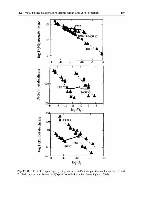
Fig. 11.10 Effect of oxygen fugacity (fO2) on the metal/silicate partition coefficient Ni, Ge andP. IW-1: one log unit below the f(O2) of iron-wüstite buffer. From Righter (2003)

11.3 Metal-Silicate Fractionation: Magma Ocean and Core Formation 419

DrGðP;T;XÞ ¼ 0 ¼ DrGoconðP;TÞ � Go

O2ð1bar;TÞ|fflfflfflfflfflfflfflfflfflfflfflfflfflfflfflfflfflfflfflfflfflfflfflffl{zfflfflfflfflfflfflfflfflfflfflfflfflfflfflfflfflfflfflfflfflfflfflfflffl}

DrG�ðTÞ

þRT lnasmCoO

aFe�lCo

� �fgO2

� �1=2ð11:3:1Þ

where the superscript o indicates pure phase, and DrGocon ¼ Go

CoOðsmÞ � GoCoðFe�lÞ.

The first two terms on the right of the above equation constitute the standard statefree energy change of the reaction (11.3.a) at T, while the appearance of fugacityinstead of activity of oxygen in the denominator of the equation is a consequence ofthe specific choice of standard state for O2(g) (a(O2) = f(O2)/f*(O2), while atP = 1 bar, f*(O2) * 1). By convention, Go

O2ð1 bar;TÞ ¼ 0: Now, defining the

partition coefficient of Co as

DFe�l=smCo ¼ XFe�l

Co

XsmCoO

ð11:3:2Þ

Eq. (11.3.1) can be written as

RT lnDFe�l=smCo ¼ DrG

ocon þRT ln csmCoO � RT ln cFe�l

Co � 12RT ln fgO2

ð11:3:3Þ

The pressure dependencies of the first and last terms on the right are evaluatedaccording to the relations (∂G/∂P)T = V and RT(∂lnfi/∂P)T = vi (Eq. 10.11.15a),respectively, where vi is the partial molar volume of i. In order to evaluate thepressure dependence of the activity coefficient terms at constant temperature, wefirst write lnc = f(P, T, X). Thus, using the total derivative of lnc at constanttemperature, we have (Eq. B.1.4)

@ ln ci@P

� �T¼ @ ln ci

@P

� �T;X

@P@P

� �Tþ @ ln ci

@Xi

� �P;T

@Xi

@P

� �T

Assuming that a dilute siderophile element obeys Henry’s law, the last term in theabove expression drops out since ci is independent of Xi within the Henry’s lawlimit at constant P-T condition and solvent composition (Sect. 8.8.1), in which case,using Eq. (10.11.7)

@ ln ci@P

� �T� @ ln ci

@P

� �T;X

¼ vi � Voi ð11:3:4Þ

where Voi and vi are, respectively, the end-member molar volume and partial molar

volume of i. Thus, we obtain

420 11 Element Fractionation in Geological Systems

@ lnDFe�l=smCo

@P

!T

¼ 1RT

DrvCo � 12vO2

� �ð11:3:5Þ

where DrvCo ¼ vCoOðsmÞ � vCoðFe�lÞ:For the general case of an arbitrary oxidation state of the partitioning metallic ion

in silicate melt, one writes (Capobianco et al. 1993)

MðFe� lÞþ n=4O2 ¼ MnþOn=2ðsilicate meltÞ ð11:3:bÞ

where n is the charge on the metal ion. Following the derivations of theEqs. (11.3.3) and (11.3.5), we then have the general expressions

RT lnDFe�1=smM ¼ DrG

ocon þRT ln csmMOn=2

� RT ln cFe�lM � n

4RT ln fgO2

ð11:3:6Þ

and

RT@ lnDFe�l=sm

M

@P

!T

¼ DrvM � n4vO2

� �ð11:3:7Þ

where the partition coefficient of M is defined as

DFe�l=smM ¼

XFe�lMOn=2

XsmM

ð11:3:8Þ

and

DrvM ¼ vMnþOn=2ðsmÞ � vMðFe�lÞ ð11:3:9Þ

The second term on the right of Eq. (11.3.7) (i.e. vO2) contributes to negative

pressure dependence of DFe�l=smM , but the net pressure dependence of D may be

either positive or negative depending on the values of DrvM and vO2.

11.3.2 Pressure Dependence of Metal-Silicate DistributionCoefficients

The distribution of a species between Fe-liquid (Fe-l) and silicate melt (sm) can alsobe treated in terms of an exchange reaction as discussed in Sect. 11.1.1. Thus, wewrite

FeðFe� lÞþCoOðsilicate meltÞ ¼ CoðFe� lÞþ FeOðsilicate meltÞ ð11:3:cÞ

11.3 Metal-Silicate Fractionation: Magma Ocean and Core Formation 421

for which the distribution coefficient, KD, is (see Eq. 11.1.2)

KDðCo� FeÞFe�l=sm ¼ XCo=XFeð ÞFe�l

XCoO=XFeOð Þsm ð11:3:10Þ

According to Eq. (11.1.3)

lnKDðCo� FeÞFe�1=sm ¼ lnK3:c � lnKcð3:cÞ ð11:3:11Þ

where Kc(3.7) is the ratio of the activity coefficients defined as

Kcð3:cÞ ¼ cCo=cFeð ÞFe�l

cCoO=cFeOð Þsm ð11:3:12Þ

Differentiating both sides of Eq. (11.3.11) with respect to pressure, and rearrangingterms, we obtain

@ lnKDðCo� FeÞFe�l=sm

@P

!T

¼ �DrvCoRT

¼ � 1RT

vCoðFe�lÞ � vFeðFe�lÞ� �� vCoOðsmÞ � vFeOðsmÞ

� � �ð11:3:13Þ

Derivation of this expression, which follows similar manipulations as those used toderive Eq. (11.3.5) including assumption of Henry’s law behavior of Co and Fe, isleft to the reader as an exercise.

For a metal that oxidizes to a valence state n, we can write the exchange reactionin the general form

n=2 FeðFe� lÞþMnþOn=2ðsilicate meltÞ ¼ MðFe� lÞþ n=2 FeOðsilicate meltÞð11:3:dÞ

for which

@ lnKDðM� FeÞFe�1=sm

@P

!T

¼ �DrvMRT

¼ � 1RT

vMðFe�1Þ � n2vFeðFe�1Þ

� �� vMOn=2ðsmÞ � n

2vFeoðsmÞ

� �h ið11:3:14Þ

422 11 Element Fractionation in Geological Systems

11.3.3 Pressure Dependencies of Ni Versus Co Partition-and Distribution-Coefficients: Depth of TerrestrialMagma Ocean

From Eq. (11.3.5) and analogous relation for DFe�l=smNi , we have at constant

temperature

@

@PD lnDFe�1=sm

Ni�Co

� �¼ 1

RTDrvNi � DrvCoð Þ

¼ 1RT

VCoðFe�1Þ � VNiðFe�1Þ� �� VCoOðsmÞ � VNiOðsmÞ

� � �ð11:3:15Þ

where D lnDFe�1=smNi�Co ¼ lnDFe�1=sm

Ni � lnDFe�1=smCo . Similarly, from Eq. (11.3.13) and

analogous expression for the distribution coefficient of Ni, we have

@

@PD lnKDðNi� CoÞFe�l=sm� �

¼ 1RT

VCoðFe�lÞ � VNiðFe�lÞ� �� VCoOðsmÞ � VNiOðsmÞ

� � �ð11:3:16Þ

where DlnKD(Ni-Co)Fe-l/sm = lnKD(Ni-Fe)

Fe-l/sm − lnKD(Co-Fe)Fe-l/sm. The right

hand terms of the last two equations are exactly the same. Consequently, the data onthe pressure dependence of lnD and lnKD, as illustrated in Fig. 11.9, are mutuallyincompatible. Thus, the issue of the relative pressure dependence of the partition ordistribution coefficient of Ni and Co between Fe-liquid and silicate melt remainsunresolved. However, we seek reasonable resolution of the problem as follows.

Since Fe (3d64s2), Co (3d74s2) and Ni (3d84s2) occupy three successivepositions in a row in the periodic table, it is reasonable to assume thatvNi=NiO � vCo=CoO � vCo=CoO � vFe=FeO; where vNi=NiO means the partial molarvolume of Ni or NiO, and so on, with the partial molar volumes of metals taken inFe-liquid, and those of metal-oxides taken in silicate melt. Thus, we write, usingEq. (11.3.16)

@

@PD lnKDðNi� CoÞFe�1=sm� �

¼ � 1RT

vNiðFe�lÞ � vCoðFe�lÞ� �� vNiOðsmÞ � vCoOðsmÞ

� � �� � 1

RTvCoðFe�lÞ � vFeðFe�lÞ� �� vCoOðsmÞ � vFeOðsmÞ

� � �ð11:3:17Þ

The quantity after the approximation sign is the same as that describing the pressuredependence of lnKD(Co-Fe)

Fe-l/sm (Eq. 11.3.13). Thus, using the experimental dataillustrated in Fig. 11.9b, the quantity within the square brackets after the approxi-mation sign is evaluated to be *8 cm3/mol. For brevity, we now denote the vol-umetric quantities within the first and second square brackets in the last equation as

11.3 Metal-Silicate Fractionation: Magma Ocean and Core Formation 423

DrVNi�Co ¼ VNiðFe�lÞ � VCoðFe�lÞ� �� VNiOðsmÞ � VCoOðsmÞ

� � ð11:3:18Þ

DrvCo�Fe ¼ vCoðFe�lÞ � VFeðFe�lÞ� �� vCoOðsmÞ � VFeOðsmÞ

� � ð11:3:19Þ

Assuming DrvCo-Fe to be insensitive to pressure, as suggested by the linear trend oflnKD versus P data at P > 3 GPa in Fig. 11.9b, we now integrate Eq. (11.3.17)between two pressures P* and Pref to obtain

D logKDðNi� CoÞ½ �p�� D logKDðNi� CoÞ½ �pref� � 8 P� � Pref� �2:303RT

ð11:3:20Þ

where

D logKDðNi� CoÞ ¼ logKDðNi� FeÞFe�1=sm � logKDðCo� FeÞFe�1=sm

at the specified pressure shown as a subscript. This equation shows that

D logKD Ni� Coð ÞP�\D logKD Ni� Coð ÞPref

at P* > Pref, that is, the logKD versus P trends of Ni and Co converge withincreasing pressure. Now, if the logKD versus P trends for Ni and Co intersect at thepressure P*, then the first term on the left of Eq. (11.3.20) is zero, so that

P� � Pref þ 2:303RT D logKDðNi� CoÞPref�

8ð11:3:21Þ

Choosing Pref as 5 GPa, and retrieving DlogKD(Ni-Co) at 5 GPa from Fig. 11.9b,we finally obtain P* � 32.3 GPa.

Thus, given the reasonable premise used in deriving the last expression, that isDrvNi-Co � DrvCo-Fe, we conclude that the dual problem of “excess abundance” ofNi and Co in the mantle and the chondritic relative abundance of these elementsmay be resolved if equilibrium was achieved between Fe-liquid and magma oceanat a depth corresponding to *32 GPa, which is similar to the depth of intersectionof the logD versus P trends of Ni and Co in Fig. 11.9a. A 20% error in the inferredvalue of DrvNi-Co yields a pressure range of 27–41 GPa for the intersection of thelogD versus P trends of Ni and Co.

11.4 Effect of Temperature and f(O2) on Metal-SilicatePartition Coefficient

Various estimates about the temperature of core formation in the Earth varybetween 2000 and 3750 K at 25–50 GPa (Rubie et al. 2007). Despite majoradvancements in the high pressure-temperature experimental studies, it is stillnecessary to extrapolate the laboratory experimental partitioning data to the high

424 11 Element Fractionation in Geological Systems

P-T conditions relevant to core formation. These extrapolations, however, need tobe guided by thermodynamic principles.

The expression for the temperature dependence of the distribution coefficient at aconstant pressure is readily obtained from Eq. (11.3.6) as

@ lnDFe�1=smM

@T

!P

¼ 1R

@ DrGocon=T

� �@T

� �Pþ

@ ln csmMOn=2=cFe�1

M

� �@T

0@

1A

p

� n4

@ ln fO2

@T

� �T

ð11:4:1Þ

To evaluate the first two terms on the right, we note that

@ðG=TÞ@T

¼ � H

RT2 ð11:4:2Þ

And

@ ln ci@T

� �P;X

¼ 1R

@ li � loi� �

@T

� �P;X

¼ � hi � Hoi

RT2 ð11:4:3Þ

where hi is the partial molar enthalpy of the component i. (The first equality in thelast equation follows from the relation li = li

o + RTlnXi + RTlnci.) AssumingHenry’s law behavior of the siderophile elements, we obtain (∂lnci/∂T)P =(∂lnci/∂T)P,X. The derivation of the last relation is analogous to that of the firstequality of Eq. (11.3.4). Thus, substitution of the last two relations in Eq. (11.4.1),and rearrangement of terms yield

@ lnDFe�1=smM

@T¼ � Drh

RT2 �n4@ ln fO2

@Tð11:4:4Þ

where Drh = h(MOn/2)sm − h(M)Fe-l, from which we obtain

lnDFe�1=smM ðT2Þ ¼ lnDFe�1=sm

M ðT1Þ � 1R

Z T2

T1

Drh

T2 dT

� n4

ln fO2ðT2Þ � ln fO2ðT1Þð Þð11:4:5Þ

It is sometimes convenient to replace – dT/T2 by d(1/T) so that, if Drh is constantover a chosen temperature interval, then

lnDFe�l=smM ðT2Þ ¼ lnDFe�l=sm

M ðT1Þþ DrhR

1T2

� 1T1

� �

� n4

ln fO2ðT2Þ � ln fO2ðT1Þð Þð11:4:6Þ

11.4 Effect of Temperature and f(O2) on Metal-Silicate Partition Coefficient 425

There are no data for the partial molar enthalpies in the systems of interest, whichmakes the extrapolation of lnD versus T very difficult. Capobianco et al. (1993)made the extrapolations assuming Drh = DrH

o.According to Eq. (11.4.6), logD versus logf(O2) relation is expected to be linear

with a slope of –n/4, if the effect of the variation of the activity coefficient terms arenegligible. The data summarized in Fig. 11.10 show that slopes of logD versuslogf(O2) relations of the different cations are almost exactly −n/4 if n is the numberof charges in the conventional valence state of the ions (2 for Ni, 4 for Ge and 5for P). Thus, it seems quite reasonable to predict −n/4 for the slopes of the logDversus logf(O2) relations of other trace elements, with n representing the number ofcharges in their conventional valences.

References

Allan NL, Blundy JD, Purton JA, Yu Lavrentiev M, Wood BJ (2001) Trace element incorporationin minerals and melts. In: Geiger CA (ed) Solid solutions in silicate and oxide systems. EötvösUniversity Press, Budapest, Hungary, pp 251–302

Asahara Y, Frost DJ, Rubie DC (2007) Partitioning of FeO between magnesiowüstite and liquidiron at high pressures and temperatures: implications for the composition of the Earth’s core.Earth Planet Sci Let 257:435–449

Blundy J, Wood B (1994) Prediction of crystal-melt partition coefficients from elastic modulii.Nature 372:452–454

Brice JC (1975) Some thermodynamic aspects of growth of strained crystals. J Cryst Growth28:249–253

Capobianco CJ, Jones JH, Drake MJ (1993) Meta-silicate thermochemistry at high temperature:magma oceans and the “excess siderophile element” problem of the Earth’s upper mantle.J Geophys Res 98:5433–5443

Ganguly J, Saxena SK (1987) Mixtures and mineral reactions. Springer, Berlin, Heidelberg, NewYork, Paris, Tokyo, p 291

Ganguly J, Cheng W, Tirone M (1996) Thermodynamics of aluminosilicate garnet solid solution:new experimental data, an optimized model, and thermometric applications. Contrib MinerPetrol 126:137–151

Gast P (1968) Trace element fractionation and the origin of tholeiitic and alkaline magma types.Geochim Cosmochim Acta 32:1057–1086

Kegler P, Holzheid A, Rubie DC, Frost DJ, Palme H (2005) New results on metal/silicatepartitioning of Ni and Co at elevated pressures and temperatures. Lunar and planetary scienceconference XXXVI, Abstr # 2030

Keppler H, Rubie DC (1993) Pressure-induced coordination changes of transition-metal ions insilicate melts. Nature 364:54–55

Li J, Agee CB (1996) Geochemistry of mantle-core differentiation at high pressure. Nature381:686–689

Liermann H-P, Ganguly J (2003) Fe2+-Mg fractionation between orthopyroxene and spinel:experimental calibration in the system FeO-MgO-Al2O3-Cr2O3-SiO2, and applications. ContribMiner Petrol 145:217–227

McDade P, Blundy JD, Wood BJ (2003) Trace element partitioning on the Tinquillo Lherzolitesolidus at 1.5 GPa. Phys Earth Planet Int 139:129–147

Ottonello G (1997) Principles of geochemistry. Columbia University Press, p 894Righter K (2003) Metal-silicate partitioning of siderophile elements and core formation in the early

Earth. Ann Rev Earth Planet Sci 31:135–174

426 11 Element Fractionation in Geological Systems

Righter K, Drake MJ (2003) Partition coefficients at high pressure and temperature. In:Carlson RW (ed) The mantle and core: treatise on geochemistry, Elsevier, pp 425–450

Rubie DC, Melosh HJ, Reid JE, Liebske C, Righter K (2003) Mechanisms of metal-silicateequilibration in the terrestrial magma ocean. Earth Planet Sci Let 205:239–255

Rubie DC, Nimmo F, Melosh HJ (2007) Formation of Earth’s core. In: Stevenson DJ(ed) Evolution of the Earth: treatise on geophysics, vol 9. Elsevier, Amsterdam, pp 51–90

Salters VJM, Longhi J (1999) Trace element partitioning during the initial stages of meltingbeneath mid-ocean ridges. Earth Planet Sci Lett 166:15–30

ShawDM(1970) Trace element fractionation during anatexis. GeochimCosmochimActa 34:237–243Sun C, Liang Y (2012) Distribution of REE between clinopyroxene and basaltic melt along a

mantle adiabat: effects of major element composition, water and temperature. Contrib MineralPetrol 163:807–823

Thibault Y, Walter MJ (1995) The influence of pressure and temperature on the metal- silicatepartition coefficients of nickel and cobalt in a model C1 chondrite and implications for metalsegregation in a deep magma ocean. Geochim Cosmochim Acta 59:991–1002

Tirone M, Ganguly J, Dohmen R, Langenhorst F, Hervig R, Becker H-W (2005) Rare earthdiffusion kinetics in garnet: experimental studies and applications. Geochim Comsochim Acta69:2385–2398

Van Westrenen W, Blundy J, Wood BJ (2000) Effect of Fe2+ on garnet-melt trace elementpartitioning: experiments in FCMAS and quantification of crystal-chemical controls in naturalsystems. Lithos 53:189–203

von Seckendorff V, O’Neill HStC (1993) An experimental study of Fe-Mg partitioning betweenolivine and orthopyroxene at 1173, 1273 and 1423 K and 1.6 GPa. Contrib Miner Petrol113:196–207

Williams ML, Grambling JA (1990) Manganese, ferric iron and the equilibrium between garnetand biotite. Am Miner 75:886–908

Wood BJ, Walter MJ, Wade J (2006) Accretion of the Earth and segregation of its core. Nature441:825–833

References 427

12Electrolyte Solutionsand Electrochemistry

An electrolyte is a compound which dissociates into charged species, eitherpartially or completely, after dissolving in a solution. In general, we can write thefollowing dissociation reaction for an electrolyte:

MmþAm� ¼ mþ ðMzþ Þ þ m�ðMz�Þ ð12:aÞ

where m+ and m− are the numbers of positive and negative ions (or ionic complexes),respectively, and z+ and z− are their respective formal charges. For example, H2SO4

dissociates in an aqueous solution according to H2SO4 = 2H+ + (SO4)2−. In this

case, m+ = 2, z+ = 1+, m− = 1, z− = 2−. Thermodynamics of electrolyte solutionsplay very important roles in the understanding of chemical equilibrium andredistribution of components in a variety of geochemical processes, such as thoserelating to ocean-atmosphere and fluid-rock interactions, solute transport in anaqueous solution, formation of sedimentary rocks, magma-hydrothermal systemsetc.

Electrolytes are classified as strong or weak electrolytes according to whetherthese dissociate strongly or weakly in an aqueous solution. In dealing with elec-trolyte solutions, it is customary to use molality as a measure of content of thesolute species. Molality is defined as the number of moles per kg of pure solvent,usually water.1 The content of dilute electrolytes in a solution is commonly reportedas ppm values, which indicate the mass of a solute per 106 g of solution. It shouldbe easy to see that the values reported as ppm can be converted to molalityaccording to the relation

molality ¼ ðppm=molecular weight of the soluteÞ � 10�3

1A similar sounding measure of content is molarity, M, which is defined as the moles of solute perliter of solution. The molarity measure is avoided since the solvent density changes as a function ofP-T condition making M a function of P-T.

© Springer Nature Switzerland AG 2020J. Ganguly, Thermodynamics in Earth and Planetary Sciences,Springer Textbooks in Earth Sciences, Geography and Environment,https://doi.org/10.1007/978-3-030-20879-0_12

429

A solution may be neutral or charged electrically. The properties of an ion in anelectrically neutral solution are much different from those in a charged solution. Indealing with the thermodynamics of electrolyte solution, the solution, as a whole istreated as electrically neutral.

12.1 Chemical Potential

The chemical potential of a species in an electrolyte solution is defined in the usualway (Box 8.1.2). For example, the chemical potential of a positive ion, l+ isdefined as

lþ ¼ @G@nþ

� �P;T;n�;nu;no

ð12:1:1Þ

where G is the total Gibbs free energy of the neutral solution, n+ and n− are thenumber of moles of positive and negative ions, respectively, nu is the number ofmoles of the undissociated solute, and no is the number of moles of the solvent.Because of the electroneutrality condition, the chemical potential of a chargedspecies cannot be measured directly by conventional methods as these require amacroscopic change in the number of moles of a charged species, while holding thenumber of moles of the species of opposite charge constant (along with the othervariables). However, it is formally correct to use chemical potentials of chargedspecies in the treatment of electrolyte solution, and a specific linear combination ofl+ and l− can be measured, as discussed below, following the exposition ofDenbigh (1981).

If lu is the chemical potential of the undissociated part of the electrolyte, thenfrom reaction (12.a), we have at equilibrium

lu ¼ mþ lþ þ m�l�; ð12:1:2Þ

Let us now consider the rate of change of Gibbs free energy of the solution withrespect to the addition of an electrolyte. If dme stands for an infinitesimal additionof the moles of electrolyte (e), then we define a chemical potential l of the elec-trolyte as a whole as the rate of change of G with respect to me. Thus,

l ¼ @G@ne

� �P;T;no

ð12:1:3Þ

Note that we are not concerned here what happens to the electrolyte after it isdissolved. Combining the expression of the total derivative of G of the solution withEq. (12.1.2) and the relationship among m and the various dissolved species, it canbe shown that at equilibrium (e.g. Denbigh 1981).

430 12 Electrolyte Solutions and Electrochemistry

l ¼ mþ lþ þ m�l� ð12:1:4Þ

Thus, since l is measurable, the linear combination of the chemical potentials of theionic species represented on the right side of the above equation is also measurable.Comparing Eqs. (12.1.2) and (12.1.4).

l ¼ lu ¼ mþ lþ þ m�l� ð12:1:5Þ

12.2 Activity and Activity Coefficients: Mean IonFormulations

The activity expressions for the dissociated and undissociated (u) solute species arebased on their molalities as

ai ¼ mici ð12:2:1Þ

where ai and mi stand respectively for the activity and molality of the species i.Because of the problem associated with the measurement of individual ion activi-ties, it is customary in the treatment of electrolyte solution to introduce linearcombination of the ion activities that can be measured, and this has led to thedevelopment of the concept of what is known as the mean ion activity and meanion activity coefficient.2

Expressing the chemical potentials of the charged species in terms of theirrespective standard state properties and activities in the usual way (Eq. 8.4.5), wehave from the last two expressions

l ¼ lu ¼ mþ l�þ þRT ln mþ cþ� �� �þ m� l�� þRT ln m�c�ð Þ� �

¼ mþ l�þ þ m�l�� þRT ln ðmþ Þmþ ðm�Þm�½ � þRT ln ðcþ Þmþ ðc�Þm�� � ð12:2:2Þ

where m+ and m− stand for the molalities of the positive and negative ions,respectively, and the superscript * stands, as usual, for the standard state at thetemperature of interest. The activity coefficient product within the last squarebrackets is used to define a mean ion activity coefficient, c±, of the electrolyte as

c�ð Þm¼ cþ� �mþ

c�ð Þm� ð12:2:3aÞ

or

2As we would see later, one often uses a quantity know as pH that is defined as pH = −log aþH .The activity of H+ ion may be determined by a combination of experimental and theoreticalprocedure, but as discussed by Pitzer (1995), “the basic uncertainty of single ion activity remains.”

12.1 Chemical Potential 431

c� ¼ cþ� �mþ

c�ð Þm�h i1=m

ð12:2:3bÞ

where m = m+ + m−. Similarly, one can define a mean ion activity of the electrolyteas

a� ¼ m�c� ð12:2:4Þ

where m±, known as the mean ion molality, is defined in a similar manner as c±,using the individual ion molalities. Equation (12.2.3b) can be generalized as

c�;k ¼Yi

cmii

!1=m

; ð12:2:5Þ

where k stands for an electrolyte, i stands for a dissociated species, mi for itsstoichiometric coefficient, and m =

Pmi.

12.3 Mass Balance Relation

An ion in a solution may exist both as a free ion and by complexing with anotherion, or simply by complexing with other ions. For example, in an aqueous solutionof NaCl and Na2SO4, sodium may be present as free Na+ ion, NaCl, NaSO�

4 ,Na(OH) and Na2SO4. In that case one can define a total molality of sodium as

mNaðtotÞ ¼ mNaþ þmNaCl þmNaSO4� þmNaðOHÞ þ 2 mNa2SO4ð Þ

(the multiplier 2 in the last term is due to the fact that there are 2 mol of Na in amole of Na2SO4). In general, we can then write

miðtotÞ ¼Xk

miðkÞmk ð12:3:1Þ

where mi(k) is the number of moles of the ith ion in the solute k and mk is the numberof moles of that solute.

12.4 Standard State Convention and Properties

12.4.1 Solute Standard State

When dealing with a major component (j) in a solution, it is usually desirable tochoose a standard state such that aj = Xj as Xj ! 1. As discussed in Sect. 8.8.2,

432 12 Electrolyte Solutions and Electrochemistry

this objective is realized by choosing a standard state of pure component at the P-Tcondition of interest. In dealing with a dilute solution, it is advantageous (to sim-plify life) to choose a standard state for the solute such that ai = mi as mi ! 0, sinceit is the property of the solute in dilute concentration that is of interest. Note that themanipulation of the theoretical framework so that the activity coefficient assumes aunit value (or any other value) does not affect the final outcome if the analysis iscarried out in a self-consistent manner.

According to Henry’s law for dilute solute (Eq. 8.8.1′), fi = K�Hmi as mi ! 0,

where i is an actual solute and K�H is a constant that is commonly referred to as the

Henry’s law constant (it is simply an activity coefficient that is independent of theconcentration of the solute within a specified range). Let us now extrapolate fi alongthe line fi = K�

Hmi, which we would refer to as ‘Henry’s law line’, to mi = 1 andchoose the resultant hypothetical state of the solute as its standard state (Fig. 12.1a).This is often referred to as the solute standard state based on the properties at theinfinite dilution. The slope of the Henry’s law line, K�

H, then becomes f�i =1 ¼ f�i .Thus, the Henry’s law transforms to

limit mi ! 0; fi ¼ f�imi

Since by definition, ai ¼ fi=f�i (Eq. 8.4.8), we then have

limit mi ! 0 ai ¼ mi; ð12:4:1Þ

as illustrated in Fig. 12.1b.For any ionic species, the solute standard state defined according to the above

procedure is a hypothetical state since an ionic species in a real solution does not

Standard state

mi 1

1

00

ai

ai = mi

Standard state

Henry’s law line

1 mi 00

fi*

fi

(a) (b)

Fig. 12.1 Illustration of the choice of solute standard state by extrapolating the Henry’s law line(dotted line) to unit molality in the (a) fugacity versus molality space and (b) activity versusmolality space. The solid lines show schematic behaviors of a real solution with negative deviationfrom ideality. In (a), the Henry’s law line follows relation f = KH(mi) where KH is a constant,whereas f* is the fugacity of the hypothetical standard state at unit molality

12.4 Standard State Convention and Properties 433

follow Henry’s law up to unit molality. However, for a neutral solute, the Henry’slaw behavior may be followed in the real solution up to unit molality, in which case,the standard state chosen according to the above procedure constitutes a real state.The solute standard state conforming to the property of unit activity at the unitmolality, whether it is real or hypothetical, will henceforth be designated by thesuperscript symbol x.

Instead of the activity of an actual solute, we may want to deal with the activityof a strong electrolyte (e.g. NaCl), ae, even though it has almost completely dis-sociated in a solution. In that case, as discussed in Sect. 8.8.1 (Eq. 8.8.12), wewould find that

ae / ðm�Þm; as m� ! 0;

where / indicates proportionality and m• is the molality of the electrolyte that onewould calculate had there been no dissociation (simply by knowing the amount ofthe electrolyte added to the solution), and m = m+ + m−. It is easy to see that theabove choice of “solute standard state” defined by the extrapolation of the Henry’slaw behavior to unit molality leads to the relation

ae ¼ ðm�Þm as m� ! 0 ð12:4:2Þ

Although it should be obvious, it is reiterated that both Eqs. (12.4.1) and (12.4.2)are statements of the Henry’s law in which the proportionality constants have beenmade to assume the value of unity through a clever choice of standard state.

12.4.2 Standard State Properties of Ions

Because of the problem with the experimental determination of single ion propertiesin a solution that is effectively electrically neutral, one obtains Gibbs free energy offormation of combination of ions, such as of H+(aq) and (OH)−(aq), NHþ

4 (aq) and(OH)−(aq), and so on. However, it is cumbersome to have listing of DGf of com-bination of ions. The convenient alternative to this practice is to have DGf of eachion in combination with a common ion, and assume the DGf of the latter to be zero.This is done by assuming that DrGf (1 bar, T) = 0 for the reaction

1=2H2ðgÞ $ Hþ ð1molal ideal aqueous solutionÞþ e�; ð12:4:aÞ

This is equivalent to saying that the standard state free energy of formation of H+

ion in an one molal ideal aqueous solution from a gaseous state is zero at anytemperature at 1 bar pressure. It follows that since ∂(DrG)/∂T = −DrS, andDrG = DrH − TDrS, both entropy and enthalpy of changes of the above reactionmust also be zero.

434 12 Electrolyte Solutions and Electrochemistry

To see how DGxf of other ions are calculated in a systematic way by assigning a

zero value to DGxf ðHþ Þ; let us consider the following example, which is discussed

by Denbigh (1981). For the ion pair H+(aq) and (OH)−(aq),

DGxf ð1 bar; 298KÞ ¼ �157; 297:48 J=mol,

whereas for the ion pair NHþ4 (aq) and (OH)−(aq),

DGxf ð1 bar; 298KÞ ¼ �236; 751:64 J=mol:

Now, since DGxf (H

+) (1 bar, 298 K) has been assigned a zero value, we have DGxf

(OH)− (1 bar, 298 K) = −157,297.48 J/mol, and consequently, DGxf [NHþ

4 (aq)](1 bar, 298 K) = −236,751.64 + 157,297.48 = −7954.16 J/mol.

12.5 Equilibrium Constant, Solubility Product and IonActivity Product: Survival of Marine CarbonateOrganisms

When the reaction (12.a) is at equilibrium, we can write, in the usual way

K � expð�DrG�=RTÞ ¼ mþð Þmþ m�ð Þm� c�ð Þm

aMmþAm�ð12:5:1Þ

where cm� is used to replace the term ðcmþþ Þðcm�� Þ (Eq. 12.2.3a). Now if Mm+Am− is a

solid electrolyte, and we have chosen pure state of that electrolyte at the P-T ofinterest as its standard state, then

RT lnKðP;TÞ ¼ mþ l�þ� �þ m� l��

� �� loMmþAv�

¼ mþ l�þ� �þ m� l��

� �� GoMmþAv�

ð12:5:2Þ

The equilibrium constant, K, defined by last relation, is called the solubility pro-duct, and is usually designated as Ksp. On the other hand, the product of theactivities of the dissociated solute in the form Pamii (i.e. numerator of the right handterm in Eq. 12.5.1) is called the ion activity product (IAP).

It follows from Eq. (12.5.1) that a solution is in equilibrium with a pure solidelectrolyte when IAP = Ksp, since for solid the standard state is pure solid (P,T) sothat the activity of a pure solid component is unity. It is easy to see that if IAP >Ksp, and the undissociated solute does not enter into solid solution, then the solutionmust precipitate additional solute in order to reduce the IAP to its equilibrium value,and vice versa. But what happens if electrolyte Mz+Az− enters into a solid solution?In that case, of course, one needs to compare the reaction quotient Q (i.e. the entire

12.4 Standard State Convention and Properties 435

right hand term of Eq. 12.5.1), not just the IAP, with Ksp. The solution wouldprecipitate the solid electrolyte when Q > Ksp, and vice versa.

As a simple illustration of the application of the concept of solubility productand ion activity product, let us consider the question of survival of marineorganisms with carbonate shells in the sea water, as discussed by Anderson (2005).The appropriate reaction to consider in this case is

CaCO3 $ Ca2þ þ ðCO3Þ2� ð12:5:aÞ

From the calculated values of the molalities Ca and (CO3)2− in the near surface

sea water, IAP for the above reaction equals 10−7.87. The Ksp value of thereaction depends on the polymorphic from of CaCO3, calcite (Cal) or aragonite(Arg), and is given by the relation Ksp = exp(−DrG*/RT) where DrG* =(CO�2

3 ) + Gxf (Ca

2+) − Gof (Calc/Arag). Using the standard state data, we have

KspðCalÞ ¼ 10�8:304

andKspðArgÞ ¼ 10�8:122

both of which are less than the IAP. Thus, the carbonate shells of marine organismswill not dissolve in the near surface sea water (marine organisms actually secretearagonite, so Ksp(Arg) is the more relevant solubility product to consider). How-ever, at depths greater than *5 km, the IAP falls below Ksp, and as a consequencethe marine organisms with carbonate shells do not survive below this depth. This isknown as the carbonate compensation depth of oceans.

The fate of marine organisms with carbonate shells is being challenged withincrease of CO2 content of the Earth’s atmosphere resulting from fossil fuelburning. The problem may be appreciated by considering the fact that increasingP(CO2) leads to an increase in the acidity of the ocean water (see Sect. 12.10) andthus a decrease of the ratio of IAP/Ksp(Arg) (XA), as illustrated in Fig. 12.2, whichis reproduced from Millero and DiTrolio (2010) (Although increasing P(CO2) leadsto increase of both H+ and CO�

3 in ocean water – see Sect. 12.10, the concentrationof H+ increases twice as fast as CO�

3 so that there is a net decrease in theconcentration of CO�

3 ).The dependence of (XA) on P(CO2) was calculated by Millero and DiTrolio

(2010) and that of P(CO2) on time by Caldeira and Wickett (2003) (seeSect. 12.10). Experimental studies show that reduction of the aragonite saturationparameter, XA, slows down the calcification rates of different coral species; thisrelationship is also borne out by historical records (Millero and DiTrolio 2010;Langdon and Atkinson 2005). The saturation parameter may even fall below unityin the late 21st century, resulting in dissolution of the aragonite skeletal structuresof marine organism.

436 12 Electrolyte Solutions and Electrochemistry

Problem 12.1 Consider the dissociation of a solid electrolyte in an aqueoussolution, and assume that it is present in a solid solution, e.g. the dissociationreaction (12.5.a) with CaCO3 dissolved in a solid solution (Ca,Mg)CO3. Will thesolid necessarily dissolve when IAP < Ksp?

Answer: No (but discuss the reason).

12.6 Ion Activity Coefficients and Ionic Strength

12.6.1 Debye-Hückel and Related Methods

A convenient starting point in the discussion about the ion activity coefficients in adilute electrolyte solution is a theoretical expression known as the Debye-Hückellimiting law. In deriving this law, which yields the activity coefficient of an ion atvery high dilution, it is assumed that (a) the deviation from ideality in a dilute ionicsolution is entirely due to the electrical interactions between the ions, (b) the ionsare point charges, (c) the solute is completely dissociated and (d) the repulsiveforces between the ions are unimportant. Since the repulsive force drops off veryrapidly with the distance of separation, the last assumption is justified in a verydilute ionic solution where the ions are far apart. Within the above framework,Debye and Hückel derived an expression for the individual ion activity coefficients,which is as follows.

log ci ¼ �AZ2i

ffiffiI

pð12:6:1Þ

Fig. 12.2 Estimated change of P(CO2) in the Earth’s atmosphere and corresponding saturationstate of aragonite in the ocean water with time. From Millero and DiTroilo (2010). Withpermission from Mineralogical Society of America

12.5 Equilibrium Constant, Solubility Product and Ion Activity Product … 437

where Zi is the charge of the ionic species i, A is a constant, in unit of (kg/mol)½,and depends on the dielectric constant and density of the solvent, and I is the ionicstrength of the solution that is given by

I ¼ 1=2X

miz2i mol=kg ð12:6:2Þ

As an example, the ionic strength of one molal solution of La2(SO4)3,whichdissociates in the solution according to La2(SO4)3 ! 2La3+ + 3(SO4)

2−, is½[2(3)2 + 3(2)2] = 15 mol/kg.

Debye and Hückel (1923) modified their earlier theory to account for the effectsof finite sizes of the ions and short range interactions between them, assuming thatthe ions are nondeformable spheres of equal radii. A widely used extension(Robinson and Stokes 1959; Helgeson 1969) of the modified Debye-Hückelexpression of activity coefficient is

log ci ¼ � Az2iffiffiI

p

1þBaiffiffiI

p þB�I, ð12:6:3Þ

where the last term ðB�IÞ represents the extension to the original Debye-Hückel(1923) form. This expression will be referred to as the extended Debye-Hückelformulation. Here B is another constant that is characteristic of the solvent, ai is the“distance of closest approach” between ions of opposite charge, and B� (oftencalled B-dot, and also referred to as “deviation function”) is an adjustable parameterto fit the experimental data. In fact the ai term can also be treated as an adjustableparameter. The unit of Bai is (kg/mol)½.

The above equation seems to work well up to around 1 molal solute concen-tration. Helgeson and Kirkham (1974a, b) have given values of A and B for waterfrom 0 to 300 °C. At 0 °C, A = 0.4911 and B = 0.3244 whereas at 300 °C, thesevalues are 1.2555 and 0.3965, respectively, with the unit of B in kg½/(mol½-Å). It iseasy to see that when the solution becomes very dilute, Eq. (12.6.3) yields theDeby-Hückel limiting law (Eq. 12.6.1) since the denominator of the first equationapproaches unity as I ! 0.

Because of the problem in measuring individual ion activity coefficients, c+ andc− are combined according to Eq. (12.2.3) to yield an expression for c±, which canbe compared with experimentally determined values. Substituting the expressionfor the individual ion activities (Eq. 12.6.3), into Eq. (12.2.3), and using a singleadjustable _a parameter, we obtain

m log c�ð Þ ¼ � AffiffiI

p

IþB _affiffiI

p mþ z2þ þ m�z2�� �þ mB�I ð12:6:4Þ

However, since the electroneutrality condition requires that |m+z+| = |m−z−|, the termwithin the parentheses can be written as (m− z−z+ + m+z+z−) = z−z+(m+ + m−) =(z−z+). Thus, we finally obtain

438 12 Electrolyte Solutions and Electrochemistry

log c� ¼ �A zþ z�j j ffiffiIp

1þB _affiffiI

p þB�I ð12:6:5Þ

In a solution consisting of the dissociation products of a single electrolyte, theexpressions for single ion and mean ion activity coefficients satisfy the relationci ! 1 as mi ! 0, which is imposed by the choice of solute standard statediscussed in Sect. 12.4.1 (Fig. 12.1). This is because I ! 0 as mi ! 0 (for thedissociation of a single electrolyte, the molalities of the dissociated species areproportional to each other). The numerator on the right hand side of Eq. (12.6.5)reflects the effect of long-range Coulomb forces. The modification of these forcesby short-range interactions between the ions in the crudest approximation ofhard-sphere model is given by the term in the denominator. The B-dot term partiallytakes care of the short-range interaction between ions and the solvent molecules andother types of short range interactions between ions that cannot be adequatelyaccounted for by the hard sphere model.

Helgeson (1969) summarized the values of the different parameters inEq. (12.6.3) for concentrated NaCl aqueous solutions that may be used to calculatethe individual activity coefficients of dissolved ions up to *300 °C at 1 barpressure. Values of A, B and _a parameters for aqueous solutions up to 60 °C canalso be found in Garrels and Christ (1965). The latter workers have calculatedindividual ion activity coefficients in aqueous solutions using the classicDebye-Hückel formulation (i.e. Eq. 12.6.3, but without the B-dot term) for severalions in aqueous solution, and compared the results with those calculated from theexperimental data on mean ion activity coefficients, c±, according to the “mean-saltmethod” that is discussed below. The results, which are illustrated in Fig. 12.3,show good agreement between the two methods up to ionic strength of 0.1. Thedeparture of Debye-Hückel prediction from the experimentally constrained result ofthe mean-salt method at higher ionic strength may be accounted for by the B-dotterm.

12.6.2 Mean-Salt Method

The “mean-salt method” was introduced by Garrels and Christ (1965) in the geo-chemical literature for the calculation of individual ion activity coefficients, ci, inaqueous solutions at ionic strengths where the classic Debye-Hückel formulationfor ci fails. The method relates ci to the mean ion activity coefficients that can bemeasured experimentally. In developing this method, it was assumed that in anaqueous solution, cKþ ¼ cCl� , as seems to be indicated by various lines of evidence(this relationship was first proposed by MacInnes (1919), and is sometimes referredto as the MacInnes’ convention). Thus, using Eq. (12.2.3b),

c�KCl ¼ ðcKþ ÞðcCl�Þ½ �1=2¼ cKþ ¼ cCl� ð12:6:6Þ

12.6 Ion Activity Coefficients and Ionic Strength 439

Using the c(K+) and c(Cl−) values calculated according to this relation from themeasured values of c± (KCl), one can systematically calculate the individualactivity coefficients of many other ions from appropriate experimental data on themean ion activity coefficients. For example, for a solution of a MCl2 electrolyte,where M is a divalent cation, one can write, using Eqs. (12.2.3b) and (12.6.6)

c�MCl2 ¼ ðcMþ ÞðcCl�Þ2h i1=3

¼ ðcMþ Þðc�KClÞ2h i1=3

so that

cMþ ¼ ðc�MCl2Þ3ðc�KClÞ2

ð12:6:7Þ

A similar method may be developed to calculate the individual activity of an anionthat combines with K to form an electrolyte, e.g. KF.

In case the electrolyte does not contain either K or Cl, one needs to employ aconnection with these ions by introducing an intermediate step, which is called the

Symbols:Debye-Hückel formulation

+

_

Fig. 12.3 Individual ion activity coefficients versus ionic strength. The symbols representcalculations using the modified Debye-Hückel formulation (Eq. 12.6.3, but without the B-dotterm), whereas the lines represent calculations of individual ion activity coefficients from themeasured values of mean ion activity coefficient according to the “mean salt method”. FromGarrels and Christ (1965). The Debye-Hückel model fails at I > 0.1. With permission from Harperand Row—Pearson Education

440 12 Electrolyte Solutions and Electrochemistry

“double bridge method” by Garrels and Christ (1965). For example, to calculatec(Cu2+) from the measured values of c±(Cu2SO4), one needs to use c(SO4)

2− that isdetermined from the experimental data for c±(K2SO4).

12.7 Multicomponent High Ionic Strength and High P-TSystems

In modeling natural processes, we usually need to deal with solutions that havemultiple electrolytes, high ionic strength, and are subjected to P-T conditions thatare often far removed from the typical 1 bar, 298 K condition of the conventionaldomain of electrolyte thermodynamics. As an example, progressive evaporation ofsea water to form brines would lead to multicomponent solution of high ionicstrength that cannot be handled with simple extension of Debye-Hückel formulationof ion activity coefficients. In addition, modeling of such geological processes asfluid-rock interactions in the mid-ocean ridges or in the Earth’s crust require anunderstanding of the behavior of electrolyte solutions at relatively high P-T con-ditions. There are two groups of major contributions to address these types ofproblems, one by Pitzer (1973, 1975, 1987) and the other by Helgeson andcoworkers (Helgeson and Kirkham 1974a, b, 1976; Helgeson et al. 1981; Tangerand Helgeson 1981, 1988; Shock et al. 1992). These are often referred to as Pitzerequations/model and HKF model.

The Pitzer equations were originally developed to treat multicomponent elec-trolytes of relatively high ionic strengths at 1 bar, 25 °C. Some attempts were latermade to extend it to higher P-T conditions (e.g. Pitzer 1987), but here we limit ourdiscussion to see how the properties of multicomponent electrolytes are treated inthe Pitzer equations since this is what the Pitzer equations are famous for. Verygood exposition of the Pitzer formulation can be found in Harvie and Weare (1980)and Wolery (1992).

Pitzer introduced an expression of ΔGxs of a multicomponent electrolyte solutionas

DGxs

RT¼ nw fðIÞþ

Xij

kijmimj þXijk

nijkmimjmk

" #ð12:7:1Þ

where nw is number of kilograms of solvent, f(I) is a “Debye-Hückel function”accounting for the long-range electrical interactions to first order, and kij and nijk arebinary and ternary interaction parameters that are, in general, functions of the ionicstrength. The first and second summations are to be carried out over every binaryand ternary sub-systems, respectively, of the multicomponent solution.

Except for the f(I) term, the above expression is formally similar to that of ΔGxs

of non-electrolyte solution (Eq. 9.3.2). It can be extended to include quaternaryinteractions, but it was found that such higher order terms are almost never required

12.6 Ion Activity Coefficients and Ionic Strength 441

to treat the properties of multicomponent electrolyte solutions (We recall thatquaternary interactions are not needed for multicomponent non-electrolyte solutionsif the bounding binaries conform to the regular or sub-regular models, as are oftenthe case). The “Debye-Hückel function” used in the above expression is not theusual Debye-Hückel expression of activity coefficient, but a similar expressionderived by Pitzer (1973). As in the case of non-electrolyte solution, the binary andternary interaction parameters are to be determined by fitting experimental data inthe binary and ternary sub-systems of the multicomponent solution. Once there isan expression for ΔGxs, all other excess thermodynamic properties, including theion activity coefficients, can be obtained by systematic thermodynamic operationson the expression of ΔGxs, as discussed in Sect. 8.6. Figure 12.4 illustrates thesuccess of Pitzer formulation to represent ion activity coefficients in aqueoussolution to high ionic strength. A computer program, EQ3NR, was developed in theLawrence Livermore National Laboratory (Wolrey 1992) to carry out calculationsusing the Pitzer model. The program has self-consistent values of the differentparameters that are needed for this purpose.

The Pitzer model has been used successfully to calculate the development ofmineral sequences in a number of geological environments at 1 bar, 25 °C.Figure 12.5 shows agreement between the phase diagram determined experimen-tally and calculated by Harvie and Weare (1980) using Pitzer model for the systemNa-Mg-Cl-SO4-H2O at 1 bar, 25 °C. Harvie and Weare (1980) calculated the

HCl (w)

HCl (KCl)

KCl

I

Fig. 12.4 The mean activity coefficient of HCl and KCl in different systems as function of ionicstrength, I. cHCl

± (w) and cHCl± (KCl): mean ion activity coefficient of HCl in HCl-H2O and KCl-H2O

systems, respectively; cKCl± : mean ion activity coefficient of KCl in KCl-H2O. The solid curve

represents calculation using Pitzer equation whereas the dashed curve is a simplified version of thePitzer equation discussed in Harvie et al. (1984). Filled circles: experimental data. From Harvieet al. (1984). With permission from Elsevier

442 12 Electrolyte Solutions and Electrochemistry

development of mineralogical sequence due to progressive evaporation of seawater. The calculated sequence essentially matches the observed sequence ofmineral zones in the classic Zechstein evaporite deposit in Germany. Simplifiedcalculations carried out earlier did not have similar level of agreement with theobserved sequence, thus leading to complex hypotheses about the formation of thisdeposit. The calculations of Harvie and Weare (1980) almost conclusively provethat the Zechstein deposit formed by the progressive evaporation of sea water.

The HKF group of papers developed internally consistent data set for thestandard state properties of species in aqueous solutions that can be used to cal-culate the equilibrium constants of a wide variety of geochemical reactions from 1to 5 kbar and 0 to 1000 °C. These calculations may be carried out using a softwarepackage, SUPCRT92 (Johnson et al. 1992) that has been used widely in geo-chemical and materials science literature. The standard state properties have beencalculated through a combination of fundamental theory and available experimentaldata that help constrain the theoretical parameters. A comprehensive discussion ofHKF papers is beyond the scope of this chapter, but it is noted that the HKFformulations account for the effects of both long- and short-range ionic interactions,local collapse of solvent structure around solvated ions, the concentration depen-dence of dielectric constant of electrolyte solutions, and the effect of ion association

BischofiteKieseriteHexahedrite

Epsomite

BloediteHalite

ThenarditeMirabilite

Na2Cl2 Na2SO4

MgSO4 MgCl2

Fig. 12.5 Comparison of the calculated and experimental (symbols) phase diagram for theNa-Mg-Cl-SO4-H2O reciprocal system. Solid lines: calculations by Harvie and Weare (1980)using the Pitzer model. The dashed lines represent results of another model discussed by Harvieet al. (1984). From Harvie et al. (1984). With permission from Elsevier

12.7 Multicomponent High Ionic Strength and High P-T Systems 443

on ionic strength. An impression of the level of success of the HKF models may beconveyed by showing examples of the agreement between predicted and measuredproperties. In this spirit, Fig. 12.6 is reproduced from Helgeson et al. (1981) andFig. 12.7 from Tanger and Helgeson (1988) showing, respectively, the variation ofmean activity coefficient of NaCl and standard partial molal volume of NaCl asfunction of pressure and temperature.

12.8 Activity Diagrams of Mineral Stabilities

At constant P-T condition, variation of fluid compositions affects the mineral sta-bilities. It is, thus, useful to construct mineral stability diagrams as function of theactivities of fluid species at constant P-T conditions. These types of diagrams areknown as activity diagrams, since both axes in the plot represent activities (orcombination of activities) of selected aqueous species. Bowers et al. (1984) havepresented an entire book of such diagrams for rock-forming minerals for pressuresand temperatures up to 5 kb and 600 °C using the standard state thermodynamicproperties from Helgeson et al. (1981). We first present below the thermodynamicmethodology for the construction of activity-activity diagrams, and then discussillustrative applications. The standard states of the mineral components and H2O

NaCl

Ionic Strength

Fig. 12.6 Comparison ofexperimental mean ionactivity coefficients (symbols)of NaCl with those calculatedfrom HKF model as functionof ionic strength at varioustemperatures (indicated in°C). The curve for 25 °C is at1 bar pressure whereas theother curves are at pressuresdefined by the liquid-vaporequilibrium at the specifiedtemperatures. From Helgesonet al. (1981). With permissionfrom American Journal ofScience

444 12 Electrolyte Solutions and Electrochemistry

have been chosen to be pure components at P-T, while the dilute aqueous speciesare referred to the solute standard states at unit molality defined by the Henry’s lawline (Fig. 12.1).

12.8.1 Method of Calculation

To illustrate the calculation of activity diagrams, let us consider the problem of thestability of K-feldspar (KAlSi3O8), kaolinite (Al2Si2O5(OH)4) and muscovite(KAl3Si3O10(OH)2) in the presence of water at 1 bar, 298 K, which has beendiscussed earlier by Anderson (2005). The reaction relations among the threeminerals and aqueous ions can be written as

KAlSi3O8 þ 1=2H2OþHþ ðaqÞ ¼ 1=2Al2Si2O5ðOHÞ4 þ 2SiO2ðaqÞþKþ ðaqÞð12:8:aÞ

3=2KAlSi3O8 þHþ ðaqÞ ¼ 1=2KAl3Si3O10ðOHÞ2 þ 3 SiO2ðaqÞþKþ ðaqÞð12:8:bÞ

and

KAl3Si3O10ðOHÞ2 þ 3=2H2OþHþ ðaqÞ ¼ 3=2Al2Si2O5ðOHÞ4 þKþ ðaqÞð12:8:cÞ

Fig. 12.7 Comparison ofstandard partial molal volumeof NaCl as a function ofpressure and temperature, ascalculated by Tanger andHelgeson (1988: curves) withthe experimental data(symbols). PSAT refers topressure along liquid-vaporsaturation pressures for H2O.From Tanger and Helgeson(1988). With permission fromAmerican Journal of Science

12.8 Activity Diagrams of Mineral Stabilities 445

To illustrate the general procedure of calculation of equilibrium boundary in theactivity space, let us now consider the reaction (12.8.a) and assume, for simplicity,that the minerals and H2O are present essentially in their respective pure states sothat a(H2O) = a(mineral) = 1. Thus, at equilibrium at 1 bar, T, we have

Kað1;TÞ ¼ e�DrG�a=RT ¼

aaqSiO2

2aaqKþ� �

aaqHþ� � ð12:8:1Þ

with

DrG�a ¼ 1=2ðDGo

fðkaoliniteÞÞ þ 2DG�fðSiO2:aqÞ þDG�

fðkþ :aqÞh i� DGo

fðk�sparÞ þ 1=2ðDGofðH2OÞÞ þDG�

fðHþ :aqÞh i ð12:8:2Þ

Using the data from Wagman et al. (1982), and noting that DGxfðHþ :aqÞ ¼ 0,

according to convention,

DrG�að1 bar; 298KÞ ¼ 1=2ð�3799:7Þþ 2ð�833:411Þþ ð�283:27Þ½ �

� �3742:9þ 1=2ð�237:129Þ½ � ¼ 11:523 kJð12:8:3Þ

Since there are three activity terms in Eq. (12.8.1), two of these terms need to becombined for a two dimensional activity diagram. The manner in which the dif-ferent activity terms should be combined is dictated by the requirement that allequilibria in the system are to be represented in a single diagram. Thus, we decideto plot the ratio a(K+)/a(H+) on the y-axis, and a(SiO2) on the x-axis. In fact, forreasons that should be obvious from the derivation below, we plot the logarithms ofthe activity terms instead of the activity terms themselves.

The next step is to calculate the slopes of the equilibrium reaction boundaries inthe activity diagram. This is easily done from the expression of K. Thus, for theequilibrium (12.8.a), we obtain by taking the logarithm of Eq. (12.8.1), and rear-ranging terms

logaKþ

aHþ¼ logKa � 2 logðaSiO2Þ ð12:8:4Þ

Similarly,

logaKþ

aHþ¼ logKb � 3 logðaSiO2Þ ð12:8:5Þ

446 12 Electrolyte Solutions and Electrochemistry

and

logaKþ

aHþ¼ logKc; ð12:8:6Þ

The last expression implies a zero slope of the equilibrium boundary of the reaction(12.8.c) in the log (aK+/aH+) versus log (aSiO2) plot.

Equations (12.8.4) and (12.8.5) are linear equations in which the coefficients oflog [a(SiO2)] define the slopes and the log K terms define the intercepts of theequilibrium boundaries in the activity plot. The log K terms can be calculated fromthe available data on the standard state free energies, using the relation lnK = −DrG*/RT. Thus, using DrG* (1 bar, 298 K) for equilibrium (a) calculatedabove, log Ka (1 bar, 298 K) = −2.019. Similarly, log Kb (1 bar, 298 K) = −4.668and log Kc = 3.281.

The reaction boundaries defining the equilibrium stability limits of muscovite,kaolinite and K-feldspar at 1 bar, 298 K, as calculated from the above values ofequilibrium constants and the last three equations, are illustrated in Fig. 12.8.According to reactions (12.8.a) and (12.8.b), increasing a(SiO2(aq)) stabilizesK-feldspar with respect to either muscovite or kaolinite. Thus, K-feldspar stabilityfield is located on the higher a(SiO2) side. Also, the change of breakdown productof K-feldspar must cause a reduction of its field of stability relative to that definedby the extension of a single reaction past the transition between kaolinite andmuscovite. This requirement leads to the topology shown in Fig. 12.8.

-2

0

2

4

6

8

10

12

-6 -5 -4 -3 -2 -1 0

log a(SiO2(aq))

log

a(K

+)/a

(H+)

Kaolinite

K-feldspar

Muscovite

Fig. 12.8 Stability relations of muscovite, kaolinite and K-feldspar at 1 bar, 298 K, as functionof activities of ions dissolved in an aqueous solution

12.8 Activity Diagrams of Mineral Stabilities 447

12.8.2 Illustrative Applications

12.8.2.1 Spring Waters

As examples of applications of activity diagrams of aqueous species to geologicalproblems, we consider here the studies of Norton and Panichi (1978) and Mariniet al. (2000) of spring waters in Italy.

Norton and Panichi (1978) studied the chemistry of the spring waters in theAbano region in northern Italy and determined the source region and subsurfacecirculation path by comparing the water chemistry with those expected fromequilibration with different minerals in the bed rock. Figure 12.8 shows the sta-bilities of the minerals kaolinite, Ca-montmorillonite and Mg-montmorillonite at1 bar, 75 °C (348 K) in a log (aCa++/(aH+)

2) versus log (aMg++/(aH+)2) plot (It is left

to the reader as an exercise to figure out the reactions that relate the equilibriumboundaries to these activity ratios). It is assumed that the mineral phases and H2Ohave unit activities.

The dashed lines in Fig. 12.9 represent the saturation conditions of the aqueoussolution for calcite (CaCO3) and dolomite (CaMg(CO3)2) at P(CO2) = 10−2 bars.The saturation condition is calculated as follows. For the dissolution of calcite in anaqueous solution, one can write

CaCO3 þ 2Hþ ðaqÞ ¼ Ca2þ ðaqÞþCO2ðgÞþH2O ð12:8:dÞ

for which

Kd � e�DrG�d ¼

aaqCa2þ

aCO2ð Þ aH2Oð Þ

aCaCO3ð Þ aaqHþ� �2 ð12:8:7Þ

Fig. 12.9 Measured compositions (squares) of water samples from Abano region, Italy, plotted oncalculated activity diagram depicting the stability of minerals in equilibriumwith an aqueous phase at1 bar, 75 °C and unit activity of H2O. Dashed lines represent saturation surfaces of calcite anddolomite at PCO2 ¼ 10�2 bars. From Norton and Panichi (1978). With permission from Elsevier

448 12 Electrolyte Solutions and Electrochemistry

With the standard state of CO2 as pure CO2 at unit fugacity at T, so that a(CO2) =f(CO2) P(CO2) and G*(CO2) Go(CO2) at 1 bar, T, and assuming that CaCO3

is in the pure state so that a(CaCO3) = 1, the last equation reduces to

Kd � e�DrG�d

aaqCa2þ

PCO2ð Þ

aaqHþ� �2 ð12:8:8Þ

with

DrG�d DG�

fðCa2þ :aqÞ þDGofðCO2Þ þDGo

fðH2OÞh i� DGo

fðCaCO3Þ þ 2DG�fðHþ :aqÞ

h i

with all G values at 1 bar, 348 K. Thus, for calcite saturation, we have

logaaqCa2þ

aaqHþ� �2 !

logKdð1 bar; 348KÞ � log PCO2 ð12:8:9Þ

Consequently, in a plot of log aCa2þ =a2Hþ

� �versus log aMg2þ =a

2Hþ

, the calcite

saturation curve is a horizontal line (i.e. the coefficient for the x-axis term is zero)with an intercept given by the value of log Kd=PCO2ð Þ. It is now left to reader todevelop the equation for dolomite saturation curve (Problem 12.2).

The square symbols in Fig. 12.9 represent the measured water compositions inthe Abano hot spring region. The compositions plot on the equilibrium boundarybetween Ca-montmorillonite and Mg-montmorillonite, and thus imply that the fluidhad passed through bed rocks containing these minerals and essentially achievedequilibrium with them. In addition, several fluid compositions (not shown inFig. 12.9) fall above or close to the calcite and dolomite saturation curves. Thisimplies that the fluid had also passed through bed rocks containing these carbonateminerals. The oxygen isotopic composition indicates that the hot spring fluid isderived from meteoric water infiltration into Permian and Mesozoic aquifers in thepre-Alps, which lie north of the Abano region. Thus, the combination of isotopegeochemistry and thermodynamic calculations leads to an understanding of thesource region and circulation path of fluid that finally found surface expression ashot springs.

Marini et al. (2000) studied the spring water chemistry in the Bisagno valley,Genoa, Italy, and developed model for the evolution of the water chemistry in termsof reaction kinetics between the bed rock minerals and aqueous fluid. The kineticaspect of this work is beyond the scope of the present chapter, but the readers areencouraged to read this analysis for a good introduction to kinetic modeling.

12.8 Activity Diagrams of Mineral Stabilities 449

Figure 12.10 shows the measured fluid compositions (circles) in two activity dia-grams, and also the computed kinetic evolution paths of the fluid compositions(crosses).

There is good agreement between the measured and computed fluid composi-tions. The measured fluid compositions fall mostly in the field of kaolinite and hadclearly evolved within the stability field of this mineral (Fig. 12.10a). The fluidcompositions also evolved along the equilibrium boundary between calcite anddolomite (Fig. 12.10b), which implies that the fluid achieved equilibrium with theseminerals as it moved through the bed rocks. The measured compositions do notshow any buffering by the kaolinite-muscovite boundary. This is in good agreementwith computed fluid compositions that account for the reaction kinetics taking intoconsideration the reacting surface areas. As noted by Marini et al. (2000), theobserved equilibration of the fluid with the carbonates (Fig. 12.10b) and lack ofbuffering by the muscovite-kaolinite boundary (Fig. 12.10a) are consistent with therelatively higher dissolution rates of the carbonates in aqueous solution.

One interesting aspect of the compositional trend of fluid of the Bisagno valley isthat the fluid compositions seem to have evolved towards the albite, K-feldspar,muscovite invariant point, representing the situation of final stable equilibriumbetween the aqueous solution and the constituent minerals of local aquifer rocksHowever, probably due to kinetic reasons, the evolutionary path does not follow themuscovite, kaolinite phase boundary, as expected based on a purely thermodynamicground. These calculations serve to illustrate the point that while activity plots ofstability of minerals in equilibrium with aqueous solutions provide useful frame-work for the understanding of fluid-rock reactions, the fluid compositions do notnecessarily evolve in thermodynamic equilibrium with the minerals.

Fig. 12.10 Measured (open symbols) and calculated (crosses) compositions of the Bisagnovalley spring waters, Genoa, Italy, plotted on activity diagrams depicting the stability of minerals.Reproduced from Marini et al. (2000). With permission from Elsevier

450 12 Electrolyte Solutions and Electrochemistry

Problem 12.2 Develop the equation for dolomite saturation of aqueous solution

and determine the slope of the line in the log aCa2þ =a2Hþ

� �versus log aMg2þ =a

2Hþ

activity diagram (Fig. 12.9).

12.8.2.2 Stability of Magnesium Silicates

As a final example of the use of activity diagram, we illustrate the stability ofmagnesium silicates (Fig. 12.11) that was calculated by Faure (1991), using

log aMg2þ =a2Hþ

and log aH2SO4ð Þ as the two axes. To illustrate the calculation of

mineral stabilities in the activity plot, let us consider the dissolution reaction offorsterite in water, viz.,

1=2Mg2SiO4 þ 2Hþ ðaqÞ $ Mg2þ þ 1=2H4SiO4ðaqÞ ð12:8:eÞ

for which the expression of equilibrium constant and standard state thermodynamicproperties yield

Fig. 12.11 Solubility limits of pure magnesium silicates in water at 1 bar, 25 °C. With increasein the activity ratio of [Mg2+/H+] and/or activity of [H4SiO4], natural water will precipitate one ofthe phases, magnesite, serpentine, sepiolite, or amorphous silica, depending on the manner inwhich these activities change. This diagram shows that at the surface of the earth, the only phasesthat are thermodynamically stable in contact with natural water are magnesite, serpentine, sepioliteand amorphous silica. From Faure (1991)

12.8 Activity Diagrams of Mineral Stabilities 451

logaMg2þ

aHþð Þ2 ¼ �0:5 log aH2SiO4ð Þþ 14:2 ð12:8:10Þ

This equation is represented by the dashed curve labeled “Forsterite” in Fig. 12.11.Forsterite is stable in equilibrium with an aqueous solution with composition abovethe dashed curve, but dissolves in aqueous solutions with composition below thiscurve.

If equilibrium is achieved, all magnesium silicate minerals would dissolve in anaqueous solution with composition below the heavy line in the lower left side of theactivity diagram. The arrow indicates the equilibrium evolution of the compositionof an aqueous solution with initial composition at the point P as a result of dis-solution of enstatite. The trajectory of fluid composition intersects the stability limitof serpentine. Thus under equilibrium condition, an aqueous solution with initialcomposition marked by the point P would precipitate serpentine after sufficientdissolution of enstatite. Figure 12.11 shows that only magnesite, serpentine,sepiolite and amorphous silica are thermodynamically stable in contact with naturalwater on the surface of the Earth.

12.9 Electrochemical Cells, Nernst Equation and f(O2)Measurement by Solid Electrolyte

12.9.1 Electrochemical Cell and Half-Cells

In an electrochemical cell, electrons released in one part the cell by oxidation of anelectrode flow through a conducting wire to another electrode and are used forreduction reaction, as illustrated in Fig. 12.12. Following IUPAC (International

ZnCu

Zn + (SO4)2-

ZnSO4 + 2(e-) (oxidation)

CuSO4 + 2(e-)

Cu + (SO4)2-

(reduction)

(SO4)2-

CuSO4ZnSO4

e-

Fig. 12.12 Schematic illustration of an electrochemical cell consisting of two half-cells.Electrons are released in the left half-cell by the oxidation of a Zn electrode, and are transferred tothe right half-cell, where these react with a CuSO4 solution to cause deposition of Cu on to theCu-electrode. The sulfate ions released due to the reduction of Cu2+ are transferred to the lefthalf-cell through a semi-permeable membrane

452 12 Electrolyte Solutions and Electrochemistry

Union of Pure and Applied Chemistry) convention, the part of the cell undergoingreduction reaction is drawn on the right and the oxidizing part on the left. In thisfigure, an electrode of Zn metal on the left undergoes oxidation by reaction with asolution according to

ZnðmetalÞ ! Zn2þ ðsolutionÞþ 2ðe�Þ ð12:9:aÞ

The released electrons travel via a conducting wire to the right electrode of Cu thatis immersed in a solution consisting of Cu2+ ions. The electrons react with thesolution according to

Cu2þ ðsolutionÞþ 2ðe�Þ ! CuðmetalÞ ð12:9:bÞ

resulting in the deposition of metallic Cu on the electrode. The two parts of the cellare called half-cells, and the above reactions constitute half-cell reactions. The netreaction in the full-cell is

ZnðmetalÞþCu2þ ðsolutionÞ ! Zn2þ ðsolutionÞþCuðmetalÞ ð12:9:cÞ

The net reaction can be observed by immersing a Zn metal rod in a CuSO4 solution.One would observe dissolution of Zn metal in the solution to form ZnSO4 (Zn +CuSO4 ! ZnSO4 + Cu) and complementary precipitation of Cu metal.

Let us suppose that the solution in the left half-cell is ZnSO4 and that in the righthalf-cell is CuSO4. Oxidation of a small amount of Zn starts the process of electrontransfer to the Cu electrode where it reacts with CuSO4 to form metallic copper(CuSO4 + 2(e−) ! Cu (metal) + (SO4)

2−). If the cells are completely isolatedexcept with respect to electron transfer, then the process will stop because of chargebuild up in the half-cells. In order for the process to continue, the half-cells need tobe connected by a semi-permeable membrane that permits transfer of (SO4)

2− ionsfrom right to the left half-cell, and thus enables continued release of electrons as aresult of the reaction Zn (metal) + (SO4)

2− ! ZnSO4 + 2(e−).

12.9.2 Emf of a Cell and Nernst Equation

The electrical potential difference between the two half-cells can be measured at anytime during the process of electron transfer by connecting the electrodes to avoltmeter or a potentiometer using similar metal wire leads. Following the IUPACconvention, the electromotive force (emf), E, of the full cell is given by

E ¼ Eðreducing electrode : rightÞ � Eðoxidizing electrode : leftÞ

If the potential on a charge v is changed by E as it moves from one part to anotherin a uniform electrical field, then the electrical work done on the charge is vE. Thus,the electrical work done on the system when n moles of electrons (negative charge)

12.9 Electrochemical Cells, Nernst Equation and f(O2) Measurement … 453

are subjected to a potential change E is given by −nF′E, where F′ is the Faradayconstant, which is the electric charge in Coulombs (C) carried by one mole ofelectron (F′ = 96,484.56 C/mol or J/V-mol). As discussed in Sect. 3.2, at equilib-rium under constant P-T condition, the Gibbs free energy change of a reaction in asystem subjected to non-PV work is given by the reversible non-PV work done onthe system (Eq. 3.2.4; Box 3.2.1). Thus, when the electrical work is the onlynon-PV work done on a system, in which the electron transfer takes place from leftto right in a reversible manner, we have at constant P-T condition

DrG ¼ �nF0E ð12:9:1Þ

This is known as the Nernst relation. Now for a reaction mA + nB = pC + qD, wehave from Eq. (10.4.5)

DrG ¼ DrG� þRT ln

aCð Þp aDð ÞqaAð Þm aBð Þn ð12:9:2Þ

Combining the last two equations, we then have, at equilibrium at constant P-Tcondition,

E ¼ E� � RTnF0

lnðaCÞpðaDÞqðaAÞmðaBÞn ð12:9:3Þ

where E* (=−DrG*/nF′) is the emf of the cell when the all ions are present in theirrespective standard states. (Here the numerator relates to the reduced assemblageand the denominator to the oxidized one.) This equation, which is of great fun-damental importance in electrochemistry, is often referred to as the Nernst equa-tion. The quantity R/F equals 8.617(10−5) V/K.

12.9.3 Oxygen Fugacity Measurement Using SolidElectrolyte Sensor

As an application of the Nernst relation to a problem in experimental petrology, letus consider determination of f(O2) in a gas mixing furnace by a solid electrolytesensor (e.g. zirconia sensor). In experiments carried out in such furnaces, it is acommon practice to flow a fixed ratio of CO2 and CO through the furnace to controlthe f(O2) via the redox equilibrium

2COþO2 ¼ 2CO2 ð12:9:dÞ

for which

DrGd ¼ DrGod þRT 2ln

fðCO2ÞfðCOÞ � lnfðO2Þ

� �ð12:9:4Þ

454 12 Electrolyte Solutions and Electrochemistry

The way the above reaction proceeds from left to right via a solid electrolyte isas follows. Oxygen from a known source, say air, for which the f(O2) is defined,flows through a solid electrolyte as O2− ions (O2(gas) + 4e− = 2O2−) and reactswith CO in the gas mixture to form CO2, thereby releasing 4e− (2O2− + 2CO =2CO2 + 4e

−

). A schematic representation of the process is shown below.

Here the reduction is on left and oxidation is on the right (electron transfer takesplace from right to left), which is opposite to the IUPAC convention.

At equilibrium, DrGd = 0. Hence, from Eq. (12.9.4), the standard state Gibbsenergy change of the reaction (12.9.d) is given by

DrGod ¼ RT lnfðO2Þeq � 2ln

fðCO2ÞfðCOÞ

� �ð12:9:5Þ

where f(O2)eq stands for the equilibrium oxygen fugacity in the imposed CO-CO2

mixture in the furnace. When the f(O2) is that in the air or a in a reference source,the Eq. (12.9.4) becomes

DrGd ¼ DrGod þRT 2ln

fðCO2ÞfðCOÞ � lnfðO2Þair

� �ð12:9:6Þ

where the subscript ‘air’ refers to air or any other reference source of oxygen.Combining the last two equations, we now have

DrGd ¼ RT lnlnfðO2ÞeqlnfðO2Þair

� �ð12:9:7Þ

Thus, at equilibrium in a CO-CO2 mixture

E ¼ RT4F0

lnlnfðO2ÞeqlnfðO2Þair

� �¼ 0:0496T log

lnfðO2ÞeqlnfðO2Þair

� �mV=K ð12:9:8Þ

Application of this and analogous relationship requires that there is no significantleakage during voltage measurement and the solid electrolytes have negligibleelectronic conduction.

Air side (reduction) Gas side (oxidation)

2(gas) + 4e → → 2O2 2 + 2CO → 2CO2 + 4eO

Electron flow

– – – –2O

12.9 Electrochemical Cells, Nernst Equation and f(O2) Measurement … 455

12.9.4 Standard Emf of Half-Cell and Full-Cell Reactions

If E* values of many half-cell reactions are available, then these can be paired indifferent combinations to yield the E* values of a variety of full-cell reactions.However, E of a half-cell reaction cannot be measured directly. Thus, in order thatthe E* of half-cells can be combined to yield that of full-cells in a self-consistentmanner, a half-cell is combined with a standard hydrogen electrode (SHE) todetermine the full-cell emf. The SHE is a gas electrode in which H2 gas is bubbledover a specially treated piece of platinum. The dissociation of the gas (catalyzed byPt) releases two moles of electrons according to

2H+(solution) + 2(e ) = H2(g)

dissociation

–

ð12:9:eÞ

(Following IUPAC convention, the reduced part is written on the right). The E*value of a full-cell, that is of SHE (or hydrogen-platinum electrode) plus thehalf-cell of interest, is taken to be the E* of the half-cell itself, assuming that E*(SHE) equals zero (This procedure is analogous to assigning a zero value toDGx

f ðHþ Þ in one molal ideal aqueous solution, as discussed in Sect. 12.4.2).As an example of the above procedure, let us consider the half-cell reaction

ZnðsolidÞ ! Zn2þ þ 2e� ð12:9:fÞ

This half-cell reaction is combined with the SHE half-cell reaction (12.9.e) togenerate the full-cell reaction Zn(solid) + 2H+ ! Zn2+ + H2(g). The measuredvalue of E* of the full-cell reaction, which happens to be 0.763 V, is then assignedto be the E* of the half-cell reaction (12.9.f).

A compilation of E* values of half-cell reactions relative to SHE half-cell forwhich E* is taken to be zero is provided by Ottonello (1997; Table 8.14). As anexample of combining these half-cell data to calculate E* of a full-cell reaction, letus consider the reaction (12.9.c). The E* values for the half-cell components rep-resented by the reactions (12.9.a) and (12.9.b) are, respectively, 0.763 and 0.340.Since the addition of these two reactions lead to the overall reaction (12.9.c), the E*(12.9.c) = E*(12.9.a) + E*(12.9.b) = 0.763 + 0.340 = 1.103 V [the E* values inthe tabulation are usually given for the reduction reactions, that is with the electronson the left side of the reaction; thus the sign of E* value needs to be changed if thehalf-cell reaction being considered is an oxidation reaction, as in reaction (12.9.a)].

12.10 Hydrogen Ion Activity in Aqueous Solution: pHand Acidity

The activity of H+ ion in aqueous solution is commonly expressed in terms of aquantity known as pH, and is defined as

456 12 Electrolyte Solutions and Electrochemistry

pH ¼ � log aHþð Þ ð12:10:1Þ

Consider now the dissociation of H2O to H+ and (OH)− ions:

H2OðlÞ ¼ Hþ ðaqÞþ ðOHÞ�ðaqÞ ð12:10:aÞ

for which the equilibrium constant at 1 bar, 298 K is 1.008(10−14). Thus,

Ka ¼aaqHþ� �

aaqðOHÞ� aH2O

¼ 1:008ð10�14Þ ð12:10:2Þ

When the water is essentially pure, a(H2O) = 1 at 1 bar, 298 K, in which case

log aaqHþ� �þ log aaqðOHÞ�

¼ �14 ð12:10:3Þ

In an acidic solution, aHþ [ aðOHÞ� , whereas in a basic or alkaline solution, thereverse is true. For a neutral solution, aHþ ¼ aðOHÞ� . Thus, we have

log aaqHþ� �

[ � 7; or pH\7 : Acid solution

log aaqHþ� �

\� 7; or pH[ 7 : Basic solution

Cross section of pH variation in the Pacific and Atlantic oceans can be found inMillero and DiTrolio (2010). The pH of ocean water has been increasing with timeas a result of the increase of anthropogenic CO2 in the Earth’s atmosphere thatcauses an increase of the H+ ion concentration in the ocean water (CO2(-gas) + H2O = 2H+ + CO�

3 (aqueous)). Caldeira and Wickett (2003) calculated thisvariation of ocean pH as a function of depth and time on the basis of the measuredand projected increase of P(CO2) in the Earth’s atmosphere. Their results areillustrated in Fig. 12.13.

12.11 Eh-pH Stability Diagrams

The electrical potential of a cell, measured against a standard hydrogen electrode(SHE) is referred in the geochemical literature as Eh. Both Eh and pH are mea-surable quantities in natural environments by the use of appropriate electrodes (Agood discussion of the topic from a practical standpoint can be found in Garrels andChrist (1965). Anderson (2005) discussed the problems attending the measurementof Eh in natural environments). It is, thus, useful to represent stabilities of mineralsand metals at constant P-T condition by diagrams that use Eh and pH as two axes.These are known as Eh-pH diagrams. An additional appeal of such diagrams stemsfrom the fact that H+ is involved, or can be made to be involved with somemanipulation, in the description of the stability relations of a large number ofminerals. The Eh-pH diagrams owe their popularity to the seminal studies of theBelgian scientist (metallurgist) Pourbaix (1949, and 54 other papers between 1952

12.10 Hydrogen Ion Activity in Aqueous Solution: pH and Acidity 457

and 1957 that are cited in Garrels and Christ 1965) The subsequent developmentand popularity of these diagrams in geochemical literature have been primarily dueto R. M. Garrels and co-workers. A compilation of Eh-pH diagrams that are usefulfor geochemical problems can be found in Brookins (1988).

The construction of Eh-pH diagrams is based on the Nernst equation,Eq. (12.9.2), and is illustrated below by considering specific examples. First, let usformulate the stability of water at 1 bar, 298 K in terms of Eh and pH. For thispurpose, we write a reaction between liquid water and gaseous oxygen as

O2ðgÞþ 4Hþ ðaqÞþ 4ðe�Þ ¼ 2H2OðlÞ ð12:11:aÞ

The Nernst equation for this reaction is

Eh ¼ E�a �

RT4F0

lnaH2Oð Þ2

agO2aaqHþ� �4 ð12:11:1Þ

With water in essentially pure state, a(H2O) = 1. Also, with the standard state of gasas pure state at unit fugacity (*1 bar) and T, a(O2) effectively equals its partialpressure. Thus, after inserting the numerical value RT/Fʹ with T = 298 K, the aboveexpression reduces to

Eh ¼ E�a þð0:0148Þ log PO2 � ð0:0591ÞpH ð12:11:2Þ

Fig. 12.13 Calculated increase in the acidity of ocean water due to the increase of CO2 emissionsfrom burning of fossil fuels. The calculations are based on the measured and projected change ofCO2 in the Earth’s atmosphere. From Caldeira and Wickett (2003). DpH represents the changes inocean pH based on horizontally averaged chemistry

458 12 Electrolyte Solutions and Electrochemistry

The E* value is obtained from the Nernst relation (Eq. 12.9.1) and the tabulateddata on standard Gibbs free energy of formations. Since Gf,e (Gibbs free energy offormation from elements) for O2 (g) and H+ (aq) are zero by convention,

DrG�a ¼ 2DGo

f;eðH2OÞ ¼ �474:26 kJ=mol;

according to the data in Wagman et al. (1982), so that E�a = (−DrGa

*/4Fʹ) = 1.23 V.Since the total pressure is fixed at one bar, the upper limit of stability (i.e. the

stability under the most oxidizing condition) is obtained by setting P(O2) = 1 bar.The lower limit of stability of water in an Eh-pH diagram corresponds to thecondition of P(H2) = 1. The P(O2) corresponding to P(H2) = 1 bar can be calcu-lated from the equilibrium constant of the reaction

2H2OðlÞ ¼ 2H2ðgÞþO2ðgÞ; ð12:11:bÞ

for which log K(1 bar, 298 K) = −83.1. Thus, at P(H2) = 1 bar, P(O2) = 10−83.1

bars. The absolute upper (P(O2) = 1 bar) and lower (P(O2) = 10−83.1 bar) stabilitylimits of water in an Eh-pH diagram, as calculated from Eq. (12.11.2), are illus-trated in Fig. 12.14.

As an illustration of the representation of mineral stabilities in an Eh-pH dia-gram, let us consider, following Garrels and Christ (1965), a simple exampleshowing the stability of iron oxides in the presence of H2O. For the reactionbetween metallic Fe and magnetite (Fe3O4), we write the half-cell reactioninvolving water (again with the reduced assemblage on the right, according toIUPAC convention)

Fe3O4ðsÞþ 8Hþ ðaqÞþ 8ðe�Þ ¼ 3FeðsÞþ 4H2O ð12:11:cÞ

The half-cell reaction for the stability of magnetite with respect to hematite (Fe2O3)in the presence of water is given by

3 Fe2O3ðsÞþ 2Hþ þ 2ðe�Þ ¼ 2Fe3O4ðsÞþH2OðlÞ ð12:11:dÞ

Assuming that the solid phases (s) are pure end members, so that the activity ofeach solid component, along with that of nearly pure water, is unity, we have

Ehc ¼ E�c �

RT8F0

ln1

aHþð Þ8 ð12:11:3Þ

and

Ehd ¼ E�d �

RT2F0

ln1

aHþð Þ2 ð12:11:4Þ

12.11 Eh-pH Stability Diagrams 459

Calculating E* values from the standard state free energy data of the phases fromWagman et al. (1982) according to the Nernst relation (Eq. 12.9.1), we then have

Ehc ¼ �0:087� 0:591 pH; DrG�c ¼ 66; 884 J ð12:11:5Þ

and

Ehd ¼ 0:214� 0:591 pH; DrG�d ¼ �41; 329 J ð12:11:6Þ

The upper and lower stability limits of magnetite in the Eh-pH space, as calculatedaccording to the last two relations, are illustrated in Fig. 12.14 along with thestability limits of water. The Fe3O4/Fe boundary, as defined by the equilibrium(12.11.c), is metastable since it falls below the lower stability limit of water(Fig. 12.15).

Next we consider the solubility of iron oxides in water. To treat the equilibriumof the iron oxides with respect to Fe2+(aq), we write the reactions

Fe3O4ðsÞþ 8Hþ ðaqÞþ 2ðe�Þ ¼ 3Fe2þ ðaqÞþ 4H2O ð12:11:eÞ

Fe2O3ðsÞþ 6Hþ ðaqÞþ 2ðe�Þ ¼ 2Fe2þ ðaqÞþ 3H2O ð12:11:fÞ

for which, at unit activities of H2O, Fe3O4 and Fe2O3

-0.8

-0.6

-0.4

-0.2

0

0.2

0.4

0.6

0.8

1

2 4 6 8 10 12

pH

Eh, V

Fe3O4 + H2O

Fe2O3 + H2O

P(O2) = 1

P(H2) = 1 Fe + H2O

Fig. 12.14 Eh-pH diagram at 1 bar, 298 K showing the stability fields of water and iron oxides.The upper and lower stability limits of water, shown by thin lines, are defined by the conditions ofP(O2) = 1 bar and P(H2) = 1 bar, respectively. The boundary between Fe3O4 and Fe in thepresence of H2O is shown by a dashed line, since it is a metastable boundary (below theequilibrium stability limit of H2O)

460 12 Electrolyte Solutions and Electrochemistry

Ehe ¼ E�e �

RT2F0

lnaaqFe2þ

3aaqHþ� �8 ð12:11:7Þ

and

Ehf ¼ E�f �

RT2F0

lnaaqFe2þ

2aaqHþ� �6 ð12:11:8Þ

Thus, for the solubility equilibrium of Fe3O4

Ehe ¼ E�e � 0:089 log aaq

Fe2þ

� 0:236 pH ð12:11:9Þ

and that for Fe2O3

Ehf ¼ E�f � 0:059 log aaq

Fe2þ

� 0:177 pH ð12:11:10Þ

with E�e = 0.88 and E�

f = 0.66 V (as before, the E* values are calculated from thestandard free energy data tabulated in Wagman et al. (1982) and Eq. (12.9.1)).

Garrels and Christ (1965) suggested that when the activity of dissolved speciesin equilibrium with a solid is less than 10−6, the solid may be treated as effectivelynot dissolved at all. Thus, a field in the Eh-pH diagram should be considered to be adomain where the solid is immobile in contact with water if dissolved species inequilibrium with a solid have a sum total activity of less than 10−6. Figure 12.15

-0.8

-0.6

-0.4

-0.2

0

0.2

0.4

0.6

0.8

1

2 4 6 8 10 12

pH

Eh, V

10-610-6

10-2

10-4

O2

Fe + H2O

Fe3O4 + H2O

Fe2O3 + H2O

Fig. 12.15 CompositeEh-pH diagram at 1 bar,298 K showing the stabilityfields of hematite andmagnetite in the presence ofwater, and contours ofconstant activities of Fe2+ inwater. When a(Fe2+) < 10−6,the solids may be consideredto be essentially insoluble inwater

12.11 Eh-pH Stability Diagrams 461

shows the fields of iron oxides with no significant dissolution in water at 1 bar,298 K, along with the stability field of water at the same condition and contours ofconstant activity of Fe2+(aq).

12.12 Chemical Model of Sea Water

The ionic strength of typical stream water is *0.01 mol/kg, whereas that of seawater is *0.7 mol/kg (Garrels and Christ 1965). These ionic strengths suggestnegligible interaction among the dissolved ionic species in a stream water butsignificant interaction among them in sea water. The problem of complex formationdue to these interactions in sea water was first addressed in a classic study byGarrels and Thompson (1962). These calculations can now be carried out using apublic domain computer program EQ3NR from the Lawrence Livermore Labora-tory that was written by Wolery (1992) for geochemical aqueous speciation-solubility calculations. It is, however, worth discussing the work of Garrels andThompson (1962) in order to develop an understanding of how this type of cal-culations may be carried out with simplifications from insightful approximations.Thus, I first discuss the work of Garrels and Thompson (1962) and then comparethe results with those in the EQ3NR test file.

The composition of average surface sea water with 19‰ (‰ implies parts perthousand) chlorinity at 25 °C that was used by Garrels and Thompson (1962) isshown below (Table 12.1). Because of the potential for complex formation, thespecies reported in this table are not necessarily the actual species present in the seawater. These simply represent the total content of different ions in the sea water.

When an ion is distributed over different ionic complexes and neutral species,one writes a mass balance constraint that must conserve the content of a givenspecies in the analysis of sea water in Table 12.1. For example, the abundance ofthe various sulfate bearing species must satisfy the relation

mSO2�4ðtotalÞ ¼ 0:028 ¼ mNaSO�

4þmKSO�

4þmCaSOo

4

þmMgSOo4þmSO2�

4ðfreeÞ ð12:12:1Þ

assuming that there is no other sulfate species in significant amount. There is also adissociation reaction for each of the metal-sulfate species such as

Table 12.1 Composition ofaverage surface sea waterwith 19‰ (parts perthousand) chlorinity at 25 °C(pH = 8.15)

Ion Molality Ion Molality

Na+ 0.48 (SO4)2− 0.028

Mg2+ 0.054 (HCO3)− 0.0024

Ca2+ 0.010 (CO3)2− 0.00027

K+ 0.010

Cl− 0.56

Source Garrels and Christ (1965)

462 12 Electrolyte Solutions and Electrochemistry

NaSO2�4 ¼ Naþ þ SO2�

4 ; ð12:12:aÞ

yielding a relation of the type

K ¼ðmNaþ ÞðmSO2�

4Þ

mNaSO�4

Kc ð12:12:2Þ

where Kc represents the usual ratio of the activity coefficients of the differentspecies.

There are four equations of similar form for the four metal-sulfate species. Now,Na+ may be complexed to ions besides SO2�

4 , such as NaCl, Na2CO3 etc. Thus, onecan write mass balance relation for Na+ similar to Eq. (12.12.1) and equilibriumconstant relations similar to Eq. (12.12.2) for the dissociation of each Na-complex.This process is repeated for every ion, thus yielding as many independent massbalance plus equilibrium constant relations as the number of unknown species.Therefore, one can, in principle, solve for the abundance of each species (since thenumber of independent relations equal the number of unknowns in the system). Thesystem of equations can be solved using a computer to obtain the molality of eachspecies, if the activity coefficients are known. The activity coefficients of the var-ious species at the ionic strength (0.7 mol/kg) of sea water, as estimated by Garrelsand Thompson (1962), are shown in Table 12.2.

The ionic strength of 0.7 mol/kg was calculated from the data in Table 12.1 thatdo not include complexing with the metal cations. However, strictly speaking, theionic strength cannot be calculated until the complexing is known. Thus, the ionicstrength should be recalculated after the molalities of the different species have beendetermined using the initial value of the ionic strength of 0.7 mol/kg, and theprocess should be repeated until there is no more significant change of ionicstrength. This is a simple task in computer calculation. However, it was found thatthe recalculated value of the ionic strength of the sea water after the first set ofcalculation is not sufficiently different from the initial value to warrant repetition ofthe calculation.

Table 12.2 Activity coefficients (c) of various species in sea water at 25 °C (ionic strength: 0.7;chlorinity: 19‰), as calculated by Garrels and Thompson (1962)

Dissolved species c Dissolved species c Dissolved species c

(NaHCO3)o 1.13 (HCO3)

− 0.68 Na+ 0.76

(MgCO3)o 1.13 (NaCO3)

− 0.68 K+ 0.64

(CaCO3)o 1.13 (NaSO4)

− 0.68 Mg2+ 0.36

(MgSO4)o 1.13 (KSO4)

− 0.68 Ca2+ 0.28

(CaSO4)o 1.13 (MgHCO3)

+ 0.68 Cl− 0.64

(CaHCO3)+ 0.68

(CO3)2− 0.20

(SO4)2− 0.12

12.12 Chemical Model of Sea Water 463

Garrels and Thompson (1962) made the initial simplifying assumption that thecations Na+, K+, Ca2+ and Mg2+ are present essentially as free ions in sea water sothat mNa+(total) = 0.48 mNa+(free), mK+(total) = 0.01 mK+(free), and so on.This is a reasonable simplification since the molalities of the metal cations farexceed those of the complexing anions SO2�

4 , CO�3 and HCO�

3 , and Cl− is presentalmost completely as free ion. Iterative solutions of the equations show that theinitial assumption is justified and only small portions of Ca2+ and Mg2+ are com-plexed with other cations.

The abundance of the major dissolved species in sea water, as derived by Garrelsand Thompson (1962), are summarized in the Table 12.3. The results in theEQ3NR test file for sea water are shown as parenthetical numbers in the same table;the italicized numbers were calculated on the basis of B-dot (Eq. 12.6.3) and relatedactivity coefficient expressions, whereas upright numbers were calculated usingPitzer equations, the general idea of which has been discussed in Sect. 12.7(For some of the ions, there are slight differences between the total molalities usedin the calculations of Garrels and Thompson (1962) and in the EQ3NR programfile). For ions with total molalities greater than 0.002, there is good agreement

Table 12.3 Major dissolved species in sea water at 25 °C (chlorinity: 19‰, pH = 8.15), ascalculated by Garrels and Thompson (1962)

Cation Molality (total) Free ion,%

Me-SO4

pair, %Me-HCO3

pair, %Me-CO3

pair, %Me-Cl

Na+ 0.48 (0.47) 99 (95) 1 (1.4) (3.5)

(100)

K+ 0.010 (0.010) 99 (98) 1 (1.6)

(100)

Mg2+ 0.054 (0.053) 87 (77) 11 (14) 1 0.3 (0.16) (8.7)

(99.8)

Ca2+ 0.010 (0.010) 91 (90) 8 (6.5) 1 0.2 (0.24) (2.2)

(99.8)

Anion Molality (total) Free ion,%

Ca-anionpair, %

Mg-anionpair, %

Na-anionpair, %

K-anionpair, %

SO2�4

0.028 (0.028) 54 (47) 3 (2.4) 22 (27) 21 (23) 0.5

(100)

HCO�3 0.0024

(0.0019)69 (69) 4 (1.76) 19 (9.6) 8 (19.7)

(100)

CO2�3

0.0003(0.0001)

9 (21.7) 7 (22.3) 67 (56) 17

(30.2) (16) (54)

Cl− 0.56 (0.54) 100 (96) (3)

(100)

The parenthetical numbers are outputs from the test case file of EQ3NR computer program ofWolery (1992)

464 12 Electrolyte Solutions and Electrochemistry

among the different results except for the abundance of Mg2+ and Ca2+ species. Thecalculations carried out with the Pitzer equations show the free ions to constitutenearly the total molalities of these species, whereas the other approaches showsignificantly less abundance of the free ions. It may be recalled, however, thatGarrels and Thompson (1962) started their calculations assuming free ions toconstitute 100% of the total molalities of Mg2+ and Ca2+.

References

Anderson GM (2005) Thermodynamics of natural systems. CambridgeBowers TS, Jackson KJ, Helgeson HC (1984) Equilibrium activity diagrams for coexisting

minerals and aqueous solutions at pressures and temperatures to 5 kb and 600 °C. Springer,Berlin, Heidelberg. New York, Tokyo, p 397

Brookins DG (1988) Eh-pH diagrams for geochemistry. Springer, Berlin, Heidelberg, New YorkCaldeira K, Wickett ME (2003) Anthropogenic carbon and ocean pH. Nature 425:365Debye P, Hückel E (1923) The theory of electrolytes. I. Lowering of freezing point and related

phenomena. Z Phys 24:185–206Denbigh K (1981) The principles of chemical equilibrium. DoverFaure G (1991) Principles and applications of inorganic geochemistry. McMillan, New York,

p 626Garrels RM, Christ CL (1965) Solutions, minerals and equilibria. Harper and Row, New York,

p 450Garrels RM, Thompson ME (1962) A chemical model for sea water at 25 °C and one atmosphere

total pressure. Am J Sci 260:57–66Harvie CE, Weare JH (1980) The prediction of mineral solubilities in natural waters: the

Na-K-Mg-Ca-Cl-SO4-H2O system from zero to high concentration at 25 °C. GeochimCosmochim Acta 44:981–999

Harvie CE, Møller N, Weare JH (1984) The prediction of mineral stabilities in natural waters: theNa-K-Mg-Ca-H-Cl-SO4-OH-HCO3-CO3-CO2-H2O system to high ionic strength at 25 oC.Geochim Cosmochim Acta 48:723–751

Helgeson HC (1969) Thermodynamics of hydrothermal systems at elevated temperatures andpressures. Am J Sci 267:729–804

Helgeson HC, Kirkham DH (1974a) Theoretical prediction of thermodynamic behavior of aqueouselectrolytes at high pressures and temperatures: II. Debye-Hückel parameters for activity. Am JSci 274:1199–1261

Helgeson HC, Kirkham DH (1974b) Theoretical prediction of thermodynamic properties ofaqueous electrolytes at high pressures and temperatures: III. Equations of states for species atinfinite dilution. Am J Sci 276:97–240

Helgeson HC, Kirkham DH (1976) Theoretical predictions of the thermodynamic properties ofaqueous electrolytes at high pressures and temperatures. III. Equation of state of aqueousspecies at infinite dilution. Am J Sci 276:97–240

Helgeson HC, Kirkham DH, Flowers GC (1981) Theoretical prediction of the thermodynamicbehavior of aqueous electrolytes at high pressures and temperatures: IV, calculation of activitycoefficients, osmotic coefficients, and apparent molal and standard and relative partial molalproperties to 600 °C and 5 kb. Am J Sci 281:1249–1516

Johnson JW, Oelkers EH, Helgeson HC (1992) SUPCRIT92: a software package for calculatingthe standard molal thermodynamic properties of minerals, gases, aqueous species, andreactions from 1 to 50000 bar and 0 to 1000 °C. Comput Geosci 18:889–947

12.12 Chemical Model of Sea Water 465

Langdon C, Atkinson MJ (2005) Effect of elevated pCO2 on photosynthesis and calcification ofcorals and interactions with seasonal change in temperature/irradiance and nutrient enrichment.J Geophys Res 110:1–16

MacInnes DA (1919) The activities of the ions of strong electrolytes. J AmChem Soc 41:1086–1092Marini L, Ottonello G, Canepa M, Cipoli F (2000) Water-rock interaction in the Bisagno valley

(Beneoa, Italy): application of an inverse approach to model spring water chemistry. GeochimCosmochim Acta 64:2617–2635

Millero FJ, DiTrolio BR (2010) Use of thermodynamics in examining the effects of oceanacidification. Elements 6:299–303

Norton DL, Panichi C (1978) Determination of the sources and circulation paths of thermal fluids:the Abano region, northern Italy. Geochim Cosmochim Acta 42:183–294

Ottonello G (1997) Principles of geochemistry. Columbia University Press, p 894Pitzer KS (1973) Thermodynamics of electrolytes-I. Theoretical basis and general equations.

J Phys Chem 77:268–277Pitzer KS (1975) Thermodynamics of electrolytes V. Effects of higher order electrostatic terms.

J Sol Chem 4:249–265Pitzer KS (1987) Thermodynamic model of aqueous solutions of liquid-like density. In:

Carmichael ISE, Eugster HP (eds) Thermodynamic modeling of geological materials: minerals,fluids and melts, Reviews in Mineralogy, vol 2. Mineralogical Society of America,Washington DC, pp 97–142

Pitzer KS (1995) Thermodynamics (International Edition). McGraw Hill Inc., p 626Pourbaix MJN (1949) Thermodynamics of dilute solutions. E. Arnold, LondonRobinson RA, Stokes RH (1959) Electrolyte solutions. Butterworths, London, p 571Shock EL, Oelkers EH, Johnson JW, Sverjensky DA, Helgeson (1992) Calculation of the

thermodynamic properties of aqueous species at high pressures and temperatures. J Chem SocFaraday Trans 88(6):803–826

Tanger JV IV, Helgeson HC (1988) Calculation of the thermodynamic and transport properties ofaqueous electrolytes at high pressures and temperatures: revised equations of state for thestandard partial molal properties of ions and electrolytes. Am J Sci 288:19–98

Wagman DD, Evans WH, Parker VB, Schumm RH, Hakow I, Bailey SM (1982) The NBS tablesof chemical thermodynamic properties. J Phys Chem Ref Data 2(Supplement No. 2) (AmericanChemical Society, Washington, DC)

Wolery TJ (1992) EQ3NR, a computer program for geochemical aqueous speciation—solubilitycalculations: theoretical manual, user’s guide, and related documentation (version 7.0).Lawrence Livermore National Laboratory, California

466 12 Electrolyte Solutions and Electrochemistry

13Surface Effects

The atoms located at or within a few atomic layers of the surface of a phase are in adifferent energetic environment than those within the interior of the phase. Thus, thesurface properties are different from the properties of the interior of a phase. Anexample of the difference between the surface and interior configurations of atomsis shown in Fig. 13.1, which represents a molecular dynamic simulation of theinterior and near-surface structural configurations of ice at 1 bar, 270 K.

The surface properties play important roles in such problems as the propagationof cracks and brittle failure of rocks, development of crystal morphology andmicrostructure of rocks as observed in thin sections, coarsening of grains andexsolution lamella, solubility and melting temperature of a solid, nucleation,interconnectivity of fluid in a solid matrix and capillary rise of liquid. Usually thespecial properties of the surface have no significant influence on the stability of aphase, but when the surface to volume ratio of a solid exceeds a critical limit, that isthe grain size becomes sufficiently small, the stability of the solid would be differentfrom what one would calculate from its bulk thermodynamic properties. In thissection we discuss the fundamental aspects of the surface properties along withillustrative applications to natural processes. The foundation of the thermody-namics of surfaces, as of many other aspects of thermodynamics, was laid byJ. W. Gibbs (see Gibbs 1961: scientific papers).

13.1 Surface Tension and Energetic Consequences

In dealing with surface effects, it is customary to introduce a property known as thesurface tension, r, which is the force per unit length, and thus has the unit of J/m2

(force/length � N/m; N: J/m). The surface tension opposes expansion of a surface.Thus, in order for a surface to expand, work must be done against this opposingforce. This work is known as the surface work. To develop the expression ofsurface work, let us consider a simple example of reversible expansion of a

© Springer Nature Switzerland AG 2020J. Ganguly, Thermodynamics in Earth and Planetary Sciences,Springer Textbooks in Earth Sciences, Geography and Environment,https://doi.org/10.1007/978-3-030-20879-0_13

467

rectangular surface of an isotropic material by a length dx, and let l be the length ofthe side that is being displaced (Fig. 13.2). The work (force times displacement)done on the system is then given by (rl)dx = rAs, where (rl) is the force due tothe surface tension, and As is the enlargement of the surface area. In the case ofsolids rAs is the work needed for the creation of a new surface of area As.

With the incorporation of surface work, the change in the internal energy of aclosed system is given by (Eq. 2.1.3),

dU ¼ dq� PdVþrdAs ð13:1:1Þ

Fig. 13.1 Molecular-dynamics simulation of the near-surface and interior arrangements of watermolecules in ice at 1 bar, 270 K. The large gray circles represent oxygen atoms and the smallblack ones, hydrogen atoms. The thin lines represent the covalent bonds connecting hydrogen andoxygen atoms. From Rosenberg (2005). With permission from American Institute of Physics

dxσl

Fig. 13.2 Expansion of the rectangular surface of a material against the force due to surfacetension (force per unit length), r

468 13 Surface Effects

Consequently, since G = U + PV and F = U − TS, we obtain for a reversibleprocess (dqrev = TdS, according to the second law) in an open system

dG ¼ �SdTþVdPþXi

lidni þrdAs ð13:1:2Þ

and

dF ¼ �SdT� PdVþXi

lidni þrdAs ð13:1:3Þ

These equations are completely general for isotropic material of any shape. Foranisotropic solids, the surface tension has directional properties.

From the last two expressions, we have

r ¼ @G@As

� �P;T;ni

ð13:1:4Þ

and

r ¼ @F@As

� �V;T;ni

ð13:1:5Þ

13.2 Surface Thermodynamic Functions and Adsorption

In order to deal with the problem of surface properties, one first needs to have anunambiguous definition of the surface or interface between two phases. If we considertwo homogeneous phases, A and B, in mutual contact, then the different properties donot change discontinuously from one phase to another across a plane, but there is asmall region of a few molecular layers through which the properties show a contin-uous change. For example, if we consider the change of the concentration of acomponent from one phase to another, then the concentration versus distance profileof the component would look something like the curve shown in Fig. 13.3.

Following Gibbs (see Gibbs 1961, scientific papers), one now defines aninterface between the two phases as any geometrical surface within the zone ofcontinuous variation of concentration that pass through “all points which are sim-ilarly situated with respect to the condition of adjacent matter.” Thus, for the chosenexample, a plane situated at x′ as indicated by a vertical dashed line, and any planeparallel to it within the zone of concentration variation can be defined as aninterface. (If we consider a spherical grain of uniform composition immersed into ahomogeneous liquid, then according to Gibbs’ definition the interface is a surfacewithin the zone of continuous variation of composition that passes through points of

13.1 Surface Tension and Energetic Consequences 469

the same radial distance from the center of the sphere). The volume of the entiresystem is divided between the two phases. Thus, the volumes of the phases A and Bare the entire volumes to the left and right, respectively, of the chosen interface, saythe plane at x′ in Fig. 13.3.

If VA and VB are respectively the volumes of the phases A and B with respect toa chosen interface, Ci

A and CiB are the concentrations (mass/volume) of the com-

ponent i within the interiors of the two phases, As is the surface of area of theinterface and Ci is the concentration of the component i per unit surface area of theinterface, then

CiAs ¼ ni � nAi � nBi¼ ni � CA

i VA � CBi VB;

ð13:2:1Þ

where ni is the total number of moles of the component i in the entire system, andniA and ni

B are its mole numbers in the interior of the phases A and B, respectively. Itshould be easy to see that because of the non-uniqueness in the position of interface,there is also a non-uniqueness in the value of the surface concentration. When thereare two or more components, it is conventional to choose an interface such that ithas zero concentration of the solvent or a major component, which we call thecomponent 1, i.e. n1 = C1

AVA + C1BVB. Geometrically it means that the interface

should be chosen at a value of x-axis such that the areas between the extensions ofC1 (dotted lines) and the concentration variation curves on two sides of the interfaceare equal, as illustrated in Fig. 13.3. In general, with this definition of the interface,there would be non-zero interface concentration, which could be either positive ornegative, of other components at the interface.

C1A

x´x´´x

A BC1

C1B

Fig. 13.3 Concentration (C1) versus distance (x) curve of a major component (1) across theinterface of two phases, A and B, each with homogeneous concentrations of the chosencomponent. The areas indicated by horizontal lines on two sides of the vertical dashed line at x″are equal. By convention, the plane at x″, which satisfies the “equal area constraint” for the C1−xcurve of the solvent, is chosen as an interface between the phases A and B. At this interface, thesurface concentration of the solvent is zero. An interface chosen at any other location between thezones of homogeneous compositions of the two phases, such as at x′, has a non-zero concentrationof the component 1

470 13 Surface Effects

Once an interface is defined, the thermodynamic functions of the interface aredefined in a formally similar way as the surface concentration. Thus, the Gibbs freeenergy per unit surface area, Gs, is related to the bulk phase properties according toGsAs = G − GA − GB, where G is the Gibbs free energy of the entire system andGA and GB are the Gibbs free energies of the phases A and B, respectively. Nowsince G ¼ P

nili, we have

GsAs ¼ G�Xi

nAi lAi �

Xi

nBi lBi ð13:2:2Þ

In general, we write

YsAs ¼ Y�Xi

nAi yAi �

Xi

nBi yBi ð13:2:3Þ

where Y is any thermodynamic property with Ys as its counterpart per unit surfacearea, and yi is the related partial molar property of the component i in the indicatedphases.

The chemical potentials of the component in either phase are unaffected by thechange of surface area. Thus, combining Eqs. (13.1.2) and (13.2.2), we obtain for achange of surface area of a closed system (i.e. constant value of ni) at constant Tand P

GsdAs ¼ rdAs �Xi

lAi dnAi �

Xi

lBi dnBi ð13:2:4Þ

Now since at equilibrium the chemical potential of a component must be the samethroughout the system, the above equation reduces to

GsdAs ¼ rdAs �Xi

li dnAi þ dnBi

� �

where li = liA = li

B. From the definition of surface concentration, (Eq. 13.2.1), thequantity within the last parentheses equals -CidAs for a closed system (for whichdni = 0). Thus, dividing both sides by dAs, we obtain

Gs ¼ rþ PiliCi ð13:2:5Þ

For a one-component system, Ci = 0 by the convention of the choice of the positionof an interface, as discussed above. Thus, for a one component system, and only fora one component system, the surface tension is the same as the surface free energyper unit area.

Differentiating the last expression and substituting the relation dGs ¼�SsdTþVsdPþ

PlidCi ¼ �SsdTþ P

lidCi (since Vs = 0), we obtain, for anuncharged surface,

13.2 Surface Thermodynamic Functions and Adsorption 471

dr ¼ �SsdT�PiCidli ð13:2:6Þ

This relation, which was derived by Gibbs, is known as the Gibbs adsorptionequation. It plays very fundamental in the further development of the field ofsurface thermodynamics.

Instead of dealing with a surface within a small interfacial volume, one may dealwith the interfacial volume itself. In that case one obtains (Cahn 1979)

dr ¼ �½S�dTþ ½V�dP�Xi

Ci½ �dli ð13:2:7Þ

where […] indicates properties of the interfacial volume.

13.3 Temperature, Pressure and Compositional Effectson Surface Tension

The temperature and pressure dependence of surface and interfacial tensions followeasily from Eq. (13.2.6). Upon differentiating it with respect to temperature, wehave

@r@T

� �¼ �Ss �

Xi

Ci@li@T

� �P;nj6¼i

¼ �Ss þXi

Cisið13:3:1Þ

Similarly, differentiation with respect to pressure at constant temperature yields

@r@P

� �¼ �

Xi

Civi ð13:3:2Þ

In these equations, vi and si are, respectively, the partial molar volume and partialmolar entropy of the component i in the bulk phase. The P-T dependence ofinterfacial tension when dr is expressed according to Eq. (13.2.7) should beobvious.

Let us now consider the surface of a phase consisting of two components, 1 and2, in solution. At constant temperature, Eq. (13.2.6) reduces to

dr ¼ �C1dl1 � C2dl2 ð13:3:3Þ

If the boundary is chosen to conform to the condition that C1 = 0 (Fig. 13.3), then

472 13 Surface Effects

C2ð1Þ ¼ � @r@l2

� �T¼ � 1

RT@r

@ ln a2

� �T

ð13:3:4aÞ

or

C2ð1Þ ¼ � 1RT

@ r@ ln f2

� �T

ð13:3:4bÞ

where f stands for fugacity (Eq. 8.4.1) and C2ð1Þ is the surface concentration ofcomponent 2 per unit area when that of component 1 is zero. For a non-dissociatingsolute obeying Henry’s law or ideal solution behavior, dl2 = RTdlnX2, so that

C2ð1Þ ¼ � 1RT

@r@ lnX2

� �T

ð13:3:5Þ

(It should be obvious that if the solute dissociates in the solution, then the factor RTon the right needs to be multiplied by the number of dissociated species). Thus, ifthere is a decrease of surface tension with increasing concentration (more rigor-ously, activity) or fugacity of the solute 2, then C2(1) > 0, that is there is an actualsurface excess of the solute at the chosen interface where C1 = 0. Because of theeffect of impurity, the surface tensions of pure materials are very difficult to obtainexperimentally. Using the last expression, the surface concentration of a solute maybe determined from the change of surface tension as a function of the mole fractionof the solute.

The effects of addition of oxygen, sulfur and carbon on the surface tension ofmolten iron in contact with air, as determined by Halden and Kingery (1955), areshown in Fig. 13.4. As we would see later, the effect of addition of sulfur andoxygen on lowering the surface tension of molten iron has interesting consequencesfor the problem of core formation in Earth and Mars.

Wt % addition

σ

Fig. 13.4 Effect of additionof carbon, sulfur and oxygenon the surface tension (r,dyn/cm) of liquid iron incontact with air. From Haldenand Kingery (1955). Withpermission from AmericanChemical Society

13.3 Temperature, Pressure and Compositional Effects … 473

13.4 Langmuir Isotherm

A relatively simple and widely used formulation for the concentration of adsorbedspecies on a planar surface of a solid at a specified temperature comes from thework of Langmuir (1918) and is known as Langmuir isotherm. It is often derivedfrom kinetic arguments (e.g. Lasaga 1998) by considering the rates of adsorptionand desorption of a gaseous species on a planar surface, as follows.

At a given temperature, the rates of adsorption and desorption of a gaseousspecies, i, on a surface are given by

Rate of adsorption ¼ kadsPi 1� hið ÞRate of desorption ¼ kdsrphi

where Pi is the partial pressure of i, the k-s represent the rate constants foradsorption (ads) and desorption (dsrp) reactions and hi is the fraction of totalnumber of surface sites that are occupied by the species i. At equilibrium, the tworates are equal, and thus

h ¼ KPi

1þ Pið13:4:1Þ

where K = kads/kdsrp. Often K is equated to the equilibrium constant for theadsorption-desorption reaction i + s = i(s), where s and i(s) stand, respectively, forsurface and adsorbed i on the surface. However, in general, this notion is erroneous.This point and other restrictions on the domain of applicability of Langmuir relationmay be appreciated by considering the statistical thermodynamic derivation of theabove relation that is due to Everett (1950), and discussed by Denbigh (1981).

Let li(h) be the chemical potential of the species i in the adsorbed state (withfractional occupancy h of the surface sites) at T, loi gð Þ is its chemical potential inthe pure gaseous state at 1 bar and T, Sm the molar entropy of the adsorbed speciesat a specific configuration of the occupied and unoccupied surface sites (Fig. 13.5)and Som gð Þ is that of the pure gaseous species state at 1 bar, T. Note that for afractional occupancy of h of an adsorbed species, there are many possible config-urations between the occupied and unoccupied sites and these lead to configura-tional entropy of mixing (see Sect. 2.5); for example, for the number of total andoccupied surface sites (12 and 5, respectively) illustrated in Fig. 13.5, there are 198different ways that the 5 units of the adsorbed species can be arranged on thesurface sites.

Now assuming (a) the molar enthalpy and molar entropy of the absorbed speciesto be independent of the degree of adsorption (i.e. independent of h) and (b) randomdistribution of the occupied and unoccupied sites, it can be shown from statisticalthermodynamic arguments that the change of chemical potential of the species iupon its transfer from a pure gaseous state at 1 bar, T to an adsorbed state is givenby (Denbigh 1981).

474 13 Surface Effects

liðhÞ � loi ðgÞ ¼ DHm � T Sm � SomðgÞ� �þRT ln

h1� h

ð13:4:2Þ

where DHm is the molar heat of adsorption at 1 bar, T. Now let us suppose that thepressure on the gaseous species is Pi when its equilibrium fractional occupancy inthe adsorbed state is h, and li(Pi, T) is the corresponding chemical potential of i inthe gaseous state. At equilibrium, li(h) = li(Pi, gas). Now, if the gas phase behavesas an ideal gas, then at equilibrium at T,

liðhÞ ¼ li Pi; gasð Þ ¼ loi ðgÞþRT ln Pi: ð13:4:3Þ

Thus, substituting the relation li hð Þ � loi gð Þ ¼ RTlnPi into Eq. (13.4.2), we obtain

Pi ¼ eDGm=RT� � h

1� h

� �ð13:4:4Þ

where DGm ¼ DHm � T Sm � Som gð Þ� �and represents molar Gibbs energy of

adsorption at 1 bar, T. Now defining K as expð�DGm=RTÞ and rearranging terms,we obtain the Langmuir relation in the form of Eq. 13.4.1.

Note that while K, as defined above, has the form of an equilibrium constant, ingeneral it is not an equilibrium constant for the adsorption reaction (K is anequilibrium constant only when the standard state is chosen to be at 1 bar, T). Alsonote that the thermodynamic properties of the gaseous state that are to be used in theLangmuir relation are for an ideal gas at 1 bar, T. Nonideal interaction in theadsorbed state may be incorporated in Eq. (13.4.4) in the enthalpic term, but there isno provision for incorporating the excess entropy of mixing in the adsorbed state. Inother words, the non-ideality of the adsorbed state, if any, should conform to aRegular or Sub-Regular solution model (see Sect. 9.2) for which the non-ideality isonly in the enthalpy of mixing.

As an example of application of the Langmuir isotherm formulation, let usconsider the problem of origin of water in the Earth that have been a highly debatedissue in the field of planetary sciences, with models ranging from water deliveryfrom exogenous sources (carbonaceous chondrites, comets, pre-solar ice) to directaccretion of water from the solar nebula by adsorption on surface of olivine grainsduring the accretion process. The last alternative is discussed below.

Fig. 13.5 Illustration of adsorption of planar surface sites of a solid by an adsorbate. There are 12reactive surface sites defined by the intersection of the dashed lines and 5 units of adsorbatemarked by filled circles

13.4 Langmuir Isotherm 475

Using Density functional theory (DFT; see Appendix C.3.3), Asaduzzaman et al.(2015) found that water could have adsorbed on the olivine surfaces from the solarnebula by a mechanism of dissociative chemical adsorption, as illustrated inFig. 13.6. In this mechanism, a H2O molecule first gets physically adsorbed on aMg atom on the surface of an olivine grain; it then dissociates to release a H+ ionthat gets bonded to a surface oxygen atom whereas the O from the water moleculegets bonded to an additional Mg atom on the surface (third panel). The dissociativeadsorption process (i.e. the transition from the second to the third panel) is achemical reaction process and is thus called dissociative chemical adsorption ofchemisorption. Using a combination of DFT based calculation and available data onthermochemical properties, Asaduzzaman et al. (2015) estimated DGm � −101kJ/mol for the average Gibbs energy of chemisorption of water on olivine surfacesat 1 bar, 900 K. They chose a condition of 10−3 bars, 900 K for the condensation ofthe Earth forming minerals from the solar nebula. This condition is compatible withthe calculation Saxena and Hrubiak (2014) for the formation of Earth via nebularcondensation (see Sect. 10.5.1, Fig. 10.27). At this condition, P(H2O) in the solarnebula has been calculated to be *10−6 bars. Substitution of the inferred P(H2O)and DGm values in Eq. (13.4.4) yields fractional occupancy, h, of adsorbed wateron an olivine surface of 0.42.

Making now the reasonable assumption that the mass of olivine in the Earthconstitutes *65% of the mass of the Earth’s mantle in the uncompressed state,Asaduzzaman et al. (2015) calculated the total ocean equivalent of water (OEW) inthe Earth as a function of the radius of the olivine grains (1 OEW = 1.4(1024) g).Their results are illustrated in Fig. 13.7. The dashed line in the figure shows theeffect of interaction with an additional layer of water if the reactive sites weresaturated by chemisorbed water that would be possible if the DGm � −93 kJ/mol,that is *8 kJ/mol higher than used in the above calculation of h (see Asaduzzamanet al. 2015, for discussion of this mechanism).

In their calculations, Asaduzzaman et al. (2015) assumed that the number ofavailable reactive sites equaled the number of Mg atoms on the surface. They alsoassumed that surfaces are free of any reactive defect sites. However, sinceaccording to Fig. 13.6, a molecule of chemisorbed water uses two Mg atoms, thenumber of reactive sites should be half as much, and hence the OEW of adsorbed

Fig. 13.6 Schematic representation of the process of physical adsorption followed by dissociativechemisorption of a water molecule on the surface of an olivine grain, as inferred from DFT(density functional theory) based calculation. From Asaduzzaman et al. (2015). With permissionfrom Meteoritical Society

476 13 Surface Effects

water should also be half as much as what has been illustrated in Fig. 13.7. On theother hand, the presence of defects on the surface would have favored furtheradsorption of water. And additionally, significant amount of water might also bechemisorbed in pyroxenes. At any rate, the study of Asaduzzaman et al. (2015)suggests the intriguing possibility that a significant fraction of the Earth’s watermight have accreted directly from the solar nebula via chemisorption on olivinesurface.

13.5 Crack Propagation

Qualitatively one may see that the stress required to propagate a crack woulddepend on the energy needed to create a new surface. Thus, the effect of adsorbedsolutes on lowering the surface tension or surface free energy has interestingimplications on crack propagation in solids. The critical stress, nc, required forcrack propagation in a solid is related to surface tension according to (Lawn andWilshaw 1975)

nc ¼2Er

1� v2ð Þpc� �1=2

ð13:5:1Þ

where E is the Young’s modulus, m is Poisson’s ratio and c is the sound velocity.Thus, lowering of the surface tension, r, by chemical adsorption reduces the criticalstress needed for crack propagation. This is illustrated in Fig. 13.8, in which thesurface free energy values of quartz, as measured under different chemical envi-ronments, are plotted against the critical crack propagation stress in the same

Post-saturation subsurface Reaction of water

Saturation of Reactive surfaces

Coverage of 42% of reactive surfaces

Grain radius, μμm

Fig. 13.7 Ocean equivalent of water (OEW) that could have been incorporated into the Earth viadissociative chemisorption of nebular water on olivine surface as a function of grain size ofolivine. From Asaduzzaman et al. (2015). With permission from Meteoritical Society

13.4 Langmuir Isotherm 477

environment. Thus, the effect of chemical adsorption on lowering of surface freeenergy has potential implications on the weakening of geological materials. Forexample, as discussed by Dunning et al. (1984), a body of rock saturated withhighly surface active brine may be substantially weaker and more prone tomicrofracturing than a dry rock or one saturated with only pure water. Furthermore,a locked up fault may yield to the stress as a result of lowering of surface tension orsurface free energy due to chemical infiltration.

13.6 Equilibrium Shape of Crystals

As proposed independently by Gibbs (see Gibbs 1961, scientific papers) and Curie(1885), the equilibrium shape of a particle is the one that minimizes the contributionof the surface area to its free energy. Thus, the process of development of equi-librium shape seeks the minimum of the quantity

PGs(J)As(J) where Gs(J) and As(J)

are, respectively, the specific interfacial free energy and area of the J th surface. Tosimplify discussion, we focus on an one component system so that Gs is equivalentto the surface tension (Eq. 13.2.5). If r is independent of orientation, then theequilibrium shape is a sphere since it is the geometric shape that represents theminimum area for a given volume. For the case that r depends on orientation of thesurface, the solution to the Gibbs-Curie problem is given by what is known as theWulff theorem. The procedure of determining the equilibrium shape of a crystalusing this theorem is as follows (see Herring 1953, for a discussion).

Construct lines radiating from the center of a crystal such that the length of a lineis proportional to the surface tension of the face normal to that line, the same scalingfactor or proportionality constant being maintained for all such lines. The result is aclosed volume with the surface describing the variation of surface tension withorientation. Figure 13.9 represents a section through such a closed volume. This is

ξc

σ

Fig. 13.8 The surfacetension of quartz(�10−5 J/cm2) versus thecrack propagation stress(MPa) in different chemicalenvironments. From Dunninget al. (1984)

478 13 Surface Effects

often referred to as c-plot, but will be a r-plot to conform to our notation (thesymbol c has been used for activity coefficient). Now draw a plane normal to eachradius vector at the point of its intersection with the enclosing surface. The planesthat can be reached by the radius vectors without crossing any other plane delineatethe equilibrium shape of the crystal, as illustrated for a two dimensional case inFig. 13.9. For a normal liquid within an isotropic environment, the above procedureyields a spherical r-plot, thus resulting in a sphere as the equilibrium shape.

Since the surface tension depends on adsorption, the equilibrium crystal shape ofa solid is not unique, but depends on its environment. An interesting example is theshapes of pyrite (FeS2) crystals that had formed under different geological envi-ronments, as shown in Fig. 13.10. Even though it can not be clearly established thatthese represent the equilibrium shapes under the different environments, thesecrystal shapes of pyrite illustrate the effect of adsorption in determining crystalmorphology. Li et al. (1990) showed that the crystal habits of KCl vary with thedegree of supersaturation of Pb2+ impurity.

Herring (1953) emphasized that in reality only small solid particles “have anyhope of equilibration of shape.” This is because of the fact that the energy needed toachieve any appreciable change of shape through atomic transport in a large particleis too large compared to the driving force that is given by the difference between the

free energyPolar plot of surface

normal to the radius

Equilibrium

Examples of planes

vectors of the plot

polyhedron

Fig. 13.9 Schematic Wulff construction to determine equilibrium shape of a crystal. Reproducedfrom Herring (1953). With permission from University of Chicago Press

Fig. 13.10 Shapes of pyrite-type crystals in different environments. From Sunagawa (1957)

13.6 Equilibrium Shape of Crystals 479

existing and equilibrium values of the surface energy. However, equilibrium shapesmay be attained during geologic processes because of the very long annealing time.Heating of crystals initially ground to the shape of a sphere to sufficiently hightemperature sometimes lead to the development of non-spherical equilibrium shapes.

On the basis of the requirement that the equilibrium shape of a crystal would besuch that the total surface energy of the crystal is minimized, one would expect thatthe prominent faces of a crystal are those with relatively small surface energies. Onthe other hand, it is commonly found that the most prominent crystal faces are thosewith the highest areal density of atoms. Thus, in a given crystal the faces with thehighest areal density of atoms would be expected to have the lowest surface energy.These faces would also have the largest interplanar spacing in order to preserve thebulk density of the crystal.

Curie (1885: 1859–1906) showed that for a crystal that has achieved the equi-librium shape, the ratio of the distance of the face (di) from the crystal center to itssurface tension (ri) is constant. In other words,

d1r1

¼ d2r2

¼ d3r3

¼ . . . ð13:6:1Þ

where 1, 2, 3, etc. are equilibrium crystal faces. Thus, larger the surface tension of aface, the further it is from the crystal center. Because of geometrical restrictions, thearea of a crystal face depends on its distance from the crystal center; further it isfrom the center, smaller is its area. This is illustrated in Fig. 13.11 which representsa cross section of a staurolite crystal normal to the c-axis. Staurolite is a prismaticmineral with orthorhombic symmetry so that the (001) face is farthest from thecrystal center. From the relative distances and areas of the crystal faces, we con-clude that in staurolite r(110) < r(010) < r(001).

It was first recognized by Becke (1913) and later by others that some meta-morphic minerals tend to have better developed crystal faces than others in naturalrocks. Thus the minerals in metamorphic rocks have been arranged into what isknown as a crystalloblastic series according to their tendency to form euhedral

Fig. 13.11 Cross section of a common form of staurolite crystal normal to the c-axis showing therelative dimensions of the crystal faces. From the latter and the relative distances from the crystalcenter, we conclude that r(110) < r(010) < r(001). From Philpotts (1990)

480 13 Surface Effects

grains (see, for example, Mueller and Saxena 1977; Philpotts 1990). This isessentially an expression of the surface energies of minerals. When minerals growin a rock, some minerals develop prominent crystal faces while others develop asspace filling crystals with anhedral shape. As discussed by Philpotts (1990), tominimize the contribution of the surface free energy to the overall free energy of therock, a compromise is struck among the crystal habits of different minerals that leadto smaller surface areas for minerals with higher surface energies and higher surfaceareas for those with relatively lower surface energies.

13.7 Contact and Dihedral Angles

When the surfaces of three different crystals meet along a line, the equilibriumangles between the surfaces are governed by the interfacial tensions of the facesunder hydrostatic condition (the instability of contact among a larger number ofgrains was demonstrated by Gibbs (1961: scientific papers). Referring toFig. 13.12, the equilibrium relation between surface tensions and contact angles canbe derived as follows. Let us consider a cross section of three grains, 1, 2 and 3,meeting at a line, and let a, b and c be the contact angles and r12, r23 and r13 be thevector representations of the interfacial tensions. Each interfacial tension exerts aforce away from the point P. At equilibrium, the magnitude of the force exerted byr12 is balanced by the net force exerted along the same straight line away from P onthe right. This net force is given by the sum of normal projections of the tensionsalong the 1–3 and 2–3 interfaces on to the line of action of the r12 force. Thus, if theinterfacial tensions are independent of orientations, we have at equilibrium

r12 ¼ r13 cos u1ð Þþr23 cos u2ð Þ; ð13:7:1Þ

where rij indicates the magnitude of the vector rij.

Fig. 13.12 Illustration of interfacial tension vectors acting at the junction of three grains, 1, 2 and 3.At equilibrium, the sum of the projected magnitudes of r13 and r23 on to the dashed line (line ofaction of r12), that is r23cosU2 + r13cosU1, balances the magnitude of r12. The angle c is called thedihedral angle when r12 represents the interfacial tension between two grains of the same phase

13.6 Equilibrium Shape of Crystals 481

For the special case that all interfacial tensions are of equal magnitude,r12 = r13 = r23, the above expression reduces to

cos u1ð Þ ¼ 1� cos u2ð Þ ð13:7:2Þ

This equation has the only solution for u1 ¼ u2 ¼ 60� ðcosð60Þ ¼ 1=2Þ. Thus,

a ¼ 180� � u1 ¼ 120

�, and similarly b = 120°. Consequently, we have

a = b = c = 120°. Three grains of the same mineral sometimes satisfy the conditionof equality of interfacial tensions.

Kretz (1994) compiled the measured contact angles at the triple junctions ofseveral minerals in granulites that show close approach to 120° in several cases ofmonomineralic contacts. An example is shown in Fig. 13.13. In several other cases,where one mineral is in contact with two grains of a different mineral, such asclinnopyroxene versus two grains of scapolite (Cpx vs. Scp-Scp), the anglebounded by the grains of the same mineral, which is known as the dihedral angle,shows departure from 120°. This is expected since the surface tensions between thelike and unlike mineral pairs are different.

Using Eq. (13.7.1) and assuming that the surface tensions are independent oforientation, one can easily express the dihedral angle in terms of the surface ten-sions between the like and unlike minerals. Let 1 and 2 be two grains of the samephase, A, and 3 of a different phase, B (Fig. 13.12). In that case, a = b andu1 ¼ u2 ¼ c=2. Thus, denoting r12 as rAA and r13 = r23 as rAB, Eq. (13.7.1)reduces to

rAA

rAB¼ 2 cos c=2ð Þ ¼ 2 cos h ð13:7:3Þ

Fig. 13.13 Contact angles at the triple junctions of grains of the same mineral in a granulite.Patterned grains: Ca-pyroxene; unpatterned grains:scapolite. From Kretz (1966). With permissionfrom Oxford University Press

482 13 Surface Effects

where h = c/2. This relation is illustrated in Fig. 13.14, which shows the variationdihedral angle, c as a function of the ratio of surface tensions between the like andunlike pairs, rAA/rAB.

It is evident that if the interfacial tensions are independent of orientations, then adihedral angle of 180° cannot be achieved since that would imply rAA = 0, whichis physically impossible. However, 180° dihedral angles are often observed innatural rocks. An example is shown in Fig. 13.15 in which dihedral angle betweenhornblende and two grains of biotite, and between biotite and two grains ofhornblende is 180°. The explanation of such dihedral angle lies in the orientationdependence of the interfacial tensions. Allowing for the orientation dependence ofr13 and r23, i.e. r13 ¼ f u1ð Þ and r23 ¼ F u2ð Þ, Herring (1953) derived the fol-lowing expression that must be satisfied when interfacial equilibrium is achieved.

r12 � r13 cos u1 � r23 cos u2 þ@r13

@u1sin u1 þ

@r23

@u2sin u2 ¼ 0 ð13:7:4aÞ

For the special case of constant interfacial tensions, this equation reduces toEq. (13.7.1).

Analytical expressions for the temperature and pressure dependence of thedihedral angle are readily derived by differentiating Eq. (13.7.3). Thus, one obtains(Passeron and Sangiorgi 1985)

r0AA ¼ 2r0

AB cos h� 2rAB sin h h0ð Þ ð13:7:4bÞ

γσ

σ

σ

Fig. 13.14 Variation of dihedral angle, c, as function of the ratio of surface tensions between thelike and unlike pair of phases. The surface tension ratio (1.73) between solid-solid and solid-fluidinterfaces that is required to develop the critical dihedral angle of 60° for fluid connectivity isshown by an arrow. There is an interconnected network of fluid channels along grain edgechannels, regardless of fluid fraction, when the c � 60°

13.7 Contact and Dihedral Angles 483

or

h0 ¼ 2r0AB cos h� r0

AA

2rAB sin hð13:7:5Þ

where the superscript ′ denotes the first derivative with respect to either pressure ortemperature. It is evident that the dihedral angle (c = 2h) would be independent ofthe temperature (or pressure) change when 2r0

AB cos h ¼ r0AA, and would increase

or decrease with temperature (or pressure) depending on whether 2r0AB cos h is

greater or less than r0AA.

Fig. 13.15 180° contact angles between hornblende (H) and biotite (B) crystals. Interface a isparallel to (110) of horblende and interface b is parallel to (001) of biotite. From Kretz (1966).With permission from Oxford University Press

(a)(b)

Fig. 13.16 Variation of dihedral angle in (a) Ni-Pb and (b) Zn-Sn systems as a function oftemperature. The two curves in (a) represent two different ways (linear and nonlinear) of fitting thedata. From Passeron and Sangiorgi (1985). With permission from Pergamon-Elsevier

484 13 Surface Effects

Dihedral angle can vary both linearly and non-linearly. Figure 13.16 shows thevariation of dihedral angle between melt and solid in the Ni-Pb and Zn-Sn systemsas a function of temperature. In the Zn-Sn system, the dihedral angle decreasesnon-linearly with very rapid change above 325 °C, dropping to zero at *340 °C,whereas in the Ni-Pb system, it decreases almost linearly as a function of tem-perature. Figure 13.17 shows the variation of dihedral angle of H2O-CO2 fluid in amatrix of quartzite as a function of temperature at 4 kbar pressure, as compiled byHolness (1993) from the available data. In view of the c versus T behavior illus-trated in these figures, one should be careful in extrapolating dihedral angle totemperature (or pressure) much beyond the range of experimental condition.

Passeron and Sangiorgi (1985) derived expressions for the temperature depen-dence of the surface tensions in terms of the change of dihedral angle, assuming thatwithin a limited domain the dihedral angle changes linearly with respect to tem-perature. This assumption implies that the second derivative of the dihedral anglewith respect to temperature, h′′, is zero. The procedure involves differentiation ofEq. (13.7.4) with respect to temperature and imposing the condition h″ = 0, fol-lowed by rearrangement of terms. The final expressions are

r0AB ¼ �rAB

h00

2h0þ h0

2 tan h

� �ð13:7:6aÞ

r0AA ¼ �rAB

h00

h0cos hþ 1þ sin2 h

sin hh0

� �ð13:7:6bÞ

Fig. 13.17 Variation of dihedral angle of H2O-CO2 fluid in a matrix of quartzite as a function oftemperature as determined by Holness (1993) at 4 kb (filled symbols) and complied from othersources (open symbols). From Holness (1993). With permission from Elsevier

13.7 Contact and Dihedral Angles 485

13.8 Dihedral Angle and Interconnected Melt or FluidChannels

The dihedral angle at the triple junction of two crystals and a fluid phase plays acritical role in determining if a given volume fraction of a fluid would form aninterconnected network or remain as isolated pockets. This, in turn, determines theextent of melt fraction that can be retained in the source region of partial melting ofrocks and consequently the melt composition, the amount of melting required forthe segregation of planetary cores, and the permeability of metamorphic rocks tofluid flow. The upward percolation of basaltic magma through the upper mantlerequires that the lower density magma form an interconnected network. The meltfraction at which such an interconnected network would be established depends on

Fig. 13.18 Melt channelshapes at constant volumetricmelt fraction of 0.01 (1%) andwetting angle between 50°and 65°. The change in shapebetween 20° and 50° is minorcompared to that between 50°and 65°. From von Bergenand Waff (1986)

486 13 Surface Effects

the dihedral angle of the magma with the mantle minerals at the mantle conditions.Furthermore, the bulk physical properties of partially molten rocks depend on themelt distribution.

The dihedral angle is also referred to as the wetting angle when the includedphase is a melt. Smith (1964) reviewed the distribution of liquid phases in metals.He found that when the ratio of the rAA to rA-Melt was greater than √3 (or 1.73), theliquid phase always formed a three dimensional network through the grains. On theother hand, when this ratio was less than √3, the liquid phase formed isolatedpockets at the grain corners. This critical ratio of surface tensions correspond to adihedral angle of 60o (Fig. 13.14). Later, Balau et al. (1979) and von Bergen andWaff (1986) showed that under condition of (a) hydrostatic stress, (b) constantcurvature of interface between solid and melt and (c) independence of dihedralangle of orientation, a melt phase would form an interconnected channel along thegrain edges, regardless of the volume fraction of the melt, when 0 < c < 60°, andwould wet grain faces only when c = 0. Figure 13.18, which is reproduced fromvon Bergen and Waff (1986), shows the melt channel shapes at a constant volu-metric melt fraction of 0.01 and wetting angles between 50° and 65°. If the wettingangle is greater than 60°, then a critical melt fraction would be needed to establishinterconnectivity. When the melt fraction for a given wetting angle falls below acritical limit, the melt gets pinched off. Figure 13.19 shows the relationshipbetween the wetting or dihedral angle and volumetric melt fraction for the con-nection and Pinch-off boundaries, as calculated by von Bergen and Waff (1986).Either pinch-off geometry or connection boundary can form within the area boundby the two curves depending on the sense of curvature of the solid-melt interface.The works of Balau et al. (1979) and von Bergen and Waff (1986) have played

θ

Fig. 13.19 Melt channel pinch off and connection boundaries in relation to volume percent ofmelt, V %, and dihedral or wetting angle, c. Open hexagons: connected channels; filled hexagons:isolated pockets; half hexagons: one of the two possible geometries. From von Bergen and Waff(1986). With permission from Elsevier

13.8 Dihedral Angle and Interconnected Melt or Fluid Channels 487

fundamental roles in the subsequent studies of dihedral angle relations in geologicaland planetary systems. A few examples are discussed below. The problem ofdetermination of true dihedral angles from the distribution of apparent dihedralangles measured on planar sections of partial melting experiments was addressed byJurewicz and Jurewicz (1986).

13.8.1 Connectivity of Melt Phase and Thin Melt Filmin Rocks

There have been many studies on the wetting angles of melts in geological systemsthat permit us to develop a general idea about connectivity of melt in a rock matrix.For olivine in contact with basaltic liquids ranging from tholeitic to nepheline-basalticcomposition, the median wetting angle falls in the range of 20°–37° at 10–30 kb,1230–1260 °C (Waff and Balau 1982). For amelt derived from peridotite, the medianwetting angle is *45° for olivine-melt contact and 60°–80° for pyroxene-meltcontact (Toramuru and Fuji 1986). Kohlstedt (1992) reported the average wettingangle of uppermantle rocks to be 20–50°. For granitic liquids in contact with quartz orfeldspar, the median wetting angles were reported to be 60° and 50°, respectively(Jurewicz and Watson 1985). Rose and Brenan (2001) studied the wetting propertiesof Fe-Ni-Co-Cu-O-Smelts against olivine and discussed their implications for sulfidemelt mobility.

Hess (1994) presented an analysis of the thermodynamic properties of thin films.He showed that thin melt film could exist between crystal faces even when thewetting angle between the solid and bulk melt phase is greater than zero. This isbecause of the fact that the melt thin film has thermodynamic properties that aredifferent from those of the bulk melt phase that forms the dihedral angle. Thisdistinction between the thermodynamic properties of the thin film and bulk meltphases have not been made in the analysis by von Bergen and Waff (1986) on therelationship between the wetting angle and presence of a melt phase between crystalsurfaces. The interested reader is referred to Hess (1994) for the details of histhermodynamic analysis and implications of the potential existence of thin film of abasaltic melt in mantle rocks.

13.8.2 Core Formation in Earth and Mars

On the basis of geophysical evidence, and phase equilibrium and density data, thecores of the Earth and Mars are generally accepted to be made of iron with someamount of dissolved sulfur and oxygen. The separation of liquid metal from a solidsilicate matrix would require melt connectivity that depends on the amount of meltfraction and the dihedral or wetting angle if the stress distribution were hydrostatic.

Gaetani and Grove (1999) determined the dihedral angle between Fe-O-S meltand olivine at 1 bar total pressure with logf(O2) = −7.9 to −10.3 bars andlog f(S2) = −1.5 to −2.5 bars. They found that trace amounts of oxygen dissolve in

488 13 Surface Effects

sulfide melts at f(O2) near the Fe-FeO oxygen buffer (Fe + ½ O2 = FeO) and thewetting angle is *90° that does not permit melt connectivity. However, at the f(O2)condition near the quartz-fayalite-magnetite buffer (3 Fe2SiO4 + O2 = 2 Fe3O4 + 3SiO2), the solubility of oxygen in the melt increases to 9 wt% and the wetting angledrops to 52°, thereby permitting melt percolation. It should be evident fromFig. 13.14 that the decrease of the wetting angle between olivine and iron meltimplies an increase of the surface tension ratio rOl-Ol/rOl-Fe(melt), and hence adecrease of rOl-Fe(melt) with increasing dissolution of oxygen in the liquid metal.Thus, the effect of dissolution of oxygen in Fe(melt) on the surface tension betweenmelt and olivine is similar to that between melt and air that is illustrated inFig. 13.4.

Since the surface tension is affected by pressure (Eq. 13.3.2), the dihedral orwetting angle between mantle silicate and Fe-O-S melt may be significantly affectedby pressure. Because of the adsorption of oxygen and sulfur in the olivine-meltinterface, the interfacial tension rOl-Fe(metal) would decrease with increasing pres-sure (Eq. 13.3.2), thereby leading to an increase of the dihedral angle (Fig. 13.14).Terasaki et al. (2005) determined the dihedral angle between olivine and Fe-O-Smelt at pressures to 20 GPa that represent more appropriate conditions for coreformation in Earth and Mars. Their results (Fig. 13.20) show a significant increaseof dihedral angle from that measured by Gaetani and Grove (1999). However, the

Fig. 13.20 Dihedral or wetting angle as a function of oxygen content of Fe-O-S melt in anolivine matrix at high P-T condition. Filled symbols (“This study”): experiments conducted byTerasaki et al. (2005); Open symbols: experimental data from others, as referenced in Terasakiet al. (2005). Reproduced from the latter. With permission from Elsevier

13.8 Dihedral Angle and Interconnected Melt or Fluid Channels 489

data of Terasaki et al. (2005) do not show any discernible change of dihedral anglewithin their P-T range of investigation of 3.5 GPa, 1377 °C to 20 GPa, 1927 °C.This observation, however, should not be taken to indicate that the dihedral angle isindependent of pressure and temperature within the stated range, since the increaseof pressure was accompanied by an increase of temperature and these two variablesmay have compensating effects. Figure 13.21 shows a bright-field transmissionelectron microscopic (TEM) image of Fe-S-O melt pocket in an olivine matrix. Thevolume percent of iron-sulfide in the starting mixture was 2%. High-resolutionTEM image of an adjacent olivine grain boundary, shown by arrow, did not revealany melt film. The dihedral angle at this grain boundary is *70°. Thus, the absenceof melt film corroborates the theoretical prediction (Fig. 13.19) of von Bergen andWaff (1986).

Following von Bergen and Waff (1986), Terasaki et al. (2005) calculated theconnection and pinch-off boundaries as a function of the Fe/(Fe + Mg) molar ratio,denoted as Fe#, of olivine for S = 10 and 14 wt% that are appropriate for the corecompositions of Earth and Mars, respectively (Fig. 13.22). Using the Fe# values ofolivines in terrestrial and Martian mantles, which are illustrated by arrows inFig. 13.22, we find that the connection boundary is located at 6 vol% for Martianmantle and 9.5 vol% for the terrestrial mantle. These results suggest that if theterrestrial and Martian cores formed by percolation of metallic melts and the stressregime was essentially hydrostatic, then the metallic melt fraction should have beengreater than the above critical values. But once the melt was drained out and fellbelow the critical limits, there would have been stranded melt pockets within thesilicate matrix. Geochemical evidences indicate that efficient segregation of Fe-O-S

Fig. 13.21 Bright-field TEM image of a Fe-S melt pocket contained within olivine grains.High-resolution TEM image of the olivine grain boundary indicated by arrow did not revealpresence of a thin film of melt. The P-T condition of the experiment was 4.6 GPa–1960 K. FromTerasaki et al. (2005). With permission from Elsevier

490 13 Surface Effects

melt from planetary silicate mantles occurred during the core formation. Thus, somemechanism needs to be invoked to release the stranded metallic melt to the core.One possibility is to have extensive melting of the silicates leading to the formationof what has become known as the “magma ocean” (also see Sect. 11.3). A secondpossibility is to have non-hydrostatic stress condition in the mantle during the coreformation. Bruhn et al. (2000) showed that shear deformation to large strain ratescan lead to significant connectivity among metallic melt pockets that were initiallystranded. Furthermore, the dihedral angle between mantle minerals and Fe-O-S meltcould decrease below the critical limit of 60o in the presence of additional impu-rities (e.g. Si) and at geologically reasonable conditions that are not encompassedby the experiments of Terasaki et al. (2005).

13.9 Surface Tension and Grain Coarsening

When there is a curved interface, whether it is for a mineral grain, liquid droplet orgas bubble, there is a pressure gradient across the grain boundary and the chemicalpotential of a component in the surface increases with the curvature of the surface.As a result, grains with large curvature (i.e. small grains) tend to be eliminated infavor of grains with small curvature (i.e. large grains). This process of coarsening ofgrains through a decrease of the average surface to volume ratio is often referred toas Ostwald ripening.

Fig. 13.22 Connection and pinch-off boundaries of iron-sulfide melt as a function ofFe/(Fe + Mg) ratio (Fe#) of olivine for sulfur contents of 10 wt% (dashed lines) and 14 wt%(solid lines) that are appropriate for the compositions of terrestrial and Martian cores, respectively.The Fe# of olivine in terrestrial and Martian mantles are indicated by arrows. From Terasaki et al.(2005). With permission from Elsevier

13.8 Dihedral Angle and Interconnected Melt or Fluid Channels 491

To understand the thermodynamic basis of the above phenomenon, let us considerthe growth of a spherical gas bubble in a liquid (Fig. 13.23). The system of gas bubbleplus liquid has a fixed volume and temperature. The pressure inside the bubble, Pi,must be higher than the external pressure, Pex, otherwise the bubble will collapse. Wenow want to derive an expression for this pressure difference, Pi – Pex. Since theoverall system is at a fixed T, V condition, the appropriate thermodynamic potential toconsider is the Helmholtz free energy, F, which must be at minimum at equilibrium.

Let Vb and Vex be the volumes of the bubble and the external medium,respectively, and As be the surface area of the bubble. From Eq. (13.1.3) the changein Helmholtz free energy of the bubble due to an infinitesimal increase of its volumeat constant temperature and composition is given by dFb = −PidVb + rdAs,whereas that of the surrounding liquid is given by dFex = −PexdVex. The change offree energy of the external medium due to a change of surface area resulting fromthe expansion of the bubble is negligible. Since the overall volume of the system iskept constant, dVex = −dVb and hence dFex = PexdVb. At equilibrium, we havedFT = dFb + dFex = 0, where FT denotes the total Helmholtz free energy of theentire system. Thus, at equilibrium

dFT ¼ 0 ¼ �dVb Pi � Pexð ÞþrdAs ð13:9:1Þ

or

Pi � Pex ¼ rdAs

dVbð13:9:2Þ

For a sphere, A = 4pr2 and V = 4/3(pr3) so that dAs = 8prdr and dVb = 4pr2dr.Consequently, the pressure difference between the interior and exterior of aspherical bubble is given by

Pi � Pex ¼ 2rr

ð13:9:3Þ

This equation is also valid for spherical liquid droplets, and spherical grain ofsolids.

Fig. 13.23 Schematic illustration of the formation of a gas bubble with an internal pressure of Piin a liquid medium with pressure Pex. The system is maintained at a constant T, V condition. r isthe surface tension at the bubble-liquid interface and As is the surface area of the bubble

492 13 Surface Effects

The last equation, which is known as the Laplace equation, allows us to expressthe chemical potential of a component within a bubble as a function of the radius ofcurvature, r. The chemical potential of a component within two spherical bubbles ofradii r1 and r2, subject to a constant external pressure, are related according to

li r2ð Þ ¼ li r1ð ÞþZP2P1

@li@P

� �dP ¼ li r1ð Þþ

ZP2P1

vidP ð13:9:4Þ

where P1 and P2 are, respectively, the pressures within the bubbles of radius r1 andr2, and vi is the partial molar volume of the component i that can be safely assumed tobe unaffected by the very small pressure change from P1 to P2, in which case the lastintegral in the above equation is given by vi(P2 − P1). Using Eq. (13.9.3),P2 − P1 = 2r(1/r2 − 1/r1), which, upon substitution into the last equation, yields

li r2ð Þ ¼ li r1ð Þþ 2rvi1r2� 1r1

� �ð13:9:5Þ

This equation is a general form of the Gibbs-Thomson equation. It is often pre-sented, assuming a single component system, in terms of Gibbs free energy dif-ference, DG, between a crystal of radius r and that of sufficiently large size at whichits surface energy contribution is insignificant (1/r*0) (recall that for a singlecomponent system, the chemical potential is the same as G). It is evident from theabove equation that if r2 > r1, the parenthetical term is negative, and consequentlyli(r2) < li(r1). In other words, the chemical potential of a component decreases withthe increase of grain size. Hence, if the kinetics of chemical transfer is favorable,components would be transferred from smaller to larger grains, leading to disap-pearance of small grains and further growth of large grains (the rich gets richer, thepoor gets poorer).

Kretz (1994) discussed the observational data on grain coarsening in metamorphicrocks, and concluded that it is a complex process in natural environments, especially ifit takes place during deformation and while the temperature of the rock increases. Thenatural and experimental results on grain coarsening have been reviewed by Joesten(1991). Kretz (1994) concluded that coarsening driven by interfacial energy is quiteconspicuous in many monomineralic rocks, such as marble and quartzite, and mayalso take place in rocks with two or more minerals under favorable conditions.Cashman and Ferry (1988) and Miyazaki (1991) advocated coarsening of garnetcrystals in a quartz-feldspar matrix driven by interfacial energy. Kretz (1994, 2006)argued against this idea on the basis of both observational and theoretical grounds(also see Atherton, 1976, and Carlson 1999). He drew attention to the fact that theinterfacial energy associated with non-coherent interfaces is a very small quantity. Forexample, in metals it is *1 � 10−4 J/cm2 (Raghavan and Cohen 1975). Kretz (2006)suggested that similar values should be expected at garnet-feldspar and garnet-quartzboundaries. In that case, using the molar volume of almandine of 115.1 cm3

13.9 Surface Tension and Grain Coarsening 493

(effectively the same as its partial molar volume, Ganguly et al. 1996), we find fromEq. (13.9.5) that the chemical potential of almandine in a large crystal (1/r*0) will belower by only 2.3 � 10−2 J/mol from that in a crystal of radius 0.1 mm. Energydifference of this order seems to be too small to drive diffusion of almandine com-ponent from a small to a large crystal.

13.10 Effect of Particle Size on Solubility and Melting

Consider now the effect of size on solubility of particles in a solution. The solutionprocess of a crystal of radius r can be represented by a reaction

i ðsolid; rÞ ¼ i ðliquidÞ ð13:10:aÞ

We now choose the standard state of solid to be pure solid at P-T of interest, butwith sufficiently large radius, r*, such that 2rvi/r* term is negligible. We designatethis standard state as li

o,s(r*). Thus, from Eq. (13.9.5)

lSi ðrÞ ¼ lSi rð Þþ 2rvir

or

lSi ðrÞ ¼ l0;si rð ÞþRT ln aSi rð Þþ 2rvir

ð13:10:1Þ

For the reaction (13.10.a), we have at equilibrium, lis(r) = li

l so that

l0;si rð ÞþRT ln asi rð Þþ 2rvir

¼ l0;1i þRT ln a1i ðrÞ ð13:10:2Þ

where lio,l represents the stated standard state of i in liquid which we choose to be

pure liquid i at the P-T condition of interest, and ail(r) is the activity of i in liquid in

equilibrium with a solid of radius r.Writing, DrG

o(P,T) = lio,l − li

o,s(r*), and rearranging terms, we have from thelast expression

RT lna1i ðrÞasi rð Þ ¼ �DrG

� ðP;TÞþ 2rvir

ð13:10:3Þ

Denoting K = exp[−DrGo(P, T)/RT], that is writing K for the usual equilibrium

constant at T without the particle size effect,

a1i ðrÞaSi rð Þ ¼ K exp

2rvirRT

� �ð13:10:4Þ

494 13 Surface Effects

This equation was derived earlier by Lasaga (1998). If we deal with the solubility ofa pure solid, then ai

s(r*) = 1. It is, thus, evident that the solubility of a solid phasewould increase as its particle size gets smaller. However, there is a threshold valueof r before the effect of particle size becomes significant.

From the last equation, the increase in the activity of a species in a melt due toreduction of the grain size of the pure solid from r* to r is given byDa1i ¼ a1i ðrÞ � a1i rð Þ ¼ K eu � 1ð Þ, where ail (r*) is the activity of i in the liquid inequilibrium with a pure solid of radius r* and u represents the terms within theparentheses of the equation (note that for equilibrium between a liquid and a puresolid of radius r*, ali rð Þ ¼ K). Thus, the fractional increase of ai

l of a grain of radiusr, which is effectively the same as its increase of solubility, is given by

Daia1i rð Þ ¼

K

a1i rð Þ eu � 1ð Þ ¼ eu � 1ð Þ ð13:10:5Þ

The last equality is due to the fact that at r = r*, ail = K when the solid is in the pure

state. As an illustrative application of this equation, let us consider the effect ofgrain size on the solubility of quartz, assuming that the particles are spherical innature. Parks (1984) reported the interfacial tension of quartz in different types ofenvironments. In contact with liquid water, the interfacial tension is 360(±50) mJ/m2. Figure 13.24 illustrates the results of calculation of the increase ofsolubility of quartz with reduction of grain size, using r = 360 mJ/m2 andv = 22.7 cm3/mol. We see a sharp increase in the solubility of quartz as the particleradius falls below 0.25 lm.

Equation (13.10.4) describes the equilibrium solubility of a solid in a coexistingliquid as a function of its radius and temperature at a fixed pressure, assuming thatthe surface tension of the solid is unaffected by r and T and the liquid droplets aresufficiently large such that the effect of surface tension of liquid can be neglected.This relation can also be used to calculate the effect of grain size reduction onmelting temperature of solids of spherical geometry under the same assumptions.

Fig. 13.24 Increase ofsolubility of quartz as afunction of grain size at 25 °Crelative to the solubility oflarge grains for which theeffect of surface energy isnegligible

13.10 Effect of Particle Size on Solubility and Melting 495

To treat the case of melting, we replace T in Eq. (13.10.3) by Tm,r, which is themelting temperature of solid of radius r, and DrG

o(P, T) by DGom P;Tm;r� �

, which isthe molar free energy of melting of pure solid of r < r* at P and Tm,r (Fig. 13.25).Thus, from Eq. (13.10.3), we have

2rvirRTm;r

¼ lnami rð Þasi r

ð Þ þDHo

m Tm;r� �� Tm;rDSom Tm;r

� �RTm;r

ð13:10:6Þ

where DHom Tm;r� �

and DSom Tm;r� �

are, respectively, the molar enthalpy and molarentropy of melting.

Let us now consider the simplest case of melting of a pure solid to a liquid of itsown composition so that the activity terms in the above equation are unity. Rear-ranging the terms, we then obtain

Tm;r ¼DHo

m Tm;r� �

DSom Tm;r� � � 2rV

rDSom Tm;r� � ð13:10:7Þ

where V is the molar volume of the pure solid. At the melting temperature (Tm,r*)of pure solid of radius r* (or greater), DGo

m Tm;r� � ¼ 0 ¼ DHo

m Tm;r� ��

Tm;rDSom Tm;r� �

so that Tm;r ¼ DHom Tm;r� �

=DSom Tm;r� �

: Assuming now that theratio of enthalpy and entropy of melting at Tm,r* is almost the same as that at Tm,r,the above equation reduces to

Tm;r � Tm;r � 2rVTm;rrDHo

m Tm;r� � ð13:10:8aÞ

Fig. 13.25 Schematic illustration of the effect of grain size reduction on melting temperature of asolid along with the thermodynamic parameters used in the derivation of the relation between Tm,r

and r, where Tm,r is the melting temperature at a specified grain radius (r) below the critical radius(r*) at which the surface effect becomes negligible

496 13 Surface Effects

or

DTm

Tm;r� 2rV

rDHom Tm;r� � ¼ 2r

rqDðHmo Þ0

ð13:10:8bÞ

where DTm = Tm,r* − Tm,r, q is the density of the solid and D Hom

� �0 is the specificenthalpy (i.e. enthalpy per unit mass) of melting.

A more elaborate treatment of grain size effect on melting temperature depres-sion is given by Buffat and Borel (1976) incorporating the effect of surface tensionof the melt droplets. Their relation reduces to the one derived above if the secondorder terms (incorporating the temperature and pressure dependencies of the ther-modynamic parameters) and the effect of surface tension of liquid droplets areneglected. Buffat and Borel (1976) also carried out experimental study of meltingpoint depression of gold as a function of grain size down to *25 Å and suc-cessfully modeled the data using their derived relation (Fig. 13.26). (Obviouslytreatment of melting point depression by grain size reduction cannot be accom-plished by classical thermodynamic treatment for grain size beyond its domain ofvalidity, i.e. macroscopic domain, but the successful modeling of the experimentalresults illustrated in Fig. 13.26 suggests that the limit is not exceeded at grain sizeprobably as small as a few tens of Å or several nm. However, for large depressionof melting temperature the simplifying assumptions about the constancy ofDHo

m=DSom between Tm,r* and Tm,r made in deriving Eq. (13.10.8) may not be valid,

and the more general formulation given by Eq. (13.10.7) may provide betteralternative for a single component system within a numerical scheme).

Fault movements associated with seismic slips are known to be associated withthe occurrence of dark glassy material known as pseudotachylyte, so called since itresembles volcanic glass, tachylyte (Shand 1917). Lee et al. (2017) discussedgeological observations in natural pseudotachylytes of quartzite that suggestmelting of quartz below its accepted equilibrium melting temperature (referred

Fig. 13.26 Comparison of experimental data (symbols) on the effect of grain size reduction onthe melting temperature of Gold with theoretical calculation (solid line). From Buffat and Borel(1976). With permission from American Institute of Physics

13.10 Effect of Particle Size on Solubility and Melting 497

henceforth as the nominal melting temperature) determined in the laboratory underdry conditions in pure SiO2 system. They carried out friction melting of quartzite attypical seismic slip rate (1.3 m/s) and demonstrated melting of quartz much belowits nominal melting temperature. This observation was attributed to the combinedeffects of metastable persistence of b-quartz and depression of melting temperaturedue to friction induced reduction of grain size of quartz.

A first order analysis of the problem of melting temperature depression of quartzmay be carried out using Eq. (13.10.8). Unfortunately, however, the required sur-face tension data of quartz in the presence of a melt is not available; instead thereare data for r(a-qtz) in the vacuum and in the presence of water vapor and liquidwater (Parks 1984). These data could be used to calculate limiting effects, asfollows, assuming that there is no significant difference between the surface ten-sions of a- and b-quartz.

According to Eq. (13.3.5), adsorption of excess solute on a surface (C2 > 0),which is defined by zero concentration of the solvent, leads to reduction of surfacetension of the solid. Consequently, calculations using r(vacuum) for a-quartzshould yield greater effect of grain size reduction on Tm relative to the situationswhere there are excess solutes on the surface in natural environments. Figure 13.27illustrates the calculated Tm versus r of b-quartz using r values in vacuum(r = 1850 mJ/m2) and in the presence of water vapor that causes surface adsorp-tion of SiOH or silanol groups (r = 585 mJ/m2). The Tm,r* of b-quartz at has beentaken to be that at 1 bar (1470 °C), according to the data in Hudon et al. (2002), andis illustrated in the Fig. 13.27 with a diamond symbol. This temperature could besomewhat lower than the metastable melting temperature of b-quartz at the pressure(1.3 kb) of the friction melting experiments (Lee et al. 2017) since the P-T slope ofmelting curve is likely to be positive up to this pressure. The molar enthalpy ofmelting, DHo

m; at the (nominal) melting temperature of b-quartz was calculated tobe 12,188 J/mol using the optimized thermochemical data in Hudon et al. (2002).The temperature range (1350–1500 °C) in the friction melting experiments isshown by horizontal dashed lines in the Fig. 13.27. The inset shows the percentagereduction of Tm (with T in K) (which is independent of the value of Tm.r*) versus rfor the two values of r used to calculate the curves in the main figure and a thirdcase in which the r value corresponds to that in the presence of liquid water(r = 355 mJ/m2).

The results illustrated in Fig. 13.27 show that at the lower end of temperaturerange (1350 °C) in the friction melting experiments by Lee et al. (2017), meltingcould have taken place only if the grain size were reduced below 0.1 lm radiusduring the friction melting experiments. In comparison, the grain size of quartz incontact with melt in these experiments has been found to be in the range of 0.01–0.1lm. The survival of grains smaller than 0.1 lm might have been due to localreduction of surface tension of quartz by adsorption of water.

Figure 13.27 shows that, depending on the surface tension property, there is athreshold size of quartz grains marking the transition from weak or moderate tostrong effect of grain size reduction on melting. This is qualitatively analogous tothe melting behavior of Au (Fig. 13.26) and is a consequence of the nature of the

498 13 Surface Effects

general expression (Eq. 13.10.8) for the dependence of melting temperature ongrain size. When the grain size falls below the threshold value, melt productivityincreases rapidly with reduction of grain size.

From theoretical analysis, McKenzie and Brune (1972) suggested that the fric-tion induced heating could cause melting of rocks between fault planes and thelubricating action of a molten film could allow the release of almost all the elasticstrain energy in the region of shock. Spray (2005) and Di Toro et al. (2006)discussed evidence of melt lubrication and low fault strength during earthquakes.The results presented in Fig. 13.27 show that the effect of frictional heating on meltproductivity becomes most efficient when the grain size falls below a thresholdvalue. The asperities or sharp points on the rough surfaces of fault planes could bethe locations for this enhanced effect of grain size reduction on melting as thesewould suffer the most intense grinding effects. The presence of sufficient inter-connected low viscosity melt pockets could tend to increase the slip rates on faultplanes and thus intensify the local stress field in the locked regions leading to crackgrowth and coalescence, and consequent release of elastic strain energy. The for-mation and freezing of melt patches that have higher viscosity relative to thecountry rock, however, may lead to fault strengthening.

Di Toro et al. (2006) argued that the production of pseudotachylyte from frictioninduced melting of rocks implies relatively dry conditions since presence of fluidswould activate other weakening mechanisms preventing sufficient frictional

Fig. 13.27 Main frame: Calculated melting temperature, Tm, of b-quartz as function of radiususing the surface energy of quartz in vacuum (solid line) and with hydroxylated surface dominatedby SiOH or silanol groups (dashed line). The diamond shows the nominal metastable meltingtemperature of b-quartz whereas the dashed horizontal lines show the measured temperature rangein the friction melting experiment. Inset: Percentage reduction of Tm (with T in Kelvin) as functionof grain size for the two cases in the main frame and an additional case relating to surfaceadsorption in the presence of liquid water (dash-dot line)

13.10 Effect of Particle Size on Solubility and Melting 499

heating. Thus, melting versus grain size relation calculated using surface tensionvalues in vacuum, such as the curve labelled “Vacuum” in Fig. 13.27, may be usedto develop an idea of the effect of grain size reduction on melting for a specific caseof pseudotachylyte occurrence in nature. The threshold radial dimension for quartzfor this scenario is *0.1 lm or 100 nm.

Using the calculations illustrated in Fig. 13.27, it may be possible to roughlyestimate the friction induced temperature increase on a fault plane in quartzite onthe basis of size of quartz grains that did not experience recrystallization and areadjacent to or included in pseudotachylyte. This is an important parameter forestimating the dynamic shear resistance on a fault plane. This approach may beextended to other minerals and rock types when sufficient surface tension databecome available to carry out calculations of melting temperature depression usingEq. (13.10.8).

Problem 13.1 Assuming ideal solution behavior for both solid and melt, show thatEq. (13.10.7) holds for melting (or solidus temperature) of a solid solution if theentropy of melting term is replaced by the partial molar entropy of melting,DsmðTm;rÞ, and also that the Eq. (13.10.8) holds if Tm,r* is taken as the nominalmelting temperature of the solid solution of the specific composition of interest.

Hint: At equilibrium, lmi Tm;r� �� lsi Tm;r

� � ¼ 0 ¼ Dhm Tm;r� �� Tm;rDsm Tm;r

� �,

and for ideal solutions, Dhm = Hom.

13.11 Coarsening of Exsolution Lamellae

It has been observed in laboratory experimental studies that exsolution lamella inminerals coarsen when these are annealed at kinetically favorable temperatures.This phenomenon constitutes another example of “Ostwald ripening” discussedabove.

Brady (1987) drew attention to the fact that continuous coarsening of perfectexsolution lamella with flat surfaces, as illustrated in Fig. 13.28, is impossible sincethis process does not lead to a reduction of the interfacial area to volume ratio of thelamellae. Furthermore, the chemical potential of a component on the flat surfaces ofthe lamella of the same composition are the same so that there is no driving forcefor the transfer of components from one lamellae to another. Brady (1987) proposedthat lamellar coarsening takes place by the growth of those with large flat surfacesat the expense of those with wedge shaped edges (WSE), as illustrated inFig. 13.29a. Wedge shaped edges have been observed in transmission electronmicroscopic images of both experimental and natural samples. An example from ameteoritic pyroxene is shown in Fig. 13.29b. The host rock is a cumulate basalt(known as cumulate eucrite) that seems to have been excavated from the asteroidVesta (the asteroid belt lies between the orbits of Mars and Jupiter).

500 13 Surface Effects

Appealing to the symmetry of the elimination process of WSE, and using afundamental result obtained by Gibbs, Brady (1987) showed that the differencebetween the molar Gibbs energy of the phase a at the WSE, Ga

mðWSEÞ; and that ata large flat side, Ga

mð1Þ; is given by

GamðWSEÞ � Ga

mð1Þ ¼ 2VarLFS

kað13:11:1Þ

Fig. 13.28 Coarsening of perfect exsolution lamella with flat surfaces at the expense of otherperfect lamella. The process is impossible since it does not lead to a reduction of the overallsurface to volume ratio of the lamella

Fig. 13.29 (a) Illustration of the process of coarsening of exsolution lamella of a phase a withlarge flat surface by diffusion of material from the wedge shaped edge of a lamellae through thematrix or host phase, b (From Brady 1987). (b) [010] Dark-field image of (001) exsolution lamellain pyroxene from the meteorite Pasamonte that is inferred to have been excavated from thecumulate basaltic rock (or cumulate eucrite) in the Asteroid Vesta. The darker phase is augitewhereas the lighter phase is pigeonite. Note the wedge shaped edge of pigeonite near the center ofthe figure. From Schwartz and McCallum (2005). With permission from Mineralogical Society ofAmerica

13.11 Coarsening of Exsolution Lamellae 501

where Va is the molar volume of the exsolved phase a, rLFS is the interfacial freeenergy of the large flat side of a and ka is the lamellar thickness of a. Thus thegrowth of a large face of the exsolution lamellae at the expense of a WSE, asillustrated in Fig. 13.29a, leads to a decrease of Gibbs energy of the system.

Brady (1987) assumed that both exsolution lamallae and the matrix or host phaseare binary solutions, which is a good approximation of natural exsolution process,and that the matrix phase is in local equilibrium with the exsolution lamella on thetwo sides. Manipulating Eq. (13.11.1) and using Fick’s law for the flux of acomponent along with geometric arguments, Brady (1987) then derived the fol-lowing relation for the coarsening of exsolution lamella as a function of time.

k2 ¼ k2o þ kt ð13:11:2Þ

where k is a rate constant, k is the average wave length of the exsolution lamella(Fig. 13.29a), and ko is the initial value of k, i.e. ko = k(t = 0).

Experimental data on lamellar coarsening kinetics show good agreement withthe above relation in that the data for k2 versus t can be fitted well by a linearrelation (Fig. 13.30). The rate constant k is a function of temperature and must bedetermined from the experimental k2 versus t relation at different temperatures. Foran interesting application of the above relation to natural process, the reader isreferred to Schwartz and McCallum (2005), who constrained the cooling rate of ameteorite (cumulate eucrite) excavated from the asteroid Vesta on the basis of theobserved coarsening of exsolution lamella of pyroxenes (Fig. 13.29b), and theavailable experimental data on the lamellar coarsening kinetics.

Fig. 13.30 Experimental coarsening data (symbols) of exsolved lamella in alkali feldspars(NaAlSi3O8-KAlSi3O8) as function of temperature and time, and fit of the isothermal dataaccording to Eq. (13.10.2). The experimental data are from Yund and Davidson (1978). FromBrady (1987). With permission from Mineralogical Society of America

502 13 Surface Effects

13.12 Nucleation

13.12.1 Theory

Transformation of one phase into another requires nucleation and growth of the newphase. However, because of the surface energy associated with the formation of tinyentities or embryos of the new phase, only those embryos that exceed a critical sizecan grow further, leading to the formation of the new phase, while those that arebelow this critical size must disappear. To understand this phenomenon, considerthe phase transformation a ! b. The change in the Gibbs energy associated withthe formation of an embryo of b from a, DGe, consists of two terms,

DGe ¼ Ve DGvð ÞþAsr;

where Ve and As are the volume and surface area of the embryo, DGv is the Gibbsfree energy change associated with the formation of unit volume of the embryo andr is the interfacial tension between the embryo and the phase a. Assuming that theembryos are spheres of radius r, we then have

DGe ¼ 43pr3ðDGvÞþ 4pr2r ð13:12:1Þ

The first term on the right is negative, sinceDGv < 0 (otherwise the transformation of ato b would be impossible), whereas the second right hand term is positive. The netresult of combination of these two terms is the development of a maximum at a certainvalue of r as illustrated in Fig. 13.31 using assumed values of DGv and r. The radiuscorresponding to the maximum of DGe(b) is known as the critical radius of nucleation,rc. Embryos with r < rc disappear since further growth of these embryos raises theGibbs free energy, whereas those with r rc continue to grow and since this processlowers the free energy. Thus, the embryos with r rc become the stable nuclei.

An expression for the critical radius, rc, can be easily derived by imposing thecondition of extremum of DGe with respect to the variation of r, which yields

@DGe

@r

� �¼ 0 ¼ 4pr2c DGvð Þþ 8prcr ¼ 4prc rcDGv þ 2rð Þ

so that

rc ¼ � 2rDGv

ð13:12:2Þ

(recall that DGv < 0 and hence rc > 0).The equilibrium number of nuclei of critical radius, Nc, is readily obtained from

the Boltzmann distribution law (Sect. 14.1) that says that the fraction of particles ata certain energy level is proportional to exp(−E/kBT), where E is the energy level ofthe particles above the ground state and kB is the Boltzmann constant. Thus,

13.12 Nucleation 503

NC / Ne�ðDGC=kBTÞ ð13:12:3Þ

where N is the number of possible nucleation sites and DGc is the free energychange associated with nucleation.

It is evident from Eq. (13.12.2) that any process that leads to the reduction of theinterfacial energy makes it easier for the formation of stable nucleus. Thus,adsorption of impurities, which causes reduction of r, as discussed above, facili-tates formation of a stable nucleus. Nucleation is also favored in crystal boundaries.This process can be understood in terms of the fact that the destruction of crystalboundaries (as a result of nucleation) releases some energy that provides part of theenergy that is needed to overcome the nucleation energy barrier. The topic ofnucleation in relation to geological processes has been treated in considerable detailby Kretz (1994) and Lasaga (1998), to which the readers are referred for furtherdiscussion of this subject.

13.12.2 Microstructures of Metals in Meteorites

Iron and stony-iron meteorites contain Fe-Ni metal alloy that shows different typesof microstructures. A proper appreciation of the energetics and process of devel-opment of these microstructures is critical to the understanding of the thermalhistory of meteorites and the chemical interactions between the metals and silicates.

-8000

-6000

-4000

-2000

0

2000

4000

6000

8000

0.00 0.50 1.00 1.50 2.00 2.50

Free

Ene

rgy ΔGe

Surface

Bulk

r

rc

Fig. 13.31 Change of the total surface free energy (4pr2r), total bulk free energy (4/3pr3(DGv))and the net free energy (DGe) of embryo as function of radius, r. The critical radius of nucleation isshown as rc

504 13 Surface Effects

Figure 13.32 shows the equilibrium phase diagram for the Fe-Ni system (stabilityfields of the phases taenite and kamacite) along with some kinetic boundaries.Figure 13.33a shows an optical micrograph of a meteorite, Guarena, in which onecan see two different types of metallic domains in a silicate matrix. On the left iszoned taenite plus kamacite, whereas on the right is a zoneless micron scale mixtureof taenite and kamacite that is known as plessite. Both metallic domains developedas a result of cooling of metals of the same initial composition, *10 wt% Ni. Theinitial T-X condition of the metals is shown by the point A in Fig. 13.32.

The development of the two types of metal microstructures can be understood interms of the effect of crystal interface on nucleation, as discussed above (this effectis also implied by the discussions of Reisener and Goldstein 2003) and Reiseneret al. 2006). In a polycrystalline aggregate of taenite, kamacite nucleates at theinterfaces between taenite particles when these cool into the two phase boundary oftaenite (T) + kamacite (K). For the taenite composition shown in Fig. 13.32, theupper limit of temperature at which kamacite nucleation can take place is repre-sented by the point B. Under equilibrium condition, the Ni content of taeniteevolves along the path B-C with progressive exsolution of kamacite, but the Nicontent of the latter increases only slightly during cooling. However, under typicalcooling rates of meteorites (degree per million years), the taenite particles do not

Tcfor γ ′′

Ni Content (Wt.%)

+ α

TAENITE (g)

Ms

700

800

900

600

500

400

300

200 SPINODALREGION

10 20 30 40 50 60100

A

B

CD

E

H LL L

6

54

31

TYPES

T (

o C)

KA

MA

CIT

E (

a)

70

Fig. 13.32 Fe-Ni binary phase diagram showing the fields of different phases, and theequilibrium cooling path of (ABDE) of a metal grain with initial T-X value designated by the pointA. H, L and LL shows the average Ni content of three types of chondritic meteorites, and numbers3–6 on the right show the peak temperatures of different metamorphic types of meteorites. FromReisener and Goldstein (2003). With permission from Meteoritical Society

13.12 Nucleation 505

achieve complete grain scale equilibration of composition. This leads to Ni zoningprofiles of the taenite grains (Fig. 13.33b) that can be used to retrieve the coolingrates of meteorites. (The method was pioneered by Wood 1964, and has been usedextensively by planetary scientists. A more recent account can be found in Hopfeand Goldstein 2001). On the other hand, isolated single crystals of taenite undercoolas homogeneous grains into the taneite plus kamacite (T + K) field. Upon coolingbelow the dashed line labeled Ms, which stands for “martensite start”, the taenitegrains undergo diffusionless taenite ! martensite transformation, which finallydecompose by the martensite ! taenite + kamacite reaction with further cooling,thus leading to the formation of plessites.

13.13 Effect of Particle Size on Mineral Stability

The surface energies of phases are too small to have any perceptible effect on thestabilities of minerals unless the grain size is in the submicron domain so that theoverall surface to volume ratio is sufficiently large. This may be appreciated from theeffect of grain size on the solubility and melting of solids, as discussed above(Fig. 13.24). With the recent emergence of the field of nano-science that is primarily

Fig. 13.33 (a) Opticalphotomicrograph of ameteorite, Guarena, showingzoned taenite + kamaciteparticle on the left andzoneless plessite on the rightin a silicate matrix.(b) Compositional profile oftaneite and kamacite along thetraverse shown by dashedline, as determined by anelectron microprobe. FromReisener and Goldstein(2003b). With permissionfrom Meteoritical Society

506 13 Surface Effects

motivated by the special properties and novel industrial applications of nanometersize particles, there seems to have been a revival of interest in understanding the effectof grain size on the thermodynamic properties of minerals. In this section, I willreview some of the recent developments and earlier studies that are of interest fromgeological and planetary science perspectives.

There has been considerable debate about the relative stabilities of hematite,Fe2O3, and goethite, FeO(OH), in soils and sedimentary rocks. Red beds, which aresedimentary rocks stained red by hematite, have been studied in detail for use aspaleoclimatic, geomagnetic and geochemical indicators. As discussed by Berner(1969), an important factor in these geological interpretations of red beds is whetheror not hematite can form by the dehydration of goethite at the surface conditionaccording to

Goethite Hematite liq2FeOðOHÞ ¼ Fe2O3 þH2O

ð13:13:aÞ

Since most fresh goethite crystals in sedimentary rocks are smaller than 0.1 lm, it isimportant to account for the surface energy of goethite in calculating its stabilitywith respect to hematite which is typically coarse grained. As we have seen above(Figs. 13.24, 13.26 and 13.27), surface energy effects may become significant atsubmicron grain size. Langmuir (1971) calculated the effect of particle size on theequilibrium condition of the above reaction.

Figure 13.34 shows the effect of particle size on the Gibbs free energy change ofthe above reaction as a function of the particle size for three different cases: I.hematite < 1 lm, goethite > 1 lm, II. hematite and goethite equal in size and <1

I. hematite < 1 μm goethite > 1 μm

II. hematite & goethite equal size & < 1 μm

III. hematite > 1 μm goethite < 1μm

G°(cal/mol)

Particle size of cubes, m

Fig. 13.34 Particle sizeeffect on Gibbs free energychange of Goethitedehydration reaction (2Goethite = hematite + H2O)at 1 bar, 298 K. FromLangmuir (1971). Withpermission from AmericanJournal of Science

13.13 Effect of Particle Size on Mineral Stability 507

lm, and III. hematite > 1 lm and goethite < 1 lm. From these calculations, it isclear that particle size variation has no significant effect on the relative stabilities ofgoethite and hematite when both are 1lm. However, when the particles are afraction of a micron, the surface energy effect would strongly influence the relativestabilities.

Figure 13.35 shows the equilibrium boundary, as calculated by Langmuir (1971)between goethite and hematite for two different particle sizes: (a) both grains aregreater than 1 lm, and (b) geothite 0.1 lm, hematite > 1 lm. Most goethites insoils and sediments are fine grained, smaller than 0.1 lm. Thus, while coarsegrained goethite is stable relative to coarse grained hematite plus water in theEarth’s surface up to 80 °C, its stability shrinks substantially when the grains are ofsubmicron size, and virtually disappears at 0.1 lm diameter grain size. These resultsreinforce the conclusion of Berner (1969) that paleoclimatic interpretation of theoccurrence of hematite in soils should be made with caution, since the temperatureat which hematite could form from goethite is sensitive to the grain size of the latter.In addition to particle size effect, kinetic effects are also important in controlling thenatural occurrence of hematite and goethite.

μ μ

μμ

Fig. 13.35 P-T stabilitydiagram of goethite andhematite with different grainssizes. The dimensionsrepresent the sides of cubes.P = PH2O. From Langmuir(1971). With permission fromAmerican Journal of Science

508 13 Surface Effects

Navrotsky (2002) reviewed the available surface enthalpy values of minerals andfound that the typical values are around 0.1–3 J/m2. Thus, as suggested by her, withsurface area of *20,000 m2/mol, the enthalpy of nano-crystallinematerials would beraised by 2–60 kJ/mol over that of the bulk material. The effect of grain size on theenthalpies of a-Al2O3 (corundum), c-Al2O3 and c-AlO(OH) (boehemite) is shown inFig. 13.36a, and that on the enthalpies of three different polymorphs of TiO2 (rutile,brookite and anatase) is shown in Fig. 13.36b. The different polymorphs showenthalpy cross-overs that could change the relative stabilities if the surface entropycontributions are negligible. Syntheses of nano-crystalline alumina usually results inthe formation of c-alumina even though corundum (a-alumina) is the stable poly-morph at the experimental P-T conditions. The enthalpy cross-over between the twopolymorph, as shown in Fig. 13.36a, explains the phenomenon. Thus, surface energystudies could be of great help in guiding the syntheses of industrially importantnano-crystalline materials that may not be stable as coarsely crystalline phases.

The stability of boehemite with respect to a- or c-alumia is determined by thereaction

2c-AlOðOHÞ ¼ Al2O3ða=cÞþH2O ð13:13:bÞ

Decreasing particle size raises the overall enthalpy of theAl2O3 phases faster than thatof boehmite. Thus, if the particle sizes of both the hydrous and anhydrous phasesdecrease at the same rate, then the decrease of particle size would favor the stability ofthe hydrous phase. However, as we have seen in the case of goethite stability, theparticle sizes of the hydrous and anhydrous phases are not, in general, the same.

(a)

(b)

Fig. 13.36 (a) Enthalpy (H) of Al2O3 polymorphs relative to coarse grained corundum (a-Al2O3)as a function surface area. The dotted line represents free energy (G) of c-Al2O3 relative tocorundum at 800 K. (b) Enthalpy of TiO2 polymorphs with respect to bulk rutile as a function ofsurface area. From McHale et al. (1997) and Navrotsky (2002), respectively. With permission fromScience

13.13 Effect of Particle Size on Mineral Stability 509

In carbonaceous chondrites the hydrous phyllosilicates (e.g. serpentine) areoften very fine grained, of the order of 100 Å (0.01 lm). One would expect that atthis small particle size, the surface energy would have a significant influence on thecondensation temperature of these minerals, if these represent primary condensatesfrom the solar nebula, or on the temperature of their formation by secondaryalteration process in the parent bodies. Specifically, the condensation or alterationtemperature would decrease relative to that of coarse grained particles if the pre-cursor anhydrous minerals which reacted with water to from the phyllosilicateswere coarse grained. The effect may be opposite if the precursor minerals were alsofine grained.

References

Asaduzzaman A, Muralidharan K, Ganguly J (2015) Incorporation of water into olivine duringnebular condensation: insights from density functional theory and thermodynamics, andimplications for phyllosilicate formation and terrestrial water inventory. Meteorit Planet Sci50:578–589

Atherton MP (1976) Crystal growth models in metamorphic tectonites. Phil Trans Royal SocLondon A 283:255–270

Balau JR, Waff HS, Tyburczy JA (1979) Mechanical and thermodynamic constraints on fluiddistribution in partial melts. J Geophys Res 84:6102–6114

Becke F (1913) Uber Mineralbestand und Structur der Krystallinischen Schiefer. Ksehr Akad WissWien 78:1–53

Berner RA (1969) Goethite stability and the origin of red beds. Geochim Cosmochim Acta33:267–273

Brady J (1987) Coarsening of fine-scale exsolution lamellae. Am Min 72:697–706Bruhn D, Groebner N, Kohlstedt DL (2000) An interconnected network of core-forming melts

produced by shear deformation. Nature 403:883–886Buffat P, Borel JP (1976) Size effect on melting temperature of gold particles. Phys Rev

A13:2287–2298Cahn JW (1979) Thermodynamics of solid and fluid surfaces. In: Johnson WC, Blakely JM

(eds) Interfacial segregation. American Inst Metals, Ohio, pp 3–24Carlson WD (1999) The case against Ostwald ripening of porphyroblasts. Canad Miner 37:403–

413Cashman KV, Ferry JM (1988) Crystal size distribution (CSD) in rocks and the kinetics and

dynamics of crystallization. 3. Metamorphic crystallization. Contrib Miner Petrol 99:401–415Curie P (1885) Sur la formation des crustaux et sur les constantes capillaires de leurs différentes

faces. Soc Minéral France Bull 8:145–150Denbigh K (1981) The principles of chemical equilibrium, DoverDi Toro G, Hirose T, Nielson S, Pennachioni G, Shimamoto T (2006) Natural and experimental

evidence of melt lubrication of faults during earthquakes. Science 311:647–649Dunning JD, Petrovski D, Schuyler J, Owens A (1984) The effects of aqueous chemical

environments on crack propagation in quartz. J Geophys Res 89:4115–4123Gaetani GA, Grove TL (1999) Wetting of mantle olivine by sulfide melt: implications for Re/Os

ratios in mantle peridotite and late-stage core formation. Earth Planet Sci Lett 169:147–163Ganguly J, Cheng W, Tirone M (1996) Thermodynamics of aluminosilicate garnet solid solution:

new experimental data, an optimized model, and thermometric applications. Contrib MinerPetrol 126:137–151

510 13 Surface Effects

Halden FH, Kingery WD (1955) Surface tension at elevated temperatures. II. Effect of carbon,nitrogen, oxygen, and sulfur on liquid-iron surface tension and interfacial energy with alumina.J Phys Chem 59:557–559

Herring C (1953) The use of classical macroscopic concepts in surface-energy problems. In:Gomer G, Smith CS (eds) Structure and properties of solid surfaces. The University of ChicagoPress, pp 5–72

Hess P (1994) Thermodynamics of thin films. J Geophys Res 99:7219–7229Holness MB (1993) Temperature and pressure dependence of quartz-aqueous fluid dihedral

angles: the control of adsorbed H2O on the permeability of quartzites. Earth Planet Sci Lett117:363–377

Hopfe WD, Goldstein JI (2001) The metallographic cooling rate method revised: application toiron meteorites and mesosiderites. Meteorit Planet Sci 36:135–154

Hudon P, Jung I-H, Baker DR (2002) Melting of b-quartz up to 2.0 GPa and thermodynamicoptimization of silica liquidus up to 6.0 GPa. Phys Earth Planet Inter 130:159–174

Joesten RL (1991) Kinetics of coarsening and diffusion-controlled mineral growth. Rev Min26:507–582

Jurewicz SR, Jurewicz JG (1986) Distribution of apparent angles on random sections withemphasis on dihedral angle measurements. J Geophys Res 91:9277–9282

Jurewicz SR, Watson EB (1985) Distribution of partial melt in a granitic system. GeochimCosmochim Acta 49:1109–11121

Kohlstedt DL (1992) Structure, rheology and permeability of partially molten rocks at low meltfractions. In: Morgan JP (ed) Mantle flow and melt generation. Geophys Monograph 71, AmGeophys Union, pp 103–121

Kretz R (1966) Interpretation of shapes of mineral grains in metamorphic rocks. J Petrol 7:68–94Kretz R (1994) Metamorphic crystallization. Wiley, p 507Kretz R (2006) Shape, size, spatial distribution and composition of garnet crystals in highly

deformed gneiss of the Otter Lake area, Québec, and a model for garnet crystallization. J MetGeol 24:431–449

Langmuir D (1971) Particle size effect on the reaction goethite = hematite + water. Am J Sci271:147–156

Lasaga AC (1998) Kinetic theory in earth sciences. Princeton University Press, New Jersey, p 811Lawn B, Wilshaw T (1975) Fracture of brittle solids. Canbridge, New YorkLee SK, Han R, Kim EJ, Jeong GJ, Khim H, Hirose T (2017) Quasi-equilibrium melting of

quartzite upon extreme friction. Nat Geosci 10:436–441Li L, Tsukamoto K, Sunagawa I (1990) Impurity adsorption and habit changes in aqueous solution

grown KCl crystals. J Cryst Growth 99:150–155McHale JM, Auroux A, Perrotta AJ, Navrotsky A (1997) Surface energies and thermodynamic

phase stabilities in nanocrystalline aluminas. Science 277:788–791McKenzie D, Brune JN (1972) Melting on fault planes during large earthquakes. Geophys J Roy

Astron Soc 29:65–78Miyazaki K (1991) Ostwald ripening of garnet in high P/T metamorphic rocks. Contr Miner Petrol

108:118–128Mueller RF, Saxena SK (1977) Chemical petrology. Springer, Berlin, p 394Navrotsky A (2002) Thermochemistry, energetic modelling, and systematics. In: Gramaciolli CM

(ed) Energy modelling in minerals, vol 14. European mineralogical union. Eötvös UniversityPress, Budapest, Hungary, pp 5–26

Parks GA (1984) Surface and interfacial free energies of quartz. J Geophys Res 89:3997–4008Passeron A, Sangiorgi R (1985) Solid-liquid interfacial tensions by the dihedral angle method.

A mathematical approach. Acta Metall 33:771–776Philpotts AR (1990) Principles of igneous and metamorphic petrology. Prentice Hall, New Jersey,

p 498Raghaven V, Cohen M (1975) Solid state phase transformations. In: Hannay NB (ed) Treatise on

solid state chemistry, vol 5. Plenum Press, New York

References 511

Reisener RJ, Goldstein JI (2003) Ordinary chondrite metallography: Part 1. Fe-Ni taenite coolingexperiments. Meteorit Planet Sci 38:1669–1678

Reisener RJ, Goldstein JI, Pataev MI (2006) Olivine zoning and retrograde olivine -orthopyroxene-metal equilibration in H5 and H6 chondrites. Meteorit Planet Sci 41:1839–1852

Rose LA, Brenan JM (2001) Wetting properties of Fe-Ni-Co-O-S melts against olivine:implications for sulfide melt mobility. Econ Geol Bull Soc Econ Geol 145–157

Rosenberg R (2005) Why ice is slippery? Phys Today 58: 50–55Saxena SK, Hrubiak R (2014) Mapping the nebular condensates and chemical composition of the

terrestrial planets. Earth Planet Sci Lett 393–119Schwartz JM, McCallum IS (2005) Comparative study of equilibrated and unequilibrated eucrites:

subsolidus thermal histories of Haraiya and Pasamonte. Am Miner 90:1871–1886Shand SJ (1917) The pseudotachylite of Parijs (Orange Free state), and its relation to “trapp-

shotten-gneiss” and “flinty-crush-rock”. Geol Soc London Q J 72:198–221Smith CS (1964) Some elementary principles of polycrystalline microstructures. Met Rev 9:1–48Spray JG (2005) Evidence for melt lubrication during large earthquakes. Geophys Res Lett 32:

L07301–L07305Sunagawa I (1957) Variation in crystal habit of pyrite. Jap Geol Surv Rep 175:41Terasaki H, Frost DJ, Rubie DC, Langenhorst F (2005) The effect of oxygen and sulfur on the

dihedral angle between Fe-O-S melt and silicate minerals at high pressure: implications forMartian core formation. Earth Planet Sci Lett 232:379–392

Toramuru A, Fuji N (1986) Connectivity of melt phase in a partially molten peridotite. J GeophysRes 91:9239–9252

von Bergen N, Waff HS (1986) Permeabilities, interfacial areas and curvatures of partially moltensystems: results of numerical computations and equilibrium microstructures. J Geophys Res91:9261–9276

Waff HS, Bulau JR (1982) Experimental determination of near equilibrium textures in partiallymolten silicates at high pressures. In: Akimoto S, Manghnani MH (eds) High pressure researchin geophysics. Center for Academic Publications, Tokyo, pp 229–236

Wood JA (1964) The cooling rates and parent planets of several meteorites. Icarus 3:429–459Yund RA, Davidson P (1978) Kinetics of lamellar coarsening in cryptoperthites. Am Miner

63:470–477

512 13 Surface Effects

14Statistical Thermodynamics Primer

As discussed in the Introductory Sect. 1.1, classical thermodynamics deals withequilibrium properties of a system at the macroscopic scale, but without any con-cern or appeal to the microscopic states that are ultimately responsible for themacroscopic properties; it cannot throw any fundamental insight about whysomething has the thermodynamic property that it has. A major goal of StatisticalThermodynamics is to fill this deficiency in our knowledge by developing formalrelationships between the macroscopic properties of a system and its microscopicstates and thus to enable, at least in principle, calculation of thermodynamicproperties of a system from energetic considerations at the molecular or atomicscale. However, this has been a dream for the complex systems of geologicalinterest, but is now becoming a “dream come true” with the advent of modernquantum chemical software packages, especially those based on density functionaltheory in quantum chemistry (see Appendix C) and computer power. Like Ther-modynamics, Statistical Thermodynamics also has two branches dealing withequilibrium and non-equilibrium problems. The objective of this chapter is toprovide a brief overview of Equilibrium Statistical Thermodynamics and showsome applications to systems of geochemical interest.

14.1 Boltzmann Distribution and Partition Function

In Sect. 1.6.2 we discussed the distribution of phonons over the quantized vibra-tional energy levels of a crystal. This discussion can be generalized to distributionof non-interacting particles over different types of quantized energy states, viz.,vibrational, rotational, translational and electronic. When subject to the constraintsthat the total number of particles and the total energy are conserved, the mostprobable fraction of particles in an allowed energy state, 2i, is given by theBoltzmann distribution law, which is as follows.

© Springer Nature Switzerland AG 2020J. Ganguly, Thermodynamics in Earth and Planetary Sciences,Springer Textbooks in Earth Sciences, Geography and Environment,https://doi.org/10.1007/978-3-030-20879-0_14

513

niN

¼ aie�2i=kBTPi aie

�2i=kBTð14:1:1Þ

where ni is the number of particles in the energy state 2i, N is the total number ofparticles and kB is the Boltzmann constant; the factor ai stands for the degeneracyof state i or the number of states with energy 2i. If there is only one state withenergy 2i, then ai = 1, for two states with the same energy, ai = 2, and so on. Thesummation term in the denominator is called a partition function and has a pro-found role in the development of relations between macroscopic (i.e. thermody-namic) and microscopic properties of a substance. The term e�2i=kBT on the righthand side is called the Boltzmann factor. Thus, the probability that a system is insome particular state 2i is proportional to the Boltzmann factor of the state.

Consider now a closed macroscopic system with a fixed volume, V, and tem-perature, T. In order to calculate the internal energy of such a system, we consider acollection of large number of systems that are identical to the one of specific interestbut are separated from one another by diathermal walls (i.e. walls that permit heattransfer but not mass transfer). We then immerse the entire ensemble within a heatbath that is maintained at a temperature T and is isolated from the surrounding(Fig. 14.1). This is known in statistical thermodynamics as a canonical ensemble.(There are also other types of ensembles, such as a microcanonical ensemble, inwhich each unit has a fixed energy instead of a fixed temperature; however, thecanonical ensemble is the one of interest to us in this chapter and also is the onemost commonly used in statistical thermodynamics).

TV N

AdiabaticWall

DiathermalWall

Heat Bath

Fig. 14.1 Schematic illustration of a canonical ensemble. Shaded block is the unit of interest withfixed V and N at temperature T. All other blocks are replica of the shaded block. A uniformtemperature is maintained throughout the ensemble by immersing it in a heat bath

514 14 Statistical Thermodynamics Primer

When equilibrium is attained, the measured temperature must be uniformthroughout the ensemble and be the same as that of the heat bath. The energy ofeach subsystem will, however, fluctuate over the allowed energy states that we nowlabel as E1, E2, E3 etc. If we are to measure the energy or any thermodynamicproperty of a single subsystem in the ensemble, it has to be carried out over a finiteinterval of time during which it would have passed through many energy states. Themeasured value of energy of the system will be its time averaged value. However,time averaging is an impossible task for a system consisting of the extremely largenumber of particles (*1023) contained in a molar quantity of material. Thisproblem was circumvented by Gibbs who introduced the concept of ensemble andhypothesized that the time averaged value of a thermodynamic property of a singlesystem is the same as the instantaneous average of the same property of the sub-systems in the canonical ensemble (this is known as ergodic hypothesis). Thus,

U ¼ E ¼P

NiEi

Ncð14:1:2Þ

where Ni is the number of subsystems at a state with energy Ei and Nc is the totalnumber of subsystems in the canonical ensemble. Combining the Boltzmann dis-tribution (i.e. Eq. 14.1.1 with ni, 2i and N being replaced by Ni, Ei and Nc,respectively) with the last expression and setting ai = 1 in order to make the for-mulations less cumbersome, we obtain

U ¼P

Eie�Ei=kBTPe�Ei=kBT

¼P

Eie�Ei=kBT

Qð14:1:3Þ

where Q ¼P e�Ei=kBT (or =P

aie�Ei=kBT) is the partition function of thecanonical ensemble.

14.2 Thermodynamic Properties

From the above definition of canonical partition function, Q, it follows that

@Q@ 1=Tð Þ� �

V¼ � 1

kB

XEie

�Ei=kBT� �

so that

@Q@T

� �V¼ 1

kBT2

XEie

�Ei=kBT� �

ð14:2:1Þ

Expressing the numerator of the Eq. (14.1.3) in terms of this relation we now obtainan expression of internal energy as

14.1 Boltzmann Distribution and Partition Function 515

U ¼ kBT2

Q

@Q@T

� �V¼ kBT

2 @lnQ@T

� �V

ð14:2:2Þ

Using his expression as a starting point, we develop below expressions of severalother thermodynamic properties in terms of Q using classical thermodynamicrelations among those properties.

From the thermodynamic relation between molar heat capacity at constantvolume, Cv, and U (Eq. 3.7.4b), we obtain

Cv ¼ @U@T

� �v¼ kB 2

@lnQ@lnT

� �vþT2 @2lnQ

@T2

� �v

� �ð14:2:3Þ

This expression can be shown to be equivalent to

Cv ¼ kBT2

@2lnQ

@ð1=TÞ2 !

v

ð14:2:4Þ

It is left to the reader to verify the equivalence (Hint: write the parentheticalquantity in the last equation as ∂/∂(1/T)(…) and use the relation d(1/T) = −dT/T2 toderive Eq. 14.2.3).

The molar entropy can now be expressed in terms of Q according to therelationship between S and Cv (Eq. 3.7.6), as follows.

S Tð Þ ¼Z

Cv

TdT ¼ 2kB

Z@lnQ@T

� �VdTþ kB

ZT

@

@T@lnQ@T

� �VdT ð14:2:5Þ

Using integration by parts1, the second integral on the right can be reduced to:

ZT

@

@T@lnQ@T

� �VdT ¼ T

@lnQ@T

� �v�Z

@lnQ@T

� �vdT ð14:2:6Þ

Thus,

S Tð Þ ¼ kB

Z@lnQ@T

� �vdTþKBT

@lnQ@T

� �v

¼ kBlnQþ kBT@lnQ@T

� �vþ IS

ð14:2:7Þ

where IS is an integration constant. Combining this expression with that for theinternal energy, U, (Eq. 14.2.2), we obtain

S Tð Þ ¼ kBlnQþ UT

þ IS ð14:2:8Þ

1Integration byparts:Rudw ¼ uw� R wdu or R uðdw=duÞdu ¼ uw� R wdu; setw ¼ @ lnQ=dT and u ¼ T.

516 14 Statistical Thermodynamics Primer

The integration constant IS drops out in thermodynamic calculations of the entropychange of a reaction, DrS. However, it can also be evaluated by invoking the thirdlaw of thermodynamics. It can be shown (McQuarrie 2003, p. 47) that as T ! 0,the first two terms also tend to zero if there is no degeneracy of states so that S(T = 0) = IS. But according to the third law, S(T = 0) = 0. Thus, IS = 0.

The expression for the Helmholtz free energy, F, follows from combining thethermodynamic relation F = U − TS (Box 3.1.1) with the expressions U and Sderived above (Eqs. 14.2.2 and 14.2.8), and some straightforward mathematicalmanipulations:

F ¼ �kBT ln Q ð14:2:9Þ

Pressure is related to F according to P ¼ �ð@F=@VÞT (Box 3.1.2) and thus, fromthe above relation,

P ¼ kBT@lnQ@V

� �T

ð14:2:10Þ

The expressions for enthalpy, H, and Gibbs free energy, G, now follow fromusing the thermodynamic relations H = U + PV and G = F + PV (Box 3.1.1). Theexpressions of different thermodynamic functions in a closed system in terms of thecanonical partition function are summarized in the Box (14.2.1). These relationsform the basis of calculations of the thermodynamic properties in the computationalquantum chemistry software packages (see Appendix C). Note that although wehave derived the relations assuming that there are no degeneracies of states (ai = 1),it can be easily verified that they are not affected if we allow for degeneracies.

U ¼ kBT2 @ lnQ

@ T

� �V

Cv ¼ kB 2@ lnQ@ lnT

� �vþT2 @2lnQ

@T2

� �v

� �¼ kB

T2

@2lnQ

@ð1=TÞ2 !

v

S Tð Þ ¼ UT

þ kBlnQ

F ¼ �kBT ln Q

H ¼ kBT@ lnQ@ lnT

� �Vþ @lnQ

@lnV

� �T

� �

G ¼ kBT@ lnQ@ lnV

� �T�lnQ

� �

ð14:2:1ÞBox

14.2 Thermodynamic Properties 517

14.3 Expressions of Partition Functions

Let us first consider a system consisting of two distinguishable but non-interactingparticles of the same type, a and b, such as two particles of an ideal gas, distributedbetween two energy levels e1 and e2. There are four distinguishable arrangements ofthe particles in the system: (1) both particles at the energy level e1; (2) both at theenergy level e2; (3) particle a at e1 and b at e2; (4) reverse of (3). The associated twoparticle energies of the system are: E1 ¼ 2e1; E2 ¼ 2e2; E3 ¼ e1 þ e2;E4 ¼ e1 þ e2. Thus, denoting −1/kBT as b, the canonical partition function of thesystem is given by

Q ¼X

ebEi ¼ e2be1 þ e2be2 þ 2eb e1 þ e2ð Þ

¼ ebe1� 2 þ ebe2

� 2 þ 2ðebe1ebe2Þ ¼ ebe1 þ ebe2� 2 ð14:3:1Þ

This expression may be written in the form Q ¼ Pebei

� 2. Since the exponent 2

equals the number of distinguishable particles, we should anticipate that, in general,

Q ¼ Pebei

� N0where N′ is number of distinguishable particles. This anticipated

relation can be shown to be rigorously correct. The summation term denotes thepartition function arising from the occupancy of a single particle in different energylevels, and is thus usually referred to as a single particle partition function (ormolecular partition function if the particle is a molecule) that we would denote bythe symbol q. Thus,

Q ¼ qð ÞN0 ð14:3:2aÞ

If, however, the particles are indistinguishable, then interchanging the position ofthe particles between different energy levels does not create a new state. Forexample, if the two particles (a and b) in the above analysis are indistinguishable,then the states (3) and (4) do not represent two different states, but just one state. Ifall N′ particles are indistinguishable and there is one particle per energy level, thenthere will be N′! permutations among the particles. Hence, for a system that hasmany more available energy levels than the number of particles so that “crowding”of the energy levels is avoided

Q ¼ qð ÞN0

N0!ð14:3:2bÞ

where the factor 1/N′! corrects for the error introduced by over-counting the statesof N′ indistinguishable particles, resulting from their treatment as distinguishableparticles. The above equation is typically applicable to an ideal gas at ordinarytemperatures and densities. Equation (14.3.2a), on the other hand, would apply tocrystals since identical particles (e.g. Mg atoms in forsterite, Mg2SiO4) are localizedat specific lattice sites and hence are distinguishable.

518 14 Statistical Thermodynamics Primer

The central problem in the derivation of the expressions of different types ofpartition functions of a molecule is finding analytical expressions for the allowedenergy levels. This is accomplished by solving the famous Schrödinger waveequation in quantum mechanics, where such solutions are possible, and makingmodifications to these solutions, if the nature of the problem demands it, using othermethods such as quantum mechanical perturbation theory.

As an example, for one dimensional motion within a bounded domain of lengtha, the solution of the wave equation yields

en ¼ n2h2=8ma2 ð14:3:3Þ

for the allowed energy levels, where n = 1, 2, 3… and m is the mass of the particle.Thus, the molecular or single particle partition function for one dimensionaltranslational motion becomes

qtr:a ¼X

exp � n2h2

kBTð8ma2Þ� �

ð14:3:4Þ

However, the translational energy levels are so closely spaced that the summationof the exponential term may be replaced by integration of the term so thatqtr:a ¼

Rexp . . .ð Þdn. Working through this integration, one finally obtains the fol-

lowing expression for one dimensional translational partition function ofnon-interacting particles

qtr:a ¼2pMkBTð Þ1=2

h

!a ð14:3:5Þ

where M is the atomic or molecular mass. For three degrees of translationalfreedom,

qtr ¼ z0tr:az0tr:bz

0tr:c ¼

2pMkBTð Þ1=2h

!3

v ð14:3:6Þ

where v is the volume (abc). The inverse of the collection of terms within theparentheses in Eq. (14.3.5) is known as the thermal de Broglie wavelength, K (i.e.K = h/(2pMkBT)

1/2). The condition of non-interactive behavior of the particles issatisfied if K is much less than the average spacing between the particles. And thisis the case for all molecular species except for H2 and He for which the molecularmasses are so small that inter-particle interaction needs to be accounted for attemperature near absolute zero.

Except for hydrogen, the rotational energy levels are also effectively continuous(Bigeleisen and Mayer 1947). If the rotational motion is decoupled from thevibrational motions, as in a rigid rotor, then the rotational partition function of alinear molecule is given by

14.3 Expressions of Partition Functions 519

qr:l ¼8p2I kBT

r0h2ð14:3:7aÞ

where r′ is the symmetry number and I is the moment of inertia. The symmetrynumber indicates the number of discrete repetitions of the same molecular con-figuration upon 360° rotation about symmetry axis axes. Thus r = 1 for aheteronuclear diatomic molecule, such as HD, r′ = 2 for a homonuclear diatomicmolecule, such as HH (one two-fold axis of symmetry) and r′ = 12 for CH4

(tetrahedral configuration with a central C atom and four apical H atoms so thatthere are four three-fold axes of symmetry coincident with the four CH bonds) etc.The above expression for partition function applies to both diatomic and linearpolyatomic molecules such as CO2 and C2H2. For nonlinear molecules such asH2O, the rotational partition function is

qr:nl ¼8p2 8p3IAIBICð Þ1=2 kBTð Þ3=2

r0h3ð14:3:7bÞ

where IA, IB and IC are moments of inertia about three special axes in the Cartesiancoordinates that are known as the principal axes. The treatment of moments ofinertia about any arbitrary set of Cartesian axes with origin at the center of mass ofthe rigid body requires a formulation with 3 � 3 matrix with diagonal elements Ixx,Iyy and Izz plus off-diagonal elements Ixy, Ixz and so on. For the principal axes, theoff-diagonal elements are zero. The moments of inertia about the principal axes areknown as the principal moments of inertia. An axis of symmetry of a moleculeconstitutes a principal axis. (Petrologists and Geochemists who deal with diffusionkinetics would note the similarity between the treatments of moments of inertia anddiffusion kinetics in anisotropic crystals in terms of principal diffusion coefficientsand axes). The above expressions for translational and rotational partition functions,which were derived by assuming the translational and rotational energy levels to beeffectively continuous, are the same as those derived in classical mechanics.

For hydrogen, the rotational partition function may be expressed by introducingcorrection terms to the classical expression (Eq. 14.3.7a) as follows (Bigeleisen andMayer 1947)

qr:l ¼8p2I kBT

r0h21þ u

3þ u2

15þ 4u3

315þ � � � :

� �ð14:3:8Þ

where u is the inverse of the leading term. Thus, with increasing temperature, therotational partition function of hydrogen approaches the classical value; even at roomtemperature, the correction term is found to be small (Bigeleisen and Mayer 1947).

For the vibrational partition function, we consider the simple case of harmonicoscillator model (see Sect. 1.6) and decoupling from the rotational motion. Sinceanharmonicity is the reason behind positive thermal expansion (see Sect. 3.7.1 for

520 14 Statistical Thermodynamics Primer

negative thermal expansion), the harmonic oscillator model breaks down abovecertain temperature that depends on the system. Still, this model yields usefulresults. And, as we would see later, sometimes there are self-cancellations ofanharmonic effects in the statistical thermodynamic calculation of the equilibriumconstants of isotopic exchange reactions. Also in a comprehensive review of thefield of oxygen isotope thermometry that is based on isotopic exchange equilibriumbetween minerals, Javoy (1977) concluded that harmonic approximation usuallygives satisfactory results when compared with experimental data.

For vibrational energy levels, solution of the Schrödinger equation yields therelation

en ¼ ðnþ 1=2Þhv ð14:3:9Þ

(with n being 0, 1, 2, 3 …), for the allowed energy levels of a harmonic oscillator.Hence, according to Eq. (14.1.1), the partition function for each normal mode ofvibration j is given by

qvj ¼X

ne�ðnþ 1=2Þhmj=kBT ¼ e�hmj=2kBT

Xne�nhmj=kBT ð14:3:10Þ

The summation term after the second equality constitutes a geometric series2. Thus,the partition function reduces to

qvj ¼e�hvj=2kBT

1� e�hvj=kBTð14:3:11Þ

The term in the numerator arises solely from the zero point energy (ZPE). If ZPEcontribution is neglected (i.e. en = nhm), as is done in some problems, then the termin the numerator becomes unity. (It should be noted that the vibrational frequenciesare typically listed in terms of wave numbers, x, which is the inverse of wavelength, k, and often with units of cm−1. Thus, these numbers need to be multipliedby the velocity of light (c = 299,792,458 m/s) for use in the calculation of hm). Theeffect of anharmonicity on the vibrational energy levels may be accounted for bythe following modification of the harmonic approximation, as obtained from thequantum mechanical perturbation theory.

en ¼ ðnþ 1=2Þhv� xeðnþ 1=2Þ2hvþ yeðnþ 1=2Þ3hv� � � � : ð14:3:12Þ

where xe, ye, … are constants. One can also incorporate into this expression theeffect of coupling between the rotational and vibrational motions (e.g. McQuarrie2003).

2In a simple geometric summation series, each term can be obtained by multiplying the precedingterm by a constant factor:

P1j¼1 a1r

j�1, where r is a constant term; the summation of such a series isgiven by S1 ¼ a1

1�r. In the summation series in Eq. (14.3.10), a1 = 1 and r = exp(−hmj/kBT).

14.3 Expressions of Partition Functions 521

A diatomic molecule has only one vibrational mode. A polyatomic molecule, onthe other hand, has a number of normal modes of vibration. In general, if n is thenumber of atoms in a molecule, then a linear molecule, such as CO2, has 3n − 5 anda nonlinear molecule, such as H2O, has 3n − 6 normal vibrational modes. (Since ittakes three coordinates to locate each atom, there are 3n coordinates for a poly-atomic molecule with n atoms. Of these, three are used to locate the center of massof the molecule; additionally two are needed to specify the angular orientation of alinear molecule and three for a nonlinear molecule. Consequently, there are 3n − 5and 3n − 6 coordinates available as internal coordinates for linear and non-linearmolecules, respectively, to specify the positions of the n atoms). Thus, CO2 has fournormal modes (3 � 3 − 5) of vibration, viz. symmetric stretch (x1 = 1340 cm−1),asymmetric stretch (x2 = 2349 cm−1) and two degenerate bending modes(x3 = 667 cm−1), which are illustrated in Fig. 14.2, whereas H2O has three normalmodes. The vibrational partition function for a polyatomic molecule is a product ofthe partition functions for each normal mode:

qv ¼ qm1qm2 . . . ¼Y

qmj ð14:3:13Þ

where vj is the jth normal vibrational mode. If there are k-modes of the samefrequency m* (k-fold degeneracy), then the corresponding qm* must be raised to thepower k in the above product function or, in other words, each degenerate modeshould be counted as a separate entity.

The Box (14.2.2) shows a summary of the expressions of single particle partitionfunctions for different types of motion of a molecule behaving as a rigid rotor and inwhich the translational and rotational energy levels have been treated as continuous.In addition to these, there are also electronic and nuclear partition functions. It,however, takes exceedingly high temperatures that far exceed anything attainable interrestrial processes to achieve nuclear excitation since the nuclear energy levels areseparated by energies of the order of 106 eV. The separation between the electronicenergy levels is usually of the order of eV, and thus it takes a few thousand degrees

C(a)

(c)

(b)

Fig. 14.2 Vibrational modes of CO, (a) symmetric stretch (x1 = 1340 cm−1), (b) asymmetricstretch (x1 = 2349 cm−1), and (c) two degenerate (one in the plane of the paper and the othernormal to it) bending modes (x3 = 667 cm−1)

522 14 Statistical Thermodynamics Primer

in most cases for any significant contribution to the partition function from exci-tation of electrons. To see this, let us consider the situation with e = 1 eV andT = 3000 K. These values yield e−e/kT = 1.9(10−7) that is vanishingly small. Thismeans that if the first electronic energy level is 1 eV above the ground state, itmakes no significant contribution to the electronic partition function. The energy eoof the ground state may be arbitrarily set to zero so that

qe ¼X

aje�ei=kBT ¼ ao þ

Xaie

�Dei=kBT1 þ . . . � a0 ð14:3:14Þ

where Dei is the energy of an excited state with respect to the ground state. For mostmolecules, there is no degeneracy of the ground state so that the electronic partitionfunction may be usually taken to be unity. Even when the first excited electronicstate is close to the ground state, it is generally sufficient to include only the firsttwo terms in the expression of qe.

The contributions of different types of motions to thermodynamic properties of asubstance can now be calculated from the relations summarized in the Box (14.2.1).As an example, let us consider the translational entropy of a monatomic gas forwhich the translational motion is effectively the only source of entropy. We setqelec = 0, and proceed in two steps: (a) first we calculate the internal energy U and(b) then use the relationship between S and U in the Box (14.2.1) to calculate S.

Translational

qtr:a ¼ 2pMkBTð Þ1=2h

� �a 1�d

qtr ¼ 2pMkBTð Þ1=2h

� �3

V 3�d

Rotational

qr:l ¼8p2I kBT

r0h2linear moleculeðr0: symmetry no:Þ

qr:nl ¼8p2 8p3IxIyIz� 1=2

kBTð Þ3=2r0h3

non-linear molecule

Vibrational

qmj ¼e�hmj=2kBT

1� e�hmj=kBTfor a normal mode j

qv ¼Q

qmjoverall: product overall normal modes

ð14:2:2Þ

From the expression of translational partition function,

Box

14.3 Expressions of Partition Functions 523

@lnqtr@T

¼ 32

@lnT@T

� �¼ 3

21T

� �ð14:3:15Þ

Taking the number of particles in the system to be L, where L is the Avogadro’snumber, Qtr = (qtr)

L/L! (Eq. 14.3.2b), and hence

@lnQtr

@T¼ L

@lnðqtrÞ@T

Thus, using Eq. (14.3.15) and the expression for U in the Box (14.2.1), we have forthe molar internal energy of a monatomic ideal gas

Utr ¼ LkBð ÞT2 @lnqtr@T

� �¼ RT2 3

2T

� �¼ 3

2RT ð14:3:16Þ

This equation can also be derived from consideration of kinetic energy of an idealgas. Using now the expression for S in terms of U in the Box (14.2.1) and Sterling’sapproximation for the factorial of large numbers,

Str ¼ Utr

Tþ kBlnQtr ¼

32Rþ kBln

qLtrL!

� �

¼ 32RþRlnqtr � kB LlnL� Lð Þ

¼ 52RþRln

qtrL

Now substituting the expression of qtr from the Box (14.2.2), we obtain, afterrearranging the terms,

Str ¼ 52RþRln

2pMkBTð Þ3=2VLh3

" #ð14:3:17aÞ

or, writing the first right hand term as Rln(e5/2),

Str ¼ Rln2pMkBTð Þ3=2e5=2V

Lh3

" #ð14:3:17bÞ

This is known as the Sackur-Tetrode equation that has been widely used tocalculate molar entropy of monatomic ideal gases. If electronic contribution is to beincluded, then one needs to add a S(elec) term on the right (e.g. McQuarrie 2003).Figure 14.3 shows a comparison of the calculated molar entropy values of 10monatomic gases (Hg, Ne, Ar, Kr, Xe. C, Na, Al, Ag and Hg) with the experi-mentally determined values at 1 bar, 273 K. The excellent agreement is obvious(the average disagreement being within 0.04%).

524 14 Statistical Thermodynamics Primer

Problem 14.1 Derive an expression for the vibrational contribution to the molarinternal energy of a diatomic gas, assuming that there is a single vibrational mode,as in a linear molecule.

Problem 14.2 Using the Sackur-Tetrode relation calculate the molar entropy of Heat 1 bar, 298 K. The experimental value is 126.0 J/mol K.

*Problem 14.3 Show that the chemical potential of a volatile species at constantT-V condition is given by the expression

li ¼ �kBTlnqini

� �ð14:3:18Þ

where qi and ni are the single particle partition function and number of moles of thespecies i.

14.4 Heat Capacity of Solids

An introductory and elementary discussion of the heat capacity of solids has beengiven Sect. 1.6 involving the concept of phonons and density of states. Additionally,the experimental observations and the important theoretical and empirical develop-ments on the temperature dependence of heat capacity of solids have been summa-rized in Sect. 4.2. In this section, we would confine ourselves primarily to thederivation of Einstein model of heat capacity of solids that not only marks thebeginning, but arguably constitutes the most important theoretical contribution in thisfield, and make some explanatory comments about the Debye model that was alsopresented in the Sect. 4.2. These discussions should be easy to understand (hopefully)after learning the formal concepts of statistical thermodynamics discussed above. Anoverview of other important advancements in this field has been given in Sect. 4.2.

120

130

140

150

160

170

180

120 130 140 150 160 170 180

Cal

cula

ted

Experimental

Fig. 14.3 Comparison between the calculated and experimental values of entropy (J/mol K) of10 monatomic gases (Hg, Ne, Ar, Kr, Xe, C, Na, Al, Ag and Hg) at 1 bar, 298 K. The calculationsare based on Sackur-Tetrode equation, Eq. (14.3.8). Data from McQuarrie (2003)

14.3 Expressions of Partition Functions 525

To recapitulate, Einstein (1907) introduced the ground breaking idea of quan-tization of elastic waves in a crystal, and named the quantized waves as phonons(as he also did for the electromagnetic waves, introducing the concept of photons).Einstein proposed that atoms in a crystal vibrate around their equilibrium positionsand made the simplifying assumptions that (a) they behave as independent har-monic oscillators and (b) that all oscillators vibrate with the same frequency. Thisfrequency is usually labeled as mE. As discussed above, in a three dimensionalcrystal of n atoms, there are 3n − 6 vibrational modes (here 6 comes from threetranslational and 3 rotational degrees of freedom of the whole crystal), but since n isvery large for a macroscopic crystal, we can set 3n − 6 � 3n for thermodynamictreatment. Thus, using 3n as the number of distinguishable particles (phonons) inEq. (14.3.2a), we have lnQv = 3n(lnqv) where qv is given by Eq. (14.3.11). Usingnow the relation between Cv and the canonical partition function Q (which is Qv fora crystal), as given by Eq. (14.2.3), and some mathematical manipulations leads tothe famous Einstein relation of heat capacity of a crystal

Cv ¼ 3Rx2ex

ex � 1ð Þ2 ð14:4:1Þ

Here x ¼ hE=T, where hE is the so called Einstein temperature introduced in theSect. 1.6 (hE ¼ hmE=2pkB, with mE being the fixed vibrational frequency of theatomic oscillators). The term R comes from setting the number of atoms n equal tothe Avogadro’s number L so that nkB = R.

The Einstein relation predicts a high temperature limiting value of molar heatcapacity Cv of a monatomic solid equal to 3R that is in agreement with the classicalthermodynamic Dulong-Petit limit (Sect. 4.2). However, the low temperature lim-iting behavior of the Einstein relation does not agree well with experimental data.Debye (1912) refined Einstein’s model by allowing for variation of vibrationalfrequencies, but conforming to a specific form in which the density of vibrationalstates versus frequency relation, g(m) versus m, has a smoothly increasing form up toa cut off limit of mD (known as the Debye frequency), as illustrated schematically inFig. 14.4. Thus, in Debye’s modelZ vD

0gðvÞdv ¼ 3n ði:e: total number of normal vibrational modesÞ ð14:4:2Þ

Debye further assumed that all lattice vibrational waves move with the speed ofsound in the solid. Hence, the Debye relation describes the heat capacity of a soliddue to acoustic modes (i.e. the vibrational modes excited by acoustic waves).

Within the framework of the above assumptions, Debye showed that the heatcapacity Cv of a monoatomic solid, can be expressed as a function of the ratio T/hD,that is Cv ¼ fD T=HDð Þ. Writing T/HD as v, the Debye function, fD(v) is given by(Lewis and Randall 1961)

fD vð Þ ¼ 9Rv3Zvo

u4eudu

eu � 1ð Þ2 ð14:4:3Þ

where u is a dummy integration variable.

526 14 Statistical Thermodynamics Primer

The Debye model correctly yields the high temperature Dulong-Petit relationand the low temperature “T to the power third” limiting relation (see Sect. 4.2) ofCv. A later formulation due to Kieffer (1979) that is usually referred to as Kieffermodel has the characteristics of both Einstein and Debye models; it has been widelyused in mineralogical literature and discussed briefly in the Sect. 4.2. With theadvent of powerful software packages in computational quantum chemistry, theemphasis now seems to have shifted to the calculation of heat capacity of solidsfrom first principles calculation of density of states, not only of vibrational but alsoof other types (Appendix C.3.3).

14.5 Chemical Equilibria and Stable Isotope Fractionation

Statistical thermodynamic calculations of reactions of geochemical interest go back tothe pioneering study ofHaroldUrey (1893–1981; Nobel Prize: 1934) in 1947 on “TheThermodynamic Properties of Isotopic Substances” followed quickly by anotherfoundational paper by Bigeleisen and Mayer (1947). Urey (1947) showed that thedifference between the thermodynamic properties of molecules differing only by theisotopic nature of an element with low mass numbers, such as C16O2 and C18O2,become sufficiently different at low temperatures to cause temperature dependentisotopic fractionation that should be measurable by a sensitive mass spectrometer.Urey (1947) remarked that “These calculations suggest investigations of particularinterest to geology.” Specifically, he discussed the possibility of using oxygen iso-topic ratio of calcite relative to the ocean water to determine the temperature at whichthey formed; this marked the beginning of the field of paleothermometry and stableisotope geochemistry. (Quite interestingly, four years later Hans Ramberg andGeorge DeVore, who were in the Geology department of the University of Chicagowhere Harold Urey was a professor in the Chemistry department, came up with theidea of high temperature geothermometry (Ramberg and DeVore 1951) on the basisof element fractionation between coexisting minerals – see Sect. 11.1). Urey’s work

Fig. 14.4 Schematic illustration of density of vibrational states, as assumed in the Debye modelof heat capacity of solids

14.4 Heat Capacity of Solids 527

was complemented by the development of mass spectrometer by the physicist AlfredNier (1911–1994) at the University of Minnesota.

The first paleothermometric measurements were made by Urey and co-workers(1951), who determined the 18O/16O ratio of CaCO3 of a Jurassic belemnite from theIsle of Skye, Scotland, at various distances from the axis of the sample. Using theirdata and showing that there could not have been any significant diffusive resetting ofthe isotopic ratio of the extracted calcite samples over a period of 100 million years,Urey et al. (1951) deduced (Fig. 14.5) the difference between the summer and wintertemperatures (21 °C vs. 15 °C; mean 17.6 °C) during the Jurassic period and pro-gressive drop of winter temperature within the life time of the belemnite (threesummers and four winters). Study of additional samples of belemnite from the Upper

T oC

Radius

Fig. 14.5 A Jurassic belemnite (2.5 cm in diameter) from the Isle of Skye, Scotland along withpaleotemperatures recorded by the oxygen isotopic composition of calcite crystals as function ofradial distance. From Urey et al. (1951). With permission from the Geological Society of America

528 14 Statistical Thermodynamics Primer

Cretaceous of United States, England and Denmark revealed a surprisingly uniformtemperature of about 15–16 °C over this latitudinal belt.

The primary focus of this section is to show the role of statistical thermody-namics in the calculation of stable isotope fractionation using selected problems andcases. The aim is not an exhaustive survey of the field for which there are excellentreview articles, notably by Richet et al. (1977), Chacko et al. (2001) and Blanchardet al. (2017), spanning a period of over 40 years that, in itself, is a reflection of thesustained interest in the field. The statistical thermodynamic treatment of stableisotope fractionation is, however, a special case of the general treatment of chemicalreaction in terms of partition functions. Thus, we first discuss the general casebefore proceeding to isotopic fractionation.

14.5.1 General Treatment of Chemical Reaction

Let us first write a generic chemical reaction, as we have done earlier (Sect. 10.4), as

XimiCi ¼ 0 ð14:5:aÞ

where, as before, the stoichiometric coefficient mi > 0 for products and < 0 forreactants. Choosing pure component at P-T as the standard states of the respectivecomponents, the equilibrium condition of any reaction at a specified P-T conditionmust satisfy the relation DrG P0;Tð Þ ¼ 0 ¼ DrGo P0;Tð ÞþRTlnP aið Þmi where ai isthe activity of the component i (unity in the pure state at any P-T). Now, since G(P’,T) = G(1 bar, T) +

RvdP over the interval 1 bar to P′, and G = F + PV, we can

write that at equilibrium at a given P′-T condition,

RTlnP aið Þmi¼ RTlnK5a ¼ � DrFo 1;Tð Þþ P1DrV

o 1;Tð ÞþZP01

DrVodP

24

35 ð14:5:1Þ

where P1 stands for 1 bar pressure and K5a stands for the equilibrium constant ofthe reaction (14.5.a). (The pressure term is retained in the second right hand termeven though it is unity, since if it is written as DrV° the unit of the second right handterm, bar(cm3), may get overlooked). The collection of terms within the squarebrackets equals DrG°(P′, T) whereas the first two terms equal DrG°(1, T), with 1 barbeing written as 1 for brevity.

The DrF°(1, T) term is amenable to evaluation from statistical thermodynamicsthrough its relation to partition function, Q (Box 14.2.1). However, in order toevaluate Q from molecular partition functions (see Eq. 14.3.2 for the relationshipbetween Q and q), we need to find a way to relate the overall molecular partitionfunction of a species, qi, to its translational and internal partition functions. To do this,we first note that the translational energy levels of a species are not affected by itsinternal properties or internal degrees of freedom so that ei ¼ ei:tr þ ei:int. With respect

14.5 Chemical Equilibria and Stable Isotope Fractionation 529

to the latter, it is commonly assumed that the rotational and vibrational states aredecoupled (rigid rotor model), as has been done in the derivation of expressions of thevibrational and rotational partition functions. Thus, we write for the energy of aspecies i, ei ¼ ei:tr þ ei:r þ ei:v þ ei:e, in which case the overall molecular partitionfunction becomes a product of the translational and internal partition functions, viz.

qi ¼X

e�ei=kT ¼ qi:trqi:rqi:vqi:e ð14:5:2Þ

(the nuclear partition function has been ignored for reasons discussed above, but ifit is to be included, it can be written as a product term on the right). It now followsfrom Eq. (14.3.2a, b) that for a mole of a gaseous species,

Qi ¼qtrqrqvqeð ÞL

L!; ð14:5:3aÞ

whereas for that of a crystalline material with distinguishable particles,

Qj ¼ qtrqrqvqeð ÞL: ð14:5:3bÞ

For reasons discussed above, we will set qe = 1 in the following developments.In order to calculate the free energy change of a reaction from partition func-

tions, the latter need to be referred to a common zero energy level for both reactantsand products (one may conceptualize this by recalling that the enthalpy change of areaction, DrH, in thermochemical calculations are calculated by using enthalpies offormation from a common base, either elements (Df,eH) or oxides (Df,oH), as dis-cussed in Sect. 4.5). Thus, according to Eq. (14.2.9), the molar Helmholtz freeenergy change of a reaction in an ideal gas phase (for which Q is expressed in termsof q according to Eq. 14.3.2b) is given by

DrF� ¼ �RTln

Y qiL!

� �mi þDrUo ð14:5:4aÞ

where DrUo, which arises from reconciling the quantum energy levels to a commonzero, is the net change of internal energy at absolute zero (see Moore 1972, 8.13, forfurther discussion). For a solid state reaction, for which Qj and qj are relatedaccording to Eq. (14.3.2a),

DrF� ¼ �RTln

Yqið Þmi þDrUo ð14:5:4bÞ

14.5.2 Stable Isotope Fractionation: Theoretical Foundation

We now consider the case of equilibrium fractionation of two isotopes, j and j*, ofan element (e.g. 16O and 18O) between two phases A and B, with j* being desig-nated as the heavier isotope. Like the case of element fractionation that has been

530 14 Statistical Thermodynamics Primer

discussed in the Sect. 11.1.1, the isotopic fractionation is also treated in terms of anisotope exchange reaction, such as, for example,

C18Oþ 1=2 C16O2 $ C16Oþ 1=2 C18O2 ð14:5:bÞ

In a general form, we write

maði-AÞþ mb i�-Bð Þ $ ma i�-Að Þþ mbði-BÞ ð14:5:cÞ

As discussed in the Sect. 11.1.1, to deal with an exchange equilibrium, it is con-venient to balance the reaction in such a way that there is one mole of exchangeablespecies involved in the reaction, as shown in the above example.

According to Eq. (14.5.1), the equilibrium constant for the reaction (14.5.c) at1 bar, T condition may be written as,

K5c 1;Tð Þ ¼ e�DrFo 1;Tð Þ=RTe�P1DrVo 1;Tð Þ=RT ð14:5:5Þ

where P1 stands for 1 bar pressure. For isotopic exchange reaction, the secondexponential term is sufficiently close to unity at 1 bar pressure and temperature ofthe order of 102 °C that we can write K5c(1, T) = exp[−DrF°(1, T)/RT] for practicalpurposes of geological interest. A further simplification stems from the fact thatDrUo is effectively zero for an isotopic exchange reaction. Combining Eqs. (14.5.4)and (14.5.5) it then follows that

Kc 1;Tð Þ ¼Y

qið Þmi ð14:5:6Þ

Note that it does not matter whether we use Eq. (14.5.4a) or (14.5.4b) since the L!terms cancel out in an isotopic exchange reaction.

To deal with an exchange equilibrium, it is convenient to deal with partitionfunction ratio of the isotopic components of a molecule and relate the equilibriumconstant to these ratios. For example, using the last expression, we write theequilibrium constant for the reaction (14.5.b) as

k5b ¼q�=qð Þ1=2CO2

q�=qð ÞCOð14:5:7Þ

where q* and q are the molecular partition functions of the heavy and light isotopiccomponents, respectively, of the specified molecule. In the treatment of isotopicexchange equilibrium, the molecular partition function of a compound may beexpressed, to a very good approximation, as a product of its translational, rotationaland vibrational partition functions. Substituting the expressions for these partitionfunctions from the Box (14.2.2), the molecular partition function ratios are given bythe following relations

14.5 Chemical Equilibria and Stable Isotope Fractionation 531

Linear molecule :q�

q¼ M�

M

� �3=2" #

I�

I

� �r0

r0ð�Þ

� �� �P

e�u�j =2

e�uj=2

!1� e�uj

1� e�u�j

� �" #

ð14:5:8Þ

Nonlinear molecule:

q�

q¼ M�

M

� �3=2" #

I�AI�BI

�C

IAIBIC

� �1=2 r0

r0ð�Þ

� �" #P

e�u�j =2

e�uj=2

!1� e�uj

1� e�u�j

� �" #ð14:5:9Þ

where uj stand for hmj /kBT for the vibrational frequency of the j th mode. The termswithin the first, second and third square brackets represent the ratios of the trans-lational, rotational and vibrational partition functions, respectively, of the heavy andlight isotopic molecules.

It should be evident from the last two equations that the temperature dependenceof equilibrium constant is solely due to that of the vibrational term, if the effect ofelectronic excitation is negligible. The first parenthetical term within the last squarebrackets, which we shall denote by uzpe, denote the zero point energy (ZPE) effectand constitutes the most dominant vibrational contribution at low temperature whilethe contribution from the second parenthetical term, u2, increases with increasingtemperature. To illustrate this, let us consider the case of CO whose vibrationalfrequencies are 2141 and 2089 cm−1 in the end-member isotopic molecules C16Oand C18O, respectively. These data yield values of 1.14592 and 1.00000 for uzpe

and u2, respectively, at 273 K; at 773 K, we get uzpe = 1.04930 and u2 = 1.0019.The treatment of isotopic exchange equilibrium in the harmonic approximation

is greatly simplified, eliminating the need for calculation of the moments of inertia,by making use of a theorem due to Teller and Redlich (Urey 1947), often referred toas the Teller-Redlich product rule. According to this theorem, the products of themass and moment of inertia terms in the last two expressions is given by(McQuarrie 2003)

½mass terms�½moment of inertia terms� ¼ Pm�

i

mi

� �3=2

Pm�imj

ð14:5:10Þ

where mi is the mass of the ith atom in a molecule and the first product is taken overi = 1 to n (the number of atoms in a molecule), and the second product over j = 1 to3n − 5 for a linear and 1 to 3n − 6 for a nonlinear molecule. Combining the lastrelation with the expressions for partition function ratios of linear and nonlinearmolecules (Eqs. 14.5.8 and 14.5.9), we get

532 14 Statistical Thermodynamics Primer

ð14:5:11Þ

where the product convention for linear and non-linear molecules is the same asabove. If the number of isotopes being exchanged exceeds one, then the exponentfor the mass term becomes 3η/2 where η is the number of isotopes.

It can be easily verified that in the expression of equilibrium constant of anisotopic exchange equilibrium, the mass terms cancel out so that the terms withinthe curly bracket in Eq. (14.5.11) are the only useful terms for the statisticalthermodynamic treatment of isotopic fractionation. This collection of terms is oftencalled the reduced partition function ratio (RPFR) of a molecule and referred toby the symbol f, following Bigeleisen and Mayer (1947), who first introduced thisfunction, although they did not name it this way. The advantage of using f stemsfrom the fact that it is a molecule specific property and thus can be used in thecalculation of equilibrium constant of any isotopic exchange equilibrium in which itis involved. For example, if one calculates f(CO) or the product term (P …) for COin the above equation in the course of calculation of K5b, one can use it later for thecalculation of the equilibrium constant for, say, H18

2 OþC16O ¼ H162 OþC18O.

When all lighter isotopes of an element in a molecule are replaced by heavierisotopes in the exchange equilibrium, the symmetry numbers would also cancel outin the expression of the equilibrium constant, such as for the case of equilibrium(14.5.b), for which the equilibrium constant (Eq. 14.5.7) can now be written as

K5b ¼q�=qð Þ1=2CO2

q�=qð ÞCO¼ fCO2ð Þ1=2

fCO¼

Pm�jmj

e�u�j=2

e�uj=2

� �1�e�uj

1�e�u�j

� �� �CO2

( )1=2

m�imi

e�u�j=2

e�uj=2

� �1�e�uj

1�e�u�j

� �� �CO

ð14:5:12Þ

A remarkable aspect of expression of equilibrium constant of an isotope exchangeequilibrium in the framework of Teller-Redlich theorem is the fact that it can becalculated only from knowledge of the vibrational frequencies of the speciesplus/minus their symmetry numbers. There has been many applications of RPFRapproach to calculate equilibrium constants for stable isotope fractionations insystems of geochemical interests, and in some of the modern applications (e.g.Schauble et al. 2006; Rustad et al. 2008, 2010) the required vibrational frequencieswere calculated from quantum chemical methods within the framework of densityfunctional theory (see Appendix C).

As an illustrative example, let us calculate the equilibrium constant for thehydrogen isotopic reaction

14.5 Chemical Equilibria and Stable Isotope Fractionation 533

H2OþD2 ¼ D2OþH2 ð14:5:dÞ

as a function of temperature at 1 bar pressure using the vibrational frequencies ofthe species and compare the results with that calculated from the available Gibbsfree energy of formation values. We use two sets of vibrational frequency data, onederived from spectroscopic studies (Huber et al. 1979) and the other calculated fromthe Density Functional Theory (DFT) based computational quantum chemistryprogram package, Gaussian (see Appendix C). The frequency data are listed belowin terms of wave numbers, x (cm−1).

Spectroscopic data Gaussian dataH2 4401 4421D2 3156 3128H2O 1595; 3657; 3756 1603; 3817; 3922D2O 1178; 2671; 2788 1174; 2751; 2874

WritingK5d ¼ fwater=fhyd and using the above vibrational frequencies, K5d can nowbe calculated as a function of temperature. Using the Gaussian frequency values, thisexercise yields fwater = 37.846 and fhyd = 7.244 at 1 bar, 400 K, so thatK5dð1; 400KÞ ¼ fwater=fhyd ¼ 5:22. At the same condition, thermochemical calcu-lation yields, using the data listed in JANAF (Joint Army, Navy and Air Force:Malcolm 1998) Tables DfG� H2Oð Þ ¼ �223:901kJ=molð ; DfG� D2Oð Þ ¼�229:379kJ=mol, so that DrGo

5d ¼ �5:478kJ=mol), K5d ¼ exp �DrG�=RTð Þ ¼ 5:19,which is almost exactly the same as the result from RPFR based calculation.Figure 14.6 shows a comparison of the values of K5d in the range of 400–2000 Kcalculated from thermochemical and vibrational frequency data. There is practicallyno difference between the results from the Gaussian frequency based and thermo-chemical calculations. The spectroscopic frequencies yield slightly smaller values ofK5d at T < 600 K (at 400 K, K5d(Spect) = 4.27). An important conclusion to bederived from the excellent agreement between the calculations based on harmonicRPFR formulation and thermochemical data over such a large temperature range(400–2000 K) is that the anharmonicity effects have cancelled out in the isotopicexchange equilibrium. Also, the non-classical behavior of the rotational partitionfunction of H2 and D2 has no effect at least down to 400 K, further corroborating theconclusion of Bigeleisen and Mayer (1947), as discussed above.

With respect to graphical representation of stable isotope fractionation databetween two phases, it is a common practice to use a lnK versus 1/T2 plot for anisotopic exchange equilibrium, which is in contrast to that of using lnK versus 1/Tplot for any other type of reaction (see, for example, Fig. 11.1). It has been shownin Sect. 10.4.2 that lnK versus 1/T relation should be linear over a restrictedtemperature interval within which DrH

o and DrSo do not change significantly as a

function of temperature, which is usually the case for common chemical reactions.However, Clayton and Epstein (1961) first observed that experimental data on

534 14 Statistical Thermodynamics Primer

oxygen isotope fractionation in the calcite–water system and also between coex-isting minerals conform to linear relations of the form of lna = A + B/T2 whereA 0, with K being equated to the isotopic fractionation factor,a ¼ i�=ið Þb= i�=ið Þ/, between the phases b and /. Since then, temperature depen-dence of a has been most frequently illustrated using lna versus 1/T2 plot evenwhen the relationship is not linear. Bigeleisen and Mayer (1947) illustrated thetemperature dependence of D–H fractionation between hydrogen and hydrogeniodide using a K versus 1/T2 plot, and this seems to be the first use of 1/T2 as the

0.00

2.00

4.00

6.00

8.00

0.00 2.00 4.00 6.00 8.00

K (R

PF)

K (Thermo)

Calculated frequency

Spectroscopic frequency

Fig. 14.6 Comparison of equilibrium constant, K, of the isotopic exchange reaction H2O +D2 = D2O + H2 calculated from (harmonic) reduced partition function ratio (RPFR) formulationwith the results from thermochemical calculations at 1 bar, 400–2000 K. Circles: RPFRcalculations using “Gaussian” vibrational frequencies; diamonds: those calculated from spectro-scopic frequencies. The dashed line represents perfect agreement between the RPFR andthermochemical calculations

-200

-160

-120

-80

-40

0

0 20 40 60 80 100 120

1000

ln(K

)

107/T2 (K)

D2 + 2HI = H2 + 2DI

Fig. 14.7 Equilibrium constant of the reaction D2 + 2HI = H2 + 2DI as a function of temper-ature. Data from Bigeleisen and Mayer (1947)

14.5 Chemical Equilibria and Stable Isotope Fractionation 535

x-axis to illustrate temperature dependence of equilibrium constant of isotopicexchange reaction. The data calculated by them for the equilibrium D2 + HI =H2 + DI are illustrated in Fig. 14.7 to show the variation of lnK versus 1/T2. Animportant point to notice is the presence of a minimum. This must be a generalfeature of any isotopic exchange equilibrium for which K is less than unity(lnK < 0) at some temperature and decreases initially with increasing temperaturesince at some high temperature, the isotopic fractionation must disappear (K = 1,lnK = 0). Calculated lnK versus 1/T2 relation for hydrogen isotopic fractionationbetween a number of hydrous minerals and water show the presence of minimum inthe temperature range 135–500 °C (Méheut et al. 2010; Asaduzzaman and Ganguly2018). For nonlinear behavior of lnK versus 1/T2, the form lnK = A + B/T + C/T2

seems to fit the data well.

*Problem 14.4 Using reduced partition function formulation, calculate the D–Hfractionation between methane and hydrogen bromide as a function of temperaturein the range of 300–800 K, using the following values of the vibrational frequencies(McQuarrie 2003).

CH4: 2917, 1534(2), 3019(3), 1306(3) cm−1

CH3D: 2200, 2945, 1310, 1471(2), 3021(2), 1155(2) cm−1

HBr: 2650; DBr: 1880 cm−1

Plot the lnK value versus 1/T and 1/T2 and comment on the expectation of con-formity to linear relationship.

14.5.3 Stable Isotope Fractionation: Some GeochemicalApplications

14.5.3.1 “Clumped Isotope” Thermometry

Application of the oxygen isotope paleo-thermometer based on 18O/16O fractiona-tion between ocean water and carbonate minerals, which began with the seminalwork of Urey (1947) and Urey et al. (1951), requires data not only for the isotopicratio of the carbonate minerals, but also of the ocean water from which the mineralsprecipitated in the geologic past. The ocean chemistry today is not necessarily thesame as it was in an ancient geologic period. For example, the 18O/16O ratio of oceanwater during the glacial periods were higher than in the modern ocean owing toisotopic fractionation between ocean water and ice, with the latter having a prefer-ence for 16O. This problem led to the development of a new type of paleother-mometer (Ghosh et al. 2006; Schauble et al. 2006) that is based on redistribution ofisotopes as a function of temperature by homogeneous equilibria within a carbonatemineral, such as

536 14 Statistical Thermodynamics Primer

Mð12C18O16O2Þ 2� þMð13C16O3Þ 2� $ Mð13C18O16O16OÞ2� þMð12C16O3Þ2�ð14:5:eÞ

where M2+ is a metal cation in the carbonate. This type of homogeneous equilib-rium is independent of the chemistry of the water from which the carbonate min-erals precipitated. One can write many reactions of this type involving isotopicvariants or isotopolgues of the carbonate ion, but the primary focus has been on theabove equilibrium since it involved the most abundant (67 ppm) doubly substitutedcarbonate ion, (13C18O)16O2−, which is advantageous for its mass spectroscopicdetermination (Ghosh et al. 2006).

Schauble et al. (2006) calculated the vibrational frequencies of the isotopicallysubstituted carbonate molecules using quantum chemical methods within theframework of density functional theory (see Sect. C.3.3 in Appendix C), and fromthose the reduced partition functions of the molecules and the equilibrium constantof the reaction (14.5.e), K5e, as a function of temperature, according to themethodology discussed in the last Sect. (14.5.2). Their result for CaCO3 is illus-trated in Fig. 14.8 that also shows a comparison with the experimental data ofGhosh et al. (2006).

14.5.3.2 Mineral-Hydrogen/Water Stable Isotope Fractionation

There have been extensive experimental and theoretical studies of stable isotopefractionations between mineral-water systems (see Valley and Cole 2001). One ofthe reasons for the sustained interest in this field in the geochemical community lies

300 100 25 0 oC

Fig. 14.8 Equilibrium constant of the homogeneous clumped isotope exchange reaction (14.5.e)in calcite, as calculated from DFT based quantum chemical calculation of vibrational frequenciesof the isotopologues and reduced partition function formulation. The filled circles show theexperimental data of Ghosh et al. (2006). From Schauble et al. (2006). With permission from theGeochemical Society

14.5 Chemical Equilibria and Stable Isotope Fractionation 537

in the determination of D/H ratio, and hence the origin of the fluid phase in ancientgeological environments from measurement of that in minerals with which the fluidhad interacted. The mineral-water 18O/16O ratios have also been utilized to generatecalibration of mineral-mineral isotopic fractionations as function of temperature andtheir applications as geothermometers ((18O/16O)mineral-A/(

18O/16O)mineral-B equalsthe ratio of the mineral-A/water and mineral-B/water isotopic fractionation data); acomprehensive review of this topic may be found in Valley (2001).

The experimental studies on mineral-water isotopic fractionation, however,suffer from two important problems, namely, failure to attain equilibrium, espe-cially at low temperatures, and solution-reprecipitation of minerals within theexperimental charges. The latter process compromises the results of mass spec-trometric analyses of isotopic ratios of mineral separates and water, intended todetermine those developed by equilibrium fractionation. To circumvent the problemof dissolution of mineral in hydrothermal experiments, a method was developed inwhich D–H fractionation could be measured between a mineral and hydrogen gas(Vennemann and O’Neil 1996), which may then be combined with D–H frac-tionation data between hydrogen and water (Fig. 14.4) to derive mineral-water D–Hfractionation as a function of temperature.

Asaduzzaman and Ganguly (2018) calculated the equilibrium constant forD–H fractionation between epidote and hydrogen/water on the basis of molecularpartition functions, qi, of the end member species in the following reactions(Eq. 14.5.6).

x01ðOHÞþ 1=2 D2O ¼ x01ðODÞþ 1=2 H2O ð14:5:fÞ

and

x0lðOHÞþ 1=2 D2 ¼ x01ðODÞþ 1=2 H2 ð14:5:gÞ

The molecular partition functions of (OH) and (OD) in epidote equal theirrespective vibrational partition functions (since there are no rotational and trans-lational motions within a crystal lattice) whereas that for a gaseous species equal theproduct of qtr, qv, qr (Eq. 14.5.2). Asaduzzaman and Ganguly (2018) calculated thepartition functions of (OH) and (OD) in epidote and the gaseous species, using adensity functional theory based quantum chemical approach, and used these data tocalculate the D–H fractionation between epidote and hydrogen/water systems. Theirresults for the epidote-hydrogen system are found to be in excellent agreement withthe experimental data of Vennemann and O’Neil (1996) (Fig. 14.9). (The K5g vs.T for the epidote-hydrogen system has been recalculated using the RPFR formu-lation (see solution to Problem 14.4) and the results are in almost exact agreementwith those of Asaduzzaman and Ganguly 2018).

In Fig. 14.9 the “experimental” curve represents the bulk D–H fractionationbetween epidote and hydrogen, a(x′l-hyd), determined on the basis of analysis of(D/H) ratio in the gas and mineral grains in a mass spectrometer, and defined asfollows.

538 14 Statistical Thermodynamics Primer

a x0l� hydð Þ ¼ D=Hð Þx0lD=Hð Þhyd

ð14:5:13Þ

The equilibrium constant for the isotopic exchange reaction (14.5.g) is, on the otherhand, defined as

K5g ¼ D=Hð Þx0lD2=H2ð Þ1=2hyd

ð14:5:14Þ

where the parenthetical terms indicate activities (a) of the specified components.This is equivalent to a(ep-hyd) if the D2 and H2 are the only deuterium andhydrogen bearing species in the gas phase because, in that case, a(D2) = (XD)

2 anda(H2) = (XH)

2 for ideal mixing (indeed a very good assumption for mixing ofisotopes), with X denoting the mole fraction of the specified species. However, thevapor phase may have non-negligible content of DH, especially at low temperature,causing a significant difference between a and K5g. This type of problem also needsto be addressed in the case of other systems in which the vapor phase may containsignificant amount of isotopic species beyond those written in the exchange equi-librium. Thus, for example, a H–D–O vapor phase may have HDO, H2O, D2O inwhich case the equilibrium constant of the exchange reactionx01ðOHÞþ 1=2D2O ¼ x01ðODÞþ 1=2H2O may differ from the experimentallydetermined fractionation factor, a, calculated on the basis of mass spectroscopicdata of bulk isotopic ratios of D to H in the crystal (x′l) and the vapor phase.

0100200300400500600700800900

1000

0.00 2.00 4.00 6.00 8.00

1000

ln(

or K

)

106/T(K)2

Exprimental: (V&O)21

Theoretical

Epidote-H2

100 oC150200300400900

60

1000ln 1000lnKα

Fig. 14.9 Comparison of the calculated D–H fractionation data between epidote and hydrogen(lnK: dashed line and ln a: solid line with circles representing calculated points) versus 1/T2 withthe experimental data of Vennemann and O’Neil (1996). From Asaduzzaman and Ganguly (2018).With permission from American Chemical Society

14.5 Chemical Equilibria and Stable Isotope Fractionation 539

The procedure for relating K (calculated from statistical thermodynamics) to a isdiscussed below with the D–H fractionation between a crystal and hydrogen gas asan example.

The equilibrium proportions of D2, H2 and HD in the gas phase are governed bythe homogeneous reaction

1=2H2 þ 1=2D2 ¼ HD ð14:5:hÞ

so that ðHDÞ ¼ K5h D2ð Þ H2ð Þ½ �1=2, where the parentheses imply the number ofmoles of a species. Thus, for the molar abundances of D and H in the gas phase, wecan write

ðDÞ � ðHDÞþ 2 D2ð Þ ¼ K5h D2ð Þ H2ð Þ½ �1=2 þ 2D2

¼ 2 D2ð Þ1=2 K5h=2 H2ð Þ1=2 þ D2ð Þ1=2h i ð14:5:15Þ

and similarly

ðHÞ � ðHDÞþ 2ðH2Þ ¼ 2 H2ð Þ1=2 K5h=2 D2ð Þ1=2 þ H2ð Þ1=2h i

ð14:5:16Þ

(the factor 2 comes from the fact that one mole of D2 or H2 yields 2 mol of D or H,respectively). Now dividing Eq. (14.5.15) by Eq. (14.5.16),

DH

� �hyd

¼ D2

H2

� �1=2

hydu ð14:5:17Þ

where

u ¼ D2ð Þ1=2 þðK5h=2Þ H2ð Þ1=2H2ð Þ1=2 þðK5h=2Þ D2ð Þ1=2

ð14:5:18Þ

Thus,

a x0l� hydð Þ D=Hð Þx0lD=Hð Þhyd

¼ D=Hð Þx0lD2

H2

� �1=2hyd

2664

3775 1u

ð14:5:19Þ

or

a x0l� hydð Þ ¼ K5g

uð14:5:20Þ

540 14 Statistical Thermodynamics Primer

The equilibrium constant K5h varies between 1.806 and 1.985 in the temperaturerange 300–1200 K. Therefore, since (H2) � D2, we may, to a very goodapproximation, write from Eq. (14.5.18)

u � ðK5h=2Þ H2ð Þ1=2H2ð Þ1=2

¼ K5h

2ð14:5:21Þ

Using the last two equations, Asaduzzaman and Ganguly (2018) calculated thebulk hydrogen isotopic fractionation between epidote and hydrogen gas, a(x’l-hyd),from the equilibrium constant of the exchange reaction, K5g, that they calculatedfrom statistical thermodynamic treatment of the isotopic exchange reaction(Fig. 14.9). Following similar procedure, it can be shown that hydrogen isotopicexchange between epidote and water is governed by analogous relations if H2O,D2O and HD are the only important species in the vapor phase, as would be the caseif H2/O2 * 2, with K5h in the last equation being replaced by the equilibriumconstant of the gas phase reaction 1=2H2Oþ 1=2D2O ¼ HDO.

Problem 14.6 Consider the oxygen isotopic exchange reaction between CO andCO2:

C18Oþ 1=2C16O2 ¼ C16Oþ 1=2C18O2 (i), for which the experimentally deter-

mined fractionation factor is defined as a ¼ 18O=16Oð ÞCO218O=16Oð ÞCO . The isotopic species in the

gas phase are also contained in the mixed isotopic molecule C16O18O and henceone can write another homogeneous reaction C16O2 þC18O2 ¼ 2C16O18O (j).Show that a ¼ Ki if Kj ¼ 4.

Hint: Develop equations similar to (14.5.15) through (14.5.19).

References

Asaduzzaman A, Ganguly J (2018) Hydrogen isotope fractionation between epidote-hydrogen andepidote-water systems: theoretical study and implications. ACS Earth Space Chem 2:1029–1034

Bigeleisen J, Mayer MG (1947) Calculation of equilibrium costants for isotopic exchangereactions. J Chem Phys 15:261–267

Blanchard M, Balan E, Schauble EA (2017) Equilibrium fractionation: a molecular modelingperspective. Rev Mineral Geochem 82:27–63

Chacko T, Cole DR, Horita J (2001) Equilibrium oxygen, hydrogen and carbon isotopefractionation factors applicable to geologic systems. In: Valley JW, Cole DR (eds) Stableisotope geochemistry. Rev Mineral Geochem 43, Mineral Soc A, 1–82

Clayton RN, Epstein S (1961) The use of oxygen isotopes in high temperature geologicalthermometry. J Geol 69:447–452

Debye P (1912) Zur Theorie der spezifischen wärmen. Ann der Physik 39:789–839Einstein A (1907) Die Plancksche theorie der strahlung und de theorie der spezifischen Warmen.

Annal der Physik 22:180–190

14.5 Chemical Equilibria and Stable Isotope Fractionation 541

Ghosh P, Adkins J, Affek H, Balta B, Guo W, Schauble EA, Shrag D, Eiler JM (2006) 13C-18Obonds in carbonate minerals: a new kind of paleothermometer. Geochim Cosmochim Acta70:1439–1456

Huber KP, Herzberg G (1979) Molecular spectra and molecular structure. Van Nostrand,New York

Javoy M (1977) Stable isotopes and geothermometry. J Geol Soc Lond 133Kieffer SW (1979) Thermodynamics and lattice vibrations of minerals: 1. Mineral heat capacities

and their relationships to simple lattice vibrational models. Rev Geophys Space Phys 17:1–19Lewis GN, Randall M (1961) Thermodynamics. McGraw-Hill, New York, p 723Malcolm WJC (1998) NIST-JANAF thermochemical tables, 4th edn. National Institute of

Standard and Technology (NIST), Gaithersburg, MD. https://janaf.nist.gov/McQuarrie DA (2003) Statistical mechanics. Viva Books, New Delhi, p 639Méheut M, Lazzeri M, Balan E, Mauri F (2010) First-principles calculation of H/D fractionation

between hydrous minerals and water. Geochim Cosmochim Acta 74:3874–3882Moore WJ (1972) Physical chemistry, 4th edn. Prentice-Hall, p 977Ramberg H, DeVore G (1951) The distribution of Fe++ and Mg++ in coexisting olivines and

pyroxenes. J. Geol. 59:193–210Richet P, Bottinga Y, Javoy M (1977) A review of hydrogen, carbon, nitrogen, oxygen sulphur,

and chlorine stable isotope fractionation among gaseous molecules. Ann Rev Earth Planet Sci5:65–110

Rustad JR, Nelmes AL, Jackson VE, Dixon DA (2008) Quantum-chemical calculations ofcarbon-isotope fractionation in CO2(g), aqueous carbonate species, and carbonate minerals.J Phys Chem A 112:542–555

Rustad JR, Casey WH, Yin Q-Z, Bylaska EJ, Felmy AR, Bogotka SA, Jackson VE, Dixon DA(2010) Isotopic fractionation of Mg2+(aq), Ca2+(aq), and Fe2+(aq) with carbonate minerals.Geochim Cosmochim Acta 74:6301–6323

Schauble EA, Ghosh P, Eiler JM (2006) Preferential formation of 13C-18O bonds in carbonateminerals, estimated first-principles lattice dynamics. Geochim Cosmochim Acta 70:2510–2529

Urey HC (1947) The thermodynamic properties of isotopic substances. J Chem Soc, London,pp 562–581

Urey HC, Lowenstam HA, Epstein S, McKinney CR (1951) Measurement of paleo-temperaturesand temperatures in the Upper Cretaceous of England, Denmark, and the Southwestern UnitedStates. Bull Geol Soc America 62:399–416

Valley J (2001) Stable isotope thermometry at high temperatures. In: Valley JW, Cole DR(eds) Stable isotope geochemistry. Rev Mineral Geochem 43, Mineral Soc Am 365–414

Valley JW, Cole DR (2001) Editors: stable isotope geochemistry. Rev Mineral Geochem 43,Mineral Soc Am 662

Vennemann TM, O’Neil JR (1996) Hydrogen isotope exchange reactions between hydrousminerals and molecular hydrogen: I. A new approach for the determination of hydrogen isotopefractionation at moderate temperatures. Geochim Cosmochim Acta 60:2437–2451

542 14 Statistical Thermodynamics Primer

Appendix ARate of Entropy Production and KineticImplications

According to the second law of thermodynamics, the entropy of an isolated systemcan never decrease on a macroscopic scale; it must remain constant whenequilibrium is achieved or increase due to spontaneous processes within the system.The ramifications of entropy production constitute the subject of irreversiblethermodynamics. A number of interesting kinetic relations, which are beyond thedomain of classical thermodynamics, can be derived by considering the rate ofentropy production in an isolated system. The rate and mechanism of evolution of asystem is often of major or of even greater interest in many problems than itsequilibrium state, especially in the study of natural processes. The purpose of thisAppendix is to develop some of the kinetic relations relating to chemical reaction,diffusion and heat conduction from consideration of the entropy production due tospontaneous processes in an isolated system.

A.1. Rate of Entropy Production: Conjugate Flux and Force

In order to formally treat an irreversible process within the framework ofthermodynamics, it is important to identify the force that is conjugate to theobserved flux. To this end, let us start with the question: what is the force that drivesheat flux by conduction (or heat diffusion) along a temperature gradient? Theintuitive answer is: temperature gradient. But the answer is not entirely correct. Tofind out the exact force that drives diffusive heat flux, let us consider an isolatedcomposite system that is divided into two subsystems, I and II, by a rigid diathermalwall, the subsystems being maintained at different but uniform temperatures of TI

and TII, respectively. It was shown in Sect. 2.8 that the entropy change of thecomposite system is given by (Eq. 2.8.2)

dS ¼ dqI1

TI �1

TII

� �

© Springer Nature Switzerland AG 2020J. Ganguly, Thermodynamics in Earth and Planetary Sciences,Springer Textbooks in Earth Sciences, Geography and Environment,https://doi.org/10.1007/978-3-030-20879-0

543

where dqI is the heat absorbed by the subsystem I (It was also shown in Sect. 2.8that because of the second law, dqI > 0 if TII > TI, and vice versa). Thus, the rate ofentropy production is given by

dSdt

¼ dqI

dt1

TI �1

TII

� �ðA:1:1Þ

If Dx is the length of the composite system and A is the cross sectional area of thewall separating the two subsystems (Fig. 2.9), then A(Dx) is the total volume of thesystem. Thus the rate of entropy production per unit volume, commonly denoted byr, is given by

r ¼ 1AðDxÞ

dSdt

� �ðA:1:2Þ

so that

r ¼ dqI

Adt

� �1=TI � 1=TII

Dx

� �ðA:1:3Þ

Considering infinitesimal change, the quantity within the second parentheses can bewritten as d(1/T)/dX. The term within the first parentheses represents the heat flux,JQ, (i.e. rate of heat flow per unit area) across the wall separating the subsystems Iand II. Thus,

r ¼ JQdð1=TÞdx

� �ðA:1:4Þ

The parenthetical derivative term in the above equation represents the forcedriving the heat flux, JQ. Note that the force is the spatial gradient of the inversetemperature instead of that of temperature itself. Noting that d(1/T) = −dT/T2, thelast equation can be written as

r ¼ � JQT2

dTdx

ðA:1:5Þ

Equation (A.1.4) shows a general property of the rate of entropy production in asystem due to an irreversible process or several irreversible processes. For eachprocess, k, the rate of entropy production per unit volume, rk, is given by theproduct of a flux term, Jk, associated with the process k (or a rate per unit volumefor chemical reaction, as shown below), and the force, vk, driving the flux. That is

544 Appendix A: Rate of Entropy Production and Kinetic Implications

r ¼ Either flux or rate per unit volumeð Þ conjugate forceð Þ¼ Jkvk

ðA:1:6Þ

Thus, consideration of the entropy production during a process leads to the properidentification of the conjugate force and flux terms for the process. The rate of totalentropy production per unit volume in a closed system due to several irreversibleprocesses is given by

r ¼ Pkrk ¼

PkJkvk ðA:1:7Þ

Let us now try to identify the appropriate forces that drive diffusion andchemical reaction by considering the rate of entropy production in a system due tothese processes. For the first problem, let us again consider an isolated compositesystem, as above, but make the wall separating the two subsystems porous to thediffusion of the component i, and denote dnIi and dnIIi as the change in the numberof moles of i in the subsystems I and II, respectively. Since the total number ofmoles of a component (ni) in the overall composite system is conserved, weobviously have dnIi ¼ �dnIIi . For simplicity, we assume that the two subsystems areat the same temperature.

The change of total entropy, S, of the composite isolated system due to a changein the number of moles of the component i in the subsystem I is given by

dS

dnIi

� �ni

¼ dSI þ dSII

dnIi¼ dSI

dnIi� dSII

dnIIiðA:1:8Þ

where SI and SII are the entropies of the subsystems I and II, respectively. Now,since the volumes of the subsystems are constant, we have, from Eq. (8.1.4) (i.e.dU = TdS – PdV + Rlidni)

dSI

dnIi¼ dUI

TdnIi� lIi

TðA:1:9aÞ

and

dSII

dnIIi¼ dUII

TdnIIi� lIIi

T

¼ � dUII

TdnIi� lIIi

T

ðA:1:9bÞ

Appendix A: Rate of Entropy Production and Kinetic Implications 545

Substituting the last two relations in Eq. (A.1.8), and noting that d(UI + UII) = 0,we obtain

dS

dnIi¼ lIIi � lII

T

� �ðA:1:10Þ

Using chain rule, Eq. (A.1.2) can be written as

r ¼ 1ADx

dS

dnIi

� �dnIidt

� �ðA:1:11Þ

Substituting Eq. (A.1.10) into the last expression and rearranging terms, we obtain

r ¼ lIIi � lIiTDx

dnIiAdt

� �ðA:1:12Þ

Thus, we can write the following expression for the rate of entropy productiondue to chemical diffusion:

r ¼ � @ðli=TÞ@x

Jd;i ðA:1:13Þ

where Jd,i, which stands for the parenthetical term in Eq. (A.1.12), is the diffusiveflux of the component i (rate of diffusive transfer of the component i per unitsurface area). From the above equation, we see that, in the absence of an externalforce, the driving force for diffusion of i is the negative gradient of li/T.

1 As weshall see later, recognition of the appropriate driving force leads to the formalunderstanding of how diffusion within a solution is affected by its thermodynamicmixing property.

Let us now consider a system undergoing irreversible chemical reaction underconstant P-T condition within an isolated system. From Eq. (10.2.5)

dSintdn

¼ AT

where Sint is the internal entropy production due to chemical reaction, and A is theaffinity of the reaction, as defined by the Eq. (10.2.6), and equals −DrG. Thus,

1If there is an external force acting on the diffusing species i, then the driving force becomes −grad(li/T) + Fi, where Fi is the force per unit mass acting on i. For example, if there is an electricalfield Ed, then there is a driving force zEd, where z is the charge of the diffusing species.

546 Appendix A: Rate of Entropy Production and Kinetic Implications

dSdt

¼ dSdn

� �dndt

� �¼ A

Tdndt

� �ðA:1:14Þ

Consequently, the rate of entropy production per unit volume due to chemicalreaction is given by

r ¼ 1VdSdt

¼ AT

dnVdt

� �ðA:1:15Þ

where V is the volume of the system. The parenthetical quantity is the reaction rateper unit volume, which we would denote by Ri for the i th reaction. Thus, the termA/T (or −DrG/T) represents the driving force for a chemical reaction.

The fluxes and conjugate forces for heat conduction (or heat diffusion), chemicaldiffusion and chemical reaction are summarized in Table A.1.

Using Eq. (A.1.7) and the conjugate flux and force terms tabulated above, thetotal rate of entropy production in a system within which both heat and chemicaldiffusion and irreversible reactions are taking place, is given by

rT ¼ � JQT2

dTdx

�Xi

Jd;idðli=TÞ

dx� Fi

� �þ

Xi

RiAi

TðA:1:16Þ

A.2. Relationship Between Flux and Force

A flux Jk depends on the conjugate force, vk. If there are other forces in the system,then Jk depends also on those other forces. In general, Jk could become a complicatedfunction of the forces. In the simplest approximation, one can write that

J1 ¼ L11v1 þL12v2 þL13v3 þ . . .

or

J1 ¼Xnj¼1

L1jvj ðA:2:1Þ

Table A.1 Summary of fluxes and conjugate forces for some irreversible processes

Process Flux Conjugate force

Heat conduction (or heat diffusion) JQ (J/s-cm2) grad (1/T)

Chemical diffusion Jd,i (mol/s-cm2) −[grad (li/T) − Fi]a

Chemical reaction Rate of reaction per unit volume A/T or −DrG/TaF: External force per unit mass acting on i

Appendix A: Rate of Entropy Production and Kinetic Implications 547

where it is assumed that there are n independent forces in the system. The L termsrepresent phenomenological coefficients. Because of the linear nature of the aboveequation, it is called an expression of flux in the domain of linear irreversiblethermodynamics. As remarked by Lasaga (1998), the linear approximation worksquite well for heat and chemical diffusion processes, but may not work well for allproblems of fluid flow of geological interest and fails for chemical reactions farfrom equilibrium for which one needs to introduce higher order terms.

In a system subjected to both heat conduction and chemical diffusion of aspecies i, we have according to the last expression

JQ � J1 ¼ L11vQ þL12vd;i

Jd;i � J2 ¼ L21vQ þL22vd;iðA:2:2Þ

Physically, these equations mean that chemical diffusion affects heat conductionand vice versa. These processes are known, respectively, as Dufour effect andSoret effect. Lesher and Walker (1991) have explored the importance of Soreteffect (also known as thermal diffusion) in petrological problems.

A.3. Heat and Chemical Diffusion Processes

The classic Fourier’s law of heat conduction (or heat diffusion) and Fick’s law ofchemical diffusion are empirical laws, but these laws of heat and chemical diffusioncan be derived rigorously from irreversible thermodynamics. Comparison betweenthe empirical and theoretical laws provides important insights about the nature ofthermal conductivity and thermodynamic effect on chemical diffusion coefficient inthe Fick’s law, as discussed below.

A.3.1. Comparison with Empirical laws

Let us consider a planar section that has a fixed position in an isotropic mediumwith respect to a Cartesian coordinate system section. Assuming that T decreases asx increases, the heat flux resulting from conductive heat transfer across the plane isconventionally expressed by the Fourier’s law as

Jq ¼ �KdTdx

ðA:3:1Þ

where K is the thermal conductivity that has a dimension of energy/(t-L-K) anddT/dX is the temperature gradient across the plane (Fig. A.1) (The thermalconductivity of common upper mantle and crustal rocks is * 3 to 4 W/(m-K); notethat J/s � W).

548 Appendix A: Rate of Entropy Production and Kinetic Implications

The relationship between heat flux and temperature gradient is easily derivedfrom Eq. (A.2.1) by assuming that the only driving force in the system is that whichdrives heat conduction, namely d(1/T)/dx (Table A.1). Thus,

JQ ¼ LQdð1=TÞdx

so that

JQ ¼ �LQ

T2

dTdx

� �ðA:3:2Þ

which has the same form as the Fourier law, Eq. (A.3.1).The flux of a diffusing species is generally described by Fick’s law, which was

formulated by analogy with the Fourier’s law of heat conduction. Diffusionprocesses are affected by thermodynamic mixing properties of the system.However, this effect is not apparent in the empirical formulation of diffusion fluxgiven by the Fick’s law, but becomes transparent when one develops the expressionof diffusion flux from Eq. (A.2.1), as shown below.

Let us again consider a planar section that has a fixed position in an isotropicmedium with respect to a Cartesian coordinate system, and assume, for simplicity,that there is no external force (such as electrical and gravitational forces) acting onthe diffusing species i. According to Fick’s law, the diffusive flux of a component i,Jd,i, through this planar section is proportional to its local concentration gradient,and is given by an equation of the same form as the Fourier law of heat conduction,Eq. (A.3.1), viz.

Jd;i ¼ �DidCi

dxðA:3:3Þ

Fig. A.1 Illustration of heatflux, according to Fourier’slaw, across a plane normal tothe X-axis at the point X1 dueto one dimensional tempera-ture gradient in an isotropicmedium, the constant K beingthe thermal conductivity ofthe medium

Appendix A: Rate of Entropy Production and Kinetic Implications 549

where Ci is the concentration of i, in moles per unit volume, decreasing in thedirection of increasing x and Di is the diffusion coefficient of i (with dimension ofL2/t). Since Di > 0, the negative sign in the above expression is introduced to makethe flux positive in the direction of decreasing Ci. The flux of a component may alsobe affected by the concentration gradient of other diffusing components, but weignore this cross-coupling effect at this stage.

Let us now derive the expression of flux from Eq. (A.2.1) that follows fromconsideration of entropy production in the system due to irreversible process. Withthe driving force given by −grad (li/T) (Table A.1; Eq. A.1.13), we have

Jd;i ¼ �Lidli=Tdx

or

Jd;i ¼ �Li

Tdlidx

� �¼ �Li

TdlidCi

� �dCi

dx

� �ðA:3:4Þ

Since at constant P-T condition, dli = RTdlnai = RTdln(Cici), the aboveexpression transforms to

Jd;i ¼ �RLi

Ci1þ d ln ci

d lnCi

� �|fflfflfflfflfflfflfflfflfflfflfflfflfflffl{zfflfflfflfflfflfflfflfflfflfflfflfflfflffl}

Di

dCi

dx

� �ðA:3:5Þ

A.3.2. Non-ideal Mixing Effect on Chemical Diffusion

The first parenthetical term on the right in Eq. (A.3.5) shows the effect ofthermodynamic mixing property on diffusion flux, and is often referred to as thethermodynamic factor. Comparing this equation with the Fickian expression ofdiffusion flux, Eq. (A.3.3), we find that at constant P-T condition

Di ¼ Dþi 1þ d ln ci

d lnCi

� �ðA:3:6Þ

where

Dþi ¼ RLi

CiðA:3:7Þ

The quantities Dþi and Di are known, respectively, as the self- and chemical-

diffusion coefficient of the component i.

550 Appendix A: Rate of Entropy Production and Kinetic Implications

From Eqs. (A.3.6) and (9.2.10), we obtain the TF for a sub-regular binary solidsolution as

TF ¼ 1þ XiXj

RTWij 2Xi � 4Xj

� �þWji 2Xj � 4Xi� � ðA:3:8Þ

For a regular solution, which represents the simplest form of deviation from idealityof mixing, Wij = Wji = W, so that

TF ¼ 1� 2XiXjWRT

ðA:3:9Þ

As an example of the effect of non-ideal mixing on the inter-diffusion coefficientof a binary solid solution, let us consider the clinopyroxene solid solution,M2Ca M1MgSi2O6 (Diopside: Di)–M2Mg M1MgSi2O6 (Enstatite: En) in which Caand Mg mix in the larger of the two octahedral sites, M2. In a binary solid solution,the expression for the flux of a component has the same form as Eq. (A.3.3) but thediffusion coefficient Di is replaced by what is known as an inter-diffusioncoefficient, D(i − j) (the term inter-diffusion implies simultaneous diffusion of twospecies in opposite directions). For a system with constant molar volume, it can beshown that

D i� jð Þ ¼ Dþ i� jð Þ d ln aid lnXi

¼ Dþ i� jð Þ 1þ d ln cid lnXi

� �|fflfflfflfflfflfflfflfflfflffl{zfflfflfflfflfflfflfflfflfflffl}

TF

ðA:3:10Þ

where D+(i − j) is the ideal part of the inter-diffusion coefficient, the explicit form ofwhich depends on whether one is dealing with inter-diffusion of neutral species, as inmetallic systems, or of charged species, and in the latter case, if charges are the sameor different. Note that the TF in Eq. (A.3.6) is written in terms of concentration, Ci,whereas in the above expression it is written in terms of Xi. This is because of the factthat at constant volume, dlnXi = dlnCi. It is left to the reader to prove that. For thegeneral case, dlnXi in Eq. (A.3.10) should be replaced by dlnCi.

For the inter-diffusion of equally charged species, as in Ca-Mg inter-diffusion inclinopyroxene, D+(i − j) has the following form (Barrer et al. 1963; Manning1968).

Dþ i� jð Þ ¼ Dþi Dþ

j

XiDþi þXjDþ

jðA:3:11Þ

Appendix A: Rate of Entropy Production and Kinetic Implications 551

(see Ganguly 2002 for further discussion). Note, incidentally, that as Xi ! 0,D+(i − j) ! Dþ

i . The same is also true for a binary metallic system involvinginter-diffusion of neutral species, for which (Darken 1948)

Dþ i� jð Þ ¼ XjDþi þXiD

þj ðA:3:12Þ

According to Lindsley et al. (1981), the Di–Enst system behaves as a Sub-Regularsolution (Sect. 9.2.2) with WCaMg = 31,217 + 0.0061(P) and WMgCa = 25,485 +0.0812(P) J/mol. The self-diffusion coefficients for Ca and Mg were determined byZhang et al. (2010) and presented in the form of Arrhenius relation,

Dþi ¼ Dþ ;o

i exp � Qi

RT

� �, where Qi is the activation energy of diffusion. The dif-

fusion parameters parallel to the c-axial direction are Dþ ;oCa ¼ 0:24 10�9ð Þm2=s,

QCa = 264.96 kJ/mol, Dþ ;oMg ¼ 1:44 10�13ð Þm2=s, QMg = 176.15 kJ/mol.

Using the above sub-regular parameters, Zhang et al. (2010) calculated the(non-coherent) TF, according to Eq. (A.3.8), as a function of composition,temperature and pressure. Their results are illustrated in Fig. A.2. At eachtemperature, the TF versus X(Di), curve has been terminated at the onset ofmiscibility gap (Fig. 8.19). Figure A.3 shows an Arrhenius plot of D(Ca-Mg) thathas been calculated using the above diffusion kinetic and thermodynamic data andcompared with those for the self-diffusion data of the individual species andD(Ca-Mg) for the ideal mixing model (i.e. setting the TF = 1). The inter-diffusioncoefficient has been calculated for two different compositions, X(Ca:Di) = 0.8 and0.7 and the lnD(Ca-Mg) trends have been terminated when these encounter thesolvus conditions at the low temperatures.

There are two important points to notice in Fig. A.3: (a) in a non-ideal solution,an inter-diffusion coefficient does not necessarily lie within the limits defined by thecorresponding self-diffusion coefficients and (b) log D(i − j) versus 1/T relationmay become quite strongly non-linear so that the usual practice of linearextrapolation of experimental data in an Arrhenius plot may lead to significanterror, aside from the problem associated with a change of diffusion mechanismwithin the extrapolated thermal regime.

Fig. A.2 Illustration of thedependence of non-coherentthermodynamic factor affect-ing diffusion coefficient in theDiop-Enst solid solution as afunction of composition,temperature and pressure; thecalculations terminate at thebinary solvus illustrated inFig. 8.19 (from Zhang et al.2010)

552 Appendix A: Rate of Entropy Production and Kinetic Implications

Problem A.1 In Eq. (A.3.10), the thermodynamic factor, TF, has been written interms of the derivative of the activity coefficient of the component i, ci. Show that theTF does not change if the derivative is taken for cj (Hint: use Gibbs-Duhem relation).

The extension of the above developments to binary and multicomponent systemsmay be found in a number of publications, such as Chakraborty and Ganguly(1991) and Ganguly (2002).

A.4. Onsager Reciprocity Relation and ThermodynamicApplications

Within the domain of validity of linear irreversible thermodynamics, expressionsfor different types of fluxes in a system subject to several irreversible processes canbe written, in a generalized form, as

J1 ¼ L11v1 þL12v2 þL13v3 þ . . .

J2 ¼ L21v1 þL22v2 þL23v3 þ . . .

J3 ¼ L31v1 þL32v2 þL33v3 þ . . .

ðA:4:1Þ

-23

-22

-21

-20

-19

-18

0.65 0.70 0.75 0.80 0.85 0.90 0.95

logD

, m2 /s

104/T(K)

1200 1100 1000 800 oC900

Ideal

0.8

X(Ca) =0.7D(Mg-Ca)

Fig. A.3 Arrhenius plot of the Ca-Mg self (D+) and inter-diffusion (D(Ca-Mg)) coefficients inclinopyroxene as a function of temperature and composition at 1 bar pressure. The dotted andcurved lines show the inter-diffusion coefficients for X(Ca) = 0.8 and 0.7, taking into account theeffect of non-ideal mixing of Ca and Mg in clinopyroxene, whereas the dashed line showD(Ca-Mg) ignoring the thermodynamic effect for the two compositions that happen to be indis-tinguishable in the plot

Appendix A: Rate of Entropy Production and Kinetic Implications 553

and so on. In a matrix notation, we can then write

J ¼ L½ �½v� ðA:4:2Þwhere J and v represent column vectors of fluxes and forces, respectively, and[L] is a matrix of the L coefficients. It was shown by Onsager (1945) (1903–1976)that if the above equations are written in terms of independent fluxes and forces,then the [L] matrix becomes symmetric, i.e. Lij = Lji. This is known as the Onsagerreciprocity relation (ORR), for which Onsager was awarded the Nobel Prize inChemistry in 1968. Physically, the reciprocity relation means that the effect of aforce v1 in driving the flux J2 is the same as the effect of the force v2 in driving theflux J1. The reciprocity relation greatly simplifies the treatment of cross-coupling ofdifferent forces in a system, and also provides upper bounds on the sizes of the Lcoefficients. Lasaga (1998), Chakraborty and Ganguly (1994) and Chakraborty(1995) have discussed applications of the ORR to geological problems.

Onsager’s reciprocity relation provides a means to test the mutual compatibilityof the diffusion and thermodynamic mixing properties of species in a system inwhich several components are diffusing simultaneously. We provide here a briefexposition of this compatibility criterion. In a system with n diffusing components,there are n − 1 independent components, since the flux of the nth component,which may be chosen arbitrarily, is determined by mass balance. Inmulticomponent diffusion, the flux of each component is affected not only by itsown concentration or chemical potential gradient, but also by those of others.Within the domain of validity of linear irreversible thermodynamics, the fluxes ofthe independent components in one-dimensional flow are given, taking intoconsideration the cross-coupling of the diffusing species, by the Ficks-Onsagerrelation (Onsager 1945) as follows

J1 ¼ �D11@C1

@X� D12

@C2

@X� � � � � � � � � � � � � � � � � � � � � � � D1ðn�1Þ

@Cn�1

@X

J2 ¼ �D21@C1

@X� D22

@C2

@X� � � � � � � � � � � � � � � � � � � � � � � D2ðn�1Þ

@Cn�1

@X� � � � � � � � � � � � � � � � � � � � � � � � � � � � � � � � � � � � � � � � � � � � � � � � � � � � � � � � � � � � � � �Jn�1 ¼ �Dðn�1Þ1

@C1

@X� Dðn�1Þ2

@C2

@X� � � � � � � � � � � Dðn�1Þðn�1Þ

@Cn�1

@X

ðA:4:3Þ

Using the principle of matrix multiplication, this can be written as

J1J2...

Jn�1

26664

37775 ¼ �

D11 D12 . . . D1ðn�1ÞD21 D22 . . . D2ðn�1Þ... ..

. ... ..

.

Dðn�1Þ1 . . . . . . Dðn�1Þðn�1Þ

26664

37775 �

@C1=@X@C2=@X

..

.

@Cn�1=@X

26664

37775 ðA:4:4Þ

554 Appendix A: Rate of Entropy Production and Kinetic Implications

or

J ¼ �Dð@C=@XÞ ðA:4:5aÞwhere J and C are (n − 1) column vectors and D is an (n − 1) � (n − 1) matrix ofdiffusion coefficients that is commonly referred to as the D-matrix. Similarly, usingL instead of D coefficients, one may write

J ¼ �Lð@ðl=TÞ=@X ðA:4:5bÞwhere l is an (n − 1) column vector of chemical potentials and L is an(n − 1) � (n − 1) matrix of the Lij coefficients.

Comparing the last two expressions, one obtains a relationship between theD and L matrices as follows (Onsager 1945)

D ¼ LG ðA:4:6Þor

DG�1 ¼ L ðA:4:60Þwhere an element of the G-matrix, commonly referred to as a thermodynamicmatrix, is given by

Gij ¼ @

@Xjli � lnð Þ; ðA:4:7Þ

ln being the chemical potential of the chosen dependent component, and G−1 theinverse of the G matrix. Evaluation of the Gij elements requires data on thethermodynamic mixing properties of the components in the system.

According to Eq. (A.4.6′), the product of the D and G−1 matrices must besymmetric since, according to the ORR, L matrix is symmetric (it is also positivedefinite). Thus, Eq. (A.4.6′) provides a test of the mutual compatibility of the dataon diffusion coefficients and thermodynamic mixing properties of components in asystem. This criterion was used by Spera and Trial (1993) and Chakraborty (1994)to test the mutual compatibility of the data on the diffusion kinetic andthermodynamic mixing properties of components in the CaO-Al2O3-SiO2 andK2O-Al2O3-SiO2 melts, respectively. Using Eq. (A.4.6′), one can also extract anunknown thermodynamic mixing parameter or a diffusion coefficient if the otherparameters are known (Chakraborty and Ganguly 1994). In this approach, onevaries the value of the unknown parameter until the product of D and G−1 matricesbecome symmetric and positive definite.

Appendix A: Rate of Entropy Production and Kinetic Implications 555

Appendix BReview of Some Mathematical Relations

One reason why the study of thermodynamics is sovaluable to students of chemistry and chemicalengineering is that it is a theory which can bedeveloped in its entirety, without gaps in theargument, on the basis of only a moderate knowledgeof mathematics

Kenneth Denbigh

The purpose of this Appendix is not to present a comprehensive review of themathematical methods used in thermodynamics, but to primarily review some of theconcepts of calculus that are used frequently in the development of classicalthermodynamics. In addition, I have tried to collect together some mathematicaltechniques that are often forgotten by the not-so-mathematically oriented reader sothat they can read the book without having to take the trouble of consultingmathematics books.

B.1. Total and Partial Differentials

Consider a function Z that can be expressed as a function of the real variables x andy, Z = f(x,y). The total change of Z, dZ, corresponding to the changes dx and dy ofx and y, respectively, is given by

dZ ¼ @Z@x

� �ydxþ @Z

@y

� �xdy

¼ ZxdxþZydy

ðB:1:1Þ

Here the parenthetical quantities on the right hand side are called partial derivativesor partial differentials. Commonly the symbol @ is used to indicate a partialderivative. The first partial derivative on the right, which is also denoted by theshort-hand notation Zx, indicates the rate of change of Z with respect to the variable x,when y is held constant. Analogous statement also applies to the second partialderivative. The differential dZ is called the total derivative or total differential of Z.

© Springer Nature Switzerland AG 2020J. Ganguly, Thermodynamics in Earth and Planetary Sciences,Springer Textbooks in Earth Sciences, Geography and Environment,https://doi.org/10.1007/978-3-030-20879-0

557

In general, if Z = f(x1, x2, x3 … xn), then one can express the total derivative of Zas

dZ ¼Xni

@Z@xi

� �j 6¼i

dxi ðB:1:2Þ

in which the subscript j 6¼ i indicates that all variables, except i, are held constant.The above equations are valid regardless of whether x and y are independent

variables or not. It follows that if x and y depend on a single independent variable,say m, then from Eq. (B.1.1), we have

dZdm

¼ @Z@x

� �y

dxdm

þ @Z@y

� �x

dydm

ðB:1:3Þ

For the special case m = y, the above relation reduces to

dZdy

¼ @Z@x

� �y

dxdy

þ @Z@y

� �x

ðB:1:4Þ

Although it should be obvious, it is reiterated that the two differentials dZ/dy and(∂Z/∂y)x must not be confused. The first one indicates the total rate of change of Zwith respect to y, taking into account the rate of change of x with respect to thelatter, whereas the partial derivative indicates the rate of change of Z with respect toy when x is held constant. The extension of the last two relations for a function thatinvolves more than two variables should be obvious.

B.2. State Function, Exact and Inexact Differentials,and Line Integrals

When Z can be expressed as function of the variables x1, x2, x3 … xn, as in theabove examples, then integration of dZ between two states a and b is given by

Zb

a

dZ ¼ ZðbÞ � ZðaÞ ðB:2:1Þ

In other words, the result of integration depends only on the values of Z in the finaland initial states, and not on the path by which the change of state is brought about.A function Z = f(x1, x2, x3 … xn) is, thus, often referred to as a state function. Asan example, consider the change in the volume of a gas between two arbitrary statesmarked as A and D in Fig. B.1.We know from experience that the change in the

558 Appendix B: Review of Some Mathematical Relations

volume of the gas depends only on the P, T conditions of the initial and final states,and not on the path in the P-T space along which the change of state is achieved.Thus, V is a state function.

Let us test the validity of the above statement for an ideal gas, for which theequation state is given by Vm = RT/P, where Vm is the molar volume. UsingEq. (B.1.1),

dVm ¼ RPdT� RT

P2dP ðB:2:2Þ

Now for the change of state of the gas from A to D along the path ABD, we have

ZDA

dVm ¼ZBA

dVm þZDB

dVm ¼ RP1

ðT2 � T1ÞþRT21P2

� 1P1

� �ðB:2:3Þ

Substitution of the relation Vm = RT/P then yields

ZDA

dVm ¼ VmðP2;T2Þ � VmðP1;T1Þ ðB:2:4Þ

Following the above procedure, exactly the same expression is obtained for theintegral of dV along the path ACD.

The differential dZ where Z = f(x1, x2, x3 … xn) is also called an exact orperfect differential, especially in thermodynamic discussions. Obviously, totaldifferential and exact differential are synonymous. Now, let us consider adifferential quantity

d/ ¼ M1dx1 þM2dx2 þM3dx3 ðB:2:5Þ

T

B

DC

A

P

Fig. B.1 Schematic illustra-tion of the change of state of agas from A to D along twodifferent paths in the P-Tspace, A ! B ! D andA ! C ! D. The figure isalso repeated as Fig. 1.4 inChap. 1

Appendix B: Review of Some Mathematical Relations 559

This expression does not necessarily imply that / is a function of the variables x1,x2 and x3. For example, if d/ = (8y)dx + (4x)dy, it is not possible to express / as afunction of x and y. The differential d/ is then not a differential of a function /, butsimply a differential quantity that stands for RMidxi. In that case, d/ is called aninexact or imperfect differential. To distinguish it from an exact or totaldifferential, which is commonly denoted by the symbol d, and inexact differential isindicated by a symbol that looks like d, but is not d, e.g. đ or d. In this book, wehave chosen to use the latter symbol for an inexact differential.

Integration along a specific path, as we have done above for the integration ofdV, is known as line integration. If the differential that is being integrated is exact,then line integration is redundant. All that we need to know are the limits ofintegration. However, the result of integration of an inexact differential not onlydepends on the terminal states but also on the path connecting those states.Consider, for example, the work done by an ideal gas as its volume changes fromthe state A to state D along the paths ABD and ACD in Fig. B.1. Integration ofdw+ = PdV along the two paths, which is posed as a problem in Chap. 1 (Prob-lem 1.1), yields different results. Line integral along a closed loop, that is a path forwhich the initial and final states are the same, is indicated by the symbol

H.

Evidently, if dZ is exact, thenHdZ ¼ 0, whereas, if it is inexact, then

HdZ 6¼ 0:

B.3. Reciprocity Relation

From Eq. (B.1.1), we derive an important property of an exact differential.Differentiating Zx with respect to y and Zy with respect to x, we get, respectively,

@Zx

@y� @

@y@Z@x

� �¼ @2Z

@y@xðB:3:1Þ

and

@Zy

@x� @

@x@Z@y

� �¼ @2Z

@x@yðB:3:2Þ

However, since the order of differentiation is immaterial,

@Zx

@y¼ @Zy

@xðB:3:3Þ

This is known as the reciprocity relation. If a differential satisfies this relation,then it must be an exact differential. An inexact differential will not satisfy thereciprocity relation. Consider, for example, the relation dZ = y2dx + (2xy)dy.Here dZ is exact since the terms on the right satisfy the reciprocity relation:

560 Appendix B: Review of Some Mathematical Relations

(@(y2)/@y) = 2y = @(2xy)/@x. However, d/ = y2dx − (2xy)dy is inexact since itdoes not satisfy the reciprocity relation. In thermodynamics, we do not test if adifferential is exact or not by using the reciprocity relation. We already know whena differential is exact, and thus use the reciprocity relation to obtain useful relationamong the variables. A set of important relations derived in this manner, which areknown as the Maxwell relations, are summarized in Sect. 3.4, Box (3.4.1).

If Z = f(x1, x2, x3 … xn) so that

dZ ¼ N1dx1 þN2dx2 þN3dx3 þ . . .Nndxn ¼Xi

Nidxi; ðB:3:4Þ

where Ni = @Z/@xi, then the reciprocity condition of exact differential is given bythe generalization of Eq. (B.3.3) as follows.

@ Ni

@ xj

� �xi 6¼xj

¼ @ Nj

@ xi

� �xj 6¼xi

; ðB:3:5Þ

where the subscripts indicate that all variables, other than the one with respect towhich the differentiation is carried out are held constant.

B.4. Implicit Function

Let us consider a simple thermodynamic system consisting of a chemicallyhomogeneous fluid or solid, which is subjected to a temperature, T, and ahydrostatic pressure, P. For a given amount of substance in the system, P, T and Vare not independent quantities, but are related by an equation of state (EoS), whichcan be expressed by a relation of the type

f P;V;Tð Þ ¼ 0 ðB:4:1ÞFor example, consider an ideal gas, which obeys the equation of state

PV ¼ nRT ðB:4:2Þwhere n is the number of moles and R is the gas constant. This can be written asf(P,V,T) = 0 where f(P,V,T) = PV − nRT.

A function that can be written in the form of Eq. (B.4.1) is known as an implicitfunction. By taking the total derivative of an implicit function f(x,y,z), and somemanipulations, as shown below, we obtain two useful relations

Appendix B: Review of Some Mathematical Relations 561

@x@y

� �z

@y@z

� �x

@z@x

� �y¼ �1 ðB:4:3Þ

or

@x@y

� �z¼ � @x=@zð Þy

@y=@zð ÞxðB:4:4Þ

In the first equation, note the order of appearance of the variables in the set (x,y,z)as (x,y)z, (y,z)x, (z,x)y that is easy to remember, with the variable outside theparentheses being held constant. For an example of thermodynamic application ofthese relations, see Sect. 3.7.

To derive the above relations, we first take the total derivative of the relationf(x,y,z) = 0, which yields

df ¼ fxdxþ fydyþ fzdz ¼ 0 ðB:4:5Þwhere, as before, fx is the partial derivative of f with respect to x, and so on. Now,differentiating with respect to y at constant z, we get

@f@y

� �z¼ @f

@x

� �y;z

@x@y

� �zþ @f

@y

� �x;z¼ 0

or

@x@y

� �z¼ � @f

@y

� �x;z

@x@f

� �y;z

ðB:4:6Þ

Similarly, by successively differentiating Eq. (B.4.5) with respect to z at constant x,and x at constant y, we get

@y@z

� �x¼ � @f

@z

� �x;y

@y@f

� �x;z

ðB:4:7Þ

and

@z@x

� �y¼ � @f

@x

� �y;z

@z@f

� �x;y

ðB:4:8Þ

Multiplication of the left hand terms in the last three equations then yields

562 Appendix B: Review of Some Mathematical Relations

@x@y

� �z

@y@z

� �x

@z@x

� �y¼ �1

B.5. Integrating Factor

In some cases, an inexact differential may be multiplied by what is known as anintegrating factor to make it exact. Consider, for example, the inexact differential

dZ ¼ 8yð Þdxþ 4xð Þdy ðB:5:1Þthat does not satisfy the reciprocity relation. However, multiplying both sides by x,we get

xdZ ¼ 8xyð Þdxþ 4x2� �

dy; ðB:5:2ÞIt can be easily verified that the expression of xdZ satisfies the reciprocity relation.Thus, the inexact differential has been transformed to an exact differential bymultiplication by x. A term that, upon multiplication, transforms an inexactdifferential to an exact differential is known as an integrating factor. Note,however, that an integrating factor does not exist for any arbitrary inexactdifferential. As discussed in Sect. 2.3, the conversion of an inexact differential,dqrev, that is the heat absorbed by a system in a reversible process, to an exactdifferential, dS, by an integrating factor (1/T) constitutes the fundamental basis ofthe second law of thermodynamics. Although the second law was derived fromlogical analysis of experimental observations, specifically the failure to completelyconvert energy to work without any wastage or dissipation, as discussed in Sect. 2.3,Carathéodery in 1910 demonstrated the existence of an integrating factor that con-verts dqrev to an exact differential, and thus derived the second law without anyrecourse to any experimental data.

B.6. Taylor Series

In the earlier chapters, we have used different types of power series expressions,viz. Binomial series, Geometric series and Taylor series. Here we discuss the lastone in greater detail because of its wide range of applications.

Consider a function f(x) that is graphically illustrated in the Fig. B.2. Supposethat we do not know the explicit relation between the function and the variable xthat is required to calculate f(x) at any value of x, but we know f(x) at some pointx = a, and its first and higher order derivatives at this point. Now, if we want tocalculate f(x) at another value of x that is very close to x = a, we can make thefollowing linear approximation, as illustrated in Fig. B.1.

Appendix B: Review of Some Mathematical Relations 563

fðxÞ � WðxÞ ¼ fðaÞþ f0ðaÞ x� að Þ ðB:6:1Þwhere f′(a) is the first derivative of f(x) at x = a, and W(x) is the approximationfunction. However, if the point of interest is sufficiently removed from x = a for thelinear approximation to be valid, then the value of the function can be approximatedby including higher derivatives of f(x) at the point x = a. This method ofapproximation is given by Taylor series, as follows

fðxÞ � wðxÞ ¼ fðaÞþ f0ðaÞðx� aÞþ f00ðaÞ2

ðx� aÞ2

þ f000ðaÞ3!

ðx� aÞ3 þ � � � þ fðnÞðaÞn!

ðx� aÞnðB:6:2Þ

where the superscript of f indicates the order of the derivative of f(x) at x = a (′: firstderivative; ″: second derivative etc. (n) nth derivative). The nature of Taylor seriesapproximation of the function f(x) is schematically illustrated in Fig. B.2, in whichW1(a) denotes the approximation function containing only the first derivative of f(x)at x = a, and Wp(a) denotes that containing up to the pth derivatives of f(x) at x = a.

In a compact form, the Taylor series can be expressed as

fðxÞ � wðxÞ ¼ fðaÞþXnm¼1

fðmÞðaÞm!

ðx� aÞm ðB:6:3Þ

xa′

f(x)

a

1(a)p(a)

f(x)

Ψ Ψ

Fig. B.2 Schematic illustration of the approximation of the value of a function f(x) by Taylorseries using the first and higher order derivatives of the function at x = a. When the value of x isclose to a, the function may be approximated by W1(a), which is given by the linear equation(B.6.1) in the text containing only the first derivative of f(x) at x = a. However, when x issufficiently removed from the point a for the linear approximation to be valid, such as when x = a′,higher order derivatives of f(x) at x = a are needed to approximate the function, as given byEq. (B.6.3). Wp(a) is the approximation function containing up to p th derivatives of f(x) at x = a

564 Appendix B: Review of Some Mathematical Relations

where f(m)(a) is the m th derivative of the function at f(x) at x = a.As an example of the application of Taylor series, consider the function ex. We

can calculate the value of this function at an arbitrary value of x by knowing thate0 = 1 and finding the successively higher derivatives of ex at x = 0. This procedureyields

ex ¼ 1þ xþ x2

2þ x3

3!þ x4

4!þ . . .:

B.7. Sterling’s Approximation

The Sterling’s approximation is a method used to calculate factorials of largenumbers. It is based on the integral expression of the factorial of a number N, whichis as follows.

N! ¼Z10

xNe�xdx ðB:7:1Þ

To a very good approximation, the integral on the right can be written as

exp[NlnN − N](2pN)1/2 so that

lnN! � N lnN� N½ � þ 1=2 ln 2pNð Þ ðB:7:2ÞThis expression yields almost the exact value for lnN! when N � 5, and theimportance of the last term decreases with increasing N. At N = 100, the exactvalue of lnN! = 363.7 whereas the terms within the square brackets equal 360.5 andthe last term equals 3.2. Thus, in thermodynamic studies, in which N is very large, itis customary to use the relation

LnN! ¼ N lnN�N ðB:7:3Þ

*Problem B.1 Consider the differential dZ = (xy2 − x2)dx + (x2y + y2)dy. Fromits very representation, you would conclude that dZ is an exact differential.However, satisfy yourself that it is indeed so. Then find the function Z = f(x, y) andevaluate its integral over a semicircular path of radius a/2 from (0,0) to (0,a).

Appendix B: Review of Some Mathematical Relations 565

Appendix CEstimation of Thermodynamic Propertiesof Solids

There is more joy in heaven in a good approximationthan in an exact solution

Julian Schwinger

Despite remarkable progress in the Earth science community in the measurement ofthermodynamic properties of end-member minerals and mixing properties of solidsolutions, and development of self-consistent data bases, important gaps still persistthat sometimes force the practitioners to estimate the missing properties throughsome empirical scheme or fundamental theoretical method. Several methods havebeen developed for the estimation of thermochemical properties of end-memberminerals and solid solutions that may be used judiciously when the required data arenot available in the thermodynamic data bases. In this section, I summarize some ofthese estimation methods that have been found to be relatively successful.

C.1. Estimation of Cp and S of End-Membersfrom Constituent Oxides

C.1.1. Linear Combination of Components

At the outset we note that properties such as entropy and heat capacity ofend-member phases that depend primarily on vibrational properties could beusually approximated much better than enthalpy that depends on the bonding andpotential energies. To develop the estimation schemes, let us consider theestimation of Cp and S of forsterite, Mg2SiO4. We may begin by using a linearcombination of the corresponding properties of MgO and SiO2 so that

CpðForÞ � 2CpðMgOÞþCp SiO2ð Þ; ðC:1:1Þand similarly for S(For). However, if data for an isostructural compound areavailable, then it is usually better to utilize those data in the estimation scheme since

© Springer Nature Switzerland AG 2020J. Ganguly, Thermodynamics in Earth and Planetary Sciences,Springer Textbooks in Earth Sciences, Geography and Environment,https://doi.org/10.1007/978-3-030-20879-0

567

this procedure provides a better approximation of the vibrational properties of thecompound for which one wishes to estimate Cp and S. Thus, for example, if the dataon Mg2SiO4 (Fo) are available, and we are to estimate the Cp and S values forFayalite (Fa), Fe2SiO4, then it is better to use the following scheme instead of a linearcombination of the corresponding values for FeO and SiO2. Writing a balancedreaction between Fa and For as Fe2SiO4 + 2 MgO = Mg2SiO4 + 2 FeO, or

Fe2SiO4 ¼ Mg2SiO4 þ 2 FeO�2MgO; ðC:1:aÞwe approximate the Cp(Fay) as

CpðFaÞ � CpðForÞþ 2CpðFeOÞ�2CpðMgOÞ ðC:1:2Þand similarly for S(Fa).

SðFaÞ � SðForÞþ 2 SðFeOÞ�2 SðMgOÞ ðC:1:3ÞThe entropy estimates can be improved by making corrections for the volume andelectronic effects, as discussed below.

C.1.2. Volume and Coordination Effects on Entropy

The effect of volume change of a compound on its entropy is given by the Maxwellrelation (Eq. 3.4.3) (@S/@V)T = (@P/@T)V. The last derivative equals the ratio a/bT(Eq. 3.7.9). Thus, to estimate entropy for a compound that does not require anyother type of correction, we proceed in two steps: first by creating a compound(j) that has the same volume as the sum of its components used in the linearcombination scheme (e.g. Eq. C.1.a), and then relaxing the volume of the com-pound to its equilibrium value at the given P-T condition according to ΔS = (a/bT)ΔV. Here ΔV = Vj − RniVi, where Vj is the equilibrium volume of the compound,Vi is the volume of a component in the linear combination scheme and ni is itsnumber of moles. Thus, incorporating the volume correction term

Sj �Xi

niSi þ abT

ðVj �Xi

niViÞ ðC:1:4aÞ

This method of correction for the volume effect was introduced by Fyfe et al.(1958), and has since been used widely. Holland (1989) derived a value of a/bT of*1.0 J/(K-cm−3) for silicate and oxide minerals from theoretical arguments andfound this value to be in excellent agreement with that derived from statisticalregression of S-V values of 60 solids. Setting a/bT of *1.0 J/(K-cm−3), the aboveexpression may be rewritten as

568 Appendix C: Estimation of Thermodynamic Properties of Solids

Sj � Vj þX

ini Si � Við Þ ðC:1:4bÞ

Holland (1989) derived the values of (Si − Vi) of different oxide units, such as[4]SiO2,

[4]Al2O3,[6]Al2O3 etc. from statistical treatment of the experimentally

determined values of S and V of oxides and silicates, and presented the data, alongwith Vj, in a tabular form.

For silicates, the data of Holland (1989) may be used to estimate, according tothe above equation, the unknown entropy of a phase in which Si is in a tetrahedralsite. However, at high pressure corresponding to the Earth’s lower mantle(Fig. 7.7), Si sometimes occupies an octahedral site such as in the mineralsstishovite (Stv), perovskite (Prv), post-perovskite (PPrv) phase and anhydrous-B(AnhB). To estimate the entropy of such phases, one needs to account for the effectof increase in the coordination number of Si from 4 to 6. This may be done byadding to the right hand side of Eq. (C.1.4) the entropy change due to the change ofcoordination number of Si from 4 to 6. An approximate value of this entropychange can be derived as follows from the entropy difference between a-quartz andStv, in which Si is present in 4- and 6-coordinated positions, respectively:

DSð½4�Si !½6� SiÞ ¼ DSðtotalÞþ a=bTðDVÞQtzwhere DS(total) = S(Stv) − S(a-Qtz), and the last term on the right accounts for theeffect of compression of a-quartz to the volume of Stv (DVQtz = VStv − VQtz),according to Eq. (C.1.4a). Setting a/bT = 1 J/(K-cm3), as above, and using thevalues in the optimized databases of Fabrichnaya et al. (2004) and Holland andPowell (2011), we obtain DS([4]Si ! [6]Si) = −8.6(± 0.5) J/mol-K of Si.

Another element that can be present in both 4 and 6 coordinated positions inoxides and silicates is Al, and as for Si, the data in Holland (1989) shows also adecrease of entropy due to the increase of coordination number of Al (also seeTable C.1). However, the opposite effect is found for the increase of coordinationnumber of Mg from 6 (common coordination) to 8, as in pyrope-garnet(Mg3Al2Si3O12), for which S equals 266–269 J/mol-K (Fabrichnaya et al. 2004;Holland and Powell 2011), as compared to the estimated value of 235 J/mol-Kusing S-V data of [6]MgO, [6]Al2O3,

[4]SiO2 in Holland (1989) and Eq. C.1.4b. Thehigh entropy value of Prp was explained by Newton and co-workers (Newton et al.1977b; Haselton and Newton 1980), who first noticed this problem by comparingtheir calorimetric entropy data to the oxide sum approximation, to be a consequenceof the presence of a small cation in a large site. Mg2+ is the smallest octahedralcation in garnet, and has an 8-coordinated ionic radius of 0.89 Å that is *20%smaller than that of a cation contacting 8 oxygen ions (this is one of the fivePauling’s rules (Pauling 1960) for structural stability that were formulated assuminghard sphere ionic radius model). According to the data in Holland (1989), theentropy of MgO increases by 7.2 J/mol-K [(S-V) by 10.31 J/mol-K] for a change inthe oxygen coordination number of Mg from 6 to 8.

Appendix C: Estimation of Thermodynamic Properties of Solids 569

C.1.3. Electronic Ordering Effect on Entropy

Wood (1981) drew attention to the fact that the removal of internal degeneracies oft2g and eg orbitals of a transition metal ion by the distortion of the coordinatingpolyhedron may have significant effect on the entropy of the compound hosting thecation. In the entropy estimation scheme involving FeO, such as given byEq. (C.1.3), there may be a change in the electronic configuration of Fe2+ if there isa change in its coordination environment, as it is transferred from the lattice site inFeO to that in another solid. In FeO, Fe2+ occupies a regular octahedral site inwhich the d-orbitals are split into two energy levels eg and t2g, consistingrespectively of two and three degenerate d-orbitals (Sect. 1.7.2 and Fig. 1.10).Since there are six d-electrons in Fe2+, one d-electron must reside in one of the threet2g orbitals in a spin-paired state. But since these three orbitals are degenerate, thereis equal probability of the existence of the sixth d-electron in any of these orbitals(that is it is disordered among three different configurational states), leading to anelectronic configurational entropy given by the Boltzmann relation (Eq. 2.5.1)

S ¼ R lnXconf ¼ R lnð3Þ ¼ 9:134 J=mol�K ðC:1:5Þwhere R(gas constant) = LKB. Now suppose that Fe2+ is transferred into a distortedoctahedral site in a crystalline lattice. The distortion of the site may completely orpartially remove the degeneracy of the t2g orbitals (Fig. 1.11). When there is onlyone orbital in the lowest energy level, the sixth d-electron exists in a spin-pairedstate in that orbital in the ground state, in which case Xconf = 1. Consequently, thereis a reduction of configurational entropy of 9.134 J/mol-K in transferring Fe2+ fromFeO into a distorted octahedral crystalline lattice that has only one orbital in thelowest energy state.

For stoichiometric FeO, Wood (1981) recommends entropy value of56.30 J/mol-K at 1 bar, 298 K. This value, along with the change of electronicentropy due to crystal field effect, should be used in the entropy estimation of aferrous compound at 298 K using linear combination scheme. For example,

S Fa : Fe2SiO4ð Þ ¼ S Fo : Mg2SiO4ð Þþ 2 ð56:30Þ�SðMgOÞ½ ��2ð9:134Þ J/mol�K

C.2. Polyhedral Approximation: Enthalpy, Entropyand Volume

Mueller (1962) introduced the idea that a particular polyhedron, such as [6]MgO inwhich a Mg ion is coordinated to 6 oxygen ions located at the apices of anoctahedron, should have distinctive thermodynamic properties that are not verysignificantly affected by the rest of the structural environments in silicate minerals.

570 Appendix C: Estimation of Thermodynamic Properties of Solids

Several workers pursued this idea to estimate the bulk modulus (Hazen 1985),enthalpy, entropy and Gibbs free energy (Chermak and Rimstidt 1989, 1990;Helgeson et al. 1978; Van Hinsberg et al. 2005) of silicate minerals. Cherniak andRimstidt (op. cit) expressed silicate minerals as linear combinations of constituentpolyhedra, and utilized the known properties of the silicates to retrieve thepolyhedral properties using statistical regression. To clarify the basic concept, let usconsider two minerals, forsterite (For: Mg2SiO4) and enstatite (En: MgSiO3). Theproperties of these two minerals can be expressed as linear combination of those of[6]MgO and [4]SiO2 according to Mg2SiO4 = 2([6]MgO) + [4]SiO2, andMgSiO3 =

[6]MgO + [4]SiO2. Consequently, if the polyhedra have properties thatdo not depend significantly on their structural arrangements, then a particular typeof polyhedral property, such as S, may be retrieved from simultaneous solution ofthe two linear equations if the properties of For and En are known.

Van Hinsberg et al. (2005) determined the properties of 30 polyhedral units bystatistical regression of the thermodynamic properties of 60 minerals each of whichcan be expressed as linear combination of the chosen polyhedral units. Theretrieved polyhedral properties are reproduced in Table C.1. The agreementbetween the input and estimated values for enthalpy and entropy are shown in

Table C.1 Thermochemical properties of polyhedral units derived from statistical regression ofthe thermochemical properties of minerals that are expressed as linear combinations of polyhedralunits

Dhi (J mol−1) SD si (J mol−1 K−1) SD vi (J bar−1) SD ðs� vÞi SD

Si-tet −921,484 5256 39.8 1.07 2.45 0.05 15.9 1.03

Al-tet −816,087 5581 40.3 1.16 2.17 0.06 19.8 1.12

Al-oct −852,961 6012 22.2 1.38 0.75 0.07 13.5 1.32

Al-OHO −1,049,365 9787 38.9 2.03 1.45 0.10 22.7 2.07

Al-OH −1,170,579 17,017 57.3 6.90 2.83 0.23 27.4 6.19

Mg-tet −633,580 29,576 53.6 5.49 2.44 0.29 32.6 5.04

Mg-oct −625,422 5274 28.3 1.37 0.91 0.06 19.2 1.30

Mg-OHO −764,482 7810 35.8 1.90 1.43 0.08 21.1 1.80

Mg-OH −898,776 11,242 48.0 2.01 2.19 0.11 27.2 1.96

Fe-oct −269,316 11,259 43.0 1.93 1.03 0.11 32.6 1.79

Fe-OHO −385,309 12,794 50.7 3.49 1.48 0.12 35.0 3.00

Mn-oct −403,304 17,588 46.1 2.38 1.13 0.10 33.8 2.00

Ti-oct −955,507 35,677 55.4 6.03 1.99 0.19 31.4 5.15

Fe3-oct −404,103 18,177 30.7 4.32 0.99 0.17 19.7 3.66

K-multi −354,612 19,274 56.0 4.80 1.31 0.18 43.6 4.15

Na-multi −331,980 18,944 38.3 3.17 0.85 0.15 27.9 2.97

Ca-oct −703,920 12,247 42.0 1.73 1.33 0.09 27.9 1.68

Ca-multi −705,941 9516 38.8 1.63 1.36 0.09 26.1 1.55

H2O free −306,991 12,836 44.1 1.97 1.46 0.09 28.3 1.93

Dhi, si and vi are, respectively, the enthalpy of formation from elements, the third law entropy andvolume of the polyhedral unit i. SD is the standard deviation. From Van Hinsberg et al. (2005)

Appendix C: Estimation of Thermodynamic Properties of Solids 571

Fig. C.1. The entropy estimates represent simple linear combination of thepolyhedral entropies without correction for the volume effect. This is because linearcombination of the volumes of the polyhedral units yields the volume of thecompound for which the entropy needs to be estimated. If this criterion is notsatisfied, then one needs to correct for the volume effect according to Eq. (C.1.4).

When there is a change of oxygen coordination of Si from four to six due toincrease of pressure, the estimated entropy of a mineral using the entropy of [4]SiO2

(Table C.1) needs to be corrected for the effect of coordination change. This may beaccomplished by using the entropy difference between stishovite, in which Si ispresent in octahedral site, and the entropy of [4]SiO2 or a-quartz adjusted, accordingto Eq. (C.1.4), for the decrease of volume to the level of stishovite. This proceduresuggests a reduction of the estimated entropy of the compound by * 8 J/mol-K ofSi to account for the effect of change of coordination number of Si from 4 to 6.Alternatively, one may use S(stishovite) as S(VISi) instead of S(IVSi) fromTable C.1, and use Eq. (C.1.4) to correct for the effect of volume change betweenthe polyhedral sum and the compound with 6-coordinated Si.

The effective thermochemical properties of polyhedral units depend on howthese are connected with one another. In order to minimize the destabilizing effectof cation-cation repulsions, the polyhedral units share corners as much as possible.However, the requirement of volume reduction at high pressure often leads toconsiderable face- and edge-sharing of polyhedra. The polyhedral properties in theTable C.1 have been derived from thermochemical properties of minerals that arestable at the P-T conditions of the Earth’s crust. Therefore, linear combination ofthese properties may not lead to useful estimate of thermochemical properties ofhigh pressure minerals for which the polyhedra are linked in significantly differentway than in the minerals from which the effective polyhedral properties have beenderived.

Fig. C.1 Comparison between the estimated and input values for enthalpy and entropy of min-erals. The estimated values are obtained from linear combination of polyhedral properties inTable C.1 whereas the input values are those used to retrieve the polyhedral properties. From VanHinsberg et al. (2005)

572 Appendix C: Estimation of Thermodynamic Properties of Solids

Problem C.1 Calculate the correction that is to be made due to the change in thecrystal field environment of Fe2+ if the entropy of spinel, FeAl2O4, in which Fe2+

occupies tetrahedral site, is to be estimated from summation of the entropies ofcomponent oxides (see Sect. 1.7.2 for crystal field effect).

Problem C.2 Using the data of polyhedral entropies in Table C.1, calculate theentropies of the high pressure Mg2SiO4 polymorphs wadsleyite and ringwoodite at1 bar, 298 K, as well as you can. These will be the entropies for the metastablepersistence of the high pressure forms that can be used to estimate the entropies atother conditions (The data in Table C.1 yield good estimate of entropy of olivine(Mg2SiO4) at 1 bar, 298 K). For comparison, the calorimetric third law entropyvalues are as follows. Wadsleyite: 86.4(±0.4) J/mol-K; Ringwoodite: 82.7(±0.5) J/mol-K. Your entropy estimates should be in good agreement with thecalorimetric values.

Problem C.3 One of the most important mineralogical transitions in the Earth’smantle is that of c-Mg2SiO4 (or ringwoodite: Rng) to MgSiO3-perovskite (Prv) andMgO (pericalse: Per) marking the boundary between the mantle transition zone andlower mantle (Box 7.1). Experimental data show the P-T slope to be slightlynegative at high P-T conditions. This is a rather unusual behavior and whether theslope is positive or negative has important consequence for plate tectonics. Discusswhat should be the sign of DrS for the equilibrium Rng = Prv + Per if the P-T slopeis indeed negative, and evaluate if it is likely to be negative on the basis ofestimated entropy change of this reaction according to the procedure and data inSect. C.1.2 (The slope of the reaction is known to decrease with increasingpressure).

Hint: First determine the sign of DrV on the basis of the fact that the transition is aresponse to increase of pressure and then the sign of DrS using Clapeyron-Clausiusrelation.

Problem C.4 As discussed in Sect. 1.7.2, Fe2+ in ferropericlase, (Fe,Mg)O,undergoes gradual spin transition at the conditions in the Earth’s lower mantle.Calculate the effect of change of the d-electron configuration on the Gibbs freeenergy of (FexMg1−x)O with x = 0.1 at 2000 K as a function of the extent of spintransition.

C.3. Estimation of Enthalpy of Mixing

The thermodynamic mixing properties of a solid solution are determined on thebasis of calorimetric data (Fig. 9.4) and/or experimental phase equilibrium data.The latter topic is discussed in Sect. 10.12. In the absence of these data, andconsidering the urgency of the problem at hand, one is forced to explore methods ofestimation of the mixing properties, of which the enthalpy of mixing is the mostdifficult problem to handle. Several empirical methods have been devised to

Appendix C: Estimation of Thermodynamic Properties of Solids 573

estimate DHxs from size mismatch data that were reviewed by Ganguly and Saxena(1987). More recently, quantum-chemical methods have been employed to estimateenthalpy of mixing of silicate minerals (Panero et al. 2006). However, powerful asthe latter method is, it is highly specialized and is not within the reach of those whousually use thermodynamic properties to calculate phase relations of minerals.Thus, we discuss below some relatively simple but effective methods for theestimation of enthalpy of mixing of solid solutions.

C.3.1. Elastic Effect

The process of formation of a solid solution [XA/ + (1 − X)B/ ! (AxB1−x)/]can be formally thought to consist of the following steps: (a) change of the molarvolumes of the end-member components to the molar volume V of the solidsolution and (b) mixing of these components to form a chemically homogeneousmixture. These two steps may be referred to as the elastic and chemical componentsof the total enthalpy of mixing, as schematically shown below.

Expanding on the formulation of Ferreira et al. (1988), the discussion of which isbeyond the scope of this section, Ganguly et al. (1993) showed that the elasticenthalpy of mixing is given by

DHmðelasticÞ ¼ 1p

ð1� X0ÞZX0

o

XZðxÞdXþX0Z1

X0

ð1� XÞZðxÞdX24

35 ðC:3:1Þ

where X′ is the mole fraction of A/,

Z ¼ bTV

dVm

dX

� �bT : isothermal bulk modulusð Þ

and p is the number of substituting atoms in the nearest neighbor cell. Thisformulation accounts for the effect of multi-atom interactions that lead to arelaxation of the elastic energy. (The expression within the square brackets yieldsthe elastic energy of mixing, ignoring the effects of multi-atom interactions, and isdue to Ferreira et al. 1988).

The concept of nearest-neighbor cell is illustrated in Fig. C.2, using the unit cellof pyrope, Mg3Al2Si3O12 (Ganguly et al. 1993). The Mg atoms form triangularnearest neighbor cells, some of which are shown in the figure. The nearest neighbor

574 Appendix C: Estimation of Thermodynamic Properties of Solids

Mg atoms are 3.509 Å apart. Divalent cations like Fe2+, Ca2+, Mn2+ substitute forMg2+ in garnet solid solution. Thus, the substituting ions in an aluminosilicategarnet solid solution form a three-atom (or three-ion) nearest neighbor cluster, sothat p = 3.

Let us now calculate DHm(elastic) for the pyrope-grossular solid solution.Ganguly et al. (1993) experimentally determined the Vm − X relation ofpyrope-grossular solid solution, and found that the data can be fitted well by asubregular model,

DVxsm ¼ Wv

CaMgXMg þWvMgCaXCa;

with WvCaMg ¼ 0:36 0:23 andWv

MgCa ¼ 1:73 0:3 cm3/mol (12 oxygen performula unit). Writing Vm ¼ XVo

1 þ 1� Xð ÞVo2 þDVxs, and expressing the last

term according to a subregular model, we have

dVdX

¼ Vo1 � Vo

2

� �þW12 þA1 þA2 ðC:3:2Þ

where A1 ¼ 2 W21�2W12ð ÞX and A2 ¼ 3 W12�W21ð ÞX2.

3.509 Å

Fig. C.2 Unit cell of pyrope showing only Mg atoms. The nearest neighbor Mg-atoms formtriangular clusters, and are 3.509 Å apart from each other. From Ganguly et al. (1993). Withpermission from Mineralogical Society of America

Appendix C: Estimation of Thermodynamic Properties of Solids 575

For simplicity, it was assumed that ratio bT/V changes linearly with compositionin the pyrope-grossular join. The assumption implies that the slope of the V-P curveat any P-T condition changes linearly with composition. Substituting Eq. (C.3.2) inthe right hand side of Eq. (C.3.1) and using the available data for bulk moduli forpyrope and grossular (taken from the literature), DHm(elastic) was evaluated bycarrying out the required integration. The results, which are illustrated in Fig. 9.4 as“Elastic effect”, are in good agreement with the calorimetric and optimized data.The interested reader is also referred to the work of Myhill (2018) for a moreelaborate treatment of elastic effect on mixing properties of a solid solution.

C.3.2. Crystal-Field Effect

In the absence of crystal-field effect (see Sect. 1.7.2 for discussion of crystal fieldeffect), the chemical effect usually does not usually seem to be significant comparedto the elastic effect, as the data presented in Fig. 9.4 suggest (the calorimetric andoptimized data show the net enthalpy of mixing due to both elastic and chemicaleffects). When there is a crystal effect, as in the pyrope-almandine oruvarovite-grossular solid solutions, the net enthalpy of mixing should incorporatethe change of crystal field stabilization energy, DCFSE, of a transition metal cation.Thus, we write

DHxsm � DHmðelasticÞþDCFSEðXÞ ðC:3:3Þ

To evaluate the last term, let us consider the formation of a garnet solid solutionfrom the pyrope (Prp) and almandine (Alm) end members, as follows

X Fe3Al2Si3O12ð Þþ 1� Xð Þ Mg3Al2Si3O12ð Þ ¼ FexMg1�xð Þ3Al2Si3O12

where X is the mole fraction of the Alm component and equals Fe/(Fe+Mg) (notethat in Alm, iron is in divalent state). In general, we can write

DCFSEðXÞ ¼ X CFSEðXÞ�CFSEðX ¼ 1Þ½ � ðC:3:4Þwhere CFSE(X) is the crystal field stabilization energy per mole of Fe2+ at thespecified composition (X). As the composition of the solid solution changes, thebond distances of the transition metal centered polyhedra also change leading to achange in the magnitude of crystal-field splitting (D) and hence of CFSE. Thechange in CFSE of Fe2+ in Alm-Prp and Alm-Spess joins, as determined by Geigerand Rossman (1994) from spectroscopic measurements, is illustrated in Fig. C.3(Al, Py and Sp correspond to almandine, pyrope and spessartine, respectively, inFig. C.3).

Let us now illustrate the calculation of CFSE(X) using the Alm-Prp solidsolution as an example. The divalent cations in garnet occupy eight-coordinateddodecahedral sites. In a regular dodecahedral site, the d-orbitals split into two

576 Appendix C: Estimation of Thermodynamic Properties of Solids

groups, with the upper (t2g) and lower (eg) groups containing three and twodegenerate orbitals, respectively (Fig. C.4) (see Sect. 1.7.2 for further discussion).Since it has 6 d-electrons, in the high spin state Fe2+ has three electrons in the twolower eg and three electrons in the three upper t2g orbitals (if DCF is the crystal fieldsplitting, then the doubly degenerate eg orbitals are 3/5(D) below and the triplydegenerate t2g orbitals are 2/5(D) above the initial pre-splitting energy level – seeSect. 1.7.2). Thus, in a regular dodecahedral site, the CFSE of Fe2+ in the high spinstate is given by

-CFS

E (c

m-1

)

Prp/Spess Alm

Alm-Prp

Alm-Spess

Fig. C.3 Change in the crystal field stabilization energy (CFSE) in the pyrope-almandine(Mg-Fe2+) and spessartine-almandine (Mn2+-Fe2+) binary joins of garnet as a function of com-position. Modified from Geiger and Rossman (1994)

+ 2/5(ΔCF)

- 3/5(ΔCF)

eg (two degenerate orbitals)

t2g (three degenerate orbitals)

ΔCF

Fig. C.4 Splitting of five degenerate orbitals of Fe2+ in a regular dodecahedral crystal field andthe distribution of electrons in a high-spin configurations, with spin pairing only in a lower egorbital

Appendix C: Estimation of Thermodynamic Properties of Solids 577

CFSEðXÞ ¼ 3 � 35DCFðXÞ

� �þ 3

25DCFðXÞ

� �¼ � 3

5DCFðXÞ ðC:3:5Þ

where DCF(X) is the crystal-field splitting at the composition X of the solid solutionand the numbers outside the parentheses are the number of electrons in the eg and t2gorbitals (DCF is usually given in the unit of cm

−1 (wave number), which is converted toJ/mol upon multiplication by 11.96). If the degeneracies of the t2g and eg orbitals arepartly or completely removed due distortion of the polyhedra (Fig. 1.11), then theCFSE(X) can be easily estimated with appropriate modification of the above schemethat should be obvious.

In the absence of detailed experimental measurement of CFSE as a function ofcomposition in a solid solution series, the change of D as a function of compositionmay be approximated according to the form D(x) / R−n, where R is the meanmetal-ligand bond distance at the composition X. From the CFSE data in garnet andcorundum, Ganguly and Saxena (1987) found n to vary between 1.12 and 1.74.

Geiger and Rossman (1994) calculated DCFSE(X) data in the Alm-Prp andAlm-Sps (Sps: Spessartine) solid solution series according to the method discussedabove, and found that the DCFSE(X) can be described very well according to(symmetric) Regular Solution model such that DCFSE(mix) = WCFX(1 − X), withWCF(Fe-Mg) = −2.8 kJ/cation-mole and WCF(Fe-Mn) = −0.8 kJ/cation-mol, asillustrated in Fig. C.5a.

Qualitatively, one can predict if the crystal-field effect has a positive or negativecontribution to the enthalpy of mixing by noting whether the average metal-ligandbond distance is larger or smaller in the solid solution compared to that in the end

-800

-400

0

400

800

1200

0.0 0.2 0.4 0.6 0.8 1.0

0

200

400

600

0.0 0.2 0.4 0.6 0.8 1.0

ΔH(mix): Elastic

ΔCFSE(mix)

ΔH(mix): Elastic +CFSE

Δ

ΔH (m

ix),

J/ca

tion-

mol

ΔH (m

ix),

J/ca

tion-

mol

e

H(mix): Experimental

(a)

(b)

Fig. C.5 a Contributions ofthe effects of elastic strain andcrystal field stabilizationenergy (CFSE) to the enthalpyof mixing in the Alm-Prp joinof garnet solid solution, in theframework of the regularsolution model; b the com-bined elastic and crystal-fieldeffects and comparison withthe enthalpy of mixing in thisbinary join, as deduced byHackler and Wood (1989)from experimental elementpartitioning data betweengarnet and olivine

578 Appendix C: Estimation of Thermodynamic Properties of Solids

member of the transition metal compound. For example, in the Alm-Prp series,substitution of Mg for Fe2+ decreases the metal-oxygen bond distance.Consequently, one would expect the crystal field splitting in the Fe2+-centeredsites to increase, as observed, with increasing Prp/Alm ratio of the binary solidsolution. Thus, according to Eq. C.3.5, CFSE(X) becomes more negative thanCFSE for pure almandine, and consequently DCFSE(X) < 0 (Eq. C.3.4), thuscontributing towards a negative deviation from ideality.

Note, however, that the CFSE data in the Alm-Sps join is not compatible withthis expectation on the effect of change of metal-oxygen bond distance on CFSE.Because Mn2+ is a d5 ion, it has zero CFSE (Eq. C.3.5) so that the change of CFSEin the Alm-Sps join is completely determined by that of Fe2+ (d6) as a function ofthe change of metal-oxygen bond distance of the Fe2+-centered dodecahedral sites.Since the 8-coordinated ionic radius of Mn2+ (0.96 Å) is slightly greater than that ofFe2+(0.92 Å) (Shanon 1970), the Fe2+-O bond distance in the dodecahedral siteshould be expected to slightly increase, and hence the CFSE of Fe2+ to slightlydecrease with increasing Sps/Alm ratio of the binary solid solution. In contrast, thedata illustrated in Fig. C.3 shows the opposite trend (slight increase of CFSE withSps/Alm ratio). The reason for this unexpected trend of the experimental dataremains unresolved (see discussion in Geiger and Rossman 1994).

C.3.3. Combination of Elastic and Crystal Field Effects

In this section we explore the combination of elastic and crystal field effects on theenthalpy of mixing between two end-member components, one of which representsa transition metal end member that has crystal field stabilization energy, CFSE. Forthis purpose, we choose the system Alm-Prp. The contribution to the DH(mix) dueto elastic strain has been calculated from the physical properties of theend-members following the method discussed in the Sect. C.3.1, and isillustrated in Fig. C.5a along with DCFSE(mix).

Hackler and Wood (1989) experimentally determined the Fe-Mg partitioningbetween garnet and olivine and deduced from these data, in conjunction with theavailable mixing property data in olivine, the Fe-Mg interaction parameters in thebinary garnet solid solution. They found that the mixing property of garnet has asmall positive deviation from ideality that can be represented very well by aSub-Regular solution model (see Sect. 9.2.2), with the following interactionparameters: WG

MgFe ¼ 2117 J/cation-mol and WGFeMg ¼ 695 J/cation-mol. Using

these data, one can calculate the molar excess Gibbs free energy of mixing, DGxsm ,

according to Eq. (9.2.9). Since DSxsm in this join is negligible, the DGxsm effectively

equals its enthalpy of mixing. The experimentally constrained DH(mix) data versuscomposition, which is illustrated in Fig. C.5b, shows reasonably good agreementwith DH(mix) obtained from combining the elastic and crystal field contributionsFig. C.5a).

The near ideality of the mixing behavior in the Fe-Mn binary join of garnet(Ganguly et al. 1996) is also well approximated by a combination of elastic andcrystal field effects. Thus, a combination of these two effects should provide a good

Appendix C: Estimation of Thermodynamic Properties of Solids 579

approximation to the mixing behavior of binary solid solutions, and provides alikely explanation for the small positive deviation from ideality or near idealbehavior of the mixing properties of ferromagnesian compounds; the positivedeviation from ideality due to the elastic strain is almost compensated by thenegative deviation arising from crystal field effect, as illustrated for the Alm-Prpjoin (Fig. C.5a).

C.3.3. Ab Initio Calculation of Thermodynamic Properties

There has been considerable effort in recent years in the Earth Sciences communityto calculate thermodynamic properties of minerals from fundamental principles(e.g. Jacobs et al. 2013; Tsuchiya et al. 2004; Ottonello 2018). These calculationsplay important roles in the development of thermodynamic databases and phaseequilibrium calculations, especially when adequate experimentally constrained datafor important mineral phases are lacking, and also lead to predictions of yetunknown phase transformations that have considerable geophysical implications.

Much of the impetus over the past few decades in the computation of chemicaland physical properties of materials have come from the development of DensityFunctional Theory (DFT) and commercial computational software packagesincorporating this theory and statistical thermodynamics. The solution of thecelebrated wave equation derived by Erwin Schrödinger (1887–1961) in 1926(Nobel prize: 1933) yields, in principle, the electronic structure of a system fromwhich all of its material properties can be calculated. However, solution of the waveequation for a real multi-electron system is a very difficult task. And the difficultyfactor increases exponentially with the number of electrons and hits what has beencalled an “exponential wall” by Kohn (1999) for many or most systems of practicalinterest, defying the capacity of even the most advanced computer systems.A practical solution to this problem is afforded by the density functional theory thatwas developed by Walter Kohn (1923–2016; Nobel Prize 1998), Pierre Hohenburgand Lu Sham in two seminal papers in 1964 and 1965 (Hohenberg and Kohn 1964;Kohn and Sham 1965).

Instead of dealing with many electron wave function, which is a mathematicalconstruct, DFT deals with electron density, which is a real property of a system. Itfirst shows, following the lead from a work by Llewellyn Thomas and Enrico Fermi(known as Thomas-Fermi theorem), that energy of a molecule and all of its groundstate properties can be determined from its spatially varying electron density, n(r),such as illustrated in Fig. C.6 for the mineral jadeite. It then develops a practicalstrategy for approximating the electron density of a real N-electron system by using“effective” single particle wave function for each electron, as if the electronicsystem is non-interacting, and taking care of the effect of the electronic interactions(both exchange and correlation) from single particle solutions of the wave equationfor all N electrons.

The word functional means function of a function; the energy, E, of a system is afunction of its electron density, which, in turn, is a function of the position in thesystem. Thus, energy is a functional of the electron density, E = f[n(r)], and the

580 Appendix C: Estimation of Thermodynamic Properties of Solids

“correct” electron density, n(r), of the system, within the framework of theapproximations, is that at which its energy functional is at a minimum. Foradditional readings, the interested reader with reasonable background of quantummechanics is referred to Kohn (1999: Nobel lecture), Oganov et al. (2002) andZangwill (2015).

As an example of many applications of DFT to problems of interest in the Earthand Planetary Sciences, I show in Fig. C.7 the calculated heat capacities (Cp, Cv) ofolivine, a-Mg2SiO4, by Ottonello et al. (2008).The calculated results are found to bein excellent agreement with the calorimetric data (Robie et al. 1982). Using DFT,Ottonello et al. (2008) also calculated the complete set of thermo-physical and-chemical properties of all of the Mg2SiO4 polymorphs (a-Mg2SiO4: Olivine;b-Mg2SiO4:Wadsleyite; c-Mg2SiO4: Ringwoodite) that constitute themost abundantphases in the Earth’s upper mantle and transition zone (see Box 7.1), as well as in theMartian mantle (Bertka and Fei 1997), and used these data to calculate the P-Tstability fields of the polymorphs. Also using thermodynamic properties derivedwithin the framework of DFT, Belmonte (2017) calculated the univariant reactionboundary marking the breakdown of Ringwoodite (Rng) to MgO (Periclase: Per) +MgSiO3 (Perovskite: Prv) that primarily defines the 660 km discontinuity in theEarth’s mantle. The experimental results for Rng to Per + Prv transition show

Fig. C.6 DFT based result of calculation of electron density in a plane of jadeite, NaAlSi2O6. Thecounters are displayed from 0 to 0.2 electron/Å3 at 0.005 intervals. From Downs (2003). Withpermission from American Mineralogist

Appendix C: Estimation of Thermodynamic Properties of Solids 581

considerable variation and the independent theoretical results allow one to isolate themore credible data set.

DFT based calculations of thermodynamic properties have also led to successfulpredictions of new metallic compounds and structures that are more stable at certain

Fig. C.7 Comparison between results of DFT based calculations (“this study”) of heat capacity ofolivine (a-Mg2SiO4) and calorimetric data of Robie et al. (2008) (Ottonello et al. 2008). The Cp

data from Holland and Powell in (b) refer to that in their optimized thermochemical data base

582 Appendix C: Estimation of Thermodynamic Properties of Solids

P-T conditions than other known isochemical phases or phase assemblages.A mineralogical example that is of considerable geophysical interest is theDFT-based prediction of the likely transition of MgSiO3 perovskite (Prv), which isthe most dominant constituent of the Earth’s lower mantle, to a “post-perovskite”phase (PPrv) at the P-T condition near the core-mantle boundary. This transition wasdiscovered almost simultaneously byMurakami et al. (2004), Litaka et al. (2004) andOganov and Ono (2004), and helped explain the seismic shear wave discontinuityand bulk sound velocity at the top of what is known as the D″ layer near thecore-mantle boundary (see Box 7.1). The work of the last group was guided byDFT-based calculation of the enthalpy of transition as a function of pressure.

A PPrv structure of MgSiO3 at very high pressure was anticipated from thebehavior of other systems such as Fe2O3 that transforms from ilmenite to perovskitestructure under pressure, just as MgSiO3, but also shows a CaIrO3-type Cmcnstructure above 60 GPa (in both Prv and PPrv, Mg and Si are in six coordinatedsites, but in PPrv the MgO6 polyhedra form an edge sharing chain as in rutile).The DFT based calculations showed that at 0 K, the enthalpy change, DrH, of thereaction MgSiO3(Prv) = MgSiO3(PPrv) decreased almost linearly as a function ofpressure (Fig. C.8) and transitioned from a positive to negative value at 84–99 GPa.At T = 0, DrG = DrH and hence the PPrv transition should be expected to takeplace within this pressure range at very low temperature.

To guide the extremely difficult high P-T experimental studies on Prv/PPrvtransition, a rough estimate of the transition pressures at conditions comparable tothe core-mantle boundary of the Earth may be made by calculating the Clapeyronslope, dP/dT = DrS/DrV (Eq. 6.4.4) of the transition and anchoring it to equilibriumpressure at 0 K. Oganov and Ono (2004) used DFT to calculate the DrS and

Fig. C.8 Calculated variation of the enthalpy change of perovskite to post-perovskite transition asa function of pressure at 0 K (Oganov and Ono, 2004). GGA and LDA stand for GeneralizedGradient Approximation and Local Density Approximation, respectively, and relate to assump-tions about the nature of electron density distribution in DFT based methods

Appendix C: Estimation of Thermodynamic Properties of Solids 583

combined that with DrV (determined from the unit cell volume of a synthetic PPrv)to calculate a P-T slope of 9.56–9.85 bar/K. However, since there is no change ofcoordination number in this phase transition, a Clapeyron slope can also be cal-culated in a simple way by expressing DrS in terms of DrV according to the relationDrS = (a/b)DrV so that dP/dT = a/b � 10 bar/K (see Sect. C.1.2) that is in verygood agreement with the result derived by Oganov and Ono (2004).

584 Appendix C: Estimation of Thermodynamic Properties of Solids

Appendix DSolutions of Selected Problems

Problem 1.1 Since the work is reversible, Wþ ¼ RPgdVg (g: gas). For one mole

of an ideal gas, PV = RT so that PdV = RdT – VdP. Thus, Wþ ¼ RRdT�R

VgdPg.For the path A ! B, P = P1 (dP = 0), so that

Wþ ðA ! BÞ ¼ R T2�T1ð Þ;whereas for B ! D, T = T2 (dT = 0) and hence V = RT2/P. Thus,

Wþ ðB ! DÞ ¼ �ZP2P1

VdP ¼ �RT2

ZP2P1

dPP

¼ �RT2lnP2P1

Thus,

Wþ ðA ! B ! DÞ ¼ R T2 � T1ð Þ � RT2lnP2P1

Similarly,

Wþ A ! C ! Dð Þ ¼ �RT1lnP2P1

þR T2 � T1ð Þ

Problem 1.2 The work performed by the force of friction is negative since thedirection of displacement is exactly opposite to that of the frictional force.

From Eq. (1.4.1), W ¼ FfrictionDX cosð180Þ ¼ �FfrictionDX.

Problem 2.4 Since the expansion is adiabatic, dq = 0. Also, since there is noexternal restraint, dx+ = 0. Consequently, DU = Q – W+ = 0. To calculate DT, weproceed as follows.

© Springer Nature Switzerland AG 2020J. Ganguly, Thermodynamics in Earth and Planetary Sciences,Springer Textbooks in Earth Sciences, Geography and Environment,https://doi.org/10.1007/978-3-030-20879-0

585

U ¼ f T,Vð Þ; thus,

dU ¼ @U@T

� �vdTþ @U

@V

� �TdV ¼ 0

Now since the internal energy of an ideal gas depends only on T, the second termon the right after the first equality is zero. However, (@U/@T)V 6¼ 0 since U dependson T. Thus, DT = 0.

To calculate DV, we use the ideal gas relation PV = nRT so that at constant T(R = 83.14 bar-cm3),

DV ¼ V2 � V1 ¼ nRT1P2

� 1P1

� �¼ 314:27 L

Problem 3.3

(a) dH = d(U + PV). Now since dq = 0 (adiabatic condition), dU = dq – PdV =−PdV. Thus, dHsystem = (VdP)gas. Also dH = CpdT. Thus, using ideal gasrelation PV = RT, (Cp/T)dT = (R/P)dP so that

RCpd lnT ¼ R

Rd ln P. Thus,

Cp� �

syslnTf

Ti¼ R ln

PfPi

where (Cp)sys � (Cp)cyl = 85 J/mol-K. Substituting the values of initialtemperature, and initial and final pressures, the above relation yields Tf = 215 K.

(b) Using the first law, dU = −dw+, where dw+ is the P-V work done by the gas(Eq. 2.1.2) under adiabatic condition (dq = 0). The internal energy of an idealgas depends only on its temperature. Thus, dUgas = (Cv)gasdT = (CP − R)gasdT(see Eq. 3.7.11). Accordingly, DUgas = (35 − 8.314)(Tf − Ti) = −2266 J/mol.Thus, W+(the total work done by the gas) = 2266 J/mol.

(c) DSð Þsys¼RTf

Ti

Cp� �

sysd lnT � ð85Þ ln 215300 ¼ �26:8 J=mol.

Problem 4.3 ln mi = f(P,T). Thus,

d ln mi ¼ @ ln mi@P

� �TdPþ @ ln mi

@T

� �PdT

so that

586 Appendix D: Solutions of Selected Problems

@ ln mi@T

� �v

¼ @ ln mi@P

� �T

@P

@T

� �v

þ @ ln mi@T

� �T

Using now the property of implicit function (f(P,V,T) = 0) (Appendix B.4)

@P@T

� �v¼ �

@P@V

� �T

@T@V

� �P

¼ akT

(the last equality follows from Eqs. (3.7.1) and (3.7.2)).Combination of the last two equations yields the desired relation.

Problem 6.8 From the combined statement of the first and second law of ther-modynamics (Eq. 2.7.4), dU = TdS − PdV for a system restricted to P-V work in areversible process. Thus,

@U@V

� �T¼0

¼ �P

Thus, at T = 0, the negative of the derivative of the U versus V curve of a phasedefines the pressure of the phase at a specific value of V. For the phases I and II relatedby a first order phase transition, common tangency to a U-V plot determines a uniquepressure experienced by both phases at absolute zero under equilibrium condition.Thus, this pressure must be the pressure of phase transition at T = 0. However, thistransition pressure does not hold at any other temperature (the volumes of the twophases at the common tangent determines the DV of transition at T = 0.

The appropriate thermodynamic potential that should be used to determine thepressure of phase transition at an arbitrary temperature is H (Helmholtz freeenergy); it is related to T and V according to dH = −PdV − SdT (Eq. 3.1.9) so that(@F/@V)T = −P.

Problem 7.1 By definition, DPth ¼R ðakTÞdT. Using Eq. (3.8.2), the parenthet-

ical term can be expressed as akT = CthCv/V. Thus, assuming CthCv and V to beconstants, we obtain

DPth ¼ Cth

V

ZT2

T1

CvdT ¼ Cth

V

ZT2

T1

dU ;

the last equality follows from Eq. (3.7.6) so that

DPth ¼ CthDUV

Appendix D: Solutions of Selected Problems 587

Problem 8.2 In an open system, G and V are related according to dG = −SdT +VdP + Rlidni. Thus,

@G@P

� �¼ V

Differentiating with respect to ni,

@

@ni

@G@P

� �¼ @V

@ni

� �¼ vi

Since the order of differentiation us inconsequential, we can rewrite the aboveequation as

@

@P@G@ni

� �¼ vi

Thus,

@li@P

� �¼ vi

It is now left to the reader to prove the other two equalities.

Problem 8.3 To derive the desired relation, we first consider a ternary solution andthen generalize the result for an n-component system.

@Ym

@Xi

� �P;T;Xj6¼i

¼ yoi þX

WijXj 6¼i

Thus, for a ternary solution, we have from (8.3.8)

y1 ¼ Ym þ yo1 þW12X2 þW13X3

� X1 yo1 þW12X2 þW13X3� �þX2 yo2 þW21X1 þW23X3

� �þX3 yo3 þW31X1 þW32X2

� �Noting that Wij = Wji, the terms within the last square brackets can be rearranged toyield […] =

PXkyoi þ 2

PWkjXkXj. Substituting the given expression of Ym, and

rearranging/cancelling terms, we obtain the desired expression.

Problem 10.5 Assuming ideality of mixing (ci = 1),we have from the equilibriumH2O ¼ H2 þ 1=2O2,

588 Appendix D: Solutions of Selected Problems

f H2Oð Þ ¼ f H2ð Þf O2ð Þ1=2K

PT � P H2Oð Þþ P H2ð Þ ¼ f H2Oð ÞU H2Oð Þ þ

f H2ð ÞU H2ð Þ

Combining these two relations

PT � f H2ð Þ f O2ð Þ½ �12K U H2Oð Þ½ � þ f H2ð Þ

U H2ð Þ ¼ f H2ð Þ f O2ð Þ½ �12K U H2Oð Þ½ � þ

1U H2ð Þ

" #

Thus, using the relation f(H2) = P(H2)U(H2), which holds for the condition of idealmixing, so that f(H2) = PT[X(H2)]U(H2),

XðH2Þ ¼ 1wþ 1

;

where w = (f(O2)1/2/K)(UH2/UH2O).

From Fig. 10.5, f(O2) * 10−27 and 10−22 at IW and QFM buffers, respectively.Choosing 1 bar, T, pure phase as the standard states of the volatile species, we have fromJANAF Thermochemical Table, K (1 bar, 800 K) = −DrG

o (1 bar, 800 K)/RT =5.2(10−14) (DrG

o = −DfG(H2O) = −203,496 J/mol). Thus, using the fugacity coefficientdata provided in the problem (U(H2) = 1.60 and U(H2O) = 0.405 at 2 kb, 800 K) andalso assuming ideal gas behavior of the end member species, we get X(H2) =0.001(0.005) and 0.293(0.621) at the f(O2) conditions defined by the OFM and IWbuffers, where the parenthetical numbers apply to ideal gas model. Thus, changing theP(O2) from QFM to IW buffer would cause significant depression of dehydrationtemperature of amineral (Comment: Such effect of P(O2) on dehydration temperature ofhydrous minerals has been demonstrated in a number of experimental studies, beginningwith the pioneering study of Eugster and Wones (1962) on the stability of ferruginousbiotite, annite).

Problem 10.14 From Eq. (10.13.8), @Inkð ÞP;T;nj 6¼k¼ @G� lk@nk � nk@lk. The last

term on the right is zero since lk is constant. Using the relations G = U – TS + PVand dU = dq – PdV + Rlidni, we obtain @Inkð ÞP;T;nj 6¼k

¼ dq� TdS. See Sect. 3.2

after this to complete the proof. Also derive the last equation using the precedingsteps.

Problem 14.3 At constant T-V condition, the chemical potential of a species isgiven by (see Sect. 8.1: Box 8.1.2)

Appendix D: Solutions of Selected Problems 589

li ¼@F@ni

� �T;V;nj 6¼ni

where F is theHelmholtz free energy and ni is the number ofmoles of the component i.F can be expressed in terms of partition function as F = −kBTlnQ (Box 14.2.1).For a volatile species, i, Qi ¼ qið Þni=ni! so that lnQi = nilnqi − ln(ni)! =nilnqi − [niln(ni) − ni], the terms within the square bracket resulting from theSterling’s approximation of lnni!. Thus,

@ lnQi

@ni¼ ln qi � ln nið Þ � ni

@ ln nið Þ@ni

þ 1

The last two terms cancel out since ni/@ni = 1/@ln(ni). Thus, li = −kBT(ln qi/ni).

Problem 14.4 Using the given vibrational frequencies and degeneracies, we cal-culate the following values of the product terms of the frequencies/functions of thefrequencies and from those, the reduced partition function ratio (RPFR), f,according to Eq. (14.4.11), for the exchange reaction CH4 + DBr = CH3D + HBr.The results of calculations at 300 K are given below. Similar calculations werecarried out up to 800 K at 100 K interval.

T, K Pmj Pðe�hmj=2kBTÞ Pð1� e�hmj=kBTÞ f

CH3D 300 4.207 (1029) 1.816 (10−20) 0.993 38.936

CH4 300 2.236 (1029) 3.312 (10−19) 0.989

DBr 300 1880 1.103E−02 1.000 4.494

HBr 300 2650 1.741E−03 1.000

Thus, K (300 K) = f(methane)/f(bromide) = 8.663. The calculations of f takecare of the effect of symmetry numbers of the heavy and light molecules of methaneand bromide (r = 3 for CH3D around the axis of symmetry along the CD bond;r = 12 for CH4, being equal to 3 along each CH bond in the tetrahedral molecule;r = 1 for both DBr and HBr).The lnK versus 1/T and versus 1/T2 are illustrated below.

1.001.251.501.752.002.252.50

1 2 3 4

1000

ln(K

)

103/T(K)

1.00

1.25

1.50

1.75

2.00

2.25

1 3 5 7 9 11 13106/T2

590 Appendix D: Solutions of Selected Problems

ln K versus 1/T and 1/T2 plots for hydrogen isotopic fractionation between methaneand hydrogen bromide (Problem 14.4).

Problem B.1 (Appendix B) To test the validity of the statement that dZ is an exactdifferential, we find out if the differential satisfies the reciprocity relation,@Zx/@y = @Zy/@x.

@Zx

@y¼ @ xy2 � x2ð Þ

@y¼ 2xy;

@Zy

@x¼ @ x2yþ y2ð Þ

@x¼ 2xy

Hence dZ is indeed an exact differential. To find the function Z, we write

Zx � @Z@x

¼ xy2 � x2

Thus, at constant x,R@Z ¼ R

xy2 � x2ð Þ@x so that Z = ½(x2y2) − x3/3 + I(integration constant). The last term is independent of x, but must be a functionof y so that Zy = x2y + y2. This condition is satisfied if I = y3/3. Thus,

Z ¼ ðxyÞ22

� x3

3þ y3

3

Now since dZ is an exact differential, the integral of dZ depends only on theinitial and final conditions. Thus,

Z0;a0;0

dZ ¼ a3

3

Comment: Even though the integral is independent of any path, the latter has beenspecified in the problem to see if you choose to follow a difficult track by carryingout a line integral of dZ, which of course will yield the correct answer, if donecorrectly, but would imply that you have not grasped the property of an exactdifferential.

Appendix D: Solutions of Selected Problems 591

References

Barrer RM, Bartholomew RF, Rees LVC (1963) Ion exchange in porous crystals. Part II. Therelationship between self and exchange-diffusion coefficients. J Phys Chem Solids 24:309–317

Bertka CM, Fei Y (1997) Mineralogy of the Martian interior up to core-mantle boundary.J Geophys Res 102:5251–5264

Chakraborty S (1994) Relationships between thermodynamic mixing and diffusive transport inmulticomponent solutions: Some constraints and potential applications. J. Phys. Chem. 98(18):4923–4926

Chakraborty S (1995) Relationships between thermodynamic mixing and diffusive transport inmulticomponent solutions: some constraints and potential applications. J Phys Chem 98(18):4923–4926

Chakraborty S, Ganguly J (1991) Compositional zoning and cation diffusion in garnets. In:Ganguly J (ed) Diffusion, atomic ordering and mass transport. Advances in physicalgeochemistry, vol 8. Springer, New York, Berlin, Heidelberg, pp 120–175

Chakraborty S, Ganguly J (1994) A method to constrain thermodynamic mixing properties anddiffusion coefficients in multicomponent solutions. Mater Sci Forum 155(156):279–283

Chermak JA, Rimstidt DJ (1989) Estimating the thermodynamic properties (ΔGfo and ΔHf

o) ofsilicate minerals from the sum of polyhedral contributions. Am Mineral 74:1023–1031

Chermak JA, Rimstidt DJ (1990) Estimating the free energy of formation of silicate minerals athigh temperatures from the sum of polyhedral contributions. Am Mineral 75:1376–1380

Darken LS (1948) Diffusion, mobility and their interrelation through free energy in binary metallicsystems. Am Inst Min Metall Eng Trans 175:184–201

Downs RT (2003) Topology of the pyroxenes as a function of pressure, temperature, andcomposition as determined from the procrystal electron density. Am Mineral 88:556–566

Eugster HP, Wones DR (1962) Stability relations of the ferruginous biotite, annite. J Petrol 3:82–125

Fabrichnaya O, Saxena SK, Richet P, Westrum EF (2004) Thermodynamic data, models, andphase diagrams in multicomponent oxide systems. Springer

Ferreira LG, Mbaye AA, Zunger A (1988) Chemical and elastic effects on isostructural phasediagrams: the e-G approach. Phys Rev B 37:10547–10570

Fyfe WS, Turner FJ, Verhoogen J (1958) Metamorphic reactions and metamorphic facies. GeolSoc Am 73:259

Ganguly J (2002) Diffusion kinetics in minerals: principles and applications totectono-metamorphic processes. In: Gramaciolli CM (ed) Energy modelling in minerals.EMU notes mineral, vol 4. Eőtvős Univ Press, pp 271–309

Ganguly J, Cheng W, O’Neill HStC (1993) Syntheses, volume, and structural changes of garnetsin pyrope-grossular join: implications for stability and mixing properties. Am Mineral 78:583–593

© Springer Nature Switzerland AG 2020J. Ganguly, Thermodynamics in Earth and Planetary Sciences,Springer Textbooks in Earth Sciences, Geography and Environment,https://doi.org/10.1007/978-3-030-20879-0

593

Ganguly J, Cheng W, Tirone M (1996) Thermodynamics of aluminosilicate garnet solid solution:new experimental data, an optimized model, and thermometric applications. Contrib MineralPetrol 126:137–151

Ganguly J, Saxena SK (1987) Mixtures and mineral reactions. Springer, Berlin, Heidelberg, NewYork, Paris, Tokyo, p 291

Geiger CA, Rossman (1994) Crystal field stabilization energies of almandine-pyrope andalmandine-spessartine garnets determined by FTIR near infrared measurements. Phys ChemMin 21:516–525

Hackler RT, Wood BJ (1989) Experimental determination of iron and magnesium exchangebetween garnet and olivine and estimation of Fe-Mg mixing properties in garnet. Am Mineral74:994–999

Haselton HT, Newton RC (1980) Thermodynamics of pyrope-grossular garnets and their stabilitiesat high temperatures and pressures. J Geophys Res 85:6973–6982

Hazen RM (1985) Comparative crystal chemistry and the polyhedral approach. In: Kieffer SW,Navrotsky A (eds) Microscopic to macroscopic. Reviews in mineralogy, vol 14. Mineral SocAmerica, pp 317–345

Helgeson HC, Delany JM, Nesbitt HW, Bird DK (1978) Summary and critique of thethermodynamic properties of rock-forming minerals. Am J Sci 278(A):1–229

Hohenburg PC, Kohn W (1964) Inhomogeneous electron gas. Phys Rev 136, B864–871Holland TJB (1989) Dependence of entropy on volume of silicate and oxide minerals. Am Mineral

74:5–13Holland TJB, Powell R (2011) An improved and extended internally consistent thermodynamic

dataset for phases of petrological interest, involving a new equation of state for solids. J MetGeol 29:333–383

Jacobs MHG, Schmid-Fetzer R, van der Berg AP (2013) An alternative use of Kieffer’s latticedynamic model using vibrational density of states for constructing thermodynamic databases.Phys Chem Min 40:207–227

Kohn W (1999) Electronic structure of matter – wave functions and density functionals. NobelLecture

Kohn W, Sham LJ (1965) Self-consistent equations including exchange and correlation effects.Phys Rev 140:A1133–A1138

Lasaga AC (1998) Kinetic theory in earth sciences. Princeton Univ Press, New Jersey, p 811Lesher CE, Walker D (1991) Thermal diffusion in petrology. In: Ganguly J (ed) Diffusion, atomic

ordering and mass transport. Advances in physical geochemistry. Springer, pp 396–141Lindsley DH, Grover JE, Davidson PM (1981) The thermodynamics of Mg2Si2O6 – CaMgSi2O6

join: a review and a new model. In: Newton RC, Navrotsky A, Wood BJ (eds) Advances inPhys Geochem, vol1. Springer-Verlag, pp 149–175

Litaka T, Hirose K, Kawamura J, Murakami M (2004) The elasticity of MgSiO3 post-perovskitephase in the Earth’s lowermost mantle. Nature 430:442–445

Manning JR (1968) Diffusion kinetics for atoms in crystals. Van Nostrand, Princeton, New JerseyMueller RF (1962) Energetics of certain silicate solid solutions. Geochim Cosmochim Acta

26:581–598Murakami M, Hirose K, Sata N, Ohishi Y, Kawamura K (2004) Phase transformation of MgSiO3

perovskite in the deep mantle. Science 304:855–858Myhill R (2018) The elastic solid solution model for minerals at high pressures and temperatures.

Contrib Min Petrol 173(12) https://doi.org/10.1007/s00410-017-1436-zNewton RC, Thompson AB, Krupka KM (1977) Heat capacity of synthetic Mg3Al2Si3O12 from

350–1000 K and the entropy of pyrope. Trans Am Geophys Union EOS 58:523Oganov AR, Ono S (2004) Theoretical and experimental evidence for a post-perovskite phase of

MgSiO3 in Earth’s D″ layer. Nature 430:445–448

594 References

Oganov AR, Brodholt JP, Price GD (2002) Ab initio theory of phase transitions andthermochemistry of minerals. In: Gramaccioli CM (ed) Energy modelling in minerals.European mineralogical union notes in mineralogy, vol 4. Eötvös University Press, Budapest,pp 83–160

Onsager L (1945) Theories and problems of liquid diffusion. N Y Acad Sci Ann 46:241–265Ottonello G (2018) Ab initio reactivity of Earth’s materials. Rivista del Nuovo Cimento 41:225–

289Ottonello G, Civaleri B, Ganguly J, Zuccolini MV, Noel Y (2008) Thermophysical properties of

the a-b-c polymorphs of Mg2SiO4. Phys Chem Min 36:87–106Panero WR, Akber-Knutson S, Stixrude L (2006) Al2O3 incorporation in MgSiO3 perovskite and

ilmenite. Earth Planet Sci Lett 252:152–161Pauling L (1960) The nature of the chemical bond. Cornell Univ Press, p 644Robie RA, Hemingway BS, Takei H (1982) Heat capacities and entropies of Mg2SiO4, Mn2SiO4

and Co2SiO4 between 5 and 380 K. Am Mineral 67:470–482Shanon RD (1970) Revised values of ionic radii. Acta Cryst B26:1046–1048Spera FJ, Trial AF (1993) Verification of Onsager reciprocal relations in a molten silicate solution.

Science 259:204–206Tsuchiya T, Tsuchita J, Umemoto K, Wentzcovitch RM (2004) Phase transition in MgSiO3

perovskite in the earth’s lower mantle. Earth Planet Sci Lett 224:241–248Van Hinsberg VJ, Vriend SP, Schumacher JC (2005) A new method to calculate end-member

thermodynamic properties of minerals from their constituent polyhedra I: enthalpy, entropy andmolar volume. J Metamorph Geol 23:165–179

Wood BJ (1981) Crystal field electronic effects on the thermodynamic properties of Fe2+ minerals.In: Newton RC, Navrotsky A, Wood BJ (eds) Advances in physical geochemistry, vol 1.Springer, pp 66–84.

Zangwill A (2015) A half century of density functional theory. Phys Today 68:34–39Zhang X, Ganguly J, Ito M (2010) Ca-Mg diffusion in diopside: tracer and chemical

inter-diffusion coefficients. Contrib Mineral Petrol 159:175–186

References 595

Author Index

AAbers, G., 150Achilli, A., 278Adams, L. H., 195, 196Ader, M., 275, 276Adkins, J., 537Affek, H., 537Agee, C. B., 417, 418Agren, J., 286Agrinier, P., 275, 276Aitta, A., 146Akaogi, M., 97Akber-Knutson, S., 574Akella, J., 153Allan, N. L., 412Allegre, C. J., 389, 391Anderson, D. L., 153, 176–178, 187, 195, 196,

387Anderson, G. M., 364, 436Anderson, O., 74, 154, 177, 178, 351Anderson, O. L., 87, 88, 126, 177Aranovich, L. Y., 304, 305Artioli, G., 44, 45Asaduzzaman, A., 476, 477, 536, 538, 539,

541Asahara, Y., 410Asimow, P. D., 192Atake, T., 97Atherton, M. P., 493Atkinson, M. J., 436Auroux, A., 509

BBailey, S. M., 446, 459–461Baker, D. R., 498Balan, E., 529, 536Balassone, G, 301, 309Balau, J. R., 487, 488Ball, D. G., 269

Barbier, B., 44, 45Barrer, R. M., 551Bartholomew, R. F., 551Basu, S., 310Becke, F., 480Becker, H-W, 411Bekenstein, J. D., 36Bell, P. M., 366, 368Belmonte, D., 125, 581Belonoshko, A. B., 120, 121, 163, 167Berman, R. G., 85, 95, 296Berner, R. A., 507Bertka, C. M., 581Bethe, H., 16Bhattacharya, P. K., 160Bhattacharyya, S., 160Bhui, U. K., 268Bickle, M. J., 189, 190, 377Bigeleisen, J., 519, 520, 527, 533–535, 541Birch, F., 122–125, 165, 197–198, 199, 200Bird, D.K., 95, 571Blanchard, M., 529Blander, M., 300, 308, 312Blundy, J. D., 412–416Boehler, R., 70, 155, 186, 187, 188, 189Bogotka, S. A., 533Bonifacie, M., 275, 276Borel, J. P., 497Born, M., 64, 85Bose, K., 92, 149, 150, 151, 168, 172Bottinga, Y., 214Bowen, N. L., 350–351, 352, 354, 363, 364Bowers, T. S., 444Brady, J., 500, 501, 502Brenan, J. M., 488Brett, R., 366, 368Brewar, L., 272, 274Brice, J. C., 414Brock, E. E., 109

© Springer Nature Switzerland AG 2020J. Ganguly, Thermodynamics in Earth and Planetary Sciences,Springer Textbooks in Earth Sciences, Geography and Environment,https://doi.org/10.1007/978-3-030-20879-0

597

Brodholt, J. P., 133, 188, 583, 584Brookins, D. G., 458Brosh, E., 95, 127Bros, J. P., 311Brown, J. M., 186, 187Brown, T. H., 387Brown, W. L., 266Bruhn, D., 491Brune, J. N., 499Bulau, J. R., 488Bullen, K. E., 200Burnham, C. W., 117, 118, 167, 180, 245, 246,

380Burns, R. G., 16, 17Burton, B., 300Buseck, P. R., 267Bylaska, E. J., 533

CCaddick, M., 377Cahn, J., 267, 472Caldeira, K., 436, 457, 458Callen, H. B., 4, 52, 57, 64, 107Cameron, A. G. W., 331Canepa, M., 448–450Capobianco, C. J., 418, 421Carlson, W. D., 493Carmichael, D. M., 340Carpenter, M. A., 134, 136Casey, W. H., 533Cashman, K. V., 493CEA, 107Chacko, T., 529Chakraborty, S., xii, xiii, 553–555Chandrashekhar, S., 29Chaplot, S. L., 83, 86Charlu, T. V., 98Chatterjee, N., 72, 95, 98, 185Chatterjee, N. D., 95, 118, 158Chatterjee, S., 44Cheng, W., 171, 309–310, 311, 313Chermak, J. A., 571Childress, A. E., 278Choudhury, N., 83, 86Christ, C. L., 439–441, 457–458, 461, 462Cipoli, F., 448–450Civaleri, B., 581, 582Clayton, J. O., 81Clayton, R. N., 534Cohen, M., 493Colburn, A. P., 310Cole, D. R., 529, 537Colinet, C., 311–312

Connolly, J. A. D., xi, 386, 387Curie, P., 478, 480

DDachs, E., 88–90Dantzig, G. B., 386Darken, L. S., 226–227, 233, 295, 297Dasgupta, S., 374Davidson, P., 502Davidson, P. M., 268Davis, N. F., 180, 245, 246de Azevedo, E. G., 226, 302–304Debye, P., 13, 74, 82–87, 89, 176–177, 178,

186, 437–442de Capitani, C., 387De Donder, T., 320, 321, 322Defay, R., 369Delany, J. M., 193Denbigh, K., 27–28, 29, 45, 82, 430, 435, 557Deshmukh, A., 279Devauchelle, O., 275, 276DeVore, G., 527Diegeler, A., 189Di Toro, G., 499Dittman, R. H., 8, 84Dixon, D. A., 533Dohmen, R., 336–337Dolezalek, F., 307Dove, M. T., 69Downs, R. T., 113, 581Drake, M. J., 417Dubrovinsky, 178Dunning, J. D., 478Dutrow, B. L., 109, 112Dziewonski, A. M., 153, 177, 178, 181, 187,

387

EEbel, D. S., 334Ehlers, E. G., 319Ehl, J., 268Ehrenfest, P., 133, 148Eiler, J. M., 533, 537Eilmelech, M., 279Einstein, A., 13, 82–84, 86, 92Elimelech, M., 279Emanuel, K., 55–56Epstein, S., 534Eriksson, G., 331, 386, 387Ernst, W. G., 319Essene, E. J., 268Eugster, H. P., 5Evans, W. H., 69

598 Author Index

FFabrichnaya, O., 95Faure, G., 451Fei, Y., 85, 120, 299, 304Felmy, A. R., 533Fermi, E., 8, 23, 27, 80–81Ferrante, J., 126Ferreira, L. G., 574Ferry, J. M., 493Feynman, R., 22Fisher, J. R., 85Fitzner, K., 311, 313Flannery, B. P., 387Flood, H., 286Flory, P. J., 301–303Flowers, G. C., 119Forland, T., 286Fowler, R. H., 301Fowler, S. J., 390, 392Freed, A. M., 387French, B. M., 346Frost, D. J., 410Fuhrman, M. L., 376Fuji, N., 488Furbish, D. J., 209Fyfe, W. S., 14, 568

GGanguly, J., 41–42, 85, 150–151, 160–161,

168, 171, 172, 175, 210–214, 253, 257,260, 261, 267, 287, 288, 295, 296, 298,300, 304, 309, 310, 311, 312–313, 325,341, 354, 374, 376, 380, 381–384, 385,387, 399–405, 429, 494, 553, 555,574–579

Gaetani, G. A., 488, 489Gai, J., 214Gambino, M., 311Garbe-Schönberg, D., 103, 109Garrels, R. M., 439–441, 457–459, 461–465Gast, P., 406Geiger, C. A., xii, 96, 577Gennerich, H-H, 103, 109Gerster, J. A., 310Ghent, E. D., 340, 379Ghiorso, M. S., 192, 227, 269, 386–387,

390–395Ghose, S., 41–42, 83, 86, 288Ghosh, P., 533, 537Ghosh, S. K., 41, 42Giauque, W. F., 81Gibbs, J. W., 467, 469, 471, 472, 478, 481Gillet, P., 84Gilvary, J. J., 155

Giunta, T., 275, 276Goldstein, J. I., 505–506Gong, X., 279Gopalan, S., 109Goswami, M. I., 377Gottschalk, M., 95Gramaccioli, C. M., 96Grambling, J. A., 403–404Green, E. J., 299Greenwood, H. J., 171, 338, 380Grjotheim, K., 286Grodzicli, M., 88–90Groebner, N., 491Grossman, L., 331, 334Grover, J. E., 552Grover, R., 153Grove, T. L., 488, 489Grüneisen, E., 73Gualda, G. A. R., 308Guggenheim, E. A., 270, 291–292, 298–299,

314Guillot, T., 103Guo, W., 537Gurry, R. W., 233Guyot, F., 84

HHacker, B. R., 150Hackler, R. T., 578, 579Haggerty, S. E., 346Hakow, I., 446, 459–461Halbach, H., 118Halden, F. H., 473Haller, G., 95Han, R., 497, 498Hansen, E. C., 213Harris, N. B. W,, 377Harvie, C. E., 441–443Haselton, H. T., 569Hatakeyama, T., 306Hawkins, S.W., 36Hays, J., 365Hazen, R. M., 571–572Heinemann, R., 44, 45Heine, V., 69–70Helffrich, G., 310Helgeson, H. C., 95, 438–439, 441, 444, 445Hemingway, B. S., 85, 93, 158, 350, 355Henderson, C. M. B., 44, 45Herring, C., 478–479, 483Hervig, R., 411Herzberg, G., 534Hess, P., 488Hildebrand, J. H., 293, 306

Author Index 599

Hillert, M., 226–228, 285–286, 290, 308, 311,314

Hirose, K., 188, 583Hirose, T., 499Hirschmann, M. M., 192Hofmann, A., 389, 391Hohenburg, P. C., 580Holdaway, M. J., 310, 375Holland, T. J. B., 95, 118, 133, 166, 305, 387Hollaway, J. R., 117, 118, 167, 380, 381Holloway, S. D., 150Holness, M. B., 485Holzheid, A., 417, 418Hopfe, W. D., 506Hoppe, U., 388, 389Horita, J., 529Hovis, G. L., 301, 309Hrubiak, R., 389, 391, 476Huang, X., 151Huber, K. P., 534Hückel, E., 438Hudon, P., 498Huggins, M. L., 301–302Hulen, J. B., 109–111Humler, E., 389, 391Hummel, F. A., 69

IIota, V., 18Isaak, D. G., 126, 155Ito, M., 552Ivy-Ochs, S., 377Iwamori, H., 152, 189

JJackson, K, J., 444Jackson, V. E., 533Jacob, K. T., 311, 313Jacobsen, S. D., 18Jacobs, M. H. G., 86, 87, 580Janardhan, A. S., 213Javoy, M., 521, 529Jayaraman, A., 152Jeanloz, R., 74Jeong, G. J., 497, 498Joesten, R. L., 493Johannes, W., 380Johnson, J. W., 95, 106, 109, 110, 443Johnson, S. M., 386Jones, J. H., 418, 421, 426Jordan, D., 310Jung, I-H., 498

Jurewicz, J. G., 488Jurewicz, S. R., 488

KKameda, M., 306Kang, W., 279Karato, S-I., 151Kawaji, H., 97Kawamura, J., 583Kawamura, K., 188, 583Kegler, P., 417Kelemen, P. B., 393, 394Kelley, K. K., 82, 85Kellogg, L. H., 188Kennedy, G. C., 103, 152–155, 187, 366–368Keppler, H., 417Kesson, W. H., 134Khim, H., 497, 498Kieffer, S. W., 86, 96, 193–194Kikuchi, R., 300Kim, E. J., 497, 498Kim, K., 367Kingery, W. D., 473Kirfel, A., 44, 45Kirkham, D. H., 438, 441Kister, A. T., 292–294, 311, 314Kittel, C., 53, 82–83, 88, 271Kleppa, O. J., 97Knapp, R., 180–182Knight, J. E., 109–111Knight, K. S., 44, 45Kohler, F., 311–312Kohlstedt, D. L., 488, 491Kohn, W., 580, 581Kojitani, H., 97Komabayashi, T., 146, 367, 368Kondepudi, D., 116, 322Korzhinskii, D. S., 169, 394Koschinsky, A., 103, 109Kosler, S., 377Koziol, A., 370, 375Kraut, E., 153, 187Kress, V., 306, 308Kretz, R., 482, 484, 493, 504Kroemer, H., 53, 82–83, 271Kroll, H., 44, 45Krueger, R., 95Krupka, K. M., 569Kubik, P. W., 377Kuzentsov, A., 18Kvasov, I. S., 121Kwong, J. N. S., 117–119, 164, 166–167

600 Author Index

LLandau, L. D., 104, 107, 136–140, 142–144,

146Langdon, C., 436Langenhorst, F., 489–491Langmuir, D., 507–508Larimer, J. W., 331Lasaga, A. C., 495, 504, 548, 554Lavenda, B. H., 5Lawn, B., 477Lazzeri, M., 536Lee, S. K., 497, 498Lesher, C. E., 548Leudemann, H. D., 153Levelt Sengers, J. M. H., 106Lewis, G. N., 66, 68, 80, 321Lewis, J. S., 229, 331–332, 334–335, 526Liang, Y., 415, 416Libby, W. F., 153Lichtenthaler, R. N., 226, 302–304Liebske, C., 416, 417, 424Liermann, H. P., 287, 402–405Lifschitz, E. M., 104, 107, 125, 136, 137, 139,

142, 144, 146Li, J., 417, 418Li, L., 479Lindemann, F. A., 155Lindsley, D. H., 256, 268, 376Linn, J. F., 18Litaka, T., 583Lithgow-Bertelloni, C., 95Locke, R., 275, 276Loewenstein, W., 41Longhi, J., 409Loucks, R. R., 227Louvat, P, 275, 276Lowenstam, H. A., 528, 536Lumsden, J., 77Luth, R., 172

MMacInnes, D. A., 439Maier, C. G., 82, 85Makov, G., 95, 127Malcolm, W. J. C., 534Mammone, J. F., 84Maniar, P., 509Manning, J. R., 551Margenau, H., 29Marini, L., xii, 448–450Martino, C. N., 109Mary, T. A., 69Mauri, F., 536

Mayer, M. G., 519, 520, 527, 533–535Mbaye, A. A., 574McCallum, I. S., 268, 501McCubbin, F. M., 343, 344McDade, P., 410McHale, J. M., 509McKenzie, D., 189–190McKinney, C. R., 528, 536McMillan, P., 12McQuarrie, D. A., 517, 521, 524, 525, 532,

536Méheut, M., 536Meijering, J. L., 261Melosh, H. J., 416, 417, 424Métivier, F., 275, 276Meyer, K. H., 301Millero, F. J., 436, 437, 457Missen, R., 383Miyashiro, A., 348Miyazaki, K., 493Mizan, T. L., 109Molin, G., 289, 294Møller, N., 442, 443Moore, W. J., 530Mueller, R. F., 250, 334–336, 481, 571Muggianu, Y. M., 311–312Mukherjee, K., 153Mukhopadhyay, B., 310Mukhopadhyay, D., 269Murakami, M., 188Muralidharan, K., 476, 477Murnaghan, F. D., 122–125Murphy, G. M., 29Myhill, R., 576

NNagamori, M., 306Navrotsky, A., 96, 263, 355, 509Nekvasil, H., 308Nelmes, A. L., 533Neogi, S., 374Nesbitt, H. W., 95Neuhoff, P. S., 301, 309Newton, R. C., 290, 295, 304–305Nicholls, J., 286Nicolas, A., 211Nicolis, G., 33Nielson, S., 499Nimmo, F., 417, 424Noel, Y., 581, 582Nord, G. L. Jr., 267Norman, R., 277, 278Norton, D. L., xi, 106–112, 180–182, 448

Author Index 601

OOelkers, E. H., 95, 443Oestrine, R., 355Oganov, A. R., 133, 188O’Hara, M. J., 192Ohishi, Y., 188, 583Ohtani, E., 151, 152Olbricht, W., 44, 95Olsen, E., 353O’Neill, H. St. C., 96, 402, 403O’Neil, J. R., 538, 539Olson, P., 188Ono, S., 188–189Onsager, L., 554–555Orgel, L. E., 17Orye, R V., 302Ottonello, G., xii, 240, 300, 313, 409, 456Owens, A., 478

PPalme, H., 417, 418Panero, W. R., 574Panichi, C., 448Parker, V. B., 446, 459–461Parks, G. A., 495, 498Parsons, I., 266Passeron, A., 483–485Pataev, M. I., 505Pauling, L., 245Peacock, S. M., 150Pelton, A. D., 300, 308, 312Pennachioni, G., 499Perrotta, A. J., 509Petrovski, D., 478Philpotts, A. R., 247, 261, 319, 480Pigage, L. G., 380Pine, M. R., 331Pippard, A. B., 134Pitzer, K. S., 121, 431, 441, 442–443,

464–465Poirier, J. P., 75, 155Pourbaix, M. J. N., 458–459Powell, R., 95, 118, 166–167, 297, 387Prakapenka, V. B., 18Prame, W. K. B., 213Prausnitz, J. M., 302–304Press, W. H., 387Price, G. D., 133, 581Prigogine, I., 33, 322Prinn, R. G., 331–332, 334Purton, J. A., 413Putnis, A., 136, 139, 145

RRaghavan, V., 493Raith, M. M., 268Ramakrishnan, J., 76Ramana, D. V., 160, 161, 214Ramberg, H., 208, 209Rammansee, W., 336, 337Randall, M., 229–230, 321Rao, B. B., 380Rao, K. R., 83, 86Ravindra Kumar, G. R., 213Razier, Yu P., 193Redfern, S. A. T., 44–45, 145Redlich, O., 117–120, 164, 166–167, 291, 311,

314Reeber, R. R., 127Rees, L. V. C., 551Reid, J. E., 416Reif, F., 34–35Reisener, R. J., 505–506Renon, H., 302–303Richet, P., 136, 214Righter, K., 417, 419Rimstidt, D. J., 571Ringwood, A. E., 388Robie, R. A., 85, 93, 158, 350, 355Robinson, R. A., 280, 438Robin, P. Y. F., 264–265, 269Robins, D. B., 340, 379Roedder, E., 261Rose, L. A., 488Rosenberg, R., 468Rosen, E., 386Ross, J. H., 126Rossman, 577, 578Rubie, D. C., xiii, 417, 424Rumble, D., 325Rushbrooke, G. S., 301Rustad, J. R., 533Ryzhenko, B., 366

SSack, R. A., 227, 269Sack, R. O., 390Saha-Dasgupta, T., 44Sakamaki, T., 151, 153Salje, E., 136, 139, 145Salje, E. K. H., 136, 139Salters, V. J. M., 409Sandler, S. J., 231Sangiorgi, R., 483–484Sata, N., 188

602 Author Index

Savage, P. E., 109Saxena, S. K., 72, 85, 95, 98, 120–121, 163,

167, 178, 185, 187, 188, 253, 257, 261,267, 304, 325, 331, 335, 336, 341, 354,385, 389, 391, 399, 405, 476, 481, 574,578

Schauble, E. A., 533, 537Schmid-Fetzer, R., 86, 87, 580Schmidt, K., 103, 109Schubert, G., 185Schumacher, J. C., 571, 572Schumm, R. H., 446, 459–461Schuyler J, 478Schwartz, J. M., 268, 501, 502Scott, R. L., 307Sengers, J. V., 106Sengupta, P., 268Sengupta, S., 44Sen, J., 269Sham, L. J., 580Shand, S. J., 497Shankland, T. J., 186, 187Shanon, R. D., 579Sharma, S. K., 84Sharp, Z. D., 343, 344Shaw, D. M., 409Shearer, C. K., 343, 344Shen, G., 72, 95, 98, 185Shibue, Y., 313Shimamoto, T., 499Shinbrot, M., 46Shi, P., 304Shneck, R. Z., 95, 127Shock, E. L., 441Shrag, D., 537Singh, R. N., 160, 161, 214Smith, C. S., 487Smith, J. R., 126, 487Smith, W. R., 383Sorcar, N., 388, 389Sourirajan, S., 103Spear, F. S., 326Spera, F. J., 204, 213, 555Spiridonov, G. A., 121Spray, J. G., 499Stacey, F. D., 54Stebbins, J. F., 301, 309Sterner, S. M., 121Stimpfl, M., 289, 294Stixrude, L., 95, 574Stokes, R. H., 280, 438Stolper, E., 247–249Stolper, E. M., 190–191, 247–249Straub, A. P., 279

Strauss, H., 103, 109Struzhkin, V. V., 18Su, G. J., 116Sunagawa, I., 479Sun, C, 415, 416Sundman, B., 286, 308Suzuki, A., 151, 152Sverjensky, D. A.S, 441Swalin, R. A., 82

TTait, P. S., 121Takahashi, E., 152, 189, 190Takayama, H., 97Takei, H., 581, 582Tanger, J. V. IV, 441, 444Temkin, M., 290, 291Terasaki, H., 489–491Teukolsky, S. A., 387Thibault, Y., 417, 418Thompson, A. B., 295, 296Thompson, J. B. Jr., 191, 293, 394Thompson, M. E., 462–465Tindle, A. G., 377Tirone, M., 411Toop, G. W., 311, 312, 315Toramuru, A., 488Tossell, J. A., 96Trial, A. F., 555Tsuchita, J., 580Tsuchiya, T., 580Tsukamoto, K., 479Tunell, G., 68Turcotte, D. L., 185Turner, F. J., 568Tuttle, O. F., 363–364Tyburczy, J. A., 487

UUlbrich, H. H., 90Umemoto, K., 580Urey, H. C., 527, 528, 532, 536Usselman, T. M., 366

VVaidya, S. N., 153, 367Valley, J. W., 537, 538Vance, D., 377van der Berg, A. P., 86, 87, 580van der Wyk, A., 301Van Hinsberg, V. J., 571Vanko, G., 18Van Laar, J. J., 303–305van Laar, P. H., 134

Author Index 603

Van Vleck, J. H., 16Van Westrenen, W., 414Vaughn, D. J., 96Veblen, D. R., 267Vennemann, T. M., 538, 539Verhoogen, J., 569Vetterling, W. T., 387Vinet, P., 126Vinograd, V. L., 293, 298, 300von Bergen, N., 487–489von Kármán, T., 85von Seckendorff, V., 402–403Vriend, S. P., 571, 572

WWade, J., 417, 418Waff, H. S., 486–490Wagman, D. D., 459, 460–461Waldbaum, D. R., 90Walker, D., 365, 548Walter, M. J., 417, 418Wang, K., 127Wang, W., 279Watson, E. B., 488Weare, J. H., 441–443Welche, P. R. L., 70Wentzcovitch, R. M., 580Westrum, E. F., 95, 97, 569White,W. B., 386Wickett, M. E., 436, 457, 458Williams, M. L., 403–404Williamson, E. D., 195–196Wilshaw, T., 477

Wilson, G. M., 301–302Winkler, H. GF., 360, 364Winter, J. D., 179, 319, 352Wohl, K., 310–312Wolery, T. J., 441, 462, 464Wones, D. R., 5Wood, B., 414, 415Wood, B. J., 286, 290, 310, 412, 414–418, 571Wood J. A., 506Wood, S. A., 213

XXu, Y., 205

YYang, H., 288, 309–313, 554, 555Yin, Q-Z, 533Yip, N. Y., 279Yoneda, S., 334Yoo, C-S, 17Yu Lavrentiev, M., 413Yund, R. A., 502

ZZangwill, A., 581Zeldovich, Ya B., 193Zemansky, M. W., 8, 84Zeng, Q., 308Zerr, A., 189Zhang, X., 279, 552Ziegler, D., 355Zuccolini, M. V., 581, 582Zunger, A., 574

604 Author Index

Subject Index

AAbsolute

temperature scale, 26–29zero (unattainibility of), 91, 92

Acidity ocean water, 436, 437Activity, 229, 244, 245

determination of, 232mean ion, 431, 432

Activity coefficientdefinition of, 203and excess free energy, 238mean ion, 431, 442, 444in a reciprocal solution, 284–288retrieval from phase equilibria, 381–383of species in sea water, 463

Activity diagram, 444–452Adiabat, 185–189, 211–214Adiabatic

decompression, 210–213flow, 55, 201–204process, 24, 26, 31, 69, 91wall/enclosure, 4–5, 23, 30, 49–50

Adsorption, 469–472chemical (chemisorption), 476Gibbs equation of, 472

Affinity (of a reaction), 321–322and entropy production, 543–547

Aluminum avoidance principle, 40–42Anharmonicity

of lattice vibration, 11–12, 69, 84, 520, 521effects, 534

Arrow of time, 31Assimilation, 393–395

Associated solutions, 306–309Athermal solution, 301, 309Azeotropic minimum, 353–355, 364Azeotropy, 353–354

BBarometric formula, 271Bernoulli equation, 206–207Beta decay, 23Binary solutions

activity relations, 232–233, 238critical condition, 257–264mixing properties of, 236–239partial molar properties of, 222–226,

227–228stability conditions of, 250–254

Binodal condition, 259, 260–264Binodes, 253Boltzmann relation, 31, 37, 39, 284, 570

distribution law, 513factor, 275, 514relation, 32

Boltzmann’s H-theorem, 45Bulk modulus, 68, 72, 73, 123

divergence near critical point, 105–106pressure derivative of, 124, 165relation with sound velocity, 193–195

CCahn function, 265Canonical ensemble, 514, 515Carbonate compensation depth, 436Carnot cycle, 26, 27–29, 53

Note: Locators in bold refers to definitions

© Springer Nature Switzerland AG 2020J. Ganguly, Thermodynamics in Earth and Planetary Sciences,Springer Textbooks in Earth Sciences, Geography and Environment,https://doi.org/10.1007/978-3-030-20879-0

605

Chemical potential, 218, 219–224, 371, 378,393–394, 471

of a componentwithin a bubble, 493within a small particle, 494in a surface, 491–494

in electrolyte solution, 430–431in a field, 269–276and matter flow, 221, 553–555

molar Gibbs energy, 234–235Chondrites, 336, 416–417, 510Clayperon-Classius relation, 148–149Closed system, 4, 29–31, 322, 326–327,

383–390Clumped isotope thermometry, 536Cluster variation method, 300Coherency strain, 264–269Compound energy model, 285Compressibility, 68, 69, 76

factor, 115temperature dependence of, 77

Consolute temperature, 255Contact angle, 481–485Convective

flows near plutons, 112fluid velocity, 110heat flux by fluid, 110

Corresponding states, 115Cotectic, 361, 362Critical condition of a solution, 257, 258, 261Critical end point, 101–105

divergence of water properties, 106V-P/T relations, 104

Critical exponents, 106, 142fluctuations, 107opalescence, 107

Cryptoperthites, 266Crystal field splitting/effect, 16, 576–578Crystallization

equilibrium, 356fractional, 359, 364

DDarcy velocity, 110Darken’s quadratic formulation, 296–298de Broglie wavelength, 519, 520Debye

temperature, 13T to the power third law, 83

Debye-Hückelextended formulation, 438limiting law, 437

Degenerate equilibria, 169Density fluctuations, 107

Density functional theory, 476, 534, 537, 580,583

Density of states (phonon), 13Density of states, vibrational/phonon, 13, 427Diffusion

coefficient, 550and entropy production, 547matrix, 554thermal, 548thermodynamic factor of, 550up-hill, 221

Dihedral angle, 481–485, 486–491Dispersion

of vibrational frequencies, 82Distribution coefficient, 44, 399–404, 417

pressure dependence of, 418–423Double bridge method, 440Dufour effect, 548Duhem’s theorem, 326, 327Dulong-Petit limit, 84, 526

EEh-pH diagram, 457–462Ehrenfest relations, 148Einstein temperature, 13Elastic collision, 34Electrochemical cell, 452–453Electron density, 580, 581Electronic transitions, 87–88Emf of a cell, 453–454Endoreversible, 52Energy balance equation, 207–208Enthalpy

definition, 59of formation, 92–94of mixing estimation, 236–238, 573of reference states, 93relationship to partition function, 517

Entropy, 28additive property, 39black hole, 36configurational, 33–39, 43–45and disorder, 36–38electronic contribution to, 87–88estimation of, 567–568, 570–573external and internal, 31fluctuations, 34magnetic contribution to, 89microscopic interpretation of, 31of mixing, 40, 236–237production, 31, 194, 202, 210–212,

321–322, 543–547residual, 81in a sublattice model, 285

606 Subject Index

and third law, 81–82vibrational, 42–45

Equations of stateBirch-Murnaghan, 124, 165Redlich-Kwong (R-K) & related, 117–120,

166–168van der Waals, 114–115Vinet, 125, 165–166virial and virial-type, 120–121

Equilibriumdisplacement of, 372reaction, 31, 156–157stable and metastable, 9–10thermal, 49–50

Equilibrium constant, 242, 247, 298, 308,327–330, 332–333, 335, 337,345–346

and solubility/ion activity product, 435–437Ergodic hypotheses, 515Eutectic

point/temperature, 350, 363pressure dependence of, 366–369system, 351, 356–358

Exact differential, 63, 64, 76, 559Excess thermodynamic property

definition of, 236–238Exchange equilibrium, 399–400Exsolution

Coherent, 265lamellar, 265–266modulated, 267

Exsolution lamellaecoarsening of, 500–502

Extent of reaction, 320

FFick’s law, 549First law, 3, 21, 22–24, 47, 48, 50, 70, 94, 202Flory–Huggins model, 301–303Fourier’s law, 548Fugacity, 65–68, 333, 345–346, 378, 380

relation with activity, 231–232of water in silicate melt, 245–248

GGeyser eruption, 208–209Gibbs–Duhem relation, 223, 232–233Gibbs free energy

change of a reaction, 322definition of, 59evaluation at high Pressure, 164of formation of a compound, 94

minimization of, 383, 386, 390of mixing, 237, 310, 312particle size effect on, 506–510of a solution, 235, 254relationship to partition function, 517

Gibbs-Thomson equation, 493Geometric series, 521Granite melting minimum, 363–365Grüneissen parameter

and Earth’ interior, 197–201and temperature gradient, 76, 184, 194, 197thermodynamic, 73–74

Guggenheim polynomial for solutions, 292,314

HHalf cell (electrochemical), 452–453Harmonic oscillator, 11, 12, 82–83, 521Hawking radiation, 521Heat capacities (Cp and Cv), 70–73, 516

Einstein and Debye theories of, 82–86,525–527

estimation of, 567–568DFT based calculations, 582functional behavior, 72, 82–87Kieffer model, 86, 527non-lattice contributions to, 87–89pressure effect, 86relationship to partition function, 517

Heat engine, 50–52in Earth’s mantle, 53in hurricane, 55–56limiting efficiency, 51, 54

Heat flux, 548Heat pump, 52–53

Refrigeration efficiency, 52Helmholtz Free energy, 57, 62, 122

relationship to partition function, 517Henry’s law, 240, 240–245, 247, 251, 407,

414, 425Hess’ Law, 94Hooke’s law, 11H-theorem, 46Hund’s rule, 15

IIdeal mixing, 352Ideal solution

properties of, 237–238Ignimbrites, 392Implicit function, 105, 561–562Incongruent melting, 350, 357, 361, 363

Subject Index 607

Inexact (imperfect) differential, 70, 558–560Integrating factor, 28, 563Intensive variables, 5, 131, 323–324, 326Interfacial tension, 472, 481–485, 489, 495,

503Internal energy, 23, 24, 94, 161, 202, 205, 393,

468of ideal gas, 48relationship to partition function, 517

Ion activity product, 435Ionic solution/model, 283–291, 351, 375, 379,

385Irreversible

decompression, 208, 210–214expansion, 211flow, 201, 209, 210process, 3, 175, 210, 218

Isenthalpic, 201assimilation, 394–395temperature change, 201

Isentropiccondition, 193cooling, 91decompression, 175, 190melting, 189–193, 213process, 69, 182temperature gradient/change, 183–185,

189, 191, 197, 198, 210, 211, 331,334

Isolated system, 4, 22, 25, 30–31, 33–34, 45,50, 394, 543, 545–546

Isotope fractionationgravitational effect, 274–275

Isotopologue, 537

JJoule-Thompson coefficient, 203–204

KK-components, 394Kelvin temperature scale, 27Korzhinski potential, 394, 394Kraut-Kennedy relation/law, 153–155

LLagrange multiplier, 383, 385Lamda transition, 134Landau potential, 137, 142Langmuir isotherm, 474–477Lattice dynamical theory, 85–85Lattice modes

optic and acoustic, 13Lattice vibrations, 10–13Legendre transformation, 58, 217, 393

Lever rule, 356, 358Lindemann-Gilvarry relation, 155Line integration, 560Liquidus curve, 350, 359Low velocity zone, 180Lunar basalts, 365

MMagma ocean, 416–417Margules parameters, 304Marine organisms survival, 436Maxwell relations, 63, 65, 561Mean field theory, 137Mean salt method, 439–441Melting

batch, 409effect of

grain size reduction, 497fractional, 409frictional heating, 499loop, 361minimum, 363, 364modal, 409non-modal, 409

Melt productivity, 190–193, 499Meteorite, 336–337, 504–506Mid-Ocean Ridge Basalts (MORB), 388Miscibility gap, 255Molality, 429

of ions in sea water, 463mean ion, 431–432

Molarity, 429Moment of inertia, 520, 532Multicomponent (solution) models, 309Multisite mixing, 309

NNebular condensation, 476Neel temperature, 90Nernst

distribution law, 407equation, 452–454relation, 454, 459

Neutrino, 23Non Random Two Liquid Model, 301–303Nucleation, 503–504

OOnsager reciprocity relation, 553–555Open system, 4, 63, 394Ordering, 38–39Order parameter

long range, 135, 137Osmotic coefficient, 279–280

608 Subject Index

Osmotic pressure, 276–277Ostwald ripening, 491

PPaleothermometry, 528Partial derivative/differential, 557Partial molar properties, 222–228Partition coefficient, 407, 409–410

estimation of, 412–416metal-silicate, 416–422

Partition function, 514, 519, 521, 522, 529, 590canonical, 515, 517, 518electronic, 522internal, 529molecular, 518, 529, 531, 538nuclear, 522reduced partition function, 533single particle, 518, 525translational, 519, 520, 523, 532rotational, 519, 520, 522, 523, 530, 530vibrational, 520, 522, 523, 530, 531

Pauli exclusion principle, 15Perfect differential, 559 See also Exact

differentialPeritectic point (temperature), 350, 361

system, 350, 356–358pH, 456–462Phase Rule, 131–132, 191, 323Phase transformations

order of, 133, 134, 138, 139Phonon, 12, 525Pitzer equations/model, 441, 443, 465Polyhedral approximation, 571–573Potential temperature, 190Preliminary Reference Earth Model (PREM),

177, 387Pseudotachylyte, 497, 499

QQuasi-chemical model, 299Quasi-harmonic approximation, 12Quasi-static process

defined, 3

RRaoult’s law, 242–244Rare Earth Element pattern, 411Reaction

extent of, 320line, 363, 365progress variable, 320quotient, 328

Reciprocal activity coefficient, 404–405

Reciprocal solution, 284, 286, 443chemical potential in, 287

Reciprocity relation (defined), 560–561Recurrence theorem Poincaré, 46Redlich-Kister relations, 292Reduced mass, 537Reduced variables, 115Regular solution, 293Reverse osmosis, 276–277Reversible process/path, 3–4, 27, 29, 47,

50–53, 175, 210, 218, 543work, 24, 48

Roozeboom plots, 402

SSackur-Tetrode equation/relation, 524, 525Schreinemakers’ principles, 168–172Second law, 3, 21, 22, 24–25, 30, 31, 69, 218,

322, 394, 543–544and adiabatic process, 182–183Bridgman paradox, 45combined statement with first law, 47and equilibrium condition, 49–50, 60–61

Second order phase transition, 134, 135, 137,148

Seismic parameter, 194, 195, 196–198Seismic wave velocities, 175, 193–194Siderophile element, 416Simple mixture, 292Solar nebula, 331–334, 389, 476Solid electrolyte, 454, 455Solidus curve, 350, 361Solubility product, 435Solution

stability of, 250–254Solvus, 255–264, 268–269, 299, 354, 359–361

chemical and coherent, 265–266intersection with melting loop, 359–361thermometry, 268–269

Soret effect, 548Sound velocity, 193, 194, 477Spinodal condition, 257Spinodal decomposition, 266–268Spinodes, 254, 255Stable isotope fractionation, 530, 537Standard state, 229, 244, 248–249, 333

of a gas, 250properties of ions, 434of a solute, 432–434

State function, 23, 27, 50, 558–560Sterling’s approximation, 37, 565Strain energy, 413Sublattice model, 285

Subject Index 609

Subregular model/solution, 294–296Supercritical fluid, 102

liquid, 102Surface energy, 493, 503, 506–509Surface tension, 467, 468–469, 472–483Symmetry number, 520, 533, 590

TTaylor series, 563–565Teller-Redlich product rule, 532Temkin model, 291Ternary

eutectic, 361–363interaction parameter, 310, 313solution, 227, 310, 311systems, 361–363

Thermal boundary layer, 180Thermal expansion coefficient, 69–70

negative, 70pressure dependence of, 76of water near critical point, 111, 112

Thermal pressure, 176–214Thermochemical cycle, 95–97Thermodynamic

factor (in diffusion), 550potentials, 61square, 64–65systems (definitions), 4–5temperature scale, 26–29variables, 5walls (definitions), 4

Third law, 3, 79–81and absolute zero, 91–92entropy, 81–82, 89, 94, 570, 573

Throttling process, 202Total derivative/differential, 200, 202, 208,

218, 272, 420, 430, 557, 561–563Trace element, 406–411Transition zone, 179, 198

Tricriticalcondition, 138point, 134–136transition/transformation, 138, 141–142,

145Tuff, 308, 392

Vvan Laar model, 303–305Vapor pressure, 65, 231–232, 240, 242Venus, 334–336Vibrational

disordering, 44energy, 11–12, 42entropy, 42–43frequency, 11, 13, 155modes, 13, 75, 522, 526properties/data, 10, 72–74, 293, 567–568states, 36, 80

Volatile ascent, 213–214Volume of mixing, 260

WWetting angle, 486–489Williamson-Adams equation, 195–196Wilson formulation (solution model), 301–302Work, 5–9, 22–25, 35, 48

conversion to/from heat, 22, 25, 50–52dissipation of, 54due to volume change, 9, 24electrical, 453–454free energy available for, 62gravitational, 7, 8surface, 467–469

Wulff theorem, 478

ZZero-point energy, 11, 521

610 Subject Index