energies

Article

Theoretical and Numerical Study of a PhotovoltaicSystem with Active Fluid Cooling by a Fully-Coupled3D Thermal and Electric Model

Antonio D’Angola 1,* , Diana Enescu 2 , Marianna Mecca 1, Alessandro Ciocia 3, Paolo Di Leo 3,Giovanni Vincenzo Fracastoro 3 and Filippo Spertino 3

1 Scuola di Ingegneria SI-UniBas, Università della Basilicata, via dell’Ateneo Lucano, 10, 85100 Potenza, Italy;marianna.mecca@unibas.it

2 Department of Electronics, Telecommunications and Energy, Valahia University of Targoviste,130004 Dambovita, Romania; diana.enescu@valahia.ro

3 Energy Department, Politecnico di Torino, Corso Duca degli Abruzzi 24, 10129 Torino, Italy;alessandro.ciocia@polito.it (A.C.); paolo.dileo@polito.it (P.D.L.);giovanni.fracastoro@formerfaculty.polito.it (G.V.F.); filippo.spertino@polito.it (F.S.)

* Correspondence: antonio.dangola@unibas.it; Tel.: +39-0971-205048

Received: 31 December 2019 ; Accepted: 8 February 2020 ; Published: 15 February 2020�����������������

Abstract: The paper deals with the three-dimensional theoretical and numerical investigation of theelectrical performance of a Photovoltaic System (PV) with active fluid cooling (PVFC) in order toincrease its efficiency in converting solar radiation into electricity. The paper represents a refinementof a previous study by the authors in which a one-dimensional theoretical model was presented toevaluate the best compromise, in terms of fluid flow rate, of net power gain in a cooled PV system.The PV system includes 20 modules cooled by a fluid circulating on the bottom, the piping network,and the circulating pump. The fully coupled thermal and electrical model was developed in athree-dimensional geometry and the results were discussed with respect to the one-dimensionalapproximation and to experimental tests. Numerical simulations show that a competitive mechanismbetween the power gain due to the cell temperature reduction and the power consumption of thepump exists, and that a best compromise, in terms of fluid flow rate, can be found. The optimumflow rate can be automatically calculated by using a semi-analytical approach in which irradianceand ambient temperature of the site are known and the piping network losses are fully characterized.

Keywords: photovoltaic modules; thermal–electrical model; computational fluid dynamics (CFD);solar energy; active cooling

1. Introduction

In order to improve the efficiency of photovoltaic (PV) cells, several research studies have recentlybeen carried out to investigate, both theoretically and experimentally, the possibility of increasing themaximum power by reducing the cell temperature, thanks to the adoption of cooling systems [1–3].In fact, the behavior of the PV efficiency can be confidently considered linear with respect to itstemperature [4–6] and, for crystalline silicon technology, efficiency variation coefficients with celltemperatures range from −0.4%/◦C to −0.5%/◦C [1–6].

Typically, active and passive cooling systems [7] are adopted to reduce PV cell temperature,and several designs have been proposed in literature [8–15]. The main advantage of active coolingsystems is a more efficient heat removal rate; for this reason, they are generally preferred topassive systems, in which a cooling fluid circulates without needing additional power. In this case,active cooling systems present an additional advantage related to the possibility of supplying an

Energies 2020, 13, 852; doi:10.3390/en13040852 www.mdpi.com/journal/energies

Energies 2020, 13, 852 2 of 17

external thermal load, as in the case of the PV-T (Photovoltaic Thermal) or PV-SAHP (PhotovoltaicSolar Assisted Heat Pump) types [16–23]. The drawback of the additional power supply requested byactive cooling can be overcome by evaluating the optimum value of the flow rate of the cooling fluidwhen irradiance, ambient temperature, and fluid losses are known. The authors proposed a theoreticaland numerical 1D thermal–electrical model [23–25], highlighting the possibility of finding the bestcompromise between the electrical power gain due to the cell temperature reduction and the powerconsumption of the circulating pump [24].

In the present work, the thermal model has been extended to a three-dimensional geometry andthermo-fluid dynamic equations have been solved by means of a Computational Fluid Dynamic (CFD)tool, fully coupled with the electrical model. The results have been compared with experimentaltests and with those obtained in the one-dimensional approximation, and comparisons have beendiscussed in order to show the range of validity of the models. The algorithm is implemented inthe commercial software tool ANSYS/FLUENT, which offers the advantage of studying complicatedgeometries, generating both structured and unstructured meshes, and of solving thermo-fluid dynamicequations with customized source terms by means of a User-Defined Function (UDF), in which thermaland electrical models have been fully coupled with the solver. In Section 2, a brief description ofthe Photovoltaic System with active fluid cooling is provided, and references have been indicatedfor further details. In Section 3, the three-dimensional CFD model is illustrated, including theuser-defined functions developed to fully couple the electrical and thermal models. Moreover,the hydro-dynamic model to compute losses in the piping network is expressed in order to calculatethe power consumption of the circulating pump. Numerical results are presented and discussedin Section 4, and comparisons with experimental tests and with the one-dimensional model arecarried out.

2. The Physical Model: The PVFC Module and the Case Study of the HybridPhotovoltaic-Thermal Plant

The system under investigation has been already described in previous works by theauthors [24,25]. In particular, in [25], the single photovoltaic system with active fluid cooling (PVFC)was studied both theoretically and experimentally by using a one-dimensional thermal model. In thefollowing, a short description is reported and further details can be found in [25].

Regarding the cross-section of each PV module, the sandwich is composed of seven layers:A polycarbonate (PC) front-sheet without glass, a first thermoplastic polyurethane (TPU) sheet, a thinlayer containing 40 series-connected monocrystalline silicon (m-Si) cells (4 columns of 10), a secondthermoplastic polyurethane sheet, an alveolar polycarbonate (PC) sheet, an air gap, and, finally,an alveolar polycarbonate crossed by the coolant fluid. In Table 1, the thermal properties and thicknessare reported.

Table 1. Thermal properties and thickness of the photovoltaic system with active fluid cooling (PVFC)module. More details can be found in [24].

k (W/m K) s (mm)

PC1 0.2 0.375TPU1 0.2 1TPU2 0.2 1.5

alveolar - 10PC2 0.2

The layout of the PVFC plant, widely described in [24], is reported in Figure 1 and consistsof: Two PVFC strings, each composed of 10 modules (maximum power of 80 W at Standard TestConditions (STC) [26] and 40 cells/module) for a total peak power of 1.6 kW, a piping network, a fluidtank (WT), and a circulation pump (P). The geometrical data of the piping network are reported in [24],

Energies 2020, 13, 852 3 of 17

where L1 represents the pipe length from the WT outlet to the inlet of the first PVFC module of thebottom string; L2 is the pipe length from the PVFC module, mentioned above, to the first PVFC moduleof the top string; L3 is the pipe length from the last module of the top string to the last module of thebottom string; L4 is the total length of the alveolar-polycarbonate ducts, while the total height of the PVmodule is 1.22 m; L5 is the pipe length from the last module of the bottom string to the WT; L6 is theheat exchanger length inside the WT. In particular, in each module, the coolant fluid is a glycol/watermixture (10%/90%) flowing into 60 alveolar polycarbonate ducts, each of them of L4 = 1.42 m (thetotal number of ducts, Nd = 1200), while the length of the helicoidal coil heat exchanger (HX) insidethe tank is L6 = 8 m.

Figure 1. Layout of the PVFC plant, composed of 20 photovoltaic (PV) modules with a total peakpower of 1.6 kWp. The cold water inlet (blue pipe) and hot water outlet (red pipe) are reported.

3. The Three-Dimensional Thermal-Electric Fluid Dynamic Model

The investigation of the PVFC plant was carried out by means of a three-dimensional model,where the thermal model of each single module was fully coupled with the electrical model, as the PVelectric efficiency is dependent on the spatial distribution of the cell temperature. For each module,40 PV cells were considered, and an average cell temperature was consistently calculated by solvingthe heat transfer equations with the surrounding ambient and with the coolant fluid. Piping networklosses were accounted for in order to calculate the net electric power gain. The assumptions made arereported in the following.

About the thermal-fluid dynamic model:

• The heat transfer through the PV module is in steady-state conditions;• the thermal conductivities of the layers are constant;• the thermal contact resistances at the interfaces are negligible;• the cell thickness is negligible;

Energies 2020, 13, 852 4 of 17

• the solar absorptivities for the thermoplastic polyurethane (TPU) and polycarbonate (PC) layersare negligible;

• the working fluids are considered as incompressible.

About the hydro-dynamic model for the pressure losses:

• The total flow rate is uniformly distributed between the 20 PV-T modules;• pipes are considered smooth and frictional losses are given by the Darcy equation, both for

laminar (friction factor given by the Darcy equation) and turbulent flows (friction factor given bythe Blasius expression).

Finally, about the electrical parameters:

• The electrical parameters, i.e., the series resistance, Rs, the shunt resistance, Rsh, thespectral-response parameter, Kph, and the diode quality factor, m, were considered constant.

In the following, more details about the hypotheses and the geometries of the PV modules and ofthe plant are given.

3.1. The PVFC Module: Structural, Thermal, and Electrical Model

Each module, as described in [25], was modeled considering seven layers, as reported in Figure 2.The thermo-fluid dynamics of the PVFC module were investigated by solving continuity and energyequations for the solid and continuity, momentum, and energy equations for the coolant fluid.Each layer differs in thickness, density, thermal conductivity, and specific heat capacity according tothe geometries and properties given in [25]. In particular, the negligible m-Si cell thicknesses andnegligible absorption coefficients of the TPU and PC layers were considered. Moreover, radiativethermal exchanges between the polycarbonate layers and the external environment were included.Polycarbonate absorbance and emissivity are considered negligible in the visible spectrum, while, inthe infrared, their behaviors are totally different, as the surfaces have a high absorbance and highemissivity: The PC layer absorbs the heat of the lower layers, which are conductive, and exchangesheat with the atmosphere by radiation. The boundary thermal conditions (heat flux, temperature,convection, radiative, and conductive transmission), absorbance, and transmittance coefficients areconsidered according to [25], and inlet fluid conditions are imposed both in mass (kg/s) and intemperature (K).

The alveolar polycarbonate sheet where the coolant flows is considered as a single channel insteadof 60 alveolar channels. This assumption is valid in the framework of the thermal–electrical modeland does not significantly affect the spatial distribution of the cell temperature. Instead, regardingthe pressure losses, all 60 of the alveolar polycarbonate ducts were accounted for, each of them ofL4 = 1.42 m. Moreover, the total flow rate is uniformly distributed between the 20 PV-T modules,considering a balanced piping network characterized by one common inlet and one common outlet.In PVFC plants with non-uniform flow rate distributions, the theoretical and numerical models canstill be applied by evaluating the cooling effects on each module.

The module was discretized by considering unstructured meshes for the m-Si cells and forthe cooling fluid and structured meshes for the other components of the module. In particular,a grid sensitivity study was carried out to demonstrate grid-independent and grid-convergent results,checking both solutions and residual values. In fact, in order to guarantee the solution accuracy,numerical results obtained over a range of significantly different grid resolutions were obtained.Relative errors of cell and fluid temperature fields and of integrated quantities such as average electricefficiencies were calculated. The final grid selected (690,366 nodes and 408,960 elements) guaranteesthe solution accuracy (maximum relative error of less than 2%). Figure 3 shows the scaled residuals [27]of the continuity, momentum, and energy equations of a simulation when the steady-state solution isreached for a case study during July in Catania (Southern Italy), with orientation SOUTH and tilt 33◦.

Energies 2020, 13, 852 5 of 17

(a)

(b)

(c)

Figure 2. (a) Sketch of the PVFC module (height of the module h = L4 = 1.42 m, i.e., the waterduct length; width of the water duct l = 0.6 m, height of the module s = 0.0363 m). (b) Layer of40 series-connected m-Si solar cells with an anti-reflective coating. The PV cells are distributed over 4columns and 10 rows for a total height of 1.22 m. (c) Particular alveolar polycarbonate ducts, each ofthem of L4 = 1.42 m.

Regarding the modeling of the solar source, ANSYS/FLUENT allows one to choose betweendifferent options by using the solar calculator function and selecting the geographical position (latitude,longitude, and timezone) and the day of the year. In this paper, the solar ray tracing model [27] wasadopted by selecting the direct solar irradiation, which accounts for both infrared and visible bandradiation, and the diffuse solar component, which accounts for the hemispherical averaged spectrum.The values for both type of irradiation are given according to the PVGIS database.

The thermal model was fully coupled with the electrical model according to the algorithmproposed in [25] with the main difference that, in 3D simulations, cell temperature spatial distributionis not averaged in the transverse direction. The source term for the energy equations of the40 series-connected m-Si cells depends on the electrical performances of the PV cells, which, in turn,are related to the cell temperature calculated by solving the heat transfer equations. By followingthis approach, a rigorous calculation of the spatial distribution of the cell temperature is carried out,considering the influence of the solar irradiance G and the ambient temperature Ta. Typically, simplelinear formulas are used to evaluate the cell temperature when irradiance and ambient temperatureare known and spatial distributions are neglected.

Energies 2020, 13, 852 6 of 17

0 50 100 150 200 250 300 350iterations

10-8

10-7

10-6

10-5

10-4

10-3

10-2

10-1

100

101

102

resi

dual

s

Figure 3. Scaled residuals of continuity, momentum, and energy equations when v̇ = 30 L/h for anaverage day of July in Catania (Southern Italy), with orientation SOUTH and tilt 33◦.

The model, inherently nonlinear, can be solved iteratively until the steady-state solution isobtained. The PV module was modeled in a three-dimensional geometry (x, y, z), where z representsthe coordinate varying along the thickness of the module and (x, y) represent the coordinates ofthe different layers. In particular, the electrical efficiency, η(Tc(x, y)), and the source term of theenergy equation of the m-Si cells, QC(x, y), are coupled as follows, considering that the fraction of theirradiance η(Tc(x, y))G is converted into electricity:

QC(x, y) =[(

τPC1 τTPU1 τARC)− η(Tc(x, y))

]G

sc, (1)

where τPC1 τTPU1 τARC is the product of the transmissivity of the first three layers (first polycarbonatesheet τPC1 = 0.93, first thermoplastic polyurethane sheet τTPU1 = 0.90, anti-reflective coatingτARC = 0.85),sc is the cell thickness and η(x, y) represents the cell performance, as follows:

η =Pmax(Tc(x, y))

GA. (2)

An UDF was developed to calculate the internal heat generation of the of the m-Si cells and thePV efficiency, and the external routine was fully coupled with the CFD solver. The electrical efficiencywas locally considered linearly dependent with respect to its temperature. For each cell, an average(spatial) temperature was calculated in order to evaluate the electrical efficiency by using the Shockleyone-diode model, in which it depends on the solar irradiance G and the ambient temperature Ta.The current I and the voltage V are related by the following equation [28]:

I = Iph − I0

(e

qVDmKT − 1

)− V + IRs

Rsh, (3)

where Iph = KphGA is the photogenerated current, ID = I0

(e

qVDmKTc − 1

)the diode current, VD the

diode bias, I0 the saturation current, Rs the series resistance, Rsh the shunt resistance, m the diodequality factor (between 1 and 2), and Tc the effective temperature of the cells. In this case, the slightdependence of electrical parameters on the temperature was neglected [29,30].

Energies 2020, 13, 852 7 of 17

The thermal model, implemented in ANSYS/FLUENT, calculates the spatial distribution ofthe temperature of each cell, while the electrical model, by using the UDF, calculates the electricalperformance of the cell (i.e., current I, voltage V, and maximum power of each cell), including theefficiency of each PV cell. Due to the non-linearity of the model, the numerical procedure to evaluateelectric performance, cell temperature, and energy source terms is iterative. When the steady-statesolution is obtained, the model can calculate all of the hydraulic losses involved in the piping network inorder to evaluate the power consumption of the circulating pump. The competitive mechanism relatedto these opposite effects is characterized by a maximum value of the net power gain, i.e., the powergain due to the cell temperature reduction less the power absorbed by the circulating pump, and canbe reached at the best compromise of the fluid flow rate. Further details of the geometry, properties,and of the hydro-dynamic model are given in the next section and in [24].

3.2. Pressure Losses in the Piping Network

The power consumption of the circulating pump is strictly related to the design of the pipingnetwork, including all of the components producing local flow losses (valves, bends, elbows, inlets,exits, tees, etc.). The present study was applied to the layout represented in Figure 1, but it can beextended to any plant when a detailed analysis of the channel geometry and a complete list of elementsproducing local pressure losses is carried out. In this case, the circulating pump can be selected andthe pressure drop can be analytically found as function of the flow rate [31].

The power absorbed from the circulation pump Pcp and partially transferred to the fluid is:

Pcp =1

ηPρgv̇4Htot, (4)

where ρ is the fluid density, g is gravitational acceleration, v̇ the volume flow rate, ηP the pumpefficiency, and4Htot the total head losses (in meters of fluid) given by the sum of the local flow losses,4HL, the frictional losses,4HR, and the static height of the system, H, as follows:

4Htot = 4HR +4HL + H (5)

The local flow losses 4HL are experimentally obtained by the manufacturers of thecomponents [32–36], and are given by the following equation:

4HL = zLw2

2g(6)

where zL is the (local) loss coefficient and w is the mean fluid velocity.The frictional losses4HR are related to the roughness of the inner surface of the pipe and can be

computed by resorting to the Darcy equation, both for laminar and turbulent flow:

4HR = fLDi

w2

2g(7)

where L is the total length of the pipe, Di is the inner diameter of the pipe, and f is the Darcy frictioncoefficient, which depends mainly on the Reynolds number Re = wLν−1. In fact, in laminar flows(Re < 2300) for a circular pipe, the friction factor f is related to the Reynolds number through theDarcy expression ( f = 64Re−1), while for turbulent flows (Re > 4000) and for smooth pipes, f is givenby the Blasius expression ( f = 0.3164Re−0.25) [32]. Typically, the pressure drop of the exchanger isgiven by the manufacturers, but can also be evaluated when the material and geometry is known.In this work, a commercial helical HX was properly selected for the problem under investigation,and the pressure drop, given by the manufacturer, was considered.

Energies 2020, 13, 852 8 of 17

3.3. The Competitive Mechanism and the Optimum Flow Rate

Flow rate affects both the power absorbed from the circulation pump Pcp and the power gaineddue to the reduction of the cell temperature, PG, given by

PG = PR − PNC, (8)

where PR is the power produced in real conditions when the cooling is active and PNC is the powerwithout active cooling. Both the power Pcp and the power gain PG increase with the flow rate, and acompetitive mechanism arises for the net power gain NPG = PG− Pcp. In this framework, the flowrate corresponding to the maximum value of the net power gain can be calculated by recurring to asemi-analytical approach.

In fact, when the piping network is fully characterized, the electrical power absorbed by thecirculating pump, Pcp, can be expressed in analytical form as a function of the flow rate v̇ as follows:

Pcp =N

∑k=1

ck v̇ek , (9)

where N is the number of coefficients in the formula of Pcp, and ck are the coefficients which dependon the geometry of the circulation loop system and the physical properties of the coolant (details aregiven in [24]).

The power gain PG is strictly related to the spatial distribution of the cell temperature, which canbe obtained by solving the thermo-fluid dynamic equations of each PVFC module of the plant. In fact,the principal parameter influencing the electrical efficiency is the cell temperature, which dependson the irradiance G, the ambient temperature Ta, and the flow rate v̇. When the irradiance and theambient temperature are known, the net power gain can be calculated as a function of the flow rate,suggesting the activation of the cooling system if positive. Moreover, the maximum gain during theaverage day of a month can be calculated in a fixed site from statistical data (i.e., PVGIS database) andcan be obtained for different values of the flow rate. A polynomial expression of the maximum idealgain as a function of the flow rate can be obtained as follows:

PG =NPG

∑k=0

ak v̇k, (10)

where NPG is the polynomial degree which gives the best approximation of the analytical function PG,and ak are the coefficients which multiply the flow rate v̇. Finally, by combining Equations (8) and (10),the analytical expression of the net power gain NPG can be obtained:

NPG = PG− Pcp =NPG

∑k=0

ak v̇k −N=4

∑k=1

ck v̇ek , (11)

and the maximum value of the NPG can be calculated. The optimum flow rate obtained by usingthis approach is based on the available statistical data of the time evolution of irradiance and ambienttemperature of a site. For each average day of the month, the maximum value of the net power gaincan be evaluated at different flow rates and the maximum value can be obtained. In the next Section,some results are reported, highlighting both the opportunity of activating the cooling system andthe determination of the maximum value of the net power gain. Finally, a discussion of the real-timeevaluation of NPG is carried out by recurring to irradiance and ambient temperature measurements.

4. Numerical Results

In this section, a set of simulations were performed in order to investigate the behavior of thePVFC plant described in the previous sections and represented in Figure 1. The PV modules were

Energies 2020, 13, 852 9 of 17

modeled by using ANSYS/FLUENT according to Sections 2 and 3 and to the geometry, the electricalcharacteristics, and the thermal properties given in [24,25]. In particular, 40 solar cells are placed inten rows made of four cells per row and are connected in series (Figure 2). The coolant flows intothe duct and into the piping network with the hypothesis of laminar flow inside the PVFC modulesand turbulent flow from the fluid tank to the inlet of the PVFC modules and from the outlet of thePVFC modules to the fluid tank. The simulations were performed during an average day of Januaryand July in Catania (Southern Italy), with orientation SOUTH and tilt 33◦ by using statistical averageclimate data and with different flow rates (in the range 0–1000 L/h). The results, obtained with thethree-dimensional model presented in this work, were compared with the one-dimensional modelin [24,25] and with experimental values. Figure 4 shows the cell temperature of a single moduleobtained in steady-state conditions for v̇ = 0 and 1000 L/h in Catania (July). Active cooling drasticallyreducees the cell temperature by presenting a two-dimensional spatial distribution which affects theelectrical efficiency in a sort of cooling thermal mismatch. In particular, Figures 5–7 show the spatialdistribution of the cell temperature and of the electrical performance obtained for three different valuesof v̇ = 0, 600 and 1000 L/h. The results show the effectiveness of the active cooling in improving theelectrical performance by reducing the cell temperature. In order to evaluate the energy source termfor the thermo-fluid dynamic equations, the average cell temperatures and electrical performance werecalculated for each cell in the ANSYS/FLUENT user-defined functions, and the spatial distribution ofthe source term was self-consistently evaluated according to Equation (1).

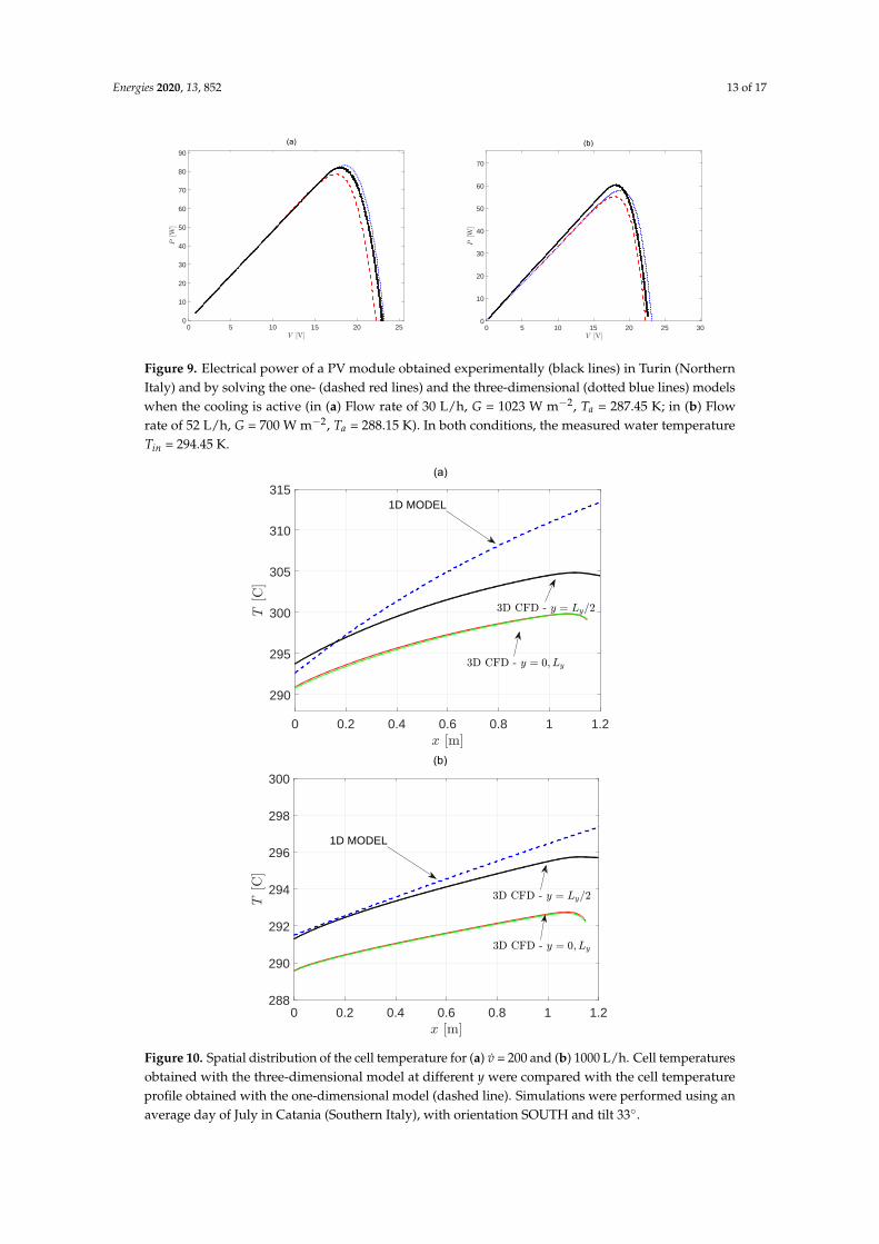
Comparisons of the results obtained by solving the three-dimensional model with theone-dimensional model presented in [25] and with outdoor experimental tests are reported inFigures 8–11. In particular, outdoor experimental tests were carried out in Turin (Northern Italy)in October. In these tests, after an accurate cleaning of the PV module to avoid the dirt and thedust, the thermal equilibrium condition was reached for some minutes with constant irradiance,ambient temperature, and wind speed. The experimental electrical characteristics were obtainedby the automatic data acquisition system described in [25], with uncertainties of measurement of±1%,±0.1%, and ±1% in terms of current, voltage, and power, respectively. In particular, 1D and 3Dnumerical results were compared with experimental steady-state test conditions when the coolingwas active (flow rates of 30 and 52 L/h for each module) and at G = 1023 W m−2, Ta = 287.45 K,and G = 700 W m−2, Ta = 288.15 K. In both conditions, the measured water temperature Tin = 294.45 K.Figures 8 and 9 show the I-V and P-V curves, respectively. From the results, the agreement with theexperimental values of the 3D model is improved with respect to the 1D model. The agreement ismainly related to the more accurate evaluation of the spatial distribution of the cell temperature. In the1D model, a single average column constituted by ten rows, each of them representing four PV cells,is considered, and the thermal gradient on the transverse direction is neglected. On the other hand, inthe 3D model, the complete 3D cell temperature field is considered and lower cell temperatures can befound, as confirmed in Figure 10.

The cell temperature profiles obtained for v̇ = 200 and 1000 L/h by solving 1D and 3D numericalmodels are in good agreement, especially for higher flow rates and, in particular, with the profile inthe middle axis (y = Ly/2). The boundary effects and the spatial distribution of the cell temperatureproduce a thermal mismatch between the cells in the same module. In fact, the one-dimensional modeldoes not take into account the y-dependence of the cell temperature and overestimates its value ofexternal columns, as confirmed by the measurements reported in Figures 8 and 9.

Figure 11 shows the spatial distribution of the cooling fluid temperature in the case of v̇ = 600 L/hin Catania (in July). The results of the three-dimensional model are reported at different z in order toshow the thermal gradients inside the ducts, and are compared with the temperature profile obtainedwith the one-dimensional model reported in [25]. The agreement between the results obtained bysolving the 1D and 3D numerical models for the case v̇ = 600 L/h is good.

The improvement of the energy production of a PVFC system with active cooling was investigatedin different conditions [25]. The difference between the no-cooling PV system and PVFC system

Energies 2020, 13, 852 10 of 17

represents the power gain PG. When the cooling is active, the pump consumption can be calculatedanalytically by recurring to Equation (9), where the exponents ek depend on the piping networkunder investigation (in this work, the system described in [24] was considered, and eks are:e1 = 1, e2 = 2, e3 = 2.75, and e4 = 3). When the power absorbed by the circulating pump isknown, the model determines at what time the cooling system must be switched on and off, and thenet power gain, given by Equation (11), can be calculated.

(a)

(b)

Figure 4. Spatial distribution of the cell temperature when v̇ = 0 (a) and 1000 L/h (b). Simulations wereperformed during an average day of July in Catania (Southern Italy), with orientation SOUTH andtilt 33◦. z− and y−axes are swapped in CFD simulations.

Energies 2020, 13, 852 11 of 17

(a)

0.2 0.4 0.6 0.8 1x [m]

0.2

0.4

y[m

]

0.128

0.13

0.132

0.134(b)

Figure 5. Spatial distribution of (a) the cell temperature, Tc, and of (b) the electrical performance, η, forv̇ = 0 L/h.

(a)

0.2 0.4 0.6 0.8 1x [m]

0.2

0.4

y[m

]

0.138

0.14

0.142

(b)

Figure 6. Spatial distribution of (a) the cell temperature, Tc, and of (b) the electrical performance, η, forv̇ = 600 L/h.

Energies 2020, 13, 852 12 of 17

(a)

0.2 0.4 0.6 0.8 1x [m]

0.2

0.4

y[m

]

0.14

0.142

(b)

Figure 7. Spatial distribution of (a) the cell temperature, Tc, and of (b) the electrical performance, η, forv̇ = 1000 L/h.

0 5 10 15 20 250

0.5

1

1.5

2

2.5

3

3.5

4

4.5

5

Figure 8. Electrical characteristics of a single PV module obtained experimentally (black line) in Turin(Northern Italy) and by solving the one- (dashed red line) and the three-dimensional (dotted blueline) models when the cooling is active (flow rate of 30 L/h for each module) at G = 1023 W m−2,Ta = 287.45 K, and inlet water temperature Tin = 294.45 K.

Energies 2020, 13, 852 13 of 17

0 5 10 15 20 250

10

20

30

40

50

60

70

80

90

(a)

0 5 10 15 20 25 300

10

20

30

40

50

60

70

(b)

Figure 9. Electrical power of a PV module obtained experimentally (black lines) in Turin (NorthernItaly) and by solving the one- (dashed red lines) and the three-dimensional (dotted blue lines) modelswhen the cooling is active (in (a) Flow rate of 30 L/h, G = 1023 W m−2, Ta = 287.45 K; in (b) Flowrate of 52 L/h, G = 700 W m−2, Ta = 288.15 K). In both conditions, the measured water temperatureTin = 294.45 K.

0 0.2 0.4 0.6 0.8 1 1.2x [m]

290

295

300

305

310

315

T[C

]

3D CFD - y = 0; Ly

3D CFD - y = Ly=2

1D MODEL

(a)

0 0.2 0.4 0.6 0.8 1 1.2x [m]

288

290

292

294

296

298

300

T[C

]

1D MODEL

3D CFD - y = 0; Ly

3D CFD - y = Ly=2

(b)

Figure 10. Spatial distribution of the cell temperature for (a) v̇ = 200 and (b) 1000 L/h. Cell temperaturesobtained with the three-dimensional model at different y were compared with the cell temperatureprofile obtained with the one-dimensional model (dashed line). Simulations were performed using anaverage day of July in Catania (Southern Italy), with orientation SOUTH and tilt 33◦.

Energies 2020, 13, 852 14 of 17

0 0.5 1 1.5x [m]

288

290

292

294

296

298

300

T[C

]

3D CFD - z = zcell

1D MODEL

3D CFD - z = zcell ! swater

3D CFD - z = zcell ! 0:5swater

(a)

(b)

Figure 11. Spatial distribution of the cooling fluid temperature for v̇ = 600 L/h. In (a), temperatures ofthe three-dimensional model at different z and at y = Ly/2 are compared with the temperature profileobtained with the one-dimensional model (dashed line). In (b), the (x, y) distribution of the coolingfluid temperature in z = zcell − 0.5scell is reported. Simulations were performed during an average dayof July in Catania (Southern Italy), with orientation SOUTH and tilt 33◦.

The net power gain depends on the power consumption that, for the case considered here, rangesbetween 65 W for 600 l/h to 130 W at 1000 L/h [24]. By using a statistical approach for climatedata (i.e., PVGIS), an optimum coolant flow rate can be estimated for every month by calculating themaximum of the net power gain NPG = 4P− Pp, obtained by combining Equations (8) and (10).Figure 12 shows that there is an optimal value of coolant flow rate for the NPG, which represents thebest compromise inside the competitive mechanism between the pump consumption and the powergain due to the cell temperature reduction. The results obtained in Catania city show that, in July,the optimum flow rate is reached at around 400 L/h (20 L/h for each module), while it is reached ataround 200 L/h in January due to the lower ambient temperature.

In a real case, the data of the average day can be considered only to evaluate the profitabilityof installing an active cooling system. Climate conditions can be strongly variable over a singleday, and the activation of the cooling system must be evaluated considering irradiance and ambienttemperature on the PV generator site. Simulations can be performed to obtain a map where, startingfrom the knowledge of irradiance G and ambient temperature Ta, the convenience of activating thecooling system in real-time conditions can be deduced [24].

Energies 2020, 13, 852 15 of 17

200 300 400 500 600 700 8000

10

20

30

40

50(a)

200 300 400 500 600 700 800 900 1000240

250

260

270

280

290

300

310(b)

Figure 12. Net Power Gain vs. coolant flow rate in January (a) and July (b) for Catania city.

5. Conclusions

5.1. Summary

In this work, a three-dimensional theoretical and numerical investigation of the electricalperformance of a photovoltaic system with active cooling was carried out. Starting from resultsobtained in previous works [24,25] by using a one-dimensional thermal–electrical model, the fullycoupled 3D thermal and electrical model shows that a competitive mechanism exists between thepower gain due to the reduction of the cell temperature and the power absorbed by the circulatingpump; a best compromise, in terms of fluid flow rate, can be found. The optimum flow rate wascalculated by using a semi-analytical approach, in which irradiance and ambient temperature of thesite are known and the piping network losses are fully characterized. Comparisons between resultsobtained by the one- and three-dimensional models and with experimental tests show the effectivenessand the limits of the one-dimensional model and the advantages of using the three-dimensional modelto investigate the effect of the spatial cell temperature distribution in a PV module in order to evaluatethermal mismatch effects.

5.2. Future Works

Finally, as a future development, the numerical model can be adopted to evaluate the opportunityof activating the cooling system by also using data acquisition and elaboration systems in orderto achieve a higher electrical efficiency. Moreover, the effects of the thermal recovery of the PVFCgenerator can be included.

Author Contributions: The authors A.D. and M.M. carried out CFD simulations and wrote the full manuscript.The authors A.D., D.E., G.V.F., F.S., A.C., and P.D.L. constructed the simulation model and analyzed the simulationresults. The authors A.D., F.S., and G.V.F. reviewed results and the whole manuscript. All authors have read andagreed to the published version of the manuscript.

Funding: This research received no external funding.

Conflicts of Interest: The authors declare no conflict of interest.

References

1. Brinkworth, B.J.; Cross, B.M.; Marshall, R.H.; Yang, H. Thermal regulation of photovoltaic cladding.Sol. Energy 1997, 61, 169–178. [CrossRef]

2. Ma, T.; Yang, H.; Zhang, Y.; Lu, L.; Wang, X. Using phase change materials in photovoltaic systems forthermal regulation and electrical efficiency improvement: A review and outlook. Renew. Sustain. Energy Rev.2015, 43, 1273–1284. [CrossRef]

Energies 2020, 13, 852 16 of 17

3. DeSoto, W.; Klein, S.A.; Beckman, W.A. Improvement and validation of a model for photovoltaic arrayperformance. Sol. Energy 2006, 80, 78–88. [CrossRef]

4. Arcuri, N.; Reda, F.; De Simone, M. Energy and thermo-fluid-dynamics evaluations of photovoltaic panelscooled by water and air. Sol. Energy 2014, 105, 147–156. [CrossRef]

5. Kawamura, T.; Harada, K.; Ishihara, Y.; Todaka, T.; Oshiro, T.; Nakamura, H.; Imataki, M. Analysis of MPPTcharacteristics in photovoltaic power system. Sol. Energy Mater. Sol Cells 1997, 47, 155–165. [CrossRef]

6. Omubo-Pepple, V.B.; Israel-Cookey, C.; Alaminokuma, G.I. Effects of Temperature, Solar flux and RelativeHumidity on the Efficient Conversion of Solar Energy to Electricity. Eur. J. Sci. Res. 2009, 35, 173–180.

7. Konjare, S.S.; Shrivastava, R.L.; Chadge, R.B.; Kumar, V. Efficiency Improvement of PV module by wayof Effective Cooling—A Review. In Proceedings of the 2015 IEEE International Conference on IndustrialInstrumentation and Control (ICIC), College of Engineering, Pune, India, 28–30 May 2015; pp. 1008-1011.

8. Krauter, S. Increased electrical yield via water flow over the front of photovoltaic panels. Sol. Energy Mater.Sol. Cells 2014, 82, 131–137. [CrossRef]

9. Ji, J.; Pei, G.; Chow, T-.; Liu, K.; He, H.; Lu, J.; Han, C. Experimental study of photovoltaic solar assisted heatpump system. Sol. Energy 2008, 82, 43–52. [CrossRef]

10. Abdolzadeh, M.; Ameri, M. Improving the effectiveness of a photovoltaic water pumping system by sprayingwater over the front of photovoltaic cells. Renew. Energy 2009, 34, 91–96. [CrossRef]

11. Kordzadeh, A. The effects of nominal power of array and system head on the operation of photovoltaic waterpimping set with array surface covered by a film of water. Renew. Energy 2010, 35, 1098–102. [CrossRef]

12. Prudhvi, P.; Sai, P.C. Efficiency Improvement of Solar PV Panels Using Active Cooling. In Proceedings ofthe 11th IEEE International Conference on Environment and Electrical Engineering (EEEIC), Venice, Italy,18–25 May 2012; pp. 1093–1097.

13. Sharma, M.; Bansal, K.; Buddhi, D. Operating temperature of PV module modified with surface cooling unitin real time condition. In Proceedings of the 6th IEEE India International Conference on Power Electronics(IICPE), Kurukshetra, India, 8–10 December 2012; pp. 1-5.

14. Kim, J.; Nam, Y. Study on the Cooling Effect of Attached Fins on PV Using CFD Simulation. Energies 2019,12, 758. [CrossRef]

15. Kim, J.; Bae, S.; Yu, Y.; Nam, Y. Experimental and Numerical Study on the Cooling Performance of Fins andMetal Mesh Attached on a Photovoltaic Module. Energies 2020, 13, 85. [CrossRef]

16. Gang, P.; Jie, J.; Wei, B.H.; Keliang, L.; Hanfeng, H. Performance of photovoltaic solar assisted heat pumpsystem in typical climate zone. J. Energy Environ. 2007, 6, 1–9.

17. Xu, G.Y.; Deng, S.M.; Zhang, X.S. Simulation of a photovoltaic/thermal heat pump system having a modifiedcollector/evaporator. Sol. Energy 2009, 83, 1967–1976. [CrossRef]

18. Teo, H.G.; Lee, P.S.; Hawlader, M.N.A. An active cooling system for photovoltaic modules. Appl. Energy2012, 90, 309–315. [CrossRef]

19. Rossi, C.; Tagliafico, L.A.; Scarpa, F.; Bianco, V. Experimental and numerical results from hybrid retrofittedphotovoltaic panels. Energy Convers. Manag. 2013, 76, 634–644. [CrossRef]

20. Elnozahya, A.; Rahmana, A.K.A.; Alib, A.H.H.; Abdel-Salamc, M.; Ookawara, S. Performance of a PVmodule integrated with standalone building in hot arid areas as enhanced by surface cooling and cleaning.Energy Build. 2015, 88, 100–109. [CrossRef]

21. Ueda, Y.; Sakurai, T.; Tatebe, S.; Itoh, A.; Kurokawa, K. Performance analysis of PV systems on the water.In Proceedings of the 2008 IEEE EU PVSEC Conference, Valencia, Spain, 1–5 September 2008; pp. 2670–2673.

22. Leow, W.Z.; Irwan, Y.M.; Irwanto, M.; Gomesh, N.; Safwati, I. PIC 18F4550 controlled solar panel coolingsystem using DC hybrid. J. Sci. Res. Rep. 2014, 3, 2801–2816. [CrossRef]

23. Makki, A.; Omer, S.; Sabir, H. Advancements in hybrid photovoltaic systems for enhanced solar cellsperformance. Renew. Sustain. Energy Rev. 2015, 41, 658–684. [CrossRef]

24. D’angola, A.; Zaffina, R.; Enescu, D.; Di Leo, P.; Fracastoro, G.V.; Spertino, F. Best compromise of net powergain in a cooled photovoltaic system. In Proceedings of the 51st International Universities Power EngineeringConference (UPEC 2016), Coimbra, Portugal, 6–9 September 2016; pp. 1–6. [CrossRef]

25. Spertino, F.; D’Angola, A.; Enescu, D.; di Leo, P.; Fracastoro, G.V.; Zaffina, R. Thermal–electrical model forenergy estimation of a water cooled photovoltaic module. Sol. Energy 2016, 133, 119–140. [CrossRef]

Energies 2020, 13, 852 17 of 17

26. Spertino, F.; Ciocia, A.; Corona, F.; di Leo, P.; Papandrea, F. An experimental procedure to check theperformance degradation on-site in grid-connected photovoltaic systems. In Proceedings of the 40th IEEEPhotovoltaic Specialist Conference (PVSC), Denver, CO, USA, 8–13 June 2014; pp. 2600–2604.

27. ANSYS Fluent Theory Guide; ANSYS, Inc.: Canonsburg, PA, USA, November 2013.28. Ahmad, J.; Ciocia, A.; Fichera, S.; Murtaza, A.F.; Spertino, F. Detection of typical defects in silicon photovoltaic

modules and application for plants with distributed MPPT configuration. Energies 2019, 23, 4547. [CrossRef]29. Murtaza, A.F.; Munir, U.; Chiaberge, M.; Di Leo, P.; Spertino, F. Variable parameters for a single exponential

model of photovoltaic modules in crystalline-silicon. Energies 2018, 11, 2138. [CrossRef]30. Spertino, F.; Fichera, S.; Ciocia, A.; Malgaroli, G.; Di Leo, P.; Ratclif, A. Toward the complete self-sufficiency

of an NZEBS microgrid by photovoltaic generators and heat pumps: Methods and applications. IEEE Trans.Ind. Appl. 2019 55, 7028–7040. [CrossRef]

31. Çengel, Y.A.; Turner, R.H. Thermal-Fluid Sciences; McGraw-Hill: New York, NY, USA, 2001.32. Fox, W.; Pritchard, P.; McDonald, A. Introduction to Fluid Meachanics, 7th ed.; John Wiley & Sons: Hoboken,

NJ, USA, 2010.33. Richter, H. Rohrhydraulik; Springer: Berlin, Germnay, 1971.34. Miller, D.S. Internal Flow; BHRA: Cranfield-Bedford, UK, 1971.35. Ward-Smith, A.I. Internal Fluid Flow; Clarendon Press: Oxford, UK, 1980.36. Blevins, R.D. Applied Fluid Dynamics Handbook; Van Nostrand Reinhold: New York, NY, USA, 1984.

c© 2020 by the authors. Licensee MDPI, Basel, Switzerland. This article is an open accessarticle distributed under the terms and conditions of the Creative Commons Attribution(CC BY) license (http://creativecommons.org/licenses/by/4.0/).