theme 4: CoastaL, estuaries anD LaKe management

theme 4:CoastaL, estuaries anD

LaKe management

editor: ahmad Khairi abd wahab

CoastaL anD estuarY morPhoDYnamiCs

NUMERICAL INVESTIGATION OF NONLINEAR M4 OVERTIDE ON THE BACKWATER

HYDRODYNAMICS IN TIDAL RIVERS

HUAYANG CAI(1), PENG YAO(2),SUYING OU(3) & QINGSHU YANG(4)

(1,2,3,4) Institute of Estuarine and Coastal Research, School of Marine Sciences, Sun Yat-sen University, Guangzhou, China, [email protected]; [email protected];[email protected]; [email protected]

ABSTRACT As river flow debouches into the sea, it is affected by the fluctuation of tide at the estuary mouth, resulting in a backwater zone where the residual water level (averaged over a lunar day) tends to rise in landward direction. It is known that backwater hydrodynamics, especially the variation of residual water level, is controlled by the river-tide interaction, while it follows the traditional stage-river discharge relation in the upstream river-dominated region. However, the contribution made by tidal asymmetry due to the generation of overtides and their interplay with river flow is poorly understood. This present study aims to understand the impact of nonlinear M4 overtide on the increase of residual water level in tidal rivers. To quantify the contribution made by nonlinear M4 overtide, the numerically computed subtidal friction is decomposed into different components representing contributions by the river flow alone, the river-tide interaction, and the tidal asymmetry due to internal generation of M4 overtide. Numerical results show that the influence of nonlinear M4 overtide on residual water level becomes important with increasing tidal amplitude to depth ratio and its relative importance can be represented by a tidal asymmetry term, which depends on the sign of the phase relation between M2 and M4. Keywords: Residual water level; tidal rivers; overtide; tidal asymmetry. 1 INTRODUCTION

Understanding backwater hydrodynamics in tidal rivers is essential for coastal flooding, sediment transport and water management (Lamb et al., 2012; Hoitink and Jay, 2016). It was shown that the residual water level (averaged over a lunar day) of a tidal river is driven by the fortnightly fluctuation, which causes a spring-neap change in residual water level along the channel axis. Meanwhile, the residual water level also tends to increase in landward direction due to the nonlinear interaction between tide and river flow (LeBlond, 1979; Godin and Martinez, 1994; Buschman et al., 2009; Sassi and Hoitink, 2013). To understand the interaction between tide and river flow in a tidal river, many authors decomposed the subtidal friction into different components contributed by tide, river and tide-river interaction (Dronkers, 1964; Godin, 1991; Godin, 1999; Buschman et al., 2009; Sassi and Hoitink, 2013). Specifically, Dronkers (1964) adopted the Chebyshev polynomials approach to approximate the quadratic velocity in the friction term, in which the resulted approximation consists of four terms with coefficients depending on the ratio of river flow velocity to the tidal velocity amplitude. Later, Godin (1991; 1999) proposed a simpler approximation that retains only the first and third order terms of the dimensionless velocity, which is comparable with Dronker’s formula in terms of accuracy.

Recently, Cai et al. (2014a; 2014b; 2016) proposed an analytical approach to determining the backwater hydrodynamics in tidal rivers. However, the theoretical analysis only accounts for one predominant tidal constituent (e.g., semidiurnal tide M2), while the contribution made by tidal asymmetry due to the generation of overtides and their interplay with river flow is poorly understood. In this paper, a fully nonlinear 1D numerical model is used to understand the impact of nonlinear M4 overtide on the backwater hydrodynamics. The key thing lies in the decomposition of the quadratic velocity in the friction term, which allows quantification of different components (i.e., tide, river and tide-river interaction) on the residual water level. The relative importance of each contribution is quantified for given different tidal amplitude to depth ratios at the estuary mouth. 2 METHOD OF ANALYSIS 2.1 RESIDUAL WATER LEVEL SLOPE

It is important to note the residual water level slope can be derived from the 1D momentum equation, which is described by:

2 4/3

| |0,

U U Z U UU g g

t x x K h

[1]

Proceedings of the 37th IAHR World Congress August 13 – 18, 2017, Kuala Lumpur, Malaysia

©2017, IAHR. Used with permission / ISSN 1562-6865 (Online) - ISSN 1063-7710 (Print) 3197

where U is the cross-sectional averaged velocity, Z the free surface elevation, h is the water depth, g the gravity acceleration, t is the time, x is the longitudinal coordinate directed landward, K is the Manning-Strickler friction coefficient.

Assuming a periodic variation of flow velocity, the integration of Eq. [1] over a tidal cycle leads to (Vignoli et al., 2003; Cai et al., 2014b):

2 4/3

| |.

Z U U

x K h

[2]

where the overbars denote the tidal average. 2.2 DECOMPOSITION OF THE QUADRATIC VELOCITYU|U|

The present study adopted a fully 1D nonlinear numerical model (see details in Toffolon et al., 2006) to understand the impact of internal overtides on the resulted residual water level due to nonlinear frictional effect. To achieve this objective, model results had been processed with harmonic analysis, decomposing the flow velocity series into M2 and M4 constituents. Thus, the flow velocity U at a specific position can be given by the following form:

0 1 2sin sin 2 ,U t u t t [3]

where t is time, u0 is the residual flow velocity generated by the freshwater discharge, υ1 and υ2 are the M2 and M4 velocity amplitudes, respectively, ω is the frequency of the semi-diurnal tide and and are M2 and M4 phase, respectively. It was shown by Godin (1991; 1999) that the quadratic velocity U|U| in the momentum equation can be approximated by the Chebyshev polynomials approach, which leads to:

0 1 22

3

0 1 2

16sin sin 2

15| | ' ,32

sin sin 215

t tU U

t t

[4]

where υ is the maximum possible value of velocity (i.e., υ ), , are the dimensionless velocity amplitudes scaled by the maximum velocity υ′.

Making use of the trigonometric equations to expand the power of cosine functions (e.g., cos ωt ψ and cos ωt ψ ) and extracting the original harmonics with frequencies of ω, 2ω and 3ω, Eq. [4] can be reduced to:

20 1 2

16| | ' sin sin 2 ,

15U U F F t F t

[5]

with

2

2 2 2 1 20 0 0 1 2

0

31 2 3 3 sin 2 ,

2F

[6]

2 2 21 1 0 1 2

31 6 3 ,

2F

[7]

2 2 22 2 0 1 2

31 6 3 ,

2F

[8]

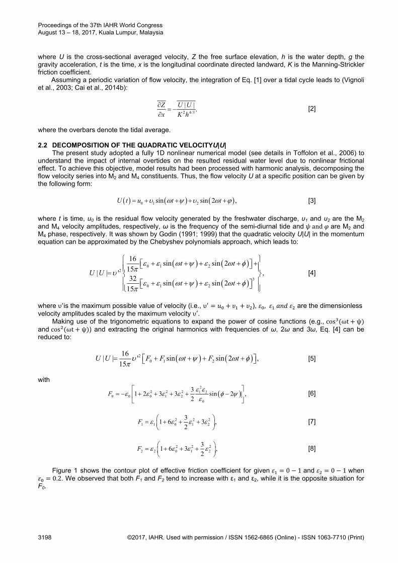
Figure 1 shows the contour plot of effective friction coefficient for given 0 1 and 0 1 when 0.2. We observed that both F1 and F2 tend to increase with ε1 and ε2, while it is the opposite situation for

F0.


3198 ©2017, IAHR. Used with permission / ISSN 1562-6865 (Online) - ISSN 1063-7710 (Print)

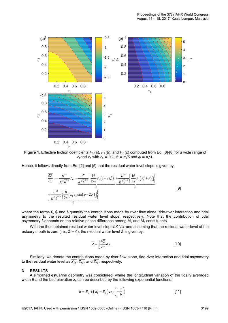
Figure 1. Effective friction coefficients F0 (a), F1 (b), and F2 (c) computed from Eq. [6]-[8] for a wide range of

and with 0.2, /5and π/4. Hence, it follows directly from Eq. [2] and [5] that the residual water level slope is given by:

2 2 22 2 2

0 0 0 0 1 24/3 4/3 4/32 2 2

221 24/32

' ' 16 ' 161 2

15 5

' 8sin 2

5

r tr

t

f f

f

ZF

x K h K h K h

K h

[9]

where the terms fr, ftr and ft quantify the contributions made by river flow alone, tide-river interaction and tidal asymmetry to the resulted residual water level slope, respectively. Note that the contribution of tidal asymmetry ft depends on the relative phase difference among M2 and M4 constituents.

With the thus obtained residual water level slope /Z x and assuming that the residual water level at the estuary mouth is zero (i.e., ̅ 0), the residual water level ̅ is given by:

0

d .x Z

Z xx

[10]

Similarly, we denote the contributions made by river flow alone, tide-river interaction and tidal asymmetry

to the residual water level as , and , respectively.

3 RESULTS A simplified estuarine geometry was considered, where the longitudinal variation of the tidally averaged

width B and the bed elevation zb can be described by the following exponential functions:

0 expf f

xB B B B

b

[11]

0.2 0.4 0.6 0.8ε1

0.2

0.4

0.6

0.8

1ε 2

-2.5

-2

-1.5

-1

-0.5

F0

0.2 0.4 0.6 0.8ε1

0.2

0.4

0.6

0.8

1

ε 2

0

1

2

3

4

5

F1

0.2 0.4 0.6 0.8ε1

0.2

0.4

0.6

0.8

1

ε 2

0

1

2

3

4

5

F2

(a)

(c)

(b)



0 expb bf b bf

xz z z z

d

[12]

where x is the longitudinal coordinate directed landward, b and d are the convergence length of width and bed elevation, respectively. The subscript 0 denotes values at the estuary mouth, while the subscript f indicates asymptotic values when distance approaches infinity. The tidally averaged depth h is defined as the distance between mean water level zws and the bed elevation zb (see Figure 2). Assuming that the cross section of the estuary is schematized as rectangular, thus the tidally averaged cross-sectional area is given by A=Bh.

Figure 2. Sketch of water levels in a tidal river.

The numerical model solves the one-dimensional momentum and continuity equations in semi-

conservative form, which allows conserving both mass and momentum. At seaward boundary, we imposed a simple semidiurnal M2 tide in a harmonic way, i.e., sin 2 / , where η0 is the tidal amplitude and T is the tidal period. In the upstream boundary, we imposed a constant freshwater discharge Q. For details, the readers can refer to Toffolon et al. (2006).

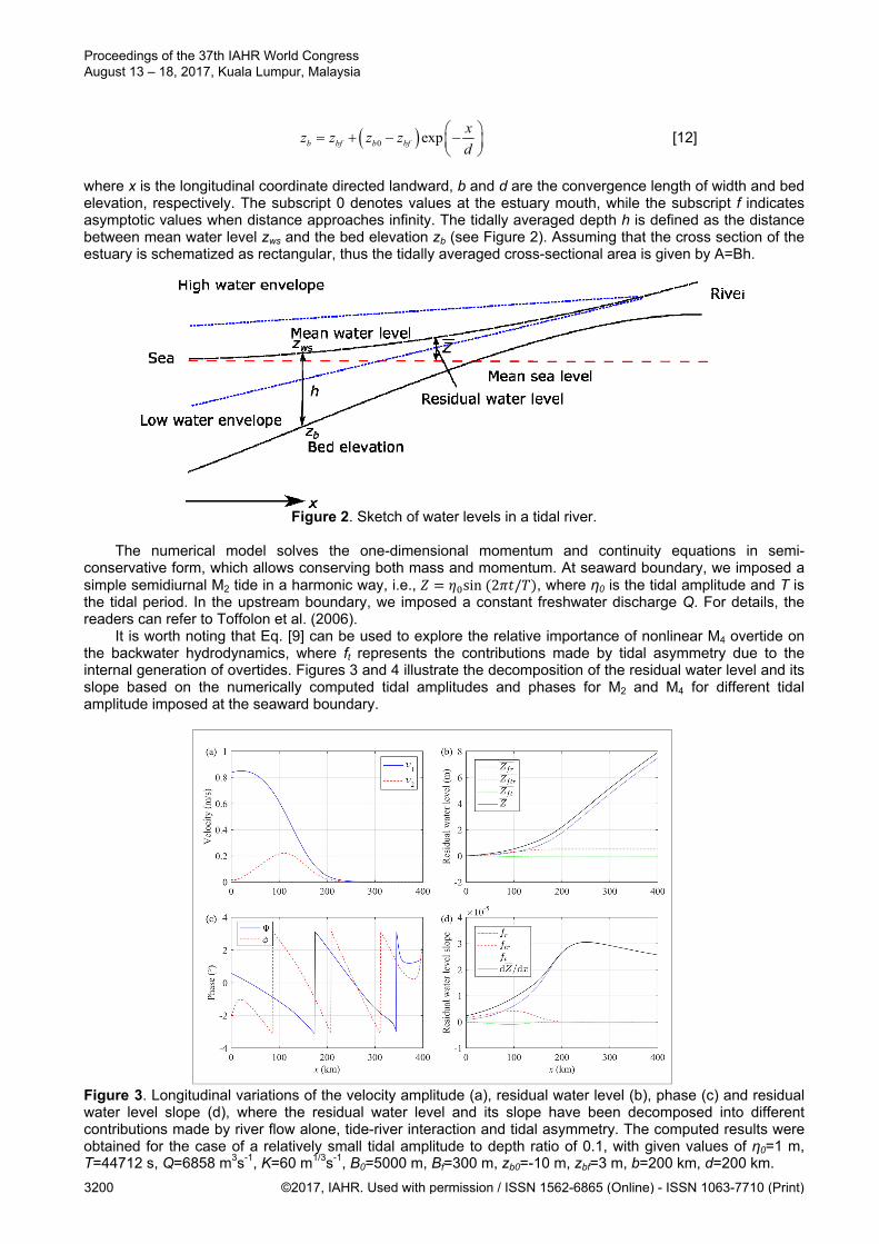
It is worth noting that Eq. [9] can be used to explore the relative importance of nonlinear M4 overtide on the backwater hydrodynamics, where ft represents the contributions made by tidal asymmetry due to the internal generation of overtides. Figures 3 and 4 illustrate the decomposition of the residual water level and its slope based on the numerically computed tidal amplitudes and phases for M2 and M4 for different tidal amplitude imposed at the seaward boundary.

Figure 3. Longitudinal variations of the velocity amplitude (a), residual water level (b), phase (c) and residual water level slope (d), where the residual water level and its slope have been decomposed into different contributions made by river flow alone, tide-river interaction and tidal asymmetry. The computed results were obtained for the case of a relatively small tidal amplitude to depth ratio of 0.1, with given values of η0=1 m, T=44712 s, Q=6858 m3s-1, K=60 m1/3s-1, B0=5000 m, Bf=300 m, zb0=-10 m, zbf=3 m, b=200 km, d=200 km.



Figure 4. Longitudinal variations of the velocity amplitude (a), residual water level (b), phase (c) and residual water level slope (d), where the residual water level and its slope have been decomposed into different contributions made by river flow alone, tide-river interaction and tidal asymmetry. The computed results were obtained for the case of a relatively large tidal amplitude to depth ratio of 0.3, with given values of η0=3 m, T=44712 s, Q=6858 m3s-1, K=60 m1/3s-1, B0=5000 m, Bf=300 m, zb0=-10 m, zbf=3 m, b=200 km, d=200 km.

Generally, we see the amplitude of M4 overtide reaches a maximum value before it becomes vanishing due to the tidal dissipation. From Figures 3b,d and 4b,d, we observed that the contribution made by tidal asymmetry to the residual water level and its slope was opposite compared with those by river flow alone and tide-river interaction, suggesting negative values of and . As pointed out by Hoitink and Jay (2016), the

sign of the tidal asymmetry term depends on the phase relation 2 , where positive value of sin 2

indicates an amplification of residual water level, while it is the opposite for negative value. In addition, we observed that the tidal asymmetry became more important with increasing tidal forcing imposed at the seaward boundary (see comparison between Figures 3b,d and 4b,d). In particular, the spatially averaged contribution made by tidal asymmetry to the residual water level was almost negligible (around -2.2% of the residual water level) for relatively small tidal forcing (η0=1 m and tidal amplitude to depth ratio at the estuary mouth being 0.1), while the ratio increased to -11.2% with large tidal forcing (η0=3 m and tidal amplitude to depth ratio at the estuary mouth being 0.3). 4 CONCLUSIONS

In this paper, a fully nonlinear numerical model is used to explore the relative importance of nonlinear M4 overtide on the backwater hydrodynamics in a tidal river. On the basis of numerically computed tidal properties (including tidal amplitude and phase) for both M2 and M4 tide constituents, it is possible to quantify the contributions made by river flow alone, tide-river interaction and tidal asymmetry to the rise of the residual water level along the estuary by using the Godin’s Chebyshev polynomials approximation to the quadratic velocity in the friction term. It is shown that the nonlinear M4 overtide becomes important with increasing tidal amplitude to depth ratio and its relative importance can be represented by the tidal asymmetry introduced by the internal generation of overtides (e.g., M4). The tidal asymmetry could amplify or partially cancel the residual water level, which depends on the sign of the phase relation 2 .

ACKNOWLEDGEMENTS

The research reported herein is funded by the National Key Research Programme of China (Grant No. 2016YFC0402600), by the National Natural Science Foundation of China (Grant No. 41476073) and by the Water Resource Science and Technology Innovation Program of Guangdong Province (Grant No. 2016-20).



REFERENCES Buschman, F.A., Hoitink, A.J.F., van der Vegt, M. & Hoekstra, P. (2009). Subtidal Water Level Variation

Controlled by River Flow and Tides. Water Resources Research, 45(10), 1-12. Cai, H., Savenije, H.H.G. & Jiang, C. (2014a). Analytical approach for Predicting Fresh Water Discharge in an

Estuary based on Tidal Water Level Observations. Hydrology and Earth System Science, 18(10), 4153-4168.

Cai, H., Savenije, H.H.G. & Toffolon, M. (2014b). Linking the River to the Estuary: Influence of River Discharge on Tidal Damping. Hydrology and Earth System Science, 18(1), 287-304.

Cai, H., Savenije, H.H.G., Jiang, C., Zhao, L. & Yang, Q. (2016). Analytical approach for determining the Mean Water Level Profile in an Estuary with Substantial Fresh Water Discharge. Hydrology and Earth System Science, 20(3), 1177-1195.

Dronkers J.J. (1964). Tidal Computations in Rivers and Coastal Waters. North-Holland Publishing Company, Amsterdam, 518.

Godin, G. (1991). Compact Approximations to the Bottom Friction Term for the Study of Tides Propagating in Channels, Continental Shelf Research, 11(7), 579-589.

Godin, G. (1999). The Propagation of Tides Up Rivers with Special Considerations on the Upper Saint Lawrence River, Estuarine Coastal and Shelf Science, 48(3), 307-324.

Godin, G. & A. Martinez (1994). Numerical Experiments to Investigate the Effects of Quadratic Friction on the Propagation of Tides in a Channel, Continental Shelf Research, 14(7-8), 723-748.

Hoitink, A.J.F., Jay, D.A. (2016). Tidal River Dynamics: Implications for Deltas. Reviews of Geophysics, 54(1), 240-272.

Lamb, M.P., Nittrouer, J.A., Mohrig, D. & Shaw, J. (2012). Backwater and River Plume Controls on Scour Upstream of River Mouths: Implications for Fluvio-Deltaic Morphodynamics. Journal of Geophysical Research, 117(F1), 1-16.

LeBlond, P. (1979). Forced Fortnightly Tides in Shallow Rivers, Atmosphere Ocean, 17(3), 253–264. Sassi, M.G. & Hoitink, A.J.F. (2013). River Flow Controls on Tides and Tide-Mean Water Level Profiles in a

Tidal Freshwater River. Journal of Geophysical Research, 118(9), 4139-4151. Toffolon, M., Vignoli, G. & Tubino, M. (2006). Relevant Parameters and Finite Amplitude Effects in Estuarine

Hydrodynamics. Journal of Geophysical Research, 111(C10), 1-17. Vignoli, G., Toffolon, M. & Tubino, M. (2003). Non-Linear Frictional Residual Effects on Tide Propagation.

Proceedings of XXX IAHR Congress, 24–29 August 2003, Thessaloniki, Greece, A, 291–298,



EFFECTS OF THE LARGE-SCALE RECLAMATION OF TIDAL FLATS ON THE

HYDRODYNAMIC CHARACTERISTICS, SEDIMENT TRANSPORTION AND TOPOGRAPHY IN THE JIAOJIANG ESTUARY, CHINA

WEIQI DAI(1), JIANFENG TAO(2), KUN ZHAO(3), QIN ZHANG(4) & YU KUAI(5)

(1,2,3,5) College of Harbor, Coastal and Offshore Engineering, Hohai University, Nanjing, China. [email protected]

(1,2) State Key Laboratory of Hydrology-Water Resources and Hydraulic Engineering, Hohai University, Nanjing, China. [email protected]

(4) Shanghai Investigation, Design & Research Institute Co., Ltd, Shanghai, China. [email protected]

ABSTRACT Jiaojiang Estuary is a typical tidal-dominated estuary. With the increasing demand of land resource, a series of large-scale tidal flat reclamation has been conducted along the coast of Jiaojiang Estuary, which may lead to the changes of hydrodynamic characteristics, suspended sediment transport and local topography. A two-dimensional mathematical model is developed to simulate the tidal current, suspended sediment transportation and wave in Jiaojiang Estuary in this study. Results of the tidal current field and suspended sediment concentration (SSC) are compared before and after the tidal flat reclamation. The effect of large-scale reclamation on the hydrodynamic characteristics are discussed based on a 2-d numerical model coupling processes of tide current, wave, and sediment-transport, and the impact of reclamations are explored. Results show that the tidal prism of the estuary is reduced after the reclamation, which leads to the decrease of tidal velocity. The reduction of tidal prism also diminishes the tidal level. Besides, the reclamation narrows the cross-sections of the channel, so that the seabed is eroded at the mouth and then accumulates in the inland river region. As a result, the suspended sediment concentration increases, despite that the tidal flow is weakened. Compared with seabed after the reclamation when considering tide current only, more topographic change of the river bed is observed when combining wave and tide current. Waves play important roles in shaping the topography in Taizhou Bay which is a macro-tidal sea area. The changes of hydrodynamics and sediment concentration are the main dynamic mechanism in scouring and silting evolution of the Jiaojiang Estuary. Keywords: Tide flat reclamation; hydrodynamic; characteristics; seabed evolution; wave-current effect. 1 INTRODUCTION

The coastal shore near estuary is a significant part of coastal zone. With the increasing demand of population and economy, land resources could not satisfy people’s demands. Tidal flat reclamation has become a foundational method to solve the problem of land resources. Reclamation of Taizhou Shoals will break the dynamic balance between original hydrodynamics and topography will reach a new equilibrium. It is very important for reasonable planning of reclamation area that simulating hydrodynamic field and the suspended sediment concentration field of Taizhou Bay before and after reclamation to analyze the influence of reclamation.

Jiaojiang Estuary is a typical mountain stream and tidal-dominated estuary. A lot of studies have been done on forming process, characteristics of hydrology and sediment of Jiaojiang Estuary. The movement of sediment in Jiaojiang Estuary is mainly reflected by suspended sediment movement. There are two kinds of sediment deposition mechanism: single particle sedimentation and flocculating settling, and the latter is the main body of suspended sediment vertical exchange (Fu and Bi, 1989). Jiaojiang Estuary turbidity maximum suspended sediment grain size distribution is influenced by material source, bottom sediment resuspension, and flocculating settling (Li et al., 1999). Ying Zhang introduced a concept--‘Antecedent sediment factor’. He considered that the preceding period sediment could characterize ‘wave-lifting-sand’ in the absence of wind and wave data, thus building a regression model about suspended sediment concentration of Jiaojiang Estuary and flow and other dynamic factors in the absence of wind and waves (Zhang, 1992). Jiang and Feng suggested that the tidal flat was divided into two parts according to the hydro-sediment characters. On the upper tidal flat, the tide flow moves to and fro, influenced by the tidal flat bedforms, and the hydro-sediment processes are intensely-changed processes affected by the standing tide wave. On the lower tidal flat, the tidal flow is quasi-rotating current affected by Taizhou Bay rotation current and the tidal flat bedforms as well. The hydro-sediment processes are gradually-changed processes (Jiang and Feng, 1992).

Many scholars also focus on dynamic geomorphology of Jiaojiang Estuary. Owing to the plenty supply of sediment with mainly derived from the sea area, the ancient bay drowned during the postglacial marine



transgression was filled up and a marine-deposited plain formed gradually. Corresponding to this process, the channel of the Jiaojiang Estuary extended and the river mouth displaced step by step. The channel boundary thus possesses properties as follows: The upstream banks and river mouth are controlled by the rocky nodes; the movability of bank material composed of the consolidated marine silt and clay is less than that of the bed material (Bi and Sun, 1984). Xie (1998) considered that accumulation is caused by abundant source of substances, higher concentration of suspended matters and counter-clockwise circulation that occur in the Taizhou Bay (Xie et al., 1988). The seabed is in slight siltation state before 1988 and on the balance status of erosion and deposition after 1988. The hyperconcentration flow in the Jiaojiang Estuary has little influence on Taizhou Bay. The sediment source of the bay is the littoral sediment transport along east coastline of Zhejiang. Since the sediment decreases from the Yangtze Estuary, the seabed is basically in silt-stable state and the SSC decreases. Therefore, Taizhou Bay has the advantages to build the deep-water harbor (Mai et al., 2009). According to topography, hydrology and sediment data and charts, analyze the evolution of Taizhou Bay beach law from the sediment characteristics, suspended sediment sources, hydrodynamics, coastline and isobaths changes. Find that it is mainly affected by the Yangtze River to reduce sediment, sea level rise, especially in the construction of offshore land reclamation works (Chi, 2010). After the implementation of project, erosion rates of Jiaojiang Estuary had gone through this process of slow-speed-slow (Ni, 2012).

Many scholars have given much attention to Jiaojiang Estuary about hydrodynamic characteristic, the distribution and transport of suspended sediment, and flocculation and settling of suspended sediment. However, there are only a few researches focusing on the evolution characteristics before and after reclamation in Jiaojiang Estuary. This paper analyzes characteristics of erosion and deposition in Jiaojiang Estuary before and after reclamation, using coupling model of tidal currents, waves, sediment motion, and topography evolution. Then, it reveals the mechanism of changes due to tidal flat reclamation. 2 STUDY AREA

Jiaojiang is the third largest river system of Zhejiang province, and it flows into the Taizhou Bay from Niutoujing (Figure 2a). Jiaojiang Estuary is bounded in Niutoujing, divided into inside and outside the estuary. There are Jiaojiang, Lingjiang, and Yongningjiang inside the estuary, as well as Jiaojiang Estuary outside the estuary. The Jiaojiang Estuary is a typical river-influenced macro-tidal estuary, which is characterized by high flood-dry runoff and suspended sediment ratio. Water transfer quantity accounts for 76% of the total water in April to June as the main water delivery period. Sediment transport volume accounts for 94.4% of the total sediment discharge in July to September as the main sediment transport period. The tidal current in the Jiaojiang estuary to the Taizhou Bay is clockwise, and its rotation gradually decreases from east to West. The wave has little effect on the distribution of suspended sediment concentration in Jiaojiang Estuary. The sediment movement is mainly reflected by suspended sediment movement. The flood current through the entrance shrinks rapidly; on the contrary, the ebb current through the entrance disperses rapidly, which results in the sediment concentration in Haimen higher than it in upper reach and open sea.

3 METHOD

3.1 Numerical model

A 2D morphodynamic model MIKE 21 (DHI, 2009) was employed to simulate the tidal flow, SSCs and bed load transport. MIKE21 solves the shallow water equations resulting in water-level and velocity fields over the model domain:

0h hu hvt x y

[1]

2 2 2

2 2 ( )

( ( ))

m

m

hu hu huv u u v ugh g hA

t x y x x xCu v

hA fvhy x y

[2]

2 2 2

2 2 ( )

( ( ))-

m

m

hv hv huv v u v vgh g hA

t y x y y yCu v

hA fuhx y x

[3]



where t (s) is time step; x and y (m) are the Cartesian co-ordinates; h=d+η (m) is the total water depth; d (m) is the still water depth; η (m) is the tidal level; u and v (m/s) are the depth-averaged flow velocities in the x and y directions, respectively; f (s-1) is the Coriolis parameter; g (m2/s) is the acceleration of gravity; C(m1/2) is the Chézy friction coefficient and Am (m/s2) is the horizontal kinematic viscosity.

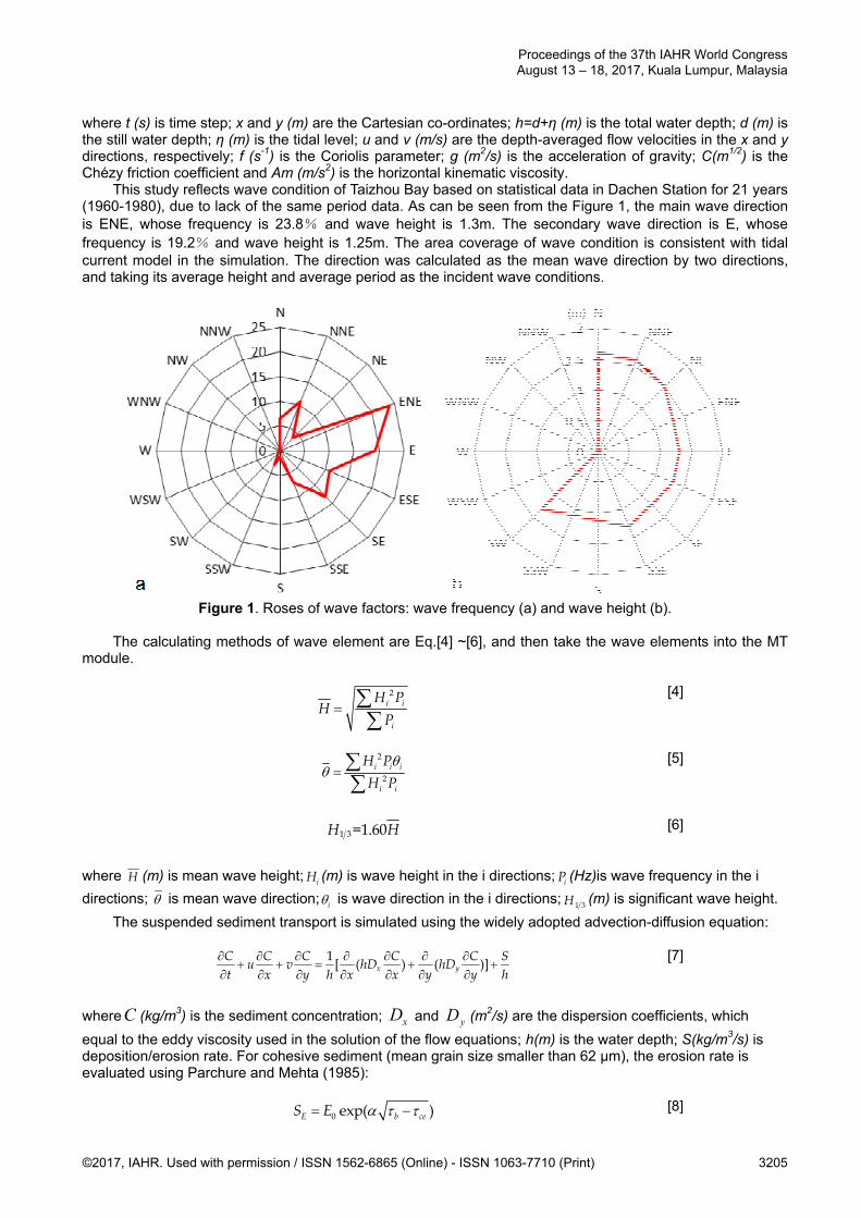
This study reflects wave condition of Taizhou Bay based on statistical data in Dachen Station for 21 years (1960-1980), due to lack of the same period data. As can be seen from the Figure 1, the main wave direction is ENE, whose frequency is 23.8％ and wave height is 1.3m. The secondary wave direction is E, whose frequency is 19.2％ and wave height is 1.25m. The area coverage of wave condition is consistent with tidal current model in the simulation. The direction was calculated as the mean wave direction by two directions, and taking its average height and average period as the incident wave conditions.

Figure 1. Roses of wave factors: wave frequency (a) and wave height (b).

The calculating methods of wave element are Eq.[4] ~[6], and then take the wave elements into the MT

module.

2i i

i

H PH

P

[4]

2

2i i i

i i

H P

H P

[5]

1 3=1.60H H [6]

where H (m) is mean wave height; iH (m) is wave height in the i directions; iP (Hz)is wave frequency in the i

directions; is mean wave direction; i is wave direction in the i directions;1 3H (m) is significant wave height.

The suspended sediment transport is simulated using the widely adopted advection-diffusion equation:

1[ ( ) ( )]x y

C C C C C Su v hD hD

t x y h x x y y h

[7]

whereC (kg/m3) is the sediment concentration; xD and yD (m2/s) are the dispersion coefficients, which

equal to the eddy viscosity used in the solution of the flow equations; h(m) is the water depth; S(kg/m3/s) is deposition/erosion rate. For cohesive sediment (mean grain size smaller than 62 μm), the erosion rate is evaluated using Parchure and Mehta (1985):

0 exp( )E b ceS E [8]



where E0 is the erosion rate coefficient; α is the power of erosion; τb (kg/m3/s2) is the bed shear stress and τce (kg/m3/s2) is the critical shear stress for erosion. The deposition is described using the formulation proposed by Krone (1962):

(1 )bD s b

cd

S w c

[9]

where ws (m/s) is the settling velocity of the suspended sediment; cb (kg/m3) is the SSC near the bottom,

which is in turn related to the depth-averaged SSC c (Teeter, 1986); τcd (kg/m/s2) is the critical shear stress for deposition. 3.2 Configuration of numerical experiments

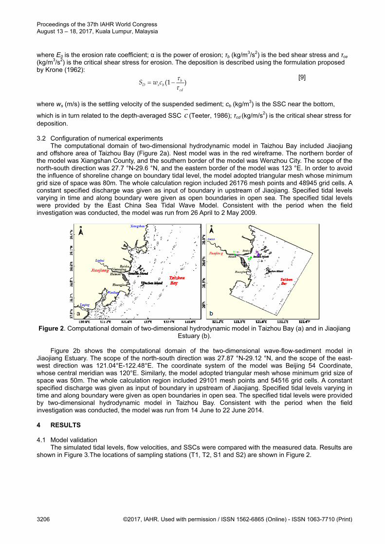
The computational domain of two-dimensional hydrodynamic model in Taizhou Bay included Jiaojiang and offshore area of Taizhou Bay (Figure 2a). Nest model was in the red wireframe. The northern border of the model was Xiangshan County, and the southern border of the model was Wenzhou City. The scope of the north-south direction was 27.7 °N-29.6 °N, and the eastern border of the model was 123 °E. In order to avoid the influence of shoreline change on boundary tidal level, the model adopted triangular mesh whose minimum grid size of space was 80m. The whole calculation region included 26176 mesh points and 48945 grid cells. A constant specified discharge was given as input of boundary in upstream of Jiaojiang. Specified tidal levels varying in time and along boundary were given as open boundaries in open sea. The specified tidal levels were provided by the East China Sea Tidal Wave Model. Consistent with the period when the field investigation was conducted, the model was run from 26 April to 2 May 2009.

Figure 2. Computational domain of two-dimensional hydrodynamic model in Taizhou Bay (a) and in Jiaojiang

Estuary (b).

Figure 2b shows the computational domain of the two-dimensional wave-flow-sediment model in Jiaojiang Estuary. The scope of the north-south direction was 27.87 °N-29.12 °N, and the scope of the east-west direction was 121.04°E-122.48°E. The coordinate system of the model was Beijing 54 Coordinate, whose central meridian was 120°E. Similarly, the model adopted triangular mesh whose minimum grid size of space was 50m. The whole calculation region included 29101 mesh points and 54516 grid cells. A constant specified discharge was given as input of boundary in upstream of Jiaojiang. Specified tidal levels varying in time and along boundary were given as open boundaries in open sea. The specified tidal levels were provided by two-dimensional hydrodynamic model in Taizhou Bay. Consistent with the period when the field investigation was conducted, the model was run from 14 June to 22 June 2014. 4 RESULTS 4.1 Model validation

The simulated tidal levels, flow velocities, and SSCs were compared with the measured data. Results are shown in Figure 3.The locations of sampling stations (T1, T2, S1 and S2) are shown in Figure 2.



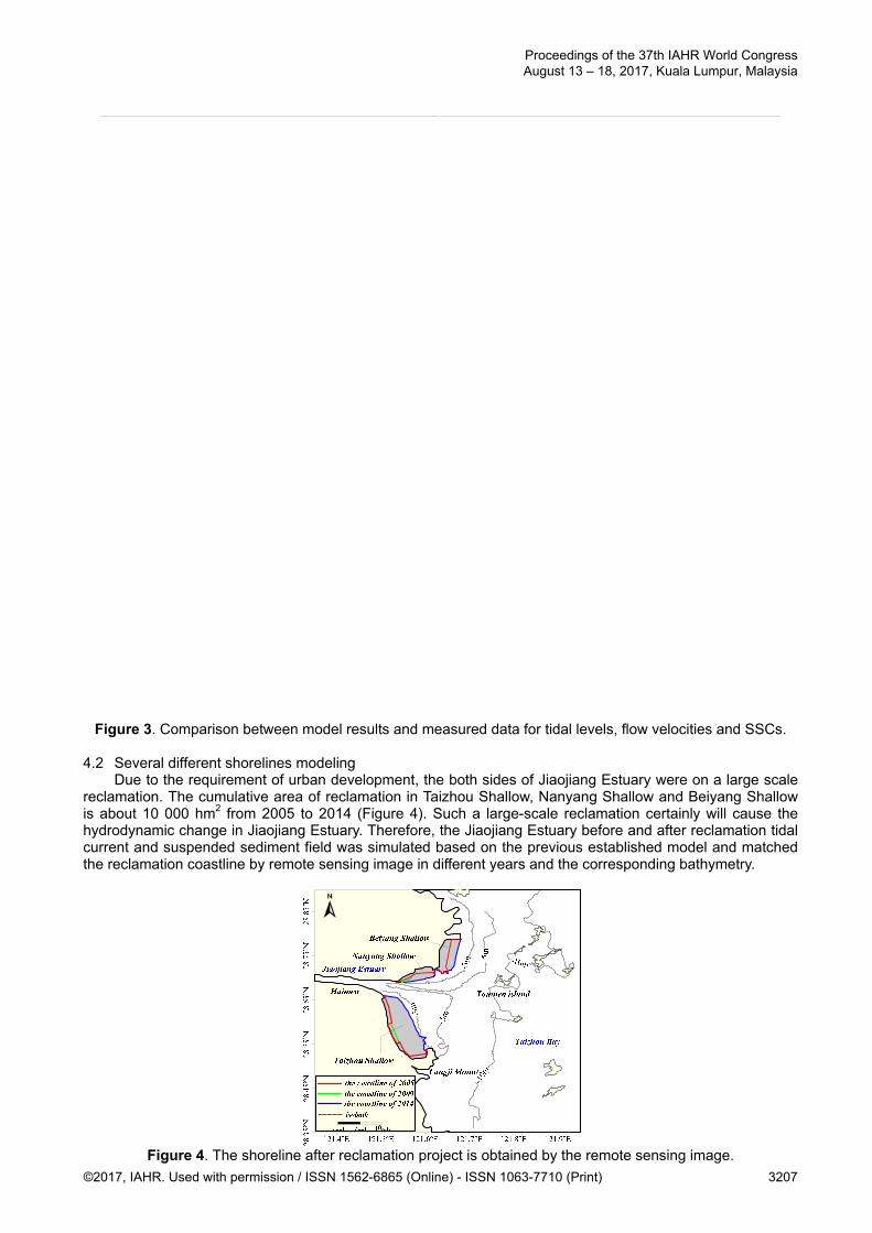
Figure 3. Comparison between model results and measured data for tidal levels, flow velocities and SSCs.

4.2 Several different shorelines modeling

Due to the requirement of urban development, the both sides of Jiaojiang Estuary were on a large scale reclamation. The cumulative area of reclamation in Taizhou Shallow, Nanyang Shallow and Beiyang Shallow is about 10 000 hm2 from 2005 to 2014 (Figure 4). Such a large-scale reclamation certainly will cause the hydrodynamic change in Jiaojiang Estuary. Therefore, the Jiaojiang Estuary before and after reclamation tidal current and suspended sediment field was simulated based on the previous established model and matched the reclamation coastline by remote sensing image in different years and the corresponding bathymetry.

Figure 4. The shoreline after reclamation project is obtained by the remote sensing image.



In order to explore the influence of flow-sediment transport on topography and coastline respectively, five calculation schemes of the numerical model were set as in Table 1. First, in order to discuss the effect of coastline change on flow-sediment transport, three programs by identical bathymetry were set up and only changing the shoreline as a result of reclamation. Then, two programs by corresponding bathymetry after reclamation were set up and meanwhile changing the shoreline as a result of reclamation.

Table 1. Setting calculation scheme of model. Case coastline bathymetry

1 2005 2005 2 2009 2005 3 2009 2009 4 2014 2005 5 2014 2014

4.3 Tidal current characteristics

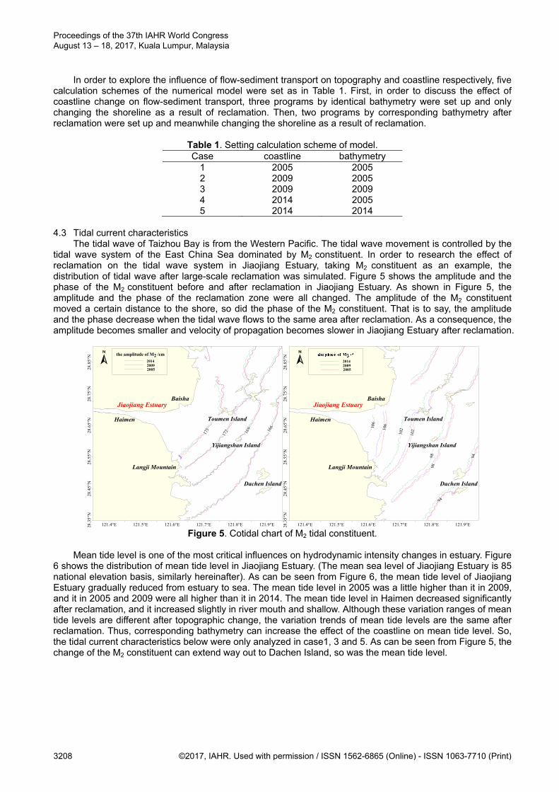
The tidal wave of Taizhou Bay is from the Western Pacific. The tidal wave movement is controlled by the tidal wave system of the East China Sea dominated by M2 constituent. In order to research the effect of reclamation on the tidal wave system in Jiaojiang Estuary, taking M2 constituent as an example, the distribution of tidal wave after large-scale reclamation was simulated. Figure 5 shows the amplitude and the phase of the M2 constituent before and after reclamation in Jiaojiang Estuary. As shown in Figure 5, the amplitude and the phase of the reclamation zone were all changed. The amplitude of the M2 constituent moved a certain distance to the shore, so did the phase of the M2 constituent. That is to say, the amplitude and the phase decrease when the tidal wave flows to the same area after reclamation. As a consequence, the amplitude becomes smaller and velocity of propagation becomes slower in Jiaojiang Estuary after reclamation.

Figure 5. Cotidal chart of M2 tidal constituent.

Mean tide level is one of the most critical influences on hydrodynamic intensity changes in estuary. Figure

6 shows the distribution of mean tide level in Jiaojiang Estuary. (The mean sea level of Jiaojiang Estuary is 85 national elevation basis, similarly hereinafter). As can be seen from Figure 6, the mean tide level of Jiaojiang Estuary gradually reduced from estuary to sea. The mean tide level in 2005 was a little higher than it in 2009, and it in 2005 and 2009 were all higher than it in 2014. The mean tide level in Haimen decreased significantly after reclamation, and it increased slightly in river mouth and shallow. Although these variation ranges of mean tide levels are different after topographic change, the variation trends of mean tide levels are the same after reclamation. Thus, corresponding bathymetry can increase the effect of the coastline on mean tide level. So, the tidal current characteristics below were only analyzed in case1, 3 and 5. As can be seen from Figure 5, the change of the M2 constituent can extend way out to Dachen Island, so was the mean tide level.

121.4°E 121.5°E 121.6°E 121.7°E 121.8°E 121.9°E28.3

5°N

28.4

5°N

28.5

5°N

28.6

5°N

28.7

5°N

28.8

5°N

Baisha

Toumen IslandHaimen

175

172 16

9 166

Yijiangshan Island

Jiaojiang Estuary

the amplitude of M2 /cm

201420092005

Dachen Island

Langji Mountain

121.4°E 121.5°E 121.6°E 121.7°E 121.8°E 121.9°E28.3

5°N

28.4

5°N

28.5

5°N

28.6

5°N

28.7

5°N

28.8

5°N

Baisha

Toumen IslandHaimen

106

106

102

102

9898

94

94

Yijiangshan Island

Jiaojiang Estuary

Dachen Island

Langji Mountain

201420092005



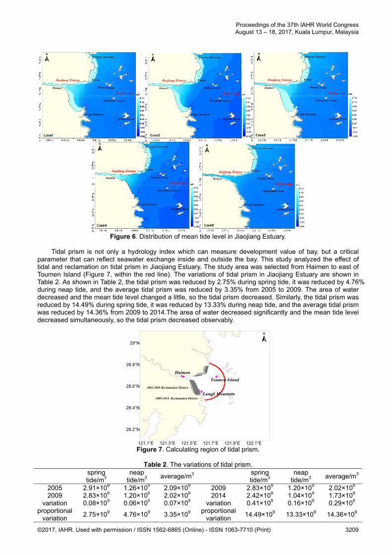
Figure 6. Distribution of mean tide level in Jiaojiang Estuary.

Tidal prism is not only a hydrology index which can measure development value of bay, but a critical

parameter that can reflect seawater exchange inside and outside the bay. This study analyzed the effect of tidal and reclamation on tidal prism in Jiaojiang Estuary. The study area was selected from Haimen to east of Toumen Island (Figure 7, within the red line). The variations of tidal prism in Jiaojiang Estuary are shown in Table 2. As shown in Table 2, the tidal prism was reduced by 2.75% during spring tide, it was reduced by 4.76% during neap tide, and the average tidal prism was reduced by 3.35% from 2005 to 2009. The area of water decreased and the mean tide level changed a little, so the tidal prism decreased. Similarly, the tidal prism was reduced by 14.49% during spring tide, it was reduced by 13.33% during neap tide, and the average tidal prism was reduced by 14.36% from 2009 to 2014.The area of water decreased significantly and the mean tide level decreased simultaneously, so the tidal prism decreased observably.

Figure 7. Calculating region of tidal prism.

Table 2. The variations of tidal prism.

spring tide/m3

neap tide/m3

average/m3 spring tide/m3

neap tide/m3

average/m3

2005 2.91×109 1.26×109 2.09×109 2009 2.83×109 1.20×109 2.02×109 2009 2.83×109 1.20×109 2.02×109 2014 2.42×109 1.04×109 1.73×109

variation 0.08×109 0.06×109 0.07×109 variation 0.41×109 0.16×109 0.29×109 proportional

variation 2.75×109 4.76×109 3.35×109

proportional variation

14.49×109 13.33×109 14.36×109

121.1°E 121.3°E 121.5°E 121.7°E 121.9°E 122.1°E

28.2°N

28.4°N

28.6°N

28.8°N

29°N

Haimen

Toumen Island

Langji Mountain

2005-2009 Reclamation District

2009-2014 Reclamation District



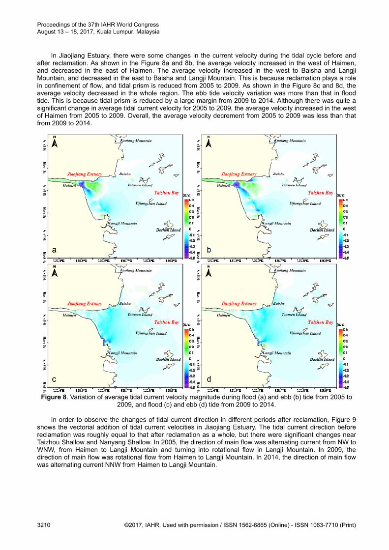
In Jiaojiang Estuary, there were some changes in the current velocity during the tidal cycle before and after reclamation. As shown in the Figure 8a and 8b, the average velocity increased in the west of Haimen, and decreased in the east of Haimen. The average velocity increased in the west to Baisha and Langji Mountain, and decreased in the east to Baisha and Langji Mountain. This is because reclamation plays a role in confinement of flow, and tidal prism is reduced from 2005 to 2009. As shown in the Figure 8c and 8d, the average velocity decreased in the whole region. The ebb tide velocity variation was more than that in flood tide. This is because tidal prism is reduced by a large margin from 2009 to 2014. Although there was quite a significant change in average tidal current velocity for 2005 to 2009, the average velocity increased in the west of Haimen from 2005 to 2009. Overall, the average velocity decrement from 2005 to 2009 was less than that from 2009 to 2014.

Figure 8. Variation of average tidal current velocity magnitude during flood (a) and ebb (b) tide from 2005 to

2009, and flood (c) and ebb (d) tide from 2009 to 2014.

In order to observe the changes of tidal current direction in different periods after reclamation, Figure 9 shows the vectorial addition of tidal current velocities in Jiaojiang Estuary. The tidal current direction before reclamation was roughly equal to that after reclamation as a whole, but there were significant changes near Taizhou Shallow and Nanyang Shallow. In 2005, the direction of main flow was alternating current from NW to WNW, from Haimen to Langji Mountain and turning into rotational flow in Langji Mountain. In 2009, the direction of main flow was rotational flow from Haimen to Langji Mountain. In 2014, the direction of main flow was alternating current NNW from Haimen to Langji Mountain.



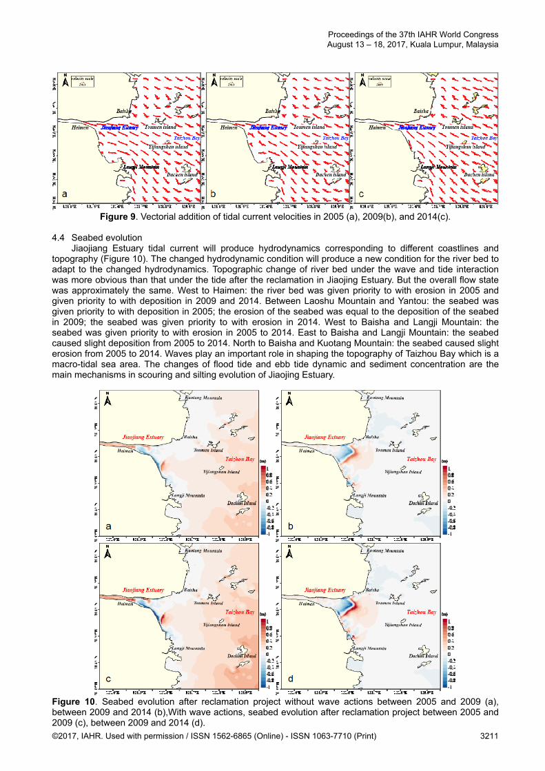
Figure 9. Vectorial addition of tidal current velocities in 2005 (a), 2009(b), and 2014(c).

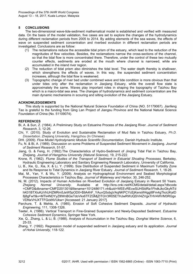
4.4 Seabed evolution

Jiaojiang Estuary tidal current will produce hydrodynamics corresponding to different coastlines and topography (Figure 10). The changed hydrodynamic condition will produce a new condition for the river bed to adapt to the changed hydrodynamics. Topographic change of river bed under the wave and tide interaction was more obvious than that under the tide after the reclamation in Jiaojing Estuary. But the overall flow state was approximately the same. West to Haimen: the river bed was given priority to with erosion in 2005 and given priority to with deposition in 2009 and 2014. Between Laoshu Mountain and Yantou: the seabed was given priority to with deposition in 2005; the erosion of the seabed was equal to the deposition of the seabed in 2009; the seabed was given priority to with erosion in 2014. West to Baisha and Langji Mountain: the seabed was given priority to with erosion in 2005 to 2014. East to Baisha and Langji Mountain: the seabed caused slight deposition from 2005 to 2014. North to Baisha and Kuotang Mountain: the seabed caused slight erosion from 2005 to 2014. Waves play an important role in shaping the topography of Taizhou Bay which is a macro-tidal sea area. The changes of flood tide and ebb tide dynamic and sediment concentration are the main mechanisms in scouring and silting evolution of Jiaojing Estuary.

Figure 10. Seabed evolution after reclamation project without wave actions between 2005 and 2009 (a), between 2009 and 2014 (b),With wave actions, seabed evolution after reclamation project between 2005 and 2009 (c), between 2009 and 2014 (d).



5 CONCLUSIONS The two-dimensional wave-tide-sediment mathematical model is established and verified with measured

data. On the basis of the model validation, five cases are set to explore the changes of the hydrodynamics during different reclamation periods from 2005 to 2014. By adding elements of the sea waves, the effects of wave on suspended sediment concentration and riverbed evolution in different reclamation periods are investigated. Conclusions are as follow:

(1) The reclamations reduce the accessible tidal prism of the estuary, which lead to the reduction of the magnitudes of flow velocities. Besides, the reclamations narrow the cross-sections of the channel, so that the tidal flow is more concentrated there. Therefore, under the control of these two mutually counter effects, sediments are eroded at the mouth where channel is narrowed, while are accumulated in the inland river region.

(2) The reduction of tidal prism also diminishes the tidal level. The water depth thereby is shallower, which strengthens the effects of waves. In this way, the suspended sediment concentration increases, although the tidal flow is weakened.

(3) Topographic change of river bed under combined wave and tide condition is more obvious than that under tides only after the reclamation in Jiaojiang Estuary, while the overall flow state is approximately the same. Waves play important roles in shaping the topography of Taizhou Bay which is a macro-tidal sea area. The changes of hydrodynamics and sediment concentration are the main dynamic mechanisms in scouring and silting evolution of the Jiaojiang Estuary.

ACKNOWLEDGEMENTS

This study is supported by the National Natural Science Foundation of China (NO. 51179067). Jianfeng Tao is grateful to the funding from Qing Lan Project of Jiangsu Province and the National Natural Science Foundation of China (No. 51109074). REFERENCES Bi, A. & Sun, Z. (1984). A Preliminary Study on Estuarine Process of the Jiaojiang River. Journal of Sediment

Research, 3, 12-26. Chi, Y. (2010). Study of Evolution and Sustainable Reclamation of Mud flats in Taizhou Estuary, Ph.D.

Dissertation. Zhejiang University, Hangzhou (In Chinese) DHI. (2009). Flow Model Hydrodynamic Module Scientific Documentation, Danish Hydraulic Institute. Fu, N. & Bi, A. (1989). Discussion on some Problems of Suspended Sediment Movement in Jiaojiang. Journal

of Sediment Research, 51-57. Jiang, G. & Feng, H. (1992).The Characteristics of Hydro-Sediment of Jinqing Tidal Flat in Taizhou Bay,

Zhejiang. Journal of Hangzhou University (Natural Science), 19, 215-222. Krone, R. (1962). Flume Studies of the Transport of Sediment in Estuarial Shoaling Processes, Berkeley,

Hydraulic Engineering Laboratory and Sanitary Engineering Research Laboratory, University of California. Li, B., Xie, Q., Xia, X. & Li, Y. (1999). Size Distribution of Suspended Sediment in Maximum Turbidity Zone

and Its Response to Tidal Dynamics in Jiaojiang River Estuary. Journal of Sediment Research, 1, 18-26. Mai, M., Yan, Y. & Wu, Y. (2009). Analysis on Hydrographical Environment and Seabed Morphological

Processes Characteristics in Taizhou Bay. Journal of Waterway and Harbor, 30, 246-252. Ni, M. (2012). Impacts of Human Activities on Riverbed Evolution of Jiaojiang Estuary in Recent 50 Years.

Zhejiang Normal University. Available at http://kns.cnki.net/KCMS/detail/detail.aspx?dbcode =CMFD&dbname=CMFD201301&filename=1012486171.nh&uid=WEEvREcwSlJHSldRa1FhdkJkcGkyNTdhK01BTXluKzVhUHZMRm5JeW5pOD0=$9A4hF_YAuvQ5obgVAqNKPCYcEjKensW4ggI8Fm4gTkoUKaID8j8gFw!!&v=MTk4NDYyZlllWnBGeTdoVkx6TFZGMjZITGV3R05ETHJwRWJQSVI4ZVgxTHV4WVM3RGgxVDNxVHJXTTFGckNVUkw= [Accessed: 21 January 2017].

Parchure, T. & Mehta, A. (1985). Erosion of Soft Cohesive Sediment Deposits. Journal of Hydraulic Engineering, 111, 1308-1326.

Teeter, A. (1986). Vertical Transport in Fine-Grained Suspension and Newly-Deposited Sediment. Estuarine Cohesive Sediment Dynamics, Springer New York.

Xie, Q., Zhang, L. & Li, B. (1988). Analysis of Accumulation in the Taizhou Bay. Donghai Marine Science, 6, 25-33.

Zhang, Y. (1992). Regression model of suspended sediment in Jiaojiang estuary and its application. Journal of Hohai University, 118-122.



BED LOAD CHANGES IN ESTUARY DUE TO SEA LEVEL RISE AND HYDRODYNAMIC

REACTION

ANIZAWATI AHMAD(1), WAN HANNA MELINI WAN MOHTAR(2) & NOR ASLINDA AWANG(3)

(1,3) National Hydraulic Research Institute of Malaysia (NAHRIM), Seri Kembangan, Malaysia

[email protected] (2) Department of Civil & Structural Engineering, Faculty of Engineering and Built Environment, Universiti Kebangsaan Malaysia 43600,

Bandar Baru Bangi, Malaysia [email protected]

ABSTRACT The complexity of estuarine hydrodynamics arises due to the continuous interaction between freshwater and saltwater. The hydrodynamic process is influenced by marine factors such as tides, waves, salt water intrusion, river discharge, sediment type and shape of the mouth. This research attempts to investigate the bed changes at Kuala Pahang due to sea level rise-induced hydrodynamic reactions. The study area experiences dominant mixed semidiurnal tides and is projected to hit with sea level rising up to 0.034, 0.144 and 0.307 m in 2020, 2060 and 2100, respectively. The rate of sea level rising is the third highest, at the East Coast of Malaysia after Kelantan and Terengganu. The increase in sea level caused changes in water depth, bathymetry and hydrodynamic pattern. The increase in flow velocity promotes erosion and the reduction in flow velocity lead to sediment deposition. MIKE 21 software is used in the numerical modeling to analyze the hydrodynamic processes while Sand Transport (ST) module is used to study the sediment transport. The sea level rise factor is combined to obtain the changes of the study area. The study is limited to the southwest monsoon. Modeling work is also conducted for a temporal scale of 14 days, taking into account a full tidal cycle. The historical analysis of bathymetry changes is done by comparing the bathymetry data in 1952 and 2014 using ArcGIS software. The analysis showed that the bathymetry has changed between -0.08 to +2.9856 m in the last 62 years. Hydrodynamic modeling results indicated that the flow velocity changed between -0.01 - +0.18 m/s on average, and the maximum values is between -0.06 - +0.2 m/s. Sediment transport modeling shows the average rate of bed level change which is between 0.2 to 0.6 m/dy and average bed load changes is between 0.0002 - 0.0008 m3/s /m. Analysis has shown that the southern part of estuaries, meanders of rivers and near island experienced decrease in flow velocity which indicated sedimentation. Keywords: Sea level rise; hydrodynamic; bed load changes. 1 INTRODUCTION

River and sea hydrodynamic processes such as tidal and waves are causing erosion and sedimentation in the estuary. The tidal area (i.e. the intertidal zone), receives continuous alternating current which is vulnerable to changes due to sediment transport. The morphology of the river and the beach slope, roughness of grooves, the type and shape of the grooves, the orientation of the coast, meeting creeks and vegetation also plays a role in the sediment transport processes. In addition, sea level changes and vertical land movement is seen to contribute to the dynamics of sediment transport. Deposition and erosion resulting from the sediment transport process affect the navigation system, the flow of water, flora and fauna as well as the aesthetics value of the area.

Sea level is influenced by changes in the geoids, human activity, greenhouse effect, changes in the volume of water bodies and sea basin. Changes in sea level increased the flood level, current velocity, longer seawater intrusion, loss of property on coastal areas, the risk of disease and adverse effects on agriculture, aquaculture, water quality and socio-economic development. The magnitude of the sea level rise impact is also affected by the vulnerability characteristics of the coastal area. Changes in environmental surroundings affect the tide and eventually the benchmark for the estuary. Sea level rise increases the depth of the sea water and the hydraulic and hydrodynamic processes of an area are subsequently modified.

Siti Waznah et. al. (2010) stated that estuaries and rivers are often the high deposition area which serves as a trap for the minerals from river and sea materials from being transported to the shore. Furthermore, the tidal river upstream direction plays a role in determining the direction of sediment transport in shallow waters (Jing et. al., 2013). Tides and waves carry sediment from the ocean to the estuary which results in the dynamic and continuous events of filling and sediment entrainment within the area.



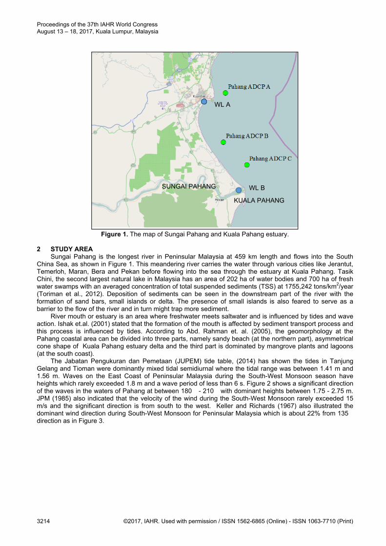
Figure 1. The map of Sungai Pahang and Kuala Pahang estuary.

2 STUDY AREA

Sungai Pahang is the longest river in Peninsular Malaysia at 459 km length and flows into the South China Sea, as shown in Figure 1. This meandering river carries the water through various cities like Jerantut, Temerloh, Maran, Bera and Pekan before flowing into the sea through the estuary at Kuala Pahang. Tasik Chini, the second largest natural lake in Malaysia has an area of 202 ha of water bodies and 700 ha of fresh water swamps with an averaged concentration of total suspended sediments (TSS) at 1755,242 tons/km2/year (Toriman et al., 2012). Deposition of sediments can be seen in the downstream part of the river with the formation of sand bars, small islands or delta. The presence of small islands is also feared to serve as a barrier to the flow of the river and in turn might trap more sediment.

River mouth or estuary is an area where freshwater meets saltwater and is influenced by tides and wave action. Ishak et.al. (2001) stated that the formation of the mouth is affected by sediment transport process and this process is influenced by tides. According to Abd. Rahman et. al. (2005), the geomorphology at the Pahang coastal area can be divided into three parts, namely sandy beach (at the northern part), asymmetrical cone shape of Kuala Pahang estuary delta and the third part is dominated by mangrove plants and lagoons (at the south coast).

The Jabatan Pengukuran dan Pemetaan (JUPEM) tide table, (2014) has shown the tides in Tanjung Gelang and Tioman were dominantly mixed tidal semidiurnal where the tidal range was between 1.41 m and 1.56 m. Waves on the East Coast of Peninsular Malaysia during the South-West Monsoon season have heights which rarely exceeded 1.8 m and a wave period of less than 6 s. Figure 2 shows a significant direction of the waves in the waters of Pahang at between 180� - 210� with dominant heights between 1.75 - 2.75 m. JPM (1985) also indicated that the velocity of the wind during the South-West Monsoon rarely exceeded 15 m/s and the significant direction is from south to the west. Keller and Richards (1967) also illustrated the dominant wind direction during South-West Monsoon for Peninsular Malaysia which is about 22% from 135� direction as in Figure 3.

WL A

WL B SUNGAI PAHANG

KUALA PAHANG



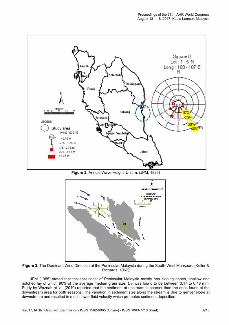
Figure 2. Annual Wave Height. Unit m. (JPM, 1985)

Figure 3. The Dominant Wind Direction at the Peninsular Malaysia during the South-West Monsoon. (Keller &

Richards, 1967)

JPM (1985) stated that the east coast of Peninsular Malaysia mostly has sloping beach, shallow and notched lay of which 90% of the average median grain size, D50 was found to be between 0.17 to 0.48 mm. Study by Waznah et. al. (2010) reported that the sediment at upstream is coarser than the ones found at the downstream area for both seasons. The variation in sediment size along the stream is due to gentler slope at downstream and resulted in much lower fluid velocity which promotes sediment deposition.

Study area

20%

30%

10%

40%



Pahang River originates from Mount Tahan and flows as far as 440 km from the height of 2187 m and is the main tributary of Sungai Jelai and Tembeling River (Tachikawa et. al., 2004). Other tributaries contributing to the flow and discharge of the river are Sungai Chini, Sungai Yap, Sungai Lubuk Paku and Sungai Temerloh. The average water discharge of Sungai Pahang from years of 1980 to 2009 was 845.78 m³/s, measured at the Sungai Yap telemetry station, while in Temerloh it produced 1008.50 m³/s discharge and about 1184.46m³/s flow was measured at Lubuk Paku (Pan et. al., 2011). Note that the telemetry stations of Sungai Yap, Temerloh and Lubuk Paku are located along Sungai Pahang, with Sungai Yap station being located at the most upstream. The study area receives an annual rainfall of 2170 mm, which mostly falls in the North-East Monsoon and the average annual temperature in Kuantan is 26.4 °C with an average relative humidity of 86%. The morphology of this area especially Sungai Pahang and Sungai Tembeling mainly were composed of alluvial soils as bed material and has different depths of less than 1 m to over 18 m (Tachikawa et. al., 2004). The beach area is mostly flat and swampy, with granite soil consisting of coarse and fine sand and clay.

3 METHOD 3.1 Sea Level Rise

Rising sea levels caused the shoreline to retreat to the mainland while the decreasing sea level promotes bigger beach (JPM, 1985). The surface level of the world's oceans had increased by 1 mm/year due to the melting of glaciers due to higher temperature, which subsequently increases the volume of ocean water. Md Din (2014) based on altimetry and vertical-corrected tidal data concluded that sea level is rising at rate of 4.47 ± 0.71 mm/year for the Malaysian region, where the average rate for South China Sea is at 3.77 ± 0.54 mm/yr.

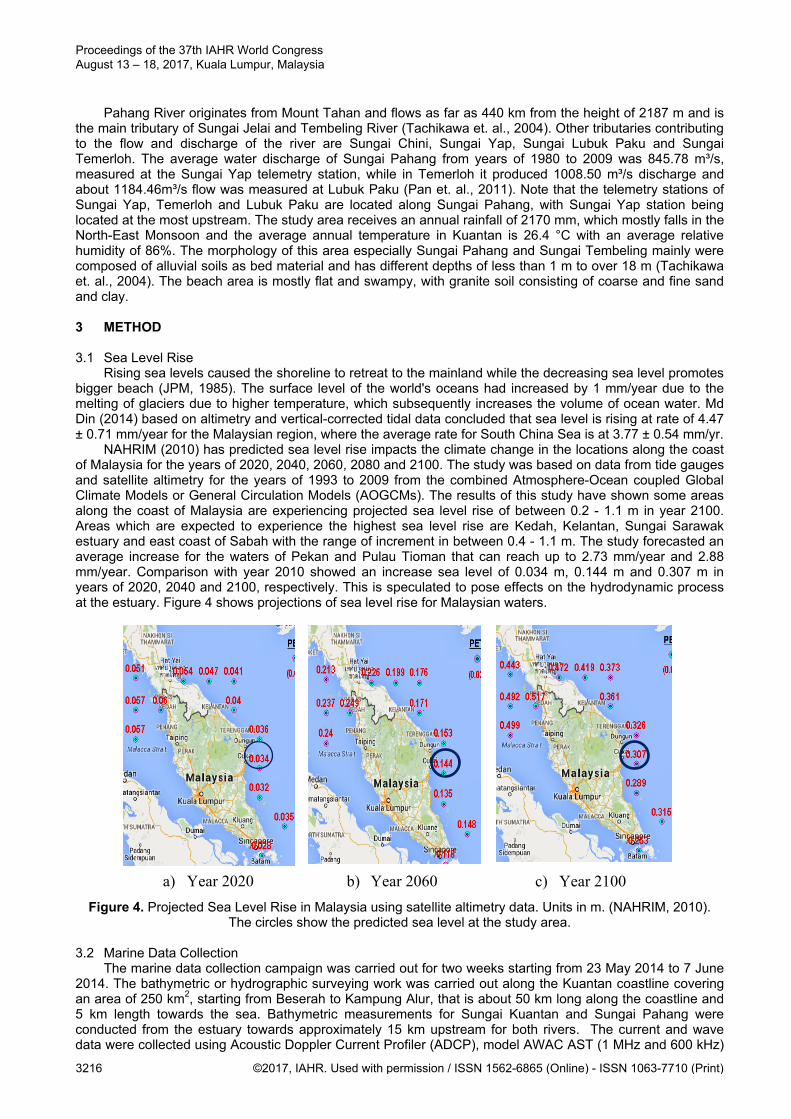
NAHRIM (2010) has predicted sea level rise impacts the climate change in the locations along the coast of Malaysia for the years of 2020, 2040, 2060, 2080 and 2100. The study was based on data from tide gauges and satellite altimetry for the years of 1993 to 2009 from the combined Atmosphere-Ocean coupled Global Climate Models or General Circulation Models (AOGCMs). The results of this study have shown some areas along the coast of Malaysia are experiencing projected sea level rise of between 0.2 - 1.1 m in year 2100. Areas which are expected to experience the highest sea level rise are Kedah, Kelantan, Sungai Sarawak estuary and east coast of Sabah with the range of increment in between 0.4 - 1.1 m. The study forecasted an average increase for the waters of Pekan and Pulau Tioman that can reach up to 2.73 mm/year and 2.88 mm/year. Comparison with year 2010 showed an increase sea level of 0.034 m, 0.144 m and 0.307 m in years of 2020, 2040 and 2100, respectively. This is speculated to pose effects on the hydrodynamic process at the estuary. Figure 4 shows projections of sea level rise for Malaysian waters.

a) Year 2020

b) Year 2060 c) Year 2100

Figure 4. Projected Sea Level Rise in Malaysia using satellite altimetry data. Units in m. (NAHRIM, 2010). The circles show the predicted sea level at the study area.

3.2 Marine Data Collection

The marine data collection campaign was carried out for two weeks starting from 23 May 2014 to 7 June 2014. The bathymetric or hydrographic surveying work was carried out along the Kuantan coastline covering an area of 250 km2, starting from Beserah to Kampung Alur, that is about 50 km long along the coastline and 5 km length towards the sea. Bathymetric measurements for Sungai Kuantan and Sungai Pahang were conducted from the estuary towards approximately 15 km upstream for both rivers. The current and wave data were collected using Acoustic Doppler Current Profiler (ADCP), model AWAC AST (1 MHz and 600 kHz)



produced by Nortek AS, Norway in two separate locations which was designated as ADCP A and ADCP B. Refer to Table 1 for the coordinate and the depth where the instruments were deployed. The measurement of tidal data was based on mean sea level (MSL), measured at two locations using Aquatec 520P water level logger by Aquatec Group UK. The device is also capable of measuring and recording temperature and air pressure. In this study, the time interval of 10 minutes had been configured to allow the instrument to record the tidal changes. The equipment was mounted on the pole piers under water by divers at both locations (Table 2). The locations of these equipments are plotted in Figure 1.

Table 1. Current and wave station Station Latitude Longitude Depth (m) ADCP A 3° 49' 49.000" N 103° 24' 47.300" E 9 ADCP B 3° 40' 25.400" N 103° 24' 23.600" E 10

Table 2. Water level station

Station Latitude LongitudeWL A 3° 31' 50.400" N 103° 27' 44.000" E WL B 3° 48' 35.600" N 103° 20' 09.800" E

3.3 Numerical Model

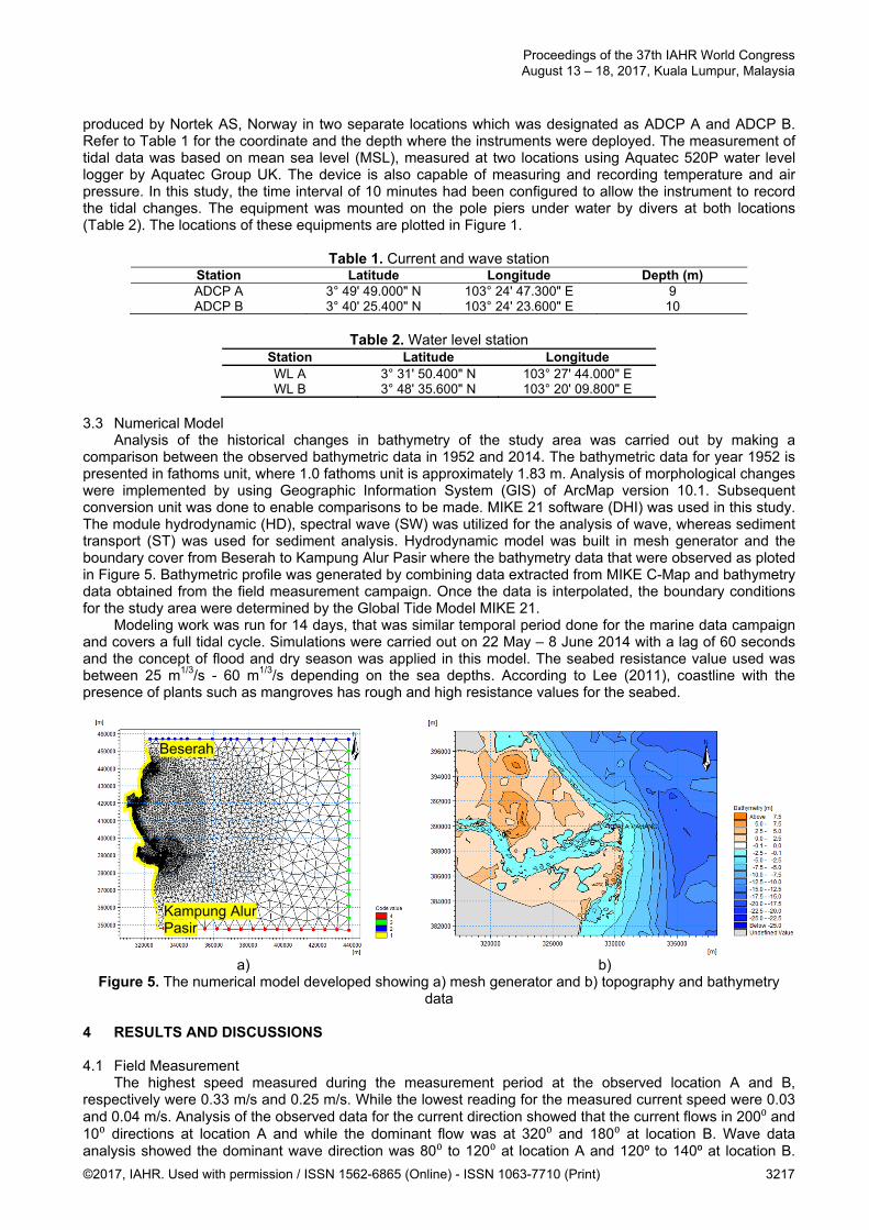
Analysis of the historical changes in bathymetry of the study area was carried out by making a comparison between the observed bathymetric data in 1952 and 2014. The bathymetric data for year 1952 is presented in fathoms unit, where 1.0 fathoms unit is approximately 1.83 m. Analysis of morphological changes were implemented by using Geographic Information System (GIS) of ArcMap version 10.1. Subsequent conversion unit was done to enable comparisons to be made. MIKE 21 software (DHI) was used in this study. The module hydrodynamic (HD), spectral wave (SW) was utilized for the analysis of wave, whereas sediment transport (ST) was used for sediment analysis. Hydrodynamic model was built in mesh generator and the boundary cover from Beserah to Kampung Alur Pasir where the bathymetry data that were observed as ploted in Figure 5. Bathymetric profile was generated by combining data extracted from MIKE C-Map and bathymetry data obtained from the field measurement campaign. Once the data is interpolated, the boundary conditions for the study area were determined by the Global Tide Model MIKE 21. Modeling work was run for 14 days, that was similar temporal period done for the marine data campaign and covers a full tidal cycle. Simulations were carried out on 22 May – 8 June 2014 with a lag of 60 seconds and the concept of flood and dry season was applied in this model. The seabed resistance value used was between 25 m1/3/s - 60 m1/3/s depending on the sea depths. According to Lee (2011), coastline with the presence of plants such as mangroves has rough and high resistance values for the seabed.

a)

b)

Figure 5. The numerical model developed showing a) mesh generator and b) topography and bathymetry data

4 RESULTS AND DISCUSSIONS 4.1 Field Measurement

The highest speed measured during the measurement period at the observed location A and B, respectively were 0.33 m/s and 0.25 m/s. While the lowest reading for the measured current speed were 0.03 and 0.04 m/s. Analysis of the observed data for the current direction showed that the current flows in 200⁰ and 10⁰ directions at location A and while the dominant flow was at 320⁰ and 180⁰ at location B. Wave data analysis showed the dominant wave direction was 80⁰ to 120⁰ at location A and 120º to 140º at location B.

Beserah

Kampung Alur Pasir



Location A indicated that the wave height went up to 0.4 m while the maximum wave height at location B exceeded 0.6 m. Contours showed the mainland area had heights exceeding 7.5 m and the sea has depth exceeding 25 m towards offshore and become shallower when approaching the coastline.

4.2 Historical Bed Level Changes

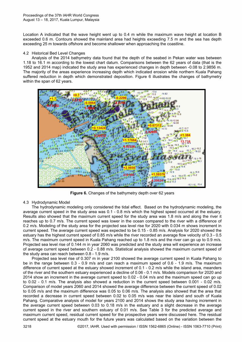
Analysis of the 2014 bathymetry data found that the depth of the seabed in Pekan water was between 1.18 to 16.1 m according to the lowest chart datum. Comparisons between the 62 years of data (that is the 1952 and 2014 map) indicated the study area has experienced changes in depth between -0.08 to 2.9856 m. The majority of the areas experience increasing depth which indicated erosion while northern Kuala Pahang suffered reduction in depth which demonstrated deposition. Figure 6 illustrates the changes of bathymetry within the span of 62 years.

Figure 6. Changes of the bathymetry depth over 62 years

4.3 Hydrodynamic Model

The hydrodynamic modeling only considered the tidal effect. Based on the hydrodynamic modeling, the average current speed in the study area was 0.1 - 0.8 m/s which the highest speed occurred at the estuary. Results also showed that the maximum current speed for the study area was 1.8 m/s and along the river it reaches up to 0.7 m/s. The current speed was lower in the ocean compared to the river with a difference of 0.2 m/s. Modeling of the study area for the projected sea level rise for 2020 with 0.034 m shows increment in current speed. The average current speed was expected to be 0.15 - 0.85 m/s. Analysis for 2020 showed the estuary has the highest current speed of 0.85 m/s while the river recorded an average flow velocity of 0.3 - 0.5 m/s. The maximum current speed in Kuala Pahang reached up to 1.8 m/s and the river can go up to 0.9 m/s. Projected sea level rise of 0.144 m in year 2060 was predicted and the study area will experience an increase of average current speed between 0.2 - 0.88 m/s. Statistical analysis showed the maximum current speed of the study area can reach between 0.8 - 1.9 m/s.

Projected sea level rise of 0.307 m in year 2100 showed the average current speed in Kuala Pahang to be in the range between 0.3 - 0.9 m/s and can reach a maximum speed of 0.6 - 1.9 m/s. The maximum difference of current speed at the estuary showed increment of 0.1 - 0.2 m/s while the island area, meanders of the river and the southern estuary experienced a decline of 0.06 - 0.1 m/s. Models comparison for 2020 and 2014 show an increment in the average current speed to 0.02 - 0.04 m/s and the maximum speed can go up to 0.02 - 0.1 m/s. The analysis also showed a reduction in the current speed between 0.001 - 0.02 m/s. Comparison of model years 2060 and 2014 showed the average difference between the current speed of 0.02 to 0.05 m/s and the maximum difference was 0.05 to 0.06 m/s. The analysis also showed that the area that recorded a decrease in current speed between 0.02 to 0.05 m/s was near the island and south of Kuala Pahang. Comparative analysis of model for years 2100 and 2014 shows the study area having increment in the average current speed between 0.03 to 0.18 m/s in the estuary and a slight decrease in the average current speed in the river and southern estuary of 0.01 m/s. See Table 3 for the predicted average and maximum current speed, residual current speed for the prospective years were discussed here. The residual current speed at the estuary mouth for the future years was calculated based on the variation between the

0.36576

-0.0864 +1.7

+0.7 -0.2296

+0.67312

+1.17664

+1.384

+2.9856

+1.59376

+0.13424

4.02336

0.9144

4.20624

5.4864

13.716

9.32688

7.3152 8.2296

0.73152



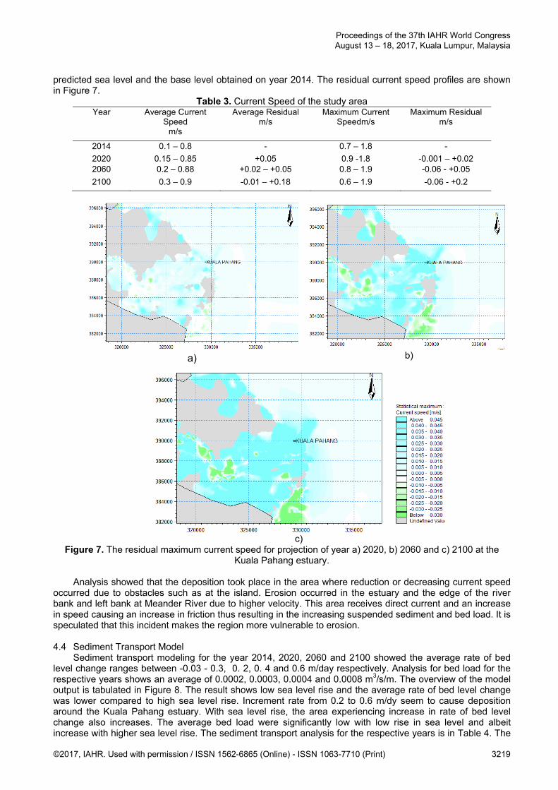
predicted sea level and the base level obtained on year 2014. The residual current speed profiles are shown in Figure 7.

Table 3. Current Speed of the study area Year Average Current

Speed m/s

Average Residual m/s

Maximum Current Speedm/s

Maximum Residual m/s

2014 0.1 – 0.8 - 0.7 – 1.8 -

2020 0.15 – 0.85 +0.05 0.9 -1.8 -0.001 – +0.02 2060 0.2 – 0.88 +0.02 – +0.05 0.8 – 1.9 -0.06 - +0.05

2100 0.3 – 0.9 -0.01 – +0.18 0.6 – 1.9 -0.06 - +0.2

a) b)

c)

Figure 7. The residual maximum current speed for projection of year a) 2020, b) 2060 and c) 2100 at the Kuala Pahang estuary.

Analysis showed that the deposition took place in the area where reduction or decreasing current speed

occurred due to obstacles such as at the island. Erosion occurred in the estuary and the edge of the river bank and left bank at Meander River due to higher velocity. This area receives direct current and an increase in speed causing an increase in friction thus resulting in the increasing suspended sediment and bed load. It is speculated that this incident makes the region more vulnerable to erosion. 4.4 Sediment Transport Model

Sediment transport modeling for the year 2014, 2020, 2060 and 2100 showed the average rate of bed level change ranges between -0.03 - 0.3, 0. 2, 0. 4 and 0.6 m/day respectively. Analysis for bed load for the respective years shows an average of 0.0002, 0.0003, 0.0004 and 0.0008 m3/s/m. The overview of the model output is tabulated in Figure 8. The result shows low sea level rise and the average rate of bed level change was lower compared to high sea level rise. Increment rate from 0.2 to 0.6 m/dy seem to cause deposition around the Kuala Pahang estuary. With sea level rise, the area experiencing increase in rate of bed level change also increases. The average bed load were significantly low with low rise in sea level and albeit increase with higher sea level rise. The sediment transport analysis for the respective years is in Table 4. The



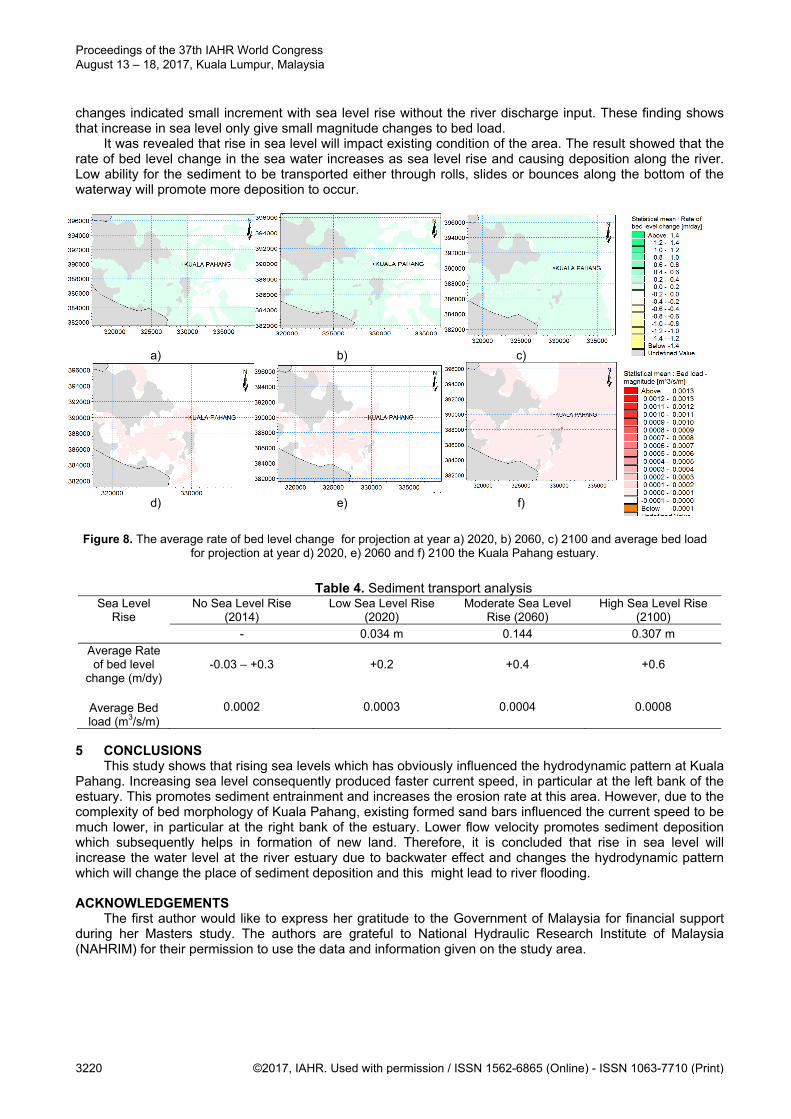
changes indicated small increment with sea level rise without the river discharge input. These finding shows that increase in sea level only give small magnitude changes to bed load.

It was revealed that rise in sea level will impact existing condition of the area. The result showed that the rate of bed level change in the sea water increases as sea level rise and causing deposition along the river. Low ability for the sediment to be transported either through rolls, slides or bounces along the bottom of the waterway will promote more deposition to occur.

a) b) c)

d) e) f)

Figure 8. The average rate of bed level change for projection at year a) 2020, b) 2060, c) 2100 and average bed load for projection at year d) 2020, e) 2060 and f) 2100 the Kuala Pahang estuary.

Table 4. Sediment transport analysis

Sea Level Rise

No Sea Level Rise (2014)

Low Sea Level Rise (2020)

Moderate Sea Level Rise (2060)

High Sea Level Rise (2100)

- 0.034 m 0.144 0.307 m

Average Rate of bed level

change (m/dy) -0.03 – +0.3 +0.2 +0.4 +0.6

Average Bed load (m3/s/m)

0.0002 0.0003 0.0004 0.0008

5 CONCLUSIONS This study shows that rising sea levels which has obviously influenced the hydrodynamic pattern at Kuala Pahang. Increasing sea level consequently produced faster current speed, in particular at the left bank of the estuary. This promotes sediment entrainment and increases the erosion rate at this area. However, due to the complexity of bed morphology of Kuala Pahang, existing formed sand bars influenced the current speed to be much lower, in particular at the right bank of the estuary. Lower flow velocity promotes sediment deposition which subsequently helps in formation of new land. Therefore, it is concluded that rise in sea level will increase the water level at the river estuary due to backwater effect and changes the hydrodynamic pattern which will change the place of sediment deposition and this might lead to river flooding. ACKNOWLEDGEMENTS The first author would like to express her gratitude to the Government of Malaysia for financial support during her Masters study. The authors are grateful to National Hydraulic Research Institute of Malaysia (NAHRIM) for their permission to use the data and information given on the study area.



REFERENCES Ab. Ghani, A., Chang, C.K., Leow, C.S. & Zakaria, N.A. (2012). Sungai Pahang Digital Flood Mapping: 2007

Flood, International Journal of River Basin Management, 2, 139-148. Abd. Rahman, A.H., Sapie, M.S., Hashim, M.R. & Mohd Nordin, M.N. (2005). The Wave-Influenced Pahang

Delta: Geomorphology, Facies and Sedimentation Trends. Petroleum Geology Conference and Exhibition 2005, Kuala Lumpur, 147-149.

Gasim, M.B., Mokhtar, M., Surif, S., Toriman, M.E., Abd. Rahim, S. & Pan, L.L. (2012). Analysis of Thirty Years Recurrent Floods of the Pahang River, Malaysia. Asian Journal of Earth Sciences, 5(1), 25-35.

Ishak, A.K., Samuding, K. & Yusof, N.H. (2001). Dinamik Air dan Sedimen Terampai di Muara Sungai Selangor. Seminar Research and Development 2000. October 2000, Malaysia Institute for Nuclear Technology Research (MINT).

Jabatan Perdana Menteri (JPM). (1985). National Coastal Erosion Study, Unit Perancang Ekonomi, Kuala Lumpur.

Keller, G.H. & Richards, A.F. (1967). Sediments of The Malacca Strait, Southeast Asia. Journal of Sedimentary Petrology, 37(1), 102-127.

Lee, H.L. (2011). Penentuan Kadar Pemendapan di Selat Pulau Pinang akibat Pendalaman Lembangan Pelabuhan Pulau Pinang. MSc Thesis. Universiti Kebangsaan Malaysia.

Luo, J., Li, M., Sun, Z. & O’Connor, B.A. (2013). Numerical Modelling of Hydrodynamics and Sand Transport in the Tide-Dominated Coastal-To-Estuarine Region. Marine Geology, 342, 14-27.

Md. Din., A.H. (2014). Sea Level Rise Estimation and Interpretation in Malaysian Region using Multi-Sensor Techniques. PhD thesis. Universiti Teknologi Malaysia.

National Hydraulic Research Institute of Malaysia (NAHRIM). (2010). The Study of the Impact of Climate Change to Sea Level Rise in Malaysia. National Hydraulic Research Institute Malaysia. 172.

Pan, L.L, Gasim, M.B., Toriman, M.E., Abd. Rahim, S. & Kamaruddin, K.A. (2011). Hydrological Pattern of Pahang River Basin and Their Relation to Flood Historical Event. Jurnal e-Bangi. 6(1), 29-37, 2011.

Siti Waznah, A., Kamaruzzaman, B.Y. Ong, M.C., Rina, S.Z. & Zahir, S. (2010). Spatial and Temporal Bottom Sediment Characteristics of Pahang River-Estuary, Pahang, Malaysia. Oriental Journal of Chemistry, 26(1), 39-44.

Sulaiman, W.N.A., Heshmatpoor A. & Rosli, M.H. (2010). Identification of Flood Source Areas in Pahang River Basin, Peninsular Malaysia. Environmental Asia 3 (special issue), 73-78.

Tachikawa, Y., James, R., Abdullah, K., Mohd. Desa, & M.N. (2004). Catalogue of Rivers for Southeast Asia and the Pacific-Volume V. The UNESCO-IHP Regional Steering Committee for Southeast Asia and the Pacific.

Toriman, M.E., Kamarudin, M.K.A., Abd Aziz, N.A., Md Din, H., Ata, F.M., Abdullah, N.M., Mushrifah, I, Jamil, N.R., Abdul Rani, N.S., Saad, M.H., Abdullah, N.W., Gasim, M.B. & Mokhtar, M. (2012). Pengurusan Sedimen Terhadap Sumber Air Bersepadu: Satu Kajian Kes di Sungai Chini, Pekan, Pahang. e-BANGI: Jurnal Sains Sosial dan Kemanusiaan, 7(1), 267-283.



MONITORING OF CONTINUOUS TIDAL CURRENT PATTERN IN ASYMMETRIC

BIFURCATION CHANNEL NETWORK USING ACOUSTIC TOMOGRAPHY METHOD AND NUMERICAL MODELING

MOCHAMMAD MEDDY DANIAL(1), KIYOSI KAWANISI(2), MASOUD BAHREINMOTLAGH(3), MOHAMAD BASEL AL SAWAF(4) & JUNYA KAGAMI(5)

(1,2,3,4,5) Dept. of Civil and Environmental Engineering, Graduate School of Engineering, Hiroshima University, Hiroshima, Japan,

[email protected]; [email protected]; [email protected]; [email protected]; [email protected]

ABSTRACT Characteristics of the estuary system are always unique due to the geometrical shape and tidal regime. In addition, interaction between river flow discharge and tidal wave can lead to inequality of velocity pattern. Therefore, monitoring complex flow patterns in estuaries is needed to understand the dynamic processes of flow field in shallow bifurcation channel influenced by tidal motion. Combination of Fluvial Acoustic Tomography System (FATS) and two-dimensional depth averaged finite element modeling are used to investigate the behavior of flow pattern in asymmetric bifurcation channel network. Besides, moored ADCP measurement campaigns are carried out for providing and establishing reference data. The flow pattern in Ota River estuary shows asymmetric behavior. In addition, the comparison between the FATS data and the numerical model results is relatively satisfactory in tidal flow patterns though there are slight differences. The FATS, however, is more reliable compared to numerical modeling in measuring flow velocity in the tidal channel network. Keywords: Tidal current pattern monitor; acoustic tomography; two-dimensional finite element modeling; asymmetric

bifurcation channel network. 1 INTRODUCTION

Estuarine is a very complex, dynamic and nonlinear system. In addition, each estuary has its own unique characteristic in terms of tidal type and its constituent (Dias and Valentim, 2011), hydrodynamic parameter and geometrical shape (Dalrymple, 1992; Dyer, 1997). Above all, the most valuable information for water resource management, socio-economic asset and also capable of representing estuary characteristic is the current velocity behavior.

This paper studies the behavior of flow velocity pattern in asymmetric channel network in the Ota River using the acoustic tomography system and numerical modeling. Tidal current in asymmetric bifurcation channel network is usually influenced by nonlinear effect due to shallow water depth that is attributable by the interplay between tidal motion and the geometrical shape of the channel network. Therefore, monitoring of complex flow pattern is needed to understand the dynamic processes of flow field in a shallow tidal channel influenced by the tidal motion. The aim of this paper is to improve the understanding of the characteristics of the Ota River estuary in relation to tidal current pattern in idealized asymmetric bifurcation channel using acoustic tomography method and numerical modeling.

This paper is the first part of three parts in studying mean flow velocity pattern in network channel induced by tidal motion (See Figure 1). The important thing of studying velocity pattern continuously is using a new method called the fluvial acoustic tomography system (FATS) developed at Hiroshima university in 1994 (Kaneko et al., 1994; Kawanisi et al., 2010; Kawanisi et al., 2012; Razaz et al., 2013). First, this study focuses on monitoring continuous flow velocity in shallow tidal channel at one part of the river branch (first part) using FATS. Second, flow velocity pattern in tidal channel network will be mapped by using two-dimensional depth averaged finite element modeling. Moreover, comparison between numerical modeling and acoustic tomography results with ADCP campaign will be presented. 2 FIELD SITE AND METHODOLOGY 2.1 Overview of the Ota estuary

The Ota River estuary is located in the southern part of Hiroshima prefecture, Japan. This estuary is characterized by mixed semi diurnal regime, mesotidal with tidal range of 2-4 m and asymmetric bifurcation channels. In addition, the geometrical shape of estuary has polynomial function which means the cross sectional area, river width and water depth decreases gradually from the river mouth to the middle of the river



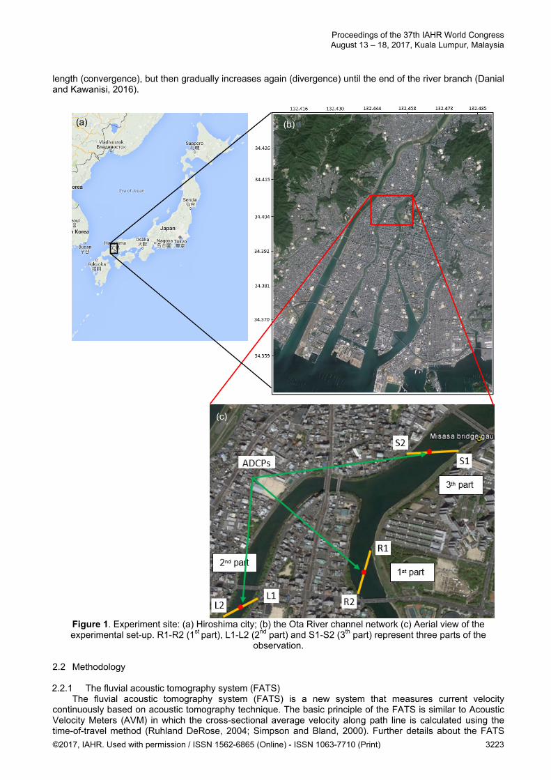
length (convergence), but then gradually increases again (divergence) until the end of the river branch (Danial and Kawanisi, 2016).

Figure 1. Experiment site: (a) Hiroshima city; (b) the Ota River channel network (c) Aerial view of the experimental set-up. R1-R2 (1st part), L1-L2 (2nd part) and S1-S2 (3th part) represent three parts of the

observation. 2.2 Methodology 2.2.1 The fluvial acoustic tomography system (FATS)

The fluvial acoustic tomography system (FATS) is a new system that measures current velocity continuously based on acoustic tomography technique. The basic principle of the FATS is similar to Acoustic Velocity Meters (AVM) in which the cross-sectional average velocity along path line is calculated using the time-of-travel method (Ruhland DeRose, 2004; Simpson and Bland, 2000). Further details about the FATS

(a) (b)

(c) (c)



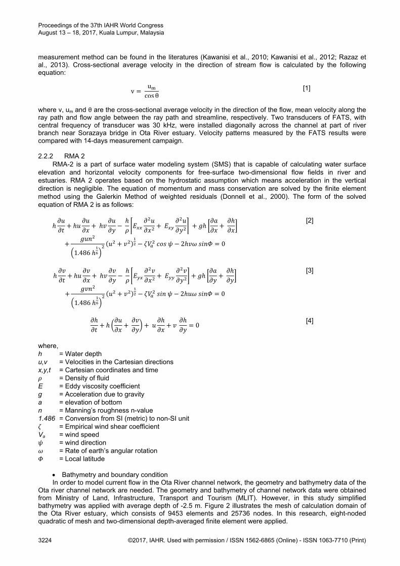
measurement method can be found in the literatures (Kawanisi et al., 2010; Kawanisi et al., 2012; Razaz et al., 2013). Cross-sectional average velocity in the direction of stream flow is calculated by the following equation:

v ucos θ

[1]

where v, um and θ are the cross-sectional average velocity in the direction of the flow, mean velocity along the ray path and flow angle between the ray path and streamline, respectively. Two transducers of FATS, with central frequency of transducer was 30 kHz, were installed diagonally across the channel at part of river branch near Sorazaya bridge in Ota River estuary. Velocity patterns measured by the FATS results were compared with 14-days measurement campaign. 2.2.2 RMA 2

RMA-2 is a part of surface water modeling system (SMS) that is capable of calculating water surface elevation and horizontal velocity components for free-surface two-dimensional flow fields in river and estuaries. RMA 2 operates based on the hydrostatic assumption which means acceleration in the vertical direction is negligible. The equation of momentum and mass conservation are solved by the finite element method using the Galerkin Method of weighted residuals (Donnell et al., 2000). The form of the solved equation of RMA 2 is as follows:

[2]

1.486 2 0

[3]

1.486 2 0

0 [4]

where, h = Water depth u,v = Velocities in the Cartesian directions x,y,t = Cartesian coordinates and time

= Density of fluid E = Eddy viscosity coefficient g = Acceleration due to gravity a = elevation of bottom n = Manning’s roughness n-value 1.486 = Conversion from SI (metric) to non-SI unit = Empirical wind shear coefficient

Va = wind speed = wind direction = Rate of earth’s angular rotation = Local latitude

Bathymetry and boundary condition In order to model current flow in the Ota River channel network, the geometry and bathymetry data of the

Ota river channel network are needed. The geometry and bathymetry of channel network data were obtained from Ministry of Land, Infrastructure, Transport and Tourism (MLIT). However, in this study simplified bathymetry was applied with average depth of -2.5 m. Figure 2 illustrates the mesh of calculation domain of the Ota River estuary, which consists of 9453 elements and 25736 nodes. In this research, eight-noded quadratic of mesh and two-dimensional depth-averaged finite element were applied.



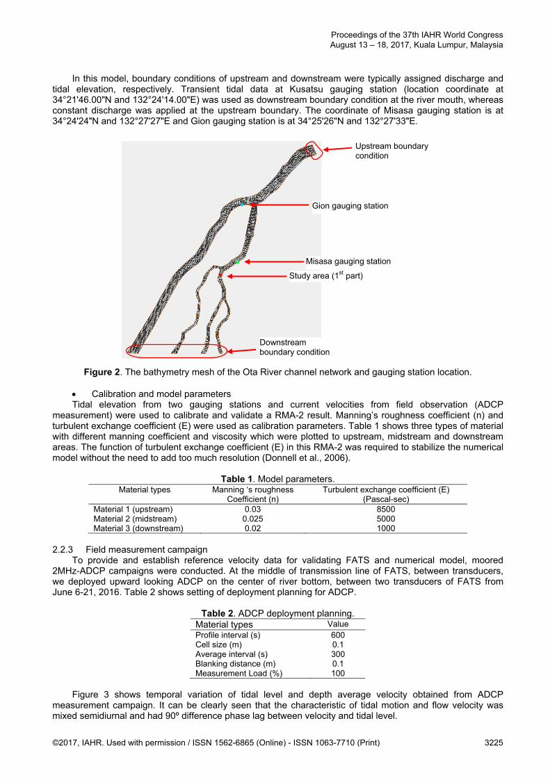
In this model, boundary conditions of upstream and downstream were typically assigned discharge and tidal elevation, respectively. Transient tidal data at Kusatsu gauging station (location coordinate at 34°21'46.00"N and 132°24'14.00"E) was used as downstream boundary condition at the river mouth, whereas constant discharge was applied at the upstream boundary. The coordinate of Misasa gauging station is at 34°24'24"N and 132°27'27"E and Gion gauging station is at 34°25'26"N and 132°27'33"E.

Figure 2. The bathymetry mesh of the Ota River channel network and gauging station location.

Calibration and model parameters Tidal elevation from two gauging stations and current velocities from field observation (ADCP

measurement) were used to calibrate and validate a RMA-2 result. Manning’s roughness coefficient (n) and turbulent exchange coefficient (E) were used as calibration parameters. Table 1 shows three types of material with different manning coefficient and viscosity which were plotted to upstream, midstream and downstream areas. The function of turbulent exchange coefficient (E) in this RMA-2 was required to stabilize the numerical model without the need to add too much resolution (Donnell et al., 2006).

Table 1. Model parameters. Material types Manning ‘s roughness

Coefficient (n) Turbulent exchange coefficient (E)

(Pascal-sec) Material 1 (upstream) 0.03 8500 Material 2 (midstream) 0.025 5000 Material 3 (downstream) 0.02 1000

2.2.3 Field measurement campaign

To provide and establish reference velocity data for validating FATS and numerical model, moored 2MHz-ADCP campaigns were conducted. At the middle of transmission line of FATS, between transducers, we deployed upward looking ADCP on the center of river bottom, between two transducers of FATS from June 6-21, 2016. Table 2 shows setting of deployment planning for ADCP.

Table 2. ADCP deployment planning. Material types Value Profile interval (s) 600 Cell size (m) 0.1 Average interval (s) 300 Blanking distance (m) 0.1 Measurement Load (%) 100

Figure 3 shows temporal variation of tidal level and depth average velocity obtained from ADCP

measurement campaign. It can be clearly seen that the characteristic of tidal motion and flow velocity was mixed semidiurnal and had 90º difference phase lag between velocity and tidal level.

Gion gauging station

Misasa gauging station

Study area (1st part)

Upstream boundary condition

Downstream boundary condition



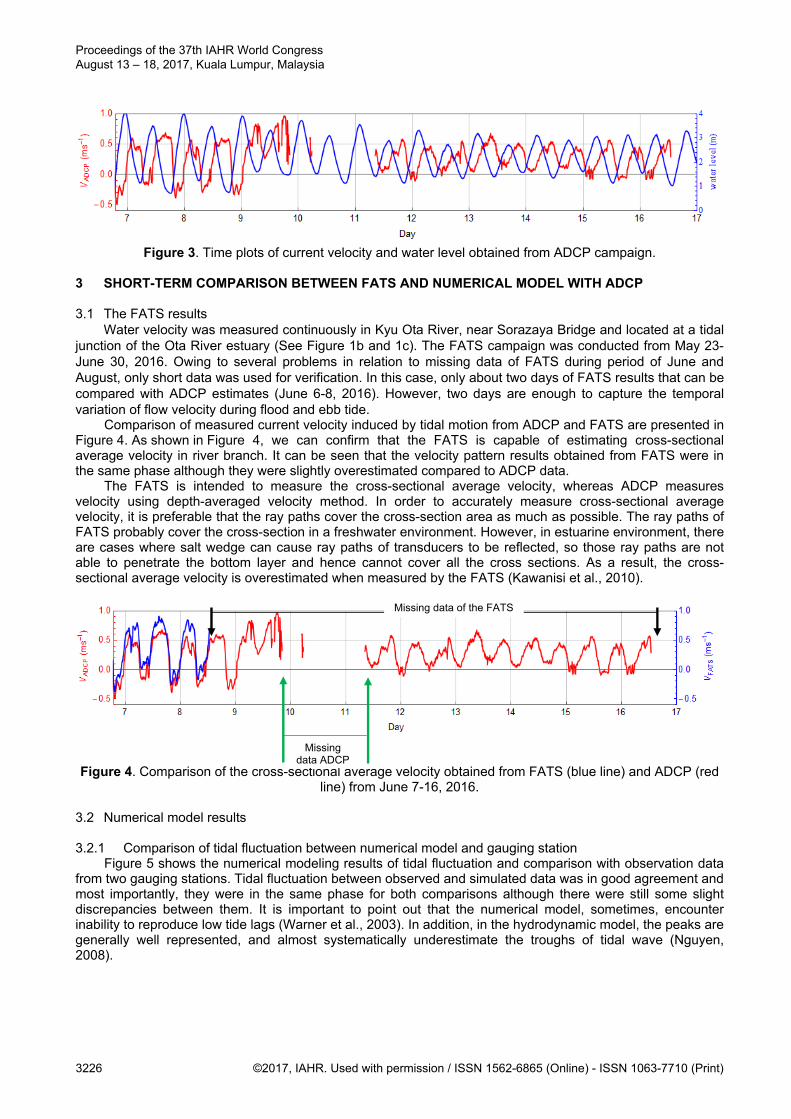
Figure 3. Time plots of current velocity and water level obtained from ADCP campaign.

3 SHORT-TERM COMPARISON BETWEEN FATS AND NUMERICAL MODEL WITH ADCP 3.1 The FATS results

Water velocity was measured continuously in Kyu Ota River, near Sorazaya Bridge and located at a tidal junction of the Ota River estuary (See Figure 1b and 1c). The FATS campaign was conducted from May 23-June 30, 2016. Owing to several problems in relation to missing data of FATS during period of June and August, only short data was used for verification. In this case, only about two days of FATS results that can be compared with ADCP estimates (June 6-8, 2016). However, two days are enough to capture the temporal variation of flow velocity during flood and ebb tide.

Comparison of measured current velocity induced by tidal motion from ADCP and FATS are presented in Figure 4. As shown in Figure 4, we can confirm that the FATS is capable of estimating cross-sectional average velocity in river branch. It can be seen that the velocity pattern results obtained from FATS were in the same phase although they were slightly overestimated compared to ADCP data.

The FATS is intended to measure the cross-sectional average velocity, whereas ADCP measures velocity using depth-averaged velocity method. In order to accurately measure cross-sectional average velocity, it is preferable that the ray paths cover the cross-section area as much as possible. The ray paths of FATS probably cover the cross-section in a freshwater environment. However, in estuarine environment, there are cases where salt wedge can cause ray paths of transducers to be reflected, so those ray paths are not able to penetrate the bottom layer and hence cannot cover all the cross sections. As a result, the cross-sectional average velocity is overestimated when measured by the FATS (Kawanisi et al., 2010).

Figure 4. Comparison of the cross-sectional average velocity obtained from FATS (blue line) and ADCP (red line) from June 7-16, 2016.

3.2 Numerical model results 3.2.1 Comparison of tidal fluctuation between numerical model and gauging station

Figure 5 shows the numerical modeling results of tidal fluctuation and comparison with observation data from two gauging stations. Tidal fluctuation between observed and simulated data was in good agreement and most importantly, they were in the same phase for both comparisons although there were still some slight discrepancies between them. It is important to point out that the numerical model, sometimes, encounter inability to reproduce low tide lags (Warner et al., 2003). In addition, in the hydrodynamic model, the peaks are generally well represented, and almost systematically underestimate the troughs of tidal wave (Nguyen, 2008).

Missing data of the FATS

Missing data ADCP



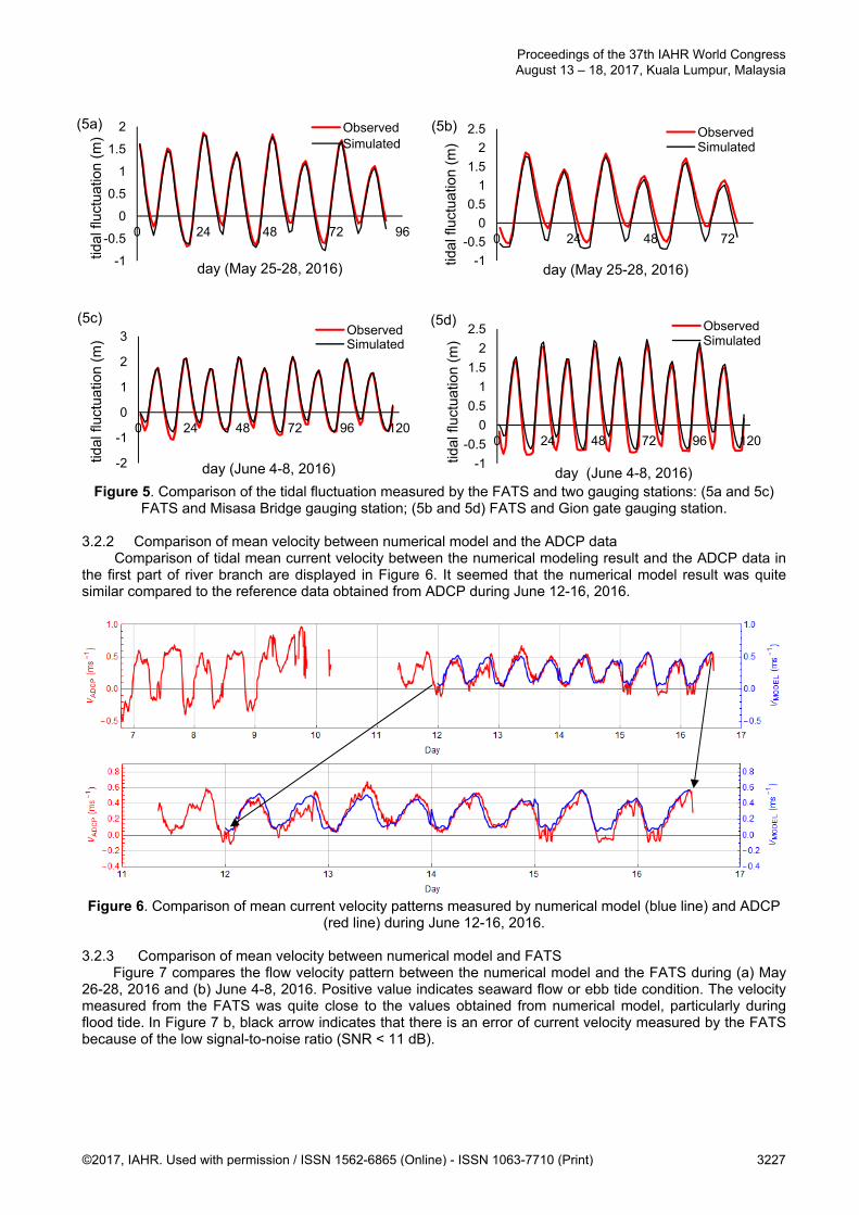
Figure 5. Comparison of the tidal fluctuation measured by the FATS and two gauging stations: (5a and 5c) FATS and Misasa Bridge gauging station; (5b and 5d) FATS and Gion gate gauging station.

3.2.2 Comparison of mean velocity between numerical model and the ADCP data

Comparison of tidal mean current velocity between the numerical modeling result and the ADCP data in the first part of river branch are displayed in Figure 6. It seemed that the numerical model result was quite similar compared to the reference data obtained from ADCP during June 12-16, 2016.

Figure 6. Comparison of mean current velocity patterns measured by numerical model (blue line) and ADCP

(red line) during June 12-16, 2016. 3.2.3 Comparison of mean velocity between numerical model and FATS

Figure 7 compares the flow velocity pattern between the numerical model and the FATS during (a) May 26-28, 2016 and (b) June 4-8, 2016. Positive value indicates seaward flow or ebb tide condition. The velocity measured from the FATS was quite close to the values obtained from numerical model, particularly during flood tide. In Figure 7 b, black arrow indicates that there is an error of current velocity measured by the FATS because of the low signal-to-noise ratio (SNR < 11 dB).

-1

-0.5

0

0.5

1

1.5

2

0 24 48 72 96

tidal

fluc

tuat

ion

(m)

day (May 25-28, 2016)

ObservedSimulated

-1

-0.5

0

0.5

1

1.5

2

2.5

0 24 48 72

tidal

fluc

tuat

ion

(m)

day (May 25-28, 2016)

ObservedSimulated

-2

-1

0

1

2

3

0 24 48 72 96 120

tidal

fluc

tuat

ion

(m)

day (June 4-8, 2016)

ObservedSimulated

-1

-0.5

0

0.5

1

1.5

2

2.5

0 24 48 72 96 120tid

al fl

uctu

atio

n (m

)

day (June 4-8, 2016)

ObservedSimulated

(5a) (5b)

(5c) (5d)



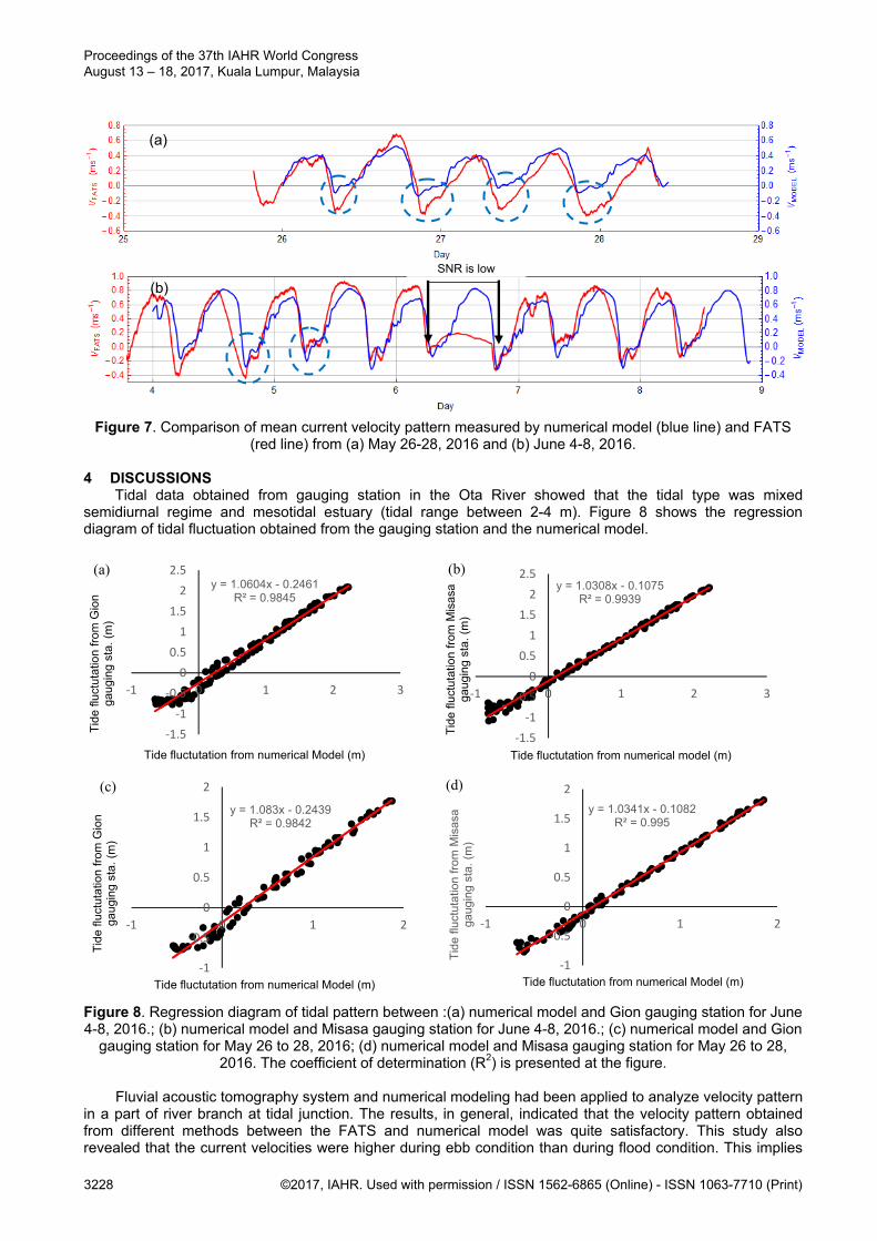
Figure 7. Comparison of mean current velocity pattern measured by numerical model (blue line) and FATS

(red line) from (a) May 26-28, 2016 and (b) June 4-8, 2016. 4 DISCUSSIONS

Tidal data obtained from gauging station in the Ota River showed that the tidal type was mixed semidiurnal regime and mesotidal estuary (tidal range between 2-4 m). Figure 8 shows the regression diagram of tidal fluctuation obtained from the gauging station and the numerical model.

Figure 8. Regression diagram of tidal pattern between :(a) numerical model and Gion gauging station for June 4-8, 2016.; (b) numerical model and Misasa gauging station for June 4-8, 2016.; (c) numerical model and Gion

gauging station for May 26 to 28, 2016; (d) numerical model and Misasa gauging station for May 26 to 28, 2016. The coefficient of determination (R2) is presented at the figure.

Fluvial acoustic tomography system and numerical modeling had been applied to analyze velocity pattern

in a part of river branch at tidal junction. The results, in general, indicated that the velocity pattern obtained from different methods between the FATS and numerical model was quite satisfactory. This study also revealed that the current velocities were higher during ebb condition than during flood condition. This implies

y = 1.0604x - 0.2461R² = 0.9845

‐1.5

‐1

‐0.5

0

0.5

1

1.5

2

2.5

‐1 0 1 2 3

Tid

e flu

ctut

atio

n fr

om G

ion

gaug

ing

sta.

(m

)

Tide fluctutation from numerical Model (m)

y = 1.0308x - 0.1075R² = 0.9939

‐1.5

‐1

‐0.5

0

0.5

1

1.5

2

2.5

‐1 0 1 2 3

Tid

e flu

ctut

atio

n fr

om M

isas

a ga

ugin

g st

a. (

m)

Tide fluctutation from numerical model (m)

y = 1.083x - 0.2439R² = 0.9842

‐1

‐0.5

0

0.5

1

1.5

2

‐1 0 1 2

Tid

e flu

ctut

atio

n fr

om G

ion

gaug

ing

sta.

(m

)


y = 1.0341x - 0.1082R² = 0.995

‐1

‐0.5

0

0.5

1

1.5

2

‐1 0 1 2

Tid

e flu

ctut

atio

n fr

om M

isas

a ga

ugin

g st

a. (

m)


(a)

(b)

(a) (b)

(c) (d)

SNR is low



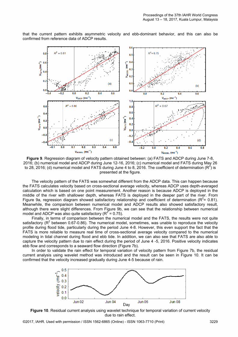
that the current pattern exhibits asymmetric velocity and ebb-dominant behavior, and this can also be confirmed from reference data of ADCP results.

Figure 9. Regression diagram of velocity pattern obtained between: (a) FATS and ADCP during June 7-8, 2016; (b) numerical model and ADCP during June 12-16, 2016; (c) numerical model and FATS during May 26 to 28, 2016; (d) numerical model and FATS during June 4 to 8, 2016. The coefficient of determination (R2) is

presented at the figure.

The velocity pattern of the FATS was somewhat different from the ADCP data. This can happen because the FATS calculates velocity based on cross-sectional average velocity, whereas ADCP uses depth-averaged calculation which is based on one point measurement. Another reason is because ADCP is deployed in the middle of the river with shallower depth, whereas FATS is deployed in the deeper part of the river. From Figure 9a, regression diagram showed satisfactory relationship and coefficient of determination (R2= 0.81). Meanwhile, the comparison between numerical model and ADCP results also showed satisfactory result, although there were slight differences. From Figure 9b, we can see that the relationship between numerical model and ADCP was also quite satisfactory (R2 = 0.75).

Finally, in terms of comparison between the numerical model and the FATS, the results were not quite satisfactory (R2 between 0.67-0.86). The numerical model, sometimes, was unable to reproduce the velocity profile during flood tide, particularly during the period June 4-8. However, this even support the fact that the FATS is more reliable to measure real time of cross-sectional average velocity compared to the numerical modeling in tidal channel during flood and ebb tide. In addition, we can also see that FATS are also able to capture the velocity pattern due to rain effect during the period of June 4 -5, 2016. Positive velocity indicates ebb flow and corresponds to a seaward flow direction (Figure 7b).

In order to validate the rain effect for temporal variation of velocity pattern from Figure 7b, the residual current analysis using wavelet method was introduced and the result can be seen in Figure 10. It can be confirmed that the velocity increased gradually during June 4-5 because of rain.

Figure 10. Residual current analysis using wavelet technique for temporal variation of current velocity

due to rain effect.



5 CONCLUSIONS

In this study, collected data from ADCP and FATS data at the first branch of the tidal channel network are conducted successfully. Continuous current velocity patterns obtained from ADCP, FATS and numerical model reveal that the comparison are reasonable. The observation results show that the Ota River estuary is classified by an ebb-dominant and mixed-semidiurnal regime. At the tidal junction, the velocity pattern is higher during an ebb tide than during flood tide. This also denotes that the velocity behavior at the tidal junction has an asymmetric pattern. The comparison between FATS data and the numerical model results is relatively satisfactory in tidal flow patterns though there are areas with slight differences. The FATS, however, is more reliable compared to numerical modeling in measuring flow velocity in the tidal channel network. ACKNOWLEDGEMENTS

The authors would like to express their gratitude to Dr. Noriaki Gohda of Hiroshima University/Aqua Environmental Monitoring Limited Liability Partnership (AEM-LLP) for his unwavering technical support. REFERENCES Ruhl, C.A. & DeRose, J.B. (2004). Investigation of Hydro Acoustic Flow-Monitoring Alternatives at the

Sacramento River at Freeport, California: Results of the 2002-2004 Pilot Study, U.S. Geological Survey, Scientific-Investigation Report, 2004-5172, 18.

Dalrymple, R.W., Zaitlin, B.A. & Boyd, R. (1992). A Conceptual Model of Estuarine Sedimentation. Journal of Sedimentary Petrology, 62, 1130-1146.

Danial, M.M. Kawanisi, K. (2016). Investigation of Physical Characteristics in Ota River Estuary. 15thInternational Conference on Civil and Environmental Engineering. October 17-19, 2016, Hiroshima University.

Donnell, B.P., King, I., Letter, J.V., McAnally, W.H. & Thomas, W.A. (2006). Users Guide for RMA2 Version 4.5.US Army, Engineer Research and Development Center, Waterways Experiment Station, Coastal and Hydraulics Laboratory

Dyer, K.R. (1997). Tides in Estuaries, a Physical Introduction 2nd Edition. John Wiley & Sons Ltd, 31-40. Dias, J.M. & Valentim, J.M. (2011). Numerical Modeling of Tagus Estuary Tidal Dynamics. Journal of Coastal

Research, 64, 1495 – 1499. Kaneko, A., Yuan, G., Gohda, N. & Nakano, I. (1994). Optimum Design of the Ocean Acoustic Tomography

System for the Sea of Japan. Journal of Oceanography, 50, 281-293. Kawanisi, K., Razaz, M., Kaneko, A. & Watanabe, S. (2010). Long-Term Measurement of Stream Flow and

Salinity in a Tidal River by the Use of the Fluvial Acoustic Tomography System. Journal of Hydrology, 380(1-2), 74-81.

Kawanisi, K., Razaz, M., Ishikawa, K., Yano, J. & Soltanias, M. (2012). Continuous Measurements of Flow Rate in a Shallow Gravel-Bed River by a New Acoustic System. Water Resources Research, 48(5), 1-10.

Nguyen, A.D. (2008). Salt Intrusion, Tides and Mixing in Multi-Channel Estuaries, Dissertation. UNESCO-IHE Institue for Water Education, Delft, the Netherlands.

Razaz, M., Kawanisi, K.,Nistor,I. & Sharifi, S. (2013). An Acoustic Travel Time Method for Continuous Velocity Monitoring in Shallow Tidal Streams. Water Resources Research, 49(8), 4885-4899.

Simpson, M.R. & Bland, R. (2000). Methods for Accurate Estimation of Net Discharge in a Tidal Channel. IEEE Journal of Oceanic Engineering, 25(4), 437-445.

Warner, J.C., Schoellhamer, D. & Schadow, G. (2003). Tidal Truncation and Barotropic Convergence in a Channel Network Tidally Driven from Opposing Entrances. Journal Estuarine Coastal and Shelf Science, 56(3), 629-639.



INVESTIGATION OF EVOLUTION OF YELLOW RIVER DELTA (1976 TO 2014)

SHASHA HAN(1), SHAN ZHENG(2) & YUNXING SHI(3)

(1,2,3) State Key Laboratory of Water Resources and Hydropower Engineering Science, Wuhan University, Hubei, China,

[email protected]; [email protected]; [email protected]

ABSTRACT Avulsion at the Yellow River delta (YRD) is very frequent due to the heavy sediment load and rapid channel aggradation. Nevertheless, the Qingshuigou channel has been maintained for about four decades, since an artificial avulsion in 1976. In this study, we comprehensively analyze the geomorphic adjustment of the channel during 1976-2014. Results showed that channel evolution processes may be divided into four phases: I (1976-1980) rapid aggradation, II (1980-1986) channel widening and enlargement, III (1986-1994) main channel aggradation and shrinkage, and IV (1994-2014) main channel incision and deepening. Fast aggradation caused the elevation of the channel bed and floodplain to generally rise by more than two meters in phase I. Channel slope decreased exponentially. A single-thread main channel is formed at about 1980. Channel evolution generally followed the sequences of “degradation—degradation and widening—aggradation and widening” in phase II during 1980-1986. Aggradation occurred at the main channel and its vicinity, forming an alluvial ridge in phase III. Steep transverse slope was formed and it generally increased in the downstream direction. Gradient advantage, defined as the ratio of transverse slope to longitudinal slope, was between 3 and 24 in 1994 and was generally greater than the critical value proposed by previous study. The normalized super elevation was also close to the critical value locally. Nevertheless, lack of overbank floods and constraint of lateral adjustment prohibit the occurrence of avulsion. Degradation in phase IV was mainly caused by anthropogenic influences including artificial avulsion at the most downstream reaches of Qingshuigou channel in 1996 and artificial floods created by water and sediment regulation since 2002. Despite of the increase of the lifespan of the recent lobe at the YRD, avulsion is inevitable in the evolution of the delta channel in the near future. Multiple criterions for avulsion should be adopted and used with caution. Keywords: Yellow river delta; qingshuigou channel; geomorphologic adjustment; avulsion; human interruption. 1 INTRODUCTION

Avulsion plays a significant role in forming deltas and/or fans, floodplain topography and alluvial stratigraphy (Allen, 1965; Smith et al., 1989; Törnqvist and Bridge, 2002; Slingerland and Smith, 2004; Aslan et al., 2005; Wang et al., 2006; Kleinhans et al., 2013). The modern Yellow River Delta (YRD) has been formed by rapid sedimentation and frequent avulsions since 1855. During the period of 1855 to 1976, major avulsions occurred about 11 times and bifurcations were very frequent (Wang and Liang, 2000). The average lifespan of channels at the delta is only about a decade, much shorter than channels at other delta’s worldwide (Wang and Liang, 2000; Shi and Zhang, 2003; Xu, 2008). For instance, the approximate avulsion time scales for the Po River delta in Italy, the Rhine-Meuse delta and the Upper Rhone River delta are, respectively, about 500, 1000 and 1450 years respectively (Gandolfi et al., 1982; Törnqvist, 1993; Stouthamer and Berendsen, 2007; Jerolmack, 2009).

The reasons for avulsion have been argued to be related to various factors, including aggradation and its rate, super elevation, lateral slope advantage, decrease in channel capacity, energy slope, sediment diameter and channel reoccupation (Allen, 1965; Makaske, 1998; 2001; Mohrig et al., 2000; Törnqvist and Bridge, 2002; Slingerland and Smith, 2004; Aslan et al., 2005; Assine, 2005; Phillips, 2011). In addition, trigger events for avulsion include human activities, extreme peak discharge or discharge variations, ice jams, levee weaknesses, neotectonics, subsidence, substrate composition and change in sinuosity among others. (Schumm et al., 1996; Törnqvist and Bridge, 2002; Aslan et al., 2005; Assine, 2005; Syvitski and Saito, 2007; Phillips, 2011). Thus far, the relative importance of these mentioned factors has not yet been thoroughly understood. Due to the lack of thorough understanding of the causes of avulsions, different criterions for the threshold of avulsion have been proposed and used in various models (Slingerland and Smith, 2004; Gouw and Autin, 2008; Jerolmack, 2009; Phillips, 2011; Clarke, 2015). For example, a super elevation threshold was adopted in the cellular automata model of avulsions proposed by Jerolmack and Paola (2007). A ‘capacity-based avulsion model’ proposed by Makaske (1998; 2001) assumed that a limited sediment transport capacity may cause channels to become hydraulically inefficient over time and cause avulsion. Mackey and Bridge (1995) model considered both gradient advantage and flood frequency.

Avulsion criterions have rarely been applied to the channels on the YRD to quantitatively estimate possible avulsion frequency, and the evolution processes of the recent channel on the delta of the



Qingshuigou channel where it have not yet been comprehensively analyzed. Based on the data provided by Yellow River Conservancy Commission (YRCC), the main objectives of this paper are: 1) to comprehensively analyze the vertical, lateral, longitudinal and planform adjustments of the Qingshuigou channel through 1976 to 2014; 2) to propose a generalized model for the geomorphic adjustment of the channel, and compare it with those that have been observed in the field and experiments; and 3) to investigate and discuss the control factors of avulsion at the delta. 2 STUDY AREA

The modern YRD began to form in 1855, when the Yellow River migrated from the south to the north to join the Bohai Sea (Figure 1A). Approximately 1 billion (=109) tons of sediment was transported to the YRD annually over a long time period (Xue, 1993; Wang and Liang, 2000; Saito et al., 2001). One-half to two-thirds of the sediment was deposited at the delta or near the shoreline due to the weak dynamics of tides, storm and wind currents at the estuary (Saito et al., 2001; Wang, 2010). Some 5,400 km2 land has been created since 1855 and the rate of channel progradation is about 2-3 km per year. The length of the tidal limit is less than 20 km and the tide range is between 1.1-1.5 m. The YRD is fluvial-dominated with irregular semidiurnal tide.

Historically, frequent avulsion had prohibited economic development at the delta where today China’s second largest oil field, Shengli Oilfield, is located. Since the foundation of the People’s Republic of China in 1949, avulsions at the delta have been controlled by human intervention. Before the flow was diverted to the Qingshuigou channel, the Diaokouhe channel was used as a conduit to transport water and sediment to the Bohai Sea during 1964-1976. On May 20th 1976, the flow was diverted to an excavated channel to the north of the present Qingshuigou channel. The excavated channel was about 250-500 m wide, 0.8-3.0 m deep and with the longitudinal slope of ~2/10,000 between Xihekou, the avulsion location, and the cross-section Q1 (Figure 1B). The excavated channel was deposited and abandoned a few months after the diversion. The main channel shifted frequently in the first few years following the avulsion as shown in Figure 1B, and it became relatively stable after about 1980 (Wang and Liang, 2000). In 1996, the flow at the downstream of Q8 cross-section was artificially diverted to a new channel for oil production. The new channel, which was initially dug at 1.6 m deep, 200 m wide and 5 km long, was generally referred to as the Q8-Chahe mouth channel (Figure 1B). The old mouth channel at the downstream of Q8 had been blocked since 1996 (Wang and Liang, 2000; Wang et al., 2012).

Levees, farm dikes, country roads, bank protection and flow diversion projects have been constructed intermittently along the Qingshuigou channel. The distance between levees increased from the upstream channel reaches to the downstream. And the distance between the levees or sea walls is so wide at the downstream of Q3 cross-section that the lower channel reaches were rarely impacted. Nevertheless, the shift of the main channel may be constricted by farm dikes and country roads as shown in Figure 1B. Outer banks of the river bends have generally been protected by revetments and short spurs as shown in Figure 1B and C. In addition, during 1988-1992, dredging was carried out in the channel reaches at the downstream of Q8 in order to mitigate sedimentation at the river mouth (Fan et al., 2006; Wang, 2010).

The channel reach at the downstream of Yuwa (denoted by YW in Figure 1B) is studied in this paper. Figure 1B shows the locations of the cross-sections. The cross-section geometries at YW, HK6, HK7, Q1, Q2, and Q3 have been measured since the avulsion in 1976, while the measurements for Q4, Q6, Q7 and Q8 started in 1977, 1980, 1985 and 1989, respectively. The cross-sections were generally surveyed twice a year, before and after the flood season. Measurements of Q8 cross-section stopped after the flow was diverted to Q8-Chahe mouth channel in 1996. It should be noted that the directions of the cross-sections of HK6, HK7 and Q1 were adjusted in 2004 so as to be perpendicular to the main stream.

The water and sediment volumes measured at Lijin station were generally regarded as being representative of the incoming water and sediment conditions at the YRD since there are no hydrologic stations at the downstream reaches. Water and sediment volumes generally decreased through 1975 to 2014, mainly due to human activities such as damming, soil and water conservation practices and water and sediment withdrawal (Fan et al., 2006; Wang and Liang, 2000; Miao et al., 2010). The Qingshuigou channel experienced seasonal dry-up events for 627 days in total during 1976-1996, and 488 days occurred in the early and middle 1990’s (Fan et al., 2006). The water and sediment volumes at Lijin station rebounded slightly after 2002, because artificial floods have been created by upstream reservoirs in order to scour the perched channel bed of the Lower Yellow River. Table 1 compares the water and sediment conditions in different time periods. These time periods correspond to the different evolution phases, which will be discussed in the next section.



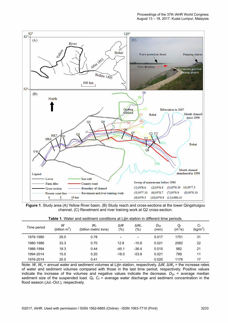
Figure 1. Study area (A) Yellow River basin, (B) Study reach and cross-sections at the lower Qingshuigou

channel, (C) Revetment and river training work at Q2 cross-section.

Table 1. Water and sediment conditions at Lijin station in different time periods.

Time period W

(billion m3) Ws

(billion metric tons) ∆W (%)

∆Ws (%)

D50 (mm)

Qf (m3/s)

Cf

(kg/m3)

1976-1980 29.5 0.78 - - 0.017 1751 31

1980-1986 33.3 0.70 12.8 -10.8 0.021 2082 22

1986-1994 18.3 0.44 -45.1 -36.4 0.015 982 21

1994-2014 15.0 0.20 -18.0 -53.8 0.021 789 11

1976-2014 20.5 0.41 - - 0.020 1176 17

Note: W, Ws = annual water and sediment volumes at Lijin station, respectively. ∆W, ∆Ws = the increase rates of water and sediment volumes compared with those in the last time period, respectively. Positive values indicate the increase of the volumes and negative values indicate the decrease. D50 = average median sediment size of the suspended load. Qf, Cf = average water discharge and sediment concentration in the flood season (Jul.-Oct.), respectively.



3 METHODS Change in the aggradation and/or degradation volume during time step ∆t between two adjacent cross-

sections,∆ (billion m3) may be roughly estimated by the following equation (Kasai et al., 2004; Zheng et al., 2014):

∆∆ ∆

∗ ∆ ∗ 10 [1]

where ∆ and ∆ changes in cross-sectional areas at the upstream and downstream cross-sections during ∆ , respectively (m2). ∆ river length between two adjacent cross-sections (km); ∆ time step, which is defined as a hydrological year in this study.

Normalized values of super elevation and gradient advantage will be used to estimate how close the channel was to the threshold of avulsion. Normalized super elevation, SE, may be calculated as follow:

, ,( , )b fp l fp r

b thal

E Min E ESE

E E

-=

- [2]

where Eb = the average value of the top elevations at both banks, Ethal = thalweg elevation, Efp,l, Efp,r = the elevations of the lowest points on the left and right floodplains, respectively, and Min() means taking the minimum number in the brackets.

The normalized gradient advantage was taken as the ratio of the cross-valley slope, Sc, to the down-valley slope; Sd. Sd may be taken as the longitudinal slope of the channel. The transverse slope generally decreases with distance from the main channel belt since sediment deposition in the vicinity of the main channel is more rapid than that in the distal floodplain. Since the floodplain at the Qingshuigou channel is very wide (locally >10 km wide), the most dangerous situation, or the steepest transverse slope was considered by taking Sc as the transverse slope of the 1-km-wide floodplains in the immediate vicinity of the main channel at each cross-section. A linear line was fitted based on the least squares regression for the transverse profile of the 1-km-wide floodplain near the left/right bank, and the slope of the fitted line is taken as Sc at the left/right floodplain. It should be noted that there was no floodplain near the right bank of Q2 as the main stream was near the levee toe. The decision coefficient (R2) for all the regression lines at the cross-sections are greater than 0.5, except for two cases, where R2=0.39 and 0.23 for empirical lines for the transverse profiles of the left 1-km-wide floodplain at Q1 and that at the right bank of Q3, respectively.

4 GEOMORPHIC ADJUSTMENT OF THE QINGSHUIGOU CHANNEL 4.1 Phase I (1976-1980): Rapid aggradation and channel forming processes

In the first few years immediately after the artificial avulsion in 1976, the annual water and sediment volumes transported to the delta were 29.5 billion m3 and 0.78 billion metric tons, respectively (Table 1). Massive sediment deposited at the Qingshuigou channel and the elevation of channel thalweg and floodplains commonly rose by > 2 m (Figure 2A). As shown in Figure 1B, the main stream shifted bewilderingly, especially at the downstream reaches, where the constrictions of levees were negligible due to the wide distance. Sediment was deposited widely at the channel and floodplains.

Comparison of the longitudinal profiles in 1976 and in 1980 (Figure 3A) shows that the aggradation rate generally increased in the downstream direction, resulting in the decrease of the channel slope. Figure 3A also shows that the initial longitudinal profile of the Qingshuigou channel was much lower than that of the Diaokouhe channel in 1976 prior to avulsion. Nevertheless, after a few years of deposition, the elevation of the Qingshuigou channel was close to that of the Diaokouhe channel. In this study, the longitudinal slope of the channel was estimated by the slopes of the regression lines of the longitudinal profiles in Figure 3. Since the decision coefficient R2 for the regression lines were all greater than 0.5, this simplicity may be accepted. The longitudinal slope was about 0.25% in 1976 and it decreased exponentially to 0.14% in 1980 (Figure 3A and 3C).

Figure 4 shows that the cumulative volume of sediment deposition, Σ∆V, was most significant in Phase I. The river length used to calculate Σ∆V also increases in 1978 since the channel reach between Q3 and Q4 was included. More than 0.29 billion m3 sediment was deposited between Yuwa and Q4 in Phase I with an annual aggradation rate of 2.42 million m3/yr./km.



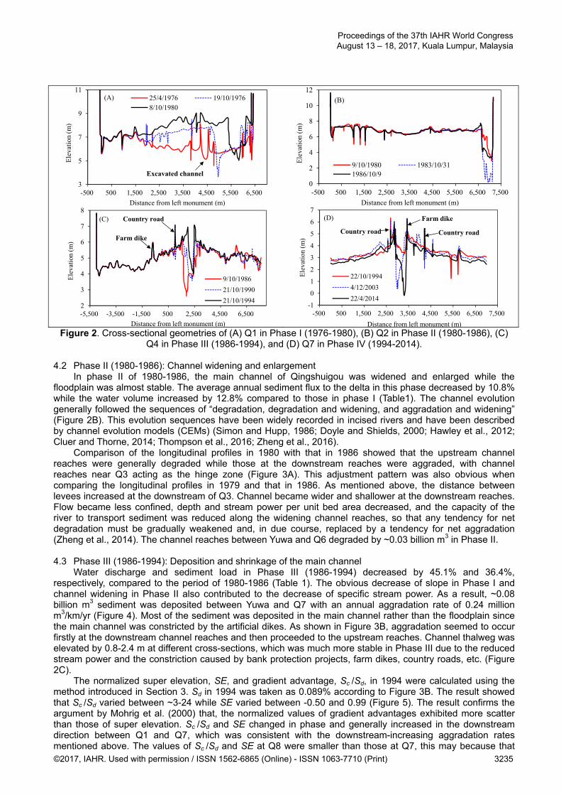
Figure 2. Cross-sectional geometries of (A) Q1 in Phase I (1976-1980), (B) Q2 in Phase II (1980-1986), (C) Q4 in Phase III (1986-1994), and (D) Q7 in Phase IV (1994-2014).

4.2 Phase II (1980-1986): Channel widening and enlargement

In phase II of 1980-1986, the main channel of Qingshuigou was widened and enlarged while the floodplain was almost stable. The average annual sediment flux to the delta in this phase decreased by 10.8% while the water volume increased by 12.8% compared to those in phase I (Table1). The channel evolution generally followed the sequences of “degradation, degradation and widening, and aggradation and widening” (Figure 2B). This evolution sequences have been widely recorded in incised rivers and have been described by channel evolution models (CEMs) (Simon and Hupp, 1986; Doyle and Shields, 2000; Hawley et al., 2012; Cluer and Thorne, 2014; Thompson et al., 2016; Zheng et al., 2016).

Comparison of the longitudinal profiles in 1980 with that in 1986 showed that the upstream channel reaches were generally degraded while those at the downstream reaches were aggraded, with channel reaches near Q3 acting as the hinge zone (Figure 3A). This adjustment pattern was also obvious when comparing the longitudinal profiles in 1979 and that in 1986. As mentioned above, the distance between levees increased at the downstream of Q3. Channel became wider and shallower at the downstream reaches. Flow became less confined, depth and stream power per unit bed area decreased, and the capacity of the river to transport sediment was reduced along the widening channel reaches, so that any tendency for net degradation must be gradually weakened and, in due course, replaced by a tendency for net aggradation (Zheng et al., 2014). The channel reaches between Yuwa and Q6 degraded by ~0.03 billion m3 in Phase II. 4.3 Phase III (1986-1994): Deposition and shrinkage of the main channel

Water discharge and sediment load in Phase III (1986-1994) decreased by 45.1% and 36.4%, respectively, compared to the period of 1980-1986 (Table 1). The obvious decrease of slope in Phase I and channel widening in Phase II also contributed to the decrease of specific stream power. As a result, ~0.08 billion m3 sediment was deposited between Yuwa and Q7 with an annual aggradation rate of 0.24 million m3/km/yr (Figure 4). Most of the sediment was deposited in the main channel rather than the floodplain since the main channel was constricted by the artificial dikes. As shown in Figure 3B, aggradation seemed to occur firstly at the downstream channel reaches and then proceeded to the upstream reaches. Channel thalweg was elevated by 0.8-2.4 m at different cross-sections, which was much more stable in Phase III due to the reduced stream power and the constriction caused by bank protection projects, farm dikes, country roads, etc. (Figure 2C).

The normalized super elevation, SE, and gradient advantage, Sc /Sd, in 1994 were calculated using the method introduced in Section 3. Sd in 1994 was taken as 0.089% according to Figure 3B. The result showed that Sc /Sd varied between ~3-24 while SE varied between -0.50 and 0.99 (Figure 5). The result confirms the argument by Mohrig et al. (2000) that, the normalized values of gradient advantages exhibited more scatter than those of super elevation. Sc /Sd and SE changed in phase and generally increased in the downstream direction between Q1 and Q7, which was consistent with the downstream-increasing aggradation rates mentioned above. The values of Sc /Sd and SE at Q8 were smaller than those at Q7, this may because that

3

5

7

9

11

-500 500 1,500 2,500 3,500 4,500 5,500 6,500

Ele

vati

on (

m)

Distance from left monument (m)

25/4/1976 19/10/19768/10/1980

(A)

Excavated channel

0

2

4

6

8

10

12

-500 500 1,500 2,500 3,500 4,500 5,500 6,500 7,500

Ele

vati

on (

m)


9/10/1980 1983/10/311986/10/9

(B)

2

3

4

5

6

7

8

-5,500 -3,500 -1,500 500 2,500 4,500 6,500

Ele

vati

on (

m)


9/10/1986

21/10/1990

21/10/1994

(C) Country road

Farm dike

-1

0

1

2

3

4

5

6

7

-500 500 1,500 2,500 3,500 4,500 5,500 6,500 7,500

Ele

vati

on (

m)


22/10/1994

4/12/2003

22/4/2014

(D) Farm dike

Country roadCountry road



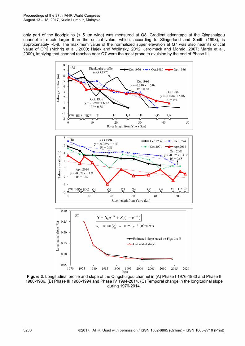
only part of the floodplains (< 5 km wide) was measured at Q8. Gradient advantage at the Qingshuigou channel is much larger than the critical value, which, according to Slingerland and Smith (1998), is approximately ~5-8. The maximum value of the normalized super elevation at Q7 was also near its critical value of O[1] (Mohrig et al., 2000; Hajek and Wolinsky, 2012; Jerolmack and Mohrig, 2007; Martin et al., 2009), implying that channel reaches near Q7 were the most prone to avulsion by the end of Phase III.

Figure 3. Longitudinal profile and slope of the Qingshuigou channel in (A) Phase I 1976-1980 and Phase II 1980-1986, (B) Phase III 1986-1994 and Phase IV 1994-2014, (C) Temporal change in the longitudinal slope

during 1976-2014.

Oct. 1976y = -0.250x + 6.32

R² = 0.88

Oct.1980y = -0.140 x + 6.09

R² = 0.88 Oct.1986

y = -0.098x + 5.06R² = 0.91

-2

-1

0

1

2

3

4

5

6

7

8

0 10 20 30 40 50

Tha

lweg

ele

vati

on (

m)

River length from Yuwa (km)

Oct.1976 Oct.1980 Oct.1986

YW HK6 HK7 Q1 Q2 Q3 Q4 Q6 Q7

(A) Diaokouhe profile in Oct.1975

Oct.1994y = -0.089x + 6.40

R² = 0.85Oct. 2001

y = -0.075x + 4.35R² = 0.58

Apr. 2014y = -0.078x + 1.90

R² = 0.42

-6

-4

-2

0

2

4

6

8

0 10 20 30 40 50

Tha

lweg

ele

vati

on (m

)

River length from Yuwa (km)

Oct.1986 Oct.1994

Oct.2001 Apr.2014

YW HK6 HK7 Q1 Q2 Q3 Q4 Q6 Q7

(B)

C1 C2 C3

0.05

0.10

0.15

0.20

0.25

0.30

1970 1975 1980 1985 1990 1995 2000 2005 2010 2015 2020

Lon

gitu

dina

l slo

pe (

‰)

Year

Estimated slope based on Figs. 3A-B

Calculated slope

(C)

(R2=0.99)

0 (1 )at ateS S e S e

1000

0.080 ; 0.253eS a yr��



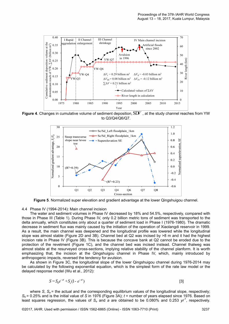
Figure 4. Changes in cumulative volume of sediment deposition, VSD , at the study channel reaches from YW to Q3/Q4/Q6/Q7.

Figure 5. Normalized super elevation and gradient advantage at the lower Qingshuigou channel. 4.4 Phase IV (1994-2014): Main channel incision

The water and sediment volumes in Phase IV decreased by 18% and 54.5%, respectively, compared with those in Phase III (Table 1). During Phase IV, only 0.2 billion metric tons of sediment was transported to the delta annually, which constitutes only about a quarter of sediment load in Phase I (1976-1980). The dramatic decrease in sediment flux was mainly caused by the initiation of the operation of Xiaolangdi reservoir in 1999. As a result, the main channel was deepened and the longitudinal profile was lowered while the longitudinal slope was almost stable (Figure 2D and 3B). Channel bed at Q2 was incised by >8 m and it had the highest incision rate in Phase IV (Figure 3B). This is because the concave bank at Q2 cannot be eroded due to the protection of the revetment (Figure 1C), and the channel bed was incised instead. Channel thalweg was almost stable at the resurveyed cross-sections, implying relative stability of the channel planform. It is worth emphasizing that, the incision at the Qingshuigou channel in Phase IV, which, mainly introduced by anthropogenic impacts, reversed the tendency for avulsion.

As shown in Figure 3C, the longitudinal slope of the lower Qingshuigou channel during 1976-2014 may be calculated by the following exponential equation, which is the simplest form of the rate law model or the delayed response model (Wu et al., 2012):

0 (1 )at ateS S e S e- -= + - [3]

where S, Se = the actual and the corresponding equilibrium values of the longitudinal slope, respectively;

S0 = 0.25% and is the initial value of S in 1976 (Figure 3A); t = number of years elapsed since 1976. Based on least squares regression, the values of Se and a are obtained to be 0.080% and 0.253 yr-1, respectively.

0

10

20

30

40

50

60

70

0.00

0.05

0.10

0.15

0.20

0.25

0.30

0.35

0.40

1975 1980 1985 1990 1995 2000 2005 2010 2015

Riv

er le

ngth

(km

)

Cum

ulat

ive

sedi

men

t dep

ositi

on v

olum

e at

the

dow

nstr

eam

rea

ch o

f Y

W, ∑

ΔV

(bill

ion

m3 )

Year

Calculated values of ΣΔV

River length in calculation

I Rapid aggradation

II Channel enlargement

III Channel shrinkage

IV Main channel incision

ΔVI = 0.29 billion m3 ΔVII = -0.03 billion m3

ΔVIII = 0.08 billion m3 ΔVIV = -0.12 billion m3

∑ΔV = 0.21 billion m3

YW-Q3

YW-Q4

YW-Q6

YW-Q7

Avulsion in 1996

Artificial floods since 2002



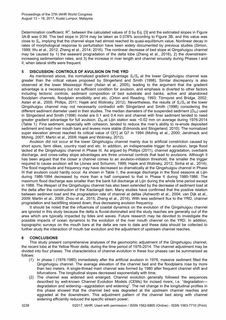
Determination coefficient, R2, between the calculated values of S by Eq. [3] and the estimated slopes in Figure 3A-B was 0.99. The bed slope in 2014 may be taken as 0.078% according to Figure 3B, and this value was close to Se, implying that the channel slope had almost reached its quasi-equilibrium value. Nonlinear decay in rates of morphological response to perturbation have been widely documented by previous studies (Simon, 1999; Wu et al., 2012; Zheng et al., 2014; 2016). The nonlinear decrease of bed slope at Qingshuigou channel may be caused by 1) the seaward progradation of the delta lobe (Zheng et al., 2016), 2) the downstream-increasing sedimentation rates, and 3) the increase in river length and channel sinuosity during Phases I and II, when lateral shifts were frequent. 5 DISCUSSION: CONTROLS OF AVULSION ON THE YRD

As mentioned above, the normalized gradient advantage Sc/Sd at the lower Qingshuigou channel was greater than the critical values proposed by Slingerland and Smith (1998). Similar discrepancy is also observed at the lower Mississippi River (Aslan et al., 2005), leading to the argument that the gradient advantage is a necessary but not sufficient condition for avulsion, and emphasis is diverted to other factors including tectonic controls, sediment composition of bed substrate and banks, active and abandoned floodplain channels, floodplain erodibility and etc. (Orton and Reading, 1993; Törnqvist and Bridge, 2002; Aslan et al., 2005; Phillps, 2011; Hajek and Wolinsky, 2012). Nevertheless, the results of Sc/Sd at the lower Qingshuigou channel may not necessarily contradict with Slingerland and Smith (1998) considering the different sediment diameter used in their studies. The median diameters of the suspended sediment (D50) used in Slingerland and Smith (1998) model are 0.1 and 0.4 mm and channel with finer sediment tended to need greater gradient advantage for full avulsion. D50 at Lijin station was ~0.02 mm on average during 1976-2014 (Table 1). Fine sediment, especially with cohesion, tended to reduce the river’s ability to re-erode deposited sediment and kept river mouth bars and levees more stable (Edmonds and Slingerland, 2010). The normalized super elevation almost reached its critical value of O[1] at Q7 in 1994 (Mohrig et al., 2000; Jerolmack and Mohrig, 2007; Martin et al., 2009; Hajek and Wolinsky, 2012).

Avulsion did not occur at the lower Qingshuigou channel mainly due to artificial constriction caused by short spurs, farm dikes, country road and etc. In addition, an indispensable trigger for avulsion, large flood lacked at the Qingshuigou channel in Phase III. As argued by Phillips (2011), channel aggradation, overbank discharge, and cross-valley slope advantages are three universal controls that lead to avulsions. Although it has been argued that the closer a channel comes to an avulsion-initiation threshold, the smaller the trigger required to cause avulsion will be (Jones and Schumm, 1999; Hajek and Wolinsky, 2012; Sinha et al., 2014). The flood magnitude and frequency may have decreased so dramatically at the Qingshuigou channel in Phase III that avulsion could hardly occur. As shown in Table 1, the average discharge in the flood seasons at Lijin during 1986-1994 decreased by more than a half compared to that in Phase II during 1980-1986. The maximum flood discharge was smaller than the bank full discharge at Lijin during the whole time period except in 1988. The lifespan of the Qingshuigou channel has also been extended by the decrease of sediment load at the delta after the construction of the Xiaolangdi dam. Many studies have confirmed that the positive relation between sediment load and the progradation rate of channel at deltas (Ashworth et al., 2004; van Dijk et al., 2009; Martin et al., 2009; Zhou et al., 2015; Zheng et al., 2016). With less sediment flux to the YRD, channel progradation and backfilling slowed down, thus decreasing avulsion frequency.

It should be noted that the influences of coastal dynamics on the evolution of the Qingshuigou channel are ignored in this study because the delta is fluvial-dominated and the study reaches are generally out of the area which are typically impacted by tides and waves. Future research may be devoted to investigate the possible impacts of ocean dynamics to the evolution of the river mouth channel on the YRD. In addition, topographic surveys on the mouth bars at the delta are rare to date and these data should be collected to further study the interaction of mouth bar evolution and the adjustment of upstream channel reaches. 6 CONCLUSIONS

This study present comprehensive analyses of the geomorphic adjustment of the Qingshuigou channel, the recent lobe at the Yellow River delta, during the time period of 1976-2014. The channel adjustment may be divided into four phases. The characteristics of channel evolution in these four phases can be summarized as follows:

(1) In phase I (1976-1980) immediately after the artificial avulsion in 1976, massive sediment filled the Qingshuigou channel. The average elevation of the channel bed and the floodplains rose by more than two meters. A single-thread main channel was formed by 1980 after frequent channel shift and bifurcations. The longitudinal slopes decreased exponentially with time;

(2) The channel was widened and enlarged. Channel evolution generally followed the sequences described by well-known Channel Evolution Models (CEMs) for incised rivers, i.e. “degradation—degradation and widening—aggradation and widening”. The net change in the longitudinal profiles in this phase showed that the channel bed was degraded at the upstream channel reaches and aggraded at the downstream. This adjustment pattern of the channel bed along with channel widening efficiently reduced the specific stream power;



(3) Aggradation occurred and the main channel shrank in phase III during 1986-1994 due to the

deterioration of the water and sediment conditions and the reduced longitudinal slopes and stream power. An alluvial ridge was formed. Transverse slope increased in the downstream direction since more sediment was deposited at the downstream channel reaches. The gradient advantage, defined as the ratio of the transverse slope to the longitudinal slope, was between about 3 and 24. Normalized super elevation was close to the critical value locally. Nevertheless, avulsion did not occur, mainly because that: 1) big floods with enough energy to trigger avulsion were lacked and 2) the lateral shift of the channel was constricted by farm dikes, country road, river training works, levees and etc.;

(4) Degradation occurred and the channel became deep and narrow while the floodplain almost remained stable in the phase IV during 1994-2014. Incision is mainly caused by artificial floods created by water and sediment regulation since 2002 as well as the artificial avulsion at the mouth channel in 1996, which shorten the river length and caused retrogressive degradation.

The evolution of Qingshuigou channel is a battle between the inherent adjustments of the dynamic and avulsive fluvial system and the intensive human interruptions in hope for the stability for the system. Although avulsion at the channel is prevented and the lifespan of the delta lobe has been expanded by human activities, aggradation and avulsions are inevitable at the delta channel. This study support previous argument that avulsion threshold cannot be represented by one single value (Tornqvist and Bridge, 2002; Jerolmack, 2009). Multiple factors including super elevation, gradient advantage, channel capacity, flood frequency, lateral adjustment as well as human activities, should be included when predicting avulsions. Meanwhile, super elevation and gradient advantage exhibit considerable scatter and caution should be practiced when using these criterions.

ACKNOWLEDGEMENTS

This study is funded by the National Natural Science Foundation of China (Grant No. 51409193) and Open Research Fund Program of the Yellow River Sediment Key Laboratory of the Ministry of Water Resources (Grant No. 2015004). We are indebted to senior engineers Kairong Wang at the Yellow River Conservancy Commission (YRCC) and Congliang Xu at the Institute of the Yellow River Estuary and Coast Science, Dongying, Shandong Province, for making the resurvey data available to us, guiding us in the field and advising us with their precious knowledge and experiences of the evolution of the Yellower River delta. REFERENCES Allen, J.R.L. (1965). A Review of the Origin and Characteristics of Recent Alluvial Sediments. Sedimentology,

5(2), 89-191. Ashworth, P.J., Best, J.L. & Jones, M. (2004). Relationship between Sediment Supply and Avulsion Frequency

in Braided Rivers. Geology, 32(1), 21-24. Aslan, A., Autin, W.J. & Blum, M.D. (2005). Causes of River Avulsion: Insights from the Late Holocene

Avulsion History of the Mississippi River, USA. Journal of Sedimentary Research, 75(4), 650-664. Assine, M.L. (2005). River Avulsions on the Taquari Megafan, Pantanal Wetland, Brazil. Geomorphology, 70,

357-371. Clarke, L.E. (2015). Experimental Alluvial Fans: Advances in Understanding of Fan Dynamics and Processes.

Geomorphology, 244, 135-145. Cluer, B. & Thorne, C.R. (2014). A Stream Evolution Model Integrating Habitat and Ecosystem Benefits. River

Research and Applications, 30(2), 135-154. Fan, H., Huang, H., Zeng, T.Q. & Wang, K. (2006). River Mouth Bar Formation, Riverbed Aggradation and

Channel Migration in the Modern Huanghe (Yellow) River Delta, China. Geomorphology, 74(1), 124-136. Gouw, M.J.P, Autin, W.J., 2008. Alluvial architecture of the Holocene Lower Mississippi Valley (U.S.A.) and a

comparison with the Rhine–Meuse delta (The Netherlands). Sedimentary Geology 204(3-4), 106-121. Hajek, E.A. & Wolinsky, M.A. (2012). Simplified Process Modeling of River Avulsion and Alluvial Architecture:

Connecting Models and Field Data. Sedimentary Geology, (257-260), 1-30. Jerolmack, D.J. & Mohrig, D. (2007). Conditions for Branching in Depositional Rivers. Geology, 35(5), 463-

466. Jerolmack, D.J. & Paola, C. (2007). Complexity in a Cellular Model of River Avulsion. Geomorphology, 91(3-

4), 259-270. Jerolmack, D.J. (2009). Conceptual Framework for Assessing the Response of Delta Channel Networks to

Holocene Sea Level Rise. Quaternary Science Reviews, 28(17), 1786-1800. Martin, J., Sheets, B., Paola, C. & Hoyal, D. (2009). Influence of Steady Base-Level Rise on Channel Mobility,

Shoreline Migration, and Scaling Properties of a Cohesive Experimental Delta. Journal of Geophysical Research, 114(F3), 287-295.

Jones, L.S. & Schumm, S.A. (1999). Causes of Avulsion: An Overview, Fluvial Sedimentology VI. Blackwell Publishing Ltd., 171-178.



Kasai, M., Marutani, T. & Brierley, G. (2004). Channel Bed Adjustments Following Major Aggradation in a Steep Headwater Setting: Findings from Oyabu Creek, Kyushu, Japan. Geomorphology, 62(3-4), 199-215.

Kleinhans, M.G., Ferguson, R.I., Lane, S.N. & Hardy, R.J. (2013). Splitting Rivers at Their Seams: Bifurcations and Avulsion. Earth Surface Processes and Landforms, 38, 47-61.

Mackey, S.D. & Bridge, J.S. (1995). Three-Dimensional Model of Alluvial Stratigraphy: Theory and Applications. Journal of Sedimentary Research, 65(1b), 7-31.

Makaske, B. (1998). Anastomosing Rivers Forms, Processes and Sediments. Nederlandse Geografische Studies.

Makaske, B. (2001). Anastomosing Rivers: a Review of their Classification, Origin and Sedimentary Products. Earth Science Reviews, 53(3-4), 149-196.

Miao, C.Y., Ni, J.R. & Borthwick, A.G.L. (2010). Recent Changes of Water Discharge and Sediment Load in the Yellow River Basin, China. Progress in Physical Geography, 34(4), 541-561.

Mohrig D., Heller, P.L, Paola, C. & Lyons, W.J. (2000). Interpreting Avulsion Process from Ancient Alluvial Sequences: Guadalope-Matarranya System (Northern Spain) and Wasatch Formation (Western Colorado). Geological Society of America Bulletin, 112(12), 143–146.

Orton, G.J. & Reading, H.G. (1993). Variability of Deltaic Processes in Terms of Sediment Supply, with Particular Emphasis on Grain Size. Sedimentology, 40(3), 475-512.

Phillips, J.D. (2011). Universal and Local Controls of Avulsions in Southeast Texas Rivers. Geomorphology, 130(1-2), 17-28.

Saito, Y., Yang, Z. & Hori, K. (2001). The Huanghe (Yellow River) and Changjiang (Yangtze River) deltas: A Review on Their Characteristics, Evolution and Sediment Discharge During the Holocene. Geomorphology, 41(2), 219-231.

Schumm, S.A., Erskine, W.D. & Tilleard, J.W. (1996). Morphology, Hydrology and Evolution of the Anastomosing Ovens and King Rivers, Victoria, Australia. Geological Society of America Bulletin, 108(10), 1212-1224.

Shi, C.X. & Zhang, D. (2003). Processes and Mechanisms of Dynamic Channel Adjustment to Delta Progradation: the Case of the Mouth Channel of the Yellow River, China. Earth Surface Processes and Landforms, 28(6), 609-624.

Simon, A. & Hupp, C.R. (1986). Geomorphic and Vegetative Recovery Processes along Modified Tennessee Streams: an Interdisciplinary Approach to Disturbed Fluvial Systems. Forest Hydrology and Watershed Management. IAHS-AISH Publication, 167, 251-262.

Simon, A. (1999). Channel and Drainage-Basin Response of the Toutle River System in the Aftermath of the 1980 Eruption of Mount St. Helens, Washington. U.S. Department of the Interior, U.S Geological Survey, Open-file report, 96-633.

Sinha, R., Sripriyanka, K., Jain, V. & Mukul, M. (2014). Avulsion Threshold and Planform Dynamics of the Kosi River in North Bihar (India) and Nepal: A GIS Framework. Geomorphology, 216(216), 157-170.

Slingerland, R.L. & Smith, N.D. (1998). Necessary Conditions for a Meandering-River Avulsion. Geology, 26(5), 435.

Slingerland, R.L. & Smith, N.D. (2004). River Avulsions and their Deposits. Annual Review of Earth & Planetary Sciences, 32(32), 257-285.

Stouthamer, E. & Berendsen, J.A.H. (2007). Avulsion: the relative Roles of Autogenic and Allogenic Processes. Sedimentation Geology, 198(3-4), 309-325.

Syvitski, J.P.M. & Saito, Y. (2007). Morphodynamics of Deltas Under the Influence of Humans. Global & Planetary Change, 57(3-4), 261-282.

Törnqvist, T.E. (1993). Holocene Alternation of Meandering and Anastomosing Fluvial Systems in the Rhine-Meuse Delta (Central Netherlands) Controlled by Sea-Level Rise and Subsoil Erodibility. Journal of Sedimentary Research, 63(4), 683-693.

Törnqvist, T.E. & Bridge. J.S. (2002). Spatial Variation of Overbank Aggradation Rate and its Influence on Avulsion Frequency. Sedimentology, 49(5), 891–905.

Wang, S.J., Hassan, M.A. & Xie, X. (2006). Relationship Between Suspended Sediment Load, Channel Geometry and Land Area Increment in the Yellow River Delta. Catena, 65(3), 302-314.

Wang, Z.Y. & Liang, Z.Y. (2000). Dynamic Characteristics of the Yellow River Mouth. Earth Surface Processes and Landforms, 25(7), 765-782.

Wang, Z.Y., Yu, G.A., Huang, H.Q. & Wang, R.Y. (2012). Gender of Large River Deltas and Parasitizing Rivers. International Journal of Sediment Research, 27, 18-36.

Wu, B.S., Zheng, S. & Thorne, C.R. (2012). A General Framework for using the Rate Law to Simulate Morphological Response to Disturbance in the Fluvial System. Progress in Physical Geography, 36(5), 575-597.

Xu, J.X. (2008). Response of Land Accretion of the Yellow River Delta to Global Climate Change and Human Activity. Quaternary International, 186(1), 4-11.

Xue, C.T. (1993). Historical Changes in the Yellow River Delta, China. Marine Geology, 113(3-4), 321-330.



Zheng, S., Wu, B.S, Thorne, C.R. & Simon, A. (2014). Morphological Evolution of the North Fork Toutle River

Following the eruption of Mount St. Helens, Washington. Geomorphology, 208, 102-116. Zheng, S., Wu, B.S., Wang, K.C., Tan, G.M., Han, S.S. & Thorne, C.R. (2016). Evolution of the Yellow River

Delta, China: Impacts of Channel Avulsion and Progradation. International Journal of Sediment Research, 32(1), 34-44.

Zhou, Y., Huang, H.Q., Nanson, G.C., Huang, C. & Liu, G. (2015). Progradation of the Yellow (Huanghe) River Delta in Response to the Implementation of a Basin-Scale Water Regulation Program. Geomorphology, 243, 65-74.



THE SIGNIFICANCE OF HYDRODYNAMIC MODELLING FOR MANGROVE GROWTH

AND SURVIVAL IN MALAYSIA

IKMALZATUL ABDULLAH(1), NOR ASLINDA AWANG(2), ANIZAWATI AHMAD(3) & SHIMATUN JUMANI IBRAHIM(4)

(1, 2, 3) National Hydraulic Research Institute of Malaysia (NAHRIM), Seri Kembangan, Malaysia

[email protected]; [email protected]; [email protected] (4) Malaysia Remote Sensing Agency, Kuala Lumpur, Malaysia

[email protected]

ABSTRACT The hydrodynamic processes that exist in the nearshore region are generated by a number of different drivers such as force of gravity, pressure, velocity and density. Under the influence of these forces, the fluid motion of the water manifests itself as coastal currents, waves and tides. Upper intertidal shorelines that experience a complex hydrodynamic condition are inhabited by mangroves. The mangrove forest is a natural ecosystem that only survives in a certain environment because its growth is influenced by several factors such as sea level, water temperature, salinity, currents, waves, beach slope and type of sediment. The ability of mangroves to serve as a natural buffer against the threat of big waves, strong winds and coastal erosion has increased the value of mangroves. In order to ensure the sustainability and the success of mangrove replanting activities, hydrodynamic conditions in the planting area need to be investigated. The right selection of the planting area is very crucial in determining the success of this project. Several studies have been conducted at Delta Kelantan, Kuala Teriang and Kudat to identify the optimum hydrodynamic conditions that will promote the growth and survival of mangrove in terms of wave action, currents and tides. Bathymetry and marine data have been measured and used as an input in the development of numerical models using MIKE 21 Hydrodynamic (HD) and Wave Spectrum (SW) modules. Model analysis and site verification reveals that in the muddy areas, current speed between 0.02 to 0.12 m/s is the most favorable condition for the growth of mangroves. In a area having current speed exceeding 0.3 m/s, coastal erosion takes place. Meanwhile, in sandy areas, current speed which is less than 0.2 m/s has caused sand precipitation on the roots of the seedlings resulting in death and stunted growth of the mangroves.

Keywords: Mangrove; currents; tides; waves; Malaysia.

1 INTRODUCTION

Mangroves are usually found in protected tropical and subtropical coastal environments. Their habitats are dependent on tidal influence and have complex hydrodynamic conditions. Mastaller (1997) and Walsh (1974) have suggested five basic requirements for extensive mangrove development, which are tropical temperature, fine grained alluvium, low wave and tidal action, salt water and large tidal range. These factors can influence the occurrence and size of mangroves, species composition and zonation, structural characteristics and the functions of the ecosystem itself (Mastaller, 1997).

The existence of mangrove forests can be said as a benchmark for approaching sea, river water, and land. Uniqueness of mangrove that grew in tidal influenced area plays an important role in the ecosystem. It became a refuge for flora and fauna in the mangrove swamps. The unique root becomes an ideal place for small fish to hide from predators and also acts as a natural breeding ground. It also acts as natural buffer against the threat of big waves, strong winds and coastal erosion. Mangrove's ability to absorb wave energy helps to stabilize the beach (Rakotomavo and Fromard, 2010).

At present, mangrove populations worldwide are threatened by the dynamic forces of nature. Studies conducted by Valiela et al. (2001) estimated that the total area of mangrove forest in the world has dropped about 35 % in the last two decades. Giri et al. (2008) showed that the mangrove forests around the world are decreasing at an alarming rate, probably faster than other types of tropical forests. Hence, the Malaysian government has taken the initiative to protect and conserve the mangrove forests at the national level in collaboration with government agencies, NGOs and local communities.

After the 2004 tsunami disaster, mangrove replanting is actively conducted throughout the world with little success, particularly in areas with strong tidal and high currents. Similarly, in Malaysia, there is less successful mangrove replanting project, because most of the planted trees were swept away by waves and currents. Lack of studies and information on hydrodynamics governing the mangrove growth has becomes a constraint to ensure successful growth of the planted mangroves. Therefore, National Hydraulic Research Institute of Malaysia (NAHRIM) has conducted several studies at coastal areas along Delta Kelantan, Kuala Teriang and Kudat in order to identify the optimum hydrodynamic conditions that promote the growth and



survival of mangrove in the area. The hydrodynamic conditions emphasized in these studies are the behavior of waves, currents and tides. Results from this study can be used as a guide for future mangrove planting projects in Malaysia. 2 STUDY AREA

Delta Kelantan, Tumpat is located at the East Coast of Peninsular Malaysia and faces the South China Sea (Figure 1 (a)). The climate in this study area is characterized by the Northeast Monsoon occurring annually, normally which starts in November and last until March. This dominant climate usually brings heavy rainfall and strong waves generated by wind (EPU, 1985).

The morphology of Kelantan Delta is characterized as an assemblage of parallel bars and spits due to numerous interrelated geomorphic and hydrological processes of erosion and deposition, both in the mainland and marine areas (Zakaria, 2005). The estuaries and lagoon areas of Delta Kelantan are protected by the development of the sand spit at the outer part of the delta. Generally, the sand spits are developed towards the west at a rate of over 0.5 km/year (Kamal and Che, 1996). Koopmans (1972) had found that Kelantan River estuary experienced incremental process towards the west as a result of the waves and current generated by Northeast Monsoon. The movement of sediments to the west can be seen from the shifted position of sandbar in front of Tumpat Bay. Analysis of aerial photo data between year 1949 and 1966 had found that the spit of Pantai Laut had grown 1,240 m westward, whereas the sandbars of the Delta Kelantan gradually shifted 630 m towards landward at present (Koopmans, 1972).

Figure 1. Study Area (a) Delta Kelantan (b) Kuala Teriang (c) Teluk Marudu.

b) KUALA TERIANG, LANGKAWI (Data collection on 24 Apr – 8 May 2013)

a) DELTA KELANTAN (Data collection on 28 Sept – 14 Oct 2011)

c) TELUK MARUDU, KUDAT (Data collection on 10 – 25 March 2015)

LEGEND

Nypa Fruticans

Study Area

Sonneratia Caseolaris

Rhizophora Apiculata Rhizophora Mucronata Eroded Area GIS Observation Area

Kg. Marasinsim



Figure 1 (b) shows another study area that is located along the shoreline of Kuala Teriang, Langkawi, Kedah. Permanent mangroves reserve in Langkawi Island was gazetted in 1937 with an area of 3,126 hectares and is managed by the North Kedah District Forest Office. Mangroves replanting were actively conducted to create a strong and stable natural buffer zone to reduce the need and cost of implementation for beach erosion control work in the future. A total of 29,500 numbers of Rhizophora Apiculata had been planted at Kuala Teriang on a 5 hectares area in August 2010. However, during the audit visit on 21 September 2010, only 17,700 numbers of them had survived. It was reported that mangrove plantation using conventional and innovative techniques at this location were unsuccessful due to the coastal erosion and wave’s impact.

Teluk Marudu is shared by three main districts in the north of Sabah named Kudat, Kota Marudu and Pitas. The accounted boundaries of the study area for hydrodynamic simulation run from The Tip of Borneo in were Simpang Mengayau and Kudat to Kampung Mangkuban laut in Pitas. Analysis of observed data and secondary data shows that the mangrove swamp within the study area is about 178.81 km2 (Figure 1 (c)).

During the site observation, it was found that mangroves cannot survive along the shoreline of Kampung Marasinsim. There was high probability that this area had been eroded by current and wave’s impact. Meanwhile, the healthy mangrove area was spotted along Sungai Matunggong to Kampung Bilis and from Malubang Bay to Kampung Mangkuban Laut. It is inhabited by Rhizophora Apiculata, Rhizophora Mucronata, Sonneratia Caseolaris and Nypa Fruticans.

3 MATERIALS AND METHODS

Numerical modeling is the main method used in this study. In order to run the simulation, observation was carried out in order to investigate the existing condition of the study area. Incorporated with that, the marine data collection were taken for a few hydrodynamic parameters consisting of current, tide, wave and bathymetry data. The data collection was conducted for a period of 2 weeks for each study area. All these collected data were used for the purpose of hydrodynamic modeling by using MIKE 21 software developed by Denmark Hydraulics Institute (DHI). Two different models were used in this study which were Hydrodynamic (HD) Model and Spectral Wave (SW) Model. The simulation results were analyzed to identify the hydrodynamic patterns of Straits of Malacca, South China Sea and Sulu Sea. 3.1 Model preparation

Preparation of the model involved digitizing the study area using satellite images, delineating model, analyze the model grid and develop the bathymetric profile of the study area. Bathymetric profiles were then generated by combining data extracted from the MIKE C-Map and bathymetry data measured in the field. Once the data interpolation was completed, the boundary conditions for the study area were determined by using the Global Tide MIKE 21 model. Upon completion of model preparation and processing, models calibration was conducted to ensure that the results were in allowance of error, which are less than 10% of tidal, 20% of current speed and 20° of the direction of flow (DID, 2013). 3.2 Hydrodynamic modeling (HD)

Hydrodynamic (HD) Model is the basic computational hydrodynamic module in MIKE 21 numerical modeling application. This module was simulated in order to provide the hydrodynamic condition mainly current speed, current direction and surface elevation. The calibrated hydrodynamic model can be used with other modules such as spectral wave module (SW), sediment transport (ST) and mud transport (MT). MIKE 21 HD simulates the difference in water level and flow in response to a variety of reactions in the ocean, lakes, estuaries, bays and coastal areas. It can be used for a variety of hydraulic related phenomena such as, tidal, wind and wave generated currents, storm and flood wave. 3.3 Spectral wave model (SW)

Spectral wave model simulation was developed to identify the significant wave heights along the study areas. Wave model simulations were conducted for the Southwest Monsoon that usually occurs in May through October for Delta Kelantan, and Northeast Monsoon for Kuala Teriang that usually occurs in November through April. During the Northeast Monsoon, waves usually approach the coast from 30° to 60°. Wave heights off less than 1.8 meters in less than 6 seconds were detected. According to EPU (1985), the west coast of Peninsular Malaysia may have poor wave magnitude compared to the east coast as it is protected by the islands of Sumatra and limit the length of about 40-130 km in the Strait of Malacca. During the Southwest Monsoon, the waves approach the coast where the highest waves may reach about 2.0 to 3.0 meters.



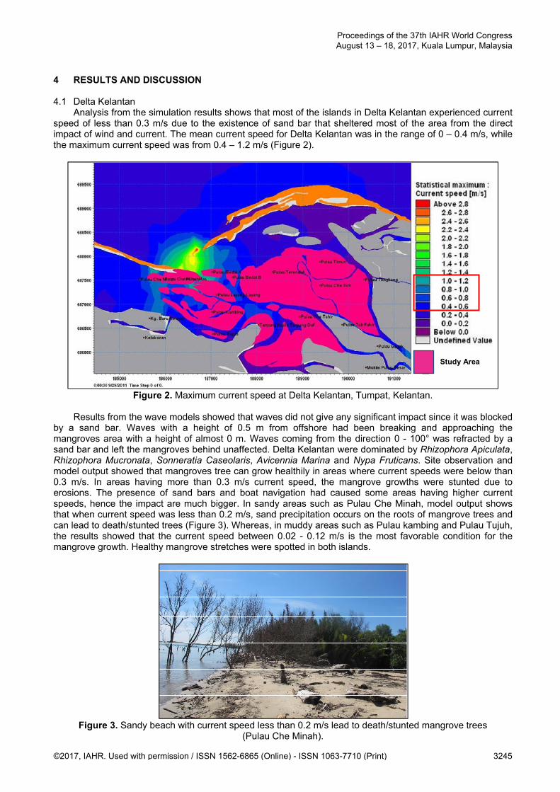
4 RESULTS AND DISCUSSION 4.1 Delta Kelantan

Analysis from the simulation results shows that most of the islands in Delta Kelantan experienced current speed of less than 0.3 m/s due to the existence of sand bar that sheltered most of the area from the direct impact of wind and current. The mean current speed for Delta Kelantan was in the range of 0 – 0.4 m/s, while the maximum current speed was from 0.4 – 1.2 m/s (Figure 2).

Figure 2. Maximum current speed at Delta Kelantan, Tumpat, Kelantan.

Results from the wave models showed that waves did not give any significant impact since it was blocked

by a sand bar. Waves with a height of 0.5 m from offshore had been breaking and approaching the mangroves area with a height of almost 0 m. Waves coming from the direction 0 - 100° was refracted by a sand bar and left the mangroves behind unaffected. Delta Kelantan were dominated by Rhizophora Apiculata, Rhizophora Mucronata, Sonneratia Caseolaris, Avicennia Marina and Nypa Fruticans. Site observation and model output showed that mangroves tree can grow healthily in areas where current speeds were below than 0.3 m/s. In areas having more than 0.3 m/s current speed, the mangrove growths were stunted due to erosions. The presence of sand bars and boat navigation had caused some areas having higher current speeds, hence the impact are much bigger. In sandy areas such as Pulau Che Minah, model output shows that when current speed was less than 0.2 m/s, sand precipitation occurs on the roots of mangrove trees and can lead to death/stunted trees (Figure 3). Whereas, in muddy areas such as Pulau kambing and Pulau Tujuh, the results showed that the current speed between 0.02 - 0.12 m/s is the most favorable condition for the mangrove growth. Healthy mangrove stretches were spotted in both islands.

Figure 3. Sandy beach with current speed less than 0.2 m/s lead to death/stunted mangrove trees

(Pulau Che Minah).

Study Area



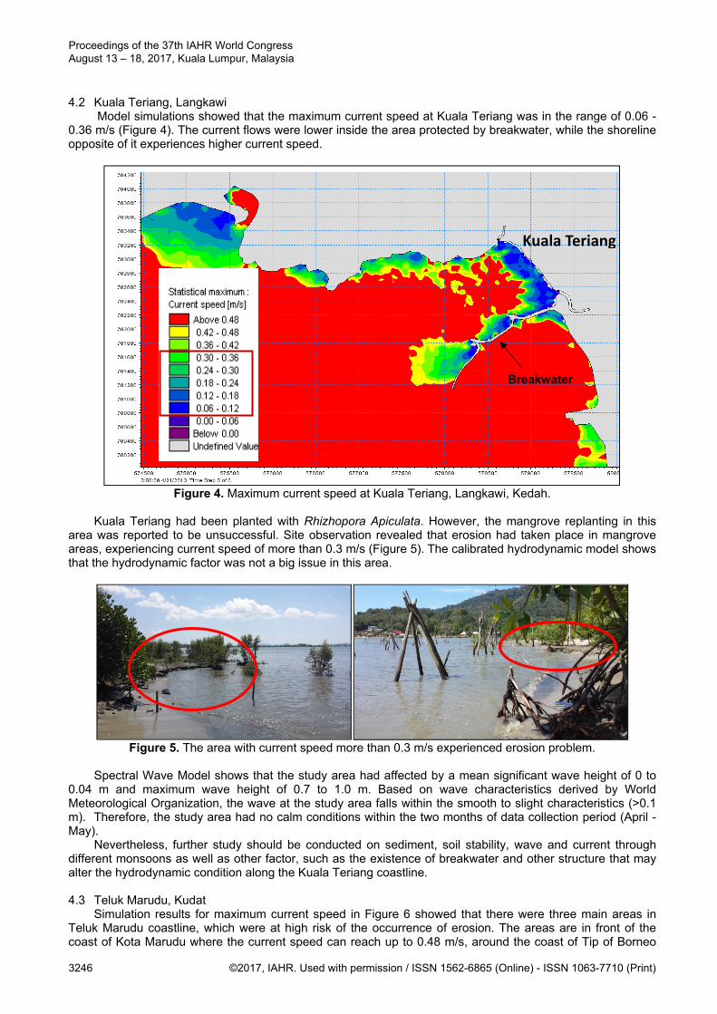
4.2 Kuala Teriang, Langkawi Model simulations showed that the maximum current speed at Kuala Teriang was in the range of 0.06 -

0.36 m/s (Figure 4). The current flows were lower inside the area protected by breakwater, while the shoreline opposite of it experiences higher current speed.

Figure 4. Maximum current speed at Kuala Teriang, Langkawi, Kedah.

Kuala Teriang had been planted with Rhizhopora Apiculata. However, the mangrove replanting in this

area was reported to be unsuccessful. Site observation revealed that erosion had taken place in mangrove areas, experiencing current speed of more than 0.3 m/s (Figure 5). The calibrated hydrodynamic model shows that the hydrodynamic factor was not a big issue in this area.

Figure 5. The area with current speed more than 0.3 m/s experienced erosion problem.

Spectral Wave Model shows that the study area had affected by a mean significant wave height of 0 to

0.04 m and maximum wave height of 0.7 to 1.0 m. Based on wave characteristics derived by World Meteorological Organization, the wave at the study area falls within the smooth to slight characteristics (>0.1 m). Therefore, the study area had no calm conditions within the two months of data collection period (April - May).

Nevertheless, further study should be conducted on sediment, soil stability, wave and current through different monsoons as well as other factor, such as the existence of breakwater and other structure that may alter the hydrodynamic condition along the Kuala Teriang coastline. 4.3 Teluk Marudu, Kudat

Simulation results for maximum current speed in Figure 6 showed that there were three main areas in Teluk Marudu coastline, which were at high risk of the occurrence of erosion. The areas are in front of the coast of Kota Marudu where the current speed can reach up to 0.48 m/s, around the coast of Tip of Borneo

Kuala Teriang

Breakwater



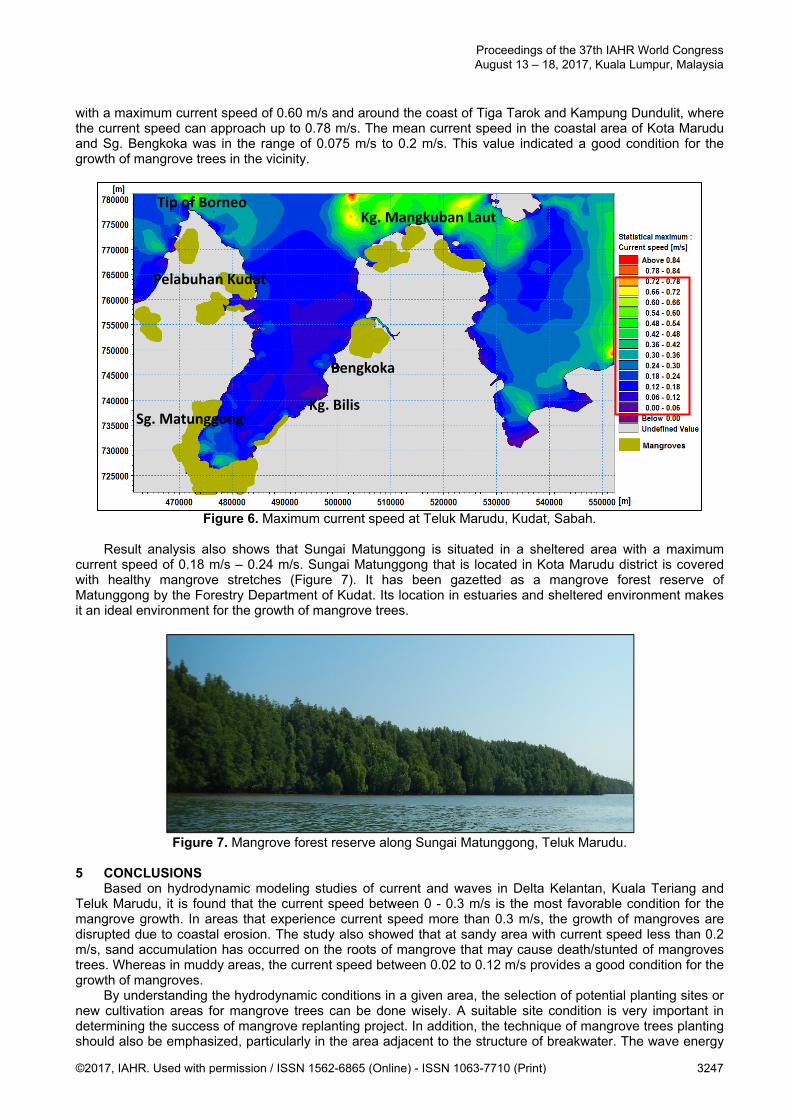
with a maximum current speed of 0.60 m/s and around the coast of Tiga Tarok and Kampung Dundulit, where the current speed can approach up to 0.78 m/s. The mean current speed in the coastal area of Kota Marudu and Sg. Bengkoka was in the range of 0.075 m/s to 0.2 m/s. This value indicated a good condition for the growth of mangrove trees in the vicinity.

Figure 6. Maximum current speed at Teluk Marudu, Kudat, Sabah.

Result analysis also shows that Sungai Matunggong is situated in a sheltered area with a maximum

current speed of 0.18 m/s – 0.24 m/s. Sungai Matunggong that is located in Kota Marudu district is covered with healthy mangrove stretches (Figure 7). It has been gazetted as a mangrove forest reserve of Matunggong by the Forestry Department of Kudat. Its location in estuaries and sheltered environment makes it an ideal environment for the growth of mangrove trees.

Figure 7. Mangrove forest reserve along Sungai Matunggong, Teluk Marudu.

5 CONCLUSIONS

Based on hydrodynamic modeling studies of current and waves in Delta Kelantan, Kuala Teriang and Teluk Marudu, it is found that the current speed between 0 - 0.3 m/s is the most favorable condition for the mangrove growth. In areas that experience current speed more than 0.3 m/s, the growth of mangroves are disrupted due to coastal erosion. The study also showed that at sandy area with current speed less than 0.2 m/s, sand accumulation has occurred on the roots of mangrove that may cause death/stunted of mangroves trees. Whereas in muddy areas, the current speed between 0.02 to 0.12 m/s provides a good condition for the growth of mangroves.

By understanding the hydrodynamic conditions in a given area, the selection of potential planting sites or new cultivation areas for mangrove trees can be done wisely. A suitable site condition is very important in determining the success of mangrove replanting project. In addition, the technique of mangrove trees planting should also be emphasized, particularly in the area adjacent to the structure of breakwater. The wave energy

Bengkoka

Sg. Matunggong

Kg. Mangkuban Laut

Kg. Bilis

Pelabuhan Kudat

Tip of Borneo



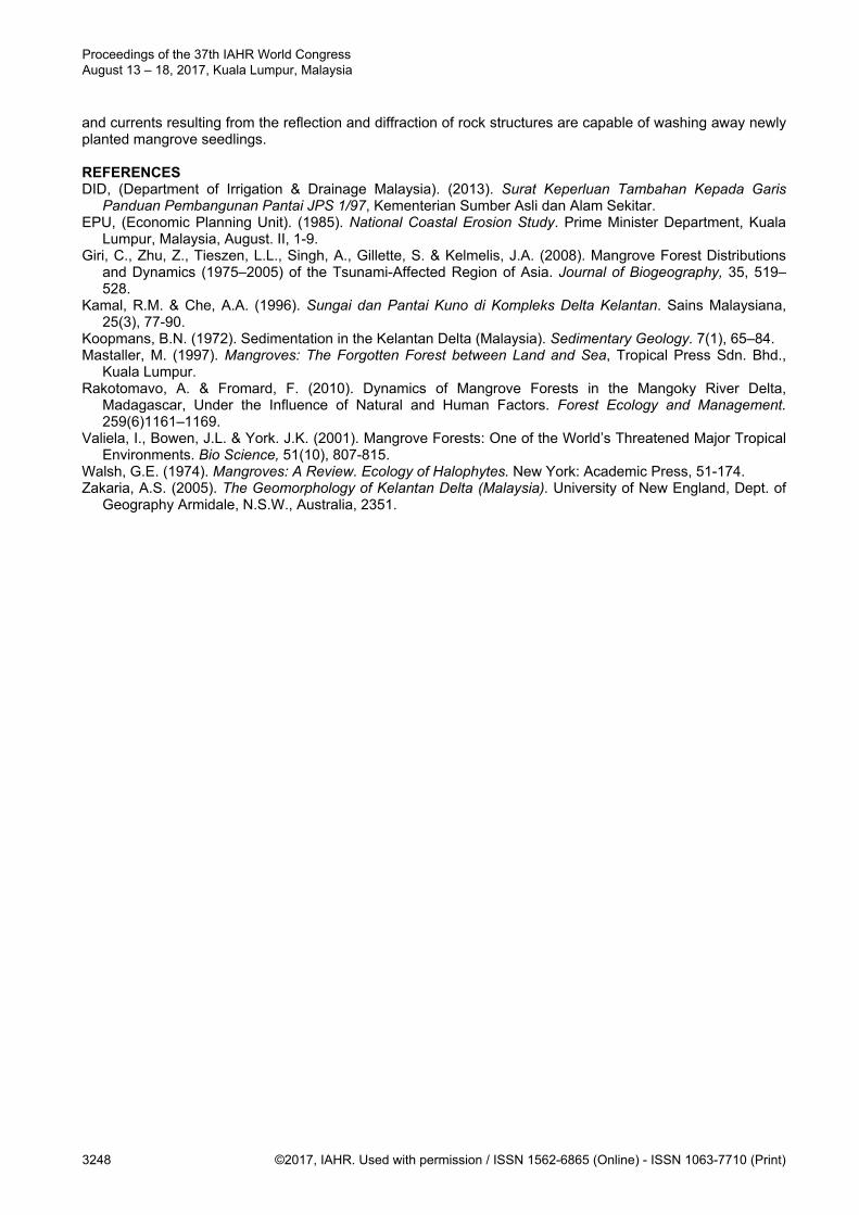
and currents resulting from the reflection and diffraction of rock structures are capable of washing away newly planted mangrove seedlings. REFERENCES DID, (Department of Irrigation & Drainage Malaysia). (2013). Surat Keperluan Tambahan Kepada Garis

Panduan Pembangunan Pantai JPS 1/97, Kementerian Sumber Asli dan Alam Sekitar. EPU, (Economic Planning Unit). (1985). National Coastal Erosion Study. Prime Minister Department, Kuala

Lumpur, Malaysia, August. II, 1-9. Giri, C., Zhu, Z., Tieszen, L.L., Singh, A., Gillette, S. & Kelmelis, J.A. (2008). Mangrove Forest Distributions

and Dynamics (1975–2005) of the Tsunami-Affected Region of Asia. Journal of Biogeography, 35, 519–528.

Kamal, R.M. & Che, A.A. (1996). Sungai dan Pantai Kuno di Kompleks Delta Kelantan. Sains Malaysiana, 25(3), 77-90.

Koopmans, B.N. (1972). Sedimentation in the Kelantan Delta (Malaysia). Sedimentary Geology. 7(1), 65–84. Mastaller, M. (1997). Mangroves: The Forgotten Forest between Land and Sea, Tropical Press Sdn. Bhd.,

Kuala Lumpur. Rakotomavo, A. & Fromard, F. (2010). Dynamics of Mangrove Forests in the Mangoky River Delta,

Madagascar, Under the Influence of Natural and Human Factors. Forest Ecology and Management. 259(6)1161–1169.

Valiela, I., Bowen, J.L. & York. J.K. (2001). Mangrove Forests: One of the World’s Threatened Major Tropical Environments. Bio Science, 51(10), 807-815.

Walsh, G.E. (1974). Mangroves: A Review. Ecology of Halophytes. New York: Academic Press, 51-174. Zakaria, A.S. (2005). The Geomorphology of Kelantan Delta (Malaysia). University of New England, Dept. of

Geography Armidale, N.S.W., Australia, 2351.



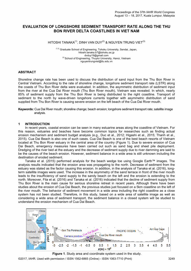
EVALUATION OF LONGSHORE SEDIMENT TRANSPORT RATE ALONG THE THU

BON RIVER DELTA COASTLINES IN VIET NAM

HITOSHI TANAKA(1), DINH VAN DUY(2) & NGUYEN TRUNG VIET(3)

(1,2) Graduate School of Engineering, Tohoku University, Sendai, Japan, [email protected]

[email protected] (3) School of Engineering, Thuyloi University, Hanoi, Vietnam

[email protected] ABSTRACT Shoreline change rate has been used to discuss the distribution of sand input from the Thu Bon River in Central Vietnam. According to the rate of shoreline change, longshore sediment transport rate (LSTR) along the coasts of Thu Bon River delta were evaluated. In addition, the asymmetric distribution of sediment input from the river at the Cua Dai River mouth (Thu Bon River mouth), Vietnam was revealed. In which, nearly 85% of sediment supply from the Thu Bon River is being distributed to the right coastline. Transport of sediment to the north by wave-driven longshore currents together with asymmetric distribution of sand supplied from Thu Bon River is causing severe erosion on the left beach of the Cua Dai River mouth. Keywords: Cua Dai River mouth; shoreline change; beach erosion; longshore sediment transport rate; satellite image

analysis. 1 INTRODUCTION

In recent years, coastal erosion can be seen in many estuarine areas along the coastline of Vietnam. For this reason, estuaries and beaches have become common topics for researches such as finding actual erosion mechanism and sediment budget analysis (e.g., Duc et al., 2012; Higashi et al., 2015; Thanh et al., 2015). Cua Dai Beach is also one of such cases. Cua Dai Beach is one of the best beach resorts of Vietnam located at Thu Bon River estuary in the central area of the country (Figure 1). Due to severe erosion of Cua Dai Beach, emergency measures have been carried out such as sand bag and sheet pile deployment. Dredging of the river bed at the estuary and the decrease of sediment supply due to river damming are said to be the causes of the beach erosion. However, sediment balance in a wide area is still unknown including the destination of eroded sediment.

Tanaka et al. (2015) performed analysis for the beach wedge toe using Google Earth™ images. The analysis results indicated that the erosion area was propagating to the north. Decrease of sediment from the estuary was stated as the factor causing this erosion. In addition, in the analysis of Tanaka et al. (2016), long-term satellite images were used. The increase in the asymmetry of the sand terrace in front of the river mouth leads to the insufficiency of sand supply to the sandy beach on the left and the erosion is extending to the north. Moreover, Fila et al. (2016) and Tanaka et al. (2016) indicated that the decline of sediment supply from Thu Bon River is the main cause for serious shoreline retreat in recent years. Although there have been studies about the erosion of Cua Dai Beach, the previous studies just focused on a 5km coastline on the left of the river mouth. The behavior of sediment movement in a wide area including the right coastline as a close system has not been studied. Therefore, in this study, based on a wide area of satellite image as well as considering a wide area of sediment transport, the sediment balance in a closed system will be studied to understand the erosion mechanism of Cua Dai Beach.

Figure 1. Study area and coordinate system used in the study.



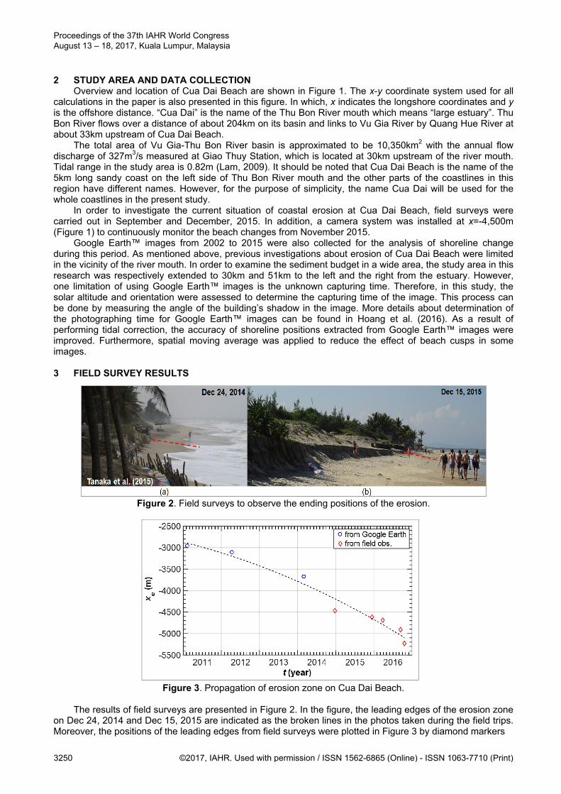
2 STUDY AREA AND DATA COLLECTION Overview and location of Cua Dai Beach are shown in Figure 1. The x-y coordinate system used for all

calculations in the paper is also presented in this figure. In which, x indicates the longshore coordinates and y is the offshore distance. “Cua Dai” is the name of the Thu Bon River mouth which means “large estuary”. Thu Bon River flows over a distance of about 204km on its basin and links to Vu Gia River by Quang Hue River at about 33km upstream of Cua Dai Beach.

The total area of Vu Gia-Thu Bon River basin is approximated to be 10,350km2 with the annual flow discharge of 327m3/s measured at Giao Thuy Station, which is located at 30km upstream of the river mouth. Tidal range in the study area is 0.82m (Lam, 2009). It should be noted that Cua Dai Beach is the name of the 5km long sandy coast on the left side of Thu Bon River mouth and the other parts of the coastlines in this region have different names. However, for the purpose of simplicity, the name Cua Dai will be used for the whole coastlines in the present study.

In order to investigate the current situation of coastal erosion at Cua Dai Beach, field surveys were carried out in September and December, 2015. In addition, a camera system was installed at x=-4,500m (Figure 1) to continuously monitor the beach changes from November 2015.

Google Earth™ images from 2002 to 2015 were also collected for the analysis of shoreline change during this period. As mentioned above, previous investigations about erosion of Cua Dai Beach were limited in the vicinity of the river mouth. In order to examine the sediment budget in a wide area, the study area in this research was respectively extended to 30km and 51km to the left and the right from the estuary. However, one limitation of using Google Earth™ images is the unknown capturing time. Therefore, in this study, the solar altitude and orientation were assessed to determine the capturing time of the image. This process can be done by measuring the angle of the building’s shadow in the image. More details about determination of the photographing time for Google Earth™ images can be found in Hoang et al. (2016). As a result of performing tidal correction, the accuracy of shoreline positions extracted from Google Earth™ images were improved. Furthermore, spatial moving average was applied to reduce the effect of beach cusps in some images. 3 FIELD SURVEY RESULTS

Figure 2. Field surveys to observe the ending positions of the erosion.

Figure 3. Propagation of erosion zone on Cua Dai Beach.

The results of field surveys are presented in Figure 2. In the figure, the leading edges of the erosion zone on Dec 24, 2014 and Dec 15, 2015 are indicated as the broken lines in the photos taken during the field trips. Moreover, the positions of the leading edges from field surveys were plotted in Figure 3 by diamond markers



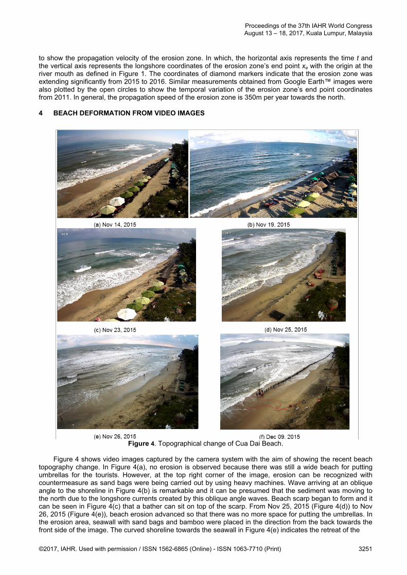
to show the propagation velocity of the erosion zone. In which, the horizontal axis represents the time t and the vertical axis represents the longshore coordinates of the erosion zone’s end point xe with the origin at the river mouth as defined in Figure 1. The coordinates of diamond markers indicate that the erosion zone was extending significantly from 2015 to 2016. Similar measurements obtained from Google Earth™ images were also plotted by the open circles to show the temporal variation of the erosion zone’s end point coordinates from 2011. In general, the propagation speed of the erosion zone is 350m per year towards the north. 4 BEACH DEFORMATION FROM VIDEO IMAGES

Figure 4. Topographical change of Cua Dai Beach.

Figure 4 shows video images captured by the camera system with the aim of showing the recent beach

topography change. In Figure 4(a), no erosion is observed because there was still a wide beach for putting umbrellas for the tourists. However, at the top right corner of the image, erosion can be recognized with countermeasure as sand bags were being carried out by using heavy machines. Wave arriving at an oblique angle to the shoreline in Figure 4(b) is remarkable and it can be presumed that the sediment was moving to the north due to the longshore currents created by this oblique angle waves. Beach scarp began to form and it can be seen in Figure 4(c) that a bather can sit on top of the scarp. From Nov 25, 2015 (Figure 4(d)) to Nov 26, 2015 (Figure 4(e)), beach erosion advanced so that there was no more space for putting the umbrellas. In the erosion area, seawall with sand bags and bamboo were placed in the direction from the back towards the front side of the image. The curved shoreline towards the seawall in Figure 4(e) indicates the retreat of the



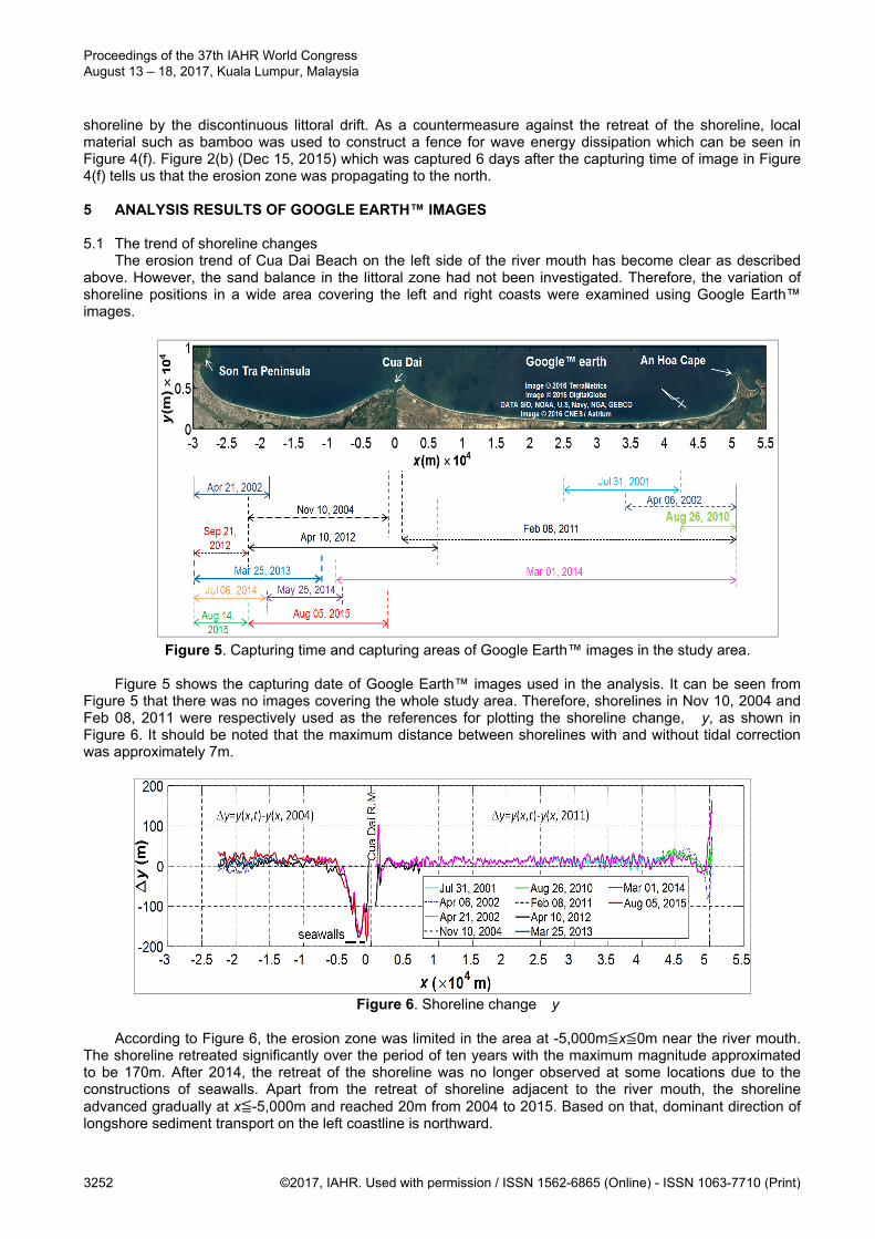
shoreline by the discontinuous littoral drift. As a countermeasure against the retreat of the shoreline, local material such as bamboo was used to construct a fence for wave energy dissipation which can be seen in Figure 4(f). Figure 2(b) (Dec 15, 2015) which was captured 6 days after the capturing time of image in Figure 4(f) tells us that the erosion zone was propagating to the north. 5 ANALYSIS RESULTS OF GOOGLE EARTH™ IMAGES 5.1 The trend of shoreline changes

The erosion trend of Cua Dai Beach on the left side of the river mouth has become clear as described above. However, the sand balance in the littoral zone had not been investigated. Therefore, the variation of shoreline positions in a wide area covering the left and right coasts were examined using Google Earth™ images.

Figure 5. Capturing time and capturing areas of Google Earth™ images in the study area.

Figure 5 shows the capturing date of Google Earth™ images used in the analysis. It can be seen from Figure 5 that there was no images covering the whole study area. Therefore, shorelines in Nov 10, 2004 and Feb 08, 2011 were respectively used as the references for plotting the shoreline change, �y, as shown in Figure 6. It should be noted that the maximum distance between shorelines with and without tidal correction was approximately 7m.

Figure 6. Shoreline change �y

According to Figure 6, the erosion zone was limited in the area at -5,000m≦x≦0m near the river mouth.

The shoreline retreated significantly over the period of ten years with the maximum magnitude approximated to be 170m. After 2014, the retreat of the shoreline was no longer observed at some locations due to the constructions of seawalls. Apart from the retreat of shoreline adjacent to the river mouth, the shoreline advanced gradually at x≦-5,000m and reached 20m from 2004 to 2015. Based on that, dominant direction of longshore sediment transport on the left coastline is northward.



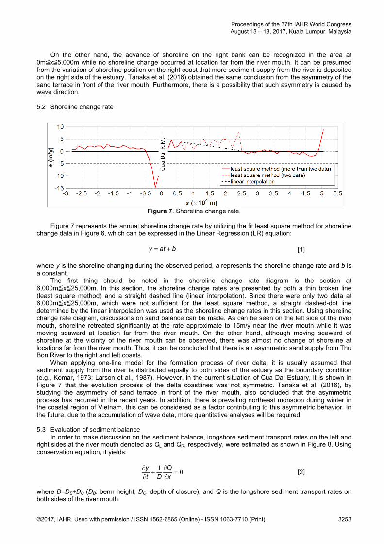
On the other hand, the advance of shoreline on the right bank can be recognized in the area at 0m≦x≦5,000m while no shoreline change occurred at location far from the river mouth. It can be presumed from the variation of shoreline position on the right coast that more sediment supply from the river is deposited on the right side of the estuary. Tanaka et al. (2016) obtained the same conclusion from the asymmetry of the sand terrace in front of the river mouth. Furthermore, there is a possibility that such asymmetry is caused by wave direction. 5.2 Shoreline change rate

Figure 7. Shoreline change rate.

Figure 7 represents the annual shoreline change rate by utilizing the fit least square method for shoreline

change data in Figure 6, which can be expressed in the Linear Regression (LR) equation: baty [1] where y is the shoreline changing during the observed period, a represents the shoreline change rate and b is a constant.

The first thing should be noted in the shoreline change rate diagram is the section at 6,000m≦x≦25,000m. In this section, the shoreline change rates are presented by both a thin broken line (least square method) and a straight dashed line (linear interpolation). Since there were only two data at 6,000m≦x≦25,000m, which were not sufficient for the least square method, a straight dashed-dot line determined by the linear interpolation was used as the shoreline change rates in this section. Using shoreline change rate diagram, discussions on sand balance can be made. As can be seen on the left side of the river mouth, shoreline retreated significantly at the rate approximate to 15m/y near the river mouth while it was moving seaward at location far from the river mouth. On the other hand, although moving seaward of shoreline at the vicinity of the river mouth can be observed, there was almost no change of shoreline at locations far from the river mouth. Thus, it can be concluded that there is an asymmetric sand supply from Thu Bon River to the right and left coasts.

When applying one-line model for the formation process of river delta, it is usually assumed that sediment supply from the river is distributed equally to both sides of the estuary as the boundary condition (e.g., Komar, 1973; Larson et al., 1987). However, in the current situation of Cua Dai Estuary, it is shown in Figure 7 that the evolution process of the delta coastlines was not symmetric. Tanaka et al. (2016), by studying the asymmetry of sand terrace in front of the river mouth, also concluded that the asymmetric process has recurred in the recent years. In addition, there is prevailing northeast monsoon during winter in the coastal region of Vietnam, this can be considered as a factor contributing to this asymmetric behavior. In the future, due to the accumulation of wave data, more quantitative analyses will be required. 5.3 Evaluation of sediment balance

In order to make discussion on the sediment balance, longshore sediment transport rates on the left and right sides at the river mouth denoted as QL and QR, respectively, were estimated as shown in Figure 8. Using conservation equation, it yields:

01

x

Q

Dt

y [2]

where D=DB+DC (DB: berm height, DC: depth of closure), and Q is the longshore sediment transport rates on both sides of the river mouth.



From Eq. [2] and Figure 8, the longshore sediment transport rate along the coastlines can be determined as in the following equations.

For the left coastline:

x

x

dxt

yDxQ

1

)( [3]

For the right coastline:

x

x

dxt

yDxQ

2

)( [4]

in which x1 and x2 indicate the x-coordinates of two boundaries for the littoral cell where Q(x)=0 is satisfied. In the study area, Son Tra Peninsula and An Hoa Cape can be considered as two boundaries at which Q(x)=0 (Figure 1). Therefore, x1=-30,000m and x2=51,000m were chosen as the boundaries for the integration of longshore sediment transport rate.

Figure 8. Diagram for estimations of longshore sediment transport rates.

Figure 9. Longshore sand transport rate calculated based on shoreline change rate values.

From the definition of shoreline change rate, y/x in Eq. [3] and [4] can be determined using the values

of shoreline change rate in Figure 7. Figure 9 represents the longshore sediment transport rate along the coastlines across Cua Dai River mouth calculated based on values of shoreline change rates in Figure 7. From Figure 8 and Figure 9, it is easy to determine the magnitudes of longshore sediment transport rates to both sides at the river mouth as QL=70,000m3/y and QR=390,000m3/y, respectively. Sediment input of Thu Bon River can be determined based on values of QL and QR as follows: RL QQq 0 [5] where q0 is sediment input from Thu Bon River, q0=460,000m3/y. This value shows good correspondence to the sediment supplies from Thu Bon River estimated by Fila et al. (2016). According to Fila et al. (2016), three different methods to estimate sediment input from Thu Bon River were proposed with the values of 390,000m3/y, 440,000m3/y, and 600,000m3/y.

In addition, Mau (2006) performed the calculations for longshore sediment transport rates around the Thu Bon River mouth with the average transport rates between 1999 and 2000 are 150,000m3/y towards the north (on the left coastline) and 230,000m3/y towards the south (on the right coastline). These estimations are in the

End of littoral cell End of littoral system

y (x,t+t)

y (x,t)

x

x

x1 x xL x x2

y

q0

QL QR

xR



same order of magnitude with the values of longshore sediment transport rates on the left and the right coastlines as in Figure 9.

Let α be the ratio of sediment transported from the river mouth to the right coastline, α can be determined from the following equation:

RL

R

QQ

Q

[6]

One important conclusion that can be drawn from Figure 9 and Eq. [6] is that about 85% of sediment

supply from Thu Bon River is transported to the right. This causes insufficient sediment supply to the left coast and results in significant erosion at Cua Dai Beach as in Tanaka et al. (2016).

Duy et al. (2016) also made analysis on this asymmetric behavior of Thu Bon River delta coastlines with a different approach by measuring the shoreline gradients at the river mouth and came to the conclusion that about 80% of sand input from Thu Bon River is transported to the right coastline. Moreover, variations of sediment inputs from Thu Bon River from 1973 to 2015 were also calculated with the values vary around 600,000m3/y. It is interesting that the results obtained by Duy et al. (2016) are quite comparable to the values of α =85% and q0=460,000m3/y in this study. 6 CONCLUSIONS

Based on the analysis of Google Earth™ images in a wide area for Cua Dai Beach, Vietnam, the sediment budget in a littoral zone has been analyzed. A large amount of sand input from Thu Bon River (85%) is distributed to the right coastline. This asymmetric distribution of sand input from the river is causing significant retreat of the left coastline at the vicinity of the river mouth. REFERENCES Duc DM., Nhuan MT. & Ngoi CV. (2012). An Analysis of Coastal Erosion in the Tropical Rapid Accretion Delta

of The Red River, Vietnam. Journal of Asian Earth Sciences, 43(1), 98-109. Duy DV., Tanaka H. & Viet NT. (2016). Study on River Mouth Delta Formation and Recent Year Erosion

Mechanism of Cua Dai Delta Coastlines in Vietnam. Vietnam-Japan Workshop on Estuaries, Coasts and Rivers 2016, 94-104.

Fila J., Kampen M., Knulst K., Marijnissen R. & Noort RV. (2016). Coastal Erosion Hoi An, Multidisciplinary Project Report, Delft University of Technology, 168.

Higashi R., Tajima Y., Gunasekara K.，Hung NT. & Hanh LC. (2015). Investigation of Sediment Transport Characteristics Along The Coast of Ma River Mouth Adjacent to The Red River Mouth. Journal of Japan Society of Civil Engineers, Ser. B2 (Coastal Engineering), 71(2), 715-720 (In Japanese).

Hoang VC.，Tanaka H.，Mitobe Y. & Duy DV. (2016). Tidal Correction Method for Shoreline Position Extracted from Google Earth Images. Journal of Japan Society of Civil Engineers, Ser. B3 (Ocean Engineering), 72(2),61-66 (In Japanese).

Komar PD. (1973). Computer Models of Delta Growth Due to Sediment Input from Rivers and Longshore Transport. Geological Society of America Bulletin, 84(7), 2217-2226.

Lam NT. (2009). Hydrodynamics and Morphodynamics of a Seasonally Forced Tidal Inlet System, PhD Thesis. Delft University of Technology.

Larson M., Hanson H. & Kraus NC. (1987). Analytical Solutions of the One-Line Model of Shoreline Change, Technical Report CERC-87-15, U.S. Army Engineer Waterways Experiment Station, 72.

Mau LD. (2006). Shoreline Changes in and Around the Thu Bon River Mouth, Central Vietnam, PhD Thesis. Goa University.

Tanaka H., Hoang VC., Viet NT. & Duy DV. (2016). Interrelationship between Serious Shoreline Retreat and Sand Terrace Formation on Cua Dai Beach, Central Vietnam. Journal of Japan Society of Civil Engineers, Ser. B1 (Hydraulic Engineering), 72(4), 361-366 (In Japanese).

Tanaka H., Viet NT., Hoang VC. & Duy DV. (2015). Erosion Mechanism on Cua Dai Beach, Central Vietnam. Journal of Japan Society of Civil Engineers, Ser. B3 (Ocean Engineering), 71(2), 449-454 (In Japanese).

Thanh TM.，Tanaka H.，Viet NT.，Mitobe Y. & Hoang VC. (2015). Seasonal Change of Longshore Sediment Transport Regime on Nha Trang Coast, Vietnam. Vietnam-Japan Workshop on Estuaries, Coasts and Rivers 2015, Hoi An, Vietnam, USB.



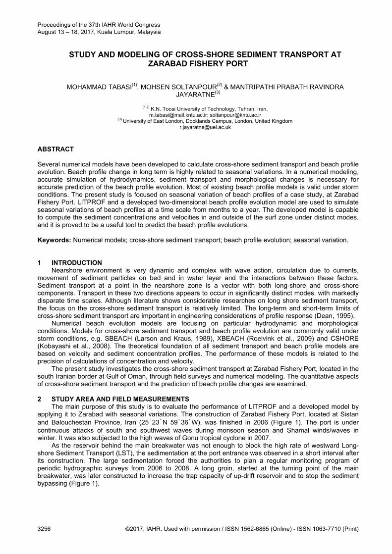
STUDY AND MODELING OF CROSS-SHORE SEDIMENT TRANSPORT AT ZARABAD FISHERY PORT

MOHAMMAD TABASI(1), MOHSEN SOLTANPOUR(2) & MANTRIPATHI PRABATH RAVINDRA JAYARATNE(3)

(1,2) K.N. Toosi University of Technology, Tehran, Iran,

[email protected]; [email protected] (3) University of East London, Docklands Campus, London, United Kingdom

[email protected]

ABSTRACT Several numerical models have been developed to calculate cross-shore sediment transport and beach profile evolution. Beach profile change in long term is highly related to seasonal variations. In a numerical modeling, accurate simulation of hydrodynamics, sediment transport and morphological changes is necessary for accurate prediction of the beach profile evolution. Most of existing beach profile models is valid under storm conditions. The present study is focused on seasonal variation of beach profiles of a case study, at Zarabad Fishery Port. LITPROF and a developed two-dimensional beach profile evolution model are used to simulate seasonal variations of beach profiles at a time scale from months to a year. The developed model is capable to compute the sediment concentrations and velocities in and outside of the surf zone under distinct modes, and it is proved to be a useful tool to predict the beach profile evolutions. Keywords: Numerical models; cross-shore sediment transport; beach profile evolution; seasonal variation. 1 INTRODUCTION

Nearshore environment is very dynamic and complex with wave action, circulation due to currents, movement of sediment particles on bed and in water layer and the interactions between these factors. Sediment transport at a point in the nearshore zone is a vector with both long-shore and cross-shore components. Transport in these two directions appears to occur in significantly distinct modes, with markedly disparate time scales. Although literature shows considerable researches on long shore sediment transport, the focus on the cross-shore sediment transport is relatively limited. The long-term and short-term limits of cross-shore sediment transport are important in engineering considerations of profile response (Dean, 1995).

Numerical beach evolution models are focusing on particular hydrodynamic and morphological conditions. Models for cross-shore sediment transport and beach profile evolution are commonly valid under storm conditions, e.g. SBEACH (Larson and Kraus, 1989), XBEACH (Roelvink et al., 2009) and CSHORE (Kobayashi et al., 2008). The theoretical foundation of all sediment transport and beach profile models are based on velocity and sediment concentration profiles. The performance of these models is related to the precision of calculations of concentration and velocity.

The present study investigates the cross-shore sediment transport at Zarabad Fishery Port, located in the south Iranian border at Gulf of Oman, through field surveys and numerical modeling. The quantitative aspects of cross-shore sediment transport and the prediction of beach profile changes are examined.

2 STUDY AREA AND FIELD MEASUREMENTS

The main purpose of this study is to evaluate the performance of LITPROF and a developed model by applying it to Zarabad with seasonal variations. The construction of Zarabad Fishery Port, located at Sistan and Balouchestan Province, Iran (25˚23́N 59˚36́W), was finished in 2006 (Figure 1). The port is under continuous attacks of south and southwest waves during monsoon season and Shamal winds/waves in winter. It was also subjected to the high waves of Gonu tropical cyclone in 2007.

As the reservoir behind the main breakwater was not enough to block the high rate of westward Long-shore Sediment Transport (LST), the sedimentation at the port entrance was observed in a short interval after its construction. The large sedimentation forced the authorities to plan a regular monitoring program of periodic hydrographic surveys from 2006 to 2008. A long groin, started at the turning point of the main breakwater, was later constructed to increase the trap capacity of up-drift reservoir and to stop the sediment bypassing (Figure 1).



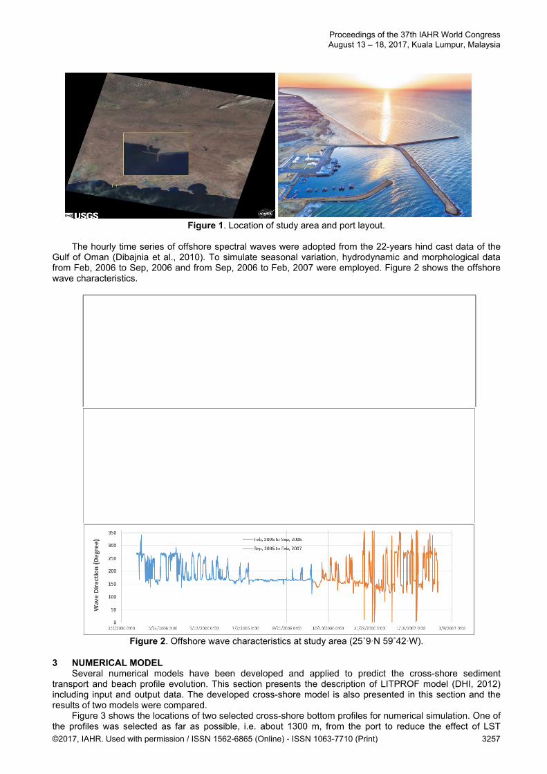
Figure 1. Location of study area and port layout. The hourly time series of offshore spectral waves were adopted from the 22-years hind cast data of the

Gulf of Oman (Dibajnia et al., 2010). To simulate seasonal variation, hydrodynamic and morphological data from Feb, 2006 to Sep, 2006 and from Sep, 2006 to Feb, 2007 were employed. Figure 2 shows the offshore wave characteristics.

Figure 2. Offshore wave characteristics at study area (25˚9 ́ N 59˚42 ́ W).

3 NUMERICAL MODEL

Several numerical models have been developed and applied to predict the cross-shore sediment transport and beach profile evolution. This section presents the description of LITPROF model (DHI, 2012) including input and output data. The developed cross-shore model is also presented in this section and the results of two models were compared.

Figure 3 shows the locations of two selected cross-shore bottom profiles for numerical simulation. One of the profiles was selected as far as possible, i.e. about 1300 m, from the port to reduce the effect of LST



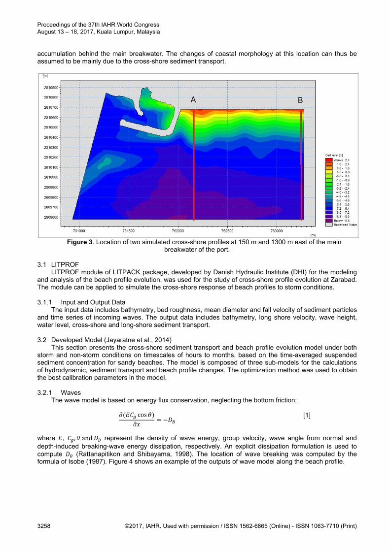
accumulation behind the main breakwater. The changes of coastal morphology at this location can thus be assumed to be mainly due to the cross-shore sediment transport.

Figure 3. Location of two simulated cross-shore profiles at 150 m and 1300 m east of the main breakwater of the port.

3.1 LITPROF

LITPROF module of LITPACK package, developed by Danish Hydraulic Institute (DHI) for the modeling and analysis of the beach profile evolution, was used for the study of cross-shore profile evolution at Zarabad. The module can be applied to simulate the cross-shore response of beach profiles to storm conditions. 3.1.1 Input and Output Data

The input data includes bathymetry, bed roughness, mean diameter and fall velocity of sediment particles and time series of incoming waves. The output data includes bathymetry, long shore velocity, wave height, water level, cross-shore and long-shore sediment transport. 3.2 Developed Model (Jayaratne et al., 2014)

This section presents the cross-shore sediment transport and beach profile evolution model under both storm and non-storm conditions on timescales of hours to months, based on the time-averaged suspended sediment concentration for sandy beaches. The model is composed of three sub-models for the calculations of hydrodynamic, sediment transport and beach profile changes. The optimization method was used to obtain the best calibration parameters in the model. 3.2.1 Waves

The wave model is based on energy flux conservation, neglecting the bottom friction:

cos

[1]

where , , and represent the density of wave energy, group velocity, wave angle from normal and depth-induced breaking-wave energy dissipation, respectively. An explicit dissipation formulation is used to compute (Rattanapitikon and Shibayama, 1998). The location of wave breaking was computed by the formula of Isobe (1987). Figure 4 shows an example of the outputs of wave model along the beach profile.



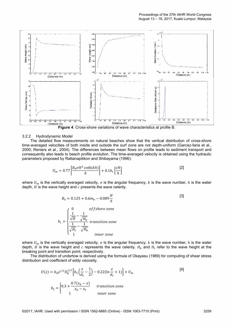
Figure 4. Cross-shore variations of wave characteristics at profile B. 3.2.2 Hydrodynamic Model

The detailed flow measurements on natural beaches show that the vertical distribution of cross-shore time-averaged velocities of both inside and outside the surf zone are not depth-uniform (Garcez-faria et al., 2000; Reniers et al., 2004). The differences between mean flows on profile leads to sediment transport and consequently also leads to beach profile evolution. The time-averaged velocity is obtained using the hydraulic parameters proposed by Rattanapitikon and Shibayama (1996):

0.77coth

0.1 [2]

where is the vertically averaged velocity, is the angular frequency, is the wave number, is the water depth, is the wave height and presents the wave celerity.

0.125 0.6 0.089 [3]

01√

1

1 1

1

where is the vertically averaged velocity, is the angular frequency, is the wave number, is the water depth, is the wave height and represents the wave celerity. and refer to the wave height at the breaking point and transition point, respectively.

The distribution of undertow is derived using the formula of Okayasu (1989) for computing of shear stress distribution and coefficient of eddy viscosity.

/ / 12

0.22 ln 1 [4]

0.30.7

1



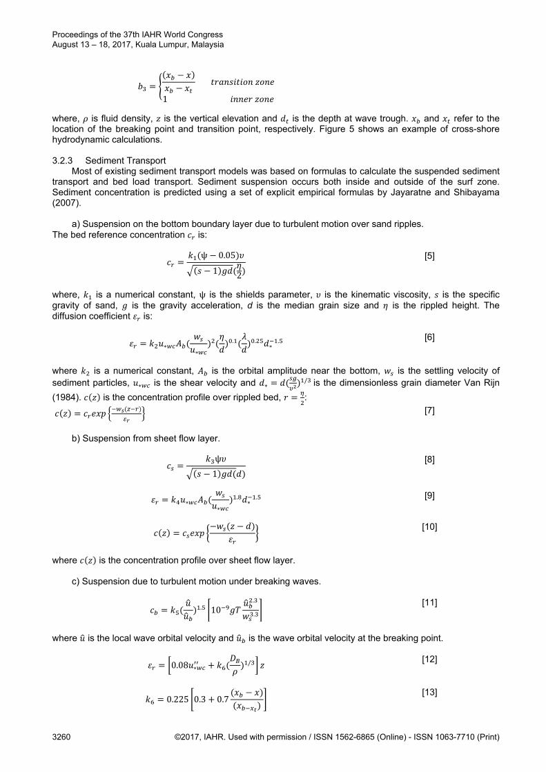
1

where, is fluid density, is the vertical elevation and is the depth at wave trough. and refer to the location of the breaking point and transition point, respectively. Figure 5 shows an example of cross-shore hydrodynamic calculations. 3.2.3 Sediment Transport

Most of existing sediment transport models was based on formulas to calculate the suspended sediment transport and bed load transport. Sediment suspension occurs both inside and outside of the surf zone. Sediment concentration is predicted using a set of explicit empirical formulas by Jayaratne and Shibayama (2007).

a) Suspension on the bottom boundary layer due to turbulent motion over sand ripples. The bed reference concentration is:

ψ 0.05

1 2

[5]

where, is a numerical constant, ψ is the shields parameter, is the kinematic viscosity, is the specific gravity of sand, is the gravity acceleration, d is the median grain size and is the rippled height. The diffusion coefficient is:

∗∗

. .∗

. [6]

where is a numerical constant, is the orbital amplitude near the bottom, is the settling velocity of sediment particles, ∗ is the shear velocity and ∗

/ is the dimensionless grain diameter Van Rijn

(1984). is the concentration profile over rippled bed, :

[7]

b) Suspension from sheet flow layer.

ψ

1

[8]

∗∗

.∗

. [9]

[10]

where is the concentration profile over sheet flow layer.

c) Suspension due to turbulent motion under breaking waves.

. 10.

. [11]

where is the local wave orbital velocity and is the wave orbital velocity at the breaking point.

0.08 ∗/

[12]

0.225 0.3 0.7 [13]



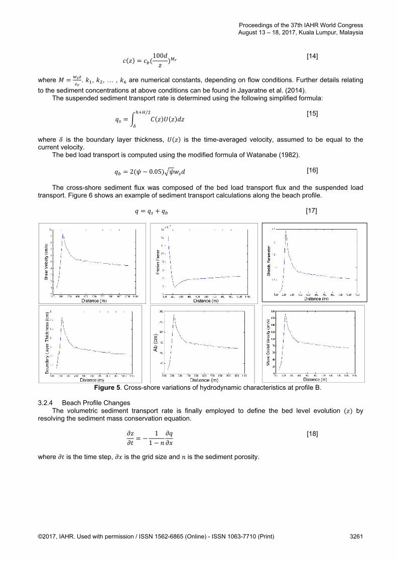
100

[14]

where . , , … , are numerical constants, depending on flow conditions. Further details relating

to the sediment concentrations at above conditions can be found in Jayaratne et al. (2014). The suspended sediment transport rate is determined using the following simplified formula:

/

[15]

where is the boundary layer thickness, is the time-averaged velocity, assumed to be equal to the current velocity.

The bed load transport is computed using the modified formula of Watanabe (1982).

2 0.05 [16]

The cross-shore sediment flux was composed of the bed load transport flux and the suspended load

transport. Figure 6 shows an example of sediment transport calculations along the beach profile.

[17]

Figure 5. Cross-shore variations of hydrodynamic characteristics at profile B.

3.2.4 Beach Profile Changes

The volumetric sediment transport rate is finally employed to define the bed level evolution by resolving the sediment mass conservation equation.

11

[18]

where is the time step, is the grid size and is the sediment porosity.



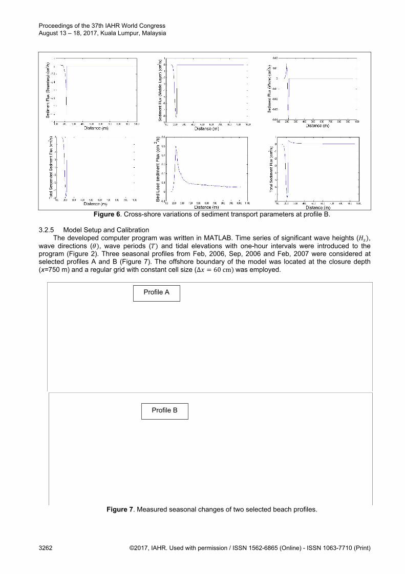
Figure 6. Cross-shore variations of sediment transport parameters at profile B. 3.2.5 Model Setup and Calibration

The developed computer program was written in MATLAB. Time series of significant wave heights ( , wave directions ( , wave periods ( and tidal elevations with one-hour intervals were introduced to the program (Figure 2). Three seasonal profiles from Feb, 2006, Sep, 2006 and Feb, 2007 were considered at selected profiles A and B (Figure 7). The offshore boundary of the model was located at the closure depth (x=750 m) and a regular grid with constant cell size (∆ 60cm was employed.

Figure 7. Measured seasonal changes of two selected beach profiles.

Profile A

Profile B



The performance of numerical model was evaluated through comparisons of the model results with

measurements. Calibration of the model outputs with measured profiles, following a numerical constant optimization process, resulted to the following numerical constants:

4.5 0.27 1.5 0.24

4.5 ∗ 10 6

3.4 ∗ 10 6 102.5 ∗ 10 10

0.225 60.176 100.125 10

4 RESULTS AND DISCUSSIONS

The calibration parameters in the surf zone were calibrated to for profile A and for profile B. Out of the surf zone, similar calibration parameters were selected for all cross-shore profiles. A linear interpolation of calibration parameters was used at cross-shore profiles between profile A and B. The application of the developed model with three distinct suspended sediment transport modes showed an acceptable performance.

Figures 8 represent the comparisons between predicted winter and summer profiles on Feb, 2006 and Sep, 2007 using LITPROF and the developed numerical model. Comparing the simulated results with measurements reveals that the developed two-dimensional model is capable to simulate the profile response to cross-shore sediment transport in the area. 5 SUMMARY AND CONCLUSIONS

Many engineering applications, such as the beach response to storms, seasonal profile changes and sediment transport in vicinity of breakwaters, are associated to processes in which cross-shore sediment transport is important. In this research, the seasonal variation of Zarabad profiles was simulated by LITPROF and a developed model, to study the dynamic cross-shore sediment transport processes. The results of monitoring program and field surveys were employed to investigate the changes of bottom profiles. Although the sediment at this location is highly transported by governing monsoon waves, the winter northeast waves due to Shamal winds are also effective on the evolution of bottom profiles. Although long-shore currents and littoral drift affect the local sediment transport and the sedimentation at up-drift side off the port, here one of the simulated profiles (profile B) was selected as far as possible, i.e. 1300 m, from the port breakwater to minimize this effect.

The developed two-dimensional model proved to be an effective tool to simulate the dynamic cross-shore sediment transport processes and the transient nature of the profiles adjustments at the site. In spite of the general assumptions of cross-shore modeling, i.e. the long shore gradients in hydrodynamic and sediment conditions are negligible and the depth contours are parallel to the coastline. The formation of bars under high monsoon waves and the simulation of equilibrium profiles after calm wave condition, in which there is no net cross-shore sediment transport, were successfully modeled. Quantitative comparisons also proved to be acceptable within the normal discrepancies of sediment transport modeling.



Figure 8. Comparisons between the simulated and measured cross-shore profiles.

Profile A (Summer)

Profile A (Winter)

Profile B (Summer)

Profile B (Winter)



REFERENCES Dean, R.G. (1995). Cross-Shore Sediment Transport Processes. Advances in Coastal and Ocean

Engineering, 1, 159-220. DHI Water & Environment. (2012). LITPROF Software Package User Guide and Scientific Documentation.

Danish Hydraulic Institute, 1-74. Dibajnia, M., Soltanpour, M., Kebriaee, A. & Haghighy, S. (2010). Development of A Long Term Hindcast for

The Indian Ocean and The Oman Sea. 9th International Conference on Hydro-Science and Engineering, Chennai, India.

Garcez-Faria, A., Thornton, E., Lippmann, T. & Stanton, T. (2000). Undertow over a Barred Beach. Journal of Geophysical Research, 105, 16999–17010.

Isobe, M. (1987). Parabolic Equation Model for Transformation of Irregular Waves Due to Refraction, Diffraction and Breaking. Coastal Engineering Jpn., JSCE, 30(1), 33–47.

Jayaratne, M.P.R. & Shibayama, T. (2007). Suspended Sediment Concentration on Beaches Under Three Different Mechanisms. Coastal Engineering Journal, JSCE, 49(4), 357–392.

Jayaratne, M.P.R., Rahman, M.R. & Shibayama, T. (2014). A Cross-Shore Beach Profile Evolution Model. Coastal Engineering Journal, 56(4), 1–70.

Kobayashi, N., Payo, A. & Schmind, L. (2008). Cross-shore Suspended Sand And Bed Load Transport on Beaches. Journal of Geophysics Research, 113(C07001), 1-17.

Larson, M. & Kraus, N.C., (1989). SBEACH: Numerical Model for Simulating Storm-Induced Beach Change, Report, 1: Empirical Foundation and Model Development. Technical Report CERC-89-9, US Army Engineer waterway Experiment Station, Coastal Engineering Research Center, Vicksburg, MS, 1-266.

Okayasu, A. (1989). Characteristics of Turbulence Structure and Undertow in Surf Zone, PhD thesis. Uni. of Tokyo, Japan.

Rattanapitikon, W. & Shibayama, T. (1996) Cross-Shore Sediment Transport and Beach Deformation Model. In Proceeding 25th Int. Conference on Coastal Engineering, ASCE, Orlando, 3062–3075.

Rattanapitikon, W. & Shibayama, T. (1998). Energy Dissipation Model for Regular and Irregular Breaking Waves. Coastal Engineering Journal, JSCE, 40(4), 327–346.

Reniers, A.J.H.M., Thornton, E., Stanton, T. & Roelvink, J. (2004). Vertical Flow Structure During Sandy Duck: Observations and Modeling. Coast. Engineering, 51, 237–260.

Roelvink, J.A., Reniers, A., van Dongeren, A.R., van Thiel de Vries, J.S.M., McCall, R. & Lescinski, J. (2009). Modeling Storm Impacts on Beaches, Dunes and Barrier Islands. Coast, Engineering, 56, 1133-1152.

Van Rijn, L.C. (1984). Sediment Transport, Part I: Bed Load Transport. Port-Coastal Ocean Engineering, ASCE, 110(10), 1431–1456.



1

SATELLITE DERIVED NEAR-SHORE BATHYMETRY USING A MACHINE LEARNING

APPROACH

ANKITA MISRA(1), ZORANVOJINOVIC(2), BALAJI RAMAKRISHNAN(3), ARJEN LUIJENDIJK(4) & ROSHANKA RANASINGHE(5)

(1,3)Indian Institute of Technology- Bombay, Mumbai, India

[email protected]; [email protected] (2,5)UNESCO-IHE, Institute for Water Education, Delft, The Netherlands

[email protected]; [email protected] (4,5)Deltares, The Netherlands

[email protected]; [email protected] (5)University of Twente, Enschede, The Netherlands

[email protected]

ABSTRACT This paper demonstrates the capability of the Support Vector Machine (SVM) technique to obtain Satellite Derived Bathymetry (SDB) maps of near-shore regions using freely available Landsat 7 ETM and Landsat 8 OLI imagery of 30 m resolution (medium). The Support Vector Machine is a nonlinear machine learning approach that utilizes the Radial Basis kernel function; and the other training factors such as the smoothing parameter, penalty parameter C and insensitivity zone ε are selected and tuned based on the learning (i.e. training) process. The approach is applied here with available bathymetric SONAR data for two regions, first, one of the Dutch Wadden sea inlets, the Ameland inlet, which has a significant mean tidal range of 2m and the second, the Dutch territory of Sint Maarten Island which has a rather insignificant mean tidal range of less than 10 cm. A comparison of the SVM retrieved depths with the available in-situ data is presented for the regions and the results highlight the ability of this approach to estimate near-shore bathymetry accurately. For Sint Maarten Island, 20.38% of training data is used as support vectors and the overall error obtained is 8.26%. The inter-comparisons between the sonar and SDB depth values shows r2 = 0.97 with RMSE of 0.69m. In the case of Ameland inlet, the number of support vectors obtained in the training phase is 21.56% of the training data and the overall errors during training and test phases are 6.88% and 6.48%, respectively. The comparison of the predicted and actual depths shows r2 = 0.98 and a RMSE of 0.64m. These results indicate that the SVM technique performs well for shallow depths and can be used effectively for deriving accurate and updated bathymetric maps (at the temporal resolution of satellite return periods of ~2 weeks). Keywords: Near-shore bathymetry; Landsat 8 OLI; Landsat 7ETM; SONAR; Support Vector Machine. 1 INTRODUCTION Near-shore bathymetry is the most important input to coastal numerical models (Roelvink and Reniers, 2011). Remote Sensing (RS) plays an important role in hydro-informatics (Mynett and Vojinovic, 2009; Vojinovic, 2014), and the ability to derive bathymetry using remote sensing techniques is a topic of increasing interest in coastal monitoring and research, especially given the high global demand for climate change impact assessments on coasts (Ranasinghe, 2016). This is primarily because conventional methods for acquiring in-situ measurements such as ship-based echo-sounding and LiDAR based techniques prove to be time consuming and expensive. RS exploits the fact that different wavelengths of the light spectrum are attenuated by varying degrees and hence can be used to derive bathymetry information at varying spatial and temporal scales. Several algorithms have been proposed for bathymetry estimation using optical remote sensing by utilizing either analytical or empirical methods. Analytical methods are based on the optical properties of water such as attenuation, backscattering etc., which are mainly characterized by the propagation of light in the water column. Empirical methods, on the other hand, establish a mathematical relationship between the remotely sensed Digital Numbers (DNs)/Radiance/Reflectance of the water body with the depth at few sampled locations. One of the initial attempts to estimate water depth from RS was done by Lyzenga (1978) utilizing a combination of aerial multispectral data and radiometric techniques. A commonly used analytical model based on flow radiative transfer model was developed by Spitzer and Dirks (1986) to estimate shallow water depths. Other analytical approaches have been suggested by Benny and Dawson (1983) and Philpot (1989). Empirical methods have also been used extensively for shallow water bathymetry estimations. The most popular approach is the linear band approach which was proposed by Lyzenga (1978, 1981, and 1985) which assumes that bottom reflected–reflectance is a linear function of the bottom reflectance and an exponential function of the water depth. This model was further modified by Conger et al. (2006) employing a single color



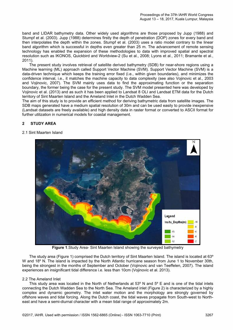
band and LIDAR bathymetry data. Other widely used algorithms are those proposed by Jupp (1988) and Stumpf et al. (2003). Jupp (1988) determines firstly the depth of penetration (DOP) zones for every band and then interpolates the depth within the zones. Stumpf et al. (2003) uses a ratio model contrary to the linear band algorithm which is successful in depths even greater than 25 m. The advancement of remote sensing technology has enabled the expansion of these methodologies to data with improved spatial and spectral resolution such as IKONOS, Quickbird and Worldview-2 (Su et al., 2008; Lyons et al., 2011; Bramante et al., 2011). The present study involves retrieval of satellite derived bathymetry (SDB) for near-shore regions using a Machine learning (ML) approach called Support Vector Machine (SVM). Support Vector Machine (SVM) is a data-driven technique which keeps the training error fixed (i.e., within given boundaries), and minimizes the confidence interval, i.e., it matches the machine capacity to data complexity (see also Vojinovic et al., 2003 and Vojinovic, 2007). The SVM mainly uses data to find the approximating function or the separation boundary, the former being the case for the present study. The SVM model presented here was developed by Vojinovic et al. (2013) and as such it has been applied to Landsat 8 OLI and Landsat ETM data for the Dutch territory of Sint Maarten Island and the Ameland Inlet in the Dutch Wadden Sea. The aim of this study is to provide an efficient method for deriving bathymetric data from satellite images. The SDB maps generated have a medium spatial resolution of 30m and can be used easily to provide inexpensive (Landsat datasets are freely available) and high density data in raster format or converted to ASCII format for further utilization in numerical models for coastal management. 2 STUDY AREA 2.1 Sint Maarten Island

Figure 1.Study Area- Sint Maarten Island showing the surveyed bathymetry

The study area (Figure 1) comprised the Dutch territory of Sint Maarten Island. The island is located at 63º W and 18º N. The island is impacted by the North Atlantic hurricane season from June 1 to November 30th, being the strongest in the months of September and October (Vojinovic and van Teeffelen, 2007). The island experiences an insignificant tidal difference i.e. less than 10cm (Vojinovic et al. 2013). 2.2 The Ameland Inlet This study area was located in the North of Netherlands at 53º N and 5º E and is one of the tidal inlets connecting the Dutch Wadden Sea to the North Sea. The Ameland inlet (Figure 2) is characterized by a highly complex and dynamic geometry. The inlet water motion and the morphology are strongly governed by offshore waves and tidal forcing. Along the Dutch coast, the tidal waves propagate from South-west to North-east and have a semi-diurnal character with a mean tidal range of approximately 2m.



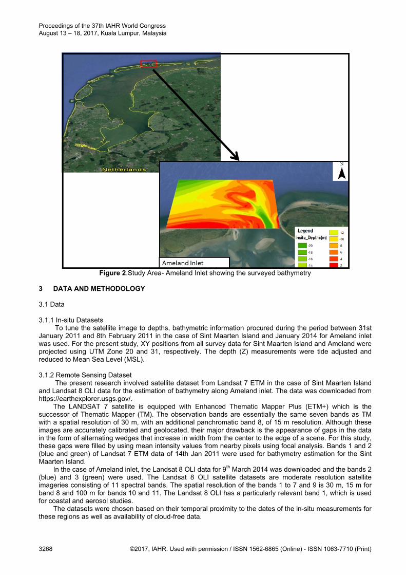
Figure 2.Study Area- Ameland Inlet showing the surveyed bathymetry

3 DATA AND METHODOLOGY 3.1 Data 3.1.1 In-situ Datasets To tune the satellite image to depths, bathymetric information procured during the period between 31st January 2011 and 8th February 2011 in the case of Sint Maarten Island and January 2014 for Ameland inlet was used. For the present study, XY positions from all survey data for Sint Maarten Island and Ameland were projected using UTM Zone 20 and 31, respectively. The depth (Z) measurements were tide adjusted and reduced to Mean Sea Level (MSL). 3.1.2 Remote Sensing Dataset The present research involved satellite dataset from Landsat 7 ETM in the case of Sint Maarten Island and Landsat 8 OLI data for the estimation of bathymetry along Ameland inlet. The data was downloaded from https://earthexplorer.usgs.gov/. The LANDSAT 7 satellite is equipped with Enhanced Thematic Mapper Plus (ETM+) which is the successor of Thematic Mapper (TM). The observation bands are essentially the same seven bands as TM with a spatial resolution of 30 m, with an additional panchromatic band 8, of 15 m resolution. Although these images are accurately calibrated and geolocated, their major drawback is the appearance of gaps in the data in the form of alternating wedges that increase in width from the center to the edge of a scene. For this study, these gaps were filled by using mean intensity values from nearby pixels using focal analysis. Bands 1 and 2 (blue and green) of Landsat 7 ETM data of 14th Jan 2011 were used for bathymetry estimation for the Sint Maarten Island. In the case of Ameland inlet, the Landsat 8 OLI data for 9th March 2014 was downloaded and the bands 2 (blue) and 3 (green) were used. The Landsat 8 OLI satellite datasets are moderate resolution satellite imageries consisting of 11 spectral bands. The spatial resolution of the bands 1 to 7 and 9 is 30 m, 15 m for band 8 and 100 m for bands 10 and 11. The Landsat 8 OLI has a particularly relevant band 1, which is used for coastal and aerosol studies. The datasets were chosen based on their temporal proximity to the dates of the in-situ measurements for these regions as well as availability of cloud-free data.



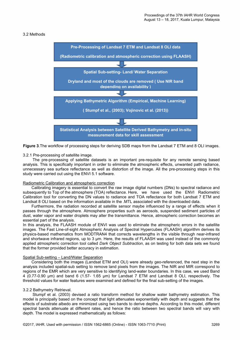
3.2 Methods Figure 3.The workflow of processing steps for deriving SDB maps from the Landsat 7 ETM and 8 OLI images.

3.2.1 Pre-processing of satellite image. The pre-processing of satellite datasets is an important pre-requisite for any remote sensing based analysis. This is specifically important in order to eliminate the atmospheric effects, unwanted path radiance, unnecessary sea surface reflectance as well as distortion of the image. All the pre-processing steps in this study were carried out using the ENVI 5.1 software. Radiometric Calibration and atmospheric correction Calibrating imagery is essential to convert the raw image digital numbers (DNs) to spectral radiance and subsequently to Top of the atmosphere (TOA) reflectance. Here, we have used the ENVI Radiometric Calibration tool for converting the DN values to radiance and TOA reflectance for both Landsat 7 ETM and Landsat 8 OLI based on the information available in the .MTL associated with the downloaded data. Furthermore, the radiation recorded at satellite sensor maybe influenced by a range of effects when it passes through the atmosphere. Atmosphere properties such as aerosols, suspended sediment particles of dust, water vapor and water droplets may alter the transmittance. Hence, atmospheric correction becomes an essential part of the analysis. In this analysis, the FLAASH module of ENVI was used to eliminate the atmospheric errors in the satellite images. The Fast Line-of-sight Atmospheric Analysis of Spectral Hypercubes (FLAASH) algorithm derives its physics-based mathematics from MODTRAN4 that corrects wavelengths in the visible through near-infrared and shortwave infrared regions, up to 3 µm. Here, the results of FLAASH was used instead of the commonly applied atmospheric correction tool called Dark Object Subtraction, as on testing for both data sets we found that the former provided better accuracy in estimation. Spatial Sub-setting – Land/Water Separation Considering both the images (Landsat ETM and OLI) were already geo-referenced, the next step in the analysis included spatial-sub setting to remove land pixels from the images. The NIR and MIR correspond to regions of the EMR which are very sensitive to identifying land-water boundaries. In this case, we used Band 4 (0.77-0.90 μm) and band 6 (1.57- 1.65 μm) for Landsat 7 ETM and Landsat 8 OLI, respectively. The threshold values for water features were examined and defined for the final sub-setting of the images. 3.2.2 Bathymetry Retrieval. Stumpf et al. (2003) devised a ratio transform method for shallow water bathymetry estimation. This model is principally based on the concept that light attenuates exponentially with depth and suggests that the effects of substrate albedo are minimized using two bands to derive depths. According to this model, different spectral bands attenuate at different rates, and hence the ratio between two spectral bands will vary with depth. The model is expressed mathematically as follows:

Pre-Processing of Landsat 7 ETM and Landsat 8 OLI data

(Radiometric calibration and atmospheric correction using FLAASH)

Spatial Sub-setting- Land/ Water Separation

Dryland and most of the clouds are removed ( Use NIR band depending on availability )

Applying Bathymetric Algorithm (Empirical, Machine Learning)

( Stumpf et al., (2003); Vojinovic et al. (2013))

Statistical Analysis between Satellite Derived Bathymetry and in-situ measurement data for skill assessment



- [1]

where,

Z is depth, is a tunable constant to scale the ratio to depth, Rw is observed reflectance in bands i and j, and is the offset.

Although, Stumpf et al. (2003) suggests a linear model, in practice the relationship between the ratio and the water depths may not always be linearly dependent. Hence, it is best captured by exploring a non-linear function (f) to map the bathymetry, further refining the equation as-

[2]

In this research, we aimed to establish this function using the data–driven machine learning approach Support Vector Machine (SVM). A Machine learning approach generally refers to an algorithm that estimates unknown values by mapping a system’s input and output using available data. The learning task applied here is based on regression, wherein the task involves prediction of real values associated with input data points. In case of the present study, the input is a ratio of the blue and green bands of the Landsat data as represented in equation 2. The following SVM model has been used in the present work –

[3] where, x denotes the external input i.e. the ratio between the blue and green bands and y represents the observed series (in-situ measurements). The SVM model used here performs learning by solving a Quadratic Programming problem and the code has been implemented using a combination of Borland Delphi and C programming languages (Vojinovic and Kecman, 2004). The regression used in SVM can be expressed using the following notation –

∑ ‖ ‖ ∑ , [4]

where,

represents the Vapnik’s ε- insensitivity loss function (Vapnik, 1998). In regression based SVM, the learning problem is pre-defined as the learning machine is given training data from which it attempts to learn the input-output relationship. The training vectors are mapped into a higher dimensional space by using a nonlinear kernel function. In this model, different kernel functions can be utilized, however, here we have used the Radial Basis Function (RBF) kernel which is expressed as follows:

, , 0[5]

where,

is the Gaussian function The other parameters that need to be selected during the learning process are the ‘shape’, i.e. the smoothing parameter in the kernel function (variance of the Gaussian RBF kernel), C i.e. the penalty parameter that determines the trade-off between the training error and the Vapnik-Chervonenkis dimension of the model and the insensitivity ε. For both the datasets, 80% of the data points were used for training and the remaining 20% data points were used for testing. Table 1 shows the statistics of the training and test datasets used for this study.



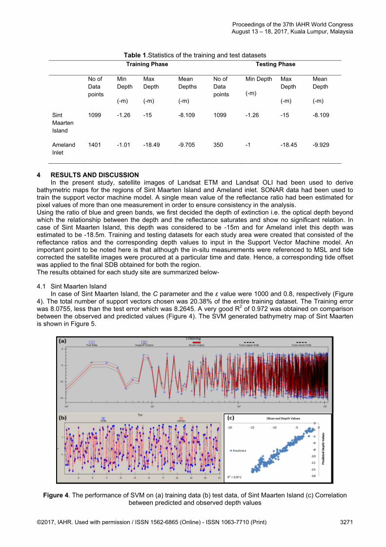
Table 1.Statistics of the training and test datasets

4 RESULTS AND DISCUSSION In the present study, satellite images of Landsat ETM and Landsat OLI had been used to derive bathymetric maps for the regions of Sint Maarten Island and Ameland inlet. SONAR data had been used to train the support vector machine model. A single mean value of the reflectance ratio had been estimated for pixel values of more than one measurement in order to ensure consistency in the analysis. Using the ratio of blue and green bands, we first decided the depth of extinction i.e. the optical depth beyond which the relationship between the depth and the reflectance saturates and show no significant relation. In case of Sint Maarten Island, this depth was considered to be -15m and for Ameland inlet this depth was estimated to be -18.5m. Training and testing datasets for each study area were created that consisted of the reflectance ratios and the corresponding depth values to input in the Support Vector Machine model. An important point to be noted here is that although the in-situ measurements were referenced to MSL and tide corrected the satellite images were procured at a particular time and date. Hence, a corresponding tide offset was applied to the final SDB obtained for both the region. The results obtained for each study site are summarized below- 4.1 Sint Maarten Island In case of Sint Maarten Island, the C parameter and the ε value were 1000 and 0.8, respectively (Figure 4). The total number of support vectors chosen was 20.38% of the entire training dataset. The Training error was 8.0755, less than the test error which was 8.2645. A very good R2 of 0.972 was obtained on comparison between the observed and predicted values (Figure 4). The SVM generated bathymetry map of Sint Maarten is shown in Figure 5.

Figure 4. The performance of SVM on (a) training data (b) test data, of Sint Maarten Island (c) Correlation between predicted and observed depth values

Training Phase Testing Phase

No of Data points

Min Depth

(-m)

Max Depth

(-m)

Mean Depths

(-m)

No of Data points

Min Depth

(-m)

Max Depth

(-m)

Mean Depth

(-m)

Sint Maarten Island

1099 -1.26 -15 -8.109 1099 -1.26 -15 -8.109

Ameland Inlet

1401 -1.01 -18.49 -9.705 350 -1 -18.45 -9.929



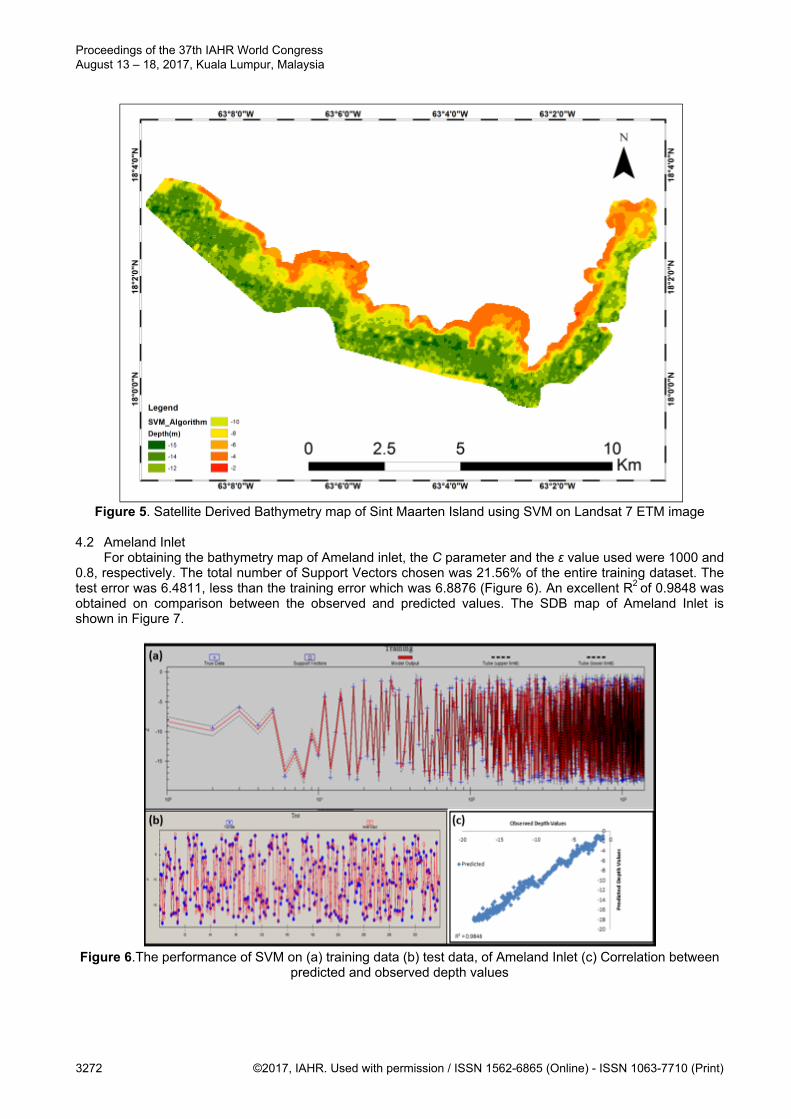
Figure 5. Satellite Derived Bathymetry map of Sint Maarten Island using SVM on Landsat 7 ETM image

4.2 Ameland Inlet For obtaining the bathymetry map of Ameland inlet, the C parameter and the ε value used were 1000 and 0.8, respectively. The total number of Support Vectors chosen was 21.56% of the entire training dataset. The test error was 6.4811, less than the training error which was 6.8876 (Figure 6). An excellent R2 of 0.9848 was obtained on comparison between the observed and predicted values. The SDB map of Ameland Inlet is shown in Figure 7.

Figure 6.The performance of SVM on (a) training data (b) test data, of Ameland Inlet (c) Correlation between

predicted and observed depth values



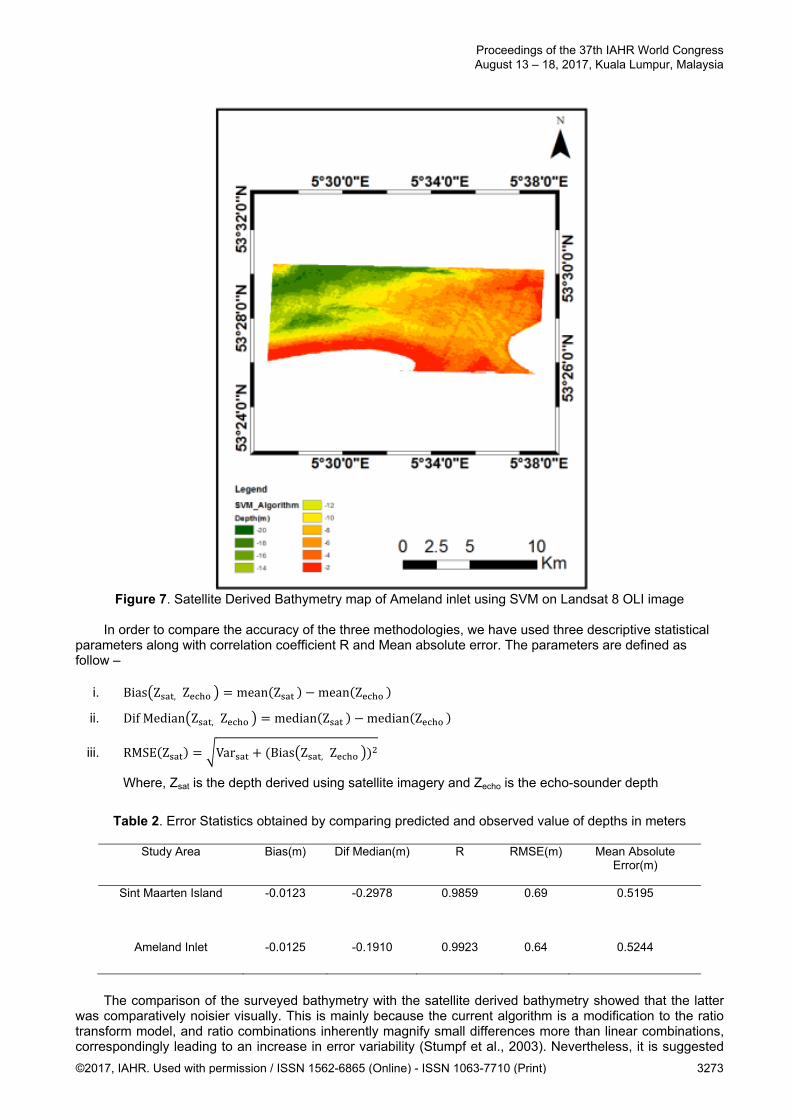
Figure 7. Satellite Derived Bathymetry map of Ameland inlet using SVM on Landsat 8 OLI image

In order to compare the accuracy of the three methodologies, we have used three descriptive statistical parameters along with correlation coefficient R and Mean absolute error. The parameters are defined as follow –

i. Bias Z ,Z mean Z mean Z

ii. DifMedian Z ,Z median Z median Z

iii. RMSE Z Var Bias Z ,Z

Where, Zsat is the depth derived using satellite imagery and Zecho is the echo-sounder depth

Table 2. Error Statistics obtained by comparing predicted and observed value of depths in meters

Study Area Bias(m) Dif Median(m) R RMSE(m) Mean Absolute

Error(m)

Sint Maarten Island -0.0123 -0.2978 0.9859 0.69 0.5195

Ameland Inlet -0.0125 -0.1910 0.9923 0.64 0.5244

The comparison of the surveyed bathymetry with the satellite derived bathymetry showed that the latter was comparatively noisier visually. This is mainly because the current algorithm is a modification to the ratio transform model, and ratio combinations inherently magnify small differences more than linear combinations, correspondingly leading to an increase in error variability (Stumpf et al., 2003). Nevertheless, it is suggested



by Stumpf et al. (2003) that ratio transform model is a more robust methodology than previously suggested methods, especially for turbid water and greater depth ranges. Hence, in the present study, a non-linear SVM approach was used for bathymetry estimation and it can be clearly inferred by the error statistics (Table 2) that the method performed well in the case of shallow water depths. 5 CONCLUSION In this study, we have proposed a machine learning approach to estimate shallow water depth values using Support Vector Machine (SVM). The model uses the reflectance ratios of blue and green bands of Landsat imageries as suggested by Stumpf et al. (2003). However, contrary to the latter model which uses a linear relationship, the SVM approach utilizes a non-linear approach to establish a relationship between the image pixel values and depths. The results obtained for both the study areas show strong capabilities of the SVM method for estimation of bathymetry for near-shore depths of approx. 15m, provided that clear satellite images (i.e. clear of clouds and turbidity) are available. The error statistics, especially the low RMSE values in case of both the regions clearly highlight the accuracy of these derived bathymetries. The further scope of this study will be to find solutions for derivation of bathymetry in the case of turbid areas, where multi-spectral imagery becomes limited. In this case, microwave remote sensing can be explored which uses the linear dispersion equation along with SAR data to estimate depths. ACKNOWLEDGEMENT The authors would like to thank Council of Scientific & Industrial Research –CSIR for providing the funding for Ms. Ankita Misra, who is CSIR-Senior Research Fellow (SRF) at Indian Institute of Technology-Bombay, Mumbai, India. This work has been carried out as a part of her doctoral research. RR is supported by the AXA Research fund and the Deltares Harbour, Coastal and Offshore engineering Research Programme'Bouwenaan de Kust'. REFERENCES Bramante, J. F., Raju, D. K. & Tsai Min, S. (2011). Derivation of Bathymetry from Multispectral Imagery in the

Highly Turbid Waters of Singapore’s South Islands: A Comparative Study. DigitalGlobe 8-Band Research Challenge 2010.

Conger, C. L., Hochberg, E. J., Fletcher, C. H. & Atkinson, M. J. (2006). Decorrelating Remote Sensing Color Bands from Bathymetry in Optically Shallow Waters. IEEE transactions on Geoscience and Remote Sensing, 44(6), 1655-1660.

Jupp, D. L. B. (1988). Background and Extensions to Depth of Penetration (DOP) Mapping in Shallow Coastal Waters. Proceedings of the Symposium on Remote Sensing of the Coastal Zone, IV-2.

Benny, A.H. & Dawson, G.J. (1983).Satellite Imagery as an Aid to Bathymetric Charting in the Red Sea. The Cartographic Journal, 20(1), 5-16.

Lyons, M., Phinn, S. & Roelfsema, C. (2011). Integrating Quickbird Multi-Spectral Satellite and Field Data: Mapping Bathymetry, Seagrasscover,Seagrass Species and Change in Moreton Bay, Australia in 2004 and 2007. Remote Sensing, 3(1), 42-64.

Lyzenga, D.R. & Polcyn, F.C. (1978). Analysis of Optimum Spectral Resolution and Band Location for Satellite Bathymetry. NASA Final Report on Contract, 7-35176.

Lyzenga, D.R. (1981). Remote Sensing of Bottom Reflectance and Water Attenuation Parameters in Shallow Water Using Aircraft and Landsat Data. International journal of remote sensing, 2(1), 71-82.

Lyzenga, D.R. (1985). Shallow-Water Bathymetry Using Combined Lidar and Passive Multispectral Scanner Data. International Journal of Remote Sensing, 6(1), 115-125.

Mynett, A.E. & Vojinovic, Z. (2009). Hydroinformatics in Multi-Colours—Part Red: Urban Flood and Disaster Management. Journal of Hydroinformatics, 11(3-4), 166-180.

Philpot, W.D. (1989). Bathymetric Mapping with Passive Multispectral imagery. Applied optics, 28(8), 1569-1578.

Ranasinghe, R. (2016). Assessing Climate Change Impacts on Open Sandy Coasts: A Review. Earth-Science Reviews, 160, 320-332.

Roelvink, J.A. & Reniers, A.J.H.M. (2011). A Guide to Coastal Morphology Modeling. Advances in Coastal and Ocean Engineering, 12.

Spitzer, D. & Dirks, R.J. (1986, November).Shallow water bathymetry and bottom classification by means of the Landsat and SPOT optical scanners.In 1986 International Symposium/Innsbruck (pp. 136-138).International Society for Optics and Photonics.

Spitzer, D. & Dirks, R. J. (1986, November). Shallow Water Bathymetry and Bottom Classification by Means of the Landsat and SPOT Optical Scanners. 1986 International Symposium/Innsbruck, 136-138.

Stumpf, R.P., Holderied, K. & Sinclair, M. (2003).Determination of Water Depth with High-Resolution Satellite Imagery over Variable Bottom Types. Limnology and Oceanography, 48(2), 547-556.

Su, H., Liu, H. & Heyman, W.D. (2008). Automated Derivation of Bathymetric Information from Multi-Spectral Satellite Imagery Using A Non-Linear Inversion Model. Marine Geodesy, 31(4), 281-298.



Vapnik, V.N. (1998). Statistical Learning Theory (Vol. 1). New York: Wiley. Vojinovic, Z., Kecman, V. &Babovic, V. (2003). Hybrid Approach for Modeling Wet Weather Response in

Wastewater Systems. Journal of Water Resources Planning and Management, 129(6), 511-521. Vojinovic, Z. & Kecman, V. (2004). Contaminant Transport Modelling with Support Vector Machine Model–An

Alternative to Classical Advection-Dispersion Equation. Hydroinformatics, 2, 1589-1596. Vojinovic, Z. (2007). A Complementary Modelling Approach to Manage Uncertainty of Computationally

Expensive Models. Water Science and Technology, 56(8), 1-9. Vojinovic, Z. & Van Teeffelen, J. (2007). An Integrated Stormwater Management Approach for Small Islands in

Tropical Climates. Urban Water Journal, 4(3), 211-231. Vojinovic, Z., Abebe, Y.A., Ranasinghe, R., Vacher, A., Martens, P., Mandl, D.J., Frye, S.W., Van Ettinger, E.

& de Zeeuw, R. (2013). A Machine Learning Approach for Estimation of Shallow Water Depths from Optical Satellite Images and Sonar Measurements. Journal of Hydroinformatics, 15(4), 1408-1424.

Vojinovic, Z. (2014). Flood Risk: The Holistic Perspective, From Integrated to Interactive Planning for Flood Resilience. London, UK: IWA Publishing



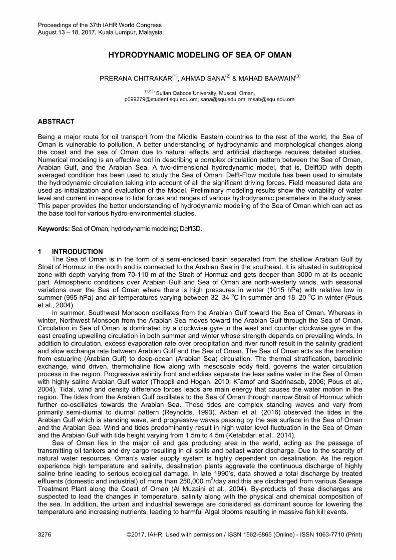
HYDRODYNAMIC MODELING OF SEA OF OMAN

PRERANA CHITRAKAR(1), AHMAD SANA(2) & MAHAD BAAWAIN(3)

(1,2,3) Sultan Qaboos University, Muscat, Oman, [email protected]; [email protected]; [email protected]

ABSTRACT Being a major route for oil transport from the Middle Eastern countries to the rest of the world, the Sea of Oman is vulnerable to pollution. A better understanding of hydrodynamic and morphological changes along the coast and the sea of Oman due to natural effects and artificial discharge requires detailed studies. Numerical modeling is an effective tool in describing a complex circulation pattern between the Sea of Oman, Arabian Gulf, and the Arabian Sea. A two-dimensional hydrodynamic model, that is, Delft3D with depth averaged condition has been used to study the Sea of Oman. Delft-Flow module has been used to simulate the hydrodynamic circulation taking into account of all the significant driving forces. Field measured data are used as initialization and evaluation of the Model. Preliminary modeling results show the variability of water level and current in response to tidal forces and ranges of various hydrodynamic parameters in the study area. This paper provides the better understanding of hydrodynamic modeling of the Sea of Oman which can act as the base tool for various hydro-environmental studies. Keywords: Sea of Oman; hydrodynamic modeling; Delft3D. 1 INTRODUCTION

The Sea of Oman is in the form of a semi-enclosed basin separated from the shallow Arabian Gulf by Strait of Hormuz in the north and is connected to the Arabian Sea in the southeast. It is situated in subtropical zone with depth varying from 70-110 m at the Strait of Hormuz and gets deeper than 3000 m at its oceanic part. Atmospheric conditions over Arabian Gulf and Sea of Oman are north-westerly winds, with seasonal variations over the Sea of Oman where there is high pressures in winter (1015 hPa) with relative low in summer (995 hPa) and air temperatures varying between 32–34 oC in summer and 18–20 oC in winter (Pous et al., 2004).

In summer, Southwest Monsoon oscillates from the Arabian Gulf toward the Sea of Oman. Whereas in winter, Northwest Monsoon from the Arabian Sea moves toward the Arabian Gulf through the Sea of Oman. Circulation in Sea of Oman is dominated by a clockwise gyre in the west and counter clockwise gyre in the east creating upwelling circulation in both summer and winter whose strength depends on prevailing winds. In addition to circulation, excess evaporation rate over precipitation and river runoff result in the salinity gradient and slow exchange rate between Arabian Gulf and the Sea of Oman. The Sea of Oman acts as the transition from estuarine (Arabian Gulf) to deep-ocean (Arabian Sea) circulation. The thermal stratification, baroclinic exchange, wind driven, thermohaline flow along with mesoscale eddy field, governs the water circulation process in the region. Progressive salinity front and eddies separate the less saline water in the Sea of Oman with highly saline Arabian Gulf water (Thoppil and Hogan, 2010; K¨ampf and Sadrinasab, 2006; Pous et al., 2004). Tidal, wind and density difference forces leads are main energy that causes the water motion in the region. The tides from the Arabian Gulf oscillates to the Sea of Oman through narrow Strait of Hormuz which further co-oscillates towards the Arabian Sea. Those tides are complex standing waves and vary from primarily semi-diurnal to diurnal pattern (Reynolds, 1993). Akbari et al. (2016) observed the tides in the Arabian Gulf which is standing wave, and progressive waves passing by the sea surface in the Sea of Oman and the Arabian Sea. Wind and tides predominantly result in high water level fluctuation in the Sea of Oman and the Arabian Gulf with tide height varying from 1.5m to 4.5m (Ketabdari et al., 2014).

Sea of Oman lies in the major oil and gas producing area in the world, acting as the passage of transmitting oil tankers and dry cargo resulting in oil spills and ballast water discharge. Due to the scarcity of natural water resources, Oman’s water supply system is highly dependent on desalination. As the region experience high temperature and salinity, desalination plants aggravate the continuous discharge of highly saline brine leading to serious ecological damage. In late 1990’s, data showed a total discharge by treated effluents (domestic and industrial) of more than 250,000 m3/day and this are discharged from various Sewage Treatment Plant along the Coast of Oman (Al Muzaini et al., 2004). By-products of these discharges are suspected to lead the changes in temperature, salinity along with the physical and chemical composition of the sea. In addition, the urban and industrial sewerage are considered as dominant source for lowering the temperature and increasing nutrients, leading to harmful Algal blooms resulting in massive fish kill events.



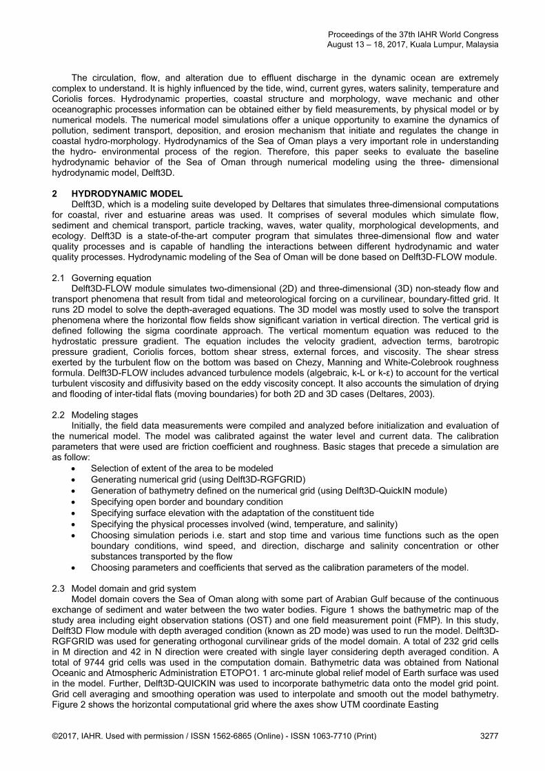
The circulation, flow, and alteration due to effluent discharge in the dynamic ocean are extremely complex to understand. It is highly influenced by the tide, wind, current gyres, waters salinity, temperature and Coriolis forces. Hydrodynamic properties, coastal structure and morphology, wave mechanic and other oceanographic processes information can be obtained either by field measurements, by physical model or by numerical models. The numerical model simulations offer a unique opportunity to examine the dynamics of pollution, sediment transport, deposition, and erosion mechanism that initiate and regulates the change in coastal hydro-morphology. Hydrodynamics of the Sea of Oman plays a very important role in understanding the hydro- environmental process of the region. Therefore, this paper seeks to evaluate the baseline hydrodynamic behavior of the Sea of Oman through numerical modeling using the three- dimensional hydrodynamic model, Delft3D. 2 HYDRODYNAMIC MODEL

Delft3D, which is a modeling suite developed by Deltares that simulates three-dimensional computations for coastal, river and estuarine areas was used. It comprises of several modules which simulate flow, sediment and chemical transport, particle tracking, waves, water quality, morphological developments, and ecology. Delft3D is a state-of-the-art computer program that simulates three-dimensional flow and water quality processes and is capable of handling the interactions between different hydrodynamic and water quality processes. Hydrodynamic modeling of the Sea of Oman will be done based on Delft3D-FLOW module. 2.1 Governing equation

Delft3D-FLOW module simulates two-dimensional (2D) and three-dimensional (3D) non-steady flow and transport phenomena that result from tidal and meteorological forcing on a curvilinear, boundary-fitted grid. It runs 2D model to solve the depth-averaged equations. The 3D model was mostly used to solve the transport phenomena where the horizontal flow fields show significant variation in vertical direction. The vertical grid is defined following the sigma coordinate approach. The vertical momentum equation was reduced to the hydrostatic pressure gradient. The equation includes the velocity gradient, advection terms, barotropic pressure gradient, Coriolis forces, bottom shear stress, external forces, and viscosity. The shear stress exerted by the turbulent flow on the bottom was based on Chezy, Manning and White-Colebrook roughness formula. Delft3D-FLOW includes advanced turbulence models (algebraic, k-L or k-ε) to account for the vertical turbulent viscosity and diffusivity based on the eddy viscosity concept. It also accounts the simulation of drying and flooding of inter-tidal flats (moving boundaries) for both 2D and 3D cases (Deltares, 2003). 2.2 Modeling stages

Initially, the field data measurements were compiled and analyzed before initialization and evaluation of the numerical model. The model was calibrated against the water level and current data. The calibration parameters that were used are friction coefficient and roughness. Basic stages that precede a simulation are as follow:

Selection of extent of the area to be modeled Generating numerical grid (using Delft3D-RGFGRID) Generation of bathymetry defined on the numerical grid (using Delft3D-QuickIN module) Specifying open border and boundary condition Specifying surface elevation with the adaptation of the constituent tide Specifying the physical processes involved (wind, temperature, and salinity) Choosing simulation periods i.e. start and stop time and various time functions such as the open

boundary conditions, wind speed, and direction, discharge and salinity concentration or other substances transported by the flow

Choosing parameters and coefficients that served as the calibration parameters of the model.

2.3 Model domain and grid system Model domain covers the Sea of Oman along with some part of Arabian Gulf because of the continuous

exchange of sediment and water between the two water bodies. Figure 1 shows the bathymetric map of the study area including eight observation stations (OST) and one field measurement point (FMP). In this study, Delft3D Flow module with depth averaged condition (known as 2D mode) was used to run the model. Delft3D-RGFGRID was used for generating orthogonal curvilinear grids of the model domain. A total of 232 grid cells in M direction and 42 in N direction were created with single layer considering depth averaged condition. A total of 9744 grid cells was used in the computation domain. Bathymetric data was obtained from National Oceanic and Atmospheric Administration ETOPO1. 1 arc-minute global relief model of Earth surface was used in the model. Further, Delft3D-QUICKIN was used to incorporate bathymetric data onto the model grid point. Grid cell averaging and smoothing operation was used to interpolate and smooth out the model bathymetry. Figure 2 shows the horizontal computational grid where the axes show UTM coordinate Easting



on the horizontal axis and Northing on the vertical axis. The model incorporates the temperature and salinity which influences the water density in the hydrodynamic simulation processes. Initially, uniform distribution of water temperature (20 oC) and salinity (35 ppt.) was used. Figure 1. Bathymetric map of study area featuring the observation stations and field measurement point using

Google Earth (map data: ©Google, Data SIO, NOAA, U.S. Navy, NGA, GEBCO, Image Landsat).

Figure 2. Model grid used in the computations. Bottom roughness was calculated using Manning’s coefficient with the roughness value of 0.024 m-1/3s. Constant horizontal eddy viscosity at 2 m2/s and constant horizontal eddy diffusivity at 10 m2/s were used. The model was used to simulate 10 days of data at a 5-minute time-interval. Two open boundaries were situated at the west and east end of the model. Physical parameter was used in calibration processes and was uniform throughout the model. Computation parameters used to simulate the model after calibration are summarized in Table 1.



Table 1. Computed Parameter used in Simulation of Mode. PARAMETER VALUE

Simulation Period December 2 to December 11, 2006 Grid (m X n) 232 X 42

Bathymetry National Oceanic and Atmospheric Administration ETOPO1, 1arc-minute global relief model of Earth surface

Time Step 5 minutes Open Boundaries 2 (East and West of the Model) Bottom Roughness Formula Manning Bottom Roughness Value 0.024 m-1/3s Horizontal eddy viscosity 2 m2/s Horizontal eddy diffusivity 10m2/s

Astronomic tidal force was induced as the tidal boundary at the ends of open boundaries. Five tidal

constitutes A0, M2, S2, K1, and O1 are considered with reference to Admiralty Tide Table (Admiralty, 2002). Amplitudes and phases of two diurnal tidal components K1 and O1 and two semidiurnal tidal components M2 and S2 were imposed at the each node of open boundaries. Table 2 shows the major tidal constitutes (amplitude and phase per constituent) used at the open boundary stations.

Table 2. Amplitude (m) and phase (°) of major tidal constituent at open boundary.

STATION LATITUDE

(N) LONGITUDE

(E) A0

(m) M2 S2 K1 O1

(Θ) (H) (Θ) (H) (Θ) (H) (Θ) (H)Jazireh-ye-Forur 26 ̊ 15′ 54 ̊ 31′ 1.07 357 0.42 042 0.14 134 0.35 096 0.2 Ras Tang 25 ̊ 21′ 59 ̊ 54′ 1.9 258 0.65 292 0.25 028 0.4 032 0.2 Ras Zubayyah 24 ̊ 15′ 53 ̊ 49′ 1.28 045 0.37 103 0.15 180 0.3 137 0.19 Bimmah 22 ̊ 59′ 59 ̊ 10′ 1.84 273 0.63 310 0.24 042 0.39 037 0.20 2.4 Results and discussions

A number of observation stations were selected in the model domain to illustrate hydrodynamic of the model. The observation station locations are listed in Table 3. In the Sea of Oman and the Arabian Gulf, the field measured hydrodynamic data were limited and asymmetric. In this study, the simulated water level data at various stations were compared with the water level predicted by the Tide Wizard Software based on Admiralty tidal elevation chart. Simulated flow velocity was compared with the current data at Wudam Station (23°49′31.64′′N, 57°32′44.75′′E) measured using an Acoustic Doppler Current Profile, deployed for days from December 4, 2006 to December 8, 2006.

Table 3. Location of Observation Stations and Field Measurement Point. STATION NAME EASTING NORTHING LOCATION OST1/ FMP 57 ̊ 32′ 23 ̊ 49′ Wudam

OST2 56 ̊ 39′ 24 ̊ 29′ Majis - Sohar OST3 56 ̊ 21′ 25 ̊ 10′ Fujayrah OST4 55 ̊ 03′ 25 ̊ 00′ Mina Jebel Ali OST5 58 ̊ 50′ 25 ̊ 32′ Koskar OST6 57 ̊ 05′ 26 ̊ 31′ Bandar-e Sirik OST7 54 ̊ 53′ 26 ̊ 33′ Bandar-e Lengeh OST8 55 ̊ 18′ 25 ̊ 32′ Jazireh-ye Tonb-e Bozorg

Figure 3 shows the computed and observed water level at Stations 1, 3, 4 and 5. For all other stations,

though the model, it had over and under predicted the elevation. The same trend of fluctuation during waxing and waning was reproduced in all stations. The difference between simulated and observed time series was analyzed by relative error calculation. Observation station 3 shows good agreement between simulated and observed water level with a less relative error of 0.79%. Where else, the observation of station 1, 4 and 5 shows the relative error of 1.67%, 2.57%, and 1.7% respectively. The station at the middle of the study area shows better match and less error between computed and observed result as compared to the stations closer to the edge or boundary of the model. All the stations in the study area predominantly showed the tides of the mixed semidiurnal pattern. In this study, only five tidal constitutes were forced at the open boundaries. However, applying more tidal components in addition to A0, M2, S2, K1, and O1 and wind induced water levels can improvise the model output.



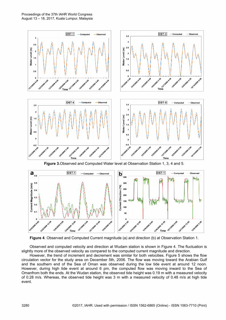
Figure 3.Observed and Computed Water level at Observation Station 1, 3, 4 and 5.

Figure 4. Observed and Computed Current magnitude (a) and direction (b) at Observation Station 1.

Observed and computed velocity and direction at Wudam station is shown in Figure 4. The fluctuation is slightly more of the observed velocity as compared to the computed current magnitude and direction.

However, the trend of increment and decrement was similar for both velocities. Figure 5 shows the flow circulation vector for the study area on December 5th, 2006. The flow was moving toward the Arabian Gulf and the southern end of the Sea of Oman was observed during the low tide event at around 12 noon. However, during high tide event at around 6 pm, the computed flow was moving inward to the Sea of Omanfrom both the ends. At the Wudan station, the observed tide height was 0.19 m with a measured velocity of 0.28 m/s. Whereas, the observed tide height was 3 m with a measured velocity of 0.48 m/s at high tide event.



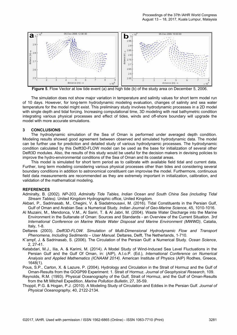
Figure 5. Flow Vector at low tide event (a) and high tide (b) of the study area on December 5, 2006.

The simulation does not show major variation in temperature and salinity values for short term model run of 10 days. However, for long-term hydrodynamic modeling evaluation, changes of salinity and sea water temperature for the model might exist. This preliminary study involves hydrodynamic processes in a 2D model with single depth and tidal forcing. Increasing computational time, 3D modeling with real bathymetric condition integrating various physical processes and effect of tides, winds and off-shore boundary will upgrade the model with more accurate simulations. 3 CONCLUSIONS

The hydrodynamic simulation of the Sea of Oman is performed under averaged depth condition. Modeling results showed good agreement between observed and simulated hydrodynamic data. The model can be further use for prediction and detailed study of various hydrodynamic processes. The hydrodynamic condition calculated by this Delft3D-FLOW model can be used as the base for initialization of several other Delft3D modules. Also, the results of this study would be useful for the decision makers in devising policies to improve the hydro-environmental conditions of the Sea of Oman and its coastal areas.

This model is simulated for short term period as to calibrate with available field tidal and current data. Further, long term modeling considering various physical processes other than tides and considering several boundary conditions in addition to astronomical constituent can improvise the model. Furthermore, continuous field data measurements are recommended as they are extremely important in initialization, calibration, and validation of the mathematical modeling. REFERENCES Admiralty, B. (2002). NP-203, Admiralty Tide Tables, Indian Ocean and South China Sea (including Tidal

Stream Tables). United Kingdom Hydrographic office, United Kingdom. Akbari, P., Sadrinasab, M., Chegini, V. & Siadatmousavi, M. (2016). Tidal Constituents in the Persian Gulf,

Gulf of Oman and Arabian Sea: a Numerical Study. Indian Journal of Geo-Marine Science, 45, 1010-1016. Al Muzaini, M., Mendonca, V.M., Al Sariri, T. & Al Jabri, M. (2004). Waste Water Discharge into the Marine

Environment in the Sultanate of Oman: Sources and Standards - an Overview of the Current Situation. 3rd International Conference on Marine Waste Water Disposal and Marine Environment (MWWD), Catalia, Italy, 1-8.

Deltares (2003). Delft3D-FLOW. Simulation of Multi-Dimensional Hydrodynamic Flow and Transport Phenomena, Including Sediments – User Manual. Deltares, Delft, The Netherlands, 1-710.

K¨ampf, J. & Sadrinasab, S. (2006). The Circulation of the Persian Gulf: a Numerical Study. Ocean Science, 2, 27-41.

Ketabdari, M.J., Ilia, A. & Karimi, M. (2014). A Model Study of Wind-Induced Sea Level Fluctuations in the Persian Gulf and the Gulf Of Oman, in: (AIP), A.I.o.P. (Ed.), International Conference on Numerical Analysis and Applied Mathematics (ICNAAM 2014). American Institute of Physics (AIP) Rodhes, Greece, 1648(1).

Pous, S.P., Carton, X. & Lazure, P. (2004). Hydrology and Circulation in the Strait of Hormuz and the Gulf of Oman-Results from the GOGP99 Experiment: 1. Strait of Hormuz. Journal of Geophysical Research, 109.

Reynolds, R.M. (1993). Physical Oceanography of the Gulf, Strait of Hormuz, and the Gulf of Oman-Results from the Mt Mitchell Expedition. Marine Pollution Bulletin, 27, 35-59.

Thoppil, P.G. & Hogan, P.J. (2010). A Modeling Study of Circulation and Eddies in the Persian Gulf. Journal of Physical Oceanography, 40, 2122-2134.



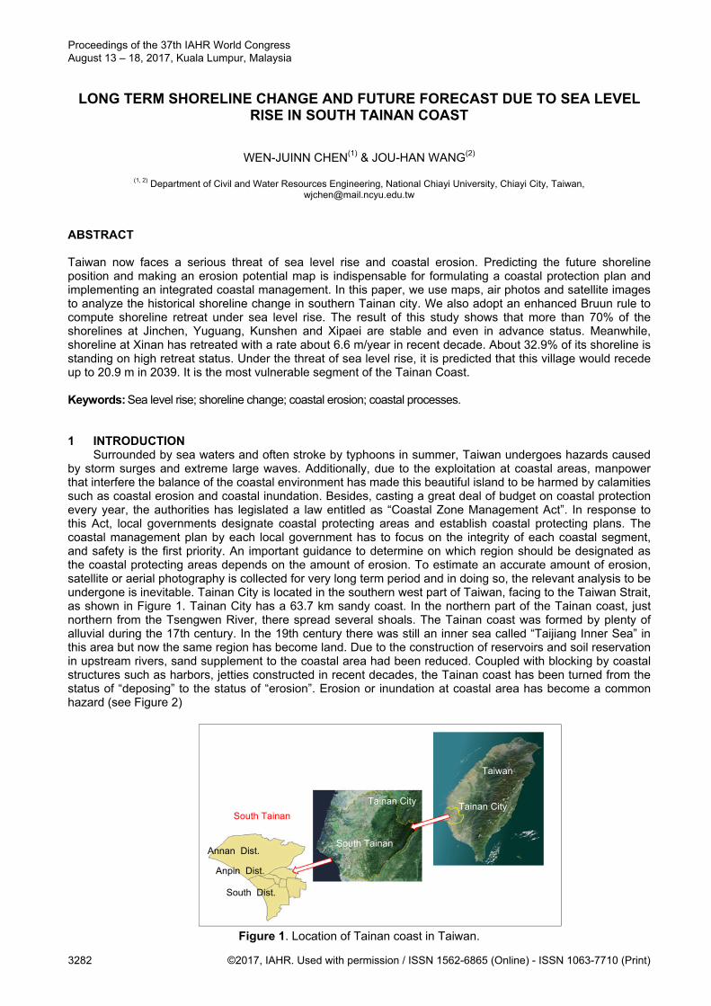
LONG TERM SHORELINE CHANGE AND FUTURE FORECAST DUE TO SEA LEVEL

RISE IN SOUTH TAINAN COAST

WEN-JUINN CHEN(1) & JOU-HAN WANG(2)

(1, 2) Department of Civil and Water Resources Engineering, National Chiayi University, Chiayi City, Taiwan, [email protected]

ABSTRACT Taiwan now faces a serious threat of sea level rise and coastal erosion. Predicting the future shoreline position and making an erosion potential map is indispensable for formulating a coastal protection plan and implementing an integrated coastal management. In this paper, we use maps, air photos and satellite images to analyze the historical shoreline change in southern Tainan city. We also adopt an enhanced Bruun rule to compute shoreline retreat under sea level rise. The result of this study shows that more than 70% of the shorelines at Jinchen, Yuguang, Kunshen and Xipaei are stable and even in advance status. Meanwhile, shoreline at Xinan has retreated with a rate about 6.6 m/year in recent decade. About 32.9% of its shoreline is standing on high retreat status. Under the threat of sea level rise, it is predicted that this village would recede up to 20.9 m in 2039. It is the most vulnerable segment of the Tainan Coast.

Keywords: Sea level rise; shoreline change; coastal erosion; coastal processes.

1 INTRODUCTION Surrounded by sea waters and often stroke by typhoons in summer, Taiwan undergoes hazards caused

by storm surges and extreme large waves. Additionally, due to the exploitation at coastal areas, manpower that interfere the balance of the coastal environment has made this beautiful island to be harmed by calamities such as coastal erosion and coastal inundation. Besides, casting a great deal of budget on coastal protection every year, the authorities has legislated a law entitled as “Coastal Zone Management Act”. In response to this Act, local governments designate coastal protecting areas and establish coastal protecting plans. The coastal management plan by each local government has to focus on the integrity of each coastal segment, and safety is the first priority. An important guidance to determine on which region should be designated as the coastal protecting areas depends on the amount of erosion. To estimate an accurate amount of erosion, satellite or aerial photography is collected for very long term period and in doing so, the relevant analysis to be undergone is inevitable. Tainan City is located in the southern west part of Taiwan, facing to the Taiwan Strait, as shown in Figure 1. Tainan City has a 63.7 km sandy coast. In the northern part of the Tainan coast, just northern from the Tsengwen River, there spread several shoals. The Tainan coast was formed by plenty of alluvial during the 17th century. In the 19th century there was still an inner sea called “Taijiang Inner Sea” in this area but now the same region has become land. Due to the construction of reservoirs and soil reservation in upstream rivers, sand supplement to the coastal area had been reduced. Coupled with blocking by coastal structures such as harbors, jetties constructed in recent decades, the Tainan coast has been turned from the status of “deposing” to the status of “erosion”. Erosion or inundation at coastal area has become a common hazard (see Figure 2)

Figure 1. Location of Tainan coast in Taiwan.

Taiwan

Tainan City Tainan City

South Tainan

South Tainan

Annan Dist.

Anpin Dist.

South Dist.



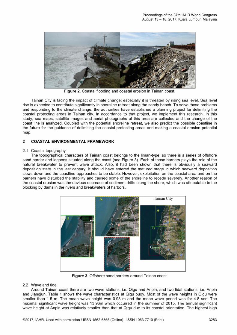
Figure 2. Coastal flooding and coastal erosion in Tainan coast.

Tainan City is facing the impact of climate change; especially it is threaten by rising sea level. Sea level

rise is expected to contribute significantly in shoreline retreat along the sandy beach. To solve those problems and responding to the climate change, the authorities have established a planning project for delimiting the coastal protecting areas in Tainan city. In accordance to that project, we implement this research. In this study, sea maps, satellite images and aerial photographs of this area are collected and the change of the coast line is analyzed. Coupled with the potential shoreline retreat, we also predict the possible coastline in the future for the guidance of delimiting the coastal protecting areas and making a coastal erosion potential map.

2 COASTAL ENVIRONMENTAL FRAMEWORK

2.1 Coastal topography

The topographical characters of Tainan coast belongs to the liman-type, so there is a series of offshore sand barrier and lagoons situated along the coast (see Figure 3). Each of those barriers plays the role of the natural breakwater to prevent wave attack. Also, it had been shown that there is obviously a seaward deposition state in the last century. It should have entered the matured stage in which seaward deposition slows down and the coastline approaches to be stable. However, exploitation on the coastal area and on the barriers have disturbed the stability and caused some of the shoreline to recede severely. Another reason of the coastal erosion was the obvious decrease of sediment drifts along the shore, which was attributable to the blocking by dams in the rivers and breakwaters of harbors.

Figure 3. Offshore sand barriers around Tainan coast. 2.2 Wave and tide

Around Tainan coast there are two wave stations, i.e. Qigu and Anpin, and two tidal stations, i.e. Anpin and Jiangjun. Table 1 shows the wave characteristics at Qigu buoy. Most of the wave heights in Qigu were smaller than 1.5 m. The mean wave height was 0.93 m and the mean wave period was for 4.8 sec. The maximal significant wave height was 13.96m which occurred in the summer of 2015. The annual significant wave height at Anpin was relatively smaller than that at Qigu due to its coastal orientation. The highest high

Tainan City

A

A

B

C C

B



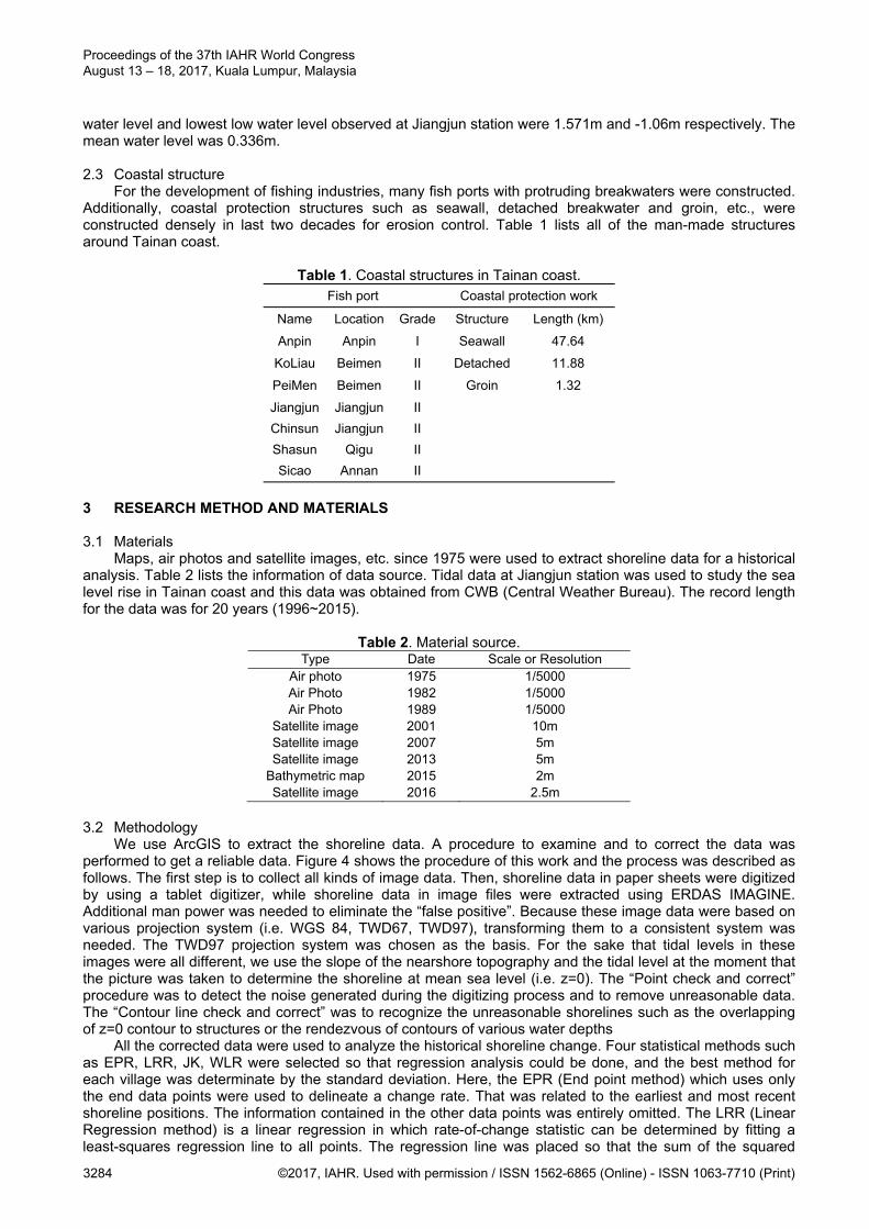
water level and lowest low water level observed at Jiangjun station were 1.571m and -1.06m respectively. The mean water level was 0.336m.

2.3 Coastal structure

For the development of fishing industries, many fish ports with protruding breakwaters were constructed. Additionally, coastal protection structures such as seawall, detached breakwater and groin, etc., were constructed densely in last two decades for erosion control. Table 1 lists all of the man-made structures around Tainan coast.

Table 1. Coastal structures in Tainan coast.

Fish port Coastal protection work

Name Location Grade Structure Length (km)

Anpin Anpin I Seawall 47.64

KoLiau Beimen II Detached 11.88

PeiMen Beimen II Groin 1.32

Jiangjun Jiangjun II

Chinsun Jiangjun II

Shasun Qigu II

Sicao Annan II

3 RESEARCH METHOD AND MATERIALS 3.1 Materials

Maps, air photos and satellite images, etc. since 1975 were used to extract shoreline data for a historical analysis. Table 2 lists the information of data source. Tidal data at Jiangjun station was used to study the sea level rise in Tainan coast and this data was obtained from CWB (Central Weather Bureau). The record length for the data was for 20 years (1996~2015).

Table 2. Material source.

Type Date Scale or Resolution Air photo 1975 1/5000 Air Photo 1982 1/5000 Air Photo 1989 1/5000

Satellite image 2001 10m Satellite image 2007 5m Satellite image 2013 5m

Bathymetric map 2015 2m Satellite image 2016 2.5m

3.2 Methodology

We use ArcGIS to extract the shoreline data. A procedure to examine and to correct the data was performed to get a reliable data. Figure 4 shows the procedure of this work and the process was described as follows. The first step is to collect all kinds of image data. Then, shoreline data in paper sheets were digitized by using a tablet digitizer, while shoreline data in image files were extracted using ERDAS IMAGINE. Additional man power was needed to eliminate the “false positive”. Because these image data were based on various projection system (i.e. WGS 84, TWD67, TWD97), transforming them to a consistent system was needed. The TWD97 projection system was chosen as the basis. For the sake that tidal levels in these images were all different, we use the slope of the nearshore topography and the tidal level at the moment that the picture was taken to determine the shoreline at mean sea level (i.e. z=0). The “Point check and correct” procedure was to detect the noise generated during the digitizing process and to remove unreasonable data. The “Contour line check and correct” was to recognize the unreasonable shorelines such as the overlapping of z=0 contour to structures or the rendezvous of contours of various water depths

All the corrected data were used to analyze the historical shoreline change. Four statistical methods such as EPR, LRR, JK, WLR were selected so that regression analysis could be done, and the best method for each village was determinate by the standard deviation. Here, the EPR (End point method) which uses only the end data points were used to delineate a change rate. That was related to the earliest and most recent shoreline positions. The information contained in the other data points was entirely omitted. The LRR (Linear Regression method) is a linear regression in which rate-of-change statistic can be determined by fitting a least-squares regression line to all points. The regression line was placed so that the sum of the squared



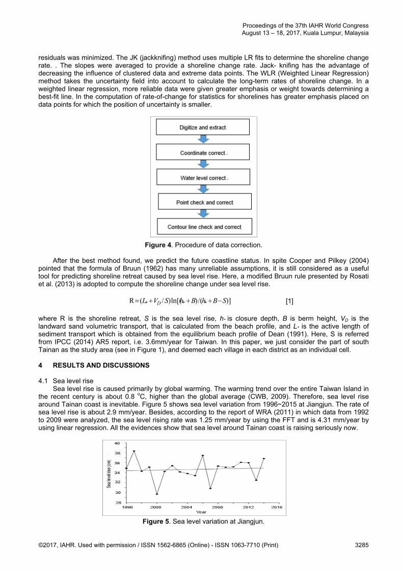
residuals was minimized. The JK (jackknifing) method uses multiple LR fits to determine the shoreline change rate. . The slopes were averaged to provide a shoreline change rate. Jack- knifing has the advantage of decreasing the influence of clustered data and extreme data points. The WLR (Weighted Linear Regression) method takes the uncertainty field into account to calculate the long-term rates of shoreline change. In a weighted linear regression, more reliable data were given greater emphasis or weight towards determining a best-fit line. In the computation of rate-of-change for statistics for shorelines has greater emphasis placed on data points for which the position of uncertainty is smaller.

Figure 4. Procedure of data correction.

After the best method found, we predict the future coastline status. In spite Cooper and Pilkey (2004)

pointed that the formula of Bruun (1962) has many unreliable assumptions, it is still considered as a useful tool for predicting shoreline retreat caused by sea level rise. Here, a modified Bruun rule presented by Rosati et al. (2013) is adopted to compute the shoreline change under sea level rise.

)]/()ln[()/(R *** SBhBhSVL D [1]

where R is the shoreline retreat, S is the sea level rise, h* is closure depth, B is berm height, VD is the landward sand volumetric transport, that is calculated from the beach profile, and L* is the active length of sediment transport which is obtained from the equilibrium beach profile of Dean (1991). Here, S is referred from IPCC (2014) AR5 report, i.e. 3.6mm/year for Taiwan. In this paper, we just consider the part of south Tainan as the study area (see in Figure 1), and deemed each village in each district as an individual cell. 4 RESULTS AND DISCUSSIONS 4.1 Sea level rise

Sea level rise is caused primarily by global warming. The warming trend over the entire Taiwan Island in the recent century is about 0.8 oC, higher than the global average (CWB, 2009). Therefore, sea level rise around Tainan coast is inevitable. Figure 5 shows sea level variation from 1996~2015 at Jiangjun. The rate of sea level rise is about 2.9 mm/year. Besides, according to the report of WRA (2011) in which data from 1992 to 2009 were analyzed, the sea level rising rate was 1.25 mm/year by using the FFT and is 4.31 mm/year by using linear regression. All the evidences show that sea level around Tainan coast is raising seriously now.

Figure 5. Sea level variation at Jiangjun.



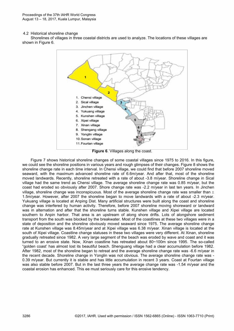
4.2 Historical shoreline change Shorelines of villages in three coastal districts are used to analyze. The locations of these villages are

shown in Figure 6.

Figure 6. Villages along the coast.

Figure 7 shows historical shoreline changes of some coastal villages since 1975 to 2016. In this figure, we could see the shoreline positions in various years and rough glimpses of their changes. Figure 8 shows the shoreline change rate in each time interval. In Chensi village, we could find that before 2007 shoreline moved seaward, with the maximum advanced shoreline rate of 6.6m/year. And after that, most of the shoreline moved landwards. Recently, shoreline retreated with a rate of about -3.8 m/year. Shoreline change in Sical village had the same trend as Chensi village. The average shoreline change rate was 0.85 m/year, but the coast had eroded so obviously after 2007. Shore change rate was -2.2 m/year in last ten years. In Jinchen village, shoreline change was inconspicuous. Most of the average shoreline change rate was smaller than 1.5m/year. However, after 2007 the shoreline began to move landwards with a rate of about -2.3 m/year. Yukuang village is located at Anping Dist. Many artificial structures were built along the coast and shoreline change was interfered by human activity. Therefore, before 2007 shoreline moving shoreward or landward was in alternation and after that the shoreline turns stable. Kunshen village and Xipei village are located southern to Anpin harbor. That area is an upstream of along shore drifts. Lots of alongshore sediment transport from the south was blocked by the breakwater. Most of the coastlines at these two villages were in a state of deposition and the shoreline obviously moved seaward since 1975. The average shoreline change rate at Kunshen village was 8.45m/year and at Xipei village was 6.38 m/year. Xinan village is located at the south of Xipei village. Coastline change statuses in these two villages were very different. At Xinan, shoreline gradually retreated since 1982. A very large segment of the beach was eroded by wave and coast and it was turned to an erosive state. Now, Xinan coastline has retreated about 80~100m since 1995. The so-called “golden coast’ has almost lost its beautiful beach. Shenguang village had a clear accumulation before 1982. After 1982, most of the shoreline began to retreat and the average shoreline change rate was -6.6 m/year in the recent decade. Shoreline change in Yonglin was not obvious. The average shoreline change rate was -0.39 m/year. But currently it is stable and has little accumulation in recent 3 years. Coast at Fourtan village was also stable before 2007. But in the last three years the average change rate was -1.54 m/year and the coastal erosion has enhanced. This ee must seriously care for this erosive tendency.



Figure 7. Historical shoreline changes.

Figure 8. Shoreline change rate at each village.



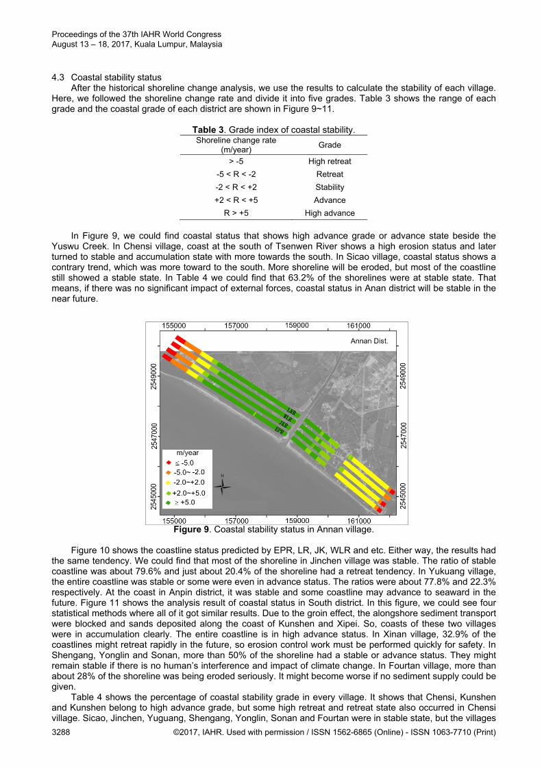
4.3 Coastal stability status After the historical shoreline change analysis, we use the results to calculate the stability of each village.

Here, we followed the shoreline change rate and divide it into five grades. Table 3 shows the range of each grade and the coastal grade of each district are shown in Figure 9~11.

Table 3. Grade index of coastal stability. Shoreline change rate

(m/year) Grade

> -5 High retreat

-5 < R < -2 Retreat

-2 < R < +2 Stability

+2 < R < +5 Advance

R > +5 High advance

In Figure 9, we could find coastal status that shows high advance grade or advance state beside the

Yuswu Creek. In Chensi village, coast at the south of Tsenwen River shows a high erosion status and later turned to stable and accumulation state with more towards the south. In Sicao village, coastal status shows a contrary trend, which was more toward to the south. More shoreline will be eroded, but most of the coastline still showed a stable state. In Table 4 we could find that 63.2% of the shorelines were at stable state. That means, if there was no significant impact of external forces, coastal status in Anan district will be stable in the near future.

Figure 9. Coastal stability status in Annan village.

Figure 10 shows the coastline status predicted by EPR, LR, JK, WLR and etc. Either way, the results had the same tendency. We could find that most of the shoreline in Jinchen village was stable. The ratio of stable coastline was about 79.6% and just about 20.4% of the shoreline had a retreat tendency. In Yukuang village, the entire coastline was stable or some were even in advance status. The ratios were about 77.8% and 22.3% respectively. At the coast in Anpin district, it was stable and some coastline may advance to seaward in the future. Figure 11 shows the analysis result of coastal status in South district. In this figure, we could see four statistical methods where all of it got similar results. Due to the groin effect, the alongshore sediment transport were blocked and sands deposited along the coast of Kunshen and Xipei. So, coasts of these two villages were in accumulation clearly. The entire coastline is in high advance status. In Xinan village, 32.9% of the coastlines might retreat rapidly in the future, so erosion control work must be performed quickly for safety. In Shengang, Yonglin and Sonan, more than 50% of the shoreline had a stable or advance status. They might remain stable if there is no human’s interference and impact of climate change. In Fourtan village, more than about 28% of the shoreline was being eroded seriously. It might become worse if no sediment supply could be given.

Table 4 shows the percentage of coastal stability grade in every village. It shows that Chensi, Kunshen and Kunshen belong to high advance grade, but some high retreat and retreat state also occurred in Chensi village. Sicao, Jinchen, Yuguang, Shengang, Yonglin, Sonan and Fourtan were in stable state, but the villages



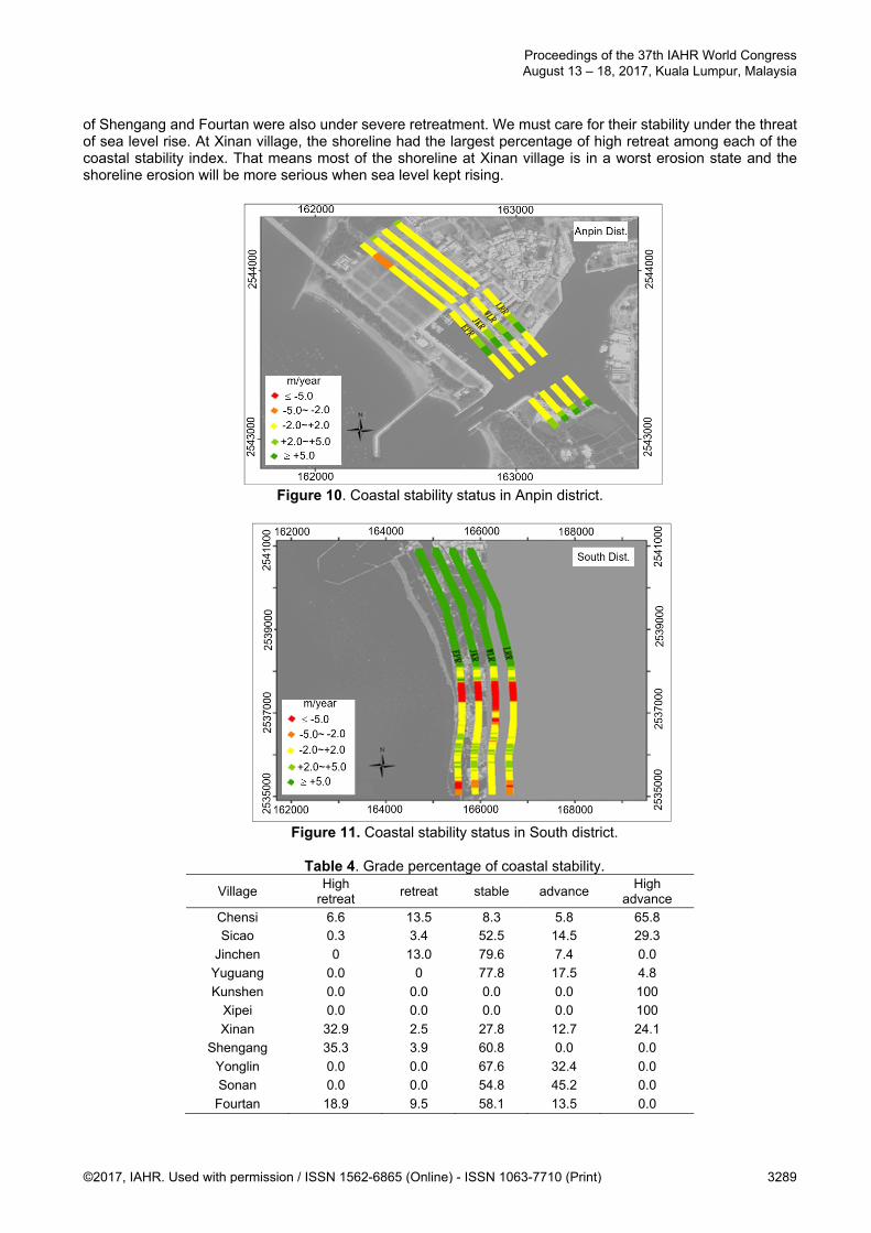
of Shengang and Fourtan were also under severe retreatment. We must care for their stability under the threat of sea level rise. At Xinan village, the shoreline had the largest percentage of high retreat among each of the coastal stability index. That means most of the shoreline at Xinan village is in a worst erosion state and the shoreline erosion will be more serious when sea level kept rising.

Figure 10. Coastal stability status in Anpin district.

Figure 11. Coastal stability status in South district.

Table 4. Grade percentage of coastal stability.

Village High

retreat retreat stable advance

High advance

Chensi 6.6 13.5 8.3 5.8 65.8 Sicao 0.3 3.4 52.5 14.5 29.3

Jinchen 0 13.0 79.6 7.4 0.0

Yuguang 0.0 0 77.8 17.5 4.8

Kunshen 0.0 0.0 0.0 0.0 100

Xipei 0.0 0.0 0.0 0.0 100

Xinan 32.9 2.5 27.8 12.7 24.1

Shengang 35.3 3.9 60.8 0.0 0.0

Yonglin 0.0 0.0 67.6 32.4 0.0

Sonan 0.0 0.0 54.8 45.2 0.0

Fourtan 18.9 9.5 58.1 13.5 0.0



4.4 Shoreline change under sea level rise Eq. [1] was employed to estimate the impact of sea level rise on shoreline retreat. Because the Bruun

rule adopts an equilibrium profile to calculate the active sediment transport length L*, three different formulae were used to determine the profile scale parameter A. The formulas were Moore (1982), CERC (1988) and Kriebel et al. (1991). The intermediate value of the scenario of RCP 6.0 in the IPCC AR5, i.e., 3.6mm/year for Taiwan was adapted to predict sea level rise in 2039. Figure 12 shows the predicted result according to the villages and Table 7 lists the shoreline retreat of each village under different sediment scale parameter A. From Figure 12 or Table 5, we could find whether we can use Kriebel et al. (1991) to calculate the sediment scale parameter A. It will give a maximum shoreline retreat value and CERC (1988) will give a minimum result. In 2039, under the impact of sea level rise, shoreline in Tainan south coast may retreat in the range of 8.6 m to 20.9 m. The maximum shoreline retreat will happen at Xinan village and ShenKuang. Their shorelines may be receding about 20.5m~20.9m. Xinan’s coast has a high erosion trend, and sea level rise will worsen its erosion state. In addition, sea level rise will enhance the frequency of coastal flooding, seawater intrusion and wave overtopping. All of these effects will let coastal disasters to deteriorate rapidly. For coastal safety, an integrated coastal protection and coastal management plan is urgent for this area.

Figure 12. Spatial distribution of the shoreline retreat due to sea level rise.

Table 5. Quantities of shoreline retreat due to sea level rise.

Village Moore(1982) Kriebel et al.(1991)

CERC(1988)

Chensi 13.4 16.1 11.3

Sicao 11.1 12.6 9.3

Jinchen 11.4 13.0 9.6

Yukuang 10.2 11.0 8.6

Kunshen 12.0 15.4 10.6

Xipei 14.1 18.0 12.4

Xinan 15.7 20.9 14.2

ShenKuang 15.6 20.5 14.0

Yunlin 14.3 18.7 12.8

Soman 11.4 13.5 9.6

Fourtan 14.6 17.7 12.5



5 CONCLUSIONS From the historical shoreline change analysis, we know that most of the coastlines in south Tainan are

stable, especially in Jinchen, Yuguang, Kunshen and Xipaei. More than 70% of the shoreline is in stable or advance status. However, the coast in Xinan village and Fourtan village has an erosion tendency. In Xinan village the average shoreline change rate is -6.6 m/year in recent decade and about 32.9% of its shoreline is standing on high retreat status. Under the threat of sea level rise, this village also has the maximum shoreline retreat. Its shoreline will recede about 20.9m in the future. Therefore, the most vulnerable coast in south Tainan is Xinan village and it is urgent to maintain its stability. Sea level rise will worsen and the coastal disasters occurring will rise in south Tainan. The Integrated coastal protection strategy must be implemented quickly as response to the threats of sea level rise. ACKNOWLEDGEMENTS

The authors would like to thank the Ministry of Science and Technology, Taiwan, R.O.C. for financially supporting this research under Grant No. NSC 101-2625-M-415 -001. REFERENCES Bruun, F.P. (1962). Sea-Level Rise as a Cause of Shore Erosion. Journal of Waterways and Harbor Division,

88, 117-130. Cooper, J.A.G. & Pilkey, O.H. (2004). Sea-Level Rise and Shoreline Retreat: Time to Abandon the Bruun

Rule. Global and Planetary Change, 43, 157–171. CWB. (2009). 1897~2008 Statistics of Climate Changes in Taiwan. GPN:1009804159, Central Weather

Bureau, Ministry of Transportation and Communications, ROC. Dean, R.G. (1991). Equilibrium Beach Profiles: Characteristics and Applications. Journal of Coastal Research,

7, 53-84. IPCC. (2014). Climate Change 2014: Impacts, Adaptation, and Vulnerability, Fifth Assessment Report, The

Intergovernmental Panel on Climate Change, 3-13. Kriebel, D.L., Kraus, N.C. & Larson, M. (1991). Engineering Method for Predicting Beach Profiles Response.

Proceedings of Coastal Sediments '91, ASCE, 557-571. Moore, B.D. (1982). Beach Profile Evolution in Response to Changes in Water Level and Wave Height. MSc.

thesis, University of Delaware, Newark, DE. Rosati, J.D., Dean, R.G. & Walton, T.L. (2013). The Modified Bruun Rule Extended for Landward Transport.

Marine Geology, 340, 71-81. WRA. (2011). A Study of Adaptation Capacity of Coastal Disasters Due to Climate Change in Order to

Strengthen Southwest Area of Taiwan (2/2). MOEAWRA1000075, the Water Resources Agency, Ministry of Economic Affairs, ROC.



ICE FORMATION AND FLOW REGIMES IN REGULATED RIVERS, CENTRAL IDAHO,

USA

ANDREW W. TRANMER(1), PETER GOODWIN(2), MATTHEW G. TIEDEMANN(3), DANIELE TONINA(4) & ROBERT ETTEMA(5)

(1,2,4) Center for Ecohydraulics Research, University of Idaho, Boise, USA

[email protected] (3) R2 Resource Consultants, Inc., Redmond, USA

(5) Colorado State University, Fort Collins, USA [email protected]

ABSTRACT In the regulated rivers of the Pacific Northwest, winter flow standards are frequently established, that set a constant minimum instream flow. The magnitude of discharge, consistent with observed winter flows for the pre-dam condition, is often based on very short-term records or sporadic point measurements. Detailed winter monitoring conducted in a remote and largely undisturbed watershed in Idaho has identified several unanticipated processes in both the regulated river and unregulated tributaries that have potential impacts on the winter survival of fish and offers new insights on potential management strategies. Areas of marginal ice formation exist at mid-latitude and mid-elevation ranges where destabilized ice cover can open leads in the river for substantial distances. Loss of ice cover can result in detrimental effects such as increased predation or formation of frazil ice that is harmful to many aquatic species. In unimpaired tributary streams, significant short-term variabilities were detected by stream gages and confirmed by observation with remote cameras. These abrupt flood waves are created when ice-jams fail or the stream is blocked by avalanches resulting in temporary loss of ice cover. The frequency of these extreme events increased in areas that had recently been impacted by wildfire. This previously undetected phenomena in the region demonstrated that the stream ecology must be resilient to these extreme fluctuations and constant winter baseflow may not represent pre-dam conditions. In regulated reaches, the reservoir release is typically warmer than the pre-dam condition and has the potential to open leads in the ice cover. The removal of the insulating layer of snow and ice cover leaves the stream vulnerable to the formation of frazil ice under the conditions of extreme diel cycles in ambient temperature. The loss of ice cover and risk of frazil or anchor ice are evaluated under a range of managed winter discharges. Keywords: Ice dynamics; stream temperature; dam operations; managed rivers; winter streamflow. 1 INTRODUCTION

Headwater and piedmont streams are important as they constitute the majority of stream density in basins and host some of the most ecologically rich aquatic communities (Bishop et al., 2008). These environments are also common for reservoir storage and hydropower production owing to their steep gradients and high potential head. Many of these streams are located along mid-latitude and mid-elevation gradients that are increasingly being affected by climate change, thereby complicating the management decisions of federal and state water agencies. These impacts become particularly acute during the winter months where frigid temperatures have historically maintained an insulating ice cover that protected aquatic species and are now subject to rain-on-snow events, early seasonal snowmelt, and decreased spring flood peaks (Luce et al., 2014; Nijssen et al., 2001). Natural winter variability occurs in mid-latitude and mid-elevation streams owing to dynamic regional weather patterns that drive iterative freeze-thaw processes, but is becoming more extreme with increased climatic variability. In the Pacific Northwest of the United States, climate change has direct and substantial consequences for winter river ice cover and aquatic habitat that manifest in 1) generally warmer temperatures during winter months, 2) increased variability of storm tracks bringing rain-on-snow precipitation events to mountainous terrain, and 3) flashy, short duration snow and ice clearing floods in tributaries and main channels (Clark, 2010; Tranmer and Goodwin, 2009). Collectively, these environmental conditions support marginal ice cover on rivers and streams as ambient conditions oscillate near 0 °C throughout the winter months.

In addition to changing regional patterns, local environmental conditions in these watersheds may further challenge in maintaining a stable ice cover, as large diel temperature swings, relatively steep slopes, and variable relative depths facilitate open leads in river surface ice. Open leads in the surface ice allow for super-cooling of river water, resulting in frazil and anchor ice formation that can be detrimental to the native ecology



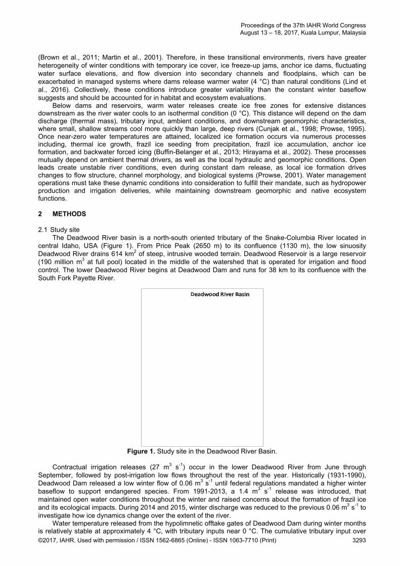
(Brown et al., 2011; Martin et al., 2001). Therefore, in these transitional environments, rivers have greater heterogeneity of winter conditions with temporary ice cover, ice freeze-up jams, anchor ice dams, fluctuating water surface elevations, and flow diversion into secondary channels and floodplains, which can be exacerbated in managed systems where dams release warmer water (4 °C) than natural conditions (Lind et al., 2016). Collectively, these conditions introduce greater variability than the constant winter baseflow suggests and should be accounted for in habitat and ecosystem evaluations.

Below dams and reservoirs, warm water releases create ice free zones for extensive distances downstream as the river water cools to an isothermal condition (0 °C). This distance will depend on the dam discharge (thermal mass), tributary input, ambient conditions, and downstream geomorphic characteristics, where small, shallow streams cool more quickly than large, deep rivers (Cunjak et al., 1998; Prowse, 1995). Once near-zero water temperatures are attained, localized ice formation occurs via numerous processes including, thermal ice growth, frazil ice seeding from precipitation, frazil ice accumulation, anchor ice formation, and backwater forced icing (Buffin-Belanger et al., 2013; Hirayama et al., 2002). These processes mutually depend on ambient thermal drivers, as well as the local hydraulic and geomorphic conditions. Open leads create unstable river conditions, even during constant dam release, as local ice formation drives changes to flow structure, channel morphology, and biological systems (Prowse, 2001). Water management operations must take these dynamic conditions into consideration to fulfill their mandate, such as hydropower production and irrigation deliveries, while maintaining downstream geomorphic and native ecosystem functions. 2 METHODS 2.1 Study site

The Deadwood River basin is a north-south oriented tributary of the Snake-Columbia River located in central Idaho, USA (Figure 1). From Price Peak (2650 m) to its confluence (1130 m), the low sinuosity Deadwood River drains 614 km2 of steep, intrusive wooded terrain. Deadwood Reservoir is a large reservoir (190 million m3 at full pool) located in the middle of the watershed that is operated for irrigation and flood control. The lower Deadwood River begins at Deadwood Dam and runs for 38 km to its confluence with the South Fork Payette River.

Figure 1. Study site in the Deadwood River Basin.

Contractual irrigation releases (27 m3 s-1) occur in the lower Deadwood River from June through September, followed by post-irrigation low flows throughout the rest of the year. Historically (1931-1990), Deadwood Dam released a low winter flow of 0.06 m3 s-1 until federal regulations mandated a higher winter baseflow to support endangered species. From 1991-2013, a 1.4 m3 s-1 release was introduced, that maintained open water conditions throughout the winter and raised concerns about the formation of frazil ice and its ecological impacts. During 2014 and 2015, winter discharge was reduced to the previous 0.06 m3 s-1 to investigate how ice dynamics change over the extent of the river.

Water temperature released from the hypolimnetic offtake gates of Deadwood Dam during winter months is relatively stable at approximately 4 °C, with tributary inputs near 0 °C. The cumulative tributary input over



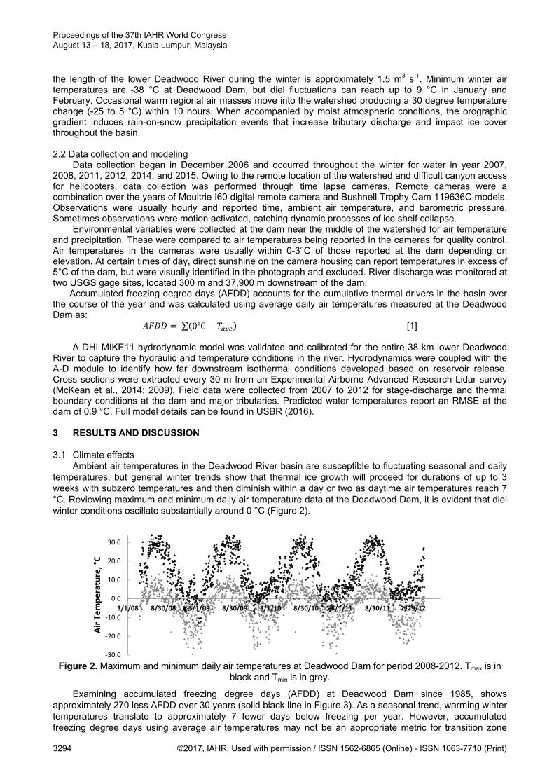
the length of the lower Deadwood River during the winter is approximately 1.5 m3 s-1. Minimum winter air temperatures are -38 °C at Deadwood Dam, but diel fluctuations can reach up to 9 °C in January and February. Occasional warm regional air masses move into the watershed producing a 30 degree temperature change (-25 to 5 °C) within 10 hours. When accompanied by moist atmospheric conditions, the orographic gradient induces rain-on-snow precipitation events that increase tributary discharge and impact ice cover throughout the basin. 2.2 Data collection and modeling

Data collection began in December 2006 and occurred throughout the winter for water in year 2007, 2008, 2011, 2012, 2014, and 2015. Owing to the remote location of the watershed and difficult canyon access for helicopters, data collection was performed through time lapse cameras. Remote cameras were a combination over the years of Moultrie I60 digital remote camera and Bushnell Trophy Cam 119636C models. Observations were usually hourly and reported time, ambient air temperature, and barometric pressure. Sometimes observations were motion activated, catching dynamic processes of ice shelf collapse.

Environmental variables were collected at the dam near the middle of the watershed for air temperature and precipitation. These were compared to air temperatures being reported in the cameras for quality control. Air temperatures in the cameras were usually within 0-3°C of those reported at the dam depending on elevation. At certain times of day, direct sunshine on the camera housing can report temperatures in excess of 5°C of the dam, but were visually identified in the photograph and excluded. River discharge was monitored at two USGS gage sites, located 300 m and 37,900 m downstream of the dam. Accumulated freezing degree days (AFDD) accounts for the cumulative thermal drivers in the basin over the course of the year and was calculated using average daily air temperatures measured at the Deadwood Dam as:

∑ 0 [1]

A DHI MIKE11 hydrodynamic model was validated and calibrated for the entire 38 km lower Deadwood River to capture the hydraulic and temperature conditions in the river. Hydrodynamics were coupled with the A-D module to identify how far downstream isothermal conditions developed based on reservoir release. Cross sections were extracted every 30 m from an Experimental Airborne Advanced Research Lidar survey (McKean et al., 2014; 2009). Field data were collected from 2007 to 2012 for stage-discharge and thermal boundary conditions at the dam and major tributaries. Predicted water temperatures report an RMSE at the dam of 0.9 °C. Full model details can be found in USBR (2016). 3 RESULTS AND DISCUSSION 3.1 Climate effects

Ambient air temperatures in the Deadwood River basin are susceptible to fluctuating seasonal and daily temperatures, but general winter trends show that thermal ice growth will proceed for durations of up to 3 weeks with subzero temperatures and then diminish within a day or two as daytime air temperatures reach 7 °C. Reviewing maximum and minimum daily air temperature data at the Deadwood Dam, it is evident that diel winter conditions oscillate substantially around 0 °C (Figure 2).

Figure 2. Maximum and minimum daily air temperatures at Deadwood Dam for period 2008-2012. Tmax is in black and Tmin is in grey.

Examining accumulated freezing degree days (AFDD) at Deadwood Dam since 1985, shows approximately 270 less AFDD over 30 years (solid black line in Figure 3). As a seasonal trend, warming winter temperatures translate to approximately 7 fewer days below freezing per year. However, accumulated freezing degree days using average air temperatures may not be an appropriate metric for transition zone

‐30.0

‐20.0

‐10.0

0.0

10.0

20.0

30.0

3/1/08 8/30/08 3/1/09 8/30/09 3/1/10 8/30/10 3/1/11 8/30/11 2/29/12

Air Temperature, °C



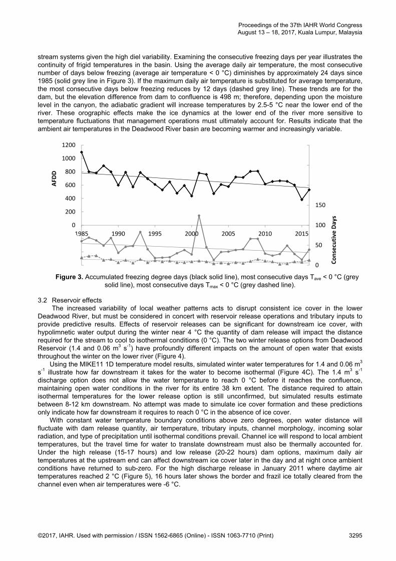
stream systems given the high diel variability. Examining the consecutive freezing days per year illustrates the continuity of frigid temperatures in the basin. Using the average daily air temperature, the most consecutive number of days below freezing (average air temperature < 0 °C) diminishes by approximately 24 days since 1985 (solid grey line in Figure 3). If the maximum daily air temperature is substituted for average temperature, the most consecutive days below freezing reduces by 12 days (dashed grey line). These trends are for the dam, but the elevation difference from dam to confluence is 498 m; therefore, depending upon the moisture level in the canyon, the adiabatic gradient will increase temperatures by 2.5-5 °C near the lower end of the river. These orographic effects make the ice dynamics at the lower end of the river more sensitive to temperature fluctuations that management operations must ultimately account for. Results indicate that the ambient air temperatures in the Deadwood River basin are becoming warmer and increasingly variable.

Figure 3. Accumulated freezing degree days (black solid line), most consecutive days Tave < 0 °C (grey solid line), most consecutive days Tmax < 0 °C (grey dashed line).

3.2 Reservoir effects

The increased variability of local weather patterns acts to disrupt consistent ice cover in the lower Deadwood River, but must be considered in concert with reservoir release operations and tributary inputs to provide predictive results. Effects of reservoir releases can be significant for downstream ice cover, with hypolimnetic water output during the winter near 4 °C the quantity of dam release will impact the distance required for the stream to cool to isothermal conditions (0 °C). The two winter release options from Deadwood Reservoir (1.4 and 0.06 m3 s-1) have profoundly different impacts on the amount of open water that exists throughout the winter on the lower river (Figure 4). Using the MIKE11 1D temperature model results, simulated winter water temperatures for 1.4 and 0.06 m3 s-1 illustrate how far downstream it takes for the water to become isothermal (Figure 4C). The 1.4 m3 s-1 discharge option does not allow the water temperature to reach 0 °C before it reaches the confluence, maintaining open water conditions in the river for its entire 38 km extent. The distance required to attain isothermal temperatures for the lower release option is still unconfirmed, but simulated results estimate between 8-12 km downstream. No attempt was made to simulate ice cover formation and these predictions only indicate how far downstream it requires to reach 0 °C in the absence of ice cover. With constant water temperature boundary conditions above zero degrees, open water distance will fluctuate with dam release quantity, air temperature, tributary inputs, channel morphology, incoming solar radiation, and type of precipitation until isothermal conditions prevail. Channel ice will respond to local ambient temperatures, but the travel time for water to translate downstream must also be thermally accounted for. Under the high release (15-17 hours) and low release (20-22 hours) dam options, maximum daily air temperatures at the upstream end can affect downstream ice cover later in the day and at night once ambient conditions have returned to sub-zero. For the high discharge release in January 2011 where daytime air temperatures reached 2 °C (Figure 5), 16 hours later shows the border and frazil ice totally cleared from the channel even when air temperatures were -6 °C.

0

50

100

150

200

250

300

‐600

‐400

‐200

0

200

400

600

800

1000

1200

1985 1990 1995 2000 2005 2010 2015

Consecutive

Days

AFD

D



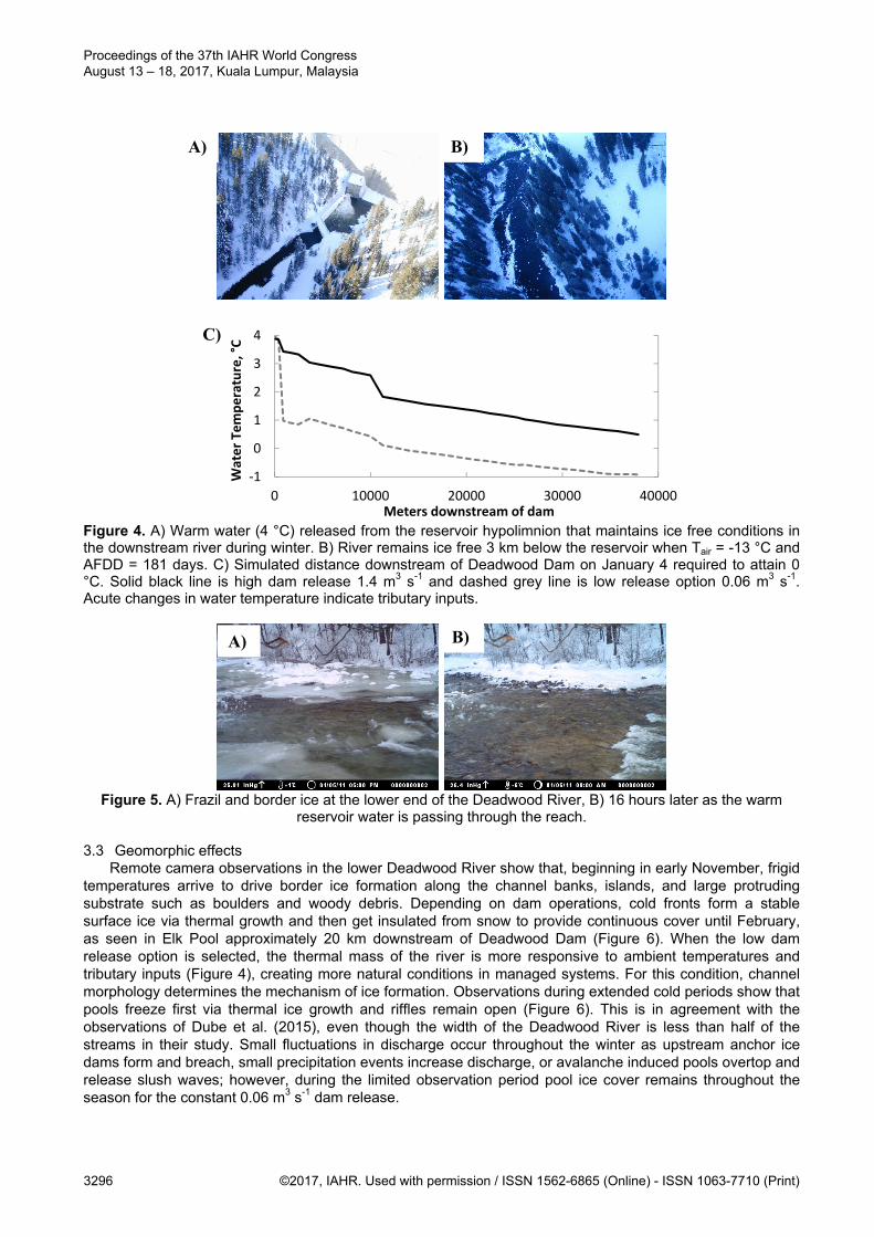
Figure 4. A) Warm water (4 °C) released from the reservoir hypolimnion that maintains ice free conditions in the downstream river during winter. B) River remains ice free 3 km below the reservoir when Tair = -13 °C and AFDD = 181 days. C) Simulated distance downstream of Deadwood Dam on January 4 required to attain 0 °C. Solid black line is high dam release 1.4 m3 s-1 and dashed grey line is low release option 0.06 m3 s-1. Acute changes in water temperature indicate tributary inputs.

Figure 5. A) Frazil and border ice at the lower end of the Deadwood River, B) 16 hours later as the warm

reservoir water is passing through the reach. 3.3 Geomorphic effects Remote camera observations in the lower Deadwood River show that, beginning in early November, frigid temperatures arrive to drive border ice formation along the channel banks, islands, and large protruding substrate such as boulders and woody debris. Depending on dam operations, cold fronts form a stable surface ice via thermal growth and then get insulated from snow to provide continuous cover until February, as seen in Elk Pool approximately 20 km downstream of Deadwood Dam (Figure 6). When the low dam release option is selected, the thermal mass of the river is more responsive to ambient temperatures and tributary inputs (Figure 4), creating more natural conditions in managed systems. For this condition, channel morphology determines the mechanism of ice formation. Observations during extended cold periods show that pools freeze first via thermal ice growth and riffles remain open (Figure 6). This is in agreement with the observations of Dube et al. (2015), even though the width of the Deadwood River is less than half of the streams in their study. Small fluctuations in discharge occur throughout the winter as upstream anchor ice dams form and breach, small precipitation events increase discharge, or avalanche induced pools overtop and release slush waves; however, during the limited observation period pool ice cover remains throughout the season for the constant 0.06 m3 s-1 dam release.

‐1

0

1

2

3

4

0 10000 20000 30000 40000

Water Temperature, °C

Meters downstream of dam

C)

A) B)

A) B)



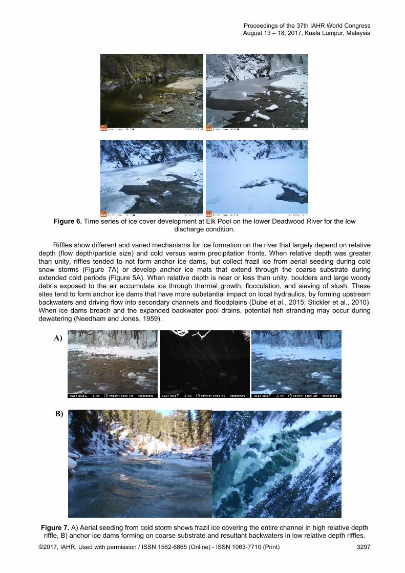
B)

Figure 6. Time series of ice cover development at Elk Pool on the lower Deadwood River for the low

discharge condition.

Riffles show different and varied mechanisms for ice formation on the river that largely depend on relative depth (flow depth/particle size) and cold versus warm precipitation fronts. When relative depth was greater than unity, riffles tended to not form anchor ice dams, but collect frazil ice from aerial seeding during cold snow storms (Figure 7A) or develop anchor ice mats that extend through the coarse substrate during extended cold periods (Figure 5A). When relative depth is near or less than unity, boulders and large woody debris exposed to the air accumulate ice through thermal growth, flocculation, and sieving of slush. These sites tend to form anchor ice dams that have more substantial impact on local hydraulics, by forming upstream backwaters and driving flow into secondary channels and floodplains (Dube et al., 2015; Stickler et al., 2010). When ice dams breach and the expanded backwater pool drains, potential fish stranding may occur during dewatering (Needham and Jones, 1959).

Figure 7. A) Aerial seeding from cold storm shows frazil ice covering the entire channel in high relative depth riffle, B) anchor ice dams forming on coarse substrate and resultant backwaters in low relative depth riffles.

A)



When anchor ice dams form around coarse substrate in the lower Deadwood River air temperatures reach -6 °C, but are usually predated with at least one daily temperature value < -10 °C (Figure 8) confirming findings in other steep streams (Hirayama et al., 1997). These backwater environments are subject to icing and can store substantial quantities of water as ice mass that impacts downstream flows until warmer temperatures cause dam breaching and ice breakup (Stickler et al., 2010; Ettema, 2007; Moore et al., 2002). In narrow canyon settings like the Deadwood River, these dams can drive water and ice into the riparian areas causing channel expansion and secondary channel formation (Figure 7B). McNamara (2000) found watersheds with drainage areas greater than 500 km2 to be subject to channel expansion from ice push, at 614 km2 the Deadwood system lies near this threshold. Evidence from the Deadwood River shows very limited floodplain extent throughout the canyon even though bankfull flows have not been reached since dam closure in 1931 (Tranmer et al., 2015), which may be a direct result of lateral and overbank ice scour.

Figure 8. Winter hydrograph for water year 2011 (blue line), arrows represent anchor ice dam backwater. Constant dam release of 1.4 m3 s-1 (red line). Average air temperature (triangles) with two point moving

average (yellow line). Precipitation at Deadwood Dam multiplied by ten for presentation purposes (green line).

Alternatively, when warm air masses arrive from the south and are combined with precipitation, rain-on-snow drives melting and tributary floods that can impose large hydrograph spikes on the mainstem even under constant dam release. In mid-January 2011, daytime temperatures at the Deadwood Dam reached 4-6 °C and were accompanied by 6 days of sporadic rain-on-snow (> 2.7 inches). Camera observations of Trail Creek tributary in the recently burned upper watershed, showed a steeply rising flood wave that passed through the tributary channel with surprisingly little disturbance to the snow cover (Figure 9). This implies that greater snow cover buffers these high tributary streams from the formation of frazil ice and detrimental ecological impacts, even during large precipitation events, which is not possible in the main river (Figure 10).

‐15

‐10

‐5

0

5

10

15

20

25

30

35

40

‐20

‐10

0

10

20

10/1 12/1 2/1 4/2

Temperature, °C

Precipitation x 10, in

Discharge, m

3s‐1



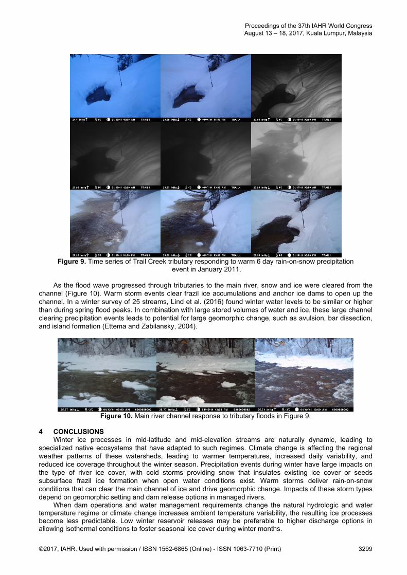
Figure 9. Time series of Trail Creek tributary responding to warm 6 day rain-on-snow precipitation

event in January 2011.

As the flood wave progressed through tributaries to the main river, snow and ice were cleared from the channel (Figure 10). Warm storm events clear frazil ice accumulations and anchor ice dams to open up the channel. In a winter survey of 25 streams, Lind et al. (2016) found winter water levels to be similar or higher than during spring flood peaks. In combination with large stored volumes of water and ice, these large channel clearing precipitation events leads to potential for large geomorphic change, such as avulsion, bar dissection, and island formation (Ettema and Zabilansky, 2004).

Figure 10. Main river channel response to tributary floods in Figure 9.

4 CONCLUSIONS

Winter ice processes in mid-latitude and mid-elevation streams are naturally dynamic, leading to specialized native ecosystems that have adapted to such regimes. Climate change is affecting the regional weather patterns of these watersheds, leading to warmer temperatures, increased daily variability, and reduced ice coverage throughout the winter season. Precipitation events during winter have large impacts on the type of river ice cover, with cold storms providing snow that insulates existing ice cover or seeds subsurface frazil ice formation when open water conditions exist. Warm storms deliver rain-on-snow conditions that can clear the main channel of ice and drive geomorphic change. Impacts of these storm types depend on geomorphic setting and dam release options in managed rivers.

When dam operations and water management requirements change the natural hydrologic and water temperature regime or climate change increases ambient temperature variability, the resulting ice processes become less predictable. Low winter reservoir releases may be preferable to higher discharge options in allowing isothermal conditions to foster seasonal ice cover during winter months.



ACKNOWLEDGEMENTS The authors would like to thank the Danish Hydraulic Institute for providing MIKE software packages to

the University of Idaho. This research was supported by U.S. Reclamation and U.S. Forest Service grant 08-JV-11221659-036. REFERENCES Bishop, K., Buffam, I., Erlandsson, M., Fölster, J., Laudon, H., Seibert, J. & Temnerud, J. (2008). Aqua

Incognita: the Unknown Headwaters. Hydrological Processes, 22, 1239–1242. Brown, R.S., Hubert, W.A. & Daly, S.F. (2011). A Primer on Winter, Ice, and Fish: What Fisheries Biologists

Should Know about Winter Ice Processes and Stream-Dwelling Fish. Fisheries, 36(1), 8-26. Buffin-Bélanger, T., Bergeron, N.E. & Dubé, J.D. (2013). Ice Formation in Small Rivers, River Ice Formation.

Committee on River Ice Processes and Environment, CGU-HS, Ed. S. Beltaos, Edmonton, Canada, 385–409.

Clark, G.M. (2010). Changes in Patterns of Streamflow from Unregulated Watersheds in Idaho, Western Wyoming, and Northern Nevada. Journal of the American Water Resources Association, 46(3), 486-497.

Cunjak, R.A., Prowse, T.D. & Parrish, D.L. (1998). Atlantic Salmon (Salmo salar) in Winter: ‘‘The Season of Parr Discontent”? Canadian Journal of Fisheries Aquatic Sciences, 55, 161–180.

Dubé, M., Turcotte, B. & Morse, B. (2015). Steep Channel Freezeup Processes: Understanding Complexity with Statistical and Physical Models. Canadian Journal Civil Engineering, 42, 622–633.

Ettema, R. (2007). Information Needs when Estimating Ice Jam Floods and Ice Runs. Extreme Hydrological Events: New Concepts for Security, Springer, 285–298.

Ettema, R. & Zabilansky, L. (2004). Ice Influences on Channel Stability: Insights from Missouri’s Fort Peck Reach. Journal of Hydraulic Engineering, 130(4), 279-292.

Hirayama, K., Terada, K., Sato, M. Sasmoto, M. & Yamasaki, M. (1997). Field Measurements of Anchor Ice and Frazil Ice. 9th Workshop on River Ice, Fredericton, Canada, 141-151.

Hirayama, K., Yamazaki, M. & Shen, H.T. (2002). Aspects of River Ice Hydrology in Japan. Hydrological Processes, 16, 891–904.

Lind, L., Alfredsen, K., Kuglerová, L. & Nilsson, C. (2016). Hydrological and Thermal Controls of Ice Formation in 25 Boreal Stream Reaches. Journal of Hydrology, 540, 797-811.

Luce, C.H., Lopez-Burgos, V. & Holden, Z. (2014). Sensitivity of Snowpack Storage to Precipitation and Temperature using Spatial and Temporal Analog Models. Water Resources Research, 50(12), 9447–9462.

Martin, M.D., Brown, R.S., Barton, D.R. & Power, G. (2001). Abundance of Stream Invertebrates in Winter: Seasonal Changes and Effects of River Ice. The Canadian Field-Naturalist, 115(1), 68-74.

McKean, J.A., Nagel, D., Tonina, D., Bailey, P., Wright, C.W., Bohn, C. & Nayegandhi, A. (2009). Remote Sensing of Channels and Riparian Zones with a Narrow-Beam Aquatic-Terrestrial LIDAR. Remote Sensing, 1, 1065-1096.

McKean, J.A., Tonina, D., Bohn, C. & Wright, C.W. (2014). Effects of Bathymetric Lidar Errors on Flow Properties Predicted with a Multi-Dimensional Hydraulic Model. Journal of Geophysical Research: Earth Surface, 119(3), 644-664.

McNamara, J.P. (2000). Bankfull Flow, Hydraulic Geometry and River Ice in a Northern River. AWRA Water Resources in Extreme Environments, Anchorage, AK, 191-196.

Moore, R.D., Hamilton, A.S. & Scibek, J. (2002). Winter Streamflow Variability, Yukon Territory, Canada. Hydrological Processes, 16, 763-778.

Needham, P.R. & Jones, A.C. (1959). Flow, Temperature, Solar Radiation and Ice in Relation to Activities of Fishes in Sagehen Creek, California. Ecology, 40(3), 465–474.

Nijssen B., O’Donnel G.M., Hamlet A.F. & Lettenmaier, D.P. (2001). Hydrologic Sensitivity of Global Rivers to Climate Change, Climate Change, 50, 143-175.

Prowse, T.D. (1995). River Ice Processes, River Ice Jams. Water Resources Publications, LLC, Highlands Ranch, Colorado, 29–70.

Prowse, T.D. (2001). River-Ice Ecology. I: Hydrology, Geomorphic and Water-Quality Aspects. Journal of Cold Regions Engineering, 15, 1–16.

Stickler, M., Alfredsen, K., Linnansaari, T.T. & Fjeldstad, H.P. (2010). The Influence of Dynamic Ice Formation on Hydraulic Heterogeneity in Steep Streams. River Research and Applications, 26, 1187–1197.

Tranmer, A.W. & Goodwin, P. (2009). Can General Circulation Models Detect Climate Change Signatures in Catchment Scale Hydrology of the Intermountain West, USA? The International Conference of Science and Information Technologies for Sustainable Management of Aquatic Ecosystems. Ed. O. Parra, January 12-16, 2009. IAHR Concepción, Chile.

Tranmer A.W., Tonina D., Benjankar R., Tiedemann M. & Goodwin, P. (2015). Floodplain Persistence and Dynamic-Equilibrium Conditions in a Canyon Environment. Geomorphology, 250, 147-158.

USBR (U.S. Bureau of Reclamation). (2016). Final Deadwood Reservoir Operations Flexibility Evaluation, Boise Project, Idaho, Pacific Northwest Region, Snake River Area Office, Boise, Idaho.



theme 4: CoastaL, estuaries anD LaKe management

Documents

Transcript of theme 4: CoastaL, estuaries anD LaKe management