36 April 2011 Physics Today www.physicstoday.org

During the first half of the 20th century, the Arcticsea-ice cover was thought to be in a near-steady seasonalcycle, reaching an area of roughly 15 million km2 each Marchand retreating to 7 million km2 each September. Ice thickenough to survive the melt season, termed perennial or mul-tiyear ice (MYI), adds to the ice cover. A large fraction of MYItypically remained in the Arctic Basin for several years andgrew to an equilibrium thickness of about 3.5 m—meltinghalf a meter at the surface from June through August andgrowing by about half a meter at the bottom from Octoberthrough March. In the late 1970s, MYI occupied more thantwo-thirds of the surface area of the Arctic Basin, with first-year ice (FYI) covering the remaining one-third. FYI is thethinner, seasonal ice that fills cracks in the ice cover andgrows on the open ocean with the southward advance of theice edge at the end of each summer.

That picture began to change significantly in the latterpart of the century. Since 1979, passive microwave measure-ments by satellite, which can distinguish between the bright-ness signatures of ice and water, have established a more ac-curate account of the seasonal cycle of ice extent. The satelliterecord reveals that over the past 30 years the average Septem-ber ice extent has been declining at an astonishing rate ofmore than 11% per decade (see figure 1 and the article byJosefino Comiso and Claire Parkinson in PHYSICS TODAY, Au-gust 2004, page 38).

As a consequence, FYI has replaced much of the MYI inthe Arctic Ocean. Satellite-borne radar scatterometers havemade it possible during the past decade to identify and di-rectly map the two primary ice types. As ice ages, brine drainsfrom it, leaving air pockets behind; the older, less saline MYIis more than twice as reflective as seasonal ice. From thatcomplementary satellite record, scientists witnessed a dra-matic loss of MYI during the past decade, as illustrated in fig-ure 2. Between 2004 and 2008, the winter cover of MYI shrankby 1.5 million km2—more than twice the size of Texas—andnow covers only one-third of the Arctic Basin.

To determine the volume of melted sea ice and the asso-ciated changes in the heat lost or gained by the ice cover, onemust make a basin-wide sampling not only of the ice’s areabut also of its thickness. The latter is the technically more dif-ficult measurement. Cross-Arctic estimates of thickness camewith the first under-ice crossing of the Arctic Basin by the nu-clear submarine USS Nautilus in 1958. Since the 1960s the US

Navy has periodically declassified measurements of icedraft—the depth of the submerged portion of the floating iceobserved by upward-looking sonars on submarines—for sci-entific analysis. The ice draft is converted to thickness usingArchimedes’s principle and the densities of ice and seawater.Since 1979, researchers have been able to infer changes in thesea-ice thickness of the central Arctic using available subma-

The thinning of Arctic sea ice Ronald Kwok and Norbert Untersteiner

The surplus heat needed to explain the loss of Arctic sea ice during the past few decades is on theorder of 1 W/m2. Observing, attributing, and predicting such a small amount of energy remain daunting problems.

Ron Kwok is a senior research scientist at the Jet Propulsion Laboratory, California Institute of Technology, in Pasadena. Norbert Untersteiner is an emeritus professor of atmospheric sciences and geophysics at the University of Washington in Seattle.

feature

Asia

Greenland

NorthAmerica

Figure 1. The extent of sea ice covering the Arctic Oceanexpands and recedes seasonally. The median ice edges inMarch (blue) and in September (red) illustrate the extremesin area over the period 1979–2000. The yellow area showsthe sea-ice extent at the end of summer 2010. (Data cour-tesy of the National Snow and Ice Data Center.)

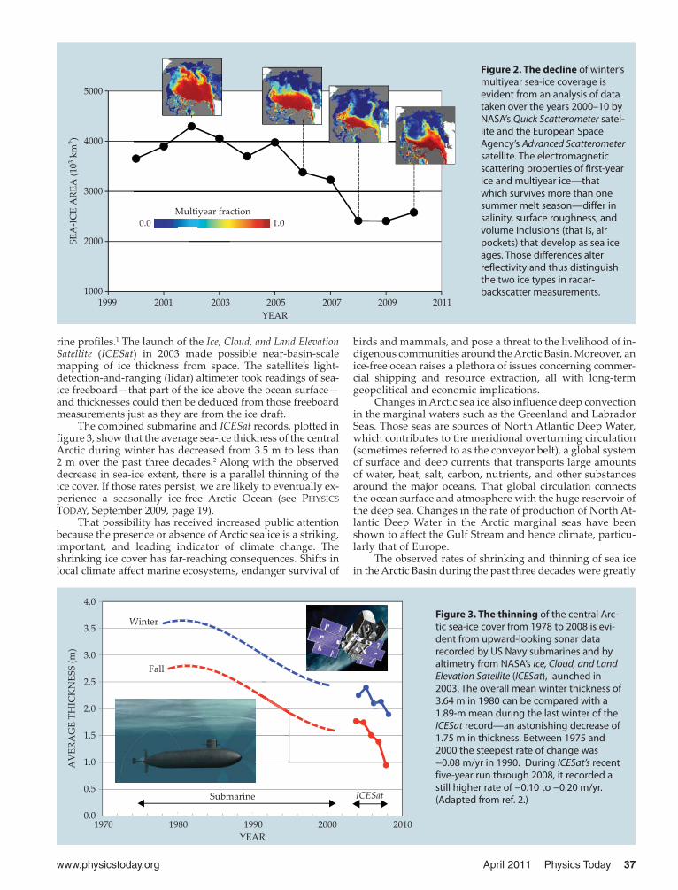
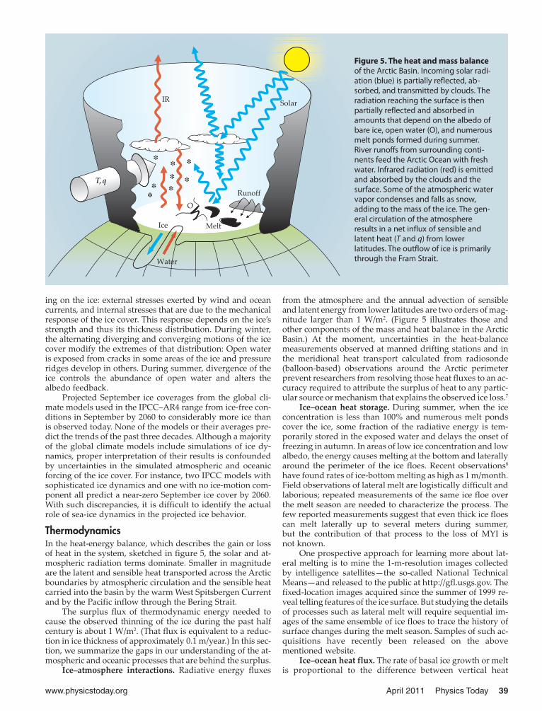
rine profiles.1 The launch of the Ice, Cloud, and Land ElevationSatellite (ICESat) in 2003 made possible near-basin-scale mapping of ice thickness from space. The satellite’s light-detection-and-ranging (lidar) altimeter took readings of sea-ice freeboard—that part of the ice above the ocean surface—and thicknesses could then be deduced from those freeboardmeasurements just as they are from the ice draft.

The combined submarine and ICESat records, plotted infigure 3, show that the average sea-ice thickness of the centralArctic during winter has decreased from 3.5 m to less than2 m over the past three decades.2 Along with the observeddecrease in sea-ice extent, there is a parallel thinning of theice cover. If those rates persist, we are likely to eventually ex-perience a seasonally ice-free Arctic Ocean (see PHYSICSTODAY, September 2009, page 19).

That possibility has received increased public attentionbecause the presence or absence of Arctic sea ice is a striking,important, and leading indicator of climate change. Theshrinking ice cover has far- reaching consequences. Shifts inlocal climate affect marine ecosystems, endanger survival of

birds and mammals, and pose a threat to the livelihood of in-digenous communities around the Arctic Basin. Moreover, anice-free ocean raises a plethora of issues concerning commer-cial shipping and resource extraction, all with long-termgeopolitical and economic implications.

Changes in Arctic sea ice also influence deep convectionin the marginal waters such as the Greenland and LabradorSeas. Those seas are sources of North Atlantic Deep Water,which contributes to the meridional overturning circulation(sometimes referred to as the conveyor belt), a global systemof surface and deep currents that transports large amountsof water, heat, salt, carbon, nutrients, and other substancesaround the major oceans. That global circulation connectsthe ocean surface and atmosphere with the huge reservoir ofthe deep sea. Changes in the rate of production of North At-lantic Deep Water in the Arctic marginal seas have beenshown to affect the Gulf Stream and hence climate, particu-larly that of Europe.

The observed rates of shrinking and thinning of sea icein the Arctic Basin during the past three decades were greatly

www.physicstoday.org April 2011 Physics Today 37

1999 2001 2003 2005 2007 2009 2011

YEAR

5000

4000

3000

2000

1000

SE

A-I

CE

AR

EA

(10

km

)3

2

Multiyear fraction0.0 1.0

1970 1980 1990 2000 2010

YEAR

Submarine ICESat

Winter

Fall

4.0

3.5

3.0

2.5

2.0

1.5

1.0

0.5

0.0

AV

ER

AG

ET

HIC

KN

ES

S(m

)Figure 2. The decline of winter’smultiyear sea-ice coverage is evident from an analysis of datataken over the years 2000–10 byNASA’s Quick Scatterometer satel-lite and the European SpaceAgency’s Advanced Scatterometersatellite. The electromagneticscattering properties of first-yearice and multiyear ice—thatwhich survives more than onesummer melt season—differ insalinity, surface roughness, andvolume inclusions (that is, airpockets) that develop as sea iceages. Those differences alter reflectivity and thus distinguishthe two ice types in radar-backscatter measurements.

Figure 3. The thinning of the central Arc-tic sea-ice cover from 1978 to 2008 is evi-dent from upward-looking sonar datarecorded by US Navy submarines and byaltimetry from NASA’s Ice, Cloud, and LandElevation Satellite (ICESat), launched in2003. The overall mean winter thickness of3.64 m in 1980 can be compared with a1.89-m mean during the last winter of theICESat record—an astonishing decrease of1.75 m in thickness. Between 1975 and2000 the steepest rate of change was−0.08 m/yr in 1990. During ICESat’s recentfive-year run through 2008, it recorded astill higher rate of −0.10 to −0.20 m/yr.(Adapted from ref. 2.)

38 April 2011 Physics Today www.physicstoday.org

underestimated by the 2007 Intergovernmental Panel on Cli-mate Change Fourth Assessment Report (IPCC–AR4) climatemodels;3 indeed, none of the models can quantitatively ex-plain the trends experienced in the Arctic. But the ice-freesummers widely forecast in press reports as impending havenot yet occurred. As long as some of the FYI is thick enoughto survive the summer, and as long as the annual export ofice out of the Arctic Basin continues to be no more than thecurrent annual average, a precipitous decline of the ice coveris not likely.

Thus the questions remain as to what actually caused thedramatic loss of ice and why the climate models have so underestimated its rate. Here we offer a perspective on thequality of the observational record, the gaps in our presentunderstanding of the physical processes involved in main-taining and altering the sea ice.

Sea-ice dynamicsThe dynamics of the ice cover is attributable to the wind and,to a lesser degree, the ocean currents. Due to the counterbal-ancing action of the atmospheric pressure gradients and theCoriolis effect, sea ice drifts roughly parallel to the friction-less wind above the surface, at about 1% of its speed. Duringwinter, when the ice concentration—the fraction of the sur-face covered by ice—is near 100% and the mechanicalstrength of the ice is high, the surface stresses are propagatedover distances comparable to the length scale of atmosphericweather systems. Fracture of the ice cover due to the gradi-ents of the external stress results in the formation of ubiqui-tous welts of compressed ice blocks, known as pressureridges, and openings in the ice caused by either divergingstresses or shear along jagged boundaries.

The approximate circulation pattern of sea ice has beenknown for more than a century, but it took the developmentof suitable satellite technology; automatic, drifting databuoys; and sophisticated methods of data transmission to de-

velop a more detailed picture. Twenty institutions from ninedifferent countries currently support the International ArcticBuoy Programme. Satellites have provided observations ofice motion on many different length scales. Generally, the cir-culation of sea ice is highly variable on weekly to monthlytime scales but is dominated, on average, by a clockwise mo-tion pattern in the western Arctic and by a persistent south-ward flow—the Transpolar Drift Stream—that exports ap-proximately 10% of the area of the Arctic Basin through theFram Strait every year. Figure 4a shows the average drift pat-tern and velocity of Arctic sea ice. An animation of the com-bined expression of the dynamic and thermodynamicprocesses—the drift of the ice and its seasonal expansion andregression during the years 1979–2009—is available athttp://iabp.apl.washington.edu/data_movie.html.

From a mass-balance perspective, the Arctic Ocean losesice volume by melt and by export—hence the interest insouthward transport of ice through the Fram Strait. The an-nual record of areal ice loss by export, based on satellite dataof ice motion, can be seen in figure 4b.4 Several authors havestudied its anomalies and trends; remarkably, the data showno decadal trend. Much less can be said about a possibledecadal trend in volume export—a more definitive measureof mass balance—due to the lack of an extended record of thethickness of ice floes that are exported through the FramStrait. Although a recent study quite clearly shows that MYIloss in the Arctic Basin has occurred by melting during thepast decade,5 the relative contributions of melt and export tothe loss remain uncertain.

Because of the system’s complexity, projections of sea-icedecline using global climate simulations are also problematic.Present-day sea-ice models include variations in the ice-thickness distributions that capture the interactions betweendynamics and thermodynamics.6 As ice thickens, it both be-comes mechanically stronger and conducts less heat. Themodels compute ice velocities from the balance of forces act-

BeaufortGyre

FramStrait

1100

1000

900

800

700

600

500

400

600

500

400

300

200

100

0

AR

EA

(10

km

)3

2

PR

ES

SU

RE

GR

AD

IEN

T(P

a)

Ice exported

Pressure gradient

79–8

0

81–8

2

83–8

4

85–8

6

87–8

8

89–9

0

91–9

2

93–9

4

95–9

6

97–9

8

99–0

0

01–0

2

03–0

4

05–0

6

07–0

8

SEASON (October–September)

5.0 km/day

a b

Tran

spolar

drift

Figure 4. Sea-ice circulation. (a) The two prominent features in the circulation of sea ice in the Arctic Ocean are the clockwisedrift in the western Arctic’s Beaufort Gyre, which shoves sea ice against Greenland and the Canadian archipelago, and the Trans-polar Drift Stream, which transports sea ice from the Siberian sector of the Arctic Basin out through the Fram Strait into theGreenland Sea. Ice drift is, on average, parallel to the atmospheric-pressure isobars (black lines). (b) The record of how much ice(blue) was annually transported through the Fram Strait between 1979 and 2008 correlates well with the atmospheric pressuregradient across the strait (red) at sea level. Every year about 10% of the Arctic Basin’s area is exported into the Greenland Sea.(Adapted from ref. 4.)

www.physicstoday.org April 2011 Physics Today 39

ing on the ice: external stresses exerted by wind and oceancurrents, and internal stresses that are due to the mechanicalresponse of the ice cover. This response depends on the ice’sstrength and thus its thickness distribution. During winter,the alternating diverging and converging motions of the icecover modify the extremes of that distribution: Open wateris exposed from cracks in some areas of the ice and pressureridges develop in others. During summer, divergence of theice controls the abundance of open water and alters thealbedo feedback.

Projected September ice coverages from the global cli-mate models used in the IPCC–AR4 range from ice-free con-ditions in September by 2060 to considerably more ice thanis observed today. None of the models or their averages pre-dict the trends of the past three decades. Although a majorityof the global climate models include simulations of ice dy-namics, proper interpretation of their results is confoundedby uncertainties in the simulated atmospheric and oceanicforcing of the ice cover. For instance, two IPCC models withsophisticated ice dynamics and one with no ice-motion com-ponent all predict a near-zero September ice cover by 2060.With such discrepancies, it is difficult to identify the actualrole of sea-ice dynamics in the projected ice behavior.

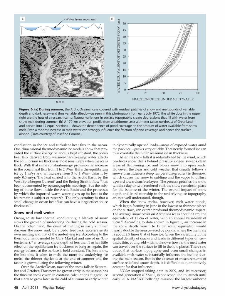
ThermodynamicsIn the heat-energy balance, which describes the gain or lossof heat in the system, sketched in figure 5, the solar and at-mospheric radiation terms dominate. Smaller in magnitudeare the latent and sensible heat transported across the Arcticboundaries by atmospheric circulation and the sensible heatcarried into the basin by the warm West Spitsbergen Currentand by the Pacific inflow through the Bering Strait.

The surplus flux of thermodynamic energy needed tocause the observed thinning of the ice during the past halfcentury is about 1 W/m2. (That flux is equivalent to a reduc-tion in ice thickness of approximately 0.1 m/year.) In this sec-tion, we summarize the gaps in our understanding of the at-mospheric and oceanic processes that are behind the surplus.

Ice–atmosphere interactions. Radiative energy fluxes

from the atmosphere and the annual advection of sensibleand latent energy from lower latitudes are two orders of mag-nitude larger than 1 W/m2. (Figure 5 illustrates those andother components of the mass and heat balance in the ArcticBasin.) At the moment, uncertainties in the heat-balancemeasurements observed at manned drifting stations and inthe meridional heat transport calculated from radiosonde(balloon-based) observations around the Arctic perimeterprevent researchers from resolving those heat fluxes to an ac-curacy required to attribute the surplus of heat to any partic-ular source or mechanism that explains the observed ice loss.7

Ice–ocean heat storage. During summer, when the iceconcentration is less than 100% and numerous melt pondscover the ice, some fraction of the radiative energy is tem-porarily stored in the exposed water and delays the onset offreezing in autumn. In areas of low ice concentration and lowalbedo, the energy causes melting at the bottom and laterallyaround the perimeter of the ice floes. Recent observations8

have found rates of ice-bottom melting as high as 1 m/month.Field observations of lateral melt are logistically difficult andlaborious; repeated measurements of the same ice floe overthe melt season are needed to characterize the process. Thefew reported measurements suggest that even thick ice floescan melt laterally up to several meters during summer,but the contribution of that process to the loss of MYI is not known.

One prospective approach for learning more about lat-eral melting is to mine the 1-m-resolution images collectedby intelligence satellites—the so-called National TechnicalMeans—and released to the public at http://gfl.usgs.gov. Thefixed- location images acquired since the summer of 1999 re-veal telling features of the ice surface. But studying the detailsof processes such as lateral melt will require sequential im-ages of the same ensemble of ice floes to trace the history ofsurface changes during the melt season. Samples of such ac-quisitions have recently been released on the abovementioned website.

Ice–ocean heat flux. The rate of basal ice growth or meltis proportional to the difference between vertical heat

Ice

Water

T,q

IRSolar

O

Runoff

Melt

Figure 5. The heat and mass balance of the Arctic Basin. Incoming solar radi -ation (blue) is partially reflected, ab-sorbed, and transmitted by clouds. Theradiation reaching the surface is thenpartially reflected and absorbed inamounts that depend on the albedo ofbare ice, open water (O), and numerousmelt ponds formed during summer.River runoffs from surrounding conti-nents feed the Arctic Ocean with freshwater. Infrared radiation (red) is emittedand absorbed by the clouds and thesurface. Some of the atmospheric watervapor condenses and falls as snow,adding to the mass of the ice. The gen-eral circulation of the atmosphere results in a net influx of sensible and latent heat (T and q) from lower latitudes. The outflow of ice is primarilythrough the Fram Strait.

40 April 2011 Physics Today www.physicstoday.org

conduction in the ice and turbulent heat flux in the ocean.One- dimensional thermodynamic ice models show that pro-vided the surface energy balance is kept constant, the oceanheat flux derived from warmer-than-freezing water affectsthe equilibrium ice thickness most sensitively when the ice isthick. With that same constant-energy provision, an increasein the ocean heat flux from 1 to 2 W/m2 thins the equilibriumice by 1 m/yr and an increase from 3 to 4 W/m2 thins it byonly 0.5 m/yr. The heat carried into the Arctic Basin by theWest Spitsbergen Current9 and the Bering Strait inflow10 hasbeen documented by oceanographic moorings. But the mix-ing of those flows inside the Arctic Basin and the processesby which the imported warm water gives up its heat to theice remain a subject of research. The only certainty is that asmall change in ocean heat flux can have a large effect on icethickness.11

Snow and melt waterOwing to its low thermal conductivity, a blanket of snowslows the growth of underlying ice during the cold season.On the other hand, the onset of melting in early summerdarkens the snow and, by albedo feedback, accelerates itsown melting and that of the underlying ice. According to thethermodynamic model by Gary Maykut and one of us (Un-tersteiner),12 an average snow depth of less than 1 m has littleeffect on the equilibrium ice thickness so long as, again, theenergy balance at the surface is held constant. The less snow,the less time it takes to melt; the more the underlying icemelts, the thinner the ice is at the end of summer and thefaster it grows during the following winter.

Over the Arctic Ocean, most of the snow falls in Septem-ber and October. Thus new ice grown early in the season hasthe thickest snow cover. In contrast, calculations suggest, icethat starts to grow later in the cold of autumn or early winter

in dynamically opened leads—areas of exposed water amidthe pack ice—grows very quickly. That newly formed ice canthus overtake the older seasonal ice in thickness.

After the snow falls it is redistributed by the wind, whichproduces snow drifts behind pressure ridges; sweeps cleanareas of flat, young ice; and blows snow into open leads.However, the clear and cold weather that usually follows asnowstorm induces a steep temperature gradient in the snow,which causes the snow to sublime and the vapor to diffuseupward toward surface layers. The process petrifies the snowwithin a day or two; rendered stiff, the snow remains in placefor the balance of the winter. The overall impact of snowdepth and its relationship to the underlying ice topographyare not well understood, though.

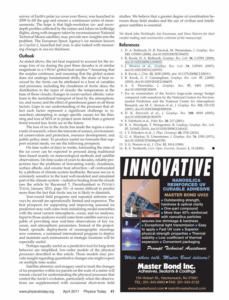
When the snow melts, however, melt-water ponds,which begin forming in June in the lowest or thinnest placeson the surface, can exert a profound thermodynamic impact.The average snow cover on Arctic sea ice is about 33 cm, theequivalent of 11 cm of water, with an annual variability of2 cm.13 According to data shown in figure 6, an increase inthe snow depth from 5 to 15 cm water equivalent wouldnearly double the area covered by ponds, where the melt rateis about 2.5 times that of bare ice. Given the variability in thespatial density of cracks and leads in different types of ice—thick, thin, young, old—it’s not known how far the melt watercan travel over the surface to fill in the low places. There’s nodoubt that surface topography and even small changes inavailable melt water substantially influence the ice loss dur-ing the melt season. But in the absence of measurements ofsurface relief and snow depth, it is difficult to quantitativelyaccount for that influence.

ICESat stopped taking data in 2009, and its successor,second-generation ICESat-2, is not scheduled to launch untilearly 2016. NASA’s IceBridge mission, the largest airborne

Water from snow melt

Ice

800 m

50

45

40

35

30

25

20

15

10

5

00 25 50 75 100

FRACTION OF ICE UNDER MELT WATER

WA

TE

RE

QU

IVA

LE

NT

OF

DE

PO

SIT

ED

SN

OW

(cm

)a b

Figure 6. (a) During summer, the Arctic Ocean’s ice is covered with residual patches of snow and melt ponds of variabledepth and darkness—and thus variable albedo—as seen in this photograph from early July 1972; the white dots in the upperright are the huts of a research camp. Natural variations in surface topography create depressions that fill with water fromsnow melt during summer. (b) A 170-km elevation profile from an airborne laser altimeter taken northeast of Greenland—and parsed into 17 equal sections—shows the dependence of pond coverage on the amount of water available from snowmelt. Even a modest increase in melt water can strongly influence the fraction of pond coverage and hence the surfacealbedo. (Data courtesy of Josefino Comiso.)

www.physicstoday.org April 2011 Physics Today 41

survey of Earth’s polar ice cover ever flown, was launched in2009 to fill the gap and ensure a continuous series of meas-urements. The hope is that high- resolution ice- and snow-depth profiles collected by the radars and lidars on IceBridgeflights, along with imagery taken by reconnaissance NationalTechnical Means satellites, may provide new insights into theproblem. The European Space Agency’s ice mission knownas CryoSat-2, launched last year, is also tasked with measur-ing changes in sea-ice thickness.

OutlookAs stated above, the net heat required to account for the av-erage loss of ice during the past three decades is of similarmagnitude to a 1-W/m2 global heat surplus.14 Assuming thatthe surplus continues, and assuming that the global systemdoes not undergo fundamental shifts, the share of heat re-ceived by the Arctic can be attributed to a host of variablesand processes, including the cloudiness of Arctic skies; thedistribution in the types of clouds; the temperature at thebase of those clouds; changes in ocean-surface albedo; varia-tions in the meridional transport of heat by the atmosphere,ice, and ocean; and the effect of greenhouse gases on all thosefactors. Gaps in our understanding of the processes that af-fect each factor represent a significant challenge to re-searchers attempting to assign specific causes for the thin-ning and loss of MYI or to project more detail than a generaltrend toward less Arctic ice in the future.

The loss of ice in the Arctic has made the region a cross-roads of research, where the interests of science, environmen-tal conservation and protection, resource development, andpublic policy meet. To produce useful ice forecasts that sup-port societal needs, we see the following prospects.

On time scales of days to weeks, forecasting the state ofthe ice cover can be expected to proceed along traditionallines based mainly on meteorological methods and satelliteobservations. On time scales of years to decades, reliable pro-jections face the problems of forecasting winds, cloudiness,surface albedo, and oceanic heat advection—all confoundedby a plethora of climate-system feedbacks. Because sea ice isextremely sensitive to the least well-modeled and simulatedpart of the climate system—radiative heating from the clouds(see the article by Raymond T. Pierrehumbert in PHYSICSTODAY, January 2011, page 33)—it seems difficult to predictmore than the fact that Arctic sea ice is likely to diminish.

Year-round field programs and repeated airborne sur-veys by aircraft are operationally limited and expensive. Thebest prospects for supporting and improving seasonal iceprediction may well come from initializing model ensembleswith the most current atmospheric, ocean, and ice analyses.Input to those analyses would come from satellite surveys ca-pable of providing near real-time observations of key ice,ocean, and atmospheric parameters. Instead of the project-based, sporadic deployments of oceanographic mooringsnow common, a sustained international program to deployand maintain such instruments at strategic locations will beespecially useful.

Perhaps equally useful as a predictive tool for long-termbehavior are simplified, low-order models of the physicalprocesses described in this article. Those models may pro-vide insight regarding quantitative changes one might expecton multiple time scales.

Satellite altimetry and imagery used to track the changesof ice properties within ice parcels on the scale of a meter willremain crucial for understanding the physical processes thatcontrol the Arctic’s evolution, particularly when the observa-tions are supplemented with occasional short-term field

studies. We believe that a greater degree of coordination be-tween those field studies and the use of civilian and intelli-gence satellites is essential.

We thank John Wettlaufer, Ian Eisenman, and Steve Warren for theircareful reading and constructive criticism of the manuscript.

References1. D. A. Rothrock, D. B. Percival, M. Wensnahan, J. Geophys. Res.

113, C05003 (2008), doi:10.1029/2007JC004252.2. R. Kwok, D. A. Rothrock, Geophys. Res. Lett. 36, L15501 (2009),

doi:10.1029/2009GL039035.3. J. Stroeve et al., Geophys. Res. Lett. 34, L09501 (2007),

doi:10.1029/2007GL029703.4. R. Kwok, J. Clim. 22, 2438 (2009), doi: 10.1175/2008JCLI2819.1. 5. R. Kwok, G. F. Cunningham, Geophys. Res. Lett. 37, L20501

(2010), doi:10.1029/2010GL044678.6. A. S. Thorndike, J. Geophys. Res. 97, 9401 (1992),

doi:10.1029/92JC00695.7. For an examination of the Arctic’s large-scale energy budget

compared with reanalysis by the National Centers for Environ-mental Prediction and the National Center for AtmosphericResearch, see M. C. Serreze et al., J. Geophys. Res. 112, D11122(2007), doi:10.1029/2006JD008230.

8. D. K. Perovich et al., J. Geophys. Res. 108, 8050 (2003),doi:10.1029/2001JC001079.

9. E. Fahrbach et al., Polar Res. 20, 217 (2001).10. R. A. Woodgate, T. Weingartner, R. Lindsay, Geophys. Res. Lett.

37, L01602 (2010), doi:10.1029/2009GL041621.11. I. V. Polyakov et al., J. Phys. Oceanogr. 40, 2743 (2010).12. G. A. Maykut, N. Untersteiner, J. Geophys. Res. 76, 1550 (1971),

doi:10.1029/JC076i006p01550.13. S. G. Warren et al., J. Clim. 12, 1814 (1999).14. K. E. Trenberth, Curr. Opin. Environ. Sustain. 1, 19 (2009). ■

154 Hobart St., Hackensack, NJ 07601TEL: 201-343-8983 ■ FAX: 201-343-2132

www.masterbond.com ■ main@masterbond.com

NANOSILICAREINFORCED UV

CURABLE ADHESIVEMASTER BOND UV22

■ Outstanding strength, hardness & optical clarity■ One-part compound■ More than 40% reinforcedwith nanosilica particles

assures low shrinkage & hardness■ Exceptional light transmission ■ Easy to apply ■ Fast UV cure ■ Superior physical strength properties ■ Thermalstability ■ Low coefficient of thermalexpansion ■ Convenient packaging

Prompt Technical Assistance

I N NOVATIVE

While others talk, Master Bond delivers!