Pan-Arctic simulation of coupled nutrient-sulfur cycling due to sea ice biology: Preliminary results

Pan-Arctic simulation of coupled nutrient-sulfur cycling due to seaice biology: Preliminary results

S. Elliott,1 C. Deal,2 G. Humphries,3 E. Hunke,1 N. Jeffery,1 M. Jin,2 M. Levasseur,4

and J. Stefels5

Received 9 January 2011; revised 8 June 2011; accepted 16 September 2011; published 15 February 2012.

[1] A dynamic model is constructed for interactive silicon, nitrogen, sulfur processing inand below Arctic sea ice, by ecosystems residing in the lower few centimeters of thedistributed pack. A biogeochemically active bottom layer supporting sources/sinks for thepennate diatoms is appended to thickness categories of a global sea ice code. Nutrientstransfer from the ocean mixed layer to drive algal growth, while sulfur metabolites arereinjected from the ice interface. Freeze, flux, flush and melt processes are linked tomultielement geocycling for the entire high-latitude regime. Major element kinetics areoptimized initially to reproduce chlorophyll observations, which extend across the seasons.Principal influences on biomass are solute exchange velocity at the solid interface, opticalaveraging in active ice and cell retention against ablation. The sulfur mechanismencompasses open water features such as accumulation of particulate dimethylsulfoniopropionate, grazing and other disruptive releases, plus bacterial/enzymaticconversion to volatile dimethyl sulfide. For baseline settings, the mixed layer trace gasdistribution matches sparging measurements where they are available. However,concentrations rise to well over 10 nM in remote, unsampled locations. Peak contributionsare supported by ice grazing, mortality and fractional melting. The model bottom layeradds substantially to a ring maximum of reduced sulfur chemistry that may be dominantacross the marginal Arctic environment. Sensitivity tests on this scenario include variationof cell sulfur composition and remineralization, routings/chemical time scales, and thephysical dimension of water layers. An alternate possibility that peripheral additions aresmall cannot be excluded from the outcomes. It is concluded that seagoing dimethyl sulfidedata are far too sparse at the present time to distinguish sulfur-ice production levels.

Citation: Elliott, S., C. Deal, G. Humphries, E. Hunke, N. Jeffery, M. Jin, M. Levasseur, and J. Stefels (2012), Pan-Arcticsimulation of coupled nutrient-sulfur cycling due to sea ice biology: Preliminary results, J. Geophys. Res., 117, G01016,doi:10.1029/2011JG001649.

1. Introduction

[2] The aerosol precursor molecule dimethyl sulfide isdistributed inhomogeneously through waters of the marginalice zone, but may act as a strong source of reduced sulfur tothe Arctic atmosphere under many circumstances (DMS)[Ferek et al., 1995; Lundén et al., 2007]. Production dis-tributions for polar DMS have not been clarified, and mustinclude contributions from both ice algae and phytoplanktonin the water column [Levasseur et al., 1994; Matrai et al.,

2007]. We demonstrate here by attaching multielementgeochemical cycles to a dynamic/thermodynamic sea icemodel that epontic ecosystems could play a significant role,on a regional and seasonal basis. Essential nutrient and sul-fur flow are coupled in our computations through a set ofporous bottom layer kinetics simulations, with radiationinputs arriving from above through geographically distrib-uted columns of snow and ice. Optimization tests on eco-dynamics of the major elements serve to reduce the numberof broad biogeochemical scenarios, while variations in themodel sulfur mechanism show that ice-derived peaks ofgreater than 10 nM are possible in remote areas. It becomesclear in the process, however, that measurement data arepresently much too sparse and uncertain to permit a truequantification of error.[3] Our development begins with individual descriptions

of the program components. Some history and an overviewof capabilities are provided for the dynamic sea ice modelCICE [Hunke and Lipscomb, 2008; Hunke and Bitz, 2009].Since the biogeochemistry involved becomes quite detailedwhether regarding nutrients or the sulfur compounds,

1Climate Ocean Sea Ice Modeling, Computational Sciences Division,Los Alamos National Laboratory, Los Alamos, New Mexico, USA.

2International Arctic Research Center, Institute of Marine Science,University of Alaska Fairbanks, Fairbanks, Alaska, USA.

3Institute of Arctic Biology, University of Alaska Fairbanks, Fairbanks,Alaska, USA.

4Department of Biology, Laval University, Quebec, Quebec, Canada.5Laboratory of Plant Physiology, Center for Life Sciences, University of

Groningen, Groningen, Netherlands.

Copyright 2012 by the American Geophysical Union.0148-0227/12/2011JG001649

JOURNAL OF GEOPHYSICAL RESEARCH, VOL. 117, G01016, doi:10.1029/2011JG001649, 2012

G01016 1 of 16

http://dx.doi.org/10.1029/2011JG001649

background information is condensed into a set of appen-dices (Appendix A for parameters and Appendix B forequations). These are organized to emphasize our segrega-tion of the reaction scheme into three layers or box models,all positioned just below CICE thickness categories. Thenumerical layers are assigned to represent nutrient injectionsfrom the water column source, processing in a well mixed icevolume and finally product buildup below the pack(Figure 1). The complete mechanism is subjected to meritfunction analysis, against selected bottom ice chlorophyllmeasurements (Table 1). We are careful to point out, how-ever, that the procedure is nonglobal in its treatment of theparameter structure. Fine points of the epontic sulfur cyclingare almost entirely unknown, and so we add them bydrawing upon open water research along with some veryrecent ice core data [Stefels et al., 2007; Hellmer et al.,2008]. Variations are then imposed upon likely stronguncertainties, including average algal composition and lossrates during routing through or below the bottom layer(Table 2). Physical configuration of the model is adjustedsystematically as well, through vertical dimensions of the

several chemical models which form the core of theapproach (Appendices A and B).[4] The trace element-ice simulations culminate in a set

of distributions for dissolved dimethyl sulfide, a key agentof natural mass transfer to atmospheric particles [Charlsonet al., 1987; Ferek et al., 1995; Lundén et al., 2007].Annular features surrounding the Arctic and local con-centrations up to tens of nanomolar are computed for heavilyimpacted surface waters. Even in a baseline case we showthat the occasional well-studied ecosystem may be repre-sented with fidelity and simultaneously, high concentrationsare indicated on the periphery. But while one subset of sen-sitivity tests raises the maxima further, for others there is apotential dominance of external sources. DMS is among asmall set of marine precursors influencing hygroscopicity ofthe remote aerosol, and hence also cloud droplet numbers[Andreae and Rosenfeld, 2008]. Effects on climate via thealbedo are global in scope, but the importance is amplified athigh latitudes [Zhou et al., 2001]. Although system simula-tions including ice biogeochemistry can now be used tobracket the uncertainties, we find that much more extensive

Figure 1. Schematic of coupled nutrient-reduced sulfur biogeochemistry attached to the CICE sea icemodel in the present work. Solid rectangles and arrows indicate actual numerical tracers and the kineticterms computed to interrelate them. Dashed quantities and arrows are dealt with implicitly or indirectly.Silicate uptake leads to formation by the pennate (ice) diatoms of frustules, one of the untracked materials.A portion of ablation from the biologically active layer is released directly into the water column. “Zoo”stands for zooplankton. Chlorophyll, carbon and particulate reduced sulfur concentrations are maintainedproportional to ice algal nitrogen. Single trace element conversion reactions are shown internal to themultiple tracer boxes. Mixed and product layers are distinguished so that the latter can be thinned sepa-rately to reflect freshwater lensing.

ELLIOTT ET AL.: NUTRIENT-SULFUR CYCLING IN ARCTIC ICE G01016G01016

2 of 16

measurements of reduced sulfur are needed both in the packand in Arctic seawater.

2. Ice Dynamics and BiogeochemistryConnections

[5] Sea ice physics adopted here is that of the Los AlamosNational Laboratory CICE model version 4 [Hunke andLipscomb, 2008]. Coding descends directly from turn of thecentury viscous-plastic rheologies but with an elastic wavemechanism introduced that allows for explicit numerics andan accurate representation of the response to stress variations[Hunke and Dukowicz, 1997]. The method has ultimatelybeen termed EVP for elastic-viscous-plastic, and it yieldshigh fidelity results for the global pack field on short time-scales. The basis for incorporating waves is actually non-physical, but they render CICE especially well suited to theparallel supercomputing requirements inherent in modern

environmental simulations. Components interacting withinthe code include a thermodynamic subunit that computeslocal growth rates of snow and ice due to vertical conductive,radiative and turbulent fluxes [Bitz and Lipscomb, 1999].Incremental remapping transport provides for the advectionof areal concentration, ice volumes and other state variables[Lipscomb and Hunke, 2004]. A ridging parameterization isinvoked to move masses of ice among thickness categories,based on energetic balance considerations and rates of strain[Lipscomb et al., 2007]. Over the last decade the CICE pro-gram has become standard within a major U.S. Earth Systemcode, the CCSM or Community Climate System Model[Briegleb et al., 2004; Collins et al., 2006].[6] In the present work, CICE is configured as a stand

alone framework consistent with the latest, optimized Arcticcoverage evolution experiments [Hunke, 2010]. The year1992 was chosen as our focus, from a run extending acrossseveral decades of the late twentieth century. It is both

Table 1. A Subset of Collected Master Data Including Chlorophyll Measurements in Arctic Bottom Ice (mg/m2) and Dimethyl SulfideDetermined by Sparging in Subinterfacial Waters (nM)a

Okh Lab Ber Chu Can Baf Sva Gyr TPD

JanFeb 40Mar 10–30 100 5 0.01Apr (100) 15

11–10 10

May 10–100 100–300 20 0.1–1Jun 10Jul .03–0.3Aug 0.3 0.1

10.3–1

10.1–1

0.3Sep 0.1–1

0.1Chl K97, M00 I90 D10, G99,

G09G97, G05,G09, U03

G99, G05, L94,M96, S97

L01 G97, G99, W07 G97, G05,G09, L99

G97, G99,LP96, L99

DMS F95 F95 LP96 L99 LP96, L99

aChlorophyll measurements are shown in italics and dimethyl sulfide values in bold. Entries are arranged chronologically downward but arrayed against abiogeography derived from Carmack and Wassman [2006] as adapted in our primary production work [Deal et al., 2011]. The ecozones are arrangedroughly in latitudinal rank order. Most concentration values were first averaged then rounded to a final, single significant digit. Parentheticals arediscussed only indirectly in the primary sources. Regional abbreviations are as follows: Okh, Sea of Okhotsk; Lab, Labrador Sea; Ber, Bering Sea; Chu,Chukchi Sea; Can, Canadian Archipelagic; Baf, Upper Baffin Bay; Sva, Svalbard and neighboring areas of the Greenland/Iceland/Norway Seas; Gyr, theBeaufort Gyre; and TPD, Transpolar Drift currents. Reference abbreviations are as follows: D10, Deal et al. [2011]; F95, Ferek et al. [1995]; G97,Gosselin et al. [1997]; G99, Gradinger [1999]; G05, Gradinger et al. [2005]; G09, Gradinger [2009]; I90, Irwin [1990]; K97, Kudoh et al. [1997];LP96, Leck and Persson [1996]; L01, Lee et al. [2001]; L94, Levasseur et al. [1994]; L99, M. Levasseur, unpublished but cited in Sharma et al.[1999]; M96, Michel et al. [1996]; M00, Monfort et al. [2000]; S97, Suzuki et al. [1997]; U03, Uzuka [2003]; and W07, Werner et al. [2007].

Table 2. A Selection From Among Sensitivity Calculations Conducted to Explore Uncertainties in the Sulfur Cyclinga

Variation

Category

Composition Routings Interchange Timing Physical

Specific S/N Ratio Graze (several) Mortality (recycle) Biomass return S e-fold (several) Box height (ice, below)Layer(s) Bottom Bottom Bottom Bottom to product Bottom and product Bottom and productSymbol RS2N fex frem frtr t lbot

Baseline 0.03 0.5 1.0 0.1 10 d 0.03 mTest 0.1 0.1 off 0.3 3 d 0.1 mDDMSpr Up ∝ Down 10s % Down 100s % Up 10s % Down 3–5�, except center SmallLocation Periphery Blooms Blooms Melt Periphery AllSymbol fsp frtr Εxclude tdis lpr

Baseline 0.5 0.1 10 d 10 mTest 0.1 1.0 3 d 3 mDDMSpr Down 10s % Up 100s % Down 3–5� Up ∝Location Blooms Melt All Periphery

aSymbols are defined in the parameter list in Table A1. Dimensionless quantities dominate toward the left side of the table, where emphasis is placedupon mole fractions and routings. Thereafter time and length units are indicated as appropriate. Product layer DMS concentration is the final gauge formajor effects.


3 of 16

proximal to a period of intense sulfur measurement activity[e.g., Levasseur et al., 1994; Ferek et al., 1995], and typicalof the Arctic situation prior to recent ice minimum years. Allsimulations were initialized in deep winter on the first ofJanuary and include full monthly variability over the fourseasons. Results are taken from year one of a given run.Reseeding and overwintering mechanisms remain grosslyunderstudied for the global ice biota and so they are notincorporated [Arrigo and Thomas, 2004; Werner et al.,2007]. We propose to investigate interannual variability inmore specialized studies.[7] Contemporary Arctic ice biogeochemistry is confined

largely to the bottom few centimeters of the column in anygiven location [Levasseur et al., 1994; Gradinger, 1999;Arrigo, 2003; Gradinger et al., 2005]. We therefore attachedour geocycling scheme below the deepest CICE verticaldivision, in a series of kinetic box models of constant vol-ume. The reactor layers represent respectively (1) input ofthe nutrients silicate, nitrate and ammonia from a data ocean,(2) nutrient and carbon cycling in the bottom ice itself, andfinally (3) sulfur compounds ejected back into the watercolumn. Mixed and product layer boxes are separated so thattheir thicknesses can be varied independently during themelt season, when thin brackish lenses may form just belowthe solid interface. Nutrients are consumed by the ice systemand also replenished through remineralization. They can berestored to climatology through an adjustable time constantwhose value is discussed in the optimization section. Theseveral kinetic models carried as layers underneath CICE arecomputed on all thickness categories. Transport and geo-graphic variation are thus experienced by the biology alongwith modulation of the radiation field by snow and ice.Tracer concentrations reported and plotted are grid cellaverages, over all categories and percent coverages.

3. Biogeochemistry Model

[8] Multiple element geocycling added to CICE in thepresent work is shown schematically in Figure 1, whichexplicitly segregates the three reactor volumes employed.A geophysical context is displayed for each layer type, withrespect to sea ice or underlying ocean waters. Note that thereare no interactions in the current work with sediments, thecontinental shelf or with terrestrial processes. In the Pan-Arctic ocean to ice grid framework adopted, biogeochemistryactually rides underneath individual pack thicknesses. Themixed layer appears twice in the figure merely as a plottingconvenience; in fact it is represented as a single entity withinthe numerics. Parameter settings and the equations repre-sented by box-arrow relationships are summarized in twoappendices. These refer primarily to a baseline case. Sensi-tivity testing is discussed in detail in section 6.[9] Basin scale nutrient distribution patterns within the

mixed layer were supplied to the model from availableArctic climatologies [HAAO, 2001; Conkright et al., 2002].The three main inorganic forms then equilibrate quickly intothe bottom layer by mutual fluxing (nitrate, ammonium andsilicate) [Reeburgh, 1984]. As sunlight becomes available atincreasing latitudes, photon restrictions are lifted and thevarious fertilizers may be consumed from within the iceduring photosynthesis [Lavoie et al., 2005; Jin et al., 2006].Internal populations of the algae rise quickly as tracked

through their chlorophyll density, so that modeled uptake ofthe solutes soon outstrips backflow to the mixed layer. Inmost regions this leads to a fundamental flux limitation onthe accumulation of biomass at the pack interface. The meltseason initiates a bottom layer purge due to snow/surfacedrainage, and this excludes all solutes [Vancoppenolle et al.,2010]. Organisms may be detached to varying degrees ofeffectiveness by the flush purge and also by continualablation.[10] Reduced sulfur chemistry is based on the assumption

that the precursor compound DMSPp (dimethyl sulfonio-propionate in particulate form) [Stefels, 2000] is synthesizedand removed inside of ice algal cells in exact proportion tothe main nitrogen currency. Rising S is later released bygrazing and mortality processes into a decay sequencefamiliar from open waters [Stefels et al., 2007]: DMSPd(dissolved) is oxidized by free lysis enzymes plus bacteria tothe volatile DMS (also dissolved, but this is traditionallyunspecified). Time constants for the sequence are derivedhere mainly by applying a crude temperature slowdownrelative to global averages [Kiene and Bates, 1990; Leck andPersson, 1996; Stefels et al., 2007]. But they are entirelyconsistent with recent ice core studies with which one of ushas been closely involved (J. Stefels, unpublished data, butsee Hellmer et al. [2008] for a cruise summary). Once thedecay series is established in simulated bottom ice, dissolvedsulfur forms pass freely to and from the product layer.[11] Polar DMS measurement campaigns are often also

associated with chlorophyll determinations, and a steadybackground of below-ice biological activity is typicallyrecorded [Levasseur et al., 1994; Leck and Persson, 1996].Usually between 0.1 and 1 mg/m3 of pigment are indicatedand attributed to one of the nondiatom phytoplankton classes(e.g., flagellates; note that epontic algae are represented aspennate). In the model product layer, a reference chlorophylllevel is thus maintained such that average cell disruption andoxidation time scales produce about a nanomolar of DMS.These values are forced externally, and function here mainlyto provide a background in accord with the rare observations.

4. Data Sets

[12] We collected data for refinement of the model systemby first seeking sulfur studies which also characterized thelocal biota, then extending to several icebreaker cruises. Forice bottom chlorophyll the values obtained in this mannerare relatively numerous, but our survey is necessarily onlypartially complete. We obtain a Pan-Arctic band of valuesconcentrated in bloom seasons and categorized biogeo-graphically in Table 1. The data clearly show a well knowntrend toward tens of mg/m2 at maximum along coastlines[Gradinger, 1999; Arrigo, 2003], plus a central oceanbackground which is orders of magnitude less concentratedbut significant nonetheless [Gradinger, 1999]. Primaryproduction measurements have been less extensive thanthose of biomass for the ice system [Arrigo, 2003], and theyare not included in the validation process for the presentwork. Please see the companion piece from our group [Dealet al., 2011] for a more complete discussion of biologicalproduction distributions.[13] The sulfur situation contrasts starkly with that of the

pigment data. Measurements are sparse to begin with, and


4 of 16

their interpretation is complicated by analytical chemistryproblems which have only been understood in the last fewyears. There is a tendency for filtration to rupture algalcells, whether in open water or ice investigations. Thisinter-converts the critical quantities DMSPp and d [Kieneand Slezak, 2006], so that only their sum is known accu-rately. From the most intense period of ice-sulfur study inthe middle nineteen nineties [e.g., Levasseur et al., 1994;Ferek et al., 1995; Leck and Persson, 1996] many mea-surements must now be viewed merely as limits for thesetwo species [Michaud et al., 2007]. The reported totalDMS(P) data are more trustworthy [e.g., Uzuka, 2003], andDMS determinations conducted directly by gas sparging arestill considered to be reliable. We insert the available purg-ing data for under-ice DMS alongside those of the bottomlayer chlorophyll, in the same table. After regional averagingprocedures are applied as described in the caption, only ahandful of points remain. In fact, we add to the availableliterature a set of results which have never before beenpublished. The new data were obtained by one of us on acircum-continental study of the North American sulfur cycle[M. Levasseur in Sharma et al., 1999], and they are criticalto the current process.[14] Total measurements can indeed be located or partially

reconstructed for the methylated sulfur compounds belowan ice interface, or within the solid matrix (DMSP + DMS)[e.g., Levasseur et al., 1994; Lee et al., 2001; Uzuka, 2003].But as a rule these quantities are also rare and poorly docu-mented. Moreover, the artifact restrictions make all suchresults difficult to analyze for present purposes. Master listsof compiled sulfur chemistry information are available fromthe authors on request, but for the moment any data beyondthe stripped DMS will be discussed explicitly only as theneed arises. In general, our assessment is that the chlorophyllcollection of Table 1 may be up to the task of adjusting majorfeatures of the overall ice biogeochemistry model, whilesulfur measurements must for the moment serve mainly as aguide to future needs.

5. Optimization

[15] The model was configured at the outset to produce aminimum of biological activity, for example by reducingsolute (flux) piston velocities to the brine exchange rate, andby ignoring reseeding [Wakatsuchi and Ono, 1983; Werneret al., 2007]. A stepwise selection procedure was then per-formed in order to establish a baseline [Gunst and Mason,1980]. Stages in the calculation were organized chronolog-ically to optimize model performance across the evolvingseasons (Table 1). Parameters were prioritized for theirimportance to the system based mainly on expert judgment.They were then tuned to match the chlorophyll data, asjudged by a minimum absolute error calculation performedrelative to log transformed values [Zar, 1984].[16] Startup concentrations of the algae were varied first

and proved to be inconsequential, since exponential growthleads quickly to nutrient limitation. The mixed to bottomlayer exchange velocity was then raised from the brineturnover rate upward, to account for boundary layer influ-ences on the thickness of laminar entry barriers [Niedrauerand Martin, 1979; Wakatsuchi and Ono, 1983]. The inter-change is treated in all our simulations as a Pan-Arctic

average, since our emphasis is on trace gas distributions. Inthe real ocean it will be faster coastally due to tides andregional currents [Cota and Horne, 1989; Gradinger, 1999;Lavoie et al., 2005]. The value 0.1 m/d has been judgedmaximal based on local, low dimensionality studies [Lavoieet al., 2005], and this was not exceeded. Basin scale nutrientpatterns are supplied by the geochemical climatologies[HAAO, 2001; Conkright et al., 2002]. Initially they wereallowed to drift per the concentration change equations.Reducing the restoration time, however, raised pigment dis-tributions into agreement with data all the way up to the meltperiod. Ultimately the reset was lowered to zero days, so thatmodel produced fluxes do not alter the oceanic distributions.Integrated vertical averaging of bottom layer radiation causedchlorophyll maxima to exceed the measured range in somelow latitude seas [Arrigo, 2003], and so it was replaced byBeer’s Law. We thus make the implicit assumption thatphotosynthesis shifts gradually toward lower portions of thebottom layer [Niedrauer and Martin, 1979; Smith et al.,1990]. This amounts to a self-shading approach [Arrigoet al., 1993].[17] Rapid flushing of the nutrient and sulfur solutes is a

given [Reeburgh, 1984; Jin et al., 2006], but removal of thealgae themselves at the melt led to sharp biomass crashesand an inadequate autumn recovery (low populations late inthe year). Although steep declines are observed in somestudies [Jin et al., 2006], others suggest retention. The mixof scenarios over the polar regime is probably actually quitecomplex [Gosselin et al., 1997; Gradinger, 1999; Uzuka,2003]. Organisms may seek refugia within the porousstructure of ice and also rely on surface chemistry to main-tain or improve their position [Krembs et al., 2000; Arrigoand Thomas, 2004]. We elected in the present work totreat algal removal mainly as a portion of and proportion toablation, or equivalently as an adjustable time constant. Stillthe autumn rebound appeared to be slow and so we intro-duced a hard floor on biomass nitrogen levels (a lower limitthat could not be bypassed). The intent was to simulate acombination of overwintering and the formation of cysts[Werner et al., 2007].[18] Through these manipulations we were able to obtain

an ice chlorophyll distribution agreeing with the Table 1 datato within a factor of two in most locations, and often muchmore closely. This simulation is defined henceforward as ourbaseline, and it is the one described most directly in theappendices. We recognize, however, that solutions to thestepwise optimization problem are non-unique and can beproblematic at environmental scales [Gunst and Mason,1980; Elliott, 2009]. The radiation and algal flushing treat-ments are particularly uncertain and could depend on theorder of parameter refinement; for example, a rapid earlypurge might well preclude the need for internal shading.Such complexities were treated through independent testsconducted off line relative to the sulfur cycle.

6. Sensitivity Tests

[19] A series of parameter adjustment experiments wasarranged in order to probe the wide variety of uncertaintiesin sulfur biogeochemistry pathways. A subset is listed withqualitative descriptors of the major outcomes in Table 2.Several broad testing categories are identified: algal


5 of 16

composition, routings and fractional exchange, time con-stants, and the dimensionality of the physical system itselfwere all manipulated systematically. It became apparentearly on that concentration swings would regularly be strongfor the major indicator, below-ice DMS. To simplify thesituation, we adopted an informal strategy of alternatingbetween parameter changes leading to increases anddecrements.[20] The first variation attempted was upon the Redfield-

type sulfur to nitrogen ratio, for organisms dwelling insidethe bottom layer. Ice is often portrayed as a stressful mediumfor algal growth [Levasseur et al., 1994; Ferek et al., 1995;Lee et al., 2001; Stefels et al., 2007]. But in fact this char-acterization is more apt for brine intensive upper level eco-systems, and these are somewhat disperse in the Arctic[Gradinger, 1999; Arrigo and Thomas, 2004]. Bottom iceconditions are favorable, since temperature and salinity areconstrained to remain close to values for surface seawater.Nevertheless drainage and flushing will push epontic algaeto osmotic extremes on occasion, and so we vary the sulfurcontent within constraints imposed by the few studies whichcan be readily interpreted to provide particulate mole ratios[e.g., Levasseur et al., 1994; Uzuka, 2003]. This meansroughly a factor of three in either direction. Dimethyl sulfidetends to track the composition of its source, but with dilu-tions superimposed from the central ocean background.[21] The cascade of routings adopted to represent cell

disruption is an especially ad hoc feature of the presentmodel (Appendix B). Care has been taken to remain close toa straightforward mechanism pioneered by Arrigo et al.[1993], then propagated indirectly in related later works[e.g., Jin et al., 2006]. Grazing is treated as a small, steadyportion of the growth rate with constant fractions redis-tributed across the nitrogen cycle. Simplicity of the methodis the primary recommendation, since it is doubtful thatactual ice ecosystems exhibit such regularity. But alternateapproaches are not readily available and marine biologysimulators are typically developed with constant yields,whether at low or high latitudes [Archer et al., 2004;Vallina et al., 2008; Lavoie et al., 2009]. Fractionationswithin the network were adjusted systematically in allpathways flowing from grazing and mortality. But effectsproved to be most important for the mortality term. It isapportioned in the model only once, and further, co-varieswith biomass rather than merely tracking primary produc-tion. The grazing channel by contrast becomes flux limitedand is eventually outpaced; nutrient restrictions are feltimmediately through Michaelis Menten limitation functions.[22] Pure time constants t occur in both the bottom and

product layer sulfur decay sequences, and also as a celldisruption rate in the under-ice reference flow. Conversionand oxidation reactions enfold complex processes involvingmediation by a variety of bacteria and free enzymes [Kieneet al., 2000; Stefels et al., 2007]. Under-ice disruptionreally involves the same suite of channels illustrated inFigure 1. Since all these time scales were slowed intention-ally relative to the global situation to attain a baseline, theywere tested later by simultaneous downward perturbation.An interesting nonlinearity was quickly observed. In someregions concentrations of DMS fell by more than the rateproportionality. In section 7 we will attribute this effectto kinetic pathway shifts internal to the bottom layer.

Furthermore, it was realized at this point in the experimentthat background injections should be treated independentlyfrom the overall water column metabolism. The magnitudeof the reference source was thus fixed (product layer celldisruption maintained at 10 days). The central plateau of theDMS field became flexible under this combination ofsettings.[23] Physical aspects of the code were varied over and

above the biogeochemical tests just described. Flushing ofthe ice algae led to lengthy population dips reflected instrong losses of DMS in the summer. Return flow fromeither the purge or ablation could be adjusted to alter gasconcentrations in the melt season. As detailed in section 5,integration of light fields over the whole bottom layer led tounrealistic bloom peaks. The sulfur content followed suit.Mixed, bottom and product layer vertical dimensions wereeach adjusted in turn. Key results from these height/volumealterations are outlined at the right side of Table 2. Since icealgae usually do not succeed in depleting nutrients before thebreak up [Gradinger, 1999; HAAO, 2001], thickness of thesource pool proved inconsequential. The baseline run entailsinstantaneous restoration in any case. Perhaps surprisingly,depth of the bottom layer also turned out to be a neutralfactor. Our interpretation is that under flux input limitation,all action centers on the interface whether it regards primaryproduction or the eventual return of sulfur. Thinning of theproduct layer concentrated the outflow precisely as would beexpected; the factors tested ranged up to an order of mag-nitude. Several lines of argument suggest that intermittentfresh water caps should form in the marginal zone [Gosselinet al., 1990; Matrai et al., 2008], but in view of the ice-breaker data at our disposal the baseline setting of ten metersseems reasonable (Appendix A) [Leck and Persson, 1996;Gosselin et al., 1997].

7. Analysis

[24] Pan-Arctic plots generated from the nutrient elementand sulfur simulations are organized as follows. The fourcentral months of a baseline year are presented first, juxta-posing the columnar ice biomass and mixed layer dimethylsulfide concentrations. Changes in the under-ice DMS arethen analyzed for key test scenarios. In many cases reducedsulfur remains behind in surface waters of the mixed layer asthe ice edge retreats, forming a residual field. This spreadingeffect is dealt with in this section as well. Sensitivity testresults are presented only for the months of May andAugust, bounding the period of most intensive geochemicalprocessing. All results are shown as monthly averages.[25] In Figures 2 and 3 bottom algal chlorophyll and

product layer DMS are shown side by side in May/June, thenJuly/August. Poleward of the Arctic circle, sunlight onlybecomes available to support photosynthesis well past theequinox. May typically represents the peak in modeled icebiomass in more thoroughly studied regions, which arescattered along the Canadian Archipelago and North Amer-ican coast [Cota and Horne, 1989; Levasseur et al., 1994;Ferek et al., 1995]. As one would expect based on our meritcomparisons, peripheral chlorophyll ranges up to about onehundred mg/m2, while values in the central ocean basinhover near unity. Local maxima are correlated mainly withmixed layer nutrient distributions, and anticorrelated with


6 of 16

snow cover [Lavoie et al., 2005; Jin et al., 2006]. The bloomannulus tends to roll inward toward the pole as a function oftime in simulations such as these, following integratedradiation penetration.[26] DMS distributions in our baseline mechanism are

closely related to the modeled primary production and/orbiomass, but are not strictly proportional to them. A term-by-term breakdown of the equations in Appendix Bdemonstrates that during the early period of rapid chloro-phyll accumulation, release by the grazing fraction is dom-inant. The in-ice mortality channel soon takes precedence,however, and this mitigates to some extent the difficultiesassociated with a constant, steady apportionment (see section 6and Appendix B). Both pathways inject DMSPd into thebottom few centimeters of the solid matrix, with rapid fluxremoval into the mixed layer followed by conversion toDMS. Melting augmentation of below-ice buildup occursearly on at low latitudes, via partial sloughing of cells andthen their (implicit) disruption below the ice. Maxima dis-played in Figures 2 and 3 can be attributed to the conjunctionof these sources and reach up to 30 nM.[27] Peaks in the mixed layer sulfur distribution are critical

features of the simulation, because they may directly aug-ment flow to the atmosphere from margins or leads [Fereket al., 1995; Lundén et al., 2007]. It can be shown byapplying analytical reaction/transport calculations to theseasonal permeability [Vancoppenolle et al., 2010] that directescape through the solid matrix will be rare except for thin

or warming (porous) systems. For most central basin andland-fast pack ice, solute movement is suppressed by brinechannel closure during winter, and then by downwardflushing during the melt [Jin et al., 2006]. Leads, however,form continually along the periphery and appear deep in theocean center during summer. DMS produced under such anetwork of openings will rapidly be available for sea-airtransfer [Ferek et al., 1995; Matrai et al., 2007].[28] A 15% ice concentration contour is indicative of the

pack edge [e.g., Hunke and Bitz, 2009], and this is repre-sented explicitly on all our plots. Algal production willcontinue for tens of kilometers on either side of this semi-arbitrary threshold, both in the model and reality. On theseaward side, horizontal transfer to open water becomesespecially fast. Sulfur interconversion via lyase enzymes andthe oxidation each require ten days in our baseline model(see Appendices A and B), so that compounds sourced fromthe bottom layer can be transported for weeks in open water.Note that the field of ice-derived DMS often lingers wellbeyond that of chlorophyll in the figures. No attempt is madehere to simulate the dynamics of sea-air transfer, but the timeconstant for the process is roughly days to several weeks sothat it will be competitive with oxidation [Stefels et al.,2007; Elliott, 2009].[29] It is clear from the sequence of images in Figures 2

and 3 that our optimized mechanism produces volatile sul-fur concentrations in excess of several nanomolar in manylocations. The distribution takes the form of a punctuated

Figure 2. Baseline simulation of ice algal source organisms, (left) log10 mg/m2 chlorophyll, along withdimethyl sulfide injected into the ocean product layer, (right) log10 nM, in May and June of 1992. Iceedges are defined by the 15% ice concentration contour (white), and thicknesses are superimposed inmeters (black).


7 of 16

band of activity ringing the ice zone and also extendingpoleward for some distance. On the logarithmic color bar,yellow tones and brighter correspond roughly with con-centrations comparable to those measured in open northernwaters (3 nM is a reasonable reference point) [Leck andPersson, 1996; Kettle and Andreae, 2000; Matrai et al.,2007]. Thus one particularly compelling scenario whichemerges from our exercise is the following: an imperfectpolar cap only partially contains strong and somewhatunexpected sources of a critical, climate-influencing tracegas. This result is consistent with arguments from the sem-inal work of Levasseur et al. [1994] and follow-ons [Fereket al., 1995; Sharma et al., 1999; Lee et al., 2001], whichdiscuss the concept of polar pulses of reduced sulfur to thetroposphere.[30] The DMS database is so sparse, however, that it is

difficult to achieve any degree of validation. Early spargingsamples taken below the ice off coastal Alaska and Canada inspringtime suggest concentrations of between 1 and 10 nM[Ferek et al., 1995]. Icebreaker cruises give convincingevidence for a steady background of 0.1 to several nMbeneath the central pack, extending along the prime meridianand across the pole [Leck and Persson, 1996; Sharma et al.,1999]. Unpublished data associated with the latter referencedemonstrate a slight relative excess in the solid bottom layer.Results offered in Figures 2 and 3 can be viewed as con-forming with all the above. But the constraints are very weakand a large portion of the agreement is guaranteed by ourproduct layer reference flow.

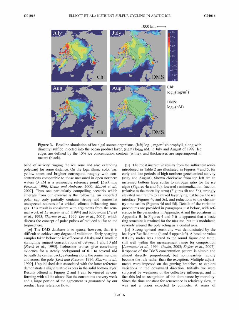
[31] The most instructive results from the sulfur test seriesintroduced in Table 2 are illustrated in Figures 4 and 5, forearly and late periods of high northern geochemical activity(May and August). Shown clockwise from top left are anincreased bottom layer sulfur to nitrogen ratio for the icealgae (Figures 4a and 5a), lowered remineralization fraction(relative to the mortality term) (Figures 4b and 5b), stronglyelevated melt return to a mixed layer lying just below the iceinterface (Figures 4c and 5c), and reductions to the chemis-try time scales (Figures 4d and 5d). Details of the variationprocedures are provided in paragraphs just below, with ref-erence to the parameters in Appendix A and the equations inAppendix B. In Figures 4 and 5 it is apparent that a basicring structure is retained for the maxima, but it is modulatedseverely around the pole acting as a central axis.[32] Strong upward sensitivity was demonstrated by the

ice-layer Redfield ratio (4 and 5 upper left). A baseline value0.03 by moles was altered to the round figure one tenth,still well within the measurement range for composition[Levasseur et al., 1994; Uzuka, 2003; Stefels et al., 2007].Response of the DMS concentration pattern is simple andalmost directly proportional, but nonlinearities rapidlybecome the rule rather than the exception. Multiple adjust-ments were imposed on the grazing branches, to explorevariations in the downward direction. Initially we weresurprised by weakness of the collective influences, and infact this led to recognition of the dominance by mortality.Since the time constant for senescence is relatively slow, itwas not a priori expected to compete. A series of

Figure 3. Baseline simulation of ice algal source organisms, (left) log10 mg/m2 chlorophyll, along withdimethyl sulfide injected into the ocean product layer, (right) log10 nM, in July and August of 1992. Iceedges are defined by the 15% ice concentration contour (white), and thicknesses are superimposed inmeters (black).


8 of 16

simulations was ultimately conducted in which the mortalityremineralization fraction was lowered systematically. Inorder to generate Figures 4b and 5b, apportionment of thereturning ecodynamic nitrogen flow was zeroed entirely.Resulting changes are strongest relative to the bloom peaksof the first two images. Note for instance the strong lossesof dimethyl sulfide in the Seas of Okhotsk and Bering, andalso along the Atlantic coast of Greenland.[33] Changes in the appendix network of fractional rout-

ings were intended mainly to perturb the sulfur cycle, butsince mass is partially conserved across algal soft parts therewere reverberations into the nitrogen system as well. Theeffects were most noticeable for the remineralization chan-nel, but net degradation to the model optimum was alwaysslight. Chlorophyll levels and mean absolute error (loga-rithmic) never differed by more than a few percent locallyfrom the baseline. Where the mechanism permitted throughinclusion of sulfur-only switches (2S in the parameters ofTable A1), we verified that the several elemental cyclescould in fact be decoupled completely. Baseline chlorophylldistributions were fully restorable. Taken together, theseruns indicate that recycling is a minor factor in the currentmodel. We do not claim, however, that this will universallybe the case [Arrigo et al., 1993; Gradinger et al., 2005].Further experimentation on the major element routingsshould be encouraged and supported.

[34] Continuing through the same figures in a clockwisemanner, semi-arbitrary melt reintroductions were bolsteredto produce Figures 4c and 5c. The baseline fractionation forthis pathway was reset from the original round value of 10 to30 and then 100 percent. Only the latter result is shown.Here the discrepancies are highly nonlinear, because they arediluted by either the mortality path or the mixed layerbackground depending on distance from the coast. In Maynoticeable shifts are apparent in the enclosed Pacific seastoward the top of the image, where ice loss begins earliestin the year. The behavior off Labrador is similar. In manyareas, however, the effects are not easy to identify and serveto underscore the relative importance of the recycling andbackground channels.[35] Various combinations and permutations were simu-

lated for the multiple, independent conversion time con-stants. Mainly the direction of these experiments could bereadily anticipated: for a given input, faster removal merelyreduced the sulfur product load. But several complexitiesemerged which are less than obvious. A standard reductionfrom 10 to 3 days was selected for most of the studies andparameters. In one particular run for which all lifetimeswere reduced together (cell disruption plus DMSP conver-sion and DMS oxidation in both layers), the tendency forconcentration buffering in the central Arctic was preserved.Production and removal changes completely balanced one

Figure 4. Product layer dimethyl sulfide distributions from four sensitivity tests conducted in May 1992.Clockwise from upper left: (a) Bottom layer sulfur to nitrogen ratio raised to one tenth; (b) remineraliza-tion fraction zeroed for the mortality channel; (c) melt fraction return of methylated sulfur raised to unity;(d) most chemical lifetimes shortened to 3 days. Units and ice property indicators are as defined inFigures 2 and 3.


9 of 16

another for the product layer in this case. From then on, themixed layer disruption constant was restored to 10 days andmaintained at this level. In the final set of images results areshown for speedups to 3 days excluding the below ice release(increases to the rate constant (Figures 4d and 5d)). The level,central basin background of 1 nM is lost and elsewhere,actual reductions to the mixed layer trace gas concentrationexceed the factor 10/3 = 3.3. They may be as large as a factorof four or five locally. It becomes clear that the relation-ship between outbound flux and conversion/oxidation ismodulated within the bottom layer. Changes from the purechemistry are then superimposed in the sub-ice realm.[36] Results from these tests and analyses can be inter-

preted in bulk since uncertainties in the system are sowidespread. Across our final two figures and assessedagainst the baseline, volatile sulfur rises from roughly ten totens of nanomolar in many places, or else is reduced to nearabsence in some instances. Maxima cluster in adjacent seasand also the coastal archipelagos (e.g., Canadian, NovayaZemlya, Eastern Greenland fjordlands). Lows hover aroundthe pole. But the essential sparge-type measurements forunder-ice dimethyl sulfide are only available in a handful ofintermediate areas, and these do not happen to correspondwith strong variability. It is thus difficult to eliminate any ofthe rather extreme possibilities highlighted by the model forthe volatile sulfur distribution. Plus it must be recalled, our

driver (major element) optimization strategy is nonglobal inthe parametric sense and open to question in its own right.

8. Summary and Discussion

[37] Numerical models are now available for representa-tion of both the physics and biogeochemistry of global seaice, and they may be applied together to simulate thebehavior of climate-active tracers in marginal waters. Wecombine several of our own codes here to estimate the con-tribution from bottom ice layers to Arctic seawater dimethylsulfide. Calculations extend across the central ocean and intoneighboring seas, for a typical climatological year prior to theturn of the century. DMS is produced in the lower few cen-timeters of the solid matrix by ice algae [Levasseur et al.,1994; Uzuka, 2003], whose growth is in turn supported byupward nutrient fluxes from the water column [Lavoie et al.,2005; Jin et al., 2006]. Key quantities adopted into ourmechanism from the physical CICE code are snow and icethickness, which determine light penetration [Hunke andLipscomb, 2008; Hunke and Bitz, 2009]. Positioning of thepack over marine nitrate and silicate fields is also critical[HAAO, 2001; Conkright et al., 2002].[38] Biogeochemical reaction schemes are carried as a set

of interlocking kinetic box models, configured as layersrepresenting (1) nutrient injections from beneath the CICEgrid, (2) processing of the biolimiting elements and sulfur in

Figure 5. Product layer dimethyl sulfide distributions from four sensitivity tests conducted in August1992. Clockwise from upper left: (a) Bottom layer sulfur to nitrogen ratio raised to one tenth; (b) reminer-alization fraction zeroed for the mortality channel; (c) melt fraction return of methylated sulfur raised tounity; (d) most chemical lifetimes shortened to 3 days. Units and ice property indicators are as definedin Figures 2 and 3.


10 of 16

porous bottom materials, and (3) reinjection of methylatedprecursors plus DMS into freshened waters adjacent to theinterface. Integrated ice chlorophyll data are relativelyplentiful across the Arctic environment [Arrigo, 2003].A selected subset is applied here in merit function mode, todown-select for basic nutrient and biomass relations. In themodel derived, critical levers are the interfacial transfervelocity, internal shading and treatment of algal removal. OurDMS production sequence is patterned after broad featuresof the global marine sulfur metabolism [Stefels, 2000;Stefels et al., 2007; Elliott, 2009], supplemented with timeconstants from recent Antarctic sea ice core studies. Base-line distributions obtained below the pack do not contradictmeasurements, but reliable data are only available from afew locations [Ferek et al., 1995; Leck and Persson, 1996].In many peripheral Arctic ecosystems, the potential exists forvolatile sulfur maxima to exceed 10 nM given ice inputsalone. Marginal cruise data are likewise in accord but non-discriminating [Leck and Persson, 1996;Matrai et al., 2007].Sensitivity tests conducted on organism composition, reactionpathways within and/or below the ice, vertical layer dimen-sions and other model features leave these general conclusionsin place. But they also open the possibility that contributionson the periphery of the ice domain are much less significant.[39] Our chlorophyll comparisons are tailored to the

requirements of a sulfur study in several crucial ways.Multiple data sets are cited, but the majority are linked withDMS campaigns so that a complete survey is not achieved;independent measurements are available which remainunexploited here. The baseline mechanism was refined in astepwise procedure which is nonglobal in its sampling of theparameter space. A more thorough strategy could well yieldareas of enhancement. It might be possible, for example, toelucidate the geographic distribution of ice-ocean boundarylayer flux controls, or the roles of flushing and melt retentionin determining bloom strength [Gradinger, 1999, 2009;Lavoie et al., 2005; Jin et al., 2006]. In order to affect ourmore important results, however, chlorophyll additionswould have to be focused in a few remote hot spots. Sparsityis the current watchword, and this is particularly true outsidefamiliar research zones of the U.S. and Canada. In a com-panion paper from our group [Deal et al., 2011], an analogmodel system is applied to the Pan-Arctic primary produc-tion problem. Simulated pigment distributions are quitesimilar, suggesting that ensembles might be used to inves-tigate the plasticity of regional biogeochemical fields.[40] Although much can be learned from such numerical

exercises, the strongest impression we are left with regardingthe ice sulfur cycle is one of pervasive uncertainty. It aboundsin all aspects of the epontic geocycling, but the difficultiesare amplified zooming on a specific tracer. A prioritized listfor improvements in an ice domain DMS model would haveto encompass all the following parameterizations: water-icesolute transfer, absorption of radiation, bottom layer purging,melt release of organisms or detritus, and the abundance ofartificial routings which interject themselves. Our analysissuggests that these issues will be relevant across the spectrumof elements and compounds now drawing polar researchattention. It may soon be necessary to consider ice columnchemical interactions for volatile halogens, trace metals, theirinorganic and organic ligands, and new crystalline phases[Lannuzel et al., 2007; Saiz-Lopez et al., 2007; Rysgaard

et al., 2009]. Detailed processes entering into ice biogeo-chemistry models will resemble the above in many cases,with perhaps an increased emphasis on resolution.[41] Networks of ecodynamic flow are particularly intri-

cate in the sulfur case [Kiene et al., 2000; Stefels, 2000;Stefels et al., 2007; Vallina et al., 2008], and our ice simu-lations underscore this point effectively. Panning across anddown the Figure 1 schematic, it is evident that a highlyinteractive web drives the trace gas response, distributedacross several phases. It may be that the only path which iswell understood at this point is the one followed by silicon[Lavoie et al., 2005, 2009]. The percentage-level grazingfractionation seems to be real, but intensity of the biomassdiversion may be either larger or smaller than we havespecified, and it may be vertically differential [Gradingeret al., 2005]. Recycling could be more important thananticipated here [Arrigo et al., 1993; Lavoie et al., 2005;Jin et al., 2006]; the reader will note that reactions withinthe bottom layer by and large follow a single metabolicdirection. Unresolved questions are the rule rather than theexception in the present work. It is difficult to escape theconclusion that this particular discipline is only in itsinfancy. Possible outcomes could be narrowed substantiallythrough renewed laboratory and field work; for example, seeLevasseur et al. [1994] and Krembs et al. [2000] or theisotope studies mentioned by Hellmer et al. [2008]. But itremains an open question whether such investigations cankeep pace over the next few decades with Arctic environ-mental change.[42] Under these circumstances a preferred strategy for the

application of systems modeling is to bracket uncertainty.The existing ensemble of global carbon cycle codes isalready viewed in this manner [Meehl et al., 2007], and agrowing collection of sulfur analogs may soon follow.Intercomparisons are now available for the full set of con-temporary open water DMS simulations [Le Clainche et al.,2010]. As international groups extend their approaches toencompass ice algae and as coupled ocean-pack models areplaced in a global change context, it should be possible tobegin the quantification process. Specifically the plan forour team is to work toward ice, aerosol, cloud interac-tions within the U.S. Community Climate System Model(CCSM). Ultimately we hope to investigate the uncertaintiesin biogeochemistry-to-brightness relations, for future polarclimate scenarios.

Appendix A: Parameters

[43] Values incorporated into the baseline simulation aregiven in the center of Table A1 as a set of examples. Thereader will note that heavy reliance has been placed on thecoastal (Chukchi) silicon/nitrogen formulation of Jin et al.[2006], which also constitutes the core of our primary pro-duction study [Deal et al., 2011]. Alternate frameworks canand will be tested with sulfur at a later date.

Appendix B: Equations

[44] Time rates of change for the biogeochemical quanti-ties under consideration are given in the following equationlist, with individual terms defined further below. Superscripts“ml, bot, pr” signify the mixed, bottom and product


11 of 16

Table A1. Parameters of Our Multielement Ice Biogeochemistry Modela

Dimensions

Quantity Symbol Base Units References and CommentsMixed layer thickness lml 30 m S95, G97Bottom layer thickness lbot 0.03 m NM79, R84, L05, J06Product layer thickness lpr 10 m G90, S95

Mixed Layer Nutrients Si(OH)4, NO3�, NH4

+

Quantity Symbol Base Units References and CommentsExchange velocities vflux,flush 0.1 m/d Optimized here plus L05, J06Nitrification time scale tnit 66 d J06

Bottom Layer Si, N, C, Chl

Quantity Symbol Base Units References and CommentsChlorophyll attenuation aChl 0.03 1/m(mg/m3) L05Normalized P versus I a/Pmax 0.8 1/W/m2 J06Light inhibition b/Pmax 0.02 1/W/m2 J06Growth preexponent gpre 1.5 1/d J06Growth T dependence gexp 0.06 1/C J06Nutrient half saturations Knut 4,1,1 mmol/m3 J06, nut = Si(OH)4, NO3

�, NH4+

Ammonia inhibition c 1.5 1/mmol/m3 J06Fraction respired fres 0.05 nondim J06Fraction grazed fgra 0.1 nondim A93, L05, added to source sulfurGraze assimilated, spilled fas,sp 0.5,0.5 nondim Central values for base caseAssimilation excreted fex 0.5 nondim Central value for base caseMortality preexponent mpre 0.02 1/d J06Mortality T dependence mexp 0.03 1/C J06Mortality remineralized frem 1 nondim Added for sulfur testingNitrification time scale tnit 66 d J06Exchange velocities vflux,flush 0.1 m/d Optimized here plus L05, J06Algae flushed ffl 0 nondim Optimized here plus G97, G99Algae ablated fme 0.1 nondim Optimized here plus G97, G99Ice algal composition RX2N 9,1.5 mole/mole CH89, S90, L05, J06, X = C, SiIce algal pigments RChl2N 3 g/mole CH89, S90, L05, J06

Bottom Layer Sulfur

Quantity Symbol Base Units References and CommentsIce algal composition RS2N 0.03 mole/mole L94, U03Excretion to sulfur fex2S 1 nondim Initially assumed efficientMortality to sulfur fmo2S 1 nondim Initially assumed efficientConversion time scale tcon 10 d >�one weekConversion yield Ycon 1 nondim Initially set to unityOxidation time scale tox 10 d >�one week

Product Layer General

Quantity Symbol Base Units References and CommentsChlorophyll below ice Chlpr 0.1 mg/m3 LP96, G97, fixedAlgal composition RC2N 7 mole/mole Nondiatoms, so no Si L94Algal pigments RChl2N 3 g/mole L94, G97Cell disruption time tdis 10 d >�one week

Product Layer Sulfur

Quantity Symbol Base Units References and CommentsAlgal composition RS2N 0.03 mole/mole L94, U03Fraction melt return frtr 0.1 nondim Rapid sinking in L09Conversion time scale tcon 10 d >�one weekConversion yield Ycon 1 nondim Initially set to unityOxidation time scale tox 10 d >�one week

aReference abbreviations are as follows: A93, Arrigo et al. [1993]; CH89, Cota and Horne [1989]; G90, Gosselin et al. [1990]; G97, Gosselin et al.[1997]; G99, Gradinger [1999]; J06, Jin et al. [2006]; L05, Lavoie et al. [2005]; L09, Lavoie et al. [2009]; LP96, Leck and Persson [1996]; L94,Levasseur et al. [1994]; NM79, Niedrauer and Martin [1979]; R84, Reeburgh [1984]; S95, Schlosser et al. [1995]; S90, Smith et al. [1990]; and U03,Uzuka [2003].


12 of 16

numerical layers. Subscripts refer mainly to specific pro-cesses or the materials cycled by them. An exception occursin the composition ratios, where for example “S2N” indi-cates a molar sulfur to nitrogen ratio.

dSi OHð Þ4mldt

¼FSi OHð Þ4

lmlðB1Þ

dNO�3ml

dt¼ knitNH

þ4ml þ

FNO�3

lmlðB2Þ

dNHþ4ml

dt¼ �knitNH

þ4ml þ

FNHþ4

lmlðB3Þ

dSi OHð Þ4botdt

¼ �UbotSi OHð Þ4 �

FSi OHð Þ4lbot

ðB4Þ

dNO�3bot

dt¼ knitNH

þ4bot � Ubot

NO�3�FNO�

3

lbotðB5Þ

dNHþ4bot

dt¼ fres þ fex fas fgra

� �Gbot þ fremM

bot � knitNHþ4bot

� UbotNHþ

4�FNHþ

4

lbotðB6Þ

dNbotal

dt¼ 1� fgra � fres

� �Gbot �M bot � Fal

lbotðB7Þ

dC Chl; Sð Þbotal

dt¼ Rbot

X2N

dNbotal

dt;

dSibotal

dt¼ 0;

dSbotal

dt¼ dDMSPbot

p

dtðB8Þ

dDMSPdbot

dt¼ Rbot

S2N fsp þ fex2S fex fas

� �fgraG

bot þ fmo2S fremMbot

� �

� kconDMSPdbot �

FDMSPd

lbot

ðB9Þ

dDMSbot

dt¼ YconkconDMSPd

bot � koxDMSbot � FDMS

lbotðB10Þ

dN C;Chl; Sð Þpraldt

¼ 0; Chlpral ¼ empirical;

Spral ¼ DMSPprp ¼ Rpr

S2N

RprChl2N

� �Chlpral ðB11Þ

dDMSP prd

dt¼ Rbot

S2N frtrFal

lpr

� �þ kdisDMSPpr

p � kconDMSPprd þ

FDMSPd

lpr

ðB12Þ

dDMSpr

dt¼ YconkconDMSP pr

d � koxDMSpr þ FDMS

lprðB13Þ

Beginning with the differentials for pure elements,“al” points directly to the ice algae. Throughout the above,“k” are pseudo-first-order rate constants obtained as recip-rocals of corresponding time scales from Table A1. Notethat the term for nitrification knitNH4

+ is similar in thesource and ice processing zones.[45] Chemical and biological tracers can be placed into

vectors T specific to each of the three layers supporting icedomain geocycling, for purposes of generalization. Theirconcentrations are then

Tml ¼ Si OHð Þ4; NO�3 ; NH

þ4 ðB14Þ

Tbot ¼ Si OHð Þ4; NO�3 ; NH

þ4 ; Sial;N C;Chl; Sð Þal; DMSPd; DMS

ðB15Þ

T pr ¼ N C;Chl; Sð Þal; DMSPd ; DMS ðB16Þ

Sal ¼ DMSPp ðB17Þ

These are carried in units of millimole per m3, exceptingmg/m3 in the case of chlorophyll. The first few compositeterms in the equation list may now be expressed as

Fsol ¼ vflux Tbotsol � Tml

sol

� �or vflushT

botsol ðB18Þ

Ubotnut ¼ Rbot

X2N fnutGbot ðB19Þ

Gbot ¼ LtotalgpreegexpC

oNbotal ðB20Þ

in which F is a flux, U is an inorganic uptake, and G isoverall growth tracked in the fundamental nitrogen currency.Subscripts “sol” and “nut” specify all solutes or else just theinorganic nutrients. Total growth limitation Ltotal accountsfor contributions related to radiation, individual sourcematerials, and also the required elements. To calculate thesubterms, we draw on the biomass distribution for attenua-tion, then on concentrations in order to build saturationcurves and apportionments.

Iavg ¼ Ilower bound ¼ Ioe�aChlChl

bot lbot ðB21Þ

Lrad ¼ 1� e� a=Pmaxð ÞIavg� �

e� b=Pmaxð ÞIavg ðB22Þ

Lnut ¼ Tbotnut = T bot

nut þ Knut

� �� e�cNHþ

4 ðB23Þ

Lelement ¼Xnut

Lnut ðB24Þ

fNO�3 ;NH

þ4¼ Lnut

Lelement; fSi OHð Þ4 ¼ 1 ðB25Þ

Ltotal ¼ Min Lrad; LN ; LSi� � ðB26Þ


13 of 16

[46] In the nutrient L factors inhibition c must be zeroexcept for nitrate, which competes with the alternate(reduced) form NH4

+. The I are radiation intensities which wecarry in units of W/m2.[47] Several processes are modeled in a primitive fashion

as cumulative or nested routings of the integrated nitrogengrowth. Examples include respiration (Res), grazing (Gra),assimilation (As) of biomass into the zooplankton, spillage(Sp) during the consumption process, and excretion (Ex) bythe zooplankton. Senescence, by contrast, has its own tem-perature dependence and tracks ice algal population.Simultaneously it drives the ultimate material remineraliza-tion. Here the factors are mortality (M) as a mirror fornitrogen growth and remineralization (Rem) of the detritus.

Resbot ¼ fresGbot; Grabot ¼ fgraG

bot; Spbot ¼ fspGrabot;

Asbot ¼ fasGrabot; Exbot ¼ fexAs

bot ðB27Þ

fres þ fgra ≤ 1; fsp þ fas ¼ 1; fex ≤ 1 ðB28Þ

Mbot ¼ mpreem expC

oNbotal ; Rembot ¼ fremM

bot ðB29Þ

Note that biomass is conserved over spillage and assimila-tion. In the interest of maintaining clarity, many of thefractionations have been written out explicitly in the aboveconcentration derivatives.[48] Removal of algae from the bottom ice volume may be

caused by flushing or else by sloughing during the melt.In the current study, sensitivity testing has been devoted todiscrimination of the respective loss portions but they remainvery uncertain. Here the change in hme is the bottom thick-ness ablated during a time step.

Fal ¼ fflvflush þ fmeDhmeDt

� �� T botal ðB30Þ

Ice-sulfur redox chemistry begins with in vivo synthesis of acomplex precursor chain, building from seawater sulfate andeventually leading to amino acids and lipids. The key ingre-dient, however, is the osmolyte/cryoprotectant DMSPp.Along with pigments and the cell carbon content, its levelsare set proportional to ice algal nitrogen. DMSPd enterssolution directly along all cell disruption pathways, but withadditional switches superimposed to provide flexibility. Inthe excretion channel, for instance, (1 � fex2S) can be held inreserve in order to remove S atoms into the hypotheticalzooplankton bin. Otherwise, the basic nitrogen forms justrecur under multiplication by RS2N. Examples include

SpbotDMSPd¼ Rbot

S2NSpbot ¼ Rbot

S2N fspGrabot ¼ Rbot

S2N fsp fgraGbot ðB31Þ

ExbotDMSPd¼ Rbot

S2N fex2S fex fas fgraGbot ðB32Þ

in which the terms are now subscripted because they are out-of-currency, and the opportunity is taken to show some of therouting cascades written out in full. Beyond the disruptionsteps, sulfur kinetics merely constitute the familiar A goes toB etc. of conversion (Con) followed by oxidation (Ox). In

these cases yield applies only to the production of dimethylsulfide, not to net DMSPd loss.

ConbotS ¼ YconkconDMSPdbot; OxbotS ¼ koxDMSbot ðB33Þ

Sulfur solutes exchange into the product layer via fluxequations identical to those outlined for the dissolved nutri-ents, except that Tpr must be substituted for Tml. A short-circuit into the “pr” volume is provided for ice bottomDMSPp, which is permitted to enter as DMSPd released fromflushed or ablated detritus. Finally in order to enhance com-parisons with the rare data, a supplemental flow is associatedwith fixed below-ice chlorophyll. Local introduction andremoval inside the product bin may then be summarized as

SloprDMSPd¼ Rbot

S2N frtrFal

lpr

� �ðB34Þ

Bkg prDMSPd

¼ kdisRprS2N

RprChl2N

� �Chlpral ¼ kdisDMSPpr

p ðB35Þ

ConprS ¼ YconkconDMSPd

pr; OxprS ¼ koxDMSpr; ðB36Þ

where Slo and Bkg are the distinct sloughing and backgroundsources. Subscript rtr stands for return from sinking detritus,and dis indicates cell disruption of some type (grazing,senescence or others).

[49] Acknowledgments. The authors would like to thank the U.S.Department of Energy Scientific Discovery through Advanced Computing(SciDAC) Program and the Experimental Program to Stimulate Competi-tive Research (EPSCoR) for support of this project (grant DE-FG02-08ER46502).

ReferencesAndreae, M. O., and A. R. Rosenfeld (2008), Aerosol-cloud-precipitationinteractions Part I. The nature and sources of cloud active aerosols, EarthSci. Rev., 89, 13–41, doi:10.1016/j.earscirev.2008.03.001.

Archer, S. D., F. J. Gilbert, J. I. Allen, J. Blackford, and P. D. Nightingale(2004), Modelling of the seasonal patterns of dimethylsulphide produc-tion and fate during 1989 at a site in the North Sea, Can. J. Fish. Aquat.Sci., 61, 765–787, doi:10.1139/f04-028.

Arrigo, K. R. (2003), Primary production in sea ice, in Sea Ice: An Intro-duction to its Physics, Chemistry, Biology and Geology, edited by D. N.Thomas and G. S. Dieckmann, pp. 143–183, Blackwell, London.

Arrigo, K. R., and D. Thomas (2004), Large scale importance of sea icebiology in the Southern Ocean, Antarct. Sci., 16, 471–486, doi:10.1017/S0954102004002263.

Arrigo, K. R., J. N. Kremer, and C. W. Sullivan (1993), A simulated Antarc-tic fast ice ecosystem, J. Geophys. Res., 98(C4), 6929–6946, doi:10.1029/93JC00141.

Bitz, C. M., and W. H. Lipscomb (1999), An energy-conserving thermody-namic model of sea ice, J. Geophys. Res., 104(C7), 15,669–15,677,doi:10.1029/1999JC900100.

Briegleb, B. P., C. M. Bitz, E. C. Hunke, W. H. Lipscomb, M. M. Holland,J. L. Schramm, and R. E. Moritz (2004), Scientific description of the seaice component in the Community Climate System Model, Version 3,Tech. Rep. NCAR/TN-463+STR, Natl. Cent. for Atmos. Res., Boulder,Colo. [Available at http://nldr.library.ucar.edu/repository/collections/TECH-NOTE-000-000-000-535]

Carmack, E., and P. Wassman (2006), Food webs and physical-biologicalcoupling on pan-Arctic shelves: Unifying concepts and comprehensiveperspectives, Prog. Oceanogr., 71, 446–447.

Charlson, R. J., J. E. Lovelock, M. O. Andreae, and S. G. Warren (1987),Oceanic phytoplankton, atmospheric sulphur, cloud albedo and climate,Nature, 326, 655–661, doi:10.1038/326655a0.

Collins, W. D., et al. (2006), The Community Climate System ModelVersion 3 (CCSM3), J. Clim., 19, 2122–2143, doi:10.1175/JCLI3761.1.


14 of 16

Conkright, M. E., H. E. Garcia, T. D. O’Brien, R. A. Locarnini, T. P. Boyer,C. Stephens, and J. I. Antonov (2002), Nutrients, vol. 4, NOAA AtlasNESDIS, NOAA, Silver Spring, Md.

Cota, G. F., and E. P. W. Horne (1989), Physical control of arctic icealgal production, Mar. Ecol. Prog. Ser., 52, 111–121, doi:10.3354/meps052111.

Deal, C., M. Jin, S. Elliott, E. Hunke, M. Maltrud, and N. Jeffery (2011),Large-scale modeling of primary production and ice algal biomass withinarctic sea ice in 1992, J. Geophys. Res., 116, C07004, doi:10.1029/2010JC006409.

Elliott, S. (2009), Dependence of DMS global sea-air flux distribution ontransfer velocity and concentration field type, J. Geophys. Res., 114,G02001, doi:10.1029/2008JG000710.

Ferek, R. J., P. V. Hobbs, L. F. Radke, J. A. Herring, W. T. Sturges, andG. F. Cota (1995), Dimethyl sulfide in the arctic atmosphere, J. Geophys.Res., 100(D12), 26,093–26,104, doi:10.1029/95JD02374.

Gosselin, M., L. Legendre, J.-C. Therriault, and S. Demers (1990), Lightand nutrient limitation of sea-ice microalgae (Hudson Bay, CanadianArctic), J. Phycol., 26, 220–232, doi:10.1111/j.0022-3646.1990.00220.x.

Gosselin, M., M. Levasseur, P. A. Wheeler, R. A. Horner, and B. C. Booth(1997), New measurements of phytoplankton and ice algal production inthe Arctic Ocean, Deep Sea Res., Part II, 44, 1623–1644, doi:10.1016/S0967-0645(97)00054-4.

Gradinger, R. (1999), Vertical fine structure of the biomass and composi-tion of algal communities in Arctic pack ice, Mar. Biol. Berlin, 133,745–754, doi:10.1007/s002270050516.

Gradinger, R. (2009), Sea-ice algae: Major contributors to primary produc-tion and algal biomass in the Chukchi and Beaufort seas during May/June, Deep Sea Res., Part II, 56(17), 1201–1212, doi:10.1016/j.dsr2.2008.10.016.

Gradinger, R., K. Meiners, G. Plumley, Q. Zhang, and B. Bluhm (2005),Abundance and composition of the sea-ice meiofauna in off-shore packice of the Beaufort Gyre in summer 2002 and 2003, Polar Biol., 28,171–181, doi:10.1007/s00300-004-0674-5.

Gunst, R. F., and R. L. Mason (1980), Regression Analysis and its Applica-tions, Marcel Dekker, New York.

HAAO (2001), Hydrochemical Atlas of the Arctic Ocean, Int. Arctic Res.Cent., Fairbanks, Alaska.

Hellmer, H. H., M. Schröder, C. Haas, G. S. Dieckmann, and M. Spindler(2008), The ISPOL drift experiment, Deep Sea Res., Part II, 55,913–917, doi:10.1016/j.dsr2.2008.01.001.

Hunke, E. C. (2010), Thickness sensitivities in the CICE sea ice model,Ocean Modell., 34, 137–149, doi:10.1016/j.ocemod.2010.05.004.

Hunke, E. C., and C. M. Bitz (2009), Age characteristics in a multidecadalArctic sea ice simulation, J. Geophys. Res., 114, C08013, doi:10.1029/2008JC005186.

Hunke, E. C., and J. K. Dukowicz (1997), An elastic-viscous-plastic modelfor sea ice dynamics, J. Phys. Oceanogr., 27, 1849–1867, doi:10.1175/1520-0485(1997)027<1849:AEVPMF>2.0.CO;2.

Hunke, E. C., and W. H. Lipscomb (2008), CICE: The Los Alamos sea icemodel documentation and software user’s manual, Version 4.0, Tech.Rep. LA-CC-06–012, Los Alamos Natl. Lab., Los Alamos, N. M.

Irwin, B. D. (1990), Primary production of ice algae on a seasonally icecovered continental shelf, Polar Biol., 10, 247–254, doi:10.1007/BF00238421.

Jin, M., C. J. Deal, J. Wang, K.-H. Shin, N. Tanaka, T. E. Whitledge,S. H. Lee, and R. Gradinger (2006), Controls of the land fast ice-ocean ecosystem offshore Barrow, Alaska, Ann. Glaciol., 44, 63–72,doi:10.3189/172756406781811709.

Kettle, A. J., and M. O. Andreae (2000), Flux of dimethylsulfide from theoceans: A comparison of updated data sets and flux models, J. Geophys.Res., 105(D22), 26,793–26,808, doi:10.1029/2000JD900252.

Kiene, R. P., and T. S. Bates (1990), Biological removal of dimethyl sulfidefrom sea water, Nature, 345, 702–705, doi:10.1038/345702a0.

Kiene, R. P., and D. Slezak (2006), Low dissolved DMSP concentrations inseawater revealed by small-volume gravity filtration and dialysis sam-pling, Limnol. Oceanogr. Methods, 4, 80–95, doi:10.4319/lom.2006.4.80.

Kiene, R. P., L. J. Linn, and J. A. Bruton (2000), New and important rolesfor DMSP in marine microbial communities, J. Sea Res., 43, 209–224,doi:10.1016/S1385-1101(00)00023-X.

Krembs, C., R. Gradinger, and M. Spindler (2000), Implications of brinechannel geometry and surface area for the interaction of sympagic organ-isms in Arctic sea ice, J. Exp. Mar. Biol. Ecol., 243, 55–80, doi:10.1016/S0022-0981(99)00111-2.

Kudoh, S., B. Robineau, Y. Suzuki, Y. Fujiyoshi, and M. Takahashi (1997),Photosynthetic acclimation and the estimation of temperate ice algal pri-mary production in Saroma-ko Lagoon, Japan, J. Mar. Syst., 11, 93–109,doi:10.1016/S0924-7963(96)00031-0.

Lannuzel, D., V. Schoemann, J. de Jong, L. Chou, B. Delille, S. Becquevort,and J. L. Tison (2007), Distribution and biogeochemical behavior ofiron in East Antarctic sea ice, Mar. Chem., 106, 18–32, doi:10.1016/j.marchem.2006.06.010.

Lavoie, D., K. Denman, and C. Michel (2005), Modeling ice algal growthand decline in a seasonally ice-covered region of the Arctic (ResolutePassage, Canadian Archipelago), J. Geophys. Res., 110, C11009,doi:10.1029/2005JC002922.

Lavoie, D., R. W. Macdonald, and K. L. Denman (2009), Primary produc-tivity and export fluxes on the Canadian shelf of the Beaufort Sea:A modeling study, J. Mar. Syst., 75, 17–32, doi:10.1016/j.jmarsys.2008.07.007.

Leck, C., and C. Persson (1996), The central Arctic Ocean as a source ofdimethyl sulfide: Seasonal variability in relation to biological activity,Tellus, Ser. B, 48, 156–177, doi:10.1034/j.1600-0889.1996.t01-1-00003.x.

Le Clainche, Y., et al. (2010), A first appraisal of prognostic ocean DMSmodels and prospects for their use in climate models, Global Biogeo-chem. Cycles, 24, GB3021, doi:10.1029/2009GB003721.

Lee, P. A., S. J. de Mora, M. Gosselin, M. Levasseur, R. C. Bouillon,C. Nozais, and C. Michel (2001), Particulate dimethylsulfoxide in Arcticsea ice algal communities: The cryoprotectant hypothesis revisited,J. Phycol., 37, 488–499, doi:10.1046/j.1529-8817.2001.037004488.x.

Levasseur, M., M. Gosselin, and S. Michaud (1994), New source ofdimethylsulfide (DMS) for the arctic atmosphere: Ice diatoms, Mar. Biol.Berlin, 121, 381–387, doi:10.1007/BF00346748.

Lipscomb, W. H., and E. C. Hunke (2004), Modeling sea ice transportusing incremental remapping, Mon. Weather Rev., 132, 1341–1354,doi:10.1175/1520-0493(2004)132<1341:MSITUI>2.0.CO;2.

Lipscomb, W. H., E. C. Hunke, W. Maslowski, and J. Jakacki (2007),Ridging, strength, and stability in high-resolution sea ice models,J. Geophys. Res., 112, C03S91, doi:10.1029/2005JC003355.

Lundén, J., G. Svensson, and C. Leck (2007), Influence of meteorologicalprocesses on the spatial and temporal variability of atmospheric dimethylsulfide in the high Arctic summer, J. Geophys. Res., 112, D13308,doi:10.1029/2006JD008183.

Matrai, P., M. Vernet, and P. Wassmann (2007), Relating temporal andspatial patterns of DMSP in the Barents Sea to phytoplankton biomassand productivity, J. Mar. Syst., 67, 83–101, doi:10.1016/j.jmarsys.2006.10.001.

Matrai, P. A., L. Tranvik, C. Leck, and J. C. Knulst (2008), Are high arcticsurface microlayers a potential source of aerosol precursors?Mar. Chem.,108, 109–122, doi:10.1016/j.marchem.2007.11.001.

Meehl, J., et al. (2007), Global climate projections, in Climate Change2007: The Physical Science Basis. Contribution of Working Group I tothe Fourth Assessment Report of the Intergovernmental Panel on ClimateChange, edited by S. Solomon et al., pp. 789–844, Cambridge Univ.Press, Cambridge, U. K.

Michaud, S., M. Levasseur, and G. Cantin (2007), Seasonal variations indimethyl sulfoniopropionate and dimethylsulfide concentrations in rela-tion to the plankton community in the St. Lawrence Estuary, EstuarineCoastal Shelf Sci., 71, 741–750, doi:10.1016/j.ecss.2006.09.020.

Michel, C., L. Legendre, R. G. Ingram, M. Gosselin, and M. Levasseur(1996), Carbon budget of sea-ice algae in spring: Evidence of a sig-nificant transfer to zooplankton grazers, J. Geophys. Res., 101(C8),18,345–18,360, doi:10.1029/96JC00045.

Monfort, P., S. Demers, and M. Levasseur (2000), Bacterial dynamics infirst-year sea ice and underlying seawater of Saroma-ko Lagoon andResolute Passage: Inhibitory effects of ice algae on bacterial dynamics,Can. J. Microbiol., 46, 623–632, doi:10.1139/w00-024.

Niedrauer, T. M., and S. Martin (1979), An experimental study of brinedrainage and convection in young sea ice, J. Geophys. Res., 84(C3),1176–1186, doi:10.1029/JC084iC03p01176.

Reeburgh, W. (1984), Fluxes associated with brine motion in growing seaice, Polar Biol., 3, 29–33, doi:10.1007/BF00265564.

Rysgaard, S., J. Bendtsen, L. T. Pedersen, H. Ramløv, and R. N. Glud(2009), Increased CO2 uptake due to sea ice growth and decay in theNordic Seas, J. Geophys. Res., 114, C09011, doi:10.1029/2008JC005088.

Saiz-Lopez, A., A. Mahajan, R. A. Salmon, S. J. B. Bauguitte, A. E. Jones,H. K. Roscoe, and J. C. Plane (2007), Boundary layer halogens in coastalAntarctica, Science, 317, 348–351, doi:10.1126/science.1141408.

Schlosser, P., J. H. Swift, D. Lewis, and S. L. Pfirman (1995), Role of thelarge scale Arctic Ocean circulation in the transport of contaminants,DeepSea Res., Part II, 42, 1341–1367, doi:10.1016/0967-0645(95)00045-3.

Sharma, S., L. A. Barrie, D. Plummer, J. C. McConnell, P. C. Brickell,M. Levasseur, M. Gosselin, and T. S. Bates (1999), Flux estimationof oceanic dimethyl sulfide around North America, J. Geophys. Res.,104(D17), 21,327–21,342, doi:10.1029/1999JD900207.


15 of 16

Smith, R. E. H., W. G. Harrison, L. R. Harris, and A. W. Herman (1990),Vertical fine structure of particulate matter and nutrients in sea ice ofthe high Arctic, Can. J. Fish. Aquat. Sci., 47, 1348–1355, doi:10.1139/f90-154.

Stefels, J. (2000), Physiological aspects of the production and conversion ofDMSP in marine algae and higher plants, J. Sea Res., 43, 183–197,doi:10.1016/S1385-1101(00)00030-7.

Stefels, J., M. Steinke, S. Turner, G. Malin, and S. Belviso (2007), Environ-mental constraints on the production and removal of the climaticallyactive gas dimethylsulphide (DMS), Biogeochemistry, 83, 245–275,doi:10.1007/s10533-007-9091-5.

Suzuki, Y., S. Kudoh, and M. Takahashi (1997), Photosynthetic and respi-ratory characteristics of an Arctic ice algal community living in low lightand low temperature conditions, J. Mar. Syst., 11, 111–121, doi:10.1016/S0924-7963(96)00032-2.

Uzuka, N. (2003), A time series observation of DMSP production in the fastice zone near Barrow, Sci. Rep. Tohoku Univ., Ser. 5, 36, 439–442.

Vallina, S. M., R. Simó, T. R. Anderson, A. Gabric, R. Cropp, andJ. M. Pacheco (2008), A dynamic model of oceanic sulfur (DMOS) appliedto the Sargasso Sea: Simulating the dimethylsulfide (DMS) summerparadox, J. Geophys. Res., 113, G01009, doi:10.1029/2007JG000415.

Vancoppenolle, M., H. Goosse, A. de Montety, T. Fichefet, B. Tremblay,and J.-L. Tison (2010), Modeling brine and nutrient dynamics in Antarcticsea ice: The case of dissolved silica, J. Geophys. Res., 115, C02005,doi:10.1029/2009JC005369.

Wakatsuchi, M., and N. Ono (1983), Measurements of salinity and volumeof brine excluded from growing sea ice, J. Geophys. Res., 88(C5),2943–2951, doi:10.1029/JC088iC05p02943.

Werner, I., J. Ivalko, and H. Schunemann (2007), Sea-ice algae in Arcticpack ice during late winter, Polar Biol., 30, 1493–1504, doi:10.1007/s00300-007-0310-2.

Zar, J. H. (1984), Biostatistical Analysis, Prentice Hall, Upper Saddle River,N. J.

Zhou, J., E. Swietlicki, O. H. Berg, P. P. Aalto, K. Hämeri, E. D. Nilsson,and C. Leck (2001), Hygroscopic properties of aerosol particles overthe central Arctic Ocean during summer, J. Geophys. Res., 106(D23),32,111–32,123, doi:10.1029/2000JD900426.

C. Deal and M. Jin, International Arctic Research Center, Institute ofMarine Science, University of Alasaka Fairbanks, Fairbanks, AK 99775-7340, USA.S. Elliott, E. Hunke, and N. Jeffery, Climate Ocean Sea Ice Modeling,

Computational Sciences Division, Los Alamos National Laboratory, MailStop D-413, Los Alamos, NM 87545, USA. ([email protected])G. Humphries, Institute of Arctic Biology, University of Alaska

Fairbanks, Fairbanks, AK 99775, USA.M. Levasseur, Department of Biology, Laval University, 1045, Avenue

de la Médecine, Pavillon Alexandre-Vachon, Quebec, QC G1V 0A6,Canada.J. Stefels, Laboratory of Plant Physiology, Center for Life Sciences,

University of Groningen, Bldg. 5173, Nijenborgh 7, NL-9747 AGGroningen, Netherlands.


16 of 16

Pan-Arctic simulation of coupled nutrient-sulfur cycling due to sea ice biology: Preliminary results

Documents

Transcript of Pan-Arctic simulation of coupled nutrient-sulfur cycling due to sea ice biology: Preliminary results