The Thermal Structure of Gas in Pre-Stellar Cores: A Case Study of Barnard 68

arX

iv:a

stro

-ph/

0603

424v

1 1

6 M

ar 2

006

Accepted by The Astrophysical Journal

The Thermal Structure of Gas in Pre-Stellar Cores: A Case

Study of Barnard 68

Edwin A. Bergin1, Sebastien Maret1, Floris F.S. van der Tak2, Joao Alves3, Sean M.

Carmody4, Charles J. Lada5

ABSTRACT

We present a direct comparison of a chemical/physical model to multitransi-

tional observations of C18O and 13CO towards the Barnard 68 pre-stellar core.

These observations provide a sensitive test for models of low UV field photodisso-

ciation regions and offer the best constraint on the gas temperature of a pre-stellar

core. We find that the gas temperature of this object is surprisingly low (∼ 7−8

K), and significantly below the dust temperature, in the outer layers (AV < 5

mag) that are traced by C18O and 13CO emission. As shown previously, the in-

ner layers (AV > 5 mag) exhibit significant freeze-out of CO onto grain surfaces.

Because the dust and gas are not fully coupled, depletion of key coolants in the

densest layers raises the core (gas) temperature, but only by ∼ 1 K. The gas

temperature in layers not traced by C18O and 13CO emission can be probed by

NH3 emission, with a previously estimated temperature of ∼ 10−11 K. To reach

these temperatures in the inner core requires an order of magnitude reduction in

the gas to dust coupling rate. This potentially argues for a lack of small grains

in the densest gas, presumably due to grain coagulation.

Subject headings: ISM: Lines and Bands, ISM: Molecules, astrochemistry, ISM:individual

(Barnard 68)

1University of Michigan, 825 Dennison Building, 500 Church St, Ann Arbor, MI 48109-1042; email:

[email protected]

2 Max-Planck-Institut fur Radioastronomie, Auf dem Hugel 69, 53121 Bonn, Germany

3 European Southern Observatory, Karl-Schwarzschild-Strasse 2, 85748 Garching, Germany

4 4824 S. 1st Street Kalamazoo, MI 49009

5 Harvard-Smithsonian Center for Astrophysics, 60 Garden Street, Cambridge, MA 02138

http://arxiv.org/abs/astro-ph/0603424v1

– 2 –

1. Introduction

Several phases of the star formation process have been observationally identified and

characterized, beginning with a centrally concentrated core of molecular gas that collapses

to form a star surrounded by a disk. Indeed, it has been the isolation of objects that have

not yet formed stars – pre-stellar cores – which has allowed us to probe the earliest stages

of star formation (see Andre et al. 2000; Alves et al. 2001; Lee et al. 2001). Of particular

importance are the density and temperature structure as these parameters are fundamental

to estimating the mechanisms via which cores are supported against gravitational collapse.

Moreover knowledge of the physical parameters is a pre-requisite for subsequent chemical

and kinematical studies (e.g. van der Tak et al. 2005).

Estimates of the density profile of pre-stellar cores have become quite commonplace

through observations of dust emission or absorption. Initial studies have suggested that

pre-stellar cores have flat density profiles in the center, falling off as a steep power law

in outer layers (e.g. Andre et al. 2000, and references therein). Less information exists

regarding the temperature structure. This is despite the importance of thermal pressure for

the stability of pre-stellar cores with little or no turbulent support (Dickman & Clemens

1983; Lada et al. 2003). Initial studies assumed isothermal structure with equivalent gas

and dust temperatures (as a result of the anticipated thermal coupling at nH2> 105 cm−3;

Burke & Hollenbach 1983). More recently, several groups have investigated the thermal

structure of dust grains heated by the normal interstellar radiation field (Evans et al. 2001;

Zucconi et al. 2001; Bianchi et al. 2003). These studies predict a dust temperature gradient

that peaks at 15 – 17 K towards the core edge and declines to near 7 - 8 K at the center

in cores with central densities of ∼ 106 cm−3. In this case the actual gas density profile,

when estimated via dust continuum emission, could be much steeper than derived assuming

constant temperature, for example as steep as r−2 (Evans et al. 2001).

Despite the effort placed towards the determination of the dust temperature profile

little has been done to characterize the temperature profile of the gas, which is the dominant

component. For cores bathed within the average interstellar radiation field (ISRF), theory

predicts that the gas temperature will rise towards the cloud edge due to the direct heating

of the gas via the photo-electric effect; in shielded gas heating by cosmic rays and dust-gas

coupling is expected to dominate (Goldsmith 2001; Galli et al. 2002).

Excellent tracers of the gas temperature are the 22 GHz inversion transitions of NH3

and cm/mm-wave transitions of H2CO. Emission from H2CO has been used to probe the

gas temperature in pre-stellar cores by Young et al. (2004) with a finding that this species

is heavily depleted in abundance in the center, limiting its value as a probe to outer layers.

NH3 does not appear to exhibit significant gas-phase freeze-out (Tafalla et al. 2002) and

– 3 –

should directly trace Tgas deep inside cores. Indeed the gas kinetic temperature derived

using ammonia is ∼ 9 − 11 K, consistent with cosmic ray heating, but above that derived

for the dust in similar objects (Tafalla et al. 2002; Hotzel et al. 2002a; Lai et al. 2003; Evans

et al. 2001; Zucconi et al. 2001). This is predicted by models of the thermal balance for cores

where the central density is ∼ 105 cm−3; in cores with higher densities (e.g. L1544) the gas

temperature is expected to drop (Galli et al. 2002). However, NH3 is limited as a probe of the

full thermal structure because its emission does not probe the outer layers of the core seen

in other tracers (e.g. C18O, CS, H2CO; Zhou et al. 1989; Tafalla et al. 2002; Young et al.

2004). Thus, while detailed estimates of the dust temperature profile in pre-stellar cores

exist and have been compared to observational data, less observational constraints exist for

the gas temperature profile.

This paper presents a detailed study of the gas temperature structure in the Barnard

68 pre-stellar core. This well-studied object presents a unique laboratory for study as its

density and extinction structure is well determined via near-infrared extinction mapping

techniques (see Alves et al. 2001, and references therein). This allows for good constraints

to be placed on the line of sight structure in chemical abundance. Observations have shown

that this, and other, pre-stellar cores are dominated by selective freeze-out (Tafalla et al.

2002; Bergin et al. 2002), wherein some species (e.g. CS and CO) only trace outer layers and

others (N2H+, NH3) trace deeper into the cloud. With knowledge of the chemical structure

obtained by detailed models we can determine which tracer is probing a given layer and use

multi-molecular studies to reconstruct the physical structure of the cloud. Thus CO and its

isotopologues can be used to constrain the gas temperature in the outer low density layers,

while NH3 probes denser gas. This enables us to perform a more detailed examination of

the gas temperature structure in the earliest stages of star formation than has been done

previously.

In §2 we present our observations and in §3 we discuss the model used to compare to

the data. Section 4 compares theory to observations and in §5–6 we discuss the implication

of and summarize our results.

2. Observations and Results

The J=1-0 (109.78218 GHz) and J=2-1 (219.560319 GHz) transitions of C18O were

observed towards B68 (α = 17h22m38.s2 and δ = −23◦49′34.′′0; J2000) during April 2000 and

2001 using the IRAM 30m telescope. The entire core was mapped using 12′′ sampling with

the half-power beam width of 22′′ at 110 GHz and 11′′ at 220 GHz. System temperatures for

the 3mm observations were typically ∼160–190 K with ∼350–450 K at 1mm and integration

– 4 –

times were typically 2–6 min. Pointing was checked frequently with an uncertainty of ∼ 2′′.

The data were taken using frequency switching and calibrated using the standard chopper

wheel method and are presented here on the Tmb scale using standard calibrations from

IRAM documentation. For the analysis the C18O J=2-1 observations were convolved to the

lower resolution of the J=1-0 transition. The J=2-1 data were reduced by fitting the spectra

with Gaussians and in cases where no emission is observed fixing the width and position of

the line using a centroid determined from J=1-0 observations. The J=1-0 observations have

been published previously by Bergin et al. (2002) and Lada et al. (2003).

Observations of 13CO J=2-1 (220.3987 GHz; θMB ∼ 33′′), 13CO J=3-2 (330.588 GHz

θMB ∼ 22′′), and C18O J=3-2 (329.330 GHz; θMB ∼ 32′′) were obtained at the 10.4m

Caltech submillimeter Observatory (CSO) during September 7-9, 2003. Data were taken

using position switching with an offset of 6′; larger reference position offsets for the position

switched observations were examined with no difference found in the results. Pointing was

checked frequently with a typical uncertainty of 3–4′′. Typical system temperatures range

from ∼400 – 500 K for the J=2-1 transition (tint ∼ 12 − 20 s) and ∼ 600− 700 K (tint ∼ 40

s) for the J=3-2 transitions. The 13CO transitions were observed over numerous positions

in the core with the goal of obtaining data corresponding to a range of total column (as

estimated from the extinction map). Observations of C18O J=3-2 were taken towards two

positions in the core with relative offsets of ∆α = 0, ∆δ = 0 and ∆α = 24′′, ∆δ = −48′′. No

line is detected at either position with a 1σ rms of ∆T ∗

A = 0.23 K and 0.25 K, respectively

in 0.05 MHz channels. An additional CSO search for C18O J=3-2 emission was performed

on May 27, 2005 (by D. Lis) with no emission detected to a level of 0.3 K (1σ) in 0.05 MHz

channels.

All data were calibrated to the T∗

A scale using the standard chopper wheel method. To

compare the CSO data to IRAM 30m observations we placed the data on the TMB scale. For

C18O and 13CO J=3-2 observations of Mars on Sep. 7, 2003 (θMars = 24.6′′) were compared

to a thermal model (M. Gurwell, priv. comm.) to estimate a main beam efficiency of 55%.

For J=2-1 we adopt a main beam efficiency of 60% (D. Lis, priv. comm.). To test this

cross-telescope calibration we also observed 13CO J=2-1 in Lynds 1544 with the CSO and

compared this to similar data obtained with the IRAM 30m (kindly provided by M. Tafalla).

We find that the IRAM 30m data (when convolved to the same resolution as CSO) agrees

to within 20%. The IRAM data shows stronger emission, which could be attributed to a

10–20% contribution from the error beam of the larger IRAM telescope (see Bensch et al.

2001). Given these differences, we have assigned a calibration uncertainty of 20% to all 230

and 345 GHz data. C18O J=1-0 data are assigned a calibration uncertainty of 10%.

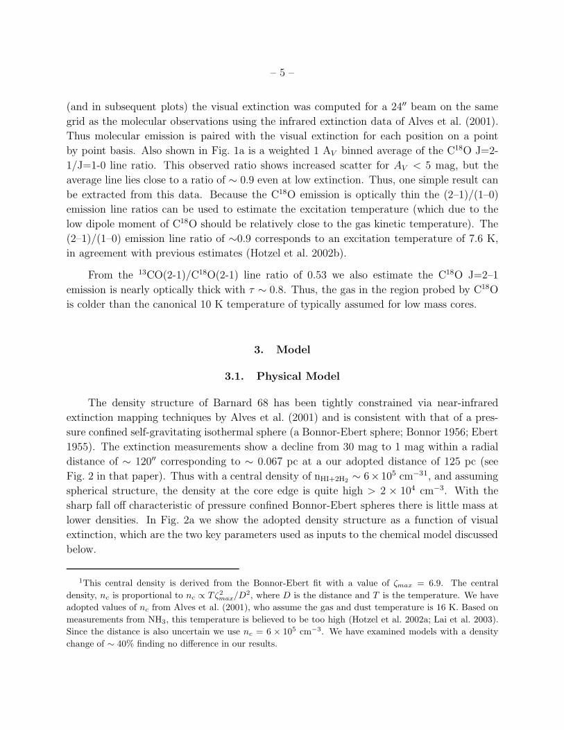
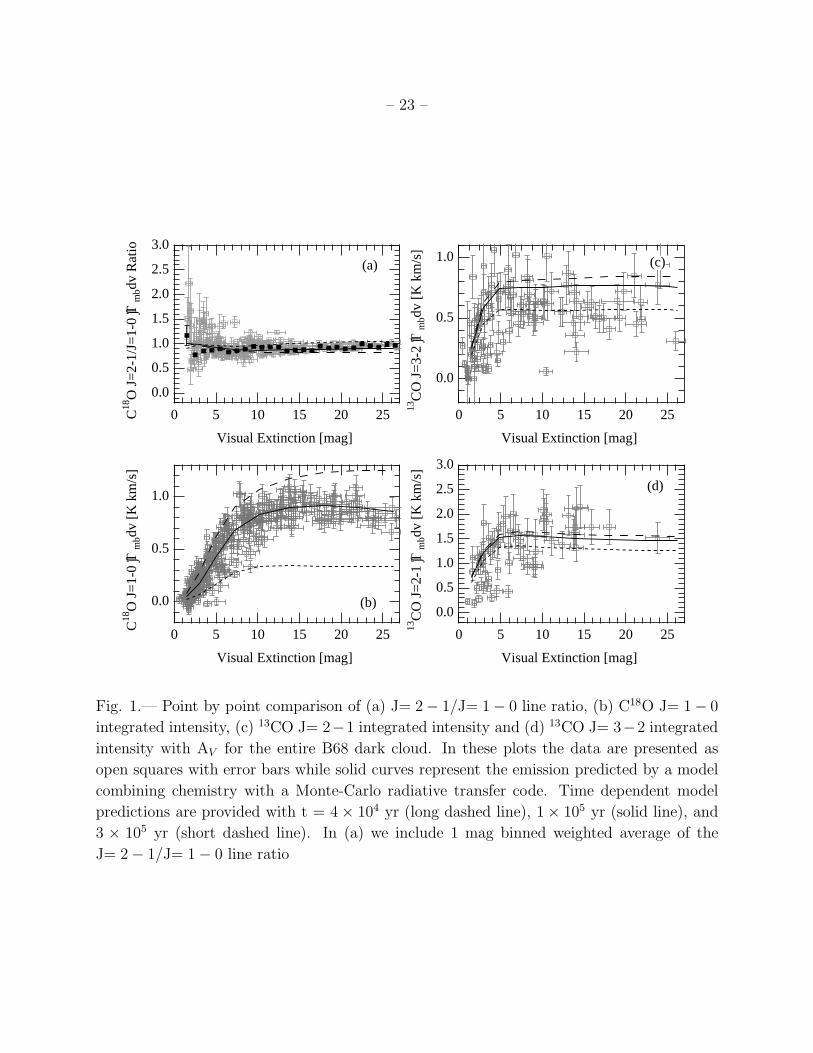
Fig. 1 presents the observational data as a function of visual extinction. In this plot

– 5 –

(and in subsequent plots) the visual extinction was computed for a 24′′ beam on the same

grid as the molecular observations using the infrared extinction data of Alves et al. (2001).

Thus molecular emission is paired with the visual extinction for each position on a point

by point basis. Also shown in Fig. 1a is a weighted 1 AV binned average of the C18O J=2-

1/J=1-0 line ratio. This observed ratio shows increased scatter for AV < 5 mag, but the

average line lies close to a ratio of ∼ 0.9 even at low extinction. Thus, one simple result can

be extracted from this data. Because the C18O emission is optically thin the (2–1)/(1–0)

emission line ratios can be used to estimate the excitation temperature (which due to the

low dipole moment of C18O should be relatively close to the gas kinetic temperature). The

(2–1)/(1–0) emission line ratio of ∼0.9 corresponds to an excitation temperature of 7.6 K,

in agreement with previous estimates (Hotzel et al. 2002b).

From the 13CO(2-1)/C18O(2-1) line ratio of 0.53 we also estimate the C18O J=2–1

emission is nearly optically thick with τ ∼ 0.8. Thus, the gas in the region probed by C18O

is colder than the canonical 10 K temperature of typically assumed for low mass cores.

3. Model

3.1. Physical Model

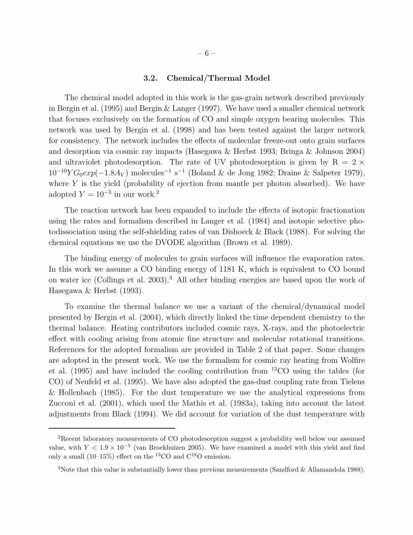
The density structure of Barnard 68 has been tightly constrained via near-infrared

extinction mapping techniques by Alves et al. (2001) and is consistent with that of a pres-

sure confined self-gravitating isothermal sphere (a Bonnor-Ebert sphere; Bonnor 1956; Ebert

1955). The extinction measurements show a decline from 30 mag to 1 mag within a radial

distance of ∼ 120′′ corresponding to ∼ 0.067 pc at a our adopted distance of 125 pc (see

Fig. 2 in that paper). Thus with a central density of nHI+2H2∼ 6×105 cm−31, and assuming

spherical structure, the density at the core edge is quite high > 2 × 104 cm−3. With the

sharp fall off characteristic of pressure confined Bonnor-Ebert spheres there is little mass at

lower densities. In Fig. 2a we show the adopted density structure as a function of visual

extinction, which are the two key parameters used as inputs to the chemical model discussed

below.

1This central density is derived from the Bonnor-Ebert fit with a value of ζmax = 6.9. The central

density, nc is proportional to nc ∝ Tζ2max

/D2, where D is the distance and T is the temperature. We have

adopted values of nc from Alves et al. (2001), who assume the gas and dust temperature is 16 K. Based on

measurements from NH3, this temperature is believed to be too high (Hotzel et al. 2002a; Lai et al. 2003).

Since the distance is also uncertain we use nc = 6 × 105 cm−3. We have examined models with a density

change of ∼ 40% finding no difference in our results.

– 6 –

3.2. Chemical/Thermal Model

The chemical model adopted in this work is the gas-grain network described previously

in Bergin et al. (1995) and Bergin & Langer (1997). We have used a smaller chemical network

that focuses exclusively on the formation of CO and simple oxygen bearing molecules. This

network was used by Bergin et al. (1998) and has been tested against the larger network

for consistency. The network includes the effects of molecular freeze-out onto grain surfaces

and desorption via cosmic ray impacts (Hasegawa & Herbst 1993; Bringa & Johnson 2004)

and ultraviolet photodesorption. The rate of UV photodesorption is given by R = 2 ×

10−10Y G0exp(−1.8AV ) molecules−1 s−1 (Boland & de Jong 1982; Draine & Salpeter 1979),

where Y is the yield (probability of ejection from mantle per photon absorbed). We have

adopted Y = 10−3 in our work.2

The reaction network has been expanded to include the effects of isotopic fractionation

using the rates and formalism described in Langer et al. (1984) and isotopic selective pho-

todissociation using the self-shielding rates of van Dishoeck & Black (1988). For solving the

chemical equations we use the DVODE algorithm (Brown et al. 1989).

The binding energy of molecules to grain surfaces will influence the evaporation rates.

In this work we assume a CO binding energy of 1181 K, which is equivalent to CO bound

on water ice (Collings et al. 2003).3 All other binding energies are based upon the work of

Hasegawa & Herbst (1993).

To examine the thermal balance we use a variant of the chemical/dynamical model

presented by Bergin et al. (2004), which directly linked the time dependent chemistry to the

thermal balance. Heating contributors included cosmic rays, X-rays, and the photoelectric

effect with cooling arising from atomic fine structure and molecular rotational transitions.

References for the adopted formalism are provided in Table 2 of that paper. Some changes

are adopted in the present work. We use the formalism for cosmic ray heating from Wolfire

et al. (1995) and have included the cooling contribution from 13CO using the tables (for

CO) of Neufeld et al. (1995). We have also adopted the gas-dust coupling rate from Tielens

& Hollenbach (1985). For the dust temperature we use the analytical expressions from

Zucconi et al. (2001), which used the Mathis et al. (1983a), taking into account the latest

adjustments from Black (1994). We did account for variation of the dust temperature with

2Recent laboratory measurements of CO photodesorption suggest a probability well below our assumed

value, with Y < 1.9 × 10−5 (van Broekhuizen 2005). We have examined a model with this yield and find

only a small (10–15%) effect on the 13CO and C18O emission.

3Note that this value is substantially lower than previous measurements (Sandford & Allamandola 1988).

– 7 –

a lower external UV field by adding additional layers of extinction based upon the following

expression: AV,add = log(G0)/(−2.5). This expression assumes that the heating effects of the

UV field decay as e−2.5AV and is likely an overestimate (to below a factor of ∼1.5) as longer

wavelength photons also contribute to dust heating. However, it provides a crude estimate

of the effects of a variable UV field. The dust temperature is assumed to be constant with

time, while the gas temperature will change as the chemistry evolves.

Since B68 is a cold pre-stellar object bathed in the normal interstellar radiation field

(ISRF) we have not coupled the thermal balance directly to the chemistry. Rather the

chemistry is calculated assuming a constant temperature of 10 K and the thermal balance is

determined using the results from the time-dependent chemical model. Both the chemistry

and the thermal balance assume the density profile (derived from dust absorption) is constant

with time. In this fashion, for each time, we derive chemical abundances as a function of cloud

depth and then compute the resulting thermal balance. This separation is reasonable given

that the gas-phase chemistry is rather insensitive to the few degree changes as a function

of depth that are found from our thermal balance calculations. The primary temperature

dependence in the chemistry arises from the isotopic fractionation of CO at the cloud edges,

where the column is small. For example, 2–3 K changes in temperature show 20% differences

at the peak C18O abundance.

Since we have adopted a density profile that is constant with time we have assumed that

the chemistry has previously evolved at lower density to the point that all carbon resides in

CO and oxygen is locked on grains in the form of water ice. In Table 1 we provide a list of

assumed initial abundances.

The variables in our calculations are (1) the overall intensity of FUV radiation field,

parameterized by G0, the FUV flux relative to that measured for the local ISM by Habing

(1968). This influences the photodissociation rate (at what depth a given CO isotopologue

appears) and the amount of photoelectric heating, which dominates the heating at low

AV . (2) Several values of the primary cosmic ray ionization rate were examined between

ζ = 1.5− 6.0× 10−17 s−1. CO is assumed to be pre-existing in our calculations and changes

in the cosmic ray ionization rate by factors of a few does not change its chemistry appreciably,

which is dominated by the grain freeze-out. It does however change the cosmic ray heating

rate, which is important for gas heating at high extinction. Because the cosmic ray desorption

rate is uncertain we assumed a constant rate in our analysis based in the formalism of

Hasegawa & Herbst (1993) and the binding energy given above. (3) Time is also a variable.

As the chemistry evolves the effects of freeze-out alters the resulting emission. (4) The final

variable is dust-gas heating/cooling rate. The dust-gas thermal coupling expression from

Tielens & Hollenbach (1985) is given as:

– 8 –

Γgas−dust = 3.5 × 10−34n2δdT0.52gas k(Tdust − Tgas) ergs cm−3s−1.

In this expression δd is the ratio of the dust abundance in the modeled region to that of the

diffuse ISM. Effectively this is a measure of the surface area trapped in more numerous small

grains, which are more efficient in thermally coupling to the gas. When δd is varied in our

models we make no correction for this in the chemistry, where it can alter the timescales.

In general, chemical models assume that large grains are responsible for freeze-out (which

is the dominant effect in this calculation). This assumes that cosmic rays can effectively

thermally cycle small grains and leave the surface bare (Leger et al. 1985). Thus the change

in the surface area or number density of the large 1000 A grains from the loss of small grains

is assumed to be small.

Our analysis proceeds in the following fashion. The adopted nH2(r) profile and Tgas =

Tdust = 10 K is used as inputs to the time-dependent gas-grain chemical model. The results

from the chemical model are used as inputs to the thermal balance calculation which provides

Tgas(r). The abundance and gas temperature structure are incorporated as inputs to the

one-dimensional spherical Monte-Carlo radiation transfer model (Ashby et al. 2000). This

model self-consistently solves for the molecular emission accounting for effects of sub-thermal

excitation, radiation trapping, and pumping by dust continuum photons. The latter is

unimportant for B68. Additional inputs to this model are the velocity line width and line

of sight velocity field. The line width includes contributions from the thermal and turbulent

widths. In our iterations we have assumed a static cloud with the turbulent contribution

to the linewidth included that increases with radius from the core center (as required by

observations; Lada et al. 2003). The model emission is convolved to the observed angular

resolution for each transition (assuming a distance of 125 pc) and onto a grid sampled every

12′′. The model emission is then placed onto∫

Tmb∆v vs. AV plots shown in §4. To compare

the velocity width to the data we fit spectra with Gaussians. To be successful a model must

reproduce both the dependence of∫

Tdv with AV for C18O J=1-0, 13CO J=2-1, J=3-2, the

C18O J=2-1/1-0 integrated emission ratio, and ∆v with radius for C18O J=1-0 and 13CO

J=2-1.

– 9 –

4. Analysis

4.1. Time Dependent Chemistry and Gas Temperature

In our analysis it became clear that we cannot reproduce the observed emission with the

core exposed to the standard ISRF (G0 = 1). Instead these data require colder outer layers

and a reduced UV field, G0 ∼ 0.2. For our initial discussion of the overall gas temperature

structure in cores dominated by freeze-out, we use the model with the reduced UV field. In

§ 4.2 we demonstrate this requirement.

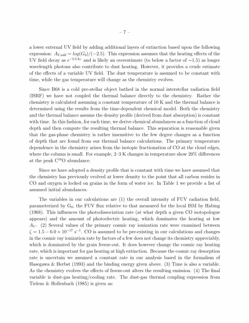
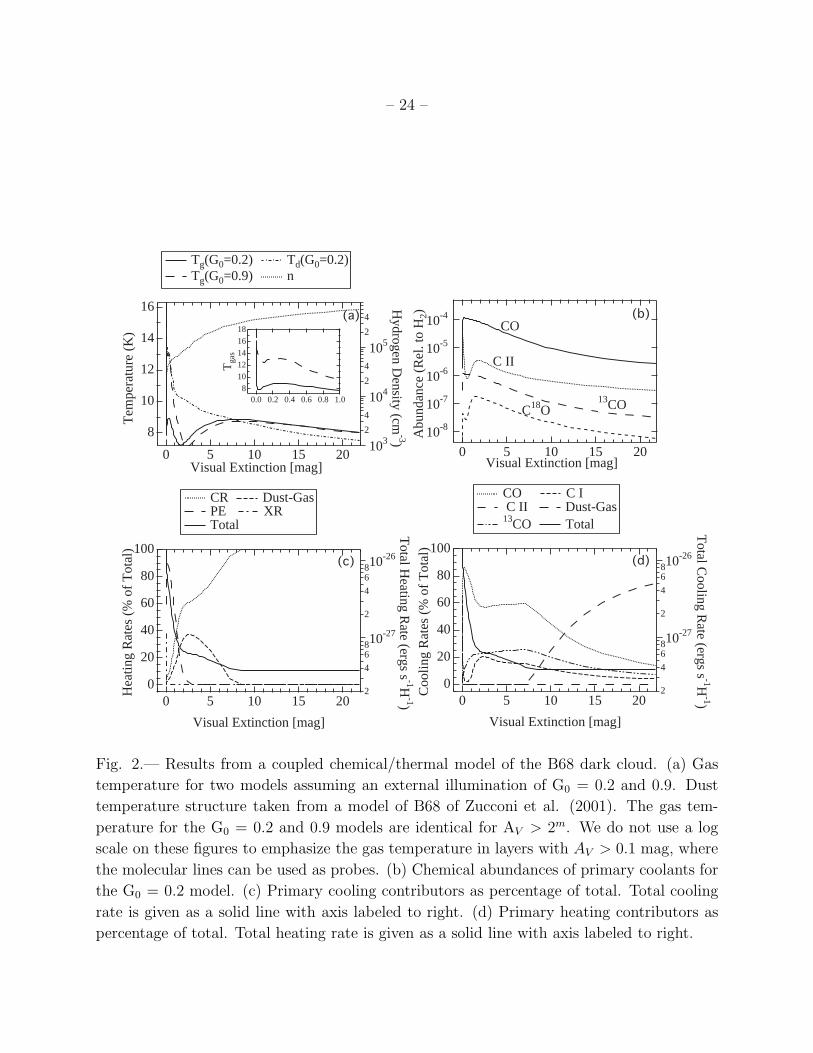
In Figure 2 we provide a 4 panel plot with the relevant physical quantities that are

inputs (e.g. density, dust temperature) or outputs (gas temperature, abundance) from the

model. To aid the discussion, we also provide the major heating and cooling terms, as a

function of cloud depth. In Fig. 1 we provide the results from a series of time-dependent

models superposed on the observational data for B68. This series of four panel plots of the

C18O J=2-1/J=1-0 integrated emission ratio plotted as a function of AV (Fig. 1a), along

with the integrated intensity of C18O J=1-0 (Fig. 1b), J=3-2 (Fig. 1c), and 13CO J=2-1

(Fig. 1d) as a function of AV are used to test our models. In each panel the symbols are

data points and lines are the model results.

The models shown in Fig. 1 sample a range of times and assume a cosmic ray ionization

rate of ζ = 3.0×10−17 s−1, δd = 1, G0 = 0.2. Our “best fit” model is at a time of t ∼ 105 yr,

with earlier and later times showing significant discrepancies with observed emission. “Best-

fit” implies agreement with CO isotopologue data. As discussed later some modifications

to this model are needed to match additional observations. The primary effect of time in

the models is increasing CO freeze-out, which lowers the column density as the core evolves.

Thus, the drop in C18O and 13CO column density directly relates to the reduction in predicted

line intensity. The magnitude of the decline depends on the optical depth of the transition,

hence it is largest for thinner C18O J=1–0 emission and smaller for thicker 13CO emission

lines. The C18O line ratio does not show strong time-dependence because CO freeze-out,

and the subsequent decrease in CO cooling, does not produce a sharp temperature rise. This

is demonstrated in Fig. 3 where we present the temperature and CO abundance structure as

a function of time. As time evolves in regions with lower density gas with weaker gas-dust

coupling (AV < 10 mag), the depletion of coolants warms the gas, but the cooling power

of dust-gas collisions compensates for this loss in the densest regions (AV > 10 mag), a

point first noted by Goldsmith (2001). The CO abundance exhibits a sharp drop below

AV = 1 mag due to photodissociation and decline at high AV due to freeze-out. The CO

photodissociation front is confined to a small range of visual extinction because of the high

densities and low UV fields at the boundary layer.

– 10 –

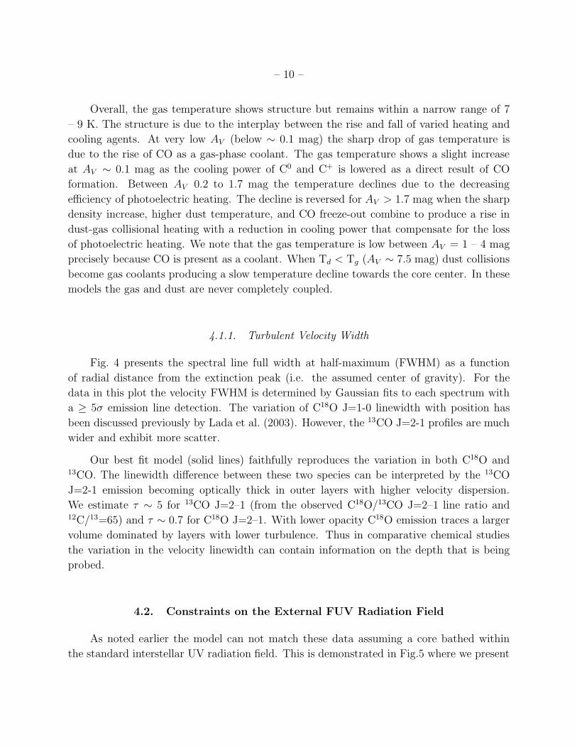
Overall, the gas temperature shows structure but remains within a narrow range of 7

– 9 K. The structure is due to the interplay between the rise and fall of varied heating and

cooling agents. At very low AV (below ∼ 0.1 mag) the sharp drop of gas temperature is

due to the rise of CO as a gas-phase coolant. The gas temperature shows a slight increase

at AV ∼ 0.1 mag as the cooling power of C0 and C+ is lowered as a direct result of CO

formation. Between AV 0.2 to 1.7 mag the temperature declines due to the decreasing

efficiency of photoelectric heating. The decline is reversed for AV > 1.7 mag when the sharp

density increase, higher dust temperature, and CO freeze-out combine to produce a rise in

dust-gas collisional heating with a reduction in cooling power that compensate for the loss

of photoelectric heating. We note that the gas temperature is low between AV = 1 – 4 mag

precisely because CO is present as a coolant. When Td < Tg (AV ∼ 7.5 mag) dust collisions

become gas coolants producing a slow temperature decline towards the core center. In these

models the gas and dust are never completely coupled.

4.1.1. Turbulent Velocity Width

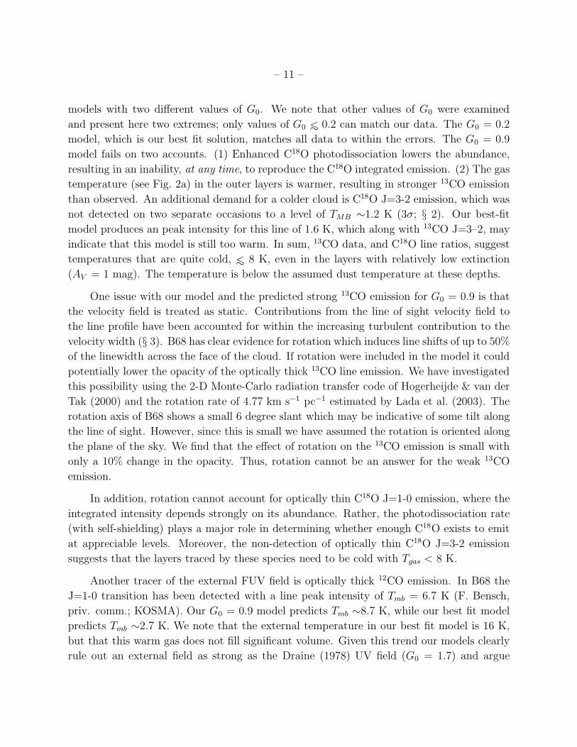
Fig. 4 presents the spectral line full width at half-maximum (FWHM) as a function

of radial distance from the extinction peak (i.e. the assumed center of gravity). For the

data in this plot the velocity FWHM is determined by Gaussian fits to each spectrum with

a ≥ 5σ emission line detection. The variation of C18O J=1-0 linewidth with position has

been discussed previously by Lada et al. (2003). However, the 13CO J=2-1 profiles are much

wider and exhibit more scatter.

Our best fit model (solid lines) faithfully reproduces the variation in both C18O and13CO. The linewidth difference between these two species can be interpreted by the 13CO

J=2-1 emission becoming optically thick in outer layers with higher velocity dispersion.

We estimate τ ∼ 5 for 13CO J=2–1 (from the observed C18O/13CO J=2–1 line ratio and12C/13=65) and τ ∼ 0.7 for C18O J=2–1. With lower opacity C18O emission traces a larger

volume dominated by layers with lower turbulence. Thus in comparative chemical studies

the variation in the velocity linewidth can contain information on the depth that is being

probed.

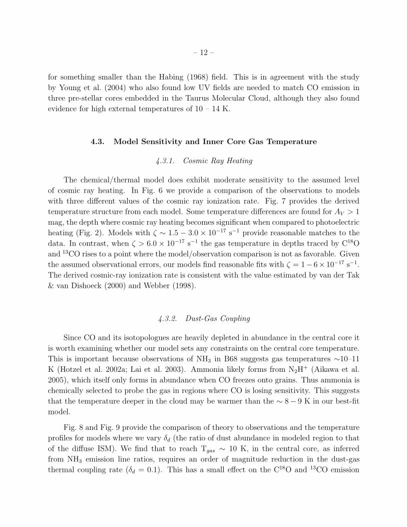
4.2. Constraints on the External FUV Radiation Field

As noted earlier the model can not match these data assuming a core bathed within

the standard interstellar UV radiation field. This is demonstrated in Fig.5 where we present

– 11 –

models with two different values of G0. We note that other values of G0 were examined

and present here two extremes; only values of G0 ∼< 0.2 can match our data. The G0 = 0.2

model, which is our best fit solution, matches all data to within the errors. The G0 = 0.9

model fails on two accounts. (1) Enhanced C18O photodissociation lowers the abundance,

resulting in an inability, at any time, to reproduce the C18O integrated emission. (2) The gas

temperature (see Fig. 2a) in the outer layers is warmer, resulting in stronger 13CO emission

than observed. An additional demand for a colder cloud is C18O J=3-2 emission, which was

not detected on two separate occasions to a level of TMB ∼1.2 K (3σ; § 2). Our best-fit

model produces an peak intensity for this line of 1.6 K, which along with 13CO J=3–2, may

indicate that this model is still too warm. In sum, 13CO data, and C18O line ratios, suggest

temperatures that are quite cold, ∼< 8 K, even in the layers with relatively low extinction

(AV = 1 mag). The temperature is below the assumed dust temperature at these depths.

One issue with our model and the predicted strong 13CO emission for G0 = 0.9 is that

the velocity field is treated as static. Contributions from the line of sight velocity field to

the line profile have been accounted for within the increasing turbulent contribution to the

velocity width (§ 3). B68 has clear evidence for rotation which induces line shifts of up to 50%

of the linewidth across the face of the cloud. If rotation were included in the model it could

potentially lower the opacity of the optically thick 13CO line emission. We have investigated

this possibility using the 2-D Monte-Carlo radiation transfer code of Hogerheijde & van der

Tak (2000) and the rotation rate of 4.77 km s−1 pc−1 estimated by Lada et al. (2003). The

rotation axis of B68 shows a small 6 degree slant which may be indicative of some tilt along

the line of sight. However, since this is small we have assumed the rotation is oriented along

the plane of the sky. We find that the effect of rotation on the 13CO emission is small with

only a 10% change in the opacity. Thus, rotation cannot be an answer for the weak 13CO

emission.

In addition, rotation cannot account for optically thin C18O J=1-0 emission, where the

integrated intensity depends strongly on its abundance. Rather, the photodissociation rate

(with self-shielding) plays a major role in determining whether enough C18O exists to emit

at appreciable levels. Moreover, the non-detection of optically thin C18O J=3-2 emission

suggests that the layers traced by these species need to be cold with Tgas < 8 K.

Another tracer of the external FUV field is optically thick 12CO emission. In B68 the

J=1-0 transition has been detected with a line peak intensity of Tmb = 6.7 K (F. Bensch,

priv. comm.; KOSMA). Our G0 = 0.9 model predicts Tmb ∼8.7 K, while our best fit model

predicts Tmb ∼2.7 K. We note that the external temperature in our best fit model is 16 K,

but that this warm gas does not fill significant volume. Given this trend our models clearly

rule out an external field as strong as the Draine (1978) UV field (G0 = 1.7) and argue

– 12 –

for something smaller than the Habing (1968) field. This is in agreement with the study

by Young et al. (2004) who also found low UV fields are needed to match CO emission in

three pre-stellar cores embedded in the Taurus Molecular Cloud, although they also found

evidence for high external temperatures of 10 – 14 K.

4.3. Model Sensitivity and Inner Core Gas Temperature

4.3.1. Cosmic Ray Heating

The chemical/thermal model does exhibit moderate sensitivity to the assumed level

of cosmic ray heating. In Fig. 6 we provide a comparison of the observations to models

with three different values of the cosmic ray ionization rate. Fig. 7 provides the derived

temperature structure from each model. Some temperature differences are found for AV > 1

mag, the depth where cosmic ray heating becomes significant when compared to photoelectric

heating (Fig. 2). Models with ζ ∼ 1.5 − 3.0 × 10−17 s−1 provide reasonable matches to the

data. In contrast, when ζ > 6.0 × 10−17 s−1 the gas temperature in depths traced by C18O

and 13CO rises to a point where the model/observation comparison is not as favorable. Given

the assumed observational errors, our models find reasonable fits with ζ = 1− 6× 10−17 s−1.

The derived cosmic-ray ionization rate is consistent with the value estimated by van der Tak

& van Dishoeck (2000) and Webber (1998).

4.3.2. Dust-Gas Coupling

Since CO and its isotopologues are heavily depleted in abundance in the central core it

is worth examining whether our model sets any constraints on the central core temperature.

This is important because observations of NH3 in B68 suggests gas temperatures ∼10–11

K (Hotzel et al. 2002a; Lai et al. 2003). Ammonia likely forms from N2H+ (Aikawa et al.

2005), which itself only forms in abundance when CO freezes onto grains. Thus ammonia is

chemically selected to probe the gas in regions where CO is losing sensitivity. This suggests

that the temperature deeper in the cloud may be warmer than the ∼ 8− 9 K in our best-fit

model.

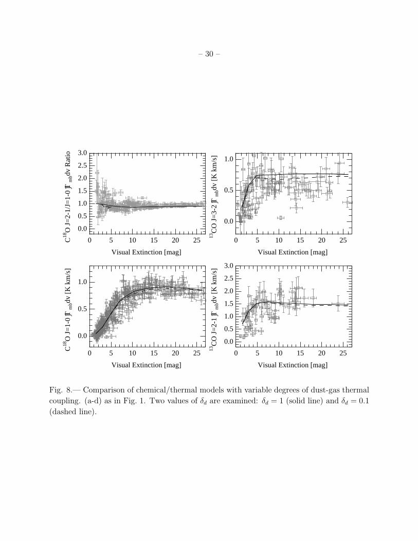
Fig. 8 and Fig. 9 provide the comparison of theory to observations and the temperature

profiles for models where we vary δd (the ratio of dust abundance in modeled region to that

of the diffuse ISM). We find that to reach Tgas ∼ 10 K, in the central core, as inferred

from NH3 emission line ratios, requires an order of magnitude reduction in the dust-gas

thermal coupling rate (δd = 0.1). This has a small effect on the C18O and 13CO emission

– 13 –

demonstrating that their emission is not a probe of the inner core gas temperature. Curiously

lowering the dust-gas thermal coupling rate reduces C18O and 13CO emission. This is because

these two species are predominantly tracing depths where collisions with dust are heating

the gas (see Fig. 2). Thus, provided our understanding of dust-gas thermal coupling rates is

correct, to match NH3 derived gas temperatures requires a reduction in the rate, potentially

due to changing dust properties.

The conclusion regarding weaker gas-dust coupling rests upon proper modeling of the

dust temperature and the calibration of the ammonia thermometer. In our models we have

not directly examined dust emission and used the formula provided by Zucconi et al. (2001)

with some modifications to account for reduced radiation field (§3). Our modifications to

the dust temperature did result in reducing the dust temperature at high depth into the

cloud. However, at AV > 10 mag our “best-fit” solution assumes Tdust ∼8 K, which is quite

close the value for similar depths used by Galli et al. (2002) in their core stability study of

B68 and is also similar to the value inferred by Zucconi et al. (2001) and Evans et al. (2001)

for the inner radii of Bonnor-Ebert spheres. Thus our the requirement for reduced dust-gas

coupling would not be altered with more exact treatment of the dust emission.

One question is whether the ammonia thermometer and measurements are calibrated to

an accuracy of ∼ 2 K. The Hotzel et al. (2002a) measurement of the gas temperature from

ammonia emission taken with a similar resolution (40′′) to our data. The raw error of this

measurement is 9.7 ±0.3 K, which is increased to 1.0 K allowing for 20% differences in the

filling factor and Tex between the two lines. This seems overly generous given the similarity

in critical density and filling factor between these lines. Moreover the Lai et al. (2003) tem-

perature estimate is 10.8 ±0.8 K. Thus both analyses suggest at least a 3σ difference between

the central core gas temperature in our model of ∼ 8 K and measurements. Regarding the

calibration of the ammonia thermometer, for T > 10 K the observed (2,2) and (1,1) inversion

transition rotational temperature is not equivalent to the gas kinetic temperature. However,

close to 10 K the rotational temperature is a measurement of Tk without any correction

(Danby et al. 1988). Thus, provided this calibration is accurate, the observed difference is

suggestive that the dust-gas coupling needs to be reduced.

Given the need for lower dust-gas thermal coupling in Fig. 10 we re-examine the time

evolution of the gas temperature in a model with reduced coupling. Similar to the discussion

in § 4.1, we find that as time evolves and gas coolants deplete the gas temperature rises.

In this case the effects of freeze-out on Tgas are stronger, but at most depletion warms the

core by ∼ 1 K. The temperature is actually lower between 0 < AV < 7 mag, because the

main heating mechanism is dust collisions in this region. Thus, while we have found that

freeze-out does raise the temperature, these effects are small and we remain in agreement

– 14 –

with previous studies of the gas temperature in cores dominated by freeze-out (Goldsmith

2001; Galli et al. 2002).

5. Discussion

5.1. The Meaning of Time in these Models

In our models we find a “best-fit” to the observations at t ∼ 105 yr. This does not

suggest that we constrain the age of this object to be 105 yrs. We have used a density

profile that is fixed in time in our time-dependent chemical calculations. Thus we have not

accounted for contemporaneous density evolution along with the chemistry. To compensate

for this effect we have assumed that all CO is pre-existing in the gas at t = 0 in our chemical

network solutions. With these assumptions this time is not the time since the cloud became

molecular (since CO is pre-existing) nor is the time since the density structure evolved (since

the structure is fixed). Rather, the best-fit time represents the time where sufficient pre-

existing CO has been frozen onto grains and the predicted gas emission matches observations.

We have also assumed a sticking coefficient of unity. A lower value would result in a higher

age determination. Moreover, if we had included any the effect of dust coagulation on the

chemistry there would be an increase in the derived timescale. In this sense our derived time

is only a lower limit to the true age of B68.

We have included a mechanism for returning CO to the gas via constant cosmic ray

desorption of CO ice, which does depend on our assumed binding energy. In our models

we do not reach a time where desorption is relevant in the sense that at late times when

pre-existing CO is frozen and equilibrium is reached between desorption and depletion there

is not enough CO in the gas to reproduce the observed emission. The binding energy would

need to be lowered well below measured values (Collings et al. 2003) and the rate of CO

desorption increased above estimated levels (Bringa & Johnson 2004) to change this condition

and raise our time estimate.

5.2. Grain Evolution

Our multi-molecular comparative chemical study (e.g. CO and NH3) suggests that the

dust-gas coupling rate is reduced in the center of B68. This potentially represents evidence

for grain coagulation inferred from gas observations. In the literature there are several lines

of evidence for grain evolution from dust observations. These include variations in the ratio

of visual extinction to reddening, RV , (Fitzpatrick 2004, and references therein) which have

– 15 –

been attributed to changes in the grain size distribution (Kim et al. 1994; Weingartner &

Draine 2001), studies of the far-infrared emission which find a lack of small grains in denser

regions (Stepnik et al. 2003), and the requirement for enhanced sub-mm emissivity in star-

forming regions (van der Tak et al. 1999; Evans et al. 2001). Theory of grain coagulation

suggests significant grain evolution is expected in only a few million years (Weidenschilling

& Ruzmaikina 1994), the expected lifetime of the pre-stellar phase (Lee et al. 2001).

To examine what grain evolution (e.g. coagulation) is needed to reach δd = 0.1 we have

used the MRN (Mathis et al. 1977) grain size distribution. This is given by:

dngr = CnHa−3.5da, amin < a < amax,

with amin = 50 A and amax = 2500 A. Draine & Lee (1984) find the normalization for silicate

grains to be C = 10−25.11 cm2.5. Integration of this equation provides ngr = 1.75 × 10−10nH

for standard ISM grains. To obtain δd = 0.1 (while maintaining a−3.5) necessitates a minimal

change in the size of the smallest grains, to amin = 150 A. This analysis is simplistic as we

have not discussed extensions of MRN towards even smaller grains that are needed for the

ISM in general (Desert et al. 1990; Weingartner & Draine 2001). However, it is illustrative

that only small changes are needed in the lower end of the size distribution to account for

the reduction in grain surface area demanded by available gas emission data.

One inconsistency is that we have included small grain photoelectric heating in our mod-

els and need to have a warmer central core with less small grains to match NH3 observations.

To this end we investigated the necessity for photo-electric heating in our theory/observation

comparison. We find that a reduction of the photoelectric heating rate of more than 50%

does not agree with our data (even with a compensating increase in cosmic ray heating).4

Thus, based upon the adopted formalism for photoelectric heating and dust-gas thermal cou-

pling, we require some small grains to be present in the outer layers but these same grains

are absent in the inner core. This is not unreasonable given the large density increase seen

in B68 (Fig. 2; Alves et al. 2001).

It is worth noting that Bianchi et al. (2003) find no evidence for dust coagulation based

on measurements of the sub-millimeter emissivity and comparison to available grain models.

However, the measured value is higher than that of diffuse dust, although only at the 2σ

level.

4In principle the dust-gas coupling could be stronger at the low density core edges because of warmer dust

temperatures and the presence of small grains and weaker in the center due to the lack of small grains. This

might further compensate from the loss of very small grains and allow for a greater decrease in photoelectric

heating.

– 16 –

5.3. Comparison to Previous Results

A major issue with our suggestion that the UV field is reduced is dust emission models

which require a core exposed to ISRF derived by Mathis et al. (1983b), which has G0 =

1.6 (Draine & Li 2001). Moreover the intensity of the ISRF incident on B68 has been

estimated independently by Galli et al. (2002) using a variety of dust continuum emission

observations with no evidence for any reduction in field strength. Thus there is nearly an

order of magnitude difference in UV field strength between gas and dust models.

A likely possibility to reconcile these differences is that there exists an extended layer

of diffuse gas around B68 that might unassociated with the core. For instance, Lombardi

et al. (2006, in prep.) have used the Near-IR extinction method to map the extinction

structure within the Pipe nebula, in which B68 is embedded. This map shows a large degree

of extended extinction in this cloud, which provides additional UV shielding for B68. If this

layer consists of only 1 mag of extinction, then the strength of the local radiation field for

B68 would be increased by a factor of 1/exp(-3) or G0 = 2. Moreover, any H2 in this layer

can contribute to CO self-shielding (Bensch et al. 2003), requiring even less dust extinction.

This would allow for higher UV fields in agreement with estimates from the dust emission.

We investigated the inclusion of such a halo in our models and find little change to our

results for CO isotopologue emission.

5.4. Cloud Support

Lada et al. (2003) used the observed linewidths of C18O and C34S to derive an estimate

of the thermal to non-thermal (turbulent) pressure of the B68 core, which is given as:

R =a2

σ2nt

In this expression a is the sound speed of the gas and σnt is the three dimensional velocity

dispersion. This measurement used fits to the observed emission profiles that are an inte-

gration along the line of sight to demonstrate that B68 is dominated by thermal pressure.

In our analysis we have derived a fit to the velocity structure in B68 (Fig. 4) which, for a

static model, includes contributions from the thermal and non-thermal velocity dispersions

as a function of position in the core.5

5We note that this analysis includes no contribution from any systematic cloud motions and thus the

derived non-thermal contribution is an upper limit.

– 17 –

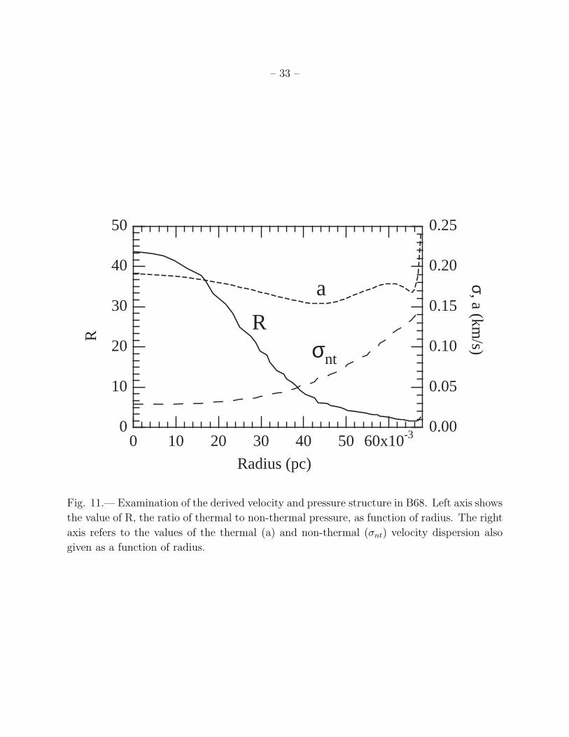
In Fig. 11 we show how the the thermal to non-thermal pressure ratio varies as a function

of radius in B68. There is a sharp variation throughout the object with the center completely

dominated by thermal motions and increasing turbulent contributions towards larger radii.

At all positions the core is dominated by thermal pressure, confirming the previous result.

Lada et al. (2003) derived values of R ∼ 4−5 for the inner core and R ∼ 1−2 for the edges.

In our model the peak C18O abundance is found at r ∼ 0.04 pc, a point which corresponds

to R ∼ 5, close to the value inferred from observation. Thus, in cores with significant

abundance and velocity field structure, the line of sight average velocity dispersion from the

emission profile is heavily weighted to radii which have the largest abundance.

It is worth noting that B68 is dominated by thermal pressure, but it is not an isothermal

object. In our preferred model that matches both CO isotopologues and NH3 (δd = 0.1;

§ 4.3.2), > 95% of the enclosed mass lies in layers with a gas temperature variation of ∼ 3

K. These changes are within the temperature range examined in the thermal balance and

stability study of B68 by Galli et al. (2002). However, the sense of the gradient is opposite to

what is normally examined for a pre-stellar object (i.e. the temperature increases inwards).

Nonetheless these changes are small and it is likely that the conclusions of Galli et al. (2002)

are still relevant and these objects will have similar characteristics to isothermal models.

6. Conclusions

We have combined a multi-molecular and multi-transitional observational study and

a thermal/chemical model to examine the line of sight gas temperature structure of the

Barnard 68 core. Our primary conclusions are as follows.

(1) The gas temperature is cold ∼ 6 − 7 K in the layers traced by 13CO and C18O and

is warmer ∼ 10 K in the gas deeper within the cloud probed by NH3. For much of the

cloud mass the temperature gradient is small ∼ 3 K, but increases towards the center. With

significantly more observational constraints than previous work, this represents the best

determination of the gas temperature structure in pre-stellar cores.

(2) In agreement with previous studies (Hotzel et al. 2002b; Bergin et al. 2002) we find

evidence for large-scale freeze-out of both CO isotopologues and demonstrate that B68 is

dominated by thermal pressure.

(3) To match the data to a model we require a UV field that is weaker than the standard

IRSF. This is in conflict with a previous examination of the dust emission and we discuss

how this discrepancy can be resolved.

– 18 –

(4) We find that the dust-gas coupling rate must be reduced by nearly an order of magnitude,

potentially through a lack of small grains in the densest regions. This presents an argument

from gas observations for grain coagulation in the central regions of the core.

Our detailed comparison of molecular emission to a PDR model in a low UV environ-

ment finds some differences which can be reconciled by assuming that the physics of dust-gas

coupling are represented correctly by changing grain properties. Whether these results have

general applicability requires more detailed investigations of other sources with well charac-

terized density structure, preferably with high UV fields. Additional improvements would

result from more direct modeling of NH3 emission.

We are grateful to the referee for a thorough and detailed report which improved this

paper. This work is supported by the National Science Foundation under Grant No. 0335207.

EAB is grateful to discussions with F. Bensch to D. Lis, M. Tafalla, M. Gurwell, and G.

Herczeg for various aspects of data calibration and observing.

REFERENCES

Aikawa, Y., Herbst, E., Roberts, H., & Caselli, P. 2005, ApJ, 620, 330

Alves, J. F., Lada, C. J., & Lada, E. A. 2001, Nature, 409, 159

Andre, P., Ward-Thompson, D., & Barsony, M. 2000, Protostars and Planets IV, 59

Ashby, M. L. N., Bergin, E. A., Plume, R., Carpenter, J. M., Neufeld, D. A., Chin, G.,

Erickson, N. R., Goldsmith, P. F., Harwit, M., Howe, J. E., Kleiner, S. C., Koch,

D. G., Patten, B. M., Schieder, R., Snell, R. L., Stauffer, J. R., Tolls, V., Wang, Z.,

Winnewisser, G., Zhang, Y. F., & Melnick, G. J. 2000, ApJ, 539, L115

Bensch, F., Leuenhagen, U., Stutzki, J., & Schieder, R. 2003, ApJ, 591, 1013

Bensch, F., Stutzki, J., & Heithausen, A. 2001, A&A, 365, 285

Bergin, E. A., Alves, J., Huard, T., & Lada, C. J. 2002, ApJ, 570, L101

Bergin, E. A., Hartmann, L. W., Raymond, J. C., & Ballesteros-Paredes, J. 2004, ApJ, 612,

921

Bergin, E. A. & Langer, W. D. 1997, ApJ, 486, 316

Bergin, E. A., Langer, W. D., & Goldsmith, P. F. 1995, ApJ, 441, 222

– 19 –

Bergin, E. A., Neufeld, D. A., & Melnick, G. J. 1998, ApJ, 499, 777

Bianchi, S., Goncalves, J., Albrecht, M., Caselli, P., Chini, R., Galli, D., & Walmsley, M.

2003, A&A, 399, L43

Black, J. H. 1994, in ASP Conf. Ser. 58: The First Symposium on the Infrared Cirrus and

Diffuse Interstellar Clouds, 355–+

Boland, W. & de Jong, T. 1982, ApJ, 261, 110

Bonnor, W. B. 1956, MNRAS, 116, 351

Bringa, E. M. & Johnson, R. E. 2004, ApJ, 603, 159

Brown, P. N., Byrne, G. D., & Hindmarsh, A. C. 1989, SIAM J. Sci. Stat. Comput., 10, 1038

Burke, J. R. & Hollenbach, D. J. 1983, ApJ, 265, 223

Collings, M. P., Dever, J. W., Fraser, H. J., & McCoustra, M. R. S. 2003, Ap&SS, 285, 633

Danby, G., Flower, D. R., Valiron, P., Schilke, P., & Walmsley, C. M. 1988, MNRAS, 235,

229

Desert, F.-X., Boulanger, F., & Puget, J. L. 1990, A&A, 237, 215

Dickman, R. L. & Clemens, D. P. 1983, ApJ, 271, 143

Draine, B. T. 1978, ApJS, 36, 595

Draine, B. T. & Lee, H. M. 1984, ApJ, 285, 89

Draine, B. T. & Li, A. 2001, ApJ, 551, 807

Draine, B. T. & Salpeter, E. E. 1979, ApJ, 231, 438

Ebert, R. 1955, Zeitschrift fur Astrophysics, 37, 217

Evans, N. J., Rawlings, J. M. C., Shirley, Y. L., & Mundy, L. G. 2001, ApJ, 557, 193

Fitzpatrick, E. L. 2004, in ASP Conf. Ser. 309: Astrophysics of Dust, 33–+

Galli, D., Walmsley, M., & Goncalves, J. 2002, A&A, 394, 275

Goldsmith, P. F. 2001, ApJ, 557, 736

Habing, H. J. 1968, Bull. Astron. Inst. Netherlands, 19, 421

– 20 –

Hasegawa, T. I. & Herbst, E. 1993, MNRAS, 261, 83

Hogerheijde, M. R. & van der Tak, F. F. S. 2000, A&A, 362, 697

Hotzel, S., Harju, J., & Juvela, M. 2002a, A&A, 395, L5

Hotzel, S., Harju, J., Juvela, M., Mattila, K., & Haikala, L. K. 2002b, A&A, 391, 275

Kim, S.-H., Martin, P. G., & Hendry, P. D. 1994, ApJ, 422, 164

Lada, C. J., Bergin, E. A., Alves, J. F., & Huard, T. L. 2003, ApJ, 586, 286

Lai, S., Velusamy, T., Langer, W. D., & Kuiper, T. B. H. 2003, AJ, 126, 311

Langer, W. D., Graedel, T. E., Frerking, M. A., & Armentrout, P. B. 1984, ApJ, 277, 581

Lee, C. W., Myers, P. C., & Tafalla, M. 2001, ApJS, 136, 703

Leger, A., Jura, M., & Omont, A. 1985, A&A, 144, 147

Mathis, J. S., Mezger, P. G., & Panagia, N. 1983a, A&A, 128, 212

—. 1983b, A&A, 128, 212

Mathis, J. S., Rumpl, W., & Nordsieck, K. H. 1977, ApJ, 217, 425

Neufeld, D. A., Lepp, S., & Melnick, G. J. 1995, ApJS, 100, 132

Sandford, S. A. & Allamandola, L. J. 1988, Icarus, 76, 201

Stepnik, B., Abergel, A., Bernard, J.-P., Boulanger, F., Cambresy, L., Giard, M., Jones,

A. P., Lagache, G., Lamarre, J.-M., Meny, C., Pajot, F., Le Peintre, F., Ristorcelli,

I., Serra, G., & Torre, J.-P. 2003, A&A, 398, 551

Tafalla, M., Myers, P. C., Caselli, P., Walmsley, C. M., & Comito, C. 2002, ApJ, 569, 815

Tielens, A. G. G. M. & Hollenbach, D. 1985, ApJ, 291, 722

van Broekhuizen, F. 2005, Ph.D. Thesis

van der Tak, F. F. S., Caselli, P., & Ceccarelli, C. 2005, A&A, 439, 195

van der Tak, F. F. S. & van Dishoeck, E. F. 2000, A&A, 358, L79

van der Tak, F. F. S., van Dishoeck, E. F., Evans, N. J., Bakker, E. J., & Blake, G. A. 1999,

ApJ, 522, 991

– 21 –

van Dishoeck, E. F. & Black, J. H. 1988, ApJ, 334, 771

Webber, W. R. 1998, ApJ, 506, 329

Weidenschilling, S. J. & Ruzmaikina, T. V. 1994, ApJ, 430, 713

Weingartner, J. C. & Draine, B. T. 2001, ApJ, 548, 296

Wolfire, M. G., Hollenbach, D., McKee, C. F., Tielens, A. G. G. M., & Bakes, E. L. O. 1995,

ApJ, 443, 152

Young, K. E., Lee, J.-E., Evans, N. J., Goldsmith, P. F., & Doty, S. D. 2004, ApJ, 614, 252

Zhou, S., Wu, Y., Evans, N. J., Fuller, G. A., & Myers, P. C. 1989, ApJ, 346, 168

Zucconi, A., Walmsley, C. M., & Galli, D. 2001, A&A, 376, 650

This preprint was prepared with the AAS LATEX macros v5.2.

– 22 –

Table 1. Initial

Abundances

Species Abundancea

He 0.14

H2Oice 2.2 ×10−4

H182 Oice 4.4 ×10−7

CO 8.5 ×10−5

13CO 9.5 ×10−7

C18O 1.7 ×10−7

Fe 3 ×10−8

Fe+ 1.2 ×10−11

aAbundances are relative

to total H.

– 23 –

3.0

2.5

2.0

1.5

1.0

0.5

0.0

C18

O J

=2-

1/J=

1-0

∫T mbd

v R

atio

2520151050

Visual Extinction [mag]

(a)1.0

0.5

0.0

13C

O J

=3

-2 ∫T

mbd

v [K

km

/s]

2520151050


(c)

1.0

0.5

0.0

C18

O J

=1

-0 ∫T

mbd

v [K

km

/s]

2520151050


(b)

3.0

2.5

2.0

1.5

1.0

0.5

0.0

13C

O J

=2

-1 ∫T

mbd

v [K

km

/s]

2520151050


(d)

Fig. 1.— Point by point comparison of (a) J= 2 − 1/J= 1 − 0 line ratio, (b) C18O J= 1 − 0

integrated intensity, (c) 13CO J= 2−1 integrated intensity and (d) 13CO J= 3−2 integrated

intensity with AV for the entire B68 dark cloud. In these plots the data are presented as

open squares with error bars while solid curves represent the emission predicted by a model

combining chemistry with a Monte-Carlo radiative transfer code. Time dependent model

predictions are provided with t = 4 × 104 yr (long dashed line), 1 × 105 yr (solid line), and

3 × 105 yr (short dashed line). In (a) we include 1 mag binned weighted average of the

J= 2 − 1/J= 1 − 0 line ratio

– 24 –

1032

4

1042

4

1052

4

Hydrogen D

ensity (cm -3)

20151050Visual Extinction [mag]

16

14

12

10

8

Tem

pera

ture

(K

)

Tg(G0=0.2) Td(G0=0.2) Tg(G0=0.9) n

100

80

60

40

20

0

Hea

ting

Rat

es (

% o

f Tot

al)

20151050


2

4

6810-27

2

4

6810-26

Total H

eating Rate (ergs s

-1H-1)

CR Dust-Gas PE XR Total

100

80

60

40

20

0

Coo

ling

Rat

es (

% o

f Tot

al)

20151050


2

4

6810-27

2

4

6810-26

Total C

ooling Rate (ergs s

-1H-1)

CO C I C II Dust-Gas 13CO Total

10-8

10-7

10-6

10-5

10-4

Abu

ndan

ce (

Rel

. to

H 2)


CO

13COC18O

C II

(a) (b)

(c) (d)

18161412108

Tga

s

1.00.80.60.40.20.0

Fig. 2.— Results from a coupled chemical/thermal model of the B68 dark cloud. (a) Gas

temperature for two models assuming an external illumination of G0 = 0.2 and 0.9. Dust

temperature structure taken from a model of B68 of Zucconi et al. (2001). The gas tem-

perature for the G0 = 0.2 and 0.9 models are identical for AV > 2m. We do not use a log

scale on these figures to emphasize the gas temperature in layers with AV > 0.1 mag, where

the molecular lines can be used as probes. (b) Chemical abundances of primary coolants for

the G0 = 0.2 model. (c) Primary cooling contributors as percentage of total. Total cooling

rate is given as a solid line with axis labeled to right. (d) Primary heating contributors as

percentage of total. Total heating rate is given as a solid line with axis labeled to right.

– 25 –

2

4

6810-5

2

4

6810-4

2

CO

Abu

ndan

ce (

Rel

. to

H 2)

20151050


12

11

10

9

8Tem

pera

ture

(K

)

20151050


t = 4 x 104 yr t = 1 x 105 yr t = 3 x 105 yr t = 1 x 106 yr

Fig. 3.— Left: CO abundance as a function of visual extinction and time. Right: Gas

temperature as a function of visual extinction and time.

– 26 –

0.6

0.4

0.2

∆v

(km

/s)

120100806040200

Radial Offset from Extinction Peak (")

13CO J=2-1 C18O J=1-0 Model

Fig. 4.— Velocity linewidth (FWHM) determined by fitting C18O J=1-0 and 13CO J=2-1

observed and model spectra with Gaussians shown as a function of radial distance from the

extinction peak. Data are given as points and model results from the best fit solution as a

solid line.

– 27 –

3.0

2.5

2.0

1.5

1.0

0.5

0.0

C18

O J

=2-

1/J=

1-0

∫T mbd

v R

atio


1.5

1.0

0.5

0.0

13C

O J

=3

-2 ∫T

mbd

v [K

km

/s]


1.0

0.5

0.0

C18

O J

=1

-0 ∫T

mbd

v [K

km

/s]


3.0

2.5

2.0

1.5

1.0

0.5

0.0

13C

O J

=2

-1 ∫T

mbd

v [K

km

/s]


(a)

(b)

(c)

(d)

Fig. 5.— Comparison of chemical/thermal models with different values of the radiation field.

(a-d) as in Fig. 1. Two values of the external radiation field are examined: G0 = 1 (dashed

lines) and G0 = 0.2 (solid lines).

– 28 –

3.0

2.5

2.0

1.5

1.0

0.5

0.0

C18

O J

=2-

1/J=

1-0

∫T mbd

v R

atio

2520151050


(a)1.0

0.5

0.0

13C

O J

=3

-2 ∫T

mbd

v [K

km

/s]

2520151050


(c)

1.0

0.5

0.0

C18

O J

=1

-0 ∫T

mbd

v [K

km

/s]

2520151050


ζ = 1.5 × 10-17s-1

ζ = 3.0 × 10-17s-1

ζ = 6.0 × 10-17s-1

(b)

3.0

2.5

2.0

1.5

1.0

0.5

0.0

13C

O J

=2

-1 ∫T

mbd

v [K

km

/s]

2520151050


(d)

Fig. 6.— Comparison of chemical/thermal models with different values of the cosmic ray

ionization rate with labels provided above. (a-d) as in Fig. 1.

– 29 –

16

14

12

10

8

Tem

pera

ture

(K

)


ζ= 1.5 × 10-17s-1

ζ= 3.0 × 10-17s-1

ζ= 6.0 × 10-17s-1

Fig. 7.— Derived temperature structure for models with different values of the cosmic ray

ionization rate with labels provided above.

– 30 –

3.0

2.5

2.0

1.5

1.0

0.5

0.0

C18

O J

=2-

1/J=

1-0

∫T mbd

v R

atio

2520151050


1.0

0.5

0.0

13C

O J

=3

-2 ∫T

mbd

v [K

km

/s]

2520151050


1.0

0.5

0.0

C18

O J

=1

-0 ∫T

mbd

v [K

km

/s]

2520151050


3.0

2.5

2.0

1.5

1.0

0.5

0.0

13C

O J

=2

-1 ∫T

mbd

v [K

km

/s]

2520151050


Fig. 8.— Comparison of chemical/thermal models with variable degrees of dust-gas thermal

coupling. (a-d) as in Fig. 1. Two values of δd are examined: δd = 1 (solid line) and δd = 0.1

(dashed line).

– 31 –

16

14

12

10

8

Tem

pera

ture

(K

)


Fig. 9.— Derived temperature structure for models with variable degrees of dust-gas thermal

coupling. Two values of δd are examined: δd = 1 (solid line) and δd = 0.1 (dashed line).

– 32 –

12

11

10

9

8

7

6

Tem

pera

ture

(K

)

20151050


t = 4 x 104 yr t = 1 x 105 yr t = 3 x 105 yr t = 1 x 106 yr

Fig. 10.— Derived temperature structure as a function of time for models assuming δd = 0.1.

– 33 –

50

40

30

20

10

0

R

60x10-350403020100

Radius (pc)

0.25

0.20

0.15

0.10

0.05

0.00

σ, a (km

/s)σnt

a

R

Fig. 11.— Examination of the derived velocity and pressure structure in B68. Left axis shows

the value of R, the ratio of thermal to non-thermal pressure, as function of radius. The right

axis refers to the values of the thermal (a) and non-thermal (σnt) velocity dispersion also

given as a function of radius.

The Thermal Structure of Gas in Pre-Stellar Cores: A Case Study of Barnard 68

Documents

Transcript of The Thermal Structure of Gas in Pre-Stellar Cores: A Case Study of Barnard 68