The Tactical Guide to Six Sigma Implementation - NIBM eHub
247
The Tactical Guide to SIX SIGMA Implementation S U R E S H PA T E L
-
Upload
khangminh22 -
Category
Documents
-
view
0 -
download
0
Transcript of The Tactical Guide to Six Sigma Implementation - NIBM eHub
K26939
ISBN-13: 978-1-4987-4538-3
9 781498 745383
90000
The Tactical Guide to
SIX SIGMAI m p l e m e n t a t i o n
S U R E S H P A T E L
“The author’s account of these dif�cult and vast subjects is very praiseworthy and proof of his vast industrial experience of more than four decades of working with MNCs in Asia, Europe, and the Americas. This is an inspirational work that is easy to learn and apply by the lay reader. I highly recommend this book to all students, teachers, executives, and organizations who want to learn and imple-ment global quality management systems, Lean Six Sigma systems, and business excellence strategies”
—Madan Mohanka, Chairman, Managing Director, and Founder, TEGA Industries Limited, Kolkata, India
Simplifying a complex subject and removing the intimidation of using statistics, The Tactical Guide to Six Sigma Implementation takes readers through the �ve phases of the Six Sigma methodology—De�ne–Measure–Analyze–Improve–Control (DMAIC). In ten clearly written and easy-to-understand chapters, readers learn the purpose of each phase and what activities must be performed in each phase.
The book illustrates the layout of the interaction of organizational processes—de�ning product and information �ows separately such that each process receives product or information and, after completion of the process, supplies the output to the next process.
The author identi�es organizational processes through turtle and SIPOC diagrams, de�ning the process owner, inputs and outputs, and process customer for each process. He also explains how to determine the measures and goals of the process, and how to document the process so that further process improvements can be implemented through management reviews.
The text presents a comprehensive process control plan assessment to comply with automotive, aerospace, and all types of manufacturing and service processes. It details 17 global quality management system processes covering management responsibility, resource management, product realization policies, and management analysis and improvement policies. It also provides comprehensive root cause analysis and problem solving techniques.
The Tactical Guide to
S I X S I G M AImplementation
Business & Management / Quality & Six Sigma
THE TA
CTIC
AL G
UID
E TO S
IX S
IGM
A IM
PLEM
ENTATIO
N
PATEL
CRC Press is an imprint of theTaylor & Francis Group, an informa business
Boca Raton London New York
A P R O D U C T I V I T Y P R E S S B O O K
The Tactical Guide to
SIX SIGMAI m p l e m e n t a t i o n
S U R E S H P A T E L
CRC PressTaylor & Francis Group6000 Broken Sound Parkway NW, Suite 300Boca Raton, FL 33487-2742
© 2016 by Taylor & Francis Group, LLCCRC Press is an imprint of Taylor & Francis Group, an Informa business
No claim to original U.S. Government worksVersion Date: 20160129
International Standard Book Number-13: 978-1-4987-4543-7 (eBook - PDF)
This book contains information obtained from authentic and highly regarded sources. Reasonable efforts have been made to publish reliable data and information, but the author and publisher cannot assume responsibility for the validity of all materials or the consequences of their use. The authors and publishers have attempted to trace the copyright holders of all material reproduced in this publication and apologize to copyright holders if permission to publish in this form has not been obtained. If any copyright material has not been acknowledged please write and let us know so we may rectify in any future reprint.
Except as permitted under U.S. Copyright Law, no part of this book may be reprinted, reproduced, transmit-ted, or utilized in any form by any electronic, mechanical, or other means, now known or hereafter invented, including photocopying, microfilming, and recording, or in any information storage or retrieval system, without written permission from the publishers.
For permission to photocopy or use material electronically from this work, please access www.copyright.com (http://www.copyright.com/) or contact the Copyright Clearance Center, Inc. (CCC), 222 Rosewood Drive, Danvers, MA 01923, 978-750-8400. CCC is a not-for-profit organization that provides licenses and registration for a variety of users. For organizations that have been granted a photocopy license by the CCC, a separate system of payment has been arranged.
Trademark Notice: Product or corporate names may be trademarks or registered trademarks, and are used only for identification and explanation without intent to infringe.
Visit the Taylor & Francis Web site athttp://www.taylorandfrancis.com
and the CRC Press Web site athttp://www.crcpress.com

I dedicate this book series to K.K. Nair, executive director
of the Ahmedabad Management Association (AMA), who
encouraged me to write this book after observing excellent
feedback from the delegates at the first-ever Lean Six Sigma
three-day course at the AMA on June 23–25, 2011.
And also to my dear wife, Pushpa, who had to bear many
disruptions and inconveniences without my help and without
whose full cooperation this book would not have materialized.

v
Contents
List of Figures ........................................................................................xiList of Tables .......................................................................................xviiForeword ..............................................................................................xixPreface ................................................................................................. xxvAcknowledgments ........................................................................... xxviiMaking It Big in Manufacturing Products and Providing Service ......xxxi
Chapter 1 Introduction to Six Sigma: A Tactical Strategy................ 1
Origin of Six Sigma at Motorola .................................................1Understanding the Variation, Spread, and Sigma ...................2DMAIC Process ............................................................................4
Chapter 2 What Is Six Sigma? ............................................................. 7
Basic Statistics ...............................................................................7Types of Statistics .....................................................................7Analytical Statistics .................................................................8
Definition of Sample Statistic, Population, and Population Parameter ...........................................................8Central Limit Theorem and Standard Normal Distribution ....9Central Tendencies .....................................................................11Measure of Dispersion ...............................................................12
Six Sigma as a Metric .............................................................13Statistical Interpretation of Six Sigma ............................13Why Is the Normal Distribution Useful? ......................14Parts per Million and Sigma Level .................................15
Six Sigma as a Management System ....................................16Six Sigma as a Methodology .................................................17
Chapter 3 Business Performance Measures ..................................... 19
Organizational Processes and Their Impact on the Organization ...................................................................19Defining Owners and Stakeholders .........................................19Balanced Scorecard ................................................................... 20
vi • Contents
Key Performance Indicators..................................................... 20Important Measures of Quality Performance ........................22
Defects per Unit .....................................................................22Defects per Million Opportunities ......................................23Throughput Yield ...................................................................23Rolled Throughput Yield .......................................................23Parts per Million ....................................................................24Cost of Poor Quality ..............................................................24
Business Failure Cost Measurements in Manufacturing and Finance .......................................27
Financial Measures ............................................................... 30Project Financial Benefits ............................................... 30Financial Benefits Defined .............................................. 30Cost–Benefit Analysis ...................................................... 30Return on Assets ...............................................................32Return on Investment.......................................................32Net Present Value ..............................................................32
Team Management .....................................................................35
Chapter 4 Define ................................................................................ 37
Key Concepts and Tools ............................................................37Voice of the Customer ................................................................38
Internal and External Customers ........................................38Customer–Supplier Chain ...............................................38
Customer Satisfaction ...........................................................38Customer Satisfaction Survey ..............................................39Quality Function Deployment ............................................ 40
Expanded House of Quality ............................................41Next Stage ...........................................................................50
CTQ Flow-Down ...................................................................51Critical to X (CTX) Requirements ..................................51CTQ Flow-Down Example ..............................................51
Project Charter ............................................................................53Project Statement ...................................................................53
Business Case .................................................................... 54Project Scope ......................................................................... 54Project Goal ........................................................................... 54
SMART Goals ................................................................... 56

Contents • vii
Project Performance ............................................................. 56Project Performance Metrics ...........................................57
Project Tracking ......................................................................... 60Gantt Chart ............................................................................ 60
Gantt Chart Procedure .................................................... 60Critical Path Analysis ............................................................62
Critical Path Analysis Procedure ....................................63PERT Chart .............................................................................63
PERT Chart Example ...................................................... 64PERT Chart Key Terms ....................................................65PERT Chart Procedure .....................................................65
Define Phase Summary............................................................. 66
Chapter 5 Measure ............................................................................. 67
Process Characteristics ..............................................................67Process Handoff Diagram ....................................................70
Challenges at Cross-Functional Areas ...........................72Data Collection ..................................................................72Qualitative and Quantitative Data .................................73Measurement Scales ..........................................................73
Measurement System Analysis .................................................74Sampling Strategy ..................................................................75Measurement Equipment .....................................................76Terms and Definitions ...........................................................77
Bias ......................................................................................77Precision .............................................................................79
Measurement System Process ............................................. 80Step 1: Prepare for the Study ...........................................81Step 2: Understand and Evaluate Stability .....................82Step 3: Evaluate Resolution ..............................................87Step 4: Determine Accuracy ........................................... 88Step 5: Calibrate the Instrument .....................................89Step 6: Evaluate Linearity .................................................89Step 7: Determine Repeatability and Reproducibility ....91
Process Capability Measurement .............................................98Process Capability Assessment ......................................... 100
Cp, Cpk, Pp, Ppk ............................................................ 100Two Opinions: Process Capability Studies .......................104
viii • Contents
Process Capability Study Procedure .................................105Measure Phase Summary ........................................................105
Chapter 6 Analyze ........................................................................... 107
Regression and Correlation .....................................................108Introduction .........................................................................108Variables and Relationships ...............................................108
Analysis of Variance .................................................................110Hypothesis Testing ...................................................................112
Hypothesis Testing with F-Statistics .................................112Hypothesis Test Definitions ...............................................113How to Write H0 and Ha .....................................................113Two Outcomes of the Hypothesis Test .............................114
Gap Analysis ..............................................................................115Root Cause Analysis .................................................................116
Five Whys ..............................................................................116Fault Tree Analysis ..............................................................116
Chapter 7 Improve ........................................................................... 119
Prioritization through Cause-and-Effect Matrix .................119Improve Process through Lean Six Sigma .......................121
Theory of Constraints ..............................................................121
Chapter 8 Control ............................................................................ 125
Statistical Process Control .......................................................125SPC Background ..................................................................125Objectives of SPC ................................................................ 126Uses of SPC Tools ................................................................ 126Benefits of SPC .................................................................... 126Basic SPC Concepts ............................................................ 126
Control Chart Guide ............................................................... 128Control Chart Road Map .........................................................129
Variable Control Charts ......................................................130Variable Data Charts ...........................................................130Equations for Variable Data Control Charts ...................130Control Chart Constants ....................................................130

Contents • ix
X-Bar and s Chart ...........................................................130X-Bar and s Chart ...........................................................130X-MR or I-XR Chart .......................................................137
Attribute Data Control Charts ...........................................140p Charts ............................................................................141np Chart ............................................................................143c and u Charts ..................................................................146
Control Plan ............................................................................. 154Introduction ........................................................................ 154
Sustenance of Improvements ..................................................156Lessons Learned ...................................................................156Implementation of Training Plan ......................................156Standard Operating Procedures and Work Instructions...........................................................................157Ongoing Evaluation .............................................................158
Chapter 9 Design for Six Sigma ...................................................... 161
DFSS and SIX SIGMA ..............................................................161DFSS and ROI ...........................................................................162DFSS Methodologies ................................................................163
DMADV ................................................................................164DMADOV .............................................................................164DFSS Teams ..........................................................................165Design for X ..........................................................................166
Concepts and Techniques for DFX ...............................166Concepts for DFX Diagram ...........................................168
Reliability ..............................................................................168Bathtub Curve .................................................................170
Tolerance ...............................................................................177Statistical Tolerance ........................................................177Stack Tolerance ................................................................178Statistical Tolerancing ....................................................180
Marketing and Porter’s Five Forces Analysis ...................181Marketing .........................................................................181Porter’s Five Forces Analysis .........................................182
TRIZ ......................................................................................183TRIZ and DFSS ...............................................................185

x • Contents
Chapter 10 Case Study: Improvement Using Lean Six Sigma ........ 187
Recognize and Identify Key Business: Game of Cricket .....187Case Study Learning Objectives .............................................191Define Phase: Identify Evidence of Singh’s Cricketing Problem ......................................................................................192
10 Steps Leading to the Team Charter ..............................192Practice Drill Process ..........................................................195Gary and Singh’s Team Charter ........................................195
Measure Phase ...........................................................................196Critical to Process ................................................................196
Analyze Phase ...........................................................................196Improve Phase ...........................................................................199
Singh’s Practice and Training Regime ..............................199Control Phase ........................................................................... 200Standardize ................................................................................201Integrate .....................................................................................201
Glossary ............................................................................................... 203
Bibliography ........................................................................................ 211
About the Author ................................................................................ 223

xi
List of Figures
Figure 1.1 Types of variations and their methods of removal .................2
Figure 1.2 Various means of measuring variation ....................................3
Figure 1.3 DMAIC process ...........................................................................5
Figure 1.4 Generic Six Sigma process .........................................................5
Figure 2.1 Normal distribution ....................................................................9
Figure 2.2 Normal distribution is symmetrical .......................................11
Figure 2.3 Mean, median, and mode in normal and skewed distributions ...............................................................................12
Figure 2.4 Formulas for measures of dispersion .....................................13
Figure 2.5 Standard normal distribution .................................................14
Figure 2.6 Significance of sigma level in defect assessment ...................15
Figure 2.7 Relation between parts per million and sigma level ............16
Figure 3.1 Organizational process with feedback loop .......................... 20
Figure 3.2 Balanced scorecard diagram ...................................................21
Figure 3.3 Example of a typical balanced scorecard ...............................22
Figure 3.4 Cost of poor quality ..................................................................27
Figure 3.5 Business failure costs ............................................................... 28
Figure 3.6 Business failure costs analyzed ...............................................29
Figure 3.7 Business cost analysis as an improvement driver .................29
Figure 4.1 Customer–supplier chain to understand and agree on mutual requirements ...........................................................39
Figure 4.2 House of quality ....................................................................... 40
Figure 4.3 Expanded house of quality ..................................................... 42
Figure 4.4 Preferred customer requirements .......................................... 43

xii • List of Figures
Figure 4.5 Competitor rating by the customer ....................................... 43
Figure 4.6 Determine company’s ability to meet customer needs ....... 44
Figure 4.7 Rate organizational difficulty to meet customer requirements ..............................................................................45
Figure 4.8 Technical analysis of competitor products ........................... 46
Figure 4.9 Target values for technical specifications ..............................47
Figure 4.10 Correlation matrix ................................................................. 48
Figure 4.11 Absolute and relative importance .........................................49
Figure 4.12 CTQ flow-down .......................................................................52
Figure 4.13 Project phases, decision gates, and performance review map ...............................................................................57
Figure 4.14 Project charter .........................................................................58
Figure 4.15 Project status report (4-up chart) ..........................................59
Figure 4.16 Gantt chart ...............................................................................61
Figure 4.17 Critical path analysis ..............................................................62
Figure 4.18 PERT chart .............................................................................. 64
Figure 5.1 Quality system documents and their hierarchy ................... 68
Figure 5.2 Spaghetti diagram for a machine shop ..................................70
Figure 5.3 Circle diagram for Six Sigma benefits ....................................71
Figure 5.4 Process handoff diagram ..........................................................71
Figure 5.5 “Breaking the Barriers” cartoon .............................................72
Figure 5.6 Bias ..............................................................................................77
Figure 5.7 Degree of accuracy ....................................................................78
Figure 5.8 Two components of precision ..................................................79
Figure 5.9 Measurement system errors .................................................... 80
Figure 5.10 Data for stability test ...............................................................83
Figure 5.11 Calculated UCL and LCL values ...........................................85
Figure 5.12 Mean and range charts .......................................................... 86

List of Figures • xiii
Figure 5.13 Chart showing out-of-control conditions ........................... 86
Figure 5.14 Linearity graph ........................................................................91
Figure 5.15 Repeatability and reproducibility data sheet .......................95
Figure 5.16 Summary of equations for one standard of deviation used in the gage R&R study .................................................. 96
Figure 5.17 Repeatability and reproducibility report .............................97
Figure 5.18 Basic process capability diagram ....................................... 100
Figure 5.19 Process capability histograms .............................................101
Figure 6.1 Continuous data classification...............................................108
Figure 6.2 Graph showing typical relationship between two variables ....................................................................................109
Figure 6.3 Correlation between the gap and the door closing effort ...109
Figure 6.4 Common FTA gate symbols ..................................................117
Figure 7.1 Cause-and-effect matrix ........................................................ 120
Figure 7.2 Lean tools to improve processes ........................................... 122
Figure 8.1 Common causes. .....................................................................127
Figure 8.2 Special causes. ......................................................................... 128
Figure 8.3 Control chart selection guide ................................................129
Figure 8.4 Equations for variable control charts ...................................131
Figure 8.5 Location of X-bar and s chart. ...............................................133
Figure 8.6 X-bar s chart data sheet ......................................................... 134
Figure 8.7 X-bar s chart calculation of grand mean ............................ 134
Figure 8.8 X-bar and s chart calculation of control limits ...................135
Figure 8.9 Draw control limits and grand mean centerline and plot sample means ...........................................................136
Figure 8.10 Draw control limits and S-bar centerline; plot sample S-values ...................................................................................136
Figure 8.11 Completed X-bar and s graph. .............................................137
Figure 8.12 Location of X-MR and I-XR charts. ....................................138
xiv • List of Figures
Figure 8.13 Formulas for X-MR and I-XR charts. .................................139
Figure 8.14 Data sheet for X-MR or I-XR chart. ....................................139
Figure 8.15 Draw control limits and mean centerline and plot sample means. ........................................................................140
Figure 8.16 Formulas for attribute data charts. .....................................141
Figure 8.17 Location of p chart. ...............................................................142
Figure 8.18 Data sheet for p chart. ...........................................................143
Figure 8.19 Calculation of p-bar, n-bar, and control limits. ................143
Figure 8.20 Drawing of a p chart. ............................................................144
Figure 8.21 Location of np chart. .............................................................144
Figure 8.22 Data sheet to calculate np-bar and p-bar. ..........................145
Figure 8.23 Calculation of UCL and LCL for np chart. ........................145
Figure 8.24 Completed np chart. .............................................................146
Figure 8.25 Location of c chart ................................................................147
Figure 8.26 Data sheet for c chart. ...........................................................148
Figure 8.27 Calculation of UCL and LCL for c chart............................148
Figure 8.28 Completed c chart. ................................................................149
Figure 8.29 Location of u chart................................................................150
Figure 8.30 Data sheet and formula for u chart ....................................150
Figure 8.31 UCL and LCL data for u chart.............................................151
Figure 8.32 Plot for u-bar centerline and UCL and LCL for n = 1 and n = 2, respectively ..........................................................151
Figure 8.33 Completed u chart ................................................................152
Figure 8.34 Math for u chart. ...................................................................153
Figure 8.35 Control plan form. ................................................................155
Figure 9.1 Venn diagram showing Six Sigma and DFSS functions ....162
Figure 9.2 Product life cycle cost .............................................................163
Figure 9.3 DMADV process .....................................................................164
List of Figures • xv
Figure 9.4 DFX concept diagram. ............................................................169
Figure 9.5 Bathtub curve. ..........................................................................170
Figure 9.6 Wear-out period normal distribution. .................................174
Figure 9.7 Part dimensional specification. .............................................178
Figure 9.8 Stack tolerance. ........................................................................180
Figure 9.9 Porter’s five forces analysis. ....................................................183
Figure 9.10 Problem of psychological inertia. ........................................184
Figure 10.1 Game of cricket. .....................................................................188
Figure 10.2 Oval-shaped cricket ground with pitch. ............................189
Figure 10.3 Dimensions of the pitch .......................................................189
Figure 10.4 Batsman and wicket keeper with personal protection equipment. ............................................................................. 190
Figure 10.5 Names of the directions in which a ball can be hit ......... 190
Figure 10.6 Team charter. .........................................................................195
Figure 10.7 Problem analysis. ...................................................................198
Figure 10.8 Data analysis using Pareto chart. ........................................199

xvii
List of Tables
Table 2.1 Sigma level and DPMO ...............................................................16
Table 3.1 Four perspectives to determine organizational strategy .......21
Table 3.2 Sigma conversion table showing relations among DPMO, sigma, and Cpk .................................................25
Table 3.3 Sigma, DPMO, yield, and short- and long-term Cpk comparison ...................................................................................26
Table 3.4 Cash flow analysis table ............................................................. 34
Table 4.1 Eight hows (Company ability to meet customer needs) ........50
Table 4.2 Eight whats (Customer requirements) .....................................50
Table 4.3 Example of business case summary .........................................55
Table 4.4 Poor and well-written problem statements ............................. 56
Table 5.1 Measurement scales.....................................................................74
Table 5.2 Sampling strategies .....................................................................76
Table 5.3 Factors used in X and R study .................................................. 84
Table 5.4 Linearity data .............................................................................. 90
Table 5.5 Example of measurement order ................................................92
Table 5.6 Values for ZO at a given confidence level ..................................93
Table 5.7 Individual heights measured in inches.................................... 99
Table 5.8 Height data frequency diagram ................................................ 99
Table 5.9 Short- and long-term sigma .....................................................103
Table 6.1 Data to analyze the effect of vitamin consumption .............110
Table 6.2 Summary of sums of squares and degrees of freedom ........112
Table 8.1 Control chart constants ............................................................132
Table 9.1 Factors for tolerance intervals values of K for two-sided intervals .......................................................................................179

xviii • List of Tables
Table 10.1 R-DMAIC-SI strategy .............................................................188
Table 10.2 Techniques of facing a ball that a batsman should learn well ..................................................................................191
Table 10.3 Measurement datasheet .........................................................197
Table 10.4 Action plan .............................................................................. 200
Table 10.5 Continuous improvement data .............................................201

xix
Foreword
1. If you believe in a product, don’t give it up halfway through. Be on it. And you will succeed one day and the results will be good.
2. Have patience during difficult times. Don’t lose your balance, and try to carry the team with you.
3. If it is a new business, plan for 50% more to standby so that you don’t have to close the business or run away.
There is a lot of scope in manufacturing. The world’s emerging econo-mies can become strong in the long run only through a manufacturing base, not with a service base. A service base is only temporary. This will not create long-term employment.
Suresh has written four books—The Global Quality Management System: Improvement through Systems Thinking, Lean Transformation: Cultural Enablers and Enterprise Alignment, The Tactical Guide to Six Sigma Implementation, and Business Excellence: Exceeding Your Customers’ Expectations Each Time, All the Time.
When I met Suresh and came to know about his operational excellence experience of more than two decades with multinational corporations (MNCs) such as Eaton Corporation and Fiat Global, a bell rang inside me and I made up my mind not only to pen the foreword, but also to leverage his Spanish language command to boost the performance of one of my South American Chilean units engaged in manufacturing wear-resistant products and material handling for the mining industry.
I knew Suresh well when I invited him to our Kolkata headquarters to spend one week at the Tega Head Office and the main plant at Joka in Kolkata, West Bengal, India. It was evident from the feedback report I received from my plant management team that this four-book series will clear the “cobwebs” and prepare any organization for the journey of con-tinuous quality improvement.
These four books are a unique and comprehensive guide on how to under-stand and implement the Global Quality Management System (GQMS),
xx • Foreword
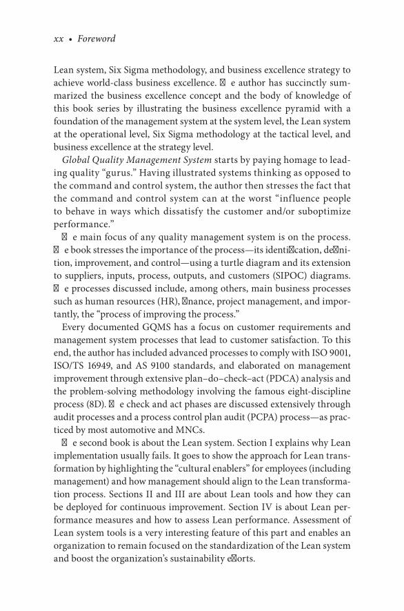
Lean system, Six Sigma methodology, and business excellence strategy to achieve world-class business excellence. The author has succinctly sum-marized the business excellence concept and the body of knowledge of this book series by illustrating the business excellence pyramid with a foundation of the management system at the system level, the Lean system at the operational level, Six Sigma methodology at the tactical level, and business excellence at the strategy level.
Global Quality Management System starts by paying homage to lead-ing quality “gurus.” Having illustrated systems thinking as opposed to the command and control system, the author then stresses the fact that the command and control system can at the worst “inf luence people to behave in ways which dissatisfy the customer and/or suboptimize performance.”
The main focus of any quality management system is on the process. The book stresses the importance of the process—its identification, defini-tion, improvement, and control—using a turtle diagram and its extension to suppliers, inputs, process, outputs, and customers (SIPOC) diagrams. The processes discussed include, among others, main business processes such as human resources (HR), finance, project management, and impor-tantly, the “process of improving the process.”
Every documented GQMS has a focus on customer requirements and management system processes that lead to customer satisfaction. To this end, the author has included advanced processes to comply with ISO 9001, ISO/TS 16949, and AS 9100 standards, and elaborated on management improvement through extensive plan–do–check–act (PDCA) analysis and the problem-solving methodology involving the famous eight-discipline process (8D). The check and act phases are discussed extensively through audit processes and a process control plan audit (PCPA) process—as prac-ticed by most automotive and MNCs.
The second book is about the Lean system. Section I explains why Lean implementation usually fails. It goes to show the approach for Lean trans-formation by highlighting the “cultural enablers” for employees (including management) and how management should align to the Lean transforma-tion process. Sections II and III are about Lean tools and how they can be deployed for continuous improvement. Section IV is about Lean per-formance measures and how to assess Lean performance. Assessment of Lean system tools is a very interesting feature of this part and enables an organization to remain focused on the standardization of the Lean system and boost the organization’s sustainability efforts.
Foreword • xxi
The author has succinctly portrayed the main principles of the Lean sys-tem as follows:
1. Define customer requirements correctly and arrive at customer value so you are providing what the customer actually wants.
2. Identify the value stream for each product or service family and remove the non-value-added (wasted) steps for which the customer will not pay and that don’t create value.
3. Make the value stream flow continuously to shorten throughput and delivery time aggressively.
4. Allow the customer to pull the product or service from your value streams as needed (rather than pushing products toward the cus-tomer on the basis of forecasts).
5. Never relent until you reach perfection, which is the delivery of pure value instantaneously with zero waste and zero defects.
The third book is about the unique way in which the so-called difficult con-cept and practice of Six Sigma methodology are depicted. It includes the col-lection of tools needed for all five phases—define, measure, analyze, improve, and control (DMAIC)—and proven best practices to identify which few process and input variables influence the process output measures. To begin with, the author describes the basic concepts of variation, spread of data, and sigma through basic statistical concepts. Before embarking on the five phases (DMAIC), the author clarifies what is needed for business performance measurement through the concepts of the balanced scorecard and impor-tant measuring units for quality performance. Notable measures discussed are defects per million opportunities (DPMO), rolled throughput yield, cost of poor quality (COPQ), business failure costs, cost–benefit analysis, return on assets (ROA), and last, a method of evaluating projects and investments known as net present value (NPV) or discounted cash flow (DCF).
The five phases of DMAIC form the bulk of the third book. The step-by-step approach taken by the author to explain the key concepts and tools required in each of these phases requires a special mention.
Define: This phase starts with the definition of the voice of the cus-tomer (VOC). Here the quality function deployment (QFD) tool is described in a simple and easy way to translate the customer’s voice into the language of the engineer. The QFD is then utilized to define and document a business improvement project charter based on the

xxii • Foreword
customer and competitive intelligence data. Project tracking tools like the Gantt chart, critical path analysis (CPA), and the project evaluation and review technique (PERT) are explained in detail. The CTQ flow-down is introduced to define customer satisfaction in four areas: quality, delivery, cost, and safety for internal and external customers.
Measure: The author has identified and discussed 16 different aspects of process characteristics. Having done this, he describes measure-ment system analysis (MSA) in great detail to ensure that the integ-rity of the measured data of important characteristics, the measuring equipment, and the human aspect of the measurement system are maintained within allowed repeatability and reproducibility (R&R) acceptance criteria.
Analyze: Here the root cause analysis methods for the problems encountered are discussed. The main techniques described include regression and correlation, analysis of variance (ANOVA), failure mode and effects analysis (FMEA), gap analysis, waste analysis, and Kaizen.
Improve: The process improvement methods discussed in this phase are prioritization through the cause-and-effect (C&F) matrix, Kaizen using Lean tools and Six Sigma, PDCA, and the theory of constraints.
Control: The key concepts and tools illustrated in the control phase are statistical process control (SPC), total productive maintenance (TPM) and overall equipment effectiveness (OEE), MSA, control plan, and visual factory. In order to sustain the improvements, the tools referred to are lessons learned, the training plan, standard operating procedures (SOPs), the work instruction, and ongoing performance assessment.
Design for Six Sigma (DFSS) methodology is a very useful and logical extension of the Six Sigma phases. The tools discussed in DFSS include define, measure, analyze, design, and verify (DMADV) and define, mea-sure, analyze, design, optimize, and verify (DMADOV). Design for X (DFX) includes reliability analysis and design of tolerance limits. Special design tools described are Porter’s five forces analysis and TRIZ (Russian for “theory of inventive problem solving”).

Foreword • xxiii
No Six Sigma book can be called complete without a case study. To this end, the author has chosen an improvement project to improve batting in the game of cricket using the Lean Six Sigma approach.
The fourth book is about business excellence strategy. There are many models of business excellence practiced by many countries of the world. At best, these models lay down business excellence assessment criteria, but the author feels that the main requirement of organizations intending to embark on business strategy is that they need a special body of knowledge with which the business excellence strategy can be implemented success-fully. The inclusion of strategies for leadership, strategic planning, cus-tomer excellence, operational excellence, and functional excellence for HR and information technology (IT) will prove to be very useful for initiated management. There is a very effective chapter on the assessment of the business excellence strategy through the use of the balanced scorecard, employee surveys, achieving performance excellence, and cost-out.
Finally, as you put these four books of knowledge into practice, you will find that the roles of leaders and managers in your organization shift. It is not enough for the leaders to keep on doing what they have always done. It is not enough for them to merely support the work of others. Rather, leaders must lead the cultural transformation and change the mindsets of their associates by building on the principles behind all these excellent tools.
The author’s account of these difficult and vast subjects is very praise-worthy and proof of his vast industrial experience of more than four decades of working with MNCs in Asia, Europe, and the Americas. This is an inspirational work that is easy to be learn and apply by the lay reader. I highly recommend this book to all students, teachers, executives, and organizations who want to learn and implement GQMS Lean Six Sigma systems and business excellence strategies.
Madan MohankaChairman and Managing Director and Founder
TEGA Industries LimitedKolkata, West Bengal, India


xxv
Preface
This book is about business excellence strategy. There are many models of business excellence practiced by many countries of the world. At best, these models lay down business excellence assessment criteria, but the author has felt that the main requirement of the organizations intend-ing to embark on business excellence needs a special body of knowledge with which the business excellence strategy can be implemented success-fully throughout the organization. The inclusion of strategies for leader-ship, strategic planning, customer excellence, operational excellence, and functional excellence for HR supported by a strong performance measure-ment, analysis, and knowledge management will prove to be very useful for the initiated management. The chapter on strategic planning promotes a virtuous cycle of trust and accountability resulting in employee empow-erment and sound organizational capability.
Assessment of business excellence strategy through the use of the bal-anced score card, employee survey, achieving performance excellence, and cost out is part of the organizational infrastructure uniting people and motivating them to achieve planned organizational goals.
Throughout the book, time-tested principles and practices are applied to the business system and processes that deliver value to customers. The result is a holistic business excellence strategy.
Almost all business organizations are engaged in providing services or products to their customers. But when it comes to providing service to customers and presenting them an experience that will make them come back time and time again, only a small minority of organizations stand out from the crowd who apply the energy, commitment, and innovative thinking to get it right. There is an enormous difference between those who are truly focused on customer and those who simply pay lip service.
This book prepares the initiated person/organization for the journey of business excellence. The guiding principle is
“An organization must constantly measure the effectiveness of its processes and strive to meet more difficult objectives to satisfy customers.”
Taiichi OhnoToyota Production System

xxvii
Acknowledgments
Acknowledging help and guidance in writing this four-book series is, to me, like churning the oceans of the world and putting all the blessings in a tea cup. I find it very daunting because during my more than 50 years of industry experience, I have been guided and helped by many persons, companies, and institutions with whose associations I have learned, prac-ticed, and taught these subjects and achieved modest to excellent results.
After I decided to return to Ahmedabad from Texas, R.D. Patel, finance professor at the Indian Institute of Management (IIM) Ahmedabad, asked me to address their small and medium enterprises program as a guest speaker to talk about Lean Six Sigma. The feedback from the attendees was good, and Professor Patel took me to the Ahmedabad Management Association (AMA) to meet with the executive director of the AMA, K.K. Nair, who asked me to conduct the first-ever three-day AMA Lean Six Sigma seminar attended by industry representatives from Rajkot, Vadodara, Surat, and Ahmedabad. This led to another seminar at the AMA and an invitation by the human resources (HR) head of the Indian Space Research Organization (ISRO) (equivalent to U.S. NASA), J. Ravisankar, to address ISRO technicians and engineers on the subject of zero defects delivery of space systems, which was well received.
All of the above made K.K. Nair ask me to write a book on Lean Six Sigma for Indian engineers. My learning and experience as an operations excellence and engineering manager at Eaton Corporation (Eden Prairie, Minnesota) and Fiat Global (Burr Ridge Operations, Chicago) made me take a holistic view and include the Global Quality Management System at the bottom rung and business excellence at the top level. This has resulted in a four-book series.
I thank the following individuals for their contributions to my knowl-edge and all the help and guidance they offered to me in my career that resulted in creating this book series: C.S. Patel, former CEO of the Anand group of leading automobile companies manufacturing automo-tive components; the late D.N. Sarkar, chairman and managing director of Gestetner Limited; Samir Kagalwala, consultant for the design and manufacture of power magnetics; Stefan Lorincz, renowned electronics engineer and source developer for key electronic components worldwide

xxviii • Acknowledgments
at Phillips, Holland; Levy Katir, former Motorola vice president, who in 1994 put me in charge of quality and reliability of the newly developed electronic ballasts; G.P. Reddy, former director of quality at Universal Lighting Technologies; Inder Khatter, international quality management system lead auditor for DNV, Houston, Texas; Dev Raheja, international consultant and author of Assurance Technologies: Principles and Practices; Frank Kobyluch, global general manager at Klein Tools and former plant manager at Eaton Corporation; and Don Johnson, director of quality at Fiat Global, Case New Holland Division.
My special thanks and gratitude go to my colleagues and team mem-bers at the following companies, where I worked, learned, and devel-oped and implemented many of the tools and techniques contained in this book series: Gestetner Limited (now Ricoh India); Energy Savings, Inc., Schaumburg, Illinois; United Lighting Technologies, Nashville, Tennessee; Eaton Hydraulics, Eden Prairie, Minnesota; and Fiat Global, Case New Holland, Burr Ridge, Chicago.
My abilities as an operations excellence manager in charge of providing quality products for compact fluorescent lamp (CFL) ballasts, hydraulic valves, pumps, hydraulic hoses, and fittings were honed, tested, and appre-ciated by customers such as GE CFL Lamps, Osram—Sylvania, John Deere, Case New Holland, Oshkosh Corporation, and several manufacturers of heavy-duty all-wheel-drive defense trucks: Caterpillar, GM Trucks, Ford Trucks, Volvo Trucks, Zamboni (ice resurfacer for the Olympic Games), and so forth.
I remain grateful to the following suppliers, who collaborated with me and my team in developing components and major assembly units requiring extremely high precision and pre- and posttreatments: Parker Hannifin, supplier of high-quality hydraulic seals and O-rings; Bosch, supplier of specialty hydraulic valves; Carraro Pune, supplier of a com-plete four-speed transmission unit for agricultural tractors; TGL-Carraro Pune, developer of precision gears and shafts for transmissions; Carraro, Quingdao, China, with whom we developed an entire rear-axle assem-bly for backhoe loaders; Graziano, Noida, where we developed a continu-ously variable transmission unit for a tractor for the first time for the U.S. market; GNA Group Punjab, supplier of forged and precision machined components for the tractor transmission assemblies; and Craftsman Automation Limited Coimbatore, who machined our large castings for transmission bodies and covers using heavy computer numerical control (CNC) machines and digital coordinate measuring machines (CMMs).

Acknowledgments • xxix
I have remained in touch with developing technology and professional knowledge through the American Society for Quality, whose membership I have held since 1993.
Illustrations and the design of charts and figures in this book series were done by Sanjay Trivedi and Minal Mehta.

xxxi
Making It Big in Manufacturing Products and Providing Service
It is a general belief that successful people in every field are blessed with talent or are just lucky. But the fact is that successful people work hard, work long, and work smart.
Marissa Ann Mayer, the current president and CEO of Yahoo, used to work 130 hours per week while working with Google. India-born Indra Krishnamurthy Nooyi, the chairman and CEO of PepsiCo, worked mid-night to 5:00 a.m. as a receptionist to earn money so that she could com-plete her master’s degree at Yale University. In 1958, Qimat Rai Gupta left his education midway through and founded electric trading operations in the electric wholesale market of Old Delhi, India. With an investment of Rs 10,000 (US$150), he started Havells. Today Havells is a billion dollar company. In his own words, “Overnight success means 25 years of hard work, devotion and dedication.”
The story of the founder and CEO of Tega Industries, based in Kolkata, India, Madan Mohanka, is unique. When he went into business, he had the right combination—hailing from a business family, having an engineering degree, earning his MBA from the Indian Institute of Management (IIM) Ahmedabad, and having a foreign collaboration as a joint partner. Yet this combination failed miserably. He witnessed the imminent closure of his company in 1979, but like the epic hero Odysseus, he never lost focus. He kept at it. Some three decades later, it was Madan’s die-hard optimism that saw Tega Industries become the second largest player in the world in rub-ber mill lining products for the mining industry.
In her book Stay Hungry, Stay Foolish, Rashmi Bansal (IIM Ahmedabad graduate) depicted Madan Mohanka’s hard-won story very aptly. She said Madan faced all the hurdles and challenges of starting from scratch, but then Madan had what you call an obsession. Over the last three decades, Madan built a strong foundation combining three technologies: mechani-cal engineering, rubber (polymer) technology, and mineral processing and grinding. In recent years, Tega has accepted challenges, grabbed over-seas marketing opportunities, and maintained consistent growth, keeping an eye on the margins.

xxxii • Making It Big in Manufacturing Products and Providing Service
Tega’s presence in 19 international locations has enabled it to increase a turnover of Rs 23 crore in 2009 to Rs 681 crore in 2014.
According to Mehul Mohanka, his U.S.-trained MBA son, the stage is now set for organic and inorganic growth—organically building up larger capabilities and inorganically looking for acquisitions for successful inte-gration with Tega’s culture, values, and philosophy.

1
1Introduction to Six Sigma: A Tactical Strategy
ORIGIN OF SIX SIGMA AT MOTOROLA
The evolution of Six Sigma began in the late 1970s at a Motorola plant in Chicago. The revealing moment came when a Japanese firm took over a Motorola factory that manufactured television sets in the United States. Under Japanese management, the factory was soon producing TV sets with 1/20 the number of defects they had produced under Motorola man-agement. Inspired by this, Bob Galvin, Motorola’s CEO in 1981, challenged his company to achieve a 10-fold improvement in performance over a five-year period. To achieve this, they needed to halve the defects each year. This initiative and subsequent hard work by Motorola engineers resulted in a worldwide tactical strategy for business excellence called Six Sigma.
The credit for coining the term Six Sigma goes to Bill Smith, a senior engineer at Motorola. In 1984, he discovered the correlation between how well the product did in its field life and how much rework and repairs were required during the manufacturing process. He found that products that were built with fewer nonconformities or those that had less variation in their specifications during manufacture were the ones that performed the best after delivery to the customer.
Bill Smith and Mikel Harry developed a four-stage problem-solving approach—measure, analyze, improve, and control (MAIC)—to find and reduce the variations, thus eliminating defects altogether.
Later, when the define stage was added, the DMAIC discipline became the road map for achieving Six Sigma quality.
2 • The Tactical Guide to Six Sigma Implementation
UNDERSTANDING THE VARIATION, SPREAD, AND SIGMA
The goal of most processes in the manufacturing and service industries is to produce products or services that have little to no variation. Variation is defined as no two items or services being exactly the same. Variation also can be defined as the extent to which or the range within which something varies.
Variation impacts performance and cost. It makes products and pro-cesses difficult, unpredictable, untrustworthy, and of poor quality. Good quality is strongly tied to reliability, trustworthiness, and no unpleasant surprises. In other words, bad quality results from too much variation, and good quality results from little variation.
It is important to reduce variation because of the economic loss result-ing from customer dissatisfaction and poor quality.
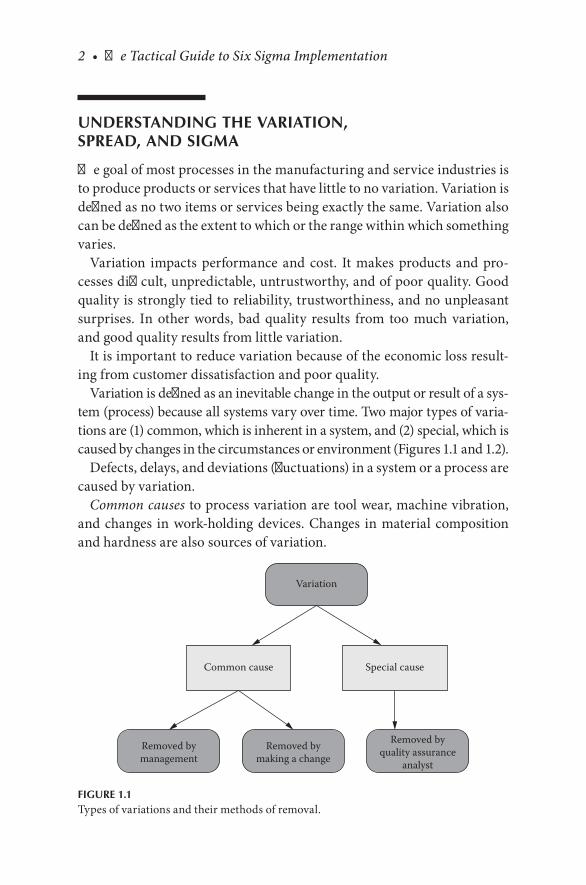
Variation is defined as an inevitable change in the output or result of a sys-tem (process) because all systems vary over time. Two major types of varia-tions are (1) common, which is inherent in a system, and (2) special, which is caused by changes in the circumstances or environment (Figures 1.1 and 1.2).
Defects, delays, and deviations (fluctuations) in a system or a process are caused by variation.
Common causes to process variation are tool wear, machine vibration, and changes in work-holding devices. Changes in material composition and hardness are also sources of variation.
Variation
Common cause Special cause
Removed bymanagement
Removed bymaking a change
Removed byquality assurance
analyst
FIGURE 1.1Types of variations and their methods of removal.
Introduction to Six Sigma • 3
Special causes to process variation are overadjusting the machine by the operator, making an error during the inspection activity, changing the machine settings, or failing to properly align the part before machining.
Examples of environmental factors affecting variation include heat, light, radiation, and humidity.
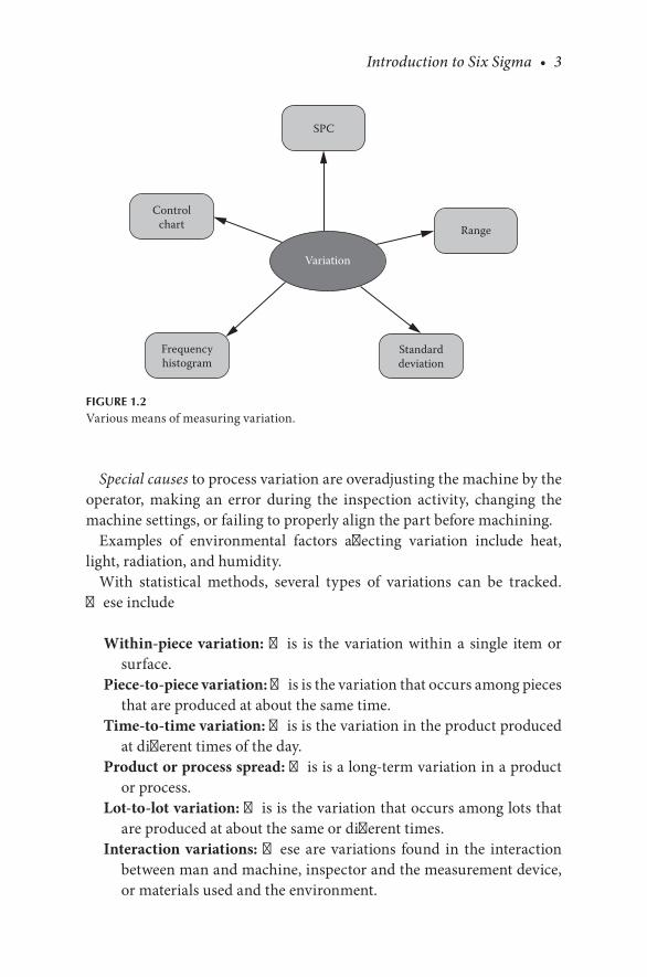
With statistical methods, several types of variations can be tracked. These include
Within-piece variation: This is the variation within a single item or surface.
Piece-to-piece variation: This is the variation that occurs among pieces that are produced at about the same time.
Time-to-time variation: This is the variation in the product produced at different times of the day.
Product or process spread: This is a long-term variation in a product or process.
Lot-to-lot variation: This is the variation that occurs among lots that are produced at about the same or different times.
Interaction variations: These are variations found in the interaction between man and machine, inspector and the measurement device, or materials used and the environment.
SPC
Range
Variation
Standarddeviation
Frequencyhistogram
Controlchart
FIGURE 1.2Various means of measuring variation.
4 • The Tactical Guide to Six Sigma Implementation
As the spread of variation becomes wider from the limits specified by the customer, or the mean or average value of the data, more defects with less yield (defect-free product) are created.
Six Sigma is the best available method to reduce process variability. The steps are
• Identify the needs of the customer.• Translate these needs into the process expert’s language through
quality function deployment (QFD).• Make improvements through the DMAIC process.• Hold the gains through statistical process control (SPC).• Provide customer satisfaction.
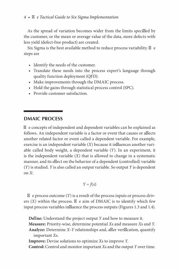
DMAIC PROCESS
The concepts of independent and dependent variables can be explained as follows. An independent variable is a factor or event that causes or affects another related factor or event called a dependent variable. For example, exercise is an independent variable (X) because it influences another vari-able called body weight, a dependent variable (Y). In an experiment, it is the independent variable (X) that is allowed to change in a systematic manner, and its effect on the behavior of a dependent (controlled) variable (Y) is studied. Y is also called an output variable. So output Y is dependent on X:
Y = f(x)
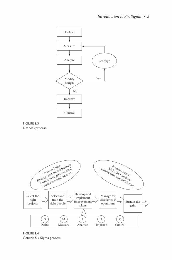
The process outcome (Y) is a result of the process inputs or process driv-ers (X) within the process. The aim of DMAIC is to identify which few input process variables influence the process outputs (Figures 1.3 and 1.4).
Define: Understand the project output Y and how to measure it.Measure: Priority-wise, determine potential Xs and measure Xs and Y.Analyze: Determine X–Y relationships and, after verification, quantify
important Xs.Improve: Devise solutions to optimize Xs to improve Y.Control: Control and monitor important Xs and the output Y over time.
Introduction to Six Sigma • 5
Define
Measure
Analyze
Modifydesign?
Improve
Control
No
Yes
Redesign
FIGURE 1.3DMAIC process.
Select theright
projects
Select andtrain the
right people
Develop andimplement
improvementplans
Manage forexcellence inoperations Sustain the
gain
D M A I C
Define Measure Analyze Improve Control
Process input:
Strategic and annual business
Goals and targets = critic
al
customer requirements
Process output:
Make the numbers
achieve customer satisfaction
FIGURE 1.4Generic Six Sigma process.

7
2What Is Six Sigma?
For the benefit of all, let us review some basic statistics to understand the concept of sigma.
BASIC STATISTICS
Types of Statistics
Dr. Deming discussed the importance of the difference between enumerative and analytic studies (also known as statistics). The basic difference is this:
Descriptive (enumerative) statistics describe data using math and graphs, and focus on the current situation, such as measuring a sam-ple and then estimating the population’s characteristics.
Inferential (analytic) statistics use sample data to predict or estimate what a population will do in the future, such as measuring periodic samples from a process that is continually manufacturing to predict the results of the next batch.
It may be helpful to consider these two examples:
1. A tailor takes a measurement (waist, chest, inseam, etc.) from a cus-tomer who purchases a new suit.
2. A doctor takes a measurement (temperature, blood pressure, heart-beat, etc.) from a patient who feels ill.
In the first instance, the tailor is taking a measurement to obtain current quantifiable information. The tailor is using a descriptive approach.

8 • The Tactical Guide to Six Sigma Implementation
In the second example, the doctor is taking a measurement to obtain a causal explanation for some observed phenomenon. The doctor is taking an analytic approach.
We use descriptive statistics to describe data, usually sample data, with math or graphics to define elements such as
• Central tendency of the data: can be measured by median, mean, and mode
• Data variation: can be measured by range of the data and variance• Graphs of the data: histograms, box plots, and so forth
Analytical Statistics
Analytical statistics involves the evaluation of ratio (or measured) data. Analytical statistics are usually performed to estimate the population parameters (estimation), to determine the difference between two popula-tions (hypothesis testing), to determine the differences among a number of populations (analysis of variance), or to evaluate the degree of relation-ship between two or more variables (correlation and regression).
Analytical statistics are usually performed using the scientific process:
1. Make a hypothesis of what we expect to find. 2. Collect data. 3. Analyze the data. 4. Draw a conclusion about the validity of the hypothesis.
So analytical statistics describes what the population should be in order to have given rise to the sample that was obtained.
For example, if a sample of four taken from a box of bubble gum is found to have three orange pieces and one red, we can conclude that the box con-tains 75% orange bubble gum. Although this may or may not be correct, a conclusion is drawn. A larger sample would provide a better estimate.
DEFINITION OF SAMPLE STATISTIC, POPULATION, AND POPULATION PARAMETER
A statistic is a quantity derived from a sample of data that assists in form-ing an opinion of a specified parameter of a target population. A sample is
What Is Six Sigma? • 9
frequently used because data on every member of a population are often impossible or too costly to collect.
A population is an entire group of objects that have been made, or will be made, containing a characteristic of interest.
A population parameter is a constant or coefficient that describes some characteristic of a target population. An example of a population param-eter is the mean or variance.
Frequently used symbols are:
Sample Population
n = Sample size N = Population sizex (X-bar) = Sample mean μ = Population meanS = Sample standard deviation σ = Population standard deviationS2 = Sample variance (square of sample standard deviation)
σ2 = Population variance (square of population standard deviation)
CENTRAL LIMIT THEOREM AND STANDARD NORMAL DISTRIBUTION
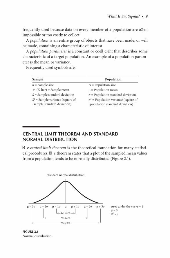
The central limit theorem is the theoretical foundation for many statisti-cal procedures. The theorem states that a plot of the sampled mean values from a population tends to be normally distributed (Figure 2.1).
µ
Standard normal distribution
Area under the curve = 1µ = 0σ2 = 168.26%
95.46%99.73%
µ + 1σµ – 1σµ – 2σµ – 3σ µ + 2σ µ + 3σ
FIGURE 2.1Normal distribution.
10 • The Tactical Guide to Six Sigma Implementation
Key points of the central limit theorem and Six Sigma include:
• Using ±3-sigma control limits, the central limit theorem is the basis of the prediction that if the process has not changed, a sample mean falls outside the control limits on an average of only 0.27% of the time. Or the process yield at the 3-sigma level is 99.73% and the defective product is 0.27%.
• Sixty-eight percent of values are within 1 standard deviation of the mean.
• Ninety-five percent of values are within 2 standard deviations of the mean.
• A total of 99.7% of values are within 3 standard deviations of the mean.
A standard normal distribution has the following characteristics:
• Most points on the curve tend to be near the average.• The curve’s shape tends to be bell shaped, and the sides tend to be
symmetrical.
The normal distribution has
• mean = median = mode.• Symmetry about the center.• Fifty percent of values less than the mean and 50% greater than the
mean.• The theorem allows the use of smaller sample averages to evaluate
any process because distributions of sample means tend to form a normal distribution.
• The theorem appears when the process is in control (predictable).• The theorem leaves variations from common causes to chance.• The theorem identifies and removes variations from special causes.
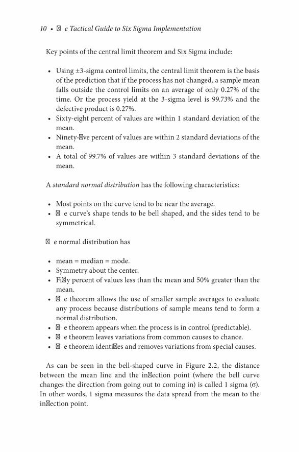
As can be seen in the bell-shaped curve in Figure 2.2, the distance between the mean line and the inflection point (where the bell curve changes the direction from going out to coming in) is called 1 sigma (σ). In other words, 1 sigma measures the data spread from the mean to the inflection point.
What Is Six Sigma? • 11
The bell-shaped curve, also called the normal curve, shows specification values concentrated in the center and decreasing specification values on either side. This means that the data have less tendency to produce unusu-ally extreme values, compared to some other distributions.
The bell-shaped curve is symmetrical. This tells you that the probability of deviations from the mean are comparably similar in either direction. The curve represents the distribution of any of the following of a set of data:
• Values• Frequencies• Probabilities
It slopes downward from a top point in the middle (mean value) or the maximum probability point (ideally 50%). Data that reflect the collective result of large numbers of unrelated events tend to result in bell curve distributions, for example, a dimension of a machined part on a computer numerical control (CNC) machine, service waiting time at McDonalds, or grades of students in a class.
CENTRAL TENDENCIES
Central tendency is a measure that characterizes the central value of a collection of data that tends to cluster somewhere between the high and
MeanMedianMode
Symmetry
50% 50%
FIGURE 2.2Normal distribution is symmetrical.

12 • The Tactical Guide to Six Sigma Implementation
low values in the data. Central tendency refers to a variety of key measure-ments, such as mean (the most common), median, and mode (Figure 2.3).
Mean• Gives the distribution’s arithmetic average (center)• Provides a reference point for relating all other data points• Is typically used with normal data
Median• The distribution’s center point (middle value)• Equal number of data points occur on either side of the median• Useful when the data set has extreme high or low values• Typically used with nonnormal data
Mode• Represents the value with the highest frequency of occurrence
(the most often repeated value)• Typically used with nonnormal data
MEASURE OF DISPERSION
In this section, we discuss measures of dispersion (Figure 2.4).All at the same time, Six Sigma is
• A metric• A methodology• A management system
Mode
Mean = median = mode
For a normal distribution For a skewed distribution
Median
Mean
FIGURE 2.3Mean, median, and mode in normal and skewed distributions.

What Is Six Sigma? • 13
Six Sigma as a Metric
Six Sigma (6σ) is a measure of quality that is very close to perfection. The statistical meaning of Six Sigma is having 6 standard deviations spread between the mean and the nearest specification limit. A Six Sigma process is virtually defect-free, with only 3.4 defects in a million opportunities. The Six Sigma process is 99.9997% defect-free.
A defect is defined as anything outside of customer specifications.An opportunity is a chance for a defect to occur. We can detect it, cor-
rect it, and prevent it from occurring again. Defects per million opportu-nities is termed DPMO.
Statistical Interpretation of Six Sigma
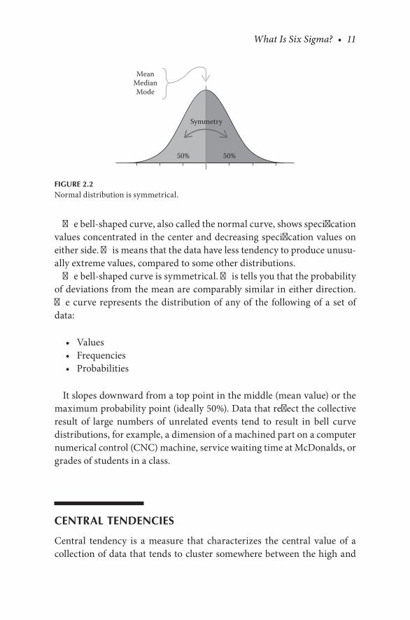
For the curve shown in Figure 2.5, the average or mean μ = 0 and the standard deviation σ = 1. The upper (USL) and lower (LSL) specifica-tion limits are at a distance of 6 sigma from the mean. Because of the properties of the normal distribution, values lying that far away from the mean are extremely unlikely. Even if the mean were to move right or left by 1.5 sigma at some point in the future (1.5-sigma shift), there is still a good safety cushion. This is why Six Sigma aims to have processes where the mean is at least 6 sigma away from the nearest specification limit.
Any normal distribution can be converted to a standard normal distribution.
Measure of dispersion Definition Formula
Range (R)
Variance (σ2, S2)
Standard deviation (σ, S)
�e difference between thelargest and smallest valuesin a data set.
�e sum of the squared deviationsfrom the mean, divided by thesample size or degree of freedom.Also, the standard deviation squared.
�e computed measure ofvariability indicating thespread of the data set aroundteam. Also, the square root ofthe variance.
A – B = RA = largest value in data setB = smallest value in data set
For a population: σ2 = Σ(x – µ)2
N
For a sample:
For a sample:
For a population: σ = Σ(x – µ)2
N
S = Σ(x – x)2
n − 1
S2 = Σ(x – x)2
n – 1
FIGURE 2.4Formulas for measures of dispersion.
14 • The Tactical Guide to Six Sigma Implementation
Here is the formula for z-score:
z x= − µ
σ
where z is the z-score (standard score), x is the value to be standardized, μ is the mean, and σ is the standard deviation.
Why Is the Normal Distribution Useful?
Many things are actually normally distributed or very close to it. For example, height, weight, and intelligence of a population are approxi-mately normally distributed. Dimensions of manufactured parts also often have a normal distribution.
The normal distribution is easy to work with mathematically. In many practical cases, the methods developed using normal theory work quite well even when the distribution is not normal.
There is a very strong connection between the size of a sample N and the extent to which a sampling distribution approaches the normal form. Many sampling distributions based on large N can be approximated by the normal distribution even though the population distribution itself is definitely not normal.
The term sigma is a letter taken from the Greek alphabet, equivalent to the English S. It is used to designate the distribution or spread on either side of the mean (average) of any parameter of a product, process, or procedure.
Sigma (σ) is used by statisticians to show the variation in a process.
LSL USL
–6 –5 –4 –3 –2 –1 0 1 2 6543µ – σ µ µ + σ
N(0,1)µ = 0σ = 1
FIGURE 2.5Standard normal distribution.

What Is Six Sigma? • 15
For example, let us bring this concept to life in our own home. The dif-ference between 4 sigma and 6 sigma is illustrated below (Figure 2.6):
4 sigma means 100% – 99.379% = 0.6210% defectives
or
0.6210 defectives out of 100
or
0.6210 × 10,000 = 6210 defectives out of a million
or
6210 parts per million (ppm)
Note: 1% = 10,000 ppm.
Parts per Million and Sigma Level
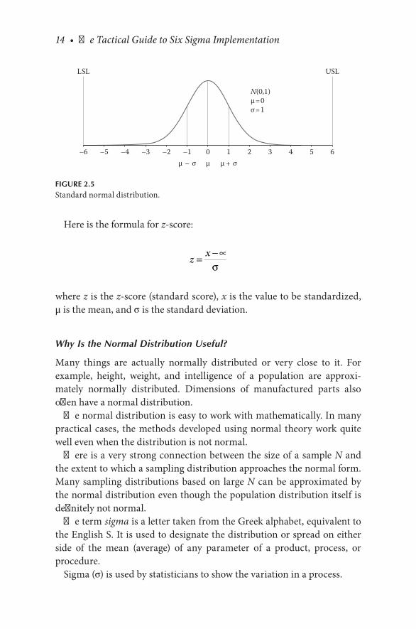
Generally, most companies operate in the range of 3–4 sigma.Notice in Figure 2.7 that as the sigma level increases, the parts per mil-
lion rate decreases.Here the data show that, on average, flight delays are 6000 ppm, or 0.6%,
while airline fatalities are 1 ppm, or 0.0001%.
4σ 6σ
99.4%Error-free
99.9997%Error-free
4σ Expect cold showers 54 hours each year
Approximately 6210 products out ofevery million would be of specLights would be out almost 1 hourper week
4σ
4σ
6σ Cold showers are reduced to less than2 minutes a yearOnly three products in every millionwould be out of specLight outage would be reduced to2 seconds a week
6σ
6σ
FIGURE 2.6Significance of sigma level in defect assessment.
16 • The Tactical Guide to Six Sigma Implementation
Table 2.1 shows the relationship between the sigma level and the defec-tive parts per million.
Six Sigma as a Management System
Six Sigma is a performance management system for executing business strategy. It aligns improvement efforts to business strategy and business goal metrics. Six Sigma leverages meaningful metrics to monitor success.
1,000,000100,000
10,0001000
10010
10.1
1 2 3 4 5 6 7
Burglary case closure Baggage handlingOrder processing
Tech center wait timeFlight delays
Airline fatality
Bogic golfIRS tax advice
FIGURE 2.7Relation between parts per million and sigma level. (Adapted from Breyfogle III, F.W., Implementing Six Sigma: Smarter Solutions Using Statistical Methods, 2nd ed., John Wiley & Sons, New York, 2003.)
TABLE 2.1
Sigma Level and DPMO
Sigma DPMO
6.0 3.45.5 305.0 2304.5 13504.0 62103.5 22,7003.0 66,8002.5 158,0002.0 308,0001.5 500,0001.0 690,0000.5 840,000

What Is Six Sigma? • 17
Six Sigma as a Methodology
Six Sigma is a disciplined and data-driven methodology to improve, design, and manage processes, by focusing on improving business perfor-mance and meeting customer requirements.
We have seen that Lean helps a company cut the time it takes to meet customer demands and eliminate all kinds of delays and wastes that it faces during the process of providing the product or service to the customer.
Six Sigma is the “best of the best”—meaning a Six Sigma strategy takes the best of the quality principles and techniques used over many years and applies them appropriately to an organization. Six Sigma helps in finding out and fixing the mistakes, errors, defects, and deviations (variations) involved in every aspect of delivering customer wants. By taking the best principles and techniques from each of these programs, organizations maximize their productivity, profitability, growth, and improvements in measurable ways.

19
3Business Performance Measures
ORGANIZATIONAL PROCESSES AND THEIR IMPACT ON THE ORGANIZATION
The Six Sigma methodology recognizes that there are many sources for inputs, outputs, and feedback for an organization. Each output may have its own process dependent on the input from other processes. All inputs and outputs of a process should be measurable so that quality can be controlled.
See Figure 3.1 to understand the organizational processes and their inter-action in terms of their inputs, outputs, product, and information flow.
It is important to know that improvements in one area may create errors in another. So the understanding of interaction and interdependence of processes is critical to the success of a Six Sigma project.
DEFINING OWNERS AND STAKEHOLDERS
Top management participation is extremely important to the success of Six Sigma projects.
Quality improvement projects cannot happen without the appropriate decision makers taking ownership of the project. “Buying in” to the change by the decision makers and leaders is the first resource requirement.
In addition to these, other resources must be available to give an appro-priate level of input and make decisions. Often, the resources that are needed are the busiest and will not find time to participate in the proj-ect unless its level of importance is appropriately elevated. The following resources as stakeholders should be identified early on and informed of their role in the project as soon as practical. A resource must commit to a certain time as required by the project.

20 • The Tactical Guide to Six Sigma Implementation
The stakeholders are:
CustomersEmployees (internal customers)SuppliersInvestorsGovernmentCommunity
BALANCED SCORECARD
A balanced scorecard (BSC) is a widely accepted approach to establishing an organizational strategy (Figure 3.2). It is a strategic measurement and management system that translates an organization’s strategy into four perspectives (Table 3.1).
Figure 3.3 shows an example of a typical balanced scorecard.
KEY PERFORMANCE INDICATORS
Every organization wishing to embark on a Six Sigma journey must set-tle on a few key performance indicators (KPIs) to use for planning and
Process
Inputs Step 1 Step 2
Feedback
Conduct measurements at both points to gagethe efficiency and effectiveness of the process.
Step 3 Outputs?
FIGURE 3.1Organizational process with feedback loop.
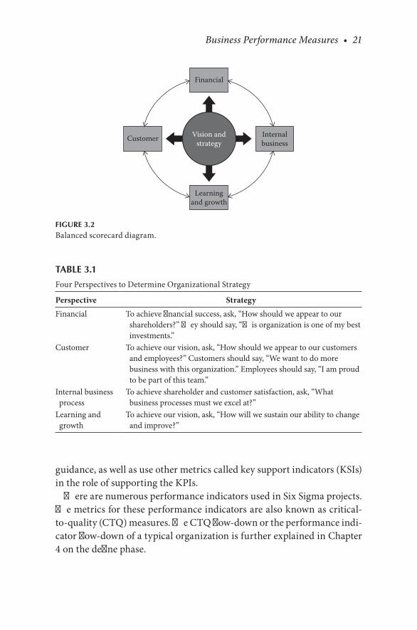
Business Performance Measures • 21
guidance, as well as use other metrics called key support indicators (KSIs) in the role of supporting the KPIs.
There are numerous performance indicators used in Six Sigma projects. The metrics for these performance indicators are also known as critical-to-quality (CTQ) measures. The CTQ flow-down or the performance indi-cator flow-down of a typical organization is further explained in Chapter 4 on the define phase.
Customer Internalbusiness
Learningand growth
Financial
Vision andstrategy
FIGURE 3.2Balanced scorecard diagram.
TABLE 3.1
Four Perspectives to Determine Organizational Strategy
Perspective Strategy
Financial To achieve financial success, ask, “How should we appear to our shareholders?” They should say, “This organization is one of my best investments.”
Customer To achieve our vision, ask, “How should we appear to our customers and employees?” Customers should say, “We want to do more business with this organization.” Employees should say, “I am proud to be part of this team.”
Internal business process
To achieve shareholder and customer satisfaction, ask, “What business processes must we excel at?”
Learning and growth
To achieve our vision, ask, “How will we sustain our ability to change and improve?”
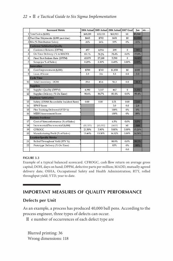
22 • The Tactical Guide to Six Sigma Implementation
IMPORTANT MEASURES OF QUALITY PERFORMANCE
Defects per Unit
As an example, a process has produced 40,000 ball pens. According to the process engineer, three types of defects can occur.
The number of occurrences of each defect type are
Blurred printing: 36Wrong dimensions: 118
FIGURE 3.3Example of a typical balanced scorecard. CFROGC, cash flow return on average gross capital; DOH, days on hand; DPPM, defective parts per million; MADD, mutually agreed delivery date; OSHA, Occupational Safety and Health Administration; RTY, rolled throughput yield; YTD, year to date.
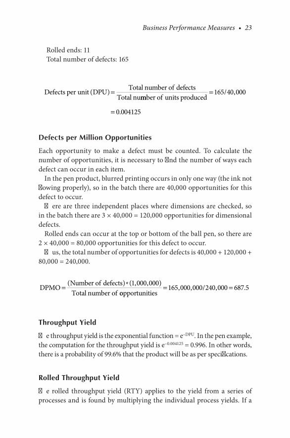
Business Performance Measures • 23
Rolled ends: 11Total number of defects: 165
Defects per unit DPU Total number of defectsTotal nu
( ) =mmber of units produced
/=
=
165 40 000
0 004125
,
.
Defects per Million Opportunities
Each opportunity to make a defect must be counted. To calculate the number of opportunities, it is necessary to find the number of ways each defect can occur in each item.
In the pen product, blurred printing occurs in only one way (the ink not flowing properly), so in the batch there are 40,000 opportunities for this defect to occur.
There are three independent places where dimensions are checked, so in the batch there are 3 × 40,000 = 120,000 opportunities for dimensional defects.
Rolled ends can occur at the top or bottom of the ball pen, so there are 2 × 40,000 = 80,000 opportunities for this defect to occur.
Thus, the total number of opportunities for defects is 40,000 + 120,000 + 80,000 = 240,000.
DPMO Number of defectsTotal number of
= ( ) ( , , )* 1 000 000oopportunities
/= =165 000 000 240 000 687 5, , , .
Throughput Yield
The throughput yield is the exponential function = e–DPU. In the pen example, the computation for the throughput yield is e–0.004125 = 0.996. In other words, there is a probability of 99.6% that the product will be as per specifications.
Rolled Throughput Yield
The rolled throughput yield (RTY) applies to the yield from a series of processes and is found by multiplying the individual process yields. If a

24 • The Tactical Guide to Six Sigma Implementation
product goes through four processes whose yields are 0.994, 0.987, 0.951, and 0.990, then
RTY = (0.994)(0.987)(0.951)(0.99) = 0.924
Parts per Million
Parts per million (ppm) is defined simply as
ppm = DPU × 1,000,000
In this example, the computation for the parts per million is
ppm = (0.004125)(1,000,000)
ppm = 4125
Parts per million is also used to refer to contaminants, as seen in the following example.
Suppose 0.23 g of sand particles is found in 25 kg of product:
PM =
×0 23
25 0001 000 000.
,, ,
Table 3.2 shows the relation among DPMO, sigma, and process capabil-ity index (Cpk).
Table 3.3 shows the relations between sigma level, process yields, and short- and long-term capabilities.
Cost of Poor Quality
The cost of poor quality (COPQ), also known as business failure cost, calculates the financial impact of defects (Figure 3.4). This is helpful in prioritizing projects in terms of their impact on the enterprise. COPQ should include the expenses involved in rework, warranty, late deliveries, customer dissatisfaction, and so on.

Business Performance Measures • 25
TABLE 3.2
Sigma Conversion Table Showing Relations among DPMO, Sigma, and Cpk
Defects per Million Opportunities
Sigma Level (with 1.5-Sigma Shift)a
Cpk (Sigma Level/3) (with 1.5-Sigma Shift)a
933,200 0.000 0.000915,450 0.125 0.042894,400 0.250 0.083869,700 0.375 0.125841,300 0.500 0.167809,200 0.625 0.208773,400 0.750 0.250734,050 0.875 0.292691,500 1.000 0.333645,650 1.125 0.375598,700 1.250 0.417549,750 1.375 0.458500,000 1.500 0.500450,250 1.625 0.542401,300 1.750 0.583354,350 1.875 0.625308,500 2.000 0.667265,950 2.125 0.708226,600 2.250 0.750190,800 2.375 0.792158,700 2.500 0.833130,300 2.625 0.875105,600 2.750 0.91784,550 2.875 0.95866,800 3.000 1.00052,100 3.125 1.04240,100 3.250 1.08330,400 3.375 1.12522,700 3.500 1.16716,800 3.625 1.20812,200 3.750 1.2508800 3.875 1.2926200 4.000 1.3334350 4.125 1.3753000 4.250 1.4172050 4.375 1.4581300 4.500 1.500
(Continued )

26 • The Tactical Guide to Six Sigma Implementation
TABLE 3.3
Sigma, DPMO, Yield, and Short- and Long-Term Cpk Comparison
Sigma Level DPMO
Percent Defective
Percentage Yield
Short-Term Cpk
Long-Term Cpk
1 691,462 69% 31% 0.33 –0.172 308,538 31% 69% 0.67 0.173 66,807 6.70% 93.30% 1 0.54 6210 0.62% 99.38% 1.33 0.835 233 0.02% 99.98% 1.67 1.176 3.4 0.00% 100.00% 2 1.57 0.019 0.00% 100.00% 2.33 1.83Note: Long-term Cpk 1.5*3 = 4.5 sigma, which becomes 6 sigma when 1.5 is added to it.
TABLE 3.2 (CONTINUED)
Sigma Conversion Table Showing Relations among DPMO, Sigma, and Cpk
Defects per Million Opportunities
Sigma Level (with 1.5-Sigma Shift)a
Cpk (Sigma Level/3) (with 1.5-Sigma Shift)a
900 4.625 1.542600 4.750 1.583400 4.875 1.625230 5.000 1.667180 5.125 1.708130 5.250 1.75080 5.375 1.79230 5.500 1.83323.4 5.625 1.87516.7 5.750 1.91710.1 5.875 1.9583.4 6.00 2.000
Note: Long-term Cpk*3 = Sigma level.a The table assumes a 1.5-sigma shift because processes tend to exhibit instability of that
magnitude over time. In other words, although statistical tables indicate that 3.4 DPMO is achieved when 4.5 process standard deviations (sigma) are between the mean and the closest specification limit, the target is raised to 6.0 (4.5 + 1.5) standard deviations to accommodate adverse process shifts over time and still produce only 3.4 DPMO.

Business Performance Measures • 27
W. Edwards Deming is frequently quoted as saying that the most impor-tant numbers are unknown and unknowable. Who can state, for instance, the value of a satisfied customer who will, in Deming’s words, “tell all his friends and some of his enemies?” Loyal customers are to be sought and cherished— he very life of the organization depends on them. To estimate the financial impact of a loyal customer, one would need to consider all the costs required to locate and recruit a new customer, including marketing and sales, and the time and effort to help make this new customer into a loyal customer.
Business Failure Cost Measurements in Manufacturing and Finance
Now let us look at these costs in a typical manufacturing business as a per-centage of the revenue (Figure 3.5). Figure 3.6 shows that 25% of the total sales revenue is eaten away by the business failure costs. The right-hand column shows the hypothetical breakup of the business failure costs. For example, if the total sales revenue is 100, the business failure costs will amount to 25.
Customer rejects
COPQ calculates the financial impact of defects.�is is helpful in prioritizing projects in terms of their impact on the enterprise.
COPQ consists of 15%–25% of the total cost.
Rework
Testing costs
Rejects
Waste
Inspection costs
Excessiveovertime
Development costof a failed product
Pricing andbilling errors
Excessive fieldservice expenses
Lack of follow-upon current projects Excessive inventory
Unused capacity
Customer allowances
Time with dissatisfiedcustomers
Incorrectly completedsales order
Excessive systemcosts
Excessive employeeturnover
Premiumfreight costs
Planningdelays Complaint
handlingOverduereceivables
Expediting costs
Late paperwork
Recalls
FIGURE 3.4Cost of poor quality.
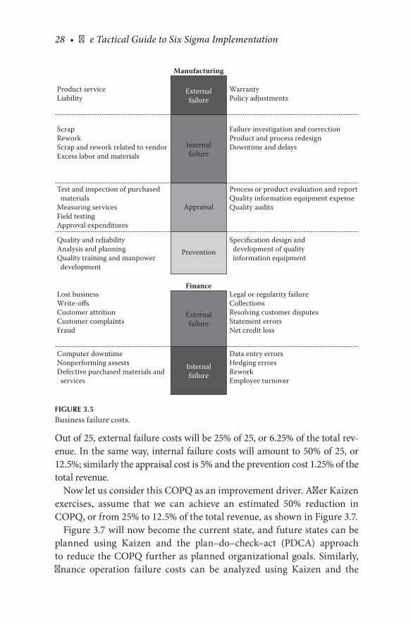
28 • The Tactical Guide to Six Sigma Implementation
Out of 25, external failure costs will be 25% of 25, or 6.25% of the total rev-enue. In the same way, internal failure costs will amount to 50% of 25, or 12.5%; similarly the appraisal cost is 5% and the prevention cost 1.25% of the total revenue.
Now let us consider this COPQ as an improvement driver. After Kaizen exercises, assume that we can achieve an estimated 50% reduction in COPQ, or from 25% to 12.5% of the total revenue, as shown in Figure 3.7.
Figure 3.7 will now become the current state, and future states can be planned using Kaizen and the plan–do–check–act (PDCA) approach to reduce the COPQ further as planned organizational goals. Similarly, finance operation failure costs can be analyzed using Kaizen and the
Manufacturing
Finance
Product serviceLiability
ScrapReworkScrap and rework related to vendorExcess labor and materials
Test and inspection of purchased materialsMeasuring servicesField testingApproval expenditures
Quality and reliabilityAnalysis and planningQuality training and manpower development
Lost businessWrite-offsCustomer attritionCustomer complaintsFraud
Computer downtimeNonperforming assestsDefective purchased materials and services
WarrantyPolicy adjustments
Failure investigation and correctionProduct and process redesignDowntime and delays
Process or product evaluation and reportQuality information equipment expenseQuality audits
Specification design and development of quality information equipment
Legal or regularity failureCollectionsResolving customer disputesStatement errorsNet credit loss
Data entry errorsHedging errorsReworkEmployee turnover
Externalfailure
Internalfailure
Externalfailure
Internalfailure
Appraisal
Prevention
FIGURE 3.5Business failure costs.
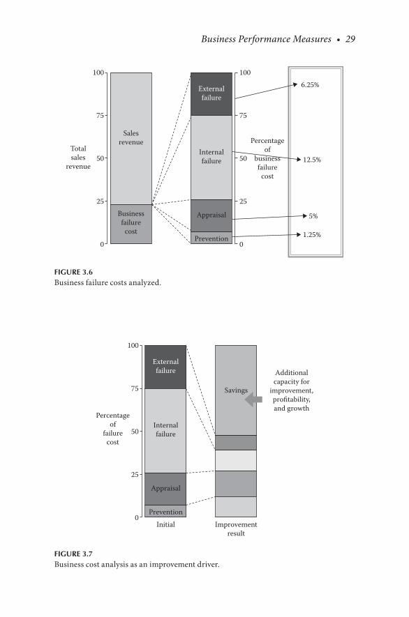
Business Performance Measures • 29
100
75
50Totalsales
revenue
Salesrevenue
Externalfailure
Internalfailure
Appraisal
Prevention
Businessfailure
cost
25
0
100
6.25%
12.5%
5%
1.25%
75
50
Percentageof
businessfailure
cost
25
0
FIGURE 3.6Business failure costs analyzed.
100
75
50
Percentageof
failurecost
Additionalcapacity for
improvement,profitability,and growth
25
0
Externalfailure
Internalfailure
Appraisal
Initial Improvementresult
Savings
Prevention
FIGURE 3.7Business cost analysis as an improvement driver.

30 • The Tactical Guide to Six Sigma Implementation
PDCA approach to reduce the cost of poor quality even more through planned organizational goals.
Financial Measures
Project Financial Benefits
When determining whether a Six Sigma project has been successful, the bottom line is often the factor that matters the most. The key question is, how much value does the organization realize as a direct result of this project’s success?
Financial Benefits Defined
Just as there are costs associated with poor quality (see COPQ), there are also financial benefits of implementing changes that result from successful Six Sigma projects.
These financial benefits include
• Additional revenue from increased sales• Cost avoidance or mitigation• Faster return on investments• Lower production costs• Lower costs associated with customer service• Increased cash flow• Enhanced profitability of existing services or products• Increased revenue of existing sources• Increased value in organization stock or perceived value
The financial factors discussed here are
• Cost–benefit analysis• Return on assets (ROA)• Return on investment (ROI)• Net present value (NPV)
Cost–Benefit Analysis
To perform a cost–benefit analysis for the project, complete these steps:
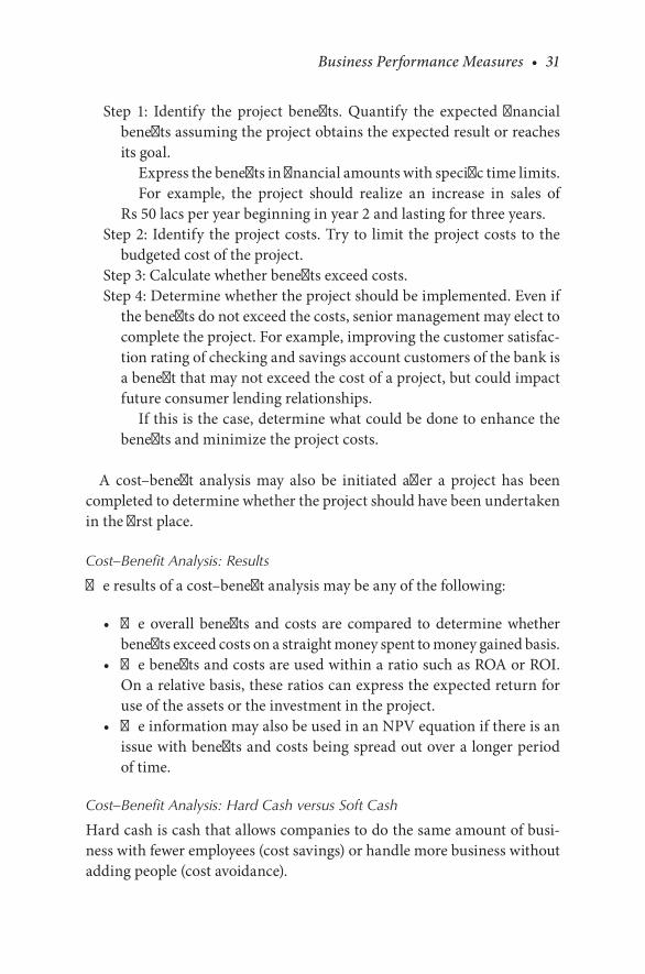
Business Performance Measures • 31
Step 1: Identify the project benefits. Quantify the expected financial benefits assuming the project obtains the expected result or reaches its goal.
Express the benefits in financial amounts with specific time limits. For example, the project should realize an increase in sales of
Rs 50 lacs per year beginning in year 2 and lasting for three years.Step 2: Identify the project costs. Try to limit the project costs to the
budgeted cost of the project.Step 3: Calculate whether benefits exceed costs.Step 4: Determine whether the project should be implemented. Even if
the benefits do not exceed the costs, senior management may elect to complete the project. For example, improving the customer satisfac-tion rating of checking and savings account customers of the bank is a benefit that may not exceed the cost of a project, but could impact future consumer lending relationships.
If this is the case, determine what could be done to enhance the benefits and minimize the project costs.
A cost–benefit analysis may also be initiated after a project has been completed to determine whether the project should have been undertaken in the first place.
Cost–Benefit Analysis: Results
The results of a cost–benefit analysis may be any of the following:
• The overall benefits and costs are compared to determine whether benefits exceed costs on a straight money spent to money gained basis.
• The benefits and costs are used within a ratio such as ROA or ROI. On a relative basis, these ratios can express the expected return for use of the assets or the investment in the project.
• The information may also be used in an NPV equation if there is an issue with benefits and costs being spread out over a longer period of time.
Cost–Benefit Analysis: Hard Cash versus Soft Cash
Hard cash is cash that allows companies to do the same amount of busi-ness with fewer employees (cost savings) or handle more business without adding people (cost avoidance).

32 • The Tactical Guide to Six Sigma Implementation
Soft cash is things such as increased customer satisfaction, reduced time to market, cost avoidance, lost profit avoidance, improved employee morale, enhanced image for the organization, and other intangibles that may result in additional savings to the organization but are harder to quantify.
Each organization may define hard and soft cash differently.
Return on Assets
Return on assets (ROA) is sometimes used for Six Sigma projects to deter-mine whether the use of organization assets is warranted based on the return realized.
The formula for ROA is
ROA = Net income/Total assets
When applied to a project, net income refers to expected earnings that result directly from the project’s results. Total assets refer to the value of the assets applied to a project.
Return on Investment
Return on investment (ROI) is also used for Six Sigma projects to deter-mine whether the investment in the project is warranted based on the return realized.
The formula for ROI is
ROI = Net income/Investment
When applied to a project, net income refers to expected earnings that result directly from the project’s results. Investment refers to the value of the outlay made in the project.
Net Present Value
Net present value (NPV) is also known as discounted cash flow (DCF). Calculating the NPV is a method for evaluating projects or investments, and is utilized in capital budgeting. It is an application of a fundamental concept in economics and finance called the time value of money, which,
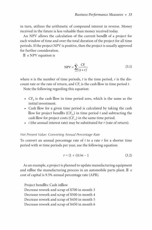
Business Performance Measures • 33
in turn, utilizes the arithmetic of compound interest in reverse. Money received in the future is less valuable than money received today.
An NPV allows the calculation of the current benefit of a project for each window of time and over the total duration of the project for all time periods. If the project NPV is positive, then the project is usually approved for further consideration.
The NPV equation is
NPV
1 )0
=+∑ CF
ti
tn
r(=
(3.1)
where n is the number of time periods, t is the time period, r is the dis-count rate or the rate of return, and CFt is the cash flow in time period t.
Note the following regarding this equation:
• CF0 is the cash flow in time period zero, which is the same as the initial investment.
• Cash flow for a given time period is calculated by taking the cash flow for project benefits (CFb,t) in time period t and subtracting the cash flow for project costs (CFc,t) in the same time period.
• i (the annual interest rate) may be substituted for r (rate of return).
Net Present Value: Converting Annual Percentage Rate
To convert an annual percentage rate of i to a rate r for a shorter time period with m time periods per year, use the following equation:
r = (1 + i)1/m – 1 (3.2)
As an example, a project is planned to update manufacturing equipment and refine the manufacturing process in an automobile parts plant. The cost of capital is 9.5% annual percentage rate (APR).
Project benefits: Cash inflowDecrease rework and scrap of $700 in month 3Decrease rework and scrap of $500 in month 4Decrease rework and scrap of $450 in month 5Decrease rework and scrap of $450 in month 6

34 • The Tactical Guide to Six Sigma Implementation
Project costs: Cash outflowInitial process redesign and training costs $400 in month 1Installing new equipment costs $840 in month 2A second round of training costs $100 in month 6
See Table 3.4 for a cash flow summary for this example.The APR of 9.5% is converted to a monthly rate using Equation 3.2:
r = (1 + 0.095)1/12 – 1 = 0.00759
The calculation for NPV is
NPV =+
=+
+ −+
+ −CFtt( ) ( . ) ( . )1
01 0 00759
4001 0 00759
80 1r
4401 0 00759
7001 0 00759
5001 0 00
20
3
( . )
( . ) ( .
+
++
++
=∑i
n
7759450
1 0 00759450 100
1 0 00759
712
4 5 6) ( . ) ( . )
$
++
+ −+
= ..80
Although financial benefits weigh most heavily in the decision to pro-ceed with a Six Sigma project, other benefits also accrue to the organiza-tion and may be considered in the decision-making process.
Other benefits to the organization from a successful process improve-ment project may include
• Improved market position relative to competitors• Improved ability to meet customer needs, especially enhanced
service• Organization behaviors aligned with vision and values• Newly created market opportunities• Project-infused spirit of continuous improvement• Improved employee morale
TABLE 3.4
Cash Flow Analysis Table
Month 0 1 2 3 4 5 6Positive cash flow 0 0 0 700 500 450 450Negative cash flow 0 400 840 0 0 0 100

Business Performance Measures • 35
• Improved overall productivity• Decreased cycle time• Increased simplicity (such as for improved customer experiences or
ease of manufacture)• Compliance with existing or emerging regulations or laws
TEAM MANAGEMENT
Obviously teams can outperform individuals. Teams offer more than just increased efficiency. Because the team members are empowered to deal with many things that affect their work, teams provide a great source of job satisfaction and employee involvement.

37
4Define
KEY CONCEPTS AND TOOLS
1. Voice of the customer (VOC)• Internal and external customers
– Divide customers for each project and show how the project will impact both internal and external customers.
• Customer satisfaction• Customer value and customer value analysis—survey• Quality function deployment (QFD) and critical-to-quality (CTQ)
flow-down– Define, select, and use appropriate tools to determine cus-
tomer requirements, such as QFD and CTQ flow-down. 2. Project charter
• Problem statement• Project scope• Project goals• Project performance measures
3. Project tracking• Gantt charts• Critical path analysis• Program evaluation and review technique (PERT) charts• Work breakdown structure
38 • The Tactical Guide to Six Sigma Implementation
VOICE OF THE CUSTOMER
Internal and External Customers
The concept of internal customers has been widely used as part of the quality movement as a way to break barriers and promote cross-functional cooperation. Slogans like “the customer is the king” are heard in many places of work.
An internal customer is an employee or department who receives an output from another employee or department. Internal customers have also been defined as the next person in the work process.
Based on this concept, all work-related activities of an organization can be viewed as a series of transactions between internal suppliers and inter-nal customers.
External customers are people or organizations who receive and pay for a product. Types of external customers include
End user or final customer: End users or final customers purchase or receive products for their own use and are not an employee or legal part of the supplier organization.
Intermediate customers: Intermediate customers include dealers, distributors, and brokers who buy products and make them avail-able to the final user. Organizations that repair or modify a prod-uct for the end user are also generally considered intermediate customers.
Customer–Supplier Chain
Companies understand that business is driven by customer requirements. Many choose a model of two-way interaction between their suppliers, their customers, and themselves (Figure 4.1). This model promotes the exchange of information about requirements and performance.
Customer Satisfaction
A general view of customer satisfaction is meeting customer requirements. Six Sigma emphasizes exceeding customer requirements and thereby “delighting the customer.” Customer delight is defined as exceeding

Define • 39
customer requirements—in ways the customer finds valuable and in ways the customer did not anticipate, but has come to expect afterward.
Customer need can be translated into customer value. Determining cus-tomer value is generally a combination of different factors:
• Product attributes• Product quality• Service• Company image and personnel• Selling price• Total cost of using product
Customer Satisfaction Survey
This is also called customer value analysis. Customer value analysis is the process many companies use to determine what customers value in terms of the company’s and competitors’ products.
Customers are asked to
• Identify the product attributes of the product that they value• Rank the relative importance of these attributes from most to least
important• Assess the company’s performance on these attributes• Rate the attributes of the company’s product against those of
competitors
Once these questions have been answered, the company can then focus its efforts on improving those product attributes that customers value most.
Understand andagree
Understand andagree
Customer−supplier
CustomerSupplier
Requ
irem
ents
Requ
irem
ents
FIGURE 4.1Customer–supplier chain to understand and agree on mutual requirements.
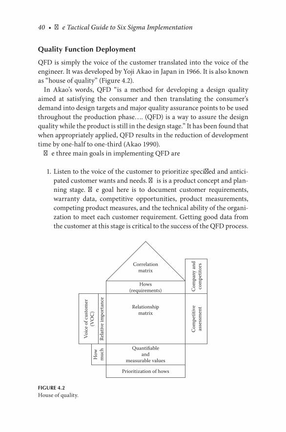
40 • The Tactical Guide to Six Sigma Implementation
Quality Function Deployment
QFD is simply the voice of the customer translated into the voice of the engineer. It was developed by Yoji Akao in Japan in 1966. It is also known as “house of quality” (Figure 4.2).
In Akao’s words, QFD “is a method for developing a design quality aimed at satisfying the consumer and then translating the consumer’s demand into design targets and major quality assurance points to be used throughout the production phase…. (QFD) is a way to assure the design quality while the product is still in the design stage.” It has been found that when appropriately applied, QFD results in the reduction of development time by one-half to one-third (Akao 1990).
The three main goals in implementing QFD are
1. Listen to the voice of the customer to prioritize specified and antici-pated customer wants and needs. This is a product concept and plan-ning stage. The goal here is to document customer requirements, warranty data, competitive opportunities, product measurements, competing product measures, and the technical ability of the organi-zation to meet each customer requirement. Getting good data from the customer at this stage is critical to the success of the QFD process.
Correlationmatrix
Hows(requirements)
Relationshipmatrix
Quantifiableand
measurable values
Prioritization of hows
Com
petit
ive
asse
ssm
ent
Rela
tive
impo
rtan
ce
Voic
e of
cus
tom
er(V
OC
)
Com
pany
and
com
petit
ors
How
muc
h
FIGURE 4.2House of quality.
Define • 41
2. In the correlation matrix, translate these needs into technical charac-teristics and specifications. This is achieved through process planning led by manufacturing and engineering. During process planning, manufacturing processes are flowcharted and process parameters (or target values) are documented.
3. Benchmark target values to build and deliver a quality product or service by focusing everybody toward customer satisfaction. At this stage, decisions are made about the risks some processes may pose and controls are put in place to prevent risks and failures by the qual-ity assurance department in concert with manufacturing.
Expanded House of Quality
The first phase in the implementation of the quality function deployment process involves putting together a house of quality, such as the one shown in Figure 4.3.
Steps to the house of quality are
Step 1: After negotiations with the customer regarding their require-ments, customer requirements are rated according to their prefer-ence on a scale from 1 to 5 and tabulated as shown in Figure 4.4 using an Excel spreadsheet.
Step 2: Customer rating of the competition. Understanding how cus-tomers rate the competition can be a tremendous competitive advan-tage. In this step of the QFD process, it is also a good idea to ask customers how your product or service rates in relation to the com-petition (Figure 4.5).
Step 3: Determine the company’s ability to meet customer needs. The relationship matrix is where the team determines the relationship between customer needs and the company’s ability to meet those needs (Figure 4.6). The team asks the question, “What is the strength of the relationship between the technical descriptors and the cus-tomer’s needs?” Relationships can be weak, moderate, or strong and carry a numeric value of 1, 4, or 9.
Step 4: Organizational difficulty. Rate the design attributes in terms of organizational difficulty (Figure 4.7). It is very possible that some attributes are in direct conflict. For example, increasing the number of sizes may be in conflict with the company’s stock holding policies. This difficulty is rated on a scale of 1–5, from easy to difficult.
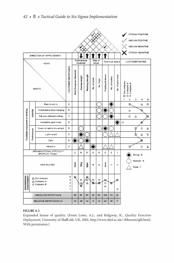
42 • The Tactical Guide to Six Sigma Implementation
FIGURE 4.3Expanded house of quality. (From Lowe, A.J., and Ridgway, K., Quality Function Deployment, University of Sheffield, UK, 2001, http://www.shef.ac.uk/~ibberson/qfd.html. With permission.)
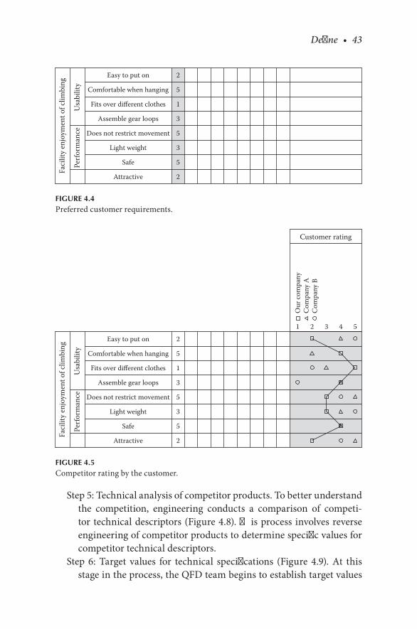
Define • 43
Step 5: Technical analysis of competitor products. To better understand the competition, engineering conducts a comparison of competi-tor technical descriptors (Figure 4.8). This process involves reverse engineering of competitor products to determine specific values for competitor technical descriptors.
Step 6: Target values for technical specifications (Figure 4.9). At this stage in the process, the QFD team begins to establish target values
Faci
lity
enjo
ymen
t of c
limbi
ng
Perf
orm
ance
Usa
bilit
yEasy to put on
Comfortable when hanging
Fits over different clothes
Assemble gear loops
Does not restrict movement
Light weight
Safe
Attractive
2
5
1
3
5
3
5
2
FIGURE 4.4Preferred customer requirements.
Faci
lity
enjo
ymen
t of c
limbi
ng
Perf
orm
ance
Usa
bilit
y
Easy to put on
Comfortable when hanging
Fits over different clothes
Assemble gear loops
Does not restrict movement
Light weight
Safe
Attractive
2
5
1
3
5
3
5
2
Customer rating
1 2 3 4 5
Our
com
pany
Com
pany
AC
ompa
ny B
FIGURE 4.5Competitor rating by the customer.
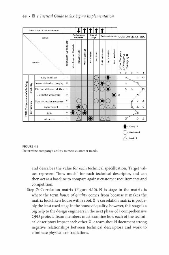
44 • The Tactical Guide to Six Sigma Implementation
and describes the value for each technical specification. Target val-ues represent “how much” for each technical descriptor, and can then act as a baseline to compare against customer requirements and competition.
Step 7: Correlation matrix (Figure 4.10). This stage in the matrix is where the term house of quality comes from because it makes the matrix look like a house with a roof. The correlation matrix is proba-bly the least used stage in the house of quality; however, this stage is a big help to the design engineers in the next phase of a comprehensive QFD project. Team members must examine how each of the techni-cal descriptors impact each other. The team should document strong negative relationships between technical descriptors and work to eliminate physical contradictions.
FIGURE 4.6Determine company’s ability to meet customer needs.

Define • 45
Step 8: Absolute importance (Figure 4.11). Finally, the team calculates the absolute importance for each technical descriptor. This numeri-cal calculation is the product of the cell value and the customer importance rating. Numbers are then added up in their respective columns to determine the importance for each technical descriptor. Now you know which technical aspects of your product matter the most to your customer. You have now reasonably satisfied that you have heard your customer’s voice.
We have eight “hows” (company ability to meet customer needs), as shown in Table 4.1.
We have eight “whats” (customer requirements, each with its own cus-tomer importance), as shown in Table 4.2.
FIGURE 4.7Rate organizational difficulty to meet customer requirements.
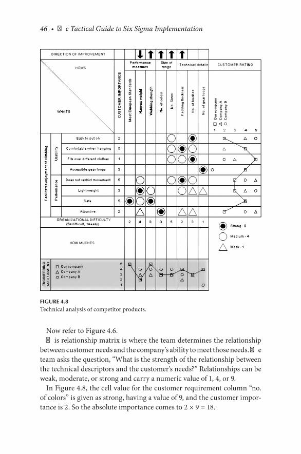
46 • The Tactical Guide to Six Sigma Implementation
Now refer to Figure 4.6.This relationship matrix is where the team determines the relationship
between customer needs and the company’s ability to meet those needs. The team asks the question, “What is the strength of the relationship between the technical descriptors and the customer’s needs?” Relationships can be weak, moderate, or strong and carry a numeric value of 1, 4, or 9.
In Figure 4.8, the cell value for the customer requirement column “no. of colors” is given as strong, having a value of 9, and the customer impor-tance is 2. So the absolute importance comes to 2 × 9 = 18.
FIGURE 4.8Technical analysis of competitor products.

Define • 47
In the same way for the customer requirement “no. of sizes,” the cell value given is 4. So for this requirement, the absolute requirement is (2 × 4) + (5 × 4) + (1 × 4) + (5 × 4) = 52.
The relative importance of the company’s ability to meet the related cus-tomer requirement is arrived at by adding all absolute importance figures (18 + 52 + … = 452) and calling the sum (452) 100%. The relative percent-age for “no. of colors” comes to (1/452% = 4%), and so on, as shown in Table 4.1.
The QFD exercise is complete.
FIGURE 4.9Target values for technical specifications.
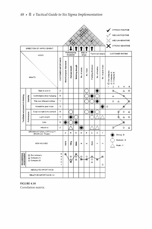
48 • The Tactical Guide to Six Sigma Implementation
FIGURE 4.10Correlation matrix.

Define • 49
FIGURE 4.11Absolute and relative importance.

50 • The Tactical Guide to Six Sigma Implementation
Next Stage
The above process is repeated in a slightly simplified way for the next three project phases.
A simplified matrix involving steps 1–3 and 5–8 above is developed where
• The voice of the engineer is translated into the voice of the part design specifications.
• The design specifications get translated into the voice of manufac-turing planning.
• The voice of manufacturing is translated into the voice of production planning.
TABLE 4.1
Eight Hows (Company Ability to Meet Customer Needs)
Ability No.Company Ability to Meet
Customer NeedsAbsolute
ImportanceRelative
Importance %
1 Meet European standards 45 162 Harness weight 67 103 Webbing strength 57 144 No. of colors 18 45 No. of sizes 52 126 Padding thickness 108 247 No. of buckles 72 168 No. of gear loops 30 8
TABLE 4.2
Eight Whats (Customer Requirements)
Requirement No. Requirement Importance
1 Easy to put on 22 Comfortable when hanging 53 Fits over different clothes 14 Assemble gear loops 35 Does not restrict movement 56 Lightweight 37 Safe 58 Attractive 2
Define • 51
QFD is a systematic means of ensuring that customer requirements are accurately translated into the technical goals and specifications through-out each stage of product development. The QFD process does not just maintain or improve product performance; it enables organizations to meet or exceed customer demands and delights customers by fulfilling their unarticulated and unanticipated desires and wants.
CTQ Flow-Down
Customer satisfaction generally falls into four dimensions:
• Quality• Delivery• Cost• Safety (for internal customers as well)
Critical to X (CTX) Requirements
This is how we define and describe various CTX requirements. Determine
• Critical to quality (CTQ)• Critical to cost (CTC)• Critical to process (CTP)• Critical to safety (CTS)• Critical to delivery (CTD)
These requirements should be measurable because they provide impor-tant goals and milestones for aligning projects with those requirements.
Cost and delivery are easy to quantify. Customers are willing to pay X money per item and expect its delivery Y days after the order is placed. Quantifying quality characteristics presents more of a challenge, and one of the tools devised to help is called the CTQ flow-down. Its purpose is to start with the high-level organizational strategic goal of customer satisfac-tion and determine how this goal “flows down” into measurable goals. The nomenclatures for the various levels are illustrated in Figure 4.12.
CTQ Flow-Down Example
The collected data for the result tracker, key support measure, key per-formance indicator, and key business driver are evaluated using a Pareto

52 • The Tactical Guide to Six Sigma Implementation
CTQ
flow
-dow
n
Spee
d
Sign
atur
e of
com
mitm
ent
Key
bus
ines
s driv
er (K
BD)
Key
per
form
ance
indi
cato
r (K
PI)
Key
supp
ort m
easu
re (K
SM)
Resu
lt tr
acke
r
Dep
loye
d to
shop
floo
r
Qua
lity
Frie
nds
coun
cil
Ope
Xco
unci
lD
eliv
ery
coun
cil
Cos
tco
unci
lM
achi
ning
coun
cil
Cos
t and
gro
wth
Safe
ty a
ndcu
lture
QM
S as
sess
men
tPe
rfor
man
ce a
sses
smen
t
Reco
rdab
lein
cide
nt ra
teSu
pplie
rD
PPM
Cus
tom
erD
PPM
Fina
l tes
tfa
ilure
rate
Cus
tom
erO
TD
Cos
tim
prov
emen
tIn
crem
enta
l/de
crem
enta
lEa
rned
hrs
vs.
wor
ked
hrs
Prot
otyp
ede
liver
yTu
rnov
er
War
rant
yre
duct
ion
Scra
pre
duct
ion
Supp
lier
OT
DC
ost-
out
lean
Mac
hini
ngpa
st d
ueSe
tup
cycl
etim
eVa
lvel
ocity
inve
ntor
yfil
led
Vari
able
MFG
expe
nse
as %
of d
irect
labo
rA
ttend
ance
QS
impl
emen
tatio
nD
istrib
utio
nm
ixO
TD
key
cust
omer
sM
anuf
actu
ring
profi
t
Tool
ing
expe
nses
trac
king
MRO
Mee
t cap
ital
spen
d
CFR
OG
ECO
/MPS
Mai
nten
ance
expe
nses
Ope
ratin
gpr
ofit a
s %of
sale
s
Cos
t out
inso
urci
ngm
anifo
lds
FLEX
trai
ning
Empl
oyee
enga
gem
ent
Haz
ardo
usw
aste
EPW
Psc
ore
MES
H
ED tr
ack
CEE
LS sc
ore
RTY
scor
eFr
eigh
t
MPV
Ove
rtim
e
Past
due
DO
H
FY01
0 St
rate
gic P
lan
Rev
1
FIG
UR
E 4.
12C
TQ fl
ow-d
own.
Define • 53
chart to obtain at least one major CTQ measure that can be measured and a process sigma that can be calculated.
Use the following tools to collect data at the Define stage (the same tools can be used at the Analyze stage):
Box and whisker plot: A tool used to display and analyze multiple sets of variation data on a single graph.
Check sheet: A generic tool that can be adapted for a wide variety of purposes. The check sheet is a structured, prepared form for collect-ing and analyzing data.
Control chart: A graph used to study how a process changes over time. Comparing current data to historical control limits leads to conclusions about whether the process variation is consistent (in control) or unpredictable (out of control, affected by special causes of variations).
Design of experiments: A method for carrying out carefully planned experiments on a process. Usually, a design of experiments involves a series of experiments that start by looking broadly at a great many variables and then focuses on the few critical ones.
Histogram: The most commonly used graph for showing frequency distributions, or how often each different value in a set of data occurs.
Scatter diagram: A diagram that graphs pairs of numerical data, one variable on each axis, to look for a relationship.
Stratification: A technique that separates data gathered from a variety of sources so that patterns can be seen.
Survey: Data collected from targeted groups of people about their opin-ions, behavior, or knowledge.
PROJECT CHARTER
Project Statement
A project statement starts with a business case first, which leads to the problem statement.
54 • The Tactical Guide to Six Sigma Implementation
Business Case
The business case is a short summary of the strategic reasons for the proj-ect (Table 4.3). The justification for a business case would typically involve at least one of the following:
• Cost per unit• Quality or defect rate• Cycle time
The problem statement will detail the issue that the project team wants to improve (Table 4.4). Problem cases include
• Historical data• What areas of the business are affected• How long the problem has existed• Any other symptoms of the problem
Project Scope
The project scope is the specific aspect of the problem that will be addressed, and it serves to specify the boundaries of the project.
Project Goal
Goals should
• Be carefully thought out and expressed.• Specify how completing the project will lead to improvements over
the existing state of affairs. You should be able to clearly describe the outcomes, deliverables, and benefits to stakeholders and customers.
• Provide the criteria you need to evaluate the success of the project in terms of time, costs, and resources.
• Be reviewed by the core team, which must reach consensus before moving to the next phase of the project.

Define • 55
TAB
LE 4
.3
Exam
ple
of B
usin
ess C
ase
Sum
mar
y
Cur
rent
Sit
uati
onIm
prov
emen
t O
bjec
tive
Key
Bus
ines
s D
rive
rPe
rfor
man
ce
Cat
egor
yM
etri
cC
urre
nt
2013
Goa
l
Q3-
13Q
3-14
Cur
rent
logi
stic
pro
cess
cau
ses
50%
of fi
nish
ed g
oods
to re
ach
our O
EMs a
nd d
irect
cus
tom
ers
late
Impr
ove
OTD
Cus
tom
er
satis
fact
ion
Cus
tom
er
satis
fact
ion
OTD
72%
80%
90%
Miss
ing
and
lost
ship
men
tsO
TDC
usto
mer
sa
tisfa
ctio
nC
usto
mer
sa
tisfa
ctio
nZe
ro
miss
ed
ship
men
ts
72%
80%
90%
The
cost
-out
opp
ortu
nitie
s due
to
line
dow
n co
sts,
cred
it to
cu
stom
ers,
and
prem
ium
frei
ght
Man
ufac
turi
ng
profi
tBu
sines
s ex
celle
nce
Cos
t im
prov
emen
tC
ost-
out
$400
K lo
st
so fa
r in
2013
$25K
$75K
Inco
min
g ra
w m
ater
ial a
nd
cust
omer
retu
rned
pro
duct
s ar
rivin
g la
te to
the
plan
ts a
nd
also
get
ting
lost
in P
harr
W
areh
ouse
Man
ufac
turi
ng
profi
t/OTD
Busin
ess
exce
llenc
eC
usto
mer
sa
tisfa
ctio
n
Cos
t im
prov
emen
tC
ost-
out
$150
K lo
st
so fa
r in
2013
$25K
$50K
Phar
r War
ehou
se d
oes n
ot h
ave
adeq
uate
reso
urce
s (sy
stem
and
m
anag
emen
t) to
repo
rt S
wiss
co
mpa
ny tr
ansa
ctio
ns
Man
ufac
turi
ng
profi
t/OTD
Busin
ess
exce
llenc
eC
usto
mer
sa
tisfa
ctio
n
Cos
t im
prov
emen
tC
ost-
out
$40K
lost
so
far i
n 20
13$2
5K$7
5K
Not
e: O
EM, o
rigi
nal e
quip
men
t man
ufac
ture
r; O
TD, o
n-tim
e de
liver
y.
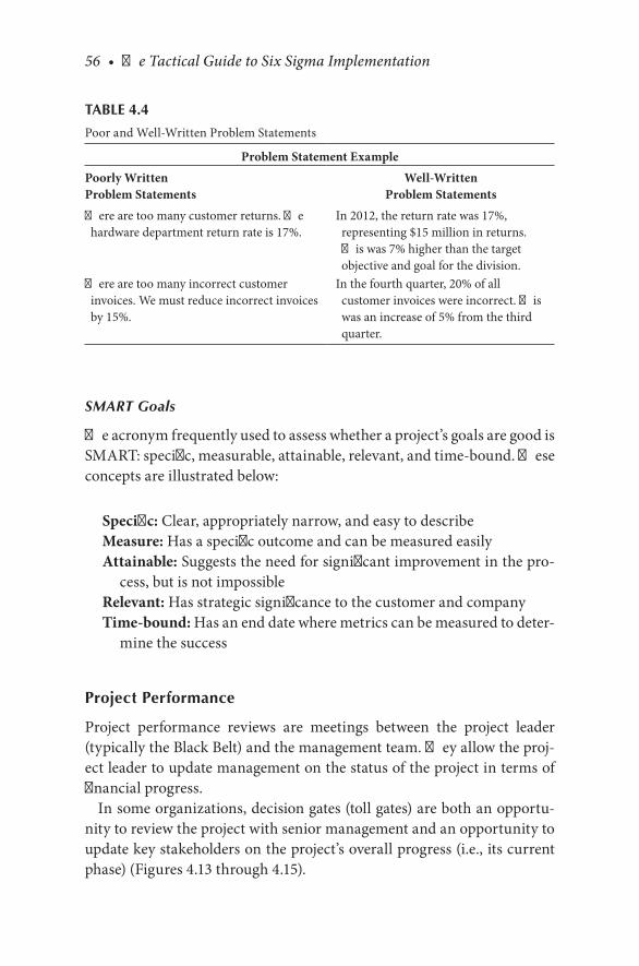
56 • The Tactical Guide to Six Sigma Implementation
SMART Goals
The acronym frequently used to assess whether a project’s goals are good is SMART: specific, measurable, attainable, relevant, and time-bound. These concepts are illustrated below:
Specific: Clear, appropriately narrow, and easy to describeMeasure: Has a specific outcome and can be measured easilyAttainable: Suggests the need for significant improvement in the pro-
cess, but is not impossibleRelevant: Has strategic significance to the customer and companyTime-bound: Has an end date where metrics can be measured to deter-
mine the success
Project Performance
Project performance reviews are meetings between the project leader (typically the Black Belt) and the management team. They allow the proj-ect leader to update management on the status of the project in terms of financial progress.
In some organizations, decision gates (toll gates) are both an opportu-nity to review the project with senior management and an opportunity to update key stakeholders on the project’s overall progress (i.e., its current phase) (Figures 4.13 through 4.15).
TABLE 4.4
Poor and Well-Written Problem Statements
Problem Statement Example
Poorly WrittenProblem Statements
Well-WrittenProblem Statements
There are too many customer returns. The hardware department return rate is 17%.
In 2012, the return rate was 17%, representing $15 million in returns. This was 7% higher than the target objective and goal for the division.
There are too many incorrect customer invoices. We must reduce incorrect invoices by 15%.
In the fourth quarter, 20% of all customer invoices were incorrect. This was an increase of 5% from the third quarter.
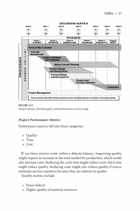
Define • 57
Project Performance Metrics
Performance metrics fall into three categories:
• Quality• Time• Cost
These three metrics work within a delicate balance. Improving quality might require an increase in the time needed for production, which would also increase costs. Reducing the cycle time might reduce costs, but it also might reduce quality. Reducing costs might also reduce quality if source materials are less expensive because they are inferior in quality.
Quality metrics include
• Fewer defects• Higher quality of material resources
FIGURE 4.13Project phases, decision gates, and performance review map.
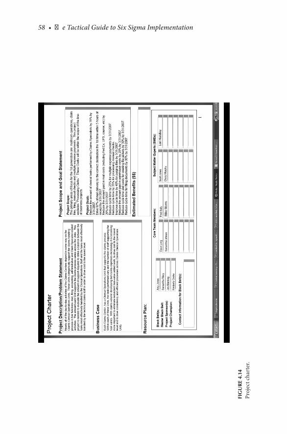
58 • The Tactical Guide to Six Sigma Implementation
FIG
UR
E 4.
14Pr
ojec
t cha
rter
.
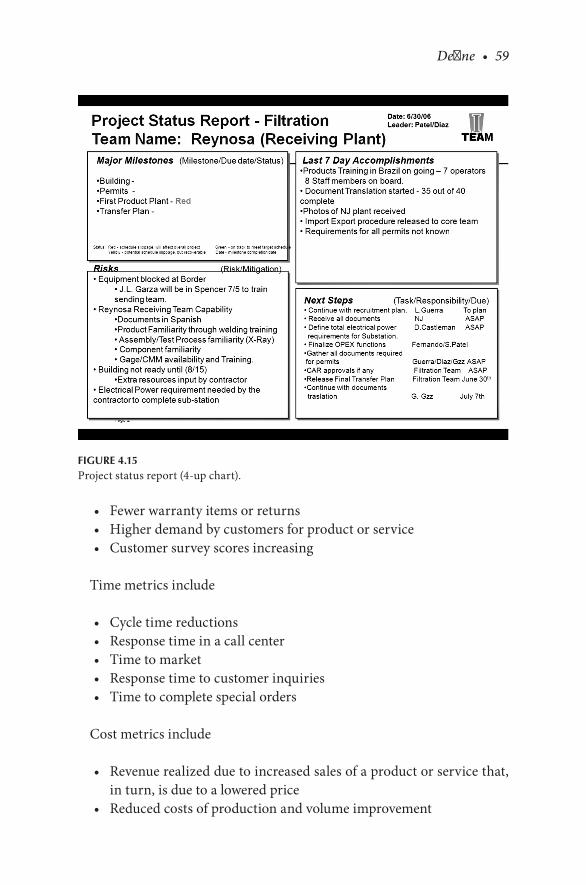
Define • 59
• Fewer warranty items or returns• Higher demand by customers for product or service• Customer survey scores increasing
Time metrics include
• Cycle time reductions• Response time in a call center• Time to market• Response time to customer inquiries• Time to complete special orders
Cost metrics include
• Revenue realized due to increased sales of a product or service that, in turn, is due to a lowered price
• Reduced costs of production and volume improvement
FIGURE 4.15Project status report (4-up chart).
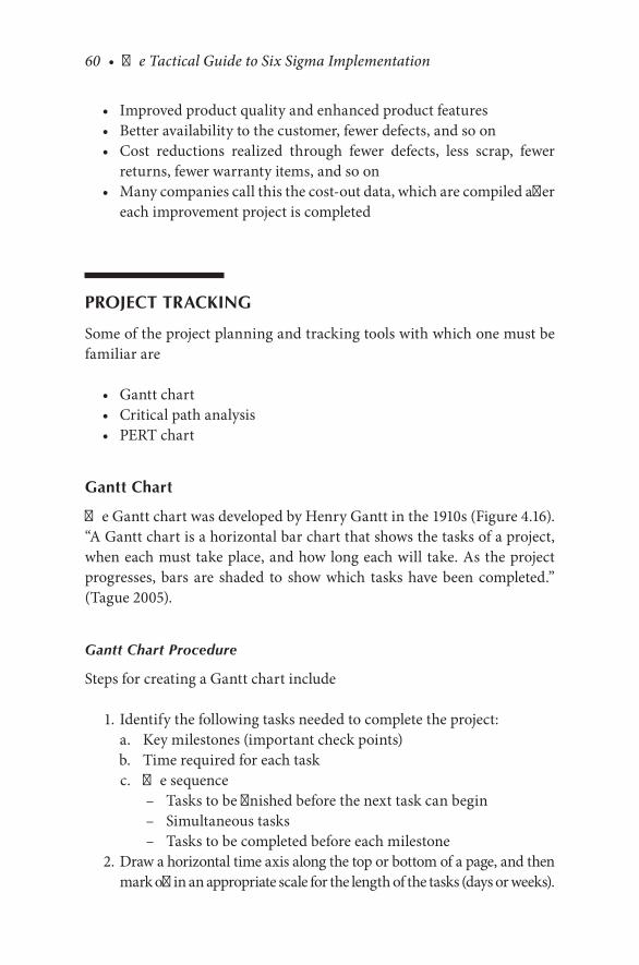
60 • The Tactical Guide to Six Sigma Implementation
• Improved product quality and enhanced product features• Better availability to the customer, fewer defects, and so on• Cost reductions realized through fewer defects, less scrap, fewer
returns, fewer warranty items, and so on• Many companies call this the cost-out data, which are compiled after
each improvement project is completed
PROJECT TRACKING
Some of the project planning and tracking tools with which one must be familiar are
• Gantt chart• Critical path analysis• PERT chart
Gantt Chart
The Gantt chart was developed by Henry Gantt in the 1910s (Figure 4.16). “A Gantt chart is a horizontal bar chart that shows the tasks of a project, when each must take place, and how long each will take. As the project progresses, bars are shaded to show which tasks have been completed.” (Tague 2005).
Gantt Chart Procedure
Steps for creating a Gantt chart include
1. Identify the following tasks needed to complete the project: a. Key milestones (important check points) b. Time required for each task c. The sequence
– Tasks to be finished before the next task can begin– Simultaneous tasks– Tasks to be completed before each milestone
2. Draw a horizontal time axis along the top or bottom of a page, and then mark off in an appropriate scale for the length of the tasks (days or weeks).
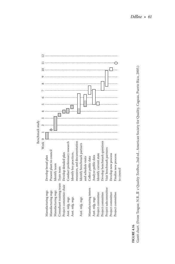
Define • 61
Man
ufac
turin
g m
gr.
Man
ufac
turin
g m
gr.
Man
ufac
turin
g m
gr.
Con
sulta
nt tr
aini
ng te
amPr
ojec
t com
mitt
ee c
hair
Ass
t. m
fg. m
gr.
Ass
t. m
fg. m
gr.
Ass
t. m
fg. m
gr.
Man
ufac
turin
g in
tern
Ass
t. m
fg. m
gr.
Proj
ect c
omm
ittee
Proj
ect c
omm
ittee
Proj
ect s
ubco
mm
ittee
Proj
ect c
omm
ittee
Proj
ect c
omm
ittee
Dev
elop
bro
ad p
lan
Pres
ent p
lant
to c
ounc
ilId
entif
y te
amTr
ain
team
Dev
elop
det
aile
d pl
anC
ondu
ct p
relim
inar
y re
sear
chId
entif
y ke
y pr
actic
es,
mea
sure
s, an
d do
cum
enta
tion
Iden
tify
benc
hmar
k pa
rtne
rsan
d sc
hedu
le v
isits
Col
lect
pub
lic d
ata
Ana
lyze
pub
lic d
ata
Iden
tify
curr
ent s
tate
Dev
elop
ben
chm
ark
ques
tions
Visit
ben
chm
ark
part
ners
Dev
elop
new
pro
cess
Fina
lize
new
pro
cess
to c
ounc
il
0W
eek
1Be
nchm
ark
stud
y2
34
56
78
910
1112
FIG
UR
E 4.
16G
antt
cha
rt. (
From
Tea
gue,
N.R
., Th
e Qua
lity
Tool
box,
2nd
ed.
, Am
eric
an S
ocie
ty fo
r Qua
lity,
Cag
uas,
Puer
to R
ico,
200
5.)

62 • The Tactical Guide to Six Sigma Implementation
3. Down the left side of the page, write each project task and milestone in order:
a. For each event happening at a point in time, draw a diamond (unfilled) under the time for that event.
b. For activities occurring over a period of time, draw a bar (unfilled) spanning the appropriate time.– Align the left end of the bar with the time the activity begins.– Align the right end with the time the activity concludes.– Ensure that every task of the project is on the chart.
4. As events and activities take place, shade the diamonds and bars to show completion. For tasks in progress, estimate the percentage of completion and shade the appropriate amount.
5. Place a vertical marker to show the current date. When posting the chart on the wall, a heavy dark string hung vertically across the chart with two thumbtacks is an easy way to show the current time.
Critical Path Analysis
Developed by project managers in the 1950s, critical path analysis (CPA), also known as the critical path method (CPM), is one of several planning tools for demonstrating and viewing chronological tasks, identifying pos-sible timing risks, and establishing the least amount of time for the project or process (Figure 4.17).
The benefits of CPA are that it
• Displays a graphical model of the project• Predicts the shortest time required to complete the project
1
3
4
5
7
6
5
2
A
B
GH
FI
EC
D
1 week 1 week
1 week
2 weeks
2 weeks
4 weeks
4 weeks 2 weeks
3 weeks
FIGURE 4.17Critical path analysis.

Define • 63
• Emphasizes activities critical to maintaining the schedule• Provides a timing reference point throughout the project• Identifies interrelationships between tasks
Three paths exist in Figure 4.17:
1-3-4-5-7 (8 weeks) (critical path, longest time)1-3-5-7 (6 weeks)1-2-6-7 (7 weeks)
Critical Path Analysis Procedure
1. Use Post-it notes to individually list all tasks in the project. Underneath each task, draw a horizontal arrow pointing right.
2. Arrange the notes in the appropriate sequence (from left to right). 3. Between each pair of tasks, draw circles to represent events and mark
the beginning or end of a task. 4. Label all events, in sequence, with numbers. Label all tasks, in
sequence, with letters. 5. For each task, estimate the completion time. Write the time below
the arrow for each task. 6. Draw the critical path by highlighting the longest path from the
beginning to the end of the project.
PERT Chart
First developed by the Navy in the 1950s to manage complex projects, pro-gram evaluation and review technique charts are powerful tools for reduc-ing the time and cost for completing a project. PERT’s planning technique accounts for randomness in time requirements (Figure 4.18).
The term critical path method will also be used for a similar approach. “The most important difference between PERT and CPM is that origi-nally the time estimates for the activities were assumed deterministic in CPM. Deterministic methods use point estimates which are often, but not necessarily always, worst case estimates. The probabilistic estimates in PERT methods allow for the use of distributions to represent the long-term profiles, and distributions of each estimate. Today, PERT and CPM actually comprise one technique and the differences are mainly histori-cal” (Pyzdek and Keller 2011).
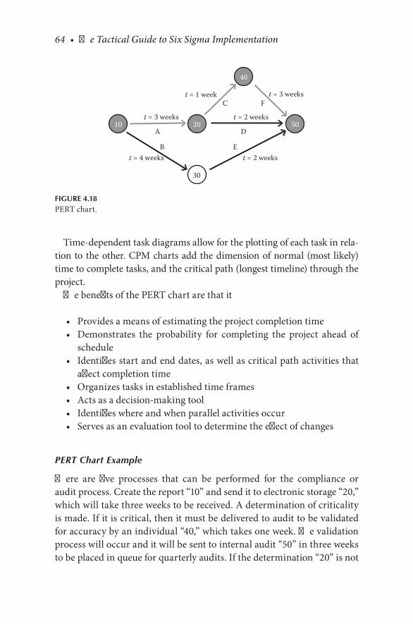
64 • The Tactical Guide to Six Sigma Implementation
Time-dependent task diagrams allow for the plotting of each task in rela-tion to the other. CPM charts add the dimension of normal (most likely) time to complete tasks, and the critical path (longest timeline) through the project.
The benefits of the PERT chart are that it
• Provides a means of estimating the project completion time• Demonstrates the probability for completing the project ahead of
schedule• Identifies start and end dates, as well as critical path activities that
affect completion time• Organizes tasks in established time frames• Acts as a decision-making tool• Identifies where and when parallel activities occur• Serves as an evaluation tool to determine the effect of changes
PERT Chart Example
There are five processes that can be performed for the compliance or audit process. Create the report “10” and send it to electronic storage “20,” which will take three weeks to be received. A determination of criticality is made. If it is critical, then it must be delivered to audit to be validated for accuracy by an individual “40,” which takes one week. The validation process will occur and it will be sent to internal audit “50” in three weeks to be placed in queue for quarterly audits. If the determination “20” is not
40
502010
30
B E
DA
C Ft = 3 weeks
t = 2 weekst = 3 weeks
t = 4 weeks t = 2 weeks
t = 1 week
FIGURE 4.18PERT chart.
Define • 65
critical, then it is sent in two weeks to be placed in queue for quarterly audits by internal audit “50.” If the report is sent to physical storage “30,” it will take four weeks to be processed, and a random group is sent to inter-nal audit “50,” which will take two weeks.
The quickest path to the audit queue is the noncritical electronic report that will take five weeks to be moved into the internal audit queue. The longest path is the electronic critical reports, which will take seven weeks to be moved into the internal audit queue.
PERT Chart Key Terms
The following terms are important to keep in mind when using PERT charts. Critical path refers to the sequence of tasks (path) that takes the longest time and determines the project’s completion date. Any delay of tasks on a critical path will delay the project completion time.
Slack time refers to the time an activity can be delayed without delaying the entire project. Tasks on the critical path have zero slack time. Slack time is the difference between the latest allowable date and the earliest expected date. It is represented by the following:
Slack time = T/L – T/E
where T/E is the earliest time (date) on which an event can be expected to occur and T/L is the latest time (date) on which an event can occur without extending the completion date of the project.
An event is the starting or ending point for a group of tasks.Activity is the work required to proceed from one event or point in time
to another.
PERT Chart Procedure
1. Use Post-it notes to individually list all tasks in the project. Underneath each task, draw a horizontal arrow pointing right.
2. Arrange the notes in the appropriate sequence (from left to right). 3. Between each two tasks, draw circles to represent events and to mark
the beginning or end of a task. 4. Label all events, in sequence, with numbers. Label all tasks, in
sequence, with letters.
66 • The Tactical Guide to Six Sigma Implementation
5. For each activity, make three estimates regarding time requirements: the shortest possible time, the most likely time, and the longest time.
6. Determine the critical path. 7. Adjustments to the PERT chart should be made to reflect any changes
to the project along the way.
DEFINE PHASE SUMMARY
The purpose of the define phase is to
• Establish the specific Six Sigma project scope and boundaries• Define the specific business problem• Describe the business process needing improvement• State the goals to be achieved
67
5Measure
The second phase of the define, measure, analyze, improve, and control (DMAIC) process is measure. It is a measure of how the key business pro-cesses are doing. It is said that if it is not measured, it is not managed. A business process consists of a series of events to produce an output. The objective is to add value at each event to produce a product or service that in turn can be sold to the customer.
Major concepts and tools discussed in the measure phase are
• Process characteristics• Measurement system analysis (MSA)• Process capability measurement
PROCESS CHARACTERISTICS
Process characteristics have an origin with written documentation (Figure 5.1). First it is necessary to review the written procedures, work instructions, flowcharts, and quality records in order to determine process characteristics.
A process map is then created for each process where all steps of the pro-cess actions are enumerated. These process maps are used for all measure activities.
Process characteristics comprise the following input and output variables:
• Suppliers, inputs, process, outputs, and customers (SIPOC)• Work in progress (WIP)• Work in queue (WIQ)• Touch time
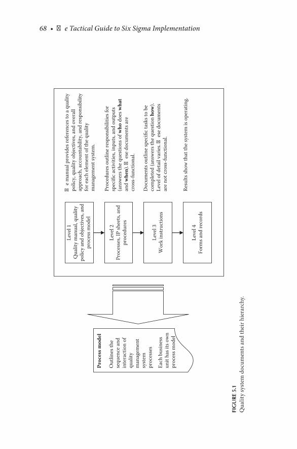
68 • The Tactical Guide to Six Sigma Implementation
Leve
l 1Q
ualit
y m
anua
l, qu
ality
polic
y an
d ob
ject
ives
, and
proc
ess m
odel
Leve
l 2Pr
oces
ses,
IP sh
eets
, and
proc
edur
es
Leve
l 3W
ork
inst
ruct
ions
Leve
l 4Fo
rms a
nd re
cord
s
�e
man
ual p
rovi
des r
efer
ence
s to
a qu
ality
polic
y, q
ualit
y ob
ject
ives
, and
ove
rall
appr
oach
, acc
ount
abili
ty, a
nd re
spon
sibili
tyfo
r eac
h el
emen
t of t
he q
ualit
ym
anag
emen
t sys
tem
.
Proc
edur
es o
utlin
e re
spon
sibili
ties f
orsp
ecifi
c ac
tiviti
es, i
nput
s, an
d ou
tput
s(a
nsw
ers t
he q
uest
ions
of w
ho d
oes w
hat
and
whe
n). �
ese
docu
men
ts a
recr
oss-
func
tiona
l.
Doc
umen
ts o
utlin
e sp
ecifi
c ta
sks t
o be
com
plet
ed (a
nsw
ers t
he q
uest
ion
how
).Le
vel o
f det
ail v
arie
s. �
ese
docu
men
tsar
e no
t cro
ss-f
unct
iona
l.
Resu
lts sh
ow th
at th
e sy
stem
is o
pera
ting.
Proc
ess m
odel
Out
lines
the
sequ
ence
and
inte
ract
ion
ofqu
ality
man
agem
ent
syst
empr
oces
ses
Each
bus
ines
sun
it ha
s its
ow
n pr
oces
s mod
el
FIG
UR
E 5.
1Q
ualit
y sy
stem
doc
umen
ts a
nd th
eir h
iera
rchy
.
Measure • 69
• Takt time• Cycle time• Throughput• Value stream maps• Process maps• Flowcharts• Procedures• Work instructions• Spaghetti diagrams• Circle diagrams
We have defined the processes through input, process, and output vari-ables, as well as using the turtle and SIPOC diagrams in Book 1. The rela-tionships of these variables and their defined characteristics need to be measured for process improvement.
Identify processes having wastes and poor utilization. Improve these processes by analyzing work in progress, work in queue, touch time, takt time, cycle time, throughput, and so forth.
Analyze processes by preparing value stream maps, process maps, flowcharts, procedures, work instructions, spaghetti diagrams, circle dia-grams, and so forth.
These variables are discussed below.
SIPOC: Covered in Books 1 and 2.WIP: Incomplete product or service that is awaiting further process-
ing and that has not reached the output stage. Sur prisingly, account-ing systems consider WIP an asset, but it is in many ways a liability because it needs upkeep expenses such as storage, environmental control, identifications, and record keeping.
WIQ: Material waiting in queue and is a component of WIP. It is impor-tant to identify WIQ at each step of the process to identify process bottlenecks or constraints. The first-in, first-out (FIFO) policy helps in reducing WIQ as long as necessary attention is given to the shelf life of the inventory.
Touch time: Time that material is actually being touched or processed at one of the steps. The processes with large touch times can be iden-tified for improvement purposes.
Takt time: Covered in Book 2.Cycle time: Covered in Book 2.
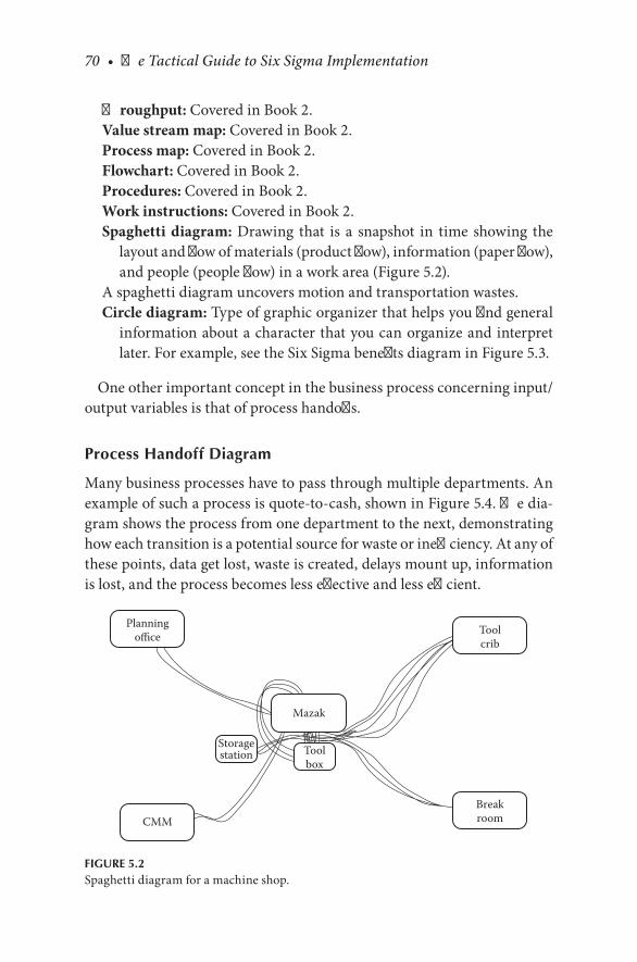
70 • The Tactical Guide to Six Sigma Implementation
Throughput: Covered in Book 2.Value stream map: Covered in Book 2.Process map: Covered in Book 2.Flowchart: Covered in Book 2.Procedures: Covered in Book 2.Work instructions: Covered in Book 2.Spaghetti diagram: Drawing that is a snapshot in time showing the
layout and flow of materials (product flow), information (paper flow), and people (people flow) in a work area (Figure 5.2).
A spaghetti diagram uncovers motion and transportation wastes.Circle diagram: Type of graphic organizer that helps you find general
information about a character that you can organize and interpret later. For example, see the Six Sigma benefits diagram in Figure 5.3.
One other important concept in the business process concerning input/output variables is that of process handoffs.
Process Handoff Diagram
Many business processes have to pass through multiple departments. An example of such a process is quote-to-cash, shown in Figure 5.4. The dia-gram shows the process from one department to the next, demonstrating how each transition is a potential source for waste or inefficiency. At any of these points, data get lost, waste is created, delays mount up, information is lost, and the process becomes less effective and less efficient.
Planningoffice Tool
crib
BreakroomCMM
Mazak
Toolbox
Storagestation
FIGURE 5.2Spaghetti diagram for a machine shop.
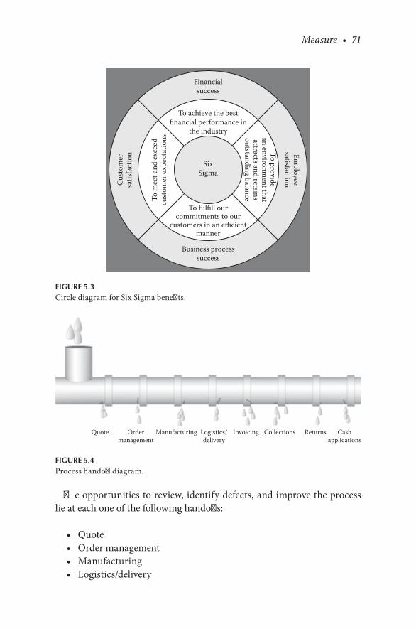
Measure • 71
The opportunities to review, identify defects, and improve the process lie at each one of the following handoffs:
• Quote• Order management• Manufacturing• Logistics/delivery
SixSigma
To achieve the bestfinancial performance in
the industry
To fulfill ourcommitments to our
customers in an efficientmanner
To m
eet a
nd e
xcee
dcu
stom
er e
xpec
tatio
ns
To providean environm
ent thatattracts and retainsoutstanding balance
Financialsuccess
Business processsuccess
Cus
tom
ersa
tisfa
ctio
n Employee
satisfaction
FIGURE 5.3Circle diagram for Six Sigma benefits.
Quote Ordermanagement
Manufacturing Logistics/delivery
Invoicing Collections Returns Cashapplications
FIGURE 5.4Process handoff diagram.
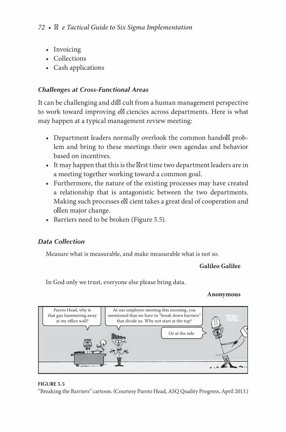
72 • The Tactical Guide to Six Sigma Implementation
• Invoicing• Collections• Cash applications
Challenges at Cross-Functional Areas
It can be challenging and difficult from a human management perspective to work toward improving efficiencies across departments. Here is what may happen at a typical management review meeting:
• Department leaders normally overlook the common handoff prob-lem and bring to these meetings their own agendas and behavior based on incentives.
• It may happen that this is the first time two department leaders are in a meeting together working toward a common goal.
• Furthermore, the nature of the existing processes may have created a relationship that is antagonistic between the two departments. Making such processes efficient takes a great deal of cooperation and often major change.
• Barriers need to be broken (Figure 5.5).
Data Collection
Measure what is measurable, and make measurable what is not so.
Galileo Galilee
In God only we trust, everyone else please bring data.
Anonymous
Pareto Head, why isthat guy hammering away
at my office wall?
At our employee meeting this morning, youmentioned that we have to “break down barriers”
that divide us. Why not start at the top?
Or at the side
FIGURE 5.5“Breaking the Barriers” cartoon. (Courtesy Pareto Head, ASQ Quality Progress, April 2013.)
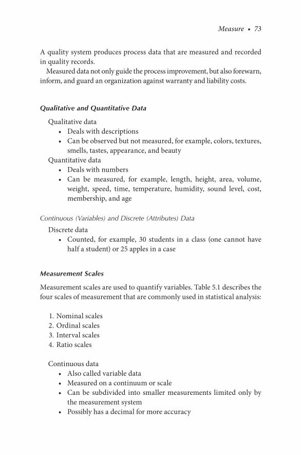
Measure • 73
A quality system produces process data that are measured and recorded in quality records.
Measured data not only guide the process improvement, but also forewarn, inform, and guard an organization against warranty and liability costs.
Qualitative and Quantitative Data
Qualitative data• Deals with descriptions• Can be observed but not measured, for example, colors, textures,
smells, tastes, appearance, and beautyQuantitative data
• Deals with numbers• Can be measured, for example, length, height, area, volume,
weight, speed, time, temperature, humidity, sound level, cost, membership, and age
Continuous (Variables) and Discrete (Attributes) Data
Discrete data• Counted, for example, 30 students in a class (one cannot have
half a student) or 25 apples in a case
Measurement Scales
Measurement scales are used to quantify variables. Table 5.1 describes the four scales of measurement that are commonly used in statistical analysis:
1. Nominal scales 2. Ordinal scales 3. Interval scales 4. Ratio scales
Continuous data• Also called variable data• Measured on a continuum or scale• Can be subdivided into smaller measurements limited only by
the measurement system• Possibly has a decimal for more accuracy

74 • The Tactical Guide to Six Sigma Implementation
• Generally more powerful than discrete data because they can be analyzed statistically
• Examples are– Physical measurements (length, volume, width, time, tem-
perature, etc.)– Using a rule to measure a single dimension only to the near-
est 0.1 inch– Using a venire caliper to measure the same dimension to the
nearest 0.005 inch– Using a micrometer to measure the same dimension to the
nearest 0.0001 inch
MEASUREMENT SYSTEM ANALYSIS
Business uses of MSA include the following:
• It is a mandatory requirement for ISO TS 16949 and AS 9100 certification.
• It discovers potential sources of process variation.
TABLE 5.1
Measurement Scales
Scale Type Definition Example Calculations
Nominal Label indicating a characteristic by a name, or presence/absence. Can only count items.
Pass or fail, accept or reject, male or female, 0 = red, 1 = white, 2 = blue
Proportion, chi-square
Ordinal Grouping into categories having an attribute. When comparing elements, order is important.
Likert scale and 1–5 scales
Rank order correlations
Interval Fixed or defined scale differentiating two successive points, but no true 0. Potential zero point in measurements.
Time of day (calendar time), temperature
CorrelationsT-testsF-testsRegressions
Ratio Relationship between two values. Characteristic able to be measured; there is a true 0. Zero point indicates an absence of an attribute. Can add, subtract, multiply, and divide these values.
% purity, miles per hour, height in inches, elapsed time
CorrelationsT-testsF-testsRegressions
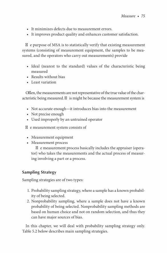
Measure • 75
• It minimizes defects due to measurement errors.• It improves product quality and enhances customer satisfaction.
The purpose of MSA is to statistically verify that existing measurement systems (consisting of measurement equipment, the samples to be mea-sured, and the operators who carry out measurements) provide
• Ideal (nearest to the standard) values of the characteristic being measured
• Results without bias• Least variation
Often, the measurements are not representative of the true value of the char-acteristic being measured. This might be because the measurement system is
• Not accurate enough—it introduces bias into the measurement• Not precise enough• Used improperly by an untrained operator
The measurement system consists of
• Measurement equipment• Measurement process The measurement process basically includes the appraiser (opera-
tor) who takes the measurements and the actual process of measur-ing involving a part or a process.
Sampling Strategy
Sampling strategies are of two types:
1. Probability sampling strategy, where a sample has a known probabil-ity of being selected.
2. Nonprobability sampling, where a sample does not have a known probability of being selected. Nonprobability sampling methods are based on human choice and not on random selection, and thus they can have major sources of bias.
In this chapter, we will deal with probability sampling strategy only. Table 5.2 below describes main sampling strategies.
76 • The Tactical Guide to Six Sigma Implementation
Measurement Equipment
The following are types of measurement equipment:
• Attribute screens (go/no-go screens to sort out mined mineral lumps, etc.)
• Gage blocks• Calipers• Optical comparator• Coordinate measuring machine (CMM)• Micrometer• Measuring machines for tensile strength, compression strength, and
so forth• Titration (Volumetric conical flask, burette having markings to mea-
sure volume and pipette with a volume noted on it.)
TABLE 5.2
Sampling Strategies
Sampling Strategy Definition Examples
Random Select sample units so that all units have the same probability of being selected. Every unit (n) has an equal chance of being selected for the sample.
Random number generator is used for census taking. Random number generator is used by a fast food chain to print a survey number on a receipt for customers to use when they call and answer questions about their experience.
Systematic Every nth record is selected from a list of the population. As long as the list does not contain any hidden order, this strategy is just as good as random sampling.
A customer service call center receives a randomly generated list of customers who have interacted with customer service representatives. The manager selects every fifth name on the list to conduct a follow-up call for quality assurance.
Stratified If the population has identified categories or strata that have a common characteristic, random sampling is used to select a sufficient number of units from each stratum. Stratified sampling is often used to reduce sampling error.
Customer survey results are divided into multiple strata based on gender and income level. A manufacturer divides data on defects into strata based on manufacturing location and equipment type used for production.
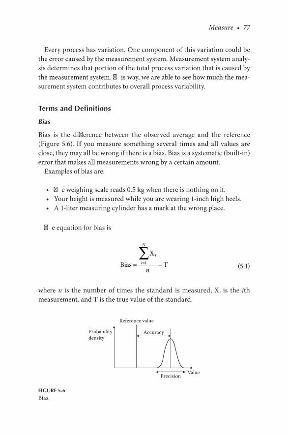
Measure • 77
Every process has variation. One component of this variation could be the error caused by the measurement system. Measurement system analy-sis determines that portion of the total process variation that is caused by the measurement system. This way, we are able to see how much the mea-surement system contributes to overall process variability.
Terms and Definitions
Bias
Bias is the difference between the observed average and the reference (Figure 5.6). If you measure something several times and all values are close, they may all be wrong if there is a bias. Bias is a systematic (built-in) error that makes all measurements wrong by a certain amount.
Examples of bias are:
• The weighing scale reads 0.5 kg when there is nothing on it.• Your height is measured while you are wearing 1-inch high heels.• A 1-liter measuring cylinder has a mark at the wrong place.
The equation for bias is
Bias
X
T= −=∑ i
i
N
n1 (5.1)
where n is the number of times the standard is measured, Xi is the ith measurement, and T is the true value of the standard.
Probabilitydensity
Precision
Accuracy
Reference value
Value
FIGURE 5.6Bias.

78 • The Tactical Guide to Six Sigma Implementation
Bias can be removed by calibration.Two characteristics contribute to the effectiveness of a measurement
method:
1. Precision 2. Accuracy
Precision has two components:
• Repeatability: The same person cannot get the same result twice on the same subject.
• Reproducibility: Different people cannot agree on the result obtained on the same subject (part or process).
Gage repeatability and reproducibility (R&R) is the combined estimate of repeatability and reproducibility.
Accuracy is related to the difference between the average and the refer-ence value (this difference is called bias). Accuracy is how close a mea-sured value is to the actual (true) value.
The degree of accuracy depends on the instrument you are measuring with (Figure 5.7). But as a general rule, the degree of accuracy is half a unit on each side of the unit of measure.
If your instrument measures in 1-inch increments, then any value between 6½ and 7½ is measured as 7 inches.
4
4 6 82
“8”
5 6 71
8 9
“7”
FIGURE 5.7Degree of accuracy.
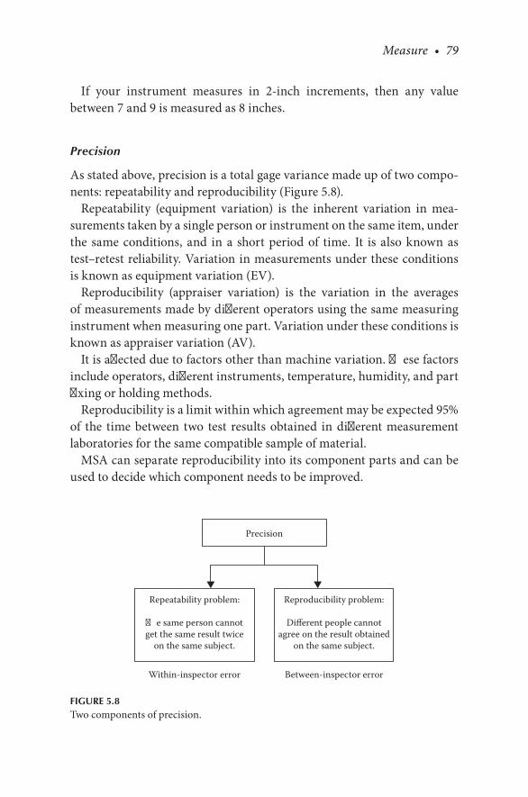
Measure • 79
If your instrument measures in 2-inch increments, then any value between 7 and 9 is measured as 8 inches.
Precision
As stated above, precision is a total gage variance made up of two compo-nents: repeatability and reproducibility (Figure 5.8).
Repeatability (equipment variation) is the inherent variation in mea-surements taken by a single person or instrument on the same item, under the same conditions, and in a short period of time. It is also known as test–retest reliability. Variation in measurements under these conditions is known as equipment variation (EV).
Reproducibility (appraiser variation) is the variation in the averages of measurements made by different operators using the same measuring instrument when measuring one part. Variation under these conditions is known as appraiser variation (AV).
It is affected due to factors other than machine variation. These factors include operators, different instruments, temperature, humidity, and part fixing or holding methods.
Reproducibility is a limit within which agreement may be expected 95% of the time between two test results obtained in different measurement laboratories for the same compatible sample of material.
MSA can separate reproducibility into its component parts and can be used to decide which component needs to be improved.
Precision
Repeatability problem:
�e same person cannotget the same result twice
on the same subject.
Reproducibility problem:
Different people cannotagree on the result obtained
on the same subject.
Within-inspector error Between-inspector error
FIGURE 5.8Two components of precision.
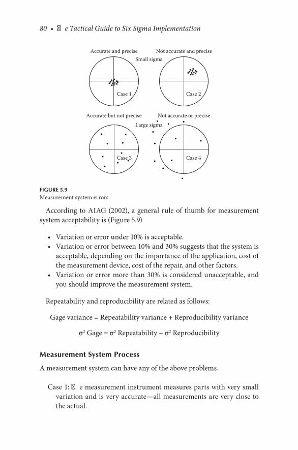
80 • The Tactical Guide to Six Sigma Implementation
According to AIAG (2002), a general rule of thumb for measurement system acceptability is (Figure 5.9)
• Variation or error under 10% is acceptable.• Variation or error between 10% and 30% suggests that the system is
acceptable, depending on the importance of the application, cost of the measurement device, cost of the repair, and other factors.
• Variation or error more than 30% is considered unacceptable, and you should improve the measurement system.
Repeatability and reproducibility are related as follows:
Gage variance = Repeatability variance + Reproducibility variance
σ2 Gage = σ2 Repeatability + σ2 Reproducibility
Measurement System Process
A measurement system can have any of the above problems.
Case 1: The measurement instrument measures parts with very small variation and is very accurate—all measurements are very close to the actual.
Small sigma
Large sigma
Case 1
Case 3
Case 2
Case 4
Accurate and precise Not accurate and precise
Accurate but not precise Not accurate or precise
FIGURE 5.9Measurement system errors.

Measure • 81
Case 2: The measurement instrument measures parts with very small variation but is not accurate.
Case 3: We could also have an instrument where the mean of the mea-surements is very close to the actual value, but the measurement data have a large variance (not precise).
Case 4: Finally, there could be a measurement instrument that is nei-ther accurate nor precise.
The MSA process steps are as follows:
1. Prepare for the study. 2. Understand and evaluate stability. 3. Evaluate resolution. 4. Determine accuracy. 5. Calibrate the instrument. 6. Evaluate linearity 7. Determine repeatability and reproducibility.
Step 1: Prepare for the Study
Objective Determine which process parameters will be used for the rest of
the study.Process
• Determine what measurement system is to be studied. This includes the instrument and the test procedure.
• Document the test procedure. Train the operators in under-standing the procedure.
• Determine the number of operators (k), the number of sample parts (n), and the number of repeated readings (r). As a rule of thumb, you may choose 3 operators, 4–10 sample parts, and 3–6 repeated readings.
• Note: The greater the number of operators or parts or readings, the greater the confidence and the greater the price—so you decide how the confidence should be utilized.
• Determine who the operators will be. The operators chosen should be selected from those who are trained or certified on the measurement system.

82 • The Tactical Guide to Six Sigma Implementation
• Determine what samples will be used and where the samples will come from. The sample parts must come from an existing pro-cess and represent its entire operating range.
• Several methods can be used, which will ensure randomly dis-tributed sample parts. The most common method includes tak-ing samples on different days during different shifts.
• The instrument should have a resolution that is no more than 1/10 of the total process variation. For example, if the variation within the characteristic is 0.05, the instrument should read a change of 0.005 or less.
Step 2: Understand and Evaluate Stability
• Stability is the change in bias over time.• Stability is the consistency of performance over time.• Stability can be evaluated using a control chart and plotting mea-
surements on the same part over time.
Objective Determine if the measurement system is stable (in statistical con-
trol) over time.Process
• Choose either 1. One sample standard. If one is not available, use a production
unit whose measurement falls into the middle of the expected measurement range.
2. Several sample standards from the low end, middle, and high end of the expected measurement range. If they are not avail-able, use production units. If several samples are chosen, sepa-rate control charts and data analyses will need to be performed.
• Measure the sample standard three to five times in as short a period of time as possible to obtain one group of data. This should be performed on a regular basis, such as hourly, daily, or weekly.
• Initially, 25 groups of data should be gathered.• Plot the data on an average (X) control chart, pronounced X, and
a range (R) control chart with their appropriate control limits. X and R charts are commonly used because the X evalu-
ates the process’s central tendency over time, while the range

Measure • 83
(R) evaluates the process spread over time. Calculating X and R requires the steps presented below.
X and R Chart ExampleStep 1: The means and ranges of each sample are calculated first
(Figure 5.10; UCL = upper control limit; LCL = lower control limit).
Step 2: For n = 5, find A2, D4, and D3 (Table 5.3).
Calculate the necessary table values and enter the results as shown in Figure 5.11.
Prepare graphs (Figure 5.12). The advantages of the X and R chart are
– They are easy to construct.– They are easy to interpret.– They are used when a process can be sufficiently monitored
by collecting variable data in small subgroups.– They can be sensitive to process changes and provide early
warning and opportunity to act before a situation worsens. The disadvantage is that the X and R chart can be used only when
data are available to collect in subgroups. Evaluation of the control charts for unstable and out-of-control
conditions is shown in Figure 5.13.
Title
Aug1
Aug2
Aug3
Aug4
Aug5
Aug6
Aug7
Aug8
12345
25.325.224.926.425.0
24.424.924.825.525.2
25.324.926.125.625.3
25.024.827.526.025.4
25.325.527.225.526.4
24.924.925.125.326.5
25.626.025.325.325.4
25.324.726.425.025.8
MeanRangeGrand meanUCLLCL
X=
X–
X–
Range meanUCLLCL
R=
R–
R–
FIGURE 5.10Data for stability test.
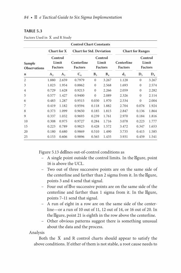
84 • The Tactical Guide to Six Sigma Implementation
Figure 5.13 defines out-of-control conditions as– A single point outside the control limits. In the figure, point
16 is above the UCL.– Two out of three successive points are on the same side of
the centerline and farther than 2 sigma from it. In the figure, points 3 and 4 send that signal.
– Four out of five successive points are on the same side of the centerline and farther than 1 sigma from it. In the figure, points 7–11 send that signal.
– A run of eight in a row are on the same side of the center-line—or a run of 10 out of 11, 12 out of 14, or 16 out of 20. In the figure, point 21 is eighth in the row above the centerline.
– Other obvious patterns suggest there is something unusual about the data and the process.
Analysis Both the X and R control charts should appear to satisfy the
above conditions. If either of them is not stable, a root cause needs to
TABLE 5.3
Factors Used in X and R Study
Control Chart Constants
Sample Observations
Chart for X Chart for Std. Deviation Chart for Ranges
Control Limit
FactorsCenterline
Factors
Control Limit
FactorsCenterline
Factors
Control Limit
Factors
n A2 A3 C4 B3 B4 d2 D3 D4
2 1.880 2.659 0.7979 0 3.267 1.128 0 3.2673 1.023 1.954 0.8862 0 2.568 1.693 0 2.5744 0.729 1.628 0.9213 0 2.266 2.059 0 2.2825 0.577 1.427 0.9400 0 2.089 2.326 0 2.1146 0.483 1.287 0.9515 0.030 1.970 2.534 0 2.0047 0.419 1.182 0.9594 0.118 1.882 2.704 0.076 1.9248 0.373 1.099 0.9650 0.185 1.815 2.847 0.136 1.8649 0.337 1.032 0.9693 0.239 1.761 2.970 0.184 1.81610 0.308 0.975 0.9727 0.284 1.716 3.078 0.223 1.77715 0.223 0.789 0.9823 0.428 1.572 3.472 0.347 1.65320 0.180 0.680 0.9869 0.510 1.490 3.735 0.415 1.58525 0.153 0.606 0.9896 0.565 1.435 3.931 0.459 1.541
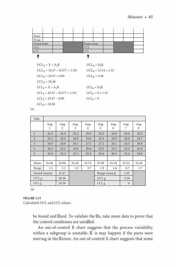
Measure • 85
be found and fixed. To validate the fix, take more data to prove that the control conditions are satisfied.
An out-of-control R chart suggests that the process variability within a subgroup is unstable. This may happen if the parts were moving in the fixture. An out-of-control X chart suggests that some
MeanRangeGrand meanUCLLCL
(a)
(b)
Range meanUCLLCL
UCLX = X + A2R
UCLX = 25.47 + (0.577 × 1.55)
UCLX = 25.47 + 0.89
UCLX = 26.36
LCLX = X + A2R
LCLX = 25.47 – (0.577 × 1.55)
LCLX = 25.47 – 0.89
LCLX = 24.58
UCLR = D4R
UCLR = 2.114 × 1.55
UCLR = 3.28
LCLR = D3R
LCLR = 0 × 1.55
LCLR = 0
Title
Aug1
Aug2
Aug3
Aug4
Aug5
Aug6
Aug7
Aug8
12345
25.325.224.926.425.0
24.424.924.825.525.2
25.324.926.125.625.3
25.024.827.526.025.4
25.325.527.225.526.4
24.924.925.125.326.5
25.626.025.325.325.4
25.324.726.425.025.8
MeanRangeGrand meanUCLLCL
X=
X–
X–
Range meanUCLLCL
R=
R–
R–
25.361.5
24.961.1
25.4726.3624.58
25.441.2
25.742.7
25.981.9
25.341.6
25.520.7
1.553.28
0
25.441.7
−
−
−
−
−
−
−
−
FIGURE 5.11Calculated UCL and LCL values.
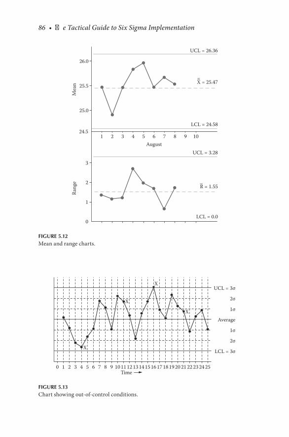
86 • The Tactical Guide to Six Sigma Implementation
26.0
25.5
25.0
24.5
3
2
1
0
1 2 3 4 5 6 7 8 9 10August
UCL = 26.36
UCL = 3.28
LCL = 24.58
LCL = 0.0
X = 25.47
R = 1.55–
=M
ean
Rang
e
FIGURE 5.12Mean and range charts.
0 1 2 3 4 5 6 7 8 9 10 11 12Time
UCL = 3σ
2σ
1σ
Average
1σ
2σ
LCL = 3σ
13 14 15 16 17 18 19 20 21 22 23 24 25
X
X
X
X
FIGURE 5.13Chart showing out-of-control conditions.
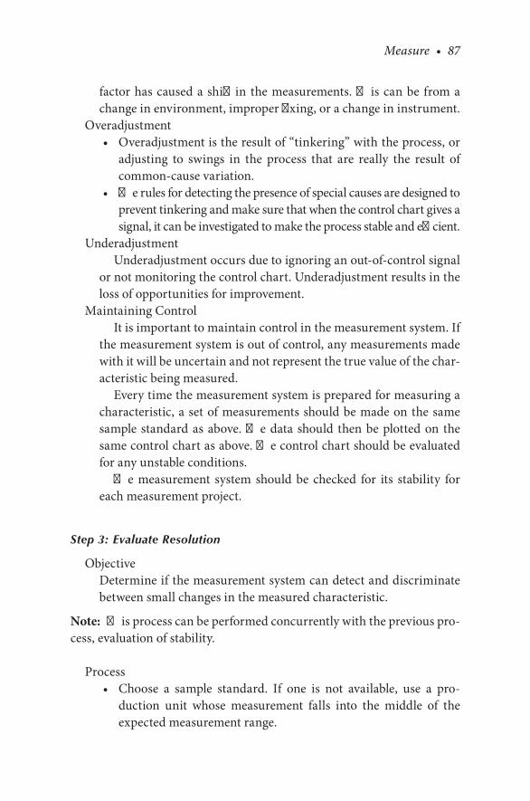
Measure • 87
factor has caused a shift in the measurements. This can be from a change in environment, improper fixing, or a change in instrument.
Overadjustment• Overadjustment is the result of “tinkering” with the process, or
adjusting to swings in the process that are really the result of common-cause variation.
• The rules for detecting the presence of special causes are designed to prevent tinkering and make sure that when the control chart gives a signal, it can be investigated to make the process stable and efficient.
Underadjustment Underadjustment occurs due to ignoring an out-of-control signal
or not monitoring the control chart. Underadjustment results in the loss of opportunities for improvement.
Maintaining Control It is important to maintain control in the measurement system. If
the measurement system is out of control, any measurements made with it will be uncertain and not represent the true value of the char-acteristic being measured.
Every time the measurement system is prepared for measuring a characteristic, a set of measurements should be made on the same sample standard as above. The data should then be plotted on the same control chart as above. The control chart should be evaluated for any unstable conditions.
The measurement system should be checked for its stability for each measurement project.
Step 3: Evaluate Resolution
Objective Determine if the measurement system can detect and discriminate
between small changes in the measured characteristic.
Note: This process can be performed concurrently with the previous pro-cess, evaluation of stability.
Process• Choose a sample standard. If one is not available, use a pro-
duction unit whose measurement falls into the middle of the expected measurement range.
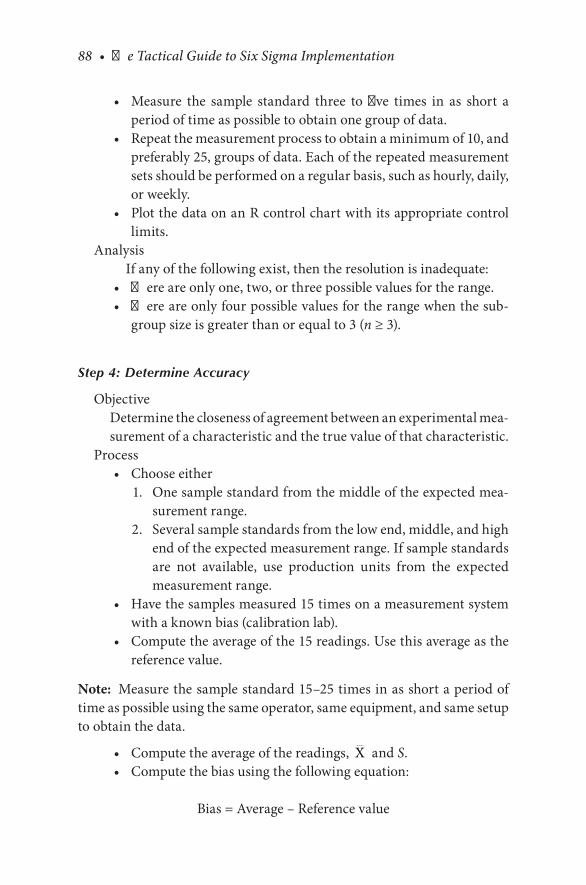
88 • The Tactical Guide to Six Sigma Implementation
• Measure the sample standard three to five times in as short a period of time as possible to obtain one group of data.
• Repeat the measurement process to obtain a minimum of 10, and preferably 25, groups of data. Each of the repeated measurement sets should be performed on a regular basis, such as hourly, daily, or weekly.
• Plot the data on an R control chart with its appropriate control limits.
Analysis If any of the following exist, then the resolution is inadequate:
• There are only one, two, or three possible values for the range.• There are only four possible values for the range when the sub-
group size is greater than or equal to 3 (n ≥ 3).
Step 4: Determine Accuracy
Objective Determine the closeness of agreement between an experimental mea-
surement of a characteristic and the true value of that characteristic.Process
• Choose either 1. One sample standard from the middle of the expected mea-
surement range. 2. Several sample standards from the low end, middle, and high
end of the expected measurement range. If sample standards are not available, use production units from the expected measurement range.
• Have the samples measured 15 times on a measurement system with a known bias (calibration lab).
• Compute the average of the 15 readings. Use this average as the reference value.
Note: Measure the sample standard 15–25 times in as short a period of time as possible using the same operator, same equipment, and same setup to obtain the data.
• Compute the average of the readings, X and S.• Compute the bias using the following equation:
Bias = Average – Reference value

Measure • 89
Step 5: Calibrate the Instrument
Objective Align the measurement instrument so that its measurement bias
is minimized when compared to some traceable standard.Process Calibrate the instrument according to the manufacturer’s instruc-
tions. This should be accomplished prior to performing any mea-surements and should be performed by an independent source, such as a metrology laboratory.
Step 6: Evaluate Linearity
Linearity is the difference in the bias (Y) values through the expected operating range of the gage reference value (X).
The linearity principle is to establish a statistical linear relationship between two sets of corresponding data (X and Y) by fitting the data to a straight line by means of the least-squares technique or regression analysis.
Linearity can be calculated as follows:
Linearity = Slope × Process variation or through a coefficient of regression
The resulting linearity line takes the general form
y = bx + a (5.2)
where a is the intercept of the line with the y-axis and b is the slope (tangent).
In regression analysis, one factor has to be independent. This factor is by convention designated as X, whereas the other factor is the dependent factor, Y (thus, we speak of regression of Y on X).
The line parameters b and a are calculated with the following equations:
b =− −
−∑
∑( )( )
( )
X X Y Y
X X
i i
i2

90 • The Tactical Guide to Six Sigma Implementation
and
a y bx= − (5.3)
The correlation coefficient r can be calculated by
r =− −
− −
∑∑ ∑
( )( )
( ) ( )
X X Y Y
X X Y Y
i i
i i2 2
(5.4)
Table 5.4 shows an example.Using the above data and the formulas, we have
b = 0.037
a = 0.626
The regression line equation is
Y = 0.626X + 0.037
and the regression coefficient is
r = 0.997
TABLE 5.4
Linearity Data
xi yi x x1 −− ( )x xi −− 2 y yi −− ( )y yi −− 2 ( )( )x x y yi1
0 0.05 –0.5 0.25 –0.3 0.09 0.15
0.2 0.14 –0.3 0.09 –0.21 0.044 0.063
0.4 0.29 –0.1 0.01 –0.06 0.004 0.006
0.6 0.43 0.1 0.01 0.08 0.006 0.008
0.8 0.52 0.3 0.09 0.17 0.029 0.051
1 0.67 0.5 0.25 0.32 0.102 0.16
3 2.1 0 0.7 0 0.2754 0.438 Σ
x = 0 5. y = 0 35.
Note: xi = Gage reference value, in our case, observed concentration value; x = mean value of x; yi = bias or, in our case, absorbance; y = mean value of y.
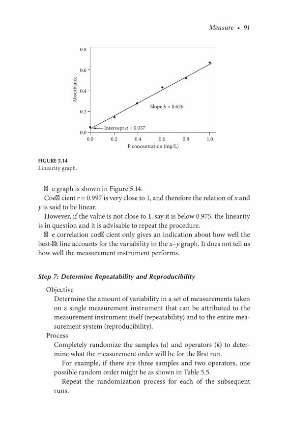
Measure • 91
The graph is shown in Figure 5.14.Coefficient r = 0.997 is very close to 1, and therefore the relation of x and
y is said to be linear.However, if the value is not close to 1, say it is below 0.975, the linearity
is in question and it is advisable to repeat the procedure.The correlation coefficient only gives an indication about how well the
best-fit line accounts for the variability in the x–y graph. It does not tell us how well the measurement instrument performs.
Step 7: Determine Repeatability and Reproducibility
Objective Determine the amount of variability in a set of measurements taken
on a single measurement instrument that can be attributed to the measurement instrument itself (repeatability) and to the entire mea-surement system (reproducibility).
Process Completely randomize the samples (n) and operators (k) to deter-
mine what the measurement order will be for the first run. For example, if there are three samples and two operators, one
possible random order might be as shown in Table 5.5. Repeat the randomization process for each of the subsequent
runs.
0.00.0
0.2
0.4
0.6
0.8
0.2
Intercept a = 0.037
Slope b = 0.626
0.4 0.6 0.8 1.0P concentration (mg/L)
Abs
orba
nce
FIGURE 5.14Linearity graph.

92 • The Tactical Guide to Six Sigma Implementation
1. Have the operators measure the samples in the measurement order that was just determined.
2. The engineer should read and record the data so that the data value remains hidden from the operator. Try to ensure that the operators do not know each other’s readings.
3. The data can then be entered into a software program such as MINITAB, where it can be analyzed using the “Gage R&R Study—ANOVA method.”
Analysis• Plot the data (see Figure 5.17).• Perform an analysis of variance (ANOVA) on the data. The
potential sources of variability can be designated as follows:Operator variance σO
2
Parts (product) variance σP2
Operators by parts σOP2
Repeatability σRepeatability2
• Calculate the total variation, ZO Total*σ :
σ σ σ σTotal P Repeatability Reproducibility= + +2 2 2 (5.5)
where
σ σ σReproducibility Operator OP2 2 2= +
ZO in the equation is used to assume a certain percent confi-dence in the spread of the data. A typical value of 5.15 is used to ensure a 99% confidence. See Table 5.6.
TABLE 5.5
Example of Measurement Order
Measurement Order k = 2 Appraiser n = 3 Sample
1 B 12 B 33 A 24 B 25 A 36 A 1
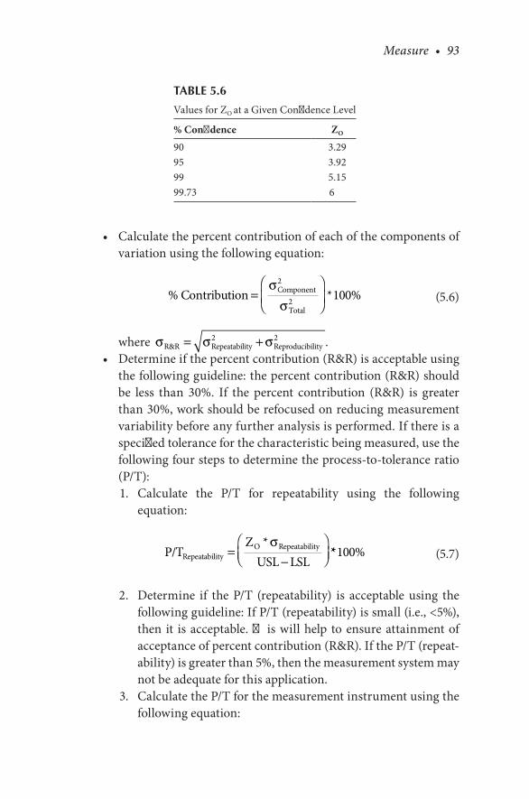
Measure • 93
• Calculate the percent contribution of each of the components of variation using the following equation:
% Contribution Component
Total
=
σ
σ
2
2 100* % (5.6)
where σ σ σR&R Repeatability Reproducibility= +2 2 .• Determine if the percent contribution (R&R) is acceptable using
the following guideline: the percent contribution (R&R) should be less than 30%. If the percent contribution (R&R) is greater than 30%, work should be refocused on reducing measurement variability before any further analysis is performed. If there is a specified tolerance for the characteristic being measured, use the following four steps to determine the process-to- tolerance ratio (P/T):
1. Calculate the P/T for repeatability using the following equation:
P/T
ZUSL LSLRepeatability
O Repeatability=−
* σ** %100 (5.7)
2. Determine if the P/T (repeatability) is acceptable using the following guideline: If P/T (repeatability) is small (i.e., <5%), then it is acceptable. This will help to ensure attainment of acceptance of percent contribution (R&R). If the P/T (repeat-ability) is greater than 5%, then the measurement system may not be adequate for this application.
3. Calculate the P/T for the measurement instrument using the following equation:
TABLE 5.6
Values for ZO at a Given Confidence Level
% Confidence ZO
90 3.2995 3.9299 5.1599.73 6

94 • The Tactical Guide to Six Sigma Implementation
P/T Z
USL LSLO R&R=
−
* * %σ 100 (5.8)
where σ σ σR&R Repeatability Reproducibility= +2 2.
4. Determine if the measurement instrument P/T is acceptable using the following guideline: percent contribution (R&R) should be less than 30%. If the percent contribution (R&R) is greater than 30%, work should be refocused on reduc-ing measurement variability before any further analysis is performed.
In reading the equipment, the readings should be estimated to the nearest number that can be obtained. If possible, read-ings should be made to one-half of the smallest graduation. For instance, if the smallest graduation is 0.0001, then the estimate for each reading should be rounded to the nearest 0.00005.
The study should be observed by a person who recognizes the importance of the caution required in conducting a reliable study.
The measurement procedure should be documented and all operators trained for the procedure prior to the study.
Each operator should use the same procedure, including all steps to obtain the readings:Step 1: Choose 10 samples and number them. Select two capable
appraisers (inspectors).Step 2: Calibrate the gage or use a calibrated gage.Step 3: Have the first inspector measure all samples in a random
order.Step 4: Have the second inspector measure all samples in a ran-
dom order.Step 5: Continue until all operators have measured the samples
once (trial 1).Step 6: Repeat steps 3–5, making sure that the inspectors do not
know previous results. Fill in the repeatability and reproducibility data sheet
(Figure 5.15).
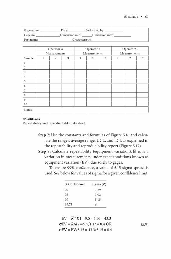
Measure • 95
Step 7: Use the constants and formulas of Figure 5.16 and calcu-late the ranges, average range, UCL, and LCL as explained in the repeatability and reproducibility report (Figure 5.17).
Step 8: Calculate repeatability (equipment variation). This is a variation in measurements under exact conditions known as equipment variation (EV), due solely to gages.
To ensure 99% confidence, a value of 5.15 sigma spread is used. See below for values of sigma for a given confidence limit:
% Confidence Sigma (Z)
90 3.2995 3.9299 5.1599.73 6
EVEV / / ORE
= = × == = =R KR d
* . . .. . .
1 9 5 4 56 43 32 9 5 1 13 8 4σ
σ VV EV/ /= = =5 15 43 3 5 15 8 4. . . . (5.9)
Gage name: ______________Date: ___________ Performed by: ____________Gage no: ________________Dimension min: _______Dimension max: ___________Part name: ______________________ Characteristic: __________________________
Sample
Operator A Operator B Operator CMeasurements Measurements Measurements
1 2 3 1 2 3 1 2 312345678910
Notes:
FIGURE 5.15Repeatability and reproducibility data sheet.
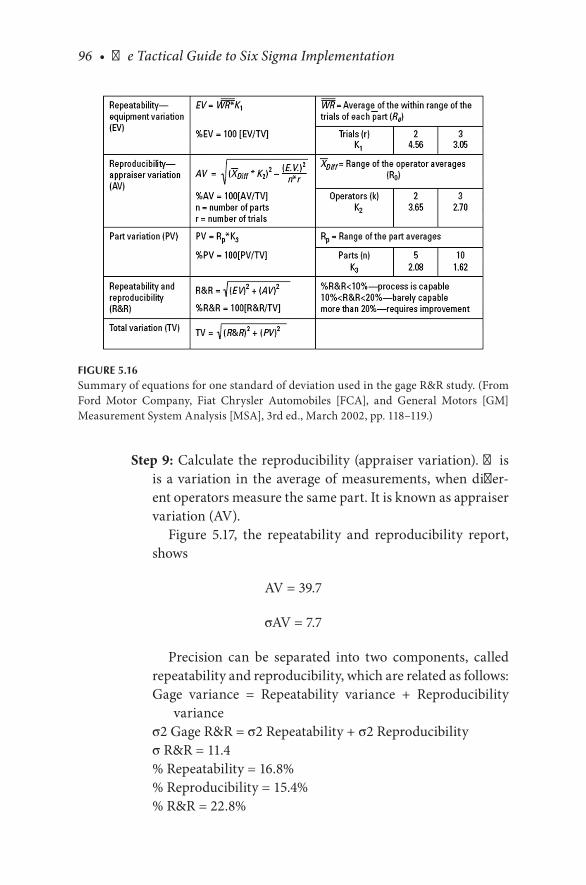
96 • The Tactical Guide to Six Sigma Implementation
Step 9: Calculate the reproducibility (appraiser variation). This is a variation in the average of measurements, when differ-ent operators measure the same part. It is known as appraiser variation (AV).
Figure 5.17, the repeatability and reproducibility report, shows
AV = 39.7
σAV = 7.7
Precision can be separated into two components, called repeatability and reproducibility, which are related as follows:Gage variance = Repeatability variance + Reproducibility
varianceσ2 Gage R&R = σ2 Repeatability + σ2 Reproducibilityσ R&R = 11.4% Repeatability = 16.8%% Reproducibility = 15.4%% R&R = 22.8%
FIGURE 5.16Summary of equations for one standard of deviation used in the gage R&R study. (From Ford Motor Company, Fiat Chrysler Automobiles [FCA], and General Motors [GM] Measurement System Analysis [MSA], 3rd ed., March 2002, pp. 118–119.)

Measure • 97
(a)
(b)
FIGURE 5.17Repeatability and reproducibility report.

98 • The Tactical Guide to Six Sigma Implementation
% R&R acceptance criteria are as follows:
Good >0 to <20%Marginal >20% to <30%Unacceptable >30%
See Figure 5.16 for the AIAG recommended summary of equations for the gage R&R study.
In the worksheet in Figure 5.17, 2 appraisers and 10 parts are selected. It uses the formulas per the Figure 5.16 above, as well as the values of K constant.
PROCESS CAPABILITY MEASUREMENT
We have studied measurement system analysis and made sure the mea-surement method has been analyzed and has an acceptable level of mea-surement error. Now we are ready to measure the capability of a process. Process needs to stay in control within the specifications (called process control limits) required by the customer.
Process limits are the voice of the process resulting from the product variations produced. The supplier collects data over time to form a pro-cess curve, known as a normal curve, for determining the variation in the units against the customer’s specification.
A histogram is a special type of graph that allows you to see the varia-tion in your process. It is sometimes called a frequency distribution.
In histograms, frequency is represented by the area of each column, unlike many bar charts, where the height alone of each column represents the frequency.
Consider a simple example where an army recruitment center wants to recruit soldiers with a target height of 69 inches out of 50 selected candi-dates. The height data that were collected from a group of 50 candidates are shown in Table 5.7.
There are only 50 measurements, but it is difficult to draw specific con-clusions about the data without further analysis. A histogram can be con-structed to provide more usable information.
Arrange the data as shown in Table 5.8.The histogram will look like that shown in Figure 5.18.

Measure • 99
The following is found:
Mean = 69.125Sigma (s) = 1.87 (s stands for short term sigma)Spread = 7.5 = 2.2 s3 s = 3.616 s = 11.22
TABLE 5.7
Individual Heights Measured in Inches
69.9 68.9 68.2 66 7169 70 68.5 66.5 72.569.6 69.5 70 67.5 7368.5 70.4 66.8 68.3 6965 71.1 69 68.2 71.365.9 71 69.3 69.1 68.267.2 72.5 69.1 70.2 68.567.5 73.1 69.4 69.5 7068 68.8 68.5 70.5 6768.6 71.3 65.5 70.8 69.2Note: Data average is 69.125 inches. Sigma = 7.5.
TABLE 5.8
Height Data Frequency Diagram
Class Height Intervals Frequency Total
1 64.4–65.0 X 12 65.1–65.6 X 13 65.7–66.2 XX 24 66.3–66.8 XX 25 66.9–67.4 XX 26 67.5–68.0 XXXX 47 68.1–68.6 XXXXXXXXX 98 68.7–69.2 XXXXXXXXX 99 69.3–69.8 XXXXXXX 710 69.9–70.4 XXX 311 70.5–71.0 XXXX 412 71.1–71.6 XX 213 71.7–72.2 XX 214 72.3–72.8 XX 2
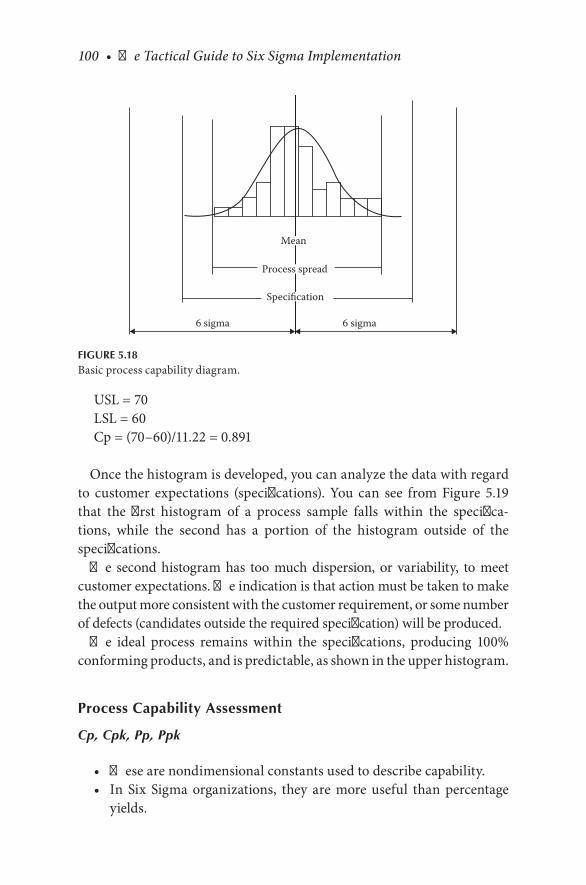
100 • The Tactical Guide to Six Sigma Implementation
USL = 70LSL = 60Cp = (70–60)/11.22 = 0.891
Once the histogram is developed, you can analyze the data with regard to customer expectations (specifications). You can see from Figure 5.19 that the first histogram of a process sample falls within the specifica-tions, while the second has a portion of the histogram outside of the specifications.
The second histogram has too much dispersion, or variability, to meet customer expectations. The indication is that action must be taken to make the output more consistent with the customer requirement, or some number of defects (candidates outside the required specification) will be produced.
The ideal process remains within the specifications, producing 100% conforming products, and is predictable, as shown in the upper histogram.
Process Capability Assessment
Cp, Cpk, Pp, Ppk
• These are nondimensional constants used to describe capability.• In Six Sigma organizations, they are more useful than percentage
yields.
Mean
Process spread
Specification
6 sigma 6 sigma
FIGURE 5.18Basic process capability diagram.
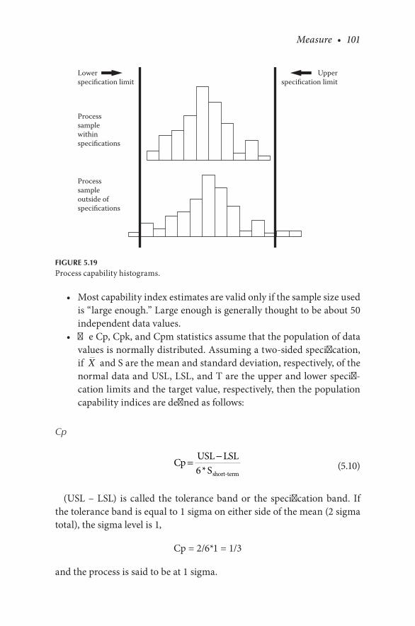
Measure • 101
• Most capability index estimates are valid only if the sample size used is “large enough.” Large enough is generally thought to be about 50 independent data values.
• The Cp, Cpk, and Cpm statistics assume that the population of data values is normally distributed. Assuming a two-sided specification, if X and S are the mean and standard deviation, respectively, of the normal data and USL, LSL, and T are the upper and lower specifi-cation limits and the target value, respectively, then the population capability indices are defined as follows:
Cp
Cp USL LSL
Sshort-term= −
6* (5.10)
(USL – LSL) is called the tolerance band or the specification band. If the tolerance band is equal to 1 sigma on either side of the mean (2 sigma total), the sigma level is 1,
Cp = 2/6*1 = 1/3
and the process is said to be at 1 sigma.
Lowerspecification limit
Upperspecification limit
Processsamplewithinspecifications
Processsampleoutside ofspecifications
FIGURE 5.19Process capability histograms.
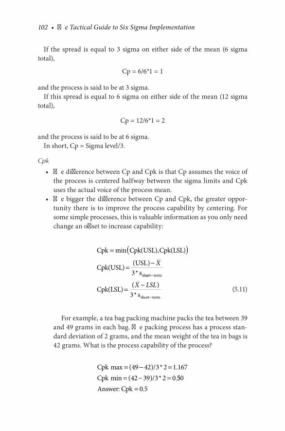
102 • The Tactical Guide to Six Sigma Implementation
If the spread is equal to 3 sigma on either side of the mean (6 sigma total),
Cp = 6/6*1 = 1
and the process is said to be at 3 sigma.If this spread is equal to 6 sigma on either side of the mean (12 sigma
total),
Cp = 12/6*1 = 2
and the process is said to be at 6 sigma.In short, Cp = Sigma level/3.
Cpk
• The difference between Cp and Cpk is that Cp assumes the voice of the process is centered halfway between the sigma limits and Cpk uses the actual voice of the process mean.
• The bigger the difference between Cp and Cpk, the greater oppor-tunity there is to improve the process capability by centering. For some simple processes, this is valuable information as you only need change an offset to increase capability:
Cpk min Cpk(USL) Cpk(LSL)
Cpk(USL) USLssh
= ( )= −
,
( )*
X3 oort term
short termCpk(LSL)
s
−
−= −( )
*X LSL
3 (5.11)
For example, a tea bag packing machine packs the tea between 39 and 49 grams in each bag. The packing process has a process stan-dard deviation of 2 grams, and the mean weight of the tea in bags is 42 grams. What is the process capability of the process?
Cpk /Cpk /
max ( ) * .min ( ) * .
= − == − =
49 42 3 2 1 16742 39 3 2 0 550
0 5Answer: Cpk = .

Measure • 103
Pp and PPk
The main difference between the Pp and Cp studies is that during the evaluation of Cp, the samples are produced at the same time and the pro-cess contains mainly the causes of variation within the sample groups. The standard deviation is therefore lower in the case of the evaluation of Cp.
During the evaluation of Pp, variation between sample groups is added, which enhances the s value, resulting in more conservative Pp estimates. The inclusion of between-group variation in the calculation of Pp makes the result more conservative than the estimate of Cp.
The formulas for Pp and Ppk are the same as those for Cp and Cpk.
• The only difference between calculating Cp and Cpk, and Pp and Ppk is that you use the short-term sigma level for C and the long-term sigma level for P.
• Remember, long-term capability = short-term capability + 1.5.• Also remember that over a long period we expect the capability of a
process to deteriorate.• So referring to Table 5.9, if a project team achieves a process that is
99% capable (short term), we expect it to be 80% capable (long term); and to create a process that is 50% good (long term), we aim for 93% (short term).
• As a guide,• Long term is more likely to include special causes.• Long term is likely to include mixtures of batches and parts and
changing personnel.
TABLE 5.9
Short- and Long-Term Sigma
Short-Term Sigma Long-Term Sigma Yield Long-Term Yield
6.0 4.5 99.9997% 99.865%5.5 4 99.9968% 99.379%5.0 3.5 99.9767% 97.725%4.5 3 99.865 93.319%4.0 2.5 99.3790% 84%3.5 2 97.72% 69%3.0 1.5 93% 50%2.5 1 84% 31%2.0 0.5 69% 16%1.5 0 50% 7%
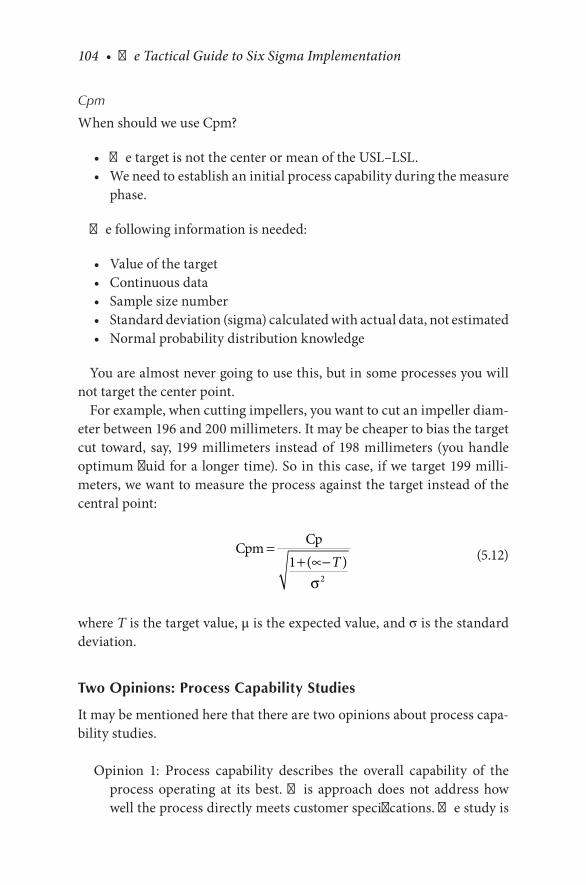
104 • The Tactical Guide to Six Sigma Implementation
Cpm
When should we use Cpm?
• The target is not the center or mean of the USL–LSL.• We need to establish an initial process capability during the measure
phase.
The following information is needed:
• Value of the target• Continuous data• Sample size number• Standard deviation (sigma) calculated with actual data, not estimated• Normal probability distribution knowledge
You are almost never going to use this, but in some processes you will not target the center point.
For example, when cutting impellers, you want to cut an impeller diam-eter between 196 and 200 millimeters. It may be cheaper to bias the target cut toward, say, 199 millimeters instead of 198 millimeters (you handle optimum fluid for a longer time). So in this case, if we target 199 milli-meters, we want to measure the process against the target instead of the central point:
Cpm Cp=+ −1
2
( )µσ
T (5.12)
where T is the target value, μ is the expected value, and σ is the standard deviation.
Two Opinions: Process Capability Studies
It may be mentioned here that there are two opinions about process capa-bility studies.
Opinion 1: Process capability describes the overall capability of the process operating at its best. This approach does not address how well the process directly meets customer specifications. The study is
Measure • 105
usually completed on a short-term basis with a 1.5 sigma adjustment to compensate for drifts in long-term variability.
Opinion 2: Process capability describes how well a process meets cus-tomer specifications. This approach takes a longer-term view of vari-ance, and short-term or long-term views are usually not considered separately.
Process Capability Study Procedure
1. Select a process to study. 2. Define and verify the process parameters. Study the process. Prepare
a process map to include all process steps and their boundaries. 3. Conduct a measurement system analysis to ensure that the mea-
surement methods produce data with total measurement error well within the limits.
4. Select a process capability analysis method (Cpk, Cp, Ppk, or Pp). 5. Obtain the data and conduct an analysis. 6. Develop an estimate of the process capability. This estimate can be
compared to the standards set by internal or external customers.
After completing a process capability study, address any undesirable special causes of variation that can be isolated. In some cases, a special cause of variation may be desirable if it produces a better product or out-put. In that case, include this special cause in the process so that the prod-uct benefits.
MEASURE PHASE SUMMARY
Measure is about measuring what is measurable, that is, data that are to be identified, collected, described, and displayed.
A sound sampling technique ensures data accuracy and integrity. Tools such as Pareto charts and histograms depict the relationship between data.
Measurement system analysis (gage R&R) correlates linearity and preci-sion for assessing the capability of the people involved in the process.
Process capability studies the link between the voice of the customer and the voice of the process. The customer sets the target and specification

106 • The Tactical Guide to Six Sigma Implementation
limits. The provider measures the process results and compares them to the customer’s expectations.
Process performance indices such as Cp, Cpk, Pp, and Ppk are numeri-cal values indicating where the process lies in terms of targets, specifica-tions, and sigma levels as per the customer’s expectations.

107
6Analyze
Analyze the problem. During the analyze phase, potential root causes for the process problem are identified.
The question that the analyze phase seeks to answer is, what is the cause of the problem?
Once the root cause is known, action can be taken in the improve phase to counter it.
The techniques are
• Regression and correlation• Analysis of variance (ANOVA)• Hypothesis testing• Failure mode and effects analysis (FMEA) (see Book 2)• Additional analysis methods
• Gap analysis– Identify gaps between current performance and goal
performance.– Prioritize opportunities to improve.– Identify sources of variation.
• Root cause analysis– Five whys– Pareto chart (see Book 2)– Fault tree analysis– Cause-and-effect diagram (see Book 2)
• Waste analysis (nine wastes) (see Book 2)• Kaizen (see Book 2)
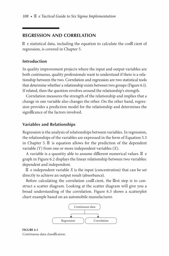
108 • The Tactical Guide to Six Sigma Implementation
REGRESSION AND CORRELATION
The statistical data, including the equation to calculate the coefficient of regression, is covered in Chapter 5.
Introduction
In quality improvement projects where the input and output variables are both continuous, quality professionals want to understand if there is a rela-tionship between the two. Correlation and regression are two statistical tools that determine whether a relationship exists between two groups (Figure 6.1). If related, then the question revolves around the relationship’s strength.
Correlation measures the strength of the relationship and implies that a change in one variable also changes the other. On the other hand, regres-sion provides a prediction model for the relationship and determines the significance of the factors involved.
Variables and Relationships
Regression is the analysis of relationships between variables. In regression, the relationships of the variables are expressed in the form of Equation 5.3 in Chapter 5. This equation allows for the prediction of the dependent variable (Y) from one or more independent variables (X).
A variable is a quantity able to assume different numerical values. The graph in Figure 6.2 displays the linear relationship between two variables: dependent and independent.
The independent variable X is the input (concentration) that can be set directly to achieve an output result (absorbance).
Before calculating the correlation coefficient, the first step is to con-struct a scatter diagram. Looking at the scatter diagram will give you a broad understanding of the correlation. Figure 6.3 shows a scatterplot chart example based on an automobile manufacturer.
Continuous data
Regression Correlation
FIGURE 6.1Continuous data classification.
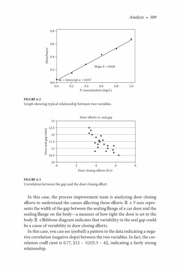
Analyze • 109
In this case, the process improvement team is analyzing door closing efforts to understand the causes affecting those efforts. The Y-axis repre-sents the width of the gap between the sealing flange of a car door and the sealing flange on the body—a measure of how tight the door is set to the body. The fishbone diagram indicates that variability in the seal gap could be a cause of variability in door closing efforts.
In this case, you can see (eyeball) a pattern in the data indicating a nega-tive correlation (negative slope) between the two variables. In fact, the cor-relation coefficient is 0.77, [(12 – 11)/(5.3 – 4)], indicating a fairly strong relationship.
0.0 0.20.0
0.2
0.4
0.6
0.8
0.4 0.6 0.8 1.0P concentration (mg/L)
Abs
orba
nce
Intercept a = 0.037
Slope b = 0.626
FIGURE 6.2Graph showing typical relationship between two variables.
010
10.5
11
11.5
12
12.5
13
2 4 6 8Door closing efforts (ft/s)
Door efforts vs. seal gap
Doo
r sea
l gap
(mm
)
FIGURE 6.3Correlation between the gap and the door closing effort.
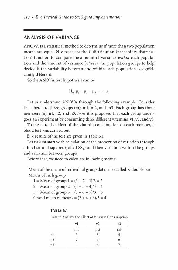
110 • The Tactical Guide to Six Sigma Implementation
ANALYSIS OF VARIANCE
ANOVA is a statistical method to determine if more than two population means are equal. The test uses the F-distribution (probability distribu-tion) function to compare the amount of variance within each popula-tion and the amount of variance between the population groups to help decide if the variability between and within each population is signifi-cantly different.
So the ANOVA test hypothesis can be
H0: μ1 = μ2 = μ3 = … μa
Let us understand ANOVA through the following example: Consider that there are three groups (m); m1, m2, and m3. Each group has three members (n); n1, n2, and n3. Now it is proposed that each group under-goes an experiment by consuming three different vitamins: v1, v2, and v3.
To measure the effect of the vitamin consumption on each member, a blood test was carried out.
The results of the test are given in Table 6.1.Let us first start with calculation of the proportion of variation through
a total sum of squares (called SST) and then variation within the groups and variation between groups.
Before that, we need to calculate following means:
Mean of the mean of individual group data, also called X-double barMeans of each group
1 = Mean of group 1 = (3 + 2 + 1)/3 = 22 = Mean of group 2 = (5 + 3 + 4)/3 = 43 = Mean of group 3 = (5 + 6 + 7)/3 = 6Grand mean of means = (2 + 4 + 6)/3 = 4
TABLE 6.1
Data to Analyze the Effect of Vitamin Consumption
v1 v2 v3
m1 m2 m3n1 3 5 5n2 2 3 6n3 1 4 7
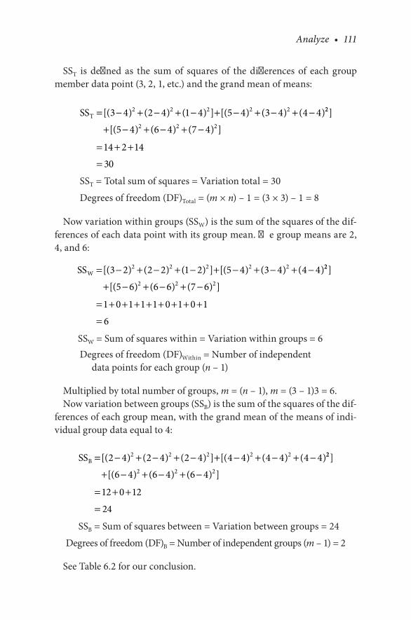
Analyze • 111
SST is defined as the sum of squares of the differences of each group member data point (3, 2, 1, etc.) and the grand mean of means:
SST = − + − + − + − + − + −[( ) ( ) ( ) ] [( ) ( ) ( )3 4 2 4 1 4 5 4 3 4 4 42 2 2 2 2 22
2 2 25 4 6 4 7 4
14 2 14
30
]
[( ) ( ) ( ) ]+ − + − + −
= + +
=
SST = Total sum of squares = Variation total = 30
Degrees of freedom (DF)Total = (m × n) – 1 = (3 × 3) – 1 = 8
Now variation within groups (SSW) is the sum of the squares of the dif-ferences of each data point with its group mean. The group means are 2, 4, and 6:
SSW = − + − + − + − + − + −[( ) ( ) ( ) ] [( ) ( ) ( )3 2 2 2 1 2 5 4 3 4 4 42 2 2 2 2 22
2 2 25 6 6 6 7 6
1 0 1 1 1 0 1 0 1
6
]
[( ) ( ) ( ) ]+ − + − + −
= + + + + + + + +
=
SSW = Sum of squares within = Variation within groups = 6 De grees of freedom (DF)Within = Number of independent
data points for each group (n – 1)
Multiplied by total number of groups, m = (n – 1), m = (3 – 1)3 = 6.Now variation between groups (SSB) is the sum of the squares of the dif-
ferences of each group mean, with the grand mean of the means of indi-vidual group data equal to 4:
SSB = − + − + − + − + − + −[( ) ( ) ( ) ] [( ) ( ) ( )2 4 2 4 2 4 4 4 4 4 4 42 2 2 2 2 22
2 2 26 4 6 4 6 4
12 0 12
24
]
[( ) ( ) ( ) ]+ − + − + −
= + +
=
SSB = Sum of squares between = Variation between groups = 24
Degrees of freedom (DF)B = Number of independent groups (m – 1) = 2
See Table 6.2 for our conclusion.
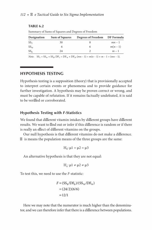
112 • The Tactical Guide to Six Sigma Implementation
HYPOTHESIS TESTING
Hypothesis testing is a supposition (theory) that is provisionally accepted to interpret certain events or phenomena and to provide guidance for further investigation. A hypothesis may be proven correct or wrong, and must be capable of refutation. If it remains factually undefeated, it is said to be verified or corroborated.
Hypothesis Testing with F-Statistics
We found that different vitamin intakes by different groups have different results. We want to find out or infer if this difference is random or if there is really an effect of different vitamins on the groups.
Our null hypothesis is that different vitamins do not make a difference. This means the population means of the three groups are the same:
H0: μ1 = μ2 = μ3
An alternative hypothesis is that they are not equal:
Ha: μ1 ≠ μ2 ≠ μ3
To test this, we need to use the F-statistic:
F ===
( ) ( )( )( )SS /DF / SS /DF
/ //
B B W W
24 2 6 612 1
Here we may note that the numerator is much higher than the denomina-tor, and we can therefore infer that there is a difference between populations.
TABLE 6.2
Summary of Sums of Squares and Degrees of Freedom
Designation Sum of Squares Degrees of Freedom DF Formula
SST 30 8 mn – 1SSW 6 6 m(n – 1)SSB 24 2 m – 1
Note: SST = SSW + SSB; DFT = DFW + DFB; (mn – 1) = m(n – 1) + m – 1 = (mn – 1).

Analyze • 113
Now let us check this statistically.Refer to the table at http://mat.iitm.ac.in/home/vetri/public_html/statistics
/f-table.pdf. For 10% significance level (90% confidence) and with DF of the numerator horizontally and DF of the denominator vertically, we get the F-value as 3.46330.
The calculated F-value is much larger than the F-statistic 3.46330. So we reject the null hypothesis and conclude that in the experiment, different vitamins did have different effects on these different groups.
Hypothesis Test Definitions
Hypothesis: Premise or claim about a property or a characteristic of a population that we want to test or investigate.
Hypothesis tests: The aim of hypothesis testing is to analyze a sample taken out of a population in an attempt to make a decision about the value of the population characteristic that is likely to occur and the population characteristic that is not likely to occur based on sample data.
Null hypothesis: Denoted by H0 (H denotes hypothesis and 0 denotes null) and stands for currently accepted value for a population char-acteristic or population parameter.
Alternative hypothesis: Denoted by Ha (H denotes hypothesis and a denotes alternative). It contains the description of the claim to be tested. The alternative hypothesis is also called a research hypoth-esis, and this is really what we want to test.
How to Write H0 and Ha
After a thorough maintenance, a machine fills cans with fluid weighing on average 12 ounces each. But the machine operator thinks that it fills less than 12 ounces.
H0: μ >/= 12 ounces
Ha: μ ≠ 12 ounces
H0 and Ha are mathematical opposites.Here we are testing two means or averages of a given population. We
can also test two proportions (percentages) or 2 standard deviations of the given populations.

114 • The Tactical Guide to Six Sigma Implementation
Two Outcomes of the Hypothesis Test
Reject the null hypothesis H0 or fail to reject the null hypothesis. How do we test this?
Collect sample data (usually more than 50 data points). In our example, assume that we have weighed 50 cans. Get the average weight and calcu-late the test statistic. Determination of the test statistic will enable us to draw a line to make a decision.
The level of confidence, C, can be 99%, 98%, or 95%. It tells us how con-fident we are in our decision.
The level of significance, α, is 1 – C if C = 95%:
α = 1 – 0.95 = 0.05
Let us now carry out a hypothesis test with a sample mean where the variance is known.
Step 1: State the null and alternate hypotheses:
H0: μ >/= 12 ounces
Ha: μ ≠ 12 ounces
Choose a sample size of 50 (greater than 30). Calculate the mean: 11.7, and σ = 1 standard deviation for the
population is the same as the sample because the sample size is large.
Step 2: Choose a significance level α:
α = 1 – C if C = 95%
α = 1 – 0.95 = 0.05
Step 3: Calculate test statistic Z:
Z = (–X – μ)/σ/√n
Calculate Z:
Z = (11.7 – 12)/1/√ 50 = –2.12

Analyze • 115
Step 4: Find the p value. Looking up the normal curve areas for the test statistic –2.12,
under Z we find
p = 0.5 – 0.4830 = 0.017
We find that the p value is less than α = 0.05 and reject H0 and conclude Ha.
The hypothesis test conclusion is that the data provide sufficient evi-dence to conclude that the mean content of the can is less than 12 ounces.
GAP ANALYSIS
A gap analysis is a tool used to identify a performance difference between a current state and a desired or future state.
The desired or future state may be set by recognizing potential perfor-mance determined through such activities as benchmarking or through organizational strategic planning.
Gap analyses are typically performed at the
• Business level: At this level, a business may compare its performance directly to that of competitors or general average industry perfor-mance. Gaps at this level are usually financial in nature.
• Process level: At this level, the current performance of a process might be compared to cost, cycle time, and quality characteristics or other processes, or at performance levels required to remain com-petitive. (Refer to Chapter 4 on quality function deployment.)
• Product level: Gaps at this level are usually identified through dif-ferences in features and capabilities, cost, quality, or generally by critical-to-X perspectives.
If the gap between the current state and the future state is sufficiently large, a series of intermediate steps or milestones may be required with more achievable gaps between each one. However, it is important to recog-nize that gaps are usually never stationary. Therefore, it may be necessary to account for an increasing gap over time, particularly when future states are set relative to competitor performance.

116 • The Tactical Guide to Six Sigma Implementation
ROOT CAUSE ANALYSIS
Solving a process problem means identifying the root cause and eliminat-ing it. The ultimate test of whether the root cause has been eliminated is the ability to turn the problem on and off by removing and replacing the root cause.
A number of tools for identifying root causes are discussed in Book 2. The five whys and fault tree analysis are two.
Five Whys
Five whys is a technique used to drill down through the layers of causes and effects to the root cause. It consists of looking at an undesired result and asking, why did this occur? When the question is answered, the next question is, why did that occur? and so on. The number five is, of course, arbitrary.
For example, a customer is not satisfied.
Why is the customer not satisfied? The order arrived late.Why did the order arrive late? It was shipped late.Why was it shipped late? Final assembly wasn’t completed on time.Why wasn’t final assembly completed on time? A part was received
from the paint line late.Why was the part from the paint line late? It arrived late from the fab-
rication department.Why was it late from the fabrication department? The fabrication
machine was running another part for the same order.Why was the fabrication machine running another part for the same
order? That’s the machine always used to run these two parts.Could they be on separate machines simultaneously when a delivery
date is imminent? Yes.
Fault Tree Analysis
Once a failure has been identified as one requiring additional study, a fault tree analysis (FTA) can be performed. Basic symbols used in FTA are bor-rowed from the electronic and logic fields. The fundamental symbols are the AND and OR gates. Each of these has at least two inputs and a single

Analyze • 117
output. Another key gate is the voting OR gate. In this gate, the output occurs if and only if k or more of the input events occur, where k is speci-fied, usually on the gate symbol. Common FTA gate symbols are depicted in Figure 6.4.
The output for the AND gate occurs if and only if all inputs occur. The output for the OR gate occurs if and only if at least one input occurs. Rectangles are typically used for labeling inputs and outputs. The failure mode being studied is sometimes referred to as the top or head event. An FTA helps the user to consider underlying causes for a failure mode and to study relationships between various failures.
AND gate OR gate Voting OR gate
Vote2/3
m / 0
FIGURE 6.4Common FTA gate symbols.

119
7Improve
Improve process performance through the following four methods:
1. Prioritization through the cause-and-effect matrix (Pugh matrix) 2. Business process improvement (BPI) and Kaizen 3. Plan–do–check–act (PDCA; focus, fix, and flex) 4. Theory of constraints (TOC)
Then implement the improvements through the following two tech niques:
1. Failure mode and effects analysis 2. Process ID (turtle diagram and suppliers, inputs, process, outputs,
and customers [SIPOC])
Then evaluate the improvements through the techniques explained in the analysis phase.
Books 1 and 2 cover methods 2 (BPI and Kaizen) and 3 (PDCA).
PRIORITIZATION THROUGH CAUSE- AND-EFFECT MATRIX
1. Identify customer requirements (outputs) from the process map. 2. Assign a priority factor to each output (usually on a 1–10 scale). 3. Identify all process steps and inputs from the process map.
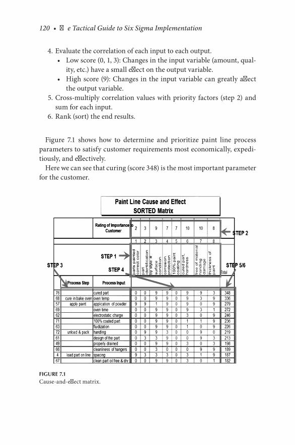
120 • The Tactical Guide to Six Sigma Implementation
4. Evaluate the correlation of each input to each output.• Low score (0, 1, 3): Changes in the input variable (amount, qual-
ity, etc.) have a small effect on the output variable.• High score (9): Changes in the input variable can greatly affect
the output variable. 5. Cross-multiply correlation values with priority factors (step 2) and
sum for each input. 6. Rank (sort) the end results.
Figure 7.1 shows how to determine and prioritize paint line process parameters to satisfy customer requirements most economically, expedi-tiously, and effectively.
Here we can see that curing (score 348) is the most important parameter for the customer.
FIGURE 7.1Cause-and-effect matrix.

Improve • 121
Improve Process through Lean Six Sigma
Figure 7.2 shows the Lean tools to improve processes.
Value stream mapping (VSM): Define process; identify opportunities for improvements.
5S: Instill discipline; free up physical resources.Standard work: Identify value-add; optimize resources with demand;
stabilize process.Total productive maintenance: Ensure equipment availability and
performance; create capacity.Error proofing: Identify opportunities for errors and eliminate; create
capacity.Setup reduction: Create capacity; reduce inventory.Continuous flow manufacturing: Optimize manpower, material, and
space; reduce cycle time.Pull: Balance system due to long logistical distances or imbalance in
adjacent process cycles.Six Sigma: Reduce process variation; stabilize process for predictability.
THEORY OF CONSTRAINTS
The theory of constraints, created by Dr. Eliyahu Goldratt, is based on the assumption that every system has at least one constraint limiting it from getting more of what it strives for. If this were not true, then the sys-tem would produce infinite output. For example, a for-profit organization would make endless profits.
The theory of constraints is both descriptive and prescriptive in nature; it not only describes why system constraints happen, but also offers guid-ance on what to do about them.
A constraint is anything that limits an organization from moving toward its goal. A constraint can be physical and internal (such as a machine, facility, or policy) or nonphysical and external (such as market conditions or demand for a product).
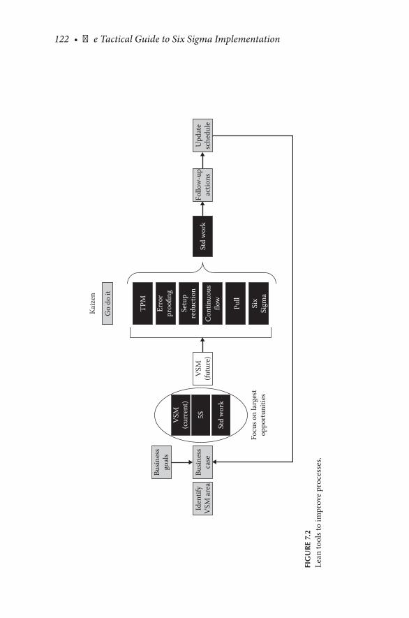
122 • The Tactical Guide to Six Sigma Implementation
Busin
ess
goal
s
Busin
ess
case
VSM
(futu
re)
VSM
(cur
rent
)
5S
Std
wor
k
Focu
s on
larg
est
oppo
rtun
ities
Upd
ate
sche
dule
Follo
w-u
pac
tions
Std
wor
k
TPM
Go
do it
Kai
zen
Erro
rpr
oofin
g
Setu
pre
duct
ion
Con
tinuo
usflo
w
Pull
Six
Sigm
a
Iden
tify
VSM
are
a
FIG
UR
E 7.
2Le
an to
ols t
o im
prov
e pr
oces
ses.
Improve • 123
Five steps for TOC implementation follow:
1. Identify the system constraint and determine whether it is a physical constraint or a policy-related issue.
2. Decide how to exploit the constraint by utilizing every bit of the con-straining component without committing to potentially expensive changes or upgrades.
3. Subordinate everything else by adjusting the rest of the system to enable the constraint to operate at maximum effectiveness, and then evaluate the results to see if the constraint is still holding back sys-tem performance. If it is, the organization proceeds to step 4. If it is not, the constraint has been eliminated, and the organization skips ahead to step 5.
4. Elevate the constraint. At this point, the organization elevates the constraint by taking whatever action is needed to eliminate it.
5. Go back to step 1, but beware of inertia. After a constraint is bro-ken, the organization repeats the steps all over again, looking for the next thing that constrains system performance. At the same time, it monitors how changes to subsequent constraints may affect the constraints that are already broken, thus preventing solution inertia.
Following are TOC metrics to determine whether an organization is moving toward its goal:
1. Increased throughput (selling price, cost of raw materials) 2. Decreased inventory 3. Decreased operating expenses
The following four measurements are used to identify results for the overall organization:
1. Net profit (NP) = Throughput – Operating expense (T – OE) 2. Return on investment = Net profit/inventory (NP/I) 3. Productivity = Throughput/Operating expense (T/OE) 4. Turnover = Throughput/Inventory (T/I)

125
8Control
KEY CONCEPTS AND TOOLS
• Statistical process control (SPC)• Control chart guide• Control chart road map• Control plan• Sustenance of improvements
• Lessons learned• Implementation of training plan• Standard operating procedures (SOPs) and work instructions• Ongoing evaluation
STATISTICAL PROCESS CONTROL
SPC Background
SPC was pioneered by Dr. Walter Shewhart in the 1920s and later enhanced by Dr. W. Edwards Deming. SPC is a collection of statistical techniques used to measure and analyze the variation in processes.
Statistical process control (SPC) is not a particular technique or proce-dure, but a philosophy focusing on optimizing continuous improvement by using statistical tools for analyzing data, making inferences about pro-cess behavior, and then making a decision.
A phenomenon will be said to be controlled, when, through the use of past experience, we can predict, at least within limits, how the phenomenon may be expected to behave in the future.
Walter Shewhart

126 • The Tactical Guide to Six Sigma Implementation
Objectives of SPC
• Produce data to inform and guide process improvement• Reduce variation• Increase knowledge about the process• Quickly detect occurrences of special causes that are shifting the
process
Uses of SPC Tools
• Monitor processes for maintaining control• Detect out-of-control conditions in processes• Analyze process capability• Serve as decision-making tools• Assure customers that product is produced consistently over time• Enable proactive process improvement
Benefits of SPC
• Assure customers that product is produced consistently over time• Increase product consistency• Improve product quality• Reduce the need for inspection• Decrease scrap and rework• Increase production output• Streamline processes
Basic SPC Concepts
• Variation: A change in the process data, a characteristic, or a func-tion that results from some cause
• Stability: The condition when observing only random variation around the process target; the absence of special causes of variation; the property of being in statistical control
• Capability: The performance of a process demonstrated to be in a state of statistical control
• Overadjustment: Making adjustments to a process based on limited data
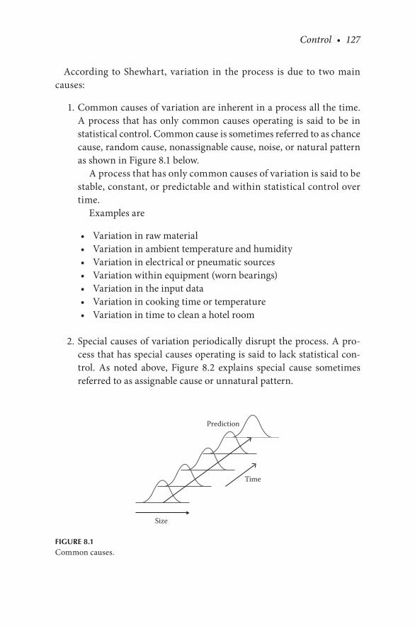
Control • 127
According to Shewhart, variation in the process is due to two main causes:
1. Common causes of variation are inherent in a process all the time. A process that has only common causes operating is said to be in statistical control. Common cause is sometimes referred to as chance cause, random cause, nonassignable cause, noise, or natural pattern as shown in Figure 8.1 below.
A process that has only common causes of variation is said to be stable, constant, or predictable and within statistical control over time.
Examples are
• Variation in raw material• Variation in ambient temperature and humidity• Variation in electrical or pneumatic sources• Variation within equipment (worn bearings)• Variation in the input data• Variation in cooking time or temperature• Variation in time to clean a hotel room
2. Special causes of variation periodically disrupt the process. A pro-cess that has special causes operating is said to lack statistical con-trol. As noted above, Figure 8.2 explains special cause sometimes referred to as assignable cause or unnatural pattern.
Size
Time
Prediction
FIGURE 8.1Common causes.

128 • The Tactical Guide to Six Sigma Implementation
Special causes of variation have the following characteristics:
• Appear sporadically in a process• Originate outside the process• Have greater impact than any single common-cause variation• Are found in unstable, unpredictable processes
Examples of special causes are
• Excessive tool wear• Large changes in raw materials• Broken equipment• Power reduction (brownout)
Where do you begin? To obtain the greatest benefit from an SPC effort, begin monitoring and improving the most critical operations and processes.
CONTROL CHART GUIDE
• Time is always the horizontal (X) axis.• Control charts must have
• Centerline (grand average)• Upper control limit (UCL)• Lower control limit (LCL)• Data points• Title
Size
Time
Prediction
FIGURE 8.2Special causes.

Control • 129
• Legend• Labeled axes
• Before starting a new control chart, the process must be in control.• The control limits calculated from the first 20 points are conditional
limits.• Recalculate the control limits after collecting at least 25–30 time-ordered
points from a period when the process is operating in control, or when-ever a significant and known change to the process has occurred.
• Developing a control chart with fewer than 25–30 points may not be statistically valid.
• If encountering an outlier when developing the control chart, inves-tigate to see if there is an assignable cause; if so, eliminate the point from the analysis.
CONTROL CHART ROAD MAP
The road map in Figure 8.3 is a control chart selection guide. To introduce a particular control chart type later in this chapter, this map will reappear highlighting the path of the particular control chart.
Select measurement
Measurementtype?
Variable
NoYes Defectives Defects
NoNoNo YesYesYes
Attribute
Subgroupsize = 1?
Subgroupsize < 10?
x-R chart
Constantsample
size?
Constantsample
size?
Defectivesor defect?
–
X-MR chart x-s chart–
x-R chart np chart p chart
c chart u chart
~
FIGURE 8.3Control chart selection guide.

130 • The Tactical Guide to Six Sigma Implementation
Variable Control Charts
Variable control charts monitor key measurable product characteristics or process variables. The formulas assume the normal distribution and limits are established based on ±3 standard deviations; thus, the chance of a part falling outside of the upper or lower control limit is 0.27%.
Variable Data Charts
1. X-bar and R chart (see Chapter 5) 2. X-bar and s chart 3. X-MR chart
Equations for Variable Data Control Charts
We will use the equations mentioned in Figure 8.4 to construct variable data control charts.
Control Chart Constants
Depending on the number of observations in a sample, use of the standard control chart constants as shown in Table 8.1 is made along with the equa-tions of Figure 8.4.
X-Bar and s Chart
Refer to the highlighted position in the road map in Figure 8.5.
X-Bar and s Chart
The formulas are
X and s Averageand StandardDeviation Chart
≥ 10 X =sum of subgroup averages
number of subgroups
s =sum of subgroup sigmas
number of subgroups
UCL = X + A3s
UCL = B4s
LCL = X – A3s
LCL = B3s
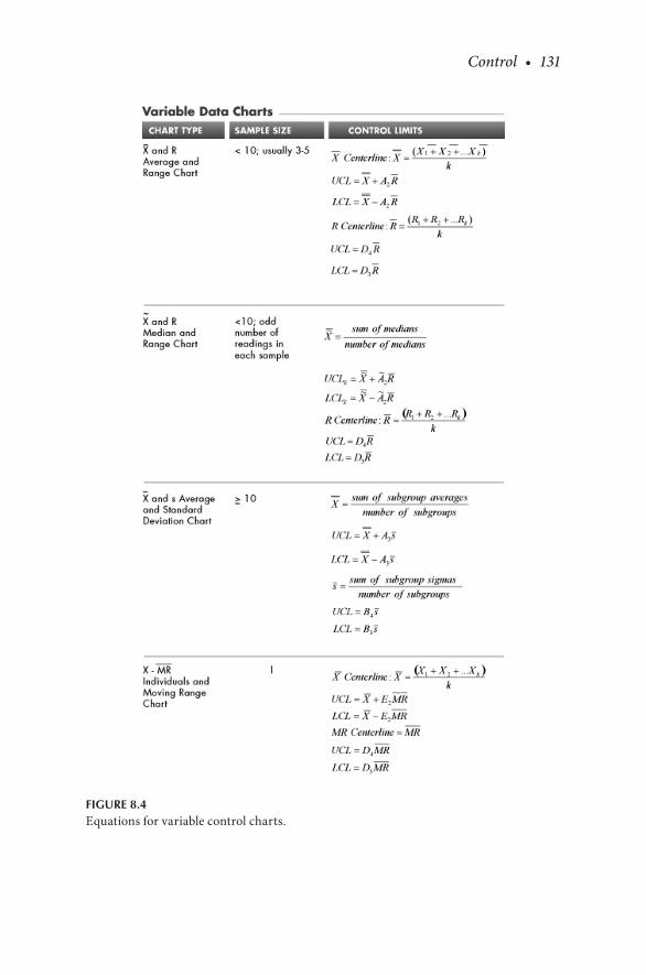
Control • 131
FIGURE 8.4Equations for variable control charts.
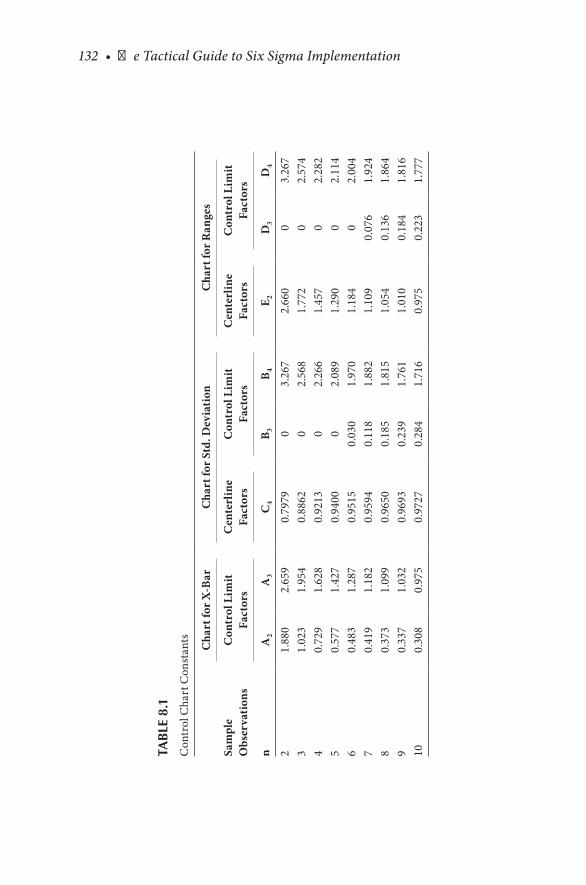
132 • The Tactical Guide to Six Sigma Implementation
TAB
LE 8
.1
Con
trol
Cha
rt C
onst
ants
Sam
ple
Obs
erva
tion
s
Cha
rt fo
r X-B
arC
hart
for S
td. D
evia
tion
Cha
rt fo
r Ran
ges
Con
trol
Lim
it Fa
ctor
sC
ente
rlin
e Fa
ctor
sC
ontr
ol L
imit
Fact
ors
Cen
terl
ine
Fact
ors
Con
trol
Lim
it Fa
ctor
s
nA
2A
3C
4B 3
B4
E 2D
3D
4
21.
880
2.65
90.
7979
03.
267
2.66
00
3.26
73
1.02
31.
954
0.88
620
2.56
81.
772
02.
574
40.
729
1.62
80.
9213
02.
266
1.45
70
2.28
25
0.57
71.
427
0.94
000
2.08
91.
290
02.
114
60.
483
1.28
70.
9515
0.03
01.
970
1.18
40
2.00
47
0.41
91.
182
0.95
940.
118
1.88
21.
109
0.07
61.
924
80.
373
1.09
90.
9650
0.18
51.
815
1.05
40.
136
1.86
49
0.33
71.
032
0.96
930.
239
1.76
11.
010
0.18
41.
816
100.
308
0.97
50.
9727
0.28
41.
716
0.97
50.
223
1.77
7
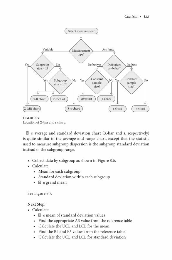
Control • 133
The average and standard deviation chart (X-bar and s, respectively) is quite similar to the average and range chart, except that the statistic used to measure subgroup dispersion is the subgroup standard deviation instead of the subgroup range.
• Collect data by subgroup as shown in Figure 8.6.• Calculate:
• Mean for each subgroup• Standard deviation within each subgroup• The grand mean
See Figure 8.7.
Next Step:• Calculate:
• The mean of standard deviation values• Find the appropriate A3 value from the reference table• Calculate the UCL and LCL for the mean• Find the B4 and B3 values from the reference table• Calculate the UCL and LCL for standard deviation
Select measurement
Measurementtype?
Variable
NoYes Defectives Defects
NoNoNo YesYesYes
Attribute
Subgroupsize = 1?
Subgroupsize < 10?
x-R chart
Constantsample
size?
Constantsample
size?
Defectivesor defect?
–
X-MR chart x-s chart–
x-R chart np chart p chart
c chart u chart
~
FIGURE 8.5Location of X-bar and s chart.

134 • The Tactical Guide to Six Sigma Implementation
Title: Units:
Sample 1
Mean
STD Dev
Grand meanX
UCLx
LCLx
STD Dev means
UCLs
LCLs
Sample 2 Sample 3 Sample 4 Sample 5
1
2
3
4
5
55
48
50
45
46
45
51
48
53
45
49
53
52
55
55
48
45
47
45
54
54
48
48
56
51
FIGURE 8.6X-bar s chart data sheet.
Title: Units:
Sample 1
Mean
STD Dev
Grand mean
UCLx
LCLx
STD Dev mean
UCLs
LCLs
Sample 2 Sample 3 Sample 4 Sample 5
1
2
3
4
5
55
48
50
45
46
48.8
4.0
45
51
48
53
45
48.6
3.4
49.9
49
53
52
55
55
52.8
2.5
48
45
47
45
54
47.8
3.7
54
48
48
56
51
51.4
3.6
FIGURE 8.7X-bar s chart calculation of grand mean.
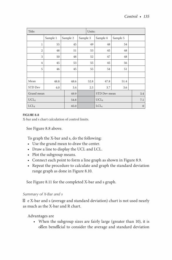
Control • 135
See Figure 8.8 above.
To graph the X-bar and s, do the following:• Use the grand mean to draw the center.• Draw a line to display the UCL and LCL.• Plot the subgroup means.• Connect each point to form a line graph as shown in Figure 8.9.• Repeat the procedure to calculate and graph the standard deviation
range graph as done in Figure 8.10.
See Figure 8.11 for the completed X-bar and s graph.
Summary of X-Bar and s
The X-bar and s (average and standard deviation) chart is not used nearly as much as the X-bar and R chart.
Advantages are• When the subgroup sizes are fairly large (greater than 10), it is
often beneficial to consider the average and standard deviation
Title: Units:
Sample 1
Mean
STD Dev
Grand mean
UCLx
LCLx
STD Dev mean
UCLs
LCLs
Sample 2 Sample 3 Sample 4 Sample 5
1
2
3
4
5
55
48
50
45
46
48.8
4.0
45
51
48
53
45
48.6
3.4
49.9
54.8
45.0
3.4
7.1
0
49
53
52
55
55
52.8
2.5
48
45
47
45
54
47.8
3.7
54
48
48
56
51
51.4
3.6
FIGURE 8.8X-bar and s chart calculation of control limits.

136 • The Tactical Guide to Six Sigma Implementation
chart, since using the range as the measure of dispersion may not yield a good estimate of process variability.
• It may also be used when more sensitivity in detecting a process shift is desired, as in the case where the product being manu-factured is quite expensive and any change in the process could either cause quality problems or add unnecessary costs.
Disadvantages are• False signals may be issued at a much higher rate than for other
types of control charts.• The X-bar and s chart is complex to construct and use.
10
2
4
6
8
2 3 4 5Sample
STD
dev
iatio
n ra
nge
s = 3.4
UCL = 7.1
LCL = 0.0
FIGURE 8.10Draw control limits and S-bar centerline; plot sample S-values.
144
46
48
50
52
54
56
2 3 4 5Sample
Mea
n
X = 49.9
UCL = 54.8
LCL = 45.0
FIGURE 8.9Draw control limits and grand mean centerline and plot sample means.

Control • 137
X-MR or I-XR Chart
See the highlighted position in the road map in Figure 8.12. Use this chart with limited data, such as when production rates are slow, testing costs are very high, or there is a high level of uncertainty relative to future projects.
This chart is suitable for
• Individual measurements or situations where there is no basis for rational subgrouping
• Infrequently repeating processes• Processes operating differently at different times
X-MR charts are applicable to situations when the sample size is n = 1. Examples include
• The early stages of a process when one is not quite sure of the struc-ture of the process data
• Monthly data
10
2
4
6
8
2 3 4 5Sample
STD
dev
iatio
n ra
nge
44
46
48
50
56
54
52M
ean
s = 3.4
UCL = 7.1
UCL = 54.8
LCL = 0.0
LCL = 45.0
X = 49.9
FIGURE 8.11Completed X-bar and s graph.

138 • The Tactical Guide to Six Sigma Implementation
• When analyzing every unit (thus no basis for rational subgrouping)• Slow production rates with long intervals between observations• When differences in measurements are too small to create an objec-
tive difference• When measurements differ only because of laboratory or analysis
error• Taking multiple measurements on the same unit (as thickness mea-
surements on different places of a sheet of aluminum)
The procedure for creating this chart using the formulas in Figure 8.13 and data sheet in Figure 8.14 is as follows:
• Collect data.• Calculate range (MR).• Calculate mean for data.• Find E2 constant.• Calculate UCL and LCL for mean and MR mean.
X-MR chart
No
No No NoYes Yes Yes
Defects
np chart p chart
Constantsample
size?
Constantsample
size?
c chart u chart
AttributeVariable
Yes
Measurementtype?
Defectives Defectivesor defects?
Subgroupsize < 10?
SubgroupSize = 1?
x·s chart
~
~
~x·R chartx·R chart
Select measurement
FIGURE 8.12Location of X-MR and I-XR charts.
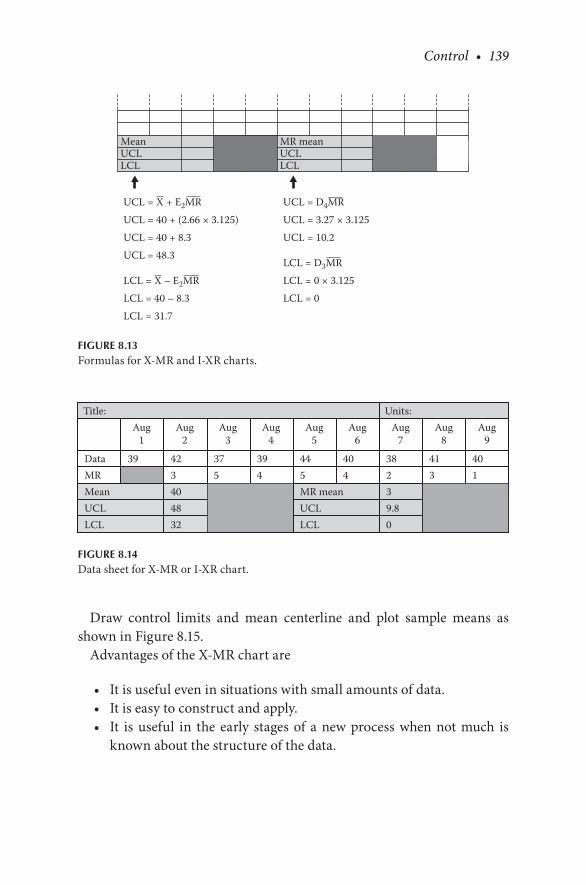
Control • 139
Draw control limits and mean centerline and plot sample means as shown in Figure 8.15.
Advantages of the X-MR chart are
• It is useful even in situations with small amounts of data.• It is easy to construct and apply.• It is useful in the early stages of a new process when not much is
known about the structure of the data.
MeanUCLLCL
UCL = X + E2MR
UCL = 40 + (2.66 × 3.125)
UCL = 40 + 8.3
UCL = 48.3
LCL = X – E2MR
LCL = 40 – 8.3
LCL = 31.7
UCL = D4MR
UCL = 3.27 × 3.125
UCL = 10.2
LCL = D3MR
LCL = 0 × 3.125
LCL = 0
MR meanUCLLCL
FIGURE 8.13Formulas for X-MR and I-XR charts.
Title:
DataMRMeanUCLLCL
39 423404832
375
394
445MR meanUCLLCL
404
38239.80
413
401
Units:Aug
1Aug
2Aug
3Aug
4Aug
5Aug
6Aug
7Aug
8Aug
9
FIGURE 8.14Data sheet for X-MR or I-XR chart.
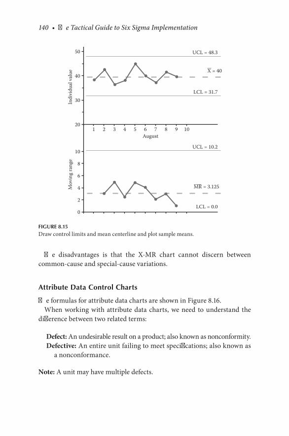
140 • The Tactical Guide to Six Sigma Implementation
The disadvantages is that the X-MR chart cannot discern between common- cause and special-cause variations.
Attribute Data Control Charts
The formulas for attribute data charts are shown in Figure 8.16.When working with attribute data charts, we need to understand the
difference between two related terms:
Defect: An undesirable result on a product; also known as noncon formity.Defective: An entire unit failing to meet specifications; also known as
a nonconformance.
Note: A unit may have multiple defects.
120
50
40
30
432 8765 9 10August
Indi
vidu
al v
alue
UCL = 48.3
LCL = 31.7
0
2
4
6
8
10
Mov
ing
rang
e
MR = 3.125
UCL = 10.2
LCL = 0.0
X = 40
FIGURE 8.15Draw control limits and mean centerline and plot sample means.
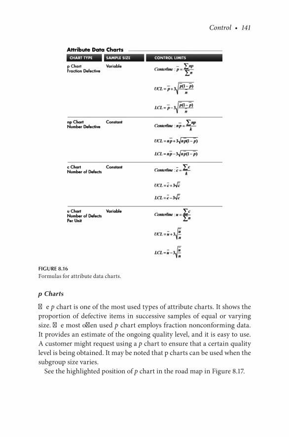
Control • 141
p Charts
The p chart is one of the most used types of attribute charts. It shows the proportion of defective items in successive samples of equal or varying size. The most often used p chart employs fraction nonconforming data. It provides an estimate of the ongoing quality level, and it is easy to use. A customer might request using a p chart to ensure that a certain quality level is being obtained. It may be noted that p charts can be used when the subgroup size varies.
See the highlighted position of p chart in the road map in Figure 8.17.
FIGURE 8.16Formulas for attribute data charts.

142 • The Tactical Guide to Six Sigma Implementation
To make a p chart for an example with varying sample sizes, do the following.
• Refer to the p chart formula.• Calculate:
• The totals• p value (proportion) of each shipment• p-bar for central line• UCL and LCL
Collect the data as shown in Figure 8.18.The finished data sheet table is shown in Figure 8.19.
p-bar = Σp/12, where p is the fraction of bruised apples in one crate (e.g., 37/200 = 0.185). Note: The graph shows the rounded figure of 0.190.
n-bar = Σn/12, where n is the number apples in one crate (e.g., 2800/12 = 233).
Draw the p chart as shown in Figure 8.20.
Select measurement
Measurementtype?
Variable
NoYes Defectives Defects
NoNoNo YesYesYes
Attribute
Subgroupsize = 1?
Subgroupsize < 10?
x-R chart
Constantsample
size?
Constantsample
size?
Defectivesor defect?
–
X-MR chart x-s chart–
x-R chart np chart p chart
c chart u chart
~
FIGURE 8.17Location of p chart.
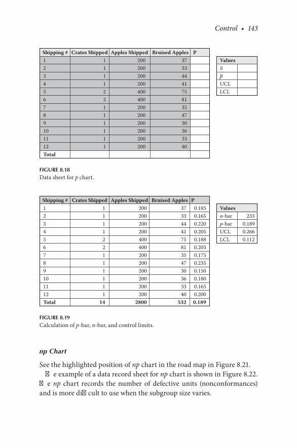
Control • 143
np Chart
See the highlighted position of np chart in the road map in Figure 8.21.The example of a data record sheet for np chart is shown in Figure 8.22.
The np chart records the number of defective units (nonconformances) and is more difficult to use when the subgroup size varies.
Shipping # Crates Shipped Apples Shipped Bruised Apples PValuesnpUCLLCL
123456789101112Total
111122111111
200200200200400400200200200200200200
373344417581354730363340
––
FIGURE 8.18Data sheet for p chart.
Shipping # Crates Shipped Apples Shipped Bruised Apples PValuesn-barp-barUCLLCL
233
0.1890.2660.112
123456789101112Total
111122111111
14
200200200200400400200200200200200200
2800
373344417581354730363340
532
0.1850.1650.2200.2050.1880.2030.1750.2350.1500.1800.1650.2000.189
FIGURE 8.19Calculation of p-bar, n-bar, and control limits.
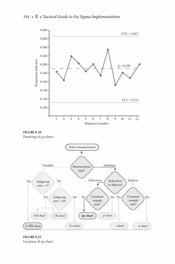
144 • The Tactical Guide to Six Sigma Implementation
1
0.100
0.120
0.140
0.160
0.180
0.200
0.220
0.240
0.280
0.260
2 3 4 5 6 7 8 9 10 11 12Shipment number
Prop
ortio
n de
fect
ive
p = 0.190
UCL = 0.267
LCL = 0.113
–
FIGURE 8.20Drawing of a p chart.
X-MR chart
No
No No NoYes Yes Yes
Defects
np chart p chart
Constantsample
size?
Constantsample
size?
c chart u chart
AttributeVariable
Yes
Measurementtype?
Defectives Defectivesor defects?
Subgroupsize < 10?
Subgroupsize = 1?
x·s chart~
x·R chart~x·R chart~
Select measurement
FIGURE 8.21Location of np chart.
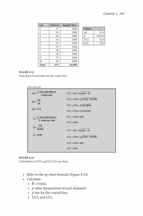
Control • 145
• Refer to the np chart formula (Figure 8.23).• Calculate:
• The totals.• p value (proportion) of each shipment.• p-bar for the central line.• UCL and LCL.
Lot Defects Sample SizeValuesnppUCLLCL
37.6
0.037655.619.6
12345678910Total
37334441354730363340
376
1000100010001000100010001000100010001000
10,000
−−
FIGURE 8.22Data sheet to calculate np-bar and p-bar.
FIGURE 8.23Calculation of UCL and LCL for np chart.
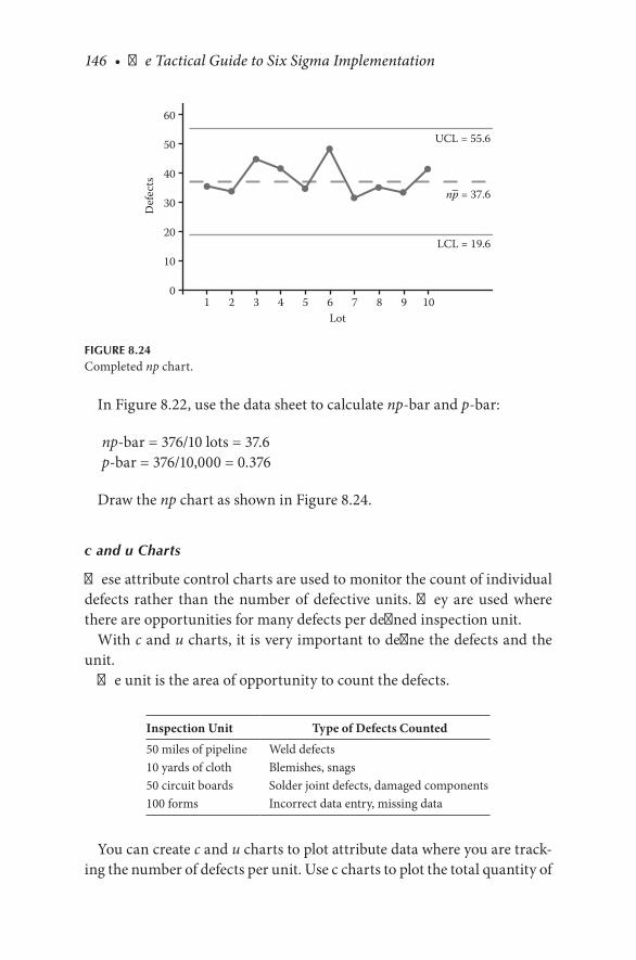
146 • The Tactical Guide to Six Sigma Implementation
In Figure 8.22, use the data sheet to calculate np-bar and p-bar:
np-bar = 376/10 lots = 37.6p-bar = 376/10,000 = 0.376
Draw the np chart as shown in Figure 8.24.
c and u Charts
These attribute control charts are used to monitor the count of individual defects rather than the number of defective units. They are used where there are opportunities for many defects per defined inspection unit.
With c and u charts, it is very important to define the defects and the unit.
The unit is the area of opportunity to count the defects.
Inspection Unit Type of Defects Counted
50 miles of pipeline Weld defects10 yards of cloth Blemishes, snags50 circuit boards Solder joint defects, damaged components100 forms Incorrect data entry, missing data
You can create c and u charts to plot attribute data where you are track-ing the number of defects per unit. Use c charts to plot the total quantity of
10
10
20
30
40
50
60
Lot
Def
ects
2 3 4 5 6 7 8 9 10
UCL = 55.6
np = 37.6
LCL = 19.6
–
FIGURE 8.24Completed np chart.

Control • 147
defects based on samples of equal size, for example, the number of record-able injuries in a plant each month. As another example, if the inspection unit is 100 forms, count the defects on a sample of 100 forms and plot that number on the c chart.
Use u charts to plot the defects per unit based on samples of equal or unequal size.
c Chart
The c chart formula assumes counting the number of defects in the same area of opportunity. The c in the formula is the number of defects found in the defined inspection unit, and that is plotted on the chart.
The c chart monitors the number of nonconformities (defects) and requires the inspection unit to be defined clearly and the area of opportu-nity to be consistent.
The c chart formula:
c
kc=
∑
See the highlighted position of c chart in the road map in Figure 8.25.
Select measurement
Measurementtype?
Variable
NoYes Defectives Defects
NoNoNo YesYesYes
Attribute
Subgroupsize = 1?
Subgroupsize < 10?
x-R chart
Constantsample
size?
Constantsample
size?
Defectivesor defect?
–
X-MR chart x-s chart–
x-R chart np chart p chart
c chart u chart
~
FIGURE 8.25Location of c chart.

148 • The Tactical Guide to Six Sigma Implementation
An example of data sheet for c chart is shown in Figure 8.26.
• Collect the data.• Calculate all values as per the formulas for c chart and the data sheet
as shown in Figure 8.27.• Draw the chart c chart as shown in Figure 8.28.
Lot DefectsValuescUCLLCL
8.6
17.40
12345678910Total
87
1410
392
12111086
–
c chart ConstantNumber of Defects Centerline: c = ∑c
kUCL = c + 3√c
LCL = c – 3√c
FIGURE 8.27Calculation of UCL and LCL for c chart.
Lot DefectsValuescUCLLCL
12345678910Total
87
1410
392
121110
−
FIGURE 8.26Data sheet for c chart.

Control • 149
u Chart
With a u chart, the number of inspection units may vary. The u chart requires an additional calculation with each sample to determine the aver-age number of defects per inspection unit. The n in the formula is the number of inspection units in the sample.
The u chart monitors the defects (nonconformities) per unit when the number of inspection units is allowed to vary. It essentially changes the counts into rates in cases where the area of opportunity varies from sam-ple to sample.
See the highlighted position of u chart in the road map in Figure 8.29.
• Collect data by sample using the form and formulas in Figure 8.30.• Total rolls shipped: 14• Total defects: 532
• Calculate the u-bar for all data:
u
u
=
= =
∑∑
c
n
/532 14 38
10
2
4
6
8
10
12
14
16
18
2 3 4 5 6 7 8 9 10Lot
Def
ects
c = 8.6
UCL = 17.4
LCL = 0.0
–
FIGURE 8.28Completed c chart.
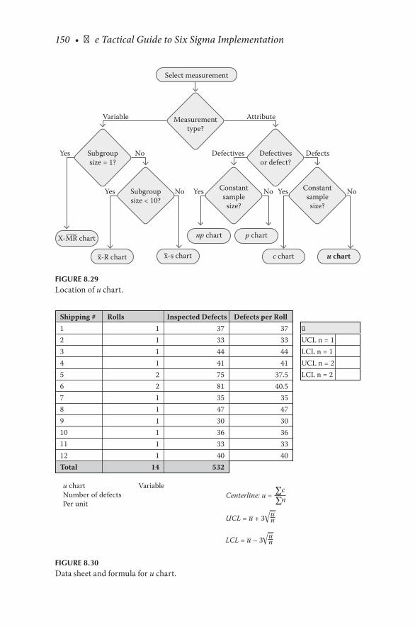
150 • The Tactical Guide to Six Sigma Implementation
Shipping # Rolls Inspected Defects Defects per RolluUCL n = 1LCL n = 1UCL n = 2LCL n = 2
123456789101112Total
111122111111
14
373344417581354730363340
532
37334441
37.540.5
354730363340
−
u chart VariableNumber of defectsPer unit
Centerline: u = ∑∑
cn
UCL = u + 3√un
LCL = u – 3√un
FIGURE 8.30Data sheet and formula for u chart.
Select measurement
Measurementtype?
Variable
NoYes Defectives Defects
NoNoNo YesYesYes
Attribute
Subgroupsize = 1?
Subgroupsize < 10?
x-R chart
Constantsample
size?
Constantsample
size?
Defectivesor defect?
–
X-MR chart
x-s chart–
np chart p chart
c chart u chart
FIGURE 8.29Location of u chart.

Control • 151
• Calculate UCL and LCL for n = 1 and n = 2 using the formulas given in Figure 8.16.
• Example: UCL and LCL for n = 1 and n = 2• UCL and LCL data for u chart is shown in Figure 8.31.• Plot the chart using the data of Figure 8.31.• The completed charts are shown in Figures 8.32 and 8.33.
Figure 8.34 shows the calculations in Math for u chart.
Shipping # Rolls Inspected Defects Defects per RolluUCL n = 1LCL n = 1UCL n = 2LCL n = 2
38.056.519.551.124.9
123456789101112Total
111122111111
14
373344417581354730363340
532
37334441
37.540.5
354730363340
−
FIGURE 8.31UCL and LCL data for u chart.
20
10
20
30
40
50UCL 56.5 n = 1
LCL 19.5 n = 1LCL 24.9 n = 2
UCL 51.1 n = 2
u = 38.0–
60
4 6 8 10 12Shipment number
Brui
ses p
er u
nit
FIGURE 8.32Plot for u-bar centerline and UCL and LCL for n = 1 and n = 2, respectively.
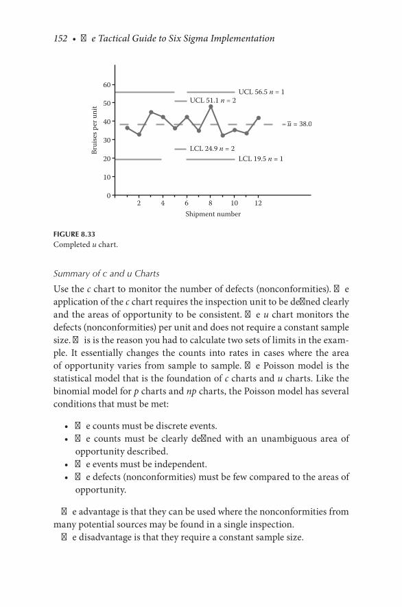
152 • The Tactical Guide to Six Sigma Implementation
Summary of c and u Charts
Use the c chart to monitor the number of defects (nonconformities). The application of the c chart requires the inspection unit to be defined clearly and the areas of opportunity to be consistent. The u chart monitors the defects (nonconformities) per unit and does not require a constant sample size. This is the reason you had to calculate two sets of limits in the exam-ple. It essentially changes the counts into rates in cases where the area of opportunity varies from sample to sample. The Poisson model is the statistical model that is the foundation of c charts and u charts. Like the binomial model for p charts and np charts, the Poisson model has several conditions that must be met:
• The counts must be discrete events.• The counts must be clearly defined with an unambiguous area of
opportunity described.• The events must be independent.• The defects (nonconformities) must be few compared to the areas of
opportunity.
The advantage is that they can be used where the nonconformities from many potential sources may be found in a single inspection.
The disadvantage is that they require a constant sample size.
20
10
20
30
40
50UCL 56.5 n = 1
LCL 19.5 n = 1LCL 24.9 n = 2
UCL 51.1 n = 2
u = 38.0–
60
4 6 8 10 12Shipment number
Brui
ses p
er u
nit
FIGURE 8.33Completed u chart.

Control • 153
FIGURE 8.34Math for u chart.
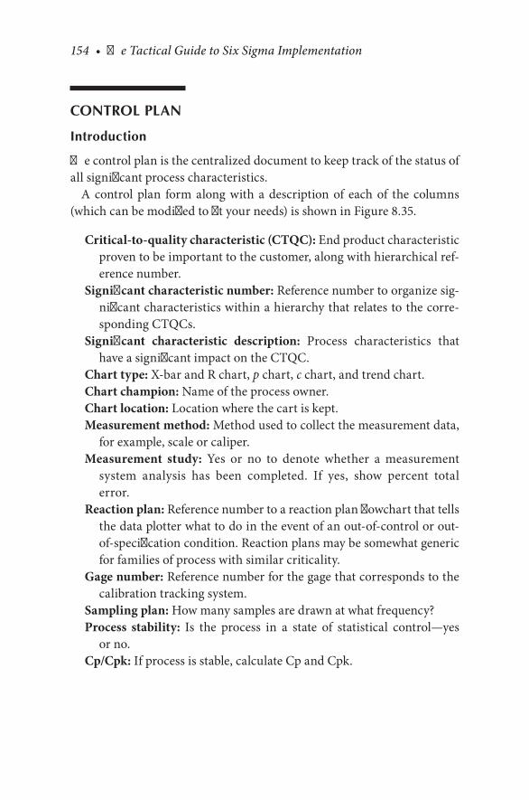
154 • The Tactical Guide to Six Sigma Implementation
CONTROL PLAN
Introduction
The control plan is the centralized document to keep track of the status of all significant process characteristics.
A control plan form along with a description of each of the columns (which can be modified to fit your needs) is shown in Figure 8.35.
Critical-to-quality characteristic (CTQC): End product characteristic proven to be important to the customer, along with hierarchical ref-erence number.
Significant characteristic number: Reference number to organize sig-nificant characteristics within a hierarchy that relates to the corre-sponding CTQCs.
Significant characteristic description: Process characteristics that have a significant impact on the CTQC.
Chart type: X-bar and R chart, p chart, c chart, and trend chart.Chart champion: Name of the process owner.Chart location: Location where the cart is kept.Measurement method: Method used to collect the measurement data,
for example, scale or caliper.Measurement study: Yes or no to denote whether a measurement
system analysis has been completed. If yes, show percent total error.
Reaction plan: Reference number to a reaction plan flowchart that tells the data plotter what to do in the event of an out-of-control or out-of-specification condition. Reaction plans may be somewhat generic for families of process with similar criticality.
Gage number: Reference number for the gage that corresponds to the calibration tracking system.
Sampling plan: How many samples are drawn at what frequency?Process stability: Is the process in a state of statistical control—yes
or no.Cp/Cpk: If process is stable, calculate Cp and Cpk.
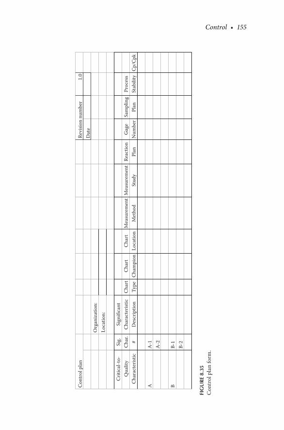
Control • 155
Crit
ical
-to-
Qua
lity
Cha
ract
erist
ic
A B
A-1
A-2
Org
aniz
atio
n:Lo
catio
n:
Revi
sion
num
ber
Dat
e1.
0
B-1
B-2
Sign
ifica
ntC
hara
cter
istic
Des
crip
tion
C
hart
Type
C
hart
Cha
mpi
on
C
hart
Loca
tion
M
easu
rem
ent
Met
hod
M
easu
rem
ent
Stud
y
Re
actio
nPl
an
G
age
Num
ber
Sa
mpl
ing
Plan
Pr
oces
sSt
abili
ty
C
p/C
pk
Sig.
Cha
r.#
Con
trol
pla
n
FIG
UR
E 8.
35C
ontr
ol p
lan
form
.
156 • The Tactical Guide to Six Sigma Implementation
SUSTENANCE OF IMPROVEMENTS
Lessons Learned
A completed Six Sigma project generates a wealth of information. Lessons learned is a process to capture, document, and share lessons learned, thus infusing change in the organization.
The process answers the following:
• What went well?• What could have been done differently?• What could be improved?• What did we do that we should not have?• Did all our various stakeholders interact efficiently and effectively?• Where were there gaps?• Where were there overlaps?• What can be done differently next time to make the situation easier
for all parties involved?
The documented process promotes continued improvement and identi-fication of additional opportunities by
• Enabling others to learn how the project was planned, implemented, and monitored
• Helping resolve issues• Allowing resources to be tracked back to their work in the project• Creating an audit trail• Providing direction to revise or revive the project later
Implementation of Training Plan
It is important to note that the training of the personnel responsible for executing the process is a critical element for sustaining the gains of improved processes.
Training is often overlooked or viewed as an unnecessary cost or impo-sition on the time of already overworked employees.
There are two types of training:
1. Initial 2. Recurring

Control • 157
Initial training is used for existing employees who have been respon-sible for executing the old process and will continue to be responsible for executing the new process.
It also addresses the needs of employees who are new to the process. It may be conducted off the job, on the job, or both. The correct combination depends on the skill levels required, process complexity, and experience levels, among other factors.
Initial training serves to calibrate employees and minimize variation in how the process is performed.
Recurring training is used to minimize deterioration in the process per-formance over time. Deterioration usually occurs as employees become comfortable with the new process and fail to recognize minor changes or tweaks to the process.
This happens through
• Carelessness• Poor documentation• Perhaps even inadequate process document control management
that permits obsolete documentation to remain in the process stream
In addition, on-the-job training is another factor that often adversely impacts process performance.
Specific facts, details, and nuances are frequently left out as they pass from worker to worker.
Recurring training restores the process execution to its original design.The frequency of recurring training should be determined based on
process metrics and employee performance. Such training may be offered at specified intervals or conducted as required to serve the needs of under-performing employees.
Standard Operating Procedures and Work Instructions
In Book 2 we have discussed the importance of standard work. Documented standard work in Lean thinking is the same as documented standard operating procedures (SOPs) and work instructions. The purpose of these documents is to make certain that the activity is performed in the same way over time. This is especially important when multiskilled, cross-trained personnel move into a variety of positions. The other main purpose of these documents is to help reduce process variation. The devel-opment and updating of these documents must involve the people who

158 • The Tactical Guide to Six Sigma Implementation
perform the work. The documentation process is begun by listing major steps. Succeeding iterations examine the steps from the previous one and break them into smaller substeps. This process can continue until further deconstruction is not useful.
Two main considerations regarding documents are
• Documents must be kept current. In an environment of continuous improvement, processes may be continuously changing. As a result, it is very possible that different documentation releases for the same documentation may be in use simultaneously. Therefore, it is vital that employees always have access to the appropriate documenta-tion based on the effectiveness of the change. It is easy to see how the complexity of managing such a documentation system can grow exponentially. With today’s web-based and other technologies, doc-umentation configuration management systems can be designed and developed to ensure that the proper documentation is available for the right process on the right part at the right time.
• Multiple formats for documentation exist. The right choice depends on how the documentation is to be used, by whom, and at what skill level. However, as we have seen in the visual factory, documentation best practices suggest developing documents that are color coded, light on words, and rely heavily on graphics, illustrations, and pho-tographs. Photographs of acceptable and unacceptable products and procedures have been found to be very useful. Some organizations have had success with the use of videotapes and DVDs for depicting complex operations. As always, the level of detail provided in any set of documentation should be reflective of the skills and education levels of the personnel doing the actual work and the degree to which variation must be controlled.
Remember, robust processes usually require less detailed documenta-tion than nonrobust processes.
Ongoing Evaluation
Once a process has been improved, it must be monitored to ensure the gains are maintained and to determine when additional improvements are required.
Control • 159
The following tools and methods are available to assist ongoing evaluation:
• Control charts: These are used to monitor the stability of the process and to determine when special cause is present and when to take appropriate action. The choice of a particular control chart depends on the nature of the process. When out-of-control conditions occur, action is required to restore stability. Control charts represent the voice of the process.
• Process capability studies: These studies provide us with the oppor-tunity to understand how the voice of the process (i.e., control lim-its) compares with the voice of the customer (i.e., specifications), and help us determine whether the process average must be shifted or recentered or the variation reduced.
• Process metrics: This includes a wide variety of in-process and end-of-process metrics that measure its overall efficiency and effectiveness.
Examples include cycle times, takt time, take rate, work in process, backlogs, defect rates, rework rates, and scrap rates.
Taken collectively, the above tools and methods help us gage the over-all health of a process, and provide triggers for reevaluating a process for further improvement.
Note: Take rate refers to the percentage of visitors who took interest in an action but did not actually follow through with that action.
So, if you have 3000 web site visitors and 600 go to the download page, your take rate is 20%. If 200 download the article your conversion rate is 6.6%.

161
9Design for Six Sigma
DFSS AND SIX SIGMA
Design for Six Sigma (DFSS) and Six Sigma have overlapping functions as shown in Figure 9.1. DFSS originated in the U.S. Department of Defense and the National Aeronautics and Space Administration (NASA). Like Six Sigma, it seeks to understand the customer’s perceptions, needs, and expectations that are critical to ensure a successful product.
Additionally, DFSS is a proactive, rigorous, and systematic method using tools, training, and measurements for integrating customer require-ments into the product development process.
By preventing defects, DFSS increases the probability of success (reli-ability) and the robustness of the product much earlier by applying scien-tific methods like
• Quality functional deployment (QFD)• Failure mode and effects analysis (FMEA)• Robust design optimization (RDO) using
• Design of experiments (DOE) and other techniques to identify the most robust design solutions for customer usage. Using RDO processes, manufacturers can identify errors early in the design process, when they are easy and less costly to fix.
• Parameter diagrams, such as RDO and P diagrams, to incor-porate robustness and reliability into the product design while keeping a control on costs.
As shown in Figure 9.1, DFSS methodologies integrate tools, methods, processes, and team members from the start and throughout the product and process design.
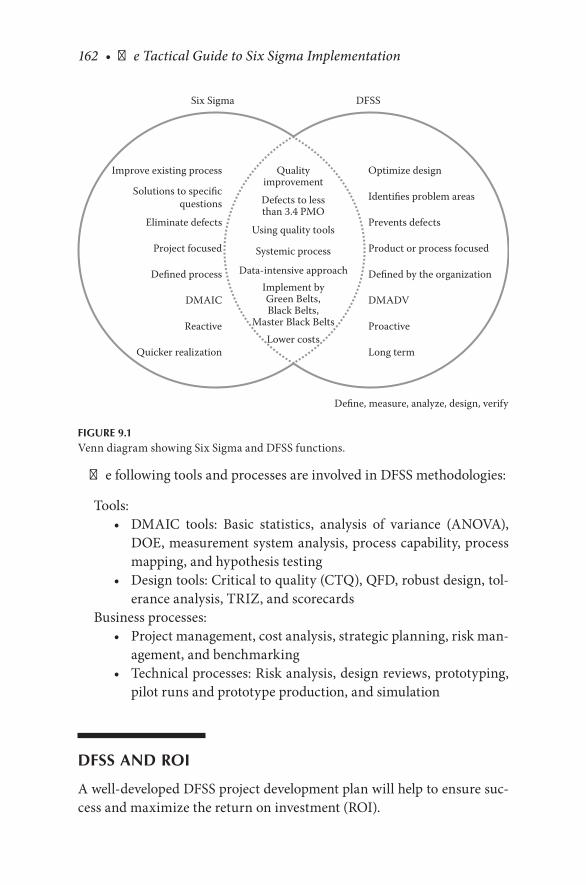
162 • The Tactical Guide to Six Sigma Implementation
The following tools and processes are involved in DFSS methodologies:
Tools:• DMAIC tools: Basic statistics, analysis of variance (ANOVA),
DOE, measurement system analysis, process capability, process mapping, and hypothesis testing
• Design tools: Critical to quality (CTQ), QFD, robust design, tol-erance analysis, TRIZ, and scorecards
Business processes:• Project management, cost analysis, strategic planning, risk man-
agement, and benchmarking• Technical processes: Risk analysis, design reviews, prototyping,
pilot runs and prototype production, and simulation
DFSS AND ROI
A well-developed DFSS project development plan will help to ensure suc-cess and maximize the return on investment (ROI).
Improve existing process
Solutions to specificquestions
Eliminate defects
Project focused
Defined process
DMAIC
Reactive
Quicker realization
Optimize designQualityimprovement
Six Sigma DFSS
Define, measure, analyze, design, verify
Defects to lessthan 3.4 PMO
Using quality tools
Systemic process
Data-intensive approach
Lower costs
Implement byGreen Belts,Black Belts,
Master Black Belts
Identifies problem areas
Prevents defects
Product or process focused
Defined by the organization
DMADV
Proactive
Long term
FIGURE 9.1Venn diagram showing Six Sigma and DFSS functions.

Design for Six Sigma • 163
It is believed that 70% to 80% of quality problems are regarded as design related. This means that the design engineers and other process designers have the best opportunity to improve product quality and save costs.
As a process moves through the phases of concept to design, prototyp-ing, and production, the cost of resource inputs increases, and so does the cost of eliminating quality problems. The greater the initial investment in DFSS methodology to eliminate design issues, the lower are the life cycle costs associated with the process (Figure 9.2).
Business challenges addressed by DFSS include
• Customers demanding product or process excellence• Managing variability• Improving predictability and capability• Reducing costs and increasing profitability• Increasing development effectiveness• Managing development costs• Meeting customer requirements
DFSS METHODOLOGIES
The main topics and tools are
• Define, measure, analyze, design, and verify (DMADV)• Define, measure, analyze, design, optimize, and verify (DMADOV)• DFSS teams• Design for X (DFX)
Concept
Rela
tive
cost
Design Prototyping Production
FIGURE 9.2Product life cycle cost.

164 • The Tactical Guide to Six Sigma Implementation
• Reliability• Tolerance
Special design tools include
• Porter’s five forces analysis• TRIZ
DMADV
As DMAIC guides the Six Sigma Black Belt process, the process stages for DFSS are define, measure, analyze, design, and verify (DMADV) (Figure 9.3). It is used when designing a new process, product, service, or transac-tion. DMADV works closely with obtaining information and analyzing the voice of the customer in order to meet customer requirements. DFSS con-tains such a large body of knowledge for each stage that DFSS is a course in itself. The purpose of this section is to provide an overview of DFSS.
DMADOV
The DMADOV process steps are outlined as follows:
Define: Define the project (define goals, identify customers, and iden-tify customer expectations).
Measure: Measure the opportunity (determine customer needs and specifications and benchmark).
Define
Measure
Analyze
Design
Verify
Define the project goals and customer (internal and external) deliverables
DMADV is used when aprocess is not in existenceof your company and oneneeds to be developed.DMADV is also used whena product or process existsand has been optimized(either using DMAIC or not)and still doesn’t meet theexpected performance level.
DMADV
Measure the process to determine current performance
Analyze and determine the root cause(s) of the defects
Design (detailed) the process to meet the customer needs
Verify the design performance and ability to meet the customer needs
FIGURE 9.3DMADV process.
Design for Six Sigma • 165
Analyze: Analyze the process options to meet customer need.Design: Design the process by developing a detailed process and exper-
iments to prove the design meets customer needs.Optimize: Optimize the process by testing the new process and rede-
signing as necessary to meet customer specifications.Validate: Validate the performance and ability of the process to meet
customer needs and deploy the new process.
DFSS Teams
When a team develops a new design from start to finish, engineering should not be the only department involved. DFSS teams can derive important information using cross-functional team members from other departments, including
FinanceMarketingSalesHuman resourcesEngineeringSupply chain managementInformation technologyLegalEnvironmental protection
The following inputs benefit the DFSS projects and are critical to the smooth operation and success of DFSS projects:
• Learning and training needs from human resources• Patent infringement advice from the legal department• Money matters from the finance department• Customer requirements from marketing and sales• Sound supply chain management from purchasing• Product design from
• Subject matter experts (SMEs)• Six Sigma Black Belts and Green Belts as team leaders• Master Black Belts as mentors and trainers• Project champions as process owners and roadblock breakers
166 • The Tactical Guide to Six Sigma Implementation
There are a wide variety of examples showing when to use DFSS and DMAIC:
1. An investment company wants to attract more young adult inves-tors: DFSS.
2. A company uses customer feedback to initiate a software update: DMAIC.
3. Problems and issues in current processes are addressed: DMAIC. 4. A hospital desires to implement a new treatment procedure: DFSS. 5. A firm decides redesign is cheaper than problem solving: DFSS.
Design for X
DFX is an approach for designing products and services that meet cus-tomer requirements.
It is a cross-functional team design activity involving manufacturing, distribution, and service organizations.
DFX strategy reviews design continually to find ways to improve the prod-uct. For instance, when considering serviceability and maintenance, ser-vice personnel are involved who address their requirements and concerns.
Due to its use of cross-functional teams and the nature of continual review, DFX is needed within concurrent engineering (simultaneous engi-neering) as an approach to improve new product development where the product and associated processes are developed in parallel.
Concepts and Techniques for DFX
Design for Cost
• Also called value engineering• Must consider price limitations
Design for Manufacturability
• Has the goal to design products and processes in such a way that they result in fewer problems during manufacturing
• Emphasizes robustness rather than ideal performance• Reduces the probability of mistakes by reducing complexity• Designs preventive mechanisms for likely errors, such as mistake
proofing or Poka Yoke• Reduces the number of parts• Reduces the number of manufacturing operations

Design for Six Sigma • 167
Design for Assembly
• Simplifies the product into fewer parts• Makes the product easy to assemble• Reduces service, decreases time to market, and reduces repair time
Sometimes design for manufacturability and design for assembly are combined (DFM/A).
The benefits of integrating DFM and DFA are
• Simpler designs• Fewer parts• Reduced assembly time• Reduced production cost• Fewer errors• Fewer suppliers• Easier to test and maintain
Design for Producibility (DFP)
• Is a key metric of the success of a product design when influencing design and concurrent engineering
• Identifies the needs of innovative manufacturing• Ensures proposed process will satisfy design requirement• Decreases cost• Reduces concept-to-build cycle times• Reduces risk
Design for Test
• Is important during development, production, and use• Makes access points easily assessable• Creates built-in test points• Uses standard connections and interfaces• Tests with standard equipment• Develops a build-in self-test• Prevents test escapes
Design for Serviceability and Safety
Serviceability• Is important to the customer• Designs easy service
168 • The Tactical Guide to Six Sigma Implementation
• Makes access points simple, yet secure• Assures reliability of individual components• Balances reliability and cost with the product’s intended use and
life• Reduces downtime for maintenance• Reduces the number of maintenance tasks• When applicable, uses disposable parts instead of parts requiring
repair• Eliminates or reduces the need for adjustment• Uses mistake-proof fasteners and connectors
Safety• Eliminates potential failure elements that may occur during
operation• Emphasizes safety throughout the product life: safe to manufac-
ture, safe to sell, safe to use, and safe to dispose
Others
• Design for user-friendliness• Design for ergonomics• Design for appearance• Design for packaging• Design for features• Design for time to market• Design for environment
Concepts for DFX Diagram
See Figure 9.4.
Reliability
Failure is a real and important customer concern, whether it is software, sensitive medical equipment, a complex machine for an industrial process, or a kitchen appliance. The concerns are
• How long will the product work?• How many failures will occur within so many years?• How do different environmental conditions affect performance?

Design for Six Sigma • 169
Since successful performance is important to customers, producers must determine how reliable the product or service will be.
Reliability is defined as the probability that a product will perform as stated, under specified operating conditions, for a given time period.
This definition contains four concepts:
1. Probability• This is the chance that a given outcome will occur.• It is a calculated, numerical value.• Probability theory provides the mathematical foundation.
2. Successful performance• This is a specifically defined set of criteria for goodness or failure.• Each unit’s condition must be clearly defined; failure could mean
total inoperativeness or diminished performance.• To calculate reliability, a product (or unit) exists in one of two
states: successful performance or failure.
Raw materials
Design formanufacturability
Design forassembly
Des
ign
for c
ost
Des
ign
for p
rodu
cibi
lity
Design fortest Design for
safety
Design forsafety
Components
Products
Test In service
FIGURE 9.4DFX concept diagram.

170 • The Tactical Guide to Six Sigma Implementation
3. Operating conditions• Operating conditions specify the environmental and use lim-
its for operating the unit. For example, “this medicine must be stored in a dry room between 56 and 87°F.”
• Customers have a responsibility to use a unit within these limits, but this is by no means a guarantee.
• Product designers must anticipate and design for stress condi-tions above proper use conditions.
4. Time• Within the context of reliability, the time period involved must
be specified.• Times could be hours, years, miles, cycles, or some other mea-
sure tied to duration or amount of use.
Bathtub Curve
The model used to describe failure patterns of a product population over the entire life of the product is called the bathtub curve, named for its shape (Figure 9.5). The bathtub curve is a “plot” of failure rate versus time. It shows how fast product failures are taking place, and if the failure rate is increas-ing, decreasing, or staying the same. The curve is divided into three regions:
1. Region where burn-in failures and infant mortality failures take place 2. Region of stable operating life 3. Region of accelerated failure and wear-out failure
1 2 3
Failu
re ra
te
Infa
nt m
orta
lity
Agi
ng st
age
FIGURE 9.5Bathtub curve.

Design for Six Sigma • 171
Region Where Burn-In Failures and Infant Mortality Failures Take Place
This region is furthest to the left of the bathtub curve and is known as early life period. Failures during this period are referred to as infant mortality or early life failures. Systems in this phase of their life cycle are considered unsuitable for routine product operation and are not suitable for delivery to customers. The failures are caused by nonconformities introduced into a product by the production process.
Common sources of infant mortality include
• Inadequate materials• Improper use• Handling damage• Overstressed components• Improper setup or installation• Power surges
Burn-in is the early life period and is sometimes called the burn-in period. Burn-in refers to the practice of running the system under conditions that simulate an operating environment for a period of time sufficient to allow the failure rate to stabilize. For many types of products, burn-in is performed at normal operating conditions. For others, burn-in is performed at higher-than-normal stress levels, such as increased temperatures and vibration levels.
During burn-in, many of the units containing nonconformities fail and are removed from the population. This improves the reliability of the units deliv-ered to the customer and reduces the likelihood that a unit will fail in customer hands because of an early life cause. Unfortunately, the burn-in approach to ensuring high reliability is also very costly and can be less than 100% effective.
Even though virtually all new products experience early life failures, the failures are generally not used to make reliability predictions. Con sequently, this section does not provide a method for calculating reliability during early life. However, it does address the relevance of quality engineering dur-ing this period.
Region of Stable Operating Life
This is the useful life period, and it has an exponential distribution. This re -gion is the center of the bathtub curve and has several distinct characteristics:
• Where product use is intended• Where customer use is the highest
172 • The Tactical Guide to Six Sigma Implementation
• Where reliability engineers make the most reliability calculations and predictions
• Where a constant failure rate is reflected
The age of the product does not affect the probability of failure.The failure rate in this region is extremely low if product reliability is to
be high.The exponential distribution can be used to model a product’s times to
failure.Reliability for this region is quantified as mean time between failures
(MTBF) for repairable product and mean time to failure (MTTF) for non-repairable product.
The formulas are as follows:
MTBF = T/R = [θ] (9.1)
where T is the total time and R is the number of failures,
MTTF = T/N (9.2)
where T is the total time and N is the number of units under test, and
R(t) = e−λt (9.3)
where R(t) is the reliability estimate for a period of time, cycles, miles, and so forth (t); e is the base of the natural logarithms (2.718281828); and λ is the failure rate (1/MTBF or 1/MTTF).
Suppose 10 devices are tested for 500 hours. During the test, two failures occur.
The estimate of the MTBF is
T = Total time = 500 * 10 = 5000 hours
R = 2
T/R = MTBF = 5000/2 = 2500
whereas MTTF = T/N = 5000/10 = 500.
Design for Six Sigma • 173
If the MTBF is known, one can calculate the failure rate as the inverse of the MTBF.
The formula for the failure rate (λ) is
λ = inverse of θ = 1/θ = R/T
The formula for calculating the reliability is
R(t) = e−λt
A system in the useful life region has an MTTF of 5000 hours.
1. What is the failure rate of the system? 2. What is the reliability of the system for a 100-hour mission? 3. What mission time will result in a reliability of 0.95?
Answer 1
λ
θλ λ= = =1 1
50000 0002. failures/hour
Answer 2The system reliability for a 100-hour mission is
R t e
t
R t e
R t
t( )
. * .
( )
( )
.
=
− = − = −
=
∴ =
−
−
λ
λ 0 0002 100 0 02
0 02
00 98.= System reliability for a 100-hour mission
Answer 3
R t eet
t
t
( )
.( . ) * .
.
. *
===
−
−
λ
0 950 95 0 0002
0 513
0 0002
In
===t
t* .
.0 0002
256 5
A mission time of 256.5 hours will result in a reliability of 0.95.

174 • The Tactical Guide to Six Sigma Implementation
Region of Accelerated Failure and Wear-Out Failure
The is the wear-out period, and it has a normal distribution.The right side of the bathtub curve has an increasing failure rate, signi-
fying that
• Probability of failure is increasing• Age is a factor in the probability of failure
This makes sense, as most items become more likely to fail with age due to accumulated wear.
The normal distribution can be used to model a product’s times to fail-ure in the wear-out period. This is because the normal distribution has an increasing failure rate, corresponding with that of the wear-out period. Both are shown in Figure 9.6.
To calculate reliability using the normal distribution, we must know the mean and the standard deviation:
z t= −1 µ
σ (9.4)
Failurerate
Time Tw
Bathtub curve
Tw Time
Increasing failure ratein the wear-out region
Normal distribution: Used to model the timesto failure of product in the wear-out region
�e area included in thedistribution to the left ofTw is the risk of havinga wear-out failure
Wear-outfailures
Wear-outperiods
FIGURE 9.6Wear-out period normal distribution.
Design for Six Sigma • 175
where t1 is the specific time and μ is the mean of the distribution, referred to as the mean wear-out time. When the normal distribution is used, 50% of the population will fail by the time the accumulated age of the product is equal to the mean wear-out time. σ is the standard deviation.
As an example, a compressor used in an industrial process has a nor-mally distributed wear-out failure time. The compressor has a mean wear-out time of 8000 hours with a standard deviation of 760 hours.
1. What is the reliability [R(t1)] of the compressor for 7050 hours (or the probability that the compressor will not fail before it has accumu-lated 7050 hours of use)?
2. When should the compressor be replaced so that the probability of failure never exceeds 0.95?
3. If the compressor has accumulated 6500 hours of use without failing, what is the reliability for the next 100 hours (or, put differently, the probability that it will not fail in the next 100 hours)?
Answer 1
z t
z
z
= −
= −
= −
1
7050 8000760
1 25
µσ
( )
.
In the Z table, reliability can be found against this value, –1.25. In the tables, it is the area to the right of the z values:
R(t1) = 0.894
where 0.894 is the probability of the compressor not failing before accu-mulating 7050 operating hours. The probability (P) of the compressor fail-ing in that period could also be calculated:
P R tP
( ) ( )( ) .system failuresystem failure
= −= −
11 0
1
8894 0 1060 106
==
.( ) .P system failure

176 • The Tactical Guide to Six Sigma Implementation
Answer 2To determine when the compressor should be replaced, we must rear-
range the translation equation to calculate for t1:
t1 = μ + z(σ)
Since μ and σ are given, z is the only figure needed to find t1. The reli-ability engineer must look up 0.95 (the target reliability figure) in normal probability tables to find that the required z is –1.65:
t zttt
1
1
1
1
8000 1 65 7608000 1254674
= += + −= −=
µ σ( )( . )( )
66 hours
If the compressor is replaced after accumulating 6746 hours of use, the reliability (the probability of not failing) will never be less than 0.95.
Answer 3To calculate reliability after a unit has successfully reached the age of t1,
it is necessary to use the formula
R(t/t1) = R(t + t1)/R(t1) (9.5)
In this case, t = 100 and t1 = 6500.Here we need to calculate two reliabilities first: R(6500) and R(6500 +
100 = 6600).
The Z value for R(6500) is
ZZ
= −= −
( ).
6500 8000 7601 97
/
Following answer 1 logic,
R(t) = R(6500) = 0.9758

Design for Six Sigma • 177
and the Z value for R(6600) is
ZZ
= −= −
( ).
6600 8000 7601 84
/
Following answer 1 logic,
R(t + t1) = R(6600) = 0.9673
Using Equation 9.5,
R t t R t t R tR t t
( ) ( ) ( )( ) . .
.
/ // /
1 1 1
1 0 9673 0 9758
0 99
= +== 113
If the compressor has successfully accumulated 6500 hours, 0.9913 is the reliability for the next 100 hours.
Tolerance
Tolerance is a permissible limit of variation in a parameter’s dimension or value.
Dimensions and parameters may vary within certain limits without sig-nificantly affecting the equipment’s function.
Designers specify tolerances with a target and specification limits (upper and lower) to meet customer requirements (Figure 9.7).
The tolerance range, the difference between those limits, is the permis-sible limit of variation.
Statistical Tolerance
Parts work together, fit into one another, interact together, and bond together.
Since each part has its own tolerance, statistical tolerance is a way to determine the tolerance of an assembly of parts.
By using sample data from the process, statistical tolerance defines the amount of variance in the process. Statistical tolerance is based on the
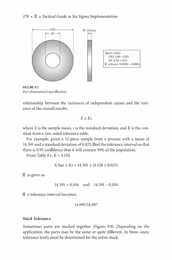
178 • The Tactical Guide to Six Sigma Implementation
relationship between the variances of independent causes and the vari-ance of the overall results:
X ± Ks
where X is the sample mean, s is the standard deviation, and K is the con-stant from a two-sided tolerance table.
For example, given a 12-piece sample from a process with a mean of 14.591 and a standard deviation of 0.025, find the tolerance interval so that there is 0.95 confidence that it will contain 99% of the population.
From Table 9.1, K = 4.150.
X-bar ± Ks = 14.591 ± (4.150 × 0.025)
This gives us
14.591 + 0.104 and 14.591 – 0.104
The tolerance interval becomes
14.695/14.487
Stack Tolerance
Sometimes parts are stacked together (Figure 9.8). Depending on the application, the parts may be the same or quite different. In these cases, tolerance levels must be determined for the entire stack.
OD �ickness
Specs (mm) OD: 2.00 + 0.01 ID: 4.70 + 0.01�ickness: 0.0500 + 0.0001
ID
FIGURE 9.7Part dimensional specification.
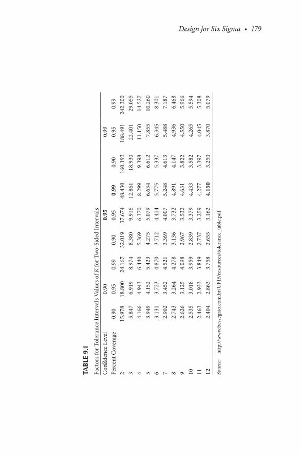
Design for Six Sigma • 179
TAB
LE 9
.1
Fact
ors f
or T
oler
ance
Inte
rval
s Val
ues o
f K fo
r Tw
o-Si
ded
Inte
rval
sC
onfid
ence
Lev
el0.
900.
950.
99Pe
rcen
t Cov
erag
e0.
900.
950.
990.
900.
950.
990.
900.
950.
992
15.9
7818
.800
24.1
6732
.019
37.6
7448
.430
160.
193
188.
491
242.
300
35.
847
6.91
98.
974
8.38
09.
916
12.8
6118
.930
22.4
0129
.055
44.
166
4.94
36.
440
5.36
96.
370
8.29
99.
398
11.1
5014
.527
53.
949
4.15
25.
423
4.27
55.
079
6.63
46.
612
7.85
510
.260
63.
131
3.72
34.
870
3.71
24.
414
5.77
55.
337
6.34
58.
301
72.
902
3.45
24.
521
3.36
94.
007
5.24
84.
613
5.48
87.
187
82.
743
3.26
44.
278
3.13
63.
732
4.89
14.
147
4.93
66.
468
92.
626
3.12
54.
098
2.96
73.
532
4.63
13.
822
4.55
05.
966
102.
535
3.01
83.
959
2.83
93.
379
4.43
33.
582
4.26
55.
594
112.
463
2.93
33.
849
2.73
73.
259
4.27
73.
397
4.04
55.
308
122.
404
2.86
33.
758
2.65
53.
162
4.15
03.
250
3.87
05.
079
Sour
ce:
http
://w
ww.
bess
egat
o.co
m.b
r/U
FJF/
reso
urce
s/to
lera
nce_
tabl
e.pd
f.
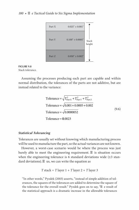
180 • The Tactical Guide to Six Sigma Implementation
Assuming the processes producing each part are capable and within normal distribution, the tolerances of the parts are not additive, but are instead related to the variance:
Tolerance
Tolerance
Part X Part Y Part Z= + +
=
T T T2 2 2
0.. . .
.
001 0 0005 0 002
0 0000052
+ +
=
=
Tolerance
Tolerance 00 0023.
(9.6)
Statistical Tolerancing
Tolerances are usually set without knowing which manufacturing process will be used to manufacture the part, so the actual variances are not known.
However, a worst-case scenario would be where the process was just barely able to meet the engineering requirement. This situation occurs when the engineering tolerance is 6 standard deviations wide (±3 stan-dard deviations). Thus, we can write the equation as
T stack = T layer 1 + T layer 2 + T layer 3
“In other words,” Pyzdek (2003) asserts, “instead of simple addition of tol-erances, the squares of the tolerances are added to determine the square of the tolerance for the overall result.” Pyzdek goes on to say, “The result of the statistical approach is a dramatic increase in the allowable tolerances
Part X
Part Y
Part Z
0.025" ± 0.001"
0.100" ± 0.0005" Stackheight
0.050" ± 0.002"
FIGURE 9.8Stack tolerance.
Design for Six Sigma • 181
for the individual piece parts.” This is an important concept in terms of tolerance because now the parts can have a greater tolerance for each part. An example is provided below (The Six Sigma Hand Book, Chapter 16: Statistical Tolerancing, pp. 600, 605).
Consider a shaft and bearing assembly where the shaft is specified to be 0.997 ± 0.001 and the bearing is specified to be 1.000 ± 0.0001. In this example, the minimum clearance between the two is 0.001 inch and the maximum clearance is 0.005 inch.
Thus, the assembly tolerance can be computed as
Tassembly = 0.005 – 0.001 = 0.004
The statistical tolerancing approach is used here in the same way as it was used above. Namely,
T T Tassembly bearing
2shaft= = +0 004 2. (9.7)
If we assume equal tolerances for the bearing and the shaft, the toler-ance for each becomes
Tassembly /= = ±( . ) .0 004 2 0 00282
which nearly triples the tolerance for each part.
Marketing and Porter’s Five Forces Analysis
Marketing
In order to understand good business process, it is necessary to under-stand marketing and selling processes.
Marketing is the management process through which goods and ser-vices move from concept to the customer. It includes the coordination of four elements called the four P’s of marketing:
1. Identification, selection, and development of a product 2. Determination of its price 3. Selection of a distribution channel to reach the customer’s place 4. Development and implementation of a promotional strategy
182 • The Tactical Guide to Six Sigma Implementation
For example, new Apple products are developed to include improved applications and systems, are set at different prices depending on how much capability the customer desires, and are sold in places where other Apple products are sold. In order to promote its devices, the company fea-tures its debuts at tech events and highly advertises them on the web and on television.
Marketing is based on thinking about the business in terms of customer needs and their satisfaction.
Marketing differs from selling because, in the words of Harvard Business School’s retired professor of marketing Theodore C. Levitt, “Selling con-cerns itself with the tricks and techniques of getting people to exchange their cash for your product. It is not concerned with the values that the exchange is all about. And it does not, as marketing invariably does, view the entire business process as consisting of a tightly integrated effort to discover, create, arouse and satisfy customer needs.” In other words, mar-keting has less to do with getting customers to pay for your product and more to do with developing a demand for that product and fulfilling the customer’s needs (Levitt 2006).
Porter’s Five Forces Analysis
Five forces analysis assumes that there are five important influences on a company that exert forces on its ability to serve its customers and make a profit (Figure 9.9).
In 1979, Michael Porter listed five forces that affect the success of an enterprise (Porter 1980):
• Bargaining power of customers: This force represents the ability and buying power of your customers to drive prices down.
• Bargaining power of suppliers: This force represents the ability and power of your suppliers to drive up prices of their products.
• Threat of new entrants: This force represents the ease by which new competitors can enter the market and drive prices down.
• Threat of substitute products: This force represents the extent to which different products or services can be substituted for your own.
• Intensity of competitive rivalry: This force represents the strength of the competition in your industry.

Design for Six Sigma • 183
There are three key steps to deal with driving forces:
Step 1: Identify forces likely to exert the greatest influence over the next one to three years. Usually no more than three or four factors qualify as real drivers of change.
Step 2: Assess impact. Are the driving forces acting to cause market demand for product to increase or decrease? Are the driving forces acting to make competition more or less intense?
Will the driving forces lead to higher or lower industry profitability?Step 3: Determine what strategy changes are needed to prepare for
impacts of driving forces.
TRIZ
TRIZ is a relatively new approach to enhancing robust design. TRIZ aids in the decision-making and problem-solving processes during the design phase of DMADV. TRIZ is a way of lateral thinking. This innovative tech-nique is based on two principles:
Competitiverivalry withinan industry
Bargaining powerof customers
�reat of newentrants
�reat of
substitute products
Bargaining powerof suppliers
FIGURE 9.9Porter’s five forces analysis.

184 • The Tactical Guide to Six Sigma Implementation
1. Somebody, sometime, somewhere has already solved your prob-lem or one similar to it. Creativity means finding that solution and adapting it to the current problem.
2. Don’t accept defects or deviations. Resolve them. Use them as a resource to solve problems.
TRIZ is an acronym for the Russian phrase Teorija Rezbenija Izobretaltelshih Zadach, meaning “theory of inventive problem solving.”
Genrich Altshuller (1926–1998), a Russian mechanical engineer, created TRIZ as a set of problem-solving design tools and techniques. After study-ing more than 400,000 patents looking for inventive problem-solving methods, Altshuller noticed patterns across different industries.
Traditionally, inventive problem solving is linked to psychology; how-ever, TRIZ is based on a systematic view of the technological world. Altshuller realized that people, including specialists, have difficulty think-ing outside of their field of reference. Given a problem (P) within their specialty, many people will only limit their search for a solution (S) to their area of specialty (Figure 9.10).
What happens if the known solution to the problem could be found in another knowledge area? Below is an example of a solution found in a seemingly unrelated area.
Traditional diamond-cutting methods cut diamonds along natural fractures, but often result in new fractures that go undetected until using the diamond. Rather than improving the existing process, cut-ters needed a new process. The key to establishing the new method was a pressurized process in the food canning industry used to split green peppers and remove the seeds. A similar technique is also used in cutting
Associatedknowledge
area 1
Specialityknowledge
area
Associatedknowledge
area 2
Associatedknowledge
area 3
P
S
FIGURE 9.10Problem of psychological inertia.

Design for Six Sigma • 185
oversize broccoli in the canning industry. Water jet cutting applied to diamond cutting resulted in cuts without additional damage to precious diamonds.
TRIZ and DFSS
By providing a methodology to think and look outside the box and avoid-ing contradictions, TRIZ can help engineers, designers, developers, researchers, and quality professionals solve problems and find new ideas leading to new product development (Table 9.2).
Some common traits of TRIZ, DFSS, and Six Sigma include
• Solving bottlenecks• Eliminating contradictions discovered in the house of quality roof• Determining target values• Identifying potential failure modes• Lowering costs• Improving serviceability
TABLE 9.2Some Links to TRIZ and DFSSStage Breakthrough Strategy Phase Objective
Identifications RecognizeDefine
Identify key businessThe problem and customer
responseCharacterization Measure
AnalyzeUnderstand current performance
levelsInstitutionalization Standardize
IntegrateTransform how day-to-day
business is conducted

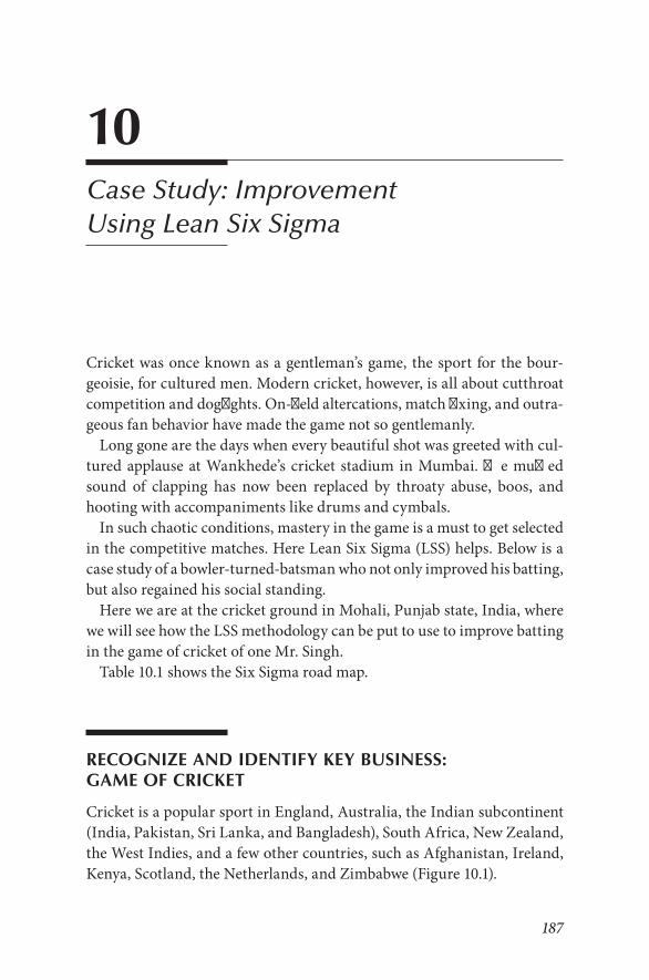
187
10Case Study: Improvement Using Lean Six Sigma
Cricket was once known as a gentleman’s game, the sport for the bour-geoisie, for cultured men. Modern cricket, however, is all about cutthroat competition and dogfights. On-field altercations, match fixing, and outra-geous fan behavior have made the game not so gentlemanly.
Long gone are the days when every beautiful shot was greeted with cul-tured applause at Wankhede’s cricket stadium in Mumbai. The muffled sound of clapping has now been replaced by throaty abuse, boos, and hooting with accompaniments like drums and cymbals.
In such chaotic conditions, mastery in the game is a must to get selected in the competitive matches. Here Lean Six Sigma (LSS) helps. Below is a case study of a bowler-turned-batsman who not only improved his batting, but also regained his social standing.
Here we are at the cricket ground in Mohali, Punjab state, India, where we will see how the LSS methodology can be put to use to improve batting in the game of cricket of one Mr. Singh.
Table 10.1 shows the Six Sigma road map.
RECOGNIZE AND IDENTIFY KEY BUSINESS: GAME OF CRICKET
Cricket is a popular sport in England, Australia, the Indian subcontinent (India, Pakistan, Sri Lanka, and Bangladesh), South Africa, New Zealand, the West Indies, and a few other countries, such as Afghanistan, Ireland, Kenya, Scotland, the Netherlands, and Zimbabwe (Figure 10.1).
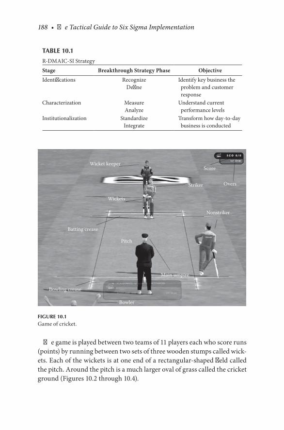
188 • The Tactical Guide to Six Sigma Implementation
The game is played between two teams of 11 players each who score runs (points) by running between two sets of three wooden stumps called wick-ets. Each of the wickets is at one end of a rectangular-shaped field called the pitch. Around the pitch is a much larger oval of grass called the cricket ground (Figures 10.2 through 10.4).
Wicket keeper
Wickets
Batting crease
Bowling crease
Bowler
Main umpire
Nonstriker
Striker Overs
Score
Pitch
FIGURE 10.1Game of cricket.
TABLE 10.1
R-DMAIC-SI Strategy
Stage Breakthrough Strategy Phase Objective
Identifications RecognizeDefine
Identify key business the problem and customer response
Characterization MeasureAnalyze
Understand current performance levels
Institutionalization StandardizeIntegrate
Transform how day-to-day business is conducted
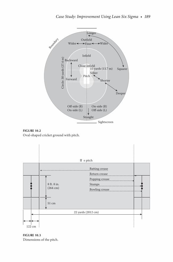
Case Study: Improvement Using Lean Six Sigma • 189
Infield
Bounda
ry
Close-infield
Sightscreen
On-side (R)Off-side (L)
Off-side (R)On-side (L)
Pitch
Longer
WiderWider
Backward
Forward Shorter
Squarer15 yards (13.7 m)Sillier
Deeper
Straight
Circ
le: 3
0 ya
rds (
27.4
m)
OutfieldFiner
FIGURE 10.2Oval-shaped cricket ground with pitch.
�e pitch
8 ft. 8 in.(264 cm)
51 cm
122 cm
22 yards (2012 cm)
Batting creaseReturn creasePopping crease
Bowling crease
Stumps
FIGURE 10.3Dimensions of the pitch.

190 • The Tactical Guide to Six Sigma Implementation
Figure 10.5 shows the directions in which a right-handed batsman may send the ball when playing various cricketing shots. The diagram for a left-handed batsman is a mirror image of this one. Table 10.2 shows the techniques of facing a ball that a batsman should learn.
The basic batting statistics of our interest include• Batting average (ave): The total number of runs divided by the total
number of innings in which the batsman was out:
HookCut
Square cut
Square drive
Cover driv
e
Off
drive
Stra
ight
driv
e
Pull
On drive
Leg gl
anceLate cut
FIGURE 10.5Names of the directions in which a ball can be hit.
Clothing
�igh pads
Box
Pads
ShoesBallBatKeeping gloves
Batting gloves
Helmet
Stumps
Keeperpads
FIGURE 10.4Batsman and wicket keeper with personal protection equipment.
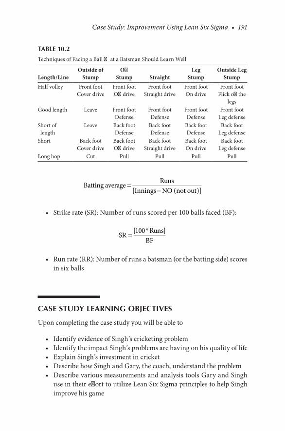
Case Study: Improvement Using Lean Six Sigma • 191
Batting average Runs
Innings NO not out=
−[ ( )]
• Strike rate (SR): Number of runs scored per 100 balls faced (BF):
SR [ Runs]
BF= 100*
• Run rate (RR): Number of runs a batsman (or the batting side) scores in six balls
CASE STUDY LEARNING OBJECTIVES
Upon completing the case study you will be able to
• Identify evidence of Singh’s cricketing problem• Identify the impact Singh’s problems are having on his quality of life• Explain Singh’s investment in cricket• Describe how Singh and Gary, the coach, understand the problem• Describe various measurements and analysis tools Gary and Singh
use in their effort to utilize Lean Six Sigma principles to help Singh improve his game
TABLE 10.2
Techniques of Facing a Ball That a Batsman Should Learn Well
Length/LineOutside of
StumpOff
Stump StraightLeg
StumpOutside Leg
Stump
Half volley Front footCover drive
Front footOff drive
Front footStraight drive
Front footOn drive
Front footFlick off the
legsGood length Leave Front foot
DefenseFront footDefense
Front footDefense
Front footLeg defense
Short of length
Leave Back footDefense
Back footDefense
Back footDefense
Back footLeg defense
Short Back footCover drive
Back footOff drive
Back footStraight drive
Back footOn drive
Back footLeg defense
Long hop Cut Pull Pull Pull Pull
192 • The Tactical Guide to Six Sigma Implementation
• Identify measures and metrics used to analyze specific aspects of Singh’s game
• List the root causes that have most impacted Singh’s cricket performance• Identify three key action steps (vital few) Singh is taking to improve
his game• Describe Gary and Singh’s plan to ensure Singh will continue to
improve his game
DEFINE PHASE: IDENTIFY EVIDENCE OF SINGH’S CRICKETING PROBLEM
A problem well defined is half solved.Here Gary helps Singh define the processes and importance of
Y = f(X)
The process outcome Y is a result (function) of process inputs X.In the define phase, we understand the project outputs (Ys) and how to
measure them.Here voice of the customer (VOC) and SIPOC are needed.SIPOC provides big Ys and little Ys. It also provides Xs.To recap SIPOC,
• Suppliers provide inputs to the process.• Inputs define the material, service, and information that are used by
the process to produce the outputs.• Process is a defined sequence of activities, and it usually adds value to
inputs to produce outputs for the customers.• Outputs are the products, services, and information that are valuable
to the customers.• Customers are the users of the outputs produced by the process.
10 Steps Leading to the Team Charter
D1: Singh’s investment• Budding cricketer• Practices twice a week
Case Study: Improvement Using Lean Six Sigma • 193
• Drums up business contacts• Lucrative deals begun on the cricket ground• Practicing exercises to improve health• Cricketing game not improved over last five years• Scores strike rate 33, batting average 5• Friends and business partners 50% better
D2: Gary’s credentials• Singh has asked his cricketing buddy Gary to help him improve
his game.• Gary will coach him on watching the ball from the bowler’s hand
in the run-up all the way to the bat, so one can determine which way the bowlers may be trying to swing the ball. Focus on the amount of swing.
• Most experienced cricketers have other areas that can pro-duce significant results, such as foot work, various shots, and stance.
• Gary is an excellent cricketer and expert in LSS.D3: Singh’s current state
• Singh was investing a lot of time and money.• His performance was not improving.• This leaves him on the sideline when his business contacts and
friends are playing.• He is frustrated and has lost business opportunities.• He planned on cricketing the rest of his life.• He is motivated to improve his cricket game.
D4: What is Singh’s problem?• His business interests hamper his game.• Friends and contacts are better players.• He doesn’t practice enough.• His performance has not improved in five years.• His scores from five years ago, over 15 one-day internationals
(ODIs), are– Strike rate (runs per 100 balls) = 16– Batting average (number of runs scored/number of times
out) = 5• Recent scores over 15 ODIs
– Strike rate 17– Batting average 5

194 • The Tactical Guide to Six Sigma Implementation
D7: Impact of Singh’s problem?• Three business contacts have distanced themselves.• They score better and play in better matches.• His best friend has almost disappeared.• His wife, who plays on a women’s team, has a better strike rate.
D8: Scorecard five years ago Why do scorecards from five years ago provide evidence of Singh’s
problem?• Demonstrate that Singh is not playing enough cricket• Demonstrate a trend that shows that Singh has not improved in
five years• Demonstrate that Singh’s playing skills are out of date• Evidence that Singh is using antiquated equipment
D9: All of the following impact Singh• His wife is a better cricketer.• He sees less and less of his best friend.• He is losing his business contacts.
D10: Problem: Cricket score is too low
Y = f(X)
Big Ys (high-level, high-impact metrics)• Cricket score• Retirement options• Social options• Revenue• Health and fitness• Quality of life
Little Ys (linked to vital X)• Average score per match• Strike rate per match• Batting average• Hours played per match• Business contacts made• Match outings planned
Vital X• Batting proficiency (key performance)• Core processes (performance drivers of vital X)
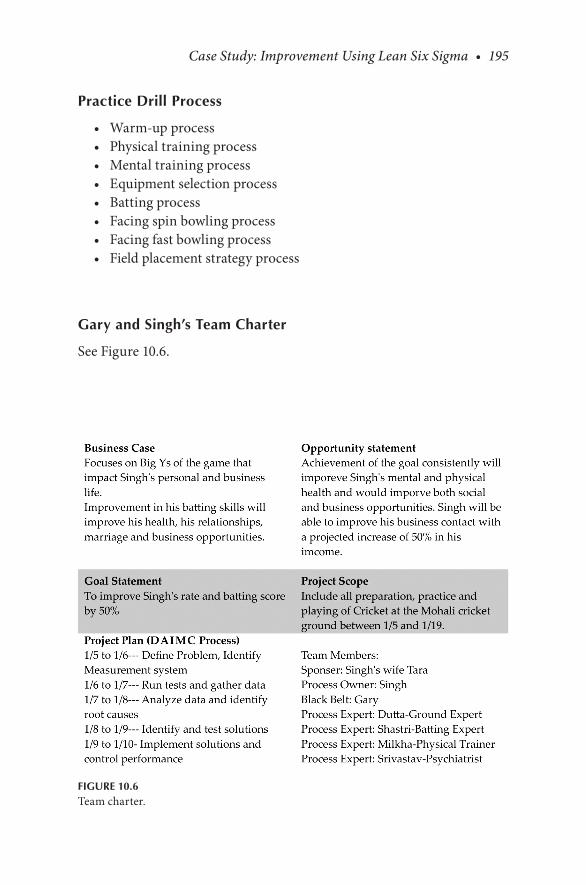
Case Study: Improvement Using Lean Six Sigma • 195
Practice Drill Process
• Warm-up process• Physical training process• Mental training process• Equipment selection process• Batting process• Facing spin bowling process• Facing fast bowling process• Field placement strategy process
Gary and Singh’s Team Charter
See Figure 10.6.
FIGURE 10.6Team charter.

196 • The Tactical Guide to Six Sigma Implementation
MEASURE PHASE
The strategic importance of measurement is that
1. Strategic importance is well understood. 2. Everyone understands the improvement opportunity.
In this phase we need to measure the performance. Here the priority is to improve the quality of the game.
In terms of cricket, this means measure the
• Number of “dot” balls• Number of singles• Number of boundaries• Number of sixes• Number of times for getting out
Critical to Process
This is how the process is performing in real time.Singh and Gary must measure factors that drive performance.The possible critical to processes (CTPs) are
• Strike rate• Batting average
Baseline data from the previous five test matches last year are
• Strike rate: 17• Batting average: 5
Table 10.3 shows the measurement plan (10 overs fast and 10 overs spin).
ANALYZE PHASE
See Figures 10.7 and 10.8.

Case Study: Improvement Using Lean Six Sigma • 197
TAB
LE 1
0.3
Mea
sure
men
t Dat
a Sh
eet
Mea
sure
Defi
niti
on
of M
easu
reD
ata
Sour
ce
and
Loca
tion
Sam
ple
Size
Who
Will
C
olle
ctH
ow C
olle
cted
Whe
n C
olle
cted
Gar
y’s
Obs
erva
tion
s
Dot
bal
lsO
n sc
orec
ard
mar
k ye
s or n
oN
otes
Sing
les
Cou
ntN
otes
Four
sC
ount
Not
esSi
xes
Cou
ntN
otes
Out
Cou
ntN
otes

198 • The Tactical Guide to Six Sigma Implementation
Fish
bone
dia
gram
—pr
oble
m a
naly
sis
Stra
ight
to fi
elde
r
Goo
d ba
ll
Wro
ng fo
ot w
ork
Wro
ng sw
ing
Wea
k sq
uare
cut
Eye
off th
e ba
ll
Wro
ng w
rist a
ctio
nLe
vel e
ye
Foot
wor
kStan
ce
Evas
ive
actio
n
Leve
l eye
Stan
ce
Wea
k sin
gles
Out
Def
ect
4 M
s: m
etho
d, m
achi
nes,
mat
eria
ls, m
anpo
wer
4 Ps
: pla
ce, p
roce
dure
, peo
ple,
pol
icie
s4
Ss: s
uppl
iers
, sys
tem
s, sk
ills,
surr
ound
ings
Low
scor
e
No
cont
act
FIG
UR
E 10
.7Pr
oble
m a
naly
sis.
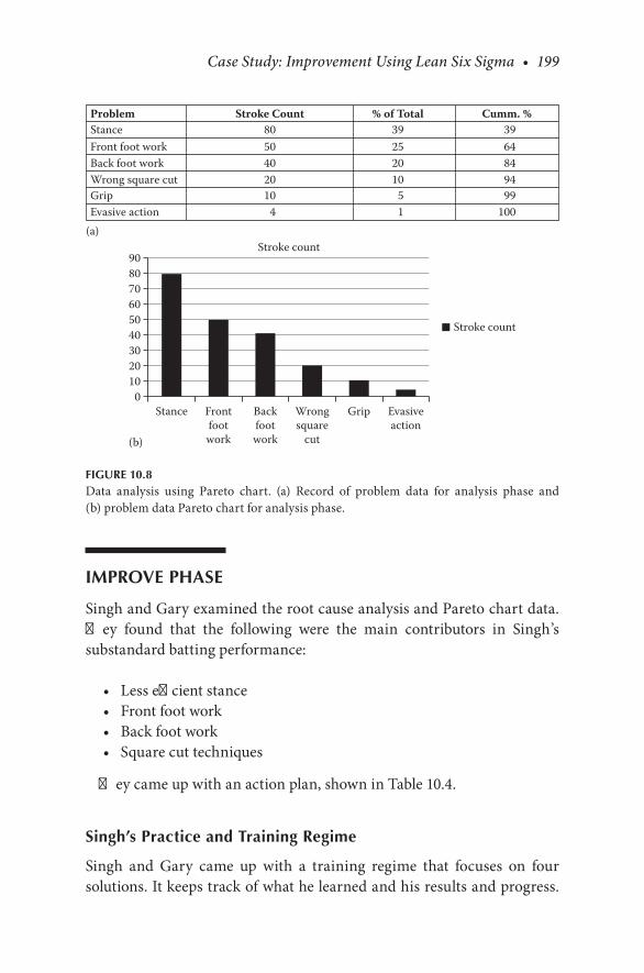
Case Study: Improvement Using Lean Six Sigma • 199
IMPROVE PHASE
Singh and Gary examined the root cause analysis and Pareto chart data. They found that the following were the main contributors in Singh’s substandard batting performance:
• Less efficient stance• Front foot work• Back foot work• Square cut techniques
They came up with an action plan, shown in Table 10.4.
Singh’s Practice and Training Regime
Singh and Gary came up with a training regime that focuses on four solutions. It keeps track of what he learned and his results and progress.
Problem
(a)
Stroke Count % of Total Cumm. %Stance 80 39 39Front foot work 50 25 64Back foot work 40 20 84Wrong square cut 20 10 94Grip 10 5 99Evasive action 4 1 100
Stance0
102030405060708090
Stroke count
Stroke count
(b)
Frontfootwork
Backfootwork
Wrongsquare
cut
Grip Evasiveaction
FIGURE 10.8Data analysis using Pareto chart. (a) Record of problem data for analysis phase and (b) problem data Pareto chart for analysis phase.
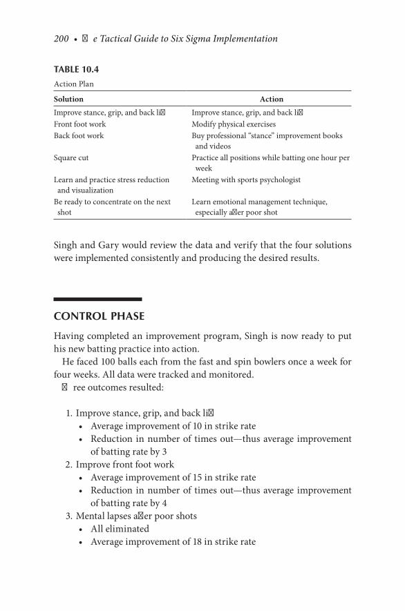
200 • The Tactical Guide to Six Sigma Implementation
Singh and Gary would review the data and verify that the four solutions were implemented consistently and producing the desired results.
CONTROL PHASE
Having completed an improvement program, Singh is now ready to put his new batting practice into action.
He faced 100 balls each from the fast and spin bowlers once a week for four weeks. All data were tracked and monitored.
Three outcomes resulted:
1. Improve stance, grip, and back lift• Average improvement of 10 in strike rate• Reduction in number of times out—thus average improvement
of batting rate by 3 2. Improve front foot work
• Average improvement of 15 in strike rate• Reduction in number of times out—thus average improvement
of batting rate by 4 3. Mental lapses after poor shots
• All eliminated• Average improvement of 18 in strike rate
TABLE 10.4
Action Plan
Solution Action
Improve stance, grip, and back lift Improve stance, grip, and back liftFront foot work Modify physical exercisesBack foot work Buy professional “stance” improvement books
and videosSquare cut Practice all positions while batting one hour per
weekLearn and practice stress reduction and visualization
Meeting with sports psychologist
Be ready to concentrate on the next shot
Learn emotional management technique, especially after poor shot
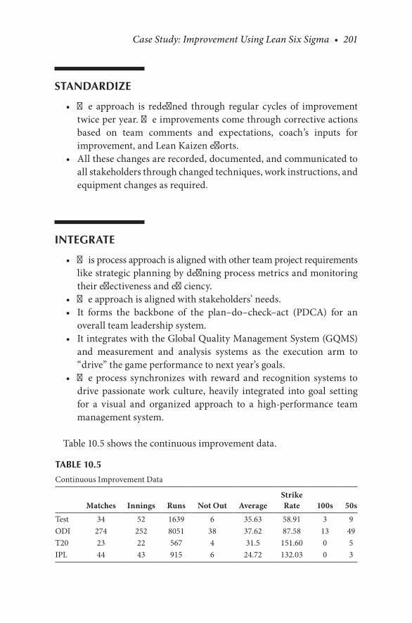
Case Study: Improvement Using Lean Six Sigma • 201
STANDARDIZE
• The approach is redefined through regular cycles of improvement twice per year. The improvements come through corrective actions based on team comments and expectations, coach’s inputs for improvement, and Lean Kaizen efforts.
• All these changes are recorded, documented, and communicated to all stakeholders through changed techniques, work instructions, and equipment changes as required.
INTEGRATE
• This process approach is aligned with other team project requirements like strategic planning by defining process metrics and monitoring their effectiveness and efficiency.
• The approach is aligned with stakeholders’ needs.• It forms the backbone of the plan–do–check–act (PDCA) for an
overall team leadership system.• It integrates with the Global Quality Management System (GQMS)
and measurement and analysis systems as the execution arm to “drive” the game performance to next year’s goals.
• The process synchronizes with reward and recognition systems to drive passionate work culture, heavily integrated into goal setting for a visual and organized approach to a high-performance team man agement system.
Table 10.5 shows the continuous improvement data.
TABLE 10.5
Continuous Improvement Data
Matches Innings Runs Not Out AverageStrike Rate 100s 50s
Test 34 52 1639 6 35.63 58.91 3 9ODI 274 252 8051 38 37.62 87.58 13 49T20 23 22 567 4 31.5 151.60 0 5IPL 44 43 915 6 24.72 132.03 0 3

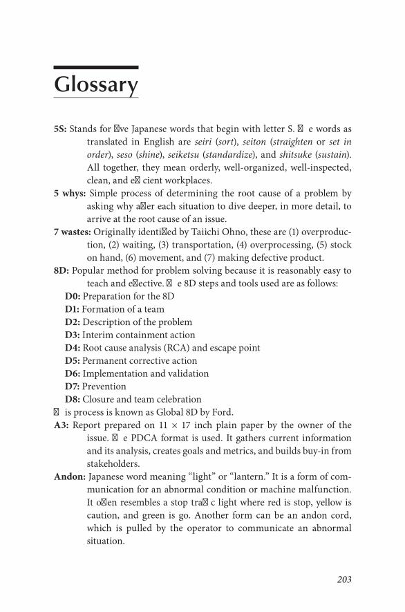
203
Glossary
5S: Stands for five Japanese words that begin with letter S. The words as translated in English are seiri (sort), seiton (straighten or set in order), seso (shine), seiketsu (standardize), and shitsuke (sustain). All together, they mean orderly, well-organized, well-inspected, clean, and efficient workplaces.
5 whys: Simple process of determining the root cause of a problem by asking why after each situation to dive deeper, in more detail, to arrive at the root cause of an issue.
7 wastes: Originally identified by Taiichi Ohno, these are (1) overproduc-tion, (2) waiting, (3) transportation, (4) overprocessing, (5) stock on hand, (6) movement, and (7) making defective product.
8D: Popular method for problem solving because it is reasonably easy to teach and effective. The 8D steps and tools used are as follows:
D0: Preparation for the 8DD1: Formation of a teamD2: Description of the problemD3: Interim containment actionD4: Root cause analysis (RCA) and escape pointD5: Permanent corrective actionD6: Implementation and validationD7: PreventionD8: Closure and team celebration
This process is known as Global 8D by Ford.A3: Report prepared on 11 × 17 inch plain paper by the owner of the
issue. The PDCA format is used. It gathers current information and its analysis, creates goals and metrics, and builds buy-in from stakeholders.
Andon: Japanese word meaning “light” or “lantern.” It is a form of com-munication for an abnormal condition or machine malfunction. It often resembles a stop traffic light where red is stop, yellow is caution, and green is go. Another form can be an andon cord, which is pulled by the operator to communicate an abnormal situation.

204 • Glossary
AS 9100: Widely adopted and standardized quality management system for the aerospace industry.
BE: Business excellence.Black Belt: Professional who can explain and practice Six Sigma philoso-
phies and principles, including supporting systems and tools.BPR: Business process reengineering. Analysis and redesign of workflow
within and between enterprises. BPR reached its maximum popu-larity in the early 1990s.
budget: Estimate of costs, revenues, and resources over a specified period, reflecting a reading of future financial conditions and goals.
CA: Corrective action taken to eliminate the cause of nonconformity.cause-and-effect diagram: This diagram-based technique helps us iden-
tify all of the likely causes of the problems faced in working environments.
changeover: Setting up a machine or production line to make a different part number or product.
changeover time: Time from the last good piece of the current production run to the first good piece of the next run.
constraint: Anything that limits a system from achieving higher perfor-mance. It is also called a bottleneck.
continual improvement: Continual indicates duration of improvement that continues over a long period of time, but with intervals of interruption, for example, a plant modification disrupted by logis-tics or traffic for nearly two years.
continuous improvement: Approach of making frequent and small changes to process whose cumulative results lead to higher levels of quality, cost, and efficiency.
countermeasure: Corrective action taken to address problems or abnormalities.
customer: Party that receives or consumes products (goods or services) and has the ability to choose between different products.
cycle: Sequence of operations repeated regularly.cycle time: Time for one sequence of operations to occur.effectiveness: Degree to which objectives are achieved and the extent to
which targeted problems are solved. In contrast to efficiency, effec-tiveness is determined without reference to costs, and whereas efficiency means “doing the thing right,” effectiveness means “doing the right thing.”
EFQM: European Foundation for Quality Management.
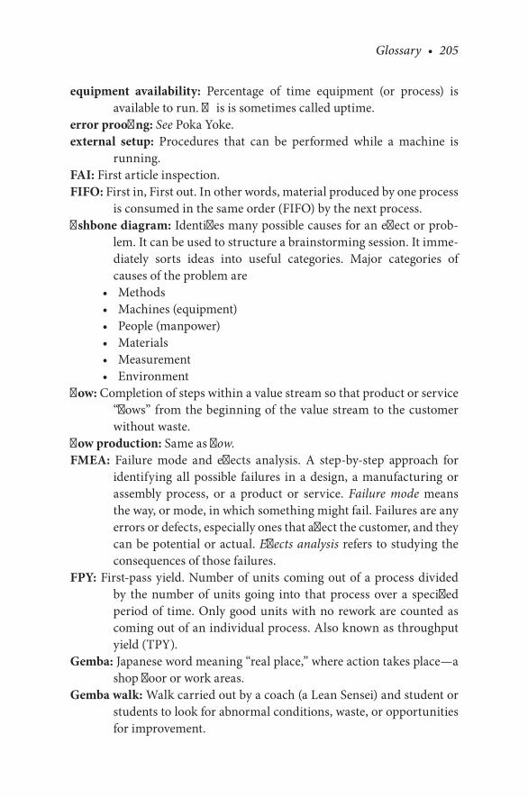
Glossary • 205
equipment availability: Percentage of time equipment (or process) is available to run. This is sometimes called uptime.
error proofing: See Poka Yoke.external setup: Procedures that can be performed while a machine is
running.FAI: First article inspection.FIFO: First in, First out. In other words, material produced by one process
is consumed in the same order (FIFO) by the next process.fishbone diagram: Identifies many possible causes for an effect or prob-
lem. It can be used to structure a brainstorming session. It imme-diately sorts ideas into useful categories. Major categories of causes of the problem are
• Methods• Machines (equipment)• People (manpower)• Materials• Measurement• Environment
flow: Completion of steps within a value stream so that product or service “flows” from the beginning of the value stream to the customer without waste.
flow production: Same as flow.FMEA: Failure mode and effects analysis. A step-by-step approach for
identifying all possible failures in a design, a manufacturing or assembly process, or a product or service. Failure mode means the way, or mode, in which something might fail. Failures are any errors or defects, especially ones that affect the customer, and they can be potential or actual. Effects analysis refers to studying the consequences of those failures.
FPY: First-pass yield. Number of units coming out of a process divided by the number of units going into that process over a specified period of time. Only good units with no rework are counted as coming out of an individual process. Also known as throughput yield (TPY).
Gemba: Japanese word meaning “real place,” where action takes place—a shop floor or work areas.
Gemba walk: Walk carried out by a coach (a Lean Sensei) and student or students to look for abnormal conditions, waste, or opportunities for improvement.
206 • Glossary
Heijunka: Method for leveling production for mix and volume.Hoshin Kanri: Strategic decision-making tool used for policy deployment.internal setup: Procedures that must be performed while the machine is
stopped.Ishikawa diagram: See fishbone diagram.Jidoka: Device that stops production or equipment when a defective con-
dition arises. Attention is drawn to this condition and the opera-tor who stopped the production. The Jidoka system has faith in the operator who is trained in the job.
just in time (JIT): Originally developed by the Toyota Production System (TPS). JIT presupposes that all waste is eliminated from the pro-duction line and only the inventory in the right quantity and at the right time is used for the production, where the rate of produc-tion is exactly as required by the customer.
Kaikaku: Japanese word meaning “innovation” or a “radical break-through.” Kaikaku requires radical thinking and takes more time in planning and implementation.
Kaizen: Japanese word meaning “change for the better” or “do good.” It is a process of making continual improvements by everyone keeping in mind quality and safety.
Kaizen event: Short team-based improvement project. Also called Kaizen blitz.
Kanban: Means “sign board” or a “label.” It serves as an instruction for production and replenishment.
KCC: Key critical characteristic.KPC: Key performance characteristic.KPI: Key performance indicator.lead time: Time required to move one piece from the time the order is
taken until it is shipped to the customer.line balancing: Technique where all operations are evenly balanced and
staffing is also balanced to meet the takt time.Manufacturing Resource Planning (MRP II): Like MRP, but takes into
consideration the capacity planning and finance requirement. It works out alternative production plans through the simulation tool.
Materials Requirement Planning (MRP): Computerized system of deter-mining quantity and timing requirements for production and delivery of products for customers as well as suppliers. This is a push production system.
Glossary • 207
MBNQA: Malcolm Baldrige National Quality Award. An award given to an organization for achieving the highest-quality standards.
milk run: Routing of supply and delivery trucks or vehicles to make mul-tiple pickups and deliveries at various locations to reduce trans-portation waste.
Muda: Japanese word for waste. It is an element that does not add value to the product or service. Also known as no-value-added activity carried out on a product or service that does not add value and the customer will not pay for it.
Mura: Japanese word for variability or unevenness.Muri: Japanese word for physical and mental strain or overburden.One- (single) piece flow: Practiced in JIT system where one work piece
flows from process to process to minimize waste.operational excellence (Opex): Element of organizational initiative that
stresses the application of a variety of principles, systems, and tools toward the sustainable improvement of key performance metrics. This philosophy is based on continuous improvement, such as a quality management system, Lean manufacturing, and Six Sigma. Operational excellence goes beyond the traditional methods of improvement and leads to a long-term change in orga-nizational culture.
overall equipment effectiveness (OEE): Product of the following key measures:
1. Operational availability 2. Performance efficiency 3. First-pass yield qualityPAIP: Process for performance analysis and improvement.PCP: Process control plan.PDCA: Plan–do–check–act cycle for continual improvement.PFMEA: Process failure mode and effects analysis.point-of-use storage (POUS): Storing or keeping materials, tools, infor-
mation, and items near to where they are used.Poka Yoke: Also known as mistake proofing. Poka in Japanese means
“inadvertent mistake,” and Yoke means “prevention.” These can be simple, low-cost devices or sophisticated electromechanical devices to prevent the production of defective product.
process: Sequence of interdependent and linked procedures that, at every stage, consume one or more resources (employee time, energy, machines, and money) to convert inputs (data, material, parts,
208 • Glossary
etc.) into outputs. These outputs then serve as inputs for the next stage until a known goal or end result is reached.
productivity: Measured as an output for a given input. Productivity increase is critical to improving living standards.
product realization: Term used to describe the work that the organization goes through to develop, manufacture, and deliver the finished product or service to the customer.
pull: Alternatively known as pull production, where the upstream sup-plier does not produce until the downstream customer signals the need.
push: Alternatively known as push production, where the upstream sup-plier produces as much as it can without regard to whether the downstream customer needs the product.
QOS: Quality operating system. Originally implemented by Ford. The methodology was established to measure the effectiveness of the quality system and to drive continuous improvement.
RPN: Risk priority number. In FMEA, RPN = Severity × Occurrence × Detection.
RTY: Rolled throughput yield. A probability that a single piece will pass through all production steps without a single defect.
shadow board: Board where each tool has a place, showing which tools are missing.
single-minute exchange of dies (SMED): Group of techniques developed by Shigeo Shingo for changeover of production equipment in less than 10 minutes.
SIPOC: Process identification where the requirements for the supplier, input, process steps, output, and customer are defined.
Six Sigma: Set of tools and techniques for process improvement. It was originally developed by Motorola in 1981.
spaghetti diagram: Diagram showing the layout and flow of information, material, and people in a work area. It is generally used to high-light motion and transportation waste.
SPC: Statistical process control. Quality control where process variations are measured and controlled.
standard work: Accurate description of every process step specifying takt time, cycle time, and minimum inventory needed and sequence of each process step. The entire process is carried out with minimum human motion and other wastes.
Glossary • 209
supermarket: Where parts are stored before they go to the next operation. The parts are managed using minimum and maximum inventory levels.
sustainability: Continued development or growth, without significant deterioration of the environment and depletion of natural resources on which human well-being depends.
SWOT: Strength, weakness, opportunity, and threat. Strength and weak-ness analysis guides us to identify the positives and negatives inside an organization (SW). Opportunity and threat analysis guides us to identify the positives and negatives outside of it. Developing a full SWOT analysis can help with strategic planning and decision making.
system: A group of interdependent processes and people that together perform a common goal.
takt time: Available production time divided by the rate of the customer demand.
TPM: Total productive maintenance. System to ensure that every produc-tion process machine is able to perform its required tasks such that production is not interrupted.
TQM: Total quality management. Management approach that originated in the 1950s. The TQM culture requires quality in all aspects of the company’s operations, with processes being done right the first time and defects and waste eradicated from operations. To be successful implementing TQM, an organization must concentrate on eight key elements:
1. Ethics 2. Integrity 3. Trust 4. Training 5. Teamwork 6. Leadership 7. Recognition 8. CommunicationVAA: Value-added activity.value: Capability provided to a customer at the right time at an appropri-
ate price. Defined by the customer.value stream: Sequence of actions required to design, produce, and pro-
vide a specific good or service, and along which information, materials, and worth flow.

210 • Glossary
visual factory: Term to describe how data and information are conveyed to a Lean manufacturing environment. Here time and resources dedicated to conveying information are a form of waste. By using visual methods, information is easily accessible to those who need it. Visual information makes the current status of all processes immediately apparent.
work in process (WIP): Incomplete product or services that are waiting further processing.
211
Bibliography
Akao, Y., ed. Quality Function Deployment. Cambridge MA: Productivity Press, 1990.American Society for Quality (ASQ). The Certified Manager of Quality/Organizational
Excellence. Foundations in Quality Learning Series. Milwaukee, WI: ASQ Quality Press, 1994.
American Society for Quality (ASQ). The Certified Quality Engineer. Milwaukee, WI: ASQ Quality Press, 2000.
ASQ Lean Six Sigma Conference, Phoenix, AZ, March 8–9, 2010.Automotive Industry Action Group (AIAG). PFMEA. 3rd ed. Southfield, MI: AIAG, 2001.Automotive Industry Action Group (AIAG). MSA. 3rd ed. Southfield, MI: AIAG, 2002.Benbow, Donald W., and Kubiak, T.M. The Certified Six Sigma Black Belt Handbook.
Milwaukee, WI: ASQ Quality Press, 2005.Brassard, Michael. The Memory Jogger Plus+®: Featuring the Seven Management and
Certified Six Sigma Black Belt Certification Preparations. Salem, NH: Goal/QPC, 1996.Crosby, Philip. Crosby’s 14 steps to improvement, Quality Progress, December 2005: 60–64.Crosby, Philip. Quality without Tears. New York: McGraw-Hill, 1984.Deming, W. Edwards. Out of the Crisis. Cambridge, MA: MIT Press, 1986.Deming, W. Edwards. The New Economics for Industry, Government, Education. 2nd ed.
Cambridge, MA: MIT Press, 1993.Dittmer, H. William. Goldratt’s Theory of Constraints: A Systems Approach to Continuous
Improvement. Milwaukee, WI: ASQ Quality Press, 1997.Feigenbaum, Armand V. Total Quality Control. 3rd ed. New York: McGraw-Hill, 1991.Galsworth, Gwendolyn. Visual-Lean Institute, Portland, OR: Visual Thinking Inc., 1992.International Organization for Standardization (ISO). Quality management principles 2.
Geneva: ISO, 2001.International Organization for Standardization (ISO). ISO for small and medium-sized
businesses: ISO/TC advice. Milwaukee, WI: ISO, 2008.ISO 9001:2008. Quality management systems—Requirements. Geneva: International
Organization for Standardization, 2008.ISO 9004. Managing for the sustained success of an organization—A quality management
approach. Geneva: International Organization for Standardization, 2010.ISO/TR 10013:2001. Guidelines for quality management system documentation. Geneva:
International Organization for Standardization, 2001.ISO/TS 16949. Southfield, MI: Automotive Industry Action Group, 2009.Keller, Paul. Six Sigma Demystified. New York: McGraw-Hill, 2005.Krueger, Kaye. Value added vs non value added activities. October 15, 2015. Available at
https://www.wisc-online.com/value-added-vs-non-value-added-activities.Levitt, Theodore C. Ted Levitt on Marketing. Watertown, MA: Harvard Business Review
Book. Chapter on “Selling versus Marketing” pp. 152–154, 2006.Lowe, A.J. and Ridgway, K. Quality function deployment. Sheffield, UK: University of
Sheffield, 2001. http://www.shef.ac.uk/~ibberson/qfd.html.Maasaki, Imai. Gemba Kaizen. New York: McGraw-Hill, 1997.Porter, Michael E. Competitive Strategy. New York: Free Press, 1980.
212 • Bibliography
Pyzdek, Thomas. The Six Sigma Handbook: A Complete Guide for Green Belts, Black Belts, and Managers at All Levels. 2nd ed. New York: McGraw-Hill, 2003.
Pyzdek, T. and Keller, P.A. Project scheduling, The Six Sigma Handbook, 4th ed., p. 218, 2011.
Pyzdek, T. and Keller P.A. Quality Engineering Handbook. ISBN 0824746147.Shiego, Shingo. A Study of the Toyota Production System, trans. Andrew Dillon. Boca Raton,
FL: CRC Press, 2005.SO/TR 10013:2001. Guidelines for quality management system documentation. Geneva:
International Organization for Standardization, 2001.Tague, N.R., Quality Toolbox, 2nd. ed., p. 558, ASQ Quality Press, March 30, 2005.Toyota Production System. http://www.toyotageorgetown.com.Wheeler, Donald J. Advanced Topics in Statistical Process Control. Knoxville, TN: SPC Press,
1995.Womack, James P. and Jones, Daniel T. Lean Thinking, Banish Waste and Create Wealth in
Your Corporation. Simon & Schuster, 2003.
223
About the Author
Suresh Patel is a former Technical Director and Operations Excellence Executive. He holds a BE degree in electrical engineering from M.S. University of Baroda, India, a Master’s degree in production technology from South Bank University, London, and an MBA degree from the University of Texas at Brownsville. He is quali-fied as a Certified Reliability Engineer, Certified Quality
Engineer, and Certified Management Systems Auditor by the American Society for Quality.
In his long career spanning more than four decades, he has developed a wide range of products/processes and has helped in establishing six man-ufacturing plants in India and five U.S. plants in Mexico. Starting with India, his career path has enabled him to work in industries in the UK, Denmark, Belgium, Canada, U.S., China, Mexico, and Chile. His career has been enriched through holding key positions with such multinational corporations as Gestetner, Motorola, United Lighting Technologies, Eaton Corporation, and Fiat Global.
Patel’s practical expertise and interests include establishing Business Excellence Strategies starting from product quality strategies, quality improvement tools deployment, and execution, leading to improvements in product/process delivery performance and reduction in product escapes and product/process variation through Lean Six Sigma and overall busi-ness excellence employing Leadership and Results “Triades” as defined in MBNQA USA. Patel’s other interests include supply chain management, manufacturing management, and building technological capabilities in manufacturing firms.

K26939
ISBN-13: 978-1-4987-4538-3
9 781498 745383
90000
The Tactical Guide to
SIX SIGMAI m p l e m e n t a t i o n
S U R E S H P A T E L
“The author’s account of these dif�cult and vast subjects is very praiseworthy and proof of his vast industrial experience of more than four decades of working with MNCs in Asia, Europe, and the Americas. This is an inspirational work that is easy to learn and apply by the lay reader. I highly recommend this book to all students, teachers, executives, and organizations who want to learn and imple-ment global quality management systems, Lean Six Sigma systems, and business excellence strategies”
—Madan Mohanka, Chairman, Managing Director, and Founder, TEGA Industries Limited, Kolkata, India
Simplifying a complex subject and removing the intimidation of using statistics, The Tactical Guide to Six Sigma Implementation takes readers through the �ve phases of the Six Sigma methodology—De�ne–Measure–Analyze–Improve–Control (DMAIC). In ten clearly written and easy-to-understand chapters, readers learn the purpose of each phase and what activities must be performed in each phase.
The book illustrates the layout of the interaction of organizational processes—de�ning product and information �ows separately such that each process receives product or information and, after completion of the process, supplies the output to the next process.
The author identi�es organizational processes through turtle and SIPOC diagrams, de�ning the process owner, inputs and outputs, and process customer for each process. He also explains how to determine the measures and goals of the process, and how to document the process so that further process improvements can be implemented through management reviews.
The text presents a comprehensive process control plan assessment to comply with automotive, aerospace, and all types of manufacturing and service processes. It details 17 global quality management system processes covering management responsibility, resource management, product realization policies, and management analysis and improvement policies. It also provides comprehensive root cause analysis and problem solving techniques.
The Tactical Guide to
S I X S I G M AImplementation
Business & Management / Quality & Six Sigma
THE TA
CTIC
AL G
UID
E TO S
IX S
IGM
A IM
PLEM
ENTATIO
N
PATEL