Journal of Structural Engineering & Applied Mechanics

2020 Volume 3 Issue 4 Pages 244-275

https://doi.org/10.31462/jseam.2020.04244275 www.goldenlightpublish.com

RESEARCH ARTICLE

The strut-and-tie model and the finite element - good design

companions

Ahmed K. Ghoraba1 , Salah E. El-Metwally *2 , Mohamed E. El-Zoughiby2

1 Misr Higher Institute of Engineering and Technology, El-Mansoura, Egypt 2 Mansoura University, Structural Engineering Department, El-Mansoura, Egypt

Abstract

The strut-and-tie method (STM) can serve as a tool for a safe design of concrete structures or members. It

aids to trace the flow of forces, appropriately lay-out the reinforcement, and safely predict the structure

capacity. On the other hand, the linear elastic finite element can be utilized as an alternative in the

development of the strut-and-tie models besides the load path method. In addition, the nonlinear finite

element analysis assists in the optimization of the design results obtained from the STM. Hence, the two

methods work well as companions in structural design. In order to demonstrate such understanding, different

examples which include a deep beam with large opening and recess, continuous deep beams with and without

openings, and beam ledges, have been utilized. In the STM solutions, the ACI 318-14 failure criteria have

been adopted. In the nonlinear finite element analysis, material nonlinearity has been accounted for. The

obtained solutions from the two methods, along with the experimental data of the selected examples of this

study, revealed the reliability of the STM in obtaining a safe solution. Besides, the nonlinear finite element

proved to be an efficient tool in obtaining an economic design.

Keywords

Reinforced concrete design; Discontinuity regions; Strut-and-tie model; Nonlinear finite element analysis;

Deep beams; Beam ledge

Received: 22 June 2020; Accepted: 03 November 2020

ISSN: 2630-5763 (online) © 2020 Golden Light Publishing All rights reserved.

1. Introduction

The method of the strut-and-tie model, STM, has

been well established in both academia and practice

for the treatment of discontinuity (D) regions; e.g.,

deep beams, openings, corbels, etc. [1,2]. The STM,

is a logical extension of the truss model by Ritter

[3] and Mörsch [4], and the major difference

between the two methods is that the strut-and-tie

model is a set of forces in equilibrium but do not

form a stable truss system. Thus, the STM is a

generalization of the truss model by Schlaich et al.

* Corresponding author

Email: selmetwally@mans.edu.eg

[2] and Schlaich and Schäfer [5]. The method has

been adopted by many codes of practice such as the

ACI 318-14 Code [6], the Eurocode 2 [7], the

Canadian Standards Association [8], and the CEB-

FIP Guidelines [9,10].

On the other hand, the implementation of the

nonlinear finite element analysis, NFEA, in practice

is very limited. Due to its very intensive

computation efforts, the method can only serve as a

benchmark for other methods or solutions. This

makes the method of STM appealing in practice for

both strength assessment and design.

245 Ghoraba et al.

In order to achieve a good design, the STM can

serve as a reliable design tool that aids to trace the

flow of forces and achieve successful detailing. For

the development of the STM, the load path method

can be used in most of the cases; however, in some

cases, it becomes easier and a straightforward

matter if a linear elastic finite element analysis is

employed. Since the STM is a lower-bound

solution, the design obtained from this method is

always on the safe side. For a given design, if

optimization is required, the NFEA can serve this

purpose. Thus, both the STM and the finite element

work together as good design companions. This

understanding is demonstrated in this paper by

many examples. These examples include deep

beams with large openings and recess, continuous

deep beams with and without large openings, and

beams with ledges.

In the STM solutions presented herein, the

failure criteria of the ACI 318-14 Code [6], are

adopted. As for the linear/nonlinear finite element

analyses, the computer software ABAQUS [11] is

utilized. In the NFEA, material nonlinearity is

accounted for. Most of the examples discussed in

this paper had been tested experimentally.

Comparisons between the experimental data and

the predicted results by the STM and the NFEA are

performed. The comparisons revealed the reliability

of the STM in obtaining a safe solution. Also, the

NFEA proved to be an efficient tool in obtaining an

economic design.

2. The strut-and-tie method

An STM consists of three types of elements;

concrete struts (with or without reinforcement), ties

with or without reinforcement, nodes, and nodal

zones, Fig. 1. Any STM may fail by one of the

following modes: yield or anchorage failure of the

tension tie, one of the struts could crush when the

stress in the strut exceeds the effective compressive

strength of concrete, or a nodal zone could fail by

being stressed beyond its capacity. In this paper, the

failure criteria of the ACI 318-14 Code [6] are

employed in the presented applications.

Fig. 1. Components of a strut-and-tie model of a deep

beam

2.1. Strength of struts

According to the ACI 318-14 [6] the nominal

compressive strength of a strut without longitudinal

reinforcement, 𝐹𝑛𝑠, shall be taken as

𝐹𝑛𝑠 = 𝑓𝑐𝑒𝑠 𝐴𝑐𝑠 (1)

where 𝑓𝑐𝑒𝑠 is the smaller of:

▪ The effective compressive strength of the

concrete in the strut.

▪ The effective compressive strength of the

concrete in the nodal zone.

and 𝐴𝑐𝑠 is the cross-sectional area at one end of the

strut. In calculating 𝐴𝑐𝑠, the strut width is measured

perpendicular to the strut axis at its end.

The effective compressive strength of the concrete

in a strut 𝑓𝑐𝑒𝑠 can be obtained from

𝑓𝑐𝑒𝑠 = 0.85𝑓𝑐

′𝛽𝑠 (2)

where 𝑓𝑐′ is the concrete cylinder strength and 𝛽𝑠 is

an effectiveness factor of concrete. Table 1 shows

the values of 𝛽𝑠 according to the ACI 318-14 Code

[6], in which the influence of the stress conditions,

strut geometry, and the angle of cracking

surrounding the strut on strength are reflected.

2.2. Nodal zones

Smeared nodes do not need to be checked if the

reinforcement is properly developed until the

extremities of the stress field. A check of concrete

stresses in the singular nodes is necessary because

of the stress concentration at these nodal regions.

The singular nodes are divided into four major

types, C-C-C, C-C-T, C-T-T, and T-T-T nodes,

where C and T stand for compression and tension,

respectively.

The strut-and-tie model and the finite element - good design companions 246

Table 1. ACI 318-14 code values of coefficient 𝛽𝑠 for struts [6]

Strut condition 𝛽𝑠

• A strut with constant cross-section along its length

• For struts located such that the width of the midsection of the strut is larger than the width at the nodes

(bottle-shaped struts)

1.0

a) With reinforcement normal to strut center-line to resist the transverse tension

b) Without reinforcement normal to the center-line of the strut

0.75

0.6λ

• For struts in tension members, or the tension flanges of members 0.40

• For all other cases 0.6λ

The effective compressive strength of the

concrete in a nodal zone, 𝑓𝑐𝑒𝑛 , can be obtained from:

𝑓𝑐𝑒𝑛 = 0.85𝑓𝑐

′𝛽𝑛 (3)

where 𝛽𝑛 is the effectiveness factor of a nodal zone.

Table 2 shows the effectiveness factor, 𝛽𝑛, for

nodal zones according to the ACI 318-14 Code [6].

2.3. Reinforced ties

The nominal strength of a tie, 𝐹𝑛𝑡, shall be taken as

𝐹𝑛𝑡 = 𝐴𝑠𝑡𝑓𝑦; where 𝐴𝑠𝑡 is the area of steel and 𝑓𝑦 is

the yield stress. The width of a tie 𝑤𝑡, is to be

determined to guarantee node safety, with an upper

limit 𝑤𝑡,𝑚𝑎𝑥.

▪ In case of using one row of bars without

sufficient development length beyond the nodal

zones, Fig. 2a:

𝑤𝑡 = 0.0 (4a)

▪ In case of using one row of bars and providing

sufficient development length beyond the nodal

zones for a distance not less than 2𝑐, where 𝑐 is

the concrete cover, Fig. 2b:

𝑤𝑡 = ∅𝑏𝑎𝑟 + 2𝑐 (4b)

where bars is the diameter of the reinforcing bars.

▪ In case of using more than one row of bars and

providing sufficient development length beyond

the nodal zones for a distance not less than 𝑠/2,

where 𝑠 is the clear distance between bars, Fig.

2c:

𝑤𝑡 = n∅𝑏𝑎𝑟 + 2c + (n – 1)s (4c)

where n is the number of rows of reinforcing bars.

In the three cases in Fig. 2, the development length

according to the ACI 318-14 [6], 𝑙𝑎𝑛𝑐 , begins at the

intersection of the centroid of the bars in the tie and

the extensions of the outlines of either the strut or

the bearing area.

For the extended nodal zone, Figs. 2b and 2c, the

upper limit of the strut width,

𝑤𝑡,𝑚𝑎𝑥 =𝐹𝑛𝑡

𝑏 𝑓𝑐𝑒𝑛

3. Linear/Nonlinear finite element analysis

In this study, 3D linear and nonlinear finite element

analyses have been performed using the computer

software ABAQUS [11]. The constitutive models

adopted in the modeling process are briefly

described here. The displacement control approach

has been employed to accurately predict the

capacity and post-cracking behavior of the studied

examples.

3.1. Finite elements of concrete and steel

reinforcement

Herein, the 3D solid continuum element C3D8R

has been employed to model concrete. This element

is an 8-noded linear brick having 3 translational

degrees of freedom at each corner node. The

reinforcing steel has been defined as individual

truss elements with steel material properties and

cross-sections using T3D2 element which is a (2-

node linear displacement) 3D truss element.

3.2. Concrete material modeling

The “Concrete damage plasticity model” (CDP) is

utilized for concrete modeling which assumes that

the main two failure modes are tensile cracking and

compressive crushing [11].

247 Ghoraba et al.

Table 2. ACI 318-14 Code values of coefficient 𝛽𝑛 for nodes

Nodal zone 𝛽𝑛

For nodal zones bounded by struts or bearing areas or both, C-C-C node 1.00

Nodal zones anchoring one tie, C-C-T node 0.80

Nodal zones anchoring two or more ties with the presence of one strut, C-T-T node 0.60

Nodal zones anchoring ties only, T-T-T node 0.40

Fig. 2. The width of the tie, 𝑤𝑡, used to determine the dimensions of the nodal zone

In this paper, the uniaxial compressive stress-strain

relationship of the concrete model, as shown in Fig.

3a is proposed by Saenz [12] as follows:

𝜎𝑐

=𝐸𝑐 𝜀𝑐

1 + (𝑅 + 𝑅𝐸 − 2) (𝜀𝑐

𝜀0) − (2𝑅 − 1) (

𝜀𝑐

𝜀0)

2

+ 𝑅 (𝜀𝑐

𝜀0)

3

(5a)

where 𝜎𝑐 is the compression stress at any 𝜀𝑐, and 𝜀0

the strain at the ultimate stress.

𝑅 = 𝑅𝐸 ( 𝑅𝜎 − 1)

( 𝑅𝜀 − 1)2−

1

𝑅𝜀

(5b)

𝑅𝐸 𝜀𝑐

𝜀0

(5c)

𝐸0 =𝑓𝑐

′

𝜀0

(5d)

where 𝑅 is the ratio relation; 𝑅𝐸 is the modular

ratio; 𝑅𝜀 = 4 = the strain ratio; 𝑅𝜎 = 4 = the stress

ratio as reported in [13]; 𝐸0 is the secant modulus.

Poisson’s ratio for concrete is assumed to be 0.20.

The softening curve of concrete under tension is

shown in Fig. 3b, where 𝑓𝑐𝑡 is the tensile strength,

and 𝐺𝑓 is the fracture energy of concrete which is

used to specify the post-peak tension failure

behavior of concrete. According to the ACI-318

[14], 𝐸𝑐 and 𝑓𝑐𝑡 were calculated by:

𝐸𝑐 = 4700√𝑓𝑐′ (6)

𝑓𝑐𝑡 = 0.35√𝑓𝑐′ (7)

3.3. Reinforcing steel modeling

The steel reinforcement has been modeled as an

elastic-perfectly plastic material in both tension and

compression.

3.4. Bond between steel and concrete

A perfect bond between concrete and reinforcement

has been assumed in this study, which was achieved

by using a constrain called Embedded Element. The

reinforcing bar is embedded into the concrete host

element; thus, all embedded element nodes have the

same translational degrees of freedom as the

concrete host element's nodes [6].

4. Deep beam with large opening and recess

4.1. Description

The deep beam in Fig. 4a with an abrupt change of

thickness and a large opening was designed to carry

a factored concentrated load of 2000.0 kN (or a

nominal load 2667.0 kN) [15]. From the beam

geometry, it is entirely considered as a D-region.

The strut-and-tie model and the finite element - good design companions 248

(a) uniaxial compressive stress-strain curve (b) tension stiffening model

Fig. 3. Concrete modeling

This beam is selected for comparison between the

two-dimensional strut-and-tie modeling and the 3D

nonlinear finite element analysis. Fig. 4 shows the

beam geometry, loading, and reinforcement details

of the beam.

The cylinder compressive strength of concrete,

𝑓𝑐′ = 31 MPa and the reinforcement is high strength

deformed steel bars, with yield stress, 𝑓y = 414

MPa. The beam height is as shown in Fig. 4a,

breadth, b = 305mm, the width of the bearing plate

𝑏1= 600mm, and 𝑏2= 𝑏3= 400 mm.

4.2. Strut-and-tie modeling

4.2.1. Geometrical parameters

The solution procedure starts with the development

of the strut-and-tie model. With the aid of the stress

pattern obtained from the linear elastic analysis, it

is obvious how the struts go around the opening to

transfer their forces to the supports. The proposed

STM is shown in Fig. 5a, and for the next

illustrations, the details of selected nodes are given

in Fig. 5b.

Concerning Figs. 5 and 4b, the reinforcement

4T32 of tie 𝑇1 is assumed to be well anchored at

nodes 3 and 4. Hence, the width of this tie (height

of nodes 3 and 4) is given by

𝑤𝑇1= 2(𝑐 + ∅𝑠𝑡𝑖𝑟𝑟𝑢𝑝) + 𝑛∅𝑏𝑎𝑟 + (𝑛 − 1)𝑠 =

202 mm.

If tie 𝑇1 yields, its nominal strength will be

𝑇1𝑛 = 𝐴𝑠 × 𝑓y = (4×804.25) × 414 = 1332 kN.

In the same manner, for the 4T25 reinforcement

of each of the ties 𝑇2 and 𝑇3, the height of each tie

at nodes 6 and 7 is 181mm and the nominal strength

is 813.0kN.

Regarding Figs. 5 and 4b, the reinforcement of

each of the ties 𝑇4 and 𝑇5 is 5T13 (2-legs) vertical

stirrups T13, spaced at 450mm center to center. The

width of each of these ties is

𝑤𝑇4= 𝑤𝑇5

= 𝑛(∅𝑏𝑎𝑟 + 𝑠) = 2315 mm.

Each of the ties 𝑇4 and 𝑇5 has a nominal

strength

𝑇4𝑛= 𝑇5𝑛 = 𝐴𝑠 × 𝑓y= (2×5×132.7) × 414 = 549.5

kN.

Also, 𝑇6 is represented by 9T13 (2-legs)

vertical stirrups, spaced at 230mm center to center.

The nominal strength of the tie 𝑇6 is

𝑇6𝑛 = 𝐴𝑠 × 𝑓y = (2×9×132.7) × 414 = 989.12 kN.

The width of this tie is

𝑤𝑇6= 𝑛(∅𝑏𝑎𝑟 + 𝑠) = 2187 mm

In the same manner, each of the ties 𝑇7, 𝑇8, 𝑇9,

and 𝑇10 are represented by 6T32, the width of these

ties or the height of nodes 10, 11, 12, 13, and 14, is

266 mm and the nominal strength is 1997.75 kN.

249 Ghoraba et al.

(a) beam geometry (dimensions in mm) and loading

(b) reinforcement arrangement

Fig. 4. Deep beam with large opening and recess

(a) model

(b) details of selected nodes

Fig. 5. Proposed STM of the deep beam with large opening and recess

The strut-and-tie model and the finite element - good design companions 250

4.2.2. Reactions

From equilibrium, 𝑉1 = 0.67P and 𝑉2 = 0.33P.

4.2.3. Model geometry and forces

To obtain the forces in the model elements, the

reinforcement of a selected tie was assumed to

reach its yield stress. The solution to this problem

was initiated by assuming that the reinforcement of

tie 𝑇2 reached its yield stress, 𝑇2 = 813.0kN. Then,

from simple truss analysis, the model forces were

obtained, Fig. 6. This led to an applied load 𝑃 =

𝐹1 + 𝐹2 = 2560 kN. It is noted that this load value

is less than the required nominal strength.

4.2.4. Effective concrete strength of the struts

The effective concrete strength of the strut

𝑓𝑐𝑒𝑠 = 0.85𝑓𝑐

′𝛽𝑠.

For prismatic strut

𝑓𝑐𝑒𝑠 = 0.85 × 31 × 1.0 = 26.35 MPa.

For bottle-shaped strut with sufficient

reinforcement to resist the transverse tension

𝑓𝑐𝑒𝑠 = 0.85 × 31 × 0.75 = 19.76 MPa

This value will be used throughout the example, and

in the end, it will be verified.

4.2.5. Effective concrete strength of the nodes

The effective concrete strength of the different

nodes, 𝑓𝑐𝑒𝑛 = 0.85𝑓𝑐

′𝛽𝑛, are

For C–C–C node, 𝑓𝑐𝑒𝑛 = 0.85×31×1.0 = 26.35 MPa

For C–C–T node, 𝑓𝑐𝑒𝑛 = 0.85×31×0.80 = 21.08 MPa

For C–T–T node, 𝑓𝑐𝑒𝑛 = 0.85×31×0.60 = 15.81 MPa

4.2.6. Check the bearing of the nodes

For nodes 1 and 2, the nominal value of the load P,

𝑃𝑛 = 26.35 × 600 × 305 = 4822.03 kN, which is

greater than the applied load, 𝑃 = 2560 kN.

For node 10, the nominal value of the reaction 𝑉2,

𝑉2𝑛 = 21.08 × 400 × 305 = 2571.75 kN, which is

greater than the reaction, 𝑉2 = 853.3 kN.

For node 14, the nominal value of the reaction 𝑉1,

𝑉1𝑛 = 21.08 × 400 × 305 = 2571.75 kN, which is

greater than the reaction, 𝑉1 = 1706.7 kN.

4.2.7. Check of stresses

Node 1:

Since the bearing stress has been checked before,

there is no need to check it again. The width of the

tie 𝑇10, 𝑤𝑇10 = 266mm. Assuming that the force in

the prismatic strut 𝐶0 is equal to its nominal

strength; then, 𝐶0 = 1762.7 kN = 26.35 × 𝑤𝐶0 × 305,

which gives, 𝑤𝐶0 = 219.3 mm. For strut 𝐶1, its angle

of inclination 𝛳1= 36.0o, which gives a width of the

strut, 𝑤𝐶11 = 300 sin 𝛳1 + 219.3 cos 𝛳1=353.75 mm.

Then, the nominal strength of the strut 𝐶1𝑛 = 19.76#

× 353.75 × 305 = 2132kN (# the smaller of the node

strength and the strut strength), which is less than

the strut force, 𝐶1 = 2166.7 kN; i.e., 𝐶1𝑛 = 0.984 𝐶1.

Fig. 6. Computed model forces (kN) assuming yielding of tie 𝑇2 reinforcement

Node 2:

251 Ghoraba et al.

Similar to node 1, the bearing stress is safe and the

nominal strength of the strut 𝐶2, 𝐶2𝑛 = 2132 kN.

Since 𝐶2 = 2166.7 kN; hence, 𝑪𝟐𝒏 = 0.984 𝑪𝟐.

Nodes 3 and 4:

The two nodes need not be checked, since they are

smeared nodes, and "the reinforcing bars passing

through the nodes are extended beyond the nodal

zones and they have sufficient anchorage length."

Hence, the strength of the struts connected with

these nodes is governed by either the strength of the

other connecting nodes or the strength of these

struts.

Node 5:

The width of the tie 𝑇2, 𝑤𝑇2 = 181 mm, and

assuming that the width of the prismatic strut 𝐶7 is

equal to the width of the bearing plate at node 14,

𝑤𝐶75 = 𝑤𝐶7

14 = 400mm, and the angle of inclination of

the strut 𝐶3, 𝛳3 = 58.0o, the width of the strut 𝐶3,

𝑤𝐶35 = 400 sin 𝛳3 + 181 cos 𝛳3 = 435.13 mm. Then,

the nominal strength of the strut, 𝐶3𝑛 = 19.76# ×

435.13 × 305 = 2622.47 kN (# the smaller of the

node strength and the strut strength), which is

greater than the strut force, 𝐶3 = 1512.22 kN.

The width of the vertical strut 𝐶7, 𝑤𝐶74 = 40 0mm.

Hence, its nominal strength, 𝐶7𝑛 = 21.08# × 400 ×

305 = 2571.76kN (# the smaller of the node strength

and the strut strength), which is greater than the

strut force, 𝐶7 = 1278.3 kN.

Node 6:

The width of the tie 𝑇2, 𝑤𝑇2 = 181 mm and of tie 𝑇4,

𝑤𝑇4= 2315 mm, and the angle of inclination of the

strut 𝐶8, 𝛳8 = 34.0o; Hence; the width of the

strut 𝐶8, 𝑤𝐶86 = 2315 sin 𝛳8 + 181 cos 𝛳8 = 1444.6

mm. Then, the nominal strength of the strut 𝐶8𝑛 =

15.81# × 1444.6 × 305 = 6965.93 kN (# the smaller

of the node strength and the strut strength), which

is greater than the strut force, 𝐶8 = 761.8 kN.

Node 7:

Similar to node 6, 𝐶9𝑛 = 6965.93 kN, greater

than 𝐶9 = 761.8 kN. For strut 𝐶5, 𝑤𝐶57 = 181 mm,

the nominal strength of the strut 𝐶5𝑛 = 𝑓𝑐𝑒𝑛× 𝑤𝐶5

7 × b

+ 𝐴𝑠′ 𝑓y = (15.81 × 181 × 503) + (4×490.87 × 414) =

2252.27 kN, which is greater than the strut force,

𝐶5 = 238.1 kN.

Node 8:

This is a smeared node and hence there is no need

to check it. Hence, the strength of the struts

connected with this node is governed by either the

strength of the other connecting nodes or the

strength of these struts.

Node 9:

This is also a smeared node and hence there is no

need to check it, provided that the reinforcement of

the tie 𝑇6 is adequately anchored.

Node 10:

Since the bearing stress has been checked before,

there is no need to check it again. The width of the

tie 𝑇10, 𝑤𝑇10 = 266 mm. For strut 𝐶12, its inclination

angle 𝛳12= 42.0o, which gives a width of the

strut 𝑤𝐶1210 = 400 sin 𝛳12 + 266 cos 𝛳12=465.3 mm.

Then, the nominal strength of the strut 𝐶12𝑛 =

19.76# × 465.3 × 305 = 2804.4 kN (# the smaller of

the node strength and the strut strength), which is

greater than the strut force, 𝐶12 = 1273.2 kN.

Nodes 11, 12, 13, and 14:

These nodes have been checked in the same manner

and they have sufficient strength.

4.2.8. Results

From the obtained results the model elements are

all safe except elements 𝐶1and 𝐶2 (similar

elements) 𝐶1𝑛= 𝐶2𝑛=0.984 𝐶1=0.984 𝐶1. Therefore,

the load P should be reduced to 98.4% of the

calculated value; i.e., the predicted collapse load

from the STM, 𝑃𝑆𝑇𝑀 = 0.984 × 2560 = 2519 kN.

Upon checking the skin reinforcement, it is found

that all the bottle-shaped struts have adequate

transverse reinforcement to resist the transverse

tension, as assumed.

4.3. Nonlinear finite element analysis

Both linear and nonlinear analyses have been

conducted for the specimen under the applied

concentrated load only. The right support is

prevented from translation in the y- and x-

directions, but the left support is prevented from

The strut-and-tie model and the finite element - good design companions 252

translation in the y-direction only. The objective of

the linear analysis was to obtain the stress

trajectories that guide to construct of the strut-and-

tie model. On the other hand, the nonlinear analysis

has been performed to obtain the displacement,

strains, and stresses at different load levels. The

stress trajectories obtained from the linear elastic

analysis are illustrated in Fig. 7a and the results

obtained from the NFEA are presented in Figs. 7b

to 7d.

(a) stress trajectories

(b) yielding stress zones

(c) concrete plastic strain distribution

(d) load-displacement curve

Fig. 7. Finite element results of the deep beam with large opening and recess

As observed from the yielding stress zones of

the reinforcement and the concrete plastic strain

distribution in Figs. 7b and 7c, respectively, the

failure mode of the beam is a concrete crushing

253 Ghoraba et al.

failure (shear failure). The main cause of failure

was the crushing of the struts below the loading

plate and the yielding of the web reinforcement,

which indicates that the part of the beam above the

opening behaves as a deep beam. The maximum

concrete compressive stress in the beam near failure

was 30 MPa. Neither the beam bottom nor the top

longitudinal bars below and above the opening

reached their yield stress; they reached 300 MPa

and 200 MPa, respectively. Fig. 7d shows the load-

displacement curve, where the initial part of the

curve is approximately linear, indicating the elastic

range under a service load of 1334 kN. The curve

revealed a gentle slope after the initial linear portion

and exhibited some ductility at failure. These

results comply with the prediction of the strut-and-

tie model. The predicted failure load from the

NFEA is 2437 kN.

4.4. Predicted capacity and required nominal

strength

The strength predicted by the STM and the NFEA

is given in Table 3 along with the nominal load. The

prediction from the STM, as expected, is on the safe

side. However, the results from the NFEA are

closer to the nominal strength.

5. Continuous deep beams

5.1. Description

Three full-size normal strength reinforced concrete

continuous deep beams (CDB1, CDB2, and CDB3)

subjected to concentrated loads at the middle of

spans that had been tested by [16] have been

selected for comparison between the 2D strut-and-

tie modeling and the 3D nonlinear finite element

analysis. Only the details of the strut-and-tie

modeling and the finite element solutions of beam

CDB2 are presented here and a summary of the

results of the other two beams, CDB1 and CDB3, is

given at the end of this section. The details of the

reinforcement of the tested deep beams are shown

in Table 4.

The beam height, h = 625 mm, depth, d = 585

mm, breadth, b = 120 mm, the width of bearing

plates 𝑏1= 120 mm, and 𝑏2= 𝑏3= 250 mm. The shear

span, a = 660 mm. The shear span-to-depth ratio,

𝑎 𝑑⁄ = 660 585⁄ = 1.12. The bottom tension steel,

𝐴𝑠1 = 452 mm2 and the top tension steel 𝐴𝑠2=

609mm2. The cylinder compressive strength of

concrete, 𝑓𝑐′ = 33.7 MPa, the yield stress of

longitudinal steel, 𝑓y = 480 MPa, the vertical web

reinforcement is 𝐴𝑠𝑣 = 15×2R8, and the horizontal

web reinforcement is 𝐴𝑠ℎ = 2×2R8. The web steel

yield stress of mild steel bar R8 is 𝑓yv= 𝑓yh= 370

MPa.

5.2. Strut-and-tie modeling of beam CDB2

Fig. 8 shows the geometry and reinforcement

details of the deep beam CDB2, whereas Fig. 9

illustrates the details of its strut-and-model.

Table 3. Strength of the deep beam with large opening and recess

𝑃𝑆𝑇𝑀 (kN) 𝑃𝑁𝐹𝐸𝐴 (kN) 𝑃𝑛 (kN) 𝑃𝑆𝑇𝑀 𝑃𝑛⁄ 𝑃𝑁𝐹𝐸𝐴 𝑃𝑛⁄

2519 2437 2667 0.94 0.91

Table 4. Details of considered continuous deep beams

Beam 𝑓𝑐

′

(MPa)

Shear span-to-depth

ratio (𝑎 𝑑⁄ )

Main longitudinal bars Web reinforcement

Bottom Top Horizontal Vertical

CDB1 30.6 1.12 4T12 4T12 + 2 T10 8R8 29R8

CDB2 33.7 1.12 4T12 4T12 + 2 T10 4R8 15R8

CDB3 22.4 1.12 4T12 4T12 + 2 T10 4R8

The strut-and-tie model and the finite element - good design companions 254

Fig. 8. Reinforcement details and geometry of the beam CDB2

(a) model

(b) details of nodes 1, 2, and half node 3

(c) refined STM model

Fig. 9. Details of STM for the continuous deep beam CDB2

5.2.1. Geometrical parameters

With reference to Fig. 9, the solution procedure

starts with assuming some geometrical parameters.

Since the reinforcement detailing allows the use of

extended nodal zones, the height of node 1, 𝑤𝑇1,

𝑤𝑇1= 2(𝑡 – 𝑑) = 2 (625 – 585) = 80 mm, or

𝑤𝑇1= 2(𝑐 + ∅𝑠𝑡𝑖𝑟𝑟𝑢𝑝) + 𝑛∅𝑏𝑎𝑟 + (𝑛 − 1)𝑠

The height of the tie in the upper node, node 2, 𝑤𝑇2,

𝑤𝑇2= 2(𝑐 + ∅𝑠𝑡𝑖𝑟𝑟𝑢𝑝) + 𝑛∅𝑏𝑎𝑟 + (𝑛 − 1)𝑠 = 90 mm

The lever arm 𝐿𝑑 is

𝐿𝑑 = d – 0.5×𝑤𝑇2 = 585 – 0.5×90 = 540 mm

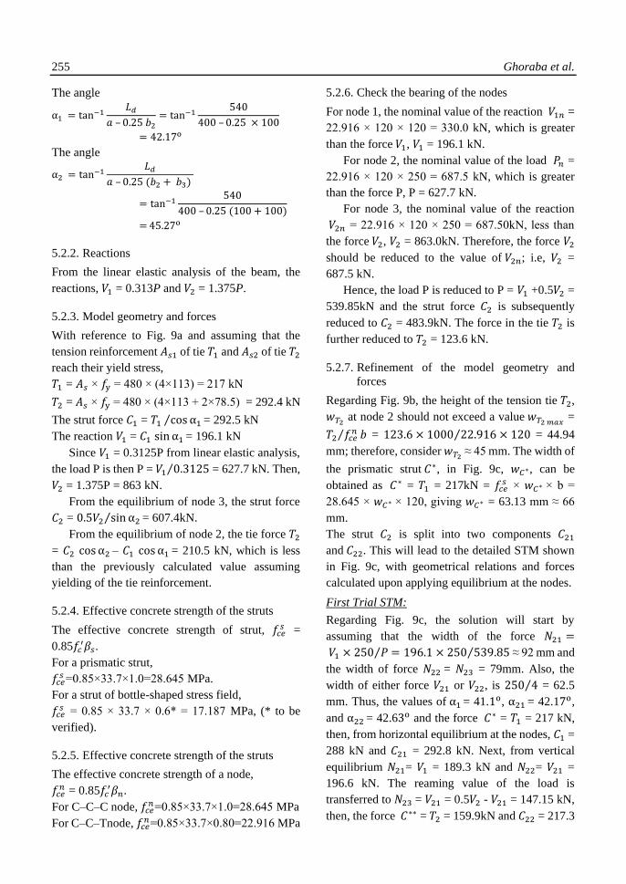
255 Ghoraba et al.

The angle

α1 = tan−1𝐿𝑑

𝑎 – 0.25 𝑏2= tan−1

540

400 – 0.25 × 100

= 42.17o

The angle

α2 = tan−1𝐿𝑑

𝑎 – 0.25 (𝑏2 + 𝑏3)

= tan−1540

400 – 0.25 (100 + 100)

= 45.27o

5.2.2. Reactions

From the linear elastic analysis of the beam, the

reactions, 𝑉1 = 0.313P and 𝑉2 = 1.375P.

5.2.3. Model geometry and forces

With reference to Fig. 9a and assuming that the

tension reinforcement 𝐴𝑠1 of tie 𝑇1 and 𝐴𝑠2 of tie 𝑇2

reach their yield stress,

𝑇1 = 𝐴𝑠 × 𝑓y = 480 × (4×113) = 217 kN

𝑇2 = 𝐴𝑠 × 𝑓y = 480 × (4×113 + 2×78.5) = 292.4 kN

The strut force 𝐶1 = 𝑇1 cos α1 ⁄ = 292.5 kN

The reaction 𝑉1 = 𝐶1 sin α1 = 196.1 kN

Since 𝑉1 = 0.3125P from linear elastic analysis,

the load P is then P = 𝑉1 0.3125⁄ = 627.7 kN. Then,

𝑉2 = 1.375P = 863 kN.

From the equilibrium of node 3, the strut force

𝐶2 = 0.5𝑉2 sin α2 ⁄ = 607.4kN.

From the equilibrium of node 2, the tie force 𝑇2

= 𝐶2 cos α2 – 𝐶1 cos α1 = 210.5 kN, which is less

than the previously calculated value assuming

yielding of the tie reinforcement.

5.2.4. Effective concrete strength of the struts

The effective concrete strength of strut, 𝑓𝑐𝑒𝑠 =

0.85𝑓𝑐′𝛽𝑠.

For a prismatic strut,

𝑓𝑐𝑒𝑠 =0.85×33.7×1.0=28.645 MPa.

For a strut of bottle-shaped stress field,

𝑓𝑐𝑒𝑠 = 0.85 × 33.7 × 0.6* = 17.187 MPa, (* to be

verified).

5.2.5. Effective concrete strength of the struts

The effective concrete strength of a node,

𝑓𝑐𝑒𝑛 = 0.85𝑓𝑐

′𝛽𝑛.

For C–C–C node, 𝑓𝑐𝑒𝑛=0.85×33.7×1.0=28.645 MPa

For C–C–Tnode, 𝑓𝑐𝑒𝑛=0.85×33.7×0.80=22.916 MPa

5.2.6. Check the bearing of the nodes

For node 1, the nominal value of the reaction 𝑉1𝑛 =

22.916 × 120 × 120 = 330.0 kN, which is greater

than the force 𝑉1, 𝑉1 = 196.1 kN.

For node 2, the nominal value of the load 𝑃𝑛 =

22.916 × 120 × 250 = 687.5 kN, which is greater

than the force P, P = 627.7 kN.

For node 3, the nominal value of the reaction

𝑉2𝑛 = 22.916 × 120 × 250 = 687.50kN, less than

the force 𝑉2, 𝑉2 = 863.0kN. Therefore, the force 𝑉2

should be reduced to the value of 𝑉2𝑛; i.e, 𝑉2 =

687.5 kN.

Hence, the load P is reduced to P = 𝑉1 +0.5𝑉2 =

539.85kN and the strut force 𝐶2 is subsequently

reduced to 𝐶2 = 483.9kN. The force in the tie 𝑇2 is

further reduced to 𝑇2 = 123.6 kN.

5.2.7. Refinement of the model geometry and

forces

Regarding Fig. 9b, the height of the tension tie 𝑇2,

𝑤𝑇2 at node 2 should not exceed a value 𝑤𝑇2 𝑚𝑎𝑥

=

𝑇2 𝑓𝑐𝑒𝑛⁄ 𝑏 = 123.6 × 1000 22.916 × 120⁄ = 44.94

mm; therefore, consider 𝑤𝑇2 ≈ 45 mm. The width of

the prismatic strut 𝐶∗, in Fig. 9c, 𝑤𝐶∗, can be

obtained as 𝐶∗ = 𝑇1 = 217kN = 𝑓𝑐𝑒𝑠 × 𝑤𝐶∗ × b =

28.645 × 𝑤𝐶∗ × 120, giving 𝑤𝐶∗ = 63.13 mm ≈ 66

mm.

The strut 𝐶2 is split into two components 𝐶21

and 𝐶22. This will lead to the detailed STM shown

in Fig. 9c, with geometrical relations and forces

calculated upon applying equilibrium at the nodes.

First Trial STM:

Regarding Fig. 9c, the solution will start by

assuming that the width of the force 𝑁21 =

𝑉1 × 250 𝑃⁄ = 196.1 × 250 539.85 ⁄ ≈ 92 mm and

the width of force 𝑁22 = 𝑁23 = 79mm. Also, the

width of either force 𝑉21 or 𝑉22, is 250 4⁄ = 62.5

mm. Thus, the values of α1 = 41.1o, α21 = 42.17o,

and α22 = 42.63o and the force 𝐶∗ = 𝑇1 = 217 kN,

then, from horizontal equilibrium at the nodes, 𝐶1 =

288 kN and 𝐶21 = 292.8 kN. Next, from vertical

equilibrium 𝑁21= 𝑉1 = 189.3 kN and 𝑁22= 𝑉21 =

196.6 kN. The reaming value of the load is

transferred to 𝑁23 = 𝑉21 = 0.5𝑉2 - 𝑉21 = 147.15 kN,

then, the force 𝐶∗∗ = 𝑇2 = 159.9kN and 𝐶22 = 217.3

The strut-and-tie model and the finite element - good design companions 256

kN is obtained from horizontal equilibrium and P =

𝑁21 + 𝑁22 + 𝑁23 = 533 kN. Then, a better estimate

of the height of the tension tie 𝑇2, 𝑤𝑇2, at node 2 can

be calculated, 𝑤𝑇2 𝑚𝑎𝑥= 𝑇2 𝑓𝑐𝑒

𝑛⁄ 𝑏 =(159.9 ×1000) ⁄

(22.916×120) = 58.1 mm; therefore, consider 𝑤𝑇2 ≈

62 mm. The STM will be updated leading to the

second trial STM.

Second Trial STM:

As illustrated before, the width of the force 𝑁21 =

189.3 × 250 533 ⁄ ≈ 90 mm, the width of the force

𝑁22 = 196.6 × 250 533 ⁄ ≈ 94 mm, and the width of

force 𝑁23 = 66mm. Also, the width of the force 𝑉21

= 196.6 × 250 2(196.6 + 147.15) ⁄ ≈ 72 mm and

the width of the force 𝑉22 = 53mm. Finally, the

values of α1 = 40.2o, α21 = 41.48o, and α22 =

41.73o, are obtained and the force 𝐶∗ = 𝑇1 = 217

kN. Then, from horizontal equilibrium at the nodes,

𝐶1 = 284.1 kN and 𝐶21 = 289.6 kN. Next, from

vertical equilibrium, 𝑁21= 𝑉1 = 183.4 kN and 𝑁22=

𝑉21 = 191.9kN. The remaining part of the load is

transferred to 𝑁23 = 𝑉21 = 151.9 kN, then, the force

𝐶∗∗ = 𝑇2 = 170.3kN and 𝐶22 = 228.2 kN can be

obtained from horizontal equilibrium and P = 𝑁21 +

𝑁22 + 𝑁23 = 527.2 kN.

5.2.8. Check of stresses

Node 1:

Since the bearing stress has been checked before,

there is no need to check it again. For strut 𝐶1, the

inclination angle α1 = 40.2o, and 𝑤𝐶11 = 120 sin α1

+ 80 cos α1 = 138.6 mm. Then, the nominal strength

of the strut is 𝐶1𝑛 = 17.187# × 120 × 138.6 = 285.8

kN (# the smaller of the node strength and the strut

strength), which is greater than the strut force.

Node 2:

Since the bearing stress has been checked before,

there is no need to check it again.

For sub-node 21, the width of the strut 𝐶1, 𝑤𝐶121 =

90 sin α1 + 66 cos α1 = 108.5 mm. Then, the

nominal strength of the strut is 𝐶1𝑛 = 17.187# × 120

× 108.5 = 223.7 kN (# the smaller of the node

strength and the strut strength), which is less than

the strut force, 𝐶1𝑛 =0.787𝐶1. There is no need to

check the prismatic strut 𝐶∗ since this was

considered during the estimate of the height of this

sub-node.

For sub-node 22, the width of the strut 𝐶21,

𝑤𝐶2122 = 94 sin α21 + 66 cos α21 = 111.7 mm. Then,

the nominal strength of the strut is 𝐶21𝑛 = 17.187#

× 120 × 111.7 = 230.4kN (# the smaller of the node

strength and the strut strength), which is less than

the strut force, 𝐶21𝑛 = 0.795𝐶1.

For sub-node 23, the width of the strut 𝐶22,

𝑤𝐶2223 = 66 sin α22 + 62 cos α22 = 90.2 mm. Then,

the nominal strength of the strut is 𝐶22𝑛 = 17.187#

× 120 × 90.2 = 186kN (# the smaller of the node

strength and the strut strength), which is less than

the strut force, 𝐶22𝑛 = 0.815𝐶22.

Node 3:

For sub-node 31, the width of the strut 𝐶21,

𝑤𝐶2131 = 72 sin α21 + 80 cos α21 = 107.6 mm. Then,

the nominal strength of the strut is 𝐶21𝑛 = 17.187#

× 120 × 107.6 = 222 kN (# the smaller of the node

strength and the strut strength), which is less than

the strut force, 𝐶21𝑛 = 0.766𝐶21.

For sub-node 32, the width of the strut 𝐶22,

𝑤𝐶2232 = 53 sin α22 + 62 cos α22 = 81.5 mm. Then,

the nominal strength of the strut is 𝐶22𝑛 = 17.187#

× 120 × 81.5 = 168.2 kN (# the smaller of the node

strength and the strut strength), which is less than

the strut force, 𝐶22𝑛= 0.737𝐶22.

5.2.9. Results

The nominal strength of the strut 𝐶2 that consists of

𝐶21𝑛 and 𝐶22𝑛 is [(0.766 × 289.6) + (0.737 × 228.2)]

= 390kN. According to the ACI 318-14 [6], the

resultant force is assumed to spread at a slop 2

longitudinally and 1 transverse. Hence, the sum of

the transverse forces of the strut is 195 kN. The skin

reinforcement of the beam within the strut length is

2 horizontal bars per face, which can resist a force

of 2 × 2 × 50.26 × 370 × sin 41. 48 = 49.3 kN

perpendicular to the crack and 3 vertical bars per

face, which can resist a force of 2 × 3 × 50.26 × 370

× sin 48.52 = 83.6 kN perpendicular to the crack.

This makes a total of 49.3 + 83.6 = 132.9 kN, which

is less than the required force, 195 kN, which

indicates that the transverse reinforcement doesn't

satisfy the strut requirement. Hence, the assumed

257 Ghoraba et al.

value 𝛽𝑠 = 0.60 in the calculation procedure is

correct.

The load P =𝑁21 + 𝑁22 + 𝑁23 = 527.2 kN, which

is less than the nominal value at the loading nodes,

which is also safe from bearing, 𝑃𝑛 = 687.5 kN.

From the obtained results the critical members are

𝐶1𝑛 = 0.787𝐶1, 𝐶21𝑛 = 0.766𝐶21, and 𝐶22𝑛 =

0.737𝐶22, while the other members attain nominal

strength greater than their forces. Therefore, the

load components should be reduced to a value of P

= 0.787×183.4+0.766×191.9+0.737×151.9 = 403.3

kN. Thus, the STM nominal strength, 2𝑃 = 806.6

kN. Since the measured collapse load was 2P = 950

kN; then, the STM solution is 85% of the value

measured in the test.

5.3. Nonlinear finite element analysis of deep

beam CDB2

Beam CDB2 has been analyzed under the two

applied concentrated loads at mid-spans and only

the middle support is prevented from translation in

the y- and x-directions, but the external supports are

prevented from translation in y-direction only. Both

linear and nonlinear analyses have been performed

for the beam. The stress trajectories obtained from

the linear elastic analysis are illustrated in Fig. 10a

and the results obtained from the nonlinear analysis

are presented in Figs. 10b-d.

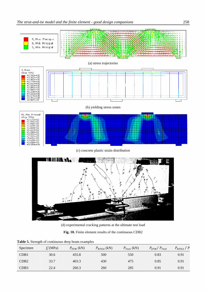
The results of the NFEA, Figs. 10b and 10c,

illustrate a major diagonal crack in the intermediate

shear span of the beam, as in the experimental

observations, Fig. 10d. The failure occurred in the

interior shear spans between the loading points and

middle support. The maximum concrete

compressive stresses in the beam CDB2 near failure

were 33MPa. Neither the bottom nor the top

longitudinal bars reached yield; they were 360MPa

and 150MPa, respectively; but the vertical web

reinforcement almost reached its yield strength. The

predicted failure load from the 3D nonlinear finite

element analysis was 2P = 860 kN, which is about

91% of the measured value in the test.

5.4. Predicted capacity and test

The strength predicted by the STM and the NFEA is

given in Table 5 along with the experimental

values. The prediction from the STM, as expected,

is on the safe side. On the other hand, the results

from the NFEA are closer to the measured strength.

6. Continuous deep beams with large openings

6.1. Description

Two full-scale continuous reinforced concrete deep

beams with large openings, specimens A and B,

subject to two concentrated loads at mid-spans

tested by [17] were selected for the comparison

between the two-dimensional strut-and-tie

modeling and the 3D nonlinear finite element

analysis, Figs. 11 and 12. The two specimens have

identical overall dimensions and loading

arrangement, albeit, different sized openings. The

opening is 200 × 200 mm in specimen A and 400 ×

200 mm in specimen B. Only specimen B is

presented here with details and the results of the

other beam will be given at the end of this section.

With reference to Fig. 12, the beam height, h =

750 mm, depth, d = 705 mm, breadth, b = 180 mm,

the width of bearing plates 𝑏1= 150 mm, and 𝑏2=

𝑏3= 200 mm. The shear span, a = 1000 mm. The

shear span-to-depth ratio, 𝑎 𝑑⁄ = 1000 705⁄ = 1.41.

The tension steel, 𝐴𝑠1 = 𝐴𝑠2= 628.3 mm2. The

concrete cylinder strength, 𝑓𝑐′ = 27.7 MPa. High

strength deformed steel bars, with yield stress, 𝑓y =

460 MPa, and mild steel bar with a nominal yield

stress, 𝑓y = 250 MPa. The vertical and horizontal

web reinforcement is as shown in the figures.

In addition to the reinforcements required at the

tie positions, confining reinforcement was

incorporated to improve the strength of nodes

where potentially high compressive stresses were

encountered. Confining reinforcement was used

below the concentrated loads, above the supports,

and around the openings, Fig. 12.

The strut-and-tie model and the finite element - good design companions 258

(a) stress trajectories

(b) yielding stress zones

(c) concrete plastic strain distribution

(d) experimental cracking patterns at the ultimate test load

Fig. 10. Finite element results of the continuous CDB2

Table 5. Strength of continuous deep beam examples

Specimen 𝑓𝑐′(MPa) 𝑃𝑆𝑇𝑀 (kN) 𝑃𝑁𝐹𝐸𝐴 (kN) 𝑃𝑇𝑒𝑠𝑡 (kN) 𝑃𝑆𝑇𝑀 𝑃𝑇𝑒𝑠𝑡⁄ 𝑃𝑁𝐹𝐸𝐴 𝑃𝑇𝑒𝑠𝑡⁄

CDB1 30.6 455.8 500 550 0.83 0.91

CDB2 33.7 403.3 430 475 0.85 0.91

CDB3 22.4 260.3 260 285 0.91 0.91

259 Ghoraba et al.

Fig. 11. Continuous deep beam with openings, specimen A

Fig. 12. Continuous deep beam with openings, specimen B

The strut-and-tie model and the finite element - good design companions 260

To eliminate potentially the detrimental effects of

apparently inadequate reinforcing details on load-

carrying capacity, the reinforcing bars passing the

nodes were extended beyond the nodal zones and

the bottom longitudinal reinforcing bars were

extended into the end supports and were anchored

using standard 180-degree hooks.

6.2. Strut-and-tie modeling of specimen B

6.2.1. Geometrical parameters

From the stress pattern obtained from the linear

elastic analysis, Fig. 15a, it is obvious how the

struts go around the openings to transfer their forces

to the supports. In addition, the connecting ties

maintaining equilibrium are logical and adhere to

the reinforcement details. Thus, developing an STM

of the beam becomes a straightforward matter. For,

the proposed STM, shown in Fig. 13, the numbering

of ties and struts is illustrated on the left part of the

model and the numbering of the nodes is illustrated

on the right part.

With reference to Fig. 13, the reinforcement of

each of the ties 𝑇1, 𝑇2, and 𝑇13 are 2T20. Since the

reinforcement details allow the use of extended

nodal zones, the width of each of these ties, the

height of nodes 1, 2, 11 and 15, are as follows,

𝑤𝑇1= 𝑤𝑇2

= 2(𝑡 – 𝑑) = 2 (750 – 705) = 90mm,

or

𝑤𝑇1= 𝑤𝑇2

= 2(𝑐 + ∅𝑠𝑡𝑖𝑟𝑟𝑢𝑝) + 𝑛∅𝑏𝑎𝑟 + (𝑛 − 1)𝑠

Each of the ties 𝑇1, 𝑇2, and 𝑇13 has a nominal

strength, 𝑇1𝑛 = 𝑇2𝑛= 𝑇13𝑛 = 460 × 628.3 = 289 kN.

Each of the ties 𝑇3, 𝑇6, 𝑇8 and 𝑇11 is represented by

2𝑇13 |(2-legs) vertical stirrups, spaced 90 mm

center to center. The width of each of these ties is

𝑤𝑇3 = 𝑤𝑇6

= … = 2c + n∅𝑏𝑎𝑟 + (𝑛 − 1)𝑠 =166 mm.

The nominal strength of each of the

ties 𝑇3, 𝑇6, 𝑇8 and 𝑇11 is

𝑇3𝑛= 𝑇6𝑛= … = 𝐴𝑠 × 𝑓y = (2×2×132.7) × 460 = 144.4kN.

In the same manner, each of the ties 𝑇4, 𝑇5, 𝑇7,

𝑇9, 𝑇10 and 𝑇12 are represented by (2T13 + 2T10)

horizontal bars with width 143 mm and nominal

strength 194.2 kN.

6.2.2. Reactions

From linear elastic analysis, 𝑉1 = 0.3125P and 𝑉2 =

1.375P.

6.2.3. Model geometry and forces

In order to obtain the forces in the model elements,

the reinforcement of a selected tie is assumed to

reach its yield stress. The choice of the tie to start

with is up to the designer; however, some elements

come to mind at the first glance; e.g., ties 𝑇2 or 𝑇13,

Fig. 13. Nevertheless, the solution to this problem

is initiated by assuming that the reinforcement of tie

𝑇10 reaches its yield stress, 𝑇10= 194.2 kN. Then,

from simple truss analysis, the model forces are

obtained, Fig. 14.

Fig. 13. Proposed strut-and-tie model for specimen B

261 Ghoraba et al.

Fig. 14. Computed model forces (𝑘𝑁) assuming yielding of 𝑇10 reinforcement

6.2.4. Effective concrete strength of the struts

The effective concrete strength of strut,

𝑓𝑐𝑒𝑠 = 0.85𝑓𝑐

′𝛽𝑠

For prismatic strut,

𝑓𝑐𝑒𝑠 = 0.85 × 27.7 × 1.0 = 23.55 MPa

For bottle-shaped strut with sufficient

reinforcement to resist the transverse tension,

𝑓𝑐𝑒𝑠 = 0.85 × 27.7 × 0.75 = 17.66 MPa

This value will be used throughout the example

and it will be checked later.

6.2.5. Effective concrete strength of the nodes

The effective concrete strength of a node,

𝑓𝑐𝑒𝑛 = 0.85𝑓𝑐

′𝛽𝑛.

For C – C – C node,

𝑓𝑐𝑒𝑛 = 0.85 × 27.7 × 1.0 = 23.55 MPa.

For C – C – T node,

𝑓𝑐𝑒𝑛 = 0.85 × 27.7 × 0.80 = 18.84 MPa.

For C – T – T node,

𝑓𝑐𝑒𝑛 = 0.85 × 27.7 × 0.60 = 14.13 MPa

6.2.6. Check the bearing of the nodes

For node 1, the nominal value of the reaction 𝑉1,

𝑉1𝑛 = 18.84 × 150 × 180 = 508.6 kN, which is

greater than the reaction, 𝑉1 = 186.8 kN.

For nodes 8 and 9, the nominal value of the load

P, 𝑃𝑛 = 23.55 × 200 × 180 = 847.6 kN, which is

greater than the load, P = 598 kN.

For node 16, the nominal value of the

reaction 𝑉2, 𝑉2𝑛 = 23.55 × 200 × 180 = 847.6 kN,

which is greater than the reaction, 𝑉2 = 822.4 kN.

6.2.7. Check of stresses

Node 1:

Since the bearing stress has been checked before,

there is no need to check it again. The inclination

angle of the strut 𝐶1, 𝛳1= 70.3o, which gives a

width of the strut 𝑤𝐶11 = 150 sin 𝛳1 +

90 cos 𝛳1=171.5 mm. Then, the nominal strength of

the strut 𝐶1𝑛 = 17.66# × 171.5 × 180 = 545.1 kN (#

the smaller of the node strength and the strut

strength), which is greater than the strut force, 𝐶1 =

198.4 kN.

Node 2:

The width of the tie 𝑇2, 𝑤𝑇2 = 90mm and of tie 𝑇3,

𝑤𝑇3 = 166 mm, and the angle of inclination of the

strut 𝐶4, 𝛳4 = 25.0o. Hence, the width of the

strut 𝐶4, 𝑤𝐶4= 166 sin 𝛳4 + 90 cos 𝛳4 = 151.7 mm.

Then, the nominal strength of the strut 𝐶4𝑛 = 14.13#

× 151.7 × 180 = 385.7 kN (# the smaller of the node

strength and the strut strength), which is greater

than the strut force, 𝐶4 = 189.2 kN.

Nodes 3, 7, 10, and 14:

These nodes need not be checked, since they are

smeared nodes, and "the reinforcing bars passing

the nodes are extended beyond the nodal zones and

they have sufficient anchorage length." Besides, the

strength of the struts connected with these nodes is

The strut-and-tie model and the finite element - good design companions 262

governed by either the strength of the other

connecting nodes or the strength of these struts.

Node 4:

The width of the tie 𝑇3, 𝑤𝑇3 = 166 mm, and of tie 𝑇5,

𝑤𝑇5 = 143 mm, and the angle of inclination of the

strut 𝐶2, 𝛳2 = 50.2o. Hence, the width of the

strut 𝐶2, 𝑤𝐶24 = 166 sin 𝛳2 + 143 cos 𝛳2 = 219 mm.

Then, the nominal strength of the strut,

𝐶2𝑛 =

14.13# × 219 × 180 = 556.8 kN (# the smaller of the

node strength and the strut strength), which is

greater than the strut force, 𝐶2 = 243.2 kN.

For strut 𝐶3, the angle of inclination is 𝛳3 = 25.0o.

Then, the width of the strut,

𝑤𝐶34 = 166 sin 𝛳3 +

143 cos 𝛳3 = 199.7 mm. Then, the nominal strength

of the strut, 𝐶3𝑛 = 14.13# × 199.7 × 180 = 508 kN

(# the smaller of the node strength and the strut

strength), which is greater than the strut force, 𝐶3 =

252.6 kN.

Node 5:

As for nodes 1, 2, and 4, 𝑤𝑇6 = 166 mm, 𝑤𝑇7

= 143

mm, 𝛳4 = 25.0o,

𝑤𝐶45 = 199.7 mm, 𝐶4𝑛 = 508 kN, greater than 𝐶4 =

189.2 kN. Also, 𝛳5 = 54.0o,

𝑤𝐶55 = 218.4 mm, 𝐶5𝑛 = 555.2 kN, greater than 𝐶5 =

231.2 kN.

Node 6:

For this node, assuming that the force in the

prismatic strut 𝐶7 is equal to its nominal strength;

then, 𝐶7 = 228.9 kN = 23.55 × 𝑤𝐶7 × 180, which

gives 𝑤𝐶7 = 54 mm. The width of the tie 𝑇6, 𝑤𝑇6

=

166 mm and the angle of inclination of the strut 𝐶3,

𝛳3 = 25.0o. Hence, the width of the strut 𝐶3, 𝑤𝐶36 =

166 sin 𝛳3 + 54 cos 𝛳3 = 119.1 mm. Then, the

nominal strength of the strut, 𝐶3𝑛 = 17.66# × 119.1

× 180 = 378.6 kN (# the smaller of the node strength

and the strut strength), which is greater than the

strut force, 𝐶3 = 252.6 kN.

Node 8:

Since the bearing stress has been checked before,

there is no need to check it again. The width of the

prismatic strut 𝐶8 can be obtained upon assuming

that the force in the strut is equal to its nominal

strength; then, 𝐶8 = 273.3 kN = 23.55 × 𝑤𝐶8 × 180,

which gives 𝑤𝐶8 = 64.5 mm. The angle of

inclination of the strut 𝐶6 is 𝛳6 = 76.6o. Hence, the

width of the strut 𝐶6, 𝑤𝐶68 = 100 sin 𝛳6 + 64.5 cos 𝛳6

= 112.2 mm. Then, the nominal strength of the strut,

𝐶6𝑛 = 17.66# × 112.2 × 180 = 356.6 kN (# the

smaller of the node strength and the strut strength),

which is greater than the strut force, 𝐶6 = 192 kN.

Node 9:

Since the bearing stress has been checked before,

there is no need to check it again. The width of the

prismatic strut 𝐶8, 𝑤𝐶8 = 64.5 mm, and the angle of

the inclination angle of the strut 𝐶10 is 𝛳10 = 76.6o.

Then, the width of the strut 𝐶10, 𝑤𝐶109 = 100 sin 𝛳10

+ 64.5 cos 𝛳10 = 112.2 mm. The nominal strength

of the strut 𝐶10 is then, 𝐶10𝑛 = 17.66# × 112.2 × 180

= 356.6 kN (# the smaller of the node strength and

the strut strength), which is less than the strut force,

𝐶10 = 422.7 kN; i.e., 𝐶10𝑛 = 0.843 𝐶10.

Node 11:

The width of the tie 𝑇8, 𝑤𝑇8 = 166 mm, and of

tie 𝑇13, 𝑤𝑇13 = 90 mm, and the angle of inclination

of the strut 𝐶14, 𝛳14 = 25.0o. Then, the width of the

strut, 𝑤𝐶14

11 = 166 sin 𝛳14 + 90 cos 𝛳14 = 151.7 mm.

Then, the nominal strength of the strut,

𝐶14𝑛 =

14.13# × 151.7 × 180 = 385.7 kN (# the smaller of

the node strength and the strut strength), which is

less than the strut force, 𝐶14 = 486.5 kN; i.e., 𝐶14𝑛

= 0.793 𝐶14.

Node 12:

As for nodes 1, 2, and 3, 𝑤𝑇8 = 166 mm, 𝑤𝑇7

= 143

mm, the angle of inclination of the strut 𝐶12, 𝛳12 =

54.0o, and 𝑤𝐶1212 = 218.4 mm. The nominal strength

of the strut 𝐶12, 𝐶12𝑛 = 555.2 kN, which is greater

than the strut force, 𝐶12 = 508.9 kN. As for

strut 𝐶13, the angle of inclination, 𝛳13 = 25.0o, and

𝑤𝐶1312 = 199.7 mm, 𝐶13𝑛 = 508 kN, which is greater

than the strut force, 𝐶13 = 485.9 kN.

Node 13:

As for nodes 1, 2, and 3, 𝑤𝑇11 = 166 mm, 𝑤𝑇12

=

143 mm, the angle of inclination of the strut 𝐶14,

𝛳14 = 25.0o and 𝑤𝐶1413 = 199.7 mm. The nominal

strength of the strut 𝐶14, 𝐶14𝑛 = 508 kN, which is

263 Ghoraba et al.

greater than the strut force, 𝐶14 = 486.5 kN. As for

strut 𝐶15, the angle of inclination, 𝛳15 = 54.0o, and

𝑤𝐶1513 = 218.4 mm; then, 𝐶15𝑛 = 555.2 kN, which is

greater than the strut force, 𝐶15 = 508.9 kN.

Node 15:

As for nodes 1, 2, and 3, 𝑤𝑇11 = 166 mm, 𝑤𝑇2

= 90

mm, the angle of inclination of the strut 𝐶13, 𝛳13 =

25.0o and 𝑤𝐶1315 = 151.7 mm. The nominal strength

of the strut 𝐶13, 𝐶13𝑛 = 385.7 kN, which is less than

the strut force, 𝐶13 = 485.9 kN; i.e., 𝐶13𝑛 =

0.794 𝐶13.

Node 16:

Since the bearing stress has been checked before,

there is no need to check it again. The width of the

prismatic strut 𝐶18 can be obtained by assuming that

the force in the strut is equal to its nominal strength;

then, 𝐶18 = 300.1 kN = 23.55 × 𝑤𝐶8 × 180, which

gives 𝑤𝐶18 = 70.8 mm. The angle of inclination of

the strut 𝐶16, 𝛳16 = 76.6o; hence, its width, 𝑤𝐶16

16 =

100 sin 𝛳16 + 70.8 cos 𝛳16 = 113.7 mm. Then, the

nominal strength of the strut, 𝐶16𝑛 = 17.66# × 113.7

× 180 = 361.4 kN, which is less than the strut force,

𝐶16 = 422.7 kN; i.e., 𝐶16𝑛 = 0.855 𝐶16.

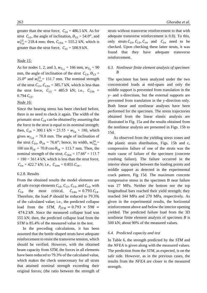
6.2.8. Results

From the obtained results the model elements are

all safe except elements 𝐶10, 𝐶13, 𝐶14, and 𝐶16, with

𝐶14 the most critical, 𝐶14𝑛 = 0.793 𝐶14.

Therefore, the load P should be reduced to 79.3%

of the calculated value; i.e., the predicted collapse

load from the STM, 𝑃𝑆𝑇𝑀 = 0.793 × 598 =

474.2 kN. Since the measured collapse load was

555 kN; then, the predicted collapse load from the

STM is 85.4% of the measured value in the test.

In the preceding calculations, it has been

assumed that the bottle-shaped struts have adequate

reinforcement to resist the transverse tension, which

should be verified. However, with the obtained

beam capacity from STM, the forces in all elements

have been reduced to 79.3% of the calculated value,

which makes the check unnecessary for all struts

that attained nominal strength exceeding their

original forces; (the ratio between the strength of

struts without transverse reinforcement to that with

adequate transverse reinforcement is 0.8). To this,

only struts 𝐶10, 𝐶13, 𝐶14 and 𝐶16 need to be

checked. Upon checking these latter struts, it was

found that they have adequate transverse

reinforcement.

6.3. Nonlinear finite element analysis of specimen

B

The specimen has been analyzed under the two

concentrated loads at mid-spans and only the

middle support is prevented from translation in the

y- and x-directions, but the external supports are

prevented from translation in the y-direction only.

Both linear and nonlinear analyses have been

performed for the specimen. The stress trajectories

obtained from the linear elastic analysis are

illustrated in Fig. 15a and the results obtained from

the nonlinear analysis are presented in Figs. 15b to

15d.

As observed from the yielding stress zones and

the plastic strain distribution, Figs. 15b and c,

compression failure of one of the struts was the

main cause of failure of the specimen (concrete

crushing failure). The failure occurred in the

interior shear spans between the loading points and

middle support as detected in the experimental

crack pattern, Fig 15d. The maximum concrete

compressive stress in the specimen B near failure

was 27 MPa. Neither the bottom nor the top

longitudinal bars reached their yield strength; they

reached 344 MPa and 270 MPa, respectively. As

given in the experimental results, the horizontal

reinforcement above and below the interior opening

yielded. The predicted failure load from the 3D

nonlinear finite element analysis of specimen B is

500 kN; about 90% of the measured values.

6.4. Predicted capacity and test

In Table 6, the strength predicted by the STM and

the NFEA is given along with the measured values.

The prediction from the STM, as expected, is on the

safe side. However, as in the previous cases, the

results from the NFEA are closer to the measured

strength.

The strut-and-tie model and the finite element - good design companions 264

(a) stress trajectories

(b) yielding stress zones

(c) concrete plastic strain distribution

(d) experimental cracking patterns at the ultimate test load

Fig. 15. Finite element results of specimen B

Table 6. Strength of specimens A and B of continuous deep beams with large openings

Specimen 𝑓𝑐′( MPa) 𝑃𝑆𝑇𝑀(𝑘𝑁) 𝑃𝑁𝐹𝐸𝐴(𝑘𝑁) 𝑃𝑇𝑒𝑠𝑡 𝑃𝑆𝑇𝑀 𝑃𝑇𝑒𝑠𝑡⁄ 𝑃𝑁𝐹𝐸𝐴 𝑃𝑇𝑒𝑠𝑡⁄

A 26.4 481.2 510 565 0.85 0.90

B 27.7 474.2 500 555 0.85 0.90

7. Ledges of inverted-T beams

7.1. Description

Four full-size normal strength reinforced concrete

Inverted-T beams (SS3-42-2.5-06, C1-42-1.85-06,

DC1-42-2.5-03, and SC1-42-1.85-03) with various

details of web reinforcement, ledge geometries,

number of point loads, and shear-span-to-depth

ratio (a/d) that had been tested by [18] were selected

for comparison between the 3D strut-and-tie

265 Ghoraba et al.

modeling and the 3D nonlinear finite element

analysis. Only the details of the strut-and-tie model

and the finite element solutions of beam SC1-42-

1.85-03 are presented here and a su mmary of the

results of the other three beams is given at the end

of this section.

Tables 7 and 8 present details and material

properties of the selected beams, where 𝑓𝑐′ is the

concrete compressive strength, 𝑓y𝑙 is the yield stress

of the longitudinal reinforcement, 𝑓yv is the yield

stress of the transverse reinforcement, 𝑓yh is the

yield stress of the skin reinforcement, and 𝑓yha is

the yield stress of the hanger steel. Besides, Table 9

gives the distance from the center of the load to the

end of the ledge for three ledge types. Fig. 16

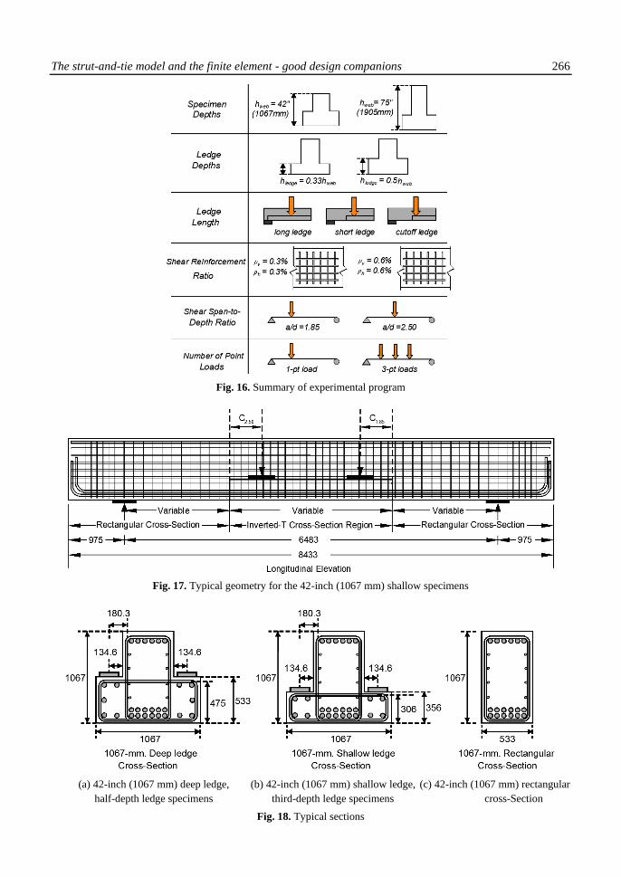
illustrates a summary of the experimental program.

More details of the test and material properties can

be found in [18, 19].

Constant web width of 533 mm was used for the

beams of the experimental program. The width of

the ledge was also the same, 267 mm, on each side

of the beams. All other dimensions varied between

the beams. Figs. 17 and 18 show typical specimen

geometries and reinforcing details of the studied

Inverted-T beams [18].

7.2. Strut-and-tie modeling of specimen SC1-42-

1.85-03

Imperative modifications for both the ACI 318 [14]

and AASHTO LRFD Codes [20] particularly for

the strength of the nodes and the strength of the

strut-to-node interfaces of Inverted-T beams have

been recommended by [18, 21, 22]. A brief

overview of the STM method and failure criteria,

adopted in this study, is presented in this section.

Table 7. Summary of beam details

Specimen

Web

Height

h, (mm)

Ledge

Depth

(mm)

Ledge

Length

Load

Point

𝑏𝑤,

(mm)

d,

(mm) a/d

Support

Plate

(mm)

Load

Plate

(mm)

SS3-42-2.50-06 1067 356 Short 3 533 956 2.50 406×508 457×229

C1-42-1.85-06 1067 ---- Cut-off 1 533 956 1.85 406×508 762×508

DC1-42-2.50-03 1067 533 Cut-off 1 533 956 2.50 406×508 457×229

SC1-42-1.85-03 1067 356 Cut-off 1 533 956 1.85 762×508 660×229

Plate dimensions: [direction of span] × [perpendicular to span direction]

Table 8. Summary of specimen material strengths

Specimen 𝑓𝑐

′

(MPa)

𝑓𝑦𝑙

(MPa)

𝑓𝑦𝑣

(MPa)

𝑓𝑦ℎ

(MPa)

𝑓𝑦ℎ𝑎

(MPa) 𝜌𝑣 𝜌ℎ

SS3-42-2.50-06 43.13 480 420 420 426.3 0.6% 0.6%

C1-42-1.85-06 25.7 480 420 420 440 0.6% 0.6%

DC1-42-2.50-03 27.8 480 430 430 440 0.3% 0.3%

SC1-42-1.85-03 30 460 460 460 440 0.3% 0.3%

Table 9. Distance from center of the load to the end of the ledge for three ledge types

Ledge Type 𝐶1.85 𝐶2.50

Cut-off (76.2 mm) past bearing end (76.2 mm) past bearing end

Short (901.7 mm) (863.6 mm)

Long (1768 mm) (2390 mm)

The strut-and-tie model and the finite element - good design companions 266

Fig. 16. Summary of experimental program

Fig. 17. Typical geometry for the 42-inch (1067 mm) shallow specimens

(a) 42-inch (1067 mm) deep ledge, (b) 42-inch (1067 mm) shallow ledge, (c) 42-inch (1067 mm) rectangular

half-depth ledge specimens third-depth ledge specimens cross-Section

Fig. 18. Typical sections

267 Ghoraba et al.

The value of the limiting compressive stress at

the face of the node, 𝑓𝑐𝑢, can be obtained from:

𝑓𝑐𝑢 = m ν 𝑓𝑐′

where m is the triaxial confinement factor, ν is the

concrete efficiency factor, and 𝑓𝑐′ is the specified

compressive strength of the concrete. The triaxial

confinement factor, m, is calculated using the

following equation: m = √𝐴2 𝐴1 ⁄ , where 𝐴1 is the

loaded area and 𝐴2 is measured on the plane

defined by the location at which a line with a 2:1

slope extended from the loading area meets the

edge of the member as shown in Fig. 19.

The concrete efficiency factors, v, are used to

reduce the compressive strength of the concrete in

the node depending on the type of node (CCC,

CCT, or CTT) and face (bearing face, back face,

strut-to-node interface) under consideration. These

factors are summarized in Table 10.

A three-dimensional strut-and-tie model as

shown in Fig. 20 has to be considered, because the

loads in Inverted-T beams are transferred from the

ledges to the web, from the tension- to the

compression-chord, and from the loading, points to

support. However, for simplification, a three-

dimensional strut-and-tie model is decomposed into

the two-dimensional longitudinal model and two-

dimensional cross-sectional model.

Input data:

The beam height, h = 1067 mm, depth, d = 956 mm,

breadth, 𝑏𝑤 = 533 mm, ledge height, ℎ1= 356 mm,

ledge depth, 𝑑1= 306 mm, the load plate width 𝑤𝑙=

229 mm, and the load plate length 𝑙𝑙= 660 mm, the

support plate width 𝑤𝑠= 508 mm, and the support

plate length 𝑙𝑠= 762 mm. The shear span, 𝐿1 = 1768

mm. The shear span-to-depth ratio, 𝑎 𝑑⁄ =

1768 956⁄ = 1.85. The tension steel, 𝐴𝑠 = 12T36=

12077.4 mm2, and the compression steel, 𝐴𝑠′ =

6T36= 6038.7 mm2 . The cylinder compressive

strength of concrete, 𝑓𝑐′ = 30 MPa = 4330 psi. High

strength deformed steel bars, with yield

strength, 𝑓y−T36 = 460 MPa, 𝑓y−T19 = 440 MPa, and

𝑓y−T13 = 460 MPa and the vertical and horizontal

web reinforcement are as shown in Fig. 21.

Fig. 19. Determination of 𝐴2 for stepped or sloped supports [6]

Table 10. Concrete efficiency factors, ν [18]

Face Node Type

CCC CCT CTT

Bearing 0.85 0.70

0.45 ≤ 0.85 – 𝑓𝑐

′

20ksi ≥ 0.65 Back

Strut-to-node interface* 0.45 ≤ 0.85 – 𝑓𝑐

′

20ksi ≥ 0.65 0.45 ≤ 0.85 –

𝑓𝑐′

20ksi ≥ 0.65

* If crack control reinforcement requirement of AASHTO Art. 5.6.3.5 is not satisfied, use 𝜈 = 0.45 for the strut-to-node interface.

The strut-and-tie model and the finite element - good design companions 268

Fig. 20. STM of Inverted-T beam [23] (a) 3D STM; (b) 2D cross-sectional model; and (c) 2D longitudinal model

Fig. 21. Elevation and cross-sectional details of SC1-42-1.85-03

7.2.1. Longitudinal STM model

Geometrical parameters

The solution procedure starts with determining the

geometrical layout for the longitudinal STM shown

in Fig. 22. The 12T36 reinforcement of each of the

ties 𝑇1, 𝑇2, 𝑇3, and 𝑇4, give a nominal strength,

𝑇1𝑛 = 𝑇2𝑛= 𝑇3𝑛 = 𝑇4𝑛 = 𝐴𝑠 × 𝑓y = 5618.64 kN.

Since the reinforcement details allow the use of

an extended nodal zone, the width of each of these

ties (height of nodes A, C, E, G, and H) are

𝑤𝑇1= 𝑤𝑇2

= 2(t – d) = 2 (1067 – 956) = 222 mm.

269 Ghoraba et al.

Fig. 22. Longitudinal strut-and-tie model for SC1-42-1.85-03

With reference to Fig. 22, the hanger ties, 𝑇5 and

𝑇6 are represented by (14T19) and (8T19),

respectively, so their nominal strengths are

𝑇5𝑛= 𝐴𝑠 × 𝑓y = (14×2×283.5) × 440 = 3492.7 kN.

𝑇6𝑛= 𝐴𝑠 × 𝑓y = (8×2×283.5) × 440 = 1995.8 kN.

In the same manner, 𝑇7 is represented by (7T13

+ 3T19), giving a nominal strength,

𝑇7𝑛 = 𝐴𝑠𝑓y = [(7 × 2 × 132.7)(460) + (3 × 2 ×

283.5)(440)] = 1603 kN.

Reactions

From linear elastic analysis, 𝑉1 = 0.73P and 𝑉2 =

0.27P

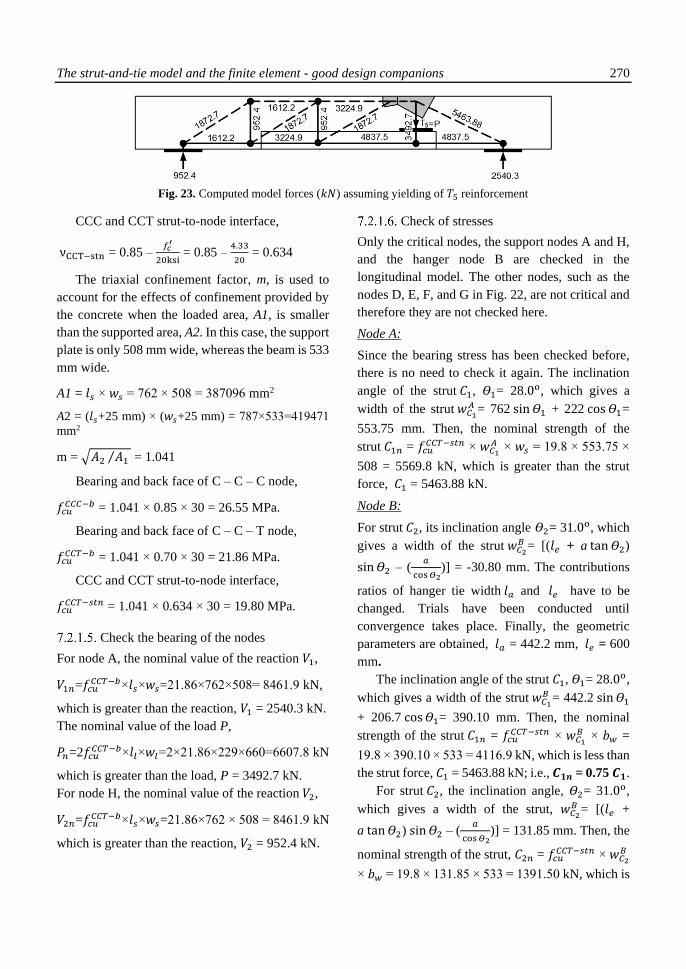
Model geometry and forces

In order to obtain the forces in the model elements,

the reinforcement of a selected tie is assumed to

reach its yield stress. The solution to this problem

is initiated by assuming that the reinforcement of tie

𝑇5 reaches its yield stress, 𝑇5 = 3492.7 kN. Then,

from simple truss analysis, the model forces are

obtained, Fig. 23. The size of the nodes has to be

specified, to determine the locations of the struts

and ties. The length of Node B in the longitudinal

direction is determined by the spread length of the

hanger tie 𝑇5, 𝑙𝑠𝑝. It is proportionally divided into 𝑙𝑒

and 𝑙𝑎 according to the amount of the applied load

that acts on the left and right support [22].

The load spread

( 𝑙𝑠𝑝) = 𝑙𝑙+ 𝑑1 +76.2 mm = 1042.2 mm

Portion of the load spread length, 𝑙𝑠𝑝, on the

right support ( 𝑙𝑎) = 𝑙𝑠𝑝 × ( 𝐿2/L) = 758 mm

Portion of the load spread length, 𝑙𝑠𝑝, on the left

support ( 𝑙𝑒) = 𝑙𝑠𝑝 × (1 – 𝐿2/L) = 284.2 mm

Distance from center of length 𝑙𝑎 to the location

of tie

𝑇5( 𝑙𝑎𝑏) = 0.50 𝑙𝑎 + 𝑙𝑒 – 0.50 𝑙𝑠𝑝 = 142.1 mm

Distance from center of length 𝑙𝑒 to the location

of tie

𝑇5( 𝑙𝑏𝑒) = 0.50 𝑙𝑒 + 𝑙𝑎 – 0.50 𝑙𝑠𝑝 = 379 mm

Distance from the end of the load spread 𝑙𝑠𝑝, to

the left support

( 𝑙2.50) = ( 𝐿2– 𝑙𝑏𝑒)/3) = 1445.3 mm.

The depth of the node is taken as the depth of

the compression stress block, a,

𝑎 = 𝐴𝑠𝑓y − 𝐴𝑠

′ 𝑓y

0.85 𝑏𝑤𝑓𝑐′

= 206.7 mm

Although a traditional flexural analysis is not

valid in a D-region due to the nonlinear distribution

of strains, defining a using the equation above is

conservative according to [22]. The moment arm,

𝑦𝑐𝑡 = 𝑑 – 0.5𝑎 = 852.7 mm.

The limiting compressive stress at the face

of each node

The limiting compressive stress at the face of the

node, 𝑓𝑐𝑢= m ν 𝑓𝑐′

A concrete efficiency factor, ν, is applied to the

concrete strength, 𝑓𝑐′, to limit the compressive stress

at the face of each node:

Bearing and back face of C – C – C node,

νCCC−b = 0.85

Bearing and back face of C – C – T node,

νCCT−b = 0.70

The strut-and-tie model and the finite element - good design companions 270

Fig. 23. Computed model forces (𝑘𝑁) assuming yielding of 𝑇5 reinforcement

CCC and CCT strut-to-node interface,

νCCT−stn = 0.85 – 𝑓𝑐

′

20ksi = 0.85 –

4.33

20 = 0.634

The triaxial confinement factor, m, is used to

account for the effects of confinement provided by

the concrete when the loaded area, A1, is smaller

than the supported area, A2. In this case, the support

plate is only 508 mm wide, whereas the beam is 533

mm wide.

A1 = 𝑙𝑠 × 𝑤𝑠 = 762 × 508 = 387096 mm2

A2 = (𝑙𝑠+25 mm) × (𝑤𝑠+25 mm) = 787×533=419471

mm2

m = √𝐴2 𝐴1 ⁄ = 1.041

Bearing and back face of C – C – C node,

𝑓𝑐𝑢𝐶𝐶𝐶−𝑏 = 1.041 × 0.85 × 30 = 26.55 MPa.

Bearing and back face of C – C – T node,

𝑓𝑐𝑢𝐶𝐶𝑇−𝑏 = 1.041 × 0.70 × 30 = 21.86 MPa.

CCC and CCT strut-to-node interface,

𝑓𝑐𝑢𝐶𝐶𝑇−𝑠𝑡𝑛 = 1.041 × 0.634 × 30 = 19.80 MPa.

Check the bearing of the nodes

For node A, the nominal value of the reaction 𝑉1,

𝑉1𝑛=𝑓𝑐𝑢𝐶𝐶𝑇−𝑏×𝑙𝑠×𝑤𝑠=21.86×762×508= 8461.9 kN,

which is greater than the reaction, 𝑉1 = 2540.3 kN.

The nominal value of the load P,

𝑃𝑛=2𝑓𝑐𝑢𝐶𝐶𝑇−𝑏×𝑙𝑙×𝑤𝑙=2×21.86×229×660=6607.8 kN

which is greater than the load, P = 3492.7 kN.

For node H, the nominal value of the reaction 𝑉2,

𝑉2𝑛=𝑓𝑐𝑢𝐶𝐶𝑇−𝑏×𝑙𝑠×𝑤𝑠=21.86×762 × 508 = 8461.9 kN

which is greater than the reaction, 𝑉2 = 952.4 kN.

Check of stresses

Only the critical nodes, the support nodes A and H,

and the hanger node B are checked in the

longitudinal model. The other nodes, such as the

nodes D, E, F, and G in Fig. 22, are not critical and

therefore they are not checked here.

Node A:

Since the bearing stress has been checked before,

there is no need to check it again. The inclination

angle of the strut 𝐶1, 𝛳1= 28.0o, which gives a

width of the strut 𝑤𝐶1𝐴 = 762 sin 𝛳1 + 222 cos 𝛳1=

553.75 mm. Then, the nominal strength of the

strut 𝐶1𝑛 = 𝑓𝑐𝑢𝐶𝐶𝑇−𝑠𝑡𝑛 × 𝑤𝐶1

𝐴 × 𝑤𝑠 = 19.8 × 553.75 ×

508 = 5569.8 kN, which is greater than the strut

force, 𝐶1 = 5463.88 kN.

Node B:

For strut 𝐶2, its inclination angle 𝛳2= 31.0o, which

gives a width of the strut 𝑤𝐶2𝐵 = [(𝑙𝑒 + a tan 𝛳2)

sin 𝛳2 – (𝑎

cos 𝛳2)] = -30.80 mm. The contributions

ratios of hanger tie width 𝑙𝑎 and 𝑙𝑒 have to be

changed. Trials have been conducted until

convergence takes place. Finally, the geometric

parameters are obtained, 𝑙𝑎 = 442.2 mm, 𝑙𝑒 = 600

mm.

The inclination angle of the strut 𝐶1, 𝛳1= 28.0o,

which gives a width of the strut 𝑤𝐶1𝐵 = 442.2 sin 𝛳1

+ 206.7 cos 𝛳1= 390.10 mm. Then, the nominal

strength of the strut 𝐶1𝑛 = 𝑓𝑐𝑢𝐶𝐶𝑇−𝑠𝑡𝑛 × 𝑤𝐶1

𝐵 × 𝑏𝑤 =

19.8 × 390.10 × 533 = 4116.9 kN, which is less than

the strut force, 𝐶1 = 5463.88 kN; i.e., 𝑪𝟏𝒏 = 0.75 𝑪𝟏.

For strut 𝐶2, the inclination angle, 𝛳2= 31.0o,

which gives a width of the strut, 𝑤𝐶2𝐵 = [(𝑙𝑒 +

a tan 𝛳2) sin 𝛳2 – (𝑎

cos 𝛳2)] = 131.85 mm. Then, the

nominal strength of the strut, 𝐶2𝑛 = 𝑓𝑐𝑢𝐶𝐶𝑇−𝑠𝑡𝑛 × 𝑤𝐶2

𝐵

× 𝑏𝑤 = 19.8 × 131.85 × 533 = 1391.50 kN, which is

271 Ghoraba et al.

less than the strut force, 𝐶2 = 1872.70 kN; i.e., 𝑪𝟐𝒏

= 0.74 𝑪𝟐.

For strut 𝐶3, the nominal strength of the

strut 𝐶3𝑛 = 𝑓𝑐𝑢𝐶𝐶𝑇−𝑠𝑡𝑛 × a × 𝑏𝑤 + 𝐴𝑠

′ 𝑓y = 19.8 × 206.7

× 533 + 6107.25 × 460 = 4990.72 kN, which is

greater than the strut force, 𝐶3 = 3224.9 kN.

Node H:

Since the bearing stress has been checked before,

there is no need to check it again. The inclination

angle of the strut 𝐶6, 𝛳6= 31.0o, which gives a

width of the strut, 𝑤𝐶6𝐻 = 762 sin 𝛳6 + 222 cos 𝛳6=

582.75 mm. Then, the nominal strength of the

strut 𝐶1𝑛 = 𝑓𝑐𝑢𝐶𝐶𝑇−𝑠𝑡𝑛 × 𝑤𝐶6

𝐻 × 𝑤𝑠 = 19.8 × 582.75 ×

508 = 5861.53 kN, which is greater than the strut

force, 𝐶6 = 1872.70 kN.

From the obtained results the longitudinal STM

model elements are all safe except elements 𝐶1 and

𝐶2, with 𝐶2 is the most critical, 𝐶2𝑛 = 0.74 𝐶2.

Therefore, the load P should be reduced to 74%

of the calculated value; i.e., the predicted collapse

load from the STM, 𝑃𝑆𝑇𝑀 = 0.74 × 3492.70 =

2584.60 kN.

7.2.2. Cross-Sectional STM model

Geometrical parameters

The geometrical layout for the cross-sectional STM

model is shown in Fig. 24a, where the numbering

of ties, struts, and nodes are illustrated. Based on

the last obtained load capacity from the longitudinal

STM model, 𝑃𝑆𝑇𝑀 = 2584.60 kN, the forces of the

cross-sectional STM model can be obtained, Fig.

24b.

Truss geometry:

𝑙4=45.7 mm 𝑙1= 𝑙4+ 25.4 mm + 0.50 𝑤𝑙 = 185.6

mm

𝑙2= 𝑏𝑤–2𝑙4=441.6 mm 𝑙3= ℎ1+0.50𝑤𝑇1+ 𝑙𝑠=186.3 mm

𝑙5 = 58.7 mm 𝑙𝑛 = 𝑙𝑠𝑝 – 𝑤𝑇1= 820.2 mm

With reference to Fig. 24, the reinforcement of

tie 𝑇𝐴𝐷 is represented by (12T19). The nominal

strength of the tie is

𝑇𝐴𝐷𝑛= 𝐴𝑠 × 𝑓y = 12×283.5×440 = 1497 kN,

which is greater than the tie force, 𝑇𝐴𝐷 =

1292.3𝑘𝑁.

Check of stresses

Since the cross-section and loading are symmetric,

only one side needs to be checked.

Node A:

Since the bearing stress has been checked before,

there is no need to check it again. For strut 𝐶𝐴𝐵, the

inclination angle, 𝛳𝐴𝐵= 45.0o, which gives a width

of the strut, 𝑤𝐶𝐴𝐵𝐴 = 𝑤𝑙 sin 𝛳𝐴𝐵 + 2𝑙5 cos 𝛳𝐴𝐵 =

244.9 mm. Then, the nominal strength of the strut,

𝐶𝐴𝐵𝑛 = 𝑓𝑐𝑢𝐶𝐶𝑇−𝑠𝑡𝑛 × 𝑤𝐶𝐴𝐵

𝐴 × 𝑙𝑙 = 19.8 × 244.9 × 660

= 3200.9 kN, which is greater than the strut force,

𝐶𝐴𝐵 = 1827.6 kN.

Node B:

For strut 𝐶𝐴𝐵, the inclination angle, 𝛳𝐴𝐵= 45.0o,

which gives a width of the strut, 𝑤𝐶𝐴𝐵𝐵 = 2𝑙4 sin 𝛳𝐴𝐵

+ 𝑤𝑇1cos 𝛳𝐴𝐵 = 221.6 mm. Then, the nominal

strength of the strut, 𝐶𝐴𝐵𝑛 = 𝑓𝑐𝑢𝐶𝐶𝑇−𝑠𝑡𝑛 × 𝑤𝐶𝐴𝐵

𝐵 × 𝑙𝑠𝑝

= 19.8 × 221.6 × 1042.2 = 4573 kN, which is greater

than the strut force, 𝐶𝐴𝐵 = 1827.60 kN. The width

of the prismatic strut, 𝐶𝐵𝐶 is equal to 𝑤𝐶𝐵𝐶= 𝑤𝑇1

=

222𝑚𝑚. Then, the nominal strength of the strut,

𝐶𝐵𝐶𝑛 = 𝑓𝑐𝑢𝐶𝐶𝑇−𝑠𝑡𝑛 × 𝑤𝐶𝐵𝐶

× 𝑙𝑛 = 19.8 × 222 × 820.2

= 3605.3 kN, which is greater than the strut force,

𝐶𝐵𝐶 = 1292.3 kN.

Since the cross-sectional STM model elements

are all safe, the STM capacity is governed by the

longitudinal STM model, 𝑃𝑆𝑇𝑀 = 0.74 × 3492.70 =

2584.60 kN.

The strut-and-tie model and the finite element - good design companions 272

(a) cross-sectional model (b) model forces ( kN).

Fig. 24. Specimen SC1-42-1.85-03

The shear capacity calculated using STM provisions

as implemented for Inverted-T beams, 𝑉𝑆𝑇𝑀 = 0.73

× 𝑃𝑆𝑇𝑀 = 0.73 × 2584.6 = 1886.7 kN. The maximum

shear carried in the critical section of the test region,

including self-weight of the specimen and test setup

is, 𝑉𝑡𝑒𝑠𝑡 = 2060 kN. The critical section was

considered to be the point halfway between the

support and the nearest load. Then, the predicted

collapse load from the STM is about 91.6% of the

value measured in the test.

7.3. Nonlinear finite element analysis of specimen

SC1-42-1.85-03

The specimen has been analyzed under the applied

loads, with the right support is prevented from

translation in the y-direction only, whereas the left

support is prevented from translation in the y- and

x-directions. Both linear and nonlinear analyses

have been performed for the specimen as in the

previous examples. The stress trajectories obtained

from the linear elastic analysis are illustrated in Fig.

25a and the results obtained from the nonlinear

analysis are presented in Figs. 25b to 25d.

As observed from the yielding stress zones in

steel and the concrete plastic strain distribution,

Figs. 25b and 25c, a local failure in the ledge due to

tie yielding associated with web shear failure was

the main cause of failure, which goes along with the

experimental model of failure Fig. 25d. As

observed from the experimental results, the

horizontal ledge stirrups reinforcement yielded,

whereas the stresses in vertical web stirrups were

near yield, they reached 430 MPa. The maximum

concrete compressive stress in the specimen near

failure was 30 MPa. Neither the beam bottom nor

the top longitudinal bars reached their yield stress;

they reached 350 MPa and 250 MPa, respectively.

The predicted maximum shear carried in the critical

section from the 3D nonlinear finite element

analysis is 1920 kN, which is about 93.2% of the

measured values.

7.4. Predicted capacity and test

The strength predicted by the STM and NFEA for

the four specimens is given in Table 11, along with

the measured values. The prediction from the STM,

as expected, is on the safe side. On the other hand,

as in the previous cases, the results from the NFEA

are closer to the measured strength.

8. Conclusions

The focus of this study was to investigate the

applicability and reliability of the strut-and-tie

modeling and the 3D nonlinear finite element

analysis for the prediction of the capacity and

behavior of discontinuity regions. The study aimed

to demonstrate the complementary role of the two

methods as design tools. The two methods have

been successfully applied to different problems,

simply supported deep beam with large opening and

recess, continuous deep beams with and without

large openings, and inverted beams with ledges.

The solutions obtained by the two methods for the

selected problems have been verified by

experimental tests.

From the obtained results the following

conclusions can be drawn:

1. Both the nonlinear finite element and strut-and-

tie method are reliable as design tools for the

prediction of the strength and behavior of

273 Ghoraba et al.

reinforced concrete structures with

discontinuity regions.

2. The strut-and-tie method as a lower-bound

solution always yields a safe solution. Also, the

STM serves as a design tool where the designer

can trace the flow of forces and hence can easily

develop efficient reinforcement details.

3. The nonlinear finite element analysis provides a

more accurate prediction of the ultimate

strength than the strut-and-tie method; however,

there is no guarantee that it provides a safe

solution in every case. Besides, the computation

effort of the NFEA is tedious in co comparison

with the STM. Clear that the NFEA provides a

useful tool in understanding the behavior of

reinforced concrete structures with

discontinuity regions concerning stiffness and

deformations.

(a) stress trajectories

(b) yielding stress zones (elevation and plan)

(c) concrete plastic strain distribution

(d) experimental cracking patterns at the ultimate test load

Fig. 25. Finite element results of specimen SC1-42-1.85-03

The strut-and-tie model and the finite element - good design companions 274

Table 11. Strength of ledge beam specimens

Specimen 𝑓𝑐′( MPa) 𝑉𝑆𝑇𝑀 ( kN) 𝑉𝑁𝐹𝐸𝐴 ( kN) 𝑉𝑇𝑒𝑠𝑡 ( kN) 𝑉𝑆𝑇𝑀 𝑉𝑇𝑒𝑠𝑡⁄ 𝑉𝐹𝐸 𝑉𝑇𝑒𝑠𝑡⁄

SS3-42-2.50-06 43.13 1846 2150 2295.3 0.80 0.93

C1-42-1.85-06 25.7 1904 2570 2833.5 0.67 0.91

DC1-42-2.50-03 27.8 1152 1500 1623.6 0.71 0.92

SC1-42-1.85-03 30 1886.7 1920 2060 0.92 0.93

Declaration of conflicting interests

The author(s) declared no potential conflicts of

interest concerning the research, authorship, and/or

publication of this article.

References

[1] El-Metwally SE, Chen WF (2017) Structural

Concrete: Strut-and-Tie Models for Unified

Design. CRC Press, New York.

[2] Schlaich J, Schäfer K, Jennewein M (1987) Toward

a consistent design of structural concrete. Journal

of the Prestressed Concrete Institute 32(3): 74-150.

[3] Ritter W (1899) Die bauweise Hennebique.

Schweizerishe Bauzeitung (Zürich) 33(7): 59-61.

[4] Mörsch E (1899) Der Eisenbetonbau, seine Theorie

und Anwendung. Herausgegeber der ersten und

zweiten Auflage. Stuttgart: K. Wittwer. 3rd edition

translated into English by E. P. Goodrich, McGraw-

Hill Book Co., New York, 1909.

[5] Schlaich J, Schäfer K (1991) Design and detailing

of structural concrete using strut-and-tie models.

Journal of the Structural Engineer 69(6): 113-125.

[6] ACI Committee 318. Building code requirements

for structural concrete (ACI 318-14) and

commentary. American Concrete Institute,

Farmington Hills, MI, 2014.

[7] Eurocode 2. Design of concrete structures. October,

2001.

[8] Canadian Standards Association. Design of

concrete structures (CSAA23.3-94). Ontario:

Rexdale, 1994.

[9] Comite´ Euro-International du Be´ton. CEB-FIP

model code 1990. London, UK: Thomas Telford

Services, Ltd., p. 437, 1993.

[10] FIP Commission 3. Practical design of structural

concrete. Lausanne, Switzerland: Fe´de´ration

internationale de la Pre´contrainte, p. 114, 1999.

[11] ABAQUS (2019) Abaqus/CAE User's Manual,

Dassault Systèmes Simulia Corp., Providence, RI,

USA.

[12] Saenz LP (1964) Discussion of ''Equation for the

stress-strain curve of concrete'' by Desayi and

Krishman. ACI J 61(9): 1229–1235.

[13] Hu H, Schnobrich W (1989) Constitutive modeling

of concrete by using nonassociated plasticity.

Journal of Materials in Civil Engineering (ASCE)

1(4): 199-216.

[14] ACI-318. Building code requirements for structural

concrete and commentary. Detroit (MI), USA:

American Concrete Institute, 1999.

[15] Novak L, Sprenger H. Example 4: Deep beam with

opening, In: Examples for the design of structural

concrete with strut-and-tie models. SP 208. ed.

Reineck, K.-H. American Concrete Institute, 2002.

[16] Ashour AF (1997) Tests of reinforced concrete

continuous deep beams. ACI Structural Journal

94(1): 3-12.

[17] Wu T, Li B (2009) Experimental verification of

continuous deep beams with openings designed

using strut-and-tie modeling. The IES Journal Part

A: Civil and Structural Engineering 2(4), 282-295.

[18] Larson N, Gómez EF, Garber D, Bayrak O,

Ghannoum W (2013) Strength and serviceability

design of reinforced concrete inverted-T beams.

The University of Texas at Austin Technical Report

0-6416-1.

[19] Garber DB, Varney NL, Gómez EF, Bayrak O

(2017) Performance of ledges in inverted-T beams.

ACI Structural Journal 114(2): 487-498.

[20] AASHTO LRFD. Bridge design specifications.

American Association of State Highway and

Transportation Officials, Washington, D.C., 2012.

[21] Birrcher D, Tuchscherer R, Huizinga M, Bayrak O,

Wood S, Jirsa J. Strength and serviceability design

of reinforced concrete deep beams. Center for

Transportation Research, the University of Texas at

Austin, Report No: 0-5253-1, 2009.

[22] Williams C, Deschenes D, Bayrak O (2012) Strut-

and-tie model design examples for bridges: Final

report. The University of Texas at Austin, Report

No: 5-5253-01-1.

275 Ghoraba et al.

[23] Fernández-Gómez E, Larson N, Garber D,

Ghannoum W, Bayrak O (2011) Strength and

serviceability of reinforced concrete inverted-T

straddle bent caps. PCI/NBC Conference

Proceedings.