the sound of friction: real-time models, playability and musical ...
224
THE SOUND OF FRICTION: REAL-TIME MODELS, PLAYABILITY AND MUSICAL APPLICATIONS a dissertation submitted to the department of music and the committee on graduate studies of stanford university in partial fulfillment of the requirements for the degree of doctor of philosophy Stefania Serafin June 2004
-
Upload
khangminh22 -
Category
Documents
-
view
0 -
download
0
Transcript of the sound of friction: real-time models, playability and musical ...
THE SOUND OF FRICTION:
REAL-TIME MODELS, PLAYABILITY AND MUSICAL
APPLICATIONS
a dissertation
submitted to the department of music
and the committee on graduate studies
of stanford university
in partial fulfillment of the requirements
for the degree of
doctor of philosophy
Stefania Serafin
June 2004

c© Copyright by Stefania Serafin 2004
All Rights Reserved
ii
I certify that I have read this dissertation and that, in
my opinion, it is fully adequate in scope and quality as a
dissertation for the degree of Doctor of Philosophy.
Prof. Julius O. Smith III(Principal Adviser)
I certify that I have read this dissertation and that, in
my opinion, it is fully adequate in scope and quality as a
dissertation for the degree of Doctor of Philosophy.
Prof. Christopher Chafe
I certify that I have read this dissertation and that, in
my opinion, it is fully adequate in scope and quality as a
dissertation for the degree of Doctor of Philosophy.
Prof. Perry R. Cook
I certify that I have read this dissertation and that, in
my opinion, it is fully adequate in scope and quality as a
dissertation for the degree of Doctor of Philosophy.
Prof. James Woodhouse
Approved for the University Committee on Graduate
Studies:
iii
Preface
Friction, the tangential force between objects in contact, in most engineering appli-
cations needs to be removed as a source of noise and instabilities.
In musical applications, friction is a desirable component, being the sound pro-
duction mechanism of different musical instruments such as bowed strings, musical
saws, rubbed bowls and any other sonority produced by interactions between rubbed
dry surfaces.
The goal of this dissertation is to simulate different instruments whose main ex-
citation mechanism is friction. An efficient yet accurate model of a bowed string
instrument, which combines the latest results in violin acoustics with the efficient
digital waveguide approach, is provided. In particular, the bowed string physical
model proposed uses a thermodynamic friction model in which the finite width of
the bow is taken into account; this solution is compared to the recently developed
elasto-plastic friction models used in haptics and robotics. Different solutions are also
proposed to model the body of the instrument.
Other less common instruments driven by friction are also proposed, and the
elasto-plastic model is used to provide audio-visual simulations of everyday friction
sounds such as squeaking doors and rubbed wine glasses.
Finally, playability evaluations and musical applications in which the models have
been used are discussed.
iv
Acknowledgements
The four years spent at CCRMA have been for me a very pleasant experience not
only professionally but especially for the incredible amount of wonderful people I met
not just at Stanford but also at conferences all around the world.
For this reason, I want to thank first of all my advisor Julius, who gave me
the possibility to study with him. Julius has a perfect combination of incredible
personality and astonishing knowledge not just in signal processing. I hope we will
still be able to have our catch up sessions frequently enough even if I moved back to
Europe.
Thanks also to all the other people that made CCRMA a special place to be: most
of all my good friends Patty and Tamara, but also all the many others I met there
during those four years: Bob, Caroline, Carr, Charles, all the Chris, Ching, Fabien,
Fred, Gary, Jeff, John, Jonathan, Juan, Max, Matthew, Michael, Nando, Scott, Sile,
Stefan, Tim, and I certainly forgot many others. Thanks to Julien, Richard and Solvi
and the lovely kids. It was great to have them around CCRMA for one year. Thanks
to the other friends that were with me in California during these years: Cristiano,
Helena, Nurit, Sha. Thanks also to Adrian, Agnieszka, Chloe, Jean-Marc, Rebecca,
Veronique, Zacarie from the Santa Cruz side.
During the summer 2002 I spent a couple of months working at Cambridge Uni-
versity. Thanks to Jim Woodhouse for welcoming me there and for the incredible
amount of knowledge and resources he shared with me.
During the last year of my PhD I had the opportunity to teach at the University
of Virginia. I have wonderful memories of the time spent to collect fresh trashness
with Juraj. Also thanks to other special people from 22903: Adina, Dave, Juraj,
v
Linda, Matt, Peter, Sage, Tabatha; they all made my short visit to the south quite
enjoyable. Thanks also to Judith and Michael for their lovely way of making me feel
welcome there.
Thanks to the people of the Analysis-Synthesis team at IRCAM that made me
start working in computer music: fratellone Christophe, Diemo, Francisco, Jeoffrey,
fratellone Marcelo, Philippe, fratellino Thomas and Xavier. Thanks to Elke, Kelly
and Nathalie and the other people of La Residence for the nice time spent outside
IRCAM. Thanks to Richard who has always been a good friend and a big supporter
from the very beginning and all through these four years.
I spent most of summer 2003 in Stockholm. Thanks to Anders, Erwin, Knut and
the other people at KTH who made my stay there really enjoyable. Thanks also to
Diana for being not only a nice person to work with but also a good friend. The same
can be said about Davide, the two Federicos, Georg and Perry; it was nice to work
with you all. The end of this dissertation corresponds to be beginning of my new life
in Denmark. Thanks to Jens for giving me the opportunity to move to this wonderful
country and be part of the medialogy department. And thanks to that special one
sitting in Copenhagen dreaming for me to be done. And finally, thanks to my family
and friends in Italy. They are the ones that have been close to me for the longest
time and that will always be there with their love and support.
vi
Contents
Preface iv
Acknowledgements v
1 Introduction 1
1.1 Overview . . . . . . . . . . . . . . . . . . . . . . . . . . . . . . . . . . 1
1.2 The sound of friction . . . . . . . . . . . . . . . . . . . . . . . . . . . 2
1.3 Scope of the thesis . . . . . . . . . . . . . . . . . . . . . . . . . . . . 2
1.4 Outline . . . . . . . . . . . . . . . . . . . . . . . . . . . . . . . . . . . 4
2 Friction 5
2.1 Introduction . . . . . . . . . . . . . . . . . . . . . . . . . . . . . . . . 5
2.2 Historical overview of friction research . . . . . . . . . . . . . . . . . 6
2.3 Static friction models . . . . . . . . . . . . . . . . . . . . . . . . . . . 8
2.3.1 Coulomb’s friction model . . . . . . . . . . . . . . . . . . . . . 8
2.3.2 Viscous friction . . . . . . . . . . . . . . . . . . . . . . . . . . 9
2.3.3 Stiction . . . . . . . . . . . . . . . . . . . . . . . . . . . . . . 9
2.3.4 Stribeck curves . . . . . . . . . . . . . . . . . . . . . . . . . . 10
2.3.5 Rate and state friction models . . . . . . . . . . . . . . . . . . 11
2.4 Dynamic friction models . . . . . . . . . . . . . . . . . . . . . . . . . 11
2.4.1 The Dahl model . . . . . . . . . . . . . . . . . . . . . . . . . . 12
2.4.2 The LuGre model . . . . . . . . . . . . . . . . . . . . . . . . . 14
2.4.3 Elasto-plastic models . . . . . . . . . . . . . . . . . . . . . . . 16
vii
3 The bowed string 19
3.1 History of the violin . . . . . . . . . . . . . . . . . . . . . . . . . . . 19
3.2 The violin . . . . . . . . . . . . . . . . . . . . . . . . . . . . . . . . . 20
3.2.1 The Helmholtz motion . . . . . . . . . . . . . . . . . . . . . . 20
3.3 The violin body . . . . . . . . . . . . . . . . . . . . . . . . . . . . . . 22
3.4 Research on bowed strings . . . . . . . . . . . . . . . . . . . . . . . . 22
3.5 Physical models of bowed strings . . . . . . . . . . . . . . . . . . . . 24
3.5.1 Exciter-resonators models . . . . . . . . . . . . . . . . . . . . 26
3.5.2 Vibrating mass-spring models . . . . . . . . . . . . . . . . . . 29
3.5.3 Modal synthesis . . . . . . . . . . . . . . . . . . . . . . . . . . 29
3.5.4 Numerical solution of partial differential equations . . . . . . . 31
3.5.5 Waveguide synthesis . . . . . . . . . . . . . . . . . . . . . . . 32
3.5.6 Accounting for losses . . . . . . . . . . . . . . . . . . . . . . . 33
3.6 Comparisons between the different techniques . . . . . . . . . . . . . 34
3.7 The bow-string interaction . . . . . . . . . . . . . . . . . . . . . . . . 35
3.7.1 Mathematical formulations of the friction curve . . . . . . . . 35
3.7.2 Plastic friction models . . . . . . . . . . . . . . . . . . . . . . 41
3.7.3 The bow hair compliance . . . . . . . . . . . . . . . . . . . . . 43
3.8 Modeling the body of the instrument . . . . . . . . . . . . . . . . . . 44
3.8.1 Previous research on body models . . . . . . . . . . . . . . . . 45
4 Computational models for bowed strings 47
4.1 Measuring Decay Times in Pizzicato Recordings . . . . . . . . . . . . 47
4.2 Accounting for bending stiffness . . . . . . . . . . . . . . . . . . . . . 49
4.3 A basic bowed string physical model . . . . . . . . . . . . . . . . . . 54
4.4 Improving the model . . . . . . . . . . . . . . . . . . . . . . . . . . . 58
4.4.1 Accounting for torsional waves . . . . . . . . . . . . . . . . . . 58
4.4.2 Accounting for string stiffness . . . . . . . . . . . . . . . . . . 60
4.4.3 Improving the friction model . . . . . . . . . . . . . . . . . . . 62
4.4.4 The elasto-plastic model . . . . . . . . . . . . . . . . . . . . . 64
4.5 Accounting for the bow width . . . . . . . . . . . . . . . . . . . . . . 70
viii
4.5.1 A two-point bow string interaction model . . . . . . . . . . . . 71
4.5.2 A refined physical model for the bow hair . . . . . . . . . . . 76
4.6 Modeling the body of a violin . . . . . . . . . . . . . . . . . . . . . . 78
4.6.1 The digital waveguide mesh . . . . . . . . . . . . . . . . . . . 79
4.6.2 Body modeling using the waveguide mesh . . . . . . . . . . . 80
4.6.3 Savart’s trapezoidal violin . . . . . . . . . . . . . . . . . . . . 91
4.6.4 Modeling Savart’s trapezoidal violin . . . . . . . . . . . . . . . 92
5 Other instruments driven by friction 100
5.1 Modal synthesis versus banded waveguides . . . . . . . . . . . . . . . 101
5.2 The musical saw . . . . . . . . . . . . . . . . . . . . . . . . . . . . . . 107
5.2.1 Acoustics of the musical saw . . . . . . . . . . . . . . . . . . . 107
5.2.2 Modeling a musical saw . . . . . . . . . . . . . . . . . . . . . 108
5.3 The glass harmonica . . . . . . . . . . . . . . . . . . . . . . . . . . . 109
5.3.1 Acoustics of wineglasses . . . . . . . . . . . . . . . . . . . . . 110
5.3.2 Analysis of the recordings . . . . . . . . . . . . . . . . . . . . 111
5.3.3 Modeling a glass harmonica . . . . . . . . . . . . . . . . . . . 112
5.4 The Tibetan bowl . . . . . . . . . . . . . . . . . . . . . . . . . . . . . 113
5.4.1 Acoustics of the Tibetan bowl . . . . . . . . . . . . . . . . . . 114
5.4.2 Modeling a Tibetan bowl . . . . . . . . . . . . . . . . . . . . . 116
5.5 Bowed cymbals and plates . . . . . . . . . . . . . . . . . . . . . . . . 116
5.5.1 Acoustics of bowed cymbals and plates . . . . . . . . . . . . . 118
5.6 Banded waveguide mesh . . . . . . . . . . . . . . . . . . . . . . . . . 119
5.6.1 Modeling bowed cymbals . . . . . . . . . . . . . . . . . . . . . 122
5.7 Other instruments . . . . . . . . . . . . . . . . . . . . . . . . . . . . 125
5.8 Friction in everyday life . . . . . . . . . . . . . . . . . . . . . . . . . 126
5.8.1 Control parameters . . . . . . . . . . . . . . . . . . . . . . . . 128
5.9 Final remarks . . . . . . . . . . . . . . . . . . . . . . . . . . . . . . . 132
6 Playability studies 136
6.1 Quality Measures . . . . . . . . . . . . . . . . . . . . . . . . . . . . . 138
6.1.1 Evaluating playability . . . . . . . . . . . . . . . . . . . . . . 138
ix
6.1.2 Schelleng Diagram . . . . . . . . . . . . . . . . . . . . . . . . 139
6.2 Simulation results . . . . . . . . . . . . . . . . . . . . . . . . . . . . . 142
6.2.1 Effect of Torsion-Wave Simulation on Playability . . . . . . . 143
6.2.2 Effect of the Bow-String Friction Model . . . . . . . . . . . . . 144
6.2.3 Effect of string stiffness . . . . . . . . . . . . . . . . . . . . . . 145
6.2.4 Velocity versus force playability region . . . . . . . . . . . . . 145
6.2.5 Three dimensional playability plots . . . . . . . . . . . . . . . 145
6.3 Conclusion . . . . . . . . . . . . . . . . . . . . . . . . . . . . . . . . . 146
7 Friction models in interactive performances 159
7.1 Playability and human computer interaction . . . . . . . . . . . . . . 159
7.2 Bow Strokes . . . . . . . . . . . . . . . . . . . . . . . . . . . . . . . . 160
7.2.1 Controlling the model using a graphical tablet . . . . . . . . . 160
7.3 Bowed string physical models and haptic feedback . . . . . . . . . . . 165
7.3.1 The virtual violin project . . . . . . . . . . . . . . . . . . . . 167
7.3.2 Adding Velocity and Bow-Bridge Distance . . . . . . . . . . . 168
7.3.3 Complete mapping . . . . . . . . . . . . . . . . . . . . . . . . 168
7.4 Recreating a virtual violin . . . . . . . . . . . . . . . . . . . . . . . . 169
7.5 Extended techniques for physical models . . . . . . . . . . . . . . . . 170
8 Conclusions and future work 171
8.1 Future work . . . . . . . . . . . . . . . . . . . . . . . . . . . . . . . . 171
8.1.1 A generalized friction controller . . . . . . . . . . . . . . . . . 171
8.1.2 Perception of chilling sounds . . . . . . . . . . . . . . . . . . . 172
8.1.3 Friction models and graphical user interfaces . . . . . . . . . . 173
8.1.4 Friction models in multimedia and virtual reality . . . . . . . 174
A Implementation 175
B Numerical issues 177
B.1 Discretization . . . . . . . . . . . . . . . . . . . . . . . . . . . . . . . 177
B.1.1 The Newton-Raphson algorithm . . . . . . . . . . . . . . . . . 180
x

C Publications 183
C.1 Bowed string physical model . . . . . . . . . . . . . . . . . . . . . . . 183
C.2 Other friction driven musical instruments . . . . . . . . . . . . . . . . 184
C.3 Control of physical models . . . . . . . . . . . . . . . . . . . . . . . . 185
C.4 Musical applications . . . . . . . . . . . . . . . . . . . . . . . . . . . 186
Bibliography 187
xi
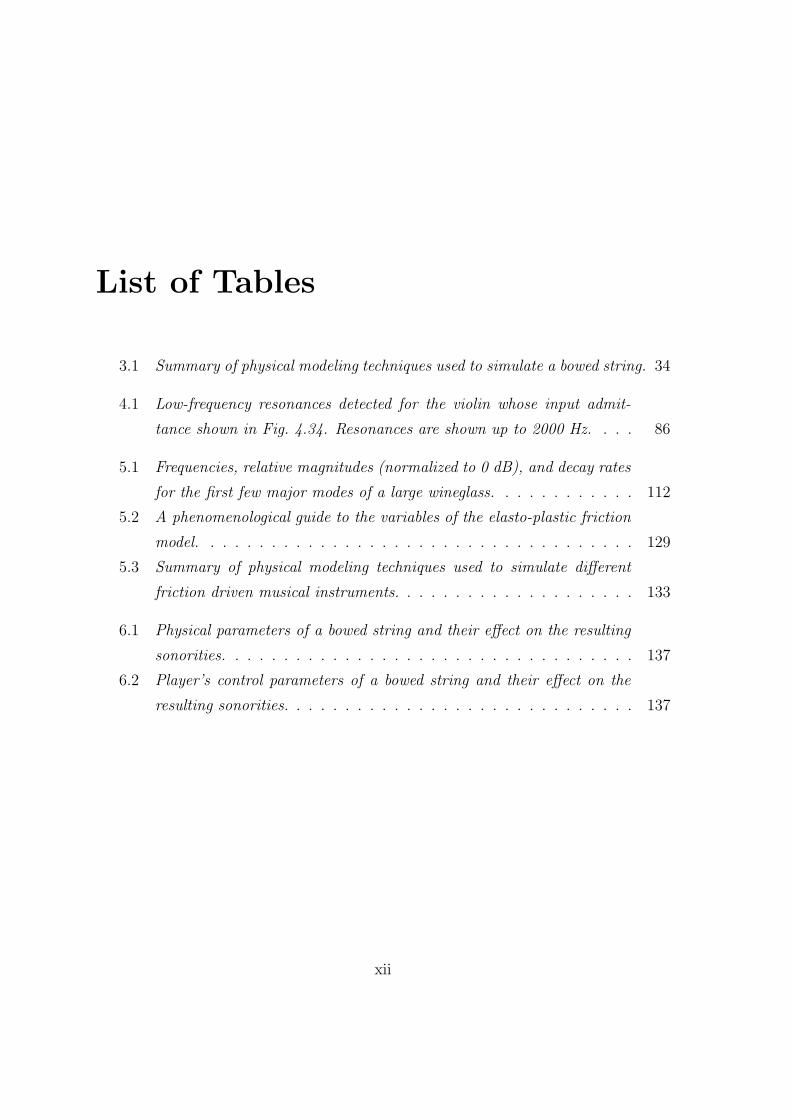
List of Tables
3.1 Summary of physical modeling techniques used to simulate a bowed string. 34
4.1 Low-frequency resonances detected for the violin whose input admit-
tance shown in Fig. 4.34. Resonances are shown up to 2000 Hz. . . . 86
5.1 Frequencies, relative magnitudes (normalized to 0 dB), and decay rates
for the first few major modes of a large wineglass. . . . . . . . . . . . 112
5.2 A phenomenological guide to the variables of the elasto-plastic friction
model. . . . . . . . . . . . . . . . . . . . . . . . . . . . . . . . . . . . 129
5.3 Summary of physical modeling techniques used to simulate different
friction driven musical instruments. . . . . . . . . . . . . . . . . . . . 133
6.1 Physical parameters of a bowed string and their effect on the resulting
sonorities. . . . . . . . . . . . . . . . . . . . . . . . . . . . . . . . . . 137
6.2 Player’s control parameters of a bowed string and their effect on the
resulting sonorities. . . . . . . . . . . . . . . . . . . . . . . . . . . . . 137
xii

List of Figures
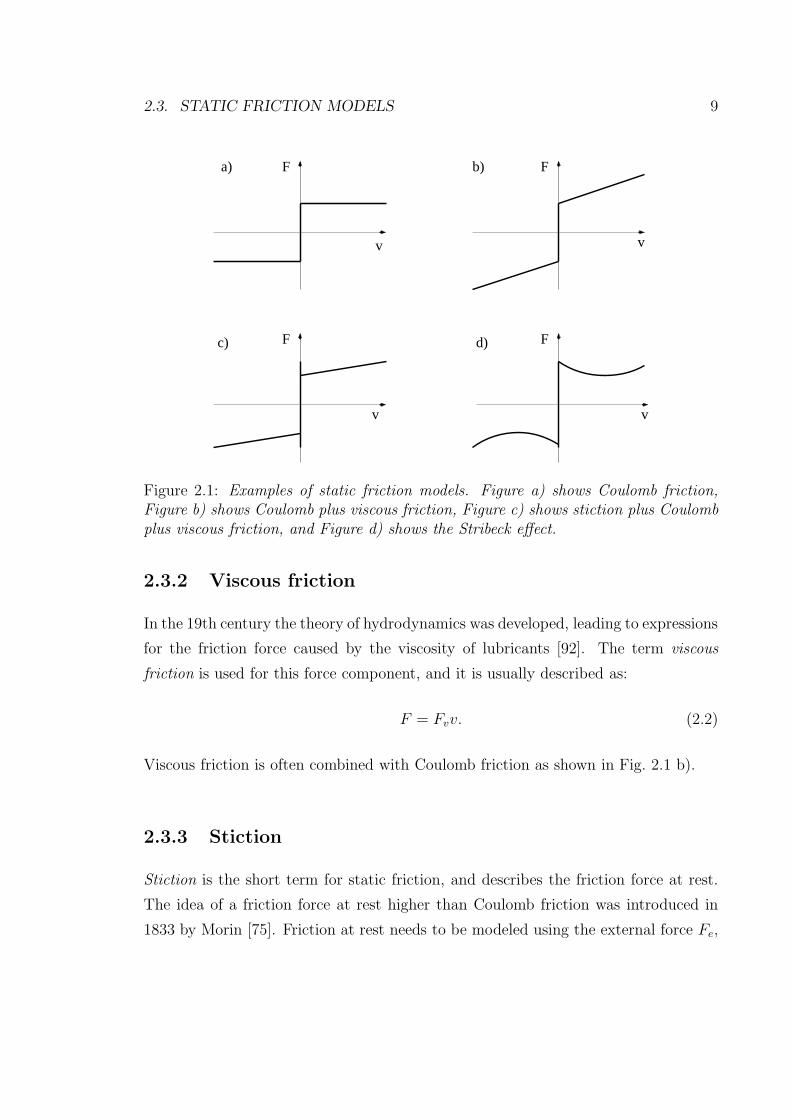
2.1 Examples of static friction models. Figure a) shows Coulomb friction,
Figure b) shows Coulomb plus viscous friction, Figure c) shows stiction
plus Coulomb plus viscous friction, and Figure d) shows the Stribeck
effect. . . . . . . . . . . . . . . . . . . . . . . . . . . . . . . . . . . . 9
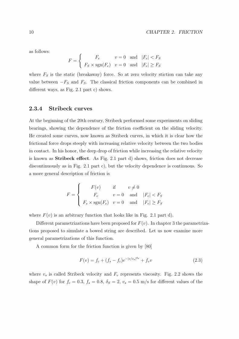
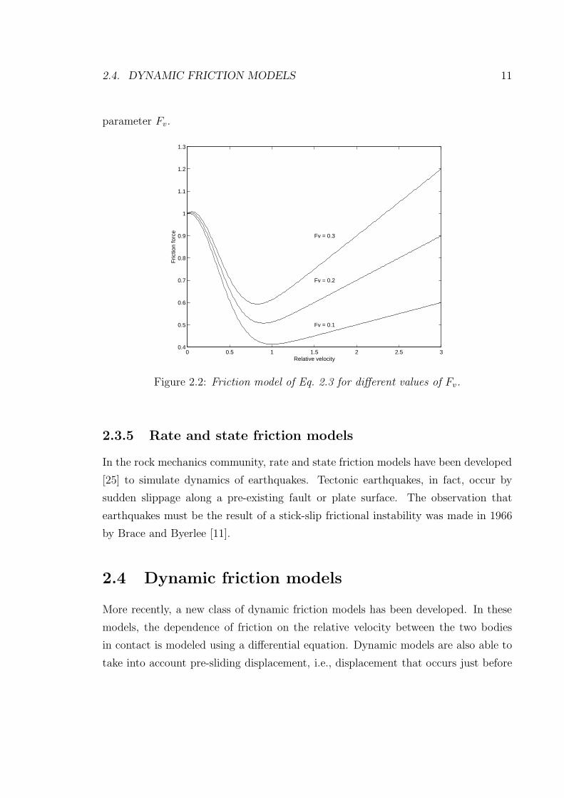
2.2 Friction model of Eq. 2.3 for different values of Fv. . . . . . . . . . . 11
2.3 Two objects connected by a spring. . . . . . . . . . . . . . . . . . . . 12
2.4 Friction force as a function of displacement in the Dahl model. . . . . 13
2.5 Bristle model. . . . . . . . . . . . . . . . . . . . . . . . . . . . . . . . 14
2.6 Contacting asperities act as small stiff springs with dampers, giving
rise to microscopic displacements (stick) and return forces. If the dis-
placement becomes too large, the junctions break. At this break-away
displacement true, macroscopic sliding (slip) starts. . . . . . . . . . . 14
2.7 The LuGre single-state averaged model. . . . . . . . . . . . . . . . . . 15
2.8 The shape of the α function . . . . . . . . . . . . . . . . . . . . . . . 18
3.1 Different components of a violin, from [32]. . . . . . . . . . . . . . . . 20
3.2 The idealized Helmholtz motion. The string moves in time from posi-
tion 1 to position 8. The rectangle represents the bow. . . . . . . . . . 21
3.3 Top: impulse response of a violin body. Bottom: input admittance of
a violin body. . . . . . . . . . . . . . . . . . . . . . . . . . . . . . . . 23
3.4 Savart’s original trapezoidal violin. From the Ecole Polytechnique col-
lection, France. . . . . . . . . . . . . . . . . . . . . . . . . . . . . . . 24
3.5 Rayleigh’s mass-spring model of a bowed string. A mass m sits upon a
conveyor belt which moves with uniform velocity v0. . . . . . . . . . 25
xiii
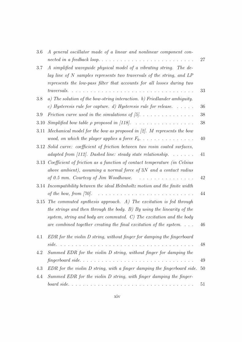
3.6 A general oscillator made of a linear and nonlinear component con-
nected in a feedback loop. . . . . . . . . . . . . . . . . . . . . . . . . . 27
3.7 A simplified waveguide physical model of a vibrating string. The de-
lay line of N samples represents two traversals of the string, and LP
represents the low-pass filter that accounts for all losses during two
traversals. . . . . . . . . . . . . . . . . . . . . . . . . . . . . . . . . . 33
3.8 a) The solution of the bow-string interaction. b) Friedlander ambiguity.
c) Hysteresis rule for capture. d) Hysteresis rule for release. . . . . . 36
3.9 Friction curve used in the simulations of [5]. . . . . . . . . . . . . . . 38
3.10 Simplified bow table ρ proposed in [118]. . . . . . . . . . . . . . . . . 38
3.11 Mechanical model for the bow as proposed in [2]. M represents the bow
wood, on which the player applies a force F0. . . . . . . . . . . . . . . 40
3.12 Solid curve: coefficient of friction between two rosin coated surfaces,
adapted from [112]. Dashed line: steady state relationship. . . . . . . 41
3.13 Coefficient of friction as a function of contact temperature (in Celsius
above ambient), assuming a normal force of 3N and a contact radius
of 0.5 mm. Courtesy of Jim Woodhouse. . . . . . . . . . . . . . . . 42
3.14 Incompatibility between the ideal Helmholtz motion and the finite width
of the bow, from [70]. . . . . . . . . . . . . . . . . . . . . . . . . . . 44
3.15 The commuted synthesis approach. A) The excitation is fed through
the strings and then through the body. B) By using the linearity of the
system, string and body are commuted. C) The excitation and the body
are combined together creating the final excitation of the system. . . . 46
4.1 EDR for the violin D string, without finger for damping the fingerboard
side. . . . . . . . . . . . . . . . . . . . . . . . . . . . . . . . . . . . . 48
4.2 Summed EDR for the violin D string, without finger for damping the
fingerboard side. . . . . . . . . . . . . . . . . . . . . . . . . . . . . . . 49
4.3 EDR for the violin D string, with a finger damping the fingerboard side. 50
4.4 Summed EDR for the violin D string, with finger damping the finger-
board side. . . . . . . . . . . . . . . . . . . . . . . . . . . . . . . . . . 51
xiv
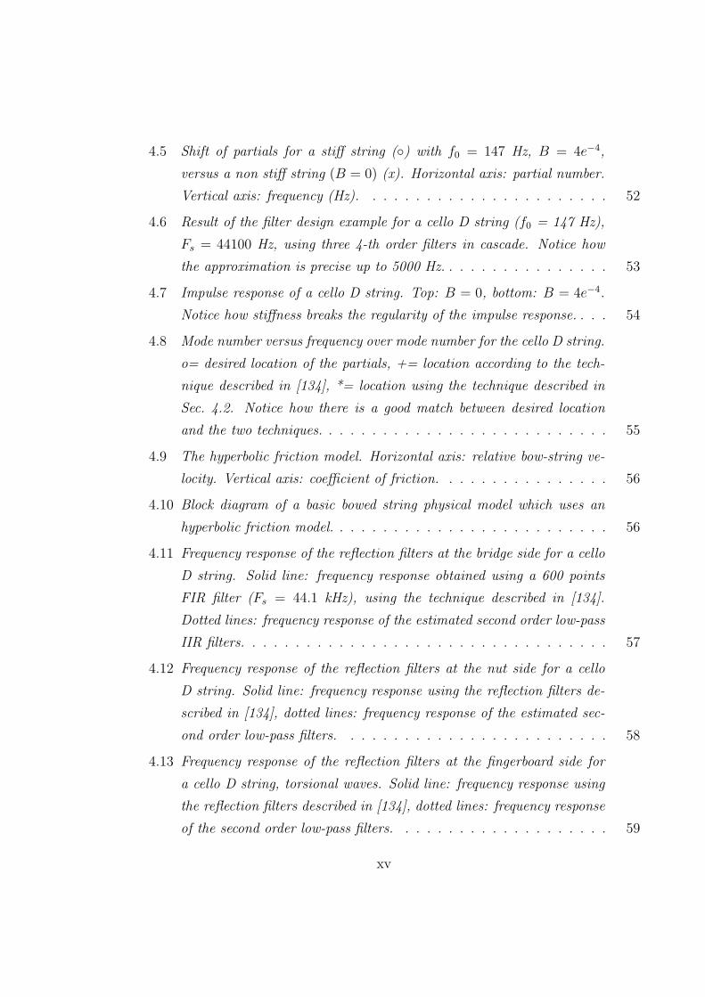
4.5 Shift of partials for a stiff string () with f0 = 147 Hz, B = 4e−4,
versus a non stiff string (B = 0) (x). Horizontal axis: partial number.
Vertical axis: frequency (Hz). . . . . . . . . . . . . . . . . . . . . . . 52
4.6 Result of the filter design example for a cello D string (f0 = 147 Hz),
Fs = 44100 Hz, using three 4-th order filters in cascade. Notice how
the approximation is precise up to 5000 Hz. . . . . . . . . . . . . . . . 53
4.7 Impulse response of a cello D string. Top: B = 0, bottom: B = 4e−4.
Notice how stiffness breaks the regularity of the impulse response. . . . 54
4.8 Mode number versus frequency over mode number for the cello D string.
o= desired location of the partials, += location according to the tech-
nique described in [134], *= location using the technique described in
Sec. 4.2. Notice how there is a good match between desired location
and the two techniques. . . . . . . . . . . . . . . . . . . . . . . . . . . 55
4.9 The hyperbolic friction model. Horizontal axis: relative bow-string ve-
locity. Vertical axis: coefficient of friction. . . . . . . . . . . . . . . . 56
4.10 Block diagram of a basic bowed string physical model which uses an
hyperbolic friction model. . . . . . . . . . . . . . . . . . . . . . . . . . 56
4.11 Frequency response of the reflection filters at the bridge side for a cello
D string. Solid line: frequency response obtained using a 600 points
FIR filter (Fs = 44.1 kHz), using the technique described in [134].
Dotted lines: frequency response of the estimated second order low-pass
IIR filters. . . . . . . . . . . . . . . . . . . . . . . . . . . . . . . . . . 57
4.12 Frequency response of the reflection filters at the nut side for a cello
D string. Solid line: frequency response using the reflection filters de-
scribed in [134], dotted lines: frequency response of the estimated sec-
ond order low-pass filters. . . . . . . . . . . . . . . . . . . . . . . . . 58
4.13 Frequency response of the reflection filters at the fingerboard side for
a cello D string, torsional waves. Solid line: frequency response using
the reflection filters described in [134], dotted lines: frequency response
of the second order low-pass filters. . . . . . . . . . . . . . . . . . . . 59
xv
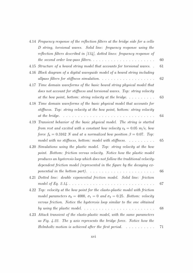
4.14 Frequency response of the reflection filters at the bridge side for a cello
D string, torsional waves. Solid line: frequency response using the
reflection filters described in [134], dotted lines: frequency response of
the second order low-pass filters. . . . . . . . . . . . . . . . . . . . . . 60
4.15 Structure of a bowed string model that accounts for torsional waves. . 61
4.16 Block diagram of a digital waveguide model of a bowed string including
allpass filters for stiffness simulation. . . . . . . . . . . . . . . . . . . 62
4.17 Time domain waveforms of the basic bowed string physical model that
does not account for stiffness and torsional waves. Top: string velocity
at the bow point, bottom: string velocity at the bridge. . . . . . . . . . 63
4.18 Time domain waveforms of the basic physical model that accounts for
stiffness. Top: string velocity at the bow point, bottom: string velocity
at the bridge. . . . . . . . . . . . . . . . . . . . . . . . . . . . . . . . 64
4.19 Transient behavior of the basic physical model. The string is started
from rest and excited with a constant bow velocity vb = 0.05 m/s, bow
force fb = 0.3162 N and at a normalized bow position β = 0.07. Top:
model with no stiffness, bottom: model with stiffness. . . . . . . . . . 65
4.20 Simulations using the plastic model. Top: string velocity at the bow
point. Bottom: friction versus velocity. Notice how the plastic model
produces an hysteresis loop which does not follow the traditional velocity-
dependent friction model (represented in the figure by the decaying ex-
ponential in the bottom part). . . . . . . . . . . . . . . . . . . . . . . 66
4.21 Dotted line: double exponential friction model. Solid line: friction
model of Eq. 2.14. . . . . . . . . . . . . . . . . . . . . . . . . . . . . . 67
4.22 Top: velocity at the bow point for the elasto-plastic model with friction
model parameters σ0 = 4000, σ1 = 0 and σ2 = 0.25. Bottom: velocity
versus friction. Notice the hysteresis loop similar to the one obtained
by using the plastic model. . . . . . . . . . . . . . . . . . . . . . . . . 68
4.23 Attack transient of the elasto-plastic model, with the same parameters
as Fig. 4.22. The y axis represents the bridge force. Notice how the
Helmholtz motion is achieved after the first period. . . . . . . . . . . 71
xvi
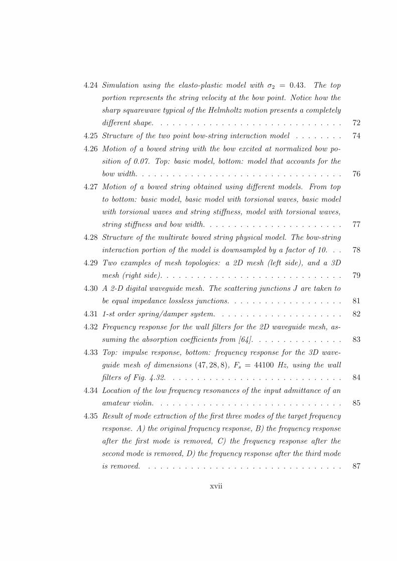
4.24 Simulation using the elasto-plastic model with σ2 = 0.43. The top
portion represents the string velocity at the bow point. Notice how the
sharp squarewave typical of the Helmholtz motion presents a completely
different shape. . . . . . . . . . . . . . . . . . . . . . . . . . . . . . . 72
4.25 Structure of the two point bow-string interaction model . . . . . . . . 74
4.26 Motion of a bowed string with the bow excited at normalized bow po-
sition of 0.07. Top: basic model, bottom: model that accounts for the
bow width. . . . . . . . . . . . . . . . . . . . . . . . . . . . . . . . . . 76
4.27 Motion of a bowed string obtained using different models. From top
to bottom: basic model, basic model with torsional waves, basic model
with torsional waves and string stiffness, model with torsional waves,
string stiffness and bow width. . . . . . . . . . . . . . . . . . . . . . . 77
4.28 Structure of the multirate bowed string physical model. The bow-string
interaction portion of the model is downsampled by a factor of 10. . . 78
4.29 Two examples of mesh topologies: a 2D mesh (left side), and a 3D
mesh (right side). . . . . . . . . . . . . . . . . . . . . . . . . . . . . . 79
4.30 A 2-D digital waveguide mesh. The scattering junctions J are taken to
be equal impedance lossless junctions. . . . . . . . . . . . . . . . . . . 81
4.31 1-st order spring/damper system. . . . . . . . . . . . . . . . . . . . . 82
4.32 Frequency response for the wall filters for the 2D waveguide mesh, as-
suming the absorption coefficients from [64]. . . . . . . . . . . . . . . 83
4.33 Top: impulse response, bottom: frequency response for the 3D wave-
guide mesh of dimensions (47, 28, 8), Fs = 44100 Hz, using the wall
filters of Fig. 4.32. . . . . . . . . . . . . . . . . . . . . . . . . . . . . 84
4.34 Location of the low frequency resonances of the input admittance of an
amateur violin. . . . . . . . . . . . . . . . . . . . . . . . . . . . . . . 85
4.35 Result of mode extraction of the first three modes of the target frequency
response. A) the original frequency response, B) the frequency response
after the first mode is removed, C) the frequency response after the
second mode is removed, D) the frequency response after the third mode
is removed. . . . . . . . . . . . . . . . . . . . . . . . . . . . . . . . . 87
xvii
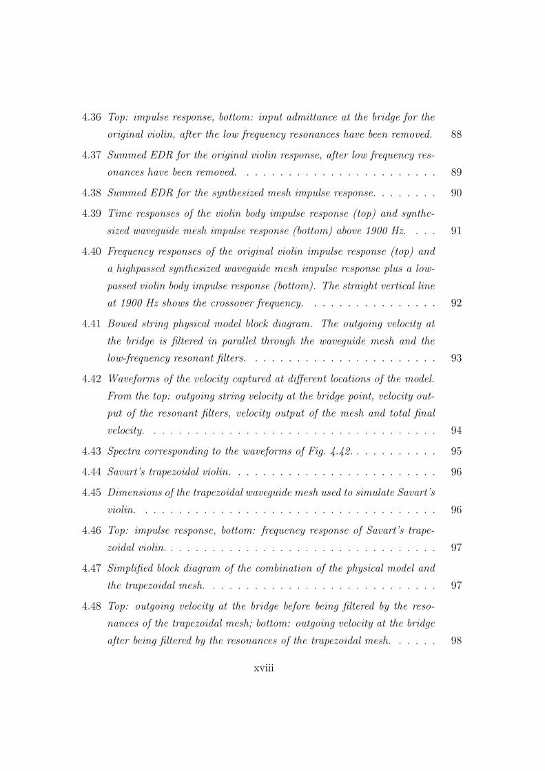
4.36 Top: impulse response, bottom: input admittance at the bridge for the
original violin, after the low frequency resonances have been removed. 88
4.37 Summed EDR for the original violin response, after low frequency res-
onances have been removed. . . . . . . . . . . . . . . . . . . . . . . . 89
4.38 Summed EDR for the synthesized mesh impulse response. . . . . . . . 90
4.39 Time responses of the violin body impulse response (top) and synthe-
sized waveguide mesh impulse response (bottom) above 1900 Hz. . . . 91
4.40 Frequency responses of the original violin impulse response (top) and
a highpassed synthesized waveguide mesh impulse response plus a low-
passed violin body impulse response (bottom). The straight vertical line
at 1900 Hz shows the crossover frequency. . . . . . . . . . . . . . . . 92
4.41 Bowed string physical model block diagram. The outgoing velocity at
the bridge is filtered in parallel through the waveguide mesh and the
low-frequency resonant filters. . . . . . . . . . . . . . . . . . . . . . . 93
4.42 Waveforms of the velocity captured at different locations of the model.
From the top: outgoing string velocity at the bridge point, velocity out-
put of the resonant filters, velocity output of the mesh and total final
velocity. . . . . . . . . . . . . . . . . . . . . . . . . . . . . . . . . . . 94
4.43 Spectra corresponding to the waveforms of Fig. 4.42. . . . . . . . . . . 95
4.44 Savart’s trapezoidal violin. . . . . . . . . . . . . . . . . . . . . . . . . 96
4.45 Dimensions of the trapezoidal waveguide mesh used to simulate Savart’s
violin. . . . . . . . . . . . . . . . . . . . . . . . . . . . . . . . . . . . 96
4.46 Top: impulse response, bottom: frequency response of Savart’s trape-
zoidal violin. . . . . . . . . . . . . . . . . . . . . . . . . . . . . . . . . 97
4.47 Simplified block diagram of the combination of the physical model and
the trapezoidal mesh. . . . . . . . . . . . . . . . . . . . . . . . . . . . 97
4.48 Top: outgoing velocity at the bridge before being filtered by the reso-
nances of the trapezoidal mesh; bottom: outgoing velocity at the bridge
after being filtered by the resonances of the trapezoidal mesh. . . . . . 98
xviii
4.49 Top: spectrum of the outgoing velocity at the bridge before being filtered
by the resonances of the trapezoidal mesh; bottom: spectrum of the
outgoing velocity at the bridge after being filtered by the resonances of
the trapezoidal mesh. . . . . . . . . . . . . . . . . . . . . . . . . . . . 99
5.1 Block diagram structure of one banded waveguide. . . . . . . . . . . . 101
5.2 Frequency response overlays for the bandpass filter of Eq. 5.5. . . . . 102
5.3 Block diagram structure of a) one modal resonator, b) one banded wave-
guide. . . . . . . . . . . . . . . . . . . . . . . . . . . . . . . . . . . . 103
5.4 Solid line: time domain simulation of an unitary impulse fed through
a bandpass filter; dotted lines: time domain simulation of an unitary
impulse fed thorugh one banded waveguide. . . . . . . . . . . . . . . . 104
5.5 Solid line: frequency response of a second order bandpass filter; dot-
ted lines: frequency response of one banded waveguide. The vertical
line represents the position in which the two systems start to behave
differently. . . . . . . . . . . . . . . . . . . . . . . . . . . . . . . . . . 105
5.6 Waves propagating around a circular resonator. . . . . . . . . . . . . 106
5.7 The author playing an ordinary handsaw. . . . . . . . . . . . . . . . . . 107
5.8 Configuration of a saw fixed at both ends. . . . . . . . . . . . . . . . . . 108
5.9 Sonogram of a bowed saw tone. The saw is bowed for about one second
and then left to resonate. While the fundamental has a long decay time,
the higher harmonics are quickly damped. . . . . . . . . . . . . . . . . 109
5.10 Sonogram of a synthetic bowed saw tone. The saw is bowed for about 1.5
seconds and then left to resonate. Notice how, as in the real instrument,
while the fundamental has a long decay time, the higher harmonics are
quickly damped. The vibrato is also strongly noticeable. . . . . . . . . 110
5.11 Benjamin Franklin’s glass harmonica, which he called “armonica”, as
seen in the Franklin Institute Science Museum in Philadelphia. Picture
courtesy of Ed Gaida. . . . . . . . . . . . . . . . . . . . . . . . . . . . 111
5.12 Young performers playing the glass harmonica. . . . . . . . . . . . . . 112
5.13 A crystal wineglass. . . . . . . . . . . . . . . . . . . . . . . . . . . . . 113
xix
5.14 Analysis and synthesis steps to obtain the bowl and wineglass models. 114
5.15 Spectrum of a large wineglass. Top: hitting the glass with a hard mallet;
center: bowing with a cello bow; bottom: rubbing with a wet finger. The
circles indicate harmonics of the (2, 0) mode, and the x’s indicate the
(m, 0) modes for m = 2 to 6. . . . . . . . . . . . . . . . . . . . . . . . 115
5.16 Digital waveguide network structure of the bowl resonator. Represen-
tation of one mode. Each bi-directional delay line contains the waves
propagating in the two sides of the bowl. . . . . . . . . . . . . . . . . 116
5.17 Complete model, connecting the exciter and the resonator. Each mode
is modeled as shown in Fig. 5.16. The dotted connection between the
source and the resonator is due to the fact that they can be connected
with either a feedback or a feed-forward loop. . . . . . . . . . . . . . . 117
5.18 The Tibetan singing bowl used for the analysis. . . . . . . . . . . . . . 117
5.19 The figure shows the eight different positions in which the bowl was hit
during the recordings. . . . . . . . . . . . . . . . . . . . . . . . . . . . 118
5.20 Position of the microphone used to record the impulse responses of the
Tibetan bowl. . . . . . . . . . . . . . . . . . . . . . . . . . . . . . . . 119
5.21 Spectra resulting from varying the excitation position of the bowl. From
top to bottom the plots represent positions from one to eight respec-
tively, according to Fig. 5.19. In the topmost plot the location of the
eight modes is also represented. Notice the evolution of the modes ac-
cording to the hitting positions. . . . . . . . . . . . . . . . . . . . . . 120
5.22 Results of the peak detection algorithm on the Tibetan bowl’s impulse
response. Notice how the algorithm correctly detects the beating, which
appear as amplitude modulation of the modes of the instrument with
the longer decay time. . . . . . . . . . . . . . . . . . . . . . . . . . . . 121
5.23 Spectrogram of the synthetic Tibetan bowl. . . . . . . . . . . . . . . . 122
5.24 An example of a bowed cymbal. Top: time domain waveform (sustain,
decay and release). Bottom: frequency response; notice the density of
high frequency modes. . . . . . . . . . . . . . . . . . . . . . . . . . . . 123
xx
5.25 Spectrum of a cymbal while hit with a hard mallet at one extremity. The
circles represent the locations of the strongest low-frequency resonances. 124
5.26 A banded waveguide mesh with an arbitrary number of one-dimensional
digital waveguides and a digital waveguide mesh. . . . . . . . . . . . . 125
5.27 Spectrum of a synthetic bowed cymbal. Top: bowed low-frequency res-
onators, center: bowed 3D mesh, bottom: the complete model. . . . . . 126
5.28 Top: time domain waveform of a synthetic bowed cymbal. Bottom:
frequency domain waveform of a synthetic bowed cymbal. . . . . . . . 127
5.29 3D animation and waveform: a wheel which rolls and slides on a cir-
cular track. . . . . . . . . . . . . . . . . . . . . . . . . . . . . . . . . 130
5.30 3D animation and waveform: a moisty finger rubbing a crystal glass. 131
5.31 3D animation and waveform: a swinging door, each of the two shutters
is linked to a friction module. . . . . . . . . . . . . . . . . . . . . . . 132
5.32 Block diagrams of the different waveguide-based data structures devel-
oped in this chapter and in the previous one. For simplicity, it is as-
sumed that the excitation point is placed at one extremity of the wave-
guide, and losses are not represented. A) a one dimensional digital
waveguide, B) a one dimensional digital waveguide filtered through the
body model described in Sec. 4.6, C) one banded waveguide, D) a con-
nection of two banded waveguides, E) a banded waveguide mesh. . . . 135
6.1 Spectral differences obtained by bowing a violin pianissimo, mezzo forte
and fortissimo, from [50]. . . . . . . . . . . . . . . . . . . . . . . . . 138
6.2 Theoretical Schelleng diagram. . . . . . . . . . . . . . . . . . . . . . . 139
6.3 An example of anomalous low frequency motion. . . . . . . . . . . . . 141
6.4 An example of multiple slips motion. . . . . . . . . . . . . . . . . . . 141
6.5 An example of raucous motion. . . . . . . . . . . . . . . . . . . . . . 142
xxi
6.6 Simulated Schelleng diagram for the plastic friction model case. High
quality Helmholtz motion is indicated by open squares, and multiple
slipping is plotted using open circles. All other symbols denote generally
less desirable modes of string motion. A cello D string (f0 = 147 Hz)
is excited with a constant bow velocity vb = 0.05 m/s. Bow force and
position are varied as shown in the figure. . . . . . . . . . . . . . . . 147
6.7 Simulated Schelleng diagram for the plastic friction model case, with
torsional wave simulation removed. As before, classic Helmholtz mo-
tion is indicated by ‘2’, and multiple slipping by ‘’. . . . . . . . . . . 148
6.8 Simulated Schelleng diagram for the plastic friction model case. A cello
D string (f0 = 147) Hz is excited with a constant bow velocity v0.05
m/s. Bow force and position are varied as shown in the figure. The
string is initialized with an already established Helmholtz motion. . . . 149
6.9 Simulated Schelleng diagram for the exponential friction model case,
with torsional waves. . . . . . . . . . . . . . . . . . . . . . . . . . . . 150
6.10 Simulated Schelleng diagram for the exponential friction model case,
with torsional waves completely removed. . . . . . . . . . . . . . . . . 151
6.11 Simulated Schelleng diagram for the hyperbolic friction model case, with
torsional waves simulations. . . . . . . . . . . . . . . . . . . . . . . . 152
6.12 Simulated Schelleng diagram for the hyperbolic friction model case, with
torsional waves completely removed. . . . . . . . . . . . . . . . . . . . 153
6.13 Simulated Schelleng diagram for the exponential friction model case,
without string stiffness. . . . . . . . . . . . . . . . . . . . . . . . . . . 154
6.14 Simulated Schelleng diagram for the exponential friction model case, in
the velocity versus force plane, without torsional waves. . . . . . . . . 155
6.15 Simulated Schelleng diagram for the exponential friction model case, in
the velocity versus force plane, with torsional waves. . . . . . . . . . . 156
6.16 3D playability plot of the basic physical model with torsional waves. . 157
6.17 Playability plot for the elasto-plastic friction model, using the same
string parameters as before, with elasto-plastic parameters σ0 = 4000,
σ1 = 0 and σ2 = 0.25 (see Chapters 2 and 4). . . . . . . . . . . . . . 158
xxii
7.1 Comparison between the degrees of freedom of the bow-string and the
ones of the pen-tablet interaction. . . . . . . . . . . . . . . . . . . . . 161
7.2 WACOM tablet fitted with additional pressure and position sensors (on
the left side of the tablet). . . . . . . . . . . . . . . . . . . . . . . . . 162
7.3 Top: pressure of the stylus on the tablet during balzato. Bottom: ve-
locity of the pen. . . . . . . . . . . . . . . . . . . . . . . . . . . . . . 163
7.4 Top: pressure of the stylus on the tablet during detache. Bottom: ve-
locity of the stylus. . . . . . . . . . . . . . . . . . . . . . . . . . . . . 164
7.5 Top: pressure of the stylus on the tablet during staccato. Bottom:
velocity of the stylus. . . . . . . . . . . . . . . . . . . . . . . . . . . . 165
7.6 Playability chart of a virtual musical instrument . . . . . . . . . . . . 166
7.7 Mapping of the bow controller to the bowed string physical model. . . . 169
A.1 The Max/MSP interface for the friction models. . . . . . . . . . . . . 176
xxiii

xxiv
Chapter 1
Introduction
1.1 Overview
Friction, the tangential force between objects in contact, in most engineering appli-
cations needs to be removed being a source of noise, energy loss, instabilities and
undesired vibrations.
From an auditory perspective, friction is constantly present in our everyday life.
The annoying sound of a brake, a squeaking door or a chalk sliding on a blackboard
are only few examples of the sonorities that frictional interactions between rubbed
dry surfaces can produce. Fortunately there also also pleasant sonorities that derive
from frictional phenomena: few examples are skilled bowed string players, rubbed
crystal wine-glasses and musical saws.
In this dissertation mathematical models that simulate friction sonorities are built,
by looking at friction as a source of noise and subtle variations part of the expressive
sonic phenomena considered to be desirable in music. In particular, the state of the
art friction models developed in haptic and robotics are studied and applied to a
musical context.
Starting from an efficient yet accurate physical model of a bowed string, simula-
tions of different instruments that have the same excitation mechanism are presented.
The ultimate goal is to provide a better understanding of the behavior of these in-
struments and to build real-time synthesis tools which composers and performers can
1
2 CHAPTER 1. INTRODUCTION
use to reproduce, explore and extend the sound of friction.
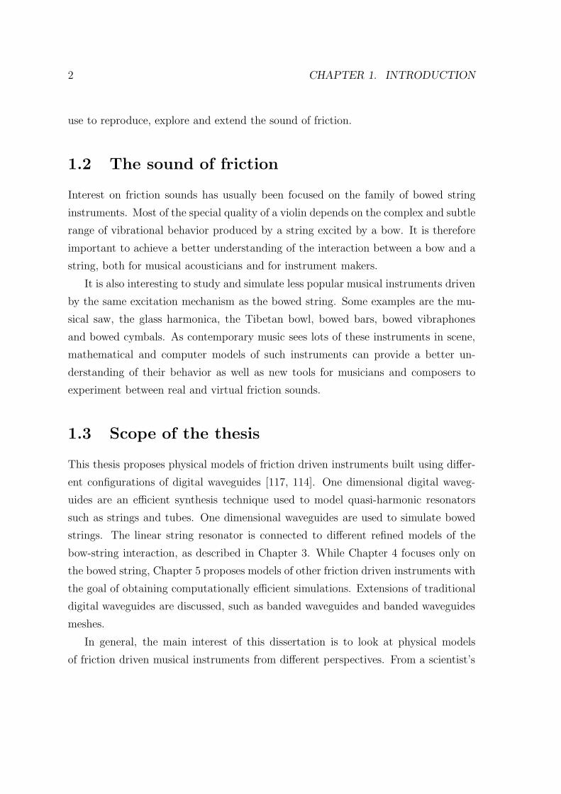
1.2 The sound of friction
Interest on friction sounds has usually been focused on the family of bowed string
instruments. Most of the special quality of a violin depends on the complex and subtle
range of vibrational behavior produced by a string excited by a bow. It is therefore
important to achieve a better understanding of the interaction between a bow and a
string, both for musical acousticians and for instrument makers.
It is also interesting to study and simulate less popular musical instruments driven
by the same excitation mechanism as the bowed string. Some examples are the mu-
sical saw, the glass harmonica, the Tibetan bowl, bowed bars, bowed vibraphones
and bowed cymbals. As contemporary music sees lots of these instruments in scene,
mathematical and computer models of such instruments can provide a better un-
derstanding of their behavior as well as new tools for musicians and composers to
experiment between real and virtual friction sounds.
1.3 Scope of the thesis
This thesis proposes physical models of friction driven instruments built using differ-
ent configurations of digital waveguides [117, 114]. One dimensional digital waveg-
uides are an efficient synthesis technique used to model quasi-harmonic resonators
such as strings and tubes. One dimensional waveguides are used to simulate bowed
strings. The linear string resonator is connected to different refined models of the
bow-string interaction, as described in Chapter 3. While Chapter 4 focuses only on
the bowed string, Chapter 5 proposes models of other friction driven instruments with
the goal of obtaining computationally efficient simulations. Extensions of traditional
digital waveguides are discussed, such as banded waveguides and banded waveguides
meshes.
In general, the main interest of this dissertation is to look at physical models
of friction driven musical instruments from different perspectives. From a scientist’s
1.3. SCOPE OF THE THESIS 3
point of view, the interest is to provide a better understanding of the sound production
mechanism of the instruments of the violin family and of other instruments driven by
friction. From the engineer’s point of view, the goal is to obtain accurate yet efficient
numerical models of these instruments. From the computer scientist’s point of view
a real-time implementation of these instruments is provided. From the musician’s
point of view, the goal is to use these tools to recreate the sonorities of friction and
to extend them in a compositional context.
This work therefore provides new results and discussions in musical acoustics,
real-time sound synthesis, digital signal processing and musical applications, aiming
both to achieve a better understanding of friction-driven musical instruments, and to
build new tools that composers can use to manipulate sounds in real-time. In fact,
in order to allow the possibility of reproducing all the subtleties of a complex action
such as bowing and at the same time to manipulate them in real-time in a personal
computer, all these models have been implemented in the Max/MSP [141], Pure Data
(pd) [89] and Synthesis Toolkit (STK) [19] environments.
An accurate study of the playability of these models shows how recent discoveries
on friction and bowed string interaction [138] improve the playability of virtual bowed
strings. Models that incorporate recent research on the thermodynamical behavior of
the bow in contact with the string, together with models for the bow-hair compliance,
are also discussed.
Physical models of musical instruments are interesting for acousticians as a tool
to validate the equations and theories on a particular instrument. It is a challenge
to completely understand the physics of an existing instrument. This is one of the
reasons why this approach to physical models is interesting to scientists. On the
other end, merely focusing on a faithful reproduction of existing musical instruments
is not appealing for composers and performers. This concept is well-known in com-
puter music, yet little effort has been done to create physical models that extend the
possibilities offered by traditional instruments. This thesis addresses both the acous-
tician’s and the composer’s interest, providing on one side accurate models of existing
musical instruments and on the other side extended techniques to create sonorities
that existing instruments cannot physically obtain.
4 CHAPTER 1. INTRODUCTION
1.4 Outline
The remaining chapters of this dissertation are organized as follows. Chapter 2 de-
scribes acoustics of friction, and describes different models to simulate frictional in-
duced vibrations.
Chapter 3 describes acoustics and previous research on bowed strings, and Chapter
4 proposes an accurate yet efficient model of a bowed string.
Chapter 5 examines other instruments whose main excitation mechanism is fric-
tion, such as the musical saw, the glass harmonica, the Tibetan bowl and the bowed
cymbal. Other everyday sounds derived by friction, such as squeaking doors and noise
brake are also described.
Chapter 6 proposes methods for evaluating playability for virtual bowed string,
from a musical acoustician’s perspective, and Chapter 7 describes issues about musical
applications and control of friction driven musical instruments. Chapter 8 presents
conclusions and suggestions for future work.
Chapter 2
Friction
2.1 Introduction
Friction, the tangential force between sliding surfaces, is a phenomenon that con-
stantly appears in our everyday life. Friction develops between sliding surfaces, and
fulfills a dual role of transmitting energy from one surface to another and dissipating
energy of relative motion [3].
Although friction appears in many mechanical systems, friction phenomena are
not completely understood and are particularly complex since are caused by different
physical mechanisms. Friction-excited vibrations common to our sonic environment,
such as brake noises, chalks on blackboards, chairs sliding on a hard pavement derive
from the energy that friction provides to a system and they are just a small sample
of all the sonorities that hard rubbed surfaces can produce.
Friction sounds have also a slightly more appealing musical dimension, which
appears, for example, in the sonorities of a bowed string or of a rubbed wineglass.
Considering that friction is abundant in nature, friction research has a long history,
and friction studies are still active nowadays. As a nonlinearity, friction is a challenge
for researchers in dynamical systems, robotics and engineering in general.
In this chapter we examine friction induced vibrations with a focus on stick-slip
oscillations. We propose an overview of the history of the study of friction in general
and more specifically as a sonic phenomenon, and we describe different friction models
5
6 CHAPTER 2. FRICTION
that will be used in the rest of this dissertation.
2.2 Historical overview of friction research
Friction is a word traceable to 15th century english, denoting the “force that resists
relative motion between two bodies in contact” [73], and derives from the Latin word
fricare, which means “to rub”.
The awareness of friction existed in ancient times, although the earliest exploita-
tions of it where not accompanied by scientific explanations [30]. Significant examples
are the advent of fire making based on rubbing wood, the development of the bow as
a hunting tool and the development of wheels.
Perhaps the first scientist who made some observations about friction was Aris-
totle, who identified the existence of this force [6]. Aristotle analyzed the motion of
bodies under a constant force resisted by friction, such as a body being pulled or
pushed along the ground, and stated that to obtain an uniform motion a constant
force must be exerted to overcome friction.
It wasn’t until the end of the 15th century, however, thanks to Leonardo da Vinci,
that friction was treated in a scientific manner. The main observations made by
Leonardo were that friction does not depend on the contact area but on the normal
force exerted on the sliding bodies.
Leonardo’s laws of friction apply to a remarkably large range of situations; Leonardo
made the observation that different materials move with different ease. He claimed
that this was a result of the roughness of the materials in question; thus, smoother
materials have smaller friction. His results were never published; the only evidence
of their existence is in his vast collection of journals.
In the late 16th century, Galileo Galilei in his Dialogues Concerning Two New
Sciences made some observations on the act of bowing a viola string or rubbing the
rim of a wineglass with a finger. He observed that “a glass of water may be made
to emit a tone merely by the friction of the finger-tip around the rim of the glass”.
He also noted the following event: in a large glass full of water, first the waves are
spaced uniformly, but, once the tone of the glass jumps one octave higher, the waves
2.2. HISTORICAL OVERVIEW OF FRICTION RESEARCH 7
divide in two.
Guillaume Amontons (1663-1705) rediscovered the two basic laws of friction that
had been discovered by Leonardo Da Vinci, and proposed an original set of theories.
He believed that friction was predominantly a result of the work done to lift one
surface over the roughness of the other, or from the deforming or the wearing of the
other surface. For several centuries after Amontons’ work, scientists believed that
friction was due to surfaces’ roughness.
Chladni in 1787 published a treatise [16] in which he described a technique of
sprinkling sand on vibrating plates to produce oscillations induced by friction. Ex-
citing plates of various shapes with a bow, he obtained patterns of different shapes
which were demonstrated to Napoleon in 1809.
Important improvements on the research of frictional induced vibrations were
obtained by Helmholtz, who in 1860 built a vibrational microscope, using which he
was able to describe the motion of a string excited by a bow, which nowadays is
known as Helmholtz motion in his honor.
Helmholtz observed that the string is attached to the bow for the longest part of
its period, detaching only once per period. This motion was coined as stick-slip by
Bowden and Leben [9], and it is a vibratory phenomenon that is sometimes observed
at frictional interfaces. Other examples of stick-slip oscillations include the squeaking
of a door, the sound of a chalk on a blackboard and the rubbing of a wineglass. Stick-
slip motions appear because the static friction coefficient is greater than the dynamic
one. When two objects are stuck together, if a force is applied to one, the friction
ramps up to the static friction limit and break away can occur. After break away the
object can begin sliding for a small amount and then sticks again.
Further observations were made by Coulomb, who treated the difference between
static and dynamic friction coefficients observing that static friction is always higher
than dynamic friction.
Coulomb laws of friction are still used in some applications, since, although they
represent a simplified version of reality, they can nevertheless provide interesting
insights into the mechanics of objects in contact. It is with Coulomb that classical
models of friction started to develop.
8 CHAPTER 2. FRICTION
At the beginning of the 20th century, Stribeck performed some experiments on
sliding bearings, showing the dependence of the friction coefficient on the sliding
velocity. He created some curves, now known as Stribeck curves, in which it is clear
how the frictional force drops steeply with increasing relative velocity between bodies
in contact.
More recently, a new class of dynamic friction models has been developed. In
these models, the dependence of friction on the relative velocity between bodies in
contact is modeled using a differential equation. In the following section static and
dynamic friction models are described in details.
2.3 Static friction models
In the static models, friction depends only on the relative velocity between two bodies
in contact. In this section the evolution of static friction models is reviewed.
2.3.1 Coulomb’s friction model
The first mathematical friction model was proposed by Coulomb in 1773 [36]. This
model, despite its simplicity, is able to capture the basic physical behavior of friction-
ally induced vibrations.
The main idea behind the model is that friction opposes motion and its magnitude
is independent of the velocity v of the contact area. The model can be described as:
F = FC × sgn(v) (2.1)
where the friction force FC is proportional to the normal load, i.e. FC = µFN , where µ
represents the friction coefficient and FN represents the normal load. This description
of friction is represented in Fig. 2.1 a).
Notice how Coulomb friction does not specify the friction force for zero velocity.
Notice also how FC depends on the normal load FN .
2.3. STATIC FRICTION MODELS 9
v
F F
FF
v v
v
a)
c)
b)
d)
Figure 2.1: Examples of static friction models. Figure a) shows Coulomb friction,Figure b) shows Coulomb plus viscous friction, Figure c) shows stiction plus Coulombplus viscous friction, and Figure d) shows the Stribeck effect.
2.3.2 Viscous friction
In the 19th century the theory of hydrodynamics was developed, leading to expressions
for the friction force caused by the viscosity of lubricants [92]. The term viscous
friction is used for this force component, and it is usually described as:
F = Fvv. (2.2)
Viscous friction is often combined with Coulomb friction as shown in Fig. 2.1 b).
2.3.3 Stiction
Stiction is the short term for static friction, and describes the friction force at rest.
The idea of a friction force at rest higher than Coulomb friction was introduced in
1833 by Morin [75]. Friction at rest needs to be modeled using the external force Fe,
10 CHAPTER 2. FRICTION
as follows:
F =
Fe v = 0 and |Fe| < FS
FS × sgn(Fe) v = 0 and |Fe| ≥ FS
where FS is the static (breakaway) force. So at zero velocity stiction can take any
value between −FS and FS. The classical friction components can be combined in
different ways, as Fig. 2.1 part c) shows.
2.3.4 Stribeck curves
At the beginning of the 20th century, Stribeck performed some experiments on sliding
bearings, showing the dependence of the friction coefficient on the sliding velocity.
He created some curves, now known as Stribeck curves, in which it is clear how the
frictional force drops steeply with increasing relative velocity between the two bodies
in contact. In his honor, the deep drop of friction while increasing the relative velocity
is known as Stribeck effect. As Fig. 2.1 part d) shows, friction does not decrease
discontinuously as in Fig. 2.1 part c), but the velocity dependence is continuous. So
a more general description of friction is
F =
F (v) if v 6= 0
Fe v = 0 and |Fe| < FS
Fs × sgn(Fe) v = 0 and |Fe| ≥ FS
where F (v) is an arbitrary function that looks like in Fig. 2.1 part d).
Different parametrizations have been proposed for F (v). In chapter 3 the parametriza-
tions proposed to simulate a bowed string are described. Let us now examine more
general parametrizations of this function.
A common form for the friction function is given by [80]
F (v) = fc + (fs − fc)e−|v/vs|δs
+ fvv (2.3)
where vs is called Stribeck velocity and Fv represents viscosity. Fig. 2.2 shows the
shape of F (v) for fc = 0.3, fs = 0.8, δS = 2, vs = 0.5 m/s for different values of the
2.4. DYNAMIC FRICTION MODELS 11
parameter Fv.
0 0.5 1 1.5 2 2.5 30.4
0.5
0.6
0.7
0.8
0.9
1
1.1
1.2
1.3
Fv = 0.1
Fv = 0.2
Fv = 0.3
Relative velocity
Fric
tion
forc
e
Figure 2.2: Friction model of Eq. 2.3 for different values of Fv.
2.3.5 Rate and state friction models
In the rock mechanics community, rate and state friction models have been developed
[25] to simulate dynamics of earthquakes. Tectonic earthquakes, in fact, occur by
sudden slippage along a pre-existing fault or plate surface. The observation that
earthquakes must be the result of a stick-slip frictional instability was made in 1966
by Brace and Byerlee [11].
2.4 Dynamic friction models
More recently, a new class of dynamic friction models has been developed. In these
models, the dependence of friction on the relative velocity between the two bodies
in contact is modeled using a differential equation. Dynamic models are also able to
take into account pre-sliding displacement, i.e., displacement that occurs just before
12 CHAPTER 2. FRICTION
a complete slip takes place.
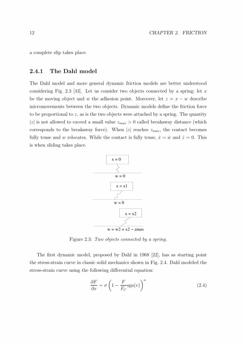
2.4.1 The Dahl model
The Dahl model and more general dynamic friction models are better understood
considering Fig. 2.3 [43]. Let us consider two objects connected by a spring; let x
be the moving object and w the adhesion point. Moreover, let z = x − w describe
micromovements between the two objects. Dynamic models define the friction force
to be proportional to z, as is the two objects were attached by a spring. The quantity
|z| is not allowed to exceed a small value zmax > 0 called breakaway distance (which
corresponds to the breakaway force). When |z| reaches zmax, the contact becomes
fully tense and w relocates. While the contact is fully tense, x = w and z = 0. This
is when sliding takes place.
x = 0
x = x1
x = x2
w = 0
w = 0
w = w2 = x2 − zmax
Figure 2.3: Two objects connected by a spring.
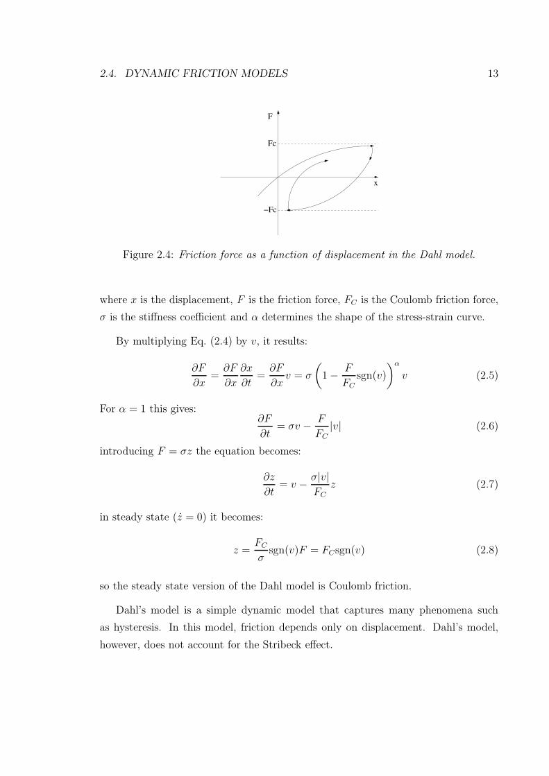
The first dynamic model, proposed by Dahl in 1968 [22], has as starting point
the stress-strain curve in classic solid mechanics shown in Fig. 2.4. Dahl modeled the
stress-strain curve using the following differential equation:
∂F
∂x= σ
(
1− F
FCsgn(v)
)α
(2.4)
2.4. DYNAMIC FRICTION MODELS 13
x
F
Fc
−Fc
Figure 2.4: Friction force as a function of displacement in the Dahl model.
where x is the displacement, F is the friction force, FC is the Coulomb friction force,
σ is the stiffness coefficient and α determines the shape of the stress-strain curve.
By multiplying Eq. (2.4) by v, it results:
∂F
∂x=∂F
∂x
∂x
∂t=∂F
∂xv = σ
(
1− F
FCsgn(v)
)α
v (2.5)
For α = 1 this gives:∂F
∂t= σv − F
FC
|v| (2.6)
introducing F = σz the equation becomes:
∂z
∂t= v − σ|v|
FC
z (2.7)
in steady state (z = 0) it becomes:
z =FC
σsgn(v)F = FCsgn(v) (2.8)
so the steady state version of the Dahl model is Coulomb friction.
Dahl’s model is a simple dynamic model that captures many phenomena such
as hysteresis. In this model, friction depends only on displacement. Dahl’s model,
however, does not account for the Stribeck effect.
14 CHAPTER 2. FRICTION
2.4.2 The LuGre model
An extension to the Dahl model is the LuGre model, whose name comes from the two
laboratories in which it was developed (Lund and Grenoble), in which the Stribeck
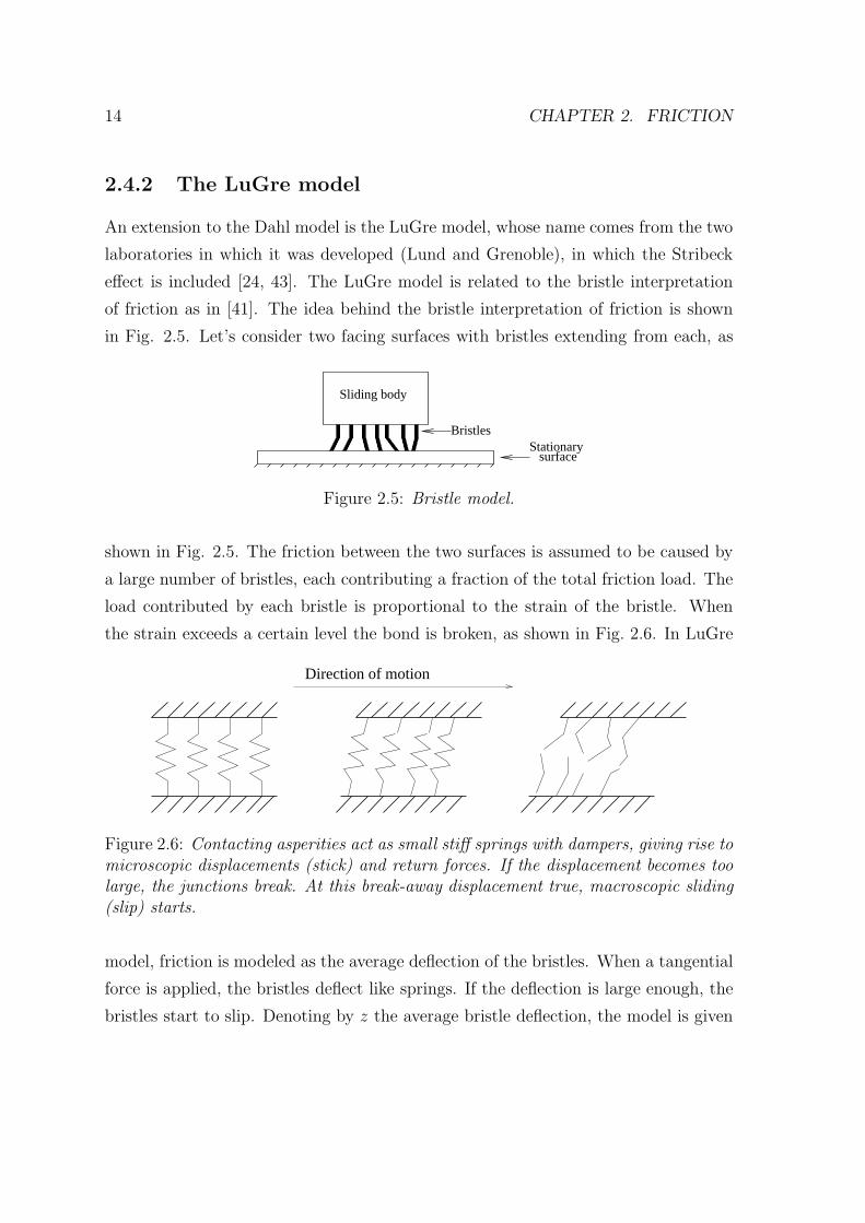
effect is included [24, 43]. The LuGre model is related to the bristle interpretation
of friction as in [41]. The idea behind the bristle interpretation of friction is shown
in Fig. 2.5. Let’s consider two facing surfaces with bristles extending from each, as
Sliding body
BristlesStationary
surface
Figure 2.5: Bristle model.
shown in Fig. 2.5. The friction between the two surfaces is assumed to be caused by
a large number of bristles, each contributing a fraction of the total friction load. The
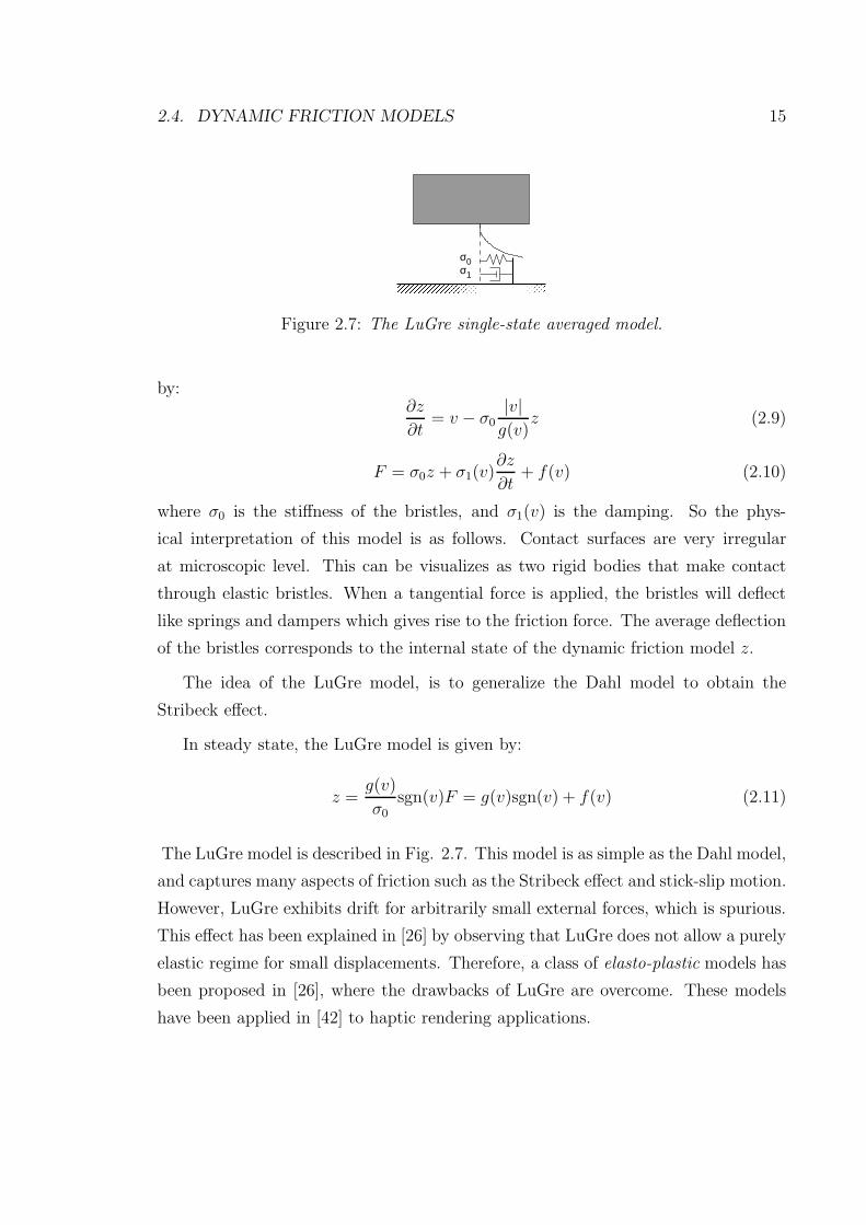
load contributed by each bristle is proportional to the strain of the bristle. When
the strain exceeds a certain level the bond is broken, as shown in Fig. 2.6. In LuGre
Direction of motion
Figure 2.6: Contacting asperities act as small stiff springs with dampers, giving rise tomicroscopic displacements (stick) and return forces. If the displacement becomes toolarge, the junctions break. At this break-away displacement true, macroscopic sliding(slip) starts.
model, friction is modeled as the average deflection of the bristles. When a tangential
force is applied, the bristles deflect like springs. If the deflection is large enough, the
bristles start to slip. Denoting by z the average bristle deflection, the model is given
2.4. DYNAMIC FRICTION MODELS 15
σ1
σ0
Figure 2.7: The LuGre single-state averaged model.
by:∂z
∂t= v − σ0
|v|g(v)
z (2.9)
F = σ0z + σ1(v)∂z
∂t+ f(v) (2.10)
where σ0 is the stiffness of the bristles, and σ1(v) is the damping. So the phys-
ical interpretation of this model is as follows. Contact surfaces are very irregular
at microscopic level. This can be visualizes as two rigid bodies that make contact
through elastic bristles. When a tangential force is applied, the bristles will deflect
like springs and dampers which gives rise to the friction force. The average deflection
of the bristles corresponds to the internal state of the dynamic friction model z.
The idea of the LuGre model, is to generalize the Dahl model to obtain the
Stribeck effect.
In steady state, the LuGre model is given by:
z =g(v)
σ0sgn(v)F = g(v)sgn(v) + f(v) (2.11)
The LuGre model is described in Fig. 2.7. This model is as simple as the Dahl model,
and captures many aspects of friction such as the Stribeck effect and stick-slip motion.
However, LuGre exhibits drift for arbitrarily small external forces, which is spurious.
This effect has been explained in [26] by observing that LuGre does not allow a purely
elastic regime for small displacements. Therefore, a class of elasto-plastic models has
been proposed in [26], where the drawbacks of LuGre are overcome. These models
have been applied in [42] to haptic rendering applications.
16 CHAPTER 2. FRICTION
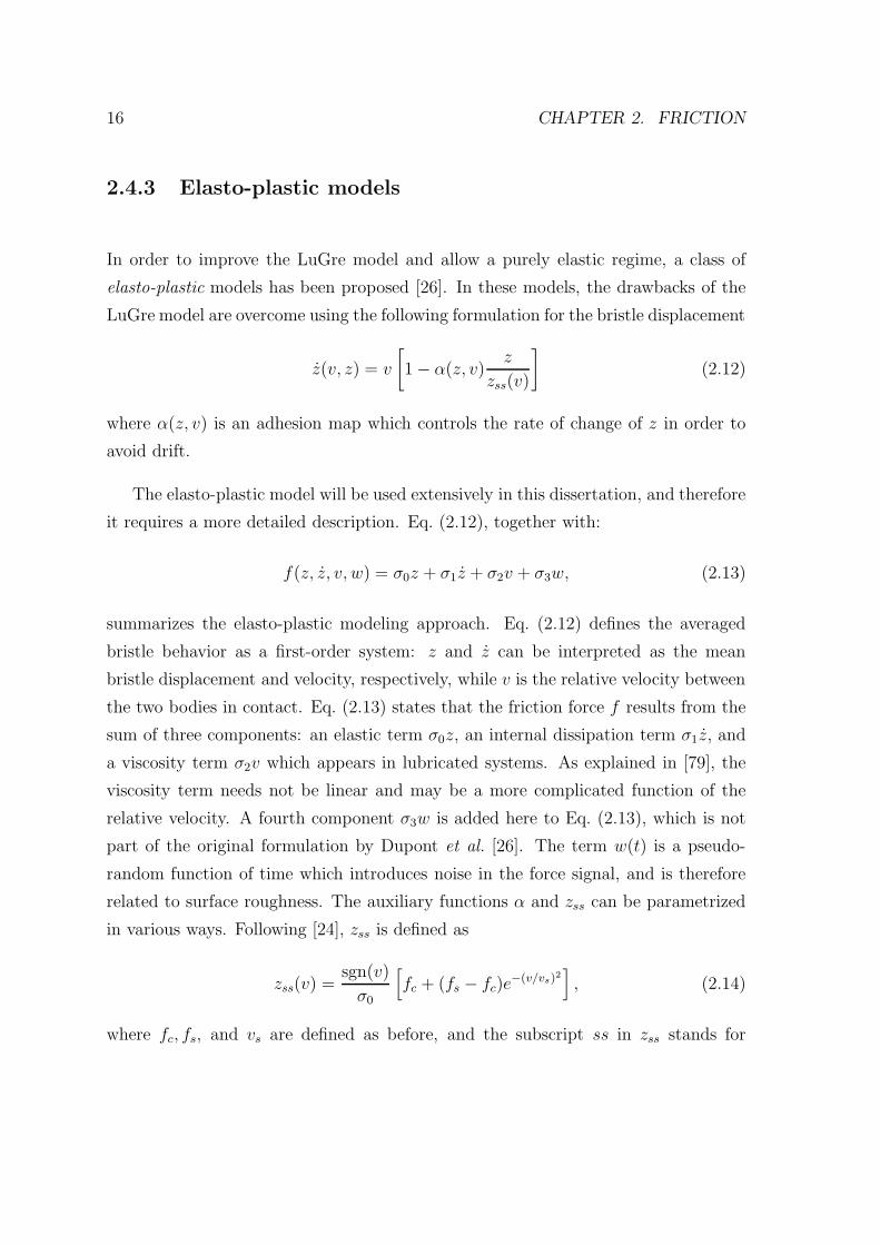
2.4.3 Elasto-plastic models
In order to improve the LuGre model and allow a purely elastic regime, a class of
elasto-plastic models has been proposed [26]. In these models, the drawbacks of the
LuGre model are overcome using the following formulation for the bristle displacement
z(v, z) = v
[
1− α(z, v)z
zss(v)
]
(2.12)
where α(z, v) is an adhesion map which controls the rate of change of z in order to
avoid drift.
The elasto-plastic model will be used extensively in this dissertation, and therefore
it requires a more detailed description. Eq. (2.12), together with:
f(z, z, v, w) = σ0z + σ1z + σ2v + σ3w, (2.13)
summarizes the elasto-plastic modeling approach. Eq. (2.12) defines the averaged
bristle behavior as a first-order system: z and z can be interpreted as the mean
bristle displacement and velocity, respectively, while v is the relative velocity between
the two bodies in contact. Eq. (2.13) states that the friction force f results from the
sum of three components: an elastic term σ0z, an internal dissipation term σ1z, and
a viscosity term σ2v which appears in lubricated systems. As explained in [79], the
viscosity term needs not be linear and may be a more complicated function of the
relative velocity. A fourth component σ3w is added here to Eq. (2.13), which is not
part of the original formulation by Dupont et al. [26]. The term w(t) is a pseudo-
random function of time which introduces noise in the force signal, and is therefore
related to surface roughness. The auxiliary functions α and zss can be parametrized
in various ways. Following [24], zss is defined as
zss(v) =sgn(v)
σ0
[
fc + (fs − fc)e−(v/vs)2
]
, (2.14)
where fc, fs, and vs are defined as before, and the subscript ss in zss stands for
2.4. DYNAMIC FRICTION MODELS 17
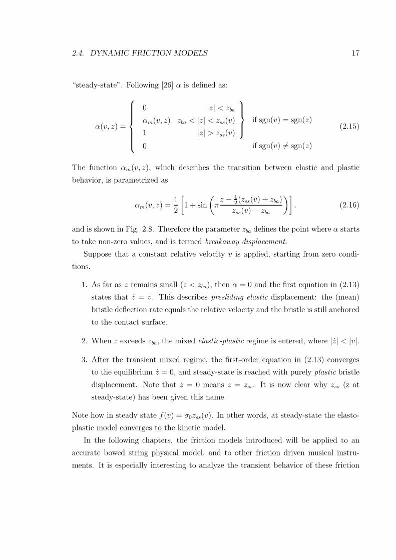
“steady-state”. Following [26] α is defined as:
α(v, z) =
0 |z| < zba
αm(v, z) zba < |z| < zss(v)
1 |z| > zss(v)
if sgn(v) = sgn(z)
0 if sgn(v) 6= sgn(z)
(2.15)
The function αm(v, z), which describes the transition between elastic and plastic
behavior, is parametrized as
αm(v, z) =1
2
[
1 + sin
(
πz − 1
2(zss(v) + zba)
zss(v)− zba
)]
. (2.16)
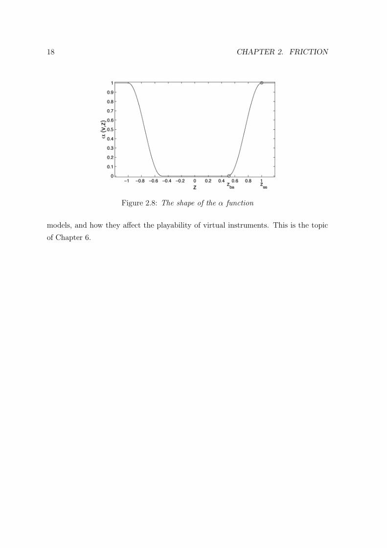
and is shown in Fig. 2.8. Therefore the parameter zba defines the point where α starts
to take non-zero values, and is termed breakaway displacement.
Suppose that a constant relative velocity v is applied, starting from zero condi-
tions.
1. As far as z remains small (z < zba), then α = 0 and the first equation in (2.13)
states that z = v. This describes presliding elastic displacement: the (mean)
bristle deflection rate equals the relative velocity and the bristle is still anchored
to the contact surface.
2. When z exceeds zba, the mixed elastic-plastic regime is entered, where |z| < |v|.
3. After the transient mixed regime, the first-order equation in (2.13) converges
to the equilibrium z = 0, and steady-state is reached with purely plastic bristle
displacement. Note that z = 0 means z = zss. It is now clear why zss (z at
steady-state) has been given this name.
Note how in steady state f(v) = σ0zss(v). In other words, at steady-state the elasto-
plastic model converges to the kinetic model.
In the following chapters, the friction models introduced will be applied to an
accurate bowed string physical model, and to other friction driven musical instru-
ments. It is especially interesting to analyze the transient behavior of these friction
18 CHAPTER 2. FRICTION
Figure 2.8: The shape of the α function
models, and how they affect the playability of virtual instruments. This is the topic
of Chapter 6.
Chapter 3
The bowed string
3.1 History of the violin
The violin as known nowadays evolved from different musical instruments including
the Greek lira, the Indian rabab, the renaissance fiddle and several other instruments
dating back to a few thousand years B.C.
By the Middle Ages, around the eleventh century, the vielle and the rote had come
into existence. Around this time, a fingerboard was added to such instruments.
The 12th century brought the last evolution of the vielle which, at that time,
looked similar to a modern guitar. It was a widely used instrument during that
period due to its ease of handling and its big tonal range. Throughout the 11th and
12th centuries ribs were added, as well as the tailpiece and a bridge. Three other
instruments appeared before the 15th century, one called the viola da gamba, since it
was held on or between the knees, the lira da braccio, and the viola da braccio.
The viola da braccio, which had originally three or four strings, became a four-
stringed instrument and it is likely the closest predecessor of the contemporary violin
[32]. The sound holes changed their shape toward the f shape used nowadays, from
which the name f-holes derives.
19
20 CHAPTER 3. THE BOWED STRING
3.2 The violin
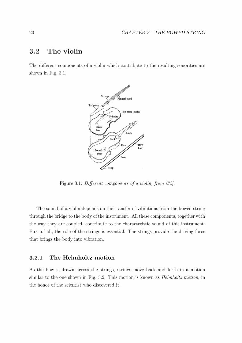
The different components of a violin which contribute to the resulting sonorities are
shown in Fig. 3.1.
Figure 3.1: Different components of a violin, from [32].
The sound of a violin depends on the transfer of vibrations from the bowed string
through the bridge to the body of the instrument. All these components, together with
the way they are coupled, contribute to the characteristic sound of this instrument.
First of all, the role of the strings is essential. The strings provide the driving force
that brings the body into vibration.
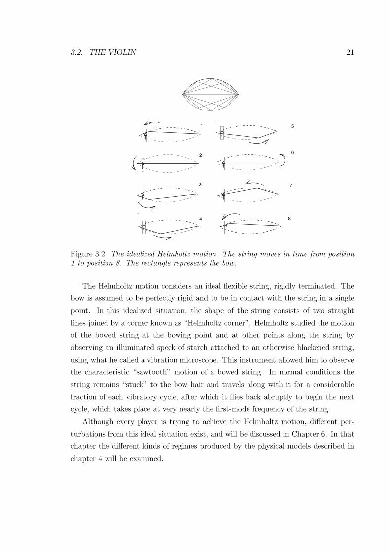
3.2.1 The Helmholtz motion
As the bow is drawn across the strings, strings move back and forth in a motion
similar to the one shown in Fig. 3.2. This motion is known as Helmholtz motion, in
the honor of the scientist who discovered it.
3.2. THE VIOLIN 21
3
51
4
26
7
8
Figure 3.2: The idealized Helmholtz motion. The string moves in time from position1 to position 8. The rectangle represents the bow.
The Helmholtz motion considers an ideal flexible string, rigidly terminated. The
bow is assumed to be perfectly rigid and to be in contact with the string in a single
point. In this idealized situation, the shape of the string consists of two straight
lines joined by a corner known as “Helmholtz corner”. Helmholtz studied the motion
of the bowed string at the bowing point and at other points along the string by
observing an illuminated speck of starch attached to an otherwise blackened string,
using what he called a vibration microscope. This instrument allowed him to observe
the characteristic “sawtooth” motion of a bowed string. In normal conditions the
string remains “stuck” to the bow hair and travels along with it for a considerable
fraction of each vibratory cycle, after which it flies back abruptly to begin the next
cycle, which takes place at very nearly the first-mode frequency of the string.
Although every player is trying to achieve the Helmholtz motion, different per-
turbations from this ideal situation exist, and will be discussed in Chapter 6. In that
chapter the different kinds of regimes produced by the physical models described in
chapter 4 will be examined.
22 CHAPTER 3. THE BOWED STRING
3.3 The violin body
The violin body acts as a resonator for the vibration generated from the strings. The
coupling of air cavity modes and top and back plate modes produces the complex
filtering which contributes strongly to the characteristic timbre of the violin.
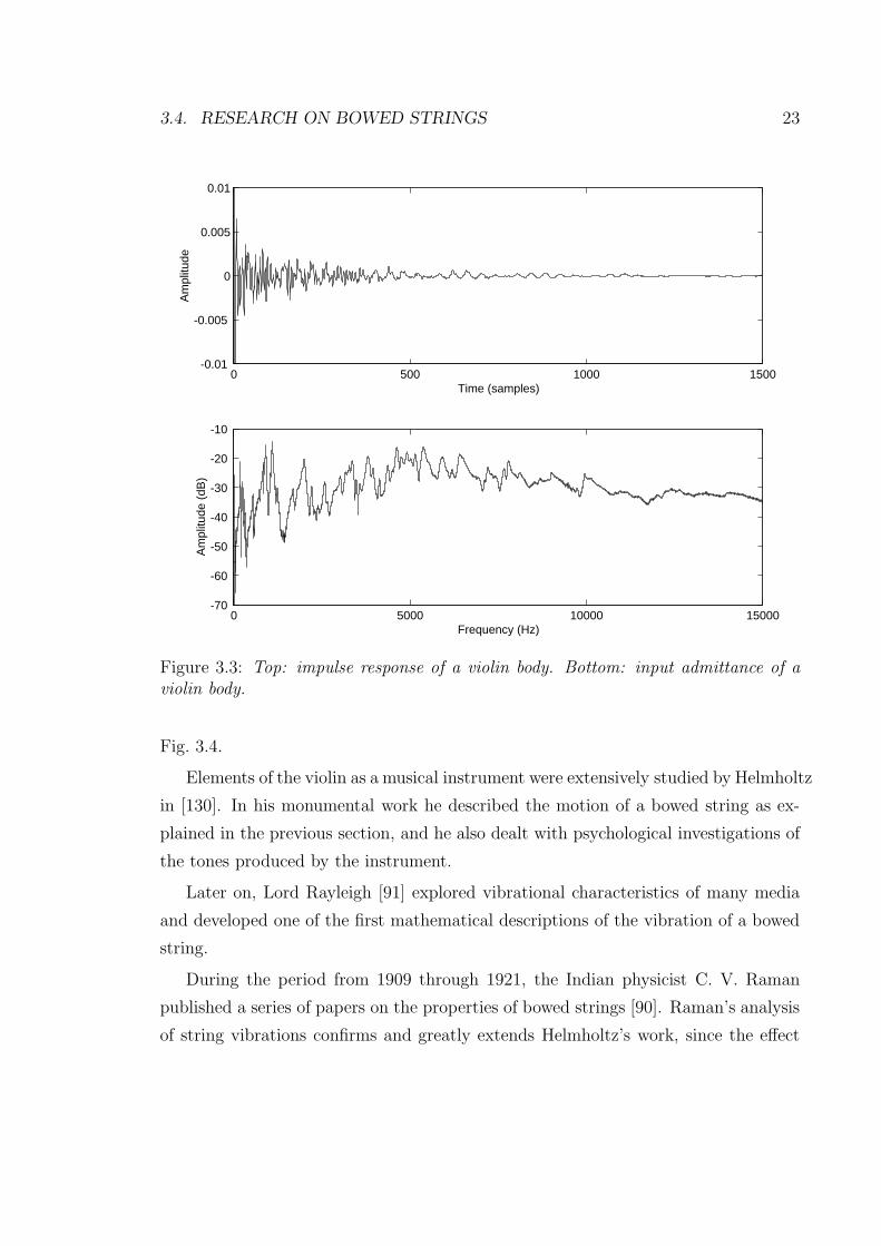
The impulse response of a violin body is shown in Fig. 3.3.1 The bottom of
Fig. 3.3 shows the input admittance. At low frequencies, the resonances of the whole
body dominate, except for the 460 Hz resonance and the air resonance [55]. With
increasing frequency, a large number of top and back plate resonances will dominate
the body vibration of a violin. At high frequencies the bridge will give a major
contribution. The sound post gives a large asymmetry at low frequencies. The violin
body therefore acts as an acoustical amplifier which gives two kinds of amplification.
First the vibration of the strings results in the vibration of the body walls, since the
vibrating string produces a vibration force on the bridge, which is transmitted via the
bridge to the top plate and thereafter to the complete body. Secondly, the resonances
of the violin body give extra amplification at specific frequencies.
3.4 Research on bowed strings
The first scientific investigations of vibrating strings are credited to the Greek philoso-
pher Pythagoras, who, in the 6th century B.C., noticed some important relationships
between string length and pitch.
Preliminary observations regarding the sound of friction for bowed objects were
made by Galileo Galilei in the 16th century [35]. Galileo noticed that when a brass
plate is scraped with an iron chisel, the scraping produces a sharp whistling sound.
In the 18th and 19th century, Savart directly experimented with violin construc-
tion and form. He studied modes and vibration of violin’s plates, using the technique
previously developed by Chladni [16], which consisted of sprinkling plates with fine
powder and putting them into vibration using a violin bow. This technique was also
used to study the vibrational modes of a trapezoidal violin such as the one shown in
1Courtesy of Jim Woodhouse.
3.4. RESEARCH ON BOWED STRINGS 23
0 5000 10000 15000-70
-60
-50
-40
-30
-20
-10
Frequency (Hz)
Am
plitu
de (
dB)
0 500 1000 1500-0.01
-0.005
0
0.005
0.01
Time (samples)
Am
plitu
de
Figure 3.3: Top: impulse response of a violin body. Bottom: input admittance of aviolin body.
Fig. 3.4.
Elements of the violin as a musical instrument were extensively studied by Helmholtz
in [130]. In his monumental work he described the motion of a bowed string as ex-
plained in the previous section, and he also dealt with psychological investigations of
the tones produced by the instrument.
Later on, Lord Rayleigh [91] explored vibrational characteristics of many media
and developed one of the first mathematical descriptions of the vibration of a bowed
string.
During the period from 1909 through 1921, the Indian physicist C. V. Raman
published a series of papers on the properties of bowed strings [90]. Raman’s analysis
of string vibrations confirms and greatly extends Helmholtz’s work, since the effect
24 CHAPTER 3. THE BOWED STRING
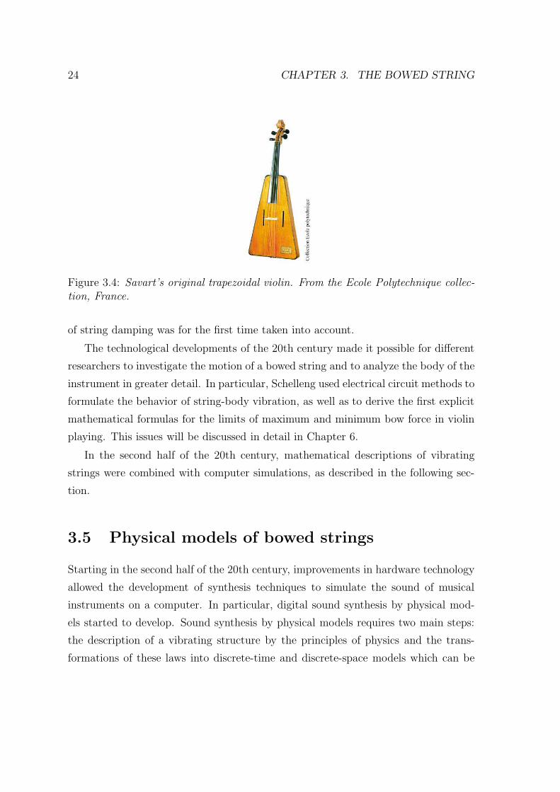
Figure 3.4: Savart’s original trapezoidal violin. From the Ecole Polytechnique collec-tion, France.
of string damping was for the first time taken into account.
The technological developments of the 20th century made it possible for different
researchers to investigate the motion of a bowed string and to analyze the body of the
instrument in greater detail. In particular, Schelleng used electrical circuit methods to
formulate the behavior of string-body vibration, as well as to derive the first explicit
mathematical formulas for the limits of maximum and minimum bow force in violin
playing. This issues will be discussed in detail in Chapter 6.
In the second half of the 20th century, mathematical descriptions of vibrating
strings were combined with computer simulations, as described in the following sec-
tion.
3.5 Physical models of bowed strings
Starting in the second half of the 20th century, improvements in hardware technology
allowed the development of synthesis techniques to simulate the sound of musical
instruments on a computer. In particular, digital sound synthesis by physical mod-
els started to develop. Sound synthesis by physical models requires two main steps:
the description of a vibrating structure by the principles of physics and the trans-
formations of these laws into discrete-time and discrete-space models which can be
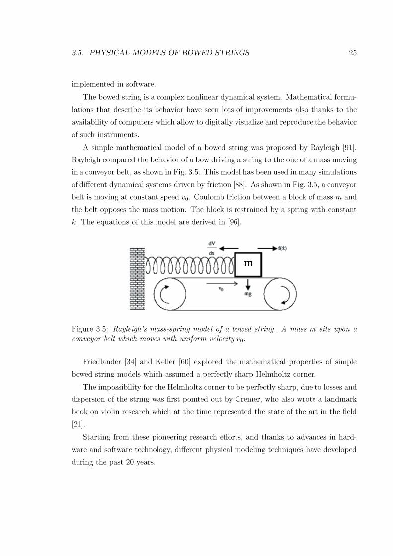
3.5. PHYSICAL MODELS OF BOWED STRINGS 25
implemented in software.
The bowed string is a complex nonlinear dynamical system. Mathematical formu-
lations that describe its behavior have seen lots of improvements also thanks to the
availability of computers which allow to digitally visualize and reproduce the behavior
of such instruments.
A simple mathematical model of a bowed string was proposed by Rayleigh [91].
Rayleigh compared the behavior of a bow driving a string to the one of a mass moving
in a conveyor belt, as shown in Fig. 3.5. This model has been used in many simulations
of different dynamical systems driven by friction [88]. As shown in Fig. 3.5, a conveyor
belt is moving at constant speed v0. Coulomb friction between a block of mass m and
the belt opposes the mass motion. The block is restrained by a spring with constant
k. The equations of this model are derived in [96].
Figure 3.5: Rayleigh’s mass-spring model of a bowed string. A mass m sits upon aconveyor belt which moves with uniform velocity v0.
Friedlander [34] and Keller [60] explored the mathematical properties of simple
bowed string models which assumed a perfectly sharp Helmholtz corner.
The impossibility for the Helmholtz corner to be perfectly sharp, due to losses and
dispersion of the string was first pointed out by Cremer, who also wrote a landmark
book on violin research which at the time represented the state of the art in the field
[21].
Starting from these pioneering research efforts, and thanks to advances in hard-
ware and software technology, different physical modeling techniques have developed
during the past 20 years.
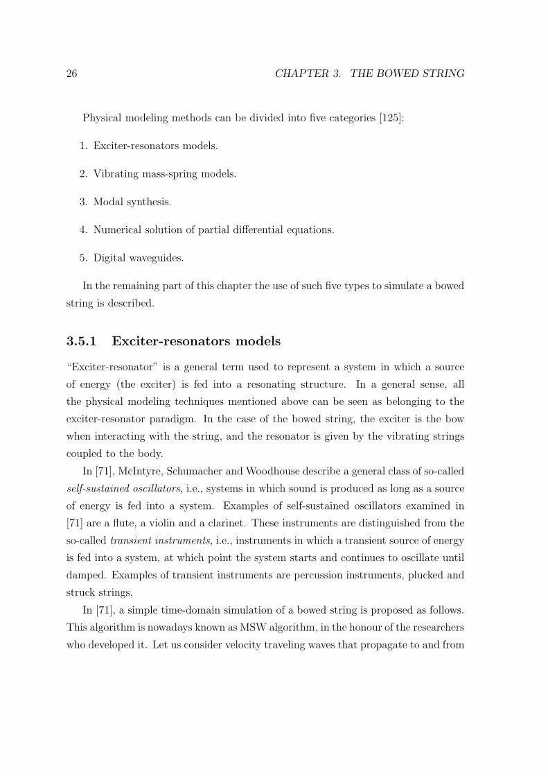
26 CHAPTER 3. THE BOWED STRING
Physical modeling methods can be divided into five categories [125]:
1. Exciter-resonators models.
2. Vibrating mass-spring models.
3. Modal synthesis.
4. Numerical solution of partial differential equations.
5. Digital waveguides.
In the remaining part of this chapter the use of such five types to simulate a bowed
string is described.
3.5.1 Exciter-resonators models
“Exciter-resonator” is a general term used to represent a system in which a source
of energy (the exciter) is fed into a resonating structure. In a general sense, all
the physical modeling techniques mentioned above can be seen as belonging to the
exciter-resonator paradigm. In the case of the bowed string, the exciter is the bow
when interacting with the string, and the resonator is given by the vibrating strings
coupled to the body.
In [71], McIntyre, Schumacher and Woodhouse describe a general class of so-called
self-sustained oscillators, i.e., systems in which sound is produced as long as a source
of energy is fed into a system. Examples of self-sustained oscillators examined in
[71] are a flute, a violin and a clarinet. These instruments are distinguished from the
so-called transient instruments, i.e., instruments in which a transient source of energy
is fed into a system, at which point the system starts and continues to oscillate until
damped. Examples of transient instruments are percussion instruments, plucked and
struck strings.
In [71], a simple time-domain simulation of a bowed string is proposed as follows.
This algorithm is nowadays known as MSW algorithm, in the honour of the researchers
who developed it. Let us consider velocity traveling waves that propagate to and from
3.5. PHYSICAL MODELS OF BOWED STRINGS 27
nonlinear element
sourceenergy
linear element
Figure 3.6: A general oscillator made of a linear and nonlinear component connectedin a feedback loop.
the two extremities of a string, which are called the bridge and the nut, and meet at
the bow point.
First of all, the contribution of the reflected waves vin and vib coming from the
nut and the bridge respectively are summed at the bow contact point:
vh = vin + vib
where vh is the notation used in [71] to denote the historical (i.e., known) string
velocity. At this point, two variables are considered, which are the transverse string
velocity v and the frictional force f . These quantities are connected in two different
ways, represented by the following equations:
f = 2Z(v − vh) (3.1)
f = µ(v − vb)fb (3.2)
where Z is the wave impedance of the string, vb is the bow velocity, fb is the bow force,
v is the velocity of the string at the contact point and µ is the frictional force. As
shown in Eq. (3.2), to a first approximation it is possible to assume that the frictional
force simply depends on the relative velocity between the bow and the string (v− vb)
and on the bow force fb. Once the friction force f has been calculated, two traveling
waves von and vob resulting from the bow string interaction propagate toward the nut
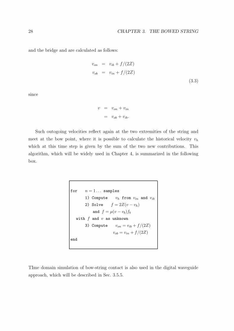
28 CHAPTER 3. THE BOWED STRING
and the bridge and are calculated as follows:
von = vib + f/(2Z)
vob = vin + f/(2Z)
(3.3)
since
v = von + vin
= vob + vib.
Such outogoing velocities reflect again at the two extremities of the string and
meet at the bow point, where it is possible to calculate the historical velocity vh
which at this time step is given by the sum of the two new contributions. This
algorithm, which will be widely used in Chapter 4, is summarized in the following
box.
for n = 1 . . . samples
1) Compute vh from vin and vib
2) Solve f = 2Z(v − vh)
and f = µ(v − vb)fb
with f and v as unknown
3) Compute von = vib + f/(2Z)
vob = vin + f/(2Z)
end
TIme domain simulation of bow-string contact is also used in the digital waveguide
approach, which will be described in Sec. 3.5.5.
3.5. PHYSICAL MODELS OF BOWED STRINGS 29
3.5.2 Vibrating mass-spring models
Another approach to simulate the vibration of a string as well other vibrating systems
is the one developed by Cadoz and coworkers [13]. They suggest to create complex
physical models by connecting basic mechanical elements such as masses, dampers
and springs.
In 1985 the first real-time bowed string simulation based on such particle-interaction
systems was proposed [13]. In it, the string was represented by a set of 25 to 60 masses
linked by visco-elastic elements.
The system implementing bowed string physical models as well as other vibrating
structures is called Cordis-Anima. In it elements that receive forces and calculate
positions are found, and interaction elements that calculate a force according to the
positions of the other elements.
The basic elements of the Cordis-Anima system are:
1. point masses
2. ideal springs
3. ideal dampers
The Cordis-Anima system is still widely used and developed at the center Acroe in
Grenoble, where Cadoz and coworkers can now take advantage of the development in
hardware technology to create complex vibrating systems that work in real-time. The
Cordis-Anima environment presents a powerful combination of physically-modeled
audio-visual simulations used in virtual reality and computer music compositions.
3.5.3 Modal synthesis
Another powerful synthesis technique inspired by the physics of vibrating objects with
a strong link to spectral models is modal synthesis. The modal synthesis approach has
been widely adopted in the sound synthesis community. As few important examples,
Klatt used it to simulate a formant based speech synthesizer [61], Serra adopted it
to simulate bar percussion instruments [111], Wawrzynek used modal synthesis for
30 CHAPTER 3. THE BOWED STRING
VLSI computation [131]. Other applications of modal synthesis to the simulation of
musical instruments were proposed by Adrien [2, 1].
Modal synthesis is based on the premise that many sound-producing objects can
be represented as a set of vibrating substructures which are defined by modal data.
Recently modal synthesis has been widely adopted in the computer music com-
munity for simulation of audio effects and sounding objects in general [20, 93, 83].
Concerning the bowed string, in [5] a detailed simulation of how a modal resonator
can be coupled to a friction excitation is described. The approach derived in [5] is
described in the following.
Let us consider the equation of an ideal vibrating string:
m∂2y
∂t2= T
∂2y
x2− η∂y
∂t+ F (x, t) (3.4)
of mass m, length L and dissipation η, where c2 = T/m, and F represents external
forces on the string. All the solutions of Eq. (3.4) can be formulated in terms of
the modal parameters mn = µL/2 (∀n), ωn = nπc/L, ηn, and modeshapes φn(x) =
sin(nπx/L), for n = 1, 2, ..., N , where the mode number N is arbitrarily chosen.
In the modal domain, the response of the string can be expressed as:
[M ]Q(t) + [C]Q(t) + [K]Q(t) = Ξ(t) (3.5)
where
[M ] = diag(m1, ..., mN ),
[C] = diag(2m1ω1ζ1, ..., 2mNωNζN),
[K] = diag(m1ω21, ..., mNω
2N),
Q(t) = < q1(t), ..., qN(t) >T ,
Ξ(t) = < χ1(t), ..., χN(t) >T
3.5. PHYSICAL MODELS OF BOWED STRINGS 31
At any time, the response of the system can be calculated by modal superposition:
y(x, t) =N∑
n=1
φn(x)qn(t) (3.6)
For given external excitation and initial conditions, the previous system of equations
can be integrated using an adequate time-step integration algorithm. It is possible
to show [83] that modal synthesis can be implemented by using resonant filters in
parallel.
The right side of Eq. (3.5) contains all the nonlinearities of the system. In the
case of the bowed string, therefore, the second term contains the frictional interaction
between the bow and the string.
3.5.4 Numerical solution of partial differential equations
In [44], Hiller and Ruiz proposed a numerical solution to the partial differential equa-
tion representing a bowed string. They were the first to take the approach of numer-
ically solving the equation of a vibrating string for sound synthesis purposes.
A similar approach which uses finite differences to simulate a bowed string was
proposed in [85]. The starting point is a variation of the wave equation of Eq. (3.4):
m∂2y
∂t2= T
∂2y
x2− η∂y
∂t+ Sj
∂3
∂x2∂t(3.7)
in which the last term represents energy losses due to internal viscous friction.
In order to integrate Eq. (3.7), the authors decompose the instantaneous shape of
the string into a set of harmonic functions up to a certain order that is the highest
allowable spatial frequency for the string. The solution for the integration of spatial
variables is similar to the use of finite elements, since it is based on the decomposi-
tion into orthonormal functions. As in [5], the shape of the string is obtained by a
sinusoidal decomposition. For the integration of the time variables, finite differences
are used.
The model described was used by the Italian composer Michelangelo Lupone in
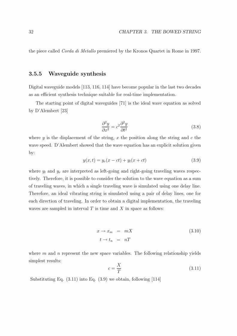
32 CHAPTER 3. THE BOWED STRING
the piece called Corda di Metallo premiered by the Kronos Quartet in Rome in 1997.
3.5.5 Waveguide synthesis
Digital waveguide models [113, 116, 114] have become popular in the last two decades
as an efficient synthesis technique suitable for real-time implementation.
The starting point of digital waveguides [71] is the ideal wave equation as solved
by D’Alembert [23]
∂2y
∂x2= c2
∂2y
∂t2(3.8)
where y is the displacement of the string, x the position along the string and c the
wave speed. D’Alembert showed that the wave equation has an explicit solution given
by:
y(x, t) = yr(x− ct) + yl(x+ ct) (3.9)
where yl and yr are interpreted as left-going and right-going traveling waves respec-
tively. Therefore, it is possible to consider the solution to the wave equation as a sum
of traveling waves, in which a single traveling wave is simulated using one delay line.
Therefore, an ideal vibrating string is simulated using a pair of delay lines, one for
each direction of traveling. In order to obtain a digital implementation, the traveling
waves are sampled in interval T is time and X in space as follows:
x→ xm = mX (3.10)
t→ tn = nT
where m and n represent the new space variables. The following relationship yields
simplest results:
c =X
T(3.11)
Substituting Eq. (3.11) into Eq. (3.9) we obtain, following [114]
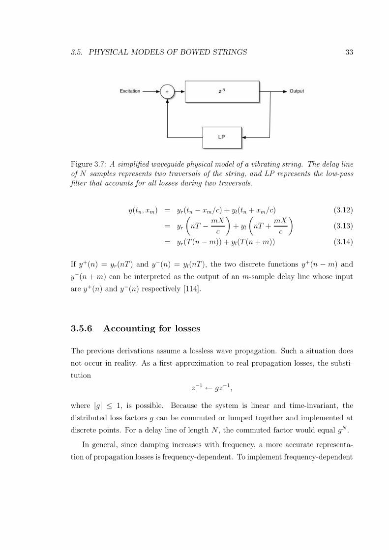
3.5. PHYSICAL MODELS OF BOWED STRINGS 33
Figure 3.7: A simplified waveguide physical model of a vibrating string. The delay lineof N samples represents two traversals of the string, and LP represents the low-passfilter that accounts for all losses during two traversals.
y(tn, xm) = yr(tn − xm/c) + yl(tn + xm/c) (3.12)
= yr
(
nT − mX
c
)
+ yl
(
nT +mX
c
)
(3.13)
= yr(T (n−m)) + yl(T (n+m)) (3.14)
If y+(n) = yr(nT ) and y−(n) = yl(nT ), the two discrete functions y+(n − m) and
y−(n + m) can be interpreted as the output of an m-sample delay line whose input
are y+(n) and y−(n) respectively [114].
3.5.6 Accounting for losses
The previous derivations assume a lossless wave propagation. Such a situation does
not occur in reality. As a first approximation to real propagation losses, the substi-
tution
z−1 ← gz−1,
where |g| ≤ 1, is possible. Because the system is linear and time-invariant, the
distributed loss factors g can be commuted or lumped together and implemented at
discrete points. For a delay line of length N , the commuted factor would equal gN .
In general, since damping increases with frequency, a more accurate representa-
tion of propagation losses is frequency-dependent. To implement frequency-dependent
34 CHAPTER 3. THE BOWED STRING
losses, each scale factor g is replaced by an appropriately designed digital filter. Be-
cause the system is linear and time-invariant, these filter responses can also be com-
muted and implemented as a single string loop filter G(z). In Fig. 3.7 the low-pass
filter LP which accounted for losses while traversing the string was introduced. The
role of LP is to simulate frequency-dependent attenuation. By using a linear-time-
invariant filter, it is possible to provide an independent gain at each frequency, as
described in [114]. Digital filters which allow to simulate losses in a violin and cello
string are described in Chapter 4.
Before describing different bow-string interaction models proposed in the litera-
ture, the characteristics of the described synthesis techniques are summarized in Table
3.1.
3.6 Comparisons between the different techniques
The different synthesis techniques used to synthesize a bowed string are summarized
in Table 3.1. Until recently, finite differences and mass-spring systems could not be
implemented in real-time due to computational issues. However, improvements in
hardware technology are allowing such techniques to see real-time implementations.
The choice of the discretization technique to model resonators is usually based on
the structure of the resonator itself. For example, for quasi-harmonic systems such
as violin strings, usually digital waveguides are the preferred choice. However, for
systems which show a strongly inharmonic spectrum, usually other techniques such
as modal synthesis are preferred.
Technique Characteristics Reference
Finite differences Numerical solution of the wave equation. [85]The MSW algorithm Precursor of digital waveguides. [71, 38, 39]Digital waveguides Efficient for quasi-harmonic systems. [119, 14, 124,
45]Modal synthesis Efficient for systems with few modes. [2, 5]Mass-spring systems High computational cost. [13]
Table 3.1: Summary of physical modeling techniques used to simulate a bowed string.
3.7. THE BOW-STRING INTERACTION 35
3.7 The bow-string interaction
“Classic” models of the bow-string interaction assume that friction depends only on
the relative velocity between the bow and the string, in a dependence similar to the
one shown in Fig. 3.8, in which friction exponentially decreases while the relative bow-
string velocity increases. The different shapes which the friction curve of Fig. 3.8 can
assume are discussed in Chapter 4.
In order to solve the interaction between the bow and the string, a graphical
solution to the system in Eq. (3.2) was first proposed in [34] and is represented in
Fig. 3.8 part a). Notice how, in a situation such as Fig. 3.8 part b) three intersections
can occur, as pointed out by Friedlander [34]. This ambiguity is solved using the
hysteresis rule proposed in [72] and described in Fig. 3.8, part c) and d): as the
string velocity increases, the bow remains in slipping mode until it reaches the capture
velocity vc. The string velocity then jumps to the bow velocity vb. The string remains
in stick velocity until it decreases to vr, at which point the maximum sticking force
is exceeded. The hysteresis rule therefore means that the solution point traverses a
different path for increasing relative bow spring speeds than for decreasing speeds.
The shape of the “classic” friction curve has been mathematically expressed in
different ways, which are described in the following section.
3.7.1 Mathematical formulations of the friction curve
Hyperbolic friction model
The hyperbolic model for the coefficient of bow-string friction is given by:
µ = µd +(µs − µd)v0
v0 + v − vb(3.15)
where v, vb and v0 are the string velocity, bow velocity and initial bow velocity,
respectively, and µd and µs are the dynamic and static coefficients of friction, respec-
tively. Notice that µs > µd. Typical values used in the literature are µs = 0.8 and
µd = 0.3 [100]. This model has been used for many years as a convenient mathe-
matical approximation which yields closed-form results for the bow-string interaction
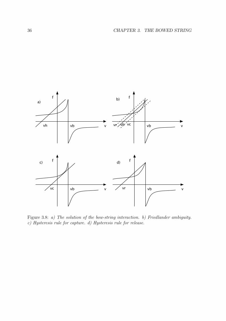
36 CHAPTER 3. THE BOWED STRING
vb v
f
vh vb v
f
vh
b)a)
vb v
f
vc
c)
vr vc
vb v
f
vr
d)
Figure 3.8: a) The solution of the bow-string interaction. b) Friedlander ambiguity.c) Hysteresis rule for capture. d) Hysteresis rule for release.
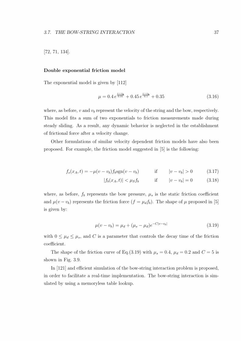
3.7. THE BOW-STRING INTERACTION 37
[72, 71, 134].
Double exponential friction model
The exponential model is given by [112]
µ = 0.4 ev−vb
0.01 + 0.45 ev−vb
0.1 + 0.35 (3.16)
where, as before, v and vb represent the velocity of the string and the bow, respectively.
This model fits a sum of two exponentials to friction measurements made during
steady sliding. As a result, any dynamic behavior is neglected in the establishment
of frictional force after a velocity change.
Other formulations of similar velocity dependent friction models have also been
proposed. For example, the friction model suggested in [5] is the following:
fs(xA, t) = −µ(v − vb)fbsgn(v − vb) if |v − vb| > 0 (3.17)
|fb(xA, t)| < µSfb if |v − vb| = 0 (3.18)
where, as before, fb represents the bow pressure, µs is the static friction coefficient
and µ(v− vb) represents the friction force (f = µdfb). The shape of µ proposed in [5]
is given by:
µ(v − vb) = µd + (µs − µd)e−C|v−vb| (3.19)
with 0 ≤ µd ≤ µs, and C is a parameter that controls the decay time of the friction
coefficient.
The shape of the friction curve of Eq.(3.19) with µs = 0.4, µd = 0.2 and C = 5 is
shown in Fig. 3.9.
In [121] and efficient simulation of the bow-string interaction problem is proposed,
in order to facilitate a real-time implementation. The bow-string interaction is sim-
ulated by using a memoryless table lookup.
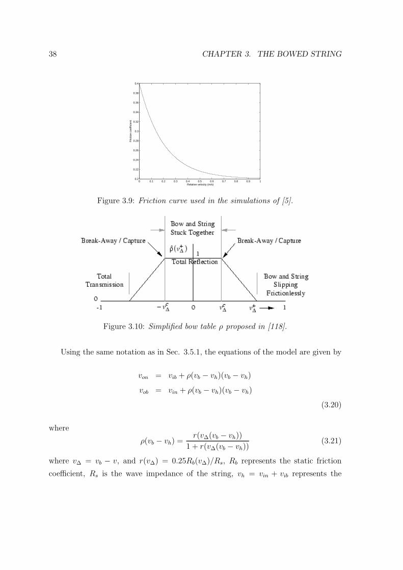
38 CHAPTER 3. THE BOWED STRING
0 0.1 0.2 0.3 0.4 0.5 0.6 0.7 0.8 0.9 10.2
0.22
0.24
0.26
0.28
0.3
0.32
0.34
0.36
0.38
0.4
Relative velocity (m/s)
Fric
tion
coef
ficie
nt
Figure 3.9: Friction curve used in the simulations of [5].
Figure 3.10: Simplified bow table ρ proposed in [118].
Using the same notation as in Sec. 3.5.1, the equations of the model are given by
von = vib + ρ(vb − vh)(vb − vh)
vob = vin + ρ(vb − vh)(vb − vh)
(3.20)
where
ρ(vb − vh) =r(v∆(vb − vh))
1 + r(v∆(vb − vh))(3.21)
where v∆ = vb − v, and r(v∆) = 0.25Rb(v∆)/Rs, Rb represents the static friction
coefficient, Rs is the wave impedance of the string, vh = vin + vib represents the
3.7. THE BOW-STRING INTERACTION 39
historical (past) velocity at the bow point and Rb is the friction coefficient of the
bow against the string. Rb is constant for |v∆| ≤ vc∆, where vc
∆ is the capture and
breakaway differential velocity.
For |v∆| > vc∆, Rb falls quickly to a low dynamic friction coefficient. The bow table
chosen in [121] is shown in Fig. 3.10. These equations are justified by the fact that
velocity input (which is injected equally in the left- and right-going directions) must
be found such that the transverse force of the bow against the string is balanced by
the reaction force of the moving string. If bow-hair dynamics are neglected, the bow-
string interaction can be simulated using a memoryless table lookup or segmented
polynomial such as the one shown in Fig. 3.10.
The flat portion corresponds to the portion of the bow “stuck” to the string,
while the outer section corresponds to the slipping part. The outer sections of the
curve give a smaller reflection coefficient corresponding to the reduced bow-string
interaction force while the string is slipping under the bow. Using this simplified
bow table, it is possible to avoid the iterative solver required when the bow-string
interaction is expressed through a nonlinear function. This friction model does not
account for hysteresis.2
Following Smith’s approach, other researchers recently proposed waveguide-based
bowed string physical models. For example, in [124] a waveguide bowed string physical
model is driven by a rule-based parameters’ engine, in order to increase its expres-
sivity. In [45] variations to the original waveguide models are also proposed. The
addition of random noise to the friction curve in order to simulate the characteristic
noise of a bowed string instrument was first proposed in [15], and recently used in
[85].3
Dynamic bow models
An interesting approach in order to obtain a dynamic model of the bow was proposed
in [2] and shown in Fig. 3.11.
2A nonlinear function generation apparatus which comprises hysteresis was developed by Yamahain a patent filled in 1990, patent number 613163.
3The addition of random noise to the friction curve was also suggested to the author by KnutGuettler [37].
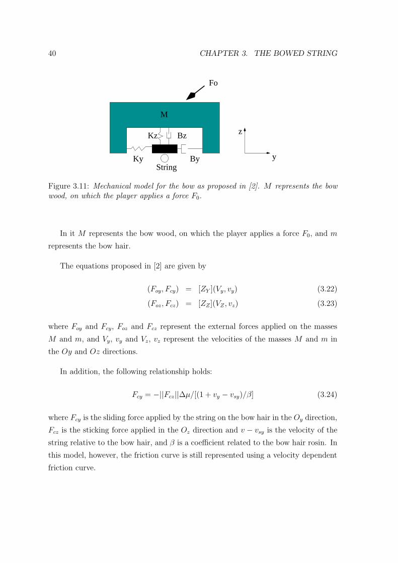
40 CHAPTER 3. THE BOWED STRING
StringKy By
BzKz
M
Fo
y
z
Figure 3.11: Mechanical model for the bow as proposed in [2]. M represents the bowwood, on which the player applies a force F0.
In it M represents the bow wood, on which the player applies a force F0, and m
represents the bow hair.
The equations proposed in [2] are given by
(Foy, Fcy) = [ZY ](Vy, vy) (3.22)
(Foz, Fcz) = [ZZ ](VZ , vz) (3.23)
where Foy and Fcy, Foz and Fcz represent the external forces applied on the masses
M and m, and Vy, vy and Vz, vz represent the velocities of the masses M and m in
the Oy and Oz directions.
In addition, the following relationship holds:
Fcy = −||Fcz||∆µ/[(1 + vy − vsy)/β] (3.24)
where Fcy is the sliding force applied by the string on the bow hair in the Oy direction,
Fcz is the sticking force applied in the Oz direction and v − vsy is the velocity of the
string relative to the bow hair, and β is a coefficient related to the bow hair rosin. In
this model, however, the friction curve is still represented using a velocity dependent
friction curve.
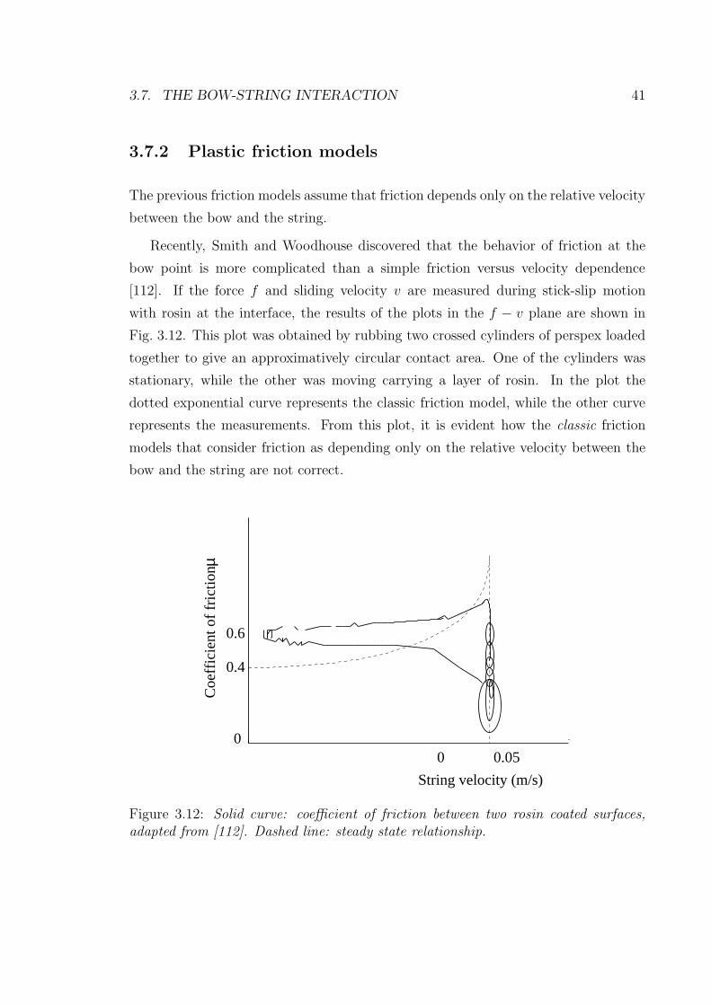
3.7. THE BOW-STRING INTERACTION 41
3.7.2 Plastic friction models
The previous friction models assume that friction depends only on the relative velocity
between the bow and the string.
Recently, Smith and Woodhouse discovered that the behavior of friction at the
bow point is more complicated than a simple friction versus velocity dependence
[112]. If the force f and sliding velocity v are measured during stick-slip motion
with rosin at the interface, the results of the plots in the f − v plane are shown in
Fig. 3.12. This plot was obtained by rubbing two crossed cylinders of perspex loaded
together to give an approximatively circular contact area. One of the cylinders was
stationary, while the other was moving carrying a layer of rosin. In the plot the
dotted exponential curve represents the classic friction model, while the other curve
represents the measurements. From this plot, it is evident how the classic friction
models that consider friction as depending only on the relative velocity between the
bow and the string are not correct.
0.0500
0.4
0.6
String velocity (m/s)
Coe
ffic
ient
of
fric
tion µ
Figure 3.12: Solid curve: coefficient of friction between two rosin coated surfaces,adapted from [112]. Dashed line: steady state relationship.
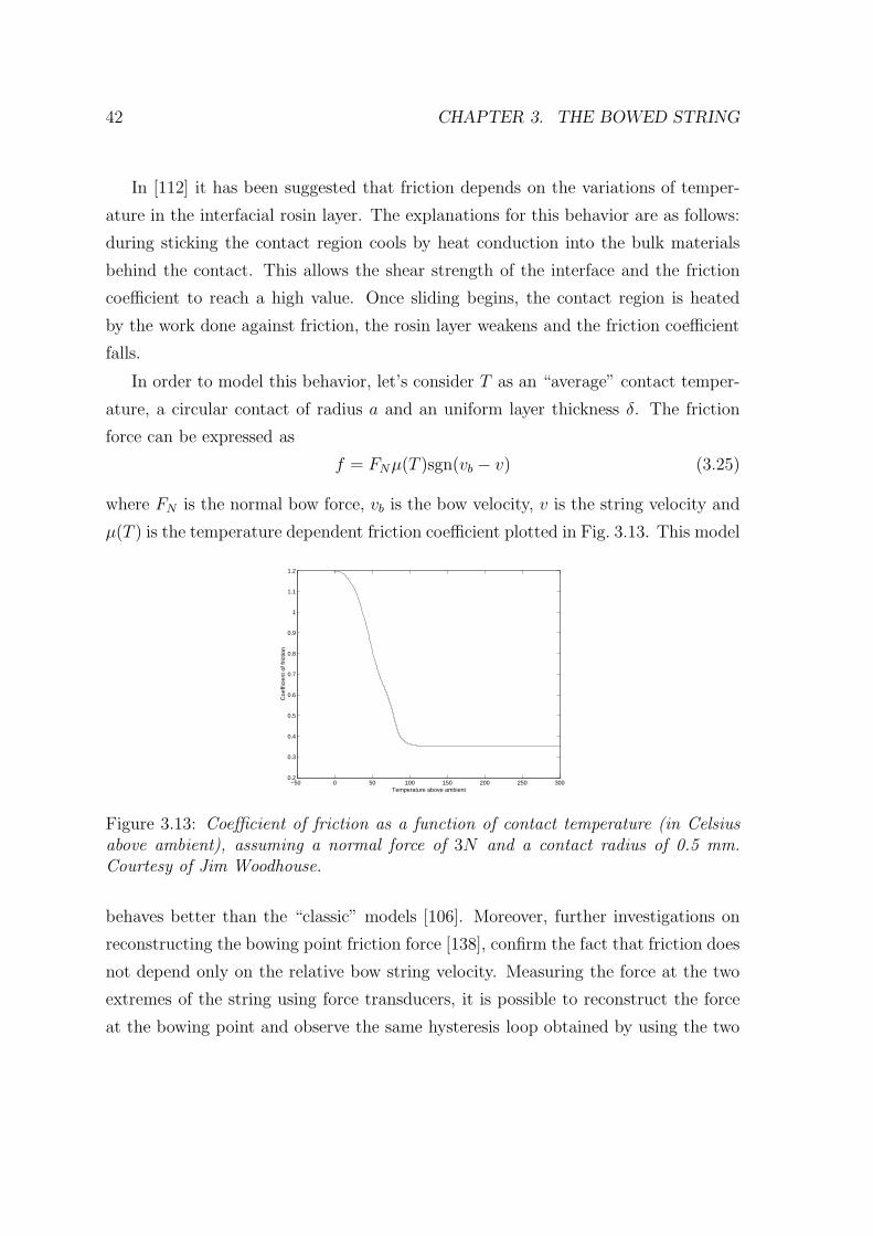
42 CHAPTER 3. THE BOWED STRING
In [112] it has been suggested that friction depends on the variations of temper-
ature in the interfacial rosin layer. The explanations for this behavior are as follows:
during sticking the contact region cools by heat conduction into the bulk materials
behind the contact. This allows the shear strength of the interface and the friction
coefficient to reach a high value. Once sliding begins, the contact region is heated
by the work done against friction, the rosin layer weakens and the friction coefficient
falls.
In order to model this behavior, let’s consider T as an “average” contact temper-
ature, a circular contact of radius a and an uniform layer thickness δ. The friction
force can be expressed as
f = FNµ(T )sgn(vb − v) (3.25)
where FN is the normal bow force, vb is the bow velocity, v is the string velocity and
µ(T ) is the temperature dependent friction coefficient plotted in Fig. 3.13. This model
−50 0 50 100 150 200 250 3000.2
0.3
0.4
0.5
0.6
0.7
0.8
0.9
1
1.1
1.2
Temperature above ambient
Coe
ffici
ent o
f fric
tion
Figure 3.13: Coefficient of friction as a function of contact temperature (in Celsiusabove ambient), assuming a normal force of 3N and a contact radius of 0.5 mm.Courtesy of Jim Woodhouse.
behaves better than the “classic” models [106]. Moreover, further investigations on
reconstructing the bowing point friction force [138], confirm the fact that friction does
not depend only on the relative bow string velocity. Measuring the force at the two
extremes of the string using force transducers, it is possible to reconstruct the force
at the bowing point and observe the same hysteresis loop obtained by using the two
3.7. THE BOW-STRING INTERACTION 43
coated cylinders.
3.7.3 The bow hair compliance
Another element that seems to have a strong effect on the frictional interaction be-
tween a bow and a string is bow hair compliance.
The bow hair-compliance was investigated by Raman [90], who stated that, while
it is possible for a single point on the string to have absolutely the same velocity as
the bow in every part of its forward motion, kinematical theory shows that it is not
possible for every element on a finite region to have absolutely the same velocity as
the bow in every part of its forward motion.
The first line of evidence comes from analyzing experimental results presented
by Cremer [21] of the reflection and transmission behavior of transverse waves on a
string incident on a bow at rest. The second line of evidence comes from simulations
of the bowed string taking into account the finite width of the bow. The nature of the
“differential slipping” which may arise due to the kinematic incompatibility of uniform
bow velocity across the width of the bow and the string velocity in standard bowed
string motion (Helmholtz motion) is strongly dependent on bow hair compliance.
Simulations also demonstrate that suitable tilting of the bow can reduce the extent
to which “differential slipping” is detrimental to the establishment of the desired
string motion. The incompatibility of finite width and idealized Helmholtz motion is
shown in Fig. 3.14, borrowed from [70].
In position 1, the Helmholtz corner has just travelled past the bow from left to right.
While the entire section of the string under the bow sticks to the bow-hair, it is carried
forward parallel to its initial position, leading to position 2. The displacement of the
string force by the finite width of the bow is in disagreement with the ideal Helmholtz
motion, in which the shape of the string consists only of two straight lines.
As explained in [70], the the finite width of the bow creates a phenomenon called
differential slipping, in which the string occasionally slips at one side of the bow
continuing to stick at the other side.
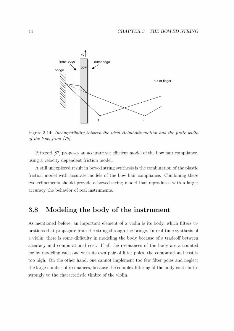
44 CHAPTER 3. THE BOWED STRING
bowouter edgeinner edge
vb
bridge
nut or finger
1 2
Figure 3.14: Incompatibility between the ideal Helmholtz motion and the finite widthof the bow, from [70].
Pitteroff [87] proposes an accurate yet efficient model of the bow hair compliance,
using a velocity dependent friction model.
A still unexplored result in bowed string synthesis is the combination of the plastic
friction model with accurate models of the bow hair compliance. Combining these
two refinements should provide a bowed string model that reproduces with a larger
accuracy the behavior of real instruments.
3.8 Modeling the body of the instrument
As mentioned before, an important element of a violin is its body, which filters vi-
brations that propagate from the string through the bridge. In real-time synthesis of
a violin, there is some difficulty in modeling the body because of a tradeoff between
accuracy and computational cost. If all the resonances of the body are accounted
for by modeling each one with its own pair of filter poles, the computational cost is
too high. On the other hand, one cannot implement too few filter poles and neglect
the large number of resonances, because the complex filtering of the body contributes
strongly to the characteristic timbre of the violin.
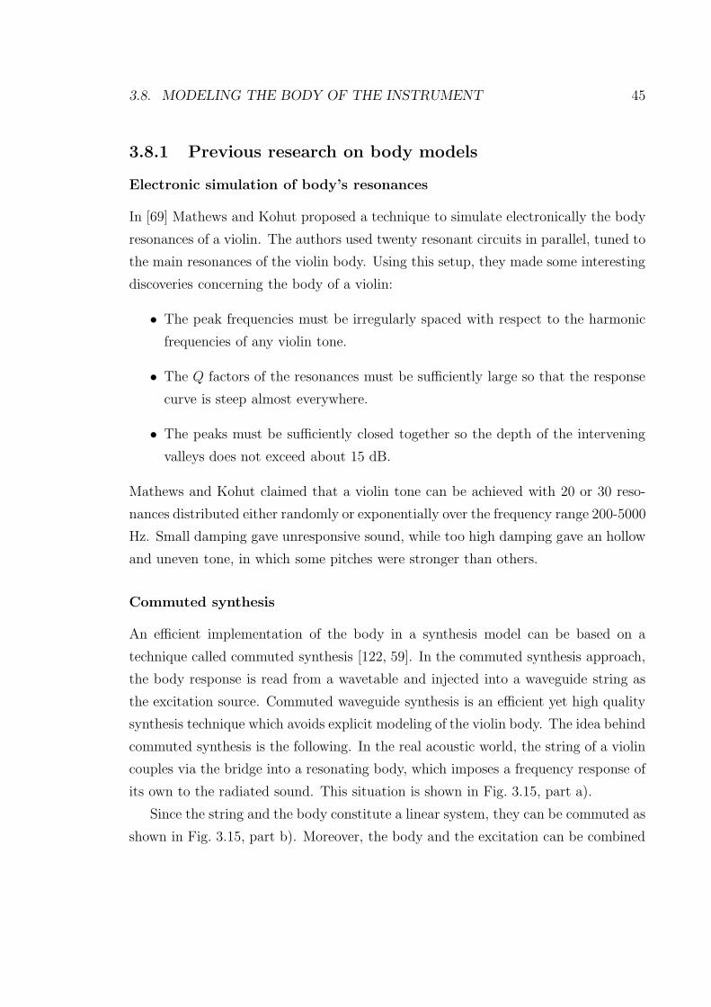
3.8. MODELING THE BODY OF THE INSTRUMENT 45
3.8.1 Previous research on body models
Electronic simulation of body’s resonances
In [69] Mathews and Kohut proposed a technique to simulate electronically the body
resonances of a violin. The authors used twenty resonant circuits in parallel, tuned to
the main resonances of the violin body. Using this setup, they made some interesting
discoveries concerning the body of a violin:
• The peak frequencies must be irregularly spaced with respect to the harmonic
frequencies of any violin tone.
• The Q factors of the resonances must be sufficiently large so that the response
curve is steep almost everywhere.
• The peaks must be sufficiently closed together so the depth of the intervening
valleys does not exceed about 15 dB.
Mathews and Kohut claimed that a violin tone can be achieved with 20 or 30 reso-
nances distributed either randomly or exponentially over the frequency range 200-5000
Hz. Small damping gave unresponsive sound, while too high damping gave an hollow
and uneven tone, in which some pitches were stronger than others.
Commuted synthesis
An efficient implementation of the body in a synthesis model can be based on a
technique called commuted synthesis [122, 59]. In the commuted synthesis approach,
the body response is read from a wavetable and injected into a waveguide string as
the excitation source. Commuted waveguide synthesis is an efficient yet high quality
synthesis technique which avoids explicit modeling of the violin body. The idea behind
commuted synthesis is the following. In the real acoustic world, the string of a violin
couples via the bridge into a resonating body, which imposes a frequency response of
its own to the radiated sound. This situation is shown in Fig. 3.15, part a).
Since the string and the body constitute a linear system, they can be commuted as
shown in Fig. 3.15, part b). Moreover, the body and the excitation can be combined
46 CHAPTER 3. THE BOWED STRING
in a single excitation unit, for computational purposes. This means that the string is
fed with the traditional excitation combined with the impulse response representing
the body resonances.
There are various ways of combining the body excitation into the system. Morever
the low frequencies least damped modes can be factored out using, for example, second
order filters. This is useful to reduce the length of the excitation table and to achieve
interesting effects with the parametric modes [114].
EXCITATION STRING BODY
STRINGBODYEXCITATION
EXCITATION STRING
A)
B)
C)
Figure 3.15: The commuted synthesis approach. A) The excitation is fed through thestrings and then through the body. B) By using the linearity of the system, string andbody are commuted. C) The excitation and the body are combined together creatingthe final excitation of the system.
The basic commuted synthesis solution is applicable only to linear, time-invariant
(LTI) systems, such as plucked and struck strings. In the case of a bowed violin, the
nonlinearity of the bow/string interaction does not allow this method to be used in
a precise way, although approximations are possible [52].
Since the computational power of computers in constantly strongly increasing, it
is possible to adopt other techniques which explicitly model the instruments’ body,
instead of sampling. In the following chapter different approaches to model a violin
body based on the waveguide mesh are proposed.
Chapter 4
Computational models for bowed
strings
In the previous chapter the acoustics of bowed string instruments was described, and
on overview of the bowed string models proposed in the literature was presented.
In this chapter an efficient yet accurate model of a bowed string is proposed.
Starting by discretizing the ideal wave equation, different solutions for solving the
interaction between a bow and a string are proposed. Sec. 4.1 describes the technique
adopted to design filters for different violin strings; Sec. 4.3 proposes a basic bowed
string physical model, Sec. 4.4 describes how to improve the model, Sec. 4.5 proposes
models to account for the finite width of the bow, and Sec. 4.6 describes how to model
the body of the instrument.
4.1 Measuring Decay Times in Pizzicato Record-
ings
As a first step, plucked violin strings were simulated. In an anechoic room, the four
violin strings were recorded while plucked at five different positions placed at equal
distance along the fingerboard. The energy decay relief (EDR) was calculated.
The EDR at time t and frequency ω is defined as the sum of all remaining energy
47
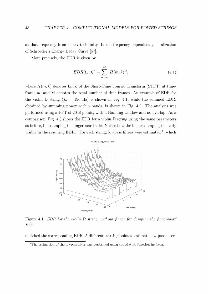
48 CHAPTER 4. COMPUTATIONAL MODELS FOR BOWED STRINGS
at that frequency from time t to infinity. It is a frequency-dependent generalization
of Schroeder’s Energy Decay Curve [57].
More precisely, the EDR is given by
EDR(tn, fk) =M∑
m=n
|H(m, k)|2, (4.1)
where H(m, k) denotes bin k of the Short-Time Fourier Transform (STFT) at time-
frame m, and M denotes the total number of time frames. An example of EDR for
the violin D string (f0 = 196 Hz) is shown in Fig. 4.1, while the summed EDR,
obtained by summing power within bands, is shown in Fig. 4.2. The analysis was
performed using a FFT of 2048 points, with a Hanning window and no overlap. As a
comparison, Fig. 4.3 shows the EDR for a violin D string using the same parameters
as before, but damping the fingerboard side. Notice how the higher damping is clearly
visible in the resulting EDR. For each string, lowpass filters were estimated 1, which
05
1015
2025 0
2
4
6
8
10-100
-80
-60
-40
-20
0
20
40
Time (frames)
re1.wav - Energy Decay Relief
Frequency (kHz)
Mag
nitu
de (
dB)
Figure 4.1: EDR for the violin D string, without finger for damping the fingerboardside.
matched the corresponding EDR. A different starting point to estimate low-pass filters
1The estimation of the lowpass filter was performed using the Matlab function invfreqz.
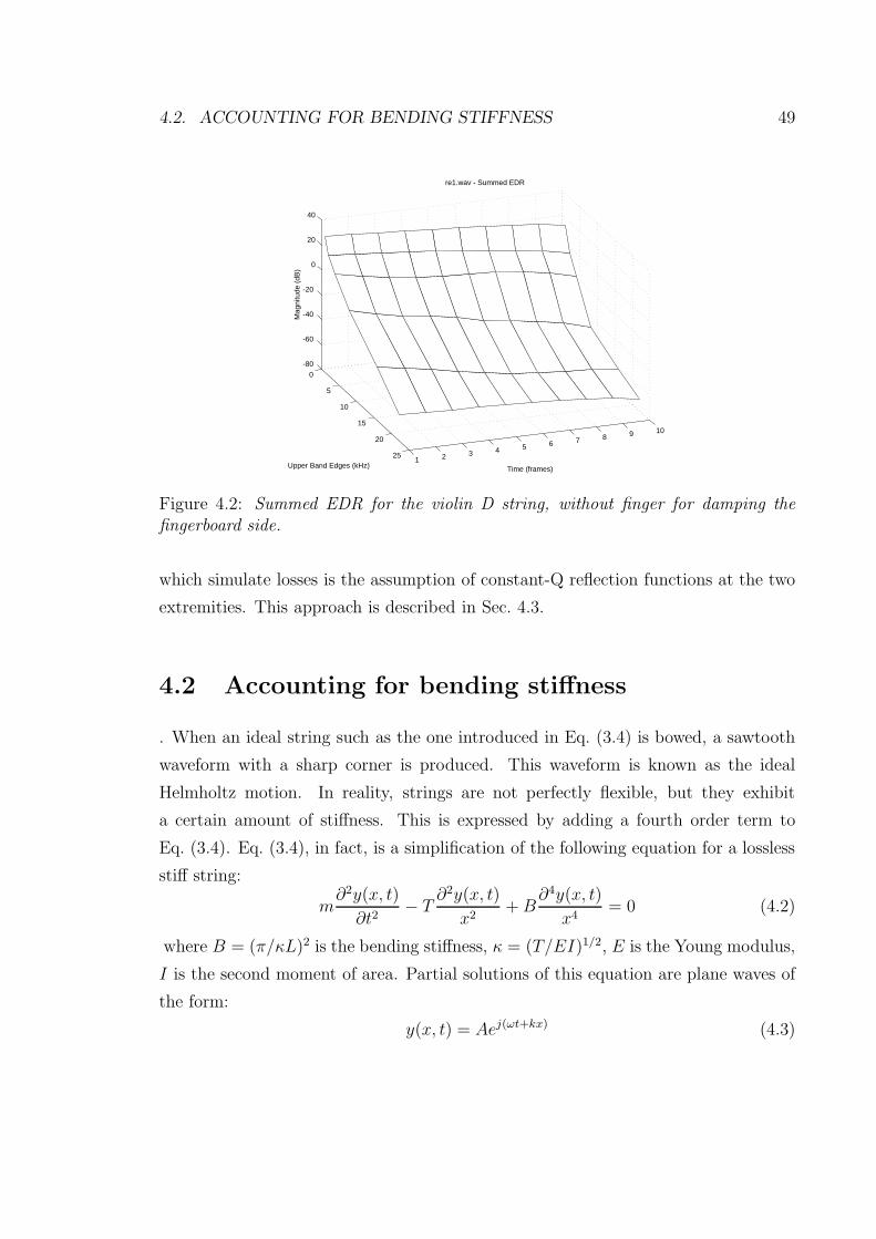
4.2. ACCOUNTING FOR BENDING STIFFNESS 49
0
5
10
15
20
251 2 3 4 5 6 7 8 9 10
-80
-60
-40
-20
0
20
40
Time (frames)
re1.wav - Summed EDR
Upper Band Edges (kHz)
Mag
nitu
de (
dB)
Figure 4.2: Summed EDR for the violin D string, without finger for damping thefingerboard side.
which simulate losses is the assumption of constant-Q reflection functions at the two
extremities. This approach is described in Sec. 4.3.
4.2 Accounting for bending stiffness
. When an ideal string such as the one introduced in Eq. (3.4) is bowed, a sawtooth
waveform with a sharp corner is produced. This waveform is known as the ideal
Helmholtz motion. In reality, strings are not perfectly flexible, but they exhibit
a certain amount of stiffness. This is expressed by adding a fourth order term to
Eq. (3.4). Eq. (3.4), in fact, is a simplification of the following equation for a lossless
stiff string:
m∂2y(x, t)
∂t2− T ∂
2y(x, t)
x2+B
∂4y(x, t)
x4= 0 (4.2)
where B = (π/κL)2 is the bending stiffness, κ = (T/EI)1/2, E is the Young modulus,
I is the second moment of area. Partial solutions of this equation are plane waves of
the form:
y(x, t) = Aej(ωt+kx) (4.3)
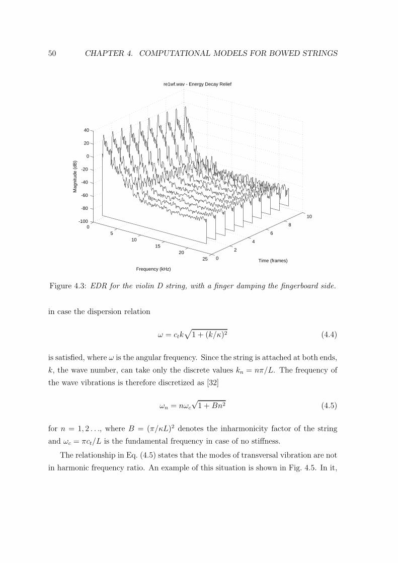
50 CHAPTER 4. COMPUTATIONAL MODELS FOR BOWED STRINGS
05
1015
2025 0
2
4
6
8
10-100
-80
-60
-40
-20
0
20
40
Time (frames)
re1wf.wav - Energy Decay Relief
Frequency (kHz)
Mag
nitu
de (
dB)
Figure 4.3: EDR for the violin D string, with a finger damping the fingerboard side.
in case the dispersion relation
ω = ctk√
1 + (k/κ)2 (4.4)
is satisfied, where ω is the angular frequency. Since the string is attached at both ends,
k, the wave number, can take only the discrete values kn = nπ/L. The frequency of
the wave vibrations is therefore discretized as [32]
ωn = nωc
√1 +Bn2 (4.5)
for n = 1, 2 . . ., where B = (π/κL)2 denotes the inharmonicity factor of the string
and ωc = πct/L is the fundamental frequency in case of no stiffness.
The relationship in Eq. (4.5) states that the modes of transversal vibration are not
in harmonic frequency ratio. An example of this situation is shown in Fig. 4.5. In it,
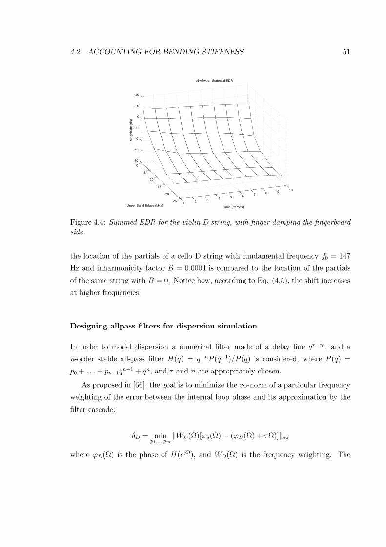
4.2. ACCOUNTING FOR BENDING STIFFNESS 51
0
5
10
15
20
251 2 3 4 5 6 7 8 9 10
-80
-60
-40
-20
0
20
40
Time (frames)
re1wf.wav - Summed EDR
Upper Band Edges (kHz)
Mag
nitu
de (
dB)
Figure 4.4: Summed EDR for the violin D string, with finger damping the fingerboardside.
the location of the partials of a cello D string with fundamental frequency f0 = 147
Hz and inharmonicity factor B = 0.0004 is compared to the location of the partials
of the same string with B = 0. Notice how, according to Eq. (4.5), the shift increases
at higher frequencies.
Designing allpass filters for dispersion simulation
In order to model dispersion a numerical filter made of a delay line qτ−τ0 , and a
n-order stable all-pass filter H(q) = q−nP (q−1)/P (q) is considered, where P (q) =
p0 + . . .+ pn−1qn−1 + qn, and τ and n are appropriately chosen.
As proposed in [66], the goal is to minimize the∞-norm of a particular frequency
weighting of the error between the internal loop phase and its approximation by the
filter cascade:
δD = minp1,...,pm
‖WD(Ω)[ϕd(Ω)− (ϕD(Ω) + τΩ)]‖∞
where ϕD(Ω) is the phase of H(ejΩ), and WD(Ω) is the frequency weighting. The
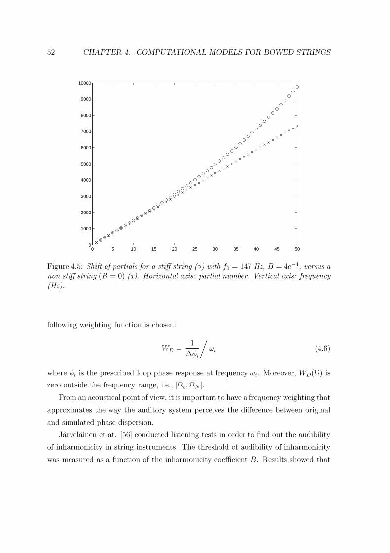
52 CHAPTER 4. COMPUTATIONAL MODELS FOR BOWED STRINGS
0 5 10 15 20 25 30 35 40 45 500
1000
2000
3000
4000
5000
6000
7000
8000
9000
10000
Figure 4.5: Shift of partials for a stiff string () with f0 = 147 Hz, B = 4e−4, versus anon stiff string (B = 0) (x). Horizontal axis: partial number. Vertical axis: frequency(Hz).
following weighting function is chosen:
WD =1
∆φi
/
ωi (4.6)
where φi is the prescribed loop phase response at frequency ωi. Moreover, WD(Ω) is
zero outside the frequency range, i.e., [Ωc,ΩN ].
From an acoustical point of view, it is important to have a frequency weighting that
approximates the way the auditory system perceives the difference between original
and simulated phase dispersion.
Jarvelainen et at. [56] conducted listening tests in order to find out the audibility
of inharmonicity in string instruments. The threshold of audibility of inharmonicity
was measured as a function of the inharmonicity coefficient B. Results showed that
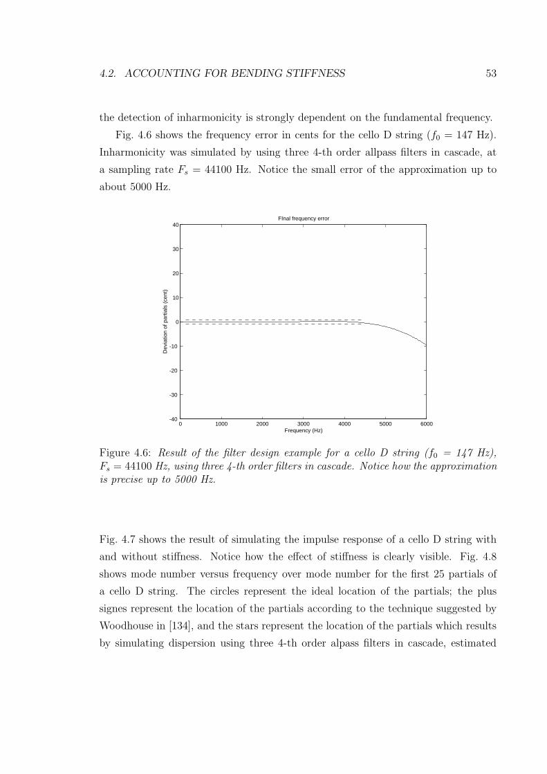
4.2. ACCOUNTING FOR BENDING STIFFNESS 53
the detection of inharmonicity is strongly dependent on the fundamental frequency.
Fig. 4.6 shows the frequency error in cents for the cello D string (f0 = 147 Hz).
Inharmonicity was simulated by using three 4-th order allpass filters in cascade, at
a sampling rate Fs = 44100 Hz. Notice the small error of the approximation up to
about 5000 Hz.
0 1000 2000 3000 4000 5000 6000-40
-30
-20
-10
0
10
20
30
40FInal frequency error
Frequency (Hz)
Dev
iatio
n of
par
tials
(ce
nt)
Figure 4.6: Result of the filter design example for a cello D string (f0 = 147 Hz),Fs = 44100 Hz, using three 4-th order filters in cascade. Notice how the approximationis precise up to 5000 Hz.
Fig. 4.7 shows the result of simulating the impulse response of a cello D string with
and without stiffness. Notice how the effect of stiffness is clearly visible. Fig. 4.8
shows mode number versus frequency over mode number for the first 25 partials of
a cello D string. The circles represent the ideal location of the partials; the plus
signes represent the location of the partials according to the technique suggested by
Woodhouse in [134], and the stars represent the location of the partials which results
by simulating dispersion using three 4-th order alpass filters in cascade, estimated
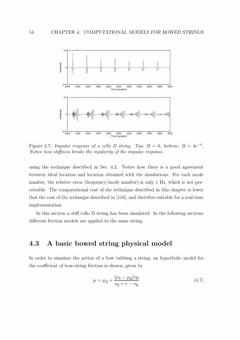
54 CHAPTER 4. COMPUTATIONAL MODELS FOR BOWED STRINGS
1000 1200 1400 1600 1800 2000 2200 2400 2600 2800 3000-0.5
0
0.5
Time (samples)
Am
plitu
de
1000 1200 1400 1600 1800 2000 2200 2400 2600 2800 3000-0.5
0
0.5
Time (samples)
Am
plitu
de
Figure 4.7: Impulse response of a cello D string. Top: B = 0, bottom: B = 4e−4.Notice how stiffness breaks the regularity of the impulse response.
using the technique described in Sec. 4.2. Notice how there is a good agreement
between ideal location and location obtained with the simulations. For each mode
number, the relative error (frequency/mode number) is only 1 Hz, which is not per-
ceivable. The computational cost of the technique described in this chapter is lower
that the cost of the technique described in [134], and therefore suitable for a real-time
implementation.
In this section a stiff cello D string has been simulated. In the following sections
different friction models are applied to the same string.
4.3 A basic bowed string physical model
In order to simulate the action of a bow rubbing a string, an hyperbolic model for
the coefficient of bow-string friction is chosen, given by
µ = µd +(µs − µd)v0v0 + v − vb
(4.7)
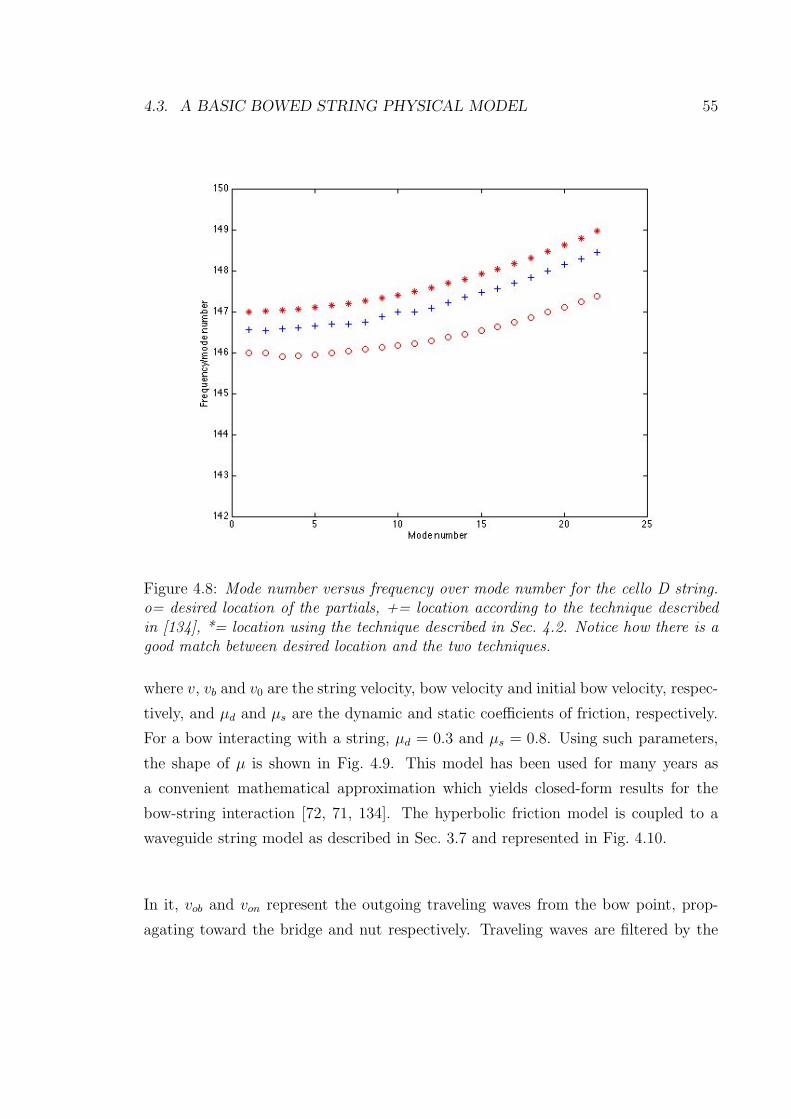
4.3. A BASIC BOWED STRING PHYSICAL MODEL 55
Figure 4.8: Mode number versus frequency over mode number for the cello D string.o= desired location of the partials, += location according to the technique describedin [134], *= location using the technique described in Sec. 4.2. Notice how there is agood match between desired location and the two techniques.
where v, vb and v0 are the string velocity, bow velocity and initial bow velocity, respec-
tively, and µd and µs are the dynamic and static coefficients of friction, respectively.
For a bow interacting with a string, µd = 0.3 and µs = 0.8. Using such parameters,
the shape of µ is shown in Fig. 4.9. This model has been used for many years as
a convenient mathematical approximation which yields closed-form results for the
bow-string interaction [72, 71, 134]. The hyperbolic friction model is coupled to a
waveguide string model as described in Sec. 3.7 and represented in Fig. 4.10.
In it, vob and von represent the outgoing traveling waves from the bow point, prop-
agating toward the bridge and nut respectively. Traveling waves are filtered by the
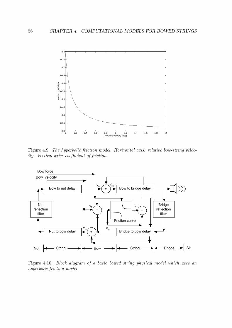
56 CHAPTER 4. COMPUTATIONAL MODELS FOR BOWED STRINGS
0 0.2 0.4 0.6 0.8 1 1.2 1.4 1.6 1.8 20.3
0.35
0.4
0.45
0.5
0.55
0.6
0.65
0.7
0.75
0.8
Relative velocity (m/s)
Fric
tion
coef
ficie
nt
Figure 4.9: The hyperbolic friction model. Horizontal axis: relative bow-string veloc-ity. Vertical axis: coefficient of friction.
Bow to nut delay Bow to bridge delay
Nut to bow delay Bridge to bow delay
Bridgereflection
filter
+
+ +
+
Bow velocityBow force
Friction curve
Nut String Bow String Bridge Air
vin vob
von vib
vb fNutreflection
filter
Figure 4.10: Block diagram of a basic bowed string physical model which uses anhyperbolic friction model.
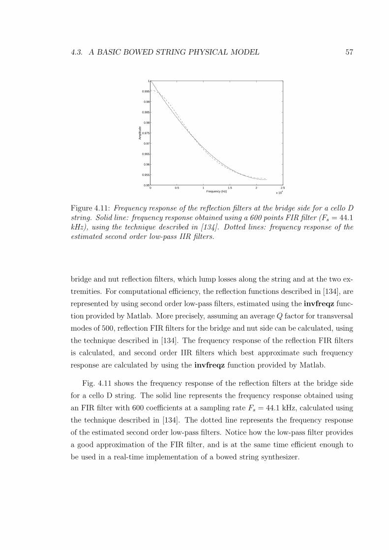
4.3. A BASIC BOWED STRING PHYSICAL MODEL 57
0 0.5 1 1.5 2 2.5
x 104
0.95
0.955
0.96
0.965
0.97
0.975
0.98
0.985
0.99
0.995
1
Frequency (Hz)
Am
plitu
de
Figure 4.11: Frequency response of the reflection filters at the bridge side for a cello Dstring. Solid line: frequency response obtained using a 600 points FIR filter (Fs = 44.1kHz), using the technique described in [134]. Dotted lines: frequency response of theestimated second order low-pass IIR filters.
bridge and nut reflection filters, which lump losses along the string and at the two ex-
tremities. For computational efficiency, the reflection functions described in [134], are
represented by using second order low-pass filters, estimated using the invfreqz func-
tion provided by Matlab. More precisely, assuming an average Q factor for transversal
modes of 500, reflection FIR filters for the bridge and nut side can be calculated, using
the technique described in [134]. The frequency response of the reflection FIR filters
is calculated, and second order IIR filters which best approximate such frequency
response are calculated by using the invfreqz function provided by Matlab.
Fig. 4.11 shows the frequency response of the reflection filters at the bridge side
for a cello D string. The solid line represents the frequency response obtained using
an FIR filter with 600 coefficients at a sampling rate Fs = 44.1 kHz, calculated using
the technique described in [134]. The dotted line represents the frequency response
of the estimated second order low-pass filters. Notice how the low-pass filter provides
a good approximation of the FIR filter, and is at the same time efficient enough to
be used in a real-time implementation of a bowed string synthesizer.
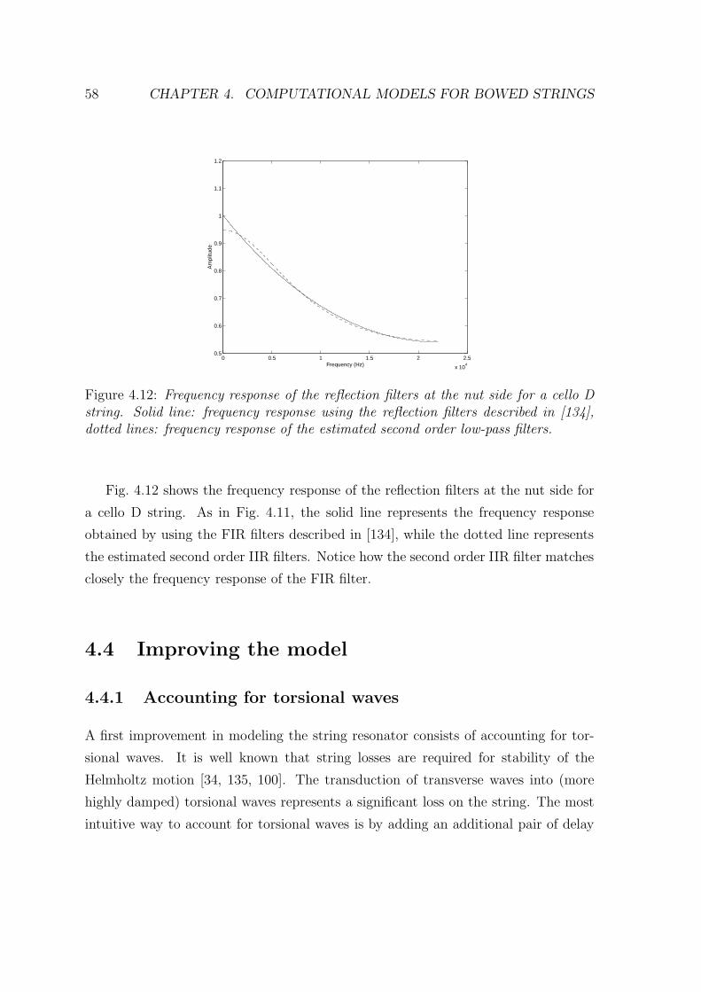
58 CHAPTER 4. COMPUTATIONAL MODELS FOR BOWED STRINGS
0 0.5 1 1.5 2 2.5
x 104
0.5
0.6
0.7
0.8
0.9
1
1.1
1.2
Frequency (Hz)
Am
plitu
de
Figure 4.12: Frequency response of the reflection filters at the nut side for a cello Dstring. Solid line: frequency response using the reflection filters described in [134],dotted lines: frequency response of the estimated second order low-pass filters.
Fig. 4.12 shows the frequency response of the reflection filters at the nut side for
a cello D string. As in Fig. 4.11, the solid line represents the frequency response
obtained by using the FIR filters described in [134], while the dotted line represents
the estimated second order IIR filters. Notice how the second order IIR filter matches
closely the frequency response of the FIR filter.
4.4 Improving the model
4.4.1 Accounting for torsional waves
A first improvement in modeling the string resonator consists of accounting for tor-
sional waves. It is well known that string losses are required for stability of the
Helmholtz motion [34, 135, 100]. The transduction of transverse waves into (more
highly damped) torsional waves represents a significant loss on the string. The most
intuitive way to account for torsional waves is by adding an additional pair of delay
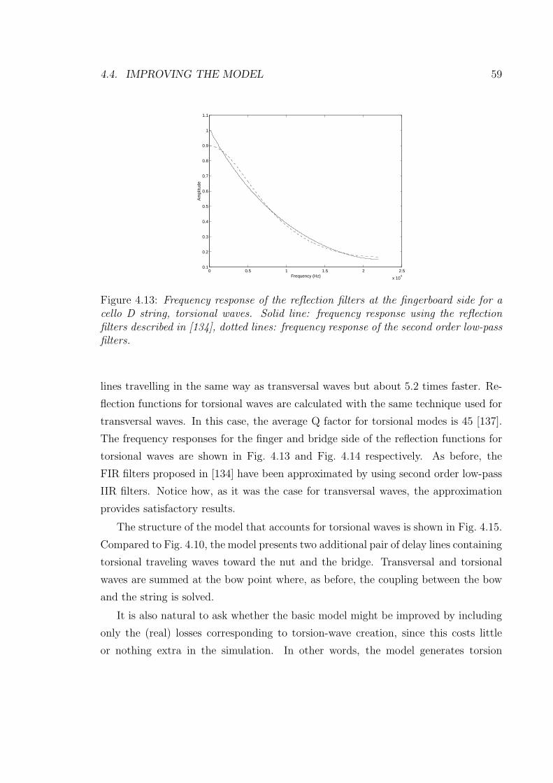
4.4. IMPROVING THE MODEL 59
0 0.5 1 1.5 2 2.5
x 104
0.1
0.2
0.3
0.4
0.5
0.6
0.7
0.8
0.9
1
1.1
Frequency (Hz)
Am
plitu
de
Figure 4.13: Frequency response of the reflection filters at the fingerboard side for acello D string, torsional waves. Solid line: frequency response using the reflectionfilters described in [134], dotted lines: frequency response of the second order low-passfilters.
lines travelling in the same way as transversal waves but about 5.2 times faster. Re-
flection functions for torsional waves are calculated with the same technique used for
transversal waves. In this case, the average Q factor for torsional modes is 45 [137].
The frequency responses for the finger and bridge side of the reflection functions for
torsional waves are shown in Fig. 4.13 and Fig. 4.14 respectively. As before, the
FIR filters proposed in [134] have been approximated by using second order low-pass
IIR filters. Notice how, as it was the case for transversal waves, the approximation
provides satisfactory results.
The structure of the model that accounts for torsional waves is shown in Fig. 4.15.
Compared to Fig. 4.10, the model presents two additional pair of delay lines containing
torsional traveling waves toward the nut and the bridge. Transversal and torsional
waves are summed at the bow point where, as before, the coupling between the bow
and the string is solved.
It is also natural to ask whether the basic model might be improved by including
only the (real) losses corresponding to torsion-wave creation, since this costs little
or nothing extra in the simulation. In other words, the model generates torsion
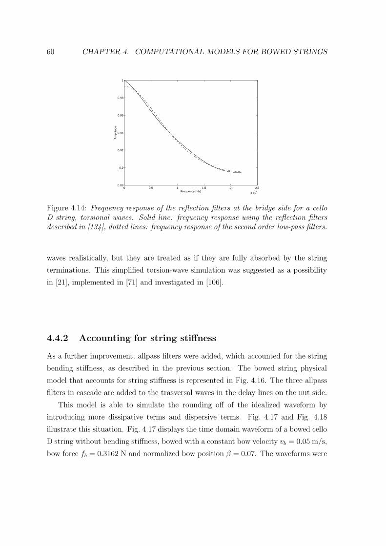
60 CHAPTER 4. COMPUTATIONAL MODELS FOR BOWED STRINGS
0 0.5 1 1.5 2 2.5
x 104
0.88
0.9
0.92
0.94
0.96
0.98
1
Frequency (Hz)
Am
plitu
de
Figure 4.14: Frequency response of the reflection filters at the bridge side for a celloD string, torsional waves. Solid line: frequency response using the reflection filtersdescribed in [134], dotted lines: frequency response of the second order low-pass filters.
waves realistically, but they are treated as if they are fully absorbed by the string
terminations. This simplified torsion-wave simulation was suggested as a possibility
in [21], implemented in [71] and investigated in [106].
4.4.2 Accounting for string stiffness
As a further improvement, allpass filters were added, which accounted for the string
bending stiffness, as described in the previous section. The bowed string physical
model that accounts for string stiffness is represented in Fig. 4.16. The three allpass
filters in cascade are added to the trasversal waves in the delay lines on the nut side.
This model is able to simulate the rounding off of the idealized waveform by
introducing more dissipative terms and dispersive terms. Fig. 4.17 and Fig. 4.18
illustrate this situation. Fig. 4.17 displays the time domain waveform of a bowed cello
D string without bending stiffness, bowed with a constant bow velocity vb = 0.05 m/s,
bow force fb = 0.3162 N and normalized bow position β = 0.07. The waveforms were
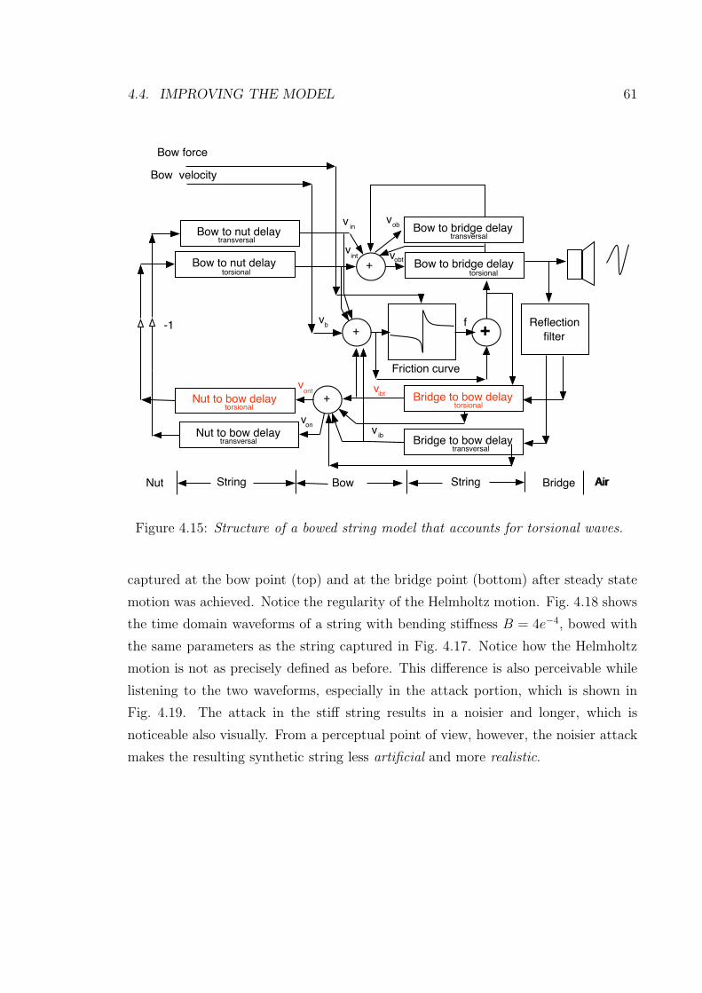
4.4. IMPROVING THE MODEL 61
Bow to nut delay Bow to bridge delay
Nut to bow delay Bridge to bow delay
Reflectionfilter
-1
+
+ +
+
Bow velocityBow force
Nut String Bow String Bridge Air
vint vobt
vont vibt
vb
Friction curve
f
torsional
Nut to bow delaytorsional
transversal
Bow to nut delay transversalBow to bridge delay
Bridge to bow delaytransversal
transversal
torsional
inv vob
ibvonv
Air
torsional
Figure 4.15: Structure of a bowed string model that accounts for torsional waves.
captured at the bow point (top) and at the bridge point (bottom) after steady state
motion was achieved. Notice the regularity of the Helmholtz motion. Fig. 4.18 shows
the time domain waveforms of a string with bending stiffness B = 4e−4, bowed with
the same parameters as the string captured in Fig. 4.17. Notice how the Helmholtz
motion is not as precisely defined as before. This difference is also perceivable while
listening to the two waveforms, especially in the attack portion, which is shown in
Fig. 4.19. The attack in the stiff string results in a noisier and longer, which is
noticeable also visually. From a perceptual point of view, however, the noisier attack
makes the resulting synthetic string less artificial and more realistic.
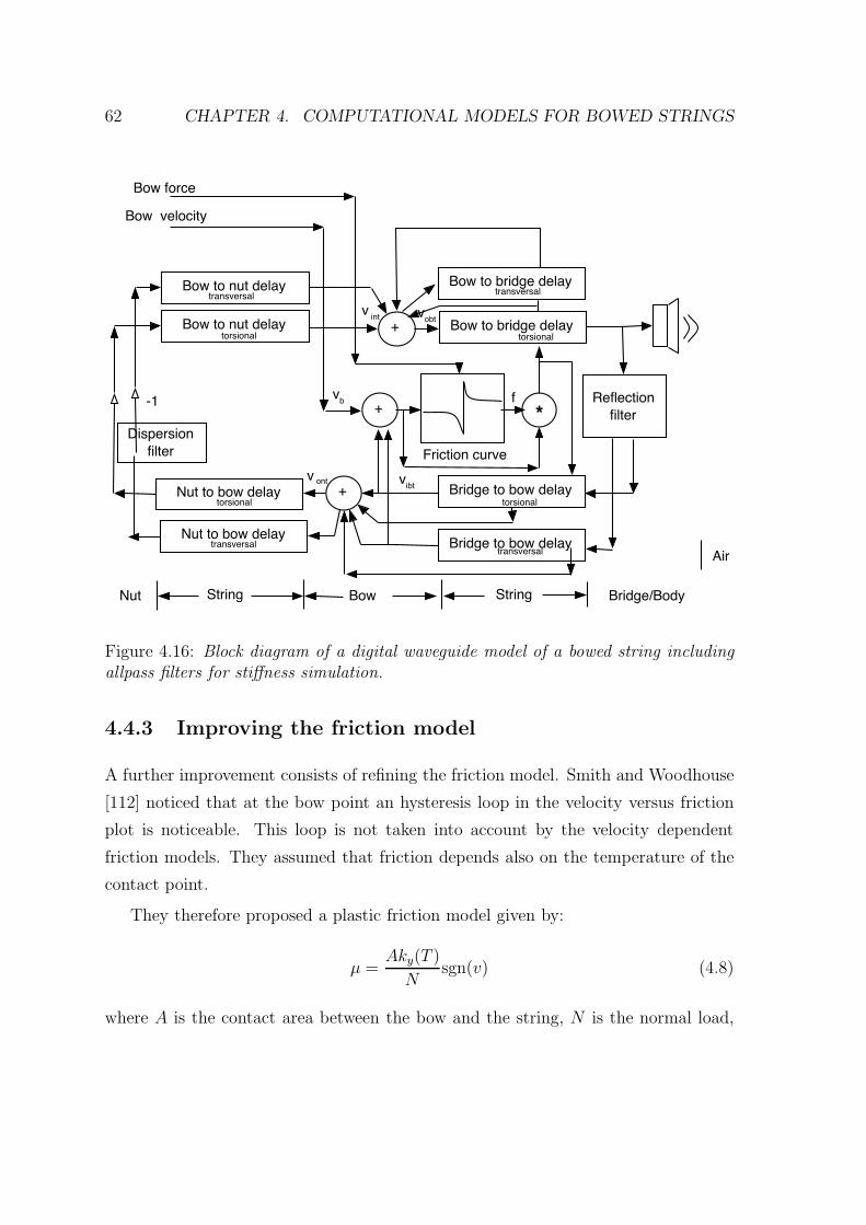
62 CHAPTER 4. COMPUTATIONAL MODELS FOR BOWED STRINGS
Bow to nut delay Bow to bridge delay
Nut to bow delay Bridge to bow delay
Reflectionfilter
-1
+
+ *
+
Bow velocityBow force
Nut String Bow String Bridge/Body
Air
v int v obt
v ont vibt
vb
Friction curve
f
torsional
Nut to bow delaytorsional
transversal
Bow to nut delay transversalBow to bridge delay
Bridge to bow delay
torsional
transversal
transversal
torsional
Dispersionfilter
Figure 4.16: Block diagram of a digital waveguide model of a bowed string includingallpass filters for stiffness simulation.
4.4.3 Improving the friction model
A further improvement consists of refining the friction model. Smith and Woodhouse
[112] noticed that at the bow point an hysteresis loop in the velocity versus friction
plot is noticeable. This loop is not taken into account by the velocity dependent
friction models. They assumed that friction depends also on the temperature of the
contact point.
They therefore proposed a plastic friction model given by:
µ =Aky(T )
Nsgn(v) (4.8)
where A is the contact area between the bow and the string, N is the normal load,
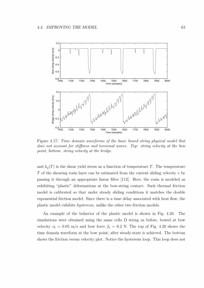
4.4. IMPROVING THE MODEL 63
7000 7100 7200 7300 7400 7500 7600 7700 7800 7900 8000-0.8
-0.6
-0.4
-0.2
0
0.2
Time (samples)
Bow
str
ing
velo
city
(m
/s)
7000 7100 7200 7300 7400 7500 7600 7700 7800 7900 8000-0.4
-0.2
0
0.2
0.4
Time (samples)
Brid
ge s
trin
g ve
loci
ty (
m/s
)
Figure 4.17: Time domain waveforms of the basic bowed string physical model thatdoes not account for stiffness and torsional waves. Top: string velocity at the bowpoint, bottom: string velocity at the bridge.
and ky(T ) is the shear yield stress as a function of temperature T . The temperature
T of the shearing rosin layer can be estimated from the current sliding velocity v by
passing it through an appropriate linear filter [112]. Here, the rosin is modeled as
exhibiting “plastic” deformations at the bow-string contact. Such thermal friction
model is calibrated so that under steady sliding conditions it matches the double
exponential friction model. Since there is a time delay associated with heat flow, the
plastic model exhibits hysteresis, unlike the other two friction models.
An example of the behavior of the plastic model is shown in Fig. 4.20. The
simulations were obtained using the same cello D string as before, bowed at bow
velocity vb = 0.05 m/s and bow force fb = 0.2 N. The top of Fig. 4.20 shows the
time domain waveform at the bow point, after steady-state is achieved. The bottom
shows the friction versus velocity plot. Notice the hysteresis loop. This loop does not
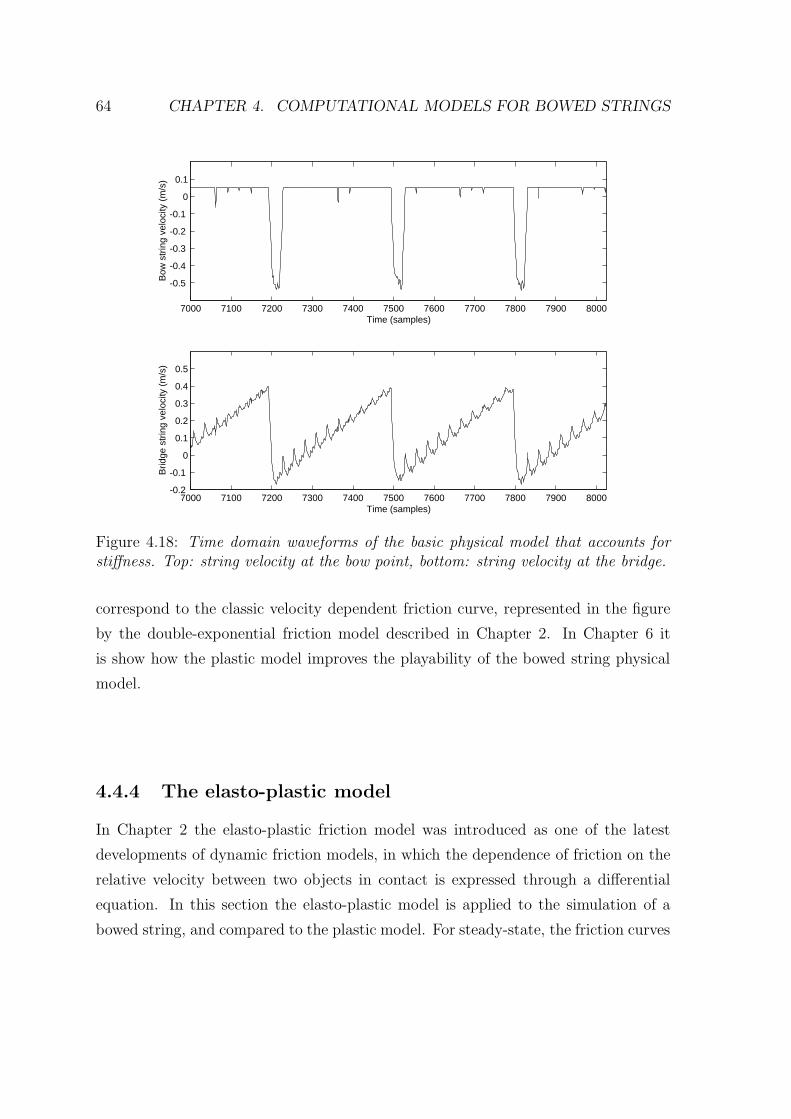
64 CHAPTER 4. COMPUTATIONAL MODELS FOR BOWED STRINGS
7000 7100 7200 7300 7400 7500 7600 7700 7800 7900 8000
-0.5
-0.4
-0.3
-0.2
-0.1
0
0.1
Time (samples)
Bow
str
ing
velo
city
(m
/s)
7000 7100 7200 7300 7400 7500 7600 7700 7800 7900 8000-0.2
-0.1
0
0.1
0.2
0.3
0.4
0.5
Time (samples)
Brid
ge s
trin
g ve
loci
ty (
m/s
)
Figure 4.18: Time domain waveforms of the basic physical model that accounts forstiffness. Top: string velocity at the bow point, bottom: string velocity at the bridge.
correspond to the classic velocity dependent friction curve, represented in the figure
by the double-exponential friction model described in Chapter 2. In Chapter 6 it
is show how the plastic model improves the playability of the bowed string physical
model.
4.4.4 The elasto-plastic model
In Chapter 2 the elasto-plastic friction model was introduced as one of the latest
developments of dynamic friction models, in which the dependence of friction on the
relative velocity between two objects in contact is expressed through a differential
equation. In this section the elasto-plastic model is applied to the simulation of a
bowed string, and compared to the plastic model. For steady-state, the friction curves
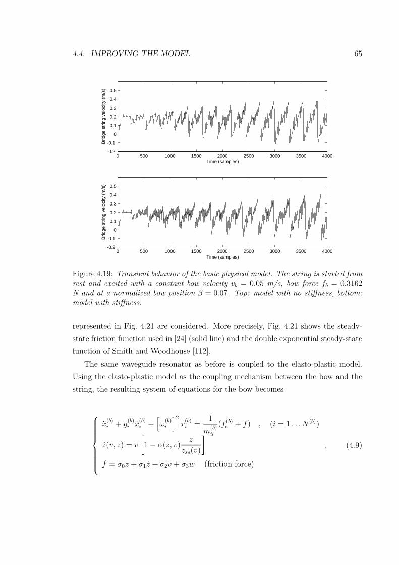
4.4. IMPROVING THE MODEL 65
0 500 1000 1500 2000 2500 3000 3500 4000-0.2
-0.1
0
0.1
0.2
0.3
0.4
0.5
Time (samples)
Brid
ge s
trin
g ve
loci
ty (
m/s
)
0 500 1000 1500 2000 2500 3000 3500 4000-0.2
-0.1
0
0.1
0.2
0.3
0.4
0.5
Time (samples)
Brid
ge s
trin
g ve
loci
ty (
m/s
)
Figure 4.19: Transient behavior of the basic physical model. The string is started fromrest and excited with a constant bow velocity vb = 0.05 m/s, bow force fb = 0.3162N and at a normalized bow position β = 0.07. Top: model with no stiffness, bottom:model with stiffness.
represented in Fig. 4.21 are considered. More precisely, Fig. 4.21 shows the steady-
state friction function used in [24] (solid line) and the double exponential steady-state
function of Smith and Woodhouse [112].
The same waveguide resonator as before is coupled to the elasto-plastic model.
Using the elasto-plastic model as the coupling mechanism between the bow and the
string, the resulting system of equations for the bow becomes
x(b)i + g
(b)i x
(b)i +
[
ω(b)i
]2
x(b)i =
1
m(b)il
(f (b)e + f) , (i = 1 . . . N (b))
z(v, z) = v
[
1− α(z, v)z
zss(v)
]
f = σ0z + σ1z + σ2v + σ3w (friction force)
, (4.9)

66 CHAPTER 4. COMPUTATIONAL MODELS FOR BOWED STRINGS
0.18 0.185 0.19 0.195 0.2 0.205 0.21 0.215 0.22−1.5
−1
−0.5
0
0.5
Time (s)
Vel
ocity
(m
/s)
−1 −0.5 00.2
0.7
1.2
String velocity (m/s)
Fric
tion
forc
e (N
)
Figure 4.20: Simulations using the plastic model. Top: string velocity at the bowpoint. Bottom: friction versus velocity. Notice how the plastic model produces anhysteresis loop which does not follow the traditional velocity-dependent friction model(represented in the figure by the decaying exponential in the bottom part).
where for clarity the superscript (b) stands for “bow”. The x variables represent the
modal displacements for the bow, while z is the mean bristle displacement. The terms
f(b)e represents external forces, while the integers N (b) are the number of modes for
the bow.
This system of equations is discretized by using the bilinear transform. Details
about the discretization are described in Appendix B.
Notice how a delay-free loop appears when coupling the excitation to the resonator.
This is solved by using the K-method [10], as described in Appendix B. The current z
value is computed with the Newton-Raphson algorithm. Experimentally, a maximum
of seven iterations is enough to achieve convergence; this allows an efficient real-time
implementation.
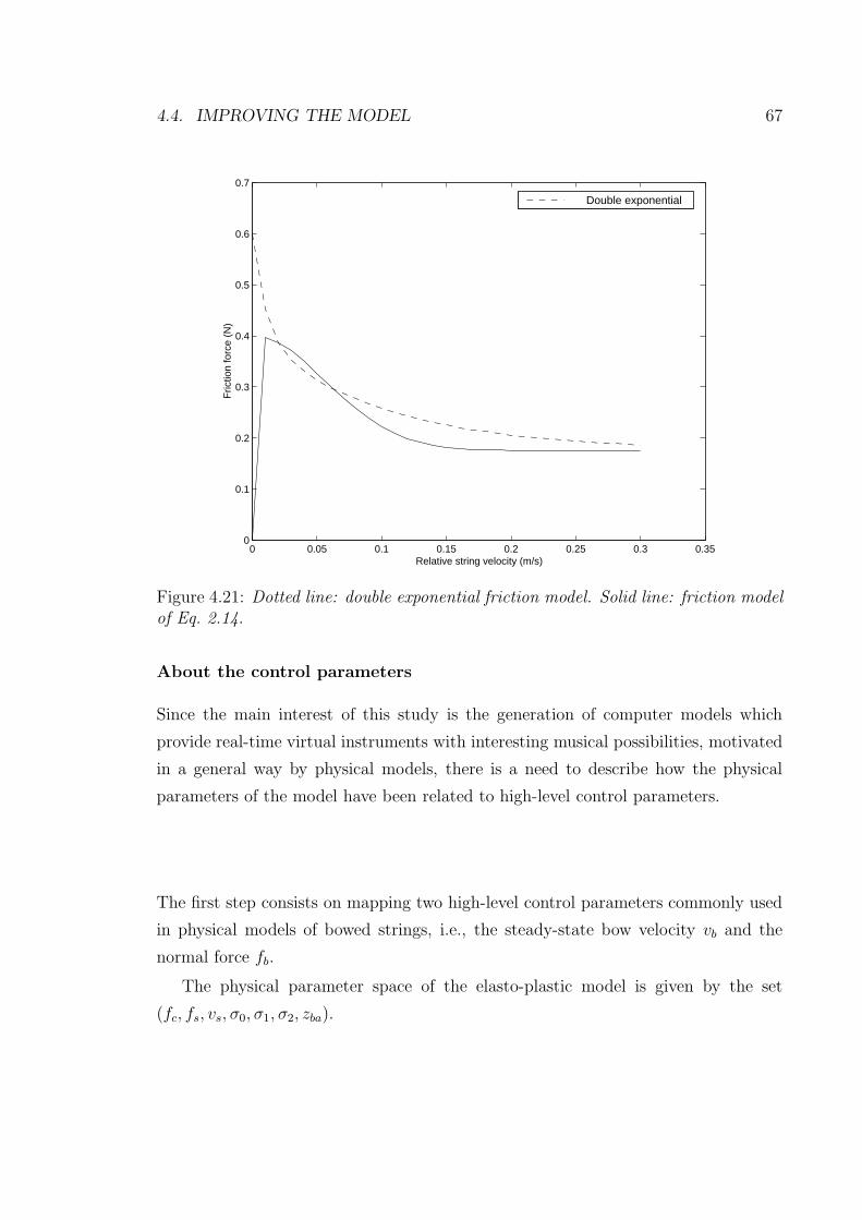
4.4. IMPROVING THE MODEL 67
0 0.05 0.1 0.15 0.2 0.25 0.3 0.350
0.1
0.2
0.3
0.4
0.5
0.6
0.7
Relative string velocity (m/s)
Fric
tion
forc
e (N
)
Double exponential
Figure 4.21: Dotted line: double exponential friction model. Solid line: friction modelof Eq. 2.14.
About the control parameters
Since the main interest of this study is the generation of computer models which
provide real-time virtual instruments with interesting musical possibilities, motivated
in a general way by physical models, there is a need to describe how the physical
parameters of the model have been related to high-level control parameters.
The first step consists on mapping two high-level control parameters commonly used
in physical models of bowed strings, i.e., the steady-state bow velocity vb and the
normal force fb.
The physical parameter space of the elasto-plastic model is given by the set
(fc, fs, vs, σ0, σ1, σ2, zba).
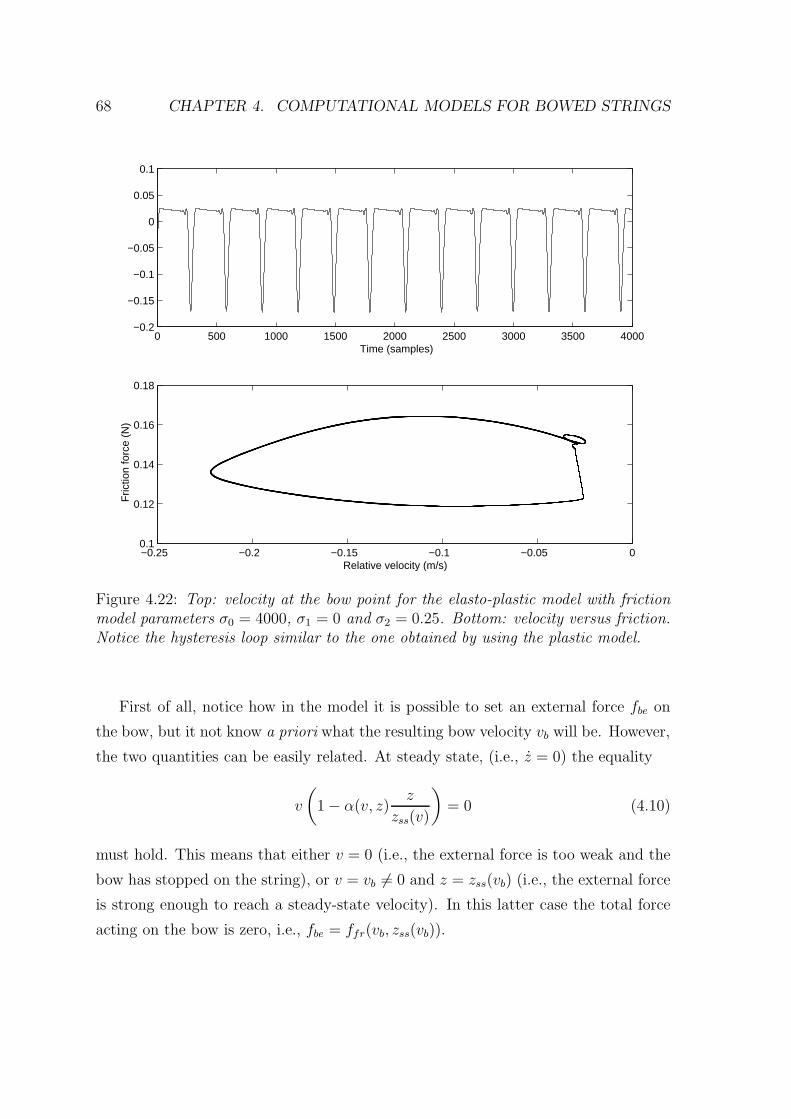
68 CHAPTER 4. COMPUTATIONAL MODELS FOR BOWED STRINGS
0 500 1000 1500 2000 2500 3000 3500 4000−0.2
−0.15
−0.1
−0.05
0
0.05
0.1
Time (samples)
−0.25 −0.2 −0.15 −0.1 −0.05 00.1
0.12
0.14
0.16
0.18
Relative velocity (m/s)
Fric
tion
forc
e (N
)
Figure 4.22: Top: velocity at the bow point for the elasto-plastic model with frictionmodel parameters σ0 = 4000, σ1 = 0 and σ2 = 0.25. Bottom: velocity versus friction.Notice the hysteresis loop similar to the one obtained by using the plastic model.
First of all, notice how in the model it is possible to set an external force fbe on
the bow, but it not know a priori what the resulting bow velocity vb will be. However,
the two quantities can be easily related. At steady state, (i.e., z = 0) the equality
v
(
1− α(v, z)z
zss(v)
)
= 0 (4.10)
must hold. This means that either v = 0 (i.e., the external force is too weak and the
bow has stopped on the string), or v = vb 6= 0 and z = zss(vb) (i.e., the external force
is strong enough to reach a steady-state velocity). In this latter case the total force
acting on the bow is zero, i.e., fbe = ffr(vb, zss(vb)).
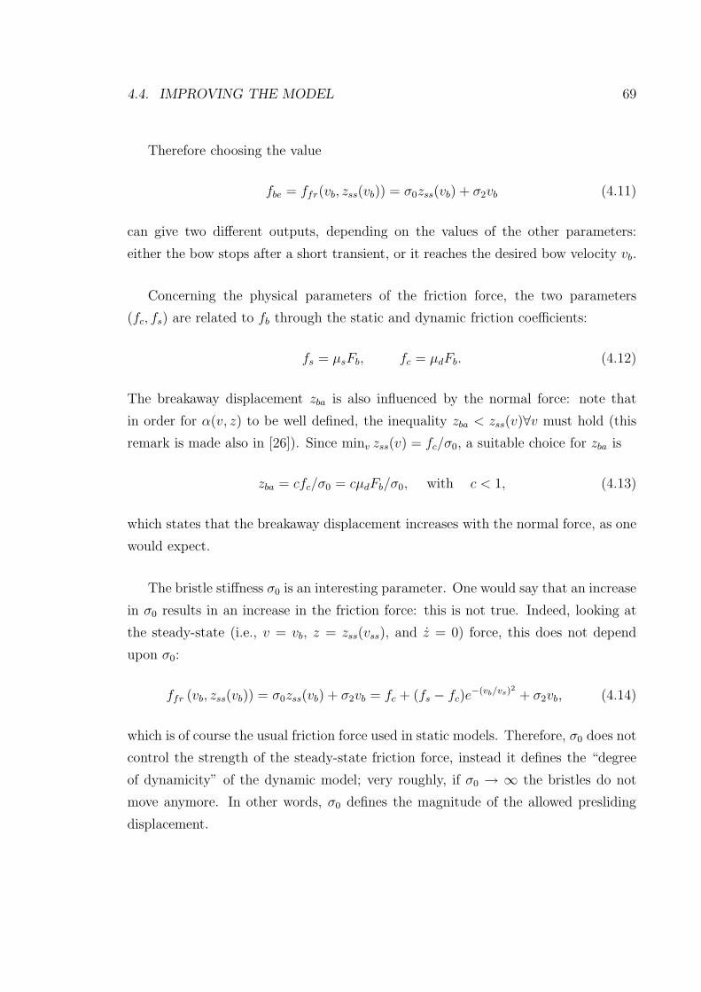
4.4. IMPROVING THE MODEL 69
Therefore choosing the value
fbe = ffr(vb, zss(vb)) = σ0zss(vb) + σ2vb (4.11)
can give two different outputs, depending on the values of the other parameters:
either the bow stops after a short transient, or it reaches the desired bow velocity vb.
Concerning the physical parameters of the friction force, the two parameters
(fc, fs) are related to fb through the static and dynamic friction coefficients:
fs = µsFb, fc = µdFb. (4.12)
The breakaway displacement zba is also influenced by the normal force: note that
in order for α(v, z) to be well defined, the inequality zba < zss(v)∀v must hold (this
remark is made also in [26]). Since minv zss(v) = fc/σ0, a suitable choice for zba is
zba = cfc/σ0 = cµdFb/σ0, with c < 1, (4.13)
which states that the breakaway displacement increases with the normal force, as one
would expect.
The bristle stiffness σ0 is an interesting parameter. One would say that an increase
in σ0 results in an increase in the friction force: this is not true. Indeed, looking at
the steady-state (i.e., v = vb, z = zss(vss), and z = 0) force, this does not depend
upon σ0:
ffr (vb, zss(vb)) = σ0zss(vb) + σ2vb = fc + (fs − fc)e−(vb/vs)2 + σ2vb, (4.14)
which is of course the usual friction force used in static models. Therefore, σ0 does not
control the strength of the steady-state friction force, instead it defines the “degree
of dynamicity” of the dynamic model; very roughly, if σ0 → ∞ the bristles do not
move anymore. In other words, σ0 defines the magnitude of the allowed presliding
displacement.
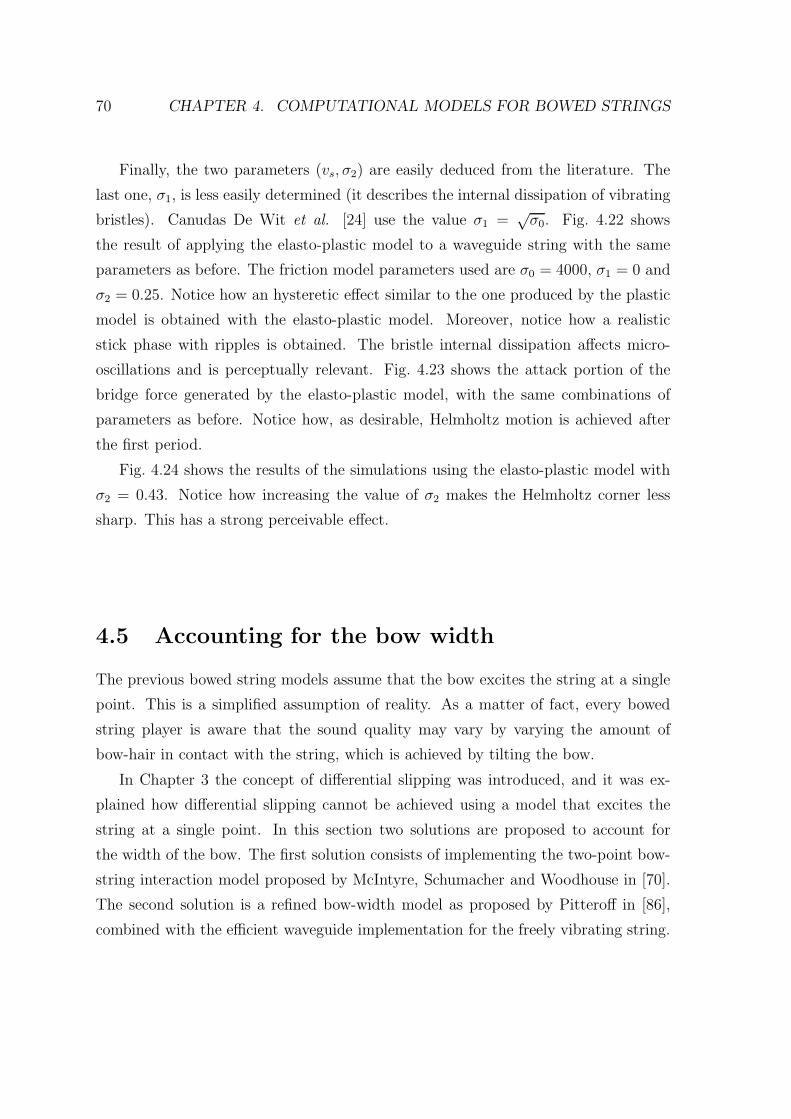
70 CHAPTER 4. COMPUTATIONAL MODELS FOR BOWED STRINGS
Finally, the two parameters (vs, σ2) are easily deduced from the literature. The
last one, σ1, is less easily determined (it describes the internal dissipation of vibrating
bristles). Canudas De Wit et al. [24] use the value σ1 =√σ0. Fig. 4.22 shows
the result of applying the elasto-plastic model to a waveguide string with the same
parameters as before. The friction model parameters used are σ0 = 4000, σ1 = 0 and
σ2 = 0.25. Notice how an hysteretic effect similar to the one produced by the plastic
model is obtained with the elasto-plastic model. Moreover, notice how a realistic
stick phase with ripples is obtained. The bristle internal dissipation affects micro-
oscillations and is perceptually relevant. Fig. 4.23 shows the attack portion of the
bridge force generated by the elasto-plastic model, with the same combinations of
parameters as before. Notice how, as desirable, Helmholtz motion is achieved after
the first period.
Fig. 4.24 shows the results of the simulations using the elasto-plastic model with
σ2 = 0.43. Notice how increasing the value of σ2 makes the Helmholtz corner less
sharp. This has a strong perceivable effect.
4.5 Accounting for the bow width
The previous bowed string models assume that the bow excites the string at a single
point. This is a simplified assumption of reality. As a matter of fact, every bowed
string player is aware that the sound quality may vary by varying the amount of
bow-hair in contact with the string, which is achieved by tilting the bow.
In Chapter 3 the concept of differential slipping was introduced, and it was ex-
plained how differential slipping cannot be achieved using a model that excites the
string at a single point. In this section two solutions are proposed to account for
the width of the bow. The first solution consists of implementing the two-point bow-
string interaction model proposed by McIntyre, Schumacher and Woodhouse in [70].
The second solution is a refined bow-width model as proposed by Pitteroff in [86],
combined with the efficient waveguide implementation for the freely vibrating string.
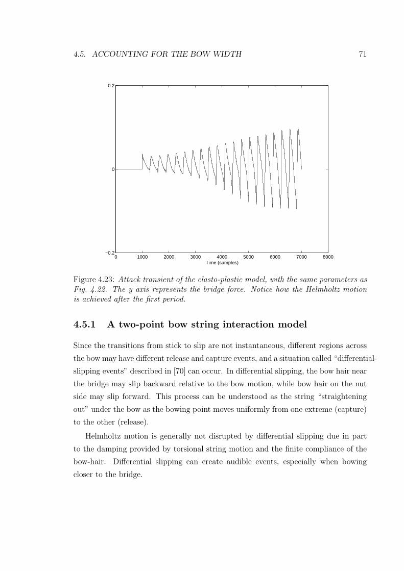
4.5. ACCOUNTING FOR THE BOW WIDTH 71
0 1000 2000 3000 4000 5000 6000 7000 8000−0.2
0
0.2
Time (samples)
Figure 4.23: Attack transient of the elasto-plastic model, with the same parameters asFig. 4.22. The y axis represents the bridge force. Notice how the Helmholtz motionis achieved after the first period.
4.5.1 A two-point bow string interaction model
Since the transitions from stick to slip are not instantaneous, different regions across
the bow may have different release and capture events, and a situation called “differential-
slipping events” described in [70] can occur. In differential slipping, the bow hair near
the bridge may slip backward relative to the bow motion, while bow hair on the nut
side may slip forward. This process can be understood as the string “straightening
out” under the bow as the bowing point moves uniformly from one extreme (capture)
to the other (release).
Helmholtz motion is generally not disrupted by differential slipping due in part
to the damping provided by torsional string motion and the finite compliance of the
bow-hair. Differential slipping can create audible events, especially when bowing
closer to the bridge.
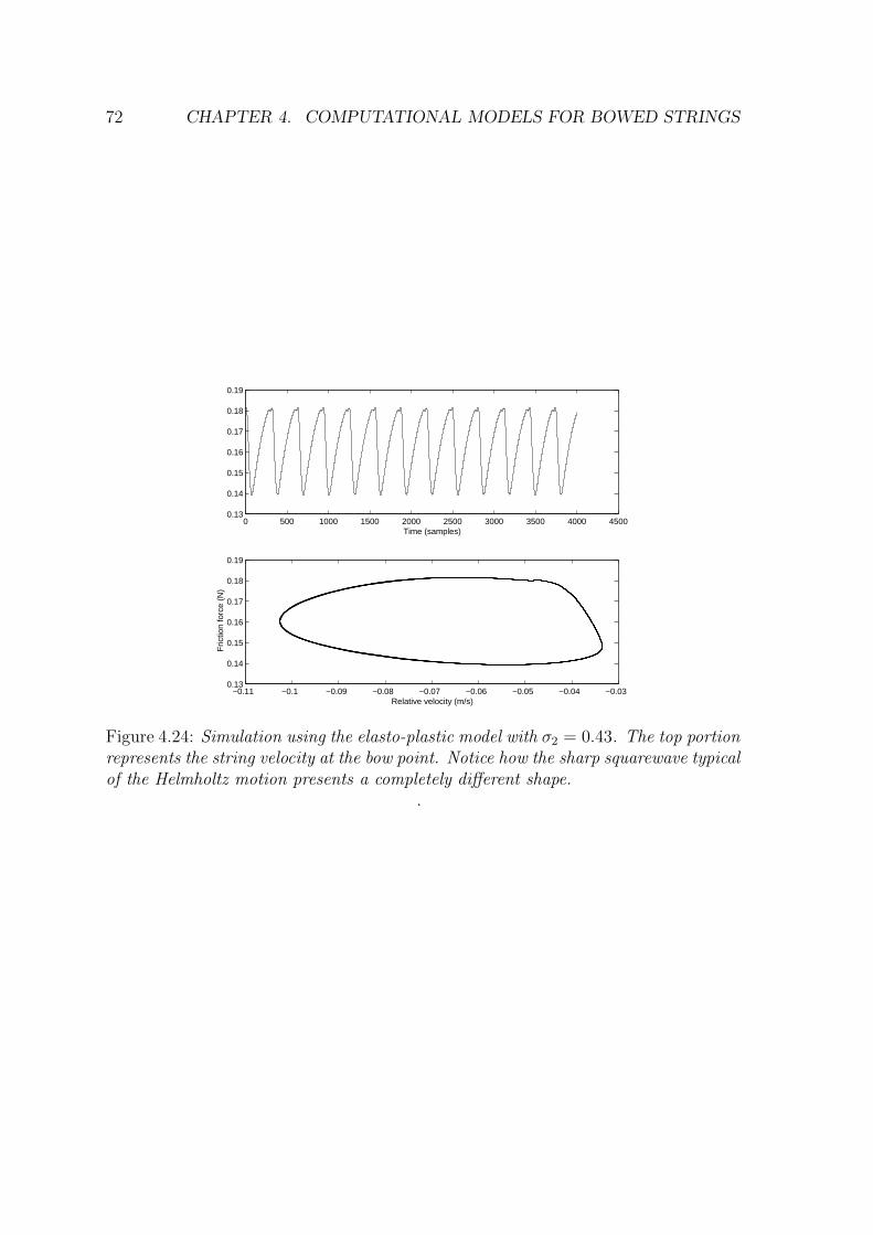
72 CHAPTER 4. COMPUTATIONAL MODELS FOR BOWED STRINGS
0 500 1000 1500 2000 2500 3000 3500 4000 45000.13
0.14
0.15
0.16
0.17
0.18
0.19
Time (samples)
−0.11 −0.1 −0.09 −0.08 −0.07 −0.06 −0.05 −0.04 −0.030.13
0.14
0.15
0.16
0.17
0.18
0.19
Relative velocity (m/s)
Fric
tion
forc
e (N
)
Figure 4.24: Simulation using the elasto-plastic model with σ2 = 0.43. The top portionrepresents the string velocity at the bow point. Notice how the sharp squarewave typicalof the Helmholtz motion presents a completely different shape.
.
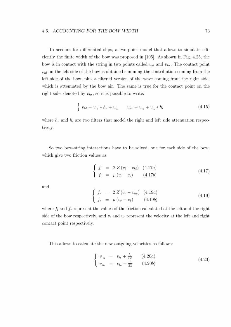
4.5. ACCOUNTING FOR THE BOW WIDTH 73
To account for differential slips, a two-point model that allows to simulate effi-
ciently the finite width of the bow was proposed in [105]. As shown in Fig. 4.25, the
bow is in contact with the string in two points called vhl and vhr. The contact point
vhl on the left side of the bow is obtained summing the contribution coming from the
left side of the bow, plus a filtered version of the wave coming from the right side,
which is attenuated by the bow air. The same is true for the contact point on the
right side, denoted by vhr, so it is possible to write:
vhl = vin ∗ hr + vib vhr = vin + vib ∗ hl (4.15)
where hr and hl are two filters that model the right and left side attenuation respec-
tively.
So two bow-string interactions have to be solved, one for each side of the bow,
which give two friction values as:
fl = 2 Z (vl − vhl) (4.17a)
fl = µ (vl − vb) (4.17b)(4.17)
and
fr = 2 Z (vr − vhr) (4.19a)
fr = µ (vr − vb) (4.19b)(4.19)
where fl and fr represent the values of the friction calculated at the left and the right
side of the bow respectively, and vl and vr represent the velocity at the left and right
contact point respectively.
This allows to calculate the new outgoing velocities as follows:
von= vib + fr
2Z(4.20a)
vob= vin + fl
2Z(4.20b)
(4.20)
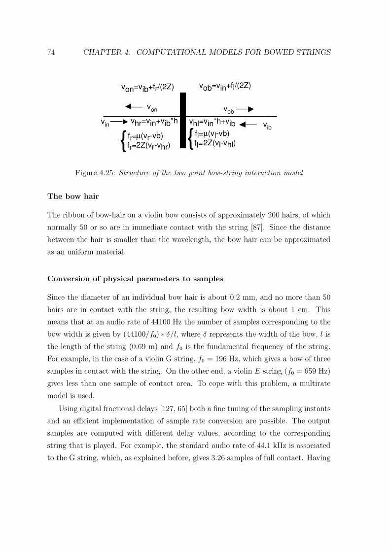
74 CHAPTER 4. COMPUTATIONAL MODELS FOR BOWED STRINGS
von vob
vibvin
vhl=vin*h+vib
fl=µ(vl-vb)
2Z(vl-vhl)fl=
vob=vin+fl/(2Z)
fr=µ(vr-vb)
2Z(vr-vhr)fr=
von=vib+fr/(2Z)
vhr=vin+vib*h
Figure 4.25: Structure of the two point bow-string interaction model
The bow hair
The ribbon of bow-hair on a violin bow consists of approximately 200 hairs, of which
normally 50 or so are in immediate contact with the string [87]. Since the distance
between the hair is smaller than the wavelength, the bow hair can be approximated
as an uniform material.
Conversion of physical parameters to samples
Since the diameter of an individual bow hair is about 0.2 mm, and no more than 50
hairs are in contact with the string, the resulting bow width is about 1 cm. This
means that at an audio rate of 44100 Hz the number of samples corresponding to the
bow width is given by (44100/f0) ∗ δ/l, where δ represents the width of the bow, l is
the length of the string (0.69 m) and f0 is the fundamental frequency of the string.
For example, in the case of a violin G string, f0 = 196 Hz, which gives a bow of three
samples in contact with the string. On the other end, a violin E string (f0 = 659 Hz)
gives less than one sample of contact area. To cope with this problem, a multirate
model is used.
Using digital fractional delays [127, 65] both a fine tuning of the sampling instants
and an efficient implementation of sample rate conversion are possible. The output
samples are computed with different delay values, according to the corresponding
string that is played. For example, the standard audio rate of 44.1 kHz is associated
to the G string, which, as explained before, gives 3.26 samples of full contact. Having
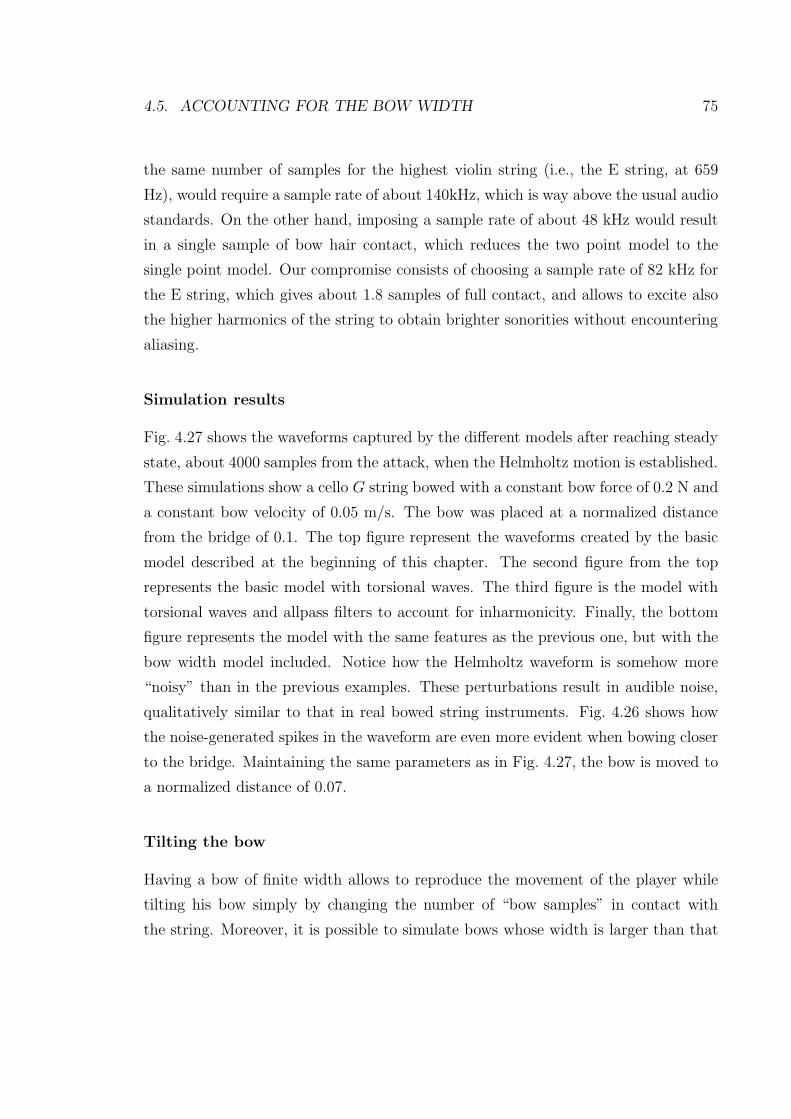
4.5. ACCOUNTING FOR THE BOW WIDTH 75
the same number of samples for the highest violin string (i.e., the E string, at 659
Hz), would require a sample rate of about 140kHz, which is way above the usual audio
standards. On the other hand, imposing a sample rate of about 48 kHz would result
in a single sample of bow hair contact, which reduces the two point model to the
single point model. Our compromise consists of choosing a sample rate of 82 kHz for
the E string, which gives about 1.8 samples of full contact, and allows to excite also
the higher harmonics of the string to obtain brighter sonorities without encountering
aliasing.
Simulation results
Fig. 4.27 shows the waveforms captured by the different models after reaching steady
state, about 4000 samples from the attack, when the Helmholtz motion is established.
These simulations show a cello G string bowed with a constant bow force of 0.2 N and
a constant bow velocity of 0.05 m/s. The bow was placed at a normalized distance
from the bridge of 0.1. The top figure represent the waveforms created by the basic
model described at the beginning of this chapter. The second figure from the top
represents the basic model with torsional waves. The third figure is the model with
torsional waves and allpass filters to account for inharmonicity. Finally, the bottom
figure represents the model with the same features as the previous one, but with the
bow width model included. Notice how the Helmholtz waveform is somehow more
“noisy” than in the previous examples. These perturbations result in audible noise,
qualitatively similar to that in real bowed string instruments. Fig. 4.26 shows how
the noise-generated spikes in the waveform are even more evident when bowing closer
to the bridge. Maintaining the same parameters as in Fig. 4.27, the bow is moved to
a normalized distance of 0.07.
Tilting the bow
Having a bow of finite width allows to reproduce the movement of the player while
tilting his bow simply by changing the number of “bow samples” in contact with
the string. Moreover, it is possible to simulate bows whose width is larger than that
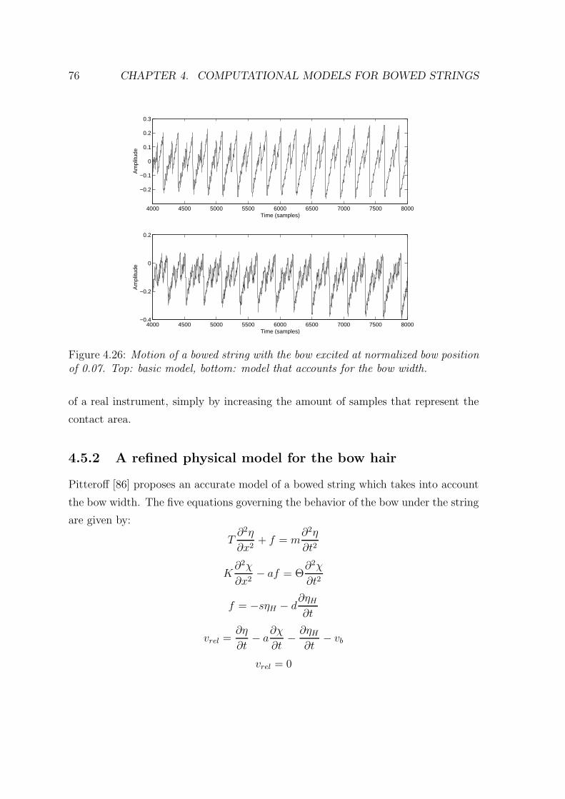
76 CHAPTER 4. COMPUTATIONAL MODELS FOR BOWED STRINGS
4000 4500 5000 5500 6000 6500 7000 7500 8000
−0.2
−0.1
0
0.1
0.2
0.3
Time (samples)
Am
plitu
de
4000 4500 5000 5500 6000 6500 7000 7500 8000−0.4
−0.2
0
0.2
Time (samples)
Am
plitu
de
Figure 4.26: Motion of a bowed string with the bow excited at normalized bow positionof 0.07. Top: basic model, bottom: model that accounts for the bow width.
of a real instrument, simply by increasing the amount of samples that represent the
contact area.
4.5.2 A refined physical model for the bow hair
Pitteroff [86] proposes an accurate model of a bowed string which takes into account
the bow width. The five equations governing the behavior of the bow under the string
are given by:
T∂2η
∂x2+ f = m
∂2η
∂t2
K∂2χ
∂x2− af = Θ
∂2χ
∂t2
f = −sηH − d∂ηH
∂t
vrel =∂η
∂t− a∂χ
∂t− ∂ηH
∂t− vb
vrel = 0
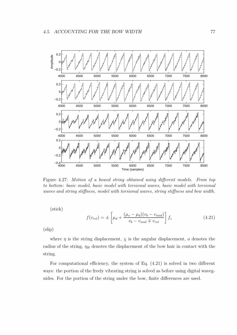
4.5. ACCOUNTING FOR THE BOW WIDTH 77
4000 4500 5000 5500 6000 6500 7000 7500 8000
−0.2
0
0.2A
mpl
itude
4000 4500 5000 5500 6000 6500 7000 7500 8000
−0.2
0
0.2
4000 4500 5000 5500 6000 6500 7000 7500 8000
−0.2
0
0.2
4000 4500 5000 5500 6000 6500 7000 7500 8000−0.4
−0.2
0
0.2
Time (samples)
Figure 4.27: Motion of a bowed string obtained using different models. From topto bottom: basic model, basic model with torsional waves, basic model with torsionalwaves and string stiffness, model with torsional waves, string stiffness and bow width.
(stick)
f(vrel) = ±[
µd +(µs − µd)(vb − vmid)
vb − vmid ∓ vrel
]
fz (4.21)
(slip)
where η is the string displacement, χ is the angular displacement, a denotes the
radius of the string, ηH denotes the displacement of the bow hair in contact with the
string.
For computational efficiency, the system of Eq. (4.21) is solved in two different
ways: the portion of the freely vibrating string is solved as before using digital waveg-
uides. For the portion of the string under the bow, finite differences are used.
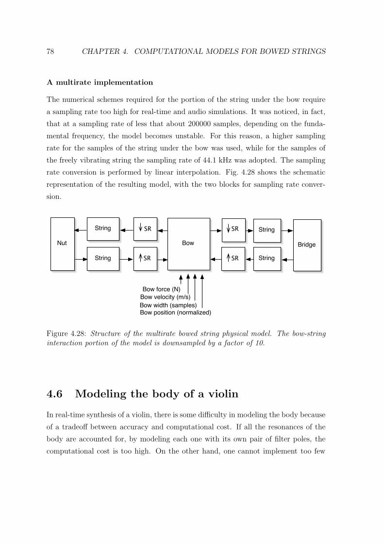
78 CHAPTER 4. COMPUTATIONAL MODELS FOR BOWED STRINGS
A multirate implementation
The numerical schemes required for the portion of the string under the bow require
a sampling rate too high for real-time and audio simulations. It was noticed, in fact,
that at a sampling rate of less that about 200000 samples, depending on the funda-
mental frequency, the model becomes unstable. For this reason, a higher sampling
rate for the samples of the string under the bow was used, while for the samples of
the freely vibrating string the sampling rate of 44.1 kHz was adopted. The sampling
rate conversion is performed by linear interpolation. Fig. 4.28 shows the schematic
representation of the resulting model, with the two blocks for sampling rate conver-
sion.
StringBow
StringBridge
Bow velocity (m/s)Bow force (N)
Bow position (normalized)
Nut
Bow width (samples)
SR
String StringSR
SR
SR
Figure 4.28: Structure of the multirate bowed string physical model. The bow-stringinteraction portion of the model is downsampled by a factor of 10.
4.6 Modeling the body of a violin
In real-time synthesis of a violin, there is some difficulty in modeling the body because
of a tradeoff between accuracy and computational cost. If all the resonances of the
body are accounted for, by modeling each one with its own pair of filter poles, the
computational cost is too high. On the other hand, one cannot implement too few
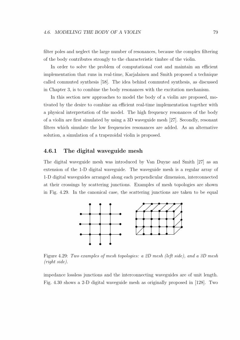
4.6. MODELING THE BODY OF A VIOLIN 79
filter poles and neglect the large number of resonances, because the complex filtering
of the body contributes strongly to the characteristic timbre of the violin.
In order to solve the problem of computational cost and maintain an efficient
implementation that runs in real-time, Karjalainen and Smith proposed a technique
called commuted synthesis [58]. The idea behind commuted synthesis, as discussed
in Chapter 3, is to combine the body resonances with the excitation mechanism.
In this section new approaches to model the body of a violin are proposed, mo-
tivated by the desire to combine an efficient real-time implementation together with
a physical interpretation of the model. The high frequency resonances of the body
of a violin are first simulated by using a 3D waveguide mesh [27]. Secondly, resonant
filters which simulate the low frequencies resonances are added. As an alternative
solution, a simulation of a trapezoidal violin is proposed.
4.6.1 The digital waveguide mesh
The digital waveguide mesh was introduced by Van Duyne and Smith [27] as an
extension of the 1-D digital waveguide. The waveguide mesh is a regular array of
1-D digital waveguides arranged along each perpendicular dimension, interconnected
at their crossings by scattering junctions. Examples of mesh topologies are shown
in Fig. 4.29. In the canonical case, the scattering junctions are taken to be equal
Figure 4.29: Two examples of mesh topologies: a 2D mesh (left side), and a 3D mesh(right side).
impedance lossless junctions and the interconnecting waveguides are of unit length.
Fig. 4.30 shows a 2-D digital waveguide mesh as originally proposed in [128]. Two
80 CHAPTER 4. COMPUTATIONAL MODELS FOR BOWED STRINGS
conditions must be satisfied for at a lossless junction J connecting lines of equal
impedance [27]:
• Sum of inputs equals the sum of outputs (flows add to zero).
• Signals at each intersecting waveguide are equal at the junction.
The first condition translates to the following equation:
∑
i
v+il,m(n) =
∑
i
v−il,m(n) (4.22)
where the l,m indices represent the spatial position of the junction in the mesh, the
n index represents the current time sample, and v+il,m(n) and v−il,m(n) represent the
four incoming and outgoing waves at a junction, respectively. The digital waveguide
mesh algorithm can be interpreted as a difference scheme for computation of the
two-dimensional wave equation [128].
4.6.2 Body modeling using the waveguide mesh
As a first attempt, the high frequency resonances of a violin body were simulated by
using a 3D waveguide mesh. The 3D rectilinear mesh is an extension of the 2D mesh
to 3 dimensions. It is made of 6-port scattering junctions arranged at integer valued
spatial positions in each of the three axial directions.
The 3D waveguide mesh is initially chosen to correspond to a physical box with
dimensions 35.5× 21.0× 3.0 cm. Such dimensions are comparable to those of a real
violin body, so it is expected for the mesh to spontaneously have a similar mode
spacing at high frequencies where the air modes dominate [21]. At a sampling rate
of 44.1 kHz, assuming a sound speed c = 344 m/s, these dimensions translate to a
rectangular mesh which is approximately 26× 16× 2 samples along each edge. 2
2Using von Neumann stability analysis [27], a physical length d is converted to samples using theformula Nd = dFs/(c
√3).
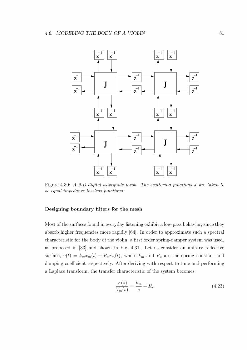
4.6. MODELING THE BODY OF A VIOLIN 81
J
J J
Jz−1
−1
z
z−1
z−1
z−1
z−1
z−1
z−1
z−1
z−1
z−1
z−1
z−1
z−1
z−1
z−1
z−1
z−1
z−1
z−1
z−1
z−1
z−1
z−1
Figure 4.30: A 2-D digital waveguide mesh. The scattering junctions J are taken tobe equal impedance lossless junctions.
Designing boundary filters for the mesh
Most of the surfaces found in everyday listening exhibit a low-pass behavior, since they
absorb higher frequencies more rapidly [64]. In order to approximate such a spectral
characteristic for the body of the violin, a first order spring-damper system was used,
as proposed in [33] and shown in Fig. 4.31. Let us consider an unitary reflective
surface, v(t) = kmxm(t) + Rsxm(t), where km and Rs are the spring constant and
damping coefficient respectively. After deriving with respect to time and performing
a Laplace transform, the transfer characteristic of the system becomes:
V (s)
Vm(s)=km
s+Rs (4.23)
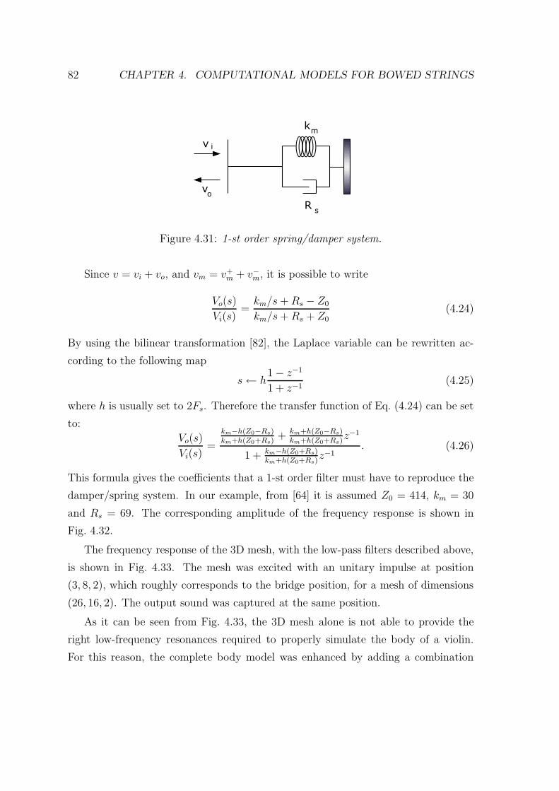
82 CHAPTER 4. COMPUTATIONAL MODELS FOR BOWED STRINGS
vk
Rv
i
o
s
m
Figure 4.31: 1-st order spring/damper system.
Since v = vi + vo, and vm = v+m + v−m, it is possible to write
Vo(s)
Vi(s)=km/s+Rs − Z0
km/s+Rs + Z0(4.24)
By using the bilinear transformation [82], the Laplace variable can be rewritten ac-
cording to the following map
s← h1− z−1
1 + z−1(4.25)
where h is usually set to 2Fs. Therefore the transfer function of Eq. (4.24) can be set
to:
Vo(s)
Vi(s)=
km−h(Z0−Rs)km+h(Z0+Rs)
+ km+h(Z0−Rs)km+h(Z0+Rs)
z−1
1 + km−h(Z0+Rs)km+h(Z0+Rs)
z−1. (4.26)
This formula gives the coefficients that a 1-st order filter must have to reproduce the
damper/spring system. In our example, from [64] it is assumed Z0 = 414, km = 30
and Rs = 69. The corresponding amplitude of the frequency response is shown in
Fig. 4.32.
The frequency response of the 3D mesh, with the low-pass filters described above,
is shown in Fig. 4.33. The mesh was excited with an unitary impulse at position
(3, 8, 2), which roughly corresponds to the bridge position, for a mesh of dimensions
(26, 16, 2). The output sound was captured at the same position.
As it can be seen from Fig. 4.33, the 3D mesh alone is not able to provide the
right low-frequency resonances required to properly simulate the body of a violin.
For this reason, the complete body model was enhanced by adding a combination
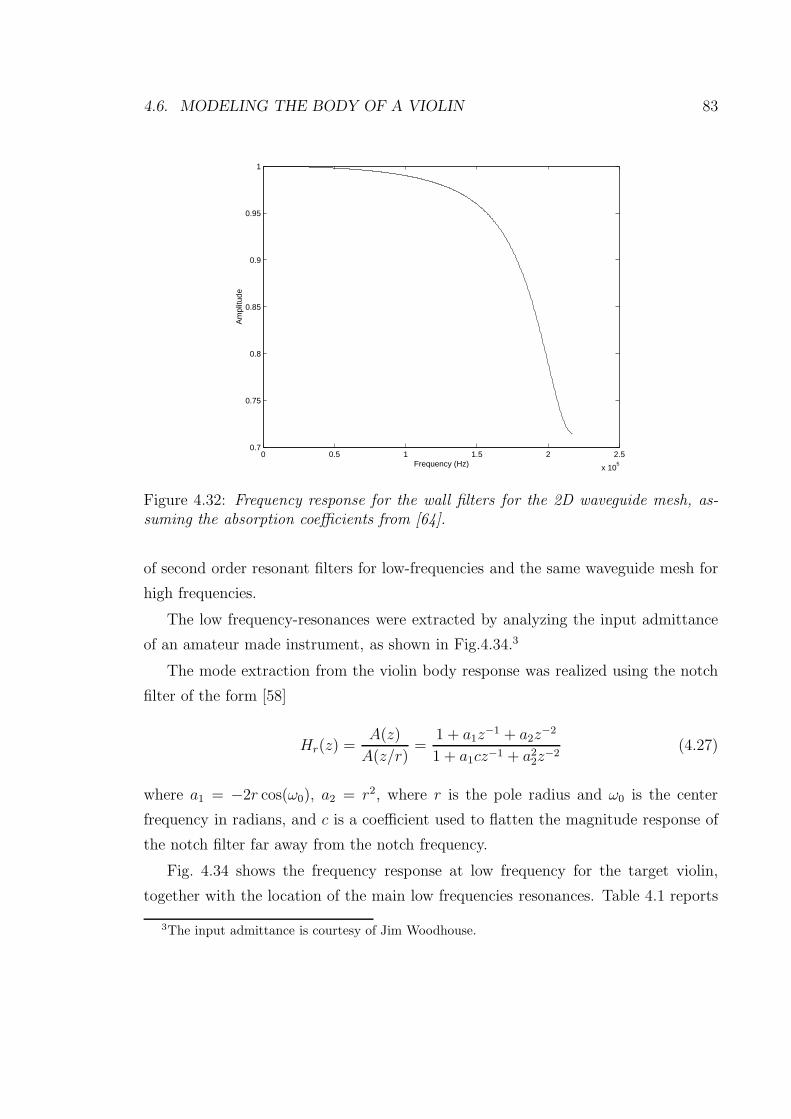
4.6. MODELING THE BODY OF A VIOLIN 83
0 0.5 1 1.5 2 2.5
x 105
0.7
0.75
0.8
0.85
0.9
0.95
1
Frequency (Hz)
Am
plitu
de
Figure 4.32: Frequency response for the wall filters for the 2D waveguide mesh, as-suming the absorption coefficients from [64].
of second order resonant filters for low-frequencies and the same waveguide mesh for
high frequencies.
The low frequency-resonances were extracted by analyzing the input admittance
of an amateur made instrument, as shown in Fig.4.34.3
The mode extraction from the violin body response was realized using the notch
filter of the form [58]
Hr(z) =A(z)
A(z/r)=
1 + a1z−1 + a2z
−2
1 + a1cz−1 + a22z
−2(4.27)
where a1 = −2r cos(ω0), a2 = r2, where r is the pole radius and ω0 is the center
frequency in radians, and c is a coefficient used to flatten the magnitude response of
the notch filter far away from the notch frequency.
Fig. 4.34 shows the frequency response at low frequency for the target violin,
together with the location of the main low frequencies resonances. Table 4.1 reports
3The input admittance is courtesy of Jim Woodhouse.
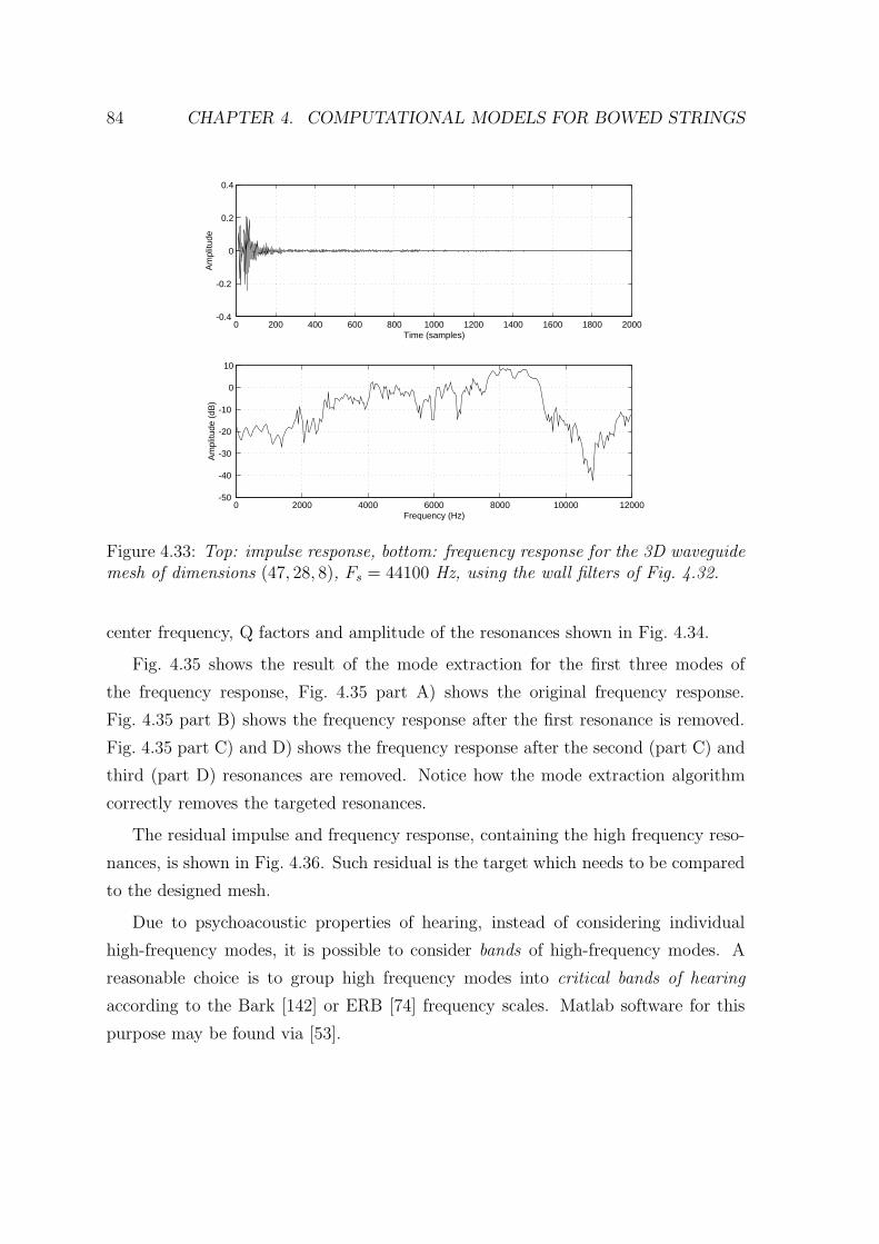
84 CHAPTER 4. COMPUTATIONAL MODELS FOR BOWED STRINGS
0 200 400 600 800 1000 1200 1400 1600 1800 2000-0.4
-0.2
0
0.2
0.4
Time (samples)
Am
plitu
de
0 2000 4000 6000 8000 10000 12000-50
-40
-30
-20
-10
0
10
Frequency (Hz)
Am
plitu
de (
dB)
Figure 4.33: Top: impulse response, bottom: frequency response for the 3D waveguidemesh of dimensions (47, 28, 8), Fs = 44100 Hz, using the wall filters of Fig. 4.32.
center frequency, Q factors and amplitude of the resonances shown in Fig. 4.34.
Fig. 4.35 shows the result of the mode extraction for the first three modes of
the frequency response, Fig. 4.35 part A) shows the original frequency response.
Fig. 4.35 part B) shows the frequency response after the first resonance is removed.
Fig. 4.35 part C) and D) shows the frequency response after the second (part C) and
third (part D) resonances are removed. Notice how the mode extraction algorithm
correctly removes the targeted resonances.
The residual impulse and frequency response, containing the high frequency reso-
nances, is shown in Fig. 4.36. Such residual is the target which needs to be compared
to the designed mesh.
Due to psychoacoustic properties of hearing, instead of considering individual
high-frequency modes, it is possible to consider bands of high-frequency modes. A
reasonable choice is to group high frequency modes into critical bands of hearing
according to the Bark [142] or ERB [74] frequency scales. Matlab software for this
purpose may be found via [53].
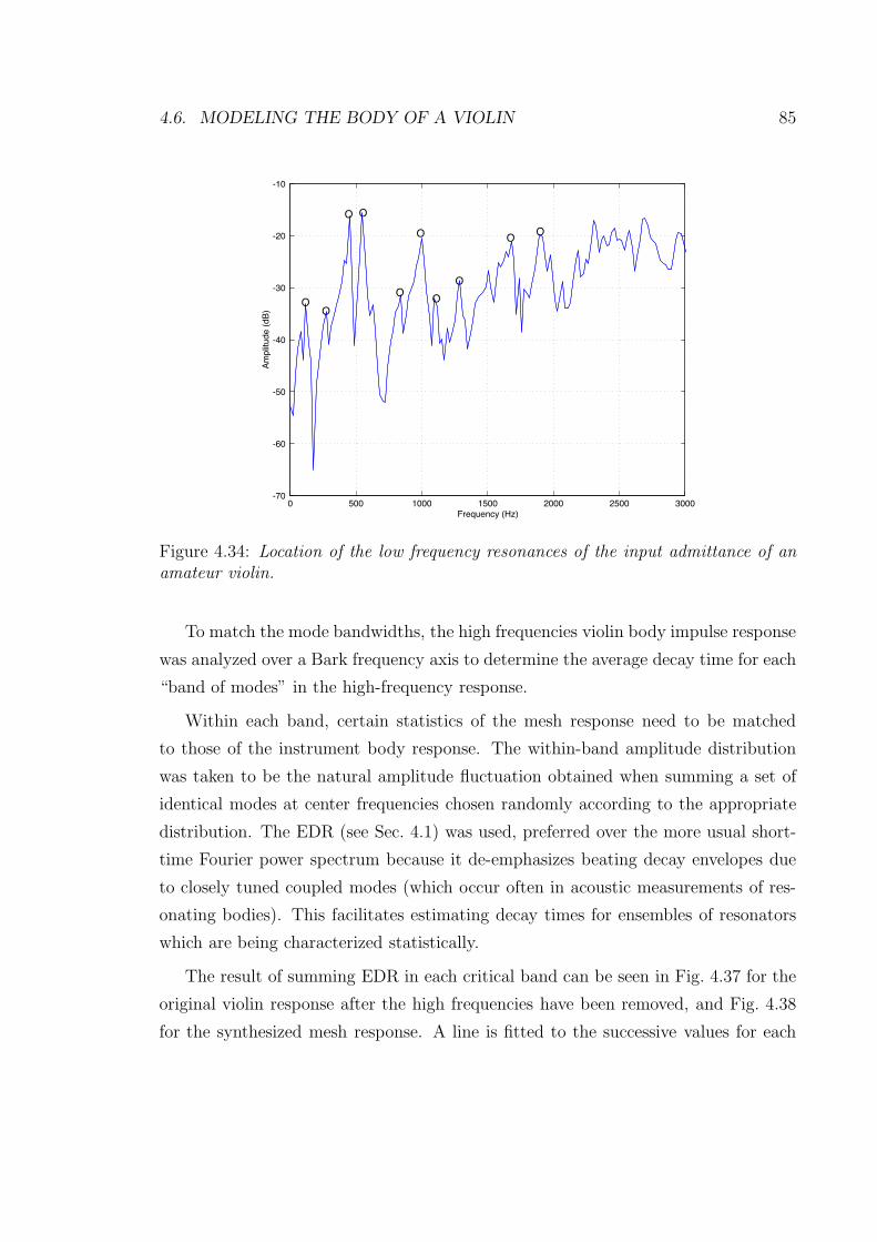
4.6. MODELING THE BODY OF A VIOLIN 85
0 500 1000 1500 2000 2500 3000-70
-60
-50
-40
-30
-20
-10
Frequency (Hz)
Am
plit
ude (
dB
)
OO
O O
O OO
O
OO
Figure 4.34: Location of the low frequency resonances of the input admittance of anamateur violin.
To match the mode bandwidths, the high frequencies violin body impulse response
was analyzed over a Bark frequency axis to determine the average decay time for each
“band of modes” in the high-frequency response.
Within each band, certain statistics of the mesh response need to be matched
to those of the instrument body response. The within-band amplitude distribution
was taken to be the natural amplitude fluctuation obtained when summing a set of
identical modes at center frequencies chosen randomly according to the appropriate
distribution. The EDR (see Sec. 4.1) was used, preferred over the more usual short-
time Fourier power spectrum because it de-emphasizes beating decay envelopes due
to closely tuned coupled modes (which occur often in acoustic measurements of res-
onating bodies). This facilitates estimating decay times for ensembles of resonators
which are being characterized statistically.
The result of summing EDR in each critical band can be seen in Fig. 4.37 for the
original violin response after the high frequencies have been removed, and Fig. 4.38
for the synthesized mesh response. A line is fitted to the successive values for each
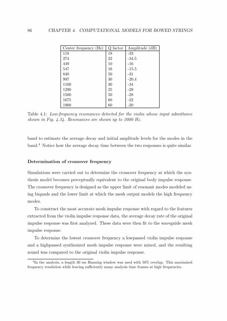
86 CHAPTER 4. COMPUTATIONAL MODELS FOR BOWED STRINGS
Center frequency (Hz) Q factor Amplitude (dB)
118 18 -33274 22 -34.5449 10 -16547 16 -15.5840 50 -31997 30 -20.41100 30 -341290 25 -291500 50 -281675 60 -221900 60 -20
Table 4.1: Low-frequency resonances detected for the violin whose input admittanceshown in Fig. 4.34. Resonances are shown up to 2000 Hz.
band to estimate the average decay and initial amplitude levels for the modes in the
band.4 Notice how the average decay time between the two responses is quite similar.
Determination of crossover frequency
Simulations were carried out to determine the crossover frequency at which the syn-
thesis model becomes perceptually equivalent to the original body impulse response.
The crossover frequency is designed as the upper limit of resonant modes modeled us-
ing biquads and the lower limit at which the mesh output models the high frequency
modes.
To construct the most accurate mesh impulse response with regard to the features
extracted from the violin impulse response data, the average decay rate of the original
impulse response was first analyzed. These data were then fit to the waveguide mesh
impulse response.
To determine the lowest crossover frequency a lowpassed violin impulse response
and a highpassed synthesized mesh impulse response were mixed, and the resulting
sound was compared to the original violin impulse response.
4In the analysis, a length 30 ms Hanning window was used with 50% overlap. This maximizedfrequency resolution while leaving sufficiently many analysis time frames at high frequencies.
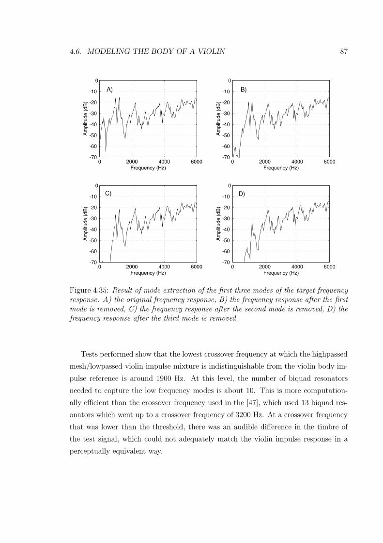
4.6. MODELING THE BODY OF A VIOLIN 87
0 2000 4000 6000-70
-60
-50
-40
-30
-20
-10
0
Frequency (Hz)
Am
plit
ude (
dB
)
0 2000 4000 6000-70
-60
-50
-40
-30
-20
-10
0
Frequency (Hz)
Am
plit
ude (
dB
)
0 2000 4000 6000-70
-60
-50
-40
-30
-20
-10
0
Frequency (Hz)
Am
plit
ude (
dB
)
0 2000 4000 6000-70
-60
-50
-40
-30
-20
-10
0
Frequency (Hz)
Am
plit
ude (
dB
)
A) B)
C) D)
Figure 4.35: Result of mode extraction of the first three modes of the target frequencyresponse. A) the original frequency response, B) the frequency response after the firstmode is removed, C) the frequency response after the second mode is removed, D) thefrequency response after the third mode is removed.
Tests performed show that the lowest crossover frequency at which the highpassed
mesh/lowpassed violin impulse mixture is indistinguishable from the violin body im-
pulse reference is around 1900 Hz. At this level, the number of biquad resonators
needed to capture the low frequency modes is about 10. This is more computation-
ally efficient than the crossover frequency used in the [47], which used 13 biquad res-
onators which went up to a crossover frequency of 3200 Hz. At a crossover frequency
that was lower than the threshold, there was an audible difference in the timbre of
the test signal, which could not adequately match the violin impulse response in a
perceptually equivalent way.
88 CHAPTER 4. COMPUTATIONAL MODELS FOR BOWED STRINGS
0 0.002 0.004 0.006 0.008 0.01 0.012 0.014 0.016 0.018 0.02-0.05
0
0.05
Time (s)
Am
plitu
de
0 5000 10000 15000-100
-80
-60
-40
-20
0
Frequency (Hz)
Am
plitu
de (
dB)
Figure 4.36: Top: impulse response, bottom: input admittance at the bridge for theoriginal violin, after the low frequency resonances have been removed.
These tests show that it is perceptually possible to use a reduced number of low-
frequency resonators and still provide high quality results. Connecting the mesh to
these resonators produces a high quality synthetic violin impulse response. The cor-
responding time domain signal is shown along with that of the original violin impulse
response in Fig. 4.39. The more pronounced beating of the highpassed waveguide
mesh output is effectively masked by the strong, long-ringing body modes present in
the original violin body impulse below 1900 Hz.
Examining smaller mesh dimensions
Since perceptual mode saturation in a critical band can be realistically achieved by a
small number of resonators, it is theoretically possible that even smaller dimensions
of waveguide meshes would have a distribution of mode amplitudes which can satisfy
the perceptual criteria for our synthesis model described above. This would allow
to build a mesh which is perceptually equivalent but whose computational cost is
reduced.
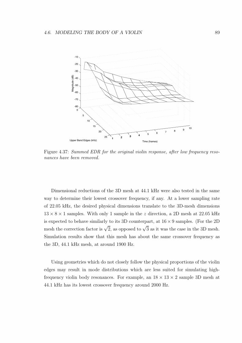
4.6. MODELING THE BODY OF A VIOLIN 89
0
-80
-70
-60
-50
-40
-30
-20
-10
Magnitude (
dB
)
5
10
15
20
251 2 3 4
Time (frames)Upper Band Edges (kHz)1 2 3 4 5 6 7 8 9
10
Figure 4.37: Summed EDR for the original violin response, after low frequency reso-nances have been removed.
Dimensional reductions of the 3D mesh at 44.1 kHz were also tested in the same
way to determine their lowest crossover frequency, if any. At a lower sampling rate
of 22.05 kHz, the desired physical dimensions translate to the 3D-mesh dimensions
13× 8× 1 samples. With only 1 sample in the z direction, a 2D mesh at 22.05 kHz
is expected to behave similarly to its 3D counterpart, at 16× 9 samples. (For the 2D
mesh the correction factor is√
2, as opposed to√
3 as it was the case in the 3D mesh.
Simulation results show that this mesh has about the same crossover frequency as
the 3D, 44.1 kHz mesh, at around 1900 Hz.
Using geometries which do not closely follow the physical proportions of the violin
edges may result in mode distributions which are less suited for simulating high-
frequency violin body resonances. For example, an 18 × 13 × 2 sample 3D mesh at
44.1 kHz has its lowest crossover frequency around 2000 Hz.
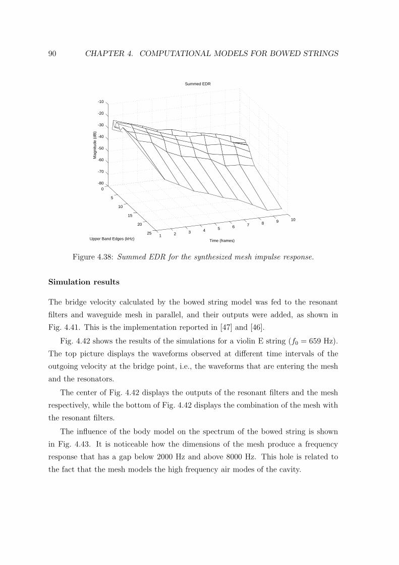
90 CHAPTER 4. COMPUTATIONAL MODELS FOR BOWED STRINGS
0
5
10
15
20
251 2 3 4 5 6 7 8 9 10
-80
-70
-60
-50
-40
-30
-20
-10
Time (frames)
Summed EDR
Upper Band Edges (kHz)
Mag
nitu
de (
dB)
Figure 4.38: Summed EDR for the synthesized mesh impulse response.
Simulation results
The bridge velocity calculated by the bowed string model was fed to the resonant
filters and waveguide mesh in parallel, and their outputs were added, as shown in
Fig. 4.41. This is the implementation reported in [47] and [46].
Fig. 4.42 shows the results of the simulations for a violin E string (f0 = 659 Hz).
The top picture displays the waveforms observed at different time intervals of the
outgoing velocity at the bridge point, i.e., the waveforms that are entering the mesh
and the resonators.
The center of Fig. 4.42 displays the outputs of the resonant filters and the mesh
respectively, while the bottom of Fig. 4.42 displays the combination of the mesh with
the resonant filters.
The influence of the body model on the spectrum of the bowed string is shown
in Fig. 4.43. It is noticeable how the dimensions of the mesh produce a frequency
response that has a gap below 2000 Hz and above 8000 Hz. This hole is related to
the fact that the mesh models the high frequency air modes of the cavity.
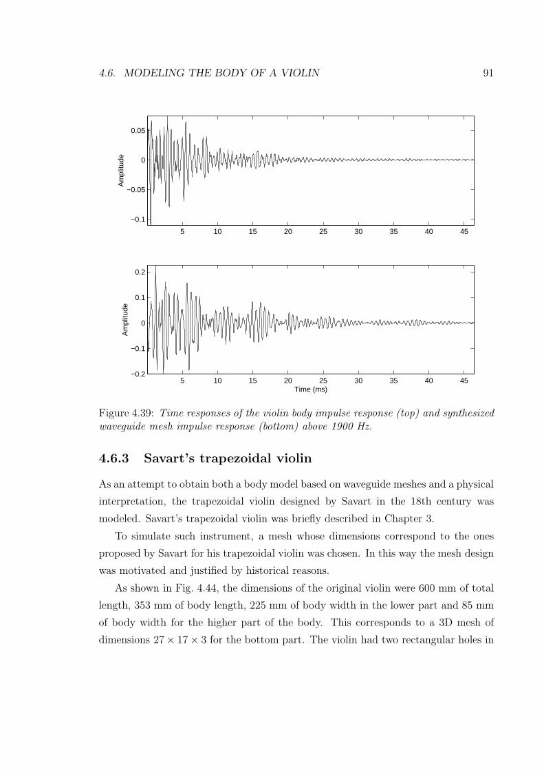
4.6. MODELING THE BODY OF A VIOLIN 91
5 10 15 20 25 30 35 40 45
−0.1
−0.05
0
0.05A
mpl
itude
5 10 15 20 25 30 35 40 45−0.2
−0.1
0
0.1
0.2
Time (ms)
Am
plitu
de
Figure 4.39: Time responses of the violin body impulse response (top) and synthesizedwaveguide mesh impulse response (bottom) above 1900 Hz.
4.6.3 Savart’s trapezoidal violin
As an attempt to obtain both a body model based on waveguide meshes and a physical
interpretation, the trapezoidal violin designed by Savart in the 18th century was
modeled. Savart’s trapezoidal violin was briefly described in Chapter 3.
To simulate such instrument, a mesh whose dimensions correspond to the ones
proposed by Savart for his trapezoidal violin was chosen. In this way the mesh design
was motivated and justified by historical reasons.
As shown in Fig. 4.44, the dimensions of the original violin were 600 mm of total
length, 353 mm of body length, 225 mm of body width in the lower part and 85 mm
of body width for the higher part of the body. This corresponds to a 3D mesh of
dimensions 27× 17× 3 for the bottom part. The violin had two rectangular holes in
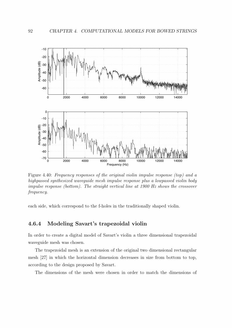
92 CHAPTER 4. COMPUTATIONAL MODELS FOR BOWED STRINGS
0 2000 4000 6000 8000 10000 12000 14000
-60
-50
-40
-30
-20
-10
Am
plit
ude (
dB
)
0 2000 4000 6000 8000 10000 12000 14000-70
-60
-50
-40
-30
-20
-10
0
Frequency (Hz)
Am
plit
ude (
dB
)
Figure 4.40: Frequency responses of the original violin impulse response (top) and ahighpassed synthesized waveguide mesh impulse response plus a lowpassed violin bodyimpulse response (bottom). The straight vertical line at 1900 Hz shows the crossoverfrequency.
each side, which correspond to the f-holes in the traditionally shaped violin.
4.6.4 Modeling Savart’s trapezoidal violin
In order to create a digital model of Savart’s violin a three dimensional trapezoidal
waveguide mesh was chosen.
The trapezoidal mesh is an extension of the original two dimensional rectangular
mesh [27] in which the horizontal dimension decreases in size from bottom to top,
according to the design proposed by Savart.
The dimensions of the mesh were chosen in order to match the dimensions of

4.6. MODELING THE BODY OF A VIOLIN 93
STRING
LOW-FREQMODES
MESH
EXCITATION +
Figure 4.41: Bowed string physical model block diagram. The outgoing velocity atthe bridge is filtered in parallel through the waveguide mesh and the low-frequencyresonant filters.
Savart’s violin. More precisely, the mesh had dimensions 27× 13× 3 samples for the
bottom part, and 7× 13× 3 for the upper part.
Fig. 4.45 shows the trapezoidal mesh used to simulate Savart’s violin. A model of
the two violin’s holes was also added. Such holes were added to the trapezoidal mesh
using the same technique adopted to model toneholes in woodwind instruments [97].
Fig. 4.46 shows the impulse response (top) and frequency response (bottom) of
the trapezoidal mesh. The response was obtained by exciting the mesh at position
4 × 1 and capturing the output waveform at 4 × 2. Notice the nice distribution of
peaks and valleys at low frequency, which resembles to the distribution typical of a
violin.
Application to the bowed string physical model
The violin body model was applied to the digital waveguide string model. The input
parameters of the string model were fb = 0.31 N, vb = 0.05 m/s and β = 0.075. As
in the case with the 3D mesh, a violin E string (f0 = 659 Hz) was used.
The outgoing velocity at the bridge point vob was filtered through the resonances
of the trapezoidal mesh, as shown in Fig. 4.47.
Fig. 4.48 shows the result of applying the trapezoidal mesh to the bowed string
physical model. The top of Fig. 4.48 represents the outgoing velocity at the bridge
vob before being filtered through the body resonances, while the bottom of Fig. 4.48
shows the output of the bowed string physical model after being filtered through
the body resonances. The waveforms were captured after steady state motion was
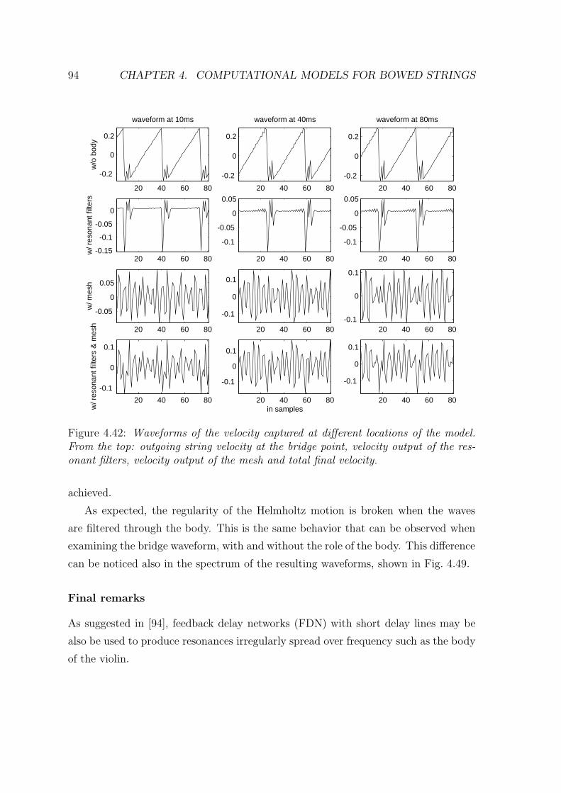
94 CHAPTER 4. COMPUTATIONAL MODELS FOR BOWED STRINGS
20 40 60 80
-0.2
0
0.2
w/o
bod
y
waveform at 10ms
20 40 60 80
-0.2
0
0.2
waveform at 40ms
20 40 60 80
-0.2
0
0.2
waveform at 80ms
20 40 60 80-0.15
-0.1
-0.05
0
w/ r
eson
ant f
ilter
s
20 40 60 80
-0.1
-0.05
0
0.05
20 40 60 80
-0.1
-0.05
0
0.05
20 40 60 80
-0.05
0
0.05
w/ m
esh
20 40 60 80
-0.1
0
0.1
20 40 60 80-0.1
0
0.1
20 40 60 80
-0.1
0
0.1
w/ r
eson
ant f
ilter
s &
mes
h
20 40 60 80
-0.1
0
0.1
in samples20 40 60 80
-0.1
0
0.1
Figure 4.42: Waveforms of the velocity captured at different locations of the model.From the top: outgoing string velocity at the bridge point, velocity output of the res-onant filters, velocity output of the mesh and total final velocity.
achieved.
As expected, the regularity of the Helmholtz motion is broken when the waves
are filtered through the body. This is the same behavior that can be observed when
examining the bridge waveform, with and without the role of the body. This difference
can be noticed also in the spectrum of the resulting waveforms, shown in Fig. 4.49.
Final remarks
As suggested in [94], feedback delay networks (FDN) with short delay lines may be
also be used to produce resonances irregularly spread over frequency such as the body
of the violin.
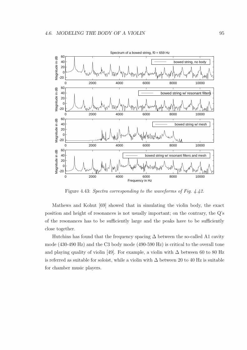
4.6. MODELING THE BODY OF A VIOLIN 95
0 2000 4000 6000 8000 10000
-20
0
20
40
60Spectrum of a bowed string, f0 = 659 Hz
Mag
nitu
de in
dB
bowed string, no body
0 2000 4000 6000 8000 10000
-20
0
20
40
60
Mag
nitu
de in
dB
bowed string w/ resonant filters
0 2000 4000 6000 8000 10000
-20
0
20
40
60
Mag
nitu
de in
dB
bowed string w/ mesh
0 2000 4000 6000 8000 10000
-20
0
20
40
60
Frequency in Hz
Mag
nitu
de in
dB
bowed string w/ resonant filters and mesh
Figure 4.43: Spectra corresponding to the waveforms of Fig. 4.42.
Mathews and Kohut [69] showed that in simulating the violin body, the exact
position and height of resonances is not usually important; on the contrary, the Q’s
of the resonances has to be sufficiently large and the peaks have to be sufficiently
close together.
Hutchins has found that the frequency spacing ∆ between the so-called A1 cavity
mode (430-490 Hz) and the C3 body mode (490-590 Hz) is critical to the overall tone
and playing quality of violin [49]. For example, a violin with ∆ between 60 to 80 Hz
is referred as suitable for soloist, while a violin with ∆ between 20 to 40 Hz is suitable
for chamber music players.
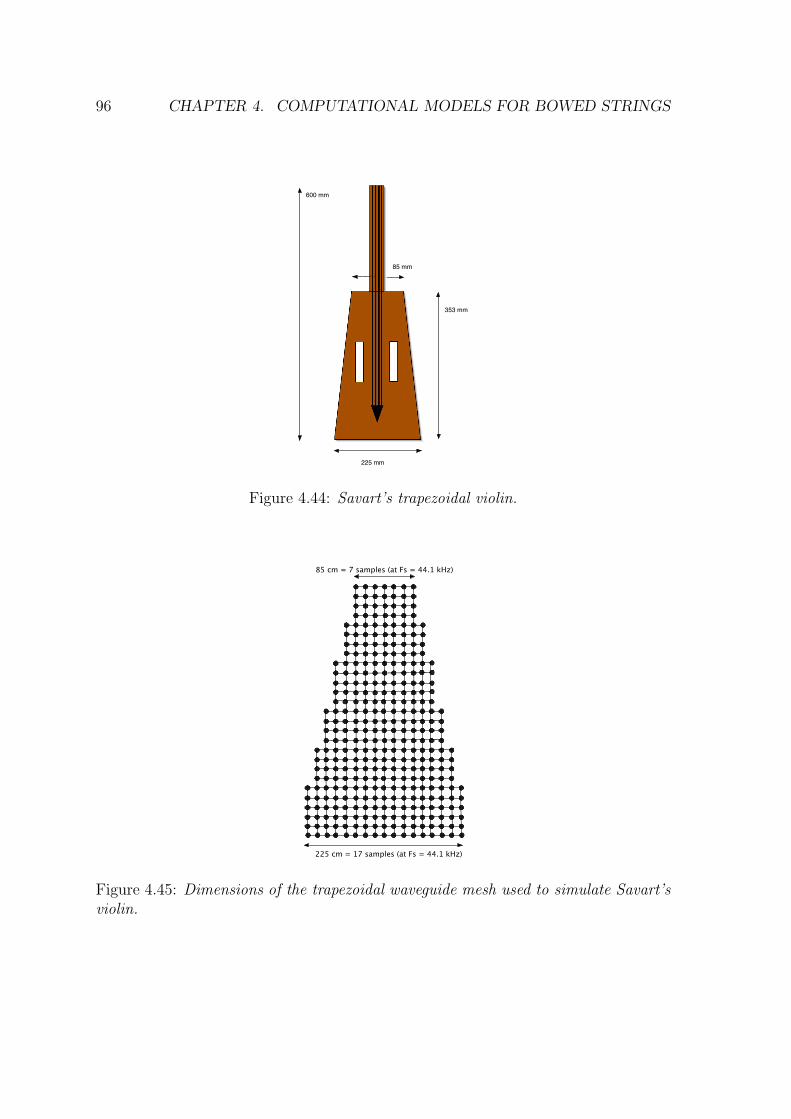
96 CHAPTER 4. COMPUTATIONAL MODELS FOR BOWED STRINGS
600 mm
353 mm
85 mm
225 mm
Figure 4.44: Savart’s trapezoidal violin.
225 cm = 17 samples (at Fs = 44.1 kHz)
85 cm = 7 samples (at Fs = 44.1 kHz)
Figure 4.45: Dimensions of the trapezoidal waveguide mesh used to simulate Savart’sviolin.
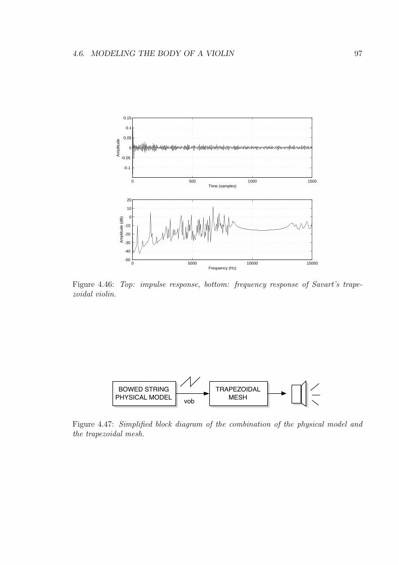
4.6. MODELING THE BODY OF A VIOLIN 97
0 500 1000 1500
-0.1
-0.05
0
0.05
0.1
0.15
TIme (samples)
Am
plitu
de
0 5000 10000 15000-50
-40
-30
-20
-10
0
10
20
Frequency (Hz)
Am
plitu
de (
dB)
Figure 4.46: Top: impulse response, bottom: frequency response of Savart’s trape-zoidal violin.
TRAPEZOIDALMESH
BOWED STRINGPHYSICAL MODEL vob
Figure 4.47: Simplified block diagram of the combination of the physical model andthe trapezoidal mesh.
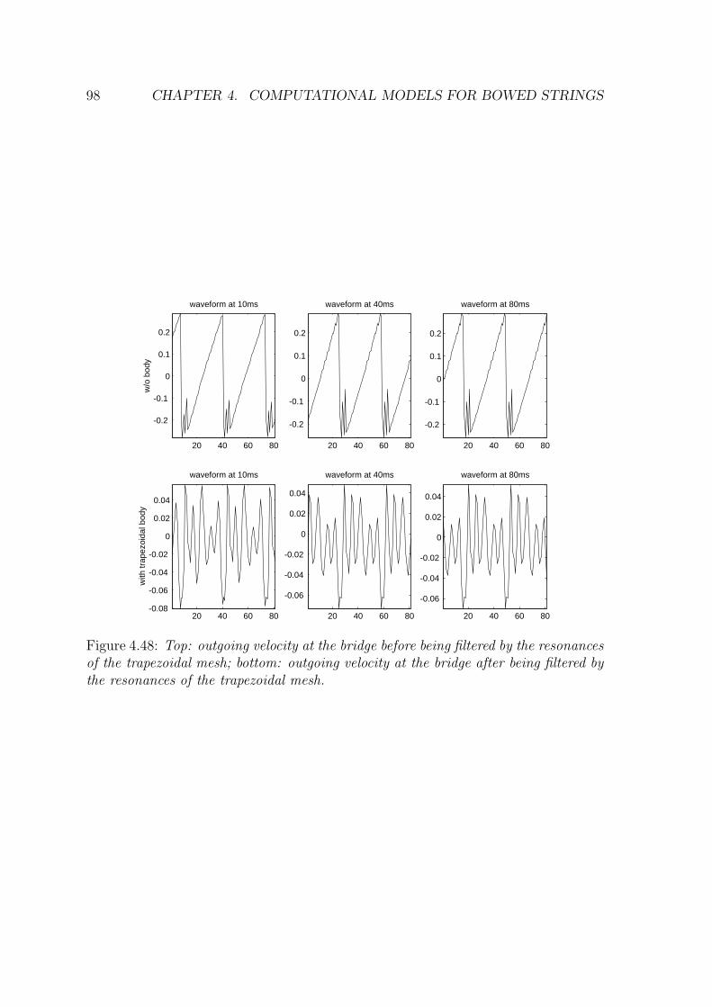
98 CHAPTER 4. COMPUTATIONAL MODELS FOR BOWED STRINGS
20 40 60 80
-0.2
-0.1
0
0.1
0.2
w/o
bod
y
waveform at 10ms
20 40 60 80
-0.2
-0.1
0
0.1
0.2
waveform at 40ms
20 40 60 80
-0.2
-0.1
0
0.1
0.2
waveform at 80ms
20 40 60 80-0.08
-0.06
-0.04
-0.02
0
0.02
0.04
with
trap
ezoi
dal b
ody
waveform at 10ms
20 40 60 80
-0.06
-0.04
-0.02
0
0.02
0.04
waveform at 40ms
20 40 60 80
-0.06
-0.04
-0.02
0
0.02
0.04
waveform at 80ms
Figure 4.48: Top: outgoing velocity at the bridge before being filtered by the resonancesof the trapezoidal mesh; bottom: outgoing velocity at the bridge after being filtered bythe resonances of the trapezoidal mesh.
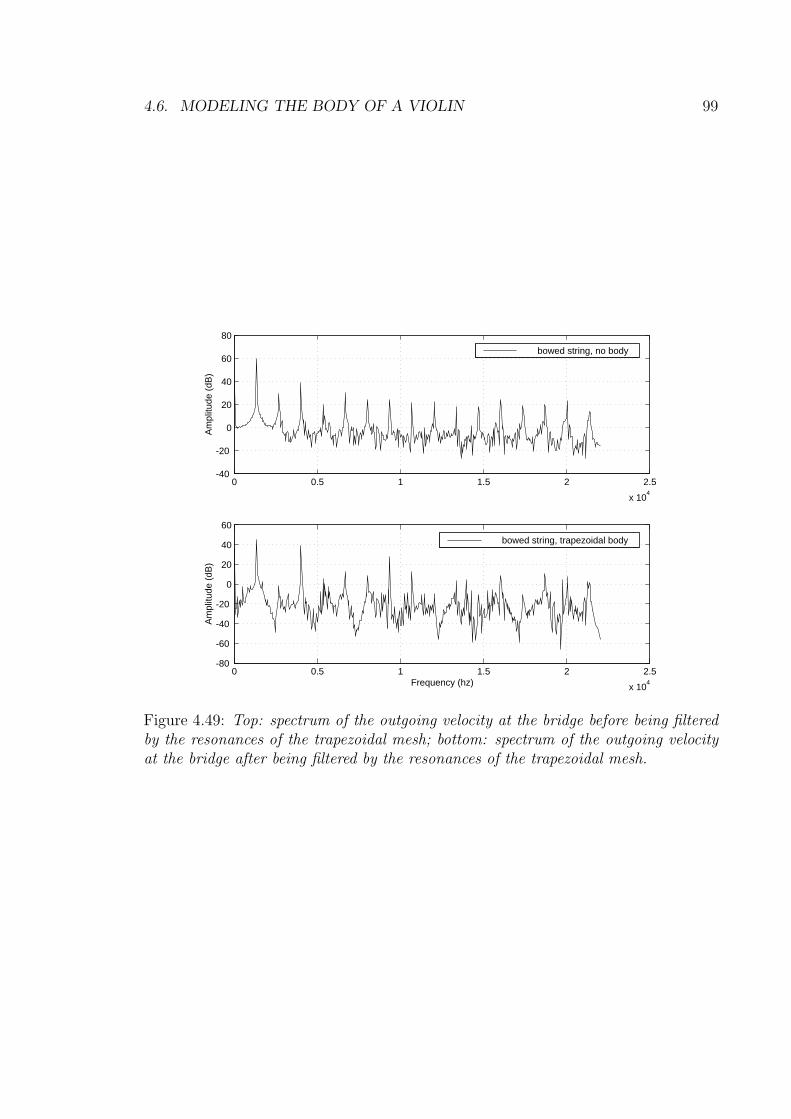
4.6. MODELING THE BODY OF A VIOLIN 99
0 0.5 1 1.5 2 2.5
x 104
-40
-20
0
20
40
60
80
Am
plitu
de (
dB)
bowed string, no body
0 0.5 1 1.5 2 2.5
x 104
-80
-60
-40
-20
0
20
40
60
Frequency (hz)
Am
plitu
de (
dB)
bowed string, trapezoidal body
Figure 4.49: Top: spectrum of the outgoing velocity at the bridge before being filteredby the resonances of the trapezoidal mesh; bottom: spectrum of the outgoing velocityat the bridge after being filtered by the resonances of the trapezoidal mesh.
Chapter 5
Other instruments driven by
friction
In the previous chapter an efficient yet accurate model of a bowed string instrument
was proposed. The string was simulated using one dimensional digital waveguides,
and the body of the instruments was simulated using waveguides meshes.
In this chapter other instruments whose main excitation mechanism is friction,
such as the musical saw, the glass harmonica, the Tibetan bowl and bowed cymbals
are examined. As contemporary music adopts lots of these instruments, efficient
computer simulations of them become an interesting tool for interactive computer
music, providing to composers and performers different new sonorities to explore.
Moreover, friction driven sonorities appear also in everyday life. The sound of
a squeaky door, the noise of a brake and a chalk on a board are few examples of
the variety of sonorities that interaction between rubbed dry surfaces can produce.
Simulations of such everyday sonorities are also proposed. Starting by examining a
musical saw, whose characteristic pure tone is suitable for an efficient implementation,
more complex instruments such as bowed cymbals and plates are modeled.
Simulations in this chapter use banded waveguides, a synthesis technique first
introduced in [29, 28], which can be interpreted as an hybrid between modal synthesis
and digital waveguides.
The first part of this chapter provides an analysis of the differences between banded
100

5.1. MODAL SYNTHESIS VERSUS BANDED WAVEGUIDES 101
waveguides and modal synthesis. The second part describes synthesis techniques to
simulate unusual friction driven musical instruments.
5.1 Modal synthesis versus banded waveguides
The most elementary banded waveguide structure is depicted in Fig. 5.1. Compared
to the waveguide structure of Fig. 3.7, the low-pass filter has been replaced by a
band-limited operation represented by the block BP.
z-M BP+x(n) y(n)
Figure 5.1: Block diagram structure of one banded waveguide.
The idea behind banded waveguides is to adopt a filtered delay-line loop to model
a mode of a resonating system. The loop contains a bandpass filter which eliminates
energy at frequencies other than the desired mode. The band-limiting operation is
achieved by using second-order bandpass filters, for their efficiency and simplicity
[123]. Considering the following transfer function
H2(z) =1− z−2
1− (2R cos θ)z−1 +R2z−2(5.1)
where R and θ are free parameters which relate to bandwidth B, center frequency ψ
and gain A0, the following equations result [123]
R ≈ 1− B/2 (5.2)
cos θ = 2R1+R2 cosψ (5.3)
A0 = (1− R2) sin θ. (5.4)
Notice how the filter of Eq. (5.1) has the same peak gain for all tunings.
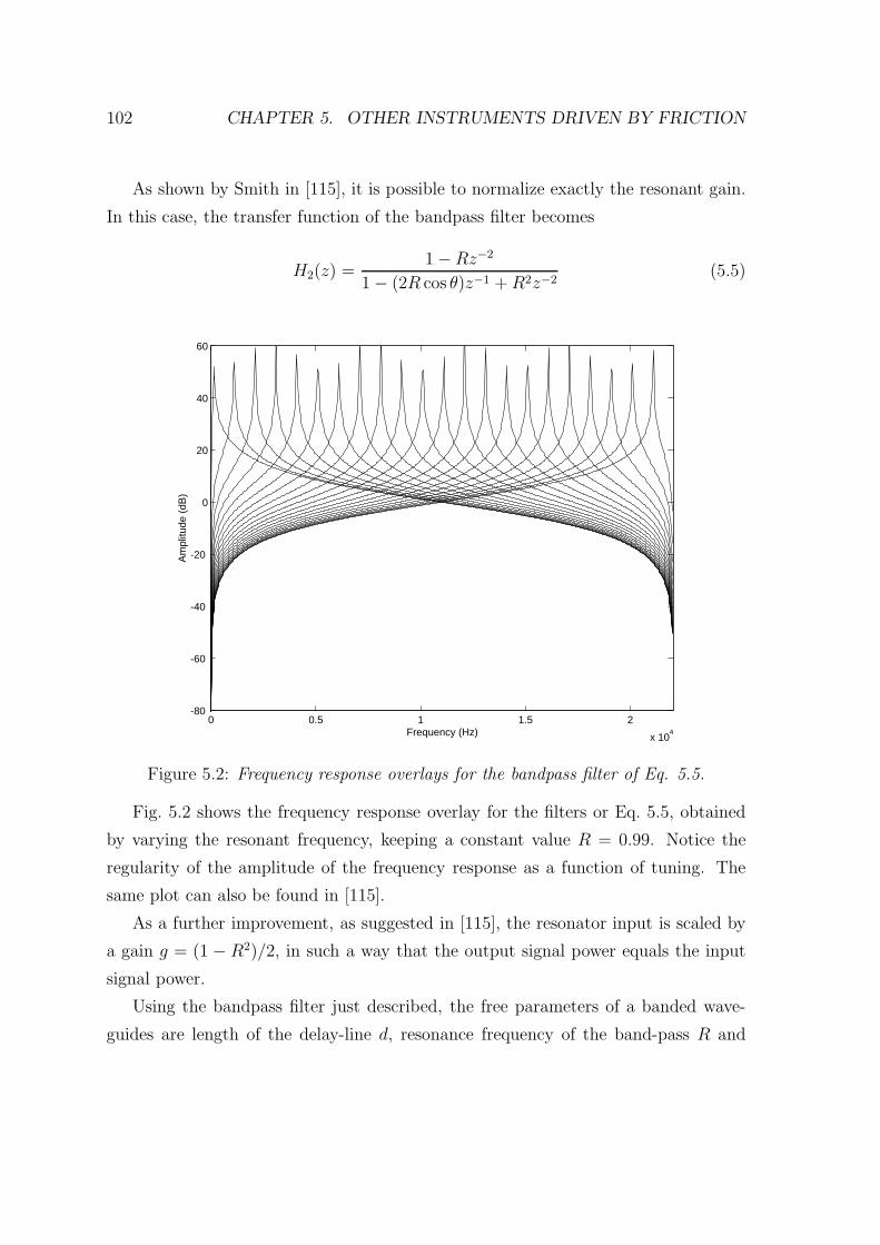
102 CHAPTER 5. OTHER INSTRUMENTS DRIVEN BY FRICTION
As shown by Smith in [115], it is possible to normalize exactly the resonant gain.
In this case, the transfer function of the bandpass filter becomes
H2(z) =1−Rz−2
1− (2R cos θ)z−1 +R2z−2(5.5)
0 0.5 1 1.5 2
x 104
-80
-60
-40
-20
0
20
40
60
Frequency (Hz)
Am
plitu
de (
dB)
Figure 5.2: Frequency response overlays for the bandpass filter of Eq. 5.5.
Fig. 5.2 shows the frequency response overlay for the filters or Eq. 5.5, obtained
by varying the resonant frequency, keeping a constant value R = 0.99. Notice the
regularity of the amplitude of the frequency response as a function of tuning. The
same plot can also be found in [115].
As a further improvement, as suggested in [115], the resonator input is scaled by
a gain g = (1 − R2)/2, in such a way that the output signal power equals the input
signal power.
Using the bandpass filter just described, the free parameters of a banded wave-
guides are length of the delay-line d, resonance frequency of the band-pass R and
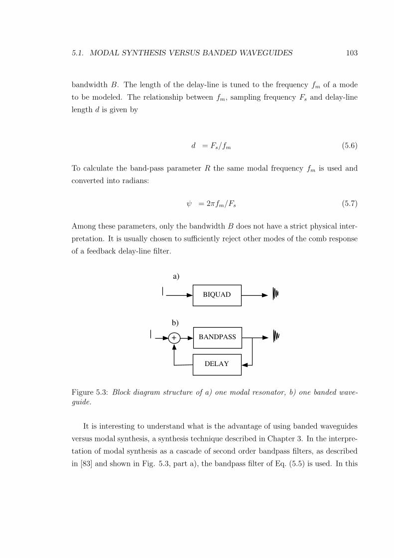
5.1. MODAL SYNTHESIS VERSUS BANDED WAVEGUIDES 103
bandwidth B. The length of the delay-line is tuned to the frequency fm of a mode
to be modeled. The relationship between fm, sampling frequency Fs and delay-line
length d is given by
d = Fs/fm (5.6)
To calculate the band-pass parameter R the same modal frequency fm is used and
converted into radians:
ψ = 2πfm/Fs (5.7)
Among these parameters, only the bandwidth B does not have a strict physical inter-
pretation. It is usually chosen to sufficiently reject other modes of the comb response
of a feedback delay-line filter.
BIQUAD
BANDPASS
a)
b)+
DELAY
Figure 5.3: Block diagram structure of a) one modal resonator, b) one banded wave-guide.
It is interesting to understand what is the advantage of using banded waveguides
versus modal synthesis, a synthesis technique described in Chapter 3. In the interpre-
tation of modal synthesis as a cascade of second order bandpass filters, as described
in [83] and shown in Fig. 5.3, part a), the bandpass filter of Eq. (5.5) is used. In this
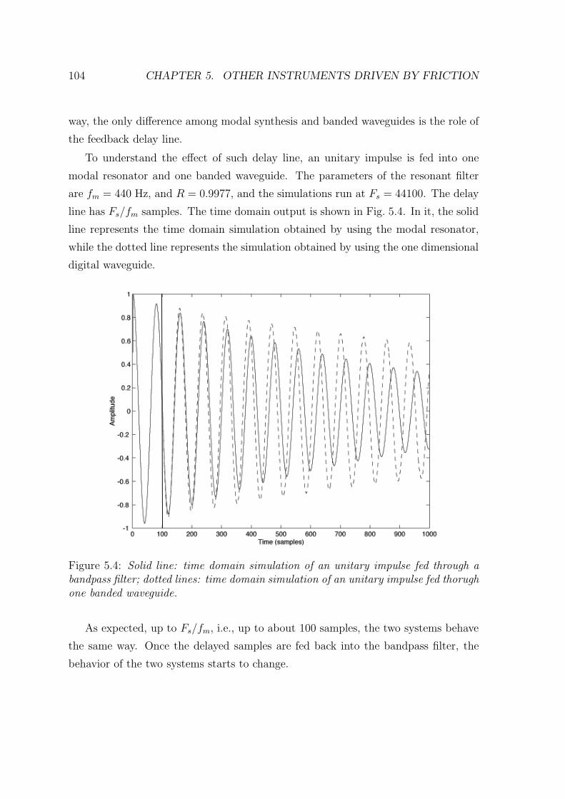
104 CHAPTER 5. OTHER INSTRUMENTS DRIVEN BY FRICTION
way, the only difference among modal synthesis and banded waveguides is the role of
the feedback delay line.
To understand the effect of such delay line, an unitary impulse is fed into one
modal resonator and one banded waveguide. The parameters of the resonant filter
are fm = 440 Hz, and R = 0.9977, and the simulations run at Fs = 44100. The delay
line has Fs/fm samples. The time domain output is shown in Fig. 5.4. In it, the solid
line represents the time domain simulation obtained by using the modal resonator,
while the dotted line represents the simulation obtained by using the one dimensional
digital waveguide.
Figure 5.4: Solid line: time domain simulation of an unitary impulse fed through abandpass filter; dotted lines: time domain simulation of an unitary impulse fed thorughone banded waveguide.
As expected, up to Fs/fm, i.e., up to about 100 samples, the two systems behave
the same way. Once the delayed samples are fed back into the bandpass filter, the
behavior of the two systems starts to change.
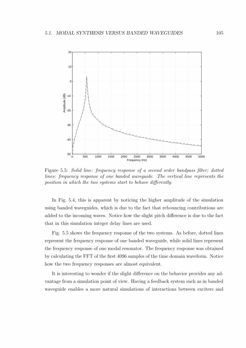
5.1. MODAL SYNTHESIS VERSUS BANDED WAVEGUIDES 105
0 500 1000 1500 2000 2500 3000 3500 4000 4500 5000-50
-40
-30
-20
-10
0
10
20
Frequency (Hz)
Am
plitu
de (
dB)
Figure 5.5: Solid line: frequency response of a second order bandpass filter; dottedlines: frequency response of one banded waveguide. The vertical line represents theposition in which the two systems start to behave differently.
In Fig. 5.4, this is apparent by noticing the higher amplitude of the simulation
using banded waveguides, which is due to the fact that rebouncing contributions are
added to the incoming waves. Notice how the slight pitch difference is due to the fact
that in this simulation integer delay lines are used.
Fig. 5.5 shows the frequency response of the two systems. As before, dotted lines
represent the frequency response of one banded waveguide, while solid lines represent
the frequency response of one modal resonator. The frequency response was obtained
by calculating the FFT of the first 4096 samples of the time domain waveform. Notice
how the two frequency responses are almost equivalent.
It is interesting to wonder if the slight difference on the behavior provides any ad-
vantage from a simulation point of view. Having a feedback system such as in banded
waveguide enables a more natural simulations of interactions between exciters and
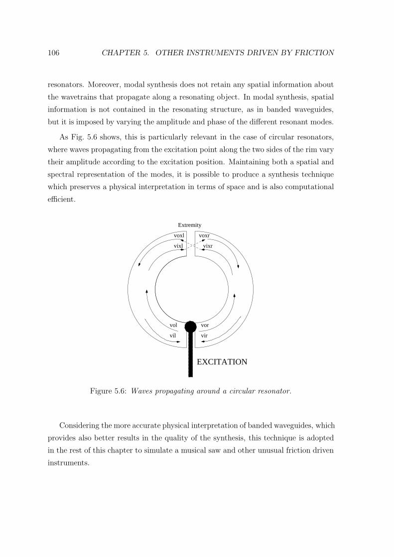
106 CHAPTER 5. OTHER INSTRUMENTS DRIVEN BY FRICTION
resonators. Moreover, modal synthesis does not retain any spatial information about
the wavetrains that propagate along a resonating object. In modal synthesis, spatial
information is not contained in the resonating structure, as in banded waveguides,
but it is imposed by varying the amplitude and phase of the different resonant modes.
As Fig. 5.6 shows, this is particularly relevant in the case of circular resonators,
where waves propagating from the excitation point along the two sides of the rim vary
their amplitude according to the excitation position. Maintaining both a spatial and
spectral representation of the modes, it is possible to produce a synthesis technique
which preserves a physical interpretation in terms of space and is also computational
efficient.
EXCITATION
vil vir
vol vor
voxl voxr
vixl
Extremity
vixr
Figure 5.6: Waves propagating around a circular resonator.
Considering the more accurate physical interpretation of banded waveguides, which
provides also better results in the quality of the synthesis, this technique is adopted
in the rest of this chapter to simulate a musical saw and other unusual friction driven
instruments.
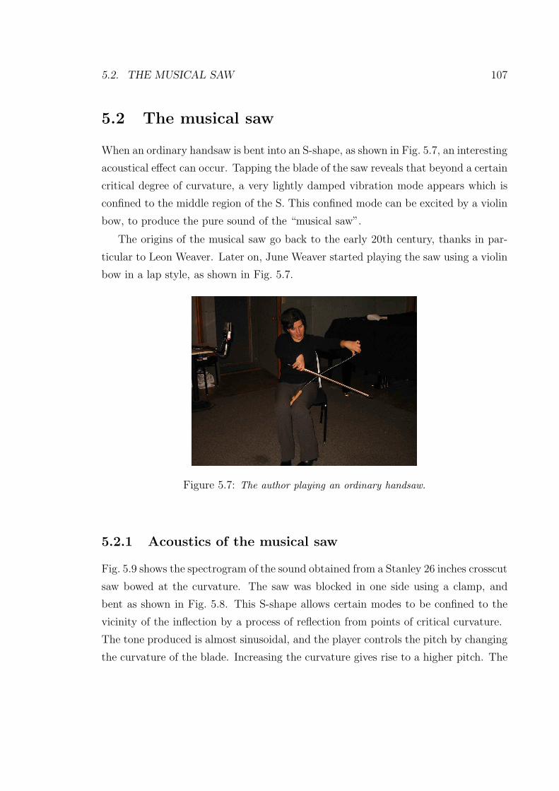
5.2. THE MUSICAL SAW 107
5.2 The musical saw
When an ordinary handsaw is bent into an S-shape, as shown in Fig. 5.7, an interesting
acoustical effect can occur. Tapping the blade of the saw reveals that beyond a certain
critical degree of curvature, a very lightly damped vibration mode appears which is
confined to the middle region of the S. This confined mode can be excited by a violin
bow, to produce the pure sound of the “musical saw”.
The origins of the musical saw go back to the early 20th century, thanks in par-
ticular to Leon Weaver. Later on, June Weaver started playing the saw using a violin
bow in a lap style, as shown in Fig. 5.7.
Figure 5.7: The author playing an ordinary handsaw.
5.2.1 Acoustics of the musical saw
Fig. 5.9 shows the spectrogram of the sound obtained from a Stanley 26 inches crosscut
saw bowed at the curvature. The saw was blocked in one side using a clamp, and
bent as shown in Fig. 5.8. This S-shape allows certain modes to be confined to the
vicinity of the inflection by a process of reflection from points of critical curvature.
The tone produced is almost sinusoidal, and the player controls the pitch by changing
the curvature of the blade. Increasing the curvature gives rise to a higher pitch. The
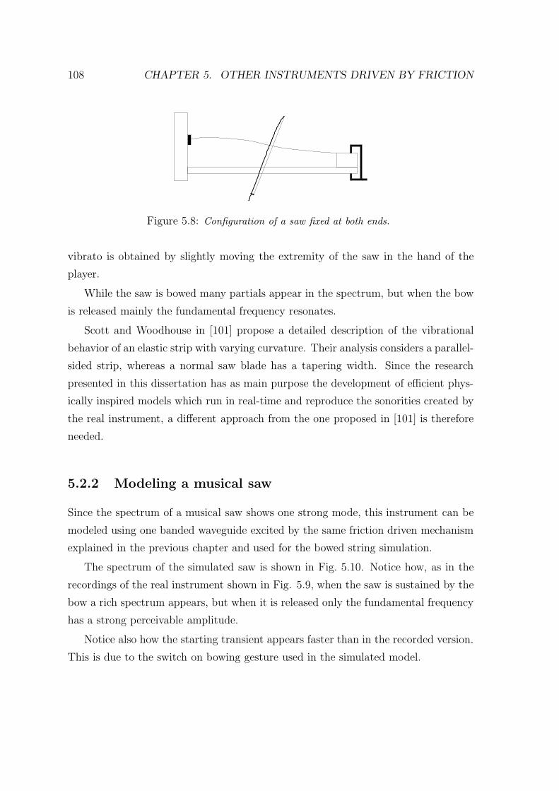
108 CHAPTER 5. OTHER INSTRUMENTS DRIVEN BY FRICTION
Figure 5.8: Configuration of a saw fixed at both ends.
vibrato is obtained by slightly moving the extremity of the saw in the hand of the
player.
While the saw is bowed many partials appear in the spectrum, but when the bow
is released mainly the fundamental frequency resonates.
Scott and Woodhouse in [101] propose a detailed description of the vibrational
behavior of an elastic strip with varying curvature. Their analysis considers a parallel-
sided strip, whereas a normal saw blade has a tapering width. Since the research
presented in this dissertation has as main purpose the development of efficient phys-
ically inspired models which run in real-time and reproduce the sonorities created by
the real instrument, a different approach from the one proposed in [101] is therefore
needed.
5.2.2 Modeling a musical saw
Since the spectrum of a musical saw shows one strong mode, this instrument can be
modeled using one banded waveguide excited by the same friction driven mechanism
explained in the previous chapter and used for the bowed string simulation.
The spectrum of the simulated saw is shown in Fig. 5.10. Notice how, as in the
recordings of the real instrument shown in Fig. 5.9, when the saw is sustained by the
bow a rich spectrum appears, but when it is released only the fundamental frequency
has a strong perceivable amplitude.
Notice also how the starting transient appears faster than in the recorded version.
This is due to the switch on bowing gesture used in the simulated model.
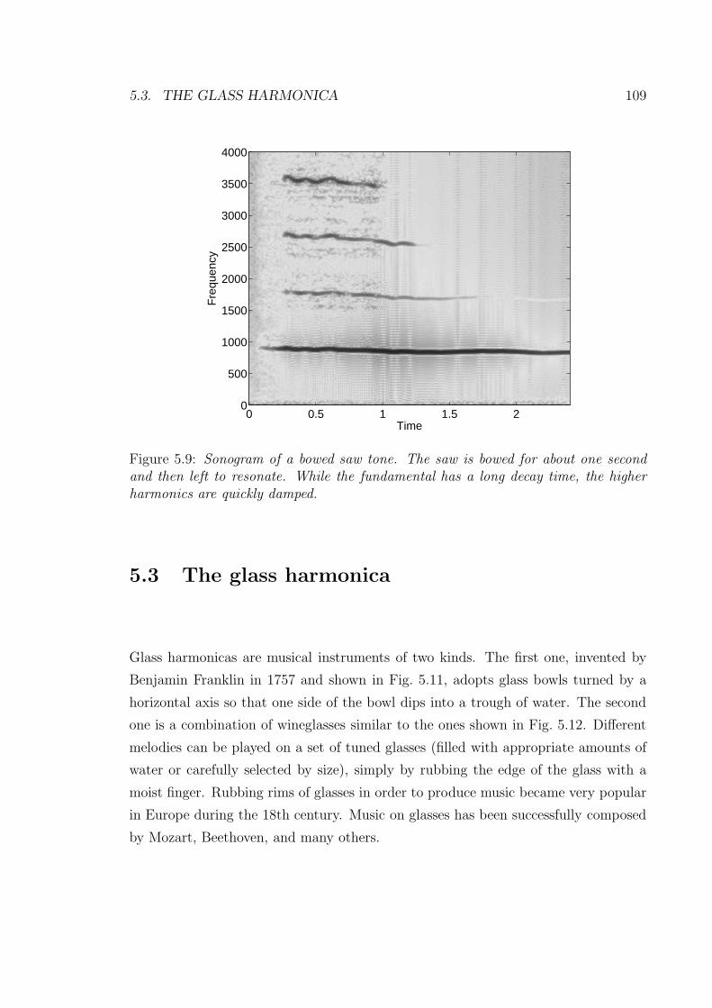
5.3. THE GLASS HARMONICA 109
Time
Fre
quen
cy
0 0.5 1 1.5 20
500
1000
1500
2000
2500
3000
3500
4000
Figure 5.9: Sonogram of a bowed saw tone. The saw is bowed for about one secondand then left to resonate. While the fundamental has a long decay time, the higherharmonics are quickly damped.
5.3 The glass harmonica
Glass harmonicas are musical instruments of two kinds. The first one, invented by
Benjamin Franklin in 1757 and shown in Fig. 5.11, adopts glass bowls turned by a
horizontal axis so that one side of the bowl dips into a trough of water. The second
one is a combination of wineglasses similar to the ones shown in Fig. 5.12. Different
melodies can be played on a set of tuned glasses (filled with appropriate amounts of
water or carefully selected by size), simply by rubbing the edge of the glass with a
moist finger. Rubbing rims of glasses in order to produce music became very popular
in Europe during the 18th century. Music on glasses has been successfully composed
by Mozart, Beethoven, and many others.
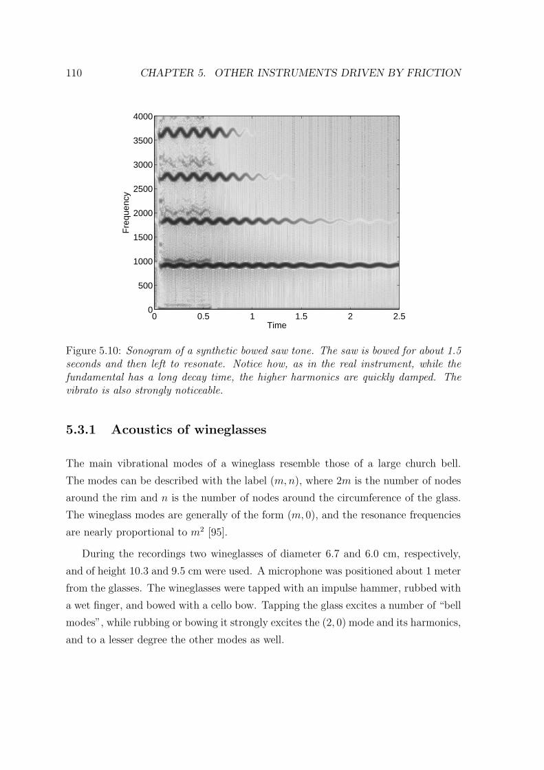
110 CHAPTER 5. OTHER INSTRUMENTS DRIVEN BY FRICTION
Time
Fre
quen
cy
0 0.5 1 1.5 2 2.50
500
1000
1500
2000
2500
3000
3500
4000
Figure 5.10: Sonogram of a synthetic bowed saw tone. The saw is bowed for about 1.5seconds and then left to resonate. Notice how, as in the real instrument, while thefundamental has a long decay time, the higher harmonics are quickly damped. Thevibrato is also strongly noticeable.
5.3.1 Acoustics of wineglasses
The main vibrational modes of a wineglass resemble those of a large church bell.
The modes can be described with the label (m,n), where 2m is the number of nodes
around the rim and n is the number of nodes around the circumference of the glass.
The wineglass modes are generally of the form (m, 0), and the resonance frequencies
are nearly proportional to m2 [95].
During the recordings two wineglasses of diameter 6.7 and 6.0 cm, respectively,
and of height 10.3 and 9.5 cm were used. A microphone was positioned about 1 meter
from the glasses. The wineglasses were tapped with an impulse hammer, rubbed with
a wet finger, and bowed with a cello bow. Tapping the glass excites a number of “bell
modes”, while rubbing or bowing it strongly excites the (2, 0) mode and its harmonics,
and to a lesser degree the other modes as well.
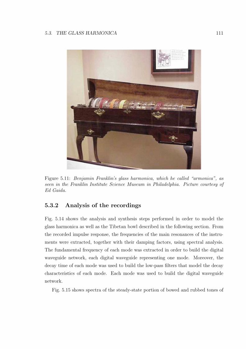
5.3. THE GLASS HARMONICA 111
Figure 5.11: Benjamin Franklin’s glass harmonica, which he called “armonica”, asseen in the Franklin Institute Science Museum in Philadelphia. Picture courtesy ofEd Gaida.
5.3.2 Analysis of the recordings
Fig. 5.14 shows the analysis and synthesis steps performed in order to model the
glass harmonica as well as the Tibetan bowl described in the following section. From
the recorded impulse response, the frequencies of the main resonances of the instru-
ments were extracted, together with their damping factors, using spectral analysis.
The fundamental frequency of each mode was extracted in order to build the digital
waveguide network, each digital waveguide representing one mode. Moreover, the
decay time of each mode was used to build the low-pass filters that model the decay
characteristics of each mode. Each mode was used to build the digital waveguide
network.
Fig. 5.15 shows spectra of the steady-state portion of bowed and rubbed tones of
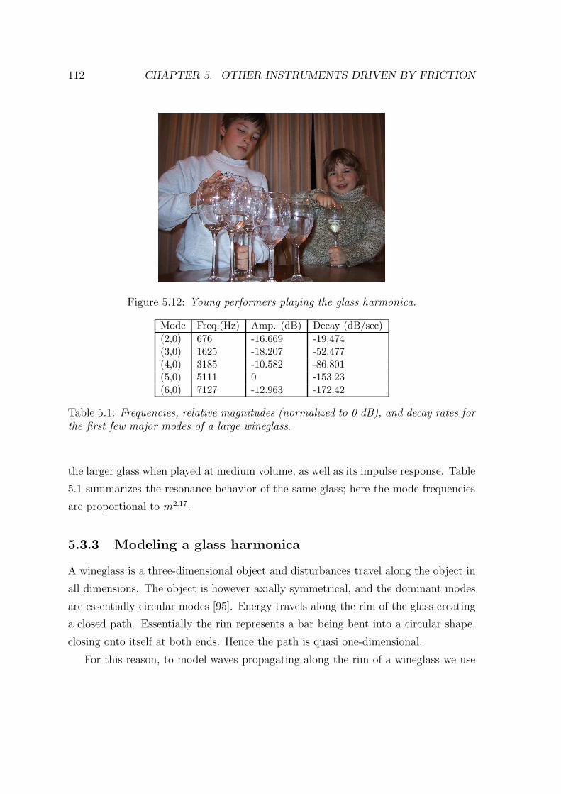
112 CHAPTER 5. OTHER INSTRUMENTS DRIVEN BY FRICTION
Figure 5.12: Young performers playing the glass harmonica.
Mode Freq.(Hz) Amp. (dB) Decay (dB/sec)
(2,0) 676 -16.669 -19.474(3,0) 1625 -18.207 -52.477(4,0) 3185 -10.582 -86.801(5,0) 5111 0 -153.23(6,0) 7127 -12.963 -172.42
Table 5.1: Frequencies, relative magnitudes (normalized to 0 dB), and decay rates forthe first few major modes of a large wineglass.
the larger glass when played at medium volume, as well as its impulse response. Table
5.1 summarizes the resonance behavior of the same glass; here the mode frequencies
are proportional to m2.17.
5.3.3 Modeling a glass harmonica
A wineglass is a three-dimensional object and disturbances travel along the object in
all dimensions. The object is however axially symmetrical, and the dominant modes
are essentially circular modes [95]. Energy travels along the rim of the glass creating
a closed path. Essentially the rim represents a bar being bent into a circular shape,
closing onto itself at both ends. Hence the path is quasi one-dimensional.
For this reason, to model waves propagating along the rim of a wineglass we use
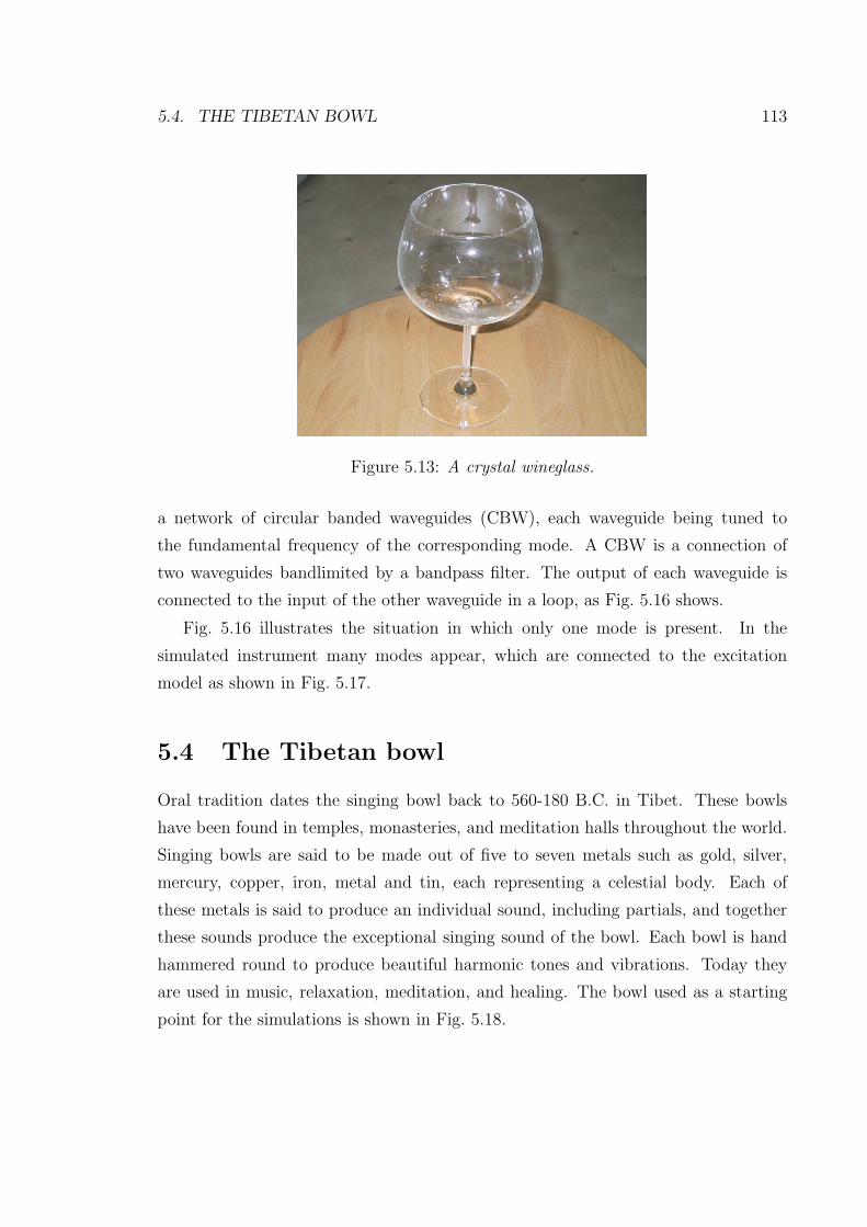
5.4. THE TIBETAN BOWL 113
Figure 5.13: A crystal wineglass.
a network of circular banded waveguides (CBW), each waveguide being tuned to
the fundamental frequency of the corresponding mode. A CBW is a connection of
two waveguides bandlimited by a bandpass filter. The output of each waveguide is
connected to the input of the other waveguide in a loop, as Fig. 5.16 shows.
Fig. 5.16 illustrates the situation in which only one mode is present. In the
simulated instrument many modes appear, which are connected to the excitation
model as shown in Fig. 5.17.
5.4 The Tibetan bowl
Oral tradition dates the singing bowl back to 560-180 B.C. in Tibet. These bowls
have been found in temples, monasteries, and meditation halls throughout the world.
Singing bowls are said to be made out of five to seven metals such as gold, silver,
mercury, copper, iron, metal and tin, each representing a celestial body. Each of
these metals is said to produce an individual sound, including partials, and together
these sounds produce the exceptional singing sound of the bowl. Each bowl is hand
hammered round to produce beautiful harmonic tones and vibrations. Today they
are used in music, relaxation, meditation, and healing. The bowl used as a starting
point for the simulations is shown in Fig. 5.18.
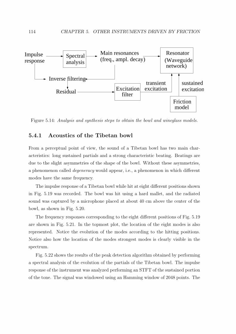
114 CHAPTER 5. OTHER INSTRUMENTS DRIVEN BY FRICTION
Impulseresponse
Spectralanalysis
Main resonances(freq., ampl. decay)
sustainedexcitationexcitation
Friction model
transientInverse filtering
Residual
Resonator(Waveguidenetwork)
Excitationfilter
Figure 5.14: Analysis and synthesis steps to obtain the bowl and wineglass models.
5.4.1 Acoustics of the Tibetan bowl
From a perceptual point of view, the sound of a Tibetan bowl has two main char-
acteristics: long sustained partials and a strong characteristic beating. Beatings are
due to the slight asymmetries of the shape of the bowl. Without these asymmetries,
a phenomenon called degeneracy would appear, i.e., a phenomenon in which different
modes have the same frequency.
The impulse response of a Tibetan bowl while hit at eight different positions shown
in Fig. 5.19 was recorded. The bowl was hit using a hard mallet, and the radiated
sound was captured by a microphone placed at about 40 cm above the center of the
bowl, as shown in Fig. 5.20.
The frequency responses corresponding to the eight different positions of Fig. 5.19
are shown in Fig. 5.21. In the topmost plot, the location of the eight modes is also
represented. Notice the evolution of the modes according to the hitting positions.
Notice also how the location of the modes strongest modes is clearly visible in the
spectrum.
Fig. 5.22 shows the results of the peak detection algorithm obtained by performing
a spectral analysis of the evolution of the partials of the Tibetan bowl. The impulse
response of the instrument was analyzed performing an STFT of the sustained portion
of the tone. The signal was windowed using an Hamming window of 2048 points. The
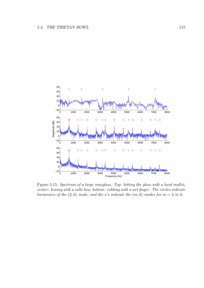
5.4. THE TIBETAN BOWL 115
0 1000 2000 3000 4000 5000 6000 7000 8000−20
0
20
40
60
80
0 1000 2000 3000 4000 5000 6000 7000 8000−20
0
20
40
60
80
Mag
nitu
de (
dB)
0 1000 2000 3000 4000 5000 6000 7000 8000−20
0
20
40
60
80
Frequency (Hz)
Figure 5.15: Spectrum of a large wineglass. Top: hitting the glass with a hard mallet;center: bowing with a cello bow; bottom: rubbing with a wet finger. The circles indicateharmonics of the (2, 0) mode, and the x’s indicate the (m, 0) modes for m = 2 to 6.
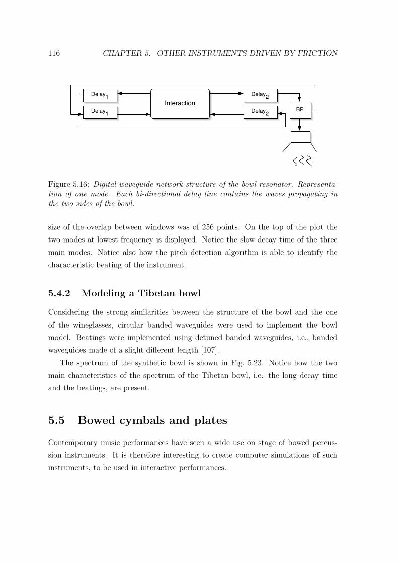
116 CHAPTER 5. OTHER INSTRUMENTS DRIVEN BY FRICTION
InteractionDelay1
Delay1
Delay2
Delay2BP
Figure 5.16: Digital waveguide network structure of the bowl resonator. Representa-tion of one mode. Each bi-directional delay line contains the waves propagating inthe two sides of the bowl.
size of the overlap between windows was of 256 points. On the top of the plot the
two modes at lowest frequency is displayed. Notice the slow decay time of the three
main modes. Notice also how the pitch detection algorithm is able to identify the
characteristic beating of the instrument.
5.4.2 Modeling a Tibetan bowl
Considering the strong similarities between the structure of the bowl and the one
of the wineglasses, circular banded waveguides were used to implement the bowl
model. Beatings were implemented using detuned banded waveguides, i.e., banded
waveguides made of a slight different length [107].
The spectrum of the synthetic bowl is shown in Fig. 5.23. Notice how the two
main characteristics of the spectrum of the Tibetan bowl, i.e. the long decay time
and the beatings, are present.
5.5 Bowed cymbals and plates
Contemporary music performances have seen a wide use on stage of bowed percus-
sion instruments. It is therefore interesting to create computer simulations of such
instruments, to be used in interactive performances.
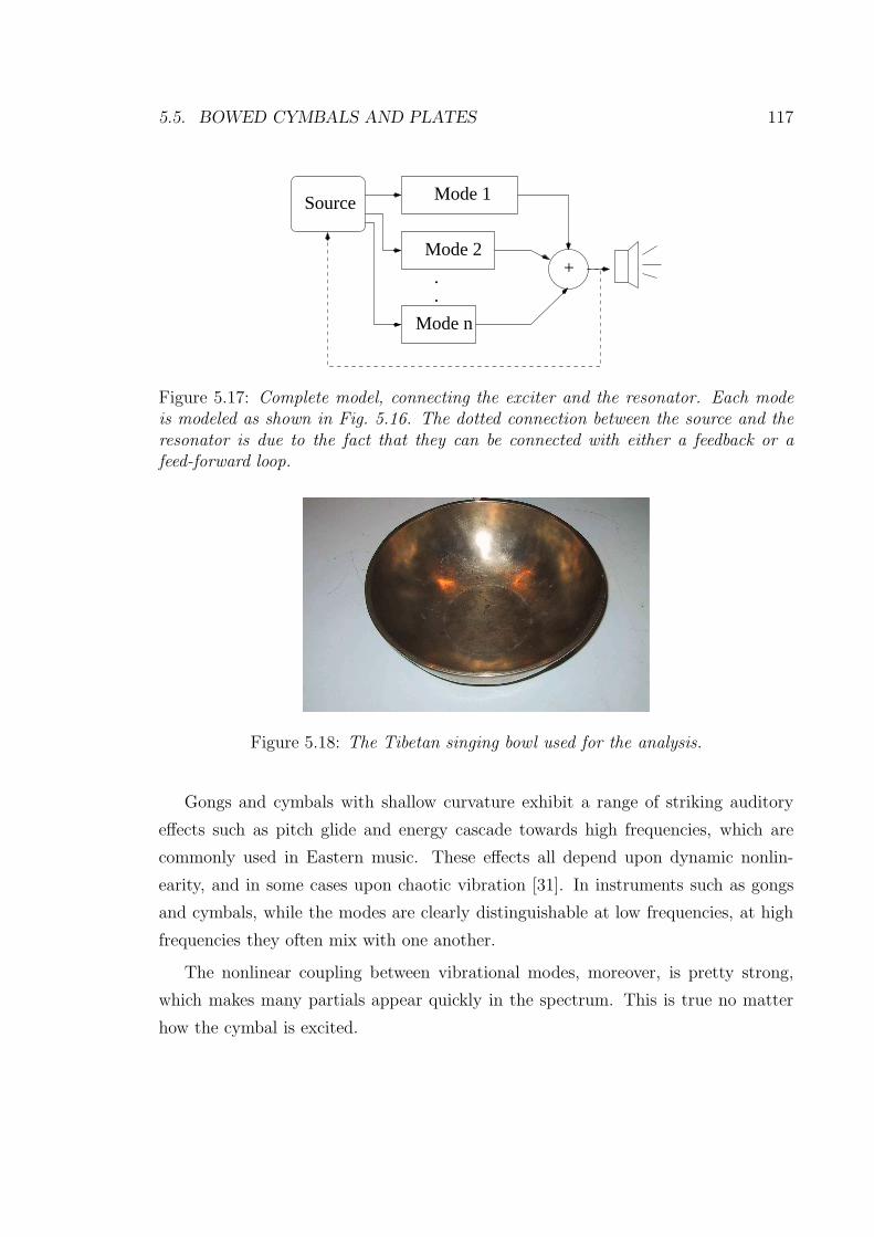
5.5. BOWED CYMBALS AND PLATES 117
Mode n
.
.
+
Source Mode 1
Mode 2
Figure 5.17: Complete model, connecting the exciter and the resonator. Each modeis modeled as shown in Fig. 5.16. The dotted connection between the source and theresonator is due to the fact that they can be connected with either a feedback or afeed-forward loop.
Figure 5.18: The Tibetan singing bowl used for the analysis.
Gongs and cymbals with shallow curvature exhibit a range of striking auditory
effects such as pitch glide and energy cascade towards high frequencies, which are
commonly used in Eastern music. These effects all depend upon dynamic nonlin-
earity, and in some cases upon chaotic vibration [31]. In instruments such as gongs
and cymbals, while the modes are clearly distinguishable at low frequencies, at high
frequencies they often mix with one another.
The nonlinear coupling between vibrational modes, moreover, is pretty strong,
which makes many partials appear quickly in the spectrum. This is true no matter
how the cymbal is excited.
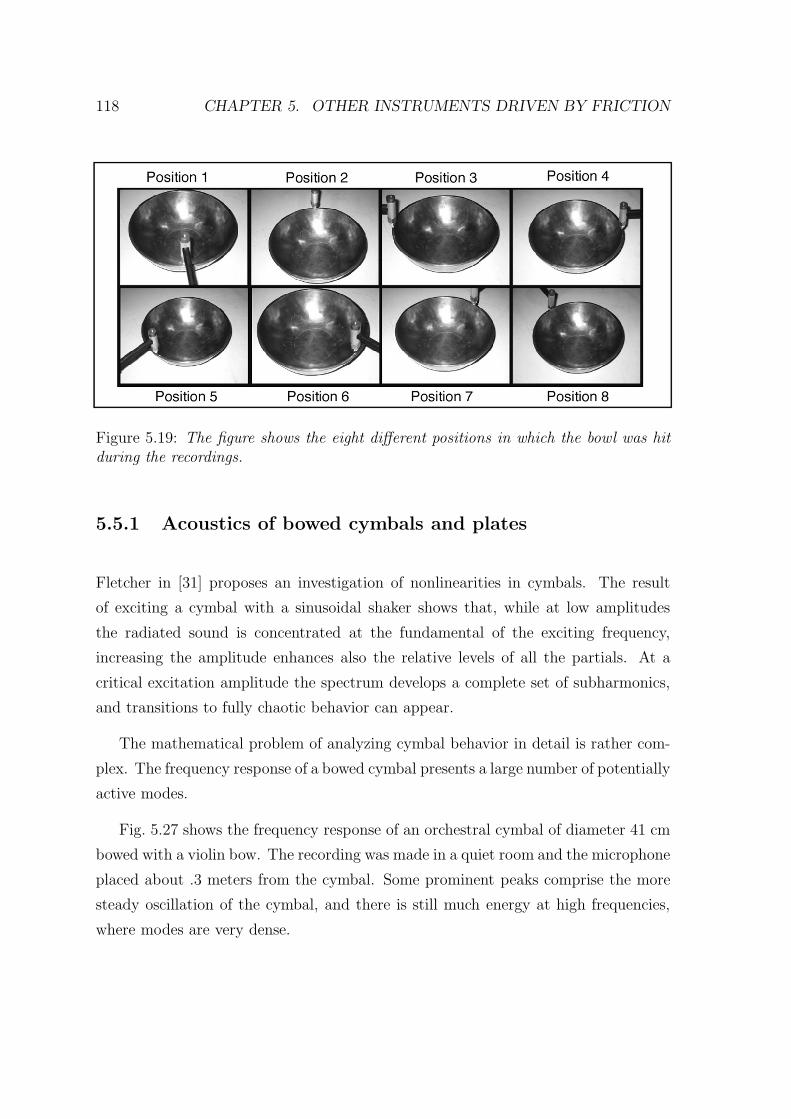
118 CHAPTER 5. OTHER INSTRUMENTS DRIVEN BY FRICTION
Figure 5.19: The figure shows the eight different positions in which the bowl was hitduring the recordings.
5.5.1 Acoustics of bowed cymbals and plates
Fletcher in [31] proposes an investigation of nonlinearities in cymbals. The result
of exciting a cymbal with a sinusoidal shaker shows that, while at low amplitudes
the radiated sound is concentrated at the fundamental of the exciting frequency,
increasing the amplitude enhances also the relative levels of all the partials. At a
critical excitation amplitude the spectrum develops a complete set of subharmonics,
and transitions to fully chaotic behavior can appear.
The mathematical problem of analyzing cymbal behavior in detail is rather com-
plex. The frequency response of a bowed cymbal presents a large number of potentially
active modes.
Fig. 5.27 shows the frequency response of an orchestral cymbal of diameter 41 cm
bowed with a violin bow. The recording was made in a quiet room and the microphone
placed about .3 meters from the cymbal. Some prominent peaks comprise the more
steady oscillation of the cymbal, and there is still much energy at high frequencies,
where modes are very dense.
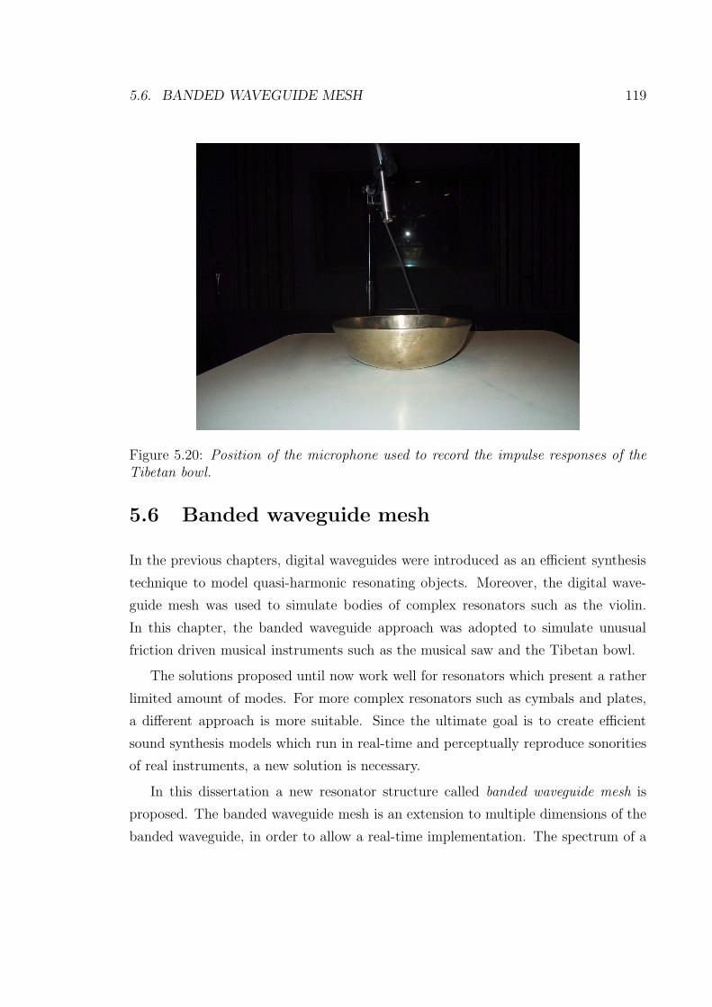
5.6. BANDED WAVEGUIDE MESH 119
Figure 5.20: Position of the microphone used to record the impulse responses of theTibetan bowl.
5.6 Banded waveguide mesh
In the previous chapters, digital waveguides were introduced as an efficient synthesis
technique to model quasi-harmonic resonating objects. Moreover, the digital wave-
guide mesh was used to simulate bodies of complex resonators such as the violin.
In this chapter, the banded waveguide approach was adopted to simulate unusual
friction driven musical instruments such as the musical saw and the Tibetan bowl.
The solutions proposed until now work well for resonators which present a rather
limited amount of modes. For more complex resonators such as cymbals and plates,
a different approach is more suitable. Since the ultimate goal is to create efficient
sound synthesis models which run in real-time and perceptually reproduce sonorities
of real instruments, a new solution is necessary.
In this dissertation a new resonator structure called banded waveguide mesh is
proposed. The banded waveguide mesh is an extension to multiple dimensions of the
banded waveguide, in order to allow a real-time implementation. The spectrum of a

120 CHAPTER 5. OTHER INSTRUMENTS DRIVEN BY FRICTION
0 1000 2000 3000 4000 5000 6000 7000 8000 9000 10000−20
020
Pos
ition
5
0 1000 2000 3000 4000 5000 6000 7000 8000 9000 10000−20
020
Pos
ition
6
0 1000 2000 3000 4000 5000 6000 7000 8000 9000 10000−20
020
Pos
ition
7
0 1000 2000 3000 4000 5000 6000 7000 8000 9000 10000−20
020
Frequency (Hz)
Pos
ition
8
0 1000 2000 3000 4000 5000 6000 7000 8000 9000 10000−20
020
Pos
ition
1
0 1000 2000 3000 4000 5000 6000 7000 8000 9000 10000−20
020
Pos
ition
2
0 1000 2000 3000 4000 5000 6000 7000 8000 9000 10000−20
020
Pos
ition
3
0 1000 2000 3000 4000 5000 6000 7000 8000 9000 10000−20
020
Pos
ition
4
Figure 5.21: Spectra resulting from varying the excitation position of the bowl. Fromtop to bottom the plots represent positions from one to eight respectively, accordingto Fig. 5.19. In the topmost plot the location of the eight modes is also represented.Notice the evolution of the modes according to the hitting positions.
vibrating system is split into frequency bands. For frequency bands where a single
resonance is present, a one-dimensional digital waveguide is used. For bands where
resonances are more complex, a 3D digital waveguide mesh is used, whose dimensions
are chosen in order to match statistically and psychoacoustically the resonances of the
high frequencies of the modeled object. More precisely, let fc be the cutoff frequency
above which an adequately high concentration of modes appear in the spectrum. For
frequencies below fc, banded waveguides simulate the modes of the resonators with
higher amplitude. For frequencies above fc, a 3D mesh simulates statistically and
perceptually the high frequencies modes of the resonator. Let f0m be the fundamental
frequency of the mesh, i.e., the lowest mode generated by the mesh. Notice that the
higher the value of f0m, the smaller the dimensions of the waveguide mesh and the
more efficient the implementation. The choice of f0m, therefore, is an important

5.6. BANDED WAVEGUIDE MESH 121
0 1 2 3 4 5 6 7 50
40
30
20
10
0
10
20
30
40
Time (s)
Am
plitu
de (
dB)
Figure 5.22: Results of the peak detection algorithm on the Tibetan bowl’s impulseresponse. Notice how the algorithm correctly detects the beating, which appear asamplitude modulation of the modes of the instrument with the longer decay time.
decision for the resulting computational cost. As an example, the spectrum of a
cymbal while hit at one extremity with a hard mallet is shown in Fig. 5.25. Notice
how, up to about 8000 Hz, it is possible to identify bands where strong resonances
are present. Above 8000 Hz modes are more dense and overlap. In this case, banded
waveguides simulates mode up to 8000 Hz, while a 3D mesh simulates the dense
concentration of modes above 8000 Hz.
The banded waveguide mesh is therefore a parallel connection of banded waveg-
uides and one 3D mesh for high frequencies. The structure of a banded waveguide
mesh is shown in Fig. 5.26. As in the case of banded waveguides, reflection filters are
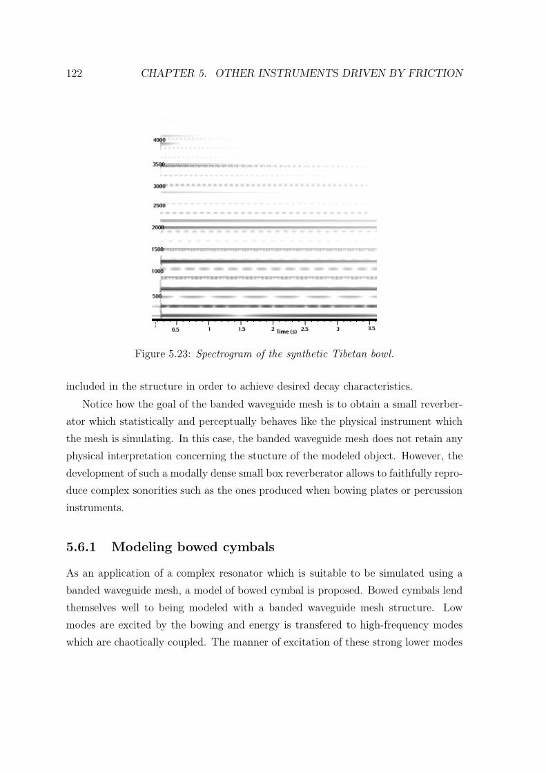
122 CHAPTER 5. OTHER INSTRUMENTS DRIVEN BY FRICTION
Figure 5.23: Spectrogram of the synthetic Tibetan bowl.
included in the structure in order to achieve desired decay characteristics.
Notice how the goal of the banded waveguide mesh is to obtain a small reverber-
ator which statistically and perceptually behaves like the physical instrument which
the mesh is simulating. In this case, the banded waveguide mesh does not retain any
physical interpretation concerning the stucture of the modeled object. However, the
development of such a modally dense small box reverberator allows to faithfully repro-
duce complex sonorities such as the ones produced when bowing plates or percussion
instruments.
5.6.1 Modeling bowed cymbals
As an application of a complex resonator which is suitable to be simulated using a
banded waveguide mesh, a model of bowed cymbal is proposed. Bowed cymbals lend
themselves well to being modeled with a banded waveguide mesh structure. Low
modes are excited by the bowing and energy is transfered to high-frequency modes
which are chaotically coupled. The manner of excitation of these strong lower modes
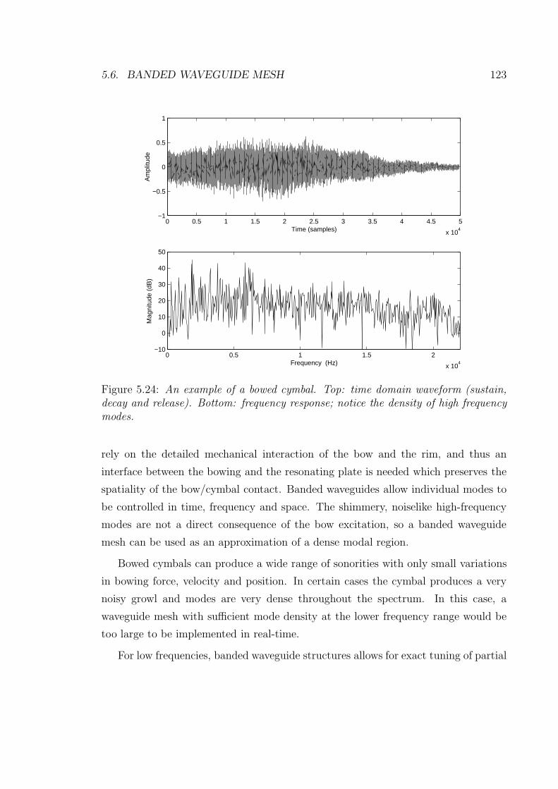
5.6. BANDED WAVEGUIDE MESH 123
0 0.5 1 1.5 2 2.5 3 3.5 4 4.5 5
x 104
−1
−0.5
0
0.5
1
Time (samples)
Am
plitu
de
0 0.5 1 1.5 2
x 104
−10
0
10
20
30
40
50
Frequency (Hz)
Mag
nitu
de (
dB)
Figure 5.24: An example of a bowed cymbal. Top: time domain waveform (sustain,decay and release). Bottom: frequency response; notice the density of high frequencymodes.
rely on the detailed mechanical interaction of the bow and the rim, and thus an
interface between the bowing and the resonating plate is needed which preserves the
spatiality of the bow/cymbal contact. Banded waveguides allow individual modes to
be controlled in time, frequency and space. The shimmery, noiselike high-frequency
modes are not a direct consequence of the bow excitation, so a banded waveguide
mesh can be used as an approximation of a dense modal region.
Bowed cymbals can produce a wide range of sonorities with only small variations
in bowing force, velocity and position. In certain cases the cymbal produces a very
noisy growl and modes are very dense throughout the spectrum. In this case, a
waveguide mesh with sufficient mode density at the lower frequency range would be
too large to be implemented in real-time.
For low frequencies, banded waveguide structures allows for exact tuning of partial
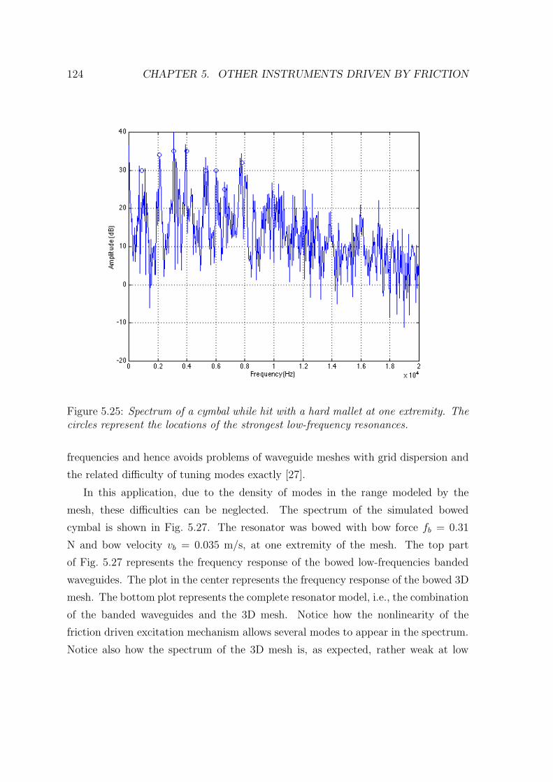
124 CHAPTER 5. OTHER INSTRUMENTS DRIVEN BY FRICTION
Figure 5.25: Spectrum of a cymbal while hit with a hard mallet at one extremity. Thecircles represent the locations of the strongest low-frequency resonances.
frequencies and hence avoids problems of waveguide meshes with grid dispersion and
the related difficulty of tuning modes exactly [27].
In this application, due to the density of modes in the range modeled by the
mesh, these difficulties can be neglected. The spectrum of the simulated bowed
cymbal is shown in Fig. 5.27. The resonator was bowed with bow force fb = 0.31
N and bow velocity vb = 0.035 m/s, at one extremity of the mesh. The top part
of Fig. 5.27 represents the frequency response of the bowed low-frequencies banded
waveguides. The plot in the center represents the frequency response of the bowed 3D
mesh. The bottom plot represents the complete resonator model, i.e., the combination
of the banded waveguides and the 3D mesh. Notice how the nonlinearity of the
friction driven excitation mechanism allows several modes to appear in the spectrum.
Notice also how the spectrum of the 3D mesh is, as expected, rather weak at low
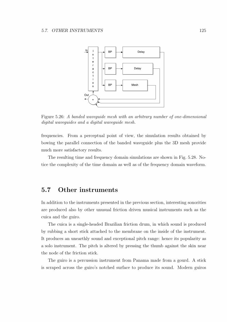
5.7. OTHER INSTRUMENTS 125
BP
BP
BP
Delay
Delay
Mesh
Interaction
In
+Out
Figure 5.26: A banded waveguide mesh with an arbitrary number of one-dimensionaldigital waveguides and a digital waveguide mesh.
frequencies. From a perceptual point of view, the simulation results obtained by
bowing the parallel connection of the banded waveguide plus the 3D mesh provide
much more satisfactory results.
The resulting time and frequency domain simulations are shown in Fig. 5.28. No-
tice the complexity of the time domain as well as of the frequency domain waveform.
5.7 Other instruments
In addition to the instruments presented in the previous section, interesting sonorities
are produced also by other unusual friction driven musical instruments such as the
cuica and the guiro.
The cuica is a single-headed Brazilian friction drum, in which sound is produced
by rubbing a short stick attached to the membrane on the inside of the instrument.
It produces an unearthly sound and exceptional pitch range: hence its popularity as
a solo instrument. The pitch is altered by pressing the thumb against the skin near
the node of the friction stick.
The guiro is a percussion instrument from Panama made from a gourd. A stick
is scraped across the guiro’s notched surface to produce its sound. Modern guiros
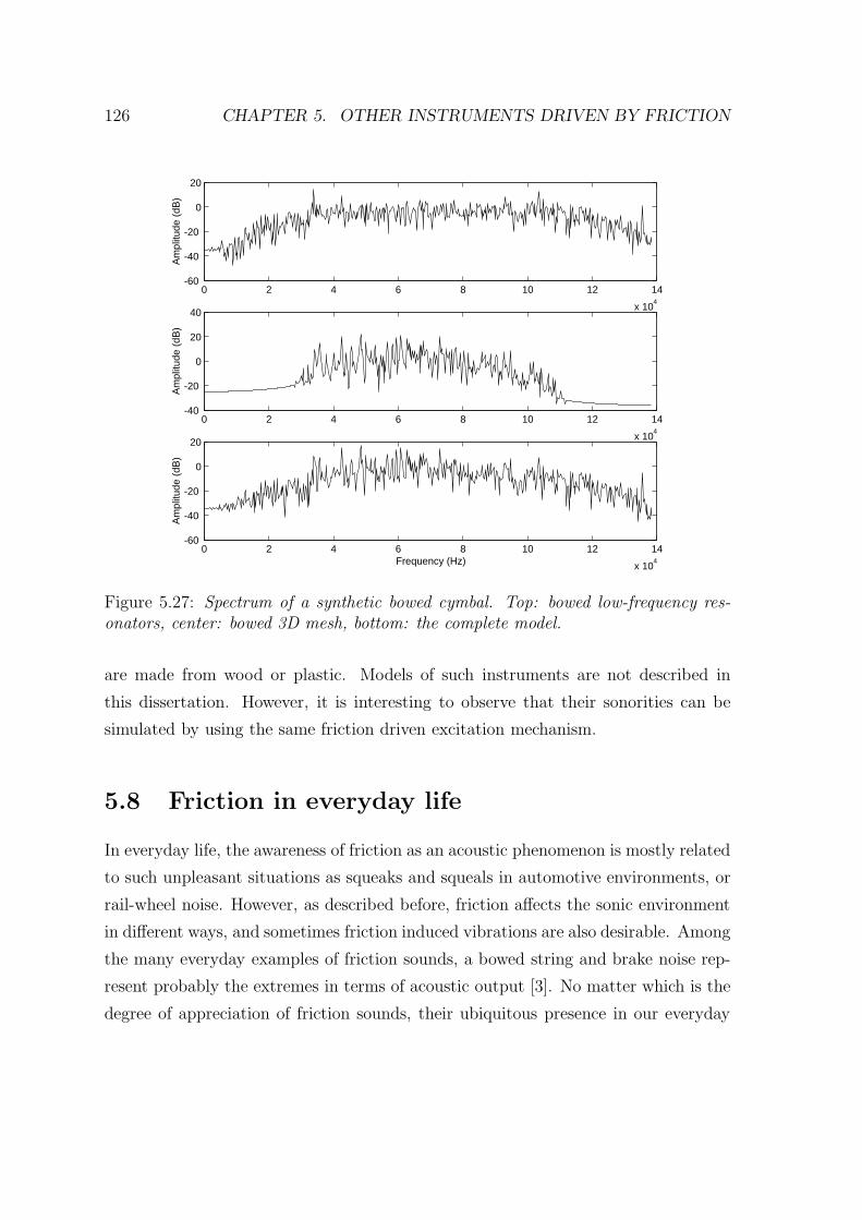
126 CHAPTER 5. OTHER INSTRUMENTS DRIVEN BY FRICTION
0 2 4 6 8 10 12 14
x 104
-60
-40
-20
0
20A
mpl
itude
(dB
)
0 2 4 6 8 10 12 14
x 104
-40
-20
0
20
40
Am
plitu
de (
dB)
0 2 4 6 8 10 12 14
x 104
-60
-40
-20
0
20
Frequency (Hz)
Am
plitu
de (
dB)
Figure 5.27: Spectrum of a synthetic bowed cymbal. Top: bowed low-frequency res-onators, center: bowed 3D mesh, bottom: the complete model.
are made from wood or plastic. Models of such instruments are not described in
this dissertation. However, it is interesting to observe that their sonorities can be
simulated by using the same friction driven excitation mechanism.
5.8 Friction in everyday life
In everyday life, the awareness of friction as an acoustic phenomenon is mostly related
to such unpleasant situations as squeaks and squeals in automotive environments, or
rail-wheel noise. However, as described before, friction affects the sonic environment
in different ways, and sometimes friction induced vibrations are also desirable. Among
the many everyday examples of friction sounds, a bowed string and brake noise rep-
resent probably the extremes in terms of acoustic output [3]. No matter which is the
degree of appreciation of friction sounds, their ubiquitous presence in our everyday
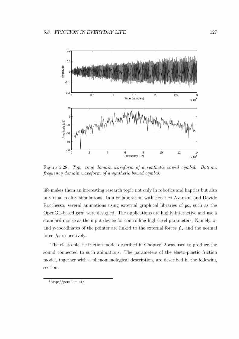
5.8. FRICTION IN EVERYDAY LIFE 127
0 0.5 1 1.5 2 2.5 3
x 104
-0.2
-0.1
0
0.1
0.2
Time (samples)
Am
plitu
de
0 2 4 6 8 10 12 14
x 104
-80
-60
-40
-20
0
20
Frequency (Hz)
Am
plitu
de (
dB)
Figure 5.28: Top: time domain waveform of a synthetic bowed cymbal. Bottom:frequency domain waveform of a synthetic bowed cymbal.
life makes them an interesting research topic not only in robotics and haptics but also
in virtual reality simulations. In a collaboration with Federico Avanzini and Davide
Rocchesso, several animations using external graphical libraries of pd, such as the
OpenGL-based gem1 were designed. The applications are highly interactive and use a
standard mouse as the input device for controlling high-level parameters. Namely, x-
and y-coordinates of the pointer are linked to the external forces fee and the normal
force fb, respectively.
The elasto-plastic friction model described in Chapter 2 was used to produce the
sound connected to such animations. The parameters of the elasto-plastic friction
model, together with a phenomenological description, are described in the following
section.
1http://gem.iem.at/
128 CHAPTER 5. OTHER INSTRUMENTS DRIVEN BY FRICTION
5.8.1 Control parameters
High-level interactions between the user and the audio objects rely mainly upon
three interaction parameters. These are the external forces acting on each of the two
objects, which are tangential to the sliding direction, and the normal force fN between
the two objects. It must be noticed that treating fN as a control parameter is a
simplifying assumption, since oscillatory normal force components always accompany
the friction force in real systems [3]. The remaining parameters belong to a lower
level control layer, as they are less likely to be touched by the user and have to be
tuned at the sound design level.
Such low-level parameters can be grouped into two subsets, depending on wether
they are related to the resonators’ internal properties or to the interaction mechanism.
Each mode of the two resonating objects is tuned according to its center frequency and
decay time. It has been shown [62] that these parameters are strictly related to the
perception of material. Additionally, a modal gain (which is inversely proportional to
the modal mass) can be set for each resonator mode, and controls the extent to which
the mode can be excited during the interaction. The implementation allows position
dependent interaction by giving the option to choose any number of interaction points.
A different set of modal gains can be set for each point.
A second subset of low-level parameters relates to the interaction force specifica-
tion. The triple (σ0, σ1, σ2) (see Eq. (2.13)) defines the bristle stiffness, the bristle
internal dissipation, and the viscous friction, and therefore affects the characteristics
of signal transients as well as the ease in establishing stick-slip motion. The triple
(fc, fs, vs) (see equation (2.14)) specifies the shape of the steady state Stribeck curve.
Specifically, the Coulomb force and the stiction force are related to the normal force
through the equations fs = µsfN and fc = µdfN , where µs and µd are the static
and dynamic friction coefficients. Finally, the breakaway displacement zba (see equa-
tion (2.15)) is also influenced by the normal force. In order for the function α(v, z) to
be well defined, the inequality zba < zss(v) ∀v must hold. Since minv zss(v) = fc/σ0,
a suitable mapping between fN and zba is
zba = cfc/σ0 = cµdfN/σ0, with c < 1. (5.8)
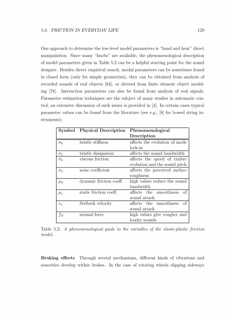
5.8. FRICTION IN EVERYDAY LIFE 129
One approach to determine the low-level model parameters is “hand and hear” direct
manipulation. Since many “knobs” are available, the phenomenological description
of model parameters given in Table 5.2 can be a helpful starting point for the sound
designer. Besides direct empirical search, modal parameters can be sometimes found
in closed form (only for simple geometries), they can be obtained from analysis of
recorded sounds of real objects [84], or derived from finite element object model-
ing [78]. Interaction parameters can also be found from analysis of real signals.
Parameter estimation techniques are the subject of many studies in automatic con-
trol, an extensive discussion of such issues is provided in [4]. In certain cases typical
parameter values can be found from the literature (see e.g., [8] for bowed string in-
struments).
Symbol Physical Description Phenomenological
Description
σ0 bristle stiffness affects the evolution of modelock-in
σ1 bristle dissipation affects the sound bandwidthσ2 viscous friction affects the speed of timbre
evolution and the sound pitchσ3 noise coefficient affects the perceived surface
roughnessµd dynamic friction coeff. high values reduce the sound
bandwidthµs static friction coeff. affects the smoothness of
sound attackvs Stribeck velocity affects the smoothness of
sound attackfN normal force high values give rougher and
louder sounds
Table 5.2: A phenomenological guide to the variables of the elasto-plastic frictionmodel.
Braking effects Through several mechanisms, different kinds of vibrations and
sonorities develop within brakes. In the case of rotating wheels slipping sideways

130 CHAPTER 5. OTHER INSTRUMENTS DRIVEN BY FRICTION
SquealBrake noise
Brake noiseRolling
Rolling
Squeal
Figure 5.29: 3D animation and waveform: a wheel which rolls and slides on a circulartrack.
across the rails, the friction forces acting at the wheel rim excite transverse vibrations.
In order to test the ability of the model to simulate brake noise, the simulation
depicted in Fig. 5.29 has been designed, where a wheel driven by the external force
fee rolls on a circular track. The rolling sound is obtained as the result of a sequence
of micro-impacts [93].
When a positive normal force is applied, the wheel is blocked from rolling and
the friction model is triggered. Neat stick-slip is established only at sufficiently low
velocities, and brake squeals are produced in the final stage of deceleration. The
resulting effect convincingly mimics real brake noise.
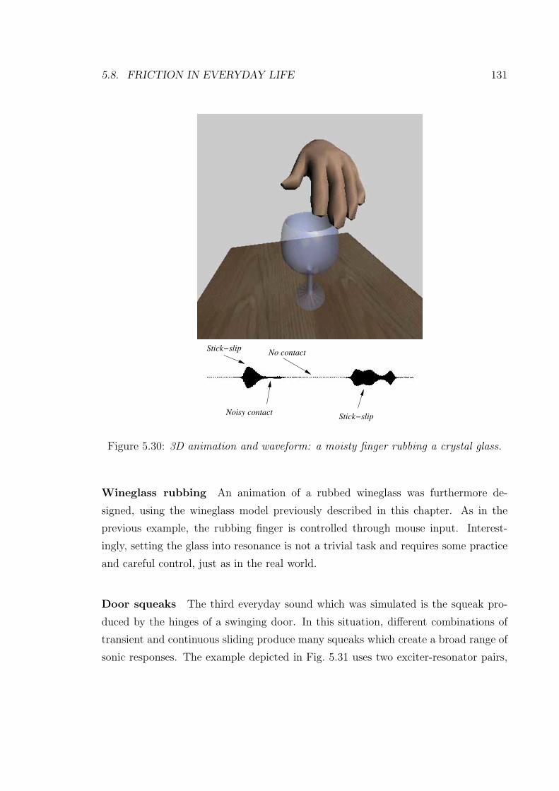
5.8. FRICTION IN EVERYDAY LIFE 131
Stick−slip
Stick−slipNoisy contact
No contact
Figure 5.30: 3D animation and waveform: a moisty finger rubbing a crystal glass.
Wineglass rubbing An animation of a rubbed wineglass was furthermore de-
signed, using the wineglass model previously described in this chapter. As in the
previous example, the rubbing finger is controlled through mouse input. Interest-
ingly, setting the glass into resonance is not a trivial task and requires some practice
and careful control, just as in the real world.
Door squeaks The third everyday sound which was simulated is the squeak pro-
duced by the hinges of a swinging door. In this situation, different combinations of
transient and continuous sliding produce many squeaks which create a broad range of
sonic responses. The example depicted in Fig. 5.31 uses two exciter-resonator pairs,
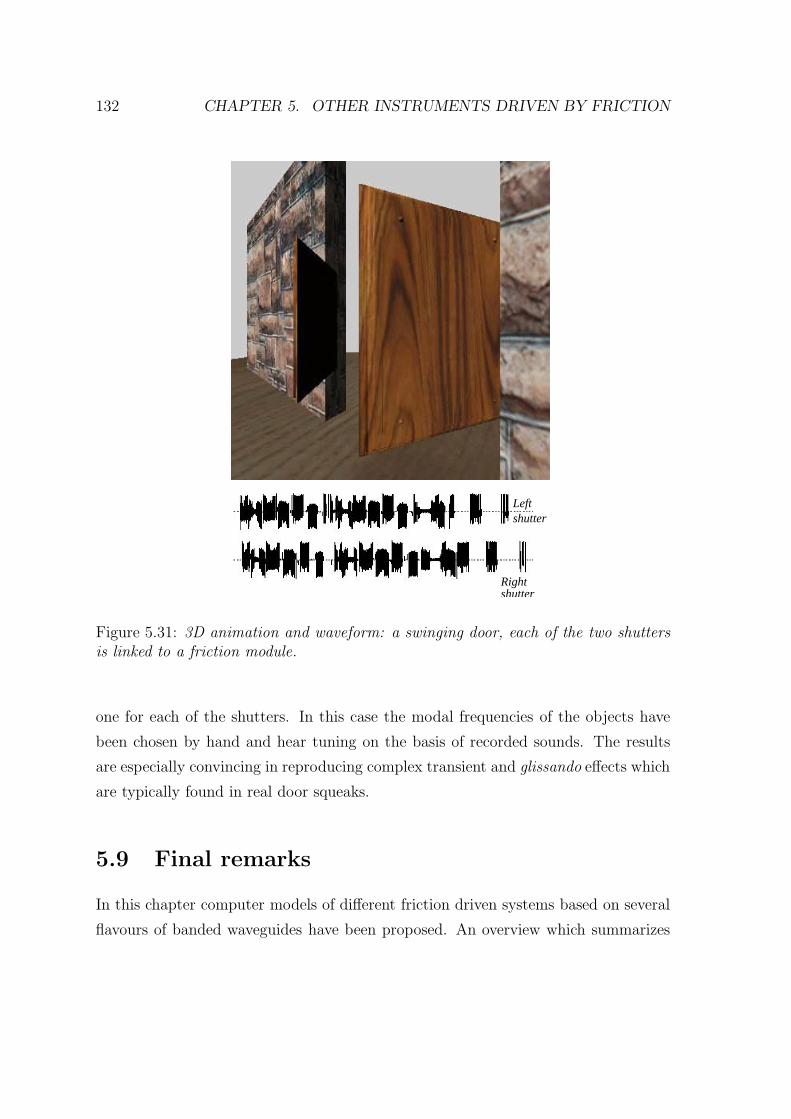
132 CHAPTER 5. OTHER INSTRUMENTS DRIVEN BY FRICTION
Left
Rightshutter
shutter
Figure 5.31: 3D animation and waveform: a swinging door, each of the two shuttersis linked to a friction module.
one for each of the shutters. In this case the modal frequencies of the objects have
been chosen by hand and hear tuning on the basis of recorded sounds. The results
are especially convincing in reproducing complex transient and glissando effects which
are typically found in real door squeaks.
5.9 Final remarks
In this chapter computer models of different friction driven systems based on several
flavours of banded waveguides have been proposed. An overview which summarizes
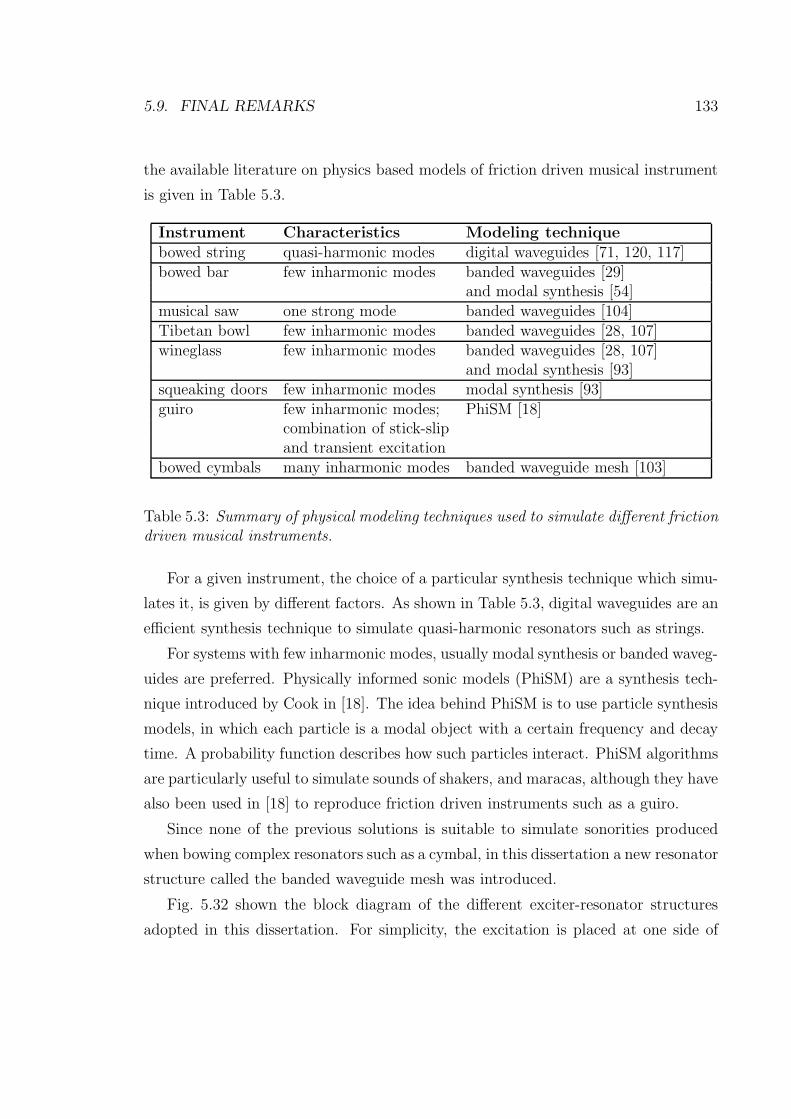
5.9. FINAL REMARKS 133
the available literature on physics based models of friction driven musical instrument
is given in Table 5.3.
Instrument Characteristics Modeling technique
bowed string quasi-harmonic modes digital waveguides [71, 120, 117]bowed bar few inharmonic modes banded waveguides [29]
and modal synthesis [54]musical saw one strong mode banded waveguides [104]Tibetan bowl few inharmonic modes banded waveguides [28, 107]wineglass few inharmonic modes banded waveguides [28, 107]
and modal synthesis [93]squeaking doors few inharmonic modes modal synthesis [93]guiro few inharmonic modes; PhiSM [18]
combination of stick-slipand transient excitation
bowed cymbals many inharmonic modes banded waveguide mesh [103]
Table 5.3: Summary of physical modeling techniques used to simulate different frictiondriven musical instruments.
For a given instrument, the choice of a particular synthesis technique which simu-
lates it, is given by different factors. As shown in Table 5.3, digital waveguides are an
efficient synthesis technique to simulate quasi-harmonic resonators such as strings.
For systems with few inharmonic modes, usually modal synthesis or banded waveg-
uides are preferred. Physically informed sonic models (PhiSM) are a synthesis tech-
nique introduced by Cook in [18]. The idea behind PhiSM is to use particle synthesis
models, in which each particle is a modal object with a certain frequency and decay
time. A probability function describes how such particles interact. PhiSM algorithms
are particularly useful to simulate sounds of shakers, and maracas, although they have
also been used in [18] to reproduce friction driven instruments such as a guiro.
Since none of the previous solutions is suitable to simulate sonorities produced
when bowing complex resonators such as a cymbal, in this dissertation a new resonator
structure called the banded waveguide mesh was introduced.
Fig. 5.32 shown the block diagram of the different exciter-resonator structures
adopted in this dissertation. For simplicity, the excitation is placed at one side of
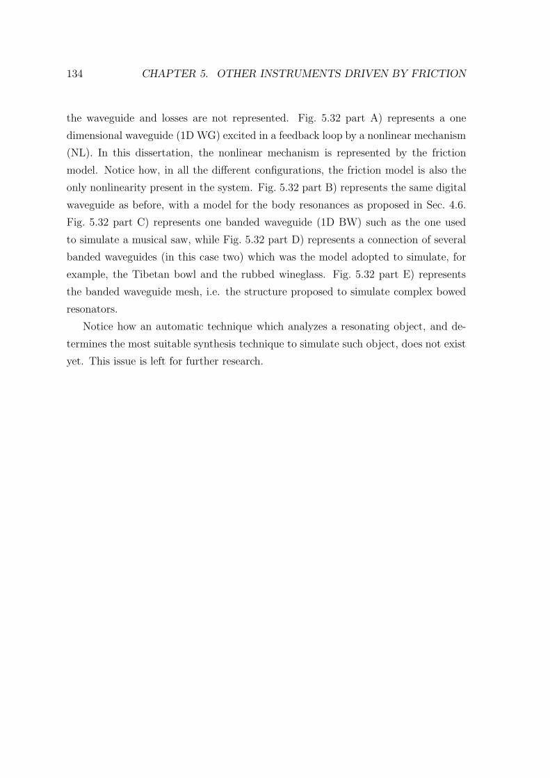
134 CHAPTER 5. OTHER INSTRUMENTS DRIVEN BY FRICTION
the waveguide and losses are not represented. Fig. 5.32 part A) represents a one
dimensional waveguide (1D WG) excited in a feedback loop by a nonlinear mechanism
(NL). In this dissertation, the nonlinear mechanism is represented by the friction
model. Notice how, in all the different configurations, the friction model is also the
only nonlinearity present in the system. Fig. 5.32 part B) represents the same digital
waveguide as before, with a model for the body resonances as proposed in Sec. 4.6.
Fig. 5.32 part C) represents one banded waveguide (1D BW) such as the one used
to simulate a musical saw, while Fig. 5.32 part D) represents a connection of several
banded waveguides (in this case two) which was the model adopted to simulate, for
example, the Tibetan bowl and the rubbed wineglass. Fig. 5.32 part E) represents
the banded waveguide mesh, i.e. the structure proposed to simulate complex bowed
resonators.
Notice how an automatic technique which analyzes a resonating object, and de-
termines the most suitable synthesis technique to simulate such object, does not exist
yet. This issue is left for further research.
5.9. FINAL REMARKS 135
NL 1D WG
NL 1D WG
NL 1D BW
3D M
NL 1D BW
1D BW+
NL 1D BW
3D M
+LF
OUTPUT
OUTPUT
OUTPUT
OUTPUT
+ OUTPUT
INPUT
INPUT
INPUT
INPUT
INPUT
A)
B)
C)
D)
E)
Figure 5.32: Block diagrams of the different waveguide-based data structures developedin this chapter and in the previous one. For simplicity, it is assumed that the excita-tion point is placed at one extremity of the waveguide, and losses are not represented.A) a one dimensional digital waveguide, B) a one dimensional digital waveguide fil-tered through the body model described in Sec. 4.6, C) one banded waveguide, D) aconnection of two banded waveguides, E) a banded waveguide mesh.
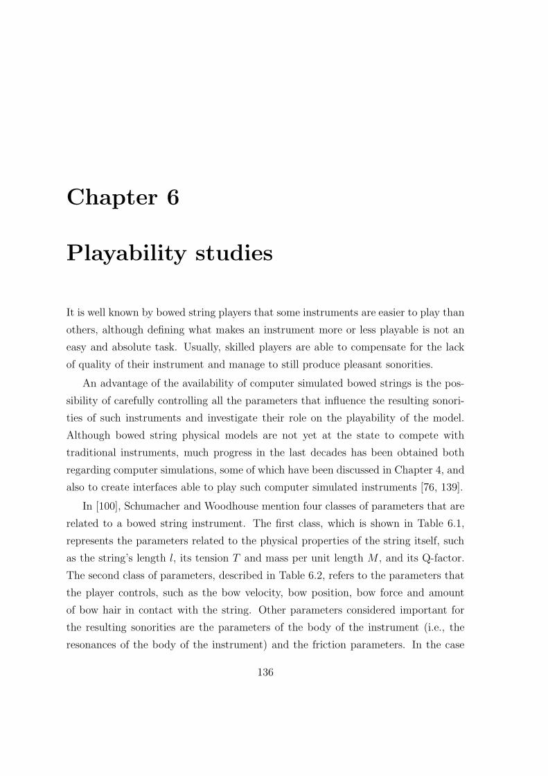
Chapter 6
Playability studies
It is well known by bowed string players that some instruments are easier to play than
others, although defining what makes an instrument more or less playable is not an
easy and absolute task. Usually, skilled players are able to compensate for the lack
of quality of their instrument and manage to still produce pleasant sonorities.
An advantage of the availability of computer simulated bowed strings is the pos-
sibility of carefully controlling all the parameters that influence the resulting sonori-
ties of such instruments and investigate their role on the playability of the model.
Although bowed string physical models are not yet at the state to compete with
traditional instruments, much progress in the last decades has been obtained both
regarding computer simulations, some of which have been discussed in Chapter 4, and
also to create interfaces able to play such computer simulated instruments [76, 139].
In [100], Schumacher and Woodhouse mention four classes of parameters that are
related to a bowed string instrument. The first class, which is shown in Table 6.1,
represents the parameters related to the physical properties of the string itself, such
as the string’s length l, its tension T and mass per unit length M , and its Q-factor.
The second class of parameters, described in Table 6.2, refers to the parameters that
the player controls, such as the bow velocity, bow position, bow force and amount
of bow hair in contact with the string. Other parameters considered important for
the resulting sonorities are the parameters of the body of the instrument (i.e., the
resonances of the body of the instrument) and the friction parameters. In the case
136
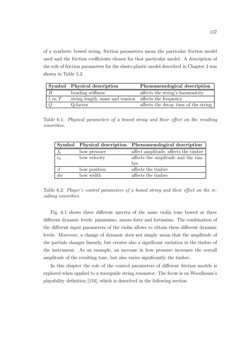
137
of a synthetic bowed string, friction parameters mean the particular friction model
used and the friction coefficients chosen for that particular model. A description of
the role of friction parameters for the elasto-plastic model described in Chapter 2 was
shown in Table 5.2.
Symbol Physical description Phenomenological description
B bending stiffness affects the string’s harmonicityl,m, T string length, mass and tension affects the frequencyQ Q-factor affects the decay time of the string
Table 6.1: Physical parameters of a bowed string and their effect on the resultingsonorities.
Symbol Physical description Phenomenological description
fb bow pressure affect amplitude, affects the timbrevb bow velocity affects the amplitude and the tim-
breβ bow position affects the timbredw bow width affects the timbre
Table 6.2: Player’s control parameters of a bowed string and their effect on the re-sulting sonorities.
Fig. 6.1 shows three different spectra of the same violin tone bowed at three
different dynamic levels: pianissimo, mezzo forte and fortissimo. The combination of
the different input parameters of the violin allows to obtain these different dynamic
levels. Moreover, a change of dynamic does not simply mean that the amplitude of
the partials changes linearly, but creates also a significant variation in the timbre of
the instrument. As an example, an increase in bow pressure increases the overall
amplitude of the resulting tone, but also varies significantly the timbre.
In this chapter the role of the control parameters of different friction models is
explored when applied to a waveguide string resonator. The focus is on Woodhouse’s
playability definition [134], which is described in the following section.
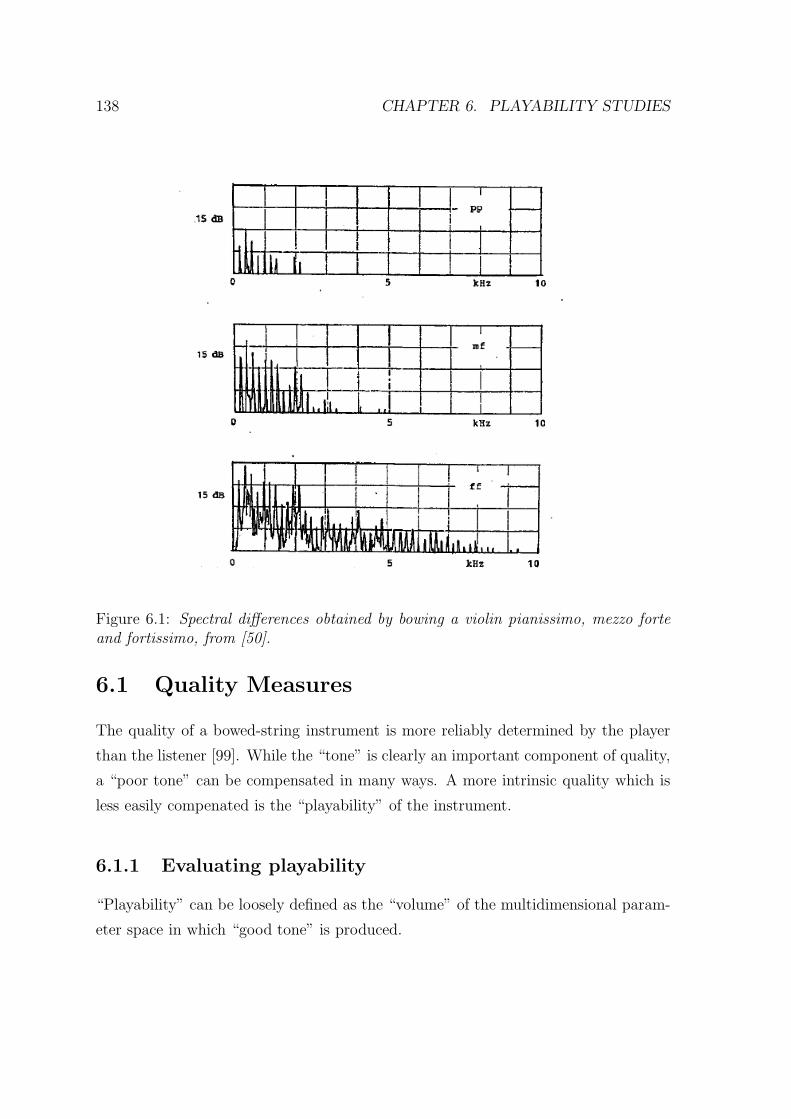
138 CHAPTER 6. PLAYABILITY STUDIES
Figure 6.1: Spectral differences obtained by bowing a violin pianissimo, mezzo forteand fortissimo, from [50].
6.1 Quality Measures
The quality of a bowed-string instrument is more reliably determined by the player
than the listener [99]. While the “tone” is clearly an important component of quality,
a “poor tone” can be compensated in many ways. A more intrinsic quality which is
less easily compenated is the “playability” of the instrument.
6.1.1 Evaluating playability
“Playability” can be loosely defined as the “volume” of the multidimensional param-
eter space in which “good tone” is produced.
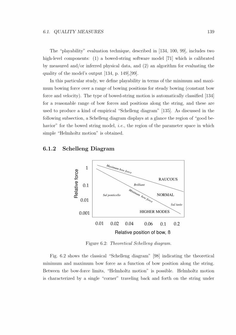
6.1. QUALITY MEASURES 139
The “playability” evaluation technique, described in [134, 100, 99], includes two
high-level components: (1) a bowed-string software model [71] which is calibrated
by measured and/or inferred physical data, and (2) an algorithm for evaluating the
quality of the model’s output [134, p. 149],[99].
In this particular study, we define playability in terms of the minimum and maxi-
mum bowing force over a range of bowing positions for steady bowing (constant bow
force and velocity). The type of bowed-string motion is automatically classified [134]
for a reasonable range of bow forces and positions along the string, and these are
used to produce a kind of empirical “Schelleng diagram” [135]. As discussed in the
following subsection, a Schelleng diagram displays at a glance the region of “good be-
havior” for the bowed string model, i.e., the region of the parameter space in which
simple “Helmholtz motion” is obtained.
6.1.2 Schelleng Diagram
Minimum bow force
Maximum bow force
Sul ponticello
Brilliant
Sul tasto
0.01 0.02 0.04 0.06 0.1
0.001
0.1
1
Relative position of bow, ß
Rela
tive f
orc
e
RAUCOUS
NORMAL
0.2
0.01
HIGHER MODES
Figure 6.2: Theoretical Schelleng diagram.
Fig. 6.2 shows the classical “Schelleng diagram” [98] indicating the theoretical
minimum and maximum bow force as a function of bow position along the string.
Between the bow-force limits, “Helmholtz motion” is possible. Helmholtz motion
is characterized by a single “corner” traveling back and forth on the string under
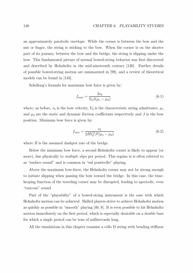
140 CHAPTER 6. PLAYABILITY STUDIES
an approximately parabolic envelope. While the corner is between the bow and the
nut or finger, the string is sticking to the bow. When the corner is on the shorter
part of its journey, between the bow and the bridge, the string is slipping under the
bow. This fundamental picture of normal bowed-string behavior was first discovered
and described by Helmholtz in the mid-nineteenth century [130]. Further details
of possible bowed-string motion are summarized in [99], and a review of theoretical
models can be found in [133].
Schelleng’s formula for maximum bow force is given by:
fmax =2vb
Y0β(µs − µd)(6.1)
where, as before, vb is the bow velocity, Y0 is the characteristic string admittance, µs
and µd are the static and dynamic friction coefficients respectively and β is the bow
position. Minimum bow force is given by:
fmin =vb
2RY 20 β
2(µs − µd)(6.2)
where R is the assumed dashpot rate of the bridge.
Below the minimum bow force, a second Helmholtz corner is likely to appear (or
more), due physically to multiple slips per period. This regime is is often referred to
as “surface sound” and is common in “sul ponticello” playing.
Above the maximum bow-force, the Helmholtz corner may not be strong enough
to initiate slipping when passing the bow toward the bridge. In this case, the time-
keeping function of the traveling corner may be disrupted, leading to aperiodic, even
“raucous” sound.
Part of the “playability” of a bowed-string instrument is the ease with which
Helmholtz motion can be achieved. Skilled players strive to achieve Helmholtz motion
as quickly as possible in “smooth” playing [40, 8]. It is even possible to hit Helmholtz
motion immediately on the first period, which is especially desirable on a double bass
for which a single period can be tens of milliseconds long.
All the simulations in this chapter examine a cello D string with bending stiffness
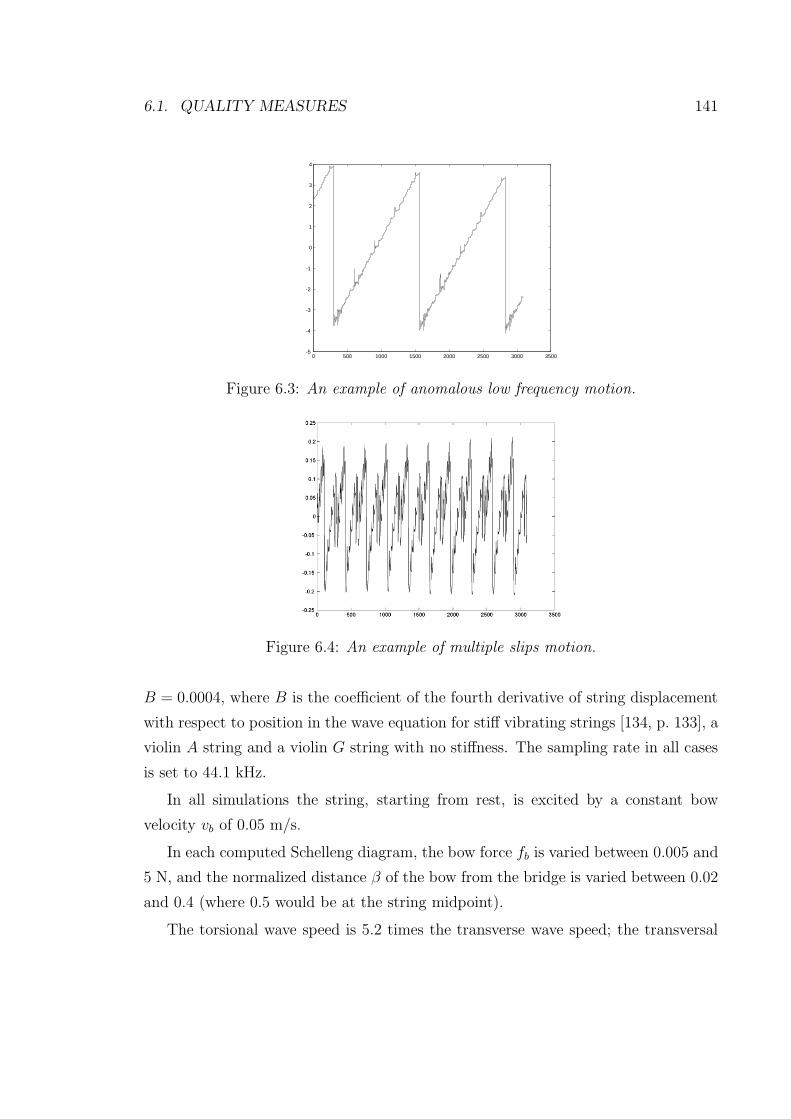
6.1. QUALITY MEASURES 141
0 500 1000 1500 2000 2500 3000 3500-5
-4
-3
-2
-1
0
1
2
3
4
Figure 6.3: An example of anomalous low frequency motion.
Figure 6.4: An example of multiple slips motion.
B = 0.0004, where B is the coefficient of the fourth derivative of string displacement
with respect to position in the wave equation for stiff vibrating strings [134, p. 133], a
violin A string and a violin G string with no stiffness. The sampling rate in all cases
is set to 44.1 kHz.
In all simulations the string, starting from rest, is excited by a constant bow
velocity vb of 0.05 m/s.
In each computed Schelleng diagram, the bow force fb is varied between 0.005 and
5 N, and the normalized distance β of the bow from the bridge is varied between 0.02
and 0.4 (where 0.5 would be at the string midpoint).
The torsional wave speed is 5.2 times the transverse wave speed; the transversal
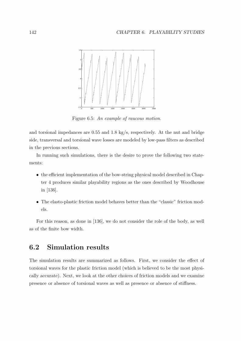
142 CHAPTER 6. PLAYABILITY STUDIES
0 500 1000 1500 2000 2500 3000 3500-1.5
-1
-0.5
0
0.5
1
1.5
Figure 6.5: An example of raucous motion.
and torsional impedances are 0.55 and 1.8 kg/s, respectively. At the nut and bridge
side, transversal and torsional wave losses are modeled by low-pass filters as described
in the previous sections.
In running such simulations, there is the desire to prove the following two state-
ments:
• the efficient implementation of the bow-string physical model described in Chap-
ter 4 produces similar playability regions as the ones described by Woodhouse
in [136].
• The elasto-plastic friction model behaves better than the “classic” friction mod-
els.
For this reason, as done in [136], we do not consider the role of the body, as well
as of the finite bow width.
6.2 Simulation results
The simulation results are summarized as follows. First, we consider the effect of
torsional waves for the plastic friction model (which is believed to be the most physi-
cally accurate). Next, we look at the other choices of friction models and we examine
presence or absence of torsional waves as well as presence or absence of stiffness.
6.2. SIMULATION RESULTS 143
6.2.1 Effect of Torsion-Wave Simulation on Playability
Fig. 6.6 shows the empirical Schelleng diagram obtained by running the simulation
with the plastic friction model installed.1 The darker shaded region including the
squares is defined as the “playable” region of the parameter space, where Helmholtz
motion is established. The region including the circles is the one in which multi-
ple slips are established. We see that there is good qualitative agreement with the
theoretical Schelleng diagram, as desired and expected.
Fig. 6.7 shows the same case of Fig. 6.6 except without including simulation of
torsional waves. We find that the playability region is not altered very much when
torsional waves are removed. Looking only at the Helmholtz region, there are 65
pixels of Helmholtz-motion in Fig. 6.6, and 63 in Fig. 6.7. On the whole, the results
are fairly comparable. However, the Helmholtz region is more contiguous without
torsional waves. Evidently, torsional waves can reflect at a “bad time” so as to
disturb the Helmholtz motion, as indicated by the ’’ amidst the ’2’s in Fig. 6.6.
The good news for synthesizer builders is that the added expense of torsional
wave simulation (which basically adds a coupled “second string”) does not appear to
improve playability. Since torsional waves are not prominent in the radiated sound
either, it seems warranted to leave them out of synthesis models, even in the highest
quality instances.
It is well known that string losses are required for stability of the Helmholtz motion
[34, 135, 100]. The transduction of transverse waves into (more highly damped)
torsional waves represents a significant loss on the string. It is therefore natural to
ask whether the preceding results might be improved by including only the (real)
losses corresponding torsional wave creation, since this costs little or nothing extra
in the simulation. In other words, the model generates torsional waves realistically,
but they are treated as if they are fully absorbed by the string terminations. This
simplified torsional wave simulation was suggested as a possibility in [100, p. 512]. It
turns out as a surprise the fact that simulating the plastic model without torsional
waves, but maintaining losses generated by torsional waves at the bow, collapses the
1The automatic evaluation technique which estimates the quality of waveforms is courtesy of JimWoodhouse.
144 CHAPTER 6. PLAYABILITY STUDIES
playability region to zero pixels. The reason why this happens is not completely clear
and left to further investigation.
Fig. 6.8 shows the Schelleng plot obtained by running the plastic friction model
with torsional waves and the same parameters as before. The string, instead of
starting from rest, starts from an already established Helmholtz motion. Notice that,
as somehow expected, the playability region in increased.
6.2.2 Effect of the Bow-String Friction Model
Up to now we have only looked at the plastic friction model which is believed to be
the most accurate physically. We now look at the effect of using the older simpler
models labeled “exponential” and “hyperbolic” in the previous chapters.
Exponential Friction Model
Fig. 6.9 shows the Schelleng diagram obtained using the classic exponential friction
model with torsional wave simulation included. We see that the plastic friction model
(see Fig. 6.6) “plays better” close to the bridge, and it has a larger region of Helmholtz
motion, especially when bowing somewhat away from the bridge. The combined areas
of Helmholtz and multiple-slipping motion, however, are somewhat larger with the
exponential friction model.
Fig. 6.10 shows the exponential friction case with torsional wave simulation re-
moved (completely). As in the plastic friction-model case, the playability is com-
parable, and arguably even improved. Note the greater “reliability” of playing near
the upper bow-force limit. While there are 48 Helmholtz pixels in the full-simulation
case, and only 42 in the case without torsional simulation, the Helmholtz region is
more contiguous and solid, having fewer interior pitfalls.
Hyperbolic Friction Model
Fig. 6.11 and Fig. 6.12 show the Schelleng diagram obtained by running the simulation
using the hyperbolic friction model, with and without torsional waves respectively.
The results are quite similar to the preceding exponential model case.
6.2. SIMULATION RESULTS 145
6.2.3 Effect of string stiffness
To examine if stiffness affects playability, Fig. 6.13 represents the simulated Schelleng
plot for a cello D string without stiffness. The simulation is run using the exponential
friction model. As expected, stiffness does not affect the playability of the model. The
same playability region as the one of Fig. 6.9 is obtained. As explained in Chapter 4,
the role of stiffness is to round the sharp Helmholtz corners. Stiffness, however, does
not affect the quality of the resulting waveform.
6.2.4 Velocity versus force playability region
It is also possible to examine if it exists a delimited playability region also in the
velocity versus force plane. Fig. 6.14 represents the simulated Schelleng plot for a
cello D string with stiffness and without torsional waves. The simulation is run
using the exponential friction model, and the plot is made in the velocity versus force
plane, maintaining a constant normalized bow position β = 0.07. Notice how it exists
a limited region in which the Helmholtz motion is achieved. As before, this region is
represented by the darker squares. Fig. 6.15 shows the simulated Schelleng diagram
for a cello D string with stiffness and with torsional waves. As in Fig. 6.14, the plot
is represented in the velocity versus force plane. Notice how the playability region
is somehow enhanced when torsional waves are taken into account. In this case the
role of torsional waves, i.e., to add losses which facilitates the establishment of the
Helmholtz motion, is apparent.
6.2.5 Three dimensional playability plots
In order to evaluate the playability for all variations of parameters, we represented the
playability in a 3 dimensional space. This is represented in Fig. 6.16. The simulation
is run using a cello D string with the exponential friction model and torsional waves.
In Fig. 6.16, only the region in which Helmholtz motion is achieved, i.e., the region
with dark squares, is represented. The z-axis represents bow velocity in a linear
scale between 0 to 1 m/s, while the x and y axis represent bow position and bow
force in a logarithmic scale respectively. For a given bow velocity of 0.05 m/s, the
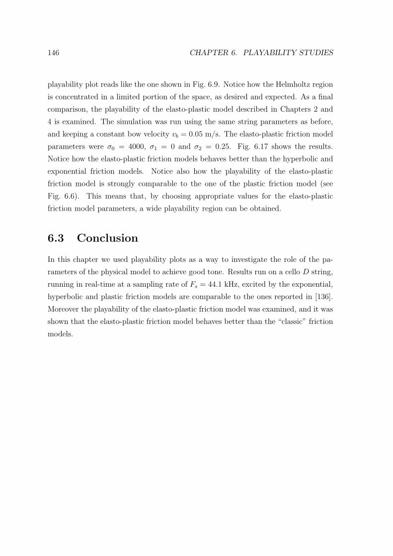
146 CHAPTER 6. PLAYABILITY STUDIES
playability plot reads like the one shown in Fig. 6.9. Notice how the Helmholtz region
is concentrated in a limited portion of the space, as desired and expected. As a final
comparison, the playability of the elasto-plastic model described in Chapters 2 and
4 is examined. The simulation was run using the same string parameters as before,
and keeping a constant bow velocity vb = 0.05 m/s. The elasto-plastic friction model
parameters were σ0 = 4000, σ1 = 0 and σ2 = 0.25. Fig. 6.17 shows the results.
Notice how the elasto-plastic friction models behaves better than the hyperbolic and
exponential friction models. Notice also how the playability of the elasto-plastic
friction model is strongly comparable to the one of the plastic friction model (see
Fig. 6.6). This means that, by choosing appropriate values for the elasto-plastic
friction model parameters, a wide playability region can be obtained.
6.3 Conclusion
In this chapter we used playability plots as a way to investigate the role of the pa-
rameters of the physical model to achieve good tone. Results run on a cello D string,
running in real-time at a sampling rate of Fs = 44.1 kHz, excited by the exponential,
hyperbolic and plastic friction models are comparable to the ones reported in [136].
Moreover the playability of the elasto-plastic friction model was examined, and it was
shown that the elasto-plastic friction model behaves better than the “classic” friction
models.
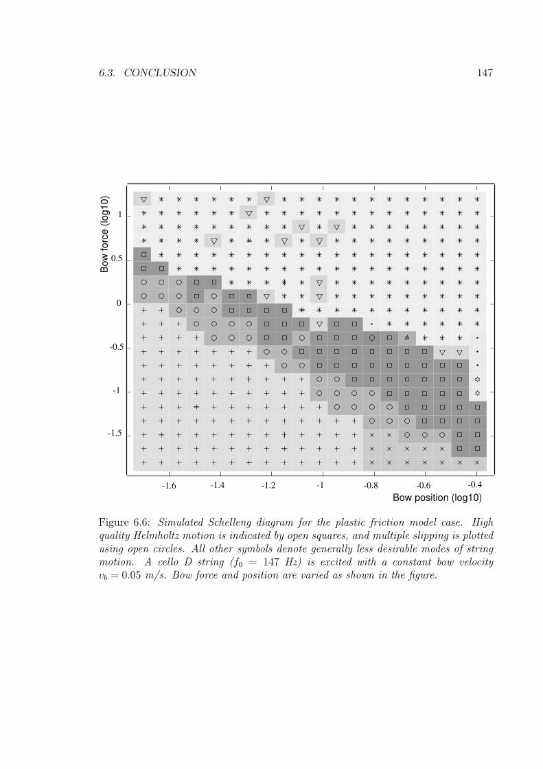
6.3. CONCLUSION 147
Bow position (log10)
Bow
forc
e (
log10)
-1.6 -1.4 -1.2 -1 -0.8 -0.6 -0.4
-1.5
-1
0
0.5
1
-0.5
1
Figure 6.6: Simulated Schelleng diagram for the plastic friction model case. Highquality Helmholtz motion is indicated by open squares, and multiple slipping is plottedusing open circles. All other symbols denote generally less desirable modes of stringmotion. A cello D string (f0 = 147 Hz) is excited with a constant bow velocityvb = 0.05 m/s. Bow force and position are varied as shown in the figure.

148 CHAPTER 6. PLAYABILITY STUDIESB
ow
forc
e (
log10)
Bow position (log10)
-1.6 -1.4 -1.2 -1 -0.8 -0.6 -0.4
-1.5
-1
0
0.5
1
-0.5
1
Figure 6.7: Simulated Schelleng diagram for the plastic friction model case, withtorsional wave simulation removed. As before, classic Helmholtz motion is indicatedby ‘2’, and multiple slipping by ‘’.
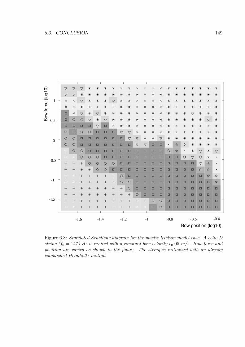
6.3. CONCLUSION 149
Bow position (log10)
-1.6 -1.4 -1.2 -1 -0.8 -0.6 -0.4
Bow
forc
e (
log10)
-1.5
-1
0
0.5
1
-0.5
1
Figure 6.8: Simulated Schelleng diagram for the plastic friction model case. A cello Dstring (f0 = 147) Hz is excited with a constant bow velocity v0.05 m/s. Bow force andposition are varied as shown in the figure. The string is initialized with an alreadyestablished Helmholtz motion.
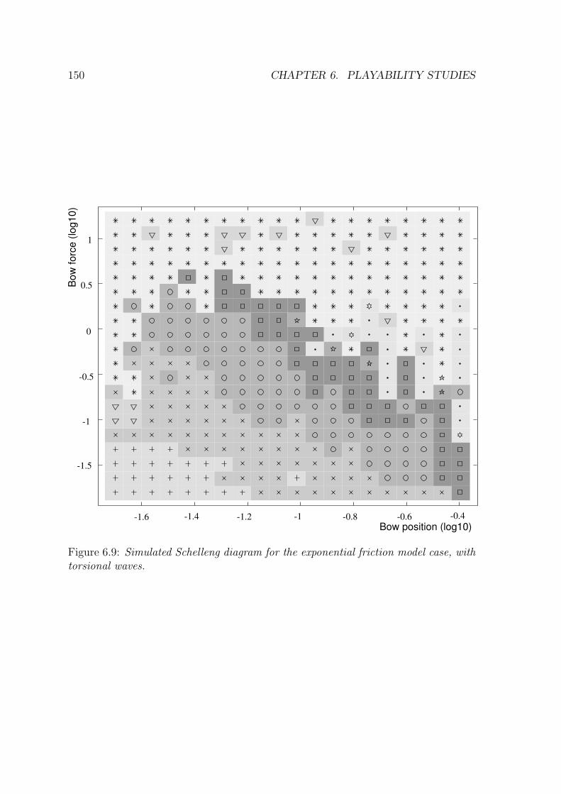
150 CHAPTER 6. PLAYABILITY STUDIES
Bow position (log10)
Bow
forc
e (
log10)
-1.6 -1.4 -1.2 -1 -0.8 -0.6 -0.4
-1.5
-1
0
0.5
1
-0.5
1
Figure 6.9: Simulated Schelleng diagram for the exponential friction model case, withtorsional waves.
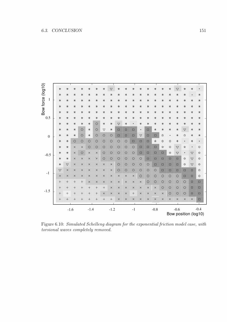
6.3. CONCLUSION 151
Bow
forc
e (
log10)
Bow position (log10)
-1.5
-1
0
0.5
1
-0.5
1
-1.6 -1.4 -1.2 -1 -0.8 -0.6 -0.4
Figure 6.10: Simulated Schelleng diagram for the exponential friction model case, withtorsional waves completely removed.
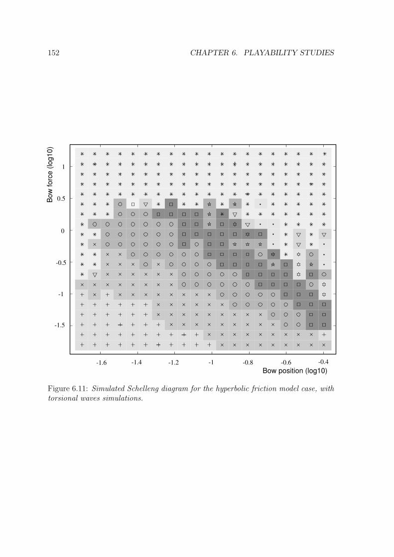
152 CHAPTER 6. PLAYABILITY STUDIESB
ow
forc
e (
log10)
Bow position (log10)-1.6 -1.4 -1.2 -1 -0.8 -0.6 -0.4
-1.5
-1
0
0.5
1
-0.5
1
Figure 6.11: Simulated Schelleng diagram for the hyperbolic friction model case, withtorsional waves simulations.
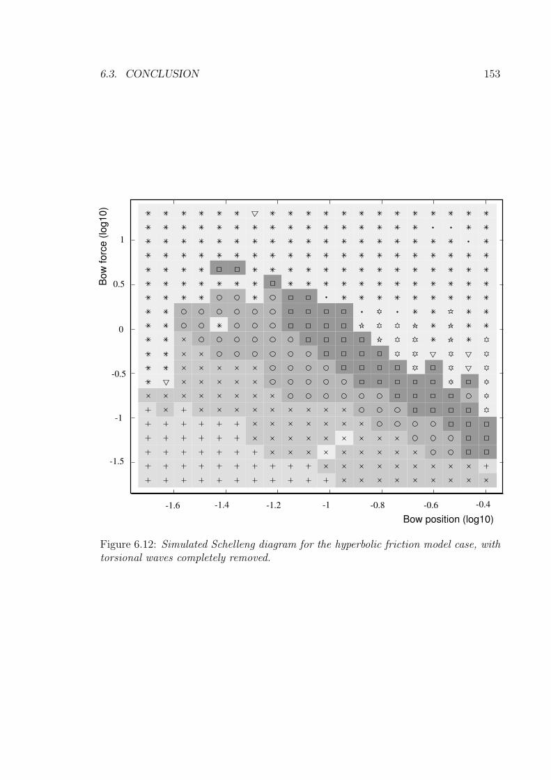
6.3. CONCLUSION 153
Bow
forc
e (
log10)
Bow position (log10)
-1.6 -1.4 -1.2 -1 -0.8 -0.6 -0.4
-1.5
-1
0
0.5
1
-0.5
1
Figure 6.12: Simulated Schelleng diagram for the hyperbolic friction model case, withtorsional waves completely removed.
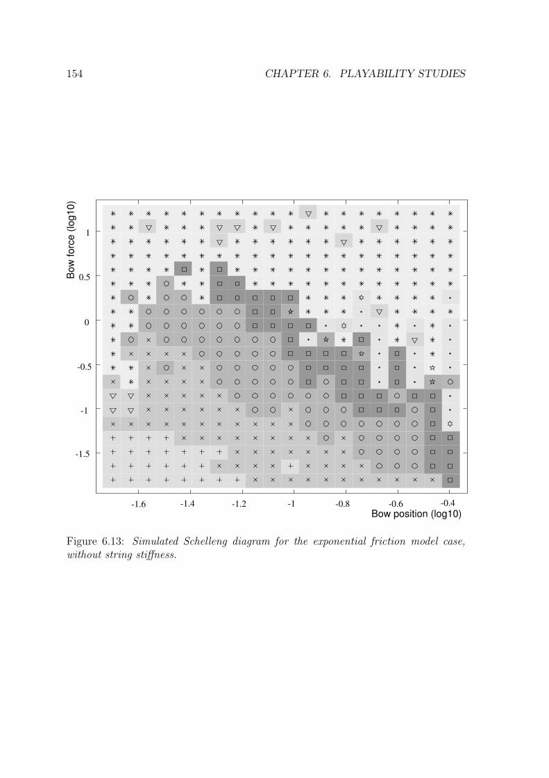
154 CHAPTER 6. PLAYABILITY STUDIES
Bow position (log10)
Bow
forc
e (
log10)
-1.6 -1.4 -1.2 -1 -0.8 -0.6 -0.4
-1.5
-1
0
0.5
1
-0.5
1
Figure 6.13: Simulated Schelleng diagram for the exponential friction model case,without string stiffness.
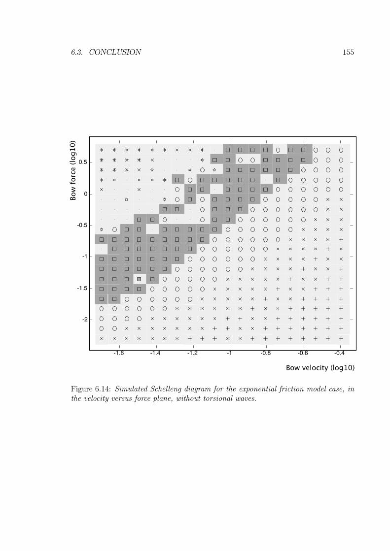
6.3. CONCLUSION 155
-1.6 -1.4 -1.2 -1 -0.8 -0.6 -0.4
-2
-1.5
-1
-0.5
0
0.5
Bow velocity (log10)
Bow
forc
e (
log10)
Figure 6.14: Simulated Schelleng diagram for the exponential friction model case, inthe velocity versus force plane, without torsional waves.

156 CHAPTER 6. PLAYABILITY STUDIES
-1.6 -1.4 -1.2 -1 -0.8 -0.6 -0.4
-2
-1.5
-1
-0.5
0
0.5
Bow velocity (log10)
Bow force (log10)
Figure 6.15: Simulated Schelleng diagram for the exponential friction model case, inthe velocity versus force plane, with torsional waves.
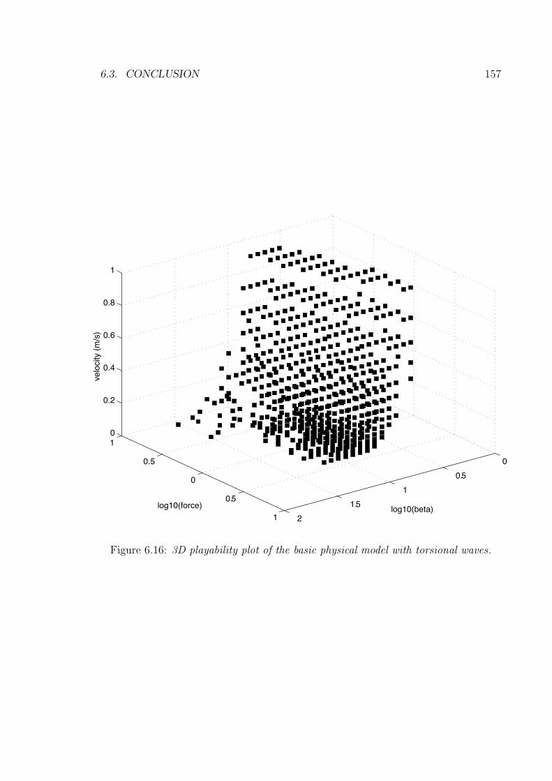
6.3. CONCLUSION 157
2
1.5
1
0.5
0
1
0.5
0
0.5
10
0.2
0.4
0.6
0.8
1
log10(beta)log10(force)
velo
city (
m/s
)
Figure 6.16: 3D playability plot of the basic physical model with torsional waves.
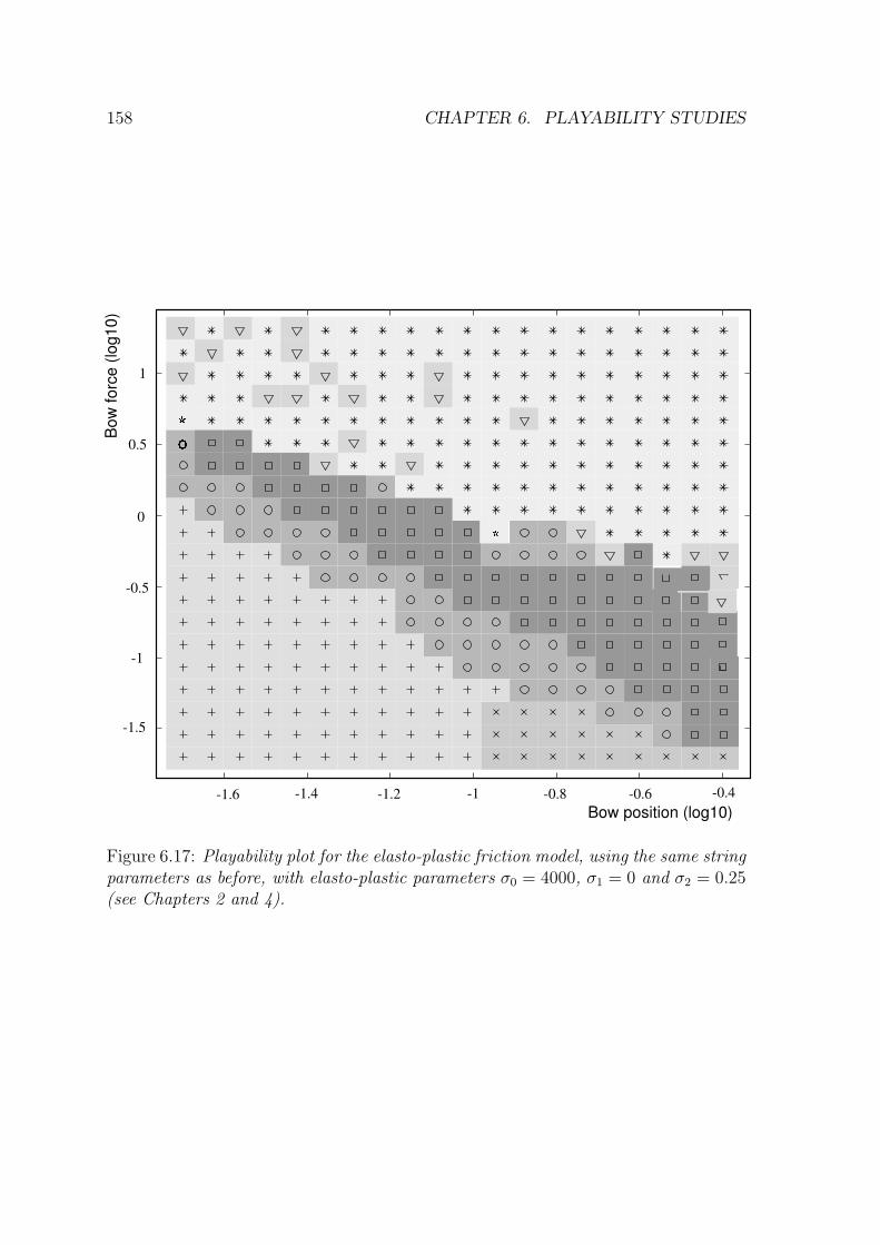
158 CHAPTER 6. PLAYABILITY STUDIESB
ow
forc
e (
log10)
Bow position (log10)-1.6 -1.4 -1.2 -1 -0.8 -0.6 -0.4
-1.5
-1
0
0.5
1
-0.5
1
Figure 6.17: Playability plot for the elasto-plastic friction model, using the same stringparameters as before, with elasto-plastic parameters σ0 = 4000, σ1 = 0 and σ2 = 0.25(see Chapters 2 and 4).
Chapter 7
Friction models in interactive
performances
In the previous chapters we examined friction sonorities with the goal of building
efficient real-time physical models. We studied the behavior of these models and
analyzed how input parameters affect their playability. We focused mainly on an
acoustical analysis of playability, i.e., we did not analyze the role of the interaction
between the human performer and the computer. During the past decade, lots of im-
provement has been made both on computer models of bowed strings and on building
input devices that allow to play such models. These devices are important in order for
the models to be playable in real-time, i.e. to be usable in an interactive performance.
This chapter describes research aimed to achieve such goals.
7.1 Playability and human computer interaction
The development of real-time modeling of musical instruments has exposed the prob-
lems of their gestural control. When a suitable device is attached to the physical
model, the natural interaction that exists between a musician and his instrument is
preserved, enabling the parameters of the model to evolve following the gestures of
the performer.
159

160 CHAPTER 7. FRICTION MODELS IN INTERACTIVE PERFORMANCES
7.2 Bow Strokes
Our first goal was the real-time simulation of highly skilled bowed string instrument
performance. In particular, we were interested in studying the model’s behaviour
when submitted to different bow strokes, such as detache, balzato, staccato, flying
staccato and so on.
The basic gestural parameters which can be used to define bow strokes include: a
specific precision grip in which all five fingers are in contact with the bow, a variable
length linear displacement in the axis of the bow, a rotational movement relative to
the strings’ axes in order to choose the string to be played, the pressure of the bow
against the string, and the bow velocity. Other important variables include the bow
position relative to the string and the amount of bow hair in contact with the string,
i.e., a rotation with respect to the bow’s axis.
One must also be aware that the technical demands required to perform many
of these bow strokes are typically obtained by musicians only after years of practice.
Furthermore, in addition to the performer’s skilled motor behaviour, these bow strokes
heavily rely upon physical properties of both the string and the bow, such as the
elasticity of the bow hair, tension of the string, etc.
7.2.1 Controlling the model using a graphical tablet
In order to obtain an accurate simulation of the bow strokes mentioned above, it is
necessary to have a flexible input controller at one’s disposition. We have therefore
decided to use an input device that provides both the means to reproduce the fun-
damental characteristics of the performer’s gestural control and which is sufficiently
generic in order to be able to extrapolate the typical violin technique. Other impor-
tant considerations for our choice of input device were availability, accuracy, precision,
resolution and affordability.
Among the commonly available standard input devices that match the above
requirements, the one that appeared to best suit our needs was a WACOM graphic
tablet equipped with a stylus transducer. One of the main factors in our decision was
the number of control parameters simultaneously available [132]. More specifically,
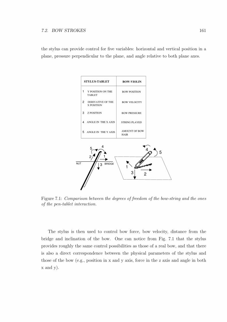
7.2. BOW STROKES 161
the stylus can provide control for five variables: horizontal and vertical position in a
plane, pressure perpendicular to the plane, and angle relative to both plane axes.
12
45
31
23
45
BRIDGENUT
BOW-VIOLIN
Y POSITION ON THE
TABLET
BOW POSITION
BOW VELOCITYDERIVATIVE OF THE
X POSITION
Z POSITION BOW PRESSURE
ANGLE IN THE X AXIS STRING PLAYED
HAIR
AMOUNT OF BOWANGLE IN THE Y AXIS
1
2
3
5
4
STYLUS-TABLET
Figure 7.1: Comparison between the degrees of freedom of the bow-string and the onesof the pen-tablet interaction.
The stylus is then used to control bow force, bow velocity, distance from the
bridge and inclination of the bow. One can notice from Fig. 7.1 that the stylus
provides roughly the same control possibilities as those of a real bow, and that there
is also a direct correspondence between the physical parameters of the stylus and
those of the bow (e.g., position in x and y axis, force in the z axis and angle in both
x and y).
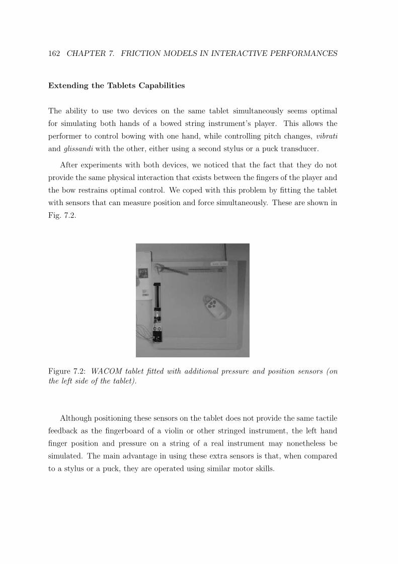
162 CHAPTER 7. FRICTION MODELS IN INTERACTIVE PERFORMANCES
Extending the Tablets Capabilities
The ability to use two devices on the same tablet simultaneously seems optimal
for simulating both hands of a bowed string instrument’s player. This allows the
performer to control bowing with one hand, while controlling pitch changes, vibrati
and glissandi with the other, either using a second stylus or a puck transducer.
After experiments with both devices, we noticed that the fact that they do not
provide the same physical interaction that exists between the fingers of the player and
the bow restrains optimal control. We coped with this problem by fitting the tablet
with sensors that can measure position and force simultaneously. These are shown in
Fig. 7.2.
Figure 7.2: WACOM tablet fitted with additional pressure and position sensors (onthe left side of the tablet).
Although positioning these sensors on the tablet does not provide the same tactile
feedback as the fingerboard of a violin or other stringed instrument, the left hand
finger position and pressure on a string of a real instrument may nonetheless be
simulated. The main advantage in using these extra sensors is that, when compared
to a stylus or a puck, they are operated using similar motor skills.
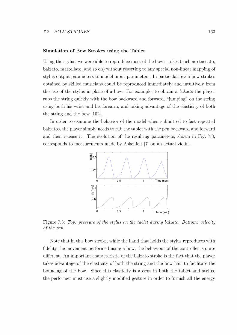
7.2. BOW STROKES 163
Simulation of Bow Strokes using the Tablet
Using the stylus, we were able to reproduce most of the bow strokes (such as staccato,
balzato, martellato, and so on) without resorting to any special non-linear mapping of
stylus output parameters to model input parameters. In particular, even bow strokes
obtained by skilled musicians could be reproduced immediately and intuitively from
the use of the stylus in place of a bow. For example, to obtain a balzato the player
rubs the string quickly with the bow backward and forward, “jumping” on the string
using both his wrist and his forearm, and taking advantage of the elasticity of both
the string and the bow [102].
In order to examine the behavior of the model when submitted to fast repeated
balzatos, the player simply needs to rub the tablet with the pen backward and forward
and then release it. The evolution of the resulting parameters, shown in Fig. 7.3,
corresponds to measurements made by Askenfelt [7] on an actual violin.
fb [
N]
0.5
0.25
Time (sec)
0 Time (sec)0.5 1
vb
[m
/s]
0 0.5 1
1
0.5
Figure 7.3: Top: pressure of the stylus on the tablet during balzato. Bottom: velocityof the pen.
Note that in this bow stroke, while the hand that holds the stylus reproduces with
fidelity the movement performed using a bow, the behaviour of the controller is quite
different. An important characteristic of the balzato stroke is the fact that the player
takes advantage of the elasticity of both the string and the bow hair to facilitate the
bouncing of the bow. Since this elasticity is absent in both the tablet and stylus,
the performer must use a slightly modified gesture in order to furnish all the energy
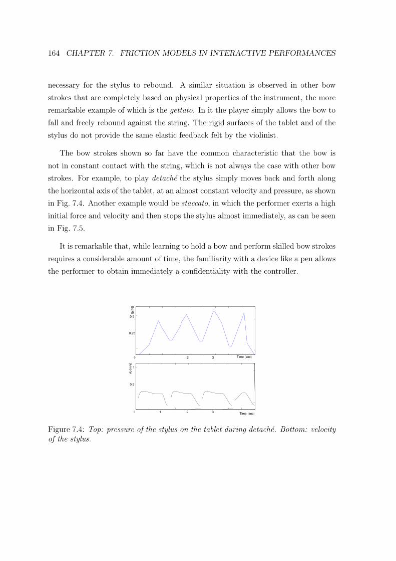
164 CHAPTER 7. FRICTION MODELS IN INTERACTIVE PERFORMANCES
necessary for the stylus to rebound. A similar situation is observed in other bow
strokes that are completely based on physical properties of the instrument, the more
remarkable example of which is the gettato. In it the player simply allows the bow to
fall and freely rebound against the string. The rigid surfaces of the tablet and of the
stylus do not provide the same elastic feedback felt by the violinist.
The bow strokes shown so far have the common characteristic that the bow is
not in constant contact with the string, which is not always the case with other bow
strokes. For example, to play detache the stylus simply moves back and forth along
the horizontal axis of the tablet, at an almost constant velocity and pressure, as shown
in Fig. 7.4. Another example would be staccato, in which the performer exerts a high
initial force and velocity and then stops the stylus almost immediately, as can be seen
in Fig. 7.5.
It is remarkable that, while learning to hold a bow and perform skilled bow strokes
requires a considerable amount of time, the familiarity with a device like a pen allows
the performer to obtain immediately a confidentiality with the controller.
0
fb [N
]
0.5
0.25
Time (sec)2 3
0
1
0.5
Time (sec)1 2 3
vb [m
/s]
Figure 7.4: Top: pressure of the stylus on the tablet during detache. Bottom: velocityof the stylus.
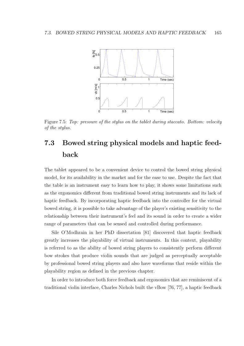
7.3. BOWED STRING PHYSICAL MODELS AND HAPTIC FEEDBACK 165
Time (sec)0 0.5 1
fb [
N]
0.5
0.25
Time (sec)0 0.5 1
vb
[m
/s]
1
0.5
Figure 7.5: Top: pressure of the stylus on the tablet during staccato. Bottom: velocityof the stylus.
7.3 Bowed string physical models and haptic feed-
back
The tablet appeared to be a convenient device to control the bowed string physical
model, for its availability in the market and for the ease to use. Despite the fact that
the table is an instrument easy to learn how to play, it shows some limitations such
as the ergonomics different from traditional bowed string instruments and its lack of
haptic feedback. By incorporating haptic feedback into the controller for the virtual
bowed string, it is possible to take advantage of the player’s existing sensitivity to the
relationship between their instrument’s feel and its sound in order to create a wider
range of parameters that can be sensed and controlled during performance.
Sile O’Modhrain in her PhD dissertation [81] discovered that haptic feedback
greatly increases the playability of virtual instruments. In this context, playability
is referred to as the ability of bowed string players to consistently perform different
bow strokes that produce violin sounds that are judged as perceptually acceptable
by professional bowed string players and also have waveforms that reside within the
playability region as defined in the previous chapter.
In order to introduce both force feedback and ergonomics that are reminiscent of a
traditional violin interface, Charles Nichols built the vBow [76, 77], a haptic feedback
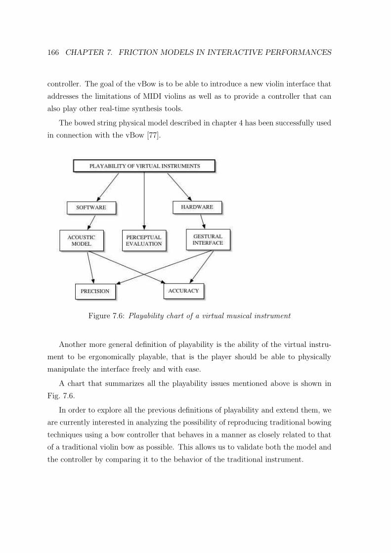
166 CHAPTER 7. FRICTION MODELS IN INTERACTIVE PERFORMANCES
controller. The goal of the vBow is to be able to introduce a new violin interface that
addresses the limitations of MIDI violins as well as to provide a controller that can
also play other real-time synthesis tools.
The bowed string physical model described in chapter 4 has been successfully used
in connection with the vBow [77].
Figure 7.6: Playability chart of a virtual musical instrument
Another more general definition of playability is the ability of the virtual instru-
ment to be ergonomically playable, that is the player should be able to physically
manipulate the interface freely and with ease.
A chart that summarizes all the playability issues mentioned above is shown in
Fig. 7.6.
In order to explore all the previous definitions of playability and extend them, we
are currently interested in analyzing the possibility of reproducing traditional bowing
techniques using a bow controller that behaves in a manner as closely related to that
of a traditional violin bow as possible. This allows us to validate both the model and
the controller by comparing it to the behavior of the traditional instrument.
7.3. BOWED STRING PHYSICAL MODELS AND HAPTIC FEEDBACK 167
7.3.1 The virtual violin project
The real-time bowed string physical model is currently used together with a wireless
bow controller developed by Diana Young [140, 108, 109]. The aim is to reproduce the
bow strokes that are most fundamental to the right hand technique of an accomplished
bowed string player.
The ultimate goal of this research is to create a bowed string instrument able
to reproduce the behavior of a traditional instrument as well as to create extended
performance techniques for bowed string players.
The bow controller used is a commercial carbon fiber bow, adapted by adding
a custom measurement system. The system is comprised of an electric field sensor
for measuring bow position (tip-frog / bow-bridge distance), commercial accelerom-
eters for detecting 3D acceleration, and foil strain gauges for measuring the strain
in the bow stick proportional to normal force on the string and the orthogonal force
corresponding to flexion toward and away from the scroll.
From these sensors, the parameters of bow velocity, bow-bridge distance, down-
ward force, and bow width (using tilt information provided by the accelerometers and
the second strain sensor) may be isolated from bowing gestures and used as input to
the physical model. For a detailed description of the bow controller, see [139].
In preliminary experiments we used a Macintosh G4 computer to run the Max/MSP
implementation of the bowed string physical model. The gestural data from the bow
controller was connected via a serial/USB converter to a USB port of the computer.
Recordings of both the violin audio and the bow controller data were made si-
multaneously within the Max/MSP environment. The gesture data was then used to
drive the physical model, which produced waveforms that were also recorded.
This setup was simple enough to allow fast and easy recording and testing, and was
used to reproduce bow strokes. The waveforms of the violin were then qualitatively
compared to those produced by the model using both time and spectral domain
evaluation and perceptual evaluation.
The integration of the bow controller hardware with the software model was ad-
dressed one input parameter at a time. In the first trial the downward strain sensor
was used to control the downward force parameter for the bowed string model.
168 CHAPTER 7. FRICTION MODELS IN INTERACTIVE PERFORMANCES
With the model parameters of bow-bridge distance, bow velocity, bow width, and
frequency held constant, the downward force was varied between 0 and 5 N.
Other than setting a threshold appropriate for the sensor range, it was unnecessary
to perform any adjustments to this mapping. Using the bow controller to play a single
string on the test violin, it was possible to compare the sound produced by the model
with that of the test violin. Sonorities which sounded appropriate for the amount of
pressure applied to the bow were produced.
Interestingly, the model produced sounds that seemed perceptually correct for
long sustained strokes as well as for short strokes with sharp attacks and decays.
7.3.2 Adding Velocity and Bow-Bridge Distance
Next, the bow velocity and bow-bridge distance controls were added by using the data
from the bow position sensor. By taking the data values corresponding to the tip and
the frog, the transverse bow position was determined, and from this the velocity value
was derived. The bow-bridge distance was taken as the sum of the tip and the frog
values.
It was possible to change the sound of the tones produced by the model by ad-
justing bow pressure, speed, bow-bridge distance, and by simply changing the bow
direction. As the sound of the test violin offered an easy comparison to the model,
playing two open strings (of the test violin) while controlling a single tone of the
model tuned to different intervals above and below the higher string was experi-
mented. Playing the small duet between real and virtual violins it was possible to
make small adjustments to the mappings so that the timbres sounded as though they
were all three emanating from the test violin.
7.3.3 Complete mapping
In order to build an expressive virtual musical instrument, the capture of the gesture
of the performance is as important as the manner in which the mapping of gestural
data onto synthesis parameters is done. In the case of physical modeling synthesis, a
one-to-one mapping approach of control values to synthesis parameters makes sense
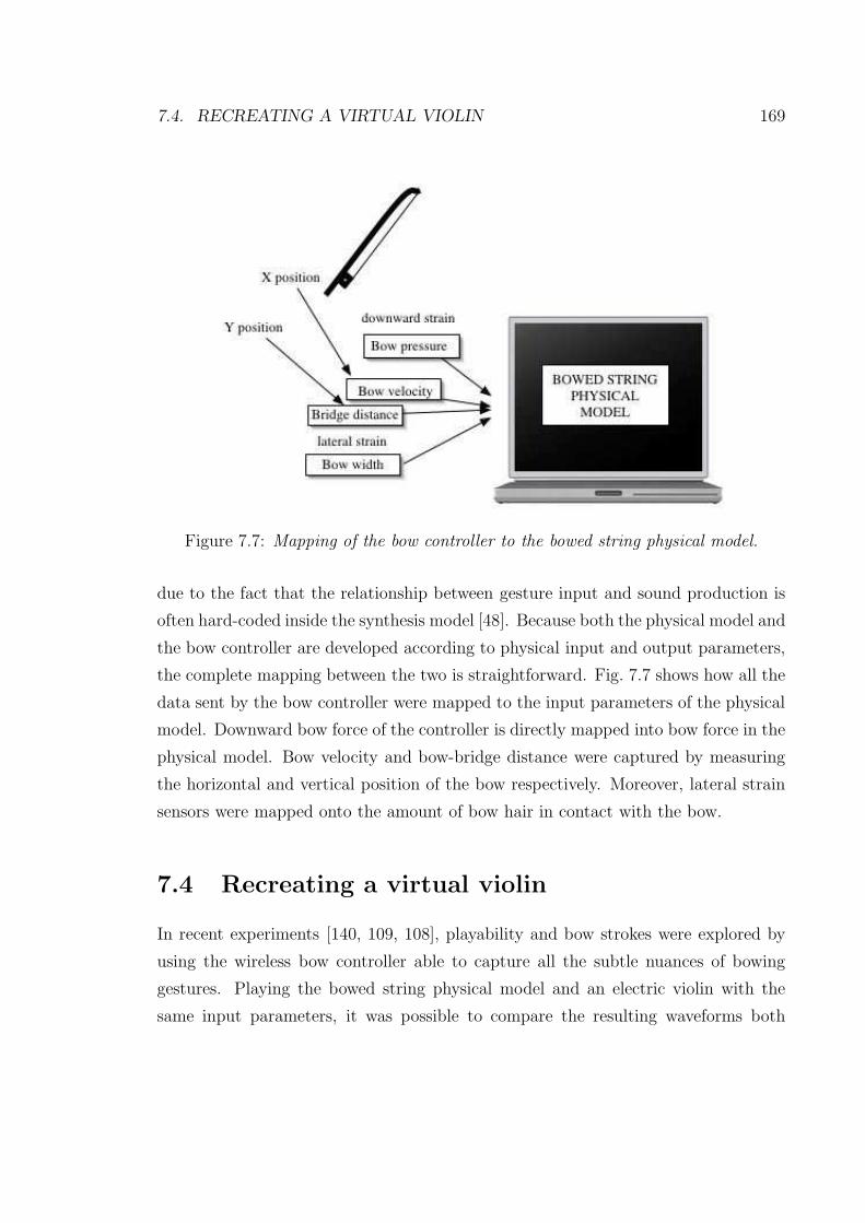
7.4. RECREATING A VIRTUAL VIOLIN 169
Figure 7.7: Mapping of the bow controller to the bowed string physical model.
due to the fact that the relationship between gesture input and sound production is
often hard-coded inside the synthesis model [48]. Because both the physical model and
the bow controller are developed according to physical input and output parameters,
the complete mapping between the two is straightforward. Fig. 7.7 shows how all the
data sent by the bow controller were mapped to the input parameters of the physical
model. Downward bow force of the controller is directly mapped into bow force in the
physical model. Bow velocity and bow-bridge distance were captured by measuring
the horizontal and vertical position of the bow respectively. Moreover, lateral strain
sensors were mapped onto the amount of bow hair in contact with the bow.
7.4 Recreating a virtual violin
In recent experiments [140, 109, 108], playability and bow strokes were explored by
using the wireless bow controller able to capture all the subtle nuances of bowing
gestures. Playing the bowed string physical model and an electric violin with the
same input parameters, it was possible to compare the resulting waveforms both
170 CHAPTER 7. FRICTION MODELS IN INTERACTIVE PERFORMANCES
perceptually and acoustically, and therefore validate the model.
7.5 Extended techniques for physical models
Up to this point, this dissertation has merely focused on the description of how
existing musical instruments can be digitally reproduced. From a musical perspective,
physical models become interesting when sonorities that cannot be achieved with real
instruments are created. Such extensions may not have scientific relevance, but are
noneless interesting from an artistic point of view.
Recent work has involved exploring extended techniques for physical models using
instrumental controller subsititution [12]. Instrumental controller substitution utilizes
the virtually disembodied nature of physical models as a means of exploring their
unique acoustic nature. The decoupling of the instrumental controller and the audio
synthesis is used as a compositional opportunity to expand the musical possibilities
of physical models.
Although such extensions are not described in this dissertation, it is important
to stress their existance which opens new possibilities for interactive compositions,
virtual reality and augmented sonic environments.
Chapter 8
Conclusions and future work
In this thesis different models of friction driven sonorities have been examined. The
importance of friction in musical applications and everyday life sonorities has been
outlined and examined, and state-of-the-art friction models have been applied to a
musical context.
The models developed in this dissertation have been implemented in real-time
under the Max/MSP and Pd platform, as described in Appendix A, and are down-
loadable from the website http://www-ccrma.stanford.edu/∼serafin.
These models have already been, in our opinion, successfully used in many real-
time interactive performances. In making such models available, the author wishes
that more composers and sound artists will find the sound of friction inspiring.
8.1 Future work
There are still many interesting applications related to friction driven physical models,
which are outlined in the following section.
8.1.1 A generalized friction controller
The idea behind a generalized friction controller is to have a device able to play all
the friction driven musical instruments. So far, many controllers for bowed strings
171
172 CHAPTER 8. CONCLUSIONS AND FUTURE WORK
have been developed, and some of them have been described in Chap. 7.
However, there does not yet exist a controller able to drive in real-time all friction
driven instruments. In the previous chapter different controllers which offer many
possibilities to performers due to their traditional feel, appearance, and function have
been discussed. It is legitimate to ask whether in many scenarios a less traditional
interface may be more beneficial. Specifically, together with Diana Young a general
interface for the control of all friction-driven instrument models is under development
[110].
Such a device would likely share some of the physical qualities of a bow, but
having characteristics that imply different playing techniques. The challenges on the
design of this device are due to the fact that friction sounds are produced in different
ways such as perpendicular motion of the exciter on the resonator (like in the case of
the bowed string and the musical saw), or circular motion (like in the Tibetan bowl
and glass harmonica). We are currently experimenting with having a pressure sensor,
a combination of different types of position sensors (Hall technique), strain/bend
sensors like the ones used in the bow controller, accelerometers, and gyros for angular
velocity.
Such an instrument will give composers and performers great possibilities to ex-
plore and extend the sound of friction.
8.1.2 Perception of chilling sounds
Another interesting research direction is a perceptual investigation of the properties of
friction sounds. As outlined in this dissertation, different sonorities can be produced
by the same excitation mechanism.
However, it is not yet clear which is the mechanism which makes the human brain
perceive such sounds as belonging to different sources, or what makes those sounds
pleasant or unpleasant. This is an interesting topic which can be further explored.
8.1. FUTURE WORK 173
8.1.3 Friction models and graphical user interfaces
Another interesting issue is related to the use of friction models in human-computer
interfaces. Enhancing information in human-computer interfaces by using different
senses is a natural choice motivated by our daily interaction with the world. In
everyday life humans communicate and interact by using multiple channels which
are interdependent. Especially in applications that present a direct manipulation
interaction (e.g., icon dragging), typical visual feedback techniques tend to give the
impression that manipulation is happening on a surrogate object rather than a real
one. In order to provide substance to the manipulated objects, physical reality must
be mimicked more closely. In particular real objects tend to resist to motion due to
their inertial properties, friction, and so on.
Many kinds of haptic devices providing force feedback have been proposed and
manufactured as a direct solution to this kind of requirements. However, there are
many practical cases where it is desirable to substitute haptic feedback with other
modalities. One possible reason is that these devices are in most cases cumber-
some and expensive, another is that they provide a strictly personal display (e.g.,
a user cannot share a sensation of effort with an audience). A number of alter-
natives have therefore been proposed. Approaches based on purely visual feedback
have been demonstrated to be effective in some cases. Cartoon animation techniques
applied to widget components and graphical object manipulation do enhance the
interaction [126]. Force-feedback has also been visually simulated via cursor displace-
ment [129] and pseudo-haptic feedback [67].
However, in many applications the visual display does not appear to be the best
choice as a replacement of kinesthetic feedback. Touch and vision represent differ-
ent priorities [63], with touch being more effective in conveying information about
“intensive” properties (material, weight, texture, and so on) and vision emphasizing
properties related to geometry and space (size, shape). Moreover, the auditory system
tends to dominate in judgments of temporal events, and intensive properties strongly
affect the temporal behavior of objects in motion, thus producing audible effects at
different time scales. In the light of these remarks, audition appears to be an ideal
candidate modality to support illusion of substance [126] in direct manipulation of
174 CHAPTER 8. CONCLUSIONS AND FUTURE WORK
virtual objects, and indeed Massimino and Sheridan [68] have shown that audition is
an effective sensorial substitute for some typical manipulation tasks.
Together with Federico Avanzini and Davide Rocchesso, we are currently inves-
tigating the use of friction sounds for sensorial substitution, to examine if auditory
feedback can facilitate the development of a more user friendly human computer
interface, especially when a tactile force feedback is not available.
8.1.4 Friction models in multimedia and virtual reality
While sound synthesis techniques have until now been adopted mainly in the computer
music community, recently their interest has increased also in virtual reality, computer
animation and computer games [20]. The availability of parametric models whose
quality is constantly improving makes such models desireable for sound designers in
the entartainment industry.
As outlined in this dissertation, many sounds that are produced by musical in-
struments and everyday objects derive from interaction between rubbed surfaces. It
is therefore an interesting application to use such models in other fields where sound
plays an important factor. In this way high quality computer generated sounds would
be appealing not only to composers but to those who are interested in sound design
from different perspectives.
Appendix A
Implementation
The models proposed in this thesis have been implemented as extensions to the
Max/MSP [141] environment.
The bowed string physical model has also been developed in the Synthesis Toolkit
(STK) platform [17]. Figure A.1 shows the interface developed. The objects im-
plemented in Max/MSP are a bowed string physical model, a rubbed wineglass, a
musical saw a bowed cymbal and a singing bowl.
The squeaking doors, rotating wheels and rubbed wineglasses have been imple-
mented in Pd [89] and are available from the Sounding Object website.1.
The friction models described in this dissertation have been used in different ap-
plications. Some examples are the following:
1. PhD dissertation of Sile OModhrain: Playing by Feel: Incorporating Haptic
Feedback into Computer-Based musical Instruments, (bowed string physical
model in STK), see [81].
2. PhD dissertation of Charles Nichols: The vbow: an expressive musical controller
haptic human-computer interface, (bowed string physical model in STK), see
[77].
3. Compositions S-Trance-S, (Dis)appeances and S-Morphe-S by Matthew Burt-
ner (extended bowed string physical model and singing bowl respectively, in
1(http:///www.soundobject.org)
175
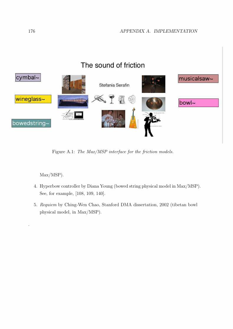
176 APPENDIX A. IMPLEMENTATION
Figure A.1: The Max/MSP interface for the friction models.
Max/MSP).
4. Hyperbow controller by Diana Young (bowed string physical model in Max/MSP).
See, for example, [108, 109, 140].
5. Requiem by Ching-Wen Chao, Stanford DMA dissertation, 2002 (tibetan bowl
physical model, in Max/MSP).
.
Appendix B
Numerical issues
In Chapter 2 we have shown that the elasto-plastic friction models are represented
through different non-linear coupling between the resonating objects. When the
continuous-time systems are discretized and turned into numerical algorithms, the
non-linear terms introduce computational problems that require to be solved ade-
quately. This is the topic of this Appendix.
B.1 Discretization
As described in Chap .4, the string resonator is represented by using a one dimen-
sional digital waveguide. In this section we describe how the interaction force f(n) for
the elasto-plastic model is computed at each time step, and coupled to the waveguide
resonator. At each time step n the variables [x(n), v(n)], representing the relative
position and velocity, and f(n), the friction force, have instantaneous mutual depen-
dence. That is, a delay-free non-computable loop has been created in the discrete-time
equations and, since a non-linear term is involved in the computation, it is not trivial
to solve the loop. This is a known problem in numerical simulations of non-linear
dynamic systems. An accurate and efficient solution, called K method, has been re-
cently proposed by Borin, De Poli and Rocchesso [10] and will be adopted here. First,
the instantaneous contribution of f(n) in the computation of vector [x(n), v(n)] can
177
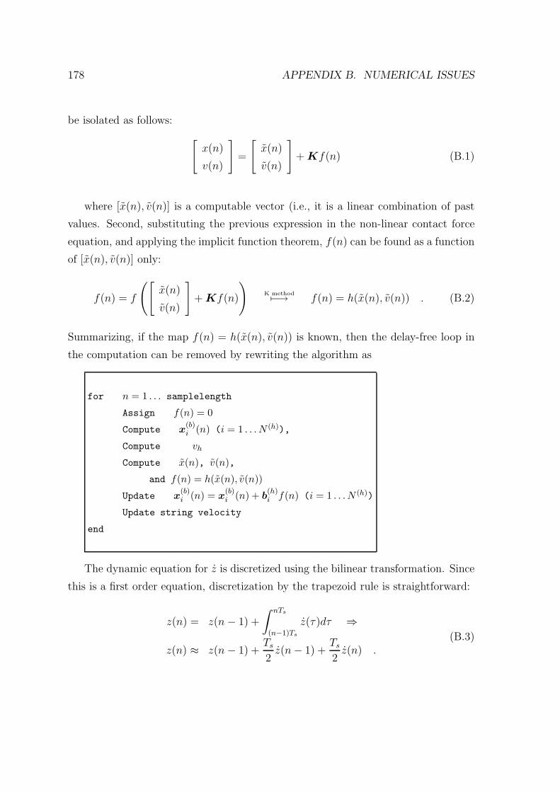
178 APPENDIX B. NUMERICAL ISSUES
be isolated as follows:
[
x(n)
v(n)
]
=
[
x(n)
v(n)
]
+ Kf(n) (B.1)
where [x(n), v(n)] is a computable vector (i.e., it is a linear combination of past
values. Second, substituting the previous expression in the non-linear contact force
equation, and applying the implicit function theorem, f(n) can be found as a function
of [x(n), v(n)] only:
f(n) = f
([
x(n)
v(n)
]
+ Kf(n)
)
K method7−→ f(n) = h(x(n), v(n)) . (B.2)
Summarizing, if the map f(n) = h(x(n), v(n)) is known, then the delay-free loop in
the computation can be removed by rewriting the algorithm as
for n = 1 . . . samplelength
Assign f(n) = 0
Compute x(b)i (n) (i = 1 . . . N (h)),
Compute vh
Compute x(n), v(n),
and f(n) = h(x(n), v(n))
Update x(b)i (n) = x
(b)i (n) + b
(h)i f(n) (i = 1 . . . N (h))
Update string velocity
end
The dynamic equation for z is discretized using the bilinear transformation. Since
this is a first order equation, discretization by the trapezoid rule is straightforward:
z(n) = z(n− 1) +
∫ nTs
(n−1)Ts
z(τ)dτ ⇒
z(n) ≈ z(n− 1) +Ts
2z(n− 1) +
Ts
2z(n) .
(B.3)
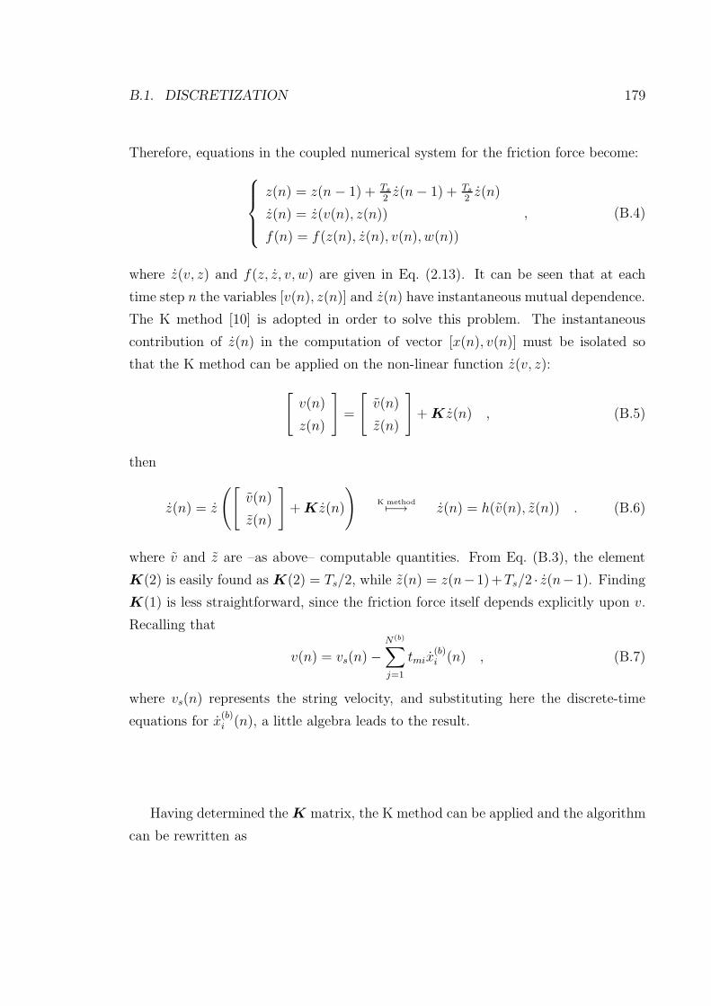
B.1. DISCRETIZATION 179
Therefore, equations in the coupled numerical system for the friction force become:
z(n) = z(n− 1) + Ts
2z(n− 1) + Ts
2z(n)
z(n) = z(v(n), z(n))
f(n) = f(z(n), z(n), v(n), w(n))
, (B.4)
where z(v, z) and f(z, z, v, w) are given in Eq. (2.13). It can be seen that at each
time step n the variables [v(n), z(n)] and z(n) have instantaneous mutual dependence.
The K method [10] is adopted in order to solve this problem. The instantaneous
contribution of z(n) in the computation of vector [x(n), v(n)] must be isolated so
that the K method can be applied on the non-linear function z(v, z):
[
v(n)
z(n)
]
=
[
v(n)
z(n)
]
+ K z(n) , (B.5)
then
z(n) = z
([
v(n)
z(n)
]
+ Kz(n)
)
K method7−→ z(n) = h(v(n), z(n)) . (B.6)
where v and z are –as above– computable quantities. From Eq. (B.3), the element
K(2) is easily found as K(2) = Ts/2, while z(n) = z(n−1)+Ts/2 · z(n−1). Finding
K(1) is less straightforward, since the friction force itself depends explicitly upon v.
Recalling that
v(n) = vs(n)−N(b)∑
j=1
tmix(b)i (n) , (B.7)
where vs(n) represents the string velocity, and substituting here the discrete-time
equations for x(b)i (n), a little algebra leads to the result.
Having determined the K matrix, the K method can be applied and the algorithm
can be rewritten as
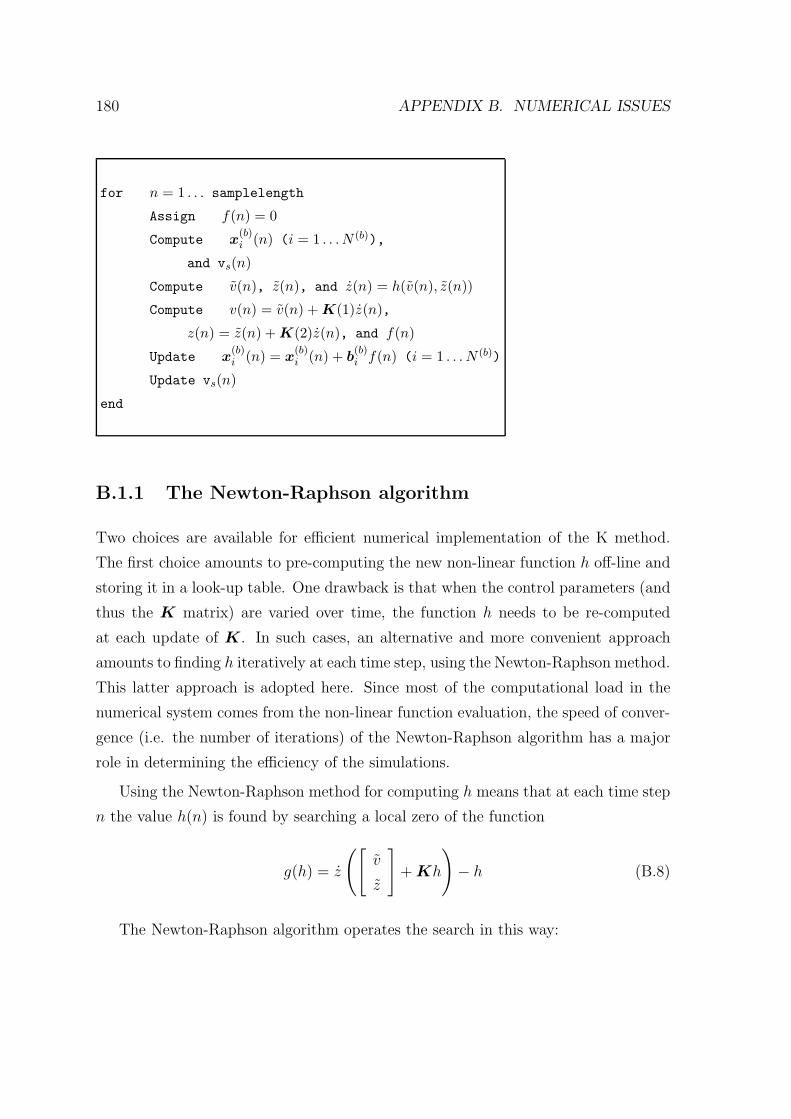
180 APPENDIX B. NUMERICAL ISSUES
for n = 1 . . . samplelength
Assign f(n) = 0
Compute x(b)i (n) (i = 1 . . . N (b)),
and vs(n)
Compute v(n), z(n), and z(n) = h(v(n), z(n))
Compute v(n) = v(n) + K(1)z(n),
z(n) = z(n) + K(2)z(n), and f(n)
Update x(b)i (n) = x
(b)i (n) + b
(b)i f(n) (i = 1 . . . N (b))
Update vs(n)
end
B.1.1 The Newton-Raphson algorithm
Two choices are available for efficient numerical implementation of the K method.
The first choice amounts to pre-computing the new non-linear function h off-line and
storing it in a look-up table. One drawback is that when the control parameters (and
thus the K matrix) are varied over time, the function h needs to be re-computed
at each update of K. In such cases, an alternative and more convenient approach
amounts to finding h iteratively at each time step, using the Newton-Raphson method.
This latter approach is adopted here. Since most of the computational load in the
numerical system comes from the non-linear function evaluation, the speed of conver-
gence (i.e. the number of iterations) of the Newton-Raphson algorithm has a major
role in determining the efficiency of the simulations.
Using the Newton-Raphson method for computing h means that at each time step
n the value h(n) is found by searching a local zero of the function
g(h) = z
([
v
z
]
+ Kh
)
− h (B.8)
The Newton-Raphson algorithm operates the search in this way:
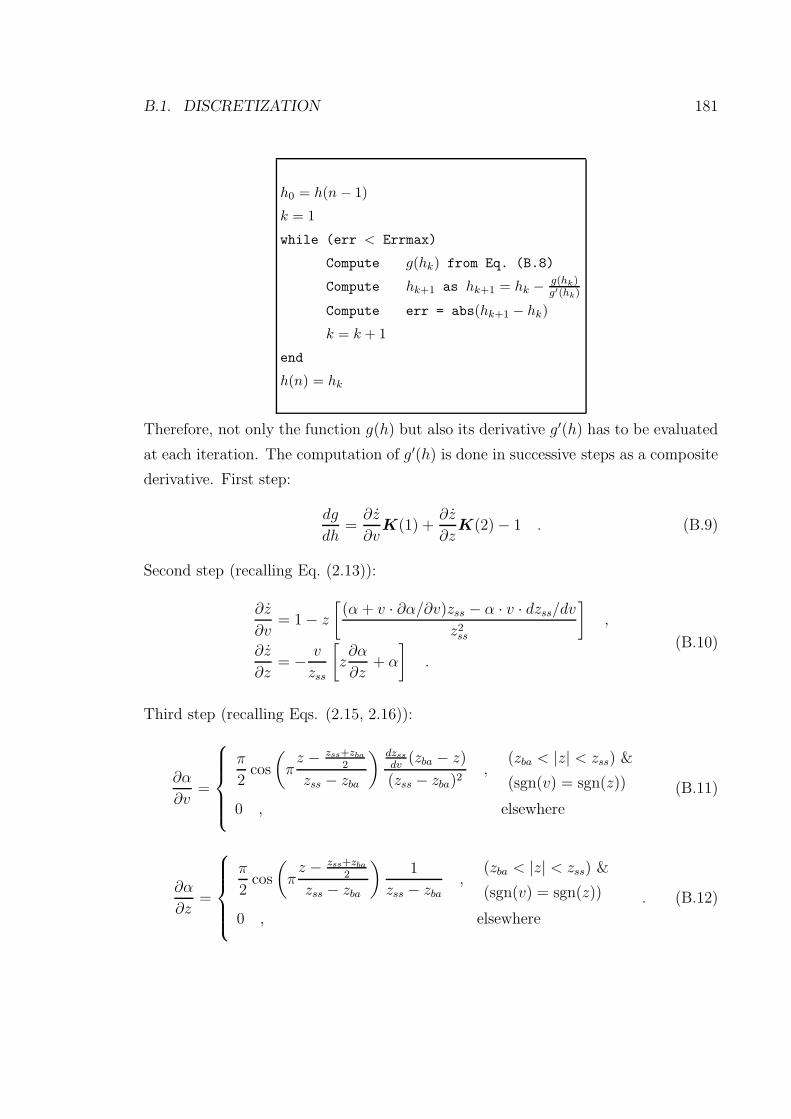
B.1. DISCRETIZATION 181
h0 = h(n − 1)
k = 1
while (err < Errmax)
Compute g(hk) from Eq. (B.8)
Compute hk+1 as hk+1 = hk − g(hk)g′(hk)
Compute err = abs(hk+1 − hk)
k = k + 1
end
h(n) = hk
Therefore, not only the function g(h) but also its derivative g′(h) has to be evaluated
at each iteration. The computation of g′(h) is done in successive steps as a composite
derivative. First step:
dg
dh=∂z
∂vK(1) +
∂z
∂zK(2)− 1 . (B.9)
Second step (recalling Eq. (2.13)):
∂z
∂v= 1− z
[
(α+ v · ∂α/∂v)zss − α · v · dzss/dv
z2ss
]
,
∂z
∂z= − v
zss
[
z∂α
∂z+ α
]
.(B.10)
Third step (recalling Eqs. (2.15, 2.16)):
∂α
∂v=
π
2cos
(
πz − zss+zba
2
zss − zba
) dzss
dv(zba − z)
(zss − zba)2,
(zba < |z| < zss) &
(sgn(v) = sgn(z))
0 , elsewhere
(B.11)
∂α
∂z=
π
2cos
(
πz − zss+zba
2
zss − zba
)
1
zss − zba,
(zba < |z| < zss) &
(sgn(v) = sgn(z))
0 , elsewhere
. (B.12)
182 APPENDIX B. NUMERICAL ISSUES
Last step (recalling Eq. (2.14)):
dzss
dv= −sgn(v)
2v
σ0v2s
(fs − fc)e−(v/vs)2 . (B.13)
Computing these terms from the last step to the first step, the derivative g′(h) can
be obtained.
In order to develop a real-time model, it is essential that the number of iterations
for the Newton-Raphson algorithm remains small in a large region of the parameter
space. To this end, analysis on the simulations has to be performed, where model
parameters are varied over a large range. Such analysis shows that in every conditions
the algorithms exhibit a high speed of convergence. Empirical results show that the
number of iterations remains smaller than seven.
Appendix C
Publications
The following is a list of the publications related to this dissertation, ordered by topic.
C.1 Bowed string physical model
1. S. Serafin, J. O. Smith, III, and J. Woodhouse. An investigation of the impact
of torsion waves and friction characteristics on the playability of virtual bowed
strings. IEEE Workshop on Signal Processing to Audio and Acoustics, New
Paltz, NY, New York, Oct. 1999, IEEE Press.
2. S. Serafin, C. Vergez, and X. Rodet. Friction and application to real-time
physical modeling of a violin. Proc. ICMC 99: International Computer Music
Conference 1999, Bejing, China, October 99 .
3. S. Serafin, J.O. Smith III Modeling stiffness in virtual bowed-string instruments
(abstract) ASA meeting, Atlanta may 2000.
4. S. Serafin, J.O.Smith III Influence of the Attack Parameters on the Playability of
a Virtual Bowed String Instrument. Proc. ICMC 2000: International Computer
Music Conference 2000, Berlin, Germany, august 2000.
5. P. Huang, S. Serafin, J.O.Smith III. A 3D Waveguide Mesh Model of High-
Frequency Violin Body Resonances. Proc. ICMC 2000: International Computer
183

184 APPENDIX C. PUBLICATIONS
Music Conference 2000, Berlin, Germany, august 2000.
6. S. Serafin, J.O.Smith III. A multirate, finite-width, bow-string interaction model.
Proc.DAFX 2000, Digital Audio Effects, Verona, Italy December 2000.
7. P. Huang, S. Serafin, J.O.Smith III. Modeling High-Frequency Modes of Com-
plex Resonators Using a Waveguide Mesh. Proc. DAFX 2000, Digital Audio
Effects, Verona, Italy December 2000.
8. Serafin and J. O. Smith. Impact of string stiffness on digital waveguide models
of bowed strings. Catgut Acoustical Society Journal, vol. 4, no. 4, 2001.
9. F. Fontana, S. Serafin. Modeling Savart ’s trapezoidal violin using a digital
waveguide mesh. Proc. SMAC 2003, Stockholm, August 2003.
10. S. Serafin, F. Avanzini, D. Rocchesso. Bowed string simulation using an elasto-
plastic friction model. Proc. SMAC 2003, Stockholm, August 2003.
C.2 Other friction driven musical instruments
11. S. Serafin, P. Huang, J.O.Smith III. The banded digital waveguide mesh. Proc.
Mosart meeting, Barcelona, November 2001.
12. S. Serafin, P. Huang, S. Ystad, C. Chafe, J.O. Smith III. Analysis and Synthesis
of Unusual Friction Driven Musical Instruments. Proc. ICMC 2002, Gotheborg,
Sweden, September 2002.
13. S. Serafin, C. Wilkerson, J.O. Smith III. Modeling bowl resonators using circular
waveguide networks. Proc. DAFX 2002, Hamburg, Germany, September 2002.
14. F. Avanzini, S. Serafin, D. Rocchesso. Modeling Interactions between Rubbed
Dry Surfaces Using an Elasto-Plastic Friction Model. Proc. DAFX 2002, Ham-
burg, Germany, September 2002.
C.3. CONTROL OF PHYSICAL MODELS 185
15. G. Essl, S. Serafin, P.Cook, J.Smith. Theory of banded waveguides, Computer
Music Journal, Spring 2004.
16. G. Essl, S. Serafin, P.Cook, J.Smith. Musical applications of banded waveg-
uides, Computer Music Journal, Spring 2004.
C.3 Control of physical models
17. S. Serafin, R. Dudas. An alternative controller for a virtual bowed string in-
strument. In M. Wanderley and M. Battier (eds): Trends in Gestural Control
of Music- Ircam.
18. S. Serafin, R. Dudas, M. Wanderley, X. Rodet. Gestural control of a real-time
physical model of a bowed string instrument. Proc. ICMC 99: International
Computer Music Conference 1999, Bejing, China, October 99 .
19. S. O’Modhrain, S. Serafin, C. Chafe, J.O.Smith III. Qualitative and quantitative
assessment on the playability of a virtual bowed string instrument. Proc. ICMC
2000: International Computer Music Conference 2000, Berlin, Germany, August
2000.
20. S. Serafin, J.O.Smith III, H. Thornburg. A pattern recognition approach to in-
vert a bowed string physical model. Proc. ISMA 2001, Perugia, Italy September
2001.
21. S. Serafin, J.O. Smith III, H. Thornburg, F. Mazzella, A. Tellier and G. Thonier.
Data driven identification and computer animation of a bowed string. Proc.
ICMC 2001, La Havana, Cuba September 2001.
22. S. Serafin, M. Burtner, S. O’Modhrain, C. Nichols. Expressive controllers for
bowed string physical models. Proc. DAFX 2001, Limerick, Ireland December
2001.
186 APPENDIX C. PUBLICATIONS
23. S. Serafin, D. Young. Bowed string physical model validation through use of a
bow controller and examination of bow strokes. Proc. SMAC 2003, Stockholm,
August 2003.
24. D. Young, S. Serafin. Playability evaluation of a bowed string physical model.
Proc. NIME 2003, Montreal, CA, May 2003.
25. S. Serafin, D. Young. Investigation of the playability of virtual bowed strings.
Proc. CIM 2003, Florence, Italy, May 2003.
C.4 Musical applications
26. M. Burtner, S. Serafin. Extended Performance Techniques for a Virtual Instru-
ment. Proc.DAFX 2000, Digital Audio Effects, Verona, Italy December 2000.
27. M. Burtner, S. Serafin. Real time extended physical models for the composer
and performer Proc. ICMC 2001, La Havana, Cuba September 2001.
28. M. Burtner, S. Serafin. Extended techniques for physical models using instru-
mental controller substitution Proc. ISMA 2001, Perugia, Italy September 2001.
29. M. Burtner, S. Serafin, D. Topper. Real-Time Spatial Processing and Transfor-
mations of a Singing Bowl. Proc. DAFX 2002, Hamburg, Germany, September
2002.
Bibliography
[1] J. Adrien. The missing link: Modal synthesis. In Giovanni De Poli, Aldo Picialli,
and Curtis Roads, editors, Representations of Musical Signals, pages 269–297.
MIT Press, Cambridge, MA, 1991.
[2] J.M Adrien, R. Causse, and E. Ducasse. Dynamic modeling of stringed and
wind instruments, sound synthesis by physical models. In Proc. ICMC, 1988.
[3] A. Akai. Acoustics of Friction. Journal of the Acoustical Society of America,
111(4):1525–1548, Apr. 2002.
[4] F. Altpeter. Friction Modeling, Identification and Compensation. PhD thesis,
Ecole Polytechnique Federale de Lausanne, 1999.
[5] J. Antunes, M. Tafasca, and L. Henrique. Simulation of the bowed string
dynamics. In 5eme Conference Francaise d’Acoustique, 2000.
[6] Aristotle. Physics. Oxford University Press, 1936.
[7] A. Askenfelt. Measurement of bow motion and bow force in violin playing.
Journal of the Acoustical Society of America, 80(4):1007–1015, Oct. 1986.
[8] A. Askenfelt. Measurement of the bowing parameters in violin playing. II:
Bow-bridge distance, dynamic range, and limits of bow force. Journal of the
Acoustical Society of America, 86(2):503–516, Aug. 1989.
[9] P.J. Blau. Friction science and technology. Marcel Dekker, 1996.
187
188 BIBLIOGRAPHY
[10] G. Borin, G. De Poli, and D. Rocchesso. Elimination of delay-free loops in
discrete-time models of nonlinear acoustic systems. IEEE Transactions on
Speech and Audio Processing, 8(6):717–727, 2000.
[11] W.F. Brace and J.D.Byerledd. Stick slip as a mechanism for earthquakes. Sci-
ence, 153:990–992, 1966.
[12] M. Burtner and S. Serafin. The exbow-metasax: Compositional applications of
bowed string physical models using instrument controller subsitution. Journal
of New Music Research, 32(4), December 2003.
[13] C. Cadoz, J.-L. Florens, and S. Gubian. Bowed string synthesis with force feed-
back gestural interaction. In Proc. International Computer Music Conference,
La Havana, Cuba, 2001.
[14] C. Chafe. Simulating performance on a bowed instrument. Technical report,
CCRMA, 1988.
[15] C. Chafe. Pulsed noise in self-sustained oscillations of musical instruments. In
In Proc. ICASSP, Albuquerque. IEEE Press, 1990.
[16] E.F. Chladni. Traite d’acoustique. Imprimeur-Libraire pour les Mathematiques,
1809.
[17] P. R. Cook. Synthesis toolkit in C++, version 1.0. In SIGGRAPH Proceedings.
Assoc. Comp. Mach., May 1996.
[18] P. R. Cook. Physically Informed Sonic Modeling (PhISM): Synthesis of Percus-
sive Sounds. Computer Music Journal, 21(3):38–49, 1997.
[19] P. R. Cook and G. Scavone. The synthesis toolkit (stk). In Proc. ICMC.
International Computer Music Association, October 1999.
[20] P.R. Cook. Real Sound Synthesis for Interactive Applications. AK Peters, 2002.
[21] L. Cremer. The Physics of the Violin. MIT Press, Cambridge, MA, 1984.
BIBLIOGRAPHY 189
[22] P. Dahl. A solid friction model. Technical report, The Aerospace Corporation,
1968.
[23] J.L. d’Alembert. Investigation of the curve formed by a vibrating string, 1747.
In Acoustics: Historical and Philosophical Development. Dowden, Hutchinson
and Ross, 1973.
[24] C. Canudas de Wit, H. Olsson, K. J. Astrom, and P. Lischinsky. A new model
for control of systems with friction. IEEE Trans. Autom. Control, 40(3):419–
425, 1995.
[25] J. Dieterich. Time dependent friction and the mechanics of stick slip. Pure
Appl. Geophys., 116:790–806, 1978.
[26] P. Dupont, V. Hayward, B. Armstrong, and F. Altpeter. Single State Elasto-
Plastic Friction Models. IEEE Trans. Autom. Control, 2002.
[27] S. Van Duyne and J. O. Smith III. Physical modeling with the 2d waveguide
mesh. In Proc. International Computer Music Conference (ICMC), pages 40–
47, The Hague, 1993. ICMA.
[28] G. Essl. Physical Wave Propagation Modeling for Real-Time Synthesis of Nat-
ural Sound. PhD thesis, Princeton University, November 2002.
[29] G. Essl and P. Cook. Measurements and efficient simulation of bowed bars.
Journal of the Acoustical Society of America, 108(1):379–388, July 2000.
[30] B. Feeny, A. Guran, N. Hinrichs, and K. Popp. A historical review on dry
friction and stick-slip phenomena. Appl. Mech. Rev., 51(5), 1998.
[31] N. Fletcher. Nonlinearity, complexity and the sounds of musical instruments.
In 16th International Congress on Acoustics, June 1998.
[32] N. H. Fletcher and T. D. Rossing. The Physics of Musical Instruments, Second
Edition. Springer Verlag, New York, 1998.
190 BIBLIOGRAPHY
[33] F. Fontana. Physics-Based Models for the Acoustic Representation of Space in
Virtual Environments. PhD thesis, University of Verona, 2002.
[34] F. G. Friedlander. On the oscillations of the bowed string. Proc. Cambridge
Philosophy Society, 49:516–530, 1953.
[35] G. Galilei. Dialogues. University of California Press, 1967. Reprinted and
translated by Drake.
[36] C.S. Gillmor. Charles Augustin Coulomb: Physics and Engineering in Eighteen
century France. Princeton, N.J., 1971.
[37] K. Guettler. Personal communications, SMAC 2003.
[38] K. Guettler. The bowed string computer simulated — some characteristic fea-
tures of the attack. Catgut Acoustical Society Journ., 2(2):22–26, Nov 1992.
Series II.
[39] K. Guettler. The bowed string. On the development of the Helmholtz motion and
on the Creations of Anomalous Low Frequencies. PhD thesis, Royal Institute
of Technology, 2002.
[40] K. Guettler and A. Askenfelt. On the kinematics of spiccato and ricochet
bowing. Catgut Acoustical Society Journal, 3(6):9–15, Nov. 1998. (Series II).
[41] D.A. Haessig and B. Friedland. On the modeling and simulation of friction. In
Transactions of the ASME, 1991.
[42] V. Hayward and B. Armstrong. A new computational model of friction ap-
plied to haptic rendering. In P. Corke and J. Trevelyan, editors, Experimental
Robotics VI, pages 403–412. Springer-Verlag, 2000.
[43] V. Hayward and B. Armstrong. A new computational model of friction applied
to haptic rendering. In Experimental Robotics, pages 404–412. Springer NY,
2000.

BIBLIOGRAPHY 191
[44] L. Hiller and P. Ruiz. Synthesizing musical sounds by solving the wave equation
for vibrating objects. Part I. Journal of the Audio Engineering Society, 19(6),
June 1971. Part II: vol. 19, no. 7, July/Aug. 1971.
[45] M. Holm. From real to virtual violin. the process in development of an artificial
model of violin. In 5th National Symposium on Music Research., 2001.
[46] P. Huang, S. Serafin, and J. O. Smith III. Modeling High-Frequency Modes
of Complex Resonators Using a Waveguide Mesh. In Proceedings of the COST
G-6 Conference on Digital Audio Effects (DAFX-00), Verona, Italy, December
7-9 2000.
[47] P. Huang, S. Serafin, and J. O. Smith III. A waveguide mesh model of high-
frequency violin mode resonances. In International Computer Music Confer-
ence, Berlin. Computer Music Association, 2000.
[48] A. Hunt, M. Wanderley, and M. Paradis. The importance of parameter mapping
in electronic instrument design. Journal of New Music Research, 3(2), June
2003.
[49] C.M. Hutchins. Tonal effects of interactions between the two lowest cavity
modes and three body modes of violin. In Stockholm Musical Acoustics Con-
ference (SMAC-93), pages 373–378, Stockholm, August 1993. Royal Swedish
Academy of Music.
[50] J. O. Smith III. Music applications of digital waveguides. Technical Report
STAN-M-39, CCRMA, 1987.
[51] J. O. Smith III. Music applications of digital waveguides. Technical Report
STAN–M–39, CCRMA, Music , Stanford University, 1987.
[52] J. O. Smith III. Nonlinear commuted synthesis of bowed strings. In Proc. ICMC
97, Greece. Computer Music Association, 1997.
[53] J. O. Smith III and J. S. Abel. Bark and ERB bilinear transforms. IEEE Trans.
Speech and Audio Processing, pages 697–708, November 1999.
192 BIBLIOGRAPHY
[54] O. Inacio, L. Henrique, and J. Antunes. Dynamical analysis of bowed bars. In
ICSV8, Hong-Kong, July 2001.
[55] E. Jansson. Acoustics for violin and guitar makers. Technical Report 3, KTH,
2002.
[56] H. Jarvelainen, V. Valimaki, and M. Karjalainen. Audibility of inharmonicity
in string instrument sounds, and implications to digital sound synthesis. In
Proc. ICMC. Computer Music Association, 1999.
[57] J.M. Jot. An analysis/synthesis approach to real-time artificial reverberation.
In Proc. Int. Conf. on Acoustics Speech and Signal Processing (ICASSP), pages
II.221–II.224, New York, 1992. IEEE Press.
[58] M. Karjalainen and J. O. Smith III. Body modeling techniques for string in-
strument synthesis. In International Computer Music Conference, Hong Kong,
pages 232–239. Computer Music Association, Aug. 1996.
[59] M. Karjalainen, V. Valimaki, and Z. Janosy. Towards high-quality sound syn-
thesis of the guitar and string instruments. In Proc. 1993 Int. Computer Mu-
sic Conference, Tokyo, pages 56–63. Computer Music Association, Sept. 10–15
1993.
[60] J. B. Keller. Bowing of violin strings. Comm. Pure Applied Math., 6:483–495,
1953.
[61] D. Klatt. Software for a cascade/parallel formant synthesizer. Journal of the
Acoustical Society of America, 67:13–33, 1980.
[62] R. L. Klatzky, Pai D. K., and E. P. Krotov. Perception of Material from Contact
Sounds. Presence, 4, 399–410., 2000.
[63] R. L. Klatzky and S. J. Lederman. Touch. In A. F. Healy and R. W. Proctor,
editors, Experimental Psychology, pages 147–176. Wiley, New York, 2002.
[64] H. Kuttroff. Room Acoustics. Elsevier Science, Essex, England, 1991.
BIBLIOGRAPHY 193
[65] T. I. Laakso, V. Valimaki, M. Karjalainen, and U. K. Laine. Splitting the
Unit Delay—Tools for Fractional Delay Filter Design. IEEE Signal Processing
Magazine, 13(1):30–60, January 1996.
[66] M. Lang. Allpass filter design and applications. IEEE Transactions on Signal
Processing, 46(9):2505–2514, 1998.
[67] A. Lecuyer, S. Coquillart, A. Kheddar, P. Richard, and P. Coiffet. Pseudo-
haptic feedback: Can isometric input devices simulate force feedback? In Proc.
IEEE Int. Conf. on Virtual Reality, pages 83–90, 2000.
[68] M.J. Massimino and T.B. Sheridan. Sensory substitution for force feedback in
teleoperation. Presence, 2(4):344–352, 1993.
[69] M. Mathews and J. Kohut. Electronic simulation of violin resonances. Journal
of the Acoustical Society of America, 53(6):1620–1626, 1973.
[70] M. E. McIntyre, R. T. Schumacher, and J. Woodhouse. Aperiodicity in bowed-
string motion. Acustica, 49(1):13–32, Sept. 1981.
[71] M. E. McIntyre, R. T. Schumacher, and J. Woodhouse. On the oscillations of
musical instruments. Journal of the Acoustical Society of America, 74(5):1325–
1345, Nov. 1983.
[72] M. E. McIntyre and J. Woodhouse. On the fundamentals of bowed string
dynamics. Acustica, 43(2):93–108, Sept. 1979.
[73] J. L. McKechnie, editor. Webster’s New Universal Unabridged Dictionary. Si-
mon ans Schuster, New York, 1983.
[74] B.C. J. Moore. An Introduction to the Psychology of Hearing. Academic Press,
New York, 1997.
[75] A.J. Morin. New friction experiments carried out at metz in 1831-1833. In
Proceedings of the French Royal Academy of Sciences, volume 4, pages 1–128,
1833.

194 BIBLIOGRAPHY
[76] C. Nichols. The vbow: A virtual violin bow controller for mapping gesture to
synthesis with haptic feedback. Organized Sound, 7(2), 2003.
[77] C. Nichols. The vbow: an expressive musical controller haptic human-computer
interface. PhD thesis, Stanford University, 2003.
[78] J. O’Brien, P. R. Cook, and G. Essl. Synthesizing sounds from physically based
motion. Proceedings of ACM SIGGRAPH, ACM Press/ACM SIGGRAPH, Los
Angeles, CA, pages 529–536, 2001.
[79] H. Olsson, K. J. Astrom, C. Canudas de Wit, M. Gafwert, and P. Lischinsky.
Friction models and friction compensation. European J. of Control, 4:176–195,
1998.
[80] H. Olsson, K.J. Astrom, C. Canudas de Wit, and M. Gafvertand P. Lischinsky.
Friction models and friction compensation. Technical report, Lund Institute of
Technology, 1997.
[81] S. O’Modhrain. Playing by Feel: Incorporating Haptic Feedback into Computer-
Based musical Instruments. PhD thesis, Music Dept., Stanford University
(CCRMA), 2000.
[82] Alan V. Oppenheim and R. W. Schafer. Discrete Time Signal Processing.
Prentice-Hall, Inc., Englewood Cliffs, NJ, 1989.
[83] D. Pai. Modal synthesis for Vibrating Objects. Audio Anecdotes. AK Peters,
2004.
[84] D. Pai, K. Van Den Doel, D. L. James, J. Lang, J. E. Lloyd, J. L. Richmond,
and S. H. Yau. Scanning physical interaction behavior of 3d objects. Proceedings
of ACM SIGGRAPH, ACM Press/ACM SIGGRAPH, Los Angeles, CA., pages
87–96, 2001.
[85] M. Palumbi and L. Seno. Metal string. In Proc. International Computer Music
Conference, Beijing, China., 1999.
BIBLIOGRAPHY 195
[86] R. Pitteroff. Contact mechanics of the bowed string. PhD thesis, Cambridge
University, 1995.
[87] R. Pitteroff. Mechanics of the contact area between a violin bow and a string.
part I: Reflection and transmission behaviour. part II: Simulating the bowed
string. part III: Parameter dependance. In Acustica-Acta Acustica, pages 543–
562, 1998.
[88] K. Popp and P. Stelter. Stick-slip vibrations and chaos. Philosophical Transac-
tions, 332:89–105, 1990.
[89] M. Puckette. Pure Data. In Proceedings of the International Computer Music
Conference (ICMC). International Computer Music Association (ICMA), 1996.
[90] C. V. Raman. On the mechanical theory of vibrations of bowed strings and
of musical instruments of the violin family, with experimental verification of
results. Indian Assoc. Cult. Sci. Bull., 15:1–158, 1918.
[91] J.W. Rayleigh. The Theory of Sound. Dover, New York, 1976.
[92] O. Reynolds. On the theory of lubrication and its application to mr. beauchamp
tower’s experiments, including an experimental determination of the viscosity
of olive oil. Phil. Trans. Royal Soc., 177:157–234, 1886.
[93] D. Rocchesso and F. Fontana, editors. The Sounding Object. Mondo estremo,
2003.
[94] D. Rocchesso and J. Smith. Circulant and elliptic feedback delay networks for
artificial reverberation. IEEE Transactions on Speech and Audio Processing,
5(1):51–63, 1997.
[95] T. D. Rossing. Acoustics of the glass harmonica. Journal of the Acoustical
Society of America, 95(2), 1994.
[96] S. Sastry, editor. Nonlinear systems: analysis, stability and control. Springer
Verlag, 1999.
196 BIBLIOGRAPHY
[97] G. Scavone and J. O. Smith III. Digital waveguide modeling of woodwind
toneholes. 132nd meeting of the Acoustical Society of America, Honolulu, Dec.
1996.
[98] J. C. Schelleng. The bowed string and the player. Journal of the Acoustical
Society of America, 53(1):26–41, Jan. 1973.
[99] R. T. Schumacher and J. Woodhouse. Computer modelling of violin playing.
Contemporary Physics, 36(2):79–92, 1995.
[100] R. T. Schumacher and J. Woodhouse. The transient behavior of models of
bowed-string motion. CHAOS, 5(3):509–523, 1995.
[101] J.F.M. Scott and J. Woodhouse. Vibration of an elastic strip with varying
curvature. Philosophical Transactions, 1992.
[102] S. Serafin and R. Dudas. An alternative controller for a virtual bowed string
instrument. Trends in Gestural Control of Music. M. Wanderley and M. Battier,
2000.
[103] S. Serafin, P. Huang, and J. O. Smith III. The Banded Digital Waveguide
Mesh. In Proc. Workshop on Future Directions of Computer Music (Mosart-
01), Barcelona, Spain, November 2001.
[104] S. Serafin, P. Huang, S. Ystad, C. Chafe, and J.O. Smith III. Analysis and
synthesis of unusual friction driven musical instruments. In Proceedings of the
International Computer Music Conference (ICMC-02), Gotheborg, 2002.
[105] S. Serafin and J. O. Smith. A multirate, finite width bow string interaction
model. In Proceedings of Cost-DAFX, Verona, Italy, 2000.
[106] S. Serafin, J. O. Smith III, and J. Woodhouse. An investigation of the impact
of torsion waves and friction characteristics on the playability of virtual bowed
strings. In Proc. IEEE Workshop on Appl. of Signal Processing to Audio and
Acoustics, New Paltz, NY, New York, Oct. 1999. IEEE Press.
BIBLIOGRAPHY 197
[107] S. Serafin, C. Wilkerson, and J. O. Smith III. Modeling Bowl Resonators Using
Circular Waveguide Networks. In Proceedings of the COST G-6 Conference on
Digital Audio Effects (DAFX-02), Hamburg, Germany, 2002.
[108] S. Serafin and D. Young. Bowed string physical model validation through use
of a bow controller and examination of bow strokes. In Proc. Stockholm Musical
Acoustics Meeting (SMAC), 2003.
[109] S. Serafin and D. Young. Investigation of the playability of virtual bowed strings.
In Italy Centro Tempo Reale, Florence, editor, Proc. XIV Colloquium Musical
Informatics, 2003.
[110] S. Serafin and D. Young. A generalized controller for friction driven musical
instruments. In Proc. NIME, 2004.
[111] X. Serra. A computer model for bar percussion instruments. In Proc. 1986 Int.
Computer Music Conf., The Hague. Computer Music Association, 1986.
[112] J. H. Smith and J. Woodhouse. The tribology of rosin. J. Mech Phys.Solids,
48:1633–1681, 1999.
[113] J. O. Smith. A new approach to digital reverberation using closed waveguide
networks. In 1985 Computer Music , Vancouver, pages 47–53. Computer
Music Association, 1985. also available in [51].
[114] J. O. Smith. Physical Audio Signal Processing: Digital Waveguide Model-
ing of Musical Instruments and Audio Effects. available online at http://-
ccrma.stanford.edu/~jos/pasp/, 2004.
[115] J.O. Smith. Introduction to Digital Filters. available online at
http://www-ccrma.stanford.edu/~jos/filters/, February 11, 2002.
[116] J.O. Smith. Selected tutorials, papers, programming examples, (some) sound
samples, and related links. Digital Waveguide Synthesis Home Page, 2003.
http://ccrma.stanford.edu/~jos/wg.html.
198 BIBLIOGRAPHY
[117] Julius O. Smith. Physical modeling using digital waveguides. Com-
puter Music Journal, 16(4):74–91, Winter 1992. special issue: Physical
Modeling of Musical Instruments, Part I. Available online at http://www-
ccrma.stanford.edu/˜jos/pmudw/.
[118] Julius O. Smith. Acoustic Modeling Using Digital Waveguides. Curtis Roads
and Stephen Travis Pope and Aldo Piccialli and Giovanni De Poli editors. Swets
and Zietlinger, Netherlands, 1997.
[119] J. O. Smith III. Synthesis of bowed strings. In Proc. ICMC. Computer Music
Association, 1982. essentially fully contained in [120].
[120] J. O. Smith III. Techniques for Digital Filter Design and System Identification
with Application to the Violin. PhD thesis, Elec.Eng. Dept., Stanford University
(CCRMA), June 1983.
[121] J. O. Smith III. Efficient simulation of the reed-bore and bow-string mecha-
nisms. In Proc. 1986 Int. Computer Music Conf., The Hague, pages 275–280.
Computer Music Association, 1986. also available in [51].
[122] J. O. Smith III. Efficient synthesis of stringed musical instruments. In Proc.
1993 Int. Computer Music Conference, Tokyo, pages 64–71. Computer Music
Association, 1993.
[123] K. Steiglitz. Digital Signal Processing Primer: With Applications to Digital
Audio and Computer Music. Benjamin Cummings, 1996.
[124] T. Takala, J. Hiipakka, M. Laurson, and V. Valimaki. An expressive synthesis
model for bowed string instruments. In Proc. International Computer Music
Conference, Berlin, Germany., 2000.
[125] T. Takala and V. Valimaki. Virtual musical instruments. natural sounds using
physical models. Organised Sound, 1996.
BIBLIOGRAPHY 199
[126] B. H. Thomas and P. Calder. Applying Cartoon Animation Techniques to
Graphical User Interfaces. ACM Trans. on Computer-Human Interaction,
8(3):198–222, Sept 2001.
[127] V. Valimaki, M. Karjalainen, and T. I. Laakso. Fractional delay digital filters.
In Proc. Int. Symp. Circuits and Systems (ISCAS-93), Chicago, New York, May
1993. IEEE Press.
[128] S. A. Van Duyne and J. O. Smith. The 2-D digital waveguide mesh. In Proc.
IEEE Workshop on Appl. of Signal Processing to Audio and Acoustics, New
Paltz, NY, New York, Oct. 1993. IEEE Press.
[129] K van Mensvoort. What you see is what you feel. In Proc. DIS, pages 345–348,
London, UK, 2002.
[130] H. L. F. von Helmholtz. On the Sensations of Tone as a Physiological Basis
for the Theory of Music. Dover, New York, 1954. English translation of 1863
(German) edition by A. J. Ellis.
[131] J. Wawrzynek, C. Mead, T. Lin, H. Liu, and L. Dyer. A VLSI approach to sound
synthesis. In Proc. ICMC 1984, pages 53–64. Computer Music Association,
1984.
[132] D. Wessel and M. Wright. Problems and prospects for intimate musical control
of computers. Computer Music Journal, (2):44–56, Summer 2002.
[133] J. Woodhouse. Idealised models of a bowed string. Acustica, 79:233–250, 1993.
[134] J. Woodhouse. On the playability of violins. Part I: Reflection functions. Part
II: Minimum bow force and transients. Acustica, 78:125–136,137–153, 1993.
[135] J. Woodhouse. On the stability of bowed string motion. Acustica, 80:58–72,
1994.
[136] J. Woodhouse. Bowed string simulations using a thermal friction model. Acus-
tica - Acta Acustica, 89:355–368, 2003.
200 BIBLIOGRAPHY
[137] J. Woodhouse and A. R. Loach. The torsional behavior of cello strings. Acustica
- ACTA Acustica, 85, 1999.
[138] J. Woodhouse, R. Schumacher, and S. Garoff. Reconstruction of bowing point
friction force in a bowed string. J. Acoust. Soc. Am., 108, 2000.
[139] D. Young. The hyperbow controller: Real-time dynamics measurement of violin
performance. In Proc. NIME, 2001.
[140] D. Young and S. Serafin. Playability evaluation of a virtual bowed string in-
strument. In Proc. NIME, Montreal, Quebec, May 2003.
[141] D. Zicarelli. An Extensible Real-Time Signal Processing Environment for Max.
In Proc. ICMC, Ann Arbour, Michigan, 1998.
[142] E. Zwicker and H. Fastl. Psychoacoustics, Facts and Models. Springer Verlag,
Berlin, 1990. See also later 1999 edition.