The Singular Set of Lipschitzian Minima of Multiple Integrals
28
ARMA manuscript No. (will be inserted by the editor) The Singular Set of Lipschitzian Minima of Multiple Integrals JAN KRISTENSEN &GIUSEPPE MINGIONE Abstract The singular set of any Lipschitzian minimizer of a general quasiconvex func- tional is uniformly porous and hence its Hausdorff dimension is strictly smaller than the space dimension. 1. Introduction and Main Result The present paper is about partial regularity of minimizers of integral function- als of the general type F [v] := Z Ω F (x, v(x), Dv(x)) dx (1.1) defined for maps v: Ω ⊂ R n → R N of the appropriate Sobolev class. We are con- cerned with the multi-dimensional case n, N ≥ 2 and throughout the discussion the set Ω is a fixed bounded open domain in R n . The integrand F : Ω × R N × R N×n → R will be subjected to a set of conditions (listed below) that by now are standard in the Calculus of Variations. Among these conditions we single out the condition of quasiconvexity as introduced by Morrey in [31]. We recall that the integrand is said to be quasiconvex provided Z (0,1) n [F (x 0 ,y 0 ,z 0 + Dϕ(x)) - F (x 0 ,y 0 ,z 0 )] dx ≥ 0 , (1.2) for every ϕ ∈ C ∞ c ((0, 1) n , R N ), i.e., for every smooth and compactly supported map, and for all x 0 ∈ Ω, y 0 ∈ R N , z 0 ∈ R N×n . This condition replaces the usual convexity condition in the multi-dimensional Calculus of Variations, and is essentially equivalent to sequential lower semicontinuity in the weak topology of appropriate Sobolev spaces [31,1]. As such it is intimately linked to the existence
-
Upload
independent -
Category
Documents
-
view
1 -
download
0
Transcript of The Singular Set of Lipschitzian Minima of Multiple Integrals

ARMA manuscript No.(will be inserted by the editor)
The Singular Set of Lipschitzian Minima ofMultiple Integrals
JAN KRISTENSEN & GIUSEPPE MINGIONE
Abstract
The singular set of any Lipschitzian minimizer of a general quasiconvex func-tional is uniformly porous and hence its Hausdorff dimension is strictly smallerthan the space dimension.
1. Introduction and Main Result
The present paper is about partial regularity of minimizers of integral function-als of the general type
F [v] :=∫
Ω
F (x, v(x), Dv(x)) dx (1.1)
defined for maps v: Ω ⊂ Rn → RN of the appropriate Sobolev class. We are con-cerned with the multi-dimensional case n, N ≥ 2 and throughout the discussionthe set Ω is a fixed bounded open domain in Rn. The integrand F : Ω × RN ×RN×n → R will be subjected to a set of conditions (listed below) that by now arestandard in the Calculus of Variations. Among these conditions we single out thecondition of quasiconvexity as introduced by Morrey in [31]. We recall that theintegrand is said to be quasiconvex provided
∫
(0,1)n
[F (x0, y0, z0 + Dϕ(x))− F (x0, y0, z0)] dx ≥ 0 , (1.2)
for every ϕ ∈ C∞c ((0, 1)n,RN ), i.e., for every smooth and compactly supportedmap, and for all x0 ∈ Ω, y0 ∈ RN , z0 ∈ RN×n. This condition replaces theusual convexity condition in the multi-dimensional Calculus of Variations, and isessentially equivalent to sequential lower semicontinuity in the weak topology ofappropriate Sobolev spaces [31,1]. As such it is intimately linked to the existence

2 JAN KRISTENSEN & GIUSEPPE MINGIONE
of minimizers for F on Dirichlet classes of Sobolev maps and, as we recall be-low and which form the main theme here, quasiconvexity in a strict form allowsto prove partial regularity of minimizers too. Hence quasiconvexity plays a role atmany levels, moreover we note that certain aspects of the mathematical founda-tions of Nonlinear Elasticity and Materials Science [3,9,32] lead to models withquasiconvex, nonconvex integrands.
We next turn to the precise statements and a description of our results, andstart with the hypotheses for the integrand, listed below in (1.3), (1.4), (1.5), (1.6),(1.8) and (1.10). As we confine attention to the case where the integrand exhibitsquadratic/super-quadratic growth (i.e., p ≥ 2), our hypotheses are identical tothose of [20], Chapter 9 (compare with (9.31)-(9.34) and (9.66) there). These con-ditions are standard in the Calculus of Variations.
Our first assumption is that for each fixed x ∈ Ω and y ∈ RN the partialfunction F (x, y, ·) is twice continuously differentiable:
z 7→ F (x, y, z) is C2. (1.3)
The second assumption is a growth and coercivity condition:
f(z) ≤ F (x, y, z) ≤ L(1 + |z|p) (1.4)
for all x ∈ Ω, y ∈ RN and z ∈ RN×n, where L > 0 and p ≥ 2 are constants andf :RN×n → R is a continuous function with p-growth, i.e.
|f(z)| ≤ L(1 + |z|p)
and, for some positive constant ν ∈ (0, L],∫
(0,1)n
f(Dϕ(x)) dx ≥ ν
∫
(0,1)n
|Dϕ(x)|p dx ,
for all z ∈ RN×n and all ϕ ∈ C∞c ((0, 1)n,RN ). The third condition is a re-inforced version of the quasiconvexity condition in (1.2). We assume that F isuniformly strictly quasiconvex in the sense that
ν
∫
(0,1)n
(1 + |Dϕ(x)|2) p−22 |Dϕ(x)|2 dx
≤∫
(0,1)n
[F (x0, y0, z0 + Dϕ(x))− F (x0, y0, z0)] dx (1.5)
for all x0 ∈ Ω, y0 ∈ RN , z0 ∈ RN×n, and every ϕ ∈ C∞c ((0, 1)n,RN ). Con-dition (1.5) was first considered in the context of regularity theory by Evans in[14].
Regarding the dependence upon “the coefficients” (x, y) we shall assume thefollowing (non-uniform) continuity condition
|F (x1, y1, z)−F (x2, y2, z)| ≤ Lθ(|y1|, |x1−x2|2 + |y1− y2|2)(1+ |z|p) (1.6)

The Singular Set of Lipschitzian Minima of Multiple Integrals 3
for all x1, x2 ∈ Ω, y, y1, y2 ∈ RN and z ∈ RN×n. Here L ≥ 1 is a constant andthe function θ:R+ × R+ → R+ is assumed to be of the form
θ(s, t) = min1, %0(s)ω(t) , (1.7)
where %0:R+ → R+ is non-decreasing and ω:R+ → R+ is a modulus of conti-nuity, by which we mean a non-decreasing, concave function such that ω(0) = 0.Finally, following [2], we shall assume no growth condition on the second deriva-tives of F with respect to the gradient variable z, Fzz , but only the existence ofa (non-uniform) modulus of continuity, that is, a separately increasing functionγ:R+ × R+ → R+, such that γ(·, 0) = 0 and
|Fzz(x, y, z1)− Fzz(x, y, z2)| ≤ γ(|y|+ |z1|+ |z2|, |z1 − z2|) (1.8)
for every x ∈ Ω, y ∈ RN and z1, z2 ∈ RN×n. For later convenience, we definethe “growth function” of Fzz as
G(M) := sup|y|+|z|≤M,x∈Ω
|Fzz(x, y, z)|1 + |z|p−2
, M ≥ 0 . (1.9)
Let us briefly comment on the last three assumptions. The condition (1.6) quanti-fies the continuity of the integrand F (x, y, z) with respect to (x, y). In particular,when we assume that
ω(r) ≤ rα/2 , α ∈ (0, 1] (1.10)
then (x, y) 7→ F (x, y, z)/(1 + |z|p) is Holder continuous with exponent α uni-formly in z. Assumption (1.8) is mild; for example, it is automatically satisfied byproduct type functionals of the form
v 7→∫
Ω
c(x, v)g(Dv) dx , (1.11)
where c = c(x, y) is a Holder continuous function with values in the interval [ν, L]and g = g(z) satisfies the quasiconvexity condition (1.5) and has p-growth.
The crucial point, mentioned briefly above, is that the quasiconvexity condi-tion (1.5), together with the other conditions, allows to prove the so-called partialregularity of minimizers, as first shown in [14]. To be more precise, define
Ωu : = x ∈ Ω : u ∈ C1,σ(A,RN ),for some σ > 0 and some neighborhood A of x (1.12)
as the set of regular points of u. Then it can be shown that the open set Ωu has fullmeasure
|Ω \Ωu| = 0 (1.13)
and that, assuming (1.10), u ∈ C1,α/2loc (Ωu,RN ) (see [14,2,13]). The closed set
Σu := Ω \Ωu (1.14)

4 JAN KRISTENSEN & GIUSEPPE MINGIONE
is called the singular set of the minimizer u. It is in general non-empty, alreadyin the classical case where F ≡ F (z) is strongly convex, as shown by celebratedexamples [7,34,38]. The above results motivate the quest for better size boundsof the singular set Σu of a minimizer u. A natural and well-established way ofmeasuring the size of a set is by its Hausdorff dimension. In the following wedenote the Hausdorff dimension of a set A ⊂ Rn by dimH(A). The first step is toexclude that Σu could be n-dimensional. In the special case where F ≡ F (z) isa strongly convex function, the estimate dimH(Σu) ≤ n − 2 is a classical resultdating back to the seventies. We recall that it is obtained by using the difference-quotient method to the Euler-Lagrange system of the functional, whereby it isshown that u ∈ W 2,2
loc . General results about W 2,2loc -maps then imply the desired
singular set estimate (see [20], Chapter 2 for details). The problem for the generalcase when z 7→ F (x, y, z) is strongly convex, was raised later (see for instancethe open problems in 3, page 269, from [16], and (a), page 117, from [19]), and,essentially under the assumptions considered above, it was settled in [24], wherewe proved that
dimH(Σu) ≤ n−minα, p(s− 1) . (1.15)
Here α > 0 is the Holder continuity exponent of (x, y) 7→ F (x, y, z) appearing in(1.10), and s is the higher integrability exponent of the gradient whose existenceis guaranteed by Gehring’s lemma,
|Du|p ∈ Lsloc(Ω) s ≡ s(n,N, p, L/ν) > 1 , (1.16)
see again [24] for details. Similar results hold for weak solutions to elliptic systems[28,29]; for an account of results on partial regularity and singular sets of minimawe refer to [30]. The proof in [24] relies on a localization technique that makesonce again essential use of the Euler-Lagrange systems of certain convex compar-ison functionals, and finally leads to establish a higher (fractional) differentiabilityof Du, which again, by general results, entails (1.15). An approach based on theEuler-Lagrange system and some kind of difference-quotient method seems to re-quire convexity. In fact, for the quasiconvex case, the Euler-Lagrange system initself cannot yield regularity results. This was recently shown by Muller & Sverakin [33], where they demonstrated even the absence of partial regularity for critical,non-minimizing points of uniformly strictly quasiconvex integrals
v 7→∫
Ω
F (Dv(x)) dx . (1.17)
That the situation is equally hopeless when the above quasiconvexity condition onthe integrand F is strengthened to polyconvexity was demonstrated more recentlyby Szekelyhidi in [39]. Therefore the task of estimating the size of the singularset of minimizers in the quasiconvex (and polyconvex) case appears to require dif-ferent methods. Hence, despite attracting some attention (see [17], Section 4.2), ithas remained an open problem since [14] as to whether the singular set of a mini-mizer of a uniformly strictly quasiconvex (or polyconvex) integral (1.17) could ben-dimensional.
In the present paper we take the first step, by considering the case of Lips-chitzian minimizers of the general quasiconvex functional F in (1.1), and proving

The Singular Set of Lipschitzian Minima of Multiple Integrals 5
Theorem 1.1. Let u ∈ W 1,∞(Ω,RN ) be a minimizer of the functional F underthe assumptions (1.3)-(1.10). Then there exists a positive number δ > 0, dependingonly on n,N, p, ν, L, L, ‖u‖W 1,∞ , the modulus of continuity γ(·) in (1.8), and thefunctions %0(·), G(·) in (1.7)-(1.9), but otherwise independent of u, of the exponentα in (1.10), and of the integrand F , such that
dimH(Σu) ≤ n− δ . (1.18)
In fact we obtain the stronger result that the singular set is uniformly porous, seeTheorem 5.1 and Section 2 for terminology. Using porosity properties to get di-mension bounds is a strategy followed also in other contexts, and our approach un-doubtedly has similarities with some of the methods developed in the parametricsetting [4,6,36]. An important point, compare Remark 3 below, is that the numberδ can be bounded explicitly in terms of the data, and, on the contrary to the boundin (1.15), it is independent of the Holder continuity exponent α. For Lipschitziansolutions this improves the results in [23,24] for minimizers of convex integrandswhen the Holder exponent α is small. Finally, by the method employed here, thebest result one can hope for is getting δ = 1, compare Remark 1 below. This is inaccordance with the results for functionals with convex dependence on the gradientvariable, see in particular Theorem 1.2 in [24]. Further results and extensions areproposed throughout the paper; in particular, the result of Theorem 1.1 also holdsfor the so-called ω-minima, see Section 3, and for solutions to quasi-monotonesystems, see Section 6. Moreover, in Section 4 we shall prove regularity propertiesof the gradient of minima stated in terms of certain Carleson type estimates. Thederivation of these estimates relies crucially on the Caccioppoli inequalities.
Finally, let us comment on the a-priori Lipschitz continuity condition on theminimizer in Theorem 1.1. This is a restrictive hypothesis, which is not alwayssatisfied, even in the classical basic case (1.17) when the integrand F is stronglyconvex (see [38]). However, it nevertheless happens to be automatically satisfiedfor large classes of quasiconvex functionals of the type (1.17). More precisely,starting from the work of Chipot & Evans [5], it is known that in order to prove theLipschitz continuity of minimizers only the behavior of F (z) for large |z|matters;more precisely, assuming that F (z) is suitably close in a C2 sense to the modelintegrand z 7→ |z|p, for large values of |z|, one can prove that any local minimizerof the functional in (1.17) is locally Lipschitz continuous. Then an estimate ofthe type (1.18) holds in the interior of Ω, that is, for any subset Σu ∩ Ω′, whereΩ′ ⊂⊂ Ω, and with δ depending also on dist(Ω′, ∂Ω). We refer to Section 6 for abrief discussion and further references on these matters.
A brief outline of the organization of the paper is as follows. In Section 2 wehave collected some preliminary material, notably the connection between porosityand Hausdorff dimension, and a special case of a square-function characterizationof Sobolev maps. Section 3 is devoted to an integral characterization of regularpoints. Section 4 combines the square-function characterization of Sobolev mapswith a Caccioppoli inequality to obtain a Carleson condition for the excess. Thiscondition is used together with the integral characterization of regular points inSection 5 to prove that the singular set is uniformly porous. Theorem 1.1 follows

6 JAN KRISTENSEN & GIUSEPPE MINGIONE
then by the discussion in Section 2. Finally, in Section 6 we discuss various exten-sions and, as mentioned above, the Lipschitz condition imposed on the minimizer.
Acknowledgments. We wish to thank L. Ambrosio, N. Fusco, and S. Muller forinteresting discussions. Part of this paper was done while G.M. was visiting theMathematical Institute in Oxford during April 2005; G.M.’s research is supportedby MIUR via the project “Calcolo delle Variazioni” (PIN 2004) and INDAM-CNRvia the project “Studio delle singolarita in problemi geometrici e variazionali”.
2. Preliminaries
In this paper we shall adopt the usual convention of denoting by c a general,positive and finite constant, that may vary from line to line. Special occurences willbe denoted by c1, c and so on. The most relevant dependencies will be indicated.With x0 ∈ Rn and R > 0, we denote by BR ≡ B(x0, R) := x ∈ Rn :|x − x0| < R the open (Euclidean) ball with radius R and center x0. Often it isclear from the context that the balls under consideration all have the same centerand in such cases we merely write BR etc.
The space of real N × n matrices, denoted by RN×n, is considered with theusual Frobenius (i.e., Euclidean) norm and its elements often denoted by z, z0, etc.
We use standard notation for maps and function spaces (e.g., as in [20]). Inparticular, for an integrable map g: B(x0, R) → H, whereH is a finite dimensionalinner-product space, we denote its average by one of the following symbols
(g)B ≡ (g)x0,R := −∫
B(x0,R)
g(x) dx :=1
|B(x0, R)|∫
B(x0,R)
g(x) dx
where |B(x0, R)| denotes the Lebesgue measure of B(x0, R).
Set porosity and Hausdorff dimension. For a subset A of Rn, a point x inRn and a positive number r > 0 we define
p(A, x, r) := sup% : B(y, %) ⊂ B(x, r) \A for some y ∈ Rn. (2.1)
Note that 0 ≤ p(A, x, r) ≤ r for all x and that 0 ≤ p(A, x, r) ≤ r/2 for x ∈ A.
Definition 1. For numbers κ > 0, λ ∈ [0, 1/2] we say that the subset A ⊂ Rn is(λ, κ)-porous provided p(A, x, r) ≥ λr holds for all x ∈ Rn and all r ∈ (0, κ).
This terminology is taken from [37]. We refer the reader to [27], page 156, for fur-ther background and references on this subject. Besides the above notion of uni-form porosity we also consider another, aimed at describing “non-uniform poros-ity” of sets, where the “size of the holes” in a ball with radius r is allowed todepend on r itself.
Definition 2. Let κ > 0 and m: (0, κ) → (0, 1/2] be a function. We say that thesubset A ⊂ Rn is (m(·), κ)-porous provided p(A, x, r) ≥ m(r)r holds for allx ∈ Rn and all r ∈ (0, κ).
The Singular Set of Lipschitzian Minima of Multiple Integrals 7
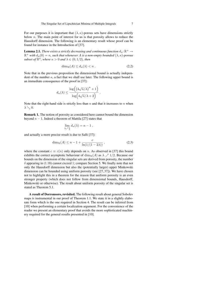
For our purposes it is important that (λ, κ)-porous sets have dimensions strictlybelow n. The main point of interest for us is that porosity allows to reduce theHausdorff dimension. The following is an elementary result whose proof can befound for instance in the Introduction of [37].
Lemma 2.1. There exists a strictly decreasing and continuous function dn:R+ →R+ with dn(0) = n, such that whenever A is a non-empty bounded (λ, κ)-poroussubset of Rn, where κ > 0 and λ ∈ (0, 1/2), then
dimH(A) ≤ dn(λ) < n . (2.2)
Note that in the previous proposition the dimensional bound is actually indepen-dent of the number κ, a fact that we shall use later. The following upper bound isan immediate consequence of the proof in [37]:
dn(λ) ≤log
((4√
n/λ)n + 1
)
log(4√
n/λ + 2) .
Note that the right-hand side is strictly less than n and that it increases to n whenλ 0.
Remark 1. The notion of porosity as considered here cannot bound the dimensionbeyond n− 1. Indeed a theorem of Mattila [27] states that
limλ 1
2
dn(λ) = n− 1 ,
and actually a more precise result is due to Salli [37]:
dimH(A) ≤ n− 1 +c
ln(1/(1− 2λ)), (2.3)
where the constant c ≡ c(n) only depends on n. As observed in [37] this boundexhibits the correct asymptotic behaviour of dimH(A) as λ 1/2. Because ourbounds on the dimension of the singular sets are derived from porosity, the numberδ appearing in (1.18) cannot exceed 1; compare Section 5. We finally note that notonly the Hausdorff dimension but also the (potentially larger) upper Minkowskidimension can be bounded using uniform porosity (see [27,37]). We have chosennot to highlight this in a theorem for the reason that uniform porosity is an evenstronger property (which does not follow from dimensional bounds, Hausdorff,Minkowski or otherwise). The result about uniform porosity of the singular set isstated as Theorem 5.1.
A result of Dorronsoro, revisited. The following result about general Sobolevmaps is instrumental in our proof of Theorem 1.1. We state it in a slightly elabo-rate form which is the one required in Section 4. The result can be inferred from[10] when performing a certain localization argument. For the convenience of thereader we present an elementary proof that avoids the more sophisticated machin-ery required for the general results presented in [10].

8 JAN KRISTENSEN & GIUSEPPE MINGIONE
Lemma 2.2. There exists a constant c ≡ c(n) depending only on n such that forany ball B(x0, 2R) ⊂ Rn and any w ∈ W 1,2(B(x0, 2R),RN ) the inequality
∫
B(x0,R)
∫ R
0
−∫
B(x,r)
∣∣∣∣w(y)− (w)x,r − (Dw)x,r(y − x)
r
∣∣∣∣2
dydr
rdx
≤ c
∫
B(x0,2R)
|Dw|2 dx (2.4)
holds.
Proof. We start the proof with some simplifications. First, by considering the map
w(y) :=1R
w(x0 + Ry), y ∈ B(0, 2),
instead of w and making appropriate substitutions in (2.4) we see that it sufficesto consider the case where x0 = 0 and R = 1. Next, as (2.4) remains unchangedunder translations w 7→ w + k we may also assume that
(w)0,2 = 0. (2.5)
For notational convenience we write B for B(0, 1) and rB for B(0, r) in the fol-lowing. Let ρ:Rn → [0, 1] be a C1 cut-off function verifying
ρ ≡ 1 on 2B, ρ ≡ 0 on Rn \ (3B) and |Dρ| ≤ 2.
Define
v(x) :=
w(x) if x ∈ 2B
w(
2x|x|2
)ρ(x) if x ∈ Rn \ (2B).
Then w ∈ W 1,2(Rn,RN ) is supported in 3B and since for |x| > 2,
Dv(x) = Dw( 2x
|x|2)2
Id|x|2 − 2x⊗ x
|x|4 ρ(x) + w( 2x
|x|2)⊗Dρ(x),
where Id denotes the n×n identity matrix and⊗ denotes the vector tensor product,we find after a routine estimation
∫
Rn\(2B)
|Dv|2 dx ≤ c
∫
2B
(|w|2 + |Dw|2
)dx .
In view of (2.5) Poincare’s inequality yields∫2B|w|2dx ≤ c
∫2B|Dw|2dx so we
arrive at ∫
Rn
|Dv|2 dx ≤ c
∫
2B
|Dw|2 dx , (2.6)

The Singular Set of Lipschitzian Minima of Multiple Integrals 9
where c ≡ c(n). Now∫
B
∫ 1
0
−∫
B(x,r)
|w(y)− (w)x,r − (Dw)x,r(y − x)|2 dydr
r3dx
≤∫
Rn
∫ ∞
0
−∫
B(x,r)
|v(y)− (v)x,r − (Dv)x,r(y − x)|2 dydr
r3dx
=∫ ∞
0
−∫
rB
∫
Rn
|v(x + y)− (v)x,r − (Dv)x,ry|2 dx dydr
r3,
where in the last equality we changed variables and integration orders. For eachfixed r > 0 and y ∈ rB the map x ∈ Rn 7→ v(x + y) − (v)x,r − (Dv)x,ry issquare integrable. Recall that the Fourier transformation on L2 is defined as
h(ξ) := limk→∞
1(2π)
n2
∫
|x|≤k
h(x)e−ix·ξ dx,
where the convergence is in the L2-sense. Hence by Plancherel’s theorem andfurther elementary properties of the Fourier transform we have
∫ ∞
0
−∫
rB
∫
Rn
|v(x + y)− (v)x,r − (Dv)x,ry|2 dx dydr
r3
=∫ ∞
0
−∫
rB
∫
Rn
∣∣∣v(ξ)eiy·ξ − −∫
rB
v(ξ)eiz·ξ dz
− −∫
rB
v(ξ)⊗ (iξ)eiz·ξ dz · y∣∣∣2
dξ dydr
r3
=∫
Rn
m(ξ)|ξ|2|v(ξ)|2 dξ,
where
m(ξ) :=1|ξ|2
∫ ∞
0
−∫
B
∣∣∣∣eiy·rξ − −∫
B
eiz·rξ dz − iy · rξ −∫
B
eiz·rξ dz
∣∣∣∣2
dydr
r3.
We assert that this multiplier is in fact a (finite) constant: m(ξ) ≡ m0 for all ξ 6= 0.This will be obvious once we have shown that m(ξ) is finite and well-defined forall ξ 6= 0. To this end we start with the observation
−∫
B
eiz·rξ dz =c
(r|ξ|)n2
Jn2(r|ξ|)
where Jn2
denotes the Bessel function of the first kind of order n/2 and c ≡ c(n)is a constant that only depends on n. Hence by standard properties of Bessel func-tions we get for some (new) constant c ≡ c(n) that
∣∣∣∣−∫
B
eiz·rξ dz − 1∣∣∣∣ ≤ cr2|ξ|2 for r|ξ| ≤ 1 (2.7)
and ∣∣∣∣−∫
B
eiz·rξ dz
∣∣∣∣ ≤c
(r|ξ|)n+12
for r|ξ| ≥ 1. (2.8)

10 JAN KRISTENSEN & GIUSEPPE MINGIONE
Consequently, by splitting the r-integral in the expression for m(ξ) as
|ξ|2m(ξ) =∫ ∞
0
(. . .
)dr
r3=
∫ 1|ξ|
0
(. . .
)dr
r3+
∫ ∞
1|ξ|
(. . .
)dr
r3, (2.9)
using the inequalities
∣∣∣∣eiy·rξ − −∫
B
eiz·rξ dz − iy · rξ −∫
B
eiz·rξ dz
∣∣∣∣2
≤ 2∣∣eiy·rξ − 1− iy · rξ
∣∣∣2
+2|1 + iy · rξ|2∣∣∣∣−∫
B
eiz·rξ dz − 1∣∣∣∣2
,
|eiy·rξ − 1− iy · rξ| ≤ cr2|ξ|2 (|y| ≤ 1 and r|ξ| ≤ 1),
and (2.7) on the first integral in (2.9), and the inequality
∣∣∣∣eiy·rξ − −∫
B
eiz·rξ dz − iy · rξ −∫
B
eiz·rξ dz
∣∣∣∣2
≤ 2 + 2∣∣∣∣−∫
B
eiz·rξ dz
∣∣∣∣2
(r|ξ|)2
and (2.8) on the second integral in (2.9), we get
supξ|m(ξ)| ≤ c(n) < ∞.
Now we can check that m(Oξ) = m(ξ) and m(tξ) = m(ξ) for all orthogonalmatrices O ∈ O(n), numbers t > 0 and ξ 6= 0 by making the appropriate substitu-tions in the integral defining m. The multiplier m is therefore constant as asserted.The proof is concluded by use of Plancherel’s theorem and (2.6).
3. An ε-regularity result
In the remainder of the paper, unless mentioned otherwise, instead of merelyconsidering minimizers, we shall consider the more general ω-minimizers. Theseintervene in many contexts when dealing with regularity problems in the Calculusof Variations [20,8,13,23].
Definition 3. A map u ∈ W 1,p(Ω,RN ) is an ω-minimizer of the functional F ifand only if
∫
BR
F (x, u(x), Du(x)) dx ≤ [1 + ω(R2)]∫
BR
F (x, v(x), Dv(x)) dx (3.1)
for any v ∈ W 1,p(BR,RN ) such that u − v ∈ W 1,p0 (BR,RN ), where ω:R+ →
R+ is a non-decreasing, concave function satisfying ω(0) = 0, and BR ⊂⊂ Ω isan arbitrary ball with radius R.

The Singular Set of Lipschitzian Minima of Multiple Integrals 11
For notational convenience we used the function ω from (1.6) also in (3.1). Itwill however be clear from the proof that different choices are possible as well.Of course, a minimizer is also an ω-minimizer (with ω ≡ 0), while ω-minimaenjoy the same partial regularity properties of minima described in Section 1 whenassuming (1.10) for some α > 0, see [20,13,23].
In the sequel we refer to points in Ωu (defined at (1.12)) as regular points ofthe fixed ω-minimizer u of the functional F . The main result of this section is anintegral characterization of such points, stated as Proposition 3.2 below. As the spe-cialist will realize, the result is not really new; rather it is a careful re-reading/re-adjustment of the proof of Proposition 9.3 in [20] under the additional assumptionthat the ω-minimizer is Lipschitz continuous. We follow the proof given in [20](which in turn is taken from [18]) mainly for two reasons. First, we want a goodestimate of the constant δ in Theorem 1.1, so we have to keep control of all theconstants appearing in the estimates, that is, we have to refer to a direct proof ofpartial regularity of ω-minimizers (not involving indirect arguments such as theblow-up technique [2,14], the A-harmonic approximation [13], etc.). Second, thedirect proof of [20] provides a decay estimate that allows us to use in an optimaland direct way our Lipschitz regularity assumption. However, the proof in [20,18] is unfortunately affected by a few inaccuracies, detectable in Theorem 9.1 andTheorem 9.5 from [20]. We shall briefly sketch how to amend these and simulta-neously take the opportunity to put certain estimates in a particular form that weneed later (in particular, the Caccioppoli inequality in Proposition 3.1 below).
Following the exposition in [20] the computations are conveniently carried outin terms of the auxiliary map
V (z) := (1 + |z|2) p−24 z , z ∈ RN×n . (3.2)
The corresponding excess functional is then
E(x0, R) := −∫
B(x0,R)
|V (Du(x))− V ((Du)x0,R)|2 dx . (3.3)
However, in view of the inequalities
c−1(1+|z1|2+|z2|2
) p−22 ≤ |V (z2)− V (z1)|2
|z2 − z1|2 ≤ c(1+|z1|2+|z2|2
) p−22
(3.4)
that are valid for all matrices z1, z2 ∈ RN×n, where c = c(n,N, p) is a constant,see Chapter 9 of [20] (or [21]), it is easily seen that for Lipschitzian maps u theexcess in (3.3) is equivalent to
H(x0, R) := −∫
B(x0,R)
|Du(x)− (Du)x0,R|2 dx . (3.5)
More precisely, for each u ∈ W 1,∞(Ω,RN ) we have for all balls B(x0, R) ⊂ Ωthat
c−1E(x0, R) ≤ H(x0, R) ≤ cE(x0, R), (3.6)for some constant c = c(n,N, p, ‖u‖W 1,∞). We start with the following Cacciop-poli type inequality (following the terminology of [20], a “Caccioppoli inequalityof the second kind”):

12 JAN KRISTENSEN & GIUSEPPE MINGIONE
Proposition 3.1. Let u ∈ W 1,p(Ω,RN ) be an ω-minimizer of the functionalF un-der the assumptions (1.3)-(1.10). For every polynomial map a(x) := u0 + 〈z0, x−x0〉, with u0 ∈ RN , z0 ∈ RN×n such that |u0| + |z0| ≤ M/2 for some M > 0,and every ball B(x0, 2R) ⊂ Ω, we have
∫
B(x0,R)
(|Du−Da|2 + |Du−Da|p
)dx (3.7)
≤ c
R2
∫
B(x0,2R)
|u− a|2 dx +c
Rp
∫
B(x0,2R)
|u− a|p dx
+c
∫
B(x0,2R)
[ω(4R2) + θ
(|u0|, 4R2 + |u− u0|2
)](1 + |Du|p) dx,
where the constant c only depends on n, N , p, ν, L, L, G(M) and M .
Proof. Let us set, for any z ∈ RN×n
g(z) := F (x0, u0, z0 + z)− F (x0, u0, z0)− 〈Fz(x0, u0, z0), z〉 ,
and w(x) := u(x) − a(x). Then, with B(x0, s) ≡ Bs, and using mean valuetheorem as in [2], we find a constant c ≡ c(n,N, p, L,G(M)) > 0 such that
g(z) ≤ cMp−2|V (z)|2 (3.8)
and, using quasiconvexity of F ,
ν
∫
Bs
|V (Dϕ)|2 dx ≤∫
Bs
g(Dϕ) dx (3.9)
for any ϕ ∈ C∞c (Bs,RN ) . Moreover we have∫
Bs
g(Dw) dx ≤∫
Bs
g(Dw + Dϕ) dx (3.10)
+c
∫
Bs
[ω(4R2) + θ
(|u0|, 4R2 + |u− u0|2
)](1 + |Du|p + |Dϕ|p) dx ,
for every s ≤ 2R, and ϕ ∈ C∞c (Bs,RN ), while c depends here on n,N, p, L, L.In order to prove the previous inequality we use (3.1) and the very definition of wto compute
∫
Bs
g(Dw) dx
=∫
Bs
[F (x, u, Du)− F (x0, u0, z0)− 〈Fz(x0, u0, z0), Dw〉] dx
+∫
Bs
[F (x0, u0, Du)− F (x, u,Du)
]dx
≤∫
Bs
[F (x, u, Du + Dϕ)− F (x0, u0, z0)− 〈Fz(x0, u0, z0), Dw + Dϕ〉] dx

The Singular Set of Lipschitzian Minima of Multiple Integrals 13
+ω(4s2)∫
Bs
F (x, u, Du + Dϕ) dx
+∫
Bs
[F (x0, u0, Du)− F (x, u,Du)
]dx
≤∫
Bs
g(Dw + Dϕ) dx + cω(4R2)∫
Bs
(1 + |Du|p + |Dϕ|p) dx
+∫
Bs
[F (x0, u0, Du)− F (x, u,Du)
]dx
+∫
Bs
[F (x, u, Du + Dϕ)− F (x0, u0, Du + Dϕ)
]dx
and then (3.10) follows by estimating the last two integrals by mean of (1.6) andusing the properties of θ. Now let us take R < t < s < 2R, and let η ∈ C∞c (Bs)be a cut-off function such that η ≡ 1 on Bt, and |Dη| ≤ 4/(s − t). Let us setφ1 := ηw and φ2 := (1− η)w, so that Dφ1 + Dφ2 = Dw. Then using first (3.9),and then (3.10), we have
ν
∫
Bs
|V (Dφ1)|2 dx ≤∫
Bs
g(Dφ1) dx =∫
Bs
g(Dw −Dφ2) dx
=∫
Bs
g(Dw) dx +∫
Bs
[g(Dw −Dφ2)− g(Dw)
]dx
≤∫
Bs\Bt
g(Dφ2) dx +∫
Bs\Bt
[g(Dw −Dφ2)− g(Dw)
]dx
+c(M)∫
Bs
[ω(4R2) + θ
(|u0|, 4R2 + |u− u0|2
)](1 + |Du|p) dx ,
where we used (3.10), and, at the end, the fact that |Dφ1|p ≤ c(|Du|p + |z0|p) ≤c(M)
(1 + |Du|p). Using (3.8) and the fact that |V (z)|2 ≈ |z|2 + |z|p, we easily
get
∫
Bt
|V (Dw)|2 dx ≤ c
∫
Bs\Bt
|V (Dw)|2 dx + c
∫
Bs
∣∣∣∣w
s− t
∣∣∣∣2
+∣∣∣∣
w
s− t
∣∣∣∣p
dx
+c
∫
Bs
[ω(4R2) + θ
(|u0|, 4R2 + |u− u0|2
)](1 + |Du|p) dx .
The assertion now easily follows by “filling the hole”, that is adding the quantityc∫
Bt|V (Dw)|2 dx to both sides of the previous inequality, and then applying a
standard iteration lemma, i.e. Lemma 6.1 from [20]. See [2] for further details. Insuch a proof, all the constants can be estimated explicitly in terms of the data.
Remark 2. Let us assume p = 2, and let us deal with genuine minimizers. By acareful examination of the previous proof, and especially the derivation of (3.8), itfollows that in the case F ≡ F (z), and assuming a growth condition of the type
|Fzz(z)| ≤ L (3.11)

14 JAN KRISTENSEN & GIUSEPPE MINGIONE
we can replace (3.7) by
∫
B(x0,R)
|Du−Da|2 dx ≤ c
R2
∫
B(x0,2R)
|u− a|2 dx , (3.12)
where the constant c only depends on n,N, ν, L.
Under the assumptions of the previous proposition, using inequality (3.7), and ar-guing as in the proof of Theorem 9.5 from [20] with minor technical modifications,we arrive at the following reverse Holder inequality, valid for any ball B2R ⊂⊂ Ω,and for any z0 ∈ RN×n:
(−∫
BR
|V (Du)− V (z0)|2q dx
) 1q
≤ c −∫
B2R
|V (Du)− V (z0)|2 dx (3.13)
+cRµ
(−∫
B2R
(1 + |Du|p) dx
)s+ µp
.
Here the constants c and q > 1 depend on n,N, ν, L, L,G(M) and M , with |z0| ≤M , and
µ =α
2
(1− 1
q
)> 0 . (3.14)
The number s > 1 is the higher integrability exponent appearing in (1.16). Con-cerning the dependence of q we have
limM∞
q(M) = 1 q ∈ (1, s) . (3.15)
With (3.13) in our hands the proof of Proposition 9.3 from [20] can be carriedout; there the exponent r must be substituted by q defined in (3.13), while µ is thenumber defined at (3.14). Proposition 9.3 from [20] is all that we need to go on inthe following:
Proposition 3.2. Let u ∈ W 1,∞(Ω,RN ) be an ω-minimizer of the functional F ,under the assumptions (1.3)-(1.10). Then there exists a positive, universal constantε > 0, depending only on n,N, p, ν, L, L, ‖u‖W 1,∞ , the modulus of continuityγ(·) in (1.8), and the function G(·) in (1.9), but otherwise independent of u, of theexponent α, and of the integrand F , such that a point x0 ∈ Ω is regular if andonly if there exists a radius R > 0 such that B(x0, 2R) ⊂⊂ Ω and
−∫
B(x0,2R)
|Du(x)− (Du)x0,2R|2 dx < ε . (3.16)
The constant ε is in particular independent of x0.

The Singular Set of Lipschitzian Minima of Multiple Integrals 15
Proof. We start by recalling the result of Proposition 9.3 from [20], describing itin some detail. Given R > 0 such that B(x0, 2R) ⊂⊂ Ω, we have the followinginequality, valid for any 0 < % < R, β > 1, and any σ > 0:
E(x0, %) ≤ A
( %
R
)2
+(
R
%
)n
× (3.17)
×[σ +
c(σ)β2
+ c(σ)χ(E(x0, 2R))]
E(x0, 2R) + H
(R
%
)n
Rµ .
Such result holds for W 1,p-ω-minimizers, without requiring their Lipschitz regu-larity. In the previous inequality we have that
A ≡ A(n, N, p, ν, L, L, |(u)x0,R|+ |(Du)x0,R|
),
is a computable, non-decreasing function of any of its arguments. The expressionc(σ) is such that
limσ0
c(σ) = ∞ ,
and it is bounded on the intervals [a,∞) for each fixed a > 0. The function χ alsodepends on β, and is defined as follows:
χ(E(x0, 2R)) ≡ χ(|(u)x0,R|+ |(Du)x0,R|+ β, E(x0, 2R)
)
≡ γ(|(u)x0,R|+ 2|(Du)x0,R|+ β,E(x0, 2R)
)1− 1q
+E(x0, 2R)1−1q . (3.18)
The number µ is defined in (3.14), while the exponent q > 1 is the one appearing(3.13), when applied with z0 := (Du)x0,R. Recall that The function γ(·) is thelocal modulus of continuity defined at (1.8). Therefore, χ is also an increasingfunction of each of its arguments. The function H is
H ≡ H(n,N, p, ν, L, L, |(u)x0,R|+ |(Du)x0,R|+ E(x0, 2R)
),
and it is also an increasing function. Note that the functions A,H and χ dependon the quantity |(u)x0,R| + |(Du)x0,R| also via G(|(u)x0,R| + |(Du)x0,R|), andwithout loss of generality we may suppose that G(·) is a non-decreasing function.We can now start with the proof, which relies on (3.17), and is a variant of thestandard iteration argument used in partial regularity proofs. We make essentialuse of the Lipschitz continuity of u, and start by setting
M := ‖u‖L∞(Ω) + 3(1 + ‖Du‖2L∞(Ω)
) p2
. (3.19)
As a first consequence we have that the number q in (3.13) is uniformly boundedaway from 1 when x0 and R vary, see (3.15); accordingly to (3.14) µ stays uni-formly bounded away from 0. Therefore, we can consider the values of q > 1 and

16 JAN KRISTENSEN & GIUSEPPE MINGIONE
µ > 0 fixed for the rest of the proof, independently of the point x0 ∈ Ω, and theradius R > 0; their dependence is exactly as the one explained in the statementfor the number ε. Now, E(x0, 2R) ≤ M , and hence for any possible point x0, andradius R, we have that
A + H ≤ A(n,N, p, ν, L, L,M) + H(n,N, p, ν, L, L,M) =: A0 + H0 .
Similarly, we have
χ(E(x0, 2R)) ≤[γ(M + β,E(x0, 2R)
)]1− 1q
+ [E(x0, 2R)]1−1q
=: χ0(β,E(x0, 2R)) (3.20)
Merging the last two inequalities with (3.17) yields
E(x0, %) ≤ A0
( %
R
)2
+(
R
%
)n
×
×[σ +
c(σ)β2
+ c(σ)χ0(β, E(x0, 2R))]
E(x0, 2R)
+H0
(R
%
)n
Rµ . (3.21)
Now, we observe that
E(x0, 2R) ≤ c(n, p) −∫
B(x0,2R)
(1 + |Du(x)|2 + |(Du)x0,2R|2
) p−22 ×
×|Du− (Du)x0,2R|2 dx
≤ c(n, p)M −∫
B(x0,2R)
|Du− (Du)x0,2R|2 dx . (3.22)
At this point we can conclude in a standard way. We start taking a number τ ≡τ(n, N, p, ν, L, L,M,G(M)) ∈ (0, 1) small enough in order to have
τ1/2A0 ≤ 14
. (3.23)
Next, insert % := τR in (3.21), to get, after an elementary estimation,
E(x0, τR) ≤
14τ3/2 +
14τ−n−1/2 ×
×[σ +
c(σ)β2
+ c(σ)χ0(β,E(x0, 2R))]
E(x0, 2R)
+H0τ−nRµ . (3.24)

The Singular Set of Lipschitzian Minima of Multiple Integrals 17
Taking into account the dependence upon the various quantities in τ , we take σ ≡σ(n,N, p, ν, L, L,M, G(M)) = τn+2/3 > 0. In turn this determines c(σ) ≡c(n, N, p, ν, L, L,M,G(M)) < ∞; then we choose
β ≡ β(n,N, p, ν, L, L,M, G(M)) :=
√3c(σ)τn+2
< ∞ .
Finally we are ready to choose ε appearing in the statement of the proposition;it is at this point that the dependence on the continuity modulus γ(·) from (1.8)appears. Using (3.16), keeping in mind (3.22), the dependence upon the variousconstants in c(σ) and τ , and the definition of χ0 given in (3.20), we take ε ≡ε(n,N, p, ν, L, L, M, G(M), γ(·)) > 0 such that
χ0(β, c(n, p)Mε) <τn+2
3c(σ), (3.25)
where c(n, p) is the constant appearing in (3.22). With these choices (3.24) can berecast as
E(x0, τR) ≤ τ3/2
2E(x0, R) + BRµ ,
and B ≡ B(τ) ≡ B(n,N, p, ν, L, L,M, G(M)) is an absolute constant. Observethat E(x0, t) ≤ τ−nE(x0, τ
kR), whenever t ∈ (τk+1R, τkR), for every k ∈N. Therefore, assuming with no loss of generality that µ ≤ 3/2, we may applyLemma 7.3 from [20] with the choice ϕ(t) := E(x0, t), whereby
E(x0, %) ≤ C( %
R
)µ
E(x0, R) + CB%µ , (3.26)
for a constant C that only depends on n,N, p, ν, L, L, ‖u‖W 1,∞ , the modulus ofcontinuity γ(·) and the growth function G(·); in particular, it is independent of thepoint x0. It is clear from the above proof that (3.26) holds as soon as (3.16) does,for the choice of ε made in (3.25). In turn, by continuity, if (3.16) holds at x0, thenit holds for all points in a small ball B(x0, r), and therefore so does (3.26). At thisstage we may refer to a well-known integral characterization of Holder continuitydue to Campanato and Meyers (see Theorem 2.9 and Chapter 9 of [20]) to deducethat Du is Holder continuous with exponent µ/2 in B(x0, r/2); x0 is therefore aregular point and the proof is concluded.
Remark 3. As also observed at the beginning of the section, in the previous proofall the constants can be bounded explicitly in terms of the data by carefully keep-ing track of the various estimates involved; therefore also the constant ε can bebounded explicitly in the terms of the data, and this will finally reflect in the pos-sibility of an explicit bound for the number δ in Theorem 1.1 in terms of the data.
Remark 4. The result of Proposition 3.2 remains true without assuming any a-priori Lipschitz regularity, in the situation considered in Remark 2, and providedcondition (1.8) is strengthened to
|Fzz(z1)− Fzz(z2)| ≤ γ(|z1 − z2|) . (3.27)

18 JAN KRISTENSEN & GIUSEPPE MINGIONE
Here γ:R+ → R+ is a bounded, concave and increasing function such that γ(0) =0. Under these assumptions the number ε appearing in (3.16) depends only onn,N, ν, L and γ(·). The partial regularity proof of minimizers in this case is sim-pler, and it can be found in Paragraph 9.4 from [20], where this model case isconsidered. Other conditions on F (z) are discussed briefly in Section 6.
4. A Carleson condition for the excess
In this section a regularity property for the gradient of an ω-minimizer is es-tablished. It can be viewed as a quantitative version of Lebesgue’s differentiationtheorem, expressed in terms of a Carleson condition. We believe the result couldbe of interest on its own and have therefore highlighted its statement in a theorem.We formulate it in terms of the excess H(x, r) defined in (3.5).
Theorem 4.1. Let u ∈ W 1,∞(Ω,RN ) be an ω-minimizer of the functional F ,under the assumptions (1.3)-(1.10). There exist two constants
C0 = C0(n,N, p, ν, L, L,G(·), ‖u‖W 1,∞), R0 = R0(C0, α), (4.1)
such that for all balls B(x0, 4R) ⊂ Ω with radii R ≤ R0, the inequality
−∫
B(x0,R)
∫ R
0
−∫
B(x,r)
|Du(y)− (Du)x,r|2 dydr
rdx ≤ C0 (4.2)
holds. In particular, C0 is independent of the Holder continuity exponent α in(1.10), and both C0 and R0 are independent of x0 ∈ Ω.
The proof of Theorem 4.1 has two ingredients. The first is Lemma 2.2, whichexpresses a general property of Sobolev maps. The second ingredient is a Cac-cioppoli inequality of the second kind, which is specific to minimizers. In fact, westress that the proof of this Caccioppoli inequality makes essential use of minimal-ity and uniform, strict quasiconvexity.Proof of Theorem 4.1. For a ball B(x, 2r) ⊂ Ω, define the affine map a(y) :=(u)x,2r + (Du)x,2r(y − x) and note that
supB(x,2r)
|u− (u)x,2r| ≤ 2mr, m := ‖u‖W 1,∞ . (4.3)
By the very definition of H in (3.5) we get
H(x, r) ≤ −∫
B(x,r)
|Du−Da|2 dy,
so that, by Proposition 3.1
H(x, r) ≤ −∫
B(x,r)
(|Du−Da|2 + |Du−Da|p) dy
≤ c(m)r2
−∫
B(x,2r)
|u− a|2 dy +c(m)rp
−∫
B(x,2r)
|u− a|p dy
+c(m) −∫
B(x,2r)
[ω(4r2) + θ
(|(u)x,2r|, 4r2 + |u− (u)x,2r|2
)]×
×(1 + |Du|p) dy. (4.4)

The Singular Set of Lipschitzian Minima of Multiple Integrals 19
The constant c, here as in the following, also depends on n,N, ν, L, L. Here wemay estimate
c(m)r2
−∫
B(x,2r)
|u− a|2 dy +c(m)rp
−∫
B(x,2r)
|u− a|p dy
≤ c(m)r2
(1 + (2m)p−2
)−∫
B(x,2r)
|u− a|2 dy
=c(m)r2
−∫
B(x,2r)
|u− a|2 dy
and, recalling that θ(s, t) = min1, %0(s)ω(t), it follows that
c(m) −∫
B(x,2r)
[ω(4r2) + θ
(|(u)x,2r|, 4r2 + |u− (u)x,2r|2
)](1 + |Du|p) dy
≤ c(m)(1 + %0(m)
) −∫
B(x,2r)
ω(4r2 + |u− (u)x,2r|2
)(1 + |Du|p) dy.
Since ω(·) is concave we have, by Jensen’s inequality and (4.3)
−∫
B(x,2r)
ω(4r2 + |u− (u)x,2r|2
)dy
≤ ω
(−∫
B(x,2r)
(4r2 + |u− (u)x,2r|2
)dy
)
≤ ω(4(1 + m2)r2) ≤ ω(c(m)r2) .
Collecting the above estimates we arrive at
H(x, r) ≤ c
r2−∫
B(x,2r)
|u− a|2 dy + cω(cr2) (4.5)
for some constant c = c(n,N, p, ν, L, L, %0,m, G(m)). We remark that the con-stant c in particular is independent of the modulus of continuity ω(·). At this stagewe invoke Lemma 2.2. Fix a ball B(x0, R) with B(x0, 4R) ⊂ Ω. Integrating (4.5)we get
∫
B(x0,R)
∫ R
0
H(x, r)dr
rdx ≤ c
∫ R
0
ω(cr2)dr
r|B(x0, R)|
+c
∫
B(x0,R)
∫ R
0
−∫
B(x,2r)
∣∣∣u(y)− (u)x,2r − (Du)x,2r(y − x)∣∣∣2
dydr
r3dx.
Since∫ R
0
−∫
B(x,2r)
|u(y)− (u)x,2r − (Du)x,2r(y − x)|2 dydr
r3
= 4∫ 2R
0
−∫
B(x,r)
|u(y)− (u)x,2r − (Du)x,2r(y − x)|2 dydr
r3

20 JAN KRISTENSEN & GIUSEPPE MINGIONE
we get by use of Lemma 2.2
∫
B(x0,R)
∫ R
0
H(x, r)dr
rdx ≤ c
∫ R
0
ω(cr2)dr
r|B(x0, R)|
+c
∫
B(x0,4R)
|Du|2 dx
≤(
c
∫ R0
0
ω(cr2)dr
r+ 4ncm2
)|B(x0, R)|.
Under the assumption (1.10) we have
∫ R0
0
ω(cr2)dr
r≤ c
α2
α
(R0
)α
≤ 1, (4.6)
where the last inequality follows taking R0 ≡ R0(c, α) > 0 small enough. Theproof is complete.
Remark 5. We do not need the condition (1.10) on ω(·) to conclude with inequal-ity (4.6). It suffices to have the following Dini condition:
∫
0
ω(r2)r
dr < ∞ . (4.7)
Indeed, under this condition we can still take R0 ≡ R0(c, ω(·)) > 0 such that
∫ R0
0
ω(r2)dr
r=
1√c
∫ √cR0
0
ω(r2)dr
rdr ≤ 1.
This observation opens the way for an extension of our results to elliptic sys-tems and quasiconvex functionals with appropriately Dini-continuous coefficients.Indeed, in such cases it is still possible to prove partial regularity of weak solu-tions/minimizers [11,13,12].
Fix an open subset Ω′ ⊂⊂ Ω, and denote d := dist(Ω′, ∂Ω) > 0. We recallthat a measure µ on Ω′ × [0, d) is called a Carleson measure provided there existconstants c ≡ c(µ(·)) < ∞ and R0 ∈ (0, d/4) such that
µ(B(x,R)× [0, R)) ≤ cRn ∀ R ∈ (0, R0) ∀ x ∈ Ω′ . (4.8)
The result of Theorem 4.1 can be restated in this terminology as
Proposition 4.2. Let u ∈ W 1,∞(Ω,RN ) be an ω-minimizer of the functional Funder the assumptions (1.3)-(1.10). There exist two constants c and R0 (as in(4.1)), such that
H(x, r)dr
rdx
is a Carleson measure in the sense of (4.8).
The Singular Set of Lipschitzian Minima of Multiple Integrals 21
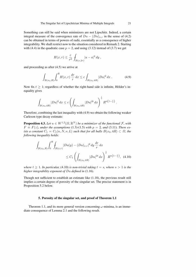
Something can still be said when minimizers are not Lipschitz. Indeed, a certainintegral measure of the convergence rate of Du − (Du)x,r in the sense of (4.2)can be obtained in terms of powers of radii, essentially as a consequence of higherintegrability. We shall restrict now to the situation considered in Remark 2. Startingwith (4.4) in the quadratic case p = 2, and using (3.12) instead of (3.7) we get
H(x, r) ≤ c
r2−∫
B(x,2r)
|u− a|2 dy ,
and proceeding as after (4.5) we arrive at
∫
B(x0,R)
∫ R
0
H(x, r)dr
rdx ≤ c
∫
B(x0,4R)
|Du|2 dx . (4.9)
Now fix t ≥ 1; regardless of whether the right-hand side is infinite, Holder’s in-equality gives
∫
B(x0,4R)
|Du|2 dx ≤ c
(∫
B(x0,4R)
|Du|2t dx
) 1t
Rn(1− 1t ) .
Therefore, combining the last inequality with (4.9) we obtain the following weakerCarleson type decay estimate:
Proposition 4.3. Let u ∈ W 1,2(Ω,RN ) be a minimizer of the functional F , withF ≡ F (z), under the assumptions (1.3)-(1.5) with p = 2, and (3.11). There ex-ists a constant C1 = C1(n,N, ν, L) such that for all balls B(x0, 4R) ⊂ Ω, thefollowing inequality holds:
∫
B(x0,R)
∫ R
0
−∫
B(x,r)
|Du(y)− (Du)x,r|2 dydr
rdx
≤ C1
(∫
B(x0,4R)
|Du|2t dx
) 1t
Rn(1− 1t ), (4.10)
where t ≥ 1. In particular, (4.10) is non-trivial taking t = s, where s > 1 is thehigher integrability exponent of Du defined in (1.16).
Though not sufficient to establish an estimate like (1.18), the previous result stillimplies a certain degree of porosity of the singular set. The precise statement is inProposition 5.2 below.
5. Porosity of the singular set, and proof of Theorem 1.1
Theorem 1.1, and its more general version concerning ω-minima, is an imme-diate consequence of Lemma 2.1 and the following result.

22 JAN KRISTENSEN & GIUSEPPE MINGIONE
Theorem 5.1. Let u ∈ W 1,∞(Ω,RN ) be an ω-minimizer of the functional F un-der the assumptions (1.3)-(1.10). Then there exists a number
λ = λ(n,N, p, ν, L, L, γ(·), G(·), %0(·), ‖u‖W 1,∞) ∈ (0, 1/2) (5.1)
such that for each Ω′ ⊂⊂ Ω there is a κ > 0 for which Ω′ ∩Σu is (λ, κ)-porous.
Proof. The proof is based on Proposition 3.2 and Theorem 4.1. Fix Ω′ ⊂⊂ Ω andlet A := Ω′ ∩Σu. Define
κ :=18
mindist(Ω′, ∂Ω), R0, (5.2)
where R0 > 0 is defined in Theorem 4.1. Let x0 ∈ Rn and note that
dist(x0, Ω′) ≥ dist(Ω′, ∂Ω)
8=⇒ p(A, x0, R) ≥ R/2 if R ∈ (0, κ] ,
since, trivially, B(x0, R/2) ∩ Ω′ = ∅. Hence for the rest of the proof we mayassume without loss of generality that dist(x0, Ω
′) < dist(Ω′, ∂Ω)/8. In thissituation B(x0, 4R) ⊂ Ω when R ≤ κ, so by virtue of Theorem 4.1,
∫
B(x0,R)
∫ R
0
H(x, r)dr
rdx ≤ C0|B(x0, R)|, (5.3)
where H(x, r) is the excess defined in (3.5). For each Λ ∈ (0, 1) we consider theset
E := x ∈ B(x0, R/2) : infΛR<r<R
H(x, r) ≥ 2−nε,where the number ε > 0 is defined in Proposition 3.2. By routine estimations
|E| ε
2nln
1Λ≤
∫
E
∫ R
ΛR
H(x, r)dr
rdx ≤ C0|B(x0, R)| (5.4)
and thus|E|
|B(x0, R/2)| ≤22nC0
ε ln 1Λ
.
If therefore we take
Λ := exp(−22n+1C0
ε
), (5.5)
then |E|/|B(x0, R/2)| ≤ 1/2 and it follows that we can find x ∈ B(x0, R/2)\E,that is, x ∈ B(x0, R/2) and H(x, r) < 2−nε for some r ∈ (ΛR, R). Now ifx′ ∈ B(x, r/2) ⊂ B(x0, R), then B(x′, r/2) ⊂ B(x, r) and
H(x′, r/2) ≤ −∫
B(x′, r2 )
|Du− (Du)x,r|2 dy ≤ 2nH(x, r) < ε,
and therefore any such x′ is a regular point by virtue of Proposition 3.2; as a conse-quence we have B(x, r/2)∩Σu = ∅. To conclude the proof we take λ := Λ/2, andnote that then B(x, λR) ⊂ B(x, r/2) ⊂ B(x0, R) \ A, that is p(A, x0, R) ≥ λRfor R ∈ (0, κ], and the (λ, κ)-porosity follows. Note that by (5.5) the dependenceon the various parameters of Λ is inherited by the ones of ε and C0; this impliesthe dependence stated in (5.1).

The Singular Set of Lipschitzian Minima of Multiple Integrals 23
In the general case where minimizers are not assumed to be Lipschitz continuousthe singular set turns out to be non-uniformly porous in the sense of Definition 2;we shall see this under the assumptions of Remarks 2 and 4.
Proposition 5.2. Let u ∈ W 1,2(Ω,RN ) be a minimizer of the functional F , withF ≡ F (z), under the assumptions (1.3)-(1.5) with p = 2, (3.11), and (3.27). Forevery Ω′ ⊂⊂ Ω there is a κ > 0 for which Ω′ ∩Σu is (m(·), κ)-porous, where
m(r) :=12
exp(−C2
rns
), (5.6)
the number C2 is a constant depending only on n, N, ν, L, γ(·), and where s is theone from (1.16). Moreover, in (5.6) the exponent s can be replaced by any t > 1such that Du ∈ L2t
loc(Ω,RN×n).
The significance of the previous result is clarified by the following observation:whenever B(x0, R) ⊂⊂ Ω is a ball, by Lebesgue’s differentiation theorem it isalways possible to find a smaller ball B(x′, λR) ⊂ B(x0, R) such that H(x′, λR)is small enough and, consequently, B(x′, λR/2) ⊂ Ω \ Σu. On the other hand,there is no a-priori lower bound on the size of λ. Proposition 5.2 provides sucha bound in terms of the function m(·), and on the structural data n,N, ν, L, γ(·).This is another, weaker and geometric way to say that the singular set is small.Also note that the integrability properties of the gradient play a relevant role inthis situation, exactly as in the convex case (see [24]).Proof of Proposition 5.2. We follow the proof and the notation of Theorem 5.1.Instead of using Theorem 4.1, we use Proposition 4.3, and instead of (5.3) we find
∫
B(x0,R)
∫ R
0
H(x, r)dr
rdx ≤ C1
ωn|B(x0, R)|1− 1
s , (5.7)
where s appears in (1.16), and C1 in Proposition 4.3. Estimating as in (5.4), anddenoting ωn := |B(0, 1)|, we get
|E||B(x0, R/2)| ≤
22nC1
ωnε ln 1Λ |B(x0, R)| 1s .
We can conclude again that |E|/|B(x0, R/2)| ≤ 1/2 provided this time we take
Λ(R) := exp(−22n+1C1
ω2nεR
ns
). (5.8)
The rest of the proof follows exactly as for Theorem 5.1, just taking
C2 :=22n+1C1
ω2nε
and keeping into account of the dependence on the parameters of C1 stated inProposition 4.3, and of the number ε, stated in Remark 4. Also observe that thenumber κ can be just defined as κ := 1/8dist(Ω′, ∂Ω).

24 JAN KRISTENSEN & GIUSEPPE MINGIONE
6. Additional results
6.1. Asymptotically regular integrands
For certain classes of quasiconvex integrals, where the integrand F (x, y, z) ≡F (z) has a sufficiently regular behaviour for large values of |z|, ω-minimizers areautomatically locally Lipschitz. In the case of minima, this has been first pointedout by Chipot & Evans in [5] when p = 2, and subsequently extended by Raymondin [35] to the cases p > 2 and more general integrands of the form F = F0(z) +a(x, y). More precisely, letting
H(z) := (1 + |z|2)p/2 , (6.1)
the integrand F (z) is assumed to satisfy
lim|z|→∞
|Fzz(z)−Hzz(z)||z|p−2
= 0 . (6.2)
A typical model case is consists of the functionals
v 7→∫
Ω
(1 + |Dv|2) p2 + g(Dv) dx , (6.3)
where g:RN×n → R+ is a C2 and quasiconvex function (not necessarily strictly),such that gzz(z)/|z|p−2 → 0 when |z| → ∞. For such functionals we have localLipschitz continuity of W 1,p-ω-minimizers, and therefore it follows from Theo-rem 1.1 that for every Ω′ ⊂⊂ Ω, there exists a positive number
δ′ ≡ δ′(n, N, p, ν, L, G(·), dist(Ω′, ∂Ω)) > 0 ,
such thatdimH(Σu ∩Ω′) ≤ n− δ′ . (6.4)
Finally, when assuming (6.2), and ∂Ω sufficiently smooth, e.g. C2, minimizing Fin a prescribed Dirichlet class u0 + W 1,p
0 (Ω,RN ), with u0 ∈ C1,β(Ω,RN ) forsome β ∈ (0, 1], that is, solving
minw
∫
Ω
F (Dw(x)) dx
w ∈ u0 + W 1,p0 (Ω,RN×n) ,
we obtain a globally Lipschitz continuous minimizer u ∈ W 1,∞(Ω,RN ). In thiscase estimate (1.18) remains valid with a δ depending only on the “data”, thatis n,N, p, ν, L, L, γ(·), G(·), ∂Ω, ‖u0‖C1,β . For such global regularity results, aswell as for their validity in the case of ω-minima we refer to recent paper by Foss[15]. Observe also that the proofs in [5] are indirect, i.e. they rely on a blow-up argument. Nevertheless, using the direct proofs developed [35] and [15], it ispossible to quantify the constants in the Lipschitz estimates, and therefore onceagain the constant δ in (1.18).

The Singular Set of Lipschitzian Minima of Multiple Integrals 25
We end this brief discussion of Lipschitz estimates with the remark that otherchoices, different from (6.1), are possible too. More precisely, what is required forthe comparison integrand H is that minimizers of
v 7→∫
Ω
H(Dv) dx ,
are fully regular. This is the case, for instance, when H(z) has the so-called “Uh-lenbeck structure”, i.e. H(z) := g(|z|), where the function g:R → R is of classC0(R) ∩ C2(R \ 0) and satisfies suitable growth and monotonicity conditions;see [30], Section 4.7. Another possibility is to use H(z) := |z|p−2〈Az, z〉, whereA is a constant tensor, satisfying 〈Az, z〉 ≥ ν|z|2. When p = 2, this is the originalexample considered in [5]. Another source of examples with this kind of behaviourfor large |z| is [22].
6.2. Quasimonotone systems
The result of Theorem 1.1 also extends to weak solutions of so-called quasi-monotone systems (see [26,40])
div a(x,Du) = 0 , (6.5)
where the vector field a:Ω×RN×n → RN×n is C1 in the last (gradient) variable,and satisfies for some constants 0 < ν < L the growth condition
|a(x, z)| ≤ L(1 + |z|2) p−12 , (6.6)
for all x ∈ Ω, z ∈ RN×n, and the uniform strict quasimonotonicity condition:
ν
∫
(0,1)n
(1 + |Dϕ(x)|2) p−22 |Dϕ(x)|2 dx
≤∫
(0,1)n
〈a(x0, z0 + Dϕ)− a(x0, z0), Dϕ〉 dx , (6.7)
for every x0 ∈ Ω, z0 ∈ RN×n and ϕ ∈ C∞c ((0, 1)n,RN ). The last condition isclearly analogous to (1.5). Finally we assume a Holder continuous dependence onthe coefficient x, that is
|a(x1, z)− a(x2, z)| ≤ L|x1 − x2|α(1 + |z|2) p−12 , (6.8)
for all x1, x2 ∈ Ω, and z ∈ RN×n, where L ≥ 1, and α ∈ (0, 1], and, as for (1.8),and the existence of the modulus of continuity γ:R+ × R+ → R+ as in for (1.8),such that
|az(x, z1)− az(x, z2)| ≤ γ(|z1|+ |z2|, |z1 − z2|) , (6.9)
for every x ∈ Ω and z1, z2 ∈ RN×n. Accordingly to (1.9), we define
G(M) := sup|z|≤M,x∈Ω
|az(x, z)|1 + |z|p−2
, M ≥ 0 . (6.10)

26 JAN KRISTENSEN & GIUSEPPE MINGIONE
A weak solution to (6.5), under the assumption (6.6), is of course a map u ∈W 1,p(Ω,RN×n) such that
∫
Ω
〈a(x,Du), Dϕ〉 dx = 0
for every ϕ ∈ W 1,p0 (Ω,RN ). Under the assumptions (6.6)-(1.8) the partial C1,α-
regularity in the sense of (1.12)-(1.13) of weak solutions to (6.5) has been estab-lished by Hamburger, see Theorem 1.1 from [21], and this time it turns out thatu ∈ C1,α
loc (Ωu,RN ). On the other hand, condition (6.7) is too weak to allow for theapplication of any type of difference quotients method, and therefore no dimensionestimate for the singular sets of weak solutions is available. Nevertheless we have
Theorem 6.1. Let u ∈ W 1,∞(Ω,RN ) be a weak solution to (6.5) under the as-sumptions (6.6)-(6.9), and let Σu := Ω \ Ωu denote its singular set. Then thereexists a positive number δ > 0, depending only on n, N, p, ν, L, L, ‖u‖W 1,∞ , themodulus of continuity γ(·) in (6.9), and the growth function G(·) in (6.10), butotherwise independent of u, of the exponent α, and of the vector field a, such thatdimH(Σu) ≤ n− δ.
The proof of the previous theorem can be obtained by the procedure in Section3, once the analogues of Propositions 3.1 and 3.2 have been established. In turnthis can be done having as a starting point a suitable analog of estimate (3.17),that is estimate (5.1) from [21]. Some remarks; the number δ here is once againexplicitly computable, since the methods in [21] are not indirect. The result ofTheorem 6.1 obviously applies to elliptic systems, that are a particular case ofstrictly quasimonotone systems as considered above, and in some cases improvesthe results in [29], where the second author proved the estimate dimH(Σu) ≤n − 2α. Here, in the case of Lipschitzian solutions the dimension estimate doesnot get lost when α → 0. Moreover, the result of Theorem 6.1 also extends to moregeneral systems of the type div a(x, u, Du) = 0, under the natural assumptionsconsidered in [21]. Finally, restricting to the autonomous case a(x, z) ≡ a(z), theassumption u ∈ W 1,∞(Ω,RN ) considered in the last theorem is automaticallysatisfied assuming the following condition, similar to the one in (6.11):
lim|z|→∞
|az(z)−Kz(z)||z|p−2
= 0 , (6.11)
where this time K(z) = (1 + |z|2)p−2/2z similarly to Subsection 6.1. A typ-ical model example is given by a(z) := (1 + |z|2)(p−2)/2z + b(z), where theC1-vector field b:RN×n → RN×n is quasimonotone and satisfies the conditionbz(z)/|z|p−2 → 0 when |z| → ∞. This follows by use of arguments similarto those applied in the case of functionals. Also for quasimonotone systems wehave a singular set estimate in the interior: we have that given a weak solution to(6.5) u ∈ W 1,p(Ω,RN ), then for every Ω′ ⊂⊂ Ω, there exists a positive numberδ′ > 0 depending on the objects n,N, p, ν, L, L, γ(·), G(·), dist(Ω′, ∂Ω), suchthat dimH(Σu ∩Ω′) ≤ n− δ′. Again, as for the case of functionals one can havedifferent choices for K(z) in (6.11). For instance one can take any vector field

The Singular Set of Lipschitzian Minima of Multiple Integrals 27
K(z) := h(|z|)z, where h satisfies suitable growth and monotonicity conditions;see again [30], Section 4.7.
Another possible extension of our results concerns the so-called W 1,q-localminima (see [25]). Because the Caccioppoli inequality in such cases only has beenestablished in a very weak form the necessary modifications are somewhat moreinvolved and we plan to report on it elsewhere.
References
1. Acerbi E. & Fusco N.: Semicontinuity problems in the calculus of variations. Arch. Ra-tion. Mech. Anal. 86 (1984), 125–145.
2. Acerbi E. & Fusco N.: A regularity theorem for minimizers of quasiconvex integrals.Arch. Ration. Mech. Anal. 99 (1987), 261–281.
3. Ball J.: Convexity conditions and existence theorems in nonlinear elasticity. Arch. Ra-tion. Mech. Anal. 63 (1976/77), 337–403.
4. Bonk M. & Heinonen J.: Smooth quasiregular mappings with branching. Publ. Math.Inst. Hautes Etudes Sci. 100 (2004), 153–170.
5. Chipot M. & Evans L. C.: Linearisation at infinity and Lipschitz estimates for certainproblems in the calculus of variations. Proc. Roy. Soc. Edinburgh Sect. A 102 (1986),291–303.
6. David G. & Semmes S: On the singular sets of minimizers of the Mumford-Shah func-tional. J. Math. Pures Appl. (9) 75 (1996), 299–342.
7. De Giorgi E.: Un esempio di estremali discontinue per un problema variazionale di tipoellittico. Boll. Un. Mat. Ital. (4) 1 (1968), 135–137.
8. Dolcini A. & Esposito L. & Fusco N.: C0,α regularity of ω-minima.Boll. Un. Mat. Ital. A (7) 10 (1996), 113–125.
9. Dolzmann G.: Variational methods for crystalline microstructure — analysis and com-putation. Lecture Notes in Math., 1803. Springer, 2003.
10. Dorronsoro J.R.: A characterization of potential spaces. Proc. Amer. Math. Soc. 95(1985), 21–31.
11. Duzaar F. & Gastel A.: Nonlinear elliptic systems with Dini continuous coefficients.Arch. Math. (Basel) 78 (2002), 58–73.
12. Duzaar F. & Gastel A. & Mingione G.: Elliptic systems, singular sets and Dini conti-nuity. Comm. Partial Differential Equations 29 (2004), 1215–1240.
13. Duzaar F. & Kronz M.: Regularity of ω-minimizers of quasi-convex variational inte-grals with polynomial growth. Differential Geom. Appl. 17 (2002), 139–152.
14. Evans L. C.: Quasiconvexity and partial regularity in the calculus of variations.Arch. Ration. Mech. Anal. 95 (1986), 227–252.
15. Foss M.: Global regularity for almost minimizers of nonconvex variational problems.Preprint 2006.
16. Giaquinta M.: Direct methods for regularity in the calculus of variations. Nonlinearpartial differential equations and their applications. College de France seminar, Vol.VI (Paris, 1982/1983), 258–274, Res. Notes in Math., 109, Pitman, Boston, MA, 1984.
17. Giaquinta M.: The problem of the regularity of minimizers. Proceedings of the Inter-national Congress of Mathematicians, Vol. 1, 2 (Berkeley, Calif., 1986), 1072–1083,Amer. Math. Soc., Providence, RI, 1987.
18. Giaquinta M.: Quasiconvexity, growth conditions and partial regularity. Partial differ-ential equations and calculus of variations. Lecture Notes in Math., 1357, pp. 211–237.Springer, Berlin, 1988.
19. Giaquinta M.: Introduction to regularity theory for nonlinear elliptic systems. Lecturesin Mathematics ETH Zurich. Birkhauser Verlag, Basel, 1993.
20. Giusti E.: Direct methods in the calculus of variations. World Scientific Publishing Co.,Inc., River Edge, NJ, 2003.

28 JAN KRISTENSEN & GIUSEPPE MINGIONE
21. Hamburger C.: Quasimonotonicity, regularity and duality for nonlinear systems of par-tial differential equations. Ann. Mat. Pura Appl. (4) 169 (1995), 321–354.
22. Kohn R. V. & Strang G.: Optimal design and relaxation of variational problems I, II,III. Comm. Pure Appl. Math. 39 (1986), 113–137, 139–182, 353–377.
23. Kristensen J. & Mingione G.: The singular set of ω-minima. Arch. Ration. Mech. Anal.177 (2005), 93–114.
24. Kristensen J. & Mingione G.: The singular set of minima of integral functionals.Arch. Ration. Mech. Anal. 180 (2006), 331–398.
25. Kristensen J. & Taheri A.: Partial regularity of strong local minimizers in the multi-dimensional calculus of variations. Arch. Ration. Mech. Anal. 170 (2003), 63–89.
26. Landes R.: Quasimonotone versus pseudomonotone. Proc. Roy. Soc. Edinb. 126A(1996), 705–717.
27. Mattila P.: Geometry of Sets and Measures in Euclidean Spaces. Cambridge UniversityPress, 1995.
28. Mingione G.: The singular set of solutions to non-differentiable elliptic systems.Arch. Ration. Mech. Anal. 166 (2003), 287–301.
29. Mingione G.: Bounds for the singular set of solutions to non linear elliptic systems.Calc. Var. Partial Differential Equations 18 (2003), 373–400.
30. Mingione G.: Regularity of minima: an invitation to the dark side of the calculus ofvariations. Applications of Mathematics 51 (2006).
31. Morrey C.B.: Quasi-convexity and the lower semicontinuity of multiple integrals. Pa-cific J. Math. 2 (1952), 25–53.
32. Muller S.: Variational models for microstructure and phase transitions. Calculus ofvariations and geometric evolution problems (Cetraro, 1996). Lecture Notes in Math.,1713, pp. 85–210. Springer, 1999.
33. Muller S. & Sverak V.: Convex integration for Lipschitz mappings and counterexam-ples to regularity. Ann. of Math. (2) 157 (2003), 715–742.
34. Necas J.: Example of an irregular solution to a nonlinear elliptic system with analyticcoefficients and conditions for regularity Theory of nonlinear operators (Proc. FourthInternat. Summer School, Acad. Sci., Berlin, 1975), pp. 197–206.
35. Raymond J. P.: Lipschitz regularity of solutions of some asymptotically convex prob-lems. Proc. Roy. Soc. Edinb. 117A (1991), 59–73.
36. Rigot S.: Uniform partial regularity of quasi minimizers for the perimeter.Calc. Var. Partial Differential Equations 10 (2000), 389–406.
37. Salli A.: On the Minkowski dimension of strongly porous fractal sets in Rn. Proc. Lon-don Math. Soc. (3) 62 (1991), 353–372.
38. Sverak V. & Yan X.: Non-Lipschitz minimizers of smooth uniformly convex variationalintegrals. Proc. Natl. Acad. Sci. USA 99/24 (2002), 15269-15276.
39. Szekelyhidi L., Jr.: The regularity of critical points of polyconvex functionals. Arch. Ra-tion. Mech. Anal. 172 (2004), 133–152.
40. Zhang K.: On the Dirichlet problem for a class of quasilinear elliptic systems ofPDEs in divergence form. In: Partial Differential Equations, Proc. Tranjin 1986. Ed.S.S. Chern. Lecture Notes in Math., 1306, pp. 262–277. Springer, 1988.
Mathematical InstituteUniversity of Oxford
24-29 St. Giles’, Oxford OX1 3LBemail:[email protected]
and
Dipartimento di MatematicaUniversita di Parma
Parco Area delle Scienze 53/a, I-43100, Parmaemail:[email protected]