Computational Optimization and Applications, 24, 289–333, 2003c© 2003 Kluwer Academic Publishers. Manufactured in The Netherlands.

The Sample Average Approximation MethodApplied to Stochastic Routing Problems:A Computational Study

BRAM VERWEIJ∗, SHABBIR AHMED† ‡ , ANTON J. KLEYWEGT∗, GEORGE NEMHAUSER∗‡AND ALEXANDER SHAPIRO∗School of Industrial and Systems Engineering, Georgia Institute of Technology, Atlanta, GA 30332-0205, USA

Received August 6, 2001; Revised October 13, 2002; Accepted October 29, 2002

Abstract. The sample average approximation (SAA) method is an approach for solving stochastic optimizationproblems by using Monte Carlo simulation. In this technique the expected objective function of the stochasticproblem is approximated by a sample average estimate derived from a random sample. The resulting sampleaverage approximating problem is then solved by deterministic optimization techniques. The process is repeatedwith different samples to obtain candidate solutions along with statistical estimates of their optimality gaps.

We present a detailed computational study of the application of the SAA method to solve three classes ofstochastic routing problems. These stochastic problems involve an extremely large number of scenarios and first-stage integer variables. For each of the three problem classes, we use decomposition and branch-and-cut to solvethe approximating problem within the SAA scheme. Our computational results indicate that the proposed method issuccessful in solving problems with up to 21694 scenarios to within an estimated 1.0% of optimality. Furthermore,a surprising observation is that the number of optimality cuts required to solve the approximating problem tooptimality does not significantly increase with the size of the sample. Therefore, the observed computation timesneeded to find optimal solutions to the approximating problems grow only linearly with the sample size. As a result,we are able to find provably near-optimal solutions to these difficult stochastic programs using only a moderateamount of computation time.

Keywords: stochastic optimization, stochastic programming, stochastic routing, shortest path, travelingsalesman

1. Introduction

This paper addresses two-stage Stochastic Routing Problems (SRPs), where the first stageconsists of selecting a route, i.e., a path or a tour, through a graph subject to arc failuresor delays, and the second stage involves some recourse, such as a penalty or a re-routingdecision. The overall objective is to minimize the sum of the first-stage routing cost and theexpected recourse cost. A generic formulation of this class of problems is

z∗ = minx∈X

cT x + EP [Q(x, ξ (ω))], (1)

∗Supported by NSF grant DMI-0085723.†Supported by NSF grant DMI-0099726.‡Supported by NSF grant DMI-0121495.

290 VERWEIJ ET AL.

where

Q(x, ξ (ω)) = miny≥0

{q(ω)T y | Dy ≥ h(ω) − T (ω)x}, (2)

x denotes the first-stage routing decision, X denotes the first-stage feasible set involvingroute defining constraints, i.e., X = R ∩ {0, 1}d for some polyhedron R of dimensiond, ω ∈ � denotes a scenario that is unknown when the first-stage decision x has to bemade, but that is known when the second-stage recourse decision y is made, � is the set ofall scenarios, and c denotes the routing cost. We assume that the probability distribution Pon � is known in the first stage. The quantity Q(x, ξ (ω)) represents the optimal value of thesecond-stage recourse problem corresponding to the first-stage route x and the parametersξ (ω) = (q(ω), h(ω), T (ω)). Note that the first-stage variables x are binary in this problem.Hence, SRP belongs to the class of two-stage stochastic programs with integer first-stagevariables.

The difficulty in solving SRP is two-fold. First, the evaluation of E[Q(x, ξ (ω))] for agiven value of x requires the solution of numerous second-stage optimization problems. If� contains a finite number of scenarios {ω1, ω2, . . . , ω|�|}, with associated probabilitiespk, k = 1, 2, . . . , |�|, then the expectation can be evaluated as the finite sum

E[Q(x, ξ (ω))] =|�|∑k=1

pk Q(x, ξ (ωk)). (3)

However, the number of scenarios grows exponentially fast with the dimension of thedata. For example, consider a graph with 100 arcs, each of which has a parameter withthree possible values. This leads to |�| = 3100 scenarios for the parameter vector of thegraph, making a direct application of (3) impractical. Second, E[Q(x, ξ (ω))], regarded as afunction defined on R

d (and not just on the discrete points X = R ∩{0, 1}d ), is a polyhedralfunction of x . Consequently, SRP involves minimizing a piecewise linear objective over aninteger feasible region and can be very difficult, even for problems with a modest numberof scenarios.

Early solution approaches for stochastic routing problems were based on heuristics [35]or dynamic programming [1, 2]. These methods were tailored to very specific problemstructures and are not applicable in general. Exact mathematical programming methods forthis class of problems have mostly been restricted to cases with a small number of scenarios,to allow for the exact evaluation of the second-stage expected value function E[Q(x, ξ (ω))].Exploiting this property, Laporte et al. [18–21] solved various stochastic routing problemsusing the integer L-shaped algorithm of Laporte and Louveaux [17]. Wallace [38–40] hasstudied the exact evaluation of the second-stage expected value function for problems inwhich the first stage feasible set is convex and the second stage involves routing decisions.

For stochastic programs with a prohibitively large number of scenarios, a number ofsampling based approaches have been proposed, for example to estimate function values,gradients, optimality cuts, or bounds for the second-stage expected value function. Weclassify such sampling based approaches into two main groups: interior sampling and ex-terior sampling methods. In interior sampling methods, the samples are modified during

SAMPLE AVERAGE APPROXIMATION METHOD 291

the optimization procedure. Samples may be modified by adding to previously generatedsamples, by taking subsets of previously generated samples, or by generating completelynew samples. For example, methods that modify samples within the L-shaped algorithmfor stochastic linear programming have been suggested by Van Slyke and Wets [36], Higleand Sen [11] (stochastic decomposition) and Infanger [14] (importance sampling). For dis-crete stochastic problems, an interior sampling branch-and-bound method was developedby Norkin et al. [24, 25]. In exterior sampling methods, a sample ω1, ω2, . . . , ωN of Nsample scenarios is generated from � according to probability distribution P (we use thesuperscript convention for sample values), and then a deterministic optimization problemspecified by the generated sample is solved. This procedure may be repeated by generat-ing several samples and solving several related optimization problems. For example, theSample Average Approximation (SAA) method is an exterior sampling method in whichthe expected value function E[Q(x, ξ (ω))] is approximated by the sample average function∑N

n=1 Q(x, ξ (ωn))/N . The Sample Average Approximation problem

zN = minx∈X

cT x + 1

N

N∑n=1

Q(x, ξ (ωn)), (4)

corresponding to the original two-stage stochastic program (1) (also called the “true” prob-lem) is then solved using a deterministic optimization algorithm. The optimal value zN andan optimal solution x to the SAA problem provide estimates of their true counterparts in thestochastic program (1). Over the years the SAA method has been used in various ways underdifferent names, see e.g. Rubinstein and Shapiro [30], and Geyer and Thompson [8]. SAAmethods for stochastic linear programs have been proposed, among others, by Plambecket al. [28], Shapiro and Homemde-Mello [32, 33], and Mak et al. [22]. Kleywegt et al. [16]analyzed the behavior of the SAA method when applied to stochastic discrete optimizationproblems. However, computational experience with this method is limited.

In this paper, we present a detailed computational study of the application of the SAAmethod combined with a decomposition based branch-and-cut framework to solve threeclasses of stochastic routing problems (SRPs). The first SRP is a shortest path problem inwhich arcs have deterministic costs and random travel times, and we have to pay a penaltyfor exceeding a given arrival deadline. In the second SRP, we are again looking for a shortestpath, but now arcs in the graph can fail and the recourse action has to restore the feasibilityof the first-stage path at minimum cost. In the third SRP, the recourse is the same as inthe first SRP, but now the first-stage solution should be a tour instead of a path. The firstand third SRPs have continuous recourse decisions, whereas the second SRP has discreterecourse decisions and a recourse problem with the integrality property, so that for all threeSRPs it is sufficient to solve continuous recourse problems.

Integrating the branch-and-cut method within the SAA method allows us to solve prob-lems with huge sample spaces �. We have been succesful in solving problems with upto 21694 scenarios to within an estimated 1.0% of optimality. Furthermore, a surprisingobservation is that the number of optimality cuts required to solve the SAA problem tooptimality does not significantly increase with the sample size. We suggest an explanationof this phenomenon.

292 VERWEIJ ET AL.

The remainder of this paper is organized as follows. Section 2 gives a general descriptionof our solution methodology for two-stage stochastic routing problems. In Section 3 weintroduce the specific problem classes and discuss their computational complexity. Weproceed in Section 4 by describing how the method of Section 2 applies to the specificproblem classes of Section 3. Our computational results along with a discussion of theempirically observed stability of the number of optimality cuts are given in Section 5.Finally, our conclusions are presented in Section 6.

2. Methodology

Our solution methodology for problem (1) consists of the integration of the SAA method, todeal with the extremely large sets �, and a decomposition based branch-and-cut algorithm,to deal with the integer variables in the SAA problems. We assume that problem (1) hasrelatively complete recourse (a two-stage stochastic program is said to have relativelycomplete recourse if for each feasible first-stage solution x ∈ X and each scenario ω ∈ �,there exists a second-stage solution y ≥ 0 such that Dy ≥ h(ω) − T (ω)x).

2.1. The sample average approximation method

As mentioned earlier, the SAA method proceeds by solving the SAA problem (4) repeat-edly. By generating M independent samples, each of size N , and solving the associatedSAA problems, objective values z1

N , z2N , . . . , zM

N and candidate solution x1, x2, . . . , x M areobtained. Let

zN = 1

M

M∑m=1

zmN (5)

denote the average of the optimal objective function values of the M SAA problems. It iswell-known that E[zN ] ≤ z∗ [22, 25]. Therefore, zN provides a statistical estimate for alower bound on the optimal value of the true problem.

For any feasible point x ∈ X , clearly the objective value cT x +E[Q(x, ξ (ω))] is an upperbound for z∗. This upper bound can be estimated by

zN ′ (x) = cT x + 1

N ′

N ′∑n=1

Q(x, ξ (ωn)), (6)

where {ω1, ω2, . . . , ωN ′ } is a sample of size N ′. Typically N ′ is chosen to be quite large,N ′ > N , and the sample of size N ′ is independent of the sample, if any, used to generatex . Then we have that zN ′ (x) is an unbiased estimator of cT x + E[Q(x, ξ (ω))], and hence,for any feasible solution x , we have that E[zN ′ (x)] ≥ z∗. The variances of the estimatorszN and zN ′ (x) can be estimated by

σ 2zN

= 1

(M − 1)M

M∑m=1

(zm

N − zN)2

(7)

SAMPLE AVERAGE APPROXIMATION METHOD 293

and

σ 2zN ′ (x) = 1

(N ′ − 1)N ′

N ′∑n=1

(cT x + Q(x, ξ (ωn)) − zN ′ (x))2, (8)

respectively.Note that the above procedure produces up to M different candidate solutions. It is natural

to take x∗ as one of the optimal solutions x1, x2, . . . , x M of the M SAA problems whichhas the smallest estimated objective value, that is,

x∗ ∈ arg min{zN ′ (x) : x ∈ {x1, x2, . . . , x M}}. (9)

One can evaluate the quality of the solution x∗ by computing the optimality gap estimate

zN ′ (x∗) − zN , (10)

where zN ′ (x∗) is recomputed after performing the minimization in (9) with an independentsample to obtain an unbiased estimate. The estimated variance of this gap estimator is

σ 2zN ′ (x∗)−zN

= σ 2zN ′ (x∗) + σ 2

zN.

The above procedure for statistical evaluation of a candidate solution was suggested inNorkin et al. [25] and developed in Mak et al. [22]. Convergence properties of the SAAmethod were studied in Kleywegt et al. [16].

2.2. Solving SAA problems using branch-and-cut

The SAA method requires the solution of the SAA problem (4). This problem can also bewritten as

minx∈X

cT x + 1

NQN (x), (11)

where QN (x) = ∑Nn=1 Q(x, ξ (ωn)), and Q is given by (2).

It is well-known that the functions Q(x, ξ (ωn)), and hence QN (x), are piecewise linearand convex in x . Thus, because of relatively complete recourse, QN (x) = max{aT

i x − ai0 |i ∈ {1, 2, . . . , p}} for all x ∈ X , for some {(ai0, ai )}, i = 1, 2, . . . , p, and some positiveinteger p. Hence problem (11) can be reformulated as a mixed-integer linear program withp constraints representing affine supports of QN , as follows.

min cT x + θ/N (12a)

subject to θ ≥ aTi x − ai0 for i ∈ {1, 2, . . . , p} (12b)

x ∈ X (12c)

294 VERWEIJ ET AL.

For a given first-stage solution x , the optimal value of θ is equal to QN (x). The coefficientsai0, ai of the optimality cuts (12b) are given by the values and extreme subgradients ofQN , which in turn are given by the extreme point optimal dual solutions of the second-stage problems (2). The number p of constraints in (12b) typically is very large. Insteadof including all such constraints, we generate only a subset of these constraints within abranch-and-cut framework. For a given first-stage solution x , the second-stage problem ofeach sample scenario can be solved independently of the others, providing a computationallyconvenient decomposition, and their dual solutions can be used to construct optimality cuts.This is the well-known Benders or L-shaped decomposition method [36].

The standard branch-and-cut procedure is an LP-based branch-and-bound algorithm formixed-integer linear programs, in which a separation algorithm is used at each node ofthe branch-and-bound tree. The separation algorithm takes as input a solution of an LPrelaxation of the integer program, and looks for inequalities that are satisfied by all integerfeasible points, but that are violated by the solution of the LP relaxation. These violated validinequalities (cuts) are then added to the LP relaxation. For more details on branch-and-cutalgorithms we refer to Nemhauser and Wolsey [23], Wolsey [43], and Verweij [37].

Our branch-and-cut procedure for (12) starts with some initial relaxation that does notinclude any of the optimality cuts (12b), and adds violated valid inequalities as the algorithmproceeds. This includes violated valid inequalities for X , and the optimality cuts (12b),which are found by solving the second-stage subproblems. We only generate optimalitycuts at solutions that satisfy all first-stage constraints, including integrality. Our approach togenerating optimality cuts is similar to the one used in the earlier exact L-shaped methods(see e.g. Wets [42]), except that we use the sample average function instead of (3), andembed it in a branch-and-cut framework to deal with integer variables in the first stage.

3. Problem classes

Here we introduce the problem classes on which we perform our computational study.Sections 3.1–3.3 deal with the shortest path problem with random travel times, the shortestpath problem with arc failures, and the traveling salesman problem with random travel times,respectively. The computational complexity of these problems is discussed in Section 3.4.In Section 3.5 we analyze the mean value problems corresponding to the specific problemclasses at hand. This is of interest because it justifies the use of stochastic models.

Each of the problems considered next involves a graph G = (V, A) or G = (V, E). Foreach node i ∈ V, δ+

G (i) (δ−G (i)) denotes the set of arcs in G leaving (entering) i , and δG(i)

denotes the set of edges in G incident to i . For any S ⊆ V, γG(S) denotes the set of arcs oredges in G with both endpoints in S. For any x ∈ R

|A| and A′ ⊆ A, x(A′) denotes∑

a∈A′ xa .

3.1. Shortest path with random travel times

In the shortest path problem with random travel times (SPRT), the input is a directed graphG = (V, A), a source node s ∈ V and a sink node t ∈ V , arc costs c ∈ R

|A|, a probabilitydistribution P of the vector of random travel times ξ (ω) ∈ R

|A|+ , and a deadline κ ∈ R.

SAMPLE AVERAGE APPROXIMATION METHOD 295

The problem is to find an s − t path that minimizes the cost of the arcs it traverses plus theexpected violation of the deadline.

The variables x ∈ {0, 1}|A| represent the path, where xa = 1 if arc a is in the path andxa = 0 otherwise. The SPRT can be stated as the following two-stage stochastic integerprogram:

minx∈{0,1}|A|

cT x + EP [Q(x, ξ (ω))] (13a)

subject to x(δ+G (i)) − x(δ−

G (i)) =

1, for i = s,

−1, for i = t,

0, for i ∈ V \{s, t},(13b)

x(γG(S)) ≤ |S| − 1, for all S ⊂ V with |S| ≥ 2, (13c)

where

Q(x, ξ (ω)) = max{ξ (ω)T x − κ, 0}.

The same recourse function was used by Laporte et al. [19] in the context of a vehicle routingproblem. Note that, if G does not contain negative-cost cycles, then the cycle eliminationconstraints (13c) can be omitted. That is, if for all cycles C in G and all ω,

∑a∈C ca ≥ 0

and∑

a∈C ξa(ω) ≥ 0; then there is an optimal solution of (13a) and (13b) that is a path.

3.2. The shortest path problem with random arc failures

Given a directed graph G = (V, A), the set of reverse arcs A−1 is defined by A−1 ={a−1 | a ∈ A}, where for (i, j) ∈ A, the arc (i, j)−1 = ( j, i) has head i and tail j . Note thatalthough (i, j) and ( j, i)−1 have the same head and tail, they are different (parallel) arcs, with(i, j) ∈ A and ( j, i)−1 ∈ A−1. In the shortest path problem with random arc failures (SPAF),the input is a directed graph G = (V, A), a source node s ∈ V and a sink node t ∈ V , arccosts c1 ∈ R

|A|, and a probability distributionP of ξ (ω) = (c2(ω), u(ω)) ∈ R2|A|×{0, 1}|A|.

Here, c2(ω) is a vector of random arc and reverse arc costs, and u(ω) is a vector of randomarc capacities, where ua(ω) = 0 denotes that arc a is not available and ua(ω) = 1 denotesthat it is. Let G ′ = (V, A ∪ A−1).

In the first stage, an s − t path P has to be chosen in G. After a first-stage path hasbeen chosen, the values of the random variables ξ (ω) = (c2(ω), u(ω)) are observed, andthen a second-stage decision is made. If an arc on the first-stage path fails, then the pathbecomes infeasible, and the first-stage flow on that arc has to be canceled. Flow on otherarcs in the first-stage path may be canceled too. First-stage flow on an arc (i, j) ∈ A iscanceled in the second stage by flow on its reverse arc (i, j)−1. Such cancelation of a unitflow incurs a cost of c2

(i, j)−1 (ω). (If c2(i, j)−1 (ω) < 0, then a refund is received if the first-

stage flow on arc (i, j) ∈ A is canceled.) The second-stage decision consists of choosingflows in G ′ in such a way that the combination of the uncanceled flow in the first-stagepath P and the second-stage flow on arcs in A forms an s − t path in G. Specifically,let x ∈ {0, 1}|A| represent the first-stage path, where xa = 1 if arc a is in the path and

296 VERWEIJ ET AL.

xa = 0 otherwise, and let y ∈ {0, 1}|A∪A−1| respresent the second-stage flow. For anyy ∈ {0, 1}|A∪A−1|, let y+, y− ∈ {0, 1}|A| be defined by y+

a = ya and y−a = ya−1 for all a ∈ A.

Then let �y ∈ {−1, 0, 1}|A| be defined by �y = y+ − y−, that is, �ya = ya − ya−1 for alla ∈ A. For (x, y) to be feasible, it is necessary that both x and x +�y be incidence vectorsof s − t paths in G. The objective of the SPAF is to minimize the sum of the cost of thefirst-stage path and the expected cost of the second-stage flow needed to restore feasibility.

Before we give a formulation of the SPAF, we characterize the structure of second-stagedecisions.

Proposition 3.1. The feasible second-stage decisions of the SPAF are circulations in G ′.

Proof: Because x and x + �y are both incidence vectors of s − t paths in G, it followsthat

(x + �y)(δ+G (i)) − (x + �y)(δ−

G (i)) = x(δ+G (i)) − x(δ−

G (i))

⇒ �y(δ+G (i)) = �y(δ−

G (i))

⇒ (y+ − y−)(δ+G (i)) = (y+ − y−)(δ−

G (i))

⇒ y(δ+G ′ (i)) = y(δ−

G ′ (i))

for all nodes i ∈ V .

However, all circulations in G ′ do not form paths when combined with a first-stage pathP . Proposition 3.2 will establish conditions under which all circulations in G ′ can be allowedin the second stage.

The SPAF can be stated as the following two-stage stochastic integer program:

minx∈{0,1}|A|

(c1)T x + E[Q(x, ξ (ω))] (14a)

subject to x(δ+G (i)) − x(δ−

G (i)) =

1, for i = s,

−1, for i = t,

0, for i ∈ V \{s, t},(14b)

x(γG(S)) ≤ |S| − 1, for all S ⊂ V with |S| ≥ 2, (14c)

where

Q(x, ξ (ω)) = min(c2(ω))T y (15a)

subject to y(δ+G ′ (i)) − y(δ−

G ′ (i)) = 0, for all i ∈ V (15b)

(x + �y)(γG(S)) ≤ |S| − 1, for all S ⊂ V with |S| ≥ 2, (15c)

ya ∈ {la(x, u(ω)), ra(x, u(ω))}, for all a ∈ A ∪ A−1, (15d)

and la(x, u(ω)), ra(x, u(ω)) are given by

la(x, u(ω)) = 0, and ra(x, u(ω)) = ua(ω)(1 − xa), for all a ∈ A

SAMPLE AVERAGE APPROXIMATION METHOD 297

and

la−1 (x, u(ω)) = xa(1 − ua(ω)), and ra−1 (x, u(ω)) = xa, for all a−1 ∈ A−1.

Upper bound ra(x, u(ω)) = ua(ω)(1 − xa) for an arc a ∈ A means that the second-stagedecision y can have ya = 1 only if xa = 0, that is, an arc that was chosen in the first stagecannot be chosen in the second stage as well. If it is acceptable to choose an arc in the firststage, and then cancel the arc in the second stage and choose it again, then the upper boundis ra(x, u(ω)) = ua(ω). This detail does not affect the rest of the development.

Proposition 3.2 shows that, under a particular condition, the cycle elimination constraints(15c) can be omitted from the second-stage problem (15).

Proposition 3.2. Consider the second-stage problem (15) associated with a feasible first-stage solution x and a scenario ω. Suppose that for all cycles C in G with ua(ω) = 1 forall a ∈ C, and for all partitions C = C0 ∪ C1, C0 ∩ C1 = �, it holds that

∑a∈C1

c2a(ω) −∑

a∈C0c2

a−1 (ω) ≥ 0 (it is cheaper to cancel the flow on the arcs in C0 than it is to incur thecosts for the arcs in C1). Then, the cycle elimination constraints (15c) can be omitted fromthe second-stage problem (15) without loss of optimality.

Proof: Consider any feasible solution y of the second-stage relaxation obtained by omit-ting the cycle elimination constraints (15c) from the second-stage problem (15). (Such a yalways exists because of the assumption of relatively complete recourse.) Solution y stillproduces a circulation because of (15b). However, x + �y may not produce a path, buta path combined with a circulation. It remains to be shown that such a circulation can beremoved without loss of optimality.

Let C ⊂ A be any cycle in the circulation produced by x + �y. It follows from thefeasibility of y that ua(ω) = 1 for all a ∈ C . Let C0 = {a ∈ C | ya = 0} and C1 = {a ∈C | ya = 1}. For each a ∈ A, let y+

a = 0 and y+a−1 = 1 if a ∈ C0, y+

a = 0 and y+a−1 = ya−1 if

a ∈ C1, and y+a = ya and y+

a−1 = ya−1 if a /∈ C . It is easy to check that y+ eliminates C fromthe circulation, and thus satisfies circulation constraints (15b). Note that ra−1 (x, u(ω)) =xa = 1 (and ya−1 = 0) for all a ∈ C0, and la(x, u(ω)) = 0 for all a ∈ C1, and thus y+ alsosatisfies capacity and integrality constraints (15d). The difference in cost between y and y+

is∑

a∈C1c2

a(ω) − ∑a∈C0

c2a−1 (ω) ≥ 0.

Repeating the procedure a finite number of times, all cycles can be eliminated from thecirculation, resulting in a second-stage solution y+ with no more cost than y, and such thatx + �y+ produces an s − t path.

Corollary 3.3 follows from the observation that, if the cycle elimination constraints (15c)are omitted from the second-stage problem (15), then the resulting relaxation is a networkflow problem, which has the integrality property.

Corollary 3.3. Suppose the conditions of Proposition 3.2 hold. Then the capacity andintegrality constraints (15d ) can be replaced with

la(x, u(ω)) ≤ ya ≤ ra(x, u(ω)) (16)

298 VERWEIJ ET AL.

for all a ∈ A ∪ A−1, without loss of optimality. Also, Q(x, ξ (ω)) is piecewise linear andconvex in x ∈ R

|A| for all ω.

In the computational work, the conditions of Proposition 3.2 were satisfied.Proposition 3.4 shows that, under some conditions, the cycle elimination constraints (14c)

can also be omitted from the first-stage problem.

Proposition 3.4. Suppose that for all a ∈ A and all ω,

(i) c1a + c2

a−1 (ω) ≥ 0 (it is not profitable to choose an arc in the first stage and cancel thearc in the second stage), and

(ii) c2a(ω) ≤ c1

a (it is not profitable to choose an arc in the first stage in anticipation ofneeding the arc in the second stage).

Then, the cycle elimination constraints (14c) can be omitted from the first-stage problem(14) without loss of optimality.

Proof: Consider any feasible solution x of the first-stage relaxation obtained by omittingthe cycle elimination constraints (14c) from the first-stage problem (14). Solution x mayproduce a path combined with a circulation, because of (14b). It remains to be shown thatsuch a circulation can be removed without loss of optimality.

Let C ⊂ A be any cycle in the circulation produced by x . Let x+a = 0 for each a ∈ C ,

and let x+a = xa for each a /∈ C . Note that x+ satisfies (14b). Consider any scenario ω, and

any feasible solution y of the resulting second-stage problem (15).Let C+ = {a ∈ C | ya−1 = 0} and C− = {a ∈ C | ya−1 = 1}. For each a ∈ A, let

y+a = 1 and y+

a−1 = 0 if a ∈ C+, y+a = ya and y+

a−1 = 0 if a ∈ C−, and y+a = ya and

y+a−1 = ya−1 if a /∈ C . It is easy to check that (x+, y+) satisfies circulation constraints (15b).

Also, x+a + y+

a − y+a−1 ≤ xa + ya − ya−1 for all a ∈ A, and thus (x+ + �y+)(γG(S)) ≤

(x + �y)(γG(S)) ≤ |S| − 1 for all S ⊂ V with |S| ≥ 2, and hence (x+, y+) satisfies thesecond-stage cycle elimination constraints (15c). Note that ra(x+, u(ω)) = ua(ω) = 1 forall a ∈ C+, and la−1 (x+, u(ω)) = 0 for all a ∈ C−, and thus (x+, y+) also satisfies capacityand integrality constraints (15d). The difference in cost between (x, y) and (x+, y+) is∑

a∈C+ (c1a −c2

a(w))+∑a∈C− (c1

a +c2a−1 (ω)) ≥ 0. Thus for any scenario ω, there is a second-

stage solution y+ such that (x+, y+) satisfies the second-stage constraints and (x+, y+) hasno more cost than (x, y).

Repeating the procedure a finite number of times, all cycles can be eliminated from thecirculation, resulting in a first-stage solution x+ with no more cost than x , and such that xproduces an s − t path.

3.3. The traveling salesman problem with random travel times

In the traveling salesman problem with random travel times (TSPRT), the input is an undi-rected graph G = (V, E), edge costs c ∈ R

|E |, a probability distribution P of the vector ofrandom travel times ξ (ω) ∈ R

|E |, and a deadline κ ∈ R. The problem is to find a Hamilto-nian cycle in G that minimizes the cost of the edges in the cycle plus the expected violationof the deadline.

SAMPLE AVERAGE APPROXIMATION METHOD 299

We use x ∈ {0, 1}|E | to represent the tour, where xe = 1 if edge e is in the tour andxe = 0 otherwise. The TSPRT can be formulated as the following two-stage stochasticinteger program:

min cT x + E[Q(x, ξ (ω))] (17a)

subject to x(δG(i)) = 2, for all i ∈ V (17b)

x(γG(S)) ≤ |S| − 1, for all S ⊂ V with |S| ≥ 2, (17c)

x ∈ {0, 1}|E |, (17d)

where Q(x, ξ (ω)) = max{ξ (ω)T x − κ, 0}.

3.4. Computational complexity

Here we discuss the computational complexity of the models introduced in Sections 3.1–3.3. We start by observing that in the case of the SPRT and the TSPRT, the stochastic partcan be made redundant by choosing a sufficiently large κ , in which case both models reduceto their deterministic counterpart. This shows that both the TSPRT and its correspondingSAA problem are NP-hard.

In the case of the SPRT, we show NP-hardness by reducing the weight constrainedshortest path problem, which is known to be NP-hard [6], to a deterministic version of theSPRT (a deterministic shortest path problem with a deadline).

Proposition 3.5. The deterministic shortest path problem with a deadline is NP-hard.

Proof: Consider an instance of the weight constrained shortest path problem on a graphG = (V, A), with source and sink nodes s, t ∈ V , arc costs c′ ∈ R

|A|, arc weights w ∈ N|A|,

and let κ ∈ N be the maximum allowed total weight of a path. Costs c′ do not form negative-cost cycles in G.

Define c′ = maxa∈A |c′a|, and let c = c′/(c′|V |). Each arc a ∈ A has travel time wa .

Then, (G, s, t, c, w, κ) defines an instance of the shortest path problem with a deadline.Note that costs c do not form negative-cost cycles in G.

Any feasible path P for the weight constrained shortest path problem is feasible for theshortest path problem with a deadline. Conversely, any path P with total travel time lessthan or equal to the deadline is feasible for the weight constrained shortest path problem.

Note that for any simple path P we have that |P| < |V |, and thus c(P) < 1 for all pathsP . Consider any path with total travel time greater than the deadline. By integrality of w

and κ , such a path incurs a penalty of at least one, so the objective value of such a path forthe shortest path problem with a deadline is greater than one. Note that c is proportionalto c′. Hence, if an optimal solution P∗ of the shortest path problem with a deadline hasobjective value strictly less than one, then P∗ is optimal for the weight constrained shortestpath problem. Otherwise, if the optimal value of the shortest path problem with a deadlineis greater than one, then the weight constrained shortest path problem is infeasible.

By choosing P{ξa(ω) = wa} = 1 for all a ∈ A, it follows that the SPRT is NP-hard.

300 VERWEIJ ET AL.

3.5. Associated mean value problems

Given a stochastic optimization problem, its associated mean value problem (MVP) isobtained by replacing all random variables by their means (see e.g. Birge and Louveaux[4]). The mean value problem associated with (1) is given by

minx∈X

cT x + Q(x, EP [ξ (ω)]) (18)

If the means EP [ξ (ω)] of the random variables ξ (ω) are known or are easy to calculate,then the mean value problem is a deterministic problem, which can be solved using deter-ministic optimization algorithms, and usually this is much easier than solving a stochasticoptimization problem. In the case of the SPRT and the TSPRT the MVP will yield (first andsecond stage) feasible solutions as long as feasible solutions exist. In the case of the SPAF,the MVP does not yield a sensible model due to the integrality constraints.

Here we show that in the case of the SPRT, the mean value problem can have an optimalsolution that is arbitrarily bad compared with an optimal solution of the stochastic problem.A similar construction can be used to show that the mean value problem can have arbitrarilybad solutions in the case of the TSPRT.

Proposition 3.6. There are instances of the SPRT in which the difference and the ratiobetween the expected cost of an optimal solution of the MVP and the optimal cost of thestochastic problem are arbitrarily large.

Proof: Consider the graph G = (V, A), where V = {s, t}, A = {a1, a2}, with a1 = a2 =(s, t). Thus there are two distinct s − t paths in G, with x1 using arc a1 and x2 using arc a2.Choose κ > 0 and b ≥ κ . Let ca1 = 1 and ca2 = 2. Let P[ξa1 (ω) = b] = κ/b,P[ξa1 (ω) =0] = 1 − κ/b, and P[ξa2 (ω) = κ] = 1. Note that

E[ξa1 (ω)

] = E[ξa2 (ω)

] = κ. (19)

Also,

ca1 + Q(x1, E[ξ (ω)]) = 1

ca2 + Q(x2, E[ξ (ω)]) = 2

Thus x1 is the optimal solution of the MVP. However,

z(x1) = ca1 + E[Q(x1, ξ (ω))] = 1 + (b − κ)κ/b

z(x2) = ca2 + E[Q(x2, ξ (ω))] = 2.

The result follows by choosing κ sufficiently large and b � κ2.

We conclude this section by observing that there are instances of the SPRT and the TSPRTfor which optimal solutions of the MVP are optimal or almost optimal for the stochastic

SAMPLE AVERAGE APPROXIMATION METHOD 301

problem. When the deadline is either very loose or very tight, the recourse function is linearin the random variables near optimal solutions. By linearity of expectation, an optimalsolution of the MVP is then an optimal solution of the stochastic problem.

4. Algorithmic details

Here we complete the description of our branch-and-cut algorithm for solving the SAAproblems for the three problem classes. Section 4.1 addresses initial relaxations and heuris-tics. Sections 4.2 and 4.3 discuss the separation of the optimality cuts.

4.1. Initial relaxations and heuristics

As mentioned before, we initialize our branch-and-cut framework by solving the LP-relaxation of formulation (12), without the optimality cuts (12b). For the SPRT, and forthe SPAF, this means that we start with only the flow conservation constraints (13b), and(14b), respectively, and the bounds 0 ≤ x ≤ 1. In the case of the TSPRT, this means westart with only the degree constraints (17b) and the bounds 0 ≤ x ≤ 1, and we add subtourelimination constraints (17c) whenever they are violated. For all three problem classes wegenerate optimality cuts if and only if the LP relaxation at hand has an integer solution. Forthe SPRT and the TSPRT, the optimality cuts and their generation are discussed in detail inSection 4.2. Section 4.3 does the same for the SPAF.

The generation of subtour elimination constraints for the TSPRT reduces to finding aglobal minimum cut in a directed graph derived from the support of a fractional solution[26, 27]. For this we use Hao and Orlin’s implementation [10] of the Gomory-Hu algorithm[9].

Solving the MIPs for the TSPRT turned out to be quite a computational challenge. Forthis reason, we decided to limit the number of nodes in the branch-and-bound tree to10000. Note that the values of zN and zm

N from Section 2.1 are then taken to be the bestlower bound obtained upon termination of the branch-and-cut algorithm. We also added arounding heuristic to the branch-and-cut algorithm, which is called occasionally startingfrom intermediate LP solutions. The heuristic tries to find a tour that is cheap with respectto the expected recourse in the support of the fractional solution, using edges that are notin the support only if they are needed to get a feasible solution. This is accomplished usingthe Lin-Kerninghan algorithm (see e.g. Johnson and McGeoch [15]).

4.2. Optimality cut generation for the SPRT and the TSPRT

Note that for the models with random travel times (the SPRT and the TSPRT), the second-stage recourse problem for sample scenario ωn , with n ∈ {1, 2, . . . , N }, is given by

Qn(x) = max(ξ (ωn)T x − κ, 0).

302 VERWEIJ ET AL.

It follows that

N∑n=1

Qn(x) = max

{ ∑n∈S

(ξ (ωn)T x − κ)

∣∣∣∣∣ S ⊆ {1, . . . , N }}

,

where S is a subset of N . Hence, in the case of the SPRT, and the TSPRT, the sample averageapproximating problem is equivalent to the mixed-integer linear problem

min cT x + θ/N (20a)

subject to Ax ≤ b (20b)

θ ≥∑n∈S

(ξ (ωn)T x − κ) for all S ⊆ {1, 2, . . . , N } (20c)

x binary, (20d)

where the inequalities (20c) are the optimality cuts, and the system Ax ≤ b represents theconstraints (13b), and (17b) and (17c), respectively. Note that (20c) represents a huge numberof constraints. However, for any feasible first-stage solution in the course of our branch-and-cut iterations, we only add the maximally violated optimality cut. The maximally violatedoptimality cut at a feasible first-stage solution x corresponds to the subset S(x) = {n ∈{1, 2, . . . , N } | ξ (ωn)T x > κ}.

4.3. Optimality cut generation for the SPAF

Assume that the conditions of Propositions 3.2 and 3.4 hold. Let Qn(x) = Q(x, ξ (ωn)) bethe optimal value of problem (15a), (15b), (16). By associating dual variables πn ∈ R

|V |,and γ n, τ n ∈ R

|A∪A−1|, with the flow conservation, lower, and upper bound constraints,respectively, we obtain the following LP dual of the recourse function

Qn(x) = max l(x, u(ωn))T γ n + r (x, u(ωn))T τ n (21a)

subject to πni − πn

j + γ n(i, j) + τ n

(i, j) ≤ c(i, j) for all (i, j) ∈ A, (21b)

πnj − πn

i + γ n(i, j)−1 + τ n

(i, j)−1 ≤ c(i, j)−1 for all (i, j)−1 ∈ A−1, (21c)

γ n ≥ 0, τ n ≤ 0. (21d)

The optimal dual multipliers from (21) then provide the optimality cut

θ ≥N∑

n=1

l(x, u(ωn))T γ n + r (x, u(ωn))T τ n. (22)

Recall that l and r are linear functions of x . We can simplify the expression for the cut bysubstituting the definitions of l and r , eliminating terms that evaluate to 0, and introducing

SAMPLE AVERAGE APPROXIMATION METHOD 303

the term α : R|A∪A−1| × R

|A∪A−1| → R|A| defined as,

αa(γ n, τ n, ωn) ={

τ na−1 − τ n

a , if ua(ωn) = 1,

τ na−1 + γ n

a−1 , if ua(ωn) = 0.(23)

The optimality cut (22) can then be expressed as

N∑n=1

α(γ n, τ n)T x ≤ θ −N∑

n=1

∑a∈An

τ na . (24)

The resulting SAA problem for the SPAF is

min cT x + θ/N

subject to (14b), and (24) for all (πn, γ n, τ n) satisfying (21b)–(21d),

with n ∈ {1, 2, . . . , N }x ∈ {0, 1}|A|.

The generation of the optimality cuts for the SPAF is implemented by maintaining onelinear program of the form (15a), (15b), (16), which we will refer to as the recourse LPin the following discussion. Suppose we are given an integer solution x to the first stageof the SPAF. To generate an optimality cut, we iterate over the scenarios. Focus on anyn ∈ {1, 2, . . . , N }. First, we regenerate ωn from a stored seed value. Next, we imposethe bounds l(x, u(ωn)) and r (x, u(ωn)) on the recourse LP. Then, we use the dual simplexmethod to solve it, starting from the optimal dual associated with the previous recourse LP.In this way, we exploit similarities between consecutive recourse LPs. This could be furtheraccelerated by techniques such as sifting [7] or bunching [41] that identify scenarios forwhich a particular recourse basis is optimal. However, we have not used such strategies in ourimplementation. We iteratively compute optimality cuts of the form (24) in each iteration byadding the terms that involve the optimal dual solution to the current recourse LP. Becausethe constraint matrix induced by the constraints (15b), (16) is totally unimodular (see e.g.Schrijver [31]), the recourse LPs yield integer optimal solutions (Corollary 3.3).

Note that because of the possibility of regenerating the random part of the constraintmatrix, it is not necessary to have the entire constraint matrix in memory at any time duringthe execution of the algorithm. This aspect is of great practical significance, as it allows usto use large values of N . In this way we can solve SAA problems that have a huge numberof non-zeros in the constraint matrix.

5. Computational results

The algorithmic framework of Section 4 has been implemented in C++ using the MIPsolver of CPLEX 7.0 [13]. The implementation takes advantage of the callback functional-ity provided by CPLEX to integrate separation algorithms and heuristics within the branch-and-bound algorithm. This section presents our computational experiments. Section 5.1

304 VERWEIJ ET AL.

discusses the generation of the problem instances, Section 5.2 provides the computationalresults, and Section 5.3 discusses the empirically observed stability of the number of op-timality cuts. We only report on a subset of our experiments; tables with the full outputcan be found in Appendix A. The CPU times reported in this section were measured on a350 MHz Sun Sparc workstation for the SPRT and the TSPRT and a 450 MHz Sun Sparcworkstation for the SPAF.

5.1. Generation of test instances

An instance of the SPRT is defined by a directed graph G = (V, A), a source and sinknode, a cost vector c, a probability distribution over the travel times on the arcs in G, and adeadline. Our approach is to generate instances from the TSP library [29] as follows.

A TSP library instance defines a set of p cities, {1, 2, . . . , p}, together with an inter-citydistance matrix D = [di j | i, j ∈ {1, 2, . . . , p}]. We associate a node vi in V with city i .Next, we iterate over the nodes in G. At iteration i , we connect node vi to the δ closestnodes that it has not already been connected to in an earlier iteration. Connecting node v

to node w is done by adding the arcs (v, w) and (w, v) to A. The cost of arc (vi , v j ) istaken to be c(vi ,v j ) = di j . To choose a source and sink node, we first find the set of pairs(u, v) with u, v ∈ V that maximize the minimum number of arcs over all u − v paths.From this set we choose one pair uniformly at random to be the source and sink. In orderto generate instances for which the associated MVP is unlikely to yield optimal solutions,we use a probability distribution which discourages the use of short arcs. For a ∈ Awe let

P{ξa(ω) = Fca} ={

p, if ca ≤ c,

0, if ca ≥ c,and P{ξa(ω) = ca} =

{1 − p if ca < c,

1, if ca ≥ c,

where c denotes the median of the arc lengths, for some parameters F > 1 and 0 < p < 1.Finally, the deadline κ is determined by computing a shortest path in G with respect to c,and taking the deadline to be the expected travel time on this path.

An instance of the SPAF is defined by a directed graph G, a source and sink node, arccosts c1 and c2(ω), and a probability distribution over ξ (ω) = (u(ω), c2(ω)). The graph G,the source and sink, and c1 are generated as above from TSP library instances. For all arcsa ∈ A we let P{c2

a(ω) = c1a} = 1, and for all arcs a−1 ∈ A−1 we let P{c2

a(ω) = 0} = 1.The distribution we use for the upper bounds u(ω) is similar in spirit to the one used for theSPRT, namely,

P{ua(ω) = 0} ={

p, if ca ≤ c,

0, if ca ≥ c,and P{ua(ω) = 1} =

{1 − p if ca < c,

1, if ca ≥ c,

with c and p as above. Note that assumptions of Propositions 3.2 and 3.4 are satisfied.Relatively complete recourse is ensured by inserting an arc (s, t) with very high cost.

An instance of the TSPRT is defined by an undirected graph G = (V, E), a cost vectorc ∈ R

|E |, a distribution over the travel times, and a deadline. The graph G is generated as

SAMPLE AVERAGE APPROXIMATION METHOD 305

Table 1. Dimensions of graphs generated from TSP library instances.

Name |V | |A| |E | Name |V | |A| |E | Name |V | |A| |E |

burma14 14 172 86 eil76 76 1412 706 kroC100 100 1892 946

ulysses16 16 212 106 pr76 76 1412 706 kroD100 100 1892 946

ulysses22 22 332 166 gr96 96 1812 906 kroE100 100 1892 946

eil51 51 912 456 rat99 99 1872 936 rd100 100 1892 946

berlin52 52 932 466 kroA100 100 1892 946 eil101 101 1912 956

st70 70 1292 646 kroB100 100 1892 946

above, except that connecting nodes v and w is done by inserting an edge {v, w} in E . Thecost of edge {vi , v j } is taken to be c{vi ,v j } = di j . The probability distribution of the traveltime on edge e ∈ E is defined by

P{ξe(ω) = Fce} ={

p, if ce < c,

0, if ce ≥ c,and P{ξe(ω) = ce} =

{1 − p if ce < c,

1, if ce ≥ c,

where c denotes the median of the edge lengths, and F > 1 and 0 < p < 1 are parameters.The deadline is taken to be the expected travel time on a shortest Hamiltonian cycle in Gwith respect to c.

In our experiments, we have used the following parameter settings for the probabilitydistribution: F = 10 for the SPRT, F = 20 for the TSPRT, and p = 0.1 for all problems.We used δ = 10 for generating graphs. We have used the following parameters for solvingthe SAA problems (see Section 2.1): M = 10, and N ′ = 105. The dimensions of the graphsunderling our experiments are summarized in Table 1.

5.2. Computational results

Figures 2, 5, and 8 give the average number of optimality cuts as a function of the samplesize N for the SPRT, the SPAF, and the TSPRT, respectively. Figures 3, 6, and 9 give theaverage number of nodes in the branch-and-bound tree for the SPRT, the SPAF, and theTSPRT, respectively. Figures 4, 7, and 10 give the average CPU time per SAA problem inseconds for the SPRT, the SPAF, and the TSPRT, respectively. In these figures, each graphshows averages taken over M SAA problems with sample sizes N ∈ {200, 300, . . . , 1000}for the set of problem instances derived from the TSP library. The key is given in figure 1.The standard deviations of the average number of optimality cuts, the average number ofnodes in the branch-and-bound tree, and the average CPU time in seconds, as a function of

Figure 1. The key to figures 2–10.

306 VERWEIJ ET AL.

the sample size N , are given in the appendix for the SPRT, the SPAF, and the TSPRT. Theappendix also gives the total CPU times for the execution of the SAA method.

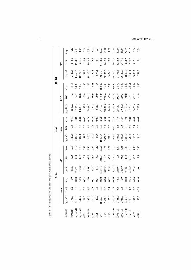
Table 2 gives solution values, optimality gaps, and their standard deviations for all ofthe problems, as observed with N = 1000. Recall from Section 3.5 that the mean valueproblem (MVP) is the deterministic optimization problem obtained by replacing all randomvariables by their means. The optimal solution of each MVP is denoted by x . Note, thatsome of the gaps in Table 2 are negative. As both the lower bound and the upper boundused to compute the gaps are random variables, and no gap is smaller than minus twice itsestimated standard deviation, this is not unexpected. Also note from Table 2 that the MVPrarely yields a competitive solution for the generated instances.

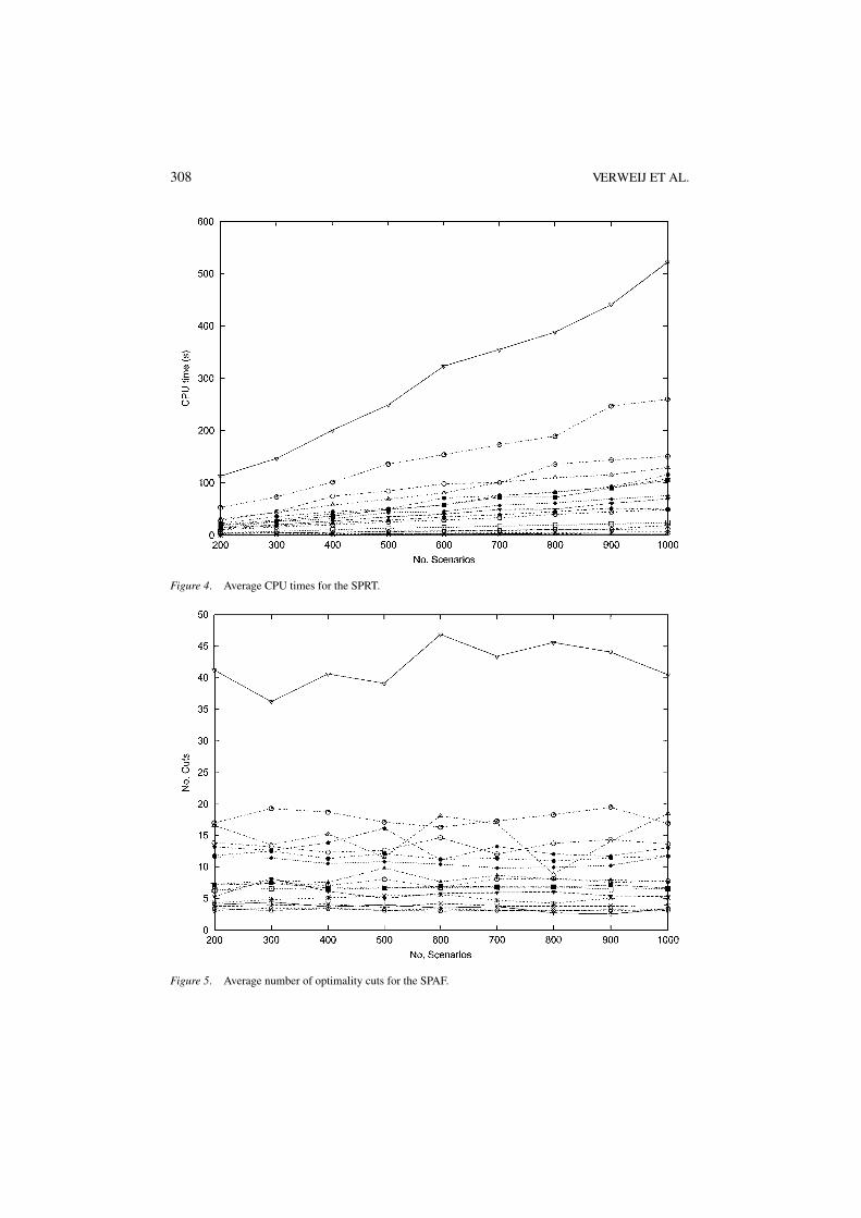
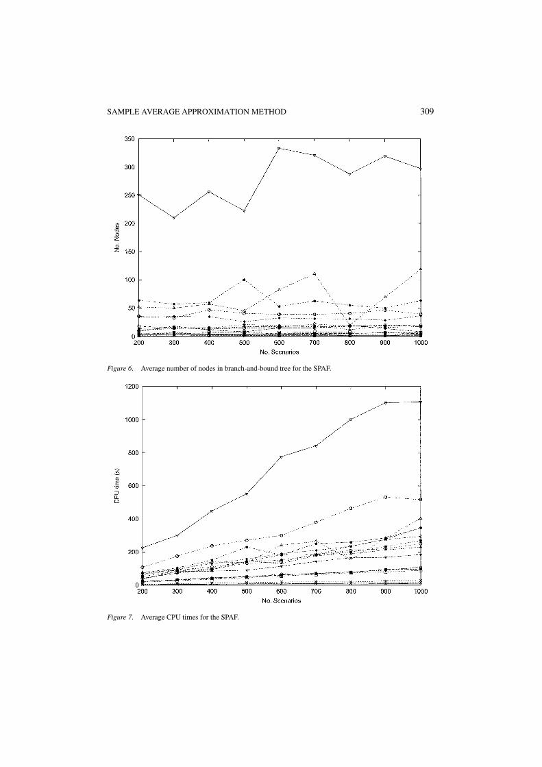
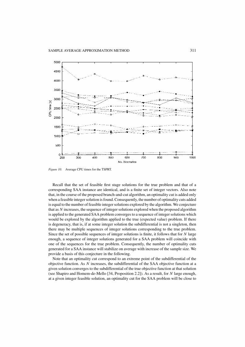
In figures 2, 5, and 8 we see that the average number of optimality cuts displays the samebehavior for all generated instances of the SPRT, the SPAF, and the TSPRT. For each of thethree problems under consideration, the average number of optimality cuts does not dependon the sample size used to formulate the SAA problem. From figures 3, 6, and to a lesserextent from figure 9 (for the TSPRT, all runs needed 10000 nodes in the branch-and-boundtree, except for the runs on the three smallest instances), it is clear that the same observationholds for the average number of nodes in the branch-and-bound tree. As a consequence, therunning time grows only linearly in the sample size. This linear growth is clearly visible infigures 4 and 7. From figure 10 we conclude that for the TSPRT the running time is dominatedby the branch-and-bound algorithm itself for N ≤ 1000, therefore the average time spent inthe generation of the optimality cuts is still a lower-order term in the average CPU time.

From Table 2 it is clear that the SAA method produces provably close to optimal solutions.The reported solutions were within an estimated 1.0%, 0.3%, and 8.7% from the lowerbounds for the SPRT, the SPAF, and the TSPRT, respectively (for N = 1000). Also, theestimated standard deviations of these estimated gaps are small; they are of the same orderof magnitude as the estimated gaps themselves for the SPRT and the SPAF, and for theTSPRT they are significantly smaller. In the case of the TSPRT, a significant part of theseestimated gaps can be attributed to the fact that the MIPs are not solved to optimality; theinstance that realized the forementioned gap of 8.7% had an average (MIP) gap betweenthe best integer solution and the best lower bound of 8.17% over the M SAA problems. Webelieve that by taking advantage of sophisticated cutting-plane and branching techniquesas applied by Applegate et al. [3], these SAA problems can be solved to optimality forthe instances we considered, thereby reducing the gap to that caused by the quality of thestochastic bounds.

From the tables in the Appendix, it is clear that as N increases, the estimated values ofthe reported solutions do not change much. For the SPRT and the TSPRT, the stochasticlower bounds improve, for the SPAF there is not much change in the lower bounds either.In all cases the estimated variance goes down as N increases.

5.3. Stability of the number of optimality cuts

It was observed empirically that on average the number of optimality cuts generated whensolving a SAA problem is fairly stable and hardly changes with change in the sample sizeN . In this section we suggest an explanation of this empirical phenomenon.

SAMPLE AVERAGE APPROXIMATION METHOD 307

Figure 2. Average number of optimality cuts for the SPRT.

Figure 3. Average number of nodes in branch-and-bound tree for the SPRT.

308 VERWEIJ ET AL.

Figure 4. Average CPU times for the SPRT.

Figure 5. Average number of optimality cuts for the SPAF.

SAMPLE AVERAGE APPROXIMATION METHOD 309

Figure 6. Average number of nodes in branch-and-bound tree for the SPAF.

Figure 7. Average CPU times for the SPAF.

310 VERWEIJ ET AL.

Figure 8. Average number of optimality cuts for the TSPRT.

Figure 9. Average number of nodes in branch-and-bound tree for the TSPRT.

SAMPLE AVERAGE APPROXIMATION METHOD 311

Figure 10. Average CPU times for the TSPRT.

Recall that the set of feasible first stage solutions for the true problem and that of acorresponding SAA instance are identical, and is a finite set of integer vectors. Also notethat, in the course of the proposed branch-and-cut algorithm, an optimality cut is added onlywhen a feasible integer solution is found. Consequently, the number of optimality cuts addedis equal to the number of feasible integer solutions explored by the algorithm. We conjecturethat as N increases, the sequence of integer solutions explored when the proposed algorithmis applied to the generated SAA problem converges to a sequence of integer solutions whichwould be explored by the algorithm applied to the true (expected value) problem. If thereis degeneracy, that is, if at some integer solution the subdifferential is not a singleton, thenthere may be multiple sequences of integer solutions corresponding to the true problem.Since the set of possible sequences of integer solutions is finite, it follows that for N largeenough, a sequence of integer solutions generated for a SAA problem will coincide withone of the sequences for the true problem. Consequently, the number of optimality cutsgenerated for a SAA instance will stabilize on average with increase of the sample size. Weprovide a basis of this conjecture in the following.

Note that an optimality cut correspond to an extreme point of the subdifferential of theobjective function. As N increases, the subdifferential of the SAA objective function at agiven solution converges to the subdifferential of the true objective function at that solution(see Shapiro and Homem-de-Mello [34, Proposition 2.2]). As a result, for N large enough,at a given integer feasible solution, an optimality cut for the SAA problem will be close to

312 VERWEIJ ET AL.

Tabl

e2.

Solu

tion

valu

esan

dab

solu

tega

psw

ithlo

wer

boun

d.

SPR

TSP

AF

TSP

RT

SAA

MV

PSA

ASA

AM

VP

Inst

ance

z 105

(x∗ )

Gap

σG

apz 1

05(x

)G

apσ

Gap

z 105

(x∗ )

Gap

σG

apz 1

05(x

∗ )G

apσ

Gap

z 105

(x)

Gap

σG

ap

burm

a14

371.

01.

21.

0941

2.3

42.5

0.99

320.

8−0

.60.

4315

62.7

7.2

3.18

2129

.657

4.0

4.12

ulys

ses1

625

10.0

0.0

0.00

2642

.113

2.1

2.82

2382

.20.

61.

0995

06.2

34.7

24.3

011

455.

619

84.1

17.4

7

ulys

ses2

214

42.4

8.6

3.83

1623

.018

9.2

3.33

1307

.10.

80.

8310

000.

980

.028

.68

1057

7.5

656.

611

.47

eil5

161

.70.

60.

2861

.80.

70.

1051

.20.

00.

0754

3.9

17.9

1.80

548.

322

.30.

68

berl

in52

839.

7−1

.91.

0012

40.7

399.

22.

8781

2.5

1.6

0.73

9481

.030

8.5

21.8

710

202.

010

29.6

12.3

3

st70

114.

90.

30.

5114

3.3

28.7

0.34

102.

70.

20.

1983

4.5

66.9

2.48

852.

885

.21.

01

eil7

649

.20.

10.

2164

.315

.20.

1246

.50.

10.

0566

1.0

30.0

1.55

674.

143

.10.

74

pr76

1820

7.0

0.0

0.00

2521

4.3

7007

.337

.90

1846

3.5

−0.5

8.60

1244

19.0

9315

.018

8.09

1358

68.0

2076

4.0

139.

73

gr96

7601

.00.

00.

0087

19.3

1118

.310

.30

7422

.60.

93.

9862

837.

423

28.4

56.5

868

136.

576

27.5

63.7

0

rat9

920

5.8

0.4

0.12

269.

363

.90.

3920

7.0

0.0

0.14

1464

.447

.42.

5014

74.0

57.0

1.39

kroA

100

3405

.420

.710

.76

3657

.327

2.6

5.07

3022

.8−2

.02.

1025

775.

112

33.8

65.3

326

563.

320

22.0

26.2

4

kroB

100

2468

.2−3

.44.

8224

69.4

−2.3

1.47

2366

.62.

41.

4526

411.

418

62.4

50.9

027

773.

632

24.6

27.5

4

kroC

100

2941

.00.

61.

3931

36.0

195.

64.

3826

49.3

0.5

3.27

2466

0.3

950.

340

.60

2612

9.0

2419

.026

.84

kroD

100

2490

.00.

00.

0025

98.4

108.

42.

4423

82.9

0.6

1.70

2546

8.7

1350

.040

.89

2680

2.9

2684

.227

.55

kroE

100

3708

.34.

32.

4540

14.2

310.

23.

5135

32.4

3.7

2.03

2577

5.5

1975

.140

.51

2779

9.1

3998

.728

.59

rd10

011

97.0

0.0

0.00

1393

.519

6.5

1.71

1166

.50.

40.

4594

78.4

439.

318

.04

9856

.281

7.1

9.84

eil1

0152

.2−0

.10.

1660

.17.

80.

1244

.50.

00.

0576

3.1

41.9

2.45

758.

337

.10.

74

SAMPLE AVERAGE APPROXIMATION METHOD 313

one of the possible optimality cuts for the true problem. A small difference in the optimalitycuts between the SAA and true problems means that the LP relaxations differ only slightly,and the feasible integer solutions do not change. As a result the next integer solution foundby the algorithm for the SAA problem will likely be the same as the next integer solutionthat would be found for the true problem, as long as corresponding extreme points of thesubdifferentials for the SAA problem and the true problem are chosen in case of degeneracy.Thus, for N large enough, the sequence of integer solutions explored for the SAA problemcorresponds to a sequence of integer solutions for the true problem.

6. Conclusions

We have applied the sample average approximation method to three classes of 2-stagestochastic routing problems. Among the instances we considered were ones with a hugenumber of scenarios and first-stage integer variables. Our experience is that the growth ofthe computational effort needed to solve SAA problems is linear in the sample size used toestimate the true objective function. The reason for this is that in the cases that we examined,neither the number of optimality cuts, nor the sizes of branch-and-bound trees needed tosolve SAA problems to optimality increase when the sample size increases. This allows usto find solutions of provably high quality to the stochastic programming problems underconsideration.

Appendix

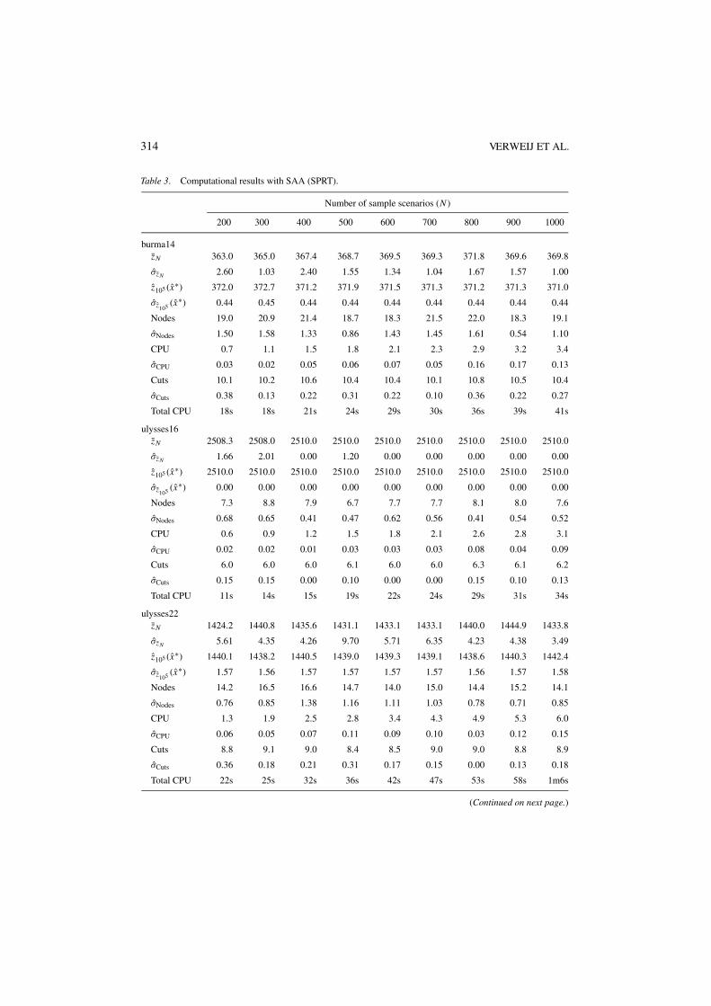
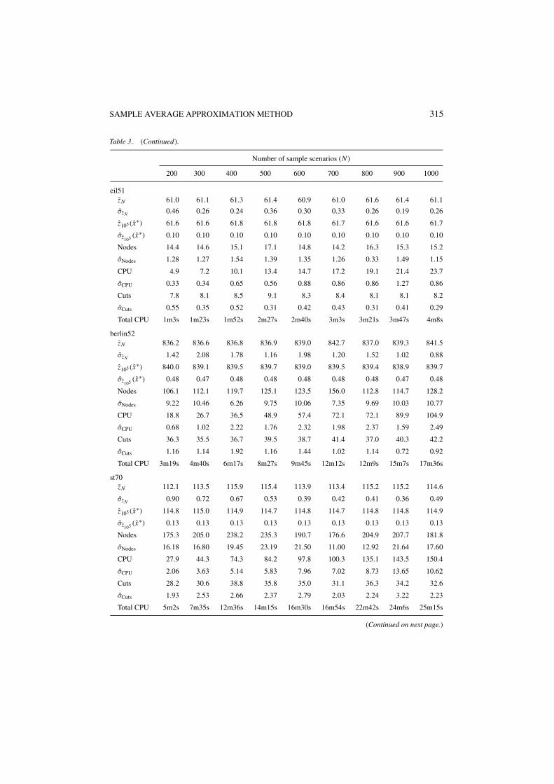
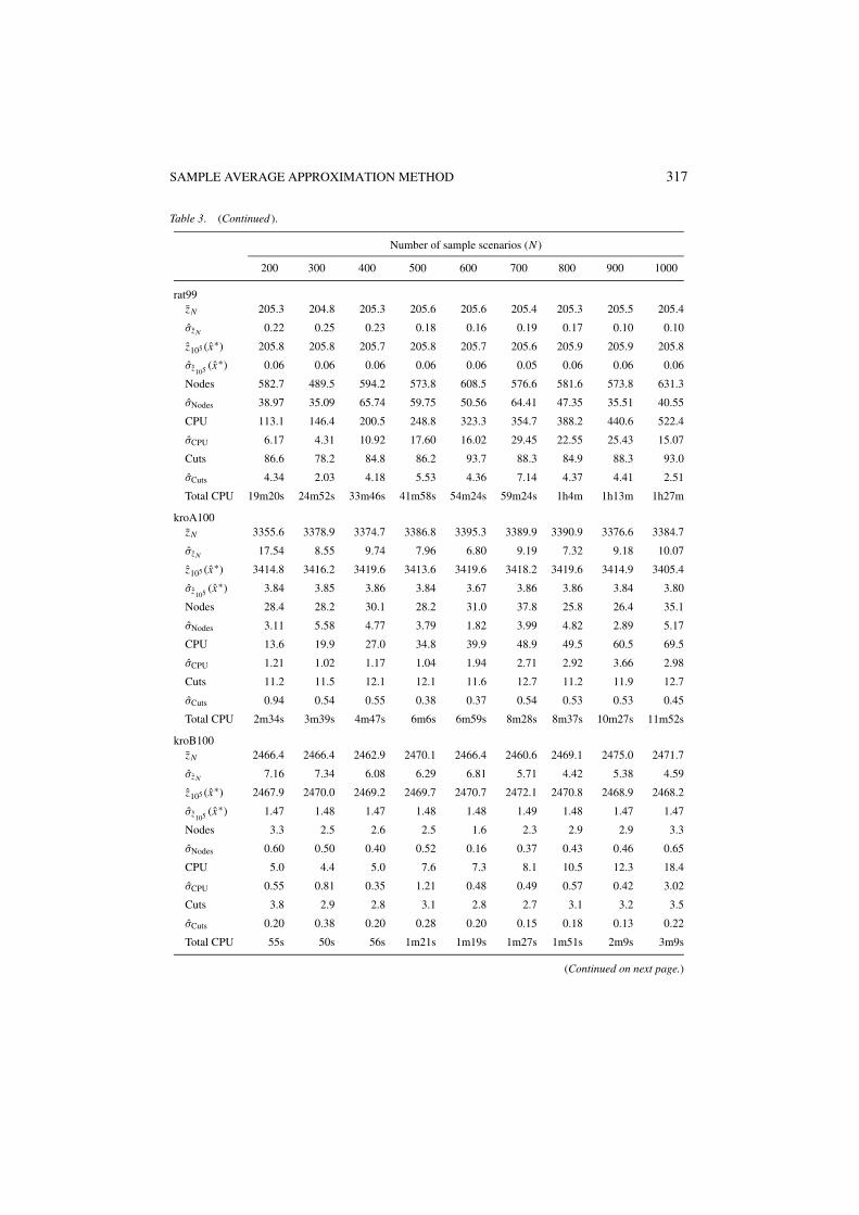
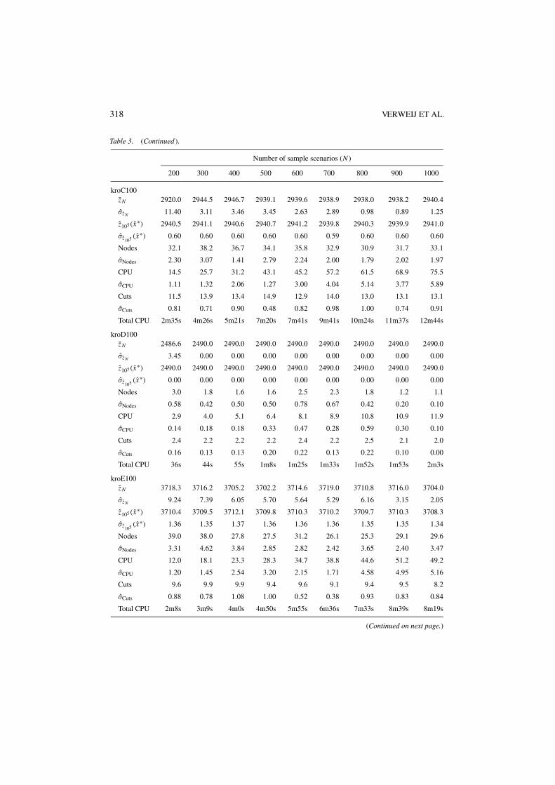
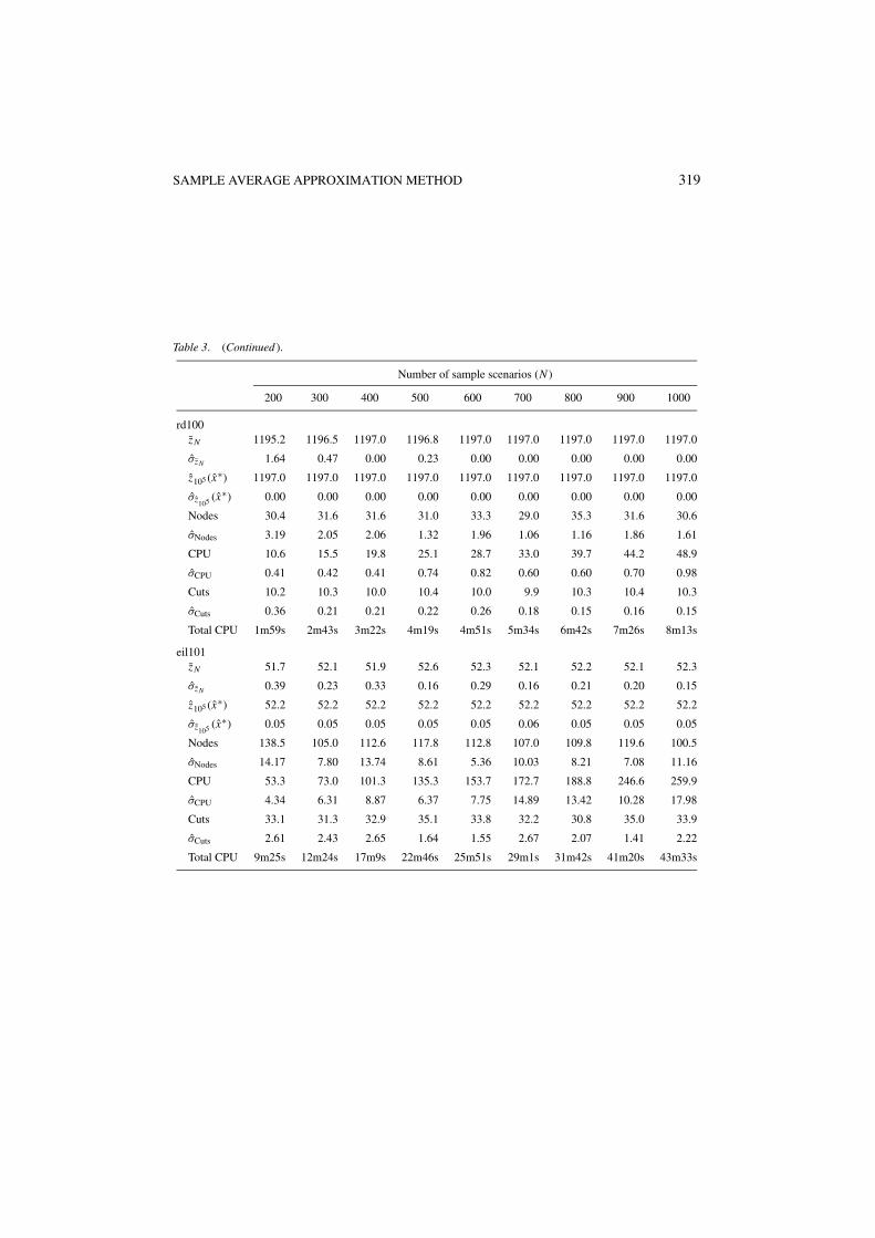
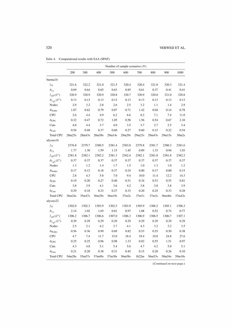
Tables 3–5 give our computational results with the SAA method. Here, for each combinationof a base instance and a number of sample scenarios N , the Nodes, σNodes, CPU, σCPU, Cuts,and σCuts rows give the average number of nodes of the branch-and-bound tree, the standarddeviation of the average number of nodes of the branch-and-bound tree, the average CPUtime in seconds, the standard deviation of the average CPU time in seconds, the averagenumber of optimality cuts, and the standard deviation of the average number of optimalitycuts, respectively, over the M = 10 SAA problems solved to find the best reported solutionand the lower bound estimate. For each combination of a base instance and a number ofsample scenarios N , the Total CPU rows give the total CPU time for solving M = 10 SAAproblems, computing the large sample average objective value zN ′ , (xm) with sample sizeN ′ = 105 for each of the M solutions xm produced, and choosing the solution x∗ with thebest value of xm , as in (6) and (9).

It can be observed that the total CPU times for the SPAF problems are significantly higherthan the times required to solve the corresponding M = 10 SAA problems. This is due to thefact that the more complicated recourse structure in the SPAF problems require considerableeffort in estimating the objective values with a large sample size N ′ = 105 for each of theM solutions produced. This effort can be significantly reduced by choosing a smaller N ′ atthe expense of a slight increase in the estimated confidence intervals. Furthermore, the I/Obottleneck for loading M × N ′ = 106 small second-stage recourse LPs into the solver canbe reduced by bunching several of these LPs into larger LPs, and using warm-start strategiesduring their solution.

314 VERWEIJ ET AL.

Table 3. Computational results with SAA (SPRT).

Number of sample scenarios (N )

200 300 400 500 600 700 800 900 1000

burma14zN 363.0 365.0 367.4 368.7 369.5 369.3 371.8 369.6 369.8

σzN 2.60 1.03 2.40 1.55 1.34 1.04 1.67 1.57 1.00

z105 (x∗) 372.0 372.7 371.2 371.9 371.5 371.3 371.2 371.3 371.0

σz105 (x∗) 0.44 0.45 0.44 0.44 0.44 0.44 0.44 0.44 0.44

Nodes 19.0 20.9 21.4 18.7 18.3 21.5 22.0 18.3 19.1

σNodes 1.50 1.58 1.33 0.86 1.43 1.45 1.61 0.54 1.10

CPU 0.7 1.1 1.5 1.8 2.1 2.3 2.9 3.2 3.4

σCPU 0.03 0.02 0.05 0.06 0.07 0.05 0.16 0.17 0.13

Cuts 10.1 10.2 10.6 10.4 10.4 10.1 10.8 10.5 10.4

σCuts 0.38 0.13 0.22 0.31 0.22 0.10 0.36 0.22 0.27

Total CPU 18s 18s 21s 24s 29s 30s 36s 39s 41s

ulysses16zN 2508.3 2508.0 2510.0 2510.0 2510.0 2510.0 2510.0 2510.0 2510.0

σzN 1.66 2.01 0.00 1.20 0.00 0.00 0.00 0.00 0.00

z105 (x∗) 2510.0 2510.0 2510.0 2510.0 2510.0 2510.0 2510.0 2510.0 2510.0

σz105 (x∗) 0.00 0.00 0.00 0.00 0.00 0.00 0.00 0.00 0.00

Nodes 7.3 8.8 7.9 6.7 7.7 7.7 8.1 8.0 7.6

σNodes 0.68 0.65 0.41 0.47 0.62 0.56 0.41 0.54 0.52

CPU 0.6 0.9 1.2 1.5 1.8 2.1 2.6 2.8 3.1

σCPU 0.02 0.02 0.01 0.03 0.03 0.03 0.08 0.04 0.09

Cuts 6.0 6.0 6.0 6.1 6.0 6.0 6.3 6.1 6.2

σCuts 0.15 0.15 0.00 0.10 0.00 0.00 0.15 0.10 0.13

Total CPU 11s 14s 15s 19s 22s 24s 29s 31s 34s

ulysses22zN 1424.2 1440.8 1435.6 1431.1 1433.1 1433.1 1440.0 1444.9 1433.8

σzN 5.61 4.35 4.26 9.70 5.71 6.35 4.23 4.38 3.49

z105 (x∗) 1440.1 1438.2 1440.5 1439.0 1439.3 1439.1 1438.6 1440.3 1442.4

σz105 (x∗) 1.57 1.56 1.57 1.57 1.57 1.57 1.56 1.57 1.58

Nodes 14.2 16.5 16.6 14.7 14.0 15.0 14.4 15.2 14.1

σNodes 0.76 0.85 1.38 1.16 1.11 1.03 0.78 0.71 0.85

CPU 1.3 1.9 2.5 2.8 3.4 4.3 4.9 5.3 6.0

σCPU 0.06 0.05 0.07 0.11 0.09 0.10 0.03 0.12 0.15

Cuts 8.8 9.1 9.0 8.4 8.5 9.0 9.0 8.8 8.9

σCuts 0.36 0.18 0.21 0.31 0.17 0.15 0.00 0.13 0.18

Total CPU 22s 25s 32s 36s 42s 47s 53s 58s 1m6s

(Continued on next page.)

SAMPLE AVERAGE APPROXIMATION METHOD 315

Table 3. (Continued).

Number of sample scenarios (N )

200 300 400 500 600 700 800 900 1000

eil51zN 61.0 61.1 61.3 61.4 60.9 61.0 61.6 61.4 61.1

σzN 0.46 0.26 0.24 0.36 0.30 0.33 0.26 0.19 0.26

z105 (x∗) 61.6 61.6 61.8 61.8 61.8 61.7 61.6 61.6 61.7

σz105 (x∗) 0.10 0.10 0.10 0.10 0.10 0.10 0.10 0.10 0.10

Nodes 14.4 14.6 15.1 17.1 14.8 14.2 16.3 15.3 15.2

σNodes 1.28 1.27 1.54 1.39 1.35 1.26 0.33 1.49 1.15

CPU 4.9 7.2 10.1 13.4 14.7 17.2 19.1 21.4 23.7

σCPU 0.33 0.34 0.65 0.56 0.88 0.86 0.86 1.27 0.86

Cuts 7.8 8.1 8.5 9.1 8.3 8.4 8.1 8.1 8.2

σCuts 0.55 0.35 0.52 0.31 0.42 0.43 0.31 0.41 0.29

Total CPU 1m3s 1m23s 1m52s 2m27s 2m40s 3m3s 3m21s 3m47s 4m8s

berlin52zN 836.2 836.6 836.8 836.9 839.0 842.7 837.0 839.3 841.5

σzN 1.42 2.08 1.78 1.16 1.98 1.20 1.52 1.02 0.88

z105 (x∗) 840.0 839.1 839.5 839.7 839.0 839.5 839.4 838.9 839.7

σz105 (x∗) 0.48 0.47 0.48 0.48 0.48 0.48 0.48 0.47 0.48

Nodes 106.1 112.1 119.7 125.1 123.5 156.0 112.8 114.7 128.2

σNodes 9.22 10.46 6.26 9.75 10.06 7.35 9.69 10.03 10.77

CPU 18.8 26.7 36.5 48.9 57.4 72.1 72.1 89.9 104.9

σCPU 0.68 1.02 2.22 1.76 2.32 1.98 2.37 1.59 2.49

Cuts 36.3 35.5 36.7 39.5 38.7 41.4 37.0 40.3 42.2

σCuts 1.16 1.14 1.92 1.16 1.44 1.02 1.14 0.72 0.92

Total CPU 3m19s 4m40s 6m17s 8m27s 9m45s 12m12s 12m9s 15m7s 17m36s

st70zN 112.1 113.5 115.9 115.4 113.9 113.4 115.2 115.2 114.6

σzN 0.90 0.72 0.67 0.53 0.39 0.42 0.41 0.36 0.49

z105 (x∗) 114.8 115.0 114.9 114.7 114.8 114.7 114.8 114.8 114.9

σz105 (x∗) 0.13 0.13 0.13 0.13 0.13 0.13 0.13 0.13 0.13

Nodes 175.3 205.0 238.2 235.3 190.7 176.6 204.9 207.7 181.8

σNodes 16.18 16.80 19.45 23.19 21.50 11.00 12.92 21.64 17.60

CPU 27.9 44.3 74.3 84.2 97.8 100.3 135.1 143.5 150.4

σCPU 2.06 3.63 5.14 5.83 7.96 7.02 8.73 13.65 10.62

Cuts 28.2 30.6 38.8 35.8 35.0 31.1 36.3 34.2 32.6

σCuts 1.93 2.53 2.66 2.37 2.79 2.03 2.24 3.22 2.23

Total CPU 5m2s 7m35s 12m36s 14m15s 16m30s 16m54s 22m42s 24m6s 25m15s

(Continued on next page.)

316 VERWEIJ ET AL.

Table 3. (Continued).

Number of sample scenarios (N )

200 300 400 500 600 700 800 900 1000

eil76zN 49.1 49.0 49.5 49.4 49.0 49.1 49.2 49.4 49.1

σzN 0.38 0.26 0.27 0.14 0.12 0.12 0.23 0.07 0.20

z105 (x∗) 49.3 49.2 49.2 49.2 49.3 49.3 49.2 49.2 49.2

σz105 (x∗) 0.05 0.05 0.05 0.05 0.05 0.05 0.05 0.05 0.05

Nodes 64.5 65.4 61.4 57.6 65.8 57.1 53.3 54.3 56.6

σNodes 6.09 4.60 2.40 3.01 4.84 2.95 4.12 2.31 3.74

CPU 22.8 35.6 44.7 50.3 70.9 75.4 81.6 92.6 115.4

σCPU 2.00 2.38 1.43 2.06 5.05 3.77 4.69 2.68 7.18

Cuts 21.6 23.3 22.1 20.1 23.2 21.3 20.4 20.6 22.8

σCuts 1.43 1.41 0.72 0.71 1.46 0.80 1.01 0.50 1.23

Total CPU 4m0s 6m4s 7m35s 8m36s 11m56s 12m42s 13m43s 15m33s 19m22s

pr76zN 18207.0 18207.0 18207.0 18207.0 18207.0 18207.0 18207.0 18207.0 18207.0

σzN 0.00 0.00 0.00 0.00 0.00 0.00 0.00 0.00 0.00

z105 (x∗) 18207.0 18207.0 18207.0 18207.0 18207.0 18207.0 18207.0 18207.0 18207.0

σz105 (x∗) 0.00 0.00 0.00 0.00 0.00 0.00 0.00 0.00 0.00

Nodes 190.3 155.7 151.2 151.3 124.4 159.5 140.1 132.9 129.1

σNodes 18.19 19.29 20.57 21.97 13.74 16.63 7.91 12.25 15.59

CPU 31.5 43.3 57.4 68.6 80.4 100.7 109.7 114.9 129.1

σCPU 2.28 4.21 5.46 4.11 6.84 8.18 4.88 8.13 8.14

Cuts 35.3 34.1 35.5 34.0 33.6 36.0 34.2 32.6 32.6

σCuts 2.53 3.07 3.06 1.79 3.01 2.48 1.64 2.34 2.15

Total CPU 5m21s 7m19s 9m40s 11m32s 13m30s 16m53s 18m23s 19m16s 21m37s

gr96zN 7601.0 7601.0 7601.0 7601.0 7601.0 7601.0 7601.0 7601.0 7601.0

σzN 0.00 0.00 0.00 0.00 0.00 0.00 0.00 0.00 0.00

z105 (x∗) 7601.0 7601.0 7601.0 7601.0 7601.0 7601.0 7601.0 7601.0 7601.0

σz105 (x∗) 0.00 0.00 0.00 0.00 0.00 0.00 0.00 0.00 0.00

Nodes 85.3 82.3 88.0 85.2 86.1 86.3 82.4 77.4 77.8

σNodes 3.49 4.33 4.70 6.54 4.28 3.51 4.59 2.43 2.62

CPU 20.3 28.8 41.3 48.5 58.2 74.9 82.9 90.5 107.5

σCPU 0.91 1.41 4.17 2.46 2.26 2.82 4.00 4.33 4.33

Cuts 21.4 21.8 23.7 22.3 22.8 24.7 24.1 23.4 24.6

σCuts 0.82 0.89 1.81 1.03 0.89 0.76 0.89 0.79 0.81

Total CPU 3m28s 4m53s 6m58s 8m9s 9m47s 12m34s 13m54s 15m9s 17m59s

(Continued on next page.)

SAMPLE AVERAGE APPROXIMATION METHOD 317

Table 3. (Continued ).

Number of sample scenarios (N )

200 300 400 500 600 700 800 900 1000

rat99zN 205.3 204.8 205.3 205.6 205.6 205.4 205.3 205.5 205.4

σzN 0.22 0.25 0.23 0.18 0.16 0.19 0.17 0.10 0.10

z105 (x∗) 205.8 205.8 205.7 205.8 205.7 205.6 205.9 205.9 205.8

σz105 (x∗) 0.06 0.06 0.06 0.06 0.06 0.05 0.06 0.06 0.06

Nodes 582.7 489.5 594.2 573.8 608.5 576.6 581.6 573.8 631.3

σNodes 38.97 35.09 65.74 59.75 50.56 64.41 47.35 35.51 40.55

CPU 113.1 146.4 200.5 248.8 323.3 354.7 388.2 440.6 522.4

σCPU 6.17 4.31 10.92 17.60 16.02 29.45 22.55 25.43 15.07

Cuts 86.6 78.2 84.8 86.2 93.7 88.3 84.9 88.3 93.0

σCuts 4.34 2.03 4.18 5.53 4.36 7.14 4.37 4.41 2.51

Total CPU 19m20s 24m52s 33m46s 41m58s 54m24s 59m24s 1h4m 1h13m 1h27m

kroA100zN 3355.6 3378.9 3374.7 3386.8 3395.3 3389.9 3390.9 3376.6 3384.7

σzN 17.54 8.55 9.74 7.96 6.80 9.19 7.32 9.18 10.07

z105 (x∗) 3414.8 3416.2 3419.6 3413.6 3419.6 3418.2 3419.6 3414.9 3405.4

σz105 (x∗) 3.84 3.85 3.86 3.84 3.67 3.86 3.86 3.84 3.80

Nodes 28.4 28.2 30.1 28.2 31.0 37.8 25.8 26.4 35.1

σNodes 3.11 5.58 4.77 3.79 1.82 3.99 4.82 2.89 5.17

CPU 13.6 19.9 27.0 34.8 39.9 48.9 49.5 60.5 69.5

σCPU 1.21 1.02 1.17 1.04 1.94 2.71 2.92 3.66 2.98

Cuts 11.2 11.5 12.1 12.1 11.6 12.7 11.2 11.9 12.7

σCuts 0.94 0.54 0.55 0.38 0.37 0.54 0.53 0.53 0.45

Total CPU 2m34s 3m39s 4m47s 6m6s 6m59s 8m28s 8m37s 10m27s 11m52s

kroB100zN 2466.4 2466.4 2462.9 2470.1 2466.4 2460.6 2469.1 2475.0 2471.7

σzN 7.16 7.34 6.08 6.29 6.81 5.71 4.42 5.38 4.59

z105 (x∗) 2467.9 2470.0 2469.2 2469.7 2470.7 2472.1 2470.8 2468.9 2468.2

σz105 (x∗) 1.47 1.48 1.47 1.48 1.48 1.49 1.48 1.47 1.47

Nodes 3.3 2.5 2.6 2.5 1.6 2.3 2.9 2.9 3.3

σNodes 0.60 0.50 0.40 0.52 0.16 0.37 0.43 0.46 0.65

CPU 5.0 4.4 5.0 7.6 7.3 8.1 10.5 12.3 18.4

σCPU 0.55 0.81 0.35 1.21 0.48 0.49 0.57 0.42 3.02

Cuts 3.8 2.9 2.8 3.1 2.8 2.7 3.1 3.2 3.5

σCuts 0.20 0.38 0.20 0.28 0.20 0.15 0.18 0.13 0.22

Total CPU 55s 50s 56s 1m21s 1m19s 1m27s 1m51s 2m9s 3m9s

(Continued on next page.)

318 VERWEIJ ET AL.

Table 3. (Continued ).

Number of sample scenarios (N )

200 300 400 500 600 700 800 900 1000

kroC100zN 2920.0 2944.5 2946.7 2939.1 2939.6 2938.9 2938.0 2938.2 2940.4

σzN 11.40 3.11 3.46 3.45 2.63 2.89 0.98 0.89 1.25

z105 (x∗) 2940.5 2941.1 2940.6 2940.7 2941.2 2939.8 2940.3 2939.9 2941.0

σz105 (x∗) 0.60 0.60 0.60 0.60 0.60 0.59 0.60 0.60 0.60

Nodes 32.1 38.2 36.7 34.1 35.8 32.9 30.9 31.7 33.1

σNodes 2.30 3.07 1.41 2.79 2.24 2.00 1.79 2.02 1.97

CPU 14.5 25.7 31.2 43.1 45.2 57.2 61.5 68.9 75.5

σCPU 1.11 1.32 2.06 1.27 3.00 4.04 5.14 3.77 5.89

Cuts 11.5 13.9 13.4 14.9 12.9 14.0 13.0 13.1 13.1

σCuts 0.81 0.71 0.90 0.48 0.82 0.98 1.00 0.74 0.91

Total CPU 2m35s 4m26s 5m21s 7m20s 7m41s 9m41s 10m24s 11m37s 12m44s

kroD100zN 2486.6 2490.0 2490.0 2490.0 2490.0 2490.0 2490.0 2490.0 2490.0

σzN 3.45 0.00 0.00 0.00 0.00 0.00 0.00 0.00 0.00

z105 (x∗) 2490.0 2490.0 2490.0 2490.0 2490.0 2490.0 2490.0 2490.0 2490.0

σz105 (x∗) 0.00 0.00 0.00 0.00 0.00 0.00 0.00 0.00 0.00

Nodes 3.0 1.8 1.6 1.6 2.5 2.3 1.8 1.2 1.1

σNodes 0.58 0.42 0.50 0.50 0.78 0.67 0.42 0.20 0.10

CPU 2.9 4.0 5.1 6.4 8.1 8.9 10.8 10.9 11.9

σCPU 0.14 0.18 0.18 0.33 0.47 0.28 0.59 0.30 0.10

Cuts 2.4 2.2 2.2 2.2 2.4 2.2 2.5 2.1 2.0

σCuts 0.16 0.13 0.13 0.20 0.22 0.13 0.22 0.10 0.00

Total CPU 36s 44s 55s 1m8s 1m25s 1m33s 1m52s 1m53s 2m3s

kroE100zN 3718.3 3716.2 3705.2 3702.2 3714.6 3719.0 3710.8 3716.0 3704.0

σzN 9.24 7.39 6.05 5.70 5.64 5.29 6.16 3.15 2.05

z105 (x∗) 3710.4 3709.5 3712.1 3709.8 3710.3 3710.2 3709.7 3710.3 3708.3

σz105 (x∗) 1.36 1.35 1.37 1.36 1.36 1.36 1.35 1.35 1.34

Nodes 39.0 38.0 27.8 27.5 31.2 26.1 25.3 29.1 29.6

σNodes 3.31 4.62 3.84 2.85 2.82 2.42 3.65 2.40 3.47

CPU 12.0 18.1 23.3 28.3 34.7 38.8 44.6 51.2 49.2

σCPU 1.20 1.45 2.54 3.20 2.15 1.71 4.58 4.95 5.16

Cuts 9.6 9.9 9.9 9.4 9.6 9.1 9.4 9.5 8.2

σCuts 0.88 0.78 1.08 1.00 0.52 0.38 0.93 0.83 0.84

Total CPU 2m8s 3m9s 4m0s 4m50s 5m55s 6m36s 7m33s 8m39s 8m19s

(Continued on next page.)

SAMPLE AVERAGE APPROXIMATION METHOD 319

Table 3. (Continued ).

Number of sample scenarios (N )

200 300 400 500 600 700 800 900 1000

rd100zN 1195.2 1196.5 1197.0 1196.8 1197.0 1197.0 1197.0 1197.0 1197.0

σzN 1.64 0.47 0.00 0.23 0.00 0.00 0.00 0.00 0.00

z105 (x∗) 1197.0 1197.0 1197.0 1197.0 1197.0 1197.0 1197.0 1197.0 1197.0

σz105 (x∗) 0.00 0.00 0.00 0.00 0.00 0.00 0.00 0.00 0.00

Nodes 30.4 31.6 31.6 31.0 33.3 29.0 35.3 31.6 30.6

σNodes 3.19 2.05 2.06 1.32 1.96 1.06 1.16 1.86 1.61

CPU 10.6 15.5 19.8 25.1 28.7 33.0 39.7 44.2 48.9

σCPU 0.41 0.42 0.41 0.74 0.82 0.60 0.60 0.70 0.98

Cuts 10.2 10.3 10.0 10.4 10.0 9.9 10.3 10.4 10.3

σCuts 0.36 0.21 0.21 0.22 0.26 0.18 0.15 0.16 0.15

Total CPU 1m59s 2m43s 3m22s 4m19s 4m51s 5m34s 6m42s 7m26s 8m13s

eil101zN 51.7 52.1 51.9 52.6 52.3 52.1 52.2 52.1 52.3

σzN 0.39 0.23 0.33 0.16 0.29 0.16 0.21 0.20 0.15

z105 (x∗) 52.2 52.2 52.2 52.2 52.2 52.2 52.2 52.2 52.2

σz105 (x∗) 0.05 0.05 0.05 0.05 0.05 0.06 0.05 0.05 0.05

Nodes 138.5 105.0 112.6 117.8 112.8 107.0 109.8 119.6 100.5

σNodes 14.17 7.80 13.74 8.61 5.36 10.03 8.21 7.08 11.16

CPU 53.3 73.0 101.3 135.3 153.7 172.7 188.8 246.6 259.9

σCPU 4.34 6.31 8.87 6.37 7.75 14.89 13.42 10.28 17.98

Cuts 33.1 31.3 32.9 35.1 33.8 32.2 30.8 35.0 33.9

σCuts 2.61 2.43 2.65 1.64 1.55 2.67 2.07 1.41 2.22

Total CPU 9m25s 12m24s 17m9s 22m46s 25m51s 29m1s 31m42s 41m20s 43m33s

320 VERWEIJ ET AL.

Table 4. Computational results with SAA (SPAF).

Number of sample scenarios (N )

200 300 400 500 600 700 800 900 1000

burma14

zN 321.6 322.2 321.0 321.5 320.4 320.4 321.0 320.3 321.4

σzN 0.69 0.64 0.65 0.63 0.85 0.61 0.37 0.41 0.41

z105 (x∗) 320.9 320.9 320.9 320.8 320.7 320.9 320.8 321.0 320.8

σz105 (x∗) 0.13 0.13 0.13 0.13 0.13 0.13 0.13 0.13 0.13

Nodes 2.9 3.2 2.8 2.6 2.5 3.2 1.1 1.4 2.9

σNodes 1.07 0.62 0.79 0.87 0.71 1.42 0.04 0.14 0.78

CPU 2.6 4.4 4.9 6.2 6.6 8.2 7.1 7.4 11.0

σCPU 0.32 0.47 0.72 1.05 0.58 1.56 0.54 0.67 2.10

Cuts 4.0 4.4 3.7 4.0 3.5 3.7 2.7 2.5 3.4

σCuts 0.56 0.48 0.37 0.60 0.27 0.60 0.15 0.22 0.54

Total CPU 28m25s 28m43s 28m58s 29m14s 29m29s 29m23s 29m43s 29m15s 30m2s

ulysses16

zN 2376.8 2379.7 2380.5 2381.4 2383.0 2379.8 2381.7 2380.3 2381.6

σzN 1.77 1.30 1.59 1.15 1.45 0.89 1.33 0.94 1.03

z105 (x∗) 2381.8 2382.1 2382.2 2381.3 2382.4 2382.1 2381.8 2381.8 2382.2

σz105 (x∗) 0.37 0.37 0.37 0.37 0.37 0.37 0.37 0.37 0.37

Nodes 1.3 1.2 1.4 1.7 1.5 1.0 1.3 1.0 1.2

σNodes 0.17 0.12 0.18 0.37 0.24 0.00 0.17 0.00 0.15

CPU 2.8 4.3 5.8 7.0 9.4 10.0 11.4 12.2 14.3

σCPU 0.19 0.20 0.27 0.40 0.51 0.34 0.53 0.55 0.81

Cuts 3.8 3.9 4.1 3.6 4.2 3.8 3.8 3.8 3.9

σCuts 0.29 0.18 0.23 0.27 0.33 0.20 0.25 0.33 0.28

Total CPU 36m24s 35m47s 36m29s 36m19s 37m2s 37m7s 37m3s 36m46s 37m42s

ulysses22

zN 1302.0 1302.3 1303.9 1302.5 1303.9 1305.9 1306.2 1305.1 1306.3

σzN 2.14 1.02 1.65 0.81 0.97 1.08 0.52 0.74 0.77

z105 (x∗) 1306.2 1306.7 1306.6 1307.0 1306.3 1306.9 1306.5 1306.7 1307.1

σz105 (x∗) 0.29 0.29 0.29 0.29 0.29 0.29 0.29 0.29 0.29

Nodes 2.5 2.1 4.2 3.7 4.1 4.3 3.2 3.2 3.5

σNodes 0.56 0.36 0.99 0.69 0.82 0.53 0.55 0.50 0.38

CPU 4.7 7.4 11.7 15.0 18.4 19.4 19.8 24.8 27.6

σCPU 0.25 0.25 0.96 0.98 1.33 0.83 0.55 1.51 0.97

Cuts 4.3 4.8 5.1 5.4 5.6 4.7 4.2 5.0 5.1

σCuts 0.21 0.20 0.38 0.31 0.45 0.15 0.20 0.26 0.10

Total CPU 54m28s 55m57s 57m49s 57m30s 56m58s 1b22m 56m53s 58m54s 59m18s

(Continued on next page.)

SAMPLE AVERAGE APPROXIMATION METHOD 321

Table 4. (Continued ).

Number of sample scenarios (N )

200 300 400 500 600 700 800 900 1000

eil51zN 51.2 51.1 51.3 51.2 51.4 51.2 51.2 51.3 51.2

σzN 0.19 0.10 0.09 0.09 0.08 0.06 0.09 0.06 0.07

z105 (x∗) 51.2 51.2 51.2 51.2 51.2 51.2 51.2 51.2 51.2

σz105 (x∗) 0.02 0.02 0.02 0.02 0.02 0.02 0.02 0.02 0.02

Nodes 5.7 6.9 7.6 7.5 6.9 7.7 7.4 6.4 6.3

σNodes 1.01 0.78 1.08 0.67 0.69 0.82 0.58 0.63 0.85

CPU 18.0 26.8 35.2 45.1 54.8 64.0 74.0 79.2 88.9

σCPU 0.98 1.06 1.20 1.02 1.62 2.35 3.27 2.69 2.94

Cuts 6.3 6.5 6.4 6.6 6.7 6.7 6.8 6.4 6.5

σCuts 0.33 0.31 0.27 0.16 0.21 0.26 0.36 0.27 0.22

Total CPU 2h39m 2h39m 2h41m 2h43m 2h44m 2h47m 2h47m 2h47m 2h50m

berlin52

zN 810.8 812.0 811.0 810.5 811.9 812.4 811.2 812.0 811.0

σzN 1.00 0.94 0.80 0.51 0.59 0.45 0.54 0.26 0.70

z105 (x∗) 812.8 812.9 812.3 812.5 812.4 812.5 812.6 812.6 812.5

σz105 (x∗) 0.18 0.19 0.18 0.18 0.18 0.18 0.18 0.18 0.18

Nodes 4.7 5.8 4.4 4.3 5.5 4.9 5.0 6.2 4.9

σNodes 1.01 0.96 1.07 0.89 1.04 0.78 0.63 0.69 0.65

CPU 21.3 30.7 38.8 49.7 61.9 69.4 78.5 94.0 96.6

σCPU 1.68 2.35 2.24 2.52 4.16 4.55 3.00 2.95 6.39

Cuts 7.1 7.4 6.6 6.6 6.9 6.8 6.7 7.1 6.6

σCuts 0.55 0.64 0.45 0.43 0.41 0.42 0.40 0.28 0.54

Total CPU 2h39m 2h40m 2h44m 2h43m 2h46m 2h47m 2h47m 2h51m 2h52m

st70

zN 102.4 101.9 102.4 102.4 102.6 102.5 102.4 102.7 102.4

σzN 0.22 0.31 0.29 0.22 0.20 0.17 0.20 0.12 0.18

z105 (x∗) 102.8 102.6 102.8 102.6 102.8 102.8 102.8 102.7 102.7

σz105 (x∗) 0.06 0.06 0.06 0.06 0.06 0.06 0.06 0.06 0.06

Nodes 18.1 15.6 15.0 14.6 14.9 14.7 17.7 19.9 19.6

σNodes 3.94 4.41 1.72 2.71 1.70 2.66 1.85 3.84 3.31

CPU 63.8 89.3 109.3 142.3 183.5 186.1 235.6 276.4 296.1

σCPU 7.85 8.03 9.06 15.09 14.74 19.07 5.99 22.73 18.18

Cuts 13.8 13.2 12.3 12.6 14.6 12.0 13.7 14.3 13.6

σCuts 1.55 1.52 0.94 1.38 1.23 1.32 0.50 1.19 1.06

Total CPU 4h11m 4h5m 4h5m 4h9m 4h29m 4h14m 4h31m 4h44m 4h38m

(Continued on next page.)

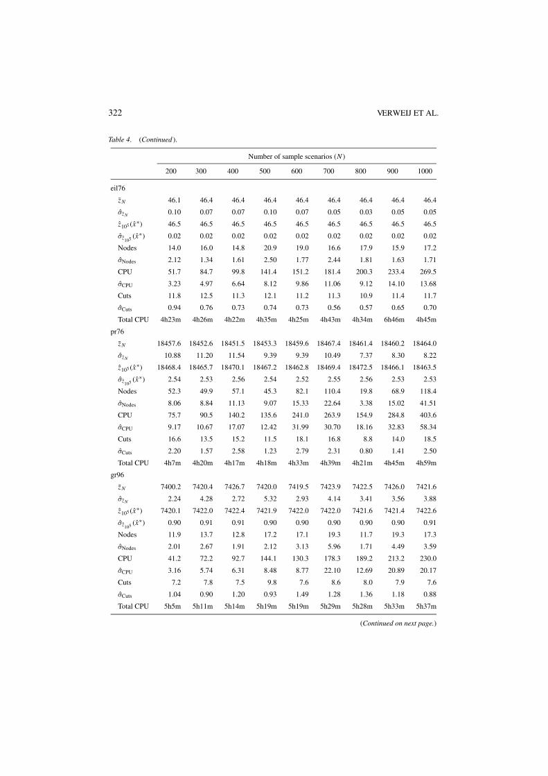
322 VERWEIJ ET AL.

Table 4. (Continued ).

Number of sample scenarios (N )

200 300 400 500 600 700 800 900 1000

eil76

zN 46.1 46.4 46.4 46.4 46.4 46.4 46.4 46.4 46.4

σzN 0.10 0.07 0.07 0.10 0.07 0.05 0.03 0.05 0.05

z105 (x∗) 46.5 46.5 46.5 46.5 46.5 46.5 46.5 46.5 46.5

σz105 (x∗) 0.02 0.02 0.02 0.02 0.02 0.02 0.02 0.02 0.02

Nodes 14.0 16.0 14.8 20.9 19.0 16.6 17.9 15.9 17.2

σNodes 2.12 1.34 1.61 2.50 1.77 2.44 1.81 1.63 1.71

CPU 51.7 84.7 99.8 141.4 151.2 181.4 200.3 233.4 269.5

σCPU 3.23 4.97 6.64 8.12 9.86 11.06 9.12 14.10 13.68

Cuts 11.8 12.5 11.3 12.1 11.2 11.3 10.9 11.4 11.7

σCuts 0.94 0.76 0.73 0.74 0.73 0.56 0.57 0.65 0.70

Total CPU 4h23m 4h26m 4h22m 4h35m 4h25m 4h43m 4h34m 6h46m 4h45m

pr76

zN 18457.6 18452.6 18451.5 18453.3 18459.6 18467.4 18461.4 18460.2 18464.0

σzN 10.88 11.20 11.54 9.39 9.39 10.49 7.37 8.30 8.22

z105 (x∗) 18468.4 18465.7 18470.1 18467.2 18462.8 18469.4 18472.5 18466.1 18463.5

σz105 (x∗) 2.54 2.53 2.56 2.54 2.52 2.55 2.56 2.53 2.53

Nodes 52.3 49.9 57.1 45.3 82.1 110.4 19.8 68.9 118.4

σNodes 8.06 8.84 11.13 9.07 15.33 22.64 3.38 15.02 41.51

CPU 75.7 90.5 140.2 135.6 241.0 263.9 154.9 284.8 403.6

σCPU 9.17 10.67 17.07 12.42 31.99 30.70 18.16 32.83 58.34

Cuts 16.6 13.5 15.2 11.5 18.1 16.8 8.8 14.0 18.5

σCuts 2.20 1.57 2.58 1.23 2.79 2.31 0.80 1.41 2.50

Total CPU 4h7m 4h20m 4h17m 4h18m 4h33m 4h39m 4h21m 4h45m 4h59m

gr96

zN 7400.2 7420.4 7426.7 7420.0 7419.5 7423.9 7422.5 7426.0 7421.6

σzN 2.24 4.28 2.72 5.32 2.93 4.14 3.41 3.56 3.88

z105 (x∗) 7420.1 7422.0 7422.4 7421.9 7422.0 7422.0 7421.6 7421.4 7422.6

σz105 (x∗) 0.90 0.91 0.91 0.90 0.90 0.90 0.90 0.90 0.91

Nodes 11.9 13.7 12.8 17.2 17.1 19.3 11.7 19.3 17.3

σNodes 2.01 2.67 1.91 2.12 3.13 5.96 1.71 4.49 3.59

CPU 41.2 72.2 92.7 144.1 130.3 178.3 189.2 213.2 230.0

σCPU 3.16 5.74 6.31 8.48 8.77 22.10 12.69 20.89 20.17

Cuts 7.2 7.8 7.5 9.8 7.6 8.6 8.0 7.9 7.6

σCuts 1.04 0.90 1.20 0.93 1.49 1.28 1.36 1.18 0.88

Total CPU 5h5m 5h11m 5h14m 5h19m 5h19m 5h29m 5h28m 5h33m 5h37m

(Continued on next page.)

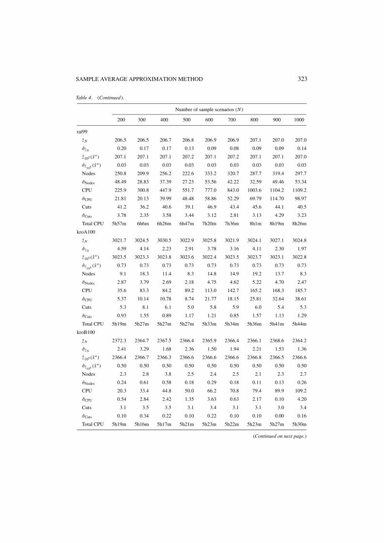
SAMPLE AVERAGE APPROXIMATION METHOD 323

Table 4. (Continued ).

Number of sample scenarios (N )

200 300 400 500 600 700 800 900 1000

rat99

zN 206.5 206.5 206.7 206.8 206.9 206.9 207.1 207.0 207.0

σzN 0.20 0.17 0.17 0.13 0.09 0.08 0.09 0.09 0.14

z105 (x∗) 207.1 207.1 207.1 207.2 207.1 207.2 207.1 207.1 207.0

σz105 (x∗) 0.03 0.03 0.03 0.03 0.03 0.03 0.03 0.03 0.03

Nodes 250.8 209.9 256.2 222.6 333.2 320.7 287.7 319.4 297.7

σNodes 48.49 28.83 37.39 27.23 53.56 42.22 32.59 49.46 53.34

CPU 225.9 300.8 447.9 551.7 777.0 843.0 1003.6 1104.2 1109.2

σCPU 21.81 20.13 39.99 48.48 58.86 52.29 69.79 114.70 98.97

Cuts 41.2 36.2 40.6 39.1 46.9 43.4 45.6 44.1 40.5

σCuts 3.78 2.35 3.58 3.44 3.12 2.81 3.13 4.29 3.23

Total CPU 5h57m 6h6m 6h26m 6h47m 7h20m 7h36m 8h1m 8h19m 8h26m

kroA100

zN 3021.7 3024.5 3030.5 3022.9 3025.8 3021.9 3024.1 3027.1 3024.8

σzN 4.59 4.14 2.23 2.91 3.78 3.16 4.11 2.30 1.97

z105 (x∗) 3023.5 3023.3 3023.8 3023.6 3022.4 3023.5 3023.7 3023.1 3022.8

σz105 (x∗) 0.73 0.73 0.73 0.73 0.73 0.73 0.73 0.73 0.73

Nodes 9.1 18.3 11.4 8.3 14.8 14.9 19.2 13.7 8.3

σNodes 2.87 3.79 2.69 2.18 4.75 4.62 5.22 4.70 2.47

CPU 35.6 83.3 84.2 89.2 113.0 142.7 165.2 168.3 185.7

σCPU 5.37 10.14 10.78 8.74 21.77 18.15 25.81 32.64 38.61

Cuts 5.3 8.1 6.1 5.0 5.8 5.9 6.0 5.4 5.3

σCuts 0.93 1.55 0.89 1.17 1.21 0.85 1.57 1.13 1.29

Total CPU 5h19m 5h27m 5h27m 5h27m 5h33m 5h34m 5h36m 5h41m 5h44m

kroB100

zN 2372.3 2364.7 2367.5 2366.4 2365.9 2366.4 2366.1 2368.6 2364.2

σzN 2.41 3.29 1.68 2.36 1.50 1.94 2.21 1.53 1.36

z105 (x∗) 2366.4 2366.7 2366.3 2366.6 2366.6 2366.6 2366.8 2366.5 2366.6

σz105 (x∗) 0.50 0.50 0.50 0.50 0.50 0.50 0.50 0.50 0.50

Nodes 2.3 2.8 3.8 2.5 2.4 2.5 2.1 2.3 2.7

σNodes 0.24 0.61 0.58 0.18 0.29 0.18 0.11 0.13 0.26

CPU 20.3 33.4 44.8 50.0 66.2 70.8 79.4 89.9 109.2

σCPU 0.54 2.84 2.42 1.35 3.63 0.63 2.17 0.10 4.20

Cuts 3.1 3.5 3.5 3.1 3.4 3.1 3.1 3.0 3.4

σCuts 0.10 0.34 0.22 0.10 0.22 0.10 0.10 0.00 0.16

Total CPU 5h19m 5h16m 5h17m 5h21m 5h23m 5h22m 5h23m 5h27m 5h30m

(Continued on next page.)

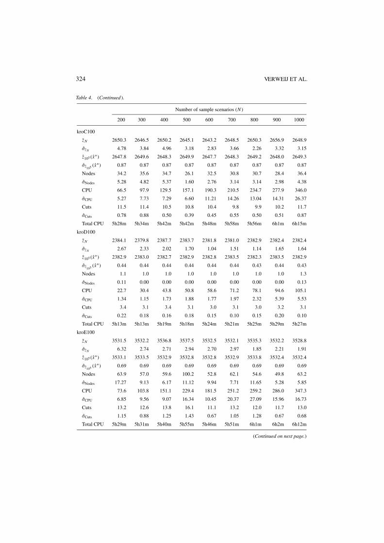
324 VERWEIJ ET AL.

Table 4. (Continued ).

Number of sample scenarios (N )

200 300 400 500 600 700 800 900 1000

kroC100

zN 2650.3 2646.5 2650.2 2645.1 2643.2 2648.5 2650.3 2656.9 2648.9

σzN 4.78 3.84 4.96 3.18 2.83 3.66 2.26 3.32 3.15

z105 (x∗) 2647.8 2649.6 2648.3 2649.9 2647.7 2648.3 2649.2 2648.0 2649.3

σz105 (x∗) 0.87 0.87 0.87 0.87 0.87 0.87 0.87 0.87 0.87

Nodes 34.2 35.6 34.7 26.1 32.5 30.8 30.7 28.4 36.4

σNodes 5.28 4.82 5.37 1.60 2.76 3.14 3.14 2.98 4.38

CPU 66.5 97.9 129.5 157.1 190.3 210.5 234.7 277.9 346.0

σCPU 5.27 7.73 7.29 6.60 11.21 14.26 13.04 14.31 26.37

Cuts 11.5 11.4 10.5 10.8 10.4 9.8 9.9 10.2 11.7

σCuts 0.78 0.88 0.50 0.39 0.45 0.55 0.50 0.51 0.87

Total CPU 5h28m 5h34m 5h42m 5h42m 5h48m 5h58m 5h56m 6h1m 6h15m

kroD100

zN 2384.1 2379.8 2387.7 2383.7 2381.8 2381.0 2382.9 2382.4 2382.4

σzN 2.67 2.33 2.02 1.70 1.04 1.51 1.14 1.65 1.64

z105 (x∗) 2382.9 2383.0 2382.7 2382.9 2382.8 2383.5 2382.3 2383.5 2382.9

σz105 (x∗) 0.44 0.44 0.44 0.44 0.44 0.44 0.43 0.44 0.43

Nodes 1.1 1.0 1.0 1.0 1.0 1.0 1.0 1.0 1.3

σNodes 0.11 0.00 0.00 0.00 0.00 0.00 0.00 0.00 0.13

CPU 22.7 30.4 43.8 50.8 58.6 71.2 78.1 94.6 105.1

σCPU 1.34 1.15 1.73 1.88 1.77 1.97 2.32 5.39 5.53

Cuts 3.4 3.1 3.4 3.1 3.0 3.1 3.0 3.2 3.1

σCuts 0.22 0.18 0.16 0.18 0.15 0.10 0.15 0.20 0.10

Total CPU 5h13m 5h13m 5h19m 5h18m 5h24m 5h21m 5h25m 5h29m 5h27m

kroE100

zN 3531.5 3532.2 3536.8 3537.5 3532.5 3532.1 3535.3 3532.2 3528.8

σzN 6.32 2.74 2.71 2.94 2.70 2.97 1.85 2.21 1.91

z105 (x∗) 3533.1 3533.5 3532.9 3532.8 3532.8 3532.9 3533.8 3532.4 3532.4

σz105 (x∗) 0.69 0.69 0.69 0.69 0.69 0.69 0.69 0.69 0.69

Nodes 63.9 57.0 59.6 100.2 52.8 62.1 54.6 49.8 63.2

σNodes 17.27 9.13 6.17 11.12 9.94 7.71 11.65 5.28 5.85

CPU 73.6 103.8 151.1 229.4 181.5 251.2 259.2 286.0 347.3

σCPU 6.85 9.56 9.07 16.34 10.45 20.37 27.09 15.96 16.73

Cuts 13.2 12.6 13.8 16.1 11.1 13.2 12.0 11.7 13.0

σCuts 1.15 0.88 1.25 1.43 0.67 1.05 1.28 0.67 0.68

Total CPU 5h29m 5h31m 5h40m 5h55m 5h46m 5h51m 6h1m 6h2m 6h12m

(Continued on next page.)

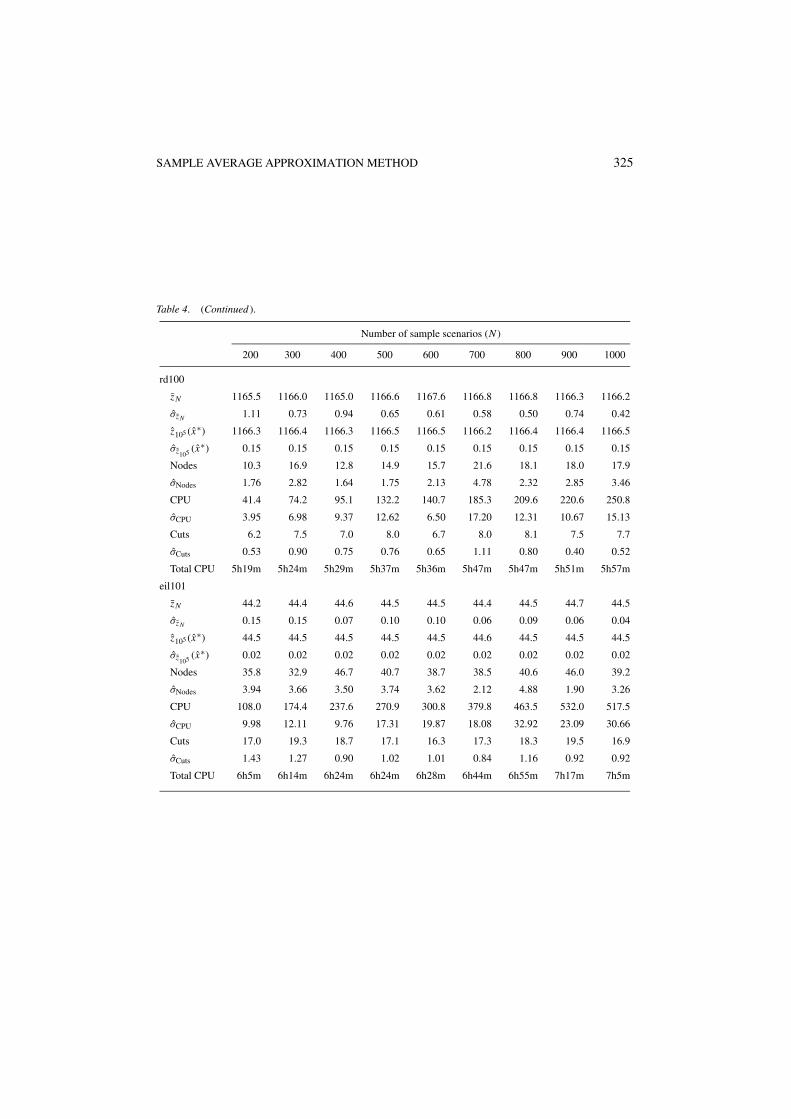
SAMPLE AVERAGE APPROXIMATION METHOD 325

Table 4. (Continued ).

Number of sample scenarios (N )

200 300 400 500 600 700 800 900 1000

rd100

zN 1165.5 1166.0 1165.0 1166.6 1167.6 1166.8 1166.8 1166.3 1166.2

σzN 1.11 0.73 0.94 0.65 0.61 0.58 0.50 0.74 0.42

z105 (x∗) 1166.3 1166.4 1166.3 1166.5 1166.5 1166.2 1166.4 1166.4 1166.5

σz105 (x∗) 0.15 0.15 0.15 0.15 0.15 0.15 0.15 0.15 0.15

Nodes 10.3 16.9 12.8 14.9 15.7 21.6 18.1 18.0 17.9

σNodes 1.76 2.82 1.64 1.75 2.13 4.78 2.32 2.85 3.46

CPU 41.4 74.2 95.1 132.2 140.7 185.3 209.6 220.6 250.8

σCPU 3.95 6.98 9.37 12.62 6.50 17.20 12.31 10.67 15.13

Cuts 6.2 7.5 7.0 8.0 6.7 8.0 8.1 7.5 7.7

σCuts 0.53 0.90 0.75 0.76 0.65 1.11 0.80 0.40 0.52

Total CPU 5h19m 5h24m 5h29m 5h37m 5h36m 5h47m 5h47m 5h51m 5h57m

eil101

zN 44.2 44.4 44.6 44.5 44.5 44.4 44.5 44.7 44.5

σzN 0.15 0.15 0.07 0.10 0.10 0.06 0.09 0.06 0.04

z105 (x∗) 44.5 44.5 44.5 44.5 44.5 44.6 44.5 44.5 44.5

σz105 (x∗) 0.02 0.02 0.02 0.02 0.02 0.02 0.02 0.02 0.02

Nodes 35.8 32.9 46.7 40.7 38.7 38.5 40.6 46.0 39.2

σNodes 3.94 3.66 3.50 3.74 3.62 2.12 4.88 1.90 3.26

CPU 108.0 174.4 237.6 270.9 300.8 379.8 463.5 532.0 517.5

σCPU 9.98 12.11 9.76 17.31 19.87 18.08 32.92 23.09 30.66

Cuts 17.0 19.3 18.7 17.1 16.3 17.3 18.3 19.5 16.9

σCuts 1.43 1.27 0.90 1.02 1.01 0.84 1.16 0.92 0.92

Total CPU 6h5m 6h14m 6h24m 6h24m 6h28m 6h44m 6h55m 7h17m 7h5m

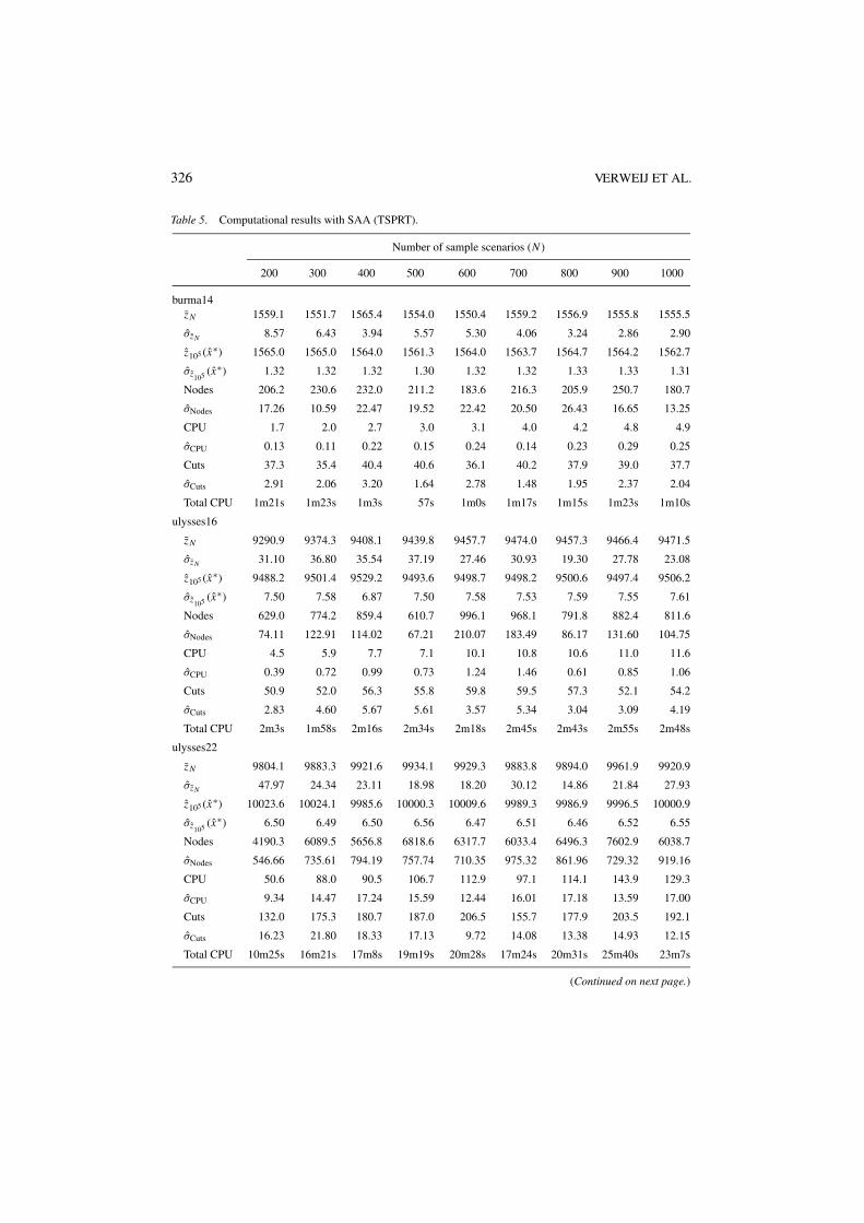
326 VERWEIJ ET AL.

Table 5. Computational results with SAA (TSPRT).

Number of sample scenarios (N )

200 300 400 500 600 700 800 900 1000

burma14zN 1559.1 1551.7 1565.4 1554.0 1550.4 1559.2 1556.9 1555.8 1555.5

σzN 8.57 6.43 3.94 5.57 5.30 4.06 3.24 2.86 2.90

z105 (x∗) 1565.0 1565.0 1564.0 1561.3 1564.0 1563.7 1564.7 1564.2 1562.7

σz105 (x∗) 1.32 1.32 1.32 1.30 1.32 1.32 1.33 1.33 1.31

Nodes 206.2 230.6 232.0 211.2 183.6 216.3 205.9 250.7 180.7

σNodes 17.26 10.59 22.47 19.52 22.42 20.50 26.43 16.65 13.25

CPU 1.7 2.0 2.7 3.0 3.1 4.0 4.2 4.8 4.9

σCPU 0.13 0.11 0.22 0.15 0.24 0.14 0.23 0.29 0.25

Cuts 37.3 35.4 40.4 40.6 36.1 40.2 37.9 39.0 37.7

σCuts 2.91 2.06 3.20 1.64 2.78 1.48 1.95 2.37 2.04

Total CPU 1m21s 1m23s 1m3s 57s 1m0s 1m17s 1m15s 1m23s 1m10s

ulysses16

zN 9290.9 9374.3 9408.1 9439.8 9457.7 9474.0 9457.3 9466.4 9471.5

σzN 31.10 36.80 35.54 37.19 27.46 30.93 19.30 27.78 23.08

z105 (x∗) 9488.2 9501.4 9529.2 9493.6 9498.7 9498.2 9500.6 9497.4 9506.2

σz105 (x∗) 7.50 7.58 6.87 7.50 7.58 7.53 7.59 7.55 7.61

Nodes 629.0 774.2 859.4 610.7 996.1 968.1 791.8 882.4 811.6

σNodes 74.11 122.91 114.02 67.21 210.07 183.49 86.17 131.60 104.75

CPU 4.5 5.9 7.7 7.1 10.1 10.8 10.6 11.0 11.6

σCPU 0.39 0.72 0.99 0.73 1.24 1.46 0.61 0.85 1.06

Cuts 50.9 52.0 56.3 55.8 59.8 59.5 57.3 52.1 54.2

σCuts 2.83 4.60 5.67 5.61 3.57 5.34 3.04 3.09 4.19

Total CPU 2m3s 1m58s 2m16s 2m34s 2m18s 2m45s 2m43s 2m55s 2m48s

ulysses22

zN 9804.1 9883.3 9921.6 9934.1 9929.3 9883.8 9894.0 9961.9 9920.9

σzN 47.97 24.34 23.11 18.98 18.20 30.12 14.86 21.84 27.93

z105 (x∗) 10023.6 10024.1 9985.6 10000.3 10009.6 9989.3 9986.9 9996.5 10000.9

σz105 (x∗) 6.50 6.49 6.50 6.56 6.47 6.51 6.46 6.52 6.55

Nodes 4190.3 6089.5 5656.8 6818.6 6317.7 6033.4 6496.3 7602.9 6038.7

σNodes 546.66 735.61 794.19 757.74 710.35 975.32 861.96 729.32 919.16

CPU 50.6 88.0 90.5 106.7 112.9 97.1 114.1 143.9 129.3

σCPU 9.34 14.47 17.24 15.59 12.44 16.01 17.18 13.59 17.00

Cuts 132.0 175.3 180.7 187.0 206.5 155.7 177.9 203.5 192.1

σCuts 16.23 21.80 18.33 17.13 9.72 14.08 13.38 14.93 12.15

Total CPU 10m25s 16m21s 17m8s 19m19s 20m28s 17m24s 20m31s 25m40s 23m7s

(Continued on next page.)

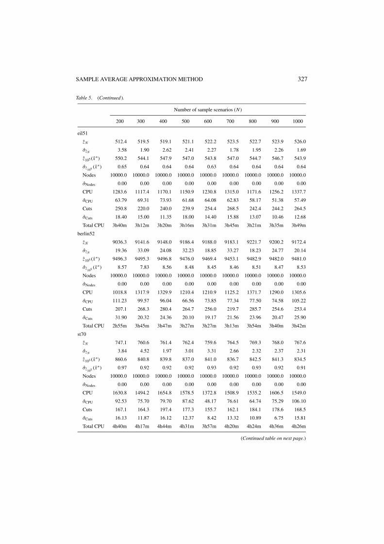
SAMPLE AVERAGE APPROXIMATION METHOD 327

Table 5. (Continued ).

Number of sample scenarios (N )

200 300 400 500 600 700 800 900 1000

eil51

zN 512.4 519.5 519.1 521.1 522.2 523.5 522.7 523.9 526.0

σzN 3.58 1.90 2.62 2.41 2.27 1.78 1.95 2.26 1.69

z105 (x∗) 550.2 544.1 547.9 547.0 543.8 547.0 544.7 546.7 543.9

σz105 (x∗) 0.65 0.64 0.64 0.64 0.63 0.64 0.64 0.64 0.64

Nodes 10000.0 10000.0 10000.0 10000.0 10000.0 10000.0 10000.0 10000.0 10000.0

σNodes 0.00 0.00 0.00 0.00 0.00 0.00 0.00 0.00 0.00

CPU 1283.6 1117.4 1170.1 1150.9 1230.8 1315.0 1171.6 1256.2 1337.7

σCPU 63.79 69.31 73.93 61.68 64.08 62.83 58.17 51.38 57.49

Cuts 250.8 220.0 240.0 239.9 254.4 268.5 242.4 244.2 264.5

σCuts 18.40 15.00 11.35 18.00 14.40 15.88 13.07 10.46 12.68

Total CPU 3h40m 3h12m 3h20m 3h16m 3h31m 3h45m 3h21m 3h35m 3h49m

berlin52

zN 9036.3 9141.6 9148.0 9186.4 9188.0 9183.1 9221.7 9200.2 9172.4

σzN 19.36 33.09 24.08 32.23 18.85 33.27 18.23 24.77 20.14

z105 (x∗) 9496.3 9495.3 9496.8 9476.0 9469.4 9453.1 9482.9 9482.0 9481.0

σz105 (x∗) 8.57 7.83 8.56 8.48 8.45 8.46 8.51 8.47 8.53

Nodes 10000.0 10000.0 10000.0 10000.0 10000.0 10000.0 10000.0 10000.0 10000.0

σNodes 0.00 0.00 0.00 0.00 0.00 0.00 0.00 0.00 0.00

CPU 1018.8 1317.9 1329.9 1210.4 1210.9 1125.2 1371.7 1290.0 1305.6

σCPU 111.23 99.57 96.04 66.56 73.85 77.34 77.50 74.58 105.22

Cuts 207.1 268.3 280.4 264.7 256.0 219.7 285.7 254.6 253.4

σCuts 31.90 20.32 24.36 20.10 19.17 21.56 23.96 20.47 25.90

Total CPU 2h55m 3h45m 3h47m 3h27m 3h27m 3h13m 3h54m 3h40m 3h42m

st70

zN 747.1 760.6 761.4 762.4 759.6 764.5 769.3 768.0 767.6

σzN 3.84 4.52 1.97 3.01 3.31 2.66 2.32 2.37 2.31

z105 (x∗) 860.6 840.8 839.8 837.0 841.0 836.7 842.5 841.3 834.5

σz105 (x∗) 0.97 0.92 0.92 0.92 0.93 0.92 0.93 0.92 0.91

Nodes 10000.0 10000.0 10000.0 10000.0 10000.0 10000.0 10000.0 10000.0 10000.0

σNodes 0.00 0.00 0.00 0.00 0.00 0.00 0.00 0.00 0.00

CPU 1630.8 1494.2 1654.8 1578.5 1372.8 1508.9 1535.2 1606.5 1549.0

σCPU 92.53 75.70 79.70 87.62 48.17 76.61 64.74 75.29 106.10

Cuts 167.1 164.3 197.4 177.3 155.7 162.1 184.1 178.6 168.5

σCuts 16.13 11.87 16.12 12.37 8.42 13.32 10.89 6.75 15.81

Total CPU 4h40m 4h17m 4h44m 4h31m 3h57m 4h20m 4h24m 4h36m 4h26m

(Continued table on next page.)

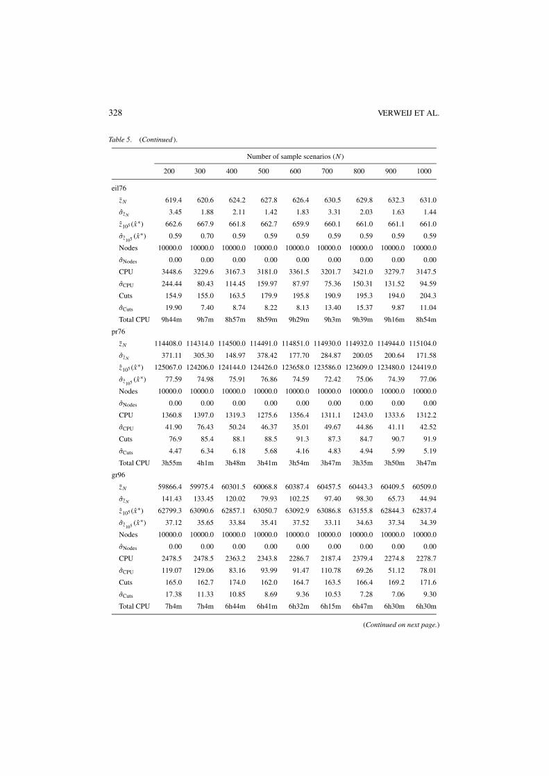
328 VERWEIJ ET AL.

Table 5. (Continued ).

Number of sample scenarios (N )

200 300 400 500 600 700 800 900 1000

eil76

zN 619.4 620.6 624.2 627.8 626.4 630.5 629.8 632.3 631.0

σzN 3.45 1.88 2.11 1.42 1.83 3.31 2.03 1.63 1.44

z105 (x∗) 662.6 667.9 661.8 662.7 659.9 660.1 661.0 661.1 661.0

σz105 (x∗) 0.59 0.70 0.59 0.59 0.59 0.59 0.59 0.59 0.59

Nodes 10000.0 10000.0 10000.0 10000.0 10000.0 10000.0 10000.0 10000.0 10000.0

σNodes 0.00 0.00 0.00 0.00 0.00 0.00 0.00 0.00 0.00

CPU 3448.6 3229.6 3167.3 3181.0 3361.5 3201.7 3421.0 3279.7 3147.5

σCPU 244.44 80.43 114.45 159.97 87.97 75.36 150.31 131.52 94.59

Cuts 154.9 155.0 163.5 179.9 195.8 190.9 195.3 194.0 204.3

σCuts 19.90 7.40 8.74 8.22 8.13 13.40 15.37 9.87 11.04

Total CPU 9h44m 9h7m 8h57m 8h59m 9h29m 9h3m 9h39m 9h16m 8h54m

pr76

zN 114408.0 114314.0 114500.0 114491.0 114851.0 114930.0 114932.0 114944.0 115104.0

σzN 371.11 305.30 148.97 378.42 177.70 284.87 200.05 200.64 171.58

z105 (x∗) 125067.0 124206.0 124144.0 124426.0 123658.0 123586.0 123609.0 123480.0 124419.0

σz105 (x∗) 77.59 74.98 75.91 76.86 74.59 72.42 75.06 74.39 77.06

Nodes 10000.0 10000.0 10000.0 10000.0 10000.0 10000.0 10000.0 10000.0 10000.0

σNodes 0.00 0.00 0.00 0.00 0.00 0.00 0.00 0.00 0.00

CPU 1360.8 1397.0 1319.3 1275.6 1356.4 1311.1 1243.0 1333.6 1312.2

σCPU 41.90 76.43 50.24 46.37 35.01 49.67 44.86 41.11 42.52

Cuts 76.9 85.4 88.1 88.5 91.3 87.3 84.7 90.7 91.9

σCuts 4.47 6.34 6.18 5.68 4.16 4.83 4.94 5.99 5.19

Total CPU 3h55m 4h1m 3h48m 3h41m 3h54m 3h47m 3h35m 3h50m 3h47m

gr96

zN 59866.4 59975.4 60301.5 60068.8 60387.4 60457.5 60443.3 60409.5 60509.0

σzN 141.43 133.45 120.02 79.93 102.25 97.40 98.30 65.73 44.94

z105 (x∗) 62799.3 63090.6 62857.1 63050.7 63092.9 63086.8 63155.8 62844.3 62837.4

σz105 (x∗) 37.12 35.65 33.84 35.41 37.52 33.11 34.63 37.34 34.39

Nodes 10000.0 10000.0 10000.0 10000.0 10000.0 10000.0 10000.0 10000.0 10000.0

σNodes 0.00 0.00 0.00 0.00 0.00 0.00 0.00 0.00 0.00

CPU 2478.5 2478.5 2363.2 2343.8 2286.7 2187.4 2379.4 2274.8 2278.7

σCPU 119.07 129.06 83.16 93.99 91.47 110.78 69.26 51.12 78.01

Cuts 165.0 162.7 174.0 162.0 164.7 163.5 166.4 169.2 171.6

σCuts 17.38 11.33 10.85 8.69 9.36 10.53 7.28 7.06 9.30

Total CPU 7h4m 7h4m 6h44m 6h41m 6h32m 6h15m 6h47m 6h30m 6h30m

(Continued on next page.)

SAMPLE AVERAGE APPROXIMATION METHOD 329

Table 5. (Continued ).

Number of sample scenarios (N )

200 300 400 500 600 700 800 900 1000

rat99

zN 1391.5 1388.0 1405.2 1410.1 1414.8 1408.2 1412.5 1413.8 1417.0

σzN 13.35 4.45 4.73 6.06 3.51 5.25 4.44 2.99 2.18

z105 (x∗) 1469.1 1465.2 1470.3 1468.5 1466.8 1462.4 1461.0 1462.3 1464.4

σz105 (x∗) 1.25 1.28 1.20 1.24 1.35 1.33 1.28 1.29 1.24

Nodes 10000.0 10000.0 9716.5 10000.0 10000.0 10000.0 10000.0 10000.0 10000.0

σNodes 0.00 0.00 283.30 0.00 0.00 0.00 0.00 0.00 0.00

CPU 3153.4 2768.7 2632.0 3099.2 2949.8 2828.6 2688.9 3067.2 2809.8

σCPU 96.82 135.33 238.09 106.67 55.83 99.21 120.97 168.82 172.06

Cuts 178.3 174.7 170.6 189.2 173.5 176.8 182.5 200.9 176.4

σCuts 13.62 10.05 14.07 9.30 9.41 14.63 11.25 19.92 12.77

Total CPU 8h57m 7h53m 7h30m 8h48m 8h23m 8h3m 7h40m 8h42m 8h0m

kroA100

zN 24141.1 24155.7 24381.7 24388.7 24369.9 24335.0 24448.1 24580.2 24541.3

σzN 112.48 87.66 68.61 73.86 58.01 73.18 57.04 42.44 62.13

z105 (x∗) 25807.5 25860.3 26004.5 25697.8 25918.0 25810.7 25793.2 25803.5 25775.1

σz105 (x∗) 19.23 21.23 20.57 19.10 19.36 17.95 20.03 20.21 20.19

Nodes 10000.0 10000.0 10000.0 10000.0 10000.0 10000.0 10000.0 10000.0 10000.0

σNodes 0.00 0.00 0.00 0.00 0.00 0.00 0.00 0.00 0.00

CPU 2681.1 2581.2 2497.5 2418.5 2311.9 2439.4 2390.2 2401.8 2263.0

σCPU 119.95 103.15 129.11 113.43 94.54 69.39 76.86 98.14 97.48

Cuts 154.6 164.6 159.4 156.5 164.0 166.2 169.1 175.6 165.6

σCuts 12.74 6.97 11.39 8.58 11.76 6.11 10.99 10.46 10.44

Total CPU 7h39m 7h22m 7h8m 6h55m 6h37m 6h58m 6h50m 6h52m 6h29m

kroB100

zN 24043.4 24506.2 24353.1 24475.2 24407.7 24457.3 24453.6 24655.2 24549.0

σzN 106.38 53.81 63.92 47.58 53.02 40.70 42.31 41.62 47.49

z105 (x∗) 26319.7 26732.1 26418.0 26466.2 26286.0 26470.1 26551.4 26356.6 26411.4

σz105 (x∗) 18.57 18.21 19.77 20.53 15.80 17.47 21.37 19.26 18.32

Nodes 10000.0 10000.0 10000.0 10000.0 10000.0 10000.0 10000.0 10000.0 10000.0

σNodes 0.00 0.00 0.00 0.00 0.00 0.00 0.00 0.00 0.00

CPU 3114.9 3156.8 2828.6 3107.4 2854.8 2796.4 2936.4 2941.2 2754.5

σCPU 155.59 108.03 88.09 155.32 119.37 71.70 84.19 96.50 99.13

Cuts 178.1 198.8 206.0 234.1 205.4 202.3 207.1 218.7 202.3

σCuts 11.58 7.43 7.38 13.69 12.46 5.42 8.53 8.57 11.66

Total CPU 8h51m 8h57m 8h3m 8h49m 8h7m 7h58m 8h21m 8h22m 7h51m

(Continued on next page.)

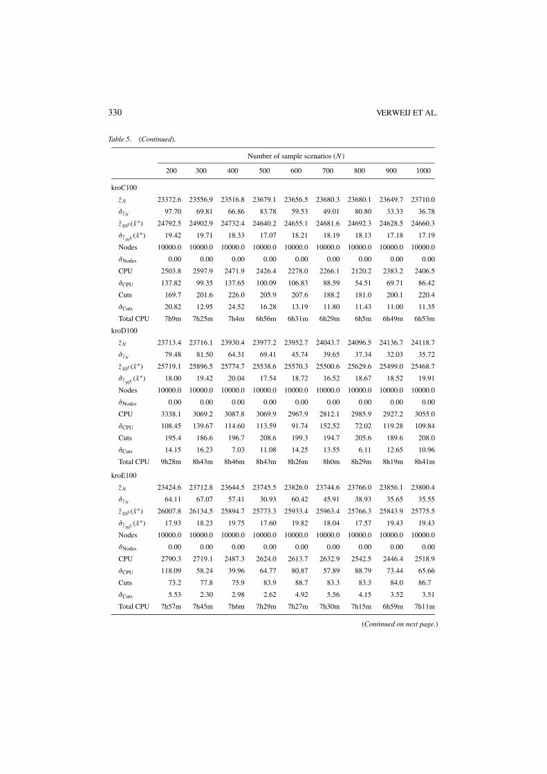
330 VERWEIJ ET AL.

Table 5. (Continued).

Number of sample scenarios (N )

200 300 400 500 600 700 800 900 1000

kroC100

zN 23372.6 23556.9 23516.8 23679.1 23656.5 23680.3 23680.1 23649.7 23710.0

σzN 97.70 69.81 66.86 83.78 59.53 49.01 80.80 33.33 36.78

z105 (x∗) 24792.5 24902.9 24732.4 24640.2 24655.1 24681.6 24692.3 24628.5 24660.3

σz105 (x∗) 19.42 19.71 18.33 17.07 18.21 18.19 18.13 17.18 17.19

Nodes 10000.0 10000.0 10000.0 10000.0 10000.0 10000.0 10000.0 10000.0 10000.0

σNodes 0.00 0.00 0.00 0.00 0.00 0.00 0.00 0.00 0.00

CPU 2503.8 2597.9 2471.9 2426.4 2278.0 2266.1 2120.2 2383.2 2406.5

σCPU 137.82 99.35 137.65 100.09 106.83 88.59 54.51 69.71 86.42

Cuts 169.7 201.6 226.0 205.9 207.6 188.2 181.0 200.1 220.4

σCuts 20.82 12.95 24.52 16.28 13.19 11.80 11.43 11.00 11.35

Total CPU 7h9m 7h25m 7h4m 6h56m 6h31m 6h29m 6h5m 6h49m 6h53m

kroD100

zN 23713.4 23716.1 23930.4 23977.2 23952.7 24043.7 24096.5 24136.7 24118.7

σzN 79.48 81.50 64.31 69.41 45.74 39.65 37.34 32.03 35.72

z105 (x∗) 25719.1 25896.5 25774.7 25538.6 25570.3 25500.6 25629.6 25499.0 25468.7

σz105 (x∗) 18.00 19.42 20.04 17.54 18.72 16.52 18.67 18.52 19.91

Nodes 10000.0 10000.0 10000.0 10000.0 10000.0 10000.0 10000.0 10000.0 10000.0

σNodes 0.00 0.00 0.00 0.00 0.00 0.00 0.00 0.00 0.00

CPU 3338.1 3069.2 3087.8 3069.9 2967.9 2812.1 2985.9 2927.2 3055.0

σCPU 108.45 139.67 114.60 113.59 91.74 152.52 72.02 119.28 109.84

Cuts 195.4 186.6 196.7 208.6 199.3 194.7 205.6 189.6 208.0

σCuts 14.15 16.23 7.03 11.08 14.25 13.55 6.11 12.65 10.96

Total CPU 9h28m 8h43m 8h46m 8h43m 8h26m 8h0m 8h29m 8h19m 8h41m

kroE100

zN 23424.6 23712.8 23644.5 23745.5 23826.0 23744.6 23766.0 23856.1 23800.4

σzN 64.11 67.07 57.41 30.93 60.42 45.91 38.93 35.65 35.55

z105 (x∗) 26007.8 26134.5 25894.7 25773.3 25933.4 25963.4 25766.3 25843.9 25775.5

σz105 (x∗) 17.93 18.23 19.75 17.60 19.82 18.04 17.57 19.43 19.43

Nodes 10000.0 10000.0 10000.0 10000.0 10000.0 10000.0 10000.0 10000.0 10000.0

σNodes 0.00 0.00 0.00 0.00 0.00 0.00 0.00 0.00 0.00

CPU 2790.3 2719.1 2487.3 2624.0 2613.7 2632.9 2542.5 2446.4 2518.9

σCPU 118.09 58.24 39.96 64.77 80.87 57.89 88.79 73.44 65.66

Cuts 73.2 77.8 75.9 83.9 88.7 83.3 83.3 84.0 86.7

σCuts 5.53 2.30 2.98 2.62 4.92 5.56 4.15 3.52 3.51

Total CPU 7h57m 7h45m 7h6m 7h29m 7h27m 7h30m 7h15m 6h59m 7h11m

(Continued on next page.)

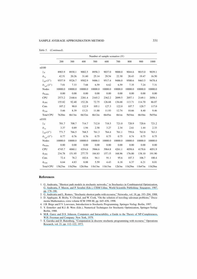
SAMPLE AVERAGE APPROXIMATION METHOD 331

Table 5. (Continued).

Number of sample scenarios (N )

200 300 400 500 600 700 800 900 1000

rd100

zN 8903.9 8930.1 9002.5 8958.3 9037.0 9000.0 9044.6 9015.0 9039.1

σzN 42.51 20.26 31.60 25.14 29.54 22.30 28.43 19.47 16.50

z105 (x∗) 9557.9 9526.7 9502.9 9486.1 9517.4 9486.0 9500.6 9463.5 9478.4

σz105 (x∗) 7.01 7.33 7.68 6.59 6.62 6.59 7.35 7.24 7.31

Nodes 10000.0 10000.0 10000.0 10000.0 10000.0 10000.0 10000.0 10000.0 10000.0

σNodes 0.00 0.00 0.00 0.00 0.00 0.00 0.00 0.00 0.00

CPU 2573.2 2168.6 2281.4 2165.2 2362.2 2099.5 2057.1 2149.1 2058.1

σCPU 155.82 92.40 152.26 72.75 126.68 136.68 113.71 114.70 86.07

Cuts 107.2 90.0 122.9 105.1 127.3 122.0 107.7 120.7 117.0

σCuts 5.66 8.39 13.21 11.88 11.93 12.74 10.66 8.40 9.46

Total CPU 7h20m 6h13m 6h32m 6h12m 6h45m 6h1m 5h54m 6h10m 5h55m

eil101

zN 701.7 708.7 714.7 712.8 718.5 721.0 720.9 720.6 721.2

σzN 3.37 0.89 1.94 2.58 3.27 2.34 2.61 1.44 2.33

z105 (x∗) 771.7 766.5 768.5 761.3 764.4 761.1 759.6 763.8 763.1

σz105 (x∗) 0.77 0.76 0.76 0.75 0.75 0.75 0.74 0.75 0.75

Nodes 10000.0 10000.0 10000.0 10000.0 10000.0 10000.0 10000.0 10000.0 10000.0

σNodes 0.00 0.00 0.00 0.00 0.00 0.00 0.00 0.00 0.00

CPU 4745.7 4060.1 4354.6 3966.6 3964.8 4261.1 4058.6 4170.6 4051.9

σCPU 234.78 151.95 277.75 184.83 157.15 168.96 176.00 138.10 191.90

Cuts 72.4 78.2 102.6 94.1 91.1 95.6 107.3 106.7 100.4

σCuts 6.64 4.83 8.88 5.59 4.43 6.18 6.37 6.21 8.01

Total CPU 13h23m 11h29m 12h18m 11h13m 11h13m 12h3m 11h29m 11h47m 11h28m

References

1. G. Andreatta, “Shortest path models in stochastic networks,” in Stochastics in Combinatorial Optimization,G. Andreatta, F. Mason, and P. Serafini (Eds.), CISM Udine, World Scientific Publishing: Singapore, 1987,pp. 178–186.

2. G. Andreatta and L. Romeo, “Stochastic shortest paths with recourse,” Networks, vol. 18, pp. 193–204, 1988.3. D. Applegate, R. Bixby, V. Chvatal, and W. Cook, “On the solution of traveling salesman problems,” Docu-

menta Mathematica, extra volume ICM 1998 III, pp. 645–656, 1998.4. J.B. Birge and F.V. Louveaux, Introduction to Stochastic Programming, Springer-Verlag: Berlin, 1997.5. Y. Ermoliev and R.J.-B. Wets (Eds.), Numerical Techniques for Stochastic Optimization, Springer-Verlag:

Berlin, 1988.6. M.R. Garey and D.S. Johnson, Computers and Intractability, a Guide to the Theory of NP-Completeness,

W.H. Freeman and Company: New York, 1979.7. S. Garstka and D. Rutenberg, “Computation in discrete stochastic programming with recourse,” Operations

Research, vol. 21, pp. 112–122, 1973.

332 VERWEIJ ET AL.

8. C.J. Geyer and E.A. Thompson, “Constrained Monte Carlo maximum likelihood for dependentdata (with discussion),” Journal of the Royal Statistical Society Series B, vol. 54, pp. 657–699,1992.

9. R.E. Gomory and T.C. Hu, “Multi-terminal network flows,” SIAM Journal on Applied Mathematics, vol. 9,pp. 551–570, 1961.

10. J. Hao and J.B. Orlin, “A faster algorithm for finding the minimum cut in a graph,” in Proceedings of the 3rdAnnual ACM-SIAM Symposium on Discrete Algorithms, 1992, pp. 165–174.

11. J.L. Higle and S. Sen, “Stochastic decomposition: An algorithm for two stage stochastic linear programs withrecourse,” Mathematics of Operations Research, vol. 16, pp. 650–669, 1991.

12. J.L. Higle and S. Sen, Stochastic Decomposition, Kluwer Academic Publishers: Dordrecht, The Netherlands,1996.

13. ILOG, Inc., CPLEX Division, Incline Village, Nevada, CPLEX, a division of ILOG, 2001.14. G. Infanger, Planning Under Uncertainty: Solving Large Scale Stochastic Linear Programs, Boyd and Fraser:

Denvers, MA, 1994.15. D.S. Johnson and L.A. McGeoch, “The traveling salesman problem: A case study,” in Local Search in

Combinatorial Optimization, E. Aarts and J.K. Lenstra (Eds.), John Wiley & Sons: Chichester, 1997, pp.215–310.

16. A.J. Kleywegt, A. Shapiro, and T. Homem-de-Mello, “The sample average approximation method for stochas-tic discrete optimization,” SIAM Journal on Optimization, vol. 12, pp. 479–502, 2001.

17. G. Laporte and F.V. Louveaux, “The integer L-shaped method for stochastic integer programs with completerecourse,” Operations Research Letters, vol. 13, pp. 133–142, 1993.

18. G. Laporte, F.V. Louveaux, and H. Mercure, “Models and exact solutions for a class of stochastic location-routing problems,” European Journal of Operational Research, vol. 39, pp. 71–78, 1989.

19. G. Laporte, F.V. Louveaux, and H. Mercure, “The vehicle routing problem with stochastic travel times,”Transportation Science, vol. 26, pp. 161–170, 1992.

20. G. Laporte, F.V. Louveaux, and H. Mercure, “A priori optimization of the probabilistic traveling salesmanproblem,” Operations Research, vol. 42, pp. 543–549, 1994.

21. G. Laporte, F.V. Louveaux, and L. van Hamme, “Exact solution of a stochastic location problem by an integerL-shaped algorithm,” Transportation Science, vol. 28, pp. 95–103, 1994.

22. W.K. Mak, D.P. Morton, and R.K. Wood, “Monte Carlo bounding techniques for determining solution qualityin stochastic programs,” Operations Research Letters, vol. 24, pp. 47–56, 1999.

23. G.L. Nemhauser and L.A. Wolsey, Integer and Combinatorial Optimization, John Wiley and Sons: New York,1988.

24. V.I. Norkin, Y.M. Ermoliev, and A. Ruszczynski, “On optimal allocation of indivisibles under uncertainty,”Operations Research, vol. 46, pp. 381–395, 1998.

25. V.I. Norkin, G.Ch. Pflug, and A. Ruszczynski, “A branch and bound method for stochastic global optimization,”Mathematical Programming, vol. 83, pp. 425–450, 1998.

26. M.W. Padberg and G. Rinaldi, “Facet identification for the symmetric traveling salesman polytope,” Mathe-matical Programming, vol. 47, pp. 219–257, 1990.

27. M.W. Padberg and G. Rinaldi, “A branch-and-cut algorithm for the resolution of large-scale symmetrictraveling salesman problems,” SIAM Review, vol. 33, pp. 60–100, 1991.

28. E.L. Plambeck, B.R. Fu, S.M. Robinson, and R. Suri, “Sample-path optimization of convex stochastic per-formance functions,” Mathematical Programming, vol. 75, pp. 137–176, 1996.

29. G. Reinelt, http://softlib.rice.edu/softlib/tsplib, 1995.30. R.Y. Rubinstein and A. Shapiro, “Optimization of static simulation models by the score function method,”

Mathematics and Computers in Simulation, vol. 32, pp. 373–392, 1990.31. A. Schrijver, Theory of Linear and Integer Programming, John Wiley & Sons: Chichester, 1986.32. A. Shapiro, “Simulation-based optimization: Convergence analysis and statistical inference,” Stochastic Mod-

els, vol. 12, pp. 425–454, 1996.33. A. Shapiro and T. Homem-de-Mello, “A simulation-based approach to two-stage stochastic programming

with recourse,” Mathematical Programming, vol. 81, pp. 301–325, 1998.34. A. Shapiro and T. Homem-de-Mello, “On rate of convergence of Monte Carlo approximations of stochastic

programs,” SIAM Journal on Optimization, vol. 11, pp. 70–86, 2001.

SAMPLE AVERAGE APPROXIMATION METHOD 333

35. A.M. Spaccamela, A.H.G. Rinnooy Kan, and L. Stougie, “Hierarchical vehicle routing problems,” Networks,vol. 14, pp. 571–586, 1984.

36. R.M. Van Slyke and R.J.-B. Wets, “L-shaped linear programs with applications to optimal control and stochas-tic programming,” SIAM Journal on Applied Mathematics, vol. 17, pp. 638–663, 1969.

37. A.M. Verweij, “Selected applications of integer programming: A computational study,” Ph.D. Thesis, Depart-ment of Computer Science, Utrecht University, Utrecht, 2000.

38. S.W. Wallace, “Solving stochastic programs with network recourse,” Networks, vol. 16, pp. 295–317, 1986.39. S.W. Wallace, “Investing in arcs in a network to maximize the expected max flow,” Networks, vol. 17,

pp. 87–103, 1987.40. S.W. Wallace, “A two-stage stochastic facility-location problem with time-dependent supply,” in Numerical

Techniques for Stochastic Optimization, Y. Ermoliev and R.J.-B. Wets, Springer-Verlag: Berlin, 1988, pp.489–513.

41. R.J-B. Wets, “Solving stochastic programs with simple recourse,” Stochastics, vol. 10, pp. 219–242, 1983.42. R.J.-B. Wets, “Large scale linear programming techniques,” in Numerical Techniques for Stochastic Opti-

mization, Y. Ermoliev and R.J.-B Wets, Springer-Verlag: Berlin, 1988, pp. 65–93.43. L.A. Wolsey, Integer Programming, John Wiley and Sons: New York, 1998.