A Smoothing Sample Average Approximation Method for

Stochastic Optimization Problems with CVaR Risk Measure

Fanwen Meng1, Jie Sun2, Mark Goh3

Abstract

This paper is concerned with solving single CVaR and mixed CVaR minimization problems.A CHKS-type smoothing sample average approximation (SAA) method is proposed for solvingthese two problems, which retains the convexity and smoothness of the original problem and iseasy to implement. For any fixed smoothing constant ε, this method produces a sequence whosecluster points are weak stationary points of the CVaR optimization problems with probabilityone. This framework of combining smoothing technique and SAA scheme can be extended toother smoothing functions as well. Practical numerical examples arising from logistics manage-ment are presented to show the usefulness of this method.

Key words. Conditional Value-at-Risk, Sample Average Approximation, Smoothing Method, Stochastic

Optimization

AMS subject classifications. 91B28, 90C90, 62P05

1 Introduction

It is very important in risk management to choose a proper risk measure, as exemplified in thegovernmental regulations such as Basel Accord II (2006), which uses Value at Risk (VaR) as

1The corresponding author. The Logistic Institute - Asia Pacific, National University of Singapore. Email:

tlimf@nus.edu.sg.2School of Business and Risk Management Institute, National University of Singapore. Email:

jsun@nus.edu.sg.3School of Business and The Logistics Institute - Asia Pacific, National University of Singapore and University

of South Australia. Email: bizgohkh@nus.edu.sg and Mark.Goh@unisa.edu.au.

1

a preferred risk measure [8]. Given a confidence level α ∈ (0, 1) and a loss function f(x, y) :IRn × IRm → IR, where x is the decision variable and y represents the uncertain factors definedon a probability space (Ω,F ,P), the VaR of the random variable f(x, y) is defined as the leftα-quantile of f , namely

VaRα(x) = minu | P(f(x, y) ≤ u) ≥ α. (1.1)

Here P(·) stands for the probability. However, as a function of the decision variable, VaR is gen-erally nonconvex and computationally nontractable which makes the resulting VaR optimizationproblems hard to solve. Due to this and other reasons, a new risk measure, called conditionalVaR (CVaR) has been studied extensively in recent literature. For x ∈ IRn, let F (x, ·) denotethe distribution of the random variable z = f(x, y). For the given confidence level α ∈ (0, 1),CVaR is defined as follows [3, 19]:

CVaRα(x) = Eα−tail[z], (1.2)

where the α-tail cumulative distribution function of z is in the form of

Fα(x, u) = P(z ≤ u) =

0, if u < VaRα(x),

F (x, u)− α

1− α, if u ≥ VaRα(x).

(1.3)

While CVaR is conceptually defined as the expectation of f(x, y) in the conditional distributionof its upper α-tail, a more operationally convenient definition by Rockafellar and Uryasev [19]is as follows.

CVaRα(x) := minη(x, u, α) | u ∈ IR, (1.4)

where

η(x, u, α) := u +1

1− αE[f(x, y)− u]+, (1.5)

where the superscript plus denotes the plus function [t]+ := max0, t, E denotes the math-ematical expectation. It has been shown that CVaR is the best convex approximation toVaR and has lots of nice properties, which makes it widely acceptable in risk management[2, 4, 7, 9, 10, 12, 14, 18, 19, 20].

In this paper, we are interested in studying CVaR-related minmization problems. The math-ematical model of these problems can be cast in the following form

minCVaRα(x) s.t. x ∈ X , (1.6)

where X stands for the feasible region of the problem, which itself may be defined by certainCVaR constraints, but for the time being, we only assume that X is convex and closed. It isknown [20] that (1.6) is equivalent to the following stochastic program

min(x,u)∈X×IR

u +

11− α

E[f(x, y)− u]+

(1.7)

2

in the sense that these two problems achieve the same minimum value and the x-component ofthe solution to (1.7) is a solution to (1.6).

Another very interesting measure of risk, called the mixed CVaR, is defined as

λ1CVaRα1(x) + · · ·+ λJCVaRαJ (x), (1.8)

where αi ∈ (0, 1) denote the probability levels and λi > 0 represent weights with∑J

i=1 λi = 1,i = 1, . . . , J . Clearly, the single CVaR is a special mixed CVaR with J = 1. Again, the mixedCVaR minimization problem

minx∈X

λ1CVaRα1(x) + · · ·+ λJCVaRαJ (x)

. (1.9)

is shown [12] to be equivalent to the following problem

min λ1

(u1 +

11− α1

E[f(x, y)− u1]+)

+ · · ·+ λJ

(uJ +

11− αJ

E[f(x, y)− uJ ]+)

s. t. (x, u1, · · · , uJ) ∈ X × IR× · · · × IR. (1.10)

Note that in problems (1.7) and (1.10), if the expectations can be evaluated analytically, thenthese two problems can be regarded as standard nonlinear programming problems. However, itmight not be easy to evaluate or compute the underlying expectations in (1.7) and (1.10). Wetherefore consider a Monte Carlo simulation based method, called the sample average approx-imation (SAA) method. See [13, 23, 24, 25, 27]. The basic idea of the method is to generatean independent identically distributed (i.i.d.) samples of y and then approximate the expectedvalue with the sample average. Consequently, the SAA program is a deterministic problem.However, the resulting SAA program may be still nonsmooth due to the nonsmoothness of theplus function in the objective functions of (1.7) and (1.10).

To deal with the nonsmoothness of the SAA programs, as well as to facilitate Newton-typemethods in solving the SAA programs, we propose a CHKS-smoothing technique in this paperand investigate in what sense the smoothed problem could approximate the original problem.We assume that f(x, y) is continuously differentiable and convex in x for any realizations of y.In this way, our smoothing SAA method will preserve the convexity and smoothness in the SAAprograms. Smoothing technique has been used in solving stochastic optimization problems byLin, Chen, and Fukushima [11], but it appears to be new to consider them under the frameworkof SAA methods and CVaR constraints. It will be seen later in this paper that the methodcan be extended without essential difficulty to other smoothing techniques and nonsmooth lossfunctions. To show the usefulness of this approach, we provide numerical examples which comefrom logistics management and present computational results.

The rest of this paper is organized as follows. Section 2 presents some basic notions anddiscusses some properties of CVaR and the SAA programs. Section 3 introduces a smoothingSAA method and analyzes its convergence. Two examples in logistics with CVaR risk measurein combination with their numerical solutions are presented in Section 4.

3

2 Preliminaries

In this section, we first recall some basic notions which will be used in the subsequent analysis.We then discuss the optimality conditions of the CVaR and mixed CVaR optimization problems.

2.1 Compact Set Mappings and Generalized Jacobians

Let ‖ · ‖ denote the Euclidean norm of a vector or a compact set of vectors. When M is acompact set of vectors, we denote the norm of M by ‖M‖ := maxM∈M ‖M‖. For two compactsets C and D, the deviation from C to D, or the excess of C over D, is defined by

D(C, D) := supx∈C

d(x,D)

where d(x,D) denotes the distance from point x to set D defined by d(x,D) := infx′∈D ‖x−x′‖.

Let A(·, y) : V → 2IRlbe a random compact set-valued mapping, where V ⊂ IRl is a compact

set of IRl and y : Ω → Ξ ⊂ IRm is a random vector. A selection of the random set A(v, y(ω)) is arandom vector A(v, y(ω)), which means A(v, y(ω)) is measurable. The expectation of A(v, y(ω)),denoted by E[A(v, y(ω))], is defined as the collection of E[A(v, y(ω))] where A(v, y(ω)) is aselection. Note that such selections exist, see Artstein and Vitale [1] and references therein. Weneed a general assumption for our discussion.

Assumption 1 E[f(x, y)− u]+ is finite for any (x, u) ∈ IRn × IR.

Assumption 1 ensures that the objective functions in CVaR minimization (1.4) and mixed CVaRminimization are well defined. Note that if there exists a measurable function κ(y) such thatE[κ(y)] < ∞ and |f(x, y)| ≤ κ(y) for all x ∈ X and y ∈ Ξ, then Assumption 1 holds.

For a locally Lipschitz continuous function Φ : Θ ⊆ U → W , where Θ is open, let DΦ denotethe set where Φ is differentiable. Then, the B-subdifferential of Φ at u′ ∈ Θ, denoted by ∂BΦ(u′),is the set of V such that

V = limk→∞

JΦ(uk), (2.11)

where uk ∈ DΦ converges to u′. Hence, Clarke’s generalized Jacobian of Φ at u′ is the convexhull of ∂BΦ(u′) [6], i.e., ∂Φ(u′) = conv∂BΦ(u′).

2.2 Optimality Conditions

Let z := (x, u). With a little abuse of notations, we write the random vector y simply as y,

η(z, α) := η(x, u, α) = u + 11−αE[f(x, y)− u]+, and Z := X × IR. Recall that minimizing CVaR

4

over X is equivalent to solving the following problem:

minz∈Z

η(z, α) := E[g(z, α, y)], (2.12)

where g(z, α, y) := u + 11−α [f(x, y) − u]+. Note that (2.12) is a convex problem since Z is a

convex set and η(·, α) is a convex function. Let NZ(z) denote the normal cone of Z at z. Then,according to [17, Theorem 23.8], the optimality condition of problem (2.12) can be written as

0 ∈ ∂zE[g(z, α, y)] +NZ(z). (2.13)

Note that, due to the convexity of the problem under consideration, we have ∂zE[g(z, α, y)] =E[∂zg(z, α, y)]. It is known that (2.13) can be further relaxed as:

0 ∈(

01

)+

11− α

E[A(z, y)] +NZ(z), (2.14)

where

A(z, y) :=

ν

(∂xf(x, y)−1

): ν ∈ ∂ (max0, t) , t = f(x, y)− u

.

It is not hard to show that the set-valued mapping A(·, y) : Z → 2IRn+1is upper semicontinuous,

which is an important property in analyzing the convergence of the stationary points. We sayz ∈ Z a weak stationary point of (2.12) if it satisfies (2.14) and z ∈ Z a stationary point of (2.12)if it satisfies (2.13). Obviously, if a point is a stationary point of (2.12), this point must be aweak stationary point but not vice versa.

Similarly, we consider the optimality conditions for the mixed CVaR minimization problem.We still use the notation z to denote (x, u1, . . . , uJ) and Z to denote X × IR× · · · × IR. Recallthat (1.9) is equivalent to

min λ1

(u1 +

11− α1

E[f(x, y)− u1]+)

+ · · ·+ λJ

(uJ +

11− αJ

E[f(x, y)− uJ ]+)

s. t. x ∈ X , u1, · · · , uJ ∈ IR. (2.15)

We say z ∈ Z a weak stationary point of problem (2.15) if it satisfies

0 ∈(

0λ

)+

λ1

1− α1E[A1(z, y)] + · · ·+ λJ

1− αJE[AJ(z, y)] +NZ(z), (2.16)

where λ = (λ1, . . . , λJ)T , Ai(z, y) :=

ν

(∂xf(x, y)

βi

): ν ∈ ∂ (max0, t) , t = f(x, y)− ui

,

βi is a vector of all zero entries except its i-th entry being −1, i.e., βi = (0, . . . ,−1, . . . , 0)T ∈ IRJ .We say z ∈ Z a stationary point of problem (2.15) if it satisfies

0 ∈ λ1E[∂zg1(x, u1, α1, y)] + · · ·+ λJE[∂zgJ(x, uJ , αJ , y)] +NZ(z), (2.17)

where gi(x, ui, αi, y) := ui + 11−αi

[f(x, y)− ui]+, i = 1, . . . , J .

5

2.3 The SAA Counterparts

We now consider the SAA method for solving CVaR minimization problem. For the single CVaRcase, let y1, y2, · · · , yN be an independent identically distributed (i.i.d) sample of y. The SAAprogram of (2.12) is as follows:

min

gN (z, α) :=

1N

N∑

i=1

g(z, α, yi) | z ∈ Z

. (2.18)

Clearly, (2.18) is a deterministic optimization problem. In order to solve the original problem(2.12), the SAA method solves a sequence of (2.18) and let the sample size N increase. Notethat, in the analysis, α ∈ (0, 1) is taken as a fixed scalar. Hence, unless otherwise specified, theunderlying derivatives are taken with respect to z. A generalized Karush-Kuhn-Tucker (GKKT)condition for (2.18) can be stated as 0 ∈ ∂zgN (z, α) +NZ(z). We say z is a weak GKKT pointof (2.18) if it satisfies

0 ∈(

01

)+

1N(1− α)

N∑

i=1

A(z, yi) +NZ(z). (2.19)

Similarly, for the mixed CVaR minimization case, let y1, y2, · · · , yN be an i.i.d sample ofy. The SAA program of (2.15) is as follows:

minz∈Z

gN (z, α1, . . . , αJ) := λ1

(1N

N∑

i=1

g1(z, α1, yi)

)+ · · ·+ λJ

(1N

N∑

i=1

gJ(z, αJ , yi)

). (2.20)

We say z is a weak GKKT point of (2.20) if it satisfies

0 ∈(

0λ

)+

λ1

(1− α1)N

N∑

i=1

A1(z, yi) + · · ·+ λJ

(1− αJ)N

N∑

i=1

AJ(z, yi) +NZ(z). (2.21)

With the notions of stationary points and by the strong law of large numbers, one can derivethe convergence of the GKKT points of SAA method, which can be found in [12]. In next section,we shall apply the smoothing method in combination with SAA approach to the original CVaRminimization problems under consideration.

3 A Smoothing SAA Method

In this section, we use some smoothing techniques to overcome computational difficulties arisingfrom the nonsmoothness of problems (2.12) and (2.15). For simplicity in analysis, we mainlyinvestigate the convergence of the smoothing SAA method in the case when f(·, y) is continu-ously differentiable and the distribution of random variable y is continuous. At the end of thissection, we briefly discuss the situations when the loss function is nondifferentiable and y follows

6

the discrete distribution, respectively. Since the arguments on the mixed CVaR minimizationproblem are similar to those for single CVaR problem, we shall concentrate on the single caseand omit the details of the mixed case.

3.1 The Case of Single CVaR

Note that the nonsmoothness of the objective η in (2.12) is essentially due to that of the plusfunction [·]+. The following are three well-known smoothing functions for the plus function [t]+,see [15] for instance.

• The neural network smoothing function:

Φ(ε, t) = t + ε ln(1 + e−t/ε); (3.22)

• The Chen-Harker-Kanzow-Smale (CHKS) smoothing function:

Φ(ε, t) =√

4ε2 + t2 + t

2; (3.23)

• The uniform smoothing function:

Φ(ε, t) =

t if t ≥ ε/2

12ε

(t + ε/2)2 if − ε/2 < t < ε/2

0 if t ≤ −ε/2.

(3.24)

Here ε > 0 is the smoothing parameter. Using the smoothing function Φ of [·]+, we then definethe following function

η(ε, z, α) := u +1

1− αE[Φ(ε, f(x, y)− u)]. (3.25)

Then, η can be rewritten as η(ε, z, α) = E[ψ(ε, z, α, y)], where

ψ(ε, z, α, y) := u +1

1− αΦ(ε, f(x, y)− u).

Note that η is convex in z if f(x, y) is convex in x. Hence, one can employ the well-developedsmoothing Newton methods for solving the resulting optimization problem. For further discus-sions on smoothing functions and smoothing techniques, see [15] and the references therein. Inthe following, we consider the smoothed counterpart using the CHKS function. We have thefollowing results.

7

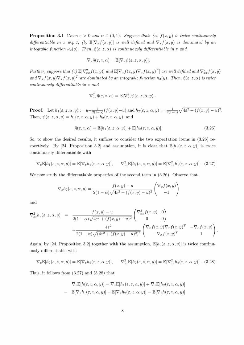
Proposition 3.1 Given ε > 0 and α ∈ (0, 1). Suppose that: (a) f(x, y) is twice continuouslydifferentiable in x w.p.1; (b) E[∇xf(x, y)] is well defined and ∇xf(x, y) is dominated by anintegrable function κ2(y). Then, η(ε, z, α) is continuously differentiable in z and

∇z η(ε, z, α) = E[∇zψ(ε, z, α, y)].

Further, suppose that (c) E[∇2xxf(x, y)] and E[∇xf(x, y)∇xf(x, y)T ] are well defined and ∇2

xxf(x, y)and ∇xf(x, y)∇xf(x, y)T are dominated by an integrable function κ3(y). Then, η(ε, z, α) is twicecontinuously differentiable in z and

∇2zz η(ε, z, α) = E[∇2

zzψ(ε, z, α, y)].

Proof. Let h1(ε, z, α, y) := u+ 12(1−α)(f(x, y)−u) and h2(ε, z, α, y) := 1

2(1−α)

√4ε2 + (f(x, y)− u)2.

Then, ψ(ε, z, α, y) = h1(ε, z, α, y) + h2(ε, z, α, y), and

η(ε, z, α) = E[h1(ε, z, α, y)] + E[h2(ε, z, α, y)]. (3.26)

So, to show the desired results, it suffices to consider the two expectation items in (3.26) re-spectively. By [24, Proposition 3.2] and assumption, it is clear that E[h1(ε, z, α, y)] is twicecontinuously differentiable with

∇zE[h1(ε, z, α, y)] = E[∇zh1(ε, z, α, y)], ∇2zzE[h1(ε, z, α, y)] = E[∇2

zzh1(ε, z, α, y)]. (3.27)

We now study the differentiable properties of the second term in (3.26). Observe that

∇zh2(ε, z, α, y) =f(x, y)− u

2(1− α)√

4ε2 + (f(x, y)− u)2

(∇xf(x, y)

−1

)

and

∇2zzh2(ε, z, α, y) =

f(x, y)− u

2(1− α)√

4ε2 + (f(x, y)− u)2

(∇2

xxf(x, y) 00 0

)

+4ε2

2(1− α)√

(4ε2 + (f(x, y)− u)2)3

(∇xf(x, y)∇xf(x, y)T −∇xf(x, y)

−∇xf(x, y)T 1

).

Again, by [24, Proposition 3.2] together with the assumption, E[h2(ε, z, α, y)] is twice continu-ously differentiable with

∇zE[h2(ε, z, α, y)] = E[∇zh2(ε, z, α, y)], ∇2zzE[h2(ε, z, α, y)] = E[∇2

zzh2(ε, z, α, y)]. (3.28)

Thus, it follows from (3.27) and (3.28) that

∇zE[h(ε, z, α, y)] = ∇zE[h1(ε, z, α, y)] +∇zE[h2(ε, z, α, y)]

= E[∇zh1(ε, z, α, y)] + E[∇zh2(ε, z, α, y)] = E[∇zh(ε, z, α, y)]

8

and

∇2zzE[h(ε, z, α, y)] = ∇2

zzE[h1(ε, z, α, y)] +∇2zzE[h2(ε, z, α, y)]

= E[∇2zzh1(ε, z, α, y)] + E[∇2

zzh2(ε, z, α, y)] = E[∇2zzh(ε, z, α, y)],

which lead to the desired results immediately.

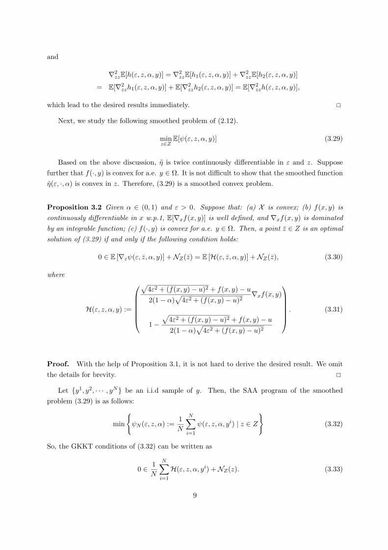
Next, we study the following smoothed problem of (2.12).

minz∈Z

E[ψ(ε, z, α, y)] (3.29)

Based on the above discussion, η is twice continuously differentiable in ε and z. Supposefurther that f(·, y) is convex for a.e. y ∈ Ω. It is not difficult to show that the smoothed functionη(ε, ·, α) is convex in z. Therefore, (3.29) is a smoothed convex problem.

Proposition 3.2 Given α ∈ (0, 1) and ε > 0. Suppose that: (a) X is convex; (b) f(x, y) iscontinuously differentiable in x w.p.1, E[∇xf(x, y)] is well defined, and ∇xf(x, y) is dominatedby an integrable function; (c) f(·, y) is convex for a.e. y ∈ Ω. Then, a point z ∈ Z is an optimalsolution of (3.29) if and only if the following condition holds:

0 ∈ E [∇zψ(ε, z, α, y)] +NZ(z) = E [H(ε, z, α, y)] +NZ(z), (3.30)

where

H(ε, z, α, y) :=

√4ε2 + (f(x, y)− u)2 + f(x, y)− u

2(1− α)√

4ε2 + (f(x, y)− u)2∇xf(x, y)

1−√

4ε2 + (f(x, y)− u)2 + f(x, y)− u

2(1− α)√

4ε2 + (f(x, y)− u)2

. (3.31)

Proof. With the help of Proposition 3.1, it is not hard to derive the desired result. We omitthe details for brevity.

Let y1, y2, · · · , yN be an i.i.d sample of y. Then, the SAA program of the smoothedproblem (3.29) is as follows:

min

ψN (ε, z, α) :=

1N

N∑

i=1

ψ(ε, z, α, yi) | z ∈ Z

(3.32)

So, the GKKT conditions of (3.32) can be written as

0 ∈ 1N

N∑

i=1

H(ε, z, α, yi) +NZ(z). (3.33)

9

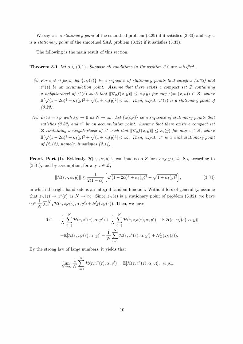
We say z is a stationary point of the smoothed problem (3.29) if it satisfies (3.30) and say z

is a stationary point of the smoothed SAA problem (3.32) if it satisfies (3.33).

The following is the main result of this section.

Theorem 3.1 Let α ∈ (0, 1). Suppose all conditions in Proposition 3.2 are satisfied.

(i) For ε 6= 0 fixed, let zN (ε) be a sequence of stationary points that satisfies (3.33) andz∗(ε) be an accumulation point. Assume that there exists a compact set Z containinga neighborhood of z∗(ε) such that ‖∇xf(x, y)‖ ≤ κ4(y) for any z(= (x, u)) ∈ Z, whereE[

√(1− 2α)2 + κ4(y)2 +

√(1 + κ4(y)2] < ∞. Then, w.p.1. z∗(ε) is a stationary point of

(3.29).

(ii) Let ε = εN with εN → 0 as N → ∞. Let z(εN ) be a sequence of stationary points thatsatisfies (3.33) and z∗ be an accumulation point. Assume that there exists a compact setZ containing a neighborhood of z∗ such that ‖∇xf(x, y)‖ ≤ κ4(y) for any z ∈ Z, whereE[

√(1− 2α)2 + κ4(y)2 +

√(1 + κ4(y)2] < ∞. Then, w.p.1. z∗ is a weak stationary point

of (2.12), namely, it satisfies (2.14).

Proof. Part (i). Evidently, H(ε, ·, α, y) is continuous on Z for every y ∈ Ω. So, according to(3.31), and by assumption, for any z ∈ Z,

‖H(ε, ·, α, y)‖ ≤ 12(1− α)

[√(1− 2α)2 + κ4(y)2 +

√1 + κ4(y)2

], (3.34)

in which the right hand side is an integral random function. Without loss of generality, assumethat zN (ε) → z∗(ε) as N → ∞. Since zN (ε) is a stationary point of problem (3.32), we have

0 ∈ 1N

∑Ni=1H(ε, zN (ε), α, yi) +NZ(zN (ε)). Then, we have

0 ∈ 1N

N∑

i=1

H(ε, z∗(ε), α, yi) +1N

N∑

i=1

H(ε, zN (ε), α, yi)− E[H(ε, zN (ε), α, y)]

+E[H(ε, zN (ε), α, y)]− 1N

N∑

i=1

H(ε, z∗(ε), α, yi) +NZ(zN (ε)).

By the strong law of large numbers, it yields that

limN→∞

1N

N∑

i=1

H(ε, z∗(ε), α, yi) = E[H(ε, z∗(ε), α, y)], w.p.1.

10

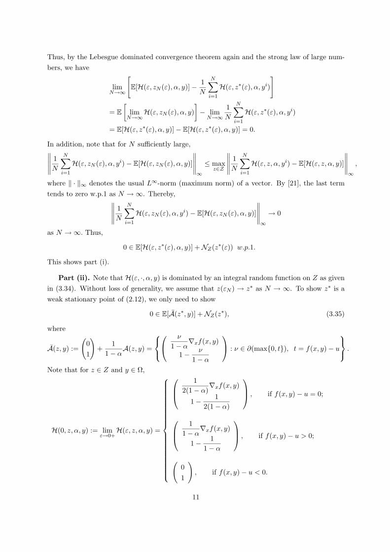
Thus, by the Lebesgue dominated convergence theorem again and the strong law of large num-bers, we have

limN→∞

[E[H(ε, zN (ε), α, y)]− 1

N

N∑

i=1

H(ε, z∗(ε), α, yi)

]

= E[

limN→∞

H(ε, zN (ε), α, y)]− lim

N→∞1N

N∑

i=1

H(ε, z∗(ε), α, yi)

= E[H(ε, z∗(ε), α, y)]− E[H(ε, z∗(ε), α, y)] = 0.

In addition, note that for N sufficiently large,∥∥∥∥∥

1N

N∑

i=1

H(ε, zN (ε), α, yi)− E[H(ε, zN (ε), α, y)]

∥∥∥∥∥∞≤ max

z∈Z

∥∥∥∥∥1N

N∑

i=1

H(ε, z, α, yi)− E[H(ε, z, α, y)]

∥∥∥∥∥∞

,

where ‖ · ‖∞ denotes the usual L∞-norm (maximum norm) of a vector. By [21], the last termtends to zero w.p.1 as N →∞. Thereby,

∥∥∥∥∥1N

N∑

i=1

H(ε, zN (ε), α, yi)− E[H(ε, zN (ε), α, y)]

∥∥∥∥∥∞→ 0

as N →∞. Thus,

0 ∈ E[H(ε, z∗(ε), α, y)] +NZ(z∗(ε)) w.p.1.

This shows part (i).

Part (ii). Note that H(ε, ·, α, y) is dominated by an integral random function on Z as givenin (3.34). Without loss of generality, we assume that z(εN ) → z∗ as N → ∞. To show z∗ is aweak stationary point of (2.12), we only need to show

0 ∈ E[A(z∗, y)] +NZ(z∗), (3.35)

where

A(z, y) :=

(01

)+

11− α

A(z, y) =

ν

1− α∇xf(x, y)

1− ν

1− α

: ν ∈ ∂(max0, t), t = f(x, y)− u

.

Note that for z ∈ Z and y ∈ Ω,

H(0, z, α, y) := limε→0+

H(ε, z, α, y) =

12(1− α)

∇xf(x, y)

1− 12(1− α)

, if f(x, y)− u = 0;

11− α

∇xf(x, y)

1− 11− α

, if f(x, y)− u > 0;

(01

), if f(x, y)− u < 0.

11

According to the assumption, it follows that for z ∈ Z

‖H(0, z, α, y)‖ ≤ max

1,1

1− α

√‖∇xf(x, y)‖2 + (1− 2α)2,

12(1− α)

√‖∇xf(x, y)‖2 + α2

≤ max

1,1

1− α

√κ4(y)2 + (1− 2α)2,

1(1− α)

√κ4(y)2 + 1

≤ max

1,1

1− α

[√κ4(y)2 + (1− 2α)2 +

√κ4(y)2 + 1

],

hence, H(0, ·, α, y) is dominated by an integral random function on Z, thereby, E[H(0, z, α, y)]is well-defined for z ∈ Z. Additionally, it is easy to see that H(0, z, α, y) ⊂ A(z, y) for any z ∈ Z

and y ∈ Ω, which leads to that E[H(0, z, α, y)] ⊂ E[A(z, y)] for z ∈ Z. Thus, to show (3.35)holds, it suffices to prove that

0 ∈ E[H(0, z∗, α, y)] +NZ(z∗).

On the other hand, let ε0 > 0 be a fixed small number. Evidently, H(·, ·, α, y) : [0, ε0) × Z →IRn+1 is a continuous vector-valued mapping for every y ∈ Ω. In addition, based on the abovediscussion and part (i), it follows that H(·, ·, α, y) is dominated by an integral random functionfor (ε, z) ∈ [0, ε0)×Z. Since z(εN ) is a stationary point of problem (3.32), we have

0 ∈ 1N

N∑

i=1

H(εN , z(εN ), α, yi) +NZ(z(εN )). (3.36)

Then,

0 ∈ 1N

N∑

i=1

H(0, z∗, α, yi) +1N

N∑

i=1

H(εN , z(εN ), α, yi)− E[H(εN , z(εN ), α, y)]

+E[H(εN , z(εN ), α, y)]− 1N

N∑

i=1

H(0, z∗, α, yi) +NZ(z(εN )).

By the strong law of large numbers and Lebesgue dominated convergence theorem, for the first,fourth, and fifth terms on the right hand side of the above equation, we have

limN→∞

1N

N∑

i=1

H(0, z∗, α, yi) = E[H(0, z∗, α, y)], w.p.1. (3.37)

limN→∞

[E[H(εN , z(εN ), α, y)]− 1

N

N∑

i=1

H(0, z∗, α, yi)

]= E[ lim

N→∞H(εN , z(εN ), α, y)]−

limN→∞

1N

N∑

i=1

H(0, z∗, α, yi)] = E[H(0, z∗, α, y)]− E[H(0, z∗, α, y)] = 0, w.p.1. (3.38)

12

Finally, we estimate the term ‖ 1N

∑Ni=1H(εN , z(εN ), α, yi)− E[H(εN , z(εN ), α, y)]‖. Note that

for N large enough, we have (εN , z(εN )) ∈ [0, ε0]×Z. Then

‖ 1N

N∑

i=1

H(εN , z(εN ), α, yi)− E[H(εN , z(εN ), α, y)]‖∞

≤ max(ε,z)∈[0,ε0]×Z

‖ 1N

N∑

i=1

H(ε, z, α, yi)− E[H(ε, z, α, y)]‖∞.

Again, by [21], limN→∞max(ε,z)∈[0,ε0]×Z ‖1N

∑Ni=1H(ε, z, α, yi)− E[H(ε, z, α, y)]‖∞ = 0, w.p.1,

thus,

limN→∞

‖ 1N

N∑

i=1

H(εN , z(εN ), α, yi)− E[H(εN , z(εN ), α, y)]‖ = 0, w.p.1 (3.39)

Therefore, by (3.36) together with (3.37), (3.38), and (3.39), w.p.1 z∗ satisfies

0 ∈ E[H(0, z∗, α, y)] +NZ(z∗),

which implies that w.p.1 z∗ satisfies (3.35), that is, z∗ is a weak stationary point of (2.12). Thiscompletes the proof.

Note that in the above analysis, we do not specify the feasible region X . In fact, X cansometimes be defined by finitely many equality and/or inequality constraint functions. In thiscase, one can derive the optimality condition using the Lagrangian function as discussed inclassical nonlinear programming. In terms of numerical computation, we can apply some well-developed Newton methods on nonsmooth equations or nonsmooth optimization problems andlet the smoothing parameter ε tend to zero, see [15, 16], for instance.

3.2 The Case of nondifferentiable loss functions

In practice, the loss function f(·, y) might not be differentiable. For instance, f(·, y) is piecewiselinear/quadratic or even piecewise smooth sometimes. In this case, we resort to some well-developed smoothing techniques. One popular way to deal with the nonsmooth functions is theso-called smoothing function technique. Recall that for a locally Lipschitz continuous functionψ : IRl → IR, ψ(s, ν) : IRl×IR → IR is called a smoothing function of ψ if it satisfies the following:

(i) for every s ∈ IRl, ψ(s, 0) = ψ(s);

(ii) for every s ∈ IRl, ψ is locally Lipschitz continuous at (s, 0);

(iii) ψ is continuously differentiable on IRl × IR \ 0.

13

where ν ∈ IR is called a smoothing parameter. Note that it is easy to verify the CHKS smoothingfunction discussed earlier satisfies these three conditions. In practice, we often consider ν > 0,which is driven to zero in computation.

For a given nondifferentiable function, one can construct its smoothing counterpart, see [15]for a detailed discussion. Now, let f(·, ν, y) be the smoothing function of f(·, y). We then derivethe following problem:

minz∈Z

E[g(z, ν, α, y)] (3.40)

whereg(z, ν, α, y) := u +

11− α

[f(x, ν, y)− u]+,

and ν > 0 is the smoothing parameter. Clearly, problem (3.40) possesses the same setting asdiscussed previously in this section. Thus, we can apply the same arguments, such as using theCHKS smoothing function, to (3.40), and derive a smoothed SAA program. Similarly, for a(small) fixed positive scalar ν, we can derive the convergence of the corresponding smoothingSAA method. Here we omit the details for brevity.

3.3 The Case of mixed CVaR optimization

Following similar arguments above, the smoothed problem of mixed CVaR optimization problem(2.15) is as follows

minz∈Z

λ1E[ψ1(ε, z, α1, y)] + · · ·+ λJE[ψJ(ε, z, αJ , y)]

where ψi(ε, z, αi, y) = ui + 11−αi

Ψ(ε, f(x, y)−ui) for i = 1, . . . , J , and Ψ is the CHKS smoothingfunction. Let y1, · · · , yN be an i.i.d sample of y, then, the corresponding SAA smoothingprogram is

minz∈Z

λ1

1N

N∑

i=1

ψ1(ε, z, α1, yi) + · · ·+ λJ

1N

N∑

i=1

ψJ(ε, z, αJ , yi)

Note that under assumptions as Theorem 3.1, the above SAA smoothing program is actuallya deterministic smoothing problem. With similar discussions as Section 4.1, we can derive thesame convergence results as Theorem 3.1 for the smoothing SAA programs. We omit the detailshere.

3.4 Discussions on the discrete distribution case

We now consider the case where the random variable y follows a discrete distribution with S

finitely many scenarios y1, y2, · · · , yS, each with probability pi, i = 1, · · · , S. Here, we only

14

discuss the mixed CVaR minimization problem (1.10). Note that in this case (1.10) can bewritten as

min λ1

(u1 +

11− α1

S∑

i=1

pi[f(x, yi)− u1]+)

+ · · ·+ λJ

(u1 +

11− αJ

S∑

i=1

pi[f(x, yi)− uJ ]+)

s. t. (x, u1, . . . , uJ) ∈ X × IR× · · · × IR.

(3.41)

Since problem (3.41) is nonsmooth, using the CHKS smoothing function, we then derive thecorresponding smoothing problem below:

min λ1

(u1 +

12(1− α1)

S∑

i=1

pi

[√4ε2 + (f(x, yi)− u1)2 + f(x, yi)− u1

])+ · · ·+

λJ

(uJ +

12(1− αJ)

S∑

i=1

pi

[√4ε2 + (f(x, yi)− uJ)2 + f(x, yi)− uJ

])

s. t. (x, u1, . . . , uJ) ∈ X × IR× · · · × IR,

(3.42)

where ε > 0 is the smoothing parameter and driven to zero.

Note that the size of the smoothed problem (3.42) keeps the same as (3.41) and the solutionof (3.42) tends to that of problem (3.41) as ε tends to zero. Regarding the computationalaspect, we can employ some well-developed smoothing Newton methods established in the pastfew years for solving (3.42), see [5, 15] for instance.

4 Computational Examples in Logistics Management

In this section, we first consider a problem concerning the supply chain of a wine company.where the random variable follows a discrete distribution. Then, we discuss a distribution mixproblem under uncertain demand with a continuous distribution.

4.1 Supply Chain Management of a Wine Company

This example is modified from Yu and Li [28]. In the company’s supply chain, there are four rawmaterial providers (uniform-quality wine in bulk) located in A, B, C, and D, and three bottlingplants located in E, F, and G, and three distribution warehouses located in three different citiesL, M, and N, respectively. We suppose that each market demand merely depends on the localeconomic condition, which is treated as an uncertain factor following a discrete distribution withfour situations: boom, good, fair, or poor and associated probabilities of 0.45, 0.25, 0.17, or 0.13,respectively.

15

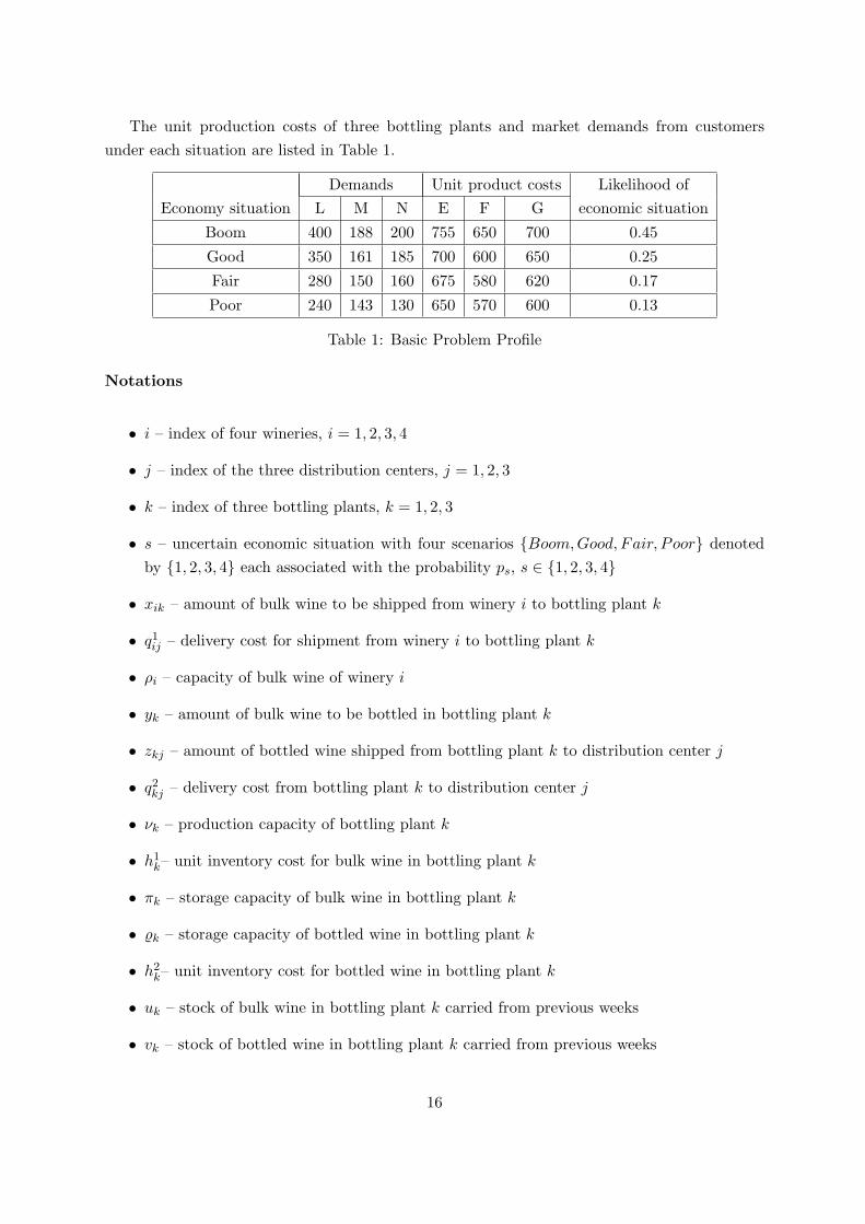
The unit production costs of three bottling plants and market demands from customersunder each situation are listed in Table 1.

Demands Unit product costs Likelihood ofEconomy situation L M N E F G economic situation

Boom 400 188 200 755 650 700 0.45

Good 350 161 185 700 600 650 0.25

Fair 280 150 160 675 580 620 0.17

Poor 240 143 130 650 570 600 0.13

Table 1: Basic Problem Profile

Notations

• i – index of four wineries, i = 1, 2, 3, 4

• j – index of the three distribution centers, j = 1, 2, 3

• k – index of three bottling plants, k = 1, 2, 3

• s – uncertain economic situation with four scenarios Boom,Good, Fair, Poor denotedby 1, 2, 3, 4 each associated with the probability ps, s ∈ 1, 2, 3, 4

• xik – amount of bulk wine to be shipped from winery i to bottling plant k

• q1ij – delivery cost for shipment from winery i to bottling plant k

• ρi – capacity of bulk wine of winery i

• yk – amount of bulk wine to be bottled in bottling plant k

• zkj – amount of bottled wine shipped from bottling plant k to distribution center j

• q2kj – delivery cost from bottling plant k to distribution center j

• νk – production capacity of bottling plant k

• h1k– unit inventory cost for bulk wine in bottling plant k

• πk – storage capacity of bulk wine in bottling plant k

• %k – storage capacity of bottled wine in bottling plant k

• h2k– unit inventory cost for bottled wine in bottling plant k

• uk – stock of bulk wine in bottling plant k carried from previous weeks

• vk – stock of bottled wine in bottling plant k carried from previous weeks

16

• cj(s) – uncertain unit cost for bottling wine in bottling plant j

• Dj(s) – the uncertain market demand from the distribution center j

• ξ(s): underlying random variables of the problem, i.e., ξ(s) = (D(s), c(s)) where D(s) =(D1(s), D2(s), D3(s)) and c(s) = (c1(s), c2(s), c3(s))

Problem Formulation

We suppose that the company would like to determine the optimal amounts of raw materialsordered from the providers, bottled wine produced in the plants, amounts of bottled wine shippedto the suppliers together with the optimal stock levels of the raw materials and bottled wine,so as to minimize the total cost using the measure of conditional value at risk, subject to thesatisfaction of necessary requirements on the resource capacity of the company and the demandof the suppliers of the supply chain.

In general, the total cost f concerning the problem includes the following three parts: i.e.,transportation cost fT, production cost fP, and inventory cost fI, which are stated as follows.

fT(x, y, z, u, v, ξ(s)) :=4∑

i=1

3∑

j=1

q1ijxij +

3∑

j=1

3∑

k=1

q2jkzjk,

fP(x, y, z, u, v, ξ(s)) :=3∑

j=1

cj(s)yj ,

fI(x, y, z, u, v, ξ(s)) :=3∑

k=1

h1k

( 4∑

i=1

xik − yk + uk

)+

3∑

k=1

h2k

(yk + vk −

3∑

j=1

zkj

).

Then, the total cost function gives

f(x, y, z, u, v, , ξ(s)) = fT(x, y, z, u, v, ξ(s)) + fP(x, y, z, u, v, ξ(s)) + fI(x, y, z, u, v, ξ(s))

=4∑

i=1

3∑

j=1

q1ijxij +

3∑

j=1

3∑

k=1

q2jkzjk +

3∑

j=1

cj(s)yj

+3∑

k=1

h1k

( 4∑

i=1

xik − yk + uk

)+

3∑

k=1

h2k

(yk + vk −

3∑

j=1

zkj

).

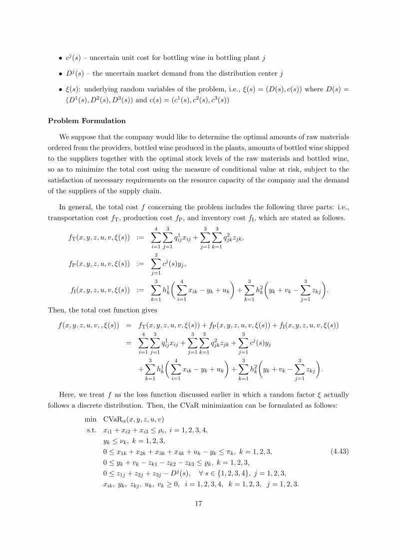
Here, we treat f as the loss function discussed earlier in which a random factor ξ actuallyfollows a discrete distribution. Then, the CVaR minimization can be formulated as follows:

min CVaRα(x, y, z, u, v)s.t. xi1 + xi2 + xi3 ≤ ρi, i = 1, 2, 3, 4,

yk ≤ νk, k = 1, 2, 3,

0 ≤ x1k + x2k + x3k + x4k + uk − yk ≤ πk, k = 1, 2, 3,

0 ≤ yk + vk − zk1 − zk2 − zk3 ≤ %k, k = 1, 2, 3,

0 ≤ z1j + z2j + z3j −Dj(s), ∀ s ∈ 1, 2, 3, 4, j = 1, 2, 3,

xik, yk, zkj , uk, vk ≥ 0, i = 1, 2, 3, 4, k = 1, 2, 3, j = 1, 2, 3.

(4.43)

17

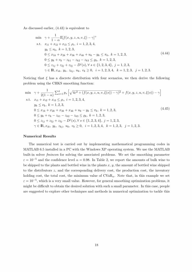
As discussed earlier, (4.43) is equivalent to

min γ +1

1− αE[f(x, y, z, u, v, ξ)− γ]+

s.t. xi1 + xi2 + xi3 ≤ ρi, i = 1, 2, 3, 4,

yk ≤ νk, k = 1, 2, 3,

0 ≤ x1k + x2k + x3k + x4k + uk − yk ≤ πk, k = 1, 2, 3,

0 ≤ yk + vk − zk1 − zk2 − zk3 ≤ %k, k = 1, 2, 3,

0 ≤ z1j + z2j + z3j −Dj(s),∀ s ∈ 1, 2, 3, 4, j = 1, 2, 3,

γ ∈ IR, xik, yk, zkj , uk, vk ≥ 0, i = 1, 2, 3, 4, k = 1, 2, 3, j = 1, 2, 3.

(4.44)

Noticing that ξ has a discrete distribution with four scenarios, we then derive the followingproblem using the CHKS smoothing function:

min γ +1

2(1− α)∑4

s=1 ps

[√4ε2 + (f(x, y, z, u, v, ξ(s))− γ)2 + f(x, y, z, u, v, ξ(s))− γ

]

s.t. xi1 + xi2 + xi3 ≤ ρi, i = 1, 2, 3, 4,

yk ≤ νk, k = 1, 2, 3,

0 ≤ x1k + x2k + x3k + x4k + uk − yk ≤ πk, k = 1, 2, 3,

0 ≤ yk + vk − zk1 − zk2 − zk3 ≤ %k, k = 1, 2, 3,

0 ≤ z1j + z2j + z3j −Dj(s),∀ s ∈ 1, 2, 3, 4, j = 1, 2, 3,

γ ∈ IR, xik, yk, zkj , uk, vk ≥ 0, i = 1, 2, 3, 4, k = 1, 2, 3, j = 1, 2, 3.

(4.45)

Numerical Results

The numerical test is carried out by implementing mathematical programming codes inMATLAB 6.5 installed in a PC with the Windows XP operating system. We use the MATLABbuilt-in solver fmincon for solving the associated problems. We set the smoothing parameterε = 10−5 and the confidence level α = 0.98. In Table 2, we report the amounts of bulk wine tobe shipped to the plants and bottled wine in the plants x, y, the amount of bottled wine shippedto the distributors z, and the corresponding delivery cost, the production cost, the inventoryholding cost, the total cost, the minimum value of CVaRα. Note that, in this example we setε = 10−5, which is a very small value. However, for general smoothing optimization problems, itmight be difficult to obtain the desired solution with such a small parameter. In this case, peopleare suggested to explore other techniques and methods in numerical optimization to tackle this

18

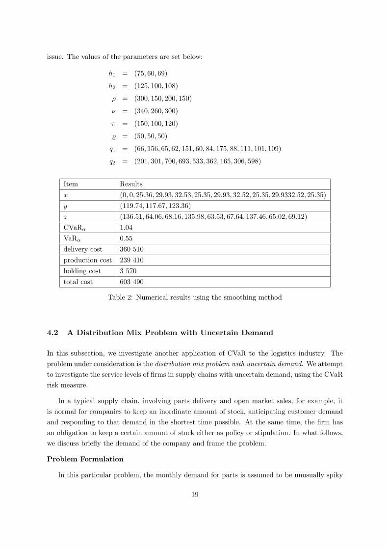
issue. The values of the parameters are set below:

h1 = (75, 60, 69)

h2 = (125, 100, 108)

ρ = (300, 150, 200, 150)

ν = (340, 260, 300)

π = (150, 100, 120)

% = (50, 50, 50)

q1 = (66, 156, 65, 62, 151, 60, 84, 175, 88, 111, 101, 109)

q2 = (201, 301, 700, 693, 533, 362, 165, 306, 598)

Item Results

x (0, 0, 25.36, 29.93, 32.53, 25.35, 29.93, 32.52, 25.35, 29.9332.52, 25.35)

y (119.74, 117.67, 123.36)

z (136.51, 64.06, 68.16, 135.98, 63.53, 67.64, 137.46, 65.02, 69.12)

CVaRα 1.04

VaRα 0.55

delivery cost 360 510

production cost 239 410

holding cost 3 570

total cost 603 490

Table 2: Numerical results using the smoothing method

4.2 A Distribution Mix Problem with Uncertain Demand

In this subsection, we investigate another application of CVaR to the logistics industry. Theproblem under consideration is the distribution mix problem with uncertain demand. We attemptto investigate the service levels of firms in supply chains with uncertain demand, using the CVaRrisk measure.

In a typical supply chain, involving parts delivery and open market sales, for example, itis normal for companies to keep an inordinate amount of stock, anticipating customer demandand responding to that demand in the shortest time possible. At the same time, the firm hasan obligation to keep a certain amount of stock either as policy or stipulation. In what follows,we discuss briefly the demand of the company and frame the problem.

Problem Formulation

In this particular problem, the monthly demand for parts is assumed to be unusually spiky

19

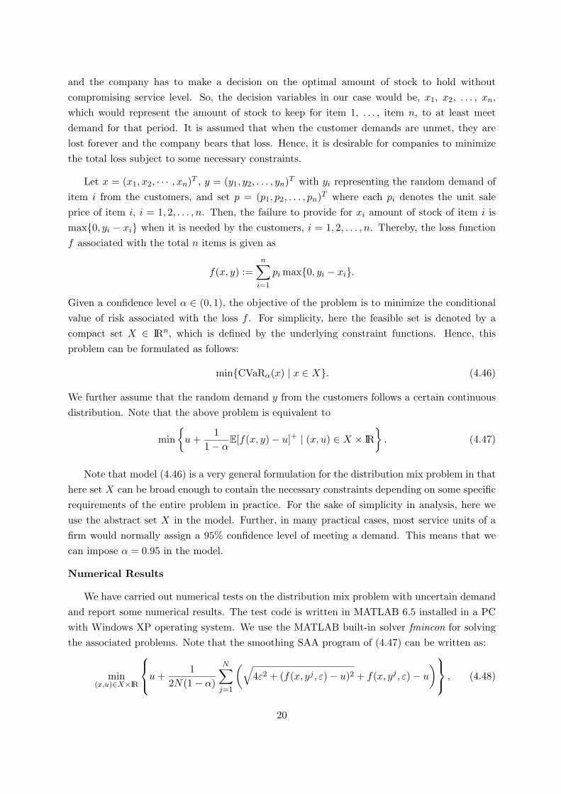
and the company has to make a decision on the optimal amount of stock to hold withoutcompromising service level. So, the decision variables in our case would be, x1, x2, . . . , xn,which would represent the amount of stock to keep for item 1, . . . , item n, to at least meetdemand for that period. It is assumed that when the customer demands are unmet, they arelost forever and the company bears that loss. Hence, it is desirable for companies to minimizethe total loss subject to some necessary constraints.

Let x = (x1, x2, · · · , xn)T , y = (y1, y2, . . . , yn)T with yi representing the random demand ofitem i from the customers, and set p = (p1, p2, . . . , pn)T where each pi denotes the unit saleprice of item i, i = 1, 2, . . . , n. Then, the failure to provide for xi amount of stock of item i ismax0, yi − xi when it is needed by the customers, i = 1, 2, . . . , n. Thereby, the loss functionf associated with the total n items is given as

f(x, y) :=n∑

i=1

pi max0, yi − xi.

Given a confidence level α ∈ (0, 1), the objective of the problem is to minimize the conditionalvalue of risk associated with the loss f . For simplicity, here the feasible set is denoted by acompact set X ∈ IRn, which is defined by the underlying constraint functions. Hence, thisproblem can be formulated as follows:

minCVaRα(x) | x ∈ X. (4.46)

We further assume that the random demand y from the customers follows a certain continuousdistribution. Note that the above problem is equivalent to

min

u +1

1− αE[f(x, y)− u]+ | (x, u) ∈ X × IR

. (4.47)

Note that model (4.46) is a very general formulation for the distribution mix problem in thathere set X can be broad enough to contain the necessary constraints depending on some specificrequirements of the entire problem in practice. For the sake of simplicity in analysis, here weuse the abstract set X in the model. Further, in many practical cases, most service units of afirm would normally assign a 95% confidence level of meeting a demand. This means that wecan impose α = 0.95 in the model.

Numerical Results

We have carried out numerical tests on the distribution mix problem with uncertain demandand report some numerical results. The test code is written in MATLAB 6.5 installed in a PCwith Windows XP operating system. We use the MATLAB built-in solver fmincon for solvingthe associated problems. Note that the smoothing SAA program of (4.47) can be written as:

min(x,u)∈X×IR

u +

12N(1− α)

N∑

j=1

(√4ε2 + (f(x, yj , ε)− u)2 + f(x, yj , ε)− u

) , (4.48)

20

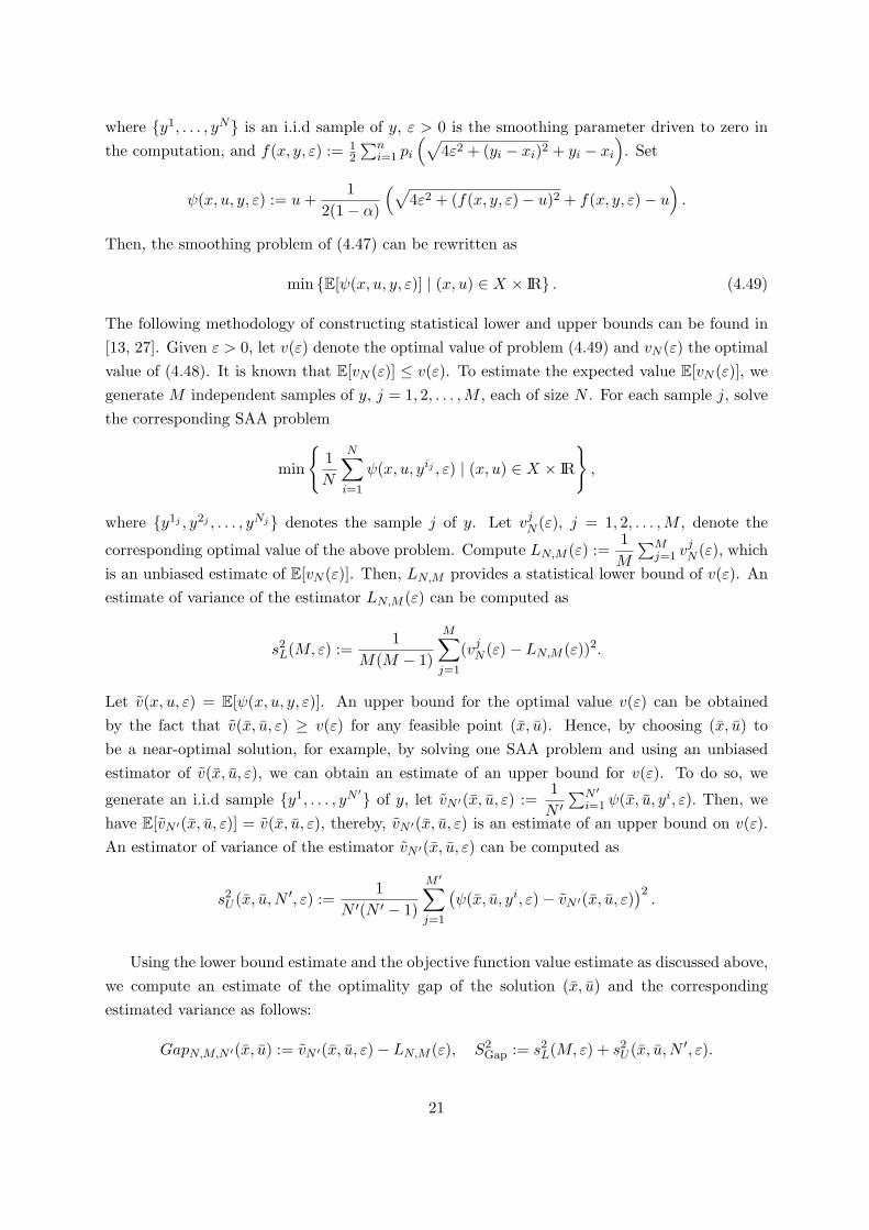
where y1, . . . , yN is an i.i.d sample of y, ε > 0 is the smoothing parameter driven to zero inthe computation, and f(x, y, ε) := 1

2

∑ni=1 pi

(√4ε2 + (yi − xi)2 + yi − xi

). Set

ψ(x, u, y, ε) := u +1

2(1− α)

(√4ε2 + (f(x, y, ε)− u)2 + f(x, y, ε)− u

).

Then, the smoothing problem of (4.47) can be rewritten as

min E[ψ(x, u, y, ε)] | (x, u) ∈ X × IR . (4.49)

The following methodology of constructing statistical lower and upper bounds can be found in[13, 27]. Given ε > 0, let v(ε) denote the optimal value of problem (4.49) and vN (ε) the optimalvalue of (4.48). It is known that E[vN (ε)] ≤ v(ε). To estimate the expected value E[vN (ε)], wegenerate M independent samples of y, j = 1, 2, . . . , M , each of size N . For each sample j, solvethe corresponding SAA problem

min

1N

N∑

i=1

ψ(x, u, yij , ε) | (x, u) ∈ X × IR

,

where y1j , y2j , . . . , yNj denotes the sample j of y. Let vjN (ε), j = 1, 2, . . . , M , denote the

corresponding optimal value of the above problem. Compute LN,M (ε) :=1M

∑Mj=1 vj

N (ε), whichis an unbiased estimate of E[vN (ε)]. Then, LN,M provides a statistical lower bound of v(ε). Anestimate of variance of the estimator LN,M (ε) can be computed as

s2L(M, ε) :=

1M(M − 1)

M∑

j=1

(vjN (ε)− LN,M (ε))2.

Let v(x, u, ε) = E[ψ(x, u, y, ε)]. An upper bound for the optimal value v(ε) can be obtainedby the fact that v(x, u, ε) ≥ v(ε) for any feasible point (x, u). Hence, by choosing (x, u) tobe a near-optimal solution, for example, by solving one SAA problem and using an unbiasedestimator of v(x, u, ε), we can obtain an estimate of an upper bound for v(ε). To do so, we

generate an i.i.d sample y1, . . . , yN ′ of y, let vN ′(x, u, ε) :=1

N ′∑N ′

i=1 ψ(x, u, yi, ε). Then, wehave E[vN ′(x, u, ε)] = v(x, u, ε), thereby, vN ′(x, u, ε) is an estimate of an upper bound on v(ε).An estimator of variance of the estimator vN ′(x, u, ε) can be computed as

s2U (x, u, N ′, ε) :=

1N ′(N ′ − 1)

M ′∑

j=1

(ψ(x, u, yi, ε)− vN ′(x, u, ε)

)2.

Using the lower bound estimate and the objective function value estimate as discussed above,we compute an estimate of the optimality gap of the solution (x, u) and the correspondingestimated variance as follows:

GapN,M,N ′(x, u) := vN ′(x, u, ε)− LN,M (ε), S2Gap := s2

L(M, ε) + s2U (x, u, N ′, ε).

21

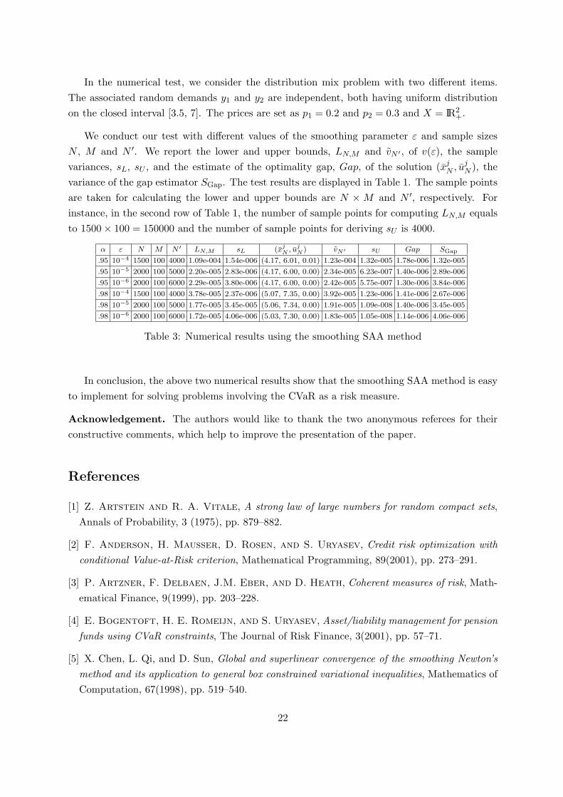
In the numerical test, we consider the distribution mix problem with two different items.The associated random demands y1 and y2 are independent, both having uniform distributionon the closed interval [3.5, 7]. The prices are set as p1 = 0.2 and p2 = 0.3 and X = IR2

+.

We conduct our test with different values of the smoothing parameter ε and sample sizesN , M and N ′. We report the lower and upper bounds, LN,M and vN ′ , of v(ε), the samplevariances, sL, sU , and the estimate of the optimality gap, Gap, of the solution (xj

N , ujN ), the

variance of the gap estimator SGap. The test results are displayed in Table 1. The sample pointsare taken for calculating the lower and upper bounds are N × M and N ′, respectively. Forinstance, in the second row of Table 1, the number of sample points for computing LN,M equalsto 1500× 100 = 150000 and the number of sample points for deriving sU is 4000.

α ε N M N ′ LN,M sL (xjN , uj

N ) vN′ sU Gap SGap

.95 10−4 1500 100 4000 1.09e-004 1.54e-006 (4.17, 6.01, 0.01) 1.23e-004 1.32e-005 1.78e-006 1.32e-005

.95 10−5 2000 100 5000 2.20e-005 2.83e-006 (4.17, 6.00, 0.00) 2.34e-005 6.23e-007 1.40e-006 2.89e-006

.95 10−6 2000 100 6000 2.29e-005 3.80e-006 (4.17, 6.00, 0.00) 2.42e-005 5.75e-007 1.30e-006 3.84e-006

.98 10−4 1500 100 4000 3.78e-005 2.37e-006 (5.07, 7.35, 0.00) 3.92e-005 1.23e-006 1.41e-006 2.67e-006

.98 10−5 2000 100 5000 1.77e-005 3.45e-005 (5.06, 7.34, 0.00) 1.91e-005 1.09e-008 1.40e-006 3.45e-005

.98 10−6 2000 100 6000 1.72e-005 4.06e-006 (5.03, 7.30, 0.00) 1.83e-005 1.05e-008 1.14e-006 4.06e-006

Table 3: Numerical results using the smoothing SAA method

In conclusion, the above two numerical results show that the smoothing SAA method is easyto implement for solving problems involving the CVaR as a risk measure.

Acknowledgement. The authors would like to thank the two anonymous referees for theirconstructive comments, which help to improve the presentation of the paper.

References

[1] Z. Artstein and R. A. Vitale, A strong law of large numbers for random compact sets,Annals of Probability, 3 (1975), pp. 879–882.

[2] F. Anderson, H. Mausser, D. Rosen, and S. Uryasev, Credit risk optimization withconditional Value-at-Risk criterion, Mathematical Programming, 89(2001), pp. 273–291.

[3] P. Artzner, F. Delbaen, J.M. Eber, and D. Heath, Coherent measures of risk, Math-ematical Finance, 9(1999), pp. 203–228.

[4] E. Bogentoft, H. E. Romeijn, and S. Uryasev, Asset/liability management for pensionfunds using CVaR constraints, The Journal of Risk Finance, 3(2001), pp. 57–71.

[5] X. Chen, L. Qi, and D. Sun, Global and superlinear convergence of the smoothing Newton’smethod and its application to general box constrained variational inequalities, Mathematics ofComputation, 67(1998), pp. 519–540.

22

[6] F. H. Clarke, Optimization and Nonsmooth Analysis, John Wiley and Sons, New York,1983.

[7] W. Hurlimann, Conditional Value-at-Risk bounds for compound Poisson risks and a normalapproximation, Journal of Applied Mathematics, 3(2003), pp. 141–153.

[8] P. Jorion, Value At Risk: the New Benchmark for Controlling Market Risk, McGraw-Hill,New York, 1997; McGraw-Hill International Edition, 2001.

[9] P. Krokhmal, J. Palmquist, and S. Uryasev, Portfolio optimization with conditionalValue-At-Risk objective and constraints, The Journal of Risk, 4(2002), pp. 43–68.

[10] A. Kuzi-Bay and J. Mayer, Computational aspects of minimizing conditional value-at-risk, Computational Management Science, 3(2006), pp. 3–27.

[11] G. Lin, X. Chen, and M. Fukushima, Solving stochastic mathematical programs withequilibrium constraints via approximation and smoothing implicit programming with penaliza-tion, Mathematical Programming, 116 (2009), pp. 343–368.

[12] F. Meng, J. Sun, and M. Goh, Stochastic optimization problems with CVaR risk measureand their sample average approximation, working paper, National University of Singapore,2009.

[13] F. Meng and H. Xu, A regularized sample average approximation method for stochasticmathematical programs with nonsmooth equality constraints, SIAM Journal on Optimization,17(2006), pp. 891–919.

[14] K. Natarajan, D. Pachamanova, and M. Sim, Incorporating asymmetric distributionalinformation in robust Value-at-Risk optimization, Management Science, 54(2008), pp–585.

[15] L. Qi, D. Sun, and G. Zhou, A new look at smoothing Newton methods for nonlinearcomplementarity problems and box constrained variational inequalities, Mathematical Pro-gramming, 87(2000), pp. 1–35.

[16] L. Qi and J. Sun, A nonsmooth version of Newton’s method, Mathematical Programming,58(1993), pp. 353–367.

[17] R. T. Rockafellar, Convex Analysis, Princeton University, 1970.

[18] R. T. Rockafellar, Coherent approaches to risk in optimization under uncertainty, Tu-torials in Operations Research, INFORMS, 38–61, 2007.

[19] R. T. Rockafellar and S. Uryasev, Conditional Value-at-Risk for general loss distri-butions, Journal of Banking & Finance, 26(2002), pp. 1443–1471.

[20] R. T. Rockafellar and S. Uryasev, Optimization of conditional Value-at-Risk, Journalof Risk, 2(2000), pp. 21–41.

23

[21] R. Y. Rubinstein and A. Shapiro, Discrete Event Systems: Sensitivity Analysis andStochastic Optimization by the Score Function Method, John Wiley and Sons, New York, 1993.

[22] A. Ruszczynski and A. Shapiro, Optimization of convex risk functions, Mathematics ofOperations Research, 31(2006), pp. 433-452.

[23] A. Shapiro, D. Dentcheva, and A. Ruszczynski, Lectures on Stochastic Programming: Mod-elling and Theory. SIAM Philadelphia, 2009.

[24] A. Shapiro, Stochastic Programming by Monte Carlo Simulation Methods, Published elec-tronically in: Stochastic Programming E-Print Series, 2000.

[25] A. Shapiro, Stochastic mathematical programs with equilibrium constraints, Journal ofOptimization Theory and Application, 128 (2006), pp. 223–243.

[26] D. Tasche, Expected shortfall and beyond, Journal of Banking and Finance, 6(2002), pp.1519–1533.

[27] H. Xu and F. Meng, Convergence analysis of sample average approximation methodsfor a class of stochastic mathematical programs with equality constraints, Mathematics ofOperations Research, 32(2007), pp. 648–668.

[28] C.-S. Yu and H. Li, A robust optimization model for stochastic logistic problems, Inter-national Journal of Production Economics, 64(2000), pp. 385–397.

24