This article appeared in a journal published by Elsevier. The attachedcopy is furnished to the author for internal non-commercial researchand education use, including for instruction at the authors institution

and sharing with colleagues.

Other uses, including reproduction and distribution, or selling orlicensing copies, or posting to personal, institutional or third party

websites are prohibited.

In most cases authors are permitted to post their version of thearticle (e.g. in Word or Tex form) to their personal website orinstitutional repository. Authors requiring further information

regarding Elsevier’s archiving and manuscript policies areencouraged to visit:

http://www.elsevier.com/copyright

Author's personal copy

Int. J. Production Economics 113 (2008) 193–204

The role of forecasting on bullwhip effectfor E-SCM applications

Erkan Bayraktara, S.C. Lenny Kohb,�, A. Gunasekaranc,Kazim Sarid, Ekrem Tatoglue

aDepartment of Industrial Engineering, Faculty of Engineering, Bahcesehir University, Besiktas, Istanbul 34349, TurkeybManagement School, University of Sheffield, 9 Mappin Street, Sheffield S1 4DT, UK

cManagement Department, University of Massachusetts-Dartmouth, 285 Old Westport Road, North Dartmouth, MA 02747-2300, USAdDepartment of International Logistics and Transportation, Beykent University, Sisli, Istanbul, Turkey

eDepartment of Business Administration, Faculty of Business Administration, Bahcesehir University, Besiktas, Istanbul 34349, Turkey

Received 14 April 2006; accepted 6 March 2007

Available online 24 July 2007

Abstract

The bullwhip effect represents the information distortion in customer demand between orders to supplier and sales to the

buyer. Demand forecasting is one of the main causes of the bullwhip effect. The purpose of this study is to analyze the

impact of exponential smoothing forecasts on the bullwhip effect for electronic supply chain management (E-SCM)

applications. A simulation model is developed to experiment the different scenarios of selecting right parameters for the

exponential smoothing forecasting technique. It is found that longer lead times and poor selection of forecasting model

parameters lead to strong bullwhip effect in E-SCM. In contrast, increased seasonality helps to reduce the bullwhip effect.

The most significant managerial implication of this study lies in the need to reduce lead times along the E-supply chain to

mitigate the bullwhip effect. While high seasonality would reduce the forecast accuracy, it has a positive influence on the

reduction of bullwhip effect. E-SCM managers are therefore strongly suggested to utilize exponential smoothing by

selecting lower values for a and b and a mid-value for g to keep the bullwhip ratio low, while at the same time to increase

forecast accuracy.

r 2007 Elsevier B.V. All rights reserved.

Keywords: Bullwhip effect; Forecasting; Exponential smoothing; E-SCM

1. Introduction

Despite shorter product life cycles and tightproduct/service costs, the idea of ‘‘any productany time any place’’ has now become possible

through advancements in communication andtransportation technologies. The contemporarybusinesses faced with these challenges have beenmore effectively coping with uncertainties emergingin their supply chains. Uncertainty is generallydefined as unknown future events that cannot bepredicted quantitatively within useful limits, thusmaking the occurrence of uncertainty unpredictable(Cox and Blackstone, 1998). The sources ofuncertainty lie in the process of matching demand

ARTICLE IN PRESS

www.elsevier.com/locate/ijpe

0925-5273/$ - see front matter r 2007 Elsevier B.V. All rights reserved.

doi:10.1016/j.ijpe.2007.03.024

�Corresponding author. Tel.: +44114 222 3395;

fax: +44114 222 3348.

E-mail address: S.C.L.Koh@Sheffield.ac.uk

(S.C. Lenny Koh).

Author's personal copy

with supply. The following sources of uncertainty,which include delivery lead times, manufacturingyields, transportation times, machining times andoperator performances (Simchi-Levi et al., 2003), alllead to supply uncertainty that has significantimpact on chain performance. On the other hand,the difficulties in predicting customer needs andwants in a given period constitute the main sourceof demand uncertainty that a good forecast maycope with this uncertainty. In fact, the ultimatesuccess lies in the ability to manage the demanduncertainty with the existent supply capabilities.

It has been emphatically pointed out that under-standing and practising supply chain management(SCM) has become an essential prerequisite to beable to manage demand uncertainties and togrowing profitably in the global competitive race(Power et al., 2001; Moberg et al., 2002). SCMincludes a set of approaches and practices to reducethe uncertainty along the chain through enabling abetter integration among suppliers, manufacturers,distributors and customers (Koh et al., 2007). It is‘‘the efficient management of the end-to-end pro-cess, which starts with the design of the product orservice and ends with the time when it has been sold,consumed, and finally, discarded by the consumer’’(Swaminathan and Tayur, 2003, p. 1387). Apartfrom traditional SCM practices, there are severaltools and techniques of electronic SCM (E-SCM) todiminish uncertainty in E-supply chains, which interalia include information sharing, third-party logis-tics (3PL) providers, centralized planning, strategicalliances and E-commerce logistics (ECL). Of thesetools, 3PL and ECL applications have beenincreasingly gaining popularity among contempor-ary businesses (Coyle et al., 1996; Lambert et al.,1999).

Given the imperatives of intense global competi-tion, the buyers dominate the market and presenttheir personalized and customized requirements.This makes the demand change rapidly and difficultto forecast (Ying and Dayong, 2005). By reducinguncertainty and improving efficiency to logisticsmanagement, 3PL could increase supply chaineffectiveness through the following ways (Simchi-Levi et al., 2003; Maloni and Carter, 2006): (1)enabling the company to focus on its core compe-tencies; (2) providing flexibility in adaptation to newtechnology, resource and workforce size; and (3)accessing to expertise of 3PL providers on theoutsourced activity and their economies of scale.3PL is a type of services of multiple distribution

activities provided by an external party (assumingno ownership of inventory) to accomplish relatedfunctions that are not desired to be renderedand/or managed by the purchasing enterprise (Sinket al., 1996). In other words, 3PL refers to theoutsourcing of transportation, warehousing andother logistics-related activities to a 3PL providerthat were originally performed in-house. Withthe use of 3PL for all or part of an enterprise’slogistics operations, significant reduction in logisticscost can be achieved while improving servicequality.

ECL is defined as the ‘‘impact of the Internet onthe supply chain process that plans, implements,and controls the efficient, effective flow and storageof goods, services, and related information from thepoint-of-origin to the point-of-consumption inorder to meet customers’ requirements’’ (Gimenezand Lourenc-o, 2004, p. 3). ECL is recognized as asubset of E-SCM that refers to ‘‘the impact thatInternet has on the integration of key businessprocesses from end user through original suppliersthat provides products, services and informationthat add value for customers and other stakeholders’’(Gimenez and Lourenc-o, 2004). E-SCM enhancesthe revenue through direct sales to customers with24/7 access from any location, personalization andcustomization of information, faster time to market,flexible pricing and efficient fund transfer; andreduces the cost through better coordination withinformation sharing, lower delivery cost and time,less product handling, lower facility and processingcosts, reduced inventory cost with centralization,and postponement product differentiation (Chopraand Meindl, 2001). According to Swaminathan andTayur (2003), the Internet has influenced SCM inthree ways: (1) increased use of ERP and advancedplanning and optimization solutions; (2) ability toaccess real-time information in order to make real-time decisions; and (3) integrate information anddecision making across different functional units.As a result, it diminishes the uncertainty with theavailability of more information.

Risk-pooling, mass customization and dynamicpricing are some of the SCM issues heavilyinfluenced by E-business applications. AlthoughInternet applications introduce new perspectives totraditional issues and enhance capabilities of SCM,many SCM-related issues are yet to be resolved.Among some of these are keeping buffer inventoryor capacity for guaranteeing the certain servicelevels and classical trade-off between fix and

ARTICLE IN PRESSE. Bayraktar et al. / Int. J. Production Economics 113 (2008) 193–204194

Author's personal copy

variable costs in procurement decisions (Swami-nathan and Tayur, 2003). The need for accuratedemand forecasting, for instance, is not completelyeliminated. Sharing point-of-sales (POS) data withchain partners and analyzing it through data miningtechniques may help to improve forecast accuracy,though for many decisions we still rely on theforecasts.

Demand forecasting is an essential tool forproduction and inventory planning, capacity man-agement and the design of the customer servicelevels. Many demand-forecasting techniques rely onthe historical data and assume the validity of thepast demand patterns for the near future. Due tohigh sensitivity of the forecast values to the mostrecent occurrences, this approach, in general,produces high (low) demand forecast values follow-ing high (low) demand periods. At the same time,customer demand is passed to the wholesalers,distributors or manufacturers in the form ofretailers’ order, which is actually the demand forhigher-level chain partners. Demand forecasts inpractice, however, are rarely accurate and theybecome even worse at higher levels of the supplychain. In most supply chains, individual chainmembers attempt to rationalize their order sizeswith economical batching decisions, though thiscreates a distortion on the real customer demandand misleads the upper-level supply chain memberswith respect to demand. Promotions and pricefluctuations also contribute to demand distortion.The need to forecast the demand at each level of thesupply chain amplifies the forecast errors, the so-called bullwhip effect, along the whole chain. Lee etal. (1997a) label this as double forecasting. There-fore, it is extremely important to establish a properdemand forecast system to reduce the bullwhipeffect.

The bullwhip effect, also known as Forrester orwhiplash effect is one of the key areas of research inSCM applications. It represents the phenomenonwhere orders to supplier tend to have largervariance than sales to the buyer, and customerdemand is distorted (Lee et al., 1997a, b). Thisdemand distortion also propagates to upstreamstages in an amplified form. In return, highinventory levels and poor customer service ratesalong the supply chain constitute typical symptomsof bullwhip effect. In addition, production andinventory holding costs as well as lead timesincrease, while profit margins and product avail-ability decrease (Chopra and Meindl, 2001, p. 363).

Metters (1997) empirically showed that eliminationof the bullwhip effect might increase productprofitability by 10–30 percent depending on thespecific business environments.

Within the context of E-SCM applications, thisstudy essentially analyzes the impact of demandforecasting on the bullwhip effect. Based on asimulation model, a two-stage E-supply chain isexamined using exponential smoothing forecastingon the bullwhip effect under linear demand assump-tion with seasonal swings. While in earlier research,Chen et al. (2000a, b) analytically examined thesimilar problem for autoregressive demand struc-tures and linear demand, they did not take intoaccount the demand seasonality. This study there-fore fills this gap by developing a simulation modelfor E-SCM applications, which experiments thedifferent scenarios of selecting suitable parametersfor exponential smoothing forecasting, lead timeand demand seasonality.

The remainder of this study is organized asfollows. The next section reviews the previousliterature related to demand uncertainty in E-SCMpractices with special emphasis on ECL and 3PLapplications. Section 3 explains the development ofan E-supply chain simulation model to test demandforecast based on exponential smoothing. Setting ofexperimental design is identified in Section 4,followed by simulation results. Conclusions are inthe final section.

2. Literature survey

Uncertainty can be defined as unpredictableevents in a supply chain that affects its plannedperformance (Koh and Gunasekaran, 2006). Owingto high transactional volume in a an E-supply chain,demand uncertainty caused by inaccurate forecastwould feed into information exchange in thenetwork, which in turn would result in the bullwhipeffect. Such an effect may affect the ability of ECLand 3PL applications in meeting the expecteddelivery performance of goods and services.

The bullwhip effect was first noticed and studiedby Forrester (1961) in a series of simulationanalysis. He named this problem as ‘‘demandamplification’’. He further concluded that theproblem of the bullwhip effect stemmed from thesystem itself with its policies, organization structureand delays in material and information flow, notstemmed from the external forces. Later, Sterman(1989) studied the bullwhip effect by playing the

ARTICLE IN PRESSE. Bayraktar et al. / Int. J. Production Economics 113 (2008) 193–204 195

Author's personal copy

‘‘beer distribution game’’ with students. He notedthat misperception of feedback loops and irrationalreaction of decision makers to a complex and tacitsystem created the bullwhip effect. As people havedifficulties to realize the impact of their orderingdecisions due to complexity of the system and thetime lags between ordering and receiving, Sterman(1989) suggests that operations managers be pro-vided necessary training on the bullwhip effect. Leeet al. (1997a, b), however, indicate that bullwhipeffect is present, even if all members of the supplychain behave in an optimal manner unless thesupply chain is redesigned with different strategicinteractions. Their analytical study points out thatthe bullwhip effect stems mainly from four factors:demand forecasting, order batching, price fluctua-tions, and rationing and shortage gaming. Whilesupporting this view on the causes of the bullwhipeffect, Miragliotta (2006) criticizes the mechanismgenerating the bullwhip effect. In their review ofbullwhip effect, Geary et al. (2006) emphasize thefollowing causes initially suggested by Jack For-rester and Jack Burbidge, twin pioneers of modernsupply chain knowledge: control systems, activitytimes in the chain, level of information transpar-ency, the number of echelons, synchronization andmultiplier effect.

Following Lee et al. (1997a), several otherresearchers have also concentrated on the causesof the bullwhip effect in order to understand theirimpacts on supply chain. Of these causes, the majoremphasis has been placed on demand forecasting.Researchers relying on different methodologies haveconstructed various models to explore the impact ofdemand forecast. For example, Chen et al.(2000a, b) used statistical methods and Andersonet al. (2000) adopted system-thinking methodology,while Dejonckheere et al. (2003, 2004) and Disneyand Towill (2003a) used control-engineering meth-odology. All of these studies concentrated predo-minantly on the forecasting methods of movingaverage, simple exponential smoothing and doubleexponential smoothing. Their results indicated thatthe number of observations used in moving averageshould be high in order to lower the bullwhip effect.Moreover, lower values of smoothing parameters(a, b) are required in exponential smoothingforecasting. While these studies offer a number ofuseful implications for E-SCM practitioners, theydo not provide all the information required as noneof these studies considered seasonality in theirmodels.

For AR(1) demand processes using order-up-toinventory policy, Chen et al. (2000a) quantified thebullwhip effect for moving the average forecastingmodel in a two-level supply chain. Their findingssupport the significance of reducing lead times tomitigate the bullwhip effect. Under similar assump-tions, Zhang (2004) derived the optimum forecast-ing procedure minimizing the mean-squaredforecasting error (MMSE) where MMSE forecastleads to lowest inventory cost under the givenconditions. Reduction of lead time has the mostsignificant impact on the decline of the bullwhipeffect under MMSE forecasts when the demandautocorrelation is positive and away from zero orone. If demand correlation is negative, exponentialsmoothing provides the most significant impact onthe bullwhip effect for reduced lead times. Chen etal. (2000b) also investigated the double exponentialsmoothing forecasting technique for demand pro-cess with a linear trend. They emphasized theimportance of selecting relatively lower values forsmoothing parameters (a, b) and reducing leadtimes to diminish the bullwhip effect. They alsostated that a retailer who forecasts a linear demandprocesses faces relatively higher-order variability ascompared with one who forecasts a stationarydemand process. This variability also does notdepend on the magnitude of the linear trend.Another important finding emerging from this studyis that exponential smoothing method also producesmore variability compared with the moving averagemethod.

Zhao et al. (2002) investigated the impact offorecasting models, demand patterns and capacitytightness of the supplier on the performance of thesupply chain in terms of total cost and service level.Their model has included one capacitated supplierwith setup and backorder costs and four retailersreplenishing according to economic order quantitymodel. Their findings have emphasized the impactof the accuracy of forecast models on the value ofinformation sharing. The supplier can improve itstotal costs and service level through informationsharing in all cases, while total costs and servicelevel for retailers may even become worseunder information sharing when capacity tightnessis low.

In fact, demand forecasting has been recognizedas only one of the four main causes of the bullwhipeffect (Lee et al., 1997a); thereby using a smootherforecasting policy is not a unique remedy for thebullwhip effect. There are also other proposed

ARTICLE IN PRESSE. Bayraktar et al. / Int. J. Production Economics 113 (2008) 193–204196

Author's personal copy

strategies, which can be summarized as follows:sharing POS data with trading partners (Dejonc-kheere et al., 2004; McCullen and Towill, 2001,2002; Chen et al., 2000a, b; Mason-Jones andTowill, 2000; Towill, 1997); echelon elimination(e.g. implementing vendor managed inventory)(Disney and Towill, 2003b; Forrester, 1961); lead-time reduction (Forrester, 1961; Lee et al., 1997a;Machuca and Barajas, 2004; Anderson et al., 2000);training decision makers for more rational decisions(Sterman, 1989); and designing robust systems thatminimize human interactions (Disney et al., 2004).

3. The supply chain simulation model

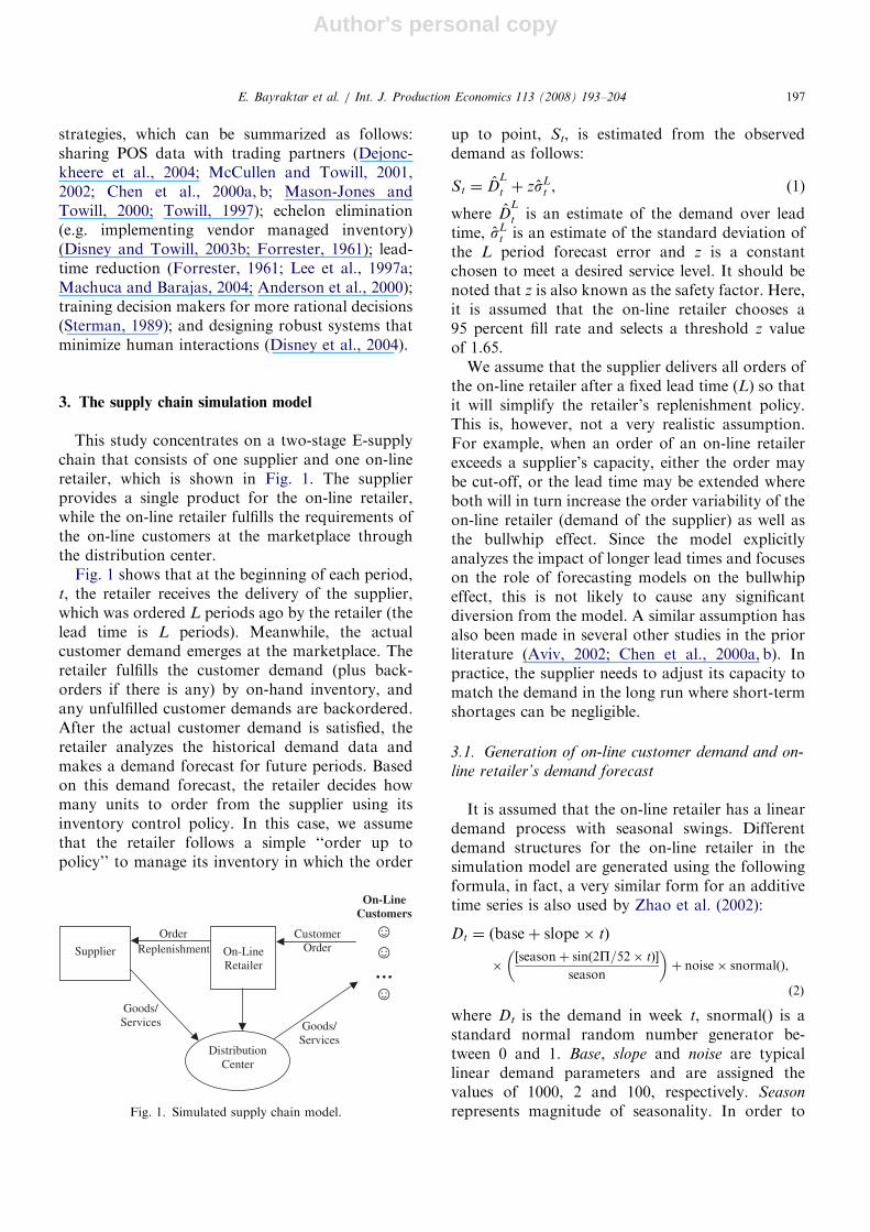
This study concentrates on a two-stage E-supplychain that consists of one supplier and one on-lineretailer, which is shown in Fig. 1. The supplierprovides a single product for the on-line retailer,while the on-line retailer fulfills the requirements ofthe on-line customers at the marketplace throughthe distribution center.

Fig. 1 shows that at the beginning of each period,t, the retailer receives the delivery of the supplier,which was ordered L periods ago by the retailer (thelead time is L periods). Meanwhile, the actualcustomer demand emerges at the marketplace. Theretailer fulfills the customer demand (plus back-orders if there is any) by on-hand inventory, andany unfulfilled customer demands are backordered.After the actual customer demand is satisfied, theretailer analyzes the historical demand data andmakes a demand forecast for future periods. Basedon this demand forecast, the retailer decides howmany units to order from the supplier using itsinventory control policy. In this case, we assumethat the retailer follows a simple ‘‘order up topolicy’’ to manage its inventory in which the order

up to point, St, is estimated from the observeddemand as follows:

St ¼ DL

t þ zsLt , (1)

where DL

t is an estimate of the demand over leadtime, sL

t is an estimate of the standard deviation ofthe L period forecast error and z is a constantchosen to meet a desired service level. It should benoted that z is also known as the safety factor. Here,it is assumed that the on-line retailer chooses a95 percent fill rate and selects a threshold z valueof 1.65.

We assume that the supplier delivers all orders ofthe on-line retailer after a fixed lead time (L) so thatit will simplify the retailer’s replenishment policy.This is, however, not a very realistic assumption.For example, when an order of an on-line retailerexceeds a supplier’s capacity, either the order maybe cut-off, or the lead time may be extended whereboth will in turn increase the order variability of theon-line retailer (demand of the supplier) as well asthe bullwhip effect. Since the model explicitlyanalyzes the impact of longer lead times and focuseson the role of forecasting models on the bullwhipeffect, this is not likely to cause any significantdiversion from the model. A similar assumption hasalso been made in several other studies in the priorliterature (Aviv, 2002; Chen et al., 2000a, b). Inpractice, the supplier needs to adjust its capacity tomatch the demand in the long run where short-termshortages can be negligible.

3.1. Generation of on-line customer demand and on-

line retailer’s demand forecast

It is assumed that the on-line retailer has a lineardemand process with seasonal swings. Differentdemand structures for the on-line retailer in thesimulation model are generated using the followingformula, in fact, a very similar form for an additivetime series is also used by Zhao et al. (2002):

Dt ¼ ðbaseþ slope� tÞ

�½seasonþ sinð2P=52� tÞ�

season

� �þ noise� snormalðÞ,

ð2Þ

where Dt is the demand in week t, snormal() is astandard normal random number generator be-tween 0 and 1. Base, slope and noise are typicallinear demand parameters and are assigned thevalues of 1000, 2 and 100, respectively. Season

represents magnitude of seasonality. In order to

ARTICLE IN PRESS

On-LineRetailer

Goods/Services

CustomerOrder

Goods/Services

DistributionCenter

OrderReplenishment

On-LineCustomers

Supplier

Fig. 1. Simulated supply chain model.

E. Bayraktar et al. / Int. J. Production Economics 113 (2008) 193–204 197

Author's personal copy

evaluate the impact of seasonality on the bullwhipeffect, three types of demand structures representingdifferent levels of seasonality are used: low, mediumand high. For each level of seasonality in Eq. (1),the respective values of 5, 15 and 30 are assignedaccordingly.

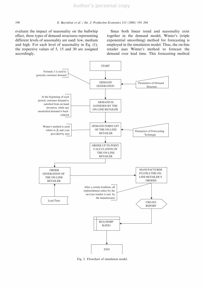
Since both linear trend and seasonality existtogether in the demand model, Winter’s (tripleexponential smoothing) method for forecasting isemployed in the simulation model. Thus, the on-lineretailer uses Winter’s method to forecast thedemand over lead time. This forecasting method

ARTICLE IN PRESS

START

DEMANDGENERATION

DEMAND FORECASTOF THE ON-LINE

RETAILER

ORDER UP TO POINTCALCULATION OF

THE ON-LINERETAILER

ORDER GENERATION OF

THE ON-LINE RETAILER

MANUFACTURER FULFILS THE ON-LINE RETAILER’S

ORDERS

At the beginning of eachperiod, customer demand is

satisfied from on-handinventory, while any

unsatisfied demand is back-ordered

CREATEREPORT

BULLWHIPRATIO

END

DEMAND ISSATISFIED BY THE ON-LINE RETAILER

Winter's method is usedwhere α, β, and γ are

provided by userParameters of Forecasting

Technique

Lead Time

Formula 1 is used togenerate customer demand

Parameters of DemandStructure

After a certain leadtime, allreplenishment orders by the

on-Line retailer is met bythe manufacturer

Fig. 2. Flowchart of simulation model.

E. Bayraktar et al. / Int. J. Production Economics 113 (2008) 193–204198

Author's personal copy

requires three smoothing parameters to updatelevel, trend and seasonal components of thedemand, which are represented by alpha (a), beta(b) and gamma (g), respectively. More detailedinformation on this forecasting method is providedin Abraham and Ledolter (1983, p. 170).

3.2. Verification and validation of simulation

A two-stage E-supply chain is simulated inMicrosoft Excel. Simulation logic along with aflowchart are shown in Fig. 2. To verify that theprogram performs as intended, the conceptualmodel is divided into three parts: demand genera-tion, forecasting and calculation of inventory levels.Each part is then debugged individually to confirmwhether the findings are in line with sample solutionproblems. A combined simulation model is alsotraced and tested with the results computedmanually.

In order to validate the simulation output, therandom demand variables generated by Excel isplotted on a scatter diagram. It is validated that thedemand function in Eq. (1) is generated. The supplychain model above was simulated for 520 weeks.The initial parameters of the forecasting model wereestimated by the first 156 weeks of simulation run,which was removed later from the output analysis toeliminate the warm-up period effect. Therefore, therest of the data were used for effective simulationoutput analysis. In addition, ten replications foreach combination of the independent variables wereconducted to reduce the impact of random varia-tions.

We also performed the sensitivity analysis fordemand parameters by changing the values of base,trend and noise. It has been further validated thatthe variation in the demand parameters does notaffect our findings. Therefore, only one combina-tion of these parameters is selected to perform theanalysis.

4. Experimental design

The purpose of the experimental design istwofold: (1) analyzing the impact of the smoothingparameters, lead time and strength of seasonality onthe bullwhip effect and (2) examining the interactionof the smoothing parameters with lead time andseasonality. Therefore, three groups of independentfactors are investigated through the experimentaldesign. The number of levels of these factors with

their respective values is listed in Table 1. The valuesof a and b parameters used in the exponentialsmoothing are suggested to be less than 0.5 in orderto obtain better forecast values from Winter’sforecasting model (Winston, 1993, p. 1268). Thelevels of these parameters are set accordingly.

The bullwhip ratio is denoted as the dependentvariable of the design of experiment. It indicates theratio of variance of the orders realized by themanufacturer to the variance of the demandobserved by the retailer as in Eq. (3):

Bullwhip ratio ¼VarðOrderÞ

VarðDemandÞ. (3)

5. Simulation output analysis

Out of 520 weeks of the simulation of the supplychain model above, data from the remaining 364weeks (from weeks 157 to 520) for ten replicationswere used for simulation output analysis. ThroughANOVA tests, the output from the simulationexperiments was compared based on mean measureswith respect to three different levels of smoothingparameters, lead time and seasonality. The ANOVAtest results for the main and interaction effects areshown in Table 2.

5.1. Main effects

ANOVA test results in Table 2 indicate that thebullwhip effect is significantly influenced by thesmoothing parameters, lead time and seasonality(po0.05), suggesting that all three factors determinethe degree of information distortion along thesupply chain. Once we have noted that all indepen-dent factors of the experimental design significantlyinfluence the bullwhip effect, we then conducted

ARTICLE IN PRESS

Table 1

Independent factors of the experimental design

Independent factors Levels

1 2 3

Smoothing parameters

Alpha (a) 0.01 0.25 0.50

Beta (b) 0.01 0.25 0.50

Gamma (g) 0.01 0.25 0.50

Strength of seasonality Low Medium High

Lead time 1 week 3 weeks 5 weeks

E. Bayraktar et al. / Int. J. Production Economics 113 (2008) 193–204 199

Author's personal copy

multiple comparisons tests in order to understandhow each of these independent variables wouldaffect the bullwhip effect. While there are a numberof multiple comparisons tests, we have conductedTukey’s procedure in this study due to its wideracceptance (Devore, 1995, p. 400). The results ofTukey’s procedure are shown in Table 3, wherehomogeneous subsets are produced.

Table 3 indicates that any increase in the values ofa and b parameters, and lead times lead to an

increase in the bullwhip effect. In contrast, theimpact of the g parameter and seasonality onthe bullwhip effect displays a different pattern. Asthe strength of seasonality increases, the value of thebullwhip ratio decreases, as shown in Table 3. Thismight be explained by the fact that the forecastingmethod used in the model performs better for higherlevels of seasonality. In other words, the variationgenerated by the seasonality cancels out thevariability created by the bullwhip effect. Whenthe g parameter is taken into account, however,Table 3 reveals that the bullwhip ratio becomes thesmallest when the g parameter is 0.25 and the largestwhen it is 0.01. This result confirms the existence ofa U-type relationship between the g parameter andthe bullwhip ratio. It is most likely that there areslight decreases in the bullwhip ratio as the valueof the g parameter increases up to a point, and thenit starts to increase with higher values of gparameter. The g parameter will be analyzed furtherin Section 5.4.

5.2. Interaction between smoothing parameters and

lead time

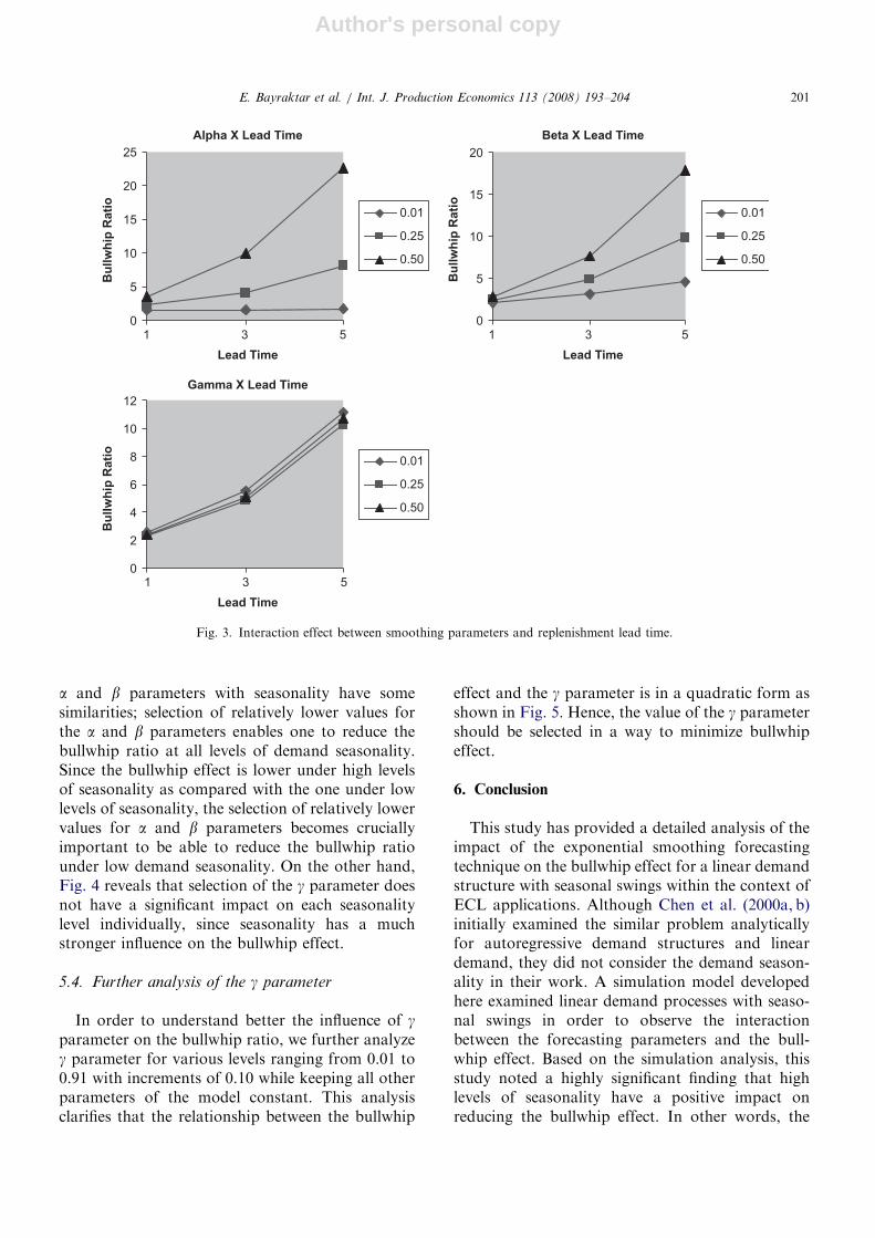
The interaction effect between smoothing para-meters and lead time is shown in Fig. 3. Fig. 3indicates that a and b parameters act very muchsimilar on the bullwhip ratio against lead times.When the lead time is low, there is not muchdifference on the bullwhip ratio based on theselection of the a and b parameters. However, thebullwhip ratio increases very quickly as the leadtime and the values of the a and b parametersincrease. Therefore, the values of the a and bparameters in the forecasting model should beselected small enough to keep the bullwhip effectlow.

When we consider the interaction of the gparameter with lead time, Fig. 3 indicates a differentsituation that longer lead times always lead to hugeincreases in the bullwhip ratio independently fromthe value of the g parameter. Therefore, we can statethat the g parameter cannot contribute sufficientlyto reduce the negative impact of longer lead times.

5.3. Interaction between smoothing parameters and

seasonality

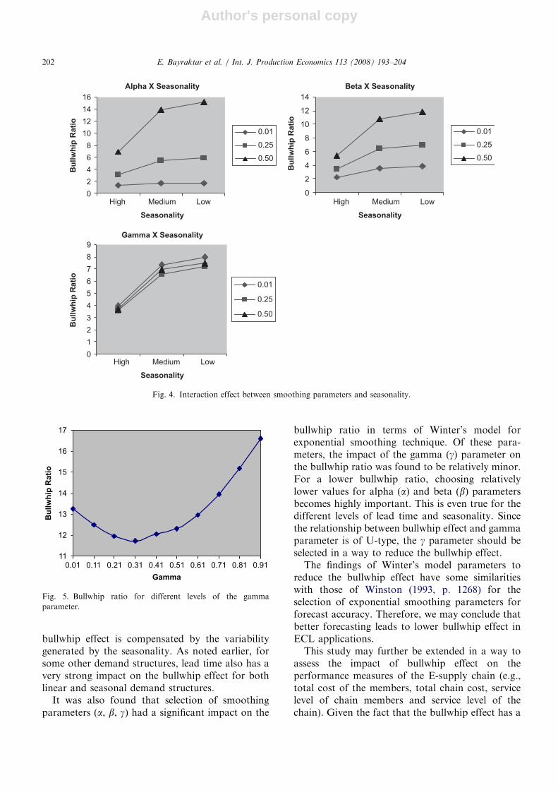
Fig. 4 shows the interaction effect betweensmoothing parameters and seasonality. It may bereadily apparent from Fig. 4 that interactions of the

ARTICLE IN PRESS

Table 2

Selected ANOVA resultsa

Source Mean square F Sig.

Alpha 104.7684 44828.4 0.0000

Beta 14.0638 6017.6 0.0000

Gamma 0.4636 198.3 0.0000

Lead time 34.7446 14866.5 0.0000

Seasonality 12.0279 5146.5 0.0000

Alpha � beta 3.3380 1428.3 0.0000

Alpha � gamma 0.0120 5.1 0.0004

Alpha � lead time 8.7309 3735.8 0.0000

Alpha � seasonality 0.7507 321.2 0.0000

Beta � gamma 0.0221 9.4 0.0000

Beta � lead time 1.5905 680.5 0.0000

Beta � seasonality 0.0458 19.6 0.0000

Gamma � lead time 0.0038 1.62 0.1668

Gamma � seasonality 0.0061 2.6 0.0337

Lead time � seasonality 0.1378 58.9 0.0000

aLog transformation of dependent variable is conducted in

order to satisfy the ANOVA assumptions.

Table 3

Homogeneous subsets of each independent variable

Variable Level N Subset Sign.

1 2 3

Alpha 0.01 810 1.5278 1.000

0.25 810 4.7314 1.000

0.50 810 11.9877 1.000

Beta 0.01 810 3.2035 1.000

0.25 810 5.6520 1.000

0.50 810 9.3914 1.000

Gamma 0,25 810 5.7972 0.208

0.50 810 6.0406

0.01 810 6.4091 1.000

Lead time 1 week 810 2.3932 1.000

3 weeks 810 5.1418 1.000

5 weeks 810 10.7119 1.000

Seasonality High 810 3.7289 1.000

Medium 810 6.9463 1.000

Low 810 7.5718 1.000

E. Bayraktar et al. / Int. J. Production Economics 113 (2008) 193–204200

Author's personal copy

a and b parameters with seasonality have somesimilarities; selection of relatively lower values forthe a and b parameters enables one to reduce thebullwhip ratio at all levels of demand seasonality.Since the bullwhip effect is lower under high levelsof seasonality as compared with the one under lowlevels of seasonality, the selection of relatively lowervalues for a and b parameters becomes cruciallyimportant to be able to reduce the bullwhip ratiounder low demand seasonality. On the other hand,Fig. 4 reveals that selection of the g parameter doesnot have a significant impact on each seasonalitylevel individually, since seasonality has a muchstronger influence on the bullwhip effect.

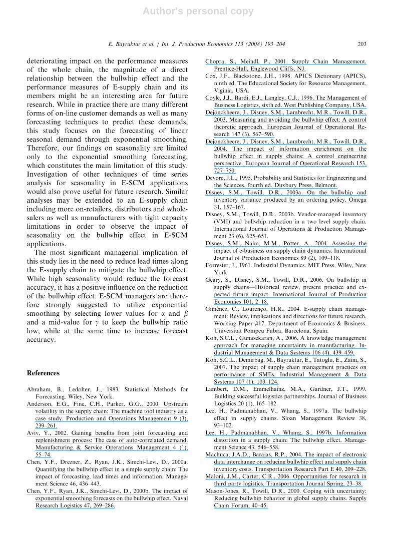
5.4. Further analysis of the g parameter

In order to understand better the influence of gparameter on the bullwhip ratio, we further analyzeg parameter for various levels ranging from 0.01 to0.91 with increments of 0.10 while keeping all otherparameters of the model constant. This analysisclarifies that the relationship between the bullwhip

effect and the g parameter is in a quadratic form asshown in Fig. 5. Hence, the value of the g parametershould be selected in a way to minimize bullwhipeffect.

6. Conclusion

This study has provided a detailed analysis of theimpact of the exponential smoothing forecastingtechnique on the bullwhip effect for a linear demandstructure with seasonal swings within the context ofECL applications. Although Chen et al. (2000a, b)initially examined the similar problem analyticallyfor autoregressive demand structures and lineardemand, they did not consider the demand season-ality in their work. A simulation model developedhere examined linear demand processes with seaso-nal swings in order to observe the interactionbetween the forecasting parameters and the bull-whip effect. Based on the simulation analysis, thisstudy noted a highly significant finding that highlevels of seasonality have a positive impact onreducing the bullwhip effect. In other words, the

ARTICLE IN PRESS

Alpha X Lead Time

0

5

10

15

20

25

1

Lead Time

Bu

llw

hip

Rati

o

0.01

0.25

0.50

Beta X Lead Time

0

5

10

15

20

Lead Time

Bu

llw

hip

Rati

o

0.01

0.25

0.50

Gamma X Lead Time

0

2

4

6

8

10

12

Bu

llw

hip

Rati

o

0.01

0.25

0.50

3 5

1

Lead Time

3 5

1 3 5

Fig. 3. Interaction effect between smoothing parameters and replenishment lead time.

E. Bayraktar et al. / Int. J. Production Economics 113 (2008) 193–204 201

Author's personal copy

bullwhip effect is compensated by the variabilitygenerated by the seasonality. As noted earlier, forsome other demand structures, lead time also has avery strong impact on the bullwhip effect for bothlinear and seasonal demand structures.

It was also found that selection of smoothingparameters (a, b, g) had a significant impact on the

bullwhip ratio in terms of Winter’s model forexponential smoothing technique. Of these para-meters, the impact of the gamma (g) parameter onthe bullwhip ratio was found to be relatively minor.For a lower bullwhip ratio, choosing relativelylower values for alpha (a) and beta (b) parametersbecomes highly important. This is even true for thedifferent levels of lead time and seasonality. Sincethe relationship between bullwhip effect and gammaparameter is of U-type, the g parameter should beselected in a way to reduce the bullwhip effect.

The findings of Winter’s model parameters toreduce the bullwhip effect have some similaritieswith those of Winston (1993, p. 1268) for theselection of exponential smoothing parameters forforecast accuracy. Therefore, we may conclude thatbetter forecasting leads to lower bullwhip effect inECL applications.

This study may further be extended in a way toassess the impact of bullwhip effect on theperformance measures of the E-supply chain (e.g.,total cost of the members, total chain cost, servicelevel of chain members and service level of thechain). Given the fact that the bullwhip effect has a

ARTICLE IN PRESS

Alpha X Seasonality

0

2

4

6

8

10

12

14

16

High

Seasonality

Bu

llw

hip

Rati

o

0.01

0.25

0.50

Beta X Seasonality

0

2

4

6

8

10

12

14

Bu

llw

hip

Rati

o

0.01

0.25

0.50

Gamma X Seasonality

0

1

2

3

4

5

6

7

8

9

Bu

llw

hip

Rati

o

0.01

0.25

0.50

LowMedium

High

Seasonality

LowMedium

High

Seasonality

LowMedium

Fig. 4. Interaction effect between smoothing parameters and seasonality.

11

12

13

14

15

16

17

Gamma

Bu

llw

hip

Ra

tio

0.81 0.910.710.610.510.410.310.210.110.01

Fig. 5. Bullwhip ratio for different levels of the gamma

parameter.

E. Bayraktar et al. / Int. J. Production Economics 113 (2008) 193–204202

Author's personal copy

deteriorating impact on the performance measuresof the whole chain, the magnitude of a directrelationship between the bullwhip effect and theperformance measures of E-supply chain and itsmembers might be an interesting area for futureresearch. While in practice there are many differentforms of on-line customer demands as well as manyforecasting techniques to predict these demands,this study focuses on the forecasting of linearseasonal demand through exponential smoothing.Therefore, our findings on seasonality are limitedonly to the exponential smoothing forecasting,which constitutes the main limitation of this study.Investigation of other techniques of time seriesanalysis for seasonality in E-SCM applicationswould also prove useful for future research. Similaranalyses may be extended to an E-supply chainincluding more on-retailers, distributors and whole-salers as well as manufacturers with tight capacitylimitations in order to observe the impact ofseasonality on the bullwhip effect in E-SCMapplications.

The most significant managerial implication ofthis study lies in the need to reduce lead times alongthe E-supply chain to mitigate the bullwhip effect.While high seasonality would reduce the forecastaccuracy, it has a positive influence on the reductionof the bullwhip effect. E-SCM managers are there-fore strongly suggested to utilize exponentialsmoothing by selecting lower values for a and band a mid-value for g to keep the bullwhip ratiolow, while at the same time to increase forecastaccuracy.

References

Abraham, B., Ledolter, J., 1983. Statistical Methods for

Forecasting. Wiley, New York.

Anderson, E.G., Fine, C.H., Parker, G.G., 2000. Upstream

volatility in the supply chain: The machine tool industry as a

case study. Production and Operations Management 9 (3),

239–261.

Aviv, Y., 2002. Gaining benefits from joint forecasting and

replenishment process: The case of auto-correlated demand.

Manufacturing & Service Operations Management 4 (1),

55–74.

Chen, Y.F., Drezner, Z., Ryan, J.K., Simchi-Levi, D., 2000a.

Quantifying the bullwhip effect in a simple supply chain: The

impact of forecasting, lead times and information. Manage-

ment Science 46, 436–443.

Chen, Y.F., Ryan, J.K., Simchi-Levi, D., 2000b. The impact of

exponential smoothing forecasts on the bullwhip effect. Naval

Research Logistics 47, 269–286.

Chopra, S., Meindl, P., 2001. Supply Chain Management.

Prentice-Hall, Englewood Cliffs, NJ.

Cox, J.F., Blackstone, J.H., 1998. APICS Dictionary (APICS),

ninth ed. The Educational Society for Resource Management,

Viginia, USA.

Coyle, J.J., Bardi, E.J., Langley, C.J., 1996. The Management of

Business Logistics, sixth ed. West Publishing Company, USA.

Dejonckheere, J., Disney, S.M., Lambrecht, M.R., Towill, D.R.,

2003. Measuring and avoiding the bullwhip effect: A control

theoretic approach. European Journal of Operational Re-

search 147 (3), 567–590.

Dejonckheere, J., Disney, S.M., Lambrecht, M.R., Towill, D.R.,

2004. The impact of information enrichment on the

bullwhip effect in supply chains: A control engineering

perspective. European Journal of Operational Research 153,

727–750.

Devore, J.L., 1995. Probability and Statistics for Engineering and

the Sciences, fourth ed. Duxbury Press, Belmont.

Disney, S.M., Towill, D.R., 2003a. On the bullwhip and

inventory variance produced by an ordering policy. Omega

31, 157–167.

Disney, S.M., Towill, D.R., 2003b. Vendor-managed inventory

(VMI) and bullwhip reduction in a two level supply chain.

International Journal of Operations & Production Manage-

ment 23 (6), 625–651.

Disney, S.M., Naim, M.M., Potter, A., 2004. Assessing the

impact of e-business on supply chain dynamics. International

Journal of Production Economics 89 (2), 109–118.

Forrester, J., 1961. Industrial Dynamics. MIT Press, Wiley, New

York.

Geary, S., Disney, S.M., Towill, D.R., 2006. On bullwhip in

supply chains—Historical review, present practice and ex-

pected future impact. International Journal of Production

Economics 101, 2–18.

Gimenez, C., Lourenc-o, H.R., 2004. E-supply chain manage-

ment: Review, implications and directions for future research.

Working Paper #17, Department of Economics & Business,

Universitat Pompeu Fabra, Barcelona, Spain.

Koh, S.C.L., Gunasekaran, A., 2006. A knowledge management

approach for managing uncertainty in manufacturing. In-

dustrial Management & Data Systems 106 (4), 439–459.

Koh, S.C.L., Demirbag, M., Bayraktar, E., Tatoglu, E., Zaim, S.,

2007. The impact of supply chain management practices on

performance of SMEs. Industrial Management & Data

Systems 107 (1), 103–124.

Lambert, D.M., Emmelhainz, M.A., Gardner, J.T., 1999.

Building successful logistics partnerships. Journal of Business

Logistics 20 (1), 165–182.

Lee, H., Padmanabhan, V., Whang, S., 1997a. The bullwhip

effect in supply chains. Sloan Management Review 38,

93–102.

Lee, H., Padmanabhan, V., Whang, S., 1997b. Information

distortion in a supply chain: The bullwhip effect. Manage-

ment Science 43, 546–558.

Machuca, J.A.D., Barajas, R.P., 2004. The impact of electronic

data interchange on reducing bullwhip effect and supply chain

inventory costs. Transportation Research Part E 40, 209–228.

Maloni, J.M., Carter, C.R., 2006. Opportunities for research in

third party logistics. Transportation Journal Spring, 23–38.

Mason-Jones, R., Towill, D.R., 2000. Coping with uncertainty:

Reducing bullwhip behavior in global supply chains. Supply

Chain Forum, 40–45.

ARTICLE IN PRESSE. Bayraktar et al. / Int. J. Production Economics 113 (2008) 193–204 203

Author's personal copy

McCullen, P., Towill, D.R., 2001. Achieving lean supply through

agile manufacturing. Integrated Manufacturing Systems 12,

524–533.

McCullen, P., Towill, D.R., 2002. Diagnosis and reduction of

bullwhip in supply chains. Supply Chain Management: An

International Journal 7 (3), 164–179.

Metters, R., 1997. Quantifying the bullwhip effect in supply

chains. Journal of Operations Management 15, 89–100.

Miragliotta, G., 2006. Layers and mechanism: A new taxonomy

for the bullwhip effect. International Journal of Production

Economics 104 (2), 365–381.

Moberg, C.R., Cutler, B.D., Gross, A., Speh, T.W., 2002.

Identifying antecedents of information exchange within

supply chains. International Journal of Physical Distribution

& Logistics Management 32 (9), 755–770.

Power, D.J., Sohal, A., Rahman, S.U., 2001. Critical success

factors in agile supply chain management: An empirical study.

International Journal of Physical Distribution and Logistics

Management 31 (4), 247–265.

Simchi-Levi, D., Kaminsky, P., Simchi-Levi, E., 2003.

Designing and Managing the Supply Chain. McGraw-Hill,

New York.

Sink, H.L., Langley, C.J., Gibson, B.J., 1996. Buyer observations of

the US third-party logistics market. International Journal of

Physical Distribution and Logistics Management 26 (3), 38–46.

Sterman, J.D., 1989. Modeling managerial behavior: Mispercep-

tions of feedback in a dynamic decision making experiment.

Management Science 35 (3), 321–339.

Swaminathan, J.M., Tayur, S.R., 2003. Models for supply chain

in E-business. Management Science 49 (10), 1387–1406.

Towill, D.R., 1997. The seamless supply chain: The predator’s

strategic advantage. International Journal of Technology

Management 13 (1), 37–56.

Winston, W.L., 1993. Operations Research: Applications and

Algorithms. Duxbury Press, California.

Ying, W., Dayong, S., 2005. Multi-agent framework for third

party logistics in E-commerce. Expert Systems with Applica-

tions 29, 431–436.

Zhao, X., Xie, J., Leung, J., 2002. The impact of forecasting model

selection on the value of information sharing in a supply chain.

European Journal of Operational Research 142, 321–344.

Zhang, X., 2004. The impact of forecasting methods on the

bullwhip effect. International Journal of Production Econom-

ics 88, 15–27.

ARTICLE IN PRESSE. Bayraktar et al. / Int. J. Production Economics 113 (2008) 193–204204