The representer method for data assimilation in single-phase Darcy flow in porous media

The representer method for data assimilation in

single-phase Darcy flow in porous media

John Baird and Clint Dawson

Center for Subsurface Modeling Y C0200; Institute for Computational Engineering and Sciences (ICES),

The University of Texas at Austin, Austin, TX 78712, USA

E-mail: [email protected]

Received 27 August 2004; accepted 9 November 2005

We apply the representer method, a data assimilation algorithm, to single-phase Darcy

flow in porous media. The measurement array that yields the assimilated data can be

expressed as a vector of linear functionals of pressure. The a priori discretization errors in

the representer method are analyzed in terms of the convergence properties of the underlying

numerical schemes used in each part of the algorithm. We formulate some proof-of-concept

numerical experiments that illustrate the error analysis.

Keywords: representer method, Darcy flow, mixed finite element methods

1. Introduction

The representer method, developed by Bennett [1], is a powerful data assimi-

lation technique that minimizes the misfit between the measured data and the model

solution in a least-squares sense. In this generalized inverse problem, the model is a

weak constraint. The solution of the generalized inversion is then the best fit to both

the model dynamics and the data in the sense given by the penalty functional for the

misfits or residuals. A particularly nice feature of Bennett’s method that distinguishes

it from algorithms such as the Kalman filter is that the search space for the generalized

or assimilated solution is collapsed into the finite-dimensional space of fields ob-

servable by the measurement array.

The representer method has been implemented with success in the fields of

oceanography and meteorology [2, 6], where data assimilation is motivated by a re-

lative abundance of real-time measurements. With the advent of new sensor arrays and

satellite imagery, such data may soon become available to the subsurface modeling

community. In particular, the so-called Be-fields,^ or instrumented oil fields, of the

future will require data assimilation techniques for the incorporation of measured

Computational Geosciences (2005) 9:247Y271

DOI: 10.1007/s10596-005-9006-2 # Springer 2006

data into reservoir simulations. Here, we study single-phase flow in porous media,

and apply the representer method to assimilate measured data into this model. We

examine the numerical accuracy of the method as it relates to the convergence

properties of the numerical scheme(s) used to compute the best-fit solution. After

deriving some theoretical results, we give numerical examples to demonstrate our

conclusions.

We summarize the derivation of the representer method applied to single-phase,

compressible flow in porous media modeled by a linear, parabolic equation in section 2.

This is the Bheat equation^ prototype. When solving the overdetermined system

consisting of the model and measurements, a common approach is to seek a solution

that is the minimization of some functional of admitted residuals. For simplicity and

clarity of derivation, we use constant weighting of residuals in time and space;

however, the penalty functional is easily extended to include more general weighting

[1]. We assume no cross-correlation between residuals and we consider only

measurements that can be formulated as linear functionals of the state variables. In

particular, a least-squares-type functional is desirable since it naturally leads to

EulerYLagrange equations with nice properties, and is furthermore statistically

optimal if all errors are Gaussian. One important property is that if the system is

linear, then so are the corresponding EulerYLagrange equations. Bennett’s method

relies on this linearity in that he utilizes the superposition principle to break the

coupling in the EulerYLagrange system. The minimizer of the functional is exactly

expressed as the linear combination of the solution to the model without the

measurements, which is referred to as the forward model, and fields called rep-

resenters that depend on each measurement. For each measurement, a representer is

computed via a backwards solve of the adjoint equation forced by an Bimpulse,^which is determined by the form of the measurement, and a forward solve involving

the computed adjoint solution. We mention some of the well-known computational

constraints of the representer method, in terms of storage needs and computational

complexity.

Given numerical algorithms for calculating the model and representers, section 3

shows how the algorithms’ convergence properties influence the numerical properties

of the representer method. The a priori error in the representer method is governed by

three terms: the error in the numerical scheme used to compute the forward model, the

error in computing the representers, and the error in computing the coefficients that

combine them. The error estimates for the forward model are typically available in the

literature. The error bounds for the representers may be more involved depending on

the manner in which the representer method is implemented. The forcing of

representers involves the adjoint problem, which must also be approximated. There-

fore, there may be additional considerations in the error analysis, especially when

dealing with errors in the forcing and boundary conditions. These errors must be

analyzed on a case-by-case basis. We consider the errors in the case of approximations

of both adjoint and representer solutions using mixed finite elements. The coefficients

248 J. Baird, C. Dawson / Single-phase Darcy flow in porous media

arise from a linear system whose matrix and right-hand side are measurements of the

computed representers and forward model, respectively. Fortunately, if the measure-

ment scheme is Bsmooth,^ the error in the coefficients can be decomposed in a general

way into two terms: one dealing with the known forward model errors, and one

involving the representer errors that we derive.

In section 4 we present some numerical experiments and discuss the dis-

cretization and choice of parameters. The discretization chosen for the adjoint

problem, the representers and the forward model is mixed finite elements with

CrankYNicolson time-stepping. We are most interested in the spatial error; therefore,

we choose small time steps relative to the grid size h, and vary the grid size to study

convergence. We first look at the issues affecting the convergence of representers

themselves. We then turn our attention to two full assimilation experiments. After

describing our measurement array and discussing other implementation issues, we

note how the weights in the formulation of the penalty functional affect the

errors. We qualitatively look at the assimilation by comparing the model and assi-

milated solution at the measurement sites where we find marked improvement,

which is the least we should expect. We briefly discuss how the representer method

affects errors away from the measurement sites, and comment on factors that might

improve the assimilation. Finally, we test our theoretical results derived in section 3

by showing that the assimilated solutions to both examples converge numerically as

expected.

The final section offers some interpretations of the theoretical and numerical

results. We then discuss issues that will appear as we begin to implement more

realistic models and measurements. One of the more important questions involves the

understanding of how nonlinearities affect the errors in the algorithm. Bennett [1]

demonstrates how nonlinearities in the model can be handled by introducing a layer of

iterations into the representer method. Our derived numerical errors will need to be

modified to reflect this extra computation.

2. Mathematical formulation

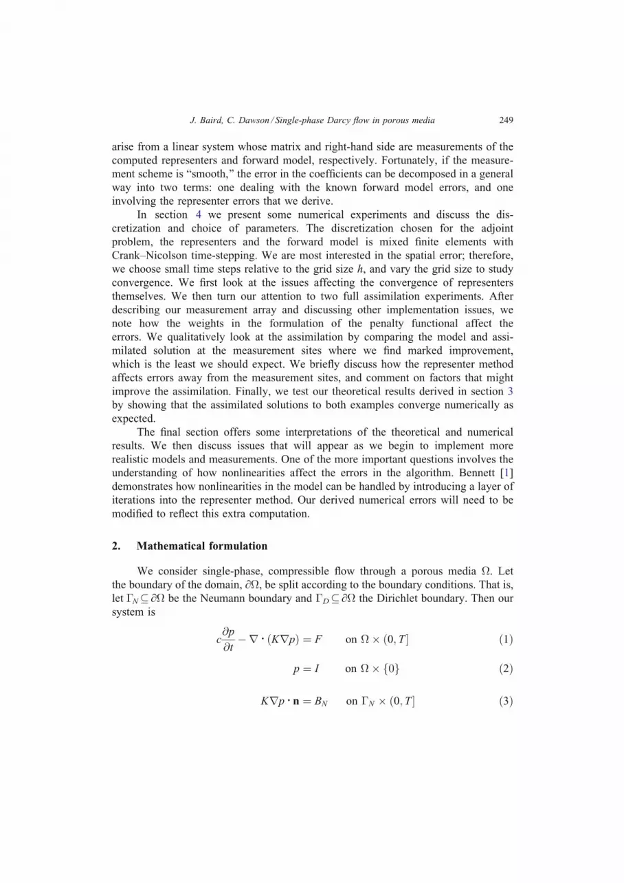
We consider single-phase, compressible flow through a porous media �. Let

the boundary of the domain, ¯�, be split according to the boundary conditions. That is,

let �N� ¯� be the Neumann boundary and �D� ¯� the Dirichlet boundary. Then our

system is

c@p

@t�r� ðKrpÞ ¼ F on �� ð0; T � ð1Þ

p ¼ I on �� f0g ð2Þ

Krp �n ¼ BN on �N � ð0; T � ð3Þ

J. Baird, C. Dawson / Single-phase Darcy flow in porous media 249

p ¼ BD on �D � ð0;T � ð4Þ

where p is pressure, c is a constant compressibility factor, F is a forcing function, I is

the initial pressure in the domain, BN and BD are the Neumann and Dirichlet boundary

conditions, and K is a symmetric positive definite matrix that describes the permea-

bility of the medium.

We suppose that we are given c, K, F, I, BN, and BD. Furthermore, suppose that

additional information is provided in the form of M measurements of the state variable

in � � ½0, T�. Each measurement is of the form

Lmð~ppÞ ¼Z T

0

Z�

Hm~ppd�dt; ð5Þ

for some prescribed kernel Hm. For the error analysis in section 3, we assume that Hm

2 L2(�) 8t. However, in practical applications we may have point measurements, in

which case Hm is a Dirac delta distribution which is not in L2. This could certainly

affect the accuracy of the representer method and thus the final solution, as discussed

in [1]. In our notation, ~pp represents the actual field from which the measurements are

taken, which is likely to be different than the forward model field, here denoted

as pF. Thus we are given a vector d 2 RM whose mth component is the mth mea-

surement, or Lmð~ppÞ.

2.1. The EulerYLagrange conditions

The problem (1)Y(4), combined with the extra information in d, is ill posed due

to the overspecification of data. Therefore, we admit residuals f, i, bN, bD, and �� defined

by the following:

c@p

@t�r� ðKrpÞ ¼ F þ f on �� ð0; T � ð6Þ

p ¼ I þ i on �� f0g ð7Þ

Krp �n ¼ BN þ bN on �N � ð0;T � ð8Þ

p ¼ BD þ bD on �D � ð0; T � ð9Þ

LLðpÞ ¼ dþ �� ð10Þ

where LLð pÞ ¼ ½Lmð pÞ�, the vector of measurements of the model, and �� is a

(unknown) vector of errors in the measurement.


Redefining the meaning of the solution, we now seek a solution p̂p, so the resi-

duals are least according to the following metric:

J ½p� ¼Z T

0

Z�

Wf f 2d�dt þZ

�

Wii2d�þ

Z T

0

Z�N

WNb2Nd�dt

þZ T

0

Z�D

WDb2Dd�dt þ w

XMm¼1

�2m; ð11Þ

where Wf, Wi, WN, WD, and w are prescribed constant weights. Generalization to fields

over the whole domain is straightforward but can obfuscate the development and is not

central to our error analysis. We require that the weights be strictly positive (sym-

metric and positive definite in the general case), although we do allow terms to not

appear in the functional. Then, the missing terms are strong constraints.

Thus we seek p̂p such that

J ½p̂p� ¼ minp

J ½p� ¼ minp

(Z T

0

Z�

Wf c@p

@t�r� ðKrpÞ � F

� �2

d�dt

þZ

�

Wi p t¼0 � Ijð Þ2d�þZ T

0

Z�N

WN Krp �n� BNð Þ2d�dt

þZ T

0

Z�D

WD p� BDð Þ2d�dt þ wXMm¼1

ðLmðpÞ � dmÞ2g: ð12Þ

The theory of Calculus of Variations states that the minimizer p̂p of J occurs when

the first variation of J, �J, is equal to zero. This condition gives rise to the well-known

EulerYLagrange equations. Let us briefly step through the derivation. The first

variation is

1

2�J ¼

Z T

0

Z�

Wf c@p


� �c@�p

@t�r� ðKr�pÞ

� �d�dt

þZ

�

Wi p t¼0 � Ijð Þ�p t¼0d�j

þZ T

0

Z�N

WN Krp � n� BNð ÞKr�p � nd�dt

þZ T

0

Z�D

WD p� BDð Þ�pd�dt þ wXMm¼1

ðLmðpÞ � dmÞLmð�pmÞ: ð13Þ


Defining � by

� ¼ Wf c@p


� �ð14Þ

and rewriting the last term using the definition of Lm, we obtain

1

2�J ¼

Z T

0

Z�

� c@�p

@t�r� ðKr�pÞ

� �d�dt þ

Z�

Wi p t¼0 � Ijð Þ�p t¼0d�j

þZ T

0

Z�N


þZ T

0

Z�D

WD p� BDð Þ�pd�dt þZ T

0

Z�

wXMm¼1

ðLmðpÞ � dmÞHm�pd�dt: ð15Þ

Integrating by parts on the first term yields

1

2�J ¼

Z�

c��p t¼Tt¼0

�� d��

Z T

0

Z�

c@�

@t�pd�dt þ

Z T

0

Z@�

Kr� � nð Þ�pd�dt

�Z T

0

Z@�

Kr�p � nð Þ�d�dt �Z T

0

Z�

r� Kr�ð Þ�pd�dt

þZ

�

Wi p t¼0 � Ijð Þ�p t¼0d�j þZ T

0

Z�N


þZ T

0

Z�D

WD p� BDð Þ�pd�dt þZ T

0

Z�

wXMm¼1

ðLmð pÞ � dmÞHm�pd�dt: ð16Þ

Now in order for �J to equal zero, the coefficients of �p must be zero. Thus we

are led to the EulerYLagrange equations for the minimizer p̂p and the multiplier �̂�. Note

that equation (21) is the definition of �̂�:

�c@�̂

@t�r� ðKr�̂Þ ¼ �w

XMm¼1

ðLmð p̂pÞ � dmÞHm on �� ½0; TÞ ð17Þ

c �̂� ¼ 0 on �� fTg ð18Þ


Kr �̂� � n ¼ 0 on �N � ½0; TÞ ð19Þ

�̂� ¼ 0 on �D � ½0;TÞ ð20Þ

c@p̂p

@t�r� ðKrp̂pÞ ¼ F þW�1

f �̂ on �� ð0;T � ð21Þ

p̂p ¼ I þW�1i c�̂ on �� f0g ð22Þ

Krp̂p � n ¼ BN þW�1N �̂ on �N � ð0; T � ð23Þ

p̂p ¼ BD þW�1D ð�Kr�̂ �nÞ on �D � ð0; T � ð24Þ

We cannot first solve for �̂� and then solve for p̂p, because p̂p appears in (17).In the case of a strong constraint, or zero residual, one merely takes the

corresponding inverse weight and sets it to zero. For example, if one were to take the

model to be perfect, which is to take f as zero, then to modify the scheme one would

set Wfj1 to zero.

2.2. The representer method

In the representer method, Bennett [1] uses the superposition principle for linear

differential equations to uncouple the EulerYLagrange equations. We assume p̂p can be

expressed as a linear combination of the forward model solution and fields that depend

on the measurements:

p̂p ¼ pF þXMm¼1

�mrm ð25Þ

where pF is the solution to the forward model (1)Y(4). The fields labeled rm are given

by the EulerYLagrange conditions stripped of the coupling and the model forcing,

which is contained in pF. Thus we compute a representer for each measurement and

solve a finite-dimensional linear system to obtain the coupling coefficient �m.

The following system defines rm:

�c@�m

@t�r� ðKr�mÞ ¼ Hm on �� ½0;TÞ ð26Þ

c�m ¼ 0 on �� fTg ð27Þ


Kr�m � n ¼ 0 on �N � ½0;TÞ ð28Þ

�m ¼ 0 on �D � ½0; TÞ ð29Þ

c@rm

@t�r� ðKrrmÞ ¼ W�1

f �m on �� ð0; T � ð30Þ

rm ¼ W�1i c�m on �� f0g ð31Þ

Krrm � n ¼ W�1N �m on �N � ð0;T � ð32Þ

rm ¼ W�1D ð�Kr�m � nÞ on �D � ð0; T �: ð33Þ

With pF and rm defined above, it remains for us to find �m. By substitution of the

definition of p̂p, (25), and the definitions of pF and rm, (30), into (21), one obtains:

Dp̂p ¼ DpF þXMm¼1

�mDrm ¼ F þXMm¼1

�mW�1f �m ð34Þ

where Dp ¼ @p

@t�r� ðKrpÞ. By the definition of �̂�

XMm¼1

�m�m ¼ Wf ðDp̂p� FÞ ¼ �̂�: ð35Þ

Furthermore, combining (17) and (26) with (35), we see that

�wXMm¼1

ðLmð p̂pÞ � dmÞHm ¼ D* �̂ ¼XMm¼1

�mD* �m ¼XMm¼1

�mHm ð36Þ

where D*p ¼ � @p

@t�r� ðKrpÞ.

Therefore �m ¼ �wðLmð p̂pÞ � dmÞ. We cannot find Lmð p̂pÞ without �m so a

substitution yields

�m ¼ �w Lmð pFÞ þXMl¼1

�lLlðrmÞ � dm

!: ð37Þ

Combining � terms yields

XMl¼1

ðLlðrmÞ þ w�1�lmÞ�l ¼ dm � Lmð pFÞ ð38Þ


where �lm is the Kronecker delta. In matrix notation, (38) is the system

Rþ w�1I� �

�� ¼ d� LLð pFÞ ð39Þ

where the entries of the matrix R are rlm ¼ LlðrmÞ, and I denotes the identity matrix.

In other words, each column of R is composed of a representer evaluated by each

measurement. It can be shown that this system is invertible. In fact, R + wj1I is a

symmetric, positiveYdefinite matrix [1].

2.3. General issues

To complete the generalized inversion, one must integrate (26)Y(29) backwards

and then integrate (30)Y(33) forwards for each measurement to obtain rm. Each

representer is measured to form R. Then, �� is computed via (39). The final solution is

calculated using (25). Thus if one has M measurements, one must perform 2M + 1

model integrations and solve one M � M linear system. Furthermore, each representer

must be stored. Note that the representer calculations are completely independent of

each other, and therefore trivially parallelized.

Alternatively, if one does not wish to store the representers, one can discard each

rm immediately after measuring its contribution to R. Because it can be shown that

�wðLmðp̂pÞ � dmÞ ¼ �m, one can solve (17)Y(20) for the multiplier �̂�, and then (21)Y(24) for the minimizer p̂p. Thus the storage requirements have been relaxed at the cost

of two extra model integrations.

3. Error analysis

In this section, we address the question of the accuracy of the solution to the

generalized inverse problem. That is, we determine how the numerical errors in

the calculations of pF and rm impact the calculation of the minimizer p̂p given by (25).

The mixed finite element method (MFEM) is chosen to calculate the forward model

pF, the adjoint variables �m and the representers rm. The MFEM is a widely used

method for porous media applications, especially on structured grids, where it is

closely related to cell-centered finite difference methods [7]. However, because the

representer method can be used with any numerical scheme or combination of

schemes, we seek to be more general when we can. Indeed, it may be advantageous to

use a different numerical method for calculating the model than for calculating the

representers, or one might want to estimate the adjoint solution in some special way

since �m are independent of many of the parameters of the problem. To this end, we

seek an a priori estimate of the minimizer p̂p given appropriate a priori estimates of the

numerical algorithms used in computing the model and the representers.

Let (I)h denote the numerical approximation to (I), and kIk be some as yet

unspecified norm over � � [0, T ). Later, for example, pF,h and rm,h will denote the


approximations to pF and rm calculated via the MFEM with CrankYNicolson time-

stepping, p̂ph will denote the approximation of p̂p, and kIk will be the L2-norm over the

domain � at the final time T. However, in the interests of generality, we do not confine

ourselves to any particular choice in this section.

From (25), we see that

p̂p� p̂ph ¼ pF � pF;h þXMm¼1

�mrm �XMm¼1

�m;hrm;h ð40Þ

which then leads directly to

kp̂p� p̂phk � k pF � pF;hk þXMm¼1

j�m � �m;hjkrmk þXMm¼1

j�m;hjkrm � rm;hk: ð41Þ

Note that the numbers �m,h are given by

Rh þ w�1I� �

��h ¼ d�LLðpF;hÞ ð42Þ

where the entries of Rh are rmn;h ¼ Lmðrn;hÞ.Bounding the first term of (41) is a straightforward application of the properties

of the numerical scheme used for the forward model.

The third term is similar to the first but is complicated by the coupling of the

representers rm with the adjoint variables �m. The initial and boundary conditions and

the forcing function for the representers in (30) are derived from the adjoint variables

�m, which in turn are forced in (26) by Hm. So, we have two possible problems: (i) that

errors in computing the data for the representers (especially the boundary conditions)

may degrade the convergence; and (ii) that if Hm is not smooth enough (for example,

in the case of point measurements), the convergence of �m, and thus rm may suffer.

We do not directly address the second problem here, although the use of point

measurements in practice is certainly of interest. The first problem is dealt with in

section 3.3.

First, however, let us deal with the second term, since it can be handled

separately from any considerations as to the particular numerical schemes used.

3.1. Analysis of the matrix problem

The second term in (41) requires some analysis of the matrix problem that yields

��, (39). One fruitful approach is to use the following lemma found in Golub and Van

Loan [3].


Lemma 3.1. Let ||I||p denote the pth vector or matrix norm as appropriate. If A is a

non-singular matrix and � K ||Aj1E||p < 1, then A + E is non-singular and

k Aþ Eð Þ�1�A�1kp � kEkp

kA�1k2p

1� � : ð43Þ

For convenience, let P = R + wj1I and define E by P + E = Ph K Rh +

wj1I. Then the entries of E are eij ¼ Liðrj;hÞ � LiðrjÞ; that is, E contains the errors

in the representers as seen by the measurement array. An application of the lemma

yields

j�m � �m;hj � k�� hkp ¼ kðP�1 � P�1h Þðd� LLð pFÞÞ � P�1

h ðLLð pFÞ � LLð pF;hÞÞkp

� kEkp

kP�1k2p

1� kP�1Ekp

kd� LLð pFÞkp þ kP�1h kpkLLð pFÞ � LLð pF;hÞkp ð44Þ

provided kPj1Ekp < 1. We expect kEkp to go to zero as h goes zero, since the entries

of E are the errors in the measurement functionals applied to the representers. So

kPj1Ekp is smaller than 1 for sufficiently small h.

Substituting (44) into (41), we have

kp̂p� p̂phk � kpF � pF;hk þXMm¼1

j�m;hjkrm � rm;hk

þ kEkp

kP�1k2p

1� kP�1Ekp

kd� LLð pFÞkp þ kP�1h kpkLLð pFÞ � LLð pF;hÞkp

!

�XMm¼1

krmk: ð45Þ

Incorporating terms that do not depend on h into constants, we obtain

kp̂p� p̂phk � kpF � pF;hk þ C1

kEkp

1� kP�1Ekp

þ C2kP�1h kpkLLð pFÞ � LLð pF;hÞkp

þXMm¼1

j�m;hjkrm � rm;hk: ð46Þ


We have reduced the question to one of howkEkp

1�kP�1Ekp

and kLLð pFÞ � LLð pF;hÞkp

behave. Since kEkp should tend to zero as h goes to zero, the fraction is dominated

by kEkp. Furthermore, because all finite dimensional norms are equivalent, it suffices

to bound, for example,

kEk1 � max1� j�M

XMi¼1

jeijj � M max1�i; j�M

jeijj ð47Þ

kLLð pFÞ � LLð pF;hÞk1 � M max1�m�M

jLmð pFÞ � Lmð pF;hÞj: ð48Þ

If Hm is in L2(�) and we are interested in errors in the L2(�)-norm, then we can

further bound (47) and (48) by

kEk1 � M max1�i; j�M

Z T

0

kHikL2ð�Þkrj � rj;hkL2ð�Þdt ð49Þ

kLLð pFÞ � LLð pF;hÞk1 � M max1�m�M

Z T

0

kHmkL2ð�Þk pF � pF;hkL2ð�Þdt: ð50Þ

Now, all terms in (46) are, as h goes to zero, Oðmaxmkrm � rm;hkL1ð0;T ;L2ð�ÞÞÞ or

Oðk pF � pF;hkL1ð0;T ;L2ð�ÞÞÞ. The L1(0, T; L2(�))-norm is the maximum L2(�)-norm

over all time. Therefore, it suffices to obtain estimates in this norm for the forward

model and the representers to bound the error in the assimilation. Then, for some

constant C,

kp̂p� p̂phkL1ð0;T ;L2ð�ÞÞ � Cðk pF � pF;hkL1ð0;T ;L2ð�ÞÞ þmaxmkrm � rm;hkL1ð0;T ;L2ð�ÞÞÞ

ð51Þ

Next, we discuss the computation of the representers using a mixed finite

element method in space, and discuss the stability and accuracy of this computation

given numerical approximations to �.

3.2. Notation

Let us begin by introducing notation. Let V = H(�, div) = {v 2 (L2(�))2: l � v 2L2(�)} and W = L2(�). Let � be partitioned into a regular triangulation T h of

elements. To analyze the errors along the boundaries, it is expedient to use Lagrange

multipliers in the Neumann part of the boundary, similar to the treatment in the hybrid

mixed method. Therefore we introduce the space �(�N) = L2(�N). The finite-

dimensional subspace in which we look for our solution is the lowest order


RaviartYThomas (RT) space [4], modified on the Neumann boundary to include a

discretization of the Lagrange multiplier space as follows. In R2, define the spaces Vh,

Wh and �h such that over each element E 2 T h and over each element edge Eih that

lies on the Neumann boundary we have

VhðEÞ ¼ fð�1xþ �1; �2yþ �2ÞT : �i; �i 2 Rg; ð52Þ

WhðEÞ ¼ f� : � 2 Rg ð53Þ

�hðEih \ �NÞ ¼ f� : � 2 Rg: ð54Þ

The test and trial functions for the fluxes are in Vh. The test and trial functions for the

pressures are in the space Wh. The Lagrange multiplier test and trial functions are in

�hðEih \ �NÞ. When working on rectangles, we use the standard nodal basis in which

the nodes are at the midpoints of the edges for Vh and �h, and for Wh the nodes are at

the centers of the elements.

In the analysis it is necessary to use the following projections. Let p be the

standard L2 projection, and �: (H1(�))2 ��! Vh be a projection with the following

properties, 8q 2 (H1(�))2:

ðr��q;wÞ ¼ ðr � q;wÞ 8w 2 Wh ð55Þ

k�q� qk � Chkqk1 ð56Þ

h�q � n; �i ¼ hq � n; �i 8� 2 �hðEhÞ: ð57Þ

Let (I,I)S denote both the scalar and vector L2 inner product over S 2 Rd , as

required by context, with S omitted when S = �. Let bI,IÀI denote the L2 inner product

over I 2 Rd�1, with I omitted if I = ¯�. Finally, let kIki,S denote the standard Sobolev

norm over S, with i omitted if i = 0. Thus, departing from the earlier notation, the

norm denoted as k�k is now specifically the L2-norm over the whole domain or

k�kL2ð�Þ.

3.3. MFEM analysis of rm

For clarity, we drop the subscript m throughout this section. Denote the

approximations to � and q = jKl� by �h and qh. At the moment, how these

approximations are computed is unspecified, we assume only that �h 2 L2(�) and qh �n 2 L2(�D) for all time t. Denote the approximations to r and �� =jKlr by rh and ��h.


Then the continuous-time MFEM scheme for rh is:

c@rh

@t;w

� �þ ðr ��h;wÞ ¼ W�1

f �h;w� �

8w 2 Whð�Þ ð58Þ

ðK�1��h; Þ � ðrh;r�Þ ¼ �hW�1D qh � n; � ni�D

� h�h; �ni�N8 2 Vhð�Þ ð59Þ

h��h � n; �i�N¼ �hW�1

N I�h; �i�N8� 2 �hðEi

h \ �NÞ ð60Þ

for rh 2 Wh(�), ��h 2 Vh(�); �h 2 �hðEih \ �NÞ, I�h is some C0 piecewise polynomial

interpolant or projection of �h, and n is the unit outward normal vector. We need the

additional smoothness that I�h provides since we have to bound the term involving I�h

with the H1/2(�N)-norm in our stability analysis.

To examine the stability of the method, let w = rh, = ��h, and m = �h. Then,

summing (58), (59), and (60) yields:

c@rh

@t; rh

� �þ K�1��h; ��h

� �¼ W�1

f �h; rh

� �

� W�1D qh �n; ��h � n�

�Dþ W�1

N I�h; �h

� �N: ð61Þ

Bounding each term on the right using standard trace theorems and inverse in-

equalities, which can be found in [11], and choosing k* e kKj1k1, we see that

W�1f �h; rh

� �� kW�1

f �hkkrhk ð62Þ

hW�1D qh � n; ��h �ni�D

� kW�1D qh � nk�D

k��h �nk�D

� CkW�1D qh � nk�D

k��hkh�12

� C

k*h�1kW�1

D qh � nk2�Dþ k*

4k��hk2 ð63Þ

hW�1N I�h; �hi�N

� CkW�1N I�hk

H12ð�NÞk�hk

H�1

2ð�NÞ

� CkW�1N I�hk1k�hk

H�1

2ð�NÞ: ð64Þ

Remark. We note that in the usual mixed method analysis, one would have the actual

flux q I n in (63) rather than its approximation qh. In this case, for sufficiently smooth


q we could put an H1/2-norm on the q term and an Hj1/2-norm on the ��h term and

avoid obtaining the hj1 term in (63). Unfortunately, qh is not assumed to be in H1/2

(�D). It may be possible to construct a smooth projection or approximation of qh to

avoid this loss, and in fact, as we see in the error analysis below, this term may

dominate in the error estimate for rh.We next need a bound on k�hk

H�1

2ð�NÞ. Therefore, consider the dual problem:

�r� ðKrÞ ¼ 0 on � ð65Þ

�Kr � n ¼ on �N ð66Þ

¼ 0 on �D: ð67Þ

Assuming � and are sufficiently smooth, by elliptic regularity

kk2 � Ck kH

12ð�NÞ

: ð68Þ

Let ¼ ��Kr, then r� ¼ 0. Using (59), we have that

ðK�1��h; Þ ¼ �hW�1D qh � n; � ni�D

� h�h; � ni�N

¼ hW�1D qh �n;Kr �ni�D

þ h�h; i�N: ð69Þ

Thus

h�h; i�N¼ �ðK�1��h; Þ þ hW�1

D qh �n;Kr � ni�D

� Ck��hkkk þ CkW�1D qh � nk�D

kKr � nk�D

� C k��hk þ kW�1D qh �nk�D

� �k k

H12ð�NÞ

ð70Þ

Taking the supremum over all 2 H12ð�NÞ implies that

k�hkH�1

2ð�NÞ� C k��hk þ kW�1

D qh �nk�D

� �: ð71Þ

Substitute this result back into (61) using (62), (63), and (64) to obtain

c@rh

@t; rh

� �þ ðK�1��h; ��hÞ �

1

"kW�1

f �hk2 þ "krhk2 þ C

k*h�1kW�1

D qh � nk2�D

þ k*

4k��hk2 þ C

k*kW�1

N I�hk21 þ

k*

4k��hk2

þ kW�1D qh � nk2

�D; ð72Þ


where " is a constant to be determined. Integrate from 0 to T * where

krhðT*Þk ¼ max0�t�T

krhðtÞk: ð73Þ

Then

ckrhðT*Þk2 þ k*

2

Z T *

0

k��hk2dt � ckrhð0Þk2 þ "Z T *

0

krhðtÞk2dt

þZ T *

0

"1

"kW�1

f �hk2 þ C

k*h�1kW�1

D qh � nk2�D

þ C

k*kW�1

N I�hk21 þ kW�1

D qh �nk2�D

#dt: ð74Þ

Combine the sixth and fourth terms on the right side of (74), and note that

"

Z T *

0

krhðtÞk2dt � "T*krhðT*Þk2:

Then choose " ¼ c2T� to hide this term, thus

c

2krhðT*Þk2 þ k*

2

Z T *

0

k��hk2dt � ckrhð0Þk2 þZ T *

0

"2T*

ckW�1

f �hk2

þ C

k*h�1kW�1

D qh � nk2�Dþ C

k*kW�1

N I�hk21

#dt; ð75Þ

which gives a stability bound in terms of the initial, boundary, and forcing data.

Lemma 3.2. For sufficiently smooth r and �, the error in the representer satisfies the

following bound in terms of �; q; �h and qh:

c

2k�ðT*Þk2 þ k*

2

Z T *

0

k��k2dt � ckW�1i ð�h � �Þð0Þk2

þZ T�

0

"Ch2k��k2

1 þ2T*

ckW�1

f ð�h � �Þk2

þ C

k*h�1kW�1

D ðqh � qÞ � nk2�Dþ C

k*kW�1

N ðI�h � �Þk21

#dt; ð76Þ

where C is a constant independent of h.


Proof. For the error analysis we can use the same machinery, except that in the first

steps, we look at the error equations instead. The error equations are:

c@ðrh � rÞ

@t;w

� �þ ðr� ð��h � ��Þ;wÞ ¼ ðW�1

f ð�h � �Þ;wÞ 8w 2 Whð�Þ ð77Þ

ðK�1ð��h � ��Þ; Þ � ðrh � r;r�Þ ¼ �hW�1D ðqh � qÞ � n; � ni�D

� h�h � �; �ni�N8 2 Vhð�Þ ð78Þ

hð��h � ��Þ � n; �i�N¼ �hW�1

N ðI�h � �Þ; �i�N8� 2 �hðEi

h \ �NÞ: ð79Þ

Let � ¼ rh � r, �� ¼ ��h ��, and � ¼ �h � �. Now, we go quickly through

several steps of algebra. Sum (77) through (79). Add and subtract r, ��, and �wherever there appears r, �� or �. Then substitute w ¼ �, ¼ ��, and � ¼ �. After

canceling some terms and using the properties of the projections involved, we have: c@�

@t; �

!þ ðK�1��; ��Þ ¼ �ðK�1ð�� Þ; ��Þ þ ðW�1

f ð�h � �Þ; �Þ

� hW�1D ðqh � qÞ � n; �� ni�D

� hW�1N ðI�h � �Þ; �i�N

:

ð80Þ

Using the same arguments as in the stability proof, we obtain

c@�

@t; �

� �þ ðK�1��; ��Þ � Ck�� k2 þ k*

2k��k2 þ 1

"kW�1

f ð�h � �Þk2

þ "k�k2 þ C

k�h�1kW�1

D ðqh � qÞ � nk2�D

þ C

k*kW�1

N ðI�h � �Þk21: ð81Þ

To complete the proof, we integrate from 0 to T*, where T* is defined as in (73)

with rh replaced by x, and choose " ¼ c2T�. Ì

Suppose we also use the lowest order MFEM in the computation of �. Then the

first and third terms in (76) give Oðh2Þ errors as expected. In the numerical

experiments, we assume the domain � is a rectangle, and we use the lowest-order

rectangular elements [4]. In this case, for sufficiently smooth �, it is well known

that �h is superconvergent to � to order h2 at the cell centers of each element [7].

One can then construct a continuous, piecewise bilinear interpolant of �h at the

cell centers, I�h, which is globally a second order approximation of �, and jjI�h �


�jj1 ¼ OðhÞ [8]. The flux qh is superconvergent to q at the midpoints of the edges,

except at Dirichlet boundaries. Experimentally, qh is observed to be only OðhÞaccurate at these boundary edges, but Oðh2Þ accurate immediately away from the

boundary. Therefore, it may be possible to extrapolate values away from the boundary

to obtain an Oðh2Þ approximation to q on �D. We have not pursued this avenue here,

but we examine below how the accuracy of this term effects the overall accuracy of rh.

Alternatively, � could be computed by some other numerical method, for

example a continuous Galerkin finite element method. In this case, I�h ¼ �h, and

assuming � is sufficiently smooth, then jj�h � �jj1 ¼ OðhÞ. The flux qh can be

constructed through a postprocessing step [9,10].

4. Numerical experiments

In this section we present some numerical examples. The first examples examine

the question of the accuracy of the representer calculation. The latter examples are

synthetic assimilation experiments that examine the ability of the method to

incorporate measured data and verify the convergence rates of the numerical scheme.

4.1. General implementation

Russell and Wheeler [5] show that, on rectangles, the lowest-order mixed finite

element method with special numerical quadrature is equivalent to a cell-centered

finite difference method. Therefore, for ease of coding, we implemente cell-centered

finite differences with CrankYNicolson time stepping for all of our experiments. The

domain is always the unit square, � ¼ ½0; 1� � ½0; 1�, and unless otherwise noted the

final time T = 0.4.

To study convergence, we construct a sequence of uniform grids: 10 � 10 (10

cells in the x- and y-directions), 20 � 20, 40 � 40, 80 � 80, and 160 � 160. Since we

are most interested in the spatial error, all grids use the same time step of 0.000267,

except where noted. When the true solution is not known, the 160 � 160 grid serves as

the truth, and the errors reported are the difference between the 160 � 160 grid and the

coarser grid.

4.2. Accuracy of the representers

The basis of the representer method is the calculation of the representers. It is

this step which is most difficult from the analysis standpoint, because, as we have

seen, it involves a backward integration to compute �m and a forward integration

influenced by �m to compute rm. Below, we perform two numerical experiments; one

with a known, smooth solution, and the other using the same measurement functional

that we use in our test assimilations.


We first test the accuracy of the representer calculation for a steady-state case

(c = 0) with analytical solutions � = r = exp(j2(x + y)). We choose the edges given by

y = 0 and y = 1 to be Dirichlet boundaries, and the other two edges to be Neumann.

We let K = I, and chose H accordingly. So the system to be solved is

�r� ðr�Þ ¼ �8 expð�2ðxþ yÞÞ ð82Þ

r� � n ¼ 2 expð�2yÞ on x ¼ 0

�2 expð�2ð1þ yÞÞ on x ¼ 1

ð83Þ

� ¼ expð�2xÞ on y ¼ 0

expð�2ðxþ 1ÞÞ on y ¼ 1

ð84Þ

�r � ðrrÞ ¼ W�1f � ð85Þ

rr �n ¼ W�1N �; on �N; ð86Þ

r ¼ �W�1D r� � n; on �D: ð87Þ

The weights then must be Wfj1 = j8, WD

j1 = j1/2 when y = 0, WDj1 = 1/2 when y =

1, WNj1 = 2 when x = 0, and WD

j1 = j2 when x = 1. Consequently, we are solving the

same problem twice; first with the analytical boundary conditions, and second with

approximate boundary and forcing conditions given by the cell-centered finite

difference solution to the first problem.

Table 1 shows the results of the experiment. We observe the optimal first-order

convergence for rh in the L2(�)-norm. The last two rows of the table give the

convergence rates for the term that would seem to dominate the error bound in Lemma

3.2, the norm of the flux through the Dirichlet boundary. We see that this term also

approaches first-order accuracy, as expected, which on the basis of Lemma 3.2, is not

sufficient to guarantee first-order accuracy of rh. The hj1 multiplying this term,

Table 1

L2(�) error.

Grid 10 � 10 20 � 20 40 � 40 80 � 80 160 � 160

krh � rkL2ð�Þ 0.05211 0.02661 0.01344 0.00675 0.00338

Rate Y 0.969 0.986 0.994 0.997

kðqh � qÞ� nk�D0.15738 0.09068 0.04860 0.02515 0.01279

Rate Y 0.795 0.900 0.951 0.975


however, is the result of a worst-case scenario analysis (trace theorem followed by an

inverse estimate) as seen in (63). It is quite possible that for certain problems this loss

of accuracy will not be felt; this was the case in all of the test examples we have tried

so far.

Next, we consider a problem with a more realistic choice for the measurement

kernel H. In this case, H is a step function of small support with

Z T

0

Z�

Hd�dt ¼ 1;

such that H mimics an impulse of magnitude one at a chosen data site. The support of

H is centered about the point (x, y, t) = (0.5,0.5,0.2), thus

Lð ~ppÞ ¼Z T

0

Z�

H~ppd�dt ~ppð0:5; 0:5; 0:2Þ:

We choose the parameters of our example problem to be: c = 1, �N ¼ ;, and K =

I. We compute the representer corresponding to the above measurement functional,

with the weights Wfj1 = 0.2, Wi

j1 = 0.5, and W Dj1 = 10. Because no analytic solution

exists, the computed representer on the 160 � 160 grid is taken to be the true solution

and compared to the solutions on the coarser grids.

The first rows of table 2 show the convergence behavior of the representer. We

see slightly better than first-order convergence. The rate seems to increase as the mesh

is refined, probably because the computed solution is approaching the 160 � 160

Btrue^ solution.

In the last rows of table 2, we also list the convergence rates for the norm of the

flux through the Dirichlet boundary. Numerically, we again observe first-order

convergence for this term. One parameter in particular that appears with this term in

the error analysis is WDj1. We might expect that for WD

j1 large, this error term may

dominate the result in Lemma 3.2. However, experiments with a wide range of values

of WDj1 give no qualitative difference in the convergence results for r.

Table 2

L1(0, T; L2(�)) error.

Grid 10 � 10 20 � 20 40 � 40 80 � 80

krh � rkL1ðL2Þ 12.527 4.5461 1.7785 0.60215

Rate Y 1.46 1.35 1.56

kðqh � qÞ� nk�D73.468 32.473 14.568 5.6566

Rate Y 1.18 1.16 1.36


4.3. Description of assimilation experiment 1

For our first numerical assimilation experiment, we create a problem with an

explicit analytical solution for the Btrue^ state of the reservoir. We let �D ¼ ;. The

solution is chosen to be

~pp ¼ t cosð8 xÞ þ cosð4 yÞð Þ þ x3y2 þ x cosðxyÞ sinðxÞ: ð88Þ

Therefore, choosing c = 1 and K as the identity matrix, the other parameters must

be:

BN ¼0 if x ¼ 0 or y ¼ 0

3y2 þ ðsinð1Þ þ cosð1ÞÞ cosð yÞ � y sinð yÞ sinð1Þ if x ¼ 1

2x3 � x2 sin2ðxÞ if y ¼ 1

8<:

ð89Þ

Fðx; y; tÞ ¼ ð64 2t þ 1Þ cosð8 xÞ þ ð16 2t þ 1Þ cosð4 yÞ � 6xy2

� 2 cos ðxyÞ cosðxÞ þ 2yðx cosðxÞ þ sinðxÞÞ sinðxyÞ þ ðxy2 þ xþ x3Þ

� cosðxyÞsinðxÞ � 2x3 ð90Þ

Iðx; yÞ ¼ x3y2 þ x cosðxyÞ sinðxÞ: ð91Þ

For the purpose of assimilation, we introduce errors into the initial condition and

forcing function, to obtain our forward model. Therefore, in calculating pF, we use

Fðx; y; tÞ ¼ ð64 2t þ 1Þ cosð8 xÞ þ ð16 2t þ 1Þ cosð4 yÞ

� 6xy2 � 2 cosðxyÞ cosðxÞ ð92Þ

Iðx; yÞ ¼ 2x3y2 þ 0:3x: ð93Þ

We make the following weight choices: W fj1 = 0.2, Wi

j1 = 0.5, WNj1 = 0, and wj1 =

0.005. Note that only the inverses of the weights need to be specified for the algorithm.

Reasons and interpretations for these choices are discussed briefly in the implementation

section.

4.4. Description of assimilation experiment 2

In the second numerical experiment, we choose a problem of more practical

interest; in particular, we look at a case where the forcing mimics an injection/


production well system. The domain remains � = [0, 1] � [0, 1], �D ¼ ;, but T =

0.002. The final time is small because we are interested in measurements before steady

state is reached. The time step is 1.33 �10j6. The parameters are c = 0.01, BN = 0, and

K ¼ 1þ xy 0

0 1

� �ð94Þ

Iðx; yÞ ¼ cosð xÞ cosð yÞ þ y2ð1� yÞ2 ð95Þ

Fðx; yÞ ¼ �ð0;0Þ � �ð1;1Þ: ð96Þ

where �(x, y) is the Dirac delta at (x, y). The solution is not explicitly known. This time,

pF is calculated with errors only in the initial condition. The forward model initial

condition is given by

Iðx; yÞ ¼ 0:5 cosð xÞ cosð yÞ þ 3y2ð1� yÞ2: ð97Þ

We choose the following weights: W fj1 = 0, Wi

j1 = 0.5, WNj1 = 0, and wj1 = 0.005.

4.5. Implementation of assimilation experiments

For the assimilation experiments, the representers and the forward model are

calculated on the same mesh. As measurements, we measure the Btrue^ solutions to

the forward model, that is the analytic solution to the forward model (88), for

experiment 1 and the 160 � 160 grid calculation of the error-free forward model for

experiment 2. The measurements for both experiments are centered at the five points

(x,y) = (0.2,0.2), (0.2,0.8), (0.8,0.8), (0.8,0.2), and (0.5,0.5) at times t = T / 4, t = T / 2,

and t = 3T/4. Thus we have a total of 15 measurements, and correspondingly 15

representers.

As Bennett explains [2], the inverses of the weights in the penalty functional

have a statistical interpretation. When the errors are Gaussian, they can be interpreted

as the covariances of the errors. We are not in a setting where we can suppose our

errors to come from any particular ensemble, thus we rather arbitrarily assign weights.

Naturally, we choose the inverse weights to be zero where there are no errors.

Fortunately, although the relative sizes of the weights can determine which numerical

error terms dominate, we have seen that they do not affect the numerical convergence

rates.

4.6. Assimilation results

We were encouraged by the results of these test cases. Although we are

interested in the convergence behavior of the representer method, we also studied the

quality of the assimilated solution by observing how the method corrected for the


introduced errors. The assimilated solutions showed a significant decrease in the errors

at the measurement sites, as expected. Table 3 shows the norm (the vector 2-norm) of

the difference between the model, pF,h, and the true solution, ~pp, versus the norm of the

difference between the assimilated solution, p̂ph, and the true solution at the

measurement sites for both examples. Note that while the assimilation solution is

more accurate at the measurement sites, we do not observe, nor expect, convergence in

this norm. Obviously, the forward model does not converge to the true solution

because of the error introduced in the data. More subtly, the assimilated solution

converges not to the true solution, but rather to something that balances the forward

model and the measurement of the true solution.

We were also interested in the improvement of errors away from the

measurement sites. Table 4 shows the L2-norm of the difference between the model

and true solutions and the assimilated and true solutions at the final time for various

grids. The assimilation improves the global errors for both examples, although

example 2 shows a better improvement than example 1, due to the presence of the

dominant forcing term in example 1. The global errors might be further improved by a

more sophisticated weighting function or by assimilating more measurements. Again,

convergence is not expected here. We do see seeming convergence between p̂ph and ~pp,

but this is misleading. In the long run, as h Y 0, these numbers tend to a positive

constant.

Finally, we ran the assimilation experiment on the finest grid, that is 160 � 160,

and considered this solution to be the true inverse solution, p̂p. We then computed on

Table 3

Model vs. assimilated solution at 15 measurement sites.

Grid 10 � 10 20 � 20 40 � 40 80 � 80

Example 1

kLðpF;hÞ � dk2 0.738659 0.459301 0.459332 0.461576

kLðp̂phÞ � dk2 0.027842 0.008257 0.006282 0.006212

Example 2

kðpF;hÞ � dk2 0.345031 0.342628 0.344248 0.345804

kLðp̂phÞ � dk2 0.032048 0.014669 0.006807 0.003646

Table 4

L2 differences at the final time t = T.

Grid 10 � 10 20 � 20 40 � 40 80 � 80

Example 1

kðpF;h � ~ppÞðTÞkL2ð�Þ 0.402722 0.225930 0.194268 0.186996

kðp̂ph � ~ppÞðTÞkL2ð�Þ 0.366810 0.144294 0.083258 0.063181

Example 2

kðpF;h � ~ppÞðTÞkL2ð�Þ 0.068233 0.067215 0.066909 0.066820

kðp̂ph � ~ppÞðTÞkL2ð�Þ 0.022217 0.010785 0.005096 0.002139


the coarser grids and looked at the convergence behavior, recalling (51). Table 5

shows the Lò(0,T; L2(�)) convergence behavior of the assimilated solution for both

assimilation experiments. We see first-order convergence in both cases, which is what

we should expect from the cell-centered finite difference method.

5. Conclusions

The representer method is a commonly used approach for data assimilation in

oceanography. In this work we have applied it to data assimilation whereby the

underlying model is Darcy flow in a porous medium. We have examined the effects of

numerical discretization on this approach, specifically in the case where the rep-

resenters and forward model are approximated using the mixed finite element method.

Numerical experiments have been performed to further assess the accuracy of this

approach, with respect to the accuracy of the numerical method and the ability of the

method to assimilate data.

The next step is to implement the representer method with more complicated

groundwater models. The most challenging hurdle will be nonlinearities. In [2], the

nonlinearities are handled by linearizing the EulerYLagrange equations, and then using

the representers on the linearized set of equations. This introduces another layer of

iteration into the computations.

Acknowledgement

This research was supported by NSF grant EIA-0121523.

References

[1] A.F. Bennett, Inverse Methods in Physical Oceanography (Cambridge University Press, New York,

NY, 1992) p. 347.

[2] A.F. Bennett, Inverse Modeling of the Ocean and Atmosphere (Cambridge University Press,

Cambridge, UK, 2002) p. 234.

[3] G.H. Golub and C.F. Van Loan, Matrix Computations, 3rd Edition (The Johns Hopkins University

Press, Baltimore, MD, 1996) p. 694.

Table 5

Convergence of kp̂ph � p̂pkL1ð0;T ;L2ð�ÞÞ.

Grid 10 � 10 20 � 20 40 � 40 80 � 80

Example 1 0.360429 0.129387 0.058437 0.025636

Rate Y 1.48 1.15 1.19

Example 2 0.108985 0.048814 0.021600 0.008492

Rate Y 1.16 1.18 1.35


[4] P.A. Raviart and J.M. Thomas, A mixed finite element method for second order elliptic problems,

in: Mathematical Aspects of Finite Element Methods: Lecture Notes in Mathematics 606, eds. I.

Galligani and E. Magenes (Springer-Verlag, Berlin, 1977) pp. 298Y315.

[5] T.F. Russell and M.F. Wheeler, Finite element and finite difference methods for continuous flows in

porous media, in: The Mathematics of Reservoir Simulation, ed. R.E. Ewing (Society for Industrial

and Applied Mathematics, Philadelphia, PA, 1983).

[6] A.F. Bennett, B.S. Chua and L.M. Leslie, Generalized inversion of a global numerical weather

prediction model, Meteorol. Atmos. Phys. 60 (1996) 165Y178.

[7] M.F. Wheeler and A. Weiser, On convergence of block-centered finite differences for elliptic

problems, SIAM J. Numer. Anal. 25(2) (1988) 351Y375.

[8] C. Dawson, M.F. Wheeler and C. Woodward, A two-grid finite difference scheme for nonlinear

parabolic equations, SIAM J. Numer. Anal. 35(2) (1998) 435Y452.

[9] I. Babuska and A. Miller, The post-processing approach in the finite element method. I. Calculation

of displacements, stresses and other higher derivatives of the displacements, Int. J. Numer. Methods

Eng. 20(2) (1984) 1085Y1109.

[10] J.A. Wheeler, Simulation of heat transfer from a warm pipeline buried in permafrost, in: 74th

National Meeting of the American Institute of Chemical Engineers, New Orleans (1973).

[11] S.C. Brenner and L.R. Scott, The Mathematical Theory of Element Methods, Texts in Applied

Mathematics (Springer-Verlag, New York, 1994) p. 294.


The representer method for data assimilation in single-phase Darcy flow in porous media

Documents

Transcript of The representer method for data assimilation in single-phase Darcy flow in porous media