1

The Relationship between Low Levels of

Urinary Albumin Excretion and

Microvascular Function

Submitted by Daniel Chapman to the University of Exeter

as a thesis for the degree of

Doctor of Philosophy in Medical Science

In September 2017

This thesis is available for Library use on the understanding that it is

copyright material and that no quotation from the thesis may be

published without proper acknowledgement.

I certify that all material in this thesis which is not my own work has been

identified and that no material has previously been submitted and

approved for the award of a degree by this or any other University.

Signature: …………………………………………………………..

2

Abstract

Increased urinary albumin excretion, known as microalbuminuria, is an established clinical

risk factor for renal disease in patients with diabetes. There is growing evidence that

increasing urinary albumin even within the normal range, is a risk factor for cardiovascular

disease (CVD) in subjects with and without diabetes.

Microvascular dysfunction has been proposed as the common process in the

pathophysiology of both diabetic renal disease and cardiovascular disease, resulting in

increased urinary albumin excretion. This is further supported by evidence that urinary

albumin excretion is associated with other microvascular complications of diabetes, such as

retinopathy and neuropathy.

It is important to investigate these relationships further as it could improve our ability to

identify those at risk of CVD, and complications of diabetes at an earlier stage. This would

result in significant improvement in the quality of lives of patients with diabetes and save

the health service resources in managing the complications of diabetes.

Studies that have investigated the relationship between albumin excretion and

microvascular dysfunction are limited by the use of clinical assays, which cannot quantify

low concentrations of urinary albumin.

In this thesis an assay is validated to quantify low concentrations of urinary albumin. An

accurate and reproducible method is developed to investigate low levels of urinary albumin

excretion. This method was developed through two clinical studies and several laboratory

experiments that investigated; a) the optimal method of collecting urine samples and

reporting the results, b) the influence of exercise on urinary albumin excretion and c) the

stability of urinary albumin in stored samples.

Patients were selected from a prospective clinical study (SUMMIT) to investigate the

relationship between low levels of urinary albumin excretion and in-vivo measures of

microvascular function and microvascular complications of diabetes for the first time. This is

3

the first longitudinal study to report the change in these measures of microvascular function

over three years and the influence of diabetes and CVD.

This thesis provides novel evidence that increasing urinary albumin excretion, including

within the normal range, is linked to generalised microvascular dysfunction. Furthermore,

impaired microvascular autoregulation may play a role in the pathogenesis and is not

influenced by diabetes. This is also supported by the association of urinary albumin

excretion with background (early) changes in diabetic retinopathy.

Declaration

I designed and conducted the clinical studies described in this thesis except for the SUMMIT

study. Microvascular function was tested by Dr Francesco Casanova, and retinal examination

was carried out by Dr Kim Gooding and research nurses. I carried out all urinary albumin

analysis throughout this thesis.

4

Contents

Abstract ................................................................................................................................................ 2

Acknowledgements ........................................................................................................................... 9

Abbreviations ................................................................................................................................... 10

Chapter 1 Introduction ................................................................................................................ 25

1.1 Reporting urinary albumin excretion....................................................................................... 26

1.2 Diabetic Kidney Disease ................................................................................................................. 29

1.3 Pathophysiology of albuminuria ................................................................................................ 40

1.4 Microalbuminuria; predictor of diabetic kidney disease .................................................. 60

1.5 Microalbuminuria; predictor of cardiovascular disease and mortality ...................... 63

1.6 Urinary albumin excretion within the normal range associated with renal and

cardiovascular morbidity ..................................................................................................................... 65

1.7 Calculating risk of cardiovascular disease .............................................................................. 66

1.8 Microvascular dysfunction precedes clinical complications of cardiovascular

disease.......................................................................................................................................................... 68

1.9 The SUMMIT study .......................................................................................................................... 69

1.10 Aims and objectives ...................................................................................................................... 70

Chapter 2 Quantifying Urinary Albumin ............................................................................... 72

2.1 Introduction ....................................................................................................................................... 72

2.2 Aim ......................................................................................................................................................... 84

2.3 Methods ................................................................................................................................................ 84

2.4 Results .................................................................................................................................................. 92

2.5 Discussion ........................................................................................................................................ 110

2.6 Conclusion ........................................................................................................................................ 114

5

Chapter 3 Investigating Methods to Adjust Urinary Albumin Concentration in

Untimed Samples to Account for Variable Urinary Concentration .......................... 115

3.1 Introduction .................................................................................................................................... 115

3.2 Quantifying urinary creatinine ................................................................................................ 116

3.3 Estimating personalised creatinine excretion rate .......................................................... 129

3.4 Validation of a urine specific gravity refractometer ........................................................ 145

3.5 Summary and conclusions ......................................................................................................... 152

Chapter 4 Urine Collection Methods to Assess the Excretion of Albumin in the

Normal Range .............................................................................................................................. 153

The Optimal Urine Collection Method to Assess the Excretion of Albumin in the

normal range .......................................................................................................................................... 154

4.1 Introduction .................................................................................................................................... 154

4.2 Aim ...................................................................................................................................................... 160

4.3 Method ............................................................................................................................................... 161

4.4 Results ............................................................................................................................................... 166

The relationship of estimating AER from an untimed spot using a personalised

creatinine excretion rate with an overnight AER ..................................................................... 178

4.5 Introduction .................................................................................................................................... 178

4.6 Aim ...................................................................................................................................................... 179

4.7 Method ............................................................................................................................................... 179

4.8 Results ............................................................................................................................................... 181

4.9 Chapter Discussion ....................................................................................................................... 184

Discussion: The Optimal Urine Collection Method to Assess the Excretion of Albumin

in the normal range.............................................................................................................................. 185

Discussion: The relationship of estimating AER from an untimed spot using a

personalised creatinine excretion rate with an overnight AER ......................................... 193

4.10 Conclusion ..................................................................................................................................... 196

6

Chapter 5 Storing Urine for the Assessment of Albumin Excretion ......................... 197

5.1 Introduction .................................................................................................................................... 197

5.2 Aim ...................................................................................................................................................... 205

5.3 The effect of multiple freeze thaw cycles on albumin and creatinine concentrations

and the assessment of ACR. .............................................................................................................. 206

5.4 Optimal storage conditions to preserve urinary albumin and creatinine

concentrations and the assessment of ACR over 12 months. .............................................. 210

5.5 The effect of storage duration on albumin and creatinine levels and the calculation

of ACR in samples stored at -80oC .................................................................................................. 244

5.6 Chapter Summary ......................................................................................................................... 255

5.7 Conclusion ........................................................................................................................................ 257

Chapter 6 Impact of Exercise on Urinary Albumin Excretion ..................................... 258

6.1 Introduction .................................................................................................................................... 258

6.2 Aim ...................................................................................................................................................... 272

6.3 Method ............................................................................................................................................... 273

6.4 Results ............................................................................................................................................... 280

6.5 Discussion ........................................................................................................................................ 299

6.6 Conclusion ........................................................................................................................................ 308

Chapter 7 Urinary Albumin Excretion and Microvascular Function ....................... 309

7.1 Background ...................................................................................................................................... 309

7.2 Introduction .................................................................................................................................... 310

7.2.1 Microvasculature ................................................................................................................... 310

7.2.2 Assessing cutaneous microvascular function ............................................................. 317

7.2.3 Post occlusive reactive hyperaemia and urinary albumin excretion ................ 324

7.2.4 Urinary albumin excretion and other microvascular complications of diabetes

................................................................................................................................................................. 326

7.2.5 Diabetes and microvascular function ............................................................................ 333

7

7.2.6 Microvascular dysfunction precedes clinical complications of cardiovascular

disease .................................................................................................................................................. 335

7.2.8 CVD risk factors ...................................................................................................................... 337

7.3 Aim ...................................................................................................................................................... 339

7.4 Method ............................................................................................................................................... 342

7.4.1. Participant recruitment ..................................................................................................... 342

7.4.2 Participant screening ........................................................................................................... 344

7.4.3 Sample analysis ...................................................................................................................... 344

7.4.4 Microvascular tests ............................................................................................................... 346

7.4.5 Retinopathy ............................................................................................................................. 349

7.4.6 Peripheral Neuropathy ....................................................................................................... 350

7.4.7 Statistical analysis ................................................................................................................. 351

7.5 Results ............................................................................................................................................... 357

Participant recruitment ................................................................................................................. 357

7.5.1 Hypothesis 1 ............................................................................................................................ 360

7.5.2 Hypothesis 2 ............................................................................................................................ 408

7.6 Discussion ........................................................................................................................................ 433

7.6.1 Participant recruitment ...................................................................................................... 433

Hypothesis 1: ..................................................................................................................................... 434

Hypothesis 2 ....................................................................................................................................... 460

7.7 Conclusion ........................................................................................................................................ 470

Chapter 8 Overall discussion, new findings, conclusions and area for future work

.......................................................................................................................................................... 472

8.1 Background ...................................................................................................................................... 472

8.2 Quantifying urinary albumin and creatinine ...................................................................... 473

8.3 Adjusting urinary albumin for urinary concentration in spot samples. .................. 474

8.4 Urinary albumin and creatinine stability during prolonged storage ........................ 474

8.5 Collecting samples and reporting urinary albumin excretion ..................................... 475

8.6 Influence of exercise, and clinical implications when collecting random spot

samples. .................................................................................................................................................... 476

8.7 Urinary albumin excretion and microvascular function in diabetes......................... 476

8

8.8 Relationship between microvascular function and urinary albumin excretion ... 477

8.9 Change in albumin excretion and microvascular function over three years. ........ 479

8.10 Interaction of CVD on the relationship between AER/ACR with microvascular

function in the normoalbuminuria range .................................................................................... 480

8.11 Random spot samples to detect walking induced urinary albumin excretion ... 480

8.12 Albumin excretion and microvascular complications of diabetes........................... 481

8.13 Future work .................................................................................................................................. 482

8.14 Overall conclusion ...................................................................................................................... 483

Appendix 1: Genway ELISA kit information ................................................................................... 484

Appendix 2: Bethyl E88-129 ELISA kit information .................................................................... 487

Appendix 3: Fitzgerald ELISA information ..................................................................................... 494

Appendix 4: Patient information sheet for urine collection study. ....................................... 499

Appendix 5: Patient information sheet for exercise study ....................................................... 506

Appendix 6: Walking increased urinary albumin excretion plots ......................................... 511

References ................................................................................................................................................... 518

9

Acknowledgements

To my supervisors Professor Angela Shore, Dr Kim Gooding and Dr Timothy McDonald,

thank you for your leadership, motivation, scientific knowledge and kindness. I am

immensely grateful for your support, encouragement and mentorship throughout this PhD.

I would like to thank all the members of the DVRC, their support and knowledge have been

essential to completing this project. This thesis would not have been possible without their

participation in my studies and their samples. I would like to thank nurses Anning, Ball, Cox,

Wilkes and Pamphilon for all their hard work and assistance in setting up studies and

ensuring their smooth and ethical operation. I would also like to acknowledge all of the

willing volunteers who kindly participated in my studies.

I am immensely grateful to Dr Francesco Casanova for his mentorship and friendship. I am

also indebted to him for all his hard work collecting the microvascular measurements in the

SUMMIT cohort. Thank you to Dr A. Shepherd and Dr D. Wilkerson for their assistance with

exercise threshold testing.

I would also like to thank Drs A.J. Jordan, S.V Hope, C.T. Thorn, J.K. Williams, K. Aizawa and

M.G. Gilchrist for their invaluable clinical perspective and contributions to lively discussion. I

would also like to thank the team in Clinical Biochemistry, especially Dr Mandy Perry, Mr

Aled Lewis and the technicians for access to their laboratory and support in carrying out my

experiments.

Finally, and most importantly, I would like to thank my family, my mum Susan Chapman, my

brother Alex Chapman and his wife Kai-Chuan, for their continued and unquestioning

support. I am eternally grateful for their help and kindness throughout this PhD.

10

Abbreviations

A/USG Albumin to urine specific gravity ratio

ACH Acetylcholine

ACR Albumin to creatinine ratio

Adj Adjusted

AER Albumin excretion rate

AU Arbitrary units

AUC Area under the curve

BMI Body mass index

BP Blood pressure

CER Creatinine excretion rate

CI Confidence interval

CKD Chronic Kidney Disease

CKD-EPI Chronic Kidney Disease Epidemiology Collaboration

CO2 Carbon dioxide output

CRM Certified reference material

CV Coefficient of variance

CVD Cardiovascular Disease

DKD Diabetic kidney disease

11

DM Diabetes

eAER Estimated albumin excretion rate

eCER Estimated creatinine excretion rate

eGFR Estimated glomerular filtration rate

ELISAs Enzyme linked immunosorbent assays

ESL Endothelial surface layer

FMV First morning void

GBM Glomerular basement membrane

GET Gas exchange threshold

GFR Glomerular filtration rate

HbA1c Glycated haemoglobin

HDL high-density lipoprotein

HPLC high pressure liquid chromatography

HSA Human serum albumin

LDF Laser Doppler fluximetry

LDL Low-density lipoprotein

LDPI Laser Doppler perfusion image

LOD Limit of detection

LOQ Limit of quantification

MBF Maximal blood flow

12

MDRD Modification of Diet in Renal Disease (study)

mGFR Measured glomerular filtration rate

MVR Minimum vascular resistance

NaOH Sodium hydroxide

NKF-KDOQI The National Kidney Foundation; Kidney Disease Outcomes quality Initiative

PORH Post occlusive reactive hyperaemia

ROC Receiver operator characteristic

SD Standard deviation

SMV Second morning void

SNP Sodium nitroprusside

UAC Urinary albumin concentration

UAE Urinary albumin excretion

USG Urine specific gravity

VO2 Oxygen uptake

VO2max Maximum oxygen uptake

13

List of Tables

Table 1 Definitions of albuminuria .......................................................................................... 27

Table 2 Gender specific ACR reference ranges ........................................................................ 28

Table 3 Summary of three predictive studies used to define microalbuminuria in individuals with T1DM................................................................................................................................ 62

Table 4 External quality assurance scheme data ..................................................................... 74

Table 5 Criteria for selected assays to undergo preliminary validation .................................. 93

Table 6 Intra-assay variation of the Genway ELISA to measure albumin in urine samples and certified reference material. .................................................................................................... 95

Table 7 Linearity of dilution results for Genway ELISA ............................................................ 97

Table 8 Intra-assay variation of the Bethyl ELISA to measure albumin in urine samples and certified reference material ..................................................................................................... 98

Table 9 Linearity of dilution results for Bethyl ELISA ............................................................. 100

Table 10 Intra-assay reproducibility of the Fitzgerald assay tested on three urine samples and two CRMs ........................................................................................................................ 101

Table 11 Linearity of dilution results for Fitzgerald ELISA in two urine samples .................. 103

Table 12 Intra-assay variation of three ELISAs to quantify urinary albumin ......................... 104

Table 13 Correlation between albumin measured by the three test ELISAs with the reference (COBAS) method .................................................................................................................... 105

Table 14 Dilution linearity results for three test ELISAs undergoing preliminary validation testing .................................................................................................................................... 105

Table 15 Inter-assay variation of albumin measurements using the Fitzgerald ELISA .......... 107

Table 16 Percentage error of CRM measurements using the Fitzgerald ELISA. .................... 107

Table 17 Reproducibility of the Fitzgerald ELISA to measure low urinary albumin concentrations ....................................................................................................................... 110

Table 18 Intra-assay reproducibility of two assays to measure urinary creatinine in quality control materials and urine samples ..................................................................................... 123

Table 19 Inter-assay reproducibility of two assays to measure urinary creatinine .............. 123

14

Table 20 Participant characteristics of 245 participants from the SUMMIT study utilised to examine the impact of estimating personalised creatinine excretion rate when reporting an ACR ......................................................................................................................................... 136

Table 21 Measured and estimated albumin excretion rates ................................................. 137

Table 22 Correlation of estimates of AER with measured AER ............................................. 140

Table 23 Diagnostic accuracy of ACR and estimates of AER to identify male individuals with microalbuminuria ................................................................................................................... 142

Table 24 Intra-assay reproducibility of USG-α to measure USG in four urine samples ........ 148

Table 25 Inter-assay reproducibility of USG-α ....................................................................... 149

Table 26 The containers used to collect different urine samples. ........................................ 163

Table 27 Characteristics of the study participants. ............................................................... 166

Table 28 Median albumin excretion levels by different urine collection methods. ............. 167

Table 29 The median intra-individual reproducibility of different urine collection methods to assess albuminuria ................................................................................................................. 168

Table 30 Inter-individual variability of different urine collection methods and different ways of reporting albumin excretion in 17 healthy participants.................................................... 172

Table 31 Correlation between spot urine collections and methods of reporting with overnight AER to assess albumin excretion. .......................................................................... 173

Table 32 Correlation of different urine spot collections and methods of reporting albumin excretion with the “gold standard” overnight AER to assess albumin excretion.................. 176

Table 33 Characteristics of SUMMIT participants included in the study. ............................. 181

Table 34 Albumin excretion from overnight and random collections in participants with and without type 2 diabetes ......................................................................................................... 182

Table 35 Association of ACR and estimates of AER from a single spot random sample with timed overnight urine collection ........................................................................................... 182

Table 36 Diagnostic accuracy of ACR and estimates of AER in a random sample to identify individuals with microalbuminuria. ....................................................................................... 183

Table 37 Impact of repeated freeze thaw cycles on albumin concentration ........................ 207

Table 38 Impact of repeated freeze thaw cycles on creatinine concentration. .................... 207

Table 39 Impact of repeated freeze thaw cycles on ACR. ..................................................... 208

Table 40 Baseline and repeated urinary albumin concentration for 30 samples stored at -20oC and -80oC for 12 months. .............................................................................................. 216

15

Table 41 Baseline and repeated urinary creatinine concentration for 30 samples stored at -20oC and -80oC for 12 months ............................................................................................... 219

Table 42 Baseline and repeated ACR for 30 samples stored at -20oC and -80oC for 12 months.. ................................................................................................................................. 223

Table 43 Change in urinary albumin concentration in 30 samples which have undergone different treatments prior to being stored at -20oC and -80oC for 12 months. .................... 231

Table 44 Change in urinary creatinine concentration in 30 samples which have undergone different treatments prior to being stored at -20oC and -80oC for 12 months. .................... 233

Table 45 Change in ACR in 30 samples which have undergone different treatments prior to being stored at -20oC and -80oC for 12 months. .................................................................... 235

Table 46 New COBAS analyser validation result for urinary albumin. .................................. 244

Table 47 New COBAS analyser validation results for urinary creatinine. .............................. 245

Table 48 Correlation between change in UAC and duration of storage at -80oC in 91 samples................................................................................................................................................. 248

Table 49 Correlation between change in creatinine and duration of storage at -80oC in 91 samples. ................................................................................................................................. 250

Table 50 Correlation between change in ACR and duration of storage in 91 samples over 850 days at -80oC. ......................................................................................................................... 252

Table 51 Albumin excretion rate before and after exercise in 16 healthy male participants................................................................................................................................................ 266

Table 52 . Characteristics of the eleven participants who completed the study .................. 280

Table 53 ACR before and after different intensities of exercise ........................................... 281

Table 54 Actual and percent change of ACR after different exercise intensities .................. 285

Table 55 Significance levels from Wilcoxon sign rank test to determine between which two intensities of exercise the change in ACR is significantly different ....................................... 286

Table 56 Time for ACR to return to resting levels after heavy exercise. ............................... 290

Table 57 ACR, albumin, creatinine and USG before and after heavy exercise in 11 healthy participants. Data presented as median [IQR]. * denotes significant difference after exercise................................................................................................................................................. 291

Table 58 Actual and percent change of ACR, albumin, creatinine and urine specific gravity after heavy exercise in 11 healthy participants. Data presented as median [IQR] or mean (SD). ........................................................................................................................................ 291

16

Table 59 Blood pressure and heart rate before and after heavy exercise in healthy individuals. Data presented as median [IQR]. * denotes significant difference after exercise. BP: blood pressure ................................................................................................................. 292

Table 60 Actual and percent change of blood pressure and heart rate after heavy exercise. Data presented as median [IQR] or mean (SD)...................................................................... 292

Table 61 No association between change in blood pressure and heart rate with change in ACR after heavy exercise in 11 healthy individuals. .............................................................. 293

Table 62 No association between percent change in blood pressure and heart rate with percent change in ACR after heavy exercise in 11 healthy individuals. ................................ 293

Table 63 Correlation between maximum blood pressure and heart rate with percent change in ACR after heavy exercise in 11 healthy participants ......................................................... 294

Table 64 Duration of exercise until exhaustion and cardio outputs in two studies. ............. 301

Table 65 Participant characteristics stratified by peak response curve morphology group . 325

Table 66 Participant inclusion criteria for each hypothesis................................................... 343

Table 67 Analytical methods used in routine analysis of blood samples .............................. 345

Table 68 Classification of diabetic retinopathy status used in the SUMMIT study. .............. 350

Table 69 Participant characteristics for Hypothesis One (n=248) ......................................... 361

Table 70 Urinary albumin excretion determined using both the Fitzgerald and Cobas methods in participants with and without diabetes ............................................................. 364

Table 71 Urinary albumin excretion and microvascular function in participants with and without diabetes .................................................................................................................... 368

Table 72 Correlation between urinary albumin excretion and microvascular function. ...... 370

Table 73 Interaction of diabetes on the relationship between microvascular function and albumin excretion .................................................................................................................. 371

Table 74 Interaction of CVD on the relationship between microvascular function and albumin excretion .................................................................................................................. 372

Table 75 Regression analysis between AER and microvascular function .............................. 374

Table 76 Regression analysis between ACR and microvascular function .............................. 376

Table 77 Correlation between urinary albumin excretion and time to peak hyperaemia (PORH) in subjects with and without CVD ............................................................................. 377

Table 78 Regression analysis between AER and microvascular function in subjects with and without CVD ........................................................................................................................... 378

17

Table 79 Distribution of AER by curve morphology after post occlusive reactive hyperaemia testing .................................................................................................................................... 379

Table 80 Participant characteristics and microvascular function stratified by peak response curve morphology group ....................................................................................................... 382

Table 81 Correlation between albuminuria and microvascular function within the normoalbuminuria range. ...................................................................................................... 383

Table 82 Interaction of diabetes in the relationships between measures of microvascular function and albumin excretion in the normoalbuminuria range. ........................................ 384

Table 83 Interaction of CVD on the relationship between microvascular function and albumin excretion in the normoalbuminuria range .............................................................. 385

Table 84 Regression analysis between AER and post-occlusive reactive hyperaemia in the normoalbuminuria range ....................................................................................................... 386

Table 85 Regression analysis between ACR and peak endothelial independent response to sodium nitroprusside in the normoalbuminuria range ......................................................... 387

Table 86 Correlation between urinary albumin excretion and microvascular function in subjects with and without CVD with normoalbuminuria ...................................................... 390

Table 87 Regression analysis between ACR and microvascular function in subjects without CVD ......................................................................................................................................... 391

Table 88 Distribution of AER by curve morphology after post occlusive reactive hyperaemia testing in the normoalbuminuria range ................................................................................. 392

Table 89 Participant characteristics and microvascular function stratified by peak response curve morphology group in subjects with normoalbuminuria .............................................. 396

Table 90 Participant characteristics for participants selected to test hypothesis 2.............. 399

Table 91 Change in ACR, blood pressure and microvascular function over 37 months (±3) in 144 participants from the SUMMIT cohort ........................................................................... 402

Table 92 Correlation between change in albuminuria with change in microvascular function in whole cohort across the full range of albumin excretion .................................................. 403

Table 93 Correlation between change in albuminuria within the normoalbuminuria range with change in microvascular function .................................................................................. 405

Table 94 Regression analysis between absolute change in ACR within the normoalbuminuria range with change in microvascular function ........................................................................ 406

Table 95 Regression analysis between percent change in ACR within the normoalbuminuria range with percent change in microvascular function .......................................................... 407

18

Table 96 Baseline participant characteristics for the individuals with type 2 diabetes selected to test Hypothesis 3 (n=321) .................................................................................................. 411

Table 97 Difference in ACR between individuals who had a meaningful progression in retinopathy and those who did not ....................................................................................... 415

Table 98 Participant characteristics for subjects who had a progression in retinopathy and those who did not .................................................................................................................. 416

Table 99 Clinical characteristics of individuals who had no progression in retinopathy who had either an ACR in the normoalbuminuria range or higher ............................................... 419

Table 100 Difference in ACR between individuals who had a meaningful progression in neuropathy and those who did not ....................................................................................... 421

Table 101 Baseline participant characteristics for the individuals with type 2 diabetes selected to test Objective 3 ................................................................................................... 424

Table 102 Change in ACR between individuals who had a progression in retinopathy and those who did not .................................................................................................................. 426

Table 103 Percent change in ACR between individuals who had a progression in retinopathy and those who did not ........................................................................................................... 427

Table 104 Participant characteristics at baseline for subjects with a progression in retinopathy and their matched controls. .............................................................................. 430

Table 105 Difference in the change in ACR between individuals who had a progression in retinopathy and matched controls ........................................................................................ 431

Table 106 Difference in the percent change in ACR between individuals who had a progression in retinopathy and matched controls ................................................................ 432

19

List of Figures

Figure 1 Incidence counts and rates of the primary causes of ESRD in the U.S. ..................... 30

Figure 2 Classification of CKD using Glomerular Filtration Rate (GFR) and ACR categories in the UK....................................................................................................................................... 32

Figure 3 Schematic representation of progression of diabetic kidney disease from the onset of diabetes ............................................................................................................................... 36

Figure 4 Annual transition rates with 96% confidence intervals through the stages of nephropathy and to death of any cause .................................................................................. 38

Figure 5: Microvascular organisation of a nephron ................................................................. 43

Figure 6: Renal handling of albumin ........................................................................................ 45

Figure 7: Scanning electron micrograph of a mouse glomerulus ............................................ 46

Figure 8: The glomerular barrier. ............................................................................................. 48

Figure 9: Pathogenesis of diabetic kidney disease. ................................................................. 54

Figure 10: Urinary albumin excretion as a predictor of renal and cardiovascular disease. A: Association between urinary albumin excretion and the risk of renal morbidity in different populations. excretion level and the risk for cardiovascular outcomes in different populations .............................................................................................................................. 64

Figure 11: Reference system showing traceability of results to higher order reference system. ..................................................................................................................................... 77

Figure 12 Different methods of enzyme linked immunosorbent assays to detect albumin. .. 82

Figure 13 Detection ranges of commercially available ELISA kits to measure human albumin.................................................................................................................................................... 92

Figure 14 Correlation between albumin measurements quantified using both the Genway ELISA and COBAS method ........................................................................................................ 96

Figure 15 Bland Altman difference plot for albumin concentration in samples quantified using both the Genway and COBAS methods. ......................................................................... 97

Figure 16 Correlation between albumin samples quantified using the Bethyl ELISA and COBAS methods ....................................................................................................................... 99

Figure 17 Bland Altman difference plot for albumin samples quantified by both Bethyl and COBAS methods. .................................................................................................................... 100

Figure 18 Correlation between albumin samples quantified using both the Fitzgerald ELISA and COBAS methods. ............................................................................................................. 102

20

Figure 19 Bland Altman difference plot for albumin samples quantified using both the Fitzgerald and COBAS methods. ............................................................................................ 103

Figure 20 Correlation between Fitzgerald ELISA and COBAS method in 44 samples with an albumin concentration less than 40mg/L. ............................................................................. 108

Figure 21 Bland Altman difference plot for Fitzgerald and COBAS methods in samples with an albumin concentration less than 40mg/L ......................................................................... 109

Figure 22 Correlation between enzymatic and Jaffe methods to measure urinary creatinine................................................................................................................................................ 124

Figure 23 Bland Altman difference plot for Jaffe and enzymatic methods to quantify urinary creatinine ............................................................................................................................... 125

Figure 24 Bland Altman percent difference plot for Jaffe and enzymatic methods to quantify urinary creatinine ................................................................................................................... 126

Figure 25 Calculating albumin excretion rate using different creatinine excretion rate estimations from an overnight urine collection .................................................................... 134

Figure 26 Correlation of measured AER with estimated AER assuming creatinine concentration is 1g/day ......................................................................................................... 138

Figure 27 Correlation of measured AER with eAER_MDRD................................................... 138

Figure 28 Correlation of measured AER with eAER_WALSER................................................ 139

Figure 29 Correlation of measured AER with eAER_CKD-EPI ................................................ 139

Figure 30 Bland Altman difference plots for the individual estimates of AER with measured AER ......................................................................................................................................... 140

Figure 31 ROC curve of ACR and eAERs to identify male individuals with microalbuminuria................................................................................................................................................. 141

Figure 32 Correlation between USG measured by USG-α refractometer and urinary creatinine ............................................................................................................................... 149

Figure 33 Box and whisker plots of intra-individual reproducibility of different collection methods ................................................................................................................................. 170

Figure 34 The intra-individual reproducibility of different methods of reporting albumin excretion in spot samples ...................................................................................................... 171

Figure 35 Correlation of FMV ACR with overnight AER, from the first collection of 17 healthy participants ............................................................................................................................ 174

Figure 36 Correlation of SMV ACR with overnight AER, from the first collection of 17 healthy participants ............................................................................................................................ 175

21

Figure 37 Correlation of random spot samples with overnight AER, from the first collection of 17 healthy participants ...................................................................................................... 175

Figure 38 Correlation of ACR and estimated AER from a random spot sample with overnight AER ......................................................................................................................................... 177

Figure 39 Percent change in urinary albumin concentration in samples stored at -20 and -80 assessed by immunonephelometry and HPLC from the PREVEND study ............................. 198

Figure 40 Percent change in urinary albumin concentration after 12 months of storage at -20 oC according to pH in the PREVEND study. ............................................................................ 203

Figure 41 Percentage change of albumin, creatinine and ACR by number of freeze thaw cycles ...................................................................................................................................... 208

Figure 42 Box and whisker plots to show the distribution of urinary albumin concentration from 30 samples at baseline (measured fresh) and after 12 months storage at -20oC and -80

oC ............................................................................................................................................ 215

Figure 43 Change in urinary albumin concentration in 30 individual samples after 12 months storage at A: -20oC, B: -80oC. ................................................................................................. 216

Figure 44 Bland Altman plots to show the difference in UAC when stored at A: -20oC, B: -80

oC, after 12 months storage ................................................................................................... 217

Figure 45 Percent different Bland Altman plots to show the proportional difference in UAC when stored at A: -20oC, B: -80 oC, after 12 months storage ................................................ 218

Figure 46 Change in urinary creatinine concentration in 30 individual samples after 12 months storage at A: -20oC, B: -80oC. .................................................................................... 220

Figure 47 Bland Altman plots to show the difference in creatinine concentration when stored at A: -20oC, B: -80 oC, after 12 months storage .......................................................... 221

Figure 48 Bland Altman plots to show the percent difference in creatinine concentration when stored at A: -20oC, B: -80 oC, after 12 months storage ................................................ 222

Figure 49 Box and whisker plots to show the distribution of ACR from 30 samples at baseline and after 12 months storage at -20oC and -80 oC .................................................................. 224

Figure 50 Bland Altman plots to show the difference in ACR when stored at A: -20oC, B: -80

oC, after 12 months storage ................................................................................................... 225

Figure 51 Bland Altman plots to show the percent difference in ACR when stored at A: -20oC, B: -80oC, after 12 months storage ......................................................................................... 226

Figure 52 Change of urinary albumin concentration in 30 samples over 12 months when stored at -20oC and -80oC ...................................................................................................... 227

22

Figure 53 Change of urinary creatinine concentration in 30 samples over 12 months when stored at -20oC and -80oC ...................................................................................................... 228

Figure 54 Change of ACR in 30 samples over 12 months when stored at -20oC and -80oC .. 229

Figure 55 Difference in urinary albumin concentration in 30 samples which have undergone different treatments prior to being stored at -20oC and -80oC for 12 months ..................... 230

Figure 56 Difference in urinary creatinine concentration in 30 samples which have undergone different treatments prior to being stored at -20oC and -80oC for 12 months .. 232

Figure 57 Difference in ACR in 30 samples which have undergone different treatments prior to being stored at -20oC and -80oC for 12 months. ............................................................... 234

Figure 58 Difference in urinary albumin concentration in 91 samples stored at -80oC over 850 days (A: actual difference, B: percent difference) .......................................................... 247

Figure 59 Difference of creatinine over 850 days in 91 samples stored at -80oC (A: actual difference, B: percent difference) ......................................................................................... 249

Figure 60 Urinary creatinine degradation during prolonged storage at -80oC over three years ....................................................................................................................................... 250

Figure 61 ACR difference over time in samples stored at -80oC over 850 days (A: actual difference, B: percent difference) ......................................................................................... 252

Figure 62 Changes in urinary albumin excretion after exercise in controls and in participants with diabetes ......................................................................................................................... 259

Figure 63 Changes in urinary albumin/β2-microglobulin ratio after exercise in controls and in participants with diabetes ..................................................................................................... 261

Figure 64 Mean ACR in controls and participants with diabetes with normoalbuminuria, at first morning void, immediately before exercise, 1 h and 2 h after a 1km treadmill walking exercise .................................................................................................................................. 264

Figure 65 Determining the gas exchange threshold using the V-Slope method. .................. 269

Figure 66 Classification of different exercise thresholds ....................................................... 270

Figure 67 Diagram representing example urine sample collection times on study days around an exercise regime .................................................................................................... 276

Figure 68 An example demonstrating how the time for ACR to return resting levels is calculated ............................................................................................................................... 279

Figure 69 Individual participant plots showing the change in ACR after resting for 30 minutes................................................................................................................................................ 282

Figure 70 Individual participant plots showing the change in ACR after moderate exercise for 15 minutes ............................................................................................................................. 283

23

Figure 71 Individual participant plots showing the change in ACR after moderate exercise for 30 minutes ............................................................................................................................. 284

Figure 72 Individual participant plots showing the change in ACR after heavy exercise ...... 284

Figure 73 Change in ACR over 24 hours after heavy exercise in 11 healthy participants. .... 288

Figure 74 Time for ACR to return to resting levels after heavy exercise ............................... 289

Figure 75 Correlation between percent of maximal heart rate and percent change in ACR after moderate exercise for 15 and 30 minutes and after heavy exercise in 11 healthy participants with .................................................................................................................... 294

Figure 76 Relationship between ACR and (A) cumulative steps, (B) step rate, after heavy exercise for participant IDL04 ................................................................................................ 295

Figure 77 Representative graph demonstrating ACR responding immediately to number of steps taken ............................................................................................................................. 296

Figure 78 Representative graph demonstrating of ACR not responding to number of steps taken ...................................................................................................................................... 297

Figure 79 Change in ACR from first morning void to second morning void for each participant following the heavy exercise visit .......................................................................................... 298

Figure 80 Correlation between the percent change in ACR from first morning void to second morning void with the rate of steps taken ............................................................................ 298

Figure 81 Architecture of skin ................................................................................................ 315

Figure 82 Skin blood flux in response to local heating .......................................................... 320

Figure 83 Blood flux during post occlusive reactive hyperaemia testing .............................. 322

Figure 84 Early peak response curve morphology ................................................................. 323

Figure 5 Peripheral neuropathy testing sites ......................................................................... 351

Figure 86 Participant recruitment and inclusion in analysis to test Hypothesis one ............ 358

Figure 87 Participant recruitment and inclusion in analysis to test Hypothesis two ............ 359

Figure 88 Bland Altman difference plot for Fitzgerald and COBAS methods to measure urinary albumin in 278 samples ............................................................................................. 365

Figure 89 Correlation between AER and peak height during post-occlusive reactive hyperaemia testing ................................................................................................................ 375

Figure 90 AER distribution by curve morphology after post occlusive reactive hyperaemia testing .................................................................................................................................... 379

24

Figure 91 Correlation between AER and peak hyperaemia from post-occlusive reactive hyperaemia testing in the normoalbuminuria range. ........................................................... 388

Figure 92 AER distribution by curve morphology after post occlusive reactive hyperaemia testing in participants in the normoalbuminuria range ........................................................ 393

Figure 93 Distribution of ACR at different stages of diabetic retinopathy. ........................... 412

Figure 94 Distribution of ACR at different monofilament scores .......................................... 413

Figure 95 Distribution of ACR among individuals who had a clinically meaningful progression in retinopathy and those who did not ................................................................................... 414

Figure 96 Diagnostic accuracy of ACR to identify men with type 2 diabetes who had a meaningful progression in retinopathy (n=22) ...................................................................... 417

Figure 97 The distribution of ACR among individuals who had a meaningful progression in neuropathy and those who did not ....................................................................................... 420

Figure 98 Distribution of the change in ACR between individuals who had a progression in retinopathy and those who did not). ..................................................................................... 426

Figure 99 Distribution of the percent change in ACR between individuals who had a progression in retinopathy and those who did not. .............................................................. 427

Figure 100 Distribution in the change of ACR between individuals who had a progression in retinopathy and matched controls ........................................................................................ 431

Figure 101 Distribution in the percent change of ACR between individuals who had a progression in retinopathy and matched controls ................................................................ 432

25

Chapter 1 Introduction

Albumin is the most abundant plasma protein in humans. It has a negative charge and a

molecular weight of 66,500 Da (Peters, 1996). Due to the large size and charge of albumin it

is not freely filtered by the kidneys and has a very low glomerular sieving coefficient

(Haraldsson and Tanner, 2014). The majority of albumin that passes across the glomerular

barrier is reabsorbed in the proximal tubule, the loop of Henle and distal tubule. However, a

small amount of albumin is excreted in urine in healthy individuals and current clinical

guidelines have termed this as normoalbuminuria. Moderately increased urinary albumin

excretion, above the normoalbuminuria range, is termed microalbuminuria.

Microalbuminuria is a predominant marker for early kidney damage in individuals with

diabetes (Mogensen, 1985). Microalbuminuria is also recognised as an indicator of increased

cardiovascular risk and a predictor of early mortality, regardless of whether an individual

has diabetes or not (Yuyun et al., 2004, Hillege et al., 2002). Further urinary albumin

excretion, above microalbuminuria, is termed macroalbuminuria, which is associated with

significant kidney damage.

The relationship between urinary albumin excretion and risk of cardiovascular disease is a

continuous relationship and there is increasing evidence that this relationship commences

within the ‘normal’, normoalbuminuria range (Hillege et al., 2002, Dwyer et al., 2012). This

is supported by observations that vascular dysfunction is associated with increasing urinary

albumin excretion even within the normoalbuminuria range (Strain et al., 2005a, Kweon et

al., 2012, Keech et al., 2005).

The overall aim of this thesis is to examine the relationship between urinary albumin

excretion within the normoalbuminuria range and microvascular function in individuals with

and without type 2 diabetes. The first stage of this research was to identify and validate a

highly sensitive assay that is capable of reproducibly measuring low levels of urinary

albumin. The next stage was to investigate different ways of reporting urinary albumin

excretion, which led to investigating the reproducibility of different measurements in

26

samples collected by different methods. The next stage of this research was to determine if

urinary albumin excretion was influenced by different intensities of exercise. The stability of

urinary albumin during prolonged frozen storage was also investigated. The results from all

this research was then used to guide the examination of the relationship between urinary

albumin excretion within the normoalbuminuria range and microvascular function in a large

cohort of patients with varying cardiovascular risk with and without diabetes.

In this introduction I will begin by describing how different levels of urinary albumin

excretion are clinically reported, which will inform a review of previous studies that have

investigated the relationship of urinary albumin excretion with renal and cardiovascular

disease (CVD).

1.1 Reporting urinary albumin excretion

There are two ways of collecting urine to assess urinary albumin excretion. Timed

collections use the duration and sample volume to calculate an albumin excretion rate

(AER). Whereas, untimed (spot) collections can only provide an albumin concentration. As

urinary albumin concentration is influenced by factors such as hydration, the result is

traditionally normalised by reporting it as a ratio to creatinine, the albumin to creatinine

ratio (ACR). Creatinine is endogenously produced at a relatively constant rate and freely

passes into the urine, as a result it is used to correct for variation in urine concentration.

Spot collections are clinically preferred as patients can find timed collections cumbersome

and are prone to making mistakes, which can lead to inaccurate results. The clinical

albuminuria ranges are characterised by both AER and ACR in Table 1.

27

As an ACR comes from an untimed sample, an AER cannot be calculated. The ACR tells us

how much albumin there is to creatinine. However, if the daily excretion of creatinine is

known, then the two can be multiplied together to provide an estimate of the daily albumin

excretion. This is what the ACR attempts to do, however it uses an assumption that 1g of

creatinine is excreted a day, and that is why it shares the same clinical ranges (in different

units) as a 24-hour collection (Table 1).

The actual amount of urinary creatinine excretion is highly variable between individuals.

Creatinine is a breakdown product from muscle metabolism, therefore, under normal

circumstances its concentration in the blood (and urine) will be influenced by muscle mass.

Men typically have a higher muscle mass than women and this is an important

consideration when reporting the ACR. As a result, the National Kidney Foundation; Kidney

Disease Outcomes quality Initiative (NKF KDOQI) guidelines also recommend the use of

gender specific ranges (Table 2). ACR from spot samples are routinely reported and

interpreted using gender specific ranges.

Category

Spot (ACR)

(U.K. units)

mg/mmol

Spot (ACR)

(U.S.A. units)

mg/g

24-Hour

collection

AER mg/day

Timed

Collection

AER µg/min

Normoalbuminuria <3.4 <30 <30 <20

Microalbuminuria 3.4-34 30-300 30-300 20-200

Macroalbuminuria >34 >300 >300 >200

Table 1 Definitions of albuminuria. Recommendations from The National Kidney

Foundation; Kidney Disease Outcomes quality Initiative (NKF KDOQI) guidelines (National

Kidney Foundation, 2007).

28

1.1.2 Terminology

Since the name ‘microalbuminuria’ was coined in 1982 (Viberti et al., 1982) there has been

some uncertainty on its context. By definition microalbuminuria should reflect the presence

of small albumin molecules in urine, not the small increase in urinary albumin excretion.

This issue is further complicated by studies that claim to have identified different forms of

urinary albumin, including small albumin fragments (Comper et al., 2004b). Given this

uncertainty and the fluctuating recommendations for clinical cut off values, especially with

cardiovascular risk present in the normoalbuminuria range, some researchers have called

for the term ‘microalbuminuria’ to be abolished (Ruggenenti and Remuzzi, 2006).

The UK’s National Institute for Health and Care Excellence (NICE), which provides guidelines

for diagnosing and monitoring diabetic kidney disease, now refer to microalbuminuria as

‘moderately increased’ with the term ‘normoalbuminuria’ replaced by ‘normal to mildly

increased’ and ‘macroalbuminuria’ by ‘severely increased’ (NICE, 2007).

This thesis will use the classical terminology (microalbuminuria, etc.) as these have been

used in the vast majority of research that has been carried out in this field.

Category Spot (ACR)

Men Women

mg/g mg/mmol mg/g mg/mmol

Normoalbuminuria <17 <1.9 <25 <2.8

Microalbuminuria 17-250 1.9-28.2 25-355 2.8-40.1

Macroalbuminuria >250 >28.2 >355 >40.1

Table 2 Gender specific ACR reference ranges. Recommendations from the NKF KDOQI

guidelines (National Kidney Foundation, 2002). Values obtained from a single study (Warram

et al., 1996).

29

1.2 Diabetic Kidney Disease

1.2.1 Epidemiology

Diabetic Kidney Disease (DKD), also referred to as Diabetic Nephropathy, is a common

complication of diabetes. In 2014, 3.9 million people in the UK had been diagnosed with

diabetes and it is estimated that over 25% will develop DKD (Diabetes UK, 2014). A

progressive loss of kidney function over months or years is known as chronic kidney disease

(CKD) which can lead to end stage renal disease (ESRD). Patients with ESRD will most likely

require dialysis or a renal transplant.

DKD is a major cause of morbidity and mortality and is the most common cause of ESRD in

Europe and the U.S. (American Diabetes Association, 2004). Data from the U.S Renal Data

System (USRDS) 2012 Annual Report (Collins et al., 2013, Stanton, 2014, USRDS, 2015a) has

been used in Figure 1 to show the incidence and prevalence of the primary causes of ESRD

in the U.S. from 1982 to 2010.

Since the early 1990s diabetes has become the leading cause of all prevalent cases and new

incidents of ESRD in the U.S. Interestingly, the incidence rates increased up until 2002 where

it has since remained fairly constant, but the overall prevalence has continued to rise due to

the rising number of people with diabetes. This may be related to the decline in overall

mortality rates among ESRD patients. From 1993 to 2002 the death rate dropped by 9% and

from 2003 to 2012 it had dropped by 26 % (USRDS, 2015b). On this basis, if ESRD patients

live longer, then the overall prevalence will continue to rise even with stabilising incidence

rates.

30

One important factor that compromises the integrity of DKD epidemiology data is the ability

to accurately diagnose DKD. Additional processes, such as hypertension, might be present in

diabetic patients and could cause kidney disease but are commonly ‘mislabelled’ as DKD.

Hypertension is the second most common cause of ESRD, which often co-exists with

microalbuminuria (Figure 1 A and B). The ‘gold standard’ method of classifying kidney

disease, which can differentiate between DKD and hypertensive kidney disease, requires

biopsy sampling. This is not routinely adopted as it is invasive and patient management is

often the same for DKD and hypertensive kidney disease. However, this undertaking would

be beneficial for research purposes and improve the accuracy of DKD epidemiology data

(Stanton, 2014). There are other renal pathologies that may be incorrectly diagnosed as DKD

as demonstrated in a study by Sessa et al. in 1998. They analysed 66 kidney biopsies from

patients with diabetes who had been diagnosed with DKD. In ten biopsies (15%) they

A

Figure 1 A. Incidence counts and rates of the primary causes of ESRD in the U.S.

Diabetes has turned into the leading cause of new ESRD cases B. Prevalence counts and

rate of the primary causes of ESRD in the U.S. Diabetes has turned into the leading cause

of all prevalent ESRD cases (Collins et al., 2013)

A

B

31

discovered heavy immunoglobulin-A (IgA) deposits, consistent with IgA nephropathy and

not DKD (Sessa et al., 1998).

To diagnose and classify an individual with CKD, regardless of the cause, both urinary

albumin excretion and kidney function need to be measured. The NICE classification

guidelines for CKD are provided in Figure 2 (NICE, 2007). This has been adapted from the

NKF KDIGO 2012 report (Inker et al., 2014) , which uses the newer term ‘moderately

increased’ to describe microalbuminuria.

Clinically, it is common practice to estimate kidney function, which might inherently be

inaccurate, despite the availability of several methods to measure functionality. Moreover,

there are also several equations that can be used, each with their own limitations. Variation

in the equations that are selected by the centres engaged in epidemiological studies could

also result in divergent datasets.

32

Figure 2: Classification of CKD using Glomerular Filtration Rate (GFR) and ACR categories in the UK.The risk of adverse outcomes increases with a rise in ACR and a reduction in GFR. A GFR of 60-89 ml/min/1.73m2 (G2) suggests a mild reduction in kidney function in young adults. In older individuals the GFR typically declines, so it is important to consider of factors, such as age, when classifying CKD (NICE, 2007).

33

1.2.2 Measuring kidney function

Measuring kidney function and urinary albumin excretion is an integral part of diagnosing,

assessing prognosis and monitoring treatment of CKD. The glomerular filtration rate (GFR) is

accepted as the best overall index of kidney function and can be directly measured (mGFR)

or estimated (eGFR). ‘Gold standard’ methods to determine kidney function measure the

clearance of an exogenous marker, for example inulin, iothalamate or iohexol. However, this

direct measurement of GFR is not routinely adopted clinically due to the invasive nature of

an intravenous infusion to deliver an exogenous marker and the complex analytical methods

involved.

Importantly, the urinary clearance of endogenous markers, commonly creatinine, can be

measured. Nonetheless, this also requires a timed urine collection from patients, which is

cumbersome and prone to errors. The Cockcroft-Gault equation was established in 1976 to

circumvent this by estimating creatinine clearance from a serum creatinine concentration

(Cockcroft and Gault, 1976). The equation incorporates age, weight and gender, as they are

associated with muscle mass; the main determinant of creatinine generation. Using

creatinine as an endogenous marker has its limitations, especially as it is not only filtered at

the glomerulus but is also secreted from the blood into the urine by renal proximal tubular

cells. As a consequence urinary creatinine clearance can overestimate the GFR (Michels et

al., 2010).

In 1999, a six-variable equation from the Modification of Diet in Renal Disease (MDRD) study

was developed which reports the eGFR from serum creatinine. This equation showed less

bias and greater precision when predicting the GFR compared to directly measuring

creatinine clearance and estimating it using the Cockcroft-Gault equation (Levey et al.,

1999). A shortened four-variable equation was later released by the same group (Levey et

al., 2000), which doesn’t require weight as a variable as it normalises the GFR for a standard

body surface area of 1.73m2. As a result clinical laboratories can incorporate information

that is already available, age, gender and ethnicity, enabling the eGFR to be calculated from

just measuring serum creatinine, revolutionising how renal function can be routinely

reported.

34

Since serum creatinine has become the most prominent marker of renal function, efforts

have been made to standardise the analytical methods that are used amongst clinical

laboratories (Myers et al., 2006b). This has enabled more rigorous evaluations to be carried

out on different GFR predicting equations. In evaluation studies, the MDRD equation

exhibits a positive bias in the higher GFR range (>60 ml/min per 1.73 m2), which is attributed

to the equation being developed in a CKD population (Stevens et al., 2007). As a result, the

CKD-EPI (Chronic Kidney Disease Epidemiology Collaboration) group decided in 2009 to pool

studies of different populations, patients with and without CKD, to sample a wider range of

GFRs. With a total of 5,504 subjects they developed the new CKD-EPI equation and validated

it with large pooled data sets, demonstrating higher accuracy than the MDRD (Levey et al.,

2009).

Studies that have attempted to compare GFR predicting equations often present conflicting

conclusions; a result of inconsistent reference GFR methods, different study populations

and different creatinine assay calibrations between studies. To overcome this an evaluation

of the most commonly used equations (Cockcroft-Gault, MDRD and CKD-EPI) was performed

using the iothalamate mGFR as a ‘gold standard’ reference method (Michels et al., 2010).

The cross-sectional study included 271 individuals, excluding children, with a mean mGFR

±SD of 78.2 ± 33.4 ml/min. The results showed that the MDRD equation had the overall

lowest mean bias, whereas the CKD-EPI was the most accurate. In the highest GFR range

(>90 ml/min) the CKD-EPI provided the most accurate GFR estimate, whereas the MDRD

performed better in the lowest range (15-29 ml/min). Interestingly, from the subgroup

analysis, the Cockcroft-Gault equation was the most accurate in individuals with a low body

weight or low body mass index (BMI) (Michels et al., 2010). The mean absolute difference

between the equations and the mGFR ranged from 12.3 to 15.3 mL/min/1.73m2, with age,

level of GFR, weight and BMI impacting on the equations in different ways. The inherent

lack of agreement among the equations needs to be considered in research studies,

especially when interpreting epidemiological data utilising the eGFR.

It is understood that an eGFR, regardless of equation selection, lacks accuracy but it is

deemed suitable for conventional clinical decision making. However, there is increasing

35

demand for measuring the GFR when an inaccurate eGFR may result in adverse

consequences (Stevens and Levey, 2009). The use of the mGFR is already being

implemented to assess kidney donors in renal units across the UK.

Clinical microalbuminuria usually precedes a reduction in the GFR; accordingly the majority

of data presented in this thesis are expected to be in the high GFR range. Consequently,

when the eGFR is reported or referred to in this thesis, it is calculated using the CKD-EPI

equation, described below.

GFR = 141 × min(Scr/κ, 1)α × max(Scr/κ, 1)-1.209 × 0.993Age × 1.018 [if female] × 1.159 [if black]

where: Scr is serum creatinine in mg/dL, κ is 0.7 for females and 0.9 for males, α is -0.329 for females and -0.411 for males, min indicates the minimum of Scr/κ or 1, and max indicates the maximum of Scr/κ or 1

1.2.3 Progression of diabetic kidney disease

Proteinuria has been associated with kidney disease and CVD for a long time, and is a widely

used screening test and therapeutic target for all types of patients. Microalbuminuria

precedes proteinuria, usually presenting before any loss in GFR, hence microalbuminuria is a

risk factor for renal disease which enables intervention to start earlier than if screening

using proteinuria. However, microalbuminuria is only used for screening in patients with

diabetes. It is unlikely that microalbuminuria and proteinuria arise from different

pathological processes, but rather that microalbuminuria, due to the physical properties of

albumin, presents before other proteins that amount to proteinuria (Mogensen, 2003).

However, some authors argue that microalbuminuria arises from proximal tubular

dysfunction, and not increased glomerular permeability to albumin (Comper, 2008).

The progression of DKD is characterised by an increasing AER and is categorised into five

clinical stages (American Diabetes Association, 2004), with proteinuria occurring in stage 3

onwards. These are displayed in Figure 3 and show how the GFR deteriorates in the later

stages as the disease progresses from the onset of diabetes (DM). This is a generalised

illustration showing the natural progression of DKD, however, in a clinical setting the course

36

of DKD becomes convoluted as patients are being treated to achieve optimal glycaemic

(Perkins et al., 2003) and blood pressure control (Parving and Hovind, 2002). Individuals

with microalbuminuria are at a higher risk of progressing to the more severe stages of DKD

and reaching ESRD. However, they may not progress and may even stay in the

microalbuminuria range or even regress to normoalbuminuria (Gonzalez Suarez et al.,

2013). Individuals who do progress to ESRD will require dialysis or a kidney transplant to

live. This is why it is so important to identify individuals who are at risk of developing ESRD

at an early stage, and this is better achieved when screening for microalbuminuria instead of

proteinuria.

Figure 3 Schematic representation of progression of diabetic kidney disease from the onset

of diabetes. This generalised overview demonstrates the clinical cut off points; the red

dashed lines represent the clinical range for microalbuminuria, the blue dashed lines

represent the clinical range for GFR and the black vertical dashed lines represent the 5 stages

of DKD: 1= normoalbuminuria (AER <20µg/min). 2= microalbuminuria (AER 20-200 µg/min).

3= Macroalbuminuria (AER >200 µg/min). 4= Progressive nephropathy (GFR <90ml/min). 5=

ESRD (GFR <15ml/min).

37

Interestingly, in the early stages of DKD the GFR can be raised, known as hyperfiltration. This

transpires from glomerular changes that occur due to the pathological development of DKD,

which is discussed later in detail (section 1.3). This demonstrates that physiological changes

are already occurring in stage 1, within the normoalbuminuria range, before the first clinical

signs of microalbuminuria present in stage 2. These early physiological changes may be

reflected by small increases of urinary albumin excretion within the normoalbuminuria

range, but the ability to investigate this relationship is restricted by routine assays being

incapable of measuring these low concentrations of urinary albumin.

To identify DKD, the current guidelines recommend annual screening for microalbuminuria

and reduced GFR in patients with DM. The NKF KDOQI guidelines recommend that

screening commences five years after diagnosis in type 1 diabetes (T1DM) and from the

time of diagnosis in type 2 diabetes (T2DM) (National Kidney Foundation, 2007). The

rationale is that microalbuminuria at the time of T1DM diagnosis is usually transient and

attributed to acute metabolic stress, usually reverting to normoalbuminuria with improved

glycaemic control. The majority of longitudinal studies reflect this and demonstrate that

microalbuminuria usually presents five years after T1DM diagnosis (National Kidney

Foundation, 2007). However, one cross-sectional study reported a significant

microalbuminuria prevalence of 16%, one to five years after T1DM diagnosis (Stephenson

and Fuller, 1994). It is important to consider the patient’s age at diagnosis when deciding

the appropriate time to commence DKD screening. Increasing duration of prepubertal T1DM

has been reported as an independent risk factor for microalbuminuria (Schultz et al., 1999),

indicating that screening should commence earlier after diagnosis if diabetes was diagnosed

at younger ages. In the case of T2DM, the inability to accurately determine the onset of

diabetes means screening for DKD at the time of diagnosis is imperative (Gross et al., 2005).

In 2003, the United Kingdom Prospective Diabetes Study (UKPDS) reported the incidence of

the different stages of DKD among 5,097 T2DM patients. At the time of T2DM diagnosis, 333

(6.5%) presented with microalbuminuria and 37 (0.7%) with macroalbuminuria. After a

median follow up time of 10.4 years, a further 867 subjects had developed

microalbuminuria, 264 macroalbuminuria, 71 had reduced renal function and 14 required

renal replacement therapy (Adler et al., 2003). Annual death rates raised with the increasing

38

stages of DKD, with CVD the most common cause of death across all DKD stages.

Cardiovascular death included deaths from stroke, myocardial infarction, sudden death and

peripheral vascular disease (Adler et al., 2003). The calculated annual transition rates

between the DKD stages reported in 2003 are summarised in Figure 4, reflecting the

progression of the disease and the increased risk of mortality with increasing AER (Adler et

al., 2003).

One weakness of the UKPDS report by Adler et al. is that a urinary albumin concentration

(UAC) from a single spot urine sample was used to assess urinary albumin excretion, as

opposed to the accepted ACR, thus reducing the usefulness of the report. In addition, a

lower limit of 50mg/L to classify microalbuminuria appears high. A recent systematic review

evaluating the diagnostic performance of UAC and ACR identified nine studies that used

UAC to identify microalbuminuria (Wu et al., 2014). Although Wu et al found no significant

difference in sensitivity (p = 0.70) or specificity (p =0 .63) between the UAC and ACR to

Figure 4 Annual transition rates with 96% confidence intervals through the stages of

nephropathy and to death of any cause. The report is obtained from assessing 5,0974 patients

with type 2 diabetes, with a median follow up period of 10.4 years (Adler et al., 2003).

39

identify microalbuminuria, they reported that the range of lower cut off values for UAC

across the nine studies was from 16.1 to 33.6 mg/L. Alder et al. used a cut off value of

50mg/L in the UKPDS report which is evidently too high, resulting in an underestimation of

the already prominent prevalence of microalbuminuria across the DKD stages. A further

underestimation of microalbuminuria frequency may also be apparent as urine samples

were stored at -20oC prior to analysis, which is understood to result in the loss of albumin

(Elving et al., 1989, Brinkman et al., 2007a, Schultz et al., 2000). The impact of various

storage conditions on urinary albumin concentration are investigated later on in Chapter 5.

Although Adler et al. used UAC to assess urinary albumin excretion, the UKPDS report does

demonstrate the clinical application of urinary albumin excretion in a large cohort of

patients with type 2 diabetes. The UKPDS report revealed that 17% of their T2DM patients

progressed from normoalbuminuria to microalbuminuria over 10 years; other studies have

reported a greater proportion making this transition in a shorter follow up period. In a

Danish population, 20% progressed in less than six years (Gall et al., 1997) and 35% in eight

years in an Israeli population (Ravid et al., 1998). The differences in transition rates between

studies can be attributed to the different cut off values used to identify microalbuminuria

with variable follow up periods.

Although these reports are historical now, and the transition rates might be lower now due

to improved treatment of blood pressure and tighter glycaemic targets, they not only

demonstrate the importance of screening for microalbuminuria at the time of T2DM

diagnosis, but also confirm that microalbuminuria is a predictor of renal disease and CVD

(see section 1.5), and that increasing AER reflects an increased risk of morbidity and

mortality.

40

1.3 Pathophysiology of albuminuria

The presence of albumin in urine is considered to be the result of the balance between

glomerular filtration and tubular reabsorption. To understand the pathophysiology of

albuminuria, it is important to first understand the properties of albumin and how it

interacts with the different structures of the kidney and then explore the physiological

changes that occur during DKD.

1.3.1 Structure of Albumin

Human serum albumin (HSA) is the most abundant plasma protein; it has many physiological

functions with extensive clinical importance. HSA is synthesised in the liver and exists as a

single polypeptide chain, composed of 585 amino acids with a molecular weight of 66,500

Da and a diameter of 3.6nm and has a negative charge (Peters, 1996, Anguizola et al., 2013).

It is arranged in a series of α-helices, folded by 17 disulphide bonds forming three

homologous domains (Peters, 1996, He and Carter, 1992). These domains have a variety of

ligand binding sites which enable HSA to transport a range of endogenous and exogenous

substances around the circulatory system.

1.3.2 Function of albumin

Although HSA has a negative charge, its strongest interactions are with hydrophobic anions

such as long chain fatty acids, bilirubin and haematin (Peters, 1996). Other molecules such

as steroids, amino acids, hormones, toxins and pharmaceuticals also bind to HSA (He and

Carter, 1992). Further to being transported by HSA, specific ligands can undergo metabolic

modifications and some potential toxins can be rendered harmless (Fasano et al., 2005).

HSA also bind metal ions, for example; copper and iron, which suppresses their ability to

form reactive oxygen species which induce oxidative stress and damage, associated with a

range of pathological conditions (Roche et al., 2008). A further antioxidant action of HSA is

to directly scavenge free radicals and reactive oxygen and nitrogen species. This is achieved

41

by HSA’s only free cysteine residue (Cys34) which provides a redox active thiol (sulphydryl

group) (Roche et al., 2008, Peters, 1996).

HSA also binds nitric oxide (NO), a well-established molecule for inducing vasodilation and

reducing platelet aggregation (Loscalzo, 2001). Through HSA’s ability of binding NO it has

been associated with anti-thrombotic function, as it slows the rate of NO inactivation,

therefore extending its anti-aggregatory effects on platelets (Evans, 2002). Further anti-

coagulant effects of HSA have also been proposed (Jørgensen and Stoffersen, 1980).

HSA is a relatively stable protein, with a considerable half-life of approximately 20 days,

which can be attributed to its 17 disulphide bonds. Due to the half-life of HSA and its

capacity for glycosylation, there is increasing research on its clinical application as an

intermediate glycation index for monitoring glycaemic control in diabetes (Roohk and Zaidi,

2008). Along with its abundance and affinity for pharmaceuticals, HSA significantly

influences the pharmacokinetics of many drugs, impacting their rate of delivery and efficacy

(Fasano et al., 2005). The binding capability of HSA is also considered in other applications

such as with contrast agents when developing cardiovascular magnetic resonance imaging

methods (Fasano et al., 2005).

HSA contributes up to 80% of the total oncotic pressure, retaining water in the circulatory

system (Weil et al., 1979, Caironi and Gattinoni, 2009). This is attributed to its abundance,

molecular weight and negative charge. Albumin synthesis is principally regulated by the

oncotic pressure of the extravascular hepatic space, but it is also influenced by hormones

such as insulin, cortisol and thyroxine (Evans, 2002). Approximately 12-25g of HSA is

produced a day in healthy young adults. The majority is released directly into the blood

circulation, of which approximately 60% travels into the extravascular interstitial

compartment (Rozga et al., 2013). The HSA reference range in blood is 35-50g/L, outside

these ranges can indicate various pathological conditions. Hypoalbuminaemia can be

attributed to several mechanisms; a decrease in HSA synthesis, increased degradation,

disrupted compartmental distribution and external losses. The most common cause of

hypoalbuminaemia is via malnutrition (Rozga et al., 2013).

42

HSA degradation is not so well understood, but it appears to primarily occur in the skin and

muscle (40-60%) and in the liver (<15%) (Peters, 1996, Gatta et al., 2012, Nicholson et al.,

2000). HSA has a low glomerular sieving coefficient of 0.00062, resulting in approximately

3.3g of albumin filtered daily by the kidneys (Tojo and Kinugasa, 2012) . The majority of

albumin which passes through the glomerular barrier is reabsorbed in the proximal tubule

(71%), the loop of Henle and distal tubule (23%), and collecting duct (3%) (Tojo and

Kinugasa, 2012). Approximately 10% of HSA is degraded by proteases within proximal

tubular cells. (Haraldsson and Tanner, 2014).

In healthy individuals a small amount of albumin is excreted in urine. In DKD there are

higher levels of albuminuria and to understand the pathological processes causing this, an

overview of the structure and function of the kidney is required, accompanied by the

normal renal handling of albumin.

1.3.3 Overview of the kidney

The kidney performs a large number of essential functions which it achieves through the

excretion of waste products such as creatinine, urea, uric acid and other substances. In

addition, the kidney manages water and electrolyte homeostasis, the acid-base balance and

regulates systemic and renal haemodynamics through the production of hormones. The

kidneys secrete renin, which contributes to systemic blood pressure regulation through the

renin-angiotensin-aldosterone system. They also secrete calcitriol which regulates the

availability of calcium and phosphates, required for bone metabolism. Erythropoietin, which

increases the synthesis of red blood cells, is also secreted by the kidneys. The kidneys also

facilitate gluconeogenesis which helps prevent hypoglycaemia during fasting, and they also

contribute to the degradation of some hormones, such as insulin. Finally, the kidneys are

also a site to activate vitamin D via hydroxylation (Reilly and Perazella, 2014).

To carry out all of these vital functions, the kidneys incorporate a range of specialised cells

which enable the filtering, reabsorption and secretion of a variety of molecules. This is

performed in a very precise manner through integrated regulation of renal haemodynamics

and tubular handling of water and solutes. Disruption to these processes can lead to life

43

threatening situations. Although this chapter focuses on the mechanisms causing

albuminuria, it will also be discussed how albuminuria itself can impact some of these

functions of the kidney.

The kidneys are at the back of the abdominal cavity and lie outside the peritoneum.

Nephrons are the functional units of the kidneys and there are approximately 400,000 –

800,000 in each one. A nephron consists of the glomerulus and associated tubules which

lead to the collecting duct (Figure 5). The outer zone of the kidney is known as the cortex

and the inner zone is the medulla. The cortex contains the glomeruli and the medulla

contains the loop of Henle and the final portions of the collecting duct. Nephrons are

surrounded by specialised (fenestrated) capillaries which enable the kidney to carry out its

vital functions (O'Callaghan, 2009).

Figure 5 Microvascular organisation of a nephron. The afferent arteriole from the renal

artery enters the glomerulus, which branches out into fenestrated capillaries. The efferent

arteriole leads out of the glomerulus and branches into the peritubular capillaries

(fenestrated) which surround the proximal tubules and the loop of Henle (vasa recta), which

all lead to the renal vein (Reece and Campbell, 2010).

44

Blood enters the kidneys via the renal artery, which receives around 20% of cardiac output.

The afferent arteriole transports blood into the glomerular capillaries, the site of filtration,

which then leaves via the efferent arteriole. It is rare for arterioles to become capillaries and

then become arterioles again, but this structure assists in maintaining intra-glomerular

pressure. From the efferent arteriole blood flows to peritubular capillaries which surround

the proximal and distal tubules. Peritubular capillaries are fenestrated and enable

reabsorption and secretion between blood and the inner lumen of the nephron. The

capillaries which surround the loop of Henle are known as vasa recta. From the capillaries

blood is returned to the heart via the renal vein which leads to the inferior vena cava. The

renal pelvis collects the urine from all the collecting ducts and leads to the ureter which

carries the urine to the bladder, which is finally excreted out of the body via the urethra

(Reece and Campbell, 2010).

There are two processes to consider when examining how albumin leaves the blood and is

excreted in the urine; firstly how albumin passes through the glomerular barrier and

secondly how it is processed as it moves through the proximal and distal tubules and the

loop of Henle (Figure 6).

45

Figure 6 Renal handling of albumin. A: cross-section through three capillaries in the

glomerulus demonstrating the movement of albumin from the blood into the urinary space

and through the proximal tubule; B: the glomerular barrier; C: reabsorption and degradation

of albumin by proximal tubular cells. In healthy individuals a small amount of albumin passes

through the basement membrane and into the urinary space, the majority of which is taken

up by proximal tubule cells where it is digested by lysosomes. Amino acids are reabsorbed

into the peritubular capillaries and the left over albumin fragments are secreted back to the

urine (Jefferson et al., 2008).

The next section in this chapter describes the different components of the kidney in greater

detail, and then focuses on the aetiology of DKD and how these renal components are

affected, demonstrating how HSA is excreted in urine and how renal function deteriorates

as DKD progresses.

46

1.3.4 The glomerulus

1.3.4.1 Glomerular capillaries

The diagram in Figure 6 shows a cross-section through three capillaries in the glomerulus

(a), and demonstrates how albumin must pass through the glomerular barrier to enter the

primary urine (b). The glomerular barrier consists of two types of cells; endothelial cells and

podocytes, between them is a specialised extracellular matrix called the glomerular

basement membrane (GBM). The glomerular capillaries are fenestrated which means the

endothelium has intracellular perforations (pores) called fenestrae (Figure 7 b).

Approximately 20-50% of the endothelium is fenestrated (perforated) (Bulger et al., 1983).

This high density of fenestrae enables water and solutes to pass through the endothelial

cell. The fenestrae have a diameter of around 60-80 nm (Satchell and Braet, 2009), so under

normal conditions it cannot be the size of the fenestrae which prevents albumin passing

through the glomerular barrier, as albumin has a diameter of 3.6 nm.

Figure 7: Scanning electron micrograph of a mouse glomerulus. A: Loop of capillaries

encased by podocytes and their foot processes. B: A view of the inside the lumen of a

fenestrated capillary showing the endothelial fenestrae, and the podocyte foot processes

that surrounds the outside. Scale bars: A = 10 µm, B = 1 µm (Haraldsson et al., 2008).

Endothelial fenestrae Podocyte foot

processess

47

Although structurally albumin may be able to pass through endothelial fenestrae, the low

glomerular sieving coefficient is most likely attributed to the biochemical properties of the

glycocalyx which restricts its passage (Figure 8). The glycocalyx is present on the luminal side

of the capillaries and is plasma membrane bound with a more loosely associated area

extending towards the lumen (Haraldsson et al., 2008). The glycocalyx is composed of

negatively charged glycoproteins, glycosaminoglycan and membrane associated

proteoglycans. This thick, negatively charged structure most likely contributes to the high

permselectivity of the glomerular barrier.

As albumin carries a negative charge it will not be able to pass freely through the glycocalyx

and only a small amount leaves the capillary through the fenestrae, in fact some albumin is

adsorbed in the glycocalyx, contributing to its negative charge. The loss of glycocalyx results

in increased urinary albumin excretion in rat models (Salmon et al., 2012)

Although albumin has a low glomerular sieving coefficient, given the abundance of albumin

in the blood some does pass through the glomerular barrier. The majority of albumin which

passes through the glomerular barrier is reabsorbed in the proximal tubule, the loop of

Henle and distal tubule (section 1.3.4.5)

48

Figure 8 The glomerular barrier. A: The schematic diagram on left represents the glomerular

barrier, demonstrating the endothelial surface layer (ESL) lining a fenestrated capillary at the

top of the image. At the bottom of the diagram; podocyte foot processes and slit

diaphragms form the lower part of the glomerular barrier. Filtration by endothelial cells and

podocytes is an integrated process, demonstrated by the production of angiotensin-1 and

vascular endothelial growth factor at the foot processes that act on the endothelial cells to

regulate their function. The glomerular basement membrane is a specialised extracellular

matrix that lies between the endothelial cell and podocyte foot processes. B: The glycocalyx

is demonstrated in more detail on the schematic on the right. The glycocalyx is composed of

membrane bound proteoglycans such as syndecan and glypican, which carry chondroitin

sulphate and/or heparan sulphate side chains. The outer region of the ESL is composed of

secreted proteoglycans (e.g. perlecan and versican) and secreted glycosaminoglycans (e.g.

hyaluronan) along with adsorbed plasma proteins, such as albumin. (Haraldsson et al.,

2008).

1.3.4.2 Glomerular basement membrane

Albumin that does pass through the glycocalyx and through the fenestrae enters the GBM.

The GBM is composed of type IV collagen, laminin, nidogen and heparan sulphate, which

A B

49

are common to all basement membranes. However, the GBM is unique as it is much thicker

(240 – 370 nm) than basement membranes in other vascular beds (e.g. 40 – 80 nm in skin,

respiratory and gastrointestinal vascular beds) (Haraldsson et al., 2008, Miner, 2011). This

has been attributed to GBM formation during glomerulogenesis where two distinct

basement membranes, the endothelial and visceral epithelial basement membranes, fuse

together (Abrahamson, 1985). The role of the GBM in glomerular filtration is unclear, it

contains proteoglycans with heparan sulphate chains attached which may contribute to

charge selectivity (Hassell et al., 1980).

Traditionally the GBM has been thought of as having the principal role in renal filtration

(Batsford et al., 1987). However, in vitro studies suggest additional components are required

to establish glomerular permselectivity. Bolton et al. compared the sieving coefficient of an

inert probe and its negatively charged counter-part in in-vitro studies using rat GBMs and

found no difference across the GBM (Bolton et al., 1998). This suggests that the majority of

charge selectivity occurs elsewhere in the glomerular barrier, most likely the endothelial or

epithelial cell layers. However, the GBM is still an important component of the glomerular

barrier as its fibrous network restricts fluid flux (Haraldsson et al., 2008).

1.3.4.3 Podocytes

Podocytes are specialised epithelial cells which encapsulate the glomerular capillaries

(Figure 7). Their large cell body protrudes into the urinary space, with long primary

processes that expand to glomerular capillaries, affixing themselves by numerous foot

processes (Figure 8). Foot processes from adjacent podocytes regularly interdigitate,

forming filtration slits that are bridged by an extracellular structure, known as the slit

diaphragm (Pavenstädt et al., 2003). The width between slit diaphragms is approximately 30

– 40nm (Furukawa et al., 1991, Rodewald and Karnovsky, 1974), large enough to let albumin

pass through. The basal membrane is where the sole of the foot processes attach to the

GBM, the luminal membrane is in contact with the primary urine, the slit diaphragm acts as

a border between them (Figure 8). The luminal membrane and slit diaphragm are coated in

50

a glycocalyx, similar to that in the ESL, however it is rich in sialoglycoprotiens (e.g.

podocalyxin and podoendin) (Huang and Langlois, 1985, Sawada et al., 1986). This provides

the podocytes with a strong negative charge, contributing to the charge selectivity of the

glomerular barrier. In addition, this anionic charge also helps to maintain a distance

between parietal and visceral cells, helping to maintain glomerular structure and function

(Kerjaschki, 1994).

1.3.4.4 Mesangial Cells

Mesangial cells are not part of the glomerular barrier; however they maintain the structure

in which it functions. Although the glomerular mesangium is unlikely to directly contribute

to permselectivity, they do have contractile properties (like smooth muscle cells) which

influence filtration (Kreisberg et al., 1985, Schlondorff, 1987). The mesangial cells also

produce collagens, laminin, fibronectin and proteoglycans, which make up the mesangial

matrix (Mene et al., 1989). This matrix provides the support for the glomerular capillaries

(Haraldsson et al., 2008).

Mesangial cells and associated matrix have been shown to play a pivotal role in glomerular

injury (Schlöndorff, 1996). It has been demonstrated that macromolecules such as

lipoproteins, advanced glycated proteins, IgG and IgA can be taken up by mesangial cells

(Skolnik et al., 1991, Schlondorff, 1993, Gómez-Guerrero et al., 1994, Santiago et al., 1991).

These macromolecules are either degraded by mesangial cells as a protective mechanism or

they have a proinflammatory action which stimulate them to produce and release

mediators of inflammation, causing glomerular injury (Schlöndorff, 1996). The actions of

mesangial cells are influenced by adverse environments like hyperglycaemia (Schlöndorff,

1996). Mesangial cell hypertrophy/proliferation and matrix expansion is another

mechanism of glomerular injury which can also lead to glomerulosclerosis (Haraldsson et al.,

2008). It is understood that this pathological process occurs during the early stages of DKD

(section 1.3.6). The glomerular capillaries are tethered to the mesangial cells, and capillary

51

hypertension can pull the cells creating strain and generate more fibrosis and thus

mesangial expansion and glomerulosclerosis (Alsaad and Herzenberg, 2007).

1.3.5 Albumin reabsorption

Although albumin has a low glomerular sieving coefficient of 0.00062, the abundance of

albumin in blood results in approximately 3.3g of albumin being filtered daily by the kidneys

in healthy individuals (Tojo and Kinugasa, 2012). However, the majority of albumin which

passes through the glomerular barrier is reabsorbed in the proximal tubule (71%), the loop

of Henle and distal tubule (23%), and collecting duct (3%) (Tojo and Kinugasa, 2012).

The reabsorption of albumin is driven by receptor mediated endocytosis. The endocytic

receptors are megalin and cubulin which coat the luminal side of the proximal tubule, the

loop of Henle and distal tubule (Birn and Christensen, 2006). Albumin-receptor complexes

become internalised and are transported to lysosomes, where receptors are recycled and

albumin is digested and its amino acids are reabsorbed into the peritubular capillaries and

the left over albumin fragments are secreted back to the urine (Jefferson et al., 2008).

Reabsorption of albumin is a normal process, with the presence of albumin in urine

considered to be the result of the balance between glomerular filtration and tubular

reabsorption. Although the majority of evidence suggests albuminuria arises from increased

glomerular permeability, some authors propose that a defective tubular retrieval system

independently causes albuminuria in the early stages of DKD (Russo et al., 2007) (section

1.3.10). It is likely that in the earliest stages of DKD, increased glomerular filtration is

compensated for by increased tubular reabsorption, and when the retrieval mechanism is

overwhelmed, increased albuminuria occurs (Phillips and Steadman, 2002). Structural and

functional changes in renal biopsies from 66 patients with T1DM demonstrates that

saturating the albumin retrieval mechanism directly causes tubular damage which leads to a

loss in renal function as the disease progresses (Mauer et al., 1984) (section 1.3.6).

Alterations to the cells and structures in and around the glomerulus initiate and drive the

development of DKD. These changes arise from the interactions of two pathways; metabolic

52

and haemodynamic. How these pathways are influenced by diabetes and their effect on the

structures of the kidney are explored next.

1.3.6 Hyperglycaemia and the pathophysiology of diabetic kidney disease

Chronic hyperglycaemia, as a result of DM, is an important initiator and promoter of DKD

(Macisaac et al., 2014). This was demonstrated in the Diabetes Control and Complications

Trial (DCCT, 1993) on T1DM, and in the UK Prospective Diabetes Study (UKPDS) (UKPDS,

1998) on T2DM. These studies investigated the incidence of microalbuminuria and

macroalbuminuria in participants who were randomly assigned to either intensive or

conventional glycaemic control. In the DCCT study; 711 participants with T1DM underwent

intensive therapy (glycaemic target was HbA1c < 6.05%, within the normal range) and 730

participants with T1DM received conventional glycaemic control (using insulin injections

twice a day to avoid hypoglycaemia) and they were all followed up for 6.5 years. The

intensive therapy group had a significantly lower incidence of microalbuminuria (10.2% vs

17.7%, P < 0.01) or macroalbuminuria compared to the conventional glycaemic control

group (1.4% vs 3.2%, P < 0.05) (DCCT, 1993). The UKPDS study had a longer follow up period

of 10 years and recruited 2,408 participants with newly diagnosed T2DM to receive

intensive therapy and 994 participants with T2DM to receive conventional glycaemic

control. The target of the intensive therapy was fasting blood glucose less than 6 mmol/L

using a sulphonylurea or with insulin. The aim of the conventional group was the best

achievable fasting blood glucose with diet alone, drugs were added if there were

hyperglycaemic symptoms or blood glucose greater than 15 mmol/L (UKPDS, 1998). They

reported a significant reduction in incidences of microalbuminuria (19% vs 25%, P < 0.001)

or macroalbuminuria (4.4% vs 6.5%, P = 0.026) in the intensive therapy group (UKPDS,

1998).

A meta-analysis evaluating 7 trials on 28,065 adults with T2DM who were monitored for 2 to

15 years, also demonstrated that intensive glucose control reduced the risk of

microalbuminuria (risk ratio, 0.86 [95% CI, 0.76-0.96]) and macroalbuminuria (0.74 [0.65-

0.85]). However, there was no reduced risk for the doubling of the serum creatinine level

(1.06 [0.92-1.22]) or death from renal disease (0.99 [0.55-1.79]) (Coca et al., 2012). This

53

evidence suggests interventions that improve glycaemia can reduce the incidence of

microalbuminuria, an early marker of DKD, and the intervention prior to microalbuminuria

prevents any GFR decline. However, a follow up period between 2 and 15 years maybe

insufficient to show changes to mortality or a decline in renal function. In addition, for a

cohort of patients with T2DM, there may be different causes of renal disease, which are not

related to diabetes which were not factored into the meta-analysis.

In DM, hyperglycaemia surrounds all the cells of every tissue. Many cells can efficiently

regulate their intake of glucose, maintaining normal intracellular glucose levels. However,

some cells cannot achieve this which damages the cells. Examples of cell types which are

susceptible to the damage caused by hyperglycaemia are; endothelial cells in the retina

(diabetic retinopathy), neurons and Schwann cells in peripheral nerves (diabetic

neuropathy) and the specialised cells of the kidney (DKD) (Brownlee, 2005).However, the

damage from hyperglycaemia is not isolated to these cells and is widespread through the

body.

A number of metabolic and haemodynamic factors contribute to DKD. Figure 9 presents a

schematic overview of the influence of hyperglycaemia on metabolic pathways within cells

(left) and impact on haemodynamic pathways (right) (Muskiet et al., 2014).

The early stages of DKD (Figure 3) are often asymptomatic although physiological changes

are occurring. Individuals often present with hyperfiltration (identified by a raised GFR) but

this is not a clinically recognised manifestation of DKD, possibly due to the challenge of

accurately estimating high GFR and its biological variation. Increased intra-glomerular

pressure could be the cause of hyperfiltration. Figure 9 demonstrates that raised intra-

glomerular pressure occurs through two mechanisms.

54

Figure 9 Pathogenesis of diabetic kidney disease. Hyperglycaemia and obesity alter

vasoactive regulators of the afferent and efferent arterioles, which increases intra-

glomerular pressure resulting in hyperfiltration and hyperperfusion. This also stretches the

mesangial cells which are attached to the capillaries and make them produce more collagen,

contributing to mesangial expansion and glomerulosclerosis. The haemodynamic changes

(blue boxes) occur early in DKD, often in combination with systemic hypertension, a failure of

autoregulation, which is important in the development and progression of DKD in T2DM. In

addition, hyperglycaemia and dyslipidaemia increase mitochondrial reactive oxygen species

production which activates several metabolic pathways (yellow boxes) which also lead to the

development and progression of DKD. These factors of the diabetic milieu lead to glomerular

damage which is characterised by glomerular basement membrane thickening, mesangial

cell/matrix expansion and podocytopathy. “Abbreviations: AGE, advanced glycation end

products; Ang II, angiotensin-2; ANP, atrial natriuretic peptide; COX, cyclooxygenase; ET-1,

endothelin-1; GBM, glomerular basement membrane; IL, interleukin; NO, nitric oxide; PGC,

glomerular capillary hydraulic pressure; ROS, reactive oxygen species; TGF, transforming

growth factor; TNF, tumour necrosis factor; VEGF, vascular endothelial growth factor A.”

(Muskiet et al., 2014).

55

The “vascular theory” suggests that there is an altered resistance ratio between the afferent

and efferent arterioles, either increased efferent vasoconstriction and/or reduced afferent

vasoconstriction. This is caused by unbalanced vasoactive factors and over activation of the

sympathetic nervous system, which leads to increased glomerular pressure and stretching of

mesangial cells (O'Callaghan, 2009).

The “tubular theory” arises from increased reabsorption of glucose and sodium at the

proximal tubule. This reduces salt delivery to the macula densa which in response releases

renin, activating the renin-angiotensin-aldosterone system (RAAS). The macula densa are

specialised cells which detect changes in sodium chloride levels in primary urine, and form

part of renal autoregulation and systemic blood pressure regulation. Activation of RAAS

increases GFR through reduced resistance in the afferent arteriole that increase blood flow

to the glomerular capillaries (Muskiet et al., 2014). Both the “tubular” and “vascular”

theories are linked to changing the resistance ratio in the glomerulus.

The tubule-glomerular feedback plays a pivotal role in renal autoregulation. Activation of

RAAS (especially elevated angiotensin II) is known to cause glomerular vascular dysfunction,

resulting in hyperfiltration, but has also been shown to induce inflammation as well as

mesangial and tubular hypertrophy which reduces albumin reabsorption by the tubules

(Chawla et al., 2010). Further to this, angiotensin II has been shown to promote the

production of the prosclerotic cytokine transforming growth factor-beta (TGF-β) which

affects the normal operation of the glomerular cells causing glomerular sclerosis which

impairs kidney function, however this will most likely occur at the later stages of DKD (Wolf

et al., 1993).

Figure 9 also demonstrates how hyperglycaemia increases flux through the polyol and

hexosamine pathways, activates protein kinase C and forms AGEs. All these mechanisms

inflict damage to the kidney, and at the root of it all is an increased production of

mitochondrial superoxide causing oxidative stress (Du et al., 2000). Oxidative stress

increases the production of proinflammatory cytokines, growth factors and vascular growth

factors. This inflammatory response accompanied by crosslinking of AGEs and mesangial

56

matrix proteins with increased profibrotic growth factors, causes structural and function

damage to the kidney (Muskiet et al., 2014, Navarro-Gonzalez et al., 2011).

1.3.7 Morphological changes in diabetic kidney disease

The earliest changes during DKD occur in the glomerulus. Glomerular hypertrophy and GBM

thickening are common and do not usually affect the performance of the kidneys (Fioretto

and Mauer, 2007). There may be other aspects occurring in the early stages of DKD, but

there is limited research as human kidneys are not biopsied in early disease. Mesangial

expansion and altered mesangial cell function causes glomerulosclerosis, which does lead to

a loss in renal function as DKD progresses (Qian et al., 2008).

Early mesangial expansion often occurs with hyperfiltration and is the result of increased

extracellular matrix deposition and mesangial cell hypertrophy. Hyperglycaemia causes

mesangial cells to become arrested in the G1-phase of the cell cycle and also causes them to

produce more TGF-β. The arresting of mesangial cells in the G1-phase causes hypertrophy

and is mediated by p27Kip1, an inhibitor of cyclin-dependent kinases (Wolf et al., 2001). The

increase in mesangial cell TGF-β production plays a pivotal role in extracellular matrix

deposition (Mason and Wahab, 2003).

Increased matrix synthesis and reduced degradation, which have in part been attributed to

the increased TGF-β activity, also contribute to the thickening of the GBM (Ziyadeh et al.,

2000). Biochemical changes occur in the GBM during DKD which includes increased

deposition of type IV collagen and loss of proteoglycans with heparan sulphate side chains

(Tsilibary, 2003). It is likely that the loss of these negatively charged proteoglycans

contribute to the loss of charge selectivity within the GBM (Raats et al., 2000). However, the

contribution of GBM heparan sulphate loss to microalbuminuria has been questioned. One

study demonstrated that the complete loss of GBM heparan sulphate in rats showed no

increase in urinary albumin excretion (Wijnhoven et al., 2007). This contradicts the findings

that the loss of glycocalyx results in increased urinary albumin excretion in rat models

(Salmon et al., 2012). However, in humans staining for heparan sulphate in renal biopsies

57

revealed no differences between control subjects and subject with T1DM and

microalbuminuria (van den Born et al., 2006). These studies have focused on the loss of

heparan sulphate in the glomerular basement membrane and have not considered heparan

sulphate surrounding podocyte foot processes.

These findings suggest that the clinical manifestation of albuminuria does not arise from the

loss of heparan sulphate in the GBM alone, and most likely involves a combination of

heparan sulphate loss with podocyte injury, endothelial dysfunction and disturbances in

protein handling by tubular cells (Ziyadeh et al., 2000).

There is increasing evidence that podocyte injury plays a role in DKD. In T1DM, increased

foot process width (Bjorn et al., 1995) and reduced podocyte numbers (Steffes et al., 2001)

have been associated with proteinuria. These findings have also been reported in T2DM

(Pagtalunan et al., 1997, Meyer et al., 1999, Dalla Vestra et al., 2003). The luminal

membrane and slit diaphragms of podocytes are coated in a glycocalyx, and similar to the

GBM, heparan sulphate is lost and reduces the charge selectivity properties of the

glomerular barrier (Ziyadeh et al., 2000).

1.3.8 Endothelial dysfunction

As well as an early marker for DKD, microalbuminuria is also a risk factor for CVD in both

general and diabetic populations (Zoccali, 2006). The steno hypothesis was the first to claim

a common link between mechanisms involved in diabetic nephropathy and CVD. The Steno

hypothesis is that urinary albumin excretion is a marker of overall vascular dysfunction with

increased urinary excretion in the kidney presenting itself from increased glomerular

permeability and also representing increased vascular permeability elsewhere increasing CV

risk (de Zeeuw et al., 2006). It is suggested the kidney was acting as a window to enable us

to examine the “state” of the vasculature.

In 1989, the ‘Steno Hypothesis’ was proposed which suggests that the common process is

the dysregulation of enzymes involved in the metabolism of extracellular matrix (Deckert et

58

al., 1989). More specifically, this theory implicates enzymes (e.g. heparanase and

hyaluronidase II) which are involved in the degradation of heparan sulphate proteoglycan,

which is found in basement membranes, plasma membranes and extracellular matrix

throughout the body. Polymorphisms of these enzymes, which are sensitive to

hyperglycaemia, have been attributed to the variable susceptibility of patients with DM to

develop DKD (Deckert et al., 1989). More recent work has shown than that the genetic

deletion of heparanase in mice prevents development of DKD (Gil et al., 2012) Further

evidence over the past 20 years supports the ‘Steno hypothesis’, confirming a disturbance in

endothelial glycocalyx is a common process causing urinary albumin excretion and

generalised endothelial dysfunction (Satchell and Tooke, 2008). However, it is unlikely to be

the only factor involved.

Reactive oxygen species and oxidative stress play a pivotal role in the mechanism of

albuminuria by influencing several metabolic pathways and having direct cellular effects,

including the disruption of the glycocalyx (Satchell and Tooke, 2008). Figure 9 demonstrates

the range of growth factors, inflammatory mediators and angiogenic factors involved in DKD

which ultimately increases the permeability of the glomerular barrier. However, renal

damage during DKD is not limited to the glomerular barrier.

1.3.9 Tubulointerstitial damage

In the early stages of DKD, glomerular hypertrophy and GBM thickening occurs along with

mesangial expansion and mesangial cell dysfunction. This leads to glomerulosclerosis, the

first cause of reduced GFR. Similarly, the proximal tubules are subjected to hypertrophy and

basement membrane alterations which precede tubulointerstitial fibrosis, causing a

progressive loss in renal function (Phillips and Steadman, 2002). As DKD progresses more

albumin and other proteins pass through the glomerular barrier. These ultra-filtered

proteins are reabsorbed by endocytosis via megalin and cubulin (endocytic receptors), as

part of their normal regulatory function (Birn and Christensen, 2006). The excessive uptake

of albumin by the proximal tubules induces the secretion of a range of proinflammatory

59

markers and profibrogenic cytokines (Ziyadeh and Wolf, 2008). This leads to a reduced

capacity to reabsorb albumin, and fibrosis causes progressive loss of renal function which is

associated with the higher levels of urinary protein excretion (macroalbuminuria).

1.3.10 The albumin retrieval hypothesis

A defective proximal tubule retrieval system is an alternative hypothesis for urinary albumin

excretion arising during the early stages of DKD (Russo et al., 2007). This theory is based on

observations in rats with hyperglycaemia that suggests the glomerular barrier is intact and

normally filters nephrotic levels of protein which is bound and retrieved by the proximal

tubule cells, and only the dysfunction of this retrieval pathway leads to urinary albumin

excretion (Russo et al., 2007, Russo et al., 2009). In addition, the same research group have

concluded that albumin fragments are present in urine which are immuno-nonreactive and

only detectable using high pressure liquid chromatography (HPLC) (Osicka and Comper,

2004). They hypothesised that immunoassays are incapable of measuring these fragments

and underestimate total urinary albumin concentration (Comper et al., 2004a). They also

demonstrated that in the urine of patients with diabetes with normoalbuminuria and low

GFR there is a high prevalence of immune-nonreactive albumin, which is in accordance with

the defective albumin retrieval hypothesis, and that HPLC analysis provides a better

indication of kidney dysfunction over conventional immunoassays (Comper et al., 2003).

However, other authors have demonstrated that immunoassays do not underestimate

albumin concentration and that the co-elution of other proteins in HPLC analysis is

responsible for the higher concentrations discovered (Sviridov et al., 2006). Methods of

quantifying urinary albumin are discussed in detail in the next chapter.

As previously discussed, during the progression of DKD the increase in albumin crossing the

glomerular barrier causes increased reabsorption by proximal tubule cells which leads to

tubulointerstitial damage. However, the defective albumin retrieval hypothesis would

suggest less albumin was being reabsorbed, attenuating tubular activation of

proinflammatory and profibrogenic cytokines. Although this theory states the glomerular

60

barrier is intact, the albumin sieving coefficient in their study was two to three orders of

magnitude higher than other estimates (Haraldsson et al., 2008). The albumin retrieval

hypothesis has not been widely accepted, which is no surprise considering the paucity of

experimental support and the hypothesis considers the morphological changes in the

glomerulus to be coincidental and of no pathophysiological significance in DKD (Haraldsson

et al., 2008).

1.4 Microalbuminuria; predictor of diabetic kidney disease

Urinary albumin excretion was first studied in 1964 by Harry Keen (Keen and Chlouverakis,

1964), which laid the foundations to develop prospective studies. The same group, in

collaboration with G.C Viberti, later published the first study that demonstrated increasing

urinary albumin excretion could predict persistent proteinuria (more than 0.5 g protein/24)

in patients with T1DM, and coined it microalbuminuria (Viberti et al., 1982). In the following

years, two more studies also reported that microalbuminuria could predict persistent

proteinuria (Mathiesen et al., 1984, Mogensen and Christensen, 1984). The three studies all

applied a different discrimination value at the bottom of the microalbuminuria range; these

values and a summary of the studies are outlined in Table 3. The disparity in discrimination

values are most likely the result of different urine collection procedures, analytical methods

and follow up durations. Interestingly, several studies have shown AER to be 30-50% higher

over a 24 hour period when compared to overnight in patients with DM (Mogensen et al.,

1995a) and without DM (Fagerstrom et al., 2015) , which may explain why the highest

discrimination value (70 µg/min) was found when using a 24 hour collection.

A few years after these three key studies were complete, the authors collaborated and

released an article in which they reviewed their results (Mogensen, 1987). A discussion on

the clinical application of microalbuminuria was led by C.E. Mogensen, and it was proposed

that microalbuminuria be defined between the range 20-200µg/min, and collecting urine

overnight or during a short-term at hospital was the preferred collection method.

61

The discussion led by Mogensen in 1987 also recommended that three collections were

required to confirm microalbuminuria, due to a coefficient of variation in urinary albumin

excretion of approximately 45% (Mogensen, 1971, Mogensen, 1987). In addition, multiple

collections help exclude other interfering factors, such a sexual intercourse (Sadri-Ardekani

et al., 2009), exercise (Climie et al., 2015, Heathcote et al., 2009, Koh et al., 2011), fever,

urinary tract infections and poor glycaemic control, which have all been shown to falsely

elevate AER (Mogensen et al., 1995b). The variability of different collection methods and

the influence of interfering factors are investigated and discussed in later chapters.

Although Mogensen stated AER from a timed overnight or short-term hospital collection

was the preferred method to assess urinary albumin excretion, he also commented that

other timed collections and spot (untimed) samples, when adjusting for creatinine, were

also acceptable (Mogensen, 1987). Given the unreliable nature of timed collections, it is

clinically preferred to collect spot samples and current guidelines now recommend their use

for microalbuminuria screening and if microalbuminuria is present in two of three samples,

which are collected within a three to six month period, then a diagnosis can be made

(American-Diabetes-Association, 2013).

62

Table 3 Summary of three predictive studies used to define microalbuminuria in

individuals with T1DM (Mogensen, 1987). Each study (Viberti et al., 1982, Mathiesen et al.,

1984, Mogensen and Christensen, 1984) used a different discriminatory value to identify

individuals who would go onto to develop diabetic kidney disease (clinical proteinuria).

(Viberti et al.,

1982) (Mathiesen et al.,

1984) (Mogensen and

Christensen, 1984)

Number of participants (%male)

63 (65%) 71 (41%) 43 (100%)

Mean age at screening (years)

40 (17-60) 30 (13-50) 25 (18-31)

Mean duration of diabetes at screening (range) (years)

10 (1-41) 12 (2-36) 12 (7-20)

Follow up period (years) 14 6 10

Proposed microalbuminuria discrimination value (µg/min)

30 70 15

Number of participants who developed DKD/ total number with values above discrimination range

7/8 7/7 12/14

Number of participants who developed DKD/ total number with values below discrimination range

2/55 3/64 0/29

Urine collection method Overnight 24 hour Short term at

hospital

Number of Urine Collections

≥1 ≥3 ≥3

Albumin measuring method

Radioimmunoassay Radial immune

diffusion Radioimmunoassay

63

1.5 Microalbuminuria; predictor of cardiovascular disease and

mortality

A systematic review which included 11 cohort studies with patients with T2DM,

demonstrated that microalbuminuria not only predicts renal disease but also mortality, with

an overall odds ratio for death being 2.4 (CI:1.8 – 3.1) and for cardiovascular morbidity or

mortality, 2.0 (1.4-2.7) (Dinneen and Gerstein, 1997). Since that review, a number of studies

have also confirmed that microalbuminuria is an independent risk factor for CVD in the

general population, in individuals without diabetes and without hypertension (Hillege et al.,

2002, Dinneen and Gerstein, 1997, Gerstein et al., 2001, Hillege et al., 2001, Valmadrid et

al., 2000).

In 2011, Lambers Heerspink et al reviewed the risk of renal and cardiovascular morbidity

with microalbuminuria across different populations from different studies (Figure 10)

(Lambers Heerspink et al., 2011). It is evident that microalbuminuria is a risk factor, not only

in patients with DM but also in patients with hypertension and in the general population.

However, the clinical utilisation of microalbuminuria outside of the management of DM has

not made it into common guidelines (de Zeeuw et al., 2006).

The use of microalbuminuria as a risk factor in hypertension has been evaluated by other

studies (Bigazzi et al., 1998) and confirmed in large cohort studies that it was independent

of other risk factors, for example; age, weight, gender, and some lipid profiles (Wachtell et

al., 2003, Jensen et al., 2000, Gerstein et al., 2001). This was also reflected in the general

population in the Framingham study (Arnlov et al., 2005).

The review by Lambers Heerspink et al (Figure 10) clearly demonstrates increasing risk with

increasing urinary albumin excretion, especially when predicting cardiovascular morbidity.

Urinary albumin excretion is a continuous risk marker with no lower limit. Therefore small

increases in urinary albumin excretion within the normoalbuminuria range are associated

with an increased risk of morbidity.

64

Figure 10: Urinary albumin excretion as a predictor of renal and cardiovascular disease. A:

Association between urinary albumin excretion and the risk of renal morbidity in different

populations. Data show the risk for ESRD for the general population (PREVEND) (Hillege et

al., 2002), T2DM population (Action in Diabetes and Vascular Disease: Preterax and

Diamicron MR Controlled Evaluation [ADVANCE]) (Heller, 2009), and individuals with

hypertensive nephrosclerosis (African American Study of Kidney Disease and Hypertension

[AASK]) (Wright et al., 2002). The centers of the squares are placed on the average urinary

albumin excretion level in each population. B: Association between urinary albumin

excretion level and the risk for cardiovascular outcomes in different populations. Data

show the risk for cardiovascular event in the general population (PREVEND), T2DM

population (ADVANCE) and hypertensive population (Losartan Intervention For Endpoint

Reduction in Hypertension study [LIFE]) (Ibsen et al., 2006). The centres of the squares are

placed on the average urinary albumin excretion level in each population. Shaded regions

illustrated the microalbuminuria range. (Lambers Heerspink et al., 2011)

Microalbuminuria range

Microalbuminuria range

65

1.6 Urinary albumin excretion within the normal range associated

with renal and cardiovascular morbidity

There is an increasing amount of evidence which demonstrates that the risk of health

complications is present with increasing urinary albumin excretion within the

normoalbuminuria range (Figure 10) (Hillege et al., 2002, Dwyer et al., 2012). This has been

observed in both patients with DM (Wachtell et al., 2003) and without DM (Rachmani et al.,

2000), with urinary albumin excretion in the upper normoalbuminuria range found to

predict both renal (Wachtell et al., 2003) and cardiovascular morbidity (Rachmani et al.,

2000, Gerstein et al., 2001).

In a population based cohort from the Framingham study, 1,568 non-hypertensive subjects

without diabetes who had no history of CVD with an ACR below the macroalbuminuria

range were followed up after a 6 year period to assess the relationship between baseline

urinary albumin excretion with incidence of CVD events and death (Arnlov et al., 2005). They

reported that the group with ACR values at or above the sex-specific median (≥3.9 mg/g for

men and ≥7.5 mg/g for women) was associated with a 3-fold risk for developing CVD

compared with the group with ACR below the median values. These results support findings

that the current threshold for microalbuminuria (30 mg/g) is above the cut-off point where

increased vascular risk begins (Arnlov et al., 2005). Receiver operating characteristic (ROC)

analysis revealed that using 4.4 mg/g in men and 9.1 mg/g in women as the discrimination

value to predict CVD yielded the most optimal performance (diagnostic sensitivity, 0.74;

specificity, 0.57). However, the authors comment that overall the area under the curve

(AUC) was <0.70, indicating suboptimal performance of ACR to correctly identify CVD

(Arnlov et al., 2005).

In a higher risk population, the Heart Outcomes Prevention Evaluation (HOPE) study,

measured CVD outcomes after a median follow-up of 4.5 years in individuals with a history

of CVD (n=5,545) or with DM and at least 1 CVD risk factor (e.g. smoking) ( n=3,498)

(Gerstein et al., 2001). In all patients, when comparing to the lowest ACR quartile (<1.95

mg/g), the relative risk (RR) of myocardial infarction, stroke or cardiovascular related death

in the second quartile (1.95-5.04 mg/g) was 1.11 (95% CI, 0.95-1.30); in the third quartile

66

(5.05- 14.33 mg/g) the RR was 1.38 (1.19-1.60) and in the fourth quartile (>14.33 mg/g) it

was 1.97 (1.73-2.25), where across the quartiles the P for trend was <0.001, even when

excluding patients with microalbuminuria. Gerstein et al. also reported that for every 3.5

mg/g increase in ACR, the adjusted hazard of cardiovascular events increased by 5.9% (95%

CI, 4.9%-7.0%) (Gerstein et al., 2001). Although the data are not separated by gender, which

is preferable when reporting the ACR (as done in the Framingham study), the results do

reiterate the fact that the risk of cardiovascular morbidity and mortality with urinary

albumin excretion is continuous, and that risk commences below the current

microalbuminuria threshold (30mg/g). A limitation to this data is that only one ACR

measurement was taken, at least 2 collections should be performed due to the high

variability in urinary albumin excretion.

Urinary albumin excretion in the normal range has also shown to be a risk factor for the

progression to hypertension, a prominent risk factor itself for CVD (Wang et al., 2005,

Forman et al., 2008, Jessani et al., 2012). With the increasing evidence that the risk of

health complications is occurring in the normoalbuminuria range, some authors have

proposed abandoning the concept of microalbuminuria as a diagnostic category and to treat

urinary albumin excretion as a continuous variable and to follow patients longitudinally (Ritz

et al., 2010, Ruggenenti and Remuzzi, 2006). Other authors propose reducing the lower limit

of microalbuminuria to 5 μg/min, as it is strongly predictive of coronary heart disease and

death in the general population (Klausen et al., 2004) and in hypertensive individuals

(Klausen et al., 2005). However, the use of urinary albumin excretion (in the normal or

microalbuminuria range) has not been adopted by clinical guidelines in relation to CVD. It is

still only used in identification and management of DKD.

1.7 Calculating risk of cardiovascular disease

There is a wealth of evidence that demonstrates increasing urinary albumin excretion is a

risk factor, even in the normoalbuminuria range, for renal and cardiovascular disease.

urinary albumin excretion is a readily available marker which is already well established in

67

routine laboratory analysis, however current models which are used to evaluate an

individual’s risk of CVD do not utilise urinary albumin excretion. This is partly due to the

inability of routine assays to measure low levels concentrations of albumin, and urinary

albumin excretion is not assessed in subjects without diabetes. CVD risk models are

valuable clinical tools for risk stratification of asymptomatic patients, determining prognosis

and treatment strategies, including commencing statin therapy (Stone et al., 2014).

In the UK, the NICE guidelines recommend the QRISK2 model should be used when

determining an individual’s risk of developing CVD over ten years in subjects without

diabetes (NICE, 2014). The QRISK2 model was developed using 1.28 million patients in the

UK, aged 35-74 years without DM or any existing CVD (Hippisley-Cox et al., 2007).

Traditionally the Framingham model , which was developed in an American population, was

adopted, but after extensive validation work the QRISK model showed better predictive

ability and was better calibrated to the UK population (Collins and Altman, 2012).

The risk factors inputted into QRISK2 the algorithm are “age, sex, smoking status, systolic

blood pressure, ratio of total serum cholesterol to high density lipoprotein, body mass

index, family history of coronary heart disease in first degree relatives aged less than 60,

area measure of deprivation, and existing treatment with antihypertensive agent”

(Hippisley-Cox et al., 2007). Although GFR and urinary albumin excretion are not inputted

into the equations, the NICE guidelines recommend not using QRISK if the eGFR is < 60

ml/min/1.73 m2 and/or if macroalbuminuria is present (NICE, 2014) as it recognises these

individuals are already at increased risk of CVD and NICE provide separate advice on

treatment with statins in CKD (NICE, 2007).

However, from the overwhelming evidence previously discussed, it is clear there is an

increased risk of CVD with small increases in urinary albumin excretion, which are below the

current clinical threshold for microalbuminuria and before impaired renal function, yet

these risk factors are not included in these prediction models. Perhaps the exclusion of

urinary albumin excretion arises from the lack of available data when developing the

models. The models were developed retrospectively using data gathered from

asymptomatic patients that did not include patients with DM, therefore ACR testing would

68

not be performed as it is only used for annual monitoring of patients with DM and in the

management of CKD and not for ‘healthy’ patients. It is therefore a considerable challenge

to truly evaluate the benefit of adding urinary albumin excretion to risk prediction models,

as measuring ACR is not routinely requested when gathering baseline data, and to

determine if models are improved, a large number of patients would be required with a long

follow up period.

1.8 Microvascular dysfunction precedes clinical complications of

cardiovascular disease

Microvascular dysfunction precedes the development of atherosclerosis and is thought to

occur in response to CVD risk factors (smoking, obesity and dyslipidaemia) (Shimokawa,

1999, Holowatz et al., 2008). Microvascular dysfunction precedes clinical complications of

CVD and is associated with other risk factors of CVD (discussed in detail in Chapter 7)

(Widmer and Lerman, 2014, Anderson et al., 2011, Levy et al., 2001, Jonk et al., 2007, Strain

et al., 2005a). The increased risk of CVD with microvascular dysfunction has been

demonstrated in healthy individuals (Anderson et al., 2011), in diabetes (Sokolnicki et al.,

2007), renal disease (Stewart et al., 2004) and hypertension (Carberry et al., 1992).

Microvascular dysfunction has been proposed as the common process in the

pathophysiology of diabetic kidney disease, and cardiovascular disease, resulting in

increased urinary albumin excretion (Deckert et al., 1989). This is further supported by

evidence that urinary albumin excretion is associated with other microvascular

complications of diabetes, such as retinopathy and neuropathy (Newman et al., 2005).

It is important to investigate these relationships further because it could improve our ability

to identify those at risk of CVD and microvascular complications of diabetes at an earlier

stage. This important area forms a major part of this thesis and is discussed in greater detail

in Chapter 7.

69

1.9 The SUMMIT study

The SUMMIT study (Surrogate markers for micro- and macro-vascular hard endpoints for

innovative diabetes tools) is a European consortium which aims at identifying markers that

predict the risk of developing diabetes related vascular complications, in particular DKD,

CVD, and diabetic retinopathy (DR). One of the objectives of SUMMIT was to identify non-

invasive surrogate markers for the early identification and monitoring of atherosclerosis and

microvascular complications of diabetes. The University of Exeter participated in the

SUMMIT consortium. As part of its involvement, participants (described below) were

comprehensively characterised, with both clinical and vascular parameters measured over

time. Four participant groups in Exeter were recruited:

• Group 1: 150 individuals with T2DM with known heart disease

• Group 2: 150 individuals with T2DM without heart disease

• Group 3: 75 individuals without diabetes but with known heart disease

• Group 4: 75 individuals without diabetes or heart disease

Structural and functional measurements of the micro and macrovascular system were

carried out on all participants, along with standard clinical assessments (e.g. blood pressure)

including blood and urine analysis. Diabetic neuropathy was tested for by sensory testing,

accompanied by recording their medical history. An additional group of 450 participants, all

of whom had a previous diagnosis of T2DM, had retinopathy assessed by traditional eye

examinations (retinal photographs) and by optical coherence tomography. A spot urine

sample was collected and ACR measured, they did not have functional vascular

measurements carried out. All participants were invited back after three years to repeat all

the assessments. Details of the vascular and clinical assessments are described in Chapter 7.

In this thesis the results from my early studies investigating different urine sample collection

methods, the impact of exercise on urinary albumin excretion and optimal sample storage

conditions are used to guide the procedures used in the SUMMIT study. The identified,

validated highly sensitive assay is used to quantify urinary albumin in the SUMMIT samples,

enabling the relationship between urinary albumin excretion within the normoalbuminuria

70

range and microvascular function in individuals with and without T2DM to be examined. The

relationship of urinary albumin excretion in the subclinical levels to predict vascular function

and back ground changes in diabetes related vascular complications has never been

instigated before, and the results are presented for the first time in this thesis.

1.10 Aims and objectives

1.10.1 Aims

The principle aim of this thesis is to develop a method to investigate low levels of urinary

albumin excretion (Objectives A), and then to apply these findings to the SUMMIT study to

investigate the relationship between urinary albumin excretion in the normoalbuminuria

range with microvascular function and with diabetes related vascular complications

(Objectives B).

71

1.10.2 Objectives

A: To develop a method to investigate the normoalbuminuria range

Specific objectives:

1. To identify and validate a reproducible assay to accurately measure low

concentrations of urinary albumin, concentrations below those assessed by currently

adopted methods.

2. To investigate different methods of reporting urinary albumin excretion.

3. To identify the optimal collection method to assess normoalbuminuria.

4. To investigate the stability of low levels of urinary albumin and creatinine during

prolonged frozen storage.

5. To assess the effects of exercise on urinary albumin and creatinine excretion in

healthy individuals.

B: To investigate the relationship between urinary albumin excretion with

microvascular function and diabetes related vascular complications

Specific objectives:

1. To assess the relationship between urinary albumin excretion and microvascular

function in individuals with and without T2DM, and CVD across the SUMMIT cohort

and within the normoalbuminuria range.

2. To investigate the relationship between changes in urinary albumin excretion over

three years with change in microvascular function in the SUMMIT cohort and within

the normoalbuminuria range.

3. To investigate the relationship between urinary albumin excretion and the early

stages of diabetic retinopathy and neuropathy.

4. To investigate the relationship between urinary albumin excretion and

progression/development of diabetic retinopathy and neuropathy over three years.

5. To determine if an increase in urinary albumin excretion over three years is related

to a progression/development of diabetic retinopathy and neuropathy.

72

Chapter 2 Quantifying Urinary Albumin

2.1 Introduction

At baseline, only 46% of participants in the SUMMIT study (who were recruited in Exeter)

provided urine samples which had measurable concentrations of albumin when using the

routine laboratory assay. The remainder had an albumin concentration below the limit of

quantification (LOQ) of the routine assay (3mg/L). These findings are supported by an

epidemiologic study carried out by Dyer and colleagues in 2004. A 24-hour urine collection

was undertaken by 4,678 participants, however, only 41% of samples had a measurable

concentration of albumin, above the lower limit of LOQ of their assay (Dyer et al., 2004).

This chapter focuses on identifying and validating an analytical method which can accurately

and reproducibly measure low urinary albumin concentrations.

2.1.1 Analytical techniques

Urinary albumin can be quantified by a variety of methods; immunoassays (Liu et al., 2011),

high pressure liquid chromatography (HPLC) (Comper et al., 2003), microfluidics (Lin et al.,

2010), electrophoresis (Maachi et al., 2004) and liquid chromatography – tandem mass

spectrometry (Seegmiller et al., 2009a). The most frequently adopted method for diagnostic

analysis is immunoassays as they are feasible for high throughput analysers in clinical

laboratories. Antibody based assays incorporate a range of different techniques to quantify

urinary albumin such as: immunoturbidimetry, immunonephelometry, radioimmunoassay,

enzyme linked immunosorbent assay (ELISA) and chemiluminescence (Liu et al., 2011).

73

Over the past decade immunoturbidimetric and nephelometric assays have become the

most common. Both methods use antibodies to bind albumin forming immune complexes

that precipitate, the higher the concentration of albumin the increased turbidity of the

sample. Turbidimetry measures the absorbance of light when passed through the sample

whereas nephelometry measures how much light is scattered. Traditionally nephelometry

has been primarily used as it has a higher sensitivity, but due to an increasing number of

samples to be needed to be analysed in clinical practice, turbidimetry has now become the

leading method as it is easier to incorporate in routine diagnostic analysers which are rapid

and inexpensive. The majority of high throughput platforms do not have expensive

photodetectors required for nephlometry, instead turbimetric assays are used which

incorporate inline detectors which are already used for every colorimetric method.

Sensitivity and other performance characteristics can be improved in immunoturbidimetric

assays by binding latex particles to the antibodies, which increases article size per complex,

increasing light absorbance (Thakkar et al., 1991).

External quality assurance (EQA) scheme data also demonstrates that turbidimetry is the

most common method for quantifying urinary albumin in clinical laboratories (Table 4). To

ensure the quality of results, it is mandatory for clinical laboratories to participate in

national EQA schemes. These schemes distribute reference material every month to all the

participating laboratories to assess their accuracy. EQA is a retrospective assessment of the

whole analytical process and the blind EQA samples are run as patient samples. This allows

identification of analytical problems and bench marks analytical platform against reference

method and other users. Table 4 describes data from the Randox International Quality

Assessment Scheme (RIQAS) (cycle 43, 2014) that The Royal Devon & Exeter NHS (RD&E)

Blood Sciences Department participates in and also presents data from another scheme;

United Kingdom National External Quality Assessment Service (UK-NEQAS) (May, 2014).

RIQAS data indicates higher inter-laboratory variation at lower urinary albumin

concentrations. This is also reflected in UK-NEQAS data which evaluated spiked human urine

reference material; at 4.5mg/L the inter-laboratory coefficient of variation (CV) was 31.1%,

whereas at 340.5mg/L the CV was 6.4%.

74

These data not only demonstrate the variability between laboratories and methods, it

shows how the variation is higher at lower concentrations. With the current clinical

reference ranges for microalbuminuria, this high variation at low concentrations may not be

considered important and deemed acceptable. However, when investigating below these

current clinical limits, in the normoalbuminuria range, it is fundamental to evaluate the

reproducibility of these methods at the lower concentrations.

RIQAS UK-NEQAS

Total number of laboratories

evaluated 302

212

Number using Nephelometry 9 (3%) 8 (4%)

Number using Turbidimetry 287 (95%) 196 (92%)

Reference Material*

Mean albumin

concentration

mg/L

Inter-

laboratory

CV %

Mean albumin

concentration

mg/L

Inter-

laboratory

CV %

1* 29.2 10.7 4.5 31.1

2* 52.9 7.4 22.1 11.4

3* 381.7 6.1 340.5 6.4

Table 4 External quality assurance scheme data. Data obtained from the Randox

International Quality Assessment Scheme (RIQAS) and United Kingdom National External

Quality Assessment Service (UK-NEQAS).Top: Frequency of nephelometric and turbidimetric

methods assessed by different external quality schemes, presented as absolute numbers and

proportion of total number (%). Bottom: Mean laboratory results for different reference

materials and inter-laboratory variation assessed by different external quality schemes.

*different reference material was used by RIQAS and UK-NEQAS

75

A consideration when interpreting EQA data is the validity of the control material used. The

term “commutability” of a control material refers to its ability to have inter-assay properties

comparable to the properties of clinical samples when measured by more than one

analytical method (Vesper et al., 2007). EQA material is often prepared by adding purified

albumin to pooled urine which is more homogenous than that normally present in urine.

This is how the control material used by RIQAS and UK-NEQAS is prepared. Various additives

may also be used to stabilise and simplify the urine matrix (composition). Simplifying the

urine matrix and adding purified albumin reduces the commutability of the reference

material as different assays are impacted in different ways by urine constituents and

detection may be influenced by albumin homogeneity (Miller et al., 2009). The variability of

results between laboratories and commutability of reference materials are considerable

factors when attempting to standardise results, especially when assessing the use of a

universal clinical range rather than locally derived reference ranges.

2.1.2 The working group for standardisation of albumin in urine

Harmonisation of clinical laboratory results means that results are comparable irrespective

of the measurement procedure used and where or when a measurement was made (Miller

et al., 2014). To achieve harmonisation, there are several key analytical considerations;

calibration traceability to a reference system (Figure 11), commutability of reference

materials used in a traceability scheme (section 2.1.3), and specificity of the measurement

of the biomolecule of interest (section 2.1.4) (Miller et al., 2014).

In 2007, a joint working group for the standardisation of albumin in urine (WG-SAU) was

formed by the National Kidney Disease Education Program (NKDEP) and the International

Federation of Clinical Chemistry and Laboratory Medicine (IFCC). Their aim was to improve

the standardisation of sample collection, measurement and reporting for urine albumin

concentration (Miller et al., 2009). With regards to the measurement of urinary albumin, the

76

WG-SAU conducted surveys on EQA scheme data across several countries and concluded

that to improve standardisation a reference system needs to be established.

A reference system requires primary and secondary reference material and a primary

reference measurement procedure, through which the assigned value of a reference

material can be accurately transferred to a patient sample through the hierarchies of a

traceability chain (Figure 11) (Miller et al., 2009). At the time of the formation of the WG-

SAU there were no high order reference materials or a reference measurement procedure,

however progress has been made in recent years.

77

Figure 11: Reference system showing traceability of results to higher order reference

system. Based on international standardisation for organisation (ISO) standard 17511:2003

(Miller et al., 2014).

78

2.1.3 Reference material

Reference material intended for calibration of routine methods should be commutable with

native urine for all methods. Immunoassays are primarily used for routine analysis (Table 4),

therefore immunochemical reactivity towards albumin in reference material should be the

same in native urine samples. However, given the high variability of urine composition,

commutability of reference materials is a challenge. Although purified albumin may not

reflect the various molecular forms in urine, it might be the most practical approach to

achieve standardised calibration of routine measurement (Miller et al., 2009).

The majority of calibrators used by routine immunoassays for measuring urinary albumin

are traceable to the serum protein reference material ERM-DA470 and its replacement lot

ERM-DA470/IFCC (Zegers et al., 2010). The albumin concentration of ERM-DA470 is 37.2g/L,

suitable for the concentration of albumin in serum, but requires considerable dilution for

the microalbuminuria clinical range. A secondary reference material specific for urinary

albumin which considers the heterogeneity property of urine, cRM-UA, has recently been

developed (Itoh et al., 2012). It is a buffer based reference material requiring less dilution

and is traceable to ERM-DA470. The same group who developed the new reference material

have also reported reduced variation between immunoassays when recalibrating with cRM-

UA (Itoh et al., 2012). cRM-UA is not currently available but incorporating a reference

material specific for urinary albumin in the future will certainly aid standardising laboratory

procedures and assist with comparability studies between methods.

2.1.4 Reference measurement procedure

It is fundamental for a reference measurement procedure to specifically measure albumin in

urine. Due to the heterogeneity of urinary albumin, immunological assays are not suitable as

a reference method because antibodies in different procedures may react with different

79

epitopes on the albumin molecule or molecular fragments (Miller et al., 2009). A candidate

reference measurement procedure has been developed by the Mayo Clinic and is currently

undergoing external validation by National Institutes of Standards and Technology (NIST)

(Lieske et al., 2013). The method requires urine samples to undergo trypsin digestion which

is followed by liquid chromatography coupled with tandem mass spectrometry. HPLC

separates the components of a sample (including the albumin peptides from the trypsin

digest), and then the separated metabolites can be further identified and quantified using

the mass spectrometer. The mass spectrometer ionises the metabolites, which are

separated and identified by their mass/charge ratio. Using tandem mass spectroscopy

improves the sensitivity of the method and provides more structural information (Grebe

and Singh, 2011).

2.1.5 High pressure liquid chromatography and immunoassays to quantify

urinary albumin

Albumin is a heterogeneous protein and is susceptible to modifications. These modifications

include glycation (Cha et al., 1991), oxidation (Musante et al., 2007) and C-terminal

truncation (Bar-Or et al., 2006). These modifications and albumin’s ability to bind a range of

ligands can result in conformational changes (Hortin and Sviridov, 2008). This diversity of

urinary albumin has led to a debate on the ability of different methodologies to quantify it.

In 2004, Comper et al developed an assay to measure urinary albumin by HPLC (Comper et

al., 2004a). When compared to routine immunoassays, HPLC produced substantially higher

results, an average of 67% higher within the microalbuminuria range. It was hypothesised

that “non-immunogenic” forms of urinary albumin were present which immunoassays were

unable to detect (Osicka and Comper, 2004). Other studies have also reported similar

differences in urinary albumin concentration by HPLC compared to immunoassays (Comper

et al., 2003, Brinkman et al., 2004, Owen and Roberts, 2005).

80

However, in 2006, Sviridov et al used mass spectrometry to show that this difference could

be attributed to the co-elution of other proteins detected by HPLC, suggesting HPLC over

estimates albumin concentration rather than immunoassays unable to detect all forms of

urinary albumin (Sviridov et al., 2006). Furthermore, in 2008, Sviridov et al. investigated the

reactivity of two urinary albumin assays with modified and fragmented albumin (Sviridov et

al., 2008). They demonstrated modified albumin had little effect on the reactivity of the

polyclonal assay whereas the reactivity of the monoclonal assay (Immulite) was

considerably reduced. Both assays were comparable when quantifying fragmented albumin.

Therefore the use of polyclonal antibodies, which recognise multiple epitopes, is preferable

when using immunoassays to quantify urinary albumin. (Miller et al., 2009, Speeckaert et

al., 2011). A limitation of these studies is that they have investigated the microalbuminuria

range, and the immunoreactivity of urinary albumin at the lowest concentrations has not

been studied.

2.1.6 Comparing immunoassays to the candidate reference method

All routine laboratory methods to measure urinary albumin are immunoassays (Table 4).

These immunoassays are robust, reproducible methods which are applied to high

throughput analysers. Three of these routine methods have been compared to the

candidate reference (LC-MS/MS) method which showed good overall agreement (Seegmiller

et al., 2009b). The two polyclonal immunoturbidimetric methods displayed a slight negative

bias in the 0-200mg/L range (y = 0.91x (CI: 0.86-0.96), and y = 0.97x (0.92-1.02), where Y=1x

represents no difference between assays. The monoclonal immunoassay (Immulite) showed

a positive bias (y = 1.15x (1.09-1.20).

As described above, Sirvidov and colleagues showed Immulite was more affected by

modified albumin than polyclonal assays. Therefore, it would be expected that the

monoclonal assay would have a negative bias when compared to LC-MS/MS, but this was

not the case. It is probable that the difference can be attributed to the variability of

81

calibrator materials used between assays and different influences of urinary composition.

This reinforces the need for standardisation among urinary albumin assays. However, the

polyclonal immunoassays showed strong agreement with the LC-MS/MS method and are a

suitable method to be used in sensitive assays to investigate low levels of urinary albumin.

2.1.7 Enzyme Linked Immunosorbent Assays (ELISAs)

ELISAs are a feasible option to quantify low concentrations of albumin below the LOQ of

routine clinical assays. ELISAs are carried out in microwells, of which there are usually 96

wells per plate. ELISAs use antibodies and colour change to identify and quantify specific

substances in a sample. ELISAs use standards (samples with a known concentration of the

analyte), for which the absorbance of light through the standard is measured and plotted in

a graph at the end of the assay. The graph is known as the standard curve. This enables the

concentration of the analyte to be determined in test samples by comparing the absorbance

of light to the standard curve. ELISAs can work in several different ways; here “sandwich”

and “competitive” methods are described (Figure 12).

There are various advantages and limitations of using different methods of ELISA. Sandwich

ELISAs use two antibodies, so are highly specific however this is more expensive.

Competitive ELISAs only require one antibody, which is not only cheaper and quicker, but it

enables them to quantify small analytes which can’t permit binding of both a capture and

detection antibody.

82

Figure 12 Different methods of enzyme linked immunosorbent assays to detect albumin.

Sandwich ELISAs have a capture antibody, which is sensitised to HSA, bound to the bottom

of a microwell. When the sample is added, urinary albumin will bind to these capture

antibodies. The rest of the sample is washed away and then detection antibodies which cross

react to a second site on the albumin protein are added and bind to the captured albumin.

These detection antibodies have a conjugated enzyme which, when substrate is added,

results in colour development. The light intensity is measured by a spectrophotometer and is

proportional to the concentration of analyte in the sample. Competitive ELISAs have albumin

bound to microwells. The sample is added first, followed by the detection antibodies. These

antibodies bind to both the albumin bound to the microwells and in the sample. The lower

the concentration of albumin in the sample, the more antibodies that will bind to the HSA

bound to the micro well. So when the well is washed, and the appropriate substrate is

added, there will be a high intensity of light when compared to a sample with a higher

albumin concentration. Therefore, in competitive ELISAs, the concentration of albumin is

inversely proportional to light intensity.

The original studies that identified microalbuminuria as a risk factor utilised immunoassays

(Parving et al., 1982, Viberti et al., 1982, Mathiesen et al., 1984, Mogensen and Christensen,

1984). Although some authors claim assays using antibodies are incapable of measuring

83

“non-immunogenic” albumin (Osicka and Comper, 2004), immunoassays have shown good

overall agreement with a candidate reference method (Seegmiller et al., 2009b). Antibody

based methods are applied to all routine diagnostic analysers and can reproducibly quantify

urinary albumin in the microalbuminuria range, but cannot at lower concentrations in the

normoalbuminuria range (Table 4). From EQA data and comparative studies it is evident that

the majority of these diagnostic methods have a LOQ between 3 and 12mg/L (Bachmann et

al., 2014). The routine assay used by the biochemistry department at the RD&E hospital has

a LOQ of 3mg/L (the “COBAS” method). Sandwich and competitive ELISAs are suitable

methods to measure below 3 mg/L, where the use of polyclonal antibodies is preferable.

84

2.2 Aim

Identify a robust assay to accurately and reproducibly quantify low levels of urinary albumin.

2.2.1 Specific objectives

1. To identify commercially available ELISA kits which can quantify urinary albumin

below 3mg/L.

2. To select assays that meet initial requirements for preliminary validation studies.

3. To select the most robust, sensitive, accurate and reproducible urine albumin assay

for more extensive validation testing to ensure its suitability for use in clinical

studies.

2.3 Methods

2.3.1 Search for commercially available ELISAs

An extensive search for commercially available ELISAs was carried out primarily by internet

searches targeting laboratory diagnostics manufacturers and distributors and contacting

sales managers for further information.

85

2.3.2 Inclusion criteria for assay to be considered for preliminary validation

The following criteria were used to identify potential assays, from which assays would be

selected to undergo preliminary validation:

1) Ability to measure human albumin in urine

2) Ability to quantify at concentrations less than 3mg/L

3) The clonality of the antibodies are known

4) Assay performance characteristics are reported by the manufacturer

2.3.3 Inclusion criteria for assay to undergo preliminary validation studies

The following criteria were used to prioritise and select assays to undergo preliminary

validation:

1) Antibodies are polyclonal

2) Manufacturer reported intra-assay variability (coefficient of variation) is < 10%

throughout the assay range.

3) Cost per test is less than £10.00 (test samples run in duplicate)

2.3.4 Parameters of preliminary validation testing and inclusion criteria to

undergo extensive validation

Assays which meet the criteria for the following parameters were selected to undergo

further more extensive validation testing. Details of the methods used for each assay to

determine these parameters follow this section.

86

Reproducibility/precision; this tests the closeness of agreement (degree of scatter)

between a series of measurements obtained by multiple testing of the same sample.

Only intra-assay variation was tested in the preliminary validation studies. A CV less

than 20% was an inclusion criteria to undergo further more extensive validation

testing. An intra-assay variation of 20% was an arbitrary cut-off value which is

generally used to exclude an assay, as >20% suggests it is not appropriate for clinical

use. However, to comprehensively determine an assay’s suitability for clinical use,

the reproducibility must be considered in conjunction with the biological variation of

the analyte being measured. This is investigated in Chapter 4.

Accuracy; this tests the closeness of test results to the true value. In these

preliminary validation experiments the COBAS method was the reference method

that the tested ELISA was compared to. All test samples were analysed in duplicate

and mean of the two results is reported. If the difference between the two results is

greater than 20% of the mean value then the test is repeated in duplicate again.

Accuracy of the ELISA is tested by the following methods:

o The correlation of the test ELISA results with the COBAS method was

determined and the difference between them assessed using Bland Altman

analysis (discussed in statistical analysis, Section 2.3.9). Samples within the

COBAS detection range were selected and then appropriately diluted to be

measured across the range of each ELISA.

o Linearity of dilution; shows the accuracy of an assay to measure samples

tested at different dilutions in duplicate (dilutions made with provided assay

diluent). Linearity of dilution test determines the extent to which the dose-

response of the analyte is linear in a particular diluent. Linearity is

determined by diluting a sample and calculating the closeness of the result to

the expected concentration when taking the dilution factor into account. The

acceptable recovery limit is 80-120%.

ELISA analyses were carried out using an automated platform, a ‘Dynex DS2’ (Dynex

Technologies, VA, USA). Automating analysis improves the reproducibility of an assay,

87

reduces the risk of human error and enables a higher throughput of samples when

compared to carrying out analysis manually.

The urine samples used in this validation work were from patients at the RD&E hospital,

who have provided consent for research analysis to be carried out on their samples. After

routine analysis the samples were stored for a maximum of four days at 4oC. Within that

time they were used in this validation work and then disposed of in accordance with local

policy and procedures.

2.3.5 Preliminary validation study method; Genway assay (Genway Biotech Inc. San

Diego, CA, USA) (assay range: 0.004 - 3 mg/L)

Intra-assay reproducibility was tested on six urine samples and two certified reference

materials (CRM1 & CRM2). CRM 1 was diluted 1:4000, CRM 2 was diluted 1:1000, and urine

samples were diluted 1:100. All dilutions were made using a 1% bovine serum albumin

solution as suggested by the manufacturer. Each sample was measured 10 times on the

same assay run.

To assess accuracy, 20 urine samples were measured by the COBAS method, then diluted

1:100 in 1% bovine serum albumin solution and measured by the Genway ELISA in duplicate,

with the average being reported.

Dilution linearity testing was carried out on two urine samples, diluting them in 1% bovine

serum albumin solution. Sample 1 was analysed after diluting at 1:2, 1:4 and 1:8. Sample 2

was analysed after diluting at 1:1.25, 1:1.6 and 1:1.95. These dilutions were chosen to

ensure the full range of the assay is being tested.

88

2.3.6 Preliminary validation study method; Bethyl E88-129 assay (Bethyl

Laboratories Inc. Montgomery, TX, USA) (assay range: 0.00069 – 0.5 mg/L)

Intra-assay reproducibility was tested on two urine samples and two CRMs. Each sample

was measured 10 times on the same assay run. CRM 1 was diluted 1:15000, CRM 2 was

diluted 1:1800, and both urine samples were diluted 1:100. All dilutions were made using

sample diluent provided by the manufacturer.

To assess accuracy, 20 urine samples were measured by the COBAS method, and then

diluted 1:100 in sample diluent provided by the manufacturer and then measured by the

Bethyl ELISA.

Dilution linearity testing was carried out on two urine samples, diluting them in sample

diluent provided by the manufacturer. Sample 1 was analysed after diluting at 1:2, 1:4, 1:8

and 1:16. Sample 2 was analysed after diluting at 1:1.25, 1:1.6, 1:1.95 and 1:2.44.

2.3.7 Preliminary validation study method; Fitzgerald assay (Fitzgerald Industries

International, North Acton, MA, USA) (assay range: 0.15 - 400 mg/L)

Intra-assay reproducibility was tested on three urine samples and two CRMs. Each sample

was measured 10 times on the same assay run. Both CRMs were diluted 1:10 using sample

diluent provided by the manufacturer and urine samples were tested undiluted.

To assess accuracy, 21 urine samples were measured by the COBAS method, then measured

undiluted by the Fitzgerald ELISA.

Dilution linearity testing was carried out on two urine samples, diluting them in sample

diluent provided by the manufacturer. Sample 1 was analysed after diluting at 1:3.3, 1:9.1,

1:27, 1:83, 1:250 and 1:1000. Sample 2 was analysed after diluting at 1:2, 1:4, 1:8, 1:16,

1:32, 1:64 and 1:128.

89

2.3.8 Parameters and method of extensive validation study

The most robust, sensitive, accurate and reproducible urine albumin assay was selected to

undergo more extensive validation testing. The following parameters and criteria were

tested to ensure its suitability for use in clinical studies.

Inter-assay variation between analytical runs was determined by repeat measures of

2 quality control materials provided by the manufacturer and 2 urine samples on 16

different ELISA kits, where new standards and reagents were used for each kit.

Samples were not diluted prior to analysis. An inter-assay CV of <20% was deemed

acceptable for an ELISA to be used for research sample analysis.

Accuracy was tested by measuring two routinely used certified reference material

(CRM). The CRMs have a known value and the closeness of the result from the test

ELISA can be calculated, where less than 10% error is generally acceptable.

Accuracy is further tested by analysing 44 samples by the COBAS (the reference

method) and the tested ELISA. The correlation between the two methods is

examined by Passing-Bablok regression and Bland Altman analysis (discussed in

section 2.3.9)

Limit of detection (LOD); this is the lowest concentration of a substance that can be

distinguished from the absence of that substance (a blank sample). LOD is estimated

by taking ten repeat measurements of a blank sample, calculating the mean and

adding three multiples of standard deviation (SD). This provides a 1% error margin

(the probability of a false positive, i.e. detecting albumin in a sample when there is

not). The acceptable cut off value for LOD will be assessed by the frequency of urine

samples which are not measurable by the assay, where an assay with a lower

LOD/LOQ may be required.

90

Limit of quantification (LOQ); The LOQ is often defined by adding the multiple of the

SD ten times to the mean of repeat blank measurements, reducing the chance of a

false negative result. However, in this validation work the reproducibility (intra-assay

CV%) is also determined at the LOQ, to ensure the assay can robustly measure at

that concentration. This is determined by diluting a standard and measuring it five

times to determine the intra-assay variation at that known concentration. The LOQ

was determined as 10 multiples of the SD added to the mean of repeat blank

measurements, at this concentration the CV must be less than 20% to be within the

limit of quantification. In addition to this the percent recovery in linearity of dilution

tests at this concentration must also be between 80% and 100%.

2.3.9 Statistical analysis

To determine the reproducibility of an assay, the CV is calculated from repeat

measurements of the same sample. The CV is presented as a percentage and is

calculated using the following equation:

CV% = Standard Deviation x 100

Mean

When evaluating the agreement between two analytical methods, a Passing-Bablok

regression was carried out to assess the correlation. Passing-Bablok regression is a

statistical method to test the equality of measurements from two different analytical

methods (Passing and Bablok, 1983). The Passing-Bablok method fits the parameters

“a” and “b” of the linear equation “y = ax + b ” using non parametric methods. The

slope coefficient “a” measures the proportional difference between the two

methods. If one is included in the confidence interval around “a” then the

proportional difference between the two methods is equal to one. The y-axis interval

91

value “b” measures the systematic differences between the methods. If zero is inside

the confidence interval around “b”, then the systematic different between the two

methods is zero. So if and “a” = 1 and “b”=0, it can be concluded that there are no

systematic and no proportional differences between the two methods, which can be

supported by a regression plot. The regression results will be presented in the legend

of correlation graphs in the following format:

[y = a (CI)x + b (CI)]

If there was a systematic difference between two analytical methods then a Bland

Altman difference plot was used to investigate the difference and determine if a

consistent bias existed. The difference between the two methods for each sample

was plotted over the value obtained by the reference method (COBAS). If the two

assays produced the exact same value for each sample, there would be no difference

and each sample would be plotted along the line of identity (y=0).

To assess the accuracy of an assay, the percentage error of a result was calculated

using the following equation: (the “actual value” is determined by the COBAS

method)

% error = (Test value – actual value) x 100

Actual value

92

2.4 Results

2.4.1 Commercially available ELISA kits

A list of commercially available ELISA kits which met the inclusion criteria (Section 2.3.2) to

be considered for preliminary validation is collated in Figure 13. From this table of available

assays, the ‘Genway’, ‘Bethyl E88-129’ and ‘Fitzgerald’ kits met the criteria to undergo

preliminary validation (Section 2.3.3). Each assay uses polyclonal antibodies, the highest

reported intra-assay CV was <10% and the cost per test was < £10 (Table 5).

Figure 13 Detection ranges of commercially available ELISA kits to measure human

albumin. Assays which use polyclonal antibodies are in blue and assays which use

monoclonal are in red. The Genway, Bethyl (E88-129) and Fitzgerald assays were selected for

preliminary validation.

0.0001 0.001 0.01 0.1 1 10 100 1000

USCN

Alpha diagnostic

Cell Bio Labs

ACE

Abnova

Assay Pro

Molecular Innov.

MDS kidney panel 5 (ECL)

My BioSource

Bethyl: E80-129

Fitzgerald

Bethyl: E88-129

Genway

COBAS (Routine Method)

Albumin Concentration (mg/L)

Polyclonal Monoclonal

Selected for

preliminary validation

93

Genway Bethyl Fitzgerald

Clonality Polyclonal Polyclonal Polyclonal

Highest reported CV across

the analytical range (%) 4.3 9.7 5.3

Cost per test (£) 0.96 9.70 2.90

Table 5 Criteria for selected assays to undergo preliminary validation. Each assay met the

criteria required to undergo preliminary validation.

2.4.1.1 Genway ELISA kit information (Genway Biotech Inc. San Diego, CA, USA)

The only components provided as part of the Genway assay are the capture and detection

antibodies and a stock calibrator solution (30mg/L), therefore the plates must be coated

prior to analysis. However, they provide enough materials to test 10 plates, making it a

feasible option for testing a large number of samples. The manufacturer states the range of

the assay is 0.004 to 3 mg/L, measuring up to the LOQ of the COBAS method. The protocol

for this sandwich ELISA and other required materials for the assay are described by the

manufacturer (appendix 1). The antibodies used in the Genway assay are immunoglobulins Y

(IgY), the major antibodies produced by chickens (Warr et al., 1995).

2.4.1.2 Bethyl E88-129 ELISA kit information (Bethyl Laboratories Inc. Montgomery,

TX, USA)

The Bethyl ELISA kit consists of a pre-coated 96-well strip plate with all the necessary

components to carry out this sandwich ELISA. The manufacturer states the range of the

assay is 0.00069 to 0.5 mg/L, the most sensitive ELISA to be selected for validation. Although

this assay has the lowest LOQ, its analytical range does not overlap or meet the COBAS

range, which is a disadvantage. The capture and detection antibodies are polyclonal

antibodies raised in goats. The protocol for the assay is described by the manufacturer

(appendix 2).

94

2.4.1.3 Fitzgerald ELISA information (Fitzgerald Industries International, North

Acton, MA, USA)

The Fitzgerald kit is a competitive ELISA and all the necessary components are provided. The

manufacturer states the assay has an analytical range of 0.15 to 400 mg/L. The Fitzgerald

ELISA has the largest range, overlapping with the COBAS method. This ELISA uses polyclonal

antibodies from rabbit serum. The protocol for the assay is described by the manufacturer

(appendix 3).

95

2.4.2 Preliminary validation results

2.4.2.1 Genway ELISA (Genway Biotech Inc. San Diego, CA, USA)

Intra-assay reproducibility was tested on six urine samples and two CRMs (Table 6). The

correlation between the COBAS and Genway methods is presented in Figure 14. A Bland

Altman plot is used to describe the difference between the two methods (Figure 15). The

results from the dilution linearity tests carried out on two samples are presented in Table 7.

Sample Mean albumin

(µg/L)

St Dev (µg/L)

CV%

CRM1 5.5 0.3 4.5

CRM2 146.9 29.0 19.7

Urine 1 6.5 0.4 6.0

Urine 2 39.6 10.1 25.5

Urine 3 58.3 4.4 7.5

Urine 4 63.1 13.7 21.7

Urine 5 155.6 29.1 18.7

Urine 6 209.4 22.8 10.9

Table 6 Intra-assay variation of the Genway ELISA to measure albumin in urine samples

and certified reference material. Each sample was measured 10 times on the same assay

run to determine reproducibility. CRM 1 was diluted 1:4000, CRM 2 was diluted 1:1000, and

urine samples were diluted 1:100. All dilutions were made using a 1% bovine serum albumin

solution as suggested by the manufacturer. For all samples, the calculated mean and

standard deviation (n = 10) do not account for dilution.

96

Figure 14 Correlation between albumin measurements quantified using both the Genway

ELISA and COBAS method. Urinary albumin was quantified in 20 urine samples by the COBAS

method and by the Genway ELISA. Samples were analysed undiluted by the COBAS method,

and were diluted 1:100 when measured by the Genway ELISA. Results have been adjusted for

dilution. The dashed line represents the line of identify, which represents where the results

would lie if there was no difference between the two methods. [y = 0.23 (0.16 – 0.31) x -

2.46 (-3.83 – 5.61) ]

97

Figure 15 Bland Altman difference plot for albumin concentration in samples quantified

using both the Genway and COBAS methods. The line of identity represents no difference in

measuring urinary albumin between the two methods. The mean difference (-14.3 mg/L) is

shown in green, with the 95% confidence intervals in red.

Dilution Factor Mean Albumin (µg/L) % Recovery

Sample 1 107

1:2 98 183

1:4 40 150

1:8 18 132

Sample 2 148

1:1.25 201 169

1:1.60 98 104

1:1.95 66 87

Table 7 Linearity of dilution results for Genway ELISA. At each concentration of a sample,

the mean of two results is reported. Recovery indicates the closeness of the result to the

expected concentration when taking the dilution factor into account. The acceptable

recovery limit is 80-120%.

98

2.4.2.2 Bethyl ELISA (Bethyl Laboratories Inc. Montgomery, TX, USA)

Intra-assay reproducibility was tested on two urine samples and two CRMs (Table 8). The

correlation between the COBAS and Bethyl assays is presented in Figure 16, and a Bland

Altman plot is used to describe the difference between the two assays (Figure 17). The

results from the dilution linearity tests carried out on two samples are presented in Table 9.

Sample Mean Albumin

(µg/L)

St Dev

(µg/L)

CV%

CRM1 2.7 0.4 16.3

CRM2 158.9 47.4 29.8

Urine 1 68.7 12.3 18.0

Urine 2 65.4 9.1 13.9

Table 8 Intra-assay variation of the Bethyl ELISA to measure albumin in urine samples and

certified reference material. Each sample was measured 10 times on the same assay run to

determine reproducibility. CRM 1 was diluted 1:15000, CRM 2 was diluted 1:1800, and urine

samples were diluted 1:100. All dilutions were made using sample diluent provided by the

manufacturer.

99

Figure 16 Correlation between albumin samples quantified using the Bethyl ELISA and

COBAS methods. Albumin was quantified in 20 urine samples by the COBAS method and by

the Bethyl ELISA. Samples were analysed undiluted by the COBAS method, and were diluted

1:100 when measured by the Bethyl ELISA. Results are adjusted for dilution. Five samples

(38-47 mg/L when measured by COBAS method) were above the analytical range of the

Bethyl ELISA and not included in this analysis. The dashed line represents the line of identify.

[y = 1.66 (1.04 – 2.40) x -2.23 (-10.89 – 4.81)]

0

10

20

30

40

50

B

eth

yl [a

lbum

in] m

g/L

0 10 20 30 40 50 COBAS [albumin] mg/L

100

Figure 17 Bland Altman difference plot for albumin samples quantified by both Bethyl and

COBAS methods. The line of identity (black line) represents no difference in measuring

urinary albumin between the two methods. The mean difference (4.4 mg/L) is shown in

green, with the 95% confidence intervals in red.

Dilution Factor Mean Albumin µg/L

% Recovery

Sample 1 335

1:2 196 117

1:4 119 142

1:8 92 219

1:16 50 239

Sample 2 322

1:1.25 288 112

1:1.60 274 133

1:1.95 231 140

1:2.44 192 145

Table 9 Linearity of dilution results for Bethyl ELISA. At each concentration of a sample, the

mean of two results is reported. Recovery indicates the closeness of the result to the

expected concentration when taking the dilution factor into account. The acceptable

recovery limit is 80-120%.

101

2.4.2.3 Fitzgerald ELISA (Fitzgerald Industries International, North Acton, MA,

USA)

Intra-assay reproducibility was tested on three urine samples and two CRMs (Table 10). The

correlation between samples quantified using both the COBAS and Fitzgerald methods is

presented in Figure 18, and a Bland Altman plot is used to describe the difference between

the two methods (Figure 19). The results from the dilution linearity tests carried out on two

samples are presented in Table 11.

Sample Mean albumin (mg/L)

St Dev (mg/L)

CV%

CRM1 37.2 1.30 3.50

CRM2 3.1 0.21 6.82

Urine 1 6.1 0.33 5.49

Urine 2 3.2 0.37 11.75

Urine 3 2.2 0.15 6.84

Table 10 Intra-assay reproducibility of the Fitzgerald assay tested on three urine samples

and two CRMs. Each sample was measured 10 times on the same assay run. Both CRMs

were diluted 1:10 using sample diluent provided by the manufacturer and urine samples

were tested undiluted.

102

Figure 18 Correlation between albumin samples quantified using both the Fitzgerald ELISA

and COBAS methods. Albumin was quantified in 21 urine samples by the COBAS method and

by the Fitzgerald ELISA. The dashed line represents the line of identify. [y = + 0.84 (0.80 –

1.00) x + 4.78 (2.61 – 6.30) ]

0

100

200

300

400

Fitzgera

ld [

alb

um

in] m

g/L

0 100 200 300 400 COBAS [albumin] mg/L

103

Figure 19 Bland Altman difference plot for albumin samples quantified using both the

Fitzgerald and COBAS methods. The line of identity (black line) represents no difference in

measuring urinary albumin between the two methods. The mean difference (-4.1 mg/L) is

shown in green, with the 95% confidence intervals in red.

Dilution Factor Mean albumin (mg/L)

% Recovery

Sample 1 335.35

1:3.3 95.12 85

1:9.1 35.62 96

1:27 10.82 87

1:83 4.34 105

1:250 1.51 109

1:1000 0.57 124

Sample 2 44.91

1:2 21.17 94

1:4 11.08 99

1:8 5.03 90

1:16 2.63 94

1:32 1.18 84

1:64 0.78 111

1:128 0.52 148

Table 11 Linearity of dilution results for Fitzgerald ELISA in two urine samples. The dilution

linearity tests show that the Fitzgerald can measure in a linear response to dilution, from

335.35 mg/L to 0.78 mg/L. Samples were diluted by diluent provided by the manufacturer.

104

2.4.2.4 Comparison of the three assays that underwent preliminary validation

The reproducibility of the three assays is compared in Table 12. The correlation of results for

each assay with the reference method (COBAS) is summarised in Table 13. Dilution linearity

results among the assays is described in Table 14.

1) Reproducibility

Genway Bethyl Fitzgerald

Mean

albumin

concentration

(µg/L)

Intra

assay CV

(%)

Mean albumin

concentration

(µg/L)

Intra

assay CV

(%)

Mean albumin

concentration

(mg/L)*

Intra

assay CV

(%)

CRM1 5.5 ± 0.3 4.5 2.7 ± 0.4 16.3 3.1 ± 0.2 6.8

CRM2 146.9 ± 29.0 19.7 158.9 ± 47.4 29.8 37.2 ± 1.3 3.5

Urine A 6.5 ± 0.4 6.0 65.4 ± 9.1 13.9 2.2 ± 0.2 6.8

Urine B 39.6 ± 10.1 25.5 68.7 ±12.3 18.0 3.2 ± 0.4 11.8

Table 12 Intra-assay variation of three ELISAs to quantify urinary albumin. CRMs were

diluted at different ratios to ensure they could be measured within the different analytical

ranges. Urine A corresponds to the urine sample with the lowest concentration of albumin

tested. Urine B corresponds to the urine sample with the highest concentration. Each sample

was measured 10 times on the same assay run. * Note samples tested on the Fitzgerald

assay did not require dilution to fit into analytical range, hence different units compared to

the Genway and Bethyl assays.

105

2) Correlation with reference method (COBAS)

Genway Bethyl Fitzgerald

Passing Bablock

[y = ax + b]

a (CI) 0.23 (0.16 – 0.31) 1.66 (1.04 – 2.40) 0.84 (0.80 – 1.00)

b (CI) -2.46 (-3.83 – 5.61) -2.23 (-10.89 – 4.81) 4.78 (2.61 – 6.30)

Table 13 Correlation between albumin measured by the three test ELISAs with the

reference (COBAS) method. Passing-Bablok regression is used to assess the correlation

between the test ELISAs and the COBAS method. The slope coefficient “a” measures the

proportional difference between the two methods. If one is included in the confidence

interval around “a” then the proportional difference between the two methods is equal to

one. The y-axis interval value “b” measures the systematic differences between the methods.

If zero is inside the confidence interval around “b”, then the systematic different between the

two methods is zero.

3) Dilution linearity

Dilution Factor

Genway Bethyl Fitzgerald

Albumin Concentration

(µg/L)

% Recovery

Albumin Concentration

(µg/L)

% Recovery

Albumin Concentration

(mg/L)

% Recovery

107

335

44.91

1:2 98 183 196 117 21.17 94

1:4 40 150 119 142 11.08 99

1:8 18 132 92 219 5.03 90

1:16 - - 50 239 2.63 94

1:32 - - - - 1.18 84

1:64 - - - - 0.78 111

1:128 - - - - 0.52 148

Table 14 Dilution linearity results for three test ELISAs undergoing preliminary validation

testing. For ease of comparison, only samples which had serial dilution of 1:2 during the

validation testing are included in this table. Different samples were used between the assays.

106

Recovery indicates the closeness of the result to the expected concentration when taking

the dilution factor into account. Recovery must be between 80-120% for an assay to

undergo further more extensive validation testing.

When assessing reproducibility and dilution linearity, only the Fitzgerald assay meets the

criteria to progress to further more extensive validation testing. When investigating the

relationship between the Fitzgerald assay and COBAS method, there is a strong correlation

at the lower concentrations of albumin, however above 40 mg/L the results become

divergent. This is not a concern for the Fitzgerald assay as it is to be used to test samples

with low concentrations, therefore the Fitzgerald assay underwent further validation work,

focusing on samples with an albumin concentration below 40mg/L.

2.4.3 Extensive validation of the Fitzgerald assay

Inter-assay reproducibility was tested on two quality controls (QCs) and two urine samples

(Table 15). To investigate the accuracy of the Fitzgerald assay, the percentage error was

calculated when measuring two CRMs, each with a known albumin concentration (Table 16).

The correlation between the COBAS and Fitzgerald methods, when quantifying samples with

an albumin concentration less than 40 mg/L is presented in Figure 20, and a Bland Altman

plot is used to describe the difference between the two methods (Figure 21).

107

1) Inter-assay reproducibility

Sample Mean albumin

(mg/L) St Dev (mg/L)

CV%

QC1 5.4 0.6 11.51

QC2 55.5 3.6 6.44

Urine 1 3.4 0.6 18.42

Urine 2 12.4 1.6 13.18

Table 15 Inter-assay variation of albumin measurements using the Fitzgerald ELISA. Inter-

assay variation between analytical runs was determined by repeat measures of 2 quality

control materials provided by the manufacturer and 2 urine samples on 16 different ELISA

kits, where new standards and reagents were used for each kit.

2) Accuracy (percent error)

Sample Expected albumin

mg/L Measured albumin

mg/L % Error

CRM1 37.60 37.22 -1.0

CRM2 2.93 3.09 5.5

Table 16 Percentage error of CRM measurements using the Fitzgerald ELISA. CRMs have a

known value and the closeness of the result from the Fitzgerald ELISA was calculated. Each

CRM was measured in duplicated, with the average reported.

108

3) Accuracy (agreement with reference method)

Figure 20 Correlation between Fitzgerald ELISA and COBAS method in 44 samples with an

albumin concentration less than 40mg/L. Dashed lights represents the line of identity.

[y = 0.98 (0.90 – 1.08) x + 3.66 (2.69 – 4.50)]

109

Figure 21 Bland Altman difference plot for Fitzgerald and COBAS methods in samples with

an albumin concentration less than 40mg/L The line of identity (black line) represents no

difference in measuring urinary albumin between the two methods. The mean difference is

3.55 mg/L (SD 2.13mg/L) which is shown in green, with the 95% confidence intervals in red.

Difference calculated as Fitzgerald result minus Cobas result.

4) Limit of detection & limit of quantification

To determine what the lowest concentration of albumin that can be reproducibly measured

by the Fitzgerald assay, the LOD and LOQ were determined. A blank sample was measured

10 times and produced a mean albumin concentration of 0.24mg/L (SD = 0.05), therefore

the LOD (mean + 3 SD) is 0.39mg/L.

Traditionally the LOQ is calculated as (mean +10 SD of the blank sample), so it would

therefore be 0.74mg/L. However, the dilution linearity test showed the assay can measure

110

in a linear response to 0.78mg/L. To determine if the Fitzgerald assay can measure

reproducibility at these low albumin concentrations, a urine sample underwent several

dilutions and was measured five times to determine the intra-assay CV at each

concentration (Table 17). The assay can reproducibility measure to 0.44mg/L, however to

include the traditional LOQ definition and to have a %recovery within 80-120% from the

dilution linearity tests; this work shows that LOQ of the Fitzgerald ELISA is 0.78mg/L.

Dilution linearity results from preliminary validation studies demonstrate the Fitzgerald

assay can measure in a linear response to dilution, from 40 mg/L to 0.78 mg/L (Table 11)

Mean Albumin

mg/L

St Dev

(mg/L)

Intra-assay

CV%

1.12 0.06 5.28

0.63 0.08 13.22

0.44 0.05 10.60

Table 17 Reproducibility of the Fitzgerald ELISA to measure low urinary albumin

concentrations. A urine sample was diluted using assay diluent provided by the

manufacturer. At each dilution the sample was measured 5 times to determine the intra-

assay CV.

2.5 Discussion

The aims of this chapter were achieved, and a validated assay that fulfils predefined

objectives, can be used to quantify low concentrations of urinary albumin.

The work of the joint working group for the standardisation of albumin in urine (WG-SAU)

demonstrates the complexity of measuring albumin in urine (Miller et al., 2009). The results

from the WG-SAU and from EQA scheme data reflect the high variability between methods

111

to quantifying urinary albumin, especially at low concentrations and the need to improve

standardisation by establishing a reference system (Miller et al., 2009).

Routine assays are unable to measure low urinary albumin concentrations, however

immunoassays using polyclonal antibodies are a suitable alternative. An extensive search of

the internet identified thirteen ELISAs (Figure 13) which met the criteria outlined in section

2.3.2. These assays were selected due to their ability to measure urinary albumin, their

analytical ranges and performance characteristics. From these assays, three met the criteria

(Section 2.3.4) to undergo preliminary validation; the Genway (Genway Biotech Inc. San

Diego, CA, USA), the Bethyl (Bethyl Laboratories Inc. Montgomery, TX, USA) and the

Fitzgerald (Fitzgerald Industries International, North Acton, MA, USA) ELISAs. Each assay

uses polyclonal antibodies, with good reproducibility at low concentrations and each test

costs under £10 (Table 5).

2.5.1 Genway preliminary validation (Genway Biotech Inc. San Diego, CA, USA)

Intra-assay CV ranged from 6% to 26% in urine samples, failing to meet the <20% criteria

(Table 6). This assay only provided the antibodies and a standard solution at high

concentrations. Although this is economically attractive, it requires all assay solutions to be

prepared at a working concentration prior to analysis, which is prone to error if not

automated. Although inter-assay variation between days was not tested for this assay, with

an intra-assay CV of up to 26% and the intricacy of assay solution preparation, it is unlikely

to be very reproducible and fulfil the <20% criteria.

The correlation of Genway results with the COBAS method were poor (Figure 14), and the

Bland Altman plot (Figure 15) reveals the Genway produces very similar results to the

COBAS method up to 15mg/L. It appears that the Genway ELISA doesn’t detect any further

increase in albumin concentration above 15mg/L as the difference in results grows with

increasing albumin concentration. The results from the dilution linearity test (Table 7) also

112

reflected inaccuracies at the higher detection range of the ELISA with percent recovery

outside the acceptable range (80-120%).

2.5.2 Bethyl validation (Bethyl Laboratories Inc. Montgomery, TX, USA)

The Bethyl ELISA showed poor intra-assay reproducibility with a high CV ranging from 13.9%

to 29.8% for both urine samples and CRMs (Table 8). The regression plot (Figure 16) and

Bland Altman plot (Figure 17) shows that the Bethyl ELISA produces higher results than the

reference method (mean difference of 4.4mg/L), except for two samples which were 21.3

and 31.8 mg/L lower. Dilution linearity tests also confirmed the Bethyl ELISA has poor

accuracy, with recovery far greater than 120% (Table 9).

2.5.3 Fitzgerald preliminary validation (Fitzgerald Industries International, North

Acton, MA, USA)

The Fitzgerald assay had the best intra-assay reproducibility among all the assays which

underwent preliminary validation. The highest CV for a urine sample was 11.8%

(concentration: 3.2mg/L) and 6.8% for CRM (3.9 mg/L) (Table 10). However, the correlation

with the COBAS method (Figure 18) showed that the assay was producing higher results

[y = + 0.84 (0.80 – 1.00) x + 4.78 (2.61 – 6.30) ] where the “y intercept” value of 4.78 mg/L

shows a positive systematic difference. This was confirmed by the Bland Altman plot, which

also demonstrated that above 40mg/L the results were discordant (Figure 19). Although the

assay lacks accuracy at the higher concentrations, the dilution linearity results demonstrate

that it does measures in a dose dependent response in the sample diluent provided (Table

11).

113

2.5.4 Comparison of the three candidate ELISAs

The performance characteristics of the Fitzgerald ELISA meet the criteria required for an

assay to accurately and reproducibly measure low concentrations of urinary albumin. The

Fitzgerald ELISA was the only assay to have an intra-assay CV < 20% across its analytical

range (Table 12). Only the Fitzgerald assay showed a strong correlation with the routine

(COBAS) method, although it lacks accuracy at higher concentrations (Table 13). The dilution

linearity results demonstrate that it is only the Fitzgerald assay that has suitable recovery

when diluting samples (Table 14). Therefore it is the Fitzgerald assay that underwent further

validation.

2.5.5 Fitzgerald extensive validation (Fitzgerald Industries International, North

Acton, MA, USA)

Inter-assay variation was also below 20%, with the highest CV being 18% for a urine sample

(concentration: 3.4mg/L) (Table 15). The Fitzgerald assay also demonstrated good accuracy

with a maximum percentage error of 5.5% (Table 16)

Although the performance of the assay is suboptimal at the higher albumin concentrations,

it is not where this research is focused. This research investigates the normoalbuminuria

range, and therefore the agreement of the assay with the COBAS method was more

extensively investigated using 44 samples with an albumin concentration below 40mg/L.

The correlation was improved [y = 0.98 (0.90 – 1.08) x + 3.66 (2.69 – 4.50)] with lower

confidence intervals around the “y intercept” which again suggested a systematic

difference, and the slope coefficient was 0.98 (0.90-1.08), demonstrating that the difference

is systematic and not proportional to the concentration of albumin (Figure 20). The Bland

Altman plot confirms this and finds a consistent positive bias of 3.55 mg/L (SD 2.13mg/L)

(Figure 21).

114

The LOD was found to be 0.24 ± 0.05 mg/L. The LOQ for the Fitzgerald assay was found to be

0.78mg/L. LOQ was determined by combining the results of the dilution linearity tests,

adding 10 SDs to the mean of 10 repeat measurements of a blank sample and the results of

intra-assay reproducibly at low albumin concentrations (Table 17).

2.6 Conclusion

The Fitzgerald ELISA will be taken forward to quantify urinary albumin in the studies and

experiments carried out in this thesis. The validated measurable range is 0.78 – 40 mg/L,

values above this are diluted in the assay diluent provided by the manufacturer. The

validation results demonstrated that the Fitzgerald ELISA has a consistent positive bias of

3.55 mg/L over the COBAS method. If the Fitzgerald ELISA was going to replace the COBAS

or if the results of a study have been determined by the different methods, then they would

need to be adjusted to make them comparable, and the bias is used to achieve this.

However, in this thesis, only the Fitzgerald ELISA will be used to measure urinary albumin,

but the bias must be considered when interpreting the results in relation to clinical

reference ranges for albuminuria.

115

Chapter 3 Investigating Methods to Adjust Urinary Albumin

Concentration in Untimed Samples to Account for Variable

Urinary Concentration

3.1 Introduction

Timed overnight collections are the “gold standard” method to collect urine to investigate

microalbuminuria; however spot samples are clinically preferred. In untimed spot samples,

the concentration of albumin is directly influenced by the overall concentration of urine,

reflecting the hydration status of the individual. Creatinine is endogenously produced at a

relatively constant rate and freely passes into the urine. Normalising the albumin result to

the urinary creatinine concentration by reporting as albumin to creatinine ratio (ACR) is the

standard clinical method to account for this variation in urine concentration. When

reporting the ACR it is therefore important to ensure an accurate and robust method is used

to quantify creatinine, especially when measuring low albumin concentrations.

The ACR calculation assumes that creatinine excretion is at the same rate for all individuals,

however, the actual amount of creatinine excretion varies between people. Creatinine

excretion is dependent on muscle mass, which is variable between individuals. This is

acknowledged by gender specific cut off values for microalbuminuria when using ACRs.

Three equations have been published that estimate creatinine excretion using clinical

characteristics. These equations can be used to estimate albumin excretion when measuring

an ACR. This chapter will explore if these equations can be used to improve the relationship

of an ACR to the “gold standard” overnight AER.

Urine specific gravity (USG) is another measure of urinary concentration. USG can be

measured by refractometry and in this chapter a digital refractometer undergoes validation,

determining its ability to measure urinary concentration. If the validation of the USG

116

refractometer is successful, the use of USG to normalise albumin concentration, instead of

creatinine, will be tested in future studies.

When using untimed spot samples it is equally important to evaluate the method for

adjusting for urine concentration as it is for measuring albumin levels. Therefore, this

chapter aims to:

1. Compare two methods of quantifying urinary creatinine

2. Evaluate different methods of estimating albumin excretion rate from untimed

samples by estimating creatinine excretion

3. Evaluate the reproducibility of a urine specific gravity refractometer and compare

test results to creatinine concentration

3.2 Quantifying urinary creatinine

3.2.1 Introduction

When reporting the ACR it is important to consider the performance characteristics of the

creatinine assay, especially when it is used in conjunction with very low albumin

concentrations. Consider the following example to demonstrate the clinical impact the

variability of a urinary creatinine assay can have when interpreting an ACR.

A male patient provides a spot sample which has an albumin concentration of 10mg/L and a

creatinine concentration of 5 mmol/L, resulting in an ACR of 2 mg/mmol (within the

normoalbuminuria range). If the creatinine assay has high variability, of 20% for example,

117

then the creatinine measured on a different day in the same sample could be 4mmol/L,

resulting in an ACR of 2.5, in the microalbuminuria range. This issue is magnified when also

considering the impact the reproducibility of the albumin assay contributes to the variability

of an ACR. As we are investigating the low levels of urinary albumin excretion in the

normoalbuminuria range, the impact of assay variability is amplified, especially when

investigating change over time.

The Jaffe reaction is the most common routine clinical method for measuring creatinine in

serum and urine samples. The Jaffe reaction is a colorimetric method which adds picric acid

to an alkaline solution with the resultant colour change being directly proportional to the

concentration of creatinine (Jaffe, 1886). However, the Jaffe reaction is susceptible to

interference by endogenous (e.g. pseudocreatinines, bilirubin, glucose) and exogenous (e.g.

cephalosporins) substances (Allegaert et al., 2014). The presence of interfering substances

in serum can lead to the overestimation of serum creatinine by as much as 15%–25%, falsely

lowering eGFR. Interferences from glucose and acetoacetate are particularly important

because people with diabetes are a high-risk population to develop CKD (Myers et al.,

2006a). The Jaffe reaction has since been modified, often by optimising kinetic assays

(where measurements are taken multiples times over a fixed interval), which have improved

specificity and minimises interference. Creatinine is routinely quantified in serum and urine

using a modified form of the Jaffe method due to the quick reaction time, adaptability to

high throughput analysers and cost effectiveness.

Enzymatic methods are also available to measure creatinine and are considered to be less

susceptible to interference and to be more precise than the Jaffe method (Apple et al.,

1986). However, there are still some substances which have been shown to interfere with

enzymatic assays (e.g. bilirubin and dopamine), however glucose does not which is

important when assessing a diabetic population (Apple et al., 1986, Myers et al., 2006a).

Studies which have investigated the agreement between enzymatic assays and the Jaffe

method have focused on quantifying serum creatinine. A study on 27 subjects, 10 with renal

impairment and 17 healthy controls, demonstrated that serum creatinine was 3 to 4mg/L

higher when measured by the Jaffe method (p<0.05), regardless of GFR (Apple et al., 1986).

118

A larger study using paired results from 529 routine clinical samples, demonstrated a mean

bias of 0.0 mg/dL (95% CI: -1.32 to 1.33) and showed no significant difference between the

Jaffe and enzymatic methods (Schmidt et al., 2015). The regression slope between the

assays was 1.006 (95% CI: 0.998 to 1.103) and the intercept was -0.005 (95% CI: -0.015 to

0.006). When investigating the impact on eGFR and classification of CKD, the risk of

misclassification due to bias is much less than the risk of misclassification due to biological

variation (Schmidt et al., 2015).

Enzymatic methods might be more accurate than the Jaffe method to quantify serum

creatinine, but they are far more expensive. The clinical impact of misclassification due to

loss in assay specificity is less than that of biological variation, therefore a simple cost

benefit analysis demonstrates that the Enzymatic method is not viable for routine analysis,

even though it is more accurate (Myers et al., 2006a).

These studies that have compared enzymatic methods with modified Jaffe methods to

quantify creatinine have been limited to serum samples, and have not evaluated their

application to analyse urine samples across a diverse population. As demonstrated by the

earlier example, the impact of assay variation on the ACR can impact clinical decisions;

therefore assay comparison studies are required on urine samples.

119

3.2.2 Aim

To evaluate the performance of the routinely used modified Jaffe method and an enzymatic

method to quantify urinary creatinine.

3.1.2.1 Objectives

1. Determine intra-assay reproducibility of both assays

2. Determine inter-assay reproducibility of both assays

3. Evaluate the agreement between both assays

3.2.3 Method

3.2.3.1 The Jaffe method

The ‘Roche Creatinine Jaffé Gen.2’ (Roche Diagnostics Ltd., Burgess Hill, UK), hereafter

referred to as the ‘Jaffe method’ was selected to undergo comparative testing.

This is the routine assay used by the RD&E Blood Science laboratory. When quantifying

serum creatinine the assay uses “rate-blanking” to minimize interference by bilirubin. To

correct for non-specific reaction caused by serum/plasma pseudo-creatinine chromogens,

including proteins and ketones, the results for serum or plasma are corrected by -26 μmol/L

120

(-0.3 mg/dL) (Roche-Cobas, 2010). When quantifying urinary creatinine, no correction is

applied.

The assay uses a 2 point calibration with an analytical range of 0.36 to 57.5 mmol/L. The

assay is traceable to ID-MS, with two quality controls tested twice every day (Roche-Cobas,

2010). Urine samples were not centrifuged prior to analysis, and were diluted (1:20) in the

analyser with deionized water. Analysis was performed on the routine high throughput

‘Roche COBAS 8000 modular analysers’ (Roche Diagnostics Ltd., Burgess Hill, UK). Data was

extracted using the application ‘Modulab’ (Systelab Technologies, S.A, Llica d’Moot, Spain).

3.2.3.2 The enzymatic method

The ‘Roche Creatinine plus Ver.2’ (Roche Diagnostics Ltd., Burgess Hill, UK), hereafter

referred to as the ‘enzymatic method’ was selected to undergo comparative testing.

This enzymatic method is based on the conversion of creatinine with the aid of creatininase,

creatinase, and sarcosine oxidase to glycine, formaldehyde and hydrogen peroxide.

Catalyzed by peroxidase the liberated hydrogen peroxide reacts with 4-aminophenazone

and HTIB (Koser’s reagent) to form a quinone imine chromogen. The colour intensity of the

quinone imine chromogen formed is directly proportional to the creatinine concentration in

the reaction mixture. (Roche-Cobas, 2011)

The assay uses a 2 point calibration with an analytical range of 0.30 to 60.0 mmol/L. The

assay is traceable to ID-MS, with two quality controls tested twice every day (Roche-Cobas,

2011). Urine samples were not centrifuged prior to analysis, and were diluted (1:10) in the

analyser with deionized water. Analysis was performed on the routine high throughput

‘Roche COBAS 8000 modular analysers ’(Roche Diagnostics Ltd., Burgess Hill, UK). Data was

extracted using the application ‘Modulab’ (Systelab Technologies, S.A, Llica d’Moot, Spain).

121

Urine samples used in the evaluation work were patient samples that had been sent to the

laboratory for routine ACR measurement. Samples were not stored prior to analysis, with

the test complete within 24 hours of sample collection.

3.2.3.3 Objective 1: Intra-assay reproducibility

Intra-assay reproducibility for each method was tested by analysing seven urine samples

and two quality control materials 20 times on the same run on the same day. The CV was

calculated as previously described at Chapter 2.3.9.

3.2.3.4 Objective 2: Inter-assay reproducibility

Inter-assay reproducibility for each method was determined by analysing one quality control

material on nine different days. The CV was then calculated from data collected using each

method. The quality control material was prepared according to the routine laboratory

standard operating procedures, with aliquots being stored at -20oC after preparation. A

sample was defrosted and thoroughly mixed on rollers and allowed to return to room

temperature prior to analysis

3.2.3.5 Objective 3: Agreement between the methods

804 urine samples were assessed at RD&E Biochemistry for routine ACR analysis, where

creatinine was quantified by both methods (only the routine Jaffe method result was

clinically reported). Passing-Bablok regression was carried out to evaluate the relationship

between the two methods. The significance and interpretation of the Passing-Bablok are

discussed in Section 2.3.9. To summarise the slope coefficient measures the proportional

122

difference between the two methods and the y-axis interval value measures the systematic

differences between the methods.

A Bland Altman plot was carried out, as described in Chapter 2.3.9, to evaluate the

difference between the two methods. The proportion of that difference (percentage) was

also plotted against the mean value of the two assays to indicate the proportionality of any

bias between the methods.

3.2.4 Results

Intra-assay reproducibility ranged from 0.86 to 4.17% and from 0.88 to 2.08% with the Jaffe

and enzymatic methods, respectively (Table 18). Inter-assay reproducibility was 2.35% and

2.14% with the Jaffe and enzymatic methods respectively (Table 19). Results from both

methods for quantifying creatinine were strongly correlated, see Figure 22. A Bland Altman

plot is used to describe a mean difference of 0.12 ± 0.26 mmol/L between the two methods

(Figure 23 and Figure 24).

123

3.2.4.1 Objective 1: Intra-assay reproducibility

Table 18 Intra-assay reproducibility of two assays to measure urinary creatinine in quality

control materials and urine samples. All samples were measured 20 times in the same run.

The mean creatinine concentration is the mean from both assays, where the value from each

assay is the mean of the 20 repeats. The mean (SD) of the CV for the Jaffe method was 1.67

±1.04 %, and 1.10 ±0.39 % for the enzymatic method.

3.2.4.2 Objective 2: Inter-assay reproducibility

Jaffe

Method Enzymatic Method

Mean creatinine concentration (mmol/L)

6.78 6.93

Standard Deviation (mmol/L) 0.16 0.15

CV% 2.35 2.14

Table 19 Inter-assay reproducibility of two assays to measure urinary creatinine. Inter-

assay variation between analytical runs was determined by repeat measures of one quality

control material on 9 different days.

Sample

Mean creatinine

concentration mmol/L

Jaffe Method

CV%

Enzymatic Method

CV%

Difference in CV%

QC 1 6.95 1.49 0.88 -0.61

QC 2 16.93 0.86 0.89 0.03

Urine 1 1.61 4.17 2.08 -2.09

Urine 2 5.01 1.76 0.83 -0.93

Urine 3 8.41 1.33 1.06 -0.27

Urine 4 10.32 1.07 0.99 -0.09

Urine 5 14.73 1.00 0.90 -0.10

Urine 6 19.24 2.30 1.25 -1.06

Urine 7 21.79 1.08 1.03 -0.05

124

3.2.4.3 Objective 3: Agreement between the methods

Figure 22 Correlation between enzymatic and Jaffe methods to measure urinary

creatinine. Urinary creatinine was quantified in 804 urine samples by the Jaffe and

enzymatic methods. The dashed line represents the line of identify, which indicates where

the results would lie if there was no difference between the two methods. Passing-Bablok

regression was carried out to show the agreement between the two methods: y = 1.03 (1.03

to 1.04) x -0.15 (-0.17 to -0.13)

0

10

2

0

30

4

0

50

C

rea

tin

ine

co

nce

ntr

atio

n (

en

zym

atic m

eth

od

) [m

mo

l/L

]

0 10 20 30 40 50 Creatinine concentration (Jaffe method) [mmol/L]

125

Figure 23 Bland Altman difference plot for Jaffe and enzymatic methods to quantify

urinary creatinine. The line of identity illustrates where results would be positioned if there

was no difference in measuring urinary creatinine between the two methods (black line)

(n=804). The enzymatic method has a mean bias (±SD) of 0.12 ± 0.26 mmol/L as shown by

the green line with 95% confidence intervals in red.

Identity

Mean

+ 1.96 SD

- 1.96 SD

-1.5

-1

-.

5

0

.5

1

1.5

Diffe

rence

in

cre

atin

ine

co

ncen

tra

tio

n [m

mol/L

]

0 10 20 30 40 50 Mean creatinine concentration of both assays [mmol/L]

126

Figure 24 Bland Altman percent difference plot for Jaffe and enzymatic methods to

quantify urinary creatinine. Percentage difference plot demonstrates if the bias between

two methods is proportional to the concentration of creatinine being quantified (n=804). The

enzymatic method has a mean bias (±SD) of 0.52 ± 3.08 %.

3.2.5 Discussion

3.2.5.1 Reproducibility

Intra-assay reproducibility for quantifying creatinine is similar for both methods, when

measuring quality control materials and urine samples (Table 18). The highest CV was 4.17%

and 2.08% for the Jaffe and enzymatic methods respectively, when analysing the sample

with the lowest creatinine concentration (1.61 mmol/L). These results are higher than the

manufacturer (Roche Diagnostics Ltd., Burgess Hill, UK) reported results; 2.1% at 1.1mmol/L

using the Jaffe method and 0.8% at 2.12mmol/L using the enzymatic method, determined

from measuring urine samples 21 times on the same run. In our validation work the mean

Identity

Mean

+ 1.96 SD

- 1.96 SD

-30

-20

-10

0

10

20

30

Pe

rce

nt

diffe

rence

in

cre

atin

ine

con

cen

tra

tio

n [%

]

0 10 20 30 40 50 Mean creatinine concentration of both assays [mmol/L]

127

(SD) of the CV for the Jaffe method was 1.67 ±1.04 %, and 1.10 ±0.39 % for the enzymatic

method.

Inter-assay reproducibility was also very similar for both methods, with a CV of 2.35% and

2.14% for the Jaffe and enzymatic methods respectively. The reproducibility results suggest

that the enzymatic assay has a slightly lower variation, but both assays are very robust and

both are suitable for routine clinical analysis.

The example (section 3.2.1) used to show the impact of assay reproducibility could have on

clinical decisions, demonstrated that an inter-assay CV of 20% could reclassify a result from

normoalbuminuria to microalbuminuria. The results presented here indicate that the

enzymatic method is marginally more precise, but with a mean intra-assay CV of 1.67

±1.04%, and an inter-assay CV of 2.35%, the variability of the Jaffe method will have minimal

impact on an ACR, certainly less than biological variation of urinary creatinine (Investigated

further in Chapter 4).

3.2.5.1 Agreement between methods

The correlation between the two methods was very strong with a Passing-Bablok regression

of: y = 1.03 (1.03 to 1.04) x -0.15 (-0.17 to -0.13) (Figure 22). The y-axis intercept at less than

zero indicates there is a systematic difference between the assays and with a slope

coefficient greater than one it can be concluded that that the difference is proportional to

the concentration of creatinine being measured. To explore this relationship further, the

Bland Altman graph (Figure 23) reveals that overall the enzymatic method has a positive

bias (0.12 ± 0.26 mmol/L) over the Jaffe method.

The largest difference between the methods is 1.4mmol/L at a creatinine concentration of

24 mmol/L. At such high concentrations a difference of 1.5mmol/L has minimal impact on

an ACR. This is reflected by the proportionality of the bias, identified by plotting the percent

difference in the Bland Altman graph (0.52 ± 3.08 %) (Figure 24).

128

There is disagreement between studies which have compared the same two methods for

quantifying serum creatinine, one reporting reported a positive bias (3 to 4mg/L) when

using the Jaffe method (p<0.05) (Apple et al., 1986), another demonstrated a mean bias of

0.0 mg/dL (95% CI: -1.32 to 1.33) and showed no significant difference between the

methods (Schmidt et al., 2015). In our evaluation testing, the Jaffe method had a slight

negative bias (-0.52 ± 3.08 %). This suggests that the interferences the Jaffe method suffers

from, causing a loss in analytical specificity, are not present or have minimal impact in urine

samples.

3.2.5.1 Summary

The Jaffe and enzymatic methods have very similar performance characteristics; the

enzymatic method is slightly more precise. The precision of the Jaffe method is acceptable

to report ACR, this is taken into consideration with the biological variation of urinary

albumin excretion in Chapter 4.

Although substances that may interfere with the methods were not directly investigated in

this experiment, previous work shows that both assays are susceptible from some

interferences (Apple et al., 1986, Myers et al., 2006a). The results from this validation

suggest many of the interfering chromogens are not present in the urine samples tested.

Routine samples were used in this evaluation work, so a diverse population was tested.

There is no reported information from the manufacturer, that a cohort of individuals with

diabetes would provide samples with properties (e.g. glycosuria) that would interfere with

the Jaffe (Roche-Cobas, 2010) or Enzymatic methods (Roche-Cobas, 2011). Therefore, either

method would be appropriate to test the SUMMIT cohort.

129

3.2.6 Conclusion

The Jaffe method is a very precise assay, with a strong agreement with the enzymatic

method, and its low cost makes it a feasible option to use in future studies, without

jeopardising clinical interpretation of an ACR. Therefore, the Jaffe method will be used to

quantify urinary creatinine in samples from the SUMMIT cohort.

3.3 Estimating personalised creatinine excretion rate

3.3.1 Introduction

The ACR is reported from untimed spot samples, instead of albumin concentration alone, to

account for differences in urinary concentration. Creatinine is endogenously produced at a

relatively constant rate and freely passes into the urine, as a result it is used to correct for

variation in urine concentration. The ACR relies on the assumption that creatinine excretion

rate (CER) is the same in every subject. This is evident from the clinical reference range to

identify microalbuminuria (Chapter 1, Table 1); from a 24 hour collection the albumin

excretion rate needs to be between 30 and 300 mg/24 hrs, and for an ACR it is 30 to 300

mg/g, therefore it is assumed that CER is 1g/day.

The actual amount of urinary creatinine excretion is variable between individuals (variability

of CER is investigated further in Chapter 4). Creatinine excretion was studied in eight healthy

males who collected 54 to 97 24-hour urine specimens (Greenblatt et al., 1976). Daily

creatinine excretion varied within individuals who underwent normal activity, the standard

deviations were from 10.5 to 14.4 per cent of the mean (Greenblatt et al., 1976).

Creatinine is a breakdown product from muscle metabolism, therefore, under normal

circumstances its concentration in the blood (and urine) will be influenced by muscle mass.

Men typically have a higher muscle mass than women (Kyle et al., 2001) and this is an

130

important consideration when reporting the ACR. As a result, the National Kidney

Foundation; Kidney Disease Outcomes quality Initiative (NKF KDOQI) guidelines recommend

the use of gender specific ranges (Chapter 1, Table 2). ACR from spot samples are routinely

reported and interpreted using gender specific ranges.

Gender specific reference ranges acknowledge that a limitation of using creatinine to adjust

urinary albumin concetration is that creatinine excretion varies. Gender specific ranges may

be sufficient to account for this limitation when clinically interpretting ACR results, but there

are alternative methods to calculate personalised cretainine excretion, which may provide a

more accurate assessment of an individuals urinary albumin excretion. The ACR tells us how

much albumin there is to creatinine. If the daily excretion of creatinine is known, then the

two can be multiplied together to provide an estimate of the daily albumin excretion.

Two recent studies by Fotheringham et al. and Abdelmalek et al. have investigated the

variation of creatinine excretion, and both studies have formulated equations to determine

personalised estimates of creatinine excretion rate (eCER) using prediction equations

(Fotheringham et al., 2014, Abdelmalek et al., 2014). These eCER equations acknowledge

that CER is not 1g/day for everyone, and provide a personalised estimate of CER considering

a combination of clinical characteristics; the individuals gender, age, ethnicity and weight

(all relating to muscle mass). These estimates of CER can be multiplied with an ACR to

provide an estimated albumin excretion rate (eAER).

Gender specific ranges may be suitable to account for variation in creatinine excretion when

clinically identifying microalbuminuria, but when investigating the low levels of urinary

albumin excretion using ACRs from spot samples and also change over time, estimating

albumin excretion using these eCER equations may improve the accuracy of an ACR and

provide a better assessment of urinary albumin excretion.

Two recent studies have detailed three equations which estimate creatinine excretion. The

equation in the MDRD study population is hereafter referred to as the eCER_MDRD

equation (Fotheringham et al., 2014). The equation developed from a pooled data set of

several CKD populations is hereafter referred to as the eCER_CKD-EPI (Abdelmalek et al.,

131

2014). The equation developed and used in a clinical practice is referred to as eCER_WALSER

(Walser, 1987). Below are the equations:

eCER_MDRD (mg/day):

Male/black: 1413.9 + (23.2 x age) - (0.3 x age2)

Female/black: 1148.6 + (15.6 x age) - (0.3 x age2)

Male/non-black: 1307.3 + (23.1 x age) - (0.3 x age2)

Female/non-black: 1051.3 + (5.3 3 age) - (0.1 x age2)

eCER_WALSER (mg/day):

Male: (28.2 - 0.172 x age) x weight (kg)

Female: (21.9 - 0.115 x age) x weight (kg)

eCER_CKD-EPI (mg/day):

879.89 + (12.51 x weight) – (6.19 x age)

+ 34.51 (if black) – 379.42 (if female)

The two studies have evaluated the equations in various populations by assessing three

factors; bias which identifies any systematic difference between eAER with measured AER

(mAER); precision which shows the spread of the differences; and accuracy which refers to a

combination of bias and precision. Overall, eCER improves the accuracy of ACR (when

assuming CER = 1g/day), but the accuracy of the equations are very variable, especially

between different populations. From the data tested, there is no equation that is superior,

although CKD and Walser consider weight which may provide a more accurate estimating of

muscle mass. Equation selection may be dependent on the study population.

132

Although these studies have evaluated the accuracy of eAER to predict mAER, they have not

investigated if eAER improves the diagnostic accuracy of an ACR to identify individuals with

microalbuminuria.

3.3.2 Aim

To investigate if estimating AER from an ACR by using a personalised creatinine excretion

rate rather than an assumed creatinine excretion rate of 1g/day, improves an ACR’s ability

to identify an individual with microalbuminuria.

3.3.2.1 Objectives

1. To investigate the relationship of estimating AER from an ACR by using a

personalised creatinine excretion rate and by assuming creatinine excretion rate of

1g/day, with measured AER.

2. To determine if estimating AER using a personalised creatinine excretion rate

improves diagnostic accuracy of an ACR to identify individuals with

microalbuminuria.

133

3.3.3 Method

3.3.3.1 Study inclusion criteria

Participants from the SUMMIT study were selected for this investigation. The inclusion

criteria are; an overnight urine collection had been received, anthropometric measurements

had been taken and routine pathology tests on blood and urine had been performed. There

were no exclusion criteria.

3.3.3.2 Sample analysis

Blood and urine samples had been sent to the RD&E Blood Science laboratory for routine

analysis of albumin and creatinine on the day of completion. Urine volume and collection

duration of the overnight urine collections were recorded. Albumin was measured by the

routine COBAS method and creatinine was quantified using the routine Jaffe method. Only

samples with measurable albumin (>2.9 mg/L) were included in the analysis.

The laboratory reports creatinine concentration as mmol/L and the ACR as mg/mmol. The

eCER equations result is in g/day. Therefore, to convert the ACR into mg/g, a conversion

factor of; 1mg/g = 0.113mg/mmol is used which makes the ACR compatible with the eCER

equations and the calculated estimated AER (eAER) result will be in mg/day.

From each overnight collection the AER was measured, mAER, this is the reference method

that the eAERs are compared to. From the same overnight collection, the ACR was also

determined. The ACR uses the assumption that creatinine excretion rate (CER) is the same in

every subject, at 1 g/day. Therefore AER can be estimated from the ACR using the

assumption that creatinine excretion is set at 1g/day for all subjects, this measure is termed

‘eAER’ throughout the analysis. As creatinine excretion varies between subjects,

personalised creatinine excretion rates are used to estimate AER from the ACR. The three

134

eCER equations (Section 3.3.1) are used to generate three estimates of AER; termed

eAER_MDRD, eAER_CKD-EPI and eAER_WALSER. Figure 25 outlines this process.

Figure 25 Calculating albumin excretion rate using different creatinine excretion rate

estimations from an overnight urine collection. Measured AER (reference method) and ACR

were determined from each timed overnight collection. AER was estimated from the ACR by

assuming creatinine excretion was constant at 1g/day (eAER) and by using personalised

estimates of creatinine excretion (eAER_MDRD, eAER_CKD-EPI and eAER_WALSER).

3.2.3.2 Statistics

Normality of the data was tested using the Shapiro-Wilk test. Normally distributed data are

presented as mean (±SD) and non-normally distributed data as the median [IQR].

Associations with non-normally distributed data were examined using the Spearman’s rank

correlation test.

To enable the relationship with eAER to be comprehensively investigated the results have

been log transformed in scatter graphs and Bland Altman plots due to the skewness of the

data. The use of Bland Altman plots has been previously described in Chapter 2.3.3.

135

To determine the diagnostic accuracy of ACR and eAERs to identify individuals with

microalbuminuria, the sensitivity and specificity of each test was calculated. Individuals with

mAER between 30 and 300 mg/day were classified with microalbuminuria.

Sensitivity measures the proportion of individuals with microalbuminuria that are correctly

identified. Specificity measures the proportion of individuals without microalbuminuria that

are correctly identified as such. Sensitivity and specificity are calculated as follows:

Sensitivity = true positives X 100 true positives + false negatives

Specificity = true negatives X 100 true negatives + false positives

Receiver operator characteristic (ROC) curve analysis was performed which examines the

performance of each test to identify microalbuminuria as the discrimination threshold is

varied. The curve is created by plotting the true positive rate (sensitivity) against the false

positive rate (which is calculated as 1 – specificity). The total area under the curve (AUC) is

equal to the probability that the test will rank a randomly chosen positive result higher than

a randomly chosen negative one. The ROC AUC therefore represents the overall accuracy of

a test to correctly identity microalbuminuria, where the closer the result is to one, the more

accurate the test is.

Individuals with mAER between 30 and 300 mg/day were classified with microalbuminuria.

The same reference range was used when testing the eAER equations. When reporting ACR;

microalbuminuria was defined as >2.5 mg/mmol in males and > 3.5mg/mmol in females.

136

3.3.4 Results

3.3.4.1 Participant characteristics

245 participants from the SUMMIT study (Table 20) met the inclusion criteria to be included

in this investigation (Section 3.3.3.1). Participant characteristics are summarised in Table 20.

Characteristic

Age (years) 68 ± 10

Gender 75% Male

Weight (kg) 85.7 [78.0 to 96.5]

HbA1c (mmol/mol) 50 [41 to 62]

Serum creatinine (µmol/L) 84 [72 to 97]

eGFR (CKD-EPI) (ml/min/1.73m2) 77.6 [66.1 to 87.7]

Table 20 Participant characteristics of 245 participants from the SUMMIT study utilised to

examine the impact of estimating personalised creatinine excretion rate when reporting

an ACR. Normally distributed results are presented as mean (±SD) and non-normally

distributed results as the median [IQR]. These participants met the inclusion criteria; an

overnight urine collection had been received, anthropometric measurements had been taken

and routine pathology tests on blood and urine had been performed.

137

3.3.4.2 The relationship of estimating AER from an ACR with measured AER.

Estimated AERs from an ACR using a personalised creatinine excretion rate and by assuming

creatinine excretion rate of 1g/day, and measured AER, are reported in Table 21. The

difference between the different estimates of AER with the reference method; measured

AER are also described in Table 21 .

mAER eAER eAER

MDRD eAER

WALSER eAER

CKD-EPI

Median AER mg/day

11.9 [6.2 to 23.0]

8.2 [4.2 to 16.5]

10.2 [5.6 to 21.0]

10.9 [6.1 to 22.5]

11.5 [6.2 to 23.8]

Median difference with mAER mg/day

-2.8 [-8.4 to -0.9]

-0.6 [-3.7 to 0.7]

-0.6 [-3.2 to 1.1]

-0.1 [-1.9 to 1.6]

Mean difference with mAER mg/day

-12.6 ± 38.7 -6.9 ± 32.8 -4.7 ± 25.7 -3.5 ± 27.2

Median % difference with mAER

-32.2 [-44.0 to -11.4]

-7.2 [-23.1 to 10.5]

-6.2 [-19.6 to 14.6]

-1.9 [-13.3 to 16.3]

Mean % difference with mAER

-23.1 ± 35.8 -3.2 ± 34.1 1.6 ± 35.6 5.6 ± 34.7

Table 21 Measured and estimated albumin excretion rates. The mean (SD) and median

[IQR] actual difference and percentage difference of estimated AER with measured AER from

245 participants from the SUMMIT cohort are displayed.

The correlation of estimating AER from an ACR by using a personalised creatinine excretion

rate and by assuming creatinine excretion rate of 1g/day, with measured AER are presented

below (Figure 26 to Figure 29, and Table 22).

138

Figure 26 Correlation of measured AER with estimated AER assuming creatinine

concentration is 1g/day. Logarithmic scales are used to spread the data from 245 subjects

of the SUMMIT cohort. The dashed black line represents the line of identity (y=x). The red

line is the line of best fit through the data. Rs = 0.915, Rs2 = 0.836, p <0.0001.

Figure 27 Correlation of measured AER with eAER_MDRD. Logarithmic scales are used to

spread the data from 245 subjects of the SUMMIT cohort. The dashed black line represents

the line of identity (y=x). The red line is the line of best fit through the data. Rs = 0.952, Rs2 =

0.907, p <0.0001.

139

Figure 28 Correlation of measured AER with eAER_WALSER. Logarithmic scales are used to

spread the data from 245 subjects of the SUMMIT cohort. The dashed black line represents

the line of identity (y=x). The red line is the line of best fit through the data. Rs = 0.951, Rs2 =

0.903, p <0.0001.

Figure 29 Correlation of measured AER with eAER_CKD-EPI. Logarithmic scales are used to

spread the data from 245 subjects of the SUMMIT cohort. The dashed black line represents

the line of identity (y=x). The red line is the line of best fit through the data. Rs = 0.957, Rs2 =

0.915, p <0.0001.

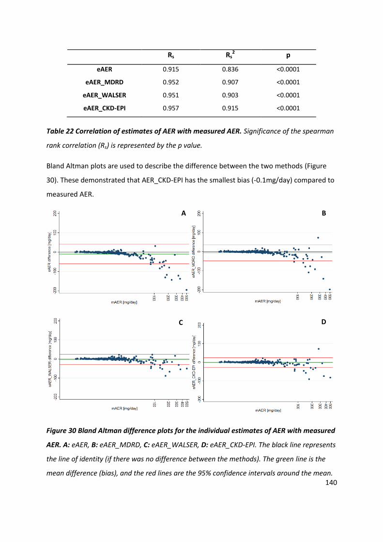
140

Table 22 Correlation of estimates of AER with measured AER. Significance of the spearman

rank correlation (Rs) is represented by the p value.

Bland Altman plots are used to describe the difference between the two methods (Figure

30). These demonstrated that AER_CKD-EPI has the smallest bias (-0.1mg/day) compared to

measured AER.

Figure 30 Bland Altman difference plots for the individual estimates of AER with measured

AER. A: eAER, B: eAER_MDRD, C: eAER_WALSER, D: eAER_CKD-EPI. The black line represents

the line of identity (if there was no difference between the methods). The green line is the

mean difference (bias), and the red lines are the 95% confidence intervals around the mean.

Rs Rs2 p

eAER 0.915 0.836 <0.0001

eAER_MDRD 0.952 0.907 <0.0001

eAER_WALSER 0.951 0.903 <0.0001

eAER_CKD-EPI 0.957 0.915 <0.0001

A= true positives X 100

t

r

u

e

p

o

s

B= true positives X 100

t

r

u

e

p

o

s

C= true positives X 100

t

D= true positives X 100

t

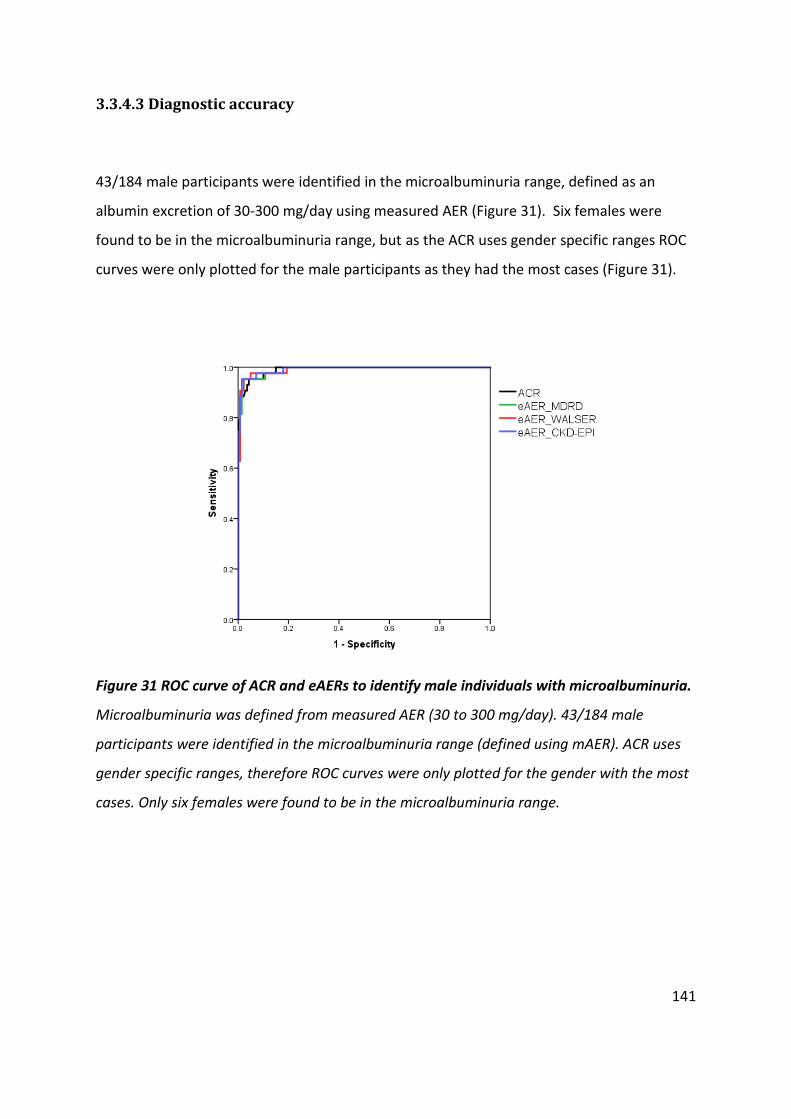
141

3.3.4.3 Diagnostic accuracy

43/184 male participants were identified in the microalbuminuria range, defined as an

albumin excretion of 30-300 mg/day using measured AER (Figure 31). Six females were

found to be in the microalbuminuria range, but as the ACR uses gender specific ranges ROC

curves were only plotted for the male participants as they had the most cases (Figure 31).

Figure 31 ROC curve of ACR and eAERs to identify male individuals with microalbuminuria.

Microalbuminuria was defined from measured AER (30 to 300 mg/day). 43/184 male

participants were identified in the microalbuminuria range (defined using mAER). ACR uses

gender specific ranges, therefore ROC curves were only plotted for the gender with the most

cases. Only six females were found to be in the microalbuminuria range.

142

A summary of the results from the ROC curve analysis are presented in Table 23. Overall

accuracy, the AUC, was similar with all eAERs, though percent correctly diagnosed varied

from 92.5% with eAER to 96.7% with eAER_CKD_EPI.

Sensitivity Specificity AUC % correctly

identified

ACR 80.4%

(66.1 to 90.6)

99.5%

(97.2 to 99.9)

0.99

(0.98 to 1.00) 95.9

eAER 63.0%

(47.6 to 76.8)

99.5%

(97.2 to 99.9)

0.99

(0.97 to 1.00) 92.5

eAER_MDRD 84.8%

(71.1 to 93.6)

98.5%

(95.6 to 99.7)

0.99

(0.98 to 1.00) 95.9

eAER_WALSER 84.8%

(71.1 to 93.6)

99.0%

(96.3 to 99.8)

0.99

(0.98 to 1.00) 96.3

eAER_CKD-EPI 89.1%

(76.4 to 96.3)

98.5%

(95.6 to 99.6)

0.99

(0.99 to 1.00) 96.7

Table 23 Diagnostic accuracy of ACR and estimates of AER to identify male individuals

with microalbuminuria. 43/184 male participants were identified in the microalbuminuria

range, defined using mAER from an overnight urine collection).

143

3.3.5 Discussion

245 participants from the SUMMIT study (Table 20) met the inclusion criteria to be included

in this investigation (Section 3.3.3.1). It is a male dominant cohort (75% males) with a mean

(SD) age of 68 ±10 years. A median eGFR of 77.6 ml/min/1.73m2 is typical for this group of

subjects of this age. 20% had microalbuminuria based on a timed overnight AER.

All methods of reporting urinary albumin excretion had a significant correlation (p<0.001)

with measured AER. Whether estimating AER from an ACR by using a personalised

creatinine excretion rate or by assuming a creatinine excretion rate of 1g/day, there is a

negative bias compared to measured AER. This is demonstrable through the difference

between methods detailed in Table 21, and visualised in the Bland Altman plots in Figure 30.

eAER_CKD-EPI has the smallest bias (-0.1mg/day). The difference in eAER across all the

Bland Altman plots is greater at higher concentrations, this is most likely due to be a

proportional bias, relative to the rate of urinary albumin excretion being measured (Figure

30).

Our findings are very similar to the work of Abdelmalek et al. who reported median

difference of: -2.3, -0.9, -0.8 and -1.0 mg/day when reporting ACR, eAER_MDRD,

eAER_Walser and eAER_CKD-EPI respectively, when compared to measured 24 hour urinary

albumin excretion (Abdelmalek et al., 2014). The study by Abdelmalek et al. included 2,711

community-living individuals from the general population of the Netherlands participating in

the PREVEND (Prevention of Renal and Vascular Endstage Disease) Study. They

demonstrated that there is no superior equation, although CKD and Walser which include

weight may provide a more accurate approximation of muscle mass (Abdelmalek et al.,

2014, Fotheringham et al., 2014).

Estimating creatinine excretion using the CKD-EPI equation has the smallest bias and

strongest correlation among the estimating equations with measured AER, but the margin

of improvement is small. Assessing diagnostic accuracy using the different equation also

144

demonstrates there is no superior equation, supporting the conclusions of others studies

(Abdelmalek et al., 2014, Fotheringham et al., 2014).

Estimating AER using the assumption that CER is 1g/day yielded the lowest diagnostic

sensitivity (63%) to identify microalbuminuria (Table 23). Clinically, it is recognised that

there is a difference in muscle mass between genders; therefore gender specific ranges are

used to identify microalbuminuria when reporting the ACR. There is no difference in AUC

from the ROC curve whether reporting the ACR or estimating AER from an ACR by using a

personalised creatinine excretion rate or by assuming creatinine excretion rate of 1g/day

(Table 23). Diagnostic sensitivity is improved when estimating AER using the personalised

creatinine excretion rates, but with no overall improvement on diagnostic accuracy, its

application in routine diagnostics is unlikely.

The use of estimating creatinine excretion equations that require weight (CKD-EPI and

WALSER) are limited in clinical practice, as that information is not readily available in

pathology laboratories where the results are generated.

The gold standard collection method to assess microalbuminuria is an overnight collection.

Clinically, microalbuminuria needs to be confirmed in at least two collections to make a

diagnosis. A limitation to this study is that only one overnight collection was used to classify

individuals with microalbuminuria. In addition, the ACR was reported from an overnight

collection, when clinically it would only be reported from untimed spot samples.

3.3.6 Conclusion

This work demonstrates that estimating AER using personalised creatinine excretion rates

does not meaningfully improve diagnostic accuracy of an ACR to identify individuals with

microalbuminuria.

Chapter 4 investigates if estimating albumin excretion from a spot sample improves the

accuracy of an ACR to identify individuals with microalbuminuria, classified by measuring

AER from an overnight urine collection.

145

3.4 Validation of a urine specific gravity refractometer

3.4.1 Introduction

A limitation of using creatinine to account for urine concentration is that the amount of

creatinine excreted is variable between individuals. The purpose of estimating an

individual’s creatinine excretion is to overcome this limitation. Urine specific gravity (USG) is

another measure of urinary concentration which can be used to adjust the concentration of

albumin to account for urine concentration. USG is determined by the concentration of

excreted molecules for example inorganic ions such as sodium, potassium, chloride,

magnesium, calcium, ammonium, sulphates, and phosphates. USG is measured as the ratio

of urine density compared with water density, where in adults the normal USG range is from

1.003 to 1.030 (Fischblach, 2004).

Using USG to normalise urinary albumin concentration is not a novel approach, and previous

studies have evaluated USG’s clinical application (Parikh et al., 2002, Moore et al., 1997,

Newman et al., 2000). USG has shown a positive correlation with urinary creatinine

concentration in both the general population (n=50) (r = 0.79, P <0.001) (Moore et al.,

1997) and in individuals with diabetes (n = 34) (r = 0.83, p < 0.001) (Parikh et al., 2002). In

1997, Moore and colleagues investigated the use of USG on diagnostic accuracy to identify

individuals with microalbuminuria in a diabetic population. When using the routine

laboratory method to measure albumin, the sensitivity and specificity when reporting ACR

was 89% and 93% respectively, and when using USG instead of creatinine it was 88% and

93% (Moore et al., 1997). They also reported USG in conjunction with an albumin result

from a urine dipstick test (Micral-Test by Roche). The Micral-Test is a cheap alternative to an

ACR and results are determined a lot quicker. An increase in diagnostic sensitivity from 63%

to 69% was reported when accounting for USG, however there was a loss in specificity (from

100% to 80%) (Moore et al., 1997). Although USG and urinary creatinine concentration have

146

shown good correlation, USG does not improve on what is currently achieved reporting

urinary creatinine, therefore it hasn’t been taken forward clinically.

The studies which have investigated the clinical application of USG have done so in the

clinical ranges of microalbuminuria and macroalbuminuria. One of the aims of this thesis is

to establish an accurate and robust method of reporting albuminuria within the normal

range of urinary albumin excretion. Before evaluating the use of USG to normalise low

urinary albumin concentrations, the device measuring USG must undergo validation to

ensure the results are accurate and reproducible. USG is the ratio of urine density to water

which can be determined using refractometry. The higher the urine concentration, the

higher urine density and therefore light is refracted more. Digital urine specific gravity

refractometers are available and in this work the commercially available USG-α (ATAGO)

refractometer (ATAGO Ltd., Tokyo, Japan) undergoes validation.

Upon satisfactory validation results, the digital refractometer can be utilised in future work

investigating its ability to adjust albumin to account for urinary concentration.

3.4.2 Aim

Validate the USG-α refractometer as a measure of USG to reflect urine concentration.

3.4.2.1 Objectives

1. Determine intra-assay reproducibility of USG-α refractometer.

2. Determine inter-assay reproducibility of USG-α refractometer.

3. Determine the correlation of USG with urine creatinine concentration as assessed by

the Jaffe method.

147

3.4.3 Method

Objective 1:

Intra-assay reproducibility was determined by 10 repeat measurements of four urine

samples, all analysed on the same day. The CV was calculated as previously described at

Chapter 2.3.3.

Objective 2:

Inter-assay reproducibility was determined by analysing four urine samples on seven

consecutive days by the same operator. Samples were stored in a fridge at 4oC throughout

the testing period. Samples returned to room temperature prior to analysis

Objective 3:

33 clinical samples were selected to assess the correlation between USG measured by USG-

α refractometer with urine creatinine concentration.

USG was measured by the USG-α refractometer (ATAGO Ltd., Tokyo, Japan) and urinary

creatinine quantified by the routine ‘Roche Creatinine Jaffé Gen.2’ method (Roche

Diagnostics Ltd., Burgess Hill, UK).

3.4.3.1 Statistics

Normality of the data was tested using the Shapiro-Wilk test. Associations with non-

normally distributed data are examined using the Spearman’s rank correlation test.

148

3.4.3.2 Sample analysis

Urine samples used in the validation experiments were patient samples sent to the RD&E

Blood Science laboratory for routine ACR measurement. Samples were not stored prior to

analysis, with the test usually complete within 24 hours of sample collection. The samples

were selected depending on their creatinine concentration to ensure a wide range was

tested. Samples underwent four hand inversions prior to creatinine and USG analysis,

measured by the USG- α refractometer.

To evaluate the relationship between the USG- α results and creatinine, scatter plots were

created with spearman’s rank correlation (Rs) reported along with the significance (p) of the

correlation.

3.4.4 Results

Intra-assay reproducibility determined on four urine samples by analysing them 10 times in

the same day ranged from 0.25 to 3.03% (Table 24). Inter-assay reproducibility for USG-α

ranged from 2.05 to 14.37% (Table 25). USG measured by the USG-α refractometer and

urinary creatinine were significantly associated (Rs= 0.95, p=<0.001) (Figure 32).

Sample Mean USG

[refraction ratio] St Dev CV%

Urine 1 1.0022 0.00006 3.03

Urine 2 1.0088 0.00009 1.04

Urine 3 1.0235 0.00016 0.67

Urine 4 1.0284 0.00007 0.25

Table 24 Intra-assay reproducibility of USG-α to measure USG in four urine samples. All

samples were measure ten times in the same assay by the same operator.

149

Sample Mean USG

[refraction ratio] St Dev CV%

Urine 1 1.0026 0.00040 14.37

Urine 2 1.0094 0.00048 5.57

Urine 3 1.0241 0.00044 2.05

Urine 4 1.0287 0.00059 2.34

Table 25 Inter-assay reproducibility of USG-α. USG was measured by USG-α refractometer

in four urine samples. All samples were measured once a day, over seven days by the same

operator.

Figure 32 Correlation between USG measured by USG-α refractometer and urinary

creatinine. 33 samples had USG determined by USG-α refractometer and urinary creatinine

quantified by the routine ‘Roche Creatinine Jaffé Gen.2’ method. The solid line represents the

line of best fit through the data. (Rs= 0.95, p=<0.001)

1.0

1

1.0

2

1.0

3

1.0

4

1.0

0

1.0

0 U

SG

[d

egre

e o

f re

fraction c

om

pare

d to w

ate

r]

0 10 20 30 40 Creatinine concentration [mmol/L]

150

3.4.5 Discussion

Previous studies have demonstrated a strong relationship between USG and urinary

creatinine concentration in the general population (n=50, r = 0.79, P <0.001) (Moore et al.,

1997) and in the individuals with diabetes (n = 34, r = 0.83, p < 0.001) (Parikh et al., 2002). In

the SUMMIT cohort a stronger correlation between USG and creatinine was determined

(Rs= 0.95, p=<0.001). This may be attributed to the differences between cohorts, where

diversity in the general population may influence this relationship.

There has been no previous evidence that diagnostic accuracy is improved when using USG

to adjust urinary albumin concentration in untimed spot samples to identify individuals with

microalbuminuria or macroalbuminuria (Moore et al., 1997). The results from the SUMMIT

cohort support this, however, ACR was not measured in spot samples, but rather from an

overnight collection.

The aim of this work was to validate the USG-α refractometer (ATAGO Ltd., Tokyo, Japan) to

measure USG. Upon successful validation, the device can then be used in future studies

which evaluate its application for adjusting low levels of urinary albumin excretion in

untimed spot samples.

The USG-α refractometer results were very reproducible, but offered no improvement over

using the Jaffe method to measure creatinine. The highest intra-assay CV reporting USG was

3.03% when repeat measuring four urine samples ten times on the same day (Table 24). The

mean (SD) of the CV for the Jaffe method was 1.67 ±1.04 % (Section 3.2).

When measuring USG, the highest intra-assay CV was identified when measuring the sample

with the lowest USG (1.0022 refraction ratio). The inter-assay CV of the same sample was

14.37%. However, in samples with a higher USG the typically day to day variation was less

than 6% (Table 25). The higher inter-assay variability can most likely be attributed to the

test being carried out manually. This is a limitation of USG testing using a manual method,

whereas quantifying creatinine using a high throughput analyser yielded lower inter-assay

151

variation (maximum CV of 2.35%, creatinine concentration 6.78mmol/L) when measured by

the routine Jaffe method (Table 19).

USG-α is strongly associated with urinary creatinine concentration (n=33, Rs= 0.95,

p=<0.001), confirming that both are markers of urinary concentration. There is less

agreement in the results with very low creatinine concentration where USG

disproportionately increases with an increase in creatinine concentration. At the highest

creatinine concentration it appears USG-α has reached its measurable limit as USG does not

increase with increasing creatinine concentration and with so few samples at this high

concentration further investigation is warranted. The manufacturer advises that USG-α can

accurately measure up to 1.0600, so further validation would be required if this was to be

used on clinical samples. This demonstrates the importance of carrying out in house

validation.

The USG-α refractometer is an acceptable method to measure USG as a marker of urinary

concentration. However, it is less precise and may be less accurate in samples with the

lowest and highest USG. In this validation work, USG has been compared to urinary

creatinine concentration as an indicator of how concentrated the urine is. As CER varies

between people, it is not the ideal reference method but it is the clinical standard. USG is a

measure of the concentration of excreted molecules and just like creatinine it may be highly

variable between individuals.

In this work USG and creatinine were quantified on fresh samples. This is consistent with

routine clinical analysis; however, research studies often freeze samples prior to analysis. A

limitation of this study was that the impact of freezing on USG prior to analysis was not

investigated. The impact of storage and freezing on urinary albumin and urinary creatinine

are evaluated in Chapter 5.

The work in the present chapter shows that USG-α (ATAGO Ltd., Tokyo, Japan) has a strong

agreement with urinary creatinine concentration, and can be taken forward in other studies

(Chapter 4) to evaluate if an albumin to USG ratio can improve the relationship of a spot

sample (when reporting ACR) with the ‘gold standard’ overnight AER.

152

3.5 Summary and conclusions

This chapter has investigated different methods of accounting for the variation in urinary

concentration, which affects the concentration of albumin in untimed samples.

Traditionally, the ACR is used to report albuminuria in spot samples. The first study

compared two methods of measuring urinary creatinine to ensure the most accurate and

reproducible method is used in future studies. There was a very strong agreement between

the two methods and they were both highly reproducible. The enzymatic assay had a

slightly lower CV%, and had a small proportional bias (0.52 ± 3.08 %) compared to the Jaffe

method. Overall, there is little improvement when using the more expensive enzymatic

assay over the routinely used Jaffe method and therefore the Jaffe method will be used in

future studies in this thesis.

The second investigation validated equations that estimate creatinine excretion. These

equations consider the limitation that creatinine excretion is highly variable between

individuals, which impacts on the ability of ACR to normalise albumin concentration in

untimed samples. The results showed a high correlation with mAER, but offered no

improvement on diagnostic accuracy compared to reporting ACR alone. Further work is

required to determine if estimating AER in random spot samples improves the relationship

of an ACR with timed collections and if diagnostic accuracy is improved.

USG is another measure of urinary concentration and it can be tested by refractometry. The

USG-α refractometer (ATAGO Ltd., Tokyo, Japan) had a strong correlation with urinary

creatinine concentration and was reproducible. USG-α can be used in other studies as a

measure of urinary concentration and its use will be evaluated when investigating different

methods of reporting albumin excretion in the low albuminuria range.

153

Chapter 4 Urine Collection Methods to Assess the Excretion of

Albumin in the Normal Range

An AER from an overnight urine collection is considered the “gold standard” for assessing

albuminuria (Mogensen et al., 1985, Mogensen, 2003). However, timed collections are

burdensome for patients, who can be prone to making mistakes, which can lead to

inaccurate results. It is clinically preferred to use untimed spot urine samples to measure

the ACR (National Kidney Foundation, 2002).

The aim of this chapter is to identify what time is best to collect a spot sample which

provides an appropriate surrogate for a timed overnight collection. To achieve this;

reproducibility (biological variability) of albumin excretion is determined in different urine

collection methods, and the correlations of spot samples with the ‘gold standard’ method

are evaluated.

In using the validated Fitzgerald ELISA to quantify urinary albumin (described in Chapter 2),

the extended normal albumin excretion range can be fully investigated, and the biological

variation of albumin excretion in healthy individuals can be determined.

Estimating albumin excretion from an ACR in spot samples by using a personalised

creatinine excretion rate was discussed in Chapter 3.3. The relationship of estimating AER

from an ACR from a spot sample with an overnight AER is also investigated in this chapter,

along with its diagnostic accuracy to identify individuals with microalbuminuria.

To fully investigate the relationships between spot samples and timed overnight collections,

this chapter consists of two different studies, the results of the first study instigating the

aims of the second study.

Investigation 1: The Optimal Urine Collection Method to Assess the Excretion of

Albumin in the normal range

Investigation 2: The relationship of estimating AER from an untimed spot using a

personalised creatinine excretion rate with an overnight AER

154

The Optimal Urine Collection Method to Assess the Excretion of

Albumin in the normal range

4.1 Introduction

4.1.1 The “gold standard” collection method to diagnose microalbuminuria

When microalbuminuria was first defined it was recommended that three timed overnight

or short-term at hospital samples, collected within a few months of each other, were

required to diagnose microalbuminuria (Mogensen, 1987). However, the majority of studies

which have investigated urine collection methods have utilised a 24 hour collection as the

“gold standard” collection.

A 24 hour collection has been the long standing “gold standard” to assess proteinuria, and

therefore it may be assumed to be the “gold standard” to assess albuminuria. It has been

proposed that albumin excretion follows a circadian rhythm (Mogensen et al., 1985, Hansen

et al., 2002, Capani et al., 1988), therefore 24 hour collections may be desirable as they

incorporate diurnal variations. Several studies have shown AER to be 30-50% higher over a

24 hour period compared to overnight in patients with diabetes (Mogensen et al., 1995a),

but these studies are limited to the higher clinical levels of albumin excretion.

The reason for lower AER overnight is most likely the result of decreased activity/exercise

(Climie et al., 2015, Heathcote et al., 2009, Koh et al., 2011), lower blood pressure and GFR

(Mogensen et al., 1995a, Miller et al., 2003) and a recumbent posture (Montagna et al.,

1983). Because these factors that raise AER have less impact during the night, it is

conceivable that the overnight collection is more reproducible than a 24 hour collection.

When the discrimination value for microalbuminuria was determined, three studies were

evaluated, each using a different collection method. The proposed discrimination values

when using timed overnight (Viberti et al., 1982), short term at hospital (Mogensen and

155

Christensen, 1984) and 24 hour collections (Mathiesen et al., 1984) were 30µg/min,

15µg/min and 70µg/min respectively (table 1.3). The higher discrimination value for

microalbuminuria found using 24 hour collections is most likely the result of higher AER

during the day. However, the microalbuminuria threshold was set at 20µg/min, determined

from the values proposed using timed overnight and short term in hospital collections;

these collections were also appointed the “gold standard” methods to collect urine

(Mogensen, 1987). Therefore, this study will use a timed overnight collection as the “gold

standard” method to assess albumin excretion.

In order to diagnose microalbuminuria, urine collections need to be repeated to reduce the

influence of intra-individual biological variation and to exclude any other interfering factors,

such as sexual intercourse (Sadri-Ardekani et al., 2009), exercise (Climie et al., 2015,

Heathcote et al., 2009, Koh et al., 2011), fever, urinary tract infections and poor glycaemic

control, which have all been shown to falsely elevate AER (Mogensen et al., 1995b). It is

important to be aware of these interfering factors so they can be limited when designing a

study that evaluates the variation of different collection methods.

4.1.2 Using spot samples to assess albumin excretion

Timed collections are burdensome for patients, who can be prone to making mistakes,

which can lead to inaccurate results. This is reflected in several studies that have reported

that up to 31% of non-hospitalised timed samples are incomplete (Garde et al., 2004,

Sampaio and Delfino, 2008). Therefore, it is clinically preferred to use untimed spot urine

samples to measure the ACR (National Kidney Foundation, 2002). There are three main

types of untimed spot samples, each characterised by the time of the collection; first

morning void (FMV), second morning void (SMV) and random.

Current guidelines now recommend the use of spot samples for microalbuminuria

screening. If microalbuminuria is present in two of three samples, which are collected within

156

a three to six month period, then a diagnosis can be made (American-Diabetes-Association,

2013).

A survey of 2,178 general practitioner (GP) surgeries across eight European countries was

carried out in 2006 (Aakre et al., 2008). The survey revealed that the majority (>70%) of

them used spot samples (unspecified) to initially screen for microalbuminuria, although

when repeat testing, they saw an increase in the use of timed collections. This suggests that

GPs consider timed collections to be more accurate than spot samples, which is

questionable given the increased risk of errors arising from the timed collection procedure.

One surprising finding from the survey was that 55% of GPs in the Netherlands only used

one result to diagnose microalbuminuria, which not only reflects the discordance with

international guidelines but also the need for education in this area.

To investigate which collection method is more reproducible for monitoring albuminuria

over time, a coefficient of variation (CV) can be calculated from repeat collections. A study

of 241 participants from the PREVEND cohort (predominately without DM), carried out

three 24 hour, FMV and random collections over three weeks (Witte et al., 2009). The CV of

the collections were 19.0%, 19.1% and 35.8% respectively, revealing that only the FMV CV

did not significantly differ from the 24 hour AER (p=0.64). The study also assessed the

accuracy of the FMV and random samples with the 24 hour collection, reporting that when

using the FMV ACR, 81.8% of participants were classified in the same category as when

using the 24 hour AER. This fell to 72.1% when using the random sample ACR. The

correlation (r2) of FMV and random samples to the 24 hour collection were 0.87 and 0.83

respectively. This indicates that ACR from a FMV would be preferable over an ACR in a

random sample to assess albuminuria.

It is logical that a FMV is more reproducible and accurate than a random sample, as factors

which may affect albumin excretion are at their least influential overnight. Another

potential contributor to explain the better reproducibility observed with FMVs compared

to random samples is that the low levels of water intake overnight usually results in more

concentrated urine, which allows easier detection of albumin by traditional assays. Other

spot collections later in the day (e.g. SMV) have not been readily investigated as they are

157

often more dilute than FMV samples and traditional assays are unable to measure at the

lower albumin concentrations. Using a more sensitive assay, alternative samples like SMV,

can now be investigated.

Although more dilute, it is well reported that spot urine samples collected throughout the

day provide higher ACR values than the FMV (Witte et al., 2009, Mogensen et al., 1995b,

Howey et al., 1987). This has been attributed to diurnal variations in AER, which may be

related to changes in posture or exercise (Hortin, 2013). A cross-sectional study of 5,247

participants in the U.S., investigated the difference between paired random and FMV

samples (Saydah et al., 2013). At the microalbuminuria threshold (an ACR of 30mg/g) they

reported that ACR from random samples were 50% higher than ACR from FMVs. The 95th

percentile in FMV samples was 28.2 mg/g compared to 46.5mg/g in the random samples.

When reviewing this study, another author, Hortin, commented that there were differences

in the shipping and handling of the different samples, which may have contributed to a

slight lowering in albumin concentration in FMV samples. Random samples were analysed

on the day of collection, whereas the FMV samples were posted, although albumin and

creatinine are considered stable for a week under those conditions (Hortin, 2013).

However, high ACR values in random samples may be clinically preferred over FMV samples

for microalbuminuria screening, as random samples have a higher diagnostic sensitivity

(fewer false negative results). Random samples are also more practical, as patients can

produce a sample whilst at their GP and are not required to make a repeat visit. The lower

diagnostic specificity can be resolved by confirming microalbuminuria through repeat

testing the ACR in FMV samples, which is necessary to make a diagnosis due to the

variability of albumin excretion. Measuring an ACR in a random sample to screen for

microalbuminuria and using an ACR in several FMV samples for confirmation is now

reflected in the international ‘Kidney Disease Improving Global Outcomes’ guidelines

(KDIGO, 2013).

158

4.1.3 Reporting albuminuria in spot samples

There are several different methods of reporting albumin excretion in spot samples,

including as urinary albumin concentration (UAC) and adjusting for hydration levels using

creatinine concentration (albumin to creatinine ratio) (ACR), or using personalised

estimated creatinine excretion (eAER) or urine specific gravity (A/USG).

Some authors argue that UAC should be measured alone, as reporting the ACR in untimed

samples introduces a second biological factor (creatinine) which increases variability

(Townsend, 1986b). A study in 2011 reported that FMV ACR correlated better with a 24

hour AER compared to a random ACR (r: 0.80 vs 0.62 respectively). Interestingly, in both the

FMV and random samples, the correlation improved when the results were reported as

UAC ( r= 0.94 and 0.92 respectively) (Chavan et al., 2011). The authors, therefore, suggested

that screening for microalbuminuria should be carried out using UAC in FMV samples.

However, this study was carried out on 104 T2DM patients who had a median 24 hour AER

of 328 mg/24 hours, which is suggestive of macroalbuminuria. In fact, the lowest AER in the

study was 90 mg/24 hours, which is three times higher than the lower microalbuminuria

threshold. This invalidates their conclusion that UAC should be used for microalbuminuria

screening, as the lower microalbuminuria threshold was not investigated, although it may

be applicable to identify macroalbuminuria.

Furthermore, an epidemiologic study of 4,678 participants across four countries (Dyer et al.,

2004), found slightly lower mean intra-individual CVs using UAC compared to ACR in men

(59.6% vs 62.0% respectively) and women (57.7% vs 60.8% respectively). The variation of 24

hour AER was 61.7% and 60.2% in men and women respectively. However, there are factors

in their methodology that may contribute to this high variability. Firstly, samples were

stored at -20oC for approximately three years before analysis. There is increasing evidence

that long term storage at -20oC results in falsely low UAC (Elving et al., 1989, Brinkman et al.,

2005, Erman et al., 1988, Schultz et al., 2000). It appears that the loss of UAC may not be

universal, with one study reporting only 28% of their samples were impacted (Kania et al.,

2010), which could have ramifications on the variability of UAC in repeat collections when

159

samples have been stored at -200C. Another considerable limitation of this epidemiologic

study was that only two 24 hour samples were collected and no spot samples, so they used

the 24 hour samples to determine 24 hour AER, ACR and UAC. Therefore no conclusion

should be made regarding the variation of ACR or UAC in a spot sample as no additional spot

samples were collected. (Gansevoort et al., 2006). Importantly, it is inaccurate to calculate a

SD from just two repeat measurements and therefore the CV is unreliable which may

explain why their results were so high.

From this it can be concluded that for studies examining the variation of collection methods,

it is important to repeat collections at least three times within a short time period, and if

urine samples can’t be analysed when they are fresh, then storage at -80oC is preferable

(storage conditions are discussed and investigated in Chapter 5).

Gender specific reference ranges to identify microalbuminuria acknowledge that a limitation

of using creatinine to adjust urinary albumin concentration is that creatinine excretion

varies. Gender specific range may be sufficient to account for this limitation when clinically

interpreting ACR results, but there are alternative methods to calculate personalised

creatinine excretion, which may provide a more accurate assessment of an individual’s

urinary albumin excretion. This will be explored in this chapter at the extended lower

albumin excretion range.

Another measure of urinary concentration is urine specific gravity. Therefore UAC can be

adjusted for dilution using USG (A/USG), which is another method of reporting albuminuria.

There are very few studies which have looked at using A/USG (Newman et al., 2000,

Fagerstrom et al., 2015, Moore et al., 1997), and there are none that have investigated its

use in different spot samples when comparing to an overnight AER.

My study will therefore, not only investigate which spot sample (FMV, SMV or random) is

best suited to replace a timed overnight collection, it also determines the best method of

reporting albuminuria within those spot samples: UAC, ACR, eAER or A/USG.

160

4.2 Aim

To identify which spot sample (FMV, SMV or random) and which method of reporting

albumin excretion (UAC, ACR, A/USG or eAER) is the best surrogate marker of a timed

overnight urine collection, when investigating the extended normal albumin excretion

range.

4.2.1 Objectives

1. To determine albumin excretion levels by different collection methods and by

different methods of reporting albumin excretion. In healthy individuals using an

ELISA to quantify urinary albumin with a validated measurable range of 0.78 – 40

mg/L.

2. To assess the intra-participant reproducibility of different collection methods and

different methods of reporting albumin excretion.

3. To assess the inter-individual variation of different collection methods and different

measures of albumin excretion.

4. To assess which spot collection method and method of reporting albumin excretion

(UAC, ACR and A/USG) correlates best to an overnight albumin excretion rate.

5. To investigate if the correlation of a spot sample with an overnight albumin

excretion rate can be improved by estimating AER.

161

4.3 Method

4.3.1 Study design

4.3.1.1 Participant recruitment

17 healthy adults (aged 21-50 years old) were recruited from the Exeter 10,000 bio-resource

of individuals interested in hearing about research, held by the NIHR Exeter Clinical

Research Facility.

The exclusion criteria for the study was; an eGFR < 60ml/min/1.73m2 an ACR above the

normoalbuminuria range, diagnosed with diabetes, cardiovascular disease, hypertension or

were on antihypertensive medication.

4.3.1.2 Study protocol

The study protocol was reviewed and approved by the South West Regional Ethics

Committee (REC Reference: 14SW0049). Written informed consent was obtained from all

participants, who then attended a screening visit, where anthropometric measurements

(height and weight) were taken along with collecting a blood and random urine sample.

Participants were not fasted, and had a normal breakfast prior to providing samples. The

blood sample was used to measure serum creatinine; to determine if eGFR meets the

inclusion criteria for the study (Section 4.3.1.1). ACR was reported from the urine sample to

ensure the participant met the study criteria to have a normal albumin excretion rate

(Section 4.3.1.1).

162

Blood and Blood pressure was measured five times in the non-dominant arm using a digital

blood pressure monitor; with the mean of the last three measurements representing

brachial blood pressure.

4.3.1.3 Study method

Each participant collected their urine over a 36 hour period on three separate occasions.

During recruitment and screening, all participants received detailed written, drawn and oral

instructions about the procedure for collecting the urine samples. The patient information

sheet that set out these details is provided at appendix 4 and is outlined in Table 26. In

summary, each participant received five numbered containers.

Firstly, they would provide a mid-stream FMV sample into container one (C1). Then they

started a timed day collection where they would collect every pass of urine throughout the

day and evening, up to and including the final void before going to bed, into container two

(C2). Then the timed overnight collection began, in which they passed all urine into

container three (C3), including the first pass of urine in the morning recording the times of

the start and finish of the collection on the bottle. Then they would collect a mid-stream

sample in container four (C4) the next time they voided urine (SMV). Finally, they were free

to provide a random mid-stream sample in container five (C5) whenever they desired (as

long as it was before 17:00 that day).

Samples were stored in a refrigerator or kept in a cool place until bringing them into the

research centre on the same day the collection was completed. Each participant carried out

the collection procedure three times, with an aim to complete all the collections within a

month.

163

Container Number Sample Type Measures of Albuminuria

C1 FMV UAC, ACR, A/USG & eAER

C2 Timed Day AER } combined for 24 Hr AER C3 Timed Night AER

C4 SMV UAC, ACR, A/USG & eAER

C5 RDM UAC, ACR, A/USG & eAER

Table 26 The containers used to collect different urine samples. Different measures of

albumin excretion for each sample type are presented. An AER is calculated for each timed

collection. A sample from both timed collections are combined together to represent a 24

hour collection. The volume of the samples added are proportional to the volumes of the

two timed collections. Each participant collected samples according to this procedure three

times. AER: albumin excretion rate, UAC: urinary albumin, ACR: albumin to creatinine ratio,

A/USG: Albumin to specific gravity ratio, eAER: estimated albumin excretion rate.

Participants were asked to avoid exercise and sexual intercourse, which can affect albumin

excretion, the evening before and during the collection period. All participants were advised

not to collect if they were ill for any reason and women were advised to avoiding collecting

whilst menstruating. When samples were received, participants were questioned about

their activities prior to and during the collection, to determine compliance with the

protocol. 2/51 collections were repeated due to exercise undertaken and one collection was

repeated due to an incomplete timed overnight sample.

164

4.3.2 Sample Processing

Timed collections were weighed to determine volume and the durations were recorded. All

samples underwent dipstick analysis (COBAS Combur-Test strips87) (Roche Diagnostics Ltd.,

Burgess Hill, UK) and were then aliquoted into several microtubes and immediately stored

at -80oC.

An AER is calculated for each timed collection. A sample from both timed collections are

combined together to represent a 24 hour collection. The volume of the samples added is

proportional to the volumes of the two timed collections. From this combined sample a 24

hour AER can be determined.

Sample analysis was carried out after all collections were complete. Prior to analysis, the

samples were left to return to room temperature and then underwent five hand inversions

to gently mix the contents. Urinary and blood creatinine was measured using the COBAS

Jaffe method (Roche Diagnostics Ltd., Burgess Hill, UK). USG was determined using a digital

refractometer (ATAGO Ltd., Tokyo, Japan). Urinary albumin was quantified by the Fitzgerald

ELISA (Fitzgerald Industries International, North Acton, MA, USA). For each participant, all

the urine samples (from all three collections) were analysed on the same ELISA plate, to

eliminate the impact of inter-plate variation on intra-individual reproducibility results.

ELISA analyses were carried out using an automated platform, a ‘Dynex DS2’ (Dynex

Technologies, VA, USA).

165

4.3.3 Statistical analysis

Sample size:

From the literature review, the reported correlations between ACR and 24 hour AER have an

r value > 0.7 (Witte et al., 2009, Chavan et al., 2011). To detect a correlation of r=>0.7, a

sample size of n=17 will give 90% power at p=0.05. (Machin et al., 2009).

Normality of data was tested using the Shapiro-Wilkes test. If data were not normally

distributed, associations were examined using the Spearman’s rank correlation test.

Normally distributed data are presented as mean (±SD) and non-normally distributed data

as the median [IQR].

Wilcoxon signed-rank test is used to test if the difference in albumin excretion is

significantly different in different collections and by different methods of reporting albumin

excretion.

For each spot collection the correlation of UAC, ACR and A/USG with overnight AER is

reported using Spearman’s rank correlation test.

Estimating AER was carried out using the MDRD, CKD and WALSER equations. eAERs and

A/USG were calculated as previously described (Chapter 3 Section 3.3).

The coefficient of variation, diagnostic sensitivity and specificity were also calculated as

previously described (Chapter 2 Section 2.3.9). For each collection method, each

participant’s CV was calculated from three repeated collections and then the median values

among participants are used to summarise intra-participant variability.

Inter-individual variability was demonstrated by calculating the CV for each collection

method between all the participants.

166

4.4 Results

Seventeen participants met the inclusion criteria (Section 4.3.1.1) and completed the three

study visits. The characteristics of this cohort are summarised in Table 27.

4.4.1 Participant characteristics:

Characteristic n=17

Age (years) 34 [22-47]

% male 47%

Weight (kg) 75.1 (15.9)

BMI (kg/m2) 24.3 [23.0 - 25.3]

Blood Creatinine (mmol/L) 76.94 (16.5)

eGFR (ml/min) 101.3 (15.6)

Systolic BP (mmHg) 116 (12)

Diastolic BP (mmHg) 72 (9)

Table 27 Characteristics of the study participants. Data presented as mean (SD) or median

[IQR] depending on normality of data. Seventeen participants met the inclusion criteria

(Section 4.3.1.1) and completed the three study visits.

4.4.2 Objective 1: To determine albumin excretion levels by different collection

methods and by different methods of reporting

Albumin excretion by different collection methods are summarised in Table 28. The unit of

AER for the 24 hour collection is µg/min, enabling an easier comparison to be made with the

other timed collections. AER is significantly lower overnight than during the day (p=0.0005).

This is also demonstrated by the spot samples, where ACR from a FMV is lower than ACR

from the SMV (p=0.005) and a random spot sample (p=0.005) collected later in the day.

Consequently, when estimating AER in spot samples, an eAER from a FMV is more

representative of an overnight AER and an eAER from a random sample is more comparable

to a timed day or 24 hour AER.

167

Table 28 Median albumin excretion levels by different urine collection methods. The median values [IQR] among 17 healthy individuals are

reported. For each participant the mean of three collections was calculated. . AER is significantly lower overnight than during the day (p<0.001).

There is no significant difference in UAC between FMV and SMV samples (p=0.650), FMV and random samples (p=0.068), and SMV and

random samples (p=0.076). When taking urinary concentration into account; FMV ACR is significantly lower than ACR from the SMV (p=0.005)

and a random spot sample (p=0.005) collected later in the day. AER: albumin excretion rate, ACR: albumin to creatinine ratio, eAER: estimated

albumin excretion rate, UAC: urinary albumin concentration.

Collection Method AER µg/min

Timed:

24 Hour 4.11 [2.48 - 5.76]

Timed Overnight 3.23 [1.20 - 3.96]

Timed Day 4.51 [2.74 - 6.92]

Spot: UAC mg/L

ACR mg/g

eAER MDRD µg/min

eAER CKD µg/min

eAER WALSER µg/min

First Morning 4.17 [1.97 – 7.99] 3.10 [2.30 - 4.51] 3.02 [2.01 – 5.22] 2.97 [2.25 – 5.08] 3.25 [3.36 - 5.88]

Second Morning 3.84 [1.81 – 8.13] 4.78 [2.83 - 6.55] 4.12 [3.22 – 6.01] 5.47 [3.08 – 6.74] 5.63 [3.24 – 7.37]

Random 1.92 [1.18 – 3.99] 4.78 [2.83 - 7.17] 5.35 [2.97 – 8.29] 4.67[3.34 – 7.34] 5.06 [3.77 – 7.11]

168

4.4.3 Objective 2: To assess the intra-participant reproducibility of different

collection methods and different methods of reporting albumin excretion.

17 healthy participants collected their urine by different methods, three times. The mean

period (±SD) to complete all three collections was 26.8 days (±12.3). To determine intra-

individual reproducibility, the CV was calculated for each collection method and for the

different methods of reporting albuminuria (Table 29 and Figure 33).

Collection Method Method of reporting

albumin excretion

Median

CV%

Min

CV%

Max

CV%

24 Hour AER 14.4 [8-30] 5.2 53.5

Overnight AER 15.4 [9-44] 2.4 58.9

Timed Day AER 17.8 [14-34] 1.5 73.6

First Morning UAC 26.8 [23-50] 2.9 162.3

Second morning UAC 42.1 [27-75] 15.2 128.5

Random UAC 60.8 [42-74] 8.0 163.5

First Morning ACR 15.9 [12-22] 2.7 157.9

Second morning ACR 22.1 [6-39] 2.1 126.8

Random ACR 22.6 [16-39] 4.2 167.4

First Morning A/USG 22.7 [18 - 28] 7.9 160.0

Second morning A/USG 28.2 [16 - 53] 3.0 126.2

Random A/USG 26.0 [16 - 50] 11.4 168.7

Table 29 The median intra-individual reproducibility of different urine collection methods

to assess albuminuria. The coefficient of variation was calculated from repeating the

collections three times by 17 participants. The median CV [IQR] is reported. Among the spot

collections; CV was only significantly improved when reporting UAC from FMV compared to

reporting UAC from random spot samples (p=0.02). AER: albumin excretion rate, ACR:

169

albumin to creatinine ratio, UAC: urinary albumin concentration, A/USG: albumin to urine

specific gravity ratio.

As this study is examining variation, all results were included in this analysis. Among the

spot samples, the FMV ACR has the lowest median CV, although one participant had the

maximum CV of 157.9%. Interestingly, dipstick analysis revealed that there was

haemoglobin in one of the FMV samples from this individual, which may have interfered

with the albumin assay, causing a falsely high result. Reproducibility is poorer (CV is higher)

when reporting UAC or A/USG in spot samples compared to the ACR.

The box and whisker plot in Figure 33 also presents intra-individual variation for the

different collection methods (only spot sample ACR CV is presented). The intra-individual CV

of UAC, ACR and A/USG in the different spot samples are presented in Figure 34.

When investigating the largest outliers across the spot collections, blood in a FMV sample

has already been identified as a potential cause of analytical error. In the SMV sample which

had the highest CV, the abnormality might have been the result of the urine being very

concentrated (creatinine = 21.6 mmol/L) subsequently causing a very high albumin

concentration of 189 mg/L.

Dipstick analysis in the highest outlying random sample indicated the presence of

leucocytes, which could suggest that the participant was experiencing an inflammatory

challenge, resulting in increased albumin excretion. These potential causes for the outlying

results are common issues when collecting samples to assess albumin excretion.

170

Figure 33 Box and whisker plots of intra-individual reproducibility of different collection

methods. The coefficient of variation was calculated from repeating the collections three

times by 17 participants. The horizontal line inside the box represents the median, the edges

of the box are the upper and lower interquartile and the whiskers represent the minimum

and maximum values, with outlying (●) results individually plotted. AER: albumin excretion

rate, ACR: albumin to creatinine ratio, FMV: first morning void, SMV; second morning void,

RND: random spot sample.

0

50

1

00

1

50

2

00

C

V %

24 Hour AER Timed Overnight AER Timed Day AER

FMV ACR SMV ACR RND ACR

171

Figure 34 The intra-individual reproducibility of different methods of reporting albumin

excretion in spot samples. The coefficient of variation was calculated from repeating the

collections three times by 17 participants. Among the spot collections; CV was only

significantly improved when reporting UAC from FMV compared to reporting UAC from

random spot samples (p=0.02).The horizontal line inside the box represents the median, the

edges of the box are the upper and lower interquartile and the whiskers represent the

minimum and maximum values, with outlying (●) results individually plotted. UAC: urinary

albumin concentration, ACR: albumin to creatinine ratio, A/USG: albumin to urine specific

gravity ratio, FMV: first morning void, SMV; second morning void, CV coefficient of variation.

FMV SMV Random 0

5

0

10

0

15

0

20

0

CV

%

UAC ACR A/USG

172

4.4.4 Objective 3: To assess the inter-individual variation of different collection

methods and different measures of albumin excretion.

Inter-individual variation was investigated by taking the result from each participant’s first

collection, so the CV between participants could be calculated. The reason for taking just

the first collection result is that it reflects what would be carried out clinically, when

screening for microalbuminuria. The variation between people is less in a timed overnight

collection compared to a timed day collection, which is to be expected as during the day

there are a lot more factors (activity, fluid intake etc.) that influence AER. This is also

reflected by the spot samples, where the variation in UAC, ACR and A/USG increases

throughout the day.

Inter-individual CV (%)

24 Hour AER 123

Overnight AER 55

Timed Day AER 140

First Morning UAC 90

Second morning UAC 131

Random UAC 302

First Morning ACR 69

Second morning ACR 79

Random ACR 114

First Morning A/USG 70

Second morning A/USG 67

Random A/USG 156

Table 30 Inter-individual variability of different urine collection methods and different

ways of reporting albumin excretion in 17 healthy participants. Albumin excretion was

determined in the samples from the first collections of 17 healthy participants. UAC, ACR

and A/USG are reported in the spot samples. AER: albumin excretion rate, ACR: albumin to

creatinine ratio, UAC: urinary albumin concentration, A/USG: albumin to urine specific

gravity ratio, CV coefficient of variation.

173

4.4.5 Objective 4: To assess which spot collection method and method of

reporting albumin excretion correlates best to an overnight albumin excretion

rate.

The correlation of spot samples to the “gold standard” overnight AER was determined in the

first collection from 17 healthy participants (Table 31). The FMV sample always

demonstrated the strongest correlation with overnight AER. The correlation of ACR was

generally higher than UAC and A/USG. Graphs of the correlation between spot sample ACR

and overnight AER are presented in Figure 35, Figure 36 and Figure 37 (ACR is reported as

mg/g to enable easier comparison with estimating eAER graphs in Section 4.4.6).

Correlation with overnight AER

Rs p

First Morning UAC 0.84 <0.001

Second Morning UAC 0.48 0.054

Random UAC 0.45 0.073

First Morning ACR 0.88 <0.001

Second Morning ACR 0.54 0.025

Random ACR 0.59 0.012

First Morning A/USG 0.87 <0.001

Second Morning A/USG 0.46 0.062

Random A/USG 0.60 0.012

Table 31 Correlation between spot urine collections and methods of reporting with

overnight AER to assess albumin excretion. For each spot collection the correlation of UAC,

ACR and A/USG with overnight AER is reported using Spearman’s rank correlation test.

Albumin excretion was determined in the samples from the first collections of 17 healthy

participants. AER: albumin excretion rate, ACR: albumin to creatinine ratio, UAC: urinary

albumin concentration, A/USG: albumin to urine specific gravity ratio.

174

Figure 35 Correlation of FMV ACR with overnight AER, from the first collection of 17

healthy participants. (Rs = 0.88, p<0.001). AER: albumin excretion rate, ACR: albumin to

creatinine ratio, FMV: first morning void.

0

2

4

6

8

10

12

0 1 2 3 4 5 6 7 8

FMV

AC

R [

mg/

g]

Overnight AER [µg/min]

175

Figure 36 Correlation of SMV ACR with overnight AER, from the first collection of 17

healthy participants. (Rs = 0.54, p=0.025). AER: albumin excretion rate, ACR: albumin to

creatinine ratio, SMV: second morning void.

Figure 37 Correlation of random spot samples with overnight AER, from the first collection

of 17 healthy participants. (Rs = 0.59, p=0.012). AER: albumin excretion rate, ACR: albumin

to creatinine ratio.

0

4

8

12

16

20

0 1 2 3 4 5 6 7 8

SMV

AC

R [

mg/

g]

Overnight AER [µg/min]

0

5

10

15

20

25

30

35

0 1 2 3 4 5 6 7 8

Ran

do

m A

CR

[m

g/g]

Overnight AER [µg/min]

176

4.4.6 Objective 5: To investigate if the correlation of spot samples with overnight

albumin excretion rate can be improved by estimating AER.

Correlations of ACR and estimates of AER from untimed spot samples with overnight AER

are displayed in Table 32. eAER in FMV samples marginally improved the correlation with

overnight AER, whereas in SMV and random samples there is an increase in correlation.

eAERMDRD improves the correlation of a random sample from 0.59 to 0.78 (Figure 38).

Table 32 Correlation of different urine spot collections and methods of reporting albumin

excretion with the “gold standard” overnight AER to assess albumin excretion. Estimating

creatinine excretion equations are applied to the spot collections to determine if the

correlation is improved by estimating albumin excretion in each untimed samples. Albumin

excretion was determined in the samples from the first collections of 17 healthy participants.

AER: albumin excretion rate, ACR: albumin to creatinine ratio, eAER: estimated albumin

excretion rate, Rs: Spearman’s rank correlation.

Correlation with overnight AER

Rs p

First Morning ACR 0.88 <0.001

eAERMDRD 0.89 <0.001

eAERCKD 0.89 <0.001

eAERWALSER 0.88 <0.001

Second Morning ACR 0.54 0.025

eAERMDRD 0.67 0.003

eAERCKD 0.71 0.001

eAERWALSER 0.71 0.001

Random ACR 0.59 0.012

eAERMDRD 0.78 <0.001

eAERCKD 0.76 <0.001

eAERWALSER 0.74 <0.001

177

Figure 38 Correlation of ACR and estimated AER from a random spot sample with

overnight AER. Albumin excretion was determined in the samples from the first collections

of 17 healthy participants. eAER was calculated using the MDRD equation (Section 4.3.3)

Correlation with overnight AER when reporting; ACR: Rs = 0.59, p=0.012, and when reporting

eAERMDRD: Rs = 0.78, p<0.001. AER: albumin excretion rate, ACR: albumin to creatinine ratio,

eAER: estimated albumin excretion rate, Rs: Spearman’s rank correlation.

0

5

10

15

20

25

0

5

10

15

20

25

30

35

0 1 2 3 4 5 6 7 8

Ran

do

m e

AER

[µ

g/m

in]

Ran

do

m A

CR

[m

g/g]

Overnight AER [µg/min] ACR

eAER MDRD

178

The relationship of estimating AER from an untimed spot using a

personalised creatinine excretion rate with an overnight AER

4.5 Introduction

The previous results (Section 4.4) suggest that an ACR in a FMV sample would be the best

spot sample as a surrogate for a timed overnight collection, when assessing the extended

lower albumin excretion range. However, when screening for microalbuminuria, random

samples are clinically more desirable as patients can provide a sample when visiting their

GP, instead of carrying out the FMV collection at home. Interestingly, when estimating AER

using the MDRD equation there is an increase in the correlation (Rs from 0.59 to 0.78) when

reporting the ACR in random spot samples with an overnight AER (Table 32, Figure 38). A

limitation of these results is the small number of healthy participants (n-17). To investigate

this further another study was carried out to test a larger and more diverse population,

more representative of the targeted patient groups.

In the SUMMIT study (described in more detail in Chapter 7), participants provided two

overnight urine collections and a random spot sample, collected at the same time as one of

the overnight samples. Therefore, it can be examined whether estimating AER improves the

correlation of an ACR in a random sample with an overnight AER. In addition, two overnight

samples were collected, therefore individuals with persistent microalbuminuria can be

identified and the diagnostic accuracy of ACR and eAER in random samples can be tested.

179

4.6 Aim

To investigate the relationships of reporting ACR and reporting an estimate of AER (using a

personalised creatinine excretion) from random untimed spot samples with albumin

excretion from an overnight urine collection.

4.6.1 Objectives

Objective 1: To determine if estimating AER improves the correlation of an ACR from a

random spot collection with a timed overnight AER in a large group of healthy individuals

and people with T2DM.

Objective 2: To determine if estimating AER improves the diagnostic accuracy of random

spot samples to identify individuals with persistent microalbuminuria.

4.7 Method

4.7.1 Participants

Participant results were selected from the SUMMIT study cohort. The only inclusion criteria

was that they had urine samples stored from a timed overnight collection and a random

spot sample, which were both completed on the same day. This cohort consisted of

participants with and without T2DM, some with reported cardiovascular disease.

180

4.7.2 Sample collection

Participants completed an overnight urine collection on the morning of their visit to the

research centre. During the course of the visit a random urine sample was collected.

Anthropometric measurements and blood pressure were also assessed. Blood pressure was

measured five times in the left arm using an automated device, with the mean of the last

three measurements taken as representative of the patients brachial blood pressure.

Participants collected a second overnight sample, usually a week later. The second sample

was only used to confirm if persistent microalbuminuria was present.

4.7.3 Sample analysis

Creatinine in blood and urine was measured using the COBAS Jaffe method (Roche

Diagnostics Ltd., Burgess Hill, UK) on the day of collection. Urine samples were aliquoted

and stored at -80 oC on the day that they were collected. Urinary albumin was later

quantified by Fitzgerald ELISA (Fitzgerald Industries International, North Acton, MA, USA).

Samples were defrosted and mixed by four hand inversions prior to analysis.

HbA1c was measured using the routine HPLC method (TOSOH-G7, Tosoh Bioscience, Inc.,

San Francisco, CA, USA).

4.7.4 Data analysis:

Estimating AER was carried out using the MDRD, CKD and WALSER equations. eAERs and

A/USG were calculated as previously described (Chapter 3 Section 3.3).

Normality of data was tested using the Shapiro-Wilkes test. If data were not normally

distributed, associations were examined using the Spearman’s rank correlation test.

181

Normally distributed data are presented in the text as mean (±SD) and non-normally

distributed data as the median [IQR].

Subjects with persistent microalbuminuria were identified from two timed overnight

collections, both with AER between 20µg/min and 200µg/min.

To determine the diagnostic accuracy of ACR and eAERs in random spot samples, the

sensitivity and specificity to identify individuals with microalbuminuria was calculated as

previously described (Chapter 3, Section 3.2.3.2) The area under the curve (AUC) from a

receiver operator characteristic (ROC) analysis and the percent of individuals correctly

identified was also calculated (Chapter 3, Section 3.2.3.2).

4.8 Results

4.8.1 Participant characteristics:

194 participants met the inclusion criteria (Section 4.7.1). The characteristics of this cohort

are summarised in Table 33.

Characteristic n=194

Age (years) 70 (±8)

% Male 64%

% T2DM 58%

Weight (Kg) 81.2 [71.8 - 91.9]

BMI (kg/m2) 27.6 [ 24.7 - 31.7]

Hba1c (mmol/mol) 47 [41 - 59]

Blood Creatinine (µmol/L) 84 [73 - 95]

eGFR (ml/min/1.73m2) 78.6 [65.7 - 86.9]

Systolic BP (mmHg) 133 (±16)

Diastolic BP (mmHg) 71 (±8)

Table 33 Characteristics of SUMMIT participants included in the study. 194 participants

met the inclusion criteria (Section 4.7.1). Data presented as means (±SD) medians [IQR]

depending on normality of data (n = 194). BMI: body mass index, T2DM; type 2 diabetes,

eGFR: estimate glomerular filtration rate, BP: blood pressure.

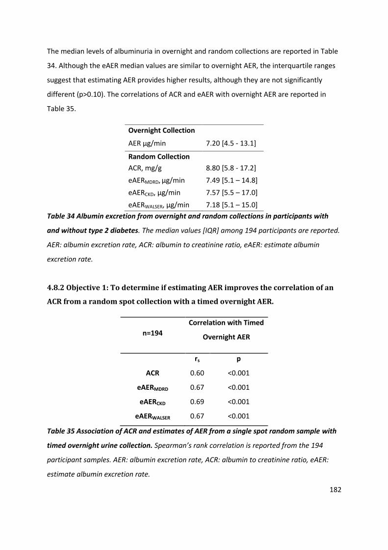
182

The median levels of albuminuria in overnight and random collections are reported in Table

34. Although the eAER median values are similar to overnight AER, the interquartile ranges

suggest that estimating AER provides higher results, although they are not significantly

different (p>0.10). The correlations of ACR and eAER with overnight AER are reported in

Table 35.

Overnight Collection

AER µg/min 7.20 [4.5 - 13.1]

Random Collection

ACR, mg/g 8.80 [5.8 - 17.2]

eAERMDRD, µg/min 7.49 [5.1 – 14.8]

eAERCKD, µg/min 7.57 [5.5 – 17.0]

eAERWALSER, µg/min 7.18 [5.1 – 15.0]

Table 34 Albumin excretion from overnight and random collections in participants with

and without type 2 diabetes. The median values [IQR] among 194 participants are reported.

AER: albumin excretion rate, ACR: albumin to creatinine ratio, eAER: estimate albumin

excretion rate.

4.8.2 Objective 1: To determine if estimating AER improves the correlation of an

ACR from a random spot collection with a timed overnight AER.

n=194

Correlation with Timed

Overnight AER

rs p

ACR 0.60 <0.001

eAERMDRD 0.67 <0.001

eAERCKD 0.69 <0.001

eAERWALSER 0.67 <0.001

Table 35 Association of ACR and estimates of AER from a single spot random sample with

timed overnight urine collection. Spearman’s rank correlation is reported from the 194

participant samples. AER: albumin excretion rate, ACR: albumin to creatinine ratio, eAER:

estimate albumin excretion rate.

183

4.8.3 Objective 2: To determine if estimating AER improves the diagnostic

accuracy of random spot samples to identify individuals with persistent

microalbuminuria.

27/194 participants had persistent microalbuminuria, which was identified from two timed

overnight collections. The ability to correctly identify individuals with microalbuminuria

when reporting either ACR or eAER in a random sample is displayed in Table 36.

Sensitivity % (CI) Specificity % (CI) AUC (CI) % Correctly Identified

ACR 85.2 (66.3 – 95.8) 92.8 (87.8 – 96.2) 0.97 (0.95 – 0.99) 91.75

eAERCKD 96.3 (81.0 – 99.9) 89.8 (84.2 – 94.0) 0.98 (0.96 – 1.00) 90.72

eAERMDRD 88.9 (70.8 – 97.7) 92.2 (87.1 – 95.8) 0.98 (0.96 – 1.00) 91.75

eAERWALSER 92.6 (75.7 – 99.1) 89.8 (84.2 – 94.0) 0.98 (0.96 – 1.00) 90.21

Table 36 Diagnostic accuracy of ACR and estimates of AER in a random sample to identify

individuals with microalbuminuria. Microalbuminuria was identified from two timed

overnight collections, 27/194 participants were identified as having persistent

microalbuminuria. Sensitivity, specificity and AUC from ROC analysis with the accompanying

95% confidence intervals are reported. The percent of correctly identified individuals (with

and without microalbuminuria) are reported.

184

4.9 Chapter Discussion

A timed overnight urine collection is the “gold standard” for assessing albumin excretion.

However, timed collections are burdensome for patients, who can be prone to making

mistakes, which can lead to inaccurate results. The overall aim of this study was to

investigate which untimed spot collection and which method of reporting albumin excretion

is the best surrogate of timed overnight collections.

The risk of cardiovascular disease with albumin excretion is continuous, starting within the

normal levels of albumin excretion. We can utilise the validated ELISA (Fitzgerald Industries

International, North Acton, MA, USA) to quantify the lowest concentrations of urinary

albumin enabling us to investigate the biological variation of albumin excretion at the

lowest levels in healthy individuals.

To fully investigate the relationships between spot samples and timed overnight collections,

this chapter consists of two different studies, the results of the first study instigating the

aims of the second study.

Investigation 1: The optimal urine collection method to assess the excretion of albumin

in the normal range in healthy individuals

Investigation 2: The relationship of estimating AER from an untimed spot using a

personalised creatinine excretion rate with an overnight AER in individuals with and

without T2DM.

185

Investigation 1: The Optimal Urine Collection Method to Assess the

Excretion of Albumin in the normal range

The results from this study indicate that a FMV is the most appropriate surrogate for an

overnight urine collection, and that ACR should be reported, as they provide the lowest

median intra-individual reproducibility (CV = 15.9%, Table 29) and have the highest

correlation with overnight AER (Rs = 0.88, Table 31).

This agrees with and extends the findings of other studies, including those from the

PREVEND cohort, who reported an intra-reproducibility of 19.0% for a FMV sample

reporting the ACR, supporting their conclusion that a FMV sample is more reliable than a

random sample (Witte et al., 2009). The PREVEND study is unable to investigate these lower

levels of albumin excretion and has a much more diverse population, closer associated with

the tested cohort in the second study (Section 4.8.1) (discussed further in Section 4.9.4)

Our study has used healthy individuals, and by using the validated ELISA (Chapter 2)

(Fitzgerald Industries International, North Acton, MA, USA) the biological variation of

albumin excretion at the lowest levels was investigated for the first time.

4.9.1 Albumin excretion levels by different collection methods and by different

methods of reporting albumin excretion.

Albumin excretion levels by different collection methods are summarised in Table 28. AER in

timed day collections was 4.5 µg/min [2.7 – 6.9] compared to an overnight AER of 3.2

µg/min [1.2 – 4.0] (p=0.0005) (Table 28). AER is significantly lower overnight than during the

day. This is also demonstrated by the spot samples, where ACR from a FMV is lower than

ACR from the SMV (p=0.005) and a random spot sample (p=0.005) collected later in the day.

Consequently, when estimating AER in spot samples, an eAER from a FMV is more

representative of an overnight AER and an eAER from a random sample is more comparable

to a timed day or 24 hour AER.

186

AER has been reported as 30-50% lower overnight compared to during the day in other

studies (Mogensen et al., 1995b, Witte et al., 2009, Howey et al., 1987). A recent study of

145 healthy participants, similar to our cohort, reported a mean 24 hour AER of 5.25 µg/min

and an overnight AER of 4.10 µg/min (Fagerstrom et al., 2015). The reported albumin

excretion is very similar to our results; however, these studies have not been able to

quantify the lowest levels of urinary albumin excretion. Presumably they have reported the

limit of quantification for samples which are unmeasurable by their assay.

The majority of authors do not report if samples which have an albumin concentration

below the measurable range of their assay are included in the analysis. All the samples

tested in our study had an albumin concentration within the measurable range of the

validated Fitzgerald ELISA (Fitzgerald Industries International, North Acton, MA, USA).

In the PREVEND study of 241 participants (predominately without diabetes), the reported

mean AER [IQR] from three 24 hour collections was 7.99 µg/min [5.00 to 12.36],

considerably higher than our reported 24 hr AER of 4.11 µg/min [2.48 to 5.76] (Witte et al.,

2009).

The higher reported AER in the PREVEND study is most likely attributed to the more diverse

and older population they tested. The mean age of the PREVEND cohort was 58.7 ± 11.3

years, the median age [IQR] of participants in our study was 34 [22-47] . However

differences between the assays used may contribute to the disparity and it is likely that they

have reported the limit of quantification for samples which are unmeasurable by their assay.

The assay used to quantify urinary albumin was the Behring BN II analyser (Dade Behring,

Marburg, Germany) which has a lower limit of detection was 2.40 mg/L (Witte et al., 2009).

The reason for reduced AER overnight, compared to during the day is most likely the result

of low levels of physical activity and a low, steady blood pressure overnight, as reflected in

the FMV sample. During the day, the influence of these factors will not only increase but

vary considerably day to day, within people as well as between individuals, resulting in an

increase in the variability of albumin excretion and the amount of albumin excretion.

187

4.9.2 Variability of albumin excretion in different urine collection methods

The intra-individual reproducibility of albumin excretion declined as the day progressed,

which was demonstrated by an increasing CV in spot samples that were collected later in

the day, with FMV, SMV and random ACRs having a CV of 15.9%, 22.1% and 22.6 %

respectively (Table 29). CV significantly improved when reporting UAC from a FMV (26.8%

[23-50]) compared to reporting UAC from a random spot sample (60.8% [42-74]) p= 0.02.

The PREVEND study of 241 participants carried out three 24 hour, FMV and random

collections over three weeks (Witte et al., 2009). The CV of the collections were 19.0%,

19.1% and 35.8% respectively, revealing that only the FMV CV did not significantly differ

from the 24 hour AER (p=0.64). In the PREVEND study, 24 hour AER was selected as the

reference method. Our investigation of the literature states that an overnight AER is the

gold standard method to assess albumin excretion. This is supported by our findings that

albumin excretion is more reproducible when taken over night or as a spot from a first

morning void. In our study the CV when reporting an ACR from a FMV had no significant

difference with overnight AER (p=0.723). There were also no significant differences between

the CV of ACR when reporting from a SMV (p=0.407) and random spot sample (p=0.163)

with overnight AER.

The inter-individual variability in albumin excretion also increased throughout the day. This

was expected, as the impact of factors that influence albumin excretion differs between

people as the day progresses, but overnight the variability of these factors is less (Table 30).

This is demonstrated by FMV ACRs in the first collection having an inter-individual CV of

69%, compared to random sample ACRs collected later in the day with a CV of 114%. The CV

increased further when only reporting UAC; with a CV of 90% and 302% in the FMV and

random samples respectively. The CV was 70% and 156% for FMV and random samples

when reporting A/USG, which is lower than reporting UAC alone, but no improvement on

the ACR. This reflects the influence of hydration status when reporting albuminuria and the

need to account for it.

188

When considering intra-individual reproducibility, the CV of spot samples was highest when

reporting UAC alone; 26.8%, 42.1% and 40.8% in FMV, SMV and random samples

respectively. When adjusting UAC by urine specific gravity (A/USG), the CV was reduced

(22.7%, 28.2% and 26.0%), but the least variability was seen when reporting ACR (15.9%,

22.1% and 22.6 %, Table 29).

Reporting the ACR from a FMV is the most reproducible method of investigating the urinary

albumin excretion in spot samples. This is in accordance with other studies which have

investigated at a higher albumin excretion than our study. Our study is the first to evaluate

the biological variability of albumin excretion in all healthy individuals, facilitated by using a

validated highly sensitive assay.

For each participant, all the urine samples (from all three collections) were analysed on the

same ELISA plate, to eliminate the impact of inter-plate variation on intra-individual

reproducibility results. This analytical approach may contribute to the variability seen

between participants. Assessing inter-individual variability was one of the study objectives,

but this limitation is accepted as intra-individual variability is a more important factor when

identifying a spot sample to be a surrogate overnight collection.

4.9.3 Reproducibility of methods of adjusting albumin concentration for variation

in urine concentration

This study finds that ACR is the most reproducible method of reporting albumin excretion in

spot samples, which contradicts the views of some authors who argue that the ACR

increases variability because another biological factor (creatinine) is being measured (Dyer

et al., 2004). However, their conclusions were drawn from an epidemiological study where

only two 24 hour samples and no spot samples were collected, with UAC being reported

from the same 24 hour samples. In our study it is evident that the ACR should be reported in

spot samples, as UAC not only resulted in higher variability, it had a poorer correlation with

overnight AER (Table 31).

189

Another method instead of creatinine to adjusting for urinary concentration is urine specific

gravity (USG), but there are major differences between them. Creatinine is a breakdown

product of muscle metabolism, which is freely filtered by the kidneys and excreted into the

urine at a relatively constant rate. A limitation of using creatinine is that creatinine

production/excretion is associated with muscle mass which varies among individuals. USG is

a marker of the density of urine, comparing the refraction of light in a sample to that of

water, which is dependent on the concentration of particles in the sample. Therefore, an

elevated concentration of particles, not related to low urinary flow, will increase USG. This is

a limitation, especially when measuring albumin excretion in patients with DM, where large

particles such as albumin and glucose may be present which refract light to a large degree,

falsely elevating USG.

Creatinine is a standardised and comparable measurement between laboratories, and with

the results of this study suggesting there is no improvement when reporting A/USG

compared to ACR, it is evident that the ACR is the preferable measure of urinary albumin

excretion in spot samples.

4.9.4 Correlation of spot samples with overnight AER

The correlation of spot samples to the “gold standard” overnight AER was determined in the

first collection from 17 healthy participants (Table 31). The FMV sample always

demonstrated the strongest correlation with overnight AER. The correlation of ACR was

generally higher than UAC and A/USG. Our findings are in accordance with the PREVEND

study which reported a correlation (rs) of ACR from FMV and random samples to the 24 hour

collection were 0.87 and 0.83 respectively (Witte et al., 2009).

In our study correlation of ACR in FMV, SMV and random spot samples with timed overnight

AER was 0.88, 0.54 and 0.59 respectively. Correlation of UAC in FMV, SMV and random spot

samples with timed overnight AER was 0.84, 0.48 and 0.45 respectively. Correlation of

A/USG in FMV, SMV and random spot samples with timed overnight AER was 0.87, 0.46 and

190

0.60 respectively. Only reporting a A/USG from a SMV and UAC from a random spot sample

did not have a significant correlation with overnight AER (A/USG-SMV: Rs=0.46 p=0.062)

(UAC-Random spot: Rs=0.45 p=0.073) (Table 31). Graphs of the correlation between spot

sample ACR and overnight AER are presented in Figure 35, Figure 36 and Figure 37.

Another study found that a FMV ACR correlated better than a random sample ACR to a 24

hour AER (their reference method) (r = 0.803 versus 0.623), however they reported that the

correlation in both samples was increased using UAC (r = 0.943 and 0.920) (Chavan et al.,

2011). In our results, the correlation of the FMV, SMV and random samples with overnight

AER was consistently reduced when reporting UAC alone (Table 31). Regardless of reporting

ACR, UAC or A/USG, the correlation is weaker in the SMV and random samples than in FMV

samples and is again most likely the result of changes in the concentration of the urine and

the influence of other factors (e.g. exercise).

The improvement in correlation Chavan et al. found using UAC in FMV samples, maybe the

result of the level of albumin excretion they were investigating. They reported a median 24

hour AER of 228 µg/min, in our study it was 4.11 µg/min [2.48 - 5.76]. Perhaps at those

higher albumin excretion levels, it is not so important to account for urinary concentration

but it is imperative when investigating the low levels of albumin excretion, especially when

screening for microalbuminuria or for the accurate estimation of lower levels of albumin in

urine which may become important for the future monitoring of individuals given the

important epidemiological evidence which suggests cardiovascular risk is increased right

down into the normal range (Rachmani et al., 2000, Gerstein et al., 2001, Hillege et al.,

2002, Dwyer et al., 2012).

191

4.9.5 Estimating AER in random samples

The Kidney Disease: Improving Global Outcomes (KDIGO) working group, who provide

reccomendations for clinical guidelines, advocate screening for microalbuminuria using

random samples, as it provides a more sensitive test (KDIGO, 2013). It is also more

convenient for patients to provide a urine sample whilst at the GP or in clinic, rather than

collecting a FMV at home.

In our study the reduced albumin excretion and better reproducibility in overnight

collections, or from the first morning void, have been attributed to low levels of physical

activity and a low, steady blood pressure overnight. Although a random sample might be

more variable than a FMV, it might be desired as a screening test for microalbuminuria

because during random testing the kidney will be under more stress. Therefore, a larger

increase in albumin excretion during the day may indicate a lack of autoregulation or

impaired autoregulation, demonstrating early abnormal findings in the kidney, increasing

the diagnostic sensitivity of the test.

In our study it was demonstrated that the correlation of a random ACR (rs = 0.59, p=0.012)

to overnight AER was improved to 0.78 (p<0.001) when estimating AER (Table 32). This

improvement is plotted in Figure 38.

Regardless of when a spot sample was taken, the correlation of the ACR always improved

when estimating AER. However the largest improvements were found in samples taken later

in the day (SMV and random), which may be related to differences in urine concentration

and variability (Table 29).

The eAERMDRD equation, which incorporates an additional clinical characteristic (weight) in

its estimation of creatinine excretion, improved the correlation the most, although previous

validation work suggested that eAERCKD-EPI was best (Chapter 3). In the previous validation

work, no spot samples were collected, only a single overnight collection and a much larger

(n=245) and a more diverse population was tested. Therefore, to determine if estimating

192

AER from a random sample can correlate to an overnight AER, potentially as well as a FMV

sample, the SUMMIT cohort were tested.

4.9.6 Limitations

The reason for finding a spot collection method to replace timed collections is because

timed collections are burdensome and are prone to errors which can lead to inaccurate

results. A fundamental limitation of this study is the uncertainty that the timed collections

were accurately completed, as is the case for every study utilising timed urine collections.

Participants were questioned when returning samples to verify that they had completed the

collection correctly, but 100% compliance cannot be guaranteed. The study could have been

improved by using para-aminobenzoic acid (PABA) as a marker of 24 hour urine collection

completeness (Bingham and Cummings, 1983). PABA is taken orally on the day of the

collection and the recovery of PABA in the urine 24 hours after indicates completeness

(Jakobsen et al., 2003).

The mean period (±SD) to complete all three collections was 26.8 days (±12.3). Ideally the

collections would have been done one after the other, however this wasn’t feasible for the

participants. Participants were questioned to determine if they deviated from the protocol,

2/51 collections were repeated due to exercise undertaken and one collection was repeated

due to an incomplete overnight sample. There may have been more protocol deviations that

participants did not report, as they were disinclined to repeat the collection.

All outlying results were investigated by urinalysis. In some cases haemoglobin was present

which may have interfered with the assay. In one case the presence leucocytes was

indicated, suggestive of an infection which may influence albumin excretion. Interestingly,

the largest outlier in the SMV samples might have been the result of it being a very

concentrated sample (creatinine = 21.6mmol/L) with a UAC of 189 mg/L. This questions the

suitability of creatinine to account for urinary concentration, especially at the high levels.

However, the answer is not measuring UAC alone. USG was also measured in this study, but

193

no improvement over ACR was found. However, it may be beneficial to measure in samples

with a high creatinine concentration. The use of USG requires further research across larger,

more diverse populations, especially in those with reduced kidney function who would have

impaired creatinine excretion.

Investigation 2: The relationship of estimating AER from an untimed

spot using a personalised creatinine excretion rate with an overnight

AER

194 participants from the SUMMIT study cohort met the inclusion criteria of having a stored

sample from an overnight urine collection and a random spot sample, both collected on the

same day (Section 4.7.1) This cohort are older (70 years old ±8) than the first study cohort

(34 years old [22-47]), with 58% diagnosed with T2DM (Table 33).

The median [IQR] AER for an overnight collection in this cohort was 7.20 µg/min [4.5 to

13.1], much higher than the median AER in the cohort of the first study 3.23 µg/min [1.20 -

3.96] (Table 28). The AER of this second cohort is closer associated with the participants of

the PREVEND study, who reported a median AER [IQR] of 7.99 µg/min [5.00 to 12.36] (Witte

et al., 2009). This might be attributed to SUMMIT and PREVEND cohorts testing older aged

subjects, indicating that albumin excretion increases with age. This is supported by the low

prevalence of diabetes in the PREVEND cohort (2%).

In this study, of subjects from the SUMMIT study (n=194), the median values for estimating

AER using personalised estimates of creatinine excretion, are similar to overnight AER (Table

334). The interquartile ranges suggest that estimating AER provides higher results, although

they are not significantly different (p>0.10).

194

4.9.6 Correlation of ACR and estimated AER in random spot samples with timed

overnight AER in the SUMMIT study.

The correlation of an ACR from a random spot sample to overnight AER was 0.60 (p<0.001)

(Table 35), which improved to 0.67, 0.69 and 0.67 when estimating AER from the spot

sample using the MDRD, CKD-EPI and WALSER eCER equations respectively (all p<0.001).

These results are similar to the findings of the previous study (n=17) (Table 31). The

previous study also showed that the correlation of random sample ACR improved from 0.59

(p=0.012) to 0.78 (p<0.001), 0.76 (p<0.001) and 0.74 (p<0.001) when estimating AER from

spot samples using the MDRD, CKD-EPI and WALSER eCER equations respectively.

In the previous study (n=17) the MDRD method to estimate albumin excretion had the

biggest improvement on correlation, whereas in this current study (n=194) the CKD-EPI

provides the biggest improvement. This demonstrates that no single method of estimating

an AER from a spot sample is superior, and selection of a method may be dependent of the

cohort being tested (Chapter 3.3).

By testing the larger, more diverse, population in the second study (n=194), which includes

subjects with diabetes (58%), the impact of estimating AER on diagnostic accuracy to

identify microalbuminuria could be tested.

4.9.7 Diagnostic accuracy of ACR and eAER in a random spot collection and

correlation with timed overnight AER

From the 194 SUMMIT participants, 27 were identified with persistent microalbuminuria

(identified using two overnight collections). Therefore, the diagnostic accuracy of the ACR

and eAERs in a single random sample could be determined. Using clinically recognised

gender specific cut-offs for microalbuminuria, the ACR in random spot samples had a

195

sensitivity of 85.2% and a specificity of 92.8%. Sensitivity increased when using the eAER

equations (maximum of 96.3% using eAERCKD), although specificity was lost (Table 36).

The positive bias found when comparing eAER with overnight AER may be contributing to

the increased sensitivity as higher values are being reported (compared to the ACR), so

more individuals with microalbuminuria are found (Table 34). This is desirable for a

screening test but comes with a loss in specificity.

Another method of investigating diagnostic accuracy is to calculate the AUC from a ROC

analysis. The AUC of each test shows the probability that the test will rank a randomly

chosen positive sample higher than a random chosen negative sample; where the closer to 1

to better the test. The AUC and percent of individuals correctly identified (Table 36) were

almost the same when using ACR and eAER, suggesting that there is not a considerable

improvement in the overall diagnostic accuracy when estimating AER. However, as the

sensitivity is increased when reporting eAER, it may be beneficial when screening for

microalbuminuria.

The eCERCKD equation had the largest improvement in correlation and diagnostic sensitivity.

This was also found in our previous validation work (Chapter 3.3), but not in the previous

study in this chapter (Section 4.4.6), which identified the MDRD equation to improve

correlation the most between random spot samples with overnight AER in 17 healthy

individuals.

Among the eCER equations, the CKD-EPI equation was developed on the largest population

with the widest range of GFRs, and the equation includes the most clinical characteristics,

which might be why it is suited to the more diverse population of the SUMMIT cohort.

However, it incorporates weight that is not readily available routine clinical laboratory

request notes, limiting its clinical use. The eCERMDRD equation does not utilise weight, just

age, gender, and ethnicity, and is therefore more clinically applicable. It also improved

random sample correlations and diagnostic accuracy, but to a lesser degree. This work

demonstrates the benefit of estimating AER in spot samples and confirms the need for

further validation.

196

4.9.9 Limitations

An important limitation of this study is the environment in which samples were collected.

The participants for this study were recruited from the Exeter 10,000 bio-resource of

individuals interested in hearing about research held by the NIHR Exeter Clinical Research

Facility. The nature of recruiting by this method can influence study results, as subjects are

not representative of the general population. In our study we collected a timed overnight

collection and a random spot sample. The participants were provided with a detailed

procedure to follow to ensure the sample was collected properly (e.g. no exercise or

caffeine before providing a sample).

This is a very controlled environment, and is not representative of collecting samples in

primary care. The random spot samples were collected during a visit to the research centre,

where some participants would have been resting in the supine position for over 2 hours

before providing a sample. In the primary care environment a real random spot sample

might be provided after walking 30 minutes to the GP surgery. The impact of exercise on

albumin excretion is investigated in Chapter 6.

4.10 Conclusion

Albumin excretion is significantly lower overnight than during the day. A FMV is the best

spot sample to investigate the lower levels of albumin excretion; the ACR should be

reported as it provides the most reproducible results and has the highest correlation with

the “gold standard” timed overnight AER. However, a random spot sample is clinically more

desirable and the correlation to overnight AER is improved when estimating AER, although

there is no improvement in overall diagnostic accuracy to identify individuals with

microalbuminuria. However, diagnostic sensitivity is increased when reporting eAER, which

may be beneficial when screening for microalbuminuria.

197

Chapter 5 Storing Urine for the Assessment of Albumin

Excretion

5.1 Introduction

Studies that have investigated the stability of albumin in frozen stored urine samples have

had mixed findings. Several studies have demonstrated insignificant changes in urinary

albumin concentration (UAC) (Collins et al., 1993, Giampietro et al., 1993, Comper et al.,

2004b, Parekh et al., 2007), whilst others have demonstrated significant losses (Elving et al.,

1989, Osberg et al., 1990, Brinkman et al., 2007a, Hara et al., 1994, Marko et al., 2009,

Erman et al., 1988, Schultz et al., 2000, MacNeil et al., 1991). The strongest agreement

amongst these studies is that urinary albumin is more stable when stored at -70oC or -80oC

when compared to -20 oC.

The disagreement between studies which have investigated the loss of UAC during storage

can be attributed to different storage temperatures, sample sizes, storage durations, sample

processing, analytical techniques, study populations and the albumin excretion range

investigated. Many studies are limited by a low sample size and short storage durations.

When interpreting the results of storage experiments it is also important to consider the

inter-assay variability of the assay (if the same assay was used) and also the type of assay.

5.1.1 Impact of analytical method when investigating loss of albumin with

prolonged frozen storage

In 2007, Brinkman and colleagues carried out a very comprehensive study which not only

looked at the effect on UAC when storing samples at -20 oC and -80 oC, they also investigated

the impact of measuring urinary albumin by different methods (Brinkman et al., 2007a).

Prior to commencing the study another research group led by W. Comper had developed a

HPLC method for quantifying urinary albumin (Comper et al., 2004a). Validation

198

experiments carried out by the same research group showed that HPLC produced higher

results compared to immunoassays and they hypothesised that immune-nonreactive forms

of urinary albumin were present which immunoassays were unable to quantify (Osicka and

Comper, 2004). This theory has been contested by other authors who have demonstrated

that the co-elution of other proteins causes the higher HPLC results (Sviridov et al., 2008).

Brinkman and colleagues tested Comper’s proposed hypothesis that albumin loses

immunogenicity and is therefore underestimated by immunoassays. It is conceivable that

prolonged freezing reduces immunoreactivity and therefore the loss would be greater when

using immunoassays, compared to HPLC, to measure albumin. To test this, urine samples

from the PREVEND study (general population) had urinary albumin quantified by

immunonephelometry and HPLC within 5 days of being collected. The fresh samples were

then aliquoted in to polypropylene vials for assessment after storage for 2, 4, 12 months at -

20 oC (n=295) and after 12 months at -80 oC (n=224). The results are summarised in Figure

39.

Figure 39 Percent change in urinary albumin concentration in samples stored at -20 and -

80 assessed by immunonephelometry and HPLC from the PREVEND study. Data are

presented as mean (SD) percentage difference in urinary albumin concentration (Brinkman

et al., 2007a).

199

The results from Brinkman’s study show that more urinary albumin is lost when stored at -

20 oC compared to -80 oC, regardless of the method used to measure it. The results also

indicate that more albumin is lost when using the HPLC method. This contradicts Comper’s

theory and supports the possibility that other proteins are being measured, as well as

albumin, by the HPLC method. It is the loss of these other proteins which causes the larger

percentage difference (Sviridov et al., 2008). These results support other studies which find

immunoassays a suitable method to measure urinary albumin and that urine samples should

be kept at -80 oC for prolonged storage (Seegmiller et al., 2009b, Schultz et al., 2000).

5.1.2 Sample processing prior to analysis

Urine samples collected in cohort studies are often kept at -20 oC for variable times before

analysis, which could jeopardise the accuracy of results. In 2005, Brinkman and colleagues

investigated the loss of albumin in samples stored at -20 oC for up to 24 months (Brinkman

et al., 2005). The samples were divided into 3 groups, the first group (n=600) were not

mixed prior to analysis, the second (n=596) underwent 3 to 4 hand inversions and the third

group (n=689) were vortex-mixed for 5 to 10 seconds. After 3months storage, there was a

considerably larger change in UAC in the unmixed samples than in the samples which were

inverted or vortex mixed (mean ±SD): -34.9% (±28.6) vs -5.3% (±30.6) and -2.6 % (±27.5),

respectively, p<0.001). The inverted and vortex mixed samples were then measured again

after 18 months storage, and showed a significant loss in UAC (-23.7% (±26.2) and -26.1%

(±24.7), respectively). Post hoc analysis showed there was no difference between the two

mixed groups and that after 8 months of storage, the difference in UAC had stabilised to

around -25% to -30% (Brinkman et al., 2005).

The results of this study from the PREVEND cohort suggest that the loss in albumin

concentration is highly variable between samples, represented by a large standard deviation

in the loss of UAC. In their analysis, the mean loss of UAC has been investigated; however,

with such large standard deviations some samples would have lost 30% of their UAC after 8

months storage, whereas some samples would have been stable with 0% loss in UAC.

200

Properties such as pH and bacterial contamination (discussed in Section 5.1.4) might be able

to help explain why some samples have a decline in UAC and why some don’t. This is

investigated further in our study.

Brinkman and colleagues also reported that the maximum loss of UAC, -28% (±33), was seen

in the 10-20mg/L category (categories determined from measurement with fresh samples).

Samples in the highest category (200-500mg/L) had a significantly lower difference, -9.2%

(±17.4), compared to the other groups. This study not only demonstrated the importance of

mixing samples prior to analysis, they also showed that the difference in UAC over time

varies between concentration ranges. The limitation of this study, and others, is they have

used assays which cannot measure the low concentrations of urinary albumin, therefore the

effect of storage in the normoalbuminuria range is not fully understood.

In 1993, a study by Collins and colleagues reported that there was no significant difference

in UAC after storage at 20 oC, 4 oC, -20 oC and -40 oC for 7 days (Collins et al., 1993). It is

important to know this, as it can take several days for samples to be analysed or stored,

especially in epidemiological studies. The samples (n=84) were from individuals with DM,

who had a range of albumin excretion. The authors also reported no significant difference in

UAC between samples which were centrifuged or not prior to analysis, and that there was

no effect of a freeze-thaw cycles on UAC. Collins and colleagues also investigated the

change in UAC in different types of storage containers at -20 oC. 26 urine samples from

patients with DM were aliquoted into polypropylene, polystyrene and borosilicate glass

tubes with and without gelatine added. There was no significant difference in UAC (p>0.97)

in any of the storage tube types when stored at -20 oC for either one week or one month.

However, after 1 month of storage the average change in UAC was -7% which was reduced

to -4% in the tubes which had gelatine added to reduce protein absorption. It is conceivable

that the adsorption of albumin to storage containers could contribute to the loss of UAC

over time at -20 oC. Since Collin’s study in 1993, storage tubes that are specifically designed

to reduce the adsorption of proteins have become available and their ability to prevent UAC

loss is investigated in this chapter.

201

5.1.3 Mechanisms of urinary albumin concentration decline during freezing

The loss of UAC as a result of protein adsorption to storage containers is one possibility for

the decline of UAC during freezing. However, further work is required beyond the Collins

study due to its small sample size and short storage duration (Collins et al., 1993). The exact

mechanism that results in the decline of UAC during freezing is still unknown as is the cause

of variation in the loss of UAC among samples (reflected by large standard deviations of UAC

loss), especially as some samples are unaffected. Some authors suggest that albumin is

trapped in precipitate, the result of an alteration in pH that occurs during freezing

(Townsend, 1986a). Other authors have suggested that bacterial contamination may cause a

loss in UAC (Kania et al., 2010) whilst others have demonstrated that the loss of UAC is

correlated to pH (Brinkman et al., 2007b). These are described in more detail below.

5.1.4 Urinary proteases

The loss of urinary albumin as a result of proteases was investigated by Kania and colleagues

in 2010. Using sodium dodecyl sulphate (to denature proteins) and polyacrylamide gel

electrophoresis (to separate the proteins) (SDS-PAGE), they demonstrated that albumin

remained intact when stored for 12 months at -70oC but was degraded at -20oC (Kania et al.,

2010). This was confirmed by using mass spectrometry to analyse the fragments. The

degradation of UAC occurred in 11/40 samples when stored at -20 oC. They also carried out

in-vitro experiments where the pH of urine samples was lowered which induced rapid

degradation of endogenous and exogenous albumin. The pattern of albumin fragments was

similar to those produced by pepsin digestion and degradation was completely inhibited in

samples with pepstatin (protease inhibitor) added. However, samples with leupeptin

(protease inhibitor) added (as well as lowered pH) showed no inhibition from proteases and

the albumin was degraded. This suggests the urinary proteases which degrade albumin may

202

belong to the pepstatin-sensitive protease family. Other studies have also reported

improved protein stability with the addition of protease inhibitors when storing urine

samples (Havanapan and Thongboonkerd, 2009, Zhou et al., 2006).

Kania and colleagues’ results suggest that urinary proteases cleave albumin but the identity

of these proteases has not yet been revealed. The proteases may arise from several sources:

glomerular filtrate, urothelial secretion and bacterial contamination (Deng et al., 2001).

Kania and colleagues demonstrated that that pepstatin can prevent degradation in-vitro,

although, there are no studies to date which have investigated if pepstatin can prevent the

loss of UAC in patient samples during long term storage. This is investigated in this chapter.

Bacterial contamination is a possible source of proteases. There is a wide range of bacteria

that can contaminate urine samples, mostly from normal skin flora. Some bacteria secrete

proteases which acts as an exotoxin, an example of a virulence factor in bacterial

pathogenesis (Frees et al., 2013). The quantity and type of bacteria present in urine varies

between people and this variability could explain the difference in the samples which lose

UAC during prolonged frozen storage. Bacterial contamination is investigated in this

chapter, to determine if there is a link with the samples which lose UAC after storage at -20

oC.

5.1.5 Urine pH

There are few studies that have investigated pH as a determinant of UAC decline associated

with freezing. A study in 1988 reported no association (Erman et al., 1988), although this

was only after 7 days storage at -20 oC. More recent studies have shown it takes longer than

1 week for UAC to decline at -20 oC (Collins et al., 1993, Brinkman et al., 2005). In 2007,

Brinkman and colleagues showed urine pH was associated with a decline of UAC in samples

stored at -20 oC (Brinkman et al., 2007b). Urine samples from the PREVEND study (n=230,

UAC>5 & <200mg/L) had UAC determined by immunonephelometry and had pH measured

by dipstick analysis and were then frozen at -20 oC. UAC was measured again after 4 and 12

months storage. Samples were thawed and mixed by hand inversions prior to analysis. The

203

results of the analysis after 12 months are shown at Figure 40. The largest decline in UAC

occurs at the lowest pH and there was a significant trend for the magnitude of loss in

relation to pH (p<0.001).

Figure 40 Percent change in urinary albumin concentration after 12 months of storage at -

20 oC according to pH in the PREVEND study. The boxes indicated lower and upper quartiles

and the central lines are medians. The whiskers represent 95% confidence intervals. P< 0.001

for trend across pH levels (Brinkman et al., 2007b).

An earlier study investigated neutralising the pH in 38 samples from patients with DM prior

to storage at -20 oC for 8 weeks (Townsend et al., 1988) . Although they had low numbers

and a short storage period, they reported no significant decrease after adjustment of pH,

while UAC decreased significantly (p<0.05) in unadjusted samples, of which 8 samples had a

decrease of 23% to 91% of their original concentration. It is not clear how UAC changed in

204

the remaining 30 samples, but this work also reflects the variation in UAC loss between

samples stored unadjusted at -20 oC.

More recently, Brinkman’s research group alkalised urine samples (n=90, from patients with

DM) to pH>8.0 and demonstrated it prevents UAC decline during storage at -20oC after one

year (Lambers Heerspink et al., 2009). The group speculated that the loss at low pH could be

associated to the relatively low iso-electric point of albumin (4.7), with less aggregation at a

higher pH resulting in less albumin being trapped in precipitate. They also suggested that

alkalinisation prevents conformational changes that occur to albumin during freezing,

improving antibody binding during quantitative immuno-analysis. Their final conjecture was

that urinary albumin is being hydrolysed by bacterial proteases from contaminated samples

and that alkalisation may inhibit the enzyme activity.

It is beneficial to combine the methods used by the Brinkman and Kania research groups to

provide insight into what effect alkalisation has on urinary albumin; whether it prevents

fragmentation or if urinary pH influences the performance of the assay. The effect of pH and

alkalising samples on UAC after frozen storage will be investigated in this chapter.

5.1.6 Summary

Previous studies have reported the effect of prolonged frozen storage on UAC, although

they have not reported the effect on creatinine and the ACR. It is important to know how

UAC changes for timed collections, but the stability of creatinine must be considered when

storing spot samples for ACR assessment.

Several approaches to reduce the loss of UAC when stored at -20 oC have been previously

tested; alkalisation, protease inhibitors and using specific sample containers. Other studies

have shown the importance of mixing prior to analysis, and have confirmed immunoassays

are acceptable methods to quantify UAC in stored samples. All these findings are applied to

the urine storage study carried out in this chapter.

205

Although previous studies report that UAC is stable at -80 oC, they have all used assays

which cannot measure the low concentrations of urinary albumin. Using the validated ELISA

described in Chapter 2, the effect of frozen storage in the extended low albumin excretion

range can now be fully explored. Using additives to prevent a loss in UAC will also provide

information on the mechanism of UAC decline.

5.2 Aim

To identify the optimal long-term frozen storage conditions to preserve urinary albumin and

creatinine concentrations for the assessment of albumin excretion rate and ACR.

5.2.1 Objectives

1. To determine the effect of multiple freeze thaw cycles on albumin and creatinine

concentrations and the assessment of ACR.

2. To identify the optimal storage conditions to preserve urinary albumin and

creatinine levels and the assessment of ACR over 12 months.

3. To investigate the effect of storage duration on albumin and creatinine

concentrations and the assessment of ACR in samples stored at -80oC.

Each of these objectives is separated into individual investigations composed of separate

methods, results and a discussion at the end of each investigation.

An overall summary all the investigations is presented at the end of the chapter with a

conclusion.

206

5.3 The effect of multiple freeze thaw cycles on albumin and

creatinine concentrations and the assessment of ACR.

5.3.1 Method

20 patient urine samples which had been sent to the RD&E Blood Science department for

routine ACR analysis were selected. All samples were received on the same day, and they

were selected to enable a wide range of albumin concentrations to be tested (3-255mg/L).

Six aliquots were taken from each sample. One aliquot remained at room temperature, and

the others underwent a different number of freeze thaw cycles before analysis (up to 5

cycles). Samples were frozen to -80oC on each cycle and remained frozen for 30 minutes.

Samples were defrosted to room temperature before being frozen again (for at least 30

minutes) if testing another freeze thaw cycle.

Prior to analysis, samples were thoroughly defrosted and underwent 4 hand inversions to

mix them. Albumin was measured by the routine COBAS method and creatinine was

quantified using the routine Jaffe method, with all samples measured in the same run.

5.3.1.1 Statistical analysis

Data are presented as mean (±SD) and median [IQR]. Normality of the data was tested

using the Shapiro-Wilkes test. For not normally distributed data, Wilcoxon sign-rank test

was used to determine the difference between freeze thawed samples and fresh samples,

p<0.05 was considered as a significant difference.

The change of albumin/creatinine/ACR after each freeze thaw is presented as percent

change from baseline, reporting the mean percent change and confidence intervals.

207

5.3.2 Results

Albumin was not influenced by repeated freeze-thaw cycles (Table 37), whilst there was a

small and significant decrease in creatinine levels with freeze-thaw cycles (Table 38) that

had no effect on ACR (Table 39). Change from fresh sample measurements are presented in

Figure 41.

Number of

freeze thaw

cycles

Mean Albumin

mg/L

Median Albumin

mg/L

Mean

difference with

fresh sample

(%)

Wilcoxon sign-

rank test

(p)

0 58.9 ± 73.5 21.0 [6.6 to 95.3]

1 58.9 ± 74.3 21.0 [6.4 to 95.9] -0.56 ±6.0 0.21

2 58.6 ± 74.1 19.9 [6.2 to 96.8] -2.7 ± 4.1 0.21

3 58.6 ± 73.8 20.2 [6.5 to 96.0] -2.7 ± 3.7 0.25

4 58.8 ± 74.1 20.3 [6.3 to 95.1] -2.1 ± 3.4 0.41

5 59.1 ± 73.8 21.5 [6.8 to 97.2] -0.0 ± 3.6 0.97

Table 37 Impact of repeated freeze thaw cycles on albumin concentration. *significant

difference between freeze thawed samples and fresh samples (0 freeze thaws).

Number of

freeze thaw

cycles

Mean

Creatinine

mmol/L

Median

creatinine

mmol/L

Mean

difference with

fresh sample

(%)

Wilcoxon sign-

rank test (p)

0 8.6 ± 4.2 7.8 [5.7 to 12.7]

1 8.6 ± 4.1 7.7 [5.7 to 12.7] -0.6 ± 1.4 0.02*

2 8.6 ± 4.2 7.7 [5.7 to 12.6] -0.2 ± 1.3 0.74

3 8.5 ± 4.2 7.6 [5.7 to 12.8] -1.7 ± 1.6 0.001*

4 8.5 ± 4.1 7.7 [5.6 to 12.6] -1.2 ± 1.5 0.004*

5 8.6 ± 4.1 7.7 [5.6 to 12.9] -1.0 ± 1.5 0.02*

Table 38 Impact of repeated freeze thaw cycles on creatinine concentration. *significant

difference between freeze thawed samples and fresh samples (0 freeze thaws).

208

Number of

freeze thaw

cycles

Mean ACR

mg/mmol

Median ACR

mg/mmol

Mean

difference with

fresh sample

(%)

Wilcoxon sign-

rank test (p)

0 7.9 ±10.3 2.7 [1.0 to 9.7]

1 7.9 ±10.4 2.7 [1.0 to 9.8] 0.1 ± 6.2 0.59

2 7.9 ±10.7 2.6 [0.9 to 9.3] -2.5 ± 4.4 0.35

3 8.0 ±10.6 2.6 [0.9 to 9.6] -1.0 ± 4.3 0.98

4 7.9 ±10.6 2.6 [0.9 to 9.9] -0.9 ± 4.0 0.68

5 8.0 ±10.6 2.7 [1.0 to 9.9] 1.0 ± 4.3 0.26

Table 39 Impact of repeated freeze thaw cycles on ACR. *significant difference between

freeze thawed samples and fresh samples (0 freeze thaws).

Figure 41 Percentage change of albumin, creatinine and ACR by number of freeze thaw

cycles. Error bars represent a 95% confidence interval around the mean change from

measured fresh.

209

5.3.3 Discussion

The freeze thaw experiment demonstrated that there is no significant difference in albumin

concentration as a result of freeze thawing (Table 37), although creatinine is significantly

reduced (Table 38). Although creatinine is lost during freeze thawing process, the actual loss

is very small (-1.7 ± 1.6 %) and it had no effect on the ACR (Table 39). The reduction of

creatinine was not influenced by the number of freeze thaw cycles. The small loss of

creatinine has minimal impact on the ACR (Figure 41).

This study was not able to assess the effect of freeze thaws at the lowest albumin

concentration, as the routine COBAS method was used. However, there was no significant

difference in albumin or ACR across the albumin excretion range tested in this study.

210

5.4 Optimal storage conditions to preserve urinary albumin and

creatinine concentrations and the assessment of ACR over 12 months.

5.4.1 Objectives

1. To determine if there is a difference in albumin and creatinine concentrations and

the assessment of ACR after 12 months storage at -20oC and -80 oC.

2. To determine how albumin and creatinine levels and the assessment of ACR change

over 12 months when stored at -20 oC and -80 oC.

3. To investigate if additives and low protein binding tubes prevent any loss of albumin,

creatinine and ACR after 12 months storage at -20 oC and -80 oC?

5.4.2 Method

20 random spot samples and 10 timed samples were collected from participants of the urine

collection study (Chapter 4, Section 4.3.1). Each sample was divided into 5 portions. Each

portion received a different treatment:

1. No additives

2. Alkalisation

3. Boric acid

4. Protease inhibitor

5. Low protein binding tubes

211

5.4.2.1 Sample treatments

1. No additives:

Samples were divided into 400µl aliquots. The storage tubes used were 2ml polypropylene

micro tubes (Sarstedt product number: 72.609.001, Sarstedt AG & Co, Nümbrecht,

Germany). These tubes were used to store all samples from all the treatments, except for

the low protein binding tubes used in treatment 5.

2. Alkalisation:

pH was measured by a portable pH tester (Hanna instruments product number: HI-98127,

Hannah Instruments, Rhode Island, USA). 15µl of NaOH 1M (Sigma Aldrich product number:

38212, Sigma Aldrich, Missouri, USA) was added to 10ml of sample. The sample was gentle

mixed by four hand inversions and then pH was measured again to ensure pH ≥ 8.

3. Boric acid:

Samples were added to containers precoated with boric acid (Sarstedt product number:

51.9923.820). Boric acid maintains the microbiological quality of a sample by preventing the

overgrowth of organisms. Urine samples sent to the microbiology laboratory for routine

analysis are transported in boric acid. The samples were gently mixed before being

aliquoted (into the same tubes used for treatments 1, 2 and 4) and stored. An aliquot was

also sent to the RD&E hospital microbiology laboratory for the following analysis:

1) Urinalysis: An inverted microscope was used to identify and semi quantify; epithelial

cells, casts, red blood cells and leucocytes

2) Culture: Urine samples are routinely cultured on specialised mediums which

specifically enable pathogens which cause urinary tract infections to grow. However,

in this investigation any bacterial growth is of interest as it might be related to a loss

of UAC during storage. Therefore the follow media was used to enable the growth of

any organisms in the samples:

212

Horse blood agar (grows majority of aerobic bacteria)

Gram + selective blood agar (prevents coliform growth which can outcompete

other organisms)

Fastidious anaerobic agar + neomycin (isolates anaerobic bacteria)

Dextrose agar (isolates yeasts & fungi).

Organisms were identified using routine biochemical tests and confirmed using matrix-

assisted laser desorption/ionization time-of-flight analysis (MALDI-TOF).

4. Protease inhibitor:

Kania and colleagues demonstrated that urinary proteases which degrade albumin may

belong to the pepstatin-sensitive protease family (Kania et al., 2010). Therefore, pepstatin

was added to the samples in this study to prevent degradation (Sigma Aldrich product

number: P5318, Sigma Aldrich, Missouri, USA). This is the same product and protocol used

in the study carried out by Kania and colleagues (Kania et al., 2010).

1mg pepstatin was dissolved in 1ml of a 10% acetic acid: 90% methanol solution (Sigma

Aldrich product numbers: 33209 and 32213 respectively, Sigma Aldrich, Missouri, USA). A

1:10 dilution was made using deionised water to make a working solution of 0.1mg/ml. The

manufacturer states the effective concentration of pepstatin is 1 µg/ml. Therefore, 100 µl of

the working solution was added to 9,900 µl of urine samples.

5. Low protein binding tubes:

400µl of sample was aliquoted into 1.5ml low protein binding micro tubes (Sarstedt product

number: 72.706.600).

213

5.4.2.2 Sample processing and analysis

After the samples had undergone the different treatments, 400 µl aliquots were made and

stored at either -20 oC or -80 oC. Baseline measurement was taken from a fresh aliquot from

the sample which underwent no treatment.

Albumin was measured by the Fitzgerald ELISA (Fitzgerald Industries International, North

Acton, MA, USA) and creatinine measured by the routine Jaffe method (Roche Diagnostics

Ltd., Burgess Hill, UK). Dip stick analysis was carried out using the Cobas Combur10 Test

(Roche Diagnostics Ltd., Burgess Hill, UK); with pH confirmed by a hand held meter (Hannah

Instruments, Rhode Island, USA).

The samples were removed from storage and analysed after 6, 9, 11 and 12 months. Prior to

analysis samples were thoroughly thawed and mixed by 4 hand inversions. When

quantifying albumin, each sample was analysed in the same microwell location on the ELISA

plate at each time point, to reduce inter-assay variability.

5.4.2.3 Statistical analysis

Normality of the data was tested using the Shapiro-Wilkes test. The median [IQR] is

reported for not normally distributed. The difference between the values from stored

samples with baseline is reported as the mean (SD) and median [IQR], for both actual

difference and percent difference. For not normally distributed data, Wilcoxon sign-rank

test was used to determine the difference is significant (p<0.05).

Box and whisker plots are used to graphical demonstrate the data. The horizontal line inside

the box represents the median, the edges of the box are the upper and lower interquartile

and the whiskers represent the minimum and maximum values, with outlying results

individually plotted.

214

Two point line graphs are used to show the change of individual samples. Bland Altman

difference plots are used to show the difference between samples measured after being

stored with the baseline value, plotted against the original concentration. The mean

difference is plotted (with 95% confidence intervals), and the shaded area shows the region

of difference which can be explained by inter-assay variability. Bland Altman plots are used

to show actual difference and percent difference.

The Fitzgerald assay was used to quantify albumin. It has an inter-assay variability of 18.3%

(Chapter 2). The assay used to measure creatinine was the routine Jaffe method, which has

an inter-assay variability of 2.35% (Chapter 3). The variability of ACR is 18.45%, and was

calculated by combining the variability of both assays, using the following equation:

Total variation CV = (Albumin CV2 + Creatinine CV2)

The change of albumin/creatinine/ACR overtime is presented as a percent of baseline which

reports the mean percent change and confidence intervals. At the 9 month time point, the

quality control values for the albumin assay were below the acceptable limit and therefore

have been excluded from the analysis.

215

5.4.3 Results

5.4.3.1 Objective 1

To determine if there is a difference in albumin and creatinine concentrations and the

assessment of ACR after 12 months storage at -20oC and -80 oC.

5.4.3.1.1 Albumin

There is a significant loss of urinary albumin when stored at -20oC for 12 months (p<0.0001),

however there is no significant difference when stored at -80 oC (p=0.06) (Figure 42, Table

40). The mean percent difference when stored at -20oC was -36 ±33.5 % whereas at -80 oC it

was -2.7 ±13.2% (Table 40). The change in UAC when stored at -80 oC compared to -20 oC

can be seen when grouping the samples together in Figure 42 or individually in Figure 43.

Figure 42 Box and whisker plots to show the distribution of urinary albumin concentration

from 30 samples at baseline (measured fresh) and after 12 months storage at -20oC and -

80 oC. The horizontal line inside the box represents the median, the edges of the box are the

upper and lower interquartile and the whiskers represent the minimum and maximum

values, with outlying results individually plotted. There is a significant loss of urinary albumin

when stored at -20oC for 12 months (p<0.0001), however there is no significant difference

when stored at -80 oC (p=0.06)

0

2

4

6

8

10

Urin

ary

alb

um

in c

oncentr

atio

n [m

g/L

]

Baseline -20 -80

216

Baseline Albumin

concentration (mg/L)

12 months Albumin

concentration (mg/L)

Difference in albumin concentration

Percent difference in albumin concentration Wilcoxon

p Number of samples with reduced UAC Median

(mg/L) Mean (mg/L)

Median (%)

Mean (%)

-20 2.7

[1.7 to 6.3]

1.7 [0.9 to 2.3]

-0.92 [-2.71 to -0.27]

-1.86 ±2.21

-24.8 [-64.1 to -10.0]

-36.9 ±33.5

<0.001 27/30 (90%)

-80 2.7

[1.8 to 5.4] -0.14

[-0.43 to 0.09] -0.26 ± 0.60

-3.5 [-15.4 to 5.9]

-2.7 ± 13.2

0.060 18/30 (60%)

Table 40 Baseline and repeated urinary albumin concentration for 30 samples stored at -20oC and -80oC for 12 months. The actual and percentage

difference at each storage temperature is reported.

Figure 43 Change in urinary albumin concentration in 30 individual samples after 12 months storage at A: -20oC, B: -80oC.

0

2

4

6

8

10

12

Baseline 12 months

Uri

nar

y al

bu

min

co

nce

ntr

atio

n [

mg/

L]

-20oC storage

0

2

4

6

8

10

12

Baseline 12 monthsU

rin

ary

alb

um

in c

on

cen

trat

ion

[m

g/L]

-80oC storage A B

217

Bland Altman plots show the difference (Figure 44) and percent difference (Figure 45) in UAC after storage for 12 months at -20 oC and -80oC.

Figure 44 Bland Altman plots to show the difference in UAC when stored at A: -20oC, B: -80 oC, after 12 months storage. The shaded orange area

demonstrates the inter-assay variability of the Fitzgerald assay. The green line represents the mean difference in UAC with the 95% confidence intervals

indicated with red lines from 30 samples. Mean (±SD) difference in UAC was = -1.86 ±2.21 mg/L when stored a t -20oC (A), and -0.26 ±0.60 mg/L at -80 oC (B).

A B

218

Figure 45 Percent different Bland Altman plots to show the proportional difference in UAC when stored at A: -20oC, B: -80 oC, after 12 months storage. The

shaded orange area demonstrates the inter-assay variability of the Fitzgerald assay. The green line represents the mean percent difference in UAC with the

95% confidence intervals indicated with red lines from 30 samples. Mean (±SD) percent difference in UAC was = -36.9 ±33.5 % when stored a t -20oC (A), and -

2.7± 13.2 % at -80oC (B).

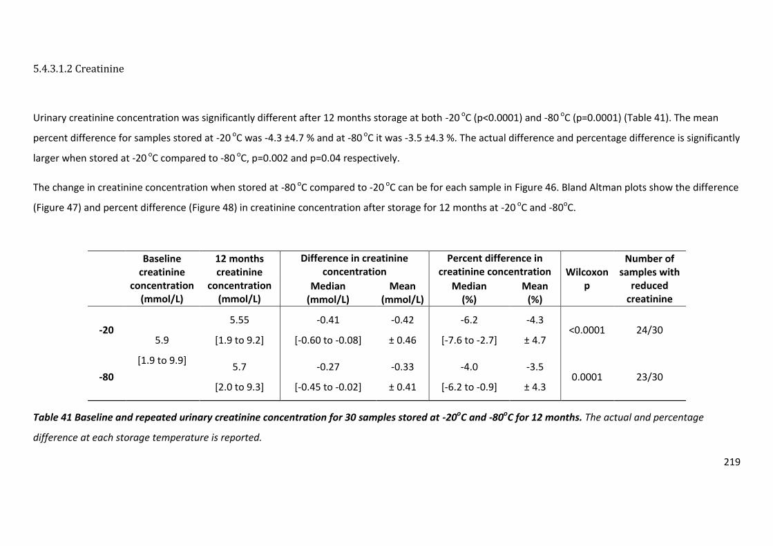
219

5.4.3.1.2 Creatinine

Urinary creatinine concentration was significantly different after 12 months storage at both -20 oC (p<0.0001) and -80 oC (p=0.0001) (Table 41). The mean

percent difference for samples stored at -20 oC was -4.3 ±4.7 % and at -80 oC it was -3.5 ±4.3 %. The actual difference and percentage difference is significantly

larger when stored at -20 oC compared to -80 oC, p=0.002 and p=0.04 respectively.

The change in creatinine concentration when stored at -80 oC compared to -20 oC can be for each sample in Figure 46. Bland Altman plots show the difference

(Figure 47) and percent difference (Figure 48) in creatinine concentration after storage for 12 months at -20 oC and -80oC.

Table 41 Baseline and repeated urinary creatinine concentration for 30 samples stored at -20oC and -80oC for 12 months. The actual and percentage

difference at each storage temperature is reported.

Baseline

creatinine concentration

(mmol/L)

12 months creatinine

concentration (mmol/L)

Difference in creatinine concentration

Percent difference in creatinine concentration Wilcoxon

p

Number of samples with

reduced creatinine

Median (mmol/L)

Mean (mmol/L)

Median (%)

Mean (%)

-20 5.9

[1.9 to 9.9]

5.55

[1.9 to 9.2]

-0.41

[-0.60 to -0.08]

-0.42

± 0.46

-6.2

[-7.6 to -2.7]

-4.3

± 4.7 <0.0001 24/30

-80 5.7

[2.0 to 9.3]

-0.27

[-0.45 to -0.02]

-0.33

± 0.41

-4.0

[-6.2 to -0.9]

-3.5

± 4.3 0.0001 23/30

220

Figure 46 Change in urinary creatinine concentration in 30 individual samples after 12 months storage at A: -20oC, B: -80oC.

0

5

10

15

20

25

Baseline 12 months

Uri

nar

y cr

eat

inin

e c

on

cen

trat

ion

[m

mo

l/L]

-20 storage

0

5

10

15

20

25

Baseline 12 months

Uri

nar

y cr

eat

inin

e c

on

cen

trat

ion

[m

mo

l/L]

-80 storage A B

221

Figure 47 Bland Altman plots to show the difference in creatinine concentration when stored at A: -20oC, B: -80 oC, after 12 months storage. The shaded

orange area demonstrates the inter-assay variability of the Jaffe method. The green line represents the mean difference in creatinine concentration with the

95% confidence intervals indicated with red lines of 30 samples. Mean (±SD) difference in creatinine concentration was = -0.42 ± 0.46mmol/L when stored a t -

20oC (A), and -0.33 ± 0.41 mmol/L at -80 oC (B).

A B

222

Figure 48 Bland Altman plots to show the percent difference in creatinine concentration when stored at A: -20oC, B: -80 oC, after 12

months storage. The shaded orange area demonstrates the inter-assay variability of the Jaffe method. The green line represents the

mean percent difference in creatinine concentration with the 95% confidence intervals indicated with red lines of 30 samples. Mean (±SD)

percent difference in creatinine concentration was = -4.3 ± 4.7% when stored a t -20oC (A), and -3.5 ± 4.3% at -80 oC (B).

C D

A B

223

5.4.3.1.3 ACR

There is a significant loss in ACR when stored at -20oC for 12 months (p<0.0001), although there is no significant difference when stored at -80 oC (p=0.91)

(Table 42). The mean percentage difference when stored at -20oC was -34.3 ±34.6% whereas at -80 oC it was 1.1 ±14.6% (Table 42).

The change in ACR when stored at -80 oC compared to -20 oC is visualised in Figure 49. Bland Altman plots show the difference (Figure 50) and percent

difference (Figure 51) in ACR after storage for 12 months at -20 oC and -80oC.

Baseline

ACR

(mg/mmol)

12 months

ACR

(mg/mmol)

Difference in ACR Percent difference in ACR Wilcoxon

p

Number of

samples with

reduced ACR Median

(mg/mmol) Mean

(mg/mmol) Median

(%) Mean

(%)

-20 0.52

[0.45 to 0.80]

0.38

[0.20 to 0.63]

-0.16

[-0.30 to -0.06]

-0.21

± 0.23

-23.9

[-61.6 to -12.3]

-34.3

± 34.6 <0.001 26/30

-80 0.54

[0.42 to 0.84]

0.001

[-0.07 to 0.07]

0.002

± 0.12

-0.21

[-12.6 to 12.7]

1.1

± 14.6 0.91 16/30

Table 42 Baseline and repeated ACR for 30 samples stored at -20oC and -80oC for 12 months. The actual and percentage difference at each storage

temperature is reported.

224

Figure 49 Box and whisker plots to show the distribution of ACR from 30 samples at baseline and after 12 months storage at -20oC and -80 oC. The

horizontal line inside the box represents the median, the edges of the box are the upper and lower interquartile and the whiskers represent the minimum and

maximum values, with outlying results individually plotted. There is a significant loss in ACR when stored at -20oC for 12 months (p<0.0001), although there is

no significant difference when stored at -80 oC (p=0.91)

0

.5

1

1.5

Alb

um

in t

o c

reatinin

e r

atio [m

g/m

mol]

Baseline -20 -80

225

Figure 50 Bland Altman plots to show the difference in ACR when stored at A: -20oC, B: -80 oC, after 12 months storage. The shaded orange area

demonstrates the inter-assay variability of the albumin and creatinine assays. The green line represents the mean difference in ACR with the 95% confidence

intervals indicated with red lines of 30 samples. Mean (±SD) difference in ACR was = -0.21 ±0.23 mg/mmol/L when stored a t -20oC (A), and -0.002 ±0.12

mg/mmol/L at -80oC (B).

A B

D

226

Figure 51 Bland Altman plots to show the percent difference in ACR when stored at A: -20oC, B: -80oC, after 12 months storage. The shaded orange area

demonstrates the inter-assay variability of the albumin and creatinine assays. The green line represents the mean percent difference in ACR with the 95%

confidence intervals indicated with red lines of 30 samples. Mean (±SD) percent difference in ACR was -34.3 ±34.6% when stored a t -20oC (A), and 1.1 ± 14.6%

at -80oC (B).

A B

227

5.4.3.2 Objective 2

To determine how albumin and creatinine concentrations and the assessment of ACR

change over 12 months when stored at -20 oC and -80 oC.

5.4.3.2.1 Albumin

The change in UAC over 12 months is shown as the mean percentage of baseline

measurement in Figure 52. The decline in UAC when stored at -20 oC appears to stabilise

after six months with around 40% of UAC lost. UAC remains stable at -80 oC over 12 months.

Figure 52 Change of urinary albumin concentration in 30 samples over 12 months when

stored at -20oC and -80oC. The left Y-axis shows the percent of baseline UAC at each time

point, reported as the mean and 95% confidence intervals. The right Y-axis is the UAC to

show the quality control measurements (green lines). The shaded region shows the percent

difference which can be attributed to inter-assay variation. Data recorded at 9 months is not

included as QC results were outside the acceptable limits.

228

5.4.3.2.2 Creatinine

The change in creatinine over 12 months is shown in Figure 53. It appears that creatinine is

increasingly lost as time increases, regardless of storage temperature, however this loss is

very small after 12 months (Section 5.4.3.1.2).

Figure 53 Change of urinary creatinine concentration in 30 samples over 12 months when

stored at -20oC and -80oC. Percent of baseline creatinine at each time point is reported as

the mean and 95% confidence intervals. The shaded region shows the percent difference

which can be attributed to inter-assay variation.

229

5.4.3.2.3 ACR

The change in ACR over 12 months is shown as the mean percentage of baseline

measurement in Figure 54. The decline in ACR follows the pattern of urinary albumin. ACR

loss in samples stored at -20 oC whereas ACR remains stable at -80 oC over 12 months.

Figure 54 Change of ACR in 30 samples over 12 months when stored at -20oC and -80oC.

Percent of baseline ACR at each time point is reported as the mean and 95% confidence

intervals. The shaded region shows the percent difference which can be attributed to inter-

assay variation.

230

5.4.3.3 Objective 3

Investigate if additives or low protein binding tubes prevent any loss of albumin, creatinine

and ACR after 12 months storage at -20 oC and -80 oC

5.4.3.3.1 Albumin

The impact different treatments have on preventing the loss of albumin concentration is

visualised in Figure 55. Alkalisation marginally reduced the loss in UAC in samples stored at -

20oC from -36.9 ±33.5% (with no additives) to -29.2 ±30.2%, but still it was significantly

different to when UAC was measured fresh (p<0.001) (Table 43). Storing samples at -20oC

with boric acid or protease inhibitor or in low protein binding tubes did not prevent the loss

of UAC (p values <0.001).

Figure 55 Difference in urinary albumin concentration in 30 samples which have

undergone different treatments prior to being stored at -20oC and -80oC for 12 months.

The shaded region shows the percent difference which can be attributed to inter-assay

variation. Each of the 30 samples had five aliquots taken, each to undergo a different

treatment. The mean UAC (95% confidence intervals) of the 30 samples for each treatment is

reported.

231

Storage

temperature Baseline After storage for 12 months

No additives Alkalisation Boric acid

Protease

inhibitor

Low protein

binding tube

-20oC

Median albumin

concentration

(mg/L)

2.7

[1.7 to 6.3]

1.7

[0.9 to 2.3]

2.5

[1.4 to 4.0]

1.5

[1.0 to 2.0]

1.5

[1.0 to 1.8]

1.5

[0.8 to 2.3]

Mean percent difference -36.9 ±33.5 -29.2 ± 30.2 -38.6 ± 30.8 -42.9 ± 31.7 -39.9 ± 36.2

Wilcoxon p value <0.001* <0.001* <0.001* <0.001* <0.001*

Number decreased 27 (90%) 29 (97%) 28 (93%) 29 (97%) 27 (90%)

-80 oC

Median albumin

concentration

(mg/L)

2.7

[1.8 to 5.4]

2.9

[1.6 to 5.6]

2.5

[1.8 to 4.0]

2.4

[1.6 to 4.8]

2.8

[1.8 to 5.2]

Mean percent difference -2.7 ± 13.2 -4.3 ± 30.1 -9.2 ± 15.7 -14.3 ± 16.6 -2.9 ± 19.4

Wilcoxon p value 0.06 0.78 0.001* <0.001* 0.28

Number decreased 18 (60%) 13 (43%) 23 (77%) 25 (83%) 15 (50%)

Table 43 Change in urinary albumin concentration in 30 samples which have undergone different treatments prior to being stored at -20oC

and -80oC for 12 months. * denotes treatment groups which are significantly different from baseline values.

232

5.4.3.3.2 Creatinine

Urinary creatinine concentration is reduced by freeze thawing, regardless of freezer storage

temperature (Section 5.3.2). None of the treatments prevented the loss in creatinine (Figure

56), with the results after storage remaining significantly different to baseline values

(p=0.0001) (Table 44). The difference in creatinine concentration in alkalised samples stored

at -20oC for 12 months was greatly increased (-15.6 ±24.9%) compared to untreated

samples (-4.3 ±4.7%), although this did not occur in the alkalised samples stored at -80oC (-

4.4 ±4.1%) (Table 44).

Figure 56 Difference in urinary creatinine concentration in 30 samples which have

undergone different treatments prior to being stored at -20oC and -80oC for 12 months.

The shaded region shows the percent difference which can be attributed to inter-assay

variation. Each of the 30 samples had five aliquots taken, each to undergo a different

treatment. The mean creatinine concentration (95% confidence intervals) of the 30 samples

for each treatment is reported.

233

Table 44 Change in urinary creatinine concentration in 30 samples which have undergone different treatments prior to being stored at -20oC

and -80oC for 12 months. * denotes treatment groups which are significantly different from baseline values .

Storage

temperature Baseline No additives Alkalisation Boric acid

Protease

inhibitor

Low protein

binding tube

-20

Median creatinine

concentration

(mmol/L)

5.9

[1.9 to 9.9]

5.6

[1.9 to 9.2]

5.6

[1.7 to 9.1]

5.6

[1.8 to 9.2]

5.5

[1.8 to 9]

5.6

[1.8 to 9]

Mean percent difference -4.3 ± 4.7 -15.6 ± 24.9 -6.2 ± 3.9 -6.5 ± 3.6 -5.1 ± 4.5

Wilcoxon p value <0.0001* <0.0001* <0.0001* <0.0001* <0.0001*

Number decreased 24/30 27/30 27/30 27/30 25/30

-80

Median creatinine

concentration

(mmol/L)

5.7

[2.0 to 9.3]

5.7

[1.8 to 9.4]

5.7

[1.9 to 9.2]

5.5

[1.9 to 9.1]

5.7

[1.9 to 9.5]

Mean percent difference -3.5 ± 4.3 -4.4 ± 4.1 -5.1 ± 4.6 -5.2 ± 4.2 -3.8 ± 4.4

Wilcoxon p value 0.0001* <0.0001* <0.0001* <0.0001* 0.0001*

Number decreased 23/30 27/30 24/30 25/30 24/30

234

5.4.3.3.3 ACR

Alkalisation of samples prior to storage for 12 months at -20oC appears to recover ACR, with

a difference that could almost be explained by the variability of the albumin and creatinine

assays (Figure 57). The difference is still significant with baseline values (p=0.0004) (Table

45) and the reduction of the difference compared to untreated samples can be attributed to

the increased loss of urinary creatinine concentration after alkalisation (Figure 56, Table 44).

The other treatments do not improve the loss of ACR when samples are stored at -20oC. For

samples stored for 12 months at -80oC, the difference with baseline values becomes

positive, again this is the result of lost creatinine due to freeze thawing. Untreated samples

stored at -80oC have the least significant difference after storage (p=0.91).

Figure 57 Difference in ACR in 30 samples which have undergone different treatments

prior to being stored at -20oC and -80oC for 12 months. The shaded region shows the

percent difference which can be attributed to inter-assay variation. Each of the 30 samples

had five aliquots taken, each to undergo a different treatment. The mean creatinine

concentration (95% confidence intervals) of the 30 samples for each treatment is reported.

235

Baseline No additives Alkalisation Boric acid Protease inhibitor

Low protein

binding tube

-20

Median ACR

(mg/mmol)

0.52

[0.45 to 0.80]

0.38

[0.20 to 0.63]

0.42

[0.34 to 0.60]

0.36

[0.19 to 0.64]

0.33

[0.17 to 0.61]

0.35

[0.16 to 0.59]

Mean percent difference -34.3 ± 34.6 -18.8 ± 22.7 -34.5 ± 33.2 -38.2 ± 33.5 -37.0 ± 38.9

Wilcoxon p value <0.0001* 0.0004* <0.0001* <0.0001* 0.0001*

Number decreased 26/30 23/30 27/30 26/30 24/30

-80

Median ACR

(mg/mmol)

0.54

[0.42 to 0.84]

0.54

[0.42 to 0.66]

0.55

[0.40 to 0.78]

0.49

[0.39 to 0.79]

0.56

[0.42 to 0.80]

Mean percent difference 1.1± 14.6 0.50 ± 33.1 -4.1 ± 17.4 -8.8 ± 18.7 1.1 ± 20.1

Wilcoxon p value 0.91 0.67 0.13 0.008* 0.64

Number decreased 16/30 11/30 18/30 21/30 12/30

Table 45 Change in ACR in 30 samples which have undergone different treatments prior to being stored at -20oC and -80oC for 12 months. * denotes treatment groups which are significantly different from baseline values

236

5.4.4 Discussion

5.4.4.1 Objective 1

Determine if there is a difference in albumin and creatinine concentrations and the

assessment of ACR after 12 months storage at -20oC and -80 oC.

5.4.4.1.1 Albumin

There is significant loss of urinary albumin when stored at -20oC for 12 months (p<0.0001),

however there is no significant difference when stored at -80 oC (p=0.06) (Figure 42, Table

40).

This is agreement with the findings that Brinkman and colleagues reported from the

PREVEND study (Brinkman et al., 2007a). They reported a mean loss of UAC, -9.2% (±17.4,

when quantifying samples with an AUC of 200-500mg/L which had been stored at -20oC for

12 months. They also reported a mean loss of UAC, -28% (±33), when quantifying samples

with an AUC of 10-20mg/L which was a significantly lower difference compared the group

assessing higher concentrations of albumin (p<0.05).

Using our validated ELISA (Chapter 2) we have now determined the same pattern continues,

that the proportion of UAC loss increases with the lower concentration of albumin in the

sample. We report mean percent loss of 36 ±33.5 % in samples with an albumin

concentration <11mg/L (p=<0.0001) (Table 40).

Brinkman and colleagues also reported the UAC was stable at -80oC for 12 months

(Brinkman et al., 2007a). We also demonstrate that this is still valid when measuring the

lowest levels urinary albumin excretion.

237

The Bland Altman plots (Figure 44, which show the difference (and percent different) across

the range of UAC, demonstrate the loss of UAC is variable between samples when stored at

-20 oC. This is reflected by the large standard deviation of the mean percent difference (36

±33.5 %). This variability has been reported in previous study at the higher albumin

excretion levels (Townsend, 1986a) (Kania et al., 2010, Brinkman et al., 2007b).

To help identify why some samples are affected more by frozen storage samples underwent

dipstick analysis then sent to microbiology for analysis prior to being stored. There was no

correlation between organisms cultured, white cell count, epithelial cell contamination and

sample pH, with reduced UAC.

There was no correlation for changes in creatinine and the ACR. 30 samples were collected

for this investigation, 20 were random spot samples and 10 were from timed overnight

collections. There was no pattern for the loss of UAC, creatinine or ACR with the sample

collection method.

The Bland Altman plots demonstrate that UAC is stable across the tested range for samples

stored at -80oC (Figure 44), with the difference attributable to inter-assay variability. If all

the samples had a negative (or positive) difference there would be a systematic difference,

but this is not the case. In the low normoalbuminuria range, UAC was stable when stored at

-80 oC for up to 12 months.

5.4.4.1.2 Creatinine

Urinary creatinine concentration was significantly different after 12 months storage at both

-20 oC (p<0.0001) and -80 oC (p=0.0001) (Table 41). The mean percent difference for samples

stored at -20 oC was -4.3 ±4.7 % and at -80 oC it was -3.5 ±4.3 %. The actual difference and

percentage difference is significantly larger when stored at -20 oC compared to -80 oC,

p=0.002 and p=0.04 respectively. When individual results from samples after storage are

plotted against baseline values (Figure 46), it is evident that the magnitude of change is

238

relatively small, although it is still significant. The Bland Altman plots (Figure 48) show that

the loss in creatinine is proportional to creatinine concentration and that the difference

cannot be attributed to inter-assay variation as there is a negative bias, regardless of the

storage temperature.

The earlier investigation showed that freeze thawing caused a significant reduction in

urinary creatinine concentration (Table 38). The mean difference after one freeze thaw cycle

at -80oC was -0.6 ± 1.4 %, although in this experiment it is much larger; -3.5 ±4.3 %. The

difference between the two methods is that samples have been stored for 12 months,

suggesting that urinary creatinine may degrade over time. This is investigated further in the

final investigation of this chapter (Section 5.5).

5.4.4.1.3 ACR

There is a significant loss in ACR when stored at -20oC for 12 months (p<0.0001), although

there is no significant difference when stored at -80 oC (p=0.91). The mean percentage

difference when stored at -20oC was -34.3 ±34.6% whereas at -80 oC it was 1.1 ±14.6%

(Table 42). The stability of ACR when stored at -80 oC compared to -20 oC can be seen in

Figure 49 when examining the repeated results with their baseline values. The Bland Altman

plots show the difference (and percentage difference) across the range of ACR (Figure 51).

Overall, when storing at -80 oC, the majority of the change in ACR can be explained by the

inter-assay variability of both the albumin and creatinine assays. However, there are several

samples which cannot be explained by assay variability and it is these samples that have

experienced the largest decline in creatinine concentration.

Whilst the degradation of creatinine might be relatively small, as it is being used as the

denominator in the ACR, the effect is amplified, falsely elevating the ACR. This study has

only investigated the change of albumin/creatinine and ACR over 12 months, if creatinine

continues to degrade then the difference in ACR might become significantly different.

239

After 12 months storage at -80 oC, UAC is stable but creatinine is not. Although the ACR is

not statistically significantly different, it is affected by creatinine degradation, which is

studied in more detail in the final investigation of this chapter (Section 5.5).

5.4.4.2 Objective 2

Determine how albumin, creatinine and ACR change over 12 months when stored at -20 oC

and -80 oC.

5.4.4.2.1 Albumin

The decline in UAC when stored at -20 oC appears to stabilise after six months with around

40% of UAC lost (Figure 52). However, UAC remains stable at -80 oC with the difference

attributed to inter-assay variation.

Our findings are very similar to those from the PREVEND study which reported that after 18

months storage at -20oC, there was a significant loss loss in UAC; -23.7% (±26.2) (p<0.05).

Post hoc analysis showed that after 8 months of storage, the difference in UAC had

stabilised to around -25% to -30% (Brinkman et al., 2005)

5.4.4.2.2 Creatinine

The change in creatinine over 12 months is shown in Figure 53. From earlier work (Table 38)

a single freeze thaw caused a significant loss in urinary creatinine concentration (-0.6 ±

1.4%, p=0.02). The impact of a freeze thaw cycle is evident at six and nine months, although

creatinine concentration continues to decline at 11 and 12 months. This suggests that

creatinine slowly degrades during frozen storage after 9 months, although this cannot be

confirmed as the storage duration is limited to 12 months, and only a few time points were

240

sampled. The loss of creatinine was shown to be greater when stored at -20 oC compared to

-80 oC (Table 41). After 11 months storage this appears to be true, the mean creatinine

difference is greater for samples stored at -20 oC, although this is less evident at 12 months.

The degradation of creatinine over a longer time period is investigated in the next

investigation presented in this chapter (Section 5.5).

5.4.4.2.3 ACR

The change in ACR over 12 months (Figure 54) follows the same pattern as UAC (Figure 52).

However, due to the possible degradation of creatinine, the ACR may be falsely elevated.

Due to the stability of UAC when stored at -80 oC, the ACR appears stable as well. However,

due to the decline in UAC when stored at -20 oC, the ACR is also reduced. Each sample had

many aliquots taken, so the change in ACR will be monitored over a longer time.

5.4.3.3 Objective 3

Investigate if additives or low protein binding tubes prevent any loss of albumin, creatinine

and ACR after 12 months storage at -20 oC and -80 oC?

5.4.4.3.1 Albumin

UAC is lost when stored for 12 months at -20oC and this investigation examined if it may be

prevented by the use of additives or specialised storage tubes. This would help to develop a

method to store samples at -20oC when freezing at -80oC is not available. The additives and

tubes used in this study have not prevented the loss of UAC at -20 oC (Figure 55). Alkalisation

marginally reduced the loss in UAC from -36.9 ±33.5% (with no additives) to -29.2 ±30.2%,

but still it was significantly different (p<0.001) and more samples had decreased UAC (90%

241

vs 97% ) (Table 43). Storing samples with boric acid or protease inhibitor or in low protein

binding tubes did not prevent the loss the UAC and all treatments provided results that

were significantly different to baseline values (p values <0.001).

There is no significant difference (p=0.06) in UAC in samples stored for 12 months at -80oC

with no additives (60% of samples had reduced UAC). The number of samples that had a

decline in UAC was reduced in those that had been alkalised, or where low protein binding

tubes had been used; 43% and 50% respectively (Table 43), with the significance further

reduced, p=0.78 and 0.28 respectively. Samples stored with boric acid or protease inhibitor

had a greater difference in UAC; -9.2± 15.7% and -14.3 ±16.6% and were both significantly

different from baseline values, p=0.001 and <0.001 respectively. It is possible that boric acid

and the protease inhibitor interfere with the assay which might cause lower results; it is

unlikely to be a dilution effect, as it would only account for a difference of 1% due to the

small volumes added.

Our results disagree with the findings of Lambers Heerspink and colleagues, who reported

that urine alkalisation prevents the decline in UAC associated with 12 months frozen storage

at −20°C (Lambers Heerspink et al., 2009). They reported a median change of UAC of -

13.67% in untreated samples stored for 12 months at -20oC, compared to +2.4% in alkalised

samples. In our investigation the mean loss of UAC was -39.6% and -29.2% in treated and

untreated samples respectively. There are differences between the methodologies which

might explain this; only urine samples from patients with DM, which had an UAC >5.0 mg/L,

were included in their study which resulted in a median baseline UAC of 15.5 [8.6–39.4]

mg/l from 90 samples. In our investigation, samples were collected from healthy controls

and the median baseline UAC was 2.7 [1.7 to 6.3] mg/L. The difference between the studies

could be attributed to testing in the different albuminuria ranges and on different

populations. However, in their method they stated that they weighed every sample before

and after the addition of sodium hydroxide to correct UAC for the added volume. We did

not do this, 15µl of NaOH 1M was added to 10ml of every sample, which would dilute the

sample by 0.15%, as it is such a small error it was deemed negligible and the UAC was not

adjusted in the analysis. Their study reported the mean addition of NaOH 1M was 00.2 ±

242

0.002 ml, which is very similar to our 15µl volume. There does not appear to be an issue

with their adjustment of samples which have been alkalised, as the change in UAC for

samples which were treated and not treated when stored at -80oC were similar, 5.6% and

5.4% respectively.

This investigation does not support the findings of Kania and colleagues, which showed

pepstatin inhibited the degradation of endogenous and exogenous albumin in in-vitro

studies (Kania et al., 2010). To our knowledge our investigation is the first study that has

investigated the use of pepstatin to inhibit UAC degradation in samples stored at -20 oC over

12 months. However, there was no reduction in UAC degradation when adding pepstatin to

samples. This may be a methodological issue; the effective concentration recommended by

the manufacturer is designed to prevent the degradation of authophagic cargo in

autophagosomes, a very different working environment to inhibiting the degradation of

albumin in urine. The same pepstatin product (Sigma Aldrich product number: P5318,

Sigma Aldrich, Missouri, USA) was used in our study and in the in-vitro study by Kania et al.

Both studies followed manufacturer recommendations when preparing pepstatin working

solutions to add to samples.Further work is required to ensure an effective concentration of

pepstatin is used in future studies investigating its use to prevent UAC degradation in urine

samples stored at -20oC.

There is no evidence UAC is preserved when storing samples in boric acid and there was no

correlation between microbial growth and samples which lost UAC, suggesting bacterial

contamination is not responsible for the loss of UAC. Low protein binding tubes did not

inhibit the loss of UAC at -20oC, which indicates albumin is not being adsorbed to the

storage containers.

Our results indicate that if ACR cannot be measured on a fresh sample, then it should be

stored at -80oC, and it is insufficient to store it at -20oC, regardless if any additives or low

protein binding tubes are used.

243

5.4.4.3.2 Creatinine

Previous studies have failed to identify and investigate the impact of additives on creatinine

and the overall assessment of ACR during prolonged storage. Our results have identified

that creatinine is lost due to freeze thawing, regardless of sample treatment and storage

temperature (Figure 56). None of the treatments prevented the loss in creatinine, with the

results after storage remaining significantly different to baseline values (p=0.0001) (Table

44). The difference in creatinine concentration in alkalised samples stored at -20oC for 12

months was greatly increased (-15.6 ±24.9%) compared to untreated samples (-4.3 ±4.7%),

although this did not occur in the alkalised samples stored at -80oC (-4.4 ±4.1%). Therefore,

alkalisation of samples either increases the degradation of creatinine when stored at -20oC,

or it affects the creatinine assay, although this is unlikely as it did not occur in the samples

stored at -80oC (Table 44).

5.4.4.3.3 ACR

Alkalisation of samples prior to storage for 12 months at -20oC appears to recover ACR, with

a difference that could almost be explained by the variability of the albumin and creatinine

assays (Figure 57). The difference is still significant (p=0.0004) (Table 45) and the reduction

of the difference compared to untreated samples can be attributed to the increased loss of

urinary creatinine concentration after alkalisation. The other treatments do not improve the

loss of ACR when samples are stored at -20oC. For samples stored for 12 months at -80oC,

the difference with baseline values becomes positive, again this is the result of lost

creatinine due to freeze thawing. Untreated samples stored at -80oC have the least

significant difference after storage (p=0.91). In light of these observations untreated

samples would be the preferred method to store samples frozen for 12 months when

measuring albumin, creatinine and the ACR.

244

5.5 The effect of storage duration on albumin and creatinine levels

and the calculation of ACR in samples stored at -80oC

5.5.1 Method

Urine samples from 91 participants of the SUMMIT study were selected for this

investigation. Samples were chosen to cover a wide range of urinary albumin concentrations

and storage times. An aliquot from each sample was sent to the RD&E Blood science

laboratory for routine analysis of albumin and creatinine on the day of collection. Albumin

was measured by the routine COBAS method (Roche Diagnostics Ltd., Burgess Hill, UK) and

creatinine was quantified using the routine Jaffe method (Roche Diagnostics Ltd., Burgess

Hill, UK). Remaining aliquots were stored at -80oC on the day of collection.

The samples were collected over three years and a stored aliquot of the selected samples

were all analysed on the same day once the study was complete. Samples were thoroughly

thawed and mixed by four hand inversions prior to analysis.

The same assays were used to measure albumin and creatinine when samples were fresh

and after storage. However, new analysers had been installed and validation work carried

out by engineers revealed a bias between the old and new analysers. The bias for the

urinary albumin assay is shown in Table 46 and for the urinary creatinine assay in Table 47.

Unfortunately, in the albumin assay validation no samples with a concentration <7mg/L

were tested.

Urinary albumin

concentration range

(mg/L)

Number of samples Mean bias

(mg/L)

Mean percent bias

(%)

7 to 40 9 -1.96 -14.7

40 to 150 3 -4.90 -9.3

Table 46 New COBAS analyser validation result for urinary albumin.

245

Urinary creatinine

concentration

range

(mmol/L)

Number of

samples

Mean bias

(mmol/L)

Mean Percent Bias

(%)

0 to 5 6 0.16 5.6

5 to 10 16 0.28 3.8

10 to 25 3 0.32 2.2

Table 47 New COBAS analyser validation results for urinary creatinine.

5.5.1.1 Statistical analysis

To determine if there is a correlation between the difference in albumin/creatinine or ACR

with duration of storage at -80oC, a difference plot (actual difference and percentage

difference) over time is used. The mean difference is plotted with 95% confidence intervals.

Normality of the data was tested using the Shapiro-Wilkes test. For non-normally

distributed data Spearman’s rank correlation test was used to investigate the relationship

between difference and duration of storage. The correlation is tested for both actual and

percentage difference. For each correlation the Rs and Rs 2 is reported along with the

significance of the correlation (p) and the coefficient to show the rate of change over time.

246

5.5.2 Results

5.5.2.1 Albumin

The difference plot for actual difference in UAC against storage time indicates that UAC loss

becomes less with time (Figure 58A) and that there is a significant correlation to reinforce

this (RS= 0.48, p=<0.001) (Table 48). However, this is not the case. Patients in the SUMMIT

study with CVD were recruited last, therefore the samples with the largest UAC have had

the shortest storage duration. This is reflected by the difference plot (Figure 58B) that

shows the proportional difference and demonstrates that there is no significant correlation

with UAC change over time (RS= -0.19, p= 0.07) (Table 48).

247

Figure 58 Difference in urinary albumin concentration in 91 samples stored at -80oC over

850 days (A: actual difference, B: percent difference). The green line represents the mean

difference in UAC with the 95% confidence intervals indicated with red lines. Mean difference

is -2.4 ±4.4 mg/L and the mean percent difference is -11.2 ±13.2 % compared to fresh

samples.

-30

-20

-10

0

10

20

30

Diffe

rence in

alb

um

in c

oncentr

ation [m

g/L

]

0 200 400 600 800 Time in -80 freezer [days]

-40

-30

-20

-10

0

10

20

30

40

Perc

ent diffe

rence in

alb

um

in c

oncentr

atio

n [%

]

0 200 400 600 800 Time in -80 freezer [days]

A

B

248

RS RS2 p Coefficient

Actual difference 0.48 0.23 <0.001 0.01

Percent difference -0.19 -0.04 0.07 -0.01

Table 48 Correlation between change in UAC and duration of storage at -80oC in 91

samples.

5.5.2.2 Creatinine

Urinary creatinine degrades over 850 days when stored at -80oC in 91 urine samples (Figure

59). This is confirmed by a strong significant correlation for both actual difference and

percent difference; RS = -0.95, p <0.0001 and RS = -1.00, p <0.0001, respectively (Table 49).

Due to the difference in analysers it appears creatinine concentration is increased after

short storage duration, however this can be attributed to the application of the new

analyser which has a positive bias of 5.6% in the 0 to 5 mmol/L range (Table 47).

249

Figure 59 Difference of creatinine over 850 days in 91 samples stored at -80oC (A: actual

difference, B: percent difference). The green line represents the mean difference in

creatinine concentration with the 95% confidence intervals indicated with red lines. Mean

difference is -0.1 ±0.3 mmol/L and the mean percent difference is -0.5 ±3.8 % compared to

fresh samples.

-1

-.5

0

.5

1

Diffe

rence in

cre

atin

ine c

oncentr

atio

n [m

mol/L]

0 200 400 600 800 Time in -80 freezer [days]

-10

-5

0

5

10

Perc

ent diffe

rence in

cre

atin

ine c

oncentr

atio

n [

%]

0 200 400 600 800 Time in -80 freezer [days]

B

A

250

RS RS2 p Coefficient

Actual difference -0.95 -0.90 <0.0001 -0.001

Percent difference -1.00 -0.99 <0.0001 -0.016

Table 49 Correlation between change in creatinine and duration of storage at -80oC in 91

samples.

It appears urinary creatinine degrades during prolonged storage at -80oC. This was

investigated further by testing an additional 360 urine samples from different participants in

the SUMMIT study. The combined results of the 360 samples and 91 samples from the

previous experiment are presented in Figure 60.

Figure 60 Urinary creatinine degradation during prolonged storage at -80oC over three

years . The percent difference in creatinine has been adjusted to account for the bias of the

new analyser using the validation results reported in Table 47. Linear regression was used to

determine the rate of degradation over 541 days, the regression coefficient/gradient was -

0.024% / day (CI: -0.029 to -0.019).

-40

-3

0

-20

-1

0

0

10

20

30

40

Perc

ent

diffe

rence in

cre

atinin

e [%

]

0 200 400 600 800 1000 Storage duration [days]

251

The results seen in Figure 60 indicate that urinary creatinine degrades and then stabilises.

Segmented regression analysis was performed to identify that at 541 days (CI: 483 to 599)

the degradation of creatinine stabilises. Linear regression was used to determine the rate of

degradation over 541 days, the regression coefficient/gradient was -0.024% / day (CI: -0.029

to -0.019).

5.5.2.3 ACR

The change in ACR over 850 days when stored at -80oC (Figure 61) reflects the same pattern

seen in the change of UAC (Figure 58). ACR distribution is also skewed as a result of

recruiting CVD patients at the end of the study, showing a positive correlation for actual

difference in ACR with storage duration (RS = 0.62, P<0.0001) (Table 50). However, no

significant correlation is found for percentage difference (RS = 0.02, P = 0.87). The mean

percentage difference is -10.7 ±13.3%, which can be explained by variability of the assays

and the change of analyser.

252

Figure 61 ACR difference over time in samples stored at -80oC over 850 days (A: actual

difference, B: percent difference). The green line represents the mean difference in ACR with

the 95% confidence intervals indicated with red lines. Mean difference is -0.71 ±2.13

mg/mmol and the mean percent difference is-10.7 ±13.3 % compared to fresh samples.

RS RS2 p Coefficient

Actual difference 0.62 0.38 <0.0001 0.004

Percent difference 0.02 0.00 0.87 0.002

Table 50 Correlation between change in ACR and duration of storage in 91 samples over

850 days at -80oC.

-15

-10

-5

0

5

10

15

Diffe

rence in

AC

R [m

g/m

mol]

0 200 400 600 800 Time in -80 freezer [days]

-40

-30

-20

-10

0

10

20

30

40

% d

iffe

rence in

AC

R [%

]

0 200 400 600 800 Time in -80 freezer [days]

B

A

253

5.5.3 Discussion

5.5.3.1 Albumin

Patients in the SUMMIT study with CVD were recruited last, therefore the samples with the

largest UAC have had the shortest storage duration. This is reflected by the difference plot

(Figure 58) that shows the proportional difference and demonstrates that there is no

significant correlation with UAC change over time (RS= -0.19, p= 0.07) (Table 12). The mean

difference is -11.2 ± 13.2%, which can be accounted for by not only inter-assay variation but

also the variation caused by using different analysers. The validation work showed the new

analysers provide UAC results with a -14.7% bias in the 7 to 40mg/L range. This

demonstrates how important it is to ensure that the same assay is used on the same

analysers in clinical trials and long term storage studies. However, this is not always

possible, as was the case in this study. It is therefore necessary to carry out validation work

to account for variability.

5.5.3.2 Creatinine

Urinary creatinine degrades over time when stored at -80oC (Figure 59). This is supported by

a strong significant correlation for both actual difference and percent difference; RS = -0.95,

p <0.0001 and RS = -1.00, p <0.0001, respectively (Table 49). Due to the difference in

analysers it appears creatinine concentration is increased after short storage duration,

however this can be attributed to the application of the new analyser which has a positive

bias of 5.6% in the 0 to 5 mmol/L range (Table 47).

Degradation of urinary creatinine is an important finding and warranted further

investigation to determine if the rate of degradation continues in stored samples over a

longer duration. Many studies (especially epidemiological research) store samples for many

years prior to analysis and the accuracy of results will be influenced by creatinine

254

degradation, especially when using it as a denominator in a ratio to account for urinary

concentration.

To investigate this further, an additional 360 urine samples were reanalysed, of which some

had been stored for over 1000 days. The combined results of the 360 samples and 91

samples from the previous experiment (Figure 60) demonstrate that urinary creatinine

degrades at a rate of 0.024% / day (CI: -0.029 to -0.019) up until 541 days (CI: 483 to 599) at

which point degradation stabilises. The results in Figure 60 were adjusted to account for

differences caused by the new analyser (Table 47). Samples which had been measured on

the day of collection by the new analysers were not adjusted. From the results of this

analysis, an equation can be created (Equation 1) to correct for the loss in urinary creatinine

in samples stored at -80oC prior to analysis.

Corrected Urinary = Measured creatinine concentration x 100 Creatinine concentration (100 – (0.029 x days stored *)

*input 541 for samples stored more than 541 days

Equation 1 Correcting for urinary creatinine degradation after storage at -80oC.

As a result of this finding, urinary creatinine results from samples stored in the SUMMIT

study will be adjusted using this equation. This is important as it improves the accuracy of

reporting an ACR from stored samples, which is essential when investigating the relationship

of ACR in the normoalbuminuria range with sensitive measures of vascular function.

5.5.3.3 ACR

Although creatinine degradation occurs, the magnitude of it is not enough to cause the ACR

result to significantly increase with storage time. However, the accuracy of an ACR to report

urinary albumin excretion in samples stored at -80oC is impaired, and is suboptimal when

255

investigating the lowest levels of albumin excretion. Accounting for the rate of creatinine

degradation will improve this accuracy.

5.6 Chapter Summary

5.6.1 Albumin

Other studies have reported that the loss of UAC in samples stored at -20oC can be

prevented by; alkalising samples, adding protease inhibitors and using specialised storage

tubes. These findings have been incorporated into our study to help identify the optimal

method to store urine samples to assess low levels of albumin excretion. Several authors

have suggested that bacterial contamination is the cause of lost UAC, therefore all samples

were cultured, but no correlation was found.

The results from this study show that UAC is unaffected by freeze thawing (up to 5 cycles).

However, a significant loss of UAC occurs in samples stored at -20oC. The decline in UAC

appears to stabilise by six months with around 36% of UAC lost. This is similar to previous

findings which have shown UAC to stabilise at around 30% loss after 8 months storage at -

20oC (Brinkman et al., 2005). None of the additives tested prevented the loss in UAC.

UAC in the normoalbuminuria range is stable when stored for up to 12 months at -80oC, any

difference between measurements can be explained by inter-assay variation. Using the

COBAS method to quantify albumin in SUMMIT samples revealed that UAC is stable for up

to 850 days at -80oC. Therefore, if timed collections cannot have UAC measured fresh, then

they must be stored at -80oC. However, many studies use random spot samples and report

the ACR, therefore the impact of frozen storage on creatinine was also investigated.

256

5.6.1 Creatinine

There is a significant difference in urinary creatinine concentration after freeze thawing,

which doesn’t increase with the number of cycles. However, this difference is small and

does not affect the ACR. After 12 months storage the difference in creatinine was larger

than a freeze thaw cycle (at both -20oC and -80oC), suggesting creatinine is degrading over

time. This was confirmed by reanalysing SUMMIT samples, where a strong correlation of

loss of creatinine with storage duration was found. Upon further investigation creatinine

was found to degrade at a rate of 0.024% / day for 541 days and then it stabilises. This

information has enabled an equation to be created which can adjust a creatinine

measurement to account for degradation (Equation 1). However, the deterioration of

creatinine did not significantly impact the ACR in samples stored over 12 months.

Creatinine degradation is an important finding, as many epidemiological studies store

samples for many years prior to analysis, and will need to account for creatinine

degradation when using it to account for variation in urinary concentration. In the SUMMIT

study, some baseline random spot samples have been stored for 5 years at -80oC prior to

ACR measurement. The creatinine measurements will be adjusted using Equation 1 in these

samples.

5.6.1 ACR

Although creatinine degradation occurs during prolonged frozen storage, the magnitude of

it is not enough to cause the ACR result to significantly increase. However, the accuracy of

an ACR to report urinary albumin excretion in samples stored at -80oC is impaired, and is

suboptimal when investigating the lowest levels of albumin excretion. Accounting for the

rate of creatinine degradation will improve this accuracy.

257

5.7 Conclusion

Urinary albumin is stable over prolonged storage at -80 oC, however creatinine degrades at a

rate of 0.024% / day for 541 days and then stabilises. Accounting for the rate of creatinine

degradation will improve the accuracy of an ACR to report urinary albumin excretion in

samples stored at -80oC.

258

Chapter 6 Impact of Exercise on Urinary Albumin Excretion

Kidney disease, urinary tract disorders, fever, heart failure and exercise have all been shown

to increase AER (Lillehoj and Poulik, 1986). Transient changes in AER after exercise has been

documented in the clinical ranges, but the extended lower range has not been investigated.

Not only is it important to understand the biological variation of albumin excretion at low

levels (Chapter 4), it is important to understand how much albumin excretion can be

influenced by additional factors, such as exercise. This needs to be understood first before

interpreting results from studies investigating the lowest levels of albumin excretion.

The influence of exercise on albumin excretion in healthy individuals will be investigated

using the validated sensitive ELISA (Chapter 2), when reporting the ACR (Chapter 3) from

samples being collected using the appropriate method (Chapter 4), which have been stored

at -80oC (Chapter 5).

6.1 Introduction

In 1978, Viberti and colleagues investigated exercise induced macroalbuminuria by

recruiting 16 patients with T1DM and nine healthy controls (Viberti et al., 1978). AER was

measured before exercise and again one hour after (cycling at 98W for 20 mins, mild

intensity exercise). The results showed that participants with T1DM had a significant

increase in AER (p<0.01), but there was no significant difference in the control group (Figure

62).

The diabetic group was divided into two subgroups, group 1 had a resting AER in the same

range as the controls (n=8) and group 2 had a higher baseline AER (n=8). By separating the

diabetic groups, the control group can be compared to patients with T1DM who had similar

259

resting AER. The increase in diabetic group 1 is much more than the controls, indicating DM

per se increases susceptibility to exercise induced albuminuria, potentially an earlier marker

of renal damage, which would not be detected from an overnight collection (Viberti et al.,

1978).

Figure 62 Changes in urinary albumin excretion after exercise in controls and in

participants with diabetes. Participants with diabetes were divided into two groups,

participants with rest AER in the range of the controls are in group 1. Only participants with

T1DM had a significant increase in AER (p<0.01) after cycling at a mild intensity for 20

minutes (Viberti et al., 1978).

6.1.1 Mechanisms of exercise induced albuminuria

Identifying raised AER after exercise in individuals with DM but not in healthy controls has

been reported in studies prior to Viberti’s work (Mogensen, 1976, Mogensen and Vittinghus,

1975), but the mechanism of how it arises was not understood. Previous authors had

speculated that exercise induced albuminuria was the result of increased glomerular

260

filtration pressure, decreased tubular reabsorption or changes in glomerular permeability,

although there was nothing conclusive to support these.

Given that 90% of albumin is reabsorbed by the proximal tubules, increased AER after

exercise can either be from increased trans-glomerular passage and/or by reduced albumin

reabsorption by the proximal cells. β-2-microglobuin (B2M) excretion can be measured to

differentiate between raised AER from increased trans-glomerular passage or reduced

proximal reabsorption. B2M is a marker of tubular function. The proximal tubules normally

reabsorb B2M so an increased B2M urinary excretion indicates reduced tubular function.

Therefore, increased AER with normal B2M excretion indicates increased glomerular

passage of albumin and not decreased proximal tubular reabsorption (Peterson et al., 1969).

Subsequently, an increase in the ratio of albumin/B2M suggests glomerular albuminuria and

a decreased ratio is an index for tubular albuminuria.

Viberti and colleagues also measured the excretion of B2M in their study and reported the

change in albumin/B2M ratio after exercise (Figure 63).

261

Figure 63 Changes in urinary albumin/β2-microglobulin ratio after exercise in controls and

in participants with diabetes (Viberti et al., 1978).

The change in albumin/B2M ratio suggests that the observed increase in AER resulted from

glomerular changes, either increased permeability to albumin or increased glomerular

filtration pressure, and not due to reduced tubular reabsorption. Hypertension is associated

with increased AER (Mani, 2016), although in Viberti’s study there was no correlation in the

change of systolic blood pressure with change in albumin excretion in both the diabetic

group and the controls. This could be due to the low sample size (n=25) tested in Viberti’s

study. Viberti concluded that it is unlikely that the change of AER after exercise is caused by

an ‘abnormal’ cardiovascular response (Viberti et al., 1978). This broad conclusion might

not be appropriate, as it does not consider that change in brachial pressure may not reflect

changes in glomerular pressures. If autoregulation is failing in the patients with diabetes

then glomerular pressures may be increasing more in patients with diabetes than in control

participants, influencing filtration of albumin. Impaired autoregulation has been

demonstrated in patients with T2DM (n=25) compared to controls matched by sex and age

262

(n=25) (Tur et al., 1991). The relationship between urinary albumin excretion and

autoregulation is investigated in SUMMIT cohort in Chapter 7.

The change in glomerular permeability during exercise has not been thoroughly

investigated, probably due to the challenge of measuring glomerular permeability in-vivo.

Increased glomerular permeability might arise from increased shedding of the glycocalyx

(Satchell and Tooke, 2008). However, one study on 21 young, healthy men demonstrated

that there was no significant change in serum syndecan-1 and heparan sulphate

concentrations (markers of glycocalyx shedding) after maximal incremental cycling exercise

until exhaustion (Majerczak et al., 2016). The links between glycocalyx shedding and urinary

albumin excretion have been investigated in in patients with T1DM, subjects with T1DM had

endothelial glycocalyx damage, the severity of which is increased in presence of

microalbuminuria (Nieuwdorp et al., 2006). Glycocalyx perturbation and increased vascular

permeability has also been demonstrated in T2DM (Broekhuizen et al., 2010).

The majority of studies that have measured biomarkers of the glycocalyx (especially urinary

biomarkers) have mostly been carried out in animal models, so assays to quantify glycocalyx

markers require validation before testing human samples. Samples from this investigation

are stored for future analysis of glycocalyx markers and also markers of proximal tubule

function.

6.1.2 Exercise induced albuminuria in different cohorts

Increased AER after exercise has been shown in T1DM (Vittinghus and Mogensen, 1981)

and T2DM (Climie et al., 2015). Jefferson and colleagues carried out a study on 40 children

with T1DM and 21 controls, the mean age (range) was 12 years (8 to 16) and showed only

children with T1DM had a significant increase in ACR after cycling for 15 minutes at a

moderate to heavy intensity (Jefferson et al., 1985) The mean duration of diabetes (range)

among the children with T1DM was 9.9 years (0.2 to 11.9), suggesting that increased ACR in

response to cycling occurs early in T1DM. The geometric mean (95% CI) ACR of the control

group (n=21) was 0.0011 (0.004 to 0.032) mg/mg before exercise, and 0.009 (0.003 to

263

0.027) mg/mg after (p>0.05). In the children with diabetes (n=40) ACR was 0.009 (0.003 to

0.0032) mg/mg before exercise and 0.016 (0.003 to 0.089) mg/mg after (p<0.0001). Young

patients with hypertension also have significantly increased AER after moderate exercise

compared to age matched normotensive controls (Pedersen et al., 1981).

In 2011, Koh and colleagues investigated the change in ACR, 1 and 2 hours after a one

kilometre treadmill walking exercise in thirty-five participants with diabetes (three with

T1DM and 32 with T2DM) and nine control subjects, those with diabetes had a range of pre

exercise levels of albumin excretion across the full albuminuria range (Koh et al., 2011).

In accordance with previous studies there was no significant difference in ACR after exercise

in the control groups, although the female controls did exhibit a non-significant trend for an

increase in ACR. Males with diabetes in the normoalbuminuria range did not have a

significant increase in ACR after exercise. However, the females with diabetes did and the

average ACR increased above the microalbuminuria threshold at 1 hour post exercise,

returning to baseline levels by 2 hours (Figure 64). This data indicates that female patients

with diabetes and normoalbuminuria have walking induced increased albumin excretion,

which might represent an early nephropathy. The clinical significance of this data requires

further study, and it is considered in conjunction with results from the SUMMIT cohort in

Chapter 7.

264

Figure 64 Mean ACR in controls and participants with diabetes with normoalbuminuria, at

first morning void, immediately before exercise, 1 h and 2 h after a 1km treadmill walking

exercise. Nine controls and 10 subjects with diabetes were include in the analysis. Sex-

specific cut-off for microalbuminuria for males is a solid line and for females a dashed line.

( ) = Control male, ( )= Control female, ( ) = Male with diabetes, ( ) = Female

with diabetes (Koh et al., 2011).

Both males and females subjects with pre-exercise ACR In the microalbuminuria and

macroalbuminuria ranges had a significant increase in ACR after exercise. In addition, by

taking repeat measurements over time, Koh and colleagues were able to determine that

ACR was not significantly different to pre-exercise ACR 2 hours after exercise was

completed.

Contrary to the findings of previous studies, in 2009 Heathcote and colleagues showed that

ACR was significantly increased in healthy individuals after exercise (Heathcote et al., 2009).

14 healthy women and 16 healthy men were exercised to maximal heart rate or exhaustion

using the Bruce Treadmill protocol. The mean baseline ACR in women was 0.5 ± 0.3

265

mg/mmol and 0.4 ± 0.1 mg/mmol in men. After high intensity exercise this increased to a

mean of 5.6 ± 9.7 and 7.6 ± 17.1 mg/mmol in women and men respectively. Overall, 40% of

the participants had an ACR in the microalbuminuria range after exercise and two

participants were in the macroalbuminuria range. However, samples were collected only 15

minutes after completing the high intensity exercise. All participants had returned to

normoalbuminuria range within 24 hours.

The reason other studies have not seen a change in ACR in healthy individuals is most likely

due to the difference in exercise intensity and the type of exercise exerted. The participants

in the study by Heathcote and colleagues were exercised to maximal heart rate of

exhaustion using a treadmill, whereas in the earlier study by Viberti (where controls had a

non-significant change in ACR) participants cycled at a moderate intensity for 20 minutes

(Viberti et al., 1978). Also the subjects from the Heathcote et al study were younger (mean

age 24 ±2 years in women and 28 ±5 years in men) than the Viberti cohort (mean age 32

±9). Tolerance to exercise induced increase urinary albumin excretion might represent

microvascular autoregulation, which has been proposed as a mechanism to cause increased

urinary albumin excretion, which reflects generalised microvascular function, this is

explored further in Chapter 7.

Studies that have investigated the change in AER after exercise all suffer from low

participant numbers and have used a wide range of methods to induce exercise, making it

challenging to draw comparisons between them. It is not only important to determine at

what intensity of exercise does AER significantly increase, and in what cohorts, but clinically

it is important to know how long AER is increased.

6.1.3 Duration of exercise induced albuminuria

The duration of increased AER after exercise is not well defined. Due to different frequency

of urination between participants, it is very challenging to determine how long it takes for

266

AER to return to resting levels. One study exerted 16 male participants to exhaustion by

cycling at 30W for two minutes then increasing the intensity by 30W every minute. Urine

samples were collected before exercise and then every hour for three hours afterwards

(Table 51) (Poortmans et al., 1989). They reported that AER declined logarithmically after

exercise with a half-life of 54 minutes. The characteristics of the participants in this study

were not described.

Pre-exercise Post exercise

1 hours 2 hours 3 hours

Albumin excretion rate

(µg/min) 15.3 ±1.3 315.6 ±30.0 136.3 ±15.8 63.6 ±12.3

Table 51 Albumin excretion rate before and after exercise in 16 healthy male participants.

16 male participants cycled to exhaustion by cycling at 30W for two minutes then increasing

the intensity by 30W every minute. Urine samples were collected before exercise and then

every hour for three hours afterwards. Data presented as mean ± standard deviation.

(Poortmans et al., 1989).

In Koh’s study of participants with DM, all participants across all the albuminuria ranges had

ACR return to pre-exercise levels within 2 hours after finishing exercise (Koh et al., 2011).

However, in a study on 30 healthy participants who were exercised to exhaustion or

maximal heart rate, AER had returned to the pre-exercise values within 24 hours (Heathcote

et al., 2009). AER could have returned to pre-exercise values sooner but they were unable to

detect this due to sampling frequency as they only sampled at 15mins and 24 hours post

exercise.

The differences between these results can be attributed to the difference in sample

collection frequency and any activity taken between collections. Studies investigating how

long it takes for albumin excretion to return to resting levels need to consider this in their

267

design. Before the recovery of albumin excretion after exercise is determined, it must be

ensured that all the participants undergo the same amount of exercise.

6.1.4 Normalising exercise intensities

Figure 62, which shows individual responses to exercise, demonstrates that regardless of

diabetes status, the change in AER after exercise varies between people. The reason for this

has not been investigated before. If the variation in responses is caused by physiological

changes, then it would be beneficial to carry out a prospective study investigating the

relationship between different responses to exercise with the risk of developing kidney and

cardiovascular disease. Previous studies have considered exercise a suitable provocation

test to unmask underlying glomerular abnormalities (Viberti et al., 1978).

However, the variation in AER response to exercise may not be the result of physiological

differences, but may arise from methodological issues. In the previously discussed studies,

exercise has been tested using a variety of methods; cycling, running, walking and sports,

each using a different measure of intensity and duration of the exercise (until maximal heart

rate (HR) is reached, 80% maximal HR, exhaustion, exercise with a fixed load for 20 minutes,

incremental loads, etc.). However, the same exercise and duration is applied to all the

participants within each study.

A limitation of using the same workload and durations for all participants is that it will affect

people in different ways, depending on their age, gender and fitness. For example, an

inactive individual cycling for 20 minutes at 60W might find it very strenuous, which could

cause a lot of stress on the body, resulting in a large change in AER, whereas a fit individual

who cycles to work every day would find it easy and might have a no change in AER.

Therefore, exercise intensities need to be relative to each individual’s level of fitness, and

personalised work rates can be calculated to ensure the same intensity of exercise is

exerted on all the participants.

268

To determine personalised work rates, exercise physiologists evaluate an individual’s

capacity for dynamic exercise using protocols which measure ventilator and gas exchange

responses to exercise. Cycle ergometry is often used in these protocols as the desired work

intensity (work rate) can be programmed and maintained automatically by adjusting

resistance in relation to cycling rate. Work rate is calculated in watts (W) and cycle

ergometry enables work rate to be increased in increments.

Ramp (incremental) exercise is used in protocols to determine an individual’s capacity for

exercise and is characterised by a linear and continuous increase in work rate (Boone and

Bourgois, 2012). Work rate continues to increase in ramp exercise and the test is only

complete once the individual has reached volitional exhaustion. Throughout the ramp test

ventilatory gas exchange analysis is carried out which provides measures of the metabolic

response to exercise. This breath by breath analysis monitors three parameters:

1. Percent O2

2. Percent CO2

3. Respiratory airflow

Knowing these three factors enables oxygen uptake (VO2) and carbon dioxide output (VCO2)

to be calculated. To establish an individual’s capacity for exercise, there are two markers of

aerobic function that are determined; the gas exchange threshold (GET) and the maximum

oxygen uptake (VO2max).

6.1.4.1 Gas exchange threshold

The GET or anaerobic threshold was first conceptualised in 1964 and is defined as the work

rate at which anaerobic metabolism supplements aerobic mechanisms during progressive

exercise (Wasserman and McIlroy, 1964). Traditionally invasive methods to quantify blood

lactate and bicarbonate concentrations were used to identify the GET (otherwise known as

the lactate threshold). Gas exchange measurements are now widely used and provide a

269

non-invasive method to determine GET. By plotting VC02 against the VO2 during progressive

exercise, the GET is determined by identifying the ‘breakpoint’ (deflection point) in the

slope caused by an increase in VCO2 from bicarbonate buffering lactic acid (Figure 65).

Identifying the GET using this method is known as the V-slope method and the level of work

rate (exercise intensity), which corresponds to this breakpoint, is considered the GET

(Whipp et al., 1981).

Figure 65 Determining the gas exchange threshold using the V-Slope method. GET is

determined from the breaking point in the slope of the relationship between VC02 and VO2.

The work rate which corresponds to the breakpoint is the GET, denoted by black arrow.

(Bergstrom et al., 2013)

6.1.4.2 Maximal oxygen uptake (VO2max)

VO2max is the maximum rate of oxygen consumption during incremental exercise and

reflects the aerobic physical fitness of an individual. VO2max is reached when oxygen

consumption remains at a steady state despite an increase in work rate. The plateau in VO2,

270

which identifies the VO2max, is not always apparent during ramp testing, as participants can

reach exhaustion prior to this. Therefore, the peak VO2 reached can be used to represent

the individual’s peak oxygen consumption (Kaminsky et al., 2014).

To normalise exercise intensity between participants in exercise studies, each participant’s

GET and VO2max (or peak) needs to be determined. Terminology of different exercise

intensities varies between studies and in this investigation two intensities are going to be

utilised: 1) ‘Moderate’ intensity defined as 80% of the work rate of the GET, ensuring

participants undergo exercise which does not require anaerobic metabolism. 2) ‘Heavy’

exercise defined as a 40% change in work rate from the GET to the VO2 peak. This is

summarised in Figure 66. These definitions of exercise thresholds are commonly used in

exercise testing (Jones et al., 2012a).

Figure 66 Classification of different exercise thresholds. ‘Moderate’ intensity is defined as

the 80% of the work rate at the GET (shown in red) ‘Heavy’ exercise is defined as a 40%

change (∆) in work rate from the GET to the VO2 peak (shown in green). The work rate at the

GET (shown in blue) was determined by plotting VC02 against the VO2 using the same

method used in Figure 65.

271

By defining exercise thresholds in this way, work rates will vary between participants, but

each participant will be tested at the same intensity relative to their capacity for exercise.

By normalising the exercise thresholds, a comprehensive investigation into the change of

AER after exercise can be carried out. Using the validated albumin ELISA kit, small changes in

AER can be detected and the influence of exercise in the normoalbuminuria range studied.

6.1.5 Investigating exercise increased albumin excretion in the lower albumin

excretion range

This study will help increase our understanding of the mechanisms underlying the increase

in albumin excretion after exercise, the change in albumin and creatinine were monitored

individually, as well as the change in urine specific gravity (USG). Creatinine and USG are

both markers of urinary concentration (Section 3.4). If only the concentration of albumin

significantly increases after exercise then the ACR is not raised due to increased urinary

concentration or a change in urinary flow, as creatinine and USG are not affected in the

same way.

272

6.2 Aim

To determine the impact of different exercise intensities on urinary albumin excretion in the

normoalbuminuria range in healthy individuals and to explore the underlying mechanisms.

6.2.1 Objectives

1. To examine if ACR changes after different intensities of exercise in young, healthy

individuals

2. To determine if the change in ACR is different between exercise intensities

3. To explore how long it takes for the ACR to return to resting levels after exercise

4. To determine how albumin, creatinine and urine specific gravity change after

exercise to differentiate the effect of exercise on albumin excretion from urinary

concentration and flow.

5. To investigate if the change in ACR after exercise is related to an increase in blood

pressure and heart rate

6. To explore the effect of participants activity levels before exercise and during

recovery on exercise induced changes in albumin excretion

273

6.3 Method

6.3.1 Participant recruitment and screening

11 healthy adults (aged 21-50 years old) were recruited from a database of individuals

interested in hearing about research held by the NIHR Exeter Clinical Research Facility. The

inclusion criteria required participants to have an eGFR > 60ml/min/1.73m2 and an ACR in

the normoalbuminuria range. Participants who had been diagnosed with diabetes,

cardiovascular disease, hypertension or were on antihypertensive medication were

excluded from the study.

The study protocol was reviewed and approved by the University of Exeter Medical School

ethics committee. Written informed consent was obtained from all participants, who then

attended a screening visit, where anthropometric measurements were taken along with a

blood and random urine sample for routine analysis (Section 6.3.4). Blood pressure was

measured five times in the non-dominant arm using a digital blood pressure monitor; with

the mean of the last three measurements representing brachial blood pressure. Participants

then underwent a ramp test to determine their personalised threshold work rates.

6.3.2 Exercise threshold analysis

Ramp test:

The ramp test was carried out using an electronically braked cycle ergometer (Lode

Excalibur Sport, Groningen, The Netherlands) and ventilatory gas exchange analysis was

carried out using the ‘Ultima Cardio O2’ gas analyser and mouthpiece (MGC diagnostics, St

Paul, Minnesota, USA). Prior to testing participants the volume transducer was calibrated

with a 3L precision syringe.

274

The seat height of the ergometer was adjusted to a comfortable height for participants. A

nose and mouth mask connected to the gas analyser was secured to participants and then

they were asked to cycle at a cadence of 60-75 rpm. The initial workload was set at 20W for

3 minutes, then it increased by 15W every 30 seconds. The test stopped at volitional

exhaustion, or when the cadence dropped below 60 rpm and could not return to above 60

rpm despite verbal encouragement. Throughout the test; %O2 intake, %CO2 output and

respiratory airflow was monitored.

Knowing these three factors enables oxygen uptake (VO2) and carbon dioxide output (VCO2)

to be calculated. To establish an individual’s capacity for exercise, there are two markers of

aerobic function that were determined; the gas exchange threshold (GET) and the maximum

oxygen uptake (VO2max), as described above.

The data from the ramp test was sent to University of Exeter Sport Science department to

be independently analysed by Dr Daryl Wilkerson and Dr Anthony Shepherd (lecturers in

exercise physiology) to determine the GET. From these results personalised threshold were

calculated.

Personalised exercise thresholds to test on study visits:

Each participant was asked to carry out the study protocol four times on different days, with

at least 2 days between visits, and all visits completed within 6 weeks. Different exercise

intensities were carried out on each visit in a random order. The personalised intensities

were defined as follows:

1. Resting (sitting for 30 minutes) (control visit)

2. Moderate exercise for 15 minutes (80% of the work rate at the GET)

3. Moderate exercise for 30 minutes (80% of the work rate at the GET)

4. Heavy exercise until volitional exhaustion (40% change in work rate from the GET to

the VO2 peak)

275

Participants cycled at 20W for 3 minutes before the work rate increased according to the

exercise intensity being tested on that visit. This did not occur when ’resting’ was being

tested.

6.3.3 Visit day protocol

Participants were asked to avoid exercise and sexual intercourse, which may affect albumin

excretion, the day before and during the study day. All participants were advised not to start

the study day if they were ill for any reason and women were advised to avoid study visits

during menstruation. During the study participants were questioned about their activities

prior to and during the collection periods, to determine compliance with the protocol.

On each visit day, as soon as the participant wakes up they were asked to put on a

pedometer. Then every time they passed urine they were required to collect a spot

(untimed) sample and record the time of collection and the pedometer reading. After each

time the participant passed urine, they were advised to gradually drink a small bottle

(330ml) of water until the next time they passed urine and to continue doing this

throughout the day. Participants were allowed other liquids, this was to ensure participants

remained hydrated and to reduce the impact of dehydration on the results. Participants

were asked to document everything they ate throughout the day and they were asked to

avoid consuming alcohol and creatine/protein supplements.

Participants attended the Diabetes and Vascular Research Centre at approximately 11am on

visit days. A spot urine sample was collected prior to cycling on the ergometer, at the

predetermined work rate for that visit. Blood pressure was measured five times in the non-

dominant arm using a digital blood pressure monitor before exercising; with the mean of

the last three measurements representing brachial blood pressure. Participants were

encouraged to maintain cycling at a cadence of 60-75 rpm.

After cycling was complete, blood pressure and heart rate were immediately measured

three times on their non-dominant arm, with the highest value reported. Participants were

asked to collect their entire next urine void in a large container within 60 minutes of

276

completing the exercise. After this participants collected a spot urine sample every time

they passed urine up to and including the second pass of urine on the following day.

The patient information sheet is provided at appendix 5, which includes diagrams that

outlines the study protocol.

Figure 67 Diagram representing example urine sample collection times on study days

around an exercise regime. On each visit day, as soon as the participant wakes up they were

asked to put on a pedometer. Then every time they passed urine they were required to

collect a spot (untimed) sample and record the time of collection and the pedometer

reading.

6.3.4 Sample processing

Blood and urine samples taken at the screening visit were sent to the RD&E Hospital Blood

Science department for analysis of blood creatinine, urinary albumin and urinary creatinine.

Albumin was measured using the routine method (COBAS, Roche Diagnostics Ltd., Burgess

Hill, UK), and creatinine using the routine Jaffe method (Roche Diagnostics Ltd., Burgess Hill,

UK).

277

Urine samples collected on study visit days were also aliquoted into ten microtubes and

immediately stored at -80oC. Sample analysis was carried out after all collections from all

participants were complete. Prior to analysis, the samples were left to return to room

temperature and then underwent five hand inversions to gently mix the contents. USG was

determined using the USG-α refractometer (ATAGO Ltd., Tokyo, Japan) in thawed samples

which had returned to room temperature prior to analysis. Urinary albumin was quantified

using Fitzgerald ELISA (Fitzgerald Industries International, North Acton, MA, USA). To reduce

inter-assay variation, samples from the same study visit were measured on the same ELISA

plate, preferably with the visits all from the same participant.

6.3.5 Dipstick analysis for indication of leukocytes

Samples from the ‘resting’ and ‘moderate intensity for 15 minutes’ exercise tests with pre-

exercise levels above the normoalbuminuria range underwent dipstick analysis (COBAS

Combur-Test strips87) (Roche Diagnostics Ltd., Burgess Hill, UK) to check for presence

leukocytes or proteinuria. Statistical analysis was repeated excluding samples positive for

the presence of leukocytes or proteinuria in the primary sample. Both results were

reported.

6.3.6 Sample Size

Heathcote and colleagues examined the change in ACR after exercise on healthy

participants (Heathcote et al., 2009). The mean baseline ACR in women was 0.5 ± 0.3

mg/mmol and 0.4 ± 0.1 mg/mmol in men. After exercise this increased to a mean of 5.6 ±

9.7 and 7.6 ± 17.1 mg/mmol in women and men respectively. The smallest mean increase

was 5.1 mg/mmol in women, which was a 10.2 fold increase of the mean or an increase of

34 standards deviations from the mean at resting. In the Heathcote et al. study, participants

exercised to maximal heart rate or exhaustion.

278

In this study participants exercised at lower intensities, where a smaller difference in ACR

was anticipated. In our sample size calculation we therefore accepted a 1 standard deviation

as the minimal detectable difference from the mean at resting. Based on within-participant

comparisons, a sample size of n=11 will enable us to detect a 1SD with 90% power at the 5%

level.

6.3.7 Statistical analysis

Data are presented as mean (±SD) and median [IQR]. Due to the non-normal distribution of

results (tested by Shapiro-Wilkes test) data was analysed using non-parametric analysis.

Wilcoxon sign-rank test was used to determine the difference between samples collected

before and after exercise, p<0.05 was considered as significant.

The Friedman test was used to explore if there was a significant difference between any of

the exercise intensity groups for absolute and percent change in ACR. The Wilcoxon sign

rank test was carried out to determine the intensities between which the change of ACR was

significant. Spearman’s rank correlation was used to evaluate the relationship between the

change in ACR with blood pressure and heart rate.

6.3.8 Defining how long for an ACR to return to resting levels

From the Urine Collection Study (Chapter 4) the median intra-individual reproducibility of a

random sample, when reporting the ACR, was 22.6%. Applying this variability to the pre-

exercise sample enables the time it takes for the ACR to return to resting levels after

exercise to be determined. Using 22.6% as the CV of a random sample, a range (the

standard deviation) can be calculated around the pre-exercise sample, and when the ACR is

back within this range it is reported as returned to resting levels. The range has been

279

determined using the following calculations (where the mean is the value of the pre-

exercise sample), as demonstrated in Figure 68.

CV% = StDev x100 Mean

StDev = CV% x Mean

100

Figure 68 An example demonstrating how the time for ACR to return resting levels is

calculated. The dashed lines represent one standard deviation (when the CV=22.6%) around

the pre-exercise sample. One the ACR is below the upper limit, it is reported that it has

returned to resting levels.

0

0.5

1

1.5

2

2.5

-120 0 120 240 360 480 600 720 840 960 1080 1200 1320 1440

AC

R [

mg/

mm

ol]

Time after exercise [minutes]

280

6.4 Results

Eleven participants met the inclusion criteria (Section 6.3.1) and completed the initial

screening and four study visits. All participants reached exhaustion after heavy exercise,

which had a mean (±SD) duration of 17 (±7) minutes. The characteristics of this cohort are

summarised in Table 27.

Characteristic n=11

Age, years 29 (±7)

% male 55

Weight, kg 75.9 (±13.4)

BMI, kg/m2 24.0 [22.7 – 28.8]

Serum Creatinine, µmol/L 78.5 (±16.8)

eGFR (CKDEPI), ml/min/1.73m2 105.0 (±15.4)

Systolic BP, mmHg 119.5 (±10.3)

Diastolic BP, mmHg 75.3 (±7.2)

Table 52 . Characteristics of the eleven participants who completed the study. Means (±SD)

and medians (IQR) are reported.

6.4.1 Objective 1

To determine if ACR changes after different intensities of exercise

When analysing all participant data, ACR was only significantly increased after moderate

exercise for 30 minutes (p=0.006) and heavy exercise (p=0.003) (Table 53). When removing

results which indicated the presence of leukocytes and/or proteinuria, the change in ACR

281

after resting became significant (p=0.03), however after moderate exercise for 15 minutes

remained not significant.

Pre and post exercise (within 1 hour post exercise) ACR values for the different exercise

intensities are summarised in Table 53 for all participants.

Table 53 ACR before and after different intensities of exercise. ACR was significantly

increased after moderate exercise for 30 minutes and heavy exercise until exhaustion in 11

healthy participants. *significant difference in ACR after exercise.

The change in ACR after resting became significant (p=0.03) when samples which showed

clinical symptoms of urinary tract infections (the presence of leukocytes from dipstick

analysis) were excluded from the analysis (participants: IDL04, 05 and 11). The change in

ACR after moderate exercise for 15 minutes remained non-significant (p=0.31) when

samples which showed the presence of leukocytes and/or proteinuria were removed from

the analysis (participants: IDL05, 07, 08 and 11).

The change in ACR in individual samples after 11 healthy subjects underwent different

intensities of exercise are shown in Figure 69, Figure 70, Figure 71 and Figure 72. Heavy

exercise increases ACR sufficiently enough to place 64% of participants into the

microalbuminuria range (Figure 72).

Exercise

intensity

Pre-exercise

Median ACR

(mg/mmol)

Post-exercise

Median ACR

(mg/mmol)

Wilcoxon

signed-

rank test p

Number of subjects

who’s ACR increased

after exercise

Resting 0.58

[0.46 to 0.89]

0.64

[0.54 to 1.17] 0.72 7/11 (70%)

Moderate

(15 minutes)

0.62

[0.40 – 3.69]

0.73

[0.60 to 2.26] 0.37 7/11 (75%)

Moderate

(30 minutes)

0.69

[0.52 to 1.05]

1.08

[0.68 to 1.91] 0.006* 10/11 (91%)

Heavy 0.85

[0.62 to 1.49]

3.55

[1.44 to 7.00] 0.003* 11/11 (100%)

282

Figure 69 Individual participant plots showing the change in ACR after resting for 30

minutes. Median ACR [IQR] before resting for the 11 healthy participants was 0.58 [0.46 to

0.89] mg/mmol and 0.64 [0.54 to 1.17] mg/mmol (p=0.72) after resting period. Samples

from participants: IDL04, 05 and 11 indicated the presence of leukocytes from dipstick

analysis.

0.00

1.00

2.00

3.00

4.00

5.00

6.00

7.00

Pre-resting Post-resting

Alb

um

in t

o C

reat

inin

e r

atio

(m

g/m

mo

l) IDL01

IDL02

IDL03

IDL04

IDL05

IDL06

IDL07

IDL08

IDL09

IDL10

IDL11

0.00

0.20

0.40

0.60

0.80

1.00

1.20

1.40

1.60

1.80

Pre-resting Post-resting

Alb

um

in t

o C

reat

inin

e r

atio

(m

g/m

mo

l)

IDL01

IDL02

IDL03

IDL04

IDL06

IDL07

IDL08

IDL09

IDL10

IDL11

283

Figure 70 Individual participant plots showing the change in ACR after moderate exercise

for 15 minutes. Median ACR [IQR] before and after moderate exercise for the 11 healthy

participants was 0.62 [0.40 to 3.69] mg/mmol and 0.73 [0.60 to 2.26] mg/mmol, respectively

(p=0.37). Samples from participants: IDL04, 05 and 11 indicated the presence of leukocytes

from dipstick analysis.

0

2

4

6

8

10

12

14

Pre-exercise Post-exercise

Alb

um

in t

o c

reat

inin

e r

atio

(m

g/m

mo

l)

IDL01

IDL02

IDL03

IDL04

IDL05

IDL06

IDL07

IDL08

IDL09

IDL10

IDL11

0

0.2

0.4

0.6

0.8

1

1.2

Pre-exercise Post-exercise

Alb

um

in t

o c

reat

inin

e r

atio

(m

g/m

mo

l)

IDL01

IDL02

IDL03

IDL06

IDL07

IDL08

IDL09

IDL10

284

Figure 71 Individual participant plots showing the change in ACR after moderate exercise

for 30 minutes. Median ACR [IQR] before moderate exercise for 30 minutes for the 11

healthy participants was 0.69 [0.52 to 1.05] mg/mmol. This increased to 1.08 [0.68 to 1.91]

mg/mmol (p=0.006).

Figure 72 Individual participant plots showing the change in ACR after heavy exercise.

Median ACR [IQR] before heavy exercise until exhaustion for the 11 healthy participants was

0.85 [0.62 to 1.49] mg/mmol. This increased to 3.55 [1.44 to 7.00] mg/mmol (p=0.003).

Heavy exercise increases ACR sufficiently enough to place 64% of participants into the

microalbuminuria range.

0

0.5

1

1.5

2

2.5

3

Pre-exercise Post-exercise

Alb

um

in t

o C

reat

inin

e r

atio

(m

g/m

mo

l)

IDL01

IDL02

IDL03

IDL04

IDL05

IDL06

IDL07

IDL08

IDL09

IDL10

0

2

4

6

8

10

12

14

16

18

Pre-exercise Post-exercise

Alb

um

in t

o C

reat

inin

e r

atio

(m

g/m

mo

l) IDL01

IDL02

IDL03

IDL04

IDL05

IDL06

IDL07

IDL08

IDL09

IDL10

IDL11

285

6.4.2 Objective 2

To determine if the change in ACR is different between exercise intensities

Absolute and percent change in ACR after each exercise intensity is presented in Table

54.The Friedman test indicated there was a significant difference across the exercise

intensity groups for actual ACR change (p=0.007) and percent change (p=0.04). The

Wilcoxon sign rank test was carried out to determine the intensities between which the

change in ACR was significantly different (Table 55).

Median change in

ACR

(mg/mmol)

Mean change

in ACR

(mg/mmol)

Median percent

change in ACR

(%)

Mean percent

change in ACR

(%)

Resting 0.04

[-0.10 to 0.16]

-0.21

± 0.86

4.5

[-21.7 to 35.6]

8.5

± 36.0

Moderate

(15 minutes)

0.10

[-0.08 to 0.23]

-0.56

± 3.88

23.6

[-13.6 to 51.8]

26.9

± 72.7

Moderate

(30 minutes)

0.22

[0.15 to 1.13]

0.56

± 0.62

34.2

[19.0 to 128.6]

71.46

± 85.9

Heavy 2.56

[0.66 to 5.51]

3.95

± 4.36

257.0

[90.7 to 495.2]

446.2

± 542.2

Table 54 Actual and percent change of ACR after different exercise intensities. Both the

mean (SD) and medians (IQR) are reported for actual and percent change in ACR. The data is

non-normally distributed therefore the median is reported. There are also individual results

with a large change which influence the mean, so the mean is also reported to demonstrate

this.

286

Table 55 Significance levels from Wilcoxon sign rank test to determine between which two

intensities of exercise the change in ACR is significantly different. *significant difference

between the two exercise intensities.

Only the change in ACR after heavy exercise is significantly different to the change after

resting, which represents normal variability. Therefore, only the increase in ACR after heavy

exercise will be investigated in the following objectives. Heavy exercise was compared to

cycling up a steep hill, where all participants reached exhaustion after a mean (±SD)

duration of 17 (±7) minutes.

6.4.3 Objective 3

To explore how long it takes for the ACR to return to normal after heavy exercise

The mean (± SD) number of samples collected the same day after heavy exercise from the

11 healthy participants was 6.7 (±2.6). The minimum number of collections was 4 and the

maximum was 11. This illustrates the variability in the number of samples collected among

the participants, which limits the conclusions which can be drawn from this investigation.

Exercise intensity

Resting Moderate

(15 minutes)

Moderate

(30 minutes)

Actual % diff Actual % diff Actual % diff

Moderate (15 minutes) p 0.93 0.80

Moderate (30 minutes) p 0.09 0.13 0.25 0.33

Heavy p 0.003* 0.003* 0.003* 0.006* 0.01* 0.01*

287

The change in ACR over 24 hours for all participants after heavy exercise is shown in Figure

73. The time for ACR to return to resting levels, using the method defined to determine

recovery time (Section 6.3.8), is investigated in Figure 74, and summarised in Table 56. The

maximum time for ACR to return to pre-exercise levels is 304 minutes.

288

Figure 73 Change in ACR over 24 hours after heavy exercise in 11 healthy participants. The variable results from participant IDL04 are

explored in objective 6 (Section 6.4.6).

0

2

4

6

8

10

12

14

16

18

-60 60 180 300 420 540 660 780 900 1020 1140 1260 1380

AC

R [

mg/

mm

ol]

Time after heavy exercise [minutes]

IDL01

IDL02

IDL03

IDL04

IDL05

IDL06

IDL07

IDL08

IDL09

IDL10

IDL11

289

Figure 74 Time for ACR to return to resting levels after heavy exercise. Resting levels are

defined as: an ACR within 1 standard deviation of the value of the pre-exercise sample (at

resting), the standard deviation is calculated using a constant that the CV=22.6% (Methods

6.3.8). Participants IDL04 and IDL08 have been excluded from the analysis due to high

activity levels following exercise test and for low frequency of sample collections,

respectively.

Samples from IDL04 were excluded from the analysis due to an aberrant number of steps

taken after exercise and IDL08 was excluded due a low frequency of sample collections (not

shown in Figure 74). A summary of the time for ACR to return to resting levels is provided in

Table 56.

0

2

4

6

8

10

12

14

16

18

-60 0 60 120 180 240 300 360

AC

R [

mg/

mm

ol]

Time after heavy exercise [minutes]

IDL01

IDL02

IDL03

IDL05

IDL06

IDL07

IDL09

IDL10

IDL11

290

Mean Median Minimum Maximum

Time to return to

normal (minutes)

199.3

±84.2

176.5

[125 to 299]

95 304

Table 56 Time for ACR to return to resting levels after heavy exercise. 9 healthy individuals

collected samples for ACR analysis after heavy exercise until exhaustion.

6.4.4 Objective 4

To determine how albumin, creatinine and urine specific gravity individually change after

heavy exercise

When analysing all participant data, only the change in ACR (p=0.003) and albumin (p=0.003

were significant after heavy exercise until exhaustion (Table 57). Creatinine (p=0.21) and

USG (p=0.053) did not significantly change after heavy exercise. Absolute and percent

change in ACR, albumin, creatinine and USG after heavy exercise intensity are presented in

Table 58.

291

Pre-heavy

exercise

Post-heavy

exercise

Wilcoxon

signed-rank test

p

Number of

subjects who’s

ACR increased

ACR (mg/mmol) 0.85

[0.62 to 1.49]

3.55

[1.44 to 7.00] 0.003* 11/11 (100%)

Albumin (mg/L) 5.0

[1.4 to 12.9]

27.2

[9.0 to 52.5] 0.003* 11/11 (100%)

Creatinine (mmol/L) 2.8

[1.6 to 20.8]

4.7

[2.5 to 23.4] 0.21 8/11 (73%)

USG (refraction

compared to water)

1.0057

[1.0031 to 1.0232]

1.0068

[1.0052 to 1.0221] 0.53 7/11 (64%)

Table 57 ACR, albumin, creatinine and USG before and after heavy exercise in 11 healthy

participants. Data presented as median [IQR]. * denotes significant difference after exercise.

Median

change

Mean

change

Median percent

change

(%)

Mean percent

change

(%)

ACR (mg/mmol) 2.56

[0.66 to 5.51]

3.95

± 4.36

257.0

[90.7 to 495.2]

446.2

± 542.2

Albumin (mg/L) 33.4

[1.7 to 39.7]

30.6

± 26.0

308.1

[132.9 to 1556.6]

840.3

± 1143.7

Creatinine (mmol/L) 1.8

[-0.4 to 3.8]

1.1

± 3.3

25

[-17.4 to 104.3]

52.7

± 86.6

USG (refraction

compared to water)

0.0011

[-0.0009 to 0.0024]

0.0002

± 0.0

7.8

[-17.0 to 67.7]

27.2

± 60.2

Table 58 Actual and percent change of ACR, albumin, creatinine and urine specific gravity

after heavy exercise in 11 healthy participants. Data presented as median [IQR] or mean

(SD).

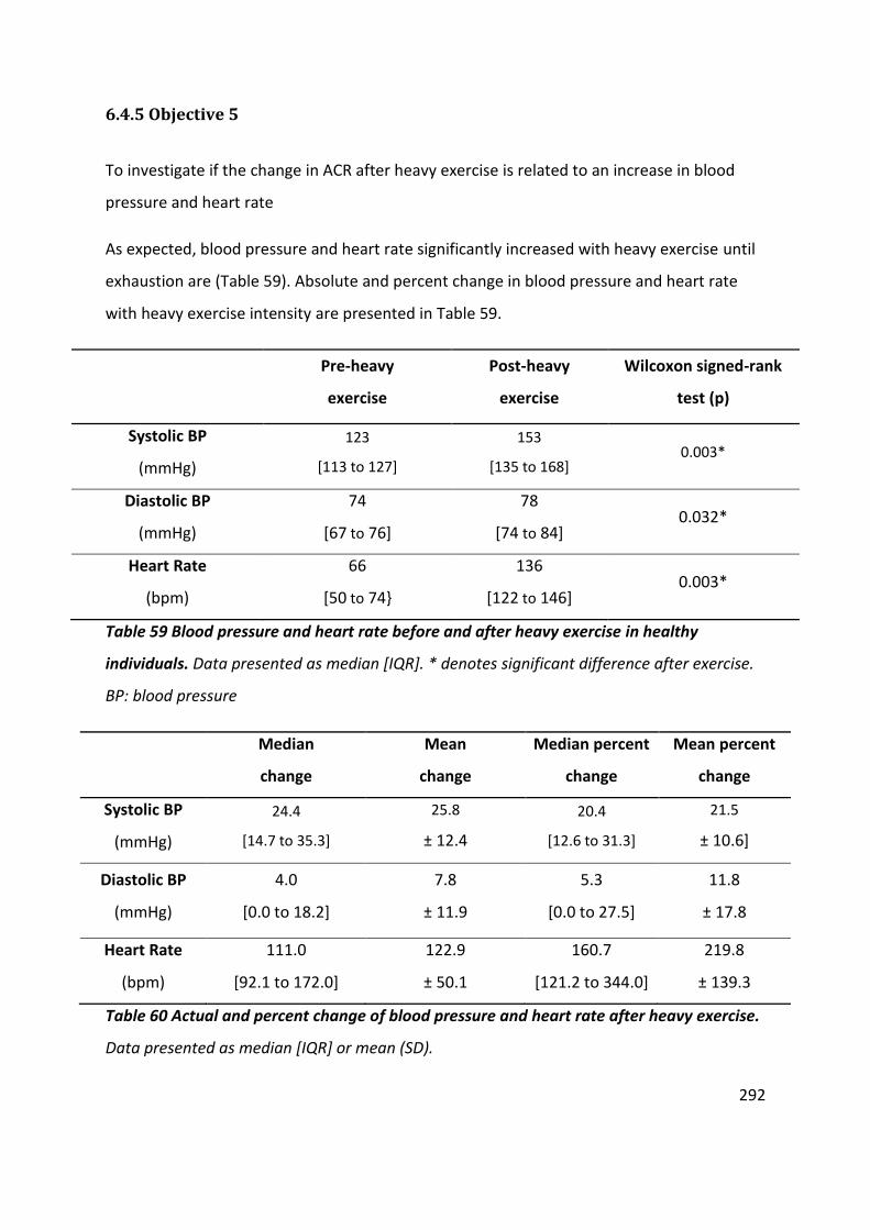
292

6.4.5 Objective 5

To investigate if the change in ACR after heavy exercise is related to an increase in blood

pressure and heart rate

As expected, blood pressure and heart rate significantly increased with heavy exercise until

exhaustion are (Table 59). Absolute and percent change in blood pressure and heart rate

with heavy exercise intensity are presented in Table 59.

Pre-heavy

exercise

Post-heavy

exercise

Wilcoxon signed-rank

test (p)

Systolic BP

(mmHg)

123

[113 to 127]

153

[135 to 168] 0.003*

Diastolic BP

(mmHg)

74

[67 to 76]

78

[74 to 84] 0.032*

Heart Rate

(bpm)

66

[50 to 74}

136

[122 to 146] 0.003*

Table 59 Blood pressure and heart rate before and after heavy exercise in healthy

individuals. Data presented as median [IQR]. * denotes significant difference after exercise.

BP: blood pressure

Median

change

Mean

change

Median percent

change

Mean percent

change

Systolic BP

(mmHg)

24.4

[14.7 to 35.3]

25.8

± 12.4

20.4

[12.6 to 31.3]

21.5

± 10.6]

Diastolic BP

(mmHg)

4.0

[0.0 to 18.2]

7.8

± 11.9

5.3

[0.0 to 27.5]

11.8

± 17.8

Heart Rate

(bpm)

111.0

[92.1 to 172.0]

122.9

± 50.1

160.7

[121.2 to 344.0]

219.8

± 139.3

Table 60 Actual and percent change of blood pressure and heart rate after heavy exercise.

Data presented as median [IQR] or mean (SD).

293

There was no association between change in blood pressure and heart rate with

change in ACR after heavy exercise in healthy individuals (actual change: Table 61

and percent change: Table 62).

Spearman’s rank correlation with

change in ACR

Rs p

Change

Systolic BP 0.02 0.96

Change

Diastolic BP -0.26 0.45

Change HR 0.41 0.21

Table 61 No association between change in blood pressure and heart rate with change in

ACR after heavy exercise in 11 healthy individuals.

Spearman’s rank correlation with

% change in ACR

Rs p

% Change

Systolic BP 0.09 0.79

% Change

Diastolic BP -0.33 0.32

% Change HR 0.38 0.25

Table 62 No association between percent change in blood pressure and heart rate with

percent change in ACR after heavy exercise in 11 healthy individuals.

The correlation between percent change in ACR with maximum reached systolic BP, diastolic

BP, heart rate and percent of maximal heart rate was also investigated (Figure 74), with the

correlation between percent of maximal heart rate reached after heavy exercise with

percent change in ACR presented in Figure 75.

294

Spearman’s rank correlation with

% change in ACR

Rs p

max Sys BP 0.25 0.47

max Dys BP -0.07 0.84

max HR 0.66 0.03*

%maximalHR 0.62 0.04*

Table 63 Correlation between maximum blood pressure and heart rate with percent

change in ACR after heavy exercise in 11 healthy participants. * denotes a significant

correlation

Figure 75 Correlation between percent of maximal heart rate and percent change in ACR

after moderate exercise for 15 and 30 minutes and after heavy exercise in 11 healthy

participants with. Spearman’s rank correlation across all the intensities (not resting)

between %maximal heart rate and percent difference was 0.61( Rs) and p= 0.0004.

295

6.4.6 Objective 6

To investigate the effect of participant’s activity levels before exercise and during recovery

on exercise induced changes in albumin excretion

The change in ACR after heavy exercise for each participant is displayed in Figure 73. The

results for participant ILD04 varied from observations from other participants, with the

change in ACR increasing later in the day compared to after heavy exercise. This was

investigated by examining the relationship of the change of ACR with the number of steps

taken as recorded by the pedometer (Figure 76).

Figure 76 Relationship between ACR and (A) cumulative steps, (B) step rate, after heavy exercise for

participant IDL04. Step rate is calculated from the number of steps taken since the previous time point

(urine collection), divided by the duration. Time at 0 mins demonstrates the time point at which heavy

exercise was complete (participant reached exhaustion). There is only one sample collected before exercise.

The final two collections are the first and second morning voids from the following day after exercise.

B A

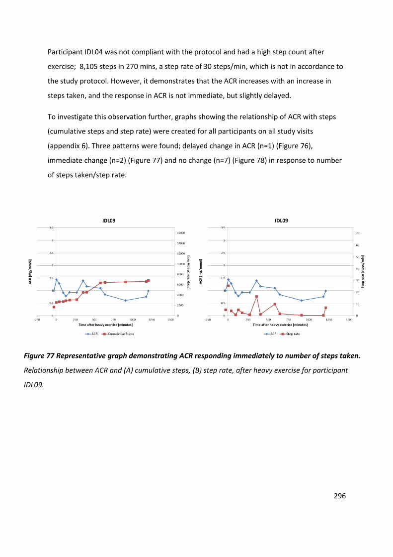
296

Participant IDL04 was not compliant with the protocol and had a high step count after

exercise; 8,105 steps in 270 mins, a step rate of 30 steps/min, which is not in accordance to

the study protocol. However, it demonstrates that the ACR increases with an increase in

steps taken, and the response in ACR is not immediate, but slightly delayed.

To investigate this observation further, graphs showing the relationship of ACR with steps

(cumulative steps and step rate) were created for all participants on all study visits

(appendix 6). Three patterns were found; delayed change in ACR (n=1) (Figure 76),

immediate change (n=2) (Figure 77) and no change (n=7) (Figure 78) in response to number

of steps taken/step rate.

Figure 77 Representative graph demonstrating ACR responding immediately to number of steps taken.

Relationship between ACR and (A) cumulative steps, (B) step rate, after heavy exercise for participant

IDL09.

297

Figure 78 Representative graph demonstrating of ACR not responding to number of steps taken.

Relationship between ACR and (A) cumulative steps, (B) step rate, after heavy exercise for participant

IDL11.

Although there were different responses to the change in ACR to the number of steps taken,

all results (where collections were received) show an increase in ACR from the FMV to SMV

on the second day (on heavy exercise visit). The FMV sample is more standardised than any

other sample, as subjects were sleeping prior to its collection. Therefore, the change in ACR

between the FMV and SMV samples are individually plotted (Figure 49). The correlation

between steps taken between the FMV and SMV with the change in ACR following the

heavy exercise visit was investigated (Figure 80). Though a trend was observed it wasn’t

significant (p=0.12).

298

Figure 79 Change in ACR from first morning void to second morning void for each

participant following the heavy exercise visit. Participants IDL07, IDL09, and IDL11 failed

either a FMV and/or a SMV the day after the heavy exercise visit.

Figure 80 Correlation between the percent change in ACR from first morning void to

second morning void with the rate of steps taken. Percent change in ACR from first morning

void to second morning void with step rate is shown for each participant following the heavy

exercise visit. Participants IDL07, IDL09, and IDL11 failed either a FMV and/or a SMV the day

after the heavy exercise visit. Spearman’s rank correlation; Rs= 0.60 , R2= 0.35, p=0.12.

0

0.5

1

1.5

2

2.5

3

3.5

4

4.5

5

First morning void Second morning void

AC

R [

mg/

mm

ol]

IDL01

IDL02

IDL03

IDL04

IDL05

IDL06

IDL08

IDL10

0

50

100

150

200

250

0 10 20 30 40

Pe

rce

nt

chan

ge in

AC

R [

%]

Step rate [steps/min]

299

6.5 Discussion

6.5.1 Change in ACR after different intensities of exercise

In young healthy individuals, ACR significantly increases after heavy exercise and returns to

resting levels within 304 minutes. Heavy exercise increases ACR sufficiently enough to place

64% of participants into the microalbuminuria range (Figure 72).

Walking can also increase ACR although it is not clear why ACR does not increase after

moderate exercise, perhaps duration of exercise is a contributing factor. Furthermore, ACR

did not change after walking for all participants, indicating altered susceptibility to walking

induced urinary albumin excretion, and further investigation is required. Next, these

findings are discussed in relation to other studies, to provide further understanding of the

underlying mechanisms and to demonstrate their clinical significance.

6.5.2 Comparison with the Heathcote et al. study

In my study the validated ELISA was used to investigate the influence on exercise in the

lowest levels of albumin excretion in healthy individuals. Our findings agree with those from

Heathcote and colleagues, that ACR significantly increases when healthy individuals are

exercised to exhaustion (Heathcote et al., 2009). 14 healthy women and 16 healthy men

were exercised to maximal heart rate or exhaustion using the Bruce Treadmill protocol in

the Heathcote study. The mean resting ACR in women was 0.5 ± 0.3 mg/mmol and 0.4 ± 0.1

mg/mmol in men. After high intensity exercise ACR increased to a mean of 5.6 ± 9.7 and 7.6

± 17.1 mg/mmol in women and men respectively. The mean increase in women was 5.1

mg/mmol, which was a 10.2 fold increase of the resting mean ACR. In my study, the median

[IQR] ACR increased from 0.85 [0.62 to 1.49] mg/mmol to 3.55 [1.44 to 7.00] mg/mmol, this

is a 4.1 increase in ACR after heavy exercise (p=0.003).

300

Overall, 40% of the participants in the Heathcote et al. study on healthy individuals had an

ACR in the microalbuminuria range after exercise and two participants were in the

macroalbuminuria range (Heathcote et al., 2009). In my study heavy exercise increases ACR

sufficiently enough to place 64% of participants into the microalbuminuria range, with none

reaching the macroalbuminuria range (Figure 72). Both studies had very similar baseline

ACR. In addition to differences in exercise protocols, a reason for the bigger increase in ACR

in the Heathcote study is that their samples were collected only 15 minutes after

completing the high intensity. In my study samples were collected within 60 minutes of

completing exercise, which may be enough time for exercise induced albumin excretion to

start recovering.

Duration of exercise and cardio outputs after exercising subjects until exhaustion on a

treadmill in the Heathcote et al. study and on a bike in my study are compared in Table 64.

This demonstrates that similar exercise thresholds were tested in the two studies, as they

have a similar duration of exercise until exhaustion. The maximal hear rate is a lot lower in

our study compared to subjects in the study by Heathcote et al. This is most likely due to

time taken to record heart rate measurements in our study, which used a digital blood

pressure monitor, instead of recording heart rate in real time. Heathcote et al. measured

blood pressure at the same time after exercise as we did, and systolic blood pressure was

very similar between the studies, reflecting similar exercise thresholds were tested.

301

My study Heathcote et al.

All subjects (n=11)

Women (n=14)

Men (n=16)

Duration of exercise (minutes)

17 (±7) 14.7 ±2.7 15.5 ±3.0

Max. Heart rate (bpm)

136 179 ±10 180 ±12

[122 to 146]

Max. Systolic BP (mmHg)

153

148 ±13 168 ±23 [135 to 168]

Table 64 Duration of exercise until exhaustion and cardio outputs in two studies. The

results from my study and the Heathcote et al. study are presented. Data are presented as

mean ± standard deviation, and median [IQR]. BP; blood pressure, bpm; beats per minute.

6.5.3 Duration of exercise induced albumin excretion to return to resting levels

after heavy exercise

This investigation showed that ACR increases after heavy exercise and returned to resting

levels within 304 minutes. Therefore, future studies that investigate the change of ACR as a

result of walking would not require long study visits over several hours. This means more

robust protocols can be established in controlled environments to ensure participants do

not walk before and after exercise, and a more regimental urine collection procedure is

used. The only other study to identify exercise induced urinary albumin excretion in healthy

individuals was not been able to determine duration as they took a single sample shortly

after exercise and 24 hours later (Heathcote et al., 2009). However, in this investigation it is

not possible to accurately determine how long it takes for the ACR to return to normal after

heavy exercise. This is due to the fact that the urine samples from individuals had variable

collection times.

Participants were asked to remain well hydrated throughout the study and to collect all

samples after exercising whilst not walking too much and to drink a standard amount

302

consistently over the period of interest. However, the protocol was not always adhered to

and the results from two participants had to be excluded (1 due to low frequency of

collection, 1 due to unexpected high step rate). Figure 74 shows how variable the time

between sample collections is among participants. Despite the frequency of samples, the

maximum time for ACR to return to normal after heavy exercise is 304 minutes (Table 56).

Although it appears that the higher the ACR after exercise the longer it takes to return to

normal, no significant correlation was found (p=0.38) , this is most likely the results of a lack

of consistent time intervals for urine sampling.

Future studies would benefit from the use of activity trackers to constantly record heart rate

and number of steps taken. Although cycle ergometers are suitable for ramp testing, the use

of treadmills is required to test the impact of walking. It would also be of value to clinically

follow up participants, to identify which participants develop kidney disease or CVD to

investigate if there is an association with increased ACR induced by exercise/steps. This

would help validate exercise as a suitable provocation test to unmask underlying

glomerular/ vascular abnormalities.

6.5.4 Change in albumin, creatinine and urine specific gravity after heavy exercise

To help understand the mechanisms behind the increase in ACR after heavy exercise, the

change in albumin and creatinine were studied individually. USG was also measured as

another marker of urinary concentration. The median percent change for albumin,

creatinine and USG was 308% [133 to 1557], 25 % [-17 to 104] and 7.8% [-17 to 68]

respectively (Table 58). Only the change in albumin was similar to that of the ACR (257% [91

to 495]) and only the concentration of albumin was significantly different after heavy

exercise (Table 57). This demonstrates that the ACR is not raised due to increased urinary

concentration or a change in urinary flow, as creatinine and USG are not affected in the

same way. The raised ACR is the result of increased albumin excretion.

303

Increased glomerular permeability in response to exercise might arise from increased

shedding of the microvascular glycocalyx (Satchell and Tooke, 2008). However, one study on

21 young, healthy men demonstrated that there was no significant change in serum

syndecan-1 and heparan sulphate concentrations (markers of glycocalyx shedding) after

maximal incremental cycling exercise until exhaustion (Majerczak et al., 2016). Impaired

proximal tubular dysfunction has also been proposed as a cause of increased urinary

albumin excretion in early stage of diabetic nephropathy (Russo et al., 2009). The response

of proximal tubular function to exercise is not known.

Samples have been stored for the later analysis of; a) markers of glycocalyx shedding to

investigate the role of increased microvascular permeability, and b) markers of proximal

tubule function, to determine if this increased albumin excretion arises from trans-

glomerular passage or reduced tubular reabsorption.

6.5.5 Relationship between blood pressure and heart rate with change in ACR

after heavy exercise

There is a significant correlation between maximum heart rate achieved (Rs = 0.66, p=0.03)

and percent change in ACR, and also between percentage of maximal heart rate (Rs = 0.66,

p=0.03) with percentage change in ACR after heavy exercise (Table 63). It is unlikely that

increasing heart rate is the cause of increasing AER, but rather reflecting how hard the

individual is exercising. This is supported by the significant correlation between percent of

maximum heart rate achieved with the percent change in ACR (Rs = 0.61, p= 0.0004) across

all intensities (except when resting as blood pressure and heart rate were not measured)

(Figure 75). The variable change in ACR seen between the participants across all the exercise

intensities may be explained by the variability in percent of maximal heart rate. However,

the purpose of using personalised exercise thresholds was to reduce this variation.

Repeating RAMP testing to determine an average GET would help to further reduce this

variability (Weston and Gabbett, 2001).

304

There was no correlation between the change in blood pressure and change in ACR, which is

expected as these are healthy participants who are normotensive and that we assume have

normal renal autonomic control, so intraglomerular pressure should not change in response

to a change in systemic pressure (Table 61). A limitation of these findings is that blood

pressure and heart rate were measured directly after exercise and not during. It is therefore

unlikely that the peak measurements were recorded.

Our results agree with those of Viberti’s study, which showed there was no correlation in

the change of systolic blood pressure with change in albumin excretion in both the diabetic

group and the controls. However, my study cannot provide evidence for Viberti’s conclusion

that it is unlikely that the change of AER after exercise is caused by an ‘abnormal’

cardiovascular response (Viberti et al., 1978). This broad conclusion might not be accurate,

as it does not consider that change in brachial pressure may not reflect changes in

glomerular pressures. If autoregulation is failing in the patients with diabetes than

glomerular pressures may be increasing more in patients with diabetic then in control

participants, influencing filtration of albumin. This is explored further to explain the

variability between subjects who demonstrate walking induced urinary albumin excretion

(Section 6.5.6).

A limitation of this study is the number of participants tested. The power analysis used was

suitable to calculate the minimum required sample size to detect a difference in ACR after

moderate exercise. However, it was not designed to detect a correlation between change in

ACR, blood pressure and heart rate. To investigate these relationships further a new power

analysis is required. The lack of correlation cannot therefore be taken as evidence that there

was no relationship between the change in ACR and cardiovascular response.

305

6.5.6 Limitations and recommendations for future research

These observations can’t be extrapolated to a population with diabetes, where greater

changes are anticipated. Individuals with DM are likely to have a greater change in ACR after

walking than was found from the healthy participants in this study (Viberti et al., 1978). This

compromises the accuracy of random spot collections to diagnose microalbuminuria and

investigate albumin excretion. This warrants further investigation and the challenges

endured in this study should be considered when designing protocols in future studies.

The importance of dipstick testing to indicate the presence of leucocytes has also been

demonstrated in this study. The presence of leucocytes has been associated with an

increase in AER, although the mechanism for this has not been fully investigated. It’s

plausible that AER increases as a result of inflammation, a process common to both

infection and exercise. A positive correlation between inflammatory biomarkers and

albuminuria has been previously reported in 3939 participants with CKD enrolled in the

Chronic Renal Insufficiency Cohort study between June 2003 and September 2008 (Gupta et

al., 2012). Several mechanisms have been proposed as to how inflammation causes

increased albuminuria, including the activation of matrix metalloproteinases (MMPs), which

shred the glycocalyx (Kolářová et al., 2014).

Personalised exercise thresholds were determined using a ramp test, to reduce the

variability in ACR responses to exercise among participants. This variation was still present

and might reflect different susceptibility to exercise, although there are several other

factors which may contribute. Despite determining personalised exercise thresholds, the

graphs show that the change in ACR after different intensities varies considerably between

subjects (Figure 69, Figure 70, Figure 71 and Figure 72). They also show that the change

increases with increasing intensity (please note the Y axis scale varies between graphs).

It was discovered that some individuals had walked a considerable distance to and from the

research centre on visit days. To help reduce this influence, participants should have been

rested prior to exercise. Participants underwent heavy exercise until volitional exhaustion,

306

although verbal encouragement was given, the duration of exercise was variable, reflecting

different levels of effort among the participants. Heavy exercise was compared to cycling up

a steep hill, where all participants reached exhaustion after a mean (±SD) duration of 17 (±7)

minutes. Being able to constantly monitor heart rate would provide further information on

the effort from participants.

Samples were also stored from this study for the later analysis of markers of proximal tubule

function, to determine if the expected increase in albumin excretion arises from trans-

glomerular passage or reduced tubular reabsorption, as investigated in the clinical ranges in

a previous study (Viberti et al., 1978). Biomarkers of glycocalyx shedding can also be

measured in stored samples, which will provide more information on microvascular

involvement in exercise/walking induced increased urinary albumin excretion.

6.5.7 Impact of walking on ACR

When investigating the relationship between the number of steps taken and the change in

ACR, it is evident that some participants did not adhere to the protocol. However, this led to

an important finding, that there are different types of responses in ACR to the number of

steps taken. Three patterns were found; delayed change in ACR (Figure 76), immediate

change (Figure 77) and no change (Figure 78). When investigating these patterns on

different visit days, the pattern between ACR and steps varied between study visits for all

participants. No participants had the same pattern between ACR and steps taken on each

study visit. This suggests more accurate methods of monitoring ACR and steps are required

to investigate this finding further to determine if walking unmasks early microvascular

dysfunction as demonstrated by increased urinary albumin excretion.

In 2011, Koh and colleagues investigated the change in ACR, 1 and 2 hours after a one

kilometre treadmill walking exercise in thirty-five participants with diabetes (three with

T1DM and 32 with T2DM) and nine control subjects, those with diabetes had a range of pre

exercise levels of albumin excretion across the full albuminuria range (Koh et al., 2011).

307

Koh et al. showed no significant change in ACR in controls in response to walking. A possible

explanation for no change in ACR in controls in the study by Koh et al. is that they were

unable to quantify the lowest levels of urinary albumin. In the study by Kol et al., ACR in

females with diabetes increased above the microalbuminuria threshold at 1 hour post

exercise on average, returning to baseline levels by 2 hours (Figure 64). Our findings support

this in healthy subjects by indicating that ACR returns to resting levels by the next void after

walking induced increased urinary albumin excretion.

This incidental finding of walking induced urinary albumin excretion is reported for the first

time in healthy normotensive individuals without diabetes in this thesis. These findings were

only achievable by using the validated sensitive ELISA (Chapter 2), when reporting the ACR

(Chapter 3) from samples being collected using the appropriate method (Chapter 4), which

have been stored at -80oC (Chapter 5).

This finding is clinically relevant as some individuals might walk to their GP surgery before

providing a urine sample, which could result in a falsely high ACR. Previous studies have

shown that individuals with DM have a larger increase in AER after exercise than healthy

individuals (Viberti et al., 1978). Given that this study was carried out on healthy individuals,

patients with DM might have an even greater rise in ACR after walking.

The majority of participants demonstrated different response patterns across the 4 visits.

However, participant IDL04 always had a response and IDL10 never had a response. The

variation in responses might be the result of the method. The pedometers used were simple

step counters, with the accumulative number of steps being manually recorded at the time

of urine collections. Therefore, it cannot be determined when the number of steps taken

between voids actually occurred. Participants who had a delayed response in ACR might

have had a sudden increase in the number of steps just before providing a sample, therefore

the ACR was only raised in the next collection. The impact of walking on the ACR was not a

primary objective of this study, and this incidental finding warrants further investigation,

especially on patients with DM. This could be achieved using a more robust protocol,

utilising activity monitors which constantly record heart rate and steps taken.

308

A sample from the first morning void is the most standardised urine collection method

among participants and an increase in ACR in the second morning void is consistent,

although the magnitude of that increase varies (Figure 79). Figure 80 shows that after a

threshold, around 18 steps/min, the ACR increases by over 100%. This threshold for change

in ACR is also reflected when correlating the percentage of maximal heart rate to change in

ACR, where change in ACR considerably increases after exercising above 70% of maximum

heart rate (Figure 75). This confirms that ACR increases with activity.

Walking induced increased albumin excretion might represent an early nephropathy,

possibly caused by impaired microvascular autoregulation. The mechanisms involved and

the clinical significance of these findings require further study, and this theory is considered

in conjunction with results from the SUMMIT cohort in Chapter 7.

6.6 Conclusion

In healthy individuals heavy exercise increases ACR sufficiently enough to place 64% of

participants into the microalbuminuria range. Thus healthy individuals should not provide a

urine sample for ACR measurement if they have undertaken heavy exercise within the

previous 5 hours.

Some individuals express increased ACR in response to walking. This needs further

investigation as patients walking to appointments could have falsely elevated ACR or it may

indicate an increased risk of cardiovascular disease.

309

Chapter 7 Urinary Albumin Excretion and Microvascular

Function

This chapter brings the earlier validated assessments of the measurements of low levels of

albumin excretion in urine into a relevant clinical population to explore the relationships

between microvascular function and urinary albumin excretion and sets this in context with

the literature.

7.1 Background

Microalbuminuria has been established a risk factor for diabetic kidney disease since the

early 1980’s (Mogensen, 1987). Since then a wealth of studies have demonstrated that

increasing urinary albumin, even within the normal range, is a risk factor for cardiovascular

disease in subjects with and without diabetes (Hillege et al., 2002) (discussed in Chapter 1) .

A good review by Lambers Heerspink et al. in 2011 summarises the risk of renal and

cardiovascular morbidity with microalbuminuria across different populations from different

studies. It is evident that microalbuminuria is a risk factor, not only in patients with DM but

also in the general population. However, the clinical utilisation of microalbuminuria outside

of the management of DM has not made it into common guidelines (de Zeeuw et al., 2006).

The review by Lambers Heerspink et al. (Figure 10) demonstrates increasing risk with

increasing urinary albumin excretion, especially when predicting cardiovascular morbidity.

Urinary albumin excretion is a continuous risk marker with no lower limit. Therefore small

increases in urinary albumin excretion within the normoalbuminuria range are associated

with an increased risk of morbidity.

310

Generalised microvascular dysfunction in diabetes, causing increased vascular permeability,

is thought to underlie the complications of DM including DKD and CVD (Deckert et al., 1989).

In the kidney this is expressed as increased urinary albumin excretion where as in larger

vessels it accelerates the “permeability” of lipids into the vascular wall leading to

atherosclerosis (Deckert et al., 1989). This is supported by evidence that urinary albumin

excretion is associated with other microvascular complications of diabetes, such as

retinopathy and neuropathy (Newman et al., 2005).

It is important to investigate these relationships further because the studies which have

investigated these relationships to date have been limited by the use of routine assays

which can’t quantify low concentrations of urinary albumin. Thus relationships to date have

been falsely constrained by assay limitations and it is unclear whether links between urinary

albumin excretion and CVD and microvascular complications or dysfunction occur right

across the spectrum of urinary albumin excretion.

Using the validated ELISA, and applying the most accurate and reproducible method to

collect and store samples, the lowest levels of urinary albumin excretion are examined and

the relationship with microvascular function and microvascular complications of diabetes

are investigated for the first time in this chapter.

7.2 Introduction

7.2.1 Microvasculature

Microalbuminuria is a microvascular complication of diabetes. To investigate the

relationship between urinary albumin excretion and systemic microvascular function, it is

important to understand the human microvasculature, and how different techniques can be

applied to assess its function.

311

Microvasculature refers to the smallest systems of blood vessels and is organised into three

sections; arterioles, capillaries and venules, which work together with specialised cells to

facilitate exchange between the circulatory system and tissues. Arterioles extend from

resistance arteries and branch out into capillaries and the blood is returned to the heart via

venules, which lead to veins. Arterioles are small vessels which are composed of endothelial

cells surrounded by a thin layer of smooth muscles. This enables arterioles to constrict and

dilate, controlling blood distribution and pressure, which is regulated by extrinsic (e.g.

autonomic nervous system) and intrinsic mechanisms (e.g. local produced vasodilators and

constrictors) (Mader et al., 2012).

Capillaries are the site of nutrient and gas exchange between blood and surrounding tissue.

Capillaries are only one endothelial cell thick and are surrounded by a basement membrane.

Capillary diameter allows a single erythrocyte to pass through at a time or in some larger

capillaries two erythrocytes to overlap as they pass through the capillary lumen. Pericytes

sparsely surround capillaries to provide structural support, and contractile properties

(Mader et al., 2012).

The traditional theory behind capillary exchange is that blood pressure gradient is higher at

the arterial end compared to protein oncotic pressure gradient, which results in water and

small solutes being pushed out of the capillary into the interstitium (Michel, 1997). Through

the midsection of capillaries, oxygen, glucose and amino acids move out and are taken up by

the surrounding cells, and metabolic waste products like carbon dioxide diffuse into the

capillary. As the pressure difference declines across the capillary towards the venular end

and falls below the opposing oncotic pressure, water and other waste products can diffuse

into the capillary with blood travelling through the venule back towards the heart (Cleaver

and Melton, 2003).

This traditional theory is based on the Starling’s principle , but has since been revisited by

Adamson and colleagues in 2004 (Adamson et al., 2004). A well-received review by Levick

and Michel proposes that across the entire capillary length, fluid is filtered into the

interstitial space, and not just at the arteriolar end (Levick and Michel, 2010). It is thought

that endothelial glycocalyx (Section 1.3.4.1) plays a key role in the semipermeable

312

capabilities of the membrane. In addition, reabsorption of interstitial fluid does not occur at

venules and the ultra-filtered fluid returns to circulation via the lymphatic system (Levick

and Michel, 2010).

There are three types of capillaries; continuous, discontinuous and fenestrated. The type of

capillary depends on the demands of the surrounding tissue and organ. For example;

fenestrated capillaries enable renal glomeruli to filter blood, whereas discontinuous

capillaries allow blood cell turnover in bone marrow, the spleen and the liver (Levick, 1991).

Continuous capillaries have no gaps in the endothelium. Continuous capillaries are present

in skin and muscle cells, although capillary density is much smaller in skin due to a lower

demand in blood supply (Levick, 1991).

The next section provides a superficial overview of some of the main components of

microvasculature, followed by a review of methods which test their functionality.

7.2.1.1 Endothelium

The endothelium lines the interior surface of blood vessels and consists of a thin layer of

squamous endothelial cells. In addition to contributing to the semi-selective barrier

between blood and surrounding tissues, the endothelium plays a central role in regulating

blood flow, blood pressure, inflammation, coagulation and angiogenesis. The functions of

the endothelium are achieved through membrane bound receptors for a wide range of

molecules, including lipids, proteins (e.g. growth factors, coagulants, and anti-coagulants),

metabolites (e.g. nitric oxide and serotonin), hormones and mechanosensors (Cines et al.,

1998).

The function of the endothelium is controlled in part by the glycocalyx, which is an

important determinant of vascular permeability (Reitsma et al., 2007). The endothelial

glycocalyx has also been suggested to act as a mechanotransducer, translating biochemical

313

forces from blood flow and shear stress into biomechanical signals to maintain vascular tone

(Reitsma et al., 2007, Florian et al., 2003).

The endothelium regulates blood flow through secretion of mediators by endothelial cells,

which are pivotal in vasoregulation. These include vasodilators such as nitric oxide and

prostacyclin, as well as vasoconstrictors such as endothelin-1 and platelet activating factor

(Cines et al., 1998). Nitric oxide is a key mediator in regulating blood flow and tests that

stimulate its production in endothelial cells can measure the blood flow response to indicate

endothelial function (Deanfield et al., 2005).

A study by Kwon et al which investigated NO generation in the renal microvasculature

supports the theory that microvascular dysfunction is the common process in the

pathophysiology of diabetic kidney disease, and cardiovascular disease, resulting in

increased urinary albumin excretion (Kwon et al., 2009). NO generation was assessed by

measuring urinary NO levels, nitrate and nitrite were quantified. Their findings, from a

hundred subjects with varying degrees of acute kidney injury (AKI), indicate that diminished

NO generation by injured endothelium could impair the vasodilatory ability of the renal

vasculature, contributing to a reduction of GFR (Kwon et al., 2009).

The findings of Kwon et al. highlight endothelial dysfunction’s pathophysiological

involvement and support the Steno Hypothesis, which was the first to claim a common link

between mechanisms involved in diabetic nephropathy and CVD. The Steno hypothesis is

that urinary albumin excretion is a marker of overall vascular dysfunction with increased

urinary excretion in the kidney presenting itself from increased glomerular permeability and

also representing increased vascular permeability elsewhere increasing CV risk (de Zeeuw et

al., 2006). However the endothelium is very heterogeneous in structure and function.

Endothelial cells from different vascular sites have different functions and employ different

strategies to mediate local haemostatic balance in different tissue beds and sizes / types of

vessels (Aird, 2007).

314

7.2.1.2 Vascular smooth muscle cells

Arterioles gain their contractile properties through smooth muscle cells that encompass

them, providing arterioles the ability to intrinsically change their luminal diameter. Vascular

smooth muscle cells respond to vasoactive substances from; endothelial cells, nerves and

from agents in the blood. Smooth muscle cells also respond to changes in blood pressure

(transmural pressure), known as the myogenic response (Davis and Hill, 1999).

The myogenic mechanism is independent of neural, metabolic, and hormonal influences,

and although it is most pronounced in arterioles, it’s occasionally demonstrated in arteries,

venules, veins and lymphatics (Johnson, 2011).When luminal blood pressure rapidly

increases, the stretching of the arteriole causes ion channels to open resulting in

polarisation of the muscle, leading to vasoconstriction reducing blood flow. Diminishing

blood pressure causes ion channels to close resulting in smooth muscle relaxation leading to

vasodilation, increasing blood flow. (Davis and Hill, 1999). An example of arteriole

autoregulation is in the renal glomeruli, where constant renal blood flow is maintained at

varying arterial pressure (Aukland, 1989).

In this chapter the relationship between urinary albumin excretion and generalised

microvascular function is being investigated and it has been proposed that the

microvascular function of the skin is a suitable model (Holowatz et al., 2008). The skin is

easily accessible and there are non-invasive methods to assess its microvascular function.

Skin microvascular function has been used as a surrogate marker for systemic vascular

health in various diseases including hypertension (Antonios et al., 1999, Feihl et al., 2006),

diabetes (Chang et al., 1997, Yamamoto-Suganuma and Aso, 2009, Jaap et al., 1994b,

Sorensen et al., 2016, Strain et al., 2005a) and end stage kidney disease (Kruger et al., 2006).

315

7.1.1.3 Skin microvasculature

Skin is the largest organ of the human body, protecting the internal environment from the

external environment and playing a pivotal role in thermoregulation. Skin is separated into

three layers; epidermis, dermis and subcutaneous tissue (also referred to as hypodermis /

subcutis) (Figure 81).

Figure 81 Architecture of skin. This illustration shows the distribution of microvessels in the

different layers of the skin (Mulroney and Myers, 2008). The microcirculation in the dermis is

characterised by two distinct horizontal plexuses. An upper horizontal plexus in the papillary

layer and a lower horizontal network between the dermis and subcutaneous tissue.

The epidermis is the uppermost layer and is the most biologically active layer as the

epithelium is constantly renewing. The epidermis is avascular and densely packed with

epithelial cells, which through an adaptive process called cornification (keratinisation) of the

316

skin forms a protective barrier against the external environment and forms the first line of

defence against external pathogens (Shetty and Gokul, 2012).

The epidermis is separated from the dermis layer by the basement membrane. The

basement membrane is composed primarily of type IV collagen which provides mechanical

stability and contains glycoproteins which promote adhesion with the epidermis (LeBleu et

al., 2007). The dermis layer, a connective tissue matrix composed of elastin and collagen,

provides elasticity and tensile strength to skin. The dermis contains blood and lymph

vessels, nerves, and other structures like sweat glands and hair follicles. These structures

have their own vascular network for example; fenestrated capillaries surround sweat glands

and dermal papilla of hairs (Braverman, 1997).

The microcirculation in the dermis is characterised by two distinct horizontal plexuses. An

upper horizontal plexus in the papillary layer and a lower horizontal network between the

dermis and subcutaneous tissue (Figure 81) (Mulroney and Myers, 2008). Arterioles and

venules travel between the lower horizontal plexus and the upper network in the papillary

layer, from which continuous capillary loops branch into the papillary dermis (Braverman

and Yen, 1977). These papillary loops are the primary site for exchanging oxygen and

nutrients to supply the epidermal cells , which also receives oxygen from outside air in

contact with the skin (Braverman and Yen, 1977).

Below the dermis is the adipose rich subcutaneous layer (hypodermis/subcutis) which

connects skin to underlying fibrous tissue of bones and muscles. The subcutaneous layer

acts as a fat reserve, through which blood vessels travel to reach the lower horizontal plexus

at the hypodermis-dermis interface (Wong et al., 2016).

317

7.2.2 Assessing cutaneous microvascular function

Optical microscopy, laser Doppler and evaluating tissue oxygenation are non-invasive

techniques commonly used to investigate microvascular function in the skin. Laser Doppler

techniques have been extensively used over the past few decades and are used in a range of

methods that measure an individual’s microvascular response to various interventions

(Roustit and Cracowski, 2012). They will be briefly reviewed here.

7.2.2.1 Laser Doppler

Laser Doppler fluximetry is a technique that uses the Doppler shift in a laser beam to

continuously measure the number and velocity of moving erythrocytes in the tissue of

interest, for example the skin microvasculature. The principle of the Doppler shift was

proposed by Austrian physicist Christian Doppler in 1842, who stated that there is a change

in frequency of a wavelength caused by the motion of the source (Oberg, 1990).

When assessing the skin microvasculature, laser light is emitted at a single frequency and

when it comes into contact with any surface the light is reflected and scattered.

Reflected/scattered light from stationary objects will have no change in frequency, whereas

light reflected/scattered from moving objects, erythrocytes, will have a changed frequency

(Oberg, 1990). A photo detector collects the reflected/scattered light and by determining

the magnitude of the shift in frequency and its occurrence, the concentration and velocity of

erythrocytes is calculated (Roustit and Cracowski, 2012, Oberg, 1990). The laser Doppler

output is not a direct measure of skin blood flow, but rather an index of skin perfusion or

flux, and is reported in arbitrary perfusion units (PU) or Volts (V) (Choi and Bennett, 2003).

The penetration depth of the laser into tissue is controlled by its wavelength. In skin, shorter

wavelengths test superficial layers, whereas longer wavelengths penetrate deeper.

Measurement depths vary depending on the tissue being tested. In the skin there is no

318

definite interpretation of what fraction of the laser Doppler shift is attributed to blood flow

in capillaries, arterioles, venules and what proportion of which plexus is being assessed

(Yvonne-Tee et al., 2006). It is suggested that laser Doppler fluximetry measurement in the

skin represents thermoregulatory blood flow and nutritional blood flow (Knotzer and

Hasibeder, 2007).

7.2.2.2 Iontophoresis

Iontophoresis is a non-invasive method of introducing vasoactive substances into skin

microvasculature. The response in skin perfusion assessed by laser Doppler imaging

provides a measure of microvascular function, more specifically the function of specific cell

types (e.g. endothelial dependent or independent) depending on the vasoactive drug used.

Iontophoresis achieves transdermal drug delivery to skin microcirculation by transferring

charged molecules using a low intensity electrical current (Roustit and Cracowski, 2012).

Several factors need to be considered for iontophoretic drug transfer including the pH and

concentration of the solution, skin thickness and hair cover, and the intensity of the current

(Kalia et al., 2004).

Acetylcholine (ACH) and sodium nitroprusside (SNP) are vasodilators commonly used to test

microvascular function. Although there is controversy over the exact mechanism of how

ACH mediates vasodilation, it is established that it induces endothelium-dependent

vasodilation (Roustit and Cracowski, 2012). The most prominent theory is that ACH binds to

muscarinic receptors on endothelial cells, mitigating the activation of endothelial nitric

oxide synthase and stimulating prostaglandin production (Turner et al., 2008). It is not

certain how ACH travels to the endothelial cells; it can travel directly through the

transepidermal route or go the appendageal route, through hair follicles and sweat glands.

If ACH travels through the transepidermal route, ACH could enter the microvasculature

through adventitia vessels. If ACH travels through the appendageal route, fenestrated caps

319

hair follicles and sweat glands would enable ACH to reach the microvasculature, however

muscarinic receptors in sweat glands may influence ACH delivery (Turner et al., 2008).

SNP does not interact with endothelial cells, once in circulation SNP breaks down to release

nitric oxide in smooth muscle cells. The increased availability of nitric oxide in smooth

muscle cells (from both ACH and SNP) induces a biochemical cascade that results in the

inhibition of vasoconstriction, increasing vasodilation (Turner et al., 2008). Therefore, ACH is

used to test endothelium-dependent vasodilation and SNP tests endothelium-independent

vasodilation, both markers of microvascular function that don’t require neuronal input.

Abnormal response to ACH does not prove endothelial dysfunction, unless the SNP response

is normal.

The response in skin perfusion is assessed by laser Doppler imaging, which needs to

measures at a depth which corresponds to the delivery site using iontophoresis.

7.2.2.3 Maximal hyperaemia

A principal function of skin is thermoregulation, aiding heat loss or conservation by

vasodilating or constricting respectively. Externally heating skin increases perfusion, and

maximal blood flow or perfusion (hyperaemia) can be estimated (Sandeman et al., 1991b)

using laser Doppler fluximetry. This vascular test indicates the microvascular capacity for

vasodilation in response to injury, an important part of healing (Cracowski et al., 2006).

The majority of heating protocols state that local warming to 42-43oC is sufficient to induce

maximal vasodilation (Johnson and Kellogg, 2010) , with 44oC being reported optimal in

healthy individuals (Saumet et al., 1998). Although the exact mechanism behind maximal

hyperaemia after local heating are not fully understood, there are at least two independent

phases; an initial phase which has a peak maximal hyperaemia within 10 minutes of heating,

followed by a plateau after 20-30 minutes (Figure 82) (Minson, 2010). Therefore, skin must

320

remain heated for at least 30 minutes before estimating MBF. It has been proposed that the

initial peak in maximal hyperaemia is predominately mediated by local sensory nerves, as

the response can be attenuated by local anaesthesia (Arildsson et al., 2000). Whereas the

second phase of vasodilation is largely attributed to local nitric oxide production (Minson et

al., 2001) though the magnitude of its involvement has been disputed (Gooding et al 2006).

Figure 82 Skin blood flux in response to local heating. Skin blood flux was determined using

laser speckle contrast imaging on the forearm (Roustit and Cracowski, 2012) PU denotes

perfusion units.

Minimum vascular resistance

Vascular resistance is the resistance that must be overcome to push blood through the

circulatory system. Minimum vascular resistance (MVR) is the lowest resistance to

overcome, which occurs during maximal vasodilation. In the microvasculature, MVR can be

321

calculated when estimating maximal hyperaemia, where vasodilation is induced by localised

heating. MVR is calculated by a rearrangement of Darcy’s law to calculate blood flow by

dividing mean arterial pressure by maximal hyperaemia (Jayalalitha et al., 2008).

High minimum vascular resistance and low maximum hyperaemia are associated with

structural alterations to microvessels (Adingupu et al., 2015, Williams and Tooke, 1992, Jaap

et al., 1994b)

7.2.2.4 Post-occlusive reactive hyperaemia

Post-occlusive reactive hyperaemia (PORH) refers to the transient increase in skin blood

flow above baseline levels following the release from arterial occlusion. Vessel beds dilate

during occlusion due to hypoxia, upon release blood rushes down the dilated vessels

causing a sudden increase in perfusion / pressure. It is thought that reactive hyperaemia is

caused by; myogenic relaxation to reduce vascular resistance, an abundance of locally

produced vasodilators (produced in response to hypoxia), and by metabolites of ischaemic

tissues (Kilbom and Wennmalm, 1976, Nowak and Wennmalm, 1979). Sensory nerves have

also been shown to be involved in the reactive hyperaemia response (Larkin and Williams,

1993). This myogenic / auto regulatory response returns blood flow to normal (Cracowski et

al., 2006).

Following the release from occlusion tissues become oxygenated, subsequently less

vasodilators are produced and normal vascular resistance returns. The contribution of the

different factors in the reactive hyperaemia response are debated (Wong et al., 2003,

Lorenzo and Minson, 2007).

Traditionally there are three measurements that are utilised when evaluating PORH; the

height of the peak in blood flux (peak hyperaemia), the time to reach it and the time to

return to baseline (Figure 83).

322

Figure 83 Blood flux during post occlusive reactive hyperaemia testing. Blood flux is shown

at a time constant of 3.0 seconds for 5 minutes resting (baseline), after which arterial

occlusion at the ankle occurred for 4 minutes to generate a biological zero. At nine minutes

the cuff is released followed by a rapid increase in flux which reaches a maximum height of

peak, where the time to reach it and time to return to baseline can be calculated.

Abbreviations: Tp, time to peak; TBL, time to baseline; AU, arbitrary unit. Adapted from

(Adingupu, 2013).

Usually only one peak is reported, however Ray et al. identified different response curves

after the release from a two minute occlusion at the ankles when reducing the time

constant to follow blood flux (Ray et al., 1999). This has been investigated further and three

distinct patterns of post-occlusive flow have been described; 1) a gradual rise to peak

response classified as ‘normal’, 2) a ‘non-dominant early peak’ with an early rise within 2

seconds but which is lower than the subsequent ‘normal’ peak and 3) a ‘dominant early

peak’ within 2 seconds which declines rapidly and is followed by a lesser ‘normal’ peak

(Strain et al., 2005).

323

Figure 84 Early peak response curve morphology. Type 1: gradual controlled rise to peak

response classified as ‘normal’, type 2: a ‘non-dominant early peak’ with an early rise within

2 seconds but which is lower than the subsequent peak and type 3: a ‘dominant early peak’

that is within 2 seconds of cuff release, which declines rapidly and is followed by a less

‘normal’ peak (Strain et al., 2005a).

324

Studies carried out by The Diabetes and Vascular Research Centre in Exeter have proposed

that impaired myogenic vasoconstriction or its modulation via the endothelium or nerves,

leads to a very rapid unmodulated increase in blood flow (Strain et al., 2005a). Wall stress is

the stimulus for the myogenic response, therefore a thickened wall structure, such as that

occurring in diabetes or hypertension, will reduce the response at a given pressure

(Matchkov et al., 2002) and may delay the onset of the myogenic response so that an early

increase in flow is observed before the myogenic vasoconstriction (Strain et al., 2005a).

Post occlusive reactive hyperaemia has been used to assess macro- and microvascular

function in healthy individuals, diabetes, and in disease states (Tur et al., 1991, Minson and

Wong, 2004, Higashi et al., 2001), with impaired reactive hyperaemia associated with risk

factors for CVD (Yamamoto-Suganuma and Aso, 2009, Morales et al., 2005, Vuilleumier et

al., 2002) and with the presence of coronary artery disease (Shamim-Uzzaman et al., 2002).

7.2.3 Post occlusive reactive hyperaemia and urinary albumin excretion

A prominent study carried out by Strain et al. investigated the relationship between in vivo

microvascular function with lower levels of urinary albumin excretion within the normal

range (Strain et al., 2005a). The study was a second analysis of participants aged 40-60 years

of African Caribbean and European descent with and without diabetes. Using a time

constant of 0.1 seconds to trace blood flux during PORH testing, early peak morphologies

were identified and used to group participants (Table 65) (described above in Figure 84 ).

325

Variable Group 1:

normal peak Group 2:

early non-dominant peak

Group 3: early dominant

peak P for trend

N 137 93 41

Sex (% male) 43 40 64 0.06

Age (years) 53 ± 7.8 55 ± 7.0 55 ± 8.5 0.053

Ethnicity (% European) 55 44 51 0.2

Resting brachial systolic (mmHg)

133 ± 20 142 ± 24 146 ± 26 0.001

Resting brachial diastolic (mmHg)

81 ± 9 84 ± 11 85 ± 11 0.01

Weight (kg) 81 ± 15 84 ± 16 90 ± 19 <0.001

Waist (cm) 92 ± 12 95 ± 13 99 ± 20 0.005

Fasting glucose (mmol/L) 5.6 (4.9-6.0) 6.1 (4.9-6.8) 6.6 (4.9-10.1) 0.001

Cholesterol (mmol/L) 5.2 ± 0.9 5.1 ± 1.1 5.1 ± 1.3 0.7

HDL (mmol/L) 1.30 ± 0.35 1.25 ± 0.33 1.20 ± 0.35 0.08

Fasting triglycerides (mmol/l)

1.08 (0.79-1.40) 1.15 (0.72-1.52) 1.23 (0.92-1.85) 0.1

Diabetes (%) 31 42 51 0.012

Smoking status (current/ex/never) (%)

14/37/49 24/23/53 32/37/32 0.02

Albumin excretion rate (µg/min)

3.69 (3.20-4.07) 7.22 (5.47-9.53) 12.56 (7.80-20.20) <0.001

Table 65 Participant characteristics stratified by peak response curve morphology group.

Data are means ± standard deviation, for skewed data the median (interquartile range) are

reported (Strain et al., 2005a).

The severity of several CVD risk factors; blood pressure, glucose concentration, obesity,

smoking status and AER, are higher in subjects with an early dominant peak compared to

those with a normal peak. These CVD risk factors all demonstrated a significant trend across

the three groups (Table 65). The relationship between AER and peak morphology was also

present when dividing the cohort by diabetes status, hypertension, and the use of

antihypertensive therapies. Furthermore, multivariate analysis was carried out to explore

potential confounding factors in the relationship between peak response curve morphology

and AER. A model composed of peak morphology, age, gender, systolic blood pressure,

weight, fasting glucose, fasting triglycerides, and smoking status to predict AER, determined

that only peak morphology is independently associated (β-coefficient= 0.57 ± 0.11, p

<0.001), with 29% of the overall variance of AER explained by the whole model. The study

326

by Strain et al. not only demonstrates that peak morphology is associated with AER,

independently of traditional CVD risk factors; it also confirms that microvascular

abnormalities are occurring within the normoalbuminuria range. However, the urinary

albumin assay used in the study by Strain et al. has a lower limit of 0.05ug/dl (0.05mg/L),

samples below this value were reported as 0.05mg/L (Strain et al., 2005a). This is most likely

the limit of detection of the assay and not limit of quantification, where the assay can

measure reproducibly with linearity.

Using the validated ELISA, described in my thesis with a measurable range 0.78 – 40 mg/L to

quantify urinary albumin, the associations between microvascular function and the lowest

levels of urinary albumin excretion can be investigated for the first time.

Microvascular dysfunction has been proposed as the common process in the

pathophysiology of cardiovascular disease and diabetic kidney disease, resulting in

increased urinary albumin excretion (Deckert et al., 1989). This is further supported by

evidence that urinary albumin excretion is associated with other microvascular

complications of diabetes, such as retinopathy and neuropathy (Newman et al., 2005). This

relationship between urinary albumin excretion and other microvascular complications of

diabetes is also investigated in the SUMMIT cohort.

7.2.4 Urinary albumin excretion and other microvascular complications of

diabetes

DM is not only a disorder of carbohydrate metabolism but it is also a cause of vascular

disease. Macrovascular complications of DM are mainly represented by atherosclerotic

disease, whereas there are three major manifestations of microvascular disease;

retinopathy, neuropathy and nephropathy. For the purpose of this chapter I will be

focussing on the diabetes related microvascular complications.

327

7.2.4.1 Diabetic retinopathy

The incidence of certifications of visual impairment (CVIs) due to diabetic retinopathy (DR)

ranged from 30.8 to 77.4 per million population per year between 2010 and 2013 in North

and Eastern Devon (Lin et al., 2017). Furthermore, DR is known as one of the leading causes

of blindness among working aged adults (Frank 2004). More recent evidence suggests

inherited retinal disorders are the leading cause of certifiable blindness among working age

adults in England and Wales, overtaking diabetic retinopathy (Liew et al., 2014). This may be

attributed to the success of nationwide diabetic retinopathy screening programmes and

improved glycaemic control. After 20 years of diagnosis, nearly all individuals with T1DM

and approximately 60 % of T2DM patients in the UK will have some degree of retinopathy

(Scanlon, 2008).

The retina is the light sensitive inner layer of the eye responsible for vision. DR is

characterised by ischaemic changes within the retina. DR is graded from vascular

morphological abnormalities on retinal photographs, including, for example capillary

microaneurysms, haemorrhages, cotton wool spots, capillary degeneration and excessive

formation of new blood vessels (neovascularisation) (Forbes and Cooper, 2013). Clinically,

DR is classified into non-proliferative (NPDR) and proliferative (PDR) disease stages with the

latter occurring at the advanced stages of DR. The early stages of DR are symptomless and it

can progress undetected until it affects vision. Excessive fluid accumulation / oedema within

the macular region, known as clinically significant diabetic macular oedema, can result in

the impairment / loss of central vision. This can occur within the NPDR stage of DR.

However, patients with DM in the UK have a comprehensive dilated eye exam every year to

18 months to detect early signs of DR.

The earliest histopathological sign of DR is a loss of pericytes (Beckman and Creager, 2016).

Pericytes are contractile cells which wrap around endothelial cells in capillaries. Pericytes

assist in the maintenance of capillary tone, growth and resistance to damage from oxidative

stress (Arboleda-Velasquez et al., 2015). As the disease progresses the basement membrane

thickens which is accompanied by potential endothelial cell permeability and

328

microaneurysms (Tarr et al., 2013). In this initial stage of NPDR there is usually no loss in

vision.

Microaneurysms are usually the earliest signs of DR on retinal photographs and the first step

on DR grading / screening scales. This tends to lead into haemorrhages, cotton wool spots,

then into marked morphological changes – venous beading and intraretinal microvascular

abnormalities and eventually into the growth of new vessels.

Visual impairment usually occurs in the proliferative stage which is characterised by

neovascularization and accumulation of fluid within the retina (Forbes and Cooper, 2013).

PDR is caused by the occlusion or degeneration of retinal capillaries, ischemia followed by a

subsequent release of angiogenic factors which stimulate neovascularisation. (Bresnick et

al., 1975).

Albuminuria and diabetic retinopathy

In 2012, Chen et al. carried out a hospital based cohort study, consisting of 487 patients with

T2DM, to compare the ability of microalbuminuria and moderately reduced eGFR to predict

the development of DR over 6 years (Chen et al., 2012b). It was reported that patients with

microalbuminuria and an eGFR ≥ 60 mL/min/1.73m2 had a significantly greater risk of

developing and progressing DR (HR 3.34 [95% CI 1.04-10.70]) compared with those with

moderate renal impairment (eGFR 30-59.9 mL/min/1.73m2) and normoalbuminuria. Chen et

al concluded that microalbuminuria predicts DR better than eGFR predicts DR. This study

investigated the clinical albumin excretion ranges with clinical retinopathy. In my thesis,

using the SUMMIT cohort, subclinical background changes in DR are compared with

subclinical urinary albumin excretion.

There are only a few studies with a large number of participants that have investigated the

association between urinary albumin excretion and DR in patients with T2DM. The majority

of studies that have reported a relationship found albumin excretion was not an

329

independent predictor for DR incidence and progression when adding it to multivariate

regression models that included age, diabetic duration, glycaemic level and blood pressure

(Newman et al., 2005). These studies are also limited by only investigating the clinical micro-

and macro- albuminuria ranges.

It is suggested that nearly all T1DM patients have retinopathy within 20 years of diagnosis

(Scanlon, 2008). Therefore it is important to consider the influence diabetes duration may

have on the relationship between urinary albumin excretion and DR. Other potential

confounding factors are discussed in Section 7.2.8.

In 2012, a prospective study of 197 patients with T2DM reported that albumin excretion,

within the normoalbuminuria range, was an independent risk factor for DR development

over 4.5 years (3.7–5.1) (Chen et al., 2012a). All patients were without DR at baseline with a

mean duration of diabetes 6.2 years ±6.0. Sixty-eight patients (22.9%) developed DR over

the 4.5 years. A discrimination value of 10.7 mg/24hr, in the normoalbuminuria range

(microalbuminuria range is 30-300 mg/24hr), has a relative risk ratio of developing DR of

2.13 (95% CI: 1.58 to3.62, p<0.001). Fifty-one patients (29.0%) of the 176 subjects with

urinary albumin excretion between 10.7 and 30 mg/24 h developed DR, while 17 patients

(14.1%) of the 121 subjects with lower albumin excretion (<10.7 mg/24 h) developed DR

(Chen et al., 2012a).

The study by Chen et al. supports the theory that increasing urinary albumin excretion

represents generalised microvascular function, and it provides further evidence that urinary

albumin excretion is a continuous risk factor for microvascular dysfunction which

commences within the clinically defined “normal” range.

7.2.4.2 Diabetic neuropathy

Diabetic neuropathy is defined as peripheral nerve dysfunction in patients with DM in whom

other causes of peripheral nerve dysfunction, such as hypertension, have been excluded

330

(Bansal et al., 2006). Approximately half of patients with DM will develop neuropathy

(Tesfaye and Selvarajah, 2012) with an estimated lifetime risk of 15% of having one or more

lower extremity amputations (Forbes and Cooper, 2013). Diabetes is the most common

cause of peripheral neuropathy, and is the most frequent cause of non-traumatic

amputations in the U.K.(Diabetes UK, 2014).

Diabetic neuropathy affects both the somatic and autonomic divisions of the peripheral

nervous system and is classified according to the distribution of the affected areas; if it is on

one side of the body (asymmetric) or both (symmetric). Distal symmetrical polyneuropathy

(DSPN) is the most common form of diabetic neuropathy, affecting more than 90% of

patients with diabetic neuropathy (Tesfaye et al., 2013). In DSPN, sensory impairment

occurs in a stocking or glove distribution and is characterised by the loss of nerve fibres

(Bansal et al., 2006). Ulcers on the feet and painful neuropathy are the main clinical

presentations of DSPN and are linked with higher morbidity and mortality (Boulton et al.,

2004). Around 10% of patients with DM experience persistent pain, which is termed painful

diabetic neuropathy. It is typically worse at night and is characterised by tingling, sharp and

shooting pain (Bansal et al., 2006).

The pathogenesis of diabetic neuropathy is not fully understood, but it is generally accepted

that microvascular dysfunction in blood vessels supplying nerves contributes to

development of neuropathy. This results in ischaemia and subsequent nerve damage due to

hypoxia. Histopathological evidence for this is vascular basement membrane thickening and

endothelial hyperplasia (Bansal et al., 2006). Nerve fibres deteriorate as the disease

progresses ultimately leading to sensory neuronal loss (Bansal et al., 2006). Diabetic

neuropathy is a consequence of longstanding hyperglycaemia, where peripheral nerve

injury occurs through microvascular damage arising from an increased flux of the polyol

pathway, enhanced advanced glycation end‐products formation, excessive release of

cytokines, activation of protein kinase C and exaggerated oxidative stress (Yagihashi et al.,

2011).

The progression of neuronal loss is when patients demonstrate clinically recognised altered

sensitivities to vibrations and thermal thresholds

331

Albuminuria and diabetic neuropathy

Diagnosing diabetic neuropathy is usually based on symptoms, medical history and a

physical exam. The physical exam focuses on the feet, which are examined for lesions and

loss of sensitivity. The formation of lesions and a loss in sensitivity occur as a result of

neuronal degeneration and death, and there are no clinical routine tests to identify those at

risk of diabetic neuropathy at an earlier stage. If vascular changes occur before neuronal

degeneration and loss, then increasing urinary albumin excretion, caused by generalised

microvascular dysfunction, could be a potential biomarker for those at risk of developing

neuropathy at an earlier stage.

An observational study carried out a medical record review of 78 patients with T2DM and

demonstrated that microalbuminuria was associated with neuropathy, diagnoses using

routine clinical assesments and sensitivity testing (Bell et al., 1992). They reported an odds

ratio (OR) of 4.83 for having diabetic neuropathy if microalbuminuria was present (p<0.005).

This relationship was still significant when adjusting for age, sex and duration of DM (OR of

4.44, p=0.01).

This finding has also been reported from a larger study of 947 T2DM patients (Savage et al.,

1996). Using chi-squared analysis they demonstrated that increasing urinary albumin

excretion was significantly associated with the presence of neuropathy (p<0.001).

Neuropathy was assessed by neurological symptom and disability scores, autonomic

function testing, and quantitative sensory exams involving thermal and vibratory sensation

(Savage et al., 1996). They reported macroalbuminuria was independently associated with

neuropathy (OR (CI) = 1.95 (1.19, 3.18), p=0.001), although microalbuminuria was not (OR

(CI) = 1.20 (0.85, 1.71), p=0.3) (Savage et al., 1996). This suggests that the clinically

recognised thresholds, using inadequate assessments, only detect diabetic neuropathy

when microvascular dysfunction/disease progression is as late as the macroalbuminuria

stage.

332

There are only a few studies that have reported the association between diabetic

neuropathy and urinary albumin excretion. This might be due to the nature of accurately

diagnosing neuropathy, which clinically relies on subjective information and inadequate

assessments. During the physical examination, the most common device to test for a loss in

sensitivity is a Semmes-Weinstein monofilament which exerts 10 g of pressure. Another

common method of quantitative sensory testing is vibration perception, but these methods

are not fully objective and the results strongly depend on the cooperation of the patient and

the operator. It is estimated that 50% of DSPN cases are asymptomatic with patients

unaware of foot lesions (Kasznicki, 2014).

Nerve conductivity tests that measure the conduction velocity of an electrical impulse

through a nerve can be used to determine nerve damage. This provides more quantifiable

data and may identify individuals with diabetic neuropathy who might be missed by the

traditional methods. However, the use of nerve conductivity tests has not been routinely

adopted in clinics.

In 2010, a study evaluated the discriminative power of; examination score, monofilament

examination, and vibration perception threshold, to diagnose diabetic neuropathy in 100

patients with T2DM (Mythili et al., 2010). They identified 71 participants who had evidence

of diabetic neuropathy, which was confirmed by nerve conduction studies. The examination

score gave a sensitivity of 83% and a specificity of 79%. The sensitivity of a monofilament

test was 98.5% with a specificity of 55%. Vibration perception thresholds yielded a

sensitivity of 86% and a specificity of 76% (Mythili et al., 2010). They concluded that a

simple neurological examination is as good as vibration perception to detect diabetic

neuropathy. However, the two tests can be used together to make a diagnosis.

The progression of neuronal loss is when patients demonstrate clinically recognised altered

sensitivities to vibrations. By assessing this in the SUMMIT cohort, the relationship between

diabetic neuropathy and urinary albumin excretion will be investigated.

333

7.2.5 Diabetes and microvascular function

7.2.5.1 Skin microvascular response to acetylcholine and sodium nitroprusside in

diabetes

Research carried out in the Diabetes and Vascular Research Centre in Exeter, investigated

endothelial and smooth muscle function in the skin microcirculation of patients with non-

insulin dependent diabetes (NIDDM) (Morris et al., 1995). Hyperaemia response of the skin

microcirculation to acetylcholine and sodium nitroprusside was carried out on 14 male

patients with NIDDM and 14 age-paired matched controls. The mean age of the cohort was

59 ± 2.5 years, with a mean duration of 9.1 ±1.9 years in subjects with NIDDM.

Morris et al. reported no significant difference in basal skin flow between groups. ACH

increased skin perfusion (p < 0.001) in all subjects, but peak response to ACH was lower in

patients with NIDDM compared to controls (0.86 ± 0.09 vs 1.36 ± 0.14 arbitrary units (AU),

p<0.01). Similarly, all subjects showed a significant increase in skin perfusion in response to

SNP (p < 0.001) that was significantly lower in patients compared to controls (0.12 ± 0.05 vs

0.45 ± 0.11 AU, respectively, p<0.01).

The only information regarding urinary albumin excretion is that 3/14 patients with NIDDM

had raised ACR, it is not reported if that refers to microalbuminuria or macro albuminuria.

6/14 patients with NIDDM had background retinopathy and one had proliferative

retinopathy. This demonstrates that this cohort has a variety of microvascular complications

of diabetes, at different stages of severity. The mean duration of diabetes was 9.1 ±1.9

years, and reflects the typical prevalence of microvascular complications after ten years

(Diabetes UK, 2014).

S Morris et al. demonstrated that endothelial and/or smooth muscle function may be

impaired in the skin microcirculation of patients with NIDDM. In this chapter, subjects

without clinically recognised levels of retinopathy and/or neuropathy are selected from the

334

SUMMIT cohort, and the relationship with early changes in microvascular function and low

levels of urinary albumin excretion is investigated.

Furthermore, studies at the Diabetes Research Centre in Exeter, have demonstrated

maximal hyperaemia is reduced in both the hypertensive and normotensive type 2

diabetic patients when compared with control subjects (Jaap et al., 1994b).

7.2.5.2 Post occlusive reactive hyperaemia and diabetes

Response to PORH is significantly different between patients with NIDDM (n=25) and

controls matched by sex and age (n=25) (Tur et al., 1991). Peak hyperaemia is also

significantly lower in patients with T1DM (p<0.02), indicating impaired autoregulation in

patients with diabetes, regardless of insulin dependency. These studies tested PORH on the

forearm, whereas in the SUMMIT cohort the skin microvasculature on the foot is studied.

The mean age of the NIDDM diabetic cohort in the study by Tur et al. was 64.5 ±2.0 years,

with a mean duration of diabetes of 16.2 ±2.3. Among the patients with diabetes, 14 had

proliferative DR and the ratio between peak hyperaemia and time to reach it, was

significantly lower in these patients compared to controls (p<0.05). Unfortunately urinary

albumin excretion was not reported in the study. The study by Tur et al. demonstrates

advanced retinopathy is associated with microvascular dysfunction and impaired

microvascular autoregulation plays a role in its aetiology. In the SUMMIT background stages

of pre-clinical retinopathy are analysed.

335

7.2.6 Microvascular dysfunction precedes clinical complications of cardiovascular

disease

Urinary albumin excretion might be a surrogate marker for microvascular damage in other

microvascular beds, which results in macrovascular disease (Strain et al., 2005a). This is

supported by further work carried out in the Diabetes and Vascular Research Centre in

Exeter that demonstrates the ability of ACR in spot samples to improve risk stratification in

patients with transient ischemic attacks (TIA) and minor stroke (Elyas et al., 2016).

Urinary ACR was measured on a spot sample in 150 patients attending a daily stroke clinic

following a recent TIA or minor stroke. Patients were followed up after 7, 30, and 90 days to

determine recurrent stroke, cardiovascular events, or death (Elyas et al., 2016). ACR was

higher in high-risk patients (3.4 [CI: 2.2 to 5.2] vs. 1.7 [1.5 to 2.1] mg/mmol, p=0.004),

independent of age, sex, blood pressure, diabetes, and previous stroke. An ACR greater than

1.5 mg/mmol predicted high-risk patients (Cox proportional hazard ratio 3.5 (95% CI 1.3-9.5,

p= 0.01) (Elyas et al., 2016).

Although this study does not consider gender specific thresholds for ACR, it demonstrates

the association of urinary albumin excretion with microvascular dysfunction in other

microvascular beds and with an ACR threshold of 1.5mg /mmol, the risk of macrovascular

disease/event commences within the normoalbuminuria range (Elyas et al., 2016).

Microvascular dysfunction is a complication of diabetes, and precedes the development of

atherosclerosis and is thought to occur in response to CVD risk factors (smoking, obesity,

hypertension, and dyslipidaemia) (Shimokawa, 1999, Holowatz et al., 2008). However, the

increased risk of CVD with microvascular dysfunction has also been demonstrated in healthy

individuals (Anderson et al., 2011),

336

7.2.7 Microvascular function is associated with risk factors of CVD

The association between microvascular dysfunction and cardiovascular risk has been

demonstrated in a healthy population (Vuilleumier et al., 2002). The relationship between

PORH assessed on the forearm with cardiovascular risk determined by Framingham risk

score was investigated in a population based cohort of 862 healthy females (mean (SD) age:

54.6 years ±7.0). The measure from PORH testing reported in this study is peak hyperaemia ,

calculated as: ((maximal hyperaemia - baseline blood flow) / baseline blood). The

Framingham risk score was low in the female population (CVD event risk (CI) at 10 years

7.89 (7.49 to 8.30), however there was a correlation between PORH and the CVD risk score (

P<0.001) (Vuilleumier et al., 2002) suggesting that a higher peak reactive hyperaemic

response is associated with a great CVD risk .

A longitudinal study of 1,547 men (mean age of 49.4 years) free from CVD demonstrated

that microvascular function predicts cardiovascular events in primary prevention (Anderson

et al., 2011). These are the long-term results from the Firefighters and Their Endothelium

(FATE) study. The mean follow-up period was 7.2 ±1.7 years, with 71 subjects identified as

having 111 CVD events. Maximal hyperaemia assessed at baseline had a hazard ratio (CI) of

0.70 (0.54 to 0.90), p=0.006) for adverse cardiovascular outcomes in a multivariable analysis

that included Framingham risk score (Anderson et al., 2011). Anderson et al. concluded that

maximal hyperaemia is a novel tool that may improve CVD risk stratification of lower-risk

healthy men (Anderson et al., 2011).

Waist circumference is an index of abdominal adipose tissue deposition (Pouliot et al., 1994)

and is accepted as a risk factor for CVD (Després, 2012). A study by de Jongh et al.

demonstrated microvascular function is associated with risk factors of CVD such as waist

and an increased risk of developing microangiopathy, hypertension, and insulin resistance

(de Jongh et al., 2004).

Twenty-eight healthy women (mean age, 38.9 ±6.7 years), 16 of whom were lean (BMI <24

kg/m2) and 12 were obese (BMI >30 kg/m2), had microvascular function examined in the

337

basal state and during physiological systemic hyperinsulinemia. Skin capillary recruitment

after arterial occlusion with capillaroscopy and skin endothelium dependent and

independent vasodilation by iontophoresis of acetylcholine and sodium nitroprusside were

investigated (de Jongh et al., 2004). Obese women had higher systolic blood pressure

(p<0.05), impaired insulin sensitivity (p<0.01), impaired capillary recruitment in the basal

state (p<0.05) and during hyperinsulinemia (p<0.05), compared with lean women.

ACH mediated vasodilation was impaired in obese woman in the basal state (P<0.05) and

during hyperinsulinemia (P<0.01), however, SNP mediated vasodilation was similar in lean

and obese women. This suggests endothelial dependent microvascular function is impaired

in obese women and is not accompanied by smooth muscle dysfunction in contrast to the

situation in T2DM where both endothelial cell and smooth muscle cell function are

impaired.

The increased risk of CVD with microvascular dysfunction has been demonstrated in

diabetes (Sokolnicki et al., 2007), renal disease (Stewart et al., 2004) and hypertension

(Carberry et al., 1992). This demonstrates the need to consider the influence of CVD risk

factors on the relationship between microvascular function and urinary albumin excretion.

7.2.8 CVD risk factors

The prominent study carried out by Strain et al. demonstrated the relationship between

PORH peak morphology with lower levels of albuminuria within the normal range, and with

other CVD risk factors (Strain et al., 2005a). Subjects with an early dominant peak had

significantly higher blood pressure (systolic bp; p=0.001), waist (p<0.001), fasting glucose

(p=0.001), a higher prevalence of diabetes (58%, p=0.012) and were more likely to be

current or ex-smokers (p=0.02) compared to subjects with other early peak morphologies.

These risk factors have also been adjusted for in other studies which have investigated

microvascular dysfunction as a risk factor for CVD. Age, waist circumference, and blood

pressure have been reported to be associated with skin blood flow in the Maastricht Study

338

(Muris et al., 2014). The Maastricht Study is an observational prospective population-based

cohort study in the Netherlands. The study focuses on the aetiology, pathophysiology,

complications, and comorbidities of T2DM and is characterized by an extensive phenotyping

approach. 506 participants from the population based cohort, all without prior CVD event

had blood flow measured using laser Doppler at rest, without localised heating. They

reported that resting skin blood flow increases with age (p < 0.001) and systolic blood

pressure (p < 0.001) and decreases with increasing waist circumference (p = 0.01).

The identified CVD risk factors from the Strain et al. study and the Maastricht cohort are

established to have a relationship with microvascular function, therefore their influence on

the relationship between increasing urinary albumin excretion and microvascular

impairment needs to be considered. To determine if urinary albumin excretion has an

independent relationship with measures of microvascular function, the following risk factors

will be adjusted for in regression analysis: age, gender, smoking, HDL, systolic blood

pressure HbA1c and waist.

Cohorts of the Strain study and the Maastricht study are population based, and when

comparing results and conclusions with cohorts like the SUMMIT cohort, which are research

volunteers, consideration must be given to the differences between cohorts, as research

volunteers tend to be more health conscious than the general public. Even population based

studies rely on volunteers so are not truly population, but more diversity is usually tested.

I am not aware of any longitudinal studies which have reported change in in vivo

measurements of microvascular function. The SUMMIT cohort is a prospective study and

the changes in microvascular function and microvascular complications are reported for the

first time.

Microvascular dysfunction is a very early feature in cardiovascular disease progression,

before clinically recognised manifestations of CVD. Using the validated sensitive ELISA, the

relationship with low levels of urinary albumin excretion can be investigated for the first

time. To support the hypothesis that urinary albumin excretion is caused by generalised

microvascular dysfunction, the association of urinary albumin excretion and pre-clinical

changes in retinopathy and neuropathy are also investigated.

339

7.3 Aim

To quantify urinary albumin in the SUMMIT cohort using the validated ELISA described in

earlier chapters of my thesis and to compare the results with those determined using the

traditional clinically routine method of assessing urinary albumin excretion.

To investigate the relationship between urinary albumin excretion and microvascular

function and with diabetes related microvascular complications in the SUMMIT cohort

The hypotheses are:

340

7.3.1 Hypothesis 1

Urinary albumin excretion is related to microvascular function, with higher levels of albumin

excretion being associated with an impairment of microvascular function. The magnitude of

change in microvascular function over three years is related to the change in albumin

excretion. Furthermore, this relationship is present in individuals with and without diabetes,

and changes of urinary albumin excretion within the normoalbuminuria range relate to

changes in microvascular function.

Objectives:

1. To quantify urinary albumin in the SUMMIT cohort using the validated ELISA and to

compare the results with those determined using the traditional routine method to

confirm earlier validation work.

2. To compare albumin excretion levels and microvascular function in individuals with

T2DM (±CVD) and individuals without diabetes (±CVD)

3. To determine if there is a correlation between urinary albumin excretion and

vascular function across the full albumin excretion range, and to evaluate the impact

diabetes and CVD has on that relationship.

4. To determine if this relationship exists within the normoalbuminuria range.

5. To determine if there is a correlation between the change in urinary albumin

excretion over three years with a change in vascular function.

6. To determine if a change in urinary albumin excretion over three years within the

normoalbuminuria range correlates to a change in vascular function.

341

7.3.2 Hypothesis 2

Urinary albumin excretion is not only an early marker of diabetic kidney disease but is an

early marker of other diabetes related microvascular complications (retinopathy and

neuropathy), with an increase in albumin excretion associated with a worsening in

complication status in patients with diabetes. Furthermore, high levels of urinary albumin

excretion, or an increase in albumin excretion over three years increases the likelihood of

disease progression.

Objectives:

1. To investigate the relationship between urinary albumin excretion and the early

stages of diabetic retinopathy and neuropathy.

2. To investigate the relationship between urinary albumin excretion and

progression/development of diabetic retinopathy and neuropathy.

3. To determine if an increase in urinary albumin excretion over three years is related

to a progression/development of diabetic retinopathy and neuropathy.

342

7.4 Method

7.4.1. Participant recruitment

The hypotheses of this chapter are tested using participants from the SUMMIT study

(Surrogate markers for micro- and macro-vascular hard endpoints for innovative diabetes

tools) cohort (Section 1.9).

SUMMIT is a European consortium (http://www.imi-summit.eu/) which aims at identifying

markers that predict the risk of developing diabetes related vascular complications, in

particular DKD, CVD, and diabetic retinopathy (DR). One of the objectives of SUMMIT was to

identify non-invasive imaging related surrogate markers for the early identification and

monitoring of atherosclerosis and retinopathy. The University of Exeter participated in the

SUMMIT consortium. As part of its involvement, participants (described below) were

comprehensively characterised, with both clinical and vascular parameters measured over

time. Four participant groups in Exeter were recruited:

Group 1: 150 individuals with T2DM with known CVD

Group 2: 150 individuals with T2DM without CVD

Group 3: 75 individuals without diabetes but with CVD

Group 4: 75 individuals without diabetes or CVD

Participants were classified as having T2DM with an Hba1c > 47 mmol/mol and were

diagnosed with T2DM after the age of 35 years. CVD was defined as a medical history of

myocardial infarction, percutaneous coronary intervention, coronary arterial bypass graft,

unstable angina, peripheral artery disease and verified cerebrovascular event (stroke and /

or transient ischaemic attack).

343

Structural and functional measurements of the micro and macrovascular system were

carried out on all participants, along with standard clinical assessments (e.g. blood pressure)

including blood and urine analysis. Diabetic neuropathy was tested for by sensory testing,

accompanied by recording their medical history.

An additional group of 450 participants, all of whom had a previous diagnosis of T2DM, had

DR assessed by traditional eye examination tests (two field retinal photographs) and also

imaged by optical coherence tomography (imaging system under investigation for SUMMIT)

(they did not have functional vascular measurements carried out).

All participants were assessed on two occasions; the first visit is termed ‘baseline’ and the

second visit ~three years later is termed ‘follow up’. The participant inclusion criteria for

each hypothesis are summarised in Table 66.

Objectives Participant inclusion criteria

Hypothesis 1

1 ,2,3 & 4 Two overnight urine collections and microvascular

measurements at follow up

5 & 6 One spot ACR and microvascular measurements at baseline and

follow up

Hypothesis 2

1 & 2 One spot ACR at baseline, retinal photography and neuropathy

tests at baseline and follow up

3 One spot ACR, retinal photography and neuropathy tests at

baseline and follow up

Table 66 Participant inclusion criteria for each hypothesis. Participants are selected from

subjects assessed in Exeter as part of the SUMMIT study.

344

7.4.2 Participant screening

Height was measured in metres (m) to two decimal places (d.p), weight was measured in

kilograms (kg) to 1 d.p, waist was measured in centimetres (cm) to 1 d.p, hip was measured

in cm to 0 d.p. These measurements were taken with the participants wearing indoor

clothing and without shoes. Height was measured when the patient stood as tall as possible,

with their back against the vertical scale, looking straight ahead with feet close to the wall.

Waist (minimum circumference between rib cage and iliac crest) and hip (maximum

circumference) were measured with the participant standing erect in a relaxed manner

whilst breathing normally, with the measurement taken at the end of a normal expiration.

Clothing, except underwear, was removed around waist and hips. Percentage body fat was

determined using scales which measured electrical impedance. Blood pressure was

measured three times in the left arm using a digital blood pressure monitor; with the mean

of the last two measurements representing brachial blood pressure.

Participants selected to test hypothesis one had provided a fasting blood sample, two

overnight urine collections and a single random spot urine sample. Participants in

hypothesis two were not fasted when they provided a blood sample and they provided a

single random spot urine sample. A clinical research nurse collected samples, recorded

medical history and conducted anthropometric measurements.

7.4.3 Sample analysis

Blood samples underwent routine analysis on the day of collection, the analytical methods

used are summarised in Table 67. Urinary creatinine was measured using the Jaffe (rate

blanked) method on the day of collection in overnight urine collection samples. In random

spot samples urinary creatinine was measured from aliquots stored at -80oC. It was

identified that urinary creatinine degrades during prolonged storage at -80oC, therefore

urinary creatinine concentration is corrected using the following equation (Chapter 5):

345

Corrected urinary = Measured creatinine concentration x 100 creatinine concentration (100 – (0.029 x days stored *)

*input 541 for samples stored more than 541 days

Aliquots from all urine samples were stored on the day of collection at -80oC. Once the

study was complete, urinary albumin was quantified using the Fitzgerald ELISA on an

automated platform (Dynex DS2).

Analyte Analyser Method

Total Cholesterol (mmol/L) Roche Modular CHOD-PAP

HDL (mmol/L) Roche Modular Direct enzymatic

LDL (mmol/L) Roche Modular Enzymatic

Triglycerides (mmol/L) Roche Modular Enzymatic (GPO/PAP)

Glucose (mmol/L) Roche Modular Enzymatic (GOD-PAP)

Creatinine (µmol/L) Roche Modular Jaffe, rate blanked

HbA1c (mmol/mol) TOSOH G7 HPLC

Table 67 Analytical methods used in routine analysis of blood samples. (HDL: high density

lipoprotein, LDL: low density lipoprotein, CHOD-PAP: cholesterol oxidase/peroxidase

aminophenazone, GPO/PAP: glycerol-3-phosphate oxidase / peroxidase aminophenazone,

GOD-PAP: glucose oxidase / peroxidase aminophenazone, HPLC: High performance liquid

chromatography)

346

7.4.4 Microvascular tests

Participants attended the clinical research facility for their microvascular assessments

having refrained from food or drink (except water) for at least two hours before the visit,

they also avoided smoking, drinking tea or coffee, alcohol, and strenuous exercise on the

study day as this can impact measures of microvascular function (Noguchi et al., 2015). If

needed, diabetic medications were altered on the study day to avoid hypoglycaemia. All

antihypertensive medications were taken as normal. After providing a blood sample,

participants were provided with a standardised meal (two slices of wholemeal bread with

butter and a glass of water). To acclimatise participants before microvascular assessment,

subjects lay in a supine position for 20 minutes in a quiet temperature controlled room (21.5

to 22.5oC).

7.4.4.1 Iontophoresis

Endothelial dependent and independent microvascular responsiveness was assessed by

measuring the skin perfusion response to iontophoretic delivered acetyl choline (ACH) and

sodium nitroprusside (SNP), respectively. The volar aspect of the right arm was wiped gently

with alcohol (Klercide 70/30) and then sterile water. Perspex direct electrode chambers (30

mm total diameter x 3 mm height, inner (drug) chamber 10 mm diameter) were attached to

forearm, using a double-sided adhesive ring, avoiding visible veins, freckles and hair.

Chambers were filled with solutions being tested; ACH (1 % Miochol-E, Novartis, Camberly,

UK) dissolved in mannitol and SNP (0.25 %) (25 mg/ml Nitropress, Hospira, Lake Forest, USA)

dissolved in 0.45 % w/v saline. A glass cover slip was placed on the drug chamber to prevent

reflection artefacts from the solution in the chamber. An indifferent electrode was attached

to the volar aspect of the participant’s wrist and connected to the chamber terminal to

complete the circuit.

347

A solid-state laser Doppler perfusion imager (LDPI, Moor Instruments, Axminster) was used

to measure the flux, with the head of the LDPI positioned 50 cm above the centre of the

Perspex chamber, the LDPI was set to scan 2.5 x 2.5cm measurement area at a penetration

depth of 1 to 1.5 mm (Braverman, 1997). The LDPI was interfaced with a computer

equipped withMoor LDI dedicated software (Version 5.3). A battery-powered iontophoresis

controller (MIC 1; Moor Instruments, Axminster, UK) was used to provide the current for

iontophoresis.

ACH was delivered using an anodal current of five pulses of 100 micro amps for 20 seconds

with a 60 seconds interval between each dose (total charge of 10mCoulombs). Forearm skin

red blood cell flux was recorded before the start of current protocol, and at the start and

end of each period of iontophoresis. SNP was delivered by cathodal current to the volar

aspect of the forearm. A single pulse of 200 micro amps was introduced for 60 seconds

(total charge of 12mCoulombs). Forearm skin red blood cell flux was assessed before the

start of the current protocol, and then every 60 seconds for 6 mins after the start.

Images obtained from the LDPI were analysed by selecting a region of interest around the

total area of skin scanned to generate a mean perfusion response. Iontophoresis data were

expressed in arbitrary units (AU). The peak response was defined as the highest cutaneous

perfusion response reached during the monitoring period, referred to as ACH or SNP peak

response in the results. To examine the total response the area under the curve (AUC) of the

whole curve, normalised for resting flow (scan 1), was determined and referred to as ACH or

SNP total response.

7.4.4.2 Maximal blood flow and minimum vascular resistance

Maximal blood flow was assessed in response to local heating. The area of the skin (foot)

under investigation was initially warmed to 36oC using warm air. A plastic collar, into which

a brass heater disc 0.7cm2 area was fitted, was attached onto a flat region on the dorsum of

the left foot not overlying any large vessels, using a double-sided adhesive disc. Skin

348

temperature was maintained at ≥ 42C for 30 minutes, as assessed by a thermocouple

underlying the heater probe. At the end of the 30 minutes heating phase, the maximum

hyperaemic response to the thermal stimulus was assessed using a single point laser

Doppler fluximeter (DRT4; Moor Instruments Axminster, UK), by measuring skin vessel flux

at eight equidistant points within the heated area for 30 seconds each and averaging the

flux. Off line analysis was carried out using the DRT4 for windows software (Version 2.0,

Moor Instruments, Axminster, UK).

Minimum vascular resistance (MVR) is the lowest resistance to overcome, which occurs

during maximal vasodilation. In the microvasculature, MVR can be calculated when

assessing maximal blood flow, where vasodilation is induced by localised heating. MVR is

calculated by a rearrangement of Darcy’s law to calculate blood flow by dividing mean

arterial pressure by MBF (Jayalalitha et al., 2008).

7.4.4.3 Post-occlusive reactive hyperaemia

Skin reactive hyperaemia was assessed in response to arterial occlusion. During

acclimatisation an appropriately sized sphygmomanometer cuff with six outlets was

carefully placed around the ankle above the medial malleolus. Peak reactive hyperaemia

was measured using single point laser Doppler fluximetry (LDF) (DRT4; Moor Instruments

Axminster, UK). A flathead LDF probe was placed on the dorsum of the foot, clear of any

visible large blood vessels or tendons, arterial pulsations and bony projections. Resting skin

basal flux was recorded for 20 minutes, as a pressure reservoir for the sphygmomanometer

cuff was primed to 200 mmHg. Participants were advised that the cuff would instantly

inflate and asked to remain still throughout the process. The cuff was rapidly inflated to 200

mmHg (or suprasystolic pressure) and maintained for 4 minutes. Prior to releasing the cuff,

participants were asked to remain still during the release and for three minutes after to

ensure the flux tracing recorded post cuff release was clean enough to allow accurate

349

determination of peak(s) morphology. Resting/baseline flux, biological zero, height of peak,

time to peak, time to return to baseline (using a 3 second time constant) and peak

morphology classification (using a 0.1 second time constant, (Strain et al., 2005a)) were

analysed on data collected on the DRT4.

7.4.4.4. Reproducibility of microvascular function tests

The operator carrying out microvascular vascular function tests on the SUMMIT cohort, at

baseline and follow up, tested their reproducibility during their initial training prior to the

study commencing. One subject was tested eight times to determine the reproducibility of

MBF which was 19.7%, and for PORH testing time to peak was 13.5% and peak hyperaemia

was 16.2%. To assess the reproducibility of assessing hyperaemia response to iontophoresis,

one subject was assessed five times on different days. Total and peak endothelial

dependent response to ACH reproducibility was 23.1% and 13.2% respectively. Total and

peak endothelial independent response to SNP reproducibility was 27.8% and 20.0%

respectively. These results are comparable with the reproducibility reported by other

studies (Klonizakis et al., 2011, Sharad et al., 2010).

Microvascular testing was carried out by Dr Francesco Casanova at the Diabetes and

Vascular Research Centre in Exeter.

7.4.5 Retinopathy

Two field retinal photography (45o nasal and macular view), obtained via the National

Diabetes Retinal Screening Programme or in house (Canon CR-DGi retinal camera), were

used for grading DR. Retinopathy status was based on the eye with the severest DR.

350

Criteria to classify DR status vary between countries. The SUMMIT study is a multinational

consortium so specific criteria were developed to ensure continuity among the different

research centres (Table 68). This criteria is very similar to the international clinical DR

severity scale recommendations (Wilkinson et al., 2003), separating background retinopathy

as defined by the National Grading Scheme into minimal and mild DR, enabling the early

stages of DR to be investigated.

Classification Clinical features

No DR No abnormalities

Minimal DR Microaneurysms only

Mild DR More than just microaneurysms (e.g.blot

haemorrhages, hard exudates, and / or cotton

wool spots)

Moderate DR Venous abnormalities (small infarcts), venous

bleeding, venous loop, venous reduplication,

and intraretinal microvascular abnormalities.

Proliferative DR Neovascularisation

Table 68 Classification of diabetic retinopathy status used in the SUMMIT study.

7.4.6 Peripheral Neuropathy

A 10g monofilament (Semmes Weinstein) was used to assess peripheral neuropathy. The

monofilament was applied to the subject’s hands so the participant knew what to expect.

When lying supine, the monofilament was applied at 90o to the skin surface at 6 points on

the feet (Figure 85). The monofilament was applied until it buckled and was then held for 1-

2 seconds. After each application the subject was asked if they could feel a sensation arising

at that site. Subjects were asked to look away during the test to avoid any false visually

351

associated positive results. Significant neuropathy is present if the subject is only able to feel

the monofilament in 3 or less of the 6 sites in one or both feet.

7.4.7 Statistical analysis

All statistical analysis was carried out using STATA 14. The statistical analysis plan is

presented in detail below. Throughout the analysis significance was defined as p<0.05.

7.4.7.1 Agreement between the Cobas and Fitzgerald methods

Passing-Bablok regression and Bland Altman analysis were used to evaluate the relationship

between the validated ELISA and the traditional routine method to quantify urinary

albumin. The details of these analyses are described in Chapter 2, Section 2.3.9.

Figure 85 Peripheral neuropathy testing sites. Six sites were tested by a 10g monofilament

to determine peripheral sensitivity.

352

7.4.7.2 Participant characteristics

Normality of data was tested using the Shaprio-Wilk test. For non-normally distributed data

the median and interquartile range is reported, for normally distributed data the mean and

standard deviation is described.

When participants’ characteristics are separated by diabetes status, the difference between

the two groups is tested using; T-test for normally distributed data, Wilcoxon rank sum test

for non-normally distributed data, and Chi-squared test for binary and categorical data.

7.4.7.3 Correlation

Correlation between AER/ACR with measures of microvascular function was carried out by

three methods:

Pearson’s correlation using transformed variables is the first method, where normal

distribution was achieved by calculating either the log, the square root or one divided by

square root of the data. The best normal distribution was determined by comparing

histograms and using the Shaprio-Wilk test for normality. The second method also tests the

Pearson’s correlation between the two variables, but the log of the data is being used for

both variables. The third method used untransformed data, and due to all variables having

non-normally distributed data, Spearman’s rank correlation was tested.

Tables demonstrating the correlation between variables have symbols next to variables

using transformed data. Caution needs to be taken when interpreting correlations, where

data has been transformed by 1/square root, as the direction of the relationship is reversed

when comparing the variables with untransformed data.

353

For all correlations the coefficient (r) value is reported and to measure the significance of

the relationship the p value is reported, where p<0.05 indicates the null hypothesis can be

rejected.

To investigate these relationships further, the interaction of diabetes and CVD in regression

models was used to determine if these relationships are different in individuals with and

without diabetes and CVD.

7.4.7.4 Regression analysis

If any of the correlations were significant, regardless of the method used to test it, then the

association between AER/ACR with measures of microvascular function were tested further

using regression analysis, to determine if the association is independent of other potential

confounding factors.

Other possible contributing variables which are used in regression models were identified

from previous literature (Strain et al., 2005a), and are common risk factors for CVD (Section

7.2.8). An assumption of regression analysis is that factors entered into the model cannot be

strongly associated with each other and where multiple measures of a related parameter

(e.g. body composition: weight, body mass index, waist, percent body fat) were available a

Spearman’s rank correlation was carried out to identify which had the strongest relationship

with each vascular measure. The most prominent among the related variables was used in

regression models. The confounding factors used in regression models are: age, gender,

smoking, high-density lipoprotein (HDL), systolic BP, previous CVD event, diabetes and

waist.

A forced entry, hierarchal approach to regression modelling was adopted where

confounding variables are accumulatively added to determine the impact on the

relationship between AER/ACR and vascular function when accounting for them individually

354

and collectively. Therefore, only the beta coefficient and p value of AER/ACR is reported for

each model.

7.4.7.5 Regression diagnostics

Each regression model is tested to ensure all assumptions for the analysis were met. In

order to ensure that the residuals had the same variance, they were plotted so

heteroscedasticity could be identified, and confirmed if p< 0.05 using Breush-Pagan/Cook

Weisburg test. Residuals were plotted to visualise their distribution, with normality checked

by the Shaprio-Wilk test.

Multicollinearity (linear relationship between predictors) was checked using variance

inflation factor, with a result >10 indicating a linear relationship between predictors.

To identify outliers the residuals were standardised by dividing the residual by an estimate

of their standard deviation (z scores). The distribution of these standardised residuals were

plotted where 95% of the results should be within 2 standard deviations. If this was not

true, the impact of individual results on the overall regression model was tested by

calculating Cook’s d value. A Cook’s d value > 1 indicates the case is over-influencing the

results from the model. The model was then re-run excluding the outlier.

7.4.7.6 Relationships with categorical variables

Box and whisker plots are used to visualise the distribution of AER by categorical data. For

binary variables a Wilcoxon rank sum test was used to test for significant difference

between the two groups. For categorical variables with more than two groups a one-way

analysis of variance (ANOVA) was used to determine whether there is any statistical

difference between the means of any of the groups. If there is a statistical difference and

355

the data met the homogeneity of variances assumption, post hoc analysis using Bonferroni

test was carried out to determine between which groups there was a significant difference.

7.4.7.7 Albuminuria classification

The AER used in the analysis is the mean AER from two overnight urine collections. The ACR

is from a single random spot sample. All albumin measurements were carried out using the

Fitzgerald ELISA and all creatinine measurements made using the routine Jaffe method.

Analysis is carried out across the whole albuminuria range and then repeated just in the

normoalbuminuria range. The normoalbuminuria range is defined as a mean AER <20

µg/min and as an ACR <2.5mg/mmol in men, and <3.5mg/mmol in women.

7.4.7.8 Progression of diabetic retinopathy classification

A progression of two retinopathy steps or more, as demonstrated in Table 68, across both

eyes was classified as being clinically significant. Therefore, individuals with a worsening of

two steps of retinopathy in one eye are classified as a progressor, as would an individual

with a worsening of one stage in both eyes.

Non progressors were defined as individuals who did not have a worsening of two steps of

retinopathy in one eye or worsening of one stage in both eyes.

Receiver operator characteristic curves (described in Chapter 3) were used to evaluate the

performance of ACR to identify individuals who had a progression in retinopathy.

356

7.4.7.9 Progression of diabetic neuropathy classification

Monofilament sensitivity was carried out on six sites on both feet. Significant neuropathy is

clinically defined if the participant is only able to feel the monofilament in three or less sites

in either foot. Therefore people who went from a score of four or above to below four, in

either foot are classified as a neuropathy progressor.

Non progressors were defined as individuals who did not have a monofilament score go

from above 4 to below 4.

357

7.5 Results

Participant recruitment

Two-hundred and forty eight participants met the inclusion criteria to test Hypothesis One

(Table 66). These participants provided two overnight urine collections and had

microvascular measurements taken at follow up (Figure 86). Objectives 1, 2, 3 and 4 are

investigated using this cohort (Table 69). Of these participants, 144 provided spot urine

samples and microvascular measurements at baseline and follow up (Table 90). Objectives 5

and 6 are investigated on these 144 participants.

Three-hundred and twenty one participants diagnosed with type 2 diabetes, who had a

urine sample from a random spot collection stored at baseline, and retinal photography and

neuropathy tests carried out at both baseline and follow up were selected to test

hypothesis two (Figure 87).

358

Hypothesis 1:

Figure 86 Participant recruitment and inclusion in analysis to test Hypothesis one. Data

was collected from 248 subjects from the SUMMIT cohort. 62 participants did not have data

recorded for potential confounding variables which were used in regression analysis. 140

subjects did not have a spot ACR sample stored at baseline; therefore objectives five and six

were tested on 144 participants.

359

Hypothesis 2:

Figure 87 Participant recruitment and inclusion in analysis to test Hypothesis two. 321

participants from the SUMMIT cohort, all diagnosed with type 2 diabetes, who had a urine

sample from a random spot collection stored at baseline, and retinal photography and

neuropathy tests carried out at baseline were selected to test Hypothesis two. Data from 58

subjects was not available at follow up. A spot ACR was not provided or stored for 93

subjects at follow up, therefore 170 subjects from the SUMMIT study were tested for

objective 3.* Attributed to participant withdrawal from the study, death or inability to collect

data.

360

7.5.1 Hypothesis 1

7.5.1.1 Participant characteristics for study 1

It is an elderly cohort with a mean age of 70 (±8.2) years, 67% of whom were male. 65% of

participants were diagnosed with diabetes, 45% had a previous CVD event, with 64% on

antihypertensive therapy and 69% on statin therapy (Table 69). The median eGFR [IQR] was

78.3 [66.3 to 87.0] ml/min/1.73m2, putting the majority of participants (67%) in the G2 stage

of CKD (eGFR between 60 and 89 ml/min/1.73m2), this mild reduction in eGFR is typical for

an elderly population (National Kidney Foundation, 2002).

Characteristic Full Cohort Diabetes No Diabetes P

(DM vs No DM)

N 248 160 88

Gender (%male) 67 73 58 0.019*

Ethnicity (% white British) 99 100 99 0.203

Age (years) 70.0 (±8.2) 70.8 (±7.8) 68.5 (±8.8] 0.03*

Height (m) 1.72 1.72 1.71

0.22 [1.65 to 1.77] [1.66 to 1.77] [1.63 to 1.78]

Weight (kg) 82.0 86.6 72.6

<0.001* [73.2 to 92.5] [79.0 to 95.6] [64.5 to 82.2]

Body fat (%) 30.6 31.9 28.4

0.001* [25.3 to 37.5] [26.2 to 39.7] [23.6 to 34.3]

BMI (kg m-2) 27 29 25

<0.001* [25 to 31] [27 to 32] [23 to 27]

Waist (cm) 100.8 (±14.1) 106.4 (±11.9) 91.0 (±12.1) <0.001*

Hip (cm) 106 110 102

<0.001* [102 to 115] [104 to 117] [97.8 to 105.9]

Waist hip ratio 0.93 (±0.09) 0.95 (±0.08) 0.89 (±0.09) <0.001*

Systolic BP (mmHg) 131.9 (±14.3) 133.7 (±14.1) 128.8 (±14.1) 0.013*

Diastolic BP (mmHg) 69.6 (±7.9) 69.9 (±8.1) 69.0 (±7.6) 0.678

Total cholesterol (mmol/L) 4.1 3.9 4.9

<0.001* [3.6 to 5.2] [3.4 to 4.6] [4.0 to 5.9]

361

Characteristic Full Cohort Diabetes No Diabetes P

(DM vs No DM)

HDL (mmol/L) 1.35 1.28 1.67

<0.001* 1.12 to 1.72] [1.06 to 1.47] [1.32 to 1.97]

LDL (mmol/L) 2.17 1.95 2.7

<0.001 [1.64 to 3.03] [1.54 to 2.63] [1.95 to 3.42]

Fasting triglycerides (mmol/L) 1.24 1.39 0.96

<0.001* [0.84 to 1.70] [0.90 to 1.94] [0.78 to 1.27]

Glucose (mmol/L) 6.5 7.6 5.1

<0.001* [5.3 to 8.2] [6.5 to 9.0] [4.9 to 5.5]

HbA1c (mmol/mol) 47 55 40

<0.001* [42 to 60] [48 to 64] [37 to 43]

Duration of diabetes (years) n/a 8 (±6) n/a

CVD n (%) 100 (45%) 70 (44%) 41 (47%) 0.737

Antihypertensive therapy n (%) 159 (64%) 125 (78%) 34 (39%) <0.001*

Statin therapy n (%) 171 (69%) 126 (79%) 44 (50%) <0.001*

Smokers (current/ex/never) (%) 4/48/48 4/49/47 5/45/50 0.883

Renal function:

Serum creatinine (µmol/L) 83 85 81

0.038* [71 to 93] [75 to 96] [69 to 90]

eGFR (ml/min/1.73m2) 78.3 77.0 79.0

0.3637 [66.3 to 87.0] [65.0 to 85.0] [66.0 to 88.0]

CKD stage n (%):

0.233

G1 38 (18%) 20 (15%) 18 (23%)

G2 142 (67%) 93 (68%) 49 (64%)

G3A 23 (11%) 14 (10%) 9 (12%)

G3B 6 (3%) 5 (4%) 1 (1%)

G4 4 (2%) 4 (3%) 0 (0%)

G5 0 (0%) 0 (0%) 0 (0%)

Table 69 Participant characteristics for Hypothesis One (n=248). Participants were selected

from the SUMMIT cohort if they met the inclusion criteria to test Hypothesis One (Table 66).

Data are presented as mean (±SD) or median [IQR]. * P value < 0.05 indicates a significant

difference in a characteristic between subjects with and without diabetes.

362

7.5.1.2 Objective 1

To quantify urinary albumin in the SUMMIT cohort using the validated ELISA and to compare

the results with those determined using the traditional routine method to confirm earlier

validation work.

Urinary albumin excretion in the SUMMIT cohort (n = 248) using the validated ELISA and the

traditional routine method are compared in Table 70. The Fitzgerald was able to quantity

urinary albumin in two overnight collections from all 248 participants. The Cobas assay

measured albumin in 106 (43%) of participants in the first collection, and 100 (40%) in the

second collection. The Cobas assay quantified albumin in 46% of random spot urine

samples.

There was no significant difference between in AER between the two overnight collections

using the Fitzgerald assay (p=0.368). Therefore the mean of the two collections is utilised for

the remaining analysis, as it provides the best estimate of albumin excretion.

Full Cohort Diabetes No diabetes P(DM vs No

DM)

First overnight urine collections:

Fitzgerald ELISA

Number of measurable samples n (%)

248 (100%) 160 (100%) 88 (100%)

Overnight AER (FITZ) 7.91 9.60 5.82 <0.001*

(µg/min) [4.75 TO 14.09]

[5.47 to 18.60]

[4.00 to 9.17]

COBAS assay

Number of measurable samples n (%)

106 (43%) 78 (49%) 28 (32%)

Overnight AER (COBAS) 9.34 11.9 5.76 <0.001*

(µg/min) [5.58 to 25.20]

[6.57 to 39.34]

[2.97 to 9.78]

363

Full Cohort Diabetes No diabetes P(DM vs No

DM)

Second overnight urine collection:

Fitzgerald ELISA

Number of measurable samples n (%)

248 (100%) 160 (100%) 88 (100%)

Overnight AER (FITZ) 7.6 9.42 5.83 <0.001*

(µg/min) [4.75 to 14.48]

[5.11 to 18.01]

[4.31 to 8.35]

COBAS assay

Number of measurable samples n (%)

100 (40%) 79 (49%) 21 (24%)

Overnight AER (COBAS) 9.06 10.59 6.32 0.035*

(µg/min) [4.63 to 22.54]

[5.48 to 29.75]

[4.00 to 10.45]

Albuminuria classification using both samples

Fitzgerald ELISA

Normoalbuminuria n (%) 224 (90%) 139 (87%) 85 (97%)

Microalbuminuria n (%) 22 (9%) 19 (12%) 3 (3%)

Macroalbuminuria n (%) 2 (1%) 2 (1%) 0 (0%)

COBAS assay

Normoalbuminuria n (%) 57 (73%) 44 (70%) 13 (87%)

Microalbuminuria n (%) 19 (24%) 17 (27%) 2 (13%)

Macroalbuminuria n (%) 2 (3%) 2 (3%) 0 (0%)

One random spot collection:

Fitzgerald ELISA

Number of measurable samples n (%)

221 (100%) 141 (100%) 80 (100%)

Spot ACR (mg/mmol) 1.11 1.44 0.82 <0.001*

[0.74 to 2.28]

[0.74 to 3.56]

[0.52 to 1.42]

364

Full Cohort Diabetes No diabetes P(DM vs No

DM)

COBAS assay

Number of measurable samples n (%)

123 (56%) 90 (64%) 33 (41%)

Spot ACR (mg/mmol) 0.92 1.25 0.62 <0.001*

[0.51 to 2.80] [0.54 to 4.11] [0.44 to 1.22]

Table 70 Urinary albumin excretion determined using both the Fitzgerald and Cobas

methods in participants with and without diabetes. Albumin excretion was assessed by two

overnight urine collection and a single spot collection for all participants (n=278). Albumin

excretion values are reported as medians [IQR] for each collection. P value indicates if there

is a significant difference in a characteristic between subjects with and without diabetes (*

denotes p<0.05). There was no significant difference in AER between the two overnight

collections using the Fitzgerald assay (p=0.368).

The Passing Bablok regression demonstrated a significant correlation between the two

methods (p<0.001) to quantify urinary albumin (y=1.37 (1.25 to 1.49) + 2.00 (1.24 to 2.81).

The “y intercept” value of 2.00 mg/L indicates a positive systematic difference between the

two methods. This was confirmed by Bland Altman analysis which demonstrates that the

Fitzgerald method has a mean positive bias of 4.24 mg/L ± 3.35 compared to the Cobas

method (Figure 88). This supports the findings of the initial validation studies, which

demonstrated a mean bias of 3.55mg/L (±2.13) over the Cobas method (Chapter 2, Section

2.3.4).

In this investigation 17 samples (6%) were identified as outliers. Future data analysis

includes these outliers. No significant difference was found when re-analysing the data

when excluding these outliers.

365

Figure 88 Bland Altman difference plot for Fitzgerald and COBAS methods to measure

urinary albumin in 278 samples. The line of identity represents no difference in measuring

urinary albumin between the two methods. The mean difference (4.24 mg/L ± 3.35) is shown

in green, with the 95% confidence intervals in red. 17 samples (6%) were identified as

outliers (outside red intervals). At the lowest mean albumin concentrations there is a floor

affect, as the difference in albumin is influenced by the limit of the Cobas assay (3mg/L).

366

7.5.1.3 Objective 2

To compare albumin excretion levels and microvascular function in individuals with T2DM

(±CVD) and individuals without diabetes (±CVD).

Albumin excretion and microvascular function in individuals with T2DM (±CVD) and

individuals without diabetes (±CVD) are reported in Table 71. Endothelial dependent and

independent microvascular response is significantly lower in patients with diabetes (p values

<0.001). Maximal blood flow is significantly lower (p=0.002) in subjects with diabetes and

minimum vascular resistance is significantly higher compared to no diabetes group (<0.001).

In regards to parameters of skin reactive hyperaemia assessed in response to arterial

occlusion; time to peak hyperaemia was significantly lower in subjects with diabetes

(<0.001), however peak hyperaemia (p=0.078) and time to baseline (p=0.073) were not

significantly different. Type of early peak morphology was not significantly different

between individuals with and without T2DM (p=0.449), with the prevalence of each peak

type similar in both groups.

Median AER [IQR] in subjects with T2DM was 9.75 µg/min [5.53 to 18.48], this is significantly

higher (p<.001) than in subjects without diabetes (AER: 6.02 µg/min [4.10 to 8.93]. The

same pattern occurs when assessing urinary albumin excretion in random spot samples,

where ACR (1.44 mg/mmol [0.74 to 3.56]) was significantly higher in the diabetes group

(p<0.001) compared to the control group (0.82 mg/mmol [0.52 to 1.42]). The relationship

between microvascular function and albumin excretion is investigated further in objective 3

367

Full Cohort Diabetes No diabetes

P (DM vs

No DM)

N 248 160 88

Two overnight collections:

Mean overnight AER (FITZ) (µg/min)

7.96 9.75 6.02 <0.001 [4.92 to

14.50] [5.53 to 18.48]

[4.10 to 8.93]

One random spot collection:

Spot ACR (FITZ) (mg/mmol) 1.00 1.44 0.82

<0.001 [0.66 to 2.31] [0.74 to 3.56] [0.52 to 1.42]

Vascular assessments:

Maximal blood flow (AU) 139.9 135.2 165.7

0.002 [106.4 to 198.5]

[99.7 to 179.8]

[117.4 to 215.6]

Minimum vascular resistance (mmHg/AU)

0.64 0.69 0.54 <0.001

[0.45 to 0.82] [0.51 to 0.89] [0.40 to 0.75]

ACH; total endothelial dependent response (AU)

82297 77170 97257

<0.001 [54922 to 111461]

[50189 to 101786}

[66345 to 122599]

ACH; peak endothelial dependent response (AU)

433.6 405.5 484.0

<0.001 [348.7 to 535.7]

[332.1 to 498.0]

[393.4 to 564.5]

SNP; total endothelial independent response (AU)

50050 45135 60385

<0.001 [32890 to 68760]

[29430 to 64560]

[44670 to 73350]

SNP; peak endothelial independent response (AU)

329.5 308.0 373.5

<0.001 [254.0 to 408.0]

[237.0 to 381.0]

[308.0 to 443.0]

PORH; peak hyperaemia (AU)

72.9 72.0 73.0

0.784 [49.5 to 105.0]

[52.5 to 104.9]

[46.7 to 106.3]

368

Full Cohort Diabetes No diabetes

P (DM vs

No DM)

PORH; time to peak hyperaemia(seconds)

14.3 12.9 16.7 <0.001

[10.6 to 23.2] [10.3 to 18.1] [12.3 to 32.2]

PORH; time to baseline (seconds)

149.7 146.1 157.8

0.073 [120.6 to 189.5]

[111.2 to 185.0]

[129.7 to 199.8]

PORH; type of peak: n=216 n=140 n=76 0.449

Normal 106 (49%) 67 (48%) 39 (51%)

Early non-dominant 72 (33%) 45 (32%) 27 (36%)

Early dominant 38 (18%) 28 (20%) 10 (13%)

Table 71 Urinary albumin excretion and microvascular function in participants with and

without diabetes. Albumin excretion is reported as the mean of two overnight urine

collections and a single spot collection for all participants (n=278). Urinary albumin was

quantified using the Fitzgerald ELISA. P value < 0.05 indicates if there is a significant

difference in a characteristic between subjects with and without diabetes.

369

7.5.1.4 Objective 3

To determine if there is a correlation between urinary albumin excretion and vascular

function across the full albuminuria range, and to evaluate the impact diabetes has on that

relationship.

There is a significant correlation between urinary albumin excretion with all the different

measures of microvascular function (Table 72). The association between AER/ACR with

measures of microvascular function is not significantly different in subjects with diabetes

compared to those without diabetes (Table 73).

Caution needs to be taken when interpreting correlations where data has been transformed

by 1/square root ($), as the direction of the relationship is reversed, compared to using

untransformed.

370

AER ACR

Best

distribution Log

Non parametric

Best distribution

Log Non

parametric

Maximal blood flow

n 249 235

r 0.17$ -0.19 -0.13 0.13$ -0.13 -0.12

p 0.008* 0.003* 0.038* 0.046* 0.045* 0.063

Minimum Vascular resistance

n 236 220

r -0.14$ 0.17 0.12 -0.13$ 0.15 0.15

p 0.029* 0.008* 0.068 0.051 0.026* 0.031*

Iontophoresis: n 246 234

ACH; total endothelial

dependent response

r 0.18$ -0.18 -0.17 0.19$ -0.17 -0.20

p 0.004* 0.005* 0.009* 0.004* 0.010* 0.003*

ACH; peak endothelial

dependent response

r 0.17$ -0.18 -0.17 0.20$ -0.19 -0.24

p 0.007* 0.004* 0.006* 0.002* 0.003* 0.000*

SNP; total endothelial

independent response

r 0.13$ -0.16 -0.11 0.20$ -0.17 -0.21

p 0.046* 0.012* 0.086 0.003* 0.010* 0.002*

SNP; peak endothelial

independent response

r 0.13$ -0.16 -0.11 0.21$ -0.19 -0.22

p 0.035* 0.014* 0.087 0.002* 0.003* 0.001*

Peak Reactive Hyperaemia:

n 225 208

Peak hyperaemia r -0.14$ 0.09 0.08 0.06$ -0.04 -0.08

p 0.033* 0.163 0.220 0.375 0.533 0.273

Time to peak hyperaemia

r n/a

-0.02 -0.13 -0.06$ 0.09 -0.03

p 0.766 0.046* 0.382 0.224 0.671

Time to baseline r

n/a -0.13 -0.22 0.07$ -0.05 -0.11

p 0.060 0.001* 0.337 0.470 0.130

Table 72 Correlation between urinary albumin excretion and microvascular function.

Pearson correlation coefficient was determined between variables using; a) transformed

data (to achieve normal data distribution) and b) log transformed data. Spearman rank

correlation was carried out on untransformed data. $ denotes result in which data was

transformed by 1/square-root. n/a denotes data which could not be transformed to achieve

normal distribution. * denotes a significant relationship where p<0.05.

371

Interaction of T2DM on

correlation between AER and microvascular function

Interaction of T2DM on correlation between ACR

and microvascular function

β-coefficient p β-coefficient p

Maximal blood flow -0.07$ 0.743 0.17$ 0.382

Minimum Vascular resistance -0.17$ 0.433 -0.31$ 0.124

Iontophoresis:

ACH; total endothelial dependent response

-0.02$ 0.917 0.03$ 0.858

ACH; peak endothelial dependent response

-0.04$ 0.840 -0.01$ 0.992

SNP; total endothelial independent response

-0.04$ 0.847 0.17$ 0.381

SNP; peak endothelial independent response

-0.09$ 0.649 0.13$ 0.507

Peak Reactive Hyperaemia:

Peak hyperaemia -0.18$ 0.176 -0.11$ 0.591

Time to peak hyperaemia -0.04$ 0.831 0.15$ 0.465

Time to baseline 0.23$ 0.273 0.24$ 0.262

Table 73 Interaction of diabetes on the relationship between microvascular function and

albumin excretion. Albumin excretion is reported as AER (from two overnight collections)

and an ACR (from a single random spot sample). This analysis was carried out on the same

participants included in the previous analysis (Table 72). $ denotes result in which data was

transformed by 1/square-root. The association between AER/ACR with measures of

microvascular function is not significantly different in subjects with diabetes compared to

those without diabetes.

372

The association between AER/ACR with measures of microvascular function is not

significantly different in subjects with diabetes compared to those without diabetes (Table

73). The SUMMIT cohort has a high prevalence of CVD (43%) which may influence the

relationship between AER/ACR with measures of microvascular function. The interaction of

CVD on this relationship is reported in Table 74, demonstrating the relationship between

AER/ACR and time to peak hyperaemia (PORH) is influenced by CVD.

Interaction of CVD on

correlation between AER and microvascular function

Interaction of CVD on correlation between ACR

and microvascular function

β-coefficient p β-coefficient p

Maximal blood flow 0.34$ 0.069 0.19$ 0.286

Minimum Vascular resistance -0.22$ 0.260 -0.12$ 0.519

Iontophoresis:

ACH; total endothelial dependent response

-0.20$ 0.267 -0.20$ 0.255

ACH; peak endothelial dependent response

-0.15$ 0.407 -0.23$ 0.189

SNP; total endothelial independent response

-0.21$ 0.240 -0.16$ 0.367

SNP; peak endothelial independent response

-0.19$ 0.290 -0.16$ 0.367

Peak Reactive Hyperaemia:

Peak hyperaemia -0.11$ 0.571 0.04$ 0.821

Time to peak hyperaemia -0.64$ 0.001* -0.65$ 0.001*

Time to peak baseline -0.12$ 0.542 0.00$ 0.994

Table 74 Interaction of CVD on the relationship between microvascular function and

albumin excretion. Albumin excretion is reported as AER (from two overnight collections)

and an ACR (from a single random spot sample). $ denotes result in which data was

transformed by 1/square-root.

373

Next regression analysis is carried out to determine if the AER has an independent

relationship with all measures of microvascular function when accounting for other

contributing factors (Table 76). This is then followed by an investigation into the interaction

of CVD on relationship between AER/ACR and time to peak hyperaemia (PORH).

All measures of microvascular function had a significant correlation with urinary albumin

excretion (Table 72). If any of the correlations were significant, regardless of the method

used to test it, then the association between AER/ACR with measures of microvascular

function were tested further using regression analysis, to determine if the association is

independent of other potential confounding factors.

Complete confounding factor data for 62 participants was not available for regression

modelling. Consequently, the correlation between AER and MBF (p=0.24), MVR (p=0.08),

SNP; total response (p=0.18), SNP; peak response (p=0.15) and time to baseline after PORH

testing (p=0.06) were no longer significant, and further analysis was not carried out. The

relationship between ACR and MBF (p=0.22) and MVR (p=0.10) also lost significance and

were not investigated further.

Regression analysis on the remaining relationships demonstrates that AER is independently

associated with peak response PORH when accounting for other contributing factors but not

with the response to ACH or PORH time to peak (Table 75). ACR did not have an

independent relationship with any of the measures of microvascular function (Table 76).

Further analysis on the relationship between skin reactive hyperaemia, assessed in response

to arterial occlusion, with ACR was not carried out as there was no indication of an initial

correlation (Table 72).

374

Regression model

ACH; total endothelial dependent response

ACH; peak endothelial dependent response

Peak reactive hyperaemia

Time to peak reactive

hyperaemia

n=207 n=207 n=186 n=186

beta P beta p beta p beta p

AER unadjusted 0.16$ 0.021* 0.15$ 0.030* -0.14$ 0.051 0.15$ 0.046*

AER adj by Age 0.14$ 0.043* 0.14$ 0.054 -0.18$ 0.012* 0.16$ 0.035*

AER adj by Age & Gender 0.13$ 0.073 0.13$ 0.075 -0.16$ 0.032* 0.12$ 0.137

AER adj by Age & Gender & Smoking 0.13$ 0.070 0.13$ 0.070 -0.16$ 0.033* 0.12$ 0.132

AER adj by Age & Gender & Smoking & HDL

0.12$ 0.102 0.12$ 0.119 -0.16$ 0.033* 0.10$ 0.185

AER adj by Age & Gender & Smoking & HDL & Sys BP

0.13$ 0.095 0.12$ 0.112 -0.17$ 0.028* 0.09$ 0.226

AER adj by Age & Gender & Smoking & HDL & Sys BP & CVD Event

0.09$ 0.241 0.13$ 0.078 -0.13$ 0.082 0.09$ 0.257

AER adj by Age & Gender & Smoking & HDL & Sys BP & CVD Event &

HbA1c 0.08$ 0.305 0.09$ 0.270 -0.15$ 0.046* 0.05$ 0.515

AER adj by Age & Gender & Smoking & HDL & Sys BP & CVD Event &

HbA1c & Waist 0.03$ 0.661 0.03$ 0.735 -0.21$ 0.008* 0.02$ 0.778

Table 75 Regression analysis between AER and microvascular function. A forced entry

approach to regression modelling with confounding variables accumulatively added. Beta

coefficient and p value of the relationship of AER with microvascular function after

adjustment is reported. * denotes a significant relationship (p<0.05) between AER and

microvascular function. $ denotes result in which data was transformed by 1/square-root.

Adj denotes adjusted.

375

AER has a significant relationship with peak hyperaemia response after arterial occlusion

when accounting for other confounding variables (p=0.008). The direct correlation between

AER and peak hyperaemia is presented in Figure 89A. The estimated relationship between

AER and peak hyperaemia when adjusting for confounding factors is displayed in Figure 89B.

Figure 89 Correlation between AER and peak height during post-occlusive reactive

hyperaemia testing. A: Correlation between peak height and AER (log scale) with no

adjustment. B: Correlation between peak height and AER (data transformed by 1/square

root) after adjusting for all the variables used in the regression model in Table 75.

0

50

100

150

200

250

Peak H

eig

ht

(AU

)

0 2 4 6 Albumin excretion rate (log) µg/min

-2

-1

0

1

2

Peak H

eig

ht

(lo

g)

AU

-.4 -.2 0 .2 .4 Albumin excretion rate (1/square root) µg/min [High AER] [Low AER]

High

Low

A

B

376

Regression model ACH AUC ACH Peak SNP AUC SNP Peak

n=194 n=194 n=190 n=190

beta p beta p beta p beta p

ACR unadjusted 0.18$ 0.009* 0.22$ 0.002* 0.18$ 0.013* 0.19$ 0.008*

ACR adj by Age 0.16$ 0.029* 0.19$ 0.007* 0.16$ 0.033* 0.18$ 0.017*

ACR adj by Age & Gender 0.17$ 0.023* 0.20$ 0.006* 0.16$ 0.033* 0.18$ 0.018*

ACR adj by Age & Gender & Smoking

0.16$ 0.026* 0.20$ 0.007* 0.15$ 0.040* 0.17$ 0.022*

ACR adj by Age & Gender & Smoking & HDL

0.15$ 0.039* 0.18$ 0.012* 0.13$ 0.066 0.15$ 0.038*

ACR adj by Age & Gender & Smoking & HDL & Sys BP

0.15$ 0.051 0.18$ 0.014* 0.13$ 0.081 0.15$ 0.050

ACR adj by Age & Gender & Smoking & HDL & Sys BP & CVD

Event 0.16$ 0.037* 0.20$ 0.009* 0.14$ 0.064 0.16$ 0.037*

ACR adj by Age & Gender & Smoking & HDL & Sys BP & CVD

Event & HbA1c 0.10$ 0.195 0.14$ 0.063 0.06$ 0.313 0.09$ 0.250

ACR adj by Age & Gender & Smoking & HDL & Sys BP & CVD

Event & HbA1c & Waist 0.06$ 0.393 0.10$ 0.172 0.04$ 0.612 0.05$ 0.513

Table 76 Regression analysis between ACR and microvascular function. A forced entry

approach to regression modelling with confounding variables accumulatively added. Beta

coefficient and p value of the relationship of ACR with microvascular function after

adjustment is reported. * denotes a significant relationship (p<0.05) between ACR and

microvascular function. $ denotes result in which data was transformed by 1/square-root.

377

Interaction of CVD on the relationship between AER and time to peak hyperaemia

(PORH)

There are significant correlations between AER and ACR with time to peak hyperaemia

(PORH) in subjects with and without CVD (Table 77), positive in the CVD group compared to

negatively associated in the non-CVD group. However, none were independent when

accounting for other confounding risk factors of CVD (Table 78). The interaction of CVD on

the relationship between microvascular function and urinary albumin excretion is

investigated further in the normoalbuminuria range in Objective 4.

Time to peak hyperaemia

r p

CVD

AER

n 104

Best distribution 0.11 0.263

Log 0.21 0.030*

Non parametric 0.09 0.377

ACR

n 98

Best distribution 0.17 0.09

Log 0.34 <0.001*

Non parametric 0.15 0.139

No CVD

AER

n 119

Best distribution -0.31 <0.001*

Log -0.30 0.001*

Non parametric -0.34 <0.001*

ACR

n 107

Best distribution -0.24 0.016*

Log -0.26 0.008*

Non parametric -0.20 0.038*

Table 77 Correlation between urinary albumin excretion and time to peak hyperaemia

(PORH) in subjects with and without CVD. Pearson correlation coefficient was determined

between variables using; a) transformed data (to achieve normal data distribution) and b)

log transformed data. Spearman rank correlation was carried out on untransformed data. *

denotes a significant relationship where p<0.05.

378

CVD No CVD

Regression model AER ACR AER ACR

Time to peak hyperaemia (PORH)

n=74 n=70 n=111 n=102

beta p beta p beta p beta p

AER/ACR unadjusted -0.02$ 0.894 -0.08

$ 0.507 -0.31

$ 0.001* -0.19

$ 0.058

AER/ACR adj by Age -0.03$ 0.828 -0.09$ 0.481 -0.32$ 0.001* -0.20$ 0.062

AER/ACR adj by Age & Gender

-0.05$ 0.723 -0.08$ 0.490 -0.25$ 0.010* -0.25$ 0.014*

AER/ACR adj by Age & Gender & Smoking

-0.06$ 0.631 -0.09

$ 0.469 -0.23

$ 0.020* -0.23

$ 0.021*

AER/ACR adj by Age & Gender & Smoking & HDL

-0.05$ 0.689 -0.09

$ 0.465 -0.22

$ 0.030* -0.20

$ 0.052

AER/ACR adj by Age & Gender & Smoking & HDL

& Sys BP -0.05

$ 0.708 -0.09

$ 0.491 -0.20

$ 0.043* -0.18

$ 0.080

AER/ACR adj by Age & Gender & Smoking & HDL & Sys BP & CVD Event &

HbA1c

-0.03$ 0.803 -0.07$ 0.568 -0.15$ 0.140 -0.12$ 0.257

AER/ACR adj by Age & Gender & Smoking & HDL & Sys BP & CVD Event &

HbA1c & Waist

0.00$ 0.980 -0.05$ 0.722 -0.12$ 0.264 -0.11$ 0.296

Table 78 Regression analysis between AER and microvascular function in subjects with and

without CVD. A forced entry approach to regression modelling with confounding variables

accumulatively added. Beta coefficient and p value of the relationship of AER/ACR with

microvascular function after adjustment is reported. * denotes a significant relationship

(p<0.05) between AER and microvascular function. $ denotes result in which data was

transformed by 1/square-root. Adj denotes adjusted.

Post occlusive reactive hyperaemia curve morphology:

AER was stratified by peak response curve morphology (Table 79, Figure 90). A one way

ANOVA demonstrated there was no significant difference in AER distribution between

groups (p=0.246).

379

Post occlusive reactive hyperaemia curve morphology:

Normal Early non-dominant Early dominant

n 107 73 38

AER (µg/min) 7.92 7.77 10.34

[4.67 to 12.56] [4.73 to 14.78] [5.45 to 16.77]

Table 79 Distribution of AER by curve morphology after post occlusive reactive hyperaemia

testing. Median AER [inter-quartile range] is presented. There is no significant difference in

the distribution of AER among the different peak types (p=0.246).

Figure 90 AER distribution by curve morphology after post occlusive reactive hyperaemia

testing. AER is presented on a log scale. The horizontal line inside the box represents the

median, the edges of the box are the upper and lower interquartile and the whiskers

represent the minimum and maximum values, with outlying results individually plotted.

There is no significant difference in the distribution of AER among the different peak types

(p=0.332). 74% of outliers across all groups were on antihypertensive therapy, and 78% on

statins.

100

200 3

00

Alb

um

in e

xcre

tio

n r

ate

(ug/m

in)

0 1 2 Normal Early non-dominant Early dominant

380

The characteristics of the participants by curve morphology are summarised in Table 80. Age

(p=0.031), weight (p=0.013), BMI (p<0.001), waist (p=0.003), hip circumference (p=0.003),

systolic blood pressure (p=0.046), history of CVD (p=0.038), on antihypertensive therapy

(p=0.049) and renal decline (p=0.034) were significantly more prominent in subjects with an

early dominant peak, demonstrating an increased risk of CVD across all groups.

Peak and total endothelial dependent response to ACH was significantly reduced in subjects

with an early dominant peak response to arterial occlusion (Total response; p=0.019, peak

response; p=0.012) (Table 80).

Characteristic Normal Early non-dominant

Early dominant

p (across all

groups)

n 107 73 38

Gender (%male) 75 (71%) 51 (71%) 26 (68%) 0.953

Ethnicity (% white British) 100% 98% 100% 0.346

Age (years) 69.0 (±7.6) 70.1 (±8.3) 72.1 (±9.1) 0.031*£

Height (m) 1.72 1.71 1.73

0.311 [1.66 to 1.78] [1.65 to 1.76] [1.67 to 1.77]

Weight (kg) 81.0 80.8 88.5

0.013*& [71.6 to 88.7] [72.7 to 94.9] [80.7 to 102.5]

Body fat (%) 28.7 30.2 32.8

0.080 [23.9 to 36.0] [25.3 to 36.9] [27.2 to 38.5]

BMI (kg m-2) 27 28 30

<0.001* [24 to 30] [25 to 32] [28 to 33]

Waist (cm) 98.5 (±13.8) 101.8 (±13.5) 106.3 (±14.5) 0.003*

Hip (cm) 104 106 109

0.003*$ [101 to 112] [101 to 113] [105 to 117]

Waist hip ratio 0.92 (±0.08) 0.94 (±0.09) 0.95 (±0.09) 0.080

Systolic BP (mmHg) 130.1 (±14.1) 133.1 (±13.5) 135.1 (±15.3) 0.046*

Diastolic BP (mmHg) 70.4 (±9.0) 68.9 (±6.3) 69.6 (±8.3) 0.444

Total cholesterol (mmol/L) 4.1 4.3 4.3

0.764 [3.5 to 5.2] [3.7 to 5.5] [3.7 to 4.9]

HDL (mmol/L) 1.4 1.31 1.31

0.068 [1.15 to 1.83] [1.09 to 1.67] [1.04 to 1.71]

381

Characteristic Normal Early non-dominant

Early dominant

p (across all

groups)

LDL (mmol/L) 2.15 2.24 2.03

0.908 [1.61 to 2.97] [1.73 to 3.25] [1.61 to 2.66]

Fasting triglycerides (mmol/L) 1.00 1.26 1.32

0.139 [0.81 to1.50] ]0.84 to 1.94] [0.88 to 1.53]

Glucose (mmol/L) 6.5 6.5 6.6

0.282 [5.1 to 8.2] [5.5 to 7.5] [5.2 to 9]

HbA1c (mmol/mol) 48 47 54

0.209$ [41 to 60] [43 to 54] [42 to 63]

CVD n (%) 42 (40%) 31 (43%) 24 (63%) 0.038*

Antihypertensive therapy n (%) 60 (57%) 48 (67%) 30 (79%) 0.049*

Statin therapy n (%) 73 (69%) 49 (68%) 28 (74%) 0.839

Smokers (current/ex/never) (%) (5/42/53) (1/61/38) 8/39/53) 0.072

Renal function:

Serum creatinine (µmol/L) 83 86 87

0.178 [70 to 92] [74 to 97] [75 to 91]

eGFR (ml/min/1.73m2) 80.4 73.3 76.2

0.034* [71.5 to 88.2] [62.8 to 84.9] [60.8 to 85.2]

CKD stage n (%):

0.034*

G1 16 (18%) 9 (15%) 5 (15%)

G2 65 (73%) 39 (64%) 21 (62%)

G3A 6 (7%) 7 (11%) 8 (24%)

G3B 2 (2%) 2 (3%) 0

G4 0 4 (7%) 0

G5 0 0 0

Albuminuria:

0.489

Normoalbuminuria n (%) 91 (86%) 59 (82%) 31 (82%)

Microalbuminuria n (%) 13 (12%) 13 (18%) 7 (18%)

Macroalbuminuria n (%) 2 (2%) 0 0

Vascular assessments:

Maximal blood flow (AU) 148.1 139.3 130.8

0.129 [112.5 to 202.0] [94.5 to 198.5] [105.6 to 181.2]

Minimum vascular resistance (mmHg/AU)

0.63 0.69 0.67 0.165

[0.44 to 0.82] [0.45 to 0.91] [0.51 to 0.79]

382

Characteristic Normal Early non-dominant

Early dominant

p (across all

groups)

ACH; total endothelial dependent response (AU)

85334 85312 65875

0.019*@ [56351 to 113561]

[59706 to 108505]

[36041 to 99729]

ACH; peak endothelial dependent response (AU)

447.3 439.0 375.7 0.012*@

[368.9 to 546.0] [345.7 to 537.4] [287.0 to 275.2]

SNP; total endothelial independent response (AU)

51890 50680 43940

0.436@ [34180 to 69200]

[36860 to 73020]

[25740 to 64560]

SNP; peak endothelial independent response (AU)

330.0 344.0 290.0 0.446@

[270.0 to 403.0] [264.0 to 425.0] [235.0 to 376.0]

PORH; peak hyperaemia (AU) 82.3 66.3 59.0

<0.001*& [57.1 to 101.5] [43.6 to 98.8] [44.1 to 91.8]

PORH; time to peak hyperaemia(seconds)

13.1 19.2 10.6 0.995&

[11.1 to 16.1] [13.3 to 38.1] [8.2 to 15.6]

PORH; time to baseline 140.9 159.4 157.2

0.248&

[116.4 to 171.1] [128.2 to 200.8] [118.3 to 212.8]

Diabetes n (%) 67 (63%) 45 (63%) 28 (74%) 0.427

Glucose (mmol/L) 8.0 7.4 8.9

0.306 [6.6 to 9.0] [6.6 to 9.0] [6.5 to 9.7]

HbA1c (mmol/mol) 57 51 60

0.381 [49 to 63] [47 to 62] [53 to 66]

Duration of diabetes (years) 6.5 (±5.6) 7.8 (±6.8) 10.6 (±6.8) 0.011*@

Table 80 Participant characteristics and microvascular function stratified by peak response

curve morphology group. Data are presented as mean (±SD) or median [IQR]. * P value <

0.05 indicates a significant difference in a characteristic between subjects with different

peak morphology, across all three groups. The following symbols represent results obtained

from transformed data to ensure normal distribution of residuals from regression analysis: £

denotes squared data, &denotes logged data, $denotes 1/square root transformation and

@denotes data transformed by square root.

383

7.5.1.5 Objective 4

To determine if the associations between urinary albumin excretion and microvascular

vascular function exists within the normoalbuminuria range.

The correlations between AER/ACR with measures of vascular function in the

normoalbuminuria range are displayed in Table 81. The interaction of diabetes on these

relationships is presented in Table 82.

AER ACR

Best

distribution Log

Non parametric

Best distribution

Log Non

parametric

Maximal blood flow

n 211 184

r n/a

-0.08 -0.09 0.06$ -0.07 -0.08

p 0.229 0.213 0.411 0.333 0.280

Minimum Vascular resistance

n 203 175

r n/a

0.06 0.07 -0.06$ 0.08 0.09

p 0.389 0.309 0.421 0.302 0.247

Iontophoresis: n 209 183

ACH; total endothelial dependent response

r -0.12$ -0.12 -0.09 0.07$ -0.06 -0.06

p 0.09 0.077 0.173 0.360 0.390 0.393

ACH; peak endothelial dependent response

r -0.09$ -0.1 -0.08 0.09$ -0.09 -0.11

p 0.199 0.152 0.233 0.237 0.233 0.127

SNP; total endothelial independent response

r -0.04$ -0.03 -0.03 0.13$ -0.11 -0.12

p 0.589 0.646 0.687 0.076 0.142 0.103

SNP; peak endothelial independent response

r -0.04$ -0.04 -0.02 0.16$ -0.15 -0.15

p 0.589 0.594 0.756 0.038* 0.049* 0.046*

Peak Reactive Hyperaemia:

n 189 161

Peak hyperaemia r

n/a 0.22 0.17 0.08$ -0.11 -0.09

p 0.003* 0.023* 0.293 0.175 0.277

Time to peak hyperaemia

r n/a

-0.12 -0.19 n/a

0.05 0.01

p 0.101 0.009* 0.493 0.862

Time to baseline r

n/a -0.16 -0.22

n/a -0.01 -0.09

p 0.033* 0.002* 0.889 0.271

Table 81 Correlation between albuminuria and microvascular function within the

normoalbuminuria range. * denotes p<0.05. $ denotes data transformed by 1/square-root.

n/a denotes data which could not be transformed to achieve normal distribution.

384

Interaction of T2DM on

correlation between AER and microvascular function

Interaction of T2DM on correlation between ACR

and microvascular function

β-coefficient p β-coefficient p

Maximal hyperaemia -0.18$ 0.498 0.07$ 0.819

Minimum Vascular resistance 0.17$ 0.546 -0.18$ 0.550

Iontophoresis:

ACH; total endothelial dependent response

-0.04$ 0.884 -0.51$ 0.076

ACH; peak endothelial dependent response

-0.05$ 0.844 -0.59$ 0.038*

SNP; total endothelial independent response

-0.19$ 0.479 -0.25$ 0.389

SNP; peak endothelial independent response

-0.25$ 0.345 -0.27$ 0.354

Peak Reactive Hyperaemia:

Peak hyperaemia 0.02$ 0.930 -0.54$ 0.088

Time to peak hyperaemia -0.06$ 0.837 0.54$ 0.087

Time to baseline 0.42$ 0.119 0.33$ 0.289

Table 82 Interaction of diabetes in the relationships between measures of microvascular

function and albumin excretion in the normoalbuminuria range. Albumin excretion is

reported as AER (from two overnight collections) and an ACR (from a single random spot

sample). This analysis was carried out on the same participants included in the previous

analysis (Table 81). $ denotes result in which data was transformed by 1/square-root. The

association between ACR with ACH peak is significantly different in subjects with diabetes

compared to those without diabetes.

The relationship between ACR and peak endothelial independent response to SNP is

influenced by diabetes. There is no significant correlation between peak hyperaemia and

ACR among subjects with T2DM (RS = -0.16, p=0.057), but there is in subjects without T2DM

(RS = -0.24, p=0.021). Both results suggest an association, and no firm hypothesis can be

385

made due to the closeness of the result in subjects with T2DM (p=0.057) to the p<0.05

threshold for significance. The loss of significance may be influenced by subjects with CVD in

the group without T2DM.

The interaction of CVD on relationship between AER/ACR and microvascular function in the

normoalbuminuria was also assessed in the SUMMIT cohort (Table 83) and shows CVD had a

significant interaction on the relationship between AER and maximal hyperaemia and

minimum vascular resistance, and also between ACR and total and peak endothelial

dependent response to ACH.

Interaction of CVD on

correlation between AER and microvascular function

Interaction of CVD on correlation between ACR

and microvascular function

β-coefficient p β-coefficient p

Maximal hyperaemia 0.61$ 0.020* 0.18$ 0.473

Minimum Vascular resistance -0.67$ 0.014* -0.22$ 0.404

Iontophoresis:

ACH; total endothelial dependent response

-0.14$ 0.581 -0.50$ 0.045*

ACH; peak endothelial dependent response

-0.10$ 0.693 -0.58$ 0.019*

SNP; total endothelial independent response

-0.03$ 0.921 -0.42$ 0.092

SNP; peak endothelial independent response

-0.01$ 0.972 -0.41$ 0.094

Peak Reactive Hyperaemia:

Peak hyperaemia -0.16$ 0.547 -0.13$ 0.633

Time to peak hyperaemia -0.24$ 0.394 -0.23$ 0.407

Time to baseline -0.13$ 0.639 0.38$ 0.156

Table 83 Interaction of CVD on the relationship between microvascular function and

albumin excretion in the normoalbuminuria range. Albumin excretion is reported as AER

(from two overnight collections) and an ACR (from a single random spot sample). $ denotes

result in which data was transformed by 1/square-root.*denotes p<0.05

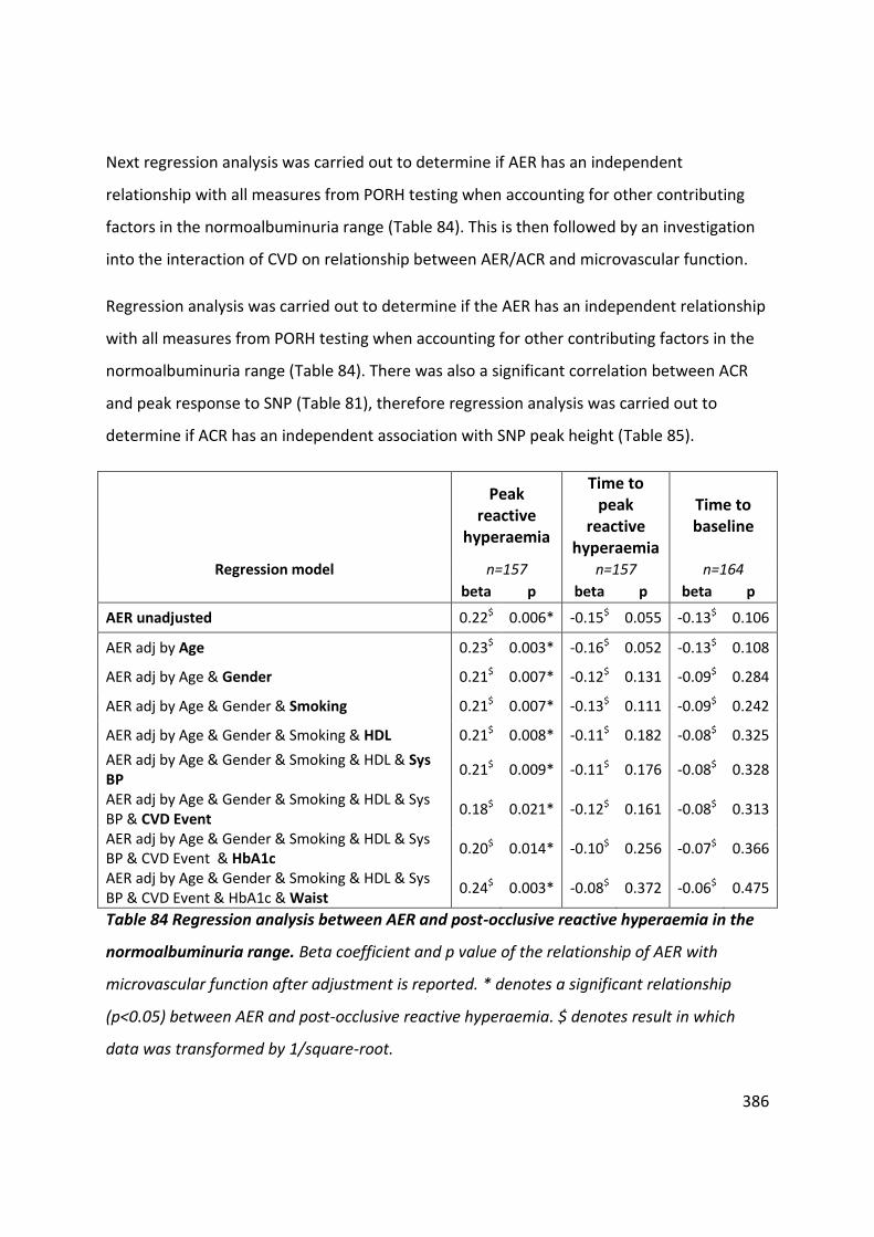
386

Next regression analysis was carried out to determine if AER has an independent

relationship with all measures from PORH testing when accounting for other contributing

factors in the normoalbuminuria range (Table 84). This is then followed by an investigation

into the interaction of CVD on relationship between AER/ACR and microvascular function.

Regression analysis was carried out to determine if the AER has an independent relationship

with all measures from PORH testing when accounting for other contributing factors in the

normoalbuminuria range (Table 84). There was also a significant correlation between ACR

and peak response to SNP (Table 81), therefore regression analysis was carried out to

determine if ACR has an independent association with SNP peak height (Table 85).

Peak reactive

hyperaemia

Time to peak

reactive hyperaemia

Time to baseline

Regression model n=157 n=157 n=164

beta p beta p beta p

AER unadjusted 0.22$ 0.006* -0.15$ 0.055 -0.13$ 0.106

AER adj by Age 0.23$ 0.003* -0.16$ 0.052 -0.13$ 0.108

AER adj by Age & Gender 0.21$ 0.007* -0.12$ 0.131 -0.09$ 0.284

AER adj by Age & Gender & Smoking 0.21$ 0.007* -0.13$ 0.111 -0.09$ 0.242

AER adj by Age & Gender & Smoking & HDL 0.21$ 0.008* -0.11$ 0.182 -0.08$ 0.325

AER adj by Age & Gender & Smoking & HDL & Sys BP

0.21$ 0.009* -0.11$ 0.176 -0.08$ 0.328

AER adj by Age & Gender & Smoking & HDL & Sys BP & CVD Event

0.18$ 0.021* -0.12$ 0.161 -0.08$ 0.313

AER adj by Age & Gender & Smoking & HDL & Sys BP & CVD Event & HbA1c

0.20$ 0.014* -0.10$ 0.256 -0.07$ 0.366

AER adj by Age & Gender & Smoking & HDL & Sys BP & CVD Event & HbA1c & Waist

0.24$ 0.003* -0.08$ 0.372 -0.06$ 0.475

Table 84 Regression analysis between AER and post-occlusive reactive hyperaemia in the

normoalbuminuria range. Beta coefficient and p value of the relationship of AER with

microvascular function after adjustment is reported. * denotes a significant relationship

(p<0.05) between AER and post-occlusive reactive hyperaemia. $ denotes result in which

data was transformed by 1/square-root.

387

SNP; peak endothelial independent response

Regression model n=152

beta p

ACR unadjusted 0.17 0.037*

ACR adj by Age 0.15 0.063

ACR adj by Age & Gender 0.16 0.071

ACR adj by Age & Gender & Smoking 0.15 0.081

ACR adj by Age & Gender & Smoking & HDL 0.14 0.111

ACR adj by Age & Gender & Smoking & HDL & Sys BP

0.14 0.114

ACR adj by Age & Gender & Smoking & HDL & Sys BP & CVD Event

0.14 0.112

ACR adj by Age & Gender & Smoking & HDL & Sys BP & CVD Event & HbA1c

0.12 0.148

ACR adj by Age & Gender & Smoking & HDL & Sys BP & CVD Event & HbA1c & Waist

0.10 0.238

Table 85 Regression analysis between ACR and peak endothelial independent response to

sodium nitroprusside in the normoalbuminuria range. Beta coefficient and p value of the

relationship of ACR with peak endothelial independent response to sodium nitroprusside

after adjustment is reported. * denotes a significant relationship (p<0.05). ACR is not

independently related to peak endothelial independent response to sodium nitroprusside in

the normoalbuminuria range.

AER in the normoalbuminuria range has an independent relationship with peak reactive

hyperaemia post arterial occlusion when accounting for other confounding variables. ACR is

not independently related to peak endothelial independent response to sodium

nitroprusside in the normoalbuminuria range.

The direct correlation between AER and peak height in the normoalbuminuria range is

demonstrated in Figure 91A. The estimated relationship between AER and peak height

when adjusting for confounding factors is displayed in Figure 91B.

388

Figure 91 Correlation between AER and peak hyperaemia from post-occlusive reactive

hyperaemia testing in the normoalbuminuria range. A: Unadjusted correlation between

peak hyperaemia and AER (log scale). B: Correlation between peak hyperaemia and AER

(data log transformed) after adjusting for all the variables used in the regression model in

Table 76.

0

50

100

150

200

250

Peak H

eig

ht

(AU

)

0 5 10 15 20 Albumin excretion rate (µg/min)

-2

-1

0

1

2

Peak H

eig

ht

(lo

g)

AU

-1.5 -1 -.5 0 .5 1 Albumin excretion rate (log) µg/min [Low AER] [High AER]

High

Low

A

B

389

Interaction of CVD on relationship between AER/ACR and microvascular function

in the normoalbuminuria range

There are significant correlations between AER and maximal blood flow and minimum

vascular resistance in subjects with CVD (Table 86). However, due to reduced sample size

during regression modelling the relationships between AER and MBF (p=0.068) and MVR

(p=0.101) were no longer significant and not investigated further.

There are significant correlations between ACR and endothelial dependent and independent

response to ACH and SNP respectively in subjects without CVD (Table 86). The relationship

between ACR and endothelial dependent response to ACH in subjects without CVD was

independent of other confounding factors for CVD (Table 87). However the relationship

between ACR and endothelial independent response to SNP was accounted by the included

confounding factors (Table 87).

390

Maximal blood

flow

Minimum Vascular

resistance

ACH; total endothelial dependent response

ACH; peak endothelial dependent response

SNP; total endothelial

independent response

SNP; peak endothelial

independent response

r p r p r p r p r p r p

CVD

AER

n 92 87 89 91 86 88

Best distribution 0.27$ 0.009* -0.26

$ 0.014* 0.13

$ 0.233 0.09

$ 0.412 0.03

$ 0.754 0.05

$ 0.613

Log -0.29 0.005* 0.29 0.006* -0.15 0.170 -0.12 0.241 -0.01 0.912 -0.05 0.672

Non parametric -0.30 0.004* 0.30 0.005* -0.09 0.412 -0.10 0.347 -0.04 0.726 -0.05 0.648

ACR

n 87 82 84 86 81 83

Best distribution 0.13$ 0.242 -0.11$ 0.319 0.01$ 0.923 0.01$ 0.964 0.03$ 0.786 0.04$ 0.703

Log -0.15 0.153 0.14 0.197 0.03 0.761 0.01 0.943 0.02 0.858 -0.02 0.883

Non parametric -0.13 0.221 0.13 0.260 0.03 0.767 0.00 0.991 -0.01 0.964 -0.03 0.800

No CVD

AER

n 119 116 118 118 117 117

Best distribution -0.08$ 0.403 0.11

$ 0.223 0.12

$ 0.202 0.10

$ 0.290 0.05

$ 0.618 0.05

$ 0.621

Log 0.10 0.299 -0.13 0.162 -0.10 0.268 -0.08 0.404 -0.05 0.565 -0.04 0.706

Non parametric 0.09 0.306 -0.10 0.266 -0.08 0.362 -0.07 0.450 0.00 0.985 0.01 0.946

ACR

n 102 100 101 101 100 100

Best distribution 0.00$ 0.983 -0.02$ 0.843 0.27$ 0.007* 0.34$ 0.001* 0.25$ 0.012* 0.27$ 0.006*

Log 0.02 0.839 0.01 0.935 -0.27 0.007* -0.35 <0.001* -0.25 0.014* -0.27 0.006*

Non parametric -0.02 0.826 0.06 0.564 -0.28 0.004* -0.37 <0.001* -0.25 0.011* -0.28 0.005*

Table 86 Correlation between urinary albumin excretion and microvascular function in subjects with and without CVD with

normoalbuminuria. Pearson correlation coefficient was determined between variables using; a) transformed data (to achieve normal data

distribution) and b) log transformed data. Spearman rank correlation was carried out on untransformed data. * denotes a significant

relationship where p<0.05. $ denotes result in which data was transformed by 1/square-root. Grey boxes highlight significant correlations.

391

No CVD

Regression model

ACH; total endothelial dependent response

ACH; peak endothelial dependent response

SNP; total endothelial

independent response

SNP; peak endothelial

independent response

n=96 n=96 n=95 n=95

beta p beta p beta p beta p

ACR unadjusted 0.26$ 0.012* 0.33

$ 0.001* 0.26

$ 0.009* 0.29

$ 0.005*

ACR adj by Age 0.22$ 0.033* 0.30

$ 0.003* 0.21

$ 0.040* 0.25

$ 0.017*

ACR adj by Age & Gender 0.25$ 0.023* 0.34

$ 0.002* 0.19

$ 0.076 0.23

$ 0.041*

ACR adj by Age & Gender & Smoking

0.26$ 0.018* 0.34

$ 0.002* 0.20

$ 0.070 0.23

$ 0.038*

ACR adj by Age & Gender & Smoking & HDL

0.26$ 0.02* 0.34$ 0.003* 0.17$ 0.126 0.20$ 0.070

ACR adj by Age & Gender & Smoking & HDL & Sys

BP 0.26

$ 0.026* 0.34

$ 0.003* 0.17

$ 0.138 0.20

$ 0.077

ACR adj by Age & Gender & Smoking & HDL & Sys

BP & HbA1c 0.23

$ 0.049* 0.32

$ 0.007* 0.14

$ 0.204 0.17

$ 0.142

ACR adj by Age & Gender & Smoking & HDL & Sys

BP & HbA1c & Waist 0.21$ 0.069 0.30$ 0.010* 0.12$ 0.275 0.15$ 0.194

Table 87 Regression analysis between ACR and microvascular function in subjects without

CVD. A forced entry approach to regression modelling with confounding variables

accumulatively added. Beta coefficient and p value of the relationship of AER/ACR with

microvascular function after adjustment is reported. * denotes a significant relationship

(p<0.05) between AER and microvascular function. $ denotes result in which data was

transformed by 1/square-root. Adj denotes adjusted.

392

Post occlusive reactive hyperaemia curve morphology:

AER in the normoalbuminuria range was stratified by PORH peak response curve

morphology (Table 88, Figure 92). A one way ANOVA demonstrated there was no significant

difference in AER distribution between groups (p=0.308).

PRH; Peak type:

Normal Early non-dominant Early dominant

n 92 60 31

AER (µg/min) 6.71 6.86 9.02

[4.26 to 9.90] [4.36 to 9.58] [5.25 to 12.01]

Table 88 Distribution of AER by curve morphology after post occlusive reactive hyperaemia

testing in the normoalbuminuria range. Median AER [inter-quartile range] is presented.

There is no significant difference in AER distribution between groups (p=0.308).

393

Figure 92 AER distribution by curve morphology after post occlusive reactive hyperaemia

testing in participants in the normoalbuminuria range. There is no significant difference in

AER distribution between groups (p=0.308).

The characteristics of the participants by curve morphology are summarised in Table 89.

Weight (p=0.040), BMI (p0.001), waist (p=0.010), hip size (p=0.004), systolic blood pressure

(p=0.036) and renal impairment (p=0.025) were significantly more prominent in subjects

with an early dominant peak across all groups, demonstrating an increased risk of CVD.

Peak and total endothelial dependent response to ACH was significantly reduced in subjects

with an early dominant peak response to arterial occlusion (Total response; p=0.043, peak

response; p=0.028). Post occlusive reactive peak hyperaemia (the second, traditional peak)

was significantly lower in subjects with an early dominant first peak (p=0.001) (Table 89).

0

5

10

15

20

Alb

um

in e

xcre

tion

rate

(u

g/m

in)

0 1 2 Normal Early non-dominant Early dominant

394

Characteristic Normal Early non-dominant

Early dominant

P (across all 3

groups)

n 92 60 31

Gender (%male) 61 (67%) 39 (65%) 19 (61%) 0.858

Ethnicity (% white British) 100% 98% 100% 0.330

Age (years) 68.6 (±7.7) 69.2 (±8.0) 71.5 (±9.7) 0.065£

Height (m)

1.72 1.71 1.71

0.151 [1.66 to 1.79] [1.65 to 1.76]

[1.64 to 1.76]

Weight (kg)

80 80.1 87

0.040*& [71.3 to 88.4] [71.9 to 90.9]

[80.6 to 97.3]

Body fat (%)

28.4 30.2 32.6

0.070 [23.6 to 35.9] [26.1 to 36.9]

[26.7 to 39.5]

BMI (kg m-2)

26.58 27.44 29.66

0.001* [24.28 to 29.87] [24.67 to 31.12]

[27.74 to 32.67]

Waist (cm) 97.4 (±14.0) 100.1 (±13.8) 104.9

(±14.2) 0.010*

Hip (cm) 104 105 108

0.004*$ [100 to 112] [100 to 113] [106 to 116]

Waist hip ratio 0.92 (±0.08) 0.93 (±0.08) 0.94 (±0.09) 0.190

Systolic BP (mmHg) 128.9 (±13.7) 132.6 (±13.4) 134.4

(±15.6) 0.036*

Diastolic BP (mmHg) 69.9 (±8.3) 68.8 (±6.0) 68.9 (±8.2) 0.442

Total cholesterol (mmol/L) 4.1 4.4 4.1

0.838 [3.5 to 5.2] [3.8 to 5.6] [3.7 to 4.7]

HDL (mmol/L) 1.4 1.3 1.4

0.094 [1.2 to 1.9] [1.1 to 1.7] [1.0 to 1.7]

LDL (mmol/L)

2.15 2.34 2.12

0.966 [1.61 to 2.97] [1.78 to 3.46]

[1.53 to 2.66]

Fasting triglycerides (mmol/L)

0.99 1.18 1.32

0.129 [0.82 to 1.50] [0.84 to 1.98]

[0.87 to 1.51]

Glucose (mmol/L) 6.0 6.1 6.6

0.096 [5.1 to 7.9] [5.4 to 7.5] [5.4 to 9.0]

395

Characteristic Normal Early non-dominant

Early dominant

P (across all 3

groups)

HbA1c (mmol/mol) 45 46 51

0.170$

[40 to 57] [42 to 51] [42 to 63]

CVD n (%) 38 (42%) 22 (37%) 18 (58%) 0.173

Antihypertensive therapy n (%) 47 (52%) 35 (58%) 23 (74%) 0.099

Statin therapy n (%) 61 (67%) 38 (63%) 21 (68%) 0.945

Smokers (current/ex/never) (%) (3/43/54) (2/56/42) (10/39/52) 0.188

Renal function:

Serum creatinine (µmol/L) 81 85 87

0.212 [69 to 90] [73 to 95] [70 to 90]

eGFR (ml/min/1.73m2) 81.4 93.3 76.2

0.025* [72.9 to 88.9] [63.1 to 85.4]

[61.5 to 83.5]

CKD stage n (%): n=75 n=51 n=28 0.212

G1 15 (20%) 8 (16%) 5 (18%)

G2 55 (73%) 34 (67%) 17 (61%)

G3A 4 (5%) 6 (12%) 6 (21%)

G3B 1 (1%) 1 (2%) 0

G4 0 2 (4%) 0

G5 0 0 0

Vascular assessments:

Maximal blood flow (AU)

148.5 139.3 134.8

0.365 [112.5 to 202.0] [102.2 to 205.9]

[118.7 to 184.9]

Minimum vascular resistance (mmHg/AU)

0.62 0.67 0.67

0.544 [0.44 to 0.81]

[0.45 to 0.91] [0.51 to

0.78]

ACH; total endothelial dependent response (AU)

92500 89087 66342

0.043*@ [58072 to 116405]

[63075 to 1221473]

[36041 to 99729]

ACH; peak endothelial dependent response (AU)

455.7 443.9 394.3

0.028*@ [372.0 to 550.1] [362.1 to 550.4]

[302.9 to 475.2]

396

Characteristic Normal Early non-dominant

Early dominant

P (across all 3

groups)

SNP; total endothelial independent response (AU)

52190 56155 45020

0.636@ [34080 to 70510]

[41050 to 84970]

[25740 to 64560]

SNP; peak endothelial independent response (AU)

333.0 351.5 301.0

0.656@ [262.0 to 408.0] [297.0 to 461.0]

[242.0 to 376.0]

PORH; peak hyperaemia (AU)

81.4 66.7 59.3

0.001*& [57.8 to 113.4] [49.4 to 101.8]

[44.4 to 91.8]

PORH; time to peak hyperaemia(seconds)

13.7 19.4 10.0 0.153&

[11.3 to 18.1] [13.3 to 38.0] [8.1 to 13.0]

PORH; time to baseline

145.3 159.5 166.8

0.525& [117.7 to 178.9] [129.0 to 197.9]

[118.3 to 212.8]

Diabetes n (%) 43 (47%) 30 (50%) 19 (61%)

Glucose (mmol/L) 7.9 7.3 8.1

0.153 [6.5 to 9.0] [6.5 to 8.5] [6.5 to 9.5]

HbA1c (mmol/mol) 56 50.0 59

0.370$ [48 to 63] [47 to 59] [49 to 68]

Duration of diabetes (years) 6.1 (±4.8) 7.4 (±7.1) 8.6 (±5.4) 0.085@

Table 89 Participant characteristics and microvascular function stratified by peak response

curve morphology group in subjects with normoalbuminuria. Data are presented as mean

(±SD) or median [IQR]. * P value < 0.05 indicates a significant difference in a characteristic

between subjects across all three groups. The following symbols represent results obtained

from transformed data to ensure normal distribution of residuals from regression analysis: £

denotes squared data, &denotes logged data, $denotes 1/square root transformation and

@denotes data transformed by square root.

397

7.5.1.6 Objective 5

To determine if there is a correlation between the change in urinary albumin excretion over

three years with a change in vascular function.

One-hundred and forty four participants who had baseline and follow-up ACR and

microvascular assessments (selection criteria from Table 66) were selected from the

SUMMIT cohort to test this hypothesis (Table 90). At baseline the mean age was 66.3 (±8.1)

years, 69% of whom were male. 69% of participants had been diagnosed with diabetes

(Hba1c > 47 mmol/mol and were diagnosed with T2DM after the age of 35 years).

50% were classified as having CVD if they had a medical history of myocardial infarction,

percutaneous coronary intervention, coronary arterial bypass graft, unstable angina,

peripheral artery disease and verified cerebrovascular event (stroke and / or transient

ischaemic attack).

At baseline 67% of subjects were on antihypertensive therapy and 73% on statin therapy.

The median eGFR [IQR] was 79.3 [68.7 to 91.0] ml/min/1.73m2, putting the majority of

participants (58%) in the G2 stage of CKD (eGFR between 60 and 89 ml/min/1.73m2).

The mean follow up period was 37 (±3) months, the minimum duration was 29 months and

the maximum was 49 months.

398

7.5.1.6.1 Participant characteristics at baseline

Characteristic Full Cohort Diabetes No

Diabetes

p

(DM vs no DM)

n 144 100 44

Sex (%male) 69 71 64 0.380

Ethnicity (% white British) 100 100 100

Age (years) 66.3 (±8.1) 67.1 (±8.4) 64.7 (±7.4) 0.094

Height (m) 1.72 1.72 1.72

0.607 [1.67 to 1.77] [1.67 to 1.77] [1.66 to 1.79]

Weight (kg) 86.0 88.8 76.9

<0.001 [76.2 to 95.6] [81.6 to 99.6] [68.4 to 84.0]

Body fat (%) 31.7 32.6 28.7

<0.001 [26.2 to 38.7] [26.8 to 41.1] [25.0 to 34.1]

BMI (kg.m-2) 29 30 26

<0.001 [26 to 32] [27 to 34] [23 to 27]

Waist (cm) 102.8 (±12.8) 106.6 (±12.0) 94.0 (±10.1) <0.001

Hip (cm)

105.9 108.6 102.6

<0.001 [101.8 to 111.8]

[104.0 to 117.0]

[98.1 to 105.3]

Waist hip ratio 0.95 (±0.08) 0.97 (±0.07) 0.91 (±0.09] <0.001

Systolic BP (mmHg) 126.7 (±15.5) 128.6 (±15.0) 122.4 (±16.0) 0.513

Diastolic BP (mmHg) 75.8 (±8.3) 76.3 (±8.6) 74.6 (±7.8) 0.798

Total Cholesterol (mmol/L) 4.2 3.8 4.9

<0.001 [3.4 to 5.1] [3.2 to 4.5] [4.2 to 5.8]

HDL (mmol/L) 1.27 1.22 1.47

<0.001 [1.09 to 1.56] [1.06 to 1.41] [1.18 to 1.90]

LDL (mmol/L) 2.07 1.84 2.78

<0.001 [1.57 to 2.89] [1.46 to 2.36] [2.09 to 3.31]

Fasting triglycerides (mmol/L) 1.28 1.30 1.17

0.082 [0.97 to 1.67] [1.00 to 1.78] [0.94 to 1.59]

399

Characteristic Full Cohort Diabetes No

Diabetes

p

(DM vs no DM)

Duration of diabetes (years) n/a 7.9 (±5.8) n/a

Fasting glucose (mmol/L) 6.8 7.8 5.2

<0.001 [5.4 to 8.4] [6.7 to 9.2] [4.8 to 5.5]

HbA1c (mmol/mol) 51 57 40

<0.001 [42 to 62] [50 to 67] [39 to 42]

CVD n(%) 50 53 43 0.330

Antihypertensive therapy n(%) 67 79 41 <0.001

Statin therapy n(%) 73 83 50 <0.001

Smokers (current/ex/never) n(%)

4/50/45 4/51/45 5/50/45 0.985

Renal function:

Serum creatinine (µmol/L) 82 82 82

0.761 [73 to 93] [73 to 94] [72 to 92]

eGFR (ml/min/1.73m2) 79.3 80.1 78.7

[68.7 to 91.0] [67.5 to 90.5] [73.4 to 91.8] 0.893

CKD stage n (%):

G1 41 (28%) 28 (28%) 13 (30%) 0.472

G2 84 (58%) 57 (57%) 27 (61%)

G3A 13 (9%) 9 (9%) 4 (9%)

G3B 6 (4%) 6 (6%) 0 (0%)

G4 0 (0%) 0 (0%) 0 (0%)

G5 0 (0%) 0 (0%) 0 (0%)

Table 90 Participant characteristics for participants selected to test hypothesis 2. Data are

presented as mean (±SD) or median [IQR] for all subjects and sub-grouped by diabetes

status. P value indicates if there is a significant difference in a characteristic between

subjects with and without diabetes.

400

7.5.1.6.2 Change in ACR and microvascular function over three years in subjects with and

without T2DM

There is a significant increase in ACR over three years across the whole cohort (p<0.001) and

in those with T2DM (p<0.001), but not in subjects without T2DM (p=0.299) (Table 91). 14

participants (10%) developed microalbuminuria (all with T2DM) over the three years. The

mean increase in ACR in subjects with diabetes was 2.36 (±6.50) mg/mmol, in subjects

without T2DM the mean change was -0.11 (±1.2) mg/mmol (the change in ACR is

significantly different when considering diabetes status, p=0.003).

Across the whole cohort, there was a significant change in microvascular function (except

for time to peak during PORH testing); however this change was not influenced by diabetes

status. There is a significant loss in total endothelial dependent response to ACH over time,

however there is a mean increase in percent change. This lack of agreement is caused by

several subjects having very large increases in response, skewing the data. There were no

reasons to exclude these data. No differences were found in the outcomes of the future

analysis if these outliers were excluded from the analysis.

Full Cohort Diabetes

No Diabetes

p (DM vs

non-DM)

Albuminuria:

Baseline ACR (mg/mmol)

0.79 0.89 0.63 0.062

[0.47 to 1.77] [0.50 to 2.06] [0.45 to 1.10]

Follow up ACR (mg/mmol)

1.15 1.53 0.81 <0.001* [0.68 to 2.69] [0.74 to 3.63] [0.52 to 1.44]

Significance between baseline and follow up (p)

<0.001 <0.001 0.299

Change in ACR (FITZ)

Actual change in ACR (mg/mmol)

1.60 (±5.57) 2.36 (±6.50) -0.11 (±1.2) 0.003*

Percent change (%) 175.4 (±466.4) 233.6 (±533.8) 43.1 (±103.6) 0.010*

401

Full Cohort Diabetes

No Diabetes

p (DM vs

non-DM)

Change from normoalbuminuria to

microalbuminuria n (%) 14 (10%) 14 (14%) 0

Change from microalbuminuria to

normoalbuminuria n (%) 7 (5%) 4 (4%) 3 (7%)

Change in vascular assessment:

Maximal blood flow (AU) -33.0 (±62.0) -26.1 (±56.2) -48.1 (±71.4) 0.087

Significance between baseline and follow up (p)

<0.001 <0.001 <0.001

Minimum vascular resistance (mmHg/AU)

0.1 (±0.3) 0.1 (±0.3) 0.2 (±0.2) 0.183

(p) <0.001 0.032 <0.001

ACH; total endothelial dependent response (AU)

-17716.8 (±39640.2)

-18634.4 (±35380.9)

-15631.2 (±48344.1)

0.609

(p) <0.001 <0.001 0.038

ACH; peak endothelial dependent response (AU)

-88.3 (±124.9) -94.7 (±119.4) -73.7

(±136.9) 0.326

(p) <0.001 <0.001 <0.001

SNP; total endothelial independent response (AU)

-13004.0 (±25435.0)

-13993.8 (±23691.0)

-10725.3 (±29234.1)

0.524

(p) <0.001 <0.001 0.038

SNP; peak endothelial independent response (AU)

-92.5 (±117.7) -99.3 (±107.4) -76.9

(±138.8) 0.288

(p) <0.001 <0.001 0.001

PORH; peak hyperaemia (AU) -14.4 (±61.1) -14.7 (±60.5) -13.8 (±63.3) 0.893

(p) 0.042 0.121 0.226

PORH; time to peak hyperaemia(seconds)

3.9 (±28.6) 2.4 (±29.8) 7.1 (±25.8) 0.462

(p) 0.220 0.680 0.130

PORH; time to baseline (seconds)

20.2 (±122.4) 26.9 (±115.8) 5.9 (±136.2) 0.316

(p) 0.035 0.033 0.557

402

Full Cohort Diabetes

No Diabetes

p (DM vs

non-DM)

Percent change in vascular assessment:

Maximal blood flow (%) -13.5 (±31.1) -10.3 (±30.4) -20.5 (±31.8) 0.122

Minimum vascular resistance (%)

25.6 (±59.1) 19.9 (±60.4) 37.4 (±55.1) 0.186

ACH; total endothelial dependent response (%)

21.8 (±411.8) 31.0 (±492.9) 0.6 (±62.8) 0.713

ACH; peak endothelial dependent response (%

-14.3 (±32.2) -16.1 (±34.3) -10.1 (±26.5) 0.273

SNP; total endothelial independent response (%)

-2.0 (±123.9) -2.3 (±144.4) -1.5 (±53.6) 0.934

SNP; peak endothelial independent response (%)

-17.7 (±30.2) -20.4 (±30.3) -11.4 (±29.2) 0.082

PORH; peak hyperaemia (%) 6.3 (±77.1) 6.0 (±76.0) 6.9 (±80.5) 0.808

PORH; time to peak hyperaemia(%)

43.2 (±133.1) 28.2 (±107.9) 76.9 (±174.0) 0.085

PORH; time to baseline (%)

44.2 (±132.7) 56.3 (±152.5) 18.1 (±68.7) 0.109

Change in blood pressure:

-3.2 -2.5 -4.9

Change in systolic blood pressure (mmHg)

[-10.8 to 2.7] [-11.2 to 4.8] [-9.4 to 0.3] 0.377

Percent change in systolic blood pressure (%)

-2.4 (±8.4) -2.0 (±8.7) -3.3 (±7.9) 0.364

Table 91 Change in ACR, blood pressure and microvascular function over 37 months (±3) in

144 participants from the SUMMIT cohort. Data are presented as mean (±SD) or median

[IQR] for all subjects and sub-grouped by diabetes status. P value indicates if there is a

significant difference in a characteristic between subjects with and without diabetes.

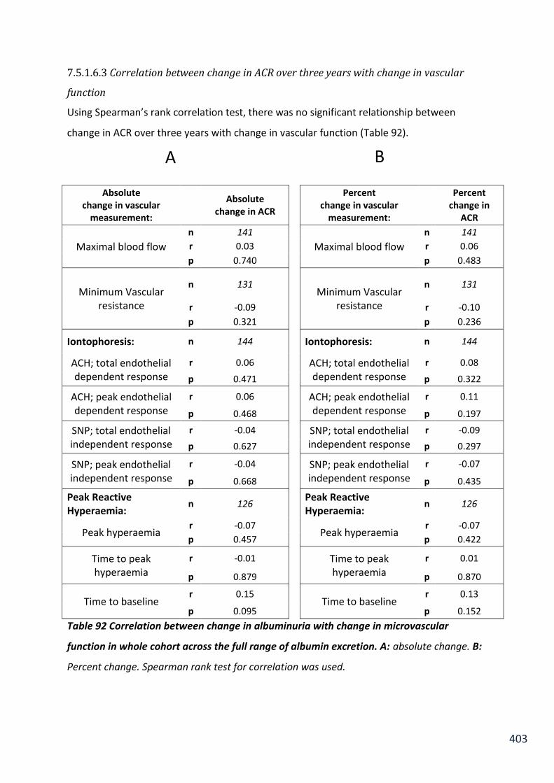
403

7.5.1.6.3 Correlation between change in ACR over three years with change in vascular

function

Using Spearman’s rank correlation test, there was no significant relationship between

change in ACR over three years with change in vascular function (Table 92).

Absolute change in vascular

measurement:

Absolute change in ACR

Percent

change in vascular measurement:

Percent

change in ACR

Maximal blood flow

n 141

Maximal blood flow

n 141

r 0.03 r 0.06

p 0.740 p 0.483

Minimum Vascular resistance

n 131

Minimum Vascular resistance

n 131

r -0.09 r -0.10

p 0.321 p 0.236

Iontophoresis: n 144

Iontophoresis: n 144

ACH; total endothelial dependent response

r 0.06 ACH; total endothelial dependent response

r 0.08

p 0.471 p 0.322

ACH; peak endothelial dependent response

r 0.06 ACH; peak endothelial dependent response

r 0.11

p 0.468 p 0.197

SNP; total endothelial independent response

r -0.04 SNP; total endothelial independent response

r -0.09

p 0.627 p 0.297

SNP; peak endothelial independent response

r -0.04 SNP; peak endothelial independent response

r -0.07

p 0.668 p 0.435

Peak Reactive Hyperaemia:

n 126 Peak Reactive

Hyperaemia: n 126

Peak hyperaemia r -0.07

Peak hyperaemia r -0.07

p 0.457 p 0.422

Time to peak hyperaemia

r -0.01

Time to peak hyperaemia

r 0.01

p 0.879 p 0.870

Time to baseline r 0.15

Time to baseline r 0.13

p 0.095 p 0.152

Table 92 Correlation between change in albuminuria with change in microvascular

function in whole cohort across the full range of albumin excretion. A: absolute change. B:

Percent change. Spearman rank test for correlation was used.

A B

404

7.5.1.6.3 Objective 6

To determine if a change in ACR over three years within the normoalbuminuria range

correlates to a change in vascular function.

In the normoalbuminuria range, there was a significant correlation between the change

(absolute and percentage change) in ACR with change in maximal blood flow and with

change in minimum vascular resistance (Table 93). To determine if this is an independent

relationship regression analysis with potential confounding variables was carried out

assessing actual change (Table 94) and percent change (Table 95).

405

Absolute change in vascular measurement:

Absolute change in ACR

Percent change in vascular

measurement:

Percent change in

ACR

Maximal blood flow

n 102 Maximal blood

flow

n 102

r 0.25

r 0.26

p 0.010*

p 0.008*

Minimum Vascular resistance

n 98 Minimum Vascular

resistance

n 98

r -0.27

r -0.24

p 0.007*

p 0.018*

Iontophoresis: n 101

Iontophoresis: n 101

ACH; total endothelial dependent response

r 0.13

ACH; total endothelial dependent response

r 0.16

p 0.183

p 0.117

ACH; peak endothelial

dependent response

r 0.07

ACH; peak endothelial dependent response

r 0.13

p 0.483

p 0.196

SNP; total endothelial independent

response

r -0.02

SNP; total endothelial

independent response

r -0.06

p 0.849

p 0.588

SNP; peak endothelial independent

response

r -0.01

SNP; peak endothelial

independent response

r -0.04

p 0.947

p 0.672

Peak Reactive Hyperaemia:

n 92

Peak Reactive Hyperaemia:

n 92

Peak hyperaemia r -0.09

Peak hyperaemia r -0.09

p 0.417

p 0.411

Time to peak hyperaemia

r -0.03

Time to peak hyperaemia

r 0.01

p 0.779

p 0.953

Time to baseline r -0.01

Time to baseline r 0.00

p 0.931

p 0.978

Table 93 Correlation between change in albuminuria within the normoalbuminuria range

with change in microvascular function. A: absolute change. B: Percent change. Spearman

rank test for correlation was used. * denotes a significant relationship where p<0.05.

B A

406

Absolute change in Maximal Blood

Flow

Absolute change in Minimum Vascular

Resistance n=79 n=79 beta p beta p

Change (∆) in ACR unadjusted 0.25 0.026* -0.25 0.025*

ACR adj by Age 0.25 0.025* -0.25 0.024*

ACR adj by Age & Gender 0.25 0.026* -0.25 0.023*

ACR adj by Age & Gender & Smoking 0.24 0.033* -0.24 0.031*

ACR adj by Age & Gender & Smoking & ∆ HDL 0.24 0.044* -0.24 0.044*

ACR adj by Age & Gender & Smoking & ∆HDL & ∆Sys BP 0.14 0.238 -0.22 0.075

ACR adj by Age & Gender & Smoking & ∆HDL & ∆Sys BP & CVD Event

0.14 0.228 -0.22 0.079

ACR adj by Age & Gender & Smoking & ∆HDL & ∆Sys BP & CVD Event & ∆HbA1c

0.15 0.197 -0.21 0.104

ACR adj by Age & Gender & Smoking & ∆HDL & ∆Sys BP & CVD Event & ∆HbA1c & ∆Waist

0.15 0.201 -0.21 0.107

Table 94 Regression analysis between absolute change in ACR within the

normoalbuminuria range with change in microvascular function. A forced entry approach

to regression modelling with confounding variables accumulatively added. Beta coefficient

and p value of the relationship of change of ACR with change of microvascular function after

adjustment is reported. ∆ denotes ‘change’, Adj denotes adjusted. Change in ACR does not

have an independent association with change in MBF and MVR in the full model. The

regression model was repeated without change in systolic blood pressure due to potential

collinearity with change in MVR; change in ACR was not independently associated with

change in MVR (p>0.05) .

407

Percent change in

Maximal Blood Flow

Percent change in Minimum Vascular

Resistance

n=79 n=79

beta p beta p

Percent Change (%∆) in ACR unadjusted 0.13 0.245 -0.15 0.181

ACR adj by Age 0.13 0.268 -0.15 0.202

ACR adj by Age & Gender 0.13 0.261 -0.15 0.201

ACR adj by Age & Gender & Smoking 0.15 0.188 -0.18 0.126

ACR adj by Age & Gender & Smoking & %∆ HDL 0.15 0.185 -0.17 0.137

ACR adj by Age & Gender & Smoking & %∆HDL & %∆Sys BP

0.10 0.376 -0.16 0.182

ACR adj by Age & Gender & Smoking & %∆HDL & %∆Sys BP & CVD Event

0.10 0.370 -0.16 0.170

ACR adj by Age & Gender & Smoking & %∆HDL & %∆Sys BP & CVD Event & %∆HbA1c

0.11 0.353 -0.16 0.185

ACR adj by Age & Gender & Smoking & %∆HDL & %∆Sys BP & CVD Event & %∆HbA1c & %∆Waist

0.11 0.362 -0.16 0.190

Table 95 Regression analysis between percent change in ACR within the

normoalbuminuria range with percent change in microvascular function. A forced entry

approach to regression modelling with confounding variables accumulatively added. Beta

coefficient and p value of the relationship of percent change of ACR with percent change of

microvascular function after adjustment is reported. %∆ denotes ‘percent change’, Adj

denotes adjusted.

408

7.5.2 Hypothesis 2

Three-hundred and twenty one participants diagnosed with type 2 diabetes, who had a

urine sample from a random spot collection stored at baseline, and retinal photography and

neuropathy tests carried out at both baseline and follow up were selected to test this

hypothesis (Figure 87). Participant characteristics were similar to the previous cohorts, with

32% having had a CVD event, 74% on hypertensive therapy and 79% on statin therapy with a

median [IQR] HbA1c of 55 [49 to 65] mmol/mol. The median ACR was 0.89 [0.45 to 1.96]

with the majority of participants in the normoalbuminuria range (77%), 20% of participants

had microalbuminuria and 3% with macroalbuminuria (Table 96).

16% of participants had significant neuropathy at baseline, with 6% of the cohort developing

significant neuropathy over the three years. Significant neuropathy is clinically defined if the

participant is only able to feel the monofilament in three or less sites in either foot.

Therefore people who went from a score of four or above to below four, in either foot are

classified as a neuropathy progressor. Non progressors were defined as individuals who did

not have a monofilament score go from above 4 to below 4.

A progression of two retinopathy steps or more, as demonstrated in Table 68, across both

eyes was classified as being clinically significant. Therefore, individuals with a worsening of

two steps of retinopathy in one eye are classified as a progressor, as would an individual

with a worsening of one stage in both eyes. Non progressors were defined as individuals

who did not have a worsening of two steps of retinopathy in one eye or worsening of one

stage in both eyes.

The majority of participants had no diabetic retinopathy (DR) (55%), 29% had minimal DR,

15% had mild DR and 2 % had moderate DR at baseline.11% had a significant progression in

DR over the three years (Table 96).

409

7.5.2.1 Participant characteristics

Characteristic: Full Cohort

n 321

Sex (%male) 69

Ethnicity (% white British) 100

Age (years) 67.4 (±9.5)

Height (m) 1.71

[1.65 to 1.77]

Weight (kg) 87.3

[79.0 to 101.1]

Body fat (%) 32.6

[27.2 to 40.8]

BMI (kg m-2) 30

[26 to 34]

Waist (cm) 107.1 (±14.4)

Hip (cm) 107

[102 to 115]

Waist hip ratio 0.97 (±0.09)

Systolic BP (mmHg) 146.6 (±18.1)

Diastolic BP (mmHg) 79.8 (±9.4)

HbA1c (mmol/mol) 55

[49 to 65]

Duration of diabetes (years) 8.2 (±7.2)

CVD event n (%) 104 (32%)

Antihypertensive therapy n (%) 238 (74%)

Statin therapy n (%) 252 (79%)

Smokers (current/ex/never) (%) 23/175/123

Renal function:

Serum creatinine (µmol/L) 84

[72 to 98]

eGFR (ml/min/1.73m2) 79

[62 to 90]

410

CKD stage n (%):

G1 81 (26%)

G2 167 (54%)

G3A 34 (11%)

G3B 23 (7%)

G4 5 (2%)

G5 0 (0%)

Albuminuria:

Baseline ACR (mg/mmol) 0.89

[0.45 to 1.96]

Normoalbuminuria n (%) 247 (77%)

Microalbuminuria n (%) 64 (20%)

Macroalbuminuria n (%) 10 (3%)

Neuropathy:

Lowest monofilament score n (%):

Full Cohort Normoalbuminuria

range

n=318 n=249

0 12 (4%) 9 (4%)

1 8 (3%) 6 (2%)

2 4 (1%) 1 (1%)

3 26 (8%) 17 (7%)

4 31 (10%) 25 (10%)

5 50 (16%) 33 (13%)

6 187 (59%) 158 (63%)

Progression from non-clinical to significant neuropathy n (%):

19/318 (6%) 14/187 (7%)

Baseline retinopathy status n (%):

Full cohort Normoalbuminuria

range

n=321 n=247

1 (No DR) 176 (55%) 143 (58%)

2 Minimal DR 92 (29%) 69 (28%)

3 Mild DR 47 (15%) 31 (13%)

4 Moderate DR 6 (2%) 4 (2%)

5 Proliferative DR 0 0

411

Progressors (two step increase across both eyes) n (%):

29/263 (11%) 6/109 (6%)

DR prevalence at initial examination n (%)

145 (45%) 104 (42%)

Developed proliferative DR over three years n (%)

2 (0.87%) 0

Table 96 Baseline participant characteristics for the individuals with type 2 diabetes

selected to test Hypothesis 3 (n=321). Participants were recruited from the SUMMIT cohort,

and included in this investigation if they met the inclusion criteria to test Hypothesis Two

(Table 66). Data are presented as mean (±SD) or median [IQR] for all subjects and sub-

grouped by diabetes status. DR = Diabetic retinopathy.

7.5.2.2 Objective 1

To investigate the relationship between urinary albumin excretion and the early stages of

diabetic retinopathy and neuropathy.

One way ANOVA demonstrates there is a significant difference (p=0.016) in the distribution

in ACR among groups; no DR, minimal DR and mild DR (moderate DR was excluded to

investigate the relationship of ACR with background retinopathy (minimal and mild DR))

(Figure 93). Post hoc analysis using Bonferroni multiple comparison test indicated that ACR

was signicantly higher in the mild DR group compared to the no DR group (p=0.012).

412

Figure 93 Distribution of ACR at different stages of diabetic retinopathy. Post hoc analysis

using Bonferroni multiple comparison test indicates a signifcant difference in ACR between

mild DR and no DR (p=0.012). Moderate DR was excluded from statistical analysis to

investigate the relationship of ACR with background retinopathy (minimal and mild DR).

One way ANOVA demonstrates there is no significant difference (p=0.199) in the

distribution in ACR among the scores for clinically non significant neuropathy (monofilament

score four to six) (Figure 94)

413

Figure 94 Distribution of ACR at different monofilament scores. One way ANOVA

demonstrates there is no significant difference (p=0.199) in the distribution in ACR amoung

the scores for clinically non significant neuropathy (four to six).

414

7.5.2.3 Objective 2

To investigate the relationship between urinary albumin excretion and progression /

development of diabetic retinopathy and neuropathy.

Diabetic retinopathy:

A progression of two retinopathy steps or more across both eyes (Table 68) was classified as

being clinically significant and identified as a progressor. Non DR progressors were defined

as individuals who did not have a worsening of two steps of retinopathy in one eye or

worsening of one stage in both eyes.

Median [IQR] ACR was 0.84 [0.42 to 1.55] mg/mmol in non DR progressors (Figure 95),

compared to 1.24 [0.62 to 7.66] mg/mmol in DR progressors (p=0.0498) (Table 97). Clinical

characteristics of DR progressors are compared to those with no clinically meaningful

progression in Table 98.

Figure 95 Distribution of ACR among individuals who had a clinically meaningful

progression in retinopathy and those who did not. ACR is significantly (p=0.0498) higher in

DR progressors (n=29) compared to those without DR progression.

415

Number of

participants (%males)

Mean (±SD) ACR

(mg/mmol)

Median [IQR] ACR

(mg/mmol)

Wilcoxon rank sum test

(p)

No retinopathy progression

234 (68%) 3.17 (±8.13 ) 0.84

0.0498* [0.42 to 1.55]

Retinopathy progression

29 (85%) 4.54 (±7.61) 1.24

[0.62 to 7.66]

Table 97 Difference in ACR between individuals who had a meaningful progression in

retinopathy and those who did not. ACR is significantly (p=0.0498) higher in DR progressors.

Due to the low numbers of individuals with a progression in retinopathy, it is not suitable to

carry out logistic regression to determine in ACR is indecently associated. However, the

clinical characteristics between individuals who had a meaningful progression in DR and

those who did not are compared in Table 98. Duration of diabetes was significantly higher in

subjects who had a meaningful progression in DR (p=0.033)

Baseline Characteristics: No DR progression DR Progression p

N 234 29

Sex n (%male) 160 (68%) 22 (75%) 0.410

Age (years) 67 (±9) 70 (±9) 0.065

Weight (kg) 87.2 86.7

0.584 [78.1 to 101.5] [79.0 to 92.7]

Body fat (%) 33.0 30.1

0.157 [27.6 to 40.9] [25.1 to 40.3]

BMI (kg m-2) 30 29

0.475 [27 to 34] [26 to 33]

Waist (cm) 106.9 (±14.6) 105.9 (±14.1) 0.935

Systolic BP (mmHg) 136 (±15) 143 (±24) 0.295

HbA1c (mmol/mol) 53 58

0.117 [49 to 63] [49 to 70]

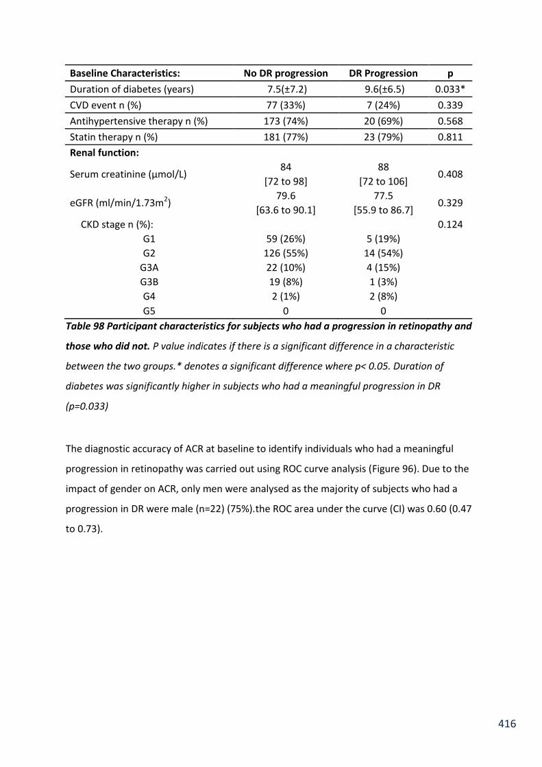
416

Baseline Characteristics: No DR progression DR Progression p

Duration of diabetes (years) 7.5(±7.2) 9.6(±6.5) 0.033*

CVD event n (%) 77 (33%) 7 (24%) 0.339

Antihypertensive therapy n (%) 173 (74%) 20 (69%) 0.568

Statin therapy n (%) 181 (77%) 23 (79%) 0.811

Renal function:

Serum creatinine (µmol/L) 84 88

0.408 [72 to 98] [72 to 106]

eGFR (ml/min/1.73m2) 79.6 77.5

0.329 [63.6 to 90.1] [55.9 to 86.7]

CKD stage n (%):

0.124

G1 59 (26%) 5 (19%)

G2 126 (55%) 14 (54%)

G3A 22 (10%) 4 (15%)

G3B 19 (8%) 1 (3%)

G4 2 (1%) 2 (8%)

G5 0 0

Table 98 Participant characteristics for subjects who had a progression in retinopathy and

those who did not. P value indicates if there is a significant difference in a characteristic

between the two groups.* denotes a significant difference where p< 0.05. Duration of

diabetes was significantly higher in subjects who had a meaningful progression in DR

(p=0.033)

The diagnostic accuracy of ACR at baseline to identify individuals who had a meaningful

progression in retinopathy was carried out using ROC curve analysis (Figure 96). Due to the

impact of gender on ACR, only men were analysed as the majority of subjects who had a

progression in DR were male (n=22) (75%).the ROC area under the curve (CI) was 0.60 (0.47

to 0.73).

417

Figure 96 Diagnostic accuracy of ACR to identify men with type 2 diabetes who had a

meaningful progression in retinopathy (n=22). ROC area under the curve (CI) = 0.60 (0.47 to

0.73). The solid diagonal line represents the line of identify, where the test is neither specific

nor sensitive.

7.5.2.3.1 Characteristics of subjects with no DR progression with and without

clinical levels of albumin excretion.

Contrary to the hypothesis, 51 subjects who had no progression in DR had an ACR in the

microalbuminuria range or above (Figure 95). To investigate this group further their

characteristics are explored and compared with subjects who had no progression with an

ACR in the normoalbuminuria range (n=183) in (Table 99).

Subjects with albumin excretion in the clinical ranges were at a higher risk of CVD than the

subjects with albumin excretion in the normal range. The group with an ACR in the clinical

ranges had a significantly higher; systolic blood pressure (p=0.014), HbA1c (p=0.022),

0.0

0

0.2

5

0.5

0

0.7

5

1.0

0

Se

nsitiv

ity

0.00 0.25 0.50 0.75 1.00 1 - Specificity

418

duration of diabetes (p=0.001), with 88% on anti-hypertensive medication compared to 70%

in the normoalbuminuria group (p=0.009) (Table 99).

Baseline Characteristics:

No DR progression with

normoalbuminuria

No DR progression & elevated albumin

excretion in the clinical range

P

N 183 51

Sex n (%male) 120 (66%) 40 (78%) 0.081

Age (years) 66 (±10) 68 (±7) 0.198

Weight (kg)

87 88.2 0.348

[78.0 to 101.1] [80.6 to 107.5]

Body fat (%)

33.8 32.3 0.109

[27.6 to 41.2] [27.0 to 36.1]

BMI (kg m-2)

30 30 0.435

[26 to 33] [27 to 34]

Waist cm) 106.3 (±14.3) 109.5 (±15.6) 0.221

Systolic BP (mmHg) 127 (±13) 138 (±12) 0.014*

Diastolic BP (mmHg) 77 (±9) 78 (±9) 0.349

HbA1c (mmol/mol)

52 55 0.022*

[48 to 62] [50 to 69]

Duration of diabetes (years)

6.7 (±6.8) 11.8 (±8.6) 0.001*

CVD event n (%) 58 (32%) 19 (37%) 0.455

Antihypertensive therapy n (%)

128 (70%) 45 (88%) 0.009*

Statin therapy n (%) 137 (75%) 44 (86%) 0.085

Smokers (current/ex/never) (%)

43/52/5 37/53/10 0.380

419

Renal function:

Serum creatinine (µmol/L)

83 84 0.091

[72 to 95] [75 to 109]

eGFR (ml/min/1.73m2)

79.6 80.1 0.178

[65.4 to 91.3] [60.1to 89.3]

CKD stage n (%):

G1 48 (27%) 11 (22%) 0.421

G2 100 (56%) 26 (52%)

G3A 17 (10%) 5 (10%)

G3B 12 (7%) 7 (14%)

G4 1 (1%) 1 (2%)

G5 0 0

ACR (mg/mmol) 0.75 6.47 <0.001*

[0.45 to 1.19] [3.75 to 13.84]

Normoalbuminuria n (%) 183 (100%) -

Microalbuminuria n (%) - 43 (84%)

Macroalbuminuria n (%) - 8 (16%)

Table 99 Clinical characteristics of individuals who had no progression in retinopathy who

had either an ACR in the normoalbuminuria range or higher. 51 participants had an ACR in

the clinically abnormal albumin excretion ranges. These subjects have a significantly higher;

systolic blood pressure (p=0.014), HbA1c (p=0.022), duration of diabetes (p=0.001), with a

larger proportion on anti-hypertensive medication (p=0.009), compared to those with

normoalbuminuria. P value indicates if there is a significant difference in a characteristic

between subjects with and without higher levels of albumin excretions.

420

Diabetic neuropathy:

Monofilament sensitivity was carried out on six sites on both feet. Significant neuropathy is

clinically defined if the participant is only able to feel the monofilament in three or less sites

in either or both feet. Therefore people who went from a score of four or above to below

four, in either foot are classified as a neuropathy progressor. Non progressors were defined

as individuals who did not have a monofilament score go from above 4 to below 4.

Median [IQR] ACR was 0.80 [0.43 to 1.47] mg/mmol in non-neuropathy progressors (Figure

97), compared to 0.73 [0.48 to 1.44] mg/mmol in progressors (p=0.683) (Table 100).

Figure 97 The distribution of ACR among individuals who had a meaningful progression in

neuropathy and those who did not. ACR is not significantly (p=0.683) different in

progressors (n=19) compared to those without progression in neuropathy.

421

Number of

participants

Mean (±SD) ACR

(mg/mmol)

Median [IQR] ACR

(mg/mmol)

Wilcoxon rank sum test (p)

No neuropathy progression

301 2.46 (±6.03) 0.80

0.683 [0.43 to 1.47]

Neuropathy progression

19 3.39 (±10.69) 0.73

[0.48 to 1.44]

Table 100 Difference in ACR between individuals who had a meaningful progression in

neuropathy and those who did not. ACR is not significantly (p=0.683) different in

progressors (n=19) compared to those without progression in neuropathy.

There was no relationship between ACR at baseline and the progression of diabetic

neuropathy, therefore only the relationship with the progression of diabetic retinopathy is

investigated further.

422

7.5.2.4 Objective 3

To determine if an increase in urinary albumin excretion over three years is related to a

progression/development of diabetic retinopathy and neuropathy.

321 participants from the SUMMIT cohort, all diagnosed with type 2 diabetes, who had a

urine sample from a random spot collection stored at baseline, and retinal photography and

neuropathy tests carried out at baseline were selected to test Hypothesis two (Figure 87).

Out of 321 participants, only 263 subjects had data available for follow up assessments to

test Objective 2. Out of those 263, only 170 subjects had a spot ACR store at follow up as

well, these subjects were used to test objective three.

7.5.2.4.1 Participant characteristics

Characteristics Full cohort

n 170

Sex (%male) 69

Ethnicity (% white British) 100

Age (years) 67.8 (±9.0)

Height (m) 1.71

[1.65 to 1.77]

Weight (kg) 87.3

[78.1 to 102.5]

Body fat (%) 32.6

423

Characteristics Full cohort

[27.2 to 40.8]

BMI (kg m-2) 30

[27 to 33]

Waist (cm) 106.3 (±14.3)

Hip (cm) 107

[102 to 116]

Waist hip ratio 0.96 (±0.11)

Systolic BP (mmHg) 140.7 (±16.2)

Diastolic BP (mmHg) 77.6 (±8.6)

HbA1c (mmol/mol) 55

[49 to 65]

CVD event n (%) 66 (39%)

Antihypertensive therapy n (%) 130 (76)

Statin therapy n (%) 131 (77)

Smokers (current/ex/never) (%) 3/55/42

Renal function:

Creatinine (µmol/L) 85

[74 to 101]

eGFR (ml/min/1.73m2) 77.5

[61.5 to 89.2]

CKD stage n (%):

G1 34 (20%)

G2 96 (58%)

G3A 20 (12%)

G3B 14 (8%)

G4 2(1%)

G5 -

Mean change in eGFR -4.8 (±8.0)

Mean percent change in eGFR (%) -7.0 (±12.8)

424

Characteristics Full cohort

Retinopathy:

Baseline Retinopathy n (%):

1 (No DR) 92 (54%) 2 Minimal DR 47 (28%)

3 Mild DR 29 (17%) 4 Moderate DR 2 (1%)

Progressors n (%): 16/170 (9%)

Urinary Albumin Status:

Baseline ACR (mg/mmol) 0.85

[0.42 to 2.23]

Normoalbuminuria n (%) 141 (83%)

Microalbuminuria n (%) 24 (14%)

Macroalbuminuria n (%) 5 (3%)

Mean change in ACR (mg/mmol) 2.47 (±12.98)

Mean percent change in ACR (%) 237 (±738)

Table 101 Baseline participant characteristics for the individuals with type 2 diabetes

selected to test Objective 3. Participants were recruited from the SUMMIT cohort, and

included in this investigation if met the inclusion criteria to test Hypothesis Two (Table 66).

Data are presented as mean (±SD) or median [IQR] for all subjects. DR = Diabetic

retinopathy.

425

7.5.2.4.2 To determine if change in ACR over three years is different between individuals

who have had a meaningful progression in retinopathy and those who have not.

A progression of two retinopathy steps or more across both eyes (Table 68) was classified as

being clinically significant and identified as a progressor. Non DR progressors were defined

as individuals who did not have a worsening of two steps of retinopathy in one eye or

worsening of one stage in both eyes.

Median [IQR] absolute change in ACR was 0.40 [0.05 to 1.43] mg/mmol in non DR

progressors (Figure 98), compared to 0.12 [-0.62 to 3.70] mg/mmol in DR progressors

(p=0.612) (Table 102). Clinical characteristics of DR progressors are compared to those with

no progression in Table 98.

Median [IQR] percent change in ACR was 53.5% [4.8 to 201.7] in non DR progressors (Figure

99), compared to 22.1% [-43.1 to 134.8] in DR progressors (p=0.156) (Table 103).

426

Figure 98 Distribution of the change in ACR between individuals who had a progression in

retinopathy and those who did not. The change in ACR is not significantly (p=0.612) higher

in DR progressors (n=16) compared to those without meaningful DR progression (n=154).

Number of

participants

Mean (±SD) absolute change

in ACR (mg/mmol)

Median [IQR] absolute change

in ACR (mg/mmol)

Wilcoxon rank sum test (p)

No retinopathy progression

154 2.54 (±13.05) 0.40

0.612 [0.05 to 1.43]

Retinopathy progression

16 1.85 (±12.64) 0.12

[-1.22 to 3.70]

Table 102 Change in ACR between individuals who had a progression in retinopathy and

those who did not. The change in ACR is not significantly (p=0.612) higher in DR progressors

(n=16) compared to those without DR progression (n=154).

-50

0

50

10

0

15

0

Ab

so

lute

diffe

rence

in

AC

R (

mg

/mm

ol)

No DR progression DR progression

427

Figure 99 Distribution of the percent change in ACR between individuals who had a

progression in retinopathy and those who did not. The percent change in ACR is not

significantly (p=0.156) higher in DR progressors (n=16) compared to those without DR

progression (n=154).

Number of

participants

Mean (±SD) percent change

in ACR (%)

Median [IQR] percent change

in ACR (%)

Wilcoxon rank sum test (p)

No retinopathy progression

154 249.2 (±769.3) 53.5

0.1556 [4.8 to 201.7]

Retinopathy progression

16 122.2 (±288.5 22.1

[-43.1 to 134.8]

Table 103 Percent change in ACR between individuals who had a progression in

retinopathy and those who did not. The percent change in ACR is not significantly (p=0.156)

higher in DR progressors (n=16) compared to those without DR progression (n=154).

0

2,0

00

4

,000

6

,000

8

,000

Pe

rcen

t d

iffe

ren

ce in

AC

R (

%)

No DR progression DR progression

428

7.5.2.5 Matched pairs analysis

There are a large proportion of participants who have had a large increase in ACR with no

DR progression (Figure 98 and Figure 99). This could be attributed to the diverse cohort

being tested, where nearly 40% of participants have already had a CVD event. To accurately

test the difference in change in ACR between individuals who had a progression in

retinopathy status and those who did not, I undertook an analysis of matched cases to

controls. Two controls were matched to each individual who had a meaningful progression

in retinopathy. Controls were matched exactly by gender, previous CVD event (not by type

of event but by a positive history of any event) and ACE inhibitor treatment. Controls were

further matched as close as possible by alpha-2 receptor blocker treatment, baseline ACR,

age (±8 years), duration of diabetes (± 5 years), waist and HbA1c. All matching was carried

out whilst blinded to the change in ACR. The characteristics of the DR progressors and

match controls are summarised in Table 104.

429

Characteristic Retinopathy progression

No retinopathy progression

p

n 16 32

Matched Characteristics:

Sex n (%male) 11 (69%) 22 (69%) 1

Ethnicity (% white British) 100 100 1

CVD event n (%) 6 (38%) 12 (38%) 1

ACE inhibitors 8 (50%) 16 (50%) 1

Alpha-1 Blockers 2(13%) 2 (6%) 0.460

ACR (mg/mmol) 2.32 1.36

0.685 [0.68 to 8.78] [0.73 to 3.65]

Age (years) 70 (±9) 69 (±7) 0.181

Duration of diabetes (years) 8 (±6) 9 (±7) 0.887

Waist (cm) 103.2 (±16.3) 105.7 (±13.7) 0.548

HbA1c (mmol/mol) 58 57

0.753 [50 to 71] [49 to 70]

Unmatched Characteristics:

Height (m) 1.71 1.71

0.785 [1.65 to 1.75] [1.64 to 1.77]

Weight (kg) 80.7 87.2

0.3526 [76.7 to 90.7] [79.0 to 94.6]

Body fat (%) 29.9 30.1

0.811 [24.7 to 40.7] [25.1 to 40.3]

BMI (kg m-2) 28 29

0.323 [26 to 31] [28 to 32]

Systolic BP (mmHg) 141 (±27) 136 (±12) 0.907

Statin therapy n (%) 13 (81%) 27 (84%) 0.784

Smokers (current/ex/never) (%) 2/10/4 2/20/10

Renal function:

Creatinine (µmol/L) 85 88

0.489 [71 to 104] [75 to 109]

eGFR (ml/min/1.73m2) 78.0 66.6

0.752 [55.9 to 89.2] [59.2 to 89.3]

430

Characteristic Retinopathy progression

No retinopathy progression

p

CKD stage n (%):

0.556

G1 3 (20%) 5 (16%)

G2 8 (53%) 18 (58%)

G3A 2 (13%) 3 (10%)

G3B 1 (7%) 5 (16%)

G4 1(7%) 0

G5 0 0

Mean change in eGFR (ml/min/1.73m2) -5.8 (±10.6) -2.5 (±8.0) 0.437

Mean percent change in eGFR (%) -9.7 (±18.7) -3.3 (±11.7) 0.378

Retinopathy:

Baseline Retinopathy n (%):

0.554

1 (No DR) 10 (63%) 18 (56%)

2 Minimal DR 5 (31%) 8 (25%)

3 Mild DR 1 (6%) 6 (18%)

4 Moderate DR 0 0

Table 104 Participant characteristics at baseline for subjects with a progression in

retinopathy and their matched controls. Participants were selected from the SUMMIT

cohort, and included in this investigation if they met the inclusion criteria to test Hypothesis

Two (Table 66). Data are presented as mean (±SD) or median [IQR] for all subjects. P value

indicates if there is a significant difference in a characteristic between subjects with and

without retinopathy progression. There are no significant differences between groups,

demonstrating their suitability for matched pair analysis.

Median [IQR] absolute change in ACR was 1.00 [0.18 to 2.08] mg/mmol in non DR

progressors (Figure 100), compared to 0.12 [-1.22 to 3.70] mg/mmol in DR progressors

(p=0.431) (Table 105).

Median [IQR] percent change in ACR was 43% [7 to 144] in non DR progressors (Figure 101),

compared to 22% [-43 to 134] in DR progressors (p=0.284) (Table 106).

431

Figure 100 Distribution in the change of ACR between individuals who had a progression in

retinopathy and matched controls. The change in ACR is not significantly (p=0.431) higher in

DR progressors (n=16) compared to those without DR progression (n=32).

Number of

participants

Mean (±SD) absolute change

in ACR (mg/mmol)

Median [IQR] absolute change

in ACR (mg/mmol)

Wilcoxon rank sum test (p)

No retinopathy progression

32 2.68 (±6.75) 1.00

0.431 [0.18 to 2.08]

Retinopathy progression

16 1.85 (±12.64) 0.12

[-1.22 to 3.70]

Table 105 Difference in the change in ACR between individuals who had a progression in

retinopathy and matched controls. The change in ACR is not significantly (p=0.431) higher in

DR progressors (n=16) compared to those without DR progression (n=32).

-40

-2

0

0

20

40

Absolu

te d

iffe

rence in

AC

R (

mg/m

mol)

No DR progression DR progression

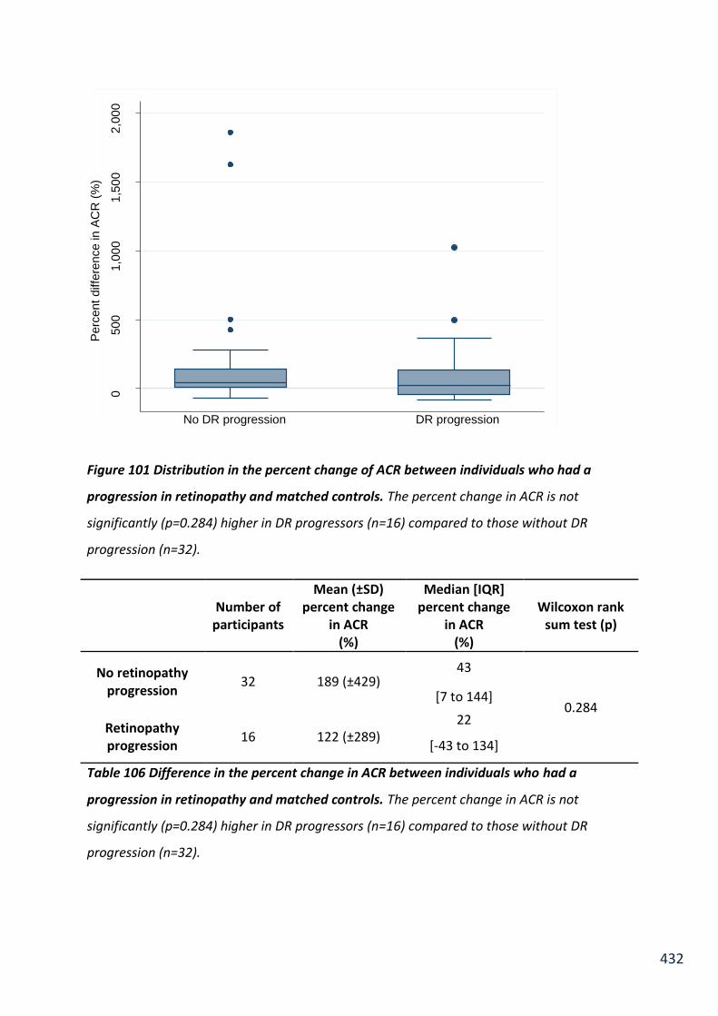
432

Figure 101 Distribution in the percent change of ACR between individuals who had a

progression in retinopathy and matched controls. The percent change in ACR is not

significantly (p=0.284) higher in DR progressors (n=16) compared to those without DR

progression (n=32).

Number of

participants

Mean (±SD) percent change

in ACR (%)

Median [IQR] percent change

in ACR (%)

Wilcoxon rank sum test (p)

No retinopathy progression

32 189 (±429) 43

0.284 [7 to 144]

Retinopathy progression

16 122 (±289) 22

[-43 to 134]

Table 106 Difference in the percent change in ACR between individuals who had a

progression in retinopathy and matched controls. The percent change in ACR is not

significantly (p=0.284) higher in DR progressors (n=16) compared to those without DR

progression (n=32).

0

500

1,0

00

1,5

00

2,0

00

Perc

ent

diffe

rence in

AC

R (

%)

No DR progression DR progression

433

7.6 Discussion

In this discussion an overview of participant recruitment to test each hypothesis is carried

out. Results are discussed individually for each objective, with a summary of the findings for

each hypothesis at the end. Future investigations to progress the findings of this chapter are

also discussed, followed by an overall conclusion.

7.6.1 Participant recruitment

Two-hundred and forty eight participants met the inclusion criteria to test Hypothesis One

(Table 66). Sixty-two of these participants did not have data recorded for various

confounding factors used in regression models (Objectives 3 & 4) and were therefore

excluded from the regression analysis. The majority of missing data are from not having

routine blood tests carried out as the participant was unable to provide a blood sample

(Figure 86).

One-hundred and forty four participants from the SUMMIT cohort where selected to

investigate the relationship between change in urinary albumin excretion and change in

microvascular function for the first in objectives 5 and 6 (Table 90). The cause for this loss in

participants is due to an inconsistency between laboratory staff to store urine samples at

baseline (104 samples not stored).

Three-hundred and twenty one participants diagnosed with type 2 diabetes, who had a

urine sample from a random spot collection stored at baseline, and retinal photography and

neuropathy tests carried out at both baseline and follow up were selected to test

hypothesis two (Figure 87). Fifty eight participants did not have retinal photography and

neuropathy data available at follow up (Objective 2), and a further 93 participants had no

spot ACR sample provided at follow up (Objective 3).

434

The target duration between visits was 36 months. The actual mean follow up period was 37

months (±3), demonstrating a good adherence to the SUMMIT study protocol by the

research nurse who made the appointments and carried out screening visits.

Across the whole SUMMIT cohort recruited in Exeter; 298 (36%) of participants did not

return after three years for a follow up visit. The most common reason was subjects unable

/ unwilling to return to the research centre, in which case a medical questionnaire was

carried out over the phone if possible. In several cases participants had moved away from

the area, some had developed serious illness, others had deceased.

Before officially entering the study, participants’ consented for researchers to access their

medical records, so their clinical information could be collected over a long period of time

for research purposes.

Hypothesis 1:

Urinary albumin excretion is related to microvascular function, with higher levels of albumin

excretion being associated with an impairment of microvascular function. The magnitude of

change in microvascular function over three years is related to the change in albumin

excretion. Furthermore, this relationship is present in individuals with and without diabetes,

and changes of urinary albumin excretion within the normoalbuminuria range relate to

changes in microvascular function.

435

7.6.1.1 Participant characteristics

It is an elderly cohort with a mean age of 70 (±8.2) years, 67% of whom were male. 65% of

participants were diagnosed with diabetes. When comparing participant characteristics by

diabetes status, attributes of diabetic milieu and risk factors for CVD arise as expected;

where subjects with diabetes are significantly heavier (p=0.03), have a higher proportion of

body fat (p=0.001), higher BMI (p<0.001), higher triglycerides (p<0.001), higher fasting

glucose (p<0.001) and HbA1c (p<0.001).

Our results are in accordance with the Maastricht study, and many other studies, which also

reported larger waist, higher systolic blood pressure, triglycerides, HbA1c, fasting glucose, in

their subjects with T2DM (n= 609) compared to non-diabetic group (n=1269) (Sorensen et

al., 2016). The Maastricht study has the largest cohort with microvascular assessments in

subjects with and without diabetes, therefore their characteristics are compared to the

SUMMIT cohort to enable comparisons to be drawn between the studies in later analyses.

Diabetic cohorts of the Maastricht and SUMMIT studies have a very similar mean age. In the

Maastricht study mean age was 62.8 ±7.6 years, compared to 68.5 ±8.8 years in the

SUMMIT study. Duration of diabetes is very similar in both studies, 8.2 ±7.0 years in the

Maastricht cohort compared to 8 ±6 years in the SUMMIT study. The most notable

difference between the cohorts is glycaemic control when assessed by glycated

haemoglobin. In the Maastricht study mean HbA1c was 51.7 ±11.4 mmol/mol, compared to

a median HbA1c in the SUMMIT cohort of 40 [37 to 43] mmol/mol.

7.6.1.2 Number of measurable samples using two assays

Urinary albumin excretion in the SUMMIT cohort was quantified using the validated

Fitzgerald ELISA and the routine Cobas method. The Fitzgerald ELISA was able to quantity

urinary albumin in two overnight collections from all 248 participants. The Cobas assay

436

could only quantify albumin in 106 (43%) of participant samples from the first collection,

and 100 (40%) in the second collection. The portion of measurable samples using the Cobas

assay reduced further in subjects without diabetes, to only 32% in the first collection and

24% in the second. This reflects the importance of using an assay with a lower quantification

limit when investigating urinary albumin excretion in subjects without diabetes.

The Cobas assay could measure albumin in 56% of random spot urine collections. This is

most likely because albumin excretion is higher during the day than overnight and so more

of the values fall within the detection range of the Cobas assay when a spot urine sample is

collected. Similar findings were observed during the urine collection studies in Chapter 4.

7.6.1.3 Agreement between the two methods of quantifying urinary albumin

From previous validation studies it was determined the Fitzgerald assay has mean bias of

3.55mg/L (±2.13) over the Cobas method (Chapter 2, Section 2.3.4). These findings were

confirmed in the SUMMIT investigation. The previous validation work determined that the

analytical range for the Fitzgerald assay was 0.78 to 40mg/L, therefore samples which had

an albumin concentration >40mg/L were diluted into this range.

The Passing Bablok regression demonstrated a significant correlation between the two

methods (p<0.001) to quantify urinary albumin (y=1.37 (1.25 to 1.49) + 2.00 (1.24 to 2.81).

The “y intercept” value of 2.00 mg/L indicates a positive systematic difference between the

two methods. This was confirmed by Bland Altman analysis which demonstrates that the

Fitzgerald method has a mean positive bias of 4.24 mg/L ± 3.35 compared to the Cobas

method (Figure 88). This supports the findings of the initial validation studies, which

demonstrated a mean bias of 3.55mg/L (±2.13) over the Cobas method (Chapter 2, Section

2.3.4). All subsequent analysis has been carried out using urinary albumin measurements

determined using the Fitzgerald assay.

437

7.6.1.4 Prevalence of microalbuminuria in the SUMMIT cohort

In the SUMMIT cohort, 3% of subjects (n=3) without diabetes were identified as having

microalbuminuria based on two overnight urine collections, compared to 12% (n=19) in

subjects with T2DM, when urinary albumin is measured using the Fitzgerald assay.

In the Maastricht cohort 4% of subjects without diabetes were in the microalbuminuria

range, compared to 17.4% in subjects with T2DM (Sorensen et al., 2016). The prevalence of

microalbuminuria in the two studies is very similar, and the higher incidence of

microalbuminuria in the Maastricht study may be attributed to the difference in urine

collection methods. Albumin excretion was assessed by two 24 hour urine collections in the

Maastricht cohort. Twenty-four hour urine collections are influenced by activity throughout

the day, elevating albumin excretion (Chapters 4 and 6).

Diabetic cohorts of the Maastricht and SUMMIT cohorts are of similar age and duration of

diabetes. Therefore it is expected that microalbuminuria prevalence would be similar in

both cohorts. In addition to different collection methods, an alternative explanation for

increased prevalence of microalbuminuria in the Maastricht study is that it is a population

based cohort with poorer glycaemic control, a known contributor to diabetes related

complications.

In 2014, 3.9 million people in the U.K. had been diagnosed with diabetes and it is estimated

that over 25% will develop diabetic kidney disease, usually ten years after diabetes

diagnoses (Diabetes UK, 2014). Prevalence of microalbuminuria in the SUMMIT cohort is

12%. This might reflect the short duration of diabetes in the cohort (8 (±6) years) or it may

reflect their good glycaemic control (median HbA1c [IQR]: 40 [37 to 43] mmol/mol).

438

7.6.1.5 Urinary albumin excretion in subjects with and without type 2 diabetes

Median [IQR] AER was 9.75 [5.53 to 18.48] µg/min in subjects with diabetes, compared to

6.02 [4.10 to 8.93] µg/min in subjects without T2DM (p<0.001). ACR was also significantly

higher in subjects with T2DM (p<0.001) as is expected and reflected in many studies (Hillege

et al., 2001). However, using the sensitive ELISA to quantify urinary albumin, this is the first

study to accurately report the full normoalbuminuria range, and report the differences in

diabetes and microvascular function.

Studies like those from the Maastricht cohort use routine clinical assays to measure urinary

albumin and are unable to quantify the lowest levels of albumin concentration. It is

probable that these studies report the LOQ of their albumin assay in undetectable samples,

if they intended to investigate relationships with albumin excretion. It is common that only

microalbuminuria and macroalbuminuria prevalence are reported to describe a cohort.

7.6.1.6 Microvascular function in the SUMMIT cohort

Endothelial dependent and independent microvascular response to iontophoretic delivery

of acetyl choline (ACH) and sodium nitroprusside (SNP) is significantly lower in subjects with

diabetes (p<0.001) (Table 71).

Maximal hyperaemia response to localised heating (p=0.002) and minimum vascular

resistance (<0.001) are also significantly lower in subjects with diabetes.

Results were mixed for skin reactive hyperaemia in response to arterial occlusion. Time to

peak hyperaemia was significantly lower in subjects with T2DM (<0.001), however peak

hyperaemia (p=0.078), time to baseline (p=0.073), and the type of early peak (p=0.449)

were not significantly different.

These relationships are explored further in the following sections.

439

7.6.1.7 Maximal hyperaemia in the SUMMIT cohort

Maximal hyperaemia, or maximal blood flow/flux, in response to localised heating is one of

the most common non-invasive tests used to represent generalised microvascular function.

Maximal hyperaemia is an indicator of the maximal capacity of the vessels to vasodilate, and

is significantly lower in subjects with T2DM (p=0.002) in the SUMMIT cohort. The

attenuation of maximal hyperaemia in diabetes has been previously reported. (Sandeman et

al., 1991a, Jaap et al., 1994a, Jaap et al., 1994b, Colberg et al., 2003, Schmiedel et al., 2007)

.

A study by Jaap et al. was carried out at the Diabetes and Vascular Research Centre in

Exeter, with very similar protocols used in their methods to those used in the SUMMIT

investigation. Jaap et al. reported significantly lower hyperaemic response to local heating in

the feet of 9 normotensive subjects with T2DM compared to 9 age- and sex-matched

control subjects (p<0.001) (Jaap et al., 1994b). Subjects with T2DM in the study by Jaap et

al. have a similar duration of diabetes (mean (range) of 7 years (4 to 19), and similar

glycaemic control compared n to those in the SUMMIT cohort (Jaap et al., 1994b).

Participants from the Jaap study were recruited from a diabetic clinic in Exeter (U.K.); the

majority of participants were European, similar to the SUMMIT cohort (99% white British).

Previous studies have demonstrated attenuated maximal hyperaemia in subjects with T2DM

in both European and African Caribbean cohorts (Strain et al., 2005b).

In the T2DM-enriched population-based Maastricht study cohort; 2,214 participants (51%

men, aged 59.7±8.2 years) had heat-induced skin hyperaemia measured by laser-Doppler

flowmeter (Sorensen et al., 2016). The percent increase in maximal hyperaemia when

heating was reported in the Maastricht study, whereas maximal hyperaemia in response to

localised heating (maximal blood flow) is reported in the SUMMIT study. Participants with

normal glucose metabolism had a mean percent increase in hyperaemia of 1235% (±810%),

compared to 1109 % (±748%) and 937% (±683%) in prediabetes and in T2DM respectively (p

<0.001). In the SUMMIT cohort, there is also a significant loss in maximal hyperaemia in

subjects with diabetes (135.2 AU [99.7 to 179.8] compared to subjects without diabetes

440

(165.7 AU [117.4 to 215.6] (p=0.002) (Table 71). Percent increase in maximal hyperaemia

was not calculated in the SUMMIT cohort, however the data is available to do so.

In the Maastricht study, flicker light induced retinal arteriolar dilation was also measured

and they concluded that prediabetes, T2DM, and measures of hyperglycaemia are

independently associated with impaired microvascular function in the retina and skin

(Sorensen et al., 2016). To determine if low levels of urinary albumin excretion are a marker

of early generalised impaired microvascular function, then it may correlate to early changes

in the retina, this is investigated in Hypothesis two.

7.6.1.8 Endothelial dependent and independent microvascular response in the

SUMMIT cohort

The findings from the SUMMIT cohort are in accordance with previous studies that have

demonstrated endothelial dependent and independent microvascular response to

iontophoretic delivery of acetyl choline (ACH) and sodium nitroprusside (SNP) is impaired in

subjects with diabetes (Beer et al., 2008, Morris et al., 1995, Caballero et al., 1999, Lim et

al., 1999, McVeigh et al., 1992).

A study by Morris et al. (1995) was conducted in the Diabetes and Vascular Research Centre

in Exeter, using similar methods to those used in the SUMMIT cohort. The finding from the

SUMMIT investigation, that the function of the endothelium and/or smooth muscle may be

attenuated in diabetes, extend the results of the study by Morris et al. into a larger, more

diverse cohort. The Morris et al. paper was published in 1995 and there have been changes

in glycaemic targets and medication regimens in this time but that even with these changes

microvascular impairments are still occurring.

In the study by Morris et al. the only information regarding urinary albumin excretion is that

3/14 patients with T2DM had raised ACR, it is not reported if that refers to micro- and/or

macro-albuminuria. There are, to my knowledge, no previous studies which have

investigated the relationship between urinary albumin excretion and endothelial dependent

441

and independent microvascular response to ACH and SNP. One study has demonstrated that

endothelial dysfunction is evident in subjects with T2DM with normoalbuminuria,

suggesting the pathogenic process of vasculopathy in T2DM occurs before the development

of microalbuminuria (Lim et al., 1999).

7.6.1.9 Post occlusive reactive hyperaemia in the SUMMIT cohort

In the SUMMIT cohort, time to peak reactive hyperaemia was significantly lower in subjects

with T2DM; however peak hyperaemia, time to baseline and the type of early peak not

significantly different. These findings contradict those from a study by Strain et al. which

demonstrated attenuated peak hyperaemia in 51 European and 66 African Caribbean

subjects with diabetes, aged between 40 and 65 years, recruited from the general

population (Strain et al., 2005b). A further analysis of the European and African Caribbean

cohort by Strain et al. demonstrated early peak morphology was influence by diabetes

status (Strain et al., 2005a). This was identified in the SUMMIT cohort.

A possible explanation for these differences between these studies is the different

populations were tested. Approximately half of the participants in the Strain et al. study

were African Caribbean, the remaining were from European descent. African Caribbean’s

have an increased risk of CVD (Chaturvedi, 2003), with the risk of stroke 1.5–2.5 times

greater than the general population (Wild and McKeigue, 1997). Although the SUMMIT

cohort might be a lower risk factor group as the subjects are all from European descent

(99% are white British), they are much older and 45% have a history of CVD.

In the SUMMIT cohort peak hyperaemia and early peak morphology were comparable

between patients with and without diabetes. A study by Yamamoto et al. demonstrated

comparable peak hyperaemia in patients with diabetes and controls, but reported

significant differences in dominant peak morphology, supporting the work described by

Strain et al. (Yamamoto-Suganuma and Aso, 2009).

442

Time to baseline was not reported in the study by Yamamoto, however PORH index, defined

as the ratio of the post-AUC 1 min relative to the pre-AUC 1 min, was significantly lower in

patients with diabetes than in control subjects (Yamamoto-Suganuma and Aso, 2009).

Yamato et al. propose that among all measures of PORH, the area under the curve (AUC)

over the duration of prolonged hyperaemia would be associated more strongly with CVD

than the traditionally reported peak hyperaemia and time to peak hyperaemia, or

morphological analysis. PORH index was not reported in the SUMMIT cohort in this analysis,

but data is available to calculate it.

Measuring microvascular function and albumin excretion in the SUMMIT cohort has

confirmed that albumin excretion is higher and vascular function is impaired in subjects with

diabetes. However, being able to quantify the lowest levels of albumin excretion, the

relationship with microvascular function can be fully investigated for the first time across

every individual in the cohort rather than assigning individuals below the detection limit of

the assay, the value equal to this lower limit.

7.6.1.10 Correlation between albumin excretion and microvascular function and

the interaction of T2DM and CVD.

There is a significant correlation between urinary albumin excretion and all measures of

microvascular function (Table 72). The association between AER/ACR with measures of

microvascular function is not significantly different in subjects with diabetes compared to

those without diabetes (Table 73). This is the first study to report the association with the

urinary albumin excretion across the full range with microvascular function.

Microvascular dysfunction precedes the development of atherosclerosis and is thought to

occur in response to CVD risk factors (smoking, obesity, hypertension, and dyslipidaemia)

(Shimokawa, 1999, Holowatz et al., 2008). The findings from the SUMMIT cohort support

443

previous findings that increased risk of CVD is associated with biomarkers of microvascular

dysfunction in healthy individuals (Anderson et al., 2011).

The results from the SUMMIT cohort support a review by Lambers Heerspink which

demonstrated that urinary albumin excretion is a predictor of all-cause mortality in diabetes

and the general population (Lambers Heerspink et al., 2011). A focal point of their review

was a prominent study by Hillege et al. from the PREVEND study (Hillege et al., 2002).

Hillege et al. demonstrated that a higher urinary albumin concentration increased the risk of

CVD and non CVD death in 40,548 subjects after adjustment for other well established risk

factors for CVD over a median follow up period of 961 days in the general population.

In the SUMMIT cohorts the direction of the relationship between AER/ACR and

microvascular function are as expected, although the increase in AER with increased peak

hyperaemia during PORH testing needs cautious interpreting.

In the SUMMIT cohort only the relationship between AER and ACR with time to peak

hyperaemia were significantly different in subjects with and without CVD. This

demonstrates that the relationship between AER/ACR with microvascular function is

present in all individuals, not just those with established CVD. There are significant

correlations between AER and ACR with time to peak hyperaemia (PORH) in subjects with

and without CVD (Table 77). However, none were independent when accounting for other

confounding risk factors of CVD (Table 78). The interaction of CVD on the relationship

between microvascular function and urinary albumin excretion was investigated further in

the normoalbuminuria range.

7.6.1.11 Microvascular function and urinary albumin excretion assessed by

overnight collection and spot samples

The discrepancies in the relationships identified between overnight AER or spot ACR and

microvascular function may be attributed to the accuracy and variability of the different

urine collection methods. AER obtained from two overnight collections provides the most

444

accurate assessment of albumin excretion however random spot samples are more

frequently used in routine practice. Previous chapters have explored the limitations of

random spot samples which have demonstrated poor reproducibility and they are

influenced by exercise.

From the results derived from the SUMMIT study, an alternative hypothesis to explain the

differences between the relationships between AER or ACR with microvascular function can

be proposed.

The discrepancies in the relationships identified between AER or ACR with microvascular

function may be attributed to overnight collections (AER) assessing resting albumin

excretion whereas ACR from a random spot sample is a marker of a stress test.

In Chapter 6, it was demonstrated that there are different types of responses in ACR to

walking. Three patterns were found; delayed change in ACR, immediate change and no

change. Perhaps the reason for the correlation between microvascular function and ACR

from random spot samples is because individuals with poor microvascular function

(impaired autoregulation) have a high ACR after walking, whereas overnight they would

have a low albumin excretion, hence there is no correlation with overnight AER. The role of

random spot samples as a stress test to identify exercise induced increased urinary albumin

needs further investigating, and its clinical application as a risk factor evaluated.

Walking induced increased urinary albumin excretion is supported by the findings of Koh

and colleagues, who in 2011 investigated the change in ACR one and two hours after one

kilometre walking on a treadmill (Koh et al., 2011). Their study involved thirty-five

participants with diabetes, with a range of pre walking levels of albumin excretion, and nine

control subjects. They demonstrated that in females with diabetes, on average ACR

increased above the microalbuminuria threshold at 1 hour post walking returning to

baseline levels by 2 hours. This data indicates that female patients with diabetes and

normoalbuminuria have walking induced increased albumin excretion, which might

represent an early sign of nephropathy. Koh et al. demonstrated no increase in ACR in

control subjects after walking.

445

It has been demonstrated that subjects with diabetes have a greater increase in ACR in

response to exercise than subjects without diabetes, although exercise induced ACR is

variable among individuals (Viberti et al., 1978). This increased susceptibility in diabetes

might help explain why controls in the study by Koh et al. did not show increased ACR after

walking, although it does not explain why male subjects with diabetes did not have

increased ACR. In our exercise study, healthy men and women demonstrated walking

induced albumin excretion. Other studies might not be able to deter walking induced

urinary albumin excretion if using inadequate assay which are unable to measure small

changes in ACR in the normoalbuminuria range.

To my knowledge, apart from my study and the study by Koh et al., there are no other

studies which have investigated the impact of walking on an ACR. Walking induced

increased urinary albumin excretion might help identify individuals at risk of CVD, and the

clinical implications of this is that samples collected from a first morning void, may not

identify these individuals. The Hillege study reported urinary albumin concentration from

early morning voids and demonstrated the risk of CVD mortality (Hillege et al., 2002). The

risk of CVD mortality might be more prominent if urinary albumin excretion was assessed in

random spot samples.

The function of a random spot ACR as a stress test is a novel theory. Previous studies have

reported exercise induced albuminuria, but they investigated the clinical ranges after very

high intensity of exercise (Mogensen, 1976, Mogensen and Vittinghus, 1975, Viberti et al.,

1978). In Chapter 6, the sensitive ELISA enabled small changes in ACR to be examined, and

due to participant discordance with the protocol, the relationship with number of steps

taken throughout the day was investigated. This is the first study to report the association of

ACR with walking, which has clinical implications when considering patients walking to GP

surgeries. This theory is revisited and supported by the findings in the normoalbuminuria

range.

446

7.6.1.12 The relationship between albumin excretion and post occlusion peak

reactive hyperaemia.

In the SUMMIT cohort; an increase in albumin excretion is independently associated with an

increase in post occlusive peak reactive hyperaemia after adjusting for age, gender, smoking

status, HDL, systolic blood pressure, history of CVD, HbA1c and waist (p=0.008) (Table 75).

This was the only independent relationship between albumin excretion and measures of

microvascular function.

This result is contradictory to other studies which suggest that low peak hyperaemia is

associated with poor health, with higher peak hyperaemia associated with individuals with

better health without any known CVD or known risk of CVD (Stewart et al., 2004, Tur et al.,

1991). There are considerable discrepancies between these studies and ours, where

different cohorts are being tested and methodological differences may explain the

inconsistent findings.

Stewart et al. reported lower peak height in individuals with end stage renal disease [ESRD]

(n=63) compared to healthy individuals, in comparison the SUMMIT cohort did not contain

any individuals with ESRD (Stewart et al., 2004). This difference in the patient characteristics

might explain the differences in findings. Tur et al reported that peak height was

significantly lower in patients with diabetes (p<0.02) compared to non-diabetic controls

(Tur et al., 1991). In the SUMMIT cohort there is no significant difference in peak reactive

hyperaemia (p=0.784) between subjects with and without T2DM (Table 69). However, the

studies by Stewart et al. and Tur et al. tested PORH on the forearm whereas in the SUMMIT

cohort it was tested on the feet, which might reflect the heterogeneity of microvascular

cells in different vascular beds. This is discussed further in Section 7.6.1.4.8.

Although it initially appears the positive correlation between AER and peak hyperaemia is

contradictory to other studies, in fact it is logical that impaired autoregulation at the

glomerulus results in increased albumin excretion, just as impaired autoregulation in skin

microvasculature results in increased peak hyperaemia after PORH testing.

447

In the SUMMIT cohort, the relationship between AER/ACR was only investigated with

individual parameters (e.g. peak hyperaemia) of post occlusive reactive hyperaemia. A study

by Yamamoto and Asp reported that PORH index correlated negatively with urinary

albumin, (Yamamoto-Suganuma and Aso, 2009). This demonstrates that the overall

response in PORH is reduced with increasing urinary albumin excretion. Perhaps the

increase in peak hyperaemia with urinary albumin excretion identified in the SUMMIT

cohort is the result of early impaired autoregulation and as CVD progresses the overall

PORH response declines as urinary albumin excretion continues to rise. The PORH index

needs to be calculated in the SUMMIT to investigate these findings further.

The study by Yamamoto and Aso demonstrates that urinary albumin excretion is association

with PORH index and that PORH index is related to peroneal motor nerve conduction

velocity (Yamamoto-Suganuma and Aso, 2009) . This supports the hypothesis that urinary

albumin excretion is linked to generalised microvascular dysfunction (de Zeeuw et al., 2006)

In the SUMMIT cohort, urinary albumin excretion correlates to time to peak reactive

hyperaemia and time to return to baseline, but these relationships are not independent of

traditional risk factors for CVD and are not influenced by diabetes. Visualising the regression

between albumin excretion and post occlusive peak reactive hyperaemia demonstrates the

variability in these biological measurements (Figure 89A). When adjusting this relationship

for all the confounding variables, the relationship is evident, but there is still a lot of

variation in the regression. (Figure 89B). This relationship is explored further in the

normoalbuminuria range in Section 7.6.1.5.

7.6.1.13 CVD risk factors

Regression analysis was carried out not only to determine if the relationship between

albumin excretion and microvascular function was independent, but also to investigate the

influence of confounding factors on those relationships.

448

Accumulatively adding variables to regression models, it is evident that waist circumference

has the largest influence on the regression coefficient factor of the relationships between

albumin excretion and microvascular function (Table 75, Table 76). Waist circumference is

an index of abdominal adipose tissue deposition (Pouliot et al., 1994) and is accepted as a

risk factor for CVD (Després, 2012). This indicates that the majority of relationships between

albumin excretion and microvascular function can be explained by abdominal fat. This is an

accordance with the results of Jongh et al. who demonstrated impaired microvascular

function in obesity (de Jongh et al., 2004)

There is a wealth of evidence demonstrating the risk of CVD with obesity, but the molecular

mechanisms are unclear. In diabetes, it has been proposed that adipocytokines, which are

produced by the adipose tissue, can directly influence the pro-atherogenic and pro-

inflammatory environment of the vascular walls (Cha et al., 2012). Leptin and adiponectin

are the two most abundant adipocytokines, and have previously been linked with vascular

complications in patients with T2DM, including subjects with nephropathy (Hanai et al.,

2010). These observations are supported by a systematic review and meta-analysis of

controlled cross sectional studies which suggests leptin and adiponectin levels are higher in

T2DM patients with microvascular complications (Rodríguez et al., 2016).

Age and gender can also explain a large proportion of the relationships. Age, gender and

abdominal fat are well established CVD risk markers (Jousilahti et al., 1999), and

demonstrate a limited use for AER being included in risk predication models, except for

estimating peak reactive hyperaemia after arterial occlusion.

7.6.1.14 Albumin excretion and post occlusion response early peak morphology

There was no significant difference in AER distribution between groups (p=0.243) when

stratifying by peak response curve morphology in this cohort (Table 79, Figure 90). This does

not support the relationship found by Strain et al. who demonstrated that AER was

significantly higher with an early dominant peak response (Strain et al., 2005a).

449

The mean age of the participants in the Strain study was approximately 55 years old, of

whom approximately 50% were African Caribbean, whereas the SUMMIT cohort are 99%

white British and much older (mean age of 77 years,). The SUMMIT cohort also has a much

lower prevalence of current smokers (4%) compared to 22% in the Strain study, which

reported that individuals with an early dominant peak were more likely to be smokers

(p=0.02). The study by Yamamoto also reported comparable urinary albumin excretion

among the three different peak morphologies, and they found no significant difference in

the prevalence of CVD (Yamamoto-Suganuma and Aso, 2009).

Visualising AER distribution by peak morphology (Figure 90) and comparing medians suggest

that AER is higher in subjects with an early dominant peak, although it is not statistically

significant (p=0.243). This lack of statistical significance may be influenced by individuals

with a high AER with normal peak curve morphology. 74% of these abnormal results were

from subjects on antihypertensive therapy and 78% on statins.

To explore the risk of CVD by different early peak morphology and to understand why the

results from the Strain study were not reflected in the SUMMIT cohort, the characteristics of

each group were summarised by peak morphology (discussed in the next section).

7.6.1.15 CVD risk factors and post occlusion reactive early peak morphology

In the SUMMIT cohort, age, weight, BMI, waist, hip size, systolic blood pressure, history of

CVD, on antihypertensive therapy and renal decline were significantly more prominent in

subjects with an early dominant peak, demonstrating an increased risk of CVD. This confirms

the findings from the Strain study (Strain et al., 2005a). The study by Yamamoto reported no

significant difference in the prevalence of CVD, but did not investigate CVD risk factors in

the different early peak morphology groups (Yamamoto-Suganuma and Aso, 2009).

Although subjects with normal peak morphology have the lowest prevalence of CVD (40%) it

is still very high and helps explain the increased albumin excretion in this group, of whom

450

57% are on antihypertensive therapy and 69% on statins. These outliers (subjects with high

AER) provide a bias in the normal peak morphology group, influencing the analysis.

This relationship between albumin excretion and post occlusion reactive early peak

morphology is examined further by studying the relationship in subjects with

normoalbuminuria. Therefore subjects with high AER in the microalbuminuria range or

above are excluded to determine if the same relationships exists without their influence.

Peak and total endothelial dependent response to ACH was significantly reduced in subjects

with an early dominant peak response to arterial occlusion (Total response; p=0.019, peak

response; p=0.012). Endothelial independent response to SNP was not significantly different

in subjects with dominant early peak morphology (Table 80). This suggests that early

dominant curve morphology may be related to impaired endothelial function, and warrants

further investigation.

7.6.1.16 Urinary albumin excretion and endothelial dependent and independent

hyperaemia

Urinary albumin excretion had a significant correlation with endothelial dependent and

independent response to the iontophoretic delivery of ACH and SNP. This relationship was

not independent when adjusting for age and gender. To my knowledge, this is the first study

to report the association of urinary albumin excretion and in vivo measures of microvascular

endothelial function. Endothelial dysfunction is a precursor to CVD, occurring at the earliest

stages. The relationship of endothelial dysfunction with small changes in albumin excretion

within the normoalbuminuria is discussed in Section 7.6.1.5.

Results from the SUMMIT cohort indicate AER has an independent relationship with peak

hyperaemia, suggesting impaired autoregulation could be driving generalised microvascular

dysfunction, resulting in increasing AER.

451

Our findings might support the ‘Steno hypothesis’, which was the first to claim a common

link between mechanisms involved in diabetic nephropathy and CVD. The Steno hypothesis

is that urinary albumin excretion is a marker of overall vascular dysfunction with increased

urinary excretion in the kidney presenting itself from increased glomerular permeability and

also representing increased vascular permeability elsewhere increasing CV risk (de Zeeuw et

al., 2006). This is tested further in the SUMMIT cohort, by assessing if urinary albumin

excretion is also associated with other microvascular complications of diabetes (Hypothesis

2).

7.6.1.17 Limitations

When assessing the relationship between measures of biological function; urinary albumin

excretion and microvascular function, it is important to consider the overall variability of

those measures. The biological variation of the different urine collection methods to assess

urinary albumin excretion needs to be considered in conjunction with assay variability to

quantity albumin (and creatinine if reporting ACR). When assessing in vivo measurements of

microvascular function; intra-individual biological variation of the different tests needs to be

considered in conjunction with the reproducibility of the method, and the operator

conducting the test (reported in Section 7.4.4.4). This overall variability becomes more

influential when investigating the relationship between these variables over time (Objective

5).

In the SUMMIT cohort, microvascular assessments are being carried out on the skin of the

arm (for iontophoretic delivery of ACH and SNP) and of the feet (PORH and maximal

hyperaemia in response to localised heating). Endothelial cells at these sites are

heterogeneous, and their function is largely influenced by thermoregulation. The measures

of microvascular function test different response pathways for example; endothelial

dependent response (ACH), endothelial independent response (SNP) and vascular

autoregulation (PORH). If there is no association between urinary albumin excretion and

452

endothelial dependent response to ACH, this does not necessarily mean that the same

results will be found when testing on the foot. The foot is more susceptible to neuropathy

due to the distance of cell bodies from the synapses and the basement membrane

thickening is substantially greater in the foot compared to the eye. These and other factors

might contribute to differences between the foot and the arm response.

7.6.1.18 Correlation between albumin excretion and microvascular function and

the interaction of T2DM in the normoalbuminuria range.

The initial results from Objective 3 demonstrated significant correlations between all

measures of microvascular function with urinary albumin excretion. In the

normoalbuminuria range the relationships with maximal blood flow, minimum vascular

resistance and endothelial dependent response to ACH were no longer significant (Table

81). This indicates that either these relationships are driven by subjects with clinically

recognised levels of urinary albumin excretion, or a reduction in sample size results in a loss

of power to get the correlation coefficient needed.

In the normoalbuminuria range there were significant correlations between all the

measures from PORH with AER, and a correlation between ACR and peak endothelial

independent response after delivery of SNP (Table 81). When accounting for other

confounding factors, only AER has an independent relationship with peak hyperaemia from

PORH testing (p=0.003). This reinforces the relationship found in Objective 3, demonstrating

that an increase in peak hyperaemia is associated with an increase in AER, and this

relationship occurs within the normoalbuminuria range (Figure 91). This is the first time that

this association has been shown, as the full normoalbuminuria range can be investigated.

Small increases in urinary albumin excretion within the normoalbuminuria range are

associated with an increased risk of CVD morbidity, in subjects with and without diabetes

(Hillege et al., 2002). The results from the SUMMIT cohort, demonstrate that impaired

453

autoregulation could be an underlying mechanism associated with increased risk of CVD and

increasing urinary albumin excretion at subclinical levels.

The distribution of AER did not significantly differ by peak response curve morphology

(Table 88, Figure 92), which does not support the hypothesis proposed by Strain et al. that a

rapid peak flow response is associated with an elevated AER, which they demonstrated

within the normoalbuminuria range (Strain et al., 2005a).

7.6.1.19 Interaction of CVD on the relationship between AER/ACR with

microvascular function in the normoalbuminuria range

There is a significant interaction of CVD on the relationship between AER/ACR with

microvascular function in the normoalbuminuria range. There are significant correlations

between AER and maximal blood flow (MBF) and minimum vascular resistance (MVR) in

subjects with CVD (Table 86) but not in those with no CVD with or without diabetes. There

are significant correlations between ACR and endothelial dependent and independent

response to ACH and SNP respectively in subjects without CVD, but not in those with CVD.

A possible reason for the association of ACR with endothelial dependent and independent

response to ACH and SNP, and not with AER is because ACR can identify stress induced

urinary albumin excretion whereas overnight AER assesses resting conditions. Stress

induced urinary albumin excretion may be an early marker of microvascular dysfunction,

and may be associated with endothelial function, but these early changes are only

detectable by using an ACR.

This is supported by the observation that the association of ACR with endothelial dependent

and independent response to ACH and SNP has been demonstrated in young subjects

without CVD with normoalbuminuria, demonstrating this is very early microvascular

impairment, and not detectable using overnight AER / resting conditions.

454

Only in subjects already with CVD was AER associated with MBF and MVR, there is no

association with spot ACR. MBF and MVR may occur later in the progression of

microvascular dysfunction, hence why this association is only found in subjects who already

have CVD.

Due to reduced sample size during regression modelling the relationships between AER and

MBF (p=0.068) and MVR (p=0.101) were no longer significant and not investigated further.

The relationship between ACR and endothelial independent response to SNP was not

independent (Table 87). However, the relationship between ACR and endothelial dependent

response to ACH in subjects without CVD was independent of other confounding factors for

CVD (Table 87), demonstrating that an increase in ACR is associated with endothelial

dysfunction in subjects without CVD with and without diabetes.

7.6.1.20 Random spot ACR to identify subject with walking induced urinary

albumin excretion

The earliest impaired microvascular dysfunction might only be detected when putting the

subject under activity / stress, for example by using walking as a stress test and using

random spot samples to assess change in ACR. The findings from Chapter 4 demonstrated

that FMV is the best surrogate of overnight urine collection, ‘the gold standard’ to identify

subjects with microalbuminuria. However, overnight collections might not identify people

with walking induced albumin excretion, which may occur at an early stage in the

progression of microvascular dysfunction, before microalbuminuria is detectable.

The clinical significance of this could be that stress testing identifies those who are

susceptible to induced urinary albumin excretion as they may be at risk of CVD compared to

those who are not.

To investigate this further in the SUMMIT cohort, the difference in ACR from the overnight

collections and random spot collections can be investigated. Microvascular function in

455

subjects with a meaningful increase in ACR may have impaired microvascular function,

supporting the hypothesis that walking induced urinary albumin excretion is an early marker

of microvascular dysfunction. The mechanism common to walking induced urinary albumin

excretion and generalised microvascular dysfunction could be impaired autoregulation. This

is supported by the post-occlusive reactive hyperaemia testing where peak hyperaemia is

independently associated with increasing urinary albumin from a random spot collection,

within the normoalbuminuria range.

This hypothesis supports the role of microvascular function in pathogenesis of increasing

urinary albumin which is a precursor to DKD. It does not support the albumin retrieval

hypothesis which proposes a defective proximal tubule retrieval system is an alternative

hypothesis for albuminuria arising during the early stages of DKD (Russo et al., 2007,

Comper, 2008). This theory is based on observations in rats that suggests the glomerular

barrier is intact and normally filters nephrotic levels of protein which is bound and retrieved

by the proximal tubule cells, and only the dysfunction of this retrieval pathway leads to

albuminuria (Russo et al., 2007, Russo et al., 2009). Additional samples have been stored in

the optimal conditions from the SUMMIT cohort, and markers of tubular function such as β-

2 macroglobulin can be measured to investigate this further (Zeng et al., 2014).

7.6.1.21 Post occlusive reactive hyperaemia and urinary albumin excretion in the

normoalbuminuria range

PORH is an indicator of autoregulation function (Cracowski et al., 2006) and refers to the

transient increase in skin blood flow above baseline levels following the release from arterial

occlusion. Reactive hyperaemia is a homeostatic mechanism of vessels to increase the

delivery of blood to tissues following a brief period of ischaemia. I have demonstrated that

there is an independent positive relationship between peak hyperaemia and urinary

albumin excretion, which is present across the full urinary albumin excretion range and

within the normoalbuminuria range, regardless of diabetes status.

456

This finding is contrary to other studies which suggest that high peak hyperaemia indicates a

healthy response, whereas a low height is associated with disease (Tur et al., 1991).

However, increased urinary albumin excretion, especially within the normoalbuminuria

range, is a very early indicator of renal disease/CVD (Lambers Heerspink et al., 2011). In the

earliest stages of diabetic kidney disease, hyper-filtration can occur which increases GFR,

whilst urinary albumin excretion remains in the normoalbuminuria range. Impaired

autoregulation has been proposed as a pathogenic mechanism in the hyper filtration

process (Helal et al., 2012).

Perhaps the same is occurring in the skin microvessels, in the earliest stages of CVD, there is

impaired autoregulation which is causing an increase in peak hyperaemia, at the same time

as AER increases. As the process of CVD progresses peak height might decline, much like

GFR in DKD.

Hyperfiltration caused by increased intra-glomerular pressure, is the result of vascular

abnormalities. Hyperfiltration can be caused by afferent arteriolar vasodilation, as seen in

patients with diabetes, and/or by efferent arteriolar vasoconstriction. These vascular

changes stimulate the renin– angiotensin–aldosterone system, leading to glomerular

hypertension (Bank, 1991, O'Bryan and Hostetter, 1997)

Due to challenges of assessing intra-glomerular pressure the majority of studies are limited

to animal models (Levine, 2008). To further investigate if autoregulation is the cause of

increasing urinary albumin excretion and hyperfiltration, improved estimates of GFR would

be required. An alternative is to measure, as opposed to estimate, GFR however doing so

has its limitations (Chapter 1. Section 1.2.2).

The results of this objective support the theory that impaired autoregulation could be the

mechanism behind increased urinary albumin levels, in the early pathological stages. This is

the first study to demonstrate the relationship between low levels of urinary albumin

excretion with generalised impaired autoregulation.

457

7.6.1.22 Change in ACR over three years

There is a significant increase in ACR over three years across the whole cohort (p<0.001) and

in those with T2DM (p<0.001), but not in subjects without T2DM (p=0.299) (Table 91). 14

participants (10%) developed microalbuminuria (all with T2DM) over the three years. The

mean increase in ACR in subjects with diabetes was 2.36 (±6.50) mg/mmol, in subjects

without T2DM the mean change was -0.11 (±1.2) mg/mmol (the change in ACR is

significantly different when considering diabetes status, p=0.003). The standard deviation of

the mean change (2.36 ±6.50 mg/mmol) demonstrates a large variability among subjects.

A limitation of the method to test this hypothesis is that change in albumin excretion was

determined by using a single ACR at baseline and a single ACR three years later. Random

spot samples have poor reproducibility, and a diagnosis of microalbuminuria requires

confirmation in at least two spot samples. Thus it is possible that the number of patients

who increased albumin excretion or entered the microalbuminuria range was

underestimated in my study even though significant changes in albumin excretion were

observed.

In 2014, 3.9 million people in the U.K. had been diagnosed with diabetes and it is estimated

that over 25% will develop diabetic kidney disease (Diabetes UK, 2014). 14% (n=14) of the

diabetic cohort progressed to develop microalbuminuria over the three year period. The

SUMMIT cohort have a short duration of diabetes (8 (±6) years) and have good glycaemic

control (median HbA1c [IQR]: 40 [37 to 43] mmol/mol, Table 69). This might explain the

slightly low incidence of microalbuminuria (10%).

Longitudinal studies following urinary albumin excretion over time are required. A further

analysis of the SUMMIT cohort could be carried out, by selecting a control group of “healthy

individuals” (no diabetes, CVD or any other disease), to determine what a “normal” change

in ACR is over three years.

458

7.6.1.23 Change in microvascular function over three years and relationship with

ACR

Across the whole cohort, there was a significant change in microvascular function (except

for time to peak during PORH testing); however this change was not influenced by diabetes

status. There is a significant loss in total endothelial dependent response to ACH over time,

however there is a mean increase in percent change. This lack of agreement is caused by

several subjects having very large increases in response, skewing the data. This

disagreement between actual change and percent change also occurs for peak hyperaemia

during PORH testing. The actual and percent changes in vascular function are highly variable

between individuals, represented by very large standard deviations in the results (Table 91).

There are, to my knowledge, no longitudinal studies which have reported change in

microvascular measurements over time, which use the same methods to assess reactive

hyperaemia to compare my results to. Studies reporting change in microvascular function in

different age groups would broaden our understanding microvascular biological variation,

which could help inform clinical decision thresholds.

There were no significant correlations between the change in ACR and change in any

measure of microvascular function across the full albuminuria range. This most likely

reflects the limitations of using a single random sample as the indicator of albumin excretion

and its change over time. As discussed in the urine collection and exercise studies, ACR from

a single random samples is affected by mild changes in activity, urinary tract disorders and

fever (Lillehoj and Poulik, 1986).

In the SUMMIT cohort, significant changes in microvascular function were detected, which

demonstrates that the reproducibility of these in vivo measures does not restrict their

analysis overtime. The clinical benefit of monitoring change in microvascular function over

time was demonstrated in a study by Jaap et al. in twelve patients with T2DM (Jaap et al.,

1995). They reported that maximal hyperaemia increased in response to improved

glycaemic control over a year, demonstrating that the early microvascular abnormalities

demonstrated in Type 2 diabetes are potentially reversible.

459

In the SUMMIT cohort, when investigating the relationship between urinary albumin

excretion and microvascular function, it was shown that blood pressure had a significant

contribution. Changes in blood pressure may explain changes in microvascular function over

time. If blood pressure increases over three years then it would be expected that maximal

hyperaemia would increase, and if there was impaired autoregulation in the glomerular

capillaries, then urinary albumin excretion might increase. However, in the SUMMIT cohort

67% of subjects receive antihypertensive therapy and is reflected by an average reduction in

blood pressure over three years.

In the normoalbuminuria range there was a significant correlation between the change

(absolute and percentage change) in ACR with change in maximal hyperaemia and with

change in minimum vascular resistance. However, these relationships were not independent

when considering all other confounding variables in regression. When investigating the

relationship between actual change (not percent change), the majority of the variability in

the relationship between change in ACR and change in MBF and MVR could be explained by

change in systolic blood pressure. Data regarding the change in blood pressure is available in

the SUMMIT cohort and warrants further analysis.

460

Hypothesis 2

Urinary albumin excretion is not only an early marker of diabetic kidney disease but is an

early marker of other diabetes related microvascular complications (retinopathy and

neuropathy), with an increase in albumin excretion associated with a worsening in

complication status in patients with diabetes. Furthermore, high levels of urinary albumin

excretion, or an increase in albumin excretion over three years increases the likelihood of

disease progression.

7.6.2.1 Participant characteristics

Three-hundred and twenty one participants, all diagnosed with type 2 diabetes, who had a

urine sample from a random spot collection stored at baseline, and retinal photography and

neuropathy tests carried out at both baseline and follow up were selected to test this

hypothesis (Table 96). Participant characteristics were similar to the previous cohorts, with

32% having had a CVD event, 74% on hypertensive therapy and 79% on statin therapy with a

median [IQR] HbA1c of 55 [49 to 65] mmol/mol.

The median ACR was 0.89 [0.45 to 1.96] mg/mmol with the majority of participants in the

normoalbuminuria range (77%), 20% of participants had microalbuminuria and 3% with

macroalbuminuria. 16% of participants had significant neuropathy at baseline, with 6% of

the cohort developing significant neuropathy over the three years.

461

7.6.2.2 Retinopathy prevalence and progression

The majority of participants had no diabetic retinopathy (DR) (55%), 29% had minimal DR,

15% had mild DR and 2 % had moderate DR at baseline. 11% had a significant progression in

DR over the three years (Table 96).

The incidence of certifications of visual impairment (CVIs) due to diabetic retinopathy (DR)

ranged from 30.8 to 77.4 per million population per year between 2010 and 2013 in North

and Eastern Devon (Lin et al. 2017). In a diabetic population, Lin et al. estimated CVI due to

DR was 0.47 to 1.21 per 1000 patients per year with diabetes for 2010–2013 (Lin et al.

2017). This low prevalence was reflected in the SUMMIT cohort tested in Hypothesis two,

where zero participants (of 321 subjects) had visual impairment, defined as proliferative

retinopathy.

In this cohort the presence of venous abnormalities (small infarcts, venous bleeding, venous

loop, venous reduplication, and intraretinal microvascular abnormalities) are used to classify

moderate DR, a precursor to visual impairment (Table 68). The incidence of moderate DR in

this T2DM diabetes population was 20 per 1000 patients (Table 96). Although Lin et al.

didn’t report the incidence of moderate DR, the incidence reported from the SUMMIT

cohort study are typical , given a CVI incidence range of 0.47 to 1.21 per 1000 patients.

The United Kingdom Diabetic Retinopathy Electronic Medical Record Users Group produced

a report of using baseline retinopathy and clinical features to predict progression of diabetic

retinopathy (Lee et al., 2017). They reported a prevalence of DR in a hospital eye clinic–

based study population as 72.4% at initial examination. In the SUMMIT cohort DR

prevalence was 46% at initial examination. This reduced incidence can be explained by the

SUMMIT investigation design, where the cohort are research volunteers purposely recruited

to investigate the early changes in DR, who were not recruited from hospital clinics.

Seventy-four percent of the SUMMIT cohort receives antihypertensive therapy, which

should reduce DR prevalence.

462

The Lee et al report also analysed data from 32,553 patients with diabetes and concluded

that approximately 44%–56% of patients with severe or very severe non-proliferative

diabetic retinopathy progress to proliferative diabetic retinopathy (PDR) or vitreous

haemorrhage in less than 3 years (Lee et al., 2017).

In the SUMMIT cohort study, only two participants (2/231, 0.87%) developed proliferative

DR over three years (one with Mild DR, the other with Moderate DR at baseline). This

reflects having so few patients with severe non-proliferative DR at baseline, and the high

prevalence of subjects on antihypertensive therapy (74%) and also the relative short

duration of diabetes in this cohort of 8 years (±7).

The higher occurrence of proliferative DR progression in the Lee et al. report may be

attributed to the inclusion of patients with T1DM. The difference in PDR progression rates

between the two studies may reflect the differences in DR pathophysiology by type of

diabetes.

Previous epidemiology studies have also reported varying rates of progression to

proliferative DR. The Wisconsin Epidemiologic Study of Diabetic Retinopathy (WESDR)

reported 9% over 4 years (Klein et al., 1989). A UK cohort of 20,686 patients between 1990

and 2006 showed an 11% progression to PDR over 10 years (Jones et al., 2012b). The

relatively low progression rate in the SUMMIT cohort (0.87%) may also be attributed to the

nature of using research participants. Research participants do not represent the general

population, as they tend to be more health conscious and are often from the same

socioeconomic group. Epidemiological studies sample a much more diverse population.

In 2014, 3.9 million people in the UK had been diagnosed with diabetes and it is estimated

that over 25% will develop microalbuminuria (Diabetes UK, 2014). This SUMMIT cohort has

a slightly lower prevalence of 20% (Table 96). This slight reduction in incidence might be

attributed again to test research participants, who in this cohort demonstrate relatively

good glycaemic control (HbA1c: 55 [49 to65] mmol/mol) (Table 96)

463

7.6.2.3 The relationship between urinary albumin excretion and the early stages

of diabetic retinopathy and neuropathy

One way ANOVA demonstrates there is a significant difference (p=0.016) in the distribution

in ACR across diabetic retinopathy groups; no DR, minimal DR and mild DR (moderate DR

was excluded to investigate the relationship of ACR with background retinopathy (minimal

and mild DR) (Table 96).

Post hoc analysis using Bonferroni multiple comparison test indicated a significant

difference in ACR between mild DR and no DR (p=0.012), supporting the hypothesis that

urinary albumin excretion is related to other microvascular complications of diabetes, and

that the risk is continuous occuring in the earliest stages of retinopathy. This is the first

study able to demonstrate this as low levels of urinary albumin were accurately measured,

and background retinoapthy was divided into different stages. However, it is not an

exclusive relationship as there are lots of individuals who have a very high ACR with no

diabetic retinopathy (Figure 93). These subjects may reflect the prevalence of CVD in the

cohort (n=104, 32%) and/or renal failure (Table 96). However, only five subjects (2%) have

an eGFR < 60 ml/min/1.73m2, which does not account for all the subjects with high ACR and

no DR.

One way ANOVA demonstrates there is no significant difference (p=0.199) in the

distribution in ACR across the scores for non clinically significant neuropathy (four to six)

(Figure 94). Furthermore, when examining distribution of ACR across all neuropathy scores,

there is no association. Other studies have demonstrated that microalbuminuria is

associated with significant neuropathy (Bell et al., 1992, Savage et al., 1996), but none have

investigated the relationship between the early/preclinical stages of neuropathy with low

levels of albuminuria.

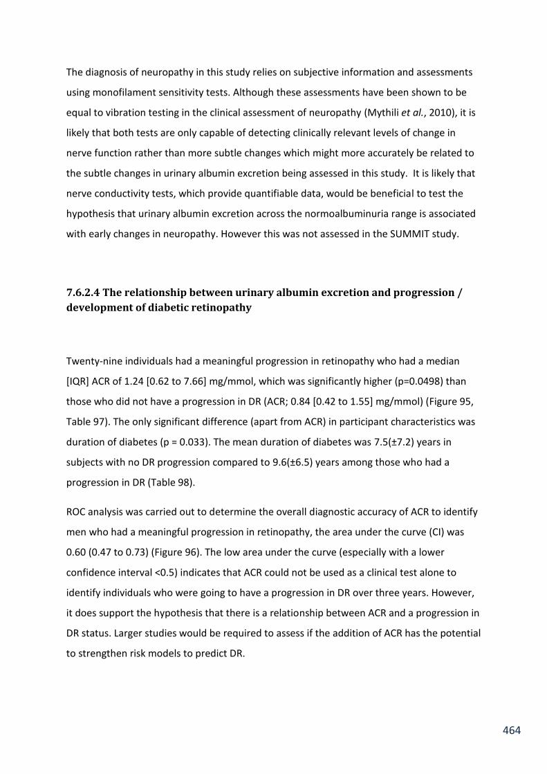
464

The diagnosis of neuropathy in this study relies on subjective information and assessments

using monofilament sensitivity tests. Although these assessments have been shown to be

equal to vibration testing in the clinical assessment of neuropathy (Mythili et al., 2010), it is

likely that both tests are only capable of detecting clinically relevant levels of change in

nerve function rather than more subtle changes which might more accurately be related to

the subtle changes in urinary albumin excretion being assessed in this study. It is likely that

nerve conductivity tests, which provide quantifiable data, would be beneficial to test the

hypothesis that urinary albumin excretion across the normoalbuminuria range is associated

with early changes in neuropathy. However this was not assessed in the SUMMIT study.

7.6.2.4 The relationship between urinary albumin excretion and progression /

development of diabetic retinopathy

Twenty-nine individuals had a meaningful progression in retinopathy who had a median

[IQR] ACR of 1.24 [0.62 to 7.66] mg/mmol, which was significantly higher (p=0.0498) than

those who did not have a progression in DR (ACR; 0.84 [0.42 to 1.55] mg/mmol) (Figure 95,

Table 97). The only significant difference (apart from ACR) in participant characteristics was

duration of diabetes (p = 0.033). The mean duration of diabetes was 7.5(±7.2) years in

subjects with no DR progression compared to 9.6(±6.5) years among those who had a

progression in DR (Table 98).

ROC analysis was carried out to determine the overall diagnostic accuracy of ACR to identify

men who had a meaningful progression in retinopathy, the area under the curve (CI) was

0.60 (0.47 to 0.73) (Figure 96). The low area under the curve (especially with a lower

confidence interval <0.5) indicates that ACR could not be used as a clinical test alone to

identify individuals who were going to have a progression in DR over three years. However,

it does support the hypothesis that there is a relationship between ACR and a progression in

DR status. Larger studies would be required to assess if the addition of ACR has the potential

to strengthen risk models to predict DR.

465

7.6.2.4.1 Characteristics of subjects with no DR progression with and without clinical

levels of urinary albumin excretion.

Contrary to the hypothesis, 51 subjects had no progression in DR and had an ACR in the

microalbuminuria range or above, impacting the diagnostic specificity of ACR to identify DR

progressors (Figure 95). Subjects who had no progression in DR and an ACR in the

microalbuminuria range or above had significantly higher blood pressure (p=0.014), HbA1c

(p=0.022), duration of diabetes (p=0.001), and a larger proportion receiving

antihypertensive therapy (p=0.009) Table 99).

88% of these individuals were already receiving antihypertensive therapy, and 85% receiving

statin therapy. Therefore, their risk of kidney disease and CVD was already known at

baseline and treatment was underway, impeding the progression of diabetic complications

or non-diabetes related chronic kidney disease.

In 2012, Chen et al. carried out a hospital based cohort study, consisting of 487 patients with

T2DM, and demonstrated that microalbuminuria was an independent risk factor for DR

development (Chen et al., 2012a). Our results suggest that ACR would not be an

independent predictor of DR progression within the earliest stages of DR, supporting the

findings of other studies (Newman et al., 2005). However there are considerable differences

in the cohorts tested and methods applied between studies including; duration of diabetes,

follow up duration and retinopathy classification. The majority of studies have focussed on

the prediction of severe levels of DR with clinical levels of albumin excretion. The study from

the SUMMIT cohort is the first to explore the lowest levels of urinary albumin excretion with

small changes in background retinopathy, which occur in the earliest stages of retinopathy.

To classify the severity of retinopathy we used criteria similar to the international

guidelines, which enable small changes in the earliest stages of retinopathy to be classified.

Retinal photography is the traditional method of assessing eye disease, however newer

technologies are available such as optical coherence tomography (OCT). This is a non-

invasive imaging test which takes cross-sectional images and measurements of the retina.

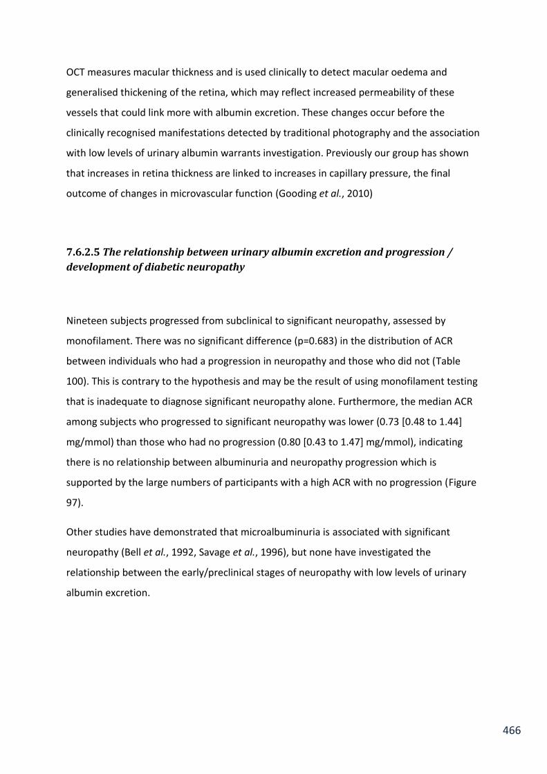
466

OCT measures macular thickness and is used clinically to detect macular oedema and

generalised thickening of the retina, which may reflect increased permeability of these

vessels that could link more with albumin excretion. These changes occur before the

clinically recognised manifestations detected by traditional photography and the association

with low levels of urinary albumin warrants investigation. Previously our group has shown

that increases in retina thickness are linked to increases in capillary pressure, the final

outcome of changes in microvascular function (Gooding et al., 2010)

7.6.2.5 The relationship between urinary albumin excretion and progression /

development of diabetic neuropathy

Nineteen subjects progressed from subclinical to significant neuropathy, assessed by

monofilament. There was no significant difference (p=0.683) in the distribution of ACR

between individuals who had a progression in neuropathy and those who did not (Table

100). This is contrary to the hypothesis and may be the result of using monofilament testing

that is inadequate to diagnose significant neuropathy alone. Furthermore, the median ACR

among subjects who progressed to significant neuropathy was lower (0.73 [0.48 to 1.44]

mg/mmol) than those who had no progression (0.80 [0.43 to 1.47] mg/mmol), indicating

there is no relationship between albuminuria and neuropathy progression which is

supported by the large numbers of participants with a high ACR with no progression (Figure

97).

Other studies have demonstrated that microalbuminuria is associated with significant

neuropathy (Bell et al., 1992, Savage et al., 1996), but none have investigated the

relationship between the early/preclinical stages of neuropathy with low levels of urinary

albumin excretion.

467

7.6.2.6 Relationship between urinary albumin excretion over three years and

progression/development of diabetic retinopathy and neuropathy

One hundred and seventy participants with diabetes, who had a from a random spot urine

sample stored and retinal photography available at baseline and follow up were selected to

test this hypothesis. The cohort was very similar to the previous cohort in Objective three

with the majority of participants (54%) having no retinopathy at baseline, and 16 (9%) of

subjects having a meaningful progression in retinopathy over three years.

A progression of two retinopathy steps or more (Table 68) across both eyes was classified as

being clinically significant. Non progressors were defined as individuals who did not have a

worsening of two steps of retinopathy in one eye or worsening of one stage in both eyes.

The mean change in ACR over three years was 2.47 (±12.98) mg/mmol with a mean percent

change of 237 (±738) % (Table 101). This large variation in the change in ACR over three

years was also identified in Hypothesis One, and can most likely be attributed to the

limitations of using a single random spot sample.

There was no significant difference in actual change (0.612) and percent change (p=0.156) in

ACR between subjects who had a progression in retinopathy and those who did not (Figure

98, Table 102, Figure 99, Table 103). This was influenced by the large number of participants

who had a big change in ACR who had no progression in retinopathy. This limitation was

discussed in Section 7.5.2.3.2. It was shown previously (Table 99) that the risk of kidney

disease and CVD was already known at baseline and treatment was underway, impeding the

progression of diabetic complications or they might have had non-diabetes related chronic

kidney disease. One study demonstrates that the lack of retinopathy in the presence of CKD

could imply that the CKD is not diabetes related in subjects with a short duration of diabetes

(< 5 years) (Dong et al., 2016)

In addition to the limitation of using a single ACR from a random spot sample to measure

change in urinary excretion, the biological variation of ACR over three years due to normal

physiological changes has not been investigated. The average increase in ACR might be a

468

normal physiological response and longitudinal studies following urinary albumin excretion

over time are required. A further analysis of the SUMMIT cohort could be carried out, by

selecting a control group of “healthy individuals” (no diabetes, CVD or any other disease).

The analysis on change in ACR does not consider the urinary albumin excretion levels of an

individual at baseline. For example; a change in ACR of 5 mg/mmol in subjects with clinically

significant macroalbuminuria is a small change compared to the change in subjects with

normoalbuminuria. These highly variable measurements of change in ACR are then being

compared by change in DR status, which have big categorical differences, almost rendering

the data unsuitable for analysis by this method. Therefore matched pair analysis was carried

out to reduce the influence of high ACR in subjects without DR progression.

7.6.2.6.1 Matched pair analysis

The aim of conducting the matched paired analysis was to remove outlying results which

were influencing the relationship between change in ACR and DR progression.

Controls were closely matched to subjects who had DR progression. There were no

significant differences in characteristics between the two groups (Table 104). In this

matched analysis there was no significant difference in actual change (p=0.431) and percent

change (p=0.284) in ACR (Figure 100, Table 105, Figure 101, Table 106). This reinforces the

limitations of using a single random spot sample, the severities of which are amplified when

measuring change in ACR over time when compared with big changes in DR status.

7.6.2.7 Limitations:

When investigating the change in measures of biological function over time, the

reproducibility of the measures is an important factor to consider. To reduce the impact of

469

the variability between visits the same protocol was applied at both visits whilst ensuring

subjects were tested at the same time of day, the same standardised meal was consumed

prior to testing, with microvascular testing carried out in the same room set at the same

temperature by the same operator.

The variability of biological markers over time is an important consideration when

comparing the change of two biological markers. Increased variability over time demands a

higher sample size to increase the confidence in the results, however a considerable number

of subjects did not attended the second visit or data/samples were not available for both

visits, resulting in a decreased number of subjects.

If a correlation between change in ACR and change in microvascular function was identified

it would require further investigation. The change in both biological measures could be

attributed to ageing, much like the normal decline in eGFR with age. To account for this a

control group needs to be established containing healthy subjects to determine the

“normal” change in ACR and microvascular function over time, enabling individuals who

have had a meaningful/pathological change to be identified.

Progression in retinopathy and neuropathy status was determined over a three year period,

which is a relatively short time period to see significant changes. In this study the incidence

of disease progression was low compared to regional data. The main reason for this is that

subjects with minimal complications were recruited to investigate early pathological

changes. The majority of the cohort were receiving statins and antihypertensive therapies,

and had a good control of their diabetes (HbA1c of 55 [49 to 65] mmol/mol) which would

reduce progression in retinopathy and neuropathy.

Novel techniques which provide sensitive measurements of retinopathy and neuropathy are

required to fully investigate the relationship between the lowest levels of albumin excretion

and microvascular complications of diabetes, at their earliest stages. OCT and nerve

conductions tests provide quantifiable data, enabling small changes over a small time period

to be detected. However the biological variation of the tests must be known first to enable

meaningful/pathological changes to be identified.

470

7.7 Conclusion

Using the validated ELISA, and applying the most accurate and reproducible method to

collect and store samples, the lowest levels of albumin excretion were examined and the

relationship with microvascular function investigated for the first time.

The Fitzgerald assay measured urinary albumin in all samples from the SUMMIT cohort, and

had a strong agreement with the Cobas method. This supports the findings of the initial

validation studies (Chapter 2, Section 2.3.4).

Albumin excretion is higher and vascular function is impaired in subjects with diabetes. The

independent relationship between urinary albumin excretion and peak reactive hyperaemia

following arterial occlusion suggests that altered autoregulation in the microvasculature

plays a role during the earliest stages of increasing albumin excretion. This relationship is

present within the normoalbuminuria range supporting work demonstrating the risk of CVD

at sub clinical levels of urinary albumin excretion.

This supports the work from Strain et al. who propose impaired myogenic vasoconstriction

or its modulation via the endothelium or nerves, leads to a very rapid unmodulated increase

in blood flow (Strain et al., 2005a).

Wall stress is the stimulus for the myogenic response, therefore a thickened wall structure,

such as that occurring in diabetes or hypertension, will reduce the response at a given

pressure (Matchkov et al., 2002) and may delay the onset of the myogenic response so that

an early increase in flow is observed before the myogenic vasoconstriction (Strain et al.,

2005a).

The discrepancies in the relationships identified between AER and ACR with microvascular

function may be attributed to overnight collections (AER) assessing resting albumin

excretion whereas ACR from a random spot sample is a marker of a stress test.

471

This is supported by the independent relationship between peak endothelial dependent

response to ACH and ACR from a random spot sample and not with AER in young subjects

without CVD with normoalbuminuria. This demonstrates that this is very early microvascular

impairment, and not detectable using overnight AER / resting conditions.

There is a relationship between ACR and early stages of diabetic retinopathy. There was no

association between ACR and neuropathy, although the study was limited by the use of

assessments unable to detect sensitive preclinical changes.

There were no independent relationships between change in ACR and change in

microvascular function or progression on diabetic retinopathy/neuropathy. When

investigating the change in measures of biological function, the reproducibility of the

measures is an important factor to consider. Single random spot samples are not suitable to

monitor change in ACR over time. In addition, progression in retinopathy and neuropathy

status was determined over a three year period, which is a short time period to see

significant changes. This has been reflected in studies such as DIRECT Protect 2 that had to

extend the duration of their studies as there was little progression in DR in their placebo

group (Sjolie et al., 2008). A further follow up of the SUMMIT cohort who had retinopathy

assessed is being performed but is not available for this thesis.

This chapter provides novel evidence that increasing urinary albumin excretion, including

within the normal range, is linked to generalised microvascular dysfunction. Furthermore,

impaired microvascular autoregulation may play a role in the pathogenesis and is not

influenced by diabetes. This is also supported by the association of urinary albumin

excretion with background (early) changes in diabetic retinopathy.

472

Chapter 8 Overall discussion, new findings, conclusions

and area for future work

This thesis provides novel evidence that increasing urinary albumin excretion, including

within the normal range, reflects generalised microvascular dysfunction. Furthermore,

impaired microvascular autoregulation plays a role in the pathogenesis and this is not

influenced by diabetes. This is also supported by the association of urinary albumin

excretion with background (early) changes in diabetic retinopathy.

This thesis describes a procedure for assessing low levels of albumin excretion and

characterises its association with microvascular function. As a direct result of this work, new

procedures for the collection, processing and storage of urine samples have been

implemented within the Diabetes and Vascular Research Centre in Exeter. There is a

validated sensitive assay to quantify urinary albumin on an automated platform available in

pathology at the Royal Devon and Exeter NHS Foundation Trust and also a correction factor

to correct for the loss of urinary creatinine during prolonged storage is being published.

This chapter provides an overview of the main findings of this thesis, the conclusions,

limitations, impact of the findings and potential areas of future research.

8.1 Background

Microvascular dysfunction has been proposed as the common process in the

pathophysiology of cardiovascular disease and diabetic kidney disease, resulting in

increased urinary albumin excretion (Deckert et al., 1989). This is further supported by

evidence that urinary albumin excretion is associated with other microvascular

complications of diabetes, such as retinopathy and neuropathy (Newman et al., 2005).

473

It is important to investigate these relationships further because it could improve our ability

to identify those at risk of CVD and microvascular complications of diabetes at an earlier

stage. Studies which have investigated these relationships are limited by the use of routine

assays which can’t quantify low concentrations of urinary albumin.

8.2 Quantifying urinary albumin and creatinine

The ability of immunoassays to measure total urinary albumin content has been questioned

(Comper et al., 2004a). However, three routine immunoassays have shown good overall

agreement to the candidate reference (LC-MS/MS) method (Seegmiller et al., 2009b). From

the three selected ELISAs to undergo validation in my thesis, only the Fitzgerald assay met

performance requirements suitable for the investigative work conducted throughout this

thesis. The routine assay could only measure albumin in 46% of participants in the SUMMIT

study at baseline (who were recruited in Exeter), therefore a sensitive assay is required to

investigate the lower levels of urinary albumin excretion.

The Fitzgerald assay ELISA is suitable for batch testing samples but it cannot be adopted for

routine use. The adaptation of immunoassays to quantify low concentrations of urinary

albumin on high throughput analysers would be required if it was considered important to

explore the clinical application of low levels of urinary albumin excretion further.

The enzymatic assay to quantify urinary creatinine had a modestly lower CV%, and had a

small proportional bias (0.52 ± 3.08 %) compared to the Jaffe method. This is the first study

to compare the two assays to measure urinary creatinine. They reflect the findings from

studies testing serum samples (Myers et al., 2006a). Overall, there is little improvement

when using the more expensive enzymatic assay over the routinely used Jaffe method and

therefore the Jaffe method was used throughout the thesis.

474

8.3 Adjusting urinary albumin for urinary concentration in spot

samples.

The albumin to creatinine ratio (ACR) is routinely reported in spot samples to account for

the variation in urinary concentration. However, creatinine excretion is highly variable

between individuals, which impacts on the ability of ACR to normalise albumin

concentration in untimed samples. Three equations that estimate albumin excretion were

validated in the SUMMIT cohort. The results showed a high correlation with measured AER,

which is in accordance to other validation studies (Fotheringham et al., 2014, Abdelmalek et

al., 2014). This was investigated further and it was demonstrated that there is no

improvement in diagnostic accuracy compared to reporting ACR alone. An alternative

measure of urinary concentration is urine specific gravity. The USG-α refractometer

validated in this theses is highly reproducible and has a strong agreement with urinary

creatinine, however it offers no clinical advantages over reporting the well-established

creatinine measurement.

8.4 Urinary albumin and creatinine stability during prolonged storage

Previous studies have demonstrated significant losses in urinary albumin during prolonged

storage at -20 oC and shown it is stable at -80 oC in the clinically relevant ranges (Brinkman et

al., 2007a). The results of this thesis support this and demonstrate the same occurs at the

lowest albumin concentrations.

The loss of urinary albumin has been attributed to sample pH (Brinkman et al., 2007a,

Townsend, 1986a) and bacterial contamination (Kania et al., 2010).This is not supported by

the results of this thesis, no additives or low protein binding tubes prevented urinary

albumin loss in samples stored at -20 oC. The decline in urinary albumin concentration

appears to stabilise by six months with around 36% of the original quantity lost. This is

475

similar to previous findings which have shown UAC to stabilise at around 30% loss after 8

months storage at -20oC (Brinkman et al., 2005).

ACR is most commonly reported in stored spot urine samples and our study is the first to

investigate the impact of prolonged storage on urinary creatinine. Urinary creatinine

degrades in samples stored at -80oC at a rate of 0.024% / day for 541 days and then

stabilises. Creatinine degradation is an important finding as many epidemiological studies

store samples for many years prior to analysis, and will need to account for creatinine

degradation when using it to account for variation in urinary concentration. The rate of

urinary creatinine degradation was accounted for in samples stored from the SUMMIT

cohort.

8.5 Collecting samples and reporting urinary albumin excretion

The results from this study indicate that, to assess albumin excretion in the normal range, a

first morning void (FMV) is the most appropriate surrogate for an overnight urine collection,

and that ACR should be reported, as they have the lowest median intra-individual

reproducibility (CV = 15.9%) and the highest correlation with overnight AER (Rs = 0.88). This

agrees with the findings of other studies in the clinical albuminuria ranges, including those

from the PREVEND cohort, who reported an intra-reproducibility of 19.0% for a FMV sample

reporting the ACR (Witte et al., 2009).

Using the validated ELISA, the biological variation of albumin excretion in healthy individuals

was investigated for the first time. Albumin excretion is significantly lower overnight than

during the day (p=0.0005). Random spot samples have the highest variability which may be

influenced by exercise/walking induced urinary albumin excretion.

476

8.6 Influence of exercise, and clinical implications when collecting

random spot samples.

In healthy individuals heavy exercise increases ACR sufficiently enough to place 64% of

participants into the microalbuminuria range. Thus healthy individuals should not provide a

urine sample for ACR measurement if they have undertaken heavy exercise within the

previous five hours. These results are in accordance with another study who also exercised

healthy subjects to exhaustion to reach microalbuminuria levels (Heathcote et al., 2009).

By measuring low concentrations of urinary albumin our study is the first to demonstrate

the relationship between walking and ACR. These results suggest there are different types of

responses in ACR to walking; delayed change in ACR, immediate change and no change. This

needs further investigation as patients walking to appointments could have falsely elevated

ACR and it may indicate an increased risk of cardiovascular disease. It has been proposed in

this thesis that random spot samples are capable of identifying subjects with walking/ stress

increased urinary albumin excretion, compared to overnight AER or a FMV, which measure

albumin excretion during a state of rest. This is discussed further and supported by

microvascular measurements in Section 8.9.

8.7 Urinary albumin excretion and microvascular function in diabetes

Median [IQR] AER was 9.75 [5.53 to 18.48] µg/min in subjects with diabetes who had good

glycaemic control, clinically appropriate treatment for their blood pressure and lipids and

who had no or background retinopathy and minimal neuropathy, compared to 6.02 [4.10 to

8.93] µg/min in subjects without T2DM (p<0.001). ACR was also significantly higher in

subjects with T2DM (p<0.001) as is expected and reflected in many studies (Hillege et al.,

2001).

477

Endothelial dependent and independent microvascular response to iontophoretic delivery

of acetyl choline (ACH) and sodium nitroprusside (SNP) is significantly lower in subjects with

diabetes (p<0.001). This reaffirms previous findings from small scale studies that suggest the

function of the endothelium and/or smooth muscle may be abnormal in T2DM (Morris et

al., 1995).

Maximal hyperaemia response to localised heating is significantly lower in diabetes

(p=0.002), supporting the findings from previous small studies in newly diagnosed patients

with diabetes and after one year of treatment (Jaap et al., 1994b) and studies from the

Maastricht cohort which were reported since the commencement of this thesis, and have a

cohort with similar age and duration of diabetes as the SUMMIT cohort (Sorensen et al.,

2016).

8.8 Relationship between microvascular function and urinary

albumin excretion

There is a significant correlation between urinary albumin excretion and all measures of

microvascular function, across the full urinary albumin excretion range. The association

between AER/ACR with measures of microvascular function is not significantly different in

subjects with diabetes compared to those without diabetes. This extends the findings of

Hillege et al. who also demonstrated, using a traditional albumin assessment, that the risk of

CVD with increasing urinary albumin concentration is not limited to diabetes and occurs in

the non-diabetic population (Hillege et al., 2002). Although not detailed in the paper, the

evidence from my study would suggest that up to 40% of the participants in the Hillege

study would fall below the limit of detection for the albumin assay and would have been

excluded from the analysis or assigned values at the detection limit of the assay as is often

practise.

In the SUMMIT cohort; an increase in albumin excretion is independently associated with an

increase in post occlusive peak reactive hyperaemia after adjusting for age, gender, smoking

478

status, HDL, systolic blood pressure, history of CVD, HbA1c and waist across the full urinary

albumin excretion range (p=0.008) and within the normoalbuminuria range (p=0.003),

regardless of diabetes status. This is the first study to demonstrate the relationship between

low levels of urinary albumin excretion with generalised impaired autoregulation.

The findings from the SUMMIT cohort do not support the albumin retrieval hypothesis

which proposes a defective proximal tubule retrieval system is an alternative hypothesis for

rising urinary albumin excretion during the early stages of DKD (Russo et al., 2007, Comper,

2008). It is most likely that tubular dysfunction arises after microvascular dysfunction, but it

does contribute to the progression of renal disease. Urine samples have been stored from

the SUMMIT cohort so markers of tubular function such as α-2 and β-2 microglobulin (Zeng

et al., 2014) can be measured and the function of proximal tubules with low levels of urinary

albumin excretion can be investigated together.

Urinary albumin excretion had a significant correlation with endothelial dependent response

to the iontophoretic delivery of ACH; however this was not an independent relationship

when adjusting for age and gender. Our findings do not support or disprove the ‘Steno

hypothesis’, which proposes a disturbance in vascular permeability, is a common process

causing increased urinary albumin excretion and generalised endothelial dysfunction

(Satchell and Tooke, 2008). A disturbance in endothelial glycocalyx disrupts endothelial

function and vascular tone, especially if driven by chronic hyperglycaemia (Sandoo et al.,

2010). Samples are stored for the analysis of glycocalyx markers to investigate this

hypothesis further.

There was no significant difference in AER distribution between groups (p=0.243) when

stratifying by peak response curve morphology in this cohort. This does not support the

relationship found by Strain et al. who demonstrated that AER was significantly higher with

an early dominant peak response (Strain et al., 2005a). In the SUMMIT cohort, the results

were influenced by individuals with a high AER with normal peak curve morphology. 74% of

these abnormal results were from subjects on antihypertensive therapy and 78% were on

statins. However, when excluding these subjects when investigating normoalbuminuria,

479

there was still no significant distribution of AER among the groups, although AER does

appear to be higher in subjects with an early dominant peak.

8.9 Change in albumin excretion and microvascular function over

three years.

Using the developed method to investigate low levels of urinary albumin excretion, it was

possible to study, for the first time, change in ACR over three years in subjects with and

without diabetes. The mean increase in ACR in subjects with diabetes was 2.36 (±6.50)

mg/mmol, in subjects without T2DM the mean change was -0.11 (±1.2) mg/mmol (the

change in ACR is significantly different when considering diabetes status, p=0.003). The large

standard deviation of mean change demonstrates a large variability among subjects.

A limitation of the method to test this hypothesis is that change in albumin excretion was

determined by using a single ACR at baseline and a single ACR three years later. These were

the only samples available in the cohort. Random spot samples have poor reproducibility,

reflected by the need to confirm microalbuminuria in at least two spot samples to make a

diagnosis.

Across the whole cohort there was a significant change in microvascular function over three

years, except for time to peak hyperaemia during PORH testing. The change in

microvascular function was not influenced by diabetes. This is the first time the change in

microvascular function has been reported when assessed by in vivo measurements. The

actual and percent changes in vascular function are highly variable between individuals.

These are in-vivo measures of microvascular function and they have high biological

variability, which suggests that large sample sizes are required to compare change in

microvascular function over time in different groups.

480

There were no significant correlations between the change in ACR and change in any

measure of microvascular function. This most likely reflects the limitations of assessing

change in ACR using a single random spot sample.

8.10 Interaction of CVD on the relationship between AER/ACR with

microvascular function in the normoalbuminuria range

This is the first study to demonstrate that the relationship between AER/ACR in the

normoalbuminuria range and microvascular function, which differed in patients with and

without cardiovascular disease. There are significant correlations between AER and maximal

hyperaemia and minimum vascular resistance (MVR) in subjects with CVD but not in those

without CVD. In contrast there are significant correlations between ACR and endothelial

dependent and independent response to ACH and SNP respectively in subjects without CVD

but not in those with CVD.

A possible reason for the association of ACR, but not AER, with endothelial dependent and

independent response to ACH and SNP, is because ACR can identify walking induced

albumin excretion. This has been demonstrated in subjects without CVD with

normoalbuminuria, suggesting this is very early microvascular impairment, and not

detectable using overnight AER. Furthermore the relationship between ACR and endothelial

dependent response to ACH in subjects without CVD was independent of other confounding

factors for CVD.

8.11 Random spot samples to detect walking induced urinary albumin

excretion

The evidence from this thesis enables a new hypothesis to be formed that can explain the

discrepancies in the relationships between AER and ACR with microvascular function.

481

Overnight urine collections assess resting albumin excretion whereas an ACR from a random

spot samples is a marker of a stress / activity test.

The earliest impaired microvascular dysfunction might only be detected by using walking as

a stress test and using random spot samples to assess change in ACR. The findings from

Chapter 4 demonstrated that FMV is the best surrogate of overnight urine collection, ‘the

gold standard’ to identify subjects with microalbuminuria. However, overnight collections

might not identify people with walking induced albumin excretion, which may occur at an

early stage in the progression of microvascular dysfunction, before microalbuminuria is

detectable.

The clinical significance of this could be that stress testing identifies those who are

susceptible to induced urinary albumin excretion as they may be at risk of CVD compared

those who are not. It is important to investigate these relationships further as it could

improve our ability to identify those at risk of CVD, and complications of diabetes at an

earlier stage. This would result in significant improvement in the quality of lives of diabetic

patients and save the health service resources in dealing with the complications of diabetes.

8.12 Albumin excretion and microvascular complications of diabetes

This thesis supports the hypothesis that microvascular dysfunction is the common process in

the pathophysiology of diabetic kidney disease, and cardiovascular disease, resulting in

increased urinary albumin excretion (Deckert et al., 1989). This hypothesis is further

supported by evidence that urinary albumin excretion is associated with diabetic

retinopathy, reinforcing previous findings (Newman et al., 2005).

The results from the SUMMIT cohort demonstrate that low levels of urinary albumin are

associated with subclinical changes in diabetic retinopathy. However, it is not an exclusive

relationship as there are lots of individuals with established CVD in the cohort who have a

very high ACR with no diabetic retinopathy. There was no association between ACR and

482

neuropathy, although the study was limited by the use of crude clinical assessments of

neuropathy.

There was no relationship between change in ACR and change in microvascular function or

progression on diabetic retinopathy/neuropathy. When investigating the change in

measures of biological function, the reproducibility of the measures is an important factor

to consider. Single random spot samples are not suitable to monitor change in ACR over

time. In addition, progression in retinopathy and neuropathy status was determined over a

three year period, which is a short time period to see significant changes, especially in these

early stages.

8.13 Future work

1) An assay which can quantify low concentrations of urinary albumin and can be

applied to high throughput analysers needs to be developed which meets clinical

requirements.

2) The creatinine degradation equation needs to be validated.

3) The relationship between walking induced urinary albumin excretion and risk of

developing CVD and the influence of diabetes needs to be fully investigated. A

matched-case control study is required to assess microvascular function, a CVD risk

factor, in subjects with walking induced urinary albumin excretion.

4) Further biomarker analysis in samples from the SUMMIT cohort is required. This is

one of the main focuses of the SUMMIT study and biomarker analysis is underway.

SUMMIT (Surrogate markers for micro- and macro-vascular hard endpoints for

innovative diabetes tools) is a European consortium which aims at identifying

483

markers that predict the risk of developing diabetes related vascular complications,

in particular DKD, CVD, and diabetic retinopathy.

5) The relationship with low levels of urinary albumin excretion and sensitive measures

of early retinopathy changes needs to be investigated. This data is available from the

SUMMIT cohort as subjects who had retinopathy assessed by retinal photography

also underwent OCT imaging for the measurement of macular thickness.

6) The diagnostic ability of low levels of urinary albumin excretion to identify subjects

who have background progression in retinopathy and neuropathy needs to be

investigated. The SUMMIT cohort who had retinopathy/neuropathy assessed, are

being followed up again 4.5 years from their initial assessment. Sensitive nerve fibre

conduction tests to examine neuropathy are being carried out and the relationship

with low levels of albumin excretion can be investigated for the first time.

8.14 Overall conclusion

This thesis provides novel evidence that increasing urinary albumin excretion, including

within the normal range, results from generalised microvascular dysfunction. Furthermore,

impaired microvascular autoregulation plays a role in the pathogenesis that is not

influenced by diabetes. This is also supported by the association of urinary albumin

excretion with background (early) changes in diabetic retinopathy.

484

Appendix 1: Genway ELISA kit information

(Genway Biotech Inc. San Diego, CA, USA)

Kit Contents: (enough for ten 96-well plates)

Coating Antibody (Catalog # 15-288-10067F)

Affinity purified Chicken IgY against Human Serum Albumin

Concentration: 2.7 mg/mL

Volume: 75 μL

Working concentration: 1.8 μg/mL

Lot: 130520A-10067F

Protein Calibrator (Catalog # 10-288-10067F)

Purified Human HSA Antigen

Concentration: 30 μg/mL

Working concentration: 3,000-4 ηg/mL

Volume: 1 mL

Lot: 130520C-10067F

Detection Antibody (Catalog # 27-288-10067F)

Affinity purified Chicken IgY against Human HSA – Horseradish Peroxidase (HRP) Conjugate

Concentration: 0.44 mg/ml

Working concentration: 200 ηg/mL

Volume: 50 μL

Lot: 130520D-10067F

Notes:

1. Range of Detection: 3,000 – 4 ηg/ml.

2. Shelf life: One year from date of receipt.

3. Storage: -20°C.

4. Assay Condition:

The kit performance has been optimized for the stated protocol using the materials listed and

standard dilutions from 3,000-4 ηg/ml of HSA. For alternative assay conditions, the operator must

determine appropriate dilutions of reagents. ELISA assay reactivity is sensitive to any variation in

operator, pipetting and washing techniques, incubation time and temperature, composition of

reagents, and kit age. Adjustments may be required to position the standard curve and/or samples in

the desired detection range.

4. Country of Origin: United States of America.

5. Assay Use: For in vitro laboratory use only. Not for any clinical, therapeutic, or diagnostic use or

consumption in human or animals. GenWay Biotech, Inc. HSA ELISA Kit Manual

______________________________________________________________________________

___ For research use only; not for diagnostic or therapeutic use. Page 3

485

HSA Quantitative ELISA Protocol Materials

1. TMB Peroxidase Substrate System. KPL, Cat. # 50-76-00.

2. Costar 96 well EIA/RIA high binding plate (Corning, Inc. Cat #. 3590)

3. Sodium Bicarbonate. MW 84.01, Sigma-Aldrich, Cat. # S6014-5kg.

4. Tris Hydroxvmethy Aminomethano Hydrochloride. MW 157.6, Fisher. Cat. # BP153-1.

5. Tris Crystallized free base. MW 121.14, Fisher. Cat. # BP 152-5.

6. NaCl, MW 58.44, Fisher. Cat. # BP 358-10.

7. Tween 20, Sigma. Cat. # P-1379.

8. BSA, Sigma. Cat. # A3059-100G.

9. Sulfuric Acid, 4.0N. Labchem Inc., Cat. # LC 25830-2. Buffer Preparation 1. Coating Buffer: 0.05 M Carbonate-Bicarbonate, pH 9.6 2. Wash Solution: 0.05% Tween 20 in PBS, pH 7.4 3. Blocking Solution: 50 mM Tris, 0.14 M NaCl, 1% BSA, pH 8.0

4. Sample/Conjugate Diluents: 50 mM Tris, 0.14 M NaCl, 1% BSA, 0.05% Tween 20, pH 8.0 Step-by-Step Method (Perform all steps at room temperature) 1. Coat with Capture Antibody 1) Determine the number of single wells needed. Standards, samples, blanks and/or controls should be analyzed in triplicates. 2) Dilute capture antibody with Coating Buffer to 1.8 ug/ml. Transfer 100 μl to each well. 3) Incubate coated plate for 60 minutes at room temperature/37 °C or overnight at 4 °C. 4) After incubation, aspirate the Capture Antibody solution from each well. 5) Wash each well with Wash Solution as follows: a. Fill each well with Wash Solution b. Remove Wash Solution by aspiration c. Repeat for a total of 3 washes. 2. Blocking 1) Add 200 μl of Blocking Solution to each well. 2) Incubate 60 minutes at room temperature. 3) After incubation, remove the Blocking Solution and wash each well three times as in Step 1.5. 3. Standards and Samples 1) Dilute the standards (calibrator) in Sample Diluent to a concentration of 3000 ηg/ml, then do a 1/3 serial dilutions down to 4.11 ηg/ml 2) Dilute the samples, based on the expected concentration of the analyte, to fall within the concentration range of the standards. 3) Transfer 100 μl of standard or sample to assigned wells.

4) Incubate plate 60 minutes at room temperature.

5) After incubation, remove samples and standards and wash each well 5 times as in Step 1.5. GenWay Biotech, Inc. HSA ELISA Kit Manual

______________________________________________________________________________

___ For research use only; not for diagnostic or therapeutic use. Page 4

486

4. HRP Detection Antibody 1) Dilute the HRP conjugate in dilution buffer to a concentration of 200 ηg/ml. (Note: Adjustments in dilution may be needed depending on substrate used, incubation time, and age of kit). 2) Transfer 100 μl to each well.

3) Incubate 60 minutes at room temperature.

4) After incubation, remove HRP Conjugate and wash each well 5 times as in Step 1.5. 5. Enzyme Substrate Reaction 1) Prepare the substrate solution according to the manufacturer’s recommendation.

2) Transfer 100 μl of substrate solution to each well.

3) Incubate plate for 5-15 minutes.

4) To stop the TMB reaction, apply 100 μl of 2.0N Sulfuric Acid to each well. If using another substrate, use the stop solution recommended by manufacturer. 6. Plate Reading Using a microtiter plate reader, read the plate at the wavelength that is appropriate for the substrate used (450 nm for TMB). Calculation of Results 1. Average the readings from each standard, control, and sample.

2. Subtract the zero reading from each averaged value above.

3. Create a standard curve by reducing the data using computer software capable of generating a four parameter logistic (4-PL) curve-fit. Other curve fits may also be used.

4. A standard curve should be generated for each set of samples. See example below: GenWay Biotech, Inc. HSA ELISA Kit Manual

______________________________________________________________________________

___ For research use only; not for diagnostic or therapeutic use. Page 5

487

Appendix 2: Bethyl E88-129 ELISA kit information

(Bethyl Laboratories Inc. Montgomery, TX, USA)

Albumin Kit

Cat. No. E88-129

Components Supplied

Human Albumin Pre-Coated 96-well Strip Plate, 1 each

Human Albumin Standard, 500 ng/vial, 2 each

Human Albumin Detection Antibody, 12 ml

20X Dilution Buffer C, 25 ml

HRP Solution A, 12 ml

TMB Substrate, 12 ml

Stop Solution, 12 ml

20X Wash Buffer, 50 ml

Sealing Tape, 6 sheets

Shelf Life: 6 months from date of sale.

For In vitro laboratory use only. Not for any clinical, therapeutic, or diagnostic

use in humans or animals. Not for animal or human consumption.

Bethyl Laboratories, Inc., www.bethyl.com

Telephone: 800-338-9579 • Fax: 866-597-6105

Introduction This enzyme linked immunosorbent assay (ELISA) is for the detection of Human

Albumin in serum, plasma, cerebrospinal fluid, milk, and urine. This kit contains

sufficient components to quantitate Human albumin in up to 40 samples, tested in

duplicate.

Background Albumin is the most abundant human protein in plasma. It constitutes about 60% of

human plasma protein. Albumin is produced in the liver and serves as a carrier for

molecules of low water solubility. Albumin is also important for regulating blood

volume by monitoring the colloid osmotic pressure of the blood compartment.

Albumin concentration in normal human serum ranges from 25 mg/ml to 50 mg/ml.

Low albumin (hypoalbuminaemia) concentrations may be caused by liver

disease, nephrotic syndrome, burns, malabsorption, malnutrition, late pregnancy,

genetic variations and malignancy. High albumin is almost always caused by

dehydration. Therefore, an accurate quantitation of albumin in plasma or serum is

important for medical diagnostics, as well as for monitoring the efficacy of treatment

regimens.

488

Principle of the Assay This kit is based on a sandwich ELISA. Human albumin present in the test

sample is captured by anti-human albumin antibody that has been pre-adsorbed

on the surface of microtiter wells. After sample binding, unbound proteins and

molecules are washed off, and a biotinylated detection antibody is added to the

wells to bind to the captured albumin. A strepavidin-conjugated horseradish

peroxidase (SA-HRP) is then added to catalyze a colorimetric reaction with the

chromogenic substrate TMB (3,3’,5,5’-tetramethylbenzidine). The colorimetric

reaction produces a blue product, which turns yellow when the reaction is

terminated by addition of dilute sulfuric acid. The absorbance of the yellow

product at 450 nm is proportional to the amount of albumin analyte present in

the sample and a four-parameter standard curve can be generated. The albumin

concentrations in the test samples can then be quantified by interpolating their

absorbance from the standard curve generated in parallel with the samples. After

factoring sample dilutions, the albumin concentrations in the original sample can

finally be calculated.

Procedure Overview

1. Add 100 l of standard or sample to designated wells.

Note: Run each standard or sample in duplicate.

2. Cover the plate and incubate at room temperature (20-25 C) for 1 hour.

3. Wash the plate FOUR times.

4. Add 100 l of anti-albumin Detection Antibody to each well.

5. Cover the plate and incubate at room temperature for 1 hour.

6. Wash the plate FOUR times.

7. Add 100 l of HRP Solution A to each well.

8. Cover the plate and incubate at room temperature for 30 minutes.

9. Wash the plate FOUR times.

10. Add 100 l of TMB Substrate Solution to each well.

11. Incubate the plate in the dark at room temperature for 30 minutes.

12. Stop the reaction by adding 100 l of Stop Solution to each well.

13. Measure absorbance on a plate reader at 450 nm.

Additional Materials Required

Ultrapure water

Precision pipettors, with disposable plastic tips

Polypropylene or polyethylene tubes to prepare standard and samples

Do not use polystyrene, polycarbonate or glass tubes.

A container to prepare 1X Dilution Buffer C

A container to prepare 1X Wash Buffer

A 96-well plate washer or a wash bottle

An autoclavable plate washer is recommended, if available.

Disposable reagent reservoirs

A standard microtiter plate reader for measuring absorbance at 450 nm for

end-point ELISA.

489

Precautions

Store all reagents at 2-8ºC. Do not freeze reagents.

All reagents must be at room temperature (20-25 C) before use.

Vigorous plate washing is essential.

Use new disposable pipette tips for each transfer to avoid crosscontamination.

Use a new adhesive plate cover for each incubation step.

Minimize lag time between wash steps to ensure the plate does not become

completely dry during the assay.

Avoid microbial contamination of reagents and equipment. Automated plate

washers can easily become contaminated and result in erroneous data.

Do not contaminate the TMB Solution. Do not expose TMB Substrate

solution to glass, foil, or metal. If the solution is blue before use, DO NOT

USE IT.

Individual components may contain preservatives. Wear gloves while

performing the assay and follow proper disposal procedures.

Handling and Preparation of Reagents, Standards, and Samples Preparation of 1X Dilution Buffer C

Prepare 1X Dilution Buffer C by diluting 25 ml of 20X Dilution Buffer C

into 475 ml of ultra pure water. Mix well. Store reconstituted 1X Dilution

Buffer C at 2-8ºC for up to six (6) months. Do not use 1X Dilution Buffer C

if it becomes visibly contaminated during storage.

Preparation of Standard Solutions

Standard solutions should be treated as a biological material and universal

precautions should be followed.

1. Reconstitute the 500-ng hAlbumin standard vial with 1.0 ml of 1X Dilution

Buffer C to achieve a final concentration of 500 ng/ml. Mix well.

2. Label seven (7) tubes, one for each standard curve point: 167, 55.6, 18.5,

6.17, 2.06, 0.69, and 0 ng/ml. The original vial of re-suspended standard

solution represents the top standard at 500 ng/ml.

3. Add 300 μl of 1X Dilution Buffer C into each of the seven tubes.

4. Serially dilute 1:3 by adding 150 l of the 500 ng/ml standard into the first

tube containing 300 l of 1X Dilution Buffer C. Mix well. Continue the

dilution by adding 150 μl of the previous standard into 300 μl of 1X

Dilution Buffer C in the next tube until the sixth tube (0.69 ng/ml).

5. The seventh tube containing 300 l of 1X Dilution Buffer C serves as the

zero standard value or blank.

Using this dilution scheme, only 350 l of the re-suspended standard

solution should be used. The remaining standard solution can be used for

another assay within the same day. Otherwise, use the second vial of

lyophilized standard.

490

Sample Handling

This ELISA assay can be used for human serum, plasma, cerebrospinal

fluid, urine, and milk samples.

All blood components and biological materials should be handled as

potentially hazardous. Follow universal precautions when handling and

disposing of infectious agents.

100 l of sample or standard is required per well.

Samples must be assayed in duplicate each time the assay is performed.

Store samples to be assayed within 24 hours at 2-8ºC. For long-term

storage, aliquot and freeze samples at -70 C. Avoid repeated freeze-thaw

cycles when storing samples.

If particulates are present in samples, centrifuge prior to analysis.

If blood samples are clotted, grossly hemolyzed, lipemic, or the integrity of

the sample is of concern, make a note on the Plate Template and interpret

results with caution.

Sample Preparation

The dilution schemes indicated below are only suggestions. Dilutions

should be based on the expected concentration of the unknown sample such

that the diluted sample falls within the dynamic range of the standard curve.

Prepare one or more dilutions of the sample in 1X Dilution Buffer C using

the same serial dilution technique described below until the desired

concentration is obtained.

Serum and plasma – Recommended starting dilution is 1:5,000,000. With

this large dilution one must strive for accurate pipetting. A typical dilution

scheme starts by adding 10 l of plasma into 990 l of 1X Dilution Buffer

C to give a 1:100 dilution. This is repeated by adding 10 l of the 1:100

diluted sample to 990 l of 1X Dilution Buffer C to give 1:10,000 dilution.

This is again repeated by adding 10 l of the 1:10,000 diluted sample to 990

l of 1X Dilution Buffer C to give 1:1,000,000 dilution. Finally, 100 l of

the 1:1,000,000 diluted sample is added to 400 l of 1X Dilution Buffer C

to result in a 1:5,000,000 dilution. It is important to mix thoroughly at each

dilution step.

Cerebrospinal fluid and milk - Recommended starting dilution is 1:5,000.

Urine - Recommended starting dilution is 1:100.

Milk – Recommended starting dilution is 1:1000.

Preparation of 1X Wash Buffer

Prepare 1X Wash Buffer diluting 20X Wash Buffer in ultrapure water. For

example, if preparing 1 L of 1X Wash Buffer, dilute 50 ml of 20X Wash

Buffer into 950 ml of ultrapure water. Mix well. Store reconstituted 1X

Wash Buffer at 2-8ºC for up to six (6) months. Do not use 1X Wash Buffer

if it becomes visibly contaminated during storage.

491

Assay Procedure Sample Incubation

Determine the number of strips required. Leave these strips in the plate

frame. Place unused strips in the foil pouch with desiccant and seal tightly.

Store unused strips at 2-8 C. After completing assay, keep the plate frame

for additional assays.

Use a Plate Template to record the locations of the standards and unknown

samples within the wells.

1. Add 100 l of appropriately diluted standards or samples to each well. Run

each standard, sample, or blank in duplicate.

Note: Serum, plasma, cerebral fluid, milk, and urine samples must be

diluted prior to testing (see Sample Preparation section above).

2. Carefully cover the wells with a new adhesive plate cover and incubate for

one (1) hour at room temperature, 20-25 C.

3. Carefully remove the adhesive plate cover and wash FOUR times with 1X

Wash Buffer, as described in the Plate Washing section below.

Plate Washing

Using a manual or automated plate washer

1. Rinse the tips of the plate washer by dispensing the 1X Wash Buffer into

the wash trough and aspirating the solution. Repeat this step five times. For

automated plate washers, program the rinse step accordingly.

Note: This initial rinse step is necessary especially if the plate washer has

been idle for several days or longer. Automated plate washers are

susceptible to microbial growth in the fluid lines and cavities.

2. Aspirate the solutions from the wells. Fill the wells to about 90% full with

1X Wash Buffer and then aspirate the wash solution. Repeat this wash step

three more times. For automated plate washers, program 4 washes at 300 l

per wash, according to the manufacturer’s instructions.

Using a squirt bottle

1. Gently squeeze the long sides of plate frame before washing to ensure all

strips remain securely in the frame.

Bethyl Laboratories, Inc., www.bethyl.com

Telephone: 800-338-9579 • Fax: 866-597-6105

8

2. Empty the plate contents by quickly dumping the contents of the wells into

the sink using a quick, flipping motion.

3. Use a squirt wash bottle to fill each well completely with 1X Wash Buffer,

and then empty the plate contents. Repeat procedure three more times for a

total of FOUR washes. Blot the plate onto paper towels or other absorbent

material.

Incubation with Detection Antibody

Only remove the required amount of Detection Antibody reagent for the

number of strips being used.

1. Add 100 l of Detection Antibody to each well containing standard, sample

or blank. Mix well by gently tapping the plate several times.

2. Carefully attach a new adhesive plate cover and incubate the plate for one

hour at room temperature, 20-25 C.

3. Carefully remove the adhesive plate cover, discard plate contents and wash

FOUR times with 1X Wash Buffer (see Plate Washing section above).

Incubation with HRP Solution A

Remove only the required amount of HRP Solution A for the number of

492

strips being used.

1. Add 100 l of HRP Solution A to each well containing standard, sample or

blank.

2. Carefully attach a new adhesive plate cover and incubate plate for 30

minutes at room temperature, 20-25°C.

3. Carefully remove the adhesive plate cover, discard plate contents and wash

FOUR times with 1X Wash Buffer (see Plate Washing section). Blot off

any residual liquid at the bottom of the wells that might interfere later with

the absorbance readings.

Incubation with TMB Substrate and Stopping the Reaction

Remove only the required amount of TMB Substrate Solution and Stop

Solution for the number of strips being used.

Do NOT use glass pipette to measure the TMB Substrate Solution. Do NOT

cover the plate with aluminum foil or metalized mylar. Do NOT return

leftover TMB Substrate to bottle. Do NOT contaminate the unused TMB

Substrate Solution. If the solution is blue before use, DO NOT USE IT!

1. Add 100 l of TMB Substrate Solution into each well and allow the

enzymatic reaction to develop a blue color at room temperature (20-25ºC)

in the dark for 30 minutes. Do NOT cover plate with a plate sealer.

2. Stop the reaction by adding 100 l of Stop Solution to each well. Tap plate

gently to mix. The solution in the wells should immediately change in color

from blue to yellow.

Absorbance Measurement

Note: Wipe the underside of the wells with a lint-free tissue.

1. For end-point ELISA, measure the absorbance on an ELISA plate reader set

at 450 nm within 30 minutes after the addition of the Stop Solution.

Calculation of Results

Duplicate absorbance values should be within 10% of each other. Care

should be taken when interpreting data with differences in absorbance

values greater than 10%.

1. Prepare a standard curve to determine the amount of albumin in an

unknown sample. Plot the average absorbance obtained for each standard

concentration on the vertical (Y) axis versus the corresponding albumin

concentration on the horizontal (X) axis using curve-fitting software.

2. Calculate the albumin concentration in unknown samples using the prepared

standard curve. Determine the amount of albumin in each unknown sample

by noting the albumin concentration (X axis) that correlates with the

absorbance value (Y axis) obtained for the unknown sample.

3. If the sample was diluted, multiply the observed albumin concentration by

the dilution factor to determine the concentration of albumin in the original,

undiluted sample.

Note: Most plate readers come with appropriate templates and curve-fitting

software. The standard curve of this assay can be fitted into a 4-parameter

curve fitting equation that can be programmed to calculate and display a

table (or tables) consisting of the raw absorbance readings, net absorbance

readings, the analyte concentration in the assay solution, dilution factors,

and analyte concentration in the original unknown sample.

Performance Characteristics Typical Standard Curve

This typical standard curve was generated using the Human Albumin

ELISA Kit Protocol. This standard curve is for demonstration only. A

standard curve must be generated for each assay.

Assay Range: 0.69 – 500 ng/ml

493

Suggested standard curve points are 500 ng/ml, 167 ng/ml, 55.6 ng/ml, 18.5

ng/ml, 6.17 ng/ml, 2.06 ng/ml, 0.69 ng/ml, and 0 ng/ml.

Expected OD value for 500 ng albumin standard is 1.8 – 2.2. OD value for

low standard should be higher than background.

Specificity

By immunoelectrophoresis and ELISA the antibodies in this set react

specifically with human albumin, not with human immunoglobulins or

other human serum proteins. Cross-reactivity with other species has not

been tested.

Representative Data

Serum, plasma, cerebrospinal fluid, milk, and urine samples were collected

from apparently healthy individuals and evaluated in this assay. The levels

of Human Albumin detected were as follows:

Human Urine (n=2): avg. = 2.19 g/ml

Human cerebral serum fluid (n=4): avg. = 347 g/ml

Human Milk (n=1): 188 g/ml

Warranty Products are warranted by Bethyl Laboratories, Inc. to meet stated product

specifications and to conform to label descriptions when used, handled and

stored according to instructions. Unless otherwise stated, this warranty is limited

to six months from date of sale. Bethyl Laboratories sole liability for the product

is limited to replacement of the product or refund of the purchase price. Bethyl

Laboratories products are supplied for research applications. They are not

intended for medicinal, diagnostic or therapeutic use. The products may not be

resold, modified for resale or used to manufacture commercial products without

prior written approval from Bethyl Laboratories, Inc.

Background References 1. Anderson NL and Anderson NG (1977). Proceeding of the National

Academy of Sciences 74: 5421–5425.

2. Adkins JN et al. (2002). Molecular and Cellular Proteomics 1: 947–955.

3. Jacobs JM et al. (2005).. Journal of Proteome Research 4: 1073–1085. Rev 120711

Bethyl Laboratories, Inc., www.bethyl.com

Telephone: 800-338-9579 • Fax: 866-597-6105

12

494

Appendix 3: Fitzgerald ELISA information

(Fitzgerald Industries International, North Acton, MA, USA)

55R-ORG5MA

MicroAlbumin ELISA kit Immunometric Enzyme Immunoassay for the determination of Micro-Albumin in urine

Fitzgerald Industries International www.fitzgerald-fii.com/55R-ORG5MA 1.NAME AND INTENDED USE: Micro-Albumin is a competitive solid phase enzyme immunoassay (ELISA) for the measurement of human albumin in urine. The assay is intended for research use only as an aid in the investigation of microalbuminuria. 2.SUMMARY AND EXPLANATION OF THE TEST: Proteins passing the glomerular basal membrane of the kidney undergo differentiated filtering. The permeability is inversely proportional to the molecular weight (albumin about 0.6 %, myoglobulin about 75 %). Nevertheless, only minimal quantities of protein are detectable in urine, because big quantities of protein are reabsorbed by the tubuli. Elevated glomerular protein permeability and high tubular plasma protein elimination can be differentiated by measuring the molecular weight distribution of the eliminated proteins. Albumin has a relative molecular mass of 66 kDa. It is contained in urine at very low concentrations. In case of a very active glomerular filtering process the albumin secretion can arise without an underlying kidney disease. This situation is called "microalbuminuria". The detection of these small secretion quantities (30 to 150 ug/min or ml) requires very sensitive test systems , i.e. immunological techniques. Physical stress can also induce elevated albumin secretion, without the occurrence of a kidney disease. 3.PRINCIPLE OF THE TEST: Highly purified human albumin is bound to microwells. Calibrators, controls and undiluted unknown samples are pipetted together with anti-human-albumin-peroxidase conjugate in the wells. Microalbumin, if present in diluted urine, will compete with coated albumin for binding of the anti-albumin-conjugate. Washing of the microwells removes unspecific components. An enzyme substrate in the presence of bound conjugate hydrolyzes to form a blue color. The addition of an acid stops the reaction forming a yellow end-product. The intensity of this yellow color is measured photometrically at 450 nm. The amount of color is inversely proportional to the concentration of albumin present in the original sample. 4.WARNINGS AND PRECAUTIONS: 1.All reagents of this kit are strictly intended for research use only. 2.Do not interchange kit components from different lots.

495

3.Components containing human serum were tested and found negative for HBsAg, HCV, HIV1and HIV2 by FDA approved methods. No test can guarantee the absence of HBsAg, HCV,HIV1 or HIV2, and so all human serum based reagents in this kit must be handled as thoughcapable of transmitting infection. 4.Avoid contact with the TMB (3,3´,5,5´-Tetramethyl-benzidine). If TMB comes into contactwith skin, wash thoroughly with water and soap. 5.Avoid contact with the Stop Solution which is acid. If it comes into contact with skin, wash thoroughly with water and seek medical attention. 6.Some kit components (i.e. Controls, Sample buffer and Buffered Wash Solution) containSodium Azide as preservative. Sodium Azide (NaN3) is highly toxic and reactive in pure form.At the product concentrations (0.09%), though not hazardous. Despite the classification asnon-hazardous, we strongly recommend using prudent laboratory practices. 7.Some kit components contain Proclin 300 as preservative. When disposing reagentscontaining Proclin 300, flush drains with copious amounts of water to dilute the componentsbelow active levels. 8.Wear disposable gloves while handling specimens or kit reagents and wash handsthoroughly afterwards. 9.Do not pipette by mouth. 10.Do not eat, drink, smoke or apply makeup in areas where specimens or kit reagents arehandled. 11.Avoid contact between the buffered peroxide solution and easily oxidized materials;extreme temperature may initiate spontaneous combustion. 12.Observe the guidelines for performing quality control by assaying controls and/or pooledsera. During handling of all kit reagents, controls and serum samples observe the existingregulations. 5.CONTENTS OF THE KIT: - Package Size: 96 determ. - Divisible microplate consisting of 12 modules of 8 wells each, coated with highly purified Lysozyme. Ready to use. - 6 vials, 1.5 ml each Micro-Albumin-Calibrators (A-F) in a PBS/BSA matrix (NaN3 <0.1% (w/w)) containing micro-albumin: 0.15; 1.5; 6; 25; 100 and 400 ug/ml. Ready to use. - 2 vials, 0.5 ml each Micro-Albumin Controls in a PBS/BSA matrix (NaN3 <0.1% (w/w)) positive (1) and negative (2), for the respective concentrations see the en-closed package insert. Ready to use. - 1 vial, 10 ml Sample buffer (Tris, NaN3 <0.1% (w/w)), yellow. Ready to use.

496

- 1 vial, 15 ml Enzyme conjugate solution (PBS, Proclin 300 <0.5% (v/v)), (light red) containing polyclonal rabbit anti-human albumin; labeled with horseradish peroxidase. Ready to use. - 1 vial, 15 ml TMB substrate solution. Ready to use. - 1 vial, 15 ml Stop solution (contains acid). Ready to use. - 1 vial, 20 ml Wash solution (PBS, NaN3 <0.1% (w/w)), concentrate (50x). 6.ADDITIONAL MATERIALS REQUIRED: - Microplate reader capable of endpoint measurements at 450 nm

- Multi-Channel Dispenser or repeatable pipette for 100 μl

- Vortex mixer

- Pipettes for 10 μl, 100 μl and 1000 μl

- Laboratory timing device

- Data reduction software Preparation of Reagents: - Distilled or deionised water

- Graduated cylinder for 100 and 1000 ml

- Plastic container for storage of the wash solution 7.STORAGE AND STABILITY: - Store the kit at 2-8 °C.

- Keep microplate wells sealed in a dry bag with desiccants.

- The reagents are stable until expiration of the kit.

- Do not expose test reagents to heat, sun or strong light during storage and usage.

- Diluted sample buffer and wash buffer are stable for at least 30 days when stored at 2-8 °C. 8.COLLECTION, STORAGE AND HANDLING OF UNKNOWNS: 1.Collect morning urine. 2.Samples may be refrigerated at 2-8 °C for up to five days or stored at -20 °C up to sixmonths. 3.Avoid repetitive freezing and thawing of urine samples. This may result in variable loss ofalbumin activity. 4.Murine samples need not to be diluted. If higher concentrations are expected, samplesshould be diluted with sample buffer and dilutions considered during calculation. 9.PROCEDURAL NOTES: 1.Do not use kit components beyond their expiration dates.

497

2.Do not interchange kit components from different lots.

3.All materials must be at room temperature (20-28 °C).

4.Have all reagents and samples ready before start of the assay. Once started, the test mustbe performed without interruption to get the most reliable and consistent results.

5.Perform the assay steps only in the order indicated.

6.Always use fresh sample dilutions.

7.Pipette all reagents and samples into the bottom of the wells.

8.To avoid carryover contamination, change the tip between samples and different kitcontrols.

9.It is important to wash microwells thoroughly and remove the last droplets of wash buffer toachieve best results.

10.All incubation steps must be accurately timed.

11.Control sera or pools should routinely be assayed as unknowns to check performance of thereagents and the assay.

12.Do not re-use microplate wells. For all controls, the respective concentrations are provided on the labels of each vial. Using these concentrations a calibration curve may be calculated to read. 10.PREPARATION OF REAGENTS: Preparation of wash solution Dilute the contents of each vial of the buffered wash solution concentrate (50x) with distilled or deionised water to a final volume of 1000 ml prior to use. Store refrigerated: stable at 2-8 °C for at least 30 days after preparation or until the expiration date printed on the label. 11.TEST PROCEDURE: 1.Prepare a sufficient number of microplate modules to accommodate calibrators, controlsand unknowns in duplicate. 2.Pipette 20 μl of calibrators, controls and unknowns into the wells.

3.Add 100 μl of enzyme conjugate solution into each well.

4.Incubate for 30 minutes at room temperature (20-28 °C)

5.Discard the contents of the microwells and wash 3 times with 300 μl of wash solution.

6.Dispense 100 μl of TMB substrate solution into each well.

7.Incubate for 15 minutes at room temperature.

8.Add 100 μl of stop solution to each well of the modules and leave untouched for 5 minutes.

9.Read the optical density at 450 nm and calculate the results. Bi-chromatic measurementwith a reference at 600-690 nm is recommended.

10.The developed color is stable for at least 30 minutes. Read optical densities during this time. Automation: The Micro-Albumin ELISA is suitable for use on open automated ELISA processors. The test procedure detailed above is appropriate for use with or without automation.

498

12.RESULTS: Quality Control This test is only valid if the optical density at 450 nm for Positive Control (1) and Negative Control (2) as well as for the Calibrator A and F complies with the respective range indicated on the Quality Control Certificate enclosed to each test kit! If any of these criteria is not fulfilled, the results are invalid and the test should be repeated. For the Micro-Albumin test a 4-Parameter-Fit with lin-log coordinates for optical density and concentration is recommended. Manual Data Reduction: Recommended Lin-Log Plot First calculate the averaged optical densities for each calibrator well. Use lin-log graph paper and plot the averaged optical density of each calibrator versus the concentration. Draw the best fitting curve approximating the path of all calibrator points. The calibrator points may also be connected with straight line segments. The concentration of unknowns may then be estimated from the calibration curve by interpolation. The dilution of urine samples has to be considered. 13.PERFORMANCE CHARACTERISTICS: Parallelism In dilution experiments urine samples with high Albumin concentrations were diluted with sample buffer and assayed in the Micro- Albumin kit. The assay showed linearity over the full measuring range. Precision (Reproducibility) Statistics were calculated for each of three samples from the results of 24 determinations in a single run for Intra-Assay precision. Run-to-run precision was calculated from the results of 5 different runs with 6 determinations each: Sensitivity: The lower detection limit for Micro-Albumin has been determined at 0.5 μg/ml. Specificity: The antisera (polyclonal, rabbit) labeled with horseradish peroxidase is highly specific for human Albumin. 14.LIMITATIONS OF PROCEDURE: The Micro-Albumin ELISA is intended for research use only – not for use in diagnostic procedures.

499

Appendix 4: Patient information sheet for urine collection

study.

Patient Information Sheet

Version 2.0 / 28th January 2014

What is the best collection method to measure albumin in urine?

Principal Investigator: Dr Kim Gooding Chief Investigator: Professor Angela Shore

We would like to invite you to take part in a research study. Before you decide, it is important for you to understand why the research is being done and what it will involve. Please take the time to read the following information and to discuss it with other people, including the researchers, your friends, relatives and your healthcare team if you wish. Ask us if there is anything that is not clear or if you would like more information or the opportunity to discuss the study further. Take time to decide whether you wish to take part in this study. Thank you for taking the time to read this information. What is the purpose of this study? Albumin is a protein produced by the liver. It then circulates in the blood stream. The kidneys filter the blood to remove waste products which then leave the body in urine. Albumin is normally retained in the blood but sometimes the kidney blood vessels are not working properly, which results in albumin leaking out of the vessels and passing out the body in urine along with other waste products. When high levels of albumin are found in the urine it is known as albuminuria, which indicates kidney damage known as diabetic nephropathy. Small amounts of albumin in urine is termed microalbuminuria and is an early marker of kidney damage, and may also suggest more widespread damage in the body. Early identification of microalbuminuria is important so patients’ can take medication to prevent the kidney damage getting worse. Hospital laboratories measure the concentration of albumin in urine to identify if microalbuminuria is present. Currently, microalbuminuria is clinically defined within a range and measurements below this range are considered ‘normal’ suggesting no risk of developing kidney damage. However, recent evidence suggests that even a small amount of albumin in urine, within the normal range, may be an early marker of damage to the blood vessels.

500

Hospital laboratories are unable to measure such small amounts of albumin but this study will use a different type of test which is able to measure albumin at these low concentrations. This type of test will be used in future studies to assess the link with early blood vessel damage. However, before we can do this we must establish the best, most reproducible, way of collecting the urine samples to be used with this test taking into account changes over the day and reliability / ease of sample collection. There are several ways of collecting the urine samples. The most comprehensive collection method to determine the level of albumin in urine is to collect all the passed urine over a timed period, this accounts for differences in the amount of albumin being passed at different times. However, this can be cumbersome and inaccurate. An alternative collection method includes obtaining on the spot untimed (random) samples from patients at various points throughout the day. However, one of the main weaknesses of these spot tests are that people drink different amounts of water so the concentration of albumin in the urine may be very high if an individual drinks very little or the concentration might be very low if they drink a lot. To account for this variation we compare the albumin concentration to the concentration of a waste product in the urine called creatinine. Creatinine is passed out of the body at a constant rate and this comparison is known as the albumin-to-creatinine ratio (ACR). The ACR can therefore be used in these spot samples to determine if microalbuminuria is present. There are several tests available to measure creatinine. This study will use two, the routine test used by hospital laboratories and a more modern test. The difference in results will be examined to determine if a more modern test provides a more accurate and reliable ACR. For this study, participants will collect urine samples over a 36 hour period in different containers on 3 separate occasions. By measuring the albumin and creatinine levels in these samples using the new tests we will determine the most reproducible way of collecting the urine and expressing the results for future studies examining the relationship between low levels of albumin and blood vessel health. Why have I been invited? To perform the study we are looking for 17 healthy individuals and we believe you fit the requirement we are looking for. Who is organising the study? The organisers of the study are Professor Angela Shore, Dr Kim Gooding and Daniel Chapman from the University of Exeter Medical School.

501

What would I have to do? Firstly, you would come to a screening visit at the Diabetes and Vascular Research Centre (DVRC) in the Royal Devon & Exeter Hospital (Wonford) site. Here you will get the chance to ask questions about the study and, if you wish to do so, give your consent to participate in this study. During this visit we would also ask you to provide us with a small urine sample. We would also discuss a suitable timeframe for you to complete the 3 collection periods, so please bring your diary with you. High albumin concentrations have been seen after heavy exercise or any out of the ordinary strenuous activity, sexual intercourse and during menstruation. As a result of this we would like to organise convenient times with you to try and avoid these factors. Following the screening visit you will be contacted to confirm the date of the first collection and to arrange giving you the urine collection containers. You will also receive a urine collection sheet which gives instructions on how to collect the urine and to be used to record all the times of the various collections. Throughout the collection period continue with your normal fluid intake. Once your collection period is complete you will need to get the samples to the DVRC by 16:45 the same day. During your screening visit we discuss the logistics of this and go through the options available to you. When the collection samples are received we will give you new containers for your next collection period. What happens during each collection period? Each collection period will require you to pass urine into different containers at different points throughout the day. Below is information on which containers to use and when. Container 1 (Spot): After waking up in the morning, pass the first morning urination into this container. Please record the time of collection on the container and collection sheet. Container 2 (Timed Day): Straight after the first morning urination record the start time on this container and collection sheet. Please collect all urine in this container throughout the day until going to sleep. When preparing to go to bed pass the final urination into this container and record the end time on the container and collection sheet. Container 3 (Timed Night): Please record the start time on the container and collection sheet which begins as soon as you go to bed. If you awake during the night then collect the urine in this container. After waking up in the morning collect

502

the first morning urination in this container and then this collection is complete. Please record the end time of collection on the container and collection sheet. Container 4 (Spot): Only collect the next urination in this container and record the time on the container and collection sheet. Container 5 (Spot): Collect a single urination in this container any time after the second morning urination on the same day before 16:30. Once done please record the time of collection on the container and collection sheet. Once complete please hand in all the samples to the Diabetes and Vascular Research Centre on the same day before 16:45. Please store the containers whilst filling or once completed filling in a cool place (e.g. in a garage) or ideally in a refrigerator until handing in. Please could you record the storage conditions on the collection sheet. Please see appendix 1 for a flow chart which summarises the collection process with example collection times. Do I have to take part? Please remember that participation is entirely voluntary and if you decide to take part you are free to leave the study at any time without having to give a reason as to why you wish to do so. If you do decide to take part, you will be asked to sign a consent form and you will be given a signed copy of the consent form and an information sheet to keep for your own records. If you decide not to take part, this will in no way affect your future medical care. It is up to you to decide whether or not to take part. What will happen to my urine samples? All the samples will be sent to the hospital laboratory so that we can measure albumin and creatinine. With your consent we will also store some of your samples within the University of Exeter Clinical Research Facility. All samples will only be used for research purposes. By storing your samples we will have the opportunity to assess alternative ways to investigate albuminuria in the future. All stored samples will be anonymised; therefore your samples will not be identifiable to anyone out of the immediate research team in Exeter. What are the potential risks or benefits of taking part? Risks Providing a urine sample is a very non-invasive procedure and minimal risks are associated with it. However, there is the burden of carrying out the collection procedure.

503

Benefits Though participating in this study may not be of any clinical benefit to you, the information we will obtain from this study will help us determine if providing spot urine samples can be used instead of timed collections, making it easier for future patients. We hope that through this research we will be able to get a better representation of albuminuria, and thus enable us to identify the individuals at risk for developing kidney damage and other vascular diseases. What happens if we identify a health concern? This study is being performed for research purposes only, however, during your participation we may identify an elevated albumin result. If this occurs, we will inform you, and with your consent we will pass the information and a copy of the results on to your own GP. We will advise you to make an appointment with your GP, who will then arrange any appropriate medical care. What if I have a complaint? Should you have reason to complain about the way you have been treated at any stage during the study you can access the NHS patient advisory liaison service (PALS) who will be able to advise and help you (pals@rdeft.nhs.uk or 01392 402093). Alternatively, you can make your complaint directly to Dr Kim Gooding, a senior investigators involved in this study (contact details at the end) or Dr Gill Baker, the Manager of the Exeter National Institute of Health Clinical Research Facility (G.C.Baker@exeter.ac.uk or 01392 406813), who will discuss the matter with you and take appropriate action. What about travel expenses? We will reimburse reasonable travel expenses. A travel expenses claim form will be made available at each visit. Are my results confidential? If you consent to take part in the study you have a right to privacy. Information from this study will be linked only to a unique study number and your name will not go outside the research team. With your permission investigators from the National Institute for Health Research (NIHR) at the Exeter Clinical Research Facility (CRF) will have access to your medical records as it is a requirement that your involvement in this study is noted in your medical records. Occasionally our studies are

504

monitored/audited by regulatory organisations such as the ethics committee and thus they may access your study data for this purpose. With your consent, your GP will be informed that you are taking part in this study. As you know, your GP will also keep this information confidential. Who is funding this research? The study is supported by the Exeter National Institute of Health Clinical Research Facility. None of the researchers will receive any financial incentive from this study. What will happen to the results of the research study? We aim to publish the findings in medical journals and talk about the results at meetings and conferences. Your data will always remain anonymous and your name will not appear on any of the results. Who has reviewed this study? All research in the NHS is looked at by an independent group of people, called a Research Ethics Committee, to protect your interests. This study has been reviewed and given favourable opinion by the South West - Exeter Research Ethics Committee. Contacts for further information If you would like more information, or if you have any further questions about the study please contact the investigators. The numbers to call are below: Daniel Chapman Tel: 01392 403059 D.Chapman@exeter.ac.uk Dr Kim Gooding Tel: 01392 403081 K.M.Gooding@exeter.ac.uk Thank you for reading the Information Sheet and considering taking part in this study.

505

Appendix 1: Flow chart of collection procedure with example collection times.

PLEASE NOTE: Women will be provided with a collecting bowl so they can easily pour the urine into to appropriate containers.

Container 1

• First Morning Urination

• e.g 07:30

Container 2

• Timed day

• e.g 07:31 – 23:30

• (include final Urination before bed)

Container 3

• Timed overnight

• e.g 23:31 – 07:31

• (include first morning Urination)

Container 4

• Second morning Urination

• e.g 09:50

Container 5

• Random Urination

• e.g 14:07

506

Appendix 5: Patient information sheet for exercise study

The Impact of Exercise on Albuminuria

INFORMATION SHEET FOR PARTICIPANTS VERSION NUMBER: 2.0 DATE: 01/10/15

Thank you for showing an interest in this project. Please read this information sheet carefully before deciding whether or not to participate. If you decide to participate we thank you. If you decide not to take part we thank you for considering our request. What is the aim of the project? The aim of this study is to examine the change in urinary albumin excretion over 24 hours after an individual has undertaken various intensities of exercise. Albumin is a protein routinely measured in urine samples. When elevated levels are found it indicates that damage maybe occurring in the kidneys, this is known as albuminuria. However, before a urine sample is collected, there are several factors which can influence how much albumin is excreted. This study focuses on the impact of exercise, investigating how albumin excretion is altered by different intensities of exercise and importantly how long it takes to go back to normal. This project is being undertaken as part of a PhD degree programme and will help improve our ability to correctly identify individuals with albuminuria. Description of participants required We are investigating very low levels of albumin, within the normal range, to achieve this we are recruiting healthy individuals (aged 18-50) who are unlikely to have any damage occurring to their kidneys. People who are in one or more of the categories listed below will not be able to participate in the project because they are not suitable for this particular study:

507

o Diabetes o Cardiovascular disease o Hypertension or on antihypertensive medication o Kidney disease o Any other medical condition which may make cycling exercise difficult,

limited or uncomfortable. o Current participation in a clinical intervention study o Taking creatine supplements

What will participants be asked to do? Should you agree to take part in this project, you will be asked to attend a screening visit at the University of Exeter NIHR Clinical Research Facility in the Royal Devon & Exeter Hospital (Wonford) site. Here you will get the chance to ask questions about the study and, if you wish to do so, give your consent to participate in this study. During the screening visit a standard medical history and clinical examination will be carried out. This will include, for example, height, weight, and questions about your medical history. During this visit we will take a blood sample and would also ask you to provide us with a small urine sample to look at your kidney function. During this visit you will need to continuously cycle on an exercise bike for approximately 15 minutes. The resistance will progressively increase and you will be required to wear a mask so we can measure your oxygen intake and carbon dioxide output, enabling us to determine your level of fitness. We will use this to calculate your personalised exercise intensities (mild, moderate and strenuous), which are exerted in the later visits. We would also discuss a suitable timeframe for you to complete the 4 visits within several weeks, so please bring your diary with you.

High albumin concentrations have been seen after vigorous exercise, out of the ordinary strenuous activity, sexual intercourse and during menstruation. Therefore, when arranging your 4 visits we would like to find convenient times for you, whilst avoiding these factors. Following the screening visit you will be contacted to confirm the date of the first visit and to arrange giving you the urine collection containers and a pedometer. You will also receive a urine collection sheet which gives instructions on how to collect the urine samples. This sheet is also used to record all the times of the collections and the value on the pedometer at those times. On each visit day, as soon as you wake up, put on the pedometer. Then every time you pass urine you will be required to collect a small sample of it, using a new container each time. Please record the time when each sample is collected and the pedometer reading at that time. After each time you pass urine, we ask that you gradually drink a small bottle (330ml) of water until the next time you pass urine and to continue doing this throughout the day. This is to ensure you remain hydrated throughout the day and to reduce the impact of dehydration on the results. You can eat and drink throughout the day as you would do normally.

508

At approximately 11am you will collect a urine sample just before cycling on an exercise bike. The exercise will go on for a maximum of 30 minutes or until you are exhausted. Your blood pressure and heart rate will be monitored and recorded. You will need to collect another urine sample within 30 minutes of completing the exercise. You will then continue to collect a urine sample every time you pass urine up to and including the second pass of urine on the following day.

On each visit day you will undergo a different exercise regime. When no exercise is to be carried out you will still need to collect urine samples as before but rest instead of cycle. Once all the samples are collected you will need to get the samples to the research centre by 14:00 the same day. During your screening visit we will discuss the logistics of this and go through the options available to you. When the samples are received we will give you new containers for your next visit.

As you will be cycling during each visit we recommend that you wear clothes that you will be comfortable in.

Please see appendix 1 and 2 which summarises this process with example collection times.

What about travel expenses? We will reimburse reasonable travel expenses in line with the University of Exeter expenses polices. A travel expenses claim form will be made available at each visit. Time commitment The screening visit will last approximately 40 minutes. The 4 subsequent visits will last no longer than an hour at the research centre; however you will be collecting urine samples before and after this. Can participants change their mind and withdraw from the Project? You may withdraw from participation in the project at any time without any disadvantage to yourself of any kind. What data or information will be collected and what use will be made of it? All samples will be sent to the hospital laboratory so that we can use standard tests to examine your kidney function. With your consent we will also store some of your urine samples indefinitely within the University of Exeter Clinical Research Facility. All samples will only be used for research purposes. By storing your urine samples we will have the opportunity to assess alternative ways to investigate albuminuria in the future. All stored samples will be anonymised; therefore your samples will not be identifiable to anyone out of the immediate research team in Exeter.

509

The information gained from the standard medical history and clinical examination during the screening visit is used to characterise participants, and all data collected will be securely stored indefinitely in such a way that only those mentioned below will be able to gain access to it. Results of this project may be published but any data included will not be individually identifiable. Participants in this project will be sent a letter summarising the results of the study. What happens if we identify a health concern? This study is being performed for research purposes only, however, during your participation we measure your blood pressure and the function of your kidneys. If anything of concern is found, we will inform you, and with your consent we will pass the information and a copy of the results on to your own GP. We will advise you to make an appointment with your GP, who will then arrange any appropriate medical care. Why me? We are asking you because we are looking for healthy individuals, aged 18-50, who will meet the study criteria. What if participants have any questions? If you have any questions about our project, either now or in the future, please feel free to contact either:- Daniel Chapman or Kim Gooding Diabetes and Vascular Research. Diabetes and Vascular Research 01392 403090 01392 403088 Complaints If you have any complaints about the way in which this study has been carried out please contact the Chair of the University of Exeter Medical School Research Ethics Committee:- Peta Foxall, PhD Chair, UEMS Research Ethics Committee Email : P.J.D.Foxall@exeter.ac.uk

This project has been reviewed and approved by the University of Exeter Medical School Research Ethics Committee

UEMS REC REFERENCE NUMBER: 15/09/078

510

APPENDIX 1. Study Outline

NOTE: These are example times and the intensity of exercise will randomised for each visit. All visits (including screening) need to be complete within 5 weeks.

511

Appendix 6: Walking increased urinary albumin excretion

plots

Walking and ACR after no exercise:

512

Walking and ACR after moderate exercise for 30 minutes:

513

514

Walking and ACR after moderate exercise for 15 minutes:

515

516

Walking and ACR after heavy exercise:

517

518

References

AAKRE, K. M., THUE, G., SUBRAMANIAM-HAAVIK, S., BUKVE, T., MORRIS, H., MÜLLER, M., LOVRENCIC, M. V., PLUM, I., KALLION, K., AAB, A., KUTT, M., GILLERY, P., SCHNEIDER, N., HORVATH, A. R., ONODY, R., OOSTERHUIS, W., RICOS, C., PERICH, C., NORDIN, G. & SANDBERG, S. 2008. Postanalytical External Quality Assessment of Urine Albumin in Primary Health Care: An International Survey. Clinical Chemistry, 54, 1630-1636.

ABDELMALEK, J. A., GANSEVOORT, R. T., LAMBERS HEERSPINK, H. J., IX, J. H. & RIFKIN, D. E. 2014. Estimated albumin excretion rate versus urine albumin-creatinine ratio for the assessment of albuminuria: a diagnostic test study from the Prevention of Renal and Vascular Endstage Disease (PREVEND) Study. Am J Kidney Dis, 63, 415-21.

ABRAHAMSON, D. R. 1985. Origin of the glomerular basement membrane visualized after in vivo labeling of laminin in newborn rat kidneys. J Cell Biol, 100, 1988-2000.

ADAMSON, R. H., LENZ, J. F., ZHANG, X., ADAMSON, G. N., WEINBAUM, S. & CURRY, F. E. 2004. Oncotic pressures opposing filtration across non-fenestrated rat microvessels. The Journal of Physiology, 557, 889-907.

ADINGUPU, D. D. 2013. PhD thesis: Determinants and Mechanisms of Microcirculatory Dysfunction. University of Exeter Medical School, Fig.9, 57.

ADINGUPU, D. D., THORN, C. E., CASANOVA, F., ELYAS, S., GOODING, K., GILCHRIST, M., AIZAWA, K., GATES, P. E., SHORE, A. C. & STRAIN, D. W. 2015. Blood Oxygen Saturation After Ischemia is Altered With Abnormal Microvascular Reperfusion. Microcirculation, 22, 294-305.

ADLER, A. I., STEVENS, R. J., MANLEY, S. E., BILOUS, R. W., CULL, C. A. & HOLMAN, R. R. 2003. Development and progression of nephropathy in type 2 diabetes: The United Kingdom Prospective Diabetes Study (UKPDS 64). Kidney Int, 63, 225-232.

AIRD, W. C. 2007. Phenotypic heterogeneity of the endothelium: II. Representative vascular beds. Circ Res, 100, 174-90.

ALLEGAERT, K., VERMEERSCH, P., SMITS, A., MEKAHLI, D., LEVTCHENKO, E. & PAUWELS, S. 2014. Paired measurement of urinary creatinine in neonates based on a Jaffe and an enzymatic IDMS-traceable assay. BMC Nephrology, 15, 62-62.

ALSAAD, K. O. & HERZENBERG, A. M. 2007. Distinguishing diabetic nephropathy from other causes of glomerulosclerosis: an update. Journal of Clinical Pathology, 60, 18-26.

AMERICAN-DIABETES-ASSOCIATION 2013. Standards of Medical Care in Diabetes—2013. Diabetes Care, 36, S11-S66.

AMERICAN DIABETES ASSOCIATION 2004. Nephropathy in Diabetes. Diabetes Care, 27, s79-s83. ANDERSON, T. J., CHARBONNEAU, F., TITLE, L. M., BUITHIEU, J., ROSE, M. S., CONRADSON, H.,

HILDEBRAND, K., FUNG, M., VERMA, S. & LONN, E. M. 2011. Microvascular function predicts cardiovascular events in primary prevention: long-term results from the Firefighters and Their Endothelium (FATE) study. Circulation, 123, 163-9.

ANGUIZOLA, J., MATSUDA, R., BARNABY, O. S., HOY, K. S., WA, C., DEBOLT, E., KOKE, M. & HAGE, D. S. 2013. Review: Glycation of human serum albumin. Clinica Chimica Acta, 425, 64-76.

ANTONIOS, T. F., SINGER, D. R., MARKANDU, N. D., MORTIMER, P. S. & MACGREGOR, G. A. 1999. Structural skin capillary rarefaction in essential hypertension. Hypertension, 33, 998-1001.

APPLE, F., BANDT, C., PROSCH, A., ERLANDSON, G., HOLMSTROM, V., SCHOLEN, J. & GOOGINS, M. 1986. Creatinine clearance: enzymatic vs Jaffé determinations of creatinine in plasma and urine. Clinical Chemistry, 32, 388-90.

519

ARBOLEDA-VELASQUEZ, J. F., VALDEZ, C. N., MARKO, C. K. & D'AMORE, P. A. 2015. From pathobiology to the targeting of pericytes for the treatment of diabetic retinopathy. Curr Diab Rep, 15, 573.

ARILDSSON, M., ASKER, C. L., SALERUD, E. G. & STROMBERG, T. 2000. Skin capillary appearance and skin microvascular perfusion due to topical application of analgesia cream. Microvasc Res, 59, 14-23.

ARNLOV, J., EVANS, J. C., MEIGS, J. B., WANG, T. J., FOX, C. S., LEVY, D., BENJAMIN, E. J., D'AGOSTINO, R. B. & VASAN, R. S. 2005. Low-grade albuminuria and incidence of cardiovascular disease events in nonhypertensive and nondiabetic individuals: the Framingham Heart Study. Circulation, 112, 969-75.

AUKLAND, K. 1989. Myogenic mechanisms in the kidney. J Hypertens Suppl, 7, S71-6; discussion S77. BACHMANN, L. M., NILSSON, G., BRUNS, D. E., MCQUEEN, M. J., LIESKE, J. C., ZAKOWSKI, J. J. &

MILLER, W. G. 2014. State of the art for measurement of urine albumin: comparison of routine measurement procedures to isotope dilution tandem mass spectrometry. Clin Chem, 60, 471-80.

BANK, N. 1991. Mechanisms of diabetic hyperfiltration. Kidney International, 40, 792-807. BANSAL, V., KALITA, J. & MISRA, U. K. 2006. Diabetic neuropathy. Postgraduate Medical Journal, 82,

95-100. BAR-OR, D., RAEL, L. T., BAR-OR, R., SLONE, D. S. & CRAUN, M. L. 2006. The formation and rapid

clearance of a truncated albumin species in a critically ill patient. Clin Chim Acta, 365, 346-9. BATSFORD, S. R., ROHRBACH, R. & VOGT, A. 1987. Size restriction in the glomerular capillary wall:

importance of lamina densa. Kidney Int, 31, 710-7. BECKMAN, J. A. & CREAGER, M. A. 2016. Vascular Complications of Diabetes. Circulation Research,

118, 1771-1785. BEER, S., FEIHL, F., RUIZ, J., JUHAN-VAGUE, I., AILLAUD, M. F., WETZEL, S. G., LIAUDET, L., GAILLARD,

R. C. & WAEBER, B. 2008. Comparison of skin microvascular reactivity with hemostatic markers of endothelial dysfunction and damage in type 2 diabetes. Vasc Health Risk Manag, 4, 1449-58.

BELL, D. S., KETCHUM, C. H., ROBINSON, C. A., WAGENKNECHT, L. E. & WILLIAMS, B. T. 1992. Microalbuminuria Associated With Diabetic Neuropathy. Diabetes Care, 15, 528-531.

BERGSTROM, H. C., HOUSH, T. J., ZUNIGA, J. M., TRAYLOR, D. A., CAMIC, C. L., LEWIS, R. W., JR., SCHMIDT, R. J. & JOHNSON, G. O. 2013. The relationships among critical power determined from a 3-min all-out test, respiratory compensation point, gas exchange threshold, and ventilatory threshold. Res Q Exerc Sport, 84, 232-8.

BIGAZZI, R., BIANCHI, S., BALDARI, D. & CAMPESE, V. M. 1998. Microalbuminuria predicts cardiovascular events and renal insufficiency in patients with essential hypertension. J Hypertens, 16, 1325-33.

BINGHAM, S. & CUMMINGS, J. H. 1983. The use of 4-aminobenzoic acid as a marker to validate the completeness of 24 h urine collections in man. Clin Sci (Lond), 64, 629-35.

BIRN, H. & CHRISTENSEN, E. I. 2006. Renal albumin absorption in physiology and pathology. Kidney Int, 69, 440-9.

BJORN, S. F., BANGSTAD, H. J., HANSSEN, K. F., NYBERG, G., WALKER, J. D., VIBERTI, G. C. & OSTERBY, R. 1995. Glomerular epithelial foot processes and filtration slits in IDDM patients. Diabetologia, 38, 1197-204.

BOLTON, G. R., DEEN, W. M. & DANIELS, B. S. 1998. Assessment of the charge selectivity of glomerular basement membrane using Ficoll sulfate. American Journal of Physiology - Renal Physiology, 274, F889-F896.

BOONE, J. & BOURGOIS, J. 2012. The Oxygen Uptake Response to Incremental Ramp Exercise. Sports Medicine, 42, 511-526.

520

BOULTON, A. J., KIRSNER, R. S. & VILEIKYTE, L. 2004. Clinical practice. Neuropathic diabetic foot ulcers. N Engl J Med, 351, 48-55.

BRAVERMAN, I. M. 1997. The cutaneous microcirculation: ultrastructure and microanatomical organization. Microcirculation, 4, 329-40.

BRAVERMAN, I. M. & YEN, A. 1977. Ultrastructure of the capillary loops in the dermal papillae of psoriasis. J Invest Dermatol, 68, 53-60.

BRESNICK, G. H., DE VENECIA, G., MYERS, F. L., HARRIS, J. A. & DAVIS, M. D. 1975. Retinal ischemia in diabetic retinopathy. Arch Ophthalmol, 93, 1300-10.

BRINKMAN, J. W., BAKKER, S. J., GANSEVOORT, R. T., HILLEGE, H. L., KEMA, I. P., GANS, R. O., DE JONG, P. E. & DE ZEEUW, D. 2004. Which method for quantifying urinary albumin excretion gives what outcome? A comparison of immunonephelometry with HPLC. Kidney Int Suppl, S69-75.

BRINKMAN, J. W., DE ZEEUW, D., DUKER, J. J., GANSEVOORT, R. T., KEMA, I. P., HILLEGE, H. L., DE JONG, P. E. & BAKKER, S. J. L. 2005. Falsely Low Urinary Albumin Concentrations after Prolonged Frozen Storage of Urine Samples. Clinical chemistry, 51, 2181-2183.

BRINKMAN, J. W., DE ZEEUW, D., LAMBERS HEERSPINK, H. J., GANSEVOORT, R. T., KEMA, I. P., DE JONG, P. E. & BAKKER, S. J. 2007a. Apparent loss of urinary albumin during long-term frozen storage: HPLC vs immunonephelometry. Clin Chem, 53, 1520-6.

BRINKMAN, J. W., HEERSPINK, H. L., DE ZEEUW, D., GANSEVOORT, R. T. & BAKKER, S. J. L. 2007b. Urinary pH affects albumin concentrations after prolonged frozen storage. Nephrology Dialysis Transplantation, 22, 3670.

BROEKHUIZEN, L. N., LEMKES, B. A., MOOIJ, H. L., MEUWESE, M. C., VERBERNE, H., HOLLEMAN, F., SCHLINGEMANN, R. O., NIEUWDORP, M., STROES, E. S. & VINK, H. 2010. Effect of sulodexide on endothelial glycocalyx and vascular permeability in patients with type 2 diabetes mellitus. Diabetologia, 53, 2646-55.

BROWNLEE, M. 2005. The Pathobiology of Diabetic Complications: A Unifying Mechanism. Diabetes, 54, 1615-1625.

BULGER, R. E., EKNOYAN, G., PURCELL, D. J. & DOBYAN, D. C. 1983. Endothelial characteristics of glomerular capillaries in normal, mercuric chloride-induced, and gentamicin-induced acute renal failure in the rat. Journal of Clinical Investigation, 72, 128-141.

CABALLERO, A. E., ARORA, S., SAOUAF, R., LIM, S. C., SMAKOWSKI, P., PARK, J. Y., KING, G. L., LOGERFO, F. W., HORTON, E. S. & VEVES, A. 1999. Microvascular and macrovascular reactivity is reduced in subjects at risk for type 2 diabetes. Diabetes, 48, 1856-62.

CAIRONI, P. & GATTINONI, L. 2009. The clinical use of albumin: the point of view of a specialist in intensive care. Blood Transfus, 7, 259-67.

CAPANI, F., D'EMILIO, A., MARCHIOLI, R., NICOLUCCI, A., VITACOLONNA, E., MENDUNI, P. & SENSI, S. 1988. Circadian rhythm of albumin excretion rate in healthy subjects. Chronobiologia, 15, 213-6.

CARBERRY, P. A., SHEPHERD, A. M. & JOHNSON, J. M. 1992. Resting and maximal forearm skin blood flows are reduced in hypertension. Hypertension, 20, 349-355.

CHA, J. J., HYUN, Y. Y., JEE, Y. H., LEE, M. J., HAN, K. H., KANG, Y. S., HAN, S. Y. & CHA, D. R. 2012. Plasma leptin concentrations are greater in type II diabetic patients and stimulate monocyte chemotactic peptide-1 synthesis via the mitogen-activated protein kinase/extracellular signal-regulated kinase pathway. Kidney Res Clin Pract, 31, 177-85.

CHA, T., TAHARA, Y., YAMATO, E., YONEDA, H., IKEGAMI, H., NOMA, Y., SHIMA, K. & OGIHARA, T. 1991. Renal handling of glycated albumin in non-insulin-dependent diabetes mellitus with nephropathy. Diabetes Res Clin Pract, 12, 149-56.

521

CHANG, C. H., TSAI, R. K., WU, W. C., KUO, S. L. & YU, H. S. 1997. Use of dynamic capillaroscopy for studying cutaneous microcirculation in patients with diabetes mellitus. Microvasc Res, 53, 121-7.

CHATURVEDI, N. 2003. ETHNIC DIFFERENCES IN CARDIOVASCULAR DISEASE. Heart, 89, 681-686. CHAVAN, V. U., DURGAWALE, P. P., SAYYED, A. K., SONTAKKE, A. V., ATTAR, N. R., PATEL, S. B., PATIL,

S. R. & NILAKHE, S. D. 2011. A Comparative Study of Clinical Utility of Spot Urine Samples with 24-h Urine Albumin Excretion for Screening of Microalbuminuria in Type 2 Diabetic Patients. Indian journal of clinical biochemistry : IJCB, 26, 283-9.

CHAWLA, T., SHARMA, D. & SINGH, A. 2010. Role of the renin angiotensin system in diabetic nephropathy. World Journal of Diabetes, 1, 141-145.

CHEN, H., ZHENG, Z., HUANG, Y., GUO, K., LU, J., ZHANG, L., YU, H., BAO, Y. & JIA, W. 2012a. A microalbuminuria threshold to predict the risk for the development of diabetic retinopathy in type 2 diabetes mellitus patients. PLoS One, 7, e36718.

CHEN, Y. H., CHEN, H. S. & TARNG, D. C. 2012b. More impact of microalbuminuria on retinopathy than moderately reduced GFR among type 2 diabetic patients. Diabetes Care, 35, 803-8.

CHOI, C. M. & BENNETT, R. G. 2003. Laser Dopplers to determine cutaneous blood flow. Dermatol Surg, 29, 272-80.

CINES, D. B., POLLAK, E. S., BUCK, C. A., LOSCALZO, J., ZIMMERMAN, G. A., MCEVER, R. P., POBER, J. S., WICK, T. M., KONKLE, B. A., SCHWARTZ, B. S., BARNATHAN, E. S., MCCRAE, K. R., HUG, B. A., SCHMIDT, A.-M. & STERN, D. M. 1998. Endothelial Cells in Physiology and in the Pathophysiology of Vascular Disorders. Blood, 91, 3527-3561.

CLEAVER, O. & MELTON, D. A. 2003. Endothelial signaling during development. Nat Med, 9, 661-668. CLIMIE, R. E. D., SRIKANTH, V., KEITH, L. J., DAVIES, J. E. & SHARMAN, J. E. 2015. Exercise excess

pressure and exercise-induced albuminuria in patients with type 2 diabetes mellitus. COCA, S. G., ISMAIL-BEIGI, F., HAQ, N., KRUMHOLZ, H. M. & PARIKH, C. R. 2012. Role of intensive

glucose control in development of renal end points in type 2 diabetes mellitus: systematic review and meta-analysis intensive glucose control in type 2 diabetes. Arch Intern Med, 172, 761-9.

COCKCROFT, D. W. & GAULT, M. H. 1976. Prediction of creatinine clearance from serum creatinine. Nephron, 16, 31-41.

COLBERG, S. R., PARSON, H. K., HOLTON, D. R., NUNNOLD, T. & VINIK, A. I. 2003. Cutaneous blood flow in type 2 diabetic individuals after an acute bout of maximal exercise. Diabetes Care, 26, 1883-8.

COLLINS, A. C., SETHI, M., MACDONALD, F. A., BROWN, D. & VIBERTI, G. C. 1993. Storage temperature and differing methods of sample preparation in the measurement of urinary albumin. Diabetologia, 36, 993-7.

COLLINS, A. J., FOLEY, R. N., HERZOG, C., CHAVERS, B., GILBERTSON, D., HERZOG, C., ISHANI, A., JOHANSEN, K., KASISKE, B., KUTNER, N., LIU, J., ST PETER, W., DING, S., GUO, H., KATS, A., LAMB, K., LI, S., LI, S., ROBERTS, T., SKEANS, M., SNYDER, J., SOLID, C., THOMPSON, B., WEINHANDL, E., XIONG, H., YUSUF, A., ZAUN, D., ARKO, C., CHEN, S. C., DANIELS, F., EBBEN, J., FRAZIER, E., HANZLIK, C., JOHNSON, R., SHEETS, D., WANG, X., FORREST, B., CONSTANTINI, E., EVERSON, S., EGGERS, P. & AGODOA, L. 2013. US Renal Data System 2012 Annual Data Report. Am J Kidney Dis, 61, A7, e1-476.

COLLINS, G. S. & ALTMAN, D. G. 2012. Predicting the 10 year risk of cardiovascular disease in the United Kingdom: independent and external validation of an updated version of QRISK2. BMJ, 344.

COMPER, W. D. 2008. Resolved: Normal Glomeruli Filter Nephrotic Levels of Albumin. Journal of the American Society of Nephrology, 19, 427-432.

522

COMPER, W. D., JERUMS, G. & OSICKA, T. M. 2004a. Differences in urinary albumin detected by four immunoassays and high-performance liquid chromatography. Clinical biochemistry, 37, 105-111.

COMPER, W. D., OSICKA, T. M., CLARK, M., MACISAAC, R. J. & JERUMS, G. 2004b. Earlier detection of microalbuminuria in diabetic patients using a new urinary albumin assay. Kidney Int, 65, 1850-5.

COMPER, W. D., OSICKA, T. M. & JERUMS, G. 2003. High prevalence of immuno-unreactive intact albumin in urine of diabetic patients. Am J Kidney Dis, 41, 336-42.

CRACOWSKI, J. L., MINSON, C. T., SALVAT-MELIS, M. & HALLIWILL, J. R. 2006. Methodological issues in the assessment of skin microvascular endothelial function in humans. Trends Pharmacol Sci, 27, 503-8.

DALLA VESTRA, M., MASIERO, A., ROITER, A. M., SALLER, A., CREPALDI, G. & FIORETTO, P. 2003. Is podocyte injury relevant in diabetic nephropathy? Studies in patients with type 2 diabetes. Diabetes, 52, 1031-5.

DAVIS, M. J. & HILL, M. A. 1999. Signaling mechanisms underlying the vascular myogenic response. Physiol Rev, 79, 387-423.

DCCT 1993. The effect of intensive treatment of diabetes on the development and progression of long-term complications in insulin-dependent diabetes mellitus. The Diabetes Control and Complications Trial Research Group. N Engl J Med, 329, 977-86.

DE JONGH, R. T., SERNÉ, E. H., IJZERMAN, R. G., DE VRIES, G. & STEHOUWER, C. D. A. 2004. Impaired Microvascular Function in Obesity. Implications for Obesity-Associated Microangiopathy, Hypertension, and Insulin Resistance, 109, 2529-2535.

DE ZEEUW, D., PARVING, H.-H. & HENNING, R. H. 2006. Microalbuminuria as an Early Marker for Cardiovascular Disease. Journal of the American Society of Nephrology, 17, 2100-2105.

DEANFIELD, J., DONALD, A., FERRI, C., GIANNATTASIO, C., HALCOX, J., HALLIGAN, S., LERMAN, A., MANCIA, G., OLIVER, J. J., PESSINA, A. C., RIZZONI, D., ROSSI, G. P., SALVETTI, A., SCHIFFRIN, E. L., TADDEI, S. & WEBB, D. J. 2005. Endothelial function and dysfunction. Part I: Methodological issues for assessment in the different vascular beds: a statement by the Working Group on Endothelin and Endothelial Factors of the European Society of Hypertension. J Hypertens, 23, 7-17.

DECKERT, T., FELDT-RASMUSSEN, B., BORCH-JOHNSEN, K., JENSEN, T. & KOFOED-ENEVOLDSEN, A. 1989. Albuminuria reflects widespread vascular damage. The Steno hypothesis. Diabetologia, 32, 219-26.

DENG, F. M., DING, M., LAVKER, R. M. & SUN, T. T. 2001. Urothelial function reconsidered: a role in urinary protein secretion. Proc Natl Acad Sci U S A, 98, 154-9.

DESPRÉS, J.-P. 2012. Body Fat Distribution and Risk of Cardiovascular Disease. An Update, 126, 1301-1313.

DIABETES UK 2014. Facts and Stats. Version 3. Revised March 2014. (accessed September 2015). DINNEEN, S. F. & GERSTEIN, H. C. 1997. The association of microalbuminuria and mortality in non-

insulin-dependent diabetes mellitus. A systematic overview of the literature. Arch Intern Med, 157, 1413-8.

DONG, Z., WANG, Y., QIU, Q., ZHANG, X., ZHANG, L., WU, J., WEI, R., ZHU, H., CAI, G., SUN, X. & CHEN, X. 2016. Clinical predictors differentiating non-diabetic renal diseases from diabetic nephropathy in a large population of type 2 diabetes patients. Diabetes Res Clin Pract, 121, 112-118.

DU, X. L., EDELSTEIN, D., ROSSETTI, L., FANTUS, I. G., GOLDBERG, H., ZIYADEH, F., WU, J. & BROWNLEE, M. 2000. Hyperglycemia-induced mitochondrial superoxide overproduction activates the hexosamine pathway and induces plasminogen activator inhibitor-1 expression by increasing Sp1 glycosylation. Proc Natl Acad Sci U S A, 97, 12222-6.

523

DWYER, J. P., PARVING, H. H., HUNSICKER, L. G., RAVID, M., REMUZZI, G. & LEWIS, J. B. 2012. Renal Dysfunction in the Presence of Normoalbuminuria in Type 2 Diabetes: Results from the DEMAND Study. Cardiorenal Med, 2, 1-10.

DYER, A. R., GREENLAND, P., ELLIOTT, P., DAVIGLUS, M. L., CLAEYS, G., KESTELOOT, H., UESHIMA, H. & STAMLER, J. 2004. Evaluation of measures of urinary albumin excretion in epidemiologic studies. Am J Epidemiol, 160, 1122-31.

ELVING, L. D., BAKKEREN, J. A., JANSEN, M. J., DE KAT ANGELINO, C. M., DE NOBEL, E. & VAN MUNSTER, P. J. 1989. Screening for microalbuminuria in patients with diabetes mellitus: frozen storage of urine samples decreases their albumin content. Clinical Chemistry, 35, 308-10.

ELYAS, S., SHORE, A. C., KINGWELL, H., KEENAN, S., BOXALL, L., STEWART, J., JAMES, M. A. & STRAIN, W. D. 2016. Microalbuminuria could improve risk stratification in patients with TIA and minor stroke. Ann Clin Transl Neurol, 3, 678-83.

ERMAN, A., RABINOV, M. & ROSENFELD, J. 1988. Albumin determination in frozen urines--underestimated results. Clin Chim Acta, 174, 255-61.

EVANS, T. W. 2002. Review article: albumin as a drug—biological effects of albumin unrelated to oncotic pressure. Alimentary Pharmacology & Therapeutics, 16, 6-11.

FAGERSTROM, P., SALLSTEN, G., AKERSTROM, M., HARALDSSON, B. & BARREGARD, L. 2015. Urinary albumin excretion in healthy adults: a cross sectional study of 24-hour versus timed overnight samples and impact of GFR and other personal characteristics. BMC Nephrology, 16, 1-9.

FASANO, M., CURRY, S., TERRENO, E., GALLIANO, M., FANALI, G., NARCISO, P., NOTARI, S. & ASCENZI, P. 2005. The extraordinary ligand binding properties of human serum albumin. IUBMB Life, 57, 787-96.

FEIHL, F., LIAUDET, L., WAEBER, B. & LEVY, B. I. 2006. Hypertension: a disease of the microcirculation? Hypertension, 48, 1012-7.

FIORETTO, P. & MAUER, M. 2007. Histopathology of Diabetic Nephropathy. Seminars in Nephrology, 27, 195-207.

FISCHBLACH, F. 2004. Manual of Laboratory & Diagnostic Tests. Philadephia, Pa: Lippincott Williams & Wilkins 7.

FLORIAN, J. A., KOSKY, J. R., AINSLIE, K., PANG, Z., DULL, R. O. & TARBELL, J. M. 2003. Heparan sulfate proteoglycan is a mechanosensor on endothelial cells. Circ Res, 93, e136-42.

FORBES, J. M. & COOPER, M. E. 2013. Mechanisms of Diabetic Complications. Physiological Reviews, 93, 137-188.

FORMAN, J. P., FISHER, N. D., SCHOPICK, E. L. & CURHAN, G. C. 2008. Higher levels of albuminuria within the normal range predict incident hypertension. J Am Soc Nephrol, 19, 1983-8.

FOTHERINGHAM, J., CAMPBELL, M. J., FOGARTY, D. G., EL NAHAS, M. & ELLAM, T. 2014. Estimated Albumin Excretion Rate Versus Urine Albumin-Creatinine Ratio for the Estimation of Measured Albumin Excretion Rate: Derivation and Validation of an Estimated Albumin Excretion Rate Equation. American Journal of Kidney Diseases, 63, 405-414.

FRANK , R. N. 2004. Diabetic Retinopathy. New England Journal of Medicine, 350, 48-58. FREES, D., BRONDSTED, L. & INGMER, H. 2013. Bacterial proteases and virulence. Subcell Biochem,

66, 161-92. FURUKAWA, T., OHNO, S., OGUCHI, H., HORA, K., TOKUNAGA, S. & FURUTA, S. 1991.

MORPHOMETRIC STUDY OF GLOMERULAR SLIT DIAPHRAGMS FIXED BY RAPID-FREEZING AND FREEZE-SUBSTITUTION. Kidney International, 40, 621-624.

GALL, M. A., HOUGAARD, P., BORCH-JOHNSEN, K. & PARVING, H. H. 1997. Risk factors for development of incipient and overt diabetic nephropathy in patients with non-insulin dependent diabetes mellitus: prospective, observational study. BMJ, 314, 783-8.

524

GANSEVOORT, R. T., BRINKMAN, J., BAKKER, S. J., DE JONG, P. E. & DE ZEEUW, D. 2006. Evaluation of measures of urinary albumin excretion. Am J Epidemiol, 164, 725-7.

GARDE, A. H., HANSEN, A. M., KRISTIANSEN, J. & KNUDSEN, L. E. 2004. Comparison of uncertainties related to standardization of urine samples with volume and creatinine concentration. Ann Occup Hyg, 48, 171-9.

GATTA, A., VERARDO, A. & BOLOGNESI, M. 2012. Hypoalbuminemia. Internal and Emergency Medicine, 7, 193-199.

GERSTEIN, H. C., MANN, J. F., YI, Q., ZINMAN, B., DINNEEN, S. F., HOOGWERF, B., HALLE, J. P., YOUNG, J., RASHKOW, A., JOYCE, C., NAWAZ, S. & YUSUF, S. 2001. Albuminuria and risk of cardiovascular events, death, and heart failure in diabetic and nondiabetic individuals. JAMA, 286, 421-6.

GIAMPIETRO, O., PENNO, G., CLERICO, A., CRUSCHELLI, L. & CECERE, M. 1993. How and how long to store urine samples before albumin radioimmunoassay: a practical response. Clin Chem, 39, 533-6.

GIL, N., GOLDBERG, R., NEUMAN, T., GARSEN, M., ZCHARIA, E., RUBINSTEIN, A. M., VAN KUPPEVELT, T., MEIROVITZ, A., PISANO, C., LI, J. P., VAN DER VLAG, J., VLODAVSKY, I. & ELKIN, M. 2012. Heparanase is essential for the development of diabetic nephropathy in mice. Diabetes, 61, 208-16.

GÓMEZ-GUERRERO, C., LÓPEZ-ARMADA, M. J., GONZÁLEZ, E. & EGIDO, J. 1994. Soluble IgA and IgG aggregates are catabolized by cultured rat mesangial cells and induce production of TNF-α and IL-6, and proliferation. Journal of Immunology, 153, 5247-5255.

GONZALEZ SUAREZ, M. L., THOMAS, D. B., BARISONI, L. & FORNONI, A. 2013. Diabetic nephropathy: Is it time yet for routine kidney biopsy? World Journal of Diabetes, 4, 245-255.

GOODING, K. M., TOOKE, J. E., VON LANY, H., MITRA, M., LING, R., BALL, C. I., MAWSON, D., SKINNER, K. & SHORE, A. C. 2010. Capillary pressure may predict preclinical changes in the eye. Diabetologia, 53, 2029-35.

GREBE, S. K. G. & SINGH, R. J. 2011. LC-MS/MS in the Clinical Laboratory – Where to From Here? The Clinical Biochemist Reviews, 32, 5-31.

GREENBLATT, D. J., RANSIL, B. J., HARMATZ, J. S., SMITH, T. W., DUHME, D. W. & KOCH-WESER, J. 1976. Variability of 24-hour urinary creatinine excretion by normal subjects. J Clin Pharmacol, 16, 321-8.

GROSS, J. L., DE AZEVEDO, M. J., SILVEIRO, S. P., CANANI, L. H., CARAMORI, M. L. & ZELMANOVITZ, T. 2005. Diabetic Nephropathy: Diagnosis, Prevention, and Treatment. Diabetes Care, 28, 164-176.

GUPTA, J., MITRA, N., KANETSKY, P. A., DEVANEY, J., WING, M. R., REILLY, M., SHAH, V. O., BALAKRISHNAN, V. S., GUZMAN, N. J., GIRNDT, M., PERIERA, B. G., FELDMAN, H. I., KUSEK, J. W., JOFFE, M. M., RAJ, D. S. & INVESTIGATORS, F. T. C. S. 2012. Association between Albuminuria, Kidney Function, and Inflammatory Biomarker Profile in CKD in CRIC. Clinical Journal of the American Society of Nephrology, 7, 1938-1946.

HANAI, K., BABAZONO, T., NYUMURA, I., TOYA, K., OHTA, M., BOUCHI, R., SUZUKI, K., INOUE, A. & IWAMOTO, Y. 2010. Involvement of visceral fat in the pathogenesis of albuminuria in patients with type 2 diabetes with early stage of nephropathy. Clin Exp Nephrol, 14, 132-6.

HANSEN, H. P., HOVIND, P., JENSEN, B. R. & PARVING, H.-H. 2002. Diurnal variations of glomerular filtration rate and albuminuria in diabetic nephropathy. Kidney Int, 61, 163-168.

HARA, F., NAKAZATO, K., SHIBA, K., SHIMODA, J., KOJIMA, T., FUKUMURA, Y. & KOBAYASHI, I. 1994. Studies of diabetic nephropathy. I. Effects of storage time and temperature on microalbuminuria. Biol Pharm Bull, 17, 1241-5.

HARALDSSON, B., NYSTROM, J. & DEEN, W. M. 2008. Properties of the glomerular barrier and mechanisms of proteinuria. Physiol Rev, 88, 451-87.

525

HARALDSSON, B. & TANNER, G. A. 2014. Zeroing in on the albumin glomerular sieving coefficient. American Journal of Physiology - Renal Physiology, 306, F577-F578.

HASSELL, J. R., ROBEY, P. G., BARRACH, H. J., WILCZEK, J., RENNARD, S. I. & MARTIN, G. R. 1980. Isolation of a heparan sulfate-containing proteoglycan from basement membrane. Proceedings of the National Academy of Sciences, 77, 4494-4498.

HAVANAPAN, P. O. & THONGBOONKERD, V. 2009. Are protease inhibitors required for gel-based proteomics of kidney and urine? J Proteome Res, 8, 3109-17.

HE, X. M. & CARTER, D. C. 1992. Atomic structure and chemistry of human serum albumin. Nature, 358, 209-215.

HEATHCOTE, K. L., WILSON, M. P., QUEST, D. W. & WILSON, T. W. 2009. Prevalence and duration of exercise induced albuminuria in healthy people. 2009, 5.

HELAL, I., FICK-BROSNAHAN, G. M., REED-GITOMER, B. & SCHRIER, R. W. 2012. Glomerular hyperfiltration: definitions, mechanisms and clinical implications. Nat Rev Nephrol, 8, 293-300.

HELLER, S. R. 2009. A Summary of the ADVANCE Trial. Diabetes Care, 32, S357-S361. HIGASHI, Y., SASAKI, S., NAKAGAWA, K., MATSUURA, H., KAJIYAMA, G. & OSHIMA, T. 2001. A

noninvasive measurement of reactive hyperemia that can be used to assess resistance artery endothelial function in humans. Am J Cardiol, 87, 121-5, a9.

HILLEGE, H. L., FIDLER, V., DIERCKS, G. F., VAN GILST, W. H., DE ZEEUW, D., VAN VELDHUISEN, D. J., GANS, R. O., JANSSEN, W. M., GROBBEE, D. E. & DE JONG, P. E. 2002. Urinary albumin excretion predicts cardiovascular and noncardiovascular mortality in general population. Circulation, 106, 1777-82.

HILLEGE, H. L., JANSSEN, W. M., BAK, A. A., DIERCKS, G. F., GROBBEE, D. E., CRIJNS, H. J., VAN GILST, W. H., DE ZEEUW, D. & DE JONG, P. E. 2001. Microalbuminuria is common, also in a nondiabetic, nonhypertensive population, and an independent indicator of cardiovascular risk factors and cardiovascular morbidity. J Intern Med, 249, 519-26.

HIPPISLEY-COX, J., COUPLAND, C., VINOGRADOVA, Y., ROBSON, J., MAY, M. & BRINDLE, P. 2007. Derivation and validation of QRISK, a new cardiovascular disease risk score for the United Kingdom: prospective open cohort study. BMJ, 335, 136.

HOLOWATZ, L. A., THOMPSON-TORGERSON, C. S. & KENNEY, W. L. 2008. The human cutaneous circulation as a model of generalized microvascular function. J Appl Physiol, 105, 370-2.

HORTIN, G. L. 2013. Identifying optimal sample types and decision thresholds for the urinary albumin-creatinine ratio. Clin Chem, 59, 598-600.

HORTIN, G. L. & SVIRIDOV, D. 2008. Analysis of molecular forms of albumin in urine. Proteomics Clin Appl, 2, 950-5.

HOWEY, J. E., BROWNING, M. C. & FRASER, C. G. 1987. Selecting the optimum specimen for assessing slight albuminuria, and a strategy for clinical investigation: novel uses of data on biological variation. Clinical Chemistry, 33, 2034-8.

HUANG, T. W. & LANGLOIS, J. C. 1985. Podoendin. A new cell surface protein of the podocyte and endothelium. The Journal of Experimental Medicine, 162, 245-267.

IBSEN, H., OLSEN, M. H., WACHTELL, K., BORCH-JOHNSEN, K., LINDHOLM, L. H., MOGENSEN, C. E., DAHLÖF, B., SNAPINN, S. M., WAN, Y. & LYLE, P. A. 2006. Does Albuminuria Predict Cardiovascular Outcomes on Treatment With Losartan Versus Atenolol in Patients With Diabetes, Hypertension, and Left Ventricular Hypertrophy?: The LIFE study. Diabetes Care, 29, 595-600.

INKER, L. A., ASTOR, B. C., FOX, C. H., ISAKOVA, T., LASH, J. P., PERALTA, C. A., KURELLA TAMURA, M. & FELDMAN, H. I. 2014. KDOQI US Commentary on the 2012 KDIGO Clinical Practice Guideline for the Evaluation and Management of CKD. American Journal of Kidney Diseases, 63, 713-735.

526

ITOH, Y., ICHIHARA, K., KISHI, K., HOSOGAYA, S. & YAMADA, T. 2012. Preparation of highly purified monomeric human serum albumin as secondary reference material for standardization of urinary albumin immunoassays. Clinica chimica acta; international journal of clinical chemistry, 413, 175-81.

JAAP, A. J., HAMMERSLEY, M. S., SHORE, A. C. & TOOKE, J. E. 1994a. Reduced microvascular hyperaemia in subjects at risk of developing type 2 (non-insulin-dependent) diabetes mellitus. Diabetologia, 37, 214-6.

JAAP, A. J., PYM, C. A., SEAMARK, C., SHORE, A. C. & TOOKE, J. E. 1995. Microvascular function in type 2 (non-insulin-dependent) diabetes: improved vasodilation after one year of good glycaemic control. Diabet Med, 12, 1086-91.

JAAP, A. J., SHORE, A. C. & TOOKE, J. E. 1994b. The influence of hypertension on microvascular blood flow and resistance to flow in the skin of patients with type 2 (non-insulin-dependent) diabetes. Diabet Med, 11, 883-7.

JAFFE, M. 1886. Ueber den Niederschlag, welchen Pikrinsäure in normalem Harn erzeugt und über eine neue Reaction des Kreatinins. Zeitschrift für physiologische Chemie.

JAKOBSEN, J., PEDERSEN, A. N. & OVESEN, L. 2003. Para-aminobenzoic acid (PABA) used as a marker for completeness of 24 hour urine: effects of age and dosage scheduling. Eur J Clin Nutr, 57, 138-42.

JAYALALITHA, G., SHANTHOSHINI DEVIHA, V. & UTHAYAKUMAR, R. 2008. Fractal model for blood flow in cardiovascular system. Comput Biol Med, 38, 684-93.

JEFFERSON, I. G., GREENE, S. A., SMITH, M. A., SMITH, R. F., GRIFFIN, N. K. & BAUM, J. D. 1985. Urine albumin to creatinine ratio-response to exercise in diabetes. Archives of Disease in Childhood, 60, 305-310.

JEFFERSON, J. A., SHANKLAND, S. J. & PICHLER, R. H. 2008. Proteinuria in diabetic kidney disease: A mechanistic viewpoint. Kidney Int, 74, 22-36.

JENSEN, J. S., FELDT-RASMUSSEN, B., STRANDGAARD, S., SCHROLL, M. & BORCH-JOHNSEN, K. 2000. Arterial hypertension, microalbuminuria, and risk of ischemic heart disease. Hypertension, 35, 898-903.

JESSANI, S., LEVEY, A. S., CHATURVEDI, N. & JAFAR, T. H. 2012. High normal levels of albuminuria and risk of hypertension in Indo-Asian population. Nephrology Dialysis Transplantation, 27, iii58-iii64.

JOHNSON, J. M. & KELLOGG, D. L., JR. 2010. Local thermal control of the human cutaneous circulation. J Appl Physiol (1985), 109, 1229-38.

JOHNSON, P. C. 2011. The Myogenic Response. Compr Physiol, Supplement 7, 409-442. JONES, A. M., KRUSTRUP, P., WILKERSON, D. P., BERGER, N. J., CALBET, J. A. & BANGSBO, J. 2012a.

Influence of exercise intensity on skeletal muscle blood flow, O(2) extraction and O(2) uptake on-kinetics. The Journal of Physiology, 590, 4363-4376.

JONES, C. D., GREENWOOD, R. H., MISRA, A. & BACHMANN, M. O. 2012b. Incidence and Progression of Diabetic Retinopathy During 17 Years of a Population-Based Screening Program in England. Diabetes Care, 35, 592-596.

JONK, A. M., HOUBEN, A. J., DE JONGH, R. T., SERNE, E. H., SCHAPER, N. C. & STEHOUWER, C. D. 2007. Microvascular dysfunction in obesity: a potential mechanism in the pathogenesis of obesity-associated insulin resistance and hypertension. Physiology (Bethesda), 22, 252-60.

JØRGENSEN, K. A. & STOFFERSEN, E. 1980. On the inhibitory effect of albumin on platelet aggregation. Thrombosis Research, 17, 13-18.

JOUSILAHTI, P., VARTIAINEN, E., TUOMILEHTO, J. & PUSKA, P. 1999. Sex, Age, Cardiovascular Risk Factors, and Coronary Heart Disease. A Prospective Follow-Up Study of 14 786 Middle-Aged Men and Women in Finland, 99, 1165-1172.

527

KALIA, Y. N., NAIK, A., GARRISON, J. & GUY, R. H. 2004. Iontophoretic drug delivery. Adv Drug Deliv Rev, 56, 619-58.

KAMINSKY, D. A., KNYAZHITSKIY, A., SADEGHI, A. & IRVIN, C. G. 2014. Assessing maximal exercise capacity: peak work or peak oxygen consumption? Respir Care, 59, 90-6.

KANIA, K., BYRNES, E. A., BEILBY, J. P., WEBB, S. A. R. & STRONG, K. J. 2010. Urinary proteases degrade albumin: implications for measurement of albuminuria in stored samples. Annals of Clinical Biochemistry, 47, 151-157.

KASZNICKI, J. 2014. Advances in the diagnosis and management of diabetic distal symmetric polyneuropathy. Archives of Medical Science : AMS, 10, 345-354.

KDIGO 2013. Kidney Disease: Improving Global Outcomes (KDIGO) CKD Work Group. KDIGO 2012 Clinical Practice Guideline for the Evaluation and Management of Chronic Kidney Disease Kidney Int, Suppl, 1-150.

KEECH, A. C., GRIEVE, S. M., PATEL, A., GRIFFITHS, K., SKILTON, M., WATTS, G. F., MARWICK, T. H., GROSHENS, M. & CELERMAJER, D. S. 2005. Urinary albumin levels in the normal range determine arterial wall thickness in adults with Type 2 diabetes: a FIELD substudy. Diabet Med, 22, 1558-65.

KEEN, H. & CHLOUVERAKIS, C. 1964. URINARY ALBUMIN EXCRETION AND DIABETES MELLITUS. The Lancet, 284, 1155-1156.

KERJASCHKI, D. 1994. DYSFUNCTIONS OF CELL BIOLOGICAL MECHANISMS OF VISCERAL EPITHELIAL-CELL (PODOCYTES) IN GLOMERULAR-DISEASES. Kidney International, 45, 300-313.

KILBOM, A. & WENNMALM, A. 1976. Endogenous prostaglandins as local regulators of blood flow in man: effect of indomethacin on reactive and functional hyperaemia. J Physiol, 257, 109-21.

KLAUSEN, K., BORCH-JOHNSEN, K., FELDT-RASMUSSEN, B., JENSEN, G., CLAUSEN, P., SCHARLING, H., APPLEYARD, M. & JENSEN, J. S. 2004. Very Low Levels of Microalbuminuria Are Associated With Increased Risk of Coronary Heart Disease and Death Independently of Renal Function, Hypertension, and Diabetes. Circulation, 110, 32-35.

KLAUSEN, K. P., SCHARLING, H., JENSEN, G. & JENSEN, J. S. 2005. New Definition of Microalbuminuria in Hypertensive Subjects. Association With Incident Coronary Heart Disease and Death, 46, 33-37.

KLEIN, R., KLEIN, B. E., MOSS, S. E., DAVIS, M. D. & DEMETS, D. L. 1989. The Wisconsin Epidemiologic Study of Diabetic Retinopathy. X. Four-year incidence and progression of diabetic retinopathy when age at diagnosis is 30 years or more. Arch Ophthalmol, 107, 244-9.

KLONIZAKIS, M., MANNING, G. & DONNELLY, R. 2011. Assessment of Lower Limb Microcirculation: Exploring the Reproducibility and Clinical Application of Laser Doppler Techniques. Skin Pharmacology and Physiology, 24, 136-143.

KNOTZER, H. & HASIBEDER, W. R. 2007. Microcirculatory function monitoring at the bedside--a view from the intensive care. Physiol Meas, 28, R65-86.

KOH, K. H., DAYANATH, B., DOERY, J. C., POLKINGHORNE, K. R., TEEDE, H. & KERR, P. G. 2011. Effect of exercise on albuminuria in people with diabetes. Nephrology (Carlton), 16, 704-9.

KOLÁŘOVÁ, H., AMBRŮZOVÁ, B., ŠVIHÁLKOVÁ ŠINDLEROVÁ, L., KLINKE, A. & KUBALA, L. 2014. Modulation of Endothelial Glycocalyx Structure under Inflammatory Conditions. Mediators of Inflammation, 2014, 17.

KREISBERG, J. I., VENKATACHALAM, M. & TROYER, D. 1985. Contractile properties of cultured glomerular mesangial cells. American Journal of Physiology - Renal Physiology, 249, F457-F463.

KRUGER, A., STEWART, J., SAHITYANI, R., O'RIORDAN, E., THOMPSON, C., ADLER, S., GARRICK, R., VALLANCE, P. & GOLIGORSKY, M. S. 2006. Laser Doppler flowmetry detection of endothelial dysfunction in end-stage renal disease patients: correlation with cardiovascular risk. Kidney Int, 70, 157-64.

528

KWEON, S. S., SHIN, M. H., LEE, Y. H., CHOI, J. S., NAM, H. S., PARK, K. S., KIM, D. H. & JEONG, S. K. 2012. Higher normal ranges of urine albumin-to-creatinine ratio are independently associated with carotid intima-media thickness. Cardiovasc Diabetol, 11, 112.

KWON, O., HONG, S. M. & RAMESH, G. 2009. Diminished NO generation by injured endothelium and loss of macula densa nNOS may contribute to sustained acute kidney injury after ischemia-reperfusion. Am J Physiol Renal Physiol, 296, F25-33.

KYLE, U. G., GENTON, L., HANS, D., KARSEGARD, V. L., MICHEL, J. P., SLOSMAN, D. O. & PICHARD, C. 2001. Total body mass, fat mass, fat-free mass, and skeletal muscle in older people: cross-sectional differences in 60-year-old persons. J Am Geriatr Soc, 49, 1633-40.

LAMBERS HEERSPINK, H. J., HOLTKAMP, F. A., DE ZEEUW, D. & RAVID, M. 2011. Monitoring Kidney Function and Albuminuria in Patients With Diabetes. Diabetes Care, 34, S325-S329.

LAMBERS HEERSPINK, H. J., NAUTA, F. L., VAN DER ZEE, C. P., BRINKMAN, J. W., GANSEVOORT, R. T., DE ZEEUW, D. & BAKKER, S. J. 2009. Alkalinization of urine samples preserves albumin concentrations during prolonged frozen storage in patients with diabetes mellitus. Diabetic medicine : a journal of the British Diabetic Association, 26, 556-9.

LARKIN, S. W. & WILLIAMS, T. J. 1993. Evidence for sensory nerve involvement in cutaneous reactive hyperemia in humans. Circ Res, 73, 147-54.

LEBLEU, V. S., MACDONALD, B. & KALLURI, R. 2007. Structure and function of basement membranes. Exp Biol Med (Maywood), 232, 1121-9.

LEE, C. S., LEE, A. Y., BAUGHMAN, D., SIM, D., AKELERE, T., BRAND, C., CRABB, D. P., DENNISTON, A. K., DOWNEY, L., FITT, A., KHAN, R., MAHMOOD, S., MANDAL, K., MCKIBBIN, M., MENON, G., LOBO, A., KUMAR, B. V., NATHA, S., VARMA, A., WILKINSON, E., MITRY, D., BAILEY, C., CHAKRAVARTHY, U., TUFAIL, A. & EGAN, C. 2017. The United Kingdom Diabetic Retinopathy Electronic Medical Record Users Group: Report 3: Baseline Retinopathy and Clinical Features Predict Progression of Diabetic Retinopathy. Am J Ophthalmol, 180, 64-71.

LEVEY, A. S., BOSCH, J. P., LEWIS, J. B., GREENE, T., ROGERS, N. & ROTH, D. 1999. A More Accurate Method To Estimate Glomerular Filtration Rate from Serum Creatinine: A New Prediction Equation. Annals of Internal Medicine, 130, 461-470.

LEVEY, A. S., GREENE, T., KUSEK, J., BECK, G. & GROUP, M. S. 2000. A simplified equation to predict glomerular filtration rate from serum creatinine .J Am Soc Nephrol 11, 115:A.

LEVEY, A. S., STEVENS, L. A., SCHMID, C. H., ZHANG, Y., CASTRO, I. I. I. A. F., FELDMAN, H. I., KUSEK, J. W., EGGERS, P., VAN LENTE, F., GREENE, T. & CORESH, J. 2009. A New Equation to Estimate Glomerular Filtration Rate. Annals of Internal Medicine, 150, 604-612.

LEVICK, J. R. 1991. Chapter 1 - Overview of the cardiovascular system. An Introduction to Cardiovascular Physiology. Butterworth-Heinemann.

LEVICK, J. R. & MICHEL, C. C. 2010. Microvascular fluid exchange and the revised Starling principle. Cardiovasc Res, 87, 198-210.

LEVINE, DAVID Z. 2008. Can rodent models of diabetic kidney disease clarify the significance of early hyperfiltration?: recognizing clinical and experimental uncertainties. Clinical Science, 114, 109-118.

LEVY, B. I., AMBROSIO, G., PRIES, A. R. & STRUIJKER-BOUDIER, H. A. 2001. Microcirculation in hypertension: a new target for treatment? Circulation, 104, 735-40.

LIESKE, J. C., BONDAR, O., MILLER, W. G., BACHMANN, L. M., NARVA, A. S., ITOH, Y., ZEGERS, I., SCHIMMEL, H., PHINNEY, K. & BUNK, D. M. 2013. A reference system for urinary albumin: current status. Clinical chemistry and laboratory medicine : CCLM / FESCC, 51, 981-9.

LIEW, G., MICHAELIDES, M. & BUNCE, C. 2014. A comparison of the causes of blindness certifications in England and Wales in working age adults (16-64 years), 1999-2000 with 2009-2010. BMJ Open, 4, e004015.

529

LILLEHOJ, E. P. & POULIK, M. D. 1986. Normal and abnormal aspects of proteinuria. Experimental pathology, 29, 1-28.

LIM, S. C., CABALLERO, A. E., SMAKOWSKI, P., LOGERFO, F. W., HORTON, E. S. & VEVES, A. 1999. Soluble intercellular adhesion molecule, vascular cell adhesion molecule, and impaired microvascular reactivity are early markers of vasculopathy in type 2 diabetic individuals without microalbuminuria. Diabetes Care, 22, 1865-1870.

LIN, C. C., TSENG, C. C., HUANG, C. J., WANG, J. H. & LEE, G. B. 2010. An integrated microfluidic chip for non-immunological determination of urinary albumin. Biomed Microdevices, 12, 887-96.

LIN, S., GUPTA, B., JAMES, N. & LING, R. H. 2017. Visual impairment certification due to diabetic retinopathy in North and Eastern Devon. Acta Ophthalmol.

LIU, R., LI, G., CUI, X.-F., ZHANG, D.-L., YANG, Q.-H., MU, X.-Y. & PAN, W.-J. 2011. Methodological evaluation and comparison of five urinary albumin measurements. Journal of clinical laboratory analysis, 25, 324-329.

LORENZO, S. & MINSON, C. T. 2007. Human cutaneous reactive hyperaemia: role of BKCa channels and sensory nerves. The Journal of Physiology, 585, 295-303.

LOSCALZO, J. 2001. Nitric Oxide Insufficiency, Platelet Activation, and Arterial Thrombosis. Circulation Research, 88, 756-762.

MAACHI, M., FELLAHI, S., REGENITER, A., DIOP, M. E., CAPEAU, J., ROSSERT, J. & BASTARD, J. P. 2004. Patterns of proteinuria: urinary sodium dodecyl sulfate electrophoresis versus immunonephelometric protein marker measurement followed by interpretation with the knowledge-based system MDI-LabLink. Clin Chem, 50, 1834-7.

MACHIN, D., CAMPBELL, M. J., TAN, S. B. & TAN, S. H. 2009. The Correlation Coefficient. Sample Size Tables for Clinical Studies. Wiley-Blackwell.

MACISAAC, R. J., EKINCI, E. I. & JERUMS, G. 2014. Markers of and risk factors for the development and progression of diabetic kidney disease. Am J Kidney Dis, 63, S39-62.

MACNEIL, M. L., MUELLER, P. W., CAUDILL, S. P. & STEINBERG, K. K. 1991. Considerations when measuring urinary albumin: precision, substances that may interfere, and conditions for sample storage. Clinical chemistry, 37, 2120-3.

MADER, S. S., WINDELSPECHT, M. & PRESTON, L. 2012. Human Biology 12th ed. New York, McGraw-Hill.

MAJERCZAK, J., DUDA, K., CHLOPICKI, S., BARTOSZ, G., ZAKRZEWSKA, A., BALCERCZYK, A., SMOLENSKI, R. T. & ZOLADZ, J. A. 2016. Endothelial glycocalyx integrity is preserved in young, healthy men during a single bout of strenuous physical exercise. Physiol Res, 65, 281-91.

MANI, A. 2016. Albuminuria in Hypertensive Patients: Where the Choice of Antihypertensive Medications Matters:: Commentary on "Several Conventional Risk Markers Suggesting Presence of Albuminuria Are Weak Among Rural Africans With Hypertension". J Clin Hypertens (Greenwich), 18, 31-2.

MARKO, L., CSEH, J., KOSZEGI, T., SZABO, Z., MOLNAR, G. A., MOHAS, M., SZIGETI, N. & WITTMANN, I. 2009. Storage at -80 degrees C decreases the concentration of HPLC-detected urinary albumin: possible mechanisms and implications. J Nephrol, 22, 397-402.

MASON, R. M. & WAHAB, N. A. 2003. Extracellular Matrix Metabolism in Diabetic Nephropathy. Journal of the American Society of Nephrology, 14, 1358-1373.

MATCHKOV, V. V., TARASOVA, O. S., MULVANY, M. J. & NILSSON, H. 2002. Myogenic response of rat femoral small arteries in relation to wall structure and [Ca²⁺]_i. American Journal of Physiology - Heart and Circulatory Physiology, 283, H118-H125.

MATHIESEN, E. R., OXENBOLL, B., JOHANSEN, K., SVENDSEN, P. A. & DECKERT, T. 1984. Incipient nephropathy in type 1 (insulin-dependent) diabetes. Diabetologia, 26, 406-10.

530

MAUER, S. M., STEFFES, M. W., ELLIS, E. N., SUTHERLAND, D. E., BROWN, D. M. & GOETZ, F. C. 1984. Structural-functional relationships in diabetic nephropathy. J Clin Invest, 74, 1143-55.

MCVEIGH, G. E., BRENNAN, G. M., JOHNSTON, G. D., MCDERMOTT, B. J., MCGRATH, L. T., HENRY, W. R., ANDREWS, J. W. & HAYES, J. R. 1992. Impaired endothelium-dependent and independent vasodilation in patients with type 2 (non-insulin-dependent) diabetes mellitus. Diabetologia, 35, 771-6.

MENE, P., SIMONSON, M. S. & DUNN, M. J. 1989. Physiology of the mesangial cell. Physiological Reviews, 69, 1347-1424.

MEYER, T. W., BENNETT, P. H. & NELSON, R. G. 1999. Podocyte number predicts long-term urinary albumin excretion in Pima Indians with Type II diabetes and microalbuminuria. Diabetologia, 42, 1341-4.

MICHEL, C. C. 1997. Starling: the formulation of his hypothesis of microvascular fluid exchange and its significance after 100 years. Exp Physiol, 82, 1-30.

MICHELS, W. M., GROOTENDORST, D. C., VERDUIJN, M., ELLIOTT, E. G., DEKKER, F. W. & KREDIET, R. T. 2010. Performance of the Cockcroft-Gault, MDRD, and New CKD-EPI Formulas in Relation to GFR, Age, and Body Size. Clinical Journal of the American Society of Nephrology, 5, 1003-1009.

MILLER, J. A., CURTIS, J. R. & SOCHETT, E. B. 2003. Relationship Between Diurnal Blood Pressure, Renal Hemodynamic Function, and the Renin-Angiotensin System in Type 1 Diabetes. Diabetes, 52, 1806-1811.

MILLER, W. G., BRUNS, D. E., HORTIN, G. L., SANDBERG, S., AAKRE, K. M., MCQUEEN, M. J., ITOH, Y., LIESKE, J. C., SECCOMBE, D. W., JONES, G., BUNK, D. M., CURHAN, G. C. & NARVA, A. S. 2009. Current issues in measurement and reporting of urinary albumin excretion. Clinical chemistry, 55, 24-38.

MILLER, W. G., TATE, J. R., BARTH, J. H. & JONES, G. R. D. 2014. Harmonization: the Sample, the Measurement, and the Report. Ann Lab Med, 34, 187-197.

MINER, J. H. 2011. Glomerular basement membrane composition and the filtration barrier. Pediatric nephrology (Berlin, Germany), 26, 1413-1417.

MINSON, C. T. 2010. Thermal provocation to evaluate microvascular reactivity in human skin. J Appl Physiol (1985), 109, 1239-46.

MINSON, C. T., BERRY, L. T. & JOYNER, M. J. 2001. Nitric oxide and neurally mediated regulation of skin blood flow during local heating. J Appl Physiol (1985), 91, 1619-26.

MINSON, C. T. & WONG, B. J. 2004. Reactive hyperemia as a test of endothelial or microvascular function? J Am Coll Cardiol, 43, 2147; author reply 2147-8.

MOGENSEN, C. E. 1971. Urinary albumin excretion in early and long-term juvenile diabetes. Scand J Clin Lab Invest, 28, 183-93.

MOGENSEN, C. E. 1976. Renal function changes in diabetes. Diabetes, 25, 872-9. MOGENSEN, C. E. 1987. Microalbuminuria as a predictor of clinical diabetic nephropathy. Kidney Int,

31, 673-89. MOGENSEN, C. E. 2003. Microalbuminuria and hypertension with focus on type 1 and type 2

diabetes. J Intern Med, 254, 45-66. MOGENSEN, C. E., CHACHATI, A., CHRISTENSEN, C. K., CLOSE, C. F., DECKERT, T., HOMMEL, E.,

KASTRUP, J., LEFEBVRE, P., MATHIESEN, E. R., FELDT-RASMUSSEN, B. & ET AL. 1985. Microalbuminuria: an early marker of renal involvement in diabetes. Uremia Invest, 9, 85-95.

MOGENSEN, C. E. & CHRISTENSEN, C. K. 1984. Predicting Diabetic Nephropathy in Insulin-Dependent Patients. New England Journal of Medicine, 311, 89-93.

MOGENSEN, C. E., KEANE, W. F., BENNETT, P. H., JERUMS, G., PARVING, H. H., PASSA, P., STEFFES, M. W., STRIKER, G. E. & VIBERTI, G. C. 1995a. Prevention of diabetic renal disease with special reference to microalbuminuria. Lancet, 346, 1080-4.

531

MOGENSEN, C. E., VESTBO, E., POULSEN, P. L., CHRISTIANSEN, C., DAMSGAARD, E. M., EISKJAER, H., FROLAND, A., HANSEN, K. W., NIELSEN, S. & PEDERSEN, M. M. 1995b. MICROALBUMINURIA AND POTENTIAL CONFOUNDERS - A REVIEW AND SOME OBSERVATIONS ON VARIABILITY OF URINARY ALBUMIN EXCRETION. Diabetes Care, 18, 572-581.

MOGENSEN, C. E. & VITTINGHUS, E. 1975. Urinary albumin excretion during exercise in juvenile diabetes. A provocation test for early abnormalities. Scand J Clin Lab Invest, 35, 295-300.

MONTAGNA, G., BUZIO, C., CALDERINI, C., QUARETTI, P. & MIGONE, L. 1983. Relationship of proteinuria and albuminuria to posture and to urine collection period. Nephron, 35, 143-4.

MOORE, R. R., JR., HIRATA-DULAS, C. A. & KASISKE, B. L. 1997. Use of urine specific gravity to improve screening for albuminuria. Kidney Int, 52, 240-3.

MORALES, F., GRAAFF, R., SMIT, A. J., BERTUGLIA, S., PETOUKHOVA, A. L., STEENBERGEN, W., LEGER, P. & RAKHORST, G. 2005. How to assess post-occlusive reactive hyperaemia by means of laser Doppler perfusion monitoring: application of a standardised protocol to patients with peripheral arterial obstructive disease. Microvasc Res, 69, 17-23.

MORRIS, S. J., SHORE, A. C. & TOOKE, J. E. 1995. Responses of the skin microcirculation to acetylcholine and sodium nitroprusside in patients with NIDDM. Diabetologia, 38, 1337-44.

MULRONEY, S. E. & MYERS, K. A. 2008. Netter's Essential Physiology. Elsevier Health Sciences. MURIS, D. M., HOUBEN, A. J., KROON, A. A., HENRY, R. M., VAN DER KALLEN, C. J., SEP, S. J., KOSTER,

A., DAGNELIE, P. C., SCHRAM, M. T. & STEHOUWER, C. D. 2014. Age, waist circumference, and blood pressure are associated with skin microvascular flow motion: the Maastricht Study. J Hypertens, 32, 2439-49; discussion 2449.

MUSANTE, L., CANDIANO, G., PETRETTO, A., BRUSCHI, M., DIMASI, N., CARIDI, G., PAVONE, B., DEL BOCCIO, P., GALLIANO, M., URBANI, A., SCOLARI, F., VINCENTI, F. & GHIGGERI, G. M. 2007. Active focal segmental glomerulosclerosis is associated with massive oxidation of plasma albumin. J Am Soc Nephrol, 18, 799-810.

MUSKIET, M. H. A., SMITS, M. M., MORSINK, L. M. & DIAMANT, M. 2014. The gut-renal axis: do incretin-based agents confer renoprotection in diabetes? Nat Rev Nephrol, 10, 88-103.

MYERS, G. L., MILLER, W. G., CORESH, J., FLEMING, J., GREENBERG, N., GREENE, T., HOSTETTER, T., LEVEY, A. S., PANTEGHINI, M., WELCH, M. & ECKFELDT, J. H. 2006a. Recommendations for Improving Serum Creatinine Measurement: A Report from the Laboratory Working Group of the National Kidney Disease Education Program. Clinical Chemistry, 52, 5-18.

MYERS, G. L., MILLER, W. G., CORESH, J., FLEMING, J., GREENBERG, N., GREENE, T., HOSTETTER, T., LEVEY, A. S., PANTEGHINI, M., WELCH, M., ECKFELDT, J. H. & GROUP, F. T. N. K. D. E. P. L. W. 2006b. Recommendations for Improving Serum Creatinine Measurement: A Report from the Laboratory Working Group of the National Kidney Disease Education Program. Clinical Chemistry, 52, 5-18.

MYTHILI, A., KUMAR, K. D., SUBRAHMANYAM, K. A. V., VENKATESWARLU, K. & BUTCHI, R. G. 2010. A Comparative study of examination scores and quantitative sensory testing in diagnosis of diabetic polyneuropathy. International Journal of Diabetes in Developing Countries, 30, 43-48.

NATIONAL KIDNEY FOUNDATION, KDOQI 2002. K/DOQI clinical practice guidelines for chronic kidney disease: evaluation, classification, and stratification. Am J Kidney Dis, 39, S1-266.

NATIONAL KIDNEY FOUNDATION, KDOQI 2007. Clinical Practice Guidelines and Clinical Practice Recommendations for Diabetes and Chronic Kidney Disease. Am J Kidney Dis, 49, S42

NAVARRO-GONZALEZ, J. F., MORA-FERNANDEZ, C., MUROS DE FUENTES, M. & GARCIA-PEREZ, J. 2011. Inflammatory molecules and pathways in the pathogenesis of diabetic nephropathy. Nat Rev Nephrol, 7, 327-40.

532

NEWMAN, D. J., MATTOCK, M. B., DAWNAY, A. B., KERRY, S., MCGUIRE, A., YAQOOB, M., HITMAN, G. A. & HAWKE, C. 2005. Systematic review on urine albumin testing for early detection of diabetic complications. Health Technol Assess, 9, iii-vi, xiii-163.

NEWMAN, D. J., PUGIA, M. J., LOTT, J. A., WALLACE, J. F. & HIAR, A. M. 2000. Urinary protein and albumin excretion corrected by creatinine and specific gravity. Clin Chim Acta, 294, 139-55.

NICE, (NATION INSTITUTE FOR HEALTH AND CLINICAL EXCELLENCE) 2007. Chronic kidney disease; early identification and management of chronic kidney disease in adults in primary and secondary care. NICE clinical guideline 182.

NICE, (NATION INSTITUTE FOR HEALTH AND CLINICAL EXCELLENCE) 2014. Lipid Modification: Cardiovascular Risk Assessment and the Modification of Blood Lipids for the Primary and Secondary Prevention of Cardiovascular Disease, London, National Clinical Guideline Centre, 2014.

NICHOLSON, J. P., WOLMARANS, M. R. & PARK, G. R. 2000. The role of albumin in critical illness. British Journal of Anaesthesia, 85, 599-610.

NIEUWDORP, M., MOOIJ, H. L., KROON, J., ATASEVER, B., SPAAN, J. A., INCE, C., HOLLEMAN, F., DIAMANT, M., HEINE, R. J., HOEKSTRA, J. B., KASTELEIN, J. J., STROES, E. S. & VINK, H. 2006. Endothelial glycocalyx damage coincides with microalbuminuria in type 1 diabetes. Diabetes, 55, 1127-32.

NOGUCHI, K., MATSUZAKI, T., SAKANASHI, M., HAMADATE, N., UCHIDA, T., KINA-TANADA, M., KUBOTA, H., NAKASONE, J., SAKANASHI, M., UEDA, S., MASUZAKI, H., ISHIUCHI, S., OHYA, Y. & TSUTSUI, M. 2015. Effect of caffeine contained in a cup of coffee on microvascular function in healthy subjects. J Pharmacol Sci, 127, 217-22.

NOWAK, J. & WENNMALM, A. 1979. A study on the role of endogenous prostaglandins in the development of exercise-induced and post-occlusive hyperemia in human limbs. Acta Physiol Scand, 106, 365-9.

O'BRYAN, G. T. & HOSTETTER, T. H. 1997. The renal hemodynamic basis of diabetic nephropathy. Semin Nephrol, 17, 93-100.

O'CALLAGHAN, C. 2009. The Renal System at a Glance. Wiley-Blackwell, 3. OBERG, P. A. 1990. Laser-Doppler flowmetry. Crit Rev Biomed Eng, 18, 125-63. OSBERG, I., CHASE, H. P., GARG, S. K., DEANDREA, A., HARRIS, S., HAMILTON, R. & MARSHALL, G.

1990. Effects of storage time and temperature on measurement of small concentrations of albumin in urine. Clinical chemistry, 36, 1428-30.

OSICKA, T. M. & COMPER, W. D. 2004. Characterization of immunochemically nonreactive urinary albumin. Clin Chem, 50, 2286-91.

OWEN, W. E. & ROBERTS, W. L. 2005. Performance characteristics of an HPLC assay for urinary albumin. American journal of clinical pathology, 124, 219-25.

PAGTALUNAN, M. E., MILLER, P. L., JUMPING-EAGLE, S., NELSON, R. G., MYERS, B. D., RENNKE, H. G., COPLON, N. S., SUN, L. & MEYER, T. W. 1997. Podocyte loss and progressive glomerular injury in type II diabetes. Journal of Clinical Investigation, 99, 342-348.

PAREKH, R. S., KAO, W. H., MEONI, L. A., IPP, E., KIMMEL, P. L., LA PAGE, J., FONDRAN, C., KNOWLER, W. C. & KLAG, M. J. 2007. Reliability of urinary albumin, total protein, and creatinine assays after prolonged storage: the Family Investigation of Nephropathy and Diabetes. Clin J Am Soc Nephrol, 2, 1156-62.

PARIKH, C. R., GYAMLANI, G. G. & CARVOUNIS, C. P. 2002. Screening for microalbuminuria simplified by urine specific gravity. Am J Nephrol, 22, 315-9.

PARVING, H.-H., OXENBØLL, B., SVENDSEN, P. A., CHRISTIANSEN, J. S. & ANDERSEN, A. R. 1982. Early detection of patients at risk of developing diabetic nephropathy. A longitudinal study of urinary albumin excretion. Acta Endocrinologica, 100, 550-555.

533

PARVING, H. H. & HOVIND, P. 2002. Microalbuminuria in type 1 and type 2 diabetes mellitus: evidence with angiotensin converting enzyme inhibitors and angiotensin II receptor blockers for treating early and preventing clinical nephropathy. Curr Hypertens Rep, 4, 387-93.

PASSING, H. & BABLOK 1983. A new biometrical procedure for testing the equality of measurements from two different analytical methods. Application of linear regression procedures for method comparison studies in clinical chemistry, Part I. J Clin Chem Clin Biochem, 21, 709-20.

PAVENSTÄDT, H., KRIZ, W. & KRETZLER, M. 2003. Cell Biology of the Glomerular Podocyte. Physiological Reviews, 83, 253-307.

PEDERSEN, E. B., MOGENSEN, C. E. & LARSEN, J. S. 1981. Effects of exercise on urinary excretion of albumin and beta 2-microglobulin in young patients with mild essential hypertension without treatment and during long-term propranolol treatment. Scand J Clin Lab Invest, 41, 493-8.

PERKINS , B. A., FICOCIELLO , L. H., SILVA , K. H., FINKELSTEIN , D. M., WARRAM , J. H. & KROLEWSKI , A. S. 2003. Regression of Microalbuminuria in Type 1 Diabetes. New England Journal of Medicine, 348, 2285-2293.

PETERS, T. 1996. All about Albumin: Biochemistry, Genetics and Medical Applications. Academic Press, San Diego and London.

PETERSON, P. A., EVRIN, P. E. & BERGGARD, I. 1969. Differentiation of glomerular, tubular, and normal proteinuria: determinations of urinary excretion of beta-2-macroglobulin, albumin, and total protein. J Clin Invest, 48, 1189-98.

PHILLIPS, A. O. & STEADMAN, R. 2002. Diabetic nephropathy: the central role of renal proximal tubular cells in tubulointerstitial injury. Histol Histopathol, 17, 247-52.

POORTMANS, J. R., RAMPAER, L. & WOLFS, J. C. 1989. Renal protein excretion after exercise in man. European Journal of Applied Physiology and Occupational Physiology, 58, 476-480.

POULIOT, M. C., DESPRES, J. P., LEMIEUX, S., MOORJANI, S., BOUCHARD, C., TREMBLAY, A., NADEAU, A. & LUPIEN, P. J. 1994. Waist circumference and abdominal sagittal diameter: best simple anthropometric indexes of abdominal visceral adipose tissue accumulation and related cardiovascular risk in men and women. Am J Cardiol, 73, 460-8.

QIAN, Y., FELDMAN, E., PENNATHUR, S., KRETZLER, M. & BROSIUS, F. C. 2008. Mechanisms of Glomerulosclerosis in Diabetic Nephropathy. Diabetes, 57, 1439-1445.

RAATS, C. J., VAN DEN BORN, J. & BERDEN, J. H. 2000. Glomerular heparan sulfate alterations: mechanisms and relevance for proteinuria. Kidney Int, 57, 385-400.

RACHMANI, R., LEVI, Z., LIDAR, M., SLAVACHEVSKI, I., HALF-ONN, E. & RAVID, M. 2000. Considerations about the threshold value of microalbuminuria in patients with diabetes mellitus: lessons from an 8-year follow-up study of 599 patients. Diabetes Res Clin Pract, 49, 187-94.

RAVID, M., BROSH, D., RAVID-SAFRAN, D., LEVY, Z. & RACHMANI, R. 1998. Main risk factors for nephropathy in type 2 diabetes mellitus are plasma cholesterol levels, mean blood pressure, and hyperglycemia. Arch Intern Med, 158, 998-1004.

RAY, S. A., BUCKENHAM, T. M., BELLI, A. M., TAYLOR, R. S. & DORMANDY, J. A. 1999. The association between laser Doppler reactive hyperaemia curves and the distribution of peripheral arterial disease. Eur J Vasc Endovasc Surg, 17, 245-8.

REECE, J. B. & CAMPBELL, A. N. 2010. Campbell Biology. Boston, Benjamin Cummings / Pearson. REILLY, R. & PERAZELLA, M. 2014. Nephrology in 30 Days. McGraw-Hill Education, 2. REITSMA, S., SLAAF, D. W., VINK, H., VAN ZANDVOORT, M. A. M. J. & OUDE EGBRINK, M. G. A. 2007.

The endothelial glycocalyx: composition, functions, and visualization. Pflugers Archiv, 454, 345-359.

RITZ, E., VIBERTI, G. C., RUILOPE, L. M., RABELINK, A. J., IZZO, J. L., JR., KATAYAMA, S., ITO, S., MIMRAN, A., MENNE, J., RUMP, L. C., JANUSZEWICZ, A. & HALLER, H. 2010. Determinants of

534

urinary albumin excretion within the normal range in patients with type 2 diabetes: the Randomised Olmesartan and Diabetes Microalbuminuria Prevention (ROADMAP) study. Diabetologia, 53, 49-57.

ROCHE-COBAS 2010. Kit insert for Creatinine Jaffe method. ROCHE-COBAS 2011. Kit insert for Creatinine Plus method. ROCHE, M., RONDEAU, P., SINGH, N. R., TARNUS, E. & BOURDON, E. 2008. The antioxidant

properties of serum albumin. FEBS Letters, 582, 1783-1787. RODEWALD, R. & KARNOVSKY, M. J. 1974. POROUS SUBSTRUCTURE OF THE GLOMERULAR SLIT

DIAPHRAGM IN THE RAT AND MOUSE. The Journal of Cell Biology, 60, 423-433. RODRÍGUEZ, A. J., NUNES, V. D. S., MASTRONARDI, C. A., NEEMAN, T. & PAZ-FILHO, G. J. 2016.

Association between circulating adipocytokine concentrations and microvascular complications in patients with type 2 diabetes mellitus: A systematic review and meta-analysis of controlled cross-sectional studies. Journal of Diabetes and its Complications, 30, 357-367.

ROOHK, H. V. & ZAIDI, A. R. 2008. A Review of Glycated Albumin as an Intermediate Glycation Index for Controlling Diabetes. Journal of diabetes science and technology (Online), 2, 1114-1121.

ROUSTIT, M. & CRACOWSKI, J.-L. 2012. Non-invasive Assessment of Skin Microvascular Function in Humans: An Insight Into Methods. Microcirculation, 19, 47-64.

ROZGA, J., PIATEK, T. & MALKOWSKI, P. 2013. Human albumin: old, new, and emerging applications. Ann Transplant, 18, 205-17.

RUGGENENTI, P. & REMUZZI, G. 2006. Time to abandon microalbuminuria? Kidney Int, 70, 1214-22. RUSSO, L. M., SANDOVAL, R. M., CAMPOS, S. B., MOLITORIS, B. A., COMPER, W. D. & BROWN, D.

2009. Impaired tubular uptake explains albuminuria in early diabetic nephropathy. J Am Soc Nephrol, 20, 489-94.

RUSSO, L. M., SANDOVAL, R. M., MCKEE, M., OSICKA, T. M., COLLINS, A. B., BROWN, D., MOLITORIS, B. A. & COMPER, W. D. 2007. The normal kidney filters nephrotic levels of albumin retrieved by proximal tubule cells: retrieval is disrupted in nephrotic states. Kidney Int, 71, 504-13.

SADRI-ARDEKANI, H., SOLTANGHORAEE, H., TAHERI, A., KASHI, T. & AKHONDI, M. A. 2009. Ejaculation as a Source of Proteinuria Regardless of the Presence or Absence of Sperm in Semen. Lab Medicine, 40, 294-296.

SALMON, A. H., FERGUSON, J. K., BURFORD, J. L., GEVORGYAN, H., NAKANO, D., HARPER, S. J., BATES, D. O. & PETI-PETERDI, J. 2012. Loss of the endothelial glycocalyx links albuminuria and vascular dysfunction. J Am Soc Nephrol, 23, 1339-50.

SAMPAIO, E. & DELFINO, V. D. 2008. Assessing albuminuria in spot morning samples from diabetic patients. Arq Bras Endocrinol Metabol, 52, 1482-8.

SANDEMAN, D. D., PYM, C. A., GREEN, E. M., SEAMARK, C., SHORE, A. C. & TOOKE, J. E. 1991a. Microvascular vasodilatation in feet of newly diagnosed non-insulin dependent diabetic patients. BMJ, 302, 1122-3.

SANDEMAN, D. D., PYM, C. A., GREEN, E. M., SEAMARK, C., SHORE, A. C. & TOOKE, J. E. 1991b. Microvascular vasodilatation in feet of newly diagnosed non-insulin dependent diabetic patients. BMJ : British Medical Journal, 302, 1122-1123.

SANDOO, A., VAN ZANTEN, J. J. C. S. V., METSIOS, G. S., CARROLL, D. & KITAS, G. D. 2010. The Endothelium and Its Role in Regulating Vascular Tone. The Open Cardiovascular Medicine Journal, 4, 302-312.

SANTIAGO, A., MORI, T., SATRIANO, J. & SCHLONDORFF, D. 1991. Regulation of Fc receptors for IgG on cultured rat mesangial cells. Kidney International, 39, 87-94.

SATCHELL, S. C. & BRAET, F. 2009. Glomerular endothelial cell fenestrations: an integral component of the glomerular filtration barrier. American Journal of Physiology - Renal Physiology, 296, F947-F956.

535

SATCHELL, S. C. & TOOKE, J. E. 2008. What is the mechanism of microalbuminuria in diabetes: a role for the glomerular endothelium? Diabetologia, 51, 714-725.

SAUMET, J. L., ABRAHAM, P. & JARDEL, A. 1998. Cutaneous Vasodilation Induced by Local Warming, Sodium Nitroprusside, and Bretylium Iontophoresis on the Hand. Microvascular Research, 56, 212-217.

SAVAGE, S., ESTACIO, R. O., JEFFERS, B. & SCHRIER, R. W. 1996. Urinary Albumin Excretion as a Predictor of Diabetic Retinopathy, Neuropathy, and Cardiovascular Disease in NIDDM. Diabetes Care, 19, 1243-1248.

SAWADA, H., STUKENBROK, H., KERJASCHKI, D. & FARQUHAR, M. G. 1986. EPITHELIAL POLYANION (PODOCALYXIN) IS FOUND ON THE SIDES BUT NOT THE SOLES OF THE FOOT PROCESSES OF THE GLOMERULAR EPITHELIUM. American Journal of Pathology, 125, 309-318.

SAYDAH, S. H., PAVKOV, M. E., ZHANG, C., LACHER, D. A., EBERHARDT, M. S., BURROWS, N. R., NARVA, A. S., EGGERS, P. W. & WILLIAMS, D. E. 2013. Albuminuria Prevalence in First Morning Void Compared with Previous Random Urine from Adults in the National Health and Nutrition Examination Survey, 2009–2010. Clinical Chemistry, 59, 675-683.

SCANLON, P. H. 2008. Article Commentary: The English national screening programme for sight-threatening diabetic retinopathy. Journal of Medical Screening, 15, 1-4.

SCHLONDORFF, D. 1987. The glomerular mesangial cell: an expanding role for a specialized pericyte. The FASEB Journal, 1, 272-81.

SCHLONDORFF, D. 1993. Cellular mechanisms of lipid injury in the glomerulus. American Journal of Kidney Diseases, 22, 72-82.

SCHLÖNDORFF, D. 1996. Roles of the mesangium in glomerular function. Kidney International, 49, 1583-1585.

SCHMIDT, R. L., STRASESKI, J. A., RAPHAEL, K. L., ADAMS, A. H. & LEHMAN, C. M. 2015. A Risk Assessment of the Jaffe vs Enzymatic Method for Creatinine Measurement in an Outpatient Population. PLoS ONE, 10, e0143205.

SCHMIEDEL, O., SCHROETER, M. L. & HARVEY, J. N. 2007. Microalbuminuria in Type 2 diabetes indicates impaired microvascular vasomotion and perfusion. Am J Physiol Heart Circ Physiol, 293, H3424-31.

SCHULTZ, C. J., DALTON, R. N., TURNER, C., NEIL, H. A. & DUNGER, D. B. 2000. Freezing method affects the concentration and variability of urine proteins and the interpretation of data on microalbuminuria. The Oxford Regional Prospective Study Group. Diabet Med, 17, 7-14.

SCHULTZ, C. J., KONOPELSKA-BAHU, T., DALTON, R. N., CARROLL, T. A., STRATTON, I., GALE, E. A., NEIL, A. & DUNGER, D. B. 1999. Microalbuminuria prevalence varies with age, sex, and puberty in children with type 1 diabetes followed from diagnosis in a longitudinal study. Oxford Regional Prospective Study Group. Diabetes Care, 22, 495-502.

SEEGMILLER, J. C., BARNIDGE, D. R., BURNS, B. E., LARSON, T. S., LIESKE, J. C. & KUMAR, R. 2009a. Quantification of urinary albumin by using protein cleavage and LC-MS/MS. Clinical chemistry, 55, 1100-7.

SEEGMILLER, J. C., SVIRIDOV, D., LARSON, T. S., BORLAND, T. M., HORTIN, G. L. & LIESKE, J. C. 2009b. Comparison of urinary albumin quantification by immunoturbidimetry, competitive immunoassay, and protein-cleavage liquid chromatography-tandem mass spectrometry. Clinical chemistry, 55, 1991-4.

SESSA, A., MERONI, M., BATTINI, G., VACCARI, M., GIORDANO, F. & TORRI TARELLI, L. 1998. IgA Nephropathy Complicating Diabetic Glomerulosclerosis. Nephron, 80, 488-489.

SHAMIM-UZZAMAN, Q. A., PFENNINGER, D., KEHRER, C., CHAKRABARTI, A., KACIROTTI, N., RUBENFIRE, M., BROOK, R. & RAJAGOPALAN, S. 2002. Altered cutaneous microvascular responses to reactive hyperaemia in coronary artery disease: a comparative study with conduit vessel responses. Clin Sci (Lond), 103, 267-73.

536

SHARAD, C. A., JOHN, A., ALAN, M. & IAN, F. P. 2010. Comparative reproducibility of dermal microvascular blood flow changes in response to acetylcholine iontophoresis, hyperthermia and reactive hyperaemia. Physiological Measurement, 31, 1.

SHETTY, S. & GOKUL, S. 2012. Keratinization and its Disorders. Oman Medical Journal, 27, 348-357. SHIMOKAWA, H. 1999. Primary endothelial dysfunction: atherosclerosis. J Mol Cell Cardiol, 31, 23-

37. SJOLIE, A. K., KLEIN, R., PORTA, M., ORCHARD, T., FULLER, J., PARVING, H. H., BILOUS, R. &

CHATURVEDI, N. 2008. Effect of candesartan on progression and regression of retinopathy in type 2 diabetes (DIRECT-Protect 2): a randomised placebo-controlled trial. Lancet, 372, 1385-93.

SKOLNIK, E. Y., YANG, Z., MAKITA, Z., RADOFF, S., KIRSTEIN, M. & VLASSARA, H. 1991. Human and rat mesangial cell receptors for glucose-modified proteins: potential role in kidney tissue remodelling and diabetic nephropathy. The Journal of Experimental Medicine, 174, 931-939.

SOKOLNICKI, L. A., ROBERTS, S. K., WILKINS, B. W., BASU, A. & CHARKOUDIAN, N. 2007. Contribution of nitric oxide to cutaneous microvascular dilation in individuals with type 2 diabetes mellitus. Am J Physiol Endocrinol Metab, 292, E314-8.

SORENSEN, B. M., HOUBEN, A. J., BERENDSCHOT, T. T., SCHOUTEN, J. S., KROON, A. A., VAN DER KALLEN, C. J., HENRY, R. M., KOSTER, A., SEP, S. J., DAGNELIE, P. C., SCHAPER, N. C., SCHRAM, M. T. & STEHOUWER, C. D. 2016. Prediabetes and Type 2 Diabetes Are Associated With Generalized Microvascular Dysfunction: The Maastricht Study. Circulation, 134, 1339-1352.

SPEECKAERT, M. M., SPEECKAERT, R., VAN DE VOORDE, L. & DELANGHE, J. R. 2011. Immunochemically unreactive albumin in urine: fiction or reality? Critical reviews in clinical laboratory sciences, 48, 87-96.

STANTON, R. C. 2014. Clinical challenges in diagnosis and management of diabetic kidney disease. Am J Kidney Dis, 63, S3-21.

STEFFES, M. W., SCHMIDT, D., MCCRERY, R. & BASGEN, J. M. 2001. Glomerular cell number in normal subjects and in type 1 diabetic patients. Kidney Int, 59, 2104-13.

STEPHENSON, J. & FULLER, J. H. 1994. Microvascular and acute complications in IDDM patients: the EURODIAB IDDM Complications Study. Diabetologia, 37, 278-285.

STEVENS, L. A., CORESH, J., FELDMAN, H. I., GREENE, T., LASH, J. P., NELSON, R. G., RAHMAN, M., DEYSHER, A. E., ZHANG, Y., SCHMID, C. H. & LEVEY, A. S. 2007. Evaluation of the Modification of Diet in Renal Disease Study Equation in a Large Diverse Population. Journal of the American Society of Nephrology, 18, 2749-2757.

STEVENS, L. A. & LEVEY, A. S. 2009. Measured GFR as a confirmatory test for estimated GFR. J Am Soc Nephrol, 20, 2305-13.

STEWART, J., KOHEN, A., BROUDER, D., RAHIM, F., ADLER, S., GARRICK, R. & GOLIGORSKY, M. S. 2004. Noninvasive interrogation of microvasculature for signs of endothelial dysfunction in patients with chronic renal failure. American Journal of Physiology - Heart and Circulatory Physiology, 287, H2687-H2696.

STONE, N. J., ROBINSON, J. G., LICHTENSTEIN, A. H., BAIREY MERZ, C. N., BLUM, C. B., ECKEL, R. H., GOLDBERG, A. C., GORDON, D., LEVY, D., LLOYD-JONES, D. M., MCBRIDE, P., SCHWARTZ, J. S., SHERO, S. T., SMITH, S. C., WATSON, K. & WILSON, P. W. F. 2014. 2013 ACC/AHA Guideline on the Treatment of Blood Cholesterol to Reduce Atherosclerotic Cardiovascular Risk in Adults: A Report of the American College of Cardiology/American Heart Association Task Force on Practice Guidelines. Circulation, 129, S1-S45.

STRAIN, W. D., CHATURVEDI, N., BULPITT, C. J., RAJKUMAR, C. & SHORE, A. C. 2005a. Albumin excretion rate and cardiovascular risk: could the association be explained by early microvascular dysfunction? Diabetes, 54, 1816-22.

537

STRAIN, W. D., CHATURVEDI, N., NIHOYANNOPOULOS, P., BULPITT, C. J., RAJKUMAR, C. & SHORE, A. C. 2005b. Differences in the association between type 2 diabetes and impaired microvascular function among Europeans and African Caribbeans. Diabetologia, 48, 2269-77.

SVIRIDOV, D., DRAKE, S. K. & HORTIN, G. L. 2008. Reactivity of urinary albumin (microalbumin) assays with fragmented or modified albumin. Clinical chemistry, 54, 61-8.

SVIRIDOV, D., MEILINGER, B., DRAKE, S. K., HOEHN, G. T. & HORTIN, G. L. 2006. Coelution of other proteins with albumin during size-exclusion HPLC: Implications for analysis of urinary albumin. Clin Chem, 52, 389-97.

TARR, J. M., KAUL, K., CHOPRA, M., KOHNER, E. M. & CHIBBER, R. 2013. Pathophysiology of Diabetic Retinopathy. ISRN Ophthalmology, 2013, 13.

TESFAYE, S., BOULTON, A. J. & DICKENSON, A. H. 2013. Mechanisms and management of diabetic painful distal symmetrical polyneuropathy. Diabetes Care, 36, 2456-65.

TESFAYE, S. & SELVARAJAH, D. 2012. Advances in the epidemiology, pathogenesis and management of diabetic peripheral neuropathy. Diabetes Metab Res Rev, 28 Suppl 1, 8-14.

THAKKAR, H., DAVEY, C. L., MEDCALF, E. A., SKINGLE, L., CRAIG, A. R., NEWMAN, D. J. & PRICE, C. P. 1991. Stabilization of turbidimetric immunoassay by covalent coupling of antibody to latex particles. Clin Chem, 37, 1248-51.

TOJO, A. & KINUGASA, S. 2012. Mechanisms of Glomerular Albumin Filtration and Tubular Reabsorption. International Journal of Nephrology, 2012, 9.

TOWNSEND, J. C. 1986a. Effect of storage temperature on the precipitation of albumin from urine. Clin Chem, 32, 1986-7.

TOWNSEND, J. C. 1986b. Urinary albumin/creatinine ratio and untimed urine specimens. Clin Chem, 32, 2224.

TOWNSEND, J. C., BLAIR, P. J. & FORREST, A. R. 1988. Effect of storage pH on precipitation of albumin from urine from diabetics. Clinical Chemistry, 34, 1355.

TSILIBARY, E. C. 2003. Microvascular basement membranes in diabetes mellitus. J Pathol, 200, 537-46.

TUR, E., YOSIPOVITCH, G. & BAR-ON, Y. 1991. Skin Reactive Hyperemia in Diabetic Patients: A Study by Laser Doppler Flowmetry. Diabetes Care, 14, 958-962.

TURNER, J., BELCH, J. J. & KHAN, F. 2008. Current concepts in assessment of microvascular endothelial function using laser Doppler imaging and iontophoresis. Trends Cardiovasc Med, 18, 109-16.

UKPDS 1998. Intensive blood-glucose control with sulphonylureas or insulin compared with conventional treatment and risk of complications in patients with type 2 diabetes (UKPDS 33). The Lancet, 352, 837-853.

USRDS, UNITED STATES RENAL DATA SYSTEM 2015a. Chapter 1: Incidence, Prevalence, Patient Characteristics, and Treatment Modalities. American Journal of Kidney Diseases, 66, S93-S110.

USRDS, UNITED STATES RENAL DATA SYSTEM 2015b. Chapter 5: Mortality. American Journal of Kidney Diseases, 66, S145-S152.

VALMADRID, C. T., KLEIN, R., MOSS, S. E. & KLEIN, B. K. 2000. THe risk of cardiovascular disease mortality associated with microalbuminuria and gross proteinuria in persons with older-onset diabetes mellitus. Archives of Internal Medicine, 160, 1093-1100.

VAN DEN BORN, J., PISA, B., BAKKER, M. A., CELIE, J. W., STRAATMAN, C., THOMAS, S., VIBERTI, G. C., KJELLEN, L. & BERDEN, J. H. 2006. No change in glomerular heparan sulfate structure in early human and experimental diabetic nephropathy. J Biol Chem, 281, 29606-13.

VESPER, H. W., MILLER, W. G. & MYERS, G. L. 2007. Reference Materials and Commutability. The Clinical Biochemist Reviews, 28, 139-147.

538

VIBERTI, G. C., HILL, R. D., JARRETT, R. J., ARGYROPOULOS, A., MAHMUD, U. & KEEN, H. 1982. Microalbuminuria as a predictor of clinical nephropathy in insulin-dependent diabetes mellitus. Lancet, 1, 1430-2.

VIBERTI, G. C., JARRETT, R. J., MCCARTNEY, M. & KEEN, H. 1978. Increased glomerular permeability to albumin induced by exercise in diabetic subjects. Diabetologia, 14, 293-300.

VITTINGHUS, E. & MOGENSEN, C. E. 1981. Albumin excretion and renal haemodynamic response to physical exercise in normal and diabetic man. Scand J Clin Lab Invest, 41, 627-32.

VUILLEUMIER, P., DECOSTERD, D., MAILLARD, M., BURNIER, M. & HAYOZ, D. 2002. Postischemic forearm skin reactive hyperemia is related to cardovascular risk factors in a healthy female population. Journal of Hypertension, 20, 1753-1757.

WACHTELL, K., IBSEN, H., OLSEN, M. H., BORCH-JOHNSEN, K., LINDHOLM, L. H., MOGENSEN, C. E., DAHLOF, B., DEVEREUX, R. B., BEEVERS, G., DE FAIRE, U., FYHRQUIST, F., JULIUS, S., KJELDSEN, S. E., KRISTIANSON, K., LEDERBALLE-PEDERSEN, O., NIEMINEN, M. S., OKIN, P. M., OMVIK, P., OPARIL, S., WEDEL, H., SNAPINN, S. M. & AURUP, P. 2003. Albuminuria and cardiovascular risk in hypertensive patients with left ventricular hypertrophy: the LIFE study. Ann Intern Med, 139, 901-6.

WALSER, M. 1987. Creatinine excretion as a measure of protein nutrition in adults of varying age. JPEN J Parenter Enteral Nutr, 11, 73S-78S.

WANG, T. J., EVANS, J. C., MEIGS, J. B., RIFAI, N., FOX, C. S., D’AGOSTINO, R. B., LEVY, D. & VASAN, R. S. 2005. Low-Grade Albuminuria and the Risks of Hypertension and Blood Pressure Progression. Circulation, 111, 1370-1376.

WARR, G. W., MAGOR, K. E. & HIGGINS, D. A. 1995. IgY: clues to the origins of modern antibodies. Immunol Today, 16, 392-8.

WARRAM, J. H., GEARIN, G., LAFFEL, L. & KROLEWSKI, A. S. 1996. Effect of duration of type I diabetes on the prevalence of stages of diabetic nephropathy defined by urinary albumin/creatinine ratio. J Am Soc Nephrol, 7, 930-7.

WASSERMAN, K. & MCILROY, M. B. 1964. DETECTING THE THRESHOLD OF ANAEROBIC METABOLISM IN CARDIAC PATIENTS DURING EXERCISE. Am J Cardiol, 14, 844-52.

WEIL, M. H., HENNING, R. J. & PURI, V. K. 1979. Colloid oncotic pressure: clinical significance. Crit Care Med, 7, 113-6.

WESTON, S. B. & GABBETT, T. J. 2001. Reproducibility of ventilation of thresholds in trained cyclists during ramp cycle exercise. J Sci Med Sport, 4, 357-66.

WHIPP, B. J., DAVIS, J. A., TORRES, F. & WASSERMAN, K. 1981. A test to determine parameters of aerobic function during exercise. Journal of Applied Physiology, 50, 217.

WIDMER, R. J. & LERMAN, A. 2014. Endothelial dysfunction and cardiovascular disease. Global Cardiology Science & Practice, 2014, 291-308.

WIJNHOVEN, T. J., LENSEN, J. F., WISMANS, R. G., LAMRANI, M., MONNENS, L. A., WEVERS, R. A., ROPS, A. L., VAN DER VLAG, J., BERDEN, J. H., VAN DEN HEUVEL, L. P. & VAN KUPPEVELT, T. H. 2007. In vivo degradation of heparan sulfates in the glomerular basement membrane does not result in proteinuria. J Am Soc Nephrol, 18, 823-32.

WILD, S. & MCKEIGUE, P. 1997. Cross sectional analysis of mortality by country of birth in England and Wales, 1970-92. Bmj, 314, 705-10.

WILKINSON, C. P., FERRIS, F. L., 3RD, KLEIN, R. E., LEE, P. P., AGARDH, C. D., DAVIS, M., DILLS, D., KAMPIK, A., PARARAJASEGARAM, R. & VERDAGUER, J. T. 2003. Proposed international clinical diabetic retinopathy and diabetic macular edema disease severity scales. Ophthalmology, 110, 1677-82.

WILLIAMS, S. A. & TOOKE, J. E. 1992. Noninvasive estimation of increased structurally-based resistance to blood flow in the skin of subjects with essential hypertension. Int J Microcirc Clin Exp, 11, 109-16.

539

WITTE, E. C., LAMBERS HEERSPINK, H. J., DE ZEEUW, D., BAKKER, S. J., DE JONG, P. E. & GANSEVOORT, R. 2009. First morning voids are more reliable than spot urine samples to assess microalbuminuria. Journal of the American Society of Nephrology : JASN, 20, 436-43.

WOLF, G., MUELLER, E., STAHL, R. A. & ZIYADEH, F. N. 1993. Angiotensin II-induced hypertrophy of cultured murine proximal tubular cells is mediated by endogenous transforming growth factor-beta. J Clin Invest, 92, 1366-72.

WOLF, G., SCHROEDER, R., ZAHNER, G., STAHL, R. A. K. & SHANKLAND, S. J. 2001. High Glucose-Induced Hypertrophy of Mesangial Cells Requires p27(Kip1), an Inhibitor of Cyclin-Dependent Kinases. The American Journal of Pathology, 158, 1091-1100.

WONG, B. J., WILKINS, B. W., HOLOWATZ, L. A. & MINSON, C. T. 2003. Nitric oxide synthase inhibition does not alter the reactive hyperemic response in the cutaneous circulation. Journal of Applied Physiology, 95, 504-510.

WONG, R., GEYER, S., WENINGER, W., GUIMBERTEAU, J. C. & WONG, J. K. 2016. The dynamic anatomy and patterning of skin. Exp Dermatol, 25, 92-8.

WRIGHT, JR, J. T., BAKRIS, G., GREENE, T. & ET AL. 2002. Effect of blood pressure lowering and antihypertensive drug class on progression of hypertensive kidney disease: Results from the aask trial. JAMA, 288, 2421-2431.

WU, H., PENG, Y., CHIANG, C. & ET AL. 2014. Diagnostic performance of random urine samples using albumin concentration vs ratio of albumin to creatinine for microalbuminuria screening in patients with diabetes mellitus: A systematic review and meta-analysis. JAMA Internal Medicine, 174, 1108-1115.

YAGIHASHI, S., MIZUKAMI, H. & SUGIMOTO, K. 2011. Mechanism of diabetic neuropathy: Where are we now and where to go? Journal of Diabetes Investigation, 2, 18-32.

YAMAMOTO-SUGANUMA, R. & ASO, Y. 2009. Relationship between post-occlusive forearm skin reactive hyperaemia and vascular disease in patients with Type 2 diabetes--a novel index for detecting micro- and macrovascular dysfunction using laser Doppler flowmetry. Diabet Med, 26, 83-8.

YUYUN, M. F., KHAW, K. T., LUBEN, R., WELCH, A., BINGHAM, S., DAY, N. E. & WAREHAM, N. J. 2004. Microalbuminuria independently predicts all-cause and cardiovascular mortality in a British population: The European Prospective Investigation into Cancer in Norfolk (EPIC-Norfolk) population study. Int J Epidemiol, 33, 189-98.

ZEGERS, I., SCHREIBER, W., LINSTEAD, S., LAMMERS, M., MCCUSKER, M., MUNOZ, A., ITOH, Y., MERLINI, G., TRAPMANN, S., EMONS, H., SHELDON, J. & SCHIMMEL, H. 2010. Development and preparation of a new serum protein reference material: feasibility studies and processing. Clin Chem Lab Med, 48, 805-13.

ZENG, X., HOSSAIN, D., BOSTWICK, D. G., HERRERA, G. A. & ZHANG, P. L. 2014. Urinary β2-Microglobulin Is a Good Indicator of Proximal Tubule Injury: A Correlative Study with Renal Biopsies. Journal of Biomarkers, 2014, 492838.

ZHOU, H., YUEN, P. S. T., PISITKUN, T., GONZALES, P. A., YASUDA, H., DEAR, J. W., GROSS, P., KNEPPER, M. A. & STAR, R. A. 2006. Collection, storage, preservation, and normalization of human urinary exosomes for biomarker discovery. Kidney Int, 69, 1471-1476.

ZIYADEH, F. N., HOFFMAN, B. B., HAN, D. C., IGLESIAS-DE LA CRUZ, M. C., HONG, S. W., ISONO, M., CHEN, S., MCGOWAN, T. A. & SHARMA, K. 2000. Long-term prevention of renal insufficiency, excess matrix gene expression, and glomerular mesangial matrix expansion by treatment with monoclonal antitransforming growth factor-beta antibody in db/db diabetic mice. Proc Natl Acad Sci U S A, 97, 8015-20.

ZIYADEH, F. N. & WOLF, G. 2008. Pathogenesis of the podocytopathy and proteinuria in diabetic glomerulopathy. Curr Diabetes Rev, 4, 39-45.

540

ZOCCALI, C. 2006. Endothelial Dysfunction and the Kidney: Emerging Risk Factors for Renal Insufficiency and Cardiovascular Outcomes in Essential Hypertension. Journal of the American Society of Nephrology, 17, S61-S63.