General rights Copyright and moral rights for the publications made accessible in the public portal are retained by the authors and/or other copyright owners and it is a condition of accessing publications that users recognise and abide by the legal requirements associated with these rights.

Users may download and print one copy of any publication from the public portal for the purpose of private study or research.

You may not further distribute the material or use it for any profit-making activity or commercial gain

You may freely distribute the URL identifying the publication in the public portal If you believe that this document breaches copyright please contact us providing details, and we will remove access to the work immediately and investigate your claim.

Downloaded from orbit.dtu.dk on: Mar 30, 2022

Complex formation between albumin and long-acting insulin analoguesA Small-Angle X-ray Scattering and Molecular Dynamics Study

Ryberg, Line Abildgaard

Publication date:2019

Document VersionPublisher's PDF, also known as Version of record

Link back to DTU Orbit

Citation (APA):Ryberg, L. A. (2019). Complex formation between albumin and long-acting insulin analogues: A Small-Angle X-ray Scattering and Molecular Dynamics Study. Technical University of Denmark.

COMPLEX FORMATION BETWEENALBUMIN AND LONG-ACTING

INSULIN ANALOGUESA Small-Angle X-ray Scattering and Molecular Dynamics Study

Line Abildgaard Ryberg

Thesis submitted in the partial fulfillmentfor the degree of Doctor of Philosophy

at the Department of Chemistry,Technical University of Denmark

May 2019

Preface

This thesis has been submitted to the Department of Chemistry, Technical University ofDenmark, in partial fulfillment of the requirements for the PhD degree. The work pre-sented herein was carried out at the Department of Chemistry, Technical University ofDenmark from April 2016 - May 2019 under the supervision of Professor Gunther H.J. Peters, Professor Pernille Harris and Senior Scientist Jens Bukrinski. In addition, dy-namic light scattering experiments were conducted at Albumedix Ltd, Nottingham, andsmall-angle X-ray scattering experiments were carried out either at the I911-4 BioSAXSbeamline at MAX IV Laboratory in Lund, Sweden or at the EMBL P12 BioSAXS beamlineat DESY in Hamburg, Germany. The PhD project was funded by an internal scholarshipfrom the Department of Chemistry, Technical University of Denmark.

The project has resulted in the following publications and manuscripts that are includedas chapters in the thesis:

Ryberg, L. A.; Sønderby, P.; Barrientos, F.; Bukrinski, J. T.; Peters, G. H. J.; Harris, P. Solu-tion Structures of Long-Acting Insulin Analogues and Their Complexes with Albumin.Acta Cryst. D 2019, 75, 272-282.

Ryberg, L. A.; Sønderby, P.; Bukrinski, J. T.; Harris, P.; Peters, G. H. J. Investigations ofAlbumin-Detemir Complexes Using Molecular Dynamics Simulations and Free EnergyCalculations. 2019 (Manuscript submitted for publication)

Ryberg, L.A.; Sønderby, P.; Barrientos, F.; Cox, A.; Cerasoli, E.; Morton, Phil; Bukrinski,J. T.; Peters, G. H. J.; Harris, P. Investigations on Albumin-Detemir Complex Formationand Its Effect on Albumin-Induced Stability. 2019 (Manuscript in preparation)

Kongens Lyngby, May 2019

Line Abildgaard Ryberg

i

Acknowledgements

I would like to express my sincere gratitude to my supervisors, Professor Gunther H. J.Peters, Professor Pernille Harris and Senior Scientist Jens T. Bukrinski for having givenme the opportunity to carry out this PhD project. I feel very privileged to have been ableto pursue my research interests for the past three years. Thanks to Gunther for allowingme to dig deep into details and for your always open door. Thanks to Pernille for helpingme with seeing the bigger picture and for introducing me to the intriguing world ofsmall-angle X-ray scattering. Thanks to Jens for sharing your immense knowledge andfor clever input. I would like to thank you all for valuable scientific discussions, yourpatience, enthusiasm and support throughout the years. I would also like to express mygratitude to the Department of Chemistry at DTU for funding my project.

I am incredibly thankful to Pernille Sønderby and Fabian Barrientos for their preliminarywork on albumin and detemir that has formed the foundation of this project. Addition-ally, I would like to thank Pernille for sharing your SAXS enthusiasm with me, nerdySAXS discussions, and valuable input.

I would like to thank Albumedix Ltd. for a fruitful collaboration and for the seeminglyinfinite amounts of albumin I have had available for my experiments. I am grateful toeveryone at Albumedix for being so welcoming during my two weeks research stay inNottingham. Additional thanks go to Eleonora Cerasoli, Anne Cox, and Phil Morton forthe collaboration on the manuscript, for your engagement in my project, and for sharingyour insights into albumin and protein stability with me.

I would also like to thank former PhD student Rita Colaco and the group of ProfessorChristian Adam Olsen from University of Copenhagen for our collaboration and for let-ting me explore SAXS-driven MD simulations on sirtuin 7. I would like to thank ProfessorJochen Hub from Saarland University for sharing the SAXS-driven MD gromacs modifi-cation with us, and PhD student Milos Ivanovic for his kind help and for answering allmy questions regarding the simulations.

I acknowledge the Otto Mønsted foundation for granting me financial support to covermy participiation in the SAS2018 conference. MAX IV Laboratory and DESY Hamburgare acknowledged for granting us beam time for the SAXS experiments. I acknowledgethe financial support received from DanScatt for the synchrotron trips, and would liketo thank the Danish Agency for Science, Technology, and Innovation for funding theinstrument center DanScatt.

ii

I would like to thank the MSc students Julie Bentzen and Helena D. Tjørnelund whoI have co-supervised on different projects for their hard and clever work. Additionalthanks go to the IT department at DTU Chemistry for their help, especially Jonas Man-soor for his help with installing several programs for me on the cluster.

I would like to thank my office mates and fellow PhD students, Tine M. Frederiksen,Ulf Molich, Kasper Tidemann, Eva Stensgaard, Sindrila D. Banik, Sowmya Indrakumar,Alina Kulakova, Sujata Mahapatra, Christin Pohl, Natalia Skawinska, Suk Kyu Ko, andIda M. Vedel for the incredible number of hours we have spend in each-other’s companythroughout the years. Thanks for coffee breaks, lunch breaks, the struggle in the summerheat in room 204, les Lanciers practice sessions, Arsfest, (mostly Indian) dinners, Christ-mas parties, being great company at conferences and for expanding my food horizon. Ifeel very privileged to have shared the PhD experience and its inevitable ups and downswith all of you. I would like to thank the Friday morning breakfast group for making Fri-day mornings special, enjoyable and fun. Thanks for a lot of cake on various occasionsand for the very important, yearly VCTA biking competition.

Thanks to Alina, Christin, Sujata, Natalia, Pernille, Pernille, and Gunther for the manysynchrotron trips including the infinitely long nights, struggle, excitement and happi-ness. I have truly enjoyed every bit of it. I would also like to thank the beamline scien-tists at the I911-4 BioSAXS beamline at MAX IV Laboratory and the EMBL P12 BioSAXSbeamline at DESY Hamburg for their invaluable assistance during beam times.

Thanks to Tine, Kasper, Sowmya for nerdy molecular dynamics discussions, and for shar-ing scripts and ideas. A special thanks to Tine for helping me with setting up free energycalculations and for proof-reading of this thesis. Thanks to Maria Blanner for taking careof so many things in the group and for making everything that you are in charge of runso smoothly. Thanks to Ulf for always being up for solving IT-related problems and forspreading a good mood.

Finally, I would like to thank my friends and family for their support, love, and un-derstanding throughout the years. Though you might not always have understood thechemical details behind my ups and downs, you have always been genuinely interested,caring and cheering for me. A special thanks to Geza for being my rock and for all yourlove and support throughout this journey. Thank you for bearing with me when I havebeen absent-minded and for connecting me to the real world when I have been too ab-sorbed with the project. The PhD project and process would not have been the samewithout you.

In loving memory of my grandfather with who I have felt very connected through this project.

iii

Abstract

The use of biopharmaceuticals in the treatment of diseases such as diabetes, cancer, andhemophilia has increased dramatically over the past decades. Despite their many advan-tages such as high potency, specificity, and low toxicity, many biopharmaceuticals suf-fer from inherent chemical and physical instabilities and short plasma half-lives, whichmake their formulation development and delivery challenging. Lipidation is a success-ful strategy for extending the half-lives of peptide drugs through lipidation-induced self-association and association to albumin. Though albumin association is exploited by sev-eral approved lipidated peptide drugs, structural knowledge about the albumin-peptidecomplexes formed and their interactions on the atomic level is limited. This thesis aims toshed light on self-association and albumin-association of two lipidated insulin analogues,insulin detemir and insulin degludec, through an interdisciplinary approach using small-angle X-ray scattering (SAXS) and molecular dynamics (MD) simulations.

We succeeded in modelling the solution structures of a detemir trihexamer, and albumin-insulin analogue complexes in 1:6, 1:12, and 2:12 stoichiometries based on SAXS data, andproposed equilibria for albumin-detemir and albumin-degludec mixtures. The structuresare the first detemir trihexamer structure and the first structures of complexes betweenalbumin and lipidated insulin analogues, and contribute to an understanding of detemirand degludec’s prolonged actions.

The albumin-detemir hexamer solution structure is ambiguous and shows four possibledetemir binding sites. In order to determine the most favorable binding site and obtainknowledge on the specific interactions in the complex, these binding sites were investi-gated by MD simulations and molecular mechanics Poisson-Boltzmann surface area freeenergy calculations. The overlapping FA3-FA4 binding site on albumin was found to bethe most favorable detemir binding site, and two lipidated detemir residues were foundto contribute to the binding with favorable electrostatic and van der Waals interactions.The atomic-level insights on the albumin-detemir binding could be utilized in a morerational design of future lipidated peptide drugs. The study, furthermore, highlights thestrength of combining SAXS with MD simulations.

The effect of albumin-detemir association on detemir’s stability was explored throughdifferent stress tests to investigate whether albumin-association could potentially be uti-lized in a formulation perspective. The presence of albumin was found to enhance de-temir’s stability against freeze-thaw and agitation stresses almost independently on com-plex formation, suggesting that albumin-detemir complex formation does not lead to fur-ther stabilization.

iv

Resume

Brugen af biopharmaceutiske lægemidler til behandling af sygdomme sasom diabetes,kræft og hæmofili er steget kraftigt i løbet af de sidste artier. Pa trods af deres mangefordele sasom høj potens, specificitet og lav toksicitet, er mange biopharmaceutiske læ-gemidler begrænset af en iboende fysisk og kemisk ustabilitet og korte plasmahalver-ingstider, hvilket gør udvikling af formuleringer og levering i kroppen udfordrende.Lipidering er en succesfuld strategi til at forlænge halveringstiden for biopharmaceutiskelægemidler ved hjælp af selvassociasering og binding til human serum albumin. Patrods af at albumin binding er veletableret og udnyttes i flere godkendte lipiderede pep-tidlægemidler, er den strukturelle viden om de komplekser, der dannes med albumin,og deres interaktioner pa det atomare niveau begrænset. Denne afhandling har til hen-sigt at belyse oligomerisering og albumin binding for de to lipiderede insulinanaloger,insulin detemir og insulin degludec, gennem en interdisciplinær tilgang, der kombinerersmavinkel røntgenspredning (SAXS) og molekyldynamiske (MD) simuleringer.

Det er lykkedes, at modellere strukturer af en detemir trihexamer og af tre albumin-insulin analog komplekser i 1:6, 1:12 og 2:12 støkiometrier i vandig opløsning baseret paSAXS data. Ud fra strukturerne, er der blevet opstillet ligevægte for albumin-detemirog albumin-degludec blandinger. Strukturerne er henholdsvis den første detemir trihex-amer struktur og de første strukturer af komplekser mellem albumin og lipiderede in-sulin analoger, og de bidrager til en forstaelse af detemir og degludec’s forøgede halver-ingstider.

Strukturerne af albumin-detemir hexamer komplekset i vandig opløsning er tvetydige ogviser fire mulige detemir bindingssteder, der er blevet undersøgt med MD simuleringerog molekylmekanik Poisson-Boltzmann overfladeareals beregninger af frie bindingsen-ergier. Ifølge resultaterne er det overlappende FA3-FA4 bindingssted i albumin det mestfavorable. I komplekset med binding i FA3-FA4 deltager to lipiderede aminosyrerester ibindingen gennem elektrostatiske og van der Waals interaktioner med albumin. Resul-taterne giver en vigtig indsigt i bindingen mellem albumin og detemir, der kan muliggøreet mere rationalt design af fremtidige lipiderede biopharmaceutiske lægemidler. Deru-dover understreger studiet styrken i at kombinere SAXS med MD simuleringer.

Ydermere blev effekten af albumin-detemir kompleksdannelse pa detemir’s stabilitet ud-forsket gennem forskellige stresstests og det blev undersøgt hvorvidt binding potentieltkan bruges i et formuleringsperspektiv. Resultaterne viste, at tilstedeværelsen af albuminøger detemir’s stabilitet mod fryse-tø- og rystestress næsten uafhængigt af kompleksdan-nelse, hvilket tyder pa, at kompleksdannelsen ikke stabiliserer yderligere.

v

List of abbreviations and symbols

albumin human serum albuminalbuminAlpha Recombumin® Alpha, Albumedix Ltd.albuminElite Recombumin® Elite, Albumedix Ltd.Aly acylated lysinedegludec insulin degludecdetemir insulin detemirDLS dynamic light scatteringDmax maximum intra-particle distanceEelec electrostatic contribution to the gas phase energyEgas gas phase energyEint internal contribution to the gas phase energyEvdW vdW contribution to the gas phase energyFA1-7 albumin’s fatty acid binding sites 1 to 7FA4 albumin’s overlapping fatty acid binding sites 3 and 4∆Gbind free energy of bindingGnp non-polar solvation energyGpol polar solvation energyGsolv solvation energyM molecular massMD molecular dynamicsMFI micro flow imagingMM molecular mechanicsMM-PBSA molecular mechanics Poisson-Boltzmann surface areaPB Poisson-BoltzmannPDB Protein Data Bankp(r) pair distance distributionR6 relaxed state of an insulin hexamerRg radius of gyration

vi

Rh radius of hydrationRMSD root-mean-square deviationS conformational entropySA solvent accesibleSASA solvent accesible surface areaSASBDB Small-Angle Scattering Biological DatabankSAXS small-angle X-ray scatteringSE solvent excludedSEC size-exclusion chromatographyT3R3 insulin hexamer with one trimer in a tense state and one trimer in

a relaxed stateT6 tense state of an insulin hexamerThT thioflavin TV Porod volumevdW van der Waals

vii

Contents

Preface i

Acknowledgements ii

Abstract iv

Resume v

List of abbreviations and symbols vi

Objectives 1

1 Introduction 21.1 Biopharmaceuticals . . . . . . . . . . . . . . . . . . . . . . . . . . . . . . . . 21.2 Diabetes . . . . . . . . . . . . . . . . . . . . . . . . . . . . . . . . . . . . . . 21.3 Native insulin, insulin detemir and insulin degludec . . . . . . . . . . . . . 31.4 Albumin . . . . . . . . . . . . . . . . . . . . . . . . . . . . . . . . . . . . . . 6

2 Theory 92.1 Small-angle X-ray scattering . . . . . . . . . . . . . . . . . . . . . . . . . . . 92.2 Molecular dynamics simulations . . . . . . . . . . . . . . . . . . . . . . . . 132.3 Molecular mechanics Poisson-Boltzmann surface area calculations . . . . 15

3 Paper: Solution structures of long-acting insulin analogues and their com-plexes with albumin 21

4 In silico studies on albumin-detemir complexes 454.1 Tests of input parameters and setup of free energy calculations . . . . . . . 464.2 Manuscript 1: Investigations of albumin-detemir complexes using molec-

ular dynamics simulations and free energy calculations . . . . . . . . . . . 53

5 Manuscript 2: Investigations on albumin-detemir complex formation and itseffect on albumin-induced stability 80

6 Discussion and perspectives 107

viii

7 Conclusion 112

References 113

Appendix A 119

Appendix B 123

ix

Objectives

The work presented in this thesis focuses on protein-protein complexes formed betweenhuman serum albumin and the two long-acting insulin analogues, insulin detemir andinsulin degludec.

The work was carried out through an interdisciplinary approach combining the exper-imental techniques, small-angle X-ray scattering and dynamic light scattering, with thein silico methods, molecular dynamics simulations and molecular mechanics Poisson-Boltzmann surface area free energy calculations.

The specific objectives are to:

• Provide insights into the solution structures of albumin-insulin analogue complexes.

• Obtain an understanding of the binding between albumin and detemir on the atomiclevel using in silico methods.

• Investigate whether albumin-detemir complex formation affects albumin’s stabiliz-ing effect on detemir.

1

1

Introduction

1.1 Biopharmaceuticals

Since the launch of recombinant insulin in 1982, biopharmaceuticals have transformedthe pharmaceutical industry. Biopharmaceuticals include peptide, protein, and nucleicacid drugs.1,2 The annual growth rate of biopharmaceuticals in 2014 was 8% which is thedouble of conventional pharma, and biopharmaceuticals are expected to account for over32% of total revenue of drugs by 2023 compared to from 22% in 2013.3

The success of biopharmaceuticals can be explained by their high specificity and potencycompared to small molecule drugs. While these advantages can be linked to the struc-tural complexity of biopharmaceuticals, the structural complexity also gives rise to someof the major challenges in the development of biopharmaceuticals. Biopharmacueticalssuffer from inherent chemical and physical instabilities that limits their manufacturabil-ity and shelf-lives, and makes formulation development challenging and costly. Anotherchallenge is the short half-lives of many biopharmaceuticals, especially peptide drugs,due to a rapid renal clearance. To compensate for short half-lives, frequent administra-tion of higher doses is necessary leading to patient inconvenience, higher costs and alarger risk of side effects.1,4,5

1.2 Diabetes

Several of the biopharmaceuticals that are currently on the market are targeted againstdiabetes mellitus,6 commonly known as diabetes. According to the World Health Organ-isation,7 the global prevalence of diabetes has risen from 4.7% in 1980 to 8.5% in 2014. In2016, 1.6 million deaths were estimated to be directly caused by diabetes and additionally2.2 millions deaths were attributed to high blood glucose.7

Diabetes is a chronic, metabolic disease characterized by elevated blood glucose levelsthat over time can lead to blindness, kidney failure, heart attacks, stroke and lower-legamputation.7 The blood glucose level is among others regulated by the peptide hormoneinsulin that is produced and stored in the pancreas and released into the blood streamat high blood glucose levels. Insulin binds to the transmembrane insulin receptor andthereby initiates a cascade of cellular processes that results in uptake of insulin in thecell.8

There are two common types of diabetes, type 1 and type 2. Type 1 diabetes usually be-gins at a young age, and its cause is currently not known. It is an autoimmune disease in

2

which the insulin producing beta cells of the pancreas are destroyed and therefore little orno insulin is produced. Consequently, daily insulin administration is required for peoplewith type 1 diabetes to regulate their blood glucose levels. Type 2 diabetes accounts for90% of diabetes cases and typically begins later in life. Obesity and lack of physical activ-ity are major predisposing factors for the development of the disease. In type 2 diabetes,the insulin level in the blood is normal to high, but the insulin receptors have becomeresistant to insulin.7,8 Insulin therapy is not always necessary in the treatment of type 2diabetes, as lifestyle changes and treatment with medication to improve insulin sensitiv-ity may sufficiently maintain glycemic control. However, as the disease progresses, mostpatients will require insulin medication at some point.9

1.3 Native insulin, insulin detemir and insulin degludec

Multiple insulin-based products are available on the market for the treatment of bothtype 1 and type 2 diabetes. In order to better understand their structural and pharma-cokinetic properties, it is meaningful first to introduce native insulin. The sequence ofnative insulin is shown in Figure 1.1. An insulin monomer consists of two chains, A andB, of 21 and 30 amino acids, respectively. Chain A contains an intra-chain disulfide bond,and is connected to chain B by two inter-chain disulfide bonds. Two monomers can asso-ciate to form a dimer that is stabilized by an antiparallel beta sheet between the monomerB chains, as illustrated in Figure 1.1. Three insulin dimers can further associate aroundtwo central zinc ions to form a hexamer, as illustrated in Figure 1.2A.10 Insulin is storedas a hexamers in the pancreas that dissociate to dimers upon entry into the blood streamand further to monomeric insulin that is suggested to be the biologically active form.11

Hexameric insulin exists in two different states dependent on whether the first eightresidues of the B chain are in an extended or alpha-helical conformation. The extendedconformation is denoted the tense (T6) state and is shown in Figure 1.2A. The alpha-helical conformation is denoted the relaxed (R6) state and is shown in Figure 1.2B. TheR6 state is induced by the presence of phenolic ligands that stabilize the alpha-helicalstructure from B1-B8. The transition from the T6 to the R6 state occurs through an inter-mediate state, T3R3, in which three monomers are in the R state and three monomers arein the T state.10 From Figure 1.2, it can be seen that the zinc ions are more shielded in theR6 hexamer compared to the T6 hexamer. This explains the higher stability of theR6 hex-amer, as the zinc ions cannot as easily diffuse away.13 Insulin-based drugs are commonlyformulated with phenolic ligands to exploit the stability of the R6 conformation.14

The main goal in the treatment of diabetes with insulin is to resemble the body’s naturalinsulin secretion and thereby maintain a stable blood glucose level and minimize the riskof short- and long-term complications. The physiological insulin secretion consists of abaseline insulin level throughout the day with large bursts in connection with the intakeof meals.9 With a half life of 4-6 minutes, native insulin does not have an ideal profilefor this. However, recombinant DNA technology has enabled the design of insulin ana-logues with more desirable pharmacokinetic profiles to mimic the physiological profile.Upon injection of native hexameric insulin, the hexamers will dissociate to dimers andmonomers in the subcutaneous tissue and eventually diffuse into the blood stream. Thedimers and monomers will diffuse faster into the blood stream than the hexamers due to

3

Figure 1.1: Schematic representations of the sequences of native insulin, degludec and detemir.Detemir and degludec differ from native insulin only in the deletion of ThrB30 and lipidation ofLysB29, and therefore only the C-terminal part of their B chains are shown. Detemir is lipidatedwith a myristate, and degludec is lipidated with a hexadecadioylate attached through a glutamatelinker. The structure of a native insulin dimer based on the PDB entry 1EV312 is shown in a greycartoon representation with the alpha helices in the A chains coloured blue and the alpha helix inthe B chain coloured orange. The same colour-coding as used for the native insulin sequence

Figure 1.2: Structures of insulin hexamers in the (A) T6 and (B) R6 states based on the PDB entries1MSO15 and 1EV3,12 respectively. The insulin hexamers are shown in a grey cartoon representationexcept for one dimer that is highlighted with A chain in blue and the B chain in green. The twomonomers of the dimer are colored in different shades. Zinc ions are shown as orange spheres,and m-cresol as magenta sticks.

4

their smaller sizes. Thus a strategy to change the half-life of native insulin is to either sta-bilize or destabilize the insulin hexamer which will lead to long-acting and short-actinginsulins, respectively. The long-acting insulin analogues can be used for maintaining thebaseline insulin level and the short-acting in connection with meals.10

Detemir and degludec are long-acting insulin analogues that differ from natural insulinby lipidation of LysB29 and deletion of ThrB30, as shown in Figure 1.1. Detemir is lip-idated with a myristate and has a half-life in the body of 5-7 hours, whereas degludecobtains a half-life of 25 hours due to its more advanced lipidation scheme with a glu-tamate linker and a hexadecadioylate (Figure 1.1). The lipidation of both detemir anddegludec leads to self-association of hexamers and association to human serum albumin(albumin). Albumin is a major transporter protein of free fatty acids in the body, and thelipidation-induced association is suggested to mimic its binding of free fatty acids.

Figure 1.3: Detemir dihexamer based on the PDB entry 1XDA.16 The hexamers are shown in agrey cartoon representation with their fatty acid chains shown as sticks in magenta. The phenolicligand resorcinol is shown as sticks colored olive, and zinc ions are shown as orange spheres.

Detemir is reported to exist in an equilibrium between monomer, hexamer, dihexamerand trihexamer,17,18 and has been crystallized as a dihexamer (Figure 1.3). The dihexameris stabilized by fatty acid chain interactions at the hexamer-hexamer interface, though ituncertain whether the interactions are crystallization-induced artefacts or not. The dihex-amer is crystallized in an R6 conformation which is very similar to the native insulin R6

hexamer structures.16 Similarly to native insulin, detemir hexamers are able to undergoconformational changes from T6 over T3R3 toR6 in solution upon titration with phenol.19

Havelund et al.18 have studied the protraction mechanism of detemir and suggested thatdetemir exists in an equilibrium between hexamer and dihexamer in formulation, andself-associates to dihexamers upon injection into the subcutaneous tissue due to equi-libration of phenol and m-cresol from the formulation with physiological electrolytes.Detemir furthermore forms complexes with interstitial albumin. Due to their larger sizesand hence lower ability to penetrate capillary walls, the dihexameric and albumin-bounddetemir are more slowly absorbed into the blood stream compared to the monomers anddimers. However, over time both dihexamers and albumin complexes will dissociate todimers and monomers resulting in steady detemir concentrations in the blood stream.It is not clear whether albumin binding of detemir monomers will further contribute tothe prolonged action of detemir.18,20 The degludec structure has been investigated bysmall-angle X-ray scattering (SAXS) and crystallography by Steensgaard et al.21 WhereSAXS reveals a stable R3T3 − T3R3 dihexamer in a solution containing zinc and phe-

5

nol, the dihexameric assembly cannot be identified in degludec crystal structures wherethe hexamers are positioned side by side instead of in extension of each other, possiblydue to crystal artifacts. In absence of phenol, SAXS shows the formation of linear mul-tihexamers consisting of hundreds of hexamers in the T6 state.21 While not being able togive the complete picture of the dihexamer association, the crystal structure of hexamericdegludec shown in Figure 1.4A does contribute to an understanding of the multihexam-erization. In the crystal structure, the terminal carboxylate of one of the fatty acids coor-dinates to zinc, and the other binds to a hydrophobic area on the neighbouring hexamer.In a similar manner, Steensgaard et al.21 suggested that the dihexamer is stabilized by aninteraction between a fatty acid chain from one hexamer and a zinc ion in the other hex-amer as illustrated in Figure 1.4B. The zinc ions are only accessible in the more open T3parts of the T3R3 hexamers, and consequently the dihexamers are not extended further.The long multihexamers are only formed in the absence of phenol where the hexamersare in the T6 state.21,22 Degludec’s protracted action is suggested to result from multihex-amerization as well as albumin binding in the subcutaneous tissue that delay absorptioninto the blood stream.22,23

Figure 1.4: (A) Degludec crystal structure based on the PDB entry 4AJX.21 Two hexamers areshown in a grey cartoon representation with their fatty acid chains shown as sticks in magenta.Not all fatty acid chains were resolved in the crystal structure. The phenolic ligand resorcinol isshown as sticks in olive, and zinc ions are shown as orange spheres. One fatty acid (marked as1) coordinates to a zinc ion within the same hexamer, whereas the other fatty acid (marked as 2)interacts with a hydrophobic patch of the neighbouring hexamer. (B) Schematic representation ofa degludec dihexamer using the same color coding as in (A). The dihexamer is in a R3T3 − T3R3

conformation. The more open T3 states in the hexamer-hexamer interface allows one fatty acidchain to interact with the zinc atom in the neighbouring hexamer.

1.4 Albumin

Albumin is in many ways an extraordinary and unique protein with several functionsin the body as well as multiple applications in the pharmaceutical industry. Albumin isa single-chain protein consisting of 585 amino acids with a molecular mass (M) of 66.5kDa. The albumin structure is presented in Figure 1.5A in which the three highly homol-ogous albumin domains, I-III, and their A and B subdomains are highlighted. Though thedomains are asymmetrically assembled, albumin has an almost symmetric heart shape.Albumin mainly consists of alpha helices that are linked by 17 disulfide bridges. As aconsequence of an excess of acidic residues over basic, albumin carries a total negativecharge at neutral pH, which contribute to its high solubility.24,25

In the body, albumin is present in the blood plasma in a concentration range between

6

Figure 1.5: Albumin crystal structures based on the PDB entry 1E7G.26 (A) The six albumin do-mains are highlighted in different colors in the albumin structure. (B) Myristates bound to al-bumin’s seven fatty acid binding sites, FA1-FA7, are shown as spheres and colored according tobinding site.

35-50 mg/mL making it the most abundant protein in the circulatory system. Due torecycling by the neonatal Fc receptor, albumin has a long plasma half-life of 19 days.Albumin interacts with a broad spectrum of molecules including free fatty acids, metalions, bilirubin, haemin, therapeutic drugs, peptides and proteins.27,28 In particular, al-bumin represents the main carrier of free fatty acids, and seven common free fatty acidbinding sites (named FA1-FA7) have been identified in its structure (Figure 1.5B). TheFA3 and FA4 binding sites are overlapping, and will be considered as one binding site,named FA4, in the present thesis. Upon fatty acid binding, significant conformationalchanges are observed in the relative rotation of its three domains.29 Albumin affects thepharmacokinetics of many drugs, mostly acidic or neutral, including warfarin, ibupro-fen and phenylbutazone that show around 99% albumin-binding in the human plasma.Sudlow et al.30 identified two major binding sites for small molecule drugs, Sudlow’s siteI and Sudlow’s site II, that overlap with the FA7 and FA4, respectively. Other biologicalfunctions of albumin include regulation of the colloidal osmotic pressure and protectionagainst oxidative stress in the human serum.31 It has furthermore been suggested thatalbumin acts as an extracellular molecular chaperone in the body.32–34

Albumin’s unique properties have been utilized in the pharmaceutical industry. Thehigh stability of albumin is exploited by adding albumin as an excipient in liquid andlyophilised biopharmaceuticals.35 Furthermore, albumin is used as a blood expander inblood transfusions, and as a component in cell culture media.36 To avoid the risk of blood-borne pathogens, recombinant albumin has been developed.35,37

The extraordinarily long half-life and abundance of albumin are utilized for half-life ex-tension and delivery of biopharmaceuticals through either covalent or reversible albu-min association.38 For instance, covalent albumin-drug carrier systems have been devel-oped, especially for treating cancer, as cancer tissue utilizes albumin at a higher rate thannormal tissue and the tumor therefore can be more effectively targeted.36 A number of

7

therapeutic proteins including human growth hormone, glucagon-like peptide 1, insulin,and blood-coagulation factor have been fused with albumin to extent their half-lives.38–40

Another way of exploiting albumin’s long half-life is through reversible association thatcan be obtained through lipidation or covalent attachment of either an albumin bindingmolecule or a proteinous albumin binding domain to the protein of interest.38 With lip-idation albumin’s natural affinity for fatty acids is utilized to obtain reversible albuminassociation. Currently, seven lipidated peptide-based drugs are on the market includingthe insulin analogues, detemir and degludec and the glucagon-like peptide 1 analoguesliraglutide and semaglutide.3 Of these, semaglutide has the longest half-life of 168 hoursenabling once-weekly injections,41,42 which demonstrates the huge potential of albumin-association through lipidation as a strategy for half-life extension of biopharmaceuticals.

8

2

Theory

2.1 Small-angle X-ray scattering

Small-angle X-ray scattering (SAXS) is an experimental technique that among other canbe used for studying biological macromolecules in solution. A number of biophysicalmolecular parameters such as M and radius of gyration (Rg) can be derived from SAXSdata. Additionally, SAXS can provide information on particle shape. The resolution ofSAXS data is commonly in the range from 50 to 10 A and thus much lower than the atomicresolution that can be obtained by NMR and macromolecular crystallography. The ad-vantages of SAXS include that the studies can be carried out in solution, crystallization isnot a prerequisite for obtaining data, the experiments are fast, there is no molecular sizelimitation, and it is possible to study flexible and dynamic systems.43

Figure 2.1: Schematic illustration of a SAXS experiment. The interaction between X-rays andelectrons in a sample lead to a scattering pattern I(q) that is measured by a detector. The re-lation between the modulus of the momentum transfer vector q and the scattering angle 2θ isgiven by Equation 2.1. The isotropic scattering pattern is integrated over all angles to give a one-dimensional scattering curve I(q) of the sample. Buffer measurements are carried out in-betweensample measurements.

A general scheme of a SAXS experiment is illustrated in Figure 2.1. A sample is placed infront of an X-ray beam, and interactions between the X-rays and electrons in the samplegive rise to scattering of the incident beam. The change in direction of the scattered beamcompared to the incident beam is described by the momentum transfer vector q. Therelation between the magnitude of q, the scattering angle (2θ) and the wavelength of thebeam (λ) is given in Equation 2.1.43,44

9

q =4π sin θ

λ(2.1)

In solution SAXS, the scattering pattern I(q) is isotropic as the particles are randomlyoriented in the sample. In Figure 2.1, it is illustrated that I(q) can be radially averagedto give a scattering curve I(q). The total scattering amplitude A(q) from a sample ofN scatterers can be calculated by Equation 2.2, where ri is the coordinates of the i’thscatterer and bi is its scattering length. I(q) is a product ofA(q) and its complex conjugateaveraged over all orientations.

A(q) =N∑i=1

bieiq·ri (2.2)

As illustrated in Figure 2.1, SAXS experiments on proteins or other macromolecules usu-ally include separate sample and buffer measurements. The scattering resulting from theprotein can be obtained by subtracting the scattering of the buffer from the scattering ofthe protein sample.44 Accurate buffer subtraction is important in SAXS data analysis andmodelling, and it is essential that the buffer exactly matches the protein sample.45

The scattering of a dilute solution of identical and non-interacting particles with a maxi-mum dimension (Dmax) is related to the pair distance distribution function (p(r)) of theparticles by the Fourier transform given in 2.3.43,46 p(r) is a histogram over intramoleculardistances in the scattering particle.

I(q) = 4π

∫ Dmax

0p(r)

sin(qr)

qrdr (2.3)

From the above it follows that theoretical scattering of a particle can be calculated fromp(r) that may be calculated from particle coordinates. Likewise, p(r) of a particle can befound as the inverse Fourier transformation of I(q):44

p(r) =r2

2π2

∫ ∞0

q2I(q)sin(qr)

qrdq (2.4)

The relationship between r and q is reciprocal. Consequently the low q-region of a SAXScurve contains information on long intramolecular distances in the protein, whereas thehigh q-region contains more local information.44

Several molecular parameters can be derived from SAXS data including M,Rg,Dmax, andPorod volume (V ). The parameters can be estimated from two independent analyses: theGuinier approximation or by calculation of the p(r) function (using Equation 2.4). TheGuinier approximation is derived from a Taylor series expansion of I(q) around q = 0resulting in the expression:43

I(q) ≈ I(0)e−13q2R2

g (2.5)

From Equation 2.5, it follows that ln(I(q)) vs. q2 is linear, which for globular proteinsis true up to qRg = 1.3.44 From a Guinier plot ln(I(q)) vs. q2, I(0) and Rg can easily be

10

extracted from slope and intercept. I(0) is proportional to the number of scatterers inthe sample, and can be used to calculate M of the particle by Equation 2.11, where c isprotein concentration, NA = 6.023 · 1023 mol−1 is the Avogadro number, and ∆ρM is thescattering contrast per mass. In the present thesis, ∆ρ2M is set to 2.09 · 1010 cm g−1, whichis based on partial specific volume for proteins of 0.7425 cm3 g−1 suggested by Mylanosand Svergun.47 Thus if the concentration of a protein sample is known, the M can beestimated by Equation 2.11. Alternatively, the M can be estimated by calibration with astandard protein with a known M as described by Mylanos and Svergun.47

M =NAI(0)/c

∆ρ2M(2.6)

Where the Guinier approximation only utilize the first part of a scattering curve to es-timate M and Rg, the full curve is used when molecular parameters are derived fromthe p(r) function.43 The calculation of p(r) from scattering intensity is, however, not asstraightforward as indicated in Equation 2.4. A direct Fourier transformation is not pos-sible as it requires measurements of I(q) over the full q-range from 0 to infinity. In a SAXSexperiment, a finite number of points N is measured in a limited q-range. The p(r) func-tion can instead be computed using an indirect Fourier transformation, which requiresan initial guess of Dmax. GNOM48 from the ATSAS package49 is an example of a programthat utilize indirect Fourier transformations for obtaining a p(r) functions. In addition toDmax, both V , Rg, I(0) and thus M can be derived from p(r). Agreement between thevalues obtained from the Guinier approximation and the p(r) function serve as an im-portant quality check of the data, as the two analyses are based on different parts of thescattering curve.43,46

Modelling

High quality data is essential for succesful SAXS modelling, and it is therefore impor-tant to assess the data quality prior to carrying out modelling. The molecular parametersderived from Guinier analysis and the p(r) function should be in agreement, and inter-particle interactions in the sample should be negligible. For most types of SAXS mod-elling, monodispersity is a prerequisite both with respect to protein conformation andcomponents in the sample.43,50

An important thing to keep in mind when carrying out SAXS based modelling is thelimited information content of the data. SAXS data is orientationally averaged and aSAXS curve typically contains 10-15 independent points, and consequently any mod-elling will be ambigious i.e. there will be multiple models that describe the SAXS dataequally well.43,51 The ambiguity can be reduced by including prior knowledge in themodelling for instance the protein sequence, the oligomeric state, the partial or completehigh-resolution structure or a homology model, or the key interacting residues in an in-terface. Prior knowledge can also be common observations for proteins e.g. that a proteinis interconnected, common Cα distances in a protein backbone or that a protein can beconsidered a particle of a uniform electron density at low resolution.51 Such observationscan be used as assumptions or penalties in SAXS modelling.

11

A general principle commonly employed in SAXS modelling is to optimimize a set up pa-rameters that describe the model by minimization of the discrepancy between calculatedand experimental intensities, χ2. χ2 is calculated by Equation 2.7, where Icalc is calcu-lated intensity of the mode, Iexp is experimental intensities, σ is experimental errors, c isa scaling factor, and N is the number of data points.52

χ2 =1

N − 1

N∑i=1

(Iexp(qi)− cIcalc(qi)

σ(qi)

)2

(2.7)

Penalties are commonly employed in SAXS modelling to reduce the ambiguity. In thiscase, a target function E is minimized. E is a sum of χ2 and penalty terms Pi that areweighted by α as given in Equation 2.8.

E = χ2 +∑

αiPi (2.8)

In the following, different types of SAXS modelling will be described. The type of mod-elling to employ largely depends on the monodispersity of the data and on whether ahigh-resolution structure is available for a part of the protein or the full protein.

Calculations of theoretical intensities

If an atomic structure for the protein of interest is available, the theoretical scatteringintensity of the structure can be calculated. The calculation of the theoretical scatteringintensity is, however, not as straightforward as given in Equation 2.3, as the hydrationlayer around the protein has a higher electron density than the bulk water, and its scatter-ing must be taken into account in the calculations. The water molecules in the hydrationlayer can be treated either implicitly or explicitly, where the explicit approaches are moreaccurate but also more computationally demanding.51,53,54 CRYSOL54 is a very popularprogram for calculating scattering from structures that assumes a uniform solvation layeraround the protein. In CRYSOL, the electron density of the solvation layer, the atomic ra-dius and the excluded volume are used as fitting parameters.51,53,54

Ab-initio modelling

Ab − initio modelling can be carried out without any a priori knowledge and is usedfor generating an approximate three dimensional shape of the particle of interest. Beadmodelling and dummy residue modelling are two common approaches to ab − initiomodelling.51,52 Bead modelling is used in the programs DAMMIN55 and DAMMIF,56 anddummy residue modelling in the program GASBOR.57 Both types of modelling carry outa simulated annealing search to minimize E as given in Equation 2.8. In bead modelling,an initial search volume consists of beads belonging either to the solute or the solvent andduring the simulated annealing, the assignment of beads to solvent or solute is changed.Penalties are given for disconnectivity and non-compactness.55,56 Dummy residue mod-elling is developed especially for proteins and considers each Cα as a dummy residue.Initially, the dummy residues are positioned randomly within a search volume. In a sim-ulated annealing search, the positions of the dummy residues are changed to optimize E.A penalty term ensures a protein-like distribution of dummy residues.57

12

Prior to ab-initio modelling, it is recommended to assess the ambiguity of the data bythe program AMBIMETER.58 The program investigates whether the experimental data isconsistent with multiple shape topologies fit or can be described by a single shape topol-ogy.50,58 Due to the ambiguity of SAXS data, it is common practice to generate multipleab-initio models and compare the models by cluster analysis, for instance by using theDAMAVER59 program suite.50 The resolution of the ab-initio modelling can furthermorebe estimated by the program SASRES.60

Rigid body modelling

Rigid body modelling can be used for modelling quaternary structure of a protein assem-bly given that structures of the individual subunits are available.52 SASREF61 is used forcarrying out rigid body modelling that use simulated annealing for minimization of Ein Equation 2.8. The subunits are considered rigid bodies that are translated and rotatedrelative to each other in each simulated annealing step. Rigid body modelling does notallow for any conformational adaptation of the subunits and neither takes chemical com-plementarity of subunits into account. However, if specific information on the bindinginterface is available, it can be included as distance constraints in the modelling. In caseof symmetric oligomers or protein complexes, particle symmetry can be specified.51,61

Modelling based on polydisperse data

Where the types of modelling described in the above assume monodispersity, SAXS mod-elling can also be carried out for samples consisting of multiple species. In this case, thetotal scattering of the K species can be described as a linear combination of the scatteringof the individual components Ik(q) weighted by volume fractions νk as given in Equation2.9.62

I(q) =K∑i=1

νkIk(q) (2.9)

OLIGOMER62 is used for calculating νk through minimization of χ2. If the molar ratiobetween different components in the system is known, it is possible to specifiy these asconstraints.49,62 A consequence of including more components in the modelling is thatthe number of degrees of freedom also increases. To reduce to risk of overinterpretation,it is recommended to carry out the calculations on multiple SAXS curves and to considerother knowledge on the system.50

2.2 Molecular dynamics simulations

Molecular dynamics (MD) simulations can be used for predicting how every atom of asystem will move over time. The atomic level knowledge that can be obtained from MDsimulations have made them increasingly important for understanding the structure andfunction of biomolecules.63,64

The underlying assumptions of MD simulations are that the energy of a system can becalculated from atomic coordinates65 and that atoms can be considered as spheres with

13

point charges.66 Quantum mechanical effects are thus ignored, and classical mechanicsare instead employed for describing the atomic interactions in a system. To obtain thetime development of a system of N atoms, Newton’s equation of motion is integrated asgiven in Equation 2.10, where Fi is the force on the i’th atom, mi is the mass of the i’thatom, ri is the position of the i’th atom, and U(r1, r2, ..., rN ) is the potential energy of thesystem. Equation 2.10 can be solved numerically by applying an integration algorithmthat advances the system through discrete time steps.67 Leap-frog68 and velocity Verlet69

are examples of integration algorithms, and are derived from Taylor expansions of atompositions and velocities. In a typical MD simulation, initial velocities for all atoms are as-signed from a Maxwell-Boltzmann distribution around the simulation temperature. Foreach time step, U(r1, r2, ..., rN ) and subsequently Fi are calculated. Upon advancement tothe next time step, atomic positions and velocities are updated according to the integra-tion scheme, and finally energy and trajectory files are written.67,70

Fi = mid2ridt2

= − δ

δriU(r1, r2, ..., rN ) (2.10)

A molecular mechanics force field is employed for calculating the potential energy of asystem. A force field consists of a mathematical expression that describe the atomic inter-actions in a system and associated parameters.66 The parameters are typically obtainedfrom quantum mechanical calculations or by fitting to experimental data.67 Force fieldshave been optimized for different molecule types including small molecules, proteins,nucleotides and lipids.65 CHARMM3671 is an example of a protein force field that hasbeen optimized by fitting to experimental NMR data. A common force field expressionis given in Equation 2.11.65,67

U =∑bonds

Kb(b− b0)2 +∑angles

Kθ(θ − θ0)2 +∑

dihedrals

Kϕ(1 + cos(nϕ− δ))

+∑

non−bondedpairs (i,j)

4εij

((σijrij

)12−(σijrij

)6)+

∑non−bondedpairs (i,j)

qiqj4πε0rij

(2.11)

Equation 2.11 consists of both bonded and non-bonded terms as illustrated in Figure 2.2and will be described in the following. The first term represents bonded energies andis calculated from binding force constant, Kb, and deviation from the equilibrium bondlength, (b − b0). The second term represents angle energies and is calculated in a similarfashion from an angle force constant, Kθ, and deviation from the equilibrium angle, (θ −θ0). The third term represents dihedral energies i.e. the energy related to rotation arounda dihedral angle, ϕ. The energies are calculated from a rotation barrier, Kϕ, phase, δ,and periodicity term, n. The fourth term represents the vdW interactions between non-bonded atoms that are described by a Lennard-Jones potential where rij is the distancebetween the atoms i and j, εij is the depth of the energy minimum and σij is the distanceat the Lennard-Jones potential equals zero. The fifth term represents the electrostaticinteractions between non-bonded, charged atoms with the partial charges qi and qj thatare described by Coloumb electrostatics, where ε0 is the vacuum permittivity.

14

Figure 2.2: Illustration of bonded and non-bonded atomic interactions that contribute to the forcefield potential energy in Equation 2.11. The atoms, A and B, are bonded with a bond length b. Theatoms, B, C, and D, form an angle θ. A dihedral angle, ϕ, is present between the atoms, C, D, E,and F. Electrostatic interactions are present between the two charged atoms, G and H, and vdWinteractions are present between the atoms, I and J.

As experiments are commonly carried out at constant temperature and pressure, it is de-sirable to carry out MD simulations in an NPT ensemble, where the number of particles,pressure, and temperature are held constant throughout the simulation.70 A number ofalgorithms, barostats and thermostats have been developed for maintaining a constantpressure and temperature, respectively. Thermostats can maintain a constant tempera-ture for instance by coupling the system to a fictional heat bath that can exchange energywith the system, and barostats can maintain a constant pressure by scaling the volume ofthe simulation box.67

MD simulations are typically set up in a cubic, octahedral or dodecahedral box of a finitesize. To avoid artificial interactions between the atoms and the boundary of the simula-tion box, periodic boundary conditions are introduces meaning that the simulation boxis repeated infinitely to form an infinite lattice. The atoms in the replicated boxes moveexactly as the atoms in the central box. Consequently, if an atom leaves the central box,one of its images will enter the central box from the opposite face.70

2.3 Molecular mechanics Poisson-Boltzmann surface area calculations

Methods for calculating free energy differences can largely be divided into three types:biomolecular docking, end point calculations, and thermodynamic pathways. Whichtype of method to employ largely depends on the biological system, scientific question,availability of computational resources and prior knowledge.72 End point methods rep-resent a compromise between speed and accuracy, being more accurate than dockingand more computationally efficient than thermodynamic pathways as only end pointsfor instance bound and unbound states are sampled.73 End point methods include themolecular mechanics Poisson-Boltzmann surface area (MM-PBSA) approach, the relatedmolecular mechanics generalized Born surface area (MM-GBSA) method and the linearinteraction energy method.72

The MM-PBSA approach was first used in 1998 to assess relative stabilities of DNA A-and B-helices,74 and has since then been successfully employed in a range of settings.75,76

These include protein design,77 assessment of conformational stability,74,78 re-scoring ofdocking poses,79–81 and estimation of binding free energies.76,82–84 Using MM-PBSA, it

15

is possible to study very different systems. Binding energies have for instance been es-timated for protein-ligand,82 protein-nucleic acid,83 and protein-protein complexes.76,84

The binding energy of a protein-protein complex is estimated from the free energy of theprotein complex (GAB) and the free energies of the unbound proteins (GA and GB):

∆Gbind = 〈GAB〉 − 〈GA〉 − 〈GB〉 (2.12)

where 〈...〉 represents an ensemble average over snapshots sampled from an MD trajec-tory. The free energies in Equation 2.12 are estimated by the sum given in Equation 2.13,where Egas is the gas phase energy, Gpol and Gnp are respectively polar and non-polarparts of the solvation energy (Gsolv), S is the conformational entropy, and T is the abso-lute temperature.

G = Egas +Gpol +Gnp − TS (2.13)

A thermodynamic cycle of an MM-PBSA binding energy calculation is shown in Fig-ure 2.3. The differences in Egas and TS between the protein complex and the unboundproteins are calculated in a gas phase. Gsolv represents the energy of solvating a pro-tein. As solvent is treated implicitly in MM-PBSA, solvation corresponds to transfering aprotein from a gas phase with a low dielectric constant into a water phase with a higherdielectric constant. Thus, by combining ∆Egas and T∆S with ∆Gsolv, the binding energyis obtained. The individual MM-PBSA terms and possible setups of the calculations willbe described in the following.

Figure 2.3: Thermodynamic cycle of binding energy calculation between proteins A and B by MM-PBSA. ∆Egas and T∆S are calculated in the gas phase, and combined with solvation free energiesof the individual proteins and the protein complex, thus: ∆Gbind = −Gsolv,A−Gsolv,B+∆Egas−T∆S +Gsolv,AB .

Gas phase energy - Egas

The gas phase energy is the sum of internal energy (Eint), electrostatic energy (Eelec) andvan der Waals (vdW) energy (EvdW ) and obtained from a molecular mechanics (MM)

16

force field, thus contributing with the ”MM” to MM-PBSA. The contributions to the gasphase energy are calculated by Equation 2.11.82

Non-polar solvation energy - Gnp

The solvation process can be decomposed into three sequential steps: i) the energy re-quired to make a cavity for the solute in the solvent, ii) the vdW interactions betweenthe solute and the solvent, while all atomic charges are set to zero, and iii) the electro-static interactions between solute and solvent when the charges are switched on.85 Thetwo first steps represent Gnp and the last step represents Gpol. Gnp is normally estimatedfrom solvent accessible surface area (SASA) of the solute:86

Gnp = γ · SASA+ b (2.14)

where the experimentally derived parameters, γ and b, are surface tension and non-polarsolvation energy for a point solute, respectively. There are no consensus values for γ andb, and the employed values vary greatly dependent on the definition of the solute surfacearea, the method employed to obtain the experimental data, and the application.87 Valuesreported for γ range from 0.0024 to 0.057 kcal/mol/A and values reported for b range from0 to 1 kcal/mol.75

While the hydrophobic effect is considered one of the most important contributions toligand binding and should be included in Gnp,76 the calculated Gnp energies are oftensmall and insignificant in comparison with the other MM-PBSA terms.75 Gnp primarilyarises from cavity formation73 and is largely entropic at physiological temperatures dueto release of solvent molecules from the binding interface.88

Polar solvation energy - Gpol

The MM-PBSA and MM-GBSA approaches solely differ in the calculation of polar solva-tion energy. Where MM-PBSA uses the Poisson-Boltzmann (PB) equation for modellingimplicit solvent and calculating polar solvation energy, MM-GBSA uses the generalizedBorn equation. In both approaches, the solute is treated as an implicit phase with a lowdielectric constant that is embedded in a solvent with a high dielectric constant.75,85

The PB equation is given in Equation 2.15 where f is the distribution of partial charges,ε is the dielectric properties of solute and solvent, φ is the electrostatic potential, and κ2

is the accessibility of ions to the solute interior. The PB equation can be simplified to thelinear PB equation by the approximation sinhφ(x) ≈ φ(x).89

f(x) = −∇ · ε(x)∇φ(x) + κ2(x) sinhφ(x) (2.15)

The Adaptive Poisson-Boltzmann Solver (APBS) is an example of an algorithm that cansolve the PB equation numerically. Setting up the calculations is, however, not trivialas the solution is highly sensitive to several adjustable system- and algorithm dependentparameters.90 A widely discussed parameter is the internal dielectric constant of a protein( εin), for which values between 1 and 20 are commonly assigned.90 The optimal value forεin is suggested to depend on the polarity of the binding interface82,84 and on whether the

17

calculations are based on a structural ensemble obtained from MD simulations or a singlestructure.90 Using a higher value for εin has been found to be advantageous for highlycharged binding interfaces82,84 and if the calculations are based on a single structure.90

The effect of varying εin and other adjustable parameters for solving the PB equation willbe discussed in greater detail in Section 4.1.

Conformational entropy - S

Entropy can be divided into four contributions: conformational, solvation, translationaland rotational entropies.91 Rotational and translational entropies naturally decrease withbinding, as the individual proteins are restricted in their movements.92 The solvationentropy can result from solvent molecules being pushed out of the binding interface orsolvent molecules participating in the binding, and is typically increased upon binding.91

The conformational entropy represents the internal entropy of the molecules that is typ-ically decreased during binding. While rotational and translational entropies are com-monly ignored in MM-PBSA calculations, the solvation entropy should be included inGnp depending on the γ value employed in Equation 2.14. Conformational entropy isoften calculated based on atomic fluctuations. The exact expression for conformationalentropy, Sconf , is given by:91

Sconf = −kB∫p(r) ln p(r) dr (2.16)

where kB is the Boltzmann constant, r is a vector of all 3N coordinates, and p(r) =e−βU(r)∫e−βU(r) dr

is the probability density function, where U(r) is potential energy and β is a

constant defined as 1kbT

where T is the absolute temperature. It is practically impossibleto use Equation 2.16 for calculating absolute conformational entropies from MD simula-tions with limited sampling, as all microstates of a system must be taken into account.The relative entropy is, however, much simpler to calculate and multiple methods existfor this.91 The two popular methods, normal mode analysis and quasi-harmonic analysis,will be described and compared in the following.91

Normal mode analysis is calculated based on coordinates of a single frame that is as-sumed to be at a potential energy minimum as illustrated in Figure 2.4. Each atom isconsidered to move as a harmonic oscillator around its position and the method thus ex-plores the local flexibility around a single conformation. The advantages of normal modeanalysis is that the calculations are relatively inexpensive computationally, whereas thelimitations are that it neglects anharmonic effects and only considers a small region ofphase space.72,91

In quasi-harmonic analysis, the conformational entropy is estimated from covariance be-tween the internal degrees of freedom in the protein. The expression for the entropy isgiven as:

Sconf =1

2nkB +

1

2nkB ln((2π)n|σ|) (2.17)

18

Figure 2.4: Estimation of the potential energy surface (black) by normal mode analysis (purple)and quasi-harmonic analysis (green).

where |σ| is the determinant of the covariance matrix, σ. Originally, it was necessaryto convert all coordinates to internal coordinates, as the determinant of the covariancematrix based on Cartesian coordinates is usually singular, i.e. |σ| = 0. However due tobreakthroughs from Sclitter in 199393 and Andricioaei and Karplus in 2001,94 it becamepossible to calculate the covariance matrix from Cartesian coordinates. An advantageof quasi-harmonic analysis is that it partly accounts for anharmonic entropy contribu-tions. Limitations include overestimation of the entropy if multiple energy wells on theenergy surface are occupied95 and the requirement of long simulations to ensure conver-gence.76,95

MM-PBSA calculation setup

There are two approaches to setting up MM-PBSA binding energy calculations, the single-trajectory and the three-trajectory approaches. In the single trajectory approach, a singlesimulation of the protein complex is carried out. Snapshots of the individual proteinsand the protein complex are extracted from this trajectory, and energy calculations arecarried out. Because the same trajectory is used, the internal energy contribution to thebinding energy cancels out, ∆EInt = 0, which leads to less noisy results. In the three tra-jectory approach, three independent simulations of protein A, protein B and the proteincomplex are carried out.82 Generally, the single trajectory approach is not a good choicefor estimating conformational entropy.82 Thus if a protein is expected to have differentbound or unbound conformations, or to be very flexible when not bound, the three tra-jectory approach should be used. However, for comparing relative binding energies ofsimilar ligands, the single trajectory is advantageous to use as the results are less noisy.73

Apart from deciding on which of the above approaches to utilize, there are also other con-siderations to take into account when setting up MM-PBSA calculations. Though it canbe tempting to carry out MD simulations with implicit solvent, Weis et al.96 have foundthat MM-PBSA based on explicit solvent simulations give more reliable results.96 Fur-thermore, it is important to run simulations for long enough time to obtain convergence,as the calculated free energy differences are very small compared to the absolute free en-

19

ergies of the proteins and the protein complex. Thus even seemingly small variations inG might affect ∆G significantly.72

20

3

Paper: Solution structures of long-acting insulin analogues andtheir complexes with albumin

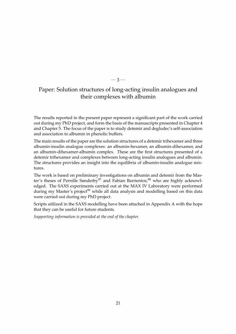
The results reported in the present paper represent a significant part of the work carriedout during my PhD project, and form the basis of the manuscripts presented in Chapter 4and Chapter 5. The focus of the paper is to study detemir and degludec’s self-associationand association to albumin in phenolic buffers.

The main results of the paper are the solution structures of a detemir trihexamer and threealbumin-insulin analogue complexes: an albumin-hexamer, an albumin-dihexamer, andan albumin-dihexamer-albumin complex. These are the first structures presented of adetemir trihexamer and complexes between long-acting insulin analogues and albumin.The structures provides an insight into the equilibria of albumin-insulin analogue mix-tures.

The work is based on preliminary investigations on albumin and detemir from the Mas-ter’s theses of Pernille Sønderby97 and Fabian Barrientos,98 who are highly acknowl-edged. The SAXS experiments carried out at the MAX IV Laboratory were performedduring my Master’s project99 while all data analysis and modelling based on this datawere carried out during my PhD project.

Scripts utilized in the SAXS modelling have been attached in Appendix A with the hopethat they can be useful for future students.

Supporting information is provided at the end of the chapter.

21

research papers

272 https://doi.org/10.1107/S2059798318017552 Acta Cryst. (2019). D75, 272–282

Received 8 October 2018

Accepted 11 December 2018

Edited by M. Czjzek, Station Biologique de

Roscoff, France

Keywords: SAXS; albumin; insulin analogues;

protein complexes; rigid-body modelling;

insulin detemir; insulin degludec.

Supporting information: this article has

supporting information at journals.iucr.org/d

Solution structures of long-acting insulin analoguesand their complexes with albumin

Line A. Ryberg,a Pernille Sønderby,a Fabian Barrientos,a Jens T. Bukrinski,b

Gunther H. J. Petersa and Pernille Harrisa*

aDepartment of Chemistry, Technical University of Denmark, Kemitorvet Building 207, 2800 Kongens Lyngby, Denmark,

and bCMC assist ApS, 2500 Copenhagen, Denmark. *Correspondence e-mail: ph@kemi.dtu.dk

The lipidation of peptide drugs is one strategy to obtain extended half-lives,

enabling once-daily or even less frequent injections for patients. The half-life

extension results from a combination of self-association and association with

human serum albumin (albumin). The self-association and association with

albumin of two insulin analogues, insulin detemir and insulin degludec, were

investigated by small-angle X-ray scattering (SAXS) and dynamic light

scattering (DLS) in phenolic buffers. Detemir shows concentration-dependent

self-association, with an equilibrium between hexamer, dihexamer, trihexamer

and larger species, while degludec appears as a dihexamer independent of

concentration. The solution structure of the detemir trihexamer has a bent

shape. The stoichiometry of the association with albumin was studied using DLS.

For albumin–detemir the molar stoichiometry was determined to be 1:6

(albumin:detemir ratio) and for albumin–degludec it was between 1:6 and 1:12

(albumin:degludec ratio). Batch SAXS measurements of a 1:6 albumin:detemir

concentration series revealed a concentration dependence of complex formation.

The data allowed the modelling of a complex between albumin and a detemir

hexamer and a complex consisting of two albumins binding to opposite ends of a

detemir dihexamer. Measurements of size-exclusion chromatography coupled to

SAXS revealed a complex between a degludec dihexamer and albumin. Based

on the results, equilibria for the albumin–detemir and albumin–degludec

mixtures are proposed.

1. Introduction

Human serum albumin (albumin) comprises more than half

of the total amount of protein in the blood plasma, with a

concentration of 35–50 mg ml�1. Albumin has many impor-

tant physiological functions involving regulation of the

colloidal osmotic pressure and the transport of a variety of

ligands such as physiological metabolites, fatty acids,

hormones, bile acids and drugs (Fanali et al., 2012; Ha &

Bhagavan, 2013; Yang et al., 2014). Albumin has a half-life of

approximately 19 days (Peters, 1985) that arises from binding

to the major histocompatibility complex-related Fc receptor

for immunoglobulin G (FcRn), resulting in a pH-dependent

recycling mechanism. Albumin is thus rescued from degra-

dation in the same manner as immunoglobulin G (Chaudhury

et al., 2003, 2006).

These pharmacokinetic properties are exploited by using

albumin as a vehicle for drug delivery to increase the half-life

of fast-degrading peptides and other smaller molecules. Half-

life extension can be obtained by the chemical conjugation of

a drug to albumin (Bukrinski et al., 2017) or by noncovalent

complexation. One widely applied strategy to obtain

ISSN 2059-7983

# 2019 International Union of Crystallography

complexation is lipidation, which exploits the natural affinity

of albumin for fatty acids (Sleep, 2014; Sleep et al., 2013).

Examples of such molecules are the lipidated insulins detemir

and degludec (trade names Levemir1 and Tresiba1, respec-

tively; Novo Nordisk A/S) and the lipidated glucagon-like

peptide-1 analogues liraglutide and semaglutide (trade names

Victoza1 and Saxenda1, and Ozempic1, respectively; Novo

Nordisk A/S).

Detemir and liraglutide are examples of first-generation

lipidated peptides; the half-life of detemir is 5–7 h (Danne et

al., 2003) and that of liraglutide is 13 h (Knudsen et al., 2000).

Optimization of the fatty acids led to the second-generation

products degludec and semaglutide. The half-life of degludec

is 25 h (Heise et al., 2012), while that of semaglutide is

approximately one week (Lau et al., 2015). The extremely long

half-life of semaglutide indicates that the albumin–sema-

glutide complex is so strong that it allows the semaglutide–

albumin complex to be recycled, mediated by the FcRn

receptor.

Apart from complexation with albumin, lipidation can lead

to self-assembly of the peptides in the subcutaneous depot,

resulting in slower diffusion into the bloodstream (Havelund

et al., 2004) or to oligomers circulating in the blood (Freder-

iksen et al., 2015). The overall mechanism whereby the

peptides obtain a longer half-life is a combination of these two

effects, complexation to albumin and oligomerization, where

the importance of each effect differs from peptide to peptide

(Deacon, 2009; Agersø et al., 2002; Jonassen et al., 2012;

European Medicines Agency, 2012; Havelund et al., 2004).

In this study, we use detemir and degludec as models to

investigate the binding of a first-generation and a second-

generation lipidated peptide. Both insulins are used in the

treatment of diabetes mellitus type 1 and type 2, and both are

long-acting lipidated insulin analogues that are used as basal

insulin to control blood sugar levels during fasting. A basal

insulin is combined with a rapid-acting insulin used in

connection with a meal to mimic the nondiabetic response to

energy uptake.

The crystal structure of detemir in the presence of phenol

was determined by Whittingham et al. (1997). The crystal

structure shows that detemir forms dihexamers stabilized by

fatty-acid interactions at the hexamer interface. Whether the

fatty-acid interactions are present in solution or simply an

artefact induced by crystal packing is not clear (Whittingham

et al., 1997). In solution, detemir has previously been shown to

exist in an equilibrium between hexamers and dihexamers

(Havelund et al., 2004), and a recent study using analytical

ultracentrifugation sedimentation velocity showed that

detemir is present in an equilibrium between monomers,

hexamers, dihexamers and trihexamers (Adams et al., 2018).

The binding of detemir to albumin and its mechanism of

protraction was studied by Havelund and coworkers using

size-exclusion chromatography (SEC). They found that

albumin binds to both dimeric and hexameric detemir and

concluded that both the oligomerization into dihexamers and

the interaction with albumin contributed to the prolonged

half-life (Havelund et al., 2004).

The solution structure of degludec has been studied by both

small-angle X-ray scattering (SAXS; Steensgaard et al., 2013)

and analytical ultracentrifugation (Adams et al., 2017, 2018;

Steensgaard et al., 2013). While there is general agreement

that degludec is found as a dihexamer in phenol-containing

solutions, different crystal forms show ambiguous inter-

molecular contacts (Steensgaard et al., 2013).

The binding of degludec to albumin and self-association was

studied by Jonassen et al. (2012) using SEC. They found that

degludec binds to albumin with a 2.4-fold higher affinity than

detemir and forms multihexamers in phenol-free buffer with

Zn2+. The protracted action of degludec mainly results from

multihexamerization in the subcutaneaous depot (Kurtzhals et

al., 2011; Seested et al., 2012; Jonassen et al., 2012) and also to

some extent from albumin binding (European Medicines

Agency, 2012).

Using SAXS in combination with dynamic light scattering

(DLS), we have studied the solution structures of detemir and

degludec alone and in complex with albumin. To our knowl-

edge, these are the first SAXS studies of detemir alone and of

albumin–detemir and albumin–degludec complexes.

2. Materials and methods

2.1. Materials

Proteins were obtained as commercially available products:

insulin detemir (detemir) as Levemir1 and insulin degludec

(degludec) as Tresiba1, both from Novo Nordisk A/S, and

recombinant human serum albumin as Recombumin1 Alpha

or Recombumin1 Elite (formally named AlbIX1) from

Albumedix Ltd.

2.2. SAXS sample preparation

The insulin analogues detemir and degludec were measured

alone and in a mixture. An overview of the samples is given in

Supplementary Table S1. All protein samples were dialyzed

over three shifts using Slide-A-Lyzer1 Dialysis Cassettes from

Thermo Scientific. The buffer from the last shift was sterile-

filtered using a 0.2 mm filter and used for sample-dilution and

buffer measurements. All of the buffers that were used are

listed in Table 1. 1 kDa cutoff spin filters were used for

concentration. If possible, protein concentrations were deter-

mined by UV–Vis spectroscopy using a NanoDrop1 1000

spectrophotometer from Thermo Scientific. The extinction

coefficient for albumin was estimated from the sequence as

research papers

Acta Cryst. (2019). D75, 272–282 Ryberg et al. � Solution structures of long-acting insulin analogues 273

Table 1Overview of the buffers, listing their constituents, pH and ionic strength(IS).

Buffer Constituents pH IS (mM)

Bufdet 5 mM Na2HPO4, 15 mM phenol, 13 mM m-cresol,173 mM glycerol, 20 mM NaCl

7.4 31

Bufalb-det 5–10 mM Na2HPO4, 10–13 mM m-cresol,11–15 mM phenol, 130–171 mM glycerol,24–69 mM NaCl

7.4 36–89

Bufdeg 25 mM Na2HPO4, 16 mM m-cresol, 16 mM phenol,213 mM glycerol, 20 mM NaCl

7.6 76

34 445 M�1 cm�1 at 280 nm using the ProtParam (Gasteiger et

al., 2005) tool from ExPaSy (Gasteiger et al., 2003). For

protein stocks containing phenol or m-cresol, the concentra-

tions were determined by scaling to SAXS data at a known

concentration or by refractometry using an Anton Paar

Abbemat 550 refractometer with a refractive-index increment,

dn/dc, of 0.19 ml g�1.

2.3. SAXS data collection

SAXS experiments were carried out on the I911-SAXS

beamline (Labrador et al., 2013) at the MAX IV Laboratory,

Lund, Sweden and on the EMBL P12 BioSAXS beamline

(Blanchet et al., 2015) at PETRA III, DESY, Hamburg,

Germany. Data-collection parameters are given in Table 2.

The sample-to-detector distance and the direct beam position

were calibrated using silver behenate, and water was measured

to place the data on an absolute scale. The buffer was

measured before and after each sample.

2.4. SEC–SAXS data collection

UV–SEC–SAXS measurements were carried out on the

EMBL P12 BioSAXS beamline (Blanchet et al., 2015) at

DESY using the experimental setup described in Table 2. A

Superdex 200 Increase 10/300 GL column (GE Healthcare

Life Sciences) was used in combination with an Agilent 1260

Infinity Bio-Inert HPLC/FPLC machine with elution through

a UV–Vis spectrophotometer and thereafter directly to the

P12 beamline. 100 ml of sample was injected and the flow rate

of Bufdeg (see Table 1) was set to 0.70 ml min�1. Prior to the

measurements, the column was equilibrated with eight column

volumes.

2.5. SAXS data analysis and modelling

For data collections at the MAX IV Laboratory, all cali-

brations, corrections and data reduction were carried out using

the PyFAI package (Kieffer & Wright, 2013). Buffer aver-

aging and subtraction were performed in PRIMUSqt

(Konarev et al., 2003). For the data collected at EMBL, an

automated pipeline (Blanchet et al., 2015) carried out all data

processing and additionally provided preliminary data

analysis. For the SEC–SAXS data, CHROMIXS (Franke et al.,

2017) was used in automated mode to select buffer and sample

regions and to perform buffer subtraction. For all SAXS

curves the scattering vector is defined as q = 4�sin�/�, where

2� is the scattering angle and � is the wavelength.

The ATSAS program package v.2.8.3 (Franke et al., 2017)

was used for data analysis and modelling. The baseline-

subtracted SAXS curves were investigated for inter-particle

interference by Guinier analysis in PRIMUSqt (Konarev et al.,

2003) and were truncated at low q values if necessary. Pair

distance distribution functions [P(r) functions] were calcu-

lated by GNOM (Svergun, 1992). Molecular parameters were

obtained from Guinier analysis and calculated P(r) functions.

Molecular masses (MMs) were calculated as MM = [NAI(0)/c]/

��M2 , where I(0)/c is the concentration-normalized forward

scattering, NA is the Avogadro constant and ��M is the

scattering contrast per mass. The average partial specific

volume for proteins of 0.7425 cm3 g�1 determined by Mylonas

& Svergun (2007) was used to calculate ��M. The MM in kDa

was, furthermore, estimated from the Porod volume (Vp) in

nm3 by the relation Vp/MM = 1.50 (Trewhella et al., 2017).

Prior to ab initio modelling, AMBIMETER (Petoukhov &

Svergun, 2015) was run in order to assess the ambiguity of the

modelling. DAMMIF (Franke & Svergun, 2009) was used to

calculate ab initio models in interactive mode with a dummy-

atom radius of 2.7 A and standard settings unless otherwise

specified. To generate models with P2 symmetry, DAMMIN

(Svergun, 1999) was used with prolate anisometry across the

symmetry axis. DAMMIN was used because it is not possible

to specify a direction of anisometry with DAMMIF, and the

models that were generated without constraining it resulted in

an undesired direction of symmetry. For each curve, 20 models

were calculated; they were subsequently aligned and averaged

using the DAMAVER program suite (Volkov & Svergun,

2003) and clustered using DAMCLUST (Petoukhov et al.,

2012). The resolution of the models was determined using

SASRES (Tuukkanen et al., 2016). The most typical model of

the ensemble or a cluster was chosen as the representative.

For rigid-body modelling, SASREFCV (Petoukhov &

Svergun, 2005, 2006; SASREF) was run using standard

settings for X-ray data on the first 80% of the scattering curve.

The fits of the models to the experimental data were calcu-

lated with CRYSOL (Svergun et al., 1995) using 500 points in

the theoretical curve and fitting up to qmax = 0.4 A�1 with

constant background subtraction. The subunits used in rigid-

body modelling were crystal structures downloaded from the

Protein Data Bank (PDB).

Both insulin and albumin exist in different conformations.

Albumin changes conformation upon the binding of fatty

acids (Ascenzi & Fasano, 2010), while insulin and detemir

(Olsen & Kaarsholm, 2000) hexamers can exist in R6, T3R3 or

T6 conformations depending on the binding of phenolic

ligands. Therefore, a fatty-acid-free (PDB entry 1ao6; Sugio et

al., 1999) and a fatty-acid-bound albumin structure (PDB

entry 1bj5; Curry et al., 1998) were used in combination with

R6, T3R3 and T6 insulin hexamers [PDB entries 1ev3 (Smith et

al., 2000), 1trz (Ciszak & Smith, 1994) and 1mso (Smith et al.,

2003), respectively]. The insulin crystal structures are not

lipidated, and it is assumed that the effect of lipidation is

negligable in rigid-body modelling. When necessary, symmetry

operations were applied to the structures to generate

hexamers. To generate dihexamers, the hexamers were trans-

research papers

274 Ryberg et al. � Solution structures of long-acting insulin analogues Acta Cryst. (2019). D75, 272–282

Table 2Experimental setup of SAXS experiments.

InstrumentI911-SAXS, MAX II,MAX IV Laboratory

P12, PETRA III,DESY

Detector PILATUS 1M PILATUS 2MWavelength (A) 0.9100 1.241q-range (nm�1) 0.0829–5.406 0.0248–5.036Exposure time (s) 4 � 30 20 � 0.05Temperature (K) 293 293Sample-to-detector distance (mm) 1962.110 3000

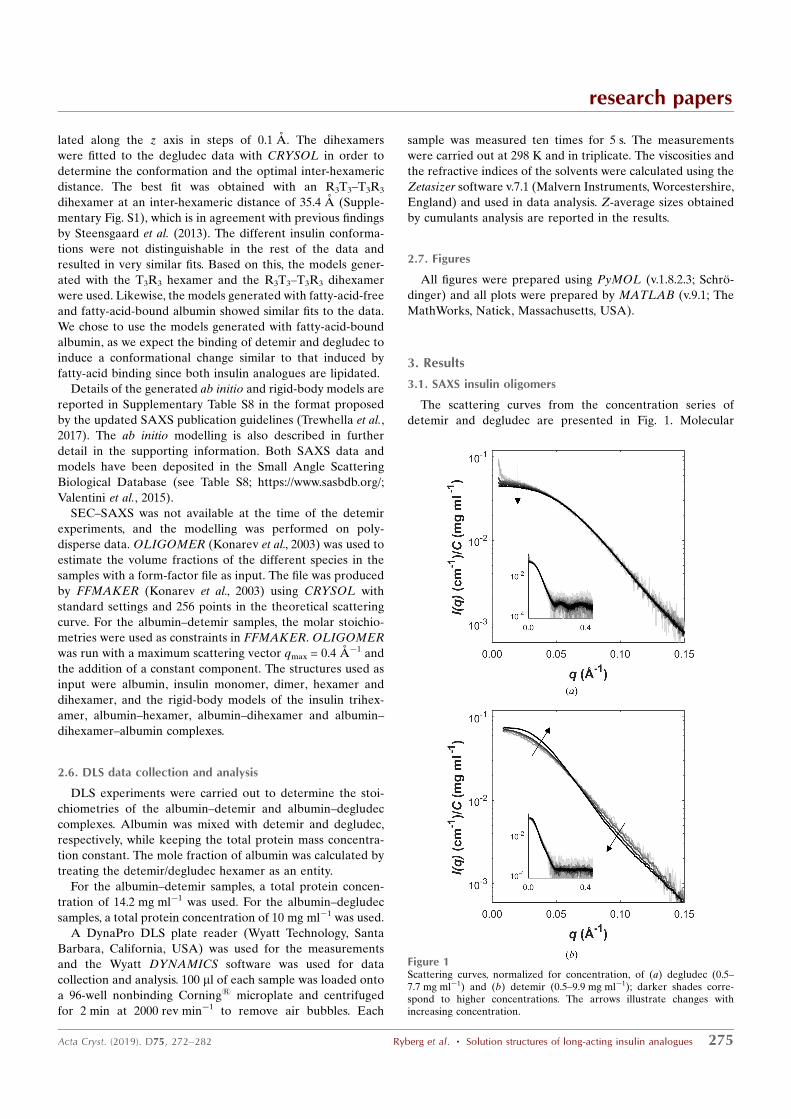
lated along the z axis in steps of 0.1 A. The dihexamers

were fitted to the degludec data with CRYSOL in order to

determine the conformation and the optimal inter-hexameric

distance. The best fit was obtained with an R3T3–T3R3

dihexamer at an inter-hexameric distance of 35.4 A (Supple-

mentary Fig. S1), which is in agreement with previous findings

by Steensgaard et al. (2013). The different insulin conforma-

tions were not distinguishable in the rest of the data and

resulted in very similar fits. Based on this, the models gener-

ated with the T3R3 hexamer and the R3T3–T3R3 dihexamer

were used. Likewise, the models generated with fatty-acid-free

and fatty-acid-bound albumin showed similar fits to the data.

We chose to use the models generated with fatty-acid-bound

albumin, as we expect the binding of detemir and degludec to

induce a conformational change similar to that induced by

fatty-acid binding since both insulin analogues are lipidated.

Details of the generated ab initio and rigid-body models are

reported in Supplementary Table S8 in the format proposed

by the updated SAXS publication guidelines (Trewhella et al.,

2017). The ab initio modelling is also described in further

detail in the supporting information. Both SAXS data and

models have been deposited in the Small Angle Scattering

Biological Database (see Table S8; https://www.sasbdb.org/;

Valentini et al., 2015).

SEC–SAXS was not available at the time of the detemir

experiments, and the modelling was performed on poly-

disperse data. OLIGOMER (Konarev et al., 2003) was used to

estimate the volume fractions of the different species in the

samples with a form-factor file as input. The file was produced

by FFMAKER (Konarev et al., 2003) using CRYSOL with

standard settings and 256 points in the theoretical scattering

curve. For the albumin–detemir samples, the molar stoichio-

metries were used as constraints in FFMAKER. OLIGOMER

was run with a maximum scattering vector qmax = 0.4 A�1 and

the addition of a constant component. The structures used as

input were albumin, insulin monomer, dimer, hexamer and

dihexamer, and the rigid-body models of the insulin trihex-

amer, albumin–hexamer, albumin–dihexamer and albumin–

dihexamer–albumin complexes.

2.6. DLS data collection and analysis

DLS experiments were carried out to determine the stoi-

chiometries of the albumin–detemir and albumin–degludec

complexes. Albumin was mixed with detemir and degludec,

respectively, while keeping the total protein mass concentra-

tion constant. The mole fraction of albumin was calculated by

treating the detemir/degludec hexamer as an entity.

For the albumin–detemir samples, a total protein concen-

tration of 14.2 mg ml�1 was used. For the albumin–degludec

samples, a total protein concentration of 10 mg ml�1 was used.

A DynaPro DLS plate reader (Wyatt Technology, Santa

Barbara, California, USA) was used for the measurements

and the Wyatt DYNAMICS software was used for data

collection and analysis. 100 ml of each sample was loaded onto

a 96-well nonbinding Corning1 microplate and centrifuged

for 2 min at 2000 rev min�1 to remove air bubbles. Each

sample was measured ten times for 5 s. The measurements

were carried out at 298 K and in triplicate. The viscosities and

the refractive indices of the solvents were calculated using the

Zetasizer software v.7.1 (Malvern Instruments, Worcestershire,

England) and used in data analysis. Z-average sizes obtained

by cumulants analysis are reported in the results.

2.7. Figures

All figures were prepared using PyMOL (v.1.8.2.3; Schro-

dinger) and all plots were prepared by MATLAB (v.9.1; The

MathWorks, Natick, Massachusetts, USA).

3. Results

3.1. SAXS insulin oligomers

The scattering curves from the concentration series of

detemir and degludec are presented in Fig. 1. Molecular

research papers

Acta Cryst. (2019). D75, 272–282 Ryberg et al. � Solution structures of long-acting insulin analogues 275

Figure 1Scattering curves, normalized for concentration, of (a) degludec (0.5–7.7 mg ml�1) and (b) detemir (0.5–9.9 mg ml�1); darker shades corre-spond to higher concentrations. The arrows illustrate changes withincreasing concentration.

parameters were derived from the curves and are presented in

Supplementary Tables S2 and S3.

3.1.1. Degludec. For the degludec curves, we observed no

concentration-dependent change in the overall curve shape

(q � 0.04 A�1; Fig. 1a). For q < 0.04 A�1 a decrease in the

normalized forward scattering [I(0)/c] was observed with

increasing protein concentration, indicating repulsion. To

obtain an ideal scattering curve, low- and high-concentration

data were merged to avoid repulsion artefacts at high

concentrations. The SAXS-derived MM ranges from 12 to 13

monomers, corresponding to a dihexamer (Supplementary

Fig. S1).

3.1.2. Detemir. For the detemir curves, we observed an

increase in curve steepness from q = 0.05 to 0.12 A�1 with

increasing concentration (Fig. 1b). The change in the shape of

the curve indicates concentration-dependent oligomerization.

Repulsion was observed at higher concentrations as a flat-

tening of the curves for low q values. MM ranges from 17 to 22

monomers, and the increase is consistent with an increase in

the Porod volume (Supplementary Table S3).

Until recently, the highest oligomer of detemir reported was

a dihexamer in equilibrium with a hexamer (Havelund et al.,

2004), but in 2018 Adams and coworkers reported detemir in a

trihexameric state in equilibrium with monomers, hexamers

and dihexamers (Adams et al., 2018).

We chose the 2.5 mg ml�1 curve for modelling the detemir

trihexamer as it was unaffected by repulsion and had an MM

close to that expected for a trihexamer. Ten rigid-body models

were generated by SASREF with three hexamers as input. In

Fig. 2, the best model is superimposed onto the representative

ab initio model generated by DAMMIF (42� 3 A resolution).

The ab initio and rigid-body models overlap nicely, which gives

confidence in the modelled trihexamer. The model fits the data

well, with �2 = 1.16 (Fig. 2a).

To assess the equilibria in the concentration series, we ran

OLIGOMER with PDB structures of the insulin monomer,

dimer, hexamer and dihexamer, and the model of the trihex-

amer. The results are presented in Table 3 and the fits to the

experimental data are shown in Fig. 3. The lower concentra-

tion samples, 0.5 and 1.0 mg ml�1, consist of an equilibrium

between hexamer, dihexamer and trihexamer. The

research papers

276 Ryberg et al. � Solution structures of long-acting insulin analogues Acta Cryst. (2019). D75, 272–282

Figure 2Modelling results of the detemir trihexamer based on the 2.5 mg ml�1

detemir scattering curve. (a) Fit of the rigid-body model (green) to theexperimental data (grey). (b) shows an error-weighted residual plot of themodel. (c) The rigid-body model (green) is superimposed onto the low-resolution ab initio model (light blue).

Table 3OLIGOMER results for detemir samples.

Results are for detemir samples in the concentration range 0.5–2.5 mg ml�1,showing volume fractions of the species with uncertainties in the last digit inparentheses and �2 fits to experimental data.

Concentration (mg ml�1) �2 Hexamer Dihexamer Trihexamer

0.5 0.64 0.07 (3) 0.13 (3) 0.80 (3)1.0 0.66 0.05 (1) 0.10 (2) 0.85 (1)2.5 1.23 0.016 (5) 0.984 (5)

Figure 3OLIGOMER results for detemir samples in the concentration range 0.5–2.5 mg ml�1. (a) OLIGOMER fits are plotted (green; darker shadescorrespond to higher concentrations) with the experimental scatteringcurves (grey). The scattering curves have been shifted on the I(q)/c axisfor clarity. (b) shows an error-weighted residual plot of the fits.

2.5 mg ml�1 curve is almost monodisperse, with 98.4%

trihexamer and 1.6% dihexamer. For the higher concentration

samples, the OLIGOMER results do not fit the experimental

data (data not shown), reflecting that higher oligomers are

needed to describe the data. This is supported by a steeper

decrease in their scattering curves around q = 0.05–0.10 A�1 in

Fig. 1(b).

3.2. DLS of albumin complexes

DLS experiments were set up to determine the binding

stoichiometry between albumin and detemir and degludec,

respectively. In the experiments, the mass fraction was varied,

the molar stoichiometry was calculated and the maximum

measured radius of hydration (Rh) was considered to repre-

sent the stoichiometry of the protein complex (Hanlon et al.,

2010).

The results are presented in Fig. 4, in which selected molar

ratios are marked on the top x axis. For detemir, a peak in Rh

is observed close to a 1:6 molar ratio. For degludec, the

maximum in Rh is more flat and is observed between ratios of

1:12 and 1:6.

3.3. Albumin–degludec complex structure

Based on the maximum in Rh between molar ratios of 1:6

and 1:12, albumin–degludec complex formation was investi-

gated at both ratios. The scattering curves of the albumin–

degludec mixtures are shown in Fig. 5 and their SAXS-derived

molecular parameters are given in Supplementary Tables S4

and S5.

The shapes of the scattering curves for the 1:12 mixtures

(Fig. 5a) do not change with protein concentration. The MM

values derived from the data were 138–141 kDa, corre-

sponding to a monodisperse 1:12 complex (MM = 140 kDa).

The overall shape of the 1:6 scattering curves (Fig. 5b) also

does not change with concentration, except for an increase in

I(0)/c corresponding to attractive interactions at higher

concentrations. The MM values derived from the 1:6 data

range between 145 and 163 kDa; they do not correspond

directly to monodisperse 1:6, 1:12 or 2:12 complexes (MM

values of 103, 140 and 206 kDa, respectively), but rather to a

mixture of different species. In order to separate the species, a

SEC–SAXS experiment was conducted.

The SAXS intensity trace of the SEC–SAXS run is shown in

Fig. 6(a) with two apparent peaks. The scattering curve of the

lowest MM peak (SEC–SAXSalbumin) is shown in Fig. 6(b)

and overlaps very well with a batch SAXS measurement

of albumin. The scattering curve of the higher MM peak

research papers

Acta Cryst. (2019). D75, 272–282 Ryberg et al. � Solution structures of long-acting insulin analogues 277

Figure 4Results of DLS experiments on albumin–detemir (blue triangles) andalbumin–degludec (olive squares) mixtures. The average hydrodynamicradius is plotted as a function of the molar fraction of albumin in themixtures. The upper x axis indicate the molar ratio between albumin andeither detemir or degludec. The error bars represent standard deviations.

Figure 5Scattering curves, normalized for concentration, of albumin and degludecmixed in (a) 1:12 and (b) 1:6 ratios; darker shades correspond to higherconcentrations.

(SEC–SAXSalbumin–degludec) is shown in Fig. 6(c) and overlaps

very well with a 1:12 albumin–degludec batch SAXS

measurement. The MM value derived from the curve is

141 kDa, which could correspond to an albumin–dihexamer or

a hexamer–albumin–hexamer complex (both with an MM of

140 kDa). These complexes will be modelled in the following

section based on the SEC–SAXSalbumin–degludec curve.

In addition to the two apparent peaks in the chromatogram,

a small shoulder consisting of two peaks is present on the left

side of the main peak, which explains the higher MM for the

1:6 mixture and corresponds to larger protein complexes.

3.3.1. Rigid-body modelling of the albumin–dihexamercomplex. Ten rigid-body models were generated by SASREF

based on the SEC–SAXSalbumin–degludec curve with albumin and

two hexamers as input in order to test whether the hexamers

bind albumin separately or as a dihexamer. We found that the

hexamers in the best-fitting model formed a dihexamer, thus

suggesting an albumin–dihexamer complex. Ten rigid-body

models were therefore generated with albumin and a dihex-

amer as input. The best of these ten models fitted the data well

with �2 = 1.74 (Fig. 7a) and showed good agreement with the

representative ab initio model generated by DAMMIF (41 �

3 A resolution; Fig. 7c). In the complex, the dihexamer binds

close to Sudlow’s site I, which is one of the major drug-binding

sites in albumin and overlaps with fatty-acid-binding site 7

(FA7; Sudlow et al., 1975).

3.4. Albumin–detemir complex structures

The scattering curves of the albumin–detemir samples are

shown in Supplementary Fig. S2. Clearly, the curves are

affected by concentration-dependent equilibria.

Two of the obtained SAXS curves were used for modelling:

the 8.5 mg ml�1 SAXS curve with an MM of 104 kDa, which

could correspond to an albumin–hexamer complex (MM of

102 kDa), and the 15.6 mg ml�1 SAXS curve with an MM of

213 kDa, which could correspond to an albumin–dihexamer–

albumin complex (MM of 204 kDa). These curves are shown

in Fig. 8.

research papers

278 Ryberg et al. � Solution structures of long-acting insulin analogues Acta Cryst. (2019). D75, 272–282

Figure 7Modelling results of the albumin–dihexamer complex based on the SEC–SAXSalbumin–degludec scattering curve. (a) Fit of the rigid-body model(orange) to the experimental data (grey). (b) shows an error-weightedresidual plot for the model. (c) The rigid-body model is shown withalbumin in grey and the dihexamer in orange. It is superimposed onto thelow-resolution ab initio model (light blue).

Figure 6SEC–SAXS results for albumin and degludec mixed in a 1:6 ratio. (a) Plotshowing average intensity and MM as a function of column volume, withpeaks marked in yellow and red. (b) Scattering curve (SEC-SAXSalbumin)of the peak at �13.2 ml (red) shown with a batch scattering curve foralbumin at 2.8 mg ml�1 (grey). (c) Scattering curve (SEC-SAXSalbumin) ofthe peak at �11.7 ml (yellow) and a batch scattering curve for albumin–degludec in a 1:12 ratio at 6.5 mg ml�1 (grey). All scattering curves arenormalized for concentration.

The curves overlap well at q-values above 0.05 A�1 (�2 =

0.91), indicating that common local features are present in

both complexes, while the higher concentration curve has

higher intensity at lower q-values, thus corresponding to a shift

in the equilibrium towards larger complexes with larger

intramolecular distances.

3.4.1. Rigid-body modelling of the albumin–hexamercomplex. Ten rigid-body models were generated by

SASREF based on the 8.5 mg ml�1 albumin–detemir curve

with albumin and a detemir hexamer as input. These ten

models could be clustered into two groups based on the

binding position on albumin: near Sudlow’s site I and near

Sudlow’s site II. The best model of each cluster and their fits to

experimental data (�2 = 1.32 and �2 = 1.88, respectively) are

shown in Fig. 9 with the representative ab initio model

(39�3 A). The �2 values of the clusters do not differ very

much (Figs. 9a and 9b) when considering that the conforma-

tions of albumin and detemir might change upon binding.

3.4.2. Rigid-body modelling of the albumin–dihexamer–albumin complex. Based on the MM from the 15.6 mg ml�1

albumin–detemir SAXS curve, the complex could consist of

two albumins and either two hexamers or one dihexamer. Ten

rigid-body models were generated with P1 symmetry using

two albumins and a dihexamer as input structures, and ten

models were generated with P2 symmetry using an albumin

and a hexamer as input structures.

The best results with P1 (�2 = 1.01) and P2 (�2 = 1.12)

symmetry and their fits to the experimental data are presented

in Fig. 10, where the rigid-body models are superimposed onto

the representative P1 and P2 ab initio models (53 � 4 and 55

� 4 A resolution, respectively). In both rigid-body models

detemir forms a dihexamer with one albumin bound to each

hexamer and the albumins appear to bind diagonally to the

dihexamer.

research papers

Acta Cryst. (2019). D75, 272–282 Ryberg et al. � Solution structures of long-acting insulin analogues 279

Figure 9Modelling results of the albumin–hexamer complex based on the8.5 mg ml�1 albumin–detemir scattering curve. (a) Fit of rigid-bodymodels binding to Sudlow’s sites I (purple) and II (magenta) to theexperimental data (grey). (b) shows error-weighted residual plots for themodels. The rigid-body models are shown in (c) and (d), respectively, withalbumin in grey and the same colour coding as in (a) for the hexamers.Both models are superimposed on the low-resolution ab initio model(light blue).

Figure 8Scattering curves, normalized for concentration, of albumin and detemirmixed in a 1:6 molar ratio with total protein concentrations of 8.5 and15.6 mg ml�1.

Figure 10Modelling results of the albumin–dihexamer–albumin complex based onthe 15.6 mg ml�1 albumin–detemir scattering curve. (a) Fit of rigid-bodymodels generated with P1 (light blue) and P2 symmetry (blue),respectively, to the experimental data (grey). (b) shows error-weightedresidual plots for the models. The rigid-body models are shown in (c) (P2symmetry) and (d) (P1 symmetry) with albumins in grey and the samecolour-coding as in (a) for the dihexamers. Both models are superimposedonto the low-resolution ab initio model (light blue).

3.4.3. Analysis of albumin–detemir equilibrium. To assess

the equilibria in the albumin–detemir concentration series,

OLIGOMER was run. The results are summarized in Table 4

and the fits to the experimental data are shown in Fig. 11.

For the lower concentration samples at 1.9 and 4.1 mg ml�1,

we observe an equilibrium between albumin, trihexamer and

the albumin–hexamer complex. At 8.5 mg ml�1, the equili-

brium shifts towards albumin–dihexamer complexes and the

sample consists of albumin, albumin–hexamer and albumin–

dihexamer complexes. At 15.6 mg ml�1, the sample consists

entirely of the albumin–dihexamer–albumin complex. For the

highest concentration sample at 20.8 mg ml�1, the

OLIGOMER result does not fit the data (data not shown),

which indicates that larger species are needed to describe the

curve.

4. Discussion

In agreement with previous studies (Steensgaard et al., 2013;

Adams et al., 2018; Havelund et al., 2004), we find degludec as

a dihexamer in phenol-containing buffer and detemir in a

concentration-dependent equilibrium between hexamers,

dihexamers, trihexamers and possibly larger multihexamers.

We present the first structure of the detemir trihexamer, which

has previously only been reported in a study using analytical

ultracentrifugation (Adams et al., 2018). Surprisingly, the

trihexamer has a bent shape.

For degludec mixed with albumin, DLS data showed that

the binding stoichiometry of an albumin–degludec complex

was somewhere between 1:6 and 1:12. However, SAXS

measurements, both inline SEC–SAXS on a 1:6 albumin–

degludec mixture and batch measurements on a 1:12 mixture,

unambiguously showed a 1:12 complex.

For detemir mixed with albumin, we determined the

stoichiometry to be 1:6 by DLS. We succeeded in modelling

an albumin–hexamer complex despite the somewhat

polydisperse curve, as well as an albumin–dihexamer–albumin

complex.

4.1. Equilibria

The different complexes of detemir and degludec with

albumin can thus be directly linked to their oligomeric states.

We propose that detemir and degludec hexamers mixed with

albumin exist in the equilibria illustrated in Fig. 12. Degludec

alone exists as a dihexamer. When mixed with albumin in a

1:12 ratio, the sample purely consists of albumin–dihexamer

complex. Detemir alone exists in an equilibrium with various

oligomers. When mixed with albumin, we observe the

formation of 1:6, 1:12 and 2:12 complexes, with higher protein

concentrations and ionic strengths favouring larger complexes.

At the highest protein concentration, however, we observe an

increase in the MM beyond the expected value for a 2:12

complex, which could be owing to larger complexes.

The differences between the behaviour of degludec and

detemir in solution are solely owing to the different fatty-acid

moieties, as the molecules are otherwise identical. The

different multihexamerizations indicate that their modes of

hexamer–hexamer association are fundamentally different.

The driving force of association results from their fatty-acid

moieties, as human insulin is normally observed in an equi-

librium between monomer, dimer and hexamer (Frankaer et

al., 2017; Jorgensen et al., 2011). While detemir has a C14 fatty

acid attached to LysB29, the second-generation product

degludec has a C16 dicarboxylic fatty acid attached through a

�-glutamate linker. The differences in these fatty-acid

moieties mean that degludec has a longer fatty-acid chain and

research papers

280 Ryberg et al. � Solution structures of long-acting insulin analogues Acta Cryst. (2019). D75, 272–282

Figure 11OLIGOMER results for albumin–detemir samples in the concentrationrange 1.9–15.6 mg ml�1. (a) OLIGOMER fits are plotted (red; darkershades correspond to higher concentrations) with the experimentalscattering curves (grey). The scattering curves have been shifted on theI(q)/c axis for clarity. (b) shows an error-weighted residual plot of the fits.

Table 4OLIGOMER results for albumin–detemir samples.

OLIGOMER results for albumin–detemir samples in the concentration range1.9–15.6 mg ml�1, showing volume fractions of the species with uncertaintiesin parentheses and �2 fits to experimental data.

Concentration(mg ml�1) �2 Albumin Trihexamer

Albumin–hexamer

Albumin–dihexamer

Albumin–dihexamer–albumin

1.9 0.57 0.497 (7) 0.257 (3) 0.25 (1)4.1 0.87 0.477 (4) 0.246 (2) 0.277 (5)8.5 0.77 0.184 (6) 0.44 (2) 0.36 (1) 0.010 (2)15.6 2.05 1.000 (1)

two extra negative charges, allowing different interactions.

Therefore, it is likely that the binding of detemir and degludec

albumin probably differs significantly at the atomic level.

5. Conclusion

Here, we have shown that detemir and degludec exist in

different equilibria in phenol-containing buffers and how

these equilibria affect their complex formation with albumin.

We have presented the solution structures of the detemir

trihexamer and of 1:6, 1:12 and 2:12 complexes between

albumin and two insulin analogues. The solution structures are

the first structures of complexes between albumin and long-

acting insulin analogues to be presented.

Acknowledgements

We would like to acknowledge MAX IV Laboratory and

DESY Hamburg for providing beam time for the SAXS

experiments. Albumedix Ltd is acknowledged for providing

proteins (including Recombumin1 Elite and Alpha) for the

experiments and for access to their DLS plate reader.

Funding information

The following funding is acknowledged: Department of

Chemistry, Technical University of Denmark (scholarship to

Line A. Ryberg); DANSCATT (The Danish Agency for

Science, Technology and Innovation; bursary to Line A.

Ryberg, Pernille Sønderby, Gunther H. J. Peters, Pernille

Harris).

References

Adams, G. G., Alzahrani, Q., Jiwani, S. I., Meal, A., Morgan, P. S.,Coffey, F., Kok, S., Rowe, A. J., Harding, S. E., Chayen, N. & Gillis,R. B. (2017). Sci. Rep. 7, 7287.

Adams, G. G., Meal, A., Morgan, P. S., Alzahrani, Q. E., Zobel, H.,Lithgo, R., Kok, M. S., Besong, D. T. M., Jiwani, S. I., Ballance, S.,Harding, S. E., Chayen, N. & Gillis, R. B. (2018). PLoS One, 13,e0195010.

Agersø, H., Jensen, L. B., Elbrønd, B., Rolan, P. & Zdravkovic, M.(2002). Diabetologia, 45, 195–202.

Ascenzi, P. & Fasano, M. (2010). Biophys. Chem. 148, 16–22.Blanchet, C. E., Spilotros, A., Schwemmer, F., Graewert, M. A.,

Kikhney, A., Jeffries, C. M., Franke, D., Mark, D., Zengerle, R.,Cipriani, F., Fiedler, S., Roessle, M. & Svergun, D. I. (2015). J. Appl.Cryst. 48, 431–443.

Bukrinski, J. T., Sønderby, P., Antunes, F., Andersen, B., Schmidt,E. G. W., Peters, G. H. J. & Harris, P. (2017). Biochemistry, 56, 4860–4870.

Chaudhury, C., Brooks, C. L., Carter, D. C., Robinson, J. M. &Anderson, C. L. (2006). Biochemistry, 45, 4983–4990.

Chaudhury, C., Mehnaz, S., Robinson, J. M., Hayton, W. L., Pearl,D. K., Roopenian, D. C. & Anderson, C. L. (2003). J. Exp. Med. 197,315–322.

Ciszak, E. & Smith, G. D. (1994). Biochemistry, 33, 1512–1517.Curry, S., Mandelkow, H., Brick, P. & Franks, N. (1998). Nature Struct.

Biol. 5, 827–835.Danne, T., Lupke, K., Walte, K., Von Schuetz, W. & Gall, M.-A.

(2003). Diabetes Care, 26, 3087–3092.Deacon, C. F. (2009). Vasc. Heal. Risk Manag. 5, 199–211.European Medicines Agency (2012). CHMP Assessment Report:

Tresiba. London: European Medicines Agency. https://www.ema.europa.eu/documents/assessment-report/tresiba-epar-public-assessment-report_en.pdf.

Fanali, G., di Masi, A., Trezza, V., Marino, M., Fasano, M. & Ascenzi,P. (2012). Mol. Aspects Med. 33, 209–290.

Frankaer, C. G., Sønderby, P., Bang, M. B., Mateiu, R. V., Groenning,M., Bukrinski, J. & Harris, P. (2017). J. Struct. Biol. 199, 27–38.

Franke, D., Petoukhov, M. V., Konarev, P. V., Panjkovich, A.,Tuukkanen, A., Mertens, H. D. T., Kikhney, A. G., Hajizadeh, N. R.,Franklin, J. M., Jeffries, C. M. & Svergun, D. I. (2017). J. Appl.Cryst. 50, 1212–1225.

Franke, D. & Svergun, D. I. (2009). J. Appl. Cryst. 42, 342–346.Frederiksen, T. M., Sønderby, P., Ryberg, L. A., Harris, P., Bukrinski,

J. T., Scharff-Poulsen, A. M., Elf-Lind, M. N. & Peters, G. H. (2015).Biophys. J. 109, 1202–1213.

Gasteiger, E., Gattiker, A., Hoogland, C., Ivanyi, I., Appel, R. D. &Bairoch, A. (2003). Nucleic Acids Res. 31, 3784–3788.

Gasteiger, E., Hoogland, C., Gattiker, A., Duvaud, S., Wilkins, M. R.,Appel, R. D. & Bairoch, A. (2005). The Proteomics ProtocolsHandbook, edited by J. M. Walker, pp. 571–607. Totowa: HumanaPress.

Ha, C.-E. & Bhagavan, N. V. (2013). Biochim. Biophys. Acta, 1830,5486–5493.

Hanlon, A. D., Larkin, M. I. & Reddick, R. M. (2010). Biophys. J. 98,297–304.

Havelund, S., Plum, A., Ribel, U., Jonassen, I., Vølund, A.,Markussen, J. & Kurtzhals, P. (2004). Pharm. Res. 21, 1498–1504.

Heise, T., Nosek, L., Bøttcher, S. G., Hastrup, H. & Haahr, H. (2012).Diabetes Obes. Metab. 14, 944–950.

Jonassen, I., Havelund, S., Hoeg-Jensen, T., Steensgaard, D. B.,Wahlund, P.-O. & Ribel, U. (2012). Pharm. Res. 29, 2104–2114.

research papers

Acta Cryst. (2019). D75, 272–282 Ryberg et al. � Solution structures of long-acting insulin analogues 281

Figure 12Proposed equilibria for albumin and (a) detemir and (b) degludechexamers under the investigated conditions. Albumin is represented asgrey hearts and the hexamers as orange circles.

Jorgensen, L., Bennedsen, P., Hoffmann, S. V., Krogh, R. L., Pinholt,C., Groenning, M., Hostrup, S. & Bukrinsky, J. T. (2011). Eur. J.Pharm. Sci. 42, 509–516.

Kieffer, J. & Wright, J. P. (2013). Powder Diffr. 28, S339–S350.Knudsen, L. B., Nielsen, P. F., Huusfeldt, P. O., Johansen, N. L.,

Madsen, K., Pedersen, F. Z., Thøgersen, H., Wilken, M. & Agersø,H. (2000). J. Med. Chem. 43, 1664–1669.

Konarev, P. V., Volkov, V. V., Sokolova, A. V., Koch, M. H. J. &Svergun, D. I. (2003). J. Appl. Cryst. 36, 1277–1282.

Kurtzhals, P., Heise, T., Strauss, H. M., Bottcher, S. G., Granhall, C.,Haahr, H. & Jonassen, I. (2011). Diabetologia, 54, S426.

Labrador, A., Cerenius, Y., Svensson, C., Theodor, K. & Plivelic, T.(2013). J. Phys. Conf. Ser. 425, 072019.

Lau, J., Bloch, P., Schaffer, L., Pettersson, I., Spetzler, J., Kofoed, J.,Madsen, K., Knudsen, L. B., McGuire, J., Steensgaard, D. B.,Strauss, H. M., Gram, D. X., Knudsen, S. M., Nielsen, F. S.,Thygesen, P., Reedtz-Runge, S. & Kruse, T. (2015). J. Med. Chem.58, 7370–7380.

Mylonas, E. & Svergun, D. I. (2007). J. Appl. Cryst. 40, s245–s249.Olsen, H. B. & Kaarsholm, N. C. (2000). Biochemistry, 39, 11893–

11900.Peters, T. (1985). Adv. Protein Chem. 37, 161–245.Petoukhov, M. V., Franke, D., Shkumatov, A. V., Tria, G., Kikhney,

A. G., Gajda, M., Gorba, C., Mertens, H. D. T., Konarev, P. V. &Svergun, D. I. (2012). J. Appl. Cryst. 45, 342–350.

Petoukhov, M. V. & Svergun, D. I. (2005). Biophys. J. 89, 1237–1250.Petoukhov, M. V. & Svergun, D. I. (2006). Eur. Biophys. J. 35, 567–

576.Petoukhov, M. V. & Svergun, D. I. (2015). Acta Cryst. D71, 1051–

1058.Seested, T., Havelund, S., Jonassen, I. B., Hoeg-Jensen, T., Pyke, C.,

Kapor, J. & Nishimura, E. (2012). Can. J. Diab. 36, S61.

Sleep, D. (2014). Expert Opin. Drug Deliv. 12, 793–812.Sleep, D., Cameron, J. & Evans, L. R. (2013). Biochim. Biophys. Acta,

1830, 5526–5534.Smith, G. D., Ciszak, E., Magrum, L. A., Pangborn, W. A. & Blessing,

R. H. (2000). Acta Cryst. D56, 1541–1548.Smith, G. D., Pangborn, W. A. & Blessing, R. H. (2003). Acta Cryst.

D59, 474–482.Steensgaard, D. B., Schluckebier, G., Strauss, H. M., Norrman, M.,

Thomsen, J. K., Friderichsen, A. V., Havelund, S. & Jonassen, I.(2013). Biochemistry, 52, 295–309.

Sudlow, G., Birkett, D. J. & Wade, D. N. (1975). Mol. Pharmacol. 11,824–832.

Sugio, S., Kashima, A., Mochizuki, S., Noda, M. & Kobayashi, K.(1999). Protein Eng. 12, 439–446.

Svergun, D., Barberato, C. & Koch, M. H. J. (1995). J. Appl. Cryst. 28,768–773.

Svergun, D. I. (1992). J. Appl. Cryst. 25, 495–503.Svergun, D. I. (1999). Biophys. J. 76, 2879–2886.Trewhella, J., Duff, A. P., Durand, D., Gabel, F., Guss, J. M.,

Hendrickson, W. A., Hura, G. L., Jacques, D. A., Kirby, N. M.,Kwan, A. H., Perez, J., Pollack, L., Ryan, T. M., Sali, A.,Schneidman-Duhovny, D., Schwede, T., Svergun, D. I., Sugiyama,M., Tainer, J. A., Vachette, P., Westbrook, J. & Whitten, A. E.(2017). Acta Cryst. D73, 710–728.

Tuukkanen, A. T., Kleywegt, G. J. & Svergun, D. I. (2016). IUCrJ, 3,440–447.

Valentini, E., Kikhney, A. G., Previtali, G., Jeffries, C. M. & Svergun,D. I. (2015). Nucleic Acids Res. 43, D357–D363.

Volkov, V. V. & Svergun, D. I. (2003). J. Appl. Cryst. 36, 860–864.Whittingham, J. L., Havelund, S. & Jonassen, I. (1997). Biochemistry,

36, 2826–2831.Yang, F., Zhang, Y. & Liang, H. (2014). Int. J. Mol. Sci. 15, 3580–3595.

research papers

282 Ryberg et al. � Solution structures of long-acting insulin analogues Acta Cryst. (2019). D75, 272–282

Acta Cryst. (2019). D75, doi:10.1107/S2059798318017552 Supporting information

Volume 75 (2019)

Supporting information for article:

Solution structures of long-acting insulin analogues and their complexes with albumin

Line A. Ryberg, Pernille Sønderby, Fabian Barrientos, Jens T. Bukrinski, Günther H. J. Peters and Pernille Harris

S1. Ab-initio modelling results

S1.1. Detemir tri-hexamer

20 ab-initio models were generated by DAMMIF based on the P(r) function with a maximum intra-

molecular dimension ( ) of 11.3 nm. The curve has an ambiguity score of 1.56 which indicate that

the ab-initio model might be ambiguous(Petoukhov & Svergun, 2015). The ensemble of models had a

resolution of 42±3 Å and a normalized spatial discrepancy (NSD) of 0.67±0.02 indicating a stable

solution. A cluster analysis was performed by DAMCLUST, resulting in three clusters. The most

typical model of one of the clusters ( 2 0.80) is presented in Fig. 2c in a light blue surface

representation. The model has a bent v-shape and seems to consist of three distinct spheres that could

correspond to three hexamers.

S1.2. Degludec albumin-di-hexamer complex

20 ab-initio models were generated by DAMMIF based on the SEC-SAXSalbumin-degludec P(r) function

with a maximum intramolecular dimension (Dmax) of 13.4 nm. The ambiguity score of the scattering

curve was calculated by AMBIMETER to 1.40 indicating that a shape reconstruction is potentially

unique. The ensemble of models had a resolution of 41±3 Å and an NSD of 0.71±0.04 indicating a

stable solution. The most typical model of the ensemble ( 2 1.67) is presented in Fig. 7c (light blue

surface representation).

S1.3. Detemir albumin-hexamer complex

20 DAMMIF models were generated based on the albumin-detemir 8.5 mg/mL P(r) function with a

Dmax of 13.0 nm and thereafter aligned and averaged by DAMAVER to an average model. The

scattering curve has an ambiguity score of 1.230 indicating that unambiguous shape reconstruction

should be possible.The ensemble of models had a resolution of 39±3 Å and an NSD of 0.68±0.02

indicating a stable solution, which is expected from the low ambiguity score. The most typical model

of the ensemble ( 2 0.86) is presented in Figs. 9c and 9d from different orientations (light blue).

S1.4. Detemir albumin-di-hexamer-albumin complex

Ab-initio modelling was carried out applying P1 and P2 symmetry based on the albumin-detemir 15.6

mg/mL P(r) function with Dmax of 19.5 nm. DAMMIF was run 20 times to generate models with P1

symmetry, and DAMMIN was run 20 times to generate models with P2 symmetry. The scattering

curve has an ambiguity score of 2.076 indicating that shape reconstruction might be ambiguous.

The ensemble of models with P1 symmetry had a resolution of 53±4 Å and with NSD of 1.0±0.1. The

ensemble of models with P2 symmetry had a resolution was 55±4 Å and an NSD 0.76±0.08. The most

typical models of the ensembles with respectively P1 ( 2 0.83) and P2 symmetry ( 2 0.89) are

1

presented in Figs. 10c and 10d. Although a stable solution was not obtained for the models with P1

symmetry (NSD > 0.7(Volkov & Svergun, 2003)), there is a good agreement between the two

representative models that are both elongated.

Table S1 Sample overview

Overview over samples listing their constituents, buffer, total protein concentration, molar ratio, and the

beamline used for data collection.

Insulin Buffer Protein conc. (mg/mL) albumin:insulin Data collection

Detemir Bufdet 0.5-9.9 - I911-SAXS (MAXII, MAXIVLab)

Degludec Bufdeg 0.5-7.7 - P12 (PETRAIII, DESY)

Detemir Bufalb-det 1.9-20.8 1:6 I911-SAXS (MAXII, MAXIVLab)

Degludec Bufdeg 10.6 (SEC-SAXS) 1:6 P12 (PETRAIII, DESY)

Degludec Bufdeg 1.5-15.3 1:6 P12 (PETRAIII, DESY)

Degludec Bufdeg 2.1-10.8 1:12 P12 (PETRAIII, DESY)

Table S2 Degludec samples – molecular parameters

Molecular parameters for degludec samples derived from SAXS analysis. The subscripts indicate whether the

parameter is derived from Guinier analysis (G) or the P(r) function (P). #monomers denotes the average number of

monomers calculated from MM P.

C (I(0)/C)G (I(0)/C)P

RgG

RgP

Dmax V MM G MM P MM V #monomers

mg/mL mL/mg mL/mg nm nm nm nm3 kDa kDa kDa

0.5 0.055 0.057 2.61 2.65 8.14 108.03 75.8 78.4 72.0 13.3

1.2 0.054 0.052 2.60 2.63 7.93 108.43 75.2 71.6 72.3 12.1

1.6 0.053 0.055 2.55 2.60 7.51 111.59 73.8 76.4 74.4 12.9

2.7 0.051 0.055 2.51 2.56 7.42 109.52 70.6 75.6 73.0 12.8

3.9 0.051 0.051 2.43 2.56 7.42 109.53 71.0 71.0 73.0 12.0

5.7 0.049 0.052 2.34 2.57 7.49 102.72 67.6 72.4 68.5 12.3

7.7 0.048 0.051 2.29 2.56 7.56 99.90 65.2 70.6 66.6 12.0

Table S3 Detemir samples – molecular parameters

Molecular parameters for detemir samples derived from SAXS analysis. The subscripts indicate whether the

parameter is derived from Guinier analysis (G) or the P(r) function (P). #monomers denotes the average number of

monomers calculated from MM P.

2

C (I(0)/C)G (I(0)/C)P

RgG

RgP

Dmax V MM G MM P MM V #monomers

mg/mL mL/mg mL/mg nm nm nm nm3 kDa kDa kDa

0.5 0.069 0.076 3.31 3.34 11.50 124.16 95.1 105.7 82.8 17.9

1.0 0.069 0.070 3.29 3.35 11.35 133.81 96.1 97.5 89.2 16.5

2.5 0.072 0.072 3.26 3.32 11.16 137.24 100.3 100.3 91.5 17.0

5.0 0.074 0.076 3.07 3.34 10.45 151.90 103.0 105.8 101.3 17.9

9.9 0.086 0.092 3.29 3.53 11.15 183.64 119.8 128.1 122.4 21.7

Table S4 Albumin-degludec (1:12) samples – molecular parameters

Molecular parameters for albumin-degludec samples in a 1:12 ratio derived from SAXS analysis. The subscripts

indicate whether the parameter is derived from Guinier analysis (G) or the P(r) function (P). #Alb-hex and #Alb-di-hex

denote the average numbers of respectively albumin-hexamer and albumin-di-hexamer complex calculated from

MM P.

C (I(0)/C)G (I(0)/C)P

RgG

RgP

Dmax V MM G MM P MM V #Alb-hex #Alb-di-hex

mg/mL mL/mg mL/mg nm nm nm nm3 kDa kDa kDa

2.1 0.010 0.010 3.77 3.84 13.61 181.10 138.5 138.5 120.7 1.3 1.0

4.4 0.010 0.010 3.77 3.86 13.56 189.10 137.9 137.9 126.1 1.3 1.0

6.5 0.010 0.010 3.73 3.81 13.12 189.28 140.6 140.6 126.2 1.4 1.0

10.8 0.010 0.010 3.6 3.73 12.22 185.11 137.0 138.2 123.4 1.3 1.0

Table S5 Albumin-degludec (1:6) samples – molecular parameters

Molecular parameters for albumin-degludec samples in a 1:6 ratio derived from SAXS analysis. The subscripts

indicate whether the parameter is derived from Guinier analysis (G) or the P(r) function (P). #Alb-hex and #Alb-di-hex

denote the average numbers of respectively albumin-hexamer and albumin-di-hexamer complex calculated from

MM P.

C (I(0)/C)G (I(0)/C)P

RgG

RgP

Dmax V MM G MM P MM V #Alb-hex #Alb-di-hex

mg/mL mL/mg mL/mg nm nm nm nm3 kDa kDa kDa

1.5 0.010 0.010 3.99 4.11 14.81 208.91 144.8 144.8 139.3 1.4 1.0

3.1 0.011 0.011 4.04 4.14 14.44 222.00 153.4 157.9 148.0 1.5 1.1

4.7 0.011 0.011 4.04 4.16 14.7 226.58 156.5 156.5 151.1 1.5 1.1

3

7.6 0.012 0.012 3.93 4.09 13.56 225.21 159.4 163.0 150.1 1.6 1.2

10.2 0.011 0.011 3.85 4.04 13.37 221.94 153.6 153.6 148.0 1.5 1.1

15.13 0.011 0.011 3.53 3.93 12.67 214.82 146.5 152.0 143.2 1.5 1.1

Table S6 Albumin-degludec (1:6) SEC-SAXS sample – molecular parameters

Molecular parameters for albumin-degludec SEC-SAXS sample in a 1:6 ratio derived from SAXS analysis. The

subscripts indicate whether the parameter is derived from Guinier analysis (G) or the P(r) function (P). #Alb-hex

and #Alb-di-hex denote the average numbers of respectively albumin-hexamer and albumin-di-hexamer complex

calculated from MM P.

Elution C (I(0)/C)G (I(0)/C)P

RgG

RgP

Dmax V MM G MM P MM V #Alb-hex #Alb-di-hex

Frame mg/mL mL/mg mL/mg nm nm nm nm3 kDa kDa kDa

1124 1.8 0.056 0.060 2.97 3.06 9.34 117.71 77.6 83.1 78.5 0.8 0.6

994 6.5 0.102 0.102 3.75 3.77 13.40 179.46 141.3 141.3 119.6 1.3 1.0

Table S7 Albumin-detemir (1:6) samples – molecular parameters

Molecular parameters for albumin-detemir samples in a 1:6 ratio derived from SAXS analysis. The subscripts

indicate whether the parameter is derived from Guinier analysis (G) or the P(r) function (P). #Alb-hex and #Alb-di-

hex-alb denote the average numbers of respectively albumin-hexamer and albumin-di-hexamer-albumin complex

calculated from MM P.

C (I(0)/C)G (I(0)/C)P

RgG

RgP

Dmax V MM G MM P MM V #Alb-hex

#Alb-di-hex-

alb

mg/mL mL/mg mL/mg nm nm nm nm3 kDa kDa kDa

1.9 0.057 0.057 3.14 3.20 10.82 125.03 78.3 78.3 83.4 0.8 0.4

4.1 0.054 0.054 3.08 3.15 10.71 126.58 74.6 74.6 84.4 0.7 0.4

8.5 0.074 0.075 3.54 3.64 13.03 162.34 102.1 103.7 108.2 1.0 0.5

15.6 0.150 0.152 5.41 5.69 19.5 309.45 208.3 211.0 206.3 2.1 1.0

20.8 0.275 0.399 7.79 8.31 27.25 650.76 380.9 552.4 433.8 5.4 2.7

4

Tab

le S

8 S

AS

exp

erim

enta

l det

ails

Thi

s ta

ble

has

been

pre

pare

d ac

cord

ing

to g

uide

line

s pu

blis

hed

by T

rew

hell

a et

al.

(201

7), A

cta

Cry

st. D

73, 7

10-7

28, h

ttps:

//doi

.org

/10.

1107

/S20

5979

8317

0115

97.

(a) S

ampl

e de

tails

D

etem

ir tr

i-he

xam

er 

1:6

com

plex

, FA

4 1:

6 co

mpl

ex, F

A7

2:

12 c

ompl

ex, P

1

2:12

com

plex

, P2

1:12

com

plex

Org

anis

m

Hom

o sa

pien

s H

omo

sapi

ens

Hom

o sa

pien

s

Sour

ce

Lev

emir

®, N

ovo

Nor

disk

A/S

Rec

ombu

min

® A

lpha

, Alb

umed

ix L

td.,

Lev

emir

®, N

ovo

Nor

disk

A/S

.

Rec

ombu

min

® E

lite

,

Alb

umed

ix L

td.,

Tre

siba

®,

Nov

o N

ordi

sk A

/S.

Uni

prot

seq

uenc

e ID

(res

idue

s in

con

stru

ct),

mod

ific

atio

ns

Insu

lin

dete

mir

: P01

308

(25-

53, 9

0-11

0), l

ipid

ated

wit

h

myr

istic

aci

d at

Lys

B29

Insu

lin d

etem

ir: P

0130

8 (2

5-53

, 90-

110)

, lip

idat

ed w

ith m

yris

tic

acid

at L

ysB

29

and

hum

an s

erum

alb

umin

: P02

768

(25-

609)

Insu

lin d

eglu

dec:

P01

308

(25-

53, 9

0-11

0), l

ipid

ated

with

hex

adec

aned

ioic

aci

d at

Lys

B29

thro

ugh

γ-gl

utam

ate

link

er a

nd h

uman

ser

um

albu

min

: P02

768

(25-

609)

Ext

inct

ion

coef

fici

ent (

A28

0,

M-1

cm-1

)

Alb

umin

: 344

45 1

Part

ial s

peci

fic

volu

me

(cm

3 g-1

)

0.74

25

Part

icle

con

tras

t ∆ (

1010

cm-2

)

2.09

Mol

ecul

ar m

ass

M f

rom

chem

ical

com

posi

tion

(kD

a)

Det

emir

: 5.9

D

etem

ir: 5

.9, a

lbum

in: 6

6.5

Deg

lude

c: 6

.1, a

lbum

in: 6

6.5

1

Not

use

d fo

r de

tem

ir o

r de

glud

ec a

s th

ey a

re in

phe

nol-

cont

aini

ng b

uffe

rs

5

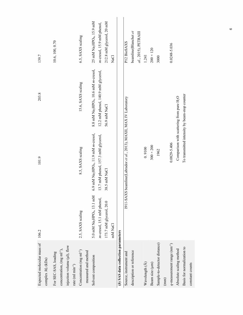
Exp

ecte

d m

olec

ular

mas

s of

com

plex

ME (

kDa)

106.

2 10

1.9

203.

8 13

9.7

For

SE

C-S

AS

, loa

ding

conc

entr

atio

n, (

mg

ml-1

),

inje

ctio

n vo

lum

e (μ

l), f

low

rate

(m

l min

-1)

10

.6, 1

00, 0

.70

Con

cent

rati

on (

mg

ml-1

)

mea

sure

d an

d m

etho

d

2.5,

SA

XS

sca

ling

8.

5, S

AX

S sc

alin

g 15

.6, S

AX

S s

calin

g 6.

5, S

AX

S sc

alin

g

Solv

ent c

ompo

sitio

n 5.

0 m

M N

a 2H

PO4,

13.

1 m

M

m-c

reso

l, 15

.1 m

M p

heno

l,

173.

7 m

M g

lyce

rol,

20.0

mM

NaC

l

6.9

mM

Na 2

HPO

4, 1

1.9

mM

m-c

reso

l,

13.7

mM

phe

nol,

157.

3 m

M g

lyce

rol,

38.5

mM

NaC

l

8.8

mM

Na 2

HP

O4,

10.

6 m

M m

-cre

sol,

12.2

mM

phe

nol,

140.

9 m

M g

lyce

rol,

56.9

mM

NaC

l

25 m

M N

a 2H

PO4,

15.

9 m

M

m-c

reso

l, 15

.9 m

M p

heno

l,

212.

8 m

M g

lyce

rol,

20 m

M

NaC

l

(b) S

AS

data

col

lect

ion

para

met

ers

Sour

ce, i

nstr

umen

t and

desc

ript

ion

or r

efer

ence

I911

-SA

XS

bea

mli

ne(L

abra

dor

et a

l., 2

013)

, MA

XII

, MA

X I

V L

abor

ator

y P1

2 B

ioSA

XS

beam

line

(Bla

nche

t et

al.,

2015

), P

ET

RA

III

Wav

elen

gth

(Å)

0. 9

100

1.24

1

Bea

m s

ize

(µm

) 30

0 ×

200

20

0 ×

120

Sam

ple-

to-d

etec

tor

dist

ance

)

(mm

)

1962

30

00

q-m

easu

rem

ent r

ange

(nm

-1)

0.08

29-5

.406

0.

0248

-5.0

36

Abs

olut

e sc

alin

g m

etho

d C

ompa

riso

n w

ith

scat

teri

ng f

rom

pur

e H

2O

Bas

is f

or n

orm

aliz

atio

n to

cons

tant

cou

nts

To

tran

smitt

ed in

tens

ity

by b

eam

-sto

p co

unte

r

6

Met

hod

for

mon

itori

ng

radi

atio

n da

mag

e

Fram

e-by

-fra

me

com

pari

son

Exp

osur

e ti

me

4

× 3

0 C

onti

nuou

s 1

s da

ta-f

ram

e

mea

sure

men

ts o

f S

EC

elut

ion

Sam

ple

conf

igur

atio

n

incl

udin

g pa

th le

ngth

and

flow

rat

e w

here

rel

evan

t

Flo

w c

ell,

effe

ctiv

e sa

mpl

e pa

th le

ngth

1.5

mm

. SE

C–S

AX

S w

ith

flow

cel

l,

effe

ctiv

e sa

mpl

e pa

th le

ngth

1.7

mm

Sam

ple

tem

pera

ture

(ºC

) 20

20

(c) S

oftw

are

empl

oyed

for

SAS

data

red

uctio

n, a

naly

sis a

nd in

terp

reta

tion

SAS

dat

a re

duct

ion

to

sam

ple–

solv

ent s

catt

erin

g,

and

extr

apol

atio

n, m

ergi

ng,

desm

eari

ng.

The

PyF

AI(

Kie

ffer

& W

righ

t, 20

13)

pack

age,

PR

IMU

Sqt(

Kon

arev

et a

l., 2

003)

and

CH

RO

MIX

S(Fr

anke

et a

l., 2

017)

fro

m A

TSA

S 2.

8.3(

Fra

nke

et

al.,

2017

)

Cal

cula

tion

of

ε fr

om

sequ

ence

Pro

tPar

am(G

aste

iger

et a

l., 2

005)

tool

fro

m E

xPaS

y(G

aste

iger

et a

l., 2

003)

Bas

ic a

naly

ses:

Gui

nier

,

P(r

), V

P

PR

IMU

Sqt(

Kon

arev

et a

l., 2

003)

fro

m A

TSA

S 2.

8.3(

Fran

ke e

t al.,

201

7)

Shap

e/be

ad m

odel

ling

DA

MM

IF(F

rank

e &

Sve

rgun

, 200

9), D

AM

MIN

(Sve

rgun

, 199

9), D

AM

AV

ER

(Vol

kov

& S

verg

un, 2

003)

and

DA

MC

LU

ST(P

etou

khov

et a

l., 2

012)

from

AT

SAS

2.8.

3(F

rank

e et

al.,

201

7)

Ato

mic

str

uctu

re m

odel

ling

SA

SRE

FC

V(P

etou

khov

& S

verg

un, 2

006,

200

5) a

nd C

RY

SOL

(Sve

rgun

et a

l., 1

995)

fro

m A

TSA

S 2.

8.3(

Fra

nke

et a

l., 2

017)

Mol

ecul

ar g

raph

ics

P

yMO

L (

vers

ion

1.8.

2.3,

Sch

rödi

nger

, LL

C)

(d) S

truc

tura

l par

amet

ers

D

etem

ir tr

i-he

xam

er 

1:6

com

plex

, FA

4 1:

6 co

mpl

ex, F

A7

2:

12 c

ompl

ex, P

1

2:12

com

plex

, P2

1:12

com

plex

G

uini

er A

naly

sis

7

I(0)

(cm

-1)

0.18

0.

63

0.63

2.

35

2.35

0.

66

Rg (Å

) 32

.6

35.4

35

.4

54.1

54

.1

38

q-ra

nge

(Å-1

) 0.

013-

0.03

8 0.

012-

0.03

7 0.

012-

0.03

7 0.

016-

0.02

4 0.

016-

0.02

4 0.

008-

0.03

4

Qua

lity 

94 %

96

%

96 %

80

%

80 %

98

%

M f

rom

I(0

) (r

atio

to

expe

cted

val

ue) 

100.

3 (0

.94)

10

2.1

(1.0

0)

102.

1 (1

.00)

20

8.3

(1.0

2)

208.

3 (1

.02)

13

8.5

(0.9

9)

 P(r)

ana

lysi

s

I(0)

(cm

-1)

0.18

0.

64

0.64

2.

38

2.38

0.

66

Rg (Å

) 33

.2

36.4

36

.4

56.9

56

.9

37.7

Dm

ax (Å

) 11

1.6

130.

3 13

0.3

195.

0 19

5.0

134.

0

q-ra

nge

(Å-1

) 0.

013-

0.24

5 0.

012-

0.22

6 0.

012-

0.22

6 0.

016-

0.14

7 0.

016-

0.14

7 0.

008-

0.21

3

Tot

al q

uali

ty e

stim

ate 

0.70

0.

67

0.67

0.

53

0.53

0.

81

M f

rom

I(0

) (r

atio

to

expe

cted

val

ue) 

100.

3 (0

.94)

10

3.7

(1.0

2)

103.

7 (1

.02)

21

1.0

(1.0

4)

211.

0 (1

.04)

13

8.5

(0.9

9)

P

orod

vol

ume,

VP (

nm3 )

13

7.20

16

2.34

16

2.34

30

9.45

30

9.45

17

9.50

R

atio

VP/c

alcu

late

d M

1.

37

1.57

1.

57

1.46

1.

46

1.30

(e) S

hape

mod

ellin

g re

sults

D

etem

ir tr

i-he

xam

er 

1:6

com

plex

, FA

4 1:

6 co

mpl

ex, F

A7

2:

12 c

ompl

ex, P

1

2:12

com

plex

, P2

1:12

com

plex

DAMMIF

(R

un in

inte

ract

ive

mod

e w

ith

dum

my

atom

rad

ius

2.7

Å, o

ther

wis

e de

faul

t par

amet

ers,

20

calc

ulat

ions

)

q-ra

nge

for

fitti

ng (

Å-1

) 0.

013-

0.24

5 0.

012-

0.22

5 0.

012-

0.22

5 0.

016-

0.14

7

0.00

8-0.

213

Shap

e co

mpa

ct

com

pact

co

mpa

ct

com

pact

Sym

met

ry, a

niso

trop

y

assu

mpt

ions

P1,

non

e P1

, non

e P

1, n

one

P1, n

one

P

1, n

one

8

NS

D (

stan

dard

dev

iatio

n),

No.

of

clus

ters

0.67

(0.

02),

3

0.68

(0.

02),

7

0.68

(0.

02),

7

0.9

5 (0

.11)

, 4

0.

71 (

0.04

), 4

2 ra

nge

0.78

5-0.

862

0.79

4-0.

924

0.79

4-0.

924

0.80

2-0.

874

1.

619-

1.70

1

Con

stan

t adj

ustm

ent t

o

inte

nsit

ies

- 1.

19

10-4

1.

19

10-4

-

3.

33

10-5

M e

stim

ate

(kD

a)

78.5

95

.7

95.7

19

9

105

Res

olut

ion

(fro

m S

ASR

ES)

(Å)

42 (

3)

39 (

3)

39 (

3)

53 (

4)

41

(3)

DAMMIN

(R

un in

exp

ert m

ode

wit

h de

faul

t par

amet

ers,

20

calc

ulat

ions

)

q-ra

nge

for

fitt

ing

0.01

6-0.

147

Init

ial s

earc

h vo

lum

e

el

lipso

id

Sym

met

ry, a

niso

trop

y

assu

mpt

ions

P2, p

rola

te

anis

omet

ry

(per

pend

icul

ar

sym

met

ry a

nd

anis

omet

ry a

xes)

NS

D (

stan

dard

dev

iatio

n),

No.

of

clus

ters

0.76

(0.

08),

4

2 ran

ge

0.86

4-0.

915

Con

stan

t adj

ustm

ent t

o

inte

nsit

ies

1.59

1

0-4

Res

olut

ion

(fro

m S

ASR

ES)

(Å)

55 (

4)

(f) A

tom

istic

mod

ellin

g  

Det

emir

tri-

hexa

mer

1:

6 co

mpl

ex, F

A4

1:6

com

plex

, FA

7

2:12

com

plex

, P1

2:

12 c

ompl

ex, P

2 1:

12 c

ompl

ex 9

SASREF

(de

faul

t par

amet

ers,

10

calc

ulat

ions

, dat

a sh

own

for

best

mod

el)

q-ra

nge

for

fitti

ng (

Å-1

) 0.

008-

0.4

15

0.00

8-0.

432

0.00

8-0.

432

0.00

8-0.

432

0.00

8-0.

432

0.00

5-0.

403

Sym

met

ry

P1

P1

P1

P1

P2

P1

2 va

lue

0.91

1.

68

0.93

0.

92

0.95

2.

62

Con

stan

t adj

ustm

ent t

o

inte

nsit

ies

8.87

1

0-5

3.77

1

0-5

4.31

1

0-5

6.11

1

0-5

6.62

1

0-5

8.77

1

0-5

CRYSOL

q-ra

nge

for

fitti

ng

0.00

8-0.

400

0.00

8-0.

400

0.00

8-0.

400

0.00

8-0.

400

0.00

8-0.

400

0.00

5-0.

400

No

cons

tant

sub

trac

tion

2 va

lue

1.16

1.

88

1.32

1.

07

1.21

2.

57

Pred

icte

d R

g (Å

) 33

.20

34.8

3 35

.35

56.3

0 56

.99

37.6

1

Vol

(Å

), R

a (Å

), D

ro (

e Å

-3)

1279

59, 1

.40,

0.0

30

1313

98, 1

.40,

0.0

20

1313

98, 1

.48,

0.0

20

2652

64, 1

.80,

0.0

25

2652

64, 1

.80,

0.0

25

1755

46, 1

.80,

0.0

18

Con

stan

t sub

trac

tion

allo

wed

2 va

lue

1.54

, 0.0

0 1.

88

1.30

1.

01

1.12

1.

74,

Pred

icte

d R

g (Å

) 33

.11

34.8

3 35

.35

56.3

8 57

.05

37.6

8

Vol

(Å

), R

a (Å

), D

ro (

e Å

-3)

1361

94, 1

.76,

0.0

22

1313

98, 1

.40,

0.0

20

1307

81, 1

.40,

0.0

20

2603

28, 1

.50,

0.0

28

2315

62, 1

.40,

0.0

25

1631

25, 1

.40,

0.0

22

(g) S

ASB

DB

IDs f

or d

ata

and

mod

els

D

etem

ir tr

i-he

xam

er

1:6

com

plex

, FA

4 1:

6 co

mpl

ex, F

A7

2:

12 c

ompl

ex, P

1

2:12

com

plex

, P2

1:12

com

plex

S

ASD

EV

5 SA

SD

EW

5 S

AS

DE

X5

SAS

DE

Y5

SA

SD

EZ

5 S

AS

DE

26

10

Figure S1 Structure of degludec R3T3-T3R3 di-hexamer with an inter-hexamer distance of 35.4 Å.

(a) Fit of the structure (purple) to experimental degludec data extrapolated to infinite dilution (grey).

The lower inset (b) shows error-weighted residual plots for the models. (c) The di-hexamer structure

(purple) is superimposed onto the low resolution ab-initio model (grey).

Figure S2 Scattering curves normalized for concentration of albumin-detemir mixed in a 1:6 ratio.

The total protein concentration range is between 1.9-20.8 mg/mL with darker shades corresponding to

higher concentrations. An increase in I(q)/C is observed corresponding to a concentration-dependent

equilibrium.

11

4

In silico studies on albumin-detemir complexes

The present chapter is divided into two parts. In Section 4.1, the effects of input parame-ters and setup when carrying out MM-PBSA free energy calculations are tested. The testsprovide valuable information for future setups of MM-PBSA free energy calculations forprotein-protein complexes and illustrate the sensitivity of the method.

The results of the tests are utilized in the manuscript that is presented in Section 4.2. Themanuscript has been submitted for publication, and builds upon the work presented inChapter 3, in which ambiguous models were obtained for the albumin-detemir hexamercomplex. The focus of the manuscript is to determine the most favorable detemir hex-amer binding site and zoom in on the albumin-detemir binding interactions.

The main result of the manuscript is that detemir binds to the FA4 binding site, whichis concluded based on results from MD simulations, MM-PBSA calculations, and DLScompetition experiments. Two lipidated detemir residues participate in the binding byforming salt bridges to basic albumin residues and by favorable vdW interactions. Apartfrom giving an insight into the specific interactions between albumin and a lipidatedinsulin analogue, the study illustrates how MD simulations can be used for expandingthe interpretation of SAXS data to an atomic level.

The scripts for carrying out the entropy calculations were developed by Tine M. Frederik-sen who is highly acknowledged. Two MD simulations, FA6a and FA7a, were initiatedduring my Master’s project.99

Scripts utilized in the calculations of polar solvation energy have been attached in Ap-pendix B with the hope that they can be useful for future students.

Supporting information is provided at the end of the chapter.

45

4.1 Tests of input parameters and setup of free energy calculations

To assess the effect of input parameters and setup of MM-PBSA calculations, tests ofdifferent parameters and setups were carried out prior to the calculations included inthe manuscript in Section 4.2. Unless otherwise mentioned, the tests are based on sin-gle frames extracted from an MD simulation of an albumin-hexamer complex using thesingle trajectory (1T) approach.

Conformational entropy

Sufficient sampling is a prerequisite for obtaining reliable entropy estimates by the quasi-harmonic approach,100,101 and convergence problems have been encountered in a numberof studies.76,100 The required number of simulation frames needed to obtain convergenceis correlated to the number of atoms included in the calculations.100 For the entropy cal-culations, the albumin-hexamer system was simplified by only including Cα atoms andC atoms of the lipidated lysine side chains.

The convergence of the entropy calculations was investigated by varying the number offrames, and the results are presented in Figure 4.1. The entropy of detemir convergedafter 2500 frames (Figure 4.1A), the entropy of albumin converged after 5000 frames(Figure 4.1B), and the entropy of the albumin-detemir complex converged after 10000frames (Figure 4.1C). The order of the convergence reflects the sizes of the systems withrespectively 414, 585, and 999 atoms. The relative entropy, ∆S is plotted in Figure 4.1D.Initially, ∆S increases and decreases reflecting the different rates of convergence. After10000 frames, ∆S has converged to the values 0.19 within 0.05 kcal/mol/K. Based onthis, it was decided to use 10000 frames for the entropy calculations presented in themanuscript in Section 4.2.

Polar solvation energy

Sørensen et al.90 have thoroughly tested several physical and numerical parameters forsolving the PB equation for three biological systems using three different PB solvers. Theyfound that the solutions were sensitive to a number of both physical and numerical pa-rameters, and recommended that proper testing should be carried out prior to settingup calculations. In the following, the sensitivity of the albumin-hexamer system to theparameters listed in Table 4.2 is reported. Based on these tests, a setup was chosen for thecalculations reported in the manuscript (Section 4.2). The test calculations were carriedout using the Adaptive Poisson-Boltzmann Solver (APBS).

Dielectric boundary, PB equation, and grid spacing

The choice of dielectric boundary between the protein and the solvent is important forcalculations of ∆Gpol. Two surface definitions are commonly employed for determiningthe dielectric interface: vdW surface and solvent excluded (SE) surface. The surface def-initions are illustrated in Figure 4.2. The vdW surface is calculated based on spheres forthe protein atoms with radii equal to their vdW radii. The SE surface corresponds to thesurface obtained by rolling a solvent probe over the vdW surface and taking the lower

46

Figure 4.1: Test calculations of conformational entropy for (A) the detemir hexamer, (B) albumin,and (C) the albumin-detemir hexamer complex. The entropies are shown as a function of numberof frames used in the calculations. (D) Conformational entropy difference between the albumin-detemir hexamer complex and the free proteins as a function of number of frames used in thecalculations.

Table 4.1: Overview over tested APBS input parameters for solving the Poisson–Boltzmann (PB)equation. SE and vdW refer to solvent excluded and vdW surface definitions, respectively.

Description Parameter Default option Tested options

Surface definition of dielec-tric boundary

SE SE, vdW

Form of the PB equation linear full, linearGrid spacing 0.5 0.2-1.5Factor by which to expandmolecular dimensions to getcoarse grid dimensions

cfac 1.7 1.1-2.3

Length (A) to add to molec-ular dimensions to get finegrid dimensions

fadd 20 10-30

Protein dielectric constant εin 2 1, 2, 6

47

envelope generated by rolling sphere. The solvent accessible (SA) surface is defined sim-ilarly, but by considering the center of the rolling sphere as shwon in Figure 4.2.90,102

Figure 4.2: Schematic illustration of three suface definitions: van der Waals surface (vdW; blue),solvent excluded surface (SE; green), and solvent accesible (SA; pink) surfaces. The overlappinglight green circles represent three atoms in a molecule represented by a circle with radii equal totheir vdW radii.

The two surface definitions are tested in combination with the full and the linear PBequations using grid spaces from 0.2-1.5 A. The results are shown in Figure 4.3. Thecalculated ∆Gpol is around 50 kcal/mol larger when the SE surface is employed comparedto the vdW surface independently on whether the full or linear PB equation is solved(Figure 4.3A). The more favorable ∆Gpol obtained using the vdW surface definition canbe explained by the closer proximity of solute charges and solvent, which gives rise tomore favorable interactions between the solute and the solvent. The SE surface is themost widely used choice for the dielectric boundary, as the vdW surface is criticized forleaving interstitial voids in the solute that are too small to be occupied by solvent.102

Figure 4.3: (A) ∆Gpol and (B) calculation time as functions of grid spacing. The calculations werecarried out on one frame using different surface definitions and forms of the PB equation. Thefollowing four combinations were tested: linear PB equation and SE surface definition (green),linear PB equation and vdW surface definition (blue), full PB equation and SE surface definition(orange), and full PB equation and vdW surface definition (violet).

48

The calculated ∆Gpol is around 50 kcal/mol larger when the linear PB equation is solvedcompared to the full PB equation. The simplified, linear PB equation thus seems to over-estimate ∆Gpol. Solving the linear PB equation is, however, approximately twice as fast assolving the full PB equation, as it can be seen in Figure 4.3B, where the computation timesfor calculating ∆Gpol for one frame are given. The calculation times increase dramaticallywith smaller grid spacings, which underline the importance of choosing an appropriategrid spacing that is exactly small enough to give converged values for ∆Gpol. Sørensenet al.90 recommend to always test the grid spacing for a system prior to calculations andgenerally recommend using at least 0.5 A irrespective of system size. For all four com-binations of parameters, ∆Gpol seems to converge at a grid spacing of 0.4 A. Sørensen etal.90 furthermore recommend to use the SE surface definition in combination with the fullPB equation. However, in the interest of time, we decided to use a SE surface in combi-nation with the linear PB equation and a grid spacing of 0.4 A. These settings were usedin the following section as well as in the manuscript.

Grid size

APBS solves the PB equation by mapping the protein onto a three-dimensional rectangu-lar grid. The calculations are initially carried out using a coarse grid, and then refinedusing a finer grid.103 An APBS input file with grid dimensions can be generated based ona structure using the inputgen.py script that is a part of the APBS distribution. Using thedefault settings, the coarse grid dimensions are calculated by expanding the dimensionsof a box enclosing the solute by a factor (cfac) set to 1.7, and the fine grid by adding a con-stant (fadd) of 20 A to the solute enclosing box dimensions. To test whether these settingsare sufficient for the albumin-hexamer system, convergence tests were carried out, andthe results are presented in Figure 4.4.

For the coarse grid, convergence of ∆Gpol is observed for cfac> 1.1 (Figure 4.4A). Witha larger grid, the calculation also requires longer computation time (Figure 4.4B). Uponconsideration of both computation time and convergence, the default setting of cfac= 1.7was chosen as an appropriate value for the calculations. For the fine grid, convergence of∆Gpol is observed for all tested values (Figure 4.4C). The computation time is, however,longer for fadd values above 20 A (Figure 4.4D), and the default setting of 20 A was chosenfor the calculations.

Grid dimensions and centering

The calculated Gpol of a solute is sensitive to the position of the solute in the grid, andits distance to the edges. Therefore, when calculating the difference between a proteincomplex and its individual constituents, ∆Gpol, it is important to use the same grid di-mensions and centering for all the calculations. In this way, errors cancel out and only thedifferences between the individual proteins and the protein complex are observed.90 Wecarried out calculations using grid dimensions and centering that was calculated for thealbumin-hexamer complex by the inputgen.py script for albumin, hexamer and albumin-hexamer complex calculations as illustrated in Figure 4.5A. Additionally, we carried outcalculations using individually calculated grids and centerings for albumin, hexamer,and albumin-hexamer complex as illustrated in Figure 4.5B. For all calculations, the set-tings used in the inputgen.py script were: cfac= 1.7 and fadd= 20A. The results are pre-

49

Figure 4.4: (A) ∆Gpol and (B) calculation time as functions of cfac. (C) ∆Gpol and (D) calculationtime as functions of fadd. ∆Gpol was obtained by solving the linear PB equation for one frameusing a 0.4 A grid spacing and the SE surface definition.

sented in Figure 4.5C where it is seen that the values of ∆Gpol calculated with the samegrid (green circles) are very similar at all grid spacings, whereas the values calculatedusing different grid dimensions (pink circles) are more randomly scattered.

Internal dielectric constant

The internal dielectric constant of the solute (εin) is a commonly user-modified parame-ters in MM-PBSA calculations.103 The underlying assumption in MM-PBSA calculationsis that the solute can be considered as a continuous phase. However, where the dielec-tric constant of water is straigthforward to determine from experiment, εin of a protein isfictitious and is not a universal constant that can be determined from experiment, as pro-teins are rarely uniform electrostatic media. The choice of value for εin is highly debatedand values in the range from 1 to 20 are commonly employed.90,103 It is generally rec-ommended to choose εin based on the characteristics of the studied system. Hou et al.82

investigated the effect of εin on MM-PBSA calculations on 98 protein-ligand complexes.The authors observed a better correlation between calculated and experimental bindingenergies for complexes with highly charged interfaces using εin = 4, while complexeswith hydrophobic interfaces obatined a better correlation when using εin = 1. Similarlybut using MM-GBSA, Chen et al.84 observed a better ability to rank binding poses of 43protein-protein complexes with highly charged interfaces using εin = 6, and a betterranking for more hydrophobic complexes with εin = 1.

50

Figure 4.5: Illustration of APBS calculation setup using (A) the same or (B) different grid dimen-sions (dim.) and centering (cent.) for the albumin-hexamer complex, albumin and hexamer calcu-lations. (C) ∆Gpol as a function of grid spacing. The calculations were carried out using a 0.4 Agrid spacing and the SE surface using either the same (green) or different (pink) box dimensionsand centering for both albumin, hexamer, and complex.

The MM-PBSA calculations presented in the manuscript in Section 4.2 were carried outusing εin values of 1, 2, and 6 for all the investigated protein complexes to assess thesensitivity of ∆Gbind. The εin parameter does not only affect the ∆Gpol energies, but also∆Eelec that is scaled by a factor 1

εinaccording to Coulomb’s law104 (fifth term in Equa-

tion 2.11). The results are presented in Table 4.2. For simplicity and to provide a betteroverview, only the results for the most favorable binding site, FA4, are presented. Thecalculations are carried out both using the single trajectory approach (1T) and the three-trajectory approach (3T). Generally, for both the 1T and 3T approaches, ∆Eelec becomesless favorable with a higher εin and ∆Gpol becomes more favorable. The sum of thetwo contributions corresponds to the total electrostatic interactions in the protein com-plex. The experimental ∆Gbind of the albumin-detemir complex has been estimated to-7.1105 and -3.8 kcal/mol.106 By considering the results obtained using the 1T approach,∆Gbind is highly overestimated to -754 and -313 kcal/mol using εin = 1 and 2, respec-tively. The overestimation of ∆Gbind results from an overestimation of electrostatic inter-actions. When employing εin = 6 and the 1T approach, ∆Eelec and ∆Gpol more or lesscancel out resulting in a net disfavorable electrostatic contribution of 45 ± 4 kcal/mol. Itis commonly observed in MM-PBSA that the terms almost cancel out. Gohlke et al.76 forinstance observed a total electrostatic contribution of 25 kcal/mol for a complex betweenhuman H-Ras and the Ras-binding domain of C-Raf1.

By using the 3T approach, ∆Gbind is calculated to −187 kcal/mol for εin = 1, which isoverestimated but much smaller than the−754 kcal/mol obtained using the 1T approach.For εin = 2 and the 3T approach, ∆Eelec and ∆Gpol are of comparable sizes giving a netelectrostatic contribution of 62± 27 kcal/mol and ∆Gbind of −31 kcal/mol. Using εin = 6,an unfavorable ∆Gbind of 84 kcal/mol is obtained, which could possibly indicate that theelectrostatic contribution of 177± 15 kcal/mol is unrealistically unfavorable.

51

From the above results, it is observed that the optimal εin depends on not only on theprotein-protein complex but also on whether the 1T or 3T approach is used. This is inline with the considerations of Genheden et al.107 that considered εin to be a compensa-tion factor for interactions that are neglected in MM-PBSA calculations and thus more amethod-dependent parameter than a physical constant. Thus not only the nature of thebinding interface but also the set up of the calculations, for instance whether entropy isincluded or not should be taken into account. If entropy terms are not included, a higherεin can be employed to bring the calculated binding energies within the range of experi-mental data.108 The most realistic result obatined using the 1T approach is obtained withthe highest εin value of 6. The higher value is in agreement with the fact that confor-mational entropy is neglected when using the 1T approach.73 Using the 3T approach, inwhich conformational entropy is included, the most realistic result is obtained with alower εin of 2. The results presented in the manuscript in Section 4.2 were based on the3T approach using εin = 2, as conformational changes were observed for albumin anddetemir upon binding, and the conformational entropy therefore was of importance.

Another reason for carrying out the MM-PBSA calculations using different εin valueswas to ensure that it did not affect the ranking of the four investigated complexes inves-tigated in the manuscript in Section 4.2. The combination of the 3T approach and εin = 6gave highly unfavorable binding energies for all complexes (data not shown), and wastherefore not considered. For the remaining calculations, the same ranking with FA4 asthe most favorable binding site was obtained independent of εin.

Table 4.2: MM-PBSA results using εin values of 1, 2, and 6 calculated by either the single-trajectory(1T) or three-trajectory (3T) approach. The results reported are for one of the duplicate simulationsof the albumin-hexamer complex where detemir binds in FA4, FA4b. The energies are reportedin kcal mol−1 and standard errors are given in parentheses. ∆Gbind is calculated as: ∆Gbind =∆Eelec + ∆EvdW + ∆Eint + ∆Gpol + ∆Gnp − T∆S. The individual terms are calculated asdescribed in the manuscript in Section 4.2. No standard error is given for ∆Gbind, as no standarderror was calculated for ∆S. The setup of the calculations that are presented in the manuscript aremarked in bold.

∆Eelec ∆Gpol ∆Eelec + ∆Gpol ∆Gbind

εin = 1

1T, FA4b -930 (6) 289 (6) -641 (8) -7543T, FA4b -415 (24) 321 (23) -94 (33) -187εin = 2

1T, FA4b -465 (3) 264 (5) -201 (6) -3133T, FA4b -208 (12) 270 (24) 62 (27) -31εin = 6

1T, FA4b -155 (1) 200 (3) 45 (4) -673T, FA4b -35 (4) 212 (14) 177 (15) 84

52

4.2 Manuscript 1: Investigations of albumin-detemir complexes usingmolecular dynamics simulations and free energy calculations

53

Investigations of albumin‐detemir complexes using molecular dy‐namics simulations and free energy calculations 

Line A. Ryberga*, Pernille Sønderbya, Jens T. Bukrinskib, Pernille Harrisa, and Günther H. J. Pe‐tersa* 

a Department of Chemistry, Technical University of Denmark, 2800 Kongens Lyngby, Denmark and b CMC assist ApS, 2500 Copenhagen, Denmark. 

Molecular dynamics, MM‐PBSA, free energy calculations, insulin detemir, albumin, protein complex, binding site 

 

ABSTRACT: Insulin detemir is a lipidated insulin analogue that obtains a half‐life extension by oligomerization and re‐versible binding to human albumin. In the present study, the complex between a detemir hexamer and albumin is investi‐gated by an integrative approach combining molecular dynamics (MD) simulations, molecular mechanics Poisson‐Boltz‐mann surface area (MM‐PBSA) free energy calculations and dynamic light scattering (DLS). Recent reported small angle X‐ray scattering data could not unambiguously resolve the exact binding site of detemir on albumin. We therefore applied MD simulations to deduce the binding site and key protein‐protein interactions. MD simulations were started from initial complex structures based on the SAXS models and free energies of binding were estimated from the simulations by using the MM‐PBSA approach for the different binding positions. The results suggest that the overlapping FA3‐FA4 binding site (named FA4) is the most favorable site with a calculated free energy of binding of ‐38±10 kcal/mol and a good fit to the reported SAXS data  throughout  the simulations. While multiple salt bridges are observed  in  the binding  interface,  the binding is driven by favorable vdW interactions. The binding to FA4 is further supported by DLS competition experiments with  the prototypical FA4  ligand,  ibuprofen, showing displacement of detemir by  ibuprofen. This study provides  infor‐mation on albumin‐detemir binding on a molecular level, which could be utilized in a rational design of future lipidated albumin‐binding peptides. 

INTRODUCTION 

Human serum albumin is the most abundant protein in the circulatory system with a blood plasma concentration of 35‐50 mg/mL and has a half‐life of 19 days in the body due to recycling by the neonatal Fc receptor.1 The biologi‐cal function of albumin is manifold, and albumin plays an important  role  in  the  regulation of  the colloidal osmotic pressure of  the blood and  in  the  transport of  long‐chain fatty acids, bilirubin2, metal  ions, and a great number of therapeutic drugs3–5. The pharmacokinetic properties of al‐bumin makes  it  interesting  in a pharmaceutical perspec‐tive as a platform for half‐life extension of biopharmaceu‐ticals.6 One of the major challenges for administering bio‐pharmaceuticals  and  especially  peptide‐based  drugs  is their limited half‐lives due to enzymatic degradation and clearance  in  the  body  by  renal  filtration.7  To  overcome these shortcomings, one successful route is the covalent or non‐covalent association to albumin, and hence, albumin has emerged as a versatile protein used in drug delivery of biopharmaceuticals. Lipidation  is a successful strategy  to obtain non‐covalent albumin association that utilize albu‐min’s natural affinity for fatty acids. Multiple products us‐ing  this  principle  are  available  on  the market,8,9  for  in‐stance  the  insulin analogues,  insulin detemir and  insulin 

degludec, and the glucagon‐like peptide 1 analogues, lirag‐lutide and semaglutide. Apart from leading to albumin as‐sociation, lipidation of the peptide‐based drugs also leads to self‐association, which additionally prolongs their half‐lives. Although the self‐association properties of the insu‐lin analogues10–16 and liraglutide17 are well studied, their as‐sociation  to  albumin  has  not  been  fully  explored  and hence,  a  molecular  understanding  of  the  complex  for‐mation has not been established. The focus of this study is on detemir’s association to albumin.  

While the albumin‐detemir binding has been the topic of other studies, there is yet no consensus on the correct binding site. Kurtzhals et al.18 studied the binding between albumin and detemir and found that long chain fatty acids (>12C) displace detemir to a higher extent than octanoate, suggesting that detemir binds to a fatty acid binding site with preference for longer fatty acids. Kjeldsen et al.19 stud‐ied the interactions between detemir and the individual al‐bumin domains I and III. The authors concluded that de‐temir binds to domain III and only weakly to domain I. Per‐forming spectrofluorophotometric studies in combination with molecular modelling, Fatima et al.20 proposed that de‐temir binds to albumin in‐between domain I and III. The binding stoichiometry between albumin and detemir was 

1

studied by Havelund et al. in 200421, and it was found that albumin binds to both dimeric and hexameric detemir.  

Recently,  small‐angle X‐ray  scattering  (SAXS)  solution structures of albumin‐detemir/degludec complexes in 1:6, 1:12,  and  2:12  (albumin:insulin  analogue)  stoichiometries were presented22.   Due to the  limited resolution of SAXS and the symmetric shape of albumin, an exact binding site for the two insulin analogues could not be identified.  

To close the gap and to gain a more detailed molecular understanding of the protein‐protein interactions, we ap‐ply molecular dynamics  (MD)  simulations on  complexes between albumin and a detemir hexamer. MD simulations and docking methodologies have been used previously to provide a molecular explanation of experimental results on albumin and insulin alone. With respect to insulin and its analogues,  studies  for  instance  focused on  the dimeriza‐tion  pathway  of  the  peptides,23,24  effect  of mutations  on protein  stability  and potency,25,26,27  interaction of  insulin analogues  with  excipients  at  different  physicochemical conditions,28,29 and the effect of water molecules and hy‐drogen bond network on peptide stability.30,31 The main fo‐cus of albumin studies is related to albumin’s capability to bind potential  therapeutic, small organic molecules,32,33,34 chemical additives,35 and natural products such as mono‐saccharides36 and flavonoids37 to determine binding poses of the ligands, binding free energy of the ligands and key interactions between albumin and  the  ligands. Albumin‐ligand and albumin‐ion interactions have also been stud‐ied  in different physicochemical conditions.  38,39 Possible conformational changes on binding of fatty acids to albu‐min have been observed through MD simulations, 40 high‐ and  low‐affinity  fatty acid binding sites on albumin have been identified based on binding free energy calculations and the pathway for the binding process of fatty acids to the highest affinity binding site has been reported.41 Fur‐thermore, studies have been performed to study the inter‐actions of albumin with other biomolecules such as Inter‐feron α‑1b42 and polyamidoamine dendrimers43 for drug de‐livery purposes and peptides to modulate protein‐protein interactions.44 Albumin  flexibility has been studied using principal  component  analysis of  the dynamics of  subdo‐mains revealing that conformational protein flexibility fa‐vorable precede ligand complexation and that ligand bind‐ing  can  induce  allosteric  effects  to other binding  sites.45 These studies emphasize the  important role of computa‐tional  tools  to  complement  experimental  studies  and  to provide the necessary molecular understanding. As men‐tioned above, our computational study  focusses on albu‐min‐detemir interactions. We used the molecular mechan‐ics Poisson‐Boltzmann surface area (MM‐PBSA) approach to  rank  different  binding  positions  and  in  combination with SAXS data to identify the most structurally and ener‐getic  favorable binding  site and key  residues  involved  in protein‐protein  interactions.   MM‐PBSA  is  an  attractive method,  since  it  is  computationally  less  expensive  than other more advanced types of free energy calculations such as  alchemical  transformations  and  potential  of  mean force46. MM‐PBSA has previously successfully been used to 

discriminate between high and low affinity fatty acid bind‐ing sites in albumin47, as well as ranking of native and non‐native poses of protein‐protein complexes48. Only a limited number of protein‐insulin studies have been reported49,50 and to the best of our knowledge, the present work is the first  systematic  computational  study  on  complexes  be‐tween  albumin  and  a  long‐acting  insulin  analogue.  The findings could be transferable to other lipidated peptides, and might enable a more rational design of lipidated albu‐min‐binding peptides in the future. 

MATERIALS AND METHODS 

Molecular dynamics simulations 

Construction of systems 

Initial  protein  coordinates  for  detemir  (PDB  entry: 1XDA51,  chain A‐D)  and  for  albumin  (PDB  entry:  1BJ552) were obtained from the Protein Data Bank (PDB). Albumin consists of three homologous domains that are asymmet‐rically assembled (Figure 1A). In the structure, seven com‐mon binding sites have been  identified  for medium‐ and long‐chain fatty acids: FA1‐FA753 (Figure 1B). Coordinates of the  fatty acid chains  in  1XDA (HETATM entries MYR) were combined with the coordinates of the acylated lysines (ATOM entries LYS) to common acylated lysine residues, hereafter referred to as Aly. PyMOL was used for building missing  residues,  and  applying  symmetry  operations  to form  the detemir hexamer. Albumin‐hexamer complexes were set up based on SAXS models. In total, four complexes were simulated in duplicate as shown in Figure 1C‐F. In ad‐dition, albumin and a hexamer were simulated in their un‐bound  forms.  In  the  following,  the  setup of and  settings used in the simulations will be described. 

Four  albumin‐hexamer  complexes with  binding  in  re‐spectively FA1, FA4, FA6, and FA7 were generated by man‐ual docking. The initial structures for the simulations are shown in Figure 1C‐F. As the binding sites FA3 and FA4 are overlapping (Figure 1A), they will be treated as one binding site and named FA4 throughout the article. The hexamer conformation used  in  the manual docking was extracted from the hexamer simulation after 5 ns, where one Aly fatty acid chain protrudes from the hexamer. This structure and the albumin crystal structure were placed relative to each other so that the protruding Aly pointed into the desired binding  site, while a good overlap with one of  the SAXS rigid body models in Figure 2 was ensured. All ligands orig‐inally present in the crystal structures were kept in the sim‐ulations  (Zn2+,  phenol,  and  myristates),  except  for  the myristates that would compete with detemir binding in the complexes. Thus, the FA1 bound myristate was deleted in the  FA1  simulations,  and  the  FA3  and  FA4  bound myristates  were  deleted  in  the  FA4  simulations.  No myristates were bound to FA6 or FA7 in the albumin crys‐tal structure used for the simulations. 

The CHARMM3654–56  all‐atom  force  field was used  for the simulation (including Zn2+ parameters57, and Na+ and Cl‐ parameters58). A topology entry for the acylated lysine 

2

 

Figure 1. (A) Albumin structure (PDB entry: 1E7G53) shown in a cartoon representation colored by domain: turquoise (domain I), purple (domain II), and light blue (domain III). (B) Albumin shown in a grey cartoon representation with myristates bound to FA1‐FA7 shown as vdW spheres. The myristates  in  the binding sites  investigated by simulation are colored  in magenta (FA1), orange (FA3 and FA4), green (FA6), and blue (FA7). Due to the overlap of FA3 and FA4, the two binding sites are considered as one and is for simplicity be named FA4 throughout the article. (C‐F) Structures of albumin‐hexamer complexes with binding in respectively FA1, FA4, FA7, and FA6. The hexamers are colored using the color coding of the myristates in (A).

residue was built based on the CHARMM36 topology en‐try for an acetylated lysine and is provided in the support‐ing information. MolProbity59,60 was used for determining protonation  states  of  titratable  residues  and  for  flipping sidechains  to optimize  the hydrogen bond network. The structures  were  prepared  for  simulation  by  the  VMD PSFgen Plugin and solvated in a box of TIP3P61 water mol‐ecules with  paddings  of  10‐15 Å  using  the VMD  Solvate Plugin version  1.6. Sodium  ions were added to neutralize the systems  (18  for detemir hexamer,  15  for albumin and one per myristate bound to albumin) and sodium and chlo‐ride ions were added to obtain an ionic strength of 0.025 M using the VMD Autoionize Plugin, version 1.3. 

Simulation setup 

The simulations were performed with NAMD62 version 2.12. The integration time step was set to 2 fs. Initially, the systems were minimized using a conjugate gradient algo‐rithm for 1500 steps for the complexes and 500 steps for the albumin and hexamer systems. The simulations were car‐ried out in an NPT ensemble at 310 K and 1 atm. The Lange‐vin method was  applied  for  temperature  control with  a damping  coefficient  of  1  ps‐1,  and  the  Langevin  piston method63 was applied for pressure control with a piston pe‐riod of 100 fs and a piston decay of 50 fs. The neighbor list was updated every 2 fs and set to a distance of 14 Å. The short‐range van der Waals (vdW) interactions were cut off at 12 Å in combination with a switching function starting at 10 Å. The long‐range electrostatics were calculated with 

the particle mesh Ewald method64,65 with a 1 Å grid spacing and  full  electrostatic  evaluation  every 4  fs. All hydrogen bonds were  kept  rigid  using  the  SHAKE  algorithm. The simulations of  the  complexes were  run  in duplicate  and each of them for 200 ns. The duplicates were initiated from the same minimized structure but using different seeds for the generation of the initial velocities. 

 

Trajectory analysis 

Root‐mean‐square deviation (RMSD) was calculated for each trajectory after alignment of the complex to domain II (Figure 1B) of albumin that was found to be the most sta‐ble throughout the simulations (data not shown). RMSDs are based on backbone atoms (C, O, N, CA) and were cal‐culated relative to the minimized structures. The fits to ex‐perimental SAXS  curves were  calculated  every  2 ns with CRYSOL66 using 500 points in the theoretical curve and fit‐

ting up to  0.4Å  with constant background sub‐traction. Based on the RMSDs and CRYSOL fits throughout the trajectories, it was evaluated that the systems were in equilibrium after 100 ns, and the equilibrium analyses de‐scribed in the following were thus carried out for the last 100 ns. 

Binding energy calculations 

The  binding  free  energy  of  a  protein‐protein  complex ∆ ) was calculated as the difference in free energy be‐tween the complex and the unbound proteins. 

3

∆  

The free energy of each state ( ) was estimated by the MM‐PBSA method: 

 

Where the three first terms are contributions to the gas‐phase energy ( ) and are respectively internal, electro‐

static and vdW energies of the solute.   and   are re‐

spectively polar and non‐polar solvation energies.   is tem‐perature, and   is the solute entropy.   was calculated 

by NAMD  Energy  Plugin,  version  1.4  in VMD  using  the same force field parameters as for the MD simulations.   

was  calculated  from  the  solvent  accessible  surface  area (SASA) by the relation:  . SASA was calcu‐

lated using VMD and a probe radius of 1.4 Å. A wide range of values have been suggested for the surface tension ( )67–71 dependent on surface area definition, origins of experi‐mental data and the system that the model is intended to be used  for.70 As we were  interested  in  including solvent entropy in our calculations, which is considered the major contribution to the non‐polar solvation energy at physio‐logical temperatures67,   was set to 47 kcal/mol/Å2 and   was set to 0 kcal/mol as derived by Sharp et al.67 These val‐ues  have  successfully  been  employed  for modelling  the solvation  entropy  for  16  protein‐protein  complexes  in  a study  by  Grünberg  et  al.72    was  calculated  using 

PDB2PQR73  in  combination  with  the  Adaptive  Poisson‐Boltzmann Solver  (APBS)  for  solving  the  linear Poisson‐Boltzmann equation. The optimal   to use for calculating 

 has been much debated and suggested to be system 

and method dependent.71,74,75 For the results presented in Table and Supplementary Table S1,   was set to 2. Addi‐tional calculations were carried out using  1 and 6 to investigate the effect on the electrostatic interactions ( ). Using  1, the electrostatic interactions were highly overestimated, while using  6 led to un‐derestimation  of  the  electrostatic  interactions  (data  not shown). The results with  2 gave reasonable estimates of the electrostatic interactions. As APBS calculations can be very sensitive with respect to grid spacing especially for larger biomolecules76, a test of different grid spacings was run prior to the actual calculations. For the present system, the optimal grid spacing was found to be 0.4 Å (data not shown). The gas phase and non‐polar  solvation energies were calculated every 10 ps of the last 100 ns of simulations thus amounting to 10000 frames. The polar solvation ener‐gies were, however, only calculated every 100 ps as the cal‐culations were very computationally demanding. Standard deviations of the gas‐phase and solvation energies were es‐timated by block averaging77.  

Configurational entropies were calculated by the quasi‐harmonic  approach.  Calculations  of  variance‐covariance matrices were carried out using  the ProDy Essential Dy‐namics Analysis software78. The systems were simplified so that only Cα and carbon atoms from the Aly residues were included. Convergence of the entropy calculations was ob‐served when  10000  frames were used  for  generating  the variance‐covariance matrices. All frames were thus used in the  calculations,  and  it  was  not  possible  to  calculate  a 

standard deviation. To assess the uncertainty of the calcu‐lated binding energies nevertheless, an average binding en‐ergy of duplicate simulations was calculated.  

The free energies of binding were calculated both by the single‐ and the three‐trajectory approaches. Using the sin‐gle‐trajectory approach, only one simulation of the protein complex is run from which the structures of the unbound proteins  are  extracted.  Using  the  three‐trajectory  ap‐proach, separate simulations of the unbound proteins are carried  out. The  single‐trajectory  approach has been  re‐ported to be advantageous for systems that do not undergo major  conformational  changes  upon  binding. Using  this approach, the intramolecular energies cancel out (∆0),  and more precise  and  less noisy  results  are obtained compared to the three‐trajectory approach. The three‐tra‐jectory  approach  should  in principle  give more  accurate binding energies as configurational changes are taken into account but is more computationally expensive.47,74,79,80 

Interface analysis 

Interactions in the albumin‐detemir interface were iden‐tified by counting albumin and detemir residues that were within 5 Å proximity of each other using an in‐house script. The structures were clustered based on contacts between albumin and detemir using the Fraction of Common Con‐tacts  Algorithm81  with  a  distance  cut‐off  of  5  Å  and  a threshold of 0.75.  

Dynamic light scattering 

Dynamic  light  scattering  (DLS)  titration  experiments were carried out for albumin‐detemir mixtures in a 1:6 mo‐lar albumin:detemir  ratio.  Insulin detemir  (detemir) was obtained from Levemir® (Novo Nordisk A/S) and dialyzed into a buffer containing 5 mM Na2HPO4, 15 mM phenol, 13 mM m‐cresol, 173 mM glycerol, and 20 mM NaCl and ad‐justed with HCl to pH 7.4. Recombinant human serum al‐bumin was obtained from Recombumin® Elite (Albumedix Ltd) and dialyzed into a buffer containing 25 mM NaH2PO4 and 215 mM NaCl and adjusted with HCl  to pH 6.5. The proteins were mixed in a 1:6 ratio to a total protein concen‐tration of 3.8 mg/mL and diluted with detemir’s dialysis buffer. The mixtures were  equilibrated  for  two hours  at room temperature without stirring. Ibuprofen sodium salt was thereafter added in stoichiometric amounts from 1‐25, and the samples were further equilibrated for three hours. After ligand addition, the final protein concentration was 3.2 mg/mL and  the  final buffer  compositions was 6 mM Na2HPO4,  14 mM m‐cresol,  13 mM phenol,  166 mM glyc‐erol, 28 mM NaCl at pH 7.4. 

The samples were measured in triplicate on a DynaPro DLS plate  reader  (Wyatt Technology Corporation,  Santa Barbara, CA). Wyatt Dynamics software was used for data collection and analysis. The samples were loaded onto 96 well non‐binding Corning® microplates and centrifuged for 2 min at 2000 rpm at room temperature to remove air bub‐bles. The sample volume was 100 µL, the temperature was 298 K, and each sample was measured  ten  times  for  five seconds. Z‐averages obtained by cumulants analysis are re‐ported in the results section as radius of hydration (Rh) and have been corrected for viscosity and refractive index. 

4

 

 

Figure 2. Rigid body modelling of the albumin‐detemir hexamer complex gives models with binding at the domain  interfaces, domain I/III, domain II/III, and domain I/II. The fits of the models to the experimental data (grey) are shown in respectively red, blue, and orange. The lower inset shows error‐weighted residual plots for the model fits. The models are shown with albumin in grey, and the hexamers with same color‐coding as in the plots.

Small‐angle X‐ray scattering 

The SAXS data used in this work and the ab‐initio model presented in Figure 2 was previously presented.22 The ex‐periments were performed at the I911‐SAXS beamline82 at the MAX IV Laboratory (Lund, Sweden). The experimental details can be found in Table 1 and Table 2 as well as the Materials  and  methods  section  in  Ryberg  et  al.  2019.22 SASREFCV83,84(SASREF) was used for rigid body modelling with standard settings for X‐ray data and based on data up to q = 0.43 Å‐1. The input structures were the same albumin and detemir hexamer structures that were used for setting up the simulations. 

PyMOL (version 1.8.2.3, Schrödinger, LLC) and MATLAB (version 9.1, The MathWorks, Inc., Natick, MA) were used for preparing all figures and plots presented in the article. 

RESULTS 

SAXS modelling 

In a previous SAXS study on complexes between albu‐min and respectively detemir and degludec, albumin‐hex‐

amer,  albumin‐di‐hexamer,  and  albumin‐di‐hexamer‐al‐bumin were modelled by ab‐initio and rigid body model‐ling.22 Due to the low resolution of SAXS and the symmet‐ric shape of albumin,  the albumin‐hexamer models were not conclusive with respect to the binding site of the de‐temir hexamer.22 In the current study, we utilize MD sim‐ulations  in  combination with MM‐PBSA  calculations  to qualify which of the binding site is the most probable site.  

Rigid  body modelling was  first  carried  out  to  identify possible binding sites using SASREF. 22 models of the al‐bumin‐hexamer  complex  were  generated  and  clustered based on binding position on albumin. One model binds between domain  I and domain  III,  four models bind be‐tween domain II and domain III, and  17 models bind be‐tween domain I and domain II. The best fitting model of each cluster  is presented  in Figure 2 with fits to the data and   value of the fits. 

The domain I/II model has the best fit to the data with 1.31, but  it does not differ very much  from  the do‐

main  II/III  model  with  1.96  as  conformational changes of albumin and detemir could be expected upon binding and are not taken into account in the modelling. 

5

The domain I/III model has a slightly worse fit to the data with  3.32.  The fact that multiple binding positions fit the data is not surprising, as albumin has an almost sym‐metrical triangular shape, which makes it difficult to dis‐tinguish between the three sides with SAXS data alone. To obtain knowledge on the albumin‐detemir hexamer com‐plex on a molecular level, we carried out MD simulations, and the results are described below. 

MD simulations 

SAXS modelling suggests that detemir can bind at three domain interfaces. As the fatty acids octanoic, dodecanoic, and  hexadecanoic  acids85  have  been  shown  to  compete with detemir binding  to albumin,  it  is assumed  that de‐temir binds in or near a fatty acid binding site. By studying the proximity of  the binding sites and  the domain  inter‐faces,  FA1,  FA4,  FA6,  and  FA7 were  considered  possible binding  sites  for detemir. The  complexes were manually docked as described in the Materials and methods section. 

Trajectory analysis 

To  evaluate whether  the  simulations  have  converged, RMSD and  values for their fit to the experimental SAXS curve were evaluated. The RMSD evolutions are presented in Figure 3. Apart from FA6a, the simulations reach a plat‐eau after 100 ns where the RMSD fluctuate around a con‐stant  value.  The  duplicates  were  started  with  different seeds for initial velocities to assess the statistical uncertain‐ties of the simulations. The RMSD evolutions of the FA4 simulations overlap the last 90 ns, whereas the evolutions of the other duplicates are very different. In Supplementary Figure S1, it is shown that the hexamer contributes more to the RMSD than albumin for all simulations. The larger hex‐amer RMSD is likely due to translation and rotation of the hexamer to accommodate binding to albumin. 

The   fits to the experimental SAXS data are presented in Figure 4. The FA4a, FA4b, and FA7a simulations have the best fits to the experimental data with average   val‐ues  based  on  the  last  100  ns  of  simulations  of  2.8±0.2, 2.0±0.3,  and  2.0±0.5,  respectively.  The  FA6  simulations have slightly worse fits to the data and larger fluctuations (average   values of 3±1). The FA1a, FA1b, and FA7b do not fit  the data with average   values of 9±4, 6±1, and  13±3, respectively. 

For the FA1a simulation, the large fluctuations in   co‐incide with large fluctuations in RMSD, whereas the fluc‐tuations are not captured in the RMSD plot for the FA7b simulation.  Instead,  it  seems  to  be  a  consequence  of  a structural change after 20 ns of simulation. Furthermore, the FA7b complex has a  larger Rg (Supplementary Figure S2)  and  center‐of‐mass  distance  (Supplementary  Figure S3) throughout the 200 ns compared to its duplicate FA7a, which could  indicate complex dissociation  if  the  simula‐tion had been run longer. 

Based on  the overall structural properties, RMSDs and fits to the SAXS data, the ranking of the binding site is FA4 > FA6 > FA7 > FA1. In the following, we zoom‐in to the in‐terfacial binding surface, to determine the binding free en‐ergies and to map interfacial key interactions.  

Figure  3. RMSD of  complexes  relative  to  the  corresponding minimized  structures.  Prior  to  the  RMSD  calculations,  the complexes were aligned to albumin’s domain II of the corre‐sponding minimized complex structure. 

 

Figure 4. SAXS  fits of  the complexes calculated by CRYSOL throughout the trajectory. 

Binding energy calculations 

The main objective of the free energy calculations is to obtain  a  ranking  of  the  four  possible  binding  sites. The MM‐PBSA method was employed to estimate the binding energies of the complexes. Constant values for individual MM‐PBSA energy contributions were reached after 100 ns (Supplementary Figures S4 and S5). The  free energies of binding were estimated by the single‐ and three‐trajectory approaches and are presented  in Supplementary Table S1 and Table,  respectively. Both approaches agree  that FA4 has the most  favorable  free energy  followed by FA1, FA7, and  FA6.  The  average  free  energies  of  binding  for  FA4 amount to ‐307 ± 9 kcal/mol and ‐38 ± 10 kcal/mol for re‐spectively  the  single‐ and  three‐trajectory approach. The binding energy has been determined experimentally to ‐3.8 kcal/mol20 and ‐7.1 kcal/mol85. While both 

6

Table 1. Contributions to the free energy of binding of the albumin‐hexamer calculated from frames extracted from the simulations by the three trajectory approach with  . The energies are given in kcal/mol, and stand‐ard deviations are calculated by block averaging. 

∆ ∆ ∆ ∆ ∆ a ∆ ∆ ∆ a ∆ b ∆ c

FA1a 190 11 ‐92 2 15 2 10 17 ‐80 12 ‐116 N/A 200 21 37 160

162 3 b 138 10 ‐43 3 6 3 69 15 ‐73 13 ‐68 N/A 207 18 ‐5 165

FA4a ‐255 11 ‐97 3 22 3 292 21 ‐142 9 ‐135 N/A 37 24 ‐7 ‐45

‐38 10 b ‐208 12 ‐79 2 ‐3 2 270 24 ‐128 9 ‐117 N/A 62 27 ‐11 ‐31

FA6a 587 13 ‐46 2 7 2 ‐45 26 ‐65 10 ‐112 N/A 543 29 47 550

475 106 b 433 11 ‐36 3 ‐12 3 ‐25 17 ‐52 11 ‐91 N/A 408 20 39 400

FA7a 350 9 ‐29 3 ‐11 2 52 16 ‐58 14 ‐113 N/A 401 18 55 417

359 82 b 329 14 ‐43 3 10 2 6 24 ‐56 12 ‐54 N/A 336 28 ‐2 302

a ∆  is calculated for all 10000 frames with sampling every 10 ps, and no standard error of mean is thus calculated. 

b ∆ ∆ ∆ ∆ ∆ ∆ ∆  a       c ∆  is the average ∆  for duplicate simulations with standard deviations given in parentheses. 

approaches give  energies  that  are  far  from  the  experi‐mental results, the energies calculated by the three‐trajec‐tory approach are closest to the experimental values. The results obtained using  the  three‐trajectory approach will thus be evaluated further in the following. 

The FA4 binding site represents the only favorable bind‐ing site with an average free energy of binding of ‐38 ± 10 kcal/mol. In comparison, the binding energies of FA1 (162 ± 3 kcal/mol), FA7 (359 ± 82 kcal/mol) and FA6 (475 ± 106 kcal/mol) are all unfavorable. Though both albumin and detemir  carry  overall  negative  charges,  favorable  ∆  contributions are observed in the FA4a (‐255 ± 11 kcal/mol) and FA4b simulations (‐208 ± 12 kcal/mol). The favorable ∆  are opposed by unfavorable ∆  contributions of 

292 ± 21 kcal/mol and 270 ± 24 kcal/mol, respectively, sum‐ming up to an overall disfavorable electrostatic contribu‐tions to the binding (37 ± 23 kcal/mol and 62 ± 26 kcal/mol, respectively).  In agreement with our observations, ∆  and ∆  are often found to partly cancel out71,80, as more 

charged residues in the protein‐protein interface are bur‐ied.  The  desolvation  of  charged  residues  consequently leads  to a  less  favorable polar solvation energy contribu‐tion. 

By  assuming  that  the  non‐polar  solvation  energy  is largely entropic,  the  total entropic effect of complex  for‐mation can be estimated as:  ∆ ∆S giving contribu‐tions of ‐7 and ‐11 kcal/mol for respectively the FA4a and FA4b simulations, thus a favorable contribution. In this es‐timate, the translational and rotational entropies are not included. As  the  terms  are  size  dependent,  they  should contribute equally for all complexes, and should not affect the ranking of the complexes. In our results, the favorable non‐polar solvation energy is almost compensated by the unfavorable  configurational  entropy,  as  it has previously been observed for protein‐protein complexes.86  

The ranking of FA4 as the most favorable detemir bind‐ing site is also reflected in the average ∆  for FA4 that is more negative compared  to  the other systems. With a total unfavorable contribution to binding from ∆  and 

∆   and  a  slightly  favorable  total  contribution  from 

∆ ∆S, the favorable∆  represents an  important 

contribution to the binding. As we show in the following, this  stems  from  favorable vdW  interactions between de‐temir’s fatty acid chain and residues in the fatty acid bind‐ing site of albumin. 

Interface analysis 

In order to get an overview of the interface residues in the complexes, we have plotted the albumin‐detemir resi‐due pairs that are in 5 Å proximity for at least 30 % of the analyzed  100 ns  in an  interaction heatmap. The heatmap for  the FA4b  simulation  is  shown  in Figure  5A,  and  the heatmaps  for  the  remaining  simulations  are provided  in Supplementary Figure S6‐S12. As natural insulin does not bind to albumin, it is expected that the fatty acid residues (Aly) must be involved in the binding. Three Alys are facing the binding interface in the complexes, namely Aly in chain D, H,  and L  (AlyD29, AlyH29,  and AlyL29). For  a  schematic overview of the chain naming in the detemir hexamer, see Figure 5C. From the heatmaps, it is seen that the Aly resi‐dues have more interactions with albumin in the FA4 sim‐ulations compared  to  the other  simulations. This  is  sum marized in Table 2 where the number of Aly‐albumin prox‐imities are listed. The FA4 complexes form 39 and 32 Aly‐albumin contacts, which can be  linked to their  favorable vdW energies (Table  1). The potential dissociation of the FA1a and FA7b complexes can be linked to the complexes having the fewest Aly‐albumin contacts accounting to re‐spectively 7 and 8. For the FA4 simulations, both AlyD29 and AlyH29 (marked with arrows in Figure 5A and Supplemen‐tary Figure S8A) are  in proximity with multiple albumin residues.  

Clustering based on common albumin‐detemir contacts was carried out to obtain representative structures for the complexes. The representative FA4a and FA4b structures are shown in Figure 5B and Supplementary Figure S8B, re‐spectively  with  the  residues  colored  according  to  their maximum  interaction  values  in  the heatmap.  In  the  fig‐ures, AlyD29 and AlyH29 are marked with light pink and

7

 

Figure 5. Analysis of interactions in the FA4b simulation. (A) Interaction heatmap of the albumin‐detemir interface with albumin residues on the y‐axis, and detemir residues on the x‐axis. The color scale goes  from blue  indicating that the residues are not within 5 Å of each other throughout the simulation to yellow that indicates that the residues are within 5 Å of each other in all simulation frames. The arrows in light pink and orange mark the fatty acid residues present in the binding interface, AlyD29 and AlyH29, respectively. (B) The representative structure of the FA4b complex shown as cartoon with Aly residues shown as vdW spheres. The residues are colored according to their maximum interaction values from the heatmap in (A). The Alys located at the interface are marked with rectangles. (C) Schematic overview over chain IDs in a detemir hexamer. Each monomer consists of two chains: chain A shown in grey and chain B shown in light blue. 

orange boxes,  respectively. A zoom  in on  the AlyD29 and AlyH29 binding sites are shown in Figure 6A and B for the FA4b simulation, and in Supplementary Figure S13A and B for  the FA4a  simulation.  In both  simulations, AlyD29pro‐trudes into the hydrophobic cleft of the FA4 binding site, and AlyH29 is positioned in the albumin‐detemir interface. In  both  simulations,  salt  bridges  are  observed  between GluC4‐Lys414  (notation:  detemir  residue‐albumin  residue), 

GluC4‐Arg410,  AlyD29‐Arg410,  AlyH29‐Lys372  and  hydrogen bonds are observed between PheD1‐ Glu393 and GlnD4‐Gln390, indicating that these are key interactions in the albumin‐detemir hexamer complex. Additionally, GlnD4‐Glu393 and CysC7‐Asn386  interactions  are observed  in  the FA4a  com‐plex, and GluB21‐Lys541, GlyC1‐Glu492 and GluG4‐Lys378 are pre‐sent in the FA4b complex. 

8

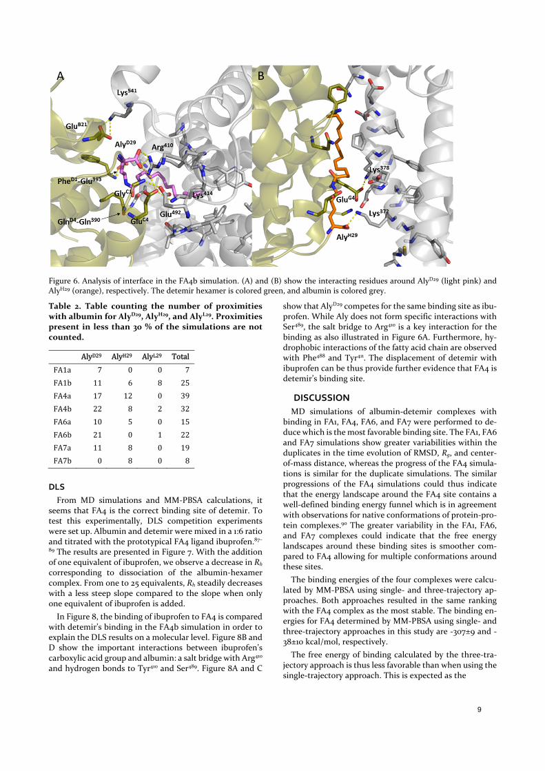
Figure 6. Analysis of interface in the FA4b simulation. (A) and (B) show the interacting residues around AlyD29 (light pink) and AlyH29 (orange), respectively. The detemir hexamer is colored green, and albumin is colored grey. 

Table  2.  Table  counting  the  number  of  proximities with albumin for AlyD29, AlyH29, and AlyL29. Proximities present  in  less than 30 % of the simulations are not counted. 

AlyD29 AlyH29 AlyL29 Total

FA1a 7 0 0 7

FA1b 11 6 8 25

FA4a 17 12 0 39

FA4b 22 8 2 32

FA6a 10 5 0 15

FA6b 21 0 1 22

FA7a 11 8 0 19

FA7b 0 8 0 8

 

DLS 

From MD  simulations  and MM‐PBSA  calculations,  it seems that FA4  is the correct binding site of detemir. To test  this  experimentally,  DLS  competition  experiments were set up. Albumin and detemir were mixed in a 1:6 ratio and titrated with the prototypical FA4 ligand ibuprofen.87–89 The results are presented in Figure 7. With the addition of one equivalent of ibuprofen, we observe a decrease in Rh corresponding  to  dissociation  of  the  albumin‐hexamer complex. From one to 25 equivalents, Rh steadily decreases with a  less steep slope compared to the slope when only one equivalent of ibuprofen is added. 

In Figure 8, the binding of ibuprofen to FA4 is compared with detemir’s binding in the FA4b simulation in order to explain the DLS results on a molecular level. Figure 8B and D  show  the  important  interactions  between  ibuprofen’s carboxylic acid group and albumin: a salt bridge with Arg410 and hydrogen bonds to Tyr410 and Ser489. Figure 8A and C 

show that AlyD29 competes for the same binding site as ibu‐profen. While Aly does not form specific interactions with Ser489, the salt bridge to Arg410 is a key interaction for the binding as also illustrated in Figure 6A. Furthermore, hy‐drophobic interactions of the fatty acid chain are observed with Phe488 and Tyr411. The displacement of detemir with ibuprofen can be thus provide further evidence that FA4 is detemir’s binding site. 

DISCUSSION 

MD  simulations  of  albumin‐detemir  complexes  with binding in FA1, FA4, FA6, and FA7 were performed to de‐duce which is the most favorable binding site. The FA1, FA6 and FA7 simulations show greater variabilities within the duplicates in the time evolution of RMSD, Rg, and center‐of‐mass distance, whereas the progress of the FA4 simula‐tions  is similar  for the duplicate simulations. The similar progressions  of  the  FA4  simulations  could  thus  indicate that the energy landscape around the FA4 site contains a well‐defined binding energy funnel which is in agreement with observations for native conformations of protein‐pro‐tein complexes.90 The greater variability  in  the FA1, FA6, and  FA7  complexes  could  indicate  that  the  free  energy landscapes  around  these binding  sites  is  smoother  com‐pared to FA4 allowing for multiple conformations around these sites.  

The binding energies of the four complexes were calcu‐lated by MM‐PBSA using single‐ and three‐trajectory ap‐proaches. Both approaches  resulted  in  the  same  ranking with the FA4 complex as the most stable. The binding en‐ergies for FA4 determined by MM‐PBSA using single‐ and three‐trajectory approaches in this study are ‐307±9 and ‐38±10 kcal/mol, respectively. 

The  free energy of binding calculated by the three‐tra‐jectory approach is thus less favorable than when using the single‐trajectory approach. This is expected as the 

9

 

Figure 7. DLS competition experiment where the albumin‐de‐temir complex is titrated with ibuprofen. With the addition of one ibuprofen equivalent (per albumin‐hexamer complex), a significant decrease in Rh is observed indicating that the com‐plex dissociates to a mixture of albumin and detemir. 

Figure  8.  The  binding  poses  of Aly D29  (orange)  from  the FA4b  simulation  (A)  and  (C)  and  ibuprofen  (PDB  entry: 2BXG5, light blue) (B) and (D) are compared. (C) and (D) are rotated 60° relative to (A) and (B). The structures have been aligned on the five alpha helices surrounding ibuprofen. The residues  responsible  for  ibuprofen  binding  are  shown  as sticks. 

unbound conformations are  sampled  in  the  three‐trajec‐tory approach which are not accessible with the single‐tra‐jectory approach  that  simply  samples  the bound  confor‐mations. The lower binding affinity thus reflects the pen‐alty for conformational changes from the unbound to the bound conformations.80 This result is in agreement with al‐bumin’s previously reported flexibility and conformational changes  upon  fatty  acid  binding.52,91  Furthermore,  some flexibility could be expected from the Aly residues of de‐temir. 

Experimentally, the free energies of binding between al‐bumin and detemir have been reported. Kurtzhals et al.85 

estimated  the binding energy  to  ‐7.1 kcal/mol with  favo‐rable enthalpic and entropic contributions of ‐4.6 kcal/mol and 2.4 kcal/mol, respectively. Fatima et al.20 estimated the binding energy  to  ‐3.8 kcal/mol with an unfavorable en‐thalpic contribution of 79.3 kcal/mol and a  favorable en‐tropic contribution of 83.2 kcal/mol. The quite large devi‐ation between the binding energies could reflect the differ‐ent  experimental  conditions.  The  three‐trajectory  ap‐proach predicts a binding energy within one order of mag‐nitude of  the experimental  results and  suggests  that  the binding is favored by enthalpic (‐29±13 kcal/mol) and en‐

tropic contributions (‐9±3 kcal/mol) which is in agreement with the results of Kurtzhals et al.85 Even though overesti‐mation of binding  energies  is  commonly observed using MM‐PBSA,71,74,80,92  the method has  successfully been em‐ployed for ranking of peptide‐protein and protein‐protein complexes,48,92,93 which puts confidence into the ranking of the albumin‐detemir complexes.  

To test whether FA4 could be the correct binding site, DLS competition experiments were set up with ibuprofen. While ibuprofen is proposed to have multiple binding sites on albumin, there is a consensus that FA4  is the primary ibuprofen binding site with a ~10‐100 times higher affinity than for the secondary  ibuprofen binding site FA6.94 The primary  association  constants  of  ibuprofen  and  detemir have been determined under the same experimental con‐ditions to be 2.7 ∙ 10  M‐1 and 2.4 ∙ 10  M‐1, respectively.18 The addition of one ibuprofen equivalent can thus be ex‐pected to compete with detemir binding. With respect to possible  allosteric  effects,  crystal  structures  of  albumin with and without ibuprofen are compared. The backbone RMSD of the structures (PDB entries: 1AO695 and 2BXG5) is 0.7 Å, suggesting that ibuprofen binding to FA4 does not induce  conformational  changes  in  albumin.  This  is  in agreement with previous studies showing ibuprofen bind‐ing to FA4 may not be allosterically linked to the FA1 bind‐ing site.96,97 In the DLS experiment, the addition of one ibu‐profen equivalent leads to a decrease in Rh indicating com‐plex  dissociation.  For  the  above‐mentioned  reasons,  the decrease  in Rh  can  be  considered  an  effect  of  ibuprofen binding  to FA4, which  thus  confirms FA4 as  the  correct binding  site.  This  is  in  agreement  with  the  findings  of Kjeldsen et al.19 that detemir binds to albumin’s domain III in which FA4 is embedded. 

In a competition study conducted by Kurtzhals et al.18, the authors found that detemir could be displaced from al‐bumin  when  more  than  one  ibuprofen  equivalent  was added. They furthermore found that the other FA4 ligand diazepam could not displace detemir, and therefore sug‐gested that FA4 may not be the correct binding site. How‐ever, a complex structure between albumin and diazepam published  in 2005 (PDB entry: 2BXF5) reveals  that diaze‐pam binds more deeply into the FA4 binding site than ibu‐profen does, and therefore does not compete with detemir Aly binding (Supplementary Figure S14). A different bind‐ing site has been suggested by Fatima et al.20 who based on docking proposed that chain B of detemir binds near FA1. The  result  is  not  directly  comparable with  ours,  as  the binding of a hexamer can be expected to differ significantly 

A B

C D

10

from the binding of only chain B of a detemir monomer. In particular,  we  observe  that  not  only  hydrophobic  Aly (chain B) interactions contributes to the binding but also salt bridges formed between residues in chain A and chain B with albumin are important for binding (Figure 6). The importance of salt bridges between basic albumin residues and detemir was previously suggested by Kurtzhals et al.85, who observed that deletion of insulin ThrB30 resulted in a stronger albumin binding suggesting that positioning the C‐terminal on position  29 was  favorable. They proposed that this is due to a favorable interaction between the C‐terminal carboxylate and a basic albumin residue. Indeed, in both FA4a and FA4b, strong  interactions are observed between  one  C‐terminal  carboxylate  (AlyD29)  and  Arg410 (Figure  6A)  and  another C‐terminal  carboxylate  (AlyH29) with Lys372 (Figure 6B). 

CONCLUSION 

In this work, we studied a complex between a detemir hexamer and albumin using MD simulations in combina‐tion with MM‐PBSA free energy calculations and DLS com‐petition  studies.  The  simulations were  set  up  based  on SAXS results22 suggesting that detemir can bind to albumin close to the albumin fatty acid binding sites, FA1, FA6, FA7, or  the  overlapping  binding  sites  FA3‐FA4  (named  FA4). The simulations were performed in duplicate to assess the statistical uncertainties and each was run for 200 ns. The RMSD progressions for the FA4 simulations were very sim‐ilar in comparison to the other simulations reflecting that this the most stable complex. The FA4 simulations further‐more had the best fits to the experimental SAXS data with an average   of 2.4±0.4, and the lowest binding free ener‐gies with an average of ‐38±10 kcal/mol. 

Several key interactions were identified between detemir and albumin: GluC4‐Lys414 (notation: detemir residue‐albu‐min  residue),  GluC4‐Arg410,  AlyD29‐Arg410,  AlyH29‐Lys372, PheD1‐Glu393 and GlnD4‐Gln390. Besides the specific interac‐tions,  we  also  monitored  hydrophobic  interactions  be‐tween the fatty acid residue (Aly) and albumin. The hydro‐phobic interactions stemming from the Aly residues were found to be an important contribution to the free energy of binding as quantified by MM‐PBSA analysis. The bind‐ing of detemir to FA4 was confirmed by a DLS competition experiment in which albumin‐detemir complexes were ti‐trated with  the FA4  ligand,  ibuprofen. Upon addition of one  ibuprofen equivalent, a decrease  in Rh was observed indicating  that detemir was displaced by direct competi‐tion. 

Thus based on structural and energetic analyses of MD simulations,  competition  experiments  and  comparison with the detailed studies by Kurtzhals et al.18,85, we propose that FA4 is the most probable binding site for detemir. The results give a molecular insight into the binding of a lipi‐dated peptide to albumin that could be exploited in the de‐sign of future drugs. 

ASSOCIATED CONTENT  

Supporting information:  

Additional RMSD plots based on albumin and  the hexamer structures; time evolutions of Rg, center‐of‐mass, electrostatic and vdW binding energies; Interaction heat maps; Clustered structures  of  the  simulated  complexes;  Figure  of  the  FA4a binding  interface; Comparison of  the FA4b detemir binding pose with the diazepam binding pose; single‐trajectory MM‐PBSA results; CHARMM36 topology entry for the Aly residue.  This material  is  available  free  of  charge  via  the  Internet  at http://pubs.acs.org. 

AUTHOR INFORMATION 

Corresponding Author 

* linear@kemi.dtu.dk * ghp@kemi.dtu.dk 

Author Contributions 

All authors have given approval to the final version of the manuscript. 

Funding Sources 

We would like to acknowledge DTU Chemistry at the Tech‐nical University of Denmark for funding of the PhD scholar‐ship. 

ACKNOWLEDGMENT  

We  would  like  to  acknowledge  MAX  IV  Laboratories  for providing beam  time  for  the SAXS experiments. Albumedix Ltd  is  acknowledged  for  providing  albumin  for  the  experi‐ments. We thank the Danish Agency for Science, Technology, and Innovation for funding the instrument center DanScatt.  

ABBREVIATIONS 

Aly, acylated lysine; DLS, dynamic light scattering; MD, mo‐lecular dynamics; MM‐PBSA, molecular mechanics Poisson‐Boltzmann surface area; RMSD, root‐mean‐square deviation; SAXS, small‐angle X‐ray scattering. 

REFERENCES 

(1)   Fanali, G.; di Masi, A.; Trezza, V.; Marino, M.; Fasano, M.; Ascenzi, P. Human Serum Albumin: From Bench to Bedside. Mol. Aspects Med. 2012, 33, 209–290. 

(2)   Zunszain, P. A.; Ghuman, J.; McDonagh, A. F.; Curry, S. Crystallographic Analysis of Human Serum Albumin Complexed with 4Z,15E‐Bilirubin‐IXα. J. Mol. Biol. 2008, 381, 394–406. 

(3)   Sudlow,  G.;  Birkett,  D.  J.;  Wade,  D.  N.  The Characterization of Two Specific Drug Binding Sites on Human Serum Albumin. Mol. Pharmacol. 1975, 11, 824–832. 

(4)   Zsila, F. Subdomain IB Is the Third Major Drug Binding Region  of  Human  Serum  Albumin:  Toward  the  Three‐Sites Model. Mol. Pharm. 2013, 10, 1668–1682. 

(5)   Ghuman, J.; Zunszain, P. A.; Petitpas, I.; Bhattacharya, A. A.; Otagiri, M.; Curry, S. Structural Basis of the Drug‐Binding Specificity of Human Serum Albumin. J. Mol. Biol. 2005, 353, 38–52. 

(6)   Sleep,  D.;  Cameron,  J.;  Evans,  L.  R.  Albumin  as  a Versatile Platform for Drug Half‐Life Extension. Biochim. Biophys. Acta ‐ Gen. Subj. 2013, 1830, 5526–5534. 

(7)   Henninot, A.; Collins, J. C.; Nuss, J. M. The Current State of Peptide Drug Discovery: Back  to  the  Future?  J. Med. Chem. 2018, 61, 1382–1414. 

11

(8)   Lau, J. L.; Dunn, M. K. Therapeutic Peptides: Historical Perspectives,  Current  Development  Trends,  and  Future Directions. Bioorganic Med. Chem. 2018, 26, 2700–2707. 

(9)   Menacho‐Melgar,  R.;  Decker,  J.  S.;  Hennigan,  J.  N.; Lynch, M.  D.  A  Review  of  Lipidation  in  the  Development  of Advanced Protein and Peptide Therapeutics.  J. Control. Release 2019, 295, 1–12. 

(10)   Adams, G. G.; Meal, A.; Morgan, P. S.; Alzahrani, Q. E.; Zobel, H.; Lithgo, R.; Kok, M. S.; Besong, D. T. M.;  Jiwani, S.  I.; Ballance,  S.;  et  al.  Characterisation  of  Insulin  Analogues Therapeutically Available to Patients. PLoS One 2018, 13, e0195010. 

(11)   Adams,  G.  G.;  Alzahrani,  Q.;  Jiwani,  S.  I.; Meal,  A.; Morgan,  P.  S.;  Coffey,  F.;  Kok,  S.;  Rowe,  A.  J.; Harding,  S.  E.; Chayen, N.; et al. Glargine and Degludec: Solution Behaviour of Higher Dose Synthetic Insulins. Sci. Rep. 2017, 7, 1–11. 

(12)   Jonassen, I.; Havelund, S.; Hoeg‐Jensen, T.; Steensgaard, D. B.; Wahlund, P.‐O.; Ribel, U. Design of the Novel Protraction Mechanism  of  Insulin  Degludec,  an  Ultra‐Long‐Acting  Basal Insulin. Pharm. Res. 2012, 29, 2104–2114. 

(13)   Whittingham, J., L.; Jonassen, I.; Havelund, S.; Roberts, Sh., M.; Dodson, E., J.; Verma, C., S.; Wilkinson, A., J.; Dodson, G., G. Crystallographic and Solution Studies of N‐Lithocholyl Insulin: A  New  Generation  of  Prolonged‐Acting  Human  Insulins. Biochemistry 2004, 43, 5987–5995. 

(14)   Jensen, M. H.; Wahlund, P.‐O.; Toft, K. N.; Jacobsen, J. K.;  Steensgaard,  D.  B.;  van  de  Weert,  M.;  Havelund,  S.; Vestergaard, B. Small Angle X‑ray Scattering‐Based Elucidation of the  Self‐  Association Mechanism  of  Human  Insulin  Analogue LysB29(Nεω‑carboxyheptadecanoyl)  Des(B30).  Biochemistry 2013, 52, 282–294. 

(15)   Olsen,  H.  B.;  Kaarsholm,  N.  C.  Structural  Effects  of Protein Lipidation as Revealed by Lys B29  ‐Myristoyl, Des(B30) Insulin. Biochemistry 2000, 39, 11893–11900. 

(16)   Steensgaard,  D.  B.;  Schluckebier,  G.;  Strauss,  H. M.; Norrman, M.; Thomsen,  J. K.; Friderichsen, A. V.; Havelund, S.; Jonassen,  I.  Ligand‐Controlled  Assembly  of  Hexamers, Dihexamers,  and  Linear  Multihexamer  Structures  by  the Engineered  Acylated  Insulin  Degludec.  Biochemistry  2013,  52, 295–309. 

(17)   Frederiksen, T. M.; Sønderby, P.; Ryberg, L. A.; Harris, P.;  Bukrinski,  J.  T.;  Scharff‐poulsen,  A.  M.;  Elf‐lind,  M.  N. Oligomerization  of  a Glucagon‐like  Peptide  1 Analog:  Bridging Experiment and Simulations. Biophys. J. 2015, 109, 1202–1213. 

(18)   Kurtzhals, P.; Havelund, S.;  Jonassen, I.; Markussen,  J. Effect of Fatty Acids and Selected Drugs on the Albumin Binding of a Long‐Acting, Acylated Insulin Analogue. J. Pharm. Sci. 1997, 86, 1365–1368. 

(19)   Kjeldsen, T.; Pettersson, A. F.; Drube, L.; Kurtzhals, P.; Jonassen, I.; Havelund, S.; Hansen, P. H.; Markussen, J. Secretory Expression  of  Human  Albumin  Domains  in  Saccharomyces Cerevisiae  and Their Binding of Myristic Acid and  an Acylated Insulin Analogue. Protein Expr. Purif. 1998, 13, 163–169. 

(20)   Fatima, S.; Sen, P.; Sneha, P.; Priyadoss, C. G. Erratum to: Hydrophobic Interaction Between Domain I of Albumin and B Chain  of Detemir May  Support Myristate‐Dependent Detemir‐Albumin Binding. Appl. Biochem. Biotechnol. 2017, 182, 82–96. 

(21)   Havelund, S.; Plum, A.; Ribel, U.; Jonassen, I.; Vølund, A.; Markussen, J.; Kurtzhals, P. The Mechanism of Protraction of Insulin  Detemir,  a  Long‐Acting,  Acylated  Analog  of  Human Insulin. Pharm. Res. 2004, 21, 1498–1504. 

(22)   Ryberg, L. A.; Sønderby, P.; Barrientos, F.; Bukrinski, J. T.; Peters, G. H. J.; Harris, P. Solution Structures of Long‐Acting Insulin  Analogues  and  Their  Complexes  with  Albumin.  Acta Crystallogr. Sect. D 2019, 75, 272–282. 

(23)   Banerjee,  P.;  Mondal,  S.;  Bagchi,  B.  Insulin  Dimer Dissociation in Aqueous Solution: A Computational Study of Free 

Energy Landscape and Evolving Microscopic Structure along the Reaction Pathway. J. Chem. Phys. 2018, 149, 114902. 

(24)   El  Hage,  K.;  Mondal,  P.;  Meuwly,  M.  Free  Energy Simulations for Protein Ligand Binding and Stability. Mol. Simul. 2018, 44, 1044–1061. 

(25)   Kim, Y. H.; Kastner, K.; Abdul‐Wahid, B.; Izaguirre, J. A. Evaluation  of  Conformational  Changes  in  Diabetes‐Associated Mutation  in  Insulin  a  Chain:  A  Molecular  Dynamics  Study. Proteins Struct. Funct. Bioinforma. 2015, 83, 662–669. 

(26)   Ong,  S.  C.;  Belgi,  A.;  Van  Lierop,  B.;  Delaine,  C.; Andrikopoulos, S.; MacRaild, C. A.; Norton, R. S.; Haworth, N. L.; Robinson, A.  J.;  Forbes, B. E. Probing  the Correlation  between Insulin Activity and Structural Stability through Introduction of the Rigid A6 –A11 Bond. J. Biol. Chem. 2018, 293, 11928–11943. 

(27)   Rege,  N.  K.; Wickramasinghe,  N.  P.;  Tustan,  A.  N.; Phillips,  N.  F.  B.;  Yee,  V.  C.;  Ismail‐Beigi,  F.;  Weiss,  M.  A. Structure‐Based Stabilization of Insulin as a Therapeutic Protein Assembly via Enhanced Aromatic–Aromatic Interactions. J. Biol. Chem. 2018, 293, 10895–10910. 

(28)   Březina,  K.; Duboué‐Dijon,  E.;  Palivec, V.;  Jiráček,  J.; Křížek,  T.;  Viola,  C. M.;  Ganderton,  T.  R.;  Brzozowski,  A. M.; Jungwirth,  P.  Can  Arginine  Inhibit  Insulin  Aggregation?  A Combined  Protein  Crystallography,  Capillary  Electrophoresis, and Molecular Simulation Study. J. Phys. Chem. B 2018, 122, 10069–10076. 

(29)   Muhammad, E. F.; Adnan, R.; Latif, M. A. M.; Rahman, M.  B.  A.  Theoretical  Investigation  on  Insulin  Dimer‐β‐Cyclodextrin  Interactions  Using  Docking  and  Molecular Dynamics Simulation. J. Incl. Phenom. Macrocycl. Chem. 2015, 84, 1–10. 

(30)   Mukherjee, S.; Mondal, S.; Deshmukh, A. A.; Gopal, B.; Bagchi, B. What Gives an Insulin Hexamer Its Unique Shape and Stability? Role of Ten Confined Water Molecules. J. Phys. Chem. B 2018, 122, 1631–1637. 

(31)   Raghunathan, S.; El Hage, K.; Desmond, J. L.; Zhang, L.; Meuwly, M. The Role of Water in the Stability of Wild‐Type and Mutant Insulin Dimers. J. Phys. Chem. B 2018, 122, 7038–7048. 

(32)   Yeggoni,  D.  P.;  Gokara,  M.;  Mark  Manidhar,  D.; Rachamallu, A.; Nakka, S.; Reddy, C. S.; Subramanyam, R. Binding and  Molecular  Dynamics  Studies  of  7‐Hydroxycoumarin Derivatives with Human Serum Albumin and Its Pharmacological Importance. Mol. Pharm. 2014, 11, 1117–1131. 

(33)   Evoli, S.; Mobley, D. L.; Guzzi, R.; Rizzuti, B. Multiple Binding Modes of Ibuprofen in Human Serum Albumin Identified by Absolute Binding Free Energy Calculations. Phys. Chem. Chem. Phys. 2016, 18, 32358–32368. 

(34)   Xiong, X.; Gan, R.; Suo, Z.; Tang, P.; Zhang, S.; Zhu, Y.; Sun, Q.; Li, H. Interactions between the Antiviral Drug Telaprevir and  Human  Serum  Albumin:  A  Combined  Study  with Spectroscopic Methods  and Molecular Modeling. New  J. Chem. 2018, 42, 9791–9800. 

(35)   Salvalaglio,  M.;  Muscionico,  I.;  Cavallotti,  C. Determination  of  Energies  and  Sites  of  Binding  of  PFOA  and PFOS  to  Human  Serum  Albumin.  J.  Phys.  Chem.  B  2010,  114, 14860–14874. 

(36)   Pongprayoon, P.; Mori, T. The Critical Role of Dimer Formation  in  Monosaccharides  Binding  to  Human  Serum Albumin. Phys. Chem. Chem. Phys. 2018, 20, 3249–3257. 

(37)   Niu, X.; Gao, X.; Wang, H.; Wang, X.; Wang, S. Insight into the Dynamic Interaction between Different Flavonoids and Bovine Serum Albumin Using Molecular Dynamics Simulations and Free Energy Calculations. J. Mol. Model. 2013, 19, 1039–1047. 

(38)   Bolel,  P.;  Datta,  S.;  Mahapatra,  N.;  Halder,  M. Exploration  of  PH‐Dependent  Behavior  of  the Anion  Receptor Pocket  of  Subdomain  IIA  of  HSA:  Determination  of  Effective Pocket Charge Using  the Debye‐Hückel  Limiting  Law.  J. Phys. Chem. B 2014, 118, 26–36. 

12

(39)   Becconi,  O.;  Ahlstrand,  E.;  Salis,  A.;  Friedman,  R. Protein‐Ion Interactions: Simulations of Bovine Serum Albumin in Physiological Solutions of NaCl, KCl and LiCl. Isr. J. Chem. 2017, 57, 403–412. 

(40)   Fujiwara, S.; Amisaki, T. Fatty Acid Binding  to Serum Albumin: Molecular  Simulation  Approaches.  Biochim.  Biophys. Acta 2013, 1830, 5427–5434. 

(41)   Rizzuti, B.; Bartucci, R.; Sportelli, L.; Guzzi, R. Fatty Acid Binding into the Highest Affinity Site of Human Serum Albumin Observed  in  Molecular  Dynamics  Simulation.  Arch.  Biochem. Biophys. 2015, 579, 18–25. 

(42)   Luo, Q.; Wang, Y.; Yang, H.; Liu, C.; Ding, Y.; Xu, H.; Wang, Q.; Liu, Y.; Xie, Y. Modeling the Interaction of Interferon α‐1b to Bovine Serum Albumin as a Drug Delivery System. J. Phys. Chem. B 2014, 118, 8566–8574. 

(43)   Wang, B.; Sun, Y.; Davis, T. P.; Ke, P. C.; Wu, Y.; Ding, F. Understanding Effects of PAMAM Dendrimer Size and Surface Chemistry  on  Serum  Protein  Binding with Discrete Molecular Dynamics Simulations. ACS Sustain. Chem. Eng. 2018, 6,  11704–11715. 

(44)   Tiwari,  G.;  Verma,  C.  S.  Toward  Understanding  the Molecular  Recognition  of  Albumin  by  P53‐Activating  Stapled Peptide ATSP‐7041. J. Phys. Chem. B 2017, 121, 657–670. 

(45)   Paris,  G.;  Ramseyer,  C.;  Enescu,  M.  A  Principal Component Analysis of the Dynamics of Subdomains and Binding Sites in Human Serum Albumin. Biopolymers 2014, 101, 561–572. 

(46)   Wereszczynski,  J.;  McCammon,  J.  A.  Statistical Mechanics  and  Molecular  Dynamics  in  Evaluating Thermodynamic Properties of Biomolecular Recognition. Q. Rev. Biophys. 2012, 45, 1–25. 

(47)   Fujiwara, S.; Amisaki, T. Identification of High Affinity Fatty Acid Binding Sites on Human Serum Albumin by MM‐PBSA Method. Biophys. J. 2008, 94, 95–103. 

(48)   Simões, I. C. M.; Coimbra, J. T. S.; Neves, R. P. P.; Costa, I. P. D.; Ramos, M. J.; Fernandes, P. A.; Neves, R. P. P. Properties That Rank Protein : Protein Docking Poses. Phys. Chem. Chem. Phys. 2018, 20, 20927–20942. 

(49)   Ruan, W.; Kang, Z.; Li, Y.; Sun, T.; Wang, L.; Liang, L.; Lai,  M.;  Wu,  T.  Interaction  between  IGFBP7  and  Insulin:  A Theoretical and Experimental Study. Sci. Rep. 2016, 6, 19586. 

(50)   Vashisth, H.; Abrams, C. F. All‐Atom Structural Models of  Insulin Binding  to  the  Insulin Receptor  in  the Presence of a Tandem  Hormone‐Binding  Element.  Proteins  Struct.  Funct. Bioinforma. 2013, 81, 1017–1030. 

(51)   Whittingham,  J.  L.; Havelund,  S.;  Jonassen,  I. Crystal Structure  of  a Prolonged‐Acting  Insulin with Albumin‐Binding Properties. Biochemistry 1997, 36, 2826–2831. 

(52)   Curry, S.; Mandelkow, H.; Brick, P.; Franks, N. Crystal Structure of Human Serum Albumin Complexed with Fatty Acid Reveals an Asymmetric Distribution of Binding Sites. Nat. Struct. Biol. 1998, 5, 827–835. 

(53)   Bhattacharya,  A.  A.;  Grüne,  T.;  Curry,  S. Crystallographic Analysis Reveals Common Modes of Binding of Medium and Long‐Chain Fatty Acids to Human Serum Albumin. J. Mol. Biol. 2000, 303, 721–732. 

(54)   Best, R. B.; Zhu, X.; Shim, J.; Lopes, P. E. M.; Mittal, J.; Feig, M.; MacKerell, A. D. Optimization of the Additive CHARMM All‐Atom Protein Force Field Targeting Improved Sampling of the Backbone φ, ψ and Side‐Chain Χ1and Χ2Dihedral Angles. J. Chem. Theory Comput. 2012, 8, 3257–3273. 

(55)   MacKerell, A. D.; Bashford, D.; Bellott, M.; Dunbrack, R. L.; Evanseck, J. D.; Field, M. J.; Fischer, S.; Gao, J.; Guo, H.; Ha, S.; et al. All‐Atom Empirical Potential  for Molecular Modeling and Dynamics Studies of Proteins †. J. Phys. Chem. B 1998, 102, 3586–3616. 

(56)   MacKerell,  A.  D.;  Feig,  M.;  Brooks,  C.  L.  Improved Treatment of the Protein Backbone  in Empirical Force Fields.  J. Am. Chem. Soc. 2004, 126, 698–699. 

(57)   Stote, R. H.; Karplus, M. Zinc Binding  in Proteins and Solution :  A  Simple  but  Accurate  Nonbonded  Representation. 1995, 31, 12–31. 

(58)   Beglov, D.; Roux, B. Finite Representation of an Infinite Bulk  System :  Solvent  Boundary  Potential  for  Computer Simulations. J. Chem. Phys. 1994, 100, 9050–9063. 

(59)   Davis,  I. W.; Leaver‐Fay, A.; Chen, V. B.; Block,  J. N.; Kapral, G. J.; Wang, X.; Murray, L. W.; Arendall, W. B.; Snoeyink, J.;  Richardson,  J.  S.;  et  al. MolProbity:  All‐Atom  Contacts  and Structure Validation for Proteins and Nucleic Acids. Nucleic Acids Res. 2007, 35, W375–W383. 

(60)   Chen, V. B.; Arendall, W. B.; Headd, J. J.; Keedy, D. A.; Immormino, R. M.; Kapral, G. J.; Murray, L. W.; Richardson, J. S.; Richardson, D. C. MolProbity: All‐Atom Structure Validation for Macromolecular Crystallography. Acta Crystallogr. Sect. D Biol. Crystallogr. 2010, 66, 12–21. 

(61)   Jorgensen,  W.  L.;  Chandrasekhar,  J.;  Madura,  J.  D.; Impey, R. W.; Klein, M. L.;  Jorgensen, W. L.; Chandrasekhar,  J.; Madura, J. D.; Impey, R. W.; Klein, M. L. Comparison of Simple Potential Functions for Simulating Liquid Water. J. Chem. Phys. 1983, 79, 926–935. 

(62)   Phillips,  J.  C.;  Braun,  R.;  Wang,  W.;  Gumbart,  J.; Tajkhorshid,  E.;  Villa,  E.;  Chipot,  C.;  Skeel,  R.  D.;  Kalé,  L.; Schulten,  K.  Scalable  Molecular  Dynamics  with  NAMD.  J. Comput. Chem. 2005, 26, 1781–1802. 

(63)   Feller,  S.  E.;  Zhang,  Y.;  Pastor,  R. W.;  Brooks,  B.  R. Constant Pressure Molecular Dynamics Simulation: The Langevin Piston Method. J. Chem. Phys. 1995, 103, 4613–4621. 

(64)   Darden, T.; York, D.; Pedersen, L. Particle Mesh Ewald: An N ⋅log( N ) Method for Ewald Sums in Large Systems. J. Chem. Phys. 1993, 98, 10089–10092. 

(65)   Essmann, U.; Perera, L.; Berkowitz, M. L.; Darden, T.; Lee, H.; Pedersen, L. G. A Smooth Particle Mesh Ewald Method. J. Chem 1995, 103, 8577–8593. 

(66)   Svergun, D.; Barberato, C.; Koch, M. H.  J. CRYSOL  ‐ a Program  to  Evaluate  X‐Ray  Solution  Scattering  of  Biological Macromolecules  from Atomic Coordinates.  J. Appl. Crystallogr. 1995, 28, 768–773. 

(67)   Sharp, K.; Nicholls, A.; Fine, R.; Honig, B. Reconciling the Magnitude of the Microscopic and Macroscopic Hydrophobic Effects. Science 1991, 252, 106–109. 

(68)   Sitkoff, D.; Sharp, K. A.; Honig, B. Accurate Calculation of Hydration Free Energies Using Macroscopic Solvent Models. J. Phys. Chem. 1994, 98, 1978–1988. 

(69)   Ashbaugh,  H.  S.;  Kaler,  E.  W.;  Paulaitis,  M.  E.  A “Universal” Surface Area Correlation for Molecular Hydrophobic Phenomena. J. Am. Chem. Soc. 1999, 121, 9243–9244. 

(70)   Levy, R. M.; Zhang, L. Y.; Gallicchio, E.; Felts, A. K. On the Nonpolar Hydration Free Energy of Proteins: Surface Area and Continuum  Solvent Models  for  the  Solute‐Solvent  Interaction Energy. J. Am. Chem. Soc. 2003, 125, 9523–9530. 

(71)   Genheden, S.; Ryde, U. The MM/PBSA and MM/GBSA Methods to Estimate Ligand‐Binding Affinities. Expert Opin. Drug Discov. 2015, 10, 449–461. 

(72)   Grünberg,  R.;  Nilges,  M.;  Leckner,  J.  Flexibility  and Conformational  Entropy  in  Protein‐Protein  Binding.  Structure 2006, 14, 683–693. 

(73)   Dolinsky, T. J.; Nielsen, J. E.; Mccammon, J. A.; Baker, N. A. PDB2PQR : An Automated Pipeline for the Setup of Poisson – Boltzmann Electrostatics Calculations. Nucleic Acids Res. 2004, 32, W665–W667. 

(74)   Hou,  T.;  Wang,  J.;  Li,  Y.;  Wang,  W.  Assessing  the Performance of  the MM/PBSA and MM/GBSA Methods:  I. The 

13

Accuracy of Binding Free Energy Calculations Based on Molecular Dynamics Simulations. J. Comput. Chem. 2011, 32, 866–877. 

(75)   Chen, F.; Liu, H.; Sun, H.; Pan, P.; Li, Y.; Li, D.; Hou, T. Assessing  the  Performance  of  the  MM/PBSA  and  MM/GBSA Methods. 6. Capability  to Predict Protein–Protein Binding Free Energies  and  Re‐Rank  Binding  Poses  Generated  by  Protein–Protein Docking. Phys. Chem. Chem. Phys. 2016, 18, 22129–22139. 

(76)   Sørensen,  J.;  Fenley,  M.  O.;  Amaro,  R.  E.  A Comprehensive  Exploration  of  Physical  and  Numerical Parameters in the Poisson–Boltzmann Equation for Applications to Receptor–Ligand Binding. In Computational Electrostatics for Biological Applications: Geometric and Numerical Approaches to the  Description  of  Electrostatic  Interaction  Between Macromolecules;  Rocchia,  W.,  Spagnuolo,  M.,  Eds.;  Springer: Cham, 2014; pp 39–71. 

(77)   Flyvbjerg,  H.;  Petersen,  H.  G.  Error  Estimates  on Averages of Correlated Data. J. Chem. Phys. 1989, 91, 461–466. 

(78)   Bakan,  A.; Meireles,  L. M.;  Bahar,  I.  ProDy :  Protein Dynamics Inferred from Theory and Experiments. Bioinformatics 2011, 27, 1575–1577. 

(79)   Homeyer, N.; Gohlke, H. Free Energy Calculations by the  Molecular  Mechanics  Poisson‐Boltzmann  Surface  Area Method. Mol. Inform. 2012, 31, 114–122. 

(80)   Gohlke,  H.;  Case,  D.  A.  Converging  Free  Energy Estimates:  MM‐PB(GB)SA  Studies  on  the  Protein‐Protein Complex Ras‐Raf. J. Comput. Chem. 2004, 25, 238–250. 

(81)   Rodrigues,  J.  P.  G.  L.  M.;  Trellet,  M.;  Schmitz,  C.; Kastritis, P.; Karaca, E.; Melquiond, A.  S.  J.; Bonvin, A. M.  J.  J. Clustering  Biomolecular  Complexes  by  Residue  Contacts Similarity. Proteins Struct. Funct. Bioinforma. 2012, 80, 1810–1817. 

(82)   Labrador, A.; Cerenius, Y.;  Svensson, C.; Theodor, K.; Plivelic, T. The Yellow Mini‐Hutch for SAXS Experiments at MAX IV Laboratory. J. Phys. Conf. Ser. 2013, 425, 1–4. 

(83)   Petoukhov, M.  V.;  Svergun,  D.  I.  Global  Rigid  Body Modeling  of  Macromolecular  Complexes  against  Small‐Angle Scattering Data. Biophys. J. 2005, 89, 1237–1250. 

(84)   Petoukhov, M. V.;  Svergun, D.  I.  Joint Use  of  Small‐Angle  X‐Ray  and  Neutron  Scattering  to  Study  Biological Macromolecules in Solution. Eur. Biophys. J. 2006, 35, 567–576. 

(85)   Kurtzhals,  P.;  Havelund,  S.;  Jonassen,  I.;  Kiehr,  B.; Larsen, U. D.; Ribel, U.; Markussen, J. Albumin Binding of Insulins Acylated with Fatty Acids: Characterization of the Ligand‐Protein Interaction and Correlation between Binding Affinity and Timing of the Insulin Effect in Vivo. Biochem. J. 1995, 312, 725–731. 

(86)   Noskov,  S. Y.; Lim, C.  Free Energy Decomposition  of Protein‐Protein Interactions. Biophys. J. 2001, 81, 737–750. 

(87)   Carter, D. C.; Ho, J. X. Structure of Serum Albumin. Adv. Protein Chem. 1994, 45, 153–203. 

(88)   Fanali, G.; Trezza, V.; Marino, M.; Fasano, M.; Ascenzi, P. Human Serum Albumin : From Bench to Bedside. Mol. Aspects Med. 2012, 33, 209–290. 

(89)   Peters,  T.  Ligand  Binding  by  Albumin.  In  All  About Albumin; Peters, T., Ed.; Academic Press: San Diego, 1995; pp 76–132. 

(90)   Radom,  F.;  Plückthun, A.;  Paci,  E. Assessment  of Ab Initio Models of Protein Complexes by Molecular Dynamics. PLoS Comput. Biol. 2018, 14, 1–13. 

(91)   Fujiwara, S.‐I.; Amisaki, T. Steric and Allosteric Effects of  Fatty  Acids  on  the  Binding  of Warfarin  to  Human  Serum Albumin  Revealed  by  Molecular  Dynamics  and  Free  Energy Calculations. Chem. Pharm. Bull. 2011, 59, 860–867. 

(92)   Spiliotopoulos, D.; Kastritis, P. L.; Melquiond, A. S.  J.; Bonvin, A. M.  J.  J.; Musco, G.; Rocchia, W.; Spitaleri, A. DMM‐PBSA: A New HADDOCK Scoring Function  for Protein‐Peptide Docking. Front. Mol. Biosci. 2016, 3, 1–13. 

(93)   Li,  L.;  Dunker,  A.  K.;  Hsu,  W.‐L.;  Meroueh,  S.  O.; Pilcher, M.  N.;  Liang,  S.;  Zhou,  Y.;  Uversky,  V.  Exploring  the Molecular  Design  of  Protein  Interaction  Sites  with Molecular Dynamics  Simulations  and  Free  Energy  Calculations. Biochemistry 2008, 48, 399–414. 

(94)   Ràfols, C.; Zarza,  S.; Bosch, E. Molecular  Interactions between  Some  Non‐Steroidal  Anti‐Inflammatory  Drugs (NSAID’s)  and Bovine  (BSA) or Human  (HSA) Serum Albumin Estimated  by Means  of  Isothermal Titration Calorimetry  (ITC) and  Frontal  Analysis  Capillary  Electrophores  (FA/CE).  Talanta 2014, 130, 241–250. 

(95)   Sugio,  S.;  Kashima,  A.;  Mochizuki,  S.;  Noda,  M.; Kobayashi, K. Crystal Structure of Human Serum Albumin at 2.5 A Resolution. Protein Eng. 1999, 12, 439–446. 

(96)   Ascenzi, P.; Masi, A.; Coletta, M.; Ciaccio, C.; Fanali, G.; Nicoletti,  F.  P.;  Smulevich,  G.;  Fasano,  M.  Ibuprofen  Impairs Allosterically Peroxynitrite Isomerization by Ferric Human Serum Heme‐Albumin. 2009, 284, 31006–31017. 

(97)   Ascenzi,  P.;  Sanctis,  G.  De;  Coletta,  M.;  Fasano, M. Ibuprofen Modulates Allosterically NO Dissociation from Ferrous Nitrosylated Human Serum Heme‐Albumin by Binding to Three Sites. Biochem. Biophys. Res. Commun. 2009, 387, 83–86.  

 

14

SUPPORTING INFORMATION 

Investigations of albumin‐detemir complexes using molecular dy‐namics simulations and free energy calculations 

1

 

Supplementary Figure S1. RMSD of albumin (grey) and detemir hexamer (colored) in the different complexes (see legends) relative to the corresponding minimized structures. Prior to the RMSD calculations, the complexes were aligned to albumin’s domain II of the corresponding minimized complex structure. 

2

Supplementary Figure S2. Rg of the complexes calculated by Crysol throughout the trajectory. 

Supplementary Figure S3. Center of mass (COM) distance between albumin and detemir. 

3

Supplementary Figure S4. Electrostatic energies were calculated using the MM‐PBSA methodology for the different simulations. 

Supplementary Figure S5. vdW energies were calculated using the MM‐PBSA methodology for the different simulations. 

4

Supplementary Figure S6. (A) FA1a interaction heatmap of the albumin‐detemir interface with albumin residues on the y‐axis, and detemir residues on the x‐axis. The color scale goes from blue indicating that the residues are not within 5 Å of each other through‐out the simulation to yellow that indicates that the residues are within 5 Å of each other in all simulation frames. The arrow in light pink marks the fatty acid residue present in the binding interface, AlyD29. (B) The representative structure of the FA1a complex shown as cartoon with Aly residues shown as vdW spheres. The residues are colored according to their maximum  interaction values from the heatmap. AlyD29 is marked with a light pink square. 

Supplementary Figure S7. (A) FA1b interaction heatmap of the albumin‐detemir interface with albumin residues on the y‐axis, and detemir residues on the x‐axis. The color scale goes from blue indicating that the residues are not within 5 Å of each other through‐out the simulation to yellow that indicates that the residues are within 5 Å of each other in all simulation frames. The arrows in light pink and orange mark the fatty acid residues present in the binding interface, AlyD29 and AlyL29, respectively. (B) The repre‐sentative structure of  the FA1b complex shown as cartoon with Aly residues shown as vdW spheres. The residues are colored according  to  their maximum  interaction values  from  the heatmap. AlyD29 and AlyL29 are marked with a  light pink and orange square, respectively. 

5

Supplementary Figure S8. (A) FA4a interaction heatmap of the albumin‐detemir interface with albumin residues on the y‐axis, and detemir residues on the x‐axis. The color scale goes from blue indicating that the residues are not within 5 Å of each other throughout the simulation to yellow that indicates that the residues are within 5 Å of each other in all simulation frames. The arrows in light pink and orange mark the fatty acid residues present in the binding interface, AlyD29 and AlyH29, respectively. (B) The representative structure of the FA4a complex shown as cartoon with Aly residues shown as vdW spheres. The residues are colored according to their maximum interaction values from the heatmap. AlyD29 and AlyH29 are marked with a light pink and orange square, respectively. 

Supplementary Figure S9. (A) FA6a interaction heatmap of the albumin‐detemir interface with albumin residues on the y‐axis, and detemir residues on the x‐axis. The color scale goes from blue indicating that the residues are not within 5 Å of each other throughout the simulation to yellow that indicates that the residues are within 5 Å of each other in all simulation frames. The arrows in light pink and orange mark the fatty acid residues present in the binding interface, AlyD29 and AlyH29, respectively. (B) The representative structure of the FA6a complex shown as cartoon with Aly residues shown as vdW spheres. The residues are colored according to their maximum interaction values from the heatmap. AlyD29 and AlyH29 are marked with a light pink and orange square, respectively. 

6

’

Supplementary Figure S10. (A) FA6b interaction heatmap of the albumin‐detemir interface with albumin residues on the y‐axis, and detemir residues on the x‐axis. The color scale goes from blue indicating that the residues are not within 5 Å of each other throughout the simulation to yellow that indicates that the residues are within 5 Å of each other in all simulation frames. The arrow in light pink marks the fatty acid residue present in the binding interface, AlyD29. (B) The representative structure of the FA6b complex shown as cartoon with Aly residues shown as vdW spheres. The residues are colored according to their maximum interaction values from the heatmap. AlyD29 is marked with a light pink square. 

Supplementary Figure S11. (A) FA7a interaction heatmap of the albumin‐detemir interface with albumin residues on the y‐axis, and detemir residues on the x‐axis. The color scale goes from blue indicating that the residues are not within 5 Å of each other throughout the simulation to yellow that indicates that the residues are within 5 Å of each other in all simulation frames. The arrows in light pink and orange mark the fatty acid residues present in the binding interface, AlyD29 and AlyH29, respectively. (B) The representative structure of the FA7a complex shown as cartoon with Aly residues shown as vdW spheres. The residues are colored according to their maximum interaction values from the heatmap. AlyD29 and AlyH29 are marked with a light pink and orange square, respectively. 

7

Supplementary Figure S12. (A) FA7b interaction heatmap of the albumin‐detemir interface with albumin residues on the y‐axis, and detemir residues on the x‐axis. The color scale goes from blue indicating that the residues are not within 5 Å of each other throughout the simulation to yellow that indicates that the residues are within 5 Å of each other in all simulation frames. The arrow in orange marks the fatty acid residue present in the binding interface, AlyH29. (B) The representative structure of the FA7b complex shown as cartoon with Aly residues shown as vdW spheres. The residues are colored according to their maximum inter‐action values from the heatmap. AlyH29 is marked with an orange square. 

Supplementary Figure S13. Analysis of interface in the FA4a simulation. (A) and (B) show the interacting residues around AlyD29 and AlyH29, respectively. 

8

Supplementary Figure S14. The binding poses of Aly D29 (orange) from the FA4b simulation (A) and (C) and diazepam (PDB entry: 2BXF5, light blue) (B) and (D) are compared. (C) and (D) are rotated 60° relative to (A) and (B). The structures have been aligned on the same five alpha helices as in Figure 8, and the same residues as shown in Figure 8 are shown as sticks. 

Supplementary Table S1. Contributions to the free energy of binding of the albumin‐hexamer calculated from frames extracted from the simulations by the single‐trajectory approach with  . The energies are given in kcal/mol, and standard deviations are calculated by block averaging. 

∆ ∆   ∆   ∆   ∆   a  ∆ ∆   ∆ a  ∆ b  ∆ c 

FA1a ‐81 1 ‐37.2 (0.4)  0  102 (4)  ‐60 (4)  ‐56 (N/A)  ‐126 (5)  ‐4  ‐166 

‐182 (21) b ‐96 1 ‐75 (1)  0  159 (2)  ‐104 (3)  ‐70 (N/A)  ‐88 (3)  ‐34  ‐197 

FA4a ‐146 1 ‐68 (1)  0  182 (5)  ‐103 (4)  ‐66 (N/A)  ‐195 (6)  ‐37  ‐300 

‐307 (9) b ‐155 1 ‐69 (1)  0  200 (3)  ‐110 (2)  ‐67 (N/A)  ‐201 (6)  ‐43  ‐313 

FA6a 57 1 ‐46.8 (0.4)  0  42 (3)  ‐69 (2)  ‐62 (N/A)  200 (7)  ‐8  145 

105 (57) b 34 1 ‐58 (1)  0  30 (2)  ‐72 (3)  ‐65 (N/A)  131 (5)  ‐7  65 

FA7a 21 1 ‐41.3 (0.3)  0  51 (4)  ‐57 (2)  ‐60 (N/A)  120 (6)  2  81 

44 (52) b ‐9 1 ‐46 (0)  0  65 (3)  ‐66 (3)  ‐67 (N/A)  53 (5)  1  8 

a ∆  is calculated for all 10000 frames with sampling every 10 ps, and no standard error of mean is thus calculated. 

b∆ ∆ ∆ ∆ ∆ ∆ ∆   a       c ∆  is the average ∆  for duplicate simulations with standard deviations given in parentheses. 

A B

C D

9

CHARMM topology entry for Aly residue 

RESI ALY 0.00 !acetylated Lysine with myristic acid (modified from ALY, CHARMM36: toppar_all36_prot_modify_res.str) GROUP ATOM N NH1 -0.47 ! | ATOM HN H 0.31 ! HN-N ATOM CA CT1 0.07 ! | HB1 HG1 HD1 HE1 HZ1 ATOM HA HB1 0.09 ! | | | | | / GROUP ! HA-CA--CB--CG--CD--CE--NZ O1 ATOM C C 0.51 ! | | | | | \ // ATOM O O -0.51 ! | HB2 HG2 HD2 HE2 C1 GROUP ! O=C | ATOM CB CT2 -0.18 ! | | ATOM HB1 HA2 0.09 ! | ATOM HB2 HA2 0.09 ! | GROUP ! | ATOM CG CT2 -0.18 ! | ATOM HG1 HA2 0.09 ! | ATOM HG2 HA2 0.09 ! | GROUP ! | ATOM CD CT2 -0.18 ! | ATOM HD1 HA2 0.09 ! | ATOM HD2 HA2 0.09 ! | GROUP ! | ATOM CE CT2 -0.02 ! | ATOM HE1 HA2 0.09 ! | ATOM HE2 HA2 0.09 ! | ATOM NZ NH1 -0.47 ! | ATOM HZ1 H 0.31 ! | GROUP ! | ATOM C1 C 0.51 ! | ATOM O1 O -0.51 ! | GROUP ! | ATOM C2 CT2 -0.18 ! H2A-C2-H2B ATOM H2A HA2 0.09 ! | ATOM H2B HA2 0.09 ! | GROUP ! | ATOM C3 CT2 -0.18 ! H3A-C3-H3B ATOM H3A HA2 0.09 ! | ATOM H3B HA2 0.09 ! | GROUP ! | ATOM C4 CT2 -0.18 ! H4A-C4-H4B ATOM H4A HA2 0.09 ! | ATOM H4B HA2 0.09 ! | GROUP ! | ATOM C5 CT2 -0.18 ! H5A-C5-H5B ATOM H5A HA2 0.09 ! | ATOM H5B HA2 0.09 ! | GROUP ! | ATOM C6 CT2 -0.18 ! H6A-C6-H6B ATOM H6A HA2 0.09 ! | ATOM H6B HA2 0.09 ! | GROUP ! | ATOM C7 CT2 -0.18 ! H7A-C7-H7B ATOM H7A HA2 0.09 ! | ATOM H7B HA2 0.09 ! | GROUP ! |

10

ATOM C8 CT2 -0.18 ! H8A-C8-H8B ATOM H8A HA2 0.09 ! | ATOM H8B HA2 0.09 ! | GROUP ! | ATOM C9 CT2 -0.18 ! H9A-C9-H9B ATOM H9A HA2 0.09 ! | ATOM H9B HA2 0.09 ! | GROUP ! | ATOM C10 CT2 -0.18 ! H10A-C10-H10B ATOM H10A HA2 0.09 ! | ATOM H10B HA2 0.09 ! | GROUP ! | ATOM C11 CT2 -0.18 ! H11A-C11-H11B ATOM H11A HA2 0.09 ! | ATOM H11B HA2 0.09 ! | GROUP ! | ATOM C12 CT2 -0.18 ! H12A-C12-H12B ATOM H12A HA2 0.09 ! | ATOM H12B HA2 0.09 ! | GROUP ! | ATOM C13 CT2 -0.18 ! H13A-C13-H13B ATOM H13A HA2 0.09 ! | ATOM H13B HA2 0.09 ! | GROUP ! | ATOM C14 CT3 -0.27 ! H14A-C14-H14B ATOM H14A HA3 0.09 ! | ATOM H14B HA3 0.09 ! | ATOM H14C HA3 0.09 ! H14C !Bonds from ALY BOND CB CA CG CB CD CG CE CD NZ CE BOND N HN N CA C CA BOND C +N CA HA CB HB1 CB HB2 CG HG1 BOND CG HG2 CD HD1 CD HD2 CE HE1 CE HE2 DOUB O C BOND NZ HZ1 NZ C1 !Bonds from GLYM DOUBLE C1 O1 BOND C1 C2 C2 H2A C2 H2B BOND C2 C3 C3 H3A C3 H3B BOND C3 C4 C4 H4A C4 H4B BOND C4 C5 C5 H5A C5 H5B BOND C5 C6 C6 H6A C6 H6B BOND C6 C7 C7 H7A C7 H7B BOND C7 C8 C8 H8A C8 H8B BOND C8 C9 C9 H9A C9 H9B BOND C9 C10 C10 H10A C10 H10B BOND C10 C11 C11 H11A C11 H11B BOND C11 C12 C12 H12A C12 H12B BOND C12 C13 C13 H13A C13 H13B BOND C13 C14 C14 H14A C14 H14B C14 H14C !IMPR, DONOR and ACCEPTOR from ALY and GLYM IMPR N -C CA HN C CA +N O IMPR NZ C1 CE HZ1 C1 C2 NZ O1

11

CMAP -C N CA C N CA C +N DONOR HN N DONOR HZ1 NZ ACCEPTOR O C

12

5

Manuscript 2: Investigations on albumin-detemir complexformation and its effect on albumin-induced stability

The present chapter consists of a manuscript in preparation. The focus of the paper isunder which conditions albumin-detemir complex formation is observed, and whetherthe complex formation enhances albumin’s stabilizing effect on detemir.

The main result of the manuscript is that albumin stabilizes detemir against freeze-thawand agitation stress almost independently of complex formation, which is possibly due tocomplex dissociation upon stress. It is, furthermore, shown that albumin-detemir com-plex formation can be promoted by dialyzing albumin into a buffer without octanoate.

My contributions to the article were carrying out and analyzing SAXS and DLS exper-iments. The manuscript was written in collaboration with the co-authors. The SAXSexperiments were performed during my Master’s project99 while all SAXS data analy-sis and modelling were carried out during my PhD project. All stability experimentswere carried out and analyzed by Eleonora Cerasoli and Anne Cox from Albumedix Ltd.Eleonora wrote the stability part of the manuscript.

Supporting information is provided at the end of the chapter.

80

 

 

Investigationsonalbumin‐detemircomplexformationanditseffectonalbumin‐inducedstability

LineA.Ryberga,PernilleSønderbya,FabianBarrientosa,AnneCoxb,EleonoraCerasolib,PhilMortonb,JensT.Bukrinskic,GüntherH.J.Petersa,andPernilleHarrisa

aDepartmentofChemistry,TechnicalUniversityofDenmark,2800KongensLyngby,Denmark,bAlbumedixLtd.,NG71FDNottingham,UnitedKingdom,andcCMCassistApS,2500Copenhagen,Denmark

ABSTRACTHuman serum albumin (albumin) is an intriguing protein with multiple applications in the pharmaceutical industry. One application is the use of albumin as a versatile platform for half‐life extension of biopharmaceuticals including the lipidated insulin analogue, insulin detemir.1 Detemir obtains a prolonged half‐life by lipidation‐induced oligomerization and reversible binding to albumin.2 Another application is stabilization of drug formulation where albumin is used as an excipient due to its stabilizing properties.3 

In the first part of the present study, we investigated the complex formation propensity with detemir of two albumin products, Recombumin® Alpha and Recombumin® Elite (albuminAlpha and albuminElite; Albumedix Ltd.), dialyzed into two different buffers named octanoate and phosphate. Complex formation was found to depend largely on the buffer, and to a smaller extent on the albumin product. In the second part of the study, we investigated whether the observed complex formation affects the stabilizing effect of albumin on detemir by applying four types of stresses: freeze‐thaw, agitation, heat‐agitation and heat incubation. Under freeze‐thaw and agitiation stresses, it was found that all albumins stabilized detemir to the same extent almost independently of complex formation. Under heat and heat‐agitation stresses, all albumins were found to destabilize detemir, with a larger destabilization in the case of complex formation. 

In conclusion, it seems that complex formation does not affect albumin’s stabilization of detemir, which could be explained by dissociation of the albumin‐detemir complex upon stress. This might not be the case for proteins with a stronger binding to albumin. The results, furthermore, suggest that albumin stabilizes detemir through interactions with partially unfolded intermediates. 

1

INTRODUCTIONHuman serum albumin (albumin) is an extensively studied protein with unique properties. Albumin is the major fatty acid transporter in the blood and also binds ions, several endogenous and exogenous ligands, and other proteins. It has an extraordinarily long half‐life in the body of 19 days due to recycling by the neonatal Fc receptor, and is the most abundant protein in the circulatory system.4 Due to these properties, albumin has multiple applications in the pharmaceutical industry.4,5 Firstly, albumin is a target for drug delivery. Many biopharmaceuticals suffer from inherently short half‐lives, and covalent or non‐covalent association  to albumin are  strategies  for half‐life extension. Non‐covalent binding  can be obtained by attachment of 1) specific albumin‐binding small molecules, 2) fatty acids, or 3) albumin‐binding domains to protein drugs.5 The second approach has been utilized in the design of the insulin analogues, insulin detemir (detemir; Levemir®) and insulin degludec (Tresiba®).5 Secondly, albumin is a very stable protein1 and able to induce stability in other proteins. In the body, albumin is suggested to act as an extracellular chaperone.6 In formulation, albumin is frequently used as an excipient, for example CytoGam®, RespiGam, Zevalin,  Alferon N  Injection®,  Rebif®,  and  Ceredase®.3  However,  to  eliminate  the  risk  of  blood  borne pathogens, recombinant albumin has been developed.7 

The stabilizing and chaperone‐like effect of albumin has been investigated in a number of papers with both physiological and pharmaceutical perspectives. Both human and bovine serum albumins have been shown to inhibit aggregation of insulin8, amyloid β peptide9,10, alpha synuclein11, and human islet amyloid polypeptide11, reduce oxidation of insulin‐like growth factor‐I12, and reactivate denatured rhodanese13. Albumin is suggested to stabilize other proteins through many different mechanisms such as protecting against oxidative stress, preventing non‐specific adsorption to surfaces and interfaces3, assisting in refolding by binding, dispersing uniformly and thereby minimizing other protein‐protein interactions14. 

In this paper, we want to shed light onto whether the stabilizing effect of albumin is caused by nonspecific interactions, or by specific binding to native or unfolded protein. Detemir is chosen as a model protein as it binds reversibly to albumin in its native form. Detemir exists in an equilibrium between monomer, dimer, hexamer, dihexamer and trihexamer15 and forms complexes with albumin both as a dimer2, hexamer and dihexamer16. Natural insulin hexamers can exist in three conformations, the relaxed (R6) state, the tense (T6) state, and the intermediate T3R3 state. The transition from T6 to R6 conformation is induced by phenol binding, and the R6 conformation is the most stable.17,18 Detemir has been shown to form stable R6 hexamers in a similar manner as natural insulin.19 

It is well established that detemir and free fatty acids compete for the same albumin binding sites and that albumin‐bound detemir is displaced by addition of free fatty acids.20,21 Similarly, Finn et al. have found that high concentrations of free fatty acids blocks complex formation between albumin and DTT‐stressed insulin and also reduces the stabilizing effect of albumin.22 Both the displacement of detemir and of stressed insulin were explained by competition or conformational changes. By investigating mixtures of albumin and detemir in buffers with and without octanoate we can tune complex formation between albumin and native detemir and investigate the effect of this native complex formation on albumin’s stabilizing properties. 

To induce aggregation via different pathways we applied different stress methods. In this way we hoped to be more able to discriminate between a stabilization due to an increase in free energy of the native 

2

state following binding to albumin, or to the interation of albumin to partially unfolded intermediates, with consequent inhibition of the aggregates growth.  

 

MATERIALSANDMETHODSProteinsProteins were derived from commercial available products, detemir from Levemir®, Novo Nordisk A/S, and recombinant albumin from Recombumin® Alpha (albuminAlpha) and Recombumin® Elite (albuminElite), Albumedix Ltd. 

BuffersandbufferexchangeThe buffers were prepared from the constituents shown in Table 1. For simplicity, the buffers are called phenol, octanoate and phosphate buffer. The phenol buffer was prepared with the purpose of ensuring detemir is in its hexameric form. Zn2+, phenol, and m‐cresol are common constituents in insulin formulations. Zn2+ promotes self‐association to insulin hexamers, where phenol and m‐cresol stabilize the hexamer in its R conformation and acts as preservatives.23,24.  Zinc acetate was not added to the buffer as it precipitates when detemir is not present. Zn2+ is, however, already bound to detemir. The octanoate buffer was prepared to mimic the albuminAlpha formulation buffer and the phosphate buffer to mimic the albuminElite formulation buffer. The major differences between the octanoate and phosphate buffers are the higher ionic strength of phosphate buffer and the presence of octanoate and polysorbate 80 in the octanoate buffer.  

Table 1: The buffer stocks are inspired by protein formulation buffers. An overview of their constituents, pH and ionic strength (IS) is given. 

Protein product  Buffer    pH  IS (mM) 

Levemir®  Phenol  5 mM Na2HPO4, 13 mM m‐cresol, 15 mM phenol, 173 mM glycerol, 20 mM NaCl 

7.4  31 

Recombumin® Alpha  Octanoate   8 mM octanoate, 137 mM NaCl, 50 mg/mL polysorbate 80  6.9  141 Recombumin® Elite  Phosphate  25 mM NaH2PO4, 215 mM NaCl  6.5  259 

 

The proteins were exchanged into the desired buffers by dialysis (SAXS and DLS experiments), or by spin filtration (stability experiments). An overview of the obtained protein stocks is given in Figure 1 that also shows the nomenclature used for the samples throughout the article.  

Unless otherwise specified, the experiments were carried out in a 1:6 albumin:detemir molar ratio. Mixtures between albumin and detemir were prepared by mixing an albumin stock in either phosphate or octanoate buffer with a detemir stock in phenol buffer, and diluting the sample with phenol buffer. The buffer system composition varies with protein concentration, as a higher albumin concentration leads to a higher volume fraction of e.g. phosphate buffer in the phosphate‐phenol buffer. Thus, the concentrations of the buffer constituents is not constant within a concentration series. 

3

 

Figure 1: Overview over protein stocks used in SAXS experiments. The samples are named by indicating the albumin product in subscript after albumin and with the buffer in parenthesis. 

DeterminationofproteinconcentrationThe concentrations of albumin in phosphate or octanoate buffer were determined by spectrophotometry using a NanoDrop® 1000 Spectrophotometer from Thermo Scientific (Rockford, IL, USA). The extinction coefficient of albumin was calculated from its sequence to be 34445 M‐1cm‐1 by the ProtParam tool25 from www.ExPASy.org. The protein concentrations in phenol buffer were not possible to determine by spectrophotometry due to overlapping absorbances of m‐cresol and phenol with tyrosine. The concentrations may instead be determined from refractive index measurements which was not available at the time of the experiments. The concentrations were determined from scaling of SAXS curves to the curves of commercial formulations of albumin and detemir with known concentrations.  

SAXSexperimentsConcentration series of albuminElite(phosphate), albuminAlpha(phosphate), albuminElite(octanoate) and albuminAlpha(octanoate) were measured individually and in mixtures with detemir in a 1:6 molar ratio. In addition, a concentration series of detemir was measured. 

The SAXS experiments were carried out at the I911‐SAXS beamline26 at the MAX IV Laboratory in Lund, Sweden or at the P12 BioSAXS beamline27 at PETRA III, DESY in Hamburg, Germany. All measurements were performed in a flow‐through cell in which the sample was oscillated during X‐ray exposure to minimize radiation damage. The sample‐to‐detector distance was calibrated with a silver behenate refence sample, and a water reference sample was used to bring the data on an absolute scale. To account for any cell‐induced disturbances, the empty sample cell was also measured. Data collection parameters for the experiment are listed in Supplementary Table S1. 

High‐throughput robotized set‐ups for solution scattering were used for the experiments. In‐between measurement, the sample cell was cleaned with water and dried with air. For data collected at the MAX IV Laboratory, the PyFAI package28 was used to carry out all data processing. For data collected at DESY, an in‐house developed automated SAXS pipeline29 was used to carry out all data processing. Before and after each sample measurement, an equivalent buffer was measured.  

The ATSAS Program Package version 2.8.130 was used for performing data analysis, and deriving structural parameters. PRIMUSqt31 was used for data averaging and buffer subtraction, and GNOM32 was used for calculating p(r) functions. The components in the albumin‐detemir mixtures were assessed 

4

using OLIGOMER31 up to q = 0.4 Å‐1 with addition of a constant component. The input structures were: insulin monomer, dimer, hexamer, dihexamer (based on the PDB entry: 1TRZ33), trihexamer (Small‐Angle Scattering Biological Databank34 (SASBDB) entry: SASDEV516), albumin monomer (PDB entry: 1AO635), albumin‐hexamer (SASBDB entry: SASDEX516), albumin‐dihexamer (SASBDB entry: SASDE2616), and albumin‐dihexamer‐albumin (SASBDB entry: SASDEY516) complexes. 

BindingstoichiometryexperimentsDynamic light scattering (DLS) was used to determine binding stoichiometry by mixing albumin and detemir in different mass fractions while keeping the total protein concentration fixed to 14.2 mg/mL. An increase in hydrodynamic radius (Rh) indicates complex formation, and the binding stoichiometry is at maximum Rh. Rh is plotted against albumin mole fraction where a detemir hexamer is treated as an entity and against albumin:detemir molar ratio. A concentration series from 0 to 14.2 mg/mL was measured for each protein to confirm that the proteins did not self‐associate.  

A DynaPro DLS plate reader (Wyatt Techonology, Santa Barbara, California, USA) was used for the measurements and Wyatt DYNAMICS software for data collection and analysis. 100 µL of each sample was loaded onto a 96 well non‐binding Corning® microplate and centrifuged for 1 min at 3000 rpm to remove air bubbles. The samples were measured in triplicate and for ten times for five seconds. The derived Rh was corrected for viscosity and refractive index.  

OctanoatecompetitionexperimentsCompetition experiments were set up to show how octanoate competes with detemir’s binding to albumin. AlbuminElite was dialyzed into 137 mM NaCl and 50 mg/mL polysorbate 80 (equivalent to the buffer named “octanoate buffer” without octanoate, see Table 1), mixed with detemir in a 1:6 molar ratio and diluted with phenol buffer. The samples were centrifuged for 20 min at 25000 g to remove dust particles. Octanoate was added after 4‐6 hours, and the samples were measured in triplicate after 18‐24 hours. The albumin concentration was 2.89 mg/mL. 

A Zetasizer Nano ZS (Malvern Instruments, Worcestershire, UK) was used for the measurements and Zetasizer Software for data analysis. 80 µL of sample was equilibrated for 60 s at 294 K prior to measurement. Each measurement consisted of twelve runs of five seconds, and a minimum of five measurements with a polydispersity index below 0.15 were used in each triplicate. The derived Rh was corrected for viscosity and refractive index.     

StabilityexperimentsThe  stability  exeriments  were  carried  out  at  detemir  concentrations  of  2.00  mg/mL  and  albumin concentrations of 3.74 mg/mL corresponding to a 1:6 (albumin:detemir) molar ratio. Different stress tests were  applied  with  the  rationale  that  diverse  stressor  could  produce  conformationally  different aggregates, as  it was observed  for monoclonal antibodies.36 The  samples were  therefore subjected  to three freeze‐thaw cycles, or were gently shaken by using a tube rotator, or were incubated in the absence of shaking at 40°C, or were incubated at 40°C under agitation. 

For these experiments a lower concentration of polysorbate 80 in the “octanoate” buffer was used than the one present in the experiments described above. In particular the exact buffer composition was:  8mM octanoate,  145mM  sodium  chloride  and  15 mg/mL  polysorbate  80.  This  was  to  ensure  that  the 

5

concentration of  polysorbate was well  below  its  critical micellar  concetration  to allow  the use of DLS without any interference from the polysorbate micelles. 

StresstestsFreeze‐thawAll the samples and controls were subjected to three freeze‐thaw cycles. In particular the samples were frozen at ‐20°C and kept at this temperature for at least 24 h. The samples were then defrosted at room temperature for 1 h before being frozen again. Before and after the three freeze‐thaw cycles all the samples were characterised by the following: visual inspection, micro flow imaging (MFI), Thioflavin T (ThT) end point assay and DLS.    AgitationTo induce a gentle shaking stress a tube rotator set at a speed of approximately 35 rpm was used. All the samples were characterised by the following: visual inspection, MFI, ThT end point assay and DLS. At time zero, after two, nine and 28 days ThT fluorescence and DLS were measured. MFI measurements were, instead, done only at time zero and after 28 days.   HeatincubationThe samples were prepared and transferred into a plate (96 well Corning 3880 Half Area non‐treated plates), sealed with paraffin oil and then transferred into the DLS instrument (DynaPro Plate reader II) set at 40°C. Then measurements were carried out over time.  

Heat‐agitationThT continuous assay was carried out on a Omega Fluostar. The ThT fluorescence was monitored in situ while incubating at 40°C and under orbital agitation (300 rpm). 

DetectionmethodsMicroflowImagingAnalysisParticle morphology was studied by using Protein Simple Microflow Imaging Unit, DPA 4200 model. The illumination was optimised on the buffer and three runs were acquired consecutively. For data analysis the first run was discarded. The number of particles with an estimated circular diameter in a defined range were summed and plotted. Both the absolute number of particles and the differences between before and after freeze‐thaw has been reported.  

DLSThe DLS measurements were done on a DynaPro Plate reader II by using 96 well Corning 3880 Half Area non‐treated plates at 25°C. The acquisition time for each correlogram was set at 5 s with 10 acquisitions per well. The samples, 120 μL per well, were measured in triplicate wells. The results presented are the average of the three determinations. 

ThTfluorescenceThT fluorescence37 was measured by using a 96 well Corning 3880 Half Area non‐treated plates on a Synergy Mx, Reader with an excitation wavelength of 440 nm (9.0 nm badwidth) in the 460‐600 nm range (9.0 nm bandwidth). The spectra were acquired by using bottom optics and a 1 nm step, gain 50 and a read speed set to “Normal”.  

6

RESULTSComplexformationpropensitiesofdifferentalbuminsThe complex formation between albumin and detemir was investigated by DLS in two different buffers as described in Materials and methods. In Figure 2, a peak in Rh is observed for albuminElite(phosphate) mixed with detemir indicating complex formation at a 1:6 molar ratio. In contrast, no peak in Rh is observed for albuminAlpha(octanoate) mixed with detemir samples suggesting that no complex formation is taking place. 

 

 

Figure 2: DLS investigation of the complex formation propensity of albuminAlpha(octanoate) (green squares) and albuminElite(phosphate) (purple triangles) with detemir. The albumin mass fraction (xAlb) is varied in the mixtures while the total protein concentration is kept constant at 14.2 mg/mL. The upper x‐axis shows the molar albumin:detemir ratios. The error bars represent the standard deviation of triplicate measurements. The albuminElite(phosphate) data was previously presented.16 

The observed complex formation was further investigated by SAXS. In Figure 3, the tendency for albuminElite(phosphate) to form complexes with detemir is seen as an increasing molecular volume with increasing protein concentration. Similarly, the lack of complexes when mixing albuminAlpha(octanoate) with detemir is consistent with lower molecular volumes. That the larger volumes observed for albuminElite(phosphate) mixtures are indeed due to complex formation between albumin and detemir is confirmed by fitting the experimental scattering curves with theoretical scattering curves of albumin, detemir, and albumin‐detemir complexes using OLIGOMER. For the albuminElite(phosphate) mixtures with detemir, an increase in volume fraction of albumin‐detemir complex from 0.7 to 1.0 is indeed observed with increasing concentration (Figure 4A). For the albuminAlpha(octanoate) mixtures with detemir, no 

7

complex formation is observed except for the lowest concentration which is probably an artifact from the noisy low‐concentration data (Figure 4B). 

 

Figure 3: SAXS derived molecular volumes (V) of 1:6 albumin‐detemir (Alb‐Det) mixtures for albuminElite(phosphate) (purple triangles), albuminAlpha(phosphate) (orange triangles), albuminElite(octanoate) (blue squares), albuminAlpha(octanoate) (green squares) plotted as a function of albumin c oncentration (cAlb). Average molecular volumes of albumin and detemir measured individually are plotted as crosses using the same color coding as for the mixtures. 

The complex formation propensities were also investigated for albuminAlpha dialyzed into phosphate buffer and albuminElite dialyzed into octanoate buffer. The molecular volumes fall in between those of albuminAlpha(octanoate) and albuminElite(phosphate) (Figure 3) suggesting some degree of complex formation, which is confirmed by OLIGOMER analysis (data not shown). However, it is seen that the behavior is dominated by the buffer chosen and not by the protein. The scattering curves and derived molecular parameters can be found in Supplementary Figure S1 and Supplementary Tables S2‐S3, respectively. The OLIGOMER fits can be found in Supplementary Figure S2. 

8

 

Figure 4: OLIGOMER analyses of components in SAXS samples of (A) albuminElite(phosphate) mixed with detemir and (B) albuminAlpha(octanoate) mixed with detemir. Volume fractions of albumin (Alb) and detemir (Det) are shown as grey circles and white circles, respectively. Volume fractions of albumin‐detemir complexes are shown as purple triangles in (A) and green squares in (B). 

CompetitionexperimentsCompetition experiments were carried out where an albumin‐detemir mixture was titrated with octanoate. A significant decrease in Rh is observed after addition of one equivalent of octanoate (relative to albumin) indicating albumin‐detemir complex dissocation (Figure 5). Rh continues to decrease with an increasing amount of octanoate. 

 

Figure 5: Competition experiment of an albumin‐detemir mixture showing Rh as a function of added octanoate equivalents. The albumin investigated was albuminElite dialyzed into 127 mM NaCl and 50 mg/mL polysorbate 80. 

StabilityexperimentsTo evaluate whether the complex formation affects stabilization of determir by albumin, four stress tests were set up: freeze‐thaw, agitation, heat‐agitation, and heat incubation. In the experiments, 

9

albuminElite(phosphate), albuminAlpha(phosphate), albuminElite(octanoate), and albuminAlpha(octanoate) were added to a detemir sample, and compared to a detemir control sample. 

Freeze‐thawFollowing freeze‐thaw there is, often, the formation of native‐like aggregates.38 This is not a single stress but a combination of multiple stresses such as pH shifts, increases in concentration, and surface denaturation.39  

After three freeze‐thaw cycles the detemir sample was opaque while all the albumin containing samples appeared clear upon visual inspection (Supplementary Figure S3). This indicates that the presence of albumin protects against the formation of visible particulates. It has to be noted that prior to the freeze‐thaw cycles, no precipitation was observed for any of the samples. 

MFI was used to detect the presence of particulates in the 2‐100 µm region. In all cases the presence of albumin prevents the formation of visible particulates (Figure 6A). By analysing the difference in number of particles before and after freeze‐thaw (Supplementary Figure S4) we can observe small but statistically relevant differences between the different albumin preparations used. While no conclusions can be made on the pattern observed in the lower size range (2‐5 µm), which is too close to the instrument detection limits, in all the other cases albuminElite(phosphate) is slightly more efficient in preventing particle formation and in particular elongation. However, all albumin solutions significantly stabilized detemir against freeze‐thaw stresses. 

DLS was used to detect particles in the 0.1 nm‐10 µm region. It was not possible to acquire any meaningful DLS measurement of the detemir control sample after the three freeze‐thaw cycles, as the sample had precipitated (Figure 6B). Pictures of the wells were, however, taken to illustrate the level of precipitation (Supplementary Figure S5). A larger Rh is observed for the albuminElite(phosphate)‐detemir sample compared to the other albumin‐detemir samples corresponding to a higher degree of complex formation as also observed in the SAXS experiments (Figure 3 for the 2 mg/mL sample). In nearly all cases there is a small increase in Rh after three freeze‐thaw cycles. This increase is similar to the one measured in the controls with only albumin and is likely due to an increased formation of albumin oligomers. 

The presence of albumin does not only reduce the absolute number of particles, but also inhibits fiber elongation. This  is observed in Supplementary Figure S6, where equivalent circular diameter is plotted against the Feret’s diameter (as obtained from the MFI experiments). This suggests that albumin inhibits fiber  growth  as  demonstrated  in  the  case  of  Aβ10.  This  is  further  supported  by  ThT  end  point  assays showing that albumin also prevents formation of ThT positive aggregates. The results are presented in Figure 6C, where an increase in fluorescence intensity from 156 to 929 a.u. is observed. For the albumin‐detemir mixtures, a slight decrease in fluorescence is observed post freeze‐thaw, which could be due to the low intensities measured. 

10

 

Figure 6: MFI, DLS and ThT fluorescence measurements before and after three freeze‐thaw cycles of a detemir control sample and mixtures between detemir and albuminElite(phosphate), albuminAlpha(phosphate), albuminElite(octanoate), and albuminAlpha(octanoate). (A) MFI – particle concentrations before and after the freeze‐thaw  cycles. The particles are counted in three size ranges: >2 µm (black), >10 µm (dark grey), and >25 µm (light grey). (B) DLS ‐ Rh obtained from the multimodal analysis of samples before (black) and after (light grey) the freeze‐thaw  cycles. The detemir control sample was precipitated after the cycles, and it was thus not meaningful to measure with DLS. (C) ThT end point assay ‐ fluorescence intensities measured before and after freeze‐thaw cycles using the same color coding as in (B). 

11

 

Figure 7: MFI, DLS and ThT fluorescence measurements before and after 28 days of agitation of a detemir control sample and mixtures between detemir and albuminElite(phosphate), albuminAlpha(phosphate), albuminElite(octanoate), and albuminAlpha(octanoate). (A) MFI – particle concentrations before and after agitation stress. The particles are counted in three size ranges: >2 µm (black), >10 µm (dark grey), and >25 µm (light grey). (B) DLS ‐ Rh obtained from the multimodal analysis of samples before (black) and after (light grey) agitation stresss. (C) ThT end point assay – fluorescence intensities measured before and after agitation using the same color coding as in (B). 

 

12

AgitationDuring agitation there is a possible role of the interfacial (air‐water) adsorption and denaturation of proteins with consequent aggregation of these partially folded structures.39 The samples were measured prior to and after 28 days of agitation. With MFI detection, an increase in particles above 2 µm was observed for the detemir sample (Figure 7A). For the samples with albumin, a much smaller increase in particles was observed, indicating that albumin prevents particle formation. From DLS measurements, a significant increase in Rh is observed for detemir indicating formation of large soluble particles (Figure 7B). For the mixtures with albumin, no such increase is observed. After 28 days of agitation, formation of ThT positive aggregates are observed in the detemir sample (Figure 7C). Compared to this, the albumin mixtures only show small increases in fluorescence intensities. In conclusion, all albumins stabilize detemir against agitation stress. 

Heat‐agitationIn the heat‐agitation experiment, it is observed that detemir is extremely stable in the phenol buffer, and that addition of albumin actually makes detemir less stable (Figure 8). The experiment has also been carried out in a 20 mM sodium phosphate buffer at pH 7.4 (Supplementary Figure S7), in which it is observed that all albumins apart from albuminAlpha(octanoate) stabilize detemir. 

HeatincubationUpon heat stress, aggregation generally occurs via partially folded intermediates with formation of non‐native aggregates.39 From DLS measurements of the samples at different time points, it seems that the detemir control sample is very resistant towards incubation at 40°C (Figure 9). The sample has stable Rh values even after 13 days of heat incubation and it is not until after 18 days of incubation that formation of soluble aggregates is observed. 

For the albumin‐detemir mixtures, larger soluble aggregates seem to form after a much shorter time of incubation. When considering the first 13 days of the experiment, the albuminElite(phosphate)‐detemir sample form  larger  aggregates  compared  to  the  other  mixtures,  and  the  aggregates  are  formed  from  the beginning of the experiment. In comparison, Rh of the albuminAlpha(octanoate)‐detemir sample is stable for a longer time until aggregate formation occurs. It thus seems that complex formation leads to a faster and larger degree of destabilization of detemir compared to conditions where detemir and albumin do not form complexes. 

13

 

Figure 8: ThT continuous assay at 40°C and at a shaking speed of 300 rpm of a detemir control sample (grey circles), and mixtures between detemir and albuminElite(phosphate) (purple triangles), albuminAlpha(phosphate) (orange triangles), albuminElite(octanoate) (blue squares), and  albuminAlpha(octanoate) (green squares). 

 

Figure 9: DLS measurements at 40°C incubation of a detemir control sample (grey circles), and mixtures between detemir and albuminElite(phosphate) (purple triangles), albuminAlpha(phosphate) (orange triangles), albuminElite(octanoate) (blue squares), and  albuminAlpha(octanoate) (green squares). 

14

DISCUSSIONIn the present study, complex formation with detemir is observed for albuminElite(phosphate) and not albuminAlpha(octanoate). Whether the observed difference is a consequence of different formulation buffers for the albumin products, or a more inherent difference between the albumins resulting from different purification strategies was investigated by SAXS experiments of mixtures between detemir and respectively albuminElite(phosphate), albuminAlpha(phsophate), albuminElite(octanoate) and albuminAlpha(octanoate). The results show that the complex formation propensity of albuminElite(phosphate) is connected to the buffer, as complex formation is mainly observed for albumins in phosphate buffer. However, when comparing albuminElite and albuminAlpha mixtures with detemir in the same buffer, albuminElite has a larger tendency to complex formation than albuminAlpha, this is true even for albuminAlpha in phosphate buffer indicating the dialysis does not fully remove octanoate. 

With competition experiments, it is confirmed that octanoates in the octanoate buffer compete with detemir for binding to albumin, which explains the lower tendency to complex formation for albumins in octanoate buffer. While it is well established that charcoal is needed to completely remove fatty acids from albumin40,41, the results show that dialysis can remove some, but not all, octanoate bound to albumin. The fact that albuminElite has a larger propensity to form complexes with detemir than albuminAlpha can be explained by the presence of octanoate in the albuminAlpha formulation buffer and higher residual levels of octanoate in albuminAlpha compared to albuminElite even after dialysis. 

The albumin‐detemir mixtures were exposed to different stresses to test whether the complex formation observed for albuminElite(phosphate) had an effect on albumin’s stabilizing properties. The freeze‐thaw and agitation experiments show that albumin stabilizes detemir almost independent of complex formation. Upon exposure to freeze‐thaw stress, albuminElite(phosphate) stabilizes detemir slightly more than the other albumins, indicating that the specific albumin‐detemir interaction has a stabilizing effect on freeze‐thaw stress. The heat‐agitation and heat incubation experiments show that albumin destabilizes detemir, and that the destabilization is more pronounced if albumin binds to detemir in its native state. The dissimilar results obtained for the different stresses illustrate the complexity of protein aggregation and its dependence on the nature of the applied stress.  

Multiple inhibition mechanisms have been suggested for how proteins can inhibit fibiril formation: by stabilizing the native monomer, by refolding unfolded monomers, by stabilizing unfolded oligomers, or by converting unfolded oligomer to native monomers.9  

15

 

Figure 10: Equilibria of detemir and how albumin is proposed to affect the equilibria. The green box illustrates the equilibria of native detemir in an equilibrium between monomer, dimer, hexamer and dihexamer (trihexamer not shown). The red box illustrates a proposed equilibria for partially unfolded detemir monomers, oligomers and a fiber. The blue box illustrates the equilibrium of completely unfolded detemir between monomer and aggregate. 

The equilibria of detemir are illustrated in Figure 10. Complex formation between albumin and native detemir oligomers can be expected to have two effects on the detemir equilibrium and fibril formation. 1) The binding of albumin to native detemir hexamers and dihexamers shifts the equilibrium from native monomer towards complexes of native detemir and albumin. In this way, the complex formation has a stabilizing effect. 2) The binding of albumins to native detemir competes with the binding of partially unfolded monomer. In this way, the complex formation with native detemir has a destabilizing effect in a similar manner as suggested by Finn et al. 22 where fatty acid binding to albumin competes with binding to stressed protein.  

In the freeze‐thaw experiments, where complex formation had a slightly stabilizing effect, the first effect seems to be dominating. When exposed to heat stresses, where a larger degree of destabilization is observed in the case of complex formation, the second effect seems to dominate. The different effects of freeze‐thaw and heat stress can be explained by the nature of the stresses. Upon heating, the number of partially unfolded intermediates increases dramatically, whereas both agitation and freeze‐thaw are more gentle stresses with a more gradual production of partially unfolded monomers.  Under heat stress, the binding of albumin to detemir hexamers and dihexamers thus seems to be too weak to shift the equilibrium towards dihexamer and away from unfolded monomer. Conversely, it seems that the 

albumin binding to acyl chain

albumin non-specific binding to partially unfolded structures

16

short lag phase observed for albuminElite(phosphate) (Figure 9) could be due to competition for albumin binding between native state dihexameric detemir and misfolded detemir monomers. 

It could, furthermore, be speculated that the observed destabilizing effect of albumin under heat and heat‐agitation stresses is related to albumin’s ability to bind phenol. The addition of phenol to natural insulin hexamers as well as to detemir hexamers induces a conformational change from the tense state to the more stable relaxed state. Thus albumin would compete with detemir for phenol binding resulting in a destabilization of native detemir hexamers. 

 

CONCLUSIONIn this work, we studied the complex formation between albumin and detemir. Two albumin products, Recombumin® Alpha and Recombumin® Elite (albuminAlpha and albuminElite; Albumedix Ltd.), were dialyzed into two different buffers named phosphate and octanoate. For albuminElite(phosphate), complex formation with detemir was observed, whereas for albuminAlpha(octanoate), no complex formation was observed. For albuminElite(octanoate) and albuminAlpha(phosphate) complex formation was observed to some extent, but to a smaller degree than albuminElite(phosphate). The different complex formation propensities largely depended on the buffer and to a lesser extent on the albumin product.  However, due to the fact that octanoate is still present on albuminAlpha post dialysis means it does not form complexes as well as albuminElite even in phosphate buffer. Competition between octanoates in the octanoate buffer and detemir was shown to explain the indisposition of complex formation for albumins in this buffer. The fact that the albumin product was not determining but still had some influence for whether complex formation was observed, suggests that dialysis can remove excess octanoate but will not fully remove that bound to the albumin. 

The affect of the complex formation on albumin’s stabilizing properties was investigated by four stress methods: freeze‐thaw, agitation, heat‐agitation and heat incubation. Under the freeze‐thaw and agitation stresses, complex formation was found to slightly improve albumin’s stabilizing effect, although non‐complexated albumin stabilized almost equally well. Under heat‐agitation and heat stresses, albumin had a destabilizing effect on detemir, and complex formation made the destabilization worse. The results suggest that albumin primarily stabilizes detemir through interaction to partially unfolded intermediates and thereby inhibits irreversible aggregation. It seems that the complex formation does not have an effect on albumin’s ability to stabilize detemir, which is likely because the binding affinity fo the complex is too low and the complex dissociates upon stress. Therefore, it could possibly be different for other proteins that have a stronger binding to albumin or in other buffer systems. 

 

REFERENCES(1)   Sleep, D.; Cameron, J.; Evans, L. R. Albumin as a Versatile Platform for Drug Half‐Life Extension. Biochim. Biophys. Acta 

‐ Gen. Subj. 2013, 1830, 5526–5534. 

(2)   Havelund, S.; Plum, A.; Ribel, U.; Jonassen, I.; Vølund, A.; Markussen, J.; Kurtzhals, P. The Mechanism of Protraction of Insulin Detemir, a Long‐Acting, Acylated Analog of Human Insulin. Pharm. Res. 2004, 21, 1498–1504. 

(3)   Hawe, A.; Frieß, W. Formulation Development for Hydrophobic Therapeutic Proteins. Pharm. Dev. Technol. 2007, 12, 223–237. 

17

(4)   Fanali, G.; Trezza, V.; Marino, M.; Fasano, M.; Ascenzi, P. Human Serum Albumin�: From Bench to Bedside. Mol. Aspects Med. 2012, 33, 209–290. 

(5)   Sleep, D. Expert Opinion on Drug Delivery Albumin and Its Application in Drug Delivery. Expert Opin. Drug Deliv. 2014, 12, 793–812. 

(6)   Marini, I.; Moschini, R.; Corso, A. Del; Mura, U. Chaperone‐like Features of Bovine Serum Albumin: A Comparison with α‐Crystallin. Cell. Mol. Life Sci. 2005, 62, 3092–3099. 

(7)   Tarelli, E.; Mire‐Sluis, A.; Tivnann, H. A.; Bolgiano, B.; Crane, D. T.; Gee, C.; Lemercinier, X.; Athayde, M. L.; Sutcliffe, N.; Corran, P. H.; et al. Recombinant Human Albumin as a Stabilizer for Biological Materials and for the Preparation of International Reference Reagents. Biologicals 1998, 26, 331–346. 

(8)   Rasmussen, T.; Tantipolphan, R.; van de Weert, M.; Jiskoot, W. The Molecular Chaperone α‐Crystallin as an Excipient in an Insulin Formulation. Pharm. Res. 2010, 27, 1337–1347. 

(9)   Luo, J.; Wärmländer, S. K. T. S.; Gräslund, A.; Abrahams, J. P. Non‐Chaperone Proteins Can Inhibit Aggregation and Cytotoxicity of Alzheimer Amyloid β Peptide. J. Biol. Chem. 2014, 289, 27766–27775. 

(10)   Milojevic,  J.;  Raditsis,  A.; Melacini,  G.  Human  Serum  Albumin  Inhibits  Aβ  Fibrillization  through  a  “Monomer‐Competitor” Mechanism. Biophys. J. 2009, 97, 2585–2594. 

(11)   Kakinen, A.; Javed, I.; Faridi, A.; Davis, T. P.; Ke, P. C. Serum Albumin Impedes the Amyloid Aggregation and Hemolysis of Human Islet Amyloid Polypeptide and Alpha Synuclein. Biochim. Biophys. Acta ‐ Biomembr. 2018, 1860, 1803–1809. 

(12)   Perkins, M. Recombinant Albumin Facilitates Formulation Design of Stable Drug Products. BioPharm Int. 2012, 25, 40–45. 

(13)   Jarabak, R.; Westley, J.; Dungan, J. M.; Horowitz, P. A Chaperone‐mimetic Effect of Serum Albumin on Rhodanese. J. Biochem. Toxicol. 1993, 8, 41–48. 

(14)   Sønderby, P.; Bukrinski, J. T.; Hebditch, M.; Peters, G. H. J.; Curtis, R. A.; Harris, P. Self‐Interaction of Human Serum Albumin: A Formulation Perspective. ACS Omega 2018, 3, 16105–16117. 

(15)   Adams, G. G.; Meal, A.; Morgan, P. S.; Alzahrani, Q. E.; Zobel, H.; Lithgo, R.; Kok, M. S.; Besong, D. T. M.; Jiwani, S. I.; Ballance,  S.;  et  al. Characterisation  of  Insulin Analogues Therapeutically Available  to Patients. PLoS One  2018,  13, e0195010. 

(16)   Ryberg, L. A.; Sønderby, P.; Barrientos, F.; Bukrinski, J. T.; Peters, G. H. J.; Harris, P. Solution Structures of Long‐Acting Insulin Analogues and Their Complexes with Albumin. Acta Crystallogr. Sect. D 2019, 75, 272–282. 

(17)   Kaarsholm, N. C.; Ko, H. C.; Dunn, M. F. Comparison of Solution Structural Flexibility and Zinc Binding Domains for Insulin, Proinsulin, and Miniproinsulin. Biochemistry 1989, 28, 4427–4435. 

(18)   Brzović, P. S.; Choi, W. E.; Borchardt, D.; Kaarsholm, N. C.; Dunn, M. F. Structural Asymmetry and Half‐Site Reactivity in the T to R Allosteric Transition of the Insulin Hexamer. Biochemistry 1994, 33, 13057–13069. 

(19)   Olsen, H. B.; Kaarsholm, N. C. Structural Effects of Protein Lipidation as Revealed by Lys B29  ‐Myristoyl, Des(B30) Insulin. Biochemistry 2000, 39, 11893–11900. 

(20)   Kurtzhals, P.; Havelund, S.; Jonassen, I.; Kiehr, B.; Larsen, U. D.; Ribel, U.; Markussen, J. Albumin Binding of Insulins Acylated with Fatty Acids: Characterization of the Ligand‐Protein Interaction and Correlation between Binding Affinity and Timing of the Insulin Effect in Vivo. Biochem. J. 1995, 312, 725–731. 

(21)   Kurtzhals, P.; Havelund, S.; Jonassen, I.; Markussen, J. Effect of Fatty Acids and Selected Drugs on the Albumin Binding of a Long‐Acting, Acylated Insulin Analogue. J. Pharm. Sci. 1997, 86, 1365–1368. 

(22)   Finn, T. E.; Nunez, A. C.; Sunde, M.; Easterbrook‐Smith, S. B. Serum Albumin Prevents Protein Aggregation and Amyloid Formation and Retains Chaperone‐like Activity in the Presence of Physiological Ligands. J. Biol. Chem. 2012, 287, 21530–21540. 

(23)   Rahuel‐Clermont, S.; French, C. A.; Kaarsholm, N. C.; Dunn, M. F. Mechanisms of Stabilization of the Insulin Hexamer through Allosteric Ligand Interactions. Biochemistry 1997, 36, 5837–5845. 

(24)   Dunn, M. F. Zinc‐Ligand Interactions Modulate Assembly and Stability of the Insulin Hexamer ‐ A Review. BioMetals 2005, 18, 295–303. 

(25)   Gasteiger, E.; Hoogland, C.; Gattiker, A.; Duvaud, S.; Wilkins, M. R.; Appel, R. D.; Bairoch, A. Protein Identification and Analysis Tools on the ExPASy Server. In The Proteomics Protocols Handbook; Walker, J. M., Ed.; Humana Press: Totowa, NJ, 2005; pp 571–607. 

(26)   Labrador, A.; Cerenius, Y.; Svensson, C.; Theodor, K.; Plivelic, T. The Yellow Mini‐Hutch for SAXS Experiments at MAX IV Laboratory. J. Phys. Conf. Ser. 2013, 425, 1–4. 

(27)   Blanchet, C. E.; Spilotros, A.; Schwemmer, F.; Graewert, M. A.; Kikhney, A.; Jeffries, C. M.; Franke, D.; Mark, D.; Zengerle, R.;  Cipriani,  F.;  et  al.  Versatile  Sample  Environments  and  Automation  for  Biological  Solution  X‐Ray  Scattering Experiments at the P12 Beamline (PETRA III, DESY). J. Appl. Crystallogr. 2015, 48, 431–443. 

(28)   Kieffer, J.; Wright, J. P. PyFAI: A Python Library for High Performance Azimuthal Integration on GPU. Powder Diffr. 2013, 28, S339–S350. 

(29)   Blanchet, C. E.; Svergun, D.  I. Small‐Angle X‐Ray Scattering on Biological Macromolecules and Nanocomposites  in Solution. Annu. Rev. Phys. Chem. 2013, 64, 37–54. 

(30)   Franke, D.;  Petoukhov, M. V.; Konarev,  P. V.;  Panjkovich, A.;  Tuukkanen, A.; Mertens, H. D.  T.; Kikhney, A. G.; 

18

Hajizadeh, N. R.; Franklin, J. M.; Jeffries, C. M.; et al. ATSAS 2.8�: A Comprehensive Data Analysis Suite for Small‐Angle Scattering from Macromolecular Solutions. J. Appl. Crystallogr. 2017, 50, 1151–1158. 

(31)   Konarev, P. V.; Volkov, V. V.; Sokolova, A. V.; Koch, M. H. J.; Svergun, D. I. PRIMUS�: A Windows PC‐Based System for Small‐Angle Scattering Data Analysis. J. Appl. Crystallogr. 2003, 36, 1277–1282. 

(32)   Svergun, D. I. Determination of the Regularization Parameter in Indirect‐Transform Methods Using Perceptual Criteria. J. Appl. Crystallogr. 1992, 25, 495–503. 

(33)   Ciszak, E.; Smith, G. D. Crystallographic Evidence  for Dual Coordination  around Zinc  in  the T3R3 Human  Insulin Hexamer. Biochemistry 1994, 33, 1512–1517. 

(34)   Valentini, E.; Kikhney, A. G.; Previtali, G.; Jeffries, C. M.; Svergun, D. I. SASBDB, a Repository for Biological Small‐Angle Scattering Data. Nucleic Acids Res. 2015, 43, D357–D363. 

(35)   Sugio, S.; Kashima, A.; Mochizuki, S.; Noda, M.; Kobayashi, K. Crystal Structure of Human Serum Albumin at 2.5 A Resolution. Protein Eng. 1999, 12, 439–446. 

(36)   Zhang, A.; Singh, S. K.; Shirts, M. R.; Kumar, S.; Fernandez, E.  J. Distinct Aggregation Mechanisms of Monoclonal Antibody under Thermal and Freeze‐Thaw Stresses Revealed by Hydrogen Exchange. Pharm. Res. 2012, 29, 236–250. 

(37)   Schlein, M. Insulin Formulation Characterization—the Thioflavin T Assays. AAPS J. 2016, 19, 397–408. 

(38)   Telikepalli,  S. N.; Kumru, O.  S.; Kalonia, C.; Esfandiary, R.;  Joshi,  S. B.; Middaugh, C. R.; Volkin, D. B.  Structural Characterization of IgG1 MAb Aggregates and Particles Generated Under Various Stress Conditions. J. Pharm. Sci. 2014, 103, 796–809. 

(39)   Mahler, H.; Friess, W.; Grauschopf, U.; Kiese, S. Protein Aggregation: Pathways,  Induction Factors and Analysis.  J. Pharm. Sci. 2009, 98, 2909–2934. 

(40)   Sogami, M.; Foster, J. F. Isomerization Reactions of Charcoal‐Defatted Bovine Plasma Albumin. The N‐F Transition and Acid Expansion. Biochemistry 1968, 7, 2172–2182. 

(41)   RF, C. Removal of Fatty Acids from Serum Albumin by Charcoal Treatment. J. Biol. Chem. 1967, 242, 173–181. 

 

 

19

SUPPORTINGINFORMATION

Investigationsonalbumin‐detemircomplexformationanditseffectonalbumin‐inducedstabilitySupplementary Table S1: Data collection parameters for SAXS measurements at MAX IV I911‐SAXS beamline. 

Instrument  MAX IV beamline I911‐SAXS 

Detector  PILATUS 1M Wavelength (Å)  0.9100 q range (nm)  0.0829‐5.4060 Exposure time (s)  4 x 30 Temperature (K)  293 Sample‐detector distance (mm)  1962.110 Sample volume (µL)  30 

 

Supplementary Table S2: Molecular parameters for albumin‐detemir samples derived from SAXS analysis. In superscript it is indicated whether a parameter is derived from Guinier analysis (G), P(r) function (P) or calculated from Porod volume (V). The molecular masses are calculated from absolute intensities.  

  Sample  c  (I(0)/c)G  (I(0)/c)P  RgG  Rg

P  Dmax  V  MMG  MMP  MMV 

    mg/mL  mL/mg  mL/mg  nm  nm  nm  nm3  kDa  kDa  kDa 

 AlbElite(phsophate)‐

Det 

1.8  0.074  0.074  3.59  3.67  12.50  156.5  102.8  102.8  104.3   3.1  0.076  0.076  3.59  3.69  12.92  162.3  105.7  105.7  108.2   7.2  0.116  0.115  4.38  4.38  13.60  236.3  160.5  158.6  157.5  

AlbAlpha(phosphate)‐Det 

1.9  0.057  0.057  3.14  3.20  10.82  125.0  78.3  78.3  83.4   4.1  0.054  0.054  3.08  3.15  10.71  126.6  74.6  74.6  84.4   8.5  0.074  0.075  3.54  3.64  13.03  162.3  102.1  103.7  108.2  

AlbElite(octanoate)‐Det 

1.8  0.054  0.057  3.08  3.20  11.11  116.3  75.1  78.3  77.5   3.3  0.055  0.055  3.06  3.12  10.44  116.7  76.5  76.5  77.8   7.9  0.057  0.059  3.02  3.11  9.88  121.8  79.3  81.0  81.2  

AlbAlpha(octanoate)‐Det 

1.4  0.041  0.042  2.90  2.93  9.94  102.8  56.5  58.5  68.5   3.4  0.044  0.046  2.83  2.88  8.58  107.4  60.2  64.3  71.6   6.4  0.048  0.050  2.78  2.90  8.83  109.9  66.6  68.7  73.3 

1

Supplementary Table S3: Molecular parameters for albumin and detemir samples derived from SAXS analysis. In superscript it is indicated whether a parameter is derived from Guinier analysis (G), P(r) function (P) or calculated from Porod volume (V). The molecular masses are calculated from absolute intensities.  

  Proteins  c  (I(0)/c)G  (I(0)/c)P  RgG  Rg

P  Dmax  V  MMG  MMP  MMV 

    mg/mL  mL/mg  mL/mg  nm  nm  nm  nm3  kDa  kDa  kDa 

 AlbElite(phsophate) 

1.1  0.046  0.045  2.89  2.89  9.97  102.4  63.2  62.0  68.2   2.2  0.045  0.045  2.93  2.89  9.53  104.2  62.0  62.0  69.4   5.6  0.045  0.045  2.82  2.81  9.05  99.4  62.0  62.0  66.2  

AlbAlpha(phosphate) 1.4  0.044  0.042  2.71  2.80  8.66  98.9  60.5  57.6  65.9 

  2.5  0.045  0.045  2.79  2.82  9.23  97.9  61.9  61.9  65.2   5.9  0.041  0.042  2.63  2.70  7.98  92.8  56.3  58.6  61.9  

AlbElite(octanoate) 1.1  0.051  0.053  3.00  2.93  9.54  112.3  70.9  73.4  74.9 

  2.1  0.048  0.048  2.85  2.91  9.52  105.7  66.1  66.1  70.5   5.2  0.046  0.046  2.77  2.81  8.45  102.0  63.4  63.4  68.0  

AlbAlpha(octanoate) 1.3  0.044  0.048  2.80  2.85  8.89  104.9  60.9  66.5  70.0 

  2.6  0.043  0.043  2.79  2.83  8.79  103.8  59.7  59.7  69.2   5.4  0.041  0.041  2.69  2.77  7.94  100.5  56.7  56.7  67.0     0.5  0.069  0.076  3.31  3.34  11.50  124.16  95.1  105.7  82.8   Detemir  1.0  0.069  0.070  3.29  3.35  11.35  133.81  96.1  97.5  89.2     2.5  0.072  0.072  3.26  3.32  11.16  137.24  100.3  100.3  91.5 

2

 

Supplementary Figure S1: SAXS curves of mixtures between detemir and (A) albuminElite(phosphate) (purple), albuminElite(octanoate) (green), (B) albuminAlpha(phosphate) (orange), and albuminAlpha (octanoate) (turquoise). The samples range from 1‐9 mg/mL in total protein concentration with darker shades corresponding to higher concentrations. 

 

Supplementary Figure S2: (A) OLIGOMER fits (red) to the experimental scattering curves (purple) for albuminElite(phosphate) mixtures with detemir. (B) Error‐weighted residual plot of the fits in (a). (C) OLIGOMER fits (blue) to the experimental scattering curves (purple) for albuminAlpha(octanoate) mixtures with detemir. (D) Error‐weighted residual plot of the fits in (c). All curves have been shifted on the I(q)/c axis for clarity. 

3

 

 

Supplementary Figure S3: Visual Inspection of samples after three freeze‐thaw cycles: 1) detemir, 2) albuminAlpha(phosphate) mixed with detemir, 3) albuminAlpha(phosphate), 4) albuminElite(octanoate) mixed with detemir, and 5) albuminElite(octanoate). 

4

Supplementary Figure S4: ΔParticles measured by MFI of mixtures between detemir and albuminElite(phosphate), albuminAlpha(phosphate), albuminElite(octanoate), and albuminAlpha(octanoate) before and after three freeze‐thaw cycles. The particles are counted in four size ranges: (A) 2‐5 µm, (B) 5‐10 µm, (C) 10‐25 µm, and (D) > 25 µm. 

 

 

5

 

 

Supplementary Figure S5: Images of wells containing the samples after three freeze‐thaw  cycles. (A) and (B) are wells containing detemir control and (C) is an example of a well containing an albumin‐detemir sample. 

 

 

Supplementary Figure S6: Plot of the estimated circular diameter versus the Feret’s diameter as obtained from MFI for detemir in light grey and albuminAlpha(octanoate) mixed with detemir in a darker shade of grey. 

 

  A     B    

6

 

Supplementary Figure S7: ThT continuous assay at 40°C and at a shaking speed of 300 rpm of a detemir control sample (grey circles), and mixtures between detemir and albuminElite(phosphate) (purple triangles), albuminAlpha(phosphate) (orange triangles), albuminElite(octanoate) (blue squares), and  albuminAlpha(octanoate) (green squares). All samples were in a 20 mM sodium phosphate buffer at pH 7.4. 

 

 

7

6

Discussion and perspectives

Lipidation is an increasingly popular approach to extend the half-lives of biopharmaceu-ticals enabling less frequent injections for the convenience of the patients. The half-lifeextension is obtained through both self-association and association to albumin. Thoughthe principle of lipidation is well-established and several lipidated drugs are either ap-proved or in phase 3,3 structural knowledge on the complexes formed with albumin islacking. In this thesis, the consequences of lipidation for the two lipidated insulin ana-logues, detemir and degludec, are investigated, with respect to structure and stability.

Detemir multihexamerization

In Chapter 3, the solution structure of a detemir trihexamer is presented. The three hex-amers are not arranged in a linear manner, but instead form a v-shape. While detemirdimers, hexamers and dihexamers are well-studied18,19 and a crystal structure of the de-temir dihexamer has been solved,16 the existence of a detemir trihexamer was not knownat the beginning of this project. The trihexamer was first observed in 2018 by Adamset al.17 using analytical ultracentrifugation, and the presented solution structure of thetrihexamer thus represents the first structure of a detemir trihexamer.

Adams et al.17 found detemir to be present in an equilibrium between monomers, hex-amers, dihexamers and trihexamers, which is in agreement with our results. However,the observed trihexamer concentration was 8% and much lower than the 80-98% trihex-amer found in our study (Table 3 in Chapter 3). While both studies were carried out inphenolic buffers, the phenol and m-cresol concentrations were lower in our study, and itcould be speculated whether the higher propensity to trihexamer formation observed inour study is a consequence of the lower concentrations of phenolic ligands.

Different mechanisms of multihexamerization have been proposed for detemir16 anddegludec.22 The fact that we observe a finite, v-shaped trihexamer that is very differentfrom the long linear multihexamers formed by degludec supports the different modes ofmultihexamerization. The detemir dihexamer is proposed to be stabilized through fattyacid chain interactions in the hexamer-hexamer interface. An extension of the dihexamercrystal structure (Figure 1.3 in Chapter 1) to a trihexamer with similar fatty acid inter-actions would lead to a linear trihexamer. For this reason, the v-shape of the detemirtrihexamer was surprising, and the positions and role of the fatty acids in the hexamer-hexamer interface are thus not clear in the bend trihexamer and could be interesting toinvestigate further.

107

Detemir is suggested to form a hexamer-dihexamer equilibrium upon injection into thesubcutaneous tissue.18 While our study was not carried out in a buffer simulating the sub-cutaneous tissue, it opens for the possibility that trihexamer formation could contributeto the prolonged action of detemir.

Albumin-detemir and albumin-degludec complex formation

Association to albumin contributes to the half-life extension of detemir and degludec aswell as the glucagon-like peptides liraglutide and semaglutide. In order to understandthe half-life extension and how it is obtained, it is crucial to gain a structural knowledgeon the complexes formed with albumin upon lipidation and an understanding of theirequilibria. This knowledge might enable a more rational design of future lipidated pep-tide drugs.

In Chapter 3, the solution structures of three albumin-insulin analogue complexes arepresented. These are the first structures of complexes between albumin and lipidated in-sulin analogues. The complexes formed by detemir and degludec can be directly linkedto their oligomeric states: detemir is found in an equilibrium between hexamer, di-hexamer, trihexamer and albumin-detemir complexes in 1:6, 1:12 and 2:12 stoichiome-tries, whereas degludec is found in an equilibrium between dihexamer and an albumin-degludec complex in a 1:12 stoichiometry.

The results are in agreement with a SEC study by Havelund et al.18 where albumin-dimerand albumin-hexamer complexes were observed for detemir. The albumin-dimer com-plexes could not be expected in our studies, as the detemir concentrations were abovethe dimerization threshold of 0.02 mM.19 Fewer studies have investigated the albumin-degludec complex formation, possibly due to degludec’s more recent approval in 2015.To our knowledge, the stoichiometry of the association has not previously been inves-tigated. Thus apart from having a 2.4 times higher binding affinity than detemir,22 notmuch is known about albumin-degludec complex formation.

While the albumin-detemir 1:6 and 1:12 complexes are modelled based on batch SAXSand not SEC-SAXS measurements, the similarity of the 1:6, 1:12 and 2:12 complexes putconfidence in the modelling. When aligning the structures of the complexes with respectto albumin, the hexamer positions overlap. This consistency implies that detemir anddegludec could bind to the same binding site.

Specific albumin-detemir interactions

Complex formation between albumin and detemir has been the topic of several stud-ies.18,105,106,109,110 Most of these studies utilized biophysical techniques to indirectly probethe albumin-detemir interactions for instance by competition studies105,109 or by investi-gating detemir binding to individual albumin domains.110 While the studies provide awealth of information on the binding, the specific interactions between albumin and de-temir were not directly probed in these studies. The aim of Chapter 4 is to obtain anatomic level description of the albumin-detemir hexamer complex through an in-silicoapproach.

108

As there was no clear consensus on the albumin-detemir binding site in the literature, andSAXS models of the albumin-hexamer complex were ambiguous (Figure 9 in Chapter 3and Figure 2 in Chapter 4), complexes with binding to respectively FA1, FA4, FA6, andFA7 were investigated. Based on MD simulations, fits to SAXS data, MM-PBSA estimatesof free energy of binding, and competition experiments, we propose that detemir bindsto the albumin FA4 binding site. This finding is in agreement with a study of Kjeldsenet al.,110 in which albumin’s domain III was found to bind to albumin in a similar wayas full length albumin, suggesting that detemir binds to domain III in which FA4 is em-bedded. The authors observed a weaker binding to domain I, which could indicate theexistence of a lower affinity binding site, while the binding capability of domain II wasnot investigated, as it was not succesfully expressed.

Kurtzhals et al.105,109 have carried out competition studies in which an albumin-complexwas titrated with fatty acids of different lengths and various small molecule drugs withbinding to different albumin sites. The authors observed displacement of detemir withaddition of octanoate and ibuprofen, which is in agreement with our competition stud-ies (Chapter 4 and 5). The displacement was, however, observed upon addition of morethan one equivalent of ibuprofen or octanoate. Based on these observations, the authorsconcluded that detemir binds to a secondary ibuprofen binding site and not the primaryibuprofen binding site, FA4, which also explained why no detemir displacement wasobserved for the other FA4 ligand diazepam. In contrast, we observe displacement af-ter addition of one equivalent of ibuprofen, which confirms detemir’s binding to FA4.The different propensities to displacement observed for ibuprofen and diazepam can beexplained by the ibuprofen-albumin and diazepam-albumin crystal structures (PDB en-tries: 2BXG and 2BXF,111 respectively) that were solved after the studies of Kurtzhals etal.109 From the structures, it can be seen that diazepam binds more deeply into the FA4binding pocket compared to ibuprofen. The ability of ibuprofen to displace detemir canbe explained on a structural level by the overlapping binding position of ibuprofen anddetemir’s fatty acid chain as proposed from our MD simulations (Figure 8 in Chapter4). Conversely, the inability of diazepam to displace detemir observed by Kurtzhals etal.109 can be explained by the lack of overlap (Supplementary Figure S14 in Chapter 4).To confirm that detemir binds to FA4, it would be interesting to use other experimen-tal techniques for instance hydrogen-deuterium exchange that could directly be used forprobing the binding site or a more indirect approach by isothermal titration calorimetrycompetition experiments with ibuprofen and other site-specific albumin ligands.

In addition to carrying out competition studies, Kurtzhals et al.105 proposed that bind-ing between albumin and detemir was favoured by electrostatic interactions between theC-terminal carboxylate on detemir’s lipidated residues and basic albumin residues aswell as hydrophobic interactions of the fatty acid chains with albumin. In the MD sim-ulations of the complexes with binding in FA4, we observe that two lipidated detemirresidues participate in the binding, one binding directly into the FA4 site and the other inthe interface between albumin and detemir. The carboxylates of both residues form keyinteractions with basic albumin residues, and the FA4 bound fatty acid chain form mul-tiple favorable hydrophobic interactions with albumin residues in the FA4 binding site.The binding mode of detemir suggested in the simulations is thus in agreement with thepredictions of Kurtzhals et al.105

109

While the solution structures of the 1:6, 1:12 and 2:12 complexes suggest that the albumin-detemir and albumin-degludec complexes are very similar on an overall level, the albumin-insulin binding could be expected to differ significantly at the atomic level. The degludecfatty acid chain is longer than the detemir fatty acid chain, is a diacid and contains an ad-ditional γ-glutamate linker. It could be speculated that the 2.4 times higher albumin affin-ity of degludec22 compared to detemir is linked to more polar interactions of degludec’sfatty acid chain. Specifically, it could be hypothesized that the terminal carboxylate ofthe diacid forms an additional contact with a basic albumin residue. It would be inter-esting to explore the binding of degludec to albumin further as it was done with detemirthrough in-silico methods.

Albumin complexation for stabilization

Albumin is suggested to act as a molecular chaperone34 and is used to stabilize drugformulations.35 Different mechanisms have been proposed for albumin’s stabilizing ef-fect.35,112 In Chapter 5, we explored whether complex formation between albumin andnative detemir would enhance albumin’s stabilizing effect by increasing the stability ofnative detemir. One of the big challenges of biopharmaceuticals is their physical andchemical instability that makes formulation development challenging.113The formulationdevelopment could potentially be simplified if a drug candidate could both exploit albu-min’s half-life extending properties in the body and stabilizing effect in formulation.

Under the investigated conditions, we find that albumin in itself has a stabilizing ef-fect against freeze-thaw and agitation stresses which is not much further improved byalbumin-native detemir complex formation. Under heat stress, albumin has a destabi-lizing effect in a phenolic buffer which can potentially be explained by albumin bindingto phenol,114 which results in a conformational change of detemir to the less stable T6state. This is supported by the observation that albumin stabilizes detemir against heatstress in a non-phenolic buffer (Supplementary Figure S8 in Chapter 5). Overall, the re-sults suggest that albumin primarily stabilizes detemir through interaction with partiallyunfolded detemir and that the albumin-native detemir binding is not strong enough tohave an effect on albumin’s stabilization of detemir.

Although an additional stabilization is not observed upon albumin-native detemir com-plex formation, it would be interesting to carry out similar experiments using a lipidatedpeptide with stronger binding to albumin for instance degludec. It would, furthermore,be interesting to investigate how phenol affects albumin’s stabilizing effect.

Combining SAXS and MD

An overall theme of the present PhD project is the complementarity of SAXS and MD sim-ulations that is explored in Chapter 4, where MD simulations were set up based on SAXSmodels of the albumin-hexamer complex. Out of the four complexes that were simulatedin duplicate, the simulations of the complexes with binding in FA4 consistently had thebest fits to the SAXS data with average χ2 fits of 2.8±0.2 and 2.0±0.3. This serves as avalidation of the simulations, and represents a successful combination of SAXS and MDsimulations, where the simulations extend the interpretation of low resolution SAXS data

110

and provide insight on key interactions between the binding partners in the interfacial re-gions. Though many other analyses of the simulations as well as free energy calculationswere carried out, the good agreeement with SAXS data could in itself have predicted FA4to be the most favorable binding site.

The complementarity of SAXS and MD simulations was further explored during the PhDproject through SAXS-driven MD simulations that were used in the refinement of a ho-mology model. The simulations have not been included in this thesis, but have never-theless demonstrated the huge potential of integrating SAXS data into MD simulationsin order to access conformational states that are practically inaccesible with conventionalMD simulation.

111

7

Conclusion

The present PhD thesis summarizes my research on protein-protein complexes betweenalbumin and the two long-acting insulin analogues, detemir and degludec, with a fo-cus on structure and stability. The research was carried out through an interdisciplinaryapproach combining SAXS and MD simulations as the main techniques.

Based on SAXS data, we have succeeded in modelling solution structures of a detemirtrihexamer, an albumin-hexamer, an albumin-dihexamer, and an albumin-dihexamer-albumin complex, and proposed equilibria for albumin-detemir and albumin-degludecmixtures. The solution structures represent the first solution structures between albuminand long-acting insulin analogues, and contribute to an understanding of detemir anddegludec’s prolonged actions.

We have zoomed-in on the modelled albumin-detemir hexamer complex and utilizedMD simulations for obtaining further insights into the albumin-detemir binding on theatomic level and thereby extended the interpretation of the SAXS data. We propose thatthe overlapping FA3-FA4 albumin fatty acid binding site to be the binding site of detemirand have succeeded in identifying several key interactions in the complex. The resultsgive an atomic level insight into the albumin-detemir binding that could be exploited inthe design of future lipidated peptide drugs.

We have investigated the effect of albumin-detemir complex formation on albumin’s abil-ity to stabilize detemir and found that the complex formation does not enhance the stabi-lizing effect possibly due to a too weak albumin-detemir binding. It would be interestingto carry out a similar study using a protein with stronger albumin binding to see if thebinding could be utilized in a formulation perspective.

112

References

(1) Mitragotri, S.; Burke, P. A.; Langer, R. Nat. Rev. Drug Discov. 2014, 13, 655–672.

(2) Parkins, D. A.; Lashmar, U. T. Pharm. Sci. Technol. Today 2000, 3, 129–137.

(3) Menacho-Melgar, R.; Decker, J. S.; Hennigan, J. N.; Lynch, M. D. J. Control. Release2019, 295, 1–12.

(4) Henninot, A.; Collins, J. C.; Nuss, J. M. J. Med. Chem. 2018, 61, 1382–1414.

(5) Lau, J. L.; Dunn, M. K. Bioorganic Med. Chem. 2018, 26, 2700–2707.

(6) Walsh, G. Nat. Biotechnol. 2018, 36, 1136–1145.

(7) World Health Organization Global Report on Diabetes; tech. rep.; Geneva, 2016,pp 1–86.

(8) Berg, J. M.; Tymoczko, J. L.; Stryer, L., Biochemistry: International Edition, 7th ed.;W. H. Freeman and Company: 2012, pp 1–1098.

(9) Bethel, M. A.; Feinglos, M. N. J. Am. Board Fam. Pract. 2005, 18, 199–204.

(10) Brange, J.; Vølund, A. Adv. Drug Deliv. Rev. 1999, 35, 307–335.

(11) Akbarian, M.; Ghasemi, Y.; Uversky, V. N.; Yousefi, R. Int. J. Pharm. 2018, 547, 450–468.

(12) Smith, G. D.; Ciszak, E.; Magrum, L. A.; Pangborn, W. A.; Blessing, R. H. ActaCrystallogr. Sect. D 2000, 56, 1541–1548.

(13) Kaarsholm, N. C.; Ko, H. C.; Dunn, M. F. Biochemistry 1989, 28, 4427–4435.

(14) Huus, K.; Havelund, S.; Olsen, H. B.; Sigurskjold, B. W.; van de Weert, M.; Frokjaer,S. Biochemistry 2006, 45, 4014–4024.

(15) Smith, G. D.; Pangborn, W. A.; Blessing, R. H. Acta Crystallogr. Sect. D 2003, 59,474–482.

(16) Whittingham, J. L.; Havelund, S.; Jonassen, I. Biochemistry 1997, 36, 2826–2831.

(17) Adams, G. G.; Meal, A.; Morgan, P. S.; Alzahrani, Q. E.; Zobel, H.; Lithgo, R.; Kok,M. S.; Besong, D. T. M.; Jiwani, S. I.; Ballance, S.; Harding, S. E.; Chayen, N.; Gillis,R. B. PLoS One 2018, 13, e0195010.

(18) Havelund, S.; Plum, A.; Ribel, U.; Jonassen, I.; Vølund, A.; Markussen, J.; Kurtzhals,P. Pharm. Res. 2004, 21, 1498–1504.

(19) Olsen, H. B.; Kaarsholm, N. C. Biochemistry 2000, 39, 11893–11900.

113

(20) Kurtzhals, P. Int. J. Obes. 2004, 28, S23–S28.

(21) Steensgaard, D. B.; Schluckebier, G.; Strauss, H. M.; Norrman, M.; Thomsen, J. K.;Friderichsen, A. V.; Havelund, S.; Jonassen, I. Biochemistry 2013, 52, 295–309.

(22) Jonassen, I.; Havelund, S.; Hoeg-Jensen, T.; Steensgaard, D. B.; Wahlund, P.-O.;Ribel, U. Pharm. Res. 2012, 29, 2104–2114.

(23) European Medicines Agency Tresiba CHMP Assessment Report; tech. rep.; London,2012, pp 1–134.

(24) Fanali, G.; Trezza, V.; Marino, M.; Fasano, M.; Ascenzi, P. Mol. Aspects Med. 2012,33, 209–290.

(25) Peters, T. In All About Albumin, Peters, T., Ed.; Academic Press: San Diego, 1995,pp 9–II.

(26) Bhattacharya, A. A.; Grune, T.; Curry, S. J. Mol. Biol. 2000, 303, 721–732.

(27) Peters, T. In All About Albumin, Peters, T., Ed.; Academic Press: San Diego, 1995,pp 76–132.

(28) Fasano, M.; Curry, S.; Terreno, E.; Galliano, M.; Fanali, G.; Narciso, P.; Notari, S.;Ascenzi, P. IUBMB Life (International Union Biochem. Mol. Biol. Life) 2005, 57, 787–796.

(29) Curry, S.; Brick, P.; Franks, N. P. Biochim. Biophys. Acta 1999, 1441, 131–140.

(30) Sudlow, G.; Birkett, D. J.; Wade, D. N. Mol. Pharmacol. 1975, 11, 824–832.

(31) Sitar, M. E.; Aydin, S.; Cakatay, U. Clin. Lab. 2013, 59, 945–952.

(32) Finn, T. E.; Nunez, A. C.; Sunde, M.; Easterbrook-Smith, S. B. J. Biol. Chem. 2012,287, 21530–21540.

(33) Luo, J.; Warmlander, S. K. T. S.; Graslund, A.; Abrahams, J. P. J. Biol. Chem. 2014,289, 27766–27775.

(34) Marini, I.; Moschini, R.; Corso, A. D.; Mura, U. Cell. Mol. Life Sci. 2005, 62, 3092–3099.

(35) Hawe, A.; Frieß, W. Pharm. Dev. Technol. 2007, 12, 223–237.

(36) Tuan, V.; Chuang, G.; Kragh-hansen, U.; Otagiri, M. Pharm. Res. 2002, 19, 569–577.

(37) Tarelli, E.; Mire-Sluis, A.; Tivnann, H. A.; Bolgiano, B.; Crane, D. T.; Gee, C.; Lemercinier,X.; Athayde, M. L.; Sutcliffe, N.; Corran, P. H.; Rafferty, B. Biologicals 1998, 26, 331–346.

(38) Sleep, D.; Cameron, J.; Evans, L. R. Biochim. Biophys. Acta - Gen. Subj. 2013, 1830,5526–5534.

(39) Shechter, Y.; Mironchik, M.; Rubinraut, S.; Saul, A.; Tsubery, H.; Fridkin, M. Bio-conjug. Chem. 2005, 16, 913–920.

(40) Li, Y.; Wang, Y.; Wei, Q.; Zheng, X.; Tang, L.; Kong, D.; Gong, M. Sci. Rep. 2016, 5,18039.

114

(41) Lau, J.; Bloch, P.; Schaffer, L.; Pettersson, I.; Spetzler, J.; Kofoed, J.; Madsen, K.;Knudsen, L. B.; McGuire, J.; Steensgaard, D. B.; Strauss, H. M.; Gram, D. X.; Knud-sen, S. M.; Nielsen, F. S.; Thygesen, P.; Reedtz-Runge, S.; Kruse, T. J. Med. Chem.2015, 58, 7370–7380.

(42) Knudsen, L. B.; Lau, J. Front. Endocrinol. (Lausanne). 2019, 10, 155.

(43) Putnam, C. D.; Hammel, M.; Hura, G. L.; Tainer, J. A. Q. Rev. Biophys. 2007, 40,191–285.

(44) Svergun, D. I.; Koch, M. H. Rep. Prog. Phys. 2003, 66, 1735–1782.

(45) Graewert, M. A.; Jeffries, C. M. In Biological Small Angle Scattering: Techniques,Strategies and Tips, Chaudhuri, B., Munoz, I. G., Qian, S., Urban, V. S., Eds.; Ad-vances in Experimental Medicine and Biology, Vol. 1009; Springer Singapore: Sin-gapore, 2017, pp 11–30.

(46) Svergun, D. I.; Koch, M. H. J.; Timmins, P. A.; May, R. P., Small Angle X-Ray andNeutron Scattering from Solutions of Biological Macromolecules, 1st ed.; Oxford Uni-versity Press: Oxford, 2013, pp 1–358.

(47) Mylonas, E.; Svergun, D. J. Appl. Crystallogr. 2007, 40, s245–s249.

(48) Svergun, D. I. J. Appl. Crystallogr. 1992, 25, 495–503.

(49) Franke, D.; Petoukhov, M. V.; Konarev, P. V.; Panjkovich, A.; Tuukkanen, A.; Mertens,H. D. T.; Kikhney, A. G.; Hajizadeh, N. R.; Franklin, J. M.; Jeffries, C. M.; Svergun,D. I.; M., R.; I., S. D. J. Appl. Crystallogr. 2017, 50, 1151–1158.

(50) Trewhella, J.; Duff, A. P.; Durand, D.; Gabel, F.; Guss, J. M.; Hendrickson, W. A.;Hura, G. L.; Jacques, D. A.; Kirby, N. M.; Kwan, A. H.; Perez, J.; Pollack, L.; Ryan,T. M.; Sali, A.; Schneidman-Duhovny, D.; Schwede, T.; Svergun, D. I.; Sugiyama,M.; Tainer, J. A.; Vachette, P.; Westbrook, J.; Whitten, A. E. Acta Crystallogr. Sect. D2017, 73, 710–728.

(51) Vestergaard, B. Arch. Biochem. Biophys. 2016, 602, 69–79.

(52) Petoukhov, M. V.; Tuukkanen, A. In Biological Small Angle Scattering: Techniques,Strategies and Tips, Chaudhuri, B., Munoz, I. G., Qian, S., Urban, V. S., Eds.; Ad-vances in Experimental Medicine and Biology, Vol. 1009; Springer Singapore: Sin-gapore, 2017, pp 87–105.

(53) Putnam, D. K.; Lowe, E. W.; Meiler, J. Comput. Struct. Biotechnol. J. 2013, 8, e201308006.

(54) Svergun, D.; Barberato, C.; Koch, M. H. J. J. Appl. Crystallogr. 1995, 28, 768–773.

(55) Svergun, D. I. Biophys. J. 1999, 76, 2879–2886.

(56) Franke, D.; Svergun, D. I. J. Appl. Crystallogr. 2009, 42, 342–346.

(57) Svergun, D. I.; Petoukhov, M. V.; Koch, M. H. Biophys. J. 2001, 80, 2946–2953.

(58) Petoukhov, M. V.; Svergun, D. I. Acta Crystallogr. Sect. D 2015, 71, 1051–1058.

(59) Volkov, V. V.; Svergun, D. I. J. Appl. Crystallogr. 2003, 36, 860–864.

(60) Tuukkanen, A. T.; Kleywegt, G. J.; Svergun, D. I. IUCrJ 2016, 3, 440–447.

(61) Petoukhov, M. V.; Svergun, D. I. Biophys. J. 2005, 89, 1237–1250.

115

(62) Konarev, P. V.; Volkov, V. V.; Sokolova, A. V.; Koch, M. H. J.; Svergun, D. I. J. Appl.Crystallogr. 2003, 36, 1277–1282.

(63) Karplus, M.; McCammon, J. A. Nat. Struct. Biol. 2002, 9, 646–652.

(64) Hollingsworth, S. A.; Dror, R. O. Neuron 2018, 99, 1129–1143.

(65) Guvench, O.; MacKerell, A. D. Methods Mol. Biol. 2008, 443, 63–88.

(66) Monticelli, L.; Tieleman, D. P. In Biomolecular Simulations. Methods in Molecular Bi-ology (Methods and Protocols), Monticelli, L., Salonen, E., Eds.; Humana Press: To-towa, NJ, 2013; Vol. 924, pp 197–213.

(67) Gonzalez, M. A. JDN 2011, 12, 169–200.

(68) Snyman, J. Appl. Math. Model. 1982, 6, 449–462.

(69) Swope, W. C.; Andersen, H. C.; Berens, P. H.; Wilson, K. R. J. Chem. Phys. 1982, 76,637–649.

(70) Hug, S. Biomolecular Simulations. Methods in Molecular Biology (Methods and Proto-cols) 2013, 924, ed. by Monticelli, L.; Salonen, E., 127–152.

(71) Huang, J.; Mackerell, A. D. J. Comput. Chem. 2013, 34, 2135–2145.

(72) Wereszczynski, J.; McCammon, J. A. Q. Rev. Biophys. 2012, 45, 1–25.

(73) Homeyer, N.; Gohlke, H. Mol. Inform. 2012, 31, 114–122.

(74) Srinivasan, J.; Cheatham, T. E.; Cieplak, P.; Kollman, P. A.; Case, D. A. J. Am. Chem.Soc. 1998, 120, 9401–9409.

(75) Genheden, S.; Ryde, U. Expert Opin. Drug Discov. 2015, 10, 449–461.

(76) Gohlke, H.; Case, D. A. J. Comput. Chem. 2004, 25, 238–250.

(77) Sirin, S.; Kumar, R.; Martinez, C.; Karmilowicz, M. J.; Ghosh, P.; Abramov, Y. A.;Martin, V.; Sherman, W. J. Chem. Inf. Model. 2014, 54, 2334–2346.

(78) Reblova, K.; Strelcova, Z.; Kulhanek, P.; Besseova, I.; Mathews, D. H.; Van Nos-trand, K.; Yildirim, I.; Turner, D. H.; Sponer, J. J. Chem. Theory Comput. 2010, 6,910–929.

(79) Simoes, I. C. M.; Coimbra, J. T. S.; Neves, R. P. P.; Costa, I. P. D.; Ramos, M. J.;Fernandes, P. A.; Neves, R. P. P. Phys. Chem. Chem. Phys. 2018, 20, 20927–20942.

(80) Spiliotopoulos, D.; Kastritis, P. L.; Melquiond, A. S. J.; Bonvin, A. M. J. J.; Musco,G.; Rocchia, W.; Spitaleri, A. Front. Mol. Biosci. 2016, 3, 1–13.

(81) Weng, G.; Wang, E.; Chen, F.; Sun, H.; Wang, Z.; Hou, T. Phys. Chem. Chem. Phys.2019, 21, 10135–10145.

(82) Hou, T.; Wang, J.; Li, Y.; Wang, W. J. Comput. Chem. 2011, 32, 866–877.

(83) Chen, F.; Sun, H.; Wang, J.; Zhu, F.; Liu, H.; Wang, Z.; Lei, T.; Li, Y.; Hou, T. Rna2018, 24, 1183–1194.

(84) Chen, F.; Liu, H.; Sun, H.; Pan, P.; Li, Y.; Li, D.; Hou, T. Phys. Chem. Chem. Phys.2016, 18, 22129–22139.

(85) Hayes, J. M.; Archontis, G. In Molecular Dynamics - Studies of Synthetic and BiologicalMacromolecules, Wang, L., Ed.; IntechOpen: Rijeka, 2012, pp 171–190.

116

(86) Genheden, S.; Mikulskis, P.; Hu, L.; Kongsted, J.; Soderhjelm, P.; Ryde, U. J. Am.Chem. Soc. 2011, 133, 13081–13092.

(87) Levy, R. M.; Zhang, L. Y.; Gallicchio, E.; Felts, A. K. J. Am. Chem. Soc. 2003, 125,9523–9530.

(88) Sharp, K.; Nicholls, A.; Fine, R.; Honig, B. Science 1991, 252, 106–109.

(89) Baker, N. A.; Sept, D.; Joseph, S.; Holst, M. J.; McCammon, J. A. Proc. Natl. Acad.Sci. 2001, 98, 10037–10041.

(90) Sørensen, J.; Fenley, M. O.; Amaro, R. E. In Computational Electrostatics for Biologi-cal Applications: Geometric and Numerical Approaches to the Description of ElectrostaticInteraction Between Macromolecules, Rocchia, W., Spagnuolo, M., Eds.; Springer:Cham, 2014, pp 39–71.

(91) Kassem, S.; Ahmed, M.; El-Sheikh, S.; Barakat, K. H. J. Mol. Graph. Model. 2015, 62,105–117.

(92) Jackson, R. M.; Sternberg, M. J. J. Mol. Biol. 1995, 250, 258–275.

(93) Schlitter, J. Chem. Phys. Lett. 1993, 215, 617–621.

(94) Andricioaei, I.; Karplus, M. J. Chem. Phys. 2001, 115, 6289–6292.

(95) Chang, C.-E.; Chen, W.; Gilson, M. K. J. Chem. Theory Comput. 2005, 1, 1017–1028.

(96) Weis, A.; Katebzadeh, K.; Soderhjelm, P.; Nilsson, I.; Ryde, U. J. Med. Chem. 2006,49, 6596–6606.

(97) Sønderby, P. Albumin – Protein Interactions Studied by Small Angle X-ray Scat-tering., MSc Thesis, Technical University of Denmark, 2013.

(98) Garcia, F. B. Pre-formulation and Stability Characterization of Therapeutic Pep-tides., MSc Thesis, Technical University of Denmark, 2015.

(99) Ryberg, L. A. Detemir-Albumin Interactions Studied by Small-Angle X-Ray Scat-tering and In-Silico Modelling., MSc Thesis, Technical University of Denmark,2016.

(100) Hsu, S. T. D.; Peter, C.; Van Gunsteren, W. F.; Bonvin, A. M. Biophys. J. 2005, 88,15–24.

(101) Grunberg, R.; Nilges, M.; Leckner, J. Structure 2006, 14, 683–693.

(102) Pang, X.; Zhou, H. X. Commun. Comput. Phys. 2013, 13, 1–12.

(103) Maffucci, I.; Contini, A. In Frontiers in Computational Chemistry, Ul-Haq, Z., Madura,J., Eds.; Elsevier Inc.: Amsterdam, 2015; Vol. 1, pp 82–120.

(104) Wang, B.; Li, L.; Hurley, T. D.; Meroueh, S. O. J. Chem. Inf. Model. 2013, 53, 2659–2670.

(105) Kurtzhals, P.; Havelund, S.; Jonassen, I.; Kiehr, B.; Larsen, U. D.; Ribel, U.; Markussen,J. Biochem. J. 1995, 312, 725–731.

(106) Fatima, S.; Sen, P.; Sneha, P.; Priyadoss, C. G. Appl. Biochem. Biotechnol. 2017, 182,82–96.

(107) Genheden, S.; Ryde, U. Proteins Struct. Funct. Bioinforma. 2012, 80, 1326–1342.

117

(108) Kar, P.; Lipowsky, R.; Knecht, V. J. Phys. Chem. B 2013, 117, 5793–5805.

(109) Kurtzhals, P.; Havelund, S.; Jonassen, I.; Markussen, J. J. Pharm. Sci. 1997, 86, 1365–1368.

(110) Kjeldsen, T.; Pettersson, A. F.; Drube, L.; Kurtzhals, P.; Jonassen, I.; Havelund, S.;Hansen, P. H.; Markussen, J. Protein Expr. Purif. 1998, 13, 163–169.

(111) Ghuman, J.; Zunszain, P. A.; Petitpas, I.; Bhattacharya, A. A.; Otagiri, M.; Curry, S.J. Mol. Biol. 2005, 353, 38–52.

(112) Sønderby, P.; Bukrinski, J. T.; Hebditch, M.; Peters, G. H. J.; Curtis, R. A.; Harris, P.ACS Omega 2018, 3, 16105–16117.

(113) Wang, W. Int. J. Pharm. 1999, 185, 129–188.

(114) Wada, S.; Tomioka, S.; Moriguchi, I. Chem. Pharm. Bull. 1969, 17, 320–323.

118

Appendix A

Script for generating multiple SASREF models

The script presented below is used for generating multiple SASREF models with the samesettings. The inputs for SASREFCV are gathered in the sasref.ans, sub.con, tab.con, andcur.con files. In the following script, models of an albumin-hexamer-hexamer complexis generated from an albumin pdb file and two insulin hexamer pdb files. The insulinhexamer crystal structures are in an T3R3 conformation, whereas two different albuminstructures are tested, PDB entries 1BJ5 and 1AO6. Prior to the modelling, two directoriesare made, 1bj5 and 1ao6, each containing a directory named Template that contains allinput files. The modelling is initiated with the command ”bash run sasrefcv.sh”.

run sasrefcv.sh

# L i s t t h e d i f f e r e n t run o p t i o n s .# In t h i s c a s e , t h e c r y s t a l s t r u c t u r e s 1 ao6 and 1 b j 5 w i l l be

t e s t e d .declare −a a r r =( ”1ao6” ”1 b j 5 ” )

# G e n e r a t e f o l d e r f o r e a c h run o p t i o n .for j in ”${ a r r [@]} ” ; do

cd $ j

# S p e c i f y t h e number o f runs f o r e a c h o p t i o nfor i in ‘ seq 1 1 0 ‘ ; do

# Make f o l d e r f o r e a c h runmkdir $ j−$ i

# Copy t h e Templa t e f o l d e r wi th i n p u t f i l e t ot h e run f o l d e r

cp Template /* $ j−$ icd $ j−$ i

# Run s a s r e f c v with t h e i n p u t s from s a s r e f . anss a s r e f c v < s a s r e f . anscd . .

119

donecd . .

done

Input files for SASREFCV

Each line in the sasref.ans input file corresponds to the prompts from SASREFCV whenrun in interactive mode. Apart from the cur.con and sub.con lines that were not allowedto be commented for the program to run, all lines are commented. The cur.con file con-tains information on the scattering curve(s) and the sub.con file contains information onthe subunits used in the modeling. A detailed explanation of the options in the input filescan be found in the SASREFCV manual.

sasref.ans

U ! Computat ion mode ( User or E xpe r t )1ao6 ! Log f i l e name

! Enter p r o j e c t d e s c r i p t i o nP1 ! Symmetrycur . con

! F i l e name with smear ing p a r a m e t e r ssub . contab . con ! F i l e name with c r o s s−d e p e n d e n c i e s

! F i l e name , c o n t a c t c o n d i t i o n sU ! E x p e c t e d p a r t i c l e s h a p e : <P>r o l a t e , <O>b l a t e , o r <U>

nknown

sub.con

31ao6 . pdb y n P1T3R3 1 . pdb y n P1T3R3 2 . pdb y n P1

tab.con

0 . 0 0 0 . 0 0 0 . 0 0

cur.con

1saxscurve . dat −1.0 P1 2 0 . 8 0 1 . 0 0 y

Script for automatic renaming of chains of SASREF models

If one of the input pdb files used to generate a SASREF model consists of multiple chains,it can be problematic to visualize secondary structure in programs such as PyMOL orVMD. This is because SASREF by default gives the same chain ID to each of the inputpdb files. To enable visualization of secondary structure, rename chains.py can be run.

120

The script changes the chain IDs of the SASREF output pdb file so that each chain will geta unique chain ID. The script is initiated with the command ”python rename chains.py”.

rename chains.py

# Give i n p u t and out pu t f i l e namesf = open ( ’ i n p u t f i l e . pdb ’ )newfi le = open ( ’ o u t p u t f i l e . pdb ’ , ’w’ )

# L i s t o f c h a i n i d e n t i f i e r s t h a t w i l l be g i v e nchains = [ ’A ’ , ’B ’ , ’C ’ , ’D ’ , ’E ’ , ’ F ’ , ’G ’ , ’H’ , ’ I ’ , ’ J ’ , ’K ’ , ’L ’ , ’M’ , ’N

’ , ’O’ , ’P ’ , ’Q’ , ’R ’ , ’ S ’ , ’T ’ , ’U ’ , ’V ’ , ’X ’ , ’Y ’ , ’Z ’ , ’A ’ , ’B ’ , ’C ’ , ’D ’, ’E ’ , ’ F ’ , ’G ’ , ’H’ , ’ I ’ , ’ J ’ , ’K ’ , ’L ’ , ’M’ , ’N’ , ’O’ , ’P ’ , ’Q’ , ’R ’ , ’ S ’ ,’T ’ , ’U ’ , ’V ’ , ’X ’ , ’Y ’ , ’Z ’ ]

# Counter s a r e s e t t o z e r ocounter = 0p r e v i o u s r e s i d = 0

# Loop through t h e l i n e s o f t h e i n p u t pdb f i l e# Note t h a t t h e f i r s t 10 l i n e s a r e s k i p p e d in t h i s example .for l i n e in f . r e a d l i n e s ( ) [ 1 0 : ] :

# Get r e s i d u e numberr e s i d =( l i n e [ 2 3 : 2 6 ] )

# I f t h e l i n e i s not an atom e n t r yi f l i n e [ 0 : 4 ] != ’ATOM’ :

# P r i n t t h e l i n eprint l i n e [ 0 : 4 ]

# I f t h e l i n e i s an atom e n t r y# and i f t h e r e s i d u e number i s l a r g e r than or e q u a l t o

t h e p r e v i o u se l i f i n t ( r e s i d ) >= i n t ( p r e v i o u s r e s i d ) :

# P r i n t t h e l i n e with c h a i n ID c h a i n s [c o u n t e r ]

newfi le . wri te ( l i n e [ 0 : 2 1 ] + chains [ counter]+ ’ ’+ l i n e [23:−1]+ ”\n” ) #The l i n e i sw r i t t e n .

# The number o f t h e p r e v i o u s r e s i d u e i supda t ed

p r e v i o u s r e s i d = i n t ( r e s i d )

# I f t h e l i n e i s an atom e n t r y# and i f t h e r e s i d u e number i s s m a l l e r than t h e p r e v i o u se l i f i n t ( r e s i d ) < i n t ( p r e v i o u s r e s i d ) :

121

# The number o f t h e p r e v i o u s r e s i d u e i supda t ed

p r e v i o u s r e s i d = i n t ( r e s i d )# A new c h a i n i s i n i t i a t e d i . e . t h e

c o u n t e r i s upda t edcounter = counter +1# P r i n t t h e l i n e with c h a i n ID c h a i n s [

c o u n t e r ]newfi le . wri te ( l i n e [ 0 : 2 1 ] + chains [ counter

]+ ’ ’+ l i n e [23:−1]+ ”\n” ) #The l i n e i sw r i t t e n .

122

Appendix B

Scripts for APBS calculations

The two scripts presented in the following are used for carrying out APBS calculationsof polar solvation energy on multiple frames. The scripts require the following pythonscripts: aconf.py, inputgen.py, psize.py, and utilities.py that are a part of the APBS dis-tribution. Two scripts are used for the calculations. start apbs calculations.sh is a bashscript that loop through the number of frames for which the solvation energies should becalculated. For each frame, the run apbs frame.sh script is run that carries out the calcu-lation for a single frame. The required input files for the calculations are pqr files that canbe generated by using the pdb2pqr.py script that is also a part of the APBS distribution.The scripts calculate the polar solvation energy difference (∆Gpol) between a protein com-plex and its constituents (that are named peptide, pep, and receptor, rec, in the scripts).The calculations are initiated with the command ”bash start apsb calculations.sh”.

start apbs calculations.sh

# ! / b in / bash

# S p e c i f y s i m u l a t i o n namesim=FA1 2# The i n p u t pqr f i l e s f o r t h e p e p t i d e , r e c e p t o r and complex# s h o u l d be named as sim−f rame−pep . pqr , sim−f rame−r e c . pqr# and sim−f rame−com . pqr , r e s p e c t i v e l y .# sim i s t h e s i m u l a t i o n name , and f rame i s t h e f rame number# and c o u l d f o r i n s t a n c e be 1 , 2 , o r 3 .

# Make d i r e c t o r y f o r s i m u l a t i o nmkdir $sim# Copy r u n a p b s f r a m e . sh t o d i r e c t o r ycp run apbs * . sh $simcd $sim

# S p e c i f y t h e range o f f r a m e s t o c a r r y out t h e c a l c u l a t i o n f o r# For e a c h f rame in t h e rangefor i in ‘ seq 0 1 9 9 9 ‘ ;do

123

# I f t h e c a l c u l a t i o n has a l r e a d y been c a r r i e d outi f [ −s $ i / t o t a l r e s u l t s . t x t ]

then# Sk ip t h e c a l c u l a t i o necho ”${ i } already e x i s t s ! No a n a l y s i s w i l l be run . ”

e lse# Make d i r e c t o r y f o r t h e c a l c u l a t i o n o f t h e f ramemkdir $ icd $ i

# Copy s c r i p t t o run c a l c u l a t i o ncp . . / run apbs frame . sh tmp . sh

# Modify s c r i p t# S p e c i f y run name f o r t h e c a l c u l a t i o n on t h e c l u s t e rsed − i ” s/runname/${sim}/g” tmp . sh# S p e c i f y run number f o r t h e c a l c u l a t i o n on t h e c l u s t e rsed − i ” s/Z/${ i }/g” tmp . sh# S p e c i f y b a s e o f f i l e name f o r t h e pqr f i l e ssed − i ” s/FAx y/${sim}/g” tmp . sh# S p e c i f y f rame number in t h e f i l e name f o r t h e pqr

f i l e ssed − i ” s/frame/ $ i /g” tmp . sh# Submit c a l c u l a t i o nbsub < tmp . shcd . .

f idone

run apbs frame.sh

# ! / b in / bash

### G e n e r a l o p t i o n s### −− s p e c i f y queue −−#BSUB −q hpc### −− s e t t h e j o b Name −−#BSUB −J runname−Z### −− a s k f o r number o f c o r e s ( d e f a u l t : 1 ) −−#BSUB −n 1### −− s p e c i f y t h a t t h e c o r e s must be on t h e same h o s t −−#BSUB −R ” span [ h o s t s =1]”### −− s p e c i f y t h a t we need 2GB o f memory p e r c o r e / s l o t −−#BSUB −R ” r u s a g e [mem=2GB]”### −− s p e c i f y t h a t we want t h e j o b t o g e t k i l l e d i f i t e x c e e d s

3 GB p e r c o r e / s l o t −−

124

#BSUB −M 3GB### −− s e t w a l l t i m e l i m i t : hh :mm −−#BSUB −W 3 : 0 0### −− s e t t h e e m a i l a d d r e s s −−# p l e a s e uncomment t h e f o l l o w i n g l i n e and put in your e−mai l

a d d r e s s ,# i f you want t o r e c e i v e e−mai l n o t i f i c a t i o n s on a non−d e f a u l t

a d d r e s s# # # .BSUB −u emai l@kemi . dtu . dk### −− send n o t i f i c a t i o n a t s t a r t −−# # # .BSUB −B### −− send n o t i f i c a t i o n a t c o m p l e t i o n −−# # # .BSUB −N### −− S p e c i f y t h e ou tp ut and e r r o r f i l e . %J i s t h e j ob−i d −−### −− −o and −e mean append , −oo and −eo mean o v e r w r i t e −−#BSUB −o Output %J . out#BSUB −e E r r o r %J . e r r

module load gcc / 8 . 2 . 0module load steno−apbs /1.5

# F i l e name − i s s p e c i f i e d in s t a r t a p b s c a l c u l a t i o n s . shf i lename=C FAx y

# Path t o i n p u t pqr f i l e spath = . . / . . / . . / . . / input

# Name o f r e s u l t f i l er e s f i l e = r e s u l t s . t x t

# APBS c a l c u l a t i o n f o r complexarray =( com )for i in ”${ array [@]} ”do

# Make new d i r e c t o r y and p r e p a r e f o r c a l c u l a t i o n smkdir $ icd $ irm * pqr * in * t x t

# Copy pqr f i l e f o r t h e complex t o t h e c a l c u l a t i o nd i r e c t o r y

cp ${path}/${ f i lename}−frame−${ i } . pqr .

#Make APBS i n p u t f i l e from complex pqr f i l epython . . / . . / . . / s c r i p t s /inputgen . py −−method=async −−

i s t r n g =0.025 −−space =0.4 ${ f i lename}−frame−${ i } . pqr

125

# Remove i n p u t f i l e s f o r p a r a l l e l c a l c u l a t i o n srm *−para . in

# Make a l i s t o f i n p u t f i l e si n f i l e s =” * in ”count=$ ( l s − l * in | wc − l )

# S e t c o u n t e r t o z e r oCOUNTER=0

# Loop through i n p u t f i l e s# The APBS c a l c u l a t i o n s i s s p l i t i n t o m u l t i p l e

c a l c u l a t i o n s us ing one CPU e a c hfor i n f i l e in $ i n f i l e s ; do

# Modify i n p u t f i l e , s e e o n l i n e APBS d o c u m e n t a t i o n f o rmore i n f o r m a t i o n

sed − i ”/\b\write pot dx pot\b/d” $ i n f i l esed − i ” s/temp 298.15/ temp 310/g” $ i n f i l esed − i ” s/elecEnergy 2 − 1/ elecEnergy 1 − 2/g” $ i n f i l esed − i ” s/pdie 2/pdie 1/g” $ i n f i l e

# Run APBS c a l c u l a t i o napbs $ i n f i l e > output−${COUNTER} . t x t

# Get r e s u l t from c a l c u l a t i o ngrep Global output−${COUNTER} . t x t | awk ’ { p r i n t f (”%.10 f \

n” , $ (NF−1) ) } ’ >> ${ r e s f i l e }

# Update c o u n t e rCOUNTER=$ ( (COUNTER+1) )donecd . .

done

# APBS c a l c u l a t i o n f o r p e p t i d e and r e c e p t o rarray =( pep rec )for i in ”${ array [@]} ”do

# Make new d i r e c t o r y and p r e p a r e f o r c a l c u l a t i o n smkdir $ icd $ irm * pqr * in * t x t

# Copy pqr f i l e f o r t h e complex t o t h e

126

c a l c u l a t i o n d i r e c t o r ycp ${path}/${ f i lename}−frame−${ i } . pqr .

# The APBS i n p u t f i l e c a l c u l a t e d f o r t h e complex i s a l s oused f o r t h e p e p t i d e and r e c e p t o r .

# Copy i n p u t f i l e f o r complexcp . . / com/* in .cp . . / com/${ f i lename}−frame−com . pqr .

# Make a l i s t o f i n p u t f i l e si n f i l e s =” * in ”count=$ ( l s − l * in | wc − l )

# S e t c o u n t e r t o z e r oCOUNTER=0

# Loop through i n p u t f i l e s# The APBS c a l c u l a t i o n s i s s p l i t i n t o m u l t i p l e

c a l c u l a t i o n s us ing one CPU e a c hfor i n f i l e in $ i n f i l e s ; do

# Modify i n p u t f i l e t o i n c l u d e p e p t i d e and r e c e p t o r# See o n l i n e APBS d o c u m e n t a t i o n f o r more i n f o r m a t i o nsed − i ”/read/a mol pqr ${ f i lename}−frame−${ i } . pqr”

$ i n f i l esed − i ” s/mol pqr ${ f i lename}−frame−${ i } . pqr/

mol pqr ${ f i lename}−frame−${ i } . pqr/g”$ i n f i l e

sed − i ” s/cgcent mol 1/ cgcent mol 2/g” $ i n f i l esed − i ” s/f g ce n t mol 1/ f g ce n t mol 2/g” $ i n f i l e

# Run APBS c a l c u l a t i o napbs $ i n f i l e > output−${COUNTER} . t x t

# Get r e s u l t from c a l c u l a t i o ngrep Global output−${COUNTER} . t x t | awk ’ { p r i n t f (”%.10 f \

n” , $ (NF−1) ) } ’ >> ${ r e s f i l e }

# Update c o u n t e rCOUNTER=$ ( (COUNTER+1) )donecd . .

done

# Gather r e s u l t s from a l l f r a m e s f o r b o t h p e p t i d e , r e c e p t o r andcomplex

127

p r i n t f ”frame \ t ” >> t o t a l r e s u l t s . t x tarray =( pep rec com )for i in ”${ array [@]} ”do# C a l c u l a t e change in s o l v a t i o n e ne r gy upon b i n d i n g .awk ’ { SUM += $1} END { p r i n t f ”%.5 f \ t ” , SUM } ’ ${ i }/${ r e s f i l e }

>> t o t a l r e s u l t s . t x t#Remove o ut pu t f i l e srm $ i /output * . t x tdonep r i n t f ”\n” >> t o t a l r e s u l t s . t x t

128