The profiling of end mill and planing tools to generate helical surfaces known by sampled points

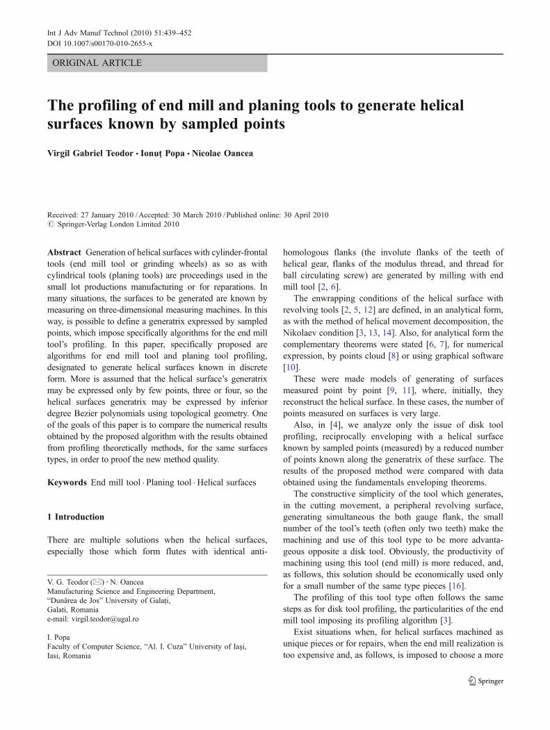
ORIGINAL ARTICLE

The profiling of end mill and planing tools to generate helicalsurfaces known by sampled points

Virgil Gabriel Teodor & Ionuţ Popa & Nicolae Oancea

Received: 27 January 2010 /Accepted: 30 March 2010 /Published online: 30 April 2010# Springer-Verlag London Limited 2010

Abstract Generation of helical surfaces with cylinder-frontaltools (end mill tool or grinding wheels) as so as withcylindrical tools (planing tools) are proceedings used in thesmall lot productions manufacturing or for reparations. Inmany situations, the surfaces to be generated are known bymeasuring on three-dimensional measuring machines. In thisway, is possible to define a generatrix expressed by sampledpoints, which impose specifically algorithms for the end milltool’s profiling. In this paper, specifically proposed arealgorithms for end mill tool and planing tool profiling,designated to generate helical surfaces known in discreteform. More is assumed that the helical surface’s generatrixmay be expressed only by few points, three or four, so thehelical surfaces generatrix may be expressed by inferiordegree Bezier polynomials using topological geometry. Oneof the goals of this paper is to compare the numerical resultsobtained by the proposed algorithm with the results obtainedfrom profiling theoretically methods, for the same surfacestypes, in order to proof the new method quality.

Keywords End mill tool . Planing tool . Helical surfaces

1 Introduction

There are multiple solutions when the helical surfaces,especially those which form flutes with identical anti-

homologous flanks (the involute flanks of the teeth ofhelical gear, flanks of the modulus thread, and thread forball circulating screw) are generated by milling with endmill tool [2, 6].

The enwrapping conditions of the helical surface withrevolving tools [2, 5, 12] are defined, in an analytical form,as with the method of helical movement decomposition, theNikolaev condition [3, 13, 14]. Also, for analytical form thecomplementary theorems were stated [6, 7], for numericalexpression, by points cloud [8] or using graphical software[10].

These were made models of generating of surfacesmeasured point by point [9, 11], where, initially, theyreconstruct the helical surface. In these cases, the number ofpoints measured on surfaces is very large.

Also, in [4], we analyze only the issue of disk toolprofiling, reciprocally enveloping with a helical surfaceknown by sampled points (measured) by a reduced numberof points known along the generatrix of these surface. Theresults of the proposed method were compared with dataobtained using the fundamentals enveloping theorems.

The constructive simplicity of the tool which generates,in the cutting movement, a peripheral revolving surface,generating simultaneous the both gauge flank, the smallnumber of the tool’s teeth (often only two teeth) make themachining and use of this tool type to be more advanta-geous opposite a disk tool. Obviously, the productivity ofmachining using this tool (end mill) is more reduced, and,as follows, this solution should be economically used onlyfor a small number of the same type pieces [16].

The profiling of this tool type often follows the samesteps as for disk tool profiling, the particularities of the endmill tool imposing its profiling algorithm [3].

Exist situations when, for helical surfaces machined asunique pieces or for repairs, when the end mill realization istoo expensive and, as follows, is imposed to choose a more

V. G. Teodor (*) :N. OanceaManufacturing Science and Engineering Department,“Dunărea de Jos” University of Galaţi,Galati, Romaniae-mail: [email protected]

I. PopaFaculty of Computer Science, “Al. I. Cuza” University of Iaşi,Iasi, Romania

Int J Adv Manuf Technol (2010) 51:439–452DOI 10.1007/s00170-010-2655-x

simple method, the milling being replaced with the planingof helical surface flank, generating a cylindrical surface,reciprocally enwrapping with the helical surface, generatingwith planing a tool of the helical surface [15].

In the both situations, the surface to be generated may beknown by a small-point number, often as results of themeasuring of a generatrix of this (not necessary an in-planegeneratrix) allowing a discrete expression for the helicalsurface to be generated.

In this paper, a methodology is proposed for end milltool’s profiling and planer tool for the case of the discreteexpression with a small-point number (three or four points)of its generatrix profile, using Bezier polynomials approx-imation [1].

2 End mill tool profiling—methods

In many practical situations, we may know or measure onlya small number of points along the generatrix of the surfaceto be generated. In these cases, the generatrix can besubstituted by a small order (two or three) of Bezierpolynomials [1] as illustrated in Fig. 1, where we haveconsidered that the generatrix of the helical surface axis, ~V(Z axis) is:

X ¼ PX lð Þ; Y ¼ PY lð Þ; Z ¼ PZ lð Þ; ð1Þwhere l 2 ½0; 1�, while PX(λ), PY(λ), and PZ(λ) are Bezierpolynomials used to approximate the generatrix G.

In the helical movement of G generatrix around axis ~Vwith helical parameter p, right helicoids,

XYZ

�� ¼

cos8 � sin8 0sin8 cos8 00 0 1

��

PX lð ÞPY lð ÞPZ lð Þ

��þ

00p8

��; ð2Þ

The helical surface of constant pitch can be expressed as:

9 l;8ð Þ :X ¼ PX lð Þ � cos8� PY lð Þ � sin8;Y ¼ PX lð Þ � sin8þ PY lð Þ � cos8;Z ¼ PZ lð Þ þ p � 8;

�� ð3Þ

Where λ and φ are variables parameters, φ rotation anglearound Z axis.

The coordinates measured along the surface’s generatrixare defined:

A XA; YA; ZA½ �; B XB; YB; ZB½ �; C XC; YC; ZC½ �;D XD; YD; ZD½ �;ð4Þ

on the generatrix known in discrete form, see Fig. 1.The λ parameter value is known only for a reduced

number of values (3 or 4) which, in many cases,approximates sufficiently well, via Bezier polynomials,the helical surface generatrix. For second-order polyno-mials, one can express the generatrix as:

P

PX lð Þ ¼ l2Ax þ 2l 1� lð ÞCX þ 1� lð Þ2BX ;

PY lð Þ ¼ l2AY þ 2l 1� lð ÞCY þ 1� lð Þ2BY ;

PZ lð Þ ¼ l2AZ þ 2l 1� lð ÞCZ þ 1� lð Þ2BZ :

�� ð5Þ

Similarly, for third-order polynomials, one can write:

P

PX lð Þ ¼ l3AX þ 3l2 1� lð ÞBX þ 3l 1� lð Þ2CX þ 1� lð Þ3DX ;

PY lð Þ ¼ l3AY þ 3l2 1� lð ÞBY þ 3l 1� lð Þ2CY þ 1� lð Þ3DY ;

PZ lð Þ ¼ l3AZ þ 3l2 1� lð ÞBZ þ 3l 1� lð Þ2CZ þ 1� lð Þ3DZ :

��ð6Þ

The coefficients AX, AY, AZ, BX, BY, BZ, CX, CY, CZ, DX,DY, and DZ can be determined using a fitting method such asleast squares from the reduced number of the actual points onthe curve for which the coordinates are known. In the casesbelow, we consider only a very small number of points suchthat direct determination of the coefficients is possible [1].

From Eqs. 3, 5, and 6, one can determine theapproximate helical surface to be generated. Consequently,it is possible to use the fundamental theorems of surfacesenwrapping to determine the peripheral surface of the tool,which would generate by enwrapping the desired helicalsurface. The helical surface can be expressed generically as:

9 l;8ð ÞX ¼ 9X l;8ð Þ;Y ¼ 9Y l;8ð Þ;Z ¼ 9Z l;8ð Þ:

�� ð7Þ

In Eq. 7, ПX(λ, φ), ПY(λ, φ),and ПZ(λ, φ) are:

9X l;8ð Þ ¼ PX lð Þ � cos8� PY lð Þ � sin8;9Y l;8ð Þ ¼ PX lð Þ � sin8þ PY lð Þ � cos8;9Z l;8ð Þ ¼ PX lð Þ þ p � 8;

ð8ÞFig. 1 Conventional points on generatrix (G) approximation byBezier polynomials

440 Int J Adv Manuf Technol (2010) 51:439–452

for a right cylindrical helix with constant pitch (p=constant).

The end mill tool’s profiling problem, for generating byenwrapping a cylindrical helical surface with constant pitch,may be solved by more methods: the Nikolaev classicalmethod [3] or complementary methods [6, 7], brieflypresented in following.

& Nikolaev method

The method assumed to know the normal at helicalsurface presented in form (7).

The normal to the approximated helical surface П(λ, φ),can be written as

N!

9 ¼i!

j!

k!

90X 8ð Þ 9

0Y 8ð Þ p

90X lð Þ 9

0Y lð Þ 9

0Z lð Þ

�� ; ð9Þ

where 90X 8ð Þ;90

X lð Þ and the others denote derivative withrespect to either of the independent parameters. In vectorform, the normal can be written as

N!

9 ¼ NX i!þ NY j

!þ NZ k!: ð10Þ

The X(λ), Y(λ), and Z(λ), see (1), polynomials will beidentified regarding the known coordinates on G generatrix.

Starting from the (3) forms of the helical surface П(λ, φ),the parameters of the normal may be defined at thesubstitutive surface.

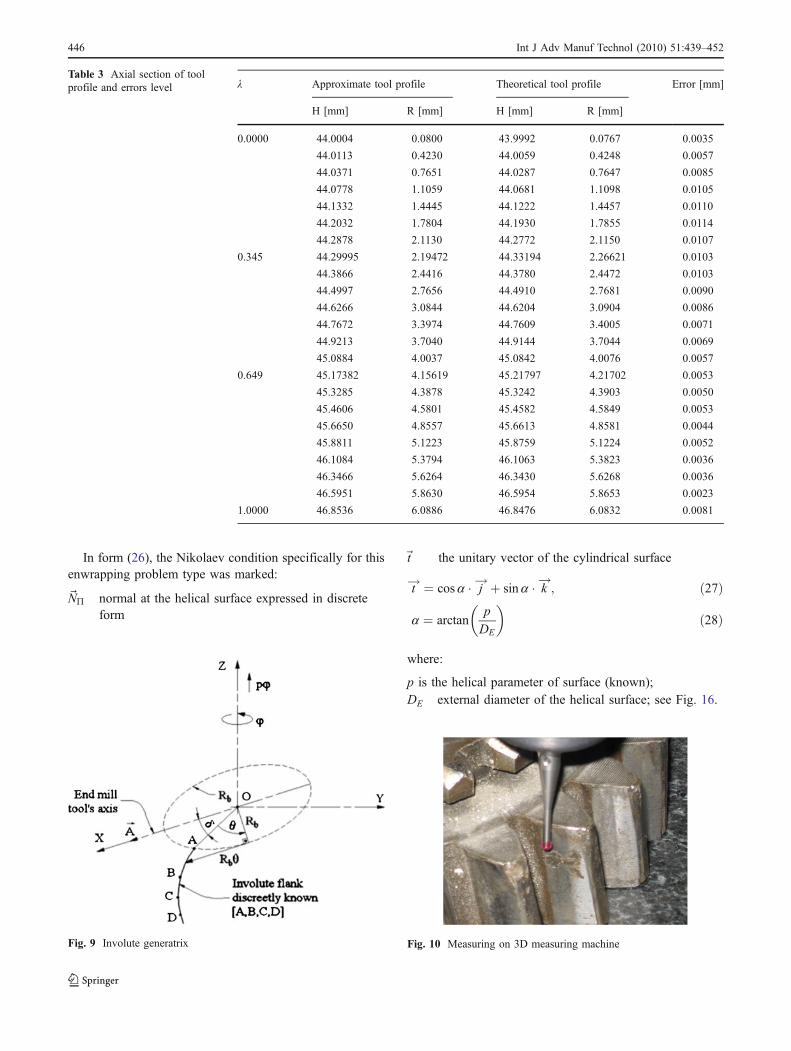
For the tool’s axis definition, see Fig. 2,

A!¼ i

! ð11Þ

and for the position vector of the current point on theП(λ, φ), see (3), surface,

r!¼ X l;8ð Þ i!þ Y l;8ð Þ j!þ Z l;8ð Þ k!; ð12Þthe enwrapping condition [2, 3, 6], known as Nikolaevtheorem,

N9�!

; A!; r!

�� q ð13Þ

with q—positive and very small (for example q=1×10-3),may bring in form

Z lð Þ þ p � 8½ � � NYj � X lð Þ � sin 8ð Þ½ � � NZ j � q: ð14Þ

The equations assembly (7) and (14), determine, on theП(λ, φ), helical surface (3), the characteristic curve, inprinciple, in form:

C9

XC9¼ X lð Þ;

YC9¼ Y lð Þ;

ZC9¼ Z lð Þ:

�� ð15Þ

The characteristic curve CП is common for the helicalsurface П(λ, φ) and for peripheral primary surface of endmill tool—S revolution surface.

The axial section of endmill cutter, see Fig. 3, is determinedstarting from the characteristic curve (15), in the form:

SAH ¼ X lð Þ;R ¼

ffiffiffiffiffiffiffiffiffiffiffiffiffiffiffiffiffiffiffiffiffiffiffiffiffiffiffiffiffiY 2 lð Þ þ Z2 lð Þ

p;

�� ð16Þ

for λ and φ couples of values which meets the condition (14).In all the presented algorithm stages, the profiles

calculus is made only for three (4) considered pointsbelonging to the profile.

Fig. 2 End mill tool, reference system and tool's axis, ~A Fig. 3 Axial section of end mill tool—SA

Int J Adv Manuf Technol (2010) 51:439–452 441

For the axial section (16), known in discrete form, for 3(4) points on this, an approximation is made by a second-degree (third) Bezier polynomial, determining a represen-tation form of this.

& The “minimum distance” method

The “minimum distance” method [6, 8] is based on acomplementary theorem, which is stated thus: “the contactcurve (characteristically curve) between a helical surfacewith constant pitch and a revolution surface is the geomet-rical place of points belonging to the helical surface, forwhich, in planes perpendicular to the revolution surface'saxis (crossing planes), the distance to this axis is minimum”.

In Fig. 4, defined are: OO1=b, positioning constant; α isthe angle between X1 axis (the axis of end mill tool) and Xaxis (the axis of reference system joined with helicalsurface). Currently, α=0°, b=0 (the two reference systemsXYZ and X1Y1Z1 are the same).

By the coordinate transformation (17), expressed is thehelical surface in the tools' reference system, X1Y1Z1 (seeFig. 4), which is a reference system associated with the endmill tool, with X1 axis overlapped to the end mill tool's axis,

X1

Y1Z1

0@

1A ¼

cosa sin a 0� sin a cosa 0

0 0 1

0@

1A �

X l;8ð ÞY l;8ð ÞZ l;8ð Þ

0@

1A�

00b

0@

1A

24

35

ð17Þwith b and α as technological constants or, in principle, inform:

@1

X1 ¼ X1 l;8ð Þ;Y1 ¼ Y1 l;8ð Þ;Z1 ¼ Z1 l;8ð Þ;

�� ð18Þ

representing the Σ helical surface, in the X1Y1Z1 referencesystem.

The intersection curve of surface (18) with planes X1=H(H arbitrary parameter), in principle, is:

@1H

X1 ¼ H ;Y1 ¼ Y1 lð Þ;Z1 ¼ Z1 lð Þ:

�� ð19Þ

As follows, in conformance with the above-statedtheorem, the contact points between the revolution surfaceand the helical surface Σ1 [Σ1H curve, (19)], is determinedfrom the condition that the distance to ~A axis, overlapped toX1 axis,

d ¼ffiffiffiffiffiffiffiffiffiffiffiffiffiffiffiffiffiffiffiffiffiffiffiffiffiffiffiffiffiY 21 lð Þ þ Z2

1 lð Þq� �

ð20Þ

to be minimum, hence

Y1 � Y 01l þ Z1 � Z 0

1l ¼ 0: ð21ÞThe equations assembly (18) and condition (21), for

different values for H, represent the characteristic curve onthe Σ1 surface, equivalent with the Eq. 15, with Y

01l and Z

01l

as partial derivatives of Eq. 19 regarding the λ parameter.

& The in-plane-generating trajectories method

The method based on a complementary theorem [7] statesthat: “the revolution surface of end mill tool, reciprocallyenwrapping with a helical cylindrical surface with constantpitch, is constituted by the circles family from the crossingplanes of revolution surfaces, representing the enveloping oftrajectories of helical surface’s profiles in these planes, in therevolution movement around the tool's axis.”

In this way, the profile Σ1H, in the rotation movementaround ~A axis (see Fig. 4),

X1

Y1Z1

�� ¼

1 0 00 cos 81 � sin81

0 sin81 cos 81

��

HY1 lð ÞZ1 lð Þ

�� ð22Þ

describes the profile's family:

@1Hð Þ8X1 ¼ H ;Y1 ¼ Y1 lð Þ cos81 � Z1 lð Þ sin81;Z1 ¼ Y1 lð Þ sin81 þ Z1 lð Þ cos 81;

�� ð23Þ

φ1 variable parameters and H arbitrary parameter.The enwrapping condition of the profile's family (23), is

give by

Y01l

Y01ϕ1

¼ Z01l

Z01ϕ1

; ð24Þ

Y1(λ, φ1), Z1(λ, φ1) give by Eq. 23.The (23) and (24) equations assembly determine the

characteristically curve of the helical surface, Σ, andFig. 4 End mill tool, peripherally surface


revolution surface S—peripheral primary surface of endmill tool, equivalent with Eq. 15.

3 Applications

3.1 End mill tool for generating a worm with circular axialsection

This surfaces type appears in construction of ball circulat-ing screw or screws for traction with increased fatigueresistance.

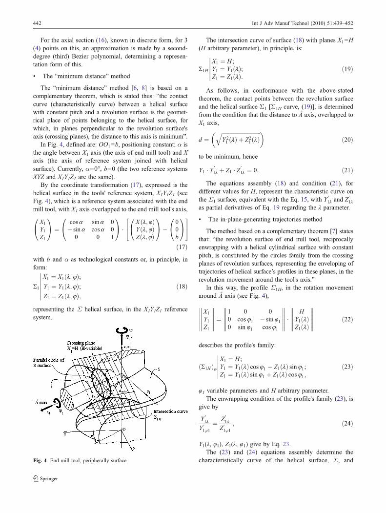
They are presumed known (measured) the coordinates offour points on the helical surface generatrix profile, inanalytical form; see Fig. 5 and Table 1.

The center coordinates of circle arc, which represent thediscreetly known generatrix of the helical surface, areOC XOC ; 0; ZOCð Þ.

The identification algorithm for the Bezier polynomialsubstitutive of the helical surface generatrix profile ispresented in Table 1, for a 3rd-degree polynomial.

Note: As was previously shown, the p parameter value isknown.

In fact, the measuring of points along the axial worm'sprofile may not respect conventional values for λ (0.33 and0.66).

In this way, it is necessary to measure more points alongthe profile in order to approximate values of λ aroundconventional values; see Table 2 and Fig. 6. This mode toapproximate the values of λ parameter was previouslydemonstrated in paper [4].

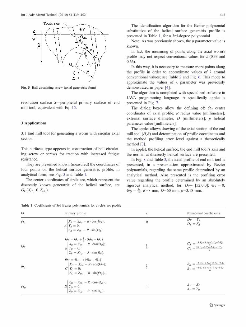
The algorithm is completed with specialized software inJAVA programming language. A specifically applet ispresented in Fig. 7.

The dialog boxes allow the defining of: OC centercoordinates of axial profile; R radius value [millimeters];external surface diameter, D [millimeters]; p helicalparameter value [millimeters].

The applet allows drawing of the axial section of the endmill tool (H,R) and determination of profile coordinates andthe method profiling error level against a theoreticallymethod [3].

In applet, the helical surface, the end mill tool’s axis andthe normal at discreetly helical surface are presented.

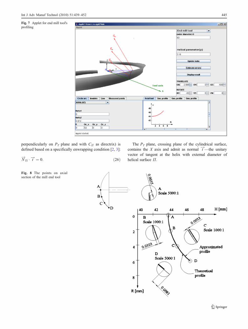
In Fig. 8 and Table 3, the axial profile of end mill tool ispresented, in a presentation approximated by Bezierpolynomials, regarding the same profile determined by ananalytical method. Also presented is the profiling errorvalue regarding the profile determined by an absolutelyrigorous analytical method, for: OC= [52,0,0]; DA ¼ 0;DD ¼ 5p

18; R=8 mm; D=60 mm; p=3.18 mm.

Fig. 5 Ball circulating screw (axial generatrix form)

Table 1 Coefficients of 3rd Bezier polynomials for circle's arc profile

Θ Primary profile λ Polynomial coefficients

ΘA

AXA ¼ XOC � R � cos DAð Þ;YA ¼ 0;ZA ¼ ZOC � R � sin DAð Þ:

��0

DX ¼ YADY ¼ ZA

ΘB

DB ¼ DA þ 13 � DD � DAð Þ

BXB ¼ XOC � R � cos DBð Þ;YB ¼ 0;ZB ¼ ZOC � R � sin DBð Þ:

��13

CX ¼ 18�XC�9�XBþ2�XA�5�XD6

CY ¼ 18�YC�9�YBþ2�YA�5�YD6

ΘC

DC ¼ DA þ 23 DD �DAð Þ

CXC ¼ XOC � R � cos DCð Þ;YC ¼ 0;ZC ¼ ZOC � R � sin DCð Þ:

��23

BX ¼ �5�XAþ2�XDþ18�XB�9�XC6

BY ¼ �5�YAþ2�YDþ18�YB�9�YC6

ΘD DXD ¼ XOC � R � cos DDð Þ;YD ¼ 0;ZD ¼ ZOC � R � sin DDð Þ:

�� 1AX ¼ XD

AY ¼ YD


The profiling error by the proposed method is relativesmall (1×10-2mm, see Fig. 8); the tool profiled in this waymay be used for the milling of this worm type.

The profiling error decreases with the increase of thesubstitution polynomials degree for the assembly of pointsmeasured on profile (4th degree or superior polynomials).

3.2 End mill tool for generating a teethed wheelwith involute frontal section

For involute generatrix of circle with Rb radius, Fig. 9 isproposed as an approximation with four points along profile.We make the remark that points may be the result of a profilemeasuring on a 2D (3D) measuring machine; see Fig. 10.

Proposed for involute approximation are 3rd-degreepolynomials (25), knowing the coordinates of points belongto the involute; see Table 4:

X ¼ AX l3 þ 3BX l

2 1� lð Þ þ 3CX l 1� lð Þ2 þ DX 1� lð Þ3;Y ¼ AYl

3 þ 3BYl2 1� lð Þ þ 3CYl 1� lð Þ2 þ DY 1� lð Þ3:

(

ð25ÞThe angular values ΘA and ΘD, are defined for the flank

of teethed wheel with m modulus and z teeth number(Fig. 11).

In Table 4, the identification algorithm for the 3rd degreepolynomial is presented, substitutive for the involutegeneratrix, for a conventional form [1].

In Table 5, the coordinates measured on the wheel togenerate profile and the value of λ parameter are presented.

In Fig. 12 and Table 6 are presented the form and coor-dinates of axial section of tool and the errors of approximatedprofile regarding the theoretical profile for generating aninvolute gear with: mt=4 mm; z=40 tooth; p=200 mm.

The proposed method is proof to be satisfactory from thepoint of view of tool geometry profiling precision. Thepoint number is relatively small (four points known alongthe profile to be generated, in a frontal plane of this profile).

4 Planing tool's profiling (cylindrical tool)

The planing tool (the cylindrical tool) which generates incutting movement a cylindrical surface reciprocally envel-oping with a helical surface known by sampled points, maybe profiled based on an algorithm similarly with thosepreviously presented.

For an in-plane generatrix, defined in discrete form andapproximated by a Bezier polynomial with small degree, asresult of knowing a small-point number on the axialgeneratrix of the helical surface (three or four points), isaccepted as expression form of helical surface presented indiscrete form; see Eq. 7.

The planing tool's profiling problem for generating byenwrapping a cylindrical helical surface with constant pitchmay be solved by more methods: the method of helicalmovement decomposition [3] or complementary methods[6, 7] presented in following.

& The method of helical movement decomposition

The kinematics of generation process includes themovement assembly:

– helical movement of blank (the movement with ~V axisand p helical parameter) around Z axis (~V , p);

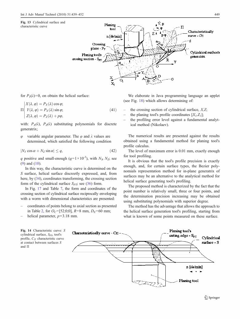
– straight-line movement of the planning tool whichdescribed the cylindrical surface reciprocally envelop-ing with the helical surface to be generated (n=doublestroke/min); see Figs. 13 and 14).

The characteristic curve, CΠ , on the Π helical surfaceexpressed in discrete form, representing the tangent curve atthe cylindrical surface (in Fig. 13, surface with generatrix

Table 2 Coordinates of actual points measured on profile

Measured points A B′ B″ C′ C″ D

X [mm] 44.000 44.269 44.315 45.208 45.320 46.853

Z [mm] 0.000 −2.070 −2.260 −4.229 −4.411 −6.124λ average λ=0 λ=0.345 λ=0.649 λ=1

Fig. 6 Points measured on profile


perpendicularly on PT plane and with CΠ as directrix) isdefined based on a specifically enwrapping condition [2, 3]:

N!

9 � t!¼ 0: ð26Þ

The PT plane, crossing plane of the cylindrical surface,contains the X axis and admit as normal t!—the unitaryvector of tangent at the helix with external diameter ofhelical surface Π.

Fig. 7 Applet for end mill tool'sprofiling

Fig. 8 The points on axialsection of the mill end tool


In form (26), the Nikolaev condition specifically for thisenwrapping problem type was marked:

~N9 normal at the helical surface expressed in discreteform

~t the unitary vector of the cylindrical surface

t!¼ cos a � j!þ sin a � k!; ð27Þ

a ¼ arctanp

DE

� �ð28Þ

where:

p is the helical parameter of surface (known);DE external diameter of the helical surface; see Fig. 16.

λ Approximate tool profile Theoretical tool profile Error [mm]

H [mm] R [mm] H [mm] R [mm]

0.0000 44.0004 0.0800 43.9992 0.0767 0.0035

44.0113 0.4230 44.0059 0.4248 0.0057

44.0371 0.7651 44.0287 0.7647 0.0085

44.0778 1.1059 44.0681 1.1098 0.0105

44.1332 1.4445 44.1222 1.4457 0.0110

44.2032 1.7804 44.1930 1.7855 0.0114

44.2878 2.1130 44.2772 2.1150 0.0107

0.345 44.29995 2.19472 44.33194 2.26621 0.0103

44.3866 2.4416 44.3780 2.4472 0.0103

44.4997 2.7656 44.4910 2.7681 0.0090

44.6266 3.0844 44.6204 3.0904 0.0086

44.7672 3.3974 44.7609 3.4005 0.0071

44.9213 3.7040 44.9144 3.7044 0.0069

45.0884 4.0037 45.0842 4.0076 0.0057

0.649 45.17382 4.15619 45.21797 4.21702 0.0053

45.3285 4.3878 45.3242 4.3903 0.0050

45.4606 4.5801 45.4582 4.5849 0.0053

45.6650 4.8557 45.6613 4.8581 0.0044

45.8811 5.1223 45.8759 5.1224 0.0052

46.1084 5.3794 46.1063 5.3823 0.0036

46.3466 5.6264 46.3430 5.6268 0.0036

46.5951 5.8630 46.5954 5.8653 0.0023

1.0000 46.8536 6.0886 46.8476 6.0832 0.0081

Table 3 Axial section of toolprofile and errors level

Fig. 10 Measuring on 3D measuring machineFig. 9 Involute generatrix


In this way, the (2) and (26) equations assemblyrepresents the characteristic curve of the two surfaces: thehelical surface, expressed in discrete form, and the cylindricalsurface, as peripheral primary surface of the planing tool forhelical surface generation.

In principle, the C9 characteristic curve is expressed byits point coordinates:

C9 ¼XC9;l¼0 YC9;l¼0 ZC9;l¼0

XC9;l¼1

2YC9;l¼1

2ZC9;l¼1

2XC9;l¼1 YC9;l¼1 ZC9;l¼1

��; ð29Þ

for the helical surface approximation with a 2nd-degreepolynomial.

Being known as the cylindrical surface generatrixdirection, t! and the characteristic curve form, C9,expressed in discrete form, is defined the S surface forpoints where is defined, in form:

R!¼ r!þ k � t!; ð30Þwhere:

r!¼ XC9 � i!þ YC9 � j

!þ ZC9 � k! ð31Þ

vector of discrete points on the C9 characteristic curve, kvariable parameter.

The results, in principle, are the S surface coordinates,

S :X S ¼ XC9 ;YS ¼ YC9 þ k cos a;ZS ¼ ZC9 þ k sin a;

�� ð32Þ

which, by coordinate transforming:

X1 ¼ w1 að Þ � X ; ð33Þleads to:

SX1Y1Z1

X1 ¼ X S ;Y1 ¼ YS cos a þ ZS sin a;Z1 ¼ �YS sin a þ ZS cos a;

�� ð34Þ

representing the discrete cylindrical surface S in X1Y1Z1reference system; see Fig. 13.

The X1Y1Z1 reference system is the reference systemwhere the crossing plane of the cylindrical surface, PT, isoverlapped with X1Z1 plane.

The crossing section of discrete cylindrical surface (34)is obtained from condition

Y1j j ¼ q1; ð35Þwith q1 arbitrary, positive, small 1×10-2...1×10-3, in form:

SPT

X1 ¼ X S ;Z1 ¼ �YS sin a þ ZS cos a;

�� ð36Þ

for k variable, see Fig. 14.

& The “minimum distance” method [6]

Θ Primary profile λ Polynomial coefficients

ΘA XA ¼ Rb cos d þ DAð Þ þ RbDA sin d þDAð ÞYA ¼ Rb sin d þDAð Þ � RbDA cos d þDAð ÞDA ¼

ffiffiffiffiffiffiffiffiffiffiR2i �R2

b

R2b

r; Ri ¼ mt �z

2 � 1 � mt;

Rb ¼ mt �z2 � cos atð Þ; at ¼ 200;

d ¼ 12

p2 � z tanat � atð Þ� � mt � cos at

0DX ¼ YADY ¼ ZA

ΘB

DB ¼ DA þ 13 � DD � DAð Þ

XB ¼ Rb cos d þ DBð Þ þ RbDB sin d þ DBð ÞYB ¼ Rb sin d þ DBð Þ � RbDB cos d þ DBð Þ

13

CX ¼ 18�XC�9�XBþ2�XA�5�XD6

CY ¼ 18�YC�9�YBþ2�YA�5�YD6

BX ¼ �5�XAþ2�XDþ18�XB�9�XC6

BY ¼ �5�YAþ2�YDþ18�YB�9�YC6

ΘC

XC ¼ Rb cos d þ DCð Þ þ RbDC sin d þDCð ÞYC ¼ Rb sin d þ DCð Þ � RbDC cos d þDCð ÞDC ¼ DA þ 2

3 DD � DAð Þ23

ΘD

XD ¼ Rb cos d þ DDð Þ þ RbDD sin d þ DDð ÞYD ¼ Rb sin d þDDð Þ � RbDD cos d þ DDð ÞDD ¼

ffiffiffiffiffiffiffiffiffiffiR2e�R2

b

R2b

r; Re ¼ mt �z

2 þ 1 � mt

1AX ¼ XD

AY ¼ YD

Table 4 Coefficients of 3rdBezier polynomials for involutearc profile of teethed wheel

Fig. 11 Points measuredon profile


The complementary theorem specifically for “minimumdistance” method is stated: “the characteristic curve of ahelical cylindrical surface, with constant pitch, reciprocallyenveloping with a cylindrical surface is the geometricalplace of points belonging to helical surface for which thedistance between the helical surface axis and the cylindricalsurface's generatrix, in the contact plane, is minimum.”

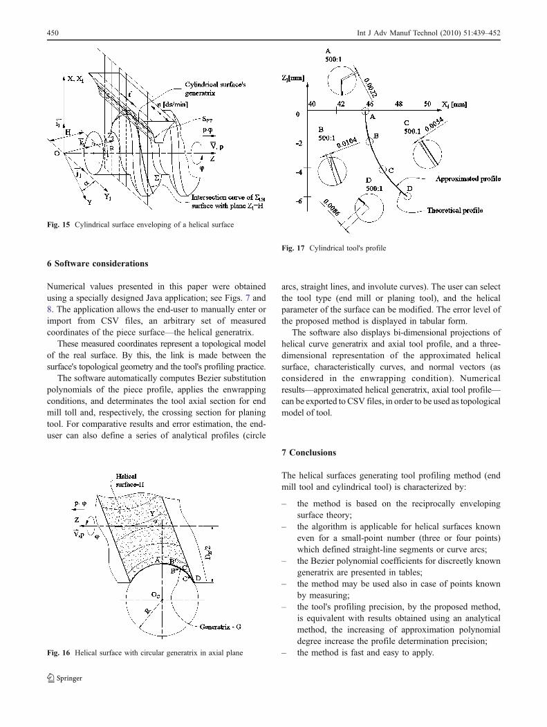
The contact plane is defined as a plane which containsthe cylindrical surface's generatrix and is perpendicular tothe plane determined by the unitary vectors of the helicalsurface's axis ~V and cylindrical surface's generatrix~t; seeFig. 15.

The Σ surface, (18), in the reference system X1Y1Z1, is:

X1 ¼ X l;8ð Þ;Y1 ¼ Y l;8ð Þ cos a þ Z l;8ð Þ sin a;Z1 ¼ �Y l;8ð Þ sin a þ Z l;8ð Þ cos a;

�� ð37Þ

α is the helix angle on the external diameter of the helicalsurface; see Eq. 28.

In-plane Z1=H, H arbitrary parameter, the intersectioncurve of the helical surface with this plane is

@1HX1 ¼ X1 l;Hð Þ;Y1 ¼ Y1 l;Hð Þ cos a þ Z1 l;Hð Þ sin a:

�� ð38Þ

According to the presented theorem, the minimumdistance between the helical surface's axis and the cylindri-cal surface's generatrix in the contact plane is obtained for

X01l ¼ 0; ð39Þ

equivalent to Eq. 26.

5 Application for planing tool for generation of helicalsurface with circular profile in axial plane

The helical surface is expressed in discrete form by an in-plane generatrix known by its points (Fig. 16).

Are knows the coordinates of points on the helicalsurfaces generatrix.

Is identified the 3rd degree Bezier polynomial for Ggeneratrix approximation.

On the helical movement, ~V ; p (see Fig. 16),

XYZ

�� ¼

cos8 � sin 8 0sin8 cos8 00 0 1

��

PX lð Þ0

PZ lð Þ

��þ

00p8

�� ; ð40Þ

Measured points A B′ B″ C′ C″ D

X [mm] 75.90574 78.3812 78.54254 80.98731 81.14147 83.6982

Y [mm] 3.783907 4.501682 4.56124 5.621388 5.697651 7.114187

λ average λ=0 λ=0.34 λ=0.6501 λ=1

Table 5 Coordinates of actualpoints measured on involute'sprofile

Fig. 12 Axial section of end mill tool

Table 6 Axial section of tool and error level

λ Approximated toolprofile

Theoretical toolprofile

Error [mm]

H [mm] R [mm] H [mm] R [mm]

0.0000 76.0000 −1.2667 76.0000 −1.2656 0.0011

76.4046 −1.3030 76.4046 −1.3025 0.0005

76.8088 −1.3436 76.8087 −1.3430 0.0005

77.2125 −1.3881 77.2125 −1.3872 0.0010

77.6159 −1.4364 77.6158 −1.4349 0.0016

78.0188 −1.4882 78.0187 −1.4860 0.0022

78.4212 −1.5434 78.4211 −1.5406 0.0028

0.3400 78.6866 −1.5816 78.6865 −1.5785 0.0032

78.8232 −1.6019 78.8231 −1.5985 0.0034

79.2247 −1.6635 79.2245 −1.6597 0.0038

79.6257 −1.7282 79.6255 −1.7241 0.0041

80.0263 −1.7960 80.0260 −1.7917 0.0043

80.4263 −1.8668 80.4259 −1.8623 0.0045

80.8257 −1.9405 80.8254 −1.9360 0.0046

0.6501 81.2246 −2.0172 81.2242 −2.0126 0.0047

81.3522 −2.0424 81.3518 −2.0377 0.0047

81.6230 −2.0968 81.6225 −2.0920 0.0048

82.0207 −2.1793 82.0203 −2.1743 0.0051

82.4179 −2.2647 82.4175 −2.2593 0.0054

82.8144 −2.3529 82.8140 −2.3470 0.0059

83.2103 −2.4440 83.2100 −2.4373 0.0067

83.6055 −2.5379 83.6053 −2.5302 0.0077

1.0000 84.0000 −2.6346 83.9921 −2.6236 0.0136


for PY(λ)=0, on obtain the helical surface:

9

X l;8ð Þ ¼ PX lð Þ cos8;Y l;8ð Þ ¼ PX lð Þ sin8;Z l;8ð Þ ¼ PZ lð Þ þ p8;

�� ð41Þ

with: PX(λ), PZ(λ) substituting polynomials for discretegeneratrix;

φ variable angular parameter. The φ and λ values aredetermined, which satisfied the following condition

NY cos a þ NZ sin aj j � q; ð42Þq positive and small-enough (q=1×10-3), with NY, NZ; see(9) and (10).

In this way, the characteristic curve is determined on theS surface, helical surface discreetly expressed, and, fromhere, by (34), coordinates transforming, the crossing sectionform of the cylindrical surface SPT; see (36) form.

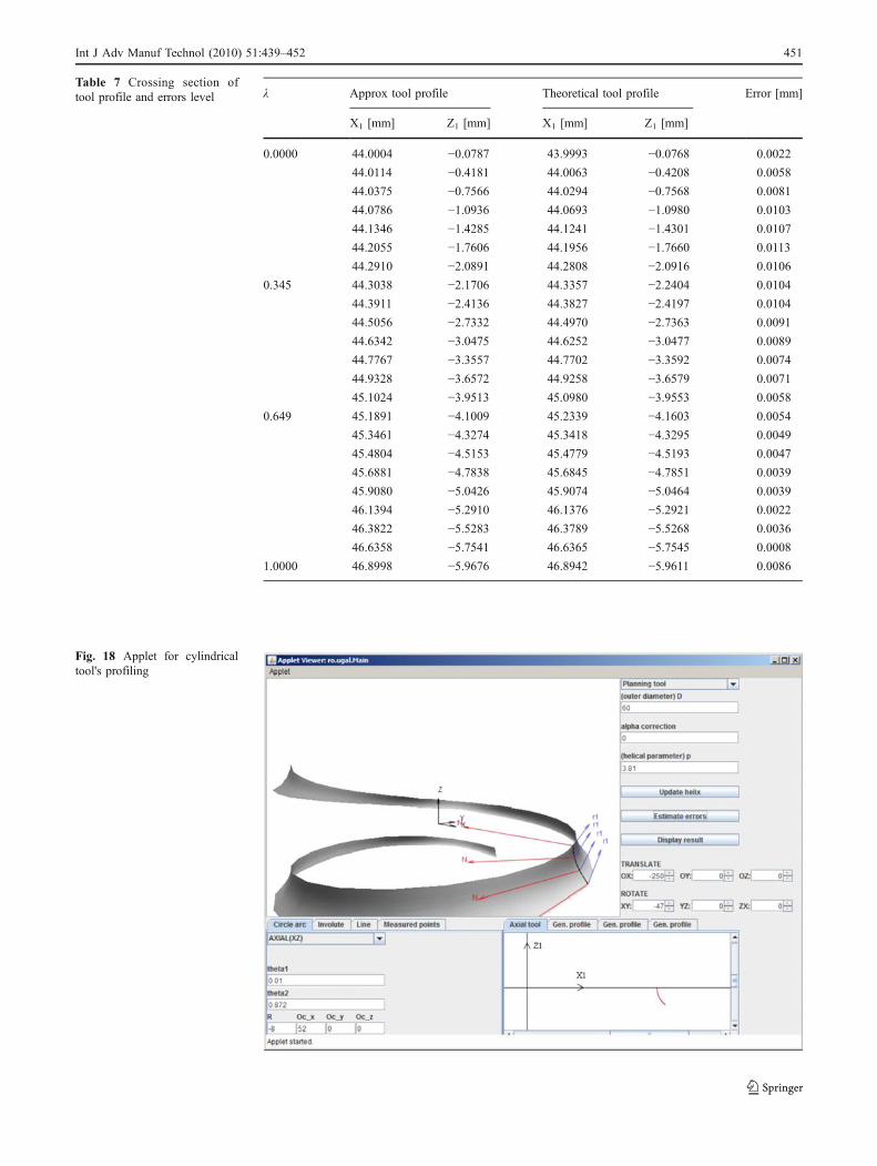
In Fig. 17 and Table 7, the form and coordinates of thecrossing section of cylindrical surface reciprocally envelopingwith a worm with dimensional characteristics are presented:

– coordinates of points belong to axial section as presentedin Table 2, for OC=[52;0;0], R=8 mm, DE=60 mm;

– helical parameter, p=3.18 mm.

We elaborate in Java programming language an applet(see Fig. 18) which allows determining of:

– the crossing section of cylindrical surface, X,Z;– the planing tool's profile coordinates [X1,Z1];– the profiling error level against a fundamental analyt-

ical method (Nikolaev).

The numerical results are presented against the resultsobtained using a fundamental method for planing tool'sprofile calculus.

The level of maximum error is 0.01 mm, exactly enoughfor tool profiling.

It is obvious that the tool's profile precision is exactlyenough, and, for certain surface types, the Bezier poly-nomials representation method for in-plane generatrix ofsurfaces may be an alternative to the analytical method forhelical surface generating tool's profiling.

The proposed method is characterized by the fact that thepoint number is relatively small, three or four points, andthe determination precision increasing may be obtainedusing substituting polynomials with superior degree.

The method has the advantage that allows the approach tothe helical surface generation tool's profiling, starting fromwhat is known of some points measured on these surface.

Fig. 13 Cylindrical surface andcharacteristic curve

Fig. 14 Characteristic curve: Scylindrical surface, SPT, tool'sprofile, CΠ characteristic curveat contact between surfaces Sand Π


6 Software considerations

Numerical values presented in this paper were obtainedusing a specially designed Java application; see Figs. 7 and8. The application allows the end-user to manually enter orimport from CSV files, an arbitrary set of measuredcoordinates of the piece surface—the helical generatrix.

These measured coordinates represent a topological modelof the real surface. By this, the link is made between thesurface's topological geometry and the tool's profiling practice.

The software automatically computes Bezier substitutionpolynomials of the piece profile, applies the enwrappingconditions, and determinates the tool axial section for endmill toll and, respectively, the crossing section for planingtool. For comparative results and error estimation, the end-user can also define a series of analytical profiles (circle

arcs, straight lines, and involute curves). The user can selectthe tool type (end mill or planing tool), and the helicalparameter of the surface can be modified. The error level ofthe proposed method is displayed in tabular form.

The software also displays bi-dimensional projections ofhelical curve generatrix and axial tool profile, and a three-dimensional representation of the approximated helicalsurface, characteristically curves, and normal vectors (asconsidered in the enwrapping condition). Numericalresults—approximated helical generatrix, axial tool profile—can be exported to CSV files, in order to be used as topologicalmodel of tool.

7 Conclusions

The helical surfaces generating tool profiling method (endmill tool and cylindrical tool) is characterized by:

– the method is based on the reciprocally envelopingsurface theory;

– the algorithm is applicable for helical surfaces knowneven for a small-point number (three or four points)which defined straight-line segments or curve arcs;

– the Bezier polynomial coefficients for discreetly knowngeneratrix are presented in tables;

– the method may be used also in case of points knownby measuring;

– the tool's profiling precision, by the proposed method,is equivalent with results obtained using an analyticalmethod, the increasing of approximation polynomialdegree increase the profile determination precision;

– the method is fast and easy to apply.

Fig. 15 Cylindrical surface enveloping of a helical surface

Fig. 16 Helical surface with circular generatrix in axial plane

Fig. 17 Cylindrical tool's profile


λ Approx tool profile Theoretical tool profile Error [mm]

X1 [mm] Z1 [mm] X1 [mm] Z1 [mm]

0.0000 44.0004 −0.0787 43.9993 −0.0768 0.0022

44.0114 −0.4181 44.0063 −0.4208 0.0058

44.0375 −0.7566 44.0294 −0.7568 0.0081

44.0786 −1.0936 44.0693 −1.0980 0.0103

44.1346 −1.4285 44.1241 −1.4301 0.0107

44.2055 −1.7606 44.1956 −1.7660 0.0113

44.2910 −2.0891 44.2808 −2.0916 0.0106

0.345 44.3038 −2.1706 44.3357 −2.2404 0.0104

44.3911 −2.4136 44.3827 −2.4197 0.0104

44.5056 −2.7332 44.4970 −2.7363 0.0091

44.6342 −3.0475 44.6252 −3.0477 0.0089

44.7767 −3.3557 44.7702 −3.3592 0.0074

44.9328 −3.6572 44.9258 −3.6579 0.0071

45.1024 −3.9513 45.0980 −3.9553 0.0058

0.649 45.1891 −4.1009 45.2339 −4.1603 0.0054

45.3461 −4.3274 45.3418 −4.3295 0.0049

45.4804 −4.5153 45.4779 −4.5193 0.0047

45.6881 −4.7838 45.6845 −4.7851 0.0039

45.9080 −5.0426 45.9074 −5.0464 0.0039

46.1394 −5.2910 46.1376 −5.2921 0.0022

46.3822 −5.5283 46.3789 −5.5268 0.0036

46.6358 −5.7541 46.6365 −5.7545 0.0008

1.0000 46.8998 −5.9676 46.8942 −5.9611 0.0086

Table 7 Crossing section oftool profile and errors level

Fig. 18 Applet for cylindricaltool's profiling


Acknowledgement The authors gratefully acknowledge the finan-cial support of the Romanian Ministry of Education, Research andInnovation through grant PN_II_ID_656/2007.

References

1. Favrolles JP (1998) Les surfaces complexes. Hermes, ISBN 2-86601-675.a

2. Litvin EL (1984) Theory of gearing, Reference Publication 1212,NASA, Scientific and Technical Information Division,Washington DC

3. Lukshin VS (1968) Theory of screw surfaces in cutting tooldesign. Machinostroyenie, Moscow

4. Oancea N, Popa I, Teodor V, Oancea V (2010) Tool profiling forgeneration of discrete helical surfaces. Int J Adv Manuf Technol.doi:10.1007/s00170-009-2492-y

5. Kaharaman A, Bajpai P, Anderson NE (2005) Influence of toothprofile deviations on helical gear wear. J Mech Des 127:656–663

6. Oancea N (2004)Generarea suprafeţelor prin înfăşurare, vol. I, II. The“Dunărea de Jos” Publishing House, Galaţi. ISBN 973-627-106-4

7. Teodor V, Oancea N, Dima M (2005) Profilarea sculelor prinmetode analitice. The “Dunărea de Jos” Publishing House, Galaţi,ISBN (10) 973-627-333-4, ISBN (13) 978-973-627-333-9

8. Oancea N (1996) Méthode numérique pour l’étude des surfacesenveloppées. Mech Mach Theory 31(7):957–972

9. Yuwen S, Jun W, Dongming G, Quiang Z (2008) Modeling andnumerical simulation for the machining of helical surface profileson cutting tools. Int J Adv Manuf Technol 36:525–534

10. Veliko I, Gentcho N (1998) Profiling of rotation tools for formingof helical surfaces. Int J Mach Tools Manuf 38:1125–1148

11. Zhang W, Wang X, He F, Xiong D (2006) A practical method ofmodelling and simulation for drill fluting. Int J Mach Tools Manuf46:667–672

12. Radzevich SP (2008) Kinematics geometry of surface machining.CRC Press, London. ISBN 978-1-4200-6340-0

13. Rodin RP (1990) Osnovy proektirovania rezhushchikh instrumen-tov (Basics of design of cutting tools). Vishcha Shkola, Kiev

14. Lashnev SI, Yulikov MI (1980) Proektirovanie rezhushchei chastiinstrumenta s primeneniem EVM (Computer Aided Design of theCutting Parts of Tools). Machinostroienie, Moskow

15. Shalamanov VG, Smetanin SD (2007) Shaping of helical surfacesby profiling circles. Russ Eng Res 27(7):470–473, ISSN 1068-798X

16. Beju LD, Brindasu PD, Mutiu NC (2007) Methodology for thedesign and manufacturing of helical tools. Proceedings of the 3rdInternational Conference onManufacturing Science and Education,July 12–14, Sibiu, ISSN 1843–2522, pp.71–72


http://dx.doi.org/10.1007/s00170-009-2492-y

The profiling of end mill and planing tools to generate helical surfaces known by sampled points

Documents

Transcript of The profiling of end mill and planing tools to generate helical surfaces known by sampled points