The probability distribution of daily precipitation at the point ...

Hydrol. Earth Syst. Sci., 22, 6519–6531, 2018https://doi.org/10.5194/hess-22-6519-2018© Author(s) 2018. This work is distributed underthe Creative Commons Attribution 4.0 License.

The probability distribution of daily precipitation at the pointand catchment scales in the United StatesLei Ye1, Lars S. Hanson2, Pengqi Ding1, Dingbao Wang3, and Richard M. Vogel41School of Hydraulic Engineering, Dalian University of Technology, Dalian, China2Institute for Public Research, Center for Naval Analyses, Arlington, Virginia, USA3Department of Civil, Environmental, and Construction Engineering, University of Central Florida, Orlando, Florida, USA4Department of Civil and Environmental Engineering, Tufts University, Medford, Massachusetts, USA

Correspondence: Lei Ye ([email protected])

Received: 22 February 2018 – Discussion started: 1 March 2018Revised: 26 September 2018 – Accepted: 11 November 2018 – Published: 17 December 2018

Abstract. Choosing a probability distribution to representdaily precipitation depths is important for precipitation fre-quency analysis, stochastic precipitation modeling and inclimate trend assessments. Early studies identified the two-parameter gamma (G2) distribution as a suitable distributionfor wet-day precipitation based on the traditional goodness-of-fit tests. Here, probability plot correlation coefficients andL-moment diagrams are used to examine distributional alter-natives for the wet-day series of daily precipitation for hun-dreds of stations at the point and catchment scales in theUnited States. Importantly, both Pearson Type-III (P3) andkappa (KAP) distributions perform very well, particularly forpoint rainfall. Our analysis indicates that the KAP distribu-tion best describes the distribution of wet-day precipitation atthe point scale, whereas the performance of G2 and P3 distri-butions are comparable for wet-day precipitation at the catch-ment scale, with P3 generally providing the improved good-ness of fit over G2. Since the G2 distribution is currently themost widely used probability density function, our findingscould be considerably important, especially within the con-text of climate change investigations.

1 Introduction

Precipitation is paramount in the fields of hydrology, meteo-rology, climatology and others. However, long series of pre-cipitation data are not always available; therefore, establish-ing a probability distribution that provides a good fit to dailyprecipitation depths has long been a topic of interest. Investi-

gations into the probability distribution of daily precipitationcan be found in at least three main research areas, namely,(1) stochastic precipitation models, (2) frequency analysis ofprecipitation and (3) precipitation trends related to global cli-mate change. Table 1 displays a sampling of the literaturerelated to those three topics, including the particular precipi-tation series and durations under investigation as well as theproposed probability distributions recommended. Table 1 isby no means exhaustive; it only attempts to document thewidespread interest in the determination of a suitable distri-bution for daily precipitation totals in a wide range of studiesacross a wide range of fields of inquiry.

1.1 Stochastic precipitation models

Our central goal is to select a suitable generalized probabil-ity distribution for modeling daily precipitation depths; thus,we are only concerned with the class of “two-part” stochas-tic daily precipitation models that utilize a probability dis-tribution function to describe precipitation amounts on wetdays, while a probabilistic representation of precipitation oc-currences can be separately described using a Markov modelor some form of a stochastic renewal process (Buishand,1978; Geng et al., 1986; Waymire and Gupta, 1981; Wat-terson, 2005). We only consider the selection of a suitabledistribution for modeling wet-day daily rainfall, leaving thestochastic representation of the occurrence of zeros to others.

It is evident from Table 1 that the wet-day precipitationseries is the primary series considered within the stochas-tic precipitation model literature. Thom’s (1951) suggestionof the two-parameter gamma (G2) distribution function for

Published by Copernicus Publications on behalf of the European Geosciences Union.

6520 L. Ye et al.: The probability distribution of daily precipitation at the point and catchment scales in US

Table 1. Review of literature pertinent to daily precipitation probability distribution selection.

Author Year Stations Series type Duration Distribution Justification

1. Stochastic precipitation modeling

Thom 1951 Wet-day 1-day GammaBuishand 1978 6 Wet-day 1-day Gamma Cv–Cs ratioGeng et al. 1986 6 Wet-day, by month 1-day, Gamma Regress. fit: β vs. mean

monthly wet-day depthWoolhiser and Roldan 1982 Wet-day 1-day Mixed exponential MLE, Akaike information

criterionDuan et al. 1995 1 Wet-day, by month 1-day Calib. W2, gamma MLE, Chi-sq testWilks 1998 25 Wet-day 1-day Mixed exponential MLE, goodness of fitWatterson and Dix 2003 Wet-day 1-day Gamma LiteratureBurgueno et al. 2005 75 Wet-day 1-day Exponential, Weibull Normalized rainfall curveKigobe et al. 2011 110 Wet-day, by month GammaLi et al. 2013 24 Wet-day 1-day Mixed exponential Goodness of fit and

Kolmogorov–Smirnovtests

Schoof et al. 2010 Gridded Wet-day 1-day Gamma Goodness of fitprecipitation

Papalexiou 2018 Wet-day 1 h, day Generalized gamma Probability plots

2. Precipitation frequency analysis

Hershfield (TP-40) 1961 AMS 24 h GumbelPilon et al. 1991 75 AMS 5 min–24 h GEV L-momentsNaghavi and Yu 1995 25 AMS 1–24 h GEV L-moments, PWMs,

Monte Carlo experimentsPark and Jung 2002 61 AMS 1, 2-day Kappa(4)Lee and Maeng 2003 38 AMS 1-day GEV, GLO L-momentsBonnin et al. 2006 AMS 5 min–24 h GEV L-momentsShoji and Kitaura 2006 243 Complete, wet-day Hour, day, Lognormal, Weibull Goodness of fit

month, yearDeidda and Puliga 2006 200 Left-censored 1-day Generalized Pareto “Failure-to-reject” method,

L-momentsWet-day PDS

Wilson and Toumi 2005 270 Complete 1-day Self-derivedPapalexiou and Koutsoyiannis 2012 11 519 Wet-day 1-day Generalized gamma L-momentsPapalexiou and Koutsoyiannis 2013 15 137 AMS 1-day GEV L-momentsPapalexiou and Koutsoyiannis 2016 14 157 Wet-day, by month 1-day Generalized gamma L-moments and

and Burr type XII Goodness of fit

3. Precipitation trends and climate change

Waggoner 1989 55 Monthly 1-month Gamma Literature reviewGroisman et al. 1999 1313 Summer (wet-day) 1-day Gamma Literature review, goodness of

fit to extreme rainfall quantilesWilby and Wigley 2002 GCM Seasonal 1-day Gamma Literature reviewYoo et al. 2005 31 Monthly (wet-day) 1-day Gamma Literature reviewWatterson 2005 GCM January, July 1-month Gamma Literature review

(daily forced)

wet-day amounts seems to carry considerable weight. Buis-hand (1978) lent support to the suggestion of the G2 distri-bution by showing that for the wet-day series at six stations,the empirical ratio of the coefficient of variation to coeffi-cient of skewness was quite close to the theoretical value of2 for a G2 distribution. Geng et al. (1986) provided a reviewof other literature supporting the use of the G2 distributionfor modeling wet-day rainfall.

While the G2 distribution is by far the most commonlyadvocated distribution for wet-day precipitation amounts,other distributions have also been suggested. Woolhiser andRoldan (1982), Wilks (1998) and Li et al. (2013) suggestedthe use of a three-parameter mixed exponential distribution

instead of G2. Through a variety of goodness-of-fit tests andlog-likelihood analyses, the mixed exponential was preferredto G2 (Wilks, 1998).

The Weibull (W2) and to a lesser extent the exponentialdistribution have also been suggested for modeling daily pre-cipitation amounts (Duan et al., 1995; Burgueno et al., 2005).Duan et al. (1995) used a Chi-squared test to demonstratethat synthetic rainfall generated from the W2 and G2 mod-els best match the observed daily rainfall data within eachmonth. Burgueno et al. (2005) used graphical methods andthe Kolmogorov–Smirnov test to give support to the W2 andexponential distributions.

Hydrol. Earth Syst. Sci., 22, 6519–6531, 2018 www.hydrol-earth-syst-sci.net/22/6519/2018/

L. Ye et al.: The probability distribution of daily precipitation at the point and catchment scales in US 6521

1.2 Precipitation frequency analysis

The second section of Table 1 displays a small portion of theliterature related to precipitation frequency analyses. Sinceextreme rainfall values are of primary importance in thesestudies, censored series of rainfall (e.g. the annual maximumseries – AMS – and partial duration series – PDS) are oftenuseful in these analyses (Stedinger et al., 1993). Table 1 dis-plays that many of the precipitation frequency investigationsof daily precipitation depths have selected the AMS series.

For many years, the most common approach to summa-rizing precipitation frequency analyses in the US was thework of Hershfield (1961), which is commonly referred toas TP-40. Hershfield (1961) fitted a Gumbel distribution tothe AMS of 24 h precipitation. In the context of a national re-vision to the TP-40, Bonnin et al. (2006) fitted a generalizedextreme value (GEV) distribution to the AMS of rainfall.

While the results of Bonnin et al. (2006) apply to theUnited States, other researchers have found similar resultsusing similar methods in other parts of the world. Pilon etal. (1991) used L-moment goodness-of-fit results to showthat the Gumbel distribution should be rejected in the favor ofthe GEV in Ontario, Canada. In Korea, Park and Jung (2002)successfully used the kappa distribution (of which the GEVis a special case) to generate extreme precipitation quantilemaps. In perhaps the most comprehensive assessment of thedistribution of precipitation extremes, Papalexiou and Kout-soyiannis (2013) examined the goodness of fit of the GEVdistribution to a global data set of AMS. Analysis of such alarge data set enabled them to conclude that GEV models ofAMS of daily precipitation provide a good approximation.

Interestingly, while a great deal of attention is given to fit-ting distributions to the relatively short AMS series of precip-itation depths, very few studies directly explore the probabil-ity distribution of the complete series of daily precipitation(including zeros) or the wet-day series of daily precipitation(zeros excluded). Shoji and Kitaura (2006) investigated bothcomplete and wet-day daily precipitation series, but includedonly the normal, lognormal, exponential, and W2 distribu-tions as candidate distributions, and did not employ mod-ern regional hydrologic methods such as the method of L-moments. Deidda and Puliga (2006) investigated the degreeof left-censoring of wet-day series needed to fit a general-ized Pareto (GPA) distribution for 200 stations in Italy witha range of modern statistical analysis techniques. Wilson andToumi (2005) derived a fundamental distribution for heavyrainfall, with a simple expression for rainfall as the productof mass flux, specific humidity and precipitation efficiency.Statistical theory predicted that the tail of the derived rainfalldistribution has a stretched exponential form with a shapeparameter of two-thirds, which was verified by a global dailyprecipitation data set.

Perhaps the most thorough investigations, to date, on theprobability distribution of daily precipitation amounts arethe global studies by Papalexiou and Koutsoyiannis (2012,

2016). Papalexiou and Koutsoyiannis (2012) derived a gen-eralized gamma (GG) distribution from entropy theory, us-ing plausible constraints for wet-day series of daily precip-itation series. Together, the two studies by Papalexiou andKoutsoyiannis (2012, 2016) revealed that the GG distributionprovides a good approximation of the behavior of observedL-moments of global series of wet-day daily precipitation at11 519 and 14 157 stations, respectively. The GG distributionwas also used in stochastic modeling of precipitation; seeFig. 5 for hourly and Fig. 6 for daily in Papalexiou (2018).Actually any distribution that describes wet-day precipitation(or at any other scale) well can be used as this stochasticmodeling scheme; this makes it feasible to use any probabil-ity distribution and any correlation structure.

1.3 Precipitation trends and changes

The third section of Table 1 summarizes a small portion ofthe precipitation trend literature, which has become a ratherlarge area of inquiry due to concerns over climate change,as evidenced from recent reviews on the subject (Easterlinget al., 2000; Trenberth, 2011; Madsen et al., 2014). Almostuniversally, the G2 distribution appears to be accepted with-out serious consideration of alternative distributions. For in-stance, Groisman et al. (1999) compared maps of the empir-ical probability of summer 1-day rainfall exceeding 50.4 mmwith maps of probabilities determined by a stochastic modelusing the fitted G2 distribution for the amounts. They foundacceptable fits in regions where there are enough observeddaily rainfall events greater than 50.4 mm.

This is an interesting contrast to the precipitation fre-quency analysis literature where a G2 distribution is oftenfit to wet-day series for the purpose of examining extremerainfall instead of using the AMS series fitted by a GEVor other distribution. Yoo et al. (2005) explained that con-ventional frequency analysis (using AMS) cannot expect topredict precipitation changes resulting from climate change,while an examination of the differences in the G2 distribu-tion’s parameters (fitted to the whole wet-day record) mightpredict such changes. They found that modifying the param-eters of the daily G2 distribution can explain changes in rain-fall quantiles predicted by general circulation models undervarious climate change scenarios.

In a national study of precipitation trends, Karl andKnight (1998) employed the G2 distribution to fill in missingprecipitation observations. Both Watterson and Dix (2003)and Watterson (2005) assumed a G2 distribution for dailyprecipitation in the development of stochastic rainfall mod-els for use in evaluating changes in precipitation extremes.

1.4 Research objectives

In summary, there are a wide variety of previous studieswhich have explored the probability distribution of daily pre-cipitation for the purposes of precipitation frequency anal-

www.hydrol-earth-syst-sci.net/22/6519/2018/ Hydrol. Earth Syst. Sci., 22, 6519–6531, 2018


Figure 1. Map showing locations of (a) 237 precipitation gagingstations and (b) 305 catchments.

ysis, stochastic precipitation modeling and trend detection.There seems to be a consensus that annual maxima appearto be well approximated by either a GEV or Gumbel prob-ability density function (pdf), while peaks above thresholdvalues are well approximated by a GPA distribution, and theseries of wet-day precipitation is well approximated by a G2,GG, W2 or in some cases a mixed exponential distribution.However, other than the two recent global studies by Pa-palexiou and Koutsoyiannis (2012, 2016), we are unaware ofany studies that have used recent developments in regionalhydrologic frequency analysis such as L-moment diagramsor probability-plot goodness-of-fit evaluations to evaluate theprobability distribution of very large regional data sets com-prised of the wet-day series of daily precipitation.

The recent studies by Papalexiou and Koutsoyian-nis (2012, 2016) represent perhaps the most comprehen-sive studies to date. However, their L-moment evaluationsonly evaluate the relationship between L-skewness and L-Cv; thus they were unable to fully evaluate the goodness offit of the several relatively new three-parameter pdfs intro-duced in their studies such as the GG and the Burr type XII

Figure 2. Distribution of full record length of point precipitationbased on weather stations.

pdfs, which would require construction of L-kurtosis versusL-skew diagrams, which are currently unavailable for thosepdfs. Analogous to those two studies, this paper uses twolarge-scale national data sets to re-examine the question ofwhich of the commonly used continuous distribution func-tions which are widely used in the fields of hydrology, mete-orology and climate best fit wet-day series of observed dailyprecipitation data. We focus our research interest on the dis-tribution of wet-day series of precipitation since the pdf ofcomplete series can be derived by a mixed distribution con-sisting of a combination of the pdf of wet-day series and astochastic model of the percentage and occurrence of zeros.

Instead of considering the GG distribution, the pdf rec-ommended by both Papalexiou and Koutsoyiannis (2012,2016), which has seen very limited use and for which ana-lytical and/or polynomial relationships for L-kurtosis are un-available (as they are for most commonly used pdfs in hy-drology), we consider the more widely used three-parametergeneralization of the G2 distribution known as the Pearsontype III (P3) distribution. Our primary objective is to use avery large national spatially distributed data set at both thepoint and catchment scales, to determine a suitable prob-ability distribution of wet-day series of daily precipitationusing L-moment diagrams and probability-plot correlation-coefficient goodness-of-fit statistics.

2 Study area and data

Precipitation depths at the point and catchment scales pro-vide important information in hydrology, meteorology andother fields; thus, our study focuses on both scales. Forpoint precipitation, we employ a data set comprised of dailyprecipitation depths at 237 first-order NOAA stations from49 US states (Hawaii is excluded due to fundamentally dif-ferent precipitation behavior). Station locations are shownin Fig. 1a. In contrast, the areal average precipitation for305 catchments in the international Model Parameter Esti-mation Experiment (MOPEX) data set (Duan et al., 2006)



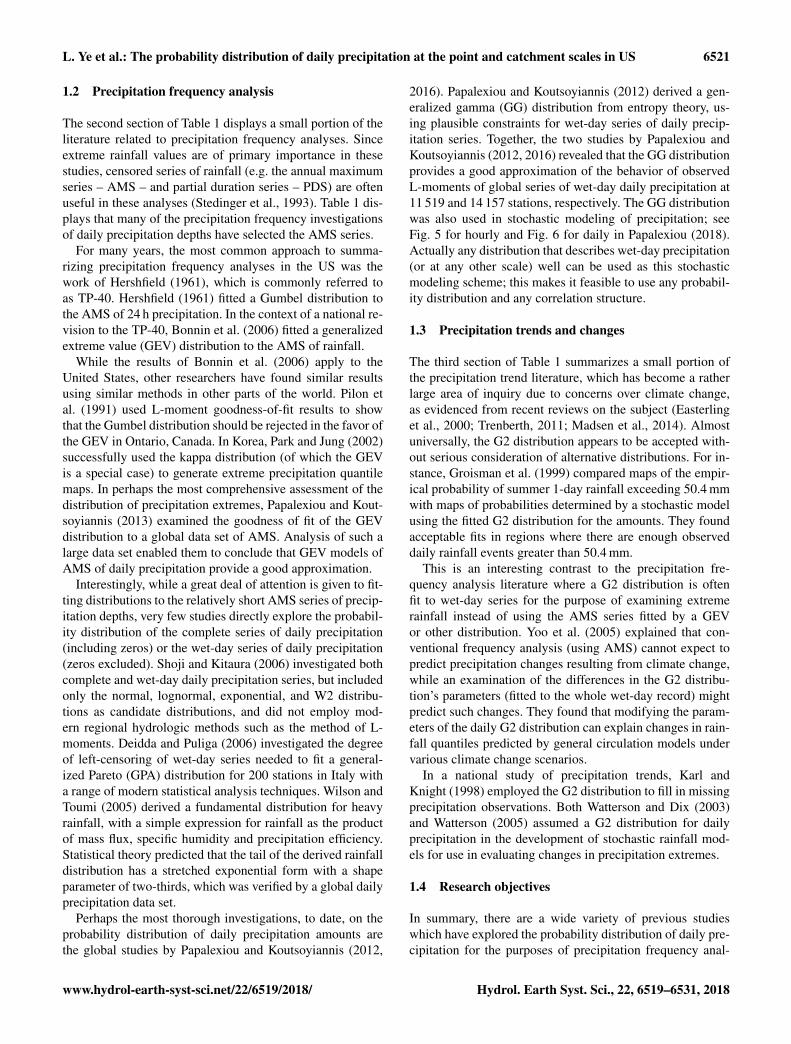
Figure 3. Distribution of wet-day record length: (a) point precipita-tion and (b) areal average precipitation over watersheds. Days withzero precipitation are removed in the wet-day records.

is also selected for analysis. The catchment locations andboundaries are shown in Fig. 1b. The data were quality con-trolled to remove null values. When more than six null val-ues occurred in a given year or more than three in a givenmonth, the full year of data was removed. When fewer thanthese numbers of null values were present, they were treatedas zeroes. The average record length for point precipitationdepths for the 237 sites is 24 657 days (67.5 years). The dis-tribution of record lengths corresponding to the 237 first-order NOAA stations is shown in Fig. 2. The MOPEX dataset consists of 56 years of areal average daily precipitationfrom 1948 to 2003, corresponding to a fixed record length of20 454 days for each of the 305 catchments shown in Fig. 1b.

The wet-day series were extracted from both data sets.The wet-day series were constructed by excluding zeroand “trace” values (those with less than 0.01 in. – approx-imately equivalent to 0.25 mm – recordable precipitation).Wilks (1990) discussed other ways to treat trace precipita-tion and left-censored data, but for convenience, they aresimply excluded. The mean wet-day record lengths for pointand areal average precipitation are 7219 days (equivalent tonearly 20 years) and 14 043 days (more than 38 years), re-spectively. The distributions of wet-day record length areshown in Fig. 3. As expected, the proportion of wet days inthe areal average precipitation data set is higher than that inthe point precipitation data set.

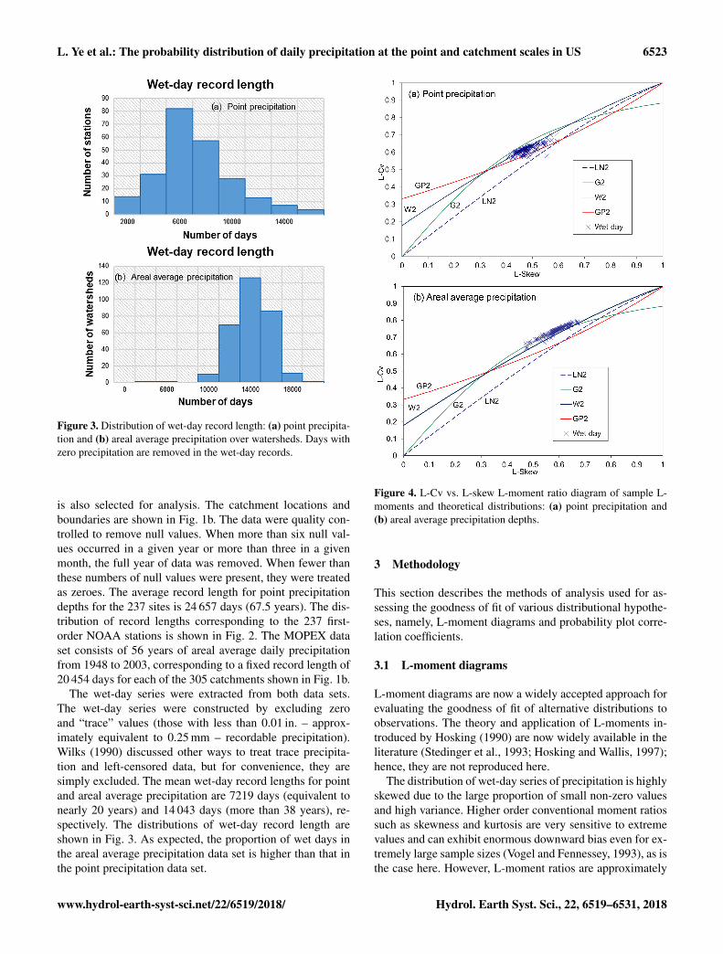
Figure 4. L-Cv vs. L-skew L-moment ratio diagram of sample L-moments and theoretical distributions: (a) point precipitation and(b) areal average precipitation depths.

3 Methodology

This section describes the methods of analysis used for as-sessing the goodness of fit of various distributional hypothe-ses, namely, L-moment diagrams and probability plot corre-lation coefficients.

3.1 L-moment diagrams

L-moment diagrams are now a widely accepted approach forevaluating the goodness of fit of alternative distributions toobservations. The theory and application of L-moments in-troduced by Hosking (1990) are now widely available in theliterature (Stedinger et al., 1993; Hosking and Wallis, 1997);hence, they are not reproduced here.

The distribution of wet-day series of precipitation is highlyskewed due to the large proportion of small non-zero valuesand high variance. Higher order conventional moment ratiossuch as skewness and kurtosis are very sensitive to extremevalues and can exhibit enormous downward bias even for ex-tremely large sample sizes (Vogel and Fennessey, 1993), as isthe case here. However, L-moment ratios are approximately



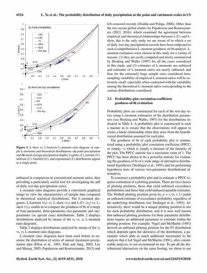
Figure 5. L-skew vs. L-kurtosis L-moment ratio diagram of sam-ple L-moments and theoretical distributions: (a) point precipitationand (b) areal average precipitation depths. Logistic (L), normal (N ),uniform (U ), Gumbel (G), and exponential (E) distributions appearas a single point.

unbiased in comparison to conventional moment ratios, thusproviding a particularly useful tool for investigating the pdfof daily wet-day precipitation series.

L-moment ratio diagrams provide a convenient graphicalimage to view the characteristics of sample data comparedto theoretical statistical distributions. The L-moment dia-grams, L-kurtosis (τ4) vs. L-skew (τ3) and L-Cv (τ2) vs. L-skew (τ3), enable us to compare the goodness of fit of a rangeof four-parameter, three-parameter, two-parameter and one-parameter (or special case) distributions. Table 2 displaysdistributions analyzed by means of the τ4 vs. τ3 L-momentratio diagrams.

Table 3 displays distributions analyzed by means of the τ2vs. τ3 L-moment ratio diagrams.

L-moment ratio diagrams have been used before to ex-amine the distribution of series of annual maximum precip-itation data (Pilon et al., 1991; Park and Jung, 2002; Leeand Maeng, 2003; Papalexiou and Koutsoyiannis, 2013) and

left-censored records (Deidda and Puliga, 2006). Other thanthe two recent global studies by Papalexiou and Koutsoyian-nis (2012, 2016), which examined the agreement betweenempirical and theoretical relationships between L-Cv and L-skew, this is the only study we are aware of in which a setof daily wet-day precipitation records have been subjected tosuch a comprehensive L-moment goodness-of-fit analysis. L-moment estimators were chosen in this study for a variety ofreasons: (1) they are easily computed and nicely summarizedby Hosking and Wallis (1997) for all the cases consideredin this study, and (2) estimates of L-moments are unbiasedand estimates of L-moment ratios are nearly unbiased, andthus for the extremely large sample sizes considered here,sampling variability of empirical L-moment ratios will be ex-tremely small, especially when contrasted with the variabilityamong the theoretical L-moment ratios corresponding to thevarious distributions considered.

3.2 Probability-plot correlation-coefficientgoodness-of-fit evaluation

Probability plots are constructed for each of the wet-day se-ries using L-moment estimators of the distribution parame-ters (see Hosking and Wallis, 1997) for the distributions in-dicated in Table 4. A probability plot is constructed in sucha manner as to ensure that the observations will appear tocreate a linear relationship when they arise from the hypoth-esized distribution assumed for each plot.

The goodness of fit of each probability plot is summa-rized using a probability plot correlation coefficient (PPCC,or simply, r) which is simply a measure of the linearity ofthe plot. The PPCC statistic has a maximum value of 1. ThePPCC has been shown to be a powerful statistic for evaluat-ing the goodness of fit of a wide range of alternative distribu-tional hypotheses (Stedinger et al., 1993) and for performinghypothesis tests of various two-parameter distributional al-ternatives.

To construct a probability plot and to estimate a PPCC re-quires estimation of a plotting position. There are two classesof plotting positions, those that yield unbiased exceedanceprobabilities and those that yield unbiased quantile estimates.The Weibull plotting position given by p = i/(n+ 1) yieldsan unbiased estimate of exceedance probability regardless ofthe underlying distribution (see Stedinger et al., 1993). Al-ternatively, there would be a unique plotting position to usefor each probability distribution, and it is now well knownthat unbiased plotting positions for three parameter distribu-tions require an additional parameter to estimate within theplotting position. For example, Vogel and McMartin (1991)derived an unbiased plotting position for the P3 distributionwhich depends upon the skewness of the distribution, a pa-rameter which adds so much additional uncertainty to theanalysis that it led Vogel and McMartin (1991), after consid-erable analysis, to not recommend its use. To put all the dis-tributional alternatives on the same footing, we chose to use



Table 2. Theoretical probability distributions presented on the L-kurtosis vs. L-skew L-moment diagram.

Distribution Abbreviation PDF Parameters

Kappa KAP F(x)={

1− γ2[1− γ1(x−α)/β

]1/γ1}1/γ2

4

f (x)= β−1[1− γ1(x−α)/β](1/γ1)−1

×[F(x)]1−γ2 , β > 0

Generalized extreme GEV f (x)= 1β

(1+ γ x−αβ

)−1/γ−1exp

[−

(1+ γ x−αβ

)−1/γ]

3

value type III

Generalized GLO f (x)=γ exp

(−x−αβ

)β(

1+exp(−x−αβ

))γ+1 3

Logistic

Generalized GPA f (x)= 1β

(1+ γ (x−α)

β

)−1/γ−13

Pareto

Lognormal LN3 f (x)= 1(x−γ )

√2πβ

exp[−

12

(ln(x−γ )−α

β

)2]

3

Pearson P3 f (x)= 1βγ0(γ )

(x−α)γ−1 exp(−x−αβ

)3

Type III

Exponential E f (x)=

{λexp(−λx), x ≥ 00, x < 0

2

Gumbel G f (x)= 1β exp

[x−αβ − exp

(x−αβ

)]2

Normal N f (x)= 1√2πβ2

exp(−(x−α)2

2β2

)2

Logistic L f (x)=exp

(−x−αβ

)β(

1+exp(−x−αβ

))2 2

Uniform U f (x)=

{ 1b−a

, a < x < b

0, x < a or x > b1

Note that α, β and γ are parameters used for location, scale and shape, respectively; if more than one parameter of the same type exists, indices (e.g. γ1,γ2) are used.

Table 3. Theoretical probability distributions presented on the L-Cv vs. L-skew L-moment diagram.

Distribution Abbreviation PDF Parameters

Gamma G2 f (x)=xγ−1 exp

(−xβ

)0(γ )βγ

2

Generalized Pareto GP2 f (x)= 1β

(1+ γ x

β

)(−1/γ−1)2

Lognormal LN2 f (x)= 1xβ√

2πexp

(−(lnx−α)2

2β2

)2

Weibull W2 f (x)=γβ

(xβ

)γ−1exp

[−

(xβ

)γ ], x ≥ 0 2

Note that α, β and γ are used for location, scale and shape, respectively; if more than one parameter of the same type exists,indices (e.g. γ1, γ2) are used.



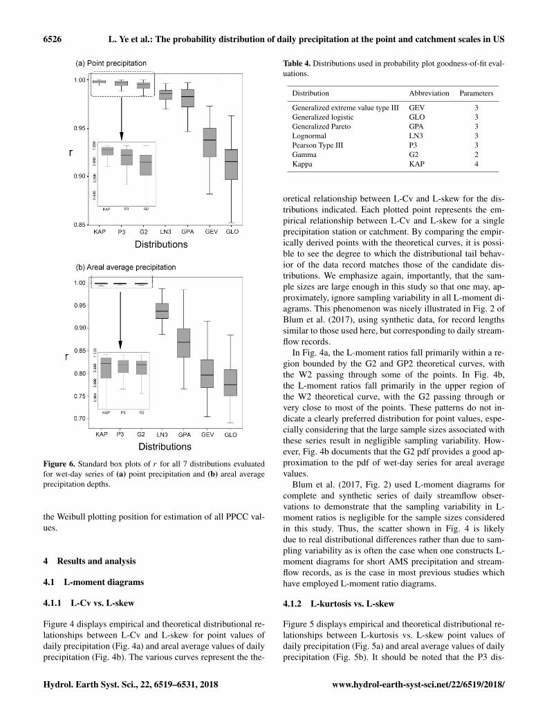
Figure 6. Standard box plots of r for all 7 distributions evaluatedfor wet-day series of (a) point precipitation and (b) areal averageprecipitation depths.

the Weibull plotting position for estimation of all PPCC val-ues.

4 Results and analysis

4.1 L-moment diagrams

4.1.1 L-Cv vs. L-skew

Figure 4 displays empirical and theoretical distributional re-lationships between L-Cv and L-skew for point values ofdaily precipitation (Fig. 4a) and areal average values of dailyprecipitation (Fig. 4b). The various curves represent the the-

Table 4. Distributions used in probability plot goodness-of-fit eval-uations.

Distribution Abbreviation Parameters

Generalized extreme value type III GEV 3Generalized logistic GLO 3Generalized Pareto GPA 3Lognormal LN3 3Pearson Type III P3 3Gamma G2 2Kappa KAP 4

oretical relationship between L-Cv and L-skew for the dis-tributions indicated. Each plotted point represents the em-pirical relationship between L-Cv and L-skew for a singleprecipitation station or catchment. By comparing the empir-ically derived points with the theoretical curves, it is possi-ble to see the degree to which the distributional tail behav-ior of the data record matches those of the candidate dis-tributions. We emphasize again, importantly, that the sam-ple sizes are large enough in this study so that one may, ap-proximately, ignore sampling variability in all L-moment di-agrams. This phenomenon was nicely illustrated in Fig. 2 ofBlum et al. (2017), using synthetic data, for record lengthssimilar to those used here, but corresponding to daily stream-flow records.

In Fig. 4a, the L-moment ratios fall primarily within a re-gion bounded by the G2 and GP2 theoretical curves, withthe W2 passing through some of the points. In Fig. 4b,the L-moment ratios fall primarily in the upper region ofthe W2 theoretical curve, with the G2 passing through orvery close to most of the points. These patterns do not in-dicate a clearly preferred distribution for point values, espe-cially considering that the large sample sizes associated withthese series result in negligible sampling variability. How-ever, Fig. 4b documents that the G2 pdf provides a good ap-proximation to the pdf of wet-day series for areal averagevalues.

Blum et al. (2017, Fig. 2) used L-moment diagrams forcomplete and synthetic series of daily streamflow obser-vations to demonstrate that the sampling variability in L-moment ratios is negligible for the sample sizes consideredin this study. Thus, the scatter shown in Fig. 4 is likelydue to real distributional differences rather than due to sam-pling variability as is often the case when one constructs L-moment diagrams for short AMS precipitation and stream-flow records, as is the case in most previous studies whichhave employed L-moment ratio diagrams.

4.1.2 L-kurtosis vs. L-skew

Figure 5 displays empirical and theoretical distributional re-lationships between L-kurtosis vs. L-skew point values ofdaily precipitation (Fig. 5a) and areal average values of dailyprecipitation (Fig. 5b). It should be noted that the P3 dis-



Table 5. Central tendency and spread of values of PPCC for the 237 precipitation stations and 305 catchments. Bold values are the optimalvalue of each column.

Distribution Point precipitation Percentiles Areal average precipitation Percentiles

Mean Median s 95th 5th Mean Median s 95th 5th

P3 0.9952 0.9971 0.0063 0.9995 0.9872 0.9977 0.9985 0.0028 0.9996 0.9936GEV 0.9338 0.9375 0.0222 0.9609 0.8944 0.8003 0.7965 0.0474 0.8917 0.7264GPA 0.9793 0.9828 0.0145 0.9949 0.9500 0.8688 0.8687 0.0484 0.9586 0.7894GLO 0.9115 0.9154 0.0235 0.9423 0.8734 0.7800 0.7750 0.0441 0.8669 0.7101LN3 0.9838 0.9855 0.0075 0.9924 0.9727 0.9362 0.9373 0.0224 0.9737 0.8983G2 0.9925 0.9949 0.0079 0.9990 0.9789 0.9974 0.9985 0.0034 0.9996 0.9924KAP 0.9971 0.9985 0.0048 0.9997 0.9915 0.9976 0.9987 0.0026 0.9998 0.9929

tribution is the two-parameter G2 with an additional locationparameter which does not affect the shape characteristics andthus the theoretical curve of P3 shown in Fig. 5 is the same asthe G2. The same holds for GPA and GP2 and for LN2 andLN3. The empirical relationships of plotted points for bothwet-day series are very similar to the theoretical relationshipfor the P3 distribution. In fact, among the pdfs consideredin Fig. 5, the P3 pdf seems to be the only three-parameterdistribution that could possibly fit the wet-day record data.Although there is a small proportion of points lying outsidethe P3 curve, the overall fit is still very striking.

It should also be noted that the L-moment ratio estimatesfor both wet-day series occupy a space that can be well rep-resented by the KAP distribution, which occupies a regionof the L-kurtosis vs. L-skew diagram as shown in Fig. A1of Hosking and Wallis (1997). A complete description ofthe four-parameter KAP distribution can be found in Hosk-ing (1994) and Hosking and Wallis (1997).

4.2 Probability plot correlation coefficient

4.2.1 Standard box plots of PPCC

The L-moment ratio diagrams were useful for identifyingseveral potential candidate distributions for representing thewet-day daily precipitation series at the point and catchmentscales. From that analysis, we conclude that a four-parameterkappa pdf is needed to approximate the pdf of point wet-dayseries whereas a G2 and P3 pdf are adequate to approximatethe pdf of areal average wet-day series. The PPCC statisticoffers another quantitative method for comparing the good-ness of fit of different distributions to the daily precipitationobservations. Table 5 summarizes the central tendency andspread of the values of PPCC for each of the distributionsfor the wet-day series of point- and catchment-scale dailyprecipitation, respectively. The highest values for the mean,median, 95th percentile and 5th percentile of the PPCC areshown in bold type. The lowest values of the sample standarddeviation of the PPCC values, denoted s, are also shown inbold. Figure 6 illustrates box plots of the values of PPCC for

distributions fitted to the wet-day series of daily precipitationdata at the point and catchment scales.

Figure 6 and Table 5 indicate that for the wet-day series ofpoint daily precipitation depths, all the distributions have me-dian PPCCs well above 0.9, but only the median PPCCs ofG2, P3 and KAP distributions are over 0.99. The same situa-tion appears in the catchment-scale precipitation, except thatthe median PPCCs of the remaining four distributions aresignificantly lower than the corresponding values for pointprecipitation.

The insets in Fig. 6 show detailed views of the box plotsof PPCC values for the G2, P3 and KAP distributions forpoint and areal average daily precipitation. From Fig. 6a,KAP distribution results in the best goodness of fit for pointprecipitation because all of its indices are the best, while theP3 distribution generally performs better than the G2 distri-bution. However, for catchment-scale precipitation (Fig. 6b),the four-parameter KAP distribution is no longer competi-tive, and both the G2 and P3 pdfs will suffice. We are reluc-tant to advocate the use of a four-parameter pdf, such as theKAP distribution, due to its inherent complexity, though sucha pdf may be needed for point values, as evidenced from ouranalyses.

4.2.2 Graphical comparison of P3, G2 and KAP

Across all previous comparisons, the P3, G2 and KAP are thebest-fitting distributions for describing daily precipitation atthe point or catchment scales. The insets in Fig. 6 identify thedistributions that exhibit the best fit to each observed series.However, these inserts do not indicate by how much the best-performing distribution outperforms the second or third best.For this purpose, pairwise comparisons of the PPCC valuesof two highly performing distributions for all the stations andcatchments are instructive. A simple graphical method canaccomplish this goal.

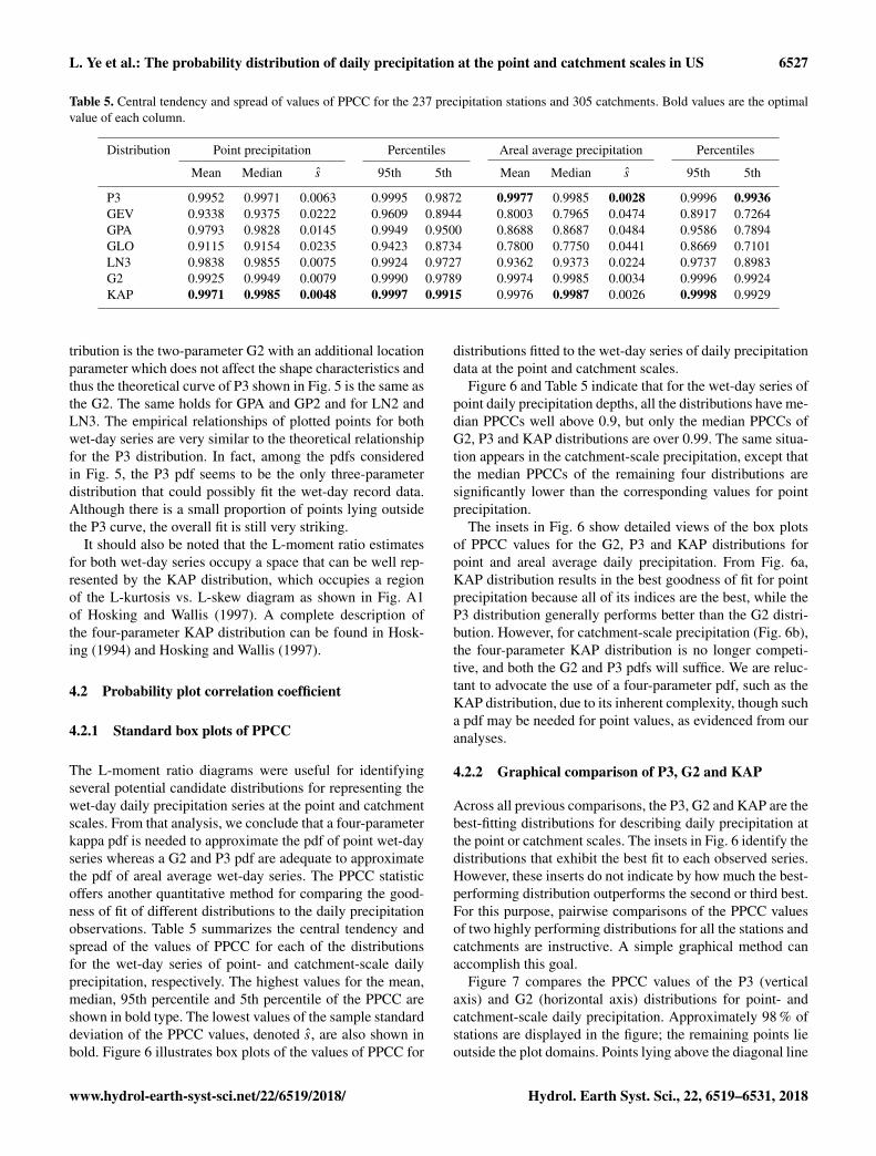
Figure 7 compares the PPCC values of the P3 (verticalaxis) and G2 (horizontal axis) distributions for point- andcatchment-scale daily precipitation. Approximately 98 % ofstations are displayed in the figure; the remaining points lieoutside the plot domains. Points lying above the diagonal line



Figure 7. Comparison of PPCC (r) values for the P3 (vertical axis) and G2 (horizontal axis) distributions for the (a) point, and (b) arealaverage precipitation depths series. Points lying above the line represent stations with a higher r for the P3 distribution than G2 distribution.

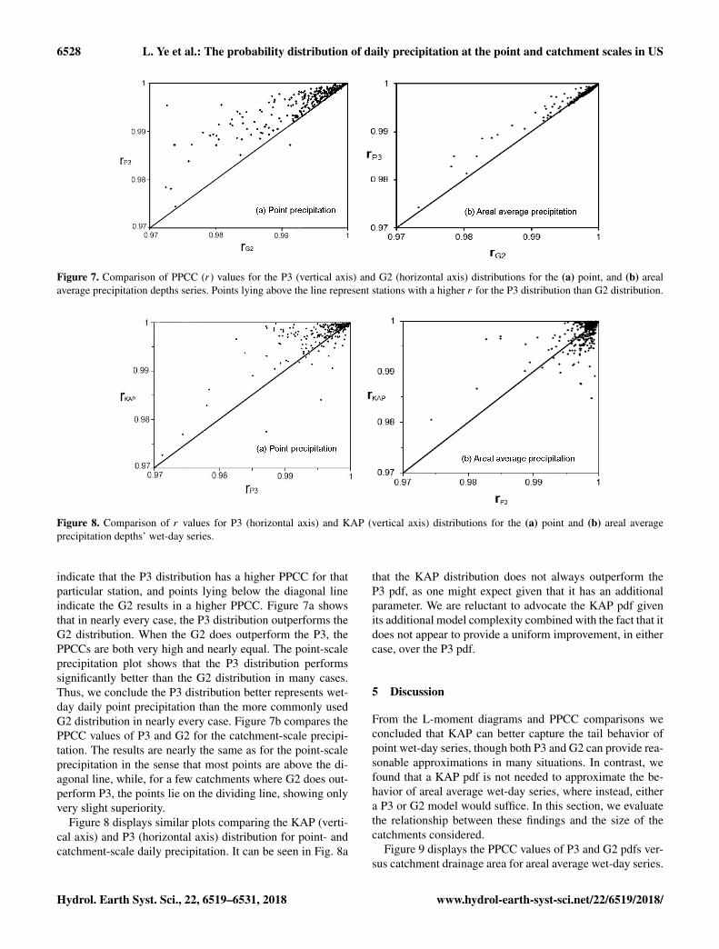
Figure 8. Comparison of r values for P3 (horizontal axis) and KAP (vertical axis) distributions for the (a) point and (b) areal averageprecipitation depths’ wet-day series.

indicate that the P3 distribution has a higher PPCC for thatparticular station, and points lying below the diagonal lineindicate the G2 results in a higher PPCC. Figure 7a showsthat in nearly every case, the P3 distribution outperforms theG2 distribution. When the G2 does outperform the P3, thePPCCs are both very high and nearly equal. The point-scaleprecipitation plot shows that the P3 distribution performssignificantly better than the G2 distribution in many cases.Thus, we conclude the P3 distribution better represents wet-day daily point precipitation than the more commonly usedG2 distribution in nearly every case. Figure 7b compares thePPCC values of P3 and G2 for the catchment-scale precipi-tation. The results are nearly the same as for the point-scaleprecipitation in the sense that most points are above the di-agonal line, while, for a few catchments where G2 does out-perform P3, the points lie on the dividing line, showing onlyvery slight superiority.

Figure 8 displays similar plots comparing the KAP (verti-cal axis) and P3 (horizontal axis) distribution for point- andcatchment-scale daily precipitation. It can be seen in Fig. 8a

that the KAP distribution does not always outperform theP3 pdf, as one might expect given that it has an additionalparameter. We are reluctant to advocate the KAP pdf givenits additional model complexity combined with the fact that itdoes not appear to provide a uniform improvement, in eithercase, over the P3 pdf.

5 Discussion

From the L-moment diagrams and PPCC comparisons weconcluded that KAP can better capture the tail behavior ofpoint wet-day series, though both P3 and G2 can provide rea-sonable approximations in many situations. In contrast, wefound that a KAP pdf is not needed to approximate the be-havior of areal average wet-day series, where instead, eithera P3 or G2 model would suffice. In this section, we evaluatethe relationship between these findings and the size of thecatchments considered.

Figure 9 displays the PPCC values of P3 and G2 pdfs ver-sus catchment drainage area for areal average wet-day series.



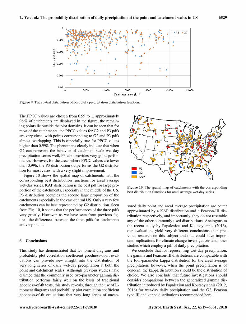
Figure 9. The spatial distribution of best daily precipitation distribution function.

The PPCC values are chosen from 0.99 to 1, approximately96 % of catchments are displayed in the figure; the remain-ing points lie outside the plot domains. It can be seen that formost of the catchments, the PPCC values for G2 and P3 pdfsare very close, with points corresponding to G2 and P3 pdfsalmost overlapping. This is especially true for PPCC valueshigher than 0.998. The phenomena clearly indicate that whenG2 can represent the behavior of catchment-scale wet-dayprecipitation series well, P3 also provides very good perfor-mance. However, for the areas where PPCC values are lowerthan 0.996, the P3 distribution outperforms the G2 distribu-tion for most cases, with a very slight improvement.

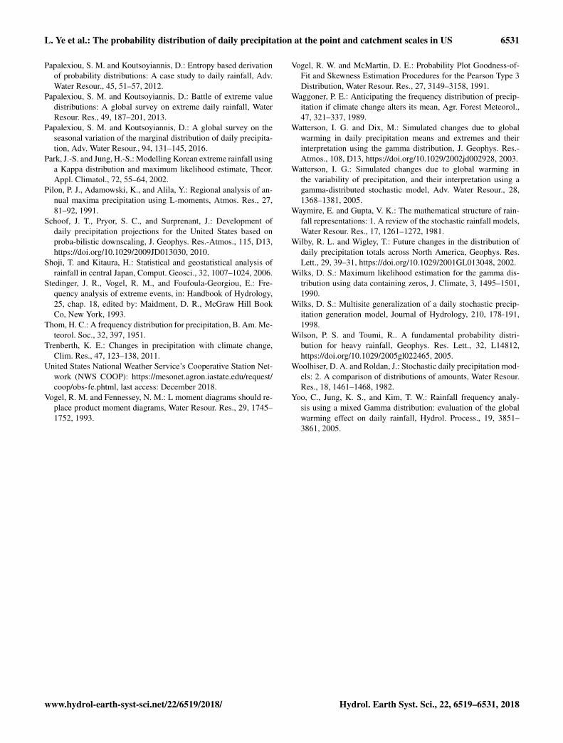
Figure 10 shows the spatial map of catchments with thecorresponding best distribution functions for areal averagewet-day series. KAP distribution is the best pdf for large pro-portion of the catchments, especially in the middle of the US.P3 distribution occupies the second large proportion of thecatchments especially in the east-central US. Only a very fewcatchments can be best represented by G2 distribution. Seenfrom Fig. 10, it seems that the performances of the three pdfsvary greatly. However, as we have seen from previous fig-ures, the differences between the three pdfs for catchmentsare very small.

6 Conclusions

This study has demonstrated that L-moment diagrams andprobability plot correlation coefficient goodness-of-fit eval-uations can provide new insight into the distribution ofvery long series of daily wet-day precipitation at both thepoint and catchment scales. Although previous studies haveclaimed that the commonly used two-parameter gamma dis-tribution performs fairly well on the basis of traditionalgoodness-of-fit tests, this study reveals, through the use of L-moment diagrams and probability plot correlation coefficientgoodness-of-fit evaluations that very long series of uncen-

Figure 10. The spatial map of catchments with the correspondingbest distribution functions for areal average wet-day series.

sored daily point and areal average precipitation are betterapproximated by a KAP distribution and a Pearson-III dis-tribution respectively, and importantly, they do not resembleany of the other commonly used distributions. Analogous tothe recent study by Papalexiou and Koutsoyiannis (2016),our evaluations yield very different conclusions than pre-vious research on this subject and thus could have impor-tant implications for climate change investigations and otherstudies which employ a pdf of daily precipitation.

We conclude that for representing wet-day precipitation,the gamma and Pearson-III distributions are comparable withthe four-parameter kappa distribution for the areal averageprecipitation; however, when the point precipitation is ofconcern, the kappa distribution should be the distribution ofchoice. We also conclude that future investigations shouldconsider comparisons between the generalized gamma dis-tribution introduced by Papalexiou and Koutsoyiannis (2012,2016) for wet-day daily precipitation and the G2, Pearsontype III and kappa distributions recommended here.



Once analytical and polynomial L-moment relationshipsand parameter estimation methods become available for theGG distribution, future studies should compare the P3 andGG distributions on wet-day series, because on the basisof this study, and Papalexiou and Koutsoyiannis (2016), theP3 and GG distributions appear to have tremendous potentialfor approximating the distribution of wet-day series.

Data availability. The point daily precipitation data come from theUnited States National Weather Service’s Cooperative Station Net-work and can be downloaded from https://mesonet.agron.iastate.edu/request/coop/obs-fe.phtml (NWS COOP, 2018). The areal aver-age precipitation data come from the MOPEX data sets (2018) andcan be downloaded from ftp://hydrology.nws.noaa.gov/pub/gcip/mopex/US_Data/.

Author contributions. LY and LSH performed the calculation of thedata and wrote the paper. PD assisted in analyzing the data. DW andRMV provided feedback on the structure of the paper and reviewedthe paper.

Competing interests. The authors declare that they have no conflictof interest.

Acknowledgements. The first and third authors are partiallysupported by the National Natural Science Foundation of China(nos. 91647201, 51709033, 91547116). Special thanks are givento Simon M. Papalexiou and other two anonymous reviewers andeditors for their constructive remarks, which led to a significantlyimproved version.

Edited by: Louise SlaterReviewed by: Simon Michael Papalexiou and two anonymousreferees

References

Blum, A. G., Archfield, S. A., and Vogel, R. M.: On the probabil-ity distribution of daily streamflow in the United States, Hydrol.Earth Syst. Sci., 21, 3093–3103, https://doi.org/10.5194/hess-21-3093-2017, 2017.

Bonnin, G. M., Martin, D., Lin, B., Parzybok, T., Yekta, M., andRiley, D.: Precipitation-frequency atlas of the United States,NOAA atlas, National Oceanic and Atmospheric Administration,National Weather Service, Silver Springs, Maryland, 14, 1–65,2006.

Buishand, T. A.: Some remarks on the use of daily rainfall models,J. Hydrol., 36, 295–308, 1978.

Burgueno, A., Martinez, M. D., Lana, X., and Serra, C.: Statisticaldistributions of the daily rainfall regime in Catalonia (northeast-ern Spain) for the years 1950–2000, Int. J. Climatol., 25, 1381–1403, 2005.

Deidda, R. and Puliga, M.: Sensitivity of goodness-of-fit statisticsto rainfall data rounding off, Phys. Chem. Earth Pt. A/B/C, 31,1240–1251, 2006.

Duan, J., Sikka, A. K., and Grant, G. E.: A comparison of stochas-tic models for generating daily precipitation at the HJ AndrewsExperimental Forest, Northwest Sci., 69, 318–329, 1995.

Duan, Q., Schaake, J., Andreassian, V., Franks, S., Goteti, G.,Gupta, H. V., Gusev, Y. M., Habets, F., Hall, A., and Hay,L.: Model Parameter Estimation Experiment (MOPEX): Anoverview of science strategy and major results from the secondand third workshops, J. Hydrol., 320, 3–17, 2006.

Easterling, D. R., Evans, J., Groisman, P. Y., Karl, T. R., Kunkel, K.E., and Ambenje, P.: Observed variability and trends in extremeclimate events: a brief review, B. Am. Meteorol. Soc., 81, 417–425, 2000.

Geng, S., de Vries, F. W. P., and Supit, I.: A simple method forgenerating daily rainfall data, Agr. Forest Meteorol., 36, 363–376, 1986.

Groisman, P. Y., Karl, T. R., Easterling, D. R., Knight, R. W., Jama-son, P. F., Hennessy, K. J., Suppiah, R., Page, C. M., Wibig, J.,and Fortuniak, K.: Changes in the probability of heavy precipi-tation: important indicators of climatic change, in: Weather andClimate Extremes, Springer, Dordrecht, 243–283, 1999.

Hershfield, D. M.: Rainfall frequency atlas of the United States fordurations from 30 minutes to 24 hours and return periods from1 to 100 years, Technical Paper 40, U.S. Dept. of Agriculture,Washington, DC, 1961.

Hosking, J. R.: L-moments: analysis and estimation of distributionsusing linear combinations of order statistics, J. Roy. Stat. Soc.Ser. B, 70, 105–124, 1990.

Hosking, J. R.: The four-parameter kappa distribution, IBM J. Res.Dev., 38, 251–258, 1994.

Hosking, J. R. M. and Wallis, J. R.: Regional frequency analysis:an approach based on L-moments, Cambridge University Press,Cambridge, 1997.

Karl, T. R. and Knight, R. W.: Secular trends of precipitationamount, frequency, and intensity in the United States, B. Am.Meteorol. Soc., 79, 231–241, 1998.

Kigobe, M., McIntyre, N., Wheater, H., and Chandler, R.: Multi-sitestochastic modelling of daily rainfall in Uganda, Hydrolog. Sci.J., 56, 17–33, 2011.

Lee, S. H. and Maeng, S. J.: Frequency analysis of extreme rainfallusing L moment, Irrig. Drain., 52, 219–230, 2003.

Li, Z., Brissette, F., and Chen, J.: Finding the most appropriate pre-cipitation probability distribution for stochastic weather genera-tion and hydrological modelling in Nordic watersheds, Hydrol.Process., 27, 3718–3729, 2013.

Madsen, H., Lawrence, D., Lang, M., Martinkova, M., and Kjeld-sen, T.: Review of trend analysis and climate change projectionsof extreme precipitation and floods in Europe, J. Hydrol., 519,3634–3650, 2014.

MOPEX data sets: ftp://hydrology.nws.noaa.gov/pub/gcip/mopex/US_Data/, last access: December 2018.

Naghavi, B. and Yu, F. X.: Regional frequency analysis of extremeprecipitation in Louisiana, J. Hydraul. Eng., 121, 819–827, 1995.

Papalexiou, S. M.: Unified theory for stochastic modelling of hydro-climatic processes: Preserving marginal distributions, correlationstructures, and intermittency, Adv. Water Resour., 115, 234–252,2018.


https://mesonet.agron.iastate.edu/request/coop/obs-fe.phtml


ftp://hydrology.nws.noaa.gov/pub/gcip/mopex/US_Data/


https://doi.org/10.5194/hess-21-3093-2017

https://doi.org/10.5194/hess-21-3093-2017




Papalexiou, S. M. and Koutsoyiannis, D.: Entropy based derivationof probability distributions: A case study to daily rainfall, Adv.Water Resour., 45, 51–57, 2012.

Papalexiou, S. M. and Koutsoyiannis, D.: Battle of extreme valuedistributions: A global survey on extreme daily rainfall, WaterResour. Res., 49, 187–201, 2013.

Papalexiou, S. M. and Koutsoyiannis, D.: A global survey on theseasonal variation of the marginal distribution of daily precipita-tion, Adv. Water Resour., 94, 131–145, 2016.

Park, J.-S. and Jung, H.-S.: Modelling Korean extreme rainfall usinga Kappa distribution and maximum likelihood estimate, Theor.Appl. Climatol., 72, 55–64, 2002.

Pilon, P. J., Adamowski, K., and Alila, Y.: Regional analysis of an-nual maxima precipitation using L-moments, Atmos. Res., 27,81–92, 1991.

Schoof, J. T., Pryor, S. C., and Surprenant, J.: Development ofdaily precipitation projections for the United States based onproba-bilistic downscaling, J. Geophys. Res.-Atmos., 115, D13,https://doi.org/10.1029/2009JD013030, 2010.

Shoji, T. and Kitaura, H.: Statistical and geostatistical analysis ofrainfall in central Japan, Comput. Geosci., 32, 1007–1024, 2006.

Stedinger, J. R., Vogel, R. M., and Foufoula-Georgiou, E.: Fre-quency analysis of extreme events, in: Handbook of Hydrology,25, chap. 18, edited by: Maidment, D. R., McGraw Hill BookCo, New York, 1993.

Thom, H. C.: A frequency distribution for precipitation, B. Am. Me-teorol. Soc., 32, 397, 1951.

Trenberth, K. E.: Changes in precipitation with climate change,Clim. Res., 47, 123–138, 2011.

United States National Weather Service’s Cooperative Station Net-work (NWS COOP): https://mesonet.agron.iastate.edu/request/coop/obs-fe.phtml, last access: December 2018.

Vogel, R. M. and Fennessey, N. M.: L moment diagrams should re-place product moment diagrams, Water Resour. Res., 29, 1745–1752, 1993.

Vogel, R. W. and McMartin, D. E.: Probability Plot Goodness-of-Fit and Skewness Estimation Procedures for the Pearson Type 3Distribution, Water Resour. Res., 27, 3149–3158, 1991.

Waggoner, P. E.: Anticipating the frequency distribution of precip-itation if climate change alters its mean, Agr. Forest Meteorol.,47, 321–337, 1989.

Watterson, I. G. and Dix, M.: Simulated changes due to globalwarming in daily precipitation means and extremes and theirinterpretation using the gamma distribution, J. Geophys. Res.-Atmos., 108, D13, https://doi.org/10.1029/2002jd002928, 2003.

Watterson, I. G.: Simulated changes due to global warming inthe variability of precipitation, and their interpretation using agamma-distributed stochastic model, Adv. Water Resour., 28,1368–1381, 2005.

Waymire, E. and Gupta, V. K.: The mathematical structure of rain-fall representations: 1. A review of the stochastic rainfall models,Water Resour. Res., 17, 1261–1272, 1981.

Wilby, R. L. and Wigley, T.: Future changes in the distribution ofdaily precipitation totals across North America, Geophys. Res.Lett., 29, 39–31, https://doi.org/10.1029/2001GL013048, 2002.

Wilks, D. S.: Maximum likelihood estimation for the gamma dis-tribution using data containing zeros, J. Climate, 3, 1495–1501,1990.

Wilks, D. S.: Multisite generalization of a daily stochastic precip-itation generation model, Journal of Hydrology, 210, 178-191,1998.

Wilson, P. S. and Toumi, R.. A fundamental probability distri-bution for heavy rainfall, Geophys. Res. Lett., 32, L14812,https://doi.org/10.1029/2005gl022465, 2005.

Woolhiser, D. A. and Roldan, J.: Stochastic daily precipitation mod-els: 2. A comparison of distributions of amounts, Water Resour.Res., 18, 1461–1468, 1982.

Yoo, C., Jung, K. S., and Kim, T. W.: Rainfall frequency analy-sis using a mixed Gamma distribution: evaluation of the globalwarming effect on daily rainfall, Hydrol. Process., 19, 3851–3861, 2005.


https://doi.org/10.1029/2009JD013030



https://doi.org/10.1029/2002jd002928

https://doi.org/10.1029/2001GL013048

https://doi.org/10.1029/2005gl022465

The probability distribution of daily precipitation at the point ...

Documents

Transcript of The probability distribution of daily precipitation at the point ...