The Price and Trade Effects of Strict Information Requirements for Genetically Modified Commodities...

Centre d’Analyse Théorique et de Traitement des données économiques

CATT-UPPA UFR Droit, Economie et Gestion Avenue du Doyen Poplawski - BP 1633 64016 PAU Cedex Tél. (33) 5 59 40 80 01 Internet : http://catt.univ-pau.fr/live/

CATT WP No. 11. May 2011

THE PRICE AND TRADE EFFECTS

OF STRICT INFORMATION REQUIREMENTS

FOR GENETICALLY MODIFIED COMMODITIES UNDER

THE CARTAGENA PROTOCOL ON BIOSAFETY

Antoine Bouët

Guillaume Gruère Laetitia Leroy

1

The Price and Trade Effects of Strict Information Requirements for Genetically Modified

Commodities under the Cartagena Protocol on Biosafety

Antoine Bouët, Guillaume Gruère, and Laetitia Leroy

Abstract

This paper assesses the global economic implications of the proposed strict documentation

requirements on traded shipments of potentially genetically modified (GM) commodities under the

Cartagena Protocol on Biosafety. More specifically, we evaluate the trade diversion, price, and welfare

effects of requiring all shipments to bear a list of specific GM events (the “does contain” rule) in the

maize and soybean sectors. Using a spatial equilibrium model with 80 maize- and 53 soybean-trading

countries, we show that information requirements would have a significant effect on the world market for

maize and soybeans. But they would have even greater effects on trade, creating significant trade

distortion that diverts exports from their original destination. The measure would also lead to significant

negative welfare effects for all members of the Protocol and nonmembers that produce GM maize,

soybeans, or both. While non-GM producers in Protocol member countries would benefit from this

regulation, consumers and producers in many developing countries would have to pay a proportionally

much heftier price for such a measure.

Key words: Genetically modified food, international trade, Cartagena Protocol on Biosafety.

2

1. Introduction

The Cartagena Protocol on Biosafety (CPB), a supplementary agreement to the United Nations

Convention on Biological Diversity introduced in 2000 (Secretariat of the COB 2000), entered into force

in September 2003 with the goal of setting up a harmonized framework of risk assessment, risk

management, and information sharing on the transboundary movements of living modified organisms

(LMOs).1 Within the Protocol, a number of rules focus on LMOs intended for direct uses as food or feed,

or in food or feed processing (noted as LMO-FFPs), which are essentially unprocessed genetically

modified (GM) agricultural commodities.2

Article 18.2(a) of the Protocol requires that each traded shipment of LMO-FFPs be labeled as

“may contain” LMO-FFPs not intended for release in the environment, though the Convention also noted

that a more specific rule on information requirements should be determined at a later date (Secretariat of

the COB 2000). At a March 2006 meeting in Brazil, after a contentious debate, Protocol members agreed

to adopt a two-option rule consisting of a more stringent option and the less stringent one that had

previously been in effect (ICTSD 2006). Under the stringent option, shipments containing LMO-FFPs

identified through means such as identity-preservation (IP) systems would be labeled as “does contain”

LMO-FFPs and would include a list of all GM events present in each shipment. Shipments containing

LMO-FFPs that are not well identified would follow previous practice and would be labeled as “may

contain” LMO-FFPs. At the same time, a complete list of GM events commercialized in the exporting

country would be available to importers via the Biosafety Clearing House (BCH), an internet database. At

the same meeting, Protocol members also agreed that the two-option rule would be reconsidered, with the

possibility of making the stringent “does contain” option mandatory for all countries (ICTSD 2006). At

1 Also called genetically modified organisms. 2 These products represent more than half the total import value of the four main GM commodities. Approximately 51 percent of the import value of soybeans and 88 percent of that of maize comes from unprocessed commodities (Gruère 2006).

3

the latest meeting of parties in October 2010 in Nagoya, Japan, discussion on the issue was postponed to

leave time for data collection, but it is planned to get the topic back to the table in 2014.

While the benefits of this proposed change are highly debatable, its implementation would

generate significant new costs (see, for example, Gruère and Rosegrant 2008; Kalaitzandonakes 2004;

and Redick 2007). More specifically, under the “does contain” rule, countries that produce and export

only non-GM products would be exempt from verifications and tests, while countries that export GM

products would have to test each shipment to verify the accuracy of GM event identification. Importers

that are ratifying parties of the CPB would also need to pay for the IP system or to conduct tests to

confirm the validity of shipment statements in order to ensure enforcement of mandatory information

requirements.

Previous studies have analyzed the economic implications of adopting the “does contain” rule in

different countries, such as Argentina (Direccion Nacional de Mercados Agroalimentarios 2004), the

United States (Kalaitzandonakes 2004), and Australia (Foster and Galeano 2006), reporting that the costs

of such a change would be potentially significant. More recently, Huang et al. (2008) showed that the cost

of implementation would be high globally but not really significant for China (their focus country).

Gruère and Rosegrant (2008) assessed the potential implementation costs of article 18.2(a) on all member

countries of Asia–Pacific Economic Cooperation (APEC)3

Yet most of these studies provide short-run, partial-cost estimates of the strict rule in particular

regions, leaving aside potential price and trade diversion effects. Huang et al. (2008) do did use a

multiregion computable general equilibrium (CGE) model to assess the potential trade effects of this new

measure, showing that it would affect the prices of maize and soybeans. But their approach focused only

and provided a range of cost estimates for

exporters and importers, noting the disproportionate cost for developing countries that have been

supportive of this measure. They also showed that it would effectively constitute a new entry cost for GM

adoption and for Protocol membership in the APEC region.

3 APEC is a regional trade body covering 21 countries located around the Pacific Ocean, from Chile to New Zealand, including large traders like Mexico, the United States, Canada, China, Japan, South Korea, Indonesia, and Australia.

4

on a few regions (China, the Americas, and the world), used the 2001 Global Trade Analysis Project

(GTAP) database, and did not provide a detailed assessment of potential trade diversions. Furthermore,

the CGE modeling approach prevents the appearance of new trade flows, leaving aside significant

possibilities in trade diversion. While their results showed that the cost of implementation would be high

for all but not really significant for China, they noted that other developing countries would likely pay a

higher price.

The objective of this paper is to complement previous studies by providing a comprehensive

global trade assessment of strict documentation requirements in all member countries of the Protocol. In

particular, our analysis intends to evaluate the market effect it would have on developing countries that

are members of the Protocol. To do so, we develop a spatial trade model and simulate scenarios to

evaluate the trade diversion, price, and welfare effects of implementing the “does contain” rule on the

maize and soybean sectors in all significant trading countries, using data from multiple sources in the

reference period 1995–2005. The model incorporates transportation costs, uses a lower level of product

analysis (four-digit codes of the Harmonized Commodity Description and Coding System [HS]), includes

more countries than GTAP-based models include, and accounts for trade diversion and the creation of

new trade flows.

The results of our policy simulation intend to provide an overview of the medium- to long-run

effects of mandating the “does contain” rule to all members of the Protocol, ahead of future negotiations

on the issue. Developing countries that are members of the CPB have been vocal supporters of using

precautionary measures for trade of GM commodities, such as Article 18.2(a), but they may have

underestimated the cost of such measures on their economies. Beyond the cost estimates and their

geographic and product differentiation, our findings aim at giving an outlook of a possible future trade

scenario for GM commodities in the presence of increasingly stricter trade regulations in specific trade

blocs.

5

In the following section we provide a conceptual framework for analysis. We then present the

simulation model, data, and policy scenarios. The fourth section presents and discusses the first results of

our simulations, and we close the paper with some policy conclusions.

6

2. Conceptual Framework

While the “may contain” and “does contain” rules may share usefulness for regulatory purposes, their

costs of implementation widely differ. Under the “does contain” rule, countries that export GM products

would have to test each shipment to verify the accuracy of the list of GM events, whereas the “may

contain” rule would not require additional tests beyond those to reject unapproved events in the importing

countries. Even if all GM events were approved in all importing nations, the exporter would be required

to provide precise information on each shipment. This could also include additional insurance costs for

shippers against the rejection of shipments. On the importing side, CPB member countries would need to

pay for the IP system or pay to conduct tests to confirm the validity of shipment statements in order to

ensure enforcement of the requirements. Naturally, importers would also have to pay the price for the

information, given the additional testing and insurance applied to shipments.

Given these considerations, we propose an analytical framework based on the characterization of

Gruère and Rosegrant (2008) that categorizes countries to assess the cost of information requirements.

More specifically, we divide countries into four groups according to their membership in the CPB and

whether they produce GM maize or GM soybeans, as presented in Table 2.1.

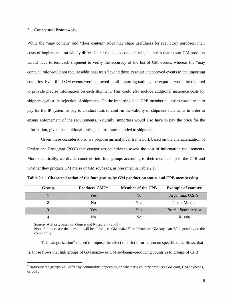
Table 2.1—Characterization of the four groups by GM production status and CPB membership

Group Produces GM?* Member of the CPB Example of country

1 Yes No Argentina, U.S.A.

2 No Yes Japan, Mexico

3 Yes Yes Brazil, South Africa

4 No No Russia

Source: Authors, based on Gruère and Rosegrant (2008). Note: * In our case the question will be “Produces GM maize?” or “Produces GM soybeans?,” depending on the commodity.

This categorization4

4 Naturally the groups will differ by commodity, depending on whether a country produces GM corn, GM soybeans, or both.

is used to impose the effect of strict information on specific trade flows, that

is, those flows that link groups of GM maize– or GM soybeans–producing countries to groups of CPB

7

members. Two types of trade relationships are bound to be affected, those that will request testing at the

import and export sides, linking GM producers (Groups 1 and 3) to CPB members (Groups 2 and 3), and

those that would affect only exporters, linking CPB member GM-producing countries (Group 3) to non-

CPB member countries (Groups 1 and 4).

We use this framework to set up a simplified partial equilibrium model of trade with four

countries (A, B, C, and D) representing the four groups (1 to 4), to illustrate the potential price effect of

such regulation. A and C produce GM, B and D do not, and B and C are members of the CPB while A and

D are not. Each country I faces a linear supply SI defined by the inverse relationship 𝑝𝐼 = 𝑐𝑘𝐼𝑄𝐼, whose

slope coefficient depends on whether the country adopts GM (k = g) or not (k = n). We assume that the

slope coefficients are ranked as follows: 0 < 𝑐𝑔𝐴 < 𝑐𝑔𝐶 < 𝑐𝑛𝐵 < 𝑐𝑛𝐷, and that A and C are net exporters,

while the two others are net importers. The demand in each country is linear and defined by the inverse

demand equation 𝑝𝐼 = 𝑎𝐼𝑄𝐼 + 𝑏𝐼 where (𝑎𝐼 < 0). The equilibrium price is reached when all excess

supply equals excess demand. The original world price (𝑝0𝑊) is

𝑝0𝑊 =− 𝑏

𝐴

𝑎𝐴 − 𝑏

𝐵

𝑎𝐵− 𝑏

𝐶

𝑎𝐶− 𝑏𝐷

𝑎𝐷1𝑐𝑔𝐴+ 1𝑐𝑔𝐶+

1𝑐𝑛𝐵+ 1𝑐𝑛𝐷− 1𝑎𝐴− 1𝑎𝐵

− 1𝑎𝐶

− 1𝑎𝐷

. (1)

The proposed regulation is modeled as an additional transport cost for GM and non-GM products

from A to B, from A to C,5 and from C to B, for simplification.6

The main equations are the following. The world price is

Let us assume a per-unit cost of τ, applied

as a relative tariff on the affected trade flows. At the equilibrium, there are two prices for commingled

commodities: one with affected flows and the other with non affected. The affected equilibrium is going

to be defined by the relationship between A, B, and C, while the non affected one will be defined by the

relationship of A and D. Naturally A and C will only export to B and D under price arbitrage conditions.

𝑝𝑊 = 𝑐𝑔𝐴𝑄𝐴 = 𝑐𝑔𝐴�𝑄𝐶𝑃𝐵𝐴 + 𝑄𝑂𝑈𝑇𝐴 � (2) 5 The basic transport costs are not included explicitly here, because we focus on the new costs associated with the regulation, but they are treated with care in the empirical application. 6 We exclude trade flows from C to C and from C to A and D.

8

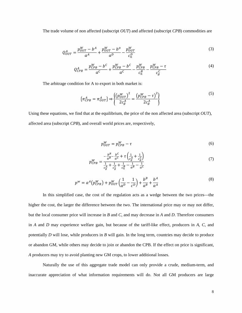
The trade volume of non affected (subscript OUT) and affected (subscript CPB) commodities are

𝑄𝑂𝑈𝑇𝐴 =𝑝𝑂𝑈𝑇𝑊 − 𝑏𝐴

𝑎𝐴+𝑝𝑂𝑈𝑇𝑊 − 𝑏𝐷

𝑎𝐷−𝑝𝑂𝑈𝑇𝑊

𝑐𝑛𝐷

(3)

𝑄𝐶𝑃𝐵𝐴 =𝑝𝐶𝑃𝐵𝑊 − 𝑏𝐶

𝑎𝐶+𝑝𝐶𝑃𝐵𝑊 − 𝑏𝐶

𝑎𝐶−𝑝𝐶𝑃𝐵𝑊

𝑐𝑛𝐵−𝑝𝐶𝑃𝐵𝑊 − 𝜏

𝑐𝑔𝐶

(4)

The arbitrage condition for A to export in both market is:

�𝜋𝐶𝑃𝐵𝐴 = 𝜋𝑂𝑈𝑇𝐴 � ⇒ ��𝑝𝑂𝑈𝑇𝑊 �2

2𝑐𝑔𝐴=�𝑝𝐶𝑃𝐵𝑊 − 𝜏�2

2𝑐𝑔𝐴�

(5)

Using these equations, we find that at the equilibrium, the price of the non affected area (subscript OUT),

affected area (subscript CPB), and overall world prices are, respectively,

𝑝𝑂𝑈𝑇𝑊 = 𝑝𝐶𝑃𝐵𝑊 − 𝜏 (6)

𝑝𝐶𝑃𝐵𝑊 =− 𝑏

𝐵

𝑎𝐵− 𝑏𝐶

𝑎𝐶 + 𝜏 � 1𝑐𝑔𝐴

+ 1𝑐𝑔𝐶�

1𝑐𝑔𝐴

+ 1𝑐𝑔𝐶

+ 1𝑐𝑛𝐵− 1

𝑎𝐵 −1𝑎𝐶

(7)

𝑝𝑤 = 𝑎𝐴�𝑝𝐶𝑃𝐵𝑊 � + 𝑝𝑂𝑈𝑇𝑊 �1𝑎𝐷

−1𝑐𝐷�+

𝑏𝐵

𝑎𝐵+𝑏𝐴

𝑎𝐴

(8)

In this simplified case, the cost of the regulation acts as a wedge between the two prices—the

higher the cost, the larger the difference between the two. The international price may or may not differ,

but the local consumer price will increase in B and C, and may decrease in A and D. Therefore consumers

in A and D may experience welfare gain, but because of the tariff-like effect, producers in A, C, and

potentially D will lose, while producers in B will gain. In the long term, countries may decide to produce

or abandon GM, while others may decide to join or abandon the CPB. If the effect on price is significant,

A producers may try to avoid planting new GM crops, to lower additional losses.

Naturally the use of this aggregate trade model can only provide a crude, medium-term, and

inaccurate appreciation of what information requirements will do. Not all GM producers are large

9

exporters; not all importers are the same; and transport costs, tariffs, and the structure of supply and

demand vary widely from one country to another, even within the same group. We will now turn to our

simulation model to explore the observable effects of the strict option under specific scenarios in the case

of GM maize and GM soybeans.

10

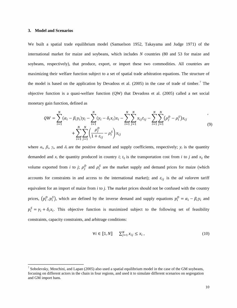
3. Model and Scenarios

We built a spatial trade equilibrium model (Samuelson 1952, Takayama and Judge 1971) of the

international market for maize and soybeans, which includes N countries (80 and 53 for maize and

soybeans, respectively), that produce, export, or import these two commodities. All countries are

maximizing their welfare function subject to a set of spatial trade arbitration equations. The structure of

the model is based on the application by Devadoss et al. (2005) in the case of trade of timber.7

𝑄𝑊 = �(𝛼𝑖 − 𝛽𝑖𝑦𝑖)𝑦𝑖

𝑁

𝑖=1

−�(𝛾𝑖 − 𝛿𝑖𝑥𝑖)𝑥𝑖

𝑁

𝑖=1

−��𝑥𝑖𝑗𝑡𝑖𝑗

𝑁

𝑗=1

𝑁

𝑖=1

−��𝜌𝑗𝐷 − 𝜌𝑖𝑆�𝑥𝑖𝑗

𝑁

𝑗=1

𝑁

𝑖=1

+ ��𝜌𝑗𝐷

1 + 𝜀𝑖𝑗− 𝜌𝑖𝑆� 𝑥𝑖𝑗

𝑁

𝑗=1

𝑁

𝑖=1

The

objective function is a quasi-welfare function (QW) that Devadoss et al. (2005) called a net social

monetary gain function, defined as

,

(9)

where αi, βi, γi, and δi are the positive demand and supply coefficients, respectively; yi is the quantity

demanded and xi the quantity produced in country i; tij is the transportation cost from i to j and xij the

volume exported from i to j; 𝜌𝑗𝐷 and 𝜌𝑖𝑆 are the market supply and demand prices for maize (which

accounts for constraints in and access to the international market); and 𝜀𝑖𝑗 is the ad valorem tariff

equivalent for an import of maize from i to j. The market prices should not be confused with the country

prices, �𝑝𝑖𝐷 ,𝑝𝑖𝑆�, which are defined by the inverse demand and supply equations 𝑝𝑖𝐷 = 𝛼𝑖 − 𝛽𝑖𝑦𝑖 and

𝑝𝑖𝑆 = 𝛾𝑖 + 𝛿𝑖𝑥𝑖. This objective function is maximized subject to the following set of feasibility

constraints, capacity constraints, and arbitrage conditions:

∀𝑖 ∈ ⟦1,𝑁⟧ ∑ 𝑥𝑖𝑗𝑁𝑗=1 ≤ 𝑥𝑖 , (10)

7 Sobolevsky, Moschini, and Lapan (2005) also used a spatial equilibrium model in the case of the GM soybeans, focusing on different actors in the chain in four regions, and used it to simulate different scenarios on segregation and GM import bans.

11

∀𝑖 ∈ ⟦1,𝑁⟧ ∑ 𝑥𝑖𝑗𝑁𝑗=1 ≤ 𝑥𝑖 (10)

∀𝑗 ∈ ⟦1,𝑁⟧ ∑ 𝑥𝑖𝑗𝑁𝑖=1 ≥ 𝑦𝑗 (11)

∀𝑖 ∈ ⟦1,𝑁⟧ 𝛼𝑖 − 𝛽𝑖𝑥𝑖 ≤ 𝜌𝑖𝐷 (12)

∀𝑖 ∈ ⟦1,𝑁⟧ 𝛾𝑖 + 𝛿𝑖𝑥𝑖 ≥ 𝜌𝑖𝑆 (13)

∀(𝑖, 𝑗) ∈ ⟦1,𝑁⟧ 2 �1 + 𝜀𝑖𝑗��𝜌𝑖𝑆 + 𝑡𝑖𝑗� ≥ 𝜌𝑗𝐷 (14)

∀(𝑖, 𝑗) ∈ ⟦1,𝑁⟧ 2 �𝑥𝑖 ≥ 0,𝑦𝑖 ≥ 0,𝑥𝑖𝑗 ≥ 0 � (15)

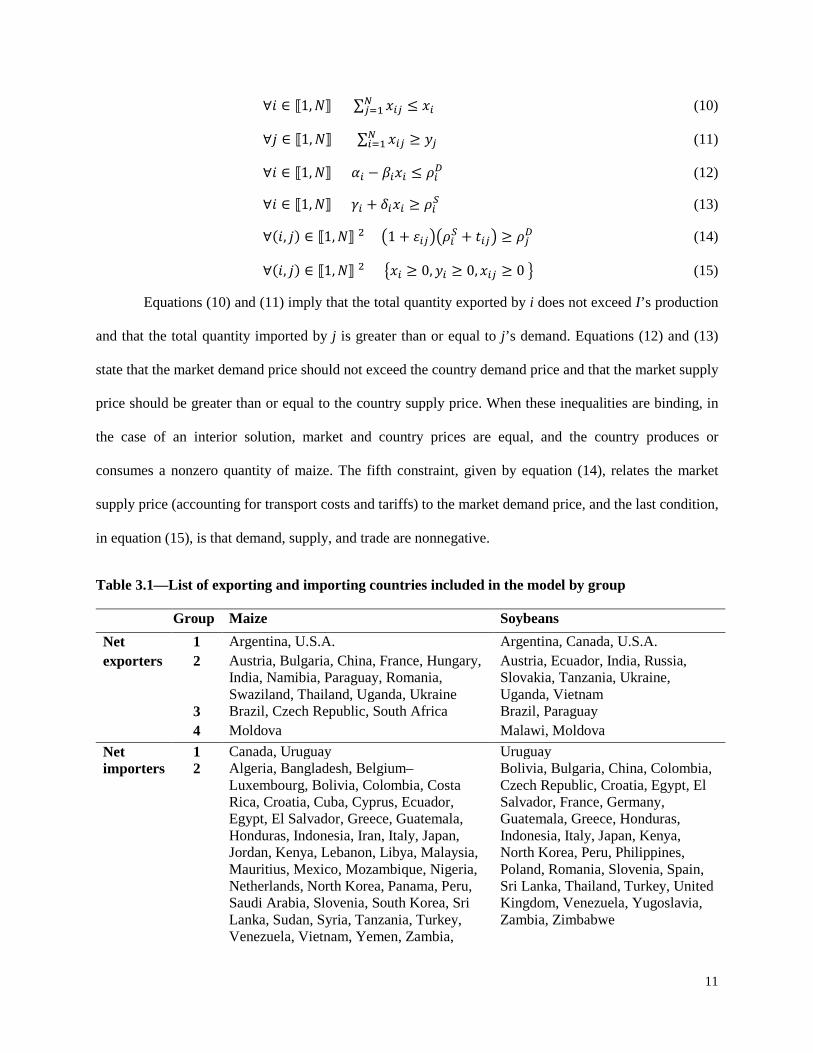
Equations (10) and (11) imply that the total quantity exported by i does not exceed I’s production

and that the total quantity imported by j is greater than or equal to j’s demand. Equations (12) and (13)

state that the market demand price should not exceed the country demand price and that the market supply

price should be greater than or equal to the country supply price. When these inequalities are binding, in

the case of an interior solution, market and country prices are equal, and the country produces or

consumes a nonzero quantity of maize. The fifth constraint, given by equation (14), relates the market

supply price (accounting for transport costs and tariffs) to the market demand price, and the last condition,

in equation (15), is that demand, supply, and trade are nonnegative.

Table 3.1—List of exporting and importing countries included in the model by group

Group Maize Soybeans Net exporters

1 Argentina, U.S.A. Argentina, Canada, U.S.A. 2 Austria, Bulgaria, China, France, Hungary,

India, Namibia, Paraguay, Romania, Swaziland, Thailand, Uganda, Ukraine

Austria, Ecuador, India, Russia, Slovakia, Tanzania, Ukraine, Uganda, Vietnam

3 Brazil, Czech Republic, South Africa Brazil, Paraguay 4 Moldova Malawi, Moldova

Net importers

1 Canada, Uruguay Uruguay 2 Algeria, Bangladesh, Belgium–

Luxembourg, Bolivia, Colombia, Costa Rica, Croatia, Cuba, Cyprus, Ecuador, Egypt, El Salvador, Greece, Guatemala, Honduras, Indonesia, Iran, Italy, Japan, Jordan, Kenya, Lebanon, Libya, Malaysia, Mauritius, Mexico, Mozambique, Nigeria, Netherlands, North Korea, Panama, Peru, Saudi Arabia, Slovenia, South Korea, Sri Lanka, Sudan, Syria, Tanzania, Turkey, Venezuela, Vietnam, Yemen, Zambia,

Bolivia, Bulgaria, China, Colombia, Czech Republic, Croatia, Egypt, El Salvador, France, Germany, Guatemala, Greece, Honduras, Indonesia, Italy, Japan, Kenya, North Korea, Peru, Philippines, Poland, Romania, Slovenia, Spain, Sri Lanka, Thailand, Turkey, United Kingdom, Venezuela, Yugoslavia, Zambia, Zimbabwe

12

Zimbabwe 3 Germany, Philippines, Spain Mexico, South Africa 4 Angola, Chile, Israel, Jamaica, Kuwait,

Malawi, Morocco, Pakistan, Russia Bosnia and Herzegovina

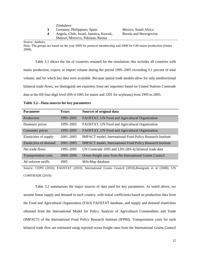
Source: Authors. Note: The groups are based on the year 2009 for protocol membership and 2008 for GM maize production (James 2008).

Table 3.1 shows the list of countries retained for the simulation; this includes all countries with

maize production, export, or import volume during the period 1995–2005 exceeding 0.1 percent of total

volume, and for which key data were available. Because spatial trade models allow for only unidirectional

bilateral trade flows, we distinguish net exporters from net importers based on United Nations Comtrade

data at the HS four-digit level (HS-4 1005 for maize and 1201 for soybeans) from 1995 to 2005.

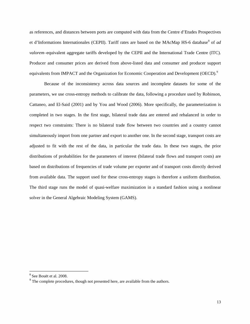
Table 3.2—Data sources for key parameters

Parameter Years Sources of original data

Production 1995–2005 FAOSTAT, UN Food and Agricultural Organization

Domestic prices 1995–2005 FAOSTAT, UN Food and Agricultural Organization

Consumer prices 1995–2005 FAOSTAT, UN Food and Agricultural Organization

Elasticities of supply 2001–2005 IMPACT model, International Food Policy Research Institute

Elasticities of demand 2001–2005 IMPACT model, International Food Policy Research Institute

Net trade flows 1995–2005 UN Comtrade 1005 and 1201 (HS-4) bilateral trade data

Transportation costs 2004–2006 Ocean freight rates from the International Grains Council

Ad valorem tariffs 2005 MAcMap database

Source: CEPII (2010), FAOSTAT (2010), International Grains Council (2010),Rosegrant et al (2008), UN

COMTRADE (2010)

Table 3.2 summarizes the major sources of data used for key parameters. As noted above, we

assume linear supply and demand in each country, with initial coefficients based on production data from

the Food and Agricultural Organization (FAO) FAOSTAT database, and supply and demand elasticities

obtained from the International Model for Policy Analysis of Agricultural Commodities and Trade

(IMPACT) of the International Food Policy Research Institute (IFPRI). Transportation costs for each

bilateral trade flow are estimated using reported ocean freight rates from the International Grains Council

13

as references, and distances between ports are computed with data from the Centre d’Etudes Prospectives

et d’Informations Internationales (CEPII). Tariff rates are based on the MAcMap HS-6 database8 of ad

valorem–equivalent aggregate tariffs developed by the CEPII and the International Trade Centre (ITC).

Producer and consumer prices are derived from above-listed data and consumer and producer support

equivalents from IMPACT and the Organization for Economic Cooperation and Development (OECD).9

Because of the inconsistency across data sources and incomplete datasets for some of the

parameters, we use cross-entropy methods to calibrate the data, following a procedure used by Robinson,

Cattaneo, and El-Said (2001) and by You and Wood (2006). More specifically, the parameterization is

completed in two stages. In the first stage, bilateral trade data are entered and rebalanced in order to

respect two constraints: There is no bilateral trade flow between two countries and a country cannot

simultaneously import from one partner and export to another one. In the second stage, transport costs are

adjusted to fit with the rest of the data, in particular the trade data. In these two stages, the prior

distributions of probabilities for the parameters of interest (bilateral trade flows and transport costs) are

based on distributions of frequencies of trade volume per exporter and of transport costs directly derived

from available data. The support used for these cross-entropy stages is therefore a uniform distribution.

The third stage runs the model of quasi-welfare maximization in a standard fashion using a nonlinear

solver in the General Algebraic Modeling System (GAMS).

8 See Bouët et al. 2008. 9 The complete procedures, though not presented here, are available from the authors.

14

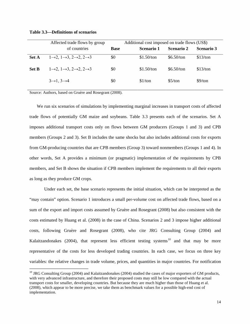
Table 3.3—Definitions of scenarios

Affected trade flows by group of countries

Additional cost imposed on trade flows (US$) Base Scenario 1 Scenario 2 Scenario 3

Set A 1→2, 1→3, 2→2, 2→3 $0 $1.50/ton $6.50/ton $13/ton

Set B 1→2, 1→3, 2→2, 2→3 $0 $1.50/ton $6.50/ton $13/ton

3→1, 3→4 $0 $1/ton $5/ton $9/ton

Source: Authors, based on Gruère and Rosegrant (2008).

We run six scenarios of simulations by implementing marginal increases in transport costs of affected

trade flows of potentially GM maize and soybeans. Table 3.3 presents each of the scenarios. Set A

imposes additional transport costs only on flows between GM producers (Groups 1 and 3) and CPB

members (Groups 2 and 3). Set B includes the same shocks but also includes additional costs for exports

from GM-producing countries that are CPB members (Group 3) toward nonmembers (Groups 1 and 4). In

other words, Set A provides a minimum (or pragmatic) implementation of the requirements by CPB

members, and Set B shows the situation if CPB members implement the requirements to all their exports

as long as they produce GM crops.

Under each set, the base scenario represents the initial situation, which can be interpreted as the

“may contain” option. Scenario 1 introduces a small per-volume cost on affected trade flows, based on a

sum of the export and import costs assumed by Gruère and Rosegrant (2008) but also consistent with the

costs estimated by Huang et al. (2008) in the case of China. Scenarios 2 and 3 impose higher additional

costs, following Gruère and Rosegrant (2008), who cite JRG Consulting Group (2004) and

Kalaitzandonakes (2004), that represent less efficient testing systems10

10 JRG Consulting Group (2004) and Kalaitzandonakes (2004) studied the cases of major exporters of GM products, with very advanced infrastructure, and therefore their proposed costs may still be low compared with the actual transport costs for smaller, developing countries. But because they are much higher than those of Huang et al. (2008), which appear to be more precise, we take them as benchmark values for a possible high-end cost of implementation.

and that may be more

representative of the costs for less developed trading countries. In each case, we focus on three key

variables: the relative changes in trade volume, prices, and quantities in major countries. For notification

15

simplicity, the scenarios in Set A will be written A1, A2, and A3, and the scenarios in Set B will be

designated B1, B2, and B3.

16

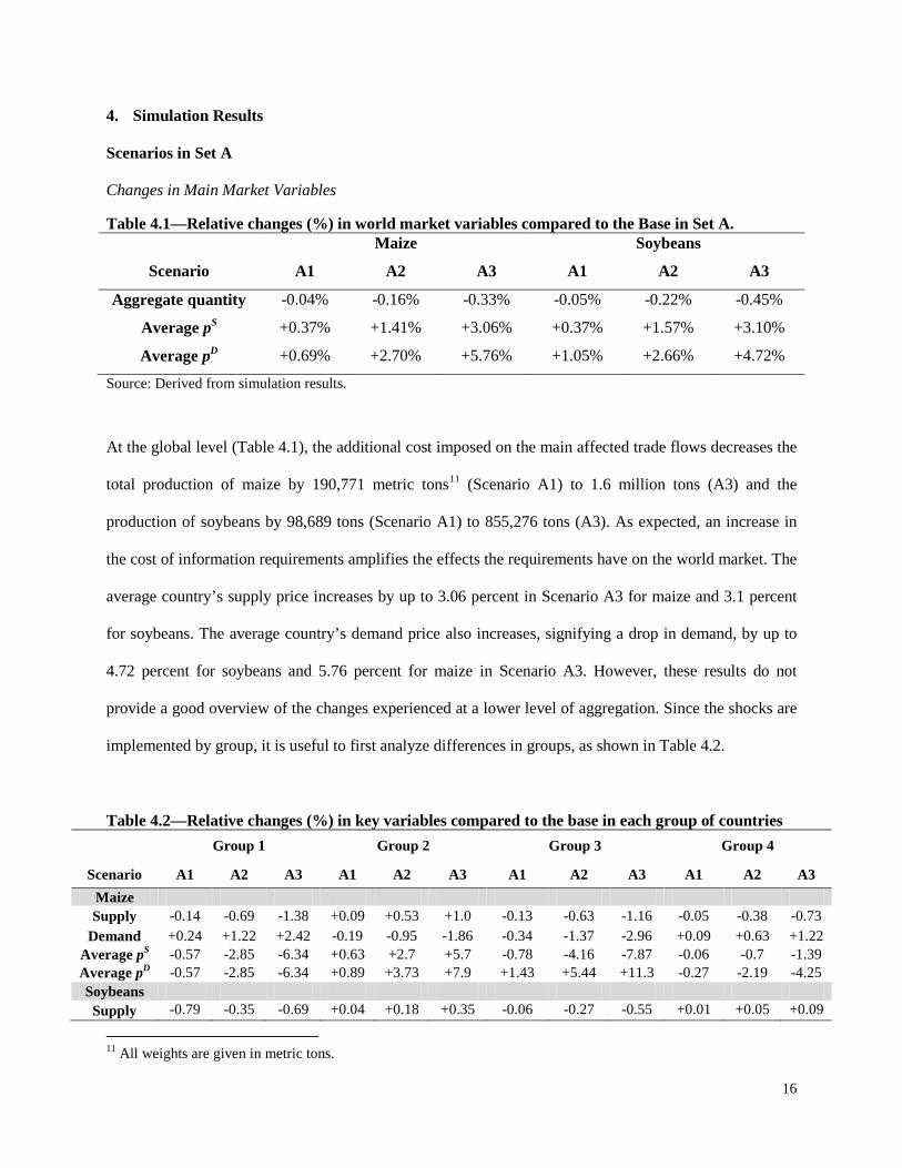
4. Simulation Results

Scenarios in Set A

Changes in Main Market Variables

Table 4.1—Relative changes (%) in world market variables compared to the Base in Set A. Maize Soybeans

Scenario A1 A2 A3 A1 A2 A3

Aggregate quantity -0.04% -0.16% -0.33% -0.05% -0.22% -0.45%

Average pS +0.37% +1.41% +3.06% +0.37% +1.57% +3.10%

Average pD +0.69% +2.70% +5.76% +1.05% +2.66% +4.72%

Source: Derived from simulation results.

At the global level (Table 4.1), the additional cost imposed on the main affected trade flows decreases the

total production of maize by 190,771 metric tons11

(Scenario A1) to 1.6 million tons (A3) and the

production of soybeans by 98,689 tons (Scenario A1) to 855,276 tons (A3). As expected, an increase in

the cost of information requirements amplifies the effects the requirements have on the world market. The

average country’s supply price increases by up to 3.06 percent in Scenario A3 for maize and 3.1 percent

for soybeans. The average country’s demand price also increases, signifying a drop in demand, by up to

4.72 percent for soybeans and 5.76 percent for maize in Scenario A3. However, these results do not

provide a good overview of the changes experienced at a lower level of aggregation. Since the shocks are

implemented by group, it is useful to first analyze differences in groups, as shown in Table 4.2.

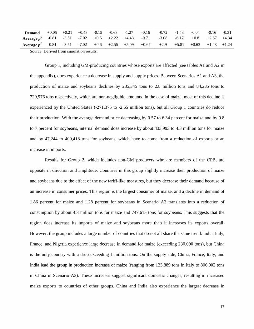
Table 4.2—Relative changes (%) in key variables compared to the base in each group of countries Group 1 Group 2 Group 3 Group 4

Scenario A1 A2 A3 A1 A2 A3 A1 A2 A3 A1 A2 A3 Maize Supply -0.14 -0.69 -1.38 +0.09 +0.53 +1.0 -0.13 -0.63 -1.16 -0.05 -0.38 -0.73

Demand +0.24 +1.22 +2.42 -0.19 -0.95 -1.86 -0.34 -1.37 -2.96 +0.09 +0.63 +1.22 Average pS -0.57 -2.85 -6.34 +0.63 +2.7 +5.7 -0.78 -4.16 -7.87 -0.06 -0.7 -1.39 Average pD -0.57 -2.85 -6.34 +0.89 +3.73 +7.9 +1.43 +5.44 +11.3 -0.27 -2.19 -4.25 Soybeans Supply -0.79 -0.35 -0.69 +0.04 +0.18 +0.35 -0.06 -0.27 -0.55 +0.01 +0.05 +0.09

11 All weights are given in metric tons.

17

Demand +0.05 +0.21 +0.43 -0.15 -0.63 -1.27 -0.16 -0.72 -1.43 -0.04 -0.16 -0.31 Average pS -0.81 -3.51 -7.02 +0.5 +2.22 +4.43 -0.71 -3.08 -6.17 +0.8 +2.67 +4.34

Average pD -0.81 -3.51 -7.02 +0.6 +2.55 +5.09 +0.67 +2.9 +5.81 +0.63 +1.43 +1.24 Source: Derived from simulation results.

Group 1, including GM-producing countries whose exports are affected (see tables A1 and A2 in

the appendix), does experience a decrease in supply and supply prices. Between Scenarios A1 and A3, the

production of maize and soybeans declines by 285,345 tons to 2.8 million tons and 84,235 tons to

729,976 tons respectively, which are non-negligible amounts. In the case of maize, most of this decline is

experienced by the United States (-271,375 to -2.65 million tons), but all Group 1 countries do reduce

their production. With the average demand price decreasing by 0.57 to 6.34 percent for maize and by 0.8

to 7 percent for soybeans, internal demand does increase by about 433,993 to 4.3 million tons for maize

and by 47,244 to 409,418 tons for soybeans, which have to come from a reduction of exports or an

increase in imports.

Results for Group 2, which includes non-GM producers who are members of the CPB, are

opposite in direction and amplitude. Countries in this group slightly increase their production of maize

and soybeans due to the effect of the new tariff-like measures, but they decrease their demand because of

an increase in consumer prices. This region is the largest consumer of maize, and a decline in demand of

1.86 percent for maize and 1.28 percent for soybeans in Scenario A3 translates into a reduction of

consumption by about 4.3 million tons for maize and 747,615 tons for soybeans. This suggests that the

region does increase its imports of maize and soybeans more than it increases its exports overall.

However, the group includes a large number of countries that do not all share the same trend. India, Italy,

France, and Nigeria experience large decrease in demand for maize (exceeding 230,000 tons), but China

is the only country with a drop exceeding 1 million tons. On the supply side, China, France, Italy, and

India lead the group in production increase of maize (ranging from 133,889 tons in Italy to 806,902 tons

in China in Scenario A3). These increases suggest significant domestic changes, resulting in increased

maize exports to countries of other groups. China and India also experience the largest decrease in

18

demand for soybeans between Scenario A1 and A3 (exceeding 300,000 tons and 130,000 tons,

respectively). On the supply side, China increases its production of soybeans from 6,953 tons to 60,271

tons; India and Bolivia also experience a large increase in their production of soybeans between A1 and

A3 (from 3,967 tons to 34,392 tons and from 1,311 tons to 11,364 tons respectively).

Group 3 countries, which include GM producers that are CPB members, represent an

intermediate situation for maize, with decreased supply and demand, a higher demand price, and a

reduction in the supply price. But the drop in demand (from -180,775 tons in Scenario A1 to -1,568,318

tons in Scenario A3) largely exceeds the decrease in supply (from -83,438 tons to -732,749 tons),

signifying a growing maize surplus. Most of the decline in demand is borne by Brazil (-946,456 tons in

A3), South Africa (-291,435 tons), and Spain (-214227 tons). The decrease in supply is also experienced

greatly by Brazil (-416,133 tons in A3) and, to a lesser extent, South Africa (-142,217 tons in A3), but

much less by other countries in the group.

Similar results can be highlighted for soybeans in terms of variation of supply, demand, and

prices. Soybeans also experience a growing surplus as evidenced by the drop in demand (from -59,311

tons in A1 to -514,072 tons in A3), which greatly exceeds the decrease in supply (from -29,310 tons to

-254,000 tons between A1 and A3). Once again, Brazil experiences the larger decline in demand (from

-57,214 tons in A1 to -495,896 tons in A3) and in supply (from -25,586 tons to -221,731 tons). To a lesser

extent, Paraguay follows with a decrease in demand (-14,202 tons in A3) smaller than the decrease in

supply (-30,176 tons in A3).

Lastly, Group 4, which includes non-GM producers that are not CPB members, has a distinct

pattern with, on average, negligible changes in supply and demand, following the same pattern as Group

2. However, the minor observed decrease in demand is associated with a minor decrease in demand

prices, suggesting the presence of heterogeneous effects in countries with differentiated demand

elasticities. Indeed, unlike other groups, there is a significant variation of demand effects within Group 4.

Moldova experiences lower maize demand (-1,636 tons in A1 to -14,858 tons in A3) while larger

countries, like Chile (+41,126 tons in A3), Russia (+21,639 tons), and Pakistan (+16,305 tons), increase

19

their demand for maize. Israel (+21,691 tons in A3) and, to a greater extent, Malawi (+55,225 tons) also

experience a significant growth in demand. These variations are consistent with demand price fluctuations

across countries. Significant variations are also observable on the supply side, with Moldova producing

more maize (up to +13,847 tons) to take advantage of higher supply prices, while other countries decrease

their production, especially larger countries such as Russia, Chile, and Pakistan. To a lesser extent, these

results also apply to soybeans, with a slight decrease in demand (-3,065 tons in A3) and a growing supply

(+3,839 tons) in Russia, while Bosnia and Herzegovina records the opposite trend.

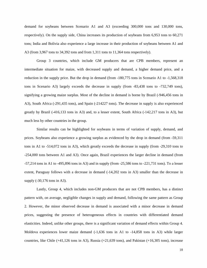
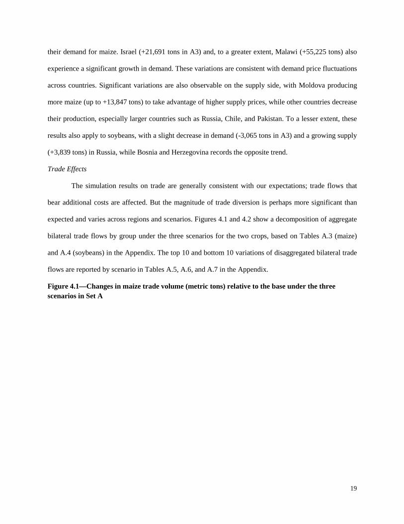
Trade Effects

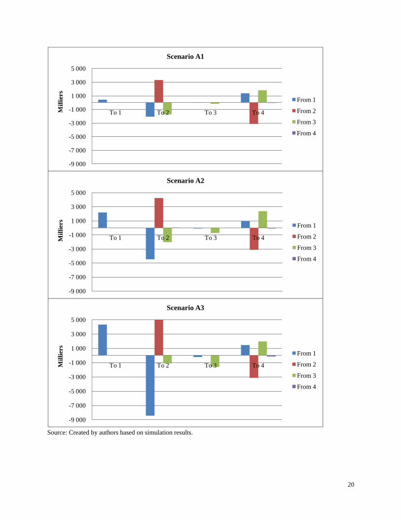
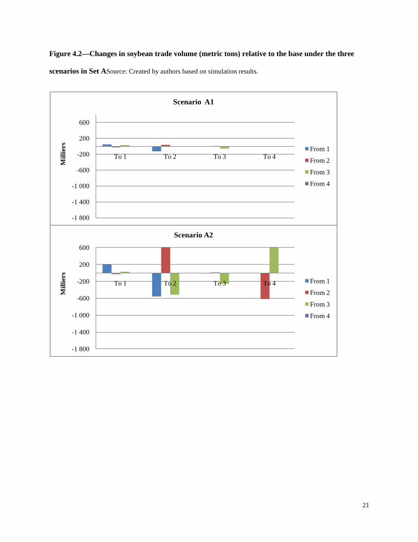
The simulation results on trade are generally consistent with our expectations; trade flows that

bear additional costs are affected. But the magnitude of trade diversion is perhaps more significant than

expected and varies across regions and scenarios. Figures 4.1 and 4.2 show a decomposition of aggregate

bilateral trade flows by group under the three scenarios for the two crops, based on Tables A.3 (maize)

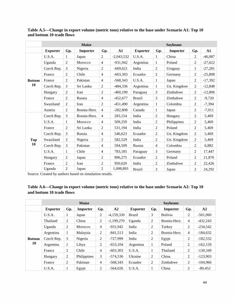
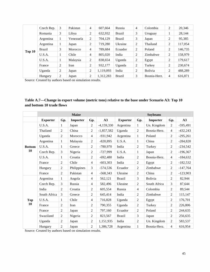
and A.4 (soybeans) in the Appendix. The top 10 and bottom 10 variations of disaggregated bilateral trade

flows are reported by scenario in Tables A.5, A.6, and A.7 in the Appendix.

Figure 4.1—Changes in maize trade volume (metric tons) relative to the base under the three scenarios in Set A

20

Source: Created by authors based on simulation results.

-9 000

-7 000

-5 000

-3 000

-1 000

1 000

3 000

5 000

To 1 To 2 To 3 To 4Mill

iers

Scenario A1

From 1

From 2

From 3

From 4

-9 000

-7 000

-5 000

-3 000

-1 000

1 000

3 000

5 000


iers

Scenario A2

From 1

From 2

From 3

From 4

-9 000

-7 000

-5 000

-3 000

-1 000

1 000

3 000

5 000


iers

Scenario A3

From 1

From 2

From 3

From 4

21

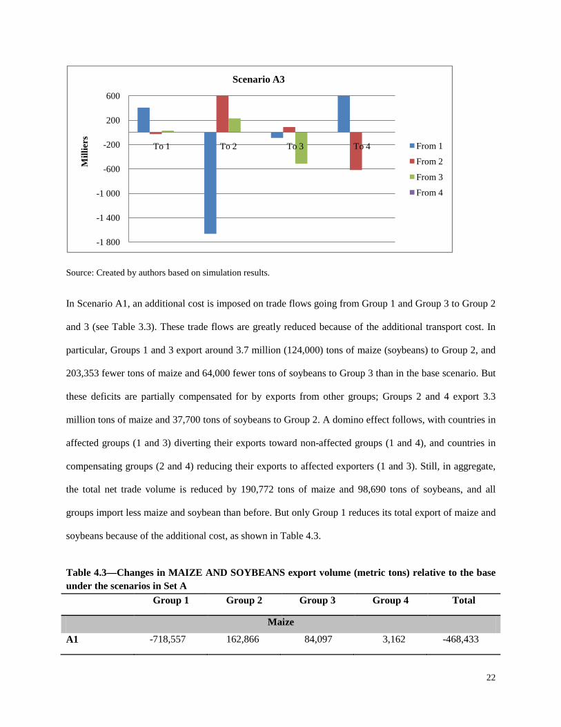
Figure 4.2—Changes in soybean trade volume (metric tons) relative to the base under the three

scenarios in Set ASource: Created by authors based on simulation results.

-1 800

-1 400

-1 000

-600

-200

200

600

To 1 To 2 To 3 To 4

Mill

iers

Scenario A2

From 1

From 2

From 3

From 4

-1 800

-1 400

-1 000

-600

-200

200

600

To 1 To 2 To 3 To 4

Mill

iers

Scenario A1

From 1

From 2

From 3

From 4

22


In Scenario A1, an additional cost is imposed on trade flows going from Group 1 and Group 3 to Group 2

and 3 (see Table 3.3). These trade flows are greatly reduced because of the additional transport cost. In

particular, Groups 1 and 3 export around 3.7 million (124,000) tons of maize (soybeans) to Group 2, and

203,353 fewer tons of maize and 64,000 fewer tons of soybeans to Group 3 than in the base scenario. But

these deficits are partially compensated for by exports from other groups; Groups 2 and 4 export 3.3

million tons of maize and 37,700 tons of soybeans to Group 2. A domino effect follows, with countries in

affected groups (1 and 3) diverting their exports toward non-affected groups (1 and 4), and countries in

compensating groups (2 and 4) reducing their exports to affected exporters (1 and 3). Still, in aggregate,

the total net trade volume is reduced by 190,772 tons of maize and 98,690 tons of soybeans, and all

groups import less maize and soybean than before. But only Group 1 reduces its total export of maize and

soybeans because of the additional cost, as shown in Table 4.3.

Table 4.3—Changes in MAIZE AND SOYBEANS export volume (metric tons) relative to the base under the scenarios in Set A

Group 1 Group 2 Group 3 Group 4 Total

Maize

A1 -718,557 162,866 84,097 3,162 -468,433

-1 800

-1 400

-1 000

-600

-200

200

600

To 1 To 2 To 3 To 4

Mill

iers

Scenario A3

From 1

From 2

From 3

From 4

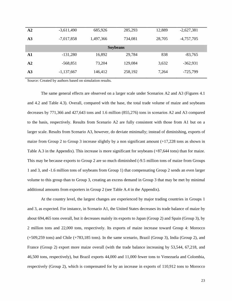
23

A2 -3,611,490 685,926 285,293 12,889 -2,627,381

A3 -7,017,858 1,497,366 734,081 28,705 -4,757,705

Soybeans

A1 -131,280 16,892 29,784 838 -83,765

A2 -568,851 73,204 129,084 3,632 -362,931

A3 -1,137,667 146,412 258,192 7,264 -725,799


The same general effects are observed on a larger scale under Scenarios A2 and A3 (Figures 4.1

and 4.2 and Table 4.3). Overall, compared with the base, the total trade volume of maize and soybeans

decreases by 771,366 and 427,643 tons and 1.6 million (855,276) tons in scenarios A2 and A3 compared

to the basis, respectively. Results from Scenario A2 are fully consistent with those from A1 but on a

larger scale. Results from Scenario A3, however, do deviate minimally; instead of diminishing, exports of

maize from Group 2 to Group 3 increase slightly by a non significant amount (+17,228 tons as shown in

Table A.3 in the Appendix). This increase is more significant for soybeans (+87,644 tons) than for maize.

This may be because exports to Group 2 are so much diminished (-9.5 million tons of maize from Groups

1 and 3, and -1.6 million tons of soybeans from Group 1) that compensating Group 2 sends an even larger

volume to this group than to Group 3, creating an excess demand in Group 3 that may be met by minimal

additional amounts from exporters in Group 2 (see Table A.4 in the Appendix).

At the country level, the largest changes are experienced by major trading countries in Groups 1

and 3, as expected. For instance, in Scenario A1, the United States decreases its trade balance of maize by

about 694,465 tons overall, but it decreases mainly its exports to Japan (Group 2) and Spain (Group 3), by

2 million tons and 22,000 tons, respectively. Its exports of maize increase toward Group 4: Morocco

(+509,259 tons) and Chile (+783,185 tons). In the same scenario, Brazil (Group 3), India (Group 2), and

France (Group 2) export more maize overall (with the trade balance increasing by 53,544, 67,218, and

46,500 tons, respectively), but Brazil exports 44,000 and 11,000 fewer tons to Venezuela and Colombia,

respectively (Group 2), which is compensated for by an increase in exports of 110,912 tons to Morocco

24

(Group 4). South Africa (Group 3) also decreases its exports of maize to various Group 2 countries by

33,819 tons but compensates by exporting 75,960 tons more to Russia (Group 4).

Results for soybeans are similar but with lower volumes, perhaps because of a lower flexibility in

the market.12

Scenarios in Set B

The United States experiences the largest decrease in net exports (-65,520 tons overall in

Scenario A1), especially toward Group 2: China (-46,087 tons) and Japan (-17,392 tons). Brazil and

Paraguay (Group 3) increase their exports (+69,219 tons overall in Scenario A1) toward countries of

Group 2 (Japan, Zimbabwe, and Germany) and Group 1 (Uruguay).

Change in Main Market Variables

Table 4.4 shows the relative changes in prices and quantities at the global level. These results are almost

identical to the ones under Set A when comparing the three scenarios (Table 4). In particular, the volume

of production and the average of supply and demand prices experience identical relative changes. This

may indicate that the additional changes have only minor effects on the market, given that they do not

represent major trade flows.

Table 4.4—Relative changes (%) in world market variables under scenarios in Set B compared with the base

Maize Soybeans

Scenario B1 B2 B3 B1 B2 B3

Aggregate quantity -0.04% -0.16% -0.33% -0.05% -0.22% -0.45%

Average pS +0.4% +1.4% +3.1% +0.38% +1.58% +3.10%

Average pD +0.7% +2.7% +5.8% +0.50% +2.13% +4.20%


Table 4.5—Relative changes (%) in key variables in each group of countries under scenarios in Set B compared with the base Group 1 Group 2 Group 3 Group 4

Scenario B1 B2 B3 B1 B2 B3 B1 B2 B3 B1 B2 B3

12 Soybean production and exports are concentrated in a few North and South American countries.

25

Maize Supply -0.13 -0.7 -1.38 +0.07 +0.53 +0.99 -0.13 -0.63 -1.17 -0.01 -0.32 -0.69

Demand +0.23 +1.2 +2.4 -0.17 -0.95 -1.86 -0.35 -1.37 -2.9 +0.06 +0.57 +1.2 Average pS -0.53 -2.86 -6.34 +0.65 +2.68 +5.7 -0.85 -4.36 -8.1 +0.02 -0.58 -1.3 Average pD -0.53 -2.86 -6.34 +0.9 +3.7 +7.9 +1.36 +5.24 +11 -0.1 -1.9 -4.08 Soybeans Supply -0.08 -0.35 -0.7 +0.04 +0.18 +0.35 -0.06 -0.27 -0.5 +0.01 +0.05 +0.09

Demand +0.05 +0.21 +0.43 -0.15 -0.63 -1.27 -0.16 -0.7 -1.4 -0.05 -0.22 -0.45 Average pS -0.8 -3.5 -7 +0.5 +2.2 +4.4 -0.7 -3.1 -6.2 +0.8 +2.67 +4.3 Average pD -0.8 -3.5 -7 +0.58 +2.54 +5.1 +0.7 +2.9 +5.8 +0.6 +1.4 +1.24


Table 4.5 presents the same relative changes by group. Once again, the results are similar to the

ones obtained under Set A, in terms of both signs and quantitative relative changes from the base. A few

changes appear for selected scenarios and variables, but never exceeding +/-0.2 percent. The only visible

difference concerns Group 4 in the case of soybeans. This group, a relatively lower trader of soybeans

than others, experiences additional costs for its imports from CPB members (countries of Group 3)

compared with Set A. This results in slightly different effects on the demand side under scenarios B2 and

B3, compared with A2 and A3. While Group 1 also witnesses the same changes for imports from CPB

members, the effects of additional transport costs are negligible, because the group is made up of mostly

net exporting regions, or regions that may compensate for their losses.

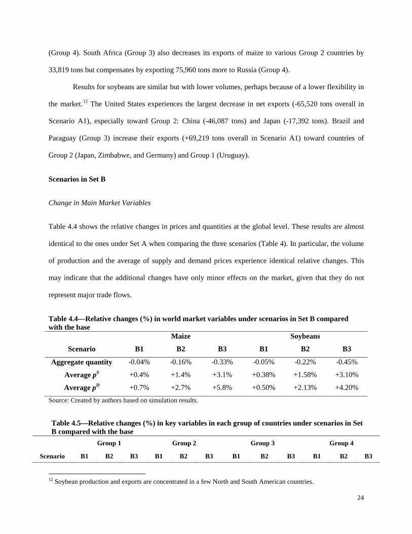
Trade Effects

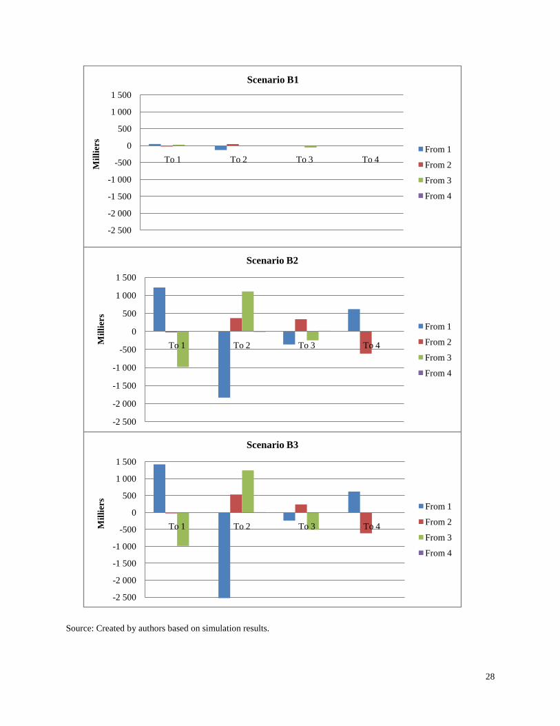
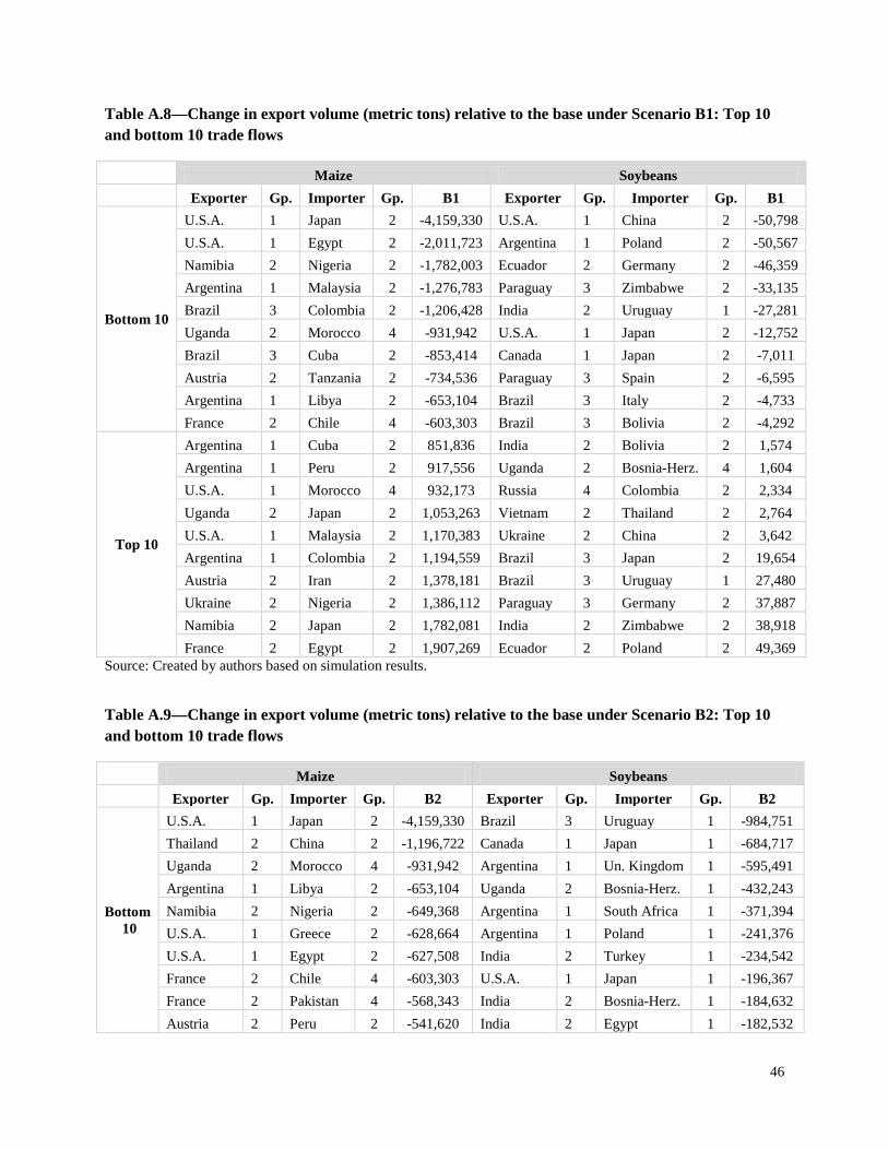
The trade effects of the shocks implemented under scenarios B1, B2, and B3 are presented in Figures 4.3

and 4.4 and Table 4.6 (total exports by group). In addition, detailed bilateral group flows are shown in

Tables A.3 and A.4 in the Appendix, as was done in the case of Set A. At first view, the aggregate results

of Table 4.6 appear quite similar to those observed in Table 4.3 (Set A). Total trade volume of maize is

reduced by 468,433 tons and soybeans by 83,765 tons under B1; the reductions for the two commodities

are 2.6 million tons and 362,931 tons under B2, and 4.8 million under B3 (725,799); slightly less than

under A3. All groups reduce their imports, and only Group 1 reduces its exports. But in the detail, the

amplitude and direction of intra- and intergroup trade change greatly, as visible in Figures 4.3 and 4.4.

26

Figure 4.3—Changes in maize trade volume (metric tons) relative to the base under the three scenarios in Set B

-12 000

-10 000

-8 000

-6 000

-4 000

-2 000

0

2 000

4 000

6 000

To 1 To 2 To 3 To 4

Mill

iers

Scenario B1

From 1

From 2

From 3

From 4

-12 000

-10 000

-8 000

-6 000

-4 000

-2 000

0

2 000

4 000

6 000


iers

Scenario B2

From 1

From 2

From 3

From 4

-12 000

-10 000

-8 000

-6 000

-4 000

-2 000

0

2 000

4 000

6 000


iers

Scenario B3

From 1

From 2

From 3

From 4

27


Figure 4.4—Changes in soybean trade volume (metric tons) relative to the base under the three scenarios in Set B

28


-2 500

-2 000

-1 500

-1 000

-500

0

500

1 000

1 500

To 1 To 2 To 3 To 4

Mill

iers

Scenario B1

From 1

From 2

From 3

From 4

-2 500

-2 000

-1 500

-1 000

-500

0

500

1 000

1 500


iers

Scenario B2

From 1

From 2

From 3

From 4

-2 500

-2 000

-1 500

-1 000

-500

0

500

1 000

1 500


iers

Scenario B3

From 1

From 2

From 3

From 4

29

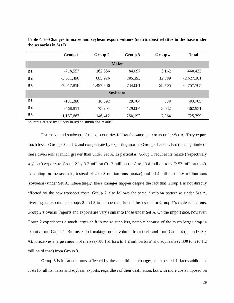
Table 4.6—Changes in maize and soybean export volume (metric tons) relative to the base under the scenarios in Set B

Group 1 Group 2 Group 3 Group 4 Total

Maize

B1 -718,557 162,866 84,097 3,162 -468,433

B2 -3,611,490 685,926 285,293 12,889 -2,627,381

B3 -7,017,858 1,497,366 734,081 28,705 -4,757,705

Soybeans

B1 -131,280 16,892 29,784 838 -83,765 B2 -568,851 73,204 129,084 3,632 -362,931 B3 -1,137,667 146,412 258,192 7,264 -725,799 Source: Created by authors based on simulation results.

For maize and soybeans, Group 1 countries follow the same pattern as under Set A: They export

much less to Groups 2 and 3, and compensate by exporting more to Groups 1 and 4. But the magnitude of

these diversions is much greater than under Set A. In particular, Group 1 reduces its maize (respectively

soybean) exports to Group 2 by 3.2 million (0.13 million tons) to 10.8 million tons (2.53 million tons),

depending on the scenario, instead of 2 to 8 million tons (maize) and 0.12 million to 1.6 million tons

(soybeans) under Set A. Interestingly, these changes happen despite the fact that Group 1 is not directly

affected by the new transport costs. Group 2 also follows the same diversion pattern as under Set A,

diverting its exports to Groups 2 and 3 to compensate for the losses due to Group 1’s trade reductions.

Group 2’s overall imports and exports are very similar to those under Set A. On the import side, however,

Group 2 experiences a much larger shift in maize suppliers, notably because of the much larger drop in

exports from Group 1. But instead of making up the volume from itself and from Group 4 (as under Set

A), it receives a large amount of maize (-188,151 tons to 1.2 million tons) and soybeans (2,300 tons to 1.2

million of tons) from Group 3.

Group 3 is in fact the most affected by these additional changes, as expected. It faces additional

costs for all its maize and soybean exports, regardless of their destination, but with more costs imposed on

30

trade to Group 2 and itself than to Group 1 and 4. Interestingly, however, these relatively smaller changes

on exports to Groups 1 and 4 lead to a complete switch in export diversion for Group 3. Group 3 reduces

its exports to Groups 1 and 4, and significantly increases its exports to Group 2 under Scenarios B2 and

B3. This may be due to different market considerations, but likely mostly to trade preference factors, such

as regular tariffs and transport costs, as well as Group 3 exporters’ own competitiveness compared with

that of other countries. The drastic drop in exports from Group 1 to Group 2 may also be a driver of this

preference for exporting to Group 2, which has the largest set of importers. Despite these significant

changes, the aggregate exports and imports under Set B scenarios are virtually identical to those under Set

A scenarios (they are actually identical for soybeans). The effect is a simple and pure trade diversion.

Lastly, trade from and to Group 4 is relatively unaffected by the new measure compared with the results

for Scenario A. Its total imports do decrease more than under Set A but by relatively small volumes.

At the country level (Tables A.8, A.9, and A.10 in the Appendix), the largest changes can be

seen in major trading nations of Group 1 and especially Group 3. For instance, in the case of Scenario B1,

the United States (Group 1) reduces its maize exports by 4.16 million tons to Japan (Group 2). It also

reduces its maize exports to Vietnam (-14,954 tons) and Turkey (-10,205 tons), both from Group 2. These

reductions are compensated for by increased maize exports to Group 4: Morocco (+932,173 tons), Chile

(+782,839 tons), Malawi (+590,932 tons), Kuwait (+403,115 tons), and to a smaller extent, Angola

(+77,944 tons) and Bosnia and Herzegovina (+12,750 tons). The United States also experiences increased

maize exports toward Group 2 countries by 1.17 million tons to Malaysia and by more than 600,000 tons

each to Ecuador, Belgium, Bangladesh, Greece, Honduras, Libya, Mauritius, Italy, and Slovenia. Its

exports to Germany (Group 3) also increase significantly, by 485,300 tons.13

Brazil (Group 3) significantly decreases its maize exports to Colombia and Cuba (Group 2) by

1.2 million tons and 853,414 tons, respectively, and to a smaller extent, toward Vietnam (Group 2) by

about 87,600 tons. These decreases are compensated for by increased exports to other countries within

Group 2: Tanzania (+717,000 tons), Sudan (+573,214 tons), Mozambique (+394,000 tons), Kenya (+

13 Overall the United States does decrease its maize exports by about 650,200 tons in this scenario.

31

325,912 tons), and Yemen (+190,876 tons). South Africa reduces its exports to Germany (Group 3) by

about 459,000 tons, and to Group 2 countries Ecuador (-116,806 tons); Belgium (-87,596 tons); Greece

and Honduras (down more than 70,000 tons each); and to a lesser extent, Slovenia, Israel, Egypt, and

Syria (down less than 4,000 tons each). These reductions are compensated for by exporting an additional

590,729 tons and 300,971 tons toward closer Japan and Bangladesh (Group 2), respectively. As expected,

each of these changes is consistent with a cost-minimizing effort on behalf of the exporting country;

substitutions are made only to countries at similar distance or closer, or those that have similar or not

significantly different trade policies.

As with maize, the largest changes for soybeans can be seen in major trading nations of Group 1

and Group 3. Under Scenario B1, the United States (Group 1) decreases its soybean exports by more than

50,000 tons to China and Poland (Group 2), while Paraguay (Group 3) reduces its exports by 33,135 tons

to Zimbabwe (Group 2) and by about 6,600 tons to Spain (Group 2). Brazil (Group 3) also decreases its

exports to Group 2 countries Bolivia, Italy, and Spain by more than 4,000 tons each and compensates by

additional exports of 24,480 tons and 19,654 tons of soybean exports to Uruguay (Group 1) and Japan

(Group 2), respectively. Paraguay (Group 3) increases its exports to Germany (Group 2) by about 38,000

tons.

Discussion: From Markets to Welfare Effects

The results from the simulations have shown that implementing strict information requirements with the

“does contain” option on maize and soybeans could have significant market and especially trade effects.

However, although there is less trade and smaller volume of maize or soybeans, which constitute clear

market losses, not all countries will experience similar welfare outcomes. In this section we look further

by analyzing economic welfare for countries in different regions.

We use the slope and intercept coefficients and the supply and demand variables to compute

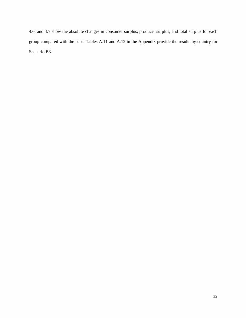
Marshallian consumer and producer surpluses for each country and group in each scenario. Figures 4.5,

32

4.6, and 4.7 show the absolute changes in consumer surplus, producer surplus, and total surplus for each

group compared with the base. Tables A.11 and A.12 in the Appendix provide the results by country for

Scenario B3.

33

Figure 4.5—Change in consumer surplus (U.S. dollars per year) for each group under each scenario

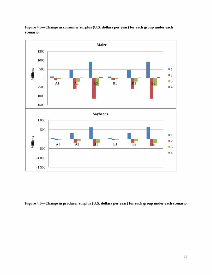
Figure 4.6—Change in producer surplus (U.S. dollars per year) for each group under each scenario

-1500

-1000

-500

0

500

1000

1500

A1 A2 A3 B1 B2 B3

Mill

ions

Maize

1

2

3

4

-1 500

-1 000

-500

0

500

1 000

A1 A2 A3 B1 B2 B3

Mill

ions

Soybeans

1

2

3

4

34

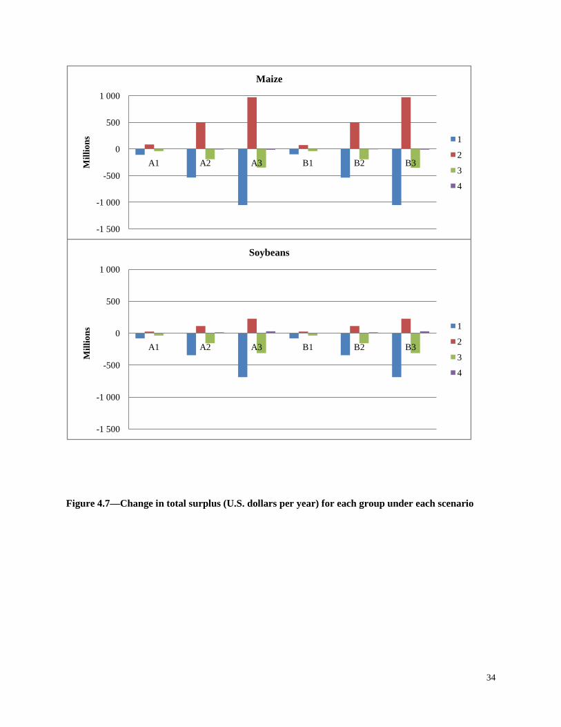
Figure 4.7—Change in total surplus (U.S. dollars per year) for each group under each scenario

-1 500

-1 000

-500

0

500

1 000

A1 A2 A3 B1 B2 B3

Mill

ions

Soybeans

1

2

3

4

-1 500

-1 000

-500

0

500

1 000

A1 A2 A3 B1 B2 B3Mill

ions

Maize

1

2

3

4

35

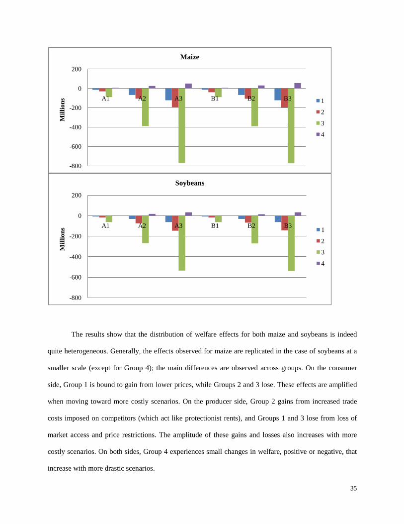
The results show that the distribution of welfare effects for both maize and soybeans is indeed

quite heterogeneous. Generally, the effects observed for maize are replicated in the case of soybeans at a

smaller scale (except for Group 4); the main differences are observed across groups. On the consumer

side, Group 1 is bound to gain from lower prices, while Groups 2 and 3 lose. These effects are amplified

when moving toward more costly scenarios. On the producer side, Group 2 gains from increased trade

costs imposed on competitors (which act like protectionist rents), and Groups 1 and 3 lose from loss of

market access and price restrictions. The amplitude of these gains and losses also increases with more

costly scenarios. On both sides, Group 4 experiences small changes in welfare, positive or negative, that

increase with more drastic scenarios.

-800

-600

-400

-200

0

200

A1 A2 A3 B1 B2 B3

Mill

ions

Maize

1

2

3

4

-800

-600

-400

-200

0

200

A1 A2 A3 B1 B2 B3

Mill

ions

Soybeans

1

2

3

4

36

Still, when considering both producer and consumer surplus (Figure 4.7), Group 4 is the only one

that derives net welfare gains, which grow from A1 to A3 and B2 to B3, with minimal losses under B1. In

contrast, Group 3 does experience non-negligible net losses for maize from US$89 million14

Overall, these results show that most countries (54 out of 80 countries for maize and 41 out of 53

for soybeans, as shown in tables A.11 and A.12 in Appendix) are bound to lose with strict information

requirements, which confirms the conclusions of other studies. But they also shed light on some of the

key supports for such requirements as the Cartagena Protocol. Nonmembers have only an indirect role to

play in negotiation, so even if the large trading countries in Group 1 (like Argentina, Canada, or the

United States) continue to push against it, they may not advance much. Group 4 countries are absent from

discussions, as smaller traders and non-members. The core of the support obviously needs to come from

member countries in Groups 2 and 3, groups that are both bound to lose overall, especially Group 3

countries for maize (Brazil and Romania are the biggest losers, as shown in Table A.11 in the Appendix)

and Groups 2 and 3 countries for soybeans (Brazil and Japan are the biggest losers, as shown in Table

A.12 in the Appendix). Yet member countries of these groups (especially Brazil, European countries, and

African countries) have generally been very supportive of the strict requirements in meetings of the

Protocol. So why do they support a measure that could be economically detrimental for them?

under

Scenarios A1 and B1 to $773 million under Scenarios A3 and B3. To a smaller extent, the total welfare

losses (which include lost tax revenues) are also quite significant for soybeans, from $62 million under

Scenarios A1 and B1 to more than $535 million under Scenarios A3 and B3. Interestingly, Group 2

countries overall, representing CPB members, lose more than Group 1 countries, which are not members

of the CPB, but that result is mostly because Group 2 countries together are net importers of maize and

soybeans, and because consumers bear more of the surplus than do producers.

As in other political forums, a well-known result from the literature (Olson 1965) is that the best-

organized groups are bound to be the most influential. In developed countries, the most influential or

well-organized parties tend to be on the production side. Results presented in Figures 4.6 and 4.7 suggest 14 All dollar amounts are in U.S. dollars.

37

that producers, especially in countries of Group 2, are bound to gain from this measure significantly. In

other countries of Group 2, notably those in Africa, producers and consumers are typically not well

represented, and the support for such measure has been seen from anti-GM organizations, which are

pushing for any restriction in the marketing of GM food.

Yet these countries are bound to be directly affected by the measure, with potentially high losses

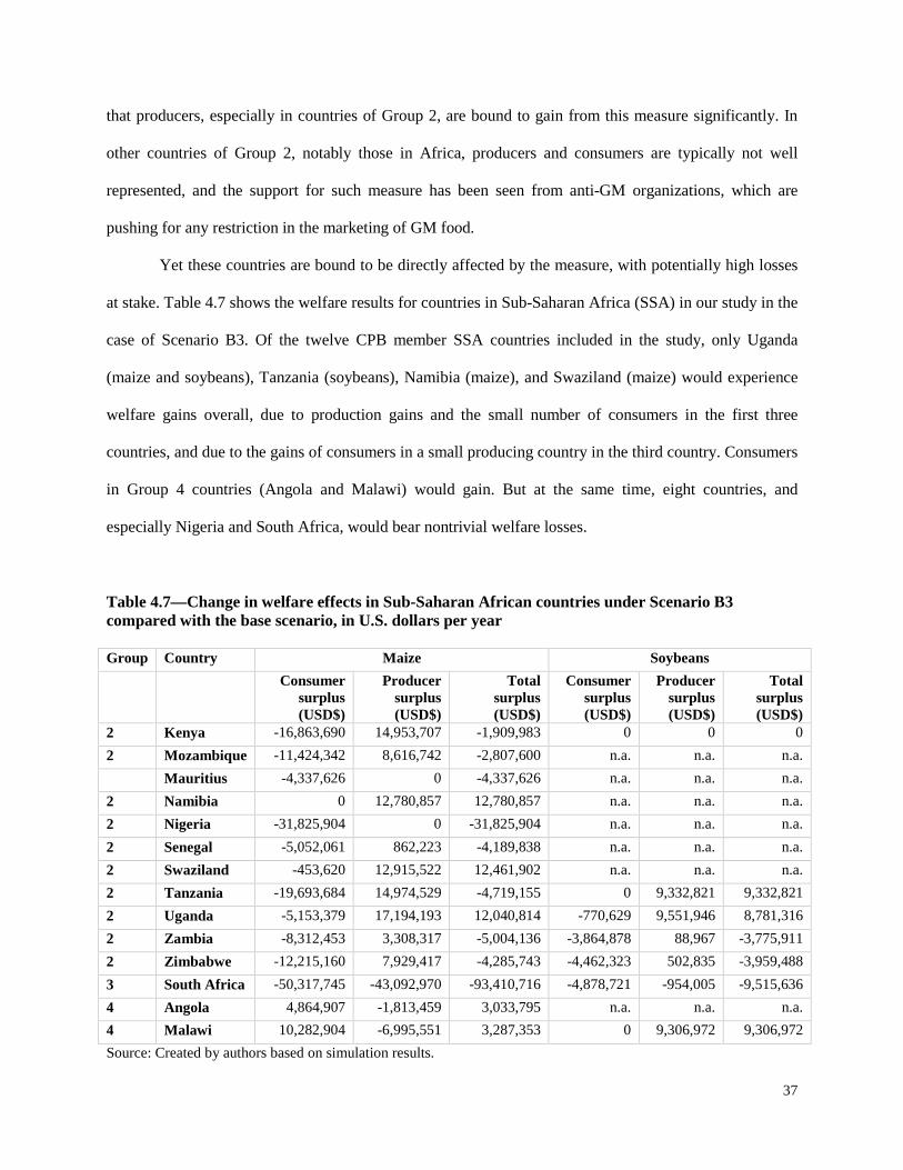
at stake. Table 4.7 shows the welfare results for countries in Sub-Saharan Africa (SSA) in our study in the

case of Scenario B3. Of the twelve CPB member SSA countries included in the study, only Uganda

(maize and soybeans), Tanzania (soybeans), Namibia (maize), and Swaziland (maize) would experience

welfare gains overall, due to production gains and the small number of consumers in the first three

countries, and due to the gains of consumers in a small producing country in the third country. Consumers

in Group 4 countries (Angola and Malawi) would gain. But at the same time, eight countries, and

especially Nigeria and South Africa, would bear nontrivial welfare losses.

Table 4.7—Change in welfare effects in Sub-Saharan African countries under Scenario B3 compared with the base scenario, in U.S. dollars per year Group Country Maize Soybeans Consumer

surplus (USD$)

Producer surplus (USD$)

Total surplus (USD$)

Consumer surplus (USD$)

Producer surplus (USD$)

Total surplus (USD$)

2 Kenya -16,863,690 14,953,707 -1,909,983 0 0 0 2 Mozambique -11,424,342 8,616,742 -2,807,600 n.a. n.a. n.a. Mauritius -4,337,626 0 -4,337,626 n.a. n.a. n.a. 2 Namibia 0 12,780,857 12,780,857 n.a. n.a. n.a. 2 Nigeria -31,825,904 0 -31,825,904 n.a. n.a. n.a. 2 Senegal -5,052,061 862,223 -4,189,838 n.a. n.a. n.a. 2 Swaziland -453,620 12,915,522 12,461,902 n.a. n.a. n.a. 2 Tanzania -19,693,684 14,974,529 -4,719,155 0 9,332,821 9,332,821 2 Uganda -5,153,379 17,194,193 12,040,814 -770,629 9,551,946 8,781,316 2 Zambia -8,312,453 3,308,317 -5,004,136 -3,864,878 88,967 -3,775,911 2 Zimbabwe -12,215,160 7,929,417 -4,285,743 -4,462,323 502,835 -3,959,488 3 South Africa -50,317,745 -43,092,970 -93,410,716 -4,878,721 -954,005 -9,515,636 4 Angola 4,864,907 -1,813,459 3,033,795 n.a. n.a. n.a. 4 Malawi 10,282,904 -6,995,551 3,287,353 0 9,306,972 9,306,972 Source: Created by authors based on simulation results.

38

Note: n.a. = Not available—countries not included in the soybean model.

While small producers in SSA countries (mostly in Group 2) do not always connect to the market

(an implicit assumption here), urban consumers are immediately affected by price increases, as observed

during the food price increase of 2008. This means that the presumed gains for producers may be

overestimated here while consumers’ losses may be underestimated. Producers in Groups 3 and 4 that are

connected to the market will also lose. Even South Africa will experience large losses for both producers

and consumers. All these groups will probably pay a much larger proportional price than consumers in

developed nations of Groups 2 and 3, given their resources, or even producers in some of the most

productive countries of Group 3.

Naturally, these welfare effects would change if countries were to change their group. Countries

like Kenya, Tanzania, and Uganda are part of a large public–private partnership to develop drought-

tolerant GM maize, and if they adopted this promising crop, they would join Group 3 and would thus bear

welfare losses for both producers and consumers. This “penalty effect” for GM adoption provides a

rationale for why the measure is so strongly supported by anti-GM groups. If in place, it could further

discourage developing countries in Africa that are already subject to external influence (see, for example,

Paarlberg 2008) from moving toward GM crop adoption.

39

5. Conclusions

In this paper we investigate the economic effects of implementing a strict information requirement (“does

contain LMO-FFPs” with a list of specific GM events) under Article 18.2(a) of the Cartagena Protocol on

Biosafety. More specifically, our analysis focuses on evaluating the effect on prices, trade, and welfare of

implementing this regulation at the global level.

Using a simple analytical model, we first show that such regulation would create price tension

with losers and winners. We then use an empirical model to validate our hypothesis in the case of maize

and soybeans. We find that under relatively conservative cost assumptions, information requirements

would have a significant effect on the world market for both maize and soybeans. But they would have

even greater effects on trade, creating significant trade distortion that diverts exports from their original

destination. In particular, nonmember countries that produce GM products would reduce their exports to

Protocol members, and GM-producing countries that are part of the Protocol would also divert their

exports to new destinations, depending on the scenario. The measure would reduce world trade and

production in maize and soybeans, with significant welfare effects.

At the global level, under the more costly scenario, total welfare effects (consumer and producer

surplus plus tax revenue) would decline by up to $1.036 billion annually for maize and by up to $716

million annually for soybeans, with significant heterogeneity across countries and agents. While non-GM

producers in Protocol member countries would benefit from increased protection, consumers and

producers in selected countries of SSA would proportionately pay a much heftier price for the regulation.

Even those that derive gains from new protectionist rents would lose if they decided to adopt potentially

beneficial GM crops currently under development, like drought-resistant maize. This situation calls for

governments in African and other affected countries to reconsider their support for this new regulation,

which does not present any clear benefit for regulators but, if implemented, would be associated with

significant costs for generations to come.

40

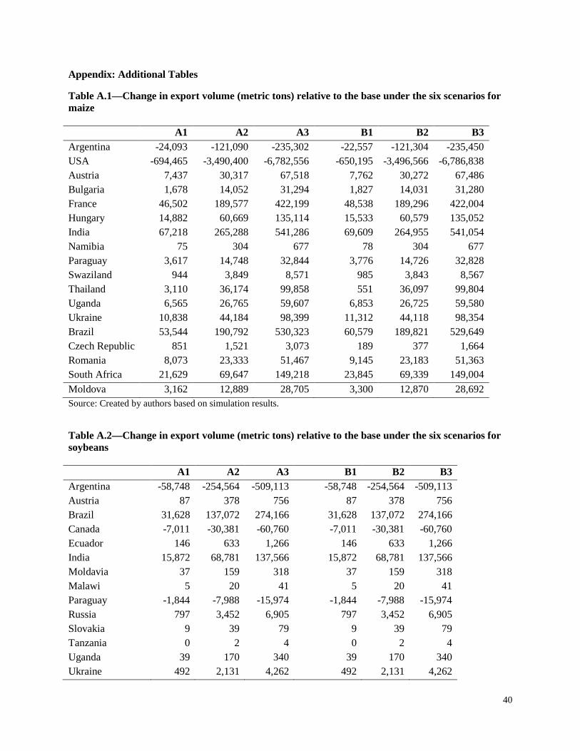
Appendix: Additional Tables

Table A.1—Change in export volume (metric tons) relative to the base under the six scenarios for maize

A1 A2 A3 B1 B2 B3 Argentina -24,093 -121,090 -235,302 -22,557 -121,304 -235,450 USA -694,465 -3,490,400 -6,782,556 -650,195 -3,496,566 -6,786,838 Austria 7,437 30,317 67,518 7,762 30,272 67,486 Bulgaria 1,678 14,052 31,294 1,827 14,031 31,280 France 46,502 189,577 422,199 48,538 189,296 422,004 Hungary 14,882 60,669 135,114 15,533 60,579 135,052 India 67,218 265,288 541,286 69,609 264,955 541,054 Namibia 75 304 677 78 304 677 Paraguay 3,617 14,748 32,844 3,776 14,726 32,828 Swaziland 944 3,849 8,571 985 3,843 8,567 Thailand 3,110 36,174 99,858 551 36,097 99,804 Uganda 6,565 26,765 59,607 6,853 26,725 59,580 Ukraine 10,838 44,184 98,399 11,312 44,118 98,354 Brazil 53,544 190,792 530,323 60,579 189,821 529,649 Czech Republic 851 1,521 3,073 189 377 1,664 Romania 8,073 23,333 51,467 9,145 23,183 51,363 South Africa 21,629 69,647 149,218 23,845 69,339 149,004 Moldova 3,162 12,889 28,705 3,300 12,870 28,692 Source: Created by authors based on simulation results.

Table A.2—Change in export volume (metric tons) relative to the base under the six scenarios for soybeans

A1 A2 A3 B1 B2 B3 Argentina -58,748 -254,564 -509,113 -58,748 -254,564 -509,113 Austria 87 378 756 87 378 756 Brazil 31,628 137,072 274,166 31,628 137,072 274,166 Canada -7,011 -30,381 -60,760 -7,011 -30,381 -60,760 Ecuador 146 633 1,266 146 633 1,266 India 15,872 68,781 137,566 15,872 68,781 137,566 Moldavia 37 159 318 37 159 318 Malawi 5 20 41 5 20 41 Paraguay -1,844 -7,988 -15,974 -1,844 -7,988 -15,974 Russia 797 3,452 6,905 797 3,452 6,905 Slovakia 9 39 79 9 39 79 Tanzania 0 2 4 0 2 4 Uganda 39 170 340 39 170 340 Ukraine 492 2,131 4,262 492 2,131 4,262

41

U.S.A. -65,520 -283,906 -567,794 -65,520 -283,906 -567,794 Venezuela 3 12 25 3 12 25 Vietnam 238 1,031 2,062 238 1,031 2,062 Zambia 6 26 53 6 26 53 Source: Created by authors based on simulation results.

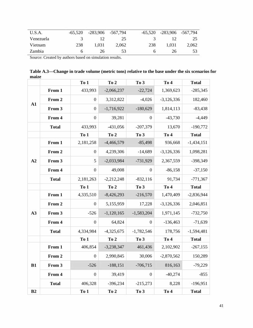
Table A.3—Change in trade volume (metric tons) relative to the base under the six scenarios for maize

To 1 To 2 To 3 To 4 Total

A1

From 1 433,993 -2,066,237 -22,724 1,369,623 -285,345

From 2 0 3,312,822 -4,026 -3,126,336 182,460

From 3 0 -1,716,922 -180,629 1,814,113 -83,438

From 4 0 39,281 0 -43,730 -4,449

Total 433,993 -431,056 -207,379 13,670 -190,772


A2

From 1 2,181,258 -4,466,579 -85,498 936,668 -1,434,151

From 2 0 4,239,306 -14,689 -3,126,336 1,098,281

From 3 5 -2,033,984 -731,929 2,367,559 -398,349

From 4 0 49,008 0 -86,158 -37,150

Total 2,181,263 -2,212,248 -832,116 91,734 -771,367


A3

From 1 4,335,510 -8,426,293 -216,570 1,470,409 -2,836,944

From 2 0 5,155,959 17,228 -3,126,336 2,046,851

From 3 -526 -1,120,165 -1,583,204 1,971,145 -732,750

From 4 0 64,824 0 -136,463 -71,639

Total 4,334,984 -4,325,675 -1,782,546 178,756 -1,594,481


B1

From 1 406,854 -3,238,347 461,436 2,102,902 -267,155

From 2 0 2,990,845 30,006 -2,870,562 150,289

From 3 -526 -188,151 -706,715 816,163 -79,229

From 4 0 39,419 0 -40,274 -855

Total 406,328 -396,234 -215,273 8,228 -196,951

B2 To 1 To 2 To 3 To 4 Total

42

From 1 2,185,643 -7,178,650 -99,770 3,656,093 -1,436,684

From 2 0 4,208,457 14,253 -3,126,336 1,096,374

From 3 -526 712,501 -744,823 -366,637 -399,485

From 4 0 48,989 0 -79,915 -30,926

Total 2,185,117 -2,208,702 -830,340 83,205 -770,720

B3


From 1 4,338,328 -10,799,805 -176,226 3,798,926 -2,838,777

From 2 0 5,211,903 -39,272 -3,126,336 2,046,295

From 3 -526 1,198,826 -1,565,476 -366,637 -733,813

From 4 0 64,811 0 -132,545 -67,734

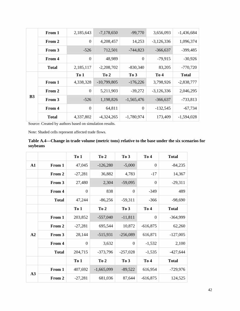
Total 4,337,802 -4,324,265 -1,780,974 173,409 -1,594,028 Source: Created by authors based on simulation results.

Note: Shaded cells represent affected trade flows.

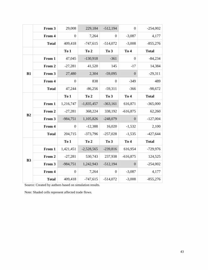
Table A.4—Change in trade volume (metric tons) relative to the base under the six scenarios for soybeans


A1 From 1 47,045 -126,280 -5,000 0 -84,235

From 2 -27,281 36,882 4,783 -17 14,367

From 3 27,480 2,304 -59,095 0 -29,311

From 4 0 838 0 -349 489

Total 47,244 -86,256 -59,311 -366 -98,690


A2

From 1 203,852 -557,040 -11,811 0 -364,999

From 2 -27,281 695,544 10,872 -616,875 62,260

From 3 28,144 -515,931 -256,089 616,871 -127,005

From 4 0 3,632 0 -1,532 2,100

Total 204,715 -373,796 -257,028 -1,535 -427,644


A3 From 1 407,692 -1,665,099 -89,522 616,954 -729,976

From 2 -27,281 681,036 87,644 -616,875 124,525

43

From 3 29,008 229,184 -512,194 0 -254,002

From 4 0 7,264 0 -3,087 4,177

Total 409,418 -747,615 -514,072 -3,008 -855,276


B1

From 1 47,045 -130,918 -361 0 -84,234

From 2 -27,281 41,520 145 -17 14,384

From 3 27,480 2,304 -59,095 0 -29,311

From 4 0 838 0 -349 489

Total 47,244 -86,256 -59,311 -366 -98,672

B2


From 1 1,216,747 -1,835,457 -363,161 616,871 -365,000

From 2 -27,281 368,224 338,192 -616,875 62,260

From 3 -984,751 1,105,826 -248,079 0 -127,004

From 4 0 -12,388 16,020 -1,532 2,100

Total 204,715 -373,796 -257,028 -1,535 -427,644

B3


From 1 1,421,451 -2,528,565 -239,816 616,954 -729,976

From 2 -27,281 530,743 237,938 -616,875 124,525

From 3 -984,751 1,242,943 -512,194 0 -254,002

From 4 0 7,264 0 -3,087 4,177

Total 409,418 -747,615 -514,072 -3,008 -855,276 Source: Created by authors based on simulation results.

Note: Shaded cells represent affected trade flows.

44

Table A.5—Change in export volume (metric tons) relative to the base under Scenario A1: Top 10 and bottom 10 trade flows

Maize Soybeans Exporter Gp. Importer Gp. A1 Exporter Gp. Importer Gp. A1

Bottom 10

U.S.A. 1 Japan 2 -2,043,532 U.S.A. 1 China 2 -46,087 Uganda 2 Morocco 4 -931,942 Argentina 1 Poland 2 -27,622 Czech Rep. 3 Nigeria 2 -669,621 India 2 Uruguay 1 -27,281 France 2 Chile 4 -603,303 Ecuador 2 Germany 2 -25,808 France 2 Pakistan 4 -568,343 U.S.A. 1 Japan 2 -17,392 Czech Rep. 3 Sri Lanka 2 -484,336 Argentina 1 Un. Kingdom 2 -12,848 Hungary 2 Iran 2 -460,190 Paraguay 3 Zimbabwe 2 -12,806 France 2 Russia 4 -452,677 Brazil 3 Zimbabwe 2 -9,720 Swaziland 2 Iran 2 -451,490 Argentina 1 Colombia 2 -7,394 Austria 2 Bosnia-Herz. 4 -282,808 Canada 1 Japan 2 -7,011

Top 10

Czech Rep. 3 Bosnia-Herz. 4 283,154 India 2 Hungary 2 5,469 U.S.A. 1 Morocco 4 509,259 India 2 Philippines 2 5,469 France 2 Sri Lanka 2 531,194 India 2 Poland 2 5,469 Czech Rep. 3 Russia 4 546,623 Ecuador 2 Un. Kingdom 2 5,469 Swaziland 2 Nigeria 2 582,529 India 2 Un. Kingdom 2 5,469 Czech Rep. 3 Pakistan 4 594,509 Russia 4 Colombia 2 6,882 U.S.A. 1 Chile 4 783,185 Paraguay 3 Germany 2 17,447 Hungary 2 Japan 2 896,275 Ecuador 2 Poland 2 21,876 France 2 Iran 2 950,620 India 2 Zimbabwe 2 22,426 Uganda 2 Japan 2 1,098,893 Brazil 3 Japan 2 24,292




Bottom 10

U.S.A. 1 Japan 2 -4,159,330 Brazil 3 Bolivia 2 -501,060 Thailand 2 China 2 -1,199,270 Uganda 2 Bosnia-Herz. 4 -432,243 Uganda 2 Morocco 4 -931,942 India 2 Turkey 2 -234,542 Argentina 1 Malaysia 2 -841,513 India 2 Bosnia-Herz. 4 -184,632 Czech Rep. 3 Nigeria 2 -727,999 India 2 Egypt 2 -182,532 Argentina 1 Libya 2 -653,104 Argentina 1 Poland 2 -162,159 France 2 Chile 4 -603,303 U.S.A. 1 Thailand 2 -130,349 Hungary 2 Philippines 3 -574,536 Ukraine 2 China 2 -123,903 France 2 Pakistan 4 -568,343 Ecuador 2 Zimbabwe 2 -104,966 U.S.A. 1 Egypt 2 -564,026 U.S.A. 1 China 2 -80,452

45

Top 10

Czech Rep. 3 Pakistan 4 607,664 Russia 4 Colombia 2 20,346 Romania 3 Libya 2 632,932 Brazil 3 Uruguay 1 28,144 Argentina 1 Venezuela 2 704,129 Brazil 3 Japan 2 95,385 Argentina 1 Japan 2 719,280 Ukraine 2 Thailand 2 117,054 Brazil 3 Morocco 4 789,684 Ecuador 2 Poland 2 146,735 U.S.A. 1 Chile 4 805,020 India 2 Zimbabwe 2 158,979 U.S.A. 1 Malaysia 2 838,654 Uganda 2 Egypt 2 179,617 France 2 Iran 2 932,177 Uganda 2 Turkey 2 230,674 Uganda 2 Japan 2 1,119,093 India 2 Bolivia 2 488,289 Hungary 2 Japan 2 1,312,283 Brazil 3 Bosnia-Herz. 4 616,871




Bottom 10

U.S.A. 1 Japan 2 -4,159,330 Argentina 1 Un. Kingdom 2 -595,491 Thailand 2 China 2 -1,857,582 Uganda 2 Bosnia-Herz. 4 -432,243 Uganda 2 Morocco 4 -931,942 Argentina 1 Poland 2 -295,261 Argentina 1 Malaysia 2 -820,895 U.S.A. 1 China 2 -284,820 U.S.A. 1 Greece 2 -780,970 India 2 Turkey 2 -234,542 Czech Rep. 3 Nigeria 2 -727,999 U.S.A. 1 Japan 2 -196,367 U.S.A. 1 Croatia 2 -692,480 India 2 Bosnia-Herz. 4 -184,632 France 2 Chile 4 -603,303 India 2 Egypt 2 -182,532 Hungary 2 Philippines 3 -574,536 Ecuador 2 Zimbabwe 2 -147,764 France 2 Pakistan 4 -568,343 Ukraine 2 China 2 -123,903

Top 10

Argentina 1 Angola 4 562,121 Brazil 3 Bolivia 2 82,944 Czech Rep. 3 Russia 4 582,496 Ukraine 2 South Africa 3 87,644 India 2 Croatia 2 605,554 Russia 4 Colombia 2 89,544 South Africa 3 Greece 2 645,414 India 2 Zimbabwe 2 115,147 U.S.A. 1 Chile 4 716,828 Uganda 2 Egypt 2 176,701 France 2 Iran 2 790,355 Uganda 2 Turkey 2 226,806 France 2 Japan 2 797,160 Ecuador 2 Poland 2 244,635 Swaziland 2 Nigeria 2 823,567 Brazil 3 Japan 2 256,635 Uganda 2 Japan 2 1,151,935 India 2 Un. Kingdom 2 583,537 Hungary 2 Japan 2 1,386,728 Argentina 1 Bosnia-Herz. 4 616,954


46

Table A.8—Change in export volume (metric tons) relative to the base under Scenario B1: Top 10 and bottom 10 trade flows

Maize Soybeans Exporter Gp. Importer Gp. B1 Exporter Gp. Importer Gp. B1

Bottom 10

U.S.A. 1 Japan 2 -4,159,330 U.S.A. 1 China 2 -50,798 U.S.A. 1 Egypt 2 -2,011,723 Argentina 1 Poland 2 -50,567 Namibia 2 Nigeria 2 -1,782,003 Ecuador 2 Germany 2 -46,359 Argentina 1 Malaysia 2 -1,276,783 Paraguay 3 Zimbabwe 2 -33,135 Brazil 3 Colombia 2 -1,206,428 India 2 Uruguay 1 -27,281 Uganda 2 Morocco 4 -931,942 U.S.A. 1 Japan 2 -12,752 Brazil 3 Cuba 2 -853,414 Canada 1 Japan 2 -7,011 Austria 2 Tanzania 2 -734,536 Paraguay 3 Spain 2 -6,595 Argentina 1 Libya 2 -653,104 Brazil 3 Italy 2 -4,733 France 2 Chile 4 -603,303 Brazil 3 Bolivia 2 -4,292

Top 10

Argentina 1 Cuba 2 851,836 India 2 Bolivia 2 1,574 Argentina 1 Peru 2 917,556 Uganda 2 Bosnia-Herz. 4 1,604 U.S.A. 1 Morocco 4 932,173 Russia 4 Colombia 2 2,334 Uganda 2 Japan 2 1,053,263 Vietnam 2 Thailand 2 2,764 U.S.A. 1 Malaysia 2 1,170,383 Ukraine 2 China 2 3,642 Argentina 1 Colombia 2 1,194,559 Brazil 3 Japan 2 19,654 Austria 2 Iran 2 1,378,181 Brazil 3 Uruguay 1 27,480 Ukraine 2 Nigeria 2 1,386,112 Paraguay 3 Germany 2 37,887 Namibia 2 Japan 2 1,782,081 India 2 Zimbabwe 2 38,918 France 2 Egypt 2 1,907,269 Ecuador 2 Poland 2 49,369




Bottom 10

U.S.A. 1 Japan 2 -4,159,330 Brazil 3 Uruguay 1 -984,751 Thailand 2 China 2 -1,196,722 Canada 1 Japan 1 -684,717 Uganda 2 Morocco 4 -931,942 Argentina 1 Un. Kingdom 1 -595,491 Argentina 1 Libya 2 -653,104 Uganda 2 Bosnia-Herz. 1 -432,243 Namibia 2 Nigeria 2 -649,368 Argentina 1 South Africa 1 -371,394 U.S.A. 1 Greece 2 -628,664 Argentina 1 Poland 1 -241,376 U.S.A. 1 Egypt 2 -627,508 India 2 Turkey 1 -234,542 France 2 Chile 4 -603,303 U.S.A. 1 Japan 1 -196,367 France 2 Pakistan 4 -568,343 India 2 Bosnia-Herz. 1 -184,632 Austria 2 Peru 2 -541,620 India 2 Egypt 1 -182,532

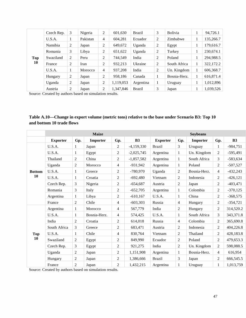
47

Top 10

Czech Rep. 3 Nigeria 2 601,630 Brazil 3 Bolivia 1 94,726.1 U.S.A. 1 Pakistan 4 604,281 Ecuador 2 Zimbabwe 1 135,266.7 Namibia 2 Japan 2 649,672 Uganda 2 Egypt 1 179,616.7 Romania 3 Libya 2 651,622 Uganda 2 Turkey 1 230,674.1 Swaziland 2 Peru 2 744,549 India 2 Poland 1 294,988.5 France 2 Iran 2 932,213 Ukraine 2 South Africa 1 322,172.2 U.S.A. 1 Morocco 4 937,208 India 2 Un. Kingdom 1 606,368.7 Hungary 2 Japan 2 958,186 Canada 1 Bosnia-Herz. 1 616,871.4 Uganda 2 Japan 2 1,119,053 Argentina 1 Uruguay 1 1,012,896 Austria 2 Japan 2 1,347,846 Brazil 3 Japan 1 1,039,526




Bottom 10

U.S.A. 1 Japan 2 -4,159,330 Brazil 3 Uruguay 1 -984,751 U.S.A. 1 Egypt 2 -2,025,745 Argentina 1 Un. Kingdom 2 -595,491 Thailand 2 China 2 -1,857,582 Argentina 1 South Africa 3 -583,634 Uganda 2 Morocco 4 -931,942 Argentina 1 Poland 2 -507,527 U.S.A. 1 Greece 2 -780,970 Uganda 2 Bosnia-Herz. 4 -432,243 U.S.A. 1 Croatia 2 -692,480 Vietnam 2 Indonesia 2 -426,121 Czech Rep. 3 Nigeria 2 -654,687 Austria 2 Japan 2 -403,471 Romania 3 Italy 2 -652,705 Argentina 1 Colombia 2 -370,125 Argentina 1 Libya 2 -610,167 U.S.A. 1 China 2 -368,575 France 2 Chile 4 -603,303 Russia 4 Hungary 2 -354,721

Top 10

Argentina 1 Morocco 4 567,779 India 2 Hungary 2 314,520.2 U.S.A. 1 Bosnia-Herz. 4 574,425 U.S.A. 1 South Africa 3 343,371.8 India 2 Croatia 2 614,018 Russia 4 Colombia 2 365,690.8 South Africa 3 Greece 2 683,471 Austria 2 Indonesia 2 404,226.8 U.S.A. 1 Chile 4 830,764 Vietnam 2 Thailand 2 428,183.8 Swaziland 2 Egypt 2 849,990 Ecuador 2 Poland 2 479,653.3 Czech Rep. 3 Egypt 2 921,275 India 2 Un. Kingdom 2 598,088.5 Uganda 2 Japan 2 1,151,908 Argentina 1 Bosnia-Herz. 4 616,954 Hungary 2 Japan 2 1,386,666 Brazil 3 Japan 2 666,545.5 France 2 Japan 2 1,432,215 Argentina 1 Uruguay 1 1,013,759


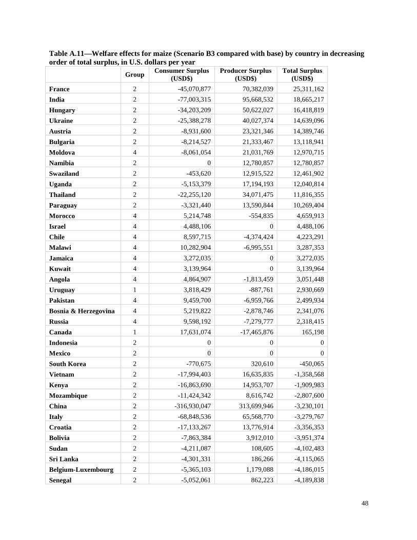
48

Table A.11—Welfare effects for maize (Scenario B3 compared with base) by country in decreasing order of total surplus, in U.S. dollars per year Group Consumer Surplus

(USD$) Producer Surplus

(USD$) Total Surplus

(USD$) France 2 -45,070,877 70,382,039 25,311,162 India 2 -77,003,315 95,668,532 18,665,217 Hungary 2 -34,203,209 50,622,027 16,418,819 Ukraine 2 -25,388,278 40,027,374 14,639,096 Austria 2 -8,931,600 23,321,346 14,389,746 Bulgaria 2 -8,214,527 21,333,467 13,118,941 Moldova 4 -8,061,054 21,031,769 12,970,715 Namibia 2 0 12,780,857 12,780,857 Swaziland 2 -453,620 12,915,522 12,461,902 Uganda 2 -5,153,379 17,194,193 12,040,814 Thailand 2 -22,255,120 34,071,475 11,816,355 Paraguay 2 -3,321,440 13,590,844 10,269,404 Morocco 4 5,214,748 -554,835 4,659,913 Israel 4 4,488,106 0 4,488,106 Chile 4 8,597,715 -4,374,424 4,223,291 Malawi 4 10,282,904 -6,995,551 3,287,353 Jamaica 4 3,272,035 0 3,272,035 Kuwait 4 3,139,964 0 3,139,964 Angola 4 4,864,907 -1,813,459 3,051,448 Uruguay 1 3,818,429 -887,761 2,930,669 Pakistan 4 9,459,700 -6,959,766 2,499,934 Bosnia & Herzegovina 4 5,219,822 -2,878,746 2,341,076 Russia 4 9,598,192 -7,279,777 2,318,415 Canada 1 17,631,074 -17,465,876 165,198 Indonesia 2 0 0 0 Mexico 2 0 0 0 South Korea 2 -770,675 320,610 -450,065 Vietnam 2 -17,994,403 16,635,835 -1,358,568 Kenya 2 -16,863,690 14,953,707 -1,909,983 Mozambique 2 -11,424,342 8,616,742 -2,807,600 China 2 -316,930,047 313,699,946 -3,230,101 Italy 2 -68,848,536 65,568,770 -3,279,767 Croatia 2 -17,133,267 13,776,914 -3,356,353 Bolivia 2 -7,863,384 3,912,010 -3,951,374 Sudan 2 -4,211,087 108,605 -4,102,483 Sri Lanka 2 -4,301,331 186,266 -4,115,065 Belgium-Luxembourg 2 -5,365,103 1,179,088 -4,186,015 Senegal 2 -5,052,061 862,223 -4,189,838

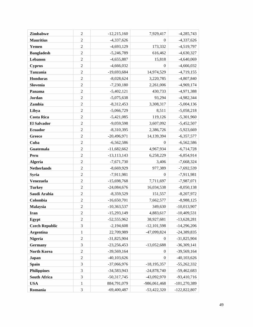
49

Zimbabwe 2 -12,215,160 7,929,417 -4,285,743 Mauritius 2 -4,337,626 0 -4,337,626 Yemen 2 -4,693,129 173,332 -4,519,797 Bangladesh 2 -5,246,789 616,462 -4,630,327 Lebanon 2 -4,655,887 15,818 -4,640,069 Cyprus 2 -4,666,032 0 -4,666,032 Tanzania 2 -19,693,684 14,974,529 -4,719,155 Honduras 2 -8,028,624 3,220,785 -4,807,840 Slovenia 2 -7,230,180 2,261,006 -4,969,174 Panama 2 -5,402,121 430,733 -4,971,388 Jordan 2 -5,075,638 93,294 -4,982,344 Zambia 2 -8,312,453 3,308,317 -5,004,136 Libya 2 -5,066,729 8,511 -5,058,218 Costa Rica 2 -5,421,085 119,126 -5,301,960 El Salvador 2 -9,059,598 3,607,092 -5,452,507 Ecuador 2 -8,310,395 2,386,726 -5,923,669 Greece 2 -20,496,971 14,139,394 -6,357,577 Cuba 2 -6,562,586 0 -6,562,586 Guatemala 2 -11,682,662 4,967,934 -6,714,728 Peru 2 -13,113,143 6,258,229 -6,854,914 Algeria 2 -7,671,730 3,406 -7,668,324 Netherlands 2 -8,669,929 977,389 -7,692,539 Syria 2 -7,911,981 0 -7,911,981 Venezuela 2 -15,698,768 7,711,697 -7,987,071 Turkey 2 -24,084,676 16,034,538 -8,050,138 Saudi Arabia 2 -8,359,529 151,557 -8,207,972 Colombia 2 -16,650,701 7,662,577 -8,988,125 Malaysia 2 -10,363,537 349,630 -10,013,907 Iran 2 -15,293,149 4,883,617 -10,409,531 Egypt 2 -52,555,962 38,927,681 -13,628,281 Czech Republic 3 -2,194,608 -12,101,598 -14,296,206 Argentina 1 22,709,989 -47,099,824 -24,389,835 Nigeria 2 -31,825,904 0 -31,825,904 Germany 3 -23,256,453 -13,052,688 -36,309,141 North Korea 2 -39,569,164 0 -39,569,164 Japan 2 -40,103,626 0 -40,103,626 Spain 3 -37,066,976 -18,195,357 -55,262,332 Philippines 3 -34,583,943 -24,878,740 -59,462,683 South Africa 3 -50,317,745 -43,092,970 -93,410,716 USA 1 884,791,079 -986,061,468 -101,270,389 Romania 3 -69,400,487 -53,422,320 -122,822,807

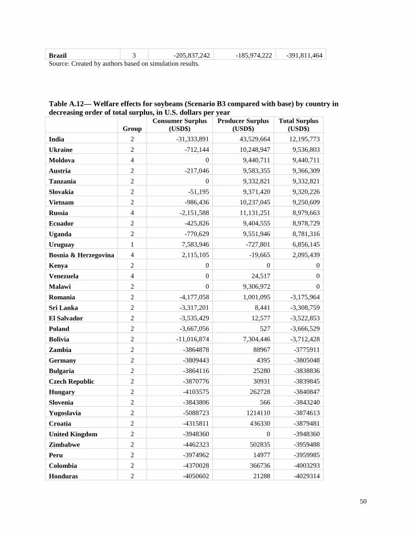
50

Brazil 3 -205,837,242 -185,974,222 -391,811,464 Source: Created by authors based on simulation results.

Table A.12— Welfare effects for soybeans (Scenario B3 compared with base) by country in decreasing order of total surplus, in U.S. dollars per year

Group Consumer Surplus

(USD$) Producer Surplus

(USD$) Total Surplus

(USD$) India 2 -31,333,891 43,529,664 12,195,773 Ukraine 2 -712,144 10,248,947 9,536,803 Moldova 4 0 9,440,711 9,440,711 Austria 2 -217,046 9,583,355 9,366,309 Tanzania 2 0 9,332,821 9,332,821 Slovakia 2 -51,195 9,371,420 9,320,226 Vietnam 2 -986,436 10,237,045 9,250,609 Russia 4 -2,151,588 11,131,251 8,979,663 Ecuador 2 -425,826 9,404,555 8,978,729 Uganda 2 -770,629 9,551,946 8,781,316 Uruguay 1 7,583,946 -727,801 6,856,145 Bosnia & Herzegovina 4 2,115,105 -19,665 2,095,439 Kenya 2 0 0 0 Venezuela 4 0 24,517 0 Malawi 2 0 9,306,972 0 Romania 2 -4,177,058 1,001,095 -3,175,964 Sri Lanka 2 -3,317,201 8,441 -3,308,759 El Salvador 2 -3,535,429 12,577 -3,522,853 Poland 2 -3,667,056 527 -3,666,529 Bolivia 2 -11,016,874 7,304,446 -3,712,428 Zambia 2 -3864878 88967 -3775911 Germany 2 -3809443 4395 -3805048 Bulgaria 2 -3864116 25280 -3838836 Czech Republic 2 -3870776 30931 -3839845 Hungary 2 -4103575 262728 -3840847 Slovenia 2 -3843806 566 -3843240 Yugoslavia 2 -5088723 1214110 -3874613 Croatia 2 -4315811 436330 -3879481 United Kingdom 2 -3948360 0 -3948360 Zimbabwe 2 -4462323 502835 -3959488 Peru 2 -3974962 14977 -3959985 Colombia 2 -4370028 366736 -4003293 Honduras 2 -4050602 21288 -4029314

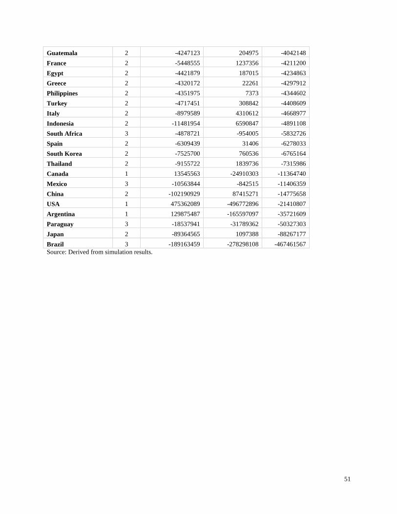
51

Guatemala 2 -4247123 204975 -4042148 France 2 -5448555 1237356 -4211200 Egypt 2 -4421879 187015 -4234863 Greece 2 -4320172 22261 -4297912 Philippines 2 -4351975 7373 -4344602 Turkey 2 -4717451 308842 -4408609 Italy 2 -8979589 4310612 -4668977 Indonesia 2 -11481954 6590847 -4891108 South Africa 3 -4878721 -954005 -5832726 Spain 2 -6309439 31406 -6278033 South Korea 2 -7525700 760536 -6765164 Thailand 2 -9155722 1839736 -7315986 Canada 1 13545563 -24910303 -11364740 Mexico 3 -10563844 -842515 -11406359 China 2 -102190929 87415271 -14775658 USA 1 475362089 -496772896 -21410807 Argentina 1 129875487 -165597097 -35721609 Paraguay 3 -18537941 -31789362 -50327303 Japan 2 -89364565 1097388 -88267177 Brazil 3 -189163459 -278298108 -467461567 Source: Derived from simulation results.

52

References

Bouët, A., Y. Decreux, L. Fontagné, S. Jean, and D. Laborde. 2008. “Assessing Applied Protection across the World.” Review of International Economics 16 (5): 850–863. Centre d’Etudes Prospectives et d’Information Internationales (CEPII). 2009. MacMaps Database consulted December 2009. Available online. http://www.cepii.fr/anglaisgraph/bdd/macmap.htm Devadoss, S., A. H. Aguiar, S. Shook, and J. Araji. 2005. “A Spatial Equilibrium of U.S.–Canadian Disputes on the World Softwood Lumber Market.” Canadian Journal of Agricultural Economics 53 (2 & 3): 177–192. Direccion Nacional de Mercados Agroalimentarios. 2004. Contexto y Opciones Para La Exportacion Segregada de Maiz y Soja OVM y No OVM en Condiciones de Bioseguridad, Conforme al Protocolo de Cartagena. Proyecto FAO/SAGPYA TCP/ARG 2903. Rome: UN Food and Agriculture Organization. FAOSTAT .2010. Database available Online<http://faostat.fao.org/faostat/collections?subset=agriculture>.

Foster, M., and D. Galeano. 2006. Biosafety Protocol-Implications of the Documentation Regime. ABARE eReport 06.2. Canberra, Australia: Australian Bureau of Agricultural and Resource Economics.

Gruère, G. P. 2006. An Analysis of Trade Related Regulations of Genetically Modified Food and their Effects on Developing Countries. EPT Discussion Paper 147, Washington DC: International Food Policy Research Institute.

Gruère, G. P., and M. W. Rosegrant. 2008. “Assessing the Implementation Effects of the Biosafety Protocol’s Proposed Stringent Information Requirements for Genetically Modified Commodities in Countries of the Asia Pacific Economic Cooperation.” Review of Agricultural Economics 30 (2): 214–232.

Huang, J., D. Zhang, J. Yang, S. Rozelle, and N. Kalaitzandonakes. 2008. “Will the Biosafety Protocol Hinder or Protect the Developing World? Learning from China’s Experience.” Food Policy 33 (1): 1–12.

ICTSD (International Centre for Trade and Sustainable Development). 2006. “Constructive Ambiguity Saves LMO Labelling Discussions at MOP-3.” 2006. Bridges Trade BioRes 6 (5): 1–3. International Grains Council. 2010. Ocean Freight Rates. Available online http://www.igc.int/en/grainsupdate/igcfreight.aspx James, C. 2008. Global Status of Commercialized Biotech/GM Crops: 2008. ISAAA Brief No. 39. Ithaca, NY: International Service for the Acquisition of Agri-Biotech Applications. JRG Consulting Group. 2004. “Economic Assessment of the Ratification of the Cartagena Protocol, Based on the Outcome of the 1st Meeting of Parties.” Final Report Prepared for Agriculture and Agri-Food Canada, Ottawa. Kalaitzandonakes, N. 2004. The Potential Impacts of the Biosafety Protocol on Agricultural Commodity Trade. IPC Technology Issue Brief. Washington, DC: International Food and Agricultural Trade Policy Council.

http://www.cepii.fr/anglaisgraph/bdd/macmap.htm�

http://faostat.fao.org/faostat/collections?subset=agriculture�

http://www.igc.int/en/grainsupdate/igcfreight.aspx�

53

Olson, M. 1965. The Logic of Collective Action. Cambridge, MA, US: MIT University Press. Paarlberg, R. 2008, Starved for Science. How Biotechnology is Being Kept Out of Africa. Harvard University Press, Cambridge, MA. Redick T. P. 2007. The Cartagena Protocol on Biosafety: Precautionary Priority in Biotech Crop Approvals and Containment of Commodities Shipments. Colorado Journal of International Environmental Law and Policy 18(Winter 2007):51–116. Rosegrant, M.W., S. Msangi, C. Ringler, T.B. Sulser, T. Zhu and S.A. Cline (2008). “International Model for Policy Analysis of Agricultural Commodities and Trade (Impact): Model Description.” Washington, D.C.: International Food Policy Research Institute. Robinson, S., A. Cattaneo, and M. El-Said. 2001. “Updating and Estimating a Social Accounting Matrix Using Cross Entropy Methods.” Economic Systems Research 13 (1): 47–64. Samuelson, P. 1952. “Spatial Price Equilibrium and Linear Programming.” American Economic Review 21: 283–303.

Secretariat of the COB (Convention on Biological Diversity). 2000. Cartagena Protocol on Biosafety to the Convention on Biological Diversity: Text and Annexes. Montreal, Canada: Secretariat of the Convention on Biological Diversity. Sobolevsky, A., G. Moschini, and H. Lapan. 2005. “Genetically Modified Crops and Product Differentiation: Trade and Welfare Effects in the Soybean Complex.” American Journal of Agricultural Economics 87 (3): 621–644.

Takayama, T., and G. Judge. 1971. Spatial and Temporal Price Allocation Models. Amsterdam: North Holland.

UN Comtrade . 2010. New York : United Nations Available at: http://comtrade.un.org/db/dqBasicQuery.aspx

You, L., and S. Wood. 2006. “An Entropy Approach to Spatial Disaggregation of Agricultural Production.” Agricultural Systems 90 (1–3): 329–347.

http://comtrade.un.org/db/dqBasicQuery.aspx�

The Price and Trade Effects of Strict Information Requirements for Genetically Modified Commodities...

Documents

Transcript of The Price and Trade Effects of Strict Information Requirements for Genetically Modified Commodities...