The power of Algorithms! - Unibo

The power of Algorithms!Lectures on algorithmic pearls

Paolo Ferragina, Universita di Pisa

These notes have been taken by the master students of the course on ”Algorithm Engi-neering” within the Laurea Magistrale in Informatica and Networking.

P.F.

Contents

1 From BWT to bzip . . . . . . . . . . . . . . . . . . . . . . . . . . . . . . 1-1

1From BWT to bzip

Alessandro Adamouadamou AT cs unibo it

Paolo Parisen Toldinpaolo.parisentoldin AT gmail com

1.1 The Burrows-Wheeler transform . . . . . . . . . . . . . . . . . . . . 1-1Forward Transform • Backward Transform

1.2 Two simple compressors: MTF and RLE . . . . . . . . . . 1-6Move-To-Front Transform • Run Length Encoding

1.3 Implementation . . . . . . . . . . . . . . . . . . . . . . . . . . . . . . . . . . . . . . . . 1-11Construction with suffix arrays

1.4 Theoretical results and compression boosting . . . . . 1-13Entropy

1.5 Some experimental tests. . . . . . . . . . . . . . . . . . . . . . . . . . . . . . 1-16

The following notes describe a lossless text compression technique devised by Michael Bur-rows and David Wheeler in 1994 at the DEC Systems Research Center. This technique,which combines simple compression algorithms with an input transformation algorithm(the so called Burrows-Wheeler Transform, or BWT), offered a revolutionary alternative todictionary-based approaches and is currently employed in widely used compressors such asbzip2.

These notes are structured as follows: we begin by describing the algorithm both forthe forward transform and for the backward transform in Section 1.1. As we will show,the BWT alone is not a compression algorithm, so two simple compressors, i.e. Move-To-Front and Run-Length Encoding, are introduced in Section 1.2. How these algorithms canbe combined for boosting textual compression is discussed with examples in Section 1.3.Section 1.4 introduces the notion of entropy and discusses the performance of the BWTwith respect to this notion. The notes conclude with a description of experiments thatcompare the implementation of BWT in the bzip2 compressor with several implementationsof dictionary-based Lempel-Ziv algorithm variants, along with a discussion on the findings.

1.1 The Burrows-Wheeler transform

The Burrows-Wheeler Transform (BWT) [4] is not a compression algorithm per se,as it does not tamper with the size, or the encoding, of its input. What the BWT doesperform is what we call block-sorting, in that the algorithm processes its input data byreordering them block-wise (i.e. the input is divided into blocks before being processed)in a convenient manner. What a “convenient manner” is, in the case of the BWT, will beshown later, but for the time being, suffice it to say that the resulting output lends itselfto greater and more effective compression by simple algorithms. Two such algorithms arethe Move-To-Front optionally followed by Run Length Encoding, both to be described insection 1.2.

c© Paolo Ferragina 1-1

1-2 Paolo Ferragina

The Burrows-Wheeler Transform consists of a pair of inverse operations; a forward trans-form rearranges the input text so that the resulting form shows a degree of “locality” inthe symbol ordering; a backward transform reconstructs the original input text, hence beingthe reverse operation of the forward transform.

1.1.1 Forward Transform

Let s = ss...sn be an input string on n characters drawn from an alphabet Σ, with a totalordering defined on the symbols in Σ.

Given s, the forward transform proceeds as follows:

1. Let s$ be the string resulting from the concatenation of s with a string consistingof a single occurrence of symbol $, where $ 6∈ Σ and $ is smaller than any othersymbol in the alphabet, according to the total ordering defined on Σ.1

2. Consider matrixM of size (n+ )×(n+ ), whose rows contain all the cyclic leftshifts of string s. M is also called the rotation matrix of s.

3. Let M′ be the matrix obtained by sorting the rows of M left-to-right accordingto the ordering defined on alphabet Σ ∪ {$}. Recall that $ is smaller than anyother symbol in Σ and, by construction, appears only once, therefore the sortoperation will always move the last row from position n+ 1 to position 0.

4. Let F and L be the first and last columns ofM′ respectively. Let l be the stringobtained by reading column L top-to-bottom, sans character $. Let r be theindex of $ in L.

5. Take bw(s) = (l, r) as the output of the algorithm.

Note that M is a conceptual matrix, in that there is no actual need to build it entirely:only the first and last columns are required for applying the forward transform. Section1.3.1 will show an example of BWT application that does not require the rotation matrixto be actually constructed in full.

Remark

An alternate enunciation of the algorithm, less frequent yet still present in the literature[5], constructs matrixM′ by sorting the rows ofM right-to-left (i.e. starting from characterat index n) in step 3. Then, in step 4, it takes string f instead of l, where f is obtainedby reading column F top-to-bottom skipping character $, and sets r as the index of $ in Finstead of L. The output is then bw(s) = (f , r). This enunciation is dual to the one givenin the following sense: although its output differs from the one generated by left-to-rightsorting, it showcases the same properties of reversibility and compression, to be illustratedbelow, as the former.

Example 1.1

We will now show an example of Burrows-Wheeler Transform applied to an input blockwhich, historically, is known to transform to a highly compressible string.

1The step that concatenates character $ to the initial string was not part of the original version of thealgorithm as described by Burrows and Wheeler. It is here introduced with the intent to simplify theenunciation. Due to its role, $ is sometimes called a sentinel character.

From BWT to bzip 1-3

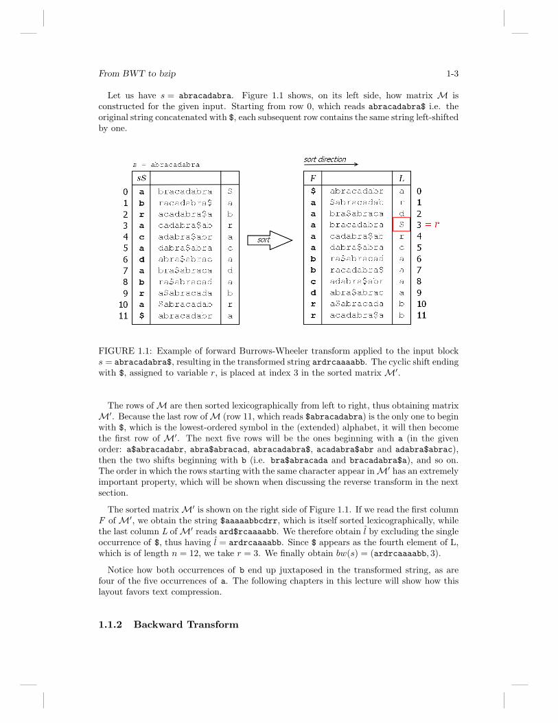
Let us have s = abracadabra. Figure 1.1 shows, on its left side, how matrix M isconstructed for the given input. Starting from row 0, which reads abracadabra$ i.e. theoriginal string concatenated with $, each subsequent row contains the same string left-shiftedby one.

FIGURE 1.1: Example of forward Burrows-Wheeler transform applied to the input blocks = abracadabra$, resulting in the transformed string ardrcaaaabb. The cyclic shift endingwith $, assigned to variable r, is placed at index 3 in the sorted matrix M′.

The rows ofM are then sorted lexicographically from left to right, thus obtaining matrixM′. Because the last row ofM (row 11, which reads $abracadabra) is the only one to beginwith $, which is the lowest-ordered symbol in the (extended) alphabet, it will then becomethe first row of M′. The next five rows will be the ones beginning with a (in the givenorder: a$abracadabr, abra$abracad, abracadabra$, acadabra$abr and adabra$abrac),then the two shifts beginning with b (i.e. bra$abracada and bracadabra$a), and so on.The order in which the rows starting with the same character appear inM′ has an extremelyimportant property, which will be shown when discussing the reverse transform in the nextsection.

The sorted matrixM′ is shown on the right side of Figure 1.1. If we read the first columnF ofM′, we obtain the string $aaaaabbcdrr, which is itself sorted lexicographically, whilethe last column L ofM′ reads ard$rcaaaabb. We therefore obtain l by excluding the singleoccurrence of $, thus having l = ardrcaaaabb. Since $ appears as the fourth element of L,which is of length n = 12, we take r = 3. We finally obtain bw(s) = (ardrcaaaabb, 3).

Notice how both occurrences of b end up juxtaposed in the transformed string, as arefour of the five occurrences of a. The following chapters in this lecture will show how thislayout favors text compression.

1.1.2 Backward Transform

1-4 Paolo Ferragina

We can observe, both by construction and from the example provided, that each column ofthe sorted cyclic shift matrixM′ contains a permutation of s$. In particular, its first columnF represents the best-compressible transformation of the original input block. However, itwould not be possible to determine how the transformed string should be reversed, even byknowing the distribution of its alphabet Σ. The Burrows-Wheeler transform represents atrade-off which retains some properties that render a transformed string reversible, yet stillremaining highly compressible.

In order to prove these properties more formally, let us define a useful function that tellsus how to locate in M′ the predecessor of a character at a given index in s.

DEFINITION 1.1 For 1 ≤ i ≤ n, let s[ki, n − 1] denote the suffix of s prefixing row iof M′. Let Ψ(i) be the index of the row prefixed by s[ki + 1, n− 1].

The function Ψ(i) is not defined for i = 0, because row 0 of M′ begins with $, which doesnot occur in s at all, so that row cannot be prefixed by a suffix of s.

For example in Figure 1.1 it is Ψ(2) = 6. Row 2 ofM′ is prefixed by abra, followed by $.We look for the one row ofM′ that is prefixed by the suffix of s that is immediately shorter(bra), and find that row 6 (which reads bra$abracada) is the one. Similarly, Ψ(11) = 4since row 11 of M′ is prefixed by racadabra and row 4 is the one prefixed by acadabra.

Property 1

For each i, L[i] is the immediate predecessor of F [i] in s. Formally, for 1 ≤ i ≤ n,L[Ψ(i)] = F [i].

Proof. Since each row of M′ contains a cyclic shift of s$, the last character of the rowprefixed by s[ki + 1, n− 1] is s[ki]. Because the index of that row is what we have definedto be Ψ(i) in Definition 1.1, this implies the claim L[Ψ(i)] = s[ki] = F [i].

Intuitively, this property descends from the very nature of every row in M and M′ thatis a cyclic shift of the original string concatenated with $, so if we take two extremes ofeach row, the symbol on the right extreme is immediately followed by the one on the leftextreme. For index j such that L[j] = $, F [j] is the first character of s.

Property 2

All the occurrences of a same symbol in L maintain the same relative orderas in F. Using function Ψ, if 1 ≤ i < j ≤ n and F [i] = F [j] then Ψ(i) < Ψ(j). This meansthat the first occurrence of a symbol in L maps to the first occurrence of that symbol inF, its second occurrence in L maps to its second occurrence in F, and so on, regardless ofwhat other symbols separate two occurrences.

Proof. Given two strings s and t, we shall use the notation s ≺ t to indicate that slexicographically precedes t.

Let s[ki, n − 1] (resp. s[kj , n − 1]) denote the suffix of s prefixing row i (resp. row j).The hypothesis i < j implies that s[ki, n − 1] ≺ s[kj , n − 1]. The hypothesis F [i] = F [j]implies s[ki] = s[kj ] hence it must be s[ki + 1, n − 1] ≺ s[kj + 1, n − 1]. The thesis followssince by construction Ψ(i) (resp. Ψ(j)) is the lexicographic position of the row prefixed bys[ki + 1, n− 1] (resp. s[kj + 1, n− 1]).

In order to re-obtain s, we need to map each symbol from the L column of M′ to itscorresponding occurrence in the sorted column F. This way, we are able to obtain thepermutation of rows that generated matrix M′ from M. This operation is what we call


LF-mapping, and it is essentially analogous to determining the values of function Ψ formatrix M′. The process is rather straightforward for symbols that occur only once, as isthe case of $, c and d in abracadabra$. However, when it comes to symbols a, b and r,which occur several times in the string, the problem is no longer trivial. It can however besolved thanks to the properties we proved [7], which hold for transformed matrix M′.

Let us now illustrate a simple algorithm for performing the LF-mapping, which will bethe starting point for the actual inverse transformation algorithm to be shown later in thissection. The LF-mapping will be stored in an array LF, ||LF || = n.

The algorithm uses an auxiliary vector C, with ||C|| = |Σ ∪ {$}|. For each symbol c, Cstores the total number of occurrences in L of symbols smaller than c. Vector C is indeedindexed by symbol rather than by integer2.

Given this initial content of C, the LF-mapping is performed as follows.

1 for (int i=0; i<n; i++) {2 LF[i] = C[L[i]];3 C[L[i]]++;4 }

This algorithm scans the entire transformed column L (lines 1,4). When a symbol isencountered in the process, the algorithm checks the value of the element in C having thatsymbol as a key. That value is assigned to the LF element with the same index as the one ofL (line 2). Having found an occurrence of that symbol, the counter expressed by the valueof LF having that symbol as a key is incremented by one (line 3). This means that vector Ccontains, for each symbol c and at a given instant, the number of occurrences smaller thanor equal to symbol c found so far. Therefore, once the algorithm has completed, vector Cwill contain, for each c, the total number of occurrences smaller than or equal to c, whilearray LF will contain the LF-mapping that can be used straight away for applying thebackward transform algorithm we will now illustrate.

Given the LF-mapping algorithm and the fundamental properties shown earlier, we areable to reconstruct s backwards starting from the transformed output bw(s), which weremind to be consisting of a permuted s plus an index r. Having bw(s) is equivalent tohaving the L column, since the latter can simply be obtained by placing symbol $ at ther-th position and right-shifting the remainder by one. Before showing the algorithm itself,it can be helpful to exemplify it.

Example 1.2

Let us show how the to re-obtain the original input block starting from its BWT-transformedblock (ardrcaaaabb, 3).

Since r = 3, we insert the sentinel character $ at position 3 and right-shift the remainderby one. We obtain the last column L of M′, which reads ard$rcaaaabb top-to-bottom.By sorting this column lexicographically, we obtain column F , which reads $aaaaabbcdrr.There will be no need to compute any other permutations in M′.

We start reconstructing s$ from the last character $. Its index in F is 0, and L[0] = a,so we append this character to the end of the string we are rebuilding, thus obtaining a$.

2By custom, the term “array” is used when referring to the linear data structures whose elements areindexed by integer ranges, while the term “vector” is used for structures whose indices belong to arbitrarysets, as is the case of C in this lecture.

1-6 Paolo Ferragina

L[0] contains the first occurrence of a, so we also locate the first occurrence of a in F (byProperty 2 we know that this relative order is preserved). Its index in F is 1 and L[1] = r.The rebuilt string now ends with ra$.L[1] contains the first occurrence of r, and its index in F is 10. Since L[10] = b, we

append it to the output and obtain bra$.Note that this process of locating in L the predecessor of each character is equivalent to

determining the values of function Ψ in M′, albeit without having to know the prefixes ofeach row of M′.

By following this rationale, we eventually rebuild the entire string to abracadabra$, andby stripping the sentinel character, the original input abracadabra is reconstructed.

Having intuitively demonstrated how it works, let us now illustrate and explain the al-gorithm itself. An auxiliary array T , ||T || = ||L|| is used for storing the output of thealgorithm.

1 Compute LF[0,n-1];2 k = 0;3 i = n;4 while (i>0) {5 T[i]=L[k];6 k = LF[k];7 i--;8 }

Given the array LF obtained by LF-mapping (line 0), we begin scanning this array (lines2,4) starting from the first element. Due to Property 1 and the fact that F is sorted startingfrom symbol $, the first symbol in L is the final symbol of the original string, and LF [0]tells us the index in L of its immediate predecessor.

We fill the new array T , starting from its last element (lines 3,5) and proceeding backwards(line 7). The array LF is not scanned linearly, since every subsequent index to be scannedboth in L (for reading the actual symbol) and from LF (for knowing the next index) isdetermined by the value of LF at the previously found index.

Once the algorithm has returned, we can obtain the string s$ by reading the content ofT left-to-right. By stripping the last symbol, the original input string is reconstructed.

1.2 Two simple compressors: MTF and RLE

Let us now focus on two simple data compression algorithms that come in very useful, nowthat the BWT has been described in detail, in order to build up the final bzip2 compressor.These compression algorithms are respectively called Move-To-Front (MTF) and Run-Length Encoding (RLE).

1.2.1 Move-To-Front Transform

The MTF [3] (Move-To-Front) transformation is a technique used to improve the perfor-mance of entropy encoding. It is based on the idea that every character is replaced with itsindex in list of the given alphabet.

Given a string s and an alphabet Σ, the algorithm produces a string sMTF on the alphabetΣMTF = {0, . . . , |Σ| − 1}.


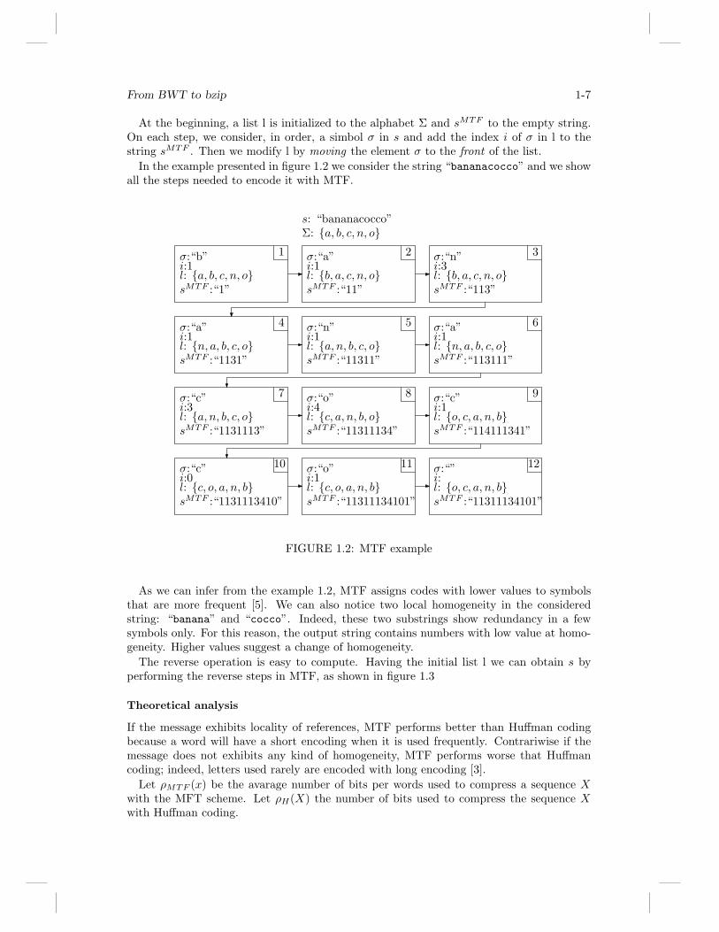
At the beginning, a list l is initialized to the alphabet Σ and sMTF to the empty string.On each step, we consider, in order, a simbol σ in s and add the index i of σ in l to thestring sMTF . Then we modify l by moving the element σ to the front of the list.

In the example presented in figure 1.2 we consider the string “bananacocco” and we showall the steps needed to encode it with MTF.

s: “bananacocco”Σ: {a, b, c, n, o}

l: {a, b, c, n, o}σ:“b”i:1

sMTF :“1”

1

l: {b, a, c, n, o}σ:“a”i:1

sMTF :“11”

2 σ:“n”i:3

sMTF :“113”

3

σ:“a”i:1

4 σ:“n”i:1

sMTF :“11311”

5 σ:“a”i:1

sMTF :“113111”

6

σ:“c”i:3

7 σ:“o”i:4

8 σ:“c”i:1

9

σ:“c”i:0

10 σ:“o”i:1

11

l: {n, a, b, c, o}

sMTF :“1131113” sMTF :“11311134” sMTF :“114111341”

σ:“”i:

12

l: {b, a, c, n, o}

l: {a, n, b, c, o} l: {n, a, b, c, o}

l: {a, n, b, c, o} l: {c, a, n, b, o} l: {o, c, a, n, b}

l: {c, o, a, n, b} l: {c, o, a, n, b} l: {o, c, a, n, b}

sMTF :“1131”

sMTF :“1131113410” sMTF :“11311134101” sMTF :“11311134101”

FIGURE 1.2: MTF example

As we can infer from the example 1.2, MTF assigns codes with lower values to symbolsthat are more frequent [5]. We can also notice two local homogeneity in the consideredstring: “banana” and “cocco”. Indeed, these two substrings show redundancy in a fewsymbols only. For this reason, the output string contains numbers with low value at homo-geneity. Higher values suggest a change of homogeneity.

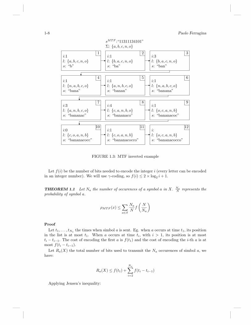
The reverse operation is easy to compute. Having the initial list l we can obtain s byperforming the reverse steps in MTF, as shown in figure 1.3

Theoretical analysis

If the message exhibits locality of references, MTF performs better than Huffman codingbecause a word will have a short encoding when it is used frequently. Contrariwise if themessage does not exhibits any kind of homogeneity, MTF performs worse that Huffmancoding; indeed, letters used rarely are encoded with long encoding [3].

Let ρMTF (x) be the avarage number of bits per words used to compress a sequence Xwith the MFT scheme. Let ρH(X) the number of bits used to compress the sequence Xwith Huffman coding.

1-8 Paolo Ferragina

s: “b”

1 2 3

4 5 6

7 8 9

10 11

i:1

12

s: “bana”

s: “ba”

i:1

s: “banan” s: “banana”

s: “ban”

s: “bananac” s: “bananaco” s: “bananacoc”

s: “bananacocc” s: “bananacocco” s: “bananacocco”

i:

Σ: {a, b, c, n, o}sMTF :“11311134101”

l: {a, b, c, n, o} l: {b, a, c, n, o}

l: {n, a, b, c, o}

l: {b, a, c, n, o}

l: {a, n, b, c, o} l: {n, a, b, c, o}

l: {a, n, b, c, o} l: {c, a, n, b, o} l: {o, c, a, n, b}

l: {c, o, a, n, b} l: {c, o, a, n, b} l: {o, c, a, n, b}

i:3

i:1 i:1 i:1

i:3 i:4 i:1

i:0 i:1

FIGURE 1.3: MTF inverted example

Let f(i) be the number of bits needed to encode the integer i (every letter can be encodedin an integer number). We will use γ-coding, so f(i) ≤ 2× log2 i+ 1.

THEOREM 1.1 Let Na the number of occurences of a symbol a in X. Na

N represents theprobability of symbol a.

ρMTF (x) ≤∑a∈S

Na

Nf

(N

Na

)

ProofLet t1, . . . , tNa the times when simbol a is sent. Eg. when a occurs at time t1, its position

in the list is at most t1. When a occurs at time ti, with i > 1, its position is at mostti − ti−1. The cost of encoding the first a is f(t1) and the cost of encoding the i-th a is atmost f(ti − ti−1).

Let Ra(X) the total number of bits used to transmit the Na occurences of simbol a, wehave:

Ra(X) ≤ f(t1) +Na∑i=2

f(ti − ti−1)

Applying Jensen’s inequality:


Ra(X) ≤ Naf

(1Na

(t1 +

Na∑i=2

(ti − ti−1)

))= Naf

(tNa

Na

)≤ Naf

(Na

Na

)If now we sum for every a ∈ S the constrain for Ra(X) and divide for N we reach the

thesis.

∑a∈S

Ra(X)N

≡ ρMTF (x) ≤∑a∈S

Na

Nf

(N

Na

)

THEOREM 1.2 We will prove the following disequation:

ρMTF (x) ≤ 2ρH(X) + 1

Proof We will start from the result in theorem 1.1. We substitute f with the γ-coding.

ρMTF (x) ≤∑a∈S

(Na

Nf

(N

Na

))≤∑a∈S

(Na

N· 2 · log

(N

Na

)+ 1)

≤ 2 · −∑a∈S

(Na

N· log

(N

Na

))+O(1)

≤ 2 ·H0(X) +O(1)

(1.1)

1.2.2 Run Length Encoding

RLE [4] (Run Length Encoding) is a lossless encoding algorithm that compresses sequencesof the same symbol in a string, into the length of the sequence plus an occurrence of thesymbol itself.

It was invented and used for compressing data for fax transmission. Indeed, a sheet ofpaper is viewed as a binary (i.e. monochromatic) bitmap with many white pixels and veryfew black pixels.

Suppose to have to compress the following string which represents a part of a monochro-matic bitmap (where W stands for “white” and B for “Black”).

WWWWWWWWWWWBWWWWWWWWWWWWBBBBBWWWWWW

We can take the first block of W and compress in the following way:

WWWWWWWWWWW︸︷︷︸11W

BWWWWWWWWWWWWBBBBBWWWWWW

We can proceed in the same fashion until the end of the line is encountered. We willachieve the following compression:

1-10 Paolo Ferragina

WWWWWWWWWWW︸︷︷︸11W

B︸︷︷︸1B

WWWWWWWWWWWW︸︷︷︸12W

BBBBB︸︷︷︸5B

WWWWWW︸︷︷︸6W

We can encode the initial string with the string 〈11,W 〉, 〈1, B〉, 〈12,W 〉, 〈5, B〉, 〈6,W 〉. Itis easy to see that the encoding is lossless and simple to reverse. In the previous examplewe have show a general scheme, even if, in this case, we could have encoded the stringin a more convenient way: 〈W, 11〉, 〈−, 1〉, 〈−, 12〉, 〈−, 5〉, 〈−, 6〉. Indeed, if |Σ| = 2 we cansimply emit the numbers (which indicate the length), while we have the alternation of thetwo simbols in the alphabet.

RLE can perform better or worse than the Huffman scheme: this depends on the messagewe want to encode.

Example 1.3

Here is an example on how RLE can perform better than the Huffman scheme. Suppose wewant to encode the following string s:

WWWWWWWWBBBBBBBBCCCCCCC

with Σ = {B,W,C}. RLE encodes s in this way:

〈W, 8〉, 〈B, 8〉〈C, 7〉we associate 0 to B, 10 to W and 11 to C. We use gamma elias coding to encode numbers

and we code 7 as 00111 and 8 as 0001000:

100001000000010001100111

We now encode s with the Huffman coding (we shall omit the calculus). The result ofencoding string s with the Huffman scheme is:

00000000010101010101010111111111111111

where we associated 0 to W , 01 to B and 11 to C. The result prove that |CHuffman| =38 > |CRLE | = 24

Example 1.4

Here is now an example on how RLE can perform worse than the Huffman scheme. Supposewe want to encode the following string s:

ABCAABCABCAB

where Σ = {A,B,C}. According to RLE scheme, we encode s in the following way:

〈A, 1〉, 〈B, 1〉, 〈C, 1〉, 〈A, 2〉, 〈B, 1〉, 〈C, 1〉, 〈A, 1〉, 〈B, 1〉, 〈C, 1〉, 〈A, 1〉, 〈B, 1〉We associate to A the encoding 0, 10 to B and 11 to C. Even if we encode the numbers

1 and 2 with bits 0 and 1, respectively, we cannot make a shorter encoding than:

00100110011001100010011000100

Here, the length of the encoding of s if 29.


The encoding with Huffman scheme assigns 0, 10, 11, according to their probability,respectively to A, B and C.

010110101101011010

We can therefore conclude that |CHuffman(s)| = 18 < |CRLE(s)| = 29

THEOREM 1.3 For any binary string s = al11 a

l22 . . . a

lnn , with ai ∈ {0, 1} and ai 6= ai+1

we have:

|CRLE(s)| = 1 +k∑

i=0

|CPF (li)|

where |CRLE(s)| is the length of encoding the string s with RLE and |CPF (li)| is thelength of encoding li with PreFixed codes.

Proof Proving the equality is very easy, as it simply derives from the definition. Let usthen analyze all the addenda in the right part of our equation.

• We have put +1 because it represents the first bit (remember that s is a binarystring). We don’t need to take care of the other bits in the succession becausewe know that there’s an alternation of them in the string.• The other addendum sums the lengths of the exponents, coded with PreFixed

scheme.

As we can deduce from the above example, RLE [5] works well when the sequences of thesame symbol are very long.

1.3 Implementation

Having seen how the BWT algorithm [4] works, let us now focus on how is it used. Weassume from now on that the reader has well understood the previous chapters.

Take a string s and a substring w. Suppose that our substring appears n times within themain string s. As we have seen, in the matrix created by BWT there will be n consecutiverows prefixed with the substring w. Let us call these rows as rw + 1, rw + 2, . . . , rw +n andlet’s call s = bwt(s).

All of these n rows will contain all the symbols that precede w in s.

Example 1.5

Recall the example in figure 1.1. The substring w ≡ bra appears 2 times within the mainstring abracadabra.

As we could expect [11], in the BWT matrix we will find two consecutive rows prefixedwith the substring bra. In the example in figure 1.1, these rows are located in the secondand third positions respectively.

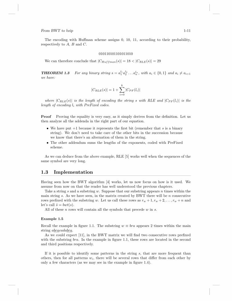
If it is possible to identify some patterns in the string s, that are more frequent thanothers, then for all patterns wi, there will be several rows that differ from each other byonly a few characters (as we may see in the example in figure 1.4).


a bracadacabrapica $b racadacabrapica $ ar acadacabrapica $ a ba cadacabrapica $ ab rc adacabrapica $ abr aa dacabrapica $ abra cd acabrapica $ abrac aa cabrapica $ abraca dc abrapica $ abracad aa brapica $ abracada cb rapica $ abracadac ar apica $ abracadaca ba pica $ abracadacab rp ica $ abracadacabr ai ca $ abracadacabra pc a $ abracadacabrap ia $ abracadacabrapi c$ abracadacabrapic a

a bracadacabrapica $a brapica $ abracada ca cabrapica $ abraca da cadacabrapica $ ab ra dacabrapica $ abra ca pica $ abracadacab ra $ abracadacabrapi cb racadacabrapica $ ab rapica $ abracadac ac a $ abracadacabrap ic abrapica $ abracad ac adacabrapica $ abr ad acabrapica $ abrac ai ca $ abracadacabra pp ica $ abracadacabr ar acadacabrapica $ a br apica $ abracadaca b$ abracadacabrapic a

FIGURE 1.4: Example of BWT applied to abracadacabrapica.

For this reason, the s string is locally homogeneous. As we can see from the examplesin figure 1.1, 1.4, there are some substrings of equal characters in the string s.

The base idea is to exploit this property [5]. For this purpose, we could use Move ToFront (MTF) encoding applied to s. If the s string is locally homogeneous, then mtf(s)is encoded with small numbers.

Example 1.6

Consider the example in figure 1.4. Let’s encode the s string.In this case, the s ≡ cdrcrcaaiaaapabba. (we omit the computation).If we apply the mtf to s we find the following string: 2362113510061602.

Since we obtain a good distribution with the mtf applied to s, we could, finally, applyHuffman [8] or Arithmetic coding [9] to the result. In this case we will obtain a goodcompression.

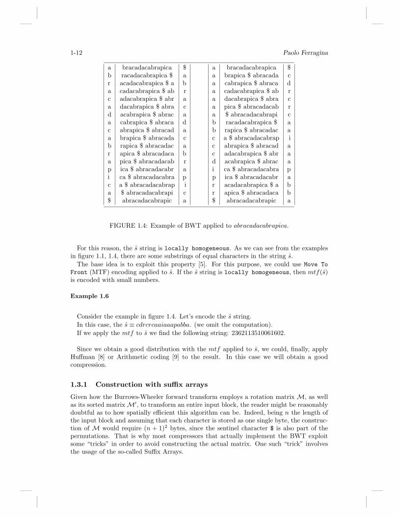
1.3.1 Construction with suffix arrays

Given how the Burrows-Wheeler forward transform employs a rotation matrix M, as wellas its sorted matrixM′, to transform an entire input block, the reader might be reasonablydoubtful as to how spatially efficient this algorithm can be. Indeed, being n the length ofthe input block and assuming that each character is stored as one single byte, the construc-tion of M would require (n + 1)2 bytes, since the sentinel character $ is also part of thepermutations. That is why most compressors that actually implement the BWT exploitsome “tricks” in order to avoid constructing the actual matrix. One such “trick” involvesthe usage of the so-called Suffix Arrays.


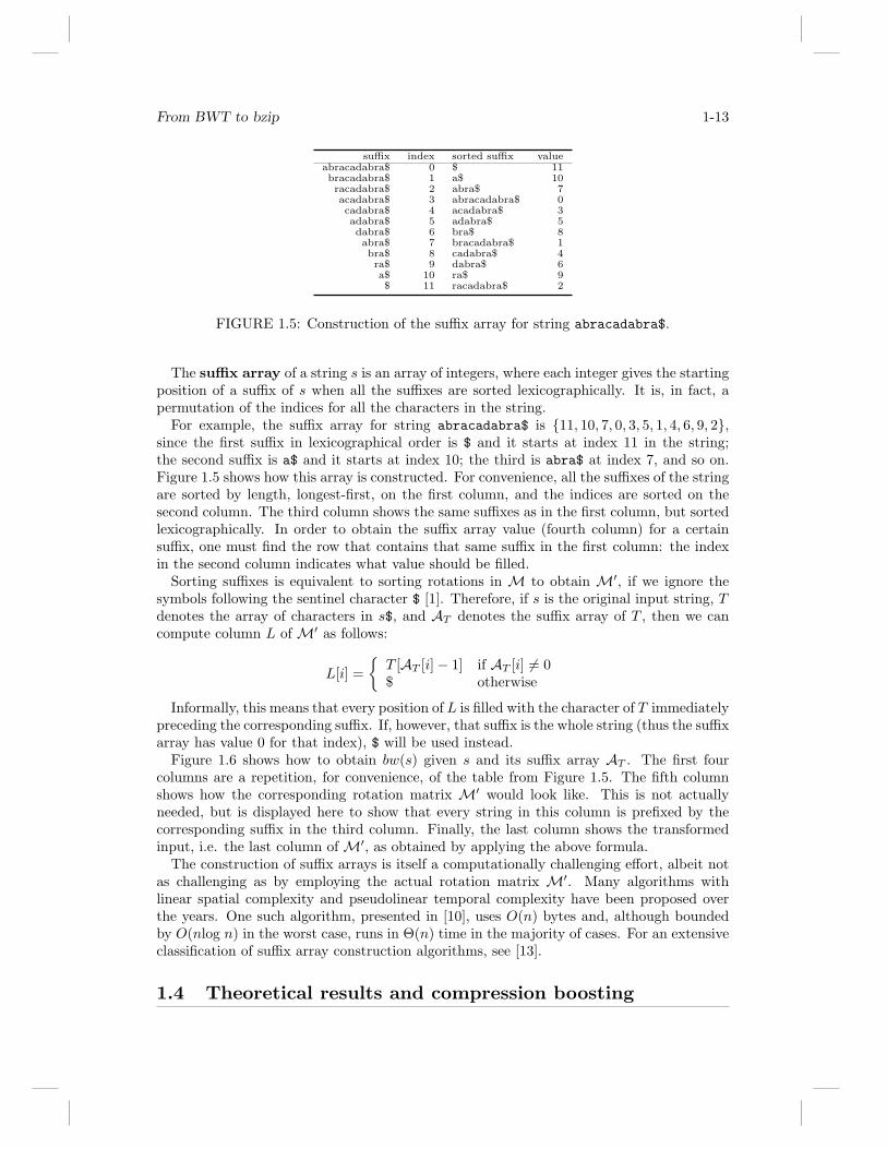
suffix index sorted suffix valueabracadabra$ 0 $ 11bracadabra$ 1 a$ 10racadabra$ 2 abra$ 7acadabra$ 3 abracadabra$ 0cadabra$ 4 acadabra$ 3adabra$ 5 adabra$ 5dabra$ 6 bra$ 8abra$ 7 bracadabra$ 1bra$ 8 cadabra$ 4ra$ 9 dabra$ 6a$ 10 ra$ 9$ 11 racadabra$ 2

FIGURE 1.5: Construction of the suffix array for string abracadabra$.

The suffix array of a string s is an array of integers, where each integer gives the startingposition of a suffix of s when all the suffixes are sorted lexicographically. It is, in fact, apermutation of the indices for all the characters in the string.

For example, the suffix array for string abracadabra$ is {11, 10, 7, 0, 3, 5, 1, 4, 6, 9, 2},since the first suffix in lexicographical order is $ and it starts at index 11 in the string;the second suffix is a$ and it starts at index 10; the third is abra$ at index 7, and so on.Figure 1.5 shows how this array is constructed. For convenience, all the suffixes of the stringare sorted by length, longest-first, on the first column, and the indices are sorted on thesecond column. The third column shows the same suffixes as in the first column, but sortedlexicographically. In order to obtain the suffix array value (fourth column) for a certainsuffix, one must find the row that contains that same suffix in the first column: the indexin the second column indicates what value should be filled.

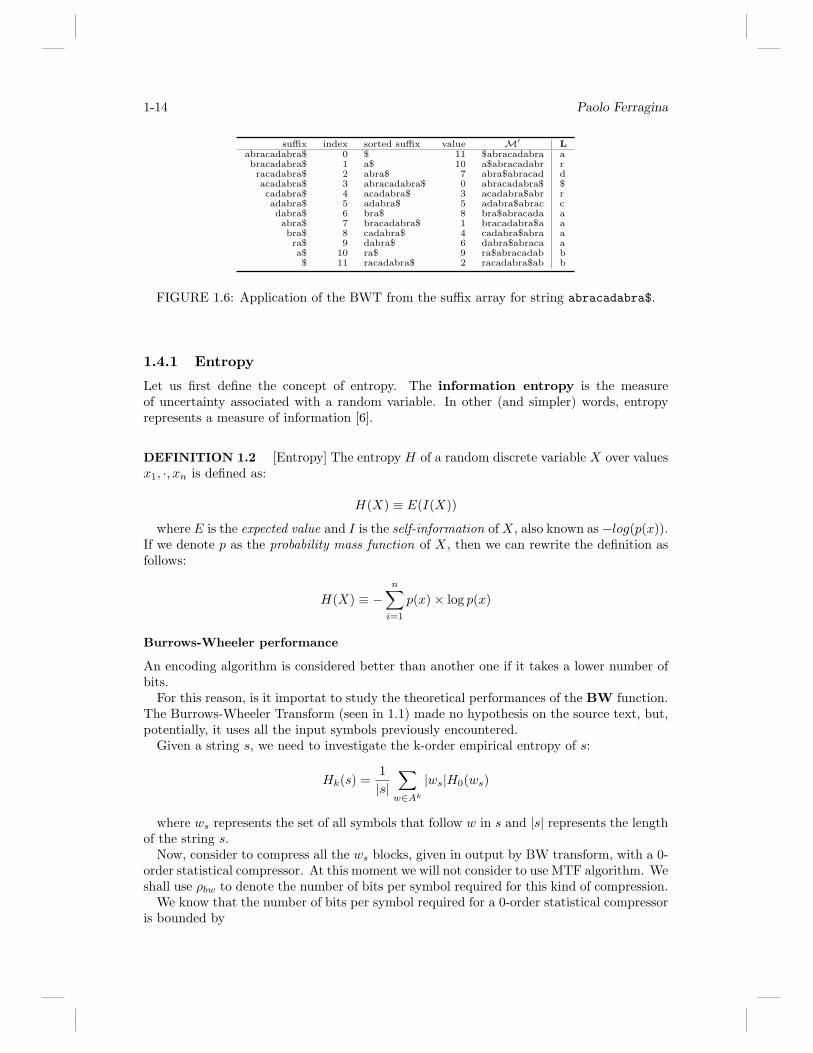
Sorting suffixes is equivalent to sorting rotations in M to obtain M′, if we ignore thesymbols following the sentinel character $ [1]. Therefore, if s is the original input string, Tdenotes the array of characters in s$, and AT denotes the suffix array of T , then we cancompute column L of M′ as follows:

L[i] ={T [AT [i]− 1] if AT [i] 6= 0$ otherwise

Informally, this means that every position of L is filled with the character of T immediatelypreceding the corresponding suffix. If, however, that suffix is the whole string (thus the suffixarray has value 0 for that index), $ will be used instead.

Figure 1.6 shows how to obtain bw(s) given s and its suffix array AT . The first fourcolumns are a repetition, for convenience, of the table from Figure 1.5. The fifth columnshows how the corresponding rotation matrix M′ would look like. This is not actuallyneeded, but is displayed here to show that every string in this column is prefixed by thecorresponding suffix in the third column. Finally, the last column shows the transformedinput, i.e. the last column of M′, as obtained by applying the above formula.

The construction of suffix arrays is itself a computationally challenging effort, albeit notas challenging as by employing the actual rotation matrix M′. Many algorithms withlinear spatial complexity and pseudolinear temporal complexity have been proposed overthe years. One such algorithm, presented in [10], uses O(n) bytes and, although boundedby O(nlog n) in the worst case, runs in Θ(n) time in the majority of cases. For an extensiveclassification of suffix array construction algorithms, see [13].

1.4 Theoretical results and compression boosting


suffix index sorted suffix value M′ Labracadabra$ 0 $ 11 $abracadabra abracadabra$ 1 a$ 10 a$abracadabr rracadabra$ 2 abra$ 7 abra$abracad dacadabra$ 3 abracadabra$ 0 abracadabra$ $cadabra$ 4 acadabra$ 3 acadabra$abr radabra$ 5 adabra$ 5 adabra$abrac cdabra$ 6 bra$ 8 bra$abracada aabra$ 7 bracadabra$ 1 bracadabra$a abra$ 8 cadabra$ 4 cadabra$abra ara$ 9 dabra$ 6 dabra$abraca aa$ 10 ra$ 9 ra$abracadab b$ 11 racadabra$ 2 racadabra$ab b

FIGURE 1.6: Application of the BWT from the suffix array for string abracadabra$.

1.4.1 Entropy

Let us first define the concept of entropy. The information entropy is the measureof uncertainty associated with a random variable. In other (and simpler) words, entropyrepresents a measure of information [6].

DEFINITION 1.2 [Entropy] The entropy H of a random discrete variable X over valuesx1, ·, xn is defined as:

H(X) ≡ E(I(X))

where E is the expected value and I is the self-information of X, also known as−log(p(x)).If we denote p as the probability mass function of X, then we can rewrite the definition asfollows:

H(X) ≡ −n∑

i=1

p(x)× log p(x)

Burrows-Wheeler performance

An encoding algorithm is considered better than another one if it takes a lower number ofbits.

For this reason, is it importat to study the theoretical performances of the BW function.The Burrows-Wheeler Transform (seen in 1.1) made no hypothesis on the source text, but,potentially, it uses all the input symbols previously encountered.

Given a string s, we need to investigate the k-order empirical entropy of s:

Hk(s) =1|s|

∑w∈Ak

|ws|H0(ws)

where ws represents the set of all symbols that follow w in s and |s| represents the lengthof the string s.

Now, consider to compress all the ws blocks, given in output by BW transform, with a 0-order statistical compressor. At this moment we will not consider to use MTF algorithm. Weshall use ρbw to denote the number of bits per symbol required for this kind of compression.

We know that the number of bits per symbol required for a 0-order statistical compressoris bounded by


H0 ≤ ρ ≤ H0 + µ (1.2)

Since we are compressing separately all the ws blocks we are sure that the length of thewhole compression is the sum of the length of the single blocks compressed. We can inferthe following inequality:

ρbw ≤1|s|

∑ws∈bw(s)

|ws|(H0(ws) + µ) (1.3)

where |s| is the length of the input (indeed we would like to calculate the number of bitsper symbol) and ws are the blocks, in output, created by BW transform.

Let’s denote with fws(c) the frequency of the symbol c in the block ws and with A(ws)the alphabet used in the string ws. We can rewrite the formula 1.3 in the following way:

ρbw ≤1|s|

∑ws∈bw(s)

|ws|(∑

c∈A(ws)

fws(c) log2

1fws

(c)+ µ) (1.4)

Indeed H0(ws) is the entropy of the block ws. So, we have rewritten H0(ws), expandingwith its definition. We can do better. Since fws(c) is the frequency of the simbol c withinthe block ws, it can be rewritten as the conditioned frequency f(c|w). Indeed when thesymbol c is contained in the block ws, it means that c follows the context w in the input.

THEOREM 1.4 We will prove the following disambiguation:

ρbw ≤ Hk(s) + µ

ProofStarting from equation 1.4, we replace fws

(c) with the conditioned frequency and carryout the µ element from the sum. We have:

ρbw ≤ µ+1|s|

∑ws∈bw(s)

|ws|(∑

c∈A(ws)

f(c|w) log2

1f(c|w)

)

and by definition of H0 we have:

ρbw ≤ µ+1|s|

∑ws∈bw(s)

|ws|(H0(ws))

and, generalizing:

ρbw ≤ µ+1|s|

∑ws∈Ak

|ws|(H0(ws))

|ws|(H0(ws)) is the number of bits necessary for our compressor of order 0 to representws. We sum for all the possibly ws strings and we have the thesis.


1.5 Some experimental tests

We will now show some results of testing an implementation of a BWT-based compressoragainst a few other well-known compression algorithms. All implementations were testedon a GNU/Linux platform.

• Bzip (combination of BWT with multiple encoding schemes including MTF,RLE and Huffman): for this algorithm we shall use the “bzip2” package fromhttp://www.bzip.org, version 1.0.5-r1.

• LZMA (LempelZivMarkov chain algorithm): we shall use the “lzip” package fromhttp://www.nongnu.org, version 1.10.

• LZ77 (original Lempel Ziv algorithm): since there are no direct implementationsof this algorithm, we will use the “lzop” package (LZ-oberhumer zip), version1.02 rc1-r1. It is the last implementation of LZO1A compression algorithm. Itcompresses a block of data into matches (using a LZ77 sliding dictionary) andruns of non-matching literals. LZO1A takes care about long matches and longliteral runs so that it produces good results on high redundant data and dealsacceptably with non-compressible data. Some ideas are borrowed from LZRWand LZV compression algorithms [12]. We chose this kind of implementationbeacuse it is a commercial and military (it has been used by NASA [2]) program.

• LZ77: for this algorithm we shall also test the DEFLATE implementation, whichcombines LZ77 with Huffman coding. We shall use the “zip” package fromhttp://www.info-zip.org/, version 3.0. It is a lossless data compression algo-rithm.

All the tests are run in RAM (using ramfs) and made under the following configuration:

• AMD Athlon(tm)X2 DualCore QL-64• 2048 PC2-6400 SoDimm ram• GNU/Linux Gentoo distribution, using zen-sources-2.6.33 p1 with bfs scheduling.

We shall test all the implementations on three different kinds of files:

• all the canticas of Divine Comedy: we’re going to test this file because it repre-sents a text with some degree of correlation.

• a raw monochromatic non-compressed image: the reason why we choose thiskind of file is because it contains a lot of “similar” information (black and whitepixels). We therefore expected a high compression rate.

• gcc-4.4.3: we will test the algorithms on this package in order to assess how theybehave on compressing a large amount of files, which are distributed across asparse directory structure with great ramification.

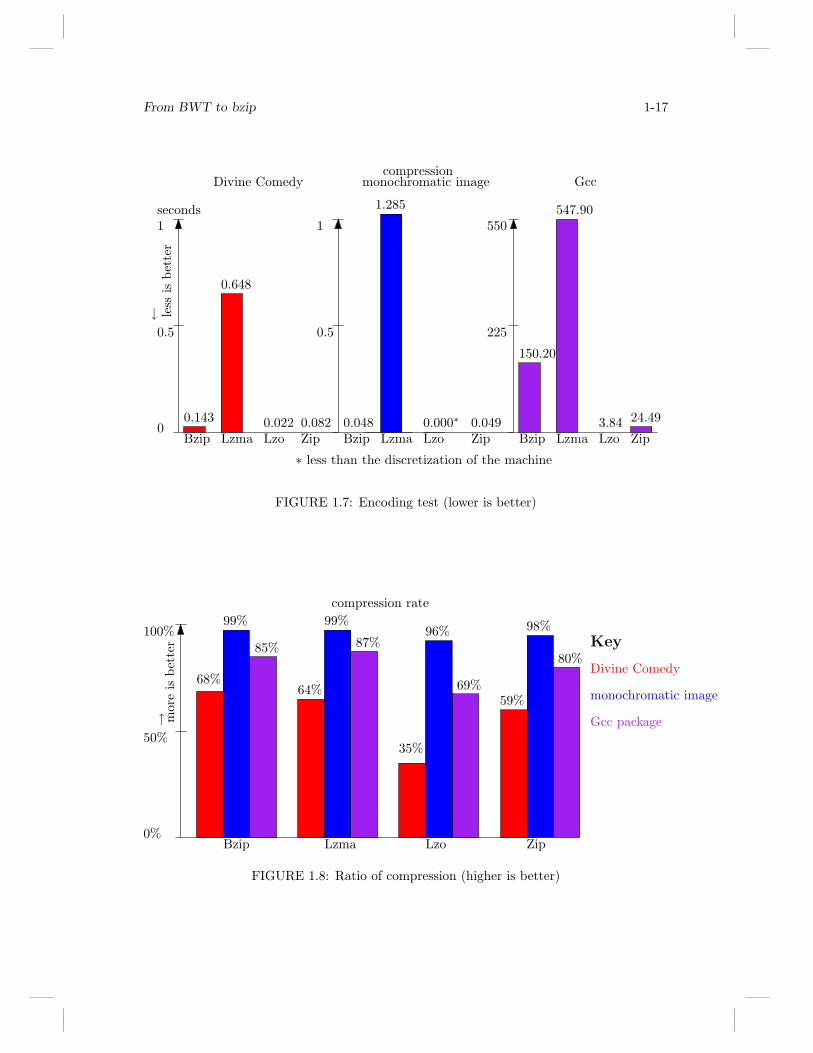
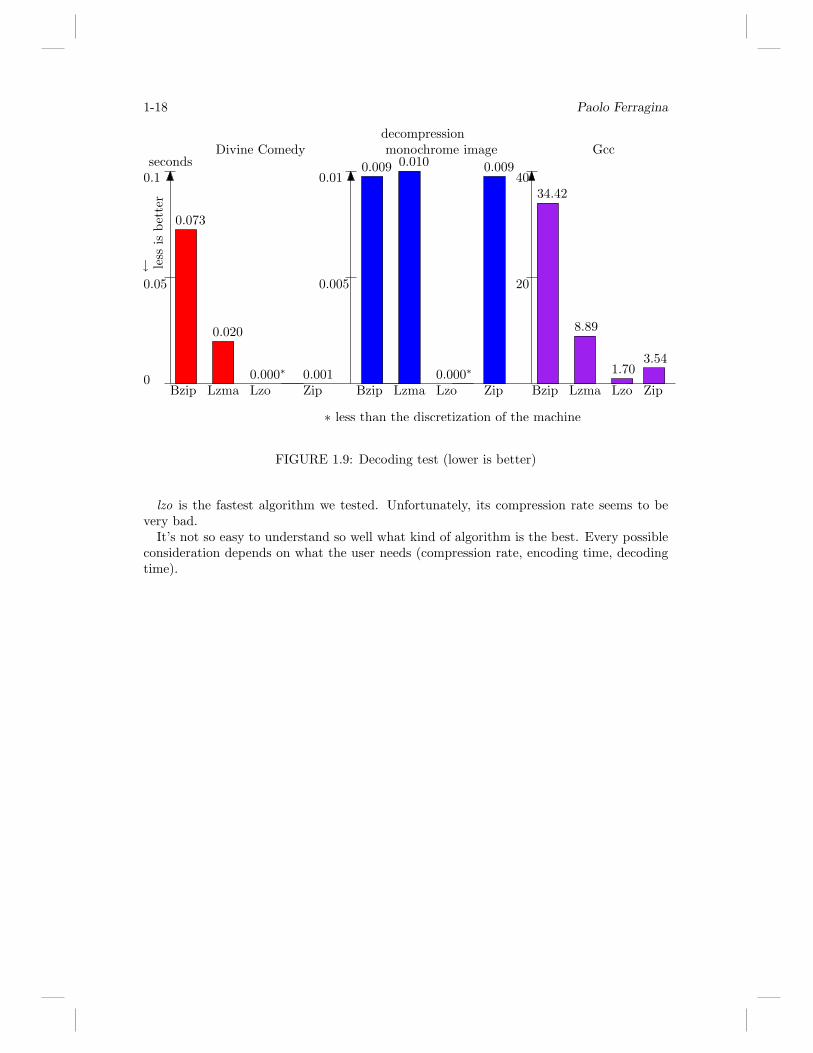
All the tests are run 100 times and we will show the avarage result.From figure 1.7,1.8,1.9 we can easly deduce some conclusions. First of all, we can conclude

that lzma is very bad. It has ever the worst compress-time and does not reach the bestcompression rate. bzip2 seems to be quite in the middle. Sometimes it takes a lot of time toencode, but it reaches the best compression rate. By considering the decompression time,bzip2 seems to slow down too much as the size of the file grows.

Perhaps the best solution seems to be the zip: it takes a short time to encode/decodeand reaches a very good compression rate.


0.143

Bzip Lzma Lzo0.022

0.648

0.082Zip

1

0

0.5

seconds

0.048Bzip Lzma Lzo

0.000∗

1.285

0.049Zip

1

0.5

∗ less than the discretization of the machine

150.20

Bzip Lzma Lzo3.84

547.90

24.49

Zip

550

225

compressionDivine Comedy monochromatic image Gcc

↓ less

isbe

tter

FIGURE 1.7: Encoding test (lower is better)

99%96%

99% 98%

68%

Bzip Lzma Lzo

35%

64%59%

Zip

50%

100%

0%

85%

69%

87%80%

compression rate

Divine Comedy

monochromatic image

Gcc package

Key

↑ mor

eis

bett

er

FIGURE 1.8: Ratio of compression (higher is better)


34.42

Bzip Lzma Lzo

1.70

8.89

Zip

40

20

3.54

0.073

Bzip Lzma Lzo0.000∗

0.020

0.001Zip

0.1

0

0.05

seconds

∗ less than the discretization of the machine

0.009

Bzip Lzma Lzo0.000∗

0.010

Zip

0.01

0.005

0.009Divine Comedy monochrome image Gcc

decompression

↓ less

isbe

tter

FIGURE 1.9: Decoding test (lower is better)

lzo is the fastest algorithm we tested. Unfortunately, its compression rate seems to bevery bad.

It’s not so easy to understand so well what kind of algorithm is the best. Every possibleconsideration depends on what the user needs (compression rate, encoding time, decodingtime).


References

[1] D. Adjeroh, T. Bell, and A. Mukherjee. The Burrows-Wheeler Transform: DataCompression, Suffix Arrays, and Pattern Matching. Springer series in statistics.Springer, 2008.

[2] National Aeronautics and Space Administration. http://marsrovers.jpl.nasa.gov/home/.[3] Jon Louis Bentley, Daniel D. Sleator, Robert E. Tarjan, and Victor K. Wei. A locally

adaptive data compression scheme. Commun. ACM, 29(4):320–330, 1986.[4] Michael Burrows and David J. Wheeler. A block-sorting lossless data compression

algorithm. Technical Report 124, Digital Systems Research Center (SRC), 1994.[5] Stefano Cataudella and Antonio Gulli. BW transform and its applications. Tutorial

on BW-transform, 2003.[6] Paolo Ferragina and Giovanni Manzini. Boosting textual compression. In Ming-Yang

Kao, editor, Encyclopedia of Algorithms, pages 1–99. Springer US, 2008.[7] Paolo Ferragina and Giovanni Manzini. Burrows-wheeler transform. In Ming-Yang

Kao, editor, Encyclopedia of Algorithms, pages 1–99. Springer US, 2008.[8] D.A. Huffman. A method for the construction of minimum redundancy codes. Pro-

ceedings IRE 40, 10:1098–1101, 1952.[9] Glen G. Langdon. An introduction to arithmetic coding. IBM J. Res. Dev., 28(2):135–

149, 1984.[10] Giovanni Manzini and Paolo Ferragina. Engineering a lightweight suffix array con-

struction algorithm. Algorithmica, 40(1):33–50, 2004.[11] Shoshana Neuburger. The burrows-wheeler transform: data compression, suffix arrays,

and pattern matching by donald adjeroh, timothy bell and amar mukherjee springer,2008. SIGACT News, 41(1):21–24, 2010.

[12] Markus Franz Xaver Johannes Oberhumer. ftp://ftp.matsusaka-u.ac.jp/pub/compression/oberhumer/lzo1a-announce.txt, 1996.

[13] Simon J. Puglisi, William F. Smyth, and Andrew Turpin. A taxonomy of suffix ar-ray construction algorithms. In Jan Holub and Milan Simanek, editors, Stringology,pages 1–30. Department of Computer Science and Engineering, Faculty of ElectricalEngineering, Czech Technical University, 2005.

The power of Algorithms! - Unibo

Documents

Transcript of The power of Algorithms! - Unibo