
The Pico- to Nanosecond Dynamics of Phospholipid Molecules
232
TECHNISCHE UNIVERSITÄT MÜNCHEN Lehrstuhl für Experimentalphysik IV und Forschungs-Neutronenquelle Heinz Maier-Leibnitz (FRM II) The Pico- to Nanosecond Dynamics of Phospholipid Molecules Vinzenz Erik Sebastian Busch Vollständiger Abdruck der von der Fakultät für Physik der Technischen Universität München zur Erlangung des akademischen Grades eines Doktors der Naturwissenschaften (Dr. rer. nat.) genehmigten Dissertation. Vorsitzender: Univ.-Prof. Dr. Martin Zacharias Prüfer der Dissertation: 1. Univ.-Prof. Dr. Winfried Petry 2. Univ.-Prof. Dr. Andreas Bausch 3. Univ.-Prof. Dr. Tobias Unruh (Friedrich-Alexander-Universität Erlangen-Nürnberg) Die Dissertation wurde am 04. 01. 2012 bei der Technischen Universität München eingereicht und durch die Fakultät für Physik am 30. 04. 2012 angenommen.
-
Upload
khangminh22 -
Category
Documents
-
view
1 -
download
0
Transcript of The Pico- to Nanosecond Dynamics of Phospholipid Molecules

TECHNISCHE UNIVERSITÄT MÜNCHENLehrstuhl für Experimentalphysik IV und
Forschungs-Neutronenquelle Heinz Maier-Leibnitz (FRM II)
The Pico- to Nanosecond Dynamicsof Phospholipid Molecules
Vinzenz Erik Sebastian Busch
Vollständiger Abdruck der von der Fakultät für Physik der Technischen Universität Münchenzur Erlangung des akademischen Grades eines
Doktors der Naturwissenschaften (Dr. rer. nat.)
genehmigten Dissertation.
Vorsitzender: Univ.-Prof. Dr. Martin ZachariasPrüfer der Dissertation:
1. Univ.-Prof. Dr. Winfried Petry2. Univ.-Prof. Dr. Andreas Bausch3. Univ.-Prof. Dr. Tobias Unruh
(Friedrich-Alexander-Universität Erlangen-Nürnberg)
Die Dissertation wurde am 04. 01. 2012 bei der Technischen Universität München eingereichtund durch die Fakultät für Physik am 30. 04. 2012 angenommen.

Physik-Department Technische Universität München
Lehrstuhl für Experimentalphysik IV andForschungs-Neutronenquelle Heinz Maier-Leibnitz (FRM II)
Dissertation
The Pico- to Nanosecond Dynamicsof Phospholipid Molecules
Sebastian Busch
2012

Vollständiger Abdruck der von der Fakultät für Physik der Technischen UniversitätMünchen zur Erlangung des akademischen Grades eines
Doktors der Naturwissenschaften (Dr. rer. nat.)
genehmigten Dissertation.
Vorsitzender: Univ.-Prof. Dr. Martin ZachariasPrüfer der Dissertation:
1. Univ.-Prof. Dr. Winfried Petry2. Univ.-Prof. Dr. Andreas Bausch3. Univ.-Prof. Dr. Tobias Unruh
(Friedrich-Alexander-Universität Erlangen-Nürnberg)
Die Dissertation wurde am 04. 01. 2012 bei der Technischen Universität Müncheneingereicht und durch die Fakultät für Physik am 30. 04. 2012 angenommen.

Contents
Zusammenfassung / Summary v
I. Dissertation 1
1. Introduction 31.1. Phospholipids in Nature and Application . . . . . . . . . . . . . . . . . . 41.2. Some Concepts of Glassy Dynamics . . . . . . . . . . . . . . . . . . . . . 81.3. Dynamics of Phospholipids . . . . . . . . . . . . . . . . . . . . . . . . . . 12
2. Theoretical Principles 172.1. Molecular Structure and Dynamics are Described by Correlation Functions 172.2. Measuring the Correlation Functions with Neutron Scattering . . . . . . 24
3. Materials and Methods 293.1. Preparation and Characteristics of the Phospholipid Samples . . . . . . . 293.2. Description of the Neutron time-of-flight Spectrometer TOFTOF . . . . . . 353.3. Choice of Measurement Parameters . . . . . . . . . . . . . . . . . . . . . 39
4. Data Reduction and Analysis 474.1. Extracting the Scattering Function from the Scattered Intensities . . . . 474.2. Finding the Mechanism of Diffusion with a Fit . . . . . . . . . . . . . . . 504.3. Model-free Determination of the Mobility . . . . . . . . . . . . . . . . . . 57
5. Results and Discussion 615.1. Methodical Enhancements . . . . . . . . . . . . . . . . . . . . . . . . . . 615.2. Molecular Dynamics in Pure Phospholipid Multibilayers . . . . . . . . . 645.3. Multibilayers of DMPC with Additives . . . . . . . . . . . . . . . . . . . . 705.4. Single Bilayers and Monolayers . . . . . . . . . . . . . . . . . . . . . . . 71
6. Outlook 736.1. Methodical Enhancements . . . . . . . . . . . . . . . . . . . . . . . . . . 736.2. Molecular Dynamics in Pure Phospholipid Multibilayers . . . . . . . . . 776.3. Multibilayers of DMPC with Additives . . . . . . . . . . . . . . . . . . . . 796.4. Single Bilayers and Monolayers . . . . . . . . . . . . . . . . . . . . . . . 79
7. Conclusion 83
iii

Contents
II. Publications 85
A. List of Publications and Presentations 87A.1. Refereed Publications . . . . . . . . . . . . . . . . . . . . . . . . . . . . . 87A.2. Non-refereed Publications . . . . . . . . . . . . . . . . . . . . . . . . . . 90A.3. Talks at International Conferences . . . . . . . . . . . . . . . . . . . . . . 90A.4. Participation in Seminars and Workshops . . . . . . . . . . . . . . . . . . 91A.5. Posters at International Conferences . . . . . . . . . . . . . . . . . . . . 92
B. Molecular Mechanism of Long-Range Diffusion in Phospholipid MembranesStudied by Quasielastic Neutron Scattering 95
C. Dynamical Transition of Protein-Hydration Water 117
D. The Slow Short-Time Motions of Phospholipid Molecules With a Focus onthe Influence of Multiple Scattering and Fitting Artefacts 123
E. The Influence of Additives on the Nanoscopic Dynamics of the PhospholipidDimyristoylphosphatidylcholine 137
F. The Picosecond Dynamics of the Phospholipid Dimyristoylphosphatidylcholinein Mono- and Bilayers 149
G. FABADA: a Fitting Algorithm for Bayesian Analysis of DAta 163
H. Fitting in a Complex χ2 Landscape Using an Optimized Hypersurface Sam-pling 173
III. Additional Information 181
I. Details of the Data Reduction 183I.1. Data Reduction Software . . . . . . . . . . . . . . . . . . . . . . . . . . . 183I.2. Data Reduction Procedure . . . . . . . . . . . . . . . . . . . . . . . . . . 188I.3. Effective Scattering Cross Section . . . . . . . . . . . . . . . . . . . . . . 192
Bibliography 195
Acknowledgements 223
iv

Zusammenfassung / Summary
ZusammenfassungDie Bewegungen des Phospholipids Dimyristoylphosphatidylcholin wurden mit quasi-elastischer Neutronenstreuung auf einer Zeitskala im Piko- bis Nanosekundenbereichuntersucht. Bis vor Kurzem war man der Meinung, dass die Moleküle bei diesen kurzenZeiten sich nur kleinräumig in einem Käfig, der von ihren Nachbarn gebildet wird, be-wegen können. Ab und zu könnten die Moleküle aus diesem Käfig springen, wenn sichdurch thermische Fluktuationen eine Leerstelle darin auftäte. Molekulardynamiksimu-lationen haben allerdings kürzlich ein anderes Bild gezeichnet: Die Moleküle springennicht aus ihrem Käfig, sondern bewegen sich vielmehr zusammen mit ihm in flussartigenStrömungen.
Es war nun möglich, die quasielastischen Neutronenstreuungsdaten mit diesem Modellauszuwerten. Die quantitative Übereinstimmung der extrahierten Flussgeschwindigkeitenmit denen der Simulationen ist ein experimenteller Hinweis, dass die bisherige Vorstellungvon Sprüngen der Moleküle von Käfig zu Käfig nicht richtig sein kann.
Im Vergleich mit anderen dichten Flüssigkeiten wird klar, dass diese kollektiven Verschie-bungen keine Besonderheit der Phospholipide sind sondern ein allgemeines Phänomen,das schon in einer Vielzahl von Systemen beobachtet wurde und dort «dynamische Hete-rogenitäten» genannt wird, weil es eine räumliche Trennung von schnellen und langsamenMolekülen gibt.
In Natur und Anwendung kommen in den allermeisten Fällen keine reinen Phospho-lipidsysteme vor, sondern Mischungen mit anderen Molekülen. Während in der NaturCholesterol eine der wichtigsten Komponenten ist, sind in der pharmazeutischen Anwen-dung Kostabilisatoren wie Natriumglycocholat von Bedeutung. Diese Kostabilisatorenwerden gemeinsam mit dem Phospholipid als Emulgatoren in Nahrungsmitteln undMedikamenten eingesetzt, um eine Entmischung der öligen und wässrigen Komponentenzu verhindern.
Wegen dieser Relevanz von Mischsystemen wurde auch der Einfluss einiger reprä-sentativer Zusätze auf die Phospholipiddynamik untersucht. Der von makroskopischenMessungen bekannte verlangsamende Effekt von Cholesterol ist zwar auf einer Zeitskalavon 55 Pikosekunden noch nicht sehr ausgeprägt, hat aber nach 900 Pikosekunden schonfast sein volles Ausmaß erreicht, das aus makroskopischen Messungen wohlbekannt ist.Interpretiert man dieses Ergebnis im Rahmen der erwähnten Flussbewegungen, wirdnicht die Flussgeschwindigkeit, die bei kurzen Zeitskalen die Bewegung dominiert, durchdie Cholesterolmoleküle abgebremst, sondern vielmehr wird die Länge verringert, die einPhospholipidmolekül in solch einer Bewegung zurücklegt, bevor es die Richtung wechselt.
v

Zusammenfassung / Summary
Im Gegensatz dazu ist die Beweglichkeit der Phospholipide in den pharmazeutischrelevanten Systemen deutlich erhöht. In den Fällen, in denen das Phospholipid eineölige Phase stabilisiert, kann die Phospholipiddichte abgesenkt werden, was die erhöhteDynamik zur Folge hat. Ein zuvor vermuteter Zusammenhang zwischen der Molekülbe-weglichkeit und der Stabilität der Proben kann indes ausgeschlossen werden.
SummaryThe motions of the phospholipid dimyristoylphosphatidylcholine were studied on a pico-to nanosecond time scale with quasielastic neutron scattering. Until a short while ago,the opinion prevailed that the molecules can only perform small-scale motions in a cageformed by their neighbours at these short times. Now and then, the molecules couldjump out of these cages when a vacancy happened to form in it. However, MolecularDynamics simulations have recently drawn another picture: the molecules do not escapefrom their cage but rather move together with it in flow-like structures.
It was now possible to evaluate the quasielastic neutron scattering data with this model.The quantitative agreement of the extracted flow velocities with the ones observed inthe simulation is experimental evidence that the hitherto existing picture of moleculesjumping from cage to cage cannot be correct.
The comparison with other dense liquids shows that these collective displacements arenot a peculiar property of the phospholipids but a universal phenomenon that has previ-ously been observed in many systems where it was termed «dynamical heterogeneities»because fast and slow molecules are spatially separated.
In nature and application, mixtures with other molecules are more frequent than purephospholipid systems. While cholesterol is one of th most important components innature, costabilizers like sodium glycocholate are important in pharmaceutical application.These costabilizers are used in combination with phospholipids as emulsifier in nutritionaland pharmaceutical products to prevent demixing of oily and watery components.
Because of the relevance of mixed systems, the influence of some representatibe additiveswas studied, as well. The slowing down effect of cholesterol known from macroscopicmeasurements is not very pronounced on a time scale of 55 picoseconds but alreadyon a time scale of 900 picoseconds, it has nearly reached the value that is well knownfrom macroscopic measurements. Interpreting this result in the frame of the mentionedflow-like motions, cholesterol does not decrease the flow velocity which dominates theresult on the short time scale but rather the length that a molecule covers in of the flowevents before changing direction.
In contrast, the mobility of the phospholipids is in the pharmaceutically relevantsystems drastically enhanced. In the cases where the phospholipid stabilizes an oilyphase, its density can be decreased which results in an enhanced dynamics. A previouslyconjectured link between the molecular mobility and the stability of the samples can beexcluded.
vi

Part I.
Dissertation
1


Chapter 1.
IntroductionUnderstanding the motions of phospholipid molecules on a molecular scale is veryimportant for both, basic biological questions and applied problems in pharmaceuticaland food industry. In this thesis, these motions are probed with quasielastic neutronscattering on a pico- to nanosecond time scale. During these times, the molecules coverdistances in the same order of magnitude as the intermolecular distances. We probetherefore the initial steps of the diffusion.
It was a lucky coincidence that the new neutron time-of-flight spectrometer TOFTOFat the high-flux continuous neutron source Forschungs-Neutronenquelle Heinz Maier-Leibnitz (FRM II) went into routine operation shortly before this thesis was started. Thevariability and low background of this instrument make it one of the best of its kindworldwide. It was this unique advantage that made it possible to advance our knowledgeof the phospholipid dynamics: the unprecedented quality of the data allowed to supportcollective, flow-like motions as a novel view of the dynamics in phospholipid systems.
With the new generation of neutron scattering instruments, the data is not the limitingfactor for the data evaluation any more. It is necessary to enhance the further steps ofthe extraction of physical information. This is reflected in this thesis: after a concisedescription of the technique and spectrometer as well as the sample characteristics, afocus will be on improved and new approaches to data reduction and evaluation.
The results are presented in full detail in several publications which originated duringthe course of this thesis and can be found in the appendices [B–H]. For an in-depthpresentation and discussion of the results, the reader is referred to these publications. Itis shown there that the molecular motions of phospholipids resemble flow-like motions [B].Although the corresponding data evaluation was partially influenced by fitting artifactswhich were discovered independently [C], it could be assured that this main result isindependent from several experimental difficulties [D]. Knowing the dynamics of the purephospholipid, it was possible to turn to the effects of additives [E] and finally to thesituation in pharmaceutically relevant systems [F]. Among the technical innovations thatlaid the ground for these studies, the arguably most important one was the developmentof a fit program [G] that is based on a novel algorithm to sample the parameter space [H].
The remainder of this thesis presents a coherent literature review, background in-formation, a more detailed description of the sample preparation and measurements,and a discussion of the different publications in a unified context. The importance ofphospholipid molecules in biological and pharmaceutical systems is presented in chapter 1,
3

Chapter 1. Introduction
Figure 1.1.: Two-dimensional cuts through typical samples used in this thesis. The headgroups of the phospholipid molecules are drawn in violet, and their tail groups inorange. Left: Multibilayers in the lamellar phase, the layers of water are shown in blue.Middle: Single bilayer in a vesicle, the water in and around the vesicle is omitted fromthe drawing. Right: Monolayer in an emulsion, the oil phase in the droplet is shown inyellow, the water around the droplet is omitted from the drawing.
followed by an introduction to some concepts that are used to describe the dynamics inglass forming systems and an overview how some of these concepts have been successfullyused to describe the dynamics in phospholipid membranes. Chapter 2 gives a concisesummary of the theory that is used to describe the molecular motions and shows howquasielastic neutron scattering makes it possible to measure them. Having treated thetheory, practical aspects of sample preparation and neutron scattering measurementsare described in chapter 3. The data obtained in the measurements were treated andevaluated as shown in chapter 4 which led to the results presented in chapter 5 wherethe dynamics of the phospholipid DMPC is described in detail. Finally, chapter 6 givesimpulses in which directions the research presented in this thesis could be continued. Inthe appendices [B–H], the aforementioned publications are included, appendix [I] givesmore details on the treatment of the data.
1.1. Phospholipids in Nature and ApplicationGeneral Properties of Phospholipids. Phospholipid molecules are amphiphilic, con-sisting of an hydrophilic head group and two lipophilic tail groups [8–10]. They formlyotropic liquid crystals with water or oil. The most relevant lyotropic phase in thecurrent context is the lamellar phase where tail groups and head groups, respectively, faceeach other. As sketched in figure 1.1, these stacks of many bilayers are separated by layersof water between the head groups. They will be called multibilayers throughout thisthesis. At very large water contents, these stacks disassemble into hollow spheres of single
bilayers, so-called vesicles which are also sketched in figure 1.1. If the system containsbesides the phospholipid and water also an oil phase, a monolayer of the phospholipidmolecules can act as a stabilizer around oil droplets (cf. figure 1.1).
Within a given lyotropic phase (e. g. the lamellar phase), there are several phases atdifferent temperatures with different arrangements of the molecules within the lamellae.
4
1.1. Phospholipids in Nature and Application
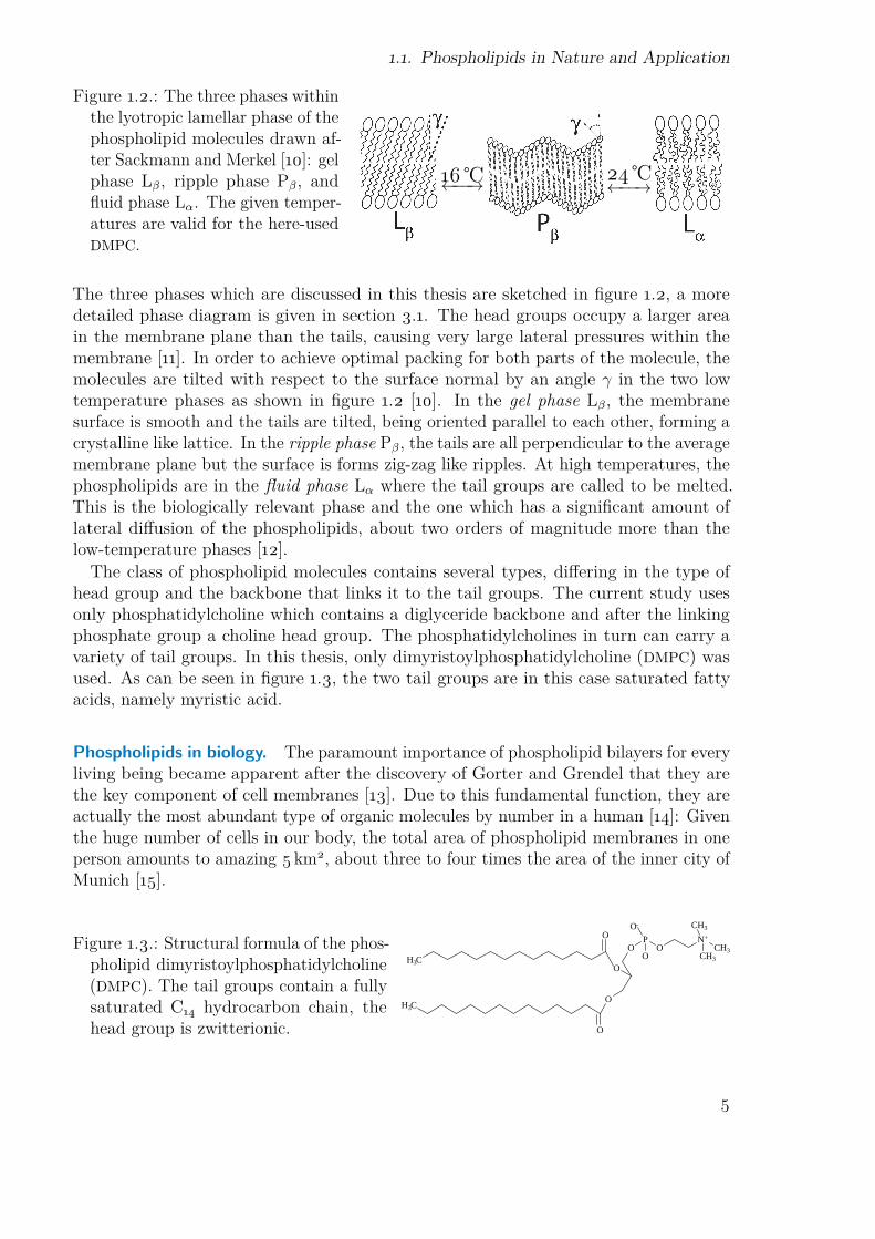
Figure 1.2.: The three phases withinthe lyotropic lamellar phase of thephospholipid molecules drawn af-ter Sackmann and Merkel [10]: gelphase Lβ, ripple phase Pβ, andfluid phase Lα. The given temper-atures are valid for the here-usedDMPC.
16 ←−−→ 24 ←−−→
The three phases which are discussed in this thesis are sketched in figure 1.2, a moredetailed phase diagram is given in section 3.1. The head groups occupy a larger areain the membrane plane than the tails, causing very large lateral pressures within themembrane [11]. In order to achieve optimal packing for both parts of the molecule, themolecules are tilted with respect to the surface normal by an angle γ in the two lowtemperature phases as shown in figure 1.2 [10]. In the gel phase Lβ, the membranesurface is smooth and the tails are tilted, being oriented parallel to each other, forming acrystalline like lattice. In the ripple phase Pβ, the tails are all perpendicular to the averagemembrane plane but the surface is forms zig-zag like ripples. At high temperatures, thephospholipids are in the fluid phase Lα where the tail groups are called to be melted.This is the biologically relevant phase and the one which has a significant amount oflateral diffusion of the phospholipids, about two orders of magnitude more than thelow-temperature phases [12].
The class of phospholipid molecules contains several types, differing in the type ofhead group and the backbone that links it to the tail groups. The current study usesonly phosphatidylcholine which contains a diglyceride backbone and after the linkingphosphate group a choline head group. The phosphatidylcholines in turn can carry avariety of tail groups. In this thesis, only dimyristoylphosphatidylcholine (DMPC) wasused. As can be seen in figure 1.3, the two tail groups are in this case saturated fattyacids, namely myristic acid.
Phospholipids in biology. The paramount importance of phospholipid bilayers for everyliving being became apparent after the discovery of Gorter and Grendel that they arethe key component of cell membranes [13]. Due to this fundamental function, they areactually the most abundant type of organic molecules by number in a human [14]: Giventhe huge number of cells in our body, the total area of phospholipid membranes in oneperson amounts to amazing 5 km2, about three to four times the area of the inner city ofMunich [15].
Figure 1.3.: Structural formula of the phos-pholipid dimyristoylphosphatidylcholine(DMPC). The tail groups contain a fullysaturated C14 hydrocarbon chain, thehead group is zwitterionic.
CH3
N+
CH3
CH3
OP
-O
OO
O
O
O
O
CH3
CH3
5

Chapter 1. Introduction
In most cases, the phospholipid molecules do not exhibit biological functionalitythemselves but they constitute the barriers of the cell that make it possible to maintaingradients of molecule concentrations. Further, they host membrane proteins [16] whichare responsible for a wide variety of functionalities, from molecular transport overmessaging to propulsion. These membrane proteins are so densely packed that thereare often only a few phospholipid molecules between two of them, not only separatingthem but also transmitting interactions between them [17, 18]. For these proteins, itis of essential importance to be mobile within the membrane and to be able to changeconformation [19]. The membrane proteins even diffuse as dynamic complexes togetherwith the phospholipid molecules [20]. One example for the influence of the mobility onthe protein functionality is an enhanced sensitivity of receptors on the cell surface ascompared to a static setup [21].
Another important component of the cell membrane is cholesterol. It has a rigid sterolbackbone and is mainly located in the lipophilic core of the membrane, its molecularstructure is shown later in chapter 3. The probably main biological function is thereduction of the fluidity and permeability of the membrane [22]. In certain mixing ratios,cholesterol is also known to induce a micro phase separation between cholesterol rich andcholesterol poor areas. It is speculated that this mechanism induces the formation ofso-called rafts in the membrane [23]. With a size of as small as 20 nm [24], they wouldprovide a platform for membrane proteins which profit from a clustering with otherproteins in the same raft.
Another possibility of the cell to influence the mobility of the proteins that should bementioned but will not be discussed in this thesis is the interaction of the cytoskeletonwith the membrane [25, 26].
Phospholipids in industry. Phospholipids are not only omnipresent in biology but havealso an important place in pharmaceutical and nutritional applications. This is also thearea where they receive most public attention. However, this attention usually boilsdown to the question «What is soy lecithin and why is it in my chocolate?»1
This application is a rather basic one that simply prevents the segregation of thelipophilic from the hydrophilic parts. In the last years there was also a lot of developmentof more complex applications such as functional food [27]. In this case, emulsifiers likephospholipids are used for example to increase the bioavailability of lipophilic nutrientsby forming emulsions [28].
The same is important for peroral (i. e. through the mouth) drug delivery of lipophiliccomponents and other molecules that are not adsorbed when taken without an appropriatedrug delivery system [29–31]. Phospholipids are here one of the many possible choices [32–34] for this task which is of increasing concern: the number of pharmaceutically relevantmolecules that are not water soluble – and therefore basically not applicable – is increasingas can be seen in figure 1.4.
Another approach for the delivery of sensitive drugs is to circumvent the digestivetract and choose a parenteral administration. Liposomes, i. e. phospholipid vesicles,
1http://www.highonhealth.org/what-is-soy-lecithin-and-why-is-it-in-my-chocolate/
6

1.1. Phospholipids in Nature and Application
2008
8.0%
(105)
19.9%
(261)
14.0%
(184)
8.1%
(106)
12.0%
(158)
8.9%
(117)
29.0%
(381)
2011
7.3%
(132)
19.7%
(358)
12.9%
(234)
7.9%
(143)
11.8%
(214)
9.1%
(165)
31.4%
(570)
very solublefreely solublesolublesparingly solubleslightly solublevery slightly solublepractically insoluble
Source: PharmaCircle
Figure 1.4.: Number of pharmaceutically relevant molecules (from research phase tomarketed) in water solubility categories of the United States Pharmacopeia. Althoughthe number of discovered molecules increased in each category during the past threeyears, only the «very slightly soluble» and «practically insoluble» molecules had also apercentile increase.
can for example be used as carrier for hemoglobin [35], anti-inflammatory drugs [36],or chemotherapeutica for cancer therapy [37]. When combined with fibrin scaffolds,they are also promising candidates for gene delivery systems [38]. For lipophilic drugs,nanoemulsions and nanosuspensions are an option. In these cases, the drug is incorporatedinto a lipophilic matrix and stabilized with a monolayer of amphiphilic molecules, forexample phospholipids [39, 40].
These drug delivery systems consisting of a lipid core covered with a phospholipidmonolayer shell are still matter of active research because they have serious problems:On the one hand, if the lipid core is liquid, the contained drug is released too quickly.On the other hand, if a solid lipid is chosen in the nanoparticle, it forms often a singlecrystal without the drug molecules which are then located at the rim of the particle andare also released too quickly [41–43].
Due to these problems, alternative drug delivery systems are needed. Polymers areone option for the dispersed phase [44, 45] which can even offer a response to externalstimuli and are therefore a step in the direction of targeted drug delivery [46, 47]. Alsomesoporous silica nanoparticles, possibly coated with phospholipids [48], can be used fora temperature controlled drug release [49].
The adequacy of phospholipids as stabilizing agent is therefore somewhat independentof the choice of the dispersed phase. The stabilizer layer plays a key role for theproperties of the drug delivery system: It determines the long-term stability against
7

Chapter 1. Introduction
chemical degradation [50], the bioavailability [51, 52], and can be used to control therelease rate of the drug [53].
These properties can be influenced by adding co-surfactants to the phospholipid. Forexample, a mixture of phospholipid and bile salt has been shown to be more potent thaneach of them alone [54] and is even capable of keeping a dispersion of a lipid phase stablewhile the lipid crystallizes [55, 56]. Such a phase transition of the dispersed phase isan especially challenging task for the stabilizer because it is accompanied by a drasticchange of the shape of the particles from droplet-like to disk-like. The stabilizer has tocover the freshly created surfaces before the particles aggregate. The co-surfactants thatcan cover these surfaces quickly enough were therefore termed fast.
That the mobility of the phospholipid molecules plays an essential role in the stabilizingproperties can also be inferred from the fact that the stabilization properties changeat the main phase transition of the phospholipids [57, 58]: One of the main changesat the main phase transition seen from the outside is the mobility of the phospholipidmolecules. It has also been suggested that the distribution of vesicles in the blood streamis influenced by the phase of the phospholipid molecules [59].
Concluding, phospholipids and their dynamics in particular are a worthwhile subjectmatter. As will be discussed later, this dynamics can be described using the conceptsdeveloped for glassy systems. Therefore, an overview of these concepts is given in thefollowing.
1.2. Some Concepts of Glassy DynamicsOn first sight, there seems to be little connection between glasses (disordered materi-als that lack the periodicity of crystals but behave mechanically like solids [60]) andphospholipids which have a distinct first order phase transition between a fluid anda crystalline state. However, the basic concepts of glass physics have been shown toexplain features observed in many soft materials with strongly interacting particles [61].Biopolymer networks [62] and phospholipid membranes [63] are only some examples.
As a liquid is cooled, it eventually passes its melting temperature Tm where mostsubstances crystallize. It is however possible to avoid crystallization, for example byexternal measures like confinement, the absence of any crystallization nuclei, or simply bysufficiently high cooling rates. In these cases, the substance becomes a supercooled liquid
in which the molecular motions slow down as the temperature is decreased. Arbitrarydefinitions call the substance finally to be in a glassy state when the viscosity reaches1013 Poise or the relaxation time 100 seconds. The corresponding temperature is quotedas the glass transition temperature Tg which usually occurs around 2
3 Tm [60, 64].Whereas a liquid can change configurations very quickly, the glassy system is basically
trapped in one conformation on the experimental time scale due to the long relaxation time.Looking at the energy landscape in the configuration space of the system, this confinementusually means that the system cannot relax to the thermodynamic equilibrium any moreon the experimental time scale [60]. This experimental time scale can be much shorterthan the 100 seconds quoted before. For example the neutron scattering experiments used
8

1.2. Some Concepts of Glassy Dynamics
in this thesis have observation times between about one picosecond and one nanosecond.If the relaxation time of a system is one or two orders of magnitude above thesevalues, it appears already frozen in the neutron scattering experiment. This microscopicmanifestation of the glass transition can happen at temperatures far above Tg [C].
There are strong parallels between the dynamics of different glass-forming substances,above as well as below Tg. This dynamics is often termed glassy dynamics and will bepresented in the following. The discussion in this thesis will stick to phenomenologicaldescriptions of the systems and touch the theoretical frameworks that aim to explainthe observations only as far as necessary. The main aim of this thesis was to determinehow the phospholipid molecules move in membranes with and without additives, inmultibilayers and single bilayers, in vesicles and emulsions. As it could be shown thatrecent concepts from glass physics can help to describe these motions, closer links to thetheories of glass physics should be established in future works. A worthwhile startingpoint for this description could be the probably best known theory of motions in glass-forming systems, the mode-coupling theory [65]. It was indeed already used to describethe motions of phospholipid molecules [63]. Although it has been shown that there aresystems where the theory fails [66], it has received renewed attention as it was embeddedin the bigger framework of the random first-order transition theory [67] and was extendedso that it could also describe the dynamical heterogeneities which will be presented inthe following [68, 69].
Glassy dynamics seen from the liquid side. There is no evidence for a qualitativechange of the dynamics anywhere near Tm [65, 70]. The dynamics in supercooled meltsshow, however, some peculiarities that are not seen in the «normal» behaviour of liquidsat high temperatures. Of these, the ones which are important in the current contextare: (i) the correlation functions of the system become stretched over a wider time rangewhich can be interpreted as an increasing distribution of the relaxation times and (ii) theaverage relaxation time of so-called fragile glass forming systems varies more stronglywith temperature than the Arrhenius dependence predicts.
The main reason for these differences between the dynamics at high and at lowtemperature is that two-body correlations determine the dynamics at high temperatureswhereas many-body correlations become important at the high densities near the glasstransition [71]. In other words, every particle experiences a cage of its neighbours asdepicted in figure 1.5 [65].
Following the motions of a particle over time, several regimes can be observed: Atvery short times, the particle does not experience any interaction with its neighbours.It moves in a free flight with a velocity according to a velocity distribution determinedby the thermal energy [72]. This motion will not be covered in this thesis because it isnot relevant for biological and pharmaceutical systems. Because these motions are on afemtosecond time scale, they are not observed by QENS.
Looking on a long time scale, it becomes clear that this initial motion can persistonly until the particle interacts with its neighbours which constitute a cage for theparticle. For a true long-range motion, the particle has to escape from this cage of
9

Chapter 1. Introduction
Figure 1.5.: A dense two-dimensional packing of discs. Itis clear that a long-range motion of any particle dependson the motions of the surrounding particles, the so-called cage of neighbours. The main difference betweenalternative visions of the dynamics is the behaviour ofthese neighbours: while the free volume theory actson the assumption that the central particle escapesfrom the cage through an opening, other approachesare based on collective rearrangements of the centralparticle together with its neighbours.
neighbours at some point [73]. While the motion of the particles can be described byrelatively simple formulae at very much longer time scales, intricate phenomena arise atthis intermediate time scale where the cage of neighbours governs the motions [74, 75].In the case of the phospholipid molecules, this intermediate time scale is on the order ofpico- to nanoseconds and therefore perfectly accessible with QENS.
The picture of Cohen and Turnbull, the free volume theory [76–78], explains theslowing down of the dynamics upon cooling with this escape step: as the temperatureis lowered, the density increases and free volume decreases – it is less likely that theneighbours open up a void that is big enough for the central particle to hop in andescape from the cage. The model has often been criticized being unable to explain severalmeasured quantities [79] and it was recently shown by comparing isothermal and isobaricdensity changes that the free volume cannot be the only parameter determining thedynamics [80, 81].
An alternative model was developed by Adam and Gibbs, explaining the same phe-nomenon with an increasing cooperativity [82]. As the sample is cooled down, more andmore particles move collectively together in transient clusters, so-called cooperatively
rearranging regions. Also this approach has problems [83] but it proved in the last yearsto be a very stimulating picture.
In recent years, dynamical heterogeneities, a clustering of velocities in a sample thatyields a separation of regions with large dynamics from ones with slow dynamics asshown in figure 1.6, were observed in a variety of dense systems, moving passively [84–87]as well as actively [88–91]. The dynamical heterogeneities, mostly studied very closeto the glass transition, were also observed far above this temperature [92, 93]. Theywere even seen in the liquid phase of systems that cannot be supercooled because theycrystallize [94, 95]. These dynamical heterogeneities were identified as the source of thenon-Gaussian part of the correlation functions [85, 94, 96] that are well-known to beobserved for dense liquids [74, 75].
At long times, these heterogeneities will average out: the fast particles will becomeslow, the slow particles will become fast; a particle will participate first in a clustermoving in some direction and later in another cluster moving in another direction. Theseare the steps of a random walk so that a homogeneous isotropic long-range diffusivemotion is restored on long time scales. Increasing the temperature will shift the transition
10

1.2. Some Concepts of Glassy Dynamics
Figure 1.6.: An example of dynamical heterogeneities [E]:The arrows show the displacement of the particles ina fixed time interval. It can be seen that differentparticles have different velocities and that regions withfast particles are spatially separated from regions withslow particles. A jump-like escape of a particle of itscage of neighbours is not observed, the central particlerather performs a flow-like motion together with itscage. Over longer times, the velocities of the particleschange and the picture is homogeneous. 0
2
4
6
8
10
12
14
16
18
20
22
24
0 2 4 6 8 10 12 14 16 18 20 22 24
y [nm]
x [nm]
from the heterogeneous to the homogeneous regime to shorter times [97].Although the identification of dynamical heterogeneities with cooperatively rearranging
regions is tempting, the relation between the two is not clarified to date [98]. It is amatter of active debate if there are any structural signatures that could be connected tothe dynamical heterogeneities. Recently, medium-range crystalline ordering, temporarilyordered domains attracted attention [99–101]. The change in local order was shown to becompletely independent of the local free volume but might indeed be the structural causeof dynamical heterogeneities [102, 103]. These ordered regions have a finite life time andoccur also in systems that do not crystallize, in contrast to crystal nuclei. However, themedium-range crystalline ordered domains are speculated to be precursors of crystalnuclei, providing an environment in which the nuclei can form [100].
In any case, a growing length scale of the correlations of the dynamics could explain thetemperature dependence of the correlation times [60]: Strong glass formers which showan Arrhenius temperature dependence are assumed to break and form bonds betweenneighbouring atoms at all temperatures. The activation energy is therefore independentof the temperature. Fragile glass formers which show a super-Arrhenius temperaturedependence are assumed to break and form interactions between growing clusters ofparticles. In this case, a decrease of the temperature causes an increase of the numberof bonds that has to be broken and formed for a rearrangement. The activation energyincreases therefore with decreasing temperature and the correlation times increase fasterthan with an Arrhenius temperature dependence.
It was shown that the interactions between the particles influence the temperature de-pendence of the relaxation times – the softer the interactions, the larger the fragility [104].There were also studies which found a fragile-to-strong transition of water [105] thatwas then related to underlying thermodynamical effects. This connection is currentlyunder scrutiny [C] and [106–113] and there is even an ongoing discussion whether one canobserve a transition from a fragile to a strong behaviour at all or if the observed effectsare not merely fit artifacts [C, D].
Glassy dynamics seen from the solid side. In disordered solids, the low-frequency(soft) modes are enhanced over the expectations from the Debye theory valid in normalcrystals and show correlations of the velocities of the particles over large distances [114–
11

Chapter 1. Introduction
116]. The disorder of these systems can be manifested either in the structure or in theinteractions of the system which means that even samples with a crystalline structurecan exhibit these excess modes [117, 118].
It was found that these soft modes are connected to irreversible reorganizations of theparticles [119] whereas neither free volume [120] nor potential energy [121] are. The energyof these surplus modes is correlated with the packing density: as the packing is loosened,the surplus modes are shifted to even lower frequency and become quasilocalized [122].
Depicting the situation, the particles in the disordered solid do not exhibit a long-rangemobility when looking on a long time scale. However, when looking only for a shorttime, one can see that the particles are displaced driven by the soft modes. As theseare localized, no regular patterns become apparent but the particles are displaced insome regions more than in others. Apart from the effect that the particles will be pulledback to their original place by the restoring forces, this picture resembles very much thedynamical heterogeneities.
Although it is not yet clear how these two effects are linked, there is increasingconsensus that they are [95, 96, 123–126]. It has also become clear that these modes varycontinuously, even through the solidification – which can be a crystallization [95, 127].This might be connected to the increasing occurrence of the medium-range crystallineordering that was observed in the liquid state and can be seen as precursors of freezingin simple two dimensional liquids [128].
In summary, the main control parameter that makes a system glassy is the tightpacking, i. e. the stereotactic hindrance. As the phospholipids are very tightly packed inthe region of the head groups [11], they can be expected to follow the same principles.As will be recapitulated in the following, this close relationship has been used verysuccessfully in the past [129] to describe phospholipid dynamics. It will be proposed inthis thesis that the new concepts which have been developed since then in glass physicsneed to find their way into the description of the phospholipids today.
1.3. Dynamics of PhospholipidsOne can distinguish three main contributions to the molecular motions of the phospholipidmolecules: the motions of the head groups, the ones of the tail groups, and the motionof the whole molecule as indicated in figure 1.7. The molecules can also change fromone leaflet to the other but this process has time constants in the minute regime and istherefore so slow that it will be neglected in the following. The localized motions of thehead and the tail groups will be treated less intensively than the long-range motion ofthe whole molecule because the long-range motion is expected to have more impact onthe biologically and pharmaceutically relevant properties of the phospholipid molecules.
The free volume theory for phospholipid systems. The long-range motion of phos-pholipid molecules is since a long time subject matter of intense research with differenttechniques that cover different time and length scales: From fluorescence recovery after
12

1.3. Dynamics of Phospholipids
Figure 1.7.: Possible motions in a phospho-lipid membrane sketched after Cevc [9].Intramolecularly, one can distinguishsmall-scale, rapid motions of the headgroups from slower and larger motionsof the tail groups. Above the mainphase transition, the molecules havealso a long-range mobility within themembrane.
photobleaching (FRAP) [130, 131] on a time scale of about 10 seconds over nuclear mag-netic resonance (NMR) [132] or single molecule tracking [133] on a time scale of about100 milliseconds and over fluorescence correlation spectroscopy [134, 135] on a time scaleof about 10 milliseconds to neutron scattering studies [136, 137] on time scales in thepico- to nanosecond regime. Neutron scattering has not only the advantage to probe thetime scale on which the phospholipids explore their immediate neighbourhood but alsoallows to follow these motions without introducing a marker into the system that mightdistort the dynamics.
In order to explain the results of diffusion measurements of hydrophobic probe moleculesin phospholipid membranes, Galla et al. [129] had the seminal idea to use the free volumetheory of Cohen and Turnbull that had been developed for glassy systems [76]. Theappeal of this description lies in the simple description of the measurements with basicallyonly one main parameter: the free volume.
This idea was therefore after its formulation in 1979 the predominant theory for roughly30 years, only slightly refined to take the viscosities of the surrounding solvent intoaccount [138, 139]. Its biggest success was probably the description of seemingly contra-dicting results obtained by different measurement techniques: the diffusion coefficientsdetermined by quasielastic neutron scattering (QENS) [136, 140] were about two ordersof magnitude higher than the ones determined with the macroscopic techniques.
This could be effortlessly explained in the frame of the free volume theory: BecauseQENS measures on a picosecond time scale, it is sensitive to the rattling of the phospholipidmolecules in the cage of their neighbours. This motion does not directly contribute tothe long-range motion. Only from time to time, a void opens up in the surroundingcage and the molecule can perform a jump out of the cage which was assumed to be thefundamental step of the long-range diffusion [141].
Collective motions call for a new description. Only a few years ago, moleculardynamics (MD) simulations became capable of describing the molecular dynamics wellenough and on sufficiently long time scales that it could contribute to the quest of thediffusion mechanism of phospholipids. The concept of the free volume was questionedas it became clear that the membrane is not adequately described as a two dimensionalliquid of hard disks and, in fact, the free volume is ill defined in the membrane [142–144].It was concluded that the fits of the theory to the data had a high quality but the
13

Chapter 1. Introduction
extracted parameter values did not have a clear relationship with the quantities theywere supposed to represent [145].
Additionally to those fundamental points of critique, there were more and more hintsfrom simulation [146–148] and experiment [137, 149] that the motions of the phospholipidmolecules were correlated over nanometer distances – an observation that the free volumetheory cannot account for. In some of these MD simulations, also structural orderwas observed in transiently ordered domains [147] which resemble the medium-rangecrystalline ordering that had been observed in glassy systems.
A break-through was achieved when Falck et al. [150] demonstrated in an MD simulationthat those molecules in their simulation that moved the largest distances in a given timerange take the cage of neighbours with them rather than escaping from it. The key ideain this simulation was to connect the position of the phospholipids at the beginning andthe end of a given time interval with vectors so that a two-dimensional flow patternbecame visible. Before, only the mean-square displacement had been evaluated. Thisobservable is dominated by the motions of the tails at short times [151] which obfuscatethe flow motions.
With quasielastic neutron scattering, it is possible to observe motions on the pico- tonanosecond time scale on which these flow-like motions prevail. Further, it is possible toconstruct models of the molecular motions that distinguish between the localized motionsof the tails and the long-range component of the whole molecule. It was therefore obviousto ask [B]
Can this novel view of flow-like motions of the phospholipids on ananosecond time scale be supported by experimental data?
The visualization of these transiently formed clusters of molecules is remarkably similarto the one of dynamical heterogeneities shown in figure 1.6. The next question wasthus [D–F]
Is it possible to interpret these motions in the picture of dynamicalheterogeneities?
To answer these questions, different models of the motion of the phospholipid moleculeshad to be evaluated against the data. In order to distinguish which of the models candescribe the data best, a focus of this thesis were data evaluation methods [C, D, G, H].
From pure DMPC to more complex systems. Independent from the exact mechanismof the molecular motions and accordingly more unambiguously determinable is the impactof environmental changes on the phospholipid mobility.
One parameter that has previously been extensively studied and is therefore keptconstant in the present contribution is the hydration of the phospholipids. Decreasing
14

1.3. Dynamics of Phospholipids
the hydration of the phospholipids gives certainly interesting insights but drives thesystem of pure DMPC even further away from systems that can be used in a biological orpharmaceutical application. All measurements for this thesis are therefore performed inthe biologically relevant fully hydrated state. Nevertheless, the most relevant results ofhydration-dependent studies are summarized in the following paragraph.
It is known from QENS measurements that a decrease of the hydration lowers the molec-ular mobility [152, 153]. Also the direct comparability of QENS measurements with MDsimulations was demonstrated [154] which revealed that the dynamics of the head groupsvaries continuously over the main phase transition. The head group was also studiedwith dielectric spectroscopy [155]. With rising hydration, the temperature dependencebecame increasingly Arrhenius-like, i. e. strong – similar to colloidal suspensions wherethe interactions are softened [104]. Also these results were interpreted in terms of slowcooperative motions, involving several lipid molecules.
Instead of going into the direction of this somewhat artificial state, in this workan attempt is made to understand the change of dynamics when going from the pureDMPC multibilayers to systems which are closer to biologically and pharmaceuticallyrelevant systems. A first step into this direction is the use of additives because neither inbiological nor in pharmaceutical systems contain only DMPC. Cholesterol was chosen asa representative of the additives that are important in biology. It is of major relevancein cell membranes and has therefore also been previously studied. In some of thosestudies, it was found that the collectivity of the phospholipid motions is influencedby cholesterol [146, 156]. As a substance that is used in pharmaceutical applications,sodium glycocholate was studied. It is an important co-surfactant for drug deliverysystems [55, 56], but had not previously been studied with QENS. Consequently, it wasstudied on the pico- to nanosecond time scale accessible with QENS [E]
How is the mobility of the phospholipids altered by additives?
From mixed DMPC– sodium glycocholate samples, the next step towards drug deliverysystems is the change from bilayers to monolayers. This is not a trivial change: monolayerscan behave very differently from bilayers, for example does the long-range mobility notshow any abrupt change when lowering the temperature [157] whereas bilayers of DMPCundergo a phase transition where the long-range mobility changes by at least an order ofmagnitude. These monolayers are studied on an oil-water interface which entails that thephospholipid density can actively be changed. An increase of the mobility with increasingarea per molecule was observed on the macroscopic scale [158]. However, up to datemeasurements of the mobility in phospholipid monolayers on a molecular scale are stillscare. QENS measurements were hence also performed to clarify [F]
How does the mobility of the phospholipids in monolayers differ fromthe one in bilayers?
15

Chapter 1. Introduction
Due to the small fractions of as little as 1% of phospholipid in the sample, thesemeasurements are challenging for both, the measurements and the data evaluationprocedures. It is only owed to the very low experimental background of the neutronscattering spectrometer TOFTOF that it was possible to evaluate the contribution of theDMPC. In addition, a focus of this thesis were the data reduction procedures [D, F].
In the next chapter, the theoretical tools to describe molecular motions will beintroduced and it will be shown how these quantities can in principle be measured withneutron scattering. The following chapters will present the practical aspects of thesemeasurements as well as their results.
16
Chapter 2.
Theoretical PrinciplesA very concise summary of the most important formulae for the description of themolecular structure and dynamics will be given, followed by an equally short descriptionof how these are linked to the quantities measured by neutron scattering. For a morein-depth treatment, the reader is referred to the extensive literature, e. g. [75, 159–164].
2.1. Molecular Structure and Dynamics are Describedby Correlation Functions
The definitions of the correlation functions. Introduced by van Hove [165], correlationfunctions became soon the common way to describe molecular motions. As will bediscussed later, one of their big advantages is that they can be accessed by scatteringmethods. In the following, it will be used that the systems do not exhibit quantum effects,that the various particles are statistically equivalent, and that the system is ergodic.
The pair correlation function Gpair(r, t) is then defined as
Gpair(r, t) =N∑
j=1⟨δ [r − (Rj(t0 + t)−Rk(t0))]⟩ (2.1)
with the number of particles N and the position Rl(t) of particle l at time t. The angularbrackets ⟨ ⟩ denote an ensemble average over all particles k and origins of time t0. Asthe system is ergodic, this is equivalent to average over all possible initial states of thesystem weighed with their probability. When multiplied with dr, it gives the probabilityto find a particle at time t in the volume dr at position r if some particle was at timet = 0 in the volume dr at position r = 0.
This information is a rather complicated one as it gives access to correlations betweenparticles – in space and time. From the pair correlation function, only the structuralcorrelations encoded in Gpair(r, t = 0) will be used in this thesis, the dynamical propertiesof the pair correlations. The dynamics will rather be extracted from the self correlation
function or auto correlation function Gself(r, t) which does not carry any informationabout the structural arrangement of different particles with respect to each other. It isdefined as
Gself(r, t) = ⟨δ [r − (Rk(t0 + t)−Rk(t0))]⟩ (2.2)
17

Chapter 2. Theoretical Principles
where the ensemble average can be calculated in an ergodic system over all particles kand the origins of time t0. Gself dr gives the probability to find a particle at time t in thevolume dr at position r if this particle was at time t = 0 in the volume dr at positionr = 0.
It is interesting to note that G(r, t) treats time and space differently: it has theunit (volume)-1 but not (time)-1. This can be understood from the interpretation as aprobability density: A given particle has to be at some point in space at every instant,therefore the integral over the whole space at any randomly chosen time must be unity.However, the particle will not necessarily visit every point in space at some instant,the integral over all times at a randomly chosen point in space can therefore have anynon-negative value.
Using Fourier transforms, it is possible to express the same information in differentrepresentations. The three important ones are:
1. The correlation function G(r, t) with the dimension (volume)-1 – because G(r, t) dris a dimensionless probability, discussed above.
2. The intermediate scattering function I(Q, t) is the Fourier transform of G(r, t) withrespect to r. The part corresponding to the self correlation, the self intermediatescattering function, can be written as
Iself(Q, t) = ⟨exp [iQ · (Rk(t0 + t)−Rk(t0))]⟩ (2.3)
which is dimensionless. The imaginary part of this function averages to zero aslong as the atomic displacements do not show a preferential direction.
3. The scattering function S(Q, ω) is the Fourier transform of I(Q, t) with respectto the time t and has the dimension [ω]-1 where [ω] denotes the unit of ω. In thisthesis, ω will be measured in units of energy. Also this function is real due to thetime reversal invariance of the dynamics in the studied samples.
Returning for a second to the structural information Gpair(r, t = 0), it is now clear thatthis quantity transforms to Ipair(Q, t = 0) and correspondingly to the static structure
factor Spair(Q) =∫∞
−∞ dω Spair(Q, ω). The self correlation function does not carrystructural information and is therefore unity, Gself(r, t = 0) = 1, which gives Iself(Q, t =0) = 1 and
∫∞−∞ dω Sself(Q, ω) = 1.
None of the samples studied in this thesis has any preferential orientation throughoutthe whole sample volume, i. e. they are all so-called powder samples. Because the recordedscattering signal is an average over all orientations, the absolute values r and Q will beused instead of the vectors r and Q.
In section 2.2, it will be shown that the scattering functions discussed above can bemeasured by neutron scattering. In order to evaluate the neutron scattering data, thescattering functions of models for molecular motions will be compared to the data. Inthe following, four different models for molecular motions will be presented together withtheir corresponding scattering functions: localized periodic and aperiodic motions as wellas long-range diffusive and flow motions.
18

2.1. Molecular Structure and Dynamics are Described by Correlation Functions
Localized periodic motions. In perfect crystals, vibrations of the molecules or atomsaround their average lattice site can be described by phonons. Roughly speaking,incoherent scattering is caused by single nuclei and every phonon will eventually pass overevery nucleus. Therefore, all phonons are visible at all measured Q and Sinelastic(Q, ω)measures the density of states. A sound derivation of this fact can be found in neutronscattering text books [160, 163]. At small energy transfers, only the acoustic phononsare visible. If Q ≪ π/a where a is the lattice spacing of the crystal, the phonondensity of states is in first approximation proportional to ω2 which results into anenergy-independent contribution to the scattering function [159, 166, 167].
With rising Q, an increasing amount of neutrons is scattered with the creation or anni-hilation of a phonon, given by the Debye-Waller factor which describes the distributionof neutron intensity between elastic and inelastic scattering,
S(Q, ω) = exp[−1
3Q2⟨u2⟩]· δ(ω) + Sinelastic(Q, ω) , (2.4)
where u is the displacement vector of the nuclei from their equilibrium position. Thisformula holds strictly for a cubic crystal where ⟨u2
x⟩ = ⟨u2y⟩ = ⟨u2
z⟩ = 13⟨u
2⟩ but it is stillapproximately correct in other cases [160].
In the case of incoherent scattering,∫∞
−∞ dω S(Q, ω) = 1 holds for all Q as statedbefore. It follows that
∞∫−∞
dω Sinelastic(Q, ω) = 1− exp[−1
3Q2⟨u2⟩]
. (2.5)
Developing the exponential in equation 2.5 into its Taylor series, it can be seen that thelattice vibrations contribute a signal to the inelastic scattering that is roughly constantin ω and has an intensity that increases proportional to Q2.
Localized aperiodic motions. For a confined or localized motion, the probability tofind a particle at the origin develops in the following manner: at time zero, it starts atunity and decays from this value because the particle can explore its cage. The shape ofthis decay depends on the properties of the motion of the particle in the cage. At longtimes, the probability to find the particle at the origin does not decay to zero because ofthe confinement. Fourier transformation of such a correlation function results in a sumof two components: a δ-function in energy space which corresponds to the non-vanishingprobability at long times and a broadened component which is the Fourier transform ofthe initial decay [168]. This combination of a δ and a broadened component is commonto all confined motions.
Using an exponential decay as a simple model for the initially decreasing probabilityto find the particle, one arrives at the scattering function
S(Q, ω) = A0(Q) · δ(ω) + (1− A0(Q)) · 1π
Γω2 + Γ2 . (2.6)
19

Chapter 2. Theoretical Principles
A0(Q) is called Elastic Incoherent Structure Factor (EISF). Its Q-dependence is determinedby the geometry of the motion (two sites jump, diffusion inside a hollow sphere, . . . ) andthe amplitude of the motions [159, 168].
A special case for a confined motion is a particle diffusing in a harmonic potential,a so-called Brownian oscillator. Despite the simplicity and physical relevance of thismodel, it is not often used by the neutron scattering community.
Its equation of motion can be set up as [169]
d2x
dt2 + β · dx
dt= −ω2 · x + F (t) (2.7)
where x is the displacement of the particle from the minimum of the potential at timet, β is the friction coefficient, ω the eigenfrequency of the particle in the potential, andF (t) a randomly fluctuating force.
For t≫ 1/β, the mean-square displacement can be calculated to
⟨x2⟩ = ϵ2 · (1− exp [−Γt]) t→∞−−−→ ϵ2 (2.8)
withϵ2 = kBT
mω2 and Γ = 2ω2
β. (2.9)
Using the so-called Gaussian approximation, this mean-square displacement can betranslated into the intermediate scattering function [170–173]
I(Q, t) = exp[−Q2 · ⟨x2⟩
]= exp
[−Q2 · ϵ2 · (1− exp [−Γt])
].
(2.10)
This expression can be Fourier transformed into the scattering function when expandingone of the exponential functions into its Taylor series,
I(Q, t) = exp[−Q2ϵ2
]· exp
[Q2ϵ2 exp [−Γt]
]= exp
[−Q2ϵ2
]·
∞∑n=0
(Q2ϵ2 exp [−Γt])n
n!
= exp[−Q2ϵ2
]·
∞∑n=0
Q2nϵ2n
n! · exp [−n · Γt] ,
(2.11)
which becomes after Fourier transform
S(Q, ω) = exp[−Q2ϵ2
]·
∞∑n=0
Q2nϵ2n
n! · 1π
n · Γ(n · Γ)2 + ω2 (2.12)
where the n = 0 term has to be understood as a δ function in energy. This term givesthe elastic incoherent structure factor
A0(Q) = exp[−Q2ϵ2
]. (2.13)
20

2.1. Molecular Structure and Dynamics are Described by Correlation Functions
Long-range diffusive motions. Diffusion results from a random walk of the particles.It is especially important for processes in the «micron world» [174] but random walkmotions can be found on vastly different time and length scales: on the nanoscopicscale for molecular motions, the microscopic scale for the so-called Brownian motion ofsuspended colloids [175, 176], or the metre scale for the motion of falling snow flakes –this last example will be discussed in an instant. The correlation function is in all casesderived as [75]
Space-time correlation function G(r, t) = (4πDt)− 32 exp
[− r2
4Dt
](2.14)
with its Fourier transforms
Intermediate scattering function I(Q, t) = exp[−DQ2t
]and (2.15)
Scattering function S(Q, ω) = 1π
DQ2
ω2 + DQ2 . (2.16)
As mentioned above, these formulae can also describe the random walk of snow flakes.They fall in the gravitational field of the earth in z direction, turbulences in the airmake them move randomly in the (x, y)-plane. The time-evolution of the position of asnowflake in this plane is resolved by its fall. The Gaussian space-time auto-correlationfunction 2.14 gives the probability of a snow flake to move a certain distance in the(x, y)-plane after some time t or equivalently after some height loss. The height h of asnow pile under a roof with a point-like hole would have a Gaussian shape. Having nota hole but a semi-infinite plane (an intact roof with an end) gives the integral over allGaussians with their starting points (centres) from −∞ to 0 (the eaves, cf. figure 2.1).This yields for the height of the snow pile h in the direction x
h(x) =0∫
−∞
dx′(4πDt)− 12 exp
[−(x− x′)2
4Dt
]= 1
2
(1− erf
[x√4Dt
])(2.17)
where D is the diffusion coefficient of the snow flakes and t the time it took the snowflakes to fall from the height of the roof onto the balustrade. It can be seen in figure 2.1that this functional dependence can reproduce the shape of the snow pile very well.
Going back to the formulae describing the random walk, it can be seen that the fullwidth at half maximum (FWHM) of the Lorentzian scattering function 2.16 is 2Γ = 2DQ2
with the diffusion coefficient D. It is important to note that the model of FickeanDiffusion does not only comprise the Lorentzian form of the scattering function butnecessarily also this quadratic Q-dependence of the line width.
A simple quadratic dependence of the line width on Q is hardly ever observed. Somecommon cases and their explanations are:
The line width is too small at intermediate values of Q where structure factormaxima result in a large amount of coherent scattering. This is normally assignedto the so-called de Gennes narrowing [177, 178].
21

Chapter 2. Theoretical Principles
Figure 2.1.: Photograph of fresh snow pil-ing on a balustrade. The roof of thehouse shields the right part – if snowwas falling like rain, the wetness wouldhave a step-like distribution. Due tothe random walk of the snow flakesduring their fall, the step function issmeared out. Also shown is a fit ofequation 2.17, demonstrating that thisdescription agrees very well with theobservation.
The line width is too large at small Q. This is often interpreted as sign of multiplescattering in the sample [179]. It could however be shown in the frame of this thesisthat this is not a necessary consequence of multiple scattering [D].
The line width is too small at large Q. This is often interpreted as a stop-and-gomotion [180]. It was however found for the spectra evaluated in this thesis thatsuch a behaviour is also observed when a wrong model is used to fit the data [B].
Long-range flow motions. A type of motion that we are more used to in daily life areflow motions, for example in a river. The particles do not change direction all the time asin the random walk but keep going in the same direction with a constant velocity until itis reflected by an obstacle. The velocity vector has three independent components thatgive the total velocity according to v2
x + v2y + v2
z = v2. Assuming that each of the threecomponents has a Gaussian probability distribution around the most probable speed v0,the probability density function (PDF) for the speed
PDF(v) = 1√
πv20
3
exp[−v2
v20
](2.18)
results [181]. This is the well-known Maxwell-Boltzmann distribution that is for instancefound for the velocity distribution of the particles of an ideal gas. In this case of the idealgas, the most probable speed is v0 =
√2kBT/m where m is the mass of the particles, kB
the Boltzmann constant, and T the temperature.In the phospholipid samples, the molecules are not expected to move completely
independent from each other like in an ideal gas but rather collectively. These collectiveflow motions are confined to the plane of the membrane. However, also in these samplesmolecules move in all directions of space because the many membranes in the sample arerandomly oriented with respect to each other. Even if the molecules are all moving in thesame directions in a small volume of the sample, they will move in any other direction insome other part of the sample. The fact that the directions are spatially separated inthis case and not in the ideal gas does not change the ensemble averaged correlation andscattering functions which are given in the following.
22
2.1. Molecular Structure and Dynamics are Described by Correlation Functions
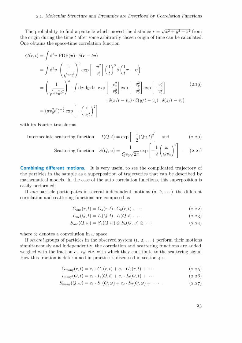
The probability to find a particle which moved the distance r =√
x2 + y2 + z2 fromthe origin during the time t after some arbitrarily chosen origin of time can be calculated.One obtains the space-time correlation function
G(r, t) =∫
d3v PDF(v) · δ(r − tv)
=∫
d3v
1√πv2
0
3
exp[−v2
v20
] (1t
)3δ(1
tr − v
)
= 1√
πv20t2
3
·∫
dx dy dz exp[−v2
x
v20
]exp
[−
v2y
v20
]exp
[−v2
z
v20
]
· δ(x/t− vx) · δ(y/t− vy) · δ(z/t− vz)
= (πv20t2)− 3
2 exp[−(
r
v0t
)2]
(2.19)
with its Fourier transforms
Intermediate scattering function I(Q, t) = exp[−1
2(Qv0t)2]
and (2.20)
Scattering function S(Q, ω) = 1Qv0√
2πexp
−12
(ω
Qv0
)2 . (2.21)
Combining different motions. It is very useful to see the complicated trajectory ofthe particles in the sample as a superposition of trajectories that can be described bymathematical models. In the case of the auto correlation functions, this superposition iseasily performed:
If one particle participates in several independent motions (a, b, . . . ) the differentcorrelation and scattering functions are composed as
Gone(r, t) = Ga(r, t) ·Gb(r, t) · · · · (2.22)Ione(Q, t) = Ia(Q, t) · Ib(Q, t) · · · · (2.23)
Sone(Q, ω) = Sa(Q, ω)⊗ Sb(Q, ω)⊗ · · · (2.24)
where ⊗ denotes a convolution in ω space.If several groups of particles in the observed system (1, 2, . . . ) perform their motions
simultaneously and independently, the correlation and scattering functions are added,weighed with the fraction c1, c2, etc. with which they contribute to the scattering signal.How this fraction is determined in practice is discussed in section 4.1.
Gmany(r, t) = c1 ·G1(r, t) + c2 ·G2(r, t) + · · · (2.25)Imany(Q, t) = c1 · I1(Q, t) + c2 · I2(Q, t) + · · · (2.26)
Smany(Q, ω) = c1 · S1(Q, ω) + c2 · S2(Q, ω) + · · · . (2.27)
23

Chapter 2. Theoretical Principles
Of course, each of the G1, G2, etc. can be a compound Gone, Gtwo etc. as defined above.In the special case where only a fraction f of the scatterers participates in a confined
motion and the other, (1− f), does not, the scattering function becomes, denoting theLorentzian with L,
S(Q, ω) = f · [A0 · δ + (1− A0) · L] + (1− f) · δ= (1− f + fA0) · δ + (f − fA0) · L= B0 · δ + (1−B0) · L with B0 = 1− f + f · A0 .
(2.28)
2.2. Measuring the Correlation Functions with NeutronScattering
There are different methods to measure the correlation functions which operate on verydifferent time and length scales. Optical microscopy measurements are currently limitedto sizes above 100 nm [182, 183]. With pulsed field gradient nuclear magnetic resonance,the length scale is very comparable [184]. In contrast to those, neutron and x-rayscattering operate on an Ångström to nanometre scale and have proven to be very usefulfor the study of phospholipid membranes [185]. X-ray scattering is very a very powerfultool for structural studies. As far as the dynamics is concerned, one can either accessthe sub-picosecond time scale with inelastic x-ray scattering [186, 187] or the millisecondrange with coherent x-ray photon correlation spectroscopy [188]. Neutron scatteringgives also access to the dynamics of the samples on a pico- to nanosecond time scale.This is the same time scale that can nowadays be covered with MD simulations. Becauseof this overlap, MD simulations and scattering methods can be used complementary tovalidate complex physical models.
Scattering cross sections. It will be outlined in the following how the measuredneutron scattering signal is connected to the correlation functions treated previously.The neutrons are assumed to have an exactly known initial energy Ei and a commonwave vector ki, i. e. a monoenergetic and collimated beam. Counting the neutrons whichare scattered into a solid angle element dΩ around a final wave vector kf and with afinal energy between Ef and Ef + dEf amounts to measuring(
d2σ
dΩ dEf
)dΩ dEf (2.29)
which is the number of scattered neutrons in a certain time divided by the number ofincident neutrons during the same time. The quantity d2σ/(dΩ dEf ) is called the double
differential cross section.A qualitative understanding of the reasons behind the redistribution of the neutron
intensity into different final energies and directions of the wave vector can be obtainedeasily: Structures in the sample with sizes on the same order of magnitude as thewavelength of the incident neutrons cause a change of the direction of the neutron,
24

2.2. Measuring the Correlation Functions with Neutron Scattering
reminding of diffraction of light at a slit. Motions in the sample can be created orannihilated by the neutrons which correspondingly lose or gain energy from the sample.
If these motions are not of interest, the energy dependence of the neutron signal canbe integrated out, resulting in the differential cross section
dσ
dΩ =∫
dEfd2σ
dΩ dEf
. (2.30)
This quantity has the advantage that it is relatively easy to measure by detecting thescattered neutrons without an analysis of their final energy. However, it will becomeclear in the following that this is not the static structure factor S(Q) mentioned above.
It is further interesting to notice that the integral of the differential cross section overthe whole solid angle is not any special quantity and does not have to be preserved: Inparticular, this is not the bound scattering cross section that is a tabulated property ofthe nuclei [189]. As a consequence, the absolute number of neutrons which are scatteredby a sample increases with increasing temperature of the sample. The reason for thisbehaviour will be discussed below. The only conserved quantity is the differential crosssection in the limit of forward scattering for which one obtains
limkf →ki
(dσ
dΩ
)= σb
4π(2.31)
where σb is the bound scattering cross section of the nucleus.
From scattering cross sections to correlation functions. The double differential crosssection can be calculated from properties of the system, assuming that each neutron wasscattered only once. It is essentially the transition rate of the neutrons to go from theirinitial to the final state. This transition is caused by the interaction with the samplewhich is seen as a time-dependent perturbation, related to the time-dependent position ofthe point-like nuclei. As the molecules used in the present study do not have significantmagnetic moments, only nuclear scattering is considered.
The incident neutron beam is not spin polarized and the polarization of the neutronsis also not analysed after the scattering event. Using that the systems can be describedwithout quantum effects and with the approximation that the spin, isotope, and elementof the scattering nuclei are completely uncorrelated with their positions, one obtains forthe double differential cross section
d2σ
dΩdEf
= 1~
d2σ
dΩdω=
1~
12π
kf
ki
∑j,k
bjbk
∞∫−∞
dt e−iωt⟨
exp [iQ · (Rj(t0 + t)−Rk(t0))]⟩
. (2.32)
In this equation, ki and kf are the moduli of the wave vectors of the neutron beforeand after the scattering event, respectively, and Q = kf − ki. The scattering length of
25

Chapter 2. Theoretical Principles
nucleus l is bl, the bar over the scattering lengths denotes an average over all possiblenuclear spin orientations and isotope types, and the angular brackets ⟨ ⟩ are an ensembleaverage over all t0 for the presented ergodic systems.
The average of the product of the scattering lengths is decomposed into the averagevalue of all scattering lengths and a variation thereof, called coherent and incoherent
scattering lengths, respectively. This can be visualized by a lattice of scatterers, all withthe same scattering length. They will scatter the neutron beam as a whole, collectiveproperties will be important and there will be a pattern in Q-space due to the patternin real space. This is the coherent scattering. In contrast, a large cloud of nuclei whichare randomly distributed and non of them close to each other will scatter incoherently:there results no pattern in Q-space as no interference of the scattered neutron waves ispossible. The nuclei scatter neutrons as if they were alone.
This reformulation allows to extract the scattering lengths from the sum and split thetotal double differential cross section into a sum of a coherent and an incoherent part. Acomparison of equation 2.32 and equation 2.3 shows that the two summands contain theFourier transform of the pair (coherent) and self (incoherent) scattering function:
d2σ
dΩdω= kf
ki
N
4π
(σincSself(Q, ω) + σcohSpair(Q, ω)
)(2.33)
where N is the number of scattering nuclei.This function shows again that the double integral of the double differential cross section
is not a conserved quantity: Taking again the example of increasing the temperature ofthe sample, the Sself(Q, ω) will increasingly cause an energy gain of the neutrons (largekf). As the integral of Sself(Q, ω) over all energies is a constant [160], this means thatthe number of neutrons scattered with a smaller kf decreases. This simple redistributionin S(Q, ω) is weighed with a factor kf to get the double differential cross section – whichtherefore increases with increasing temperature.
So far, the energy change of the neutron was denoted by ~ω = Ef −Ei. As is a sloppyhabit in neutron scattering, the ~ is often suppressed in this thesis, resulting in a quantitycalled ω which is an energy.
That, at least, is the theory. As mentioned above, quite some assumptions are usedwhich will hardly ever be met in any experiment. The three most important of these are:
It was assumed that the incident neutrons had all the same energy Ei and wavevector ki, i. e. a collimated, monoenergetic beam. In reality, both quantities aredistributed. As the superposition principle holds, the final neutron distributionsare a convolution of the initial neutron distribution and the response of the sample.Its influence is discussed in section 3.2 and the corresponding publication [D].
The recorded signal was assumed to be determined only by a single scattering eventin the sample. However, also the geometry and scattering properties of the sampleinfluences the measured neutron signal: The extension of the sample can introduceadditional time-of-flight differences, the neutron can be absorbed or scattered a
26

2.2. Measuring the Correlation Functions with Neutron Scattering
second time on its way through the sample. Effects caused by the geometry of thesample and the absorption of neutrons in the sample are discussed in section 3.3,multiple scattering is discussed in the corresponding publication [D].
The scattering cross sections of the nuclei were assumed to be uncorrelated withthe positions of the nuclei in the sample. Although this is clearly not the case for abiomolecule which is functional only because the atoms are always on the samespots, it is a quite good approximation because by far the largest contribution tothe scattered intensity is due to the incoherent scattering of hydrogen – which isdue to the spin alignments between neutron and proton and is therefore really notcorrelated with the position in the molecule.
The details on how the measurements were performed and how these experimentaldeviations from the theory are visible in the measurements is presented in the followingchapter. In the next but one, it will be shown how the data evaluation took these effectsinto account.
27


Chapter 3.
Materials and MethodsThe preparation of the samples and some of their basic properties are described inthis chapter, followed by a description of the neutron spectrometer TOFTOF where themeasurements of the systems were performed. Finally, a few examples are given how theobtained spectra are influenced by the set-up of the instrument and how the correspondingsettings were chosen for the measurements presented in this thesis.
3.1. Preparation and Characteristics of the PhospholipidSamples
The dynamics of the phospholipid was first studied in multibilayers of only DMPC andD2O [B, D]. The advantage of this system is that it has only two components and a largesignal-to-background ratio which makes it possible to study the motions in detail. Somebackground information about the hydration water, which is also an interesting subjectmatter on its own right [C], is given in this section, followed by the description of thepreparation of the multibilayers. It is followed by the description of multibilayers ofDMPC mixed with additives [E] and the one of single bilayers of pure DMPC [F] whichlead to the preparation of monolayers of DMPC mixed with additives on both, emulsionsand suspensions [F]. This stepwise increase of the complexity of the systems will make itpossible to distinguish the influences of different factors on the phospholipid dynamics.
Hydration water. All systems discussed in this thesis contain hydration water. Whileit is the main topic of one study [C], it is a nuisance contribution in the case of thephospholipid samples [B, D–F] and will not be evaluated in these cases.
Briefly following the course of the hydration of DMPC, one water molecule per phos-pholipid molecule corresponds to a mass fraction cw of roughly 2.5% [8] (cf. figure 3.1).A single layer of water on the phospholipids is reached at 5-6 mol H2O / mol DMPC [190],corresponding to 0.13 g H2O / g DMPC or a cw of about 12%.
This hydration range is interesting for studies of water because the first layer of wateradsorbed on surfaces usually does not freeze, making measurements of the water dynamicsat low temperatures in the amorphous state possible [105, 155]. However, the interactionsbetween the water molecules and the substrate influence the dynamics of the molecules.
29

Chapter 3. Materials and Methods
0 10 20 30 40 500
20
40
60
80
cw (% H2O)
T (
°C)
Lα
Pβ
Lβ
Lc
Figure 3.1.: Phase diagram of diacyl-phosphatidylcholines in water [8, 9], the temperatureaxis refers to DPPC. The main phase transition of DMPC is 8 below the one of DPPC,namely at 24 . The continuous lines show phase boundaries between the crystallineLc, gel Lβ, ripple Pβ, and fluid Lα phase. The broken lines show special hydrationvalues: The long dashed line corresponds to one water molecule per phospholipidmolecule, the short dashed line shows the maximal water uptake from the vapourphase, and the dotted line the maximal water uptake from the liquid phase. Thecrystalline phase Lc is formed only when the sample is stored over several days at4 [9] and is not covered in the measurements presented here.
It is therefore questionable if the hydration water is a suitable model system for bulkwater [C].
For the study of phospholipids in the fully hydrated state, the hydration was increasedto much higher values. Full hydration is reached at a cw of about 40% (cf. figure 3.1),therefore many previous studies had aimed to reach exactly this value. However, neutrondiffraction on these samples showed long-standing inconsistencies. It was finally foundthat already very small temperature gradients between the wall of the sample containerand the sample are sufficient to decrease the relative humidity from the supposed 100%,resulting in a lower hydration of the sample [191].
As a decrease in hydration was found to influence the dynamics [153], it is necessaryto ensure the full hydration of the sample. Therefore, all phospholipid samples wereproduced with surplus D2O. The resulting mixture is not homogeneous – areas with fullyhydrated phospholipid alternate with bubbles of D2O. As will be discussed in section 4.1,this does not pose a problem for the data analysis because the corresponding signal ofD2O can be subtracted when the composition of the sample is known.
However, this subtraction necessarily assumes that the reference measurement of abulk D2O sample yields the same spectrum as the D2O in the mixture. The beforementioned interaction between the water and the biomolecules was also observed in waterlayers adsorbed on phospholipids together with a reduced mobility [192]. These effects
30

3.1. Preparation and Characteristics of the Phospholipid Samples
are pronounced in weakly hydrated membranes [193] but hardly visible in fully hydratedmembranes because it was shown that only the dynamics of the first layer of water wasobservably affected on a picosecond time scale [190, 194]. Therefore, the vast majority ofthe D2O in the fully hydrated samples can be expected in good approximation to havebulk-like properties and a subtraction of its contribution is thus well justified.
Multibilayers of pure DMPC. The phospholipid DMPC was obtained as dry powderfrom Lipoid GmbH, Ludwigshafen, Germany, and used as received. The common startof many preparation procedures described in the literature to dissolve the phospholipidin chloroform was purposefully avoided in order to exclude the possibility of any residualchloroform in the samples. The omission of this step did not impede the hydrationbecause the phospholipid was obtained as a very fine powder.
Another difference to the commonly used preparation procedures for neutron scatteringmeasurements [137, 153, 156, 195–200] was the omission of a solid support of themembranes. This brings the disadvantage that the phospholipid layers cannot be alignedwith respect to the scattering vector and the measured signal is therefore always a powderaverage. However, the big advantage is that any distortion of the dynamics by the solidsupport can be excluded and no misleading signal from the supporting material canpossibly be observed.
It is known that a solid support interacts with the phospholipids [201] which sets limitsto the similarity between supported lipid bilayers and biologically relevant systems [202].In fact, some of the measurements presented here [B] have been compared with similarones which were performed on samples with a solid support [203] where a differentdynamical behaviour was observed. It can be speculated that this difference is caused bythe interaction with the solid support.
The only step for the preparation of the multibilayers is to hydrate the dry phospholipidpowder. To avoid a rapid uncontrolled formation of phospholipid vesicles and nanotubesand other non liquid crystalline phases [204, 205], the first part of the hydration wasperformed via the vapour phase: A small jar containing the phospholipid was placed in abigger bottle which could be sealed and contained about 5 ml of D2O. This assemblywas placed in a constant temperature environment at 40 (above the main phasetransition of the phospholipid, see below) for 24 hours or more. Under these conditions,the phospholipid hydration from the vapour phase reaches about 20% as depicted fromthe phase diagram displayed in figure 3.1. In a second step, liquid D2O was added witha pipette up to an amount of at least 50 mass % and the mixture was stirred gently.
Multibilayers of DMPC and additives. The sample preparation was very similar to theone of the pure DMPC multibilayers, the only difference was that one of the additivesmyristic acid, farnesol, cholesterol, or sodium glycocholate was mixed with the phospho-lipid powder before the hydration. The compositions of the samples are listed in detailin the corresponding publication [E].
These additives can change the phase transition temperatures and induce even newphases. For example, when adding cholesterol, there is a micro phase separation into
31

Chapter 3. Materials and Methods
1.00 1.25 1.50 1.75 2.00
1.0
2.0
3.0
4.0
Q (A-1)
S(Q
,ω≈0)
(a.u
.)
20
°C40
°C
N10M03F09
C40C30C20C10D Figure 3.2.: The acyl chain correlation
peak of DMPC in multibilayers at 1.5 Å-1
shown at two temperatures – below andabove the main phase transition – pure(D) and with several additives: sodiumglycocholate (N), myristic acid (M), far-nesol (F), and cholesterol (C). The num-bers indicate the amount of additive inrelation to the phospholipid in mol% [E].
a cholesterol-rich and a cholesterol-poor phase [131]. However, on the time- and lengthscales covered in the presented measurements, the structure and dynamics changed onlygradually. This is covered in detail in the corresponding publication [E] and can also beseen exemplarily in figure 3.2. In this figure, the pronounced structure factor maximumin the diffraction patterns at 1.5 Å-1 is shown which is caused by the regular arrangementof the acyl chains [156, 206]. It can be seen that the feature is much more pronouncedat low temperatures below the main phase transition but not heavily influenced by theadditives.
Single bilayers in vesicles. Single bilayers were studied without any solid support invesicles which are unilamellar hollow spheres with a diameter of about 130 nm thatcontain the phospholipid only in the outer shell with 5 nm thickness. This diameter waschosen to be in the same order of magnitude as in drug delivery systems. For those, theparticles must have a diameter between 10 and 200 nm [44]: smaller particles are filteredout by the kidney and larger particles are sequestrated by the spleen and liver, also theuptake by cells depends on the size. Compared to a cell, these vesicles are thereforerather small as can be seen in figure 3.3. The small size of the vesicles results in anincreased curvature of the phospholipid bilayer.
For vesicles with a diameter of about 100 nm, the main phase transition is slightlybroadened but still at the same temperature as found for multibilayer samples. Signifi-
Red Blood Cell
≈25
00nm
≈15
00nm
≈ 7500 nm
Nanodroplet, ∅ ≈ 130 nm
Figure 3.3.: Comparison of the cross-section ofa vesicle or nanodroplet and a red blood cell.It can readily be seen that the curvature ofthe surface is much stronger in the case ofthe vesicles or nanodroplets as compared tothe one of the cell.
32

3.1. Preparation and Characteristics of the Phospholipid Samples
cantly smaller vesicles exhibit a very broad transition that is shifted to lower temperaturesby several degrees [207].
Most of the vesicle samples consists of the aqueous phase: for vesicles with a diameterof 130 nm, the mass fraction of DMPC in the sample is limited to only approx. 12% atclose-packing (volume fraction φ = π/3/
√2 ≈ 0.740) or approx. 10% at the maximally
random jammed state (φ ≈ 0.64) [208].The vesicles were produced using two techniques: sonication and extrusion. With
sonication, the vesicles are produced using ultrasound waves while with extrusion, themixture of phospholipids and D2O is pressed through a plastic membrane that containsholes of a well-defined diameter. While the former can produce smaller vesicles, thelatter is more gentle to the molecules, the resulting vesicles exhibit less polydispersity,multilamellar vesicles, and chemical degeneration of the phospholipids.
Sonication was performed with a Bandelin Sonopuls UW 2070 ultrasound generatorwith a tip diameter of 3 mm (MS73), Bandelin electronic, Berlin, Germany. The deviceuses a frequency of 20 kHz with an output power of up to 70 W. The preparationprocedures can be found in table 3.1.
For the extrusion, a commercially available extrusion device [210] was heated togetherwith the syringes and the suspension of the swollen DMPC to 40 . The suspension waspassed 21 times through a membrane with 100 nm pore size, keeping the equipment allthe time close to 40 , i. e. above the main phase transition of the phospholipid.
Monolayers in emulsions. Phospholipid monolayers in emulsions were prepared usingsonication. Attempts to produce emulsions also by extrusion have not been successful.Extrusion would have offered an opportunity to treat the stabilizer molecules with lessstress and potentially also obtain a less polydisperse size distribution of the emulsiondroplets.
The monolayers consisted either of pure DMPC or mixed with sodium glycocholate(abbreviated as NaGC or SGC). The sonication procedures can be found in table 3.1,the exact compositions of the samples are listed in the corresponding publication [F].
As in the case of the vesicles, the amount of phospholipid in these samples is verylimited. The maximally achievable mass fraction of about 10% obtained there reducesin the case of the emulsions even to half of this value, i. e. 5%, because vesicles containbilayers and emulsions only monolayers.
Monolayers in suspensions. Phospholipid monolayers in suspensions were preparedusing high-pressure homogenization. In these suspensions, the aqueous phase was D2Oand the stabilizer DMPC and NaGC. As dispersed phases, either protonated tripalmitinor perdeuterated tetracosane were used. The suspensions were produced from mixturesof the following compositions:
8.46% protonated tripalmitin, 2.13% DMPC, 0.34% NaGC, 89.07% D2O
10.30% perdeuterated tetracosane, 1.19% DMPC, 0.12% NaGC, 88.39% D2O1
1Prepared by Martin Schmiele, Friedrich-Alexander-Universität Erlangen-Nürnberg
33

Chapter 3. Materials and Methods
name time (min) cycle power (%) ∅ (nm) PDI
vS 2 × 5 3 102 × 5 3 20 430 0.314 × 5 3 20 131 0.28
eD23N00 5 × 1 1 101 × 10 3 10 180 0.181 × 5 3 10 154 0.191 × 5 3 10 144 0.211 × 5 3 10 132 0.21
eD13N00 10 × 1 1 10 30010 × 1 1 101 × 10 1 101 × 10 3 10 1751 × 10 3 20 136 0.13
eD11N02 2 × 5 3 102 × 5 3 20 218 0.174 × 5 3 20 174 0.154 × 5 3 20 134 0.14
eD11N01 5 × 1 3 10 220 0.165 × 1 3 10 200 0.121 × 5 1 20 180 0.191 × 5 3 20 168 0.152 × 5 3 20 124 0.14
eD09N02 1 × 10 3 10 179 0.132 × 5 3 20 154 0.142 × 5 3 20 133 0.13
Table 3.1.: Production procedures of the samples that were produced by sonication. Thenaming follows the same convention as in the corresponding publication [F]: v denotesvesicles, e emulsions. S stands for sonicated, Dxx and Nxx are the mass fractions xx(in %) of DMPC and NaGC, respectively. «cycle» indicates how many tenths of eachsecond are spent in the active interval, no ultrasound radiation is produced duringthe remainder of each second. The z-averaged diameter of the particles ∅ and thepolydispersity index PDI are obtained from a cumulant analysis of photocorrelationspectroscopy (PCS) data [209].
34

3.2. Description of the Neutron time-of-flight Spectrometer TOFTOF
3.11% perdeuterated tetracosane, 0.92% DMPC, 0.10% NaGC, 95.87% D2O1
Predispersions of these mixtures were prepared 20 above the melting temperatureof the lipid dispersed phase using high-speed stirring with an IKA UltraTurrax andsubsequent high-pressure homogenization using an APV-2000 (APV Deutschland GmbH,Unna, Germany) thermostatted at the same temperature for 2 min at approx. 1.2 kbar.The size of the recrystallized particles was determined by dynamic light scattering (photoncorrelation spectroscopy, PCS).
It should be noted that the production of the suspensions involves minor uncontrolledlosses of material, e. g. evaporation of D2O, residual material at the UltraTurrax orinside the high-pressure homogenizer. The final composition of the samples will thereforeslightly deviate from the original sample weights given here.
3.2. Description of the Neutron time-of-flightSpectrometer TOFTOF
The neutron time-of-flight spectrometer TOFTOF at the Forschungs-Neutronenquelle HeinzMaier-Leibnitz (FRM II) [211, 212] is sketched in figure 3.4. It measures the energy of theneutrons before and after the sample by determining their velocity via their time-of-flight(tof). This takes place in both the primary part of the spectrometer where the neutronbeam is prepared by tof monochromatization (TOF-) and in the secondary part wheretof is used to measure the energy transfer from or to the sample (-TOF). Hence the nameof the instrument: TOFTOF.
The primary spectrometer. The white continuous beam of neutrons from the coldsource of the FRM II gets chopped into short bunches of polyenergetic neutrons by a firstpair of choppers (see figures 3.4 and 3.5). After a certain distance, this bunch will havebroadened due to the different energies and therefore velocities of the neutrons. Then,another chopper pair at the end of the primary spectrometer, (numbers 6 & 7) transmitsonly a fraction of this bunch. As it took the neutrons in this fraction approximately thesame time to travel the distance between the two chopper pairs, they have about thesame velocity. The ones that are too fast or too slow are absorbed in the boron coatingof the chopper.
To ensure that only neutrons with the wanted velocity can pass the chopper system,two more higher order choppers (numbers 3 & 4) are positioned in between. They suppressthe transmission of neutrons which have higher order wavelengths.
Chopper 5, the frame overlap chopper, completes the setup. It rotates at a fraction ofthe speed of the others and opens therefore only for every nth pulse, where n is calledthe frame overlap ratio. This prolongs the time that neutrons have after the scatteringevent to get detected before the fastest neutrons of a new pulse arrive. The maximalneutron energy loss that can be measured before the next pulse reaches the sample willbe calculated in section 3.3.
35
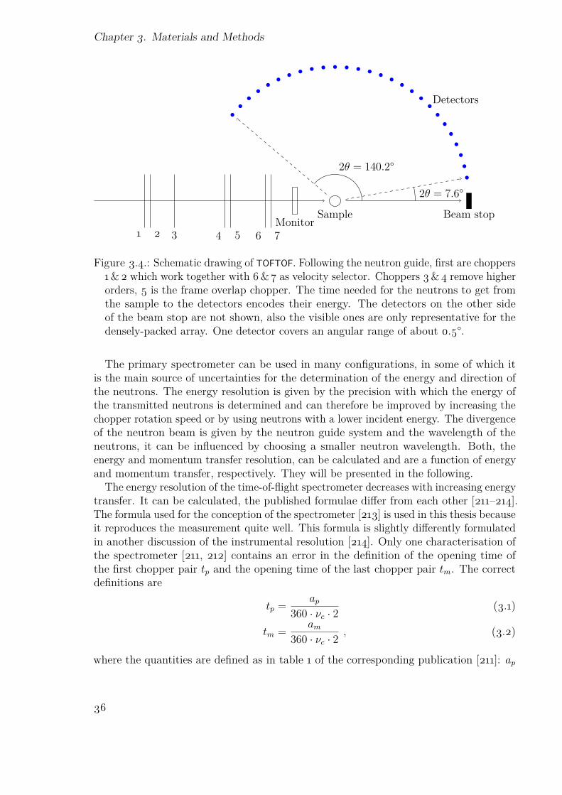
Chapter 3. Materials and Methods
Beam stopSample1 2 3 4 5 6 7
Monitor
Detectors
2θ = 7.6°
2θ = 140.2°
Figure 3.4.: Schematic drawing of TOFTOF. Following the neutron guide, first are choppers1 & 2 which work together with 6 & 7 as velocity selector. Choppers 3 & 4 remove higherorders, 5 is the frame overlap chopper. The time needed for the neutrons to get fromthe sample to the detectors encodes their energy. The detectors on the other sideof the beam stop are not shown, also the visible ones are only representative for thedensely-packed array. One detector covers an angular range of about 0.5°.
The primary spectrometer can be used in many configurations, in some of which itis the main source of uncertainties for the determination of the energy and direction ofthe neutrons. The energy resolution is given by the precision with which the energy ofthe transmitted neutrons is determined and can therefore be improved by increasing thechopper rotation speed or by using neutrons with a lower incident energy. The divergenceof the neutron beam is given by the neutron guide system and the wavelength of theneutrons, it can be influenced by choosing a smaller neutron wavelength. Both, theenergy and momentum transfer resolution, can be calculated and are a function of energyand momentum transfer, respectively. They will be presented in the following.
The energy resolution of the time-of-flight spectrometer decreases with increasing energytransfer. It can be calculated, the published formulae differ from each other [211–214].The formula used for the conception of the spectrometer [213] is used in this thesis becauseit reproduces the measurement quite well. This formula is slightly differently formulatedin another discussion of the instrumental resolution [214]. Only one characterisation ofthe spectrometer [211, 212] contains an error in the definition of the opening time ofthe first chopper pair tp and the opening time of the last chopper pair tm. The correctdefinitions are
tp = ap
360 · νc · 2(3.1)
tm = am
360 · νc · 2, (3.2)
where the quantities are defined as in table 1 of the corresponding publication [211]: ap
36

3.2. Description of the Neutron time-of-flight Spectrometer TOFTOF
Figure 3.5.: A chopper pair of TOFTOF (thepair 1 & 2) upside-down during mainte-nance. The discs are made of carbon fi-bres and coated with boron. The slits inthe chopper discs are visible. Due to thehigh rotation speed of the discs, they areoperated in an evacuated environment.
and am are the opening angle of the first and the last chopper pair, respectively, and νc
is the rotation speed of the choppers measured in rounds per second. The factor 2 in theformula is due to the opening time reduction caused by the counter rotating chopperpair. It can be speculated that a wrong reduction of this factor led to the formula givenin the aforementioned publication [211, 212]. The resulting energy transfer dependentinstrumental energy resolution is shown in figure 3.6 for the set-ups used in this thesis.
The momentum transfer resolution ∆Q is mainly given by the divergence determinedby the last part of the neutron guide which has m = 3.6 where m is defined as the ratioof the critical angle of total reflection of the neutron guide compared to an hypotheticalneutron guide coated with natural nickel. It roughly means that the neutron guidereflects neutrons with an incident angle (measured in degrees) of up to m · λ where λ isthe wavelength of the neutrons measured in nanometres. The obtained results, shown infigure 3.6, are in good agreement with Monte Carlo simulations of the instrument [213].This part of the resolution is hardly affected by the wavelength of the neutrons whichcan be seen from the calculation
∆Q = Qmax −Qmin = 4π
λsin
(2θ + m · λ
2π
180
)− 4π
λsin
(2θ −m · λ
2π
180
)
≈ 4π2
180λ·(
2θ + m · λ2 − 2θ −m · λ
2
)= π2
45 ·m (3.3)
which is – in this approximation – completely independent of the wavelength.For the evaluation of the measurements, the limited resolution in Q is neglected. This
can be justified because the energy-dependence of the incoherent scattering is evaluated,not the Q dependence of the coherent scattering. This necessitates that the limitedresolution of the energy transfer between neutron and sample must be considered. For thispurpose, the resolution is measured using a sample that does not show any quasielasticbroadening. This can be either the sample at low temperatures or some other solidsubstance. In the present studies, most of the samples show strong coherent peaks ofthe formed D2O ice. Therefore, the second option was used and a vanadium sample was
37

Chapter 3. Materials and Methods
-1.0 -0.5 0.0 0.5 1.00.000
0.025
0.050
0.075
0.100
ω (meV)
FW
HM
(m
eV
)
x10x10
λi = 6 A, 12000 rpmλi = 14 A, 16000 rpm
0 0.5 1 1.5 20.000
0.025
0.050
0.075
0.100
Q (A-1)
∆Q
(A
-1)
λi = 6 Aλi = 14 A
Figure 3.6.: The uncertainty of the determination of energy transfer (left) and momentumtransfer (right), shown as a function of the energy transfer and momentum transfer,respectively. The two setups shown are the ones used in this thesis: chopper rotationspeed 12000 rpm with incident neutron wavelength of 6 Å as well as 16000 rpm with14 Å. The uncertainty of the energy transfer determination is shown as the full widthat half maximum (FWHM) of the quasi-Gaussian resolution. For better visibility, thehigh-resolution setup is shown also after magnification of both, energy transfer andFWHM, by a factor 10.
employed for the determination of the resolution.
The secondary spectrometer. The detectors at TOFTOF make use of a nuclear reactionof the neutrons with 3He nuclei to register them. When the neutron is captured by sucha nucleus, the compound decays first to an excited state of 4He which has spin zero. Thisintermediate step causes the extreme sensitivity of the 3He nuclei to the relative spinorientation of the neutron with respect to its own nuclear spin which makes for examplespin filters possible. The intermediate state decays into an unbound state of a protonand a tritium which scatter apart and produce a detectable current pulse.
The neutron detection events are binned into time-of-flight channels. The number ofchannels in a frame can be chosen by the user, it defaults to 1024. Due to a CPU speed of20 MHz, the width of one channel is always a multiple of 50 ns. As the frame length canbe chosen completely arbitrarily by the user (see section 3.3), it follows that it happens
3He+n
4He*, Jπ=0+
p+T
20.6 MeV
20.2 MeV
19.8 MeV
Figure 3.7.: The part of the energy level diagram of4He which is relevant for the detection of the neu-trons (n) [215–217]. The difficulty for neutron detec-tion is the charge neutrality of the neutron. There-fore, the nuclear reaction with 3He is used to gen-erate charged particles (proton, p, and tritium, T)which are then detected.
38

3.3. Choice of Measurement Parameters
channel
dE = 0
0 n 0
Figure 3.8.: Time-of-flight channel structure of the experiment. A frame starts withtime channel 0 when the neutrons are at the sample position. After some time, theelastically scattered neutrons arrive. The next neutron pulse arrives at the sampleduring the filling of channel n. Because the spectrometer advances immediately to thenext frame, the time spent in channel n might be shorter than in the other channels.The intensity peak of elastically scattered neutrons is sketched and labelled withdE = 0.
quite regularly that a new frame starts while not all of the 1024 channels are filled yet.In fact, the new frame will normally start not even after completely filling a channel butat an arbitrary time in between, cf. figure 3.8.
3.3. Choice of Measurement ParametersSeveral parameters of the measurements can be adjusted at TOFTOF. In the following,the influence of some of them are described in detail: the dynamic range of momentumand energy transfers accessible to the neutrons, the observation time during which theneutrons can follow the motions of the molecules in the sample, as well as the distributionof the available time between several measurements, the amount and geometry of thesample.
Neutron wavelength and frame length determine the dynamic range. The theoret-ically accessible window in Q-ω-space is determined by the wavelength of the incomingneutrons. Neutrons can be scattered with scattering angles 2θ between 0° and 180°.
TOFTOF adds two restrictions to that: first, it does not measure the neutrons whichare scattered with 2θ below 7.4° or above 140.4° and second, it does not wait an infiniteamount of time after a neutron pulse. The latter means that neutrons which have a verylow velocity after the interaction with the sample are counted in the next frame as energygain neutrons.
The ratio of neutron pulses let through by the frame overlap chopper has to bedetermined by trading off the accessible energy loss range versus flux. Knowing the timebetween pulses, determined by chopper speed and ratio, it is possible to calculate theminimal speed of a neutron before the fastest neutrons of the next pulse arrive at thedetectors. As a worst case scenario, the fastest neutrons are assumed to have an infinitevelocity after the sample. This conservative estimate makes sure that no neutron of this
39

Chapter 3. Materials and Methods
pulse that went through the sample can arrive at the detectors before time zero.Typical operating conditions were a chopper rotation speed of 12000 rpm, λ = 6 Å, and
ratio 4. The initial energy of the neutrons Ei was therefore
Ei = p2
2m= (h/λ)2
2mn
≈ 81.81(λ[Å])2
≈here
2.27 meV (3.4)
The largest accessible neutron energy loss in the frame is calculated via the minimalenergy that neutrons may have after the scattering process Ef and still arrive at thedetectors before the next pulse. This in turn is determined by the time between twopulses which amounts (with two slits per chopper disc and ratio 4) to
12000 rpm · 2pulsesround ·
160
minutesecond /4 = 100 pulses
second ⇒ 0.01secondpulse . (3.5)
The neutrons have at most 0.01 second to travel the 4 m from the sample to the detectorsbefore the next pulse arrives. This corresponds to a final energy after the interaction of
Ef = 12mnv2 = 1
2mn
(4 m
t [second]
)2
≈here
0.84 meV (3.6)
The energy a neutron can transfer to the sample while still being detected before thenext pulse is consequently
Emax = Ef − Ei ≈here−1.43 meV . (3.7)
This is also visible in figure 3.9: there is a sharp cut-off on the neutron energy loss side.This cut-off can be shifted by increasing the frame overlap ratio or by shuffling channelsfrom the beginning of the frame to its end. This procedure relies on the fact that onlyfew neutrons gained very large amounts of energy.
The measurements presented in this thesis were performed either with the aforementioned 12000 rpm, λ = 6 Å, ratio 4 resulting in 55 µeV instrumental energy resolutionor with 16000 rpm, λ = 14 Å, ratio 8 for an instrumental energy resolution of 4 µeV.
The uncertainty of the energy determination causes an effective observation time.The instrumental energy resolution is mainly determined by the precision with which theprimary part of the spectrometer selects monoenergetic neutrons. Two parameters canbe used to change this resolution: the chopper speed and the selected wavelength of theincoming neutrons. As described by Heisenberg’s uncertainty principle, a more preciseselection of the incident neutron energy yields longer neutron wave trains. The wave ofone neutron will therefore run longer over the sample, will be influenced by the motionsof the nuclei during a longer observation time.
The observation times that can be realized at TOFTOF are roughly in the range of 1 psto 1 ns [218]. These values correspond to the times at which the spectrometer detectsa decay of the correlation function of a static scatterer (the vanadium standard) to
40

3.3. Choice of Measurement Parameters
Figure 3.9.: The dynamical range that canbe reached with neutron scattering atthe typical incident neutron wavelengthof 6 Å is compared with the one thatcan actually be accessed at TOFTOF withthe conditions given in the figure. Theparts missing at small and large Q aredue to the incomplete coverage of 2θvalues with detectors, the one missingat large neutron energy loss (here onthe left) is caused by the neutron pulserepetition rate. It can be changed byshifting neutrons from the end of theframe with the danger of mixing neutronenergy gain and loss.
-2.0 -1.0 0.0 1.0 2.00.0
0.5
1.0
1.5
2.0
2.5
ω (meV)
Q(2
θ,ω
) (A
-1)
theo. limitexp. limit
λ=6A12000 rpmratio 4
2θ=18
0°
2θ=140°
2θ=7.6°
2θ=0°
0.1. Experience has shown that the correlation functions of samples could be evaluatedwithout problems up to this value. In the measurements presented in this thesis, the twoemployed instrumental energy resolutions of 55 µeV and 4 µeV correspond to observationtimes of about 60 picoseconds and 900 picoseconds, respectively.
Measurements at different observation times can give very different results. Whenusing the models introduced in section 2.1 to evaluate the data, it is important to keepin mind that this description is only valid on the given time scale.
One macroscopic example where a model is valid only for a given amount of time iswater flowing in a river. If one looks at the motion only for a fraction of a second, thewater seems to flow in a certain direction. It is however clear that the direction of theflow changes completely if one follows the water over several days and many loops of theriver. The model of a flow in a constant direction is therefore valid at short time scalesbut does not describe the system on long time scales.
Another macroscopic example demonstrates that the distinction between localized andlong-range motions in section 2.1 is also only valid on the specified time scale: A closedbottle is half-filled with water and shaken up and down. On a time scale of a fraction ofa second, the water is flowing through the bottle – already on a second scale it becomesclear that it is actually only moving back and forth.
Adequate distribution of the measurement time can decrease the resulting errorbar. Given the limited time available for a series of measurements, it is necessary tobudget the time spent for a specific measurement. There are several opinions on howto distribute the time between the samples, the most common option is to spend thesame time on every measurement. It will be shown in the following that this rule can beoptimized for the samples measured for this thesis.
In the present case, there is typically a sample measurement and a backgroundmeasurement, for example pure D2O. If the sample contains a D2O volume fraction φand scatters with a rate Rs neutrons per second while the D2O background scatters with
41

Chapter 3. Materials and Methods
a rate Rb, the quantity that has to be evaluated is
R = Rs − φRb . (3.8)
The aim of distributing the beam time is to minimize the relative error ∆R/R.The total time t is spent for ts on the sample and for tb on the background measurement
with ts + tb = t. The respective counts are Ns in the sample and Nb in the backgroundmeasurement. Assuming a reasonably large number of counts, Gaussian statistics canbe used and the statistical error bars of the rates are ∆Rs = ∆Ns/ts =
√Ns/ts and
∆Rb = ∆Nb/tb =√
Nb/tb. When calculating equation 3.8, these add up quadratically:
∆R2 = ∆R2s + φ2 ·∆R2
b = Ns/t2s + φ2 ·Nb/t2
b . (3.9)
For the determination of the time distribution at which the total relative error becomesminimal, the derivative of (∆R/R)2 with respect to ts has to be zero. Assuming thatRs − φRb = 0, i. e. assuming that the sample scatters some intensity in addition to thebackground, this leads to
ts = 1φ
√Rs
Rbtb . (3.10)
As an example, in a typical sample that consists of 50% protonated DMPC with50% D2O, the time of the D2O background measurement can be less than a fourth ofthe one of the sample according to this calculation.
The rule oversimplifies the problem because the spectra of the sample and the back-ground have a different energy- and Q-dependence so that the ratio between the signalsis a function of these variables and not a single number. This can be considered bycalculating the time ratio of the measurements using those points in the evaluated partof the spectra where the signals of the sample and the background are the closest toeach other. For the measurements presented in this thesis, this happens at large energytransfers.
The measurement time of the vanadium standard has to be adjusted to the purposeof the measurement. If it is used only for the calibration of the detector intensities,a relatively short measurement is sufficient. However, if it is used to determine theinstrumental resolution of the spectrometer and is numerically convolved with thetheoretical function fitted to the data, its error bars can be the limiting factor for theprecision of the fit results. This problem is discussed in more detail in section 4.2. Specialcare was taken in the presented data sets to obtain a high quality of this measurement.
The amount of sample can be optimized. Due to the weak interaction with thesample, most neutrons fly straight through the sample and are absorbed in the beamstop. Some neutrons are absorbed by the sample, others are scattered. The amount ofsample is normally chosen with three opposing requirements in mind: If there is too littlesample in the beam, very few neutrons will be scattered and the resulting bad statisticsof the data will impede a detailed analysis. If there is too much sample, neutrons willare more likely to be absorbed within the sample which brings about that the number of
42

3.3. Choice of Measurement Parameters
scattered neutrons is not proportional to the amount of sample and makes the backgroundsubtraction more challenging. Also in the case of too much sample, neutrons mightundergo more than one scattering event. As the theory that is used to evaluate the dataassumes that the momentum- and energy-transfer which a neutron experiences is causedby only one scattering event, an occurrence of multiple scattering will impede a detailedanalysis, as well.
A common rule of thumb is therefore to use samples with transmission values of about90% and all the samples studied in this thesis had transmission values in this orderof magnitude. The absorption of neutrons in the samples was in most cases found tobe of minor importance but will be discussed in the frame of the choice of the samplegeometry again. Regarding multiple scattering, it was possible to show in the frame ofthis thesis [D] that the long-range motional component can be reliably extracted evenfrom samples with a much lower transmission.
Different sample geometries have different advantages. In the present case, thesamples were contained either in hollow cylindrical or flat aluminium sample containers.The flat sample containers were oriented with their surface normal towards a scatteringangle of 135° in the direction of the detectors.
One difference between the two is that the hollow cylindrical sample containers havethe advantage that the absorption of neutrons in the sample depends hardly on thescattering angle [219, 220]. In the case of flat sample containers, neutrons which arescattered into the direction of the plane of the sample have to cover a large distancewithin the sample. On this way, they are very likely to get scattered again or be absorbed– hardly any of them arrives in a detector in this direction. This effect can clearly beseen in figure 3.10.
From this point of view, hollow cylindrical sample holders such as the one shown infigure 3.11 are clearly favourable and were used for all measurements with an instrumentalresolution of 55 µeV in this thesis. It will, however, become clear in the following thatthey are not suitable for high-resolution measurements at TOFTOF for which the flatsample containers were used, accepting their shadowing effects.
This is due to the other difference between flat and hollow cylindrical sample holders:the distribution of the flight paths. Seen from large scattering angles of about 135°, thedistance between the sample in flat sample holder and the detectors is always the same.In contrast, the neutrons can be scattered by the back wall of the hollow cylinder ortransverse the hollow cylinder, get scattered by the front wall, and transverse the hollowcylinder again. On a time-of-flight instrument, the energy transfer between the neutronand the sample is calculated from the time the neutrons need from the last chopper viathe sample to the detectors. However, this time-of-flight does not only depend on thevelocity of the neutrons but also on the length of their flight path. Therefore, such adistribution of flight paths appears as a distribution of energy transfers.
This effect can be nicely seen in figure 3.12 where a hollow cylindrical sample showstwo peaks – corresponding to scattering from the front wall and from the back wall. Thiseffect is hardly visible at small scattering angles, i. e. small Q, because the neutrons have
43

Chapter 3. Materials and Methods
0.0 0.2 0.4 0.6 0.80
5
10
15
20
Q (A-1)
S(Q
,-5
0µ
eV
<ω
<5
0µ
eV
) (a
.u.)
10°CDMPCVanadiumD2O
0.0 0.2 0.4 0.6 0.80.0
0.1
0.2
0.3
0.4
0.5
Q (A-1)
S(Q
,-5
0µ
eV
<ω
<5
0µ
eV
) (a
.u.)
10°CDMPCVanadiumD2O
Figure 3.10.: Diffraction patterns of the sample at 10 (orange), vanadium (green), andD2O at 10 (blue). The two graphs show the same data on different y scales. Themeasurement set-up was the one for 4 µeV measurements. The coherent scatteringof the sample can be seen at low Q, the dip shortly before Q = 0.4 Å-1 is caused bythe shadowing of the sample container towards scattering angles of 45°. The slowlydecreasing intensity at the highest values of Q is because the neutrons which arescattered from regions far away from the beam centre are not transmitted by the radialcollimator.
to travel through the sample either before or after the scattering event. In contrast, it isstrongly visible at large scattering angles, i. e. large Q, where one neutron does not haveto travel through the sample at all while the other has to do so two times.
In principle, it would be possible to account for this effect with a measurement ofthe instrumental resolution – as it is done for example for the geometrical inaccuraciesof the detectors. However, if vanadium has to be used for this measurement, the highabsorption cross section of vanadium makes this impossible: As can be seen in figure 3.12,the double peak is not symmetric. The component on the neutron energy loss side hasa lower intensity than the other one. This is the peak caused by neutrons which hadto travel for a longer time, i. e. the one of the back wall. Neutrons scattered here haveto pass two times through the front wall where they can be absorbed. As the intensityloss depends on the absorption properties of the sample, they will be different for thesample and vanadium. The unsymmetrical measurement is therefore not a suitablerepresentation of the instrumental resolution.
The high-resolution measurements presented in this thesis are therefore performed withflat sample holders which are oriented with their surface normal towards a scatteringangle of 135° in the direction of the detectors. In this configuration, the neutrons whichare emitted into the direction of large scattering angles have all very similar lengthsto travel, making a high energy resolution with a symmetric resolution function of thespectrometer possible. The drawback of this configuration is that the long path of theneutrons through the sample towards a scattering angle of 45° causes a shadowing in
44

3.3. Choice of Measurement Parameters
Figure 3.11.: The type of sample cells that were used for the measurement in hollowcylindrical sample containers in this thesis. Left: Three-dimensional technical drawingof the hollow cylindrical sample cells (drawn by Ph. Jüttner, FRM II). Middle: Two-dimensional cut through the sample holder; the sample is only in a thin layer at theoutside of the container (drawn by Ph. Jüttner, FRM II). Right: A neutron radiography(kindly provided by Johannes Brunner from ANTARES at the FRM II) of a hollowcylindrical sample container filled with H2O. The support on which the containerwas measured is also visible at the bottom. On the top, the two thick aluminiumplates which contain the screws are visible along with the Teflon seal. In the middle, abulging is visible which makes the amount of sample in the beam not proportional tothe amount of sample in the sample cell because only the middle part of the samplecell is normally hit by the neutron beam.
Figure 3.12.: Measurement of the vana-dium hollow cylindrical standard atTOFTOF with an incoming neutron wave-length of 10 Å, chopper rotation speed16000 rpm, and frame overlap ratio 8,resulting in an instrumental resolution ofabout 10 µeV. At large scattering angles,a double peak becomes visible whichis caused by scattering of neutrons onthe front and back wall of the samplecontainer. The peaks are not of equalheight because of neutron adsorption inthe front wall.
-20 -10 0 10 200
40
80
120
160
ω (µeV)
S (
Q,ω
) (a
.u.)
Q=0.9 A-1
Q=1.0 A-1
Q=1.1 A-1
45

Chapter 3. Materials and Methods
this direction as can be seen in figure 3.10.A completely different problem is also visible in the radiography of a filled sample
container shown in figure 3.11: The sample is not uniformly distributed over the wholecan but bulging can occur. Additionally to the uncertainties of the layer thickness due tobulging, there is also the uncertainty of the manufacturing process. Given a sample layerthickness of 0.1 mm and a typical precision of the manufacturing process of 1/100 mm,there is an intrinsic variation of about 10% between sample containers. Also the wallsof the containers have varying thicknesses within the same precision. This becomesproblematic because the neutron beam does not cover the whole sample container inthe vertical direction but only a part in the middle of the container with about threequarters of its height: the uncertainties of the thicknesses of sample layer and container inthis area cause directly proportional uncertainties of their contributions to the scatteredsignal. It will be discussed in section 4.1 how the subtraction of background contributionscan absorb these uncertainties and a proposal will be presented in section 6.1 how theycould be avoided by using a different design of the sample containers.
46

Chapter 4.
Data Reduction and AnalysisThe measured systems consist of mixtures of several components. Of these components,only the phospholipid is of interest in this thesis. Therefore, the contributions of theother substances to the scattering signal have to be subtracted. Given that the fractionof phospholipid in the samples can be as low as 1%, this is a delicate task and will bedescribed in this chapter.
Also two approaches to evaluate the information that is contained in the spectra willbe discussed in detail:
The first one is to create a model of the molecular motions. It is required that thismodel agrees with previously known facts, e. g. the molecular structure, and with thedata measured in the course of this thesis. While the previous knowledge has to be takeninto account for creating the model, the compatibility with the data has to be determinedfrom a fit. If this is given, the parameters of the best fit of the model can be extracted –which obviously depend on the choice of the model.
The second, model-free, approach to extract information from the data aims in theopposite direction: By extracting only very few quantities from the data without fittingany model, only a small fraction of the information contained in the spectra is evaluated.The resulting quantities do not have a similarly well-defined meaning as the parametersused in a model. However, they can be extracted very reliably and comparisons betweenseries of similar systems give access to the evaluation of the dynamics upon the changeof a control parameter.
Both approaches have been used in the present work: The fit of a model was used todetermine the mechanism of the diffusion of the phospholipid molecules. As the results ofthe fit depend also on the fit procedure, special attention was paid to the fitting processitself. Independently of these results, the evaluation of the structure and dynamics wasfollowed when varying temperature, lateral pressure, and composition by a model-freeapproach.
4.1. Extracting the Scattering Function from theScattered Intensities
General data treatment. The scattering functions can be calculated from the measureddata in several steps which are given in detail in appendix [I] and are summarized in the
47

Chapter 4. Data Reduction and Analysis
following. Depending on the specifics of the sample compositions and the requirements ofthe data evaluation, not all of these steps have been performed in each of the presentedstudies. The concrete data reduction steps are given in the respective publications [B–F].
Generally, the data were converted to be a function of neutron energy transfer, theenergy-dependent detector efficiency was corrected, and the detector sensitivity wasnormalized using the scattering of a vanadium standard. The obtained scatteringfunction S(2θ, ω) was corrected for absorption effects.
These absorption effects can be explained with a simple hypothetical example: if theemulsions consisted of a normally-scattering oil phase dispersed in an imaginary waterphase that would absorb all neutrons, the signal of the mixture (no scattered neutron) isnot equal to the sum of the two single signals (no neutrons from the pure water phaseand some neutrons from the pure dispersed phase). This phenomenon is well-knownin scattering techniques and is usually corrected with the algorithm of Paalman andPings [221]. It takes the scattering and absorption cross section of the respective samplesand returns scattering angle and energy transfer dependent correction factors that canbe used to scale the measurements.
Finally, the data were grouped into spectra at constant Q, resulting in the scatteringfunctions S(Q, ω) of the whole system in the beam. From this quantity, the contributionof the phospholipid molecules has to be extracted by subtracting the background contri-butions. Before the methods for the background subtraction for the different samplesare discussed in detail, it should be mentioned that the obtained Smeasured(Q, ω) is notexactly equal to the S(Q, ω) defined in chapter 2: Whereas the theoretical definitionis symmetrical with respect to neutron energy loss and energy gain, the occupation ofexcited states in the real system is governed by the Boltzmann-factor. This causes thatit is less likely that the sample transfers energy to the neutron than that the neutrontransfers energy to the sample which results in
Smeasured(Q,−ω) = exp(
~ω
kBT
)· Smeasured(Q, ω) (4.1)
where ω > 0 denotes a neutron energy gain scattering event. This is known as theprinciple of detailed balance. It was found for the data presented in this thesis that acorrection for this factor did not give better results. The detailed balance was thereforenot corrected. This can be justified because the detailed balance factor is approximatelyconstant at the high temperatures of the samples and the low evaluated energy transfers.Furthermore, the signals of some samples were weak so that contributions which do notfollow the principle of detailed balance (e. g. the instrumental background) could havehad a distorting effect when multiplied with the correction factor.
Background subtraction from the data of multibilayer samples using the respectivevolume fractions. In the case of the multibilayer samples [B, D, E], the backgroundcontributions are at least one order of magnitude below the signal of the phospholipid.In these cases, it was found sufficient to subtract the spectra of the aluminium can andthe D2O weighed with their respective volume fractions. The volume fractions have to
48

4.1. Extracting the Scattering Function from the Scattered Intensities
be used because the measurement is always done on the same volume in the beam, notthe same mass.
Background subtraction from the data of vesicles and emulsions using the diffrac-tion patterns. For the samples of single bilayers and monolayers [F], there is much lessphospholipid in the sample and it was found in these cases that this procedure is notaccurate enough to ensure that the background contributions are much smaller than theone of the phospholipid. Reasons for this inaccuracy can be the uncertainties regardingsample composition and volume that have been discussed in sections 3.1 and 3.3, respec-tively. Also the employed absorption correction is not accurate because it does considersneutrons after a second scattering process as absorbed. In the present samples where asecond scattering process is much more probable than absorption, a thorough treatmentof multiple scattering effects would be necessary which is not available.
An alternative approach is to use features in the data themselves to determine thecontributions of the different components to the total scattering signal [222]. Thediffraction patterns of the vesicles and emulsions show very clearly the peaks contributedby the DMPC at 1.5 Å-1, the D2O at 2.0 Å-1, and of the perdeuterated hexadecane (dHD)at 1.4 Å-1. It was therefore possible to use the diffraction patterns in order to determinehow much of the D2O and dHD signals had to be subtracted in order to remove thecorresponding peaks from the diffraction pattern [F].
This method is based on the assumption that the scattering patterns are added withoutregarding interference effects. This is true in the high Q regime above about 1 Å-1 wheretypical distances below 1 nanometre are probed but it clearly fails at low Q wherethe layering of DMPC and water molecules and eventually also the droplets as a wholecontribute to the coherent scattering signal as becomes visible in the large coherentstructure factor maxima at Q values of about 0.1 and 0.2 Å-1 (cf. for example figure 3.10).
In order to use this procedure to produce more than only qualitatively correct results,also a target scattering pattern has to exist which is used to fit the coefficients of thesubtraction. In the current cases, the scattering pattern of fully hydrated DMPC wasused after pro-rata subtraction of the D2O signal as described before.
Background subtraction from the data of the suspensions currently not possible.For this procedure to work, it is also necessary that the scattering patterns and thereforethe structure of the substances must be the same in the bulk and in the emulsion.Although this cannot be assumed for the hexadecane and water molecules close to thephospholipid molecules, most of them are far enough away from the interface to exhibitbulk properties as discussed in section 3.1. However, this requirement turns out to be themain problem for the treatment of the suspension sample data because the scatteringpatterns of the employed solid fat phases, protonated tripalmitin and perdeuteratedtetracosane, are different in the bulk and the nanoparticular state as can be seen infigure 4.1. Therefore, it is not possible to subtract the signal of the bulk material fromthe one of the nanoparticle system. For this reason, the spectra of the suspension sampleswere not evaluated in this thesis.
49

Chapter 4. Data Reduction and Analysis
0.0 0.5 1.0 1.5 2.00.0
1.0
2.0
3.0
Q (A-1)
dσ
/dΩ
(Q)
(a.u
.)
dTC bulkdTC nano
0.0 0.5 1.0 1.5 2.00.0
0.5
1.0
1.5
2.0
Q (A-1)
dσ
/dΩ
(Q)
(a.u
.)
pTP bulkpTP nano
Figure 4.1.: Diffraction patterns of perdeuterated tetracosane (dTC, left) and protonatedtripalmitin (pTP, right) as bulk samples (orange) and in nanoparticles (blue). It isobvious that the diffraction patterns of the bulk samples are different from the ones ofthe nanoparticles.
4.2. Finding the Mechanism of Diffusion with a FitAssumptions of fits. It is important to remember that the parameter values with theirerror bars that are extracted from a fit of a model to the data are necessarily based on
the assumptions
the data are correct
the data error bars are correct
the model is correct
the difference between the model and the data can be expressed by a cost functionsuch as χ2
the fit algorithm finds the absolute minimum of this cost function for the determi-nation of the parameter values
the fit algorithm determines the shape of the minimum of the cost function correctlyfor the determination of the parameter value error bars.
If any of these requirements is not met, the obtained results might not have anythingto do with the description of the system or have a completely different value in reality.This uncertainty is not expressed in the error bars of the parameters which are definedonly on grounds of the above assumptions [G, H].
In the following, each of these requirements will be discussed critically. Also thedifferences between the Levenberg-Marquardt (LM) algorithm and a Monte Carlo (MC)approach to perform the fit [G, H] will be discussed. Both of these algorithms aim to
50
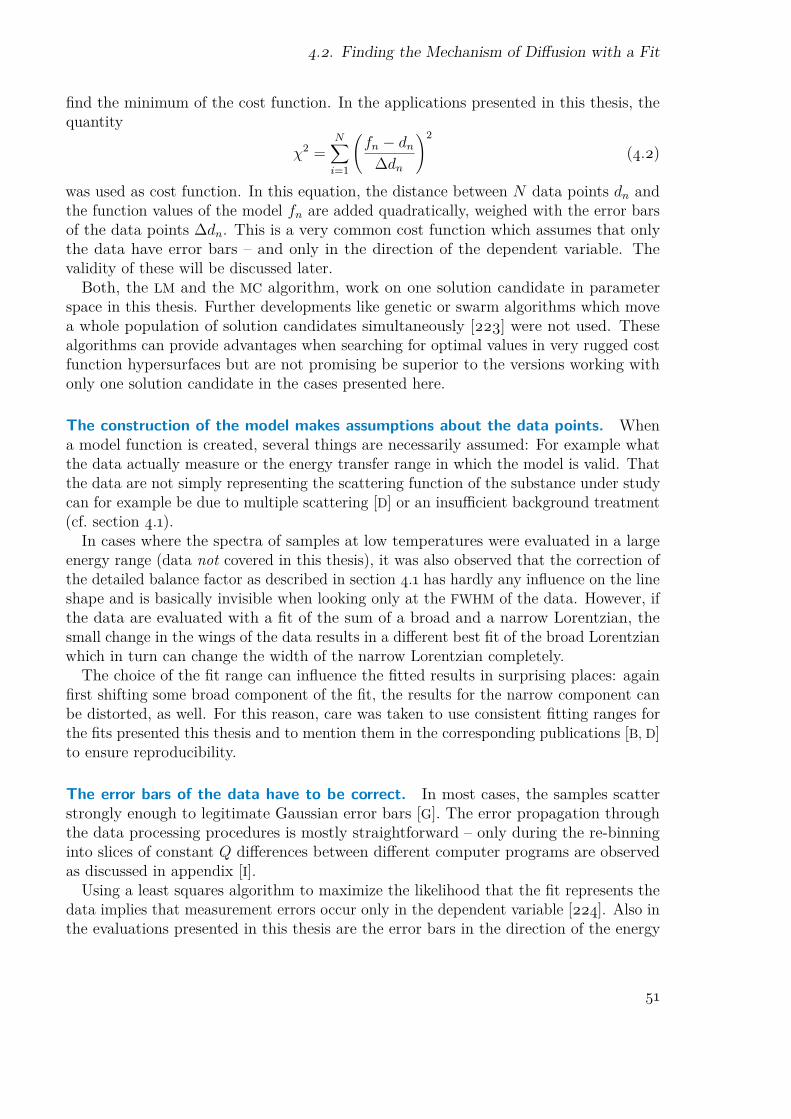
4.2. Finding the Mechanism of Diffusion with a Fit
find the minimum of the cost function. In the applications presented in this thesis, thequantity
χ2 =N∑
i=1
(fn − dn
∆dn
)2
(4.2)
was used as cost function. In this equation, the distance between N data points dn andthe function values of the model fn are added quadratically, weighed with the error barsof the data points ∆dn. This is a very common cost function which assumes that onlythe data have error bars – and only in the direction of the dependent variable. Thevalidity of these will be discussed later.
Both, the LM and the MC algorithm, work on one solution candidate in parameterspace in this thesis. Further developments like genetic or swarm algorithms which movea whole population of solution candidates simultaneously [223] were not used. Thesealgorithms can provide advantages when searching for optimal values in very rugged costfunction hypersurfaces but are not promising be superior to the versions working withonly one solution candidate in the cases presented here.
The construction of the model makes assumptions about the data points. Whena model function is created, several things are necessarily assumed: For example whatthe data actually measure or the energy transfer range in which the model is valid. Thatthe data are not simply representing the scattering function of the substance under studycan for example be due to multiple scattering [D] or an insufficient background treatment(cf. section 4.1).
In cases where the spectra of samples at low temperatures were evaluated in a largeenergy range (data not covered in this thesis), it was also observed that the correction ofthe detailed balance factor as described in section 4.1 has hardly any influence on the lineshape and is basically invisible when looking only at the FWHM of the data. However, ifthe data are evaluated with a fit of the sum of a broad and a narrow Lorentzian, thesmall change in the wings of the data results in a different best fit of the broad Lorentzianwhich in turn can change the width of the narrow Lorentzian completely.
The choice of the fit range can influence the fitted results in surprising places: againfirst shifting some broad component of the fit, the results for the narrow component canbe distorted, as well. For this reason, care was taken to use consistent fitting ranges forthe fits presented this thesis and to mention them in the corresponding publications [B, D]to ensure reproducibility.
The error bars of the data have to be correct. In most cases, the samples scatterstrongly enough to legitimate Gaussian error bars [G]. The error propagation throughthe data processing procedures is mostly straightforward – only during the re-binninginto slices of constant Q differences between different computer programs are observedas discussed in appendix [I].
Using a least squares algorithm to maximize the likelihood that the fit represents thedata implies that measurement errors occur only in the dependent variable [224]. Also inthe evaluations presented in this thesis are the error bars in the direction of the energy
51

Chapter 4. Data Reduction and Analysis
transfer ω and of the momentum transfer Q not taken into account. A way to considerthese error bars of the independent variables ∆xi is to translate them into an errorbar in the direction of the dependent variable ∆y with the so-called effective variance
technique [224–227],
∆y =
√√√√∆d2 +∑
i
(∂f
∂xi
∆xi
)2
, (4.3)
where ∆d is the error bar of the measured point in the direction of the dependent variableand f is the fit function. Although it is known that the correct treatment of these errorsis more intricate than this simple redefinition of the error bar, this formula is a goodestimate of the result [228]. In the presented measurements, the additional contributionsto the error bar were kept as small as possible: In the direction of the energy transferω, the spectra are sampled in very narrow intervals so that the corresponding ∆xω issmall. In the direction of the momentum transfer Q, the fit function does not exhibit bigchanges, i. e. ∂f/∂xQ is small. These circumstances made it possible to use the statisticalerror bar of the data points ∆d as a measure of the overall error and to use the standardfitting algorithms.
The «error bars of the model» have to be correct. Using a χ2 minimization algorithmfor the determination of the best fit to the data assumes that the fit function does notcarry any statistical error bars. While this is certainly true for the model itself which is amathematical function, it does not hold any more for the fit function after the numericalconvolution of the theoretical scattering function with a vanadium measurement toaccount for the instrumental resolution: This step introduces the error bars of thevanadium measurement to the calculated curve. To the best knowledge of the author,these error bars are never regarded when fitting quasielastic neutron scattering data. Inthe following, a procedure is proposed which would allow to take the error bars of themodel function into account. For the data evaluation used in this thesis, the standardapproach was used which neglects these error bars. It is therefore also demonstratedthat the error bars of the vanadium measurements used in this thesis are small enoughto justify this approximation.
The probability that a data point dn measured on some x scale with a Gaussianprobability distribution function with standard deviation (error bar) ∆dn is correctlydescribed by a value of a theoretical function fn that has no error bar, i. e. that is a δfunction, is given by [G, H]
P(dn | fn) =∞∫
−∞
dx δ(x− fn) · 1∆dn
√2π
exp−1
2
(x− dn
∆dn
)2 =
1∆dn
√2π
exp−1
2
(fn − dn
∆dn
)2 . (4.4)
In the case that N data points should be described by the theory, one can extract the
52

4.2. Finding the Mechanism of Diffusion with a Fit
quantity
χ2 =N∑
n=1
(fn − dn
∆dn
)2
(4.5)
which is minimized during a fit.However, the value of the fit function is in the presented cases not the theoretical
one but its convolution with the vanadium measurement and it therefore has an errorbar, as well. The numerical convolution of the theoretical function and the vanadiummeasurement is performed according to
gn = (f ⊗ v)n =N∑
m=1fm · vn−m (4.6)
where N is the total number of measured points and fn and vn are the values of thetheoretical function (without error) and of the vanadium measurement (with error bar∆vn), respectively [D]. Using Gaussian error propagation, this results in a Gaussianprobability density function for the point gn with a standard deviation (error bar) of
∆gn = ∆(f ⊗ v)n =
√√√√ N∑m=1
(fm ·∆vn−m)2 . (4.7)
The χ2 is now somewhat half-heartedly redefined, taking into account that the fitvalues of the function changed but neglecting that also the error bars changed (from noerror bar to some error bar) as
χ2 =N∑
n=1
(gn − dn
∆dn
)2
. (4.8)
This definition is implemented in the standard data evaluation programs and was alsoused throughout this thesis.
A possibility to include the error bars of the fit function follows from the probabilitydefinition as in equation 4.4, exchanging the δ function of the theoretical value with theGaussian distribution of the value of the fit function. Assuming that the data and the fitfunction have the same sign (usually they are both positive), one arrives at
P(dn | fn) =∞∫
−∞
dx1
∆gn
√2π
exp−1
2
(x− gn
∆gn
)2 · 1
∆dn
√2π
exp−1
2
(x− dn
∆dn
)2 =
1(∆g2
n + ∆d2n)√
2πexp
[−1
2(gn − dn)2
∆g2n + ∆d2
n
]. (4.9)
The cost function that the fit has to minimize is therefore
χ2 =N∑
n=1
((gn − dn)2
∆g2n + ∆d2
n
). (4.10)
53

Chapter 4. Data Reduction and Analysis
49.50 49.75 50.00 50.25 50.50100
101
102
103
104
Γ (µeV)
χ2
conventional definitionproposed definition
Figure 4.2.: Comparison of the χ2 land-scape in the direction of the line widthΓ when fitting a single Lorentzian withfixed amplitude and centre position totoy data. It can be seen that the valueof Γ where χ2 reaches its minimal valuevaries by less than 1%.
In order to demonstrate the difference between the two different definitions of χ2 givenin equations 4.8 and 4.10, a toy example was constructed by convolving one Lorentzianwith a vanadium measurement and adding random noise as a «data set». The amplitudeof the Lorentzian was chosen such that the signal-to-noise ratio was the same as in thecase of the real measurements, the half width at half maximum was set to Γ = 50 µeV.In a next step, the two χ2 were calculated for the convolution of a Lorentzian withvarying line width and the vanadium measurement. The result, shown in figure 4.2,shows that the best fit, i. e. the minimal χ2 is achieved at very similar values of Γ. It canbe concluded that the good statistical quality of the vanadium measurements makes theconventional approach to calculate χ2 a valid approximation.
Is the model correct? This somewhat ill-posed question can be either expressed bysaying «all models are wrong but some are useful» [229] or «models are never wrong,they are just more or less appropriate» [230].
Regardless of the formulation, a model has to reproduce the scattering function atevery value of Q and the Q-dependence of its parameters has to follow the theoreticalprediction (linear, quadratic, . . . ). In some cases, it is completely obvious that one modelfits the data better than another [F] but generally it is not straight-forward to decide ifthe fit reproduces the data – due to the error bars of the data (and the fit, as discussedabove).
It is therefore necessary to define a quality criterion that makes it possible to judgethe quality of the fit – and to compare different fit functions. χ2, the sum of the squareddistances between the data and the fitted function as shown in equation 4.5, is minimizedduring the fitting process. A smaller χ2 designates a closer agreement between data andfit. It is however obvious that this quantity cannot be a valid base for comparison of twomodels with a different number of parameters.
In the spirit of Ockham’s razor, this is avoided by either taking the reduced χ2, χ2
divided by the numbers of degrees of freedom (which equals number of data pointsminus the number of parameters) in the Levenberg-Marquardt (LM) approach – or bythe explicit sampling of the χ2 hypersurface in the Monte Carlo (MC) approach, as will
54

4.2. Finding the Mechanism of Diffusion with a Fit
-10 -5 0 5 100
25
50
75
100
125
x
y /
10
3
y = 105 - 103x2 + 5x4 + ∆
230 235 240 245 2500.00
0.05
0.10
0.15
0.20
0.25
χ2
PD
F
y = a + bx2 + cx4
y = a + bx2 + cx4 + dx6
Figure 4.3.: An example for model selection. Left: A polynomial with powers of x 0, 2,and 4, evaluated at 201 points. Gaussian distributed noise (centered around zero) wasadded, the width of the Gaussian was given by √y as in a counting experiment. Right:The comparison of two possible fit functions: the first with powers of x 0, 2, and 4;the second with 0, 2, 4, and 6. The minimal χ2 of the model with more parameters issomewhat lower but the maximum and the mean of the probability density function(PDF) is clearly at higher χ2, showing that the additional parameter is not supportedby the data.
be discussed in detail later. Introducing a new parameter into a model will necessarilydecrease the minimum χ2 – but only if it also decreases the mean χ2 or the one with themaximum probability, this parameter is considered to be justified by the data.
An example of such a model selection is shown in figure 4.3, using a simple polynomial.Synthetic data were produced by evaluating the polynomial, adding a Gaussian distributednoise as if the data were obtained in a counting measurement, and setting the data errorbars accordingly. This approach was also used for the comparison of different models forthe long-range motion of phospholipid molecules [B].
Does the cost function χ2 represent the model accurately? One difficulty can arisefrom fitting the histogram S(Q, ω) with a function as it is normally done. As the dataare binned into intervals of Q and ω, it can happen that very narrow components ofthe fit function disappear between two data points. This is for example the case for a δfunction in energy – if it is not positioned at the same place as a data point, it is invisiblein the cost function. The normal solution for this problem is to distribute the δ functionon the two neighbouring channels.
Errors can also occur when convolving the theoretical model with the instrumentalresolution before fitting it to the data [C, D]. One problem is the shortcoming of thevanadium measurement to represent the instrumental resolution. The measurementdoes not capture the dependence of the resolution on the energy transfer and thereis experimental background in the measurement, partially caused by phonons in thevanadium, which is not part of the instrumental resolution. While these points were found
55

Chapter 4. Data Reduction and Analysis
to have only little impact on the evaluation of the data presented in this thesis, there isalso a very intricate effect which is caused by the discrete sampling of the theoreticalfunction at the points where the instrumental resolution is determined. As this effecthas a visible effect on the data evaluation, it is introduced in the following.
The numerical convolution of the fit function with the vanadium measurement accordingto equation 4.6 brings about that the fit function is only evaluated at the sampling pointsof the vanadium measurement. This is unproblematic as long as the value of the functionat this point is representative for the whole bin. If the curvature of the fit function is verylarge, this requirement is no longer fulfilled. A rule of thumb for Lorentzian fit functionswas found in the frame of this thesis [D]: the convolution produces erroneous results if themodel function has a FWHM below the distance between two points. This was discoveredwhen evaluating very slow motions of protein hydration water [C] which had previouslybeen found to exhibit a line width that narrows drastically with decreasing temperatureat high temperatures and then apparently changes to a nearly temperature independentwidth at low temperatures [105].
Does the fit algorithm find the absolute minimum of the χ2 hypersurface? Findingthe absolute minimum of the χ2 hypersurface corresponds to finding the optimal parametervalues [G, H]. An analogue physical system would be a melt of a somewhat complicatedsubstance that is cooled. The absolute minimum of the energy hypersurface correspondsto the single crystalline state, many local minima around correspond for example toamorphous or polycrystalline structures.
The LM algorithm will only find the bottom of the χ2 valley in which it was initializedbecause its steps can lead only downhill in the χ2 hypersurface. This means that thefitted solution can be very far off the best fit if the initialization values are poorly chosen.The physical analogue is to quench the melt to zero temperature – often, the system willget stuck in an amorphous state and not form a single crystal. This problem is mostlycircumvented by human guidance of the LM fit by choosing suitable parameter values orby using a more advanced algorithm.
Of these, MC algorithms provide an elegant solution: They explore the parameterspace and can also go uphill in the χ2 hypersurface. Therefore, they can easily includethe possibility to jump from one valley to the next, eventually ending up in the globalminimum, even if initialized far away. The physical analogue here is to cool the meltslowly to facilitate crystallisation.
Does the fit algorithm determine the shape of the minimum of the χ2 hypersurfacecorrectly? The second drawback of LM algorithms is on first sight a smaller one butturns out to be the relevant in the present case: they assume that the parameters arenot correlated and the χ2 depends quadratically on all parameters near the best fit. Thisassumed quadratic dependence corresponds to a Gaussian probability distribution of theparameter around its best fit value. While this does not influence the parameter valuesof the best fit, it gives wrong – usually too small – parameter error bars [G, H].
Error bars given by LM algorithms are the standard deviation σ of the assumed
56

4.3. Model-free Determination of the Mobility
Gaussian distribution of the fitted around the true value. Due to the direct samplingof the parameter space in the MC approach, the results are rather given as explicitprobability distribution functions (PDF). From these, it is then possible to extract anerror bar which also reflects correlations between the parameters, for example by takingthe interval of the PDF which encloses 68% of its area which would be the normaldefinition in the case of a Gaussian PDF. These error bars can also be asymmetric, incontrast to the ones obtained with LM.
4.3. Model-free Determination of the MobilityThe motions of the molecules cause a re-distribution of the scattered intensity of neutronswith respect to the energy transfer: Whereas a static sample scatters neutrons onlyelastically, periodic motions decrease the elastically scattered intensity in favour of risinginelastic bands and aperiodic motions cause a broadening of the elastic line.
Simply looking at these features and comparing them between different samples ordifferent temperatures can give valuable information. This has been successfully doneby measuring the full width at half maximum (FWHM): a smaller FWHM correspondsto a smaller mobility of the molecules. This type of data evaluation does not allow thevalidation of a special molecular model of the molecular motions but gives a reliablecharacteristic of the spectrum, corresponding to the general mobility of the molecules.
Even if the amount of sample is too small to allow the exact determination of theline shape, it is often still possible to extract the FWHM. Therefore, this method wasused to evaluate the dynamics of the monolayers on emulsion droplets which could bemeasured only with poor statistics because of the small fraction of the signal intensitythat is caused by the phospholipid molecules.
Evaluating the Q-dependence of the scattered intensity. When the scattered neutronintensity is low, either due to the neutron flux or the amount of sample, so-called elastic
scans are often used [231–233]. In these, the line shape in energy direction is not resolvedbut only those neutrons are counted that are scattered within an energy transfer thatcannot be distinguished from zero within the instrumental resolution. It is then possibleto compare the Q-dependence of this intensity as a function of the temperature or betweendifferent samples. Without any model for the motions, it can be stated that a strongerQ-dependence corresponds to a bigger mobility of the scatterers on the observation timescale. It is also possible to introduce a model for the motions and extract the mean-squaredisplacement of the scatterers.
This procedure was extended and an explicit detection of the time evolution wasintroduced by combining measurements with different energy resolutions, correspondingto different observation times [234].
The point measured at zero energy transfer contains always contributions from neutronswhich have been scattered with energy transfers within the instrumental resolution. It istherefore also possible to work with a fixed resolution and integrate the scattering signalafterwards over varying energy transfers. Due to the Gaussian shape of the resolution
57

Chapter 4. Data Reduction and Analysis
function, this integration could be called an «error function transform» which is verysimilar to the normal cosine transform used in Fourier transforms. The error functionand the cosine are in fact very similar to each other, up to only a few percent in therelevant range.
It was however concluded that this method to evaluate the molecular mobility is notsuited for the samples used in this thesis. The first reason is that although they share theproblem of a low amount of the substance of interest in the beam with other studies [234–236], these previous samples were pure substances and were therefore evaluated withoutany major background subtraction. In contrast, for the composite samples used in thisthesis, subtraction is of major importance. It is clear that a method which relies solelyon the intensity in a single point is especially sensitive to uncertainties in the backgroundsubtraction.
The second reason applies also to the multibilayer samples where the backgroundsubtraction is less important: The phospholipid samples studied here do not alwayshave the same structure. Not only the phase transitions but also the additives changethe molecular arrangements. As the coherent scattering is sensitive to changes in thestructure of the molecules, this can result in intensity shifts (cf. section 3.1). Such aneffect would wrongly be attributed to changes of molecular motions.
Evaluating the ω-dependence of the scattered intensity. The line shape of thescattering function carries much more information about the motion of the scatterersthan only its highest point. A model-free characterization of the line shape can beattempted by two approaches: The first one is to calculate the Fourier transform ofthe sample spectra and the instrumental resolution, eliminating resolution effects bydividing the Fourier transform of the data by the one of the instrumental resolution, andevaluating the resulting intermediate scattering function. While this is the method ofchoice for the direct comparison of molecular dynamics simulations and experiments [154],it did not show any practical advantage in the present data evaluation.
Therefore, the second approach was employed: extracting the full width at halfmaximum (FWHM) of the sample and the vanadium measurement, subtracting the widthof the instrumental resolution from the one of the sample data, and using the remainingbroadening as a measure of the dynamics in the sample.
Background contributions which have a sharp peak at zero energy transfer can distortthe FWHM as shown in figure 4.4 because they decrease the value of the maximum butnot of the points at half height. These contributions can be caused by solid substances.In contrast, a flat background of the same height disturbs the signal much less. In thecase of multibilayer samples, vesicles, and emulsions, the FWHM is therefore only possiblydistorted by an incorrect subtraction of the empty can as it is the only solid componentin the system. The other components of the samples, liquid hexadecane and D2O, aremuch less problematic because their spectra are broad lines with respect to the energytransfer. Due to the variances in the sample composition discussed in section 3.1, thecontributions of hexadecane and D2O are less well known than the one of the aluminiumcan. It is therefore advantageous that these uncertainties do not influence the result very
58

4.3. Model-free Determination of the Mobility
Figure 4.4.: The FWHM of a measurementof D2O before and after the subtractionof the scattering function of the emptyaluminum hollow cylinder (EC), togetherwith the FWHM of the measurement ofthe vanadium standard for the deter-mination of the instrumental resolution.Also shown is the intensity scattered bythe EC. It can be seen that the three (for-bidden) Bragg peaks of the aluminium,albeit small, leave a characteristic tracein the FWHM.
0.0 0.5 1.0 1.5 2.00
200
400
600
Q (A-1)
FW
HM
(Q)
(µeV
), d
σ/d
Ω(Q
)
FWHM D2O before subtr.FWHM D2O after subtr.FWHM vanadiumdσ/dΩ EC
much.The interesting quantity is the FWHM of the scattering function S(Q, ω) of the sample.
However, this is always measured convolved with the instrumental resolution which can bemeasured separately using a vanadium standard. Unfortunately, a direct deconvolutionof the data to access the scattering function is not applicable with standard methodsbecause the level of noise becomes very high after the deconvolution. This might changein the future with more advanced deconvolution techniques [237].
Therefore, the following procedure was applied: The FWHM of the vanadium measure-ment and the FWHM of the sample measurement were extracted. In order to see howmuch the sample signal broadens the measured line on top of the instrumental resolution,the FWHM of the vanadium measurement was subtracted from the one of the samplemeasurement.
In order to check if this procedure can measure the width of the broadening, a toyexample was evaluated: A Gaussian with width σ was convolved with Lorentzians withhalf widths at half maximum Γ between 10-1σ and 101σ. It can be seen in figure 4.5 thatthe result of the subtraction method is nearly proportional to the true value of Γ anddoes never deviate more than a factor 2. The real spectra that were evaluated with thismethod have full widths at half maximum of 2σ or less [E, F]. It can be concluded thatthe observed widths are about a factor 2 smaller than the real values and that there is asmall distortion because this effect gets weaker as Γ increases.
These systematic errors introduced by the evaluation method were eliminated bynormalizing the extracted widths to the one of a standard, the width of pure DMPC,which was obtained with the same method. These data points were then averaged overall values of Q which resulted in a quantity that was termed the relative mobility.
Limits of the model-free approach. As noted before, the approach to extract theFWHM works more reliably than to fit a model with several components to the data.However, it fails if the spectra contain sharp peaks in the energy direction, caused bysolid substances in the beam, as is also visible in figure 4.4. This is the case for thesuspensions because the dispersed fatty phase is solid. The contribution of this solid
59

Chapter 4. Data Reduction and Analysis
10-1 100 10110-1
100
101
Γ (σ)
FW
HM
[G⊗
L] -
FW
HM
[G]
Figure 4.5.: A Gaussian with a standarddeviation of σ was convolved with aLorentzian with different half widths athalf maximum Γ. The FWHM of the re-sulting profile was determined and theFWHM of the Gaussian was subtracted.Also shown are a solid line for the casethat the result of the subtraction is equalto Γ and a dotted line if the result isequal to Γ/2.
substance is practically impossible to determine and can not be subtracted reliably asdescribed in section 4.1. Therefore, the dynamics of the phospholipid in the suspensionsamples cannot be evaluated with this method.
The thought behind the model-free evaluation of the data is partially that it shouldbe possible to characterize the mobility of the particles without knowing their exactmechanism of motion, e. g. without knowing if the particles are performing flow-likemotions or diffusion. However, it is not possible to link the FWHM ∆ω with a simplequantity like the mean-square displacement independent of the type of motion of theparticle because the distance a particle covers during t = 1/∆ω depends on that type ofmotion: A particle diffusing with diffusion coefficient D would escape from a sphere withradius r
∆ω = 2D ·Q2 = 6D
r2 ⇒√
r2 =√
3Q
(4.11)
whereas a particle flowing with velocity v would escape from a sphere with radius r
∆ω = 2v√
2 ln 2 ·Q ⇒ r = tv = v
∆ω= 1
2√
2 ln 2 ·Q. (4.12)
The corresponding formulae that determine the two FWHM are given in section 4.2.This brings about that a change of the mechanism of the motion (for example from
a flow motion to a diffusive motion) can be misinterpreted by this simple method as achange of mobility, even if the particles would take the same time before and after toescape from a sphere with the same radius.
In the following chapter, the results that were obtained with these data evaluationprocedures are presented and discussed. The chapter after that one will then proposehow the data evaluation techniques could be further improved in the future.
60

Chapter 5.
Results and DiscussionAfter describing some methodical studies and enhancements that lay the base for thedata evaluation in this thesis, the dynamics of the phospholipid molecules studied withquasielastic neutron scattering will be presented in this chapter in several stages: first,the motions in pure DMPC systems are evaluated in detail so that an in-depth modelof the motions can be obtained. Then the influences of several additives are studied,among them the biologically important cholesterol and sodium glycocholate which isused in pharmaceutically relevant systems. Knowing the influence of the additives onbilayers of DMPC, the last step is to compare this behaviour to the one in monolayers ofthe stabilizer situated on an emulsion droplet.
Following the change in mobility from the pure DMPC over the mixed state withadditives to the emulsion systems is possible in a model-free data evaluation without anyassumptions. These results are therefore valid independently from the intricate analysisof the motions of the pure phospholipid.
5.1. Methodical EnhancementsThe study of the phospholipid motions over the full pico- to nanosecond regime presentedin this thesis is challenging for both, the instrument and the data evaluation. In thefollowing, four methodical points are presented where contributions to the state of theart could be made.
High-resolution measurements are possible with time-of-flight spectroscopy. Inorder to study the long-range motion of phospholipid molecules on a nanosecond timescale, the energy resolution of the neutron scattering spectrometer has to be on theorder of few µeV. It was possible to push the length of the observation times at TOFTOFup to the territory of other high-resolution neutron spectroscopy methods, especiallybackscattering spectroscopy. In the frame of this thesis, the probably best-resolvedmeasurement on a neutron time-of-flight spectrometer has been performed, with aninstrumental resolution of only 2 µeV (FWHM) as shown in figure 5.1. The instrumentalsettings were an incident neutron wavelength of 18 Å, chopper rotation speed 16000 rpm,and frame overlap ratio 10. The measurement time was 20 hours; the data evaluationwas performed with the program Frida 1.
61

Chapter 5. Results and Discussion
-4 0 4
100
101
102
ω (µeV)
S(Q
,ω)
(a.u
.)
0 250 500 750 10000.0
0.5
1.0
1.5
2.0
ω (µeV)
Q(2
θ,ω
) (A
-1)
Figure 5.1.: The first measurement with an instrumental resolution of only 2 µeV atTOFTOF. Left: The spectrum of a vanadium sample at Q = 0.1 Å-1 with the FWHMshown in the figure. The signal-to-background ratio is about 100:1. Right: thecorresponding dynamical range of TOFTOF (orange), compared to the one of thebackscattering spectrometer SPHERES at the FRM II (blue).
With this measurement, it has been demonstrated that the long-existing gap of aboutone order of magnitude between the energy resolution of backscattering and time-of-flightspectroscopy is now closed. The two techniques feature complementary advantages: Thebackscattering spectrometer can measure to higher Q. However, at Q below approx.0.6 Å-1 where the resolution of the backscattering spectrometer is reduced, the time-of-flight instrument can extend the dynamical range to much higher energy transfers. Thisrange of small Q is especially interesting for the study of long-range motions becausesmall values of Q correspond to large distances in real space.
Measurements used in this thesis were routinely performed with a slightly relaxedenergy resolution of 4 µeV in order to obtain shorter measurement times. It should alsobe noted that the instrumental settings used for the 2 µeV measurements were not withinthe specifications of the spectrometer. Further validation of this high-resolution mode istherefore needed in order to exclude the possibility that an error in the data analysisprogram accidentally produces the expected result.
The width of the time-of-flight bins must be adjusted to the expected line broad-ening. While the instrumental resolution gives the width of an elastic line, e. g. 4 µeV,the choice of the length of the time bins determines the distance between the points atwhich this line is sampled. It is clear that this sampling must be finer than the resolutionto resolve this line – a common rule of thumb is to have around 10 points over the elasticline.
If the sample is static, the measured signal has the width of the instrumental resolu-tion. If there are motions in the sample, the measured signal is the convolution of theinstrumental resolution with the line shape of the sample, i. e. it is broader than theresolution. As the physical information is contained only in the additional broadening
62

5.1. Methodical Enhancements
Figure 5.2.: The width of the narrow of twoLorentzians fitted to spectra of H2O withdifferent thicknesses as indicated in the fig-ure [D], compared to the width of the nar-rowest of four Lorentzian lines taken fromthe literature [238] – all at 20 .
0.0 0.5 1.0 1.5 2.00
100
200
300
400
Q (A-1)
Γnarr
ow (
µeV
)
d [mm]
0.10.20.30.51.02.03.0
Teixeira et al.
originating from the sample, the fit function is also convolved with the instrumentalresolution before the result is fitted to the data as discussed in section 4.2.
For this convolution, the instrumental resolution has to be determined. This is normallydone by the measurement of a static sample – either the sample at low temperature orvanadium. The theoretical fit function can then be either convolved with this measurementdirectly or with an analytic approximation of it. In the fits presented in this thesis, thetheoretical functions were numerically convolved with the vanadium measurement itself.
It was demonstrated in the frame of this thesis [C, D] that the numerical convolutionmakes it necessary to adjust the choice of the bin width not to measured data or theinstrumental resolution but to the theoretical fit function. If the distance between twopoints is not smaller than about half the width of the narrowest component of thetheoretical fit function, this width is systematically distorted towards too large values.
Multiple scattering does not necessarily distort the line width of quasielastic neu-tron scattering spectra. For the measurements of pure DMPC in multibilayers, a verydetailed line shape analysis was performed. In order to evaluate how multiple scatteringof the neutrons can distort the spectra, a dedicated measurement of H2O, a very strongscatterer, was performed. By varying the thickness of the sample, the amount of multiplescattering could be changed and its influence on the results of the data evaluation couldbe determined. As is shown in the corresponding publication [D], multiple scattering hashardly any influence on the evaluation of the long-range motion. This fact is also visiblein figure 5.2 where the line width of the long-range motional component is plotted versusmomentum transfer Q for different thicknesses of H2O. It can be seen that all pointsbasically superimpose on each other.
Another observation can be made in figure 5.2 by comparing the data points measuredfor this thesis with data from the literature [238]: In their evaluation, the authors used amodel of the scattering function with one Lorentzian component more than in the presentcase [D]. The extracted widths show a weaker Q dependence than the data presented herewhich follow a Q2 behaviour rather well [D]. It is not surprising that different models ofthe scattering function lead to different parameter values but it is interesting that a lessdetailed model of the scattering function tends to have a width that is closer to a Q2
63

Chapter 5. Results and Discussion
dependence. This trend can also be seen in previous measurements of the phospholipiddynamics: When the data quality did not allow a detailed line shape analysis [140],the line width was found to be proportional to Q2. As different components couldbe identified in the scattering function, a more intricate model did not show this Q2
behaviour any more [152].
Monte Carlo fitting techniques can give additional information. The assessmentwhich of two models is a better representation of the data was an important factorfor the determination of the mechanism of diffusion in phospholipid multibilayers [B].Although it is also possible to get a measure for the quality of the fit from the «normal»Levenberg-Marquardt algorithm via the reduced χ2, this procedure gives only correctresults if the minimum of the χ2 hypersurface is parabolic in all parameter directionsand the parameters are not correlated. The Monte Carlo approach [G, H] used in thepresented data evaluation [B] does not rely on any assumption because it samples the χ2
hypersurface explicitly.Furthermore, the results are not given as parameters with symmetric error bars
(a consequence of Levenberg-Marquardt’s assumption of a parabolic shape of the χ2
hypersurface minimum) but as probability distribution functions. It is therefore alsopossible to see for example if the data determine only an upper limit to the line width.
The advantages of this approach in the current context were therefore the possibilityof a model comparison without making any assumptions on the χ2 hypersurface as wellas determining the upper and lower limits of the parameter error bars explicitly.
5.2. Molecular Dynamics in Pure PhospholipidMultibilayers
The question «how does the phospholipid molecules move in the membrane?» becamerelevant again after MD simulations observed flow-like motions of transient clusters ofmolecules [150]. As the time scale of these simulations was on the same order of magnitudeas the observation time of neutron scattering measurements, this observation should alsogive a ground that makes it possible to explain the neutron spectra consistently.
Whereas a simulation makes it easy to extract very special quantities, e. g. only themotion of the centres of mass, neutron spectra carry the averaged information of allscattering nuclei. In order to extract the long-range motion of the whole molecule, itis necessary to make a model that includes both, this long-range motion and restrictedmotions of the different parts of the molecule that are mobile but cannot move arbitrarilyfar away from the other parts.
It was attempted to describe the restricted motions of the phospholipid moleculesby the models given in chapter 2.1 and all possible combinations thereof: Brownianoscillators with varying radii for the motions of the protons in the head and tail groupstogether with a background caused by vibrational modes with low energy. Although notstatistically relevant, the fits including the vibrational background exhibited throughout
64

5.2. Molecular Dynamics in Pure Phospholipid Multibilayers
systematic deviations from the data and were in that regard inferior to the ones usingonly Brownian oscillators. In all cases, the extracted parameters for the mean-squaredisplacement of the Brownian oscillator and for the level of vibrational backgroundincreased at low values of Q.
One could argue that a strict Q2 dependence of the vibrational background can onlybe expected in perfect cubic crystals. The surplus contributions at low Q observed in thepresented measurements caused by an increased amount of long wavelength vibrationalmodes which is a well-known feature in disordered systems. However, the deviations inthe description of the restricted diffusive motions cannot be explained as appealingly.
This suggested that both effects are actually not physically motivated but rather anartefact. In a dedicated study, it could be shown that multiple scattering is indeed aplausible cause since it redistributes the intensity from the quasi-elastic region to a broadbackground, in first approximation independently of Q [D].
The corresponding decrease of elastically scattered intensity decreases the elasticincoherent structure factor (EISF) which directly translates into an increased mean-squaredisplacement of the Brownian oscillator, cf. equation 2.13. The intensity of the signalcaused by multiple scattering is roughly independent of Q but all influences of the sampleon the spectra vanish as Q→ 0. Therefore, the influence of multiple scattering is mainlyvisible at small Q.
Therefore, the decrease of the EISF caused by the multiple scattering had to beaccounted for. Using the fact that it is hardly dependent on Q, this can be achieved byintroducing an overall scaling factor. However, this additional parameter is correlatedwith the parameters of the models.
For this reason, the confined motions were evaluated with the approximation that theirscattering function is a sum of a δ function and only one Lorentzian, an approximationwhich was shown previously to be a very good description [239]. A more detailedevaluation requires the correction of multiple scattering effects.
The confined motions could now be described with two components: The head groupsare assumed to perform a fast small motion in the very dense neighbourhood of the otherhead groups while the tail groups perform a slower and more extended motion in thehydrophobic core of the membrane [B].
In the following, the change of motions will be traced from very high temperaturesdownwards, also crossing the phase transitions.
Simple diffusive behaviour at high temperatures. At temperatures of up to 80 ,i. e. far above the main phase transition, the spectra with an observation time of 55 ps canbe described very well assuming that the head and tail groups perform their restrictedmotions while they diffuse with the whole molecule along the membrane [F]. Thisbehaviour is expected and known from many liquids, e. g. alkanes [239].
As the temperature is lowered, the evolution of the dynamics can be followed viameasures extracted indirectly via the fit of a model or directly from the data. Bothmethods show that the dynamics slows down as the temperature is lowered, exhibitingthe expected Arrhenius behaviour [F]. The same behaviour has been previously observed
65
Chapter 5. Results and Discussion
with the same technique in other liquids [239, 240] as well as with other techniques inthe same system [131, 132, 143–145].
However, there are also differences to the macroscopic measurements [131, 132]: neutronscattering shows a lower activation energy of the long-range motion and a larger velocity.This was observed already before [136] and is due to probing vastly different time- andlength scales. It had been explained with the free volume theory [129, 131] which assumesthat the phospholipid molecules rattle in a cage of their neighbouring molecules fromwhich they hop out from time to time. While QENS detects the fast rattling motion, thehopping events are the basic steps of the long-range diffusion which is then measuredwith macroscopic techniques.
The invalidity of these assumptions was shown by MD simulations [142–145, 150] whichcould be supported with the QENS measurements presented here. It should be noted thatthese neutron scattering measurements alone would be a weak base to formulate the newview of phospholipid motions that is presented in the following – however, they are inperfect agreement with the observations made in the simulations.
As the temperature is lowered towards the main phase transition, the motionsbecome flow-like. The MD simulations had observed correlated, flow-like motions ofthe phospholipid molecules [150]. In these «flows», the single molecules do not diffuseindependently from each other by a hopping mechanism out of the local cage but rathermove together with the neighbours in a certain direction. Regions of flowing and restingmolecules were spatially separated.
Exactly the same becomes visible in the neutron scattering data when the temperatureis lowered towards the main phase transition (which is at 24 ): the long-range motioncan no longer be explained with the assumption of a simple diffusive motion but ratherby flow-like motions [F]. This transition occurs at a certain time (about the persistencetime of the flow events) which decreases with increasing temperature of the system.This explains the above mentioned transition of the spectra from diffusive to flow-likeat a constant observation time of 55 ps when the temperature was lowered: Whilethe persistence time of the flows was much shorter than the observation time at hightemperatures, it increased as the temperature was lowered and the flows became visiblein the spectra.
If the velocity of these flow motions is extracted from the measurements [B] andcompared with the ones observed in the simulations, an astonishing agreement is foundas shown in figure 5.3. This result is clear experimental support for the simulations.
Why was this behaviour not observed before in phospholipid membranes? Thereare several different answers to this question for the different techniques. From theexperimental side, most measurements were performed on a much larger time- and lengthscale [129, 131, 132, 241] where the single flow events have averaged out: the mean-squaredisplacement is the one of a random walk. Without direct evidence, the elementarysteps of this process had been identified as the hopping of the molecules. Replacing thisassumption with the novel view of small-scale flow-like events as the elementary stepposes no inconsistency.
66

5.2. Molecular Dynamics in Pure Phospholipid Multibilayers
Figure 5.3.: The most probable flow veloc-ity as a function of time. Shown are theresults of an MD simulation [150] (black)and the here presented neutron scatter-ing measurements [B] (blue). The er-ror bars of the simulation values denotethe velocity distribution in the samplewhereas the ones of the measurementshow the experimental uncertainty – thewidth of the corresponding Maxwell-Boltzmann distribution is directly givenby the value of the most probable flowvelocity. 101 102 103
observation time (ps)
10-1
100
101
flow
velo
city
(m/s
)Previous neutron scattering experiments [136, 140] had already found that the motions
on a short time scale are different from the ones observed macroscopically but the dataquality two decades ago was not sufficiently good to resolve the details of the long rangemotion. What appeared as a single Lorentzian in one study or as a combination of aδ function with Lorentzian wings in the other can now be recognized as a broadenedfunction with Lorentzian wings [B]. Also in this case the previous data do not contradictthe present interpretation.
One neutron scattering experiment has been set out to check if these flow-like motionsare also visible in solid-supported single bilayers [203]. Direct evidence for the motionshas not been found in these systems but it was also not possible to perform a consistentdata analysis with another model. This is probably due to the very large backgroundcontribution of the solid support.
As far as the MD simulations are concerned, most studies concentrated on the mean-square displacement [63, 242] which is however known to be dominated by the restrictedmotions, especially of the flexible tails of the molecule [151]. Those studies which lookedfor a correlation of the motions between molecules also found it [137, 148] but theemerging flow patterns became obvious only by the «trick» to show the displacement ofthe molecules over a certain amount of time which emphasises the long-range motion [150].This method had been well-known in the analysis of colloidal systems [243, 244] but wasnot previously used on phospholipid simulations.
It were also colloidal systems in which very similar effects had been observed before [84,94, 243, 244] which have been termed dynamical heterogeneities. These flow-like motionswhere slow and fast regions are spatially separated in the sample have since then beenobserved in many systems, including normal liquids above their melting transition [93].As the density of these systems increases (usually with decreasing temperature), the lifetimes of the dynamical heterogeneities are found to increase.
Considering the phospholipid layer as a quasi two dimensional liquid, it is thereforeby no means surprising to find the dynamical heterogeneities also here [E]. The denselypacked head groups [11] are the limiting factors that determine the behaviour of thesystem. Comparing the change of area per molecule in the phospholipid membrane across
67
Chapter 5. Results and Discussion
the main phase transition to the one of many elements (random close packing) [245],a very similar value is obtained. The density is therefore not exceptionally high whichexplains why the dynamical heterogeneities can be seen only on the microscopic scale. Itis however impressive how close the flow patterns seen in molecular dynamics simulationsof phospholipids [150] resemble the ones in two dimensional Lennard-Jones systems [246,247] which indeed suggests that these flow patterns can be identified with dynamicalheterogeneities [E].
As a last question, one can ask why the free volume theory was successful in describingthe link between diffusion in phospholipid membranes with the free volume even whenits basic assumptions are not met [142–144]. As a side note, concerns about the literalvalidity of these assumptions have been raised already in some of the pioneering worksabout the free volume theory applied to phospholipid membranes [131]. It is clear that aless densely packed membrane allows for more motion. Although the free volume is notspatially correlated with the mobility [120], it is needed to allow the collective particlemotion [103]. While the precise connection between the amount of free volume and thecollective motions is a matter of active research, it seems clear that there is a positivecorrelation between the two. So the free volume does not connect to the long-rangediffusion by facilitating single particle jumps but by facilitating flow-like events. Onecould imagine that this erroneous assignment is the underlying reason for the discrepancybetween the parameters of the free volume theory and the extraction of the quantitiesthat these parameters are supposed to represent from other methods [145].
It is known that true two dimensional systems have a so-called hexatic phase betweenthe solid and the liquid phase [248]. The particle trajectories in this hexatic phase remindof dynamical heterogeneities [243]. This poses the question if it has to be consideredin the description of the phospholipid membranes, as well. However, dedicated studiesfound no evidence for a hexatic phase in phospholipid systems [249], in agreementwith the observation that this phase appears only in nearly perfectly two dimensionalsystems [250] for which the phospholipid bilayers do not qualify.
Soft modes preserve limited local mobility below the main phase transition. Uponfurther lowering of the temperature, a clear first order phase transition is crossed at24 [F] caused by the freezing of the chain groups into a crystalline order. At 16 , itis followed by another first order phase transition where the liquid crystalline structurechanges [9].
The fast periodic vibrational motions visible in the inelastic part of the spectrum reactas expected: The occupation of the relatively slow vibrational modes around 0.5 THz(2 meV) decreases upon solidification and approximately one order of magnitude fastermodes (5 THz or 20 meV) are populated as can be seen in figure 5.4.
This part of the spectrum has been studied in detail before on oriented chain-deuteratedDMPC [195]. That neither the there-found non-dispersive (optical) mode at about 14 meVnor the dispersive mode around 4 to 5 meV correspond to maxima in χ′′ observed here isprobably due to the different systems. However, also attempts with the same system asthe original study could not reproduce these results due to background contributions to
68
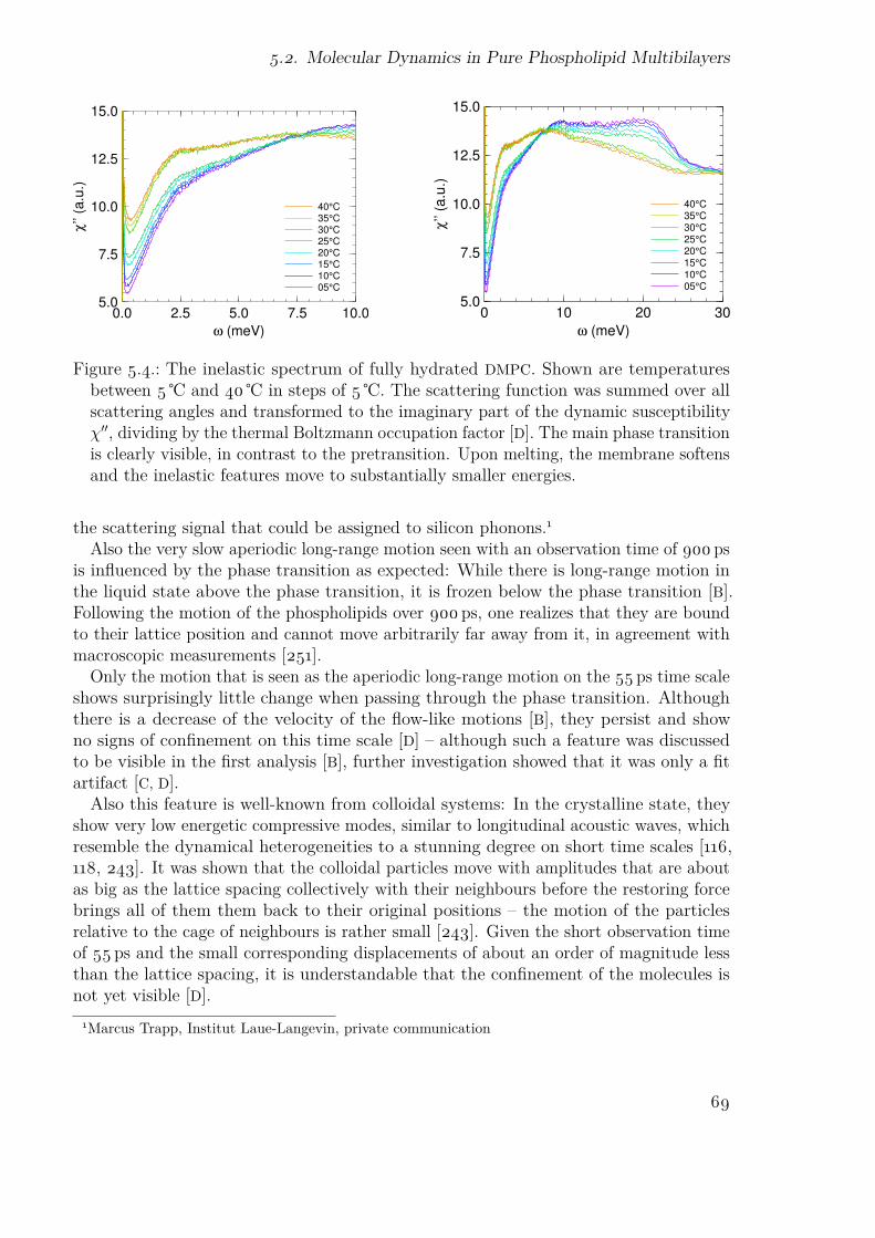
5.2. Molecular Dynamics in Pure Phospholipid Multibilayers
0.0 2.5 5.0 7.5 10.05.0
7.5
10.0
12.5
15.0
ω (meV)
χ’’
(a.u
.)
40°C35°C30°C25°C20°C15°C10°C05°C
0 10 20 305.0
7.5
10.0
12.5
15.0
ω (meV)
χ’’
(a.u
.)
40°C35°C30°C25°C20°C15°C10°C05°C
Figure 5.4.: The inelastic spectrum of fully hydrated DMPC. Shown are temperaturesbetween 5 and 40 in steps of 5 . The scattering function was summed over allscattering angles and transformed to the imaginary part of the dynamic susceptibilityχ′′, dividing by the thermal Boltzmann occupation factor [D]. The main phase transitionis clearly visible, in contrast to the pretransition. Upon melting, the membrane softensand the inelastic features move to substantially smaller energies.
the scattering signal that could be assigned to silicon phonons.1Also the very slow aperiodic long-range motion seen with an observation time of 900 ps
is influenced by the phase transition as expected: While there is long-range motion inthe liquid state above the phase transition, it is frozen below the phase transition [B].Following the motion of the phospholipids over 900 ps, one realizes that they are boundto their lattice position and cannot move arbitrarily far away from it, in agreement withmacroscopic measurements [251].
Only the motion that is seen as the aperiodic long-range motion on the 55 ps time scaleshows surprisingly little change when passing through the phase transition. Althoughthere is a decrease of the velocity of the flow-like motions [B], they persist and showno signs of confinement on this time scale [D] – although such a feature was discussedto be visible in the first analysis [B], further investigation showed that it was only a fitartifact [C, D].
Also this feature is well-known from colloidal systems: In the crystalline state, theyshow very low energetic compressive modes, similar to longitudinal acoustic waves, whichresemble the dynamical heterogeneities to a stunning degree on short time scales [116,118, 243]. It was shown that the colloidal particles move with amplitudes that are aboutas big as the lattice spacing collectively with their neighbours before the restoring forcebrings all of them them back to their original positions – the motion of the particlesrelative to the cage of neighbours is rather small [243]. Given the short observation timeof 55 ps and the small corresponding displacements of about an order of magnitude lessthan the lattice spacing, it is understandable that the confinement of the molecules isnot yet visible [D].
1Marcus Trapp, Institut Laue-Langevin, private communication
69

Chapter 5. Results and Discussion
5.3. Multibilayers of DMPC with AdditivesAfter the motions of the pure phospholipid have been characterised, it was possible tostudy the influence of additives on the dynamics of the phospholipids. This is a firststep towards biologically and pharmaceutically relevant systems. The characterizationof these systems has purposefully been based on a much simpler and robust model-freedata evaluation method than the one of pure DMPC multibilayers. The main reason fortaking this approach is to make a subsequent comparison with the monolayer samplespossible. The data quality of the phospholipid monolayers is not sufficient for a reliablefit of the model that was used to describe the pure DMPC multibilayers. An additionalbenefit of this model-free approach is that these results are valid independently of thecorrectness of the model used for the pure DMPC.
The influence of several additives on the mobility was extracted from the comparisonof the FWHM of the samples with the ones of pure DMPC [E]. Of the studied additives,cholesterol, farnesol, myristic acid, and sodium glycocholate, cholesterol had the largestinfluence, decreasing the dynamics of the phospholipid molecules. The good miscibility ofphospholipid and cholesterol made it possible to use much larger amounts of cholesterolthan of the other substances, impeding a direct comparison of the influence of theadditives at very high concentrations. The relative decrease of the phospholipid mobilitywas on the nanosecond time scale already about as large as on the millisecond time scaleprobed with other techniques [132]. The phospholipid molecules do not move very farduring the short times observed in the present study, in particular only very few of themhad the opportunity to interact with the cholesterol molecules directly.
The decrease of mobility can however be explained seamlessly in the picture of flow-likemotions. If one regards the flow events in which the particles participate as the elementalsteps of a random walk, one can connect the two by assuming either that the cholesteroldecreases the speed of the flow events but leaves the length of such a flow event unchangedor that it decreases the length of a flow event while not changing the speed of the flowmotion – or a combination of the two scenarios.
The mean-square displacement ⟨r2⟩ of a particle performing a random walk as afunction of the time t depends on both, the time for a single step δt and the length ofthe step b as
⟨r2⟩(t) t≫δt−−→ t
δt· b2 = t · v · b (5.1)
where v = b/δt is the velocity of the particle during a step. The two scenarios (decreasingv at constant b or constant v with a decreasing b) are therefore in the long time limitequivalent.
They are, however, different on a time scale that is shorter than the length of a flowevent δt: If the flow velocity is decreased, the effect is also visible at short times; ifthe flow length is decreased, the effect should be less visible as the observation time isdecreased.
The measurements of mixtures of DMPC with cholesterol show that the influence onthe mobility is only a minor effect on the time scale of 55 ps while it is very visible on the900 ps scale. In fact, the relative decrease of mobility compared to the case of pure DMPC
70

5.4. Single Bilayers and Monolayers
is on the 900 ps scale already nearly as large as on macroscopic time and length scales [E].It can be concluded that the influence of cholesterol on the phospholipid dynamics isalready nearly fully established on the 900 ps time scale.
In the picture of flow-like motions, this influence consists mainly of decreasing thepersistence time of the flow events while not changing the flow velocities very much. Thisdecrease is a smooth function of the cholesterol content, in contrast to early macroscopicmeasurements [131] but in agreement with subsequent macroscopic measurements [132]and MD simulations [142–144].
Comparing again with the dynamical heterogeneities found in other systems, exactlythe opposite behaviour would be expected: an increase of the density results in an increaseof the persistence time of the flow motions with a decrease of the flow velocity. That thisis not the case here can be understood from the structure of the membrane: while thehead group region of the phospholipids is the dense structure that governs the behaviourof the flows in the pure membrane, the cholesterol is mainly incorporated into the tailregion of the phospholipids. This brings about that the density in the head group regionis only little influenced. It also lets only a very thin part of the cholesterol molecule bepresent in the head group layer, hereby increasing the polydispersity here. An increase indispersity was found to decrease the persistence length of dynamical heterogeneities [99]– this connection merits closer investigation in the future.
However, it should be noted that this model-based interpretation is taken from a dataevaluation that was model-free on purpose. It should therefore in future works be backedup with a detailed analysis of MD simulations that can be validated with the neutronscattering data.
Of the other additives, sodium glycocholate is the most interesting in the currentcontext because it is also used in drug delivery systems. It was found to slightly increasethe dynamics of the phospholipids at a temperature of 20 and reversing this effect toa slight decrease at the studied temperatures of 30 and 40 [E].
5.4. Single Bilayers and MonolayersThe data of single bilayers and monolayers were evaluated with the same model-freeapproach as the multibilayers of DMPC with additives introduced before.
Vesicles are hollow spheres of single bilayers. The big difference to the multibilayersamples is that they are more or less strongly curved – the curvature has been found toplay a role for vesicles with a diameter of less than about 100 nm [252]. The mobility ofthe molecules increases slightly with increasing curvature [F] which can be attributed tothe increasing packing frustration in the bilayer.
The dynamics of the phospholipids in the pharmaceutically relevant systems is notonly of importance for the drug release properties but also for the storage stability,e. g. the stability of the emulsion droplets against coagulation. One prominent exampleis the production of suspensions via melt extrusion: During the production at hightemperatures, the fatty phase is liquid and the particle a spherical droplet. At lowtemperatures, the fat crystallizes and changes its form drastically to a platelet. While
71

Chapter 5. Results and Discussion
pure DMPC is not capable of keeping the particles from coagulating during this transition,a mixture of DMPC and sodium glycocholate can [55, 56].
The important length and time scale for such a collision of two particles can beestimated on the example of emulsions with a volume fraction of the dispersed phase oftypically 10%. With a droplet diameter of 130 nm, the mean surface to surface distanceis very close to 100 nm. The droplets diffuse in the water and collide – the time scalebetween two collisions can be estimated with
⟨r2⟩(t) = 6 kBT
6πηRt (5.2)
to the order of 1 ms. In this light, measuring the dynamics on a sub-nanosecond scalemight seem not directly relevant. In the case of cholesterol, the relative slow-downobserved on this short time scale was already very similar to the one on a macroscopicscale which was only slightly more pronounced.
The mobility of the phospholipids on the emulsion droplets was found to be faster thanin the multibilayer samples. It increases as the density of the phospholipid moleculesdecreases [F]. This can be intuitively understood because the molecules can move morefreely with less hindering by their neighbours. On this example, it becomes clear thatthere is no direct correlation between the mobility of the stabilizer and the stability ofthe emulsion: Samples with little stabilizer are less stable than samples with a largeamount of stabilizer – which is also intuitively expected because the coverage of thedroplets is better with more stabilizer.
Adding sodium glycocholate results in about the same increase of phospholipid mobilityat 20 in multibilayers and in the monolayers around emulsion droplets. Having addedsodium glycocholate, the density of phospholipid can be further reduced which leads to afurther increase of the mobility [F].
72

Chapter 6.
OutlookIt was possible in this thesis to provide experimental evidence for the flow-like motions ofphospholipid molecules that had been observed in MD simulations. Further, the evolutionof the mobility on a pico- to nanosecond time scale under the influence of additives andin monolayers around emulsion droplets could be followed.
Both, the results and the tools presented in this thesis lay the ground for tacklingfurther, related challenges. Some of these are sketched in the following.
6.1. Methodical EnhancementsA new generation of sample containers can make the subtraction of backgroundcontributions easier. Most of today’s sample containers distribute the sample in a thinlayer over a relatively large area of a few cm2. This is owed to two reasons: first, theneutron flux at most instruments is distributed over this area and second, one wantsto avoid that the neutrons travel a long time through the sample on their way froma scattering event to a detector which increases the probability to be scattered againor to be absorbed. However, both of these restrictions are currently being lifted: Newfocussing neutron guides will be able to deliver the neutron flux to a smaller area andnew data reduction algorithms will be able to handle multiple scattering effects1.
The current sample containers have some disadvantages: The thickness of sample andaluminium layers have uncertainties of about 10% in the neutron beam area due to thelimited manufacturing precision and bulging of the containers. Because the manufacturingis very complicated, they are reused for different samples. The samples studied in thisthesis are water-based and react therefore with the aluminium can. The reaction of thesamples with the can causes differences in the scattering of the cans, depending on theirhistory. This contamination of the can and the fact that not the whole can is in theneutron beam impedes a determination of the scattering contributions by the weights ofthe cans.
Differing amounts of sample in the beam or varying contributions by the container are abig challenge in the present case can be seen easily. The samples discussed here (presentedin detail in chapter 3) have the following characteristics: They are heterogeneous mixturesof different substances of which only one is of interest. The part of the sample that is
1Joachim Wuttke, JCNS, private communication.
73

Chapter 6. Outlook
regarded as a nuisance can be as big as a mass fraction of 99 %. These backgroundcontributions are also measured as bulk samples and subtracted from the mixture. Avery large part of the scattered intensity will therefore be subtracted which can amplifythe uncertainties.
Finally, the design of the hollow cylindrical sample containers brings some additionalproblems: as viscous samples are filled in the outer container and then squeezed into thegap by pushing with the inner container, they are likely to de-mix if more and less viscousparts are present. The fluid part will go first into the gap, followed by the viscous part.Therefore, the sample composition in the beam is actually unknown. When squeezing inthe inner container, it can also not be excluded that air bubbles are also trapped whichmay come out after the sample, replacing parts of it in the neutron beam.
It seems that all these problems could be avoided if one puts the traditional samplecontainers out of service. Instead, small compact single-use aluminium containers sealedwith a cold-welded cover as used in differential scanning calorimetry could contain thesample. These small containers should be completely bathed in the neutron beam so thatalways the whole sample contributes to the scattering. The weight of the can would givea precise measure of the amount of sample and container in the beam and as every canis used only one time, no contamination effects would have to be expected. Additionally,the small time-of-flight differences in this compact geometry would even improve theresolution of the spectrometer. In contrast to the current containers, air in the samplecan would not be a problem because the amount of sample in the beam can be determinedby weight if the whole container is in the beam.
Challenges of this approach are that either the neutron flux on the sample is decreasedor the divergence increased. However, the Q dependence of the scattering signal is inmost analyses of quasielastic neutron scattering data far from being a limiting factor.Also, the compact form makes the correction of multiple scattering and absorption ofscattered neutrons mandatory. The corresponding software is in the moment under heavydevelopment so that this should also not be seen as a big hurdle.
The sample environment for moderate temperatures could be trimmed towardsfaster sample changes. When using the cryostat, the coupling of the stick to thecryostat is always much colder than room temperature. This does not only requirecare to prevent air from entering into the cryostat but also the sample stick has to bedefrosted and dried from the condensed water. Combined with the time that is neededfor a decrease of the activation of the aluminium or vanadium, a sample change in thecryostat needs about one hour. Compared to measurement times that can be also asshort as one hour, this becomes a limiting time factor at modern neutron scatteringinstruments.
Flat sample containers introduce the additional problem that the orientation of theirsurface normal with respect to the incoming neutron beam is important. The currentsetup does not allow a relative reproducibility of much below 1° and a similar absoluteaccuracy which might be of minor importance, though.
These problems could be circumvented by an improved sample changing procedure in
74

6.1. Methodical Enhancements
which the new sample would be placed in an air lock. After reaching a low pressure, theold sample would be exchanged with the new sample in the cryostat using a manipulator.These measures would speed the sample change up dramatically.
Free data exchange would open the possibility to reanalyze existing data. Cur-rently, data of neutron scattering experiments are hardly accessible to other researchersthan the ones who conducted the measurement. This can be an obstacle for checking theresults, as became visible during this thesis [C]: Previously presented results [105] weresuspected to be an artifact of the data analysis. As the data were not available, a newmeasurement with another sample had to be performed although it would have probablybeen sufficient to reevaluate the existing data sets.
Data exchange is currently debated in may fields of science [253]. A few disciplineslike astronomy [254] and biology [255, 256] take the lead in this regard. It is obviousthat data without the details of the sample preparation are nearly useless in condensedmatter physics while this issue is completely negligible in astronomy. Nevertheless, incases like the one mentioned above where only the data evaluation and not the samplepreparation is under scrutiny, free data exchange could prove profitable.
Data reduction software. The software that is currently used for the data reductionat TOFTOF deserves replacement, especially because of the numerous bugs in the programsome of which are listed in the appendix [I]. With the presented package sihl, thereis a functioning alternative which can serve as an immediate replacement until theScientific Computing group at the FRM II implements a unified data reduction softwarefor the backscattering and time-of-flight spectrometers. Due to its easily extendableobject-oriented approach, sihl could even be the starting point for this project.
Although the current implementation of data with experimental errors in chaste isworking, these parts can be replaced with the free and open uncertainties package [257]which might be faster. The determination of the time-of-flight of the elastically scatteredneutrons will also be performed with a sub-pixel accuracy, using a spline interpolationbetween the data points. Care will be taken to not take the maximum of the scatteredsignal in time-of-flight space but in energy space. If sihl was in use on TOFTOF for alonger time, it would be rather straightforward to implement a graphical user interfacefor it in order to make it more user friendly.
Independently from the data reduction, the data correction for self shielding andmultiple scattering in the sample should be tackled. The program that is currentlydeveloped for the correction of backscattering spectra2 could be extended for the time-of-flight spectra. If only the quasielastic region of the spectrum is of interest, this extensionshould not require much time and effort.
Data analysis procedure. The various advantages of Monte Carlo fit algorithms werediscussed in detail. The proposed scaling of the parameter ump lengths [H] which is
2Joachim Wuttke, JCNS
75

Chapter 6. Outlook
implemented in the program FABADA [G] will now be incorporated3 into the Pythonpackage PyMC [258]. This will not only make it accessible to a broader user communitybut also facilitate the comparisons of different parameter jump adaption methods.
The algorithm itself is still based on two parameters that have to be manually adjustedto the problem at hand: The number of steps that are performed before the parameterjumps are adjusted and the cooling schedule of the simulated annealing. A furtherdevelopment of the algorithm would consist of an automated choice of these values.
A simple criterion for the automatic choice of the number of parameter steps could beused as an alternative to previously suggested methods [259]: the χ2 hypersurface shouldbe sampled until acceptance ratio pi of the parameter i is defined «well enough» up toan uncertainty s for a meaningful comparison with the target value. Assuming that theacceptance ratio does not change considerably when the jump length is constant, thesubsequent tries can be seen as success or failure in n independent experiments each ofwhich has the probability of success p. If the acceptance is for example tuned towardsp = 33% [G], «well enough» would be on the order of s = 1%. Using the standarddeviation of the binomial distribution, one arrives at n = p · (1 − p)/s2 which can beevaluated during the Monte Carlo run. With the given example of p = 33% and s = 1%,this parameter should be varied on the order of 104 times before adjusting its jumplength. A careful evaluation of the performance of this simple rule compared to thepublished ones [259] will be performed.
For the adjustment of the cooling schedule, it could be helpful to understand the χ2
hypersurface as an energy surface and consider the analogy of a cooling liquid. Thecooling schedule should then be adjusted such that the system is not trapped in anyother than the single crystalline state but can relax to thermal equilibrium. One way tofoster this relaxation is to keep the system ergodic so that it can sample all the availablestates. The ergodicity could be ensured using an idea from swarm methods [223] andtake many independent configurations, i. e. parameter combinations which move on theχ2 hypersurface. It is then possible to check if the time average is equal to the ensembleaverage which should be the case in an ergodic system. Alternatively, two-time correlationfunctions could be used to check if the system exhibits aging which would be anotherindication for non-ergodicity.
Another interesting subject matter is the analogy between the fit and a thermodynam-ical system itself. The temperature dependence of the relaxation time in glass formingsystems is proposed to show an Arrhenius behaviour if the underlying energy surface issimple and a super-Arrhenius behaviour if it contains many local minima. χ2 hypersur-faces can also be simple or ragged – does the relaxation time of the fitted parametersalso show an Arrhenius or super-Arrhenius temperature dependence, respectively?
Once the fit reached the minimum of the χ2 hypersurface, it essentially performs arandom walk in a more or less harmonic potential – confer to the model of the Brownianoscillator used for the localised motions in the phospholipid. Whereas the Levenberg-Marquardt algorithm simply makes the approximation that the potential is harmonic,the Monte Carlo algorithm explores it explicitly and experiences all the deviations from a
3In collaboration with Jean-François Moulin, Helmholtz Zentrum Geesthacht
76

6.2. Molecular Dynamics in Pure Phospholipid Multibilayers
Figure 6.1.: Snapshot of an MD simulationof a fully hydrated DMPC bilayer at25 . The shown simulation consists of128 phospholipid molecules and 3654 wa-ter molecules which were equilibratedfor a simulated time of 2 ns. The simu-lation was performed with the softwareNAMD2 using the force field CHARMM27,the bound lengths in this all-atom modelwere considered to be constant. Pictureby courtesy of Jordi Martí.
harmonic behaviour that are present. The effect of an anharmonic potential on the mean-square displacement of the particle was discussed on the phenomenon of the so-calleddynamical transition of proteins [233]. It would be interesting to see if the error barsof the parameters (corresponding to the mean-square displacements of the parameters)show a similar temperature dependence.
6.2. Molecular Dynamics in Pure PhospholipidMultibilayers
Closer link between measurements and simulations. The potential of the model-based data evaluation is probably exhausted with the model presented, given the qualityof the data. More information should be accessible in MD simulations. In the moment,MD simulations from the literature were converted into a sensible model of which thelong-range component showed excellent agreement with the one extracted from the neu-tron scattering data. However, a much more direct comparison would be possible whencalculating the intermediate scattering function from the simulation. This could be com-pared over the full time range with resolution-resolved neutron scattering measurementswhich has already been proven to work perfectly in the case of n-alkanes.4
For this purpose, own MD simulations of a DMPC bilayer have already been started.5.A snapshot of this simulation can be seen in figure 6.1. After their validation againstsimulations from the literature and the QENS data, the properties of the fast andslow regions can be evaluated, checking the local density, short range order, four-pointcorrelation functions, etc.
Coherent neutron scattering measurements could potentially provide further supportto the idea of correlated motion of neighbouring molecules because it probes the paircorrelation functions. In order to probe the correlations between neighbouring molecules,Q values around 2π/8 Å≈0.8 Å-1 and observation times in the nanosecond range wouldbe needed. Although these values are at the limit of what can be seen at TOFTOF, a
4Humphrey Morhenn, Technische Universität München, private communication.5In collaboration with Jordi Martí, Computer Simulation in Condensed Matter Research Group,
Universitat Politècnica de Catalunya, Barcelona.
77

Chapter 6. Outlook
0.0 0.5 1.0 1.5 2.00.0
0.5
1.0
1.5
2.0
Q (A-1)
dσ
/dΩ
(Q)
(a.u
.)
perdeuterated DMPC
4°C20°C30°C
Figure 6.2.: Left: Diffraction pattern of fully hydrated perdeuterated DMPC after subtrac-tion of the water contribution at different temperatures across the phase transitions.In the low temperature measurement, the chain correlation peak at 1.5 Å-1 is clearlyvisible, the small peak highlighted at 0.8 Å-1 is caused by the head groups. Thesepeaks broaden significantly and shift to lower values of Q as the temperature is raised.The measurement at 30 is performed above the main phase transition – as can beseen from the chain correlation peak. Right: Sketch of the phospholipid molecules,seen from the top [10]. The big head group is shown in violet. The positions of thetwo chains which are facing away from the observer are shown in orange. It can beseen that the head groups form an orthorhombic lattice with a bigger lattice spacingthan the one of the hexagonal lattice of the chains.
separation of coherent and incoherent scattering is here not possible in the moment.Unfortunately, the coherent scattering intensity of perdeuterated DMPC is very small atthis position, only about 4% of the incoherent one as shown in figure 6.2. This was alsoobserved in earlier measurements and simulations [206]. It is therefore questionable if anextraction of this signal would be possible even if a neutron spin analysis was installedat TOFTOF that would allow to suppress the incoherent scattering signal. For this reason,most coherent neutron scattering measurements that aim to characterize the correlationof in-plane motions resort to the chain correlations (visible in the peak at 1.5 Å-1 infigure 6.2) [137].
Comparison with a quasi-two-dimensional colloidal system Another interesting ques-tion is if this behaviour is indeed governed by the phospholipid head groups. This couldbe tackled by approximating the head groups with ellipsoids – with or without dipolemoment – that are confined to two dimensions. From the MD simulation, one couldfurther extract the probability distribution function of the orientation of the ellipsoidsout of the plane and use this input parameter in the simplified simulation. If the flow-likemotions are indeed caused by the dense packing in the head group area, they should alsobe visible in this simplified simulation.
78

6.3. Multibilayers of DMPC with Additives
6.3. Multibilayers of DMPC with AdditivesFurther evaluation of the data. The spectra of the mixed systems of phospholipidswith additives have so far been evaluated only with the model-free approach [E]. Furtherinformation could be extracted either by using a model of the molecular motions or byusing the data to validate molecular dynamics simulations. The model used successfullyfor the evaluation of the data of pure DMPC could be taken as a starting point for themodel-based data evaluation.
Molecular dynamics simulations of phospholipids mixed with additives are stateof the art. Especially cholesterol has received much attention due to its biologicalimportance [142, 260–262]. Calculating the intermediate scattering function from both,measurements and simulation, would allow to validate the simulations. These simulationswould then allow to study the evaluation of the flow patterns upon the addition ofcholesterol in detail [E].
Parallels to binary colloidal systems. If the analogy to quasi two dimensional colloidalsystems holds, the addition of cholesterol to the DMPC would correspond to add colloidalparticles with a smaller size to the system under study. Binary colloidal systems havebeen used to study glass-forming systems [244, 263, 264] because they do not crystallizein a range of concentrations and ratios of radii. If this effect is related to the suppressionof the main phase transition in phospholipids by cholesterol [265] has to be evaluated.From the viewpoint taken in this thesis, this seems rather unlikely because the mainphase transition is caused be the tails of the molecules whereas the glassy behaviour istriggered by the densely packed head group area.
Regardless of the influence of cholesterol on the main phase transition of the phos-pholipids, it would be interesting to study the evaluation of the flow patterns upon theaddition of smaller spheres. A decrease of the persistence length of the flow patternswith hardly any influence on the flow speed would be in line with the interpretation ofthe neutron scattering data [E]. Existing data of polydisperse mixtures seem to be inagreement with this view, exhibiting a decrease of the correlation length of dynamicalheterogeneities as the polydispersity increases [99, 266, 267].
6.4. Single Bilayers and MonolayersPreparation and characteristics of the phospholipid samples. It was found in thisthesis that the surface occupancy of the emulsion droplets is an important factor forthe mobility of the phospholipid molecules. In order to quantify the results further, thesurface occupancy should be characterized in more detail. Three factors are probablyof main importance: First, the losses of the different substances during the production.Second, the diameters of the emulsion droplets which are not monodisperse and cantherefore have a different total surface. And third, the amount of phospholipid is presenteither as vesicles or as mixed micelles with sodium glycocholate. The two latter points
79

Chapter 6. Outlook
will be tackled by structural studies.6
More measurements of the dynamics in vesicles and emulsions. So far, the mea-surements have been performed only at a temperature of 20 , below the main phasetransition of the phospholipids. This is the phase interesting for the storage of thedrug delivery systems – future measurements should study the same systems also at atemperature above the main phase transition which would correspond to the situationwhere the drug delivery system is used in the human body.
The result is not completely trivial as it was seen in the case of DMPC multibilayersthat the addition of sodium glycocholate causes contrary reactions: from an increase ofthe speed at 20 to a slight decrease at 30 and 40 [E]. However, it is expected thatthe addition of sodium glycocholate will reduce the density of the phospholipid in theinterface by creating micelles. The reduced density will then again result in an increasedmobility.
Concerning the mobility of phospholipid monolayers on emulsion droplets, the presentedstudies [F] were performed at 20 , corresponding to storage conditions. Comparing thedynamics with the one at 40 , corresponding to body temperature and above the mainphase transition of DMPC, is certainly desirable.
Going further, the effects of oil viscosity and interdigitation of the oil molecules intothe chain region of the phospholipids can be studied by varying the length of the oilmolecules, the length of the phospholipid tails, and the temperature. Measurementson TOFTOF can be complemented with macroscopic measurements of a flat oil-waterinterface, for example with fluorescence microscopy.
These macroscopic measurements are expected to give better access to the solid fat-water interface because the solid substances do in this case not contribute an interferingsignal as they do in the case of the neutron scattering measurements. It is known fromsuch measurements that the phospholipid mobility decreases as the viscosity of the oilyphase increases. Does this decrease continue to a complete arrest when the oily phasebecomes a solid or are the phospholipids expelled from the crystal and become againmore mobile on the surface?
Evaluating the data of the suspensions. It would also be interesting to extend thestudies on phospholipid layers on solid lipid nanoparticles: are the phospholipid moleculesstill mobile if the fatty phase beneath is solid? However, this requires an understandingof the diffraction patterns of the nanoparticles before, cf. section 4.1. Measuring themalso at high temperatures where the fatty substance is liquid in the droplets and in bulkallows to determine the amount of this substance in the suspension. If it is then possibleto calculate the diffraction pattern of the nanocrystalline phase, a correct subtractionshould be feasible.
As it was shown in section 4.1, the bulk substances have strong diffraction peaks atvalues of Q where the nanocrystalline samples have either only very weak ones or noneat all. An idea might therefore be to subtract the spectrum of vanadium instead of the
6Martin Schmiele, Friedrich-Alexander-Universität Erlangen-Nürnberg
80
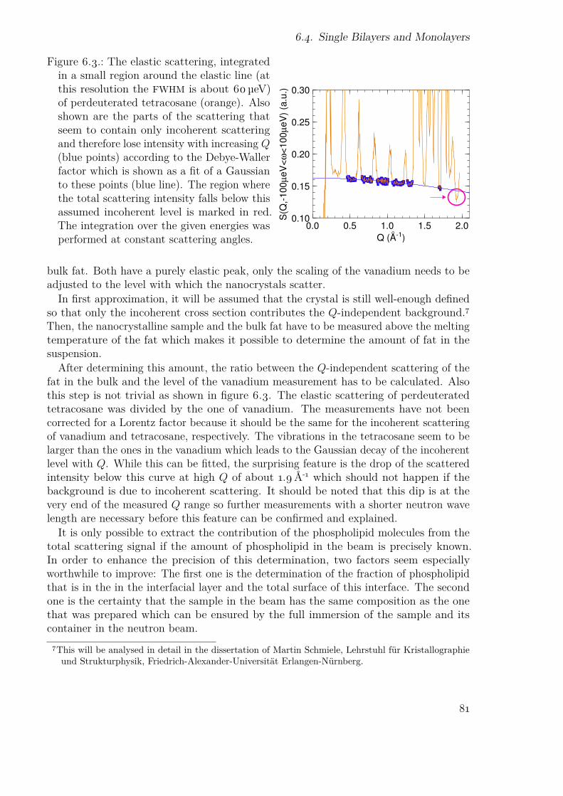
6.4. Single Bilayers and Monolayers
Figure 6.3.: The elastic scattering, integratedin a small region around the elastic line (atthis resolution the FWHM is about 60 µeV)of perdeuterated tetracosane (orange). Alsoshown are the parts of the scattering thatseem to contain only incoherent scatteringand therefore lose intensity with increasing Q(blue points) according to the Debye-Wallerfactor which is shown as a fit of a Gaussianto these points (blue line). The region wherethe total scattering intensity falls below thisassumed incoherent level is marked in red.The integration over the given energies wasperformed at constant scattering angles.
0.0 0.5 1.0 1.5 2.00.10
0.15
0.20
0.25
0.30
Q (A-1)
S(Q
,-1
00
µeV
<ω
<100
µeV
) (a
.u.)
bulk fat. Both have a purely elastic peak, only the scaling of the vanadium needs to beadjusted to the level with which the nanocrystals scatter.
In first approximation, it will be assumed that the crystal is still well-enough definedso that only the incoherent cross section contributes the Q-independent background.7Then, the nanocrystalline sample and the bulk fat have to be measured above the meltingtemperature of the fat which makes it possible to determine the amount of fat in thesuspension.
After determining this amount, the ratio between the Q-independent scattering of thefat in the bulk and the level of the vanadium measurement has to be calculated. Alsothis step is not trivial as shown in figure 6.3. The elastic scattering of perdeuteratedtetracosane was divided by the one of vanadium. The measurements have not beencorrected for a Lorentz factor because it should be the same for the incoherent scatteringof vanadium and tetracosane, respectively. The vibrations in the tetracosane seem to belarger than the ones in the vanadium which leads to the Gaussian decay of the incoherentlevel with Q. While this can be fitted, the surprising feature is the drop of the scatteredintensity below this curve at high Q of about 1.9 Å-1 which should not happen if thebackground is due to incoherent scattering. It should be noted that this dip is at thevery end of the measured Q range so further measurements with a shorter neutron wavelength are necessary before this feature can be confirmed and explained.
It is only possible to extract the contribution of the phospholipid molecules from thetotal scattering signal if the amount of phospholipid in the beam is precisely known.In order to enhance the precision of this determination, two factors seem especiallyworthwhile to improve: The first one is the determination of the fraction of phospholipidthat is in the in the interfacial layer and the total surface of this interface. The secondone is the certainty that the sample in the beam has the same composition as the onethat was prepared which can be ensured by the full immersion of the sample and itscontainer in the neutron beam.
7This will be analysed in detail in the dissertation of Martin Schmiele, Lehrstuhl für Kristallographieund Strukturphysik, Friedrich-Alexander-Universität Erlangen-Nürnberg.
81

Chapter 6. Outlook
In the case of suspensions, the amount of fatty substance in the sample can be deter-mined from the diffraction patterns only if this substance is liquid, in the nanoparticularstate as well as in the bulk. If the scattering pattern of the nanoparticles can be calculated,it should be possible to extract the phospholipid dynamics also from the suspension sam-ples. However, this will always be a challenging task because the phospholipid dynamicsis not the only narrow component in the spectra any more. For the multibilayer, vesicle,and emulsion samples, the background contributions are automatically separated in thespectra from the signal of the phospholipid which made the data evaluation more robustagainst small errors in the background subtraction.
82

Chapter 7.
ConclusionThis thesis aimed to study the molecular motions of phospholipid molecules in differentenvironments. The traditional view that the molecules rattle in a cage of their neigh-bouring molecules and hop out of this cage from time to time had been challenged bymolecular dynamics simulations. These suggested that the phospholipids formed transientclusters that moved in flow-like patterns. As neutron scattering is one of the very fewexperimental techniques that can probe motions on the pico- to nanosecond time scalethat is important for these motions, it was employed to give experimental evidence forone of the opposing views.
It was indeed possible to find experimental support – for the novel view of flow-likemotions in the membrane. In the quest for statistically relevant conclusions, the completedata reduction procedure was reimplemented which is now available also for other users ofthe spectrometer TOFTOF. The evaluation of the data was performed with a new programthat explicitly samples the parameter space which is compatible with the data. It couldbe shown with this approach that the model of flow-like motions fits the data.
This occurrence of transient clusters of molecules with similar motions and the spatialseparation of fast and slow molecules was found to resemble a feature of glass-formingsystems, the so-called dynamical heterogeneities. It was argued that the high density inthe head group area is responsible for this similarity. The persistence of these flow-likemotions on a picosecond time scale below the main phase transition of the phospholipidwas interpreted as localized soft modes, another behaviour known from glass-formingsystems.
Interestingly enough, also the old view of cages and hopping motions had been a(very successful) loan from glass physics at the time. Taking into account that this verysimple idea has long been replaced with more elaborate concepts in glass physics, itcan be suggested that the description of phospholipid membranes does profit from moreadaptations of modern viewpoints in glass physics, as the one of dynamical heterogeneities.
Moving away from the systems containing pure DMPC, the influence of a few repre-sentative additives on the phospholipid dynamics was studied. Of special interest werecholesterol, a component of cell membranes, and sodium glycocholate which can beused as co-stabilizer of emulsions. Cholesterol decreased the mobility of the phospho-lipid molecules already on the nanosecond time scale by about the same fraction as onmacroscopic time scales. This slowing down was tentatively explained by a reduction ofthe persistence length of the flow patterns, stimulated by corresponding observations in
83

Chapter 7. Conclusion
colloidal systems.Sodium glycocholate was not only added to the phospholipid bilayers but this mixture
was also used to stabilize emulsion droplets. The distribution of the molecules onthe surface of the droplets triggered an increase in the dynamics, probably due to areduction of their density. This effect was clearly stronger than the influence of sodiumglycocholate on the dynamics of the phospholipids. It seems therefore safe to concludethat the influence of sodium glycocholate on the pico- to nanosecond dynamics of thephospholipids is not the key to explain its boosting effect on the stabilizing properties.
A crucial step for the evaluation of the phospholipid mobility in stabilizer layers is thesubtraction of the contributions of the other components of the sample which can amountto 99% of the sample mass. It was possible to remove the background contributionsin the case of the emulsion samples after the identification of their contributions tothe diffraction patterns. It is however exactly this step which impedes currently theevaluation of the suspension samples where the subtraction of the solid phase fails becausethe nanoparticles do not show the same diffraction pattern as the bulk. This problemwill be solvable as soon as the diffraction patterns of the nanoparticles can be computedwhich is currently attempted.
Studying the dynamics of stabilizing phospholipid monolayers in suspensions is onlyone of many exciting possibilities for future projects. To name but a few examples,theemployed data fitting techniques will be developed further and the comparability offinding the best solution in the parameter space with a crystallizing liquid will be explored.Molecular dynamics simulations and quasielastic neutron scattering measurements of pureDMPC as well as systems with additives will be dovetailed to yield further possibilities tocharacterise the observed flow patterns. Simultaneously, complementary experiments withquasi two dimensional colloidal systems would allow to analyse if the observed motionsand their change upon the addition of co-surfactants are universally valid properties ofdensely packed systems or rather special properties of these molecules.
The new paradigm of flow-like motions in phospholipid membranes could be fosteredwith experimental data in this thesis. It is impossible to assess the importance of thepresence of dynamical heterogeneities in these systems today. It will most certainly notbe such a big leap forward as the introduction of the previous model of hopping motions,but it might prove to be another step towards a better understanding of the dynamicalprocesses in phospholipid membranes.
84

Part II.
Publications
85


Appendix A.
List of Publications and PresentationsListed are the publications and presentations that originated during the course of thethesis. The refereed publications with immediate relevance for the presented work canalso be found in full text in the indicated appendices.
A.1. Refereed Publications1. The Picosecond Dynamics of the Phospholipid Dimyristoylphosphatidylcholine in
Mono- and Bilayers.Sebastian Busch, Luis Carlos Pardo, Christoph Smuda, and Tobias Unruh.Soft Matter, 8:3576, 2012.http://dx.doi.org/10.1039/c2sm07380c
Included in appendix [F].
2. Differences in first neighbor orientation behind the anomalies in the low and highdensity trans-1,2-dichloroethane liquidMuriel Rovira-Esteva, Arul Murugan, Luis Carlos Pardo, Sebastian Busch,Josep Lluis Tamarit, Gabriel Julio Cuello, and Francisco Javier Bermejo.The Journal of Chemical Physics, 136(12):124514, 2012.http://dx.doi.org/10.1063/1.3697849
3. The slow short-time motions of phospholipid molecules with a focus on the influenceof multiple scattering and fitting artifacts.Sebastian Busch and Tobias Unruh.Journal of Physics: Condensed Matter, 23(25):254205, 2011.http://dx.doi.org/10.1088/0953-8984/23/25/254205
Included in appendix [D].
4. The influence of additives on the nanoscopic dynamics of the phospholipid di-myristoylphosphatidylcholine.Sebastian Busch and Tobias Unruh.Biochimica et Biophysica Acta (BBA) – Biomembranes, 1808(1):199–208, 2011.http://dx.doi.org/10.1016/j.bbamem.2010.10.012
Included in appendix [E].
87
Appendix A. List of Publications and Presentations
5. The influence of 2 kbar pressure on the global and internal dynamics of humanhemoglobin observed by quasielastic neutron scattering.Marie-Sousai Appavou, Sebastian Busch, Wolfgang Doster, Ana M. Gaspar, andTobias Unruh.European Biophysics Journal with Biophysics Letters, 40(6):705–714, 2011.http://dx.doi.org/10.1007/s00249-011-0678-3
6. FABADA: a Fitting Algorithm for Bayesian Analysis of DAta.Luis Carlos Pardo, Muriel Rovira-Esteva, Sebastian Busch, María Dolores Ruiz-Martín, and Josep Lluis Tamarit.Journal of Physics: Conference Series, 325(1):012006, 2011.http://dx.doi.org/10.1088/1742-6596/325/1/012006
Included in appendix [G].
7. Fitting in a complex χ2 landscape using an optimized hypersurface sampling.Luis Carlos Pardo, Muriel Rovira-Esteva, Sebastian Busch, Jean-François Moulin,and Josep Lluis Tamarit.Physical Review E, 84(4):046711, 2011.http://dx.doi.org/10.1103/PhysRevE.84.046711
Included in appendix [H].
8. Interplay between intra- and intermolecular structures of 1,1,2,2-tetrachloro-1,2-difluoroethane.Muriel Rovira-Esteva, Arul Murugan, Luis Carlos Pardo, Sebastian Busch,Josep Lluis Tamarit, Szilvia Pothoczki, Gabriel Julio Cuello, and Francisco JavierBermejo.Physical Review B, 84(6):064202, 2011.http://dx.doi.org/10.1103/PhysRevB.84.064202
9. Molecular mechanism of long-range diffusion in phospholipid membranes studiedby quasielastic neutron scattering.Sebastian Busch, Christoph Smuda, Luis Carlos Pardo, and Tobias Unruh.Journal of the American Chemical Society, 132(10):3232, 2010.http://dx.doi.org/10.1021/ja907581s
Included in appendix [B].
10. Dynamical transition of protein-hydration water.Wolfgang Doster, Sebastian Busch, Ana M. Gaspar, Marie-Sousai Appavou,Joachim Wuttke, and Hugo Scheer.Physical Review Letters, 104(9):098101, 2010.http://dx.doi.org/10.1103/PhysRevLett.104.098101
Included in appendix [C].
11. Microscopic structures and dynamics of high- and low-density liquid trans-1,2-dichloroethylene.Muriel Rovira-Esteva, Arul Murugan, Luis Carlos Pardo, Sebastian Busch,
88

A.1. Refereed Publications
María Dolores Ruiz-Martín, Marie-Sousai Appavou, Josep Lluis Tamarit, ChristophSmuda, Tobias Unruh, Francisco Javier Bermejo, Gabriel Julio Cuello, and Syl-wester J. Rzoska.Physical Review B, 81(9):092202, 2010.http://dx.doi.org/10.1103/PhysRevB.81.092202
Physical Review B, 81(9):099908, 2010 (Publisher’s note).http://dx.doi.org/10.1103/PhysRevB.81.099908
Physical Review B, 82(9):099906, 2010 (Erratum).http://dx.doi.org/10.1103/PhysRevB.82.099906
12. Using polarization analysis to separate the coherent and incoherent scattering fromprotein samples.Ana M. Gaspar, Sebastian Busch, Marie-Sousai Appavou, Wolfgang Häußler,Robert Georgii, Yixi Su, and Wolfgang Doster.Biochimica et Biophysica Acta (BBA) – Proteins & Proteomics, 1804(1):76–82,2009.http://dx.doi.org/10.1016/j.bbapap.2009.06.024
13. Methyl group dynamics in polycrystalline and liquid ubiquinone Q0 studied byneutron scattering.Christoph Smuda, Sebastian Busch, René Schellenberg, and Tobias Unruh.Journal of Physical Chemistry B, 113(4):916–922, 2009.http://dx.doi.org/10.1021/jp807601g
14. Dynamics in shear flow studied by x-ray photon correlation spectroscopy.Sebastian Busch, Torben H. Jensen, Yuriy Chushkin, and Andrei Fluerasu.European Physical Journal E, 26:55–62, 2008.http://dx.doi.org/10.1140/epje/i2007-10305-2
15. Self-diffusion in molecular liquids: Medium-chain n-alkanes and coenzyme Q10studied by quasielastic neutron scattering.Christoph Smuda, Sebastian Busch, Gerd Gemmecker, and Tobias Unruh.The Journal of Chemical Physics, 129:014513, 2008.Selected for the Virtual Journal of Biological Physics Research 16(2), 2008.http://dx.doi.org/10.1063/1.2943673
16. Methyl group dynamics in glassy, polycrystalline, and liquid coenzyme Q10 studiedby quasielastic neutron scattering.Christoph Smuda, Sebastian Busch, Bernd Wagner, and Tobias Unruh.The Journal of Chemical Physics, 129:074507, 2008.Selected for the Virtual Journal of Biological Physics Research 16(5), 2008.http://dx.doi.org/10.1063/1.2967188
17. Dynamics of well-folded and natively disordered proteins in solution: a time-of-flightneutron scattering study.Ana M. Gaspar, Marie-Sousai Appavou, Sebastian Busch, Tobias Unruh, and
89

Appendix A. List of Publications and Presentations
Wolfgang Doster.European Biophysics Journal with Biophysics Letters, 37:573–582, 2008.http://dx.doi.org/10.1007/s00249-008-0266-3
18. Diffusive motions in liquid medium-chain n-alkanes as seen by quasielastic time-of-flight neutron spectroscopy.Tobias Unruh, Christoph Smuda, Sebastian Busch, Jürgen Neuhaus, and WinfriedPetry.The Journal of Chemical Physics, 129:121106, 2008.http://dx.doi.org/10.1063/1.2990026
A.2. Non-refereed Publications1. QuasiElastic Neutron Scattering at the time-of-flight spectrometer TOFTOF at
the FRM IIChristoph Smuda, Sebastian Busch, Humphrey Morhenn, and Tobias Unruhhttp://www.ph.tum.de/studium/praktika/fopra/versuche/61/Anleitung_TOFTOF.
pdf, 2010.
2. sihl: Scattered intensity handling library.Sebastian Busch.http://www.thamnos.de/repos/sihl/, 2009–.Software.
3. Bayesian analysis of QENS data: From parameter determination to model selection.Luis Carlos Pardo, Muriel Rovira-Esteva, Sebastian Busch, María Dolores Ruiz-Martín, Josep Lluis Tamarit, and Tobias Unruh.http://arxiv.org/abs/0907.3711, 2009.
4. chaste: Collection of tools for handling data with standard errors.Sebastian Busch.http://www.thamnos.de/repos/chaste/, 2008–.Software.
5. FABADA: a Fitting Algorithm for Bayesian Analysis of DAta.Luis Carlos Pardo, Muriel Rovira-Esteva, and Sebastian Busch.http://gcm.upc.edu/members/luis-carlos/bayesiano, 2008–.Software.
A.3. Talks at International Conferences1. «The Pico- to Nanoscond Dynamics in Phospholipid Bi- and Monolayers»
Spring Meeting of the Deutsche Physikalische GesellschaftTechnische Universität Dresden, Dresden (Germany)March 2011
90

A.4. Participation in Seminars and Workshops
2. «Influence of Additives on the Short-Time Dynamics of the Phospholipid DMPC»Spring Meeting of the Deutsche Physikalische GesellschaftUniversität Regensburg, Regensburg (Germany)March 2010
3. «Long-Range Motion of Phospholipids on a Picosecond Timescale as Seen withQuasielastic Neutron Scattering»Spring Meeting of the Deutsche Physikalische GesellschaftTechnische Universität Dresden, Dresden (Germany)March 2009
4. «The Long-Range Motion of the Phospholipid DMPC in Mono- and Bilayers»9th International Conference on Quasielastic Neutron ScatteringPaul Scherrer Institute, Villigen (Switzerland)February 2009
5. «The Time-of-Flight Spectrometer TOFTOF at FRM II: Scientific Highlights andFuture Prospects»JCNS Workshop 2008: Modern Trends in Neutron Scattering InstrumentationBernried (Germany)October 2008
6. «Picosecond-Dynamics in DMPC in Mono- and Bilayers Investigated by QuasielasticNeutron Scattering»22nd Conference of the European Colloid and Interface SocietyJagiellonian University, Cracow (Poland)September 2008
A.4. Participation in Seminars and Workshops1. «Getting to grips with the short-time dynamics of cell membrane models»
Forschungs-Neutronenquelle Heinz Maier-Leibnitz (FRM II)Technische Universität München, Burg Rothenfels (Germany)May 2011
2. «2nd Backscattering Workshop»Jülich Centre for Neutron Science (JCNS)Forschungszentrum Jülich GmbH, member of the Helmholtz Association of GermanResearch Centres, Garching bei München (Germany)May 2011
3. «2nd Brainstorming meeting ‹New paradigm of how to run a user facility›»in the framework of the EU European Spallation Source Preparatory Phase projectThe European Neutron Scattering Association ENSA, Zurich (Switzerland)July 2009
91

Appendix A. List of Publications and Presentations
4. «Incoherent Quasielastic Neutron Scattering Reveals the Motions of Model Mem-branes on a Molecular Scale»Forschungs-Neutronenquelle Heinz Maier-Leibnitz (FRM II)Technische Universität München, Burg Rothenfels (Germany)June 2009
5. «1st Brainstorming meeting ‹New paradigm of how to run a user facility›»in the framework of the EU European Spallation Source Preparatory Phase projectThe European Neutron Scattering Association ENSA, Zurich (Switzerland)February 2009
6. «Phospholipids: Their Role in Nature & Biotechnology, Their Picosecond-Dynamics,and Possible Connections»Grup de Caracterització de MaterialsUniversitat Polytècnica de Catalunya, Barcelona (Spain)October 2008
7. «Phospholipid Dynamics»Physik Department E13Technische Universität München, Garching bei München (Germany)June 2008
A.5. Posters at International Conferences1. «How glassy are biological membranes?»
Spring Meeting of the Deutsche Physikalische GesellschaftTechnische Universität Dresden, Dresden (Germany)March 2011
2. «Panta Rhei – Flow Behaviour in Phospholipid Membranes»Spring Meeting of the Deutsche Physikalische GesellschaftUniversität Regensburg, Regensburg (Germany)March 2010
3. «Fragile–Strong–Crossover in Surface Water?»Deutsche Tagung für Forschung mit Synchrotronstrahlung, Neutronen und Ionen-strahlen an GroßgerätenFreie Universität Berlin, Berlin (Germany)February 2010
4. «Phospholipid Dynamics & the Influence of Additives»Deutsche Tagung für Forschung mit Synchrotronstrahlung, Neutronen und Ionen-strahlen an GroßgerätenFreie Universität Berlin, Berlin (Germany)February 2010
92

A.5. Posters at International Conferences
5. «The Pico- to Nanosecond Dynamics of Phospholipids»6th International Discussion Meeting on Relaxations in Complex SystemsSapienza – Università di Roma, Rome (Italy)September 2009
6. «Dynamics of protein hydration water studied on a nanosecond time scale withneutron backscattering spectroscopy»Biomolecular Dynamics and Protein-Water InteractionsFeldafing (Germany)September 2008
7. «Dynamics of Phospholipids used as Stabilizers in Colloidal Dispersions studied byQuasielastic Neutron Scattering»Deutsche NeutronenstreutagungTechnische Universität München, Garching bei München (Germany)September 2008
8. «Investigations on the Structure and Dynamics of DMPC-Monolayers used asStabilizers in Colloidal Dispersions»Spring Meeting of the Deutsche Physikalische GesellschaftTechnische Universität Berlin, Berlin (Germany)February 2008
93


Appendix B.
Molecular Mechanism of Long-RangeDiffusion in Phospholipid MembranesStudied by Quasielastic NeutronScattering
Sebastian Busch, Christoph Smuda, Luis Carlos Pardo, and Tobias UnruhJournal of the American Chemical Society, 132(10):3232, 2010
http://dx.doi.org/10.1021/ja907581s
In this publication, the author supervised the work of Sarah Kurmulis with whom heprepared the samples. She helped with the neutron scattering measurements with aninstrumental resolution of 55 µeV, he performed the measurements with an instrumentalresolution of 4 µeV as well as all of the data reduction and evaluation. The idea toevaluate the data with the flow-model and to show the statistically significant superiorityof this model with the Bayesian data evaluation software [G, H] was the author’s. Heinterpreted the results and wrote the publication.
Following a model that was proposed from MD simulations [150], the long-rangecomponent of the phospholipid motions can be evaluated as flow-like. This assumptionrequires a linear increase of the line width σ of the narrow component of a fit toquasielastic neutron scattering data as a function of the momentum transfer Q [268].Such a behaviour was observed over a large range of Q – deviations at small line widthsfrom this behaviour were shown to be a fit artifact [C, D].
Extracting the flow velocities, a quantitative agreement with the MD simulations isobtained, hereby presenting the first experimental evidence for the correctness of thesimulations. The evaluation of the flow-like motions with varying temperature wasstudied later in more detail [D, F] and it was suggested that they can be identified withdynamical heterogeneities [E].
Reproduced with permission from Journal of the American Chemical Society, 132(10):3232, 2010.Copyright 2010 American Chemical Society.
95

Molecular Mechanism of Long-Range Diffusion in Phospholipid MembranesStudied by Quasielastic Neutron Scattering
Sebastian Busch,† Christoph Smuda,‡ Luis Carlos Pardo,§ and Tobias Unruh*,†
Forschungsneutronenquelle Heinz Maier-Leibnitz (FRM II), Technische UniVersitat Munchen,Garching bei Munchen, Germany, Center for Radiopharmaceutical Science, Eidgenossische Technische
Hochschule Zurich, Zurich, Switzerland, and Grup de Caracteritzacio de Materials, Departament de Fısica iEnginyeria Nuclear, UniVersitat Politecnica de Catalunya, Barcelona, Spain
Received September 15, 2009; E-mail: [email protected]
Phospholipid membranes have been the subject of intense researchever since the discovery of their function as cell membranes in 1925.1
Not only their natural abundance (every human body contains severalsquare kilometers2) but also their widespread application in agricultural,food, and pharmaceutical applications3 makes them a worthwhilesubject matter for structural and dynamical studies.
Whereas the opinions about the structure seem to converge,4
the discussion about the dynamical properties is in full swing. Thefundamental issue is that many processes in cell membranes take placeon a scale of a few nanometers, as this is approximately the distancebetween two proteins,5 and it turned out in the early 1990s that thedynamics on this scale differs drastically from the macroscopic(micrometer) behavior: Incoherent quasielastic neutron scattering(QENS) experiments6,7 observed a fast localized motion of the wholemolecule on the probed microscopic temporal and spatial scale of upto a few tens of picoseconds and few nanometers whereas macroscopicmeasurements observed a significantly slower long-range diffusion.8,9
This contradiction could be explained by adapting the freevolume theory to membranes:10 The phospholipid molecules arethought to rattle in a cage of neighbors (fast, localized motion)until a free volume of the size of a phospholipid molecule opensup and the molecule can slip into it. This random walk of themolecules from void to void is then observed as the macroscopicslow, long-range diffusive motion. It is clear that “all models arewrong but some are useful”,11 but the remarkable success of thisdescription of macroscopic effects can be misleading, taking itsmicroscopic image too literally. When increased computing powermade Molecular Dynamics (MD) simulations of these complexsystems feasible, it became more and more obvious that rattlingand slipping motions could not be seen on a molecular scale8,12
although the results were still sometimes interpreted in this frame.13
Rather, simulation and experiment agreed that the molecularmotions are collective in nature14 and finally, a flow-like behavioras found in quasi-two-dimensional suspensions15 was observed inMD simulations of phospholipids in the liquid phase.16
To resolve this discrepancy, we repeated the neutron scatteringstudies6,7 that triggered the implementation of the free volumetheory with highly improved instrumentation at the time-of-flightneutron spectrometer TOFTOF17 at the neutron source FRM II,Munich, Germany. We will show that, in contrast to the formerinterpretation, QENS does not provide any indication for the pictureof phospholipid molecules rattling and escaping from local cageson a molecular scale. Rather, the data agree well with the MDsimulations of ballistic, flow-like motions as the means of long-range transport on a nanometer scale in the membranes.
The sample was chosen to be a typical phospholipid, dimyris-toylphosphatidylcholine (DMPC), which was hydrated with D2Oto form a liquid crystal of fully hydrated multilayers without solidsupport. Its dynamics was measured with an observation time of35 ps, corresponding to an instrumental resolution of 60 µeV (fullwidth at half-maximum).18 The sample temperature was variedbetween 5 and 40 °C, probing the dynamics below and in the regionof interest above the main phase transition (at 24 °C).
At the spectrometer, neutrons with a well-known energy impingeon the sample and interact with the nuclei. If the sample was static,there would be no energy change pω of the neutrons and they wouldbe detected smeared by the instrumental resolution. Aperiodicmotions in the sample cause a quasielastic broadened energyspectrum that is measured at different momentum transfers pQ (cf.Figure 1). The shape and width of the broadening are essentiallydetermined by the decay of the autocorrelation function of thehydrogen nuclei.19 The simplest meaningful function describingthe data in the present case was found to consist of a long-rangemotion of the whole molecule and two localized motions,20
where G denotes a Gaussian and L a Lorentzian with theQ-dependent standard deviation σ and the Q-independent half widthat half-maximum Γ, respectively; X designates convolution inenergy space. The use of a Gaussian follows from Maxwell-Boltzmann distributed ballistic motions. The function is finallyconvolved with the instrumental resolution to obtain the experi-mentally observed scattering function.
For a flow motion, the standard deviation of the Gaussian σincreases linearly with Q, the slope given by the flow velocity. If the
† Technische Universitat Munchen, FRM II.‡ Eidgenossische Technische Hochschule Zurich.§ Universitat Politecnica de Catalunya.
Figure 1. Left: QENS spectrum of DMPC shown exemplarily at 30 °Cand Q ) 1.0 Å-1. The instrumental resolution is displayed as a black line,along with the best fit of eq 1 (red) and its components. Right: the extractedstandard deviations σ of the long-range component as a function of Q fortemperatures ranging from 5 °C (bottom) to 40 °C (top) in steps of 5 °C.The lines through the origin are fits to the data in the range 0.75 Å-1 < Q< 1.45 Å-1. At temperatures below the main phase transition, σ levels offbelow Qc ≈ 0.7 Å-1.
S(Q, ω) ) a(Q) · G(σ(Q), ω) X[Afast(Q) · δ(ω) + (1 - Afast(Q)) · L(Γfast, ω)] X[Aslow(Q) · δ(ω) + (1 - Aslow(Q)) · L(Γslow, ω)],
(1)
Published on Web 02/17/2010
10.1021/ja907581s 2010 American Chemical Society3232 9 J. AM. CHEM. SOC. 2010, 132, 3232–3233
Appendix B. Molecular Mechanism of Long-Range Diffusion in Phospholipid
Membranes Studied by Quasielastic Neutron Scattering
96
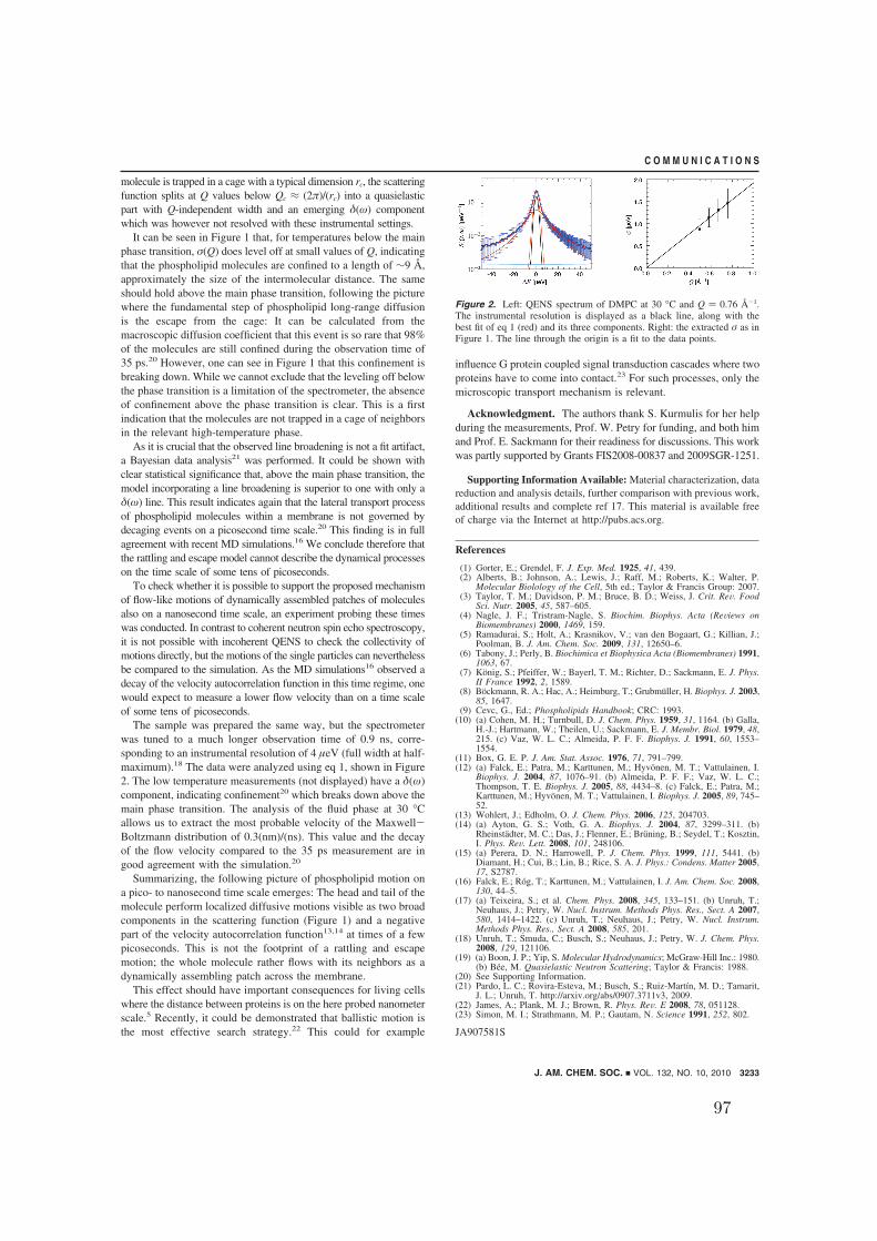
molecule is trapped in a cage with a typical dimension rc, the scatteringfunction splits at Q values below Qc ≈ (2π)/(rc) into a quasielasticpart with Q-independent width and an emerging δ(ω) componentwhich was however not resolved with these instrumental settings.
It can be seen in Figure 1 that, for temperatures below the mainphase transition, σ(Q) does level off at small values of Q, indicatingthat the phospholipid molecules are confined to a length of ∼9 Å,approximately the size of the intermolecular distance. The sameshould hold above the main phase transition, following the picturewhere the fundamental step of phospholipid long-range diffusionis the escape from the cage: It can be calculated from themacroscopic diffusion coefficient that this event is so rare that 98%of the molecules are still confined during the observation time of35 ps.20 However, one can see in Figure 1 that this confinement isbreaking down. While we cannot exclude that the leveling off belowthe phase transition is a limitation of the spectrometer, the absenceof confinement above the phase transition is clear. This is a firstindication that the molecules are not trapped in a cage of neighborsin the relevant high-temperature phase.
As it is crucial that the observed line broadening is not a fit artifact,a Bayesian data analysis21 was performed. It could be shown withclear statistical significance that, above the main phase transition, themodel incorporating a line broadening is superior to one with only aδ(ω) line. This result indicates again that the lateral transport processof phospholipid molecules within a membrane is not governed bydecaging events on a picosecond time scale.20 This finding is in fullagreement with recent MD simulations.16 We conclude therefore thatthe rattling and escape model cannot describe the dynamical processeson the time scale of some tens of picoseconds.
To check whether it is possible to support the proposed mechanismof flow-like motions of dynamically assembled patches of moleculesalso on a nanosecond time scale, an experiment probing these timeswas conducted. In contrast to coherent neutron spin echo spectroscopy,it is not possible with incoherent QENS to check the collectivity ofmotions directly, but the motions of the single particles can neverthelessbe compared to the simulation. As the MD simulations16 observed adecay of the velocity autocorrelation function in this time regime, onewould expect to measure a lower flow velocity than on a time scaleof some tens of picoseconds.
The sample was prepared the same way, but the spectrometerwas tuned to a much longer observation time of 0.9 ns, corre-sponding to an instrumental resolution of 4 µeV (full width at half-maximum).18 The data were analyzed using eq 1, shown in Figure2. The low temperature measurements (not displayed) have a δ(ω)component, indicating confinement20 which breaks down above themain phase transition. The analysis of the fluid phase at 30 °Callows us to extract the most probable velocity of the Maxwell-Boltzmann distribution of 0.3(nm)/(ns). This value and the decayof the flow velocity compared to the 35 ps measurement are ingood agreement with the simulation.20
Summarizing, the following picture of phospholipid motion ona pico- to nanosecond time scale emerges: The head and tail of themolecule perform localized diffusive motions visible as two broadcomponents in the scattering function (Figure 1) and a negativepart of the velocity autocorrelation function13,14 at times of a fewpicoseconds. This is not the footprint of a rattling and escapemotion; the whole molecule rather flows with its neighbors as adynamically assembling patch across the membrane.
This effect should have important consequences for living cellswhere the distance between proteins is on the here probed nanometerscale.5 Recently, it could be demonstrated that ballistic motion isthe most effective search strategy.22 This could for example
influence G protein coupled signal transduction cascades where twoproteins have to come into contact.23 For such processes, only themicroscopic transport mechanism is relevant.
Acknowledgment. The authors thank S. Kurmulis for her helpduring the measurements, Prof. W. Petry for funding, and both himand Prof. E. Sackmann for their readiness for discussions. This workwas partly supported by Grants FIS2008-00837 and 2009SGR-1251.
Supporting Information Available: Material characterization, datareduction and analysis details, further comparison with previous work,additional results and complete ref 17. This material is available freeof charge via the Internet at http://pubs.acs.org.
References
(1) Gorter, E.; Grendel, F. J. Exp. Med. 1925, 41, 439.(2) Alberts, B.; Johnson, A.; Lewis, J.; Raff, M.; Roberts, K.; Walter, P.
Molecular Biolology of the Cell, 5th ed.; Taylor & Francis Group: 2007.(3) Taylor, T. M.; Davidson, P. M.; Bruce, B. D.; Weiss, J. Crit. ReV. Food
Sci. Nutr. 2005, 45, 587–605.(4) Nagle, J. F.; Tristram-Nagle, S. Biochim. Biophys. Acta (ReViews on
Biomembranes) 2000, 1469, 159.(5) Ramadurai, S.; Holt, A.; Krasnikov, V.; van den Bogaart, G.; Killian, J.;
Poolman, B. J. Am. Chem. Soc. 2009, 131, 12650–6.(6) Tabony, J.; Perly, B. Biochimica et Biophysica Acta (Biomembranes) 1991,
1063, 67.(7) Konig, S.; Pfeiffer, W.; Bayerl, T. M.; Richter, D.; Sackmann, E. J. Phys.
II France 1992, 2, 1589.(8) Bockmann, R. A.; Hac, A.; Heimburg, T.; Grubmüller, H. Biophys. J. 2003,
85, 1647.(9) Cevc, G., Ed.; Phospholipids Handbook; CRC: 1993.
(10) (a) Cohen, M. H.; Turnbull, D. J. Chem. Phys. 1959, 31, 1164. (b) Galla,H.-J.; Hartmann, W.; Theilen, U.; Sackmann, E. J. Membr. Biol. 1979, 48,215. (c) Vaz, W. L. C.; Almeida, P. F. F. Biophys. J. 1991, 60, 1553–1554.
(11) Box, G. E. P. J. Am. Stat. Assoc. 1976, 71, 791–799.(12) (a) Falck, E.; Patra, M.; Karttunen, M.; Hyvönen, M. T.; Vattulainen, I.
Biophys. J. 2004, 87, 1076–91. (b) Almeida, P. F. F.; Vaz, W. L. C.;Thompson, T. E. Biophys. J. 2005, 88, 4434–8. (c) Falck, E.; Patra, M.;Karttunen, M.; Hyvonen, M. T.; Vattulainen, I. Biophys. J. 2005, 89, 745–52.
(13) Wohlert, J.; Edholm, O. J. Chem. Phys. 2006, 125, 204703.(14) (a) Ayton, G. S.; Voth, G. A. Biophys. J. 2004, 87, 3299–311. (b)
Rheinstädter, M. C.; Das, J.; Flenner, E.; Brüning, B.; Seydel, T.; Kosztin,I. Phys. ReV. Lett. 2008, 101, 248106.
(15) (a) Perera, D. N.; Harrowell, P. J. Chem. Phys. 1999, 111, 5441. (b)Diamant, H.; Cui, B.; Lin, B.; Rice, S. A. J. Phys.: Condens. Matter 2005,17, S2787.
(16) Falck, E.; Rog, T.; Karttunen, M.; Vattulainen, I. J. Am. Chem. Soc. 2008,130, 44–5.
(17) (a) Teixeira, S.; et al. Chem. Phys. 2008, 345, 133–151. (b) Unruh, T.;Neuhaus, J.; Petry, W. Nucl. Instrum. Methods Phys. Res., Sect. A 2007,580, 1414–1422. (c) Unruh, T.; Neuhaus, J.; Petry, W. Nucl. Instrum.Methods Phys. Res., Sect. A 2008, 585, 201.
(18) Unruh, T.; Smuda, C.; Busch, S.; Neuhaus, J.; Petry, W. J. Chem. Phys.2008, 129, 121106.
(19) (a) Boon, J. P.; Yip, S. Molecular Hydrodynamics; McGraw-Hill Inc.: 1980.(b) Bee, M. Quasielastic Neutron Scattering; Taylor & Francis: 1988.
(20) See Supporting Information.(21) Pardo, L. C.; Rovira-Esteva, M.; Busch, S.; Ruiz-Martın, M. D.; Tamarit,
J. L.; Unruh, T. http://arxiv.org/abs/0907.3711v3, 2009.(22) James, A.; Plank, M. J.; Brown, R. Phys. ReV. E 2008, 78, 051128.(23) Simon, M. I.; Strathmann, M. P.; Gautam, N. Science 1991, 252, 802.
JA907581S
Figure 2. Left: QENS spectrum of DMPC at 30 °C and Q ) 0.76 Å-1.The instrumental resolution is displayed as a black line, along with thebest fit of eq 1 (red) and its three components. Right: the extracted σ as inFigure 1. The line through the origin is a fit to the data points.
J. AM. CHEM. SOC. 9 VOL. 132, NO. 10, 2010 3233
C O M M U N I C A T I O N S
97

Supporting information for: Molecular Mechanism of
Long-Range Diffusion in Phospholipid Membranes
Studied by Quasielastic Neutron Scattering
Sebastian Busch,†,‡ Christoph Smuda,¶ Luis Carlos Pardo,§ and Tobias Unruh∗,‡,†
Physik Department E13, Technische Universität München, Garching bei München, Germany,
Forschungsneutronenquelle Heinz Maier-Leibnitz (FRM II), Technische Universität München,
Garching bei München, Germany, Center for Radiopharmaceutical Science, Eidgenössische
Technische Hochschule Zürich, Zürich, Switzerland, and Grup de Caracterització de Materials,
Departament de Física i Enginyeria Nuclear, Universitat Politècnica de Catalunya, Barcelona,
Spain
E-mail: [email protected]
Experimental Details
Dimyristoylphosphatidylcholine (DMPC) was purchased from Lipoid GmbH, Ludwigshafen, Ger-
many, and used as received. The dry phospholipid powder was hydrated with D2O (99.90%,
Euriso-Top, Gif sur Yvette, France) via the vapour phase at 40°C for two days after which the
sample was homogeneous and transparent. As the dynamics of the phospholipid is known to
depend on the hydration,1 additional D2O was added to ensure full hydration during the whole
To whom correspondence should be addressed†Technische Universität München, Physik Department‡Technische Universität München, FRM II¶Eidgenössische Technische Hochschule Zürich§Universitat Politècnica de Catalunya
S1
Appendix B. Molecular Mechanism of Long-Range Diffusion in Phospholipid
Membranes Studied by Quasielastic Neutron Scattering
98

experiment. The final concentration was adjusted to 50 mass percent. The integrity of DMPC was
confirmed by Differential Scanning Calorimetry, cf. Figure 1.
10 20 30 400
20
40
60
80
T [°C]
c p(a
.u.)
CH3
N+ CH3CH3
OP
-OO
O
OO
O O
CH3 CH3
Head groupσinc = 1445 barn= 25%
Tailsσinc = 4334 barn= 75%
Figure 1: Left: Differential Scanning Calorimetry of a fully hydrated DMPC liquid crystal. Thepre- and main phase transition are visible at about 16 and 24 °C, respectively. Right: A DMPCmolecule2 and the corresponding incoherent neutron scattering cross sections3 of the head and tailgroup together with the respective fraction compared to the whole molecule.
Two measurement series were performed at the neutron time-of-flight spectrometer TOFTOF4
at the Forschungsneutronenquelle Heinz Maier-Leibnitz (FRM II), Munich, Germany, to realize
two different observation times, 35 ps and 0.9 ns.5 This was done by changing the instrumental
resolution. It is important to note that the instrumental resolution does not correspond to a lower
limit of the broadenings which can be determined.
Measuring the momentum and energy transfer between neutron and sample, one obtains the
scattering function S(Q,ω) which is the double Fourier transform of the autocorrelation func-
tion.6,7 Due to the very large incoherent scattering cross section of the protons, they dominate the
scattering signal by far. However, as they are sampling the molecule quite uniformly, the motion
of the whole molecule becomes visible.
The primary part of the spectrometer uses seven choppers to cut the continuous white beam
delivered from the cold source of the reactor into short monochromatic pulses of neutrons. They
S2
99

interact with the sample and may change momentum and energy. After the sample, the neutrons
fly 4 m in the secondary part of the spectrometer until they are detected in one of 600 3He-filled de-
tector tubes. As the scattering angle of each detector is well-known and the time-of-flight between
the sample and the detector is recorded, momentum and energy transfer can be calculated.
The amount of sample was in both cases approx. 1 ml, chosen such that multiple scattering has
only a minor effect.
For the 35 ps measurement, the sample was filled in an aluminum hollow cylinder container8
with a gap thickness of 0.2 mm. A temperature-controlled sample environment was used to sta-
bilize the sample temperature to ±0.1°C during the measurements. A mean neutron wavelength
of λ = 6 Å, a rotation speed of the choppers of 12000 rpm, and frame overlap ratio 4 were used,
leading to an instrumental resolution (FWHM) of about 60 µeV. The temperature was varied from
5 °C to 40 °C in steps of 5 °C. For each temperature, the sample was measured for 8 h and pure
D2O for 4 h. The empty can was measured at the lowest and highest temperature for 4 h each and
a Vanadium standard (hollow cylinder with 0.6 mm wall thickness) was measured at 20 °C for 3 h.
For the 0.9 ns measurement, the sample was filled in an aluminum flat slab, its surface normal
was oriented to a scattering angle of 2θ = 135°. The wavelength was λ = 14 Å, chopper speed
16000 rpm, and ratio 8, giving a instrumental resolution (FWHM) of about 4 µeV. The temperature
was set to 10 °C, 20 °C, and 30 °C, respectively. At each temperature, the sample was measured for
12 h and D2O for 10 h. The empty can was measured for 10 h at 30 °C and Vanadium powder was
measured in the same sample holder for 14 h at 30 °C. The data at scattering angles below ≈ 50°
were discarded due to self-shielding and coherent small angle scattering of the sample.
The data were treated using the program Frida19 and using the Vanadium measurement for
three purposes: time-of-flight at zero energy transfer, detector sensitivity normalization, and in-
strumental resolution.
During the conversion from time-of-flight to energy transfer, the energy-dependent detector
efficiency was corrected. At the employed wavelengths, Vanadium scatters the same intensity in
every solid angle. The intensity of its elastic line was integrated, corrected for the Debye-Waller
S3
Appendix B. Molecular Mechanism of Long-Range Diffusion in Phospholipid
Membranes Studied by Quasielastic Neutron Scattering
100

factor, and used for normalization of the detector sensitivities. The instrumental resolution could
be determined because the Vanadium atoms do not perform any non-periodic motion and therefore
do scatter the neutrons without a quasielastic smearing.
After subtraction of the empty can measurements from both, the sample and the D2O, an angle-
and energy-dependent self-absorption correction10 was performed before proportional subtraction
of the D2O from the sample signal. It has to be kept in mind that the water adsorbed to the
membrane will have other dynamical properties than bulk water which can therefore only serve as
an approximate reference. However, as can be seen exemplarily in Figure 2, the scattering signal
of D2O is at least one order of magnitude below the one of DMPC, therefore a slightly incorrect
subtraction should not alter the results significantly.
The data were converted from scattering angle 2θ to the absolute value of the scattering vector,
Q. The data of the 35 ps measurement were then grouped into bins of constant Q in the range from
0.3 Å−1 to 1.9 Å−1 in steps of 0.1 Å−1, the data of the 0.9 ns measurement into 4 equidistant bins
between 0.49 Å−1 and 0.8 Å−1. Some spectra are shown exemplarily in Figure 2. It can be seen
that the scattering of D2O does not give an important contribution to the narrow component due to
both, its lower scattering cross section and its much faster dynamics.
We would like to point out that the analysis of the broad component is not essential for the
interpretation of the nature of the long-range motion. This is valuable as disturbing effects of mul-
tiple scattering or incorrect background subtraction influence this part of the scattering function.
Their influence will turn up in the analysis of the internal motions.
The Bayesian analysis, performed with the program FABADA,11 convolved the theoretical
functions numerically with the instrumental resolution. The algorithm was run for 1000000 cycles
with an automatic adjustment of the step size every 100000 cycles. The convergence factor was set
to 0.66. The fitting ranges were ±1.0 meV for the 35 ps measurement and ±50µeV for the 0.9 ns
measurement.
S4
101

-0.05 0.00 0.05 0.10
100
101
102
103
∆E [meV]
S(Q,ω
)[m
eV−
1 ]
DMPC + D2ODMPCD2O
Figure 2: Spectra of the sample (DMPC + D2O, top), bulk D2O (bottom), and the pure DMPC(sample after proportional subtraction of the bulk D2O spectrum, middle) of the 0.9 ns (4 µeV)measurement after conversion to constant Q around Q = 0.58Å−1. It can be seen that the D2Osignal hardly contributes, especially in the region of interest around ∆E = 0.
Proposed Models
It was found that models including one (only long-range) or two (one long-range and one localized)
components could not fit the data of the 35 ps measurement. Therefore, four models comprising
two localized and one long-range component were compared: Three possibilities for the long-
range motion with a quasi model-free approach for the localized motions are discussed: a long-
range motion that is so slow that the corresponding line broadening cannot be observed, a diffusive
motion, and a flow motion. It will be shown that this comparison favours the last possibility. For
this case, a further model with explicit assumptions about the localized motions was fitted showing
that the freedom of the generalized approach is necessary to extract information from this complex
molecule.
If there is no long-range motion visible, the scattering function incorporating two localized
S5
Appendix B. Molecular Mechanism of Long-Range Diffusion in Phospholipid
Membranes Studied by Quasielastic Neutron Scattering
102

motions (fast and slow) reads
S(Q,ω) = a(Q) ·δ(ω)⊗[Aslow(Q) ·δ (ω)+
(1−Aslow(Q)
)·L(Γslow,ω
)]⊗
[Afast(Q) ·δ (ω)+
(1−Afast(Q)
)·L(Γfast,ω
)]. (1)
In this and the following equations, a(Q) denotes a prefactor which comprises also the Debye-
Waller factor, Aslow/fast(Q) are the elastic incoherent structure factors (EISF) of the respective lo-
calized motions that contain information about their geometry and amplitude. The rates of the
localized motions are given by the respective half widths at half maximum (HWHM) Γslow/fast of
the Lorentzians L:
L(Γ,ω) =1π· Γ
Γ2 +ω2 . (2)
If a diffusive long-range motion is visible, the scattering function changes to
S(Q,ω) = a(Q) ·L(Γ(Q),ω
)⊗
[Aslow(Q) ·δ (ω)+
(1−Aslow(Q)
)·L(Γslow,ω
)]⊗
[Afast(Q) ·δ (ω)+
(1−Afast(Q)
)·L(Γfast,ω
)](3a)
where the HWHM of the first component is given by the respective equations
Γ(Q) =
h ·DQ2 for continuous diffusion or
h · DQ2
1+DQ2τ for stop & go diffusion(3b)
The stop & go motion12 is taken in the limit where the particle is much longer trapped than dif-
fusing and does not perform oscillatory motions during this period. D denotes here the diffusion
coefficient and τ the time between two diffusive events.
S6
103

Finally, in the case of a flow motion, one obtains a Gaussian central component,
G(σ ,ω) =1
σ√
2πexp[− ω2
2σ2
], (4)
yielding a scattering function of
S(Q,ω) = a(Q) ·G(σ(Q),ω
)⊗
[Aslow(Q) ·δ (ω)+
(1−Aslow(Q)
)·L(Γslow,ω
)]⊗
[Afast(Q) ·δ (ω)+
(1−Afast(Q)
)·L(Γfast,ω
)](5a)
where the standard deviation σ of the Gaussian G is determined by
σ(Q) = h · v0Q (5b)
when the motions are assumed to be ballistic with a Maxwell-Boltzmann distribution of speeds
around the most probable value v0. This is also the model for the phase of “free flight” the
molecules exhibit before the interactions with their environment have built up. However, the two
scenarios can be distinguished as during “free flight” , v0 would be√
2kBT/m, whereas in the
case of a flow motion, this value has to be much lower. The analogy to a gas requires an isotropic
average which is done by using a powder sample where all orientations of the liquid crystal occur
statistically throughout the sample.
The standard deviation σ of a Gaussian is connected to its full width at half maximum by
FWHM = 2 ·√
2ln(2) ·σ ≈ 2.4 ·σ . (6)
As it turns out that the fast component is very broad, the data were for comparison also fitted
with a model of long-range flow, a Brownian oscillator as the slow localized motion, and low
energetic vibrational motions for the fast localized motions. Using a Debye model, it can be
S7
Appendix B. Molecular Mechanism of Long-Range Diffusion in Phospholipid
Membranes Studied by Quasielastic Neutron Scattering
104

calculated that this contribution is in first order expansion a background proportional to Q2 and
nearly independent of energy at the present temperatures,
S(Q,ω) = a(Q) ·G(σ(Q),ω
)⊗
exp[−Q2δ 2] ·
∞
∑n=0
Q2nδ 2n
n!·L(nΓslow,ω
)+
b ·Q2 · hω
exp[
hωkBT
]−1
. (7)
The scaling factor b was introduced to account for Q and ω independent factors such as the Debye
frequency. The advantage of this model is that it does not need an artificial division of the scatterers
into two classes and has less parameters than model (5). It has also some disadvantages: the inten-
sities of the elastic and quasielastic component are linked, it lacks generality, and the assumptions
(Debye model &c.) can only be approximately correct.
Identification of the Long-Range Motion
Visibility of the Broadening
First, we determine whether a long-range motion can be seen with QENS before we try to dis-
tinguish the type of motion – diffusion or flow. This broadening is not influenced by disturbing
effects such as solvent subtraction of multiple scattering.13
Macroscopic measurements of the long-range diffusional motion have shown that the diffusion
coefficient below the main phase transition is nearly three orders of magnitude below the one above
the main phase transition.14 It is therefore not possible any more to resolve this motion with QENS,
as can be seen in Figure 3 for the 0.9 ns measurement. There, it is obvious that the central line is
not broadened beyond the instrumental resolution at temperatures below the main phase transition.
S8
105

-10 -5 0 5 1010 -2
10 -1
100
∆E [µeV]
S(Q,ω
) nor
m[µ
eV−
1 ]
30 °C20 °C10 °CVan
Figure 3: Spectra of Vanadium and DMPC at three temperatures, all at Q = 0.58 Å−1 and normal-ized to S(Q,ω = 0). It can be seen that the measurement at 30 °C has a significant broadening inthe central region whereas the other two have the same HWHM as Vanadium, only shifted by abackground caused by localized motions.
Check of the Rattling & Jump Model
The rattling & jump model, the primary step of diffusion is thought to be the displacement of a
phospholipid molecule into a neighbouring void. Using the molecular area of DMPC15 and the
long-range diffusion coefficient of 8.4 · 10−12 m2
s ,14 every molecule should do such a jump only
every0.64nm2
4 ·8.4 ·10−12 m2
s
≈ 20ns . (8)
This means that during the 35 ps observation time, 98% of the molecules do not perform a long-
range motion in this model. This should result in a not broadened central line as in equation (1),
given that this line is caused by the long-range motion.
As in the case of the 35 ps measurement the instrumental resolution does not allow for a clear
separation of central line broadening and a shift induced by internal motions any more, the decision
cannot be made by a simple optical inspection as it was possible in Figure 3. Therefore, a Bayesian
data analysis was performed. This method has already previously been successfully used to analyze
QENS data of phospholipids.16
In this method, the sum of squared residuals is essentially understood as an energy. The best
S9
Appendix B. Molecular Mechanism of Long-Range Diffusion in Phospholipid
Membranes Studied by Quasielastic Neutron Scattering
106

fit to the data with the minimal χ2 corresponds therefore to the state with lowest energy. A ther-
modynamic system would however for any non-zero temperature explore also states with higher
energies. The Bayesian algorithm does so by generating parameter sets around the best fit with a
Monte Carlo method.
The probability that the fit populates a state with a given χ2 depends on the χ2 hypersurface
and the number of degrees of freedom (i. e. parameters). If a new parameter is introduced, the most
probable χ2 will decrease if and only if the data can support this additional parameter.
560 565 570 575 580 5850
0.01
0.02
0.03
χ2
PD
F(χ2 )
broadeneddelta
Figure 4: Comparison of the models broadened central line vs. non-broadened central line using aBayesian data analysis of the data at 25 °C and 1.4 Å−1. It can be seen that the data do favour themodel with a broadened central line.
It can be clearly seen in Figure 4 that at a temperature above the main phase transition, the data
favour the broadened model (5) over the “rattling & jump” model (1).
Diffusion or Flow
A point not discussed in the main paper is whether this broadening is due to a diffusive or flow
motion. In the previous neutron scattering experiments, always a diffusive motion was assumed.17
As lined out above, the diffusive motion results in a Lorentzian line shape with Γ ∝ Q2 whereas
the flow motion results in a Gaussian line shape with σ ∝ Q. As the fits of a Lorentzian / Gaussian
to the data are of the same quality, one can not exclude either possibility.
S10
107

In the case of the 35 ps measurement, the model of simple diffusion does not fit the half widths
at half maximum satisfactorily, cf. Figure 5 (giving a diffusion coefficient of 180 · 10−12 m2
s ). As
normally done with complex liquids, this fit can be improved by assuming a stop & go motion,
yielding a diffusion coefficient of 240 ·10−12 m2
s and a stopping time of 10 ps. As calculated above,
this cannot be the rattling phase of the rattling & jump model. The diffusion coefficient resulting
from either model is about two orders of magnitude above the macroscopic diffusion coefficient.
The introduction of this additional parameter can be naturally avoided when assuming a flow
motion with the most likely velocity v0 ≈ 1.8 nmns at 30 °C and v0 ≈ 2.1 nm
ns at 40 °C. The good
agreement with the MD simulation can be seen in Figure 6.
0.0 0.5 1.0 1.5 2.0Q [Å−1]
0
10
20
30
40
σ,Γ
[µeV
]
v = 2.1 m/sD = 178 ·10−12 m2/sD = 235 ·10−12 m2/s, τ = 10 ps
0.0 0.2 0.4 0.6 0.8 1.0Q [Å−1]
0.0
0.5
1.0
1.5
2.0
σ,Γ
[µeV
]
v = 0.3 m/sD = 44 ·10−12 m2/s
Figure 5: Left: Evaluation of the 35 ps measurement at 40 °C with models (3) and (5). The resultingline widths (standard deviations and half widths at half maximum, respectively) are fitted with thecorresponding equations (3b) and (5b). Both diffusion models are plotted: continuous diffusion asdrawn-out line and stop & go diffusion as dashed line. Right: Same for the 0.9 ns measurement at30 °C (the only one measured above the main phase transition). Due to the limited amount of datapoints, stop & go diffusion was not fitted.
For the 0.9 ns measurement, both, diffusion and flow do fit the line width (standard deviation
and half width at half maximum, respectively). However, the diffusion coefficient is 40 ·10−12 m2
s ,
still one order of magnitude above the macroscopic value. In contrast, the velocity of a ballistic
motion coincides very nicely with the value obtained by Falck et al. at a simulation time of 1 ns
– about 0.3 nmns . This suggests that the reason for the observed faster motion is indeed the flow
S11
Appendix B. Molecular Mechanism of Long-Range Diffusion in Phospholipid
Membranes Studied by Quasielastic Neutron Scattering
108

motion.
101 102 103
observation time [ps]
10−1
100
101
flow
velo
city
[m/s
]
Figure 6: Flow velocity as a function of observation time. Black: results from MD simulation ofDPPC roughly 20 K above the main phase transition, taken from Falck et al. 18 Blue: results fromthe present study of DMPC, also roughly 20 K above the main phase transition (at 30 °C). Theerror bars indicate the width of the Maxwell-Boltzmann distribution.
It should be noted that the flow velocity is nearly three orders of magnitude below the thermal
expectation value√
2kBT/m. Therefore, it can be excluded that this is the initial phase of “free
flight” every molecule performs before the interactions with the neighbouring molecules have com-
pletely built up. This is in agreement with time scales obtained from NMR experiments and MD
simulations.19,20
Identification of the Internal Motions
This study is not focussed on the internal motions which have been investigated elsewhere in
detail (cf. the references in the following). Their interpretation is decoupled from the long-range
motion and therefore not essential for the question examined here. However, as they are measured
naturally along with the long-range motion on a quasielastic neutron scattering spectrometer, we
add a short overview over different models and possible interpretations.
S12
109

Explicit Model
Fitting model (7) with a vibrational background and a Brownian oscillator to the 35 ps measure-
ment at 30 °C yields at large Q for the Brownian oscillator a δ 2 of 0.25 Å2. However, this value is
not independent of Q but increases at small Q to more than 1 Å. Also the intensity of the vibrational
background shows anomalies in this region, not following a Q2 behaviour any more but levelling
off at a plateau. These effects are probably due to the rigidity of the model and multiple scattering
effects.13,21
Also other explicit models incorporating for example CH3 group rotation had the same prob-
lems at low Q. Therefore, the generalized model was preferred which is flexible enough to be
largely unaffected by the disturbing effects. As will be shown, the extracted δ 2 is in agreement
with the value extraced here in the high Q limit.
Generalized Approach
In model (5), the localized motions were assumed to have an exponentially decaying intermediate
scattering function that levels off at a plateau value, the EISF. The rates of the decays were fitted
to 0.11 ps−1 for the slow motion and 1.4 ps−1 for the fast motion. The corresponding EISF, shown
in Figure 7, does not decay to zero at large Q which was accounted for by assuming that not all
protons participate in both motions.
The EISF is influenced by both, the spread of the motion and the fraction of participating
protons.22 The introduction a fraction of participating scatterers p results in a definition of the
EISF as a function of the EISF that would be observed if all scatterers participated,
Afraction = 1− p+ p ·Aall . (9)
As can be seen in Figure 7, the EISFs drop stronger as the temperature is increased, corre-
sponding to an increased mobility. The values of the fast and the slow motion are very similar
for the low temperatures, however the slow motion spreads significantly more than the fast motion
S13
Appendix B. Molecular Mechanism of Long-Range Diffusion in Phospholipid
Membranes Studied by Quasielastic Neutron Scattering
110

0.0 0.5 1.0 1.5 2.0Q [Å−1]
0.0
0.2
0.4
0.6
0.8
1.0
Asl
ow
0.0 0.5 1.0 1.5 2.0Q [Å−1]
0.0
0.2
0.4
0.6
0.8
1.0
Afa
stFigure 7: The elastic incoherent structure factor of the slow and fast localized motion, respectively.The drawn-out lines are fits of equations (10) and (11) to the data points. The points at 1.5 Å−1
are left out due to anomalies caused by coherent scattering. The size of the fast motion increasesnotably at the main phase transition, the one of the slow motion at both, the pre and main transition.
when the sample is heated. The main phase transition is effecting both motions, the pretransition
only the slow motion.
Arguing that the tails dominate the scattering signal, these motions can be attributed to two
modes from the tails. Following Doxastakis et al. ,23 these two modes could be fast torsional
vibrations around mean values and conformational jumps between these values as they observed
in MD simulations of dry phospholipid.24
Another tentative assignment of the two motions would be – justified only by approximate
correspondence of the fractions of participating scatterers with the scattering cross sections of head
and tail, respectively – a slow, large-scale motion of the tails and a fast, more restricted motion of
the head groups. The EISF of the slow component (tentatively assigned to the tails) was in this
frame analyzed with the model of particles diffusing inside spheres24,25 with increasing radii. This
assumes that the protons can move in a small restricted volume which gets bigger the further away
the proton is located from the backbone. It reads
Aslow(Q) = a ·(
p · 1N·
N
∑i=0
(3 · j1(Q ·Ri)
Q ·Ri
)2
+(1− p)
)(10a)
S14
111

with
Ri = Rmin +iN· (Rmax−Rmin) . (10b)
A prefactor a was introduced to account for multiple scattering effects as A(Q→ 0) 6= 1, cf. Fig-
ure 7.13 j1 is the spherical Bessel function of first order. N was set to 13, the number of hydro-
carbon units in the tails, but no change was observed when increasing N to e. g. 30. The minimal
radius of the spheres increases with temperature from 0.0 to 0.2 Å, the maximal from 2.0 to 3.6 Å.
Both phase transitions are visible as increase of the radii, as can already be seen in Figure 7.
For the thorough analysis of the data with the model “diffusion inside a sphere”, one would
need to employ a more explicit fit function than equation (5). However, as shown above, this does
not lead to consistent results due to the introduced inflexibility which is given here essentially by
the prefactor a. It is obvious that this effect is strongest at small values of Q which explains the
difficulties of the explicit model in this region.
The EISF of the fast motion, which was preliminary assigned to motions of the head group, was
analyzed with the model of a Brownian oscillator,7,26 describing particles that perform diffusive
motions in a harmonic potential by
Afast(Q) = a ·(
p · e−Q2·δ 2+(1− p)
). (11)
The resulting mean squared displacement δ 2 rises with temperature from 0.24 to 0.37 Å2. Note
that this agrees well with the large Q limit obtained from the explicit model equation (7) which is
a further indication that it is valid to use the generalized approach. The main phase transition is
visible as increase of the mean squared displacement.
It seems natural to assign the fast motion to the head group and the slow one to the tails.
The head groups are more densely packed and perform fast oscillating diffusive motions between
their neighbours. The tails have more space, are more affected by the phase transitions, and can be
described by the plausible model of diffusion in spheres with increasing radii. Also the fractions of
participating protons agree roughly with the scattering cross sections shown in Figure 1. It should
S15
Appendix B. Molecular Mechanism of Long-Range Diffusion in Phospholipid
Membranes Studied by Quasielastic Neutron Scattering
112

however be noted that these fractions change with temperature which shows that – as expected –
the localized motions of this complex molecule cannot be described by such a simple model.
References
(1) (a) König, S.; Bayerl, T. M.; Coddens, G.; Richter, D.; Sackmann, E. Biophysical Journal
1995, 68, 1871; (b) Klösgen, B.; Reichle, C.; Kohlsmann, S.; Kramer, K. D. Biophysical
Journal 1996, 71, 3251.
(2) Pearson, R. H.; Pascher, I. Nature 1979, 281, 499.
(3) Sears, V. F. Neutron News 1992, 3, 26.
(4) (a) Unruh, T.; Neuhaus, J.; Petry, W. Nucl. Instrum. Methods Phys. Res., Sect. A 2007, 580,
1414–1422; (b) Unruh, T.; Neuhaus, J.; Petry, W. Nucl. Instrum. Methods Phys. Res., Sect. A
2008, 585, 201.
(5) Unruh, T.; Smuda, C.; Busch, S.; Neuhaus, J.; Petry, W. The Journal of Chemical Physics
2008, 129, 121106.
(6) (a) Squires, G. L. Introduction to the Theory of Thermal Neutron Scattering; Dover Pub-
lications, 1996; (b) Bée, M. Quasielastic Neutron Scattering; Taylor & Francis, 1988; (c)
Boon, J. P.; Yip, S. Molecular Hydrodynamics; McGraw-Hill Inc.,US, 1980.
(7) Neutron Scattering in Biology: Techniques and Applications (Biological and Medical
Physics, Biomedical Engineering), 1st ed.; Fitter, J., Gutberlet, T., Katsaras, J., Eds.;
Springer, 2006.
(8) (a) Wuttke, J. Physica B Condensed Matter 1999, 266, 112; (b) Wuttke, J. Physica B Con-
densed Matter 2000, 292, 194.
(9) Wuttke, J. Fast Reliable Interactive Data Analysis. http://sourceforge.net/
projects/frida/.
S16
113

(10) Paalman, H. H.; Pings, C. J. Journal of Applied Physics 1962, 33, 2635.
(11) (a) Pardo, L. C.; Rovira-Esteva, M.; Busch, S. Fitting Algorithm for Bayesian Anal-
ysis of Data. http://gcm.upc.edu/members/luis-carlos/bayesiano; (b)
Pardo, L. C.; Rovira-Esteva, M.; Busch, S.; Ruiz-Martín, M. D.; Tamarit, J. L.; Un-
ruh, T. http://arxiv.org/abs/0907.3711v3 2009; (c) Sivia, D. S.; Skilling, J. Data Analysis:
A Bayesian Tutorial, 2nd ed.; Oxford University Press, USA, 2006.
(12) Singwi, K. S.; Sjölander, A. Physical Review 1960, 119, 863.
(13) Busch, S. et al. in preparation 2010.
(14) Phospholipids Handbook, 1st ed.; Cevc, G., Ed.; CRC, 1993.
(15) Cevc, G.; Marsh, D. Phospholipid Bilayers: Physical Principles and Models (Cell Biology :
a Series of Monographs, Vol 5); John Wiley & Sons, 1987.
(16) Sivia, D. S.; Carlile, C. J.; Howells, W. S.; König, S. Physica B Condensed Matter 1992, 182,
341.
(17) Tabony, J.; Perly, B. Biochimica et Biophysica Acta (BBA) - Biomembranes 1991, 1063, 67.
(18) Falck, E.; Róg, T.; Karttunen, M.; Vattulainen, I. J. Am. Chem. Soc. 2008, 130, 44–5.
(19) Ayton, G. S.; Voth, G. A. Biophys. J. 2004, 87, 3299–311.
(20) Wohlert, J.; Edholm, O. The Journal of Chem. Phys. 2006, 125, 204703.
(21) Perez, J.; Zanotti, J.-M.; Durand, D. Biophysical Journal 1999, 77, 454.
(22) Smuda, C.; Busch, S.; Schellenberg, R.; Unruh, T. Journal of Physical Chemistry B 2009,
113, 916–922.
(23) Doxastakis, M.; Sum, A. K.; de Pablo, J. J. The journal of physical chemistry. B 2005, 109,
24173–81.
S17
Appendix B. Molecular Mechanism of Long-Range Diffusion in Phospholipid
Membranes Studied by Quasielastic Neutron Scattering
114

(24) Doxastakis, M.; García Sakai, V.; Ohtake, S.; Maranas, J. K.; de Pablo, J. J. Biophys. J. 2007,
92, 147–61.
(25) König, S.; Pfeiffer, W.; Bayerl, T. M.; Richter, D.; Sackmann, E. Journal de Physique II
France 1992, 2, 1589.
(26) (a) Knapp, E. W.; Fischer, S. F.; Parak, F. The Journal of Physical Chemistry 1982, 86, 5042;
(b) Knapp, E. W.; Fischer, S. F.; Parak, F. The Journal of Chemical Physics 1983, 78, 4701;
(c) Parak, F.; Knapp, E. W.; Kucheida, D. Journal of Molecular Biology 1982, 161, 177.
(27) Teixeira, S.; Ankner, J.; Bellissent-Funel, M.-C.; Bewley, R.; Blakeley, M.; Coates, L.;
Dahint, R.; Dalgliesh, R.; Dencher, N.; Dhont, J.; Fischer, P.; Forsyth, V.; Fragneto, G.;
Frick, B.; Geue, T.; Gilles, R.; Gutberlet, T.; Haertlein, M.; Hauß, T.; Häußler, W.; Heller, W.;
Herwig, K.; Holderer, O.; Jurányi, F.; Kampmann, R.; Knott, R.; Kohlbrecher, J.; Kreuger, S.;
Langan, P.; Lechner, R. E.; Lynn, G.; Majkrzak, C.; May, R.; Meilleur, F.; Mo, Y.;
Mortensen, K.; Myles, D.; Natali, F.; Neylon, C.; Niimura, N.; Ollivier, J.; Ostermann, A.;
Peters, J.; Pieper, J.; Rühm, A.; Schwahn, D.; Shibata, K.; Soper, A.; Straessle, T.; Suzuki, U.;
Tanaka, I.; Tehei, M.; Timmins, P.; Torikai, N.; Unruh, T.; Urban, V.; Vavrin, R.; Weiss, K.;
Zaccai, G. Chemical Physics 2008, 345, 133–151.
S18
115


Appendix C.
Dynamical Transition ofProtein-Hydration Water
Wolfgang Doster, Sebastian Busch, Ana M. Gaspar, Marie-Sousai Appavou,Joachim Wuttke, and Hugo Scheer
Physical Review Letters, 104(9):098101, 2010http://dx.doi.org/10.1103/PhysRevLett.104.098101
In this publication, the author participated in the measurements and data evaluation.He performed the fits presented in figure 3 of the publication. He participated activelyin the preparation of the manuscript and wrote large parts of its third page, relying onprevious versions of Wolfgang Doster and Joachim Wuttke. He also took part in thedevelopment of the data evaluation software used in this publication.
The mean correlation times ⟨τ⟩ of protein hydration water had previously been found toexhibit a peculiar shape when shown in an Arrhenius plot [105]: a transition from a fragile,super-Arrhenius temperature dependence at high temperatures and small correlationtimes to a strong, Arrhenius behaviour at low temperatures and correspondingly longcorrelation times. As long correlation times correspond to small line widths in the neutronscattering spectra, this means that the levelling off of the data points at long correlationtimes corresponds to a levelling off at small line widths: a phenomenon that was alsoobserved in the phospholipid samples [B].
It could be shown here that this levelling off can be prevented by using an improvedfit routine. With a closer study of the mechanisms that cause this fit artifact, it becameclear that the levelling off observed for the phospholipid samples is also not related to aphysical effect but merely to the data evaluation procedure [D].
Wolfgang Doster, Sebastian Busch, Ana M. Gaspar, Marie-Sousai Appavou, Joachim Wuttke,and Hugo Scheer, Physical Review Letters, 104(9):098101, 2010.
“Copyright 2010 by the American Physical Society.”
117

Dynamical Transition of Protein-Hydration Water
W. Doster,* S. Busch, and A.M. Gaspar
Physik Department E 13 and ZWE FRM II, Technische Universitat Munchen, 85747 Garching, Germany
M.-S. Appavou and J. Wuttke
Forschungszentrum Julich, JCNS at FRM II, Lichtenbergstrasse 1, 85747 Garching, Germany
H. Scheer
Botanisches Institut II, Ludwig-Maximilians-Universitat Munchen, Menzinger Strasse 67, 80638 Munchen, Germany(Received 22 July 2009; published 2 March 2010)
Thin layers of water on biomolecular and other nanostructured surfaces can be supercooled to
temperatures not accessible with bulk water. Chen et al. [Proc. Natl. Acad. Sci. U.S.A. 103, 9012
(2006)] suggested that anomalies near 220 K observed by quasielastic neutron scattering can be explained
by a hidden critical point of bulk water. Based on more sensitive measurements of water on perdeuterated
phycocyanin, using the new neutron backscattering spectrometer SPHERES, and an improved data
analysis, we present results that show no sign of such a fragile-to-strong transition. The inflection of
the elastic intensity at 220 K has a dynamic origin that is compatible with a calorimetric glass transition at
170 K. The temperature dependence of the relaxation times is highly sensitive to data evaluation; it can be
brought into perfect agreement with the results of other techniques, without any anomaly.
DOI: 10.1103/PhysRevLett.104.098101 PACS numbers: 64.70.pm, 87.15.H
In contrast to bulk water, protein-hydration water can besupercooled down to a glass transition at Tg ’ 170 K. Near
Tg translational degrees of freedom arrest, which induces
discontinuities in the specific heat and the thermal expan-sion coefficient of the hydration water [1–4]. Because ofthe dynamic nature of the glass transition, freezing ofmicroscopic degrees of freedom can already be observedfar above Tg.
The protein dynamic transition is an abrupt onset ofatomic displacements on the microscopic length and timescale probed by quasielastic neutron scattering (QENS).First observed 20 years ago in hydrated myoglobin andlysozyme at T ’ 240 K [5], it is now known to be ageneric property of hydrated proteins, while it is absentin dehydrated systems. It is therefore related to the dynam-ics of the hydration shell.
In QENS, mean squared dispacements hx2i are de-duced from the elastic scattering intensity Sðq; 0Þ.Because of the finite spectrometer resolution (FWHM2!), one actually measures Sðq; j!j & !Þ. Full spec-tral measurements show that the anomalous decrease of thecentral peak is compensated by increasing inelastic wings[5,6]. These effects have been interpreted as precursors ofthe glass transition. Since QENS probes structural relaxa-tion at !1 ’ 100 ps, while the calorimetric Tg refers to
a time scale of 100 s, it is natural that T is located farabove Tg: the protein dynamic transition is the microscopic
manifestation of the glass transition in the hydration shell.The time-scale dependence of T also explains its variationwith viscosity [7–9].
Recently, these views have been challenged by the sug-gestion that there might be a time-scale independent tran-
sition. Support came mainly from QENS experiments onthe backscattering spectrometer HFBS at NIST. In hy-drated lysozyme, DNA and RNA, a kink was found notonly in Sðq; j!j & !Þ, but also in the relaxation timehi deduced from full spectra Sðq;!Þ [10–13]. This changeof hiðTÞ from high-T super-Arrhenius to low-T Arrheniusbehavior at TL ’ 220 K has been interpreted as a fragile-to-strong-transition (FST) from the high density (HDL) tothe less fluid low density phase (LDL) of supercooledwater [14]. In this view, a qualitative change in the dynam-ics occurs when the so-calledWidom line is crossed, whichextrapolates the phase boundary beyond the conjecturedcritical point [15,16].Similar behavior was found for confined water in various
nonbiological environments [[17,18] and referencestherein]; TL was mostly located between 215 and 228 K.There were, however, two remarkable exceptions: makinga substrate hydrophobic lowered TL by 35 K [19]; usinganother neutron spectrometer with wider dynamic rangelowered TL by about 10 to 20 K [20]. Critics objected thatrelaxation times measured by other spectroscopic tech-niques show no anomaly at TL [21–23].In this Letter we will argue that the changing tempera-
ture dependence of logðhiÞ is likely to be an artifact of thedata analysis, and that the kink in the elastic intensity alsoadmits a conventional, dynamic interpretation. We willrefer to the hydration shell of different proteins. If theanomalies observed around TL were due to an intrinsicproperty of water, then the choice of the protein should notmatter.To improve the empirical base, we measured the motion
of protein-hydration water with enhanced sensitivity, using
PRL 104, 098101 (2010) P HY S I CA L R EV I EW LE T T E R Sweek ending
5 MARCH 2010
0031-9007=10=104(9)=098101(4) 098101-1 2010 The American Physical Society
Appendix C. Dynamical Transition of Protein-Hydration Water
118

a new neutron spectrometer and a fully deuterated protein.We chose deuterated C-phycocyanin (D-CPC), a lightharvesting, blue copper protein. Deuteration drasticallyreduces scattering from the protein so that we becomemore sensitive to weak quasielastic scattering from thehydration water. CPC has been investigated by neutronscattering before [24–28]. The sample was purified froma preparation of Crespi [28,29] with nearly 99% deutera-tion. The absorbance ratio A620 nm=A280 nm ’ 7:3 is abovethe analytic-grade value of 5 [30]. The integrity of thesecondary structure was ascertained by CD spectroscopy.The protein was dialyzed against distilled water, freezedried, and rehydrated to h ¼ 0:3 g=g [27], the same degreeof hydatrion as in Ref. [10].
QENS was performed on 500 mg of hydrated D-CPCwith the new backscattering spectrometer SPHERES atFRM II [31]. It has a resolution (FWHM) of 0:62 eV(HFBS 0:85 eV), high flux, and an outstanding signal-to-noise ratio of 1000:1. Scattering wave numbers q range
from 0.2 to 1:8 A1. We chose about the same energyrange 10 eV as customary at HFBS. Spectra at tem-peratures T between 100 and 300 K were collected for 6 to12 h. An empty cell measurement was subtracted andspectra were normalized to a vanadium standard. Theanalysis was performed with the program FRIDA [32].
Figure 1 displays selected spectra in the relevant tem-perature range. The logarithmic intensity scale emphasizesboth the broad, asymmetric wing of the instrumental reso-lution function, unavoidable in a crystal spectrometer, andthe quasielastic scattering. At least two distinct compo-nents of the scattering function Sðq;!Þ can be observed:(i) An elastic component that has the shape of the instru-mental resolution function Rqð!Þ. It is mainly due to the
coherent structure factor of the protein (as evidenced by
strong small-angle scattering for q 1 A1 [27]), as wellas to a protein incoherent term mainly due to the ex-changed protons (25%). Also immobilized water nearcharged groups contributes to this component. (ii) A qua-sielastic component that appears above about 170 K. It ismainly due to motion of adsorbed H2O molecules.To start with a model-free data characterization, we
examined the T dependence of the integrated inelasticintensity for different ! intervals, preferentially on the!< 0 side where the resolution wing is weaker. Between180 and 230 K, the inelastic intensity begins to risestrongly. There is no sharp kink; the temperature ofmaximum inflection depends on the ! range and on q[Fig. 2(a)]. This is a first indication for a dynamic phe-nomenon rather than a hidden phase transition: the q and Tdependence is compatible with a smooth onset of transla-tional diffusion. The elastic intensity in compensationshows a steplike decrease at 220 K in parallel with dataobtained with lysozyme. This suggests a common transi-
-10 -5 0 5 10hω (µeV)
0.001
0.01
S (
q,ω
) (
µeV
-1)
1.0 ± 0.15 A-1
300 K274 K250 K240 K230 K217 K200 K100 K
0 0.5 1hω (µeV)
0.1
1
S (
q,ω
) / S
(q,
0)
FIG. 1. Neutron scattering spectra of H2O on D-CPC at q ¼1:0 0:15 A1. Note the truncated logarithmic scale. Solid linesare fits with (1), convoluted with the instrumental resolution(sample data at 100 K).—Inset: central peak, normalized to thevalue at ! ¼ 0.
100 150 200 250 300
T (K)
0
0.01
0.02
0.03
0.04
inel
astic
inte
nsity
(a)0.3 A-1
0.5 A-1
1.0 A-1
1.5 A-1
0
0.25
0.5
0.75
1
elas
tic in
tens
ity
(b)
1.0 A-1
Eq. (2)lysozyme (HFBS)myoglobin (IN13)
T∆ T∆
100 150 200 250 300
T (K)
-2.5
0
2.5
5
7.5
ther
mal
exp
ansi
on (
104 K
-1)
(c)
lysozyme (densitometry)lysozyme (spectroscopy)bulk water
Tg
FIG. 2. (a) Scattering intensity integrated over @!<3 eV.(b) Elastic scattering intensity Sðq; 0Þ and result of (2), comparedto literature data [5,10]. (c) Thermal expansion coefficient P ofwater in hydrated lysozyme powder (þ , spectroscopic measure-ment [3]), of hydration water in lysozyme solution ( , densi-tometry, [36]), of bulk water (line).
PRL 104, 098101 (2010) P HY S I CA L R EV I EW LE T T E R Sweek ending
5 MARCH 2010
098101-2
119
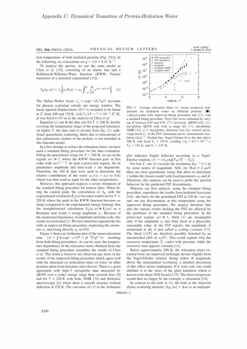
tion temperature of both hydrated proteins [Fig. 2(b)]. In
the following, we concentrate on q ¼ 1:0 0:15 A1.To analyze the spectra, we use the same model as
Chen et al. [10], consisting of an elastic line and aKohlrausch-Williams-Watts function (KWW, Fouriertransform of a stretched exponential [33]):
Sthðq;!Þ ¼ fq
a1ð!Þ þ a2
Z 1
1dt
2ei!tðjtj=Þ
: (1)
The Debye-Waller factor fq ¼ expðhx2iq2Þ accounts
for phonon scattering outside our energy window. Themean squared displacement hx2i is assumed to be linear
in T; from 100 and 170 K: @hx2i=@T ¼ 7 104 A2=K. was fixed to 0.5 as in the analysis of Chen et al.
Equation (1) can fit the data sets for T 240 K, herebycovering the temperature range of the proposed transition.At higher T, the data start to deviate from Eq. (1): addi-tional quasielastic scattering, likely due to relaxational orfast anharmonic motion of the protein, is not included inthis bimodal model.
In a first attempt to extract the relaxation times, we haveused a standard fitting procedure for the data evaluation.Fitting the quasielastic wings for T < 240 K, we are in theregime ! 1, where the KWW function goes in firstorder with ð!Þ1. In such a power-law regime, the fitparameters amplitude and time-scale are degenerate.Therefore, the 240 K data were used to determine therelative contribution of the water a2=ða1 þ a2Þ to 0.42which was then used as input for the other temperatures.
However, this approach neglects a severe limitation ofthe standard fitting procedure for narrow lines: When fit-ting the central peak, the convolution of Sth with theexperimental resolution Rqð!Þ becomes nontrivial for T &
220 K where the peak in the KWW function becomes sosharp (compared to the experimental energy binning) thatthe straightforward calculation Sthðq;!Þ Rqð!Þ as a
Riemann sum yields a wrong amplitude a1. Because ofthe mentioned degeneracy of amplitude and time scale, thisresults in a distorted hi. We have therefore repeated the fitswith an improved fitting procedure, neglecting the errone-ous a1 and fixing directly a2 at 0.42.
Figure 3 shows an Arrhenius plot of the mean relaxationtime hi ¼ R
dt expðt=Þ ¼ 1ð1Þ resultingfrom both fitting procedures. As can be seen, the tempera-ture dependence of the relaxation times obtained from thestandard fitting procedure resembles the results of Chenet al. This trend is however not observed any more in theresults of the improved fitting procedure which agree wellwith the structural (-)relaxation times of water on otherproteins taken from literature (also shown). There is a goodagreement with high-T myoglobin data measured byQENS over a wider energy range than covered here [8]and for T & 220 K with both, NMR [34] and dielectricspectroscopy [4] which show a smooth increase withoutinflection at 220 K. The curvature of hi in the Arrhenius
plot indicates fragile behavior according to a Vogel-Fulcher relation, hi ¼ hi0 exp½TH=ðT T0Þ.For low T, our hi exceeds the resolution !1 ’ 2 ns
by some orders of magnitude. Still, for j@!j * 2 eVthere are clear quasielastic wings that allow to determine within the chosen model with fixed parameters a2 and .Therefore, this analysis can be used to probe the spectralbehavior for the predicted FST discontinuity.Whereas our first analysis, using the standard fitting
procedure, reproduces the results from hydrated lysozyme[10]—the basis for the postulated FST at 220 K—we canrule out any discontinuity at this temperature using theimproved fitting procedure. We suspect therefore thatalso the various results backing the FST are affected bythe problems of the standard fitting procedure: In thepower-law regime ! 1, fitted hi are meaningfulonly if the amplitude a2 has been fixed at a physicallyreasonable value. In the FST reports, the amplitude, ifmentioned at all, is just called a scaling constant [17].The fitted hiðTÞ are therefore possibly distorted by anuncontrolled drift of a2ðTÞ. This could explain why thecrossover temperature TL varies with pressure, while thecrossover time appears constant [13].Below approximately 200 K, the relaxation times ex-
tracted from our improved technique deviate slightly fromthe Vogel-Fulcher relation. Being orders of magnitudeabove the instrumental resolution, a detailed discussionof this effect seems inadequate. If it were real, one couldattribute it to the onset of the glass transition which isknown to be about 30 K broad [4,35]. The observed processwould then no longer be the isotropic relaxation [34].In contrast to the kink in hi, the kink in the observed
elastic scattering intensity Sðq; j!j & !Þ is an undisput-
3 4 5 61000 K / T
10-11
10-10
10 -9
10 -8
10 -7
10 -6
10 -5
⟨τ⟩
(s)
CPC improved fitCPC standard fitlysozymemyoglobinmyoglobin (NMR)myoglobin (diel)
TL
(∆ω)-1
FIG. 3. Average relaxation times hi versus reciprocal tem-perature for hydration water on different proteins: (j):c-phycocyanin with improved fitting procedure and (h): witha standard fitting procedure. Error bars were estimated by vary-ing between 0.45 and 0.55. (5): lysozyme, QENS [10]. (4):myoglobin, QENS with wide ! range [8]. (): myoglobin,NMR [34]. (þ): myoglobin, dielectric loss [4], vertical arrow:conjectured TL of the FST, horizontal arrow: instrumental reso-lution ð!Þ1. Dashed line: Vogel-Fulcher fit to the data above200 K with fixed Tg ¼ 170 K, yielding hi0 ¼ 6:5 1013 s,
TH ¼ 745 K, and T0 ¼ 147 K.
PRL 104, 098101 (2010) P HY S I CA L R EV I EW LE T T E R Sweek ending
5 MARCH 2010
098101-3
Appendix C. Dynamical Transition of Protein-Hydration Water
120

able experimental fact. Figure 2(b) shows that observationsat SPHERES (D-CPC) and HFBS (lysozyme [10]) almostcoincide below 240 K. The difference at higher T can beexplained by our use of deuterated CPC, which reduces therelative contribution of the protein.
The expected elastic scattering is
Sexpðq; 0Þ ¼Z
d!Sthðq;!ÞRqð!Þ
¼ fq
a1Rqð0Þ þ ð1 a1Þ
Z 1
0
dt
eðt=Þ ~RqðtÞ
(2)
with ~RqðtÞ ¼Rd! cosð!tÞRqð!Þ. Indeed, the low-T data
are perfectly reproduced by Eq. (2) using the values fromthe Vogel-Fulcher relation for hi. This confirms the longestablished explanation of the protein dynamic transitionas a time-scale dependent glass transition: When 1 ex-ceeds the instrumental resolution !, then the central partof the KWW spectrum starts to broaden so that Sðq; j!j &!Þ falls below fq.
This is further corroborated by elastic scattering (q ¼1:4 A1) from hydrated myoglobin on the thermal neutronbackscattering spectrometer IN13 [5]. Its resolution width2@! ¼ 8 eV is an order of magnitude larger than thatof HFBS or SPHERES, and the kink in Sðq; j!j & !Þ isobserved accordingly at a higher temperature, namely, theoften reported T ’ 240 K.
Previous QENS experiments were motivated by the hopethat hydration layers would provide an opportunity to studywater in a deeply supercooled state that is not accessible inthe bulk. However, thin hydration layers seem to be quali-tatively different from bulk water [21]. This view is alsosupported by literature data of the thermal expansion co-efficient P of lysozyme hydration water [Fig. 2(c)]. Inconcentrated solution, P is nearly T independent andmuch larger than the bulk value [36]. In hydrated powder,P is estimated from the O-H stretching frequency ofwater, which varies with the average H bond length. Astriking step is found near 170 K, induced by the softeningof the O-H–O hydrogen bond network [3]. No anomaly isobserved at TL ’ 220 K.
All observations agree, however, with a glass transitionof the hydration shell and a dynamic onset temperature T,which varies with the probe frequency [Fig. 2(b)]. Thedifferent values of P for bulk and hydration water couldindicate that the protein acts as a patch-breaker [37],suppressing critical fluctuations present in bulk water.
This work has been supported by Deutsche Forschungs-gemeinschaft through SFB 533. We thank the late HenryCrespi for providing D-CPC.
*[email protected][1] W. Doster, BBA Proteins and Proteomics 1804, 3 (2010).
[2] Y. Miyazaki, T. Matsuo, and H. Suga, J. Phys. Chem. B104, 8044 (2000).
[3] F. Demmel, W. Doster, W. Petry, and A. Schulte, Eur.Biophys. J. 26, 327 (1997).
[4] H. Jansson and J. Swenson, BBA Proteins and Proteomics1804, 20 (2010).
[5] W. Doster, S. Cusack, and W. Petry, Nature (London) 337,754 (1989).
[6] W. Doster, S. Cusack, and W. Petry, Phys. Rev. Lett. 65,1080 (1990).
[7] H. Lichtenegger et al., Biophys. J. 76, 414 (1999).[8] W. Doster and M. Settles, BBA Proteins and Proteomics
1749, 173 (2005).[9] W. Doster, Eur. Biophys. J. 37, 591 (2008).[10] S.-H. Chen et al., Proc. Natl. Acad. Sci. U.S.A. 103, 9012
(2006).[11] S.-H. Chen, L. Liu, and Y. Zhang, J. Chem. Phys. 125,
171103 (2006).[12] X.-Q. Chu et al., Phys. Rev. E 77, 011908 (2008).[13] X.-Q. Chu et al., J. Phys. Chem. B 113, 5001 (2009).[14] P. Poole, F. Sciortino, U. Essmann, and H. E. Stanley,
Nature (London) 360, 324 (1992).[15] K. Ito, C. T. Moynihan, and C.A. Angell, Nature (London)
398, 492 (1999).[16] L. Xu et al., Proc. Natl. Acad. Sci. U.S.A. 102, 16558
(2005).[17] E. Mamontov et al., Chem. Phys. 352, 117 (2008).[18] E. Mamontov et al., Phys. Rev. E 79, 051504 (2009).[19] X.-Q. Chu et al., Phys. Rev. E 76, 021505 (2007).[20] E. Mamontov et al., J. Phys. Chem. C 112, 12334 (2008).[21] J. Swenson, H. Jansson, and R. Bergman, Phys. Rev. Lett.
96, 247802 (2006).[22] S. Pawlus, S. Khodadadi, and A. P. Sokolov, Phys. Rev.
Lett. 100, 108103 (2008).[23] M. Vogel, Phys. Rev. Lett. 101, 225701 (2008).[24] H. D. Middendorf and S. J. Randall, Phil. Trans. R. Soc. B
290, 639 (1980).[25] M. C. Bellissent-Funel, J. Teixera, K. F. Bradley, and S.-H.
Chen, J. Phys. I (France) 2, 995 (1992).[26] I. Koper, S. Combet, W. Petry, and M.C. Bellissent-Funel,
Eur. Biophys. J. 37, 739 (2008).[27] A. Gaspar et al., BBA Proteins and Proteomics 1804, 76
(2010).[28] K. Bradley, S.-H. Chen, M.C. Bellissent-Funel, and H. L.
Crespi, Biophys. Chem. 53, 37 (1994).[29] H. L. Crespi, in Stable Isotopes in The Life Sciences
(IAEA, Vienna, 1977), p. 111.[30] G. Patil, S. Chethana, A. S. Sridevi, and K. S.M. S.
Raghavarao, J. Chromatogr. A 1127, 76 (2006).[31] J. Wuttke et al. (to be published), see http://www.jcns.info/
jcns_spheres.[32] J. Wuttke, FRIDA: fast reliable inelastic data analysis
(http://www.messen-und-deuten.de/frida).[33] J. Wuttke, libkww (http://www.messen-und-deuten.de/
kww); arXiv:0911.4796v1.[34] S. A. Lusceac, M.R. Vogel, and C. R. Herbers, BBA
Proteins and Proteomics 1804, 41 (2010).[35] S. Khodadadi, A. Malkovskiy, A. Kisliuk, and A. P.
Sokolov, BBA Proteins and Proteomics 1804, 15 (2010).[36] M. Hiebl and R. Maksymiw, Biopolymers 31, 161 (1991).[37] H. E. Stanley and J. Teixera, J. Chem. Phys. 73, 3404
(1980).
PRL 104, 098101 (2010) P HY S I CA L R EV I EW LE T T E R Sweek ending
5 MARCH 2010
098101-4
121


Appendix D.
The Slow Short-Time Motions ofPhospholipid Molecules With a Focuson the Influence of Multiple Scatteringand Fitting Artefacts
Sebastian Busch and Tobias UnruhJournal of Physics: Condensed Matter, 23(25):254205, 2011http://dx.doi.org/10.1088/0953-8984/23/25/254205
In this publication, the author conceived the experiments and prepared the samples.The measurements were performed either by himself, together with students in the frameof teaching activities, or by Humphrey Morhenn. He performed the data evaluation andexplained the mechanism behind the fit artefacts that he had got to know in the courseof another publication [C]. He interpreted the results and wrote the publication.
The line width σ of the narrow component of a fit to quasielastic neutron scatteringdata, assigned to the long-range component, had previously been found to level off atsmall widths [B]. In this publication, it was shown that this effect is due to the same fitartifacts discussed elsewhere [C]. Although in this case a normal Levenberg-Marquardtalgorithm is used for fitting, the artifact influences the results of a Monte Carlo fit [G, H]the same.
After taking measures to avoid the fit artifacts, is can be seen that the line widthsdo not level off at small values, on the observation time of about 60 ps, a confinementof the molecules is therefore not visible – neither above nor below the main phasetransition of the phospholipid. This was interpreted as the consequence of relatively largelateral displacements caused by sloppy modes which are proposed to be connected to thedynamical heterogeneities that are visible above the main phase transition [E].
Copyright 2011 by the Institute of Physics (IOP).
123

The slow short-time motions of phospholipid molecules with a focus on the influence of
multiple scattering and fitting artefacts
This article has been downloaded from IOPscience. Please scroll down to see the full text article.
2011 J. Phys.: Condens. Matter 23 254205
(http://iopscience.iop.org/0953-8984/23/25/254205)
Download details:
IP Address: 129.187.254.46
The article was downloaded on 09/06/2011 at 12:22
Please note that terms and conditions apply.
View the table of contents for this issue, or go to the journal homepage for more
Home Search Collections Journals About Contact us My IOPscience
Appendix D. The Slow Short-Time Motions of Phospholipid Molecules With a Focus on
the Influence of Multiple Scattering and Fitting Artefacts
124

IOP PUBLISHING JOURNAL OF PHYSICS: CONDENSED MATTER
J. Phys.: Condens. Matter 23 (2011) 254205 (11pp) doi:10.1088/0953-8984/23/25/254205
The slow short-time motions ofphospholipid molecules with a focus on theinfluence of multiple scattering and fittingartefactsSebastian Busch1 and Tobias Unruh1,2
1 Physik Department E13 and Forschungs-Neutronenquelle Heinz Maier-Leibnitz (FRM II),Technische Universitat Munchen, Lichtenbergstraße 1, 85748 Garching bei Munchen,Germany2 Lehrstuhl fur Kristallographie und Strukturphysik, Friedrich-Alexander-UniversitatErlangen-Numberg, Staudtstraße 3, 91058 Erlangen, Germany
E-mail: [email protected] and [email protected]
Received 14 January 2011, in final form 28 February 2011Published 8 June 2011Online at stacks.iop.org/JPhysCM/23/254205
AbstractQuasi-elastic neutron scattering is a powerful tool for the study of non-periodic motions incondensed matter, as a detailed line shape analysis can give information about the geometry andrate of the scatterers’ displacements. Unfortunately, there are also a number of artefacts whichcan masquerade as signatures of motions and can therefore lead to erroneous results. Theirinfluence on the evaluation of the motions of the phospholipid dimyristoylphosphatidylcholine(DMPC) is discussed. On a 60 ps timescale, the long-range motion of the molecules has aflow-like character with similar velocities above and below the main phase transition. It isproposed that the concepts of dynamical heterogeneities and ‘floppy modes’ developed in glassphysics provide a framework for explaining the observed behaviour.
(Some figures in this article are in colour only in the electronic version)
1. Introduction
Recently, a quasi-elastic neutron scattering (QENS) exper-iment on the fully hydrated phospholipid dimyristoylphos-phatidylcholine (DMPC) was published [1]. It corroboratedcollective flow-like motions as a novel view of the long-rangemotion of phospholipid molecules that had been put forwardon the basis of molecular dynamics simulations [2]. A fit tothe data showed that the component which was assigned to thelong-range flow-like motion of the molecules levelled off attemperatures below the main phase transition (24 C) and lowvalues of Q as shown in figure 1. This was discussed as a signof a confinement of the molecules during the 60 ps observationtime in a cage of their neighbours—or an artefact [1, 3, 4].
The macroscopic diffusion of phospholipid molecules isknown to decrease by about one order of magnitude when themembrane is cooled below the main phase transition [5]. Incontrast, the high-Q part of the broadening caused by the long-range motion shown in figure 1 decreases much less. The
confinement length that was extracted from the position ofthe deviation of the linear behaviour at low Q to about 9 Acoincides quite well with the molecular repeating distance inthe membrane. This made a flow-like motion of the singlemolecules until they hit the cage of the neighbouring moleculesseem reasonable.
However, it was already speculated there that this mightbe an artefact, as the broadening is very small compared tothe instrumental resolution. A caging effect should also notonly cause a plateau of the quasi-elastic broadening but alsosimultaneously cause an emerging elastic δ(ω) componentwhich was not observed. On a physical level, it is not clear whythe flow-like, collective motions of the molecules, togetherwith their caging neighbours above the phase transition, shouldpersist at low temperatures for the single molecules within thecages.
The present contribution aims to clarify the picture of themotions of phospholipid molecules on a 60 ps timescale belowthe main phase transition. The two likely artefacts that could
0953-8984/11/254205+11$33.00 © 2011 IOP Publishing Ltd Printed in the UK & the USA1
125

J. Phys.: Condens. Matter 23 (2011) 254205 S Busch and T Unruh
Figure 1. Width of the narrow Gaussian line of a three-component fitto the spectra of the fully hydrated phospholipiddimyristoylphosphatidylcholine (DMPC), very similar to the resultspublished before in [1] where it was speculated that the levelling offof the widths at low temperatures and small Q could either be asignature of confinement of the molecules or an artefact. Thedistance between two data points in the spectra, δE = 10 μeV, isindicated in the figure. The energy resolution is about 60 μeV,corresponding to an observation time of about 60 ps. The solid linesare fits to the filled points in the medium-Q region.
simulate the observed plateau of the broadening at low Q arestudied: multiple scattering and fitting artefacts.
Only two years after the collection of the first neutrondiffraction patterns ever in 1946 [6], multiple scatteringwas identified as the source of a spurious backgroundcontribution [7]. A few years later, efforts to treatmultiple scattering (semi-)analytically began [8–11] and latercomplemented with Monte Carlo simulations [12–19].
However, still by far most quasi-elastic neutron scatteringexperiments study samples with very high transmission, inorder to be able to neglect rather than correct multiplescattering. The transmission needed to justify this neglect isnot agreed on in the literature—some authors feel safe withsamples with a transmission of 99% [20], most adjust theirsamples to achieve a transmission of about 90% [21, 22], whileothers still feel comfortable with samples with a transmissionas low as 70% [23].
It is also often unclear what to expect from uncorrectedmultiple scattering. An artificial broadening due to multiplescattering was, for example, assumed to yield a diffusioncoefficient that was higher [24] than the generally acceptedvalue [25, 26]. Others suggested that this broadening resultsin a Q dependence of the linewidth as shown in figure 1 whichis normally interpreted as confined diffusion [4]. Offsets of thelinewidth and the elastic incoherent structure factor (EISF) arealso often observed [1, 11, 27, 28], some of which were shownto be due to multiple scattering.
Whereas the neutron scattering community is well awareof the problem of multiple scattering, fitting artefacts arewidely ignored, which can lead to erroneous results: onecrucial step is the numerical convolution of the theoreticalfit function with the measured instrumental resolution [29].
The instrumental resolution gets more important as neutronspectroscopy is employed for the study of very slow motionsbecause the line broadening caused by the sample gets small.
It is even sometimes said that the instrumental resolutionshould be seen as a lower limit for the detectable broadening.However, while this is a valid rule of thumb for localizedmotions, many measurements of long-range motions whichcause a broadening of the whole line are done below this limit:from neutron scattering studies of diffusion in water [30] overproteins [28] to metallic liquids [31] or x-ray scattering studiesof glass formers [32].
In the following, a short repetition of the basicassumptions of neutron scattering data evaluation is presented,highlighting the points where multiple scattering and fitartefacts come into play. After giving a description of thesystems studied, the effects of multiple scattering and thepoint density used for the fit are described generally enoughto be useful also for other experiments. The consequencesfor the evaluation of long-range and localized motions arepresented and, with this knowledge, a coherent picture for thephospholipid dynamics is proposed.
2. Concepts of QENS data evaluation
The evaluation of QENS data relies vitally on the fact thatthe recorded number of neutrons as a function of solid angleand energy transfer, the double-differential cross section, canbe transformed into the scattering functions Sexp
coh,inc(Q, ω)
via [33–35](d2σ
dω d
)= Nσcoh
4π
k f
kiSexp
coh(Q, ω) + Nσinc
4π
k f
kiSexp
inc (Q, ω).
(1)In this relation, it is assumed that a monochromatic beamof neutrons was scattered at most once in the sample andthat the scattering lengths of the atoms do not correlate withtheir positions. It is often further simplified by neglecting thecoherent scattering contributions of hydrogen-rich samples andusing only the absolute value of the scattering vector, Q, forpowder samples.
In order to account for the non-perfect monochromaticityof the incident neutron beam and the finite energy resolutionof the spectrometer, the experimentally obtained scatteringfunction Sexp
inc (Q, ω) is understood as the convolution of theinstrumental resolution function R(Q, ω) with the theoreticalscattering function Stheo
inc (Q, ω):
Sexpinc (Q, ω) = Stheo
inc (Q, ω) ⊗ R(Q, ω). (2)
For the analysis of QENS data, this convolution is carried outonly in the energy direction. As the real resolution of thespectrometer does not strictly follow an analytical function, theintegral form of this convolution
Sexpinc (Q, ω) =
∫ ∞
−∞Stheo
inc (Q, ω′) · R(Q, ω − ω′) dω′ (3)
is mostly replaced by the discrete equivalent
Sexpinc (Q, ωn) =
N∑m=1
Stheoinc (Q, ωm) · R(Q, ωn − ωm) · δω (4)
2
Appendix D. The Slow Short-Time Motions of Phospholipid Molecules With a Focus on
the Influence of Multiple Scattering and Fitting Artefacts
126

J. Phys.: Condens. Matter 23 (2011) 254205 S Busch and T Unruh
Figure 2. Molecular structure of DMPC.
where N is the total number of points of a spectrum in theenergy direction and δω the width of a bin.
The relevant motions of the scatterers are then assumed tobe independent of each other so that the scattering function canbe approximated as composed of e.g. translational, rotational,and vibrational contributions [36]:
Stheoinc (Q, ω) = Strans
inc (Q, ω) ⊗ Srotinc(Q, ω) ⊗ Svib
inc (Q, ω). (5)
The amount of physics and approximations containedin these equations is so overwhelming that it seems safe topostulate that by far most neutron scatterers (including theauthors) settle for using these approximations after followingthe calculations a few times.
In this contribution, we discuss the influence of two ofthese steps: (a) the assumption that all detected neutrons werescattered only once in the sample and (b) the consideration ofthe limited instrumental resolution by the discrete convolutionof the theoretical scattering function with an experimentallyobtained instrumental resolution function.
3. Experimental details
3.1. Materials
A vanadium hollow cylinder standard with an outer radius11.75 mm and wall thickness 0.6 mm was measured at 20 C.The transmission was calculated by numerical integrationof the path length of the neutrons through the scatterer intransmission geometry and assuming an exponential decay ofthe neutron intensity in the medium [37] to 93%.
For all samples, hollow cylindrical aluminium samplecontainers [38, 39] with an inner radius of the outer aluminiumlayer of 11.25 mm and varying radii of the inner aluminiumlayer were used. The choice of the insert determined the gapsize and therefore the sample layer thickness.
The phospholipid dimyristoylphosphatidylcholine(DMPC; see figure 2) was obtained from Lipoid GmbH,Ludwigshafen (Germany), and used as received. It washydrated at 40 C via the gas phase with D2O 99.90% fromEuriso-Top, Gif-sur-Yvette (France), for at least 48 h until aclear phase formed. Subsequently, further D2O was addedup to 50 wt% to ensure full hydration during the wholeexperiment. With a gap size of 0.2 mm, a calculatedtransmission of 85% was obtained. The measurements wereperformed at 10, 20, 30, and 40 C. Also pure D2O wasmeasured at these temperatures.
Pure H2O, already used previously for multiple-scatteringstudies [40, 41], was taken from a Barnstead EASYpure II
ultrapure water system with a resistivity of ρ 18.2 M cmand filled into the sample containers with gap sizes of 0.1, 0.2,0.3, 0.5, 1.0, 2.0, and 3.0 mm. These samples have calculatedtransmissions of 85%, 72%, 62%, 46%, 23%, 6.4%, and 2.2%,respectively; the mean free path length of a neutron in H2O isabout 2 mm. The measurements were performed at 20 C.
3.2. Measurements and data treatment
All experiments were performed at the cold neutron time-of-flight spectrometer TOFTOF [42, 43] at the Forschungs-Neutronenquelle Heinz Maier-Leibnitz (FRM II), Garchingbei Munchen, Germany. The spectrometer is equipped withdetectors in an angular range from 7.5 to 140.
An incident neutron wavelength of 6 A was used, herebygiving for quasi-elastic scattering access to Q values from 0.3to 1.8 A
−1. The maximal momentum transfer of elastically
scattered neutrons at this wavelength is h · 2.1 A−1
forbackscattered neutrons. An instrumental resolution of about60 μeV (full width at half-maximum) was reached with achopper rotation speed of 12 000 rpm which required a frameoverlap ratio of 4. The corresponding observation time is about60 ps [44].
Today’s normal way of histogramming the data onlineduring the experiment adds a restriction to the rebinning of thedata. The online histogramming was done using 1024 timechannels, resulting in a width of about 7.5 μeV of the bins atzero energy transfer. These data points were then rebinned intobins with a constant step in energy of δE = 10 μeV duringdata reduction into slices of constant Q. Additionally, thephospholipid was also measured with an online histogramminginto 4096 time channels, resulting in a width of about 1.9 μeVat zero energy transfer and a constant step of δE = 2 μeV afterrebinning.
The data were normalized to the scattering of thevanadium standard to correct for different detector efficiencies.An empty can measurement was subtracted from allmeasurements and the D2O spectra were subtracted pro-rata from the ones of the phospholipid at the correspondingtemperatures. The obtained spectra were not normalized to theamount of sample in the beam or the total scattered intensity.
Diffraction patterns dσ/d(2θ) were obtained byintegrating the double-differential cross section over allenergies. Spectra were obtained by regrouping the data intoslices of constant Q [37]. In energy, the spectra were evaluatedin the region of E = hω from −1 to +1 meV where positivevalues for the energy transfer denote an energy gain of theneutron during the scattering process(es).
The fits of the theoretically calculated scattering functionsStheo
inc (Q, ω) to the measured ones Sexpinc (Q, ω) were numerically
convolved with the instrumental resolution R(Q, ω) asdetermined by the measurement of the vanadium hollowcylinder standard.
In order to enhance the visibility of the inelastic part of thespectrum, a representation as the imaginary part of the dynamicsusceptibility is also shown; the transformation was performedusing
χ ′′(Q, ω) = Sexpinc (Q, ω)/n(ω) (6)
3
127

J. Phys.: Condens. Matter 23 (2011) 254205 S Busch and T Unruh
where the scattering functions are divided by the Boseoccupation factor
n(ω) = 1/(exp[hω/(kBT )] − 1). (7)
Intermediate scattering functions I expinc (Q, t) were obtained
via the cosine Fourier transform of the energy spectra andsubsequent division of the sample data by the instrumentalresolution as determined by the vanadium measurement.Again, the data were not normalized to I exp
inc (Q, t = 0) = 1.Instead, an overall scaling factor a was included into the fittingfunction.
3.3. Fitting models
The data for the phospholipid were fitted with a convolutionof a Gaussian for the long-range flow-like motion with twolocalized diffusive contributions, each of the form
Stheoinc (Q, ω) = A0(Q) · δ(ω) + (1 − A0(Q)) · L(broad(Q), ω)
(8)where L denotes a Lorentzian
L((Q), ω) = (Q)/π
(Q)2 + ω2. (9)
The different localized contributions were assigned to themotions of the atoms in the head and tail groups [1]. TheGaussian then captures only the long-range motion of thewhole molecule. The Gaussian line shape with a linewidth of
σ(Q) = v · Q (10)
results from the assumption of flow motions with Maxwell–Boltzmann distributed flow velocities around the most likelyvelocity v [1].
The spectra of H2O were fitted with a common functionin quasi-elastic neutron scattering, the sum of two Lorentzianswhich is motivated [44] by the convolution of a long-rangediffusive motion
Stheoinc (Q, ω) = L(narrow(Q), ω), (11)
with a localized motion (8). With a scaling prefactor aaccounting for the scattering power of the sample, this yields
Stheoinc (Q, ω) = a · L(narrow(Q), ω) ⊗ [A0(Q) · δ(ω)
+ (1 − A0(Q)) · L(broad(Q), ω)]= a · A0(Q) · L((Q)narrow, ω)
+ a · (1 − A0(Q)) · L((Q)narrow + (Q)broad, ω). (12)
A specific model for the localized motion, giving an expressionfor A0(Q) as used in previous works [30], was avoided becauseof the distortion by multiple scattering [1, 17, 36].
For the evaluation of the intermediate scattering function,another fit function will be used which is also very common forthe evaluation of QENS data: a stretched exponential,
I theoinc (Q, t) = a exp[−(t/τ)β]. (13)
The alternative, a sum of two exponential decays, gives resultsvery similar to the ones obtained from the fit of the scatteringfunction with two Lorentzians, as one would expect [45, 46].The resulting relaxation time is shown as the mean relaxationtime 〈τ 〉 = τ(β−1)β−1 where is the Gamma function,reducing the dependence of τ on β [17, 29].
4. Results
4.1. Multiple scattering
This section is organized as follows. After looking qualitativelyat the data and their distortion caused by multiple scattering,the two most common methods for the quantitative evaluationof QENS data will be presented: fits of a sum of Lorentziansto the scattering function Sexp
inc (Q, ω) and the fit of a stretchedexponential to the intermediate scattering function I exp
inc (Q, t).
4.1.1. The angular dependence of the scattered intensity. Thealgorithm of Paalman and Pings [47] was used to calculatethe path lengths of the neutrons through the samples as afunction of the scattering angle. Using the average scatteringcross section, the probabilities for them to be scattered weredetermined from this length [37]. Only those neutrons whichwere scattered exactly once were considered to be detected. Tofacilitate comparability with the measured data, the resultingdifferential scattering cross sections were scaled with a factorthat was chosen such that the calculated integral scatteringcross section in the angular range covered is equal to themeasured one for the 0.1 mm sample; see figure 3(a).
The energy-integrated scattering cross section, thediffraction pattern that one would measure at a standarddiffraction instrument, is shown in figure 3(b). Severaldifferences from the calculated one are visible. (a) Thescattered amount of neutrons is much higher than expectedfrom the calculation because double-scattered neutrons are notactually lost. (b) Increasing the thickness of the water layergenerally also increases the scattered intensity. This increaseis, however, very small for the thick samples—the 3.0 mmsample scatters hardly more, at small scattering angles evenless than for the 2.0 mm sample. (c) The angular variationof the scattered intensity is lower than expected from thecalculation.
The elastically scattered intensity determined by integra-tion of an energy range of ±60 μeV is shown in figure 3(c).It can easily be seen that the amount of elastically scatteredneutrons does not scale linearly with the amount of sample—the thickest sample even scatters fewer neutrons elasticallythan the thinnest at low angles.
4.1.2. Intensity redistribution in (Q, ω)-space. Comparingthe scattering function Sexp
inc (Q, ω) of the thinnest and thethickest sample in figure 4(a), it becomes clear that the elasticsignal of the 3.0 mm measurement depends much less onQ than that of the 0.1 mm measurement, in agreement withfigure 3(c). At higher energy transfers, the 3.0 mm samplehas up to one order of magnitude more signal than the0.1 mm measurement. This artificial gain in intensity distortsthe dynamical susceptibility even more than the scatteringfunction.
To look closer at the redistribution of the scatteredintensity in the quasi-elastic region, the double-differentialscattering cross section of the 3.0 mm measurement and thatof the 0.1 mm measurement were independently normalizedto the same total scattering cross section in the dynamicalrange. The data for the 3.0 mm measurement were then
4
Appendix D. The Slow Short-Time Motions of Phospholipid Molecules With a Focus on
the Influence of Multiple Scattering and Fitting Artefacts
128

J. Phys.: Condens. Matter 23 (2011) 254205 S Busch and T Unruh
Figure 3. From left to right: (a) calculated angular dependence of the differential cross section of H2O, caused only by single-scatteredneutrons; (b) measured angular dependence of the differential cross section of H2O; (c) measured angular dependence of the elastic part of thescattering function of H2O.
Figure 4. From left to right: (a) the scattering function Sexpinc (Q, ω) as well as the imaginary part of the dynamical susceptibility χ ′′(Q, ω) for
two H2O samples (0.1 and 3.0 mm sample layer thickness) and values of Q from 0.4 to 10.0 A−1
in steps of 0.2 A−1
; due to the dynamicalrange of the spectrometer, the data at low Q do not reach high energy transfers and vice versa; (b) the ratio of the normalizeddouble-differential cross sections of the 3.0 mm measurement and the 0.1 mm measurement; (c) the same as for (b) but after conversion fromscattering angle 2θ to Q.
divided by the ones for the 0.1 mm measurement. The resultis shown as a function of energy transfer and scattering anglein figure 4(b) and also as a function of energy transfer and Qin figure 4(c). Values smaller than 100 designate areas wheremultiple scattering caused a loss of intensity, values bigger than100 those where additional, multiply scattered neutrons weredetected.
The pattern shows a slight asymmetry with respect tothe energy transfer. The lower intensity observed on theneutron energy loss side was attributed to the higher absorptionprobability for slower neutrons.
At low scattering angles, the signal of the 0.1 mmmeasurement decreases more rapidly as a function of energytransfer than the signal of the 3.0 mm measurement which ismore smeared out; cf figure 4(a). This leads to the high relativeintensity at low scattering angles and large energy transfers.With increasing scattering angle, the shapes of the scatteringfunctions become more similar to each other.
4.1.3. Evaluation of the scattering function with twoLorentzians. In the fit with two Lorentzians (12), theproperties of the narrow and the broad one, corresponding tolong-range and localized motions, respectively, are discussedin the following.
The arguably most important observation in the measure-ments presented is shown in figures 5(a) and (b): the linewidth
of the narrow Lorentzian is largely unaffected by multiplescattering. This means that a reliable determination of thediffusion coefficient is possible even when a massive amountof multiple scattering is present. This will be detailed in thediscussion.
The intensity distribution between the two Lorentzians,the EISF, follows quite well for the thin samples; the expectedGaussian-like decrease with Q; see figure 5(c). However, it isalready visible in the 0.1 mm measurement that the EISF doesnot extrapolate to 1 as Q approaches 0. This well-known signof multiple scattering [36] gets much stronger with increasingsample layer thickness.
The width of the broad Lorentzian is shown in figure 5(d).An overall trend to larger widths with increasing Q is visible,on top of which a thicker sample size increases the width ratherindependently of Q. As can be seen in figure 5(a), the data areat large energy transfers even flatter than the fit. This meansthat multiple scattering causes a very broad, background-likecontribution.
4.1.4. Evaluation of the intermediate scattering function witha stretched exponential. The intermediate scattering functioncan be fitted well with a stretched exponential as can be seenin figure 6(a).
The prefactor, displayed in figure 6(b), is basicallythe value I exp
inc (Q, t = 0), i.e. the zeroth Fourier
5
129

J. Phys.: Condens. Matter 23 (2011) 254205 S Busch and T Unruh
Figure 5. From left to right: (a) scattering function of H2O, shown at two Q values and two sample layer thicknesses; also shown is avanadium measurement as a measure of the instrumental resolution and fits of the sum of two Lorentzians to the data (solid lines), and for thetwo measurements at low Q, also the two components of the fit are shown (dashed lines); (b) the linewidth of the narrower of the twoLorentzians; (c) the elastic incoherent structure factor A0; (d) the linewidth of the broader of the two Lorentzians.
Figure 6. From left to right: (a) intermediate scattering function of H2O, shown at two Q values and two sample layer thicknesses; alsoshown is the fit of stretched exponentials to the data (solid lines); (b) the prefactor a; (c) the mean relaxation time multiplied by Q2; (d) thestretching exponent β.
Figure 7. From left to right: (a) width of the narrow Gaussian line of a three-component fit to the spectra of the fully hydrated phospholipiddimyristoylphosphatidylcholine (DMPC); the levelling off of the widths at low temperatures and small Q (cf figure 1) is practicallynonexistent, the distance between two data points, δE = 2 μeV, is indicated in the figure, the energy resolution is about 60 μeV, and the solidlines are fits to the filled points in the medium-Q region; (b) close-up view of the low-Q region of the width of the narrow Gaussian line of athree-component fit to the spectra of DMPC, measured with different point distances; it can be clearly seen that the effect of levelling off atsmall Q can be nearly completely removed by choosing a higher point density.
component, which is the area under the scattering function,∫ 1 meV−1 meV Sexp
inc (Q, ω) dω. The limits of the integration are givenby the region where the scattering function was evaluated—which in turn is limited by the dynamical range of theexperiment.
The mean relaxation time is influenced by multiplescattering, both in its average value and its Q dependence. Thestrongest effect can be observed in figure 6(c) at intermediateQ (around 0.7 A
−1) where the apparent speed-up is most
pronounced, in agreement with Monte Carlo simulations [17].The stretching factor is more influenced than the mean
relaxation time [14]. Stretching increases (β decreases)systematically, most at small values of Q; cf figure 6(d).
4.2. Fitting artefacts
The width of the narrow component of the fit to thephospholipid data with a binning of δE = 10 μeV is shownin figure 1. The analogous fit to the data with δE = 2 μeVyields the linewidths in figure 7(a). Also shown in both figuresare fits of straight lines to the medium-Q-range data points andthe width of the bins.
It can be seen that in the case of the coarse energy binningshown in figure 1, the data points deviate strongly from thelinear behaviour at low Q and level off to a value of aboutδE/2. With a finer energy binning, figure 7(a), they display amuch more linear behaviour.
6
Appendix D. The Slow Short-Time Motions of Phospholipid Molecules With a Focus on
the Influence of Multiple Scattering and Fitting Artefacts
130

J. Phys.: Condens. Matter 23 (2011) 254205 S Busch and T Unruh
Figure 8. From left to right: (a) Lorentzian curves with different widths plotted double logarithmically; after a plateau, the curves become apower law for hω ; (b) the Riemann sum over a Lorentzian as a function of its width , shown for different values of their centres c; bothwidth and centre are given in units of the distance between two points at which the Lorentzians are evaluated, δE ; for δE/2, the Riemannsum deviates significantly from the correct value of 1, and the direction of the deviation depends on the relative position of the centre of theLorentzian with respect to the points.
This is shown in detail in figure 7(b) where the fit resultsfor the two energy binnings are compared. The effect isstriking: the levelling off which was discussed as being eitherconfinement or a fit artefact [1] is clearly the latter.
5. Discussion
5.1. Evaluation of the long-range motion
Both the geometry and the rate of the long-range motion aresurprisingly little affected by multiple scattering. The rate ofthe diffusion is connected to the overall value of narrow/Q2
or 〈τ 〉 · Q2, the geometry to the dependence on Q of thesequantities.
The evaluation of the scattering function S(Q, ω) with thesum of two Lorentzians where the narrower one accounts forthe long-range motion yields very robust parameters for thenarrow component. As can be seen in figure 5(b), only forsmall Q does an increasing scattering power of the samplecorrelate with an increase of the linewidth.
Of the large deviation of the measured linewidth from theexpected values for low Q shown in figure 1, up to 125%,only a very small part can be attributed to multiple scattering:extrapolating the 72% and 85% transmission measurements toone with 100% transmission, we expect a deviation at small Qof about 3%. This extrapolation is known to be not suitablefor the precise evaluation of multiple scattering [40, 41] but itshows that the effects caused by multiple scattering are morethan one order of magnitude lower than the observed deviationsin figure 1.
In great contrast, the fitting artefacts distort the observedgeometry of the long-range motion heavily. It will be shownin the following that a systematically too large line broadening(or too small correlation time) is obtained.
A Lorentzian line is practically indistinguishable from apower law for any hω , namely (/ω)2, as shown infigure 8. This means that for any energy transfer bigger than ,the fit can be shifted to bigger values of y either by increasingthe always present prefactor a or—completely equivalently—by increasing .
Increasing a or increasing makes a difference only atenergy transfers smaller than : increasing a increases the
values of y in this range whereas increasing decreases them.It is therefore this range which determines a and .
The discrete convolution of the theoretical fit functionStheo
inc (Q, ω) with the instrumental resolution R(Q, ω) is theorigin of this problem: whereas R is in the present case verywell-behaved, Stheo
inc becomes so sharply peaked as decreasesthat the evaluated values at the points near zero energy transferare not representative for the whole bin any more. Thisis because the curvature in the centre of the Lorentzian is−2/(π3) and diverges therefore for → 0.
The consequence is that the integral convolution in (3)cannot be substituted by the discrete convolution (4) anymore: whereas the integral under the Lorentzian is unityindependently of , the Riemann sum deviates very stronglywhen the linewidth is smaller than about half of the distancebetween two evaluated points, δE/2.
It will be shown in the following that the systematicallytoo large fit value for the linewidth does not depend on thedirection of this deviation in the critical cases discussed here( ≈ 1 μeV, δE = 10 μeV):
(a) If the sum is calculated as too big (the centre of theLorentzian is close to a measured point), the central pointsare mistakenly calculated as too high. Only the centralpoint which is evaluated at the centre of the Lorentzian isin the plateau region of the Lorentzian.
(a.1) The fit can increase and thereby lower thecentral points through both the natural decrease(figure 8(a)) and the better calculation (figure 8(b)).Simultaneously, the function values in the wings ofthe Lorentzian will increase (figure 8(a)) which willbe compensated by a smaller value for the prefactora, making only a small counter-contribution to lowerthe central points.
(a.2) The fit could alternatively decrease the prefactor toget the central points down. This leads to a fitcurve that is systematically below the data points atlarge energy transfers—it will be shifted upwards byincreasing .
(b) If the sum is calculated as too small (the centre of theLorentzian is close to the middle in between two measured
7
131
J. Phys.: Condens. Matter 23 (2011) 254205 S Busch and T Unruh
points), the central points are mistakenly calculated as toolow. The points which are evaluated close to the centre ofthe Lorentzian are already in the power law wing regionof the Lorentzian.
(b.1) The fit can increase and hereby increase thecentral points through both the natural increase(figure 8(a)) and the better calculation (figure 8(b)).Simultaneously, the function values in the wings ofthe Lorentzian will increase (figure 8(a)) which willbe compensated by a smaller value for the prefactor awhich cannot compensate the increase caused by thebetter calculation though.
(b.2) The fit could alternatively increase the prefactor to getthe central points up. This leads to a fit curve that issystematically above the data points at large energytransfers—it would need to be shifted downwards bydecreasing . However, this would yield even lowercentral points (figure 8(b)) and is therefore not anoption for the fit.
In conclusion, the fit will always yield a linewidth thatis too broad if δE/2. In the example of the phospholipidmeasurements shown in figures 1 and 7, the deviation froma linear behaviour at small Q is decreased from 125% (infigure 1) to about 30% (in figure 7) by choosing a smallerenergy step between measured points.
This 30% deviation might very well be due to thebackground in the resolution measurement, caused by theinstrument and phonons in the vanadium. Comparing thefits using a convolution with the instrumental resolutionas determined by a vanadium measurement at temperaturesbetween 4 and 300 K as well as Gaussians with flatbackground, the fitted values differed by this order ofmagnitude without showing clear trends. This will be studiedin more detail and presented in a forthcoming publication.
5.2. Evaluation of the localized motions
The evaluation of the localized motions in the two-componentfit of the scattering function is influenced in both rate andgeometry. This is because the multiply scattered neutronsobtain relatively large energy transfers, yielding a nearly flatbackground in the energy direction. With an increasing amountof multiple scattering, this background increases. The broadLorentzian which accounts for localized motions thereforebroadens and gets more intensity.
The geometry is increasingly hard to evaluate fromthe EISF as it does not approach 1 for small momentumtransfers any more. It seems to be the most sensitiveindicator for multiple scattering. Including an arbitrary scalingfactor in the definition of the EISF as done previously [1]makes an approximate evaluation possible at reasonabletransmissions [17].
In the following, we will try to explain the effectsof multiple scattering with simple phase space arguments,assuming for the calculation of Q that the neutron does notchange its energy in a scattering process and neglecting thegeometry of the sample [48]. Knowing that the spectrumof multiply scattered neutrons is essentially a convolution
of the double-differential cross section with itself for everyscattering process [12], and that double scattering is the mostprobable multiple-scattering event [49], the Q values of thetwo scattering events are the interesting quantities. The widthof the observed scattering function will then be approximatelythe sum of those of the two single-scattering processes.
Using Monte Carlo simulations [17], it was determinedthat the probability distribution of the scattering anglesof the single-scattering processes is—independent of thetotal scattering angle—nearly triangular with a maximumprobability of 90, corresponding to a Q already of 0.71Qmax
(elastic), in this case 1.5 A−1
. A similar assessment has alsobeen used elsewhere [50]. Half of the neutrons will be scatteredwith a larger Q and result in a very broad line contributed bythe multiply scattered neutrons.
The upper limit for the values of Q that can possiblyparticipate in a double-scattering event is given by thewavelength of the neutrons: Qmax
1,2 = 4π/λ. The lower limit forQ1,2 seen from a given Qtot can be deduced from figure 9(a)where the vectorial momentum transfer of the first scatteringprocess is denoted as Q1, that of the second as Q2, and the total(observed) as Qtot = Q1 + Q2. This means, for the absolutevalues, Q1 + Q2 Qtot. The distribution of possible Q valuesin the scattering process and therefore of relaxation times istherefore largest at small Qtot (cf figure 6(d)).
The shift with regard to the scattering angle and thecut-off of Q resulting from the choice of the wavelengthof the incoming neutrons brings about the change ofthis wavelength influencing multiple scattering not onlyfor coherently scattering samples [10, 15–17] but also forincoherently scattering samples [17, 49], although to a smallerextent.
To understand the resulting linewidth, one needs theconditional probability for the two scattering events givensome Qtot. We have calculated the mean Q2 after a given Q1 asfollows (cf figure 9(a)): the probability for a certain (Q1, Q2)combination is directly proportional to the number of allowed(Q1,Q2) combinations, weighted with the corresponding solidangles.
The probability of having an event with a certain Q1,2 isinversely proportional to the surface of a sphere with radiusQ1,2, 1/(4π Q2
1,2). Multiplying these two probabilities givesthe one for reaching a certain Qtot via a given point ofconnection of Q1 and Q2. Each of the two scattering eventshas to be multiplied with the solid angle accessible with a givenscattering angle, sin(2θ1,2)/λ.
As all connection points which satisfy Q1,2 Qmax canbe used equivalently, this probability has to be multiplied withthe circumference l of the circle around Qtot,
l = π
Qtot· Re[−(Qtot − Q1 − Q2) · (Qtot − Q1
+ Q2)(Qtot + Q1 − Q2) · (Qtot + Q1 + Q2)]1/2, (14)
where Re denotes the real part of the argument.The result, symmetrical in Q1 and Q2, is displayed in
figure 9(b). It can be seen that even if one scattering processalready has Q1 = Qtot, the other scattering process still has anonzero Q2. Two limiting behaviours can be observed: on the
8
Appendix D. The Slow Short-Time Motions of Phospholipid Molecules With a Focus on
the Influence of Multiple Scattering and Fitting Artefacts
132
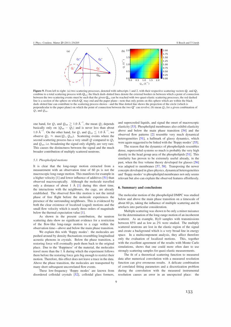
J. Phys.: Condens. Matter 23 (2011) 254205 S Busch and T Unruh
Figure 9. From left to right: (a) two scattering processes, denoted with subscripts 1 and 2, with their respective scattering vectors Q1 and Q2
combine to a total scattering process with Qtot; the black dash–dotted lines denote the external borders in between which a point of connectionbetween the two scattering events must be such that the given Qtot can be reached with two quasi-elastic scattering processes, the red dashedline is a section of the sphere on which Q′
1 may end and the paper plane—note that only points on this sphere which are within the blackdash–dotted line can contribute to the scattering process shown—and the blue dotted line shows the projection of the circle (which isperpendicular to the paper plane) on which the point of connection between the two Q′′ can revolve; (b) mean Q2 for a given combination ofQ1 and Qtot.
one hand, for Q1 and Qtot 1.0 A−1
, the mean Q2 dependsbasically only on |Qtot − Q1| and is never less than about1.0 A
−1. On the other hand, for Q1 and Qtot 1.0 A
−1, we
observe Q2 ≈ max(Q1, Qtot). Scattering events where thesecond scattering process has a very small Q compared to Q1
and Qtot, i.e. broadening the signal only slightly, are very rare.This causes the distinctness between the signal and the muchbroader contribution of multiply scattered neutrons.
5.3. Phospholipid motions
It is clear that the long-range motion extracted from ameasurement with an observation time of 60 ps is not themacroscopic long-range motion. This manifests for example ina higher velocity [1] and lower influence of additives [51] thanobserved macroscopically. Although the molecule travelledonly a distance of about 1 A [1] during this short time,the interactions with the neighbours, the cage, are alreadyestablished. The observed flow-like motion is not the initialphase of free flight before the molecule experiences thepresence of the surrounding neighbours. This is evidenced byboth the clear existence of localized (caged) motions and thesmall flow velocity which is nearly three orders of magnitudebelow the thermal expectation value [1].
As shown in the present contribution, the neutronscattering data show no significant evidence for a restrictionof the flow-like long-range motion to a cage within theobservation time—above and below the main phase transition.
We explain this with ‘floppy modes’: the molecules arepushed around by density fluctuations resembling longitudinalacoustic phonons in crystals. Below the phase transition, arestoring force will eventually push them back to the originalplace. Due to the ‘floppiness’ of the material, the moleculestravel more than the 1 A during which the experiment followsthem before the restoring force gets big enough to restrict theirmotion. Therefore, this effect does not leave a trace in the data.Above the phase transition, the molecules are transported bymany short subsequent uncorrelated flow events.
These low-frequency ‘floppy modes’ are known fromdisordered colloidal crystals [52], colloidal glass formers,
and supercooled liquids, and signal the onset of macroscopicelasticity [53]. Phospholipid membranes also exhibit elasticityabove and below the main phase transition [54] and theobserved flow patterns [2] resemble very much dynamicalheterogeneities [51], a hallmark of glassy dynamics, whichwere again suggested to be linked with the ‘floppy modes’ [55].
The reason that the dynamics of phospholipids resemblesdense, supercooled systems so much is probably the very highdensity in the head group area of the phospholipids [51]. Thissimilarity has proven to be extremely useful already, in thepast, when the free volume theory developed for glasses [56]was adapted to membranes [57, 58]. Transposing the newerconcepts developed in glass physics, dynamical heterogeneitiesand ‘floppy modes’ to phospholipid membranes not only seemsrelevant but also can explain the observed features effortlessly.
6. Summary and conclusions
The molecular motion of the phospholipid DMPC was studiedbelow and above the main phase transition on a timescale ofabout 60 ps, taking the influence of multiple scattering and fitartefacts into particular consideration.
Multiple scattering was shown to be only a minor nuisancefor the determination of the long-range motion of an incoherentscatterer. As an example, H2O samples with transmissionsbetween 85% and as low as 2% were studied. The multiplyscattered neutrons are lost in the elastic region of the signaland create a background which is a very broad line in energyspace. In a multicomponent analysis, they affect thereforeonly the evaluation of localized motions. This, togetherwith the excellent agreement of the results with Monte Carlosimulations, shows that one could more often dare to usestrongly scattering samples for quasi-elastic measurements.
The fit of a theoretical scattering function to measureddata after numerical convolution with a measured resolutionfunction can give erroneous results. A delicate combinationof correlated fitting parameters and a discretization problemduring the convolution with the measured instrumentalresolution causes an error in an unexpected place: the
9
133

J. Phys.: Condens. Matter 23 (2011) 254205 S Busch and T Unruh
linewidth. Analysing the data with different bin widths shouldgive indications if this problem is present. The lower limit forthe bin width is often given by the online histogramming of theneutrons during the experiment—a complete event recordingof the detected neutrons, in principle possible, would removethis limitation.
Flow-like motions of the phospholipid molecules bear astriking resemblance to dynamical heterogeneities above themain phase transition and to ‘floppy modes’ below. Theconfinement of the molecules below the main phase transitionis not visible in the long-range component of the fit due to theshort observation time of the experiment. It seems that thedescription of motions in the phospholipid membrane couldprofit greatly from transferring the up-to-date concepts usedin glass physics.
Acknowledgments
We would like to express our gratitude to Professor W Petrywho has extensively supported our work. We enjoyed thelively discussions with him and his special interest in themultiple-scattering effects discussed here. We have verymuch profited from the earlier work of and many discussionswith J Wuttke who first pointed out the importance ofthe numerical convolution to us. We would like to thankA Stadler for discussions; G Brandl, F Lipfert, B Mihiretie,and A Tischendorf for their participation in the measurementsof H2O; and H Morhenn for performing the phospholipidmeasurements.
References
[1] Busch S, Smuda C, Pardo L C and Unruh T 2010 Molecularmechanism of long-range diffusion in phospholipidmembranes studied by quasielastic neutron scattering J. Am.Chem. Soc. 132 3232
[2] Falck E, Rog T, Karttunen M and Vattulainen I 2008 Lateraldiffusion in lipid membranes through collective flows J. Am.Chem. Soc. 130 44–5
[3] Swenson J and Howells W S 2002 Quasielastic neutronscattering of propylene glycol and its 7-mer confined in clayJ. Chem. Phys. 117 857
[4] Zorn R 2010 Neutron spectroscopy for confinement studiesEur. Phys. J. Spec. Top. 189 65
[5] Ghosh S, Adhikari A, Mojumdar S S and Bhattacharyya K 2010A fluorescence correlation spectroscopy study of thediffusion of an organic dye in the gel phase and fluid phaseof a single lipid vesicle J. Phys. Chem. B 114 5736–41
[6] Shull C 1995 Early development of neutron scattering Rev.Mod. Phys. 67 753
[7] Wollan E and Shull C 1948 The diffraction of neutrons bycrystalline powders Phys. Rev. 73 830
[8] Vineyard G 1954 Multiple scattering of neutrons Phys. Rev.96 93
[9] Skold K, Rowe J, Ostrowski G and Randolph P 1972Coherent- and incoherent-scattering laws of liquid argonPhys. Rev. A 6 1107
[10] Sears V F 1975 Slow-neutron multiple scattering Adv. Phys.24 1
[11] Zorn R, Frick B and Fetters L J 2002 Quasielastic neutronscattering study of the methyl group dynamics inpolyisoprene J. Chem. Phys. 116 845
[12] Copley J R D 1974 Monte Carlo calculation of multiplescattering effects in thermal neutron scattering experimentsComput. Phys. Commun. 7 289
[13] Wuttke J, Kiebel M, Bartsch E, Fujara F, Petry W andSillescu H 1993 Relaxation and phonons in viscous andglassy orthoterphenyl by neutron scattering Z. Phys. B91 357
[14] Wuttke J, Chang I, Randl O G, Fujara F and Petry W 1996Tagged-particle motion in viscous glycerol:diffusion-relaxation crossover Phys. Rev. E 54 5364
[15] Russina M and Mezei F 1999 New procedure for multiplescattering correction Neutrons and Numerical Methods; AIPConf. Proc. 479 47–54
[16] Mezei F and Russina M 1999 Intermediate range orderdynamics near the glass transition J. Phys. Condens. Matter11 A341
[17] Wuttke J 2000 Multiple-scattering effects on smoothneutron-scattering spectra Phys. Rev. E 62 6531
[18] Trouw F R, Borodin O, Cook J C, Copley J R D andSmith G D 2003 Quasielastic neutron-scattering study of thelocal dynamics of poly(ethylene glycol) dimethyl ether inaqueous solution J. Phys. Chem. B 107 10446
[19] Hugouvieux V, Farhi E, Johnson M R and Kob W 2004 Virtualneutron scattering experiments Physica B 350 151
[20] Pieper J, Buchsteiner A, Dencher N A, Lechner R E andHauss T 2009 Light-induced modulation of proteindynamics during the photocycle of bacteriorhodopsinPhotochem. Photobiol. 85 590–7
[21] Stadler A M, Embs J P, Digel I, Artmann G M, Unruh T,Buldt G and Zaccai G 2008 Cytoplasmic water andhydration layer dynamics in human red blood cells J. Am.Chem. Soc. 130 16852–3
[22] Trapp M, Gutberlet T, Juranyi F, Unruh T, Deme B,Tehei M and Peters J 2010 Hydration dependent studies ofhighly aligned multilayer lipid membranes by neutronscattering J. Chem. Phys. 133 164505
[23] Thompson H, Skipper N T, Wasse J C, Howells W S,Hamilton M and Fernandez-Alonso F 2006 Proton dynamicsin lithium–ammonia solutions and expanded metals J. Chem.Phys. 124 024501
[24] Aliotta F, Fontanella M E, Pieruccini M, Salvato G, Trusso S,Vasi C and Lechner R E 2002 Percolative phenomena inlecithin reverse micelles: the role of water Colloid Polym.Sci. 280 193
[25] Spehr T L 2010 Water dynamics in soft confinement PhDThesis Technische Universitat Darmstadt
[26] Spehr T L, Frick B, Zamponi M and Stuhn B 2011 Dynamicsof water confined to reverse AOT micelles Soft Matteraccepted doi:10.1039/C1SM05204G
[27] Gaspar A M, Appavou M-S, Busch S, Unruh T andDoster W 2008 Dynamics of well-folded and nativelydisordered proteins in solution: a time-of-flight neutronscattering study Eur. Biophys. J. Biophys. Lett. 37 573–82
[28] Stadler A M, Digel I, Artmann G M, Embs J P, Zaccai G andBuldt G 2008 Hemoglobin dynamics in red blood cells:correlation to body temperature Biophys. J. 95 5449–61
[29] Doster W, Busch S, Gaspar A M, Appavou M-S, Wuttke J andScheer H 2010 Dynamical transition of protein-hydrationwater Phys. Rev. Lett. 104 098101
[30] Teixeira J, Bellissent-Funel M-C, Chen S-H andDianoux A-J 1985 Experimental determination of the natureof diffusive motions of water molecules at low temperaturesPhys. Rev. A 31 1913
[31] Meyer A, Wuttke J, Petry W, Randl O G and Schober H R 1998Slow motion in a metallic liquid Phys. Rev. Lett. 80 4454
[32] Sette F, Krisch M H, Masciovecchio C, Ruocco G andMonaco G 1998 Dynamics of glasses and glass-formingliquids studied by inelastic x-ray scattering Science280 1550
[33] Van Hove L 1954 Correlations in space and time and Bornapproximation scattering in systems of interacting particlesPhys. Rev. 95 249
10
Appendix D. The Slow Short-Time Motions of Phospholipid Molecules With a Focus on
the Influence of Multiple Scattering and Fitting Artefacts
134

J. Phys.: Condens. Matter 23 (2011) 254205 S Busch and T Unruh
[34] Furrer A, Mesot J and Strassle T 2009 Neutron Scattering inCondensed Matter Physics (Series on Neutron Techniquesand Applications) 1st edn (Singapore: World Scientific)
[35] Squires G L 1996 Introduction to the Theory of ThermalNeutron Scattering (New York: Dover)
[36] Bee M 1988 Quasielastic Neutron Scattering (London: Taylorand Francis)
[37] Wuttke J 1990 Frida1: Fast Reliable Interactive Data AnalysisSoftware http://sourceforge.net/projects/frida/
[38] Wuttke J 1999 Improved sample holder for multidetectorneutron spectrometers Physica B 266 112
[39] Wuttke J 1999 Self-absorption coefficient for tubularsamples—erratum and addendum to Physica B 266 (1999)112 Physica B 266 194
[40] Slaggie E L 1967 Multiple scattering in slow-neutrondouble-differential measurements Nucl. Sci. Eng. 30199–212
[41] Slaggie E L 1969 Multiple scattering in double differentialmeasurements as a function of neutron path length Nucl. Sci.Eng. 36 105–7
[42] Unruh T, Neuhaus J and Petry W 2008 The high-resolutiontime-of-flight spectrometer TOFTOF Nucl. Instrum.Methods Phys. Res. A 585 1414–22
[43] Unruh T, Neuhaus J and Petry W 2008 The high-resolutiontime-of-flight spectrometer TOFTOF (vol 580, p 1414,2007) Nucl. Instrum. Methods Phys. Res. A 585 201
[44] Unruh T, Smuda C, Busch S, Neuhaus J and Petry W 2008Diffusive motions in liquid medium-chain n-alkanes as seenby quasielastic time-of-flight neutron spectroscopy J. Chem.Phys. 129 121106
[45] Smuda C, Busch S, Gemmecker G and Unruh T 2008Self-diffusion in molecular liquids: medium-chain n-alkanesand coenzyme Q10 studied by quasielastic neutron scatteringJ. Chem. Phys. 129 014513
[46] Smuda C 2009 Diffusive Bewegungen in molekularenFlussigkeiten PhD Thesis Technische Universitat Munchen
[47] Paalman H H and Pings C J 1962 Numerical evaluation of x-rayabsorption factors for cylindrical samples and annularsample cells J. Appl. Phys. 33 2635
[48] Busch S 2007 Protein diffusion in concentrated solutionsMaster’s Thesis Technische Universitat Munchen
[49] Settles M 1996 Die Zeitabhangigkeit und die Geometrie derintramolekularen Dynamik globularer Proteine bis 100ps ausNeutronenstreudaten PhD Thesis Technische UniversitatMunchen
[50] Cusack S and Doster W 1990 Temperature dependence of thelow frequency dynamics of myoglobin. Measurement of thevibrational frequency distribution by inelastic neutronscattering Biophys. J. 58 243
[51] Busch S and Unruh T 2011 The influence of additives on thenanoscopic dynamics of the phospholipiddimyristoylphosphatidylcholine Biophysica Acta(BBA) - Biomembranes 1808 199–208
[52] Kaya D, Green N L, Maloney C E and Islam M F 2010 Normalmodes and density of states of disordered colloidal solidsScience 329 656–8
[53] Ghosh A, Mari R, Chikkadi V, Schall P, Kurchan J andBonn D 2010 Density of states of colloidal glasses andsupercooled liquids Soft Matter 6 3082
[54] Harland C W, Bradley M J and Parthasarathy R 2010Phospholipid bilayers are viscoelastic Proc. Natl. Acad. Sci.107 19146
[55] Donati C, Douglas J, Kob W, Plimpton S, Poole P andGlotzer S C 1998 Stringlike cooperative motion in asupercooled liquid Phys. Rev. Lett. 80 2338
[56] Cohen M H and Turnbull D 1959 Molecular transport in liquidsand glasses J. Chem. Phys. 31 1164
[57] Galla H-J, Hartmann W, Theilen U and Sackmann E 1979 Ontwo-dimensional passive random walk in lipid bilayers andfluid pathways in biomembranes J. Membr. Biol. 48 215
[58] Vaz W L C and Almeida P F F 1991 Microscopic versusmacroscopic diffusion in one-component fluid phase lipidbilayer-membranes Biophys. J. 60 1553–4
11
135


Appendix E.
The Influence of Additives on theNanoscopic Dynamics of thePhospholipidDimyristoylphosphatidylcholine
Sebastian Busch and Tobias UnruhBiochimica et Biophysica Acta (BBA) – Biomembranes, 1808(1):199, 2011
http://dx.doi.org/10.1016/j.bbamem.2010.10.012
In this publication, the author conceived all experiments (the MD simulation wasperformed by Tobias Unruh). The experiments were performed either by himself ortogether with students in the frame of teaching activities. He performed the dataevaluation, interpreted the results, and wrote the publication.
In contrast to the previous study of the pure phospholipid [B], where a very intricatemodel was used together with involved fitting procedures [G, H], the mixtures investigatedhere were evaluated with a model-free approach. This excludes any distortion by fitartifacts [C, D]. It also makes it possible to compare these results directly with theones obtained from very small amounts of sample where reliable model fitting is notpossible [F].
Reprinted from Biochimica et Biophysica Acta (BBA) - Biomembranes, 1808, Sebastian Busch,Tobias Unruh, The influence of additives on the nanoscopic dynamics of the phospholipiddimyristoylphosphatidylcholine, 199-208, Copyright (2011), with permission from Elsevier.
137
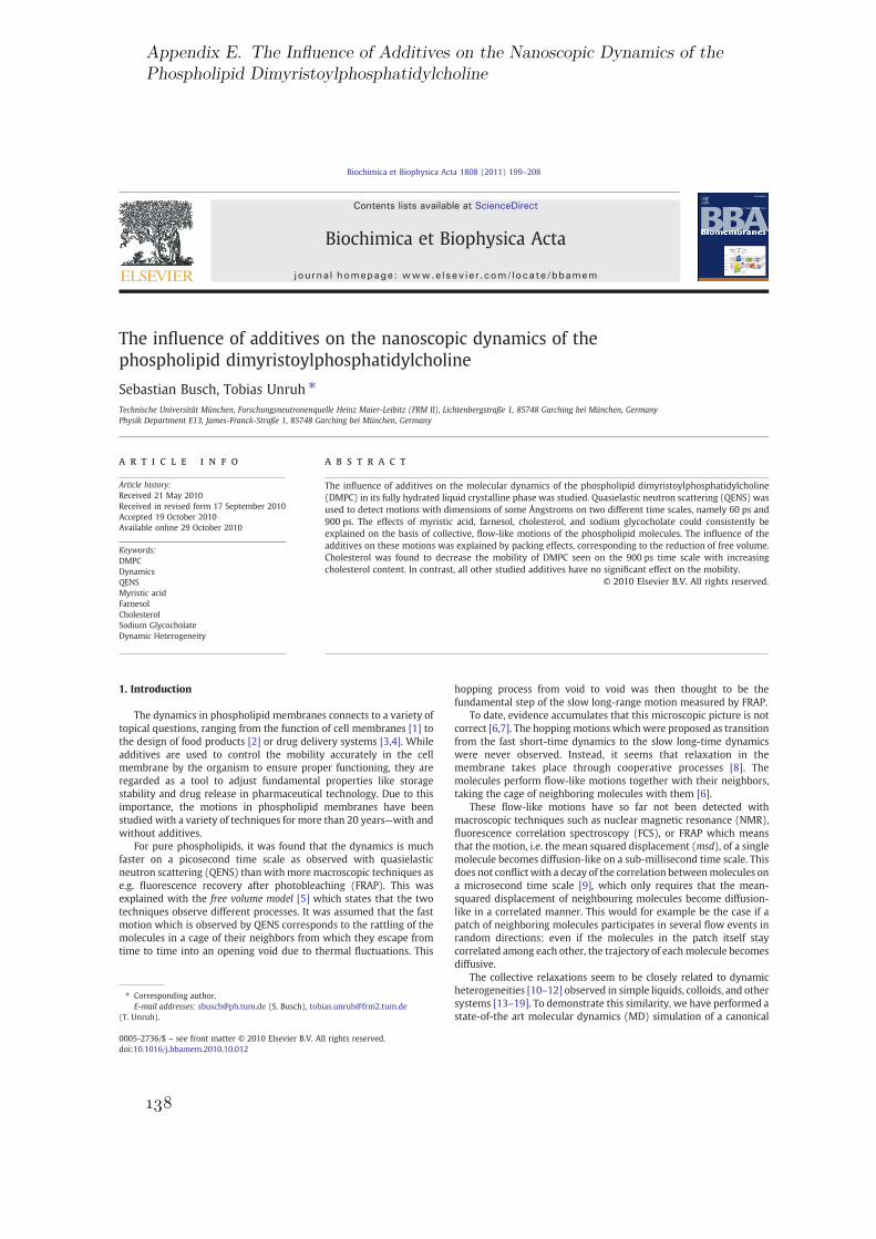
The influence of additives on the nanoscopic dynamics of thephospholipid dimyristoylphosphatidylcholine
Sebastian Busch, Tobias Unruh ⁎Technische Universität München, Forschungsneutronenquelle Heinz Maier-Leibitz (FRM II), Lichtenbergstraße 1, 85748 Garching bei München, GermanyPhysik Department E13, James-Franck-Straße 1, 85748 Garching bei München, Germany
a b s t r a c ta r t i c l e i n f o
Article history:Received 21 May 2010Received in revised form 17 September 2010Accepted 19 October 2010Available online 29 October 2010
Keywords:DMPCDynamicsQENSMyristic acidFarnesolCholesterolSodium GlycocholateDynamic Heterogeneity
The influence of additives on the molecular dynamics of the phospholipid dimyristoylphosphatidylcholine(DMPC) in its fully hydrated liquid crystalline phase was studied. Quasielastic neutron scattering (QENS) wasused to detect motions with dimensions of some Ångstroms on two different time scales, namely 60 ps and900 ps. The effects of myristic acid, farnesol, cholesterol, and sodium glycocholate could consistently beexplained on the basis of collective, flow-like motions of the phospholipid molecules. The influence of theadditives on these motions was explained by packing effects, corresponding to the reduction of free volume.Cholesterol was found to decrease the mobility of DMPC seen on the 900 ps time scale with increasingcholesterol content. In contrast, all other studied additives have no significant effect on the mobility.
© 2010 Elsevier B.V. All rights reserved.
1. Introduction
The dynamics in phospholipid membranes connects to a variety oftopical questions, ranging from the function of cell membranes [1] tothe design of food products [2] or drug delivery systems [3,4]. Whileadditives are used to control the mobility accurately in the cellmembrane by the organism to ensure proper functioning, they areregarded as a tool to adjust fundamental properties like storagestability and drug release in pharmaceutical technology. Due to thisimportance, the motions in phospholipid membranes have beenstudied with a variety of techniques for more than 20 years—with andwithout additives.
For pure phospholipids, it was found that the dynamics is muchfaster on a picosecond time scale as observed with quasielasticneutron scattering (QENS) than withmore macroscopic techniques ase.g. fluorescence recovery after photobleaching (FRAP). This wasexplained with the free volume model [5] which states that the twotechniques observe different processes. It was assumed that the fastmotion which is observed by QENS corresponds to the rattling of themolecules in a cage of their neighbors from which they escape fromtime to time into an opening void due to thermal fluctuations. This
hopping process from void to void was then thought to be thefundamental step of the slow long-range motion measured by FRAP.
To date, evidence accumulates that this microscopic picture is notcorrect [6,7]. The hopping motions which were proposed as transitionfrom the fast short-time dynamics to the slow long-time dynamicswere never observed. Instead, it seems that relaxation in themembrane takes place through cooperative processes [8]. Themolecules perform flow-like motions together with their neighbors,taking the cage of neighboring molecules with them [6].
These flow-like motions have so far not been detected withmacroscopic techniques such as nuclear magnetic resonance (NMR),fluorescence correlation spectroscopy (FCS), or FRAP which meansthat the motion, i.e. the mean squared displacement (msd), of a singlemolecule becomes diffusion-like on a sub-millisecond time scale. Thisdoes not conflict with a decay of the correlation betweenmolecules ona microsecond time scale [9], which only requires that the mean-squared displacement of neighbouring molecules become diffusion-like in a correlated manner. This would for example be the case if apatch of neighboring molecules participates in several flow events inrandom directions: even if the molecules in the patch itself staycorrelated among each other, the trajectory of eachmolecule becomesdiffusive.
The collective relaxations seem to be closely related to dynamicheterogeneities [10–12] observed in simple liquids, colloids, and othersystems [13–19]. To demonstrate this similarity, we have performed astate-of-the art molecular dynamics (MD) simulation of a canonical
Biochimica et Biophysica Acta 1808 (2011) 199–208
⁎ Corresponding author.E-mail addresses: [email protected] (S. Busch), [email protected]
(T. Unruh).
0005-2736/$ – see front matter © 2010 Elsevier B.V. All rights reserved.doi:10.1016/j.bbamem.2010.10.012
Contents lists available at ScienceDirect
Biochimica et Biophysica Acta
j ourna l homepage: www.e lsev ie r.com/ locate /bbamem
Appendix E. The Influence of Additives on the Nanoscopic Dynamics of the
Phospholipid Dimyristoylphosphatidylcholine
138

(NVT) ensemble of a 2D-Lennard–Jones liquid, following previousstudies [20]. The 1024 particles were distributed inside a square 2D-box of 25.237 nm side length and equilibrated for 106 time steps,corresponding to 1 ns, followed by a 100 ps production run. TheLennard–Jones potential between two particles i and j located at adistance rij from each other is given by
VL−J rij
= 4ijσij
rij
!12
−σij
rij
!6" #ð1Þ
The parameter σij=0.7 nm was chosen inspired by phospholipidmolecules [21,22] and ij=5.0 kJ/mol close to the thermal kineticenergy of particles in a two dimensional system to be in the fluidphase. Periodic boundary conditions were applied and a Berendsentemperature coupling with time constant of 50 fs to a temperaturebath with 310.14 K was used.
By connecting the positions for each particle at time t=1.0 ns withits position 100 ps later by an arrow, the picture in Fig. 1 was obtained.It can be seen that neighboring particles move often collectively withsimilar speeds and directions and that different areas move verydifferently—some patches are nearly static while others move withrelatively high velocities. These are the so-called dynamic hetero-geneities. As mentioned above, this picture strongly resembles similarrepresentations of the simulated dynamics of DPPC molecules inbilayers [6]. The similarity of the displacement patterns observed in2D Lennard–Jones systems and phospholipid membranes has alsobeen observed recently in other simulations [23].
We suggest that this similarity indicates that the mobility of themolecules on the picosecond time scale is determined mainly by theclosely 2D-packed head groups of the phospholipid molecules whichwere compared to a densely packed 2D liquid already before [22]. Incomparison, the tail groups are more loosely packed at temperaturesabove the main phase transition [24]. From colloids, it is well knownthat more densely packed systems exhibit slower dynamics [25]. Weassume therefore that the dense phospholipid head groups are thelimiting factor for the mobility.
Independently from the validity of the microscopic mechanism,free volume is accepted to play an important role in dynamic
processes—at least these quantities are positively correlated [24,26–28]. However, we will interpret the results also in the frame ofcorrelated, flow-like motions.
In the present article, we discuss the influence of additives on themobility of phospholipid molecules (dimyristoylphosphatidylcholine,DMPC) in this frame. We propose that the chain-like moleculesmyristic acid (MA) and farnesol increase the area covered by themembrane but not the density—and do therefore not change themobility. Cholesterol increases the density in the chain area andhereby causes a decrease of themobility. In contrast, the co-emulsifiersodium glycocholate (NaGC, SGC) has basically no influence whichcan be explained by the larger hydrophilic head group.
2. Materials and methods
2.1. Samples
D2O (99.90%) was supplied by Euriso-Top, Gif sur Yvette, France.The phospholipid DMPC was purchased from Lipoid GmbH, Ludwig-shafen, Germany and used as received. All other substances (myristicacid, cholesterol, farnesol, and sodium glycocholate) were obtainedfrom Sigma Aldrich, Münster, Germany and also used without furtherpurification. The relevant molecular structures are displayed in Fig. 2.
The additives were mixed with the phospholipid in the ratiosgiven in Table 1 with mole fractions xadditive of up to 40 mol%. Themixtures were then exposed to a saturated D2O atmosphere at 40 °Cfor at least 48 h until a clear sample consisting of randomly-orientedliquid-crystalline domains formed. Finally, additional D2O was addedto ensure full hydration during the whole experiment. All sampleswere bulk samples to exclude potential disturbing effects of a support.
2.2. Basic properties of the samples
D2O was used instead of H2O because it has essentially the samechemical properties but a significantly smaller neutron scatteringcross section which facilitates the subtraction of its signal.
DMPC is a typical phospholipid with amphiphilic properties due toits hydrophilic head and hydrophobic tail groups. When adding water(or D2O), it self-assembles in bilayers and forms liquid crystallinephases. In both, H2O and D2O, it has a main phase transition at 24 °Cwhich is attributed to the melting of the chains. The macroscopicdiffusion coefficient below the main phase transition has been foundto be about one order of magnitude below the one above the mainphase transition [29]. Phospholipids like DMPC can be used tostabilize dispersed particles with respect to aggregation and coales-cence. In this case, DMPC acts as an interface active substance andstabilizes the particles by forming a molecular monolayer in theinterface between the particle and the dispersion medium.
Myristic acid is a water-insoluble chain-like molecule which is thefatty acid contained in DMPC. Previously, it was found that stearic acidgenerates a slight positive excess volume at low concentrations [30].Free fatty acids can cause cell death which was attributed to anincreased membrane permeability for hydrophilic substances [31].The phase diagram of the myristic acid–DMPC–water system as afunction of the myristic acid mole fraction xMA is known [32]. Duringthe preparation of the samples, it was observed that their viscosityincreased significantly with increasing amount of MA.
Farnesol is insoluble in water, too. Due to the double bonds it isstiffer than MA. It can cause apoptosis which, however, seems to becaused by interactions with proteins rather than with the membrane[33]. The phase diagram of the farnesol–DMPC–water mixture as afunction of the farnesol content was studied e.g. by NMR [34,35].
Cholesterol, also insoluble in water, is known to increase themembrane bending rigidity [36] and to suppress the phase transitionsof the phospholipid [37]. Cells use it to regulate the properties of thecell membrane [38]. It is known that it has a condensing effect on the
0
2
4
6
8
10
12
14
16
18
20
22
24
0 2 4 6 8 10 12 14 16 18 20 22 24
y [nm]
x [nm]
Fig. 1. Visualization of flow-like motions observed in an MD simulation of a simple 2D-Lennard–Jones liquid. The arrows connect the position of the particles with a timedifference of 100 ps.
200 S. Busch, T. Unruh / Biochimica et Biophysica Acta 1808 (2011) 199–208
139

membrane, as summarized by Róg et al. [39], which corresponds tothe filling-up of voids in the lipophilic core of the membrane [40]. Asimultaneous decrease of phospholipid mobility was observed byseveral groups [24,26,27,41–44] but also an increase of the dynamicshas been reported [45,46]. The motions of cholesterol in phospholipidmembranes were also previously studied with QENS [47], comple-mentary to the present study of the phospholipid motions. The phasediagram of the cholesterol–DMPC–water system is well studied, forexample by differential scanning calorimetry [48] and electronparamagnetic resonance (EPR) [43].
Sodium glycocholate is a water soluble ionic surfactant with acritical micelle concentration of about 8 mM [49,50]. It is used in thedigestive system to emulsify fatty substances and hereby enablingabsorption [38]. In pharmaceutical technology, it is used to stabilizedispersions which undergo a phase transition of the dispersed phasefrom liquid (production) to solid (storage). During crystallization, theinterface of the particles expands abruptly due to the change of theparticle shape from spherical to platelet-like. In dispersions stabilized
by phospholipids, it is assumed that the newly formed interfacecannot be stabilized fast enough to avoid aggregation. It was foundthat these instabilities can be prevented when using NaGC as co-stabilizer [51]. The stabilizing property of NaGC is attributed to itshigh mobility. One question addressed in this contribution is whetherthis kind of rapidness in covering freshly generated interfaces can beobserved by QENS. During preparation of the samples, it was observedthat samples containing NaGC were more fluid and had a less turbidappearance.
2.3. Neutron scattering
The focus of this work is the influence of additives on themotion ofphospholipid molecules on a pico- to nanosecond time scale asobserved with quasielastic neutron scattering. An advantage ofneutron scattering with respect to other methods like electronparamagnetic resonance spectroscopy or fluorescence correlationspectroscopy is that marker molecules are not needed [52,53].
The measurements were performed with the neutron time-of-flight spectrometer TOFTOF [54] at the research reactor FRM II(Garching, Germany), equipped with a temperature-controlledsample environment. Neutrons with well-known momentum andenergy interact with the sample. The resulting changes in momentumand energy give access to structural and dynamical information,respectively [55,56]. The uncertainty of the determination of theenergy transfer between sample and neutron determines theinteraction time of the neutron and the nuclei, the observation time.Several factors influence this uncertainty, among them the initialneutron wavelength and the sample geometry. Two measurementseries were performed, both giving access to Q≈1 Å-1, and to timescales of 60 ps and 900 ps, respectively [57].
To realize the 60 ps measurement, the samples were filled intohollow cylindrical aluminum sample containers, minimizing self-shielding effects [58], with a sample layer thickness of 0.2 mm. Anincident neutron wavelength of 6 Å, a chopper rotation speed of12000 rpm, and a chopper ratio of 4 were chosen, leading to an elasticline width of about 60 μeV and an accessible Q range of about 0.4–1.8 Å−1.
For the 900 ps measurement, a flat sample holder was used whichwas oriented such that its surface normal pointed to a scattering angleof 135° measured towards the location of the detectors, herebyminimizing flight-time uncertainties at the expense of a strong self-shielding around scattering angles of 45°. The corresponding
OH
H
OHH
NH
O
O
O-
Na+
HO
H
H
OH
H
H3C
H3C
H3C
H3C
H3C
H3C
H3C
H
H
H
CH3
CH3
CH3 CH3 CH3
OH
OH
O
CH3
N+
CH3
H3C
OP
-O
OO
O
O
O
O
CH3
CH3
CH3
Fig. 2. Structures of molecules discussed in this work. Left: phospholipid DMPC (top), myristic acid (middle), farnesol (bottom); center: cholesterol; right: sodium glycocholate.
Table 1Compositions of the samples. The missing quantity up to 100% is D2O. axadditive, relatedto amount of phospholipid; brelated to sample mass.
Name [Additive] [DMPC]
/mol%a /mass%b /mass%b
Additive: noneD – – 50.1
Additive: myristic acidM01 1.0 0.12 33.6M02 1.7 0.20 33.5M03 2.6 0.30 33.4
Additive: farnesolF05 4.7 0.8 49.0F09 9.1 1.6 49.0F14 13.5 2.5 49.0F18 17.8 3.4 48.0
Additive: cholesterolC05 5.1 1.5 48.8C10 10.0 3.0 47.1C20 19.9 6.2 43.8C30 30.0 9.8 40.1C40 40.1 13.8 36.2
Additive: sodium glycocholateN05 5.2 1.7 48.5N10 10.0 3.3 46.8N14 13.6 3.3 32.7
201S. Busch, T. Unruh / Biochimica et Biophysica Acta 1808 (2011) 199–208
Appendix E. The Influence of Additives on the Nanoscopic Dynamics of the
Phospholipid Dimyristoylphosphatidylcholine
140
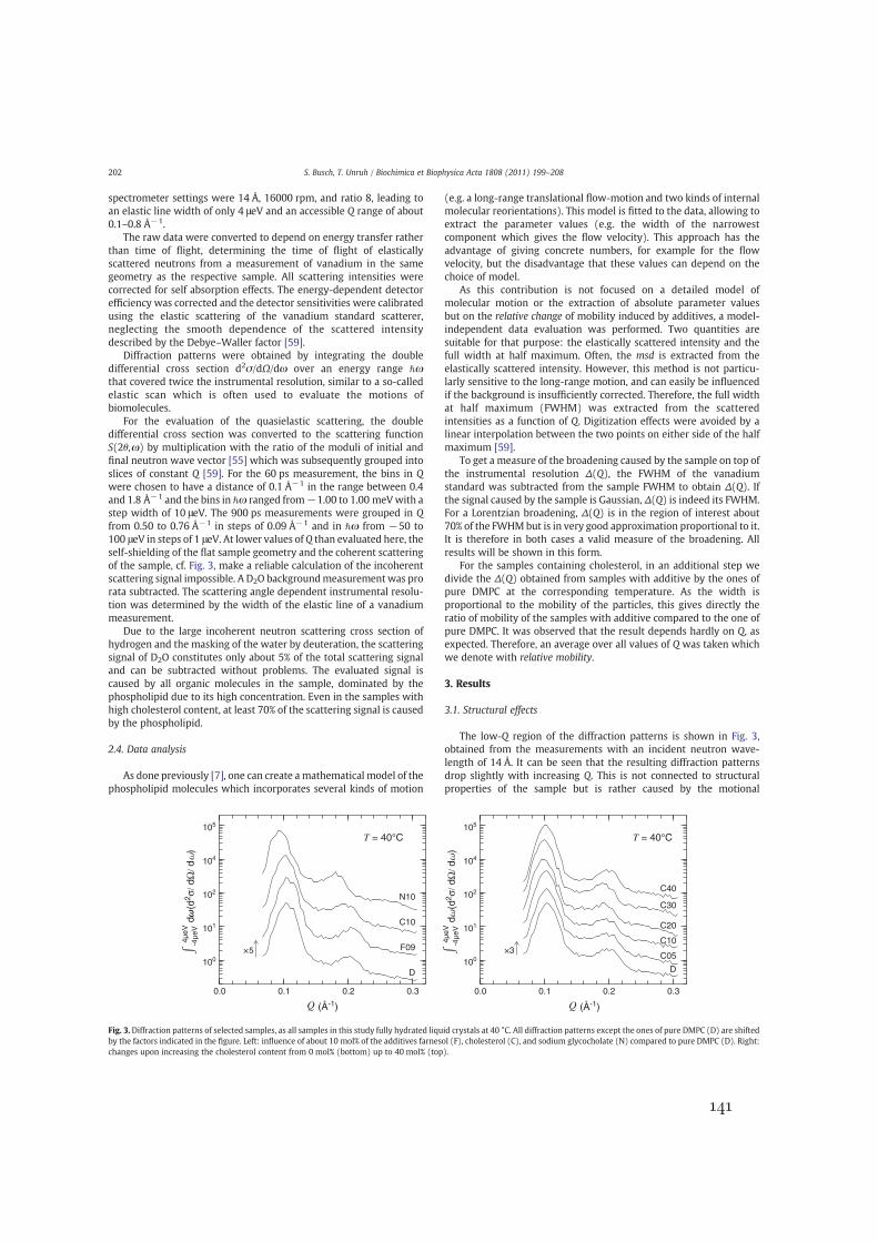
spectrometer settings were 14 Å, 16000 rpm, and ratio 8, leading toan elastic line width of only 4 μeV and an accessible Q range of about0.1–0.8 Å−1.
The raw data were converted to depend on energy transfer ratherthan time of flight, determining the time of flight of elasticallyscattered neutrons from a measurement of vanadium in the samegeometry as the respective sample. All scattering intensities werecorrected for self absorption effects. The energy-dependent detectorefficiency was corrected and the detector sensitivities were calibratedusing the elastic scattering of the vanadium standard scatterer,neglecting the smooth dependence of the scattered intensitydescribed by the Debye–Waller factor [59].
Diffraction patterns were obtained by integrating the doubledifferential cross section d2σ/dΩ/dω over an energy range ℏωthat covered twice the instrumental resolution, similar to a so-calledelastic scan which is often used to evaluate the motions ofbiomolecules.
For the evaluation of the quasielastic scattering, the doubledifferential cross section was converted to the scattering functionS(2θ,ω) by multiplication with the ratio of the moduli of initial andfinal neutron wave vector [55] which was subsequently grouped intoslices of constant Q [59]. For the 60 ps measurement, the bins in Qwere chosen to have a distance of 0.1 Å−1 in the range between 0.4and 1.8 Å−1 and the bins in ℏω ranged from−1.00 to 1.00 meVwith astep width of 10 μeV. The 900 ps measurements were grouped in Qfrom 0.50 to 0.76 Å−1 in steps of 0.09 Å−1 and in ℏω from −50 to100 μeV in steps of 1 μeV. At lower values ofQ than evaluated here, theself-shielding of the flat sample geometry and the coherent scatteringof the sample, cf. Fig. 3, make a reliable calculation of the incoherentscattering signal impossible. A D2O backgroundmeasurement was prorata subtracted. The scattering angle dependent instrumental resolu-tion was determined by the width of the elastic line of a vanadiummeasurement.
Due to the large incoherent neutron scattering cross section ofhydrogen and the masking of the water by deuteration, the scatteringsignal of D2O constitutes only about 5% of the total scattering signaland can be subtracted without problems. The evaluated signal iscaused by all organic molecules in the sample, dominated by thephospholipid due to its high concentration. Even in the samples withhigh cholesterol content, at least 70% of the scattering signal is causedby the phospholipid.
2.4. Data analysis
As done previously [7], one can create amathematical model of thephospholipid molecules which incorporates several kinds of motion
(e.g. a long-range translational flow-motion and two kinds of internalmolecular reorientations). This model is fitted to the data, allowing toextract the parameter values (e.g. the width of the narrowestcomponent which gives the flow velocity). This approach has theadvantage of giving concrete numbers, for example for the flowvelocity, but the disadvantage that these values can depend on thechoice of model.
As this contribution is not focused on a detailed model ofmolecular motion or the extraction of absolute parameter valuesbut on the relative change of mobility induced by additives, a model-independent data evaluation was performed. Two quantities aresuitable for that purpose: the elastically scattered intensity and thefull width at half maximum. Often, the msd is extracted from theelastically scattered intensity. However, this method is not particu-larly sensitive to the long-range motion, and can easily be influencedif the background is insufficiently corrected. Therefore, the full widthat half maximum (FWHM) was extracted from the scatteredintensities as a function of Q. Digitization effects were avoided by alinear interpolation between the two points on either side of the halfmaximum [59].
To get a measure of the broadening caused by the sample on top ofthe instrumental resolution Δ(Q), the FWHM of the vanadiumstandard was subtracted from the sample FWHM to obtain Δ(Q). Ifthe signal caused by the sample is Gaussian, Δ(Q) is indeed its FWHM.For a Lorentzian broadening, Δ(Q) is in the region of interest about70% of the FWHMbut is in very good approximation proportional to it.It is therefore in both cases a valid measure of the broadening. Allresults will be shown in this form.
For the samples containing cholesterol, in an additional step wedivide the Δ(Q) obtained from samples with additive by the ones ofpure DMPC at the corresponding temperature. As the width isproportional to the mobility of the particles, this gives directly theratio of mobility of the samples with additive compared to the one ofpure DMPC. It was observed that the result depends hardly on Q, asexpected. Therefore, an average over all values of Q was taken whichwe denote with relative mobility.
3. Results
3.1. Structural effects
The low-Q region of the diffraction patterns is shown in Fig. 3,obtained from the measurements with an incident neutron wave-length of 14 Å. It can be seen that the resulting diffraction patternsdrop slightly with increasing Q. This is not connected to structuralproperties of the sample but is rather caused by the motional
0.0 0.1 0.2 0.3 0.0 0.1 0.2 0.3
100
101
102
104
105
100
101
102
104
105
4µeV
-4µe
Vd
(d2 σ/
dΩ
/ d
)
T = 40°C T = 40°C
×5
D
F09
C10
N10
×3
D
C05
C10
C20
C30
C40
4µeV
-4µe
Vd
(d2 σ/
dΩ
/ d
)
(Å-1) (Å-1)
Fig. 3. Diffraction patterns of selected samples, as all samples in this study fully hydrated liquid crystals at 40 °C. All diffraction patterns except the ones of pure DMPC (D) are shiftedby the factors indicated in the figure. Left: influence of about 10 mol% of the additives farnesol (F), cholesterol (C), and sodium glycocholate (N) compared to pure DMPC (D). Right:changes upon increasing the cholesterol content from 0 mol% (bottom) up to 40 mol% (top).
202 S. Busch, T. Unruh / Biochimica et Biophysica Acta 1808 (2011) 199–208
141

broadening of the quasielastic line whichmakes intensity move out ofthe integrated energy transfer region. The peaks are caused by thecoherent scattering interferences due to the repeating units of thebilayers in the direction of the surface normal.
It can be seen that the overall diffraction pattern and therefore thebilayered structure of the membrane stacks is conserved. The peakposition does not shift upon addition of 10 mol% farnesol, meaningthat the repeating distance of the bilayers is not affected. A shift tolower values of Q can be observed when adding either 10 mol% ofcholesterol or sodium glycocholate, corresponding to an increase ofthe repeating distance. The trends in the diffraction patterns ofcholesterol agree with the ones observed by X-ray scattering [60,61]and MD simulations [62].
There is another correlation peak in the diffraction patterns athigher values of Q caused by the repeating distances of the chainswithin the membrane plane, becoming visible in the measurementsusing an incident neutron wavelength of 6 Å (not shown). While it isquite pronounced at 1.5 Å−1 at 20 °C, it smears out drastically andmoves to about 1.4 Å−1 at temperatures above the chain meltingtransition. The additives do not change the position of this peakwhichdoes however not allow conclusions about a possible change of thearea per lipid [22]. The peak height decreases with increasingcholesterol content, in agreement with previous studies [63].
3.2. Molecular mobility on a 60 ps time scale
While the diffraction patterns, obtained from integration of theenergy-dependent spectra, yield information about the structure ofthe sample, the energy-dependence itself is connected to the motionsof the molecules. Looking at a time scale of about 60 ps, the centralline is visibly broadened compared to the one of a vanadium standard(instrumental resolution) of 60 μeV as can be seen in Fig. 4exemplarily for some samples. The spectra–and therefore theobserved motions–of the different samples are quite similar on thistime scale.
The full width at half maximum Δ(Q) as defined above wasextracted from the data at different momentum transfers Q. Allspectra exhibit a line which is significantly broader than theinstrumental resolution. All Δ(Q) show a small dip at Q=1.5 Å-1 at20 °C which shifts to about 1.4 Å-1 at higher temperatures as can beseen in Figs. 5 and 6. This is due to the so-called de Gennes narrowing atthe structure factor maximum of a disordered phase. Therefore, thesedips in Δ(Q) coincide with the peaks at large Q in the diffractionpatterns discussed above.
The addition of myristic acid does not induce changes of thisfeature. Farnesolmakes the dip less pronounced, especially at 20 °C, in
contrast to cholesterol which also reduces the dip—except at 20 °C,similar to sodium glycocholate.
For a quick overview of the different effect of different substances,Δ(Q) of pure DMPC and samples with 10 mol% of all the studiedadditives except MA are compared with each other in Fig. 5. At 20 °C,below the main phase transition, the additives cause either no effector an increased mobility compared to the pure DMPC. At the highertemperatures, farnesol seems to cause a small increase of thedynamics while cholesterol and NaGC slow the motions down bymore or less the same amount.
Looking in more detail at the concentration dependent influenceof the different additives one at a time in Fig. 6, it is evident that theaddition of myristic acid has no systematic influence on the 60 psdynamics of DMPC in its fluid phase; there is a trend towards lowermobility which is more pronounced at 20 °C. A systematic increaseof the dynamics is observed for the Farnesol doped samples on thetime scale of 60 ps, both, below and above the main phasetransition. The addition of cholesterol does not change the dynamicsat 20 °C at all but shows a clear systematic effect on the dynamicsabove the main phase transition. This decrease is rather continuous,compatible with NMR measurements [44]. Sodium glycocholateaffects the line width similar to cholesterol above the main phasetransition. Additionally, it enhances the dynamics at 20 °C slightlybut not as much as farnesol.
-0.50 -0.25 0.00 0.25 0.50 -0.50 -0.25 0.00 0.25 0.500.00
0.25
0.50
0.75
1.00
VanDC40N10
T = 40°C
= 1.50Å-1
T = 40°C
= 1.50Å-1
10-2
10-1
100
(meV)
VanDC40N10
(meV)
Fig. 4. Plot of selected normalized spectra–pure DMPC (D), 40 mol% cholesterol (C40), and 10 mol% sodium glycocholate (N10)–measured at 40 °C shown together with theinstrumental resolution as determined by a vanadium measurement (Van), as seen with an instrumental resolution of 60 μeV, corresponding to an observation time of 60 ps, at amomentum transfer of Q=1.5 Å-1. The same spectra are shown on a linear scale (left) and on a logarithmic scale (right).
0.0 0.5 1.0 1.5 2.00
20
40
60
80
(Å-1)
Δ(
) (µ
eV)
40°C30°C
20°C
DF09C10N10
Fig. 5. Broadenings (FWHM) caused by selected samples: pure DMPC (D), farnesol (F),cholesterol (C), and sodium glycocholate (N). The points of pure DMPC are connectedby straight lines for better clarity. Seen with an instrumental resolution of 60 μeV,corresponding to an observation time of 60 ps, at 20 °C, 30 °C, and 40 °C.
203S. Busch, T. Unruh / Biochimica et Biophysica Acta 1808 (2011) 199–208
Appendix E. The Influence of Additives on the Nanoscopic Dynamics of the
Phospholipid Dimyristoylphosphatidylcholine
142

3.3. Molecular mobility on a 900 ps time scale
On a time scale of 900 ps, the differences between the spectra aremore pronounced (cf. Fig. 7). However, it becomes already clear whenlooking at the spectra that the influence depends very much on thetype of additive: NaGC shows hardly any effect whereas cholesterolnarrows the line considerably (which is still clearly broader than theinstrumental resolution).
This picture is confirmed by the extracted widths Δ(Q) of the10 mol% samples compared with the one of pure DMPC in Fig. 8: on a
time scale of 900 ps and at a temperature of 40 °C, none of the probedadditives causes an increase of the dynamics. Instead, farnesol andNaGC have basically no influence on the speed of the motions. Indeed,the width extracted from the samples with 10 mol% farnesol orsodium glycocholate differ by only 1% from the one of pure DMPC. Incontrast, cholesterol causes a slowing down which is much morepronounced than on the 60 ps scale.
The quasielastic broadening of measurements with increasingcholesterol content is displayed in Fig. 9. The dynamics decreasescontinuously with increasing cholesterol concentration.
0.0 0.5 1.0 1.5 2.00
20
40
60
80
0.0 0.5 1.0 1.5 2.00
20
40
60
80
0.0 0.5 1.0 1.5 2.00
20
40
60
80
0.0 0.5 1.0 1.5 2.00
20
40
60
80
40°C30°C
20°C
DM01M02M03
40°C30°C
20°CDF05F09F14F18
40°C30°C
20°C
DC10C20C30C40
40°C30°C
20°C
DN05N09N14
(Å-1)
Δ(
) (µ
eV)
(Å-1)
Δ(
) (µ
eV)
(Å-1)
Δ(
) (µ
eV)
(Å-1)
Δ(
) (µ
eV)
Fig. 6. Broadenings (FWHM) caused by all discussed samples at all discussed temperatures as observed with an instrumental resolution of 60 μeV, corresponding to an observationtime of 60 ps. Top left: myristic acid; top right: farnesol; bottom left: cholesterol; bottom right: sodium glycocholate. The points of pure DMPC are connected by straight lines forbetter clarity.
-50 -25 0 25 50 -50 -25 0 25 500.00
0.25
0.50
0.75
1.00
(µeV)
VanDC40N10
10-2
10-1
100
VanDC40N10
(µeV)
T = 40°C
= 0.76Å-1
T = 40°C
= 0.76Å-1
Fig. 7. Plots of selected normalized spectra–pure DMPC (D), 40 mol% cholesterol (C40), and 10 mol% sodium glycocholate (N10)–measured at 40 °C shown together with theinstrumental resolution as determined by a vanadium measurement (Van), as seen with an instrumental resolution of 4 μeV, corresponding to an observation time of 900 ps, at amomentum transfer of Q=0.76 Å-1. The same spectra are shown on a linear scale (left) and on a logarithmic scale (right).
204 S. Busch, T. Unruh / Biochimica et Biophysica Acta 1808 (2011) 199–208
143

4. Discussion
Different motions dominate the msd of atoms and molecules andhereby the signal of a QENS experiment when studying a sample ondifferent time scales [57]: On a short time scale, fast motions–whichare mostly reorientations within the molecule–predominate. Onlonger time scales, these motions can only contribute a constant tothe msd which is then governed by the slower but non-localizedmotions of the whole molecule. Within the short times, the moleculesexplore their immediate vicinity whereas the larger motions havealready previously been interpreted in the frame of flow-like motionsof transient assembling patches of molecules in the membrane [6,7].
It is not surprising that these flowmotions resemble the dynamicalheterogeneities observed in 2D Lennard–Jones fluids, colloidalsystems or granular media as the head groups form a dense 2Dsystem. As the density in the head region is larger than the one inthe tail region [24,64], we speculate that the mobility of thephospholipid molecules in the native membranes will be governedby the interaction of the head groups.
Additives can influence the head and tail region separately byincreasing or decreasing the respective density (Fig. 10). If an additivecaused a density in-/decrease in the head region, this would translatedirectly into a de-/increase of the DMPCmobility. For themore loosely
packed tails, the connection is more intricate: A density decreasewould not cause a further increase of the mobility as the head groupsare the limiting factor already. Nevertheless, when increasing thedensity in the tail group region of a membrane by additives, a reducedmobility of DMPC molecules should be observed.
Thus, we suggest to interpret the influence of additives on thedynamics of DMPC in the liquid crystalline phase according to theamount of free volume in the DMPC bilayer created or annihilated bythe intercalation of guest molecules and the influence of this freevolume on the flow-like motions in the membrane. The results of ourmeasurements, summarized in Table 2 for the different additives, arediscussed in this sense below. We would like to stress that we do notsee this as a support for the free volume theorywhich relies on furtherassumptions such as jump-like motions of the molecules.
If only the head region is densely packed, the displacements of themolecules will be caused by the density fluctuations there. If also thetail region is densely packed, the molecules will be influenced also bydensity fluctuations in this region. Should the fluctuations in the tworegions be completely correlated, there will be no influence on theflow-like motions of the molecules. Every decorrelation between thetwowill decrease the persistence time of a flow event of onemolecule.This interpretation also agrees with results from coarse-grainedsimulations which found a disrupting effect of cholesterol on thecollective diffusion of the phospholipid molecules [65]. A reduction ofthe flow time and correspondingly flow length of a random walktranslates directly in a reduction of the resulting diffusion coefficient.
4.1. Myristic acid
Although the effects of myristic acid as an additive did not cause asignificant effect on the microscopic scale (cf. Fig. 6), drastic changesof themacroscopic behavior (increasing viscosity) of the phospholipidwere observed already for low myristic acid concentrations. It cannotbe excluded that stronger effects would be visible if the concentrationcould be increased to levels comparable to, e.g., cholesterol. But thisdoes not seem not to be very likely because myristic acid is a chain-like molecule and can thus be expected to be oriented mainly parallelto the DMPC chains. The hydrophilic carboxyl group can be expectedto stick into the headgroup region of the DMPC layers. Therefore,
0.5 0.6 0.7 0.80.0
1.0
2.0
3.0
4.0
DF09C10N10
T = 40°C
Δ(
) (µ
eV)
(Å-1)
Fig. 8. Broadenings (FWHM) caused by selected samples: pure DMPC (D), farnesol (F),cholesterol (C), and sodium glycocholate (N). The points of pure DMPC are connectedby straight lines for better clarity. Seen with an instrumental resolution of 4 μeV,corresponding to an observation time of 900 ps, at 40 °C.
0.0
1.0
2.0
3.0
4.0
DC05C10C20C30C40
0.5 0.6 0.7 0.8
Δ(
) (µ
eV)
(Å-1)
T = 40°C
Fig. 9. Broadenings (FWHM) caused by samples with increasing cholesterol content at40 °C as observed with an instrumental resolution of 4 μeV, corresponding to anobservation time of 900 ps. The points of pure DMPC are connected by straight lines forbetter clarity.
D M D F D N D C D D
Fig. 10. Sketch of the proposed configuration of themolecules, denoted by D (DMPC), M(myristic acid), F (farnesol), N (NaGC), and C (cholesterol). The hydrophilic parts areschematically displayed as violet bubbles, the hydrophobic chains and steroid as orangesticks.
Table 2Summary of the observed effects of several additives on the dynamics of DMPC on timescales of 60 and 900 ps. While∅ indicates no change of the dynamics, the number of +and − correspond to the degree of increase or decrease of the mobility.
60 ps 900 ps
20 °C 30 °C 40 °C 40 °C
MA − ∅ ∅Farnesol ++ + + ∅Cholesterol ∅ − − −NaGC + − − ∅
205S. Busch, T. Unruh / Biochimica et Biophysica Acta 1808 (2011) 199–208
Appendix E. The Influence of Additives on the Nanoscopic Dynamics of the
Phospholipid Dimyristoylphosphatidylcholine
144

myristic acid should not fill up free volume in the tail region of DMPCbilayers and should also not alter their head group packingsignificantly [30]. This is in agreement with corresponding studiesusing short chain alcohols as additives where also no effect on thephospholipid dynamics was observed [66].
4.2. Farnesol
The behavior of farnesol inside DMPC bilayers seems to be similarto the one of myristic acid. From NMR measurements, it could not bedetermined whether the molecules intercalate between the DMPCmolecules or are placed in between the two leaflets [35]. Thediffraction patterns in Fig. 3 show no influence of Farnesol on peakdistance and height of the first two layer repeating peaks. Althoughwe cannot exclude that a change in the bilayer thickness is exactlycompensated by an accompanying change in water thickness, we seeno evidence for a change of the bilayer thickness upon the addition offarnesol. This indicates that the molecules intercalate between theDMPCmolecules. Respecting that the effect on themobility of DMPC isnegligible, we conclude that the molecules align themselves along thephospholipid molecules similar to the case of myristic acid. It isknown from NMR measurements [34] that farnesol has a differentinfluence on the surrounding phospholipid molecules compared tocholesterol. While cholesterol causes an increase of the molecularorder parameters, farnesol does not. However, farnesol lowers themain phase transition temperature which might explain the unusualincreased dynamics at 20 °C: the addition of farnesol probably inducesa melting of the phospholipid chains.
4.3. Cholesterol
Cholesterol causes an increasing thickness of the membrane. Thiswas also observed by X-ray diffraction and simulations and reflectsthe condensation effect [39,60,61]. The incorporation of cholesterolinto the phospholipid membrane can be understood in the frame ofthe umbrella model [67]: The hydrophobic cholesterol moleculeresides between the hydrophobic tails of the phospholipids. Thehydrophilic heads of the phospholipid shield the tails and cholesterolfrom the surrounding water. This leads to an increase of the density inthe hydrophobic part of the bilayers.
This density increase reduces the free volume in the chain regionof the DMPC molecules. In this situation, the mobility of thephospholipid molecules is no more mainly determined by thedynamic inhomogeneities in the densely packed head groups butalso by those in the nowmore closely packed tail groups resulting in asignificantly slower molecular transport.
The influence of cholesterol on DMPC as seen with quasielasticneutron scattering in the present study is summarized in Fig. 11: thewidths Δ(Q) are normalized to the widths of pure DMPC at the sametemperature and averaged over all Q values, yielding the relativemobility. It can immediately be seen that in no case the addition ofcholesterol causes an increased dynamics of DMPC.
The motions detected within an observation time of 60 ps are notaffected by the addition of cholesterol at temperatures below themain phase transition. At temperatures above the main phasetransition, the tails experience the density increase caused bycholesterol. The relative decrease of the linewidth is completelyidentical at 30 °C and 40 °C for all measured cholesterol concentra-tions which indicates that the observed motions are not sensitive tothe absolute distance from the phase transition temperature as onemight expect for local motions.
The mobility decrease of DMPC is enhanced when looking on atime scale of 900 ps where the influence of 5 mol% cholesterol affectsthe phospholipids more strongly at 30 °C than at 40 °C. Thecorresponding motions are, therefore, more sensitive to an increasein density if the sample temperature is closer to the main phase
transition temperature which we see again as a signature of the long-range nature of this motion.
Also other techniques were used to measure the long-rangemotion of the phospholipid molecules. MD simulations [24] of thephospholipid DPPC at 50 °C, i.e. 8 K above the main phase transition ofpure DPPC, show a strong impact of cholesterol on the phospholipidmobility on a 100 ns time scale—stronger than our measurements at40 °C, even a bit more than the one at 30 °C, i.e. 6 K above the mainphase transition of pure DMPC.
Fluorescence correlation spectroscopy of the phospholipid DLPC[42] on a 10 ms time scale at 25 °C, i.e. 27 K above the main phasetransition of DLPC, shows an impact of cholesterol on the dynamicswhich is very comparable to the results obtained on a 100 ms timescale with NMR [44] for DMPC at 40 °C.
The comparison between all these results is not straightforward asdifferent temperatures and even phospholipids were used. Only theNMR measurements were done with exactly same temperature andphospholipid as studied here and show a very good agreement withour results. All these techniques measure on longer time scales thanQENS and we would therefore expect them to show a stronger impacton the dynamics—as they do. The NMR data also show a strongerinfluence of cholesterol on the phospholipid motions the closer thetemperature is to the main phase transition.
Much in contrast, two measurements on even larger time (about10 s) and length scales using FRAP [41,43] observed a smaller impactof cholesterol on the dynamics. The degree varies between themeasurements, one [43] even observes no impact up to about 15 mol%cholesterol in the sample. The difference between the FRAPmeasurements and the values obtained by NMR were discussed interms of the susceptibility of FRAP to the formation of microdomainsin the membrane [44].
4.4. Sodium glycocholate
Sodium glycocholate is a charged molecule. It is known thatcharged phospholipids induce an increase of the thickness of thewater layer between the bilayers but not of the membrane itself [68].This swelling is the thickness increase observed in the diffractionpatterns. At low concentrations, the influence of NaGC on the
0 10 20 30 40 500.00
0.25
0.50
0.75
1.00
χchol (mol%)
rela
tive
mob
ility
L L +Lo Lo
L L +Lo Lo
20 °C, 60ps30 °C, 60ps40 °C, 60ps30 °C, 900ps40 °C, 900ps40 °C, 100ms(NMR)
α α
β β
Fig. 11. The relative mobility (mobility normalized to the one of pure DMPC, cf. text) asa function of cholesterol concentration at different temperatures. Open symbols areextracted from measurements with an instrumental resolution of 60 μeV,corresponding to an observation time of 60 ps; closed symbols are extracted frommeasurements with an instrumental resolution of 4 μeV, corresponding to anobservation time of 900 ps. NMR measurements taken from Filippov et al. [44] at40 °C are also shown. The phase boundaries are drawn after EPR results of Sankaram[43] and are only valid for the displayed measurements. They are only displayed toshow the respective phases of themeasurements and do not represent a phase diagram.
206 S. Busch, T. Unruh / Biochimica et Biophysica Acta 1808 (2011) 199–208
145

dynamics of the phospholipid is similar to the one of cholesterol.However, cholesterol is uncharged, has not such an influence on thestructure and can, therefore, be present in membranes in much higherconcentrations.
The practical importance of sodium glycocholate is based on itsability to stabilize emulsions even during crystallization of the oilyphase. In the case of triglyceride or alkane nanoemulsions, the shape ofthe stabilized particles changes drastically during crystallization: from aspherical droplet to an elongated crystalline platelet. This is connectedto a sudden increase of the surface of the particle. One could imaginethat this results in a partial coverage of the particle with stabilizer—theuncoveredsurfaces are then theoriginof aggregation.A redistributionofthe stabilizer onto the naked surface could prevent aggregation,happens however so slowly that the aggregation took place before.
As the addition of sodium glycocholate prevents aggregation,it could have had the effect of enhancing the dynamics of thephospholipid, making the redistribution of the stabilizer so fast thataggregation is suppressed.
However, sodium glycocholate does not influence the phospho-lipid dynamics. It can be excluded that it did not mix with thephospholipid because it is water soluble, caused a decrease ofviscosity, made the samplemore transparent, and changed the bilayerspacing. As NaGC is hydrophilic, an enhanced partition into the chainregion should not be expected. We see two likely structuralarrangements: Either the NaGC is intercalated inside the bilayeroriented with the hydrophilic part in the region of the phospholipidhead groups and the hydrophobic part in the chain region of thebilayer. Obviously, this leads to hardly any change in the free volumein either region of the membrane. Or–as already previouslyspeculated for sodium cholate in lecithin [69] –a flat placement ofthe molecules on the bilayer in the head region. This would lead to adensity decrease in the tail region which would, as we have arguedbefore, not influence the dynamics.
4.5. Other influences on membrane dynamics
Using NMR, the influence of the antimicrobial peptide gramicidinwas found to be comparable to the one of cholesterol on a sub-nanosecond time scale [70]. Also neutron scattering experimentsshowed a decreased mobility on a time scale of about 150 ps [71]. Ourresults are in good agreement with the view that the effects caused bygramicidin are directly comparable with the ones caused bycholesterol. However, we would like to point out that the underlyingmechanism might be very different as gramicidin is approximativelybarrel-like [72] and does therefore not increase the density in the tailregion. However, the same study showed that the hydration of thephospholipid molecules in the vicinity of the peptide is decreased. Adecreased hydration is in turn known to decrease the dynamics [73]so the decreased hydration might actually influence the dynamicsmore than the change in density.
In MD simulations, it was observed that proteins in the membranecause a slowing down of adjacent phospholipid molecules [23]. Thiseffect could be reproduced for a number of different proteins in themembrane and also 2D Lennard–Jones systems which suggests thatthis effect is partly caused by the obstacles hindering phospholipidmotions, and complemented by specific effects due to protein-lipidinteractions.
Whereas these interactions of phospholipids with peptides andproteins might be dominated by other effects than density changes,their aforementioned use as stabilizer in suspensions and emulsionscould be directly influenced by the density as it might very well bethat the amount of phospholipid is lower than what one would needfor a full monolayer around the particles. Preliminary results indeedseem to show that the effect of decreasing mobility upon increasingdensity can hereby be reversed, observing increasing dynamics whenartificially decreasing the density by stretching a monolayer [28,74].
5. Conclusion
Summarizing, we studied the effect of several additives on thedynamics of the phospholipid DMPC on time scales of 60 ps and900 ps. Myristic acid and farnesol, two more linear, chain-likemolecules seem to incorporate into the membrane without modifi-cation of the mobility. Cholesterol has a pronounced slowing downeffect on the dynamics. This effect can be qualitatively understoodassuming that the persistence lengths of flow patterns decrease. Theflow-like mobility of the molecules is the equivalent to dynamicheterogeneities observed in supercooled liquids, suspensions andgranular systems. Sodium glycocholate has–in contrast to its strongmacroscopic influences–no effect on the mobility.
Acknowledgments
We would like to thank W. Petry for his enduring interest andsupport as well as L. C. Pardo, T. Gutberlet, and J. Horbach for manystimulating discussions.
References
[1] D. Axelrod, Lateral motion of membrane proteins and biological function,J. Membr. Biol. 75 (1) (1983) 1, doi:10.1007/bf01870794.
[2] L. Sagalowicz, M.E. Leser, Delivery systems for liquid food products, Curr. Opin.Colloid Interface Sci. 15 (1-2) (2010) 61, doi:10.1016/j.cocis.2009.12.003.
[3] C. Peetla, A. Stine, V. Labhasetwar, Biophysical interactions with model lipidmembranes: applications in drug discovery and drug delivery, Mol. Pharm. 6 (5)(2009) 1264–1276, doi:10.1021/mp9000662.
[4] K. Kawano, E. Onose, Y. Hattori, Y. Maitani, Higher liposomal membrane fluidityenhances the in vitro antitumor activity of folate-targeted liposomal mitoxan-trone, Mol. Pharm. 6 (1) (2009) 98–104, doi:10.1021/mp800069c.
[5] W.L.C. Vaz, P.F.F. Almeida, Microscopic versus macroscopic diffusion in one-component fluid phase lipid bilayer-membranes, Biophys. J. 60 (6) (1991)1553–1554, doi:10.1016/S0006-3495(91)82190-7.
[6] E. Falck, T. Róg, M. Karttunen, I. Vattulainen, Lateral diffusion in lipid membranesthrough collective flows, J. Am. Chem. Soc. 130 (1) (2008) 44–45, doi:10.1021/ja7103558.
[7] S. Busch, C. Smuda, L.C. Pardo, T. Unruh, Molecular mechanism of long-rangediffusion in phospholipid membranes studied by quasielastic Neutron Scattering,J. Am. Chem. Soc. 132 (10) (2010) 3232, doi:10.1021/ja907581s.
[8] M.C. Rheinstädter, J. Das, E. Flenner, B. Brüning, T. Seydel, I. Kosztin, Motionalcoherence in fluid phospholipid membranes, Phys. Rev. Lett. 101 (24) (2008)248106, doi:10.1103/physrevlett.101.248106.
[9] T. Apajalahti, P.S. Niemelä, P.N. Govindan, M.S. Miettinen, E. Salonen, S.-J. Marrink,I. Vattulainen, Concerted diffusion of lipids in raft-like membranes, FaradayDiscuss. 144 (2010) 411, doi:10.1039/b901487j.
[10] W. Kob, C. Donati, S. Plimpton, P. Poole, S.C. Glotzer, Dynamical heterogeneities ina supercooled Lennard–Jones liquid, Phys. Rev. Lett. 79 (15) (1997) 2827, doi:10.1103/physrevlett.79.2827.
[11] C. Donati, J. Douglas, W. Kob, S. Plimpton, P. Poole, S.C. Glotzer, Stringlikecooperative motion in a supercooled liquid, Phys. Rev. Lett. 80 (11) (1998) 2338,doi:10.1103/physrevlett.80.2338.
[12] H.R. Schober, C. Gaukel, C. Oligschleger, Collective jumps in amorphous materials,Defect Diffus. Forum 143-147 (1997) 723, doi:10.4028/www.scientific.net/ddf.143-147.723.
[13] R. Richert, Heterogeneous dynamics in liquids: fluctuations in space and time,J. Phys. Condens. Matter 14 (23) (2002) R703, doi:10.1088/0953-8984/14/23/201.
[14] A. Marcus, J. Schofield, S.A. Rice, Experimental observations of non-Gaussianbehavior and stringlike cooperative dynamics in concentrated quasi-two-dimensional colloidal liquids, Phys. Rev. E 60 (5) (1999) 5725, doi:10.1103/physreve.60.5725.
[15] W.K. Kegel, Direct observation of dynamical heterogeneities in colloidal hard-spheresuspensions, Science 287 (5451) (2000) 290, doi:10.1126/science.287.5451.290.
[16] B. Cui, B. Lin, S.A. Rice, Dynamical heterogeneity in a dense quasi-two-dimensionalcolloidal liquid, J. Chem. Phys. 114 (20) (2001) 9142, doi:10.1063/1.1369129.
[17] R. Zangi, S.A. Rice, Cooperative dynamics in two dimensions, Phys. Rev. Lett. 92 (3)(2004) 035502, doi:10.1103/physrevlett.92.035502.
[18] A.S. Keys, A.R. Abate, S.C. Glotzer, D.J. Durian, Measurement of growing dynamicallength scales and prediction of the jamming transition in a granular material, Nat.Phys. 3 (4) (2007) 260, doi:10.1038/nphys572.
[19] R. Matena, M. Dijkstra, A. Patti, Non-Gaussian dynamics in smectic liquidcrystals of parallel hard rods, Phys. Rev. E 81 (2) (2010) 021704, doi:10.1103/physreve.81.021704.
[20] M. Hurley, P. Harrowell, Kinetic structure of a two-dimensional liquid, Phys. Rev. E52 (2) (1995) 1694, doi:10.1103/physreve.52.1694.
[21] S. Tristram-Nagle, Y. Liu, J. Legleiter, J.F. Nagle, Structure of gel phase DMPCdetermined by X-ray diffraction, Biophys. J. 83 (6) (2002) 3324, doi:10.1016/s0006-3495(02)75333-2.
207S. Busch, T. Unruh / Biochimica et Biophysica Acta 1808 (2011) 199–208
Appendix E. The Influence of Additives on the Nanoscopic Dynamics of the
Phospholipid Dimyristoylphosphatidylcholine
146

[22] J.S. Hub, T. Salditt, M.C. Rheinstädter, B.L. de Groot, Short-range order andcollective dynamics of DMPC bilayers: a comparison betweenmolecular dynamicssimulations, X-ray, and neutron scattering experiments, Biophys. J. 93 (9) (2007)3156–3168, doi:10.1529/biophysj.107.104885.
[23] P.S. Niemelä, M.S. Miettinen, L. Monticelli, H. Hammaren, P. Bjelkmar, T. Murtola,E. Lindahl, I. Vattulainen, Membrane proteins diffuse as dynamic complexes withlipids, J. Am. Chem. Soc. 132 (22) (2010) 7574, doi:10.1021/ja101481b.
[24] E. Falck, M. Patra, M. Karttunen, M.T. Hyvönen, I. Vattulainen, Lessons ofslicing membranes: interplay of packing, free area, and lateral diffusion inphospholipid/cholesterol bilayers, Biophys. J. 87 (2) (2004) 1076–10918 doi:10.1529/biophysj.104.041368.
[25] P.N. Pusey, W. van Megen, Observation of a glass transition in suspensions ofspherical colloidal particles, Phys. Rev. Lett. 59 (18) (1987) 2083, doi:10.1103/physrevlett.59.2083.
[26] P.F.F. Almeida, W.L.C. Vaz, T.E. Thompson, Lipid diffusion, free area, andmolecular dynamics simulations, Biophys. J. 88 (6) (2005) 4434–44388 doi:10.1529/biophysj.105.059766.
[27] E. Falck, M. Patra, M. Karttunen, M.T. Hyvönen, I. Vattulainen, Response tocomment by Almeida et al.: free area theories for lipid bilayers—predictive or not?Biophys. J. 89 (1) (2005) 745–752, doi:10.1529/biophysj.105.065714.
[28] M. Javanainen, L. Monticelli, J.B. de la Serna, I. Vattulainen, Free volume theoryapplied to lateral diffusion in Langmuir monolayers: atomistic simulations for aprotein-free model of lung surfactant, Langmuir 26 (19) (2010) 15436–154448doi:10.1021/la102454m.
[29] S. Ghosh, A. Adhikari, S. Sen Mojumdar, K. Bhattacharyya, A fluorescencecorrelation spectroscopy study of the diffusion of an organic dye in the gelphase and fluid phase of a single lipid vesicle, J. Phys. Chem. B 114 (17) (2010)5736–5741, doi:10.1021/jp911971p.
[30] G. Peters, F. Hansen, M. Møller, P. Westh, Effects of fatty acid inclusion in a DMPCbilayermembrane, J. Phys. Chem. B 113 (1) (2009)92–102, doi:10.1021/jp806205m.
[31] V. Oberle, Untersuchungen zum Einfluß freier Fettsäuren auf die Eigenschaftenbiologischer und Modellmembranen, Ph.D. thesis, Martin-Luther-Universität,Halle (Saale), 1999.
[32] R. Koynova, B. Tenchov, G. Rapp, Mixing behavior of saturated short-chainphosphatidylcholines and fatty acids: eutectic points, liquid and solid immisci-bility, non-lamellar phases, Chem. Phys. Lipids 88 (1) (1997) 45, doi:10.1016/s0009-3084(97)00043-1.
[33] J. Joo, A. Jetten, Molecular mechanisms involved in farnesol-induced apoptosis,Cancer Lett. 287 (2) (2010) 123–135, doi:10.1016/j.canlet.2009.05.015.
[34] A.C. Rowat, J.H. Davis, Farnesol-DMPC phase behaviour: a (2)H-NMR study, Biochim.Biophys. Acta 1661 (2) (2004) 178–187, doi:10.1016/j.bbamem.2004.01.002.
[35] A.C. Rowat, D. Keller, J.H. Ipsen, Effects of farnesol on the physical properties ofDMPC membranes, Biochim. Biophys. Acta 1713 (1) (2005) 29–39, doi:10.1016/j.bbamem.2005.04.014.
[36] G. Orädd, V. Shahedi, G. Lindblom, Effect of sterol structure on the bending rigidity oflipid membranes: a 2H NMR transverse relaxation study, Biochim. Biophys. Acta(BBA) - Biomembr. 1788 (9) (2009) 1762–1771, doi:10.1016/j.bbamem.2009.06.019.
[37] D.A. Mannock, R.N. Lewis, R.N. McElhaney, A calorimetric and spectroscopiccomparison of the effects of ergosterol and cholesterol on the thermotropic phasebehavior and organization of dipalmitoylphosphatidylcholine bilayer membranes,Biochim.Biophys. Acta1798(3) (2010)376–388,doi:10.1016/j.bbamem.2009.09.002.
[38] J.M. Berg, J.L. Tymoczko, L.Stryer, Biochemie, Spektrum Akademischer Verlag, 5. a.edn., ISBN 9783827413031, 2003.
[39] T. Róg, M. Pasenkiewicz-Gierula, I. Vattulainen, M. Karttunen, Ordering effects ofcholesterol and its analogues, Biochim. Biophys. Acta 1788 (1) (2009) 97–121,doi:10.1016/j.bbamem.2008.08.022.
[40] E. Falck, M. Patra, M. Karttunen, M.T. Hyvönen, I. Vattulainen, Impact ofcholesterol on voids in phospholipid membranes, J. Chem. Phys. 121 (24)(2004) 12676–12689, doi:10.1063/1.1824033.
[41] J.L. Rubenstein, B.A. Smith, H.M. McConnell, Lateral diffusion in binary mixtures ofcholesterol and phosphatidylcholines, Proc. Natl Acad. Sci. USA 76 (1) (1979) 15–18.
[42] J. Korlach, P. Schwille, W.W. Webb, G.W. Feigenson, Characterization of lipidbilayer phases by confocal microscopy and fluorescence correlation spectroscopy,Proc. Natl Acad. Sci. USA 96 (15) (1999) 8461–8466.
[43] P.F.F. Almeida, W.L.C. Vaz, T.E. Thompson, Lateral diffusion in the liquid phases ofdimyristoylphosphatidylcholine/cholesterol lipid bilayers: a free volume analysis,Biochemistry 31 (29) (1992) 6739, doi:10.1021/bi00144a013.
[44] A. Filippov, G. Orädd, G. Lindblom, The effect of cholesterol on the lateral diffusionof phospholipids in oriented bilayers, Biophys. J. 84 (5) (2003) 3079, doi:10.1016/s0006-3495(03)70033-2.
[45] A.-L. Kuo, C.G. Wade, Lipid lateral diffusion by pulsed nuclear magnetic resonance,Biochemistry 18 (11) (1979) 2300, doi:10.1021/bi00578a026.
[46] J. Zidar, F. Merzel, M. Hodošček, K. Rebolj, K. Sepčić, P. Maček, D. Janežič, Liquid-ordered phase formation in cholesterol/sphingomyelin bilayers: all-atommoleculardynamics simulations, J. Phys. Chem. B 113 (2009) 15795, doi:10.1021/jp907138h.
[47] C. Gliss, O. Randel, H. Casalta, E. Sackmann, R. Zorn, T.M. Bayerl, Anisotropicmotion of cholesterol in oriented DPPC bilayers studied by quasielastic neutronscattering: the liquid-ordered phase, Biophys. J. 77 (1) (1999) 331, doi:10.1016/s0006-3495(99)76893-1.
[48] R. Tampe, A. Von Lukas, H.-J. Galla, Glycophorin-induced cholesterol-phospholipiddomains in dimyristoylphosphatidylcholine bilayer vesicles, Biochemistry 30 (20)(1991) 4909, doi:10.1021/bi00234a011.
[49] P. Schurtenberger, N. Mazer, W. Känzig, Micelle to vesicle transition in aqueoussolutions of bile salt and lecithin, J. Phys. Chem. 89 (6) (1985) 1042, doi:10.1021/j100252a031.
[50] K. Matsuoka, M. Maeda, Y. Moro, Micelle formation of sodium glyco- andtaurocholates and sodium glyco- and taurodeoxycholates and solubilization ofcholesterol into their micelles, Colloids Surf., B 32 (2) (2003) 87, doi:10.1016/s0927-7765(03)00148-6.
[51] K. Westesen, B. Siekmann, Investigation of the gel formation of phospholipid-stabilized solid lipid nanoparticles, Int. J. Pharm. 151 (1) (1997) 35, doi:10.1016/s0378-5173(97)04890-4.
[52] S. Teixeira, J. Ankner, M.-C. Bellissent-Funel, R. Bewley, M. Blakeley, L. Coates, R.Dahint, R. Dalgliesh, N. Dencher, J. Dhont, P. Fischer, V. Forsyth, G. Fragneto, B.Frick, T. Geue, R. Gilles, T. Gutberlet, M. Haertlein, T. Hauß, W. Häußler, W. Heller,K. Herwig, O. Holderer, F. Jurányi, R. Kampmann, R. Knott, J. Kohlbrecher, S.Kreuger, P. Langan, R.E. Lechner, G. Lynn, C. Majkrzak, R. May, F. Meilleur, Y. Mo, K.Mortensen, D. Myles, F. Natali, C. Neylon, N. Niimura, J. Ollivier, A. Ostermann, J.Peters, J. Pieper, A. Rühm, D. Schwahn, K. Shibata, A. Soper, T. Strässle, U. Suzuki, I.Tanaka, M. Tehei, P. Timmins, N. Torikai, T. Unruh, V. Urban, R. Vavrin, K. Weiss, G.Zaccai, New sources and instrumentation for neutrons in biology, Chem. Phys. 345(2–3) (2008) 133–151, doi:10.1016/j.chemphys.2008.02.030.
[53] V. García Sakai, A. Arbe, Quasielastic neutron scattering in soft matter, Curr. Opin.Colloid Interface Sci. 14 (6) (2009) 381, doi:10.1016/j.cocis.2009.04.002.
[54] T. Unruh, J. Neuhaus, W. Petry, The high-resolution time-of-flight spectrometerTOFTOF, Nucl. Instrum. Methods Phys. Res. Sect. A 580 (3) (2007) 1414–1422, doi:10.1016/j.nima.2007.07.0158 and585 (3) (2008)201, doi:10.1016/j.nima.2007.11.019.
[55] A. Furrer, J. Mesot, T. Strässle, Neutron Scattering in Condensed Matter Physics(Neutron Techniques and Applications) (Series on Neutron Techniques andApplications), 1 ed., World Scientific Publishing Company, ISBN: 9789810248314,2009.
[56] M. Bée, Quasielastic Neutron Scattering, Taylor & Francis, ISBN: 9780852743713,1988.
[57] T. Unruh, C. Smuda, S. Busch, J. Neuhaus, W. Petry, Diffusive motions in liquidmedium-chain n-alkanes as seen by quasielastic time-of-flight neutron spectros-copy, J. Chem. Phys. 129 (2008) 121106, doi:10.1063/1.2990026.
[58] J. Wuttke, Improved sample holder for multidetector neutron spectrometers,Phys. B Condensed Matter 266 (1-2) (1999) 112, doi:10.1016/s0921-4526(98)01503-8.
[59] J. Wuttke, Frida1: Fast Reliable Interactive Data Analysis, http://sourceforge.net/projects/frida/, URL http://sourceforge.net/projects/frida/, software, 1990–.
[60] W.-C. Hung, M.-T. Lee, F.-Y. Chen, H.W. Huang, The condensing effect ofcholesterol in lipid bilayers, Biophys. J. 92 (11) (2007) 3960–3967, doi:10.1529/biophysj.106.099234.
[61] B. Brüning, M.C. Rheinstädter, A. Hiess, B. Weinhausen, T. Reusch, S. Aeffner, T.Salditt, Influence of cholesterol on the collective dynamics of the phospholipidacyl chains in model membranes, Eur. Phys. J. E Soft Matter 31 (4) (2010)419–4288 doi:10.1140/epje/i2010-10574-6.
[62] M. Alwarawrah, J. Dai, J. Huang, A molecular view of the cholesterol condensingeffect in DOPC lipid bilayers, J. Phys. Chem. B 114 (22) (2010) 7516–7523, doi:10.1021/jp101415g.
[63] S.W. Hui, N.B. He, Molecular organization in cholesterol-lecithin bilayers by x-rayand electron diffraction measurements, Biochemistry 22 (5) (1983) 1159, doi:10.1021/bi00274a026.
[64] S.J. Marrink, R.M. Sok, H.J.C. Berendsen, Free volume properties of a simulatedlipid membrane, J. Chem. Phys. 104 (22) (1996) 9090, doi:10.1063/1.471442.
[65] G.S. Ayton, G.A. Voth, Mesoscopic lateral diffusion in lipid bilayers, Biophys. J. 87 (5)(2004) 3299–3311, doi:10.1529/biophysj.104.047811.
[66] T. Gutberlet, D. Posselt, T. Unruh, Influence of short chain alcohols on localdynamics of DMPC, Experimental Report 935, Forschungsneutronenquelle HeinzMaier-Leibnitz (FRM II), Technische Universität München, Germany, 2008.
[67] J. Huang, A microscopic interaction model of maximum solubility of cholesterol inlipid bilayers, Biophys. J. 76 (4) (1999) 2142, doi:10.1016/s0006-3495(99)77369-8.
[68] R.P. Rand, Interacting phospholipid bilayers: measured forces and inducedstructural changes, Annu. Rev. Biophys. Bioeng. 10 (1981) 277–314, doi:10.1146/annurev.bb.10.060181.001425.
[69] J. Ulmius, G. Lindblom, H. Wennerstroem, L.B.A. Johansson, K. Fontell, O.Soederman, G. Arvidson, Molecular organization in the liquid-crystalline phasesof lecithin-sodium cholate-water systems studied by nuclear magnetic resonance,Biochemistry 21 (7) (1982) 1553, doi:10.1021/bi00536a014.
[70] Z.Y. Peng, V. Simplaceanu, S.R. Dowd, C. Ho, Effects of cholesterol or gramicidin onslow and fast motions of phospholipids in oriented bilayers, Proc. Natl Acad. Sci.USA 86 (22) (1989) 8758–8762.
[71] U. Wanderlingh, G. D'Angelo, V. Conti Nibali, M. Gonzalez, C. Crupi, C. Mondelli,Influence of gramicidin on the dynamics of DMPC studied by incoherent elasticneutron scattering, J. Phys. Condens. Matter 20 (10) (2008) 104214, doi:10.1088/0953-8984/20/10/104214.
[72] J.A. Killian, B. De Kruijff, Importance of hydration for gramicidin-inducedhexagonal HII phase formation in dioleoylphosphatidylcholine model mem-branes, Biochemistry 24 (27) (1985) 7890, doi:10.1021/bi00348a007.
[73] S. König,W. Pfeiffer, T.M. Bayerl, D. Richter, E. Sackmann,Molecular dynamics of lipidbilayers studied by incoherent quasi-elastic neutron scattering, J. Phys. II Fr. 2 (8)(1992) 1589, doi:10.1051/jp2:1992100.
[74] S. Busch, et al., in preparation.
208 S. Busch, T. Unruh / Biochimica et Biophysica Acta 1808 (2011) 199–208
147


Appendix F.
The Picosecond Dynamics of thePhospholipidDimyristoylphosphatidylcholine inMono- and Bilayers
Sebastian Busch, Luis Carlos Pardo, Christoph Smuda, and Tobias UnruhSoft Matter, 8:3576, 2012
http://dx.doi.org/10.1039/c2sm07380c
In this publication, the author prepared the samples, partially with Tobias Unruh. Heperformed the measurements, developed the method for the determination of the amountof background to be subtracted, and performed the data reduction and evaluation. Heinterpreted the results and wrote the publication.
After the detailed study of phospholipid motions in multibilayers of pure DMPC [B, D]and the characterisation of the change of this dynamics under the influence of additives [E],the mixed systems of DMPC and additives are now used in pharmaceutically relevantsystems. The data evaluation is model-free as previously [E] because the low amountof sample does not allow a more detailed evaluation. It was found that the mobility ofthe phospholipid molecules on the emulsion droplets increases with increasing area permolecule.
Reproduced by permission of The Royal Society of Chemistry.
149

The picosecond dynamics of the phospholipid dimyristoylphosphatidylcholinein mono- and bilayers†
Sebastian Busch,*a Luis Carlos Pardo,b Christoph Smudac and Tobias Unruh*ad
Received 14th December 2011, Accepted 18th January 2012
DOI: 10.1039/c2sm07380c
The dynamics of the fully hydrated phospholipid dimyristoylphosphatidylcholine (DMPC) were
studied on a time scale of about 60 picoseconds with quasielastic neutron scattering. Three types of
samples were employed: multibilayers without solid support, single bilayers in vesicles, and monolayers
in emulsions of perdeuterated hexadecane. The vesicles and emulsion droplets had diameters of about
130 nanometres; some of the emulsions also contained sodium glycocholate to enhance the stability. It
could be shown that the mobility of the phospholipid molecules in the observed time regime increases
from multibilayers over single bilayers to monolayers. Additionally, the high quality of the data of the
multibilayer samples allows an evaluation of the molecular mechanism of the motions: while the
interpretation in the frame of flow-like motions fits well at temperatures shortly above the main phase
transition, the model of diffusive motions fits better at high temperatures of up to 80 C.
1 Introduction
The dynamics of phospholipids is of interest in fields as different
as biology – they are the main constituent of cell membranes1,2 –
or pharmaceutical and food technology, where they can function
as a bio-compatible stabilizing agent around lipid emulsions or
suspensions, facing the dispersed phase with their lipophilic tail
groups and the aqueous surrounding with their hydrophilic head
group.3–5
It was found that the stabilizer layer plays an important role
for the stability of the emulsions, not only concerning coagula-
tion but also chemical degradation.6 The stabilizing capability of
phospholipids can be greatly enhanced by adding co-stabilizers
such as sodium glycocholate (NaGC)7,8 which can provide
stability even for crystallizing emulsion droplets which undergo
a change of shape from droplet-like to platelet-like.9 It was
speculated that the speed with which the freshly created surfaces
are covered with the stabilizing agent has a major influence on
the stability during this transition. The dynamics of the phos-
pholipid molecules with and without co-stabilizer, in bi- and
monolayers promises therefore to be a key component in the
understanding of the stabilizing mechanisms.
The evolution of phospholipid dynamics over many length and
time scales necessitates the use of different techniques to get
a complete picture. More macroscopically, one uses from fluo-
rescence recovery after photobleaching (FRAP) on a 10 s
scale,10,11 through pulsed field gradient nuclear magnetic reso-
nance (PFG-NMR) on a 100 ms scale,12 to fluorescence corre-
lation spectroscopy (FCS) on a 10 ms scale.13 Nanoscopically,
the dynamics on a scale of fundamental molecule–molecule
interactions is accessible with quasielastic neutron scattering
(QENS), which was used in this study to see the motions of the
phospholipid dimyristoylphosphatidylcholine (DMPC) on
a 60 ps time scale.
The vast majority of QENS experiments have been performed
on multibilayer stacks which were aligned with the help of
a supporting solid substrate.14–17 Although it has been argued
that these systems can behave differently from single bilayers, for
example in vesicles,18 these differences can be expected to be
small on small spatial scales. Also, the influence of the solid
support was seen to act only on the leaflet in direct contact with
the support.19,20
In order to facilitate comparisons with vesicles, experiments on
non-supported multibilayers have also been performed, e. g. refs
21–23. In these, a novel view of the nanoscopic dynamics that
had been proposed by molecular dynamics (MD) simulations24
could be supported: the phospholipid molecules do not move
independently from each other but form transient clusters which
aTechnische Universit€at M€unchen, Physik Department E13 andForschungs-Neutronenquelle Heinz Maier-Leibnitz (FRM II),Lichtenbergstr. 1, 85748 Garching bei M€unchen, Germany. E-mail:[email protected]; Fax: +49-89-289-14911; Tel: +49-89-289-14922bUniversitat Politecnica de Catalunya, Grup de Caracterizacio deMaterials, Departament de Fısica i Enginyeria Nuclear, ETSEIB,Diagonal 647, 08028 Barcelona, Catalonia, SpaincEidgen€ossische Technische Hochschule Z€urich, Animal Imaging Center–PET, Center for Radiopharmaceutical Sciences of ETH, PSI and USZ,Wolfgang-Pauli-Str. 10, 8093 Z€urich, SwitzerlanddFriedrich-Alexander-Universit€at Erlangen-N€urnberg, Lehrstuhl f€urKristallographie und Strukturphysik, Staudtstr. 3, 91058 Erlangen,Germany. E-mail: [email protected]; Fax: +49-9131-85-25182; Tel: +49-9131-85-25189
† Electronic supplementary information (ESI) available: details of thinlayer chromatography as well as differential scanning calorimetry, thecalculation of the area per molecule, and the fit functions. See DOI:10.1039/c2sm07380c
3576 | Soft Matter, 2012, 8, 3576–3585 This journal is ª The Royal Society of Chemistry 2012
Dynamic Article LinksC<Soft Matter
Cite this: Soft Matter, 2012, 8, 3576
www.rsc.org/softmatter PAPER
Appendix F. The Picosecond Dynamics of the Phospholipid
Dimyristoylphosphatidylcholine in Mono- and Bilayers
150

exhibit correlated, flow-like motions. Before, the accepted view
of diffusion in phospholipid membranes had been that the
molecules rattle in a cage of their neighbours from which they
escape only rarely by a jump into a void that had been created in
the cage by thermal fluctuations.25 It became clear in the simu-
lations that this picture is not correct on a nanoscopic level
because the molecules do not escape from their cage but rather
move together with the cage.
With the extremely high density in the head group region of the
phospholipids in mind,26 it is not surprising that these flow
patterns resemble dynamical heterogeneities which are well-
known from glass physics where they are seen as a universal
feature of densely-packed systems.27–31 Similar effects have even
been observed in dense, actively swimming cells.32–34 It should
however be noted that in these more complicated systems, other
effects might also play a role, for example an exchange of
information between the cells.
Also, unsupported multibilayer stacks are not necessarily good
model-systems for cell membranes or stabilizing layers which are
a single bilayer and a monolayer, respectively. The behaviour of
molecules in monolayers and single bilayers has already been
shown to differ from each other,35 making it impossible for
multibilayer data to describe both simultaneously. The differ-
ences seem to depend heavily on the details of the system – while
some studies saw an increase of dynamics by a factor of 2–3
compared to multibilayers,36 others observed a decrease by the
same factor.37 This triggered recent endeavours to use QENS for
the study of single bilayers on support,38 single bilayers without
support, i.e. vesicles,39 and even monolayers.40
In this contribution, we present the evolution of the dynamics
that were previously characterized by QENS in DMPC multi-
bilayers21–23 when changing two control variables: first, the
multibilayers are compared with single bilayers in vesicles and
monolayers in emulsions – with and without the co-stabilizer
NaGC – being more similar to cells and drug delivery systems,
respectively. Second, the multibilayers are studied at elevated
temperatures (30–80 C), providing further experimental ground
for the treatment of phospholipid motions in the frame of glass-
forming systems.
2 Materials and methods
2.1 Samples
The phospholipid dimyristoylphosphatidylcholine (DMPC) was
obtained from Lipoid GmbH, Ludwigshafen, Germany; sodium
glycocholate (NaGC or SGC) from Sigma Aldrich, M€unster,
Germany; perdeuterated n-hexadecane (dHD, C16D34, 98%)
from Cambridge Isotope Laboratories, MA, USA; D2O from
Euriso-Top, Gif sur Yvette, France. All substances were used as
received. The structural formulae of these molecules except D2O
are displayed in Fig. 1.
The multi-bilayer samples were prepared by hydrating the dry
DMPC powder at 40 C via the vapour phase with D2O for two
days until the white powder became homogeneous and clear,
indicating that the sample was in the liquid crystalline phase.
Further D2O was added up to at least 50 weight%, cf. Table 1, to
ensure full hydration of the phospholipid during the whole
experiment.
Vesicles were produced by mixing the amounts of DMPC and
D2O given in Table 1, leaving it for at least one day at 40 C. Twoprocedures were used to form vesicles: sonication and extrusion,
see below. The size and polydispersity of the vesicles were
checked with photon correlation spectroscopy (PCS).
Sonication was performed with a Bandelin Sonopuls UW 2070
ultrasound generator with a tip diameter of 3 mm (MS73),
Bandelin electronic, Berlin, Germany. The device uses
a frequency of 20 kHz with an output power of up to 70W. It was
operated with duty cycle 3/10 and 20% of the maximal output
power for approx. 30 min.
Extrusion was performed inside a hot-air cabinet thermo-
statted at 40 C through a 100 nm pore size membrane in an
extrusion device manufactured by Avestin, Mannheim, Ger-
many41 21 times.
Hexadecane nanoemulsions42 were prepared by sonication (as
described above) of thoroughly mixed DMPC, NaGC, dHD, and
Fig. 1 Molecules used in this study. From top to bottom: dimyr-
istoylphosphatidylcholine (DMPC), sodium glycocholate (NaGC), and
perdeuterated hexadecane (dHD, C16D34). As the experiments were
performed in D2O, the exchangeable protons of OH and NH groups are
replaced by deuterium as well.
Table 1 Samples used in this study. The short names used in thismanuscript are shown together with the compositions and the particlesizes where applicable. The name is composed of m, v, or e, corre-sponding to multibilayer, vesicle, or emulsion, respectively, and D, N, E,S for DMPC, NaGC, extruded, and sonicated, respectively. Theconcentrations of the substances are given in mass%, the missing amountto make 100% is D2O. The diameter Ø (z-average) and polydispersityindex PDI are determined with photocorrelation spectroscopy
Name[DMPC](%)
[NaGC](%)
[dHD](%) Ø (nm) PDI
mD 50 — — — —mN 33 3.3 — — —vE 5.0 — — 143 0.07vS 4.8 — — 131 0.28eD23N00 2.3 — 7.5 132 0.21eD13N00 1.3 — 10.1 136 0.13eD11N02 1.1 0.21 8.8 134 0.14eD11N01 1.1 0.11 8.8 124 0.14eD09N02 0.87 0.22 9.1 133 0.13
This journal is ª The Royal Society of Chemistry 2012 Soft Matter, 2012, 8, 3576–3585 | 3577
151

D2O in the compositions given in Table 1. DMPC and NaGC act
as stabilizers for the droplets of dHD in D2O. These emulsions
are not thermodynamically stable microemulsions but the coa-
lescence of the droplets is only kinetically hindered. The size and
polydispersity of the droplets were checked with PCS.
The PCS measurements were performed with a Brookhaven
Instruments goniometer and light scattering system BI-200SM,
using a Mini L-30 Diode Laser with 30 mW at 637 nm and
a scattering angle of 90. The samples were diluted to obtain
count rates of approximately 100 kcps and the scattered intensity
was correlated with a TurboCorr correlator. The size and poly-
dispersity of the particles were determined with the BIC BI-9000
Particle Sizing Software.
Although the z-averages of the diameter of the samples were
similar, the polydispersity differed widely, as can be seen in Table
1. As the big particles essentially determine the z-average,43 this
means that there are many small vesicles in those samples which
have a large polydispersity. This is primarily the case for soni-
cated samples, in agreement with a previous publication.44
2.2 Neutron scattering measurements
Slow neutrons are scattered by the nuclei in the sample. During
this scattering process, motions of the molecules translate into an
energy transfer between the neutron and the sample. Aperiodic
motions result in a broadening of the elastic line (quasi-elastic).
The total measured energy distribution of the scattered neutrons
consists of a part due to the spectrometer, the instrumental
resolution which determines the observation time, and a part
contributed by the sample: more motion in the sample results in
a stronger broadening. This broadening can be extracted either
by extracting the full width at half maximum (FWHM) or by
fitting a model to the data.
It is useful to distinguish a coherent and an incoherent part in
the scattered intensity. The intensity of the coherent part depends
strongly on the momentum transfer -Q and gives information
about the structure of the sample. Peaks at a certain Q can be
roughly assigned to typical distances of r ¼ 2p/Q in the sample.
Incoherent scattering has the same intensity at all values of Q –
with a Q-dependent energy distribution – and is governed by the
autocorrelation function of the nuclei.45–47
Due to their very large incoherent scattering cross section,48
the hydrogen nuclei dominate the scattered signal by far. This
gives the possibility to strongly diminish the contributions of
specific substances by deuteration. In the measurements pre-
sented in this study, the samples are chosen such that the phos-
pholipid molecules scatter mainly incoherently which makes the
evaluation of their dynamics possible. Additionally, there is
a small contribution of the coherent scattering signal which
contains information about the structure of the phospholipid
molecules. This part of the scattering signal is not clear enough to
evaluate the structure in detail because of the choice of samples
which were optimized to measure the dynamics rather than the
structure of the phospholipid molecules.
All neutron measurements were performed at the neutron
time-of-flight spectrometer TOFTOF at the Forschungs-Neu-
tronenquelle Heinz Maier-Leibnitz (FRM II), Munich, Ger-
many.49,50 The incident wavelength was chosen as 6 A, the
chopper rotation speed 12000 rpm, and the frame overlap ratio
was 4. The resulting instrumental resolution of about 60 meV,
determined by measuring a containerless vanadium standard,
corresponds to an observation time of about 60 ps.51
The samples were filled into hollow cylindrical sample
containers52,53 with wall thicknesses of 0.2 mm if not noted
otherwise. This yields transmissions in the order of 90%. Using
a temperature-controlled sample environment, most measure-
ments were performed at 20 C, only the multibilayers were
measured every 5 C from 30 to 80 C.The measurement times varied from 4 h for measurements of
multibilayers up to 18 h in the case of the emulsions, i.e.
monolayers. The long measurement times diminish the relative
statistical error of the data. However, the samples consist of as
little as 1% of DMPC, cf. Table 1. This means that a big part of
the measured signal must be subtracted (the contributions of
D2O and dHD) which necessitates that the resulting line shape
of the vesicle and emulsion samples can not be determined with
the same accuracy as the one of the multibilayer.
2.3 Data reduction and analysis
To obtain diffraction patterns, the double differential cross
section was integrated over all energies. The scattering angle was
converted to Q using the Bragg equation for elastically scattered
neutrons. The spectrometer TOFTOF is not dedicated to struc-
ture determination by the measurement of the diffraction
patterns which are only a natural by-product of the measure-
ments. Keeping in mind that the instrumental broadening due to
the divergence of the neutron beam is about 0.1 A1, some
information can be extracted especially from the comparison
between diffraction patterns of different samples under the same
experimental conditions. Dedicated diffraction measurements
are however needed to obtain a clearer picture of the structure.
The data were also converted to scattering functions S(Q, u)
depending on the transfer of momentum -Q and energy DE¼ -u
between the neutron and the sample using the program
FRIDA1.54 The data were binned into Q steps of 0.1 A1 from
0.3 to 1.8 A1 and in DE steps of 0.01 meV from 1.00 to
1.00 meV.
The spectra of an empty can at 20 C were subtracted from all
measurements except the one of vanadium which was measured
without a container. The measurements of D2O were subtracted
pro-rata from the ones of the multibilayers. For the samples with
a small amount of DMPC, the amount of D2O and, where
applicable, dHD background contributions was determined by
fitting a linear combination of the diffraction patterns to the
diffraction pattern of fully hydrated DMPC multibilayers at the
same temperature of which a D2O measurement was pro-rata
subtracted. The diffraction patterns of pure D2O and dHD as
well as the ones of the samples after background subtraction are
shown in Fig. 2. Typical spectra after subtraction of the back-
ground contributions of D2O and dHD are shown in Fig. 3.
For all measurements, the full width at half maximum
(FWHM) was extracted. The small amount of phospholipid in
the formulation of vesicles and especially of emulsions impedes
a more detailed analysis of the line shape with a model for the
molecular motions. The long-range motional component can
therefore not be specifically extracted but the mobility can be
evaluated using the additional broadening on top of the
3578 | Soft Matter, 2012, 8, 3576–3585 This journal is ª The Royal Society of Chemistry 2012
Appendix F. The Picosecond Dynamics of the Phospholipid
Dimyristoylphosphatidylcholine in Mono- and Bilayers
152

instrumental resolution (full width at half maximum) D(Q). This
approach has already been employed to compare the influence of
several additives on the mobility of DMPC.22 It comprises not
only the long-range motion but also local motions, for example
of the hydrophobic tails. As these show a more diffusive
behaviour, D(Q) is expected22 to be roughly proportional to Q2.
By dividing the D(Q) by the values of pure DMPC and aver-
aging over all Q, a measure for the dynamics as compared to the
one of pure DMPC was obtained which is called relative mobility
in the following. It is interpreted as a function of an area per
molecule (in arbitrary units) which is proportional† to the one
calculated assuming a monodisperse sample with the z-average
diameter Ø,
area per moleculef½dHD
½DMPC$B ; (1)
where the concentrations and diameter Ø are given in Table 1.
With an increasing polydispersity of the sample, this quantity
increasingly underestimates the true area per molecule as the big
particles essentially determine the z-average43 but the small
particles provide additional surface for the phospholipid
molecules.
In the case of the multibilayer samples, the high data quality
allowed a more detailed data evaluation, using a model for the
molecular motions. A previously introduced fit function21 was
used to extract the long-range motional component of the
phospholipid molecules in multibilayers.† The theoretical fit
function was numerically convolved with the instrumental reso-
lution function as determined by the measurement of a vanadium
standard.
In short, this model assumes that the spectra are caused by
three independent motions: (i) the localized motions of the head
group, (ii) the localized motions of the tails, and (iii) the long-
range motion of the whole molecule. The localized motions were
described with a so-called Brownian oscillator.55–58 This is a very
generic model for localized motions, the data do not allow
a more elaborate evaluation which has been performed in other
studies.15,59
For the long-range motion, two common models are
compared: flow and diffusion.21 Assuming flow-like motions
with a Maxwell-Boltzmann velocity distribution, the fit function
contains a Gaussian with a standard deviation s(Q) ¼ v $ Q
where v is the most probable flow velocity. Assuming diffusion,
the fit function contains a Lorentzian with a half width at half
maximum G(Q) ¼ D $ Q2 where D is the diffusion coefficient.
3 Results and discussion
3.1 Molecular structure
This study was primarily aimed at the dynamics of the phos-
pholipid molecules in different environments and not at their
Fig. 2 Neutron diffraction patterns of the samples at a temperature of 20 C. The samples shown on the left are bulk or extruded samples, the ones on
the right are sonicated samples. The diffraction patterns were obtained as described in the text, it is indicated in the figures which patterns were
subsequently shifted for better visibility. The nomenclature of the samples can be found in Table 1.
Fig. 3 Spectra of three samples after subtraction of the background
contributions of D2O and dHD together with the one of vanadium as
a measure of the instrumental resolution. For better visibility, the spectra
are shifted vertically so that the peak maxima are at 100 (multibilayer),
101 (single bilayer), and 102 (monolayer and vanadium), respectively.
The nomenclature of the samples can be found in Table 1.
This journal is ª The Royal Society of Chemistry 2012 Soft Matter, 2012, 8, 3576–3585 | 3579
153

structure. Therefore, samples were chosen which scatter much
more incoherently than coherently, resulting in a poor signal-to-
background ratio of the coherent features. In the following,
a very short summary of the coherent contributions to the data is
given with the remark that dedicated measurements are needed
to draw clear conclusions about the structure and position of the
molecules.60
The diffraction patterns of the extruded vesicles are very
similar to the ones of the pure DMPCmultibilayer as can be seen
in Fig. 2. The acyl chain correlation peak at 1.5 A1 is caused by
the nearest neighbour distance of the acyl chains.61 It is a little bit
less pronounced in the vesicles, indicating a less well-defined
distance which could be due to the curvature of the membrane in
the vesicle.
Adding NaGC to the multibilayer seems to decrease the
intensity of this peak further, indicating more disorder in the tail
region. A shift of the peak position in Q can not be determined
reliably. However, the acyl chain correlation peak is not very
sensitive to a change of the area per molecule because the acyl
chains are not distributed on a homogeneous hexagonal lattice.62
Therefore a possible extending effect of NaGC on the tail region
of the DMPC molecules cannot be determined from this peak.
All samples that were produced by sonication exhibit a drop of
intensity at high values of Q. By varying the amounts of sub-
tracted D2O and dHD, it could be excluded that this is an effect
due to wrong subtraction. This is corroborated by the fact that
the highest slope of the drop is at high values of Q where the
diffraction patterns of both D2O and dHD are flat, as can readily
be seen in Fig. 2.
The acyl chain correlation peak of the sonicated vesicles is at
the same position as the one of the extruded vesicles. The chains
therefore have similar distances in the two samples. The peak is
very clear and pronounced in the two emulsion samples which
were stabilized with only DMPC, i. e. a monolayer of DMPC on
dHD – even more than in the multibilayer sample. This effect has
been observed before with X-ray scattering and was attributed to
the removal of the chain tilt by interdigitation of the alkanes
between the acyl chains.63
3.2 Evolution of the dynamics of DMPC without NaGC from
multibi- to monolayer
The extruded vesicles show essentially the same mobility as the
multibilayers, as can be seen in Fig. 4. Also, the de Gennes
narrowing64 at 1.5 A1 is clearly visible for both samples, in
agreement with the structure factor maximum at this position in
the diffraction patterns (cf. Fig. 2). The sonicated vesicles exhibit
systematically faster dynamics but do also show a clearly visible
de Gennes narrowing.
The Q-average of the ratio of the D(Q) of the vesicles over the
ones of the pure multibilayer, the relative mobility, summarizes
the speed-up of the molecules in the vesicles as it can be extracted
from the data and is shown in Fig. 5. The increase of the mobility
in the sonicated vesicles is about twice as high as the one in the
extruded vesicles. Three possible reasons for this speed-up were
considered: a degradation of the molecules during sonication, an
increase of hydration, or the strong curvature of these vesicles.
Degradation is not expected at the relatively low sound
frequency of 20 kHz. However, as the hydrolysis would result in
a free fatty acid and lyso-phosphatidylcholine, thin layer
chromatography† was used to ascertain that less than 5% of
hydrolization products were contained in the samples after
sonication. Additionally, it has been shown before that on the
60 ps time scale even large amounts of additives evoke only very
minor changes in mobility.22 In the case of myristic acid, the most
probable product of the lysis, the dynamics would even be
expected to decrease.22 It can be concluded that degradation is
not expected, not observed, and would not explain this effect.
The mobility is known to increase with increasing hydra-
tion.14,17 The observed increase of the mobility could therefore
also be explained with an increase in hydration – a process that
has been observed in many studies that compared vesicles with
stacks of multibilayers. It was however found that this increase in
hydration was an artifact, caused by gradients of the relative
humidity in the sample cells.65,66 The multibilayer samples pre-
sented in the present study were prepared with excess D2O in
order to exclude the possibility that such an effect played a role.
As a consequence, it is assumed that the hydration is the same for
all the samples. If this is not the case, the increase in hydration
from multibilayers to vesicles would be a likely cause for the
increase in mobility from multibilayers to vesicles.
The sonicated vesicles are much smaller than the extruded
ones. Hints on faster diffusion in smaller vesicles have previously
been found by NMR67 although this was shown to be only
a minor effect.68 Also, the main phase transition was affected,
smeared out and shifted to lower temperatures with smaller
cooperative units.69 While the mobility on the 60 ps time scale is
hardly affected by the phase transition,21,23 the curvature could
induce geometrical packing frustration. Although the data at
hand do not allow a quantification, packing frustration increases
the area per phospholipid molecule which in turn would be
expected to benefit the mobility.
The dynamics in the monolayers of the emulsion samples are
even faster, cf. Fig. 4. The de Gennes narrowing is very
pronounced in the two samples of pure DMPC as stabilizing
layer, in agreement with the strong structure factor seen in the
diffraction patterns in Fig. 2.
The mobility of phospholipid molecules in monolayers was
found to be positively correlated with the area per molecule in
molecular dynamics (MD) simulations70 and fluorescence
recovery after photobleaching (FRAP) studies.71 Because of the
polydispersity, it is not possible to calculate the area per molecule
precisely. Regarding the sample as monodisperse with the z-
average diameter, the amount of phospholipid in the sample
suffices for more than a monolayer around the emulsion drop-
lets. The rest of the phospholipid would then be present as
vesicles or multibilayers in the stabilizer layer. However, the
small droplets in the sample, indicated by the relatively high
polydispersity index, adsorb much the superfluous phospholipid.
It is known that the mobility of phospholipid molecules on an
oil–water interface follows the Stokes–Einstein prediction up to
a viscosity of the oil phase of 105 mPa s.72 In a subsequent
experiment, this was confirmed for oils with viscosities below
approximately 103 mPa s. At higher oil viscosities, the diffusion
of the phospholipid molecules did not decrease as much as
expected.71 This was tentatively explained by a hopping mecha-
nism where the molecules detach from the interface from time to
time and diffuse in the water. In the present case with viscosities
3580 | Soft Matter, 2012, 8, 3576–3585 This journal is ª The Royal Society of Chemistry 2012
Appendix F. The Picosecond Dynamics of the Phospholipid
Dimyristoylphosphatidylcholine in Mono- and Bilayers
154

of water between about 0.5 and 1 mPa s,73 and hexadecane
between about 2 and 4 mPa s,74 a hopping diffusion mechanism
has no significant influence.
The phospholipid molecules are therefore located at the
interface between water and oil and feel the drag of both. It is
generally accepted that hydrophobic molecules like alkanes mix
with the hydrocarbon chains of the phospholipids – the
measurements of the solubility vary63,75–80 – and the water
molecules penetrate between the head groups.81 The mobility of
the phospholipid molecules is therefore influenced by the
surrounding (oil and water) as well as the neighbouring phos-
pholipid molecules.82
Comparing the two emulsion samples containing 1.3% and
2.3% of DMPC, respectively, shows very little difference in the
molecular mobility. The 2.3% emulsion sample contained excess
phospholipid. This resulted in smaller particles, which can be
seen from the high polydispersity in Table 1. The surface occu-
pancy of the emulsion droplets in the two samples is therefore
very similar. This is not reflected in the area per molecule used in
Fig. 5 which assumes a monodisperse sample and therefore
underestimates the area per molecule in the case of the poly-
disperse 2.3% sample significantly.
The main phase transition of phospholipid monolayers was
observed to shift to lower temperatures when increasing the area
per molecule83 but in the present case of DMPC at 20 C, it wasshown that there is no phase transition when increasing the area
per molecule.84 In combination with the fact that the 60 ps
dynamics are not heavily influenced by phase transitions,21,23 it
can be concluded that the big gain in relative mobility is not
triggered by an unintentional phase transition but is a generic
difference between bi- and monolayer.
In summary, the mobility of the phospholipid molecules is
higher in single bilayers than in multibilayers and increases with
increasing curvature. The mobility in monolayers is even larger,
reaching about twice the mobility of the multibilayers.
3.3 Evolution of the dynamics of DMPC mixed with NaGC
from multibi- to monolayer
The de Gennes narrowing in the multibilayer sample containing
NaGC is at smaller Q than the one of pure DMPC, namely at
1.4 A1 (cf. Fig. 4). The dynamics are enhanced compared to the
one of the pure multibilayer sample, as can be seen in Figs 4 and
5. This effect was observed in a previous study,22 where changes
in the mobility were explained by changes in the packing density
of the phospholipid head groups.
Fig. 4 The measured experimental broadenings (full width at half maximum) as a function of the momentum transfer Q measured at 20 C. Shown in
both graphs is the reference of a pure DMPC multibilayer where the points have been connected with lines to enhance the visibility. Samples without
NaGC are shown on the left and samples with NaGC are shown on the right. The nomenclature of the samples can be found in Table 1.
Fig. 5 The mobility of the samples relative to the pure DMPC multi-
bilayer at 20 C as a function of the area per molecule, calculated
according to eqn (1). The samples represented with dashes are bilayers
where the area per molecule is at its equilibrium value. The ones shown as
points are monolayers where the area per molecule can also be influenced
by the available surface of the droplets. Filled points correspond to
samples without NaGC, open points to the ones with NaGC. The
nomenclature of the samples can be found in Table 1.
This journal is ª The Royal Society of Chemistry 2012 Soft Matter, 2012, 8, 3576–3585 | 3581
155

The emulsions containing NaGC exhibit de Gennes narrowing
at an even lower Q value of about 1.3 A1. The proximity of this
value to the position of the structure factor maximum of dHD
could have been a sign of an incorrect subtraction of the dHD
signal if the diffraction patterns in Fig. 2 would not clearly show
that there is no coherent scattering peak at this position. Inter-
digitation of the hexadecane molecules between the alkyl chains
of the phospholipids would probably cause an effect at thisQ but
this effect should then also be visible in the samples without
NaGC.
Adding NaGC to the emulsions results in a jump of the
mobility at constant area per molecule, as can be seen in Fig. 5
(eD13N00 vs. eD11N02). The size of this jump is about the same
as the one that the NaGC induced in multibilayers and is dis-
cussed in detail elsewhere.22 It can be excluded that this is a trivial
result of seeing simply an additive mixture of DMPC dynamics
and (faster) NaGC dynamics by taking a look at the other
NaGC/DMPC compositions: an increase of the NaGC concen-
tration at constant DMPC concentration and constant area per
molecule (eD11N01 vs. eD11N02) does not translate directly in
an increase of the mobility. In contrast, the mobility is increased
when the area per molecule is increased at a constant NaGC
concentration (eD09N02 vs. eD11N02).
At low concentrations, NaGC increases the mobility but the
effect is not proportional to the amount of NaGC at higher
concentrations. A similar effect has been observed before85 where
co-surfactants like NaGC were incorporated into the phospho-
lipid layer which became saturated and further co-surfactant was
not taken up. This incorporation increased the lateral pressure in
the monolayer.
It is known that NaGC enhances the ability of the phospho-
lipid to stabilize emulsions. This effect is particularly visible in
samples where the dispersed oil phase crystallizes when the
temperature is decreased. These samples are only stable against
coagulation if NaGC is added to the DMPC. During the crys-
tallization, the shape of the particles changes suddenly from
a droplet to platelets. It seems clear that this should be connected
to the speed of the stabilizer to cover the newly created surfaces.9
In the present contribution, it could be shown that the addition
of NaGC increases the mobility on a 60 ps time scale by a factor
of about 1.5 compared to monolayers without NaGC. This
increase of mobility is beneficial but is hardly enough for the
observed drastic change of stabilizing potential. Other mecha-
nisms can therefore be expected to contribute as well: collective
motions and the adsorption from the aqueous phase, discussed
below.
The presented measurements probed only the autocorrelation
of the molecules under steady state conditions. Therefore,
collective effects are not visible. One formation of those could be
caused by the impurity sites induced by the sodium glycocholate
molecules in the phospholipid lattice, inducing a calving process.
Big chunks of stabilizer would separate from the covered area,
swimming out onto the naked particle and cover it. Another
possibility is the fast expansion of a homogeneous stabilizer layer
that is driven by the big lateral pressure induced by the NaGC.85
The corresponding collective diffusion coefficient is independent
from the self diffusion coefficient measured here.
Another contribution will arise from the NaGC that is not
incorporated in the monolayer and may even have solubilized
a part of the phospholipid molecules into the aqueous phase.8
This reservoir of stabilizer molecules can attach to the newly
created surface directly from the solution, making the distance to
be covered by diffusion much shorter.9
Summing up, the addition of NaGC initially enhances the
mobility but this effect saturates. Having added NaGC, it is
possible to reduce the amount of DMPC which in turn increases
the mobility. The increase in mobility on the 60 ps time scale
seems to play a secondary role in the enhancement of the stabi-
lizing properties.
3.4 The dynamics of DMPC in multibilayers at high
temperatures
Depending on the method, different measures of the width can be
extracted from the same data. As done with the previous
samples, the model-free determination of the full width at half
maximum is plotted in Fig. 6. Because of the high quality of the
spectra due to the large amount of sample, a model-based eval-
uation can additionally be performed which allows the specific
extraction of the long-range motional component. Assuming
flow-like motions, s(Q) is obtained; assuming diffusion G(Q).
Both are shown in Fig. 7.
The mobility D(Q), obtained from the model-free approach, is
shown in Fig. 6. As expected, it increases with temperature – it is
not expected to follow any particularQ dependence. A quadratic
function in Q was used in Fig. 6 without a theoretical justifica-
tion. The fact that it fits the data better at low temperatures than
at high temperatures is therefore not meaningful. The strong rise
with Q is given by the localized motions which contribute espe-
cially at high Q.
Turning to the model-bound evaluations of the long-range
motional component in Fig. 7, it is clear that the extracted s(Q)
follow the required linear dependence on Q at low temperatures
while the G(Q) show a good agreement with the required
quadratic Q dependence at high temperatures. This shows that
Fig. 6 The full width at half maximum of the sample spectra minus the
full width at half maximum of the vanadium spectra which indicate the
instrumental resolution shown as a function of Q for different tempera-
tures. The lines are fits of quadratic functions in Q.
3582 | Soft Matter, 2012, 8, 3576–3585 This journal is ª The Royal Society of Chemistry 2012
Appendix F. The Picosecond Dynamics of the Phospholipid
Dimyristoylphosphatidylcholine in Mono- and Bilayers
156

the observed dynamics in the 60 ps regime can be described better
by the model of flow-like, cooperative rearrangements of
dynamically assembled patches of molecules at low temperatures
while the model of diffusive motions is the better one at high
temperatures.
Concentrating on s(Q), the increasing deviation from
a proportional dependence on Q to a more quadratic behaviour
with increasing temperature was also observed in other systems.
Some glass-forming liquids show a transition from flow-like
displacements at temperatures shortly above the glass transition
temperature to a normal diffusive behaviour at high tempera-
tures.86The fact that the deviation from a linear dependence onQ
is first visible at high Q has also been observed before and was
discussed in connection with dynamical heterogeneities.87
This transition from flow-like to diffusive is also observed
when changing the observation time in studies of colloidal
motions:88,89At short times, flow-like motions are seen which
constitute the steps of a random walk – the diffusion at long
times. In the present case, the observation time is not changed
but rather the rising temperature shifts the transition time from
flow-like to diffusive towards shorter times and through the
constant window of the observation time.
In order to qualify the temperature evolution of the total
mobility, D(Q) was fitted with a quadratic function inQ as shown
in Fig. 6. The temperature evolution of the long-range motion
was followed by fitting s(Q) with a linear function inQ, cf. Fig. 7.
We note again that these functions show systematic deviations
from the data and can therefore not be seen as a consistent
model. However, although the limits of validity of the models are
passed, it is still possible to extract the temperature dependence
of the long-range motion and total mobility qualitatively.
This approach gives access to v with the dimension of
a velocity for the long-range motion and toD with the dimension
of a diffusion coefficient for the total mobility. These quantities
are shown in Fig. 8 in an Arrhenius plot as a function of inverse
temperature. Their behaviours follow an Arrhenius temperature
dependence, another indication that the dynamics at tempera-
tures far above the main melting transition (which is at 24.3 C†)do not show any peculiarities, as expected.
An Arrhenius behaviour of the motions of phospholipid
molecules is found not only on the here-presented time scale of
about 60 ps but also at about 100 ns,90 100 ms,12 and 100 s.11 It
was observed that colloids with a hard-disk-like interaction
potential exhibit a stronger temperature dependence, termed
super-Arrhenius, which becomes Arrhenius-like with softer
interaction potentials.91 As the head group rotation exhibits an
Arrhenius temperature dependence in the fully hydrated state
Fig. 7 Left: standard deviation s of the narrow Gaussian component in a multicomponent fit shown as a function of Q for different temperatures. The
lines are fits of linear functions in Q. Right: half width at half maximum G of the narrow Lorentzian component in a multicomponent fit shown as
a function of Q for different temperatures. The lines are fits of quadratic functions in Q.
Fig. 8 An Arrhenius plot of the mobility in DMPC multibilayers for
temperatures from 30 to 80 C in steps of 5 C. Shown are v, the best-fit
values to s(Q) ¼ v $ Q, and D, the best-fit values to D(Q) ¼ D $ Q2,
together with fits of Arrhenius equations to them. The arrow denotes the
temperature of the main phase transition of DMPC, determined by DSC
as 24.3 C.†
This journal is ª The Royal Society of Chemistry 2012 Soft Matter, 2012, 8, 3576–3585 | 3583
157

which becomes super-Arrhenius when decreasing the hydra-
tion,92 one can speculate that the water molecules which pene-
trate between the head groups81 act as a plasticiser.
Collective motions of several molecules are often connected to
a super-Arrhenius temperature which was not observed here.
However, this does not contradict the assumption of dynamic
heterogeneities in the membrane at temperatures shortly above
the main phase transition on a pico- to nanosecond time scale.22
These have also been observed in glass formers obeying an
Arrhenius behaviour93 and even above the melting point of
colloidal liquids that exhibit a first order freezing phase transi-
tion, i. e. that are not in the glassy regime.30
The fits of Arrhenius equations with a logarithmic weight yield
apparent activation energies for the long-range motion
EvA ¼ 11 kJ mol1 and for the mobility ED
A ¼ 30 kJ mol1,
respectively. As discussed previously,70 these activation energies
have to be interpreted with care – especially when comparing
different time scales on which they are known to depend even for
simpler molecules.94 The thermal expansion of the membrane can
be expected to be the main driving force behind the speed-up of
the motions, linking the dynamics to the area per molecule just as
in the case of the monolayers in emulsions discussed earlier in this
contribution.
The activation energies which are extracted in procedures
comparable to our method12,90 yielded about 30 kJ mol1 for the
long-range motion – about three times the value of 11 kJ mol1
extracted in the present study. This is in agreement with our
previous observation that the flow velocity of the phospholipid
molecules decreases with increasing observation time21 which
means that the molecules did not experience all barriers in the
picosecond time range. The agreement of the here determined
apparent activation energy of the mobility with the activation
energy of the long-time diffusion observed by other techniques
seems to be purely coincidental.
The diffusion of probe molecules in polystyrene95 has shown
that the long-range translational and localized rotational relax-
ations show different temperature dependences and – exactly as
in our case – the long-range component has a significantly
weaker temperature dependence.
To summarize, flow-like motions are supported by the data in
the observed 60 ps time scale close to the main phase transition.
As the temperature is increased, the correlations between the
molecules decay faster and normal diffusive behaviour is
observed.
4 Conclusions
The dynamics of the phospholipid DMPC were studied with
quasielastic neutron scattering on a timescale of 60 ps in multibi-,
single bi- and monolayers at full hydration. Samples with low
amounts of DMPC were evaluated in a model-free approach that
gives access to the overall mobility of the molecules. This
procedure was complemented with a model-bound data analysis
for the samples with a large amount of DMPC and corre-
spondingly good statistics.
The mobility of pure DMPC was found to increase in the
following order: multibilayer (reference) < single bilayer (factor
of 1.3) < monolayer (factor of 2). Within the single bilayers, the
mobility increased with decreasing diameter of the vesicles (up to
a factor of 1.5); in the case of the monolayers, it increased with
increasing area per molecule.
The addition of sodium glycocholate (NaGC) was found to
increase the mobility as well. Adding 10 weight% of NaGC (in
relation to the amount of DMPC) increased the mobility simi-
larly in the multibilayers and in the monolayers (a factor of 1.5
compared to the same systems without the addition of NaGC).
Further addition of NaGC to the monolayers did not show an
effect. However, having added NaGC, it was possible to further
increase the area per DMPC molecule, reaching a highly
increased mobility compared to the multibilayers (more than
a factor of 3). It can be concluded that the packing density of the
phospholipid molecules is correlated with their mobility.
The data of the unsupported multibilayers in the temperature
range between 30 and 80 C was additionally evaluated with
a model-bound data evaluation. While a model of flow-like
motions in the membrane fits well at low temperatures, a model
of diffusive motions fits better at high temperatures. As the
observation time is fixed at 60 ps, this corresponds to a decrease
of the correlation times of the flow-like motions through this
range when the temperature is increased.
Acknowledgements
We would like to thank Prof. W. Petry for his continuous
support, T. Gutberlet for useful discussions, and the reviewers
for their helpful suggestions. This work was partly supported by
the Spanish Ministry of Science and Technology (FIS2008-
00837) and by the Catalonia government (2009SGR-1251).
References
1 D. Axelrod, J. Membr. Biol., 1983, 75, 1.2 G. Pabst, N. Kucerka, M.-P. Nieh, M. C. Rheinst€adter andJ. Katsaras, Chem. Phys. Lipids, 2010, 163, 460–479.
3 S. Martins, B. Sarmento, D. C. Ferreira and E. B. Souto, Int. J.Nanomed., 2007, 2, 595–607.
4 L. Sagalowicz and M. E. Leser, Curr. Opin. Colloid Interface Sci.,2010, 15, 61.
5 D. J. McClements and Y. Li, Adv. Colloid Interface Sci., 2010, 159,213–228.
6 R. Shukat and P. Relkin, Colloids Surf., B, 2011, 86, 119–124.7 M. Wickham, Biochim. Biophys. Acta, Mol. Cell Biol. Lipids, 2002,1580, 110.
8 P. J. Wilde and B. S. Chu, Adv. Colloid Interface Sci., 2011, 165, 14–22.
9 K. Westesen and B. Siekmann, Int. J. Pharm., 1997, 151, 35.10 J. L. Rubenstein, B. A. Smith and H. M. McConnell, Proc. Natl.
Acad. Sci. U. S. A., 1979, 76, 15–8.11 P. F. F. Almeida, W. L. C. Vaz and T. E. Thompson, Biochemistry,
1992, 31, 6739.12 A. Filippov, G. Or€add and G. Lindblom, Biophys. J., 2003, 84, 3079.13 J. Korlach, P. Schwille, W. W. Webb and G. W. Feigenson, Proc.
Natl. Acad. Sci. U. S. A., 1999, 96, 8461–6.14 S. K€onig, W. Pfeiffer, T. M. Bayerl, D. Richter and E. Sackmann, J.
Phys. II, 1992, 2, 1589.15 S. K€onig, T. M. Bayerl, G. Coddens, D. Richter and E. Sackmann,
Biophys. J., 1995, 68, 1871.16 S. K€onig and E. Sackmann,Curr. Opin. Colloid Interface Sci., 1996, 1,
78–82.17 M. Trapp, T. Gutberlet, F. Juranyi, T. Unruh, B. Deme, M. Tehei and
J. Peters, J. Chem. Phys., 2010, 133, 164505.18 D. Berti, G. Caminati and P. Baglioni, Phys. Chem. Chem. Phys.,
2011, 13, 8769–82.19 R. Merkel, E. Sackmann and E. Evans, J. Phys., 1989, 50, 1535–1555.20 C. Xing and R. Faller, J. Phys. Chem. B, 2008, 112, 7086–94.
3584 | Soft Matter, 2012, 8, 3576–3585 This journal is ª The Royal Society of Chemistry 2012
Appendix F. The Picosecond Dynamics of the Phospholipid
Dimyristoylphosphatidylcholine in Mono- and Bilayers
158

21 S. Busch, C. Smuda, L. C. Pardo and T. Unruh, J. Am. Chem. Soc.,2010, 132, 3232.
22 S. Busch and T. Unruh, Biochim. Biophys. Acta, Biomembr., 2011,1808, 199–208.
23 S. Busch and T. Unruh, J. Phys.: Condens. Matter, 2011, 23, 254205.24 E. Falck, T. Rog, M. Karttunen and I. Vattulainen, J. Am. Chem.
Soc., 2008, 130, 44–5.25 W. L. C. Vaz and P. F. F. Almeida, Biophys. J., 1991, 60, 1553–
1554.26 J. M. Vanegas, M. L. Longo and R. Faller, J. Am. Chem. Soc., 2011,
133, 3720–3723.27 M. Hurley and P. Harrowell, Phys. Rev. E: Stat. Phys., Plasmas,
Fluids, Relat. Interdiscip. Top., 1995, 52, 1694.28 W. Kob, C. Donati, S. Plimpton, P. Poole and S. C. Glotzer, Phys.
Rev. Lett., 1997, 79, 2827.29 W. K. Kegel and A. van Blaaderen, Science, 2000, 287, 290.30 B. Cui, B. Lin and S. A. Rice, J. Chem. Phys., 2001, 114, 9142.31 T. Kawasaki and H. Tanaka, J. Phys.: Condens. Matter, 2011, 23,
194121.32 H. P. Zhang, A. Be’er, E.-L. Florin and H. L. Swinney, Proc. Natl.
Acad. Sci. U. S. A., 2010, 107, 13626–13630.33 J. P. Garrahan, Proc. Natl. Acad. Sci. U. S. A., 2011, 108, 4701–
4702.34 T. E. Angelini, E. Hannezo, X. Trepat, M. Marquez, J. J. Fredberg
and D. A. Weitz, Proc. Natl. Acad. Sci. U. S. A., 2011, 108, 4714–4719.
35 C. B. Babayco, S. Turgut, A. M. Smith, B. Sanii, D. Land andA. N. Parikh, Soft Matter, 2010, 6, 5877–5881.
36 T. Adalsteinsson and H. Yu, Langmuir, 2000, 16, 9410.37 G. Hennere, P. Prognon, F. Brion and I. Nicolis, Chem. Phys. Lipids,
2009, 157, 86–93.38 C. L. Armstrong, M. D. Kaye, M. Zamponi, E. Mamontov,
M. Tyagi, T. Jenkins and M. C. Rheinst€adter, Soft Matter, 2010, 6,5864–5867.
39 T. Gutberlet, D. Posselt and T. Unruh, Influence of short chainalcohols on local dynamics of DMPC, ForschungsneutronenquelleHeinz Maier-Leibnitz (FRM II), Technische Universit€at M€unchen,Germany Experimental Report 935, 2008.
40 T. Unruh, C. Smuda, G. Gemmecker and H. Bunjes, Quasi-ElasticNeutron Scattering Conference 2006 (QENS2006), Warrendale, PA,2007, pp. 137–145.
41 R. C. MacDonald, R. I. MacDonald, B. P. M. Menco, K. Takeshita,N. K. Subbarao and L.-R. Hu, Biochim. Biophys. Acta, Biomembr.,1991, 1061, 297.
42 T. G. Mason, J. N. Wilking, K. Meleson, C. B. Chang andS. M. Graves, J. Phys.: Condens. Matter, 2006, 18, R635–R666.
43 B. J. Berne and R. Pecora, Dynamic Light Scattering: WithApplications to Chemistry, Biology, and Physics, Dover Publications,2000.
44 G. Maulucci, M. De Spirito, G. Arcovito, F. Boffi, A. C. Castellanoand G. Briganti, Biophys. J., 2005, 88, 3545–50.
45 M. Bee, Quasielastic Neutron Scattering, Taylor & Francis, 1988.46 G. L. Squires, Introduction to the Theory of Thermal Neutron
Scattering, Dover Publications, 1996.47 A. Furrer, J. Mesot and T. Str€assle, Neutron Scattering in Condensed
Matter Physics (Neutron Techniques and Applications) (Series onNeutron Techniques and Applications), World Scientific PublishingCompany, 1st edn, 2009.
48 V. F. Sears, Neutron News, 1992, 3, 26.49 T. Unruh, J. Neuhaus and W. Petry, Nucl. Instrum. Methods Phys.
Res., Sect. A, 2007, 580, 1414–1422.50 T. Unruh, J. Neuhaus and W. Petry, Nucl. Instrum. Methods Phys.
Res., Sect. A, 2008, 585, 201.51 T. Unruh, C. Smuda, S. Busch, J. Neuhaus and W. Petry, J. Chem.
Phys., 2008, 129, 121106.52 J. Wuttke, Phys. B, 1999, 266, 112.53 J. Wuttke, Phys. B, 2000, 292, 194.54 J. Wuttke, Frida1: Fast Reliable Interactive Data Analysis, 1990,
http://sourceforge.net/projects/frida/, Software.55 F. Parak, E. W. Knapp and D. Kucheida, J. Mol. Biol., 1982, 161,
177.56 E. W. Knapp, S. F. Fischer and F. Parak, J. Phys. Chem., 1982, 86,
5042.57 E. W. Knapp, S. F. Fischer and F. Parak, J. Chem. Phys., 1983, 78,
4701.
58 K. Achterhold, A. Ostermann, M. Moulin, M. Haertlein, T. Unruhand F. Parak, Phys. Rev. E: Stat., Nonlinear, Soft Matter Phys.,2011, 84, 041930.
59 M. Doxastakis, V. Garcıa Sakai, S. Ohtake, J. K.Maranas and J. J. dePablo, Biophys. J., 2007, 92, 147–61.
60 T. Unruh, J. Appl. Crystallogr., 2007, 40, 1008.61 C. M€unster, J. Lu, S. Schinzel, B. Bechinger and T. Salditt, Eur.
Biophys. J., 2000, 28, 683.62 J. S. Hub, T. Salditt, M. C. Rheinst€adter and B. L. de Groot, Biophys.
J., 2007, 93, 3156–68.63 T. McIntosh, S. Simon and R. MacDonald, Biochim. Biophys. Acta,
Biomembr., 1980, 597, 445.64 P. de Gennes, Physica, 1959, 25, 825.65 J. F. Nagle and S. Tristram-Nagle, Biochim. Biophys. Acta, Rev.
Biomembr., 2000, 1469, 159.66 J. Katsaras, N. Kucerka and M.-P. Nieh, Biointerphases, 2008, 3,
FB55.67 D. Marsh, A. Watts and P. Knowles, Biochim. Biophys. Acta,
Biomembr., 1977, 465, 500.68 L. Lepore, J. Ellena and D. Cafiso, Biophys. J., 1992, 61, 767.69 K. Michiko, M. Takahiro and T. Yasuhiro, Biochim. Biophys. Acta,
Lipids Lipid Metab., 1993, 1169, 90.70 M. Javanainen, L. Monticelli, J. B. de la Serna and I. Vattulainen,
Langmuir, 2010, 26, 15436–44.71 R. B. Walder, A. Honciuc and D. K. Schwartz, J. Phys. Chem. B,
2010, 114, 11484–11488.72 M. Negishi, H. Seto,M. Hase andK. Yoshikawa, Langmuir, 2008, 24,
8431–4.73 G. Beggerow, inOrganic compounds – water, ed. K. Sch€afer, 1980, vol.
4, p. 239.74 C. Wohlfarth and B. Wohlfahrt, in C16, ed. M. D. Lechner, 2002, vol.
18B, p. 724.75 G. Hunt and L. Tipping, Biochim. Biophys. Acta, Biomembr., 1978,
507, 242.76 E. Lea, Int. J. Biol. Macromol., 1979, 1, 185.77 J. M. Pope and D. W. Dubro, Biochim. Biophys. Acta, Biomembr.,
1986, 858, 243.78 B. G. Dzikovskii and V. A. Livshits, Russ. Chem. Bull., 1998, 47, 402.79 K. Tajima, Y. Imai, A. Nakamura andM. Koshinuma,Colloids Surf.,
A, 1999, 155, 311.80 A. G. Richter, S. A. Dergunov, B. Ganus, Z. Thomas, S. V. Pingali,
V. Urban, Y. Liu, L. Porcar and E. Pinkhassik, Langmuir, 2011, 27,3792–3797.
81 G. Ma and H. C. Allen, Langmuir, 2006, 22, 5341–9.82 W. L. C. Vaz, R. M. Clegg and D. Hallmann, Biochemistry, 1985, 24,
781.83 D. Steppich, J. Griesbauer, T. Frommelt, W. Appelt, A. Wixforth and
M. F. Schneider, Thermo-mechanic-electrical coupling in phospholipidmonolayers near the critical point, 2010, http://arxiv.org/abs/1005.4860.
84 J. Mingins, J. A. G. Taylor, B. A. Pethica, C. M. Jackson andB. Y. T. Yue, J. Chem. Soc., Faraday Trans. 1, 1982, 78, 323.
85 B.-S. Chu, A. P. Gunning, G. T. Rich, M. J. Ridout, R. M. Faulks,M. S. J. Wickham, V. J. Morris and P. J. Wilde, Langmuir, 2010,26, 9782–93.
86 S. Schramm, T. Blochowicz, E. Gouirand, R. Wipf, B. St€uhn andY. Chushkin, J. Chem. Phys., 2010, 132, 224505.
87 H. Guo, G. Bourret, M. Corbierre, S. Rucareanu, R. Lennox,K. Laaziri, L. Piche, M. Sutton, J. Harden and R. L. Leheny, Phys.Rev. Lett., 2009, 102, 075702.
88 R. Huang, I. Chavez, K. M. Taute, B. Lukic, S. Jeney, M. G. Raizenand E.-L. Florin, Nat. Phys., 2011, 7, 576–580.
89 P. N. Pusey, Science, 2011, 332, 802.90 H.-J. Galla, W. Hartmann, U. Theilen and E. Sackmann, J. Membr.
Biol., 1979, 48, 215.91 J. Mattsson, H. M. Wyss, A. Fernandez-Nieves, K. Miyazaki, Z. Hu,
D. R. Reichman and D. A. Weitz, Nature, 2009, 462, 83–6.92 P. Berntsen, C. Svanberg and J. Swenson, J. Phys. Chem. B, 2011, 115,
1825–1832.93 V. Teboul, A. Monteil, L. C. Fai, A. Kerrache and S. Maabou, Eur.
Phys. J. B, 2004, 40, 49.94 C. Smuda, S. Busch, G. Gemmecker and T. Unruh, J. Chem. Phys.,
2008, 129, 014513.95 M. T. Cicerone, F. R. Blackburn and M. D. Ediger,Macromolecules,
1995, 28, 8224.
This journal is ª The Royal Society of Chemistry 2012 Soft Matter, 2012, 8, 3576–3585 | 3585
159
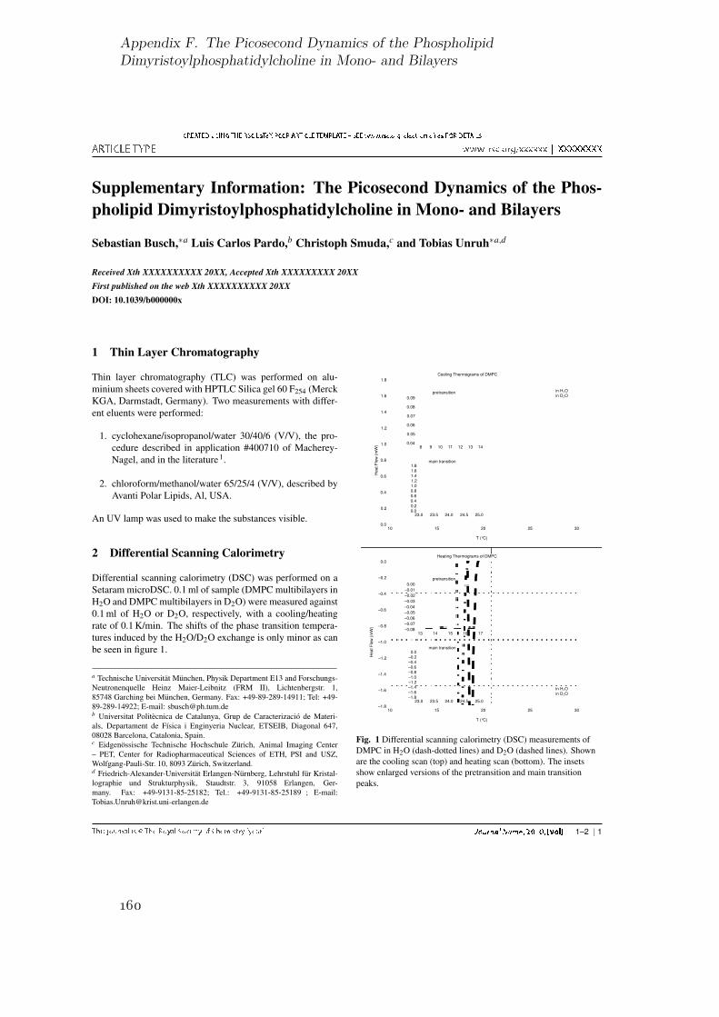
Supplementary Information: The Picosecond Dynamics of the Phos-pholipid Dimyristoylphosphatidylcholine in Mono- and Bilayers
Sebastian Busch,∗a Luis Carlos Pardo,b Christoph Smuda,c and Tobias Unruh∗a,d
Received Xth XXXXXXXXXX 20XX, Accepted Xth XXXXXXXXX 20XXFirst published on the web Xth XXXXXXXXXX 20XXDOI: 10.1039/b000000x
1 Thin Layer Chromatography
Thin layer chromatography (TLC) was performed on alu-minium sheets covered with HPTLC Silica gel 60 F254 (MerckKGA, Darmstadt, Germany). Two measurements with differ-ent eluents were performed:
1. cyclohexane/isopropanol/water 30/40/6 (V/V), the pro-cedure described in application #400710 of Macherey-Nagel, and in the literature1.
2. chloroform/methanol/water 65/25/4 (V/V), described byAvanti Polar Lipids, Al, USA.
An UV lamp was used to make the substances visible.
2 Differential Scanning Calorimetry
Differential scanning calorimetry (DSC) was performed on aSetaram microDSC. 0.1 ml of sample (DMPC multibilayers inH2O and DMPC multibilayers in D2O) were measured against0.1 ml of H2O or D2O, respectively, with a cooling/heatingrate of 0.1 K/min. The shifts of the phase transition tempera-tures induced by the H2O/D2O exchange is only minor as canbe seen in figure 1.
a Technische Universitat Munchen, Physik Department E13 and Forschungs-Neutronenquelle Heinz Maier-Leibnitz (FRM II), Lichtenbergstr. 1,85748 Garching bei Munchen, Germany. Fax: +49-89-289-14911; Tel: +49-89-289-14922; E-mail: [email protected] Universitat Politecnica de Catalunya, Grup de Caracterizacio de Materi-als, Departament de Fısica i Enginyeria Nuclear, ETSEIB, Diagonal 647,08028 Barcelona, Catalonia, Spain.c Eidgenossische Technische Hochschule Zurich, Animal Imaging Center– PET, Center for Radiopharmaceutical Sciences of ETH, PSI and USZ,Wolfgang-Pauli-Str. 10, 8093 Zurich, Switzerland.d Friedrich-Alexander-Universitat Erlangen-Nurnberg, Lehrstuhl fur Kristal-lographie und Strukturphysik, Staudtstr. 3, 91058 Erlangen, Ger-many. Fax: +49-9131-85-25182; Tel.: +49-9131-85-25189 ; E-mail:[email protected]
10 15 20 25 30
T (°C)
0.0
0.2
0.4
0.6
0.8
1.0
1.2
1.4
1.6
1.8H
eatF
low
(mW
)Cooling Thermograms of DMPC
in H2Oin D2O
8 9 10 11 12 13 140.04
0.05
0.06
0.07
0.08
0.09pretransition
23.0 23.5 24.0 24.5 25.00.00.20.40.60.81.01.21.41.61.8
main transition
10 15 20 25 30
T (°C)
–1.8
–1.6
–1.4
–1.2
–1.0
–0.8
–0.6
–0.4
–0.2
0.0
Hea
tFlo
w(m
W)
Heating Thermograms of DMPC
in H2Oin D2O
13 14 15 16 17–0.08–0.07–0.06–0.05–0.04–0.03–0.02–0.010.00
pretransition
23.0 23.5 24.0 24.5 25.0–1.8–1.6–1.4–1.2–1.0–0.8–0.6–0.4–0.20.0
main transition
Fig. 1 Differential scanning calorimetry (DSC) measurements ofDMPC in H2O (dash-dotted lines) and D2O (dashed lines). Shownare the cooling scan (top) and heating scan (bottom). The insetsshow enlarged versions of the pretransition and main transitionpeaks.
1–2 | 1
Appendix F. The Picosecond Dynamics of the Phospholipid
Dimyristoylphosphatidylcholine in Mono- and Bilayers
160

3 Calculation of the area per molecule
Spherical droplets with radius r and diameter 2r = ∅ have avolume of V = 4/3πr3, a surface of S= 4πr2, and correspond-ingly S/V = 3/r = 6/∅ ∝ 1/∅. Approximating the density ofall components with 1, the volume of spherical droplets in aunit sample volume is given by the concentration of perdeuter-ated hexadecane, [dHD]. Therefore, the surface area of theemulsion droplets in the same volume is
area ∝[dHD]
∅. (1)
As the number of DMPC molecules in the same volume isproportional to the concentration of DMPC in the sample,[DMPC], one finally arrives at
area per molecule ∝[dHD]
[DMPC] ·∅ . (2)
This number is only a relatively rough measure for thetrue value because it assumes that the emulsion droplets aremonodisperse and all DMPC molecules are adsorbed to theinterface. The formula neglects the surface area occupied byNaGC molecules because the NaGC molecules are water sol-uble and the amount of NaGC is much lower than the one ofDMPC.
4 Fit functions
The fit function used for the determination of the long-rangemotional component has been discussed in detail before2. Itis
S(Q,ω) = a ·X(Q,ω)⊗[A1(Q) ·δ (ω)+(1−A1(Q)) ·L1(Q,ω)]⊗
[A2(Q) ·δ (ω)+(1−A2(Q)) ·L2(Q,ω)] (3)
where X is discussed in the following, δ is the delta function,and L1 and L2 denote Lorentzians. The first term is caused bylong-range motions, the two latter ones by localized motions.
4.1 Flow motions
Assuming flow-like motions with a Maxwell-Boltzmann dis-tribution of the flow velocities, X is a Gaussian in ω with astandard deviation σ(Q) = v ·Q where v is the most probableflow velocity.
4.2 Diffusion
Assuming diffusion, X is a Lorentzian in ω with a half widthat half maximum Γ(Q) = D ·Q2 where D is the diffusion co-efficient.
References1 F. M. Helmy and M. H. Hack, Journal of Chromatography B: Biomedical
Sciences and Applications, 1986, 374, 61.2 S. Busch, C. Smuda, L. C. Pardo and T. Unruh, Journal of the American
Chemical Society, 2010, 132, 3232.
2 | 1–2
161


Appendix G.
FABADA: a Fitting Algorithm forBayesian Analysis of DAta
Luis Carlos Pardo, Muriel Rovira-Esteva, Sebastian Busch,María Dolores Ruiz-Martín, and Josep Lluis Tamarit
Journal of Physics: Conference Series, 325(1):012006, 2011.http://dx.doi.org/10.1088/1742-6596/325/1/012006
In this publication, the author actively participated in the development of the program.He incorporated cross-platform capability and replaced the central component of thesoftware, the random number generator, with a free and open version that was publiclyavailable. He contributed to the writing of the manuscript.
The program FABADA presented here is a Monte Carlo fit program that was used forthe model-based evaluation of the data of pure DMPC [B]. One of its advantages comparedto normal Levenberg-Marquardt algorithm used e. g. in [C, D] is that correlations betweenparameters are naturally taken into account, giving their «true» error bars.
This publication describes the general features of Bayesian fitting methods and demon-strates the versatility of the technique at several examples. The presented programfeatures also a special optimization procedure of the parameter jump values that distin-guishes it from other Bayesian fitting software [H].
Copyright 2011 by the Institute of Physics (IOP).
163
FABADA: a Fitting Algorithm for Bayesian Analysis of DAta
This article has been downloaded from IOPscience. Please scroll down to see the full text article.
2011 J. Phys.: Conf. Ser. 325 012006
(http://iopscience.iop.org/1742-6596/325/1/012006)
Download details:
IP Address: 129.187.254.46
The article was downloaded on 24/10/2011 at 15:18
Please note that terms and conditions apply.
View the table of contents for this issue, or go to the journal homepage for more
Home Search Collections Journals About Contact us My IOPscience
Appendix G. FABADA: a Fitting Algorithm for Bayesian Analysis of DAta
164

FABADA: a Fitting Algorithm for Bayesian
Analysis of DAta
L. C. Pardo1, M. Rovira-Esteva1, S. Busch2, M. D. Ruiz-Martin1,J. Ll. Tamarit1
1Grup de Caracteritzacio de Materials, Departament de Fısica i Enginyieria Nuclear, ETSEIB,Universitat Politecnica de Catalunya, Diagonal 647, 08028 Barcelona, Catalonia, Spain2Physik Department E13 and Forschungs-Neutronenquelle Heinz Maier-Leibnitz (FRM II),Technische Universitat Munchen, Lichtenbergstr. 1, 85748 Garching, Germany
Abstract. The fit of data using a mathematical model is the standard way to know if themodel describes data correctly and to obtain parameters that describe the physical processeshidden behind the experimental results. This is usually done by means of a χ2 minimizationprocedure. Although this procedure is fast and quite reliable for simple models, it has manydrawbacks when dealing with complicated problems such as models with many or correlatedparameters. We present here a Bayesian method to explore the parameter space guided onlyby the probability laws underlying the χ2 figure of merit. The presented method does not getstuck in local minima of the χ2 landscape as it usually happens with classical minimizationprocedures. Moreover correlations between parameters are taken into account in a natural way.Finally, parameters are obtained as probability distribution functions so that all the complexityof the parameter space is shown.
1. IntroductionScience is based on the success of an hypothesis to describe experimental results, i. e., is based onthe amount of “truth” and “falsity” of an hypothesis when contrasted with experimental results[1]. In order to find a quantitative method to determine this “amount of truth”, hypothesesin science should at the end be reduced to a mathematical expression depending on a set ofparameters with some physical meaning. The “amount of truth” is then determined by fittingthe mathematical model to some experimental data. To quantify that, a figure of merit χ2 canbe defined as
χ2 =n∑
k=1
(HkPi −Dk)2
σ2k
(1)
where n is the number of experimental points, Dk (k = 1, . . . , n) are the experimental data,HkPi (k = 1, . . . , n) are the values obtained from our hypothesis (the mathematical model)using the Pi (i = 1, . . . ,m) set of parameters contained in the model, m is the number ofparameters, and σk (k = 1, . . . , n) are the experimental errors associated with the respectivemeasured points Dk.
Data fitting is usually done by minimizing χ2 (equation 1) using the Levenberg-Marquardtalgorithm, which aims to find the minimum of the χ2Pi hypersurface. This fit procedure hasa twofold goal: first, to find the set of parameters Pi which best describes the experimentaldata within their errors, and second, using this set of parameters, to define a figure of merit
5th Meeting of the Spanish Neutron Scattering Association IOP PublishingJournal of Physics: Conference Series 325 (2011) 012006 doi:10.1088/1742-6596/325/1/012006
Published under licence by IOP Publishing Ltd 1
165

which quantifies the “amount of truth” of the proposed hypothesis, taking into account howwell it describes the data. In order to be able to compare different hypotheses with differentnumbers of parameters, it is reasonable to define a figure of merit which penalizes the addition
of parameters such as the reduced χ2 defined as χ2ν = χ2
n−m . In this equation, n is the number ofexperimental points and m is the number of parameters, so n −m is the number of degrees offreedom.
This way to quantify how well experimental data are described by a hypothesis is based onwhat is called a frequentist approximation of the problem [2], and has many drawbacks associatedwith both the fit procedure (it usually gets stuck in local minima of the χ2 hypersurface whenthe model is complex) and the way to quantify the correctness of the hypothesis describingexperimental data. The final result using this method is characterized by a set of parameterswith an associated error (Pk ± εk) and the figure of merit χ2
ν . This way of quantifying thebest fit to the data is based on the supposition that there is only one minimum in the χ2Pihypersurface within the data error, and that the functional dependence of χ2Pi is quadraticon each parameter i (i. e., one can stop at the second term of a Taylor expansion of the obtainedminimum), and thus allowing only symmetric errors. Moreover, errors are usually calculateddisregarding possible correlations between parameters and are thus generally underestimated.
The main difference of Bayesian inference from the previously exposed frequentist methodis the absence of any supposition on the χ2Pi landscape which will rather be explicitlyexplored taking into account experimental data. The method results in a different way toexpress fitted parameters and the figure of merit showing all the complexity of the final solution:they become Probability Distribution Functions (PDFs) obtained directly from exploring theχ2Pi hypersurface.
Although Bayesian methods are widely used in astronomy or biology [3], they are scarcelyused in condensed matter and usually for very specific tasks such as in the analysis of QENSdata [4], and the analysis of diffraction data [5, 6]. We present in this work a general methodto perform fittings and to analyze results based exclusively on probability by using Bayesianinference.
Although the presented Bayesian method is general, it is specially useful in three situations.Firstly, when the classical fitting procedure gets stuck in a local minimum of the chi squaredhypersurface, i.e. when the present parameter set does not correspond to the best obtainablefit but any small parameter value change even decreases the fit quality. This may happen forexample when fitting the intramolecular structure to diffraction data [7] but is a well knownproblem in basically every fit normally surpassed by a careful choice of the initial parametervalues. Secondly when an intricate model selection shall be performed, such as in the case ofmodels that describe molecular motions using QENS [8] or dielectric data [9]. Finally when themodel is ill defined and more than one combination of parameters is able to describe data, orwhen data only allows to limit the range of parameters but not to obtain a best fitting value[10].
2. Data analysis using the Bayesian method2.1. What is behind the ubiquitous χ2?The objective of the so called Bayesian methods [4, 14] is to find the probability that a hypothesisis true given some experimental evidence. This is done by taking into account both our priorstate of knowledge concerning the hypothesis, and the likelihood that the data is described by theproposed hypothesis. Using probability notation, and considering the case that the experimentconsists of a series of data Dk and that the hypothesis is represented by Hk, we can relate theaforementioned probabilities using the Bayes theorem [13, 14]:
P (Hk |Dk) =P (Dk |Hk)P (Hk)
P (Dk)(2)
5th Meeting of the Spanish Neutron Scattering Association IOP PublishingJournal of Physics: Conference Series 325 (2011) 012006 doi:10.1088/1742-6596/325/1/012006
2
Appendix G. FABADA: a Fitting Algorithm for Bayesian Analysis of DAta
166

Figure 1. Poisson statistics fol-lowed by data in a counting ex-periment such as a scattering one(lines), and its usual Gaussian ap-proximation (points) for an increas-ing number of expected counts. Foran increasing number of counts, thePoisson distribution (line) can beapproximated by a Gaussian func-tion (points) with σ =
√n, being
the number of counts n. The insetshows that for a number of countsas great as 100 the approximationworks quite well.
where P (Hk |Dk) is called the posterior, the probability that the hypothesis is in fact describingthe data. P (Dk | Hk) is the likelihood, the probability that our data is well described byour hypothesis. P (Hk) is called the prior, the PDF summarizing the knowledge we havebeforehand about the hypothesis, and P (Dk) is a normalization factor to assure that theintegrated posterior probability is unity. In the following, we will assume no prior knowledge(maximum ignorance prior [14]), and in this special case Bayes theorem takes the simple formP (Hk |Dk) ∝ P (Dk |Hk) ≡ L, where L is a short notation for likelihood.
In order to quantify the Bayes theorem, we need first to find the likelihood that one datapoint Dk is described by the mathematically modeled hypothesis Hk. In a counting experiment,this probability follows a Poisson distribution. It can be well approximated by a Gaussiandistribution with σ =
√Dk (see also [14]) if the number of counts is high enough as it is shown
in figure 1. Therefore for one experimental point (k = i, i = 1, . . . , n):
P (Dk=i |Hk=i) =Hk
Dk e−Hk
Dk!≈ 1
σ√2π
exp
[−1
2
(Hk −Dk
σk
)2]
(3)
Where on the right hand side of the expression it is not explicitly written that the equation isrelated to a single experimental point i = k for simplicity. The likelihood that the set of datapoints Dk is correctly described by the hypothesis Hk can be therefore written as
P (Dk |Hk) ∝n∏
k=1
exp
[−1
2
(Hk −Dk
σk
)2]= exp
[−1
2
n∑
k=1
(Hk −Dk
σk
)2]= exp
(−χ2
2
). (4)
The figure of merit χ2 is therefore related to the likelihood that the data is well describedby the hypothesis Hk. The probability theory behind χ2 also allows to deal with the case ofexperiments with only few counts where the Gaussian approximation, for which χ2 = −2 lnL,is not valid anymore and the Poisson distribution must be employed, simply by redefining χ2
[14] as
χ2 = −2 ·n∑
k=1
ln
[Hk
Dke−Hk
Dk!
](5)
5th Meeting of the Spanish Neutron Scattering Association IOP PublishingJournal of Physics: Conference Series 325 (2011) 012006 doi:10.1088/1742-6596/325/1/012006
3
167

Figure 2. Upper row: PDFs as-sociated with the center xc, am-plitude a and width w of a Gaus-sian function (solid circles) togetherwith the χ2(Pi) around its mini-mum value, fixing all parametersexcept Pi (lines). Bottom row:χ2(Pi, Pj) plots showing the corre-lation between parameters, the con-tour lines have a distance of Δχ2 =1.
2.2. The Bayesian methodThe probabilistic understanding of χ2 makes it possible to define a unique method, first to fitthe experimental data, and then to analyze the obtained results, using a Markov Chain MonteCarlo (MCMC) technique where a set of parameters P new
i is generated from an old set P oldi by
randomly changing one of the parameters, i. e., P newi = P old
i +(RND−0.5) ·2ΔPmaxi . In the last
equation ΔPmaxi is the maximum change allowed for the parameter and will be called parameter
jump for short, and RND is a random number between 0 and 1. The probability to accept thenew set of parameters is given by
P (H(P newi ) |Dk)
P (H(P oldi ) |Dk)
= exp
(−χ2
new − χ2old
2
)(6)
where χ2new and χ2
old correspond to the χ2 (as defined in equation 1) for the new and old set ofparameters. Both fitting and analysis consist therefore in the successive generation of parametersets Pi (Markov Chains) with the successive acceptations ruled by equation 6.
3. Two academic examples3.1. Fitting a GaussianIn order to test the fit algorithm, a standard function such as a Gaussian
y(x) = a/√2πw exp
[−(x− xc)
2/(2w2)]+ b (7)
was generated with the parameter set a, w, xc = 10.0, 1.0, 5.0 and being b fixed to zero. Thedata were generated with a Normal distributed error associated with each point of 0.05 andsubsequently fitted by the presented algorithm using the same formula (with b = 0).
The calculated PDFs associated with each parameter Pi are shown in the top row of figure 2together with the χ2 dependence on this parameter, calculated by varying only the parameterPi and leaving the others fixed, i. e., making a cut of the hypersurface χ2a, w, xc. As one mayexpect, the minimum of χ2 coincides with the maximum probability of each parameter PDF.
The most probable parameter values – the ones where the PDF is maximal – coincide verynicely with the original values as can be seen in the top row of figure 2. In the following,the discussion will focus on the determination of the parameter errors. There are two ways todetermine the parameter errors: (i) the commonly used definition of the error as the value ofthe parameter that increases χ2 by one unit (ΔP = |P (χ2
min)−P (χ2min +1)|) and (ii) the width
of the Gaussian associated with the PDF (the width of the Gaussian at y = e−0.5 · ymax).
5th Meeting of the Spanish Neutron Scattering Association IOP PublishingJournal of Physics: Conference Series 325 (2011) 012006 doi:10.1088/1742-6596/325/1/012006
4
Appendix G. FABADA: a Fitting Algorithm for Bayesian Analysis of DAta
168

The obtained PDFs can be well described by a Gaussian function in the present examples(solid line in the PDFs shown in figure 2). This proves that in this simple case the minimumof χ2Pi is quadratic in each parameter, and therefore the frequentist definitions of errors canbe used – the two measures of the parameter errors should coincide. The error is the defined insuch a way that Pi has a 68% probability to be within Pi − σPi and Pi + σPi (see [15]).
In figure 2 it can be seen that errors calculated from the PDFs are equal (for xc) or larger(for a and w) than those calculated using the method of incrementing χ2. This discrepancy canbe explained by parameter correlations seen in the contour plots of the two-dimensional cutsthrough the χ2(Pi, Pj) hypersurface shown in the bottom row of figure 2: from the symmetryof the contours involving xc it can be concluded that xc is independent from both, a and w,whereas these two parameters are correlated, causing the main axis of the contour ellipsoids tobe not parallel to the parameter axes. For the parameters a and w, the error calculated fromthe PDF coincides with the limits of the contour χ2 = χ2
min + 1. The error calculated from χ2
coincides with the intersection of the contour with the x axis, thus underestimating its value.Although this fact is well known in the frequentist approximation [15], to take correlations
between parameters into account would involve diagonalizing the covariant matrix. That isscarcely done and in any case is useful only in simple cases as the one presented when errors aresymmetric, i. e., when χ2Pi is quadratic in Pi. The Bayesian approach takes in a natural wayany correlation between parameters into account, and can also treat non-Gaussian PDFs beingmuch more powerful than the frequentist approximation.
3.2. Fitting with Poisson statisticsThe standard way of fitting data using the minimization of χ2 (as defined in equation 4) is nolonger valid when the number of counts is low. However, as we have seen, simply by redefiningχ2 using equation 5, we can perform the fits when the number of counts is arbitrarily low.
To test our algorithm we have generated a series of random numbers DK following a Poissondistribution around different fixed values HK . We have then fitted these series of randomlygenerated points using the usual definition of χ2, equation 4, therefore wrongly assuming thatthe numbers were generated following a Gaussian PDF (see Fig. 1) and with the definition givenin equation 5, that is, correctly assuming that DK follows a Poisson PDF around HK .
In figure 3 we show the relative discrepancy between the fitted value and the value HK used togenerate the series of points using both methods as a function of the value HK on a logarithmicscale. As expected, for HK greater than about 103 both methods yield the same result. On thecontrary for smaller values the discrepancy increases, reaching 30% for HK = 1.
It is therefore important to take into account that in the limit of low counts the usualapproximation between Poisson and Gaussian statistics should not be used. In figure 3 it isdisplayed the fit of a Gaussian function (equation 7) with parameters a, w, xc, b = 20, 5, 1, 2each point DK being generated following a Poisson distribution. The fit using Poisson statisticsis closer to the generated function, i. e., unaffected by the error, as it can be seen in the figureproving that the proposed algorithm is also useful to fit in the case of low count rates.
4. ConclusionsWe have proposed a general Bayesian method to fit data and analyze results from the fit [12].The classical frequentist approach makes some assumptions concerning the χ2 landscape: there isonly a minimum of χ2Pi able to describe data within its error, this minimum has a quadraticdependence on the parameters, and the parameters are not correlated. The here proposedmethod avoids such problems, sampling the parameter space only with the guide of probabilityrules. This method has already been successfully used to analyze experiments coming fromdiffraction experiments [16], quasielastic neutron scattering [17, 10, 8] and dielectric spectroscopy[9]. We finally summarize the main advantages of the proposed method:
5th Meeting of the Spanish Neutron Scattering Association IOP PublishingJournal of Physics: Conference Series 325 (2011) 012006 doi:10.1088/1742-6596/325/1/012006
5
169

Figure 3. (a) Discrepancy between the fits to a constant value HK set to 10i, i = 0, 1, . . . , 5using a Gaussian (empty circles) and a Poisson statistic (full circles), being DK values generatedusing a Poisson statistics. (b) Gaussian function generated assuming a low-count experiment(circles), i. e., assuming a Poisson statistics for each point. The solid line is the generatedfunction unaffected by the error, and the dashed line the fitted function. Dotted line is the fitassuming a normal distribution of errors.
The Bayesian method will not get stuck in local minima of the χ2 hypersurface during the fitprocedure if its barrier is smaller than the error associated with the experimental data set [16].
Parameters are obtained as PDFs and, because the whole parameter space is sampled,correlations between parameters are taken into account. Moreover, a natural way to defineerrors based on the PDF of parameters is obtained within this method [17, 10, 9].
The likelihood (which as we have seen is directly related to χ2) obtained by this method isalso a PDF hence revealing the whole complexity of the parameter landscape. Model selection isthen performed taking into account all parameter combinations compatible with the experiment[8].
This work was supported by the SpanishMinisterio de Ciencia e Innovacion (FIS2008-00837)and by the Catalonia government (2009SGR-1251 ). We would also like to thank helpful com-ments on the manuscript made from K. Kretschmer, T. Unruh and I. Pereyra.
References[1] Popper K R 2002 Conjectures and Refutations: The Growth of Scientific Knowledge ed. Routledge Classics[2] The frequentist description defines probability of a certain event A (P (A)) as the limiting frequency with
which the event A is observed when a great number of events A is taken into account.[3] Trotta R 2008 Contemp. Phys. 49(2) 71; Huelsenbeck J P, Ronquist F, Nielsen R and Bollback J P 2001
Science 294 5550; McVean G A T, Myers S R, Hunt S, Deloukas P, Bentley D R and Donnelly P 2004Science 304 5670; Diehl R et al. 2006 A&A 449 1025
[4] Sivia D, Carlile C J and Howells W S 1992 Physica B 182 4 341[5] Bermejo F J, Santoro J, Mompean F J and Dore J C 1988 Nucl. Instrum. Meth. Phys. Res. B, 34 505;
Bacallado S, Chodera J D and Pande V 2009 J. Chem. Phys. 131(4) 45106[6] O Gereben, P Jovari, L Temleitner, L Pusztai 2007 J. Optoelectron. Adv. Mater. 9 10 3021; Sz Pothoczki, L
Temleitner, P Jovari, S Kohara and L Pusztai 2009 J. Chem. Phys. 130 064503[7] Adyaa A K and Bianchi L 2000 J. Chem. Phys. 1129 4231; Leclercq F, Damay P, Foukani M, Chieux P,
Bellisent-Funel M C, Rassat A, Fabre C 1993 Phys. Rev. B 484 2748[8] Busch S, Smuda C, Pardo L C and Unruh T 2010 J. Am. Chem. Soc. 132(10) 3232
5th Meeting of the Spanish Neutron Scattering Association IOP PublishingJournal of Physics: Conference Series 325 (2011) 012006 doi:10.1088/1742-6596/325/1/012006
6
Appendix G. FABADA: a Fitting Algorithm for Bayesian Analysis of DAta
170
[9] Martinez-Garcia J C, Tamarit J Ll, Pardo L C, Barrio M, Rzoska S J and Droz-Rzoska A 2010 J. Phys.Chem. B 114 6099
[10] Pardo L C, Rovira-Esteva M, Busch S, Ruiz-Martin M D, Tamarit J Ll and Unruh T 2009 Bayesian Analysisof QENS data: From parameter determination to model selection Preprint arXiv:0907.3711
[11] Hastings W K 1970 Biometrika 57(1) 97[12] FABADA program (Fit Algortihm for Bayesian Analysis of DAta) can be found in
http://gcm.upc.edu/members/luis-carlos/bayesiano[13] Bayes T 1764 Phil. trans. Roy. Soc. 53 370[14] Sivia D 2006 Data Analysis: A bayesian tutorial Oxford University Press[15] Press W H, Teukolsky S A, Vetterling W T and Flannery B P 1992 Numerical Recipes in Fortran 77: the
art of scientific computing Ed. Cambridge University Press, 2nd edition[16] Rovira-Esteva M et al. Interplay of intramolecular and intramolecular structure: a Bayesian analysis To be
published[17] Rovira-Esteva M et al. 2010 Phys. Rev. B 81(9) 092202
5th Meeting of the Spanish Neutron Scattering Association IOP PublishingJournal of Physics: Conference Series 325 (2011) 012006 doi:10.1088/1742-6596/325/1/012006
7
171


Appendix H.
Fitting in a Complex χ2 LandscapeUsing an Optimized HypersurfaceSampling
Luis Carlos Pardo, Muriel Rovira-Esteva, Sebastian Busch, Jean-François Moulin,and Josep Lluis Tamarit
Physical Review E, 84(4):046711, 2011.http://dx.doi.org/10.1103/PhysRevE.84.046711
In this publication, the author actively participated in the development of the program.He tested the program and implemented several corrections and enhancements. He tookpart in the interpretation of the results and contributed to the writing of the manuscript.
In order to explore the χ2 landscape efficiently, the program FABADA [G] was providedwith the here presented optimised parameter jump sizes adaptation. A good choice of theparameter jump lengths is of utmost importance for Monte Carlo fits – if not adjusted tothe right value, for example a model selection as used for the DMPC multibilayers [B],will yield erroneous results because the χ2 hypersurface is not uniformly scanned.
Luis Carlos Pardo, Muriel Rovira-Esteva, Sebastian Busch, Jean-François Moulin,and Josep Lluis Tamarit, Physical Review E, 84(4):046711, 2011.
“Copyright 2011 by the American Physical Society.”
173

PHYSICAL REVIEW E 84, 046711 (2011)
Fitting in a complex χ 2 landscape using an optimized hypersurface sampling
L. C. Pardo,1 M. Rovira-Esteva,1 S. Busch,2 J. -F. Moulin,3 and J. Ll. Tamarit11Grup de Caracteritzacio de Materials, Departament de Fısica i Enginyieria Nuclear, ETSEIB, Universitat Politecnica de Catalunya,
Diagonal 647, 08028 Barcelona, Catalonia, Spain2Physik Department E13 and Forschungs-Neutronenquelle Heinz Maier-Leibnitz (FRM II), Technische Universitat Munchen,
Lichtenbergstr. 1, 85748 Garching, Germany3Helmholtz-Zentrum Geesthacht, Institut fur Werkstoffforschung, Abteilung WPN, Instrument REFSANS, Forschungs-Neutronenquelle Heinz
Maier-Leibnitz (FRM II), Lichtenbergstr. 1, 85748 Garching, Germany(Received 25 March 2011; revised manuscript received 12 September 2011; published 25 October 2011)
Fitting a data set with a parametrized model can be seen geometrically as finding the global minimum of theχ 2 hypersurface, depending on a set of parameters Pi. This is usually done using the Levenberg-Marquardtalgorithm. The main drawback of this algorithm is that despite its fast convergence, it can get stuck if theparameters are not initialized close to the final solution. We propose a modification of the Metropolis algorithmintroducing a parameter step tuning that optimizes the sampling of parameter space. The ability of the parametertuning algorithm together with simulated annealing to find the global χ2 hypersurface minimum, jumping acrossχ 2Pi barriers when necessary, is demonstrated with synthetic functions and with real data.
DOI: 10.1103/PhysRevE.84.046711 PACS number(s): 02.60.Pn, 02.50.Cw, 02.50.Ng, 02.50.Tt
I. INTRODUCTION
Fitting a parametrized model to experimental results is themost usual way to obtain the physics hidden behind data.However, as nicely reported by Transtrum et al. [1], this canbe quite challenging, and it usually takes “weeks of humanguidance to find a good starting point.” Geometrically, theproblem of finding a best fit corresponds to finding the globalminimum of the χ2 hypersurface. As this hypersurface is oftenfull of fissures, local minima prohibit an efficient search. Thehuman guidance consists usually of a set of tricks (dependingon every particular problem) that allow us to choose the startingpoint in this landscape such that the first minimum found isindeed the global minimum.
This problem is usually due to the mechanism that is behindclassical fit algorithms such as Levenberg-Marquardt (LM) [2]:A set of parameters Pi is optimized by varying the parametersand accepting the modified parameter set as a starting pointfor the next iteration only if this new set reduces the value ofa cost or merit function such as χ2. From a geometrical pointof view, those algorithms allow only downhill movements inthe χ2Pi hypersurface. Therefore they can get stuck in localminima or get lost in flat regions of the χ2 landscape [1]. Thismeans that they are able to find an optimal solution only ifthey are initialized around the absolute minimum of the χ2
hypersurface.The challenge of finding the global minimum can be
alternatively tackled by Bayesian methods [3,4] as demon-strated in different fields such as astronomy or biology [5],solid-state physics [6], quasielastic neutron-scattering dataanalysis [7], and reverse Monte Carlo methods [8]. We followa Bayesian approach to the fit problem in this contribution.This method is based on another mechanism to wanderaround in parameter space: Instead of allowing only downhillmovements, parameter changes that increase χ2 can also beaccepted if the change in χ2 is compatible with the dataerrors.
To do that, a Markov chain Monte Carlo (MCMC) method isused, where the Markov chains are generated by the Metropolis
algorithm [9]. However, while in the case of the LM algorithmthe initialization of parameters is critical to the convergenceof the algorithm, it is here that the tuning of the maximumparameter change allowed at each step (called parameter jumpshereafter) is what will decide the success of the algorithm tofind the global χ2Pi minimum in an efficient way.
If the parameter jumps are chosen too small, the algorithmwill always accept any parameter change, getting lost inirrelevant details of the χ2Pi landscape. If chosen too large,the parameters will hardly be accepted, and the algorithm willget stuck every now and then. Moreover, in the case of modelsdefined by more than one parameter, when parameter jumps arenot properly chosen, the parameter space can be overexploredin the direction of those parameters with too small jumplengths; in other words, the model would be insensitive tothe proposed change of these parameters. On the other hand,some other parameters can be associated to a jump so big thatchanges are hardly ever accepted.
Different schemes have been proposed in order to changeparameter jumps to explore the target distribution efficientlyusing Markov chains under the generic name of adaptiveMCMC [10]. Using the framework of stochastic approxima-tion [11] we present in this work an algorithm belongingto the group of “controlled Markov chains” [12,13] wherethe calculation of new parameter jumps takes the historyof the Markov chain and previous parameter jumps intoaccount.
Two main approaches are known that take the Markovchain history into account: adaptive Metropolis (AM) al-gorithms [14] (implemented, for example, in PyMC [15])and algorithms that use rules following the Robbins-Monroupdate [13,16,17]. In the first case, parameter jumps are tunedusing the covariance matrix at every step, so that once theadaptation is finished the algorithm should be wandering witha parameter jump close to the “error” of the parameter (definedas the variance of the posterior parameter probability densityfunction [PDF]). In some cases, this kind of algorithm [10]can get stuck if the acceptance ratio of a parameter is too
046711-11539-3755/2011/84(4)/046711(7) ©2011 American Physical Society
Appendix H. Fitting in a Complex χ2 Landscape Using an Optimized Hypersurface
Sampling
174

PARDO, ROVIRA-ESTEVA, BUSCH, MOULIN, AND TAMARIT PHYSICAL REVIEW E 84, 046711 (2011)
high or too low. In this case the Markov chain stops learningfrom the past history, and thus the optimization is stoppedwith suboptimal parameter jumps. This problem is overcomeby Robbins-Monro update rules that change parameter jumpsso that they are accepted with an optimal ratio.
The main danger of optimized Metropolis algorithms is thatadaptation might cause the Markov chain to not converge tothe target distribution anymore. In other words, the Markovchain might lose its ergodicity. For example in the case ofAM algorithms, the generated chain is not Markovian since itdepends on the history of the chain. However, as demonstratedby Haario et al. [14], the chain is able to reproduce thetarget distribution, i.e., is ergodic. In the second type ofalgorithms, the Robbins-Monro type, ergodicity propertiesmust be ensured by updating only at regeneration times [16]. Inany case, as pointed out by Andrieu et al. [10], the convergenceto the target distribution is ensured if optimization vanishes. Inother words, if parameter jumps oscillate around a fixed value,the ergodic property of the Markov chain is ensured.
The presented algorithm is based on the stochastic approachof Robbins-Monro with an updating rule inspired by the one ofGilks et al. [16]. Optimization of parameter jumps is thereforeperformed with two goals in mind:
(1) To calculate them in such a way that all parameters areaccepted with the same ratio. Adjusting parameter jumps sothat all parameter changes will have the same acceptance ratiois important to explore the χ2Pi landscape with the sameefficiency in all parameter directions.
(2) To adjust parameter jumps to a value tailored to the stageof the fit. This will turn out to be important when exploring theχ2Pi hypersurface using the simulated annealing technique[18], since this allows the parameter jumps to be optimizedto explore χ2Pi (see subsection fitting in a complex χ2
landscape): At the beginning of the fit process the algorithmwill set parameter jumps to a large value to explore largeportions of the χ2 landscape, and at the final stages theseparameter jumps will be set to small values by the samealgorithm in order to find its absolute minimum.
Geometrically, we can interpret the algorithm as setting theparameter step sizes to a value related to the hypersurface land-scape. First, it modifies the parameter jump to take into accountthe shape of the hypersurface along a parameter direction. Ifχ2Pk (the cut along a parameter k) is flat (the parameterdirection is “sloppy” following Sethna’s nomenclature [19]),the parameter step size is set to a larger value, and parameterswill move faster in this sloppy direction. On the contrary, inthe directions where the χ2Pk has a larger slope (the “stiff”direction following Sethna’s nomenclature), parameter stepswill be set to a smaller value so that they are accepted with thesame as the previous ones. Second, it modifies the parameterjumps to take the shape of the global χ2 landscape into accountwhen the simulated annealing is used. At the beginning of thefit parameter jumps will be set to a large value so that detailsof χ2Pk, i.e., local minima, will be smeared out, making iteasier to find the global minimum. However, during the laststeps of the fitting process, parameter steps will be set to a smallvalue by the algorithm so that the system will be allowed torelax inside the minimum.
The present work gives a detailed description on howthe algorithm works and is organized as follows: We first
recall briefly on the Metropolis method applied to generateMarkov chains. In the next section, the proposed algorithmto optimize the parameter step size is introduced. Then wecheck its robustness to find optimized parameter jumps usinga simple test function; and finally we test the ability of theregenerative algorithm combined with the simulated annealingtechnique to find the global minimum of χ2, even with poorinitialization values, using a simple function with a complexχ2Pi landscape. The algorithm presented in this work hasbeen implemented in the program FABADA (Fit Algorithm forBayesian Analysis of DAta) [20].
II. THE FIT METHOD
A. Fitting with the Bayesian ansatz
Fitting data using the Metropolis algorithm is based on aniterative process where successively proposed parameter setsare accepted according to the probability that these parametersdescribe the actual data, given all available evidence. Hencethis method makes use of our knowledge of the error bars ofthe data.
We now briefly recall how this can be done using aMetropolis algorithm, to proceed in the next section with thealgorithm to adjust parameter jumps.
We should first start with the probabilistic bases behind theχ2 definition. The probability P (H |D) that an hypothesis H iscorrectly describing an experimental result D is related to thelikelihood P (D|H ) that experimental data Dk (k = 1, . . . ,n)are correctly described by a model or hypothesis Hk (k =1, . . . ,n); using Bayes’ theorem [3,4],
P (Hk|Dk) = P (Dk|Hk)P (Hk)
P (Dk), (1)
where P (Hk|Dk) is called the posterior, the probability thatthe hypothesis is in fact describing the data. P (Dk|Hk) is thelikelihood, the probability that the description of the data bythe hypothesis is good. P (Hk) is called the prior, the PDFsummarizing the knowledge we have about the hypothesisbefore looking at the data. P (Dk) is a normalization factor toensure that the integrated posterior probability is unity.
In the following we will assume no prior knowledge(maximum ignorance prior [4]), and in this special case Bayes’theorem takes the simple form
P (Hk|Dk) ∝ P (Dk|Hk) ≡ L, (2)
where L is a short notation for likelihood.Although this is by no means a prerequisite, we will assume
in the following that the likelihood that every single datapoint Dk described by the model or hypothesis Hk followsa Gaussian distribution. The case of a Poisson distribution wasdiscussed previously [21]. For data with a Gaussian distributeduncertainty with width σ , the likelihood for each individualdata point takes the form
P (Dk|Hk) = 1
σ√
2πexp
[− 1
2
(Hk − Dk
σk
)2 ], (3)
046711-2
175

FITTING IN A COMPLEX χ 2 LANDSCAPE USING . . . PHYSICAL REVIEW E 84, 046711 (2011)
and correspondingly, the likelihood that the whole data set isdescribed by this hypothesis is
P (Dk|Hk) ∝n∏
k=1
exp
[−1
2
(Hk − Dk
σk
)2 ]
= exp
[−1
2
n∑k=1
(Hk − Dk
σk
)2]
= exp
(−χ2
2
). (4)
The Metropolis algorithm will in this special case consist ofthe proposition of successive sets of parameters Pi. A newset of parameters is generated changing one parameter at atime using the rule
P newi = P old
i + rP maxi , (5)
where P maxi is the maximum change allowed to the parameter
or parameter jump and r is a random number between −1.0and 1.0. The new set of parameters will always be accepted ifit lowers the value of χ2, or, if the opposite happens, it will beaccepted with a probability
P(H
P l+1
i
∣∣Dk
)P
(H
P l
i
∣∣Dk
) = exp
(−χ2
l+1 − χ2l
2
), (6)
where χ2l+1 and χ2
l correspond to the χ2 for the proposed newset of parameters and the old one, respectively. Otherwise, thisnew parameter value will be rejected, and the fit function doesnot change during this step.
The Metropolis algorithm described here is very similar tothe one used in statistical physics to find the possible molecularconfigurations (microstates) at a given temperature. In thatcase the algorithm minimizes the energy of the system whileallowing changes in molecular positions that yield an increaseof the energy if it is compatible with the temperature.
Inspired by the similarities between fitting data using aBayesian approach and molecular modeling using MonteCarlo methods, a simulated annealing procedure proposed byKirkpatrick [18] might optionally be used (see, for example,Refs. [22,23]). Following the idea of that work, the χ2
landscape might be compared with an energy landscape usedto describe glassy phenomena [24]. What we do is to startat high temperatures, i.e., in the liquid phase, where detailsof the energy landscape are not so important. By loweringthe temperature fast enough the system might fall into a localminima, i.e., in the glassy phase. In that case the system isquenched as is normally done by standard fitting methods.The presented algorithm aims to avoid being trapped inlocal minima using an “annealing schedule” as suggested byKirkpatrick. This is done by artificially increasing the errorsof the data to be fitted and letting the errors slowly relax untilthey reach their true values. Because this is very similar to whatis performed in molecular modeling, the parameter favoringthe uphill movements in Eq. (7) is usually called temperature,yielding the acceptance rule
P(H
(P l+1
i
)∣∣Dk
)P
(H
(P l
i
)∣∣Dk
) = exp
(− χ2
l+1 − χ2l
2T
). (7)
As happens with Monte Carlo simulations, increasing thetemperature will increase the acceptance of parameter sets thatincrease χ2, thus making the jump over χ2 barriers betweenminima easier.
B. Adjusting the parameter step size
The objective of tuning the parameter step size is to choosea proper value for P max
i in Eq. (5) to optimize the parameterspace exploration.
Given the total number of algorithm steps N and thenumber of steps that yield a change in χ2, i.e., the numberof successful attempts, K , the ratio R of steps yielding aχ2 change is R = K/N . Rdesired is defined as the ratio withwhich some parameter should be accepted in a step. As wewant every parameter to be changed with the same ratio,Ri,desired = Rdesired/m where m is the number of parameters.
The algorithm is initialized with a first guess for theparameter step sizes. This first guess, as will be seen shortly,is not important due to the fast convergence of the algorithmto the optimized values. The calculation of a new P max
i , i.e.,the regeneration of the Markov chain, is done after N steps,i.e., at regeneration times, through the equation
Pmax,newi = P
max,oldi
Ri
Ri,desired, (8)
where Ri is the actual acceptance ratio of parameter i. Follow-ing the previous equation, if the calculated ratio Ri/Ri,desired isequal to one, i.e., if all parameters are changing with the samepredefined ratio, P max
i will not be changed.If during the fit process a change of parameter Pi is too
often accepted, the parameter space is being overexplored withregard to parameter i. The algorithm will then make P max
i
larger in order to reduce its acceptance. The contrary happensif the acceptance is too low for a parameter: The algorithmmakes P max
i smaller to increase its acceptance ratio. Thiswill set different step sizes for each parameter, making theexploration of all of them equally efficient.
III. DEMONSTRATIONS OF FITTING FUNCTIONS
A. Fitting in a well-behaved χ 2 landscape
The optimization of the parameter step size is shown usingthe Gaussian function
y(x) = A
W√
2πexp
[− (x − C)2
2W 2
], (9)
where A is the amplitude, W is the width, and C is thecenter of the Gaussian. A function has been generated with theparameter set A,W,C = 10,1,5, and a normally distributederror with σ = 0.1 was added. A series of tests with differentinitial values for parameter jumps and different desiredacceptance ratios have been carried out (see below for details).The initial parameters for the fit were A,W,C = 2,2,2. Inall cases the algorithm was able to fit the data as can be seenin Fig. 1.
The parameter step size was adjusted every 1000 steps.Three cases are shown in Fig. 2: an initial P max
i of 10 (a verylarge jump compared to the parameter values, nearly alwaysresulting in a rejection of the new parameters) and an Rdesired
046711-3
Appendix H. Fitting in a Complex χ2 Landscape Using an Optimized Hypersurface
Sampling
176

PARDO, ROVIRA-ESTEVA, BUSCH, MOULIN, AND TAMARIT PHYSICAL REVIEW E 84, 046711 (2011)
FIG. 1. (Color online) Circles: Generated Gaussian function totest the algorithm with the parameters A,W,C = 10,1,5. Dashedline: Starting point for all performed tests (A,W,C = 2,2,2).Solid line: Best fit, i.e., minimum χ 2 fit, of the Gaussian function.
of 66%, the same P maxi with an Rdesired of 9% and finally a
P maxi of 10−4 (a very small jump compared to the parameter
values, resulting in a slow exploration of the parameter space)and an Rdesired of 9%. It can be seen that the algorithm managesin all these extreme cases to adapt the jump size quickly andreliably in order to make R equal to Rdesired.
In Fig. 3 we show the three individual acceptance ratios Ri
for the different parameters as a function of the fit steps fordifferent initialization values of the parameter jumps Pi ,for different values of Rdesired, and setting the number ofsteps to recalculate parameter jumps N to 1000. When thetotal acceptance ratio is set to Rdesired = 66% (solid line), thealgorithm is able to change all parameter jumps [see Fig. 3(b)],making the acceptance ratio Ri of every parameter equal toRdesired/m = 22% and thus the total acceptance ratio R to66%. The same happens if the acceptance is set to 9%: Thealgorithm finds the parameter step sizes [see dashed line inFig. 3(b)], which yield a total acceptance ratio of 9% withinthe first 5000 steps, no matter how the parameter step sizeswere initialized.
To explicitly show how this is linked with the geometricalfeatures of the χ2 landscape, the inset of Fig. 3(b) shows acut of the χ2 hypersurface along parameters A and C, leavingparameter W fixed to its best fit value WBF. As can readilybe seen, the χ2A,C,W = WBF hypersurface is sloppy in the
FIG. 2. Total acceptance ratio R as a function of the numberof steps when Rdesired is set to 66% and 9% (solid and dashed ordotted lines). In the second case (Rdesired = 9%), dashed and dottedlines represent the values of R as a function of algorithm step fortwo different parameter step size initializations (P max
i = 10 andP max
i = 10−4, respectively).
( ) ( )
FIG. 3. (Color online) (a) Acceptance ratio Ri for parametersA, W , C involved in the fit of the Gaussian following Eq. (9) (redtriangles, green squares, and blue circles, respectively) when Rdesired
is set to 66% and 9% (solid and dashed lines). (b) Parameter step sizeas a function of the number of steps (line and symbols code as inpanel a). The inset shows a cut through the χ 2 hypersurface along A
and C directions fixing W to the best-fit value.
direction of parameter A and stiff in the direction of parameterC. The algorithm has thus correctly calculated a parameterstep size that is larger for A than for C, along whose directionthe χ2 well is narrower. This fact makes the final parameterstep sizes proportional to the errors of each parameter—ifthe global minimum is not multimodal and is quadratic in allparameters, and those are not correlated.
In order to show the robustness of the algorithm, we havealso made disparate initial guesses for parameter step sizesP max
i about three decades below the correct acceptance ratio,setting Rdesired = 9%. As displayed in Fig. 3, after about 5000steps the acceptance ratio R (N is again 1000 steps) has alreadyreached the desired value. It can be seen in Fig. 4(a) that theacceptance ratio for each parameter reaches again the valueRdesired/m = 3% and parameter step sizes are virtually equalto those obtained previously as shown in Fig. 4(b).
To stress the relevance of the aforementioned algorithmto explore the parameter space correctly, thus ensuring itsconvergence, we have calculated the normalized χ2PDF inall tested cases. As can be seen in Fig. 5, the χ2 PDF after105 steps matches the χ2 distribution
P (χ2) ∝ (χ2)(
m2 −1
)exp
(−χ2
2
), (10)
FIG. 4. (Color online) (a) Acceptance ratio Ri for parameters A
(triangles), W (squares), C (circles) involved in the fit of the Gaussianfollowing Eq. (9) when initial parameter step sizes are set to Pi =10 (dashed line) and Pi = 10−4 (dotted line). (b) Parameter stepsize as a function of the number of steps (lines and symbols as inpanel a).
046711-4
177

FITTING IN A COMPLEX χ 2 LANDSCAPE USING . . . PHYSICAL REVIEW E 84, 046711 (2011)
FIG. 5. (Color online) The dashed line represents a χ2 distribu-tion for three parameters, i.e., m = 3 (see text for details). Solidline is the obtained PDF associated to χ2 when calculated for105 steps. Circles represent the same distribution when calculatedusing only 104 steps. The inset shows the χ 2 PDFs when calculatedwith parameters allowed to change with Pi = 10−4, Pi = 10,P = 0.1Pi . Successive PDFs are displaced on the ordinate axis forclarity of the figure.
with m = 3 as expected [2]. In Fig. 5 we show the χ2 PDFobtained after 104 steps for different cases: first, setting P max
i
equal to the value calculated by the algorithm and, second,setting P max
i equal to the initial guess, and finally to a value,calculated a posteriori, which is proportional to the best-fitparameters P max
i = 0.1Pi (inset of Fig. 5)As can be seen in Fig. 5, when P max
i is set much higherthan the optimal step sizes, the Metropolis algorithm scans thewhole parameter space Pi, but jumping between disparateregions with very different values of χ2, therefore with alow acceptance rate of new parameter sets (dashed line inFig. 5). This causes a poor exploration of parameter space. Incontrast, a small value overexplores only a restricted portion ofPi, falling very often in local minima of the parameter space(dotted line in the same figure). Also choosing parameter jumpsproportional to the final parameters leads to a poor explorationof parameter space (solid line in the same figure). Finally, afterthe same number of steps, when using the optimized parameterstep sizes obtained by the algorithm the χ2 PDF follows thetheoretical expectation, meaning that the parameter space iscorrectly sampled.
B. Fitting in a complex χ 2 landscape
As pointed out before, one of the main problems whendealing with data fitting using the LM algorithm is to finda proper set of initial parameters close enough to the globalminimum of the χ2Pi hypersurface. As an example we showin Fig. 6 the function sin(x/W ) for W = 5 affected by a normaldistributed error with σ = 0.1. In Fig. 7(a) we show the χ2W landscape associated to the generated function. As can be seen,the χ2W landscape for this function has a great numberof local minima and a global minimum at W = 5. We havefitted the function using the LM algorithm and initializing theparameter at Wi = 2 and Wi = 15 (see Fig. 6). As expected,both fits were not able to find the global minimum that fits
FIG. 6. (Color online) Synthetic sin(x/5) function (circles)together with the best fit using parameter step sizes tuning togetherwith simulated annealing (line). Dashed lines are the fits using theLM algorithm with starting parameters Wi = 2 and Wi = 15.
the function. In fact, only if the LM algorithm is initializedbetween W = 3.6 and W = 9.0 is it able to succeed in fittingthe data.
We now test the ability of our algorithm to jump acrossχ2 barriers delimiting successive local minima to find theglobal one. For this task we have used the simulated annealingmethod, decreasing the temperature one decade every 3000steps from T = 1000 to 1. The parameter jump calculationhas been performed every N = 1000 steps. While the initialtemperature allows to explore wide regions of the parameterspace, the last temperature will let the acceptance be deter-mined only by the real errors of the data.
In Fig. 7(b) we show the parameter W as a functionof algorithm step for the two aforementioned initializationstogether with the χ2 landscape (a). Parameter step sizes wereinitialized after a first run of optimization of 2000 steps. As canbe seen in this figure, after 3000 steps both runs have alreadyreached the absolute χ2 minimum. Successive steps just relaxthe system to the final temperature T = 1.
FIG. 7. (Color online) (a) χ 2W landscape obtained for thefunction sin(x/W ) with a normal error associated of σ = 0.1 (seeFig. 6). (b) Algorithm steps for two different initializations, blacksolid line for Wi = 2 and red dashed line for Wi = 15, as a functionof parameter W.
046711-5
Appendix H. Fitting in a Complex χ2 Landscape Using an Optimized Hypersurface
Sampling
178

PARDO, ROVIRA-ESTEVA, BUSCH, MOULIN, AND TAMARIT PHYSICAL REVIEW E 84, 046711 (2011)
As it can be seen in Fig. 7, the way the minimum is reacheddepends on the parameter initialization. Parameter step sizesare larger for the run started with Wi = 15 with a flat localminimum. The contrary happens with the run initialized atWi = 2, parameter step sizes are set small due to the narrowwells of the χ2 landscape in this region. However, both runsare able to avoid getting stuck in local minima, jumping overrather high χ2 barriers and successfully reaching the best fit.
IV. CONCLUSION
Classical fit schemes are known to fail when the parametersare not initialized close enough to the final solution. We haveproposed in this work to use an Adaptive Markov ChainMonte Carlo Through Regeneration scheme, adapted fromthat of Gilks et al. [16], combined with a simulated annealingprocedure to avoid this problem.
The proposed algorithm tunes the parameter step size inorder to assure that all of them are accepted in the sameproportion. Geometrically the parameter step size is set largewhen a cut of χ2Pi along this parameter is flat, i.e., whenthe change of the χ2Pi hypersurface along this parameter issloppy. Similarly the parameter step size is set small if χ2Piwells are narrow.
Moreover, the step sizes can be modulated by a temperatureadded to the acceptance equation that makes jumps across χ2
barriers easier, i.e., using a simulated annealing method [18].From a geometric point of view, a high temperature makes theχ2Pi wells artificially broader, smearing out details of localminima. This is important at the first stages of a fit process.
At final stages of the fitting, temperature is decreased, makingparameter jumps smaller, and thus allowing the system to relax,once it is inside the global minimum.
By fitting simulated data including statistical errors weverified that our algorithm actually fulfills the requirementsof ergodicity (it converges to the target distribution), ro-bustness (the ability to reach the χ2 minimum independentof the choice of starting parameters), and ability to escapelocal minima and to explore efficiently the χ2 landscapeand guarantees that it will self-tune to converge to theglobal minimum avoiding an infinite search with largesteps.
More complex problems have already successfully beenstudied with this algorithm such as model selection usingquasielastic neutron-scattering data [25], nonfunctional fitsin the case of dielectric spectroscopy [26], or finding themolecular structure from diffraction data with a model definedby as many as 27 parameters [27]. In the last case, the properinitialization of parameters to use a LM algorithm would havebeen a difficult task, made easy by the use of the presentedalgorithm.
ACKNOWLEDGMENTS
This work was supported by the Spanish Ministry of Sci-ence and Technology (FIS2008-00837) and by the Cataloniagovernment (2009SGR-1251). We would also like to thankhelpful comments and discussions on the manuscript madefrom K. Kretschmer, Anand Patil, Christopher Fonnesbeck,and A. Font.
[1] M. K. Transtrum, B. B. Machta, and J. P. Sethna, Phys. Rev.Lett. 104, 060201 (2010).
[2] W. H. Press, S. A. Teukolsky, W. T. Vetterling, and B. P.Flannery, Numerical Recipes in Fortran 77: The Art of ScientificComputing, 2nd ed. (Cambridge University Press, CambridgeUK, 1992).
[3] T. Bayes, Philos. Trans. R. Soc. Lond. 53, 370 (1764).[4] D. Sivia, Data Analysis—A Bayesian Tutorial (Oxford
University Press, Oxford, 2006).[5] R. Trotta, Contemp. Phys. 49, 71 (2008); J. P. Huelsenbeck,
F. Ronquist, R. Nielsen, and J. P. Bollback, Science 294, 2310(2001); G. A. T. McVean, S. R. Myers, S. Hunt, P. Deloukas,D. R. Bentley, and P. Donnelly, ibid. 304, 581 (2004); R. Diehlet al., Astron. Astrophys. 449, 1025 (2006); A. N. Naganathan,R. Perez-Jimenez, V. Munoz, and J. M. Sanchez-Ruiz, Phys.Chem. Chem. Phys. 13, 17064 (2011).
[6] J. J. Mortensen, K. Kaasbjerg, S. L. Frederiksen, J. K. Norskov,J. P. Sethna, and K. W. Jacobsen, Phys. Rev. Lett. 95, 216401(2005); F. J. Bermejo, J. Santoro, F. J. Mompean, and J. C. Dore,Nucl. Instrum. Meth. Phys. Res. B 34, 505 (1988); S. Bacallado,J. D. Chodera, and V. Pande, J. Chem. Phys. 131, 045106(2009).
[7] D. Sivia, C. J. Carlile, and W. S. Howells, Physica B 182, 341(1992).
[8] R. L. McGreevy and L. Pusztai, Molec. Simul. 1, 359 (1988); L.Pusztai, J. Non-Cryst. Sol. 227–230, 88 (1998); R. L. McGreevy,
J. Phys. Condens. Matter 13, R877 (2001); G. Evrard and L.Pusztai, ibid. 17, S1 (2005); O. Gereben, P. Jovari, L. Temleitner,and L. Pusztai, J. Optoelectron Adv. M 9, 3021 (2007).
[9] N. Metropolis, A. Rosenbluth, M. Rosenbluth, A. Teller, andE. Teller, J. Chem. Phys. 21, 1087 (1953); W. K. Hastings,Biometrika 57, 97 (1970).
[10] C. Andrieu and J. Thoms, Stat. Comput. 18, 343(2008).
[11] A. Benveniste, M. Metivier, and P. Priouret, Adaptive Algorithmsand Stochastic Approximations (Springer, Berlin, 1990).
[12] V. S. Borkar, Topics in Controlled Markov Chains (Longman,Harlow, 1990).
[13] C. Andrieu, and C. P. Robert, Tech. Rep. 0125, Cahiersde Mathematiques du Ceremade, Universite Paris-Dauphine(2001).
[14] H. Haario, E. Saksman, and J. Tammien, Bernouilli 7, 223(2001).
[15] A. Patil, D. Huard, and J. F. Christopher, J. Stat. Soft. 35, 1(2010).
[16] W. R. Gilks, G. O. Roberts, and S. K. Sahu, J. Am. Stat. Assoc.93, 1045 (1998).
[17] H. Robbins and S. Monro, Math. Stat. 22, 400 (1951).[18] S. Kirkpatrick, J. Stat. Phys. 34, 347 (1984).[19] J. J. Waterfall, F. P. Casey, R. N. Gutenkunst, K. S. Brown,
C. R. Myers, P. W. Brouwer, V. Elser, and J. P. Sethna, Phys.Rev. Lett. 97, 150601 (2006).
046711-6
179

FITTING IN A COMPLEX χ 2 LANDSCAPE USING . . . PHYSICAL REVIEW E 84, 046711 (2011)
[20] FABADA program (Fit Algorithm for Bayesian Analysis ofDAta) can be found at http//fisicaetseib.upc.es/gcm/members/lcpardo/software.
[21] L. C. Pardo, M. Rovira-Esteva, S. Busch, M. D. Ruiz-Martın,and J. Ll. Tamarit, in J. Phys.: Conf. Ser., Conference Proceedingof the Spanish Neutron Scattering Society Meeting 2010; L. C.Pardo, M. Rovira-Esteva, S. Busch, M. D. Ruiz-Martın, J. Ll.Tamarit, and T. Unruh, e-print arXiv:0907.3711.
[22] J. J. Mortensen, K. Kaasbjerg, S. L. Frederiksen, J. K. Nørskov,J. P. Sethna, and K. W. Jacobsen, Phys. Rev. Lett. 95, 216401(2005).
[23] J. S. Schulte, Phys. Rev. E 53, R1348 (1996).
[24] P. G. Debenedetti and F. H. Stillinger, Nature (London) 410, 259(2001).
[25] M. Rovira-Esteva et al., Phys. Rev. B 81, 092202 (2010); S.Busch, C. Smuda, L. C. Pardo, and T. Unruh, J. Am. Chem.Soc. 132, 3232 (2010).
[26] J. C. Martinez-Garcia, J. Ll. Tamarit, L. C. Pardo, M. Barrio,S. J. Rzoska, and A. Droz-Rzoska, J. Phys. Chem. B 114, 6099(2010).
[27] M. Rovira-Esteva, N. A. Murugan, L. C. Pardo, S. Busch, J. Ll.Tamarit, Sz. Pothoczki, G. J. Cuello, and F. J. Bermejo, Phys.Rev. B 84, 064202 (2011).
046711-7
Appendix H. Fitting in a Complex χ2 Landscape Using an Optimized Hypersurface
Sampling
180

Part III.
Additional Information
181


Appendix I.
Details of the Data ReductionThis chapter lists several programs that can be used for the data reduction. The one usedin this thesis, Frida 1, will be introduced in more detail and all the errors in the programthat were found during the course of this thesis are listed. A new data reduction programthat was developed by the author of this thesis is advertised and the algorithm which isused for the reduction of quasielastic time-of-flight neutron scattering data is described.The chapter finishes with a presentation of the concept of an effective scattering crosssection that can be used in conjunction with existing programs to make a zeroth-ordercorrection of multiple scattering until a dedicated program for that purpose is available.
I.1. Data Reduction SoftwareOverview over Existing Programs. The standard data reduction and evaluation toolused at TOFTOF is the program Frida 1 [269]. It was started in 1990 by Wuttke, is writtenin Fortran and uses a proprietary library and compiler. These facts make it harder andharder to maintain and distribute it. Despite its age, it is however still used at severalneutron sources and user groups around the world. It was even very recently ported towork with the Intel Fortran compiler.1
Although in use for over 20 years, there are still many errors in the algorithms.Most of them become visible only due to the high accuracy and versatility of today’sinstrumentation. As Frida 1 will probably stay the standard data reduction software onTOFTOF in the near future, a detailed list of bugs which were found during the course ofthis thesis is given below.
Most of the problems encountered during the data evaluation for this thesis could besolved within the existing program. However, taken together with the dated programminglanguage, compiler, and libraries, it became clear that a completely other alternativemust be found. In order to facilitate experiments on single crystals with TOFTOF, thesoftware should also have additional capabilities, for example reading only the detectorsin the horizontal scattering plane.
There are a few alternative programs which are potentially capable of reducing thetime-of-flight data, the most important ones being
1Triggered by Gerald Schneider, Jülich Center for Neutron Science, 2011
183

Appendix I. Details of the Data Reduction
TOFSYS (Jülich) which has similar age-related problems as Frida 1. It has aninterface to DISCUS, a multiple scattering simulation program.
DATREAT (Jülich) is still in use, also at the JCNS, but suffers from similar problemsthan Frida 1 and TOFSYS.
DAVE (NIST) has no read-in routine for TOFTOF data. Its features, especially regard-ing the data analysis, are limited so that it seems questionable if the implementationof a better interoperability is desirable.
LAMP (ILL) can be used with TOFTOF data only since 2009.
In conclusion, none of the existing programs could fulfil the requirements at TOFTOF atthe beginning of this thesis, LAMP should now be critically evaluated. This situation iscommon with many other neutron scattering instruments in the moment which triggeredthe start of development of two data reduction and analysis frameworks which are bothin relatively early stages of development but aim both to become universal tools acrossinstitutes:
The Mantid Project (initiated by ISIS, recently joined by the SNS and HFIR).
slaw (JCNS, Joachim Wuttke) for data reduction, can be combined with e. g. Frida 2(JCNS, Joachim Wuttke) for the data evaluation.
Although both of these projects are promising to offer a modern way of data reductionand analysis and one of them or both will probably become standard at TOFTOF at somepoint in the future, they are both not ready yet. As LAMP was not capable of workingwith TOFTOF data when this thesis was started, the data reduction procedures wereimplemented in a new program which can serve as a replacement for Frida 1 until a newstandard is agreed on.
Errors in Frida 1. The following is a list of errors that were found during the courseof this thesis. There is no central, updated version of the program but many differentcopies in different institutes which grew apart over time. It is therefore not possible tocorrect these mistakes in the copies at different institutes, every user of the program isurged to check if these errors are corrected in his or her version.
The normalization to the incident beam monitor does not account for its wavelength-dependent sensitivity.
The detector sensitivities are calibrated by the elastic scattering of a vanadiumstandard. For this purpose, the area under the elastic peak of the vanadiumspectrum is integrated and stored in a variable that contained the maximum ofthe peak before. This value was used to detect bad detectors where the peak valueor position deviates from the mean. If such a deviation is found, the detector isdeleted and the procedure is restarted with an updated mean value. However, thevariable that contained the peak maximum now contains the area.
184

I.1. Data Reduction Software
When reading the data from TOFTOF, the routine offers to subtract a backgroundmeasurement right away. If the background signal happens to be stronger than theone of the sample, e. g. due to absorption, the data error bars are calculated toosmall by a factor 2.2
The conversion of the time of flight of the neutrons to energy transfer necessarilyassumes that the neutrons arrive during the same frame at which they started atthe sample. If this is not the case, i. e. if the repetition rate is set so high that newneutrons start before the ones of the previous pulse arrive at the detectors, thisconversion gives completely wrong results.
For the determination of the position of the time channel of the arrival of theelastically scattered neutrons, the program searches the maximum of the arrivingneutrons. If this maximum happens to be an inelastic feature (very hot samples),this point is assumed to correspond to zero energy transfer.3
Even if inelastic features play no significant role, this mode of peak determinationcan be faulty. The conversion from time of flight to energy transfer involvesmultiplying the data with a factor t−3, cf. section 4.1. If the peak is δ shaped,that does not shift its position. However, a broadened peak will not have thesame maximum position for counts (time of flight), double differential cross section(energy transfer), or scattering function (energy transfer). It is therefore necessaryto determine the time-of-flight of elastically scattered neutrons such that themaximum of the scattering function (taking the detailed balance into account) isat zero energy transfer.
Adding spectra of detectors can cause uncontrollable shifts of the elastic peakposition. If S(Q, ω) is produced, this error can be circumvented by not adding thespectra of different detectors before the conversion to Q and rebinning into slicesof constant momentum transfer.
If several detectors are at the same scattering angle (as it is the case at TOFTOF),it is not possible to normalize them by hand because the program tries to identifythe detectors by their angle and does not rely on their order.
That this cautionary measure has actually a justification becomes clear when tryingto perform calculations involving one file loaded from TOFTOF and another oneread in from the hard disk: Due to internal re-structuring of the data during thesave and read process, this operation fails.
The self absorption correction routine asks for the sum of coherent and incoherentscattering cross section. This is misleading as not the sum of the tabulated valuesof the scattering cross sections have to be used but the «effective scattering crosssection» as described in detail in appendix I.3.
2This was not discovered by the author but by Jonas Okkels Birk, Niels Bohr Institute, Copenhagen.3This was not discovered by the author.
185

Appendix I. Details of the Data Reduction
0 40 80 1200.9350
0.9375
0.9400
0.9425
0.9450
2θ
Assc
20/20 radial/angular meshes40/40 radial/angular meshes60/60 radial/angular meshes
Figure I.1.: The factor calculated for theself absorption correction depends onthe parameters chosen for the numer-ical calculation. The standard values20/20 for the radial and angular meshes,respectively, show very big oscillationswhich gets smaller with an increasingnumber of meshes. Also the averagevalue changes when changing the set-tings but in contrast to the oscillationsit does not shift monotonously.
The self absorption correction routine returns a result that has two problems whichare a function of the choice supposedly only internal variables (number of radialand angular meshes). The first issue is the oscillation of the calculated value whichdecreases with increasing mesh numbers, the second the discontinuous shift of theabsolute value by the choice of the meshes as demonstrated in figure I.1.Additionally to that, this routine regards all neutrons which are multiply scatteredas not counted. However, these neutrons are counted, although not at the expectedenergy and momentum transfer. As the scattering cross sections of all the regardedsamples are larger than the absorption cross sections, this effect is actually the moreimportant one to correct but is not accounted for. The self absorption correctionshould therefore be replaced by a comprehensive treatment of absorption andmultiple scattering.
The transformation of the data from the recorded spectra at constant scatteringangle to spectra at constant modulus of the scattering vector yields data error barswhich are too large by approximately one order of magnitude.4 This is alreadyobvious when looking at the data because the statistical noise is much less thanthe error bar and prohibits any extractable information from the reduced χ2.
The Voigt function, the convolution of a Gaussian and a Lorentzian, is implementedusing a tabulated function [270] but called wrongly, yielding wrong line width andarea under the curve. Using the definitions
G(x) = 1√2πσ· exp
[−1
2
(x− c
σ
)2]
(I.1)
and
L(x) = 1π· Γ
(x− c)2 + Γ2 , (I.2)
4This was not discovered by the author but by Björn Fåk, CEA INAC SPSMS, Grenoble
186

I.1. Data Reduction Software
their convolution is approximated using the tabulated function K(a, b) [270]:
(G⊗ L)(x) = 1√2π · σ
·K(a, b) (I.3)
where a and b have to be
a = x− c√2σ
and b = Γ√2σ
. (I.4)
The resulting function fulfills the checks to have (i) an area of 1 (within 1%) and(ii) a full width at half maximum of 3.6 with the following combinations of (σ, Γ):(0, 1.8), (0.01, 1.8), (1.0, 1.0), (1.3, 0.5), (1.53, 0.01), (1.53, 0).
Plotting functions that are convolved online with a vanadium measurement asresolution function have sometimes wild oscillations which is obviously wrong.However, also when looking reasonable, they are often wrong, in all observed casesbeing plotted too low. This does not occur when the convolution is performedexplicitly.
The error bars of the fitted parameters can be corrected for correlations betweenthe parameters by diagonalizing the covariance matrix. This is attempted but theoutput of the corresponding routine is processed wrongly, multiplying with thedouble of the reduced χ2 which the routine does already. As the reduced χ2 is toosmall due to the wrong data error bars (see above), the parameter error bars arecalculated too small.
When calculating the average value of N values yi with error bars ∆yi, the averagevalue y is calculated correctly as
y =N∑
i=1
yi
N(I.5)
but the error bar of the averaged value ∆y is calculated as5
∆y =
√√√√ N∑i=1
∆y2i
N(I.6)
instead of
∆y =
√∑Ni=1 ∆y2
i
N. (I.7)
5This was discovered in collaboration with Humphrey Morhenn, FRM II, Technische UniversitätMünchen, Munich
187

Appendix I. Details of the Data Reduction
The new neutron time-of-flight scattering data reduction library sihl. An object-oriented library for the data reduction of time-of-flight neutron scattering data, namedsihl [271], has been implemented in Python 2.5 based on the packages scipy [272], thealso self-written chaste [273], and optionally matplotlib [274]. Whereas the scipy andmatplotlib are standard Python libraries, chaste is a self-written collection of tools tohandle data with error bars, it makes for example sure that the error bars are correctlypropagated during addition etc.
chaste introduces a general class for variables, Var, that is the parent for the fivetypes of variables that can be found in a typical experiment: AddVar is normally thedependent variable of a measurement that must be e. g. be added when adding differentmeasurements, propagating the error bar. EquVar is normally the independent variableof the measurement – in order to add two measurements, these values must be equal.Apart from these, there are values like the temperature that must be averaged whentwo measurements are added, AvgVar, values that can exist only once like the name orstarting time, WinVar, and a history of data manipulations in a LogVar.
Most experiments are performed in a series of varying x and measuring the corre-sponding y values. Such a series can have a further independent variable, called z. Itis represented in the Dataset class which in turn can be combined with other Datasetsinto measurements of y as a function of x and z in the class Data.
sihl is the specialization of these concepts for neutron scattering measurements. While aDetector inherits from Dataset as it contains for example counts as a function of time-of-flight, the result of many Detectors is combined in a Measurement which correspondinglyinherits from Data.
A Measurement contains algorithms needed at all spectrometers, for example normal-ization to the monitor counts. This is then further specialized in TofMeasurement whichinherits from Measurement and adds time-of-flight specific capabilities, for examplethe conversion from time-of-flight to energy transfer. ToftofMeasurement inherits fromTofMeasurement, adding TOFTOF specifics, for example reading the TOFTOF data fileformat.
These packages are now ready for active use and are already employed for datatreatment in the soft matter group at TOFTOF. However, the measurements presented inthis thesis were still reduced with the old Frida 1.
I.2. Data Reduction ProcedureIn any data reduction program, a certain procedure is followed which varies only slightlybetween the different programs. In the following, the procedure implemented in sihl isdescribed in detail.
188

I.2. Data Reduction Procedure
Basic operations on all TOFTOF measurements.
One measurement is often distributed over several files. Read all TOFTOF data filesthat contain the measurement. Take the sum of the counts of the different files –as if a single long measurement would have been performed.
Delete the signal of detectors which are not installed.
For powder samples: take the absolute value of the scattering angle.
Sort the detectors by increasing scattering angle.
Set error bars for all detectors and the monitor to the square root of the numberof counts in the respective detector – if no neutron was counted, set the error barto 1. It should be noted that the use of Gaussian statistics is in this case is notjustified [G]. Luckily, the signals that are evaluated in practice are much strongerbecause using Poisson statistics would not only complicate the error propagationvery much but would also require different approaches to fitting the data [G].
Divide the counts in the detectors by the one in the monitor, propagating the errorbar and respecting the wavelength-dependence of the monitor efficiency.
Delete all channels in the frame which are empty, as described in section 3.2.
Multiply the last channel which was only partially filled to get a measure for thenumber of neutrons it would have seen if the instrument had filled it the same timeas the others. This procedure has the advantage over deleting this channel whenchannels are moved from one end of the frame to the other that there is no gapbetween two channels.
If the time-of-flight of the elastically scattered neutrons is longer than the totallength of the frame, add the total number of channels in the frame to each framenumber until the elastic peak is within the frame.
Convert the channel numbers to time-of-flight by multiplying the channel numberwith the length of one channel (which is given by the instrument in units of 50 ns).
It is practical to avoid that the first channel has a time-of-flight of zero becausethis translates into an infinitely large energy. Therefore, the first couple of channelsare moved to the end of the frame.
Convert the time-of-flight tof to energy transfer dE. Using the length of thesecondary spectrometer l = 4 m, the tof-axis is changed according to
dE = Ef − Ei = 12mn
l2
tof2− 1
2mnl2
tof(elastic)2 . (I.8)
189

Appendix I. Details of the Data Reduction
Because the scattering function is a density in energy (as discussed in section 2.1,this can be seen on the unit which is energy-1), the intensity axis has to be changedwith
d2σ
dΩ dE= d2σ
dΩ dtof ·dtofdE
(I.9)
anddE
dtof = mnl2
tof3. (I.10)
Sort the channels by increasing energy transfer.
Correct the energy-dependence of the detector efficiency using the formula andTOFTOF-specific parameters [211].
Optional: Apply the detailed balance correction.
Optional: Subtract the scattering of the container.
At this point, the double differential cross section d2σ/d(2θ) dE would be obtained ifthe detectors were calibrated on an absolute scale. They are not, making the normalisationto an isotropic scatterer, often vanadium, necessary.
Correcting the detector sensitivities.
Read the vanadium data and treat as described above.
Integrate the elastic line, correct this number with the Q-dependent Debye-Wallerfactor and save it per detector. Alternatively, it is possible to integrate the intensityscattered at the same Q over all E. However, in this case the intensity that isscattered into the theoretically accessible but practically uncovered dynamicalrange (cf. figure 3.9) is lost.
Normalize the detector sensitivity by dividing the spectrum of every detector bythis number.
The result is the double differential cross section d2σ/d(2θ) dE up to a scaling factordue to the normalization to the vanadium standard.
Option 1: Calculating the diffraction pattern.
Integrate the double differential cross section over all energies, resulting in thedifferential cross section dσ/dΩ(2θ) up to the aforementioned scaling factor.
This diffraction pattern is very similar to the differential cross section dσ/dΩ that ismeasured at dedicated diffractometers which do not analyze the energy of the neutronsafter the scattering event. When measured at a diffractometer, Plazcek corrections canbe used to account for the energy-dependent sensitivity of the detectors [160] – this effectis already corrected in the TOFTOF data as described above.
190

I.2. Data Reduction Procedure
Figure I.2.: The trajectory of detectors atTOFTOF in Q-ω-space, using an incidentwavelength of 6 Å. Shown are representa-tive detectors with an equidistant spac-ing of 10° starting at the first detectorwhich has a scattering angle of 7.6°. Theenergy transfer is shown in the quasi-elastic region of ±1 meV. The compres-sion at large values of Q brings aboutthat the angular range between 140° and180° corresponds only to a relativelysmall area in Q-ω-space. This is alsovisible in figure 3.9 which gives a biggeroverview of the dynamical range.
-1.0 -0.5 0.0 0.5 1.00.0
0.5
1.0
1.5
2.0
ω (meV)
Q(2
θ,ω
) (A
-1)
What is not corrected is the Lorentz factor – because it is different for coherent andincoherent scattering. The corresponding signals would need to be separated before thiscorrection. The reason is that incoherent scattering results in equal intensity in equaldΩ. Because all detectors have the same size and are at the same distance l = 4 m fromthe sample, no correction factor is needed. Coherent scattering of powder samples isdistributed on Debye-Scherrer cones and therefore on different lengths U depending onthe scattering angle 2θ:
U = 2πr = 2πl sin(2θ) . (I.11)The coherent scattering signal would need to be divided by this number. As the intensitiesof the Bragg peaks are not evaluated, this correction was not performed.
It can be seen in figure I.2 that this integration of intensities at a fixed scattering angle2θ does not integrate intensities at a fixed Q. The transformation from the obtaineddσ/dΩ(2θ) via the Bragg equation
Q = 4π
λsin
(2θ
2
)(I.12)
to an dσ/dΩ(Q) is therefore not correct. This was nevertheless done in this thesisbecause the resulting errors are expected to be very small and the scattering angle is nota physically meaningful axis.
Alternatively, one could perform a proper transformation of the double differential crosssection from scattering angle to Q as shown below and integrate then. This procedurehas however the drawback that intensity is lost which is scattered into regions of thedynamical range which are accessible theoretically but not experimentally, cf. figure 3.9.
Option 2: Calculating the scattering function.Convert the double differential cross section to the scattering function by multiplyingthe double differential cross section with ki/kf . This conversion is correct up to anoverall scaling factor which contains the scattering cross sections of the vanadiumand the sample.
191

Appendix I. Details of the Data Reduction
Convert the scattering angle 2θ to the modulus of the scattering vector Q using
Q =√
2mn
~2
(Ei − 2
√EiEf · cos(2θ) + Ef
). (I.13)
The corresponding trajectories of the detectors at constant 2θ after the transforma-tion to Q are shown in figure I.2. A rescaling of the intensity axis is in this casenot necessary because the scattering function is not a density in Q but a normalfunction. This is expressed in the unit, [S(Q, ω)] = energy-1: It is a density in theenergy transfer but not in the momentum transfer, cf. section 2.1.
In order to facilitate the comparison between theory and data, rebin into slices ofconstant Q. Stop at energy transfers when not the whole Q range is covered bythe dynamical range any more. As can be seen in figure I.2, this happens at smallQ (negative and positive energy transfer) as well as at large Q (negative energytransfer).
I.3. Effective Scattering Cross SectionThe algorithm of Paalman and Pings [221] to correct the absorption or multiple scatteringof neutrons on their way through the sample requires the scattering cross sections ofthe sample. It will be recalled in the following that this scattering cross section is notnecessarily one of the tabulated values [189]. While a thorough correction of theseeffects requires the full scattering function of the sample as input, a simple way will bedemonstrated that can be used to get an approximation of the effective scattering cross
section. This value is introduced as the integrated differential cross section, i. e. as theprobability that a neutron is scattered in the sample.
The need for an effective scattering cross section can be easily seen at the example ofaluminium which has σcoh = 1.495 barn, σinc = 0.0082 barn, and σabs = 0.231 barn. Thecoherent cross section dominates by far and yields a substantial scattering power. However,given the crystal structure of aluminium (fcc) with a lattice spacing of a = 4.05 Å [275],the coherent cross section has to be taken into account only if the wavelength is equalor shorter than necessary to reach Q = 3.10 Å-1, λ = 4π/Q6 4.05 Å. Similarly holds forvanadium (bcc, a = 3.02 Å) with the cross sections σcoh = 0.0184 barn, σinc = 5.08 barn,and σabs = 5.08 barn that there is no coherent scattering before Q = 2.94 Å-1.
In fact, even when there is no coherent scattering, the effective scattering cross sectioncannot be simply calculated as the sum of the tabulated scattering cross sections if thesample contains several isotopes or elements due to the mixing of the nuclei. It would bepossible to calculate the contributions of coherent and incoherent scattering using thescattering lengths of the nuclei and taking the structure of the molecules into account.
However, there is also a simpler approach that approximates the effective scatteringcross section, assuming that not much intensity is lost into regions of Q-ω-space that arekinematically accessible but not covered by the spectrometer’s detectors (cf. figure 3.9).The vanadium standard is better known than the samples, it scatters incoherently with
192

I.3. Effective Scattering Cross Section
5.08 barn. The level of this incoherent scattering in the differential cross section cantherefore be used to get the reference of 5.08 barn, provided that self absorption andmultiple scattering are corrected. This knowledge can be used to calibrate the differentialcross sections of the measured samples in absolute units and to obtain their effectivescattering cross section by integrating over all scattering angles.
This simple approximation allows to determine the probability that a neutron isscattered in the sample without any knowledge of its composition or fractions of coherentor incoherent scattering. It can be used for a basic correction of the data of the samplesfor absorption and multiple scattering effects. This correction is based on the assumptionthat also the neutrons which are scattered again are effectively absorbed and do notreach a detector. Therefore, as stated above, a full treatment of multiple scatteringeffects based on a physical model of the scattering function would be preferable. Such atreatment will be available soon.6
6Joachim Wuttke, JCNS
193

Bibliography[1] Sebastian Busch, Christoph Smuda, Luis Carlos Pardo, and Tobias Unruh. Molec-
ular mechanism of long-range diffusion in phospholipid membranes studied byquasielastic neutron scattering. Journal of the American Chemical Society, 132(10):3232, 2010. doi: 10.1021/ja907581s. Included as appendix in this thesis.
[2] Wolfgang Doster, Sebastian Busch, Ana M. Gaspar, Marie-Sousai Appavou,Joachim Wuttke, and Hugo Scheer. Dynamical transition of protein-hydrationwater. Physical Review Letters, 104(9):098101, 2010. doi: 10.1103/Phys-RevLett.104.098101. URL http://arxiv.org/abs/0911.5033. Included as ap-pendix in this thesis.
[3] Sebastian Busch and Tobias Unruh. The slow short-time motions of phospho-lipid molecules with a focus on the influence of multiple scattering and fittingartifacts. Journal of Physics: Condensed Matter, 23(25):254205, 2011. doi:10.1088/0953-8984/23/25/254205. URL http://arxiv.org/abs/1103.4336. In-cluded as appendix in this thesis.
[4] Sebastian Busch and Tobias Unruh. The influence of additives on thenanoscopic dynamics of the phospholipid dimyristoylphosphatidylcholine. Biochim-
ica et Biophysica Acta (BBA) – Biomembranes, 1808(1):199–208, 2011. doi:10.1016/j.bbamem.2010.10.012. URL http://mediatum.ub.tum.de/node?id=
1006911. Included as appendix in this thesis.
[5] Sebastian Busch, Luis Carlos Pardo, Christoph Smuda, and Tobias Unruh. Thepicosecond dynamics of the phospholipid dimyristoylphosphatidylcholine in mono-and bilayers. Soft Matter, 8:3576, 2012. doi: 10.1039/c2sm07380c. Included asappendix in this thesis.
[6] Luis Carlos Pardo, Muriel Rovira-Esteva, Sebastian Busch, María Dolores Ruiz-Martín, and Josep Lluis Tamarit. FABADA: a Fitting Algorithm for BayesianAnalysis of DAta. Journal of Physics: Conference Series, 325(1):012006, 2011.doi: 10.1088/1742-6596/325/1/012006. Included as appendix in this thesis.
[7] Luis Carlos Pardo, Muriel Rovira-Esteva, Sebastian Busch, Jean-François Moulin,and Josep Lluis Tamarit. Fitting in a complex χ2 landscape using an optimizedhypersurface sampling. Physical Review E, 84(4):046711, 2011. doi: 10.1103/Phys-RevE.84.046711. Included as appendix in this thesis.
195

Bibliography
[8] W. Hoppe, W. Lohmann, H. Markl, and H. Ziegler, editors. Biophysik (German
Edition). Springer, 2 edition, 1982. ISBN 9783540113355. Cited on pages 4, 29,and 30.
[9] Gregor Cevc, editor. Phospholipids Handbook. CRC, 1 edition, 1993. ISBN9780824790509. Cited on pages 4, 13, 30, and 68.
[10] Erich Sackmann and Rudolf Merkel. Lehrbuch der Biophysik (German Edition).Wiley-VCH, 2010. ISBN 9783527405350. Cited on pages 4, 5, and 78.
[11] Juan M. Vanegas, Marjorie L. Longo, and Roland Faller. Crystalline, ordered anddisordered lipid membranes: Convergence of stress profiles due to ergosterol. Journal
of the American Chemical Society, 133(11):3720–3723, 2011. doi: 10.1021/ja110327r.Cited on pages 5, 12, and 67.
[12] Jean-François Tocanne, Laurence Dupou-Cézanne, and André Lopez. Lateraldiffusion of lipids in model and natural membranes. Progress in Lipid Research,33(3):203, 1994. doi: 10.1016/0163-7827(94)90027-2. Cited on page 5.
[13] E Gorter and F Grendel. On bimolecular layers of lipoids on the chromo-cytes of the blood. Journal of Experimental Medicine, 41(4):439, 1925. doi:10.1084/jem.41.4.439. Cited on page 5.
[14] Robert A Freitas, Jr. Nanomedicine, Vol. I: Basic Capabilities. Landes Bioscience,1 edition, 1999. ISBN 9781570596803. Cited on page 5.
[15] Bruce Alberts, Alexander Johnson, Julian Lewis, Martin Raff, Keith Roberts, andPeter Walter. Molecular Biology of the Cell. Taylor & Francis Group, fifth edition,2007. ISBN 978-0-8153-4105-5. Cited on page 5.
[16] S. J. Singer and G. L. Nicolson. The fluid mosaic model of the structure of cellmembranes. Science, 175(4023):720, 1972. doi: 10.1126/science.175.4023.720.Cited on page 6.
[17] Donald M Engelman. Membranes are more mosaic than fluid. Nature, 438(7068):578–80, 2005. doi: 10.1038/nature04394. Cited on page 6.
[18] S Ramadurai, A Holt, V Krasnikov, G van den Bogaart, JA Killian, and B Poolman.Lateral diffusion of membrane proteins. J. Am. Chem. Soc., 131(35):12650–6,2009. doi: 10.1021/ja902853g. Cited on page 6.
[19] Daniel Axelrod. Lateral motion of membrane proteins and biological function. The
Journal of Membrane Biology, 75(1):1, 1983. doi: 10.1007/bf01870794. Cited onpage 6.
[20] Perttu S Niemelä, Markus S. Miettinen, Luca Monticelli, Henrik Hammaren, PärBjelkmar, Teemu Murtola, Erik Lindahl, and Ilpo Vattulainen. Membrane proteinsdiffuse as dynamic complexes with lipids. Journal of the American Chemical
Society, 132(22):7574–5, 2010. doi: 10.1021/ja101481b. Cited on page 6.
196
Bibliography
[21] Gerardo Aquino and Robert Endres. Increased accuracy of ligand sensing byreceptor diffusion on cell surface. Physical Review E, 82(4):041902, 2010. doi:10.1103/physreve.82.041902. Cited on page 6.
[22] Emma Leah. Cholesterol. Lipidomics Gateway, 2009. doi:10.1038/lipidmaps.2009.3. Cited on page 6.
[23] K Simons and E Ikonen. Functional rafts in cell membranes. Nature, 387(6633):569–72, 1997. doi: 10.1038/42408. Cited on page 6.
[24] Rodrigo F M de Almeida, Luís M S Loura, Alexander Fedorov, and ManuelPrieto. Lipid rafts have different sizes depending on membrane composition: atime-resolved fluorescence resonance energy transfer study. J. Mol. Biol., 346(4):1109–20, 2005. doi: 10.1016/j.jmb.2004.12.026. Cited on page 6.
[25] Akihiro Kusumi and Yasushi Sako. Cell surface organization by the membraneskeleton. Current Opinion in Cell Biology, 8(4):566, 1996. doi: 10.1016/s0955-0674(96)80036-6. Cited on page 6.
[26] T Betz, M Lenz, JF Joanny, and C Sykes. ATP-dependent mechanics of red bloodcells. Proc. Natl. Acad. Sci. U.S.A., 2009. doi: 10.1073/pnas.0904614106. Citedon page 6.
[27] Michael Schneider. Phospholipids for functional food. European Jour-
nal of Lipid Science and Technology, 103(2):98, 2001. doi: 10.1002/1438-9312(200102)103:2<98::aid-ejlt98>3.0.co;2-g. Cited on page 6.
[28] Laurent Sagalowicz and Martin E. Leser. Delivery systems for liquid food prod-ucts. Current Opinion in Colloid & Interface Science, 15(1-2):61, 2010. doi:10.1016/j.cocis.2009.12.003. Cited on page 6.
[29] Fude Cui, Kai Shi, Liqiang Zhang, Anjin Tao, and Yoshiaki Kawashima. Biodegrad-able nanoparticles loaded with insulin-phospholipid complex for oral delivery:Preparation, in vitro characterization and in vivo evaluation. Journal of Controlled
Release, 114(2):242–250, 2006. doi: 10.1016/j.jconrel.2006.05.013. Cited onpage 6.
[30] David Julian McClements and Yan Li. Structured emulsion-based delivery systems:Controlling the digestion and release of lipophilic food components. Advances in
Colloid and Interface Science, 159(2):213–228, 2010. doi: 10.1016/j.cis.2010.06.010.Cited on page 6.
[31] Gert Fricker, Torsten Kromp, Armin Wendel, Alfred Blume, Jürgen Zirkel, HerbertRebmann, Constanze Setzer, Ralf-Olaf Quinkert, Frank Martin, and ChristelMüller-Goymann. Phospholipids and lipid-based formulations in oral drug delivery.Pharm. Res., 27(8):1469–86, 2010. doi: 10.1007/s11095-010-0130-x. Cited onpage 6.
197

Bibliography
[32] Renata Negrini and Raffaele Mezzenga. pH-responsive lyotropic liquid crystalsfor controlled drug delivery. Langmuir : the ACS journal of surfaces and colloids,2011. doi: 10.1021/la200591u. Cited on page 6.
[33] Amit K Jain, Nitin K Swarnakar, Manasmita Das, Chandraiah Godugu, Ra-man Preet Singh, Poduri Rama Rao, and Sanyog Jain. Augmented anticancerefficacy of doxorubicin-loaded polymeric nanoparticles after oral administrationin a breast cancer induced animal model. Molecular pharmaceutics, 2011. doi:10.1021/mp200011f. Cited on page 6.
[34] Mei-Chin Chen, Kiran Sonaje, Ko-Jie Chen, and Hsing-Wen Sung. A review of theprospects for polymeric nanoparticle platforms in oral insulin delivery. Biomaterials,2011. doi: 10.1016/j.biomaterials.2011.08.087. Cited on page 6.
[35] Shahid Rameez and Andre F Palmer. Simple method for preparing poly(ethyleneglycol)-surface-conjugated liposome-encapsulated hemoglobins: Physicochemicalproperties, long-term storage stability, and their reactions with O2, CO, and NO.Langmuir : the ACS journal of surfaces and colloids, 2011. doi: 10.1021/la201246m.Cited on page 7.
[36] Jolanda M van den Hoven, Sophie R van Tomme, Josbert M Metselaar, Bas-tiaan Nuijen, Jos H Beijnen, and Gert Storm. Liposomal drug formulationsin the treatment of rheumatoid arthritis. Molecular pharmaceutics, 2011. doi:10.1021/mp2000742. Cited on page 7.
[37] Elina Mamasheva, Christi O’Donnell, Amey Bandekar, and Stavroula Sofou. Het-erogeneous liposome membranes with ph-triggered permeability enhance the in vitroantitumor activity of folate-receptor targeted liposomal doxorubicin. Molecular
pharmaceutics, 2011. doi: 10.1021/mp200079y. Cited on page 7.
[38] Mangesh Kulkarni, Udo Greiser, Timothy O’Brien, and Abhay Pandit. A temporalgene delivery system based on fibrin microspheres. Molecular pharmaceutics, 2010.doi: 10.1021/mp100295z. Cited on page 7.
[39] J. M. Gutiérrez, C González, A Maestro, I Solè, C M Pey, and J Nolla. Nano-emulsions: New applications and optimization of their preparation. Current Opinion
in Colloid & Interface Science, 13(4):245, 2008. doi: 10.1016/j.cocis.2008.01.005.Cited on page 7.
[40] Heike Bunjes. Structural properties of solid lipid based colloidal drug deliv-ery systems. Current Opinion in Colloid & Interface Science, 2011. doi:10.1016/j.cocis.2011.06.007. Cited on page 7.
[41] Susana Martins, Bruno Sarmento, Domingos C Ferreira, and Eliana B Souto.Lipid-based colloidal carriers for peptide and protein delivery–liposomes versuslipid nanoparticles. International Journal of Nanomedicine, 2(4):595–607, 2007.Cited on page 7.
198
Bibliography
[42] Markus Thommes, David Richard Ely, Maria Teresa Carvajal, and Rodolfo Pinal.Improvement of the dissolution rate of poorly soluble drugs by solid crystal sus-pensions. Molecular pharmaceutics, 2011. doi: 10.1021/mp1003493. Cited onpage 7.
[43] Rohan V. Tikekar and N. Nitin. Effect of physical state (solid vs. liquid) of lipidcore on the rate of transport of oxygen and free radicals in solid lipid nanoparticlesand emulsion. Soft Matter, 7(18):8149, 2011. doi: 10.1039/c1sm05031a. Cited onpage 7.
[44] Roberto Solaro, Federica Chiellini, and Antonella Battisti. Targeted delivery of pro-tein drugs by nanocarriers. Materials, 3(3):1928, 2010. doi: 10.3390/ma3031928.Cited on pages 7 and 32.
[45] Guolin Li, Jinyao Liu, Yan Pang, Ruibin Wang, Limin Mao, Deyue Yan, XinyuanZhu, and Jian Sun. Polymeric micelles with water-insoluble drug as hydrophobicmoiety for drug delivery. Biomacromolecules, 2011. doi: 10.1021/bm200372s.Cited on page 7.
[46] Jinyao Liu, Yan Pang, Wei Huang, Xiaohua Huang, Lili Meng, Xinyuan Zhu,Yongfeng Zhou, and Deyue Yan. Bioreducible micelles self-assembled from am-phiphilic hyperbranched multiarm copolymer for glutathione-mediated intracellulardrug delivery. Biomacromolecules, 2011. doi: 10.1021/bm200275j. Cited onpage 7.
[47] Maheshika Kuruppuarachchi, Huguette Savoie, Ann Lowry, Cristina Alonso, andRoss W Boyle. Polyacrylamide nanoparticles as a delivery system in photodynamictherapy. Molecular pharmaceutics, 2011. doi: 10.1021/mp200023y. Cited onpage 7.
[48] Valentina Cauda, Hanna Engelke, Anna Sauer, Delphine Arcizet, ChristophBräuchle, Joachim O Rädler, and Thomas Bein. Colchicine-loaded lipid bilayer-coated 50 nm mesoporous nanoparticles efficiently induce microtubule depolymer-ization upon cell uptake. Nano Lett., 10(7):2484–92, 2010. doi: 10.1021/nl100991w.Cited on page 7.
[49] Axel Schlossbauer, Simon Warncke, Philipp M E Gramlich, Johann Kecht, AntonioManetto, Thomas Carell, and Thomas Bein. A programmable DNA-based molecularvalve for colloidal mesoporous silica. Angewandte Chemie (International ed. in
English), 49(28):4734–4737, 2010. doi: 10.1002/anie.201000827. Cited on page 7.
[50] Rizwan Shukat and Perla Relkin. Lipid nanoparticles as vitamin matrix carriers inliquid food systems: on the role of high-pressure homogenisation, droplet size andadsorbed materials. Colloids and Surfaces B: Biointerfaces, 86(1):119–124, 2011.doi: 10.1016/j.colsurfb.2011.03.028. Cited on page 8.
199

Bibliography
[51] Amelia Torcello-Gómez, Julia Maldonado-Valderrama, Antonio Martín-Rodríguez,and David Julian McClements. Physicochemical properties and digestibility ofemulsified lipids in simulated intestinal fluids: influence of interfacial characteristics.Soft Matter, 2011. doi: 10.1039/c1sm05322a. Cited on page 8.
[52] Che-Ming J Hu, Li Zhang, Santosh Aryal, Connie Cheung, Ronnie H Fang, andLiangfang Zhang. Erythrocyte membrane-camouflaged polymeric nanoparticles asa biomimetic delivery platform. Proceedings of the National Academy of Sciences
of the United States of America, 2011. doi: 10.1073/pnas.1106634108. Cited onpage 8.
[53] P. Pattekari, Z. Zheng, X. Zhang, T. Levchenko, V. Torchilin, and Y. Lvov.Top-down and bottom-up approaches in production of aqueous nanocolloids oflow solubility drug paclitaxel. Physical Chemistry Chemical Physics, 2011. doi:10.1039/c0cp02549f. Cited on page 8.
[54] M Wickham. A physicochemical investigation of two phosphatidylcholine/bile saltinterfaces: implications for lipase activation. Biochimica et Biophysica Acta (BBA)
- Molecular and Cell Biology of Lipids, 1580(2-3):110, 2002. doi: 10.1016/s1388-1981(01)00196-2. Cited on page 8.
[55] Kirsten Westesen and Britta Siekmann. Biodegradable colloidal drug carriersystems based on solid lipids. In Simon Benita, editor, Microencapsulation (Drugs
and the Pharmaceutical Sciences). Informa Healthcare, 1 edition, 1996. ISBN9780824797034. Cited on pages 8, 15, and 72.
[56] Kirsten Westesen and Britta Siekmann. Investigation of the gel formation ofphospholipid-stabilized solid lipid nanoparticles. International Journal of Pharma-
ceutics, 151(1):35, 1997. doi: 10.1016/s0378-5173(97)04890-4. Cited on pages 8,15, and 72.
[57] Carlee E. Ashley, Eric C. Carnes, Genevieve K. Phillips, David Padilla, Paul N.Durfee, Page A. Brown, Tracey N. Hanna, Juewen Liu, Brandy Phillips, Mark B.Carter, Nick J. Carroll, Xingmao Jiang, Darren R. Dunphy, Cheryl L. Willman,Dimiter N. Petsev, Deborah G. Evans, Atul N. Parikh, Bryce Chackerian, WalkerWharton, David S. Peabody, and C. Jeffrey Brinker. The targeted delivery ofmulticomponent cargos to cancer cells by nanoporous particle-supported lipidbilayers. Nature Materials, 2011. doi: 10.1038/nmat2992. Cited on page 8.
[58] Darrell J. Irvine. Drug delivery: One nanoparticle, one kill. Nature Materials, 2011.doi: 10.1038/nmat3014. Cited on page 8.
[59] Himanish Basu, Aditya K. Dharmadhikari, Jayashree A. Dharmadhikari, Shob-hona Sharma, and Deepak Mathur. Tank treading of optically trapped redblood cells in shear flow. Biophysical Journal, 101(7):1604–1612, 2011. doi:10.1016/j.bpj.2011.08.043. Cited on page 8.
200

Bibliography
[60] P G Debenedetti and F H Stillinger. Supercooled liquids and the glass transition.Nature, 410(6825):259–67, 2001. doi: 10.1038/35065704. Cited on pages 8and 11.
[61] Luca Cipelletti and Laurence Ramos. Slow dynamics in glassy soft matter.Journal of Physics: Condensed Matter, 17(6):R253, 2005. doi: 10.1088/0953-8984/17/6/r01. Cited on page 8.
[62] Christine Semmrich, Tobias Storz, Jens Glaser, Rudolf Merkel, Andreas R.Bausch, and Klaus Kroy. Glass transition and rheological redundancy in f-actin solutions. Proc. Natl. Acad. Sci. U.S.A., 104(51):20199–203, 2007. doi:10.1073/pnas.0705513104. Cited on page 8.
[63] Elijah Flenner, Jhuma Das, Maikel C Rheinstädter, and Ioan Kosztin. Subdiffusionand lateral diffusion coefficient of lipid atoms and molecules in phospholipid bilayers.Physical Review E, 79(1):011907, 2009. doi: 10.1103/physreve.79.011907. URLhttp://arxiv.org/abs/0809.2986. Cited on pages 8, 9, and 67.
[64] Joachim Wuttke. Fast relaxation in viscous liquids. In Bernhard Kramer, editor,Advances in Solid State Physics 40, volume 40 of Advances in Solid State Physics,page 481. Springer Berlin / Heidelberg, 2000. doi: 10.1007/bfb0108374. Cited onpage 8.
[65] Wolfgang Götze. Complex Dynamics of Glass-Forming Liquids: A Mode-Coupling
Theory (International Series of Monographs on Physics). Oxford University Press,USA, 2009. ISBN 9780199235346. Cited on page 9.
[66] Ludovic Berthier and G. Tarjus. Testing "microscopic" theories of glass-forming liq-uids. The European Physical Journal E, 34(9):66004, 2011. doi: 10.1140/epje/i2011-11096-5. Cited on page 9.
[67] G. Biroli and J.-P. Bouchaud. The random first-order transition theory of glasses:a critical assessment, 2009. URL http://www.arxiv.org/abs/0912.2542. Citedon page 9.
[68] G. Biroli and J.-P. Bouchaud. Diverging length scale and upper critical dimensionin the mode-coupling theory of the glass transition. Europhysics Letters (EPL), 67(1):21–27, 2004. doi: 10.1209/epl/i2004-10044-6. Cited on page 9.
[69] Giulio Biroli, Jean-Philippe Bouchaud, Kunimasa Miyazaki, and David R Reich-man. Inhomogeneous mode-coupling theory and growing dynamic length in super-cooled liquids. Physical Review Letters, 97(19):195701, 2006. doi: 10.1103/phys-revlett.97.195701. Cited on page 9.
[70] A. Meyer, S. Stüber, D. Holland-Moritz, O. Heinen, and Tobias Unruh. Determi-nation of self-diffusion coefficients by quasielastic neutron scattering measurementsof levitated ni droplets. Physical Review B, 77(9), 2008. doi: 10.1103/phys-revb.77.092201. Cited on page 9.
201

Bibliography
[71] Michio Tokuyama. Single master curve for self-diffusion coefficients in distinctlydifferent glass-forming liquids. Physical Review E, 82(4), 2010. doi: 10.1103/phys-reve.82.041501. Cited on page 9.
[72] Rongxin Huang, Isaac Chavez, Katja M. Taute, Branimir Lukić, Sylvia Jeney,Mark G. Raizen, and Ernst-Ludwig Florin. Direct observation of the full transitionfrom ballistic to diffusive brownian motion in a liquid. Nature Physics, 2011. doi:10.1038/nphys1953. Cited on page 9.
[73] Henry Eyring. Viscosity, plasticity, and diffusion as examples of absolute reactionrates. The Journal of Chemical Physics, 4(4):283, 1936. doi: 10.1063/1.1749836.Cited on page 10.
[74] B Nijboer and A Rahman. Time expansion of correlation functions and thetheory of slow neutron scattering. Physica, 32(2):415, 1966. doi: 10.1016/0031-8914(66)90068-1. Cited on page 10.
[75] Jean Pierre Boon and Sidney Yip. Molecular Hydrodynamics. McGraw-Hill Inc.,US, 1980. ISBN 9780070065604. Cited on pages 10, 17, and 21.
[76] Morrel H Cohen and David Turnbull. Molecular transport in liquids and glasses.The Journal of Chemical Physics, 31(5):1164, 1959. doi: 10.1063/1.1730566. Citedon pages 10 and 13.
[77] David Turnbull and Morrel H Cohen. Free-volume model of the amorphousphase: Glass transition. The Journal of Chemical Physics, 34(1):120, 1961. doi:10.1063/1.1731549. Cited on page 10.
[78] David Turnbull and Morrel H Cohen. On the free-volume model of the liquid-glass transition. The Journal of Chemical Physics, 52(6):3038, 1970. doi:10.1063/1.1673434. Cited on page 10.
[79] Martin Goldstein. Viscous liquids and the glass transition: A potential en-ergy barrier picture. The Journal of Chemical Physics, 51(9):3728, 1969. doi:10.1063/1.1672587. Cited on page 10.
[80] R. Richert and C. A. Angell. Dynamics of glass-forming liquids. V. on the linkbetween molecular dynamics and configurational entropy. The Journal of Chemical
Physics, 108(21):9016, 1998. doi: 10.1063/1.476348. Cited on page 10.
[81] M D Ediger. Spatially heterogeneous dynamics in supercooled liquids. Annu Rev
Phys Chem, 51:99–128, 2000. doi: 10.1146/annurev.physchem.51.1.99. Cited onpage 10.
[82] Gerold Adam and Julian H. Gibbs. On the temperature dependence of cooperativerelaxation properties in glass-forming liquids. The Journal of Chemical Physics,43(1):139, 1965. doi: 10.1063/1.1696442. Cited on page 10.
202

Bibliography
[83] Jeppe C. Dyre, Tina Hechsher, and Kristine Niss. A brief critique of the Adam-Gibbs entropy model. Journal of Non-Crystalline Solids, 355(10-12):624, 2009.doi: 10.1016/j.jnoncrysol.2009.01.039. Cited on page 10.
[84] M. Hurley and Peter Harrowell. Kinetic structure of a two-dimensional liquid.Physical Review E, 52(2):1694, 1995. doi: 10.1103/physreve.52.1694. Cited onpages 10 and 67.
[85] Willem K. Kegel and Alfons van Blaaderen. Direct observation of dynamicalheterogeneities in colloidal hard-sphere suspensions. Science, 287(5451):290, 2000.doi: 10.1126/science.287.5451.290. Cited on page 10.
[86] Bente M. I. Flier, Moritz Baier, Johannes Huber, Klaus Müllen, Stefan Mecking,Andreas Zumbusch, and Dominik Wöll. Single molecule fluorescence microscopyinvestigations on heterogeneity of translational diffusion in thin polymer films.Physical Chemistry Chemical Physics, 2011. doi: 10.1039/c0cp01801e. Cited onpage 10.
[87] Zexin Zhang, Peter Yunker, Piotr Habdas, and A. Yodh. Cooperative rearrange-ment regions and dynamical heterogeneities in colloidal glasses with attractiveversus repulsive interactions. Physical Review Letters, 107(20):208303, 2011. doi:10.1103/PhysRevLett.107.208303. Cited on page 10.
[88] H. P. Zhang, Avraham Be’er, E.-L. Florin, and Harry L. Swinney. Collectivemotion and density fluctuations in bacterial colonies. Proceedings of the National
Academy of Sciences of the United States of America, 107(31):13626–13630, 2010.doi: 10.1073/pnas.1001651107. Cited on page 10.
[89] T. E. Angelini, E. Hannezo, X. Trepat, M. Marquez, J. J. Fredberg, and D AWeitz. Glass-like dynamics of collective cell migration. Proceedings of the National
Academy of Sciences, 108(12):4714–4719, 2011. doi: 10.1073/pnas.1010059108.Cited on page 10.
[90] Juan P Garrahan. Dynamic heterogeneity comes to life. Proceedings of the National
Academy of Sciences of the United States of America, 108(12):4701–4702, 2011.doi: 10.1073/pnas.1101436108. Cited on page 10.
[91] Luis Cisneros, John Kessler, Sujoy Ganguly, and Raymond Goldstein. Dynamics ofswimming bacteria: Transition to directional order at high concentration. Physical
Review E, 83(6), 2011. doi: 10.1103/physreve.83.061907. Cited on page 10.
[92] Sharon C. Glotzer. Spatially heterogeneous dynamics in liquids: insights from simu-lation. Journal of Non-Crystalline Solids, 274(1-3):342, 2000. doi: 10.1016/s0022-3093(00)00225-8. Cited on page 10.
[93] X. Han and H. Schober. Transport properties and Stokes-Einstein relation in acomputer-simulated glass-forming Cu33.3Zr66.7 melt. Physical Review B, 83(22),2011. doi: 10.1103/physrevb.83.224201. Cited on pages 10 and 67.
203

Bibliography
[94] Bianxiao Cui, Binhua Lin, and Stuart A Rice. Dynamical heterogeneity in a densequasi-two-dimensional colloidal liquid. The Journal of Chemical Physics, 114(20):9142, 2001. doi: 10.1063/1.1369129. Cited on pages 10 and 67.
[95] Ronen Zangi and Stuart A Rice. Cooperative dynamics in two dimensions. Physical
Review Letters, 92(3):035502, 2004. doi: 10.1103/physrevlett.92.035502. Citedon pages 10 and 12.
[96] Andrew Marcus, Jeremy Schofield, and Stuart A Rice. Experimental observationsof non-Gaussian behavior and stringlike cooperative dynamics in concentratedquasi-two-dimensional colloidal liquids. Physical Review E, 60(5):5725, 1999. doi:10.1103/physreve.60.5725. Cited on pages 10 and 12.
[97] Hideyuki Mizuno and Ryoichi Yamamoto. Computational studies on dynamicalheterogeneity in a highly supercooled liquid, 2010. URL http://arxiv.org/abs/
1009.1733. Cited on page 11.
[98] Nicolas Giovambattista, Sergey Buldyrev, Francis Starr, and H. Stanley. Connectionbetween Adam-Gibbs theory and spatially heterogeneous dynamics. Physical
Review Letters, 90(8):085506, 2003. doi: 10.1103/physrevlett.90.085506. Citedon page 11.
[99] Takeshi Kawasaki, Takeaki Araki, and Hajime Tanaka. Correlation between dy-namic heterogeneity and medium-range order in two-dimensional glass-formingliquids. Physical Review Letters, 99(21):215701, 2007. doi: 10.1103/phys-revlett.99.215701. Cited on pages 11, 71, and 79.
[100] Takeshi Kawasaki and Hajime Tanaka. Structural origin of dynamic heterogeneityin three-dimensional colloidal glass formers and its link to crystal nucleation.Journal of Physics: Condensed Matter, 22(23):232102, 2010. doi: 10.1088/0953-8984/22/23/232102. Cited on page 11.
[101] Takeshi Kawasaki and Hajime Tanaka. Structural signature of slow dynamics anddynamic heterogeneity in two-dimensional colloidal liquids: glassy structural order.Journal of Physics. Condensed Matter, 23(19):194121, 2011. doi: 10.1088/0953-8984/23/19/194121. Cited on page 11.
[102] Hajime Tanaka, Takeshi Kawasaki, Hiroshi Shintani, and Keiji Watanabe. Critical-like behaviour of glass-forming liquids. Nature Materials, 9(4):324–31, 2010. doi:10.1038/nmat2634. Cited on page 11.
[103] Hajime Tanaka. Roles of bond orientational ordering in glass transition andcrystallization. Journal of Physics: Condensed Matter, 23(28):284115, 2011. doi:10.1088/0953-8984/23/28/284115. Cited on pages 11 and 68.
[104] Johan Mattsson, Hans M Wyss, Alberto Fernandez-Nieves, Kunimasa Miyazaki,Zhibing Hu, David R Reichman, and David A Weitz. Soft colloids make strong
204

Bibliography
glasses. Nature, 462(7269):83–6, 2009. doi: 10.1038/nature08457. Cited onpages 11 and 15.
[105] Sow-Hsin Chen, L Liu, E Fratini, P Baglioni, A Faraone, and E. Mamontov.Observation of fragile-to-strong dynamic crossover in protein hydration water. Proc.
Natl. Acad. Sci. U.S.A., 103(24):9012–6, 2006. doi: 10.1073/pnas.0602474103.Cited on pages 11, 29, 56, 75, and 117.
[106] Yael Sarah Elmatad, David Chandler, and Juan P Garrahan. Correspondingstates of structural glass formers. ii. J Phys Chem B, 114(51):17113–9, 2010. doi:10.1021/jp1076438. Cited on page 11.
[107] S Khodadadi, J H Roh, A Kisliuk, E. Mamontov, M. Tyagi, S A Woodson,R M Briber, and AP Sokolov. Dynamics of biological macromolecules: nota simple slaving by hydration water. Biophys. J., 98(7):1321–6, 2010. doi:10.1016/j.bpj.2009.12.4284. Cited on page 11.
[108] S A Lusceac and M Vogel. 2H NMR study of the water dynamics in hydratedmyoglobin. J Phys Chem B, 114(31):10209–16, 2010. doi: 10.1021/jp103663t.Cited on page 11.
[109] S. Capaccioli, K. L. Ngai, S. Ancherbak, P. A. Rolla, and N. Shinyashiki. The roleof primitive relaxation in the dynamics of aqueous mixtures, nano-confined waterand hydrated proteins. Journal of Non-Crystalline Solids, 357(2):641, 2011. doi:10.1016/j.jnoncrysol.2010.07.054. Cited on page 11.
[110] S Capponi, A. Arbe, S Cerveny, R Busselez, B Frick, J P Embs, and J Colmen-ero. Quasielastic neutron scattering study of hydrogen motions in an aqueouspoly(vinyl methyl ether) solution. J Chem Phys, 134(20):204906, 2011. doi:10.1063/1.3592560. Cited on page 11.
[111] Yael Sarah Elmatad. Fragile-to-strong crossover in supercooled liquids remainselusive. Proceedings of the National Academy of Sciences of the United States of
America, 2011. doi: 10.1073/pnas.1103757108. URL http://arxiv.org/abs/1103.
6063. Cited on page 11.
[112] F. Mallamace, C. Corsaro, Sow-Hsin Chen, and H. E. Stanley. Reply to Elmatad:Supercooled viscous liquids display a fragile-to-strong dynamic crossover. Proceed-
ings of the National Academy of Sciences, 2011. doi: 10.1073/pnas.1106373108.Cited on page 11.
[113] Salvatore Magazù, Federica Migliardo, and Antonio Benedetto. Puzzle of pro-tein dynamical transition. The journal of physical chemistry. B, 2011. doi:10.1021/jp111421m. Cited on page 11.
[114] A. Chumakov, I. Sergueev, U. van Bürck, W. Schirmacher, T. Asthalter, R. Rüffer,O. Leupold, and W. Petry. Collective nature of the boson peak and universal
205

Bibliography
transboson dynamics of glasses. Physical Review Letters, 92(24):245508, 2004.doi: 10.1103/PhysRevLett.92.245508. Cited on page 11.
[115] Antina Ghosh, Vijayakumar Chikkadi, Peter Schall, Jorge Kurchan, and DanielBonn. Density of states of colloidal glasses. Physical Review Letters, 104(24):248305, 2010. doi: 10.1103/physrevlett.104.248305. Cited on page 11.
[116] Antina Ghosh, Romain Mari, Vijayakumar Chikkadi, Peter Schall, Jorge Kurchan,and Daniel Bonn. Density of states of colloidal glasses and supercooled liquids.Soft Matter, 6(13):3082, 2010. doi: 10.1039/c0sm00265h. Cited on pages 11, 12,and 69.
[117] Walter Schirmacher, Gregor Diezemann, and Carl Ganter. Harmonic vibrationalexcitations in disordered solids and the “boson peak”. Physical Review Letters, 81(1):136–139, 1998. doi: 10.1103/PhysRevLett.81.136. Cited on page 12.
[118] D Kaya, N L Green, C E Maloney, and M F Islam. Normal modes and densityof states of disordered colloidal solids. Science, 329(5992):656–8, 2010. doi:10.1126/science.1187988. Cited on pages 12 and 69.
[119] Asaph Widmer-Cooper, Heidi Perry, Peter Harrowell, and David R Reichman.Irreversible reorganization in a supercooled liquid originates from localized softmodes. Nature Physics, 4(9):711, 2008. doi: 10.1038/nphys1025. Cited on page 12.
[120] Asaph Widmer-Cooper and Peter Harrowell. Free volume cannot explainthe spatial heterogeneity of Debye-Waller factors in a glass-forming binaryalloy. Journal of Non-Crystalline Solids, 352(42-49):5098, 2006. doi:10.1016/j.jnoncrysol.2006.01.136. Cited on pages 12 and 68.
[121] Asaph Widmer-Cooper and Peter Harrowell. Predicting the long-time dynamicheterogeneity in a supercooled liquid on the basis of short-time heterogeneities.Physical Review Letters, 96(18):185701, 2006. doi: 10.1103/physrevlett.96.185701.Cited on page 12.
[122] Ke Chen, Wouter Ellenbroek, Zexin Zhang, Daniel Chen, Peter Yunker, SilkeHenkes, Carolina Brito, Olivier Dauchot, Wim van Saarloos, Andrea Liu, andA. Yodh. Low-frequency vibrations of soft colloidal glasses. Physical Review Letters,105(2):025501, 2010. doi: 10.1103/physrevlett.105.025501. Cited on page 12.
[123] Claudio Donati, Jack Douglas, Walter Kob, Steven Plimpton, Peter Poole, andSharon C. Glotzer. Stringlike cooperative motion in a supercooled liquid. Physical
Review Letters, 80(11):2338, 1998. doi: 10.1103/physrevlett.80.2338. Cited onpage 12.
[124] B Rossi, G Viliani, E Duval, L Angelani, and W Garber. Temperature-dependentvibrational heterogeneities in harmonic glasses. Europhysics Letters (EPL), 71(2):256, 2007. doi: 10.1209/epl/i2004-10535-4. Cited on page 12.
206

Bibliography
[125] K. Vollmayr-Lee, W. Kob, K. Binder, and A. Zippelius. Dynamical heterogeneitiesbelow the glass transition. The Journal of Chemical Physics, 116(12):5158, 2002.doi: 10.1063/1.1453962. Cited on page 12.
[126] D J Ashton and J P Garrahan. Relationship between vibrations and dynamicalheterogeneity in a model glass former: extended soft modes but local relaxation.Eur Phys J E Soft Matter, 30(3):303–7, 2009. doi: 10.1140/epje/i2009-10531-6.Cited on page 12.
[127] H. von Grünberg, P. Keim, K Zahn, and G Maret. Elastic behavior of a two-dimensional crystal near melting. Physical Review Letters, 93(25), 2004. doi:10.1103/physrevlett.93.255703. Cited on page 12.
[128] F. Saija, S. Prestipino, and P. V. Giaquinta. Entropy, correlations, and orderingin two dimensions. The Journal of Chemical Physics, 113(7):2806, 2000. doi:10.1063/1.1305887. Cited on page 12.
[129] Hans-Joachim Galla, W Hartmann, U Theilen, and Erich Sackmann. Ontwo-dimensional passive random walk in lipid bilayers and fluid pathways inbiomembranes. The Journal of Membrane Biology, 48(3):215, 1979. doi:10.1007/bf01872892. Cited on pages 12, 13, and 66.
[130] J L Rubenstein, B A Smith, and Harden M McConnell. Lateral diffusion in binarymixtures of cholesterol and phosphatidylcholines. Proc. Natl. Acad. Sci. U.S.A.,76(1):15–8, 1979. Cited on page 13.
[131] Paulo F F Almeida, Winchil L C Vaz, and T E Thompson. Lateral diffusion inthe liquid phases of dimyristoylphosphatidylcholine/cholesterol lipid bilayers: afree volume analysis. Biochemistry, 31(29):6739, 1992. doi: 10.1021/bi00144a013.Cited on pages 13, 32, 66, 68, and 71.
[132] Andrey Filippov, Greger Orädd, and Göran Lindblom. The effect of cholesterol onthe lateral diffusion of phospholipids in oriented bilayers. Biophysical Journal, 84(5):3079, 2003. doi: 10.1016/s0006-3495(03)70033-2. Cited on pages 13, 66, 70,and 71.
[133] Michael J. Skaug, Roland Faller, and Marjorie L. Longo. Correlating anomalousdiffusion with lipid bilayer membrane structure using single molecule tracking andatomic force microscopy. The Journal of Chemical Physics, 134(21):215101, 2011.doi: 10.1063/1.3596377. Cited on page 13.
[134] J Korlach, P Schwille, W W Webb, and G W Feigenson. Characterization of lipidbilayer phases by confocal microscopy and fluorescence correlation spectroscopy.Proc. Natl. Acad. Sci. U.S.A., 96(15):8461–6, 1999. Cited on page 13.
[135] V. Mueller, C. Ringemann, A. Honigmann, G. Schwarzmann, R. Medda,M. Leutenegger, S. Polyakova, V. N. Belov, S. W. Hell, and C. Eggeling. Sted
207

Bibliography
nanoscopy reveals molecular details of cholesterol- and cytoskeleton-modulatedlipid interactions in living cells. Biophysical Journal, 101(7):1651–1660, 2011. doi:10.1016/j.bpj.2011.09.006. Cited on page 13.
[136] Sabine König, W Pfeiffer, Thomas M Bayerl, D Richter, and Erich Sackmann.Molecular dynamics of lipid bilayers studied by incoherent quasi-elastic neutron scat-tering. Journal de Physique II France, 2(8):1589, 1992. doi: 10.1051/jp2:1992100.Cited on pages 13, 66, and 67.
[137] Maikel C Rheinstädter, Jhuma Das, Elijah Flenner, Beate Brüning, Tilo Seydel,and Ioan Kosztin. Motional coherence in fluid phospholipid membranes. Physical
Review Letters, 101(24):248106, 2008. doi: 10.1103/physrevlett.101.248106. Citedon pages 13, 14, 31, 67, and 78.
[138] Winchil L C Vaz and Dieter Hallmann. Experimental evidence against the ap-plicability of the Saffman-Delbrück model to the translational diffusion of lipidsin phosphatidylcholine bilayer membranes. FEBS Letters, 152(2):287, 1983. doi:10.1016/0014-5793(83)80397-4. Cited on page 13.
[139] Winchil L C Vaz, Robert M Clegg, and Dieter Hallmann. Translational diffusion oflipids in liquid crystalline phase phosphatidylcholine multibilayers. a comparison ofexperiment with theory. Biochemistry, 24(3):781, 1985. doi: 10.1021/bi00324a037.Cited on page 13.
[140] J Tabony and B Perly. Quasielastic neutron scattering measurements of fast localtranslational diffusion of lipid molecules in phospholipid bilayers. Biochimica et
Biophysica Acta (BBA) - Biomembranes, 1063(1):67, 1991. doi: 10.1016/0005-2736(91)90354-b. Cited on pages 13, 64, and 67.
[141] Winchil L C Vaz and Paulo F F Almeida. Microscopic versus macroscopic diffusionin one-component fluid phase lipid bilayer-membranes. Biophys. J., 60(6):1553–1554, 1991. doi: 10.1016/S0006-3495(91)82190-7. Cited on page 13.
[142] Emma Falck, Michael Patra, Mikko Karttunen, Marja T Hyvönen, and IlpoVattulainen. Lessons of slicing membranes: interplay of packing, free area, andlateral diffusion in phospholipid/cholesterol bilayers. Biophys. J., 87(2):1076–91,2004. doi: 10.1529/biophysj.104.041368. Cited on pages 13, 66, 68, 71, and 79.
[143] Paulo F F Almeida, Winchil L C Vaz, and T E Thompson. Lipid diffusion, freearea, and molecular dynamics simulations. Biophys. J., 88(6):4434–8, 2005. doi:10.1529/biophysj.105.059766. Cited on pages 13, 66, 68, and 71.
[144] Emma Falck, Michael Patra, Mikko Karttunen, Marja T Hyvönen, and Ilpo Vat-tulainen. Response to comment by almeida et al.: free area theories for lipidbilayers–predictive or not? Biophys. J., 89(1):745–52, 2005. doi: 10.1529/bio-physj.105.065714. Cited on pages 13, 66, 68, and 71.
208

Bibliography
[145] Matti Javanainen, Luca Monticelli, Jorge Bernardino de la Serna, and Ilpo Vat-tulainen. Free volume theory applied to lateral diffusion in langmuir monolayers:atomistic simulations for a protein-free model of lung surfactant. Langmuir, 26(19):15436–44, 2010. doi: 10.1021/la102454m. Cited on pages 14, 66, and 68.
[146] Gary S Ayton and Gregory A Voth. Mesoscopic lateral diffusion in lipid bilayers.Biophys. J., 87(5):3299–311, 2004. doi: 10.1529/biophysj.104.047811. Cited onpages 14 and 15.
[147] Teemu Murtola, Tomasz Róg, Emma Falck, Mikko Karttunen, and Ilpo Vattulainen.Transient ordered domains in single-component phospholipid bilayers. Physical
Review Letters, 97(23):238102, 2006. doi: 10.1103/physrevlett.97.238102. Citedon page 14.
[148] Matthew Roark and Scott E Feller. Molecular dynamics simulation study ofcorrelated motions in phospholipid bilayer membranes. The journal of physical
chemistry. B, 113(40):13229–34, 2009. doi: 10.1021/jp902186f. Cited on pages 14and 67.
[149] Y Gambin, R Lopez-Esparza, M Reffay, E Sierecki, N S Gov, M Genest, R S Hodges,and W Urbach. Lateral mobility of proteins in liquid membranes revisited. Proc.
Natl. Acad. Sci. U.S.A., 103(7):2098–102, 2006. doi: 10.1073/pnas.0511026103.Cited on page 14.
[150] Emma Falck, Tomasz Róg, Mikko Karttunen, and Ilpo Vattulainen. Lateraldiffusion in lipid membranes through collective flows. Journal of the American
Chemical Society, 130(1):44–5, 2008. doi: 10.1021/ja7103558. Cited on pages 14,64, 66, 67, 68, and 95.
[151] Jakob Wohlert and Olle Edholm. Dynamics in atomistic simulations of phospholipidmembranes: Nuclear magnetic resonance relaxation rates and lateral diffusion. The
Journal of Chem. Phys., 125(20):204703, 2006. doi: 10.1063/1.2393240. Citedon pages 14 and 67.
[152] Sabine König, Thomas M Bayerl, G Coddens, D Richter, and Erich Sack-mann. Hydration dependence of chain dynamics and local diffusion in L-α-dipalmitoylphosphtidylcholine multilayers studied by incoherent quasi-elastic neu-tron scattering. Biophysical Journal, 68(5):1871, 1995. doi: 10.1016/s0006-3495(95)80364-4. Cited on pages 15 and 64.
[153] Marcus Trapp, Thomas Gutberlet, Fanni Jurányi, Tobias Unruh, Bruno Demé,Moeava Tehei, and Judith Peters. Hydration dependent studies of highly alignedmultilayer lipid membranes by neutron scattering. The Journal of Chemical Physics,133(16):164505, 2010. doi: 10.1063/1.3495973. Cited on pages 15, 30, and 31.
[154] Manolis Doxastakis, Victoria García Sakai, S Ohtake, J K Maranas, and Juan Jde Pablo. A molecular view of melting in anhydrous phospholipidic membranes.
209

Bibliography
Biophys. J., 92(1):147–61, 2007. doi: 10.1529/biophysj.106.089631. Cited onpages 15 and 58.
[155] P Berntsen, C Svanberg, and Jan Swenson. Interplay between hydration waterand headgroup dynamics in lipid bilayers. The Journal of Physical Chemistry. B,115(8):1825–1832, 2011. doi: 10.1021/jp110899j. Cited on pages 15 and 29.
[156] Beate Brüning, Maikel C Rheinstädter, A Hiess, B Weinhausen, T Reusch, S Aeffner,and Tim Salditt. Influence of cholesterol on the collective dynamics of the phos-pholipid acyl chains in model membranes. The European physical journal. E, Soft
matter, 31(4):419–28, 2010. doi: 10.1140/epje/i2010-10574-6. Cited on pages 15,31, and 32.
[157] Christopher B. Babayco, Sennur Turgut, Andreia Michelle Smith, Babak Sanii,Donald Land, and Atul N. Parikh. A comparison of lateral diffusion in sup-ported lipid monolayers and bilayers. Soft Matter, 6:5877–5881, 2010. doi:10.1039/c0sm00643b. Cited on page 15.
[158] Robert B Walder, Andrei Honciuc, and Daniel K Schwartz. Phospholipid diffusionat the oil-water interface. The Journal of Physical Chemistry. B, 114(35):11484–11488, 2010. doi: 10.1021/jp1053869. Cited on page 15.
[159] Marc Bée. Quasielastic Neutron Scattering. Taylor & Francis, 1988. ISBN9780852743713. Cited on pages 17, 19, and 20.
[160] Gordon Leslie Squires. Introduction to the Theory of Thermal Neutron Scattering.Dover Publications, 1996. ISBN 048669447X. Cited on pages 17, 19, 26, and 190.
[161] Sebastian Busch. Protein diffusion in concentrated solutions. Master’s thesis,Technische Universität München, 2007. URL http://users.physik.tu-muenchen.
de/sbusch/diplomarbeit.pdf. Cited on page 17.
[162] Sow-Hsin Chen and Michael Kotlarchyk. Interaction of Photons and Neutrons
With Matter: An Introduction. World Scientific Publishing Company, 2 edition,2007. ISBN 9789810242145. Cited on page 17.
[163] Albert Furrer, Joël Mesot, and Thierry Strässle. Neutron Scattering in Condensed
Matter Physics (Neutron Techniques and Applications) (Series on Neutron Tech-
niques and Applications). World Scientific Publishing Company, 1 edition, 2009.ISBN 9789810248314. Cited on pages 17 and 19.
[164] Christoph Smuda, Sebastian Busch, Humphrey Morhenn, and Tobias Unruh.QuasiElastic Neutron Scattering at the time-of-flight spectrometer TOFTOFat the FRM II, 2010. URL http://www.ph.tum.de/studium/praktika/fopra/
versuche/61/Anleitung_TOFTOF.pdf. Cited on page 17.
210

Bibliography
[165] Léon van Hove. Correlations in space and time and born approximation scatter-ing in systems of interacting particles. Physical Review, 95(1):249, 1954. doi:10.1103/physrev.95.249. Cited on page 17.
[166] Joachim Wuttke, M. Kiebel, E. Bartsch, Franz Fujara, Winfried Petry, andH. Sillescu. Relaxation and phonons in viscous and glassy orthoterphenyl byneutron scattering. Zeitschrift für Physik B Condensed Matter, 91(3):357, 1993.doi: 10.1007/bf01344065. Cited on page 19.
[167] Javier Perez, Jean-Marc Zanotti, and Dominique Durand. Evolution of the internaldynamics of two globular proteins from dry powder to solution. Biophysical Journal,77(1):454, 1999. doi: 10.1016/s0006-3495(99)76903-1. Cited on page 19.
[168] Marc Bée. A physical insight into the elastic incoherent structure factor. Physica B
Condensed Matter, 182(4):323, 1992. doi: 10.1016/0921-4526(92)90034-p. Citedon pages 19 and 20.
[169] G. E. Uhlenbeck and L S Ornstein. On the theory of the Brownian motion. Physical
Review, 36(5):823, 1930. doi: 10.1103/physrev.36.823. Cited on page 20.
[170] E W Knapp, S F Fischer, and F Parak. Protein dynamics from Mössbauer spectra.the temperature dependence. The Journal of Physical Chemistry, 86(26):5042,1982. doi: 10.1021/j100223a002. Cited on page 20.
[171] F Parak, E W Knapp, and D Kucheida. Protein dynamics: Mössbauer spectroscopyon deoxymyoglobin crystals. Journal of Molecular Biology, 161(1):177, 1982. doi:10.1016/0022-2836(82)90285-6. Cited on page 20.
[172] E W Knapp, S F Fischer, and F Parak. The influence of protein dynamics onMössbauer spectra. The Journal of Chemical Physics, 78(7):4701, 1983. doi:10.1063/1.445316. Cited on page 20.
[173] Wolfgang Doster and Marcus Settles. Protein-water displacement distributions.Biochim. Biophys. Acta, 1749(2):173–86, 2005. doi: 10.1016/j.bbapap.2005.03.010.Cited on page 20.
[174] E. M. Purcell. Life at low reynolds number. American Journal of Physics, 45(1):3,1977. doi: 10.1119/1.10903. Cited on page 21.
[175] Robert Brown. Xxvii. a brief account of microscopical observations made inthe months of june, july and august 1827, on the particles contained in thepollen of plants; and on the general existence of active molecules in organic andinorganic bodies. Philosophical Magazine Series 2, 4(21):161–173, 1828. doi:10.1080/14786442808674769. Cited on page 21.
[176] Albert Einstein. Über die von der molekularkinetischen theorie der wärme gefordertebewegung von in ruhenden flüssigkeiten suspendierten teilchen. Annalen der Physik,322(8):549–560, 1905. doi: 10.1002/andp.19053220806. Cited on page 21.
211

Bibliography
[177] P de Gennes. Liquid dynamics and inelastic scattering of neutrons. Physica, 25(7-12):825, 1959. doi: 10.1016/0031-8914(59)90006-0. Cited on page 21.
[178] Kurt Sköld. Small energy transfer scattering of cold neutrons from liquid argon.Physical Review Letters, 19(18):1023, 1967. doi: 10.1103/physrevlett.19.1023.Cited on page 21.
[179] Reiner Zorn. Neutron spectroscopy for confinement studies. The European Physical
Journal Special Topics, 189(1):65, 2010. doi: 10.1140/epjst/e2010-01310-4. Citedon page 22.
[180] K S Singwi and Alf Sjölander. Diffusive motions in water and cold neutronscattering. Physical Review, 119(3):863, 1960. doi: 10.1103/physrev.119.863.Cited on page 22.
[181] Wolfgang Nolting. Grundkurs Theoretische Physik 6: Statistische Physik (Springer-
Lehrbuch). Springer, Berlin, 6 edition, 2007. ISBN 9783540688709. Cited onpage 22.
[182] E. van Putten, D. Akbulut, J. Bertolotti, W. Vos, A. Lagendijk, and A. Mosk.Scattering lens resolves sub-100 nm structures with visible light. Physical Review
Letters, 106(19), 2011. doi: 10.1103/physrevlett.106.193905. Cited on page 24.
[183] Carlo Manzo, Thomas S van Zanten, and Maria F Garcia-Parajo. Nanoscalefluorescence correlation spectroscopy on intact living cell membranes with NSOMprobes. Biophys. J., 100(2):L8–L10, 2011. doi: 10.1016/j.bpj.2010.12.3690. Citedon page 24.
[184] Konstantin Ulrich, Monica Sanders, Farida Grinberg, Petrik Galvosas, and SergeyVasenkov. Application of pulsed field gradient NMR with high gradient strength forstudies of self-diffusion in lipid membranes on the nanoscale. Langmuir : the ACS
journal of surfaces and colloids, 24(14):7365–70, 2008. doi: 10.1021/la8002355.Cited on page 24.
[185] G Pabst, N Kučerka, M-P Nieh, Maikel C Rheinstädter, and J Katsaras. Ap-plications of neutron and x-ray scattering to the study of biologically relevantmodel membranes. Chemistry and Physics of Lipids, 163(6):460–479, 2010. doi:10.1016/j.chemphyslip.2010.03.010. Cited on page 24.
[186] F Sette. Dynamics of glasses and glass-forming liquids studied by inelastic x-rayscattering. Science, 280(5369):1550, 1998. doi: 10.1126/science.280.5369.1550.Cited on page 24.
[187] Sow-Hsin Chen, C Y Liao, H W Huang, T M Weiss, Marie-Claire Bellissent-Funel, and F Sette. Collective dynamics in fully hydrated phospholipid bilayersstudied by inelastic x-ray scattering. Physical Review Letters, 86(4):740, 2001. doi:10.1103/physrevlett.86.740. Cited on page 24.
212

Bibliography
[188] Sebastian Busch, Torben H. Jensen, Yuriy Chushkin, and Andrei Fluerasu. Dy-namics in shear flow studied by x-ray photon correlation spectroscopy. European
Physical Journal E, 26:55–62, 2008. doi: 10.1140/epje/i2007-10305-2. URLhttp://arxiv.org/abs/0803.2843. Cited on page 24.
[189] Varley F Sears. Neutron scattering lengths and cross sections. Neutron News, 3(3):26, 1992. doi: 10.1080/10448639208218770. URL http://www.ncnr.nist.gov/
resources/n-lengths/. Cited on pages 25 and 192.
[190] M. Hishida and K. Tanaka. Long-range hydration effect of lipid membrane studiedby terahertz time-domain spectroscopy. Physical Review Letters, 106(15), 2011.doi: 10.1103/physrevlett.106.158102. Cited on pages 29 and 31.
[191] Norbert Kučerka, Yufeng Liu, Nanjun Chu, Horia I Petrache, Stephanie Tristram-Nagle, and John F Nagle. Structure of fully hydrated fluid phase DMPC andDLPC lipid bilayers using x-ray scattering from oriented multilamellar arrays andfrom unilamellar vesicles. Biophys. J., 88(4):2626–37, 2005. doi: 10.1529/bio-physj.104.056606. Cited on page 30.
[192] Jan Swenson, Florian Kargl, P Berntsen, and C Svanberg. Solvent and lipiddynamics of hydrated lipid bilayers by incoherent quasielastic neutron scattering.The Journal of chemical physics, 129(4):045101, 2008. doi: 10.1063/1.2955753.Cited on page 30.
[193] Victor V Volkov, D Jason Palmer, and Roberto Righini. Heterogeneity of water atthe phospholipid membrane interface. The journal of physical chemistry. B, 111(6):1377–83, 2007. doi: 10.1021/jp065886t. Cited on page 31.
[194] K J Tielrooij, D Paparo, L Piatkowski, H J Bakker, and M Bonn. Dielectricrelaxation dynamics of water in model membranes probed by terahertz spectroscopy.Biophys. J., 97(9):2484–92, 2009. doi: 10.1016/j.bpj.2009.08.024. Cited onpage 31.
[195] Maikel C Rheinstädter, C Ollinger, G Fragneto, Franz Demmel, and Tim Salditt.Collective dynamics of lipid membranes studied by inelastic neutron scattering.Physical Review Letters, 93(10):108107, 2004. doi: 10.1103/physrevlett.93.108107.Cited on pages 31 and 68.
[196] Maikel C Rheinstädter, Tilo Seydel, Franz Demmel, and Tim Salditt. Molecularmotions in lipid bilayers studied by the neutron backscattering technique. Physical
Review E, 71(6):061908, 2005. doi: 10.1103/physreve.71.061908. Cited on page 31.
[197] Maikel C Rheinstädter, Wolfgang Häußler, and Tim Salditt. Dispersion relation oflipid membrane shape fluctuations by neutron spin-echo spectrometry. Physical
Review Letters, 97(4):048103, 2006. doi: 10.1103/physrevlett.97.048103. Citedon page 31.
213

Bibliography
[198] Maikel C Rheinstädter, Tilo Seydel, and Tim Salditt. Nanosecond molecularrelaxations in lipid bilayers studied by high energy-resolution neutron scatteringand in situ diffraction. Physical Review E, 75(1):011907, 2007. doi: 10.1103/phys-reve.75.011907. Cited on page 31.
[199] Maikel C Rheinstädter, Karin Schmalzl, Kathleen Wood, and Dieter Strauch.Protein-protein interaction in purple membrane. Physical Review Letters, 103(12):128104, 2009. doi: 10.1103/physrevlett.103.128104. Cited on page 31.
[200] Martin Kaye, Karin Schmalzl, Valeria Nibali, Mounir Tarek, and Maikel C Rhein-städter. Ethanol enhances collective dynamics of lipid membranes. Physical Review
E, 83(5), 2011. doi: 10.1103/physreve.83.050907. Cited on page 31.
[201] Hanna P Wacklin. Composition and asymmetry in supported membranes formedby vesicle fusion. Langmuir : the ACS journal of surfaces and colloids, 2011. doi:10.1021/la200683e. Cited on page 31.
[202] Debora Berti, Gabriella Caminati, and Piero Baglioni. Functional liposomes andsupported lipid bilayers: towards the complexity of biological archetypes. Phys
Chem Chem Phys, 13(19):8769–82, 2011. doi: 10.1039/c0cp02400g. Cited onpage 31.
[203] Clare L. Armstrong, Martin D. Kaye, Michaela Zamponi, Eugene Mamontov,Madhusudan Tyagi, Timothy Jenkins, and Maikel C Rheinstädter. Diffusion insingle supported lipid bilayers studied by quasi-elastic neutron scattering. Soft
Matter, 6:5864–5867, 2010. doi: 10.1039/c0sm00637h. Cited on pages 31 and 67.
[204] Ulrike Lauf. DMPC-Nanotubes – Untersuchungen einer neuartigen Vesikelstruktur
in Dispersionen aus 1,2-Dimyristoyl-sn-glycero-3-phosphatidylcholin. PhD thesis,Friedrich-Schiller-Universität Jena, 2003. Cited on page 31.
[205] Ulrike Lauf, Alfred Fahr, Kirsten Westesen, and Anne S Ulrich. Novel lipidnanotubes in dispersions of dmpc. Chemphyschem : a European journal of chemical
physics and physical chemistry, 5(8):1246–9, 2004. doi: 10.1002/cphc.200400235.Cited on page 31.
[206] Jochen S Hub, Tim Salditt, Maikel C Rheinstädter, and Bert L de Groot. Short-range order and collective dynamics of dmpc bilayers: a comparison betweenmolecular dynamics simulations, x-ray, and neutron scattering experiments. Bio-
phys. J., 93(9):3156–68, 2007. doi: 10.1529/biophysj.107.104885. Cited onpages 32 and 78.
[207] M J Hope, M B Bally, G Webb, and P R Cullis. Production of large unilamellarvesicles by a rapid extrusion procedure. characterization of size distribution, trappedvolume and ability to maintain a membrane potential. Biochimica et Biophysica
Acta (BBA) - Biomembranes, 812(1):55, 1985. doi: 10.1016/0005-2736(85)90521-8. Cited on page 33.
214

Bibliography
[208] S. Torquato, T. Truskett, and P G Debenedetti. Is random close packing ofspheres well defined? Physical Review Letters, 84(10):2064–2067, 2000. doi:10.1103/physrevlett.84.2064. Cited on page 33.
[209] Bruce J. Berne and Robert Pecora. Dynamic Light Scattering: With Applications to
Chemistry, Biology, and Physics. Dover Publications, 2000. ISBN 9780486411552.Cited on page 34.
[210] Robert C MacDonald, Ruby I MacDonald, Bert Ph M Menco, Keizo Takeshita,Nanda K Subbarao, and Lan-rong Hu. Small-volume extrusion apparatus forpreparation of large, unilamellar vesicles. Biochimica et Biophysica Acta (BBA) -
Biomembranes, 1061(2):297, 1991. doi: 10.1016/0005-2736(91)90295-j. Cited onpage 33.
[211] Tobias Unruh, Jürgen Neuhaus, and Winfried Petry. The high-resolution time-of-flight spectrometer TOFTOF. Nucl. Instrum. Methods Phys. Res., Sect. A, 580(3):1414–1422, 2007. doi: 10.1016/j.nima.2007.07.015. Cited on pages 35, 36, 37,and 190.
[212] Tobias Unruh, Jürgen Neuhaus, and Winfried Petry. The high-resolution time-of-flight spectrometer TOFTOF (vol 580, pg 1414, 2007). Nucl. Instrum. Methods
Phys. Res., Sect. A, 585(3):201, 2008. doi: 10.1016/j.nima.2007.11.019. Cited onpages 35, 36, and 37.
[213] Stephan V Roth. Konzeption und neutronenoptische Optimierung des kalten
Flugzeitspektrometers am FRM-II. PhD thesis, Technische Universität München,2001. Cited on pages 36 and 37.
[214] Ana M. Gaspar. Methods for analytically estimating the resolution and intensityof neutron time-of-flight spectrometers. the case of the TOFTOF spectrometer,2007. URL http://arxiv.org/abs/0710.5319. Cited on page 36.
[215] Joseph Cerny, Claude Détraz, and Richard Pehl. Li4 and the excited levels of He4.Physical Review Letters, 15(7):300, 1965. doi: 10.1103/physrevlett.15.300. Citedon page 38.
[216] L. Passell and R. Schermer. Measurement of the spin dependence of the He3(n,p)Treaction and of the nuclear susceptibility of adsorbed He3. Physical Review, 150(1):146, 1966. doi: 10.1103/physrev.150.146. Cited on page 38.
[217] Richard B Firestone. Table of Isotopes CD-ROM. Wiley-Interscience, 8 cdr edition,1996. ISBN 9780471164050. Cited on page 38.
[218] Tobias Unruh, Christoph Smuda, Sebastian Busch, Jürgen Neuhaus, and WinfriedPetry. Diffusive motions in liquid medium-chain n-alkanes as seen by quasielastictime-of-flight neutron spectroscopy. The Journal of Chemical Physics, 129:121106,2008. doi: 10.1063/1.2990026. Cited on page 40.
215

Bibliography
[219] Joachim Wuttke. Improved sample holder for multidetector neutron spectrom-eters. Physica B Condensed Matter, 266(1-2):112, 1999. doi: 10.1016/s0921-4526(98)01503-8. Cited on page 43.
[220] Joachim Wuttke. Self-absorption coefficient for tubular samples – Erratum andAddendum to Physica B 266 (1999) 112. Physica B Condensed Matter, 292(3-4):194, 2000. doi: 10.1016/s0921-4526(00)00479-8. Cited on page 43.
[221] H H Paalman and C J Pings. Numerical evaluation of x-ray absorption factors forcylindrical samples and annular sample cells. Journal of Applied Physics, 33(8):2635, 1962. doi: 10.1063/1.1729034. Cited on pages 48 and 192.
[222] Ana M. Gaspar, Marie-Sousai Appavou, Sebastian Busch, Tobias Unruh, andWolfgang Doster. Dynamics of well-folded and natively disordered proteins insolution: a time-of-flight neutron scattering study. European Biophysics Journal
with Biophysics Letters, 37:573–582, 2008. doi: 10.1007/s00249-008-0266-3.Cited on page 49.
[223] Thomas Weise. Global Optimization Algorithms - Theory and Application. Self-Published, second edition, 2009. URL http://www.it-weise.de/. Online availableat http://www.it-weise.de/. Cited on pages 51 and 76.
[224] M. Clutton-Brock. Likelihood distributions for estimating functions when bothvariables are subject to error. Technometrics, 9(2):261–269, 1967. URL http:
//www.jstor.org/stable/1266422. Cited on pages 51 and 52.
[225] Jay Orear. Least squares when both variables have uncertainties. American Journal
of Physics, 50(10):912, 1982. doi: 10.1119/1.12972. Cited on page 52.
[226] Matthew Lybanon. Comment on "least squares when both variables have uncer-tainties". American Journal of Physics, 52(3):276, 1984. doi: 10.1119/1.13713.Cited on page 52.
[227] Jay Orear. Erratum for "least squares when both variables have uncertainties"[am. j. phys. 50, 912 (1982)]. American Journal of Physics, 52(3):278, 1984. doi:10.1119/1.13941. Cited on page 52.
[228] Matthew Lybanon. A better least-squares method when both variables haveuncertainties. American Journal of Physics, 52(1):22, 1984. doi: 10.1119/1.13822.Cited on page 52.
[229] George E. P. Box. Science and statistics. Journal of the Am. Stat. Assoc., 71(356):791–799, 1976. URL http://www.jstor.org/stable/2286841. Cited on page 54.
[230] Andreas Maximilian Stadler, Lambert van Eijck, Franz Demmel, and Gerhard MArtmann. Macromolecular dynamics in red blood cells investigated using neutronspectroscopy. J R Soc Interface, 8(57):590–600, 2011. doi: 10.1098/rsif.2010.0306.URL http://arxiv.org/abs/1104.1551. Cited on page 54.
216

Bibliography
[231] F Fujara and W Petry. Fast local motion around tg in a molecular glass as observedby incoherent neutron scattering. Europhysics Letters (EPL), 4(8):921–927, 1987.doi: 10.1209/0295-5075/4/8/011. Cited on page 57.
[232] B. Frick, D. Richter, W. Petry, and U. Buchenau. Study of the glass transition orderparameter in amorphous polybutadiene by incoherent neutron scattering. Zeitschrift
für Physik B Condensed Matter, 70(1):73–79, 1988. doi: 10.1007/BF01320541.Cited on page 57.
[233] Wolfgang Doster, Stephen Cusack, and Winfried Petry. Dynamical transition ofmyoglobin revealed by inelastic neutron scattering. Nature, 337(6209):754–6, 1989.doi: 10.1038/337754a0. Cited on pages 57 and 77.
[234] Wolfgang Doster, M Diehl, R Gebhardt, Ruep E Lechner, and J Pieper. Tof-elasticresolution spectroscopy: time domain analysis of weakly scattering (biological) sam-ples. Chemical Physics, 292(2-3):487, 2003. doi: 10.1016/s0301-0104(03)00156-3.Cited on pages 57 and 58.
[235] Salvatore Magazù, Giacomo Maisano, Federica Migliardo, Giovanni Galli, AntonioBenedetto, Denis Morineau, F Affouard, and M Descamps. Characterization ofmolecular motions in biomolecular systems by elastic incoherent neutron scattering.The Journal of chemical physics, 129(15):155103, 2008. doi: 10.1063/1.2989804.Cited on page 58.
[236] Salvatore Magazù, Giacomo Maisano, Federica Migliardo, and Antonio Benedetto.Biomolecular motion characterization by a self-distribution-function procedure inelastic incoherent neutron scattering. Physical Review E, 79(4):041915, 2009. doi:10.1103/physreve.79.041915. Cited on page 58.
[237] Andreas Roncat, Gunther Bergauer, and Norbert Pfeifer. B-spline deconvolutionfor differential target cross-section determination in full-waveform laser scanningdata. ISPRS Journal of Photogrammetry and Remote Sensing, 66(4):418, 2011.doi: 10.1016/j.isprsjprs.2011.02.002. Cited on page 59.
[238] José Teixeira, Marie-Claire Bellissent-Funel, Sow-Hsin Chen, and Albert-JoséDianoux. Experimental determination of the nature of diffusive motions of wa-ter molecules at low temperatures. Physical Review A, 31(3):1913, 1985. doi:10.1103/physreva.31.1913. Cited on page 63.
[239] Christoph Smuda, Sebastian Busch, Gerd Gemmecker, and Tobias Unruh. Self-diffusion in molecular liquids: Medium-chain n-alkanes and coenzyme Q10 studiedby quasielastic neutron scattering. The Journal of Chemical Physics, 129:014513,2008. doi: 10.1063/1.2943673. Selected for the Virtual Journal of BiologicalPhysics Research 16(2), 2008. Cited on pages 65 and 66.
217

Bibliography
[240] Andreas Meyer, Joachim Wuttke, Winfried Petry, Oliver G Randl, and Helmut RSchober. Slow motion in a metallic liquid. Physical Review Letters, 80(20):4454,1998. doi: 10.1103/physrevlett.80.4454. Cited on page 66.
[241] Rainer A Böckmann, Agnieszka Hac, Thomas Heimburg, and Helmut Grubmüller.Effect of sodium chloride on a lipid bilayer. Biophysical Journal, 85(3):1647, 2003.doi: 10.1016/s0006-3495(03)74594-9. Cited on page 66.
[242] Christopher Hofsäß, Erik Lindahl, and Olle Edholm. Molecular dynamics simula-tions of phospholipid bilayers with cholesterol. Biophysical Journal, 84(4):2192,2003. doi: 10.1016/s0006-3495(03)75025-5. Cited on page 67.
[243] K Zahn and G Maret. Dynamic criteria for melting in two dimensions. Physical
Review Letters, 85(17):3656, 2000. doi: 10.1103/physrevlett.85.3656. Cited onpages 67, 68, and 69.
[244] H König, R Hund, K Zahn, and G Maret. Experimental realization of a modelglass former in 2d. Eur Phys J E Soft Matter, 18(3):287–93, 2005. doi:10.1140/epje/e2005-00034-9. Cited on pages 67 and 79.
[245] W. C. Duer, J. R. Greenstein, G. B. Oglesby, and F. J. Millero. Qualitative observa-tions concerning packing densities for liquids, solutions, and random assemblies ofspheres. Journal of Chemical Education, 54(3):139, 1977. doi: 10.1021/ed054p139.Cited on page 68.
[246] Ludovic Berthier and Giulio Biroli. Theoretical perspective on the glass transitionand amorphous materials. Reviews of Modern Physics, 83(2):587, 2011. doi:10.1103/revmodphys.83.587. Cited on page 68.
[247] Ludovic Berthier. Dynamic heterogeneity in amorphous materials. Physics, 4:42,2011. doi: 10.1103/physics.4.42. Cited on page 68.
[248] Etienne Bernard and Werner Krauth. Two-step melting in two dimensions: First-order liquid-hexatic transition. Physical Review Letters, 107(15):155704, 2011. doi:10.1103/physrevlett.107.155704. Cited on page 68.
[249] Siewert J Marrink, Jelger Risselada, and Alan E. Mark. Simulation of gel phaseformation and melting in lipid bilayers using a coarse grained model. Chem. Phys.
Lipids, 135(2):223–44, 2005. doi: 10.1016/j.chemphyslip.2005.03.001. Cited onpage 68.
[250] Nadezhda Gribova, Axel Arnold, Tanja Schilling, and Christian Holm. How closeto two dimensions does a lennard-jones system need to be to produce a hexaticphase? J Chem Phys, 135(5):054514, 2011. doi: 10.1063/1.3623783. Cited onpage 68.
218

Bibliography
[251] Subhadip Ghosh, Aniruddha Adhikari, Supratik Sen Mojumdar, and KankanBhattacharyya. A fluorescence correlation spectroscopy study of the diffusion of anorganic dye in the gel phase and fluid phase of a single lipid vesicle. The journal
of physical chemistry. B, 114(17):5736–41, 2010. doi: 10.1021/jp911971p. Cited onpage 69.
[252] Megumi Shintani, Ken Yoshida, Shun Sakuraba, Masaru Nakahara, and NobuyukiMatubayasi. NMR-NOE and MD simulation study on phospholipid membranes:Dependence on membrane diameter and multiple time scale dynamics. The Journal
of Physical Chemistry B, page 110705093840002, 2011. doi: 10.1021/jp204051f.Cited on page 71.
[253] Cameron Neylon, Carol Tenopir, Suzie Allard, Kimberly Douglass, Arsev UmurAydinoglu, Lei Wu, Eleanor Read, Maribeth Manoff, and Mike Frame. Datasharing by scientists: Practices and perceptions. PLoS ONE, 6(6):e21101, 2011.doi: 10.1371/journal.pone.0021101. Cited on page 75.
[254] Alexander Szalay and Jim Gray. The world-wide telescope. Science, 293(5537):2037–2040, 2001. doi: 10.1126/science.293.5537.2037. Cited on page 75.
[255] E. Birney, T. J. Hudson, E. D. Green, C. Gunter, S. Eddy, J. Rogers, J. R. Harris,S. D. Ehrlich, R. Apweiler, C. P. Austin, et al. Prepublication data sharing. Nature,461(7261):168–170, 2009. doi: 10.1038/461168a. Cited on page 75.
[256] Paul N. Schofield, Tania Bubela, Thomas Weaver, Lili Portilla, Stephen D. Brown,John M. Hancock, David Einhorn, Glauco Tocchini-Valentini, Martin Hrabe deAngelis, and Nadia Rosenthal. Post-publication sharing of data and tools. Nature,461(7261):171–173, 2009. doi: 10.1038/461171a. Cited on page 75.
[257] Eric O Lebigot. uncertainties. http://packages.python.org/uncertainties/, 2010.URL http://packages.python.org/uncertainties/. Software. Cited on page 75.
[258] Anand Patil, David Huard, and Christopher J. Fonnesbeck. Pymc: Bayesianstochastic modelling in python. Journal of Statistical Software, 35(4):1–81, 2010.ISSN 1548-7660. URL http://www.jstatsoft.org/v35/i04. Cited on page 76.
[259] Walter R. Gilks, Gareth O. Roberts, and Sujit K. Sahu. Adaptive markov chainmonte carlo through regeneration. Journal of the American Statistical Association,93(443):1045, 1998. doi: 10.2307/2669848. Cited on page 76.
[260] Emma Falck, Michael Patra, Mikko Karttunen, Marja T Hyvönen, and IlpoVattulainen. Impact of cholesterol on voids in phospholipid membranes. The
Journal of chemical physics, 121(24):12676–89, 2004. doi: 10.1063/1.1824033.Cited on page 79.
[261] Manolis Doxastakis, Amadeu K Sum, and Juan J de Pablo. Modulating membraneproperties: the effect of trehalose and cholesterol on a phospholipid bilayer. The
219

Bibliography
journal of physical chemistry. B, 109(50):24173–81, 2005. doi: 10.1021/jp054843u.Cited on page 79.
[262] Tomasz Róg, Marta Pasenkiewicz-Gierula, Ilpo Vattulainen, and Mikko Karttunen.Ordering effects of cholesterol and its analogues. Biochim. Biophys. Acta, 1788(1):97–121, 2009. doi: 10.1016/j.bbamem.2008.08.022. Cited on page 79.
[263] Donna N. Perera and Peter Harrowell. Relaxation dynamics and their spatialdistribution in a two-dimensional glass-forming mixture. The Journal of Chemical
Physics, 111(12):5441, 1999. doi: 10.1063/1.479804. Cited on page 79.
[264] Takayuki Narumi, Scott V. Franklin, Kenneth W. Desmond, Michio Tokuyama,and Eric R. Weeks. Spatial and temporal dynamical heterogeneities approachingthe binary colloidal glass transition. Soft Matter, 2011. doi: 10.1039/c0sm00756k.Cited on page 79.
[265] Todd P W McMullen, Ruthven N. A. H. Lewis, and Ronald N McElhaney. Differ-ential scanning calorimetric study of the effect of cholesterol on the thermotropicphase behavior of a homologous series of linear saturated phosphatidylcholines.Biochemistry, 32(2):516–522, 1993. doi: 10.1021/bi00053a016. Cited on page 79.
[266] François Sausset and Gilles Tarjus. Comment on "correlation between dynamic het-erogeneity and medium-range order in two-dimensional glass-forming liquids". Phys-
ical Review Letters, 100(9):099601, 2008. doi: 10.1103/physrevlett.100.099601.Cited on page 79.
[267] Takeshi Kawasaki, Takeaki Araki, and Hajime Tanaka. Reply to comment on"correlation between dynamic heterogeneity and medium-range order in two-dimensional glass-forming liquids". Physical Review Letters, 100(9):099602, 2008.doi: 10.1103/physrevlett.100.099602. Cited on page 79.
[268] Luca Cipelletti, Laurence Ramos, S Manley, E. Pitard, D A Weitz, Eugene E.Pashkovski, and Marie Johansson. Universal non-diffusive slow dynamics in agingsoft matter. Faraday Discussions, 123:237, 2002. doi: 10.1039/b204495a. Citedon page 95.
[269] Joachim Wuttke. Frida1: Fast reliable interactive data analysis, 1990–. URLhttp://sourceforge.net/projects/frida/. Software. Cited on page 183.
[270] D G Rancourt. Accurate site populations from Mössbauer spectroscopy. Nuclear
Instruments and Methods in Physics Research Section B Beam Interactions with
Materials and Atoms, 44(2):199, 1989. doi: 10.1016/0168-583x(89)90428-x. Citedon pages 186 and 187.
[271] Sebastian Busch. sihl: Scattered intensity handling library. http://www.thamnos.
de/repos/sihl/, 2009–. URL http://www.thamnos.de/repos/sihl/. Software.Cited on page 188.
220

Bibliography
[272] Eric Jones, Travis Oliphant, Pearu Peterson, et al. SciPy: Open source scientifictools for Python, 2001–. URL http://www.scipy.org/. Cited on page 188.
[273] Sebastian Busch. chaste: Collection of tools for handling data with standard errors.http://www.thamnos.de/repos/chaste/, 2008–. URL http://www.thamnos.
de/repos/chaste/. Software. Cited on page 188.
[274] John D. Hunter. Matplotlib: A 2D graphics environment. Computing In Science
& Engineering, 9(3):90–95, 2007. Cited on page 188.
[275] Neil W. Ashcroft and David N. Mermin. Solid State Physics. Thomson Press(India) Ltd, 2003. ISBN 9788131500521. Cited on page 192.
221


AcknowledgementsIt is my pleasure and concern to thank the many people without whom this thesis couldnot have been carried out. Representatively for them all, I would like to mention
Prof. Winfried Petry for supervising this thesis, his steady interest in the progress, and– representatively for many – for the outstanding conditions at the Forschungs-Neutronenquelle Heinz Maier-Leibnitz (FRM II).
Prof. Martin Zacharias and Prof. Andreas Bausch who accepted to chair and to cor-rect this dissertation, respectively. Further, I would like to thank Prof. Bausch tospark my interest in biophysics during my studies.
Prof. Tobias Unruh for countless hours of discussion in his office in Munich and forcounterbalancing my urge to reanalyze vanadium for the (n+1)th time.
Luis Carlos Pardo who explained glass physics and Bayesian concepts to me. And again.And again. . .
Jean-François Moulin for abducting me now and then into the beautiful south of Munichand nearly daily into interesting science and python topics.
Joachim Wuttke to whom I could come with any new idea I had – only to find out thathe had had this very idea already many years ago.
Muriel Rovira-Esteva for introducing me to the subtleties of the structure of liquids,allowing me to profit from her work, and letting me know about interesting joboffers.
Kathrin Buchner for everything – help, food, chocolate, mountains, walks, runs, andmovies to name just a few.
Humphrey Morhenn, Martin Schmiele, and Christoph Smuda for the good times wehad in the office; Christoph for his start-off aid and Humphrey for a helping handon TOFTOF.
Marie-Sousai Appavou, Wolfgang Doster, and Ana Gaspar for keeping me involvedin their research and for several cultural and culinary getaways.
223

Acknowledgements
Sarah Kurmulis for her help with the dynamic light scattering setup and for helpingout with sample changes at TOFTOF.
Johannes Brunner for taking the neutron radiography of our sample can at ANTARES.
Prof. Erich Sackmann for his encouragement.
Thomasz Róg for his hospitality in Helsinki.
Jakob Mayer for making the FRM II very quickly my new home.
The whole chair E13 at the physics department – my second home.
My family, parents, brothers and sisters as well as Jennifer for making this work pos-sible – and especially for letting me know that their love is completely independentfrom it.
I further thank Ana, Humphrey, Jean-François, Luis Carlos, and Tobias for readingthe manuscript critically and their numerous comments; and last but not least the readerwho actually made his or her way through to the last page.
Thank you.
224


![Interfacial interactions between poly[L-lysine]-based branched polypeptides and phospholipid model membranes](https://static.fdokumen.com/doc/165x107/633df5f7df741406dc0b4c83/interfacial-interactions-between-polyl-lysine-based-branched-polypeptides-and.jpg)


