The Persistent Activity of Jupiter-Family Comets at 3 to 7 AU

Michael S. Kelleya,b,∗, Yanga R. Fernandezb, Javier Licandroc, Carey M. Lissed, William T.Reache, Michael F. A’Hearna, James Bauerf, Humberto Campinsb, Alan Fitzsimmonsg,

Olivier Groussinh, Philippe L. Lamyh, Stephen C. Lowryi, Karen J. Meechj, JanaPittichovaj, Colin Snodgrassk, Imre Tothl, Harold A. Weaverd

aDepartment of Astronomy, University of Maryland, College Park, MD 20742-2421, USAbDepartment of Physics, University of Central Florida, 4000 Central Florida Blvd., Orlando, FL

32816-2385, USAcInstituto de Astrofısica de Canarias, c/Vıa Lactea s/n, 38205, La Laguna, Tenerife, Spain

dApplied Physics Laboratory, Johns Hopkins University, 11100 Johns Hopkins Rd, Laurel, MD 20723, USAeStratospheric Observatory for Infrared Astronomy, Universities Space Research Association, MS 211-3,

Moffett Field, CA 94035, USAfNASA Jet Propulsion Laboratory, 4800 Oak Grove Dr., Pasadena, CA 91109, USA

gAstrophysics Research Centre, School of Physics and Astronomy, Queen’s University Belfast, Belfast BT71NN, UK

hAix Marseille Universite, CNRS, LAM (Laboratoire d’Astrophysique de Marseille) UMR 7326, 13388,Marseille, France

iCentre for Astrophysics and Planetary Science, University of Kent, Ingram Building, Canterbury, KentCT2 7NH, UK

jInstitute for Astronomy, University of Hawaii, 2680 Woodlawn Drive, Honolulu, HI 96822, USAkMax-Planck-Institut fur Sonnensystemforschung, Max-Planck-Str. 2, 37191 Katlenburg-Lindau, Germany

lKonkoly Observatory, PO Box 67, Budapest 1525, Hungary

Abstract

We present an analysis of comet activity based on the Spitzer Space Telescope componentof the Survey of the Ensemble Physical Properties of Cometary Nuclei. We show that thesurvey is well suited to measuring the activity of Jupiter-family comets at 3–7 AU from theSun. Dust was detected in 33 of 89 targets (37 ± 6%), and we conclude that 21 comets(24 ± 5%) have morphologies that suggest ongoing or recent cometary activity. Our dustdetections are sensitivity limited, therefore our measured activity rate is necessarily a lowerlimit. All comets with small perihelion distances (q < 1.8 AU) are inactive in our survey, andthe active comets in our sample are strongly biased to post-perihelion epochs. We introducethe quantity εfρ, intended to be a thermal emission counterpart to the often reported Afρ,and find that the comets with large perihelion distances likely have greater dust productionrates than other comets in our survey at 3–7 AU from the Sun, indicating a bias in thediscovered Jupiter-family comet population. By examining the orbital history of our surveysample, we suggest that comets perturbed to smaller perihelion distances in the past 150 yrare more likely to be active, but more study on this effect is needed.

∗Corresponding authorEmail addresses: msk@astro.umd.edu (Michael S. Kelley), yfernandez@physics.ucf.edu (Yanga R.

Accepted for publication in Icarus 2013 April 10

arX

iv:1

304.

3818

v1 [

astr

o-ph

.EP]

13

Apr

201

3

1. Introduction

The Survey of the Ensemble Physical Properties of Cometary Nuclei (SEPPCoN) providesa data set with which we may examine comet activity at intermediate heliocentric distances,rh (here, 3–7 AU). The primary goal of SEPPCoN is to measure, in a consistent manner, thesizes and surface properties of a statistically significant number (≈ 100) of Jupiter-familycomet nuclei. SEPPCoN is comprised of two observational campaigns: a mid-infrared (mid-IR) component utilizing the imaging capabilities of the Spitzer Space Telescope (Werner et al.2004), and a visible light component using ground-based instrumentation. Early results fromthe Spitzer survey on Comets 22P/Kopff and 107P/Wilson-Harrington were presented byGroussin et al. (2009) and Licandro et al. (2009), respectively. Fernandez et al. (2011), here-after Paper I, presented the first survey results from SEPPCoN. In Paper I, we measuredand analyzed the thermal emission from 89 comet nuclei, and presented results on the cu-mulative size distribution and spectral properties of the Spitzer survey targets. The goal ofthe present paper is to examine the dust and activity of those same targets.

Active comets produce a coma. A coma is a gravitationally unbound atmosphere, drivenby the outflow of volatiles from the nucleus surface or sub-surface. As comets approach theSun, their surfaces warm, eventually causing gases to be released from the nucleus due tosublimation of volatile ices. The heliocentric distance at which this occurs depends on thephysical properties of the nucleus in question: shape, composition, and internal structure.Volatile driven mass loss due to insolation is typical of comet activity, i.e., we may not evenconsider an object to have cometary activity unless we observe a coma and/or tail generatedby solar heating of volatiles (as opposed to impact driven mass loss). In addition to thegases, the coma typically includes escaping dust and/or icy grains lifted off the nucleus bythe gas outflow. As a comet recedes from the Sun, the nucleus cools and activity may bequenched.

Water ice is typically the primary driver of comet atmospheres inside of 3 AU (Meech andSvoren 2004). Water is by far the most abundant ice near the nucleus surface, as inferredfrom remote spectrophotometric compositional studies of comae. The next most abundantgases are CO2 and CO with relative fractions / 20% (Bockelee-Morvan et al. 2004, Ootsuboet al. 2012). However, CO2 can also drive activity, even though it is generally less abundantthan water, as shown by the Deep Impact flybys of Comets 103P/Hartley 2 (A’Hearn et al.2011) and 9P/Tempel 1 (Feaga et al. 2007). Outside of 3 AU, the relative contributions ofwater ice and more volatile ices to activity is less well understood. Activity has been observedin more than 80 comets with large perihelion distances (q > 5 AU), despite the inferred lowsurface temperatures at such great distances. Ices more volatile than water must play largerroles in driving activity for these distant comets than for comets closer to the Sun. Watersublimates at T ≈ 170 K (which occurs in the solar system near rh ≈ 3 AU), whereas CO2

ice sublimates at T ≈ 80 K (rh ≈ 12 AU) and CO at T ≈ 20 K (rh ≈ 50 AU). Recent resultsfrom the Akari satellite show that the coma mixing ratio of CO2 to H2O is systematicallylarger for comets outside of 2.5 AU, indicating the diminishing role of water sublimation asheliocentric distance increases (Ootsubo et al. 2012). In addition to sublimation of ices, thecrystallization of amorphous water ice could release trapped gases and drive activity at 120–

Fernandez)

2

160 K (Schmitt et al. 1989, Meech and Svoren 2004), and has been proposed as the dominantdriver of activity in Centaurs (Jewitt 2009). Whatever the mechanism that drives activityin comets with q > 5 AU, not all comets are active at such large heliocentric distances. Bystudying the activity of comets at intermediate heliocentric distances we may learn whichproperties of comet nuclei initiate activity as they approach the Sun, and quench or sustainactivity as they recede from the Sun.

Mid-IR broadband images of comets, such as those taken as part of our survey, are dom-inated by thermal emission from the nuclei and surrounding dust. With few exceptions, thegas is undetected or only forms a minor component of the emission. Because gas expansionis a critical component to comet activity, but remains undetected in most mid-IR images, inthis work we infer activity from the presence and morphology of dust structures larger thanthe point source nucleus, rather than from the direct detection of gases.

With SEPPCoN Spitzer images, we measure the dust activity of comet nuclei at 3–7 AU, distances where water ice sublimation is typically low. First, we review the Spitzerobservations which were presented in detail in Paper I (§2). Next, we present the morphologyand the photometric properties of the dust detected in the survey, and assess the nature of thedust (§3). Then, we discuss the frequency of cometary activity versus heliocentric distanceand other parameters, their implications on the structure and heating of comet nuclei, andanalyze the color temperature of comet dust at 3–7 AU (§4). Finally, we summarize ourfindings (§5).

2. Observations and Reduction

The purpose of the Spitzer component of the survey is to obtain a robust estimate of thesize distribution of known Jupiter-family comet nuclei. To this end, 100 JFCs were selectedthat met the following criteria: 1) the ephemeris was constrained well enough such that thecomet could be expected to lie within a 5′×5′ field of view (the footprint of Spitzer ’s largestarrays); 2) the comet must have been observable by Spitzer and beyond ≈ 4 AU from theSun during Spitzer Cycle 3 (July 2006 to July 2007); and, 3) the nucleus must have beenbrighter than V = 24.0 mag to make ground-based optical observations feasible. Criterion 3requires an estimate of the nucleus radius (R), which we obtained from the compilation ofLamy et al. (2004). If no estimate existed, we used the following assumption: R = 1.0 kmfor comets with perihelion distances q < 2.0 AU, R = 1.5 km for 2.0 < q < 2.5 AU, andR = 2.0 km for q > 2.5 AU. The assumption attempts to account for the fact that it isincreasingly difficult to discover smaller comets at larger perihelion distances.

Two Spitzer instruments were well suited for the survey: the 24-µm (λeff = 23.7 µm,2.55 arcsec pixel−1, 5.4′ × 5.4′ field of view) camera of the Multiband Imaging Photometerfor Spitzer (MIPS; Rieke et al. 2004), and the 16-µm and 22-µm Infrared Spectrograph (IRS;Houck et al. 2004) peak-up arrays (λeff = 15.8 and 22.3 µm, 1.85 arcsec pixel−1, 0.9′ × 1.4′

field of view). Our choice of instrument was based on each comet’s ephemeris uncertainties.If the 3σ uncertainty was under 30′′ we selected the IRS peak-up arrays; if the uncertaintywas between 30 and 200′′ we selected the 24-µm MIPS camera. The two IRS peak-up arrayswere preferred because they allowed us to measure a color for each nucleus, which providesan indication of the effective temperature of the surface (required for the size estimate).

3

The Spitzer spacecraft tracked each comet given the computed ephemerides, and observedeach target twice. For the IRS, each target was first observed with the 16-µm peak-up array,followed immediately with the 22-µm peak-up array. IRS peak up background observationswere obtained in the array that was not centered on the comet, although the background ob-servations were not always useful due to variable detector artifacts (especially latent charges),and nearby background sources (stars). For the MIPS, a duplicate (shadow) observation wasexecuted 1 to 30 hr after the primary observation. The shadow observation was close enoughin time to the primary such that the comet remained within the MIPS field of view butdisplaced from the original position. The goal signal-to-noise ratio on the total flux of eachnucleus observation was 30, based on the radius estimates discussed above. In Table 1 we listthe 89 comets identified in Paper I with their observing circumstances and relevant orbitalparameters. Details on the general image reduction, and the identification of specific targetsare presented in Paper I. Out of the 100 targeted comets, two were not in the field of viewof their observations, six were in the field of view but were not detected, and three have anunknown status (i.e., the ephemeris is sufficiently uncertain that we cannot conclude if thecomet was in the field of view).

3. Results

3.1. Dust morphology

There are three types of comet dust morphologies relevant to this paper: comae, tails,and trails. The coma begins at the surface of the nucleus. In the rest frame of the nucleus,entrained dust grains move away from the surface. At a telescope we observe a roughlyelliptically shaped coma with a surface brightness distribution that decreases with distancefrom a central source. The presence of this extended dust coma is the best evidence forrecent and ongoing activity in mid-IR observations.

As the coma expands, the morphology becomes increasingly dependent on the dynamicaland physical properties of the dust. Gas expansion accelerates dust grains from the nucleussurface and places each grain into a new orbit around the Sun. The grain’s orbit depends onits velocity and response to solar radiation pressure. The radiation force is size dependent. Ingeneral, smaller grains feel a greater acceleration from radiation pressure. The trend reversesin the sub-micron range where grains are too small to efficiently absorb solar radiation (Burnset al. 1979). In studies of comet grain dynamics, the radiation force is commonly expressedas the unitless parameter β = Fr/Fg ∝ Qpr/a, where Fr is the force from solar radiation, Fgis the force from solar gravity, Qpr is the grain-dependent radiation pressure efficiency, anda is the grain radius.

The nucleus may also experience non-gravitational forces. The comet nucleus does notfeel an appreciable radiation force, but instead insolation drives mass loss that producessignificant secular changes in the comet’s orbit (Whipple 1950, Marsden et al. 1973). Alto-gether, the nucleus and the dust grains are in different heliocentric orbits, and as the dustcoma expands it transforms into a dust tail. The presence of a dust tail may indicate recentactivity, but it is not as conclusive as the presence of a dust coma. Ambiguity is present be-cause the tail, as projected on the sky, may be composed of intermediate-sized slow-movinggrains that were ejected weeks prior to the observation, whereas smaller grains will havemuch shorter lifetimes.

4

The largest grains are removed from the nucleus with the lowest ejection velocities, andweakly interact with solar radiation (i.e., they have small β values). The heliocentric orbitsof the large grains are so similar to the nucleus that only months or years after ejection willtheir presence be apparent as a long, linear dust feature along or near the projected orbit ofthe nucleus (Sykes and Walker 1992). Such a linear structure may be interpreted as a dusttrail, and its presence indicates activity on month-to-year timescales.

For each image, we searched for the presence of dust using two methods: PSF matchingand visual inspection. In Paper I, we fitted the central source of each comet with a scaledPSF. Those comets with residual emission in excess of a smooth background were identifiedas potentially having dust. Visual inspection of each image served to verify the initial resultsfrom the PSF fitting, and to identify dust emission outside of the PSF fit radius (typically 5 to8 pixels). The images were inspected with a range of color scales and smoothing techniquesto verify potential dust. Since there are two images of each comet, finding dust in bothimages gives credence to our interpretation, but is not strictly required as contaminationfrom artifacts and background sources could obscure dust in one image but not the other.In practice, dust is easily found via visual inspection for most targets. Only in images ofcomet 50P/Arend were the PSF fit residuals suggestive of dust that could not be verifiedwith visual inspection due to confusion with background sources (star streaks).

If dust is detected, we describe it as a coma, tail, trail, or some combination of the three.To aid our identifications, we generated a set of zero-ejection-velocity syndynes (curves ofconstant β but variable emission time), calculated for β = 1, 10−1, 10−2, 10−3, and 10−4,using the software of Kelley (2006) and Kelley et al. (2008). The survey images with dustdetections are presented in Figs. 1 through 6, along with model syndynes. Our identificationsare listed in Table 2 and are based on the following guidelines:

1. Comets with bright dust surrounding the nucleus are described as having comae (e.g.,32P, 74P, 213P).

2. Comets with dust following the β > 10−3 syndynes are described as having tails (e.g.,159P, 173P).

3. Comets with long linear dust features following the β ≤ 10−3 syndynes are describedas having trails (e.g., 74P, 219P). We also labeled the dust as a trail if it leads thecomet along the projected orbit (e.g., 22P, 144P).

4. Comets with thin linear dust features that overlap multiple syndynes and the projectedorbit of the comet are ambiguous, and are described with the label tail/trail (e.g., 56P,78P).

5. Comets with broad, but short, dust detections along any syndyne are labeled as tails(e.g., 119P, P/2005 JD108).

Out of 89 comets, 56 comets (63%) do not have clear morphological evidence for dust.The remaining 33 dust detections are described in Table 2. In addition, 2 comets are markedas tentative detections of dust: Comet 6P/d’Arrest may have a very faint trail along the pro-jected orbit of this comet, and Comet 50P/Arend has a slight surface brightness excess alongthe β = 0.1 syndyne (but there is also a nearby star, which complicates the interpretation).Both comets are shown in Fig. 1. These cases are “tentative” as opposed to “ambiguous”because dust has not been definitively detected.

5

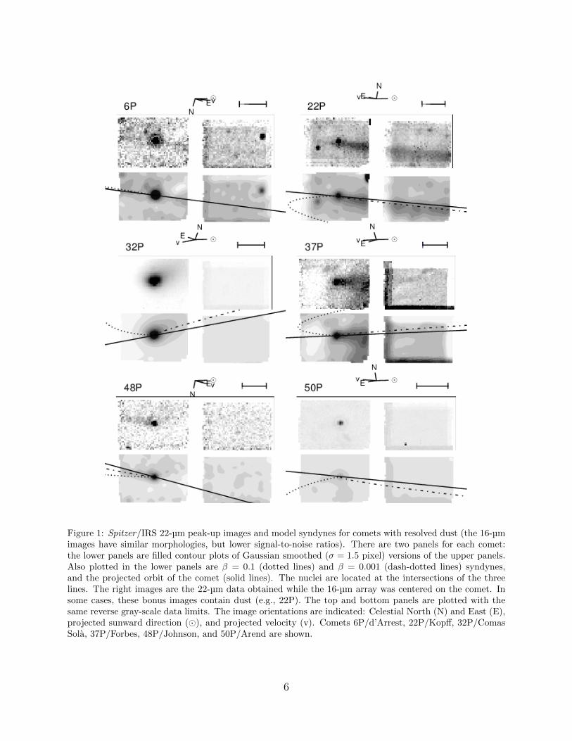
Figure 1: Spitzer/IRS 22-µm peak-up images and model syndynes for comets with resolved dust (the 16-µmimages have similar morphologies, but lower signal-to-noise ratios). There are two panels for each comet:the lower panels are filled contour plots of Gaussian smoothed (σ = 1.5 pixel) versions of the upper panels.Also plotted in the lower panels are β = 0.1 (dotted lines) and β = 0.001 (dash-dotted lines) syndynes,and the projected orbit of the comet (solid lines). The nuclei are located at the intersections of the threelines. The right images are the 22-µm data obtained while the 16-µm array was centered on the comet. Insome cases, these bonus images contain dust (e.g., 22P). The top and bottom panels are plotted with thesame reverse gray-scale data limits. The image orientations are indicated: Celestial North (N) and East (E),projected sunward direction (�), and projected velocity (v). Comets 6P/d’Arrest, 22P/Kopff, 32P/ComasSola, 37P/Forbes, 48P/Johnson, and 50P/Arend are shown.

6

Figure 2: Same as Fig. 1, but for Comets 56P/Slaughter-Burnham, 69P/Taylor, 74P/Smirnova-Chernykh,78P/Gehrels 2, 101P/Chernykh, and 118P/Shoemaker-Levy 4.

7

Figure 3: Same as Fig. 1, but for Comets 119P/Parker-Hartley, 121P/Shoemaker-Holt 2, 129P/Shoemaker-Levy 3, 152P/Helin-Lawrence, 159P/LONEOS, and 171P/Spahr.

8

Figure 4: Same as Fig. 1, but for Comets 173P/Mueller 5, 213P/2005 R2 (Van Ness), 246P/2004 F3 (NEAT),P/2004 V5-A (LINEAR-Hill), and P/2004 VR8 (LONEOS).

9

Figure 5: Same as Fig. 1, but for Spitzer/MIPS 24-µm images. Most images are background subtractedwith the second (shadow) observation of the same comet. In these cases, the grayscale data limits are chosento enhance the contrast of only one of the two comet images. Comets 16P/Brooks 2, 62P/Tsuchinshan 1,144P/Kushida, 219P/2002 LZ11 (LINEAR), 260P/2005 K3 (McNaught), and C/2005 W2 (Christensen) areshown.

10

Figure 6: Same as Fig. 5, but for Comets P/2004 A1 (LONEOS), P/2004 H2 (Larsen), P/2005 JD108

(Catalina-NEAT), P/2005 T5 (Broughton), P/2005 W3 (Kowalski), and P/2005 Y2 (McNaught).

11

3.2. Dust photometry

The Spitzer images allow us to estimate each comet’s dust mass and, for the IRS observa-tions, color temperature. For comets with a coma and/or tail, we measure the total thermalemission in 3–6 pixel radius apertures centered on the comet. The smaller aperture sizesare necessary in some images to reduce background contamination. When possible, we alsoexamine an aperture offset at least 5 pixels from the nucleus in order to measure emissionfrom tails and trails. The size and shape of the tail/trail aperture varies comet-by-cometand depends on the morphology of the dust. The background is estimated from areas oflow contamination from dust and background sources. As the thermal emission from cometstypically contains significant emission from the nucleus, we only use the nucleus subtractedimages from Paper I. The fluxes have been aperture corrected and color corrected assumingthe spectral shape of an isothermal blackbody sphere in local thermodynamic equilibrium(LTE), according to the methods prescribed by the MIPS and IRS instrument handbooks(Colbert 2010, Spitzer Science Center 2009). The dust fluxes are listed in Table 2.

With the two IRS peak-up arrays, we measure the 16–22-µm color temperature of thedust in our survey, centered on the nucleus and in the tail/trail (if applicable) for all fluxeswith signal-to-noise ratios ≥ 5. Dust color temperatures are listed in Table 3 as a ratiowith the temperature of an isothermal blackbody sphere in LTE at the same heliocentricdistance (TBB = 278 r

−1/2h ). The error-weighted mean of all color-temperature measurements

is 〈T/TBB〉 = 1.074 ± 0.006, of the center apertures is 1.079 ± 0.007, and of the tail/trailapertures is 1.065± 0.010.

The color temperature of the dust will only serve as an approximation to the true physicaltemperature of the grains because physical temperatures depend on the grain sizes, shapes,and compositions, and comet dust structures are collections of grains with a wide range ofproperties. For example, dust grains with sizes . 1 µm have higher equilibrium temperaturesthan larger grains because the former have smaller emission cross sections at 10–20 µm, thewavelength regime at which the peak of the thermal emission occurs for a blackbody spherein the inner solar system. Thus, their equilibrium temperatures are increased over thatof a blackbody. These increases are composition dependent as carbonaceous grains, whichhave high absorption and emission efficiencies, will have different equilibrium temperaturesthan an equally-sized silicate grain, which is less absorptive at most optical and infraredwavelengths. For more discussion on these effects, and how they may constrain thermalemission spectra, see Wooden (2002).

Despite the ambiguity in correlating color temperatures to coma grain properties, comet-to-comet differences indicate variations of those (unknown) dust parameters among the mem-bers of our survey. For example, the color temperature of 74P/Smirnova-Chernykh’s comais greater than 101P-A/Chernykh’s coma (1.16± 0.02 versus 0.96± 0.03, respectively). Thisdifference indicates that 74P’s coma is composed of different grains than 101P’s coma, andwe can speculate that they are smaller and/or more carbon rich in the former.

3.3. Survey sensitivity

3.3.1. All dust

The SEPPCoN survey was designed to detect comet nuclei with a signal-to-noise ratio of30. The exposure times are not based on potential dust emission but solely on our estimated

12

nucleus sizes and temperatures. To verify that we can draw meaningful results on the dustactivity of Jupiter-family comets as a whole, we must estimate the survey’s sensitivity todust. Rather than using a theoretical estimate (i.e., observation planning tools), we preferto measure the sensitivities from our observations, which will easily take into account theeffects of background objects (stars, asteroids, etc.), variances in instrument calibration (e.g.,flat-fielding), latent charge on the detector, etc. To measure the sensitivity of an image, wefirst filter the image to remove structures larger than 5×5 pixels (i.e., dust and the smoothlyvarying background). To be more specific, we applied a morphological gray closing operator,followed by the opening operator, and subtracted the result from the original image. Theopening and closing operators effectively convolve the image with a 5 × 5 box, but insteadof replacing each pixel with the average of the surrounding pixels, the closing and openingoperators replace each pixel with the maximum and minimum pixel values within the box,respectively. Applying the closing and opening operators is similar to applying a medianfilter, except more of the small scale structure is lost in median filtering. Because small scalestructure affects our ability to detect dust, we prefer the closing and opening filters overthe median. See Lea and Kellar (1989) and Appleton et al. (1993) for further discussionand other applications of morphological operators in astronomy. In the part of the co-addedimage where the integration time was the highest, we measure the standard deviation of theimage after iteratively removing 3σ outliers (i.e., the comet itself, and the central cores ofstars).

The image sensitivities are measured in units of MJy sr−1. However, dust surface bright-ness depends on heliocentric distance: a surface brightness of 1 MJy sr−1 at 3 AU impliesless dust than 1 MJy sr−1 at 7 AU due to the different equilibrium temperatures. A morerelevant representation of the sensitivity is needed. We have chosen to transform the mea-sured surface brightnesses into optical depths. To compute the image sensitivity to dust interms of optical depth, we use the equation:

στ =σIν

C(Td)Bν(Td)√A, (1)

where στ is the optical depth (or effective fill factor) of a 1σ per pixel detection of dust, σIν isthe measured sensitivity (1σ per pixel) in units of MJy sr−1, Td is the effective temperature ofthe dust, C(Td) is the instrument color correction for a blackbody spectrum at a temperatureTd, Bν(Td) is the Planck function evaluated at temperature Td in units of MJy sr−1, and Ais the area of a fictitious dust aperture in units of square pixels. Our default aperture sizein Table 2 is a 6 pixel radius circle. In §3.2, we computed a mean color temperature ofTc/TBB = 1.08 in the center aperture. A priori, we do not know the color temperature ofany specific comet. Rather than using one value for 70 comets and our measured values forthose 10 comets in Table 3, we assume Td ≈ Tc = 1.08TBB = 300 r

−1/2h K for all comets.

Histograms of the observed dust optical depths and the survey image sensitivities arepresented in Fig. 7 for the IRS 22-µm and MIPS 24-µm observations. Notice that the dustdetections fall off at the same optical depths as our estimated 3σ image sensitivities. Thisfall off strongly suggests our dust detections are sensitivity limited.

13

3.3.2. Trail dust

In a survey of 34 comets taken with the MIPS instrument, Reach et al. (2007) foundthat at least 80% of all short-period comets have dust trails. Since dust trails are long livedfeatures (§3.1) we may expect a similar rate for the SEPPCoN targets, but instead we finda rate of 10%.

To better understand the dramatic difference in trail rates, we compared our surveytarget list to that in Reach et al. and found the following 12 comets in both surveys.

• Comet 107P did not have a trail, or any other dust, in any observation.

• Comet 62P had a trail in both surveys.

• Comet 78P’s dust was classified as a possible trail in SEPPCoN, and as having a trailby Reach et al..

• Comet 121P had a trail in SEPPCoN but only a tail in the Reach et al. survey. Wesuggest that this comet’s trail only becomes apparent at large true anomalies (trailsurvey f = 31◦, SEPPCoN f = 123◦).

• Comets 32P, 69P, 123P, and 131P had trails in the Reach et al. survey, but theyappear to be too faint to detect in the SEPPCoN images. In particular, 123P’s SEP-PCoN images have several nearby point sources and background subtraction artifacts(Fernandez et al. 2011).

• Comets 48P and 129P had clear leading and following trails in the Reach et al. survey.The fields-of-view of the SEPPCoN observations are limited in the trailing directionand tails overlap with the orbit. It is surprising that the leading trails are not observedin either case. The leading trail may be a transient feature.

• Comets 94P and 127P were classified as an “intermediate trail” by Reach et al., i.e.,the dust more closely followed the β = 10−3 syndyne than the projected orbit of thecomet (this label is consistent with our “trail” label). Neither of these comets havedust in our survey images and both were taken at larger true anomalies, emphasizingthat such dust may be relatively short lived (trail survey f = 62◦ and 77◦, SEPPCoNf = 150◦ and -152◦).

In summary, out of the 12 comets in both surveys, three morphologies have consistent de-scriptions (62P, 78P, and 107P), four trails appear to be too faint for SEPPCoN (32P, 69P,123P, and 131P), two intermediate trails appear to be short lived and limited to smaller trueanomalies (94P and 127P), one comet’s trail may not be present at very small true anomalies(121P), and two trails may be obfuscated by dust tails, whereas their leading trails are possi-bly transient features (48P and 129P). From this comet-by-comet comparison, it appears thelow trail detection rate of SEPPCoN can be explained by: 1) observation timing/geometry;2) the limited field-of-view of the IRS peak-up arrays; and, 3) the survey’s sensitivity todust. The last point is discussed further below.

A portion of the difference in trail detection rates is due to the typical observing geome-tries of short-period comets at rh & 4 AU, which cause tails and trails to overlap on the sky

14

(e.g., compare 22P to 48P in Fig. 1). However, obfuscation from brighter coma and tail dustdoes not explain the lack of trails in the 56 images of apparently bare nuclei. Instead, wemust consider the survey differences in sensitivity. First note that the Reach et al. surveytargeted comets within 3.5 AU from the Sun, whereas the SEPPCoN observations were allat rh ≥ 3.4 AU. Also note that the trail survey integration times were shallow (either 42 or140 s on source with MIPS) compared to the SEPPCoN observations (140 to 2500 s withMIPS). We can make direct comparisons between the surveys by converting trail fluxes intooptical depths. We examined the peak τ values listed in Table 2 of Reach et al., and find thetrails have 0.2×10−9 ≤ τ ≤ 9×10−9 in the mid-IR, with a median of 1.2×10−9. For the eightSEPPCoN targets with trail detections, we find 0.4×10−9 ≤ τ ≤ 11×10−9, and a median of1.3×10−9. In Fig. 7, we also show a histogram of the peak optical depths from the Reachet al. survey. The range and median trail optical depths of the two surveys roughly agree.But the Reach et al. trail survey did detect most of the faintest trails, and this is likely themain difference between the two surveys.

4. Discussion

4.1. Comet activity

Comet activity is controlled by physical and dynamical processes at the nucleus. Physicalproperties, such as composition and geology, determine if a comet is active under a given setof solar illumination conditions. Besides size and color temperature, little is known about thephysical properties of our targets. The dynamical properties of a nucleus are described by itsorbit and rotation state, and together they also determine the solar illumination conditionsand history. The rotation states are known for only a few of our targets. In contrast, all ofthe orbital parameters are constrained well enough to make meaningful comparisons. Thegeometrical circumstances of each observation are also well constrained and can be tested.For example, we might test for a correlation between activity and observer-comet distancebecause dust around comets farther from the telescope is more difficult to detect (lowerspatial resolution, possibly cooler dust temperatures).

For this work we have tested for the presence of a correlation between recent activityand eight observational and orbital parameters: rh, ∆S (Spitzer -comet distance), φS (phaseangle, Sun-comet-Spitzer), f (true anomaly), q (perihelion distance), e (orbital eccentricity),a (orbital semi-major axis), and ∆q|150 (perihelion distance history, described below). Allorbital parameters are measured from their osculating elements at the time of the observa-tion, except ∆q|150. We integrated each comet’s current orbit back 300 yr in 90 day stepsusing HORIZONS (Giorgini et al. 1996); ∆q|150 is the difference between the minimum andmaximum q over the past 150 yr,

∆q = min(q)−max(q) (2)

where a negative ∆q|150 indicates the perihelion distance was larger in the past. A relation-ship between any one of the above parameters and activity is not necessarily expected (e.g.,we don’t expect activity to depend on the phase angle of the observation), but we testedfor correlations in order to perform an unbiased study while getting a useful sense of whata “null hypothesis” result looks like.

15

Figure 7: Histograms of the IRS 22-µm and MIPS 24-µm center (top panel) and tail/trail (upper-middlepanel) photometry expressed as dust optical depth. Also shown are dust sensitivities (3σ per 6-pixel radiusaperture) in terms of optical depth for all IRS 22-µm and MIPS 24-µm images (lower-middle panel) andSpitzer trail survey peak optical depths (bottom panel) from Table 2 of Reach et al. (2007).

16

For each parameter, we compute a two-sided Kolmogorov-Smirnov (K-S) statistic, D,and two-tailed p-value with the null hypothesis that the active and inactive comets in oursurvey are drawn from the same distribution. The p-value (or false positive probability)indicates the probability that uncorrelated data sets might result yield a D greater thanthat observed. When D is small, or when the p-value is large, the null hypothesis cannot berejected. At first, only those comets with comae and/or tails were considered to be active.Comets with trails, or without dust are considered inactive. The four comets with ambiguousmorphologies (tail/trail) are dropped from the analysis. With these definitions, the numbersof active and inactive comets are 21 and 64. Our K-S test results are listed in Table 4.

In §3.1, we argue that dust tails are associated with activity on longer timescales thandust comae, and that they do not necessarily indicate a currently active comet. As anadditional check on the significance of our K-S tests, we removed tail-only detections fromour active comet list, and compared the remaining comets to the inactive comets. Thischange reduced the number of active comets to 10. The second set of K-S tests are alsopresented in Table 4.

The p-values in Table 4 indicate that the active and inactive comets have significantlydifferent f , q, e, and a distributions. The distribution of ∆S is slightly different but withless confidence, indicating that comet-Spitzer distance does not have a strong influence onour results. Figure 8 presents the cumulative probability functions for f , q, a, and ∆S. Thecumulative probability functions for ∆q|150 are presented in Fig. 9. We discuss each resultbelow.

4.1.1. True anomaly

The active and inactive comets have significantly different distributions in true anomaly.In Fig. 8, we see that the active comets are strongly biased toward positive true anomalies(i.e., post-perihelion), with only 2 active comets at f < 0◦ (i.e., pre-perihelion). Restrictingour definition of active to only those comets with a coma does not diminish our conclusion.In addition, no comet in our survey is active between f = −180◦ and −125◦.

As an alternative metric of post-perihelion activity, we estimate the true anomalies atwhich activity starts and stops. Figure 10 shows a histogram of activity versus true anomaly,with a horizontal line plotted at exp(−1). We chose exp(−1) because it marks the half lengthof an exponential fall-off, however we note that our histogram does not necessarily suggestthis particular functional relationship between activity and true anomaly. By comparing theline to the histogram, we estimate that activity in the average JFC turns on at f > −120◦

and turns off at f ≈ 140◦.A few scenarios may result in apparent persistent post-perihelion activity: 1) a temporary

dust mantle insulates the ices during the pre-perihelion portion of the orbit but is lost nearperihelion allowing persistent activity on the outbound leg of the orbit; 2) the surface layersretain a significant seasonal thermal wave that continues to heat the comet sub-surface wheninsolation would normally be insufficient; 3) a seasonal effect near perihelion that causespersistent activity well outside of perihelion; or, 4) asymmetric activity caused by the lateonset of volatile production. For the purposes of this paper, we define a dust mantle to bean ice-free layer at the surface of the nucleus.

As solar insolation warms the surface of a comet a thermal wave propagates inward. Atsome depth the thermal wave heats ices to sublimation temperatures, which drives mass loss.

17

Figure 8: Cumulative probability functions comparing the distributions of Spitzer -comet distance (∆S),true anomaly (f), orbital semi-major axis (a), and perihelion distance (q) for active (coma and/or tail) andinactive comets in our survey. The active distributions based solely on the presence of a coma are also shown.

18

Figure 9: (Top left) Cumulative probability functions comparing the distributions of perihelion distancevariations in the past 150 yr (∆q|150) for active and inactive comets in our survey. (Top right) Plot of ∆qversus observed rh computed for 50-, 150-, and 300-yr orbital histories (comae: black, tails: gray, inactive:white). (Bottom left) Cumulative probability functions for peak-sub-solar-temperature variations in the past150 yr (∆T |150). (Bottom right) Plot of ∆T versus observed rh computed for 50-, 150-, and 300-yr orbitalhistories.

19

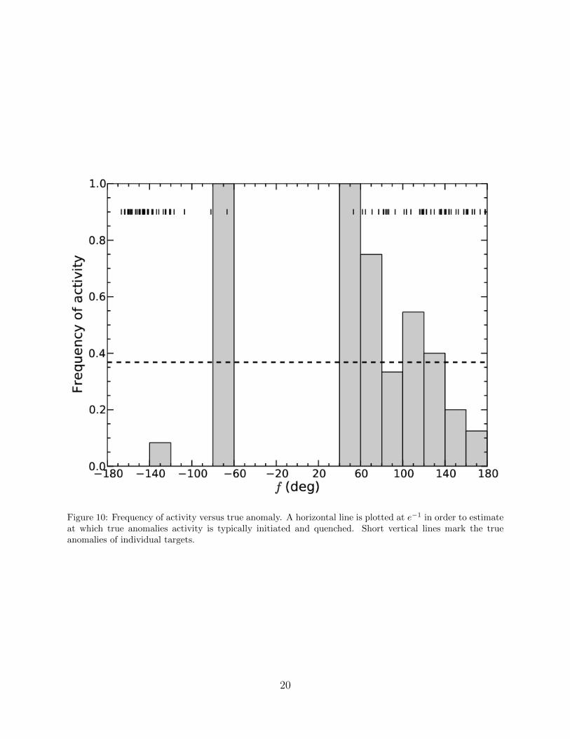
Figure 10: Frequency of activity versus true anomaly. A horizontal line is plotted at e−1 in order to estimateat which true anomalies activity is typically initiated and quenched. Short vertical lines mark the trueanomalies of individual targets.

20

The depth of those ices, the thermal properties of the layers above them, and the rotationaland orbital states of the nucleus will determine when activity is initiated. Suppose thatactivity becomes so vigorous that any putative dust mantle is ejected, either partially orcompletely, from the comet. As the comet recedes from the Sun, activity would be strongerthan the pre-perihelion orbit, but it would eventually decrease to the point at which itcan no longer lift some grains from the surface, perhaps because of their large sizes, anda dust mantle will redevelop. Thus, a pre-perihelion nucleus could be insulated by a dustmantle, whereas the post-perihelion nucleus might not. Brin and Mendis (1979) presentone of the first 1-D models of comet mantle formation and destruction that causes pre- andpost-perihelion asymmetries near rh = 1 AU. Mantle formation and destruction in nucleusthermal models is reviewed by Prialnik et al. (2004).

In the second scenario, where activity is driven by seasonal heating, the dust mantle is notlost but retains heat from the perihelion passage. Energy deposited on diurnal timescales willradiate back to space on roughly the same timescale, but sub-surface temperatures can buildup on longer timescales as a comet approaches perihelion. After the comet passes perihelion,the thermal wave cools to both space and the comet sub-surface. If sub-surface ices continueto be warmed to sublimation temperatures, despite the increasing heliocentric distance,activity will persist. In order to observe a pre-/post-perihelion asymmetry, the ices must beburied at depths closer to the annual thermal skin depth than the diurnal thermal skin depth.If this is true, gas production should not vary diurnally at the intermediate heliocentricdistances in our survey, or, at least, it should be weakly correlated with rotational insolation.There is limited support for this scenario in flyby images of nuclei. Jet activity occurs fromsurfaces in local night at 81P/Wild 2, 9P/Tempel 1, and 103P/Hartley 2 (Sekanina et al.2004, Farnham et al. 2007, A’Hearn et al. 2011), but the apparent timescales of this activityare much shorter than what is required for a pre-/post-perihelion asymmetry.

The near-surface structure of comets was directly examined by the Deep Impact mission(A’Hearn et al. 2005). Deep Impact excavated a crater with a diameter of 50–200 m onComet 9P/Tempel 1 (Richardson and Melosh 2013, Schultz et al. 2013). According toA’Hearn (2008), most observations of the ejecta are consistent with dust-to-volatile ratiosof order unity, and Groussin et al. (2010) came to the same conclusion. Since the dust-to-volatile ratio is not � 1, it appears the thermal wave in this nucleus had not sublimatedmuch of the water ice on the scale of the crater depth. Even greater constraints on the depthof thermal penetration were obtained with Deep Impact spectra of the comet’s surface.Groussin et al. (2007) analyzed the thermal emission from the surface and showed that ithas a low thermal inertia, nearly in instantaneous equilibrium with sunlight. They arguethat cometary activity must originate within the first centimeters to meters of the surface.From the thermal inertia upper-limits and assumptions on conductivity and heat capacity,A’Hearn (2008) computes the diurnal skin depth to be 3 cm, and the annual skin depth to be90 cm. These numbers are order of magnitude consistent with theoretical models of cometnuclei made before the Deep Impact mission results (Prialnik et al. 2004), and with Spitzermid-IR spectral measurements of the nucleus thermal emission at 5 AU (Lisse et al. 2005).In order for dust mantles to quench activity on diurnal timescales, they must be larger than∼ 1 cm thick, and to prevent the seasonal thermal wave from driving activity, volatiles mustbe more than ∼ 10 cm from the surface.

Weissman (1987) proposed that the sudden illumination of a nucleus hemisphere caused

21

by the rapid change of season near perihelion causes cracks in the mantle, and these crackscreate new active areas on the nucleus. The hemisphere illuminated on the in-bound legof the orbit does not develop these cracks because it is gradually heated, and the surfacecan better accommodate the changes. If this hemisphere continues to be illuminated as thecomet recedes from the Sun, the comet’s activity could be greater than that of it’s inboundleg.

Meech et al. (2011) propose that the pre-/post-perihelion asymmetry of Comet 103P/Hartley2 is caused by the late on-set of CO2 driven activity. They find that this comet’s activitywas first initiated in 2010 at 4.3 AU by water sublimation. When the comet reached 1.4 AU(pre-perihelion) CO2 driven activity dominated, to the point at which water ice can be drivenoff the surface, as if it were dust. The CO2 driven activity would persist beyond the comet’saphelion (Meech et al. 2011).

Whatever the cause, the effect is clear in the SEPPCoN. Because the survey took aconsistent approach to its observations, it can be used to test these and other inhibitors anddrivers of activity in a statistical manner.

4.1.2. Perihelion distance

The inactive comets have smaller perihelion distances than the active comets. The medianq is 2.0 AU for the inactive comets and 3.0 AU for the active comets. This difference maybe a selection effect. Cometary activity is driven by insolation, and, in general, comets aremost likely to be active when they are near perihelion. Our survey targets were observed atheliocentric distances ranging from 3 to 7 AU. However, a comet with a perihelion distancebetween 3 and 7 AU is a priori more likely to be active in our survey, since its activity atsuch distances has already been established (otherwise it would not have been designated acomet, and not observed by SEPPCoN). Therefore, the greater rate of activity for cometswith larger perihelion distances appears to partially be an artifact of the survey.

To further demonstrate the larger activity rates of the large perihelia comets, we plotthe cumulative frequency of activity in our survey, sorted by perihelion distance, in Fig. 11.That the frequency of activity almost continuously increases for q > 2 AU shows the higheractivity rate of this population.

Figure 12 presents an alternative view on these large perihelia comets, and shows thaton average they produce more dust than the smaller perihelia comets. Here, we plot εfρversus perihelion distance. We define the parameter εfρ as the product of effective emissivity(ε), filling factor (f), and projected aperture radius (ρ, in units of cm). This parameter isintended to be analogous to the Afρ parameter commonly computed for scattered lightobservations (A’Hearn et al. 1984). Further discussion of εfρ can be found in AppendixA. We based our εfρ values on the mean MIPS 24-µm, or the IRS 22-µm center aperturephotometry (Table 5). Comets with small εfρ values, i.e., low-activity comets, are missingfrom the large-perihelion population. We suggest that this bias is due to the discoverycircumstances of large-perihelia comets, and that low-activity comets with large-periheliaare as yet missing from the discovered JFC population.

Although we cannot make definite conclusions on the activity of comets with large-perihelia, we can consider the activity of small-perihelia comets, whose discovery rates arelikely more complete and less biased. Of those comets with q < 2.5 AU, 7 out of 59 comets

22

Figure 11: The cumulative frequency of activity in our survey versus perihelion distance.

23

Figure 12: (Left) Comet activity, quantified with the parameter εfρ, versus perihelion distance. (Right) Thesame as on the left, but εfρ has been scaled by (rh/3 AU)2, so that comets can be more directly comparedto each other. Note the paucity of low-εfρ comets with large perihelion distances, indicating that our surveyand the discovered JFC population is sensitivity limited.

24

(12%) are active, and none of the 30 comets with q < 1.8 AU are active (Fig. 11).1 Thereforeany short-period comet with a small perihelion distance is likely inactive at 3–7 AU. Thisfinding may be explained if relatively more volatile ices are lost for comets that approachthe Sun more closely during their perihelion passages, but this hypothesis seems inconsistentwith the results of A’Hearn et al. (2012). They studied the H2O, CO2, and CO contentof comets in the literature, and found no correlation with orbital parameters, except fora decreasing CO2-to-H2O mixing ratio for comets with decreasing perihelion distance, forq < 1 AU. They rightly dismiss this correlation as due to small number statistics (only 4comets have a measured CO2 abundance for q < 1 AU) and for the fact that it contradictstheir result that CO/H2O is uncorrelated with q. Taking our results together with thediscussion of A’Hearn et al. (2012), we suggest that comets with small perihelion distanceshave a thicker insulating surface than comets with larger perihelion distances.

4.1.3. Perihelion distance history

Licandro et al. (2000) surveyed 18 comets in order to estimate the effective sizes oftheir nuclei. Seven of their targets were active: one at rh = 3.04 AU, and the rest atrh > 4 AU. They examined their orbital histories and found that all but one of their cometsrecently perturbed to orbits with smaller perihelion distances in the past 150 yr (∆q|150 <−1 AU) were active. Licandro et al. hypothesize that the perturbations to smaller periheliondistances caused a marginally stable mantle to be destroyed, exposing fresh ices. The absenceof a mantle allows activity to persist to larger than usual perihelion distances. When weexamined the pre-/post-perihelion asymmetry in SEPPCoN, we also introduced the conceptof a temporary mantle, only in our case the mantle is partially or completely lost eachperihelion passage. We now examine the orbital histories of SEPPCoN targets to furtherinvestigate the potential existence of dust mantles. Note that a small ∆q is not the sameas small q, i.e., a comet may be perturbed from the Centaur region (a > 5.2 AU) into theJupiter-family comet region (a < 5.2 AU), yielding ∆q < 0, yet still have a large periheliondistance in our survey.

Recognizing that the same ∆q is more significant at small perihelion distances thanat large perihelion distances, we have also computed the maximum sub-solar-temperaturedifference, ∆T . The sub-solar temperature of a spherical comet nucleus is

T =

[(1− A) ∗ F�r2hηεσSB

]1/4

, (3)

where A is the Bond albedo, F� = 1365 W m −2 is the solar constant at 1 AU, rh is theheliocentric distance in AU, η = 1.03 is the IR-beaming parameter, ε = 0.95 is the IRemissivity of the surface, and σSB is the Stefan-Boltzmann constant in W m−2 K−4 (Harris1998, Fernandez et al. 2011). For our purposes, we compute ∆T |x using the minimum andmaximum q values from our ∆q|x integrations; ∆T > 0 signifies the temperature was coolerin the past.

1Because the strong bias in activity to post-perihelion epochs, we verified that the 30 comets with q <1.8 AU have the same true anomaly distribution as comets with q > 1.8 AU. A K-S test yields a 1%probability that the two populations are different.

25

Figure 9 shows that active comets in SEPPCoN appear more likely to have ∆q|150 < 0 and∆T |150 > 0 than the inactive comets. In addition, no active comet has ∆q|150 > 0.5 AU, yet≈ 10% of the inactive comets do have such large values. The K-S probabilities for ∆q|150 and∆T |150 are 28% and 10%, indicating that the difference between active and inactive cometsmay be significant. But, given the striking differences in Fig. 9, this problem deserves futurestudy because it may lead to an understanding of the timescales of mantle formation.

The difference in perihelion distance histories between the active and inactive cometsmay be related to their discovery circumstances. When an unknown comet is perturbedto a smaller perihelion distance, it should become brighter to observers on the Earth, andtherefore more likely to be discovered. To investigate this possible effect, we searched theNASA JPL Small-Body Database Browser and the NASA Planetary Data System SmallBodies Node for each comet’s year of discovery. We plot this year versus the year of theminimum ∆q|150 in Fig. 13. Data points near a slope of 1 indicate a comet that was discoveredat a 150-year low in its perihelion distance history. Fifteen comets are found within 20 yearsof this line, indicating that reductions in perihelion distance is a factor in JFC discoverydates. In the plot we indicate which comets were active in our survey. Those cometsdiscovered soon after being scattered to smaller perihelion distances appear to have a higheractivity rate in our survey, 8 out of 22 (36 ± 13%) versus 15 out of 70 (21 ± 6%), but thelow significance precludes us from making a firm conclusion.

Most of our survey targets were discovered in the past 20 years, but the year of minimum∆q|150 for these comets is uniformly distributed over the past 150 years. This distribu-tion may be the result of uncertain orbital histories for these comets, rather than a lackof correlation between the two parameters. However, it is also possible that the increasingsophistication and sensitivity of Solar System surveys in the past 20 years has led to JFC dis-coveries that are independent of their perihelion distance history. Both of these possibilitiescould be a cause for the low significance of the K-S tests based on ∆q.

4.1.4. Semi-major axis and Spitzer-comet distance

On average, the active comets have larger semi-major axes than the inactive comets.Since perihelion distance and semi-major axis are correlated in the Jupiter-family cometpopulation, this difference may be an observational bias related to the perihelion distancebias described above. A similar argument may be made for the slight differences in ∆S forthe active and inactive comets. Nuclei with larger q are more likely to be observed at larger∆S.

4.1.5. Other investigations

Comet lightcurve asymmetries have been recognized for many years. Asymmetries nearperihelion are not directly relevant to our survey since most of our targets are observed attrue anomalies greater than 90◦ from perihelion. The secular light curves of 27 comets werestudied by Ferrın (2010). Considering only the Jupiter-family comets, and excluding the one-time active Comet 107P/Wilson-Harrington (leaving 17 comets), the ratios of the heliocentricdistance at which activity ceases (roff ) to the distance at which activity initiates (ron) rangesfrom 0.7 to 2.0, with a mean roff/ron = 1.20± 0.38. Although this result cannot be directlycompared to our survey results, they qualitatively agree in that it appears persistent post-perihelion activity is common to individual Jupiter-family comets.

26

Figure 13: Year of comet discovery (Tdisc) versus the year of the comet’s 150-year minimum in periheliondistance history (T∆q|150). Comets between the dotted and solid trend lines are those that were discoverednear a 150-year minimum in perihelion distance: 8 out of the 22 comets in this region are active in oursurvey.

27

The activity of short-period comets has also been examined by Mazzotta Epifani et al.(2009). They searched the literature for optical and infrared observations of short-periodcomets (Jupiter-family, Encke type, and Halley type) at rh > 3 AU. In their compilationof 90 comets they find that 10–20% are active beyond 4.5 AU. Furthermore, they also finda perihelion asymmetry with activity detected in 22% of the pre-perihelion observations,and 59% of the post-perihelion observations. In our survey data (rh > 3.4) we find slightlydifferent values: 24±5% (21 comets) of our sample was active, with activity in 5±4% (2/39)of the pre-perihelion observations, and 38± 9% (19/50) in the post-perihelion observations.With only a few comets in each bin, and understanding that the Mazzotta Epifani et al.study is based on a literature search, and not on a consistent data set, we consider theSEPPCoN results to be compatible with the results of Mazzotta Epifani et al.. In addition,they also conclude that recent perihelion distance changes are not a strong predictor ofdistant activity, agreeing with our results above.

4.2. Dust color temperature

The effective temperatures of comet comae at 5–20 µm typically range from ≈ 0− 30%warmer than an isothermal blackbody sphere at the same heliocentric distance (Gehrz andNey 1992, Lisse et al. 1998, Sitko et al. 2004, Woodward et al. 2011). In Table 3 we finda similar result, even though our observations are obtained at larger heliocentric distancesand longer wavelengths than are typically measured with ground-based observatories.

We test for correlations between Tc/TBB for the 11 IRS center aperture measurements andthe parameters rh, q, F22 (22- or 24-µm flux), and εfρ. The results are presented in Table 5.For each parameter, we calculate the linear correlation coefficient and apply a Spearman “ρ”test. The Spearman test is a more robust estimate of correlation than the linear correlationcoefficient. It is based on the relative rankings of each parameter being tested, and does nottest for a specific functional form of the correlation. After computing the Spearman ρ, wederive Z, the number of standard deviations by which the Spearman statistic deviates fromthe null hypothesis expectation value for uncorrelated data. To account for measurementuncertainties in the correlation tests, we tested 104 data sets generated with a Monte Carlotechnique based on our measurements and associated uncertainties. No significant correlationis found, and the correlations in our Monte Carlo runs never exceeded a 3σ significance. Welist our results in Table 6.

5. Conclusions

We presented an analysis of the dust and activity of comets observed by the Spitzer SpaceTelescope as part of the Survey of the Ensemble Physical Properties of Cometary Nuclei(SEPPCoN). We have shown that SEPPCoN can be used to study the dust and activityof Jupiter-family comets at 3–7 AU, although some care must be taken when interpretingthe results as the dust detections are limited by the image sensitivities, and that cometswith large perihelion distances are a priori more active. We detected dust around 33 of 89(37± 6%) survey targets, and 21 targets (24± 5%) have comae or tails that suggest recentcometary activity. Since faint dust (τ . 0.5×10−9) may remain undetected in our images, weconclude our detections are a lower limit and that at least ≈ 24% of Jupiter-family cometsare active at 3–7 AU from the Sun. We also studied the crude spectral properties of the

28

dust. The 16- to 22-µm color temperature of the dust is 7.4± 0.6% warmer on average thanan isothermal blackbody sphere in LTE.

We introduce the quantity εfρ, intended to be a thermal emission counterpart to theoften reported Afρ for observations of light scattered by comets. The εfρ versus periheliondistance distribution of our survey sample shows that low-activity comets with large perihe-lion distances are missing from the survey, and therefore are likely missing from the knownJupiter-family comet population.

We compared the frequency of activity of survey targets to their orbital and observationalparameters. All 30 comets with q < 1.8 AU appear inactive in our survey. Whatever drivestheir activities is effectively quenched at larger distances from the Sun.

Comets that have been perturbed to smaller perihelion distances in the past 150 yearsseem more likely to be active in our survey (cf. Licandro et al. 2000). Kolmogorov-Smirnovtests indicate a tentative result, so a better statistical characterization, perhaps with moredetailed orbital histories, is warranted.

The activity of Jupiter-family comets at 3–7 AU from the Sun is significantly biased topost-perihelion epochs. Of the 21 comets that appear to be recently active, 19 were observedpost-perihelion. We tentatively estimate the true anomaly at which activity is initiated to bef > −120◦, but small number statistics make this limit uncertain. With better confidence,we find that for many comets activity has ceased by f ≈ 140◦. Similar findings on thepersistent post-perihelion activity were found by Mazzotta Epifani et al. (2009), and Ferrın(2010). No comet in our survey is active between f = −180◦ and −125◦.

We discussed several causes for a pre-/post-perihelion activity asymmetry. Whatever thecause, the effect is clear in our survey. Because SEPPCoN took a consistent approach toits observations, it can be used to test the drivers and inhibitors of activity in a statisticalmanner. The Rosetta spacecraft, which will orbit Comet 67P/Churyumov-Gerasimenko(Glassmeier et al. 2007) as it approaches perihelion from 4 AU, should also provide newperspectives on this problem of the evolutionary history of comet surfaces.

Acknowledgments

The authors appreciate Paul Weissman’s careful review of our manuscript. This workis based on observations made with the Spitzer Space Telescope, which is operated bythe Jet Propulsion Laboratory, California Institute of Technology under a contract withNASA. Support for this work was, in part, provided by NASA through an award issuedby JPL/Caltech. CS has received funding from the European Union Seventh FrameworkProgramme (FP7/2007-2013) under grant agreement no. 268421.

References

A’Hearn, M. F., 2008. Deep Impact and the Origin and Evolution of Cometary Nuclei.Space Sci. Rev. 138, 237–246.

A’Hearn, M. F., et al., 2011. EPOXI at Comet Hartley 2. Science 332, 1396–1400.

A’Hearn, M. F., et al., 2005. Deep Impact: Excavating Comet Tempel 1. Science 310, 258–264.

29

A’Hearn, M. F., et al., 2012. Cometary Volatiles and the Origin of Comets. Astrophys. J.758, 29.

A’Hearn, M. F., Millis, R. L., Schleicher, D. G., Osip, D. J., Birch, P. V., 1995. The ensembleproperties of comets: Results from narrowband photometry of 85 comets, 1976-1992. Icarus118, 223–270.

A’Hearn, M. F., Schleicher, D. G., Millis, R. L., Feldman, P. D., Thompson, D. T., 1984.Comet Bowell 1980b. Astron. J. 89, 579–591.

Appleton, P. N., Siqueira, P. R., Basart, J. P., 1993. A morphological filter for removing’Cirrus-like’ emission from far-infrared extragalactic IRAS fields. Astron. J. 106, 1664–1678.

Bockelee-Morvan, D., Crovisier, J., Mumma, M. J., Weaver, H. A., 2004. The compositionof cometary volatiles. The University of Arizona Press, Tucson, pp. 391–423.

Brin, G. D., Mendis, D. A., 1979. Dust release and mantle development in comets. Astro-phys. J. 229, 402–408.

Burns, J. A., Lamy, P. L., Soter, S., 1979. Radiation forces on small particles in the solarsystem. Icarus 40, 1–48.

Colbert, J. (Ed.), 2010. MIPS Instrument Handbook. Spitzer Science Center, Pasadena.URL http://ssc.spitzer.caltech.edu/mips/mipsinstrumenthandbook/

Farnham, T. L., et al., 2007. Dust coma morphology in the Deep Impact images of Comet9P/Tempel 1. Icarus 191, 146–160.

Feaga, L. M., A’Hearn, M. F., Sunshine, J. M., Groussin, O., Farnham, T. L., 2007. Asym-metries in the distribution of H2O and CO2 in the inner coma of Comet 9P/Tempel 1 asobserved by Deep Impact. Icarus 190, 345–356.

Fernandez, Y. R., et al., 2011. Thermal Properties, Sizes, and Size Distribution of Jupiter-Family Cometary Nuclei. Icarus, submitted.

Ferrın, I., 2010. Atlas of secular light curves of comets. Planet. Space Sci. 58, 365–391.

Gehrz, R. D., Ney, E. P., 1992. 0.7- to 23-micron photometric observations of P/Halley 2986III and six recent bright comets. Icarus 100, 162–186.

Gehrz, R. D., Ney, E. P., Piscitelli, J., Rosenthal, E., Tokunaga, A. T., 1989. Infraredphotometry and spectroscopy of Comet P/Encke 1987. Icarus 80, 280–288.

Giorgini, J. D., et al., 1996. JPL’s On-Line Solar System Data Service. Bull. Am. As-tron. Soc.28, 1158 (abstract).

Glassmeier, K.-H., Boehnhardt, H., Koschny, D., Kuhrt, E., Richter, I., 2007. The RosettaMission: Flying Towards the Origin of the Solar System. Space Sci. Rev. 128, 1–21.

30

Groussin, O., et al., 2010. Energy balance of the Deep Impact experiment. Icarus 205, 627–637.

Groussin, O., et al., 2007. Surface temperature of the nucleus of Comet 9P/Tempel 1. Icarus187, 16–25.

Groussin, O., Lamy, P., Jorda, L., Toth, I., 2004. The nuclei of comets 126P/IRAS and103P/Hartley 2. Astron. Astrophys. 419, 375–383.

Groussin, O., et al., 2009. The size and thermal properties of the nucleus of Comet 22P/Kopff.Icarus 199, 568–570.

Harker, D. E., et al., 2011. Mid-infrared Spectrophotometric Observations of Fragments Band C of Comet 73P/Schwassmann-Wachmann 3. Astron. J. 141, 26.

Harris, A. W., 1998. A Thermal Model for Near-Earth Asteroids. Icarus 131, 291–301.

Houck, J. R., et al., 2004. The Infrared Spectrograph (IRS) on the Spitzer Space Telescope.Astrophys. J. Suppl. 154, 18–24.

Jewitt, D., 2009. The Active Centaurs. Astron. J. 137, 4296–4312.

Kelley, M. S., 2006. The size, structure, and mineralogy of comet dust. Ph.D. thesis, Uni-versity of Minnesota, Minneapolis.

Kelley, M. S., Reach, W. T., Lien, D. J., 2008. The dust trail of Comet 67P/Churyumov-Gerasimenko. Icarus 193, 572–587.

Kelley, M. S., et al., 2006. A Spitzer Study of Comets 2P/Encke, 67P/Churyumov-Gerasimenko, and C/2001 HT50 (LINEAR-NEAT). Astrophys. J. 651, 1256–1271.

Lamy, P. L., Toth, I., Fernandez, Y. R., Weaver, H. A., 2004. The sizes, shapes, albedos,and colors of cometary nuclei. The University of Arizona Press, Tucson, pp. 223–264.

Lea, S. M., Kellar, L. A., 1989. An algorithm to smooth and find objects in astronomicalimages. Astron. J. 97, 1238–1246.

Licandro, J., et al., 2009. Spitzer observations of the asteroid-comet transition object andpotential spacecraft target 107P (4015) Wilson-Harrington. Astron. Astrophys. 507, 1667–1670.

Licandro, J., Tancredi, G., Lindgren, M., Rickman, H., Hutton, R. G., 2000. CCD Photom-etry of Cometary Nuclei, I: Observations from 1990-1995. Icarus 147, 161–179.

Lisse, C. M., et al., 2005. Rotationally Resolved 8-35 Micron Spitzer Space Telescope Ob-servations of the Nucleus of Comet 9P/Tempel 1. Astrophys. J. 625, L139–L142.

Lisse, C. M., et al., 1998. Infrared Observations of Comets by COBE. Astrophys. J. 496,971–991.

31

Lisse, C. M., et al., 2009. Spitzer Space Telescope Observations of the Nucleus of Comet103P/Hartley 2. Publ. Astron. Soc. Pacific 121, 968–975.

Marsden, B. G., Sekanina, Z., Yeomans, D. K., 1973. Comets and nongravitational forces.V. Astron. J. 78, 211–225.

Mason, C. G., Gehrz, R. D., Jones, T. J., Woodward, C. E., Hanner, M. S., Williams, D. M.,2001. Observations of Unusually Small Dust Grains in the Coma of Comet Hale-BoppC/1995 O1. Astrophys. J. 549, 635–646.

Mason, C. G., Gehrz, R. D., Ney, E. P., Williams, D. M., Woodward, C. E., 1998. TheTemporal Development of the Pre-perihelion Infrared Spectral Energy Distribution ofComet Hyakutake (C/1996 B2). Astrophys. J. 507, 398–403.

Mazzotta Epifani, E., Palumbo, P., Colangeli, L., 2009. A survey on the distant activity ofshort period comets. Astron. Astrophys. 508, 1031–1044.

Meech, K. J., et al., 2011. EPOXI: Comet 103P/Hartley 2 Observations from a WorldwideCampaign. Astrophys. J. 734, L1.

Meech, K. J., Svoren, J., 2004. Using cometary activity to trace the physical and chemicalevolution of cometary nuclei. The University of Arizona Press, Tucson, pp. 317–335.

Ootsubo, T., et al., 2012. AKARI Near-infrared Spectroscopic Survey for CO2 in 18 Comets.Astrophys. J. 752, 15.

Prialnik, D., Benkhoff, J., Podolak, M., 2004. Modeling the structure and activity of cometnuclei. The University of Arizona Press, Tucson, pp. 359–387.

Reach, W. T., Kelley, M. S., Sykes, M. V., 2007. A survey of debris trails from short-periodcomets. Icarus 191, 298–322.

Richardson, J. E., Melosh, J. H., 2013. An examination of the Deep Impact collision siteon Comet Tempel 1 via Stardust-NExT: Placing further constraints on cometary surfaceproperties. Icarus 222, 492–501.

Rieke, G. H., et al., 2004. The Multiband Imaging Photometer for Spitzer (MIPS). Astro-phys. J. Suppl. 154, 25–29.

Schmitt, B., Espinasse, S., Grim, R. J. A., Greenberg, J. M., Klinger, J., 1989. Laboratorystudies of cometary ice analogues. In: J. J. Hunt & T. D. Guyenne (Ed.), Physics andMechanics of Cometary Materials. Vol. 302 of ESA Special Publication. pp. 65–69.

Schultz, P. H., Hermalyn, B., Veverka, J., 2013. The Deep Impact crater on 9P/Tempel-1from Stardust-NExT. Icarus 222, 502–515.

Sekanina, Z., Brownlee, D. E., Economou, T. E., Tuzzolino, A. J., Green, S. F., 2004.Modeling the Nucleus and Jets of Comet 81P/Wild 2 Based on the Stardust EncounterData. Science 304, 1769–1774.

32

Sitko, M. L., Lynch, D. K., Russell, R. W., Hanner, M. S., 2004. 3-14 Micron Spectroscopyof Comets C/2002 O4 (Honig), C/2002 V1 (NEAT), C/2002 X5 (Kudo-Fujikawa), C/2002Y1 (Juels-Holvorcem), and 69P/Taylor and the Relationships among Grain Temperature,Silicate Band Strength, and Structure among Comet Families. Astrophys. J. 612, 576–587.

Sitko, M. L., et al., 2010. Comet 103P/Hartley. IAU Circ. 9181, 1.

Spitzer Science Center, 2009. IRS Instrument Handbook. Spitzer Science Center, Pasadena.URL http://ssc.spitzer.caltech.edu/irs/irsinstrumenthandbook/

Sykes, M. V., Walker, R. G., 1992. Cometary dust trails. I - Survey. Icarus 95, 180–210.

Weissman, P. R., 1987. Post-perihelion brightening of comet P/Halley: Springtime for Halley.Astron. Astrophys. 187, 873.

Werner, M. W., et al., 2004. The Spitzer Space Telescope Mission. Astrophys. J. Suppl. 154,1–9.

Whipple, F. L., 1950. A comet model. I. The acceleration of Comet Encke. Astrophys. J.111, 375–394.

Wooden, D. H., 2002. Comet Grains: Their IR Emission and Their Relation to ISM Grains.Earth Moon and Planets 89, 247–287.

Wooden, D. H., et al., 1999. Silicate Mineralogy of the Dust in the Inner Coma of CometC/1995 01 (Hale-Bopp) Pre- and Postperihelion. Astrophys. J. 517, 1034–1058.

Woodward, C. E., et al., 2011. Dust in Comet C/2007 N3 (Lulin). Astron. J. 141, 181.

33

Table 1: SEPPCoN target list, observational geometry, and orbital parameters: Obs. date – Spitzer observation date,for MIPS observations, only one of the two epochs are listed; rh – heliocentric distance; ∆S – Spitzer comet distance;φS – Sun-comet-Spitzer angle; f – true anomaly, 0◦ at perihelion; T − Tp – time from perihelion, < 0 when f < 0; a– semi-major axis; e – eccentricity; q – perihelion distance; ∆q|150 – change in q over the past 150 yr.

Name Obs. date rh ∆S φS f T − Tp a e q ∆q|150(UT) (AU) (AU) (◦) (◦) (days) (AU) (AU) (AU)

6P/d’Arrest . . . . . . . . . . . . . . . . . . . . . . . . . 2007-02-13 22:48 4.39 3.85 12 -145 -548 3.49 0.61 1.35 -0.237P/Pons-Winnecke . . . . . . . . . . . . . . . . . . 2007-04-19 14:39 4.34 4.03 13 -146 -526 3.43 0.63 1.25 0.5011P/Tempel-Swift-LINEAR . . . . . . . . . 2006-09-01 15:12 4.40 4.04 13 -146 -611 3.42 0.54 1.56 0.5614P/Wolf . . . . . . . . . . . . . . . . . . . . . . . . . . . 2007-03-20 17:52 4.52 4.53 13 -120 -709 4.25 0.36 2.72 1.2515P/Finlay . . . . . . . . . . . . . . . . . . . . . . . . . 2007-02-28 03:06 4.40 4.32 13 -149 -480 3.48 0.72 0.97 0.2116P/Brooks 2 . . . . . . . . . . . . . . . . . . . . . . . 2007-04-10 09:32 3.40 3.37 17 -125 -368 3.36 0.56 1.47 0.4322P/Kopff . . . . . . . . . . . . . . . . . . . . . . . . . . 2007-04-19 14:10 4.87 4.38 11 -156 -767 3.46 0.54 1.58 -0.5731P/Schwassmann-Wachmann 2 . . . . . 2006-11-09 10:30 5.02 4.59 11 -167 -1423 4.23 0.19 3.42 1.5732P/Comas Sola . . . . . . . . . . . . . . . . . . . . 2006-08-01 03:59 4.14 3.76 14 122 486 4.27 0.57 1.83 -0.4233P/Daniel . . . . . . . . . . . . . . . . . . . . . . . . . 2006-11-09 17:14 4.40 4.17 13 -127 -619 4.03 0.46 2.17 0.7837P/Forbes . . . . . . . . . . . . . . . . . . . . . . . . . 2007-03-12 00:56 4.31 4.19 13 144 587 3.43 0.54 1.57 -0.1947P/Ashbrook-Jackson . . . . . . . . . . . . . . 2007-03-21 10:56 4.32 4.32 13 -117 -682 4.12 0.32 2.79 -1.7648P/Johnson . . . . . . . . . . . . . . . . . . . . . . . . 2006-11-11 18:43 4.41 4.32 13 141 761 3.65 0.37 2.31 -0.3550P/Arend . . . . . . . . . . . . . . . . . . . . . . . . . . 2006-10-23 18:43 3.48 3.31 17 -107 -373 4.09 0.53 1.92 -0.1551P-A/Harrington . . . . . . . . . . . . . . . . . . 2007-04-06 23:24 3.77 3.35 15 -125 -438 3.70 0.55 1.68 0.1956P/Slaughter-Burnham . . . . . . . . . . . . 2006-12-23 13:48 5.08 5.04 12 120 708 5.10 0.50 2.53 0.1257P-A/du Toit-Neujmin-Delaporte . . 2007-06-15 08:34 4.11 3.92 14 -138 -560 3.45 0.50 1.72 0.4662P/Tsuchinshan 1 . . . . . . . . . . . . . . . . . 2006-10-03 02:00 4.72 4.66 12 150 664 3.52 0.58 1.48 -0.8468P/Klemola . . . . . . . . . . . . . . . . . . . . . . . . 2007-02-12 09:42 5.47 5.28 10 -138 -709 4.89 0.64 1.76 -0.2969P/Taylor . . . . . . . . . . . . . . . . . . . . . . . . . 2006-07-29 05:19 4.25 3.66 12 135 605 3.65 0.47 1.94 0.4274P/Smirnova-Chernykh . . . . . . . . . . . . 2007-01-28 17:01 4.42 4.01 12 -121 -914 4.17 0.15 3.56 -2.1477P/Longmore . . . . . . . . . . . . . . . . . . . . . . 2007-02-10 07:38 4.59 4.18 12 -152 -878 3.60 0.36 2.31 -0.9078P/Gehrels 2 . . . . . . . . . . . . . . . . . . . . . . 2007-03-10 02:00 4.98 4.46 10 153 865 3.74 0.46 2.01 -1.0179P/du Toit-Hartley . . . . . . . . . . . . . . . . 2006-09-17 23:10 4.37 4.08 13 -158 -618 3.03 0.59 1.23 -0.2289P/Russell 2 . . . . . . . . . . . . . . . . . . . . . . . 2007-05-01 09:31 4.76 4.18 11 -146 -839 3.80 0.40 2.28 -0.3093P/Lovas 1 . . . . . . . . . . . . . . . . . . . . . . . . 2006-10-03 23:46 4.01 3.56 14 -121 -439 4.39 0.61 1.71 0.0794P/Russell 4 . . . . . . . . . . . . . . . . . . . . . . . 2006-11-14 19:47 4.79 4.20 11 178 1174 3.51 0.36 2.24 -0.43101P-A/Chernykh . . . . . . . . . . . . . . . . . . . 2007-04-22 13:51 4.34 3.76 12 103 483 5.78 0.59 2.35 -0.31107P/Wilson-Harrington . . . . . . . . . . . . 2007-02-12 07:43 4.08 3.52 13 166 582 2.64 0.62 0.99 0.05113P/Spitaler . . . . . . . . . . . . . . . . . . . . . . . 2006-10-22 15:58 3.86 3.55 15 -120 -518 3.69 0.42 2.13 0.36118P/Shoemaker-Levy 4 . . . . . . . . . . . . 2006-09-17 11:45 4.95 4.58 12 178 1159 3.47 0.42 2.00 -0.21119P/Parker-Hartley . . . . . . . . . . . . . . . . 2007-02-12 08:01 4.21 3.67 12 103 629 4.29 0.29 3.04 -2.24121P/Shoemaker-Holt 2 . . . . . . . . . . . . . 2006-08-01 02:40 4.35 3.97 13 123 696 4.02 0.34 2.65 -1.10123P/West-Hartley . . . . . . . . . . . . . . . . . 2006-10-21 23:31 5.34 4.91 10 161 1049 3.86 0.45 2.13 -0.23124P/Mrkos . . . . . . . . . . . . . . . . . . . . . . . . 2006-09-16 19:19 4.23 3.76 13 -149 -588 3.21 0.54 1.47 -0.45127P/Holt-Olmstead . . . . . . . . . . . . . . . . 2007-03-08 16:37 4.59 4.43 13 -164 -957 3.44 0.37 2.18 -0.21129P/Shoemaker-Levy 3 . . . . . . . . . . . . 2007-04-19 00:39 4.01 3.67 14 119 679 3.76 0.25 2.81 -3.06130P/McNaught-Hughes . . . . . . . . . . . . 2006-11-14 10:57 4.45 4.20 13 146 752 3.54 0.41 2.10 -0.21131P/Mueller 2 . . . . . . . . . . . . . . . . . . . . . 2007-02-12 08:54 4.42 3.96 12 140 787 3.68 0.34 2.42 -1.24132P/Helin-Roman-Alu 2 . . . . . . . . . . . 2007-06-07 19:26 3.99 3.80 15 120 478 4.09 0.53 1.92 0.28137P/Shoemaker-Levy 2 . . . . . . . . . . . . 2007-03-16 13:11 5.47 5.45 11 -142 -788 4.48 0.58 1.89 0.21138P/Shoemaker-Levy 7 . . . . . . . . . . . . 2007-01-22 19:49 4.21 4.21 14 136 552 3.63 0.53 1.71 0.14139P/Vaisala-Oterma . . . . . . . . . . . . . . . 2006-11-02 07:11 4.10 3.57 13 -82 -535 4.51 0.25 3.40 -0.83143P/Kowal-Mrkos . . . . . . . . . . . . . . . . . . 2007-03-09 16:14 4.99 4.74 11 -133 -825 4.30 0.41 2.54 0.65144P/Kushida . . . . . . . . . . . . . . . . . . . . . . 2007-07-09 22:38 4.61 4.16 12 -142 -567 3.86 0.63 1.44 -0.11146P/Shoemaker-LINEAR . . . . . . . . . . 2006-08-06 20:20 5.08 4.86 12 -147 -649 4.03 0.66 1.39 0.15148P/Anderson-LINEAR . . . . . . . . . . . . 2006-11-02 10:30 4.31 3.89 13 -137 -567 3.68 0.54 1.70 -1.36149P/Mueller 4 . . . . . . . . . . . . . . . . . . . . . 2007-02-09 03:36 5.55 5.46 10 -150 -1106 4.33 0.39 2.65 -0.70152P/Helin-Lawrence . . . . . . . . . . . . . . . 2006-09-17 20:19 5.70 5.58 10 158 1364 4.50 0.31 3.11 -1.28159P/LONEOS . . . . . . . . . . . . . . . . . . . . . 2007-02-13 08:58 6.12 5.74 9 118 1078 5.88 0.38 3.65 -0.14160P/LINEAR . . . . . . . . . . . . . . . . . . . . . . 2006-12-19 16:49 4.99 4.83 12 144 798 3.98 0.48 2.08 -0.68162P/Siding Spring . . . . . . . . . . . . . . . . . 2007-03-17 23:43 4.82 4.27 11 173 858 3.05 0.60 1.23 0.14163P/NEAT . . . . . . . . . . . . . . . . . . . . . . . . 2006-08-06 17:59 4.09 3.95 14 130 552 3.67 0.48 1.92 0.27168P/Hergenrother . . . . . . . . . . . . . . . . . . 2007-05-23 02:26 4.49 4.09 12 144 567 3.63 0.61 1.42 1.17169P/NEAT . . . . . . . . . . . . . . . . . . . . . . . . 2007-03-01 18:40 4.29 4.01 13 168 530 2.60 0.77 0.61 -0.05171P/Spahr . . . . . . . . . . . . . . . . . . . . . . . . . 2007-03-16 13:00 4.16 4.09 14 137 559 3.53 0.51 1.73 -0.84172P/Yeung . . . . . . . . . . . . . . . . . . . . . . . . 2006-10-18 20:36 4.25 4.06 14 -141 -725 3.51 0.36 2.24 -1.09173P/Mueller 5 . . . . . . . . . . . . . . . . . . . . . 2006-10-24 09:18 4.82 4.32 11 -67 -572 5.71 0.26 4.21 0.09Continued on next page

34

Table 1: continued

Name Obs. date rh ∆S φS f T − Tp a e q ∆q|150(UT) (AU) (AU) (◦) (◦) (days) (AU) (AU) (AU)

197P/LINEAR . . . . . . . . . . . . . . . . . . . . . . 2006-11-04 17:12 4.21 4.02 14 -159 -561 2.87 0.63 1.06 -0.15213P/2005 R2 (Van Ness) . . . . . . . . . . . 2006-11-13 12:57 4.05 3.71 14 137 641 3.43 0.38 2.13 -0.22215P/2002 O8 (NEAT) . . . . . . . . . . . . . 2007-01-08 17:45 4.77 4.24 11 -161 -1245 4.03 0.20 3.22 -1.01216P/2001 CV8 (LINEAR) . . . . . . . . . 2007-01-01 12:48 4.41 3.95 12 -131 -648 3.89 0.44 2.16 -0.43219P/2002 LZ11 (LINEAR) . . . . . . . . . 2007-06-07 04:31 4.78 4.22 11 -160 -1004 3.65 0.35 2.37 0.12221P/2002 JN16 (LINEAR) . . . . . . . . . 2007-04-10 02:54 4.40 3.83 12 -145 -656 3.48 0.49 1.79 -0.31223P/2002 S1 (Skiff) . . . . . . . . . . . . . . . . 2007-04-06 00:18 5.70 5.15 9 -163 -1229 4.14 0.42 2.41 -0.74228P/2001 YX127 (LINEAR) . . . . . . . 2006-10-22 11:26 4.84 4.44 12 162 1330 4.16 0.18 3.43 -0.78246P/2004 F3 (NEAT) . . . . . . . . . . . . . . 2006-12-17 23:20 4.28 3.71 12 119 712 4.02 0.29 2.87 -1.01256P/2003 HT15 (LINEAR) . . . . . . . . 2006-12-06 12:30 6.21 5.66 -8 158 1328 4.61 0.42 2.68 -0.22260P/2005 K3 (McNaught) . . . . . . . . . 2007-01-01 07:44 4.20 3.94 14 136 508 3.69 0.59 1.51 0.20C/2005 W2 (Christensen) . . . . . . . . . . . 2007-01-01 04:24 4.07 3.76 14 53 280 18.93 0.82 3.33 -0.02P/2001 R6 (LINEAR-Skiff) . . . . . . . . . 2007-04-05 14:06 5.74 5.18 9 -158 -1086 4.15 0.48 2.17 -0.29P/2003 O3 (LINEAR) . . . . . . . . . . . . . . 2007-07-09 12:00 4.28 4.10 14 -153 -571 3.10 0.60 1.25 -0.60P/2004 A1 (LONEOS) . . . . . . . . . . . . . . 2007-03-05 01:21 6.52 6.42 9 71 910 7.96 0.31 5.48 -4.38P/2004 DO29 (Spacewatch-LINEAR) 2006-09-18 04:24 5.55 5.21 10 82 712 7.36 0.44 4.09 -0.14P/2004 H2 (Larsen) . . . . . . . . . . . . . . . . . 2007-01-01 20:40 5.46 5.07 10 140 965 4.51 0.42 2.62 0.23P/2004 V3 (Siding Spring) . . . . . . . . . . 2006-09-18 05:33 5.36 4.90 10 82 676 7.12 0.45 3.94 -0.20P/2004 V5-A (LINEAR-Hill) . . . . . . . . 2007-03-10 01:13 5.81 5.57 10 77 737 7.98 0.45 4.42 -0.03P/2004 VR8 (LONEOS) . . . . . . . . . . . . 2006-08-07 18:51 3.44 3.35 17 85 339 4.86 0.51 2.38 -0.19P/2005 GF8 (LONEOS) . . . . . . . . . . . . 2006-11-12 23:27 4.16 3.79 14 87 452 5.85 0.52 2.83 0.24P/2005 JD108 (Catalina-NEAT) . . . . . 2007-01-01 21:20 4.77 4.32 11 65 509 6.45 0.38 4.03 -0.90P/2005 JQ5 (Catalina) . . . . . . . . . . . . . . 2006-11-21 13:58 4.02 4.00 15 160 482 2.69 0.69 0.83 -0.06P/2005 L4 (Christensen) . . . . . . . . . . . . 2007-03-11 23:02 4.15 4.07 14 116 564 4.12 0.43 2.37 0.76P/2005 Q4 (LINEAR) . . . . . . . . . . . . . . 2007-02-28 09:05 4.41 3.93 12 127 518 4.46 0.61 1.75 -0.12P/2005 R1 (NEAT) . . . . . . . . . . . . . . . . . 2006-12-19 12:41 4.12 3.72 14 108 -276 5.50 0.63 2.05 0.16P/2005 S3 (Read) . . . . . . . . . . . . . . . . . . . 2007-05-23 02:48 4.12 3.88 14 93 500 4.90 0.42 2.84 -0.15P/2005 T5 (Broughton) . . . . . . . . . . . . . 2006-10-09 13:43 3.99 3.71 15 62 340 7.26 0.55 3.25 -0.09P/2005 W3 (Kowalski) . . . . . . . . . . . . . . 2006-12-08 04:36 4.36 4.35 13 84 472 6.40 0.53 3.01 -0.24P/2005 XA54 (LONEOS-Hill) . . . . . . . 2007-06-04 23:12 4.42 3.86 12 116 454 6.13 0.71 1.77 0.11P/2005 Y2 (McNaught) . . . . . . . . . . . . . 2007-01-20 05:02 5.41 5.07 10 101 753 6.30 0.47 3.36 0.14

35

Table 2: Dust morphology and photometry. Table columns: Instrument – the name of the instrument used; Morph. – Morphology “N” for no dustdetected, “C” for coma, “Ta” for tail, “Tr” for trail, a “?” indicates a tentative detection of dust; ρ – the radius of the circular aperture centeredon the comet nucleus; For MIPS, F1 and F2 are the flux densities of the two 23.7-µm observations; For IRS, F1 and F2 are the flux desnities of the15.8-µm and 22.3-µm peak up arrays; d – The distance of the tail/trail aperture from the center of the comet nucleus; A – The area of the apertureused to measure the tail/trail flux.

Center aperture Tail or trail aperture

Comet Instru- Morph. ρ F1 σ1 F2 σ2 d A F1 σ1 F2 σ2ment (px) (mJy) (mJy) (px) (px) (mJy) (mJy)

6P/d’Arrest . . . . . . . . . . . . . . . . . . . IRS Tr? 6 · · · · · · · · · · · · · · · · · · · · · · · · · · · · · ·16P/Brooks 2. . . . . . . . . . . . . . . . . . MIPS Ta/Tr 6 0.528 0.062 · · · · · · 5 16.9 0.180 0.023 · · · · · ·22P/Kopff . . . . . . . . . . . . . . . . . . . . . IRS Tr 6 0.726 0.075 1.16 0.17 11 91.8 1.109 0.067 2.53 0.1632P/Comas Sola . . . . . . . . . . . . . . . IRS C+Ta 6 16.21 0.27 33.10 0.55 5 138.9 8.21 0.30 19.15 0.6237P/Forbes . . . . . . . . . . . . . . . . . . . . IRS Ta/Tr 6 · · · · · · 0.625 0.051 7 58.3 0.205 0.028 0.536 0.03648P/Johnson . . . . . . . . . . . . . . . . . . IRS Ta 6 0.61 0.16 0.69 0.21 12 47.9 0.63 0.10 0.99 0.1350P/Arend . . . . . . . . . . . . . . . . . . . . IRS Ta? · · · · · · · · · · · · · · · · · · · · · · · · · · · · · · · · ·56P/Slaughter-Burnham . . . . . . . IRS Ta/Tr 3 · · · · · · · · · · · · 15 77.2 0.216 0.027 0.315 0.05862P/Tsuchinshan 1 . . . . . . . . . . . . MIPS Tr 4 0.177 0.034 0.242 0.050 12 72.0 0.377 0.040 · · · · · ·69P/Taylor . . . . . . . . . . . . . . . . . . . . IRS C 4 · · · · · · 0.477 0.031 · · · · · · · · · · · · · · · · · ·74P/Smirnova-Chernykh . . . . . . . IRS C+Tr 6 6.52 0.19 13.30 0.19 14 104.2 1.55 0.18 3.28 0.1878P/Gehrels 2 . . . . . . . . . . . . . . . . . IRS Ta/Tr · · · · · · · · · · · · · · · 13 59.8 0.320 0.035 0.804 0.084101P-A/Chernykh . . . . . . . . . . . . . IRS C 6 1.136 0.060 3.20 0.13 · · · · · · · · · · · · · · · · · ·118P/Shoemaker-Levy 4 . . . . . . . IRS Ta 6 0.248 0.074 · · · · · · 6 64.9 · · · · · · 0.405 0.085119P/Parker-Hartley. . . . . . . . . . . IRS Ta 6 1.81 0.10 4.16 0.18 12 88.0 1.914 0.088 4.27 0.14121P/Shoemaker-Holt 2 . . . . . . . IRS Tr · · · · · · · · · · · · · · · 13 148.4 2.33 0.13 4.98 0.23129P/Shoemaker-Levy 3 . . . . . . . IRS Ta 6 · · · · · · 4.65 0.23 7 43.6 · · · · · · 3.05 0.14144P/Kushida . . . . . . . . . . . . . . . . . MIPS Tr 6 · · · · · · · · · · · · 27 142.2 · · · · · · 0.61 0.18152P/Helin-Lawrence . . . . . . . . . . IRS Ta 6 · · · · · · 0.427 0.072 12 57.4 0.321 0.038 0.818 0.050159P/LONEOS . . . . . . . . . . . . . . . . IRS Ta 6 0.315 0.036 0.539 0.060 15 57.6 0.259 0.025 0.891 0.042171P/Spahr . . . . . . . . . . . . . . . . . . . IRS Tr · · · · · · · · · · · · · · · 15 50.2 0.285 0.030 0.293 0.038173P/Mueller 5 . . . . . . . . . . . . . . . . IRS Ta 6 6.75 0.26 16.96 0.27 15 111.9 4.65 0.26 13.03 0.27213P/2005 R2 (Van Ness) . . . . . IRS C+Ta 6 14.96 0.39 32.35 0.74 14 224.7 21.82 0.57 45.6 1.1219P/2002 LZ11 (LINEAR) . . . . MIPS Tr 4 · · · · · · · · · · · · 37 217.9 1.01 0.11 0.98 0.10246P/2004 F3 (NEAT) . . . . . . . . IRS C+Ta 6 25.57 0.48 59.2 1.1 11 327.5 36.33 0.88 87.6 2.0260P/2005 K3 (McNaught) . . . . MIPS Tr · · · · · · · · · · · · · · · 38 402.2 2.33 0.12 · · · · · ·C/2005 W2 (Christensen) . . . . . . MIPS Ta 6 · · · · · · 1.41 0.14 24 163.9 2.04 0.18 2.68 0.17P/2004 A1 (LONEOS). . . . . . . . . MIPS C+Ta 6 6.65 0.14 6.10 0.11 21 217.9 6.55 0.20 5.98 0.16P/2004 H2 (Larsen) . . . . . . . . . . . MIPS C 4 0.415 0.062 · · · · · · · · · · · · · · · · · · · · · · · ·P/2004 V5-A (LINEAR-Hill) . . IRS Ta 6 0.640 0.048 1.463 0.087 14 79.3 0.350 0.040 0.988 0.072P/2004 VR8 (LONEOS) . . . . . . . IRS Ta 6 · · · · · · 11.6 1.1 12 125.5 14.87 0.79 28.8 1.2P/2005 JD108 (Catalina-NEAT) MIPS C+Ta 6 10.20 0.14 10.53 0.14 23 212.5 9.68 0.20 10.13 0.20P/2005 T5 (Broughton). . . . . . . . MIPS Tr 4 · · · · · · 0.44 0.12 22 129.1 1.90 0.25 1.58 0.20P/2005 W3 (Kowalski) . . . . . . . . MIPS Ta 5 2.30 0.14 2.27 0.15 12 81.9 1.85 0.14 · · · · · ·P/2005 Y2 (McNaught). . . . . . . . MIPS C+Ta 6 13.94 0.22 15.79 0.23 17 173.1 6.79 0.27 7.37 0.29

36

Table 3: Color-temperature excess (Tc/TBB) for IRS peak up observations with photometry in both filters(Table 2). Only temperatures with uncertainties less than 40 K are listed. Table columns: TBB , thetemperature of an isothermal blackbody sphere in local thermodynamic equilibrium at the same rh; Center,the color temperature and error, normalized by TBB , for the center aperture of Table 2; Tail or Trail, thesame as Center, but for the tail or trail aperture.

Comet rh TBB Center Tail or Trail

(AU) (K) Tc/TBB σ Tc/TBB σ

22P . . . . . . . . . 4.87 126 1.43 0.23 1.14 0.0532P . . . . . . . . . 4.14 137 1.12 0.02 1.04 0.0337P . . . . . . . . . 4.31 134 · · · · · · 1.00 0.0848P . . . . . . . . . 4.41 132 · · · · · · 1.37 0.2474P . . . . . . . . . 4.42 132 1.16 0.02 1.13 0.0978P . . . . . . . . . 4.98 125 · · · · · · 1.09 0.09101P . . . . . . . . 4.34 133 0.96 0.03 · · · · · ·119P . . . . . . . . 4.21 135 1.06 0.04 1.07 0.03121P . . . . . . . . 4.35 133 · · · · · · 1.12 0.05152P . . . . . . . . 5.70 116 · · · · · · 1.16 0.08159P . . . . . . . . 6.12 112 1.52 0.17 1.04 0.05173P . . . . . . . . 4.82 127 1.08 0.02 1.02 0.03213P . . . . . . . . 4.05 138 1.07 0.02 1.09 0.02246P . . . . . . . . 4.28 134 1.06 0.01 1.04 0.02P/2004 V5-A 5.81 115 1.24 0.07 1.11 0.07P/2004 VR8 . 3.44 150 · · · · · · 1.05 0.04

Table 4: Kolmogorov-Smirnov statistic, D, and p-value used to determine if active comets and inactive cometsare drawn from different distributions, based on 7 parameters: rh, heliocentric distance; ∆S , Spitzer -cometdistance; φS , phase angle; f , true anomaly; a, orbital semi-major axis; e, orbital eccentricity; q, periheliondistance; ∆q|150, change in q over the past 150 years. Active comets are those 21 targets that were observedto have a coma and/or tail. As an additional test, we removed comets with tail-only morphologies from theactive list, leaving 10 comets with coma detections.

Active vs. Inactive Coma vs. InactiveParameter D p D p

rh 0.18 0.67 0.19 0.88∆S 0.29 0.12 0.36 0.17φS 0.20 0.52 0.33 0.24f 0.51 0.00024 0.48 0.025a 0.45 0.0021 0.43 0.053e 0.34 0.039 0.38 0.13q 0.50 0.00045 0.44 0.051

∆q|150 0.24 0.28 0.31 0.33∆T |150 0.30 0.10 0.26 0.52

37

Table 5: εfρ values for all center aperture photometry in Table 2. εfρ16 and εfρ22 are computed fromIRS peak-up photometry, εfρ24 is computed from MIPS photometry. For comets with two epochs of MIPSphotometry, εfρ is computed from the average. For all comets, ε is computed assuming a grain temperature10% warmer than a blackbody in LTE.

Comet εfρ16 σ16 εfρ22 σ22 εfρ24 σ24

(cm) (cm) (cm)

16P . . . . . . . . . · · · · · · · · · · · · 1.4 0.222P . . . . . . . . . 20.1 2.1 13.2 2.0 · · · · · ·32P . . . . . . . . . 230.3 3.8 223.6 3.7 · · · · · ·37P . . . . . . . . . · · · · · · 5.1 0.4 · · · · · ·48P . . . . . . . . . 12.1 3.2 6.2 1.9 · · · · · ·62P . . . . . . . . . · · · · · · · · · · · · 2.3 0.369P . . . . . . . . . · · · · · · 5.0 0.3 · · · · · ·74P . . . . . . . . . 120.8 3.6 110.7 1.6 · · · · · ·101P-A . . . . . 18.7 1.0 23.9 1.0 · · · · · ·118P . . . . . . . . 7.6 2.2 · · · · · · · · · · · ·119P . . . . . . . . 26.4 1.5 28.4 1.1 · · · · · ·129P . . . . . . . . · · · · · · 28.6 1.4 · · · · · ·152P . . . . . . . . · · · · · · 9.1 1.5 · · · · · ·159P . . . . . . . . 25.3 2.9 14.1 1.6 · · · · · ·173P . . . . . . . . 178.0 6.8 185.5 3.0 · · · · · ·213P . . . . . . . . 196.3 5.1 205.6 4.7 · · · · · ·246P . . . . . . . . 397.0 7.4 424.6 7.9 · · · · · ·C/2005 W2 . · · · · · · · · · · · · 6.1 0.6P/2004 A1 . . · · · · · · · · · · · · 139.1 2.0P/2004 H2 . . · · · · · · · · · · · · 6.9 1.0P/2004 V5-A 41.3 3.1 32.6 1.9 · · · · · ·P/2004 VR8 . · · · · · · 47.5 4.6 · · · · · ·P/2005 JD108 · · · · · · · · · · · · 72.6 0.7P/2005 T5 . . · · · · · · · · · · · · 2.3 0.6P/2005 W3 . · · · · · · · · · · · · 15.9 0.7P/2005 Y2 . . · · · · · · · · · · · · 162.1 1.7

Table 6: Linear correlation coefficients and Spearman ρ tests used to test if color-temperature excess (T/TBB)for the 11 IRS peak-up center apertures (Table 3) is correlated with heliocentric distance, flux, and εfρ (fluxand εfρ are measured at 22 or 24 µm). For the Spearman test: Z is the number of standard deviations bywhich the Spearman ρ deviates from its null hypothesis expected value; PZ is the probability that a valueof Z or greater may occur with uncorrelated data sets; 〈Z〉 is the mean Z from Monte Carlo runs based onour measurements and errors.

Parameter r Z PZ 〈Z〉rh 0.77 2.1 0.03 1.8q 0.09 0.6 0.60 0.5

F22 -0.44 1.6 0.12 1.5εfρ22 -0.44 1.1 0.31 1.1

38

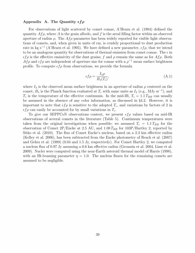
Appendix A. The Quantity εfρ

For observations of light scattered by comet comae, A’Hearn et al. (1984) defined thequantity Afρ, where A is the grain albedo, and f is the areal filling factor within an observedaperture of radius ρ. The Afρ parameter has been widely reported for visible light observa-tions of comets, and, when given in units of cm, is crudely proportional to dust productionrate in kg s−1 (A’Hearn et al. 1995). We have defined a new parameter, εfρ, that we intendto be an analogous quantity for observations of thermal emission from comet comae. The ε inεfρ is the effective emissivity of the dust grains; f and ρ remain the same as for Afρ. BothAfρ and εfρ are independent of aperture size for comae with a ρ−1 mean surface brightnessprofile. To compute εfρ from observations, we provide the formula

εfρ =Iλρ

Bλ(Tc), (A.1)

where Iλ is the observed mean surface brightness in an aperture of radius ρ centered on thecomet, Bλ is the Planck function evaluated at Tc with same units as Iλ (e.g., MJy sr−1), andTc is the temperature of the effective continuum. In the mid-IR, Tc = 1.1TBB can usuallybe assumed in the absence of any color information, as discussed in §4.2. However, it isimportant to note that εfρ is sensitive to the adopted Tc, and variations by factors of 2 inεfρ can easily be accounted for by small variations in Tc.

To give our SEPPCoN observations context, we present εfρ values based on mid-IRobservations of several comets in the literature (Table 5). Continuum temperatures weretaken from the original investigations when possible; we assumed Tc = 1.1TBB for theobservation of Comet 2P/Encke at 2.5 AU, and 1.08TBB for 103P/Hartley 2, reported bySitko et al. (2010). The flux of Comet Encke’s nucleus, based on a 2.3 km effective radius(Kelley et al. 2006), has been subtracted from the Encke photometry of Reach et al. (2007)and Gehrz et al. (1989) (0.04 and 1.5 Jy, respectively). For Comet Hartley 2, we computeda nucleus flux of 0.97 Jy assuming a 0.6 km effective radius (Groussin et al. 2004, Lisse et al.2009). Nuclei were computed using the near-Earth asteroid thermal model of Harris (1998),with an IR-beaming parameter η = 1.0. The nucleus fluxes for the remaining comets areassumed to be negligible.

39

Table A.7: εfρ values computed from selected comet observations in the literature, presented for comparison to the comets in our survey. The tablehas been sorted by εfρ.

Comet rh λ ρ εfρ σ Notes(AU) (µm) (km) (cm) (cm)

2P/Encke 2.52 23.7 18 300 31 · · · Reach et al. (2007)73P-B/Schwassman-Wachmann 3 1.11 11.7 430 744 8 ≈ 1 week post-outburst, Harker et al. (2011)

103P/Hartley 2 1.06 11.6 330 814 26 Meech et al. (2011)73P-C/Schwassman-Wachmann 3 1.09 11.7 350 2 518 25 Harker et al. (2011)

2P/Encke 0.38 10.0 2 000 2 720 60 Gehrz et al. (1989)C/1995 O1 (Hale-Bopp) 2.8 7.8 3 300 52 400 5 200 pre-perihelion, Wooden et al. (1999)C/1996 B2 (Hyakutake) 0.34 10.3 14 400 53 500 1 500 Mason et al. (1998)

1P/Halley 0.59 10.3 12 600 127 000 · · · Gehrz and Ney (1992)C/1995 O1 (Hale-Bopp) 0.92 10.3 13 400 1 280 000 120 000 Mason et al. (2001)

40