The Offset to an Algebraic Curve and an Application to Conics

The Offset to an Algebraic Curve and an Application to

Conics

Francois Anton, Ioannis Z. Emiris, Bernard Mourrain, Monique Teillaud

To cite this version:

Francois Anton, Ioannis Z. Emiris, Bernard Mourrain, Monique Teillaud. The Offset to anAlgebraic Curve and an Application to Conics. International Conference on ComputationalScience and its Applications, May 2005, Singapore, Singapore. Springer Verlag, 3480, pp.683-696, 2005, LNCS. <inria-00350878>

HAL Id: inria-00350878

https://hal.inria.fr/inria-00350878

Submitted on 7 Jan 2009

HAL is a multi-disciplinary open accessarchive for the deposit and dissemination of sci-entific research documents, whether they are pub-lished or not. The documents may come fromteaching and research institutions in France orabroad, or from public or private research centers.

L’archive ouverte pluridisciplinaire HAL, estdestinee au depot et a la diffusion de documentsscientifiques de niveau recherche, publies ou non,emanant des etablissements d’enseignement et derecherche francais ou etrangers, des laboratoirespublics ou prives.

https://hal.archives-ouvertes.fr

https://hal.inria.fr/inria-00350878

The Offset to an Algebraic Curve and anApplication to Conics

Francois Anton1, Ioannis Emiris2,Bernard Mourrain3, and Monique Teillaud3

1 Department of Computer Science,University of Calgary, 2500 University Drive N.W.,

Calgary, Alberta, T2N 1N4, [email protected]

2 Department of Informatics and Telecommunications,National Kapodistrian University of Athens,

Panepistimiopolis 15784, Greece3 INRIA Sophia-Antipolis, B.P. 93, 2004,

route des Lucioles, 06902, Sophia-Antipolis, France

Abstract. Curve offsets are important objects in computer-aided de-sign. We study the algebraic properties of the offset to an algebraic curve,thus obtaining a general formula for its degree. This is applied to com-puting the degree of the offset to conics. We also compute an implicitequation of the generalised offset to a conic by using sparse resultantsand the knowledge of the degree of the implicit equation.

1 Introduction

An important object in nonlinear computational geometry, Computer-aided Ge-ometric Design and geometric modelling is the offset of a given curve or surface,which is defined as the locus of points at a given distance. A related questionconcerns the bisector of two curves or surfaces. Both problems have been ad-dressed for some classes of curves or surfaces, mostly for their applications (see[1] for the application to the Voronoi diagram of semi-algebraic sets).

What Hoffmann and Vermeer [8] define as offset curves, Arrondo, Sendraand Sendra [2] define as generalised offset curves. The extraneous solutions (cor-responding to a point of the curve or surface which corresponds to infinitelymany points on the generalised offset) have been addressed in [8]. Hoffmann andVermeer [8] did not address the offset computations, but they gave some numer-ical examples computed using Grobner bases. Arrondo, Sendra and Sendra [2]computed the genus of the generalised offset curve.

In this paper, we will address the degree of the offset to an algebraic planecurve in its most general setting. Our main contributions are a general formulafor the degree of the offset curve and its application for the determination ofan implicit equation of the generalised offset to a conic. The conic is definedimplicitly by a formal polynomial (i.e., a polynomial whose coefficients are formal

O. Gervasi et al. (Eds.): ICCSA 2005, LNCS 3480, pp. 683–696, 2005.c© Springer-Verlag Berlin Heidelberg 2005

684 F. Anton et al.

constants). We used the general formula of the degree of the offset curve toeliminate the extraneous factors from the sparse resultant [3, 4] in order to getan implicit equation defining the generalised offset to a conic.

This paper is organised as follows: in Section 2, we study the equation of theoffset. In Section 3, we study the algebraic properties of the offset to an algebraiccurve in order to determine its degree. In Section 4, we show how to computethe implicit equation of the generalised offset to a conic.

2 Equations Defining the Offset

This section uses notions of algebraic geometry; for further background one mayconsult [9]. We assume the most general setting for the problem at hand, i.e. com-plex numbers and we let k = C. In this paper, we assume that V (f1, . . . , fs) ⊂ Edenotes the set of all the points of E whose coordinates (x1, . . . , xn) satisfy thepolynomial equations f1 (x1, . . . , xn) = · · · = fs (x1, . . . , xn) = 0. If E = kn is anaffine space, then the set V is called an affine variety. If E = P

n is a projectivespace over k, then the set V is called a projective variety. Distances are alwaysmeasured in the Euclidean metric. The distance of a point to a curve is thesmallest distance of the point from any point on the curve.

Definition 1. (Offset curve) Let C = V (f) ⊂ k2, for f ∈ k[x, y], be an algebraiccurve and R ∈ R

+ be the offset parameter. The R−offset curve to C is the locusof points lying at distance R from C (see Figure 1).

Definition 1 is equivalent to saying that each point q = (u, v) of the offset curveis the centre of a circle D of radius R, which is tangent to C, and does notcontain any point of C in its interior. We will suppose that f has positive degree(thus C is not empty) and R �= 0 unless stated otherwise.

Definition 2. (Generalised offset) The generalised R-offset curve to C denotedO is the locus of the centres q = (u, v) of circles D of radius R, that are tangentto C (see Figure 1).

The R−generalised offset to C is a superset of the true R−offset curve to C.Indeed, the circle centred on a point q′ of the true R−offset curve to C of radius

C

R

Dq O

O

C

C

O

O

m

Fig. 1. The Maple plots of a strophoid (C), its true offset (left) and of its generalised

offset O (right)

The Offset to an Algebraic Curve and an Application to Conics 685

R is tangent to C. Its interior does not intersect C. The Zariski closure [9] of anaffine (resp. projective) variety V is the smallest affine (resp. projective) varietycontaining X. The generalised offset to a hypersurface ν at distance R is theZariski closure of the set of intersection points of the spheres with centre on νand radius R, and the normal lines to ν at the centre of the spheres, cf. [2].We will now establish the systems of equations and inequalities that define thegeneralised R-offset O and the true R-offset to an algebraic curve C = V (f).The normal to C at a given point p = (x, y) ∈ C is the set of points q = (u, v)for which nx,y(u, v) = 0, where nx,y(u, v) = −fy(x, y) · (u−x)+fx(x, y) · (v−y).Here fx and fy denote the partial derivatives of f . A point p of an algebraiccurve V (f) ⊂ k2 is called a singular point if, and only if, both partial deriva-tives of f vanish at p (i.e., fx(p) = fy(p) = 0). For a given q = (u, v) ∈k2, let M ⊂ R

2 be the the set of points m = (α, β) ∈ C ∩ R2 such that

nα,β(u, v) = 0. This condition is achieved whenever the normal to C ∩ R2 at

m passes through q, or m is singular. In the general case, M is finite. How-ever, if C ∩ R

2 is a circle centred on q, then M = C ∩ R2. More generally, if

f is not square-free, there is an infinity of singular points. To get in all casesa finite set of points m of C ∩ R

2 such that nα,β(u, v) = 0, we use S = Mwhen M is finite, and S = {w} for an arbitrary point w of C ∩ R

2 when M isinfinite.

Lemma 1. The set of all the closest points on C∩R2 from q is contained in M.

Proof. The polynomial n (considered here as a polynomial in α, β for fixed u, v)defining M expresses half of the differential of the scalar product −→qm ·−→qm (whichis equal to the square of the Euclidean distance δ(q, m)) with respect to m. Theclosest points on C ∩ R

2 from q are global minima of the Euclidean distanceδ(q,m), so, the differential (and thus, n) vanishes on them. ��The point q = (u, v) on the generalised R-offset curve O can be constructedfrom a non-singular point p = (x, y) on C as the intersection of the normal toC at p (given by nx,y, as mentioned previously) and the circle D centred on p,and of radius R. The equation of this circle is dx,y(u, v) = 0, where dx,y(u, v) =

(u − x)2 + (v − y)2 − R2. Let us consider the mapπ : k6 → k2

(x, y, u, v, α, β) �→ (u, v) .

π can also be seen as the canonical projection of k4 ⊂ k6 onto k2. If we con-sider the inclusion map from k2 to k4, V (f) can be seen as a variety of k4,which is the image of C by this inclusion map. Let n(x, y, u, v) = nx,y(u, v)and d(x, y, u, v) = dx,y(u, v) be considered now as polynomials in k[x, y, u, v].V (n) is a proper subset of k4 provided that p = (x, y) is not singular. If f isnot square-free, there is an infinity of singular points. From now on, the affineand projective varieties will be considered in different underlying spaces. Whennecessary, we will specify the underlying space by an inclusion, e.g. V (f) ⊂ k4

or V (f) ⊂ k2. The generalised R-offset O is the image by π of the affine varietyof k4 defined by the following system of equations and inequalities:

686 F. Anton et al.

⎧⎪⎪⎨

⎪⎪⎩

f(x, y) = 0n(x, y, u, v) = 0d(x, y, u, v) = 0fx(x, y) �= 0 or fy(x, y) �= 0

O is the image of (V (f) ∩ V (n) ∩ V (d)) \ V (fx, fy) by the canonical projectionπ : k4 → k2 onto the (u, v)-plane. The true R-offset lies in R

2 and is obtained asthe difference of the generalised R-offset O and the union of the images by π ofthe sets defined by the following system of equations and inequalities, for eachpoint m = (α, β) of S:

⎧⎨

⎩

f(α, β) = 0n(α, β, u, v) = 0(u − α)2 + (v − β)2 − R2 < 0

3 The Degree of the Offset Curve

This section relies on several algebraic concepts, which can be found in moredetail in [9]. Consider polynomials in the variables x, y, u and v with coefiicientsin k and the projective space P

4 (of lines in k5 passing through the origin).The homogenisation variable will be denoted by t. We consider the point q =(u, v) on the generalised R-offset curve O constructed above from an arbitrarypoint p = (x, y) on C. Let g = tdegree(g)g(x

t , yt , u

t , vt ) be the homogenisation

of a polynomial g, V denote the projective closure of the variety V , i.e. thesmallest projective variety containing V , and gT denote the polynomial definingthe component at infinity (i.e. the points with homogeneous coordinate equal tozero) of V (g). Note that V (g) = V (g) [9–p. 33]. Thus, V (f), V (n), V (d) ⊂ P

4.We are now going to decompose the projective closure of V (f, n, d) ⊂ k4 into

the union of its component at infinity, its singular component (points induced bysingular points p on C), and the generalised offset considered in k4 (i.e. the affinevariety V (f, n, d) \ V (fx, fy) ⊂ k4). We will thus obtain the generalised offsetconsidered in k4 as a difference of projective varieties, and we will determinetheir dimensions and degrees in order to determine the degree of the generalisedoffset.

Let us define W = V (f) ∩ V (n) ∩ V (d), Wa = W \ (V (fx, fy) ∪ V (t)) ⊂ P4,

WS = W ∩ V (fx, fy), and W∞ = W ∩ V (t). We recall here the definitionof a quasi-projective variety. In the Zariski topology, the only sets that areclosed are algebraic (affine or projective) varieties. A quasi-projective varietyis an open subset of a projective variety. Wa is a quasi-projective variety sinceV (f) ∩ V (n) ∩ V (d) and V (fx, fy) ∪ V (t) ⊂ P

4 are projective varieties. WS isa projective variety and W∞ = V (fT , dT , nT , t) a projective subvariety. A va-riety X is called reducible if there exist varieties X1 ⊂ X, X2 ⊂ X, X1 �= X,X2 �= X, such that X = X1∪X2. A polynomial is reducible if it can be factorizedinto two polynomials of positive degree. Let d1 := −ι(u − x) + (v − y), d2 :=ι(u − x) + (v − y), and let ι be a root of the equation x2 + 1 = 0 in the


algebraically closed field k. Then V (dT ) = V (d1) ∪ V (d2) is a minimal de-composition, i.e. into the smallest number of irreducible varieties. We considerthe ring k[x1, . . . , xn] of polynomials in n variables with coefficients in k. Let〈f1, . . . , fs〉 = {g1f1 + · · · + gnfn : ∀i, gi ∈ k[x1, . . . , xn]} denote the ideal gener-ated by f1, . . . , fs ∈ k[x1, . . . , xn]. Let

√I = {f ∈ k[x1, · · · , xn] : ∃n ∈ N, fn ∈ I}

denote the radical of an ideal I. Lastly, for any variety W , let I(W ) denote theset of all polynomials vanishing on W ; this is easily shown to be an ideal. Forany variety W = V (p), I(W ) =

√(〈p〉) by Hilbert’s Nullstellensatz [9]. Now,

we will prove some lemmas that will be needed for the proof of Lemma 6. LetV (fT ) = V (h1) ∪ V (h2) ∪ · · · ∪ V (hs) be minimal: ∀j �= i, V (hi) �⊂ V (hj).

Lemma 2. None of the irreducible components of V (fT ) ⊂ P4 is contained in

an irreducible component of V (dT ) ⊂ P4. Equivalently, none of the hi

divides dT .

Proof. Let us first establish the equivalence of the two statements. For any i,we have V (hi) ⊂ V (dT ) ⇔ dT ∈ I(V (hi)) =

√〈hi〉. Since hi is irreducible, thelatter ideal equals 〈hi〉. Hence, an equivalent expression is that hi divides dT .We will prove the second statement by contradiction. Assume dT ∈ I(V (hi)) ⊂k[x, y, u, v, t] for some i ∈ {1, 2, . . . , s}. Thus, there exists g ∈ k[x, y, u, v, t] suchthat dT = g · hi. The sum of the degrees of g and of hi equals 2. There are threecases, namely that the respective degrees equal 0,2 or 1,1 or 2,0. If the degreeof hi is 2, then hi is reducible, therefore the first case is not possible. In thesecond case, dT = g · (αx + βy + γ), where α, β, γ are coefficients of k. Thiswould imply that the terms in u2 and the terms in v2 of dT must come from g.These terms induce terms in u2x, u2y, v2x, and v2y which cannot be canceled.So the second case is also infeasible. In the last case, hi cannot be a constant bydefinition. ��We consider the projective space P

N and we let ξ ∈ PN be denoted by (ξ0 :

· · · : ξN ), where ξi ∈ k, i = 0, . . . , N and not all the ξi are 0. Let ANi ⊂ P

N

consist of all the points for which ξi �= 0 (thus, it is isomorphic to the affine spacekN ). We now define regular functions, regular mappings of affine varieties, andregular mappings of quasi-projective varieties. Let X be an affine variety in kN . Afunction g on X is regular [9] if there exists a polynomial G with coefficients in ksuch that g(x) = G(x), ∀x ∈ X. Let Y be a variety of kN . A mapping g : X → Yis regular if there exists N regular functions g1, . . . , gN on X such that g(x) =(g1(x), .., gN (x)), ∀x ∈ X. Let f : X → Y be a mapping of quasi-projectivevarieties and Y ⊂ P

N . This mapping is called regular if for every point x ∈ X andevery open affine set A

Ni containing the point f(x) there exists a neighbourhood

U of x such that f(U) ⊂ ANi , and the mapping f : U → A

Ni is regular. The

dimension of a variety X is sup {n : X0 � · · · � Xn ⊂ X and ∀i,Xi irreducible}.

Theorem 1. [9–theorem.8, Sect.1.6] Let f : X → Y be a regular mapping be-tween projective varieties with f(X) = Y . Suppose that Y is irreducible and thatall the fibres f−1(y) for y ∈ Y are irreducible and of the same dimension, thenX is irreducible.

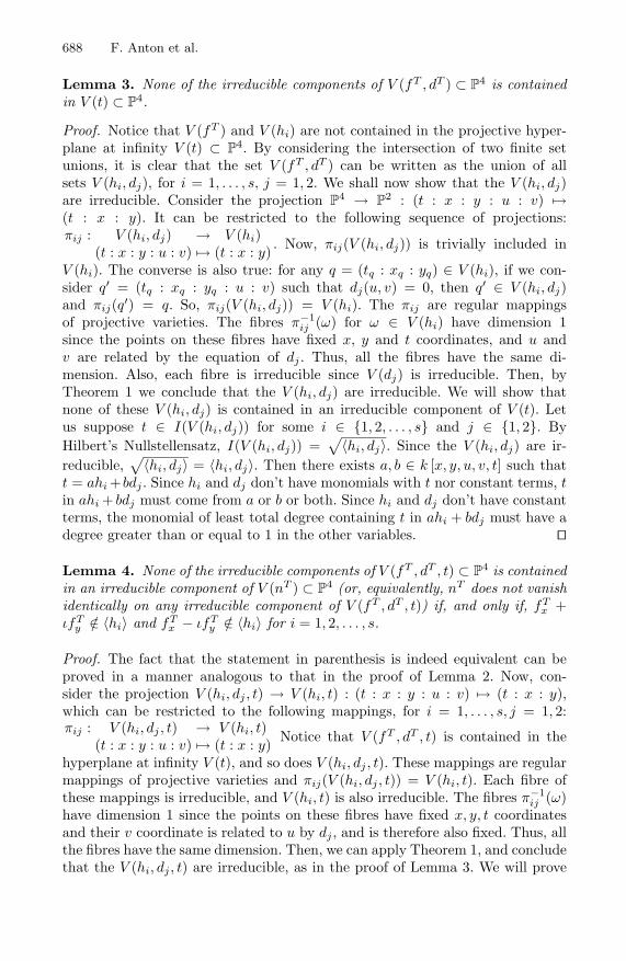
688 F. Anton et al.

Lemma 3. None of the irreducible components of V (fT , dT ) ⊂ P4 is contained

in V (t) ⊂ P4.

Proof. Notice that V (fT ) and V (hi) are not contained in the projective hyper-plane at infinity V (t) ⊂ P

4. By considering the intersection of two finite setunions, it is clear that the set V (fT , dT ) can be written as the union of allsets V (hi, dj), for i = 1, . . . , s, j = 1, 2. We shall now show that the V (hi, dj)are irreducible. Consider the projection P

4 → P2 : (t : x : y : u : v) �→

(t : x : y). It can be restricted to the following sequence of projections:πij : V (hi, dj) → V (hi)

(t : x : y : u : v) �→ (t : x : y) . Now, πij(V (hi, dj)) is trivially included in

V (hi). The converse is also true: for any q = (tq : xq : yq) ∈ V (hi), if we con-sider q′ = (tq : xq : yq : u : v) such that dj(u, v) = 0, then q′ ∈ V (hi, dj)and πij(q′) = q. So, πij(V (hi, dj)) = V (hi). The πij are regular mappingsof projective varieties. The fibres π−1

ij (ω) for ω ∈ V (hi) have dimension 1since the points on these fibres have fixed x, y and t coordinates, and u andv are related by the equation of dj . Thus, all the fibres have the same di-mension. Also, each fibre is irreducible since V (dj) is irreducible. Then, byTheorem 1 we conclude that the V (hi, dj) are irreducible. We will show thatnone of these V (hi, dj) is contained in an irreducible component of V (t). Letus suppose t ∈ I(V (hi, dj)) for some i ∈ {1, 2, . . . , s} and j ∈ {1, 2}. ByHilbert’s Nullstellensatz, I(V (hi, dj)) =

√〈hi, dj〉. Since the V (hi, dj) are ir-reducible,

√〈hi, dj〉 = 〈hi, dj〉. Then there exists a, b ∈ k [x, y, u, v, t] such thatt = ahi +bdj . Since hi and dj don’t have monomials with t nor constant terms, tin ahi + bdj must come from a or b or both. Since hi and dj don’t have constantterms, the monomial of least total degree containing t in ahi + bdj must have adegree greater than or equal to 1 in the other variables. ��

Lemma 4. None of the irreducible components of V (fT , dT , t) ⊂ P4 is contained

in an irreducible component of V (nT ) ⊂ P4 (or, equivalently, nT does not vanish

identically on any irreducible component of V (fT , dT , t)) if, and only if, fTx +

ιfTy /∈ 〈hi〉 and fT

x − ιfTy /∈ 〈hi〉 for i = 1, 2, . . . , s.

Proof. The fact that the statement in parenthesis is indeed equivalent can beproved in a manner analogous to that in the proof of Lemma 2. Now, con-sider the projection V (hi, dj , t) → V (hi, t) : (t : x : y : u : v) �→ (t : x : y),which can be restricted to the following mappings, for i = 1, . . . , s, j = 1, 2:πij : V (hi, dj , t) → V (hi, t)

(t : x : y : u : v) �→ (t : x : y) Notice that V (fT , dT , t) is contained in the

hyperplane at infinity V (t), and so does V (hi, dj , t). These mappings are regularmappings of projective varieties and πij(V (hi, dj , t)) = V (hi, t). Each fibre ofthese mappings is irreducible, and V (hi, t) is also irreducible. The fibres π−1

ij (ω)have dimension 1 since the points on these fibres have fixed x, y, t coordinatesand their v coordinate is related to u by dj , and is therefore also fixed. Thus, allthe fibres have the same dimension. Then, we can apply Theorem 1, and concludethat the V (hi, dj , t) are irreducible, as in the proof of Lemma 3. We will prove


the first direction. Let us suppose fTx + ιfT

y ∈ 〈hi〉 for some i ∈ {1, 2, . . . , s}.We have to show that nT = 0 on V (hi, d1, t). Since (fT

x ) + ι(fTy ) ∈ 〈hi〉,

there exists a polynomial g such that (fTx ) + ι(fT

y ) = g · hi. But, hi = 0 onV (hi, d1, t). Thus, (fT

x ) + ι(fTy ) = 0, i.e. fT

y = ιfTx . Then, replacing in nT , we

get nT = −ιfTx (u−x)+fT

x (v−y) = (−ι(u−x)+(v−y))fTx on V (hi, d1, t). Since

d1 = −ι(u−x)+ (v− y) = 0 on V (hi, d1, t), then nT = 0 on V (hi, d1, t). We canprove in the same way that if (fT

x ) − ι(fTy ) ∈ 〈hi〉 then nT = 0 on V (hi, d2, t).

Reciprocally, let us suppose nT = 0 on V (hi, d1, t) for some i ∈ {1, 2, . . . , s}.Since none of nT , hi, d1 depend on t, nT = 0 on V ( hi, d1). Since

d1 = 0 on V (hi, d1),{

nT = −fTy (u − x) + ιfT

x (u − x) = 0nT = ιfT

y (v − y) + fTx (v − y) = 0 on V (hi, d1). Since

(−fTy + ιfT

x ) = ι(ιfTy + fT

x ), we can rewrite the last system of equations as{

(−fTy + ιfT

x )(u − x) = 0(−fT

y + ιfTx )(v − y) = 0 on V (hi, d1). The subvariety V (hi, d1, u−x, v−y) =

V (hi, u − x, v − y) is a one-dimensional variety in the two-dimensional varietyV (hi, d1). The set V (hi, d1) \ V (hi, d1, u − x, v − y) is a dense open subset ofV (hi, d1). From the last system, we know that (−fT

y + ιfTx ) vanishes on this

dense open subset. Now, we consider V (hi, d1,−fTy + ιfT

x ). This is a closed pro-jective set. We know that it contains the open set V (hi, d1)\V (hi, d1, u−x, v−y).Thus, it contains also its Zariski closure i.e. V (hi, d1). Thus, (−fT

y +ιfTx ) vanishes

on V (hi, d1). Therefore, there exists a, b ∈ k[x, y, u, v] such that −fTy + ιfT

x =ahi + bd1 = ahi + b(−ι(u − x) + v − y). Let auv be the sum of all the termsof a containing the variables u or v. Since (−fT

y + ιfTx ) does not depend on

any of the variables u and v, so auvhi = b(ιu − v). Since the left hand sideof this equality lies in 〈hi〉, so does the right-hand side, hence b ∈ 〈hi〉. Thus,−fT

y + ιfTx ∈ 〈hi〉. Thus, fT

x + ιfTy ∈ 〈hi〉. In the same way, we can prove that

if nT = 0 on V (hi, d2, t) ⊂ P4 then fT

x − ιfTy ∈ 〈hi〉. ��

We are going to analyse the dimension of the one-dimensional component of W∞.

Let l ={

1 if fTx + ιfT

y ∈ 〈hi〉 or fTx − ιfT

y ∈ 〈hi〉 for some i ∈ {1, 2, . . . , s}0 otherwise . We

will now introduce hypersurfaces, necessary in the proofs of the next lemma andof Theorem 3. If X is a projective variety in P

N and F �= 0 is a form on X (i.e.a real-valued homogeneous polynomial function on X), then we denote by XF

the sub-variety of X, known as a hypersurface, defined by F = 0.

Theorem 2. [9–Theorem 4, p. 57] If a form F is not identically 0 on an irre-ducible projective variety X, then dim XF = dimX − 1.

In order to apply this theorem on the projective variety W∞ whose irreducibilityis not known, we have determined if none of its irreducible components is con-tained in an irreducible component of V (F ). Indeed, if an irreducible componentV (hi) is contained in an irreducible component V (Fi) of V (F ), then Fi vanisheson V (hi), and dim V (hi)

⋂V (F ) = dim V (hi).

Lemma 5. The dimension of W∞ = V (fT , nT , dT , t) ⊂ P4 is equal to l.

690 F. Anton et al.

Proof. We start in P4, which has dimension 4. By Lemmas 2, 3 and repeated

application of Theorem 2 (from V (fT ) to V (fT , dT ), and from V (fT , dT ) toV (fT , dT , t)) we get that V (fT , dT , t) has dimension 4 − 3 = 1. Thus, the di-mension of W∞ is 0 or 1. By Theorem 2, the dimension of W∞ is 0 if, and onlyif, l = 0 by Lemma 4. ��

The following two lemmas give the degrees of two one-dimensional compo-nents, when these exist. The one-dimensional component at infinity and theone-dimensional component of WS . They will allow us to conclude with the de-gree of the offset in Theorem 3. For this theorem, but also more generally, werecall the notion of degree. The degree of a n−dimensional projective varietyX ⊂ P

N is the maximum number of points of intersection of X with a pro-jective linear subspace P

N−n in general position with respect to X (see page234 in [9]). Thus, the degree of a projective variety is the degree of its maximaldimensional component. We recall the definition of localisation at a prime idealP ⊂ k [t1, . . . , tm], where k is a field. We denote by k [x1, . . . , xm]P the set of allrational functions f/g such that f, g ∈ k[x1, . . . , xm] where g �∈ P.

Definition 3. (adapted from [7–Def.A.8.16,p.480]) Let F, G ∈ k[z, x, y] be ho-mogeneous polynomials, let p = (p0 : p1 : p2) ∈ V (F )

⋂V (G) ⊂ P

2, and letMp = 〈p0x− p1z, p0y − p2z〉 be the homogeneous ideal of p. Assume that p0 �= 0then, the intersection multiplicity of V (F ) and of V (G) at p is µp(F, G) :=dimk(k[z, x, y]Mp

/〈F, G〉).Let C∞ be the component at infinity of the projective closure of C, i.e. C∞ =V (fT , t) ⊂ k2. Let CS be the affine subvariety of C composed of all its singularpoints, i.e. CS = V (fx, fy, f) ⊂ k2.

Lemma 6. The one-dimensional component of W∞ has degree2l

∑p∈C∞ µp′(V (fT ), V (nT )), where p′ is an arbitrary point of W∞ whose pro-

jection on the projective (t, x, y)-plane is p.

Proof. The variety’s degree is given by that of the component with maximumdimension. By lemma 5, l = 0 iff dim W∞ = 0 and we say that the degreeof the (non-existant) 1-dimensional component is 0. In the rest of the proof,we study the degree of the 1-dimensional component, assuming it exists, ie.,for l = 1. Note that this component may not be connected. There exist i ∈{1, . . . , s}, j ∈ {1, 2} in the above notation, such that nT = 0 on V (hi, dj , t), byLemma 4. Hence, adding nT to 〈dT , fT , t〉 does not change its radical. Thus, thepoints of W∞ = V (fT , dT , nT , t) and V (

√〈dT , fT , t〉) are the same, but theirmultiplicities may differ. The one-dimensional component of V (

√〈dT , fT , t〉) isconstituted of all the points p′ whose projection on the projective (t, x, y)-planeis a point p of C∞ ⊂ P

2 and whose projection on the affine (u, v)-plane is thecircle V (dT ). The degree of the one-dimensional component of V (

√〈dT , fT , t〉)equals the product of the degree of dT (which is 2) by the number of isolatedpoints in C∞, counted with multiplicities. The reason is that each point of C∞generates a one-dimensional component of W∞ with the x, y coordinates of the


point of C∞, and where the t, u, v coordinates satisfy dT . The degree of the one-dimensional component of W∞ is twice the sum of the intersecting multiplicitiesof V (fT , nT ) ⊂ P

4 at the points p′ for all the points p of C∞. ��

Lemma 7. The degree of the one-dimensional component of WS, defined at thebeginning of this section, is: 2

∑q∈CS

(µq′(V (f), V (n))− 1), where q′ is an arbi-trary point of WS whose projection on the affine (x, y)-plane is q. This componentdoes not exist iff the degree vanishes.

Proof. Each point q of CS induces a trivial equation n. Thus, at the level of WS ,each point q of multiplicity m induces a one-dimensional variety that consistsof all the points q′ whose projection on the affine (x, y)-plane is q and whoseprojection on the projective (t, u, v)-plane is a projective circle centred at q and ofradius R with multiplicity m−1 (the extraneous component may be simple). Theonly component at infinity of WS are the points (0 : x0 : y0 : 1 : y0 ± ι(1 − x0)),where (x0, y0) is a common root of fT , fT

x (x, y), and fTy (x, y). It follows that

WS does not have a one-dimensional component at infinity. The points of WS

are the same as the points of V (√

〈fx, fy, f , d〉), but their multiplicities differ.

The degree of the one-dimensional component of V (√

〈fx, fy, f , d〉) equals the

product of the degree of d (which is 2) by the number of isolated points inCS . The degree of the one-dimensional component of WS is twice the sum ofthe multiplicities of V (f, n) ⊂ P

4 at the points q′ minus 1 for all the points qof CS . ��

Theorem 3. Let p′ and q′ be defined as in Lemmas 6 and 7. The degree of thegeneralised R-offset O to an algebraic curve V (f) ⊂ k2 of degree m, such as fis square free is :

2m2 − 2l∑

p∈C∞

µp′(V (fT ), V (nT )) − 2∑

q∈CS

(µq′(V (f), V (n)) − 1). (1)

Proof. Bezout’s Theorem [9] states that, for projective varieties, the degree of theintersection of two varieties is generically equal to the product of the varieties’degrees. Therefore, the degree of W is generically 2m2. The quasi-projectivevarieties W , Wa, W∞, and WS are related by Wa = W \ (W∞ ∪ WS). SinceW is defined by three polynomials, its dimension is at least 1 according toTheorem 2. Since n has two more variables than f and the same degree, n cannot identically vanish on V (f). Hence, dim V (f, n) ≤ 2, by Theorem 2. Since dhas coefficients that are polynomials in R, R �= 0 and the coefficients of f and ddo not depend on R, d can not identically vanish on B∩N . Thus, the dimension ofW is exactly one by the same theorem. Since W is one-dimensional, the degreeof W is the sum of the degrees of its one-dimensional components. Thus, thedegree of Wa equals the degree of W minus the degree of the one-dimensionalcomponent of W∞∪WS . Since WS has no one-dimensional component at infinity(see proof of Lemma 7), the one-dimensional components of W∞ and of WS are

692 F. Anton et al.

disjoint, and the degree of the one-dimensional component of W∞ ∪ WS is thesum of the degrees of the one-dimensional components of W∞ and of WS . ByLemmas 6 and 7, the degree of Wa is given by Equation 1. By definition, tnever vanishes on Wa. Finally, O is the image of Wa by the canonical projectionπ : P

4 \ {(1 : 0 : 0 : 0 : 0)} → k2 : (t : x : y : u : v) �→ (ut , v

t ) that is a one-to-onemapping. Indeed, there is generically only one point of the curve correspondingto a point of the generalised offset. Thus, the result. ��

By applying the results from this section, we get [1] the following degrees forconic offsets:

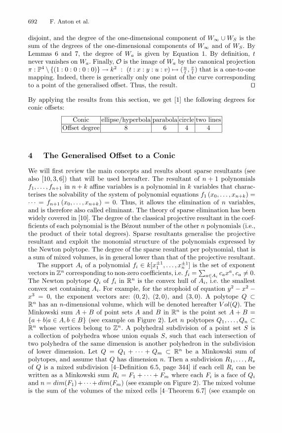
Conic ellipse/hyperbola parabola circle two linesOffset degree 8 6 4 4

4 The Generalised Offset to a Conic

We will first review the main concepts and results about sparse resultants (seealso [10, 3, 6]) that will be used hereafter. The resultant of n + 1 polynomialsf1, . . . , fn+1 in n + k affine variables is a polynomial in k variables that charac-terises the solvability of the system of polynomial equations f1 (x0, . . . , xn+k) =· · · = fn+1 (x0, . . . , xn+k) = 0. Thus, it allows the elimination of n variables,and is therefore also called eliminant. The theory of sparse elimination has beenwidely covered in [10]. The degree of the classical projective resultant in the coef-ficients of each polynomial is the Bezout number of the other n polynomials (i.e.,the product of their total degrees). Sparse resultants generalise the projectiveresultant and exploit the monomial structure of the polynomials expressed bythe Newton polytope. The degree of the sparse resultant per polynomial, that isa sum of mixed volumes, is in general lower than that of the projective resultant.

The support Ai of a polynomial fi ∈ k[x±11 , . . . , x±1

n ] is the set of exponentvectors in Z

n corresponding to non-zero coefficients, i.e. fi =∑

a∈Aicaxa, ca �= 0.

The Newton polytope Qi of fi in Rn is the convex hull of Ai, i.e. the smallest

convex set containing Ai. For example, for the strophoid of equation y2 − x2 −x3 = 0, the exponent vectors are: (0, 2), (2, 0), and (3, 0). A polytope Q ⊂R

n has an n-dimensional volume, which will be denoted hereafter V ol(Q). TheMinkowski sum A + B of point sets A and B in R

n is the point set A + B ={a + b|a ∈ A, b ∈ B} (see example on Figure 2). Let n polytopes Q1, . . . , Qn ⊂R

n whose vertices belong to Zn. A polyhedral subdivision of a point set S is

a collection of polyhedra whose union equals S, such that each intersection oftwo polyhedra of the same dimension is another polyhedron in the subdivisionof lower dimension. Let Q = Q1 + · · · + Qm ⊂ R

n be a Minkowski sum ofpolytopes, and assume that Q has dimension n. Then a subdivision R1, . . . , Rs

of Q is a mixed subdivision [4–Definition 6.5, page 344] if each cell Ri can bewritten as a Minkowski sum Ri = F1 + · · · + Fm where each Fi is a face of Qi

and n = dim(F1)+ · · ·+dim(Fm) (see example on Figure 2). The mixed volumeis the sum of the volumes of the mixed cells [4–Theorem 6.7] (see example on


��

��

y

x0

0

2

1

1 2��

��

y

x

00

1

2

1��

��

30

1

4

y

x

0

A+B

��

��

��

��

y

x

MV=4

Fig. 2. The Minkowski sum (third diagram) of the point sets A (first) and B (second)

and its mixed subdivision (filled-in cells are copies of Newton polytopes and mixed

cells are unfilled)

Figure 2). If we replace a polytope Qi by a polytope Q′i included in it, the mixed

volume of the Qi does not increase.A conic C can be defined implicitly as the variety defined by a second degree

formal polynomial: f(x, y) = αx2 + βxy + γy2 + δx + εy + ζ = 0. We shallcompute an implicit equation of its generalised offset. The partial derivativesare fx = 2αx + βy + δ and fy = βx + 2γy + ε. An equation of the normalN = V (n) ⊂ k4 to the original conic at the point (x, y) is: n(x, y, u, v) =−(βx + 2γy + ε)(u− x) + (2αx + βy + δ)(v − y) = 0. If a conic is not degenerate(proper conic different from the union of two lines), then it has no singularpoints, and S = ∅. The generalised offset to a conic is the Zariski closure of theprojection of the affine variety V(f, n, d)\V (fx, fy) onto the (u, v) plane. This is asubvariety of the Zariski closure of the projection of V (f, n, d). Thus the equationof the generalised offset is a factor of the equation of the Zariski closure of theprojection of V (f, n, d), which is the resultant of f, n, d expressing the eliminationof x, y. The objective in the computations is to simplify the polynomials, whileproducing a system of equations equivalent to the original one. In the case of thesparse resultant computation, this has been achieved by replacing one polynomialby a linear combination of polynomials, and having a Newton polytope inscribedin the Newton polytope of the original polynomial. The sparse resultants havebeen computed thanks to the sparse resultant software developed by Emiris[6, 5]. We computed the determinant of this matrix and its factorisation. Thedegree of the offset to conics allowed us to identify the factor that correspondsto an implicit equation of the generalised offset. In the case where α and β aredifferent from 0, we call the conic “generic”. Hereafter, all conics are generic.

The polynomial n can be rewritten in the following way: n(x, y, u, v) =βx2 − βy2 + 2(γ − α)xy + (−βu + ε + 2αv)x + (βv − δ − 2γu)y + (−εu +δv) = 0. The monomial in x2 can be eliminated if we replace n(x, y, u, v)by αn(x, y, u, v) − βf(x, y) (see Figure 3). Similarly, if we replace d(x, y, u, v)by f(x, y) − αd(x, y, u, v), the monomial in x2 disappears (see Figure 3). Themixed volumes are MV (f, αn − βf) = MV (f, f − αd) = 4 (see Figure 4), andMV (αn − βf, f − αd) = 3. We get an equation for the generalised offset as thesparse resultant of f, αn − βf and f − αd. Hereafter, all the implicit equationsare publicly available at: http:// pages.cpsc.ucalgary.ca/ antonf.

However, it is possible to further simplify the equation of a non-degenerateconic by using a coordinate system with origin at one of the foci (in the caseof an ellipse or hyperbola) or the apex (in the case of a parabola), and one

694 F. Anton et al.

��

��

1

00 1 2

y

2

x��

��

1

00 1 2

y

2

x��

��

1 2

2

1

y

x

00 ��

��

��

1

00 1 2

y

2

x��

��

1 2

2

1

y

x

00

Fig. 3. The Newton polytopes of f , n, αn − βf , d, and of f − αd

��

��

��

��

y

x

MV=4

��

��

��

��

y

x

MV=4 ��

��

��

��

y

x

MV=3

Fig. 4. The mixed volumes of f and αn − βf , of αn − βf and f − αd, and of f and

f − αd

��

��

1

00 1 2

y

2

x��

��1

00 1 2

y

2

x��

��

1

00 1 2

y

2

x��

��

1

00 1 2

y

2

x

Fig. 5. The Newton polytopes of f , n, d and of ad − f for ellipses and hyperbolas

��

��

��

��

MV=4

x

y

��

��

��

��

y

x

MV=3

��

��

��

��

y

x

MV=4

Fig. 6. A mixed subdivision and mixed volume computation of f, n, of n, f − d, and of

f, f − d for ellipses and hyperbolas

of the axes being the axis of the conic. By a simple change of coordinates, wecan obtain easily the general equation of the generalised offset. Then, an ellipseor hyperbola simplifies to x2

a2 ± y2

b2 − 1 = 0, assuming ab �= 0. We can get anequivalent equation x2 + cy2 + e = 0, where e ± b2c = 0. Let f := x2 + cy2 + e.It is easy to see from Figure 5 that no linear combination of f and d has termsin common with n. If we replace d(x, y, u, v) = (u − x)2 + (v − y)2 − R2 = 0 byf(x, y) − d(x, y, u, v), the monomial in x2 disappears (see Figure 5). The mixedvolumes are MV (f, n) = MV (f, f−d) = 4 and MV (n, f−d) = 3 (see Figure 6).We get an equation for the generalised offset as the sparse resultant of f, n, f −din the variables u and v. Examples are shown in Figure 7.

In the case of a parabola, the equation of the conic in a coordinate systemwith origin at the summit of the parabola, and one of the axes being the axis ofthe parabola, simplifies to y2−2px = 0. The polynomial defining N = V (n) ⊂ k4

can be rewritten in the following way: n(x, y, u, v) = −2yu+2xy−2pv+2py = 0.It is easy to see from Figures 8 that no linear combination of f and d has terms


–3

–2

–1

1

2

3

v

–2 –1 1 2

u

–6

–4

–2

0

2

4

6

v

–4 –2 2 4

u

–4

–2

2

4

v

–4 –2 2 4

u

–6

–4

–2

2

4

6

v

–6 –4 –2 2 4 6

u

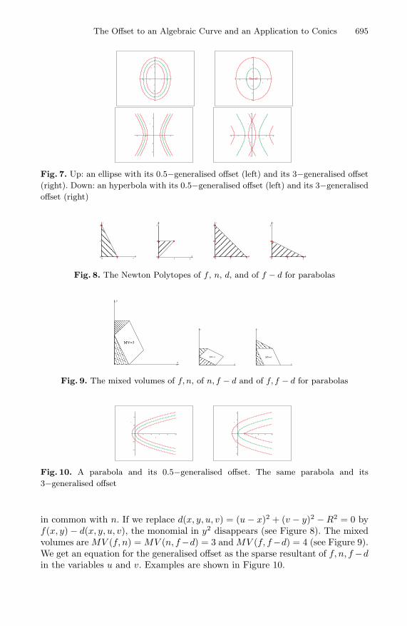
Fig. 7. Up: an ellipse with its 0.5−generalised offset (left) and its 3−generalised offset

(right). Down: an hyperbola with its 0.5−generalised offset (left) and its 3−generalised

offset (right)

��

��

1 2

2

1

y

x

00 ��

��

��

1

00 1 2

y

2

x��

��

1

00 1 2

y

2

x��

��1

00 1 2

y

2

x

Fig. 8. The Newton Polytopes of f , n, d, and of f − d for parabolas

��

��

��

��

y

x

MV=3

��

��

��

��

y

x

MV=3

��

��

��

��

y

x

MV=4

Fig. 9. The mixed volumes of f, n, of n, f − d and of f, f − d for parabolas

–4

–2

2

4

v

2 4 6 8 10

u

–6

–4

–2

2

4

6

v

2 4 6 8 10

u

Fig. 10. A parabola and its 0.5−generalised offset. The same parabola and its

3−generalised offset

in common with n. If we replace d(x, y, u, v) = (u − x)2 + (v − y)2 − R2 = 0 byf(x, y) − d(x, y, u, v), the monomial in y2 disappears (see Figure 8). The mixedvolumes are MV (f, n) = MV (n, f−d) = 3 and MV (f, f−d) = 4 (see Figure 9).We get an equation for the generalised offset as the sparse resultant of f, n, f −din the variables u and v. Examples are shown in Figure 10.

696 F. Anton et al.

5 Conclusions

We have obtained a general formula for the degree of the offset to an algebraiccurve defined in its most general setting. We have obtained an implicit equationof the generalised offset to a conic defined by a formal polynomial, and simplifiedequations in the two cases of a circle, an ellipse or an hyperbola, and a parabola.This implicit equation of the generalised offset to a conic has been used in orderto compute the Delaunay graph for conics and for semi-algebraic sets (see [1]).

References

1. F. Anton. Voronoi diagrams of semi-algebraic sets. PhD thesis, The University ofBritish Columbia, Vancouver, British Columbia, Canada, January 2004.

2. E. Arrondo, J. Sendra, and J. R. Sendra. Genus formula for generalized offsetcurves. J. Pure Appl. Algebra, 136(3):199–209, 1999.

3. J. F. Canny and I. Z. Emiris. A subdivision-based algorithm for the sparse resul-tant. J. ACM, 47(3):417–451, 2000.

4. D. Cox, J. Little, and D. O’Shea. Using algebraic geometry. Springer-Verlag, NewYork, 1998.

5. I. Emiris. A general solver based on sparse resultants: Numerical issues and kine-matic applications. Technical Report 3110, SAFIR, 1997.

6. I. Z. Emiris and J. F. Canny. Efficient incremental algorithms for the sparseresultant and the mixed volume. J. Symbolic Comput., 20(2):117–149, 1995.

7. G.-M. Greuel and G. Pfister. A Singular introduction to commutative algebra.Springer-Verlag, Berlin, 2002.

8. C. M. Hoffmann and P. J. Vermeer. Eliminating extraneous solutions in curve andsurface operations. Internat. J. Comput. Geom. Appl., 1(1):47–66, 1991.

9. I. R. Shafarevich. Basic algebraic geometry. 1. Springer-Verlag, Berlin, secondedition, 1994. Varieties in projective space, Translated from the 1988 Russianedition and with notes by Miles Reid.

10. B. Sturmfels. Sparse elimination theory. In Computational algebraic geometry andcommutative algebra (Cortona, 1991), Sympos. Math., XXXIV, pages 264–298.Cambr. Univ. Press, Cambridge, 1993.

The Offset to an Algebraic Curve and an Application to Conics

Documents

Transcript of The Offset to an Algebraic Curve and an Application to Conics