arX

iv:m

ath/

0602

248v

1 [

mat

h.A

G]

11

Feb

2006

On the Parallel Lines for Nondegenerate Conics

Rafa l Ab lamowicz1) Jane Liu2)

January 30, 2006

Abstract

Computation of parallel lines (envelopes) to parabolas, ellipses, and hyperbolas is of importance instructure engineering and theory of mechanisms. Homogeneous polynomials that implicitly define paral-lel lines for the given offset to a conic are found by computing Grobner bases for an elimination ideal of asuitably defined affine variety. Singularity of the lines is discussed and their singular points are explicitlyfound as functions of the offset and the parameters of the conic. Critical values of the offset are linkedto the maximum curvature of each conic. Application to a finite element analysis is shown.

Keywords: Affine variety, elimination ideal, Grobner basis, homogeneous polynomial, singularity,family of curves, envelope, pitch curve, undercutting, cam surface

Contents

1 Introduction 2

2 Parallel Lines to a Parabola 22.1 Parallel lines for specific parameters p and r . . . . . . . . . . . . . . . . . . . . . . . . . . . . 32.2 Parallel lines for arbitrary parameters p and r . . . . . . . . . . . . . . . . . . . . . . . . . . . 6

3 Parallel Lines to an Ellipse 93.1 Parallel lines for specific parameters a, b, r . . . . . . . . . . . . . . . . . . . . . . . . . . . . . 103.2 Parallel lines for arbitrary parameters a, b, r . . . . . . . . . . . . . . . . . . . . . . . . . . . . 14

4 Parallel Lines to a Hyperbola 194.1 Parallel lines for specific parameters a, b, r . . . . . . . . . . . . . . . . . . . . . . . . . . . . . 194.2 Parallel lines for arbitrary parameters a, b, r . . . . . . . . . . . . . . . . . . . . . . . . . . . . 23

5 Applications and Conclusions 285.1 Parallel lines to an ellipse in the finite element method . . . . . . . . . . . . . . . . . . . . . . 29

AMS Subject Classification: 13P10, 14Q05, 68W30

1) Department of Mathematics, Box 5054, Tennessee Technological University, Cookeville, TN 38505,USAE-mail: rablamowicz@tntech.edu, URL: http://math.tntech.edu/rafal/2) Department of Civil and Environmental Engineering, Box 5015, Tennessee Technological Univer-sity, Cookeville, TN 38505, USAjliu@tntech.edu, http://http://www.tntech.edu/cee/faculty/jane liu.html

1

A Appendix: Reduced Grobner basis for the idealI = 〈f1, f2, f3〉 ⊂ R[y0, x0, x, y, r, p] 30

B Appendix: Reduced Grobner basis for the idealI = 〈f1, f2, f3〉 ⊂ R[y0, x0, x, y, a, b, r] 32

C Appendix: Reduced Grobner basis for the idealIS = 〈h1, h2, h3, h4, h5, g〉 ⊂ R[x, y, a, b, r] 37

1 Introduction

The present paper introduces the Reader to a computation of parallel lines (envelopes) to three nondegenerateconics: a parabola, an ellipse, and a hyperbola. In each case, we show how to find a single polynomialg ∈ R[x, y] that implicitly generates a suitable elimination ideal of an affine variety containing the parallellines for the given offset r and for the given parameters of the conic. This amounts to a computation of areduced Grobner basis [4], [5], [7], [15] for the ideal for an appropriately chosen total order. We use Maple

[9] and Singular [7] to accomplish computations. We show an application of the results presented here to afinite element analysis. We also make a connection with a design of surface cams in mechanical engineering[11], [13].

In each of the next three sections we discuss three cases of parallel lines for the specific values of theoffset 0 < r < rcrit, r = rcrit, and r > rcrit for a parabola (Section 2), an ellipse (Section 3), and a hyperbola(Section 4). Then, in each section, we consider a general case of each conic while imposing essentially nocondition on the offset except that r > 0. In Section 5 we show one possible application of the results to afinite element analysis of a composite material of elliptical shape. In Appendices A and B we collect some ofthe more cumbersome expressions while in Appendix C we show in detail how we found the singular pointsfor the parallel lines of the ellipse.

2 Parallel Lines to a Parabola

In this section we compute parallel lines to a parabola defined by a polynomial f1 :

f1 = 4py0 − x20 = 0 (1)

where |p| denotes the distance between the focus F = (0, p) and the vertex V = (0, 0).1 Polynomial f2 definesa circle of radius (offset) r centered at a point (x0, y0) on the parabola f1,

f2 = (y − y0)2 + (x − x0)2 − r2 = 0 (2)

while a polynomial f3f3 = 2xp− 2x0p + x0y − x0y0 = 0 (3)

gives a condition that a point P (x, y) on the circle f2 lies on a line perpendicular to the parabola f1 andpassing through the point (x0, y0) on the parabola. The family of such circles is called the family of curvesdetermined by the polynomial f1 (see [4]). There are of course two such points for any given point (x0, y0) :one on each side of the parabola. All these points P belong to an affine variety V = V(f1, f2, f3) – theenvelope of the family of circles – and define two parallel lines at the distance r from the parabola. In whatfollows we will compute a reduced Grobner basis for V and by eliminating variables x0, y0 we will obtain onepolynomial g in variables x and y alone (also p, r in a general case) that defines both parallel lines on eachside of the parabola for the given value of the offset r. Thus, in general, we have f1, f2, f3 ∈ R[x0, y0, x, y, p, r].However, first we illustrate computation for specific values of the parameters p and r, and later we showcomputation for unspecified parameters.

1Without any loss of generality, we assume that the parabola has its vertex at the origin and its focus on the y-axis.

2

2.1 Parallel lines for specific parameters p and r

The parallel lines constitute a subvariety of the affine variety V = V(I) where I = 〈f1, f2, f3〉. In order tofind the polynomial g for the second elimination ideal I2 = I ∩ R[x, y], we first find a Grobner basis G forV for the lexicographic order y0 > x0 > x > y that contains sixteen polynomials.2 Then, we reduce G toa minimal Grobner basis Gm that contains six (or eight, depending on the case) polynomials and, further,to a unique reduced Grobner basis Gr with three (or five, depending on the case) polynomials only. Finally,we eliminate from Gr all polynomials that contain variables y0 and x0, and keep the single polynomialg ∈ R[x, y] that gives the parallel lines and generates the second elimination ideal I2 = 〈g〉.

We are also interested when the parallel lines form a smooth (non singular) variety V(g) or a C∞ 1-manifold or a hypersurface defined by g. Since g can be viewed as a C∞ function R

2 → R and V(g) ={(x, y) ∈ R

2 | g(x, y) = 0}, it is known that V(g) is a smooth manifold at those points p ∈ V(g) where(∇g)(p) 6= 0. [10, Theorem 2.6] We will find singular points of V(g) by finding points p ∈ V(g) where(∇g)(p) = 0.

Thus, V(g) can be thought of as a union of points where the gradient is zero and those points where thegradient is not zero. Connected components of V(g) where the gradient is not zero form the 1-dimensionalmanifold of the parallel lines. However, we are also interested in describing a discrete finite set S of singularpoints where the gradient is zero. For a formal definition of a singular point of an affine variety V(g) see [4,page 136].

Example 1 (r < rcrit) Let p = 13 and r = 1

4 . Then,

V = V(4y0 − 3x20, 16y2 − 32yy0 + 16y20 + 16x2 − 32xx0 + 16x2

0 − 1, 2x− 2x0 + 3x0y − 3x0y0)

We find that the reduced Grobner basis Gr contains only three polynomials including

g = 331776x6 − 42192x2 + 48400y2 − 448512y3 − 84480x2y + 589824y4 + 28032y

− 25344x4 + 1138176x2y2 − 884736x2y3 − 1105920x4y − 5329 + 331776x4y2 (4)

whose gradient is

∇g = (−879x− 1760yx− 1056x3 + 23712xy2 − 46080x3y − 18432y3x + 13824x3y2 + 20736x5)i

+ (3025y − 2640x2 − 42048y2 + 876 + 71136x2y − 34560x4 − 82944x2y2 + 73728y3 + 20736x4y)j . (5)

Thus, the only real point S1 on V(g) where (∇g)(S1) = 0 is S1 = (0, 73192 ). We will refer to this point as a

virtual singular point for the following reason: V(g) is a disjoint union of {S1} and a non-singular smoothsubvariety Π where the gradient ∇g does not vanish. The subvariety Π constitutes the set of two parallellines that we have been seeking. We show all in Figure 1.

We have verified by direct computation that as the value of the offset r increases towards some criticalvalue rcrit, the virtual singular point approaches the smooth component of the variety V(g), that is, itapproaches the parallel lines Π.3 As the next example shows, when r = rcrit, then the virtual singular pointis actually located on the smooth component Π of the variety V(g).

2Computations have been performed with Groebner package in Maple 8 [9] as well as with a small package written by theAuthors [2], and the results have been confirmed with Singular [7] using [1].

3In the next subsection we will derive a formula for the critical value rcrit of r for a general parabola.

3

f1

g

g

FS1

–0.4

–0.2

0

0.2

0.4

0.6

0.8

1

y

–1 –0.8 –0.6 –0.4 –0.2 0.2 0.4 0.6 0.8 1

x

Figure 1: Parabola with parallel lines g, focus F and one virtual singular point S1 for p = 13 and r = 1

4

Example 2 (r = rcrit) Let p = 13 and r = 2

3 . Then,

V = V(4y0 − 3x20, 9y

2 − 18yy0 + 9y20 + 9x2 − 18xx0 + 9x20 − 4, 2x− 2x0 + 3x0y − 3x0y0)

In this case, we have found that the reduced Grobner basis Gr contains five polynomials including

g = 768y − 288x2 − 1728y3 + 1944x2y2 − 891x4 − 2430x4y

− 1944x2y3 + 1296y4 + 729x4y2 + 729x6 − 256 (6)

whose gradient is

∇g = (−32x + 216xy2 − 198x3 − 540x3y − 216y3x + 162x3y2 + 243x5)i

+ (128 − 864y2 + 648x2y − 405x4 − 972x2y2 + 864y3 + 243x4y)j . (7)

Thus, like in Example 1, there is only one real point S1 on V(g) where (∇g)(S1) = 0 : it is S1 = (0, 23 ).

However, unlike in the first example, this time point S1 is not disjoint from the rest of the variety V(g) asit can be seen in Figure 2. We will refer to this point as a singular point of the variety V(g). The latter canstill be thought of as union of {S1} and the non-singular smooth subvariety Π where the gradient ∇g doesnot vanish. We will say that in this case the parallel lines possess one singular point.

Probably the most interesting case occurs when the value of the offset r > rcrit as shown in the nextexample. In this case, the single singular point of the variety V(g) splits into three singular points.

4

F

g

g

f1

S1

–1

–0.5

0.5

1

1.5

y

–1 –0.8 –0.6 –0.4 –0.2 0.2 0.4 0.6 0.8 1

x

Figure 2: Parabola with parallel lines g, focus F and one singular point S1 for p = 13 and r = 2

3

Example 3 (r > rcrit) Let p = 13 and r = 3

2 . Then,

V = V(4y0 − 3x20, 4y

2 − 8yy0 + 4y20 + 4x2 − 8xx0 + 4x20 − 9, 2x− 2x0 + 3x0y − 3x0y0)

In this case, we have found that the reduced Grobner basis Gr again contains only three polynomials including

g = 83808y + 52812x2 + 16900y2 − 37248y3 − 4896x2y2 − 34416x4 − 17280x4y

− 13824x2y3 + 9216y4 + 5184x4y2 + 5184x6 − 84681 + 6240x2y (8)

whose gradient is

∇g = (4401x− 408xy2 − 5736x3 − 2880x3y − 1152y3x + 864x3y2 + 1296x5 + 520yx)i

+ (10476 + 4225y− 13968y2 − 1224x2y − 2160x4 − 5184x2y2 + 4608y3 + 1296x4y + 780x2)j . (9)

Thus, unlike in the above two examples, this time there are three singular points: S1 = (0, 9748 ) located on the

y-axis (the symmetry axis of the parabola), and two additional points S2 and S3

S2 =

(√

65 + 36 · 121

3 − 27 · 122

3

6,

3 · 121

3

4− 1

3

)

, (10)

S3 =

(

−√

65 + 36 · 121

3 − 27 · 122

3

6,

3 · 121

3

4− 1

3

)

(11)

5

located symmetrically on each side of the y-axis as shown in Figure 3. We will say that in this case theparallel lines possess three singular points. A similar figure can be found in [4, page 141]

g

g

f1F

S1

S2S3

–2

–1

1

2

3

y

–2 –1 1 2

x

Figure 3: Parabola with parallel lines g, focus F and three singular points S1, S2, S3 for p = 13 and r = 3

2

2.2 Parallel lines for arbitrary parameters p and r

In this section we will find a general polynomial g that will generate the second elimination ideal I2 =I ∩ R[x, y, p, r] where I = 〈f1, f2, f3〉 and the generating polynomials are defined in equations (1), (2),and (3). We will also find a formula for the critical value rcrit of r that determines whether V(I2) has oneor three singular points, and, we will find general formulas for the coordinates of the said singular points forarbitrary values of the parameters p and r.

We begin with a computation of a Grobner basis for the ideal I for the lexicographic order y0 > x0 >x > y > r > p.

I = 〈4py0 − x20, y

2 − 2yy0 + y20 + x2 − 2xx0 + x20 − r2, 2xp− 2x0p + x0y − x0y0〉 ⊂ R[y0, x0, x, y, r, p]

Using Maple and Singular [1], [7] we found that a reduced Grobner basis for I consists of fourteenhomogeneous polynomials of degrees: 7 (two polynomials), 6 (two polynomials), 5 (two polynomials), 4(two polynomials), 3 (three polynomials), and 2 (three polynomials). These polynomials are displayed inAppendix A.

6

Thus, in this general case we observe that I2 = 〈g〉 where g = g1/p is the following homogeneouspolynomial in R[x, y, r, p] of degree six:

g = −2pr2yx2 + 8pr2y3 + 8p2r2y2 − 32yp3r2 + 16p4r2 − 16y4p2 + 32y3p3

− 16p4y2 + 3r2x4 + 8p2r4 + 20p2r2x2 − y2x4 + 10ypx4 − x6 − x4p2 + 8py3x2

− 32x2y2p2 + 8x2yp3 − 3r4x2 + 2r2x2y2 + r6 − r4y2 − 8pr4y (12)

We want to find now the singular points on the variety V = V(g) where the gradient ∇g is zero. Thus, Vcan be thought of as union of points where the gradient is zero and those points where the gradient is notzero. Connected components of V where the gradient is not zero constitute the 1-dimensional manifold thatwe encountered above. We are interested in the finite set S of the singular points of the variety. We willshow next that the critical value of r is rcrit = |2p| = 2|p|. Therefore, we compute ∇g = ∇g(x, y, r, p) :

∇g =

< −x(2ypr2 − 6x2r2 − 20p2r2 + 2x2y2 − 20ypx2 + 3x4 + 2x2p2 − 8py3 + 32y2p2 − 8yp3 + 3r4 − 2r2y2),

− x2pr2 + 12y2pr2 + 8yp2r2 − 16p3r2 − 32y3p2 + 48p3y2 − 16yp4 − yx4 + 5x4p + 12x2py2 − 32x2p2y

+ 4x2p3 + 2r2yx2 − r4y − 4pr4,

r(−2ypx2 + 8py3 + 8y2p2 − 32yp3 + 16p4 + 3x4 + 16p2r2 + 20x2p2 − 6x2r2 + 2x2y2 + 3r4

− 2r2y2 − 16ypr2),

− r2yx2 + 4r2y3 + 8y2pr2 − 48yp2r2 + 32p3r2 − 16y4p + 48y3p2 − 32p3y2 + 8pr4 + 20x2pr2

+ 5yx4 − x4p + 4y3x2 − 32x2py2 + 12x2p2y − 4r4y > (13)

In order to find solutions to the vector equation ∇g = 0, we need to solve in fact a resulting system offour polynomial equations in variables x, y, p, r. The system could be simplified by assuming r > 0, yet toefficiently analyze its solutions one can again employ the Grobner basis approach and find a reduced Grobnerbasis for the ideal IS generated by the four equations. Since we want to make sure that the solutions belong toV(g), we add equation g = 0 to our system. Let F be a list consisting of the five polynomial equations, thatis, F = [∇g = 0, g = 0] and let IS = 〈∇g, g〉. Thus, we find that the affine variety V(IS) of singular pointsis generated by a reduced Grobner basis consisting of eleven homogeneous polynomials si, i = 1, . . . , 11, iny, x, r, and p with total degrees varying from 5 through 17. The third polynomial s3 in the basis has thefollowing form:

s3 = xr(640p6y − 320p7 + 3r4yx2 − 3r2yx4 − 12pr2x4 + 48x2p3r2 − r6y + 14r6p

+ 84p3r4 − 480p5r2 + yx6 + 13x6p− 24x4p3 − 384x2p5 − 96yp2r2x2 − 15pr4x2

− 60yp2r4 + 96yp4r2 − 60yx4p2 − 96x2p4y) (14)

It appears that since r and p are non-zero, one possible solution to the equation s3 = 0 is x = 0. Let’s thensee if the remaining polynomials in F can be solved when x = 0. Upon substituting x = 0 into the list F,one obtains

[0,−(−4py + r2 + 4p2)(−8py2 + yr2 + 4pr2 + 4yp2), r(−4py + r2 + 4p2)(−2y2 + 3r2 − 4py + 4p2),

4(−y + 2p)(r − y)(r + y)(−4py + r2 + 4p2), (r − y)(r + y)(−4py + r2 + 4p2)2] (15)

7

Since r > 0, one possible solution to (15) is r = y which gives the following system:

F1 = [0,−(r − 2p)4r, (r − 2p)4r, 0, 0] (16)

This leads to the critical value of rcrit = 2p. Of course, this makes sense only when p > 0, that is, in generalwe have rcrit = |2p| = 2|p|. When p < 0, we can still get the same critical value of r when we select r = −yin (15) which leads to

F2 = [0, (r + 2p)4r, (r + 2p)4r, 0, 0]. (17)

Thus, the critical value of r in this case is rcrit = −2p. Combining both cases we get rcrit = |2p| = 2|p|.Another solution of the system (15) can be found by setting y =

4p2 + r2

4p= p +

r2

4p(p 6= 0). This gives

the singular point

S1 =

(

0,r2 + 4p2)

4p

)

=

(

0, p +r2

4p

)

when p 6= 0 and r > 0 (18)

found in Examples 1, 2 and 3 above. When 0 < r < rcrit = 2|p|, then this is the only singular point S1 as

shown in Figure 1 that is not located on the continuous part of V(g) : It is located at the distancer2

4|p| above

the focus (when p > 0) and below the focus (when p < 0) on the symmetry line of the parabola (the y-axis inour case). Then, the parallel line is smooth at the points (0, r) and (0,−r). These points are located on they axis above and below the vertex of the parabola. As r approaches rcrit from the left, then S1 approachesone of these points: It approaches the point located on the parallel line on the concave side of the parabola(see Figure 1). When r = rcrit then the singular point S1 is located on the parallel line on the concave sideof the parabola (see Figure 2).

Now we look for those singular points on V(g) for which x 6= 0. These points will be present only whenr > rcrit. Thus, we now proceed to solve the system of five polynomial equations contained in the list F,or, equivalently, the system of eleven polynomial equations si = 0, i = 1, . . . , 11, in the Grobner basis for ISunder the condition that x 6= 0. Using approach described in more details in Appendix C for the ellipse, inthe case when r > rcrit one obtains the following two additional singular points

S2 =

(

α,β

γ

)

and S3 =

(

−α,β

γ

)

when p 6= 0 and r > rcrit = 2|p|. (19)

The expressions α, β and γ are as follows:

α =

√

(pr2)2

3 r2 + 6r2p221

3 − 3(pr2)1

3 pr222

3 − 4(pr2)2

3 p2

3

√

pr2, (20)

β = pr2(22r6(pr2)2

3 + 1452r6p221

3 + 7456p3r422

3 (pr2)1

3 − 6560p2r4(pr2)2

3

− 15488p4r421

3 − 39680p5r222

3 (pr2)1

3 + 37600p4r2(pr2)2

3 + 7936p821

3

− 15872p722

3 (pr2)1

3 + 45760p6r221

3 − 33r821

3 − 5376p6(pr2)2

3 ), (21)

γ = 2(pr2)1

3 (8640p6r2(pr2)1

3 − 3968p721

3 (pr2)2

3 + 1984p7r222

3

− 3920r4p4(pr2)1

3 − 9920p5r221

3 (pr2)2

3 + 4960p5r422

3 + 484r6p2(pr2)1

3

+ 1864p3r421

3 (pr2)2

3 − 932p3r622

3 − 11r8(pr2)1

3 ). (22)

Thus, in summary, we have these three cases:

8

(i) One (virtual) singular point S1 = (0, p + r2

4p ) when r < rcrit = 2|p|. In particular, when p = 13 and

r = 14 , we get from (18) that S1 = (0, 73

192 ) : That is the only (discrete) singular point of V(g) found inExample 1. Formula (12) then gives

g =5329

331776− 3025

20736y2 − 73

864y +

55

216yx2 +

73

54y3 +

293

2304x2

+11

144x4 − 247

72x2y2 − 16

9y4 +

10

3yx4 +

8

3y3x2 − x6 − y2x4

which is, up to the form and sign, the same as polynomial (4).

(ii) One (true) singular point S1 = (0, p + r2

4p ) when r = rcrit = 2|p|. In particular, when p = 13 and r = 2

3 ,

we get from (18) that S1 = (0, 23 ) : That is the only singular point of located on the continuous part ofV(g) found in Example 2. Formula (12) then gives

g =256

729− 256

243y +

64

27y3 +

32

81x2 +

11

9x4 − 8

3x2y2 − 16

9y4 +

10

3yx4 +

8

3y3x2 − x6 − y2x4

which is, up to the form and sign, the same as polynomial (6).

(iii) Three singular points: S1 = (0, p + r2

4p ), S2 = (α, βγ ), and S3 = (−α, β

γ ) when r > rcrit = 2|p|. In

particular, when p = 13 and r = 3

2 , we get from (18) that S1 = (0, 9748 ) while from (19) we get the two

additional singular points S2 and S3 displayed in (10) and (11) found in Example 3. Formula (12) thengives

g =9409

576− 4225

1296y2 − 97

6y − 65

54yx2 +

194

27y3 − 163

16x2 +

239

36x4

+17

18x2y2 − 16

9y4 +

10

3yx4 +

8

3y3x2 − x6 − y2x4

which is, up to the form and sign, the same as polynomial (8).

As a final comment, let’s notice that for the parabola 4p(y− k) = (x− h)2 the critical value of the offset

rcrit = 2|p| =1

κmax= ρmin

is the reciprocal of κmax, the maximum curvature of the parabola at its vertex, or, equivalently, it equalsρmin, the minimum radius of the osculating circle.4 Furthermore, the quantity 2|p| is known as the semi-latusrectum and represents the distance from the parabola focus to the parabola measured along a line parallelto the parabola directrix. [14]

3 Parallel Lines to an Ellipse

In this section we compute various parallel lines to an ellipse defined by a polynomial

f1 = b2y20 + a2x20 − a2b2 = 0 (23)

4Recall that when β(t) is a regular curve in R3 then κ = |β × β|/|β|3. [10, page 46].

9

where we assume that a > b and the center of the ellipse is at the origin. Polynomial f2 defines a circle ofradius (offset) r centered at a point P = (x0, y0) on the ellipse,

f2 = (y − y0)2 + (x − x0)2 − r2 = 0 (24)

while polynomial f3f3 = b2(x− x0)y0 − a2(y − y0)x0 = 0 (25)

gives a condition that a point P (x, y) on the circle f2 lies on a line perpendicular to the ellipse f1 and passingthrough the point (x0, y0) on the ellipse. All these points P belong to the affine variety V = V(f1, f2, f3)– the envelope – and, like for the parabola, define two parallel lines at the distance r from the ellipse. Weproceed like in Section 2: We will compute a reduced Grobner basis for V and by eliminating variablesx0, y0 we will obtain one polynomial g in variables x and y alone (also a, b, r in a general case) that definesboth parallel lines on each side of the ellipse for the given value of the offset r. Thus, in general, we havef1, f2, f3 ∈ R[y0, x0, x, y, a, b, r]. However, first we illustrate computations for specific values of the parametersa, b and r, and later we show computation for unspecified parameters.

3.1 Parallel lines for specific parameters a, b, r

The parallel lines constitute a subvariety of the affine variety V = V(I) where, like before, I〈f1, f2, f3〉.In order to find the polynomial g for the second elimination ideal I2 = I ∩ R[x, y], we first find a Grobnerbasis G for V for the lexicographic order y0 > x0 > x > y and reduce it eventually to a unique reducedbasis Gr of nine (or eleven, depending on the case) polynomials only. Finally, we eliminate from that basisall polynomials that contain variables y0 and x0, and keep the single polynomial g ∈ R[x, y] that gives theparallel lines and generates the second elimination ideal I2 = 〈g〉. We will also proceed to find all singularpoints p of V(g) where (∇g)(p) = 0. Thus, let’s consider three cases when 0 < r < rcrit, r = rcrit, andr > rcrit. In the next section we will consider a general case for arbitrary values of a, b (a > b > 0) andr (r > 0).

Example 4 (r < rcrit) Let a = 3, b = 32 , and r = 1

2 . Then,

V = V(y20 + 4x20 − 9, 4y2 − 8yy0 + 4y20 + 4x2 − 8xx0 + 4x2

0 − 1, y0x + 3y0x0 − 4x0y)

We find that the reduced Grobner basis Gr contains nine polynomials including

g = 256x8 + 2080x6 − 41685x2 + 44100 − 25356y2 + 5353y4 − 4751x4 − 488y6 − 3360y4x2

− 4680y2x4 + 528y4x4 + 640x6y2 + 160y6x2 + 16y8 + 21410x2y2 (26)

whose gradient is

∇g = x(1024x6 + 6240x4 − 41685 − 9502x2 − 3360y4 − 9360x2y2 + 1056y4x2

+ 1920y2x4 + 160y6 + 21410y2)i

+ y(−12678 + 5353y2 − 732y4 − 3360x2y2 − 2340x4 + 528y2x4 + 320x6

+ 240y4x2 + 32y6 + 10705x2)j .

(27)

There are exactly two solutions to the equation (∇g)(p) = 0 on V(g) :

S1 = (0,√

6) and S2 = (0,−√

6)

10

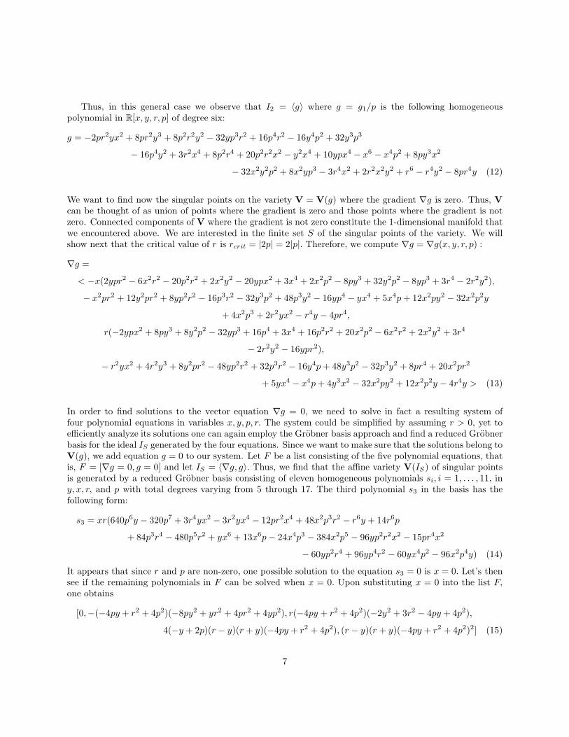
We will refer to these points as virtual singular points for the following reason: V(g) is a disjoint unionof {S1, S2} and a non-singular smooth subvariety Π where the gradient ∇g does not vanish. The subvariety

Π constitutes the set of two parallel lines that we have been seeking. Note that the foci F1 = (0, 3√3

2 ) and

F2 = (0,− 3√3

2 ) are different from the singular points. We show all in Figure 4.

f1g

g

S2

S1

F2

F1

–4

–3

–2

–1

0

1

2

3

4

y

–2 –1 1 2

x

Figure 4: Ellipse with parallel lines g, foci F1, F2 and two singular points S1, S2 for a = 3, b = 32 and r = 1

2

We have verified by direct computation that as the value of the offset r increases towards some criticalvalue rcrit, the virtual singular points approach the smooth component of the variety V(g), that is, theyapproach the parallel lines Π.5 As the next example shows, when r = rcrit, then the virtual singular pointsare actually located on the smooth component Π of the variety V(g).

Example 5 (r = rcrit) Let a = 3, b = 32 , and r = 3

4 . Then,

V = V(y20 + 4x20 − 9, 16y2 − 32yy0 + 16y20 + 16x2 − 32xx0 + 16x2

0 − 9, y0x + 3y0x0 − 4x0y)

We find that the reduced Grobner basis Gr contains eleven polynomials including

g = −29673216x4 + 19035648y4 + 95178240x2y2 − 1916928y6 − 14376960y4x2

− 21012480y2x4 + 7372800x6 + 65536y8 + 2162688y4x4 + 655360y6x2

+ 2621440x6y2 + 1048576x8 − 79361856y2 + 119574225− 198404640x2 (28)

5In the next subsection we will derive a formula for the critical value rcrit of r for a general ellipse.

11

whose gradient is

∇g = x(−1854576x2 + 2974320y2 − 449280y4 − 1313280x2y2 + 691200x4 + 135168y4x2

+ 20480y6 + 245760y2x4 + 131072x6 − 6200145)i

+ y(594864y2 + 1487160x2 − 89856y4 − 449280x2y2 − 328320x4 + 4096y6

+ 67584y2x4 + 30720y4x2 + 40960x6 − 1240029)j .

(29)

There are exactly two solutions to the equation (∇g)(p) = 0 on V(g) :

S1 =

(

0,9

4

)

and S2 =

(

0,−9

4

)

These points are the singular points of the variety V(g) : At every other point of this variety the gradient∇g does not vanish. We will collect these points as before into a non-singular subvariety Π. The variety

Π constitutes the set of two parallel lines that we have been seeking. Note that the foci F1 = (0, 3√3

2 ) and

F2 = (0,− 3√3

2 ) are still different from the singular points. We show all in Figure 5.

f1

S2

g

g

F1

F2

S1

–4

–3

–2

–1

0

1

2

3

4

y

–2 –1 1 2

x

Figure 5: Ellipse with parallel lines g, foci F1, F2 and two singular points S1, S2 for a = 3, b = 32 and r = 3

4

As we can see from the last figure, when r = rcrit = 34 for the given values of a and b, the singular points

are located on the continuous component of Π.

12

Probably the most interesting parallel lines we obtain when r > rcrit as we show in the next example.There, we will find six singular points as each of the two singular points found in Example 5 splits into threepoints.

Example 6 (r > rcrit) Let a = 3, b = 32 , and r = 3

2 . Then,

V = V(y20 + 4x20 − 9, 9y2 − 18yy0 + 9y20 + 9x2 − 18xx0 + 9x2

0 − 16, y0x + 3y0x0 − 4x0y)

We find that again the reduced Grobner basis Gr contains nine polynomials including

g = 23461560x2y2 + 1221025 + 186624x8 − 2984040y4x2 − 5015520y2x4

− 284472y6 + 384912y4x4 − 43658160x2 + 518400x6 + 466560x6y2

+ 116640y6x2 + 11664y8 − 2228394y2 − 10769184x4 + 1344177y4 (30)

whose gradient is

∇g = x(977565y2 + 31104x6 − 124335y4 − 417960x2y2 + 32076y4x2 − 1819090 + 64800x4

+ 58320y2x4 + 4860y6 − 897432x2)i

+ y(3910260x2 − 994680x2y2 − 835920x4 − 142236y4 + 128304y2x4 + 77760x6

+ 58320y4x2 + 7776y6 − 371399 + 448059y2)j .

(31)

There are exactly six solutions to the equation (∇g)(p) = 0 on V(g), or, in another words, six singular pointsof the variety:

S1 =

(

0,

√51

6

)

and S2 =

(

0,−√

51

6

)

S3 =

(√

525 + 324 · 62

3 − 864 · 61

3

18,

2√

231 − 81 · 62

3 + 54 · 61

3

9

)

,

S4 =

(

−√

525 + 324 · 62

3 − 864 · 61

3

18,

2√

231 − 81 · 62

3 + 54 · 61

3

9

)

,

S5 =

(√

525 + 324 · 62

3 − 864 · 61

3

18,−2

√

231 − 81 · 62

3 + 54 · 61

3

9

)

,

S6 =

(

−√

525 + 324 · 62

3 − 864 · 61

3

18,−2

√

231 − 81 · 62

3 + 54 · 61

3

9

)

.

We display these six points in Figure 6.

13

F2

F1

f1

S4

S6

g

gS1

S2

S3

S5

–4

–2

0

2

4

y

–3 –2 –1 1 2 3

x

Figure 6: Ellipse with parallel lines g, foci F1, F2 and six singular points Si, i = 1, . . . , 6, for a = 3, b = 32

and r = 43

3.2 Parallel lines for arbitrary parameters a, b, r

In this section we will find a general polynomial g that will generate the second elimination ideal I2 =I ∩ R[x, y, a, b, r] where I = 〈f1, f2, f3〉 and the generating polynomials are defined in equations (23), (24),and (25). We will also find a formula for the critical value rcrit of r that determines whether V(I2) has twoor six singular points, and, we will find general formulas for the coordinates of the said singular points forarbitrary values of the parameters a, b and r.

We begin with a computation of a Grobner basis for the ideal I for the lexicographic order y0 > x0 >x > y > a > b > r.

I = 〈b2y20 + a2x20 − a2b2, y2 − 2yy0 + y20 + x2 − 2xx0 + x2

0 − r2, b2y0x− b2y0x0 − a2x0y + a2x0y0〉

We found that a reduced Grobner basis for I consists of fifteen homogeneous polynomials of degrees: 16(two polynomials), 14 (one polynomial), 12 (one polynomial), 11 (two polynomials), 10 (two polynomials),9 (one polynomial), 8 (one polynomial), 7 (two polynomials), 5 (one polynomial), 4 (one polynomial), and 2(one polynomial). These polynomials are displayed in Appendix B.

Thus, in this general case we observe that I2 = 〈g〉 where g = g1/(a2b2) is the following homogeneous

14

polynomial in R[x, y, a, b, r] of degree twelve6:

g = 6 b4 x4 a4 − 4 y6 b4 a2 − 6 a6 x4 b2 − 4 b6 x2 a4 + 6 b4 x2 a6 + a4 b8 − 2 y2 b8 a2

+ 6 y2 b6 x2 a2 + 6 a6 y2 x2 b2 − 10 b4 x2 a4 y2 + y8 b4 + b8 r4 + b4 r8 − 2 b6 r6

− 2 b4 y2 x4 r2 − 6 x2 y4 b4 r2 + 6 x2 b4 r4 y2 − 4 b4 y6 r2 + 2 b4 y6 x2 + y4 b4 x4

+ b4 x4 r4 − 2 b4 r6 x2 − 2 b6 x2 r4 + 6 y4 b4 r4 − 2 b8 y2 r2 + 6 b6 r4 y2 − 4 b4 r6 y2

+ 6 a4 y2 b6 + 6 a6 y2 b2 r2 + 2 a4 b2 x4 y2 − 4 a4 x6 b2 + 4 a6 x2 b2 r2 − 8 b4 x2 a4 r2

+ 10 a4 x4 b2 r2 − 6 b4 r2 a2 x2 y2 − 6 a4 x2 b2 r2 y2 − 8 a4 x2 b2 r4 − 6 b4 r2 a2 x4

+ 4 b4 r4 a2 x2 − 6 y4 a4 b2 x2 − 6 b4 x4 a2 y2 + 6 b6 x2 r2 a2 + 2 b4 x2 y4 a2

+ 10 b4 y4 a2 r2 + 4 b6 y2 r2 a2 − 8 b4 y2 r4 a2 − 8 b4 y2 a4 r2 + 2 r6 a2 b4 + a8 b4

− 6 a4 y4 r2 b2 + 4 a4 y2 r4 b2 − 2 a8 b2 x2 + x4 a4 y4 + 4 x2 b6 y2 r2 − 6 y4 b6 a2

− 4 a6 y2 b4 − 2 y4 a4 x2 r2 + 2 b2 r2 a2 x4 y2 − 2 r8 a2 b2 + r8 a4 + a8 x4 + a4 x8

− 4 a4 x6 r2 + 6 a4 x4 r4 + 2 b2 r2 a2 x6 − 6 b2 r4 a2 x4 − 2 a6 r6 + 2 a6 x6 + a8 r4

+ 2 y6 b2 a2 x2 − 2 r6 a4 y2 + 6 r6 b2 y2 a2 − 2 a8 x2 r2 + y4 a4 r4 − 6 y4 b2 r4 a2

− 2 a6 y2 r4 + 4 x2 a6 y2 r2 + 6 x2 a4 y2 r4 + 2 y4 b2 x2 a2 r2 − 10 x2 b2 y2 r4 a2

+ 2 y6 b2 a2 r2 + 6 r6 b2 x2 a2 + 4 b2 x4 y4 a2 + 2 a4 x6 y2 − 6 a6 x4 r2 − 4 r6 a4 x2

+ 2 b2 x6 a2 y2 + 6 r4 a6 x2 − 6 a4 x4 r2 y2 + 2 b6 y6 − 2 a8 b2 r2 − 2 x2 y4 b6

+ 6 a4 y4 b4 + y4 b8 − 6 y4 b6 r2 − 2 x4 a6 y2 − 2 a6 b6 + 2 b6 r4 a2 − 2 b8 r2 a2

+ 2 b4 a6 r2 − 6 b4 a4 r4 + 2 r2 a4 b6 + 2 r4 a6 b2 + 2 r6 a4 b2

(32)

We want to find now those points on the variety V = V(g) where the gradient ∇g is zero. Thus, V canbe thought of as union of points where the gradient is zero and those points where the gradient is not zero.Connected components of V where the gradient is not zero constitute the 1-dimensional manifold. We areinterested in a discrete finite set S of points where the gradient is zero. These points will give the singular

points of the variety V. We will show next that the critical value of r is rcrit = b2

a . Therefore, we computethe gradient ∇g = ∇g(x, y, a, b, r) =< h1, h2, h3, h4, h5 > where

h1 = x(2 a4 b6 − 2 a4 b2 x2 y2 − 6 b4 x2 a4 + 5 b4 y2 a4 + b6 y4 + 6 b4 y2 a2 x2 + b6 r4

− 2 b6 y2 r2 − a8 x2 − 2 a6 y2 r2 + a4 y4 r2 − 3 a4 y2 r4 + 2 a4 r6 + a8 r2 − 3 a6 r4

− b4 r4 x2 + b4 r6 − 4 x2 b2 a2 y4 − 3 x4 b2 a2 y2 − x2 b4 y4 − a2 y6 b2 − 3 x4 a4 y2

+ 6 a4 x2 r2 y2 − b2 y4 a2 r2 + 5 b2 y2 r4 a2 − 3 b2 a2 x4 r2 + 6 b2 a2 x2 r4 + 6 a4 x4 r2

+ 6 a6 x2 r2 − 6 a4 x2 r4 + 2 b4 y2 x2 r2 − 3 b4 r4 y2 + 3 y4 b4 r2 − 3 b2 r6 a2

− 2 b2 a2 x2 r2 y2 + 3 y4 a4 b2 + a8 b2 − 2 a6 b2 r2 + 4 a4 b2 r4 + 4 a4 b4 r2 − 3 a6 x4

− b4 y6 + 3 b4 y2 a2 r2 − 10 a4 b2 x2 r2 + 3 a4 b2 y2 r2 + 6 b4 x2 a2 r2 + 6 x2 a6 b2

− 3 a6 b2 y2 − 3 b6 y2 a2 − y4 b4 a2 − 3 b6 r2 a2 − 2 b4 r4 a2 + 2 x2 y2 a6 + 6 x4 a4 b2

− 3 a6 b4 − a4 y4 x2 − 2 x6 a4)

(33)

6We assume a > b > 0.

15

h2 = y(3 a2 b4 x4 − 3 a4 b6 + 6 a4 b2 x2 y2 + 5 b4 x2 a4 − 6 b4 y2 a4 + 2 b6 y2 x2 − 3 b6 y4

− 2 b4 y2 a2 x2 − 3 b6 r4 + 6 b6 y2 r2 − a4 y2 r4 + a4 r6 + a6 r4 + x4 b4 r2 − 3 b4 r4 x2

− 2 b6 x2 r2 + b8 r2 + 2 b4 r6 − 3 x2 b2 a2 y4 − 4 x4 b2 a2 y2 − x6 b2 a2 − 3 x2 b4 y4

− x4 b4 y2 − x4 a4 y2 + 2 a4 x2 r2 y2 − 3 b2 y4 a2 r2 + 6 b2 y2 r4 a2 − b2 a2 x4 r2

+ 5 b2 a2 x2 r4 + 3 a4 x4 r2 − 2 a6 x2 r2 − 3 a4 x2 r4 + 6 b4 y2 x2 r2 − 6 b4 r4 y2

+ 6 y4 b4 r2 − 3 b2 r6 a2 − 2 b2 a2 x2 r2 y2 + b8 a2 − 3 a6 b2 r2 − 2 a4 b2 r4

+ 4 a4 b4 r2 + a6 x4 − b8 y2 − 2 b4 y6 − 10 b4 y2 a2 r2 + 3 a4 b2 x2 r2 + 6 a4 b2 y2 r2

+ 3 b4 x2 a2 r2 − 3 x2 a6 b2 − 3 x2 b6 a2 + 6 b6 y2 a2 + 6 y4 b4 a2 − 2 b6 r2 a2

+ 4 b4 r4 a2 − x4 a4 b2 + 2 a6 b4 − x6 a4)

(34)

h3 = 6 a2 b4 x4 + 3 a4 b6 − 9 a4 b2 x2 y2 − 9 b4 x2 a4 + 6 b4 y2 a4 − 3 b6 y2 x2 + 3 b6 y4

+ 10 b4 y2 a2 x2 − b6 r4 − 2 b6 y2 r2 + 3 a4 y2 r4 + 3 a4 r6 − 2 a6 r4 + 3 x4 b4 r2

− 2 b4 r4 x2 − 3 b6 x2 r2 + b8 r2 − b4 r6 + 6 x2 b2 a2 y4 − 2 x4 b2 a2 y2 + 4 x6 b2 a2

− x2 b4 y4 + 3 x4 b4 y2 − a2 r8 − 3 r6 x2 b2 − 3 r6 b2 y2 + 5 x2 b2 y2 r4 − x4 b2 r2 y2

− x2 b2 y4 r2 − a2 x8 − x6 b2 y2 − 2 x4 b2 y4 − 6 a2 x2 y2 r4 − y6 b2 r2 + 3 y4 b2 r4

+ 6 a2 x4 r2 y2 + 2 a2 y4 x2 r2 − b2 x2 y6 − x6 b2 r2 + 3 x4 b2 r4 + 3 x4 a4 y2

− 6 a4 x2 r2 y2 + 6 b2 y4 a2 r2 − 4 b2 y2 r4 a2 − 10 b2 a2 x4 r2 + 8 b2 a2 x2 r4

+ 9 a4 x4 r2 + 4 a6 x2 r2 − 9 a4 x2 r4 + 3 b4 y2 x2 r2 + 4 b4 r4 y2 − 5 y4 b4 r2

− 2 b2 r6 a2 + 6 b2 a2 x2 r2 y2 − b8 a2 + 4 a6 b2 r2 − 3 a4 b2 r4 − 3 a4 b4 r2 − 2 a6 x4

+ b8 y2 + 2 b4 y6 + 8 b4 y2 a2 r2 − 6 a4 b2 x2 r2 − 9 a4 b2 y2 r2 + 8 b4 x2 a2 r2

+ 4 x2 a6 b2 + 4 x2 b6 a2 − 6 b6 y2 a2 − 6 y4 b4 a2 − 2 b6 r2 a2 + 6 b4 r4 a2

+ 9 x4 a4 b2 − 2 a6 b4 − 3 x6 a4 + 4 a2 x6 r2 + 4 a2 r6 x2 − a2 y4 x4 − 6 a2 x4 r4

− 2 a2 x6 y2 − a2 y4 r4 + 2 a2 r6 y2 + r8 b2

(35)

16

h4 = 2 a4 b6 − 10 a4 b2 x2 y2 − 6 b4 x2 a4 + 9 b4 y2 a4 + 2 b6 y4 + 9 b4 y2 a2 x2 + 2 b6 r4

− 4 b6 y2 r2 − a8 x2 + 3 a6 y2 r2 − 3 a4 y4 r2 + 2 a4 y2 r4 + a4 r6 − a8 r2 + a6 r4

− 3 b4 r4 x2 − 3 b4 r6 + 2 x2 b2 a2 y4 − 6 x4 b2 a2 y2 − 3 x2 b4 y4 − 4 a2 y6 b2 − a2 r8

− 2 r6 x2 b2 − 4 r6 b2 y2 + 6 x2 b2 y2 r4 − 2 x4 b2 r2 y2 − 6 x2 b2 y4 r2 + x4 b2 y4

− 5 a2 x2 y2 r4 − 4 y6 b2 r2 + 6 y4 b2 r4 + a2 x4 r2 y2 + a2 y4 x2 r2 + 2 b2 x2 y6

+ x4 b2 r4 + x4 a4 y2 − 3 a4 x2 r2 y2 + 10 b2 y4 a2 r2 − 8 b2 y2 r4 a2 − 6 b2 a2 x4 r2

+ 4 b2 a2 x2 r4 + 5 a4 x4 r2 + 2 a6 x2 r2 − 4 a4 x2 r4 + 6 b4 y2 x2 r2 + 9 b4 r4 y2

− 9 y4 b4 r2 + 2 b2 r6 a2 − 6 b2 a2 x2 r2 y2 + 6 y4 a4 b2 + a8 b2 + 2 a6 b2 r2

− 6 a4 b2 r4 + 3 a4 b4 r2 − 3 a6 x4 + 3 b4 y6 + 6 b4 y2 a2 r2 − 8 a4 b2 x2 r2

− 8 a4 b2 y2 r2 + 9 b4 x2 a2 r2 + b2 y8 + a2 y6 r2 + x2 a2 y6 + 6 x2 a6 b2 − 4 a6 b2 y2

− 4 b6 y2 a2 − 9 y4 b4 a2 − 4 b6 r2 a2 + 3 b4 r4 a2 + 3 x2 y2 a6 + 6 x4 a4 b2 − 3 a6 b4

− 3 a4 y4 x2 − 2 x6 a4 + a2 x6 r2 + 3 a2 r6 x2 + 2 a2 y4 x4 − 3 a2 x4 r4 + a2 x6 y2

− 3 a2 y4 r4 + 3 a2 r6 y2 + r8 b2

(36)

h5 = 3 a2 b4 x4 + a4 b6 − 3 a4 b2 x2 y2 − 4 b4 x2 a4 − 4 b4 y2 a4 + 2 b6 y2 x2 − 3 b6 y4

− 3 b4 y2 a2 x2 − 3 b6 r4 + 6 b6 y2 r2 − a8 x2 − 2 a6 y2 r2 + a4 y4 r2 − 3 a4 y2 r4

+ 2 a4 r6 + a8 r2 − 3 a6 r4 + x4 b4 r2 − 3 b4 r4 x2 − 2 b6 x2 r2 + b8 r2 + 2 b4 r6

+ x2 b2 a2 y4 + x4 b2 a2 y2 + x6 b2 a2 − 3 x2 b4 y4 − x4 b4 y2 + a2 y6 b2 − 3 x4 a4 y2

+ 6 a4 x2 r2 y2 − 6 b2 y4 a2 r2 + 9 b2 y2 r4 a2 − 6 b2 a2 x4 r2 + 9 b2 a2 x2 r4

+ 6 a4 x4 r2 + 6 a6 x2 r2 − 6 a4 x2 r4 + 6 b4 y2 x2 r2 − 6 b4 r4 y2 + 6 y4 b4 r2

− 4 b2 r6 a2 − 10 b2 a2 x2 r2 y2 − 3 y4 a4 b2 − a8 b2 − b8 a2 + 2 a6 b2 r2 + 3 a4 b2 r4

− 6 a4 b4 r2 − 3 a6 x4 − b8 y2 − 2 b4 y6 − 8 b4 y2 a2 r2 − 8 a4 b2 x2 r2 + 4 a4 b2 y2 r2

+ 4 b4 x2 a2 r2 + 2 x2 a6 b2 + 3 x2 b6 a2 + 3 a6 b2 y2 + 2 b6 y2 a2 + 5 y4 b4 a2

+ 2 b6 r2 a2 + 3 b4 r4 a2 + 2 x2 y2 a6 + 5 x4 a4 b2 + a6 b4 − a4 y4 x2 − 2 x6 a4

(37)

are polynomials in R[a, y, a, b, r]. Continuing our approach from Section 2, in order to find solutions to thevector equation ∇g = 0 in V(g), we need to solve a system of six polynomial equations hi = 0, i = 1, . . . , 5,and g = 0 in the variables x, y, a, b, r under the assumption that a > b > r > 0. Let IS = 〈∇g, g〉 =〈h1, h2, h3, h4, h5, g〉 and let F be a list containing the six polynomial equations:

F = [h1 = 0, h2 = 0, h3 = 0, h4 = 0, h5 = 0, g = 0] (38)

In order to solve system (38), we can either employ the Grobner basis approach again (see Appendix C) orsimply use solve command in Maple. Thus we find that the affine variety V(IS) consists of the followingeight singular points of which six are real and two are complex:

S1 =

(

0,

√

−(a2 − b2) (r2 − b2)

b

)

, S2 =

(

0, −√

−(a2 − b2) (r2 − b2)

b

)

, (39)

17

S3 =

(

√

(a2 − b2) (−a2 + r2)

a, 0

)

, S4 =

(

−√

(a2 − b2) (−a2 + r2)

a, 0

)

, (40)

S5 =

(√

− δ

(−a2 + b2) (a b r)2

3

, −√

(−a2 + b2) ε

(a b r)1

3 (−a2 + b2)

)

, (41)

S6 =

(

−√

− δ

(−a2 + b2) (a b r)2

3

, −√

(−a2 + b2) ε

(a b r)1

3 (−a2 + b2)

)

, (42)

S7 =

(√

− δ

(−a2 + b2) (a b r)2

3

,

√

(−a2 + b2) ε

(a b r)1

3 (−a2 + b2)

)

, (43)

S8 =

(

−√

− δ

(−a2 + b2) (a b r)2

3

,

√

(−a2 + b2) ε

(a b r)1

3 (−a2 + b2)

)

, (44)

where

δ = −3 b2 a2 r2 + r2 a2 (a b r)2

3 + 3 (a b r)1

3 b3 a r − b4 (a b r)2

3 , (45)

ε = −a4 (a b r)2

3 + 3 (a b r)1

3 b r a3 − 3 b2 a2 r2 + (a b r)2

3 b2 r2. (46)

Notice that δ becomes zero in three cases:

1. When r = 0 – this is not possible since we expect r > 0,

2. When r = − b2

a – this is not possible as r > 0,

3. When r = b2

a .

Only this last value is possible thus we set rcrit = b2

a . When r = rcrit, then under the assumptions thata > b > r > 0, we essentially obtain two real singular points:

S1 = S5 = S6 =

(

0,a2 − b2

a

)

and S2 = S7 = S8 =

(

0,−a2 − b2

a

)

, (47)

while the complex points S3 and S4 become:

S3 =

(√a2 + b2(a2 − b2)

a2i, 0

)

and S4 =

(

−√a2 + b2(a2 − b2)

a2i, 0

)

. (48)

For the ellipse with a > b, the ratio l = b2

a is again called a semi-latus rectum. It is the distance betweena focus and the ellipse itself measured along a line perpendicular to the major axis. The value of l is alsothe reciprocal of the maximum curvature κmax of the ellipse, or, it is equal to the radius of the smallestosculating circle. [14]

To summarize, the variety V(IS) contains the following real singular points:

1. Two virtual points S1 and S2 shown in (39) when 0 < r < rcrit. In particular, when a = 3, b = 32 , and

r = 12 , upon substituting these values into (32) we obtain the parallel lines (26) derived in Example 4.

Furthermore, when these values are substituted into (39), then we obtain the two virtual singularpoints found in the same example.

18

2. Two points S1 and S2 shown in (47) when r = rcrit. In particular, we can recover results of Example 5when we substitute values a = 3, b = 3

2 , and r = 34 into the general equation (32) and the singular

points (47).

3. Six points S1, S2, S5, S6, S7, S8 shown in (39), (41), (42), (43), and (44) when r > rcrit. In particular wecan recover in the same manner six points and the equation for the parallel lines found in Example 6when we set a = 3, b = 3

2 , and r = 32 . These six singular points are displayed in Figure 6.

4 Parallel Lines to a Hyperbola

Since a parabola, an ellipse, and a hyperbola belong to the same class of nondegenerate conic

C : (X2 + Y 2 − Z2 = 0)

in P2(R), (cf. [12]) we expect essentially similar results for a hyperbola. Thus, our approach will be similar to

the one for the ellipse from Section 3. In particular, there is only one sign change needed in the polynomialsf1 and f2 shown in (23) and (25) whereas the polynomial f2 remains the same. Thus, we have now

f1 = b2y20 − a2x20 − a2b2 = 0 (49)

where we assume that a > b and the center of the hyperbola is at the origin. Polynomial f2 defines a circleof radius (offset) r centered at a point P = (x0, y0) on the hyperbola,

f2 = (y − y0)2 + (x − x0)2 − r2 = 0 (50)

while polynomial f3f3 = b2(x− x0)y0 + a2(y − y0)x0 = 0 (51)

gives a condition that a point P (x, y) on the circle f2 lies on a line perpendicular to the hyperbola f1and passing through the point (x0, y0) on the hyperbola. All these points P belong to the affine varietyV = V(f1, f2, f3) – the hyperbola envelope – and, like for the parabola in Section 2 and the ellipse inSection 3, define two parallel lines at the distance r from the hyperbola. We proceed like in Section 3: Wewill compute a reduced Grobner basis for V and by eliminating variables x0, y0 we will obtain one polynomialg in variables x and y alone (also a, b, r in the general case) that defines both parallel lines on each side ofthe hyperbola for the given value of the offset r. Thus, in general, we have f1, f2, f3 ∈ R[y0, x0, x, y, a, b, r].However, first we illustrate computations for specific values of the parameters a, b and r, and later we showcomputation for unspecified parameters.

4.1 Parallel lines for specific parameters a, b, r

The parallel lines constitute a subvariety of the affine variety V = V(I) where, like before, I〈f1, f2, f3〉. Inorder to find the polynomial g for the second elimination ideal I2 = I∩R[x, y], we first find a Grobner basis Gfor V for the lexicographic order y0 > x0 > x > y and reduce it eventually to a unique reduced basis Gr ofnine (or eleven, depending on the case) polynomials. Finally, we eliminate from that basis all polynomialsthat contain variables y0 and x0, and keep the single polynomial g ∈ R[x, y] that gives the parallel lines andgenerates the second elimination ideal I2 = 〈g〉. We will also proceed to find all singular points of V(g) where(∇g)(p) = 0. Thus, let’s consider three cases when 0 < r < rcrit, r = rcrit, and r > rcrit. In the followingsection we will consider a general case for arbitrary values of a, b (a > b > 0) and r (r > 0).

19

Example 7 (r < rcrit) Let a = 3, b = 32 , and r = 1

2 . Then,

V = V(y20 − x20 − 1, 4y2 − 8yy0 + 4y20 + 4x2 − 8xx0 + 4x2

0 − 1, xy0 + yx0 − 2y0x0)

We find that the reduced Grobner basis Gr contains nine polynomials including

g = 225 + 64y8 + 288x6 + 480x2y4 − 800y2x4 − 480y6 − 128y4x4

− 1180y2 + 516x2 − 1320x2y2 + 532x4 + 1236y4 + 64x8 (52)

whose gradient is

∇g = x(216x4 + 120y4 − 400x2y2 − 64x2y4 + 129 − 330y2 + 266x2 + 64x6)i

− y(−64y6 − 240x2y2 + 200x4 + 360y4 + 64y2x4 + 295 + 330x2 − 618y2)j .(53)

There are exactly two solutions to the equation (∇g)(p) = 0 on V(g) :

S1 =

(

0,

√10

2

)

and S2 =

(

0,−√

10

2

)

.

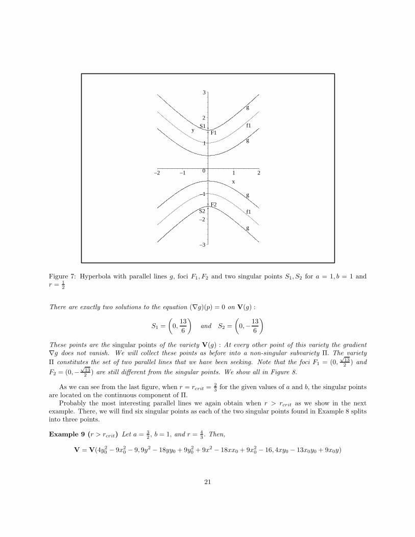
We will refer to these points as virtual singular points for the following reason: V(g) is a disjoint unionof {S1, S2} and a non-singular smooth subvariety Π where the gradient ∇g does not vanish. The subvarietyΠ constitutes the set of two parallel lines that we have been seeking. Note that the foci F1 = (0,

√2) and

F2 = (0,−√

2) are different from the singular points. We show all in Figure 7.

We have verified by direct computation that as the value of the offset r increases towards some criticalvalue rcrit, the virtual singular points approach the smooth component of the variety V(g), that is, theyapproach the parallel lines Π.7 As the next example shows, when r = rcrit, then the virtual singular pointsare actually located on the smooth component Π of the variety V(g).

Example 8 (r = rcrit) Let a = 32 , b = 1, and r = 2

3 . Then,

V = V(4y20 − 9x20 − 9, 9y2 − 18yy0 + 9y20 + 9x2 − 18xx0 + 9x2

0 − 4, 4xy0 − 13x0y0 + 9x0y)

We find that the reduced Grobner basis Gr contains eleven polynomials including

g = 9447840x6y2 − 4199040y6x2 + 53800200x6 + 1679616y8 + 124857369x4

+ 127471968y4 − 159339960x2y2 − 24820992y6 + 46539360y4x2 − 105471720y2x4

− 4933872y4x4 + 120670225 + 8503056x8 − 250879824y2 + 156799890x2 (54)

whose gradient is

∇g = x(1574640y2x4 − 233280y6 + 8966700x4 + 13873041x2 − 8852220y2 + 2585520y4

− 11719080x2y2 − 548208y4x2 + 1889568x6 + 8711105)i

+ y(131220x6 − 174960y4x2 + 93312y6 + 3540888y2 − 2213055x2 − 1034208y4

+ 1292760x2y2 − 1464885x4 − 137052y2x4 − 3484442)j .

(55)

7In the next subsection we will derive a formula for the critical value rcrit of r for a general hyperbola.

20

g

f1

f1

g

g

g

F2

F1S1

S2

–3

–2

–1

0

1

2

3

y

–2 –1 1 2

x

Figure 7: Hyperbola with parallel lines g, foci F1, F2 and two singular points S1, S2 for a = 1, b = 1 andr = 1

2

There are exactly two solutions to the equation (∇g)(p) = 0 on V(g) :

S1 =

(

0,13

6

)

and S2 =

(

0,−13

6

)

These points are the singular points of the variety V(g) : At every other point of this variety the gradient∇g does not vanish. We will collect these points as before into a non-singular subvariety Π. The variety

Π constitutes the set of two parallel lines that we have been seeking. Note that the foci F1 = (0,√132 ) and

F2 = (0,−√132 ) are still different from the singular points. We show all in Figure 8.

As we can see from the last figure, when r = rcrit = 23 for the given values of a and b, the singular points

are located on the continuous component of Π.Probably the most interesting parallel lines we again obtain when r > rcrit as we show in the next

example. There, we will find six singular points as each of the two singular points found in Example 8 splitsinto three points.

Example 9 (r > rcrit) Let a = 32 , b = 1, and r = 4

3 . Then,

V = V(4y20 − 9x20 − 9, 9y2 − 18yy0 + 9y20 + 9x2 − 18xx0 + 9x2

0 − 16, 4xy0 − 13x0y0 + 9x0y)

21

F1

F2

f1

f1

g

g

g

g

S1

S2

–4

–3

–2

–1

0

1

2

3

4

y

–2 –1 1 2

x

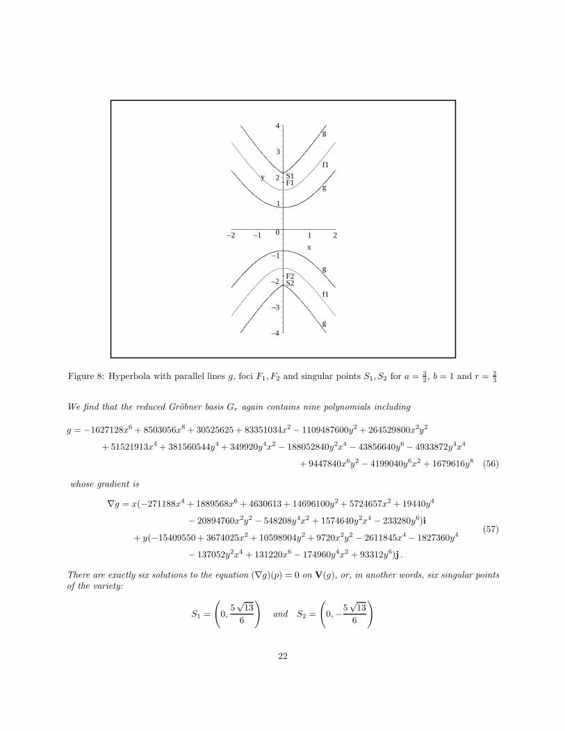
Figure 8: Hyperbola with parallel lines g, foci F1, F2 and singular points S1, S2 for a = 32 , b = 1 and r = 2

3

We find that the reduced Grobner basis Gr again contains nine polynomials including

g = −1627128x6 + 8503056x8 + 30525625 + 83351034x2 − 1109487600y2 + 264529800x2y2

+ 51521913x4 + 381560544y4 + 349920y4x2 − 188052840y2x4 − 43856640y6 − 4933872y4x4

+ 9447840x6y2 − 4199040y6x2 + 1679616y8 (56)

whose gradient is

∇g = x(−271188x4 + 1889568x6 + 4630613 + 14696100y2 + 5724657x2 + 19440y4

− 20894760x2y2 − 548208y4x2 + 1574640y2x4 − 233280y6)i

+ y(−15409550 + 3674025x2 + 10598904y2 + 9720x2y2 − 2611845x4 − 1827360y4

− 137052y2x4 + 131220x6 − 174960y4x2 + 93312y6)j .

(57)

There are exactly six solutions to the equation (∇g)(p) = 0 on V(g), or, in another words, six singular pointsof the variety:

S1 =

(

0,5√

13

6

)

and S2 =

(

0,−5√

13

6

)

22

S3 =

(

2√

39 − 78 · 21

3 + 39 · 22

3

13,

√

12805 + 11232 · 21

3 + 12636 · 22

3

78

)

,

S4 =

(

−2√

39 − 78 · 21

3 + 39 · 22

3

13,

√

12805 + 11232 · 21

3 + 12636 · 22

3

78

)

,

S5 =

(

2√

39 − 78 · 21

3 + 39 · 22

3

13,−√

12805 + 11232 · 21

3 + 12636 · 22

3

78

)

,

S6 =

(

−2√

39 − 78 · 21

3 + 39 · 22

3

13,−√

12805 + 11232 · 21

3 + 12636 · 22

3

78

)

.

We display these six points in Figure 9.

g

g

f1

f1

S4

S6

g

g

S1

S2

S3

S5

F2

F1

–4

–2

0

2

4

y

–3 –2 –1 1 2 3

x

Figure 9: Hyperbola with parallel lines g, foci F1, F2 and six singular points Si, i = 1, . . . , 6, for a = 32 , b = 1

and r = 43

4.2 Parallel lines for arbitrary parameters a, b, r

In this section we will find a general polynomial g that will generate the second elimination ideal I2 =I ∩ R[x, y, a, b, r] where I = 〈f1, f2, f3〉 and the generating polynomials are defined in equations (49), (50),

23

and (51). We will also find a formula for the critical value rcrit of r that determines whether V(I2) has twoor six singular points, and, we will find general formulas for the coordinates of the said singular points forarbitrary values of the parameters a, b and r.

We begin with a computation of a Grobner basis for the ideal I for the lexicographical order y0 > x0 >x > y > a > b > r.

I = 〈b2y20 − a2x20 − a2b2, y2 − 2yy0 + y20 + x2 − 2xx0 + x2

0 − r2, b2y0x− b2y0x0 + a2x0y − a2x0y0〉

We found that a reduced Grobner basis for I consists of fifteen homogeneous polynomials of degrees: 16(two polynomials), 14 (one polynomial), 12 (one polynomial), 11 (two polynomials), 10 (two polynomials),9 (one polynomial), 8 (one polynomial), 7 (two polynomials), 5 (one polynomial), 4 (one polynomial), and2 (one polynomial). We will not display these polynomials as they are similar to the polynomials for theellipse shown in Appendix B.

Thus, in this general case we observe that I2 = 〈g〉 where g = g1/(a2b2) is the following homogeneouspolynomial in R[x, y, a, b, r] of degree twelve:

g = 6 a4 x4 r4 − 2 b2 x4 a2 r2 y2 + 4 b6 x2 a4 + 2 a8 b2 x2 + 2 a6 x6 + 6 y4 a2 b6 − 2 a4 b2 x4 y2

+ 4 a4 x6 b2 − 6 a6 x2 b2 y2 − 4 a6 x2 b2 r2 − 10 a4 x2 b4 y2 − 8 a4 x2 b4 r2

+ 8 a4 x2 b2 r4 − 6 b4 r2 a2 x4 + 4 b4 r4 a2 x2 − 10 a4 x4 b2 r2 − 6 b4 r2 a2 x2 y2

+ 6 a4 x2 b2 r2 y2 − 6 b4 x4 a2 y2 + 2 b4 x2 y4 a2 − 6 b6 x2 r2 a2 + 10 b4 y4 a2 r2

− 8 b4 y2 a4 r2 − 4 b6 y2 r2 a2 − 8 b4 y2 r4 a2 + 6 y4 a4 b2 x2 − 2 a2 y2 b8 + 6 b4 y4 a4

− 4 b4 y6 a2 − 6 y2 a4 b6 + 6 a4 x4 b4 − 4 y2 a6 b4 − 6 y2 a6 r2 b2 + 6 y4 a4 r2 b2

− 4 y2 a4 r4 b2 + 2 a6 b6 + a4 b8 + 6 a6 b4 x2 + 6 a6 x4 b2 + b8 r4 + a8 b4 − 2 a2 b8 r2

− 2 a2 b6 r4 + 2 b6 x2 r4 − 4 b6 x2 y2 r2 + 6 b2 x4 a2 r4 + 4 a6 x2 r2 y2 − 2 b2 x2 a2 y6

+ 2 b4 x2 y6 − 2 b2 x2 y4 a2 r2 + 6 b4 x2 y2 r4 + 10 b2 x2 y2 a2 r4 + 2 b6 x2 y4

− 6 b4 x2 y4 r2 + a4 x8 + 2 b6 r6 + b4 r8 + 6 a6 x2 r4 − 6 a6 x4 r2 − 2 a8 x2 r2

− 6 a4 b4 r4 − 2 a4 b6 r2 − 2 a6 y2 r4 − 2 a6 b2 r4 − 6 a2 r6 b2 y2 − 2 a4 r6 y2

− 6 a4 x4 r2 y2 + 6 a2 y4 b2 r4 + 2 a8 b2 r2 + a4 y4 r4 − 2 a2 y6 b2 r2 − 4 a4 r6 x2

+ a8 x4 + 6 a4 x2 y2 r4 − 4 a4 x6 r2 + a8 r4 + 2 a4 x6 y2 − 2 a6 x4 y2 − 2 a6 r6

− 2 a4 r6 b2 + 2 a6 r2 b4 + a4 y4 x4 + 2 a2 r8 b2 − 2 a4 y4 x2 r2 + 2 a2 b4 r6 + a4 r8

+ 6 y4 b4 r4 + 6 y4 b6 r2 − 4 y6 b4 r2 − 4 y2 b4 r6 − 6 y2 b6 r4 + y4 b8 + y8 b4 − 2 y6 b6

− 2 b2 x6 a2 y2 − 2 b4 x2 r6 − 6 b2 x2 r6 a2 + b4 x4 y4 − 4 b2 x4 y4 a2 + b4 x4 r4

− 2 b2 x6 a2 r2 − 2 b4 x4 r2 y2 − 2 y2 b8 r2 − 6 y2 x2 a2 b6

(58)

We want to find now those points on the variety V = V(g) where the gradient ∇g is zero. Thus, V canbe thought of as union of points where the gradient is zero and those points where the gradient is not zero.Connected components of V where the gradient is not zero constitute the 1-dimensional manifold. We areinterested in a discrete finite set S of points where the gradient is zero. These points will give the singular

points of the variety V. We will show next that the critical value of r is rcrit = b2

a . Therefore, we compute

24

∇g = ∇g(x, y, a, b, r) =< h1, h2, h3, h4, h5 > where

h1 = x(2 b6 y2 r2 − a8 b2 + b4 r6 − x2 b4 r4 + 2 x2 b4 r2 y2 − 3 b4 y2 r4 + 3 b4 y4 r2 − b6 y4

− 3 a6 b4 − a8 x2 − 2 a4 b6 − 3 a4 y4 b2 + 3 y2 a6 b2 + 3 y2 b6 a2 + 5 b4 y2 a4

− b4 y4 a2 − 6 a4 x2 b4 + r2 a8 − b4 x2 y4 + 2 a6 x2 y2 + 6 b4 x2 a2 y2 + 2 a4 b2 x2 y2

− b4 y6 − b6 r4 + 10 a4 x2 b2 r2 − 6 a6 x2 b2 − 6 a4 x4 b2 − 3 a6 x4 + 3 b6 r2 a2

− 2 b4 r4 a2 + 2 r6 a4 + 3 r6 b2 a2 − 3 r4 a6 + 4 r2 a4 b4 + 2 b2 r2 a2 x2 y2

+ 6 a4 x2 r2 y2 + 6 a6 x2 r2 + 3 b2 r2 a2 x4 − 6 a4 x2 r4 + b2 y4 a2 r2 − 5 b2 y2 r4 a2

− 3 y2 a4 r4 − 6 b2 r4 a2 x2 + 3 b2 x4 a2 y2 + 4 b2 x2 y4 a2 − y4 a4 x2 − 3 a4 x4 y2

+ 6 a4 x4 r2 − 2 y2 a6 r2 + y4 a4 r2 + b2 y6 a2 + 3 b4 y2 a2 r2 − 3 b2 y2 a4 r2

+ 2 b2 a6 r2 + 6 b4 x2 a2 r2 − 4 b2 a4 r4 − 2 a4 x6)

(59)

h2 = y(−6 b6 y2 r2 + 2 b4 r6 − 3 x2 b4 r4 + 6 x2 b4 r2 y2 − 6 b4 y2 r4 + 6 b4 y4 r2 + r2 b8

+ b4 x4 r2 + 2 x2 b6 r2 + 3 b6 y4 + 2 a6 b4 + 3 a4 b6 − 6 y2 b6 a2 − 6 b4 y2 a4

+ 6 b4 y4 a2 + b2 x6 a2 + 3 b6 x2 a2 + 3 b4 a2 x4 + 5 a4 x2 b4 + a2 b8 − 2 y2 x2 b6

− 3 b4 x2 y4 − b4 x4 y2 − 2 b4 x2 a2 y2 − 6 a4 b2 x2 y2 − 2 b4 y6 + 3 b6 r4

− 3 a4 x2 b2 r2 − y2 b8 + 3 a6 x2 b2 + a4 x4 b2 + a6 x4 + 2 b6 r2 a2 + 4 b4 r4 a2 + r6 a4

+ 3 r6 b2 a2 + r4 a6 + 4 r2 a4 b4 + 2 b2 r2 a2 x2 y2 + 2 a4 x2 r2 y2 − 2 a6 x2 r2

+ b2 r2 a2 x4 − 3 a4 x2 r4 + 3 b2 y4 a2 r2 − 6 b2 y2 r4 a2 − y2 a4 r4 − 5 b2 r4 a2 x2

+ 4 b2 x4 a2 y2 + 3 b2 x2 y4 a2 − a4 x4 y2 + 3 a4 x4 r2 − 10 b4 y2 a2 r2 − 6 b2 y2 a4 r2

+ 3 b2 a6 r2 + 3 b4 x2 a2 r2 + 2 b2 a4 r4 − a4 x6)

(60)

h3 = 2 b2 x4 y4 + b2 x6 y2 + b2 x2 y6 + 2 b6 y2 r2 − b4 r6 − 2 x2 b4 r4 + 3 x2 b4 r2 y2

+ 4 b4 y2 r4 − 5 b4 y4 r2 + r2 b8 + 3 b4 x4 r2 + 3 x2 b6 r2 − 3 b6 y4 − 2 a6 b4 − a2 x8

+ b2 x4 r2 y2 + b2 x2 y4 r2 − 5 b2 x2 y2 r4 − a2 y4 x4 − r8 b2 + 2 a2 r6 y2 − a2 y4 r4

+ 4 a2 r6 x2 − 6 a2 x4 r4 − 3 b2 x4 r4 + 6 a2 x4 r2 y2 − 3 y4 b2 r4 + 3 r6 b2 y2 + y6 b2 r2

− 6 a2 x2 y2 r4 + 2 a2 y4 x2 r2 + 3 b2 x2 r6 + b2 x6 r2 + 4 a2 x6 r2 − 2 a2 x6 y2 − r8 a2

− 3 a4 b6 + 6 y2 b6 a2 + 6 b4 y2 a4 − 6 b4 y4 a2 − 4 b2 x6 a2 − 4 b6 x2 a2 − 6 b4 a2 x4

− 9 a4 x2 b4 − a2 b8 + 3 y2 x2 b6 − b4 x2 y4 + 3 b4 x4 y2 + 10 b4 x2 a2 y2

+ 9 a4 b2 x2 y2 + 2 b4 y6 + b6 r4 + 6 a4 x2 b2 r2 + y2 b8 − 4 a6 x2 b2 − 9 a4 x4 b2

− 2 a6 x4 + 2 b6 r2 a2 + 6 b4 r4 a2 + 3 r6 a4 + 2 r6 b2 a2 − 2 r4 a6 − 3 r2 a4 b4

− 6 b2 r2 a2 x2 y2 − 6 a4 x2 r2 y2 + 4 a6 x2 r2 + 10 b2 r2 a2 x4 − 9 a4 x2 r4

− 6 b2 y4 a2 r2 + 4 b2 y2 r4 a2 + 3 y2 a4 r4 − 8 b2 r4 a2 x2 + 2 b2 x4 a2 y2

− 6 b2 x2 y4 a2 + 3 a4 x4 y2 + 9 a4 x4 r2 + 8 b4 y2 a2 r2 + 9 b2 y2 a4 r2 − 4 b2 a6 r2

+ 8 b4 x2 a2 r2 + 3 b2 a4 r4 − 3 a4 x6

(61)

25

h4 = b2 x4 y4 + 2 b2 x2 y6 − 4 b6 y2 r2 + a8 b2 + 3 b4 r6 + 3 x2 b4 r4 − 6 x2 b4 r2 y2

− 9 b4 y2 r4 + 9 b4 y4 r2 + 2 b6 y4 + 3 a6 b4 + b2 y8 + a8 x2 − 2 b2 x4 r2 y2

− 6 b2 x2 y4 r2 + 6 b2 x2 y2 r4 − 2 a2 y4 x4 + r8 b2 − 3 a2 r6 y2 + 3 a2 y4 r4 − 3 a2 r6 x2

+ 3 a2 x4 r4 + b2 x4 r4 − a2 x4 r2 y2 + 6 y4 b2 r4 − 4 r6 b2 y2 − 4 y6 b2 r2 + 5 a2 x2 y2 r4

− a2 y4 x2 r2 − 2 b2 x2 r6 − a2 x6 r2 − a2 x6 y2 + r8 a2 − x2 a2 y6 − a2 y6 r2 + 2 a4 b6

+ 6 a4 y4 b2 − 4 y2 a6 b2 − 4 y2 b6 a2 − 9 b4 y2 a4 + 9 b4 y4 a2 + 6 a4 x2 b4 + r2 a8

+ 3 b4 x2 y4 − 3 a6 x2 y2 − 9 b4 x2 a2 y2 − 10 a4 b2 x2 y2 − 3 b4 y6 + 2 b6 r4

− 8 a4 x2 b2 r2 + 6 a6 x2 b2 + 6 a4 x4 b2 + 3 a6 x4 − 4 b6 r2 a2 − 3 b4 r4 a2 − r6 a4

+ 2 r6 b2 a2 − r4 a6 − 3 r2 a4 b4 − 6 b2 r2 a2 x2 y2 + 3 a4 x2 r2 y2 − 2 a6 x2 r2

− 6 b2 r2 a2 x4 + 4 a4 x2 r4 + 10 b2 y4 a2 r2 − 8 b2 y2 r4 a2 − 2 y2 a4 r4 + 4 b2 r4 a2 x2

− 6 b2 x4 a2 y2 + 2 b2 x2 y4 a2 + 3 y4 a4 x2 − a4 x4 y2 − 5 a4 x4 r2 − 3 y2 a6 r2

+ 3 y4 a4 r2 − 4 b2 y6 a2 − 6 b4 y2 a2 r2 − 8 b2 y2 a4 r2 + 2 b2 a6 r2 − 9 b4 x2 a2 r2

− 6 b2 a4 r4 + 2 a4 x6

(62)

h5 = −6 b6 y2 r2 + a8 b2 + 2 b4 r6 − 3 x2 b4 r4 + 6 x2 b4 r2 y2 − 6 b4 y2 r4 + 6 b4 y4 r2 + r2 b8

+ b4 x4 r2 + 2 x2 b6 r2 + 3 b6 y4 + a6 b4 − a8 x2 − a4 b6 + 3 a4 y4 b2 − 3 y2 a6 b2

− 2 y2 b6 a2 − 4 b4 y2 a4 + 5 b4 y4 a2 − b2 x6 a2 − 3 b6 x2 a2 − 3 b4 a2 x4 − 4 a4 x2 b4

+ r2 a8 − a2 b8 − 2 y2 x2 b6 − 3 b4 x2 y4 − b4 x4 y2 + 2 a6 x2 y2 − 3 b4 x2 a2 y2

+ 3 a4 b2 x2 y2 − 2 b4 y6 + 3 b6 r4 + 8 a4 x2 b2 r2 − y2 b8 − 2 a6 x2 b2 − 5 a4 x4 b2

− 3 a6 x4 − 2 b6 r2 a2 + 3 b4 r4 a2 + 2 r6 a4 + 4 r6 b2 a2 − 3 r4 a6 − 6 r2 a4 b4

+ 10 b2 r2 a2 x2 y2 + 6 a4 x2 r2 y2 + 6 a6 x2 r2 + 6 b2 r2 a2 x4 − 6 a4 x2 r4

+ 6 b2 y4 a2 r2 − 9 b2 y2 r4 a2 − 3 y2 a4 r4 − 9 b2 r4 a2 x2 − b2 x4 a2 y2 − b2 x2 y4 a2

− y4 a4 x2 − 3 a4 x4 y2 + 6 a4 x4 r2 − 2 y2 a6 r2 + y4 a4 r2 − b2 y6 a2 − 8 b4 y2 a2 r2

− 4 b2 y2 a4 r2 − 2 b2 a6 r2 + 4 b4 x2 a2 r2 − 3 b2 a4 r4 − 2 a4 x6

(63)

Continuing our approach from Section 3, in order to find the solutions to the vector equation ∇g = 0, weneed to solve a system of six polynomial equations hi = 0, i = 1, . . . , 5 and g = 0 in the variables x, y, a, b, runder the assumption that a > b > r > 0. Let IS = 〈∇g, g〉 = 〈h1, h2, h3, h4, h5, g〉 and let F be a listcontaining the six polynomial equations:

F = [h1 = 0, h2 = 0, h3 = 0, h4 = 0, h5 = 0, g = 0] (64)

In order to solve system (64), we can again either employ the Grobner basis approach similar to the oneshown in Appendix C in case of the ellipse, or simply use solve command in Maple. Thus we find that theaffine variety V(IS) consists of the following eight singular points of which six are real and two are complex:

S1 =

(

0,

√

(a2 + b2) (r2 + b2)

b

)

, S2 =

(

0, −√

(a2 + b2) (r2 + b2)

b

)

, (65)

26

S3 =

(

√

(a2 + b2) (−a2 + r2)

a, 0

)

, S4 =

(

−√

(a2 + b2) (−a2 + r2)

a, 0

)

, (66)

S5 =

√

− δ

(a2 + b2)(r b)2

3

, −

√

(r b)1

3 (a2 + b2)ε

(r b)1

3 (a2 + b2)

, (67)

S6 =

−√

− δ

(a2 + b2)(r b)2

3

, −

√

(r b)1

3 (a2 + b2)ε

(r b)1

3 (a2 + b2)

, (68)

S7 =

√

− δ

(a2 + b2)(r b)2

3

,

√

(r b)1

3 (a2 + b2)ε

(r b)1

3 (a2 + b2)

, (69)

S8 =

−√

− δ

(a2 + b2)(r b)2

3

,

√

(r b)1

3 (a2 + b2)ε

(r b)1

3 (a2 + b2)

, (70)

where

δ = 3 b2 a4

3 r2 − r2 a2 (r b)2

3 − 3 a2

3 (r b)(1/3) b3 r + b4 (r b)2

3 , (71)

ε = a4 (r b)1

3 + b2 r2 (r b)1

3 + 3 b a4

3 r (r b)2

3 + 3 a8

3 b r. (72)

Notice that δ becomes zero in three cases:

1. When r = 0 – this is not possible since we expect r > 0,

2. When r = − b2

a – this is not possible as r > 0,

3. When r = b2

a .

Only this last value is possible thus we set rcrit = b2

a . When r = rcrit, then under the assumptions thata > b > r > 0, we essentially obtain two real singular points:

S1 = S7 = S8 =

(

0,a2 + b2

a

)

=

(

0,c2

a

)

and S2 = S5 = S6 =

(

0,−a2 + b2

a

)

=

(

0,−c2

a

)

, (73)

while the complex points S3 and S4 become:

S3 =

(

a2 + b2

a2

√

a2 − b2 i, 0

)

and S4 =

(

−a2 + b2

a2

√

a2 − b2 i, 0

)

. (74)

For a hyperbola with a > b, the ratio l = b2

a is called a semi-latus rectum. It is the distance between afocus and the hyperbola itself measured along a line perpendicular to the major axis. The value of l is alsothe reciprocal of the maximum curvature κmax of the hyperbola, or, it is equal to the radius of the smallestosculating circle. [14]

To summarize, the variety V(IS) contains the following real singular points:

27

1. Two virtual points S1 and S2 shown in (65) when 0 < r < rcrit. In particular, when a = 1, b = 1, andr = 1

2 , upon substituting these values into (58) we obtain the parallel lines (52) derived in Example 7.Furthermore, when these values are substituted into (65), then we obtain the two virtual singularpoints S1 and S2 found in the same example. The remaining six singular points are complex.

2. Two points S1 and S2 shown in (65) when r = rcrit. In particular, we can recover results of Example 8when we substitute values a = 3

2 , b = 1, and r = 23 into the general equation (58) and the singular

points (73). To be precise, three of the singular points give S1, another three give S2 whereas theremaining two gave two distinct complex points.

3. Six points S1, S2, S5, S6, S7, S8 shown in (65), (67), (68), (69), and (70) when r > rcrit. In particular wecan recover in the same manner six points and the equation for the parallel lines found in Example 9when we set a = 3

2 , b = 1, and r = 43 . These six singular points are displayed in Figure 9. The

remaining two points are complex and distinct.

5 Applications and Conclusions

There are several immediate applications for the results obtained in the previous sections as well as for thegeneral method of solving systems of polynomial and rational equations using the Grobner basis technique.In particular, we refer to the explicit form of the polynomial g that defines the parallel lines to the conicsgiven in (12), (32), and (58). While finding g amounts to computing the reduced Grobner bases for theappropriate ideals and then applying the elimination theory – both being standard techniques of algebraicgeometry [4], [5], [6], [8], [12] – these techniques are not used and probably not even known in the area ofengineering applications where numeric, CAD generated curves, dominate. However, it does not mean thatthe fact that the critical value rcrit of r equals the reciprocal of the maximum curvature of the curve – asderived above for the non-generate conics – is not known in engineering: In fact, this fact is very well knownin the theory of mechanisms when designing cams with reciprocating roller follower [11, Chapter 8], [13,Section 5.10].

In the theory of machines, the “inner” parallel line (on the concave side of the curve) is referred to asthe cam profile, while the path followed by a center of a roller – in our case it was always given above asthe polynomial f1 – is referred to as the pitch curve [11], [13]. The pitch curve is usually a smooth curvedefined piece-wise by the pre-determined motion of the follower that could be harmonic, or determined by apolynomial of degree eight (the so called displacement function). This results in more complicated – than inour examples above – cam contours that may have portions which are concave, convex or flat [11, page 404].The problem of the inner curve being “non smooth”, or, in our language, having singularity points on thesmooth portion of the variety V(g), is referred to as undercutting – when the radius r of the roller follower isgreater than rcrit. When r = rcrit, that is when the radius of the roller follower equals the minimum positive(convex) radius of the pitch curve, a cutter cutting out the cam will create a cusp point on the cam surface.In this latter case, while the cam contour is a continuous curve, it is not smooth at one or more points thatresults in a cam not running well at high speeds. In the first case when r > rcrit, the cutter cutting thecam out (...) undercuts or removes material needed for cam contours in different locations and also createsa sharp point or cusp on the cam surface. This cam no longer has the same displacement function you socarefully designed [11, page 404]. Such cams are not acceptable as the radius of the roller follower is toolarge. As a rule of thumb, the absolute value of the minimum radius of curvature of the cam pitch curve ispreferably at least 2 or 3 time as large as the radius of the roller follower r. These situations that correspondto our cases discussed in examples 2 and 3 for the parabola, 5 and 6 for the ellipse, and 8 and 9 for thehyperbola, are depicted very well in [11, Figure 8-45] and in [13, Figure 5-29].

28

What differs in the approaches to the problem of parallel lines presented above and designing cam profilesis that (i) in the former approach we obtain explicit formulas for the parallel lines given by the polynomial grather than obtain a numeric representation for it using some CAD software, (ii) in reality, cam profiles aremore complicated as they are not determined by a single curve but are determined piecewise and, preferably,smooth-wise. Our approach allows for an analytic, hence exact, representation of the parallel lines, and ittherefore affords an exact differential calculus to be applied to g. There is no reason why in principle thisapproach could not be extended to piece-wise defined pitch curves. In particular, it allows for the exactcomputation of the coordinates of the singular points.

In the following, we briefly show one application of the result presented in Example 4. Finally, we remarkthat these methods extend to non conics such as a Bezier cubic [3].

5.1 Parallel lines to an ellipse in the finite element method

Let us consider an ellipse determined by a polynomial f1 :

f1 = 4 y20 + 16 x20 − 64 (75)

for the values of a = 4 and b = 2. Thus, c = 2√

3 and rcrit = b2

a = 1. We will generate a finite element meshby choosing these values for the offset r = 0.2, 0.4, 0.6. These numbers determine thicknesses of layers, or,the distances of the parallel lines to the ellipse. Number of rows in the mesh matrix is twice the number ofvalues of r values plus 1.

Remark 1 The reason we are interested in generating several smooth parallel lines to the ellipse is that wewant to apply the finite element analysis to composite materials that are built precisely from smooth layers ofvarious materials. As long as the parallel lines are smooth, and this is guaranteed in the range 0 < r < rcrit,the layers are smooth and touch at each point. This guarantees, in turn, an optimal performance of thecomposite.

For each of the chosen values of r, we can now compute the corresponding polynomial g by substitutingvalues of a, b, r into (32). Thus, we get:

g1 = −0.1083369141 · 108 y2 − 0.1281707488 · 108 x2 + 0.4086271181 · 107 y2 x2

+ 33792 y4 x4 + 10240 x2 y6 + 40960 x6 y2 − 495206.40 x4 y2 − 369868.80 x2 y4

+ 259850.24 x6 − 57180.16 y6 + 0.1185870643 · 107 y4 − 564800.7168 x4 + 1024 y8

+ 16384 x8 + 0.3681277971 · 108 when r = 0.2, (76)

g2 = −0.1031174671 · 108 y2 − 0.1349849501 · 108 x2 + 0.4156607693 · 107 y2 x2

+ 33792 y4 x4 + 10240 x2 y6 + 40960 x6 y2 − 506265.60 x4 y2 − 373555.20 x2 y4

+ 252968.96 x6 − 56688.64 y6 + 0.1155347251 · 107 y4 − 684903.6288 x4 + 1024 y8

+ 16384 x8 + 0.3409692932 · 108 when r = 0.4, (77)

g3 = −0.9465872249 · 107 y2 − 0.1456495775 · 108 x2 + 0.4277898445 · 107 y2 x2

+ 33792 y4 x4 + 10240 x2 y6 + 40960 x6 y2 − 524697.60 x4 y2 − 379699.20 x2 y4

+ 241500.16 x6 − 55869.44 y6 + 0.1104343859 · 107 y4 − 880291.0208 x4

+ 0.2986886575 · 108 + 1024 y8 + 16384 x8 when r = 0.6. (78)

Thus, so far we have rows in a mesh matrix. In order to create columns, we select some y values thatdetermine the y-coordinates of points on the ellipse through which we draw perpendicular lines to the

29

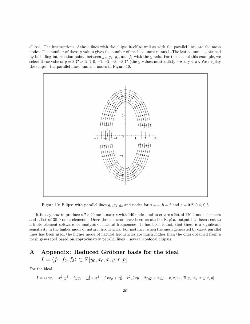
ellipse. The intersections of these lines with the ellipse itself as well as with the parallel lines are the meshnodes. The number of these y-values gives the number of mesh columns minus 1. The last column is obtainedby including intersection points between g1, g2, g3, and f1 with the y-axis. For the sake of this example, weselect these values: y = 3.75, 3, 2, 1, 0,−1,−2,−3,−3.75 (the y-values must satisfy −a < y < a). We displaythe ellipse, the parallel lines, and the nodes in Figure 10.

–4

–2

0

2

4

y

–3 –2 –1 1 2 3

x

Figure 10: Ellipse with parallel lines g1, g2, g3 and nodes for a = 4, b = 2 and r = 0.2, 0.4, 0.6

It is easy now to produce a 7×20 mesh matrix with 140 nodes and to create a list of 120 4-node elementsand a list of 30 9-node elements. Once the elements have been created in Maple, output has been sent toa finite element software for analysis of natural frequencies. It has been found, that there is a significantsensitivity in the higher mode of natural frequencies. For instance, when the mesh generated by exact parallellines has been used, the higher mode of natural frequencies are much higher than the ones obtained from amesh generated based on approximately parallel lines – several confocal ellipses.

A Appendix: Reduced Grobner basis for the ideal

I = 〈f1, f2, f3〉 ⊂ R[y0, x0, x, y, r, p]

For the ideal

I = 〈4py0 − x20, y

2 − 2yy0 + y20 + x2 − 2xx0 + x20 − r2, 2xp− 2x0p + x0y − x0y0〉 ⊂ R[y0, x0, x, y, r, p]

30

using lex order with y0 > x0 > x > y > r > p, a reduced Grobner basis for I is given by the followingfourteen polynomials:8

> g1:=factor(reducedG[1]);

g1 := p(−2 p r2 y x2 + 8 p r2 y3 + 8 p2 r2 y2 − 32 y p3 r2 + 16 p4 r2 − 16 y4 p2 + 32 y3 p3

− 16 p4 y2 + 3 r2 x4 + 8 p2 r4 + 20 p2 r2 x2 − y2 x4 + 10 y p x4 − x6 − x4 p2 + 8 p y3 x2

− 32 x2 y2 p2 + 8 x2 y p3 − 3 r4 x2 + 2 r2 x2 y2 + r6 − r4 y2 − 8 p r4 y)> g2:=factor(reducedG[2]);

g2 := p(−114 x3 p2 y + 232 x p3 y2 + 40 x p4 y − 316 x p3 r2 − 8 x y3 p2 − 2 x3 p3 + 16 x p5

− 16 p y2 x r2 − 12 p y2 x0 r2 + 54 x y p2 r2 − 120 y p2 x0 r2 − 32 y p4 x0

+ 104 p3 x0 r2 − 14 p y2 x3 + 32 p2 y3 x0 + 32 x p r4 − 46 x3 p r2 − 16 p5 x0

+ 14 x5 p + 27 r4 x0 p + 2 y x5 + 2 y3 x3 − 2 y3 x r2 − 4 y3 x0 r2 + 2 y x r4 − 4 y x3 r2

− 24 p y4 x + 16 p y4 x0 )> g3:=factor(reducedG[3]);

g3 := p(4 x2 p3 + 56 p3 r2 − 4 x p3 x0 − 56 p3 y2 + 48 y3 p2 + 42 x2 p2 y − 12 x p2 y x0

− 48 y p2 r2 − 4 x4 p + 8 y4 p + 14 p r4 − 10 x2 p r2 − 12 x p y2 x0 − 8 x2 p y2

+ 27 x p x0 r2 − 22 y2 p r2 + 2 r4 y + 2 y3 x2 + 2 y x4 − 4 r2 y x2 − 4 x y3 x0 − 2 r2 y3)> g4:=factor(reducedG[4]);

g4 := p(112 x p4 − 112 x0 p4 − 120 y x p3 + 176 y x0 p3 − 124 x p2 r2 − 80 y2 x0 p2

− 16 x0 p2 r2 + 160 x p2 y2 − 96 x2 p2 x0 + 82 x3 p2 − 28 x3 y p + 4 y x0 p r2

− 24 p x y3 + 16 p y3 x0 + 22 x y p r2 − 4 r2 y2 x0 + 2 y2 x3 − 4 r2 x3 − 2 r2 x y2

+ 2 r4 x + 3 r4 x0 − 3 x2 x0 r2 + 2 x5)> g5:=factor(reducedG[5]);

g5 := 8 x p y2 − 6 x3 p + 7 x0 p x2 + 6 x p r2 + 4 p x0 y2 + y x0 x2 − y x0 r2 + 8 y x p2

− 12 y x0 p2 + 2 x0 p r2 − 8 x p3 + 8 x0 p3

> g6:=factor(reducedG[6]);

g6 := p(8 p2 r2 − 8 y2 p2 − 4 x0 x p2 + 4 x2 p2 + 4 x y x0 p + 8 p y3 + 2 y p x2 − 8 y p r2

+ 3 x0 x r2 − 2 r2 y2 + 2 x4 + 2 r4 + 2 x2 y2 − 4 x2 r2 − 3 x0 x3 − 4 x y2 x0 )> g7:=factor(reducedG[7]);

g7 := x0 x4 − 2 x2 x0 r2 + 44 x2 p2 x0 + 32 y2 x0 p2 − 12 y x0 p r2 − 80 y x0 p3 + r4 x0

+ 16 x0 p2 r2 + 48 x0 p4 − 2 x3 y p− 38 x3 p2 − 40 x p2 y2 + 2 x y p r2 + 56 y x p3

+ 20 x p2 r2 − 48 x p4

> g8:=factor(reducedG[8]);

g8 := 3 x02 r2 − 12 x02 p2 + 16 x y x0 p + 32 x0 x p2 − 20 x2 p2 − 48 y2 p2 + 48 p2 r2

− 2 x0 x3 + 2 x0 x r2 + 4 y p x2

> g9:=factor(reducedG[9]);

g9 := −4 p y2 − 4 p x2 + 6 p x x0 − 2 p x02 + 4 p r2 + x0 2 y

8We display these polynomials in a form returned by Maple. Polynomials g1, g2, g3, g4, g6 can be further simplified by dividingthem by p under the assumption that p 6= 0.

31

> g10:=factor(reducedG[10]);

g10 := −2 x0 x2 + 3 x02 x + 2 x0 r2 + 4 y x p− 8 p x0 y − 8 x p2 + 8 x0 p2

> g11:=factor(reducedG[11]);

g11 := x0 3 − 8 x p2 + 8 x0 p2 − 4 p x0 y

> g12:=factor(reducedG[12]);

g12 := 4 p y0 − x0 2

> g13:=factor(reducedG[13]);

g13 := −2 x p + 2 x0 p− x0 y + x0 y0

> g14:=factor(reducedG[14]);

g14 := y2 − 2 y y0 + y0 2 + x2 − 2 x x0 + x0 2 − r2

B Appendix: Reduced Grobner basis for the ideal

I = 〈f1, f2, f3〉 ⊂ R[y0, x0, x, y, a, b, r]

For the ideal

I = 〈b2y20+a2x20−a2b2, y2−2yy0+y20+x2−2xx0+x2

0−r2, b2y0x−b2y0x0−a2x0y+a2x0y0〉 ⊂ R[y0, x0, x, y, a, b, r]

using lex order with y0 > x0 > x > y > a > b > r, a reduced Grobner basis for I is given by the followingfifteen polynomials:9

> g1:=factor(reducedG[1]);

9We display these polynomials in a form returned by Maple. All polynomials except g13 and g14 can be further simplifiedby dividing them by a2, b2 under the assumption that a, b 6= 0.

32

g1 := a2 b2(6 b4 x4 a4 − 4 y6 b4 a2 − 6 a6 x4 b2 − 4 b6 x2 a4 + 6 b4 x2 a6 + a4 b8 − 2 y2 b8 a2

+ 6 y2 b6 x2 a2 + 6 a6 y2 x2 b2 − 10 b4 x2 a4 y2 + y8 b4 + b8 r4 + b4 r8 − 2 b6 r6

− 2 b4 y2 x4 r2 − 6 x2 y4 b4 r2 + 6 x2 b4 r4 y2 − 4 b4 y6 r2 + 2 b4 y6 x2 + y4 b4 x4

+ b4 x4 r4 − 2 b4 r6 x2 − 2 b6 x2 r4 + 6 y4 b4 r4 − 2 b8 y2 r2 + 6 b6 r4 y2 − 4 b4 r6 y2

+ 6 a4 y2 b6 + 6 a6 y2 b2 r2 + 2 a4 b2 x4 y2 − 4 a4 x6 b2 + 4 a6 x2 b2 r2 − 8 b4 x2 a4 r2

+ 10 a4 x4 b2 r2 − 6 b4 r2 a2 x2 y2 − 6 a4 x2 b2 r2 y2 − 8 a4 x2 b2 r4 − 6 b4 r2 a2 x4

+ 4 b4 r4 a2 x2 − 6 y4 a4 b2 x2 − 6 b4 x4 a2 y2 + 6 b6 x2 r2 a2 + 2 b4 x2 y4 a2

+ 10 b4 y4 a2 r2 + 4 b6 y2 r2 a2 − 8 b4 y2 r4 a2 − 8 b4 y2 a4 r2 + 2 r6 a2 b4 + a8 b4

− 6 a4 y4 r2 b2 + 4 a4 y2 r4 b2 − 2 a8 b2 x2 + x4 a4 y4 + 4 x2 b6 y2 r2 − 6 y4 b6 a2

− 4 a6 y2 b4 − 2 y4 a4 x2 r2 + 2 b2 r2 a2 x4 y2 − 2 r8 a2 b2 + r8 a4 + a8 x4 + a4 x8

− 4 a4 x6 r2 + 6 a4 x4 r4 + 2 b2 r2 a2 x6 − 6 b2 r4 a2 x4 − 2 a6 r6 + 2 a6 x6 + a8 r4

+ 2 y6 b2 a2 x2 − 2 r6 a4 y2 + 6 r6 b2 y2 a2 − 2 a8 x2 r2 + y4 a4 r4 − 6 y4 b2 r4 a2

− 2 a6 y2 r4 + 4 x2 a6 y2 r2 + 6 x2 a4 y2 r4 + 2 y4 b2 x2 a2 r2 − 10 x2 b2 y2 r4 a2

+ 2 y6 b2 a2 r2 + 6 r6 b2 x2 a2 + 4 b2 x4 y4 a2 + 2 a4 x6 y2 − 6 a6 x4 r2 − 4 r6 a4 x2

+ 2 b2 x6 a2 y2 + 6 r4 a6 x2 − 6 a4 x4 r2 y2 + 2 b6 y6 − 2 a8 b2 r2 − 2 x2 y4 b6

+ 6 a4 y4 b4 + y4 b8 − 6 y4 b6 r2 − 2 x4 a6 y2 − 2 a6 b6 + 2 b6 r4 a2 − 2 b8 r2 a2

+ 2 b4 a6 r2 − 6 b4 a4 r4 + 2 r2 a4 b6 + 2 r4 a6 b2 + 2 r6 a4 b2)> g2:=factor(reducedG[2]);

g2 := b2(−2 y a2 b2 + b2 y0 y2 + y0 a2 b2 − b2 y0 r2 + 3 a2 y x x0 − a2 y0 x2 + a2 y2 y0

− a4 y0 + a2 y0 r2 + a4 y − a2 y3 − a2 y x2 + a2 y r2)> g3:=factor(reducedG[3]);

g3 := a2(−x0 b2 y2 + x0 a2 x2 + x0 a2 b2 − x0 a2 r2 + 3 y b2 y0 x− 2 xa2 b2 + b2 x2 x0

− b4 x0 + x0 b2 r2 + b4 x− b2 x y2 − b2 x3 + x b2 r2)> g4:=factor(reducedG[4]);

g4 := b2(3 x0 a2 x3 + 6 a4 x x0 − 3 b2 xa2 x0 − 3 x x0 a2 r2 + 4 a2 y y0 x2 + 2 a2 y3 y0

− 2 a4 y y0 − b2 y0 y3 + 5 y y0 a2 b2 − 4 a2 y y0 r2 + y b2 y0 r2 − 3 x4 a2 − 5 x2 y2 a2

− 2 y4 a2 − 3 a4 x2 + 2 a4 y2 + 3 b2 x2 a2 − y2 a2 b2 − 3 a4 b2 + 6 x2 a2 r2 + 5 y2 a2 r2

+ 3 a4 r2 + 3 b2 a2 r2 − 3 r4 a2)> g5:=factor(reducedG[5]);

g5 := b2(−b4 x y0 r2 + a2 b4 y0 x + 3 x0 b4 y a2 − 5 b4 x y a2 + b4 y2 y0 x + 2 b2 x3 a2 y

− 7 b2 xa2 y2 y0 − 3 x0 b2 y a2 r2 − a2 b2 y0 x3 − 3 x0 a4 y b2 − 2 b2 xa2 y r2

+ 2 b2 xa2 y3 + 5 xa4 y b2 + 3 x0 b2 y3 a2 + a4 x y2 y0 − x3 y a4 + a4 x y0 r2

+ 3 a4 x0 y r2 − a6 x y0 − a4 x y3 − a4 y0 x3 + y a4 x r2 + a6 x y)> g6:=factor(reducedG[6]);

g6 := b2(−2 a4 y4 − 6 b2 r2 a2 x x0 + b4 y2 a2 + 4 a4 y y0 b2 + 4 y0 b4 y a2 − b2 x2 a2 y2

+ 3 b2 x2 a2 r2 + 4 b2 y2 a2 r2 − 4 a2 y b2 y0 x2 − 4 a2 y b2 y0 r2 − 2 b4 y0 y3

+ 3 b4 r2 a2 − 3 b2 r4 a2 − 3 a4 b4 + 2 y b4 y0 r2 − b2 y4 a2 + 6 a4 b2 x2 + 6 a4 b2 r2

− 3 a6 b2 + 4 a4 y y0 x2 − 4 a4 y y0 r2 + 3 a6 r2 − 3 a4 r4 + 2 a4 y3 y0 − 2 a6 y y0

+ 6 a4 x2 r2 + 5 a4 y2 r2 + 6 a6 x x0 − 3 x4 a4 − 3 x2 a6 − 5 a4 x2 y2 + 2 a6 y2)

33

> g7:=factor(reducedG[7]);

g7 := b2(−21 a4 x b4 − 6 x3 b4 a2 + 2 a6 y2 x− 3 x5 a4 + 6 b6 xa2 + 9 a6 b2 x + 6 a4 y2 b2 x

− 5 b4 y2 xa2 − 5 y2 a4 x3 − 2 y4 a4 x + 12 a4 b2 x3 − 3 a6 x3 − 6 a6 b2 x0

− 6 b6 x0 a2 + 4 y a4 y0 x3 + 2 y3 a4 x y0 − 2 y a6 x y0 − 14 y a4 b2 y0 x

− 4 y a4 x y0 r2 + 5 y2 a4 x r2 − 4 y0 b2 x3 a2 y + 22 y0 b4 x y a2 + 6 a4 x3 r2

+ 3 a6 x r2 − 2 b4 x y0 y3 − 3 a4 x r4 − b2 x3 a2 y2 − b2 y4 xa2 − 6 b4 y2 a2 x0

− 12 b2 a4 x0 r2 + 6 b4 x2 a2 x0 + 6 x0 b4 r2 a2 + 6 x0 a6 r2 + 6 x0 a4 b2 y2

+ 2 b4 x y y0 r2 + 12 x0 a4 b4 + 3 b2 x3 a2 r2 − 4 y a2 b2 x y0 r2 − 3 b2 x r4 a2

− 6 b2 x2 r2 a2 x0 + 4 b2 y2 xa2 r2 + 9 b4 r2 a2 x)> g8:=factor(reducedG[8]);

g8 := b2(4 a4 y3 − 2 a4 x2 y − 4 a2 y3 x2 − 2 y5 a2 − 2 a6 y − 2 a2 b2 y0 x2 + 4 a2 b2 y0 y2

+ 4 a2 b2 y0 r2 + 2 a4 y b2 − 2 b2 y3 a2 − 2 b4 y a2 − b4 y0 r2 + b4 y0 a2 + b4 y0 y2

− 3 a4 y0 b2 + 2 a4 y r2 + 2 b2 y a2 r2 + 4 b2 y a2 x2 + 2 a6 y0 + 4 x2 a2 y r2

+ 3 x2 a2 y2 y0 − 2 x2 a2 y0 r2 − 3 a2 y2 y0 r2 − b2 y2 y0 x2 + 2 b2 y2 y0 r2

+ b2 x2 y0 r2 + 4 y3 a2 r2 − 2 y r4 a2 + r4 a2 y0 − 3 a4 y0 r2 − b2 y4 y0 − b2 r4 y0

+ 2 a2 y4 y0 + a2 y0 x4 + 3 x2 a4 y0 − 4 a4 y2 y0 − 2 x4 y a2)> g9:=factor(reducedG[9]);

g9 := b2(−4 b2 x2 a2 y2 y0 − 2 x2 a2 b2 y0 r2 − 2 b4 y4 y0 + b4 y3 a2 − b2 y5 a2 − 3 y a4 b4

+ 4 b4 y2 y0 a2 + 4 b4 y2 y0 r2 − b2 x2 a2 y3 + 6 x2 a4 y b2 − 2 a2 y2 b2 y0 r2

+ 2 a4 y2 y0 b2 + 2 b2 y3 a2 r2 − y b4 r2 a2 − y b2 r4 a2 + 8 y a4 b2 r2 + b2 x2 a2 y r2

+ 2 r4 a2 b2 y0 + 2 a2 b4 y0 r2 − 2 a6 y0 b2 + a6 y b2 − 2 r4 b4 y0 − 3 a4 x4 y

+ 4 a6 y3 − 2 a4 y5 − 5 x2 a4 y3 − 2 a6 r2 y0 + a6 r2 y + 5 a4 r2 y3 − 3 a4 r4 y

+ 2 a4 y4 y0 − 4 a6 y2 y0 + 2 a6 x2 y0 + 2 a8 y0 + 6 a4 x2 y r2 + 4 a4 x2 y2 y0

− 4 a4 r2 y0 y2 − a6 x2 y − 2 a8 y)> g10:=factor(reducedG[10]);

g10 := b2(2 a6 b4 − 2 a4 b6 − 16 a4 y4 b2 + 2 a4 x6 − 4 b4 r4 a2 + 2 b6 r2 a2 − 4 b6 y0 y3

+ 3 a4 x4 y2 − 2 a8 y2 + 4 a6 y4 − 4 a6 r2 b2 + 4 a4 b2 x2 y2 + 9 a6 y2 b2 + 2 b4 a4 r2

+ 6 b4 x2 a4 − 6 y2 a4 x2 r2 + 2 r6 b2 a2 − 4 x2 a6 r2 + 6 x2 a4 r4 + 6 b2 x4 y2 a2

− 6 a4 x4 r2 + 3 y2 a2 r4 b2 + 13 y4 b2 a2 x2 − 12 y4 b2 a2 r2 − 2 r6 a4 + 2 r4 a6

+ a4 y4 r2 + 3 a4 y2 r4 + 5 a6 y2 r2 + 2 a6 x4 + 2 b2 r2 a2 x4 − 4 x2 b2 r4 a2

− 9 y2 b2 r2 a2 x2 + 7 y6 a2 b2 − 6 x4 a4 b2 − 4 b4 x2 r2 a2 + 2 y5 a4 y0 − 4 y3 a6 y0

+ 2 y a8 y0 + 6 b4 y5 y0 + 6 b2 r2 a2 x2 y y0 − 4 b2 x2 a2 y3 y0 + 14 b2 y3 a2 y0 r2

− 6 b2 a2 y r4 y0 − 4 b4 x2 y y0 r2 + 4 b4 x2 y3 y0 − 8 b2 y5 a2 y0 + 6 a6 x2 y y0

− 6 a6 y r2 y0 − 12 b4 y3 y0 r2 + 6 b4 y r4 y0 + 2 a4 b2 r4 − 2 y6 a4 + 18 a4 y3 b2 y0

− 10 a6 y y0 b2 + 8 a4 y0 b4 y + b4 y2 a2 r2 + 4 b6 y y0 r2 − 8 a4 y b2 y0 x2

+ 28 a4 y b2 y0 r2 − 26 a2 y b4 y0 r2 + 4 a4 b2 x2 r2 − 18 a4 b2 y2 r2 − 12 a2 b4 y0 y3

− x2 y4 a4 − 4 x2 a6 b2 + 3 y4 b4 a2 − 7 a4 b4 y2 + 6 y2 b6 a2 − 12 b4 x2 y2 a2

− 5 a6 y2 x2)> g11:=factor(reducedG[11]);

34

g11 := b2(−12 b4 x4 a4 + 18 y6 b4 a2 + 14 b6 x2 a4 − 6 b4 x2 a6 − 5 a4 b8 + 15 y2 b8 a2

− 27 y2 b6 x2 a2 + 6 a6 y4 b2 − 8 a6 y2 x2 b2 − 6 b4 x2 a4 y2 − 11 a4 y2 b6

+ 22 a6 y2 b2 r2 + 15 a4 b2 x4 y2 + 24 b6 y5 y0 + 2 a4 x6 b2 + 16 a6 x2 b2 y y0

− 24 b4 x2 a4 y y0 − 8 a6 x2 b2 r2 + 6 b4 x2 a4 r2 − 9 a4 x4 b2 r2 − 33 b4 r2 a2 x2 y2

+ 18 b4 r2 a2 x2 y y0 − 29 a4 x2 b2 r2 y2 − 4 a4 x2 b2 r2 y y0 + 12 a4 x2 b2 r4

+ 3 b4 r2 a2 x4 − 10 b4 r4 a2 x2 − 6 b4 x2 a2 y3 y0 + 8 x2 b6 y3 y0 − 8 x2 b6 y y0 r2

− 42 b6 y3 y0 a2 − 48 b6 y3 y0 r2 − 7 y4 a4 b2 x2 + 50 b4 y3 a2 y0 r2 + 9 b4 x4 a2 y2

− 9 b6 x2 r2 a2 + 43 b4 x2 y4 a2 − 22 b4 y5 a2 y0 + 50 b4 y3 a4 y0 − 29 b4 y4 a2 r2

+ 10 b6 y2 r2 a2 + 4 b4 y2 r4 a2 − 73 b4 y2 a4 r2 + 7 r6 a2 b4 + a8 b4 + 86 y a4 b4 y0 r2

− 78 y a2 b6 y0 r2 − 10 y3 b8 y0 − 28 y a6 b4 y0 + 24 y a4 b6 y0 + 10 y b8 y0 r2

− 28 a2 y r4 b4 y0 + 4 a4 y3 r2 b2 y0 − 18 a6 y r2 y0 b2 + 4 a4 y r4 b2 y0

− 9 a4 y4 r2 b2 + 14 a4 y2 r4 b2 + 24 y b6 r4 y0 − 2 a8 b2 x2 − 6 y3 a6 y0 b2

+ 4 y a8 y0 b2 + x4 a4 y4 + y4 b6 a2 − 4 a8 y2 b2 + 22 a6 y2 b4 − 2 y3 b2 r2 a2 y0 x2

− 2 y4 a4 x2 r2 − 2 x4 b4 y y0 r2 − b2 r2 a2 x4 y2 − r8 a2 b2 + r8 a4 + a8 x4 − 2 y8 b2 a2

+ a4 x8 − 4 a4 x6 r2 + 6 a4 x4 r4 + b2 r2 a2 x6 − 3 b2 r4 a2 x4 − 2 a6 r6 + 2 a6 x6 + a8 r4

− y6 b2 a2 x2 + 2 x2 y b4 r4 y0 − 2 r6 a4 y2 + 5 r6 b2 y2 a2 − 2 a8 x2 r2 + y4 a4 r4

− 9 y4 b2 r4 a2 + 2 a2 y7 b2 y0 − 2 a6 y2 r4 − 4 y5 b2 a2 y0 r2 + 2 y3 a2 r4 b2 y0

+ 4 x2 a6 y2 r2 + 6 x2 a4 y2 r4 + 5 y4 b2 x2 a2 r2 − 7 x2 b2 y2 r4 a2 + 2 y5 b2 a2 y0 x2

− 4 x2 b4 y3 y0 r2 + 7 y6 b2 a2 r2 + 3 r6 b2 x2 a2 + 2 x2 b4 y5 y0 + 4 b2 x4 y4 a2

+ 2 a4 x6 y2 − 6 a6 x4 r2 − 4 r6 a4 x2 + 2 x4 b4 y3 y0 + 3 b2 x6 a2 y2 + 6 r4 a6 x2

− 6 a4 x4 r2 y2 − 2 a8 b2 r2 − 41 a4 y4 b4 − 2 x4 a6 y2 + 4 a6 b6 − 11 b6 r4 a2

+ 5 b8 r2 a2 − 10 b4 a6 r2 + 2 b4 a4 r4 + 7 r2 a4 b6 + 8 r4 a6 b2 − 5 r6 a4 b2)> g12:=factor(reducedG[12]);

35

g12 := b2(−3 y6 b4 a2 x2 − 9 a4 r6 b4 + 2 a6 b8 + 2 a8 r4 b2 − 19 a6 r2 b6 + 32 a6 b4 r4

− 13 a8 b4 r2 + 20 a4 b8 r2 − 10 a4 b6 r4 + 8 a8 b6 + 24 y2 b10 a2 − 15 a6 r6 b2

+ 10 a6 x6 b2 − 17 a6 x4 y2 b2 − 39 y2 b8 x2 a2 + 23 a6 y2 x2 b4 − 16 a8 x2 y2 b2

− 37 a4 y4 x2 b4 + 24 x2 y4 a6 b2 − 16 b10 y3 y0 + 2 b4 x6 a4 + 94 y4 b6 x2 a2

+ 9 y2 b6 x4 a2 − 52 b6 x2 a4 y2 + 48 b4 x4 a4 y2 − 8 b10 a4 − 18 a6 b4 x4 + 8 b10 r2 a2

− 22 b8 r4 a2 + 21 b6 r6 a2 + 16 b10 y y0 r2 − 8 r8 a2 b4 + 8 r8 a4 b2 − 16 b6 x4 a4

+ 21 b8 x2 a4 + 2 y3 b4 r2 a2 y0 x2 − 20 y4 a4 b2 x2 r2 − 2 a10 b4 − 2 a10 x4

+ 4 a10 b2 x2 + a4 x10 − 3 a8 x6 − 19 a8 b4 x2 + 14 a8 x4 b2 − 16 a4 b2 y6 x2

− 2 a6 x6 y2 + 5 y4 a4 x6 + 4 a4 x8 y2 − 6 x4 a6 y4 + 6 x4 a8 y2 + 2 y6 a4 x4 + 6 b6 x2 a6

− 14 y4 b8 a2 + 24 b6 y6 a2 + 20 a6 y2 b6 − 4 x4 b6 y y0 r2 − 8 b4 r2 a2 x4 y2

− 8 a4 x6 b2 r2 + 24 a4 x4 b2 r4 + b4 r2 a2 x6 − 10 b4 r4 a2 x4 + 4 x4 b6 y3 y0

+ 3 b4 x6 a2 y2 + 4 b4 a4 x2 r4 + 40 r4 a6 x2 b2 − 10 r2 a4 x2 b6 + 17 r6 b4 x2 a2

− 24 r6 a4 x2 b2 − 20 a4 x4 b2 r2 y2 − 30 x2 b4 y2 r4 a2 − 2 x2 a2 y r4 b4 y0

+ 40 x2 a4 y2 r4 b2 − 12 b6 x2 r4 a2 + 8 x2 b6 y5 y0 + 6 b4 x4 y4 a2 + 3 b6 x4 a2 r2

− 35 a6 x4 b2 r2 + 16 y4 b4 x2 a2 r2 + 116 y3 a2 b6 y0 r2 − 4 y5 b4 a2 y0 r2

+ 2 y3 a2 r4 b4 y0 + 34 x2 a6 y2 b2 r2 − 20 x2 b6 y3 y0 r2 + 10 b8 x2 y0 y3

− 13 b8 x2 r2 a2 − 50 y5 b6 y0 a2 − 10 y5 b6 y0 r2 + 39 y6 b4 a2 r2 − 8 y4 a4 b2 x4

− 67 y4 a4 b4 r2 − 31 y4 b6 a2 r2 − 8 y3 a6 b4 y0 + 8 y3 b6 r4 y0 + 24 y4 a6 r2 b2

− 16 y6 a4 r2 b2 + 28 y4 a4 r4 b2 − 56 y4 b4 r4 a2 + 3 b4 a4 x4 r2 + 6 b4 a6 x2 r2

+ 4 a8 y2 b4 − 10 y8 b4 a2 + 100 a4 y3 b6 y0 − 17 a6 y2 b2 r4 − 16 a8 y2 b2 r2

− 178 a4 b6 y2 r2 + 48 a4 b4 r4 y2 − 94 b8 y3 y0 a2 − 114 b8 y3 y0 r2 + 32 b8 y2 a2 r2

− 14 b6 r4 y2 a2 − 20 r6 a4 b2 y2 + 35 r6 b4 y2 a2 + 6 y a8 b4 y0 − 54 y a6 b6 y0

+ 56 y b8 r4 y0 − 12 b4 y a4 x2 y0 r2 + 30 b4 y a6 x2 y0 − 2 b6 y3 a2 y0 x2

− 48 b6 y a4 y0 x2 + 32 b6 y a2 x2 y0 r2 − 82 b4 y2 a4 x2 r2 − 10 b8 x2 y y0 r2

− 70 b6 y2 x2 a2 r2 + 8 a4 y3 b4 y0 r2 − 34 y a6 b4 y0 r2 + 170 y a4 b6 y0 r2

+ 10 y a4 r4 b4 y0 − 66 y a2 b6 r4 y0 − 152 y b8 a2 y0 r2 + 77 a6 y2 b4 r2

+ 58 b8 y5 y0 + 48 y a4 b8 y0 − 52 a4 y4 b6 + 2 b4 y9 y0 + 4 b6 y7 y0 + 6 b4 y7 y0 x2

− 12 a6 y4 b4 + 12 x2 a6 y4 r2 + 10 x2 y3 b4 r4 y0 − 12 x2 a8 y2 r2 + 4 r8 a4 y2

− 7 r8 b2 y2 a2 + 2 y6 a4 r4 − 2 y3 b4 r6 y0 − 4 y6 a4 x2 r2 − 6 b4 y7 y0 r2

+ 11 b2 y6 x4 a2 + 4 b2 y8 x2 a2 + 4 b2 y8 a2 r2 − 13 b2 y6 r4 a2 + 6 b4 y5 r4 y0

+ 5 r8 a4 x2 − 4 r8 b2 x2 a2 − 16 a8 b2 x2 r2 + 9 a8 x4 r2 − 9 a8 r4 x2 − 5 a4 x8 r2

+ 10 a4 x6 r4 + b2 r2 a2 x8 − 4 b2 r4 a2 x6 + 2 x6 b4 y3 y0 + 3 b2 x8 a2 y2

+ 6 r6 b2 x4 a2 − 10 r6 a4 x4 + 6 x4 b4 y5 y0 + 10 b2 x6 y4 a2 − 12 x4 b2 y2 r4 a2

+ 24 x4 a4 y2 r4 − 5 y4 b2 x4 a2 r2 − 10 x4 b4 y3 y0 r2 − 6 a6 x2 y2 r4 − 15 y4 a4 x4 r2

− 2 x6 b4 y y0 r2 − 2 b2 r2 a2 x6 y2 + 4 r4 x4 b4 y y0 + 15 x2 y4 a4 r4

− 20 x2 y4 b2 r4 a2 − 16 x2 r6 a4 y2 + 18 x2 r6 b2 y2 a2 + 12 x2 y b6 r4 y0

+ 6 a6 x4 r2 y2 − 16 a4 x6 r2 y2 − 14 b4 y5 x2 y0 r2 + 2 b2 y6 x2 a2 r2 − 6 y4 a6 r4

− 5 y4 r6 a4 + 15 y4 r6 b2 a2 + 6 a8 y2 r4 + 2 a6 r6 y2 + 2 y b4 r6 a2 y0 − 2 y b6 r6 y0

+ 20 y6 a4 b4 + 4 a10 x2 r2 − 2 r6 x2 b4 y y0 − 2 a10 r4 + 4 a10 b2 r2 + 3 a8 r6

+ r10 a2 b2 − r10 a4)

36

> g13:=factor(reducedG[13]);

g13 := y2 − 2 y y0 + y0 2 + x2 − 2 x x0 + x0 2 − r2

> g14:=factor(reducedG[14]);

g14 := b2 y0 x− b2 y0 x0 − a2 x0 y + a2 x0 y0

> g15:=factor(reducedG[15]);

g15 := b2 (x0 y0 x + y y0 2 − y0 x2 − y0 y2 − y0 a2 + y0 r2 + y a2)

C Appendix: Reduced Grobner basis for the ideal

IS = 〈h1, h2, h3, h4, h5, g〉 ⊂ R[x, y, a, b, r]

In order to solve system (38), we have found a reduced Grobner basis for IS using the total term order tdegfor y > x > a > b > r with ties broken by inverse lexicographical order. We used package Groebner fromMaple 8 supplemented by a small custom package RJGrobner written by the Authors. [2] The reduced basiscontains fourteen homogeneous polynomials with degrees ranging from 10 through 15 and the number ofmonomials terms ranging from 51 through 112. We will not display these polynomials here. However, hereis the factorization the fourth polynomial b4 in the basis:

b4 = b2 x(4 y2 r4 a2 − 5 y4 a2 r2 + a4 r2 y2 − 2 b2 x2 r4 + b2 x4 r2 − 9 x2 b2 y2 a2 − 11 b2 y2 a2 r2

− 2 x2 b4 r2 + 4 a6 r2 − 2 a8 − b6 a2 − a4 b4 + 4 a6 b2 + 6 y2 a6 − a4 r4 − r6 a2

− 4 y4 b4 − 6 y4 a4 − 4 a6 x2 + 2 y6 a2 − a4 x4 − b6 y2 + b6 r2 + r6 b2 − 4 b4 r4

+ 2 a4 b2 x2 − 9 a4 b2 y2 + 2 x2 b4 y2 + 5 b4 y2 a2 − a4 x2 y2 − 3 b2 a2 x4 + 6 b2 y4 a2

+ 3 x2 b4 a2 − y6 b2 + a2 x6 − 2 b2 x2 a2 r2 + 2 a4 x2 r2 − 3 a2 x4 r2 + 3 a2 x2 r4

− 8 x2 y2 a2 r2 + 4 b2 x2 y2 r2 + 8 b4 y2 r2 + 5 b2 r4 a2 + 5 b4 r2 a2 − 3 b2 r4 y2

+ 3 b2 y4 r2 − 10 b2 a4 r2 − b2 x4 y2 − 2 y4 b2 x2 + 4 a2 x4 y2 + 5 a2 y4 x2)

(79)

It appears, that since b > 0, one possible solution is x = 0. Upon substituting x = 0 into the list F shownin (38), one gets

[0,−y A(2 b2 y4 + b4 y2 − 4 b2 r2 y2 − 4 b2 y2 a2 + y2 a2 r2 − b4 a2 − b4 r2 + 2 b2 r4 + 2 a4 b2 − a4 r2 − r4 a2),

−A(−2 b2 y4 + r2 y4 − b4 y2 + 2 b2 r2 y2 + 4 b2 y2 a2 − 3 y2 a2 r2 − 2 r4 y2 + b4 a2 − b4 r2 − 2 a4 b2

+ 2 b2 a2 r2 + r6 + 2 a4 r2 − 3 r4 a2),

(y + r − a) (y + r + a) (a− y + r) (−a− y + r) (−y2 + r2 + a2 − 2 b2)A,

A(−y4 a2 + 2 b2 y4 + b4 y2 − 4 b2 r2 y2 − 2 b2 y2 a2 + 3 y2 a2 r2 + 2 a4 y2 + b4 a2 − b4 r2 − 2 b2 a2 r2

+ 2 b2 r4 + 3 a4 r2 − 2 r4 a2 − a6),

(y + r − a) (y + r + a) (a− y + r) (−a− y + r)A2]

(80)

whereA = −y2 b2 − b4 − r2 a2 + b2 a2 + b2 r2. (81)

37

It can be easily verified that setting y = −r − a or y = r + a in (80) does not yield any critical values for r,as the system becomes, respectively,

F1 = [0, −2 (r + a) (b2 + r a)4 r a, 2 (b2 + r a)4 r (r + a), 0, −2 (b2 + r a)4 a (r + a), 0], (82)

F4 = [0, 2 (r + a) (b2 + r a)4 r a, 2 (b2 + r a)4 r (r + a), 0, −2 (b2 + r a)4 a (r + a), 0] (83)

as a > b > r > 0 and is insolvable. However, setting y = −r+ a or y = r− a does yield rcrit = b2

a and makesthe system solvable in each case:

F2 = [0, 2 (r − a) (−b2 + r a)4 r a, 2 (−b2 + r a)4 r (r − a), 0, 2 (−b2 + r a)4 a (r − a), 0], (84)

F3 = [0, −2 (r − a) (−b2 + r a)4 r a, 2 (−b2 + r a)4 r (r − a), 0, 2 (−b2 + r a)4 a (r − a), 0] (85)

Another possibility for solving the system is to set

y2 =−b4 − r2a2 + b2a2 + b2r2

b2(86)

Thus,(

x = 0, y = ±√

−b4 − r2a2 + b2a2 + b2r2

b2

)

(87)

provide two solutions to the system without any condition on r except that r > 0. These are the two virtualsingular points found earlier that are always present for a > b > r > 0. Observe also that the critical valueof r satisfies

rcrit =b2

a=

(

b

a

)

b < b since a > b.

Another possibility to solve the system is to set

y2 = r2 + a2 − 2 b2 (88)

When we substitute the above expressions for y2 into F, we get[

0, −6 y (−b2 + r a)2 (b2 + r a)2 b2, 6 (−b2 + r a)2 (b2 + r a)2 (−b + r) (b + r), 0,

6 (−b2 + r a)2 (b2 + r a)2 (b − a) (b + a),

(a + r − y) (a + r + y) (r − a + y) (−a + r − y) (−b2 + r a)2 (b2 + r a)2]

(89)

The above shows that in this case in order to satisfy the equations of the variety of singular points V(IS)

we must also have r = rcrit = b2

a . Hence we get

(

x = 0, y = ±(

a2 − b2

a

)

=c2

a

)

when r =b2

a, (90)

which is the special case of the above singular points discussed above.Finally, we have special cases that we are not interested in but we mention them for completeness. They

result when we set y = 0 in the list F (in addition to x = 0. The first case is when a = b, that is, when theellipse is a circle. The second case is when r = b or r = a.

Thus, to summarize, we have these two cases of singular points when x = 0 :

1.(

x = 0, y2 = −−b2r2+b4+a2r2−a2b2

b2

)

and r is arbitrary as long as b > r > 0. This yields singular points

that are always present.

38

2.(

x = 0, y = ±(−r + a) = ±(

c2

a

))

when r = rcrit = b2

a and c2 = a2 − b2. This yields singular points

in the special case r = rcrit.

In order to complete the analysis of all solutions of the system F, we need to consider the case whenx, y 6= 0. The fourteen-polynomial reduced Grobner basis found for IS when solving system (38), could besimplified by diving each polynomial by x, y, a2, or b2, as appropriate. Let I ⊂ R[x, y, a, b, r] denote theideal generated by these fourteen simplified polynomials. In an effort to eliminate variable y from somepolynomials, we computed10 the Grobner basis for the first elimination ideal Ix = I ∩ R[x, a, b, r] for thelexicographic order y > r > a > b > x. The first polynomial in this new thirteen-polynomial homogeneousbasis for Ix is of degree 12. It is the square of the following polynomial gx ⊂ R[x, a, b, r] of degree 6 in x :

gx = (b6 − 3 b4 a2 + 3 a4 b2 − a6)x6 + (6 b6 a2 + 3 a6 r2 − 6 b2 a4 r2 + 3 b4 r2 a2 − 3 b8 − 3 a4 b4)x4

+ (−21 b4 a4 r2 + 3 b10 − 3 b8 a2 + 21 b6 r2 a2 + 3 a4 b2 r4 − 3 r4 a6)x2

− 3 b4 a4 r4 − b12 + 3 b8 r2 a2 + a6 r6(91)

Upon substituting z = x2 this becomes an easily solvable cubic equation for z that has the following solution:

z =3 b2 a2 r2 − r2 a2 (a b r)

2

3 − 3 b3 (a b r)1

3 a r + b4 (a b r)2

3

(a b r)2

3 (−a2 + b2)= − δ

(a b r)2

3 (−a2 + b2)(92)

where δ is given in (45). Thus, we have derived the x-coordinates of the singular points S5, S6, S7 and S8

listed in (41), (42), (43), and (44).To find the y coordinates of these four singular points, we proceed in a similar fashion except that we

eliminate the x variable. Thus, compute the first elimination ideal Iy = I ∩R[y, a, b, r] for the lexicographicorder x > r > a > b > y. The first polynomial in this new six-polynomial homogeneous basis for Iy is ofdegree 12. It is the square of the following polynomial gy ⊂ R[y, a, b, r] of degree 6 in y :

gy = (−b6 + 3 b4 a2 − 3 a4 b2 + a6) y6 + (3 b2 a4 r2 + 3 b6 r2 − 3 a4 b4 + 6 a6 b2 − 3 a8 − 6 b4 r2 a2) y4

+ (3 b4 a2 r4 − 3 b6 r4 − 21 b4 a4 r2 + 3 a10 + 21 a6 b2 r2 − 3 a8 b2) y2 + b6 r6

− 3 b4 a4 r4 − a12 + 3 a8 b2 r2(93)

Upon substituting z = y2 this becomes an easily solvable cubic equation for z that has the following solution:

z =−a4 (a b r)

2

3 + 3 (a b r)1

3 b r a3 − 3 b2 a2 r2 + b2 r2 (a b r)2

3

(a b r)2

3 (a2 − b2)2=

(−a2 + b2) ε

(a b r)2/3 (−a2 + b2)2(94)

where ε is given in (46). Thus, we have derived the y-coordinates of the singular points S5, S6, S7 and S8

listed in (41), (42), (43), and (44).

Acknowledgment:The first author, R.A., gratefully acknowledges financial support from the College of Arts and Sciences

and the Department of Mathematics, Tennessee Technological University, to present a preliminary versionof this paper at the 5th Annual Hawaii International Conference on Statistics, Mathematics and RelatedFields, Honolulu, January 2006.

10We used gbasis procedure from the Groebner package with the total order lexdeg([y],[r,a,b,x]) indicating that thevariable y needed to be eliminated.

39

References

[1] Ab lamowicz, R.: SINGULARlink - A Maple 8 procedure that provides an interface between Maple andSingular vers. 2-3-1 and 3-1-0 for the purpose of computing Grobner bases (2005)

[2] Ab lamowicz, R., and Liu, J.: RJGrobner - A Small Package for Grobner Bases for Maple 8, October 2,2005

[3] Ab lamowicz, R., and Liu, J.: Parallel lines to Bezier cubic (in preparation)

[4] Cox, D., Little, J., and O’Shea, D.: Ideals, Varieties, and Algorithms: An Introduction to ComputationalAlgebraic Geometry and Commutative Algebra (Springer, New York, 2005)

[5] Cox, D., Little, J., and O’Shea, D.: Using Algebraic Geometry (Springer, New York, 1998)

[6] Eisenbud, David.: Commutative Algebra with a View Toward Algebraic Geometry (Springer, New York,2004)

[7] Greuel, G.-M., and Pfister, G.: A Singular Introduction to Commutative Algebra (Springer-Verlag,Berlin Heidelberg, 2002)

[8] Hartshorne, R.: Algebraic Geometry (Springer, New York, 1997)

[9] Waterloo Maple Incorporated, Maple, A General Purpose Computer Algebra System, Waterloo,http://www.maplesoft.com (2005)

[10] Millman, R. S., and Parker, G.: Elements of Differential Geometry (Prentice-Hall Inc., EnglewoodCliffs, 1977)

[11] Norton, R. L.: Design of Machinery: An Introduction to the Synthesis and Analysis of Mechanisms andMachines , Second edition (McGraw-Hill, Boston, 1999)

[12] Reid, M.: Undergraduate Algebraic Geometry (Cambridge University Press, Cambridge, 1988)

[13] Uicker, J. J., Pennock, G. R., and Shigley, J. E.: Theory of Machines and Mechanisms , Third edition(Oxford University Press, New York, 2003)

[14] Wikipedia: The Free Encyclopedia, at http://en.wikipedia.org/wiki/ (2005)

[15] Wright, F.: Computing with Maple (Chapman & Hall/CRC, Boca Raton, 2002)

Submitted: January 30, 2006; Revised: TBA.

40