University of Montana University of Montana

ScholarWorks at University of Montana ScholarWorks at University of Montana

Graduate Student Theses, Dissertations, & Professional Papers Graduate School

1959

The national income multiplier: Its theory its philosophy its utility The national income multiplier: Its theory its philosophy its utility

John Colin Jones The University of Montana

Follow this and additional works at: https://scholarworks.umt.edu/etd

Let us know how access to this document benefits you.

Recommended Citation Recommended Citation Jones, John Colin, "The national income multiplier: Its theory its philosophy its utility" (1959). Graduate Student Theses, Dissertations, & Professional Papers. 8768. https://scholarworks.umt.edu/etd/8768

This Thesis is brought to you for free and open access by the Graduate School at ScholarWorks at University of Montana. It has been accepted for inclusion in Graduate Student Theses, Dissertations, & Professional Papers by an authorized administrator of ScholarWorks at University of Montana. For more information, please contact scholarworks@mso.umt.edu.

THE NATIOHAL INCOME MULTIPLIER;ITS THEORY, ITS PHILOSOPHY, ITS UTILITY

J» COLIN H. JONES

B.A. University of WaJes^ U.C.W., Aberystwyth, 195Ô

Presented in partial fulfillment of the requirements for the degree of

Master of Arts

MONTANA STATE UNIVERSITY

1959

Approved by:

, Board of Examiners

Dean, Graduate School

AUG 6 1959

D a te

UMI Number: E P 39569

All rights reserved

IN FO R M A TIO N TO ALL U SER S The quality of this reproduction is dependent upon the quality of the copy submitted.

In the unlikely event that the author did not send a complete manuscript and there are missing pages, these will be noted. Also, if material had to be removed,

a note will indicate the deletion.

UMIDis»art«t)on Publishsng

UMI E P 39569

Published by ProQuest LLC (2013). Copyright in the Dissertation held by the Author.

Microform Edition © ProQuest LLC.All rights reserved. This work is protected against

unauthorized copying under Title 17, United States Code

ProQuestProQuest LLC.

789 East Eisenhower Parkway P.O. Box 1346

Ann Arbor, Ml 48106 - 1346

Acknovledgemerxts

I ■would like to acknovledge the aid and encouragement given to me hy three people. First, J. J. Botha, -who, at the University College of Wales, Aheryst'wyth, initially introduced me to the complexities of the multiplier concept. Second, Dr. Richard E. Shannon, vho made a plethora of useful suggestions regarding form. Third, Dr. Thomas A. Matinsek, "Vîho unselfishly gave a "whole year of tireless energy and stimulating discussion particularly as regards rigorous mathematical definition, formulation, and proof. However, although the extent of their assistance is great, the expression of appreciation must, as is customary, appear perfunctory.

-11-

In so far as millionaires find their satisfaction in building mighty mansions to contain their bodies ■when alive and pyramids to shelter them after death, or, repenting of their sins, erect cathedrals and endow monastries or foreign missions, the day when abundance of capital will interfere with abundance of output may be postponed, "To dig holes in the ground", paid for out of saving, will increase not only employment, but the real national dividend of useful goods and services.

J. M. KeynesGeneral Theory p. 220

-111-

TABLE OF CONTENTS

PageChapter I. . . . . ........................ 1

Main Theme and Tools of AnalysisPart I The Theory

Chapter II . . . .......... . . . . . . . . . . . . . . 15The Static Keynesian Multiplier

Chapter III........................................ . . 24Extensions of the Static Multiplier :Dynamic and Compound Multipliers

Chapter IV .................. 5IPart II The Appraisal

Chapter V. ° . 89Theoretical and Empirical Criticism:Predictory Econometric Models

Chapter V I ............ .118Conclusion

Bibliography . . . . . . . . . . . . . . . . . . . . . .122

-IV-

ILLUSTRA.O?IONSPage

Figure I. . . . . . . . . . . . . . . . . . . . . . . . I9The Linear Consumption Function

Figure II .......... . . . . . . . . . . . . . . . . . 22The Static Multiplier

Figure III........ . . . . . . . . . . . . . . . . . . 28The Dynamic Multiplier Expansionist Case

Figure I V ................ 31J.R. Hicks Adjustment Process Using Saving and Investment Schedules

Figure V . . . . . . . . 34Three Lags in the Circular Flow of Income

Chart I . . . . ............ UlDerivation of the Compound Multiplier

Figure V I .................................... U3The Compound Multiplier

Figure VII........................... . . . . . . . . . U5The Time Shape of Income Behaviour

Figure V I I I ................ kjThe Dynamic Stability of Equilibrium

Figure IX . . .......... . . . . . . . . . . . . . . .The Stability of Dynamic Equilibrium

Figure X ................ 6lThree Paths to Full Employment

Figure XI .................... 84-Three Paths to Full Employment

Figure XII. 86Three Paths to Full Employment

Table 1 . . . . . . . . . . . . . . 112Predictions and Actual Estimates

—V —

Chapter 1

Main Theme and Tools of Analysis

In the historiography of economic ideas the works of many economists are the subject of perhaps two or three Journal articles, sometimes an obituary or anniversary article, -vdiich reviews their ideas in a few brief paragraphs; but with others their ideas are, to use a Marshallian phrase, "an existing yeast ceaselessly working in the Cosmos." Alfred Marshall is a prime example and John Maynard Keynes is another. As for Keynes, in the field of macro-economics and public policy the work of no other man has come under such a powerful microscope, giving rise to a mixture of adulation and violent criticism, but never indifference. We are concerned in this thesis with one of Keynes' concepts : that of the "multiplier".As an original contribution, the multiplier concept is not strictly Keynes'; in fact, it is not even that of R. F. Kahn who formulated it in more or less its modern form in 1931*^ The lineage of the

pconcept has been traced by Hugo Hegeland depicting the influencesof others, particularly Bagehot. But G- L. S. Shackle points out,with regard to Kahn's acknowledgment of non-originality :

...It is, I think only on a very narrow and impoverished definition of originality that this disclaimer can be accepted. Important advances in any branch of knowledge are almost

^ "The Relation of Home Investment to Unemployment, " Economic Journal, June, 1931.

^The Multiplier Theory, Lund, 195^, Ch. I.—1—

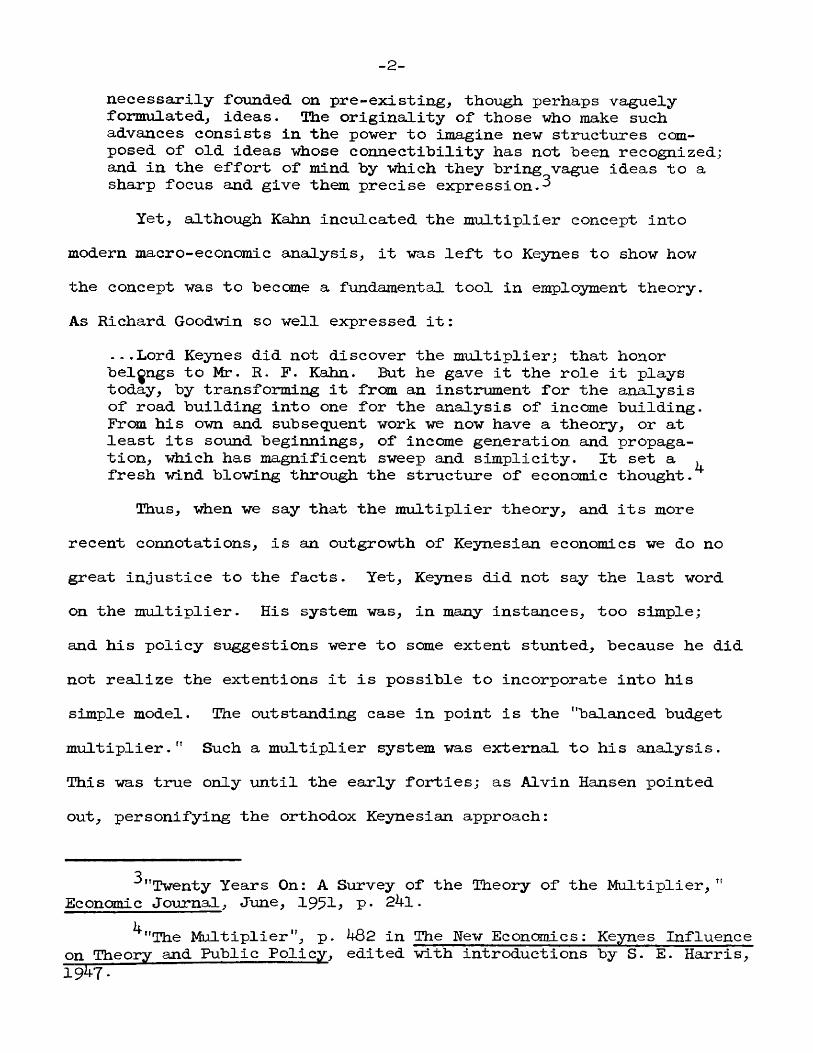
_2-necessajTîly fcïunded on pre-exis’ting^ "though perhaps vaguely formulated; ideas. The originality of those who make such advances consists in the power to imagine new structures com­posed of old ideas whose connectihility has not "been recognized; and in the effort of mind by which they bring vague ideas to a sharp focus and give them precise expression.^

Yet, although Kahn inculcated the multiplier concept intomodern macro-economic analysis, it was left to Keynes to show howthe concept was to become a fundamental tool in employment theory.As Richard Goodwin so well expressed it :

...Lord Keynes did not discover the multiplier; that honor belgngs to Mr. R. F. Kahn. But he gave it the role it plays today, by transforming it from an instrument for the analysis of road building into one for the analysis of income building.From his own and subsequent work we now have a theory, or at least its sound beginnings, of income generation and propaga­tion, which has magnificent sweep and simplicity. It set a , fresh wind blowing through the structure of economic thought.

Thus, when we say that the multiplier theory, and its more recent connotations, is an outgrowth of Keynesian economics we do no great injustice to the facts. Yet, Keynes did not say the last word on the multiplier. His system was, in many instances, too simple; and his policy suggestions were to some extent stunted, because he did not realize the extentions it is possible to incorporate into his simple model. The outstanding case in point is the "balanced budget multiplier." Such a multiplier system was external to his analysis. This was true only until the early forties; as Alvin Hansen pointed out, personifying the orthodox Keynesian approach:

^"Twenty Years On: A Survey of the Theory of the Multiplier, " Economic Journal, June, 1951^ P* 24l.

^"The Multiplier", p. kQ2 in The New Economics: Keynes Influence on Theory and Public Policy, edited with introductions by S. E. Harris,

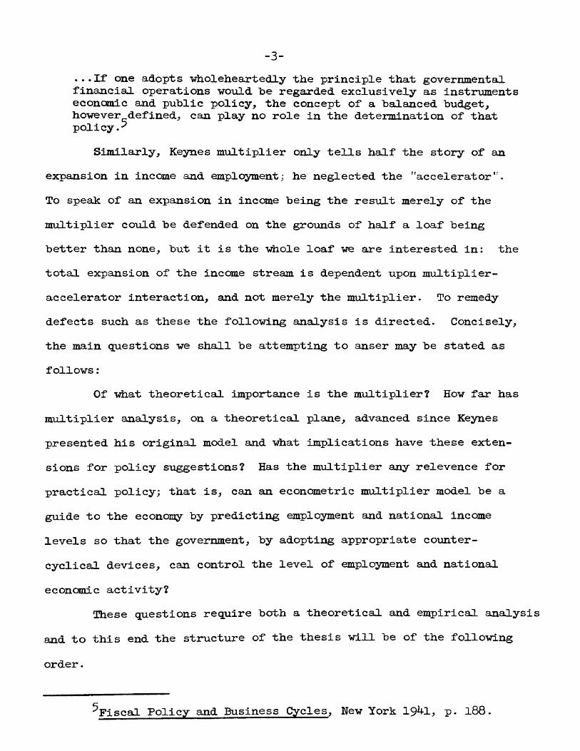
-3-...If one adopts "wholelieartedly the principle that governmental financial operations would he regaxded exclusively as instruments economic and public policy, the concept of a balanced budget, however defined, can play no role in the determination of that policy.^

Similaxly, Keynes multiplier only tells half the story of an expansion in income and employment; he neglected the "accelerator".To speak of an expansion in income being the result merely of the multiplier could be defended on the grounds of half a loaf being better than none, but it is the "vdiole loaf ve are Interested in: thetotal expansion of the income stream is dependent upon multiplier- accelerator interaction, and not merely the multiplier. To remedy defects such as these the following analysis is directed. Concisely, the main questions we shall be attempting to anser may be stated as follows :

Of Tdiat theoretical importance is the multiplier? How far has multiplier analysis, on a theoretical plane, advanced since Keynes presented his original model and what implications have these exten­sions for policy suggestions? Has the multiplier any relevence for practical policy; that is, can an econometric multiplier model be a guide to the economy by predicting employment and national Income levels so that the government, by adopting appropriate counter­cyclical devices, can control the level of employment and national economic activity?

These questions require both a theoretical and empirical analysis and to this end the structure of the thesis will be of the following order.

Fiscal Policy and Business Cycles, Hew York 19^1, p. l88

Initially, it is divided into two parts; part I, dealing with the multiplier on a theoretical plane and part II, considers the empirical evidence surrounding the multiplier and its relevence to the real world.

Part IChapter II, presents the static Keynesian multiplier.Chapter III, gives the multiplier concept a more realistic

coloring hy introducing a dynamic element, because the instantaneous adjustments to equilibrium propounded by Keynes are not facts in the real world. Therefore, the introduction of a time period is necessary. Upon the dynamic model we superimpose the accelerator and arrive therefore at the concept of the "Compound" or "Super" multiplier.Thus, at the termination of Chapter III the multiplier has achieved a theoretical "real world consistency", as a theoretical tool, -vdiich was quite foreign to Keynes.

Chapter IV, takes the theoretical analysis, and applies it (still on a theoretical level) to fiscal policy. We derive multi­pliers for changes in components of the governmental budgets -which can be utilized as counter-cyclical devices. We further note that complications arise -with "federal" multipliers because counter-cyclical measures by federal authorities are somewhat nullified by state and local authorities. Then to give theoretical fiscal policy a more realistic air, we briefly discuss actual real world fiscal policy.

Part IIChapter V appraises the practical importance of the theoretical

concept. To do this we view the various elements -which make up the

-5-concept to see if the multiplier is still too artificial: premierattention is devoted to the consumption function. Then the empirical evidence surrounding the concept as a predictive device is considered. Here we examine and evaluate various projections that were advanced during World War 11 forecasting employment and output in the transition from war to peace, and the various post-war attempts that have been made to refine such projections so as to bring them more in tune with the facts.

In conclusion, we will consider the relevence of the npHtiplier as a useful device and consider whether or not it is a piece of stream­lined abstraction without value in the real world.

Following this resume of the course of the analysis, we should make explicit the major assumptions and parameters which enclose the theoretical framework. First, based on Keynesian analysis the system is a closed one; that is, the foreign trade multiplier is excluded from the analysis, although in Part IX, the potential dangers of abstracting foreign trade from the analysis are fully discussed. But, to include the foreign trade multiplier would so attenuate the original theme as to make it unmanageable. Moreover, the whole analysis is so frought with possibilities of extention in many directions (for example, in chapter II, we briefly develop inflationary gap analysis but having formulated the problem and indicated causation we carry it no further. The same is true for growth and cycle models, which we also briefly develop); that to incorporate them all would make the whole analysis ridiculously unwieldly. In these cases it is rather unfortunate that the multiplier is important in developing growth and cycle models but it does emphasize the importance of the concept. Thus, rather than

-6-iCLCOrporate these ext eut ions into the analysis we have considered our objective as passing along a main highway along which all branches and crossings are closed off with stop signs.

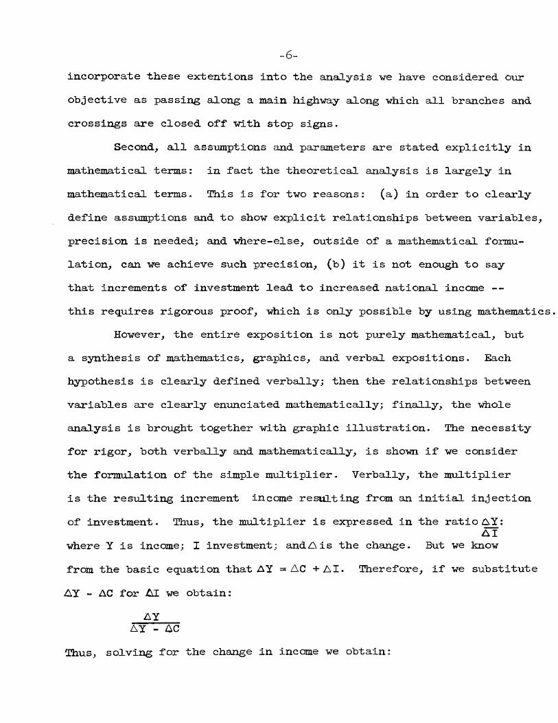
Second, all assumptions and parameters are stated explicitly in mathematical terms: in fact the theoretical analysis is largely inmathematical terms. This is for two reasons: (a) in order to clearlydefine assumptions and to show explicit relationships between variables, precision is needed; and where-else, outside of a mathematical formu­lation, can we achieve such precision, (b) it is not enough to say that increments of investment lead to increased national income -- this requires rigorous proof, which is only possible by using mathematics

However, the entire exposition is not purely mathematical, but a synthesis of mathematics, graphics, and verbal expositions. Each hypothesis is clearly defined verbally; then the relationships between variables are clearly enunciated mathematically; finally, the whole analysis is brought together with graphic illustration. The necessity for rigor, both verbally and mathematically, is shown if we consider the formulation of the simple multiplier. Verbally, the multiplier is the resulting increment income resulting from an initial injectionof investment. Thus, the multiplier is expressed in the ratio AY :

AIwhere Y is income; 1 investment; and A is the change. But we knowfrom the basic equation that AY = AC +AI. Therefore, if we substituteAY - AC for Al we obtain :

AY AY - AC

Thus, solving for the change in income we obtain:

-7-1

1 - AC

Ttie ratio AC is the marginal propensity to consnme. AY

Therefore, the multiplier fonmjla can be -written:1 or its reciprocal 1

1 - c s•where c is the marginal propensity to consume and s the marginal pro­pensity to save.

The use of mathematics in economics has, on the one hand, beengreatly criticised; although on the other, it has been lauded as "theonly way". These are two diametrically opposed vie-wpoints, and whilewe do not agree that all economic orientated mathematics is relativelysuperfluous -we also do not agree with Paul Samuel son when he objectsto William Gibbs*, "Mathematics is a language", because it is 25 percent too long and it should become "Mathematics ^ language".^Obviously, mathematics is only one aspect of language; as Schumpterhas pointed out "There is no place you can go by railroad that youcannot go a f o o t Y e t in many respects math^matics is an easier,more efficient path; it is what R. G. R. Allen has called "the steamshovel of logical argument", altho-ugh it may or may not be profitable

8to use it. In substance mathematics are sentences; both Samuel son and David Roviek, an avowed opponent of mathematics, agree on this contention

^P. A. Samuel son, "Economic Theory and Mathematics :--An Appraisal Papers and Proceedings of the American Economic Association, May, 1952, P- 59-

7Quoted by Samuleson, ibid.gR. G. R. Allen, Mathematical Economics, London 1956, Intro­

duction, p. XV.

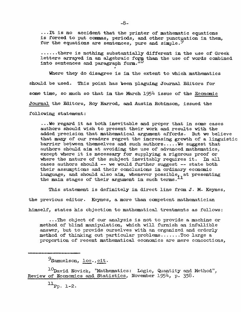
-8-. ' .It is no accident that the printer of mathematic equations is forced to put commas^ periods, and other pnnctuation in them, for the equations are sentences, pure and simple. ..... there is nothing substantially different in the use of Greekletters arrayed in an algebraic form than the use of vords combined into sentences and paragraph form.^^

Where they do disagree is in the extent to 'which mathematicsshould be used. This point has been plaguing Journal Editors forsome time, so much so that in the March 195^ issue of the EconomicJournal the Editors, Roy Harrod, and Austin Robinson, issued thefoil o'wing st at ement :

. . .We regard it as both inevitable and proper that in some cases authors should ■wish to present their "work and results ■with the added precision that mathematical argument affords. But ■we believe that many of our readers regret the increasing growth of a linguisticbarrier between themselves and such authors We suggest thatauthors should aim at avoiding the use of advanced mathematics, except tdiere it is necessary for supplying a rigorous proof or where the nature of the subject inevitably requires it. In all cases authors should — we would further suggest — state both their assumptions and their conclusions in ordinary economic language, and should also aim, whenever possible, at presenting the main stages of their argument in such terms.

This statement is definitely in direct line from J. M. Keynes, the previous editor. Keynes, a more than competent mathematician himself, states his objection to mathematical treatments as follows:

. . .The object of our analysis is not to provide a machine or method of blind manipulation, which will furnish an infallible answer, but to provide ourselves with an organized and orderlymethod of thinking out particular problems...... Too large aproportion of recent mathematical economics are mere concoctions.

^Samuelson, loc.,cit.^^David Wovick, "Mathematics : Logic, Quantity and Method",

Re-view of Economics and Statistics, November 195^> p. 35Ô*^Pp. 1-2 .

_9-as imprecise as the initial assumptions they rest on, ■which allows the author to lose sight of the ccmplexities and interdependenciej^ of the real "world in a maze of pretentions and -anhelpful symbols.

As far as this -was concerned Keynes was in the Marshallian tradition, because Marshall abhored mathematics used -without relevence to the real world. He gave to economics six rules for the incorpora­tion of mathematics into the subject as a useful tool : (l) use mathe­matics as a short-hand language rather than as an engine of inquiry;(2) keep to them until you have done; (3) translate into English;(4) then illustrate by examples that are important in read life;(5) b u m the mathematics; (6) if you succeed in (4) burn (3 ).^^Yet, some economists seem to argue that some of these rules do not in fact apply. Lawrence Klein seems to argue that (3) is not a true test because "non mathematical contributions to economic analysis often tend to be fat, sloppy and vague. There is a real merit in condensing wordly volumes or manuscripts into a few •understandable pages He further goes so far as to say that the confusion which surrounds Keynes' "General Theory" is due to non-mathematical authors. Yet both Marshall and Keynes achieved great things without extensive use of high powered mathematics of thich they were capable. On the other hand mathematics has given tremendous insight into economic theory.

12J. M. Keynes, The General Theory of Employment, Interest and Money, New York, 193^, pp. 297-298.

13Letter from Marshall to Bowley, 1906; quoted by A. C. Pigou in Alfred Marshall and Current Thought, New York, 1993, PP-8-9-

14 "The Contributions of Mathematics in Economics", Review of Economics and Statistics, November, 195^, P* 3^0-

—10 —for example in the works of WaJ_ras and Pareto, Slutsky, Hicks, andAllen; and we are inclined to agree with Klein where he says, "Perhapswe would not have come upon the fundamental equation of value theory(the Slutsky equation) without the help of mathematics. Alsothe real world is so complex that

...By constructing model's in which a comparatively small number of dominating influences only are present we may get to under­stand the working of these influences, whereas, if we were for- bidden to isolate them in thought, this might well prove impossible. '

However, let us be quite sure and quite clear what function mathematics does perform in economics. First, mathematics does not perform some functions in economics. Second, it does perform some functions in competition with "literary economics". Third, in seme economic formulations mathematics is the only way. Under the first

^^Ibid.^^However, some economists may prefer the statement of general

equilibrium made by H. J. Davenport ;"The price of pig Is something big;Because its com, you'll understand.Is high-priced too;Because it grewUpon the high-priced farming land.If you'd know That land is high.Consider this: its price is bigBecause it pays Thereon to raiseThe costly com, the high-priced pig. "

H. J. Davenport, The Economics of Enterprise, New York, 1913; pp.l07-108 ITA. C. Pigou, "Newspaper Reviewers Economics and Mathematics",

in Essays in Economics, London, 1952, p. Il6 .^^The following paragraph is based on Jan Tinbergen's article

"The Functions of Mathemat ic Treatment ", Review of Economics and Statistics, November, 195^; PP-3^5-3^9*

-11-heading mathemat les does not enumerate the phenomena included in the analysis. This is essentially quantitative and is a task of the 'literary economist'. In competition with the literaxy approach it offers (a) ^nnbolism for clarity or efficiency, (h) symbolism in equations, (c) Statistical testing, (d) a solution of the problem.In cases (c) and (d) mathematics is the only way out ; while in (a) and (b) mathematics gives rise to such violent and successful competi­tion, that Tinbergen concludes, "In less simple cases the balance, in my opinion, quickly changes in favor of mathematics.

Thus we must realize that mathematics has limitations when applied to economic theory and it is in fact not the 'be all and end all' of economic exposition. But why did excellent mathematicians like Marshall and Keynes make their mathematics so simple and primarily concentrate on literary economics? The answer we feel lies in the matter of communication. They wanted their work and ideas to be available to everyone. Of Marshall it has been said: "Naturally,Marshall, who desired above all things to be useful, deferred to the

20prejudices of those that he wished to persuade". The same may be said concerning Keynes because, above all, his economics contained "communication with others": a thing which most mathematical econ­omists do not appreciate, or to use J. S. Duesenberry's picturesque

, p. 367-'Quoted by Pigc ___________________ _

op. cit;from Memorials of Alfred lytershall, pp. 66-67.Quoted by Pigou in Alfred Marshall and Current Thought,

-12-Piphrase, there are "too many chief’s and not enough Indians". However,

there are certain areas where a literary translation of mathematics is impossible, that is, in the field of econometric models. But the question arises if such mathematics cannot be translated are they of any use, or is the mathematician merely selling a wide public samples of "intellectual gold bricks"? Yet such econometric models are widely used both by the free lance economist and by government departments; the question is, why? Perhaps the reason is that if models could be erected that could predict on a 100 per cent accuracy basis, then economics, in both the theoretical and practical spheres would take an immense step forward. But this does not mean that economics has now become a mathematician’s daydream and a literary economist's nightmare, because as Tinbergen has pointed out, mathenfâtics does not enumerate the phenomena included in any analysis; this still remains the province of the literary economist.

Therefore, from the vast hybrid of arguments for mathematical economics we can propound three simple statements which seem to be at the heart of the matter; (l ) mathematics has the advantage of efficiency over much which tends to be verbose; (2) it offers rigor in a proof of any theory; (3) it offers us a solution. It is in these three areas that mathematics has the advantage, but it is certainly not the only means of expression. There is much to be said for literary economics and as Duesenberry asserts, "Criticisms

^ "The Methodological Basis of Economic Theory", Review of Economics and Statistics, November, 195^> P- 362.

-13-of math.ema'tical methods may be a bit childish, but after all it was a

ppchild who saw that the king had no clothes.' On the question ofmethodology Marshall was probably correct when he wrote

There are nine or sixty way of constructing tribal lays And every single one of them is right.

Thus, from this hybrid of mathematical charges and counter charges,the use of mathematics in this thesis can be justified by twoexpressions. As a preface to Part I substitute D. G. Champemawne ' swords :

. . .Economic theory which is not rigorously set out can suggest false conclusions and indirectly persuade a wide public into accepting them. The mathematical presentation of axioms, reasoning and deductions is a discipline which, strictly followed, will pinpoint assumptions, expose weak logic to expert scrutiny, and confine conclusions to their proper limits. ^

As a similar perfunctory note to Part II substitute the wordsof R. G. D. Allen:

o..An economist who ventures to set up a theoretical model of empirical content is well advised to do so in explicit mathe­matical form. He risks failure if he does not, or at least, he is liable to overlook some cases or possibilities which may be important and to make empirical testing of his model more difficult.

^^rbld., p. 363-the Use and Misuse of Mathematics in Presenting Economic

Theory", Review of Economics and Statistics, November, 195 j» P* 370*214-Op. cit., p. XVI.

PART I

THE THEORY

Through out the General The ory Keynes had merely presented a skeleton. It remained largely for others to add blood and flesh, and this process continues at an accelerated pace even today.

Seymour Harris

Chapter II

The Static Keynesian Multiplier

The first precise statement of the Multiplier Theory was made by E . F. Kahn in 1931*^ Altho-ugh the "Classicalsparticularly the "Wicksellian" school had recognized that there was an important connection between an increment of income to an increment of invest­ment, the analysis had been left in the vaguest form and it was left to Kahn to provide the first full theoretical analysis. Kahn -was followed in 1936 by J. M. Keynes, who, in his "General Theory of Employment, Interest and Money", produced a similar formulation, although whereas Kahn's multiplier -was an "employment multiplier", Keynes produced an "investment multiplier". That is, Kahn's formu­lation is a coefficient relating an increment of employment, to the ensuing increment of total employment, primary and secondary combined. If primary employment is Ngj, total employment N, and the multiplier, then k^

Keynes' multiplier, on the other hand, is the coefficient relating an increment of investment to an increment of income. If y is income and I investment, while k is the multiplier then kl = Y. Keynes, in discussing his "investment" multiplier stated that :

^ "The Relation of Home Investment to Unemployment", lor, cit.^Alvin Hansen, A Guide to Keynes, New York, 1953, P« 8 6.

-15-

-l6-...Mto Kahn's multiplier is a little different from this, being ■vdiat we may call the emplcyment multiplier. Ihere is no reason in general to suppose that k = . For there is no necessarypresumption that the shapes of the relevant portions of the aggre­gate supply functions for different types of industry are such that the ratio of the increment of demand tdiich has stimulated it; will be the same as in the other set of industries.^

kBut as Alvin Hansen has pointed out; Kahn assumed a perfectly elastic supply of labour and consumables with regard to their money prices, "employment and investment" multipliers are n^jmerically equal. Thus, in the following analysis we will be primarily concerned with the Keynesian multiplier.

The basic mathematical exposition of the Keynesian system can be expressed as follows

The identity(1) Y = C + I

Consumption(2) C = f(Y,l)

Investment(3) I = f(i,C)

Where Y is income; C consumption; I investment and i the interest rate.

The multiplier is the reciprocal of the marginal propensity to save; therefore it can be expressed either as l/l-c or l/si

^J. M. Keynes, General Theory of Employment, Interest, and Money, Chapter X, pp. 115-116'

kA Guide to Keynes, p. 8 7 .5oscar Lange, "The Rate of Interest and the Optimum Propensity

to Consume", Economica, I938.

-17-where c is the marginal propensity to consume and s the marginal propen^ sity to save.

The formula can he derived from the basic identity Y = C + I,but here we use only 'increments' expressed by delta (fi).( ^ ) A Y = AC + A l

A Y _ AC + Al AY AY a y

A l _ 1 -AC A Y A Y

AY ____ ^ _ 1 _ 1AI 1-AC 1-c s

a y

Provided the rate of investment does not change and therefore with time subscripts, investment (l), = 1^-1=..=1^. With thesymbols possessing the same meaning as in the last algebraic example the following, time sub-scripted equation, shows how national income can be related to past injections of investment.

Where C^ = cY^-1(5) Yt = C. + 1^

= Lt + c(l^-l + cY^-2 )

= + cit += I. + ci(. + c^I^-2 +....

00 „

n = oThe actual size of the multiplier is directly determined by

the marginal propensity to consume; and the marginal propensity to consume is expressed, diagramatically, by the slope of the consumption curve (or consumption function).

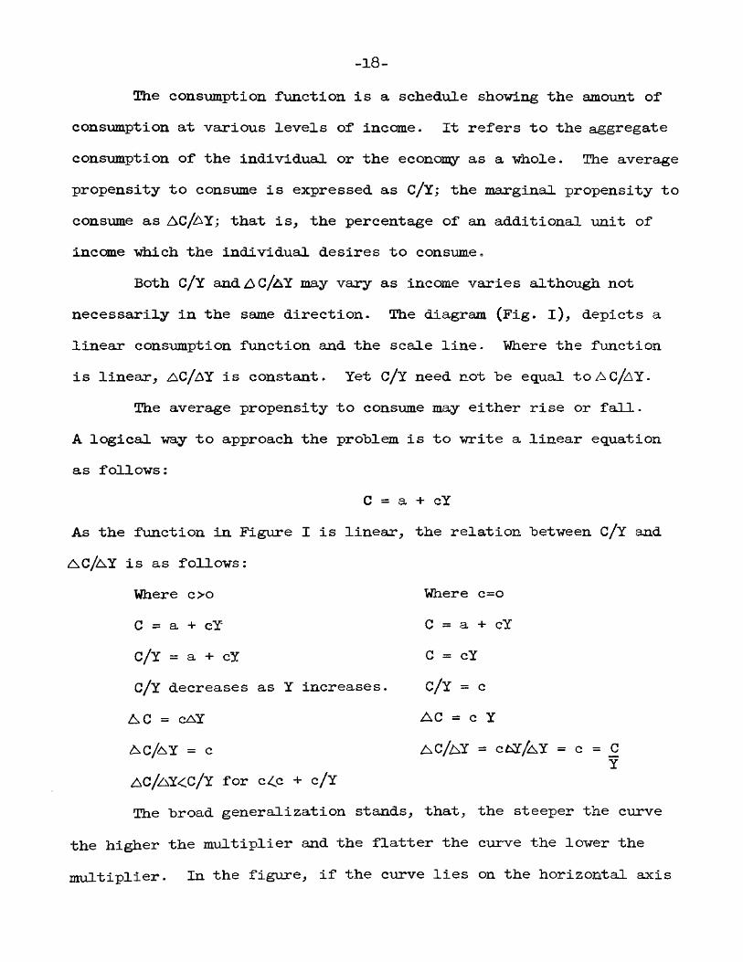
-18-Hie consumpt i on function is a schedule shoving the amount of

consumption at various levels of income. It refers to the aggregateconsumption of the individual or the economy as a whole. The averagepropensity to consume is expressed as C/Y; the marginal propensity to consume as AC/^Y; that is the percentage of an additional unit of income which the individual desires to consume.

Both C/Y and a c /a y may vary as income varies although not necessarily in the same direction. The diagram (Fig. X), depicts a linear c on sumpt i on function and the scale line. Where the function is linear; AC/AY is constant. Yet C/Y need not he equal toAC/2xY.

The average propensity to consume may either rise or fall.A logical way to approach the problem is to write a linear equationas follows :

C - a + cYAs the function in Figure I is linear ; the relation between C/Y andAC/AY is as follows:

Where o o Where c=oC = a + cY C = a + cYC/Y = a + cY G = cYC/Y decreases as Y increases. C/Y = cA C = cAY AC c Yac/ay = c ac/ay = c6Y/^Y = c = C

YAC/^Y<C/Y for c^c + c/YThe broad generalization stands, that, the steeper the curve

the higher the multiplier and the flatter the curve the lower the multiplier. In the figure, if the curve lies on the horizontal axis

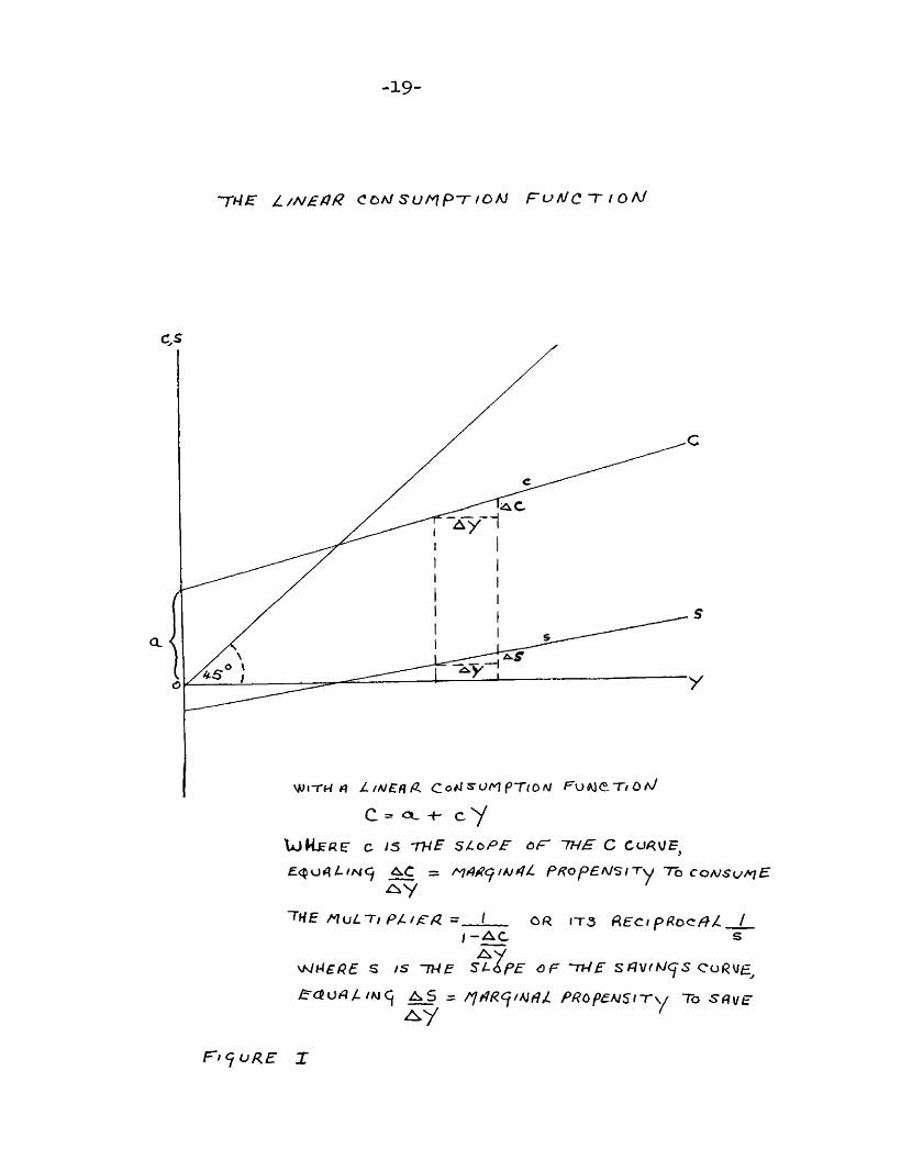
-19"

l . / N £ a R CO/J S U / ^ P - T fOAJ r u A / C ~ T I OAJ

WITH doiJSUtnpTlON PuMeT/ÔA/C = a . + c Y

UjRe«E C V5 TH£' SLoPB OF' TH£ C CU^VE,= r^Afic^thii^lL P F o p E N ^ i~ r \j To coa/^l/a/P

PluLT/ F/i/E'P = _ I OR tT3 RECi pfiooPÂ /_I -AC S

WHE/CÎE s /s -7WE <3P -TWE SrtV/MCyS Co«V£^

EceuAl /Aiq AS = PROpeAlSi~T\/ To SRVE

n<juRE X

-20-the marginal propensity to consnme is equal to 1 and the multiplier becomes infinite.

Arithmetically, the "whole process is generated as follows. If $2 million is spent on private construction or public works (Kahn deals with the problem of employment and road building), and income rises by

million, the multiplier would be 2. Yet things are never as simple as this. Why, (taking Kahn's example), does not the employment of a million workers, under conditions of underemployment, lead to the employment of a million more; and so on until all the unemployed are absorbed. The answer is "leakages".

These may be of several kinds: for example, a part of new incomeis used to pay off debts or a part may go to increase idle cash balances. Thus with Kahn's example, we may say that the primary employment process had induced a certain amount of secondary employment, but the amount Induced may not be enough to completely absorb all the unemployed. This process can be demonstrated as follows:

Initially we assume constant private investment (l) and consump­tion C_|_2=cY^, some fraction of income in the previous period. Then. . .(6) Yt+I = CY^ + Ï

Yj = cY* + I (where Y* is initial income)Yg = c(cY* + ! ) + ! = c ^ * + CÏ + IY^ = c(cY* + cl + l) + I = c^Y* + c^I + cl + IY_ = c^Y* + c^-ll + c^-^i +..... +CÏ + Ït

= c^Y* + l(c^"’'*" + c ^ +..... + c + l)

6See Hugo Hegeland, The Multiplier Theory, Lund, 195^> Ch. IX.

- 2 1 -

S ^ - l + c + c ^ + .... +cS^ = c + c +.....+ ^ ^

®t " ^ ^(i-c)a^. = i - c ^

8 . = 1-c^^ 1 - c

Therefore,t

= c‘‘y* + i(t=#-)

= ^ (^*-^c)c^_ 1-C.(Y*- I ) c- >0

1 “ C t —

- i -1-cWe have now indicated the "hare bones" of the multiplier theory.

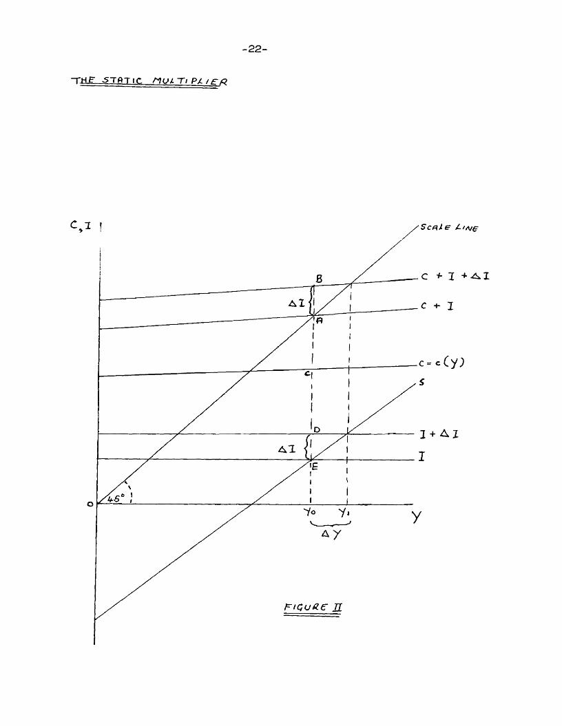
All that remains in this section is to draw the whole together diagram- atically (Figure II). This ^static' multiplier process assumes that: there is no time lag involved; no induced investment; the marginal pro­pensity to consume remains constant throughout; there is an initial level of investment of I followed by an autonomous increase of invest­ment I which is held constant throughout. Consumption (C) and invest' ment (l) are measured on the vertical axis and income (y) on the hori­zontal axis. We begin at Yo, the original equilibrium position where 8 = 1. With the increase of investment (AI), the economy moves instantaneously forward to Y , a higher level of income. The distance AB gives the increased investment, with AC as savings. The movement from Yo to Y^ increases income building up savings enough to equal the increment of investment, with the result that the economy settles at a new level of income.

-22-

-rH_g S T A T I C P/Lt

C»

Al

I + A I

A y

-23-A similar acLjustment process can be shown by the savings curve

(s). If we extend the vertical axis downwards^ we can draw In the savings curve (s) to cut newly drawn investment curves I and 1 + AI- Once again, beginning Tdiere S - I we can show the same adjustment process; AB being the same as DE = I. !The diagram Is expressed In "real" terms and describes Keyne s"l ogi cal theory of the multiplier, ■vdilch holds good continuously without time lag at all moments of time.

7Op. cit.. General Theory, p. 122,

Chapter III

Extensions of the Static Multiplier Dynamic and Compo-und Multipliers

The Keynesian static multiplier developed in Chapter II is obviously too simple a model of the real world because it neglects the dynamic elements in the economy and also the fact that investment induces not only consumption but also further investment. Thus, to incorporate these elements into more realistic models extension of the foregoing analysis is necessary. This chapter is devoted to a discussion and elaboration of such extensions.

The dynamic Multiplier.The model differs from the earlier Keynesian exposition in that

lags and expectations are introduced. The most useful tools of analysis in this context are those developed by the "Stockholm School", that is the "ex ante" and "ex post" approach. Ex ante refers to prospective magnitudes, while ex post refers to retrospective magnitudes; and whereas in a static model, holding good at all moments of time, there was no ex post - ex ante conflict, period analysis involves the rela­tionship between savings and investment both ex ante and ex post.Definitionally, savings and investment are always equal ex post because

Ralph Turvey, "Period Analysis", contributed to W. J. Baumol's, Economic Dynamics : An Introduction, Macmillan, New York, 1951^ Ch. 8.

Ralph Turvey, "Some Notes on Multiplier Theory", American Economic Review, June, 1953, p. 287 ff.

-24-

-25-of the identity of income and output in national income accounting.On an ex ante (prospective) basis savings and investment will not beequal; unless^ (ex ante) The dynamic approach makes provisionfor the possibility of unintended saving (for instance, in the form ofunplanned additions to balances held by consumers or by firms), or forunintended investment (for example, stock accumulation above that whichwas not planned). If there are no 'unintended magnitudes' (saving orinvestment), this is because they have been explicitly assumed away.For instance, the diagramatic version of the model with which we willwork, assumes that plans are realized; equating the ex post to theex ante value. Saving may equal investment ex ante, if we assume aninitial prospective equality between savings and investment, andbetween and 1 . The link, however, is quite unnecessary and as

2R.G.D. Allen points out it "all turns on whether the assumption is arealistic one in the sense that it give rise to a dynamic model ofeconomic significance." He cites the example of models involvingmonetary factors in which it is desired to use the concept of "liquiditypreference" because unintended liquidity is of prime importance, notunintended savings or investment. However, the model we will develophere is expressed, as the static model was, in real terms. Monetaryfactors are excluded, although it is possible to incorporate a dynamic

3monetary mechanism into such a model, as J. R. Hicks has done.

^.D.G. Allen, Mathematical Economics, p. 53.^J. R. Hicks, A Contribution to the Theory of the Trade Cycle,

Oxford, 1950 Ch' 11-12.

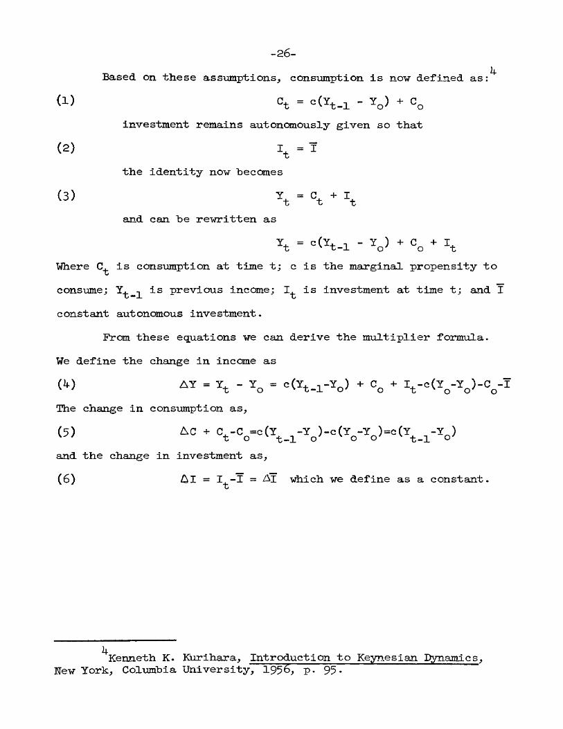
—26“Based on these assumptions^, consumption is now defined as:

(1 ) = c(Yt_i - Yo) +investment remains autonomously given so that

(2) It = the identity now hecomes

(3) \ = \and can he rewritten as

- ^o) + Co + ItWhere is consumption at time t; c is the marginal propensity to consume; is previous income; is investment at time t; and Iconstant autonomous investment.

From these equations we can derive the multiplier formula.We define the change in income asW AY = - Y^ = c(Yt_i-Y„) + + I^-c(Y^-Y^)-C^-IThe change in consumption as,(5) AC + C^-C^=o(Y^_^-Y^)-c(Y^-Y^)=c(Y^_^-Y„)and the change in investment as,(6) Al = I^-l = Al which we define as a constant.

J4.Kenneth K. Kurihara, Introduction to Keynesian fiynamics. New York, Columbia University, I956, p. 95.

-27-

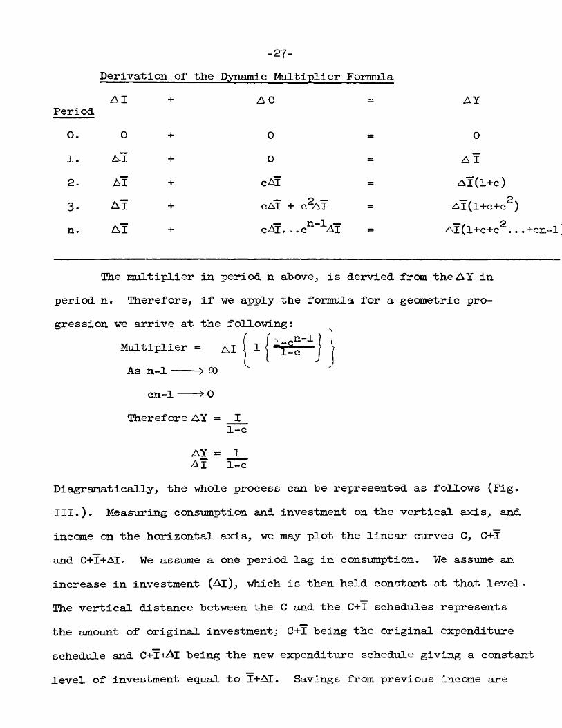
ïriodAI + A C — AY

0. 0 + 0 = 01. AÏ + 0 A Ï2. AÏ + cAl Al(l+c)3. AÏ + c Æ + c % î = Al(l+C+C^)n. AÏ + cAl...c AI Al(l+C+C^o .. +cri"l

The multiplier in period n above_, is dervied from the A Y inperiod n- Therefore, if we apply the formula for a geometric pro­gression we arrive at the following:

Multiplier = Al ( 1 (As n-1--- CO

cn-1-- > 0Therefore AY = I

1-cAY = 1AI 1-c

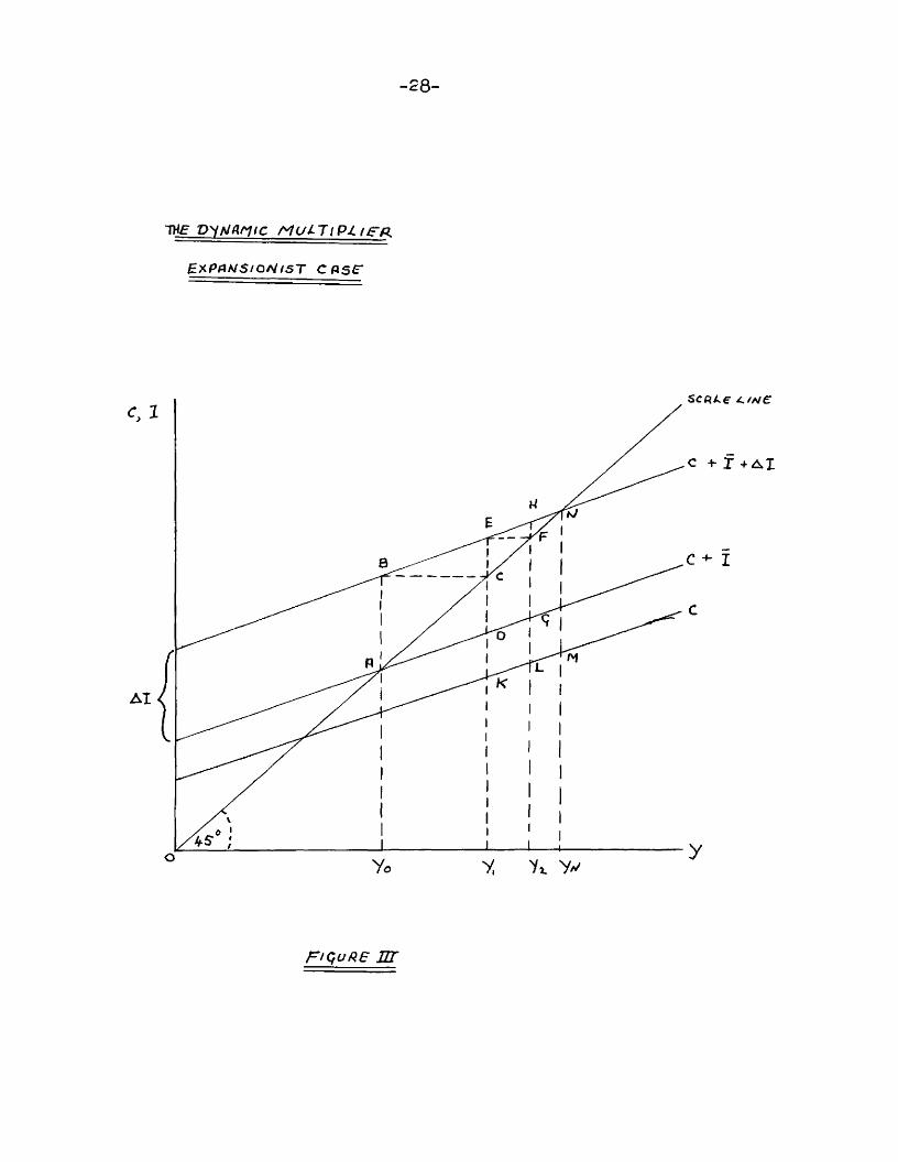
Diagramatically, the whole process can be represented as follows (Fig. III.). Measuring consumption and investment on the vertical aocis, and income on the horizontal axis, we may plot the linear curves C, C+I and C+Ï+Alo We assume a one period lag in consumption. We assume an increase in investment (Aj), which is then held constant at that level. The vertical distance between the C and the C+I schedules represents the amount of original investment; C+I being the original expenditure schedule and C+I+Al being the new expenditure schedule giving a constant level of investment equal to I+AE. Savings from previous Income are

-28-

TXC V'iNflntC M u l 7 / PI /SR

HXPAW5/0/V/5T cose*

SCRLe /N€

AI

FIÇUR6 nr

-29-measured by the vertical distance between the scale line and the C curve The system was in quilibrium at income in period O.

+ Co + Ï . y^A Investment I = Saving

Investment now suddenly changes and is increased by AI = AB. In the diagram there is an equal horizontal change for the vertical change so that AB = BC. With the consumption lag assumed, consumption remains unchanged, as does intended saving. Thus, in period 1 there is a change in income so that,(8 ) Y-i = C + Î + AI = Y B = Yt C-L O Q XBut, intended saving equals I; whereas ex post saving equals IThis discrepancy, plus the fact that consumption in period 2 is greaterthan in period 1, causes a further increase in income, AI = CE = EF,Thus in period 2, income equals,(9) Yg = c (AI) + Cq + ï + AI = Y E = YgFwith consumption equal to(10) c(Al) + Cg = YgL (Figure III)Once again intended saving, T + (l-c)AI = LF, falls short of ex post saving, EH, and impells income further upward. Similar adjustment processes can be shown for subsequent periods, until final equilibrium is reached in period n. At income Yn, ex ante savings and investment are equal (MKT) . Note that the gap between the scale line and the C+Ï +AI curve) gets continuously smaller as income rises.

The ex ante process demonstrated above is expansionist in form; that is, income rises. But it is also possible to demonstrate a contractionist process in exactly the reverse order from the expansionist analysis. All that need be done is to assume that when

-30—equilibrium is reached at the increment of investment A I is removed. In such a situation, until equilibrium is reached at Y^, ex ante saving always exceeds ex ante investment and ex ante savings also exceeds ex post saving.

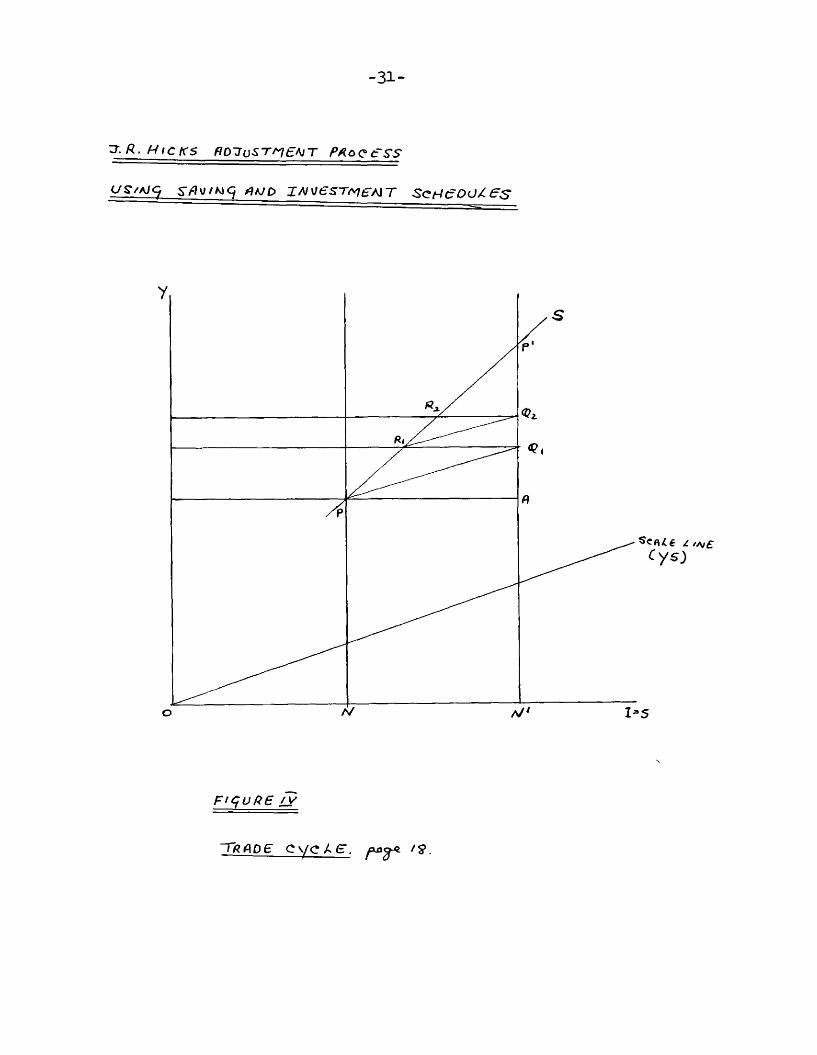
The expansionist process, using ex post saving and investment curves, has been demonstrated by J. R. Hicks.^ (Figure IV. ) Income is measured on the vertical axis and saving and investment on the horizontal. The S curve is the saving curve (the consumption curve in reverse); it shows the amount of saving corresponding to any given level of income. The scales for each axis is different because saving is only a small portion of income, and therefore, if we use the same unit of measurement on each axis, the savings curve would lie too close

7to the vertical axis for operative purposes. There is, therefore, a smaller scale for S and I. The scale difference is marked by YS drawn t hr ought the origin at an angle which corresponds to the scale ratio.If the scale was the same on each axis, the YS line would be at an angle of 4^^, but it is positioned nearer to the S, I axis in view of the scale adjustment. The scale line shows the position which would be taken by the savings curve if the entire income were saved.

A given volume of investment is marked in Figure IV by a vertical line (l). The level of income which will engender a volume of saving equal to the given investment is shown by the vertical co-ordinate of the point P; that is, \diere the I line cuts the S curve. With a given increase in investment, the I line would move to the right and the point

R. Hicks, op. cit., p. l87Ibid., pp. 18-19.

-31-

3./?. H icks bd^o s t / e m t pAccess

<yg/A/< spMmq puo jMMesTr^eMr ScHeou/ie s

FtçüPe /y

~TAfipe C\/CAE. fS.

-32-of iirtersection vould be correspondii^ly higher: thus, the increasein income which corresponds to a given increase in investment, depends upon the slope of the S curve. It is the slope which measures the multiplier.

The system is in equilibrium at P (i.e. S=l), but this initial position is distrubed by an increase of investment (which nowremains constant); but saving being dependent on the income of the proceeding period remains at ON. Investment minus saving, therefore, equals UN* and income increases in the first period by an amount equal to ÏÏN' . This increase can be shown by drawing a line through P parallel to the scale line intersecting the vertical through N* at Q^. C^N' is the income earned in the first period after the change. Por the second period savings can be shown on the S curve by the point at which the horizontal through ^ intersects the S curve (R^). R^M^ is then the savings corresponding to the income of the proceeding period Q^N.The gap between investment and saving in the second period is R^,and this can be shown by a similar parallel construction as in period1. The income of the second period is therefore Q^N' and the position of the economy is at Similar constructions can be repeated untilequilibrium at P* is reached.

Thus, we can sum up the processes described in the foregoing models quite simply. Where saving is defined ex ante:

I > S RisesIWhere C + (l=S) = Y = Equilibrium position

I < S Falls

-33-The d oianiic process has so far taken eonsiamption and saving as

being directly dependent on income. The fact ignored is that there is a dichotomy in the saving process; only part of the total saving is done by consnmers; the rest is in the form of undistributed profits. Also, the only lag assumed was between earning and spending income.Two other types of lags were ignored: that between spending andproduction by businesses, and between production and income earned by

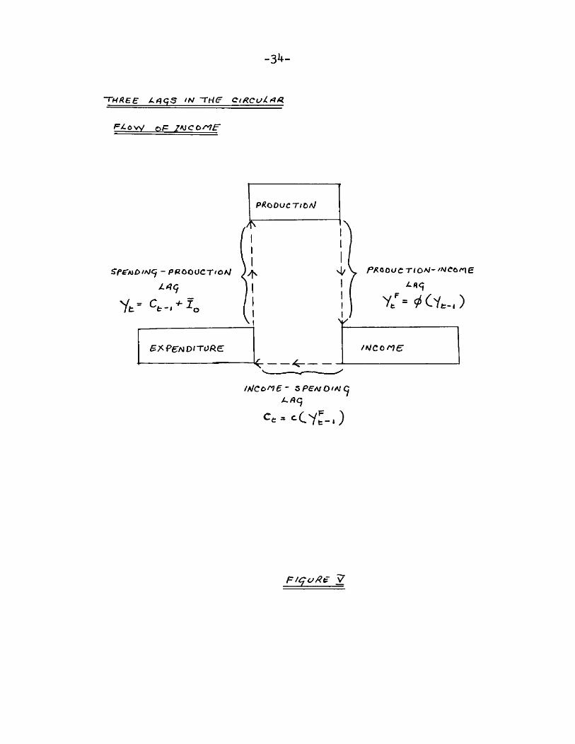
othe factors. The analysis is easily extended to incorporate these facts be separating two markets: that for goods and that for factorsof production. We have then, two sections; one composed of consumers (persons) and the other of firms. The chief difference now is that the marginal propensity to consume is compounded of two marginal pro­pensities to spend; one for firms and one for private persons. In such a dynamic model three lags can be introduced. Where they are one period long, they are:

(a) The product ion-spending lag, where factor income in period t is obtained from output in period t-1;

(b) Income-spending lag, where personal income in period t-1 is the basis for expenditure in period t;

(c) Spending-production lag, where production in period t is based on production for autonomous investment and consumption, based on actual consumer expenditure in period t-1. This analysis may be conveniently shown in Figure V .

gL.A. Metzler, "Three Lags in the Circular Flow of Income", in

Income, Employment and Public Policy, New York, Norton, 19^; R.D.G. Allen, 0£. cit., pp. 55-59; Ralph Turvey, "Some Notes on Multiplier Theory", loc. cit., pp. 275-295; and Ralph Turvey and Hans Brems, "The Factor and Goods Markets", Economica, 1951, p. 57*

-3k-

~T-Hfi.se /A/ Ot/^cuh^a.

F/.ÛVV o/r zt^cprne-

/=’OOUCT/OA/-

y ;=9* c y .-.)

^ fVU£)/A/<5 - PffOOUCT'ÛA/z^9

Yt=

P ODUCT/OA/

5XPerA)OfT(jfte

fhicc>ne- SPEA/0/A/9

c . - c C V ^ . )

pigu/^e 7

-35-Ttie scheme discussed above gives a relation between and

Y ; that is, a third order difference equation involving one lag t"3three periods long. Thus we can rewrite the basic equations, intro­ducing a further variable 'F', denoting income earned and expended by factors. In the linear case....

Consumption now becomes(11) = c(T^_^)

Expenditure of firms becomes(12) = (Yt_i)

Introducing autonomous investment, total income can be expressed

(13) Yt = C^_l + ÏQAssuming only linear cases, consumer spending becomes (on sub­stitution)

( 1 4 ) ^

Business spending becomes(15) = aï ^_3 + P

Thus we can rewrite (l3) a.s(16) Y^ = ^.2

+(X+ IOor

(17) - acY^_3 = + c ^ + C KIn the "one lag three periods long" scheme adopted above, the

circular flow of income takes three periods to work itself out. Total output in period t-3 is business receipts paid to productive factors in the next period, t-2. The personal incomes of consumers are spent on purchases of consumer goods in the following period, t-1; and finally, the sales to consumers in period t-1 lead in the third period to

-36-production of consumers' goods "by firms, and hence to total output (Y^)in equation (l6 ).

The lags can he interpreted entirely in terms of expectations,and therefore, once again, we introduce ex post and ex ante conceptsand obtain a "gap" analysis.

In (a) firms expect receipts to be Y (ex ante), but theyt •—1turn out to be Y^ ( ex post). In (b) consumers expect incomes to be Y^_2 ante), but they became Y^ (ex post). In (c) firms expectsales to be ^ (ex ante), but they turn out to be ( ex post).If we denote ex ante values with a superscript (e.g. Y'^) then for (a):(18) ^t-1 ^^stitute Y'^(19) For (b): Y^ ^ substitute Y^(20) For (c): substitute

The relationship between ex post and ex ante savings and invest­ment and the nature of the model can now be seen.

Ex Ante Ex PostSavings

By Firms ï't - <By Individuals < ' - c .Total \ - Ct

Investment \ - C'tS minus I (ï't - 0

+ (C't -(21) The difference between saving and investment ex ante is:

(?'t - + K ' - + (C't + c^)= Output Gap + Factor Gap + Goods Gap.

-37-Instead of one lag there are now three, and to correspond there

are three gaps (each representing an excess of demand). In suramary, we may say as follows that, in (a) payment to the factors lags behind output, which provides the firms receipts: the lag arising because of the output gap - Y^). In (b) spending lags behind personal income:the lag matches the factor gap (Y^ - Y^). In (c) production for con­sumption lags behind consumer purchases: the lag corresponds to thegoods gap (C'^ + C^).

The Compound Multiplier.. . . "In an economy where any dollar of governmental deficit spending would result in a hundred dollars less of private investment than would otherwise have been undertaken, the ratio of total induced 'national income' to the initial expenditure is overwhelmijagly negative, yet the 'multiplier* in the strict sense must be positive. The answer to the puzzle is simple. What the multiplier does give is the ratio of the total increase in the national income to the total amount of investment, governmental and private....the effects upon private investments are often regarded as tertiary influences and receive little systematic attention."

That is, *vdiat we have ignored so far in this analysis is the "accelerator". Quite simply, this means that if the demand for con­sumption goods increases, such demand has a generating effect upon the demand for the factor of production which produces the consumption good: hence the level of investment becomes a function of the rate ofchange of consumption. Thus, in order to continue the analysis we just delete the assumption that we have made continually, that is, investment acts as an 'inducing agent' only for consumption: investment

^Paul A. Samuel8on, "Interaction between the Multiplier Analysis and the Principle of Acceleration", Review of Economic Statistics, May, 1939, P- 76.

-38-nov generates not only induced consumption^ tut also induced investment.This gives us the "compound" or "super" multiplier.

2 qBoth Paul A. Samuel son and Kenneth K. Kurihara have refinedthe basic Keynesian identity in order to incorporate the acceleratorinto an algebraic analysis. Kurihara has left the identity (Equation(l)Chapter II ) very much as Keynes left it although he adds time-sub scripts;but Samuel son has added to the right hand side of the equation^ "G*%the governmental sector.

Kurihara's system is defined as follows :the basic identity

(22) ït = °t ^ \the variables may then be defined. Consumption becomes

(23) = G(Y^_^-Y^) + investment becomes

(2k) I^ = ^(^t-l'^o) * oBy combining (23) and (2k) we have the fundamental income

equation for the compound multiplier:

(25) = (= + '> + Icwhere is current income; C ; current consumption; I , current invest­ment; c, the marginal propensity to consume; v, the marginal propensityto invest; Y. _ previous income; Y , initial income; C , initial t—1 o oconsumption and I^ initial investment.

^Ibld., p. 102^K. K. Kurihara; 0£. cit., p. 102.

-39-Samuelson Introduces the government ”G” sector into his basic

equation and so the identity now becomes ;

(26) + It + Gtconsumption becomes

(27) Ct = cYt_iinvestment becomes

(28) It = - Ct.i)

= - =^t-2)and the government sector is assumed constant

(29) Qt = GtTherefore, his "multiplier-accelerator" form becomes:

(30) Yt = cYt_i + v(cYt_i - cYt_g) + Gt= c(l+v)Y^_^ - YcYt_2 + Gt

There is one difficulty with Samuel son's formulations and that is, to obtain consumption we must apply the equation (26) in an arib- trary period. As equation (26) is lagged, linear and homogeneous, it can only be applied when the marginal propensity to consume equals the average propensity to consume. However, if we revert to the Kurihara equation (23), we see that it can be used in all cases. We merely take the rise in investment and add the consumption of the proceeding period; that is, as in equation (23):

We also utilize Kurihara's investment equation (24).There are two distinct versions of the "super multiplier"

case (a) recurring and (b) non-recurring investment. Thus, from the following algebraic expressions we can derive the compound multiplier. We, initially, take the most simple case (non-recurring investment,

-ko-

±•6 . AI is a ^once and for all' injection)^ and vorking with increments^ expressed by (A), we arrive at the following result :

A I + A C A YPeriod0 0 + 0 = 01 A I + 0 A I2 vAl + cAI Al(c+v)3 vAl(ctv) + cAl(c+v) = Al(c+v)^n vAl(c+v)^"^ + cAl(c+v)^"^ =

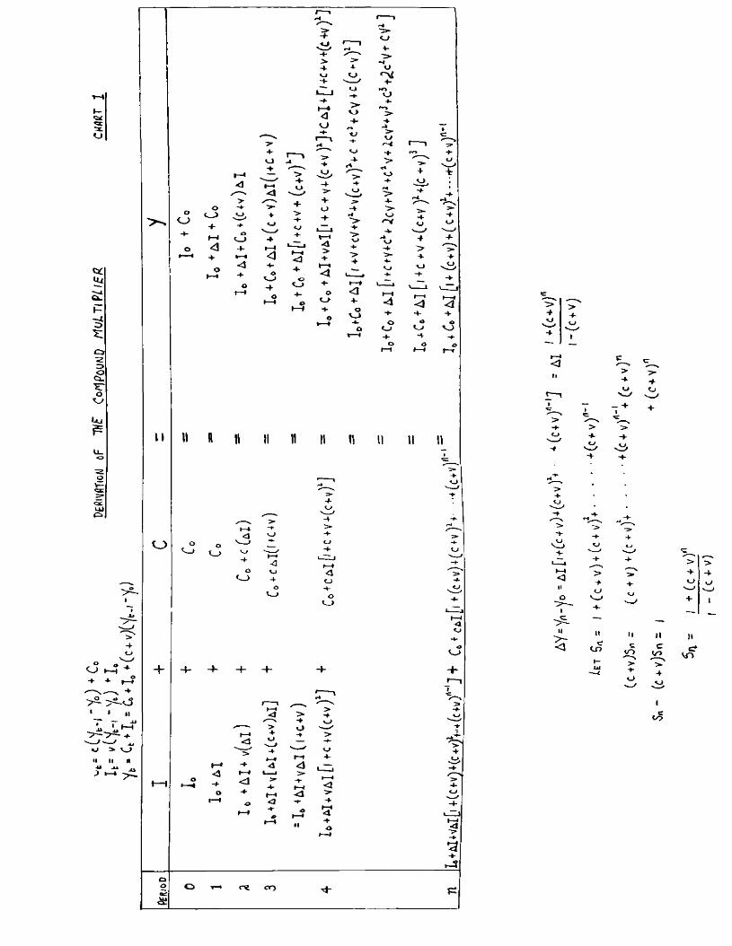
Upon this simple case we superimpose equations (22) and (23), so that the 'once and for all' nature of AI is replaced by AI occilating from period to period. We also assume a lag of one period in consumption^ a similar induced investment lag, and also an initial increment of in­vestment, which is initially autonomously given. Then once again working with increments we derive the compound multiplier (See Chart l).

That is, in period 0 the system is in equilibrium with S=I and I + C = total income. In period 1, a constant increment of investment is introduced, but because of the equilibrium situation prevailing in period 0, there is no prior increment of income which will induce immediate changes in consumption or investment. Inc one in period 1 is increased only by the amount of new autonomous investment (Al).In period 2, induced consumption comes into play as does the accelera­tor, and income rises from I + A l + to I + +Al(l+c+v). Thereis a similar occurrence in period 3 until final equilibrium is reached in the n^^ period, and income reaches its maximum expansionist limit.

From this expansionist process we can calculate the investment multiplier. We know that the ultimate increase in income is the

o+■+ w o

OXJI— l +1— Io

o

ot—I

4--4-t-

f— *

I— »

VJ«— I

O4- t—t

1—I 4

-hr—t

<1-+

t—»I— ♦

O

+o

<3II01

>4-O

co

> + o I

c<o c<y->+Ito

•41-

•~h-2—

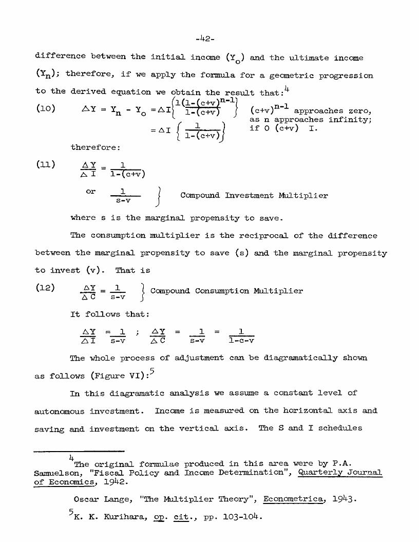
betveen tbe Initial, income (Y^) and the ultimate income(^n)^ therefore, if we apply the formula for a geometric progressionto the derived equation we obtain the result that :(lO) A Y = - Y^ =Al| i-[c+v| j (c+v)^ ^ approaches zero,

as n approaches infinity; = AI f — 4 r/ lY 0 (c+v) I.l-(c+v)

therefore :(11) ^ = 1

A I l-(c+v)

— J Compound Investment Multiplier

vhere s is the marginal propensity to save.The consumption multiplier is the reciprocal of the difference

between the marginal propensity to save (s) and the marginal propensity to invest (v). That is

(12) .ÊZ = _i— I Compound Consumption MultiplierA C s-v jIt follows that :

A Y =_1 ; = 1 = 1A I s-v A C s-v 1-c-v

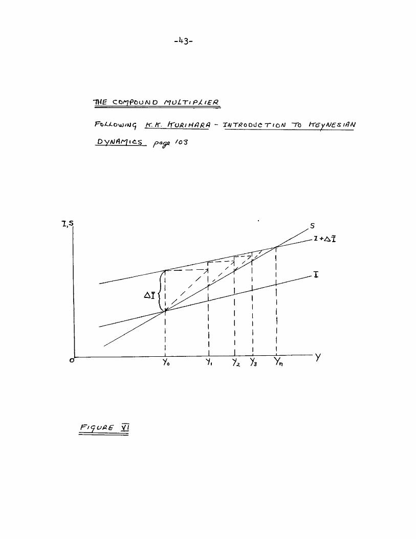
The whole process of adjustment can be diagramatically shownczas follows (Figure Vl):

In this diagramatic analysis we assume a constant level of autonomous Investment. Income is measured on the horizontal axis and saving and investment on the vertical axis. The S and I schedules

The original formulae produced in this area were by P.A.Samuel son, "Fiscal Policy and Income Determination", Quarterly Journal of Economics, 19^2.

Oscar Lange, "The Multiplier Theory", Econcmetrica, 19^3*^K. K. Kurihara, 0£. cit., pp. 103-104.

-43-

IH E co^7PouM D noLiri PjitBR

K.K. - TA/T/?ooüe 7~fQA/ ~To freyAf£s i/fAJ

”u

AI

-44-represent induced Investment and savings; the slope of the I curve"being equal to v . The constant rate of investment is increased "by A I;therefore, giving rise to the I + AI curve. Thus, total investment"becomes greater than total saving at by the amount AX. This excessof investment over intended savings is the amount by which incomesincrease from period 0 to period 1; for Y-, exceeds Y by an amount

^ oequal to the difference between current Investment and current savings, which depend on the preceding period's income.

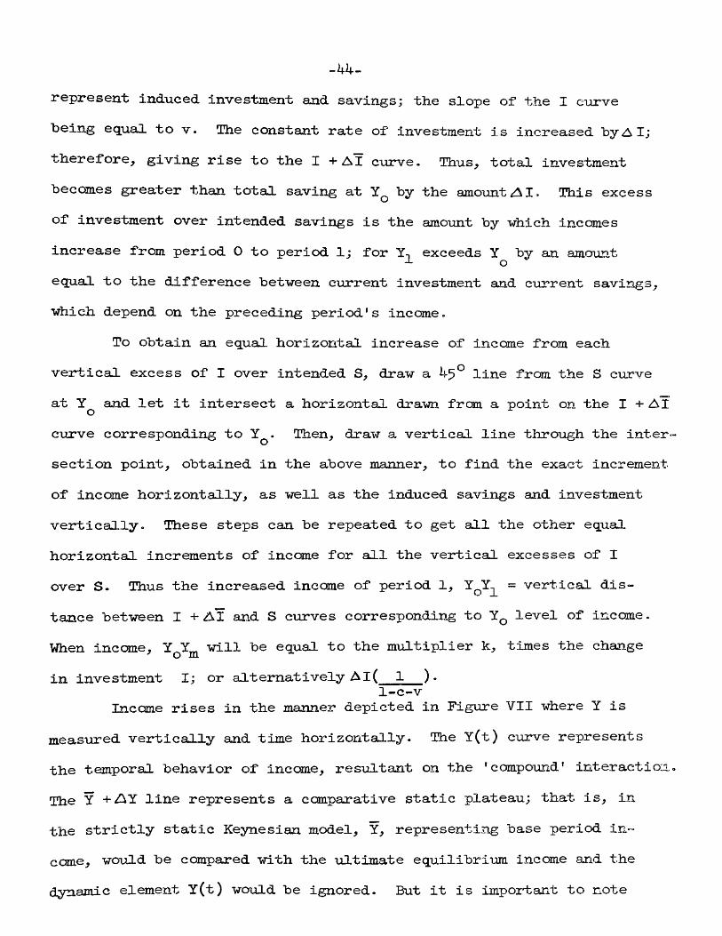
To obtain an equal horizontal increase of income from each vertical excess of I over intended S, draw a 4^° line from the S curve at Y^ and let it intersect a horizontal drawn from a point on the I 4- AI curve corresponding to Y^. Then, draw a vertical line through the inter­section point, obtained in the above manner, to find the exact increment of income horizontally, as well as the induced savings and investment vertically. These steps can be repeated to get all the other equal horizontal increments of income for all the vertical excesses of I over S. Thus the increased income of period 1, Y^Y^ = vertical dis­tance between I + AÎ and S curves corresponding to Y^ level of income. When income, Y Y will be equal to the multiplier k, times the changein investment I; or alternatively A I ( 1 ).

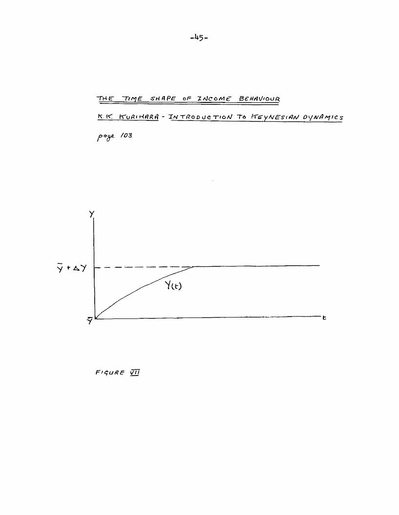
1-c-vIncome rises in the manner depicted in Figure VII where Y is

measured vertically and time horizontally. The Y(t) curve represents the temporal behavior of income, resultant on the 'compound' interaction- The Y + A Y line represents a comparative static plateau; that is, in the strictly static Keynesian model, Y, representing base period in­come, would be compared with the ultimate equilibrium income and the dynamic element Y(t) would be ignored. But it is important to note

-h3-

TMF ~Tlf^£ S H d P e OF ZfJCoMe Wl/'OURK. « - Ta/T<?og g e ~r<oA/ To /"Tg yA/£~s~ftfA/ Q\/A/4^IC s

yc / 03

FiquRE \W

-46-that the model we have developed only shows a stable upward movementwhen v^c<:l; that is, the marginal propensity to consume is positiveand less than one and greater than the marginal propensity to invest.Otherwise the whole model will 'explode'; that is, become very unstable.

As the system has an inherent tendency toward instability, the conditions which must prevail to offset this instability can be

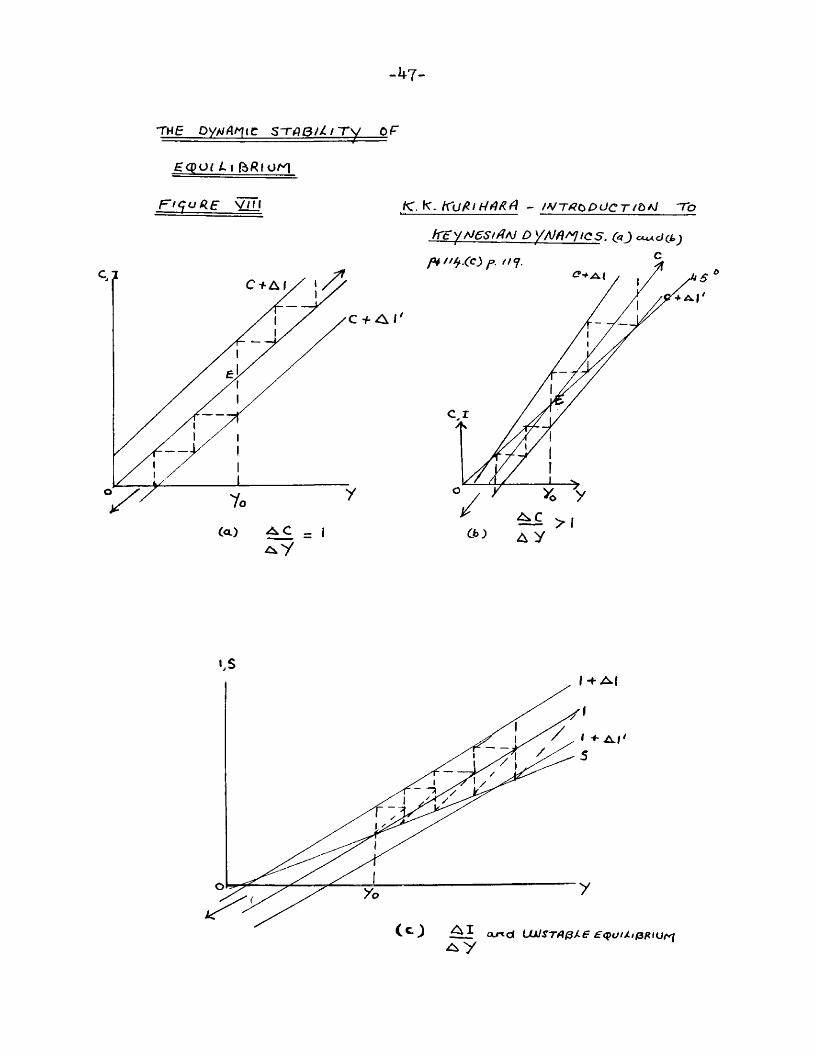
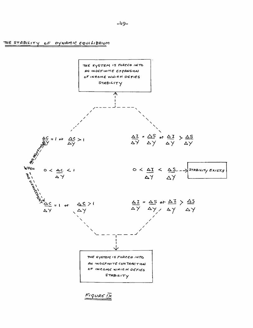
7demonstrated as follows. The marginal propensity to consume be posi­tive but less than unity, i.e. 0<a c/aY<.1. If this condition is not satisfied, income will move away from equilibrium although a 'ceiling' and a 'floor', i.e. the upper and lower turning points, are ultimately reached. This can be illustrated by Figure VIII. Income is measured

Although convergence toward equilibrium is the general tendency, "It is not impossible that there may be a range within which instability does, in fact, prevail. " J.M. Keynes, General Theoi*y, pp. 252.

For further discussion of the stability question see: J.R.Hicks, 0£ cit., chapters 5-7 and 9-

R.J. Harrod, Towards A I»ynamic Economics, London, Macmillan,1948, Lecture 3 •

R.J. Harrod, Trade Cycle, Oxford, I936, chapter 2.5.5. Alexander, "Mr. Harrod's Dynamic Model", Economic Journal,

1950.5.5. Alexander, "Issues of Business Cycle Theory Raised by

Mr. Hicks", American Economic Review, 1951*L.B. Yeager, "Some Questions about Growth Economics", American

Economic Review, 1954.R.D.G. Allen, o^. cit., chapter 3 . ("The Acceleration Principle"

■where he discusses the Harrod-Domar growth models; Phillips' 'lagged' multiplier model; and the Samuelson-Hicks Moltiplier-accelerator. )

^K.K. Kurihara, cit, pp. 109-122. The remaining portionof the chapter (122-128) discusses non-linear functions which are irrelevant for our purposes.

-4?-

TKE Py^AniC S-TAG/Z/ TV OF

£0Ol L t

FtqudE vTTl K. K. ~ /A^TfiOPÜCT/ÙAj To

freyNes/ Aj o VAJ/ tcs. o dcuj

C+A(C + A

^ >1 A y

IS

^ and ütA/T/«?/3Xf £’<p(///(j3/îiu/v|

-48-on the horizontal axis and cons\mption and investment on the vertical axis. Investment is autonomously given hut consumption is lagged; and it is assumed that the initial dis equilibrating circumstances are brought about by an unexpected change in autonomous investment. In Figure VIII (a), AC/a Y = 1 therefore, the C curve becomes a 4-5 line.A sudden disturbance in the system, due to a constant stream of invest­ment, moves the C + I curve above and parallel to the C curve and the economy is thrown into disequilibrium. If the economy begins at income Y^ and E and moves away from this point, it moves in the direction of 'nowhere in particular', because income expands on a 100^ basis. Conversely, disinvestment will lead to an infinite contraction of in­come until employment is nil. The C +Al' moves beneath the C curve moving 11 mi ties sly away from equilibrium. Thus, we can see that with a marginal propensity of unity, the sli^test of disequilibrating forces engenders an infinite divergence from equilibrium, and with the consequent multiplier of infinity there is no stable income determina­tion for the system.

In Figure VIII (b) AC/AY 1. The C curve is steeper than the scale line, and with constant investment C + A l represents a situation where there is an increasing excess of net investment over net saving for each subsequent multiplier period. Thus, while investment remains positive, net saving above E becomes progressively negative, and there is nothing to dampen the expansion. A constant stream of disinvestment has the reverse effect, moving in the direction indicated by the arrow.

There is a second basic stability condition which needs to be satisfied, namely, the marginal propensity to invest must be less than the marginal propensity to save, A i/^Y<AS/a Y. Once again we assume

-49-

"TW6 S - r A ^ U i T \ / ofT oywAM'C ecçot Lt 0Riof^

~me ys~re/ 'S for cofwoeF'Mi-re ÊT'pflwsio/j

oF ;UeoM.e WM<eH PÊFi S STrt BI » T y

AIII

I -

\\

\

/VHcnw%

| y " ' “AZ = ^ ^ ^ a V A y A y A y

O < < I o < ^ < ^ ___>>^ 7 A y

STARlllTy e^lST^

1 «-\\

\\

A,Z - A S <j4 ^ AsA YA y A y /

/

//

/\

TMF 'S o /A/TO

A A! 'N D£F/A#/Tf cow TA CT'OfJ ÔF /M<io/ e WHICH oer/£‘s

S‘"TH[SiA I T y

f^tquRe jX

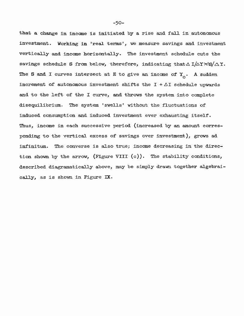
-50-that a change in incame is initiated by a rise and fall in autonomous investment. Working in ’real terms', we measure savings and investment vertically and income horizontally. The investment schedule cuts the savings schedule S from below, therefore, indicating that A >

The S and I curves intersect at E to give an income of Y^. A sudden increment of autonomous investment shifts the I + AI schedule upwards and to the left of the I curve, and throws the system into complete disequilibrium. The system 'swells' without the fluctuations of induced consumption and induced investment ever exhausting itself.Thus, income in each successive period (increased by an amount corres­ponding to the vertical excess of savings over investment), grows ad inf ini turn. The converse is also true; income decreasing in the direc­tion shown by the arrow, (Figure VIII (c)). The stability conditions, described diagramatically above, may be simply drawn together algebrai­cally, as is shown in Figure IX.

Chapter IV

The Multiplier and Fiscal Policy

In the foregoing chapters a "general" theory of the multiplier has been developed; general, in the sense that no explicit reference was made to practical application. However, in this section, the practical application of the general theory will be demonstrated in terms of its pertinence to the field of fiscal policy. Without a conception of a multiplier theory (no matter how simple), it is impossible to demonstrate that changes in the government budget or its components can expand and contract the national income and generate consequent effects on the level of employment within the economy. At the heart of budgetary policy, and the keystone in the fiscal edifice, is the theory of the multiplier. In order to demonstrate this contention and show the impact upon the economy of fiscal policy, we will prove that governmental surpluses, deficits, and balanced budgets yield multipliers, through a change in the budgetary components; such as changes in the expenditure, tax or transfer structures. An extension of this latter contention is the notion of "built-in flexibility"; that is, taxes, transfers, and often governmental expenditures, change, almost automatically, with changes in income. Further, state and local authorities often counteract ahti- cyclical federal measures, therefore having important consequences for the influence of any "federal" multiplier.

Therefore, the structure of this chapter will be as follows: first, we will deal with multipliers under the general heading of

-51-

-52-"Federal" multipliers^ consisting of changes in central governmental expenditures^ transfers, taxes, and changes vhen the budget is balanced. Each change vill be considered individually and it is assumed that no change occurs in the other budgetary components, that is, we apply ceteris paribus to all other components; second, we will introduce state and local government into the picture and examine their influences on federal budgets, adding, eventually, a multiplier formulation which would include federal, state, and local influences within its scope; finally, we will draw the whole complex system of federal budgets, as counter-cyclical devices, into a diagramatic analysis and show how various combinations of expenditures, taxes and transfers can act as anti-cyclical agents.

Federal MultipliersIn order to incorporate the central government into the theor­

etical multiplier system we must make additions to, and further assump­tions about, the basic Keynesian identity Y = C + X. So far, "govern­ment, " as a separate variable, has been excluded from the analysis, or implicitly, its expenditures have been included in C and I. As a dis­tinct, income-influencing, variable the government sector was non-exis­tent. However, we now assume that the government has a positive role, and to the basic identity we add "G:; that is, a variable expressinggovernment expenditure on goods and services. Therefore, the basicidentity now becomes:(1 ) y = C + I + G

In order to arrive at a determinate solution for the now four-variable system we must make additional assumptions. Provisionally, as

-53"\re are excluding accelerator influences, we may make investment a constant (2) 1 = 1

Further, as governmental expenditure (g ) is primarily a policy consideration, and as we are treating transfers under a separate heading,G may be considered a constant :(3) G = G

Now, the consumption function as a variable dependent on national income, becomes more complicated. We now make it a function of dispos­able income "after net algebraic taxes or withdrawals".^ Symboli­cally, Samuel son designates this as Y - W, \diere W is the net figure for taxes minus transfers; but as we are going to treat both tax andtransfer multipliers, we define it as Y - (T^ - T ) where T is netr' Xtaxes, defined exogenously as:(4) T = TX X(Note that taxes are defined purely as withdrawals, with no reference to the various tax structures; that is, they are merely payments to the government by consumers who obtain no direct return. )

is net transfers, also exogenously defined as:

(5) \(Transfers include payment by the government without receipt of good and services; that is, welfare payments, interest on the national debt, and similar payments . )

Thus, consumption becomes:(6) C = c(Y^ - + T^)

^P.A. Samuel son, "The Simple Mathematics of Income Determination", p. 138, in Income, Employment and Public Policy.

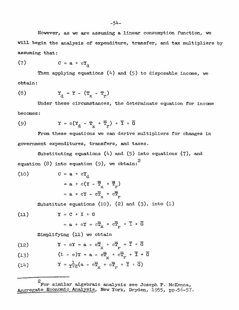
-54-However, as ve are assuming a linear" consumption function; we

will tegin the analysis of expenditure; transfer; and tax multipliers hy assuming that;(7) C = a + cY^

Then applying equations (i|-) and (5 ) to disposable income, weobtain:

(8) \ ^Under these circumstances; the determinate equation for income

becomes :(9 ) Y = e(Y, - T + f ) + I + Gd X r'

From these equations we can derive multipliers for changes ingovernment expenditures; transfers; and taxes.

Substituting equations (4) and (5 ) into equations (7 ); and2equation (8) into equation (9); we obtain:

(10) C = a + cY^= a + c (Y - T + T )' X r= a + cY - cT + cTX r

Substitute equations (lO); (2) and (3), into (l)(11) Y = C + I + G

= a + cY = cT^ + cT^ + I + G Simplifying (ll) we obtain

(12) Y - cY = a - cT + c T + I + G X r(13) (1 - c)Y = a - cT^ + cT^ + I + G(1I4.) Y = - cT^ + cf + Ï + G)

2For similar algebraic analysis see Joseph P. McKenna; Aggregate Economic Analysis; New York; Dryden; 1955^ pp.98-97"

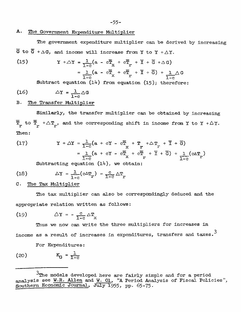
-55“A. The Govemment Exrpendltiire Multiplier

The government expenditure multiplier can be derived by increasing G to G +AGj ajid income will increase from Y to Y + AY.(15) Y + A Y = (a - cT + cT + Ï + G +AG)1-c X r

= 1 (a - cT + cT + I + G) + 1 A G1-c ^ ^ 1-c

Subtract equation (l4) from equation (15); therefore:(16) ay = _J^AG1 -cB. The Transfer Multiplier

Similarly, the transfer multiplier can be obtained by increasing T^ to T^ +AT^, and the corresponding shift in income from Y to Y + A Y. Then:(i t ) Y + a y = + cY - cT + T + A T + Ï + G)1-c X r r

= 1 (a + cY - cT + cT + I + G) + 1 (cAT )1-c X r 1-c ^

Subtracting equation (l^), we obtain:(18) AY = _L_(cAT ) = _£_AT1-c ^ J--0 rC . The Tax Multiplier

The tax multiplier can also be correspondingly deduced and the appropriate relation written as follows :(19) A y = - _A_

Thus we now can write the three multipliers for increases in3income as a result of increases in expenditures, transfers and taxes.

For Expenditures:

(20) «G = ] &

3The models developed here are fairly simple and for a period analysis see W.R. Allen and W. 01, "A Period Analysis of Fiscal Policies”, Southern Economic Journal, July 1955 pp. 65-79.

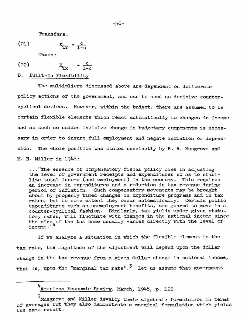
-$6-Transfers:

cTaxes:

(22) c1-c

D. Built-In FlexibilityThe multipliers discussed above are dependent on deliberate

policy actions of the government, and can be used as decisive counter­cyclical devices. However, within the budget, there are assumed to be certain flexible elements which react automatically to changes in income and as such no sudden incisive change in budgetary components is neces­sary in order to insure full employment and negate inflation or depres­sion. The whole position was stated succinctly by R. A. Musgrove and M. H. Miller in 19^:

. . . "The essence of compensatory fiscal policy lies in adjusting the level of government receipts and expenditures so as to stabi­lize total income (and employment) in the economy. This requires an increase in expenditures and a reduction in tax revenue during period of inflation. Such compensatory movements may be brought about by properly timed changes in expenditure programs and in tax rates, but to some extent they occur automatically. Certain public expenditures such as unemployment benefits, are geared to move in a counter-cyclical fashion. Similarly, tax yields under given statu­tory rates, will fluctuate with changes in the national income since the size of the tax base usually varies directly with the level of income."

If we analyze a situation in which the flexible element is the tax rate, the magnitude of the adjustment will depend upon the dollar change in the tax revenue from a given dollar change in national income, that is, upon the "marginal tax rate".^ Let us assume that government

^American Economic Review, March, 1948, p. 122Musgrove and Miller develop their algebraic formulâtion in terms

of averages but they also demonstrate a marginal formulation tdiich yields the same result.

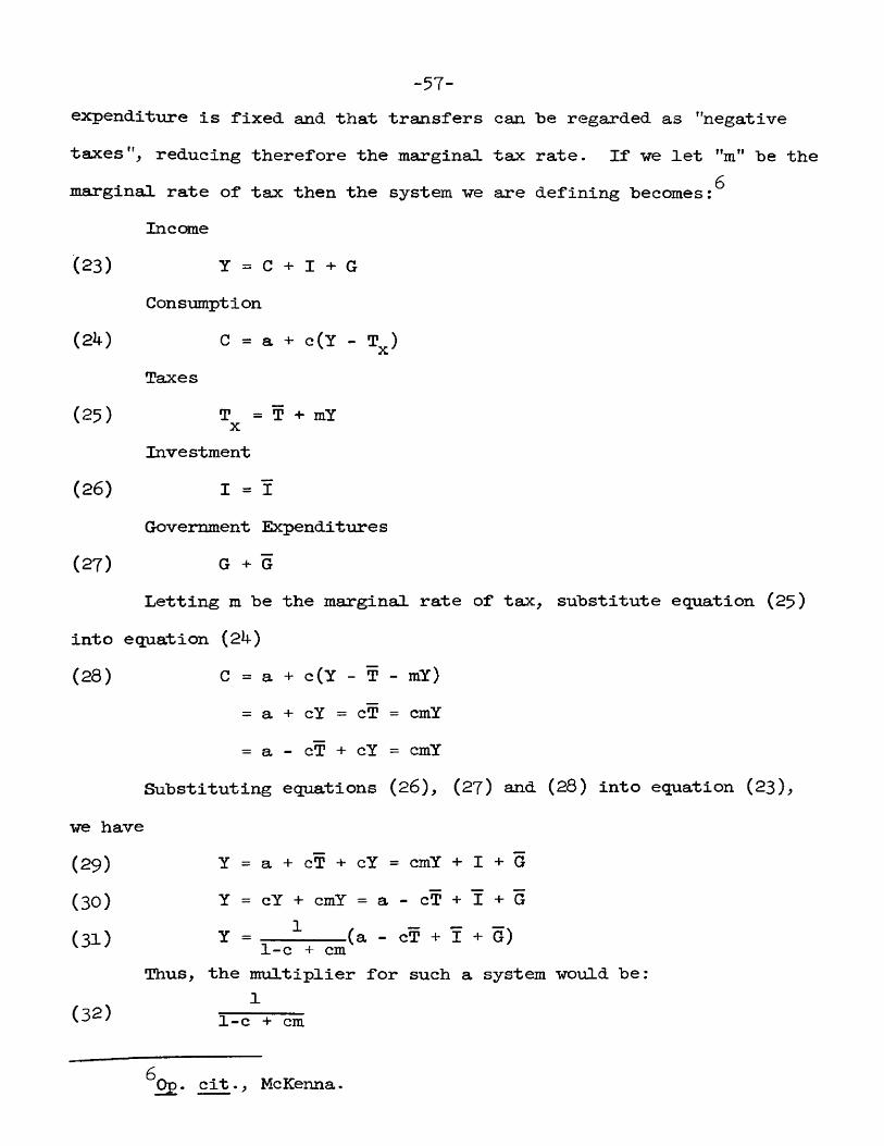
-57-expendi*ture is fixed and that transfers can be regarded as "negative taxesreducing therefore the marginal tax rate. If we let "m" be the marginal rate of tax then the system we are defining becomes :

Income(23) Y = C + I + G

Consumption(24) c = a + c(y - T^)

Taxes(25) T^ = T + mY

Investment(26) 1 = 1

Government Expenditures(27) G + G

Letting m be the marginal rate of tax, substitute equation (25) into equation (2I4-)(28) C = a + c(Y - T - mY)

= a + cY = cT = cmY= a - cT + cY = cmY

Substituting equations (26), (2?) and (28) into equation (23),we have(29) Y = a + cT + cY = cmY + I + G(30) Y = cY + cmY = a - cT + I + G(31) Y =---- -----(a - cT + I + G)1-c + cm

Thus, the multiplier for such a system would be:

(32) 1-c + cm

^Op. cit., McKenna.

-58-E. The Balanced. Budget Multiplier

So far the nrultipliers considered have been with reference to deficit or surplus budgets^ but we now come to a conception that is quite extraneous to the Keynesian system; the concept of the balanced budget multiplier. The first clear theoretical exposition of the con-

Tcept was made in 19^5 by Trygve Haavelmo, although brief incursionsinto the field were made by A. H. Hansen and H. S. Perloff,^ H. C.

9 10 Wallich and N. Kaldor.HoweverP. N. Rasmussen^ has pointed out that the concept and

the theorem was developed a few years earlier, and independently of Haavelmo, by Jorgen Gelting and Kjeld Philip in 19^2. Even so, the war leaves no doubt concerning Haavelmo ' s originality and as all sub­sequent comment on the theorem derives directly from Haavelmo * s article, we do no great Injustice to the facts if we place the originality at Haavelimo's door. The historical practice of a blanced budget is well known, although the practice seems to have been based on the wrong facts, that is, that such a balanced budget would have no multiplier

7"Multiplier Effects of a Balanced Budget", Econometrica, October, 19^5•

6State and Local Finance in the National Economy, Hew York, 19^^; ppT2^5“2^8 . "

^"Income-generating Effects of a Balanced Budget", Quarterly Journal of Economics, Vol. LIX (1944); Pp.78-91*

^^Appendix C to W.H. Beveridge, Full Employment in a Free Society, London, 19^5, Pp.346-34?.

^^"A note on the History of the Balanced-Budget Multiplier, " Fnonomic Journal, March, I958.

“59“12effects. Yet, even today, balanced budgets seem to be an inherent

part of every administration, although the reason is not clear. Presi­dent Truman acknowledged that :

... "We should make it the first principle of economic and fiscal policy in these times to maintain a blanced budget and to finance the cost of national defense on a 'pay-as-ve-go^ basis. "^3

While President Eisenhower still believes in 1959 "what hebelieved in 1953:

.. .The first order of business is the elimination of the annual deficit....a balanced budget is an essential first measure in checking further depreciation in the buying power of the dollar... As the budget is balanced and inflation checked, the t ^ burden that today stifles initiative can and must be eased. . .

The simple fact is that inflation or depression cannot beavoided if every change in government spending were matched by acorresponding change in government taxes. As Samuel son has put it,"In fact a dollar of expenditure always increases income by exactly

15one dollar more than does a dollar reduction of taxes". Although a balanced budget multiplier of 1 is a limiting case, this does not, in any way, invalidate the argument.

The fact that the balanced budget multiplier was equal to 1 was the point of departure for Haavelmo. Initially, the contention that a balanced budget yields a multiplier seems paradoxical because, as he points out ;

Burkhead, "The Balanced Budget", Quarterly Journal of Economics, May, 195^*

ISEconomic Report of the President, January, 1951 •^^"State of the Union Message", February, 1953*^^Op. cit., p. l40.

-6o-• .It is commonly argued that public spending, to be a remedy

against unemployment, must be deficit spending and not spending balanced by an equal amount of taxes, since, in the latter case, the government would only be taJcing back with one hand what it gives with the other.

But :This is false...in a situation with unemployment and idle resources there is a definite employment-creating effect of public outlays even when they are fully covered by tax revenues.

Haavelmo*s analysis, in quantitative terms, is built on the fact that the consumption function is linear; remains unchanged throughout the process; the redistribution of income has no effect on consumption; the marginal propensity to consume is the same for different income classes; and there axe no induced investment effects--investment remains constant throughout. At the outset he attacks Kaldor, Hansen and Perl off, and Wallich. Kaldor conveyed the idea that taxes equal to public expenditures can create employment only to the extent that they cut down individual saving. Haavelmo negated this argument by showing that public expenditures covered by taxes have an employment generating effect which is independent of the numerical value of the propensity to consume. Hansen and Perloff together with Wallich come to the con­clusion that expenditure covered by taxes will raise income (and employ­ment) by the amount of the tax. But they assumed that the initial ex­penditure wan financed by borrowing: the hypothesis is unnecessary.

The exposition of Hsuavelmo's system is as follows: if we definenet income as income after taxes have been paid, and gross income as income before taxes have been paid; then the demand for goods and

^^Op. cit., p. 3 1 1.

— 61“services is a function of net income and employment is a function of gross income. If taxes are paid in a particular period and re spent in the same period, this would leave total net income unchanged and, therefore, demand unchanged. This means that the government is buying part of total output, which, assuming full employment, reduces the quantity of goods and services available for private consumption. In that case the individual could not offset the tax by working more.But with unemployment, output and employment are likely to increase; therefore, gross income will rise although net income remains constant Thus, from an employment point of view we get the same result as if the government had put idle resources to work without any direct com­pensation.

In algebraic terms the demonstration of Haavelmo*s theorem is 1 7quite simple.

Let government expenditure and taxes both increase by an amount X; that is(33) A G - A T ^ = X

The increase in income will be the sum of the effects of the increase in expenditures and taxes: that is(34) A Y = K^X + K ^ XWhere and represent, respectively, the expenditure multiplierand the tax multiplier. Substitute the values obtained in equations (20) and (22);

17McKenna, op. cit., p. 69.

—62—(35) A Y = X - -2- X

1 - C 1 - C

= 1-c „

= X

This gives us Haavelmo's balanced budget multiplier of 1 regard­less of the propensity to consume.

The assumptions upon "which the model is erected seem rather un­realistic. Let us briefly reviev them and consider "what "would happen if they were removed.

(a) Taxpayer's consumption is reduced by a fraction of the tax; that fraction equaling the marginal propensity to conSTjme. Also^ the newly employed increase spending by the marginal propensity to cons"ume times expenditure. There is no induced accelerator effect and national income rises by the extent of the tax. In this analysis, a most important qualifying assumption is that the marginal propensities to consume are the same for the "old" employed and the "ne"wly" employed.(b) Government expenditure must constitute an effective demand for output. That is, there must be no "transfers" in the in­creased government expenditure.(c) Government expenditure must not affect the vie"ws of business men on the profitability of investment.(d) The "Whole model is of a closed economy.Therefore, we may comment that the theorem relies, over-heavily,

on the fact that the consumption propensities of taxpayers and recipients are the same -- "tAiich is totally unrealistic. Further, the time element enters strongly into the analysis, i.e. collection and dispersal of

-63-*taxes takes time. During this time^ consumption is likely to fall unless taxpayers dishoard or unless the government insures a simultan­eous dispersion and collection of payments and receipts, that is, by borrowing. Therefore, to make the analysis more realistic we must introduce a lag. Gottfried Haberler has pointed out that :

If there were such a lag, that is to say, if it took the moneysome time to travel from the taxpayer to the government, thence to the unemployed, and on to the market for consumption goods, there would be a drop in private expenditures on consumption, and, assuming (with Haavelmo) unchanged wages and prices, employment would fall. ^

R. M. Goodwin has introduced such a lag and concludes that if consumption and income are taken to be continuous functions of time, and if time is measured in unit la^s, "It is identical with Haavelmo's r e s u l t B y introducing a spending lag the theorem is not invalidated but the unit multiplier is reached only after a time lapse.

Still, the major criticism is that the value of the Haavelmo*s multiplier is independent of the value of the marginal propensity to consume. The model can be made more realistic by assuming taxes to be a function of income. Further, it is obvious that private investment will not remain constant. This being the case, we can approach realism by assuming that private investment is a function of disposable income

20or govei*nment expenditure. Everett E. Hagen has made these ext entions ,

18 "Multiplier Effects of a Balanced Budget: Some MonetaryImplications of Mr. Haavelmo^s Paper", Egonometrica, April, 1946, p. l48.

^^"Tbe Implications of a Lag for Mr. Haavelmo’s Analysis ", Econometrica, April, 1946, p. 150.

"Multiplier Effects of a Balanced Budget: Further Analysis",Econometrica, April, 1946.

-64-and using the results of his analysis we see that

...the increase in national income will be greater at any given length of time after an increase in taxes and governmental expen­ditures, the lower the marginal propensity to consume. The initial depressing effect of taxes upon consumption will be greater, the higher the marginal propensity to consume.

He also introduces private investment as a function of governmentexpenditure. He shows that the increase in national income will tendto be equal to the tax, plus the change in private investment, timesthe multiplier. Thus, the multiplier can really be anything dependingupon the marginal propensity to consume and entrepreneurial reactions.

Yet, even in 1943 this fact was not fully recognized. Samuel sonpointed out ;

...Thus, the balanced-budget expenditure has a multiplier of exactly one; without recognizing this quantitative fact, we miss the kemal of the theorem.Thus the way was open for a more conclusive and simple proof.

The first elements of conclusive proof were offered in 1953 by Ralph2'R 24Turvey, while a more general proof was formulated by W. J. Baumol

and M. N. Peston in 1955, followed by a more specific formulation by 25A. T. Peacock in I956. The general proof stated that the balanced

budget multiplier was not unity, if the device of introducing the idea

^^Ibid., p. 154.22Op. cit., p. l42.

"Some notes on Multiplier Theory", American Economic Review, June, 1953, pp.285-226.

24 "More on the Multiplier Effects of a Balanced Budget", American Economic Review, March, 1955, pp.l40-8.

"A Note on the Balanced Budget Multiplier", Economic Journal, June, 1956.

-65-of the marginal propensity of the public sector to spend on currently, domeStically-produced goods and services, was adhered to.^^ Calling this k (O^Xel), and the marginal propensity of the private sector to consume currently, domestically-produced goods and services C, a bal­anced budget change equivalent to (change in taxes), would causeincome to change by:

k — c^qi k — c 1 - c X 1 - c

being the balanced budget multiplier. It is easily seen that the balanced budget multiplier could be positive, negative, or zero depending on the relationship between k and c, and that a requirement for it being unity is that k = 1 .

State and Local Governmental Influences on Federal MultipliersThe multipliers derived for changes in central government bud­

gets are complicated by the fact that state and local authorities have influences on counter-cyclical policy lÆiich are not always in the same direction as federal efforts. The Employment Act of 1946 recognized the importance of state and local governments in carrying out national economic policies. Thus, Congress deemed it necessary to include in the Act the "assistance and co-operation" of these governmental units, "to promote maximum employment, production and purchasing power". Therefore, if national fiscal objectives are to be achieved, state and local financing must be harmonized with federal policies. However, direct alignment with the federal government at the state-local level

^^See also M. H. Peston, "Generalizing the Balanced Budget Multiplier ", Review of Economics and Statistics, August, 1950*

-66-

is prevented, by characteristics inherent in the nature of the services Tirtiich these authorities supply; the character of their tax structures, and the market for credit which is available to them. In brief, many institutional and political factors are involved. In order to put things in perspective let us examine, a little more closely, these institutional and political factors.

First, the character of certain state and local services is such that the demand for the service bears no direct relation to changes in the business cycle. Expenditure on education depends on the school population rather than upon conditions of prosperity or depression. Similarly, welfare expenditures on hospitals are, to a great extent, unrelated to cyclical economic changes. These services cannot easily be tied to flexible counter-cyclical devices.

Second, some local and state revenue structures lack elastic revenue sources \Ai±ch would give some anti-cyclical characteristics.For example, the present high level of federal tax rates on personal incomes, corporate incomes, and certain commodities, prevents utiliza­tion of these revenue sources to a greater extent by state and local government.

Third, constitutional and statutory restrictions on borrowing and tax rates prevent counter-cyclical methods of financing. A con­stitutional amendment permitting borrowing is required in twenty states, and a popular referendum is required in twenty others. Limitations on

^?See W.D. Ross, "State-Local Fiscal Policy and Economic Growth", National Tax Journal, March, 1957^ pp. 68-69; and E.A. Myers and R.A.St out "The Role of the State and Local Governments in National Fiscal Policy", ibid., June, 1957, pp. 172-173-

-67-state property tax rates are found in twelve states^ while limitations on property taxes in local government circles are found in all hut the New England states and Maryland. Such restrictions in terms of cyclicalpolicy are, to say the least, formidable.

Fourth, flexibility in state fiscal structures is often hampered because substantial expenditures are rigidly fixed by constitutional provisions or continuing appropriations. For instance, in California more than 65 per cent of the 1955“56 General Fund expenditure was rigidly established by these provisions.

Fifth, the widespread practice of "earmarking " revenues by means of statutory provisions also adds a degree of inflexibility to fiscal structures. The 1955 survey of the Tax Foundation, "Earmarked State Taxes", shows that in the fiscal year 195^, 50 per cent of total state tax collections was earmarked for expenditure only on designated func­tions. In Alabama, Colorado, Kansas, Louisiana, New Mexico, and Texas, the figure was over 75 T>er cent -

Sixth, finally, poor and inadequate administrative methods haveadded greater inflexibility to fiscal structures, for example, the lack of equalization of property assessments and poor operation of the property tax.

Because of these limitations a series of proposals have been put forward, proposing basic changes in state and local fiscal structures

28in order to align state and local with federal policy. Most proposals

p8See M. Newcomer, "State and Local Financing in Relation to Economic Fluctuations", National Tax Journal, 195^, pp. 97-109; M. White and A- White, "The Impact of Economic Fluctuations", National Tax Journal, 19514., pP-17-29; D.M. Blank, "Reform of State-Local Fiscal Relations in New York", National Tax Journal, 1950, p. 326; and ibid., 1951^PP*79-91 •

-68-

do not seem to be very practical although some integration is necessary,Perhaps programs such as W. D. Ross suggests would be in order:

...If it should ever again become necessary for the federal govern­ment to maJ£e large expenditures for public works as a means of com­bating a major recession or threat of depression, it may well be that such action should be planned as a thoroughly integrated pro­gram to be conducted simultaneously at the federal, state and local levels of government. The major share of the operation of such a program might well be administered at the state and local levels. Such a procedure could be more efficient from an administrative point of view and almost certainly would assure a more accurate job of matching expenditures with legitimate priority local needs. Counter cyclical fiscal policy and efficient public administration need not be incompatible.^9

From a theoretical viewpoint, we need something more than a multiplier which expresses changes in components of the central govern­ment *s budget; we need a multiplier which incorporates state and local influences as well as one which shows federal changes. On the basis of the fact that

...state and local expenditures...are influenced by tax revenues Tdiich in turn are controlled by national income, which is affected by a.l ]. governmental expenditiAres--federal, state and local. ..30

H. M. Somers has built a multiplier based on the three sectors.His general formulation is ;(37) A Y = ________Ea__________ 31

1 - % -Where Ea is the change in the federal government's autonomous expendi­tures; that is, those expenditures not influenced by national income

PQ5E* c i t p. 70, quoting from Financing Highway Improvements in Louisiana, Baton Rouge, 1955 •

30ff^e Multiplier in a Tri-Fiscal Economy”, Quarterly Journal of Economics, 19^9, P* 258.

^^Ibid., p. 264. Note that X within this formula is the marginal propensity to consume elsewhere designated as ”c” in this thesis.

—6^—changes. X is the marginal propensity to consnme for the economy as a \ùiole, that is,

C = XYis the marginal propensity to spend of the federal government which

is the fraction of any change in national income which the governmentspends; that is^

N = X Y a awhere is the change in the federal government's induced expenditures;that iS; those influenced by national income changes. is the marginalpropensity to spend of the state government and is the fraction of any change in national income which the state spends; that is,

= Vwhere is the change in the state's induced expenditures, that is,those influenced by national income changes.X^ is the marginal propensity to spend of local government which isthe fraction of any change in national income which the local authorityspends; that is

N = X Yc cwhere is the change in the local authority's induced expenditures,that is, those influenced by national income changes,y is the change in national income in money terms.

This formulation Somers claims is an advantage over the tradi­tional 1

1 -cUsing the traditional formula for a change in total government

expenditure, we have to assume that all government expenditure is given. This seems reasonable if all government units were independent of

-70-national. income. But;, as the ass'umption is that expenditures of state and local governments are determined hy tax revenues, which are depen­dent on national income, the traditional formula becomes unworkable.It is impossible to designate figures for total government expenditure in the multiplier formula, because a major component -- state and local expenditures — is to be determined by the multiplier process itself.To make an estimate of total governmental expenditures for use in the usual formula, we would have to guess at the ultimate changes in national income. While Somers' multiplier equation does require esti­mates of the relationship between state and local expenditures and the national income, it does not require any guess at the ultimate level of national income, which is implicitly involved in the use of the traditional equation. It confines itself to the assumed predetermined element in total government expenditures; that is, autonomous federal expenditures. Reviewing the whole subject he concludes;

...These diverse relationships emphasize the importance of an adequate formulation of the multiplier relationship. Failure to recognize either of these opposing effects or failure to distinguish one type of effect from the other may lead to serious errors in income estimation and to either excessive or inadequate federal expenditures and deficits (or surplus') for any desired change in national income.

Three Paths to Full Employment - A Diagramatic AppraisalFrom the purely theoretical point of view, we have derived

government expenditure, transfer, tax and balanced budget multipliers, and have noted that such multipliers can be subjected to bolstering or countervailing influences by state and local expenditures. From this

^^Ibid., p. 2 7 2.

-71-the natinral outlet is to consider the policies that may he

inferred from these multipliers in the real world. Naturally^ this is a task of great magnitude and to do it full justice one cannot consider these policies in isolation. When dealing with econometric models it is easy enough to erect explicit parameters and to allow ceteris paribus to cover a good deal of "sin''; but in the real world; ceteris paribus does not exist. When considering the question of fiscal policy; it would be entirely unrealistic to give monetary policy a "back seat"; because in many areas they are substitutes. Furthermore; Milton Fried­man has contended that a blanced budget backed by appropriate monetary policy is the best method of dealing with the problems of inflation and unemployment. AlsO; even within the field of fiscal policy; there has been a tendency to regard uhat Keynes advocated as final; that iS; government expenditure to cure unemployment. However; this is not SO; and Keynes himself recognized that deficit spending was not the only way out :

. . .Public loan expenditure is not; of course; the only way; and not necessarily the best way to increase employment. Nor is it always sufficiently effective to overcome other adverse influences. The state of confidence and expectations about uhat will happen next; the condition of credit; the rate of interest; the growth of population; the state of foreign trade; the readiness of the public to spend are scarcely less important.

He recognized the importance of tax changes and suggested tax cuts in35"The Means to Prosperity" and a letter to the Times on April 5; 1933*

^^Milton Friedman; "Comments on Monetary Policy", in Essays in Positive Economics; Chicago; 1953^ P- 264.

^^Letter to the Times (London), December 28, 1934.35Quoted by Harris in John Maynard Keynes Economist and Policy

Maker, New York, 1955, P- 154.

-72-Poliliical pajrties and political pressure groups also exercise

a great deal of influence on the fiscal and monetary climate. Forinstance, if a vhole host of economists decreed that the only way tocure inflation was to raise the tax rate -- would a political party go to the polls with this as an economic platform. In fact in circum­stances such as this the whole question of fiscal policy may he removed from the economic sphere and become nothing more than a political value judgment, which funds a close correlation with the phrase "political suicide".

However, to try and give some degree of continuity between theory and practical realism, and to emphasize the the use of tools supplied by the economist is not purely a matter of judgment of the excellence of these tools, but more of value judgment, we will briefly consider "the three paths to full employment". This will not be acompletely exhaustive treatment; but, before we bind the already devel­oped theoretical analysis with a diagramatic exposition, we deem it necessary to indicate tAiy certain budgetary policies are advocated above others, and why certain budgetary policies are not advocated at all.

The three paths to full employment have been characterized by R . L . Bi shop:

..."deficit spending", i.e. raising expenditures without raising taxes, is by no means the only expansionist fiscal policy. A depressed national income may also be raised to a more satisfactory level by a balanced increase of both government expenditures and taxes, or it may be raised by simply reducing taxes and so inducing an expansion of private consumption. . .These are conveniently con­sidered as the poles of fiscal policy.3^

3^"Alternative Expansionist Fiscal Policies: A DiagramaticAnalysis", in Income Employment and Public Policy, p. 317.

-73-ActuaJ-ly, these are not the only "usable" fiscal measures^, but

'Whatever combinations of taxes and expenditures^ deficit and surplus are used, they must fall into one of the three areas delineated above. Very little is heard of the "transfer multiplier", probably because transfer incomes represent only a relatively small portion of United States national income. This has even been greatly accentuated by the fact that payments of interest on the national debt have been re­moved from the transfer category. As taxes vastly out*weigh transfers, for incorporation into any analysis they may be treated as "negative taxes". Further, the subsequent income generating effects of the "transfer multiplier", as regards "acceleratory effects", is probably very small. On the other hand, expenditures and taxes are assumed to have a bigger "acceleration" effect. In this case it is possible that, although the "pure expenditure multiplier" is larger than the "pure tax multiplier", acceleration effects may be greater for a change in taxation; and, therefore, the ultimate increase of national income may rise to a higher level than that initiated by the expenditure multiplier. That is, in order to find the complete result of a change in government fiscal policy on the level of national income, it is necessary to combine the direct multiplier effects with induced accel­erator effects.37 Thus, the total change in income is expressed by:(38) A Y = K AG + K or g I(39) A Y = K^AT^ +where expresses the accelerator.

37See McKenna, 0£. cit.,pp. 232-235*

-74-This is a fact that has long been argued by the proponents of

tax cut8; In order to remedy unemployment. Taxes, they argue, areblocks to incentive and the removal of penal tax rates will do more tofoster growth in the economy, and consequently employment, than anyother fiscal measure adopted by governmental authorities. Taxationhas come to be regarded as an "incentive ogre" and has acquired thedictum of an unnecessary "idiite man's burden". Colin Clark has longemphasized the point that taxes above 25 per cent of the nationalincome have, not only strong disincentive tendencies, but also violent

38inflationary features. However, Mr. Clark's analysis has been questioned both on empircal and theoretical grounds and has been found wanting in several respects.39

At the time of the entry of the Employment Act into Congress in 1946, a most typical attitude was taken by Robert B. Heppenstall, President of the Pennsylvania State Chamber of Commerce: what wasneeded was

. . . economies in government operation, reduction of taxes, elimin­ation of regimentation, with encouragement of business enterprises, large and small.40

3 See "Public Finance and the Value of Money", Economic Journal, December, 1945, p. 371-89; "The Danger Point in Taxes", Harpers Maga- zine, December, 1950,p p. 67-69; also "Three Economic Illusiôns --Is Britain Heading for a Big Inflation", Manchester Guardian, September18, 1951-

39j./ . Pechman and T . Mayer, "Mr. Colin Clark on the Limits of Taxation", Review of Economics and Statistics, v. 34, 1952,pp. 234-242; also in the same volume see D.T- Smith, "Note on Inflationary Conse­quences of High Taxation",p p. 234-47.

Quoted by S.S. Alexander in "Opposition to Deficit Spending for the Prevention of Unemployment", in Income, Employment and Public Policy, p. 185.

-75-Mos*t of the arguments for tax relief seem to be based implicitly

on t wo lines of reasoning: first, the tax relief is a necessity toincentive; and second, that it is the least of all fiscal evils.Fiscal policy implies some type of direct governmental intervention into the free enterprise system, but the "loosening" of the tax struc­ture minimizes controls, putting the onus on the individual; Tdiere any good follower of Adam Smith deems the onus to be. Therefore, almost every argument for reducing tax rates necessarily implies, on the grounds of retaining a free enterprise system and all that it entails, an argument against deficit spending. Deficit spending is the epitome of what the government should not do, that is, intervene in the private sector of the economy. To this group Dr. L. von Mises' argument is still paramount :

. . .At the bottom of the interventionalist argument there is always the idea that the government or the state is an entity outside and above the social process of production, that it owns something which is not derived from taxing its submects, and that it can spend this mythical something for definite purposes. This is the Santa Claus fable raised by Lord Keynes to the dignity of an econ­omic doctrine and enthusiastically endorsed by all those who expect personal advantage from government spending.

Of course this depends upon the role which government is expected to take in economic life. Some suggest that a too positive govern­mental role would imply a lack of confidence in the American system of private enterprise; although viewing the present number of unemployed in the United States reminds us of Philip Wicksteeds' words... "thepresent system performs miracles but does not perform miracles enough,

kpand does not perform them satisfactorily .

iflHuman Action, 19^9, p. 737* ^^Tbe Inquirer, 28.11, I908.

-76-Many of the arguments against deficit spending are based on a

misunderstanding of "what deficit spending entails. Opponents of the New Deal were fond of quoting Franklin D. Roosevelt^ who at Pittsburgh in 1933 said that, "The credit of the family depends chiefly on whether that family is living within its income, and that is equally true of the nation." John D. Rockefeller joined the anti-deficit spending bandwagon and is reputed to have enunciated that, "For individuals and for govern­ment, thrift is the best policy". While even more popular slogans ran: "I can't spend ray way to prosperity, you can't do it, and UncleSam can't do it"; "Hard work and production make for wealth and pros­perity, and not the handing out of borrowed money by the government.

The clamoring of manufacturers against the original "employment act" and deficit financing in general makes it hard to avoid posing the question--do manufacturers want full employment. Undoubtedly, the in­flationary tendency of the post-war American and British economies has placed great strength in the hands of Trade Unions, who have almost been able to dictate terms on the wages front. Some percentage of unemployment would tend to reverse this trend, and in a system of free private enterprise it is often claimed that unemployment is the price "we pay for freedom, idiile full employment can only exist in a totali­tarian framework. In 19^8, Sydney Alexander^ posed the question "idiether or not there -was political and "class antagonism" involved.For instance, he says that the Full Employment Act may give rise to

Quoted by S.S. Alexander, loc. cit *, footnote 8.j.kIbid., p. 191-192.

-77-the feeling that it was a piece of "class legislation". An interestingsidelight on this contention is that H. A. Clegg and R. Adams in alabour market study maintain that they were brought about not becauseof industrial unrest but because of the struggle for power within the

k-3industry. The employers tried to enlist governmental aid but they miscalculated and lost the struggle. Nevertheless, the central theme of the study stresses the fact that it was not purely an industrial dispute.

A further charge against deficit spending is the question of the"burden of the national debt". A popular slogan once ran: "Thenational debt is a burden of over two thousand dollars on every man,woman and child in America. Deficit spending puts further burdens onunborn generations". Since Lerner's article in 1^48^^ this fallacyhas been removed, but the debt still poses a very wide problem in terms

kjof flexible monetary policy.. . .Every Treasury Department facing a large debt is inevitably and quite naturally biased in favour of a stable, and fairly low, level of market interest rates on fixed-interest bonds, having always

^H.A. Clegg and R. Adams, The Employers Challenge: A Studyof the National Shipbuilding and Engineering Disputes of 1957,Oxford, 1957•

^^A.P. Lemer, "The Burden of the National Debt", in Income, Employment and Public Policy.

^^Edward Nevin, The Problem of the National Debt, Cardiff, University of Wales Press, 195^, p- 28-29. Nevin's footnotes (a,b,c, d) as given in the text are as follows: (a) Even when strict budgeteconomy is not thought to be necessary, there are invariably forms of government expenditure which will have infinitely more appeal than debt service for modern democratic governments; (b) Monetary Policy and the Management of the Public Debt (U.S. Government Printing Office, Washington, 1952), Part 1, q. 27, p. 102; (c) Ibid., Part II, q. 30, p. 105; (d) See The Economist, September 26, I953, p. 869; October 3j1953, p- '‘■1-

-78-■fche problem of holding domi the claim of the debt service on total budgetary resources The grovth of the public debt therefore implies a prima facie greater resistance to the use of flexible monetary policy. Hov serious an impediment this vill constitute for credit policy is difficult to determine^ and it probably varies as between governments. There seems to be reason for supposing that in the United States^ for example, this factor has been--and remains - - of considerable importance. The Secretary of the United States Treasury admitted that his department would be reluctant to see falling bond prices which

'might make the next refunding harder. People might besuspicious that the weakness would go further. . .Giventhe high volume of the federal debt, however, I do not believe it would be wise to take unnecessary chances.*^

Elsewhere he stated quite baldly that the service of the publicdebt had come to be a significant factor in decisions as to thedirection of monetary policy:

' traditional measures for the general regulation of credit through changes in its cost of availability have to be weighed in the light of their impact on the price and interest-rate structure of United States Government securities, on the successful refunding of maturing issues.'

Such direct evidence is unfortunately not available for other coun­tries, but there can be little doubt of the importance of this factor in the employment, or lack of employment, of monetary measures by other financial authorities. In the United Kingdom, for example, it seems probable that debt considerations (including those affect­ing compensation issues in respect of nationalized industries idiich are not part of the national debt in the strict sense) had a major bearing on the pursuit of the ' cheaper money' policy of 19^5-^8 . Similarly, the problem of debt refunding probably explains at least partly the care taken by the British monetary authorities to pre­vent any severe impact on the market in long-term securities of the dear money policy introduced in November, 1951* Conversely, a good many observers suspected that the reduction of bank rate in September, 1953, was not entirely unconnected with the Treas­ury's need to refund maturing debt and to attend to the sale of securities in connection with the denationalization of the iron and steel industry.

Thus, even if we exclude the opposing theoretical arguments against fiscal policy, that is, monetary policy, we can still see that most aspects of fiscal policy have come under very heavy fire. Bal­anced budgets have been the order of the day and although it is true

-79-that fu]_l employment in the post-war world negated the need for defi­cits, serious regional 'unemployment in 1959 suggests that some form of deficit spending may he necessary. Yet the President has presented a hlanced budget to Congress. “Whether he feels that a certain percentage of unemployment is necessary or whether he feels that deficits will strengthen still further the inflationary spiral, is conjecture. How­ever, there is no doubt that the President is doing one thing and that is, ""walking a political tight rope".

With this brief resume of the "three paths to full employment" we will present the diagramatic analysis.

The best diagramatic analysis of the paths to full employmentiighas been presented by John G. Gurley. Similar* types of analysis,

both verbal and diagramatic have been presented by Alvin Hansen,49Richard Mus grave, R. L. Bishop and L. S. Ritter, but because Gurley’s

analysis allows us to envisage more than "three paths to unemployment" ■within his analysis, we consider his formulation more complete than any other. Moreover, the diagramatic formulations of Hansen and Bishop appear too complex, and their various functional dependencies are such that ^ e n the tax rate structure alters, the consumption function shifts, leading to a shift in the total spending function. Thus, the reader is

^J.G. Gurley, "Fiscal Policies for Full Employment: A Dia­gramatic Analysis", Journal of Political Economy, December, 1952.

^^See A. H. Hansen, "Three Methods of Expansion Through Fiscal Policy", American Economic Review, June, 19^5; R*A. Musgrave, "Alter­nate Budget Policies for Full Employment ", ibid.; R.L. Bishop, in Income, Employment and Public Policy; L.S. Ritter, "Alternative Anti- Inflationary Fiscal Policies", Review of Economic Studies, XVIII, No. 3,1950-51*

-8o-32most lost in an attempt to follow the various moves. However^ Gur­ley's model is not without its limitations. These may he classed imder three heads: first, the analysis is entirely quantitative innature, ignoring the possible effects of various types of taxes; second, private investment and government expenditures are not con­sidered to he a variable function of national income; third, bowing to simplicity, the effects of alternate fiscal policies on interest rates, income distribution, liquid asset holding, and incentives, are ignored.

Gurley begins in a closed economy in equilibrium at a level of gross national product (G.N.P. ) below that of full employment, with a balanced budget (Fig. X) . Private disposable income is measured on the horizontal axis and is compounded of personal income and gross business saving; the latter being equal to net business saving plus depreciation allowances. Gross national product is measured vertical 1 y and full employment G.N.P. is assumed equal to OF. The consumption curve C, is the propensity to consume out of private disposable in­come. Gross private investment (G.P.I.) and government expenditijres are assumed to be exogenously determined, and therefore C + G.P.I. =C + I curve. Incorporating government expenditure G, we deduce the familiar C + I + G curve. The line OT represents a tax function, so that the horizontal distance between it and the 4^° line, shows the amount of taxes collected (at constant tax rates), at each level of GoNoP. Government transfer payments are ignored in Gurley's analysis.

50See Gurley, loc. cit., p. 5^6.

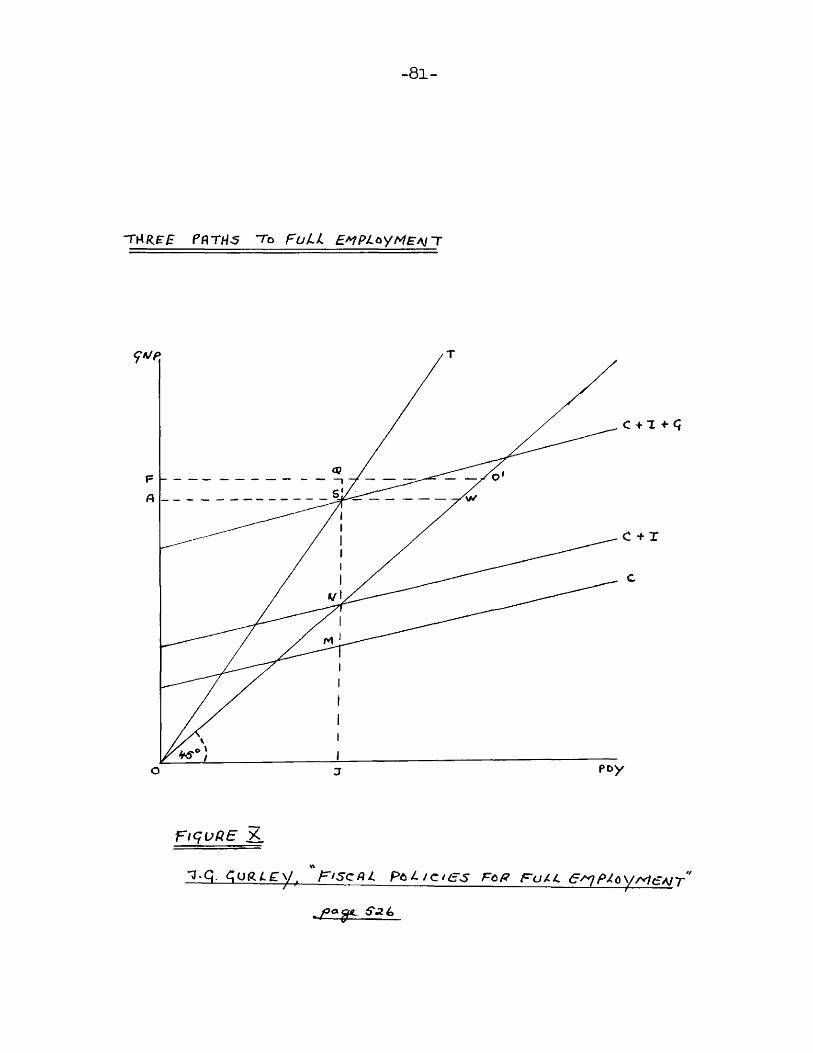
-8 1-

TMRgg FftTHS To Fu/ L E'^PLùyMEAj'T

C + %+S

C + X

O J

FiqudE A

T-Q <;uR A c y . Ptil/Cf(zS FùR FuAL E^P/oyMeAJT

-8 2-although, as ve have stlreauiy pointed out; to treat them as negative taxes would be more satisfactory. AlsO; taxes are assumed constant, whereas, if the O.T. curve is concave to the 45^ line, tax receipts decrease as a percentage of G.N.P. as the latter rises. If it is convex, the reverse occurs; and where O.T. is linear, tax receipts as a percentage of G.N.P. are constant at various G.N.P. levels.

The equilibrium level of G.N.P. is at S, where the OT and C + I + G curves intersect. From private disposable income OJ, JM is consumed, and JM, plus gross private investment MN, plus government expenditures NS, yields a total expenditure of JS (=OR=RW). From RW total expenditures, SW taxes are collected by the government, leaving RS (=0J) private disposable income. At this equilibrium level, con­sumption expenditures have fallen short of private disposable income by MN; this amount being equal to personal and gross business saving. Since gross private investment also equals MN, personal and gross business saving equals gross private investment. Government expenditure equals NS, tax receipts equal SW (=NS) and therefore the budget is balanced.

From this "under-employed" equilibrium we must move to full em­ployment. For full employment G.N.P., OF, to be reached the C + I + G curve must intersect the OT curve on a horizontal FO' . Any point on FO' represents a possible meeting place for these two curves, and once they have met there, a route to full employment has been t a k e n . I f

the curves intersect to the left of Q , the government will run a surplus budget at full employment. If intersection is made at Q , the budget

^^Ibid., p. 5 2 7*

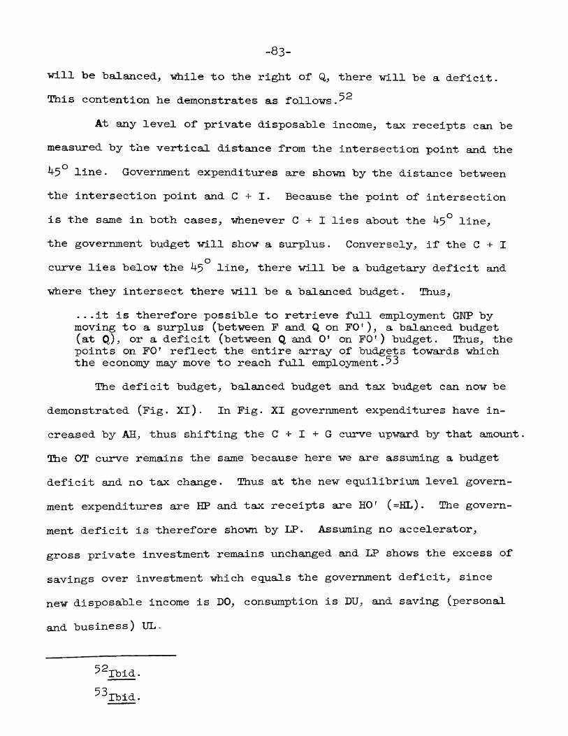
-83-will be balaaced, -while to the right of* there will be a deficit-This contention he demonstrates as follo-ws.^^

At any level of private disposable income, tax receipts can bemeasured by the vertical distance from the intersection point and the^5^ line. Government expenditures are sho-wn by the distance bet-weenthe intersection point and C + I. Because the point of intersectionis the same in both cases, -whenever G + I lies about the 4^^ line,the government budget will show a surplus. Conversely, if the C + Icurve lies below the 45^ line, there will be a budgetary deficit andwhere they intersect there will be a balanced budget. Thus,

...it is therefore possible to retrieve full employment GHP by moving to a surplus (bet-ween F and Q on FO' ), a balanced budget (at Q), or a deficit (between Q and O' on FO’) budget. Thus, the points on FO' reflect the entire array of budgets towards which the economy may move to reach full e m p l o y m e n t . 53

The deficit budget, balanced budget and tax budget can now be demonstrated (Fig. XI). In Fig. XI government expenditures have in­creased by AH, thus shifting the C + I + G curve upward by that amount The OT curve remains the same because here we are ass-uming a budget deficit and no tax change. Thus at the new equilibrium level govern­ment expenditures sure HP and tax receipts are HO' (=HL). The govern­ment deficit is therefore sho-wn by HP. Assuming no accelerator, gross private investment remains unchanged and LP shows the excess of savings over investment which equals the government deficit, since new disposable income is DO, consumption is DU, and saving (personal and business) UL -

52pbid.^^Ibid.

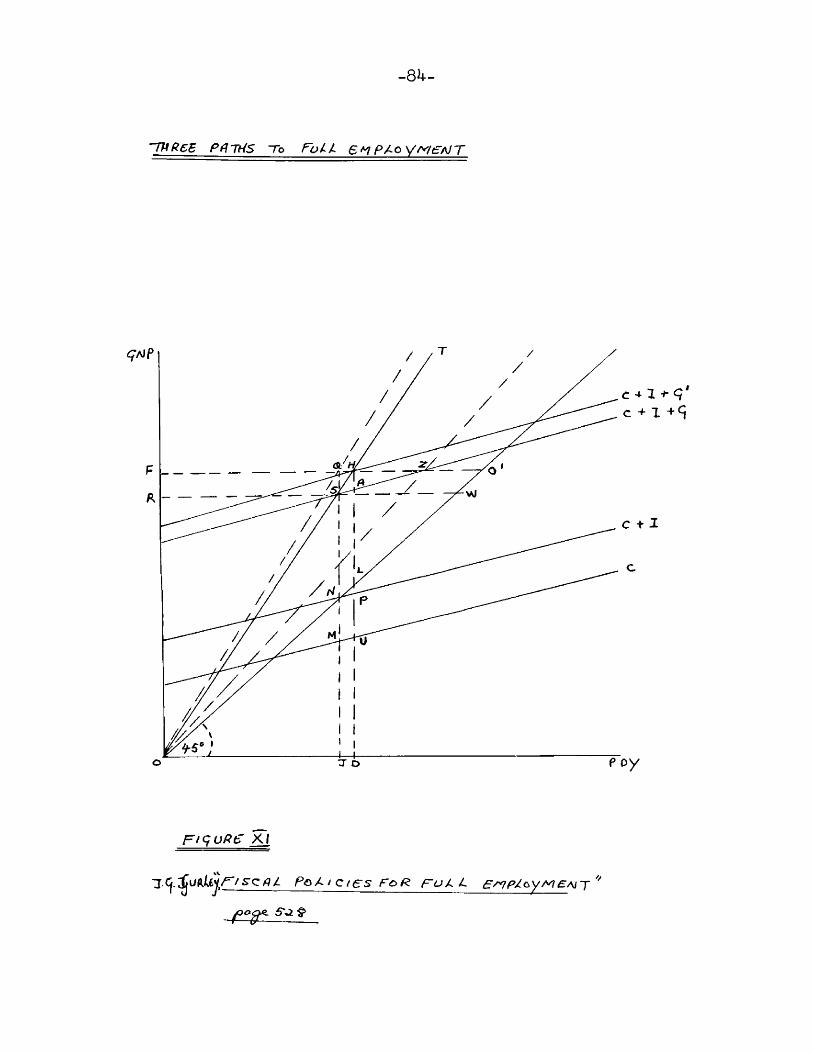
-84-

I V R e s P ^ lU S ~To roAA S M P A o V M ^ aJ T

/ (i

p o yT D

F t q u R e X/

F i s <z r L Pf^AiCtesFoR r o L L F'^p/cyy^FAjT

5\2 - 4 ^

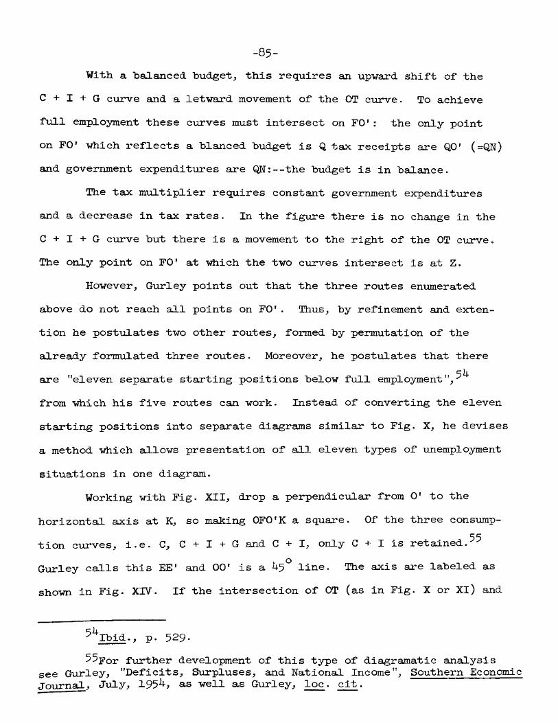
-85-With a balanced budget, this requires an upward shift of the

C + I + G curve and a let ward movement of the OT curve. To achieve full employment these curves must intersect on FO': the only pointon FO* which reflects a blanced budget is Q tax receipts are QO' (=QIî) and government expenditures are QW:--the budget is in balance.

The tax multiplier requires constant government expenditures and a decrease in tax rates. In the figure there is no change in the C + I + G curve but there is a movement to the right of the OT curve. The only point on FO' at which the two cirrves intersect is at Z.

However, Gurley points out that the three routes enumerated above do not reach all points on FO' . Thus, by refinement and ext en- tion he postulates two other routes, formed by permutation of the already formulated three routes. Moreover, he postulates that there are "eleven separate starting positions below full employment from which his five routes can work. Instead of converting the eleven starting positions into separate diagrams similar to Fig. X, he devises a method which allows presentation of all eleven types of unemployment situations in one diagram.

Working with Fig. XII, drop a perpendicular from O' to thehorizontal axis at K, so making OFO'K a square. Of the three consump-

55tion curves, i.e. C, C + I + G and C + I, only C + I is retained.Gurley calls this EE' and 00' is a 45° line. The axis are labeled as shown in Fig. XIV. If the intersection of OT (as in Fig. X or XI) and

^^Ibid., p. 529-55por further development of this type of diagramatic analysis

see Gurley, "Deficits, Surpluses, and National Income", Southern Economic Journal; July, 195^, as well as Gurley, loc. cit.

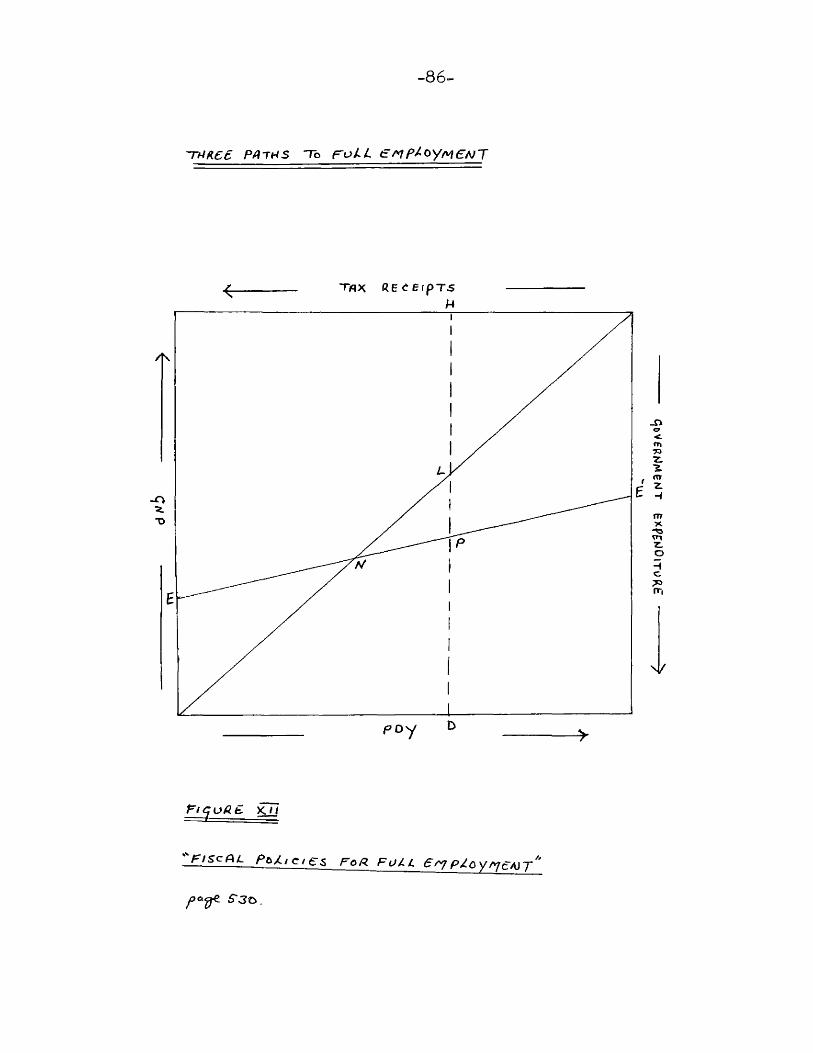
-86.

TkiRee p/i TU s To roiL ernpAoyMeAJT

TAX RE e EipT5 M

-o

Dpoy

73z:%nrz.4mX

ZLOHc,?)n-|

udh. KH

V/SCP/. Pa//c/e$ Fo/R FUÂL €r ploYr^CA^J

f> < S'3t>.

-87-C + I + G is imagined to take place at H, then P on EE' (=C + l) represents a full employment budget with government expenditures of HP and tax receipts of O'H (=HL). Similarly^ any point on EE' yields a full employment level of GHP. All budgets represented by points above EE' represent total expenditure levels below full employment. Any budget represented below EE' corresponds to a total expenditure level above full employment. Any budget shown by a point on the line is balanced; above the line is a surplus, below the line is a deficit. Thus all full employment budgets between E and N on EE' are surpluses, and all between N and E* are deficits. N represents a balanced budget at full employment.

PART II

THE APPRAISAL

A study of the history of opinion is a necessary preliminary to the emancipation of the mind.

Lord Keynes

Chapter V

Theoretical and EtnplricaLl Criticism;Predictory Econometric Models

Part I saw the completion of the theoretical development of the multiplier. We have passed from Keynes static instantaneous model, to the dynamic and compound models of J. R. Hicks, Kenneth Kurihara and Paul Samuel son; and we have related the theory to practical policy in the area of fiscal policy. However, the foregoing analysis was entirely in terms of theoretical models and the question now arises, how far do these models allow us to put into practice what they teach? The most important point to note is that they are merely models developed with­out regard for any statistical information; they are purely the results of deductive reasoning, of working logically from a given promise with rigidly defined parameters. But, if such models are to he something more than intellectual exercises, they must have a relevance for the real world. E. F. Beach has drawn the distinction between mathematical models and econometric models in the following way:

. . .Mathematical models are theoretical constructions which are tested against reality mainly on the grounds of consistency and reasonableness. Only partial information about the real world is brought forth in their support. The econometric model, on the other hand, is designed to make more systematic use of statistical data in assessing their adequacy..

We maintain that if none of the models developed above, nor any part of them can be used, at least, as first approximations to the real

^Economic Models, New York, 1957, P* vii of the Preface.-89-

— 90—then they are merely intellectual gymnastics which allows us to

say nothing about the real world. To be useful they must become yard­sticks; just as pure competition is a "yardstick first approximation" in microeconomic theory. The obvious step from the mathematical models described by Beach is to move to econometric m o d e l a n d thereby clothe our skeleton with the flesh and blood of reality. We must agree whole­heartedly with Everett E. Hagen when he writes :

...all useful knowledge implies prediction, and rational considera­tion of any policy, public or private, involves explicitly or implicitly forecasting its results.

It is this predictory element we next investigate.Yet, the models have also come under very heavy conceptual fire.

Some economists believe that such models can say nothing pertainingto the real world because the conceptual framework is wrong, HugoHegeland, for instance, has challenged Keynes’ assumptions, which hemaintains reduced the multiplier concept to almost a truism:

. . .The basic weakness of the multiplier theory lies in its assump­tions, which in fact eliminate the real problems involved and make the theory almost a truism.3

However, multiplier theory is derived from a consumption func­tion which is a behavior relation. If in fact the truistic nature of the theory were correct there would be no need to discuss either the logic or the nature of the assumptions. Moreover, many of Hegeland's

^"The Reconversion Period: Reflections of a Forecaster",Review of Economic Statistics, May, 19^7, P* 100.

^Op. cit., p. 73; p . 15Ô footnote 1.^See A.H. Metzer's review of Hegeland's, The Multiplier Theory

in the American Economic Review, June, 1955 -

criticisms are extremely vague; for example^ he says the theory is "founded, on utilitarian assumptions" and in the multiplier model the behavior of corporations, of special groups of interest, of power blocks, or of human beings acting as entrepreneurs, is entirely ruled out. Thus, as far as denouncing multipier theory merely on the grounds of hypotheses, we are inclined to agree with M. R. Fisher when he writes

...the direction of the study is misconceived and that the effect of such ^ approach is to inhibit rather than promote economic inquiry.

Even so, there is much ti*uth in the fact that certain assumptions have been a little "strained"; that is, throughout we have utilized linear curves, a closed economy, and Keynes' "normal psychological law" of a stable propensity to consume dependent entirely on income, C = f(Y).In order to see how these assumptions offset the analysis we will remove them; and, thus, as far as content is concerned the form of chapter five will be as follows.

We will remove the assumptions alluded to above and therefore consider: (l) the impact of non-linear functions; (2) the multiplierin an "open economy"; (3 ) is the consumption function merely a func­tion of income and is it stable?; (4) the multiplier as a predictory device.

(l) Non-Linear and Discontinuous FignctionsThis we will dismiss quite lightly because the effect of non­

linear or discontinuous functions on the Tdiole analysis gives rise to

^Op. cit., p. 68; see also the review by J.S. Chipman in the Journal of Political Economy, April, 1956 .

^M.R. Fisher in a review of The Multiplier Theory, Economic Journal, March, 195 6 .

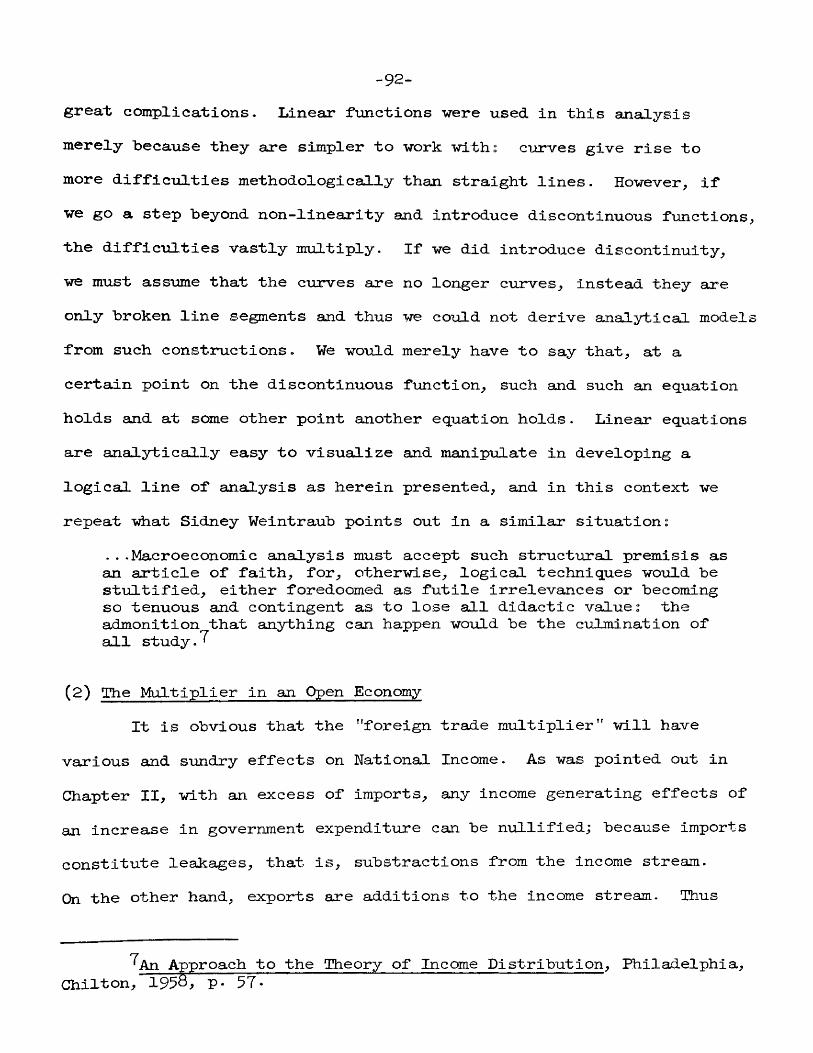
-92-great complications. Linear functions were used in this analysismerely because they are simpler to work with : curves give rise tomore difficulties methodologically than straight lines. However, ifwe go a step beyond non-linearity and introduce discontinuous functions,the difficulties vastly multiply. If we did introduce discontinuity,we must assume that the curves are no longer curves, instead they areonly broken line segments and thus we could not derive analytical modelsfrom such constructions. We would merely have to say that, at acertain point on the discontinuous function, such and such an equationholds and at some other point another equation holds. Linear equationsare analytically easy to visualize and manipulate in developing alogical line of analysis as herein presented, and in this context werepeat what Sidney Weintraub points out in a similar situation:

...Macroeconomic analysis must accept such structural premisis as an article of faith, for, otherwise, logical techniques would be stultified, either foredoomed as futile irrelevances or becoming so tenuous and contingent as to lose all didactic value: theadmonition that anything can happen would be the culmination of all study.

(2) (The Multiplier in an Open EconomyIt is obvious that the "foreign trade multiplier" will have

various and sundry effects on National Income. As was pointed out inChapter II, with an excess of imports, any income generating effects ofan increase in government expenditure can be nullified; because imports constitute leakages, that is, sub str act ions from the Income stream.On the other hand, exports are additions to the income stream. Ihus

^An Approach to the Theory of Income Distribution, Philadelphia, Chilton, 1958, P- 57*

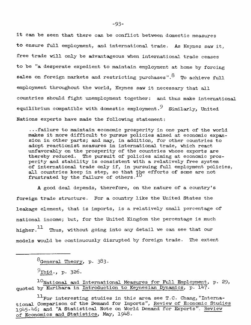
-93"

it can te seen that there can he conflict betveen domestic measuresto ensure full employment, suad international trade. As Keynes saw it,free trade will only be advantageous when international trade ceasesto be "a desperate expedient to maintain employment at home by forcingsales on foreign markets and restricting purchases" To achieve fullemployment throughout the world, Keynes saw it necessary that allcountries should fight unemployment together: and thus make internationalequilibrium compatible with domestic employment.^ Similarly, UnitedNations experts have made the following statement :

. . . failure to maintain economic prosperity in one part of the world makes it more difficult to pursue policies aimed at economic expan­sion in other parts; and may, in addition, for other countries to adopt reactionist measures in international, trade, which react unfavorably on the prosperity of the countries whose exports are thereby reduced. The pursuit of policies aiming at economic pros­perity and stability is consistent with a relatively free system of international trade only if, in pursuing full employment policies, all countries keep in step, so that the efforts of some are not frustrated by the failure of other s.

A good deal depends, therefore, on the nature of a country's foreign thade structure. For a country like the United States the leakage element, that is imports, is a relatively small percentage of national income; but, for the United Kingdom the percentage is much h i g h e r . T h u s , without going into any detail we can see that our models would be continuously disrupted by foreign trade. The extent

^General Theory, p. 3^3-

^Ibid., p. 326.^^National and International Measures for Full Employment, p . 29,

quoted by Kurihara in Introduction to Keynesian Dynamics, p. 14%.^^For interesting studies in this area see T.C. Chang,"Interna­

tional Comparison of the Demand for Imports", Review of Economic Studies 1 9 k^-h6 ; and "A Statistical Note on World Demand for Export.s", Review of Economics and Statistics, May, 19h3.

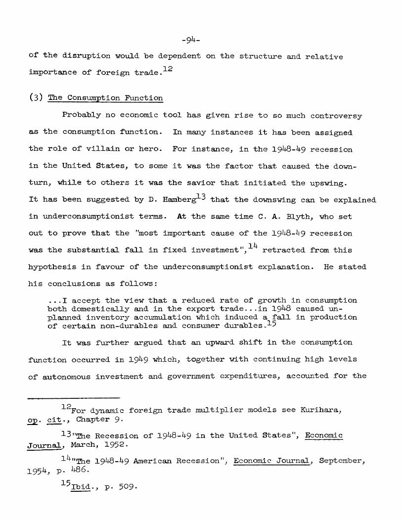
-94-of the disruption would be dependent on the structure and relative importance of foreign trade.

(3) The Consumption FunctionProbably no economic tool has given rise to so much controversy

as the consumption function. In many instances it has been assigned the role of villain or hero. For instance, in the 1948-49 recession in the United States, to some it was the factor that caused the down­turn, while to others it was the savior that initiated the upswing.It has been suggested by D. Eamberg^^ that the downswing can be explained in underconsumptionist terms. At the same time C. A. Blyth, who set- out to prove that the "most important cause of the 1948-49 recession was the substantial fall in fixed investment retracted from thishypothesis in favour of the underconsumptionist explanation. He stated his conclusions as follows :

...I accept the view that a reduced rate of growth in consumption both domestically and in the export trade. . .in 19^ caused un­planned inventory accumulation which induced a fall in production of certain non-durables and consumer d u r a b l e s . ^5

It was further argued that an upward shift in the consumptionfunction occurred in 19^9 which, together with continuing high levelsof autonomous investment and government expenditures, accounted for the

1 pFor dynamic foreign trade multiplier models see Kurihara, op. cit., Chapter 9-

13"2he Recession of 1948-49 in the United States", Economic Journal, March, 1952.

l4ii^e American Recession", Economic Journal, September,1994, p. 486.

^^Ibid., p. 5 0 9*

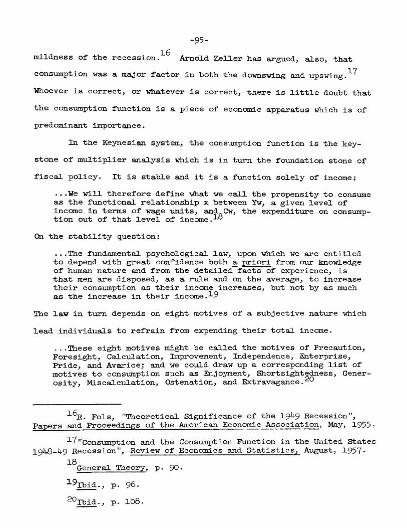
-95-mildness of the recession.Arnold Zeller hats argued, also, that consumption vas a major factor in hoth the dovnsving and upsvlng Whoever is correct, or vhatever is correct, there is little doubt that the consumption function is a piece of economic apparatus which is of predominant importance.

In the Keynesian system, the consumption function is the key­stone of multiplier analysis ^ich is in turn the foundation stone of fiscal policy. It is stable and it is a function solely of income;

*. .We will therefore define what ve call the propensity to consume as the functional relationship x between Yw, a given level of income in terms of wage units, and Cw, the expenditure on consump­tion out of that level of income.

On the stability question:...The fundamental psychological law, upon which we are entitled to depend with great confidence both a priori from our knowledge of human nature and from the detailed facts of experience, is that men are disposed, as a rule and on the average, to increase their consumption as their income increases, but not by as much as the increase in their income. 9

The law in turn depends on eight motives of a subjective nature whichlead individuals to refrain from expending their total income.

. . .These eight motives might be called the motives of Precaution, Foresight, Calculation, Improvement, Independence, Enterprise, Pride, and Avarice; and we could draw up a corresponding list of motives to consumption such as Enjoyment, Shortsightedness, Gener­osity, Miscalculation, Ostenation, and Extravagance.^^

Pels, "Theoretical Significance of the 19^9 Recession", Papers and Proceedings of the American Economic Association, May, 1955 •

^^"Consumption and the Consumption Function in the United States 1^^8_49 Recession", Review of Economics and Statistics, August, 1957-

18General Theory, p. 90•^9%bid., p. 96.^^Ibid., p. 108.

—

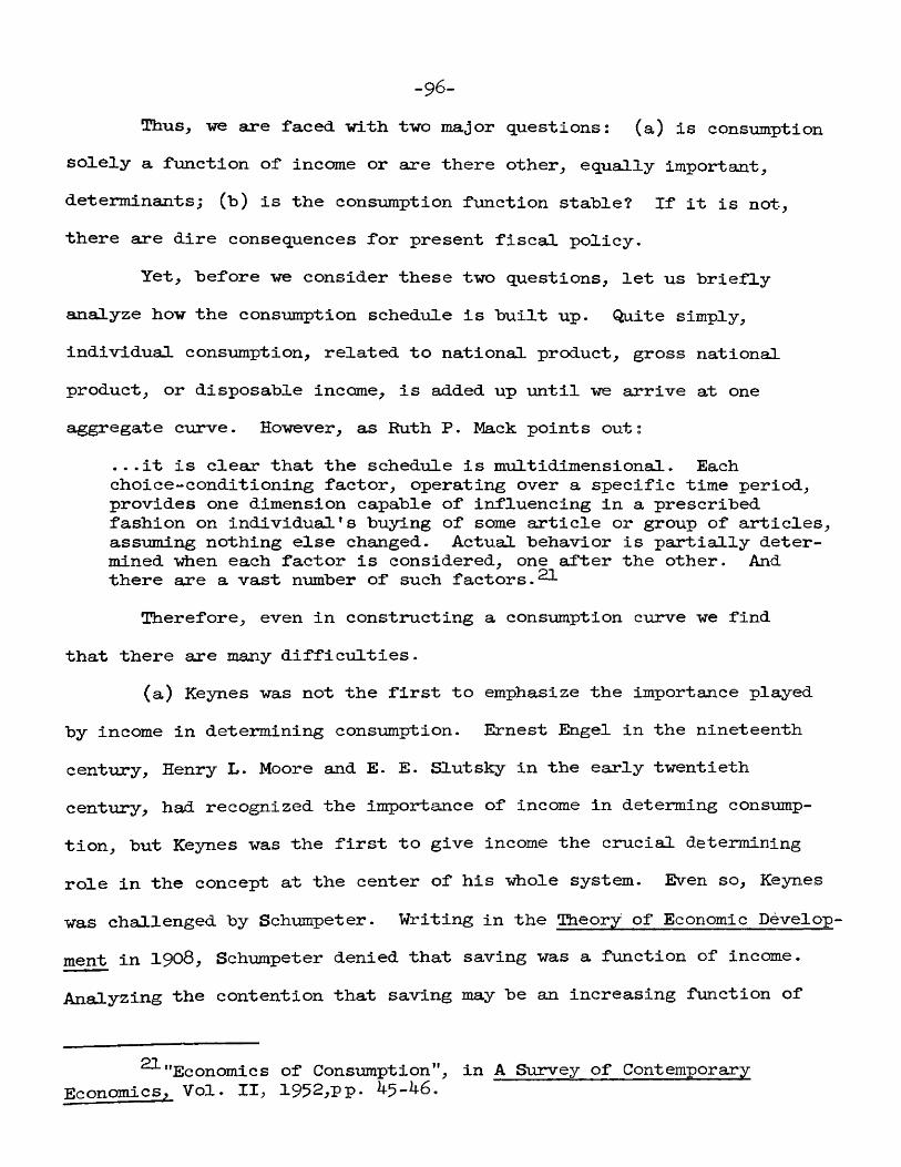
Thus, ve are faced -with two major questions: (a) is consumptionsolely a function of income or are there other, equally important,determinants; (b) is the consumption function stable? If it is not,there are dire consequences for present fiscal policy.

Yet, before we consider these two questions, let us brieflyanalyze how the consumption schedule is built up. Quite simply,individual consumption, related to national product, gross nationalproduct, or disposable income, is added up until we arrive at oneaggregate curve. However, as Ruth P. Mack points out :

...it is clear that the schedule is multidimensional. Each choice-conditioning factor, operating over a specific time period, provides one dimension capable of influencing in a prescribed fashion on individual * s buying of some article or group of articles, assuming nothing else changed. Actual behavior is partially deter­mined ”vÆien each factor is considered, one after the other. And there are a vast number of such factors.

Therefore, even in constructing a consumption curve we find that there are many difficulties.

(a) Keynes was not the first to emphasize the importance played by income in determining consumption. Ernest Engel in the nineteenth century, Henry L. Moore and E. E. Slutsky in the early twentieth century, had recognized the importance of income in determing consump­tion, but Keynes was the first to give income the crucial determining role in the concept at the center of his whole system. E\ren so, Keynes was challenged by Schumpeter. Writing in the Iheory of Economic Develop- ment in I908, Schumpeter denied that saving was a function of income. Analyzing the contention that saving may be an increasing function of

^"Economics of Consumption", in A Survey of ContemporaryEconomics, Vol. II, 1952,pp. 4^-46.

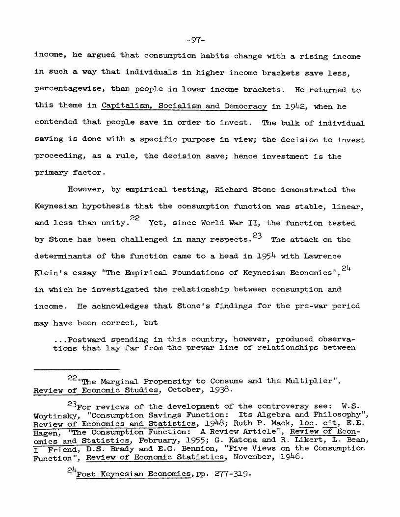
-97-income, he argued that consumption habits change -with a rising income in such a way that individuals in higher income brackets save less, percentagewise, than people in lower income brackets. He returned to this theme in Capitalism, Socialism and Democracy in 19^2, tAien he contended that people save in order to invest. The bulk of individual saving is done with a specific purpose in view; the decision to invest proceeding, as a rule, the decision save; hence investment is the primary factor.

However, by empirical testing, Richard Stone demonstrated theKeynesian hypothesis that the consumption function was stable, linear,

22and less than unity. Yet, since World War II, the function tested2^by Stone has been challenged in many respects- The attack on the

determinants of the function came to a head in 195^ with Lawrence2hKlein's essay "The Empirical Foundations of Keynesian Economics",

in which he investigated the relationship between consumption andincome. He acknowledges that Stone's findings for the pre-war periodmay have been correct, but

. . .Postward spending in this country, however, produced observa­tions that lay far from the prewar line of relationships between

^^"The Marginal Propensity to Consume and the Multiplier", Review of Economic Studies, October, 1938.

^3por reviews of the development of the controversy see: W.S.Woytinsky, "Consumption Savings Function: Its Algebra and Philosophy",Review of Economics and Statistics, 19^8; Ruth P. Mack, loc. cit, E.E. Hagmn, "The Consumption Function: A Review Article", Review of Econ-omics and Statistics, February, 1955; G. Katona and R. Likert, L. Bean, I Friend, D.S. Brady and E.G. Bennion, "Five Views on the Consumption Function", Review of Economic Statistics, November, 19^6.

piiPost Keynesian Economics, pp. 277-319*

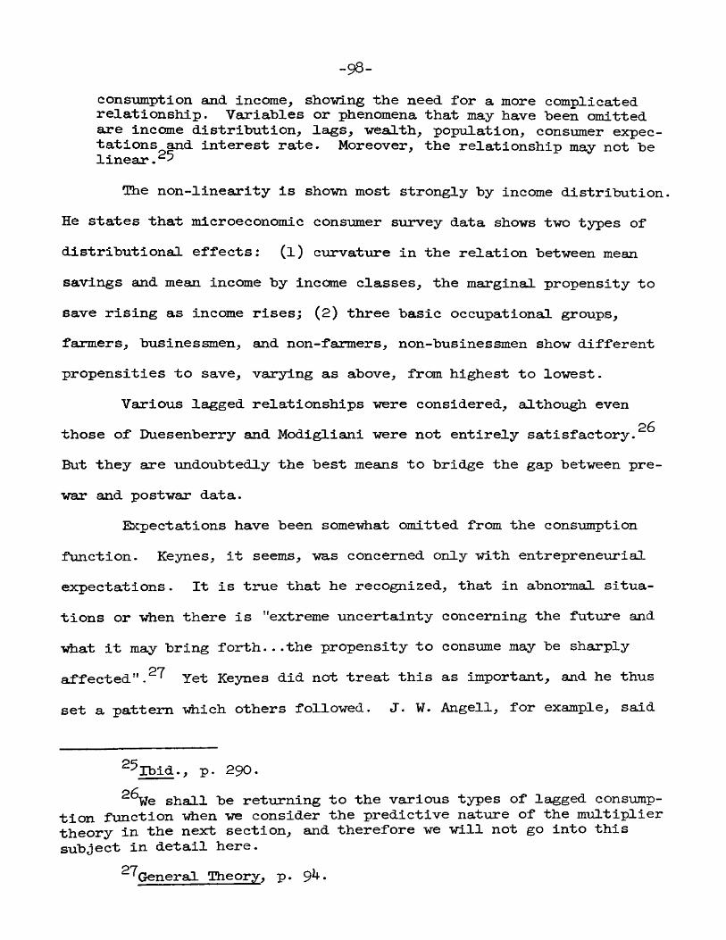
-98-con sumpt ion and income, showing the need for a more complicated relationship. Variables or phenomena that may have been omitted are income distribution, lags, wealth, population, consumer expec­tations and interest rate. Moreover, the relationship may not belinear.5

The non-linearity is shown most strongly by income distribution He states that microeconomic consumer survey data shows two types of distributional effects: (l) curvature in the relation between meansavings and mean income by income classes, the marginal propensity to save rising as income rises; (2) three basic occupational groups, farmers, businessmen, and non-farmers, non-businessmen show different propensities to save, varying as above, from highest to lowest.

Various lagged relationships were considered, although even those of Duesenberry and Modigliani were not entirely satisfactory.^^ But they are undoubtedly the best means to bridge the gap between pre­war and postwar data.

Expectations have been some-vdiat omitted from the consumption function. Keynes, it seems, was concerned only with entrepreneurial expectations. It is true that he recognized, that in abnormal situa­tions or when there is "extreme uncertainty concerning the future and what it may bring forth. . .the propensity to consume may be sharply affected" Yet Keynes did not treat this as important, and he thusset a pattern which others followed. J. W. Angell, for example, said

^^Ibid., p. 290.^^We shall be returning to the various types of lagged consump­

tion function when we consider the predictive nature of the multiplier theory in the next section, and therefore we will not go into this subject in detail here.

^^General Theory, p. 9^•

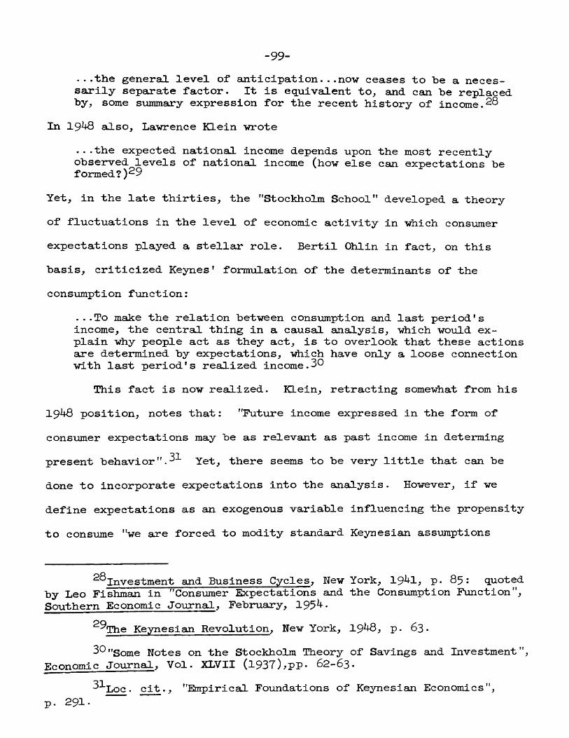
-99-. .the general level of anticipation. . .nov ceases to be a neces­

sarily sepajc-ate factor. It is equivalent tO; and can be replaced by; some summary expression for the recent history of income.

In 19^ also, Lavrence Klein "wrote...the expected national income depends upon the most recentlyobserved levels of national income (how else can expectations beformed?)29

Yet, in the late thirties, the "Stockholm School" developed a theoryof fluctuations in the level of economic activity in which consumerexpectations played a stellar role. Bertil Ohlin in fact, on thisbasis, criticized Keynes' formulation of the determinants of theconsumption function:

...To make the relation bet"ween consumption and last period's income, the central thing in a causal analysis, which would ex­plain why people act as they act, is to overlook that these actions are determined by expectations, which have only a loose connection with last period's realized income.30

This fact is now realized. Klein, retracting somewhat from his1948 position, notes that: "Future income expressed in the form ofconsumer expectations may be as relevant as past income in determingpresent behavior Yet, there seems to be very little that can bedone to incorporate expectations into the analysis. However, if wedefine expectations as an exogenous variable influencing the propensityto consume "we are forced to modity standard Keynesian assumptions

^^Investment and Business Cycles, New York, 194-1, p. 8 5: quotedby Leo Fishman in "Consumer Expectations and the Consumption Function", Southern Economic Journal, February, 1954.

^^The Keynesian Revolution, New York, 1948, p. 63.3^"Some Notes on the Stockholm Theory of Savings and Investment",

Economic Journal, Vol. XLVII (1937),pp. 62-63.3^Loc. cit., "Empirical Foundations of Keynesian Economics",

p. 2 9 1.

—100—about; the stability of the consumption function".

The effects of the interest rate on the consumption function have never been demonstrated empirically. There is no infallible reason to believe that the interest rate will influence consumption in any one direction. In Classical economics the explanation was that a high interest rate stimulated saving; but; on the other hand; a high rate of interest may diminish saving. Keynes recognized this and thought it impossible to postulate any one clearly defined relation between the interest rate and consumption. However; in the long ruu; we may say that the interest rate modifies social habit; therefore; the influence is of a secular nature; but even sO; it is still impos­sible to say in which direction the modification lies.

As far as the consumption function is concerned population is mainly a statistical problem- Population changes do affect consump­tion . It is possible; however; in statistical studies to allow for this effect.

Wealth; also; may be an important influence on the consumption function. Like the rate of interest; it is impossible to say in which direction the "wealth effect" has influence. In low income groups the effect of liquid assets on saving is negative; but Klein concludes that; at high income levelS; this negative effect is dim­inished and even becomes positive.

The results of Klein's investigations are summarized as follows...in an aggregate econometric model; an adequate description of consumer spending behavior would require the use of variables to

pp.291-292

—l o i —

represent income level. Income distribution, lags in behavior, population growth and wealth.

Thus, in equation form, no longer is C = f(y); but in Klein’sestimation becomes

C = f(y,i,d,p,e,A)where Y is income; i, the interest rate; d, income distribution, p,population; e, expectations; and A, wealth.

(b) Klein has raised the question: is the consumption functionstable? If it is not, then as a prediction device it is almost useless.The stability of the function has been questioned by many. In theimmediate postwar years a large number of economists saw the failure ofprediction models in the unstable nature of the consumption function.Is it, or is it not, unstable? This is the question that confronts us.W. D . Ross has made the comment that the accuracy of pre-war analysiscannot be doubted:

. . .However, it is an observable fact that the economic conditions, the cultural patterns, the social group relationships and the psychological attitudes that exist in this nation today are not the same that existed in the period observed and analysed by J. M. Keynes. The psychological law has changed, and the impli­cations of this change for fiscal policy are tremendous and far- reaching... .This, it is contended, is a fundamental and permsuaent change in the economic, social and cultural life of the nation.The change is the result of a fundamental transformation in the institutional and cultural structure of our society and of a general weakening or virtual elimination of some of the main motives which, as accurately analysed by Keynes, led individuals to refrain

33rbid., p. 294.3^In economic theory there is much to be said for simplicity

from which a solution is possible, but Klein, by adding more variables to the consumption function, may be moving towards a general equili­brium analysis from which no solution is possible.

-102-from spending ont of their incomes in the period between the two wars.35

The influencing factors,, Boss maintains, are nnmerons. However, primary importance may be attached to six factors. First, the high degree of security in the United States economy has almost negated the need to build up reserves against unforeseen contingencies.Second, the desire to postpone consumption and accumulate interest on current savings has been readily undermined by postwar expansion in consumption, in which installment credit plays a crucial role. Third, the speculative motive has been rapidly transformed : institutional saving and institutional investment, through insurance companies, trust funds, retained corporate earnings, etc., have replaced indivi­dual saving as a source of new equity. Fourth, the pure "miserliness", or what Keynes regarded as "unreasonable but insistent inhibitions against acts of expenditures" have drastically fallen, and now there is a new element present called "Keeping up with the Joneses" or what J . S . Davies has described as :

. . .The standard of consumption or living is the level that is urgently desired and striven for, special gratification attending substantial success and substantial failure yielding bitter frustration.

Fifth, the expect at ional element of rising family income has called forth projected expenditure. Lastly, institutional changes in govern-

35loc. cit., "State-Local Fiscal Policy and Economic Growth", p. 72; Rn for an earlier discussion of the instability question see W.S. Woytinsky, "Relationship Between Consumers’ Expenditures, Saving and Disposable Income", Review of Economics Statistics, February, 19^6

"Standards and Content of Living", American Economic Review, March, 19^5, P* 3*

-103-ment, corporate changes in business, changes in the tax structure, and the subjecting of the liquidity motive to statutory control, have had considerable impact on motives for improvement and financial pru­dence .

However, Morris Cohen has presented the other side of the pic­ture. He notes that the prewar consumption function did not hold good for the immediate postwar world but;

...by 19^^ the function appears to have resumed a more "normal" shape. The relative speed with which the functional relationship of consumption to income reasserted itself after the great shocks ajssociated with World War II is indeed remarkable, and provides evidence for the fundamental stability of the consumption func­tion . 37

His observations are based on empirical evidence, whereas Ross' assertions are not. However, Ross' thesis seems reasonable and as Klein, too, has questioned the stability of the consumption func­tion, it may be that in its present C = f(Y) state, the function is unstable. If the function is unstable it has important consequences for fiscal policy, both on a Federal and State and Local level. If ^ a t Ross maintained is in fact true, it means, roughly, the end of counter-cyclical fiscal policy in the Keynesian sense, that is the end of the budget-deficit-budget-surplus approach to fiscal policy.For tax policy, Ross' analysis suggests more use of "consumption répressives" to control inflation. It means an end to public works for purely counter-cyclical fiscal policy. These suggestions are far reaching, but as yet instability has not been conclusively proved.

"Postwar Consumption Functions", Review of Economics and Statistics, Vol. XXIV, 1952, pp.l8-19.

3^Boss, loc. cit., p. 7 5 .

-104-To be conclusive, all that we can say, with any justifiable certainty,is to repeat E. E. Hagen's very true words:

. . - Not many topics in the history of the development of economic theory have occasioned more discussion within a period of the same two decades than has the consumption function since the publication of the General Theory in 1936.. .And the end is not yet... This is natural. The maturation period of an idea is often longer than that of man.39

(4) Empirical testing of the multiplier theory and the predictive ability of econometric models.

The models Keynes developed of the economic system are suscept­ible to econometric and empirical treatment. As Schumpeter, one of his most vitriolic critics, points out, "Keynes gave a lead and an impulse to what we call econometrics".^^ This is borne out by Tinbergen who remarked:

...it seems to me that in many respects there is a good deal of agreement between the contributions made by Lord Keynes and those made by the econometricians, which reinforces some of the conclu­sions to tdiich these contributions have led us.

But do these models conform with the facts? This is the ques­tion we seek to analyze and in order to carry this to its logical end we will develop the analysis in two stages: first, we will view thedepression of the 1930's in 'sdiich several governments put into effect large public works, which they hoped would raise the level of income and employment, and try to analyze if in fact the multiplier did really

^^Loc. cit., "The Consumption Function: A Review Article" p. 48."Keynes and Statistics", Review of Economic Statistics,

November, 1946, p. 195*"The Significance of Keynes Theories from the Econometric

Point of View”, in The New Economics, p. 219.

-105-, k-2work; second, we will take tip the predictive nature of the models for

the transition period in the United States following World War II.During the depression of the 1930's, three governments, Germany,

Sweden, and the United States, put into operation large public works projects \^ich, it was hoped, would form a basis for an upswing in the cycle.

In Germany the effects of public works were, to a large extent, inconclusive because, simultaneously with the expansion in the public works program, the idiole economic policy was changed in an effort to make the country self-sufficient. The expansion of the textile industry and the house-building industry was artificially stunted by the govern­ment because expansion was favored in heavy industry, rather than con­sumption industry. However, the policy changed, and for the brief period 1933-37, it is possible to analyze the effects of "pure public works". Deficit spending increased the number of workers employed in industry from mid-1933 to mid-1936 by 3*5 million. Yet, the increase in employment was largely confined to primary employment, and secondary employment was someidiat unaffected. The improvement in consumption goods industries did not appear until 1937 on the crest of the wave of general recovery. The failure of consumption industries to grow was the result of three major factors: (a) governmental policy (especiallywith regard to stimulating heavy industry); (b) the structure of the German economy (the concentration of spending in particular areas, for instance, agricultural areas, with very limited possibilities of

^^This section is based on Hegeland's evidence in The Multiplier Theory, pp.236-247.

- l o 6 -

re-spending); (c) consumer reactions (large fractions of the incre­mental income wsts used to pay off outstanding debts). The operation of the accelerator was impeded by the large amount of excess capacity in German industry; a fact which was further accentuated because raw materials had to be purchased abroad^ and these purchases became "leakages". Thus, by and large, the multiplier did not work in Germany in the 1930*s. But we feel it did not work (and this is contrary to Hegeland's hypothesis), because it was not allowed to work: governmental controls were orientated directly against itsworking.

When Sweden left the gold standard in 1931, her economy was not in dire straits. The high level of activity in the domestic con­struction industry alleviated, to some extent, the severe repercus­sions of the international depression, although the export industries suffered considerably and unemployment slowly rose. Thus, Swedish econ­omic policy during 1931-32 was characterized by a certain cautiousness, and it was not until the spring of 1933 that a deficit spending program was introduced. Though something in the nature of deficit spending was carried out in 1932, it was not until an act was passed in 1933 that the program became a full scale government project. Yet, even so, between 1932-34 government investment projects only amounted to 4-6 million dollars per year. It was only during the fiscal year 1934-35 that operations came into full swing, but by then the recovery was in progress. The basic cause of the recovery, Hegel and places at the door of expansionist monetary policy and the "undervaluation" of the Swedish crown, making expansionist spending policies possible without unfavorable repercussions on the balance of payments. Thus, whether deficit

-107-spending would have turned the tide is a matter of conjecture^ because at the time of the inauguration of the deficit program the general im­provement in international markets, especiadly in England and the United States, was being felt. Therefore, in point of fact, it is impossible say whether the multiplier worked or did not work, because it is diffi­cult to disentangle deficit influences from other influences. At the same time, the close relationship between exports and national income in Sweden, indicates that any improvement in that direction might be sufficient to generate an upswing.

In the United States, the analysis is rather complex because there is no close relation between amounts of public works and amounts of net-increasing government expenditure ; and because of the compli­cations resulting from the "tri-fiscal" structure of government, that

h?is. Federal, State, and Local. However, Hegeland, following Villard, shows that annual amounts of public works and net government income- increasing expenditures were moving in the same direction during 1932- 38. The main cause of the depression, Hegeland states, was "the deep- going disproportional development of various forms of investment in relation to the actual structure of demand".Thus, because a period was necessary to reorganize to the actual structure of demand, the period 1930 to I932 meant a further decline in economic activity. Net government income increasing expenditure declined in 1932, reaching its lowest figure of $190 million in the fourth quarter of 1933- Simultaneously, however, income payments within businesses increased

^^Ibid., p. 2h0 .kk.Ibid.

—lo8“slowly. Therefore, when the amount of puhlic works was increased in the first quarter of 1934 to a little over $1100 millions, the upturn in business activity was already underway. Once again we cannot definitely say whether or not public works caused the upswing or how big a boost it gave to the recovery: but it was undoubtedly an import­ant factor, even if it was only a psychological boost to businessmen.

In the third quarter of 1937 there was a recession in business income payments simultaneously with a decline in net government income increasing expenditure, although causation is rather vague. Yet, the immense drop in government income increasing expenditure from $500 million in the first quarter of 1937, to $200 million in the third quarter, has strong suggestions of causal relations. In 193^ net govern­ment income increasing expenditure was raised to the same level as the average in 193^-3&j but total production and income declined. Income increasing expenditure increased until the end of 1939, "when the out­break of World War II saw a sudden upheaval in demand. Hegeland is probably correct -vÆien he says:

. . .Thus during this past period the assumptions of the multiplier theory may have been partly fulfilled and the cause of both the recession in 1937, the checking of it and the recovery in 1938 might have been the decrease and increase, respectively, of deficit spending.

However, we maintain that Hegeland cannot definitely assert that events in Europe negate the multiplier from a practical point of view. In Germany events were not left to work themselves out. It

^^Ibid., p. 24l. It is much easier for a Swede to make and believe this statement than it is for most American economists, par­ticularly those who lived through the depression of the 1930's.

Ibid., p. 243.

—109"“seems as if the attempt to ‘boost heavy industry was an attempt to put the accelerator before the multiplier. In Sweden nothing can be definitely said concerning the boosting effects of the multiplier, because of other extraneous influences. But, if Hegeland maintains that it was an Increase in foreign trade that caused the upswing, it sounds suspiciously like the foreign trade multiplier.

As far as the predictive ability of the models are concerned, there is only one period which we can view in both an ex ante and ex post sense. This is the period immediately following World War II, ^ e n numerous predictions were made concerning unemployment after the war.Ihe predictions were extremely pessimistic, forecasting something akin to 8 million unemployed in the United States. As it turned out, these predictions were entirely wide of the mark and instead of intense depression, the United States was faced with cumulative inflation. Tbe forecasts, then, were in grave error, which seemed to limit, not only the practical usefulness of econometric models based on past experience in general, but models such as we have developed, in particular. How­ever, let us review the situation and the postwar attempts at improving the models.

The forecast with which we will deal is that of Everett E. Hagen, aspects of whose analysis appeared in five different journals. ' Other

"^Hagen and E.A. Goldenweiser, "Jobs After the War", Federal Reserve Bulletin, May, ±9hk; Hagen and H-B. Kirkpatrick, "Rational Out- pxit at Full Employment", American Economic Review, September, 19^4; "Postwar Output in the United States at Full Employment", Review of Ecf nrmic Statistics, May, 1945; "Output and Demand After the War", Postwar Economic Studies, No. 1, Board of Governors of the Federal Reserve System, August, 1945; "Foreca.sting Gross National Product and Ehiployment During the Transition Period: An Example of the Nation's Budget Method", Studies in Income and Wealth, Vol. X, National Bureau of Economic Research.

-110-

estimates also appeared; bixt they are not as concise or easy to handle as Hagen thereforeprimary concentration will be on Hagen^ although the criticisms apply equally as well to the others. The model Hagen worked from is as follows :

The basic equation is:GHP = C(GHP) + I

where GHP is gross national product; C(GHP) the consumption function; and I autonomous investment. Included in consumption are oni y non­durables and services, exclusive of paid rentals. Durable consumer goods and rent are classified with I. The consumption function is esti­mated in two steps. First, the relation between consumption and dis­posable income, C = c(Yd), is calculated. The difference between gross national products and disposable income is governmental revenue plus business reserves, plus corporate savings, minus transfer payments. The function C(GHP) depends on the relation between Yd and GHP, based on autonomous governmental action with respect to taxation, unemployment compensation, etc. Second, the Bureau of the Budget carefully computed Yd = Yd (GHP ) for different periods of the transition. For each tax system they obtain a different relation between Yd and GHP. They then substitute the appropriate autonomous function Yd = Yd (GHP) into the

See for example S.M. Livingston, "Postwar Manpower and Its Capacity to Produce", Survey of Current Business, April, 19^3; Symposium by A. Smithies, J. Mosak and S.M. Livingston, forecasting Postwar Demand", Econametrica, January, 19^5; S. Slichter, "Jobs After the War", Atlantic Monthly, October, I9U6; J.J. O'Leary, "Consumption as a Factor in Postwar Employment", Papers euid Proceedings of American Economic Association, May, 19^5; W.S- Woytinsky, "Relationship Between Consumer's EKpf^n^ ]res. Savings and Disposable Income", loc. cit.

^^See also L.R. Klein, "A Post-Mortem on Transition Predictions of National Product", Journal of Political Economy, August, 19^6 .

-111-

behavlor equation C = c(Yd) to get C = C(GïïP) . The components of X are computed item by item.

Hagen's ex ante estimates and the ex post actualities are repro­duced in Table X , As Hagen himself admits :

. . .The primary fact to be noted concerning the forecast is that it was conspiciously in error. Gross national product was expected to fall to an annual rate of $l62 billion by the first quarter of X9h6 and unemployment to rise by 8 million persons. Actually, in the first quarter of 1946, output was $12 billion higher (in con­stant prices) than forecast, and unemployment 5-4 less.51

As will be seen from the table, in some areas the estimates were not so wide of the mark, but as he points out, "The major source of error in the unemployment forecast lay in the estimates of output... "5^ In brief, government purchases were greatly overestimated, but private capital formation and consumer purchases were greatly underestimated: the net result was an underestimation of gross national product. Simi­lar assessments of the forecasting error were made by L.R. KLein^^ and Micheal Sapir.^^ As Klein put it:

. . .the forecast failed in the prediction of consumer expenditures, particularly on nondurable goods. The forecast of most of the autonomous items of government expenditure of capital formulation are only slightly below the observations and these errors together do not contribute so much to the total error as does the error in consumption a l o n e .55

^^The Table is taken from his admirably frank article, "The Reconversion Period: Reflections of a Forecaster", loc. cit.

^^Ibid., p. 95- ^ Ibid., p. 98.53"A Post-Mortem on Transition Predictions of National Product",

loc. cit.54"Review of Economic Forecasts for the Transition Period",

Studies in Income and Wealth, Vol. XI, 1949*^^Loc. cit., p. 2 9 1'

?

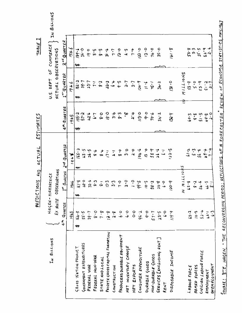
vnU iH'Xr

-Jt i3KoŒ

toZot—oo

CLCL

V»?o

OQ3H

luKJt£L iZroo

Llo

HC Ltua

inO

to"2OHtx>CKUjv>t oO

Œ3h-O

Ct•uhcc<xO9^

o i

o&

Qt(U

OOf

«T

O a t O

If) Ln -Û p' CÔ t - ct

inr~

o o o Û t» 00m3 ro it inm J a COV rt<f>

n* r - ^ Ô — ^ otvj rl

04V )

ns j-r f0»

intr r * CO of t V? CO

in% oo " O' o cr o( i~~à $ % c: G."'

If)' *O '

Ol Oi "U) I— O %/ r6 6 g :D &> % fn 6O 'D CO 1ÙO ■*■ Ou COo -

ëCO oo CO IP Oo M — O' n('-o to

H)V*Hr>zm<jkHVITo:zoui\LO

5w5Uict

q;UihV )cnejLiQC01l

u.oâVJU julUlCL

v>? cto tilo t- H<LCC QXh- oCT Cto_ wV tn ecf SÜ — 'oÜt *uz V-Ui 2 QCUi1-VJ~■cr ctX J} Q

>J:Q-

ri CO <~nCo no ~~o 0®rtr T

V» r~9 9oo CO o

nfO O" — m rt

o t2 *o—Ûrt rt tf) trj ^

Co^ --------------

V: O— ^ A ^ ^ tocO — cO rO oo oo to cO O

X-

O O cx)

r* — Cr- C3"

CT> nt 9 O'O Oo o<r> rt—' CO ft Uk to —

Oo

e *

in%a- iuCQ

O'ui m r~ oo^oooo o o o o t" Co O O' n 0“ J-

O' T-~to

COr< co o rt<-o

KqJooat io-■ZoV-

lOLUCtoko2luo.X QCUI «1-Zw —1Z3•XQCUitu ouIT*u_

(%T32o%

(Cci

ΠO o

- t o z ztu I -Œ - > £

2oHsrCtioIL

ta.tEointnofiCi rtiiH

oV-o3ofI-v>2Oo

(UISSUJaQC

ostuI

LiCT'2%'Zu>otp12

j -U i%

tnhqCâXtiiHlU%

Li<XId

IVCUiccLir3W1

u

aC t

O' in 3

o aÔ LU^ill%L iCÜ

U i

OoSLi- iCÛ< xt no

o _t n

itt tft* 1

11-

woQC

£

= 2 l5|UI' " £^ ^ ? 3 .Œ. Vj Ll O

CSI,20

mQC1olitc £

Ui?iUiI Ti r3 :

» u

l i

w

cU3O

V )

- 112-

-113-Thus, it is seen that the estimates fall down on the fact that

the consumption function was in error. This being the case, there were two courses of action open: (a) discard econometric models and predicton an intuitive basis; or (b) make use of the evidence accumulated and strive to produce better models. On the latter basis, it is probably better to proceed on a ’’successive approximation basis”, than to attempt to became an intuitive oracle. This second course of action was taken, and the history of the consumption function since lp46 has been one of attempting to find a formula in tune with the facts. Yet, some econo­mists still argue that the consumption function utilized in the esti­mates was quite correct : the only thing wrong was that it was appliedin the wrong majiner. Morris Cohen^^ maintains that we must distinguish between secular and cyclical consumption functions.

. . .The fact that actual postwar personal consumption expenditures are in excess of those expected from prewar cyclical relationships with disposable income is primarily due to the upward secular drift of the consumption function.5T

This has some relevance and it is noticeable that the twin as­pects of the consumption function have advanced under the sure guidance of J. S. Duesenberry^^ and Franco Modigliani

’’Postwar Consumption Functions”, loc. cit.^^Ibid., p . 1 8 .^^Income, Saving and the Theory of Consumer Behaviour, Cambridge,

Mas sachusetts, 19^9^^^’’Fluctuations in the Saving-Income Ratio: A Problem in

Economie Forecasting ”, in Studies in Income and Wealth, Vol. XI, 19^9*

-114-Tom E. Davies^^ has neatly classified attempts at constructive

postvar consumption functions into three categories:(1) Using disposable income as the single independent variable and consumption as the dependent variable, there are three varia­tions :

(a) Jacob Mosak^^ correlated these variables "without any attempt at deflation.

(b) J. M. Keynes initiated the function in real terms, that is, “with appropriate deflation for price changes.

(c) Paul A. SaiHuelson^^ formed the regression equation after deflating these variables for price level and population changes.

(2 ) Functions based on two independent variables correlated with consumption. There are three formulations:

(a) T. C. Lin and C. G. Chang used consumer price index and gross national product as independent variables.

(b) V. Lewis Basie^ utilized population ais an independent variable, rather than solely as a deflator; and real disposable income.

(c) Arthur Smith!es^^ used a time trend with disposable income after deflating the latter for price and popu­lation changes.

^"The Consumption Function as a Tool for Prediction", Review of Economics and Statistics, 1952.

^^"Forecasting Postwar Demand", loc. cit.^^"A Statistical Analysis of the Consumption Function", in A.H.

Hansen, Fiscal Policy and Business Cycles, New York, 1941."U.S. Consumption and Investment Propensities Prewar and

Postwar", American Economic Review, September, I95O."Consumer Expenditures in War and Transition", Review of

Economic Statistics, August, 1946.^^"Forecasting Postwar Demand", loc. cit.

-115-(3) A radically new function containing cyclical Income Indices and gross national product as the Independent variable and the average propensity to consume as the dependent variable. The marginal propensity to consume Is the cyclical variable.

(a) J. S. Duesenberryobtains his Independent variable by dividing current disposable Income by peak pre­ceding disposable Income.

(b) Franco Modiglianisubtracts peak preceding disposable Income from current disposable Income and then divides the result by current disposable Inccane In order to form his Independent variable.

To these three groups Davies applies three tests: (l) deter­mining the magnitude of error In current dollars, between the predicted value and the actual value of consumption 19^6-50; (2 ) comparing this magnitude with a similar margin of error which results from adopting the form that this year ' s consumption will be Identical with last year's^ In order to discover the superiority of the two methods; (3) calculating values for two sets of data- - "the probability of occurrence of a postwar mean error" and a variance ratio. A low value for these measures means that the prewar consumption function has not been re- establl shed.

The results were only gratifying as far a^ group (3) was con­cerned but even then there was rather an over-estimate:

. . .our examination of several existing consumption functions has shown that they are unacceptable as a tool for postwar forecasting.In the case of the linear functions, this Is due mainly to the sizeable errors resulting from predictions which In every case

^^Op. cit. " XjOC . cit.

-116-represen*ted tmderestImates of Gons-umption expenditures. In the case of the cyclical variable functions^ the forecats, •vÆiile much closer to the actual level of consumption, were consistently in excess of it, so that these functi^s did not appear to be re­established in the postwar period.^

Davies himself, working f oui the Duesenberry equation, plotted a new function but substituted peak previous consumption for peak pre­vious income. The postwar deviations are approximately one-half as large as those from the original Duesenberry function. Therefore, Davies is justified in not rejecting the hypothesis that this consump­tion function is unaltered in the postwar world.

It is with J. S. Duesenberry and variations of his analysis that the consumption function now rests. It is true, in the late fifties, Milton Friedman and G. S. Becker^^ have further attacked the concept of the multiplier and the consumption function. However, as both J. lohnston^^ and Lawrence KLein^ have demonstrated, the equation upon tdiich they base their assumptions has been utilized before, and better, truer functions erected by Duesenberry and Modigliani. Their criticism of the multiplier (. . . "if our analysis is valid, this widespread belief that consumption and income can be regarded as dancing primarily to the tune of unstable investment is largely the product of a statistical

68Davies, loc. cit., p. 275*Statistical Illusion in Judging Keynesian Models", Journal

of Political Economy, February, 1957*7 0 Statistical Illusion in Judging Keynesian Models: Comment",

Review of Economics and Statistics, August, 195Ô-71 "The Friedman-Becker Illusion", Journal of Political Economy,

December, 1958; see also the reply by Friedman and Becker in the same issue.

-117-illusion”)" , lÆille not altogether invalid seems less than objective because the simple multiplier model is not suitable for more than pedagogical use in the classroom.

Thus, although controversy over the consumption function is still very much alive and the matter is far from settled, predictions still go on. One of the latest attempts is by Gerhard Colm in his book. The American Economy in i960, published in 1952.^3 Colm's work was received very well, perhaps not because of his startling predic­tions, but because it shows the dimensions of the problem. As Kenneth Boulding has said;

. . .The value of these models is that they point up very clearly the dimension of the problem. What they cannot do, and do not pretend to do, is to "predict", for in order to do that it would be necessary to know much more about the dynamics of the system; of course, prediction in the sense in ■vdiich astronomers use the term would be impossible because of the existence of random or exogenous elements in the system.7^

In summary, we can say that econometric models developed in the postwar world, while not absolutely perfect, are like the curate's

;— good in parts.

7^Loc. cit., p. kh.73see the review articles in the November 1953 number of the

Review of Economics and Statistics by K- E. Boulding, "Projection, Prediction, and Precariousness"; Summers H. Slichted, "Growth and Stability"; and Alvin H. Hansen, "Long-Run and Short-Run Adjustments"

7^ "Projection, Prediction and Precariousness", ibid., p. 2 5 8.

Chapter VI

Conclusion

The main theme in this thesis was to answer three questions.Of what theoretical importance is the multiplier concept? How far has the multiplier theory advanced since Keynes (1936)? Has the multiplier any use for practical policy? The first two questions we have answered in Part I; by superimposing dynamic elements and the acceleration principle on the simple models and by showing their relevence to fiscal policy. The last question we have analysed in Part II, but have so far come to no conclusive answer. If we are to use any tool as the guide to practical policy, then that tool must be water-tight; that is, the logic end the analysis surrounding that tool must be un­questioned. On this basis we cannot say that the multiplier is such a water-tight tool. As we have indicated, the consumption function (empirically) is not altogether satisfactory. However, we have not been able to demonstrate (in spite of Hegel and ' s analysis), that the multiplier does not work. On the other hand, we cannot prove that it does. Therefore, as predictive tools our models do not seem to be very successful. Does this deal a death blow to such models? The answer we maintain is unconditionally no. Because at first glance our models do not fit the real world we need not throw them away.We must remember that such testing is still in its infancy as is the analysis per se. That the results have not been immediately forthcoming

-118-

—U n ­does not mean that cm* attempts at analysis are "wrong. At the same time, it does not mean that our models are wrong. What it does mean is that we must recognize the limitations of our analysis and of our models. The models are only successive approximations, and we must beware of expecting too much from too little. Trygve Haavelmo has said:

...The concrete results of our efforts at quantitative measurement often seem to get worst the more refinement of tools and logical stringency we call into play. . .However, I think we may well find part of tÿe explanation...in the shortcomings of basic economic theory...

This is part of the price we pay for attempting to become too scientificwithout the advantage of precise scientific tools. There are thosethat stress the fact that economic forecasting is an art rather thana science. Micheal Sapir stressed the fact that forecasting is an

2art, althO"ugh he tended to think that the art could become more scien­tific. Yet, there are others who feel that prediction will always remain an art. For instance, Rufus S. Tucker has said:

...Since the days of the early Babylonian star gazers, imaginative thinkers have indulged the hope that prophecy might become a science and have frequently persuaded themselves and others that that desirable goal has already been attained or at least is just around the corner.3

Further, Ely Devons, the British planning expert, stresses that pro­jections are so hypothetical that they have very little usefulness.He compares the economists who prepare projections with the diviners of old who examined chicken entrails for advising on war and peace.

^"The Role of the Econometrician in the Advancement of Economic Theory";, Egonometrica, July, 195#, PP« 35^-355 •

pLoc. cit.3gee "Comment", p. 3^5-367, on Micheal Sapir's article in

Studies in Income and Wealth, Vol. XI, p. 365*

- 1 2 0 -

vhen and -where to hunt; and -whether and whom to marry. To him, hoth the modern economic adviser and the old magician help to avoid endless -wrangling where, with existing knowledge, the chances of doing right or wrong appear to he even.^ Even so, the fact remains that predic­tions and forecasts are being carried out on a national level, not only in the United States but also in Continental Europe,5

Because this is the case, we should not halt because our tools, as developed here, initially fail us. The precise application of economic theory is not something which can be stringently demonstrated in many areas. As economists we are not dealing -with inanimate sub­stances, but with human beings. Our theory, while it gives us only a rough approximation from tdiich we can begin to work, is still vastly superior than the "nothing" we possess without it. Perhaps our fail-ure in part lies in the fact that -we are still too conscious of parameters, of segregating everything into "economic boses". There is an infinite amount of truth in the adage that life and man's actions cannot be rigidly defined. When all is said and done mathematical models are not everything, but they do provide a point of depart-ure from which to work and think. Even so analytically manageable models are blessed with too much rigidity. It is in this context that the words of Sir

^Quoted by Gerhard Colm, "Economic Projections: Tools of Econ­omic Analysis and Decision Making", Papers yid Proceedings of the Amer­ican Economic Association, May, 19^8, p* 178-179-

5gee for example in the United States, Potential Economic Growth of the United States During the Next Decade, Joint Economic Committee, Washington D.C., 195^; also see Hans Brems, "Current Economic Thought and its Applications and Methodology in Continental Europe; The Scandinavian Countries", Papers and Proceedings of the American Econ- omic Association, May, 195&J and in the same issue. Hi ^eil, "On the Theory of Econcanic Policy".

-121-

Dennis Robeirtson are very appropriate : As soon as I could safely toddle yiy parents handed me a model.My brisk and energetic pater Provided the accelerator^My mother^ -with her kindly gumption^The function guiding my consumption;And every week I had from her A lovely new parameter.With lots of little leads and lags In pretty parabolic bags.With optimistic expectations I started on my explorations.And swore to move without a swerve Along my sinusoidal curve.Alas! I knew how it would end;I 've mixed the cycle and the trend.And fear that, growing daily skinnier,I have at length become non-linear.I wander glumly round the house As though I were exogenous.And hardly capable of feelingThe difference ’tween floor and ceilingX scarcely now, a pallid ghost.Can tell ex ante from ex post;My thoughts are sadly inelastic.My acts incurably stochastic.

^"The Won-econometrician ’ s Lament", in Economic Commentaries, London, Staples, 195^.

BIBLIOGRAPHY

BOOKS

Allen^ R.G.D., Mathemat 1 caJ. Economics. London: Macmillan, 1956 .Beach, E.F., Economic Models, An Exposition. New York: Wiley, 1957.Duesenherry, J.S., Income, Saving, and the Theory of Consumer Behaviour.

Cambridge, Massachusetts : I949.Hansen, A.H., Fiscal Policy and Business Cycles. New York: Norton, 1941__________ ; A Guide to Keynes. New York: McGraw-Hill, 1953.Harris, S.E., John Maynard Keynes, Economist and Policy Maker. New

York; Scribner, 1955*Harrod, R.F., The Trad.e Cycle. Oxford: Clarendon Press, I936.Hegeland, H., The Multiplier Theory. Lund; Gleerup, 1954.Hicks, J.R., A Contribution to the Theory of the Trade Cycle. Oxford:

Clarendon Press, 1950-Keynes, J.M., The General Theory of Employment, Interest and Money.

London : Macmillan, 1936 *Klein, L.R., The Keynesian Revolution. New York: Macmillan, 19^7*Kurihara, K.K., Introduction to Keynesian Dynamics. New York;

Columbia University Press, 195^».Nevin, E., The Problem of the National Debt. Cardiff ; University of

Wales Press, 195^* ~

ARTICLES AND ESSAYS

Alexander, S.S., "Opposition to Deficit Spending for the Preventionof Unemployment ", Income, Employment, and Public Policy. Essays in Honor of Alvin Hansen, New York, Norton, 19^*

, "Mr. Harrod*s Dynamic Model", Economic Journal, 1950*, "Issues of Business Cycle Theory Raised by Mr. Hicks",

American Economic Review, I95I.-123-

-124-AU.en, R.G.D., "The Engineers Approach to Economic Models"^ Economica,

May; 1955-Allen; W-K. and W. 01; "A Period Analysis of Fiscal Policies", Southern

Economic Journad, July, 1955 •Basie; V.L., "Consumer Expenditures in War and Transition", Review of

Economic Statistics, August, 1946.Baumol; W.J. and Pest on, "More on the Multiplier Effects of a Balanced

Budget"; American Economic Review, March, 1955-Bean, L., "Five Views on the Consumption Function", Review of . Economic

Statistics, November, 1946.Bishop, R.L., "Alternative Expansionist Fiscal Policies; A Diagramatic

Analysis", Income, Employment, and Public Policy. Essays in Honor of Alvin Hansen, New York, Norton, 19481

Blank, D.M., "Reform of State-Local Fiscal Relations in New York", National Tax Journal, 1950 *

Blyth, C.A., "The 1948-49 American Recession", Economic Journal, September, 1954.

Boulding, K.E., "Projection, Prediction, and Precautiousness", Review of Economics and Statistics, November, 1953*

Brady, D-S. and E.G. Bennion, "Five Views on the Consumption Function", Review of Economic Statistics, November, 1946.

Brems, H., "Current Economic Thought and its Applications and Methodo­logy in Continental Europe: The Scandinavian Countries ", Papers and Proceedings of the American Economic Association, May J 195^-

Burkhead, J., "The Balanced Budget", Quarterly Journal of Economics,May, 1954.

Champemawne, D.G., "On the Use and Misuse of Mathematics in Presenting Economic Theory", Review of Economics and Statistics, November,1954.

Chang, T.C., ''Intemational Comparison of the Demand for Imports",Review of Economic Studies, 1945-46.

, "A Statistical Note on World Demand for Exports", Review of Economics and Statistics, May, 1948.

Chipman, J.S., "Empirical Testing and Mathematical Models", Review of Economics and Statistics, November, 1954.

-125--- j "Review of The Multiplier Theory"; Journal of PoliticalEconomy, April; 1956,Clark; C.; "Public Finance and the Value of Money”; Economic Journal;

December, 19^5.; "The Danger Point in Taxes", Harpers Magazine, December,

1950.; "Three Economic Illusions— Is Britain Heading for a Big

Inflation"; Manchester Guardian, September I8, I951.Cohen, M., "Postwar Consumption Functions", Review of Economics and

Statistics, XXIV (1952).Colm, G., "Economic Projections: Tools of Economic Analysis and

Decision Making", Papers and Proceedings of the American Economic Association, May, 1958•

Davies, J.S., "Standards and Content of Living", American Economic Review, March, 19^5 •

Davies, T.E., "The Consumption Function as a Tool for Prediction", Review of Economics and Statistics, 1952.

Dorfman, R ., "A Catechism: Mathematics in Social Science", Review of Economics and Statistics, November, 195^*

Duesenberry, J.8 ., "The Methodological Basis of Economic Theory",Review of Economics and Statistics, November, 195^-

Fels, R., "Theoretical Significance of the 19^9 Recession", Papersand Proceedings of the American Economic Association, May, 1955 •

Fisher, M.R., "Review of The Multiplier Theory", Economic Journal,March, 1 9 5 8 .

Fishman, L., "Consumer Expectations and the Consumption Function", Southern Economic Journal, February, 195^-

Friedman, M., "Comments on Monetary Policy", Essays in Positive Economics, Chicago, University of Chicago Press, 1953*

and G.S. Becker, "A Statistical Illusion in Judging Keynesian Models", Journal of Political Economy, February, 1957-

Friend, I., "Five Views on the Consumption Function", Review of Economic Statistics, November, 19^6.

Goodwin, B.-, "The Implications of a Lag for Mr. Haavelmo ' s Analysis", Econometrica, April, 19^8.

-126-

"The Multiplier"; The New Economics. Keynes' Influence onTheory and Public Policy, New York, Kiopf, 19^7

Gurley, J.G., "Fiscal Policies for Full Employment : A Diagramatic Analysis", Journal of Political Economy, December, 1952.

"Deficits, Surpluses, and National Income ", SouthernEconomic Journal, July, 195^.

Haavelmo, T-, "Multiplier Effects of a Balanced Budget", Ec onometri ca, October, 19^5•

__________ , "The Role of the Econometrician in the Advancement ofEconomic Theory", Econometrica, July, 1958.

Haberler, G., "Multiplier Effects of a Balanced Budget : Some Monetary Implications of Mr. Haavelmo *s Paper", Ec onometri ca, April, 1946.

Hagen, E.E., "Postwar Output in the United States at Full Employment", Review of Economic Statistics, May, 19^5 •

, "Output and Demand After the War", Postwar Economic Studies,No. 1, Board of Governors of the Federal Reserve System, August, 19^5-_____ , "Forecasting Gross National Product and Employment Duringthe Transition Period : An Example of the Nation's Budget Method", Studies in Income and Wealth, Vol. X, National Bureau of Economic Research._____ , "Multiplier Effects of a Balanced Budget: Further Analysis",Econometrica, April, 1946.

, "The Consumption Function: A Review Article", Review ofEconomics and Statistics, February, 1955•

, "The Reconversion Period: Reflections of a Forecaster", Review of Economic Statistics, May, 1957•

and E.A. Goldenweiser, "Jobs After the War", Federal Reserve Bulletin, May, 1944.

and N.B. Kirkpatrick, "National Output at Full Employment" American Economic Review, September, 1944.

Hamberg, D., "The Recession of 1948-49 in the United States", Economic Journal, March, 1952.

Hansen, A.H., "Three Methods of Expansion Through Fiscal Policy", American Economic Review, June, 19^5 •

-127-j "Long-Run and Short-Run Adjustments";, Review of Economics

and Statistics, November^ 1953-Harris ; S., "Postscript", to the symposium "Mathematics in Economics",

Review of Economics and Statistics, November, 19^4.Harrod, R.J., "Lecture 3"j» Towards a Dynamic Economics, London, Macmil­

lan, 19^9 •Johnston, J., "A Statistical Illusion in Judging Keynesian Models:

Comment", Review of Economics and Statistics, August, 19^8.Kahn, R.F., "The Relation of Home Investment to Unemployment",

Economic Journal, June, 1931*Kaldor, N ., "Appendix C", to W.H. Beveridge, Full Employment in a Free

Society, New York, Norton, 19^5.Katona, G . and R. Likert, "Five Views on the Consumption Function ",

Review of Economic Statistics, November, 1946.Keynes, J.M., "Letter", to the London Times, December 28, 1934.KLein, L.R., "A Post-Mortem on Transition Predictions of National Pro­

duct ", Journal of Political Economy, August, 1956., "The Enpirical Foundations of Keynesian Economics", Post

Keynesian Economics, New Brunswick, Rutgers University Press, 195^*__________ , "The Contributions of Mathematics in Economics", Review of

Economics and Statistics, November, 195^•, "The Friedman-Becker Illusion", Journal of Political

Economy, December, 195^.Koopmans, T.C., "On the Use of Mathematics in Economics", Review of

Economics and Statistics, November, 1954.Lange, 0., "The Rate of Interest and the Optimum Propensity to Consume",

Economica, 1938•, "The Multiplier Theory", Econometrica, 19^3*

Lemer, A.P., "The Burden of the National Debt", Income, Employment, and Public Policy", Essays in Honor of Alvin Hansen, New York, Norton, 1948.

Lin, T.C. and C.G. Chang, "U.S. Consumption and Investment Propensities Prewar and Postwar", American Economic Review, September, 1950.

-128-

Livingston^ 8.M., "Postwar Manpower and its Capacity to Produce"^Survey of* Current Business, April, 1943.

Mack, P.P., "Economics of Consumption", Survey of Contempory Economics,Vol. II, 1952. 'Metzer, A.H., "Review" of The Multiplier Theory, American Economic Review, June, 1955.Metzler, L.A., "Three Lags in the Circular Flow of Income", Income,

Employment, and Public Policy. Essays in Honor of Alvin Hansen, New York, Norton, 1948.

Modigliani, F ., "Fluctuations in the Saving-Income Ratio: A Problem inEconomic Forecasting", Studies in Income and Wealth, Vol. XI, 1949.

Mosak, J. and S.M. Livingston, "Forecasting Postwar Demand", Econo­metrica, January, 1945.

Musgrave, R.A., "Alternative Budget Policies for Full Employment", American Economic Review, June, 1945.

and M.H. Miller, "Built In Flexibility", American EconomicReview, March, 1948.

Myers, E.A. and R.A. Stout, "The Role of the State and Local Govern­ments in the National Fiscal Policy", National Tax Journal, June,1957.

Newcomer, M., "State and Local Financing in Relation to Economic Func­tions ", National Tax Journal, 1954.

Ohlin, B., "Some Notes on the Stockholm Theory of Savings and Invest­ment", Economic Journal, Vol. XLII (1937)*

O'Leary, J.J., "Consumption as a Factor in Postwar Employment", Papers and Proceedings of the American Economic Association, May, I945.

Norvick, D , "Mathematics: Logic, Quantity and Method", Review of Economics and Statistics, November, 1954.

Peacock, A.T., "A Note on the Balanced Budget Multiplier", Economic Journal, June, 195^*

Pechman, J.A. and T. Mayer, "Mr. Colin Clark on the Limits of Taxa­tion", Review of Economics and Statistics, Vol. 34, 1952.

Feston, M.H., "Generalizing the Balanced Budget Multiplier", Review of Economics and Statistics, August, 195Ô.

-129-Plgou, Aj^C., Newspaper Reviewers, Economics and. Mathematics ", Essays

in Economics, London, Macmillan, I952.Rasmussen, P.N., "A Note on the History of the Balanced Budget Multi­

plier", Economic Journal, March, I958.Ritter, L.S., "Alternative Anti-inflationary Fiscal Policies", Review

of Economic Studies, XVIII No. 3, I95O-5I .Robert son, D.H., The Non-econometrician * s Lament", Economic Commen­

taries, London, Staples, I956.Ross, W.D., "State-Local Fiscal Policy and Economic Growth", National

Tax Journal, March, 1958*Samuel son, P. A., "A Statistical Analysis of the Consumption Function",

in A.H. Hansen, Fiscal Policy and Business Cycles, New York, Norton, 1941.

, "Interaction Between the Multiplier Analysis and thePrinciple of Acceleration", Review of Economic Statistics, May,1939.

, "Fiscal Policy and Income Determination", Quarterly Journalof Economics, 19^2._____ , "The Simple Mathematics of Income Determination", Income,Employment and Public Policy, Essays in Honor of Alvin Hansen, New York, Norton, 1948._____ , "Economic Theory and Mathematics: An Appraisal", Papersand Proceedings of the American Economic Association. May, 1952.

, "Some Psychological Aspects of Mathematics and Economics", Review of Economics and Statistics, November, 195^*

Sapir, M., "Review of Economic Forecasts for the Transition Period", Studies in Income and Wealth, Vol. XI, 19^9*

Schumpeter, J.A., "Keynes and Statistics", Review of Economic Statis­tics, November, 1946.

Shackle, G.L.S., "Twenty Years On: A Survey of the Theory of the Multi­plier", Economic Journal, June, 1951*

Slichter, S., "Jobs After the War", Atlantic Monthly, October, 1946. , "Growth and Stability", Review of Economics and Statistics,Novemb er, 1953*

-130-Smi th, D.T., "Note on the Inflationary Consequences of High Taxation",

Review of Economics and Statistics, Vol. 3k, 1952.Smithies, A., "Forecasting Postwar Demand", Econometri ca, January, 19^5*Solow, R., "The Sirrvival of MathematicaJ. Economics", Review of Economics

and Statistics, November, 1954.Somers, H.M., "The Multiplier in a Tri-Fiscal Economy", Quarterly

Journal of Economics, 1949.Stone, R., "The Marginal Propensity to Consume and the Multiplier",

Review of Economic Studies, October, 1938-Theil, Ho, "On the Theory of Economic Policy", Papers and Proceedings

of the American Economic Association, May, I958*Tinbergen, J., "The Significance of Keynes' Theories from the Econo­

metric Point of View", The New Economics. Keynes Influence on Theory and Public Policy, New York, Knopf, 1947.

, "The Functions of Mathematical Treatment", Review of Econ-omics and Statistics, November, 1954.

Tucker, R.S., "Comment", on Micheal Sapir's article, Studies in Income and Wealth, Vol. XI.

Turvey, R., "Period Analysis", contributed to W.J. Baumol's. Economic Dynamics : An Introduction.

, "Some Notes on Multiplier Theory", American Economic Review, June, 1953*

, and H. Brems, "The Factor and Goods Market", Economica, 1951*Wallich, H.C., "Income-Generating Effects of a Balanced Budget",

Quarterly Journal of Economics, Vol. LIX (1944).White, M. and A. White, "The Impact of Economic Functions", National

Tax Journal, 19^4.Woytinsky, W.S., "Relationship Between Consumer's Expenditures, Saving

and Disposable Income", Review of Economics and Statistics, February, 1946.

"Consumption-Savings Function: Its Algebra and Philosophy", Review of Economics and Statistics, 1948.

Yeager, L.B., "Some Questions About Growth Economics", American Economic Review, 1954.

GOVERHMENT PUBLICATIONSUnited. Nations Depaortmen'b of Economic AffairS; "Maintenance of Full

Employment Lake Success^ 19^9•

-131-