The Modelling of Surface Roughness after the Ball Burnishing ...

��

Citation: Kanovic, Z.; Vukelic, D.;

Simunovic, K.; Prica, M.; Saric, T.;

Tadic, B.; Simunovic, G. The

Modelling of Surface Roughness after

the Ball Burnishing Process with a

High-Stiffness Tool by Using

Regression Analysis, Artificial Neural

Networks, and Support Vector

Regression. Metals 2022, 12, 320.

https://doi.org/10.3390/

met12020320

Academic Editor: Badis HADDAG

Received: 7 January 2022

Accepted: 9 February 2022

Published: 11 February 2022

Publisher’s Note: MDPI stays neutral

with regard to jurisdictional claims in

published maps and institutional affil-

iations.

Copyright: © 2022 by the authors.

Licensee MDPI, Basel, Switzerland.

This article is an open access article

distributed under the terms and

conditions of the Creative Commons

Attribution (CC BY) license (https://

creativecommons.org/licenses/by/

4.0/).

metals

Article

The Modelling of Surface Roughness after the Ball BurnishingProcess with a High-Stiffness Tool by Using RegressionAnalysis, Artificial Neural Networks, and SupportVector RegressionZeljko Kanovic 1 , Djordje Vukelic 1,* , Katica Simunovic 2 , Miljana Prica 1, Tomislav Saric 2, Branko Tadic 3

and Goran Simunovic 2

1 Faculty of Technical Sciences, University of Novi Sad, Trg Dositeja Obradovica 6, 21000 Novi Sad, Serbia;[email protected] (Z.K.); [email protected] (M.P.)

2 Mechanical Engineering Faculty in Slavonski Brod, University of Slavonski Brod, Trg Ivane Brlic Mazuranic 2,35000 Slavonski Brod, Croatia; [email protected] (K.S.); [email protected] (T.S.); [email protected] (G.S.)

3 Faculty of Engineering, University of Kragujevac, Sestre Janjic 6, 34000 Kragujevac, Serbia; [email protected]* Correspondence: [email protected]; Tel.: +381-21-485-2326

Abstract: Surface roughness is an important indicator of the quality of the machined surface. One ofthe methods that can be applied to improve surface roughness is ball burnishing. Ball burnishingis a finishing process in which a ball is rolled over the workpiece surface. Defining adequate inputvariables of the ball burnishing process to ensure obtaining the required surface roughness is a typicalproblem in scientific research. This paper presents the results of experiments to investigate ballburnishing of AISI 4130 alloy steel with a high-stiffness tool and a ceramic ball. The experimentswere conducted following a randomized full factorial design for different levels of input variables.The input variables included the initial arithmetic mean roughness (the initial surface roughness), thedepth of ball penetration, the burnishing feed, and the burnishing ball diameter, while the outputvariable was the arithmetic mean roughness after ball burnishing (the final surface roughness). Thesurface roughness modeling was performed based on the experimental results, using regressionanalysis (RA), artificial neural network (ANN), and support vector regression (SVR). The regressionmodel displayed large prediction errors at low surface roughness values (below 1 µm), but it provedto be reliable for higher roughness values. The ANN and SVR models have excellently predictedroughness across a range of input variables. Mean percentage error (MPE) during the experimentaltraining research was 29.727%, 0.995%, and 1.592%, and MPE in the confirmation experiments was34.534%, 1.559%, and 2.164%, for RA, ANN, and SVR, respectively. Based on the obtained MPEs, it canbe concluded that the application of ANN and SVR was adequate for modeling the ball burnishingprocess and prediction of the roughness of the treated surface in terms of the possibility of practicalapplication in real industrial conditions.

Keywords: ball burnishing; surface roughness; artificial neural networks; support vector regression;regression analysis

1. Introduction

Ball burnishing is a process in which the ball rolls on the surface and causes elastic,elastoplastic, and plastic deformations of the surface layer of the workpiece [1]. As aresult, the workpiece changes shape, dimensions, roughness, hardness, stresses, etc. Thisprocess can provide excellent geometric specifications and high dimensional accuracy [2].Prismatic and cylindrical workpieces are mainly processed, but complex-shaped surfacescan also be treated [3]. Ball burnishing can significantly increase wear resistance, fatigueresistance, corrosion resistance, etc. [4]. This process can manage various materials such

Metals 2022, 12, 320. https://doi.org/10.3390/met12020320 https://www.mdpi.com/journal/metals

https://doi.org/10.3390/met12020320


https://creativecommons.org/

https://creativecommons.org/licenses/by/4.0/

https://creativecommons.org/licenses/by/4.0/

https://www.mdpi.com/journal/metals

https://www.mdpi.com

https://orcid.org/0000-0003-1456-1135

https://orcid.org/0000-0003-2420-6778

https://orcid.org/0000-0001-5748-7110

https://orcid.org/0000-0002-8391-4152

https://orcid.org/0000-0002-7159-2627


https://www.mdpi.com/journal/metals

https://www.mdpi.com/article/10.3390/met12020320?type=check_update&version=2

Metals 2022, 12, 320 2 of 24

as steel, copper, aluminum, brass, polymers, titanium, nickel–chromium–molybdenum,wood, etc. [5].

Ball burnishing tools use various functional mechanisms to generate burnishing force.Burnishing force is most often generated with the spring [6–15], pressurized fluid [16,17],and high stiffness tools [18–20]. There are also hybrid ball burnishing tools, such as vibration-assisted ball burnishing tools [21–32], magnetic-assisted ball burnishing tools [33,34], etc.Burnishing force is usually generated by a single ball, although ball burnishing tools withmultiple balls also exist. Burnishing balls are mostly made of tungsten carbide, chrome-plated steel, high-speed steel, high-hardened steel, silicon nitride and titanium, stainless steel,carbon steel, ceramic, and synthetic diamond.

Previously, the ball burnishing process was studied in numerous ways, most often bythe use of experiments. The literature cites a variety of experimental research that applieddifferent techniques to study the relationship between input and output variables in ballburnishing. The investigations are mainly based on the development of new burnishingtool concepts, as well as analysis of the effect of input process variables (burnishing load,feed, number of passes, lubricant, etc.) on output process variables (residual stresses,surface roughness, hardness, etc.). The cost and time are merely some of the disadvantagesof the conducted investigations. Furthermore, the obtained results can only be appliedin conditions equal to those of the conducted experiments. The consequence of suchinvestigations is the emergence of research on the prediction and modeling of the ballburnishing process.

Another research direction is the research of the ball burnishing process based on finiteelement analysis (FEA) [35–42]. Three-dimensional finite element models were developedto predict the deformation mechanics, plastic flow, hardness, and residual stress [41]. Thedisadvantage of these studies is time, especially if many FEA iterations with different inputvariables are to be conducted. This significantly prolongs the testing time, and thus therelated costs. Furthermore, a considerable problem with FEA is the accurate determinationof the coefficient of friction. The coefficient of friction can be variable not only between theball and the surface to be treated but also between the ball and the supporting elements inthe ball burnishing tool. This coefficient is an important input for accurate analysis in FEAand has a dominant impact on the results [42].

In earlier studies of the ball burnishing process, the Taguchi method [43–50] andresponse surface methodology (RSM) [51–56] were widely used. The Taguchi methodreduces the number of experiments required for analysis but considers only the maineffects on the process and does not allow consideration of the interaction between theinput variables. RSM approach provides obtaining empirical, i.e., regression models,which quantify the effect of input variables on the output variables of the ball burnishingprocess. RSM is used to generate a polynomial model that includes ball burnishing processvariables, as well as to diagnose their statistical significance. These traditional methods, i.e.,the Taguchi method and RSM, are not characterized by great adaptability, especially if theexperimentally obtained dependencies between the input and output variables of the ballburnishing are complex.

As computer technology developed, soft computing methods have also begun tobe used to model ball burnishing processes. Soft computing differs from conventionalcomputing in that it tolerates inaccuracy, uncertainty, and approximation. Soft computingtechniques have attracted the attention of researchers because of their potential to studymultidimensional, nonlinear, and complex problems. For example, Cagan et al. [49] investi-gated the effect of burnishing parameters such as the number of passes, burnishing force,burnishing speed, and feed rate on the surface roughness and hardness using differentartificial neural network models. Basak and Goktas [57] used a fuzzy logic (FL) model toachieve the best parameters (number of revolutions, feed, number of passes, and pressureforce), which affect surface roughness after the burnishing process. Al-Saeedi et al. [58] pre-dicted surface roughness values by FL for dry and fluid burnishing in relation to burnishingspeed, depth, and feed. Ibrahim et al. [59] studied the effect of burnishing parameters (feed,

Metals 2022, 12, 320 3 of 24

speed, force, and the number of balls) on surface roundness via fuzzy logic. Esme et al. [60]used grey-based FL for the optimization of the ball burnishing process. The burnishingforce, the number of passes, feed, and burnishing speed were selected as input parameters.Surface roughness and hardness were selected as output parameters. Esme et al. [61] devel-oped a surface roughness prediction model using an artificial neural network (ANN). TheANN model of surface roughness was developed considering the conditions as burnishingforce, the number of tool passes, feed, and burnishing speed. Esme et al. [62] predictedsurface roughness in the ball burnishing process using regression and ANN techniques.Surface roughness was taken as the output variable, and the burnishing force, the numberof passes, feed rate, and burnishing speed were taken as input parameters. Basak et al. [63]and Basak and Sonmez [64] examined the effects of burnishing force, feed rate, and thenumber of passes on surface hardness and surface roughness. A new ANN model withdifferent neuron structures and algorithms was developed. Magalhaes et al. [65] obtainedresidual surface stress and hardness values using an ANN. The ANN was employed todetermine the recommended burnishing pressure values and number of passes. StalinJohn and Vinayagam [66] developed a fuzzy neural network (FNN) to examine the effectsof force, feed, ball diameter, and the number of passes on the surface roughness. Singhand Bilga [67] generated an FNN model using different burnishing parameters (number ofrevolution, feed, number of tool passes, and pressure force) to achieve the required surfaceroughness and hardness. In previous research in the field of soft computing, FL [57–60],ANN [49,61–65], and FNN [66,67] were used to model the ball burnishing process. Thereare a number of modeling methods. It is necessary to analyze them, make a comparison,and choose the appropriate method for the given processing conditions.

The study of ball burnishing processes based on experimental data in combinationwith modeling methods is the most promising for future research. This can reduce costs,minimize the subjective influence of the operator, and improve the performance of the ballburnishing process in the context of obtaining the necessary output variables. This enablesa greater universality of application, greater objectivity, and lower costs. The underlyingproblem is the correct and accurate modeling of the ball burnishing process with small,i.e., acceptable errors that occur between the obtained (experimental) results and theirpredicted values. The modeling methods solve the problem in different ways, but theessence is identical, to simulate the actual ball burnishing process as realistically as possible.Nevertheless, unambiguous and universal criteria for the application of these methodscannot be defined. In recent years, researchers have studied the possibility of modelingthe ball burnishing process. However, there are still some issues with the choice of themodeling method in terms of obtaining the most accurate prediction results. Therefore,it is necessary to model the process with different methods and compare the appliedmethodologies. Modeling of the ball burnishing process of AISI 4130 alloy steel with ahigh-stiffness tool and a ceramic ball was not previously performed. The experimentsneed to be conducted in different environments to obtain the practical data required bythe industry.

Unlike previous research, this study aims to evaluate the surface roughness after theball burnishing process with a high-stiffness tool based on a constant penetration depthof the ceramic ball. The influence of all possible combinations of input variables on thesurface roughness of the ball burnishing process was evaluated. Additionally, the surfaceroughness modeling was performed after the ball burnishing process with regressionanalysis and ANN. In addition to these two techniques, modeling was performed by thesupport vector regression (SVR) method, which, to the best of the authors’ knowledge, hasnot been used for this purpose so far. By using three methods, the surface roughness wasmodeled, and its prediction was performed in a wide range of input variables, even forthose processing parameters for which no experimental research was conducted. Thesethree methods were compared based on the accuracy of the prediction of the outputvariable of the ball burnishing process. The comparison was made based on the obtained

Metals 2022, 12, 320 4 of 24

deviations, i.e., percentage errors between the current (experimental) and predicted values.The validation of the developed models was conducted on many confirmation experiments.

The remainder of the paper is organized as follows. Section 2 describes the frameworkof the research work. In this section, the methods and materials used in the research werealso described. Section 3 presents detailed results of conducted experimental research, aswell as results of surface roughness modeling using regression analysis, artificial neuralnetwork, and support vector regression. In order to objectively evaluate the efficiency ofall three developed models, confirmation experiments were also presented in Section 3.Section 4 provides a discussion of the results and demonstrates the analysis of the results.Section 5 includes a summary in the form of main conclusions, limitations, and futureresearch directions.

2. Materials and Methods

The ball burnishing process was conducted on a milling machine (HAAS—ToolroomMill TM-1HE, Haas, Oxnard, CA, USA) (Figure 1) in one pass at 1800 mm/min burnishingspeed. During the ball burnishing process, the rotation of the main spindle was blocked.The ball burnishing process was performed only with translational movements of theworkpiece that was located and clamped in a vise. By considering the increasingly stringentenvironmental requirements, ball burnishing was conducted in a dry environment.

Metals 2022, 12, x FOR PEER REVIEW 4 of 25

These three methods were compared based on the accuracy of the prediction of the output variable of the ball burnishing process. The comparison was made based on the obtained deviations, i.e., percentage errors between the current (experimental) and predicted val-ues. The validation of the developed models was conducted on many confirmation exper-iments.

The remainder of the paper is organized as follows. Section 2 describes the frame-work of the research work. In this section, the methods and materials used in the research were also described. Section 3 presents detailed results of conducted experimental re-search, as well as results of surface roughness modeling using regression analysis, artifi-cial neural network, and support vector regression. In order to objectively evaluate the efficiency of all three developed models, confirmation experiments were also presented in Section 3. Section 4 provides a discussion of the results and demonstrates the analysis of the results. Section 5 includes a summary in the form of main conclusions, limitations, and future research directions.

2. Materials and Methods The ball burnishing process was conducted on a milling machine (HAAS—Toolroom

Mill TM-1HE, Haas, Oxnard, CA, USA) (Figure 1) in one pass at 1800 mm/min burnishing speed. During the ball burnishing process, the rotation of the main spindle was blocked. The ball burnishing process was performed only with translational movements of the workpiece that was located and clamped in a vise. By considering the increasingly strin-gent environmental requirements, ball burnishing was conducted in a dry environment.

Figure 1. Graphical framework of the research work. Figure 1. Graphical framework of the research work.

Four input variables were varied: the initial surface roughness, the depth of ballpenetration, burnishing feed, and ball diameter. The output variable was the surfaceroughness after the ball burnishing process (the final surface roughness).

Metals 2022, 12, 320 5 of 24

The ball burnishing process was performed with a high-stiffness tool [18–20], whichensures ball rolling without sliding. The rolling of the ball was ensured by the constructionof the high-stiffness tool. The ball and three roller bearings are housed in a commonsupport. The three-roller bearings arranged at an angle of 120◦ in relation to the directionof penetration of the ball into the material of the workpiece ensure that the ball rolls. Thehigh-stiffness tool operates on the principle of the constant depth of ball penetration. Thedepth of penetration is given to the ball burnishing tool. The burnishing force necessary toperform the ball burnishing process is generated indirectly by setting the value of the depthof ball penetration into the workpiece. Ball burnishing with a high-stiffness tool, whichis based on setting the depth of ball penetration, does not require additional equipmentto achieve and monitor the required burnishing force. During ball burnishing, the surfacelayer of the workpiece is deformed. The peaks begin to deform and fill the valleys. Thisreduces the height parameters of surface roughness.

The research was conducted on prismatic workpieces made of steel AISI 4130. Thechemical composition of workpieces is shown in Table 1, and the mechanical, physical, andthermal properties are presented in Table 2. This alloy 4130 steel is widely used, and sometypical applications include commercial aircraft, aircraft engine mounts, military aircraft,automotive, machine tools, hydraulic tools, auto racing, aerospace, oil and gas industries,agricultural, defense industries, etc.

Table 1. Workpieces chemical composition.

Element Content (%)

Iron 97.03–98.22Chromium 0.80–1.10Manganese 0.40–0.60

Carbon 0.28–0.33Silicon 0.15–0.30

Molybdenum 0.15–0.25Sulphur 0.04

Phosphorous 0.035

Table 2. Workpieces’ mechanical, physical, and thermal properties.

Properties Value

Density 7.85 g/cm3

Tensile strength 560 MPaYield strength 460 MPa

Modulus of elasticity 200 GPaPoisson’s ratio 0.29

Hardness 37 HRCThermal conductivity 42.7 W/mK

The experiments were conducted with ceramic balls made from silicon nitride (Si3N4)with the following chemical composition: silicon nitride 97%, iron 0.5%, carbon 0.3%,silicon 0.3%. Si3N4 is characterized by its high strength over a wide temperature range,high fracture toughness, high hardness, excellent wear resistance, high thermal resistanceand good chemical resistance, high shock, and thermal resistance. Balls were differentonly in diameter. Other balls’ characteristics were identical: sphericity 99.9995%, density3.27 g/cm3, elastic modulus 310 GPa, Poisson’s ratio 0.24, hardness 78 HRC, thermalconductivity 29 W/mK, coefficient of thermal expansion 3.3 × 10−6 ◦C, compressivestrength 4055 MPa, maximum surface roughness 0.025 µm, diameter tolerance 0.5 µm, andsphericity tolerance 0.25 µm.

The surface roughness was measured before and after the experimental research. Themeasurement was performed on a Talysurf 6 measuring device with a diamond ball stylus,stylus radius 2 µm, stylus force 1 mN, and traverse speed 0.5 mm/s. The measurement was

Metals 2022, 12, 320 6 of 24

conducted with a cut-off length of 0.8 mm (Gaussian filter), a sampling length of 0.8 mm,and an evaluation length of 4 mm. Surface roughness values were calculated as meanvalues derived from five repeated measurements.

The workpiece surfaces treated with ball burnishing were pre-treated to the values ofthe arithmetic mean deviation of roughness profile Ra = 3 µm, 4 µm, 5 µm (the initial surfaceroughness). For these values of Ra, the following values of maximum profile peak heightRp = 12.05 µm, 16.31 µm, and 19.59 µm, maximum profile valley depth Rv = 11.75 µm,15.96 µm, 20.06 µm, and the maximum height of roughness profile Rz = 23.8 µm, 32.27 µm,and 39.65 µm were obtained, respectively.

After the experiments, the ball burnishing process was modeled with the help of RA,ANN, and SVR. These three methods were used to predict the output variable—the finalsurface roughness (Ra). The theoretical foundations of these methods are presented below.

2.1. Regression Modelling

Regression modeling is a procedure by which statistical processing and analysis ofexperimental data give mathematical dependencies between the output and input variables,often using the method of least squares. This way, regression models are obtained, which,if there are two or more input variables, can be represented graphically using the responsesurface. It is best when the lowest order polynomial response surface can be obtained, i.e.,one should not strive for an overly complex model of the higher-order. Models can be usedto predict output variables for determining the values of input variables. They can alsobe a starting point or a basis for optimization, especially for optimizing the parameters oftechnological processes. The application of this method also indicates which of the inputvariables have a significant effect on the output variables.

For the derived regression model, it is necessary to carry out an analysis of varianceand obtain significant statistics, e.g., mean, standard deviation, coefficient of variation, aswell as ordinary, adjusted, and prediction coefficients of determination. Furthermore, theobtained model was analyzed graphically by the use of the following plots:

• Normal probability plot of residuals;• Residuals versus input variables;• Residuals versus predicted values;• Residuals versus run.

The comparison of actual and predicted values calculated by the model is also significant.

2.2. Artificial Neural Networks

Artificial Neural Network (ANN) is a machine learning tool consisting of multi-processing elements called neurons. Neurons in ANNs are divided into an input layer,one or more hidden layers, and an output layer. Neurons are connected through intercon-nection weight coefficients, so the structure of ANN mimics the actual biological neuralnetwork. The number of hidden layers and the number of neurons in each hidden layerare problem-dependent.

ANNs are widely used in various applications, such as pattern recognition, classi-fication, regression, time series prediction, etc. When used in regression problems, thearchitecture of ANN is usually a feed-forward multilayer perceptron, which means thatsignals are transmitted through the network only in one direction, from input to outputlayer [68]. The main task of such a network is to determine the relationship between inputand output data, i.e., to substitute a classical mathematical regression function.

For the given training dataset {(xi, yi)}Ni=1 ∈ Rm × R, where xi is some m-dimensional

input vector and yi is the corresponding output value, the weights in ANN need to beadjusted to obtain minimum output error compared to the training dataset. The processof weight adjustment is referred to as network training, and it is conducted using one ofthe optimization techniques (backpropagation, gradient descent, scaled conjugate gradient,

Metals 2022, 12, 320 7 of 24

Levenberg–Marquardt, Gaus–Newton, genetic algorithm, etc.) [69]. Once the network istrained, it can be used to obtain output values for any set of input parameter values.

2.3. Support Vector Regression

Support Vector Machines (SVM) is a very popular and powerful supervised machinelearning technique used mostly to solve classification problems in a wide range of applica-tions in various domains. However, SVMs can also be successfully applied to regressionproblems. In that case, they are commonly referred to as Support Vector Regression (SVR).The main advantages of SVR are their generalization ability, obtained by maximization ofdata margin, and the efficient learning of nonlinear functions by using kernel trick [70].

SVR is a technique of estimation of a linear function F that maps input data to a realnumber based on the provided training dataset {(xi, yi)}N

i=1 ∈ Rm × R. This function canbe written as:

F(x) = w·x + b, (1)

where w is the vector of appropriate weights and b is the bias. The main task is to determineoptimal values of these parameters to obtain an accurate regression model, i.e., to providean accurate approximation of the training dataset by function F(x). Instead of trying todetermine the regression function, which minimizes the error of the training dataset, as withmost mathematical regression techniques, SVR tries to maximize the margin around thefunction F, which envelops the training data, considering the constraints that approximationerror must be less than some specified value ε. In other words, SVR solves the followingoptimization problem:

maximize : Lm(w) = 1||w|| , i.e., minimize L(w) = 1

2 ||w||2

subject to : |yi − w·xi − b| ≤ ε ∀(xi, yi) ∈ D,(2)

where Lm is the actual margin width, and L is the alternative optimization criterion, whichis more convenient for calculation. This optimization problem is usually solved by themethod of Lagrange multipliers [69] in order to obtain optimal parameters w and b.

The above-explained SVR method is the simplest one, implying that all trainingdata fall into “ε-tube”. In general, some of the data will fall outside the ε boundary.These deviations need to be minimized, which is obtained using slack variables ξi for anydata value falling outside of ε. In this case, the optimization problem is modified in thefollowing way:

minimize : L(w) = 12 ||w||

2 + CN

∑i=1

ξi

subject to : |yi − w·xi − b| ≤ ε + ξi, ∀(xi, yi) ∈ D, ξi ≥ 0,

(3)

where ξi represents the deviation of the predefined error limit ε, and C represents theadjustable penalty parameter. This extended SVR model is called soft margin SVR, whichis explained in more detail in [69].

The graphical representation of the SVR problem with one-dimensional input vector xis depicted in Figure 2.

If the regression function is nonlinear, which is a common case, SVR can still be usedapplying the kernel trick, meaning that some kernel function Φ(x) is used to transformthe original m-dimensional feature space to some more-dimensional space in which theregression function is linear so that all previous considerations can be applied. The mostcommon kernel functions are polynomial, Radial Basis Function (RBF), sigmoid, etc. [69].

Metals 2022, 12, 320 8 of 24

After the RA, ANN, and SVR modeling processes, the actual (measured) Ra valueswere compared with the predicted values. The comparison between the measured andpredicted Ra values were made based on the following equations:

PERAi , ANNi ,SVRi =

∣∣Raipv − Raimv∣∣

ximv·100%, (4)

MPERA,ANN,SVR =100%

n ∑ni=1

∣∣∣∣Raipv − Raimv

Raimv

∣∣∣∣, (5)

where Raimv represents measured Ra value, Raipv is the predicted Ra value, PE is thepercentage error, MPE is the mean percentage error.


Figure 2. SVR problem with one-dimensional input.

If the regression function is nonlinear, which is a common case, SVR can still be used applying the kernel trick, meaning that some kernel function Φ(x) is used to transform the original m-dimensional feature space to some more-dimensional space in which the re-gression function is linear so that all previous considerations can be applied. The most common kernel functions are polynomial, Radial Basis Function (RBF), sigmoid, etc. [69].

After the RA, ANN, and SVR modeling processes, the actual (measured) Ra values were compared with the predicted values. The comparison between the measured and predicted Ra values were made based on the following equations: 𝑃𝐸 , , = ∙ 100%, (4)

𝑀𝑃𝐸 , , = % ∑ , (5)

where Raimv represents measured Ra value, Raipv is the predicted Ra value, PE is the per-centage error, MPE is the mean percentage error.

3. Results Experimental studies were conducted following a randomized full factorial experi-

ment that allows the investigation of all combinations of input variable levels. Two exper-iments were conducted; the first one, named training experiment, was used for models obtaining, and the second one, named confirmation experiment, was used to examine the accuracy of models formed and trained on data from the training experiment. The struc-ture of inputs and outputs was the same for both experiments.

3.1. Training Experiment During the training experimental research, four processing parameters (input varia-

bles) were varied at the following levels: • The depth of ball penetration—ap = 8, 12, 16, 20, 24 (μm); • The initial surface roughness—Ra1 = 3, 4, 5 (μm); • Burnishing feed—fb = 0.1, 0.2, 0.3 (mm); • Burnishing ball diameter—Db = 6, 8, 10 (mm).

By considering the adopted levels of input variables, a total of 5 × 3 × 3 × 3 = 135 experiments were conducted within the training experiment. The measured values of the surface roughness are presented in Table 3.

Figure 2. SVR problem with one-dimensional input.

3. Results

Experimental studies were conducted following a randomized full factorial experimentthat allows the investigation of all combinations of input variable levels. Two experimentswere conducted; the first one, named training experiment, was used for models obtaining,and the second one, named confirmation experiment, was used to examine the accuracy ofmodels formed and trained on data from the training experiment. The structure of inputsand outputs was the same for both experiments.

3.1. Training Experiment

During the training experimental research, four processing parameters (input vari-ables) were varied at the following levels:

• The depth of ball penetration—ap = 8, 12, 16, 20, 24 (µm);• The initial surface roughness—Ra1 = 3, 4, 5 (µm);• Burnishing feed—fb = 0.1, 0.2, 0.3 (mm);• Burnishing ball diameter—Db = 6, 8, 10 (mm).

By considering the adopted levels of input variables, a total of 5× 3× 3× 3 = 135 experimentswere conducted within the training experiment. The measured values of the surface roughness arepresented in Table 3.

Figure 3 provides a graphical representation of the measured data presented in Table 3.The value of output parameter Ra2 is depicted, related to pairs of input parameters, i.e., Ra1-ap, Ra1-fb, and Ra1-Db, respectively. The experimental data were approximated by a surface,obtained using cubic interpolation among all 135 data in Matlab’s Curve Fitting Toolbox

Metals 2022, 12, 320 9 of 24

(MathWorks, Matlab version 2017b). The cubic interpolation method constructs the surfaceinterpolating experimental data by bicubic interpolation function using the least-squaresmethod. In comparison to the other two commonly used two-dimensional interpolationtechniques, bilinear and nearest-neighbor methods, cubic interpolation obtains a smoothersurface, which provides a more intuitive interpretation of experimental data [71].

Table 3. The measured values of the surface roughness.

Run ap(µm)

Ra1(µm)

fb(mm)

Db(mm)

Ra2Measured

(µm)Run ap

(µm)Ra1(µm)

fb(mm)

Db(mm)

Ra2Measured

(µm)Run ap

(µm)Ra1(µm)

fb(mm)

Db(mm)

Ra2Measured

(µm)

1 12 5 0.3 8 3.02 46 8 4 0.3 6 3.23 91 8 5 0.3 8 4.052 24 3 0.2 10 3.38 47 16 4 0.2 10 0.37 92 8 5 0.1 10 3.123 24 5 0.3 8 1.97 48 24 3 0.2 6 3.81 93 16 4 0.3 10 0.874 24 4 0.3 10 2.87 49 8 4 0.2 10 2.35 94 20 5 0.1 8 0.135 24 3 0.1 6 3.53 50 20 5 0.1 6 0.15 95 16 4 0.1 10 0.136 24 5 0.2 6 1.57 51 8 3 0.2 10 1.37 96 16 5 0.1 8 1.167 12 5 0.3 6 3.24 52 20 4 0.1 10 1.13 97 8 3 0.2 8 1.448 24 4 0.2 8 2.49 53 16 3 0.1 6 1.27 98 24 3 0.3 8 4.079 16 4 0.1 6 0.14 54 16 3 0.2 6 1.55 99 12 4 0.1 6 1.2710 20 5 0.2 6 0.41 55 12 5 0.1 10 2.15 100 12 3 0.2 10 0.3811 20 3 0.2 8 2.49 56 16 5 0.1 6 1.28 101 12 3 0.2 6 0.4212 12 5 0.1 6 2.4 57 16 3 0.3 10 1.87 102 16 3 0.3 6 2.1313 20 3 0.2 10 2.38 58 8 5 0.1 6 3.52 103 20 4 0.2 6 1.5714 24 5 0.3 6 2.14 59 8 3 0.3 8 1.97 104 20 4 0.2 10 1.3715 8 3 0.1 10 1.15 60 12 4 0.2 10 1.38 105 24 4 0.1 6 2.4216 20 3 0.3 8 3.04 61 20 5 0.3 10 0.87 106 8 4 0.1 8 2.2317 8 4 0.2 6 2.69 62 16 3 0.1 8 1.16 107 20 4 0.3 6 2.1218 24 4 0.1 10 2.15 63 12 5 0.2 8 2.47 108 8 5 0.2 6 3.8319 16 4 0.1 8 0.13 64 20 3 0.1 6 2.41 109 24 4 0.3 6 3.2420 24 5 0.2 8 1.42 65 8 4 0.3 8 3.02 110 8 4 0.3 10 2.8821 12 3 0.3 6 0.99 66 12 4 0.1 10 1.14 111 8 3 0.3 10 1.8622 20 5 0.2 10 0.35 67 12 5 0.2 6 2.67 112 20 3 0.3 10 2.8623 12 3 0.1 6 0.14 68 16 5 0.2 6 1.56 113 12 5 0.3 10 2.8724 20 4 0.1 6 1.26 69 8 3 0.1 8 1.18 114 8 3 0.1 6 1.2625 12 5 0.2 10 2.36 70 16 5 0.2 8 1.43 115 20 3 0.1 10 2.1326 20 4 0.1 8 1.19 71 16 4 0.3 8 0.91 116 24 4 0.2 6 2.6627 8 4 0.1 10 2.11 72 24 5 0.1 10 1.11 117 24 3 0.2 8 3.5428 20 5 0.3 6 0.97 73 8 5 0.1 8 3.28 118 24 4 0.2 10 2.3729 12 5 0.1 8 2.25 74 8 3 0.3 6 2.12 119 24 3 0.3 10 3.8730 16 3 0.1 10 1.13 75 8 5 0.3 6 4.39 120 16 5 0.1 10 1.1431 12 4 0.3 6 2.14 76 24 5 0.3 10 1.86 121 20 4 0.2 8 1.4332 12 4 0.2 6 1.54 77 24 4 0.1 8 2.24 122 16 4 0.2 8 0.3833 24 3 0.3 6 4.38 78 24 5 0.1 8 1.17 123 24 3 0.1 10 3.1334 16 5 0.3 8 1.94 79 16 4 0.3 6 0.98 124 24 5 0.1 6 1.2635 12 3 0.1 8 0.15 80 8 4 0.1 6 2.42 125 20 5 0.1 10 0.1336 16 5 0.2 10 1.36 81 16 4 0.2 6 0.42 126 8 5 0.3 10 3.8637 8 3 0.2 6 1.55 82 20 3 0.2 6 2.68 127 16 3 0.3 8 1.9938 8 5 0.2 10 3.37 83 20 5 0.3 8 0.9 128 12 3 0.1 10 0.1339 24 4 0.3 8 3.04 84 12 3 0.2 8 0.39 129 12 3 0.3 10 0.8940 20 5 0.2 8 0.37 85 20 3 0.3 6 3.25 130 8 5 0.2 8 3.5441 20 4 0.3 10 1.88 86 16 3 0.2 10 1.36 131 12 4 0.1 8 1.1942 16 5 0.3 6 2.14 87 24 3 0.1 8 3.27 132 8 4 0.2 8 2.4843 12 3 0.3 8 0.92 88 12 4 0.2 8 1.44 133 24 5 0.2 10 1.3744 16 3 0.2 8 1.45 89 12 4 0.3 8 1.96 134 16 5 0.3 10 1.8545 12 4 0.3 10 1.87 90 20 4 0.3 8 1.96 135 20 3 0.1 8 2.23


Figure 3 provides a graphical representation of the measured data presented in Table 3. The value of output parameter Ra2 is depicted, related to pairs of input parameters, i.e., Ra1-ap, Ra1-fb, and Ra1-Db, respectively. The experimental data were approximated by a sur-face, obtained using cubic interpolation among all 135 data in Matlab’s Curve Fitting Toolbox (MathWorks, Matlab version 2017b). The cubic interpolation method constructs the surface interpolating experimental data by bicubic interpolation function using the least-squares method. In comparison to the other two commonly used two-dimensional interpolation techniques, bilinear and nearest-neighbor methods, cubic interpolation ob-tains a smoother surface, which provides a more intuitive interpretation of experimental data [71].

Figure 3. Graphical representation of the measured data presented in Table 3 (a) pair of input pa-rameters Ra1-ap; (b) pair of input parameters Ra1-Db; (c) pair of input parameters Ra1-fb.

Based on the statistical processing of the experimental data, using the Design Expert software (Stat-Ease, Inc., Design Expert version DX8, 8.0.7.1), a regression model was ob-tained. It was then transformed and reduced. The analysis of variance of the obtained regression model is presented in Table 4. Table 4 also shows other useful information. The ordinary coefficient of determination R2 is close to 1, as well as its variations, R2 adjusted and R2 for prediction.

Table 4. ANOVA for Response Surface Reduced Quadratic Model.

Source Sum of Squares

Degrees of Freedom

Mean Square F Value

p-Value Prob > F

Model 850.34 8 106.29 386.46 <0.0001 A—Depth of ball penetration 5.16 × 10−4 1 5.16 × 10−4 1.87 × 10−3 0.9655 B—Initial surface roughness 2.79 × 10−3 1 2.79 × 10−3 0.010 0.9199

C—Burnishing feed 74.02 1 74.02 269.13 <0.0001 D—Burnishing ball diameter 9.21 1 9.21 33.48 <0.0001

AB 474.82 1 474.82 1726.34 <0.0001 A2 274.64 1 274.64 998.55 <0.0001 B2 13.43 1 13.43 48.84 <0.0001 C2 4.21 1 4.21 15.32 0.0001

Residual 34.66 126 0.28 R2 0.9608 Standard Deviation 0.52

R2 adjusted 0.9584 Mean 3.21 R2 for prediction 0.9550 Coefficient of Variation % 16.33

Adequate Precision 73.0790 Predicted Residual Sum of Squares 39.83

Figure 3. Graphical representation of the measured data presented in Table 3 (a) pair of inputparameters Ra1-ap; (b) pair of input parameters Ra1-Db; (c) pair of input parameters Ra1-fb.

Metals 2022, 12, 320 10 of 24

Based on the statistical processing of the experimental data, using the Design Expertsoftware (Stat-Ease, Inc., Design Expert version DX8, 8.0.7.1), a regression model wasobtained. It was then transformed and reduced. The analysis of variance of the obtainedregression model is presented in Table 4. Table 4 also shows other useful information. Theordinary coefficient of determination R2 is close to 1, as well as its variations, R2 adjustedand R2 for prediction.

Table 4. ANOVA for Response Surface Reduced Quadratic Model.

Source Sum ofSquares

Degrees ofFreedom

MeanSquare F Value p-Value

Prob > F

Model 850.34 8 106.29 386.46 <0.0001A—Depth of ball penetration 5.16 × 10−4 1 5.16 × 10−4 1.87 × 10−3 0.9655B—Initial surface roughness 2.79 × 10−3 1 2.79 × 10−3 0.010 0.9199

C—Burnishing feed 74.02 1 74.02 269.13 <0.0001D—Burnishing ball diameter 9.21 1 9.21 33.48 <0.0001

AB 474.82 1 474.82 1726.34 <0.0001A2 274.64 1 274.64 998.55 <0.0001B2 13.43 1 13.43 48.84 <0.0001C2 4.21 1 4.21 15.32 0.0001

Residual 34.66 126 0.28R2 0.9608 Standard Deviation 0.52

R2 adjusted 0.9584 Mean 3.21R2 for prediction 0.9550 Coefficient of Variation % 16.33

Adequate Precision 73.0790 Predicted Residual Sum of Squares 39.83

Regression model in terms of natural factors is as follows:

Ra21.6 = 0.15013− 0.080284·ap + 1.13779·Ra1 − 5.92032· fb − 0.15994·Db − 0.40604·ap·Ra1

+0.005327·a2p + 0.66916·Ra1

2 + 37.47329· f 2b

(6)

Figure 4 is a graphical representation of the significant interaction between the factorsA—depth of ball penetration (ap) and B—the initial surface roughness (Ra1), for burnishingfeed of 0.15 mm and burnishing ball diameter of 6 mm. These two factors, A and B arenonsignificant (Table 4), but their interaction is significant (Table 4), so they were addedto the model after the backward elimination regression. It can be seen in Figure 4 thatthe different effects on the final surface roughness (Ra2) for the smallest (3 µm) and thelargest (5 µm) initial surface roughness is in the range of the depth of ball penetration from12 to 20 µm. For the smallest initial surface roughness, with the increasing depth of ballpenetration from 12 µm to 20 µm, the final surface roughness also increases, while for thelargest initial surface roughness, with the increasing depth of ball penetration from 12 µmto 20 µm, the final surface roughness reduces. For the depth of ball penetration lowerthan 12 µm, the final surface roughness reduces for both the smallest and the largest initialsurface roughness, while for the depth of ball penetration greater than 20 µm, the finalsurface roughness increases for both the smallest and the largest initial surface roughness.

Below, Figures 5–7 represent the normal probability plot of internally studentizedresiduals, plot of residuals versus C (burnishing feed), and plot of residuals versus D(burnishing ball diameter), respectively.

Analysis of variance and the statistical parameters shown (Table 4), as well as Figures 5–7above, indicate the adequacy of the regression model because the residuals are distributednormally (plot in Figure 5 resembles the straight line), and the internally studentized residualsare not higher than 3 or 4 standard deviations from zero and are quite structureless.

For modeling purposes of the burnishing process using ANN, input parameters werethe depth of ball penetration, the initial surface roughness, burnishing feed, burnishingball diameter, and the output was the predicted value of the final surface roughness.Two main characteristics must be defined for the ANN—its architecture and the training

Metals 2022, 12, 320 11 of 24

method used to optimize network weights. For the purposes of modeling, the mostoften used network type is a feed-forward multilayer perceptron network, which wasalso used in this study. The optimal architecture of the network was determined usingthe trial-and-error method, and it consists of three hidden layers with four, five, andfour neurons, respectively (4–5–4 scheme), as shown in Figure 8. For neurons in thehidden layer, the sigmoid activation function is applied, while the neurons in the outputlayer are activated by the linear activation function, which is a common choice for feed-forward multilayer perceptron ANNs used in regression purposes [72]. Three populartraining methods were applied, i.e., Levenberg–Marquardt, Scaled Conjugate Gradient,and Resilient Backpropagation. Among these methods, Levenberg–Marquardt was chosenbecause it provided the best results [73]. The optimization criterion, Mean Square Error(MSE), was used, which is common in similar applications. The ANN was implementedusing Matlab’s Deep Learning Toolbox.


Regression model in terms of natural factors is as follows: 𝑅𝑎 . = 0.15013 − 0.080284 ∙ 𝑎 + 1.13779 ∙ 𝑅𝑎 − 5.92032 ∙ 𝑓 − 0.15994 ∙ 𝐷 − 0.40604 ∙ 𝑎 ∙ 𝑅𝑎+ 0.005327 ∙ 𝑎 + 0.66916 ∙ 𝑅𝑎 + 37.47329 ∙ 𝑓 (6)

Figure 4 is a graphical representation of the significant interaction between the factors A—depth of ball penetration (ap) and B—the initial surface roughness (Ra1), for burnishing feed of 0.15 mm and burnishing ball diameter of 6 mm. These two factors, A and B are nonsignificant (Table 4), but their interaction is significant (Table 4), so they were added to the model after the backward elimination regression. It can be seen in Figure 4 that the different effects on the final surface roughness (Ra2) for the smallest (3 μm) and the largest (5 μm) initial surface roughness is in the range of the depth of ball penetration from 12 to 20 μm. For the smallest initial surface roughness, with the increasing depth of ball pene-tration from 12 μm to 20 μm, the final surface roughness also increases, while for the larg-est initial surface roughness, with the increasing depth of ball penetration from 12 μm to 20 μm, the final surface roughness reduces. For the depth of ball penetration lower than 12 μm, the final surface roughness reduces for both the smallest and the largest initial surface roughness, while for the depth of ball penetration greater than 20 μm, the final surface roughness increases for both the smallest and the largest initial surface roughness.

Figure 4. Interaction between factors A and B.

Below, Figures 5–7 represent the normal probability plot of internally studentized residuals, plot of residuals versus C (burnishing feed), and plot of residuals versus D (bur-nishing ball diameter), respectively.

Analysis of variance and the statistical parameters shown (Table 4), as well as Figures 5–7 above, indicate the adequacy of the regression model because the residuals are dis-tributed normally (plot in Figure 5 resembles the straight line), and the internally studen-tized residuals are not higher than 3 or 4 standard deviations from zero and are quite structureless.

Figure 4. Interaction between factors A and B.


Figure 5. Normal probability plot of internally studentized residuals.

Figure 6. The plot of internally studentized residuals versus C (burnishing feed).

Figure 7. The plot of internally studentized residuals versus D (burnishing ball diameter).

For modeling purposes of the burnishing process using ANN, input parameters were the depth of ball penetration, the initial surface roughness, burnishing feed, burnishing ball diameter, and the output was the predicted value of the final surface roughness. Two main characteristics must be defined for the ANN—its architecture and the training method used to optimize network weights. For the purposes of modeling, the most often used network type is a feed-forward multilayer perceptron network, which was also used in this study. The optimal architecture of the network was determined using the trial-and-


The available data set, consisting of 135 samples, was divided into three sets: thetraining set (95 randomly chosen data samples, which is approximately 70% of the wholedata set), the validation set (20 samples, i.e., 15%), and the testing set (20 samples, i.e., 15%).The optimization of networks weights was conducted iteratively on the training data set,and results were verified using the validation set. When the error of the validation setreached the minimal value, the training was terminated to prevent overfitting, which is

Metals 2022, 12, 320 12 of 24

the standard procedure for ANN training. The test set was used to evaluate the quality ofnetwork prediction for the data that were not used in training.














error method, and it consists of three hidden layers with four, five, and four neurons, respectively (4–5–4 scheme), as shown in Figure 8. For neurons in the hidden layer, the sigmoid activation function is applied, while the neurons in the output layer are activated by the linear activation function, which is a common choice for feed-forward multilayer perceptron ANNs used in regression purposes [72]. Three popular training methods were applied, i.e., Levenberg–Marquardt, Scaled Conjugate Gradient, and Resilient Backprop-agation. Among these methods, Levenberg–Marquardt was chosen because it provided the best results [73]. The optimization criterion, Mean Square Error (MSE), was used, which is common in similar applications. The ANN was implemented using Matlab’s Deep Learning Toolbox.

Figure 8. The architecture of the ANN applied for modeling.

The available data set, consisting of 135 samples, was divided into three sets: the training set (95 randomly chosen data samples, which is approximately 70% of the whole data set), the validation set (20 samples, i.e., 15%), and the testing set (20 samples, i.e., 15%). The optimization of networks weights was conducted iteratively on the training data set, and results were verified using the validation set. When the error of the valida-tion set reached the minimal value, the training was terminated to prevent overfitting, which is the standard procedure for ANN training. The test set was used to evaluate the quality of network prediction for the data that were not used in training.

In the modeling of the burnishing process using SVR, the same inputs and outputs as with RA and ANN modeling were used. Matlab’s Regression Learner Application was used for software implementation. In order to avoid overfitting, k-fold validation was ap-plied as a standard statistical method to estimate the SVR quality. In this procedure, the experimental data set was divided into k groups (k = 5 in this study), and a total of k models were fitted using the optimization procedure explained in Section 2.3. Each of these mod-els was formed by holding out one group and using the remaining k − 1 group of data for the SVR training. The group of data that was held out is used to evaluate the SVR model since it represented the data “not seen” by the model. When all k models were evaluated, the average efficiency was used as the estimation of the SVR model quality.

Besides the linear SVR, three different kernel functions were also applied to construct nonlinear SVR, namely quadratic, cubic, and Gaussian. The best results were obtained using the quadratic kernel function.

Table 5 shows all measured (actual), as well as regression (predicted) values and per-centage errors (PE) calculated based on Equation (4).

Figure 8. The architecture of the ANN applied for modeling.

Metals 2022, 12, 320 13 of 24

In the modeling of the burnishing process using SVR, the same inputs and outputsas with RA and ANN modeling were used. Matlab’s Regression Learner Application wasused for software implementation. In order to avoid overfitting, k-fold validation wasapplied as a standard statistical method to estimate the SVR quality. In this procedure, theexperimental data set was divided into k groups (k = 5 in this study), and a total of k modelswere fitted using the optimization procedure explained in Section 2.3. Each of these modelswas formed by holding out one group and using the remaining k − 1 group of data for theSVR training. The group of data that was held out is used to evaluate the SVR model sinceit represented the data “not seen” by the model. When all k models were evaluated, theaverage efficiency was used as the estimation of the SVR model quality.

Besides the linear SVR, three different kernel functions were also applied to constructnonlinear SVR, namely quadratic, cubic, and Gaussian. The best results were obtainedusing the quadratic kernel function.

Table 5 shows all measured (actual), as well as regression (predicted) values andpercentage errors (PE) calculated based on Equation (4).

Table 5. Measured and predicted values of the surface roughness and percentage errors for train-ing experiment.

Runap

(µm)Ra1(µm)

fb(mm)

Db(mm)

Ra2Measured

(µm)

RA ANN SVR

Ra2Predicted

(µm)

PE(%)

Ra2Predicted

(µm)

PE(%)

Ra2Predicted

(µm)

PE(%)

1 12 5 0.3 8 3.02 2.813 6.868 3.028 0.272 3.013 0.2442 24 3 0.2 10 3.38 3.618 7.039 3.373 0.207 3.413 0.9803 24 5 0.3 8 1.97 1.954 0.833 1.984 0.694 1.991 1.0504 24 4 0.3 10 2.87 2.797 2.543 2.860 0.364 2.859 0.3765 24 3 0.1 6 3.53 3.649 3.369 3.522 0.237 3.471 1.6716 24 5 0.2 6 1.57 1.522 3.067 1.542 1.811 1.558 0.7917 12 5 0.3 6 3.24 2.919 9.911 3.247 0.204 3.226 0.4228 24 4 0.2 8 2.49 2.460 1.190 2.497 0.275 2.585 3.8259 16 4 0.1 6 0.14 0.725 418.053 0.151 7.645 0.146 4.120

10 20 5 0.2 6 0.41 1.015 147.471 0.406 0.877 0.390 4.99911 20 3 0.2 8 2.49 2.365 5.033 2.493 0.116 2.547 2.30612 12 5 0.1 6 2.4 2.279 5.025 2.414 0.597 2.334 2.73813 20 3 0.2 10 2.38 2.244 5.735 2.356 0.994 2.409 1.21914 24 5 0.3 6 2.14 2.085 2.582 2.143 0.140 2.132 0.37315 8 3 0.1 10 1.15 0.864 24.859 1.132 1.540 1.106 3.80416 20 3 0.3 8 3.04 2.817 7.327 3.037 0.085 3.016 0.80017 8 4 0.2 6 2.69 2.573 4.339 2.661 1.063 2.749 2.19418 24 4 0.1 10 2.15 2.137 0.599 2.140 0.485 2.133 0.79119 16 4 0.1 8 0.13 0.450 245.818 0.136 4.453 0.139 7.12520 24 5 0.2 8 1.42 1.361 4.134 1.443 1.619 1.451 2.21521 12 3 0.3 6 0.99 1.689 70.622 0.991 0.112 1.027 3.73522 20 5 0.2 10 0.35 0.550 57.028 0.355 1.424 0.345 1.42423 12 3 0.1 6 0.14 0.648 362.997 0.152 8.440 0.145 3.80924 20 4 0.1 6 1.26 1.262 0.194 1.274 1.089 1.246 1.09825 12 5 0.2 10 2.36 2.238 5.163 2.355 0.221 2.405 1.91026 20 4 0.1 8 1.19 1.081 9.193 1.190 0.033 1.178 0.97827 8 4 0.1 10 2.11 2.135 1.181 2.103 0.355 2.138 1.31728 20 5 0.3 6 0.97 1.685 73.746 0.966 0.425 0.946 2.45529 12 5 0.1 8 2.25 2.155 4.204 2.246 0.197 2.230 0.86930 16 3 0.1 10 1.13 0.752 33.495 1.117 1.167 1.117 1.12431 12 4 0.3 6 2.14 2.094 2.143 2.125 0.693 2.076 3.00932 12 4 0.2 6 1.54 1.533 0.442 1.545 0.340 1.545 0.355

Metals 2022, 12, 320 14 of 24

Table 5. Cont.

Runap

(µm)Ra1(µm)

fb(mm)

Db(mm)

Ra2Measured

(µm)

RA ANN SVR

Ra2Predicted

(µm)

PE(%)

Ra2Predicted

(µm)

PE(%)

Ra2Predicted

(µm)

PE(%)

33 24 3 0.3 6 4.38 4.150 5.250 4.192 4.301 4.360 0.46734 16 5 0.3 8 1.94 1.884 2.873 1.962 1.109 1.944 0.19635 12 3 0.1 8 0.15 0.342 128.156 0.137 8.584 0.144 4.19336 16 5 0.2 10 1.36 1.094 19.578 1.361 0.050 1.359 0.05337 8 3 0.2 6 1.55 1.525 1.640 1.545 0.353 1.548 0.12238 8 5 0.2 10 3.37 3.613 7.214 3.355 0.452 3.318 1.55339 24 4 0.3 8 3.04 2.904 4.485 3.046 0.197 3.031 0.29640 20 5 0.2 8 0.37 0.803 116.967 0.376 1.644 0.367 0.78441 20 4 0.3 10 1.88 1.828 2.748 1.877 0.137 1.828 2.76842 16 5 0.3 6 2.14 2.018 5.695 2.125 0.724 2.061 3.68343 12 3 0.3 8 0.92 1.539 67.299 0.936 1.743 0.959 4.20544 16 3 0.2 8 1.45 1.280 11.694 1.449 0.067 1.453 0.23845 12 4 0.3 10 1.87 1.827 2.292 1.858 0.632 1.831 2.06246 8 4 0.3 6 3.23 3.006 6.929 3.249 0.594 3.226 0.11347 16 4 0.2 10 0.37 0.641 73.174 0.365 1.397 0.364 1.51448 24 3 0.2 6 3.81 3.800 0.261 3.794 0.432 3.836 0.67349 8 4 0.2 10 2.35 2.340 0.422 2.359 0.370 2.451 4.30150 20 5 0.1 6 0.15 0.641 327.589 0.150 0.219 0.147 1.92751 8 3 0.2 10 1.37 1.192 13.021 1.370 0.012 1.374 0.31252 20 4 0.1 10 1.13 0.878 22.294 1.120 0.925 1.112 1.55153 16 3 0.1 6 1.27 1.163 8.444 1.269 0.103 1.254 1.27054 16 3 0.2 6 1.55 1.446 6.681 1.544 0.377 1.556 0.35755 12 5 0.1 10 2.15 2.027 5.721 2.110 1.874 2.137 0.58656 16 5 0.1 6 1.28 1.156 9.657 1.267 0.999 1.275 0.41057 16 3 0.3 10 1.87 1.749 6.449 1.889 1.003 1.829 2.21258 8 5 0.1 6 3.52 3.644 3.527 3.514 0.173 3.486 0.97759 8 3 0.3 8 1.97 1.956 0.714 1.963 0.354 1.968 0.12160 12 4 0.2 10 1.38 1.202 12.928 1.366 1.026 1.376 0.28961 20 5 0.3 10 0.87 1.375 58.099 0.867 0.361 0.863 0.83362 16 3 0.1 8 1.16 0.970 16.348 1.186 2.229 1.187 2.30963 12 5 0.2 8 2.47 2.359 4.474 2.487 0.708 2.549 3.20464 20 3 0.1 6 2.41 2.285 5.200 2.402 0.336 2.377 1.38865 8 4 0.3 8 3.02 2.902 3.913 3.034 0.453 3.024 0.14266 12 4 0.1 10 1.14 0.876 23.140 1.129 0.968 1.106 2.95167 12 5 0.2 6 2.67 2.477 7.222 2.664 0.237 2.720 1.86468 16 5 0.2 6 1.56 1.441 7.637 1.544 1.021 1.548 0.79069 8 3 0.1 8 1.18 1.068 9.466 1.192 0.978 1.179 0.09870 16 5 0.2 8 1.43 1.274 10.879 1.436 0.418 1.451 1.43671 16 4 0.3 8 0.91 1.586 74.309 0.916 0.630 0.913 0.27772 24 5 0.1 10 1.11 0.860 22.497 1.122 1.121 1.110 0.03273 8 5 0.1 8 3.28 3.551 8.275 3.305 0.751 3.296 0.49374 8 3 0.3 6 2.12 2.087 1.556 2.120 0.001 2.097 1.06575 8 5 0.3 6 4.39 4.146 5.567 4.387 0.077 4.332 1.32376 24 5 0.3 10 1.86 1.817 2.316 1.870 0.512 1.841 1.01077 24 4 0.1 8 2.24 2.262 0.969 2.262 0.968 2.255 0.66878 24 5 0.1 8 1.17 1.065 8.981 1.194 2.010 1.173 0.25179 16 4 0.3 6 0.98 1.734 76.910 0.973 0.684 0.973 0.73780 8 4 0.1 6 2.42 2.380 1.642 2.402 0.732 2.344 3.14981 16 4 0.2 6 0.42 1.080 157.039 0.416 1.036 0.390 7.19282 20 3 0.2 6 2.68 2.482 7.380 2.672 0.316 2.705 0.91983 20 5 0.3 8 0.9 1.535 70.567 0.908 0.896 0.910 1.08884 12 3 0.2 8 0.39 0.809 107.369 0.395 1.276 0.384 1.56285 20 3 0.3 6 3.25 2.923 10.048 3.250 0.011 3.227 0.71486 16 3 0.2 10 1.36 1.100 19.094 1.376 1.211 1.358 0.156

Metals 2022, 12, 320 15 of 24

Table 5. Cont.

Runap

(µm)Ra1(µm)

fb(mm)

Db(mm)

Ra2Measured

(µm)

RA ANN SVR

Ra2Predicted

(µm)

PE(%)

Ra2Predicted

(µm)

PE(%)

Ra2Predicted

(µm)

PE(%)

87 24 3 0.1 8 3.27 3.556 8.755 3.291 0.653 3.261 0.26388 12 4 0.2 8 1.44 1.373 4.623 1.439 0.043 1.462 1.52089 12 4 0.3 8 1.96 1.963 0.172 1.965 0.276 1.949 0.54190 20 4 0.3 8 1.96 1.965 0.231 1.991 1.567 1.965 0.26691 8 5 0.3 8 4.05 4.060 0.245 4.101 1.258 4.032 0.45592 8 5 0.1 10 3.12 3.457 10.808 3.096 0.768 3.118 0.06693 16 4 0.3 10 0.87 1.430 64.362 0.875 0.529 0.864 0.73494 20 5 0.1 8 0.13 0.332 155.525 0.135 3.490 0.129 1.02195 16 4 0.1 10 0.13 / / 0.125 3.792 0.132 1.34796 16 5 0.1 8 1.16 0.963 16.961 1.187 2.291 1.192 2.72297 8 3 0.2 8 1.44 1.364 5.263 1.441 0.092 1.459 1.30998 24 3 0.3 8 4.07 4.064 0.138 3.999 1.746 4.082 0.28899 12 4 0.1 6 1.27 1.261 0.713 1.268 0.119 1.267 0.213

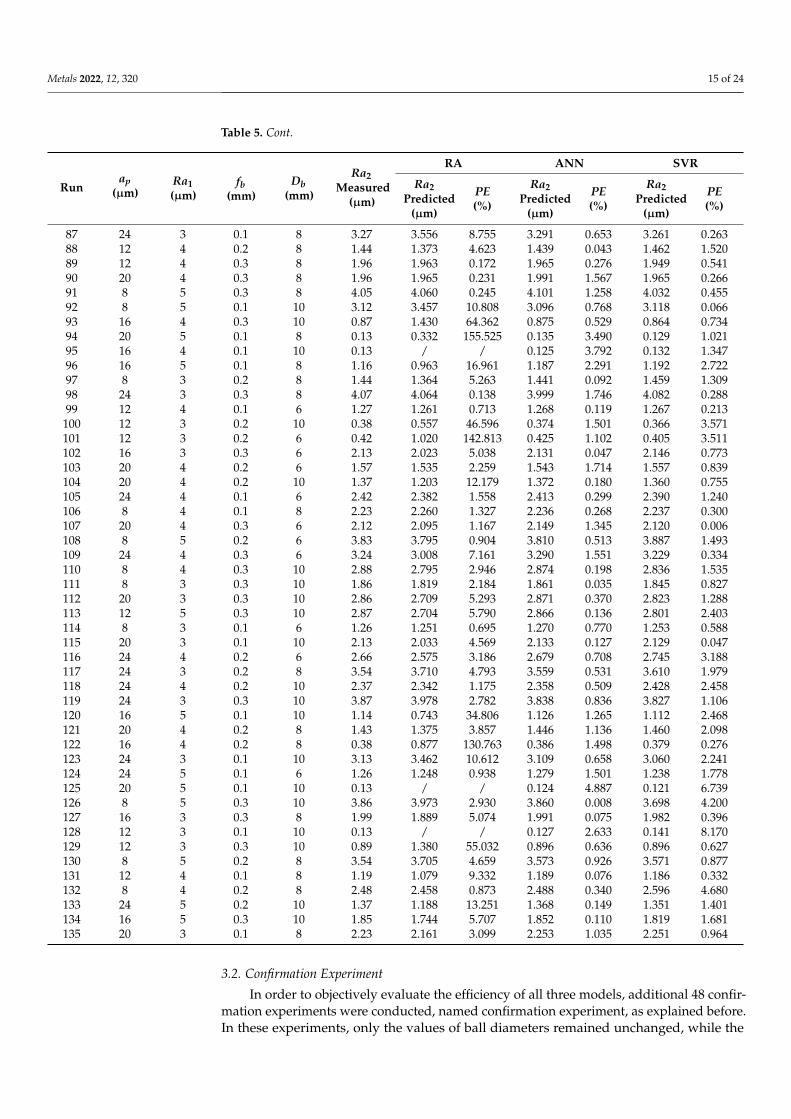
100 12 3 0.2 10 0.38 0.557 46.596 0.374 1.501 0.366 3.571101 12 3 0.2 6 0.42 1.020 142.813 0.425 1.102 0.405 3.511102 16 3 0.3 6 2.13 2.023 5.038 2.131 0.047 2.146 0.773103 20 4 0.2 6 1.57 1.535 2.259 1.543 1.714 1.557 0.839104 20 4 0.2 10 1.37 1.203 12.179 1.372 0.180 1.360 0.755105 24 4 0.1 6 2.42 2.382 1.558 2.413 0.299 2.390 1.240106 8 4 0.1 8 2.23 2.260 1.327 2.236 0.268 2.237 0.300107 20 4 0.3 6 2.12 2.095 1.167 2.149 1.345 2.120 0.006108 8 5 0.2 6 3.83 3.795 0.904 3.810 0.513 3.887 1.493109 24 4 0.3 6 3.24 3.008 7.161 3.290 1.551 3.229 0.334110 8 4 0.3 10 2.88 2.795 2.946 2.874 0.198 2.836 1.535111 8 3 0.3 10 1.86 1.819 2.184 1.861 0.035 1.845 0.827112 20 3 0.3 10 2.86 2.709 5.293 2.871 0.370 2.823 1.288113 12 5 0.3 10 2.87 2.704 5.790 2.866 0.136 2.801 2.403114 8 3 0.1 6 1.26 1.251 0.695 1.270 0.770 1.253 0.588115 20 3 0.1 10 2.13 2.033 4.569 2.133 0.127 2.129 0.047116 24 4 0.2 6 2.66 2.575 3.186 2.679 0.708 2.745 3.188117 24 3 0.2 8 3.54 3.710 4.793 3.559 0.531 3.610 1.979118 24 4 0.2 10 2.37 2.342 1.175 2.358 0.509 2.428 2.458119 24 3 0.3 10 3.87 3.978 2.782 3.838 0.836 3.827 1.106120 16 5 0.1 10 1.14 0.743 34.806 1.126 1.265 1.112 2.468121 20 4 0.2 8 1.43 1.375 3.857 1.446 1.136 1.460 2.098122 16 4 0.2 8 0.38 0.877 130.763 0.386 1.498 0.379 0.276123 24 3 0.1 10 3.13 3.462 10.612 3.109 0.658 3.060 2.241124 24 5 0.1 6 1.26 1.248 0.938 1.279 1.501 1.238 1.778125 20 5 0.1 10 0.13 / / 0.124 4.887 0.121 6.739126 8 5 0.3 10 3.86 3.973 2.930 3.860 0.008 3.698 4.200127 16 3 0.3 8 1.99 1.889 5.074 1.991 0.075 1.982 0.396128 12 3 0.1 10 0.13 / / 0.127 2.633 0.141 8.170129 12 3 0.3 10 0.89 1.380 55.032 0.896 0.636 0.896 0.627130 8 5 0.2 8 3.54 3.705 4.659 3.573 0.926 3.571 0.877131 12 4 0.1 8 1.19 1.079 9.332 1.189 0.076 1.186 0.332132 8 4 0.2 8 2.48 2.458 0.873 2.488 0.340 2.596 4.680133 24 5 0.2 10 1.37 1.188 13.251 1.368 0.149 1.351 1.401134 16 5 0.3 10 1.85 1.744 5.707 1.852 0.110 1.819 1.681135 20 3 0.1 8 2.23 2.161 3.099 2.253 1.035 2.251 0.964

3.2. Confirmation Experiment

In order to objectively evaluate the efficiency of all three models, additional 48 confir-mation experiments were conducted, named confirmation experiment, as explained before.In these experiments, only the values of ball diameters remained unchanged, while the

Metals 2022, 12, 320 16 of 24

other three input parameters (the depth of ball penetration, the initial surface roughness,and burnishing feed) had different values from those used in the training experiment.

During the confirmation experimental research, four processing parameters (inputvariables) were varied at the following levels:

• The depth of ball penetration—ap = 10, 14, 18, 22 (µm);• The initial surface roughness—Ra1 = 3.5, 4.5 (µm);• Burnishing feed—fb = 0.15, 0.25 (mm);• Burnishing ball diameter—Db = 6, 8, 10 (mm).

After the confirmation experiments, the measurement and prediction of the final arith-metic mean roughness (Ra2) was performed for the three previously described models (RA,ANN, and SVR). Table 6 shows the obtained results of Ra2 measurements, Ra2 predictions,and the obtained percentage errors for the three models.

Table 6. Measured and predicted values of the surface roughness and percentage errors for confirma-tion experiment.

Runap

(µm)Ra1(µm)

fb(mm)

Db(mm)

Ra2Measured

(µm)

RA ANN SVR

Ra2Predicted

(µm)

PE(%)

Ra2Predicted

(µm)

PE(%)

Ra2Predicted

(µm)

PE(%)

1 10 3.5 0.15 6 1.40 1.361 2.755 1.396 0.284 1.368 2.2972 10 3.5 0.25 6 1.81 1.793 0.940 1.814 0.229 1.785 1.3943 10 3.5 0.15 8 1.31 1.189 9.267 1.305 0.360 1.283 2.0504 10 3.5 0.25 8 1.69 1.649 2.448 1.689 0.069 1.658 1.8955 10 3.5 0.15 10 1.25 0.999 20.072 1.239 0.887 1.210 3.1916 10 3.5 0.25 10 1.61 1.496 7.066 1.605 0.301 1.558 3.2107 14 3.5 0.15 6 0.25 0.833 233.334 0.238 4.980 0.251 0.2688 14 3.5 0.25 6 0.67 1.370 104.405 0.701 4.562 0.649 3.2039 14 3.5 0.15 8 0.23 0.588 155.482 0.217 5.615 0.237 3.198

10 14 3.5 0.25 8 0.63 1.197 90.057 0.650 3.157 0.605 3.90411 14 3.5 0.15 10 0.22 0.248 12.603 0.210 4.676 0.227 3.20212 14 3.5 0.25 10 0.60 1.009 68.136 0.631 5.123 0.571 4.83613 18 3.5 0.15 6 1.37 1.321 3.604 1.368 0.171 1.368 0.14414 18 3.5 0.25 6 1.81 1.759 2.845 1.805 0.249 1.791 1.04415 18 3.5 0.15 8 1.29 1.144 11.300 1.280 0.763 1.292 0.14516 18 3.5 0.25 8 1.69 1.612 4.596 1.690 0.024 1.678 0.73317 18 3.5 0.15 10 1.23 0.950 22.791 1.210 1.597 1.215 1.20118 18 3.5 0.25 10 1.61 1.458 9.458 1.606 0.253 1.563 2.89419 22 3.5 0.15 6 1.92 1.820 5.217 1.920 0.002 1.897 1.18820 22 3.5 0.25 6 2.33 2.193 5.871 2.334 0.156 2.313 0.72421 22 3.5 0.15 8 1.80 1.677 6.842 1.798 0.127 1.803 0.15522 22 3.5 0.25 8 2.17 2.066 4.785 2.172 0.109 2.188 0.81123 22 3.5 0.15 10 1.70 1.526 10.228 1.701 0.054 1.724 1.40024 22 3.5 0.25 10 2.05 1.934 5.645 2.053 0.137 2.075 1.21425 10 4.5 0.15 6 2.48 2.404 3.066 2.479 0.047 2.508 1.12726 10 4.5 0.25 6 2.93 2.726 6.959 2.925 0.177 2.920 0.34427 10 4.5 0.15 8 2.31 2.284 1.124 2.308 0.096 2.347 1.60228 10 4.5 0.25 8 2.74 2.615 4.554 2.735 0.191 2.733 0.27329 10 4.5 0.15 10 2.18 2.160 0.907 2.175 0.242 2.211 1.43630 10 4.5 0.25 10 2.59 2.501 3.420 2.592 0.094 2.573 0.67431 14 4.5 0.15 6 1.40 1.317 5.932 1.397 0.236 1.372 1.98532 14 4.5 0.25 6 1.81 1.755 3.016 1.809 0.033 1.782 1.52533 14 4.5 0.15 8 1.31 1.140 12.960 1.304 0.433 1.280 2.27434 14 4.5 0.25 8 1.68 1.609 4.222 1.681 0.070 1.652 1.68535 14 4.5 0.15 10 1.25 0.945 24.385 1.239 0.901 1.207 3.431

Metals 2022, 12, 320 17 of 24

Table 6. Cont.

Runap

(µm)Ra1(µm)

fb(mm)

Db(mm)

Ra2Measured

(µm)

RA ANN SVR

Ra2Predicted

(µm)

PE(%)

Ra2Predicted

(µm)

PE(%)

Ra2Predicted

(µm)

PE(%)

36 14 4.5 0.25 10 1.60 1.454 9.109 1.595 0.284 1.553 2.94437 18 4.5 0.15 6 0.24 0.830 246.005 0.234 2.631 0.247 2.74038 18 4.5 0.25 6 0.67 1.367 104.081 0.699 4.292 0.641 4.34439 18 4.5 0.15 8 0.23 0.584 153.914 0.213 7.408 0.234 1.64140 18 4.5 0.25 8 0.63 1.195 89.684 0.658 4.380 0.599 4.87041 18 4.5 0.15 10 0.21 0.242 15.064 0.198 5.529 0.223 5.98142 18 4.5 0.25 10 0.60 1.006 67.701 0.628 4.701 0.566 5.64043 22 4.5 0.15 6 0.80 0.985 23.175 0.816 2.006 0.784 2.02844 22 4.5 0.25 6 1.22 1.486 21.763 1.231 0.911 1.201 1.53445 22 4.5 0.15 8 0.73 0.769 5.342 0.746 2.248 0.763 4.55946 22 4.5 0.25 8 1.13 1.322 17.025 1.120 0.927 1.146 1.43347 22 4.5 0.15 10 0.66 0.507 23.224 0.674 2.093 0.636 3.58548 22 4.5 0.25 10 1.03 1.146 11.277 1.041 1.039 1.050 1.907

4. Discussion

Descriptive parameters of the measured values of surface roughness after ball bur-nishing during the training and confirmation experiments are shown in Table 7. The valuesof the surface roughness range from 0.13 µm to 4.39 µm. This points to two very importantfacts. First, a minimum surface roughness value of 0.13 µm indicates that the extremelyhigh quality of the treated surface can be obtained by this procedure. Second, the ratio ofmaximum and minimum values (Ramax/Ramin) of 33.77 is extremely high. This indicatesthat with a suitable combination of process parameters, Ra can be significantly affected. Inother words, a suitable choice of input parameters of the process can achieve the requiredroughness in a very wide range. This is important from the point of view of practical appli-cation, considering that it is not necessary to insist on the minimum but on the requiredsurface roughness. The predicted values of Ra have the same trend as the measured values.The Ra values obtained by the training and confirmation experiments have close values forthe RA, ANN, and SVR models. Differences between values are acceptable and occur asa consequence of the fact that the confirmation was performed on the input parameterson which no training was performed, i.e., on “unknown” input variables. Moreover, theMPE for the ANN and SVR models is lower for confirmation experiments than for trainingexperiments, while for the RA model, it is negligibly higher. This confirmed the correctchoice of training parameters and the correctly performed training process for all models.

Table 7. Descriptive parameters of the surface roughness Ra2 measured.

ParameterRa2 Measured (µm)

Training Experiments Confirmation Experiments

Min 0.13 0.21Max 4.39 2.93

Mean 1.90 1.36St. dev. 1.06 0.73Ratio 33.77 13.95

In most experiments (Tables 5 and 6), the surface roughness after the ball burnishingprocess is lower than the initial one (Ra2 < Ra1), which was the goal. However, in severalexperiments, it can be observed that the surface roughness obtained after the ball burnishingprocess was higher than the initial surface roughness, i.e., Ra2 > Ra1. This is a consequenceof inadequate process parameters. These are also cases that represent the full expediency ofthe modeling process because the knowledge and experience of the operator are minimized

Metals 2022, 12, 320 18 of 24

if the process is well modeled, and inadequate process parameters that can lead to scrapare avoided.

Based on the results of experiments, the following can generally be stated:

• The depths of ball penetration close to the maximum profile height before processinggenerate the lowest surface roughness. For depth values greater and smaller than thisone, the surface roughness increases;

• As the burnishing feed decreases, the surface roughness reduces;• As the ball diameter increases, the surface roughness reduces.

Figure 3 shows an archlike dependence of the surface roughness obtained after ballburnishing (Ra2) in relation to the initial surface roughness (Ra1) and the depth of ballpenetration (ap). For depths of ball penetration (ap) lower than the initial value of the profileheight, when the ball reaches and “touches” the treated surface under the effect of highcontact pressures, the peaks begin to flow and fill the valleys in the roughness profile andreduce surface roughness. This happens up to a certain depth of ball penetration (ap),approximately when ap ≈ Rp. For these values, the lowest surface roughness was achievedafter processing. With a further increase in the depth of ball penetration (ap), the surfaceroughness (Ra2) worsens. Larger depths of ball penetration (ap) cause the emergence oflarger valleys, which results in higher roughness (Ra2), i.e., a reduction in the quality of thetreated surface. Larger depths of ball penetration (ap) also induce greater forces that candamage the surface and create surface cracks. At greater depths of ball penetration (ap),the depth of the valleys enlarges, which results in a large amount of plastic deformationthat causes deeper traces of penetration. As a result, the surface roughness worsens (Ra2),and cracks can occur, which further damages the surface topography. The effect of thedeterioration of surface roughness after a certain depth of ball penetration (ap) can beattributed to the greater hardening of the superficial workpiece layer due to compression.Furthermore, there may be a superficial peeling on the workpiece. With the reductionin burnishing feed (fb) and with the unchanged other process parameters, the roughnessof the treated surface (Ra2) reduces. In all experimental studies, the surface roughness(Ra2) increased with increasing burnishing feed (fb), while the increased trend remainsmild. The burnishing feed (fb) values were selected so as not to negatively affect the surfacethat was processed during the earlier tool movement. If two consecutive movements ofthe ball are close to each other, the material of the workpiece that has already filled thevalleys could begin to overflow laterally (perpendicular to the direction of the movement)and thus worsen the roughness (Ra2) of the pre-treated surface on which the peaks havealready filled valleys. This negative phenomenon, in the context of the movement, wasavoided in this research. A larger ball diameter (Db), under the unchanged other processingconditions, reduces the surface roughness (Ra2). This can be explained by the very natureof the process, i.e., the contact that takes place between the ball and the treated surface.With larger ball diameters (Db), the contact area between the tool and the treated surface islarger, which reduces roughness (Ra2).

Descriptive parameters for PE obtained by modeling via RA, ANN, and SVR areshown in Tables 8 and 9. Figure 9 shows the PE for all conducted experiments. The ANNand SVR models predicted the obtained roughness for both experimental data and the“unknown” data very successfully during confirmation experiments, while predictionusing the RA model indicated significantly lower accuracy, especially in cases when surfaceroughness values were very low. Based on the obtained data, identical trends can beobserved for both the training experiment and the confirmation experiments. The lowestminimum and mean PE is provided by ANN, while the lowest maximum PE is suggestedby SVR.

Metals 2022, 12, 320 19 of 24

Table 8. Descriptive parameters of percentage errors for the training experiments.

Surface Roughness ParameterMain Experiment

RA ANN SVR

Ra2 < 1 µm

No. 27Min 46.596 0.112 0.276Max 418.053 8.584 8.170

Mean 134.513 2.293 2.888St. dev. 102.671 2.482 2.351

1 µm < Ra2 < 2 µm

No. 48Min 0.172 0.012 0.032Max 34.806 2.291 3.804

Mean 9.080 0.777 1.086St. dev. 8.744 0.653 0.924

2 µm < Ra2 < 3 µm

No. 34Min 0.422 0.001 0.006Max 7.380 1.874 4.680

Mean 3.413 0.504 1.783St. dev. 2.063 0.410 1.269

3 µm < Ra2 < 4 µm

No. 22Min 0.261 0.008 0.066Max 10.808 1.551 4.200

Mean 6.026 0.478 0.983St. dev. 3.068 0.361 0.952

4 µm < Ra2 < 5 µm

No. 4Min 0.138 0.077 0.288Max 5.567 4.301 1.323

Mean 2.800 1.846 0.633St. dev. 3.015 1.781 0.467

All experiments

No. 135Min 0.138 0.001 0.006Max 418.053 8.584 8.170

Mean 29.727 0.995 1.592St. dev. 65.917 1.400 1.563

Table 9. Descriptive parameters of percentage errors for the confirmation experiments.

Surface Roughness ParameterConfirmation Experiment

RA ANN SVR

Ra2 < 1 µm

No. 15Min 5.342 2.006 0.268Max 246.005 7.408 5.981

Mean 92.814 4.227 3.600St. dev. 76.632 1.530 1.539

1 µm < Ra2 < 2 µm

No. 24Min 0.940 0.002 0.144Max 24.385 1.597 3.431

Mean 9.547 0.425 1.736St. dev. 6.983 0.418 0.952

2 µm < Ra2 < 3 µm

No. 9Min 0.907 0.047 0.273Max 6.959 0.242 1.602

Mean 4.037 0.139 0.912St. dev. 2.089 0.060 0.464

All experiments

No. 48Min 0.907 0.002 0.144Max 246.005 7.408 5.981

Mean 34.534 1.559 2.164St. dev. 57.921 2.024 1.496

Metals 2022, 12, 320 20 of 24


St. dev. 6.983 0.418 0.952

2 μm < Ra2 < 3 μm

No. 9 Min 0.907 0.047 0.273 Max 6.959 0.242 1.602

Mean 4.037 0.139 0.912 St. dev. 2.089 0.060 0.464

All experiments

No. 48 Min 0.907 0.002 0.144 Max 246.005 7.408 5.981

Mean 34.534 1.559 2.164 St. dev. 57.921 2.024 1.496

Figure 9. Percentage errors (a) training experiments; (b) confirmation experiments.

5. Conclusions This paper discusses the application of the burnishing process on a workpiece made

of AISI 4130 alloy steel with a high-stiffness tool and a ceramic ball. Different values of process input parameters were applied to assess their effect on the surface roughness of the workpiece after processing. Three methods were applied in the process modeling, RA, ANN, and SVR, respectively.

Based on experimental and modeling investigations, it is possible to draw several conclusions: • The obtained experimental results of surface roughness indicate the values of surface

roughness range from 0.13 μm to 4.39 μm, which means that it is possible to obtain very low values of surface roughness, below 1 μm. The minimum value of surface

Figure 9. Percentage errors (a) training experiments; (b) confirmation experiments.

Out of a total of 183 experiments conducted, percentage errors PE greater than 5%occur only for eight predictions via ANN and six predictions via SVR. It should be notedthat in these, from the point of view of prediction, the most unfavorable cases, the absoluteerror, i.e., the difference between the realized and the predicted value of Ra is in the range0.01–0.03 µm, which is an acceptable deviation from a practical point of view. In all othercases, the errors obtained via ANN and SVR are significantly lower. Therefore, ANN andSVR models can be implemented in the actual industrial conditions, while the RA model canbe successfully applied when it is not necessary to obtain extremely low surface roughness.

5. Conclusions

This paper discusses the application of the burnishing process on a workpiece madeof AISI 4130 alloy steel with a high-stiffness tool and a ceramic ball. Different values ofprocess input parameters were applied to assess their effect on the surface roughness ofthe workpiece after processing. Three methods were applied in the process modeling, RA,ANN, and SVR, respectively.

Based on experimental and modeling investigations, it is possible to draw several conclusions:

• The obtained experimental results of surface roughness indicate the values of surfaceroughness range from 0.13 µm to 4.39 µm, which means that it is possible to obtainvery low values of surface roughness, below 1 µm. The minimum value of surfaceroughness after ball burnishing was 0.13 µm, which relates to the N3 InternationalOrganization for Standardization (ISO) grade number. This is a very high quality ofthe treated surface;

• The influence of input variables on surface roughness after ball burnishing is different.The depths of ball penetration close to the maximum profile height before processing

Metals 2022, 12, 320 21 of 24

generate the lowest surface roughness. For depth values greater and smaller than thisone, the surface roughness increases. Moreover, the surface roughness decreases withdecreasing burnishing feed and with increasing ball diameter;

• The quality of RA, ANN, and SVM models was assessed based on the results of thetraining and confirmation experiments. The evaluation of the model was performedbased on PEs. For a complete series of conducted experiments, the minimum andmean PEs are lower for the ANN model, but the maximum PE is lower for the SVRmodel. Bigger errors, but without a significant effect on applicability in practice, areobtained for values of Ra < 1 µm. For surface roughness values Ra≥ 1 µm, these errorsare negligible from a practical point of view since the majority of PE is lower than 1%;

• The obtained PEs for ANN and SVR models are considered acceptable for practicalapplication. ANN and SVR models have successfully predicted surface roughness,so they can be successfully implemented in the industry when planning the produc-tion process.

The main limitation of the applied methodology is that the process was modeled forcertain experimental conditions in terms of defined tools, workpieces, and equipment.However, the applied approach is sufficiently general and universal so that it can be easilyapplied and implemented for other conditions of the ball burnishing process.

Future research will focus on investigating the ball burnishing process with othermodeling methods. Furthermore, the aim is to cover a larger number of input and out-put processing parameters, as well as to perform multi-criteria optimization of the ballburnishing process.

Author Contributions: Conceptualization, Z.K., M.P., B.T. and G.S.; methodology, Z.K., D.V., K.S.and G.S.; software, Z.K. and K.S.; validation, D.V., M.P. and B.T.; formal analysis, K.S. and T.S.;investigation, M.P., T.S. and G.S.; resources, D.V. and B.T.; data curation, Z.K. and K.S.; writing—original draft preparation, Z.K., D.V., K.S. and M.P.; writing—review and editing, T.S., B.T. and G.S.;visualization, T.S.; supervision, G.S. All authors have read and agreed to the published version ofthe manuscript.

Funding: This research was funded by the University of Slavonski Brod, Mechanical Engineer-ing Faculty in Slavonski Brod, Republic of Croatia, grant number SV001 and by the Ministry ofEducation, Science and Technological Development of Republic of Serbia, grant number 451-03-68/2021-14/200156.

Institutional Review Board Statement: Not applicable.

Informed Consent Statement: Not applicable.

Data Availability Statement: Not applicable.

Conflicts of Interest: The authors declare no conflict of interest.

References1. Maximov, J.T.; Duncheva, G.V.; Anchev, A.P.; Ichkova, M.D. Slide burnishing—Review and prospects. Int. J. Adv. Manuf. Technol.

2019, 104, 785–801. [CrossRef]2. Tadic, B.; Randjelovic, S.; Todorovic, P.; Zivkovic, J.; Kocovic, V.; Budak, I.; Vukelic, D. Using a high-stiffness burnishing tool for

increased dimensional and geometrical accuracies of openings. Precis. Eng. 2016, 43, 335–344. [CrossRef]3. Travieso-Rodríguez, J.A.; Dessein, G.; González-Rojas, H.A. Improving the surface finish of concave and convex surfaces using a

ball burnishing process. Mater. Manuf. Process. 2011, 26, 1494–1502. [CrossRef]4. Saldana-Robles, A.; Plascencia-Mora, H.; Aguilera-Gómez, E.; Saldana-Robles, A.; Marquez-Herrera, A.; Diosdado-De la Peña, J.A.

Influence of ball-burnishing on roughness, hardness and corrosion resistance of AISI 1045 steel. Surf. Coat. Technol. 2018, 339,191–198. [CrossRef]

5. Vukelic, D.; Tadic, B.; Dzunic, D.; Kocovic, V.; Brzakovic, L.; Zivkovic, M.; Simunovic, G. Analysis of ball-burnishing impact onbarrier properties of wood workpieces. Int. J. Adv. Manuf. Technol. 2017, 92, 129–138. [CrossRef]

6. Shreehah, T.A.A. Developing and investigating of elastic ball burnishing tool. Int. J. Adv. Manuf. Technol. 2008, 36, 270–279.[CrossRef]

7. Gharbi, F.; Sghaier, S.; Al-Fadhalah, K.J.; Benameur, T. Effect of ball burnishing process on the surface quality and microstructureproperties of AISI 1010 steel plates. J. Mater. Eng. Perform. 2011, 20, 903–910. [CrossRef]

http://doi.org/10.1007/s00170-019-03881-1

http://doi.org/10.1016/j.precisioneng.2015.08.014

http://doi.org/10.1080/10426914.2010.544819

http://doi.org/10.1016/j.surfcoat.2018.02.013

http://doi.org/10.1007/s00170-017-0134-3

http://doi.org/10.1007/s00170-006-0838-2

http://doi.org/10.1007/s11665-010-9701-6

Metals 2022, 12, 320 22 of 24

8. Hamadache, H.; Zemouri, Z.; Laouar, L.; Dominiak, S. Improvement of surface conditions of 36 Cr Ni Mo 6 steel by ball burnishingprocess. J. Mech. Sci. Technol. 2014, 28, 1491–1498. [CrossRef]

9. Banh, Q.N.; Shiou, F.J. Determination of Optimal Small Ball-Burnishing Parameters for Both Surface Roughness and SuperficialHardness Improvement of STAVAX. Arab. J. Sci. Eng. 2016, 41, 639–652. [CrossRef]

10. Shiou, F.J.; Banh, Q.N. Development of an innovative small ball-burnishing tool embedded with a load cell. Int. J. Adv. Manuf.Technol. 2016, 87, 31–41. [CrossRef]

11. Garcia-Granada, A.A.; Gomez-Gras, G.; Jerez-Mesa, R.; Travieso-Rodriguez, J.A.; Reyes, G. Ball-burnishing effect on deep residualstress on AISI 1038 and AA2017-T4. Mater. Manuf. Process. 2017, 32, 1279–1289. [CrossRef]

12. Boozarpoor, M.; Elyasi, M.; Hosseinzadeh, M. An investigation of the surface quality of burnished AISI 4340 steel. Proc. Inst.Mech. Eng. E J. Process. Mech. Eng. 2018, 232, 299–313. [CrossRef]

13. Bounouara, A.; Hamadache, H.; Amirat, A. Investigation on the effect of ball burnishing on fracture toughness in spiral API X70pipeline steel. Int. J. Adv. Manuf. Technol. 2018, 94, 4543–4551. [CrossRef]

14. El-Tayeb, N.S.M.; Low, K.O.; Brevern, P.V. Enhancement of surface quality and tribological properties using ball burnishingprocess. Mach. Sci. Technol. 2008, 12, 234–248. [CrossRef]

15. El-Axir, M.H. An investigation into the ball burnishing of aluminium alloy 6061-T6. Proc. Inst. Mech. Eng. B J. Eng. Manuf. 2007,221, 1733–1742. [CrossRef]

16. Chomienne, V.; Valiorgue, F.; Rech, J.; Verdu, C. Influence of ball burnishing on residual stress profile of a 15-5PH stainless steel.CIRP J. Manuf. Sci. Technol. 2016, 13, 90–96. [CrossRef]

17. Cao, C.; Zhu, J.; Tanaka, T.; Shiou, F.J.; Sawada, S.; Yoshioka, H. Ball burnishing of Mg alloy using a newly developed burnishingtool with on-machine force control. Int. J. Autom. Technol. 2019, 13, 619–630. [CrossRef]

18. Vukelic, D.; Miljanic, D.; Randjelovic, S.; Budak, I.; Dzunic, D.; Eric, M.; Pantic, M. A burnishing process based on the optimaldepth of workpiece penetration. Mater. Tehnol. 2013, 47, 43–51.

19. Tadic, B.; Todorovic, P.; Luzanin, O.; Miljanic, D.; Jeremic, B.; Bogdanovic, B.; Vukelic, D. Using specially designed high-stiffnessburnishing tool to achieve high-quality surface finish. Int. J. Adv. Manuf. Technol. 2013, 67, 601–611. [CrossRef]

20. Randjelovic, S.; Tadic, B.; Todorovic, P.M.; Vukelic, D.; Miloradovic, D.; Radenkovic, M.; Tsiafis, C. Modelling of the ball burnishingprocess with a high-stiffness tool. Int. J. Adv. Manuf. Technol. 2015, 81, 1509–1518. [CrossRef]

21. Travieso-Rodriguez, J.A.; Gomez-Gras, G.; Dessein, G.; Carrillo, F.; Alexis, J.; Jorba-Peiro, J.; Aubazac, N. Effects of a ball-burnishing process assisted by vibrations in G10380 steel specimens. Int. J. Adv. Manuf. Technol. 2015, 81, 1757–1765. [CrossRef]

22. Travieso-Rodriguez, J.A.; Gras, G.G.; Peiro, J.J.; Carrillo, F.; Dessein, G.; Alexis, J.; Rojas, H.G. Experimental study on themechanical effects of the vibration-assisted ball-burnishing process. Mater. Manuf. Process. 2015, 30, 1490–1497. [CrossRef]

23. Gomez-Gras, G.; Travieso-Rodriguez, J.A.; Gonzalez-Rojas, H.A.; Napoles-Alberro, A.; Carrillo, F.J.; Dessein, G. Study of aball-burnishing vibration-assisted process. Proc. Inst. Mech. Eng. B J. Eng. Manuf. 2015, 229, 172–177. [CrossRef]

24. Gomez–Gras, G.; Travieso–Rodriguez, J.A.; Jerez–Mesa, R.; Lluma-Fuentes, J.; Gomis de la Calle, B. Experimental study of lateralpass width in conventional and vibrations-assisted ball burnishing. Int. J. Adv. Manuf. Technol. 2016, 87, 363–371. [CrossRef]

25. Teimouri, R.; Amini, S.; Bami, A.B. Evaluation of optimized surface properties and residual stress in ultrasonic assisted ballburnishing of AA6061-T6. Measurement 2018, 116, 129–139. [CrossRef]

26. Teimouri, R.; Liu, Z. An analytical prediction model for residual stress distribution and plastic deformation depth in ultrasonic-assisted single ball burnishing process. Int. J. Adv. Manuf. Technol. 2020, 111, 127–147. [CrossRef]

27. Lluma, J.; Gomez-Gras, G.; Jerez-Mesa, R.; Rue-Mascarell, J.; Travieso-Rodriguez, J.A. Mechanical strengthening in s235jr steelsheets through vibration-assisted ball burnishing. Metals 2020, 10, 1010. [CrossRef]

28. Jerez-Mesa, R.; Landon, Y.; Travieso-Rodriguez, J.A.; Dessein, G.; Lluma-Fuentes, J.; Wagner, V. Topological surface integritymodification of AISI 1038 alloy after vibration-assisted ball burnishing. Surf. Coat. Technol. 2018, 349, 364–377. [CrossRef]

29. Jerez-Mesa, R.; Travieso-Rodriguez, J.A.; Gomez-Gras, G.; Lluma-Fuentes, J. Development, characterization and test of anultrasonic vibration-assisted ball burnishing tool. J. Mater. Process. Technol. 2018, 257, 203–212. [CrossRef]

30. Jerez-Mesa, R.; Plana-García, V.; Llumà, J.; Travieso-Rodriguez, J.A. Enhancing surface topology of udimet® 720 superalloythrough ultrasonic vibration-assisted ball burnishing. Metals 2020, 10, 915. [CrossRef]

31. Jerez-Mesa, R.; Fargas, G.; Roa, J.J.; Llumà, J.; Travieso-Rodriguez, J.A. Superficial effects of ball burnishing on trip steel AISI301ln sheets. Metals 2021, 11, 82. [CrossRef]

32. Ituarte, I.F.; Salmi, M.; Papula, S.; Huuki, J.; Hemming, B.; Coatanea, E.; Nurmi, S.; Virkkunen, I. Surface modification of additivelymanufactured 18% nickel maraging steel by ultrasonic vibration-assisted ball burnishing. J. Manuf. Sci. Eng. Trans. ASME 2020,142, 4046903. [CrossRef]

33. Kovacs, Z.F.; Viharos, Z.J.; Kodacsy, J. Determination of the working gap and optimal machining parameters for magnetic assistedball burnishing. Measurement 2018, 118, 172–180. [CrossRef]

34. Kovacs, Z.F.; Viharos, Z.J.; Kodacsy, J. Surface flatness and roughness evolution after magnetic assisted ball burnishing ofmagnetizable and non-magnetizable materials. Measurement 2020, 158, 107750. [CrossRef]

35. Livatyali, H.; Has, E.; Turkoz, M. Prediction of residual stresses in ball burnishing TI6AL4V thin sheets. Int. J. Adv. Manuf. Technol.2020, 110, 1083–1093. [CrossRef]

36. Sayahi, M.; Sghaier, S.; Belhadjsalah, H. Finite element analysis of ball burnishing process: Comparisons between numericalresults and experiments. Int. J. Adv. Manuf. Technol. 2013, 67, 1665–1673. [CrossRef]

http://doi.org/10.1007/s12206-014-0135-1

http://doi.org/10.1007/s13369-015-1710-1

http://doi.org/10.1007/s00170-016-8413-y

http://doi.org/10.1080/10426914.2017.1317351

http://doi.org/10.1177/0954408917694215

http://doi.org/10.1007/s00170-017-1181-5

http://doi.org/10.1080/10910340802067536

http://doi.org/10.1243/09544054JEM818

http://doi.org/10.1016/j.cirpj.2015.12.003

http://doi.org/10.20965/ijat.2019.p0619

http://doi.org/10.1007/s00170-012-4508-2

http://doi.org/10.1007/s00170-015-7319-4

http://doi.org/10.1007/s00170-015-7255-3

http://doi.org/10.1080/10426914.2015.1019114

http://doi.org/10.1177/0954405414526383

http://doi.org/10.1007/s00170-016-8490-y

http://doi.org/10.1016/j.measurement.2017.11.001

http://doi.org/10.1007/s00170-020-06068-1

http://doi.org/10.3390/met10081010

http://doi.org/10.1016/j.surfcoat.2018.05.061

http://doi.org/10.1016/j.jmatprotec.2018.02.036

http://doi.org/10.3390/met10070915

http://doi.org/10.3390/met11010082

http://doi.org/10.1115/1.4046903

http://doi.org/10.1016/j.measurement.2018.01.033

http://doi.org/10.1016/j.measurement.2020.107750

http://doi.org/10.1007/s00170-020-05837-2

http://doi.org/10.1007/s00170-012-4599-9

Metals 2022, 12, 320 23 of 24

37. Saldana-Robles, A.; Aguilera-Gómez, E.; Plascencia-Mora, H.; Ledesma-Orozco, E.R.; Saldana-Robles, N.; Reveles-Arredondo, J.F.Three-dimensional modeling of surface roughness for burnishing process. DYNA 2015, 90, 423–432. [CrossRef]

38. Mohammadi, F.; Sedaghati, R.; Bonakdar, A. A Finite element analysis and design optimization of low plasticity burnishingprocess. Int. J. Adv. Manuf. Technol. 2014, 70, 1337–1354. [CrossRef]

39. Charfeddine, Y.; Youssef, S.; Sghaier, S.; Sghaier, J.; Hamdi, H. Study of the simultaneous Grinding/Ball-burnishing of AISI 4140based on finite element simulations and experiments. Int. J. Mech. Sci. 2021, 192, 106097. [CrossRef]

40. Borysenko, D.; Welzel, F.; Karpuschewski, B.; Kundrak, J.; Voropai, V. Simulation of the burnishing process on real surfacestructures. Precis. Eng. 2021, 68, 166–173. [CrossRef]

41. Uddin, M.S.; Hall, C.; Hooper, R.; Charrault, E.; Murphy, P.; Santos, V. Finite element analysis of surface integrity in deepball-burnishing of a biodegradable AZ31B Mg alloy. Metals 2018, 8, 136. [CrossRef]

42. Amini, C.; Jerez-Mesa, R.; Travieso-Rodriguez, J.A.; Llumà, J.; Estevez-Urra, A. Finite element analysis of ball burnishing onball-end milled surfaces considering their original topology and residual stress. Metals 2020, 10, 638. [CrossRef]

43. Sagbas, A.; Kahraman, F. Determination of optimal ball burnishing parameters for surface hardness. Mater. Tehnol. 2009, 43,271–274.

44. El-Taweel, T.A.; El-Axir, M.H. Analysis and optimization of the ball burnishing process through the Taguchi technique. Int. J. Adv.Manuf. Technol. 2009, 41, 301–310. [CrossRef]

45. Esme, U. Use of grey based Taguchi method in ball burnishing process for the optimization of surface roughness and microhard-ness of AA 7075 aluminum alloy. Mater. Tehnol. 2010, 44, 129–135.

46. Babu, P.R.; Ankamma, K.; Prasad, T.S.; Raju, A.V.S.; Prasad, N.E. Optimization of burnishing parameters and determination ofselect surface characteristics in engineering materials. Sadhana-Acad. Proc. Eng. Sci. 2012, 37, 503–520. [CrossRef]

47. Revankar, G.D.; Shetty, R.; Rao, S.S.; Gaitonde, V.N. Selection of optimal process parameters in ball burnishing of titanium alloy.Mach. Sci. Technol. 2014, 18, 464–483. [CrossRef]

48. Ramesh, D.R.; Prasad, A.M.K.; Kumar, A.C.S. Analysis of ball and roller burnishing by optimizing the process parameters forsurface roughness indices using grey based Taguchi method. Int. J. Appl. Eng. Res. 2014, 9, 7191–7200.

49. Cagan, S.C.; Aci, M.; Buldum, B.B.; Aci, C. Artificial neural networks in mechanical surface enhancement technique for theprediction of surface roughness and microhardness of magnesium alloy. Bull. Pol. Acad. Sci. Technol. Sci. 2019, 67, 729–739.[CrossRef]

50. Jawahar, M.; Suresh kumar, J.; Srikiran, M.; Ismail, S. Experimental Investigation of Ball Burnishing Process ParametersOptimization for Al 5083 Using Taguchi Method. In Lecture Notes in Mechanical Engineering; Recent Trends in MechanicalEngineering; Narasimham, G., Babu, A., Reddy, S., Dhanasekaran, R., Eds.; Springer: Singapore, 2020; pp. 189–204. [CrossRef]

51. Stalin John, M.R.; Vinayagam, B.K. Optimization of Ball Burnishing Process on Tool Steel (T215Cr12) in CNC Machining CentreUsing Response Surface Methodology. Arab. J. Sci. Eng. 2011, 36, 1407–1422. [CrossRef]

52. Sagbas, A. Analysis and optimization of surface roughness in the ball burnishing process using response surface methodologyand desirabilty function. Adv. Eng. Softw. 2011, 42, 992–998. [CrossRef]

53. Kahraman, F. Application of the response surface methodology in the ball burnishing process for the prediction and analysis ofsurface hardness of the aluminum alloy AA 7075. Mater. Test. 2015, 57, 311–315. [CrossRef]

54. Amdouni, H.; Bouzaiene, H.; Montagne, A.; Nasri, M.; Iost, A. Modeling and optimization of a ball-burnished aluminum alloy flatsurface with a crossed strategy based on response surface methodology. Int. J. Adv. Manuf. Technol. 2017, 88, 801–814. [CrossRef]

55. Nguyen, T.T.; Le, C.H. Optimization of compressed air assisted-turning-burnishing process for improving machining quality,energy reduction and cost-effectiveness. Proc. Inst. Mech. Eng. B J. Eng. Manuf. 2021, 235, 1179–1196. [CrossRef]

56. Nguyen, T.T.; Cao, L.H. Optimization of the Burnishing Process for Energy Responses and Surface Properties. Int. J. Precis. Eng.Manuf. 2020, 21, 1143–1152. [CrossRef]

57. Basak, H.; Goktas, H.H. Burnishing process on al-alloy and optimization of surface roughness and surface hardness by fuzzylogic. Mater. Des. 2009, 30, 1275–1281. [CrossRef]

58. Al-Saeedi, S.; Sarhan, A.A.D.; Bushroa, A.R. Investigating the Surface Tribology of Roller-Burnished Polymer Using the FuzzyRule–Based Approach. Tribol. Trans. 2015, 58, 240–246. [CrossRef]

59. Ibrahim, A.A.; Abd Rabbo, S.M.; El-Axir, M.H.; Ebied, A.A. Center rest balls burnishing parameters adaptation of steel componentsusing fuzzy logic. J. Mater. Process. Technol. 2009, 209, 2428–2435. [CrossRef]

60. Esme, U.; Kulekci, M.K.; Ustun, D.; Kahraman, F.; Kazancoglu, Y. Grey-based fuzzy algorithm for the optimization of the ballburnishing process. Mater. Test. 2015, 57, 666–673. [CrossRef]

61. Esme, U.; Sagbas, A.; Kahraman, F.; Kulekci, M.K. Use of artificial neural networks in ball burnishing process for the prediction ofsurface roughness of AA 7075 aluminum alloy. Mater. Tehnol. 2008, 42, 215–219.

62. Esme, U.; Kulekci, M.K.; Ozgun, S.; Kazancoglu, Y. Predictive modelling of ball burnishing process using regression analysis andneural network. Mater. Test. 2013, 55, 187–192. [CrossRef]

63. Basak, H.; Ozkan, M.T.; Toktas, I. Experimental research and ANN modeling on the impact of the ball burnishing process on themechanical properties of 5083 Al-Mg material. Kov. Mater. 2019, 57, 61–74. [CrossRef]

64. Basak, H.; Sonmez, F. Examination of the effects of burnishing apparatus on surface roughness and hardness in burnishingprocess. Indian J. Eng. Mater. Sci. 2017, 24, 115–122.

http://doi.org/10.6036/7440

http://doi.org/10.1007/s00170-013-5406-y

http://doi.org/10.1016/j.ijmecsci.2020.106097

http://doi.org/10.1016/j.precisioneng.2020.12.004

http://doi.org/10.3390/met8020136

http://doi.org/10.3390/met10050638

http://doi.org/10.1007/s00170-008-1485-6

http://doi.org/10.1007/s12046-012-0092-2

http://doi.org/10.1080/10910344.2014.897848

http://doi.org/10.24425/bpasts.2019.130182

http://doi.org/10.1007/978-981-15-1124-0_17

http://doi.org/10.1007/s13369-011-0126-9

http://doi.org/10.1016/j.advengsoft.2011.05.021

http://doi.org/10.3139/120.110721

http://doi.org/10.1007/s00170-016-8817-8

http://doi.org/10.1177/0954405420976661

http://doi.org/10.1007/s12541-020-00326-8

http://doi.org/10.1016/j.matdes.2008.06.063

http://doi.org/10.1080/10402004.2014.962205

http://doi.org/10.1016/j.jmatprotec.2008.05.040

http://doi.org/10.3139/120.110763

http://doi.org/10.3139/120.110423

http://doi.org/10.4149/km_2019_1_61

Metals 2022, 12, 320 24 of 24

65. Magalhaes, F.C.; Ventura, C.E.H.; Abrao, A.M.; Denkena, B.; Breidenstein, B.; Meyer, K. Prediction of surface residual stress andhardness induced by ball burnishing through neural networks. Int. J. Manuf. Res. 2019, 14, 295–310. [CrossRef]

66. Stalin John, M.R.; Vinayagam, B.K. Optimization of nonlinear characteristics of ball burnishing process using Sugeno fuzzyneural system. J. Braz. Soc. Mech. Sci. Eng. 2014, 36, 101–109. [CrossRef]

67. Singh, J.; Bilga, P.S. Optimization of Dry Ball Burnishing Process Using Neuro-Fuzzy Interface System and Genetic Algorithm.In Proceedings of the International Conference on Research and Innovations in Mechanical Engineering, Guru Nanak DevEngineering College, Ludhiana, Punjab, India, 24–26 October 2013; pp. 165–178. [CrossRef]

68. Meireles, M.R.G.; Almeida, P.E.M.; Simoes, M.G. A Comprehensive Review for Industrial Applicability of Artificial NeuralNetworks. IEEE Trans. Ind. Electron. 2003, 50, 585–601. [CrossRef]

69. Huang, T.M.; Kecman, V.; Kopriva, I. Kernel Based Algorithms for Mining Huge Data Sets; Springer: Berlin/Heidelberg,Germany, 2006.

70. Yu, H.; Kim, S. SVM Tutorial: Classification, Regression, and Ranking. In Handbook of Natural Computing; Rozenberg, G., Back, T.,Kook, J.N., Eds.; Springer: Berlin/Heidelberg, Germany, 2012; pp. 479–506.

71. de Boor, C. A Practical Guide to Splines; Springer: New York, NY, USA, 1978.72. Shin, S.; Jin, C.; Yu, J.; Rhee, S. Real-Time Detection of Weld Defects for Automated Welding Process Base on Deep Neural

Network. Metals 2020, 10, 389. [CrossRef]73. Casalino, G.; Losacco, A.M.; Arnesano, A.; Facchini, F.; Pierangeli, M.; Bonserio, C. Statistical analysis and modelling of an Yb:

KGW femtosecond laser micro-drilling process. Procedia CIRP 2017, 62, 275–280. [CrossRef]

http://doi.org/10.1504/IJMR.2019.100994

http://doi.org/10.1007/s40430-013-0060-8

http://doi.org/10.1007/978-81-322-1859-3_15

http://doi.org/10.1109/TIE.2003.812470

http://doi.org/10.3390/met10030389

http://doi.org/10.1016/j.procir.2016.06.111

The Modelling of Surface Roughness after the Ball Burnishing ...

Documents

Transcript of The Modelling of Surface Roughness after the Ball Burnishing ...